Guaranteed and robust a posteriori error estimates for singularly

perturbed reaction–diffusion problems

Ibrahim Cheddadi1, Radek Fucık2∗, Mariana I. Prieto3, and Martin Vohralık4†

1 Laboratoire Jean Kuntzmann, B.P. 53, 38041 Grenoble Cedex 9, Francee-mail: ibrahim.cheddadi@imag.fr

2 Department of Mathematics, Faculty of Nuclear Sciences and Physical Engineering, CzechTechnical University in Prague, Trojanova 13, 12000 Prague, Czech Republic

e-mail: fucik@fjfi.cvut.cz3 Departamento de Matematica, Facultad de Ciencias Exactas y Naturales, Universidad de

Buenos Aires, Intendente Guiraldes 2160, Ciudad Universitaria, C1428EGA, Argentinae-mail: mprieto@dm.uba.ar

4 UPMC Univ. Paris 06, UMR 7598, Laboratoire Jacques-Louis Lions, 75005, Paris, France &CNRS, UMR 7598, Laboratoire Jacques-Louis Lions, 75005, Paris, France

e-mail: vohralik@ann.jussieu.fr

Abstract

We derive a posteriori error estimates for singularly perturbed reaction–diffusion problems whichyield a guaranteed upper bound on the discretization error and are fully and easily computable.Moreover, they are also locally efficient and robust in the sense that they represent local lowerbounds for the actual error, up to a generic constant independent in particular of the reactioncoefficient. We present our results in the framework of the vertex-centered finite volume methodbut their nature is general for any conforming method, like the piecewise linear finite elementone. Our estimates are based on a H(div)-conforming reconstruction of the diffusive flux inthe lowest-order Raviart–Thomas space linked with mesh dual to the original simplicial one,previously introduced by the last author in the pure diffusion case. They also rely on elaboratedPoincare, Friedrichs, and trace inequalities-based auxiliary estimates designed to cope optimallywith the reaction dominance. In order to bring down the ratio of the estimated and actual overallenergy error as close as possible to the optimal value of one, independently of the size of thereaction coefficient, we finally develop the ideas of local minimizations of the estimators by localmodifications of the reconstructed diffusive flux. The numerical experiments presented confirmthe guaranteed upper bound, robustness, and excellent efficiency of the derived estimates.

Key words: vertex-centered finite volume/finite volume element/box method, singularly pertur-bed reaction–diffusion problem, a posteriori error estimates, guaranteed upper bound, robustness

AMS subject classifications: 65N15, 65N30, 76S05

∗This author has been partly supported by the project “Applied Mathematics in Technical and Physical Sciences”MSM 6840770010 of the Ministry of Education of the Czech Republic.

†This author has been partly supported by the GdR MoMaS project “Numerical Simulations and MathematicalModeling of Underground Nuclear Waste Disposal”, PACEN/CNRS, ANDRA, BRGM, CEA, EdF, IRSN, France.

1

1 Introduction

We consider in this paper the model reaction–diffusion problem

− ∆p + rp = f in Ω, (1.1a)

p = 0 on ∂Ω, (1.1b)

where Ω ⊂ Rd, d = 2, 3, is a polygonal (polyhedral) domain (open, bounded, and connected set),

r ∈ L∞(Ω), r ≥ 0, is a reaction coefficient, and f ∈ L2(Ω) is a source term. We denote respectivelyby cr,S and Cr,S the best nonnegative constants such that cr,S ≤ r ≤ Cr,S a.e. on a given subdomainS of Ω. Our purpose is to derive optimal a posteriori error estimates for vertex-centered finitevolume approximations of problem (1.1a)–(1.1b), with extensions to other conforming methodslike the piecewise linear finite element one.

Averaging a posteriori error estimates like the Zienkiewicz–Zhu [23] one are quite popular for thepurpose of adaptive mesh refinement in boundary value problems simulations but actually do notgive a guaranteed upper bound on the error made in a numerical approximation. More severely, forproblem (1.1a)–(1.1b) in particular, they are not robust in the sense that the ratio of the estimatedand true energy errors blows up for high values of r. The improvement of the equilibrated residualmethod to singularly perturbed reaction–diffusion problems by Ainsworth and Babuska [1] does nothave this drawback and yields robust estimates. It also gives a guaranteed upper bound but thisbound is actually not computable, since it is based on a solution of an infinite-dimensional localproblem on each mesh element. Approximations to these problems have to be used in practice,which rises the question of preservation of the guaranteed upper bound and even of the robustness.This question, along with a robust extension to anisotropic meshes, is treated by Grosman in [8]. Byintroducing suitable finite-dimensional approximations of the local infinite-dimensional problems,Grosman proves the robustness of the final practical estimate. Moreover, he also shows that theseapproximations yield an estimate which is equivalent with the original infinite-dimensional one upto an unknown constant, independent of the mesh size h and the reaction parameter r. He thusensures the reliability of the final discrete version of the equilibrated residual method, the presentednumerical results are excellent, but still the guaranteed upper bound property in the strict senseis lost, as one can notice it in [8, Table 1]. Moreover, this approach seems rather complicated andcomputationally quite expensive, although the evaluation cost remains linear.

Verfurth in [17] derived robust residual a posteriori error estimates for singularly perturbedreaction–diffusion problems which are explicitly and easily computable. Unfortunately, these es-timates are not guaranteed in the sense that they contain various undetermined constants; theyare suitable for adaptive mesh refinement but not for the actual error control. An extension ofthis result to anisotropic meshes is then given by Kunert [11]. Recently, Repin and Sauter [14] orKorotov [10] presented estimates which do give a guaranteed upper bound also for problem (1.1a)–(1.1b). However, for accurate error control, computational amount comparable to that necessaryto the computation of the approximation itself is required and it is quite likely that this amountwill grow for growing coefficient r, which does not match with the term robustness. Coincidently,no (local) efficiency is proved in these references. Guaranteed and locally computable estimatorsfor problem (1.1a)–(1.1b) are also arrived at by Vejchodsky [16], but, once again, no lower boundis proved and the estimate is not expected to be robust.

A family of “equilibrated fluxes” estimates was established recently for various numerical meth-ods in [20, 19, 6, 21]. These estimates are explicitly and easily computable and yield a guaranteedupper bound together with local efficiency; the estimates of [21] for the pure diffusion case are more-over completely robust with respect to an inhomogeneous diffusion coefficient. In the conformingcase, these estimates resemble ideas going back to the Prager–Synge equality [13].

2

The purpose of this paper is to extend the estimates of [21] to the singularly perturbed reaction–diffusion problem (1.1a)–(1.1b). We first in Section 3, after giving the necessary preliminaries inSection 2, present an abstract a posteriori error estimate for conforming (contained in H1

0 (Ω))approximations to problem (1.1a)–(1.1b). This estimate is shown to be optimal, i.e., equivalentto the energy error, and gives the basic framework for the further study. We start in Section 4by presenting the ideas of the diffusive flux reconstruction in the lowest-order Raviart–Thomasspace linked with the mesh dual to the original simplicial one and prove some important Poincare,Friedrichs, and trace inequalities-based auxiliary estimates designed to cope optimally with thereaction dominance. Then the first main result, an a posteriori error estimate which is explicitlyand easily computable and which gives a guaranteed upper bound on the overall energy error,is stated and proved. We present all these results in the framework of the vertex-centered finitevolume method but their nature is general for any conforming method, like the piecewise linearfinite element one. We finally in Section 5 present our second main result, the local efficiency androbustness, with respect to reaction (and also diffusion) dominance and also with respect to thespatial variation of r under the condition that r is piecewise constant on the dual mesh, of thederived a posteriori error estimates in the finite volume case. We there actually show that ourestimates represent local lower bounds for those of Verfurth [17].

The numerical experiments of Section 6, using the package FreeFem++ [9], where our estimatesare implemented, confirm all the theoretical results. The only element missing for perfection isthat the effectivity index (the ratio of the estimated and actual error) is not as close to the optimalvalue of 1 as one would have wished (it ranges between 2 and 6 in the presented results). Thisphenomenon has been already observed in the pure diffusion case in [5] and [21]. A remedy tothis has been proposed in these references, consisting in local minimizations of the estimators bylocal modifications of the reconstructed diffusive flux. In particular, an (approximate) full localminimization over the available degrees of freedom has been proposed and studied in [5]. Such aminimization leads to the solution of a local linear system for each vertex (of size equal to twicethe number of sides sharing the given vertex); although the cost remains linear, the complexityis indeed slightly increased. The solution of local linear systems was completely avoided by thesimplified minimization approach of [21, Section 7]. We extend in this paper the two approaches tothe singularly perturbed reaction–diffusion problem (1.1a)–(1.1b). It turns out that the completelyexplicit simplified local minimization gives almost always the best results, so it can for its simplicityand efficiency be recommended for practical computations. In particular, with its use, the effectivityindex in the presented results ranges between 1 and 3 for all the meshes from the coarsest to thefinest and from uniformly to adaptively refined and for all values of the reaction coefficient r. Wefinally remark that the homogeneous Dirichlet boundary condition is considered only for simplicityof exposition. For inhomogeneous Dirichlet and Neumann boundary conditions in the presentsetting (with r = 0), we refer to [22].

2 Preliminaries

We set up in this section the considered meshes description and all notation and describe thecontinuous and discrete problems we shall work with.

2.1 Notation

We shall work in this paper with triangulations Th which for all h > 0 consists of triangles K suchthat Ω =

⋃K∈Th

K and which are conforming, i.e., if K,L ∈ Th,K 6= L, then K ∩ L is either anempty set or a common face, edge, or vertex of K and L. Let hK denote the diameter of K and

3

Th

Dh

Sh

Figure 1: Original simplicial mesh Th, the associated dual mesh Dh, and the fine simplicial mesh Sh

let h := maxK∈ThhK . We next denote by Eh the set of all sides of Th, by E int

h the set of interior,by Eext

h the set of exterior, and by EK the set of all the sides of an element K ∈ Th; hσ stands forthe diameter of σ ∈ Eh. Finally, we denote by Vh (V int

h ) the set of all (interior) vertices of Th anddefine for V ∈ Vh and σ ∈ Eh, respectively, TV := L ∈ Th;L ∩ V 6= ∅, Tσ := L ∈ Th;σ ∈ EL.

We shall next consider dual partitions Dh of Ω such that Ω =⋃

D∈DhD and such that each

V ∈ Vh is in exactly one DV ∈ Dh. The notation VD stands inversely for the vertex associatedwith a given D ∈ Dh. When d = 2, we construct Dh as follows. For each vertex V , we considerall the triangles K ∈ TV . Then, the dual volume DV associated to V is the polygon which hasthese triangle barycenters and the midpoints of the edges passing trough V as vertices. An exampleof such a dual volume is shown in Figure 1. If d = 3, in each tetrahedron, face barycentres arefirst connected with face vertices and face edges midpoints. Then small tetrahedra are formed bythe resulting triangles in each face and the tetrahedron barycentre. Finally, the union of all smalltetrahedra sharing a given vertex VD is the dual volume D. We use the notation Fh for all sides ofDh, F int

h (Fexth ) for all interior (exterior) sides of Dh, and Dint

h (Dexth ) to denote the dual volumes

associated with vertices from V inth (Vext

h ).Finally, in order to define our a posteriori error estimates, we need a second simplicial trian-

gulation Sh of Ω. This is given by Sh := ∪D∈DhSD, where the local triangulation SD of D ∈ Dh

is given as shown in Figure 1 if d = 2 and by the “small” tetrahedra if d = 3. We will use thenotation Gh for all sides of Sh and Gint

h (Gexth , for all interior (exterior) sides of Sh. Also, we will

note GintD all σ ∈ Gint

h contained in the interior of a D ∈ Dh.Next, for K ∈ Th, n always denotes its exterior normal vector and we employ the notation nσ

for a normal vector of a side σ ∈ Eh, whose orientation is chosen arbitrarily but fixed for interiorsides and coinciding with the exterior normal of Ω for exterior sides. For a function ϕ and a sideσ ∈ E int

h shared by K,L ∈ Th such that nσ points from K to L, we define the jump operator [[·]] by

[[ϕ]] := (ϕ|K)|σ − (ϕ|L)|σ . (2.1)

We put [[ϕ]] := 0 for any σ ∈ Eexth . For σ = σK,L ∈ E int

h , we define the average operator · by

ϕ :=1

2(ϕ|K)|σ +

1

2(ϕ|L)|σ, (2.2)

whereas for σ ∈ Eexth , ϕ := ϕ|σ. We use the same type of notation also for the meshes Dh and Sh.

In what concerns functional notation, we denote by (·, ·)S the L2-scalar product on S and by ‖·‖S

the associated norm; when S = Ω, the index is dropped off. We denote by |S| the Lebesgue measureof S, by |σ| the (d − 1)-dimensional Lebesgue measure of σ ⊂ R

d−1, and in particular by |s| the

4

length of a segment s. Next, H1(S) is the Sobolev space of functions with square-integrable weakderivatives and H1

0 (S) is its subspace of functions with traces vanishing on ∂S. Finally, H(div, S)is the space of functions with square-integrable weak divergences, H(div, S) = v ∈ L2(S);∇ · v ∈L2(S), and 〈·, ·〉∂S stands for the appropriate duality pairing on ∂S.

2.2 Continuous and discrete problems

For problem (1.1a)–(1.1b), we define a bilinear form B by

B(p, ϕ) := (∇p,∇ϕ) + (r1/2p, r1/2ϕ),

where p, ϕ ∈ H10 (Ω), and the associated energy norm by

|||ϕ|||2 := B(ϕ,ϕ). (2.3)

The standard weak formulation for this problem is then to find p ∈ H10 (Ω) such that

B(p, ϕ) = (f, ϕ) ∀ϕ ∈ H10 (Ω). (2.4)

For the approximation of problem (1.1a)–(1.1b), we will consider the vertex-centered finitevolume method, also known as the finite volume element or the box method. It reads: find ph ∈ X0

h

such that− 〈∇ph · n, 1〉∂D + (rph, 1)D = (f, 1)D ∀D ∈ Dint

h , (2.5)

whereX0

h :=ϕh ∈ H1

0 (Ω); ϕh|K ∈ P1(K) ∀K ∈ Th

with P1(K) the space of linear polynomials on K ∈ Th. This method for the approximationof problem (1.1a)–(1.1b) is very closely related to the piecewise linear finite element one, whichconsists in finding ph ∈ X0

h such that

B(ph, ϕh) = (f, ϕh) ∀ϕh ∈ X0h.

In particular, for the considered dual meshes, the discretization of the diffusion term completelycoincides, cf. [21, Lemma 3.8]. Similarly, if f is piecewise constant on Th, the discretization of theright-hand side again coincides, see [21, Lemma 3.11], whereas the discretization of the reactionterm only differs by a numerical quadrature. We refer to [21] for the relations to other methodsyielding an approximation in the space X0

h.

3 Optimal abstract framework for a posteriori error estimation

In this section, we recall the basic results of [20, 6], giving an optimal abstract framework for aposteriori error estimation in problem (1.1a)–(1.1b).

3.1 Abstract estimate

The first result is the following abstract upper bound:

Theorem 3.1 (Abstract a posteriori error estimate). Let p be the weak solution of problem (1.1a)–(1.1b) given by (2.4) and let ph ∈ H1

0 (Ω) be arbitrary. Then

|||p − ph||| ≤ inft∈H(div,Ω)

supϕ∈H1

0(Ω), |||ϕ|||=1

(f −∇ · t − rph, ϕ) − (∇ph + t,∇ϕ). (3.1)

5

Proof. We first notice that according to the definition of the energy norm by (2.3),

|||p − ph||| = B

(p − ph,

p − ph

|||p − ph|||

).

Here, as well as in the sequel, we treat the possible occurrence of 0/0 as 0 for the simplicity ofnotation. Next, as ϕ := (p − ph)/|||p − ph||| ∈ H1

0 , we have B(p, ϕ) = (f, ϕ) by (2.4). So, for anyt ∈ H(div,Ω), adding and subtracting (t,∇ϕ), we have

|||p − ph||| = (f, ϕ) − B(ph, ϕ)

= (f, ϕ) − (∇ph,∇ϕ) − (rph, ϕ)

= (f, ϕ) − (∇ph + t,∇ϕ) − (rph, ϕ) + (t,∇ϕ)

= (f −∇ · t − rph, ϕ) − (∇ph + t,∇ϕ),

(3.2)

where we have lastly applied the Green theorem yielding (t,∇ϕ) = −(∇ · t, ϕ). As t ∈ H(div,Ω)was chosen arbitrarily and |||ϕ||| = 1, this concludes the proof.

3.2 Efficiency of the abstract estimate

Concerning the efficiency of the above estimate, we have:

Theorem 3.2 (Global efficiency of the abstract estimate). Let p be the weak solution of problem(1.1a)–(1.1b) given by (2.4) and let ph ∈ H1

0 (Ω) be arbitrary. Then

inft∈H(div,Ω)

supϕ∈H1

0(Ω), |||ϕ|||=1

(f −∇ · t − rph, ϕ) − (∇ph + t,∇ϕ) ≤ |||p − ph|||.

Proof. We add and subtract the term (rp, ϕ), put t = −∇p, and use the fact that p is the weaksolution to obtain

inft∈H(div,Ω)

supϕ∈H1

0(Ω), |||ϕ|||=1

(f −∇ · t − rph, ϕ) − (∇ph + t,∇ϕ)

= inft∈H(div,Ω)

supϕ∈H1

0(Ω), |||ϕ|||=1

(f −∇ · t − rp, ϕ) − (∇ph + t,∇ϕ) + (rp − rph, ϕ)

≤ supϕ∈H1

0(Ω), |||ϕ|||=1

(f + ∆p − rp, ϕ) − (∇ph −∇p,∇ϕ) + (rp − rph, ϕ)

= supϕ∈H1

0(Ω), |||ϕ|||=1

(∇(p − ph),∇ϕ) + (r(p − ph), ϕ).

The proof is concluded by using the Cauchy–Schwarz inequality, the fact that |||ϕ||| = 1, and thedefinition of the energy norm (2.3).

4 Guaranteed a posteriori error estimates

We derive here a locally computable version of the abstract a posteriori estimate of the previoussection. The first step is to properly choose a reconstructed diffusive flux th ∈ H(div,Ω) to be usedas t ∈ H(div,Ω) in Theorem 3.1. We next recall the Poincare, Friedrichs, and trace inequalitiesand derive some auxiliary estimates that will turn out later as crucial in order to obtain robustness.We finally state our guaranteed a posteriori error estimates.

6

4.1 Diffusive flux reconstruction

We present here a particular diffusive flux reconstruction th ∈ H(div,Ω) in the vertex-centeredfinite volume method (2.5), which will be crucial in our a posteriori error estimates. We define itin the lowest-order Raviart–Thomas–Nedelec space over the fine simplicial mesh Sh introduced inSection 2. The space RTN(Sh) is a space of vector functions having on each K ∈ Sh the form(aK + dKx, bK + dKy)t if d = 2 and (aK + dKx, bK + dKy, cK + dKz)t if d = 3. Note that therequirement RTN(Sh) ⊂ H(div,Ω) imposes the continuity of the normal trace across all σ ∈ Gint

h

and recall that v · nσ is constant on all σ ∈ Gh and that these side fluxes also represent thedegrees of freedom of RTN(Sh). For more details, we refer to Brezzi and Fortin [3] or Roberts andThomas [15].

Let us thus define th ∈ RTN(Sh) by

th · nσ = −∇ph · nσ ∀σ ∈ Gh, (4.1)

where · is the average operator defined in Section 2. Note that th · nσ is given directly by−∇ph · nσ for such σ ∈ Gh where there is no jump in ∇ph, i.e., on all the sides σ ∈ Gh which arein the interior of some K ∈ Th or at the boundary of Ω. In the other cases, we may think of th

as of a H(div,Ω)-conforming smoothing of −∇ph, which itself is not contained in H(div,Ω). Thefollowing important property holds for th constructed in this way:

Lemma 4.1 (Reconstructed diffusive flux). Let ph ∈ X0h be given by the vertex-centered finite

volume method (2.5) and let th ∈ RTN(Sh) be given by (4.1). Then

(∇ · th + rph, 1)D = (f, 1)D ∀D ∈ Dinth .

Proof. The local conservativity of the vertex-centered finite volume method (2.5) and the defini-tion (4.1) of th imply that

〈th · n, 1〉∂D + (rph, 1)D = (f, 1)D ∀D ∈ Dinth ,

noticing that ∇ph · nσ = ∇ph · nσ for all σ ⊂ ∂D, since all such sides lie in the interior of someK ∈ Th, where ∇ph is constant. The assertion of the lemma now follows by the Green theorem.

4.2 Poincare, Friedrichs, and trace inequalities-based auxiliary estimates

In order to define our estimators, we will need the Poincare, Friedrichs, and trace inequalities, whichwe recall below. We then prove several important auxiliary estimates, designed to cope optimallywith the reaction dominance.

Let D be a polygon or a polyhedron. The Poincare inequality states that

‖ϕ − ϕD‖2D ≤ CP,Dh2

D‖∇ϕ‖2D ∀ϕ ∈ H1(D), (4.2)

where ϕD is the mean of ϕ over D given by ϕD := (ϕ, 1)D/|D| and where the constant CP,D canfor each convex D be evaluated as 1/π2, cf. [12, 2]. To evaluate CP,D for nonconvex elements Dis more complicated but it still can be done, cf. Eymard et al. [7, Lemma 10.2] or Carstensen andFunken [4, Section 2].

The Friedrichs inequality states that

‖ϕ‖2D ≤ CF,D,∂Ωh2

D‖∇ϕ‖2D ∀ϕ ∈ H1(D) such that ϕ = 0 on ∂Ω ∩ ∂D 6= ∅. (4.3)

As long as ∂Ω is such that there exists a vector b ∈ Rd such that for almost all x ∈ D, the first

intersection of Bx and ∂D lies in ∂Ω, where Bx is the straight semi-line defined by the origin x and

7

the vector b, CF,D,∂Ω = 1, cf. [18, Remark 5.8]. To evaluate CF,D,∂Ω in the general case is morecomplicated but it still can be done, cf. [18, Remark 5.9] or Carstensen and Funken [4, Section 3].

Finally, for a simplex K, the trace inequality states that

‖ϕ‖2σ ≤ Ct,K,σ(h−1

K ‖ϕ‖2K + ‖ϕ‖K‖∇ϕ‖K) ∀ϕ ∈ H1(K), (4.4)

cf., e.g., Carstensen and Funken [4, Theorem 4.1]. For the value of Ct,K,σ if d = 2, see Remark 4.3below.

Lemma 4.2 (Auxiliary estimates on simplices). Let K ∈ Sh, σ ∈ EK , ϕ ∈ H1(K), and ϕK :=(ϕ, 1)K/|K|. Then

‖ϕ − ϕK‖K ≤ mK |||ϕ|||K (4.5)

withmK := min

C

1/2P,KhK , c

−1/2r,K

. (4.6)

Moreover,

‖ϕ − ϕK‖σ ≤ C1/2t,K,σm

1/2K |||ϕ|||K (4.7)

with

mK := min

(CP,K + C

1/2P,K

)hK , c−1

r,Kh−1K +

1

2c−1/2r,K

. (4.8)

Proof. We begin by the first assertion. As ϕK is the L2 projection of ϕ over the constants, we have

‖ϕ − ϕK‖K ≤ ‖ϕ‖K . (4.9)

Now, using that

‖ϕ‖K =∥∥∥r1/2

r1/2ϕ∥∥∥

K≤ c

−1/2r,K |||ϕ|||K , (4.10)

we obtain ‖ϕ − ϕK‖K ≤ c−1/2r,K |||ϕ|||K . On the other hand, from the Poincare inequality (4.2) and

definition (2.3) of the energy norm, the estimate ‖ϕ−ϕK‖K ≤ C1/2P,KhK |||ϕ|||K follows easily, whence

we conclude (4.5).In order to prove the second assertion, we use the trace inequality (4.4) for ϕ − ϕK . We have

‖ϕ − ϕK‖2σ ≤ Ct,K,σ(h−1

K ‖ϕ − ϕK‖2K + ‖ϕ − ϕK‖K‖∇(ϕ − ϕK)‖K)

≤ Ct,K,σ(CP,KhK‖∇ϕ‖2K + C

1/2P,KhK‖∇ϕ‖2

K)

≤ Ct,K,σ

(CP,K + C

1/2P,K

)hK |||ϕ|||2K ,

using that ∇ϕK = 0 and employing the Poincare inequality (4.2) and definition (2.3) of the energynorm. Similarly,

‖ϕ − ϕK‖2σ ≤ Ct,K,σ

(h−1

K ‖ϕ‖2K + ‖ϕ‖K‖∇ϕ‖K

)

≤ Ct,K,σ

(c−1r,Kh−1

K |||ϕ|||2K + c−1/2r,K ‖r1/2ϕ‖K‖∇ϕ‖K

)

≤ Ct,K,σ

(c−1r,Kh−1

K |||ϕ|||2K +1

2c−1/2r,K |||ϕ|||2K

),

using (4.9), (4.10), the inequality 2ab ≤ a2+b2, and definition (2.3) of the energy norm, whence (4.7)follows.

8

Remark 4.3 (Improved estimate on triangles). In two space dimensions, owing to the form of thetrace inequality

‖ϕ‖2σ ≤ Ct,K,σ

(h−1

K ‖ϕ‖2K +

2

3‖ϕ‖K‖∇ϕ‖K

)

with

Ct,K,σ =3

2|σ|hK |K|−1, (4.11)

which follows from Carstensen and Funken [4, Theorem 4.1], we can actually use the somewhatsharper bound

mK := min

(CP,K +

2

3C

1/2P,K

)hK , c−1

r,Kh−1K +

1

3c−1/2r,K

(4.12)

instead of (4.8) in (4.7).

Lemma 4.4 (Auxiliary estimates on dual volumes). Let D ∈ Dh, ϕ ∈ H1(D), and ϕD :=(ϕ, 1)D/|D|. Then,

‖ϕ − ϕD‖D ≤ mD|||ϕ|||D , D ∈ Dinth ,

‖ϕ‖D ≤ mD|||ϕ|||D , D ∈ Dexth ,

where

mD := min

C1/2P,DhD, c

−1/2r,D

, D ∈ Dint

h , (4.13)

mD := min

C1/2F,D,∂ΩhD, c

−1/2r,D

, D ∈ Dext

h , (4.14)

with CP,D the constant from the Poincare inequality (4.2) and CF,D,∂Ω that from the Friedrichsinequality (4.3).

Proof. The proof of the first statement is analogous to the proof of (4.5) in Lemma 4.2. For

D ∈ Dexth , we use ‖ϕ‖D ≤ c

−1/2r,D |||ϕ|||D (cf. (4.10)) and the Friedrichs inequality (4.3) to obtain the

second statement.

4.3 Guaranteed a posteriori error estimates

We define and prove here our a posteriori error estimates in a rather general form motivated bythe diffusive flux reconstruction of Section 4.1:

Theorem 4.5 (Guaranteed a posteriori error estimate). Let p be the weak solution of prob-lem (1.1a)–(1.1b) given by (2.4) and let ph ∈ H1

0 (Ω) be arbitrary. Let next th ∈ H(div,Ω) besuch that

(∇ · th + rph, 1)D = (f, 1)D ∀D ∈ Dinth . (4.15)

Define the residual estimator by

ηR,D := mD‖f −∇ · th − rph‖D, D ∈ Dh, (4.16)

where mD is given by (4.13)–(4.14), and the diffusive flux estimator

ηDF,D := minη

(1)DF,D, η

(2)DF,D

, D ∈ Dh, (4.17)

whereη

(1)DF,D := ‖∇ph + th‖D

9

and

η(2)DF,D :=

∑

K∈SD

mK‖∆ph + ∇ · th‖K + m

1/2K

∑

σ∈EK

C1/2t,K,σ‖(∇ph + th) · n‖σ

2

1/2

,

with mK given by (4.6), and m1/2K and C

1/2t,K,σ respectively by (4.8) and (4.4) (or, more precisely,

by (4.12) and (4.11) if d = 2). Then

|||p − ph||| ≤

∑

D∈Dh

(ηR,D + ηDF,D)2

1/2

. (4.18)

Proof. Putting t = th in (3.2) we have (with ϕ defined in the proof of Theorem 3.1)

|||p − ph||| = (f −∇ · th − rph, ϕ) − (∇ph + th,∇ϕ).

Next, multiplying (4.15) by ϕD := (ϕ, 1)D/|D|, we come to

(f −∇ · th − rph, ϕD)D = 0 ∀D ∈ Dinth .

Thus|||p − ph||| =

∑

D∈Dint

h

(f −∇ · th − rph, ϕ − ϕD)D − (∇ph + th,∇ϕ)D

+∑

D∈Dext

h

(f −∇ · th − rph, ϕ)D − (∇ph + th,∇ϕ)D .(4.19)

Using the Cauchy–Schwarz inequality and Lemma 4.4, we have for D ∈ Dinth

(f −∇ · th − rph, ϕ − ϕD)D ≤ ‖f −∇ · th − rph‖D‖ϕ − ϕD‖D

≤ mD‖f −∇ · th − rph‖D|||ϕ|||D = ηR,D|||ϕ|||D(4.20)

and for D ∈ Dexth

(f −∇ · th − rph, ϕ)D ≤ ‖f −∇ · th − rph‖D‖ϕ‖D

≤ mD‖f −∇ · th − rph‖D|||ϕ|||D = ηR,D|||ϕ|||D .(4.21)

In order to estimate the terms −(∇ph + th,∇ϕ)D, we can use Cauchy–Schwarz inequality andthe definition (2.3) of the energy norm to obtain

− (∇ph + th,∇ϕ)D ≤ ‖∇ph + th‖D‖∇ϕ‖D ≤ η(1)DF,D|||ϕ|||D . (4.22)

However, the estimate ‖∇ϕ‖D ≤ |||ϕ|||D is too strong if r ≫ 1 and an a posteriori error estimate

featuring only η(1)DF,D would not be robust. We fortunately notice that there is another way of

estimating the terms −(∇ph + th,∇ϕ)D. Using the fact that ∇ϕK = 0 for ϕK := (ϕ, 1)K/|K| forall K ∈ SD and the Green theorem, we obtain

−(∇ph + th,∇ϕ)D =∑

K∈SD

−(∇ph + th,∇(ϕ − ϕK))K

=∑

K∈SD

−〈(∇ph + th) · n, ϕ − ϕK〉∂K + (∆ph + ∇ · th, ϕ − ϕK)K.(4.23)

10

We now estimate the terms of the last sum separately. Using the Cauchy–Schwarz inequalityand estimate (4.7) from Lemma 4.2, the first terms of (4.23) can be estimated as

−〈(∇ph + th) · n, ϕ − ϕK〉∂K ≤∑

σ∈EK

‖(∇ph + th) · n‖σ‖ϕ − ϕK‖σ

≤∑

σ∈EK

‖(∇ph + th) · n‖σC1/2t,K,σm

1/2K |||ϕ|||K .

(4.24)

For the second terms of (4.23), we use the Cauchy–Schwarz inequality and estimate (4.5) fromLemma 4.2 in order to obtain

(∆ph + ∇ · th, ϕ − ϕK)K ≤ ‖∆ph + ∇ · th‖K‖ϕ − ϕK‖K

≤ ‖∆ph + ∇ · th‖KmK |||ϕ|||K . (4.25)

Putting inequalities (4.24) and (4.25) into (4.23), we obtain

−(∇ph + th,∇ϕ)D ≤

≤∑

K∈SD

m

1/2K

∑

σ∈EK

C1/2t,K,σ‖(∇ph + th) · n‖σ + mK‖∆ph + ∇ · th‖K

|||ϕ|||K

≤ η(2)DF,D|||ϕ|||D ,

(4.26)

employing finally the Cauchy–Schwarz inequality.Now, using estimates (4.22) and (4.26), we have that

− (∇ph + th,∇ϕ)D ≤ ηDF,D|||ϕ|||D . (4.27)

Hence, (4.19) with (4.20), (4.21), and (4.27), the Cauchy–Schwarz inequality, and the fact that|||ϕ||| = 1 yield

|||p − ph||| ≤∑

D∈Dh

(ηR,D + ηDF,D)|||ϕ|||D ≤

∑

D∈Dh

(ηR,D + ηDF,D)2

1/2

.

Remark 4.6 (The estimate for the vertex-centered finite volume method (2.5)). By Lemma 4.1,th ∈ RTN(Sh) given by (4.1) for the vertex-centered finite volume method (2.5) satisfies (4.15),whence it can directly be used in Theorem 4.5.

Remark 4.7 (Extensions to other conforming methods). Using the general form of Theorem 4.5,extension of our a posteriori error estimates to other methods yielding a conforming approxima-tion ph consists only in finding an appropriate th ∈ H(div,Ω) satisfying (4.15). For the purediffusion case, we refer in this respect to [21].

5 Local efficiency and robustness of the a posteriori error esti-

mates

We prove in this section the local efficiency of the a posteriori error estimators of Theorem 4.5 forthe vertex-centered finite volume method (2.5) and in particular their robustness, with respect toreaction (and also diffusion) dominance and also with respect to the spatial variation of r underthe condition that r is piecewise constant on Dh. We actually show that they represent local lowerbounds for those of Verfurth [17].

11

Theorem 5.1 (Local efficiency and robustness of the a posteriori error estimate). Let the functionsf and r be piecewise polynomials on Th of degree m, let p be the weak solution of problem (1.1a)–(1.1b) given by (2.4), and let ph be its vertex-centered finite volume approximation given by (2.5).Let next Th be shape-regular, i.e., let minK∈Th

|K|/hdK ≥ κT for some positive constant κT . Let

finally the a posteriori error estimate be given by Theorem 4.5 with in particular th given by (4.1).Then, for each D ∈ Dh, there holds

ηDF,D + ηR,D ≤ C|||p − ph|||D , (5.1)

where the constant C depends only on the space dimension d, on the shape regularity parameter κT ,on the polynomial of degree m of f and r, on the constants CP,D if D ∈ Dint

h , CF,D,∂Ω if D ∈ Dexth ,

and maxK∈SDmaxσ∈EK∩Gint

DCt,K,σ, and finally on the local variation of r through Cr,D/cr,D.

Proof. Let D ∈ Dh be fixed. We first note that as −∇ph · nσ = th · nσ for all σ ⊂ ∂D by (4.1)and by the definition of the average operator, we may change the summation over σ ∈ EK to the

summation over σ ∈ EK ∩ GintD in the definition of η

(2)DF,D. Then using the definition of the residual

and diffusive flux estimators and the triangle inequality, we have

ηDF,D + ηR,D =min

η(1)DF,D, η

(2)DF,D

+ ηR,D ≤ η

(2)DF,D + ηR,D

≤

∑

K∈SD

mK‖∆ph + ∇ · th‖K + m

1/2K

∑

σ∈EK∩Gint

D

C1/2t,K,σ‖(∇ph + th) · n‖σ

2

1/2

+ mD‖f + ∆ph − rph‖D + mD‖∆ph + ∇ · th‖D.

So, squaring the above estimate and applying the Cauchy–Schwarz inequality, we obtain

C−11 (ηDF,D + ηR,D)2 ≤

∑

K∈SD

m2K‖∆ph + ∇ · th‖

2K +

∑

K∈SD

mK

∑

σ∈EK∩Gint

D

Ct,K,σ‖(∇ph + th) · n‖2σ+

+ m2D‖f + ∆ph − rph‖

2D + m2

D‖∆ph + ∇ · th‖2D

for some constant C1 depending only on d and κT .Noticing that m2

D ≤ C2m2K for all K ∈ SD, with a constant C2 which depends only on CP,D if

D ∈ Dinth , CF,D,∂Ω if D ∈ Dext

h , κT , and Cr,D/cr,D, we have from the last inequality

(ηDF,D + ηR,D)2 ≤C1(1 + C2)∑

K∈SD

m2K‖∆ph + ∇ · th‖

2K

+ C1

∑

K∈SD

mK

∑

σ∈EK∩Gint

D

Ct,K,σ‖(∇ph + th) · n‖2σ

+ C1C2

∑

K∈SD

m2K‖f + ∆ph − rph‖

2K .

Recall now that for a simplex K and v ∈ RTN(K), we have the inverse inequality ‖∇ · v‖2K ≤

C3h−2K ‖v‖2

K , with C3 depending only on d and κT , and the estimate (cf., e.g. [6, Lemma 4.11])

‖v‖2K ≤ C4hK

∑

σ∈EK

‖v · n‖2σ ,

with C4 again depending only on d and κT . Thus, as ∇ph + th ∈ RTN(K),

‖∆ph + ∇ · th‖2K ≤ C3h

−2K ‖∇ph + th‖

2K ≤ C3C4h

−1K

∑

σ∈EK∩Gint

D

‖(∇ph + th) · n‖2σ ,

12

using also again the fact that −∇ph · nσ = th · nσ for all σ ⊂ ∂D. Hence, putting Ct,K :=maxσ∈EK∩Gint

DCt,K,σ, we have the estimate

(ηDF,D + ηR,D)2 ≤C1

∑

K∈SD

(

(1 + C2)C3C4m2Kh−1

K + Ct,KmK

) ∑

σ∈EK∩Gint

D

‖(∇ph + th) · n‖2σ

+ C1C2

∑

K∈SD

m2K‖f + ∆ph − rph‖

2K .

Let us now recall that by definition (4.1) of th, we have

(∇ph + th)|K · nσ = (∇ph · nσ)|K − ∇ph · nσ =1

2nσ · n[[∇ph · nσ]]

if σ ∈ EK ∩ GintD , where nσ · n = ±1 is used for sign alternation. Thus, we infer, for a constant C5

only depending on the constants C1–C4, maxK∈SDCt,K , d, and κT ,

(ηDF,D + ηR,D)2 ≤ C5

∑

K∈SD

m2

K‖f + ∆ph − rph‖2K + (m2

Kh−1K + mK)

∑

σ∈EK∩Gint

D

‖[[∇ph · n]]‖2σ

.

We now show that m2Kh−1

K + mK ≤ C6mK with some constant C6 only dependent on CP,K

(recall that CP,K = 1/π2 as simplices are convex). Firstly, m2Kh−1

K ≤ C1/2P,KmK is obvious noticing

that this statement is equivalent to mK ≤ C1/2P,KhK , which follows from the definition (4.6) of mK .

Secondly, employing also this bound, we have

mK ≤ min(

CP,K + C1/2P,K

)hK , c−1

r,Kh−1K

+ min

(CP,K + C

1/2P,K

)hK ,

1

2c−1/2r,K

≤(1 + C

−1/2P,K

)min

CP,KhK , c−1

r,Kh−1K

+

(1 + C

1/2P,K

)min

C

1/2P,KhK , c

−1/2r,K

=(1 + C

−1/2P,K

)m2

Kh−1K +

(1 + C

1/2P,K

)mK

≤ 2(1 + C

1/2P,K

)mK ,

whence the assertion follows. Combining the previous bounds, we thus have

(ηDF,D + ηR,D)2 ≤ C7

∑

K∈SD

m2

K‖f + ∆ph − rph‖2K + mK

∑

σ∈EK∩Gint

D

‖[[∇ph · n]]‖2σ

,

for a constant C7 depending only on C5 and C6. We now finally note from this estimate that ourestimators represent a local lower bound for the residual a posteriori error estimators of Verfurth [17,Proposition 4.1] (for the case of r constant and on the mesh Sh instead of the mesh Th). Hence, inorder to show their fully robust local efficiency, it is sufficient to use the results of this reference.In particular, applying the bubble function estimates (4.13) and (4.16) from this reference to asimplex K ∈ SD and its side σ ∈ Gint

D for r constant and f piecewise linear, we get

mK‖f + ∆ph − rph‖K ≤ C|||p − ph|||K ,

m1/2K ‖[[∇ph · n]]‖σ ≤ C|||p − ph|||Sσ

(recall that Sσ are the two simplices sharing σ ∈ GintD ), whence (5.1) follows. Finally, one can

extend this result to general piecewise polynomial f and r, which gives the final dependencies ofthe constant C of (5.1) indicated in the announcement of the theorem.

13

10−6

10−4

10−2

100

102

104

106

10−8

10−6

10−4

10−2

100

102

104

reaction term r

ener

gy n

orm

uniform grid, 512 triangles

ηR

, jump est.

ηDF(1), jump est.

ηDF(2), jump est.

10−6

10−4

10−2

100

102

104

106

10−15

10−10

10−5

100

105

reaction term r

ener

gy n

orm

uniform grid, 512 triangles

ηR

, min. est.

ηDF(1), min. est.

ηDF(2), min. est.

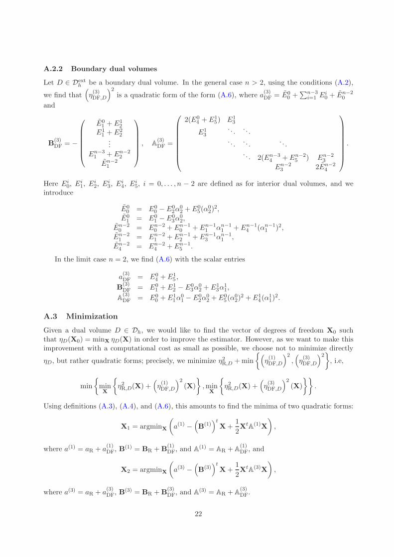
Figure 2: Comparison of the different estimators for the original jump estimate (4.18) with th givenby (4.1) (left) and for the minimization estimate (C.1) (right) in dependence on r

6 Numerical experiments

We present in this section a series of numerical experiments which confirm the theoretical resultsof the paper. The a posteriori error estimate of Theorem 4.5 with the reconstructed diffusive fluxth given by (4.1) gives a guaranteed upper bound on the overall energy error but the effectivityindex is never close to the optimal value of one in our tests. For this reason, we also present resultsemploying a local minimization procedure, consisting in modifications of the flux th in the interiorof each D ∈ Dh. This procedure is in detail described in the appendix below.

We perform our numerical experiments for problem (1.1a) with Ω = (0, 1) × (0, 1), a constantreaction coefficient r, and f = 0. We prescribe the Dirichlet boundary condition by the exactsolution

p(x, y) = e−r1/2x + e−r1/2y,

as in [8]. This solution exhibits a boundary layer along the coordinate axes for high values of r. Inorder to carry out the tests, we have implemented our estimates into the FreeFem++ [9] packageand all the results presented have been computed using FreeFem++. Finally, we shall in thissection term estimate (4.18) of Theorem 4.5 with th given by (4.1) as the jump estimate, as thisreconstructed diffusive flux th leads to estimators of the form ‖(∇ph + th) · n‖σ = ‖[[∇ph · n]]‖σ/2,and estimate (C.1) following from the local minimization strategy described in Appendix C belowas the minimization estimate. We however note that in the majority of cases, it is the simplechoice (B.1) which gives the minimum, so that very similar results may be presented with (B.1)instead of (C.1).

We first in the left part of Figure 2 show the different estimators of the original jump esti-mate (4.18) with th given by (4.1) on a fixed uniformly refined mesh with 512 elements in depen-dence on the reaction coefficient r, which we let vary between 10−6 and 106. We remark that thehighest contribution is always given by the residual estimate ηR :=

∑D∈Dh

η2R,D

1

2 , whereas the

contributions of the diffusive flux estimates η(i)DF :=

∑D∈Dh

(η(i)DF,D)2

1

2 are smaller. Note also that

although the estimate η(1)DF gives smaller values for moderate values of r, it gets eventually outper-

formed by the estimate η(2)DF. We next in Figure 3 present, for two different (uniformly refined)

grids, the corresponding effectivity indices. We can clearly see that they are bounded uniformlywith respect to r which demonstrates the full robustness of our estimates. Unfortunately, in partic-ular for smaller values of r, they are not too close to the optimal value of 1. This is the reason for

14

10−6

10−4

10−2

100

102

104

106

0

1

2

3

4

5

6

7

reaction term r

effe

ctiv

ity in

dex

uniform grid, 32 triangles

jump. est.min. est.

10−6

10−4

10−2

100

102

104

106

0

1

2

3

4

5

6

7

reaction term r

effe

ctiv

ity in

dex

uniform grid, 131072 triangles

jump. est.min. est.

Figure 3: Effectivity indices for the original jump estimate (4.18) with th given by (4.1) and forthe minimization estimate (C.1) in dependence on r for two different (uniformly refined) meshes

the introduction of a local minimization procedure which we have devised in [5] and [21, Section 7]in the pure diffusion case and which we adapt to the present case in the appendix below. Theresults using the minimization estimate (C.1) are then presented in the right part of Figure 2 andin Figure 3. We can see that for moderate values of r, the residual estimate has been decreasedunder the diffusive flux ones and consequently the effectivity index gets close to the optimal valueof 1. In what follows, we present the results only for the minimization estimate (C.1).

Apart from overall error control, a posteriori error estimates are a key element for adaptivemesh refinement. We exploit for this purpose the capabilities of FreeFem++. We mark an elementfor refinement if the estimator exceeded 50% of the maximal element estimators but we recallthat FreeFem++ actually generates a completely new mesh on the basis of this criterion and thisnew mesh is thus not a simple refinement of the previous one. In the adaptive refinement case,the elements marked for refinement were selected using the original jump estimators (4.18) withth given by (4.1). This approach seems to give better numerical results (better error decreasingwith the number of elements) and is in coincidence with our theoretical results, since we prove thelocal efficiency for these original estimators in Theorem 5.1. We firstly plot, in the left parts ofFigures 4 and 5, respectively, the estimated and actual errors against the number of elements in bothuniformly and adaptively refined meshes for r = 1 and r = 106. In the first case, the solution possesno singularity, so the adaptive approach only leads to a slight improvement of the error attained fora given number of unknowns on coarse meshes, whereas this tendency is reversed for fine meshes. Inthe second case with a singular solution, the adaptive approach leads to an important improvementof the error attained for a given number of unknowns. The effectivity indices are then shown in theright parts of Figures 4 and 5, respectively. In the first case, they improve considerably with themesh refinement and especially in the adaptive refinement mode they get very close to the optimalvalue of 1, whereas in the second one they are rather stable around the value of 2.4. Finally, tofurther promote the usability of our estimates for adaptive mesh refinement, we present in Figure 6the excellently matching predicted and actual error distribution and the corresponding adaptivelyrefined mesh as given by the jump estimator for r = 106.

15

101

102

103

104

105

106

10−3

10−2

10−1

100

number of triangles

ener

gy n

orm

min. est., uniformmin. est., adaptiveexact error, uniformexact error, adaptive

101

102

103

104

105

106

1

1.1

1.2

1.3

1.4

1.5

1.6

1.7

1.8

1.9

number of triangles

effe

ctiv

ity in

dex

min. est., uniformmin. est., adaptive

Figure 4: Estimated and actual error against the number of elements in uniformly/adaptively re-fined meshes (left) and corresponding effectivity indices (right) of the minimization estimator (C.1),r = 1

101

102

103

104

105

101

102

103

number of triangles

ener

gy n

orm

min. est., uniformmin. est., adaptiveexact error, uniformexact error, adaptive

101

102

103

104

105

2.25

2.3

2.35

2.4

2.45

2.5

2.55

number of triangles

effe

ctiv

ity in

dex

min. est., uniformmin. est., adaptive

Figure 5: Estimated and actual error against the number of elements in uniformly/adaptively re-fined meshes (left) and corresponding effectivity indices (right) of the minimization estimator (C.1),r = 106

Acknowledgments

This work was initiated during the summer school CEMRACS organized by the laboratory of thelast author in summer 2007 in Luminy/Marseille, France and the authors gratefully acknowledgeall the support.

References

[1] Ainsworth, M., and Babuska, I. Reliable and robust a posteriori error estimating forsingularly perturbed reaction-diffusion problems. SIAM J. Numer. Anal. 36, 2 (1999), 331–353.

[2] Bebendorf, M. A note on the Poincare inequality for convex domains. Z. Anal. Anwendungen22, 4 (2003), 751–756.

16

IsoValue0.4258781.277632.129392.981143.83294.684665.536416.388177.239928.091688.943439.7951910.646911.498712.350513.202214.05414.905715.757516.6092

Estimated Error DistributionIsoValue0.1740440.5221310.8702181.218311.566391.914482.262572.610662.958743.306833.654924.0034.351094.699185.047275.395355.743446.091536.439626.7877

Exact Error Distribution

Figure 6: Estimated error (left) and exact error (right) distribution using the original jump esti-mate (4.18) with th given by (4.1) on an adaptively refined mesh for r = 106

[3] Brezzi, F., and Fortin, M. Mixed and hybrid finite element methods, vol. 15 of SpringerSeries in Computational Mathematics. Springer-Verlag, New York, 1991.

[4] Carstensen, C., and Funken, S. A. Constants in Clement-interpolation error and residualbased a posteriori error estimates in finite element methods. East-West J. Numer. Math. 8, 3(2000), 153–175.

[5] Cheddadi, I., Fucık, R., Prieto, M. I., and Vohralık, M. Computable a posteriorierror estimates in the finite element method based on its local conservativity: improvementsusing local minimization. Submitted to ESAIM Proc., 2008.

[6] Ern, A., Stephansen, A. F., and Vohralık, M. Improved energy norm a posteriorierror estimation based on flux reconstruction for discontinuous Galerkin methods. Submit-ted to SIAM J. Numer. Anal., 2007.

[7] Eymard, R., Gallouet, T., and Herbin, R. Finite volume methods. In Handbook ofNumerical Analysis, Vol. VII. North-Holland, Amsterdam, 2000, pp. 713–1020.

[8] Grosman, S. An equilibrated residual method with a computable error approximation for asingularly perturbed reaction-diffusion problem on anisotropic finite element meshes. M2ANMath. Model. Numer. Anal. 40, 2 (2006), 239–267.

[9] Hecht, F., Pironneau, O., Le Hyaric, A., and Ohtsuka, K. FreeFem++.Tech. rep., Laboratoire Jacques-Louis Lions, Universite Pierre et Marie Curie, Paris,http://www.freefem.org/ff++, 2007.

[10] Korotov, S. Two-sided a posteriori error estimates for linear elliptic problems with mixedboundary conditions. Appl. Math. 52, 3 (2007), 235–249.

17

[11] Kunert, G. Robust a posteriori error estimation for a singularly perturbed reaction-diffusionequation on anisotropic tetrahedral meshes. Adv. Comput. Math. 15, 1-4 (2001), 237–259(2002). A posteriori error estimation and adaptive computational methods.

[12] Payne, L. E., and Weinberger, H. F. An optimal Poincare inequality for convex domains.Arch. Rational Mech. Anal. 5 (1960), 286–292 (1960).

[13] Prager, W., and Synge, J. L. Approximations in elasticity based on the concept of functionspace. Quart. Appl. Math. 5 (1947), 241–269.

[14] Repin, S., and Sauter, S. Functional a posteriori estimates for the reaction-diffusionproblem. C. R. Math. Acad. Sci. Paris 343, 5 (2006), 349–354.

[15] Roberts, J. E., and Thomas, J.-M. Mixed and hybrid methods. In Handbook of NumericalAnalysis, Vol. II. North-Holland, Amsterdam, 1991, pp. 523–639.

[16] Vejchodsky, T. Guaranteed and locally computable a posteriori error estimate. IMA J.Numer. Anal. 26, 3 (2006), 525–540.

[17] Verfurth, R. Robust a posteriori error estimators for a singularly perturbed reaction-diffusion equation. Numer. Math. 78, 3 (1998), 479–493.

[18] Vohralık, M. On the discrete Poincare–Friedrichs inequalities for nonconforming approxi-mations of the Sobolev space H1. Numer. Funct. Anal. Optim. 26, 7–8 (2005), 925–952.

[19] Vohralık, M. Residual flux-based a posteriori error estimates for finite volume discretizationsof inhomogeneous, anisotropic, and convection-dominated problems. Submitted to Numer.Math., 2006.

[20] Vohralık, M. A posteriori error estimates for lowest-order mixed finite element discretiza-tions of convection-diffusion-reaction equations. SIAM J. Numer. Anal. 45, 4 (2007), 1570–1599.

[21] Vohralık, M. Guaranteed and fully robust a posteriori error estimates for conforming dis-cretizations of diffusion problems with discontinuous coefficients. Submitted to Math. Comp.,2008.

[22] Vohralık, M. Two types of guaranteed (and robust) a posteriori estimates for finite volumemethods. Proc. FVCA5, to appear, 2008.

[23] Zienkiewicz, O. C., and Zhu, J. Z. A simple error estimator and adaptive procedure forpractical engineering analysis. Internat. J. Numer. Methods Engrg. 24, 2 (1987), 337–357.

Appendix: Improvements by local minimization

In Sections 4 and 5, we have shown that a choice of th ∈ H(div,Ω) in Theorem 4.5 for the vertex-centered finite volume method (2.5) leading to a guaranteed upper bound, local efficiency, androbustness is given by (4.1). However, it is not apparent at all whether this choice leads to the bestupper bound. In particular, by closer investigation, it turns out that whereas in mixed finite elementor discontinuous Galerkin (finite volume) methods, the residual estimator represents a higher-orderterm, as in these methods one has (with an appropriate th) (∇ · th + rph, 1)K = (f, 1)K for allK ∈ Th, it is not the case here, as (4.15) is only true on a set of elements SD of each interior

18

dual volume D and not on each element K ∈ SD. The numerical experiments for th given by (4.1)presented in Section 6 indeed show that the residual estimators ηR,D represent a major contributionto the estimate.

A natural idea in order to decrease the estimate is to try to choose another th ∈ H(div,Ω)satisfying (4.15). Notice now that th ∈ RTN(Sh) given by (4.1) only for such σ ∈ Gh which are atthe boundary of some D ∈ Dint

h satisfies th ∈ H(div,Ω) and (4.15) and we can choose any value forthe other edges. In particular, we can choose values that minimize the estimate. Moreover, as theestimator is build locally on each dual volume, we can perform this optimization process locally oneach dual volume.

We describe in this appendix two ways of a local minimization. In the pure diffusion case, thefirst one was devised in [5] and consists in true local minimization for the given degrees of freedom,leading to a small linear system solution for each vertex. The second, simplified one, was proposedin [21, Section 7] and avoids any local linear system solution. We adapt them here to the reaction–diffusion case; our exposition will be given in two space dimensions but a similar development canbe done in three space dimensions. For the sake of simplicity, we assume henceforth that f and rare piecewise constant on Th.

A A full local minimization strategy

We outline here the generalization of the “full minimization strategy” of [5] to the reaction–diffusioncase.

A.1 Notation and previous results

Let D ∈ Dh be the dual volume corresponding to a vertex VD as in Figure 7; D is decomposed intoa subdivision SD of n subtriangles K0, . . . ,Kn−1, numbered in the counter-clockwise direction. Oneach subtriangle Ki, the vertex 0 is the center of the volume D, the other vertices are numberedin the counter-clockwise direction, and we call σi

j the edge opposite to the vertex j and nσij

the

exterior normal vector of the edge σij. Let next ψi

j , j = 0, 1, 2, be the basis function of RTN(Ki)

corresponding to the vertex j, i.e., ψij = 1

d|Ki|(x− V i

j ), where V ij is vertex j of the triangle Ki. On

Ki, th can consequently be written as th|Ki = αi0ψ

i0 + αi

1ψi1 + αi

2ψi2.

The values of the external fluxes over ∂D are prescribed by (4.1) in the same way as before:for any dual volume D ∈ Dh, αi

0 = −|σi0|∇ph · nσi

0

, i = 0, . . . , n − 1; if D ∈ Dexth , then in addition

α02 = −|σ0

2 |∇ph ·nσ0

2

and αn−11 = −|σn−1

1 |∇ph ·nσn−1

1

. The internal fluxes, given by the coefficients

αi1 and αi

2, have to first fulfill the continuity of the normal trace across the edges, which imposes

• if D ∈ Dinth ,

αi1 + αi+1

2 = 0, i = 0, . . . , n − 1 with αn2 = α0

2; (A.1)

• if D ∈ Dexth ,

αi1 + αi+1

2 = 0, i = 0, . . . , n − 2. (A.2)

Therefore, there are n degrees of freedom X = (α0, . . . , αn−1)t if D ∈ Dinth and n − 1 degrees of

freedom X = (α0, . . . , αn−2)t if D ∈ Dexth left and these can be chosen in order to minimize the

estimator; from now on, the local estimator ηD(X) = ηDF,D(X) + ηR,D(X) will be considered as afunction of them. Later on, we will also employ the notation ηD(th) = ηDF,D(th) + ηR,D(th).

19

K0

K1

Kn−1 Ki

1

2

1

2

1 2

10

2

00

0

K0Kn−1

K1

Ki

0

0

0

0

1

1

1

12

2

2

2

Figure 7: Dual volume and its subdivision SD. Left: interior dual volume; right: boundary dualvolume

It has been in particular shown in [5, Section 3] that the square of the first diffusive flux

estimator η(1)DF,D on a dual volume D ∈ Dh is a quadratic form with respect to X of the form

(η

(1)DF,D

)2(X) = a

(1)DF −

(B

(1)DF

)tX +

1

2Xt

A(1)DFX; (A.3)

we refer to this reference for the precise form of the entries. Similarly, by a slight modification ofthe approach of this reference, one can derive that

η2R,D(X) = aR − Bt

RX +1

2Xt

ARX. (A.4)

We now accomplish a similar task for the diffusive flux estimator η(2)DF,D.

A.2 Diffusive flux estimator η(2)DF,D

By the definition, the square of the second diffusive flux estimator η(2)DF,D on a dual volume D ∈ Dh

is not a quadratic form with respect to the degrees of freedom X as the other ones. As our purposeis to improve the estimator without increasing too much the computational cost, we choose not to

minimize(η

(2)DF,D

)2directly, but an upper bound instead: we have

(η

(2)DF,D

)2≤ 2

∑

K∈SD

(m2

K ||∇ · th||2K + 2mK

(Ct,K,σ1

‖(∇ph + th) · n‖2σ1

+Ct,K,σ2‖(∇ph + th) · n‖2

σ2

)),

using the inequality (a + b)2 ≤ 2(a2 + b2) and the fact that on the edge σ0 of each subtriangle K,

th is prescribed such that (∇ph + th)|K · nσ0= 0. We denote by

(η

(3)DF,D

)2this upper bound and

study it separately for interior and exterior dual volumes.

20

A.2.1 Interior dual volumes

Let D ∈ Dinth and SD = K0, . . . ,Kn−1 be its subtriangulation. Using the definition of ψi

j

and (A.1), we have

th|K0= 1

d|K0|

(α0

0(x − V 00 ) + α0(x− V 0

1 ) − αn−1(x − V 02 )

),

th|Ki = 1d|Ki|

(αi

0(x − V i0 ) + αi(x− V i

1 ) − αi−1(x − V i2 )

), i = 1, . . . , n − 1

(A.5)

and consequently

‖∇ · th‖2K0

= 1|K0|

(α00 + α0 − αn−1)2,

‖∇ · th‖2Ki

= 1|Ki|

(αi0 + αi − αi−1)2, i = 1, . . . , n − 1.

Using (A.5) and the fact that the normal components of the basis functions ψij are constant over

the edges, we have

‖(∇ph + th) · nσi1

‖2σi1

= |σi1|

(∇ph · nσi

1

+ 1|σi

1|αi

)2, i = 0, . . . , n − 1,

‖(∇ph + th) · nσ0

2

‖2σ0

2

= |σ02 |

(∇ph · nσ0

2

− 1|σ0

2|αn−1

)2,

‖(∇ph + th) · nσi2

‖2σi2

= |σi2|

(∇ph · nσi

2

− 1|σi

2|αi−1

)2, i = 1, . . . , n − 1.

Therefore, we find that(η

(3)DF,D

)2is a quadratic form with respect to X = (α0, . . . , αn−1)t:

(η

(3)DF,D

)2(X) = a

(3)DF −

(B

(3)DF

)tX +

1

2Xt

A(3)DFX, (A.6)

where a(3)DF =

∑n−1i=0 Ei

0 and

B(3)DF = −

E01 + E1

2...

En−11 + E0

2

, A

(3)DF =

2(E04 + E1

5) E13 E0

3

E13

. . .. . .

. . .. . .

. . .. . .

. . . En−13

E03 En−1

3 2(En−14 + E0

5)

.

Here

Ei0 = 2m2

Ki

(αi0)2

|Ki|+ 4mKi(Ct,Ki,σi

1

|σi1|(∇ph · nσi

1

)2 + Ct,Ki,σi2

|σi2|(∇ph · nσi

2

)2),

Ei1 = 4m2

Ki

αi0

|Ki|+ 8Ct,Ki,σi

1

mKi∇ph · nσi1

,

Ei2 = −4m2

Ki

αi0

|Ki|− 8Ct,Ki,σi

2

mKi∇ph · nσi2

,

Ei3 = −4

m2

Ki|Ki|

,

Ei4 = 2

m2

Ki|Ki|

+ 4C

t,Ki,σi1

mKi

|σi1|

,

Ei5 = 2

m2

Ki|Ki|

+ 4C

t,Ki,σi1

mKi

|σi2|

.

21

A.2.2 Boundary dual volumes

Let D ∈ Dexth be a boundary dual volume. In the general case n > 2, using the conditions (A.2),

we find that(η

(3)DF,D

)2is a quadratic form of the form (A.6), where a

(3)DF = E0

0 +∑n−3

i=1 Ei0 + En−2

0

and

B(3)DF = −

E01 + E1

2

E11 + E2

2...

En−31 + En−2

2

En−21

, A(3)DF =

2(E04 + E1

5) E13

E13

. . .. . .

. . .. . .

. . .. . . 2(En−3

4 + En−25 ) En−2

3

En−23 2En−2

4

.

Here Ei0, Ei

1, Ei2, Ei

3, Ei4, Ei

5, i = 0, . . . , n − 2 are defined as for interior dual volumes, and weintroduce

E00 = E0

0 − E02α0

2 + E05(α0

2)2,

E01 = E0

1 − E03α0

2,

En−20 = En−2

0 + En−10 + En−1

1 αn−11 + En−1

4 (αn−11 )2,

En−21 = En−2

1 + En−12 + En−1

3 αn−11 ,

En−24 = En−2

4 + En−15 .

In the limit case n = 2, we find (A.6) with the scalar entries

a(3)DF = E0

4 + E15 ,

B(3)DF = E0

1 + E12 − E0

3α02 + E1

3α11,

A(3)DF = E0

0 + E11α0

1 − E02α0

2 + E05(α0

2)2 + E1

4(α11)

2.

A.3 Minimization

Given a dual volume D ∈ Dh, we would like to find the vector of degrees of freedom X0 suchthat ηD(X0) = minX ηD(X) in order to improve the estimator. However, as we want to make thisimprovement with a computational cost as small as possible, we choose not to minimize directly

ηD, but rather quadratic forms; precisely, we minimize η2R,D + min

(η

(1)DF,D

)2,(η

(3)DF,D

)2

, i.e,

min

minX

η2R,D(X) +

(η

(1)DF,D

)2(X)

,min

X

η2R,D(X) +

(η

(3)DF,D

)2(X)

.

Using definitions (A.3), (A.4), and (A.6), this amounts to find the minima of two quadratic forms:

X1 = argminX

(a(1) −

(B(1)

)tX +

1

2Xt

A(1)X

),

where a(1) = aR + a(1)DF, B(1) = BR + B

(1)DF, and A

(1) = AR + A(1)DF, and

X2 = argminX

(a(3) −

(B(3)

)tX +

1

2Xt

A(3)X

),

where a(3) = aR + a(3)DF, B(3) = BR + B

(3)DF, and A

(3) = AR + A(3)DF.

22

The matrices AR and A(1)DF are positive, and so is A

(1); it is also definite: one can easily prove

that XtARX and Xt

A(1)DFX cannot be zero at the same time except if X = 0. Thus, finding X1 is

reduced to computing the unique solution of the linear system A(1)X = B(1). This is also true for

X2. Then we define the local estimator as

ηmin,fullD := min ηD(X1), ηD(X2), ηD(th) . (A.7)

Here th is given by (4.1) and we include the term ηD(th) for the sake of security, as, havingminimized the quadratic forms, we are not sure to have found the minimum. Once again, we stressthat this minimization process is local and the size of the matrices is small: it corresponds tothe number of subtriangles of the dual volume, which is generally of the order of 10. Thus, thecomputational cost of the estimator does not increase excessively and remains linear.

B A simplified local minimization strategy

We generalize here one part of the “simplified minimization strategy” of [21, Section 7] to thereaction–diffusion case.

Let D ∈ Dh be fixed. We construct tD ∈ RTN(SD) given by (4.1) only for such σ ∈ Gh

contained in D which are at the boundary of some E ∈ Dinth and such that (∇·tD+rph, 1)K = (f, 1)K

for all K ∈ SD. Note that as (∇ · tD + rph, 1)D = (f, 1)D when D ∈ Dinth , this can be done without

any (local) linear system solution by choosing the flux over one interior side and a sequentialconstruction as

∑K∈SD

(f, 1)K = (f, 1)D. If D ∈ Dexth , this argument is then replaced by the fact

that we are free to choose the fluxes over the exterior sides. We thus can define a local estimator

ηmin,locD := min ηD(tD), ηD(th) , (B.1)

where th is given by (4.1). We remark that in [21, Section 7], a parameter α such that ηD(αth+(1−α)tD) was (approximately) minimal was searched in addition and the value ηD(αth + (1 − α)tD)was included in the above minimum. We do not perform here such an additional minimizationsince the above extremely simple choice already works very well.

C A minimization strategy used in the numerical experiments

In the numerical experiments of this paper, we finally use the minimization estimate of the form

|||p − ph||| ≤

∑

D∈Dh

(ηminD )2

1/2

, ηminD := min

ηmin,full

D , ηmin,locD

, (C.1)

where ηmin,fullD is given by (A.7) and ηmin,loc

D by (B.1). As however noted in the text, in the majorityof the cases, it is the simple choice (B.1) which gives the minimum.

23