Growth patterns of secondary Nothofagus obliqua– N. alpina forests in southern Chile

Growth patterns of secondary Nothofagus obliqua–N. alpinaforests in southern Chile

Cristian Echeverrıaa,b,*, Antonio Larab,1

aDepartment of Plant Sciences, University of Cambridge, Downing Street, Cambridge CB2 3EA, UKbInstituto de Silvicultura, Universidad Austral de Chile, Casilla 567, Valdivia, Chile

Received 13 November 2002; received in revised form 6 January 2004; accepted 20 February 2004

Abstract

The environmental factors that influence the diameter-growth of the Nothofagus obliqua and Nothofagus alpina were

investigated in secondary forests in southern Chile. A total of 17 edaphic, topographic and climatic variables were studied. The

annual periodic diameter increment (API) in 15 and 20 year-old trees was measured using dendrochronological techniques. A

multiple correspondence factorial analysis (MCFA) indicated that longitude, minimum precipitation, summer humidity index,

frost-free period, maximum drought period, and percentage of silt and sand in the soil were driving variables influencing

diameter-growth. The first three factors accounted for 70% of the total variation. Higher diameter-growth rates were associated

with intermediate annual rainfall, a short dry period, and sandy soil. Lower rates were associated with an intermediate frost-free

period, a low summer humidity index, a long dry period and silty soil. A spatial pattern of the driving variables was found in the

study area. The first two factors showed a longitudinal division separating the sites located in the Central Depression, Coastal

Range and Andean Range. Using the results generated by MCFA, an ascendant hierarchic classification analysis (AHCA) was

conducted to classify the study area into five sites of homogeneous productivity. The highest diameter-growth (>7.1 mm per

year) sites were located in the pre-Andes of Valdivia Province, followed by sites in the northern pre-Andes of Cautin Province

and the Andean Range of both provinces. Intermediate growth rates corresponded to the coastal site. The lowest diameter-growth

(<5.3 mm per year) was located in the Central Depression in both provinces. The use of multivariate methods and the adequate

selection of environmental variables enabled us to identify the diameter-growth driving variables, as well as to classify the study

area into five productivity categories.

# 2004 Elsevier B.V. All rights reserved.

Keywords: Site productivity; Diameter-growth; Nothofagus; Second-growth forest; Chile

1. Introduction

Nothofagusobliqua–N. alpina forests cover 1.2 mil-

lion hectares in south-central Chile ranging from

368300 to 408300S at the Coastal and Andean Ranges

(Donoso, 1993; CONAF et al., 1999), but are also

present in adjacent areas in Argentina. These decid-

uous forests may be either pure stands of species or

mixed stands in various proportion of N. obliqua or N.

alpina. N. dombeyi, an evergreen broad-leaved spe-

cies, may also be dominant in these stands. Nothofa-

gus obliqua–N. alpina forests occur from 100 to 900 m

of elevation (Donoso, 1981). They grow both under a

Mediterranean-type climate and under an Oceanic

Forest Ecology and Management 195 (2004) 29–43

* Corresponding author. Tel.: þ56-63-221228/

þ44-1223-330213; fax: þ56-63-221230/þ44-1223-333953.

E-mail addresses: [email protected] (C. Echeverrıa),

[email protected] (A. Lara).1 Tel.: þ44-1223-330213; fax: þ44-1223-333953.

0378-1127/$ – see front matter # 2004 Elsevier B.V. All rights reserved.

doi:10.1016/j.foreco.2004.02.034

Temperate climate further south, with an annual rain-

fall ranging from 1000 to 3000 mm, on deep well,

drained, volcanic spoils, that are loamy in texture

(Donoso, 1993). Most of these forests are second-

growth, relatively even-aged stands originating after

recurrent large-scale human (e.g. fires and clear cut-

tings) and natural disturbances (e.g. landslides and

volcanism) (Veblen and Ashton, 1978; Donoso, 1993;

Veblen et al., 1997).

As a result of their simple structure and composition,

different researchers have remarked the suitability of

these forests for silvicultural management (Grosse,

1987; Donoso, 1988; Espinosa et al., 1988; Donoso

et al., 1993b; Damby, 1994; Lara, 1996; Grosse and

Quiroz, 1999; Lara et al., 1999; Martinez, 1999).

Secondary N. obiqua–N. alpina forests are accessible

and are characterized by their relatively rapid-growth

rate compared to other forest types. Their high quality

wood is used for furniture, building, and handicrafts.

These young forests have a potential by high-produc-

tivity and it is important to develop silvicultural tools to

promote their sustainable management (Donoso et al.,

1993b; Damby, 1994; Otero and Monfil, 1994; Grosse

and Quiroz, 1999; Lara et al., 1999). Adequate manage-

ment of secondary N. obliqua–N. alpina forests has

been promoted by specific guidelines that forest owners

may decide to follow and further technical information

is needed in order to improve their management and

regulation (Lara et al., 1999, 2000).

Identification and classification of site productivity is

of great importance for the definition of silvicultural

methods best suited to particular sites. Previous studies

have defined four large growth-zones throughout the

entire range of secondary N. obliqua–N. alpina forests

using yield parameters (Donoso et al., 1993a). Large

areas may incorporate considerable physiographic

variation (Daniel et al., 1982; Pritchett, 1991), where

several environmental factors occur simultaneously.

Therefore, it is recommended to subdivide such areas

into smaller homogenous sites. Site classification re-

quiresanappropriate selectionof thedrivingvariables to

ensure an adequate classification of tree growth (Van-

clay, 1994; Vanclay et al., 1995; Davel, 1998; Curt et al.,

2001; Wilson et al., 2001). Other researchers have

acknowledged that the reliability of site classification

dependsonthequalityandtypeofdatasetusedinfinding

the driving variables (Gustavsen et al., 1998). Methods

using multivariate statistics have proved to be a suitable

method for defining sites of homogenous producti-

vity using environmental factors (Hagglund, 1981).

Studies using tree-ring techniques have been con-

ducted to understand the spatial and temporal patterns

of tree growth of Nothofagus pumilio forests at tree-line

in the Central Andes of Chile (358400–388400S, 1490–

1720 m elevation) and southern Chilean Patagonia (51–

558S, 300–980 m elevation) (Lara et al., 2001; Aravena

et al., 2002). Other tree-ring studies have described the

spatial and temporal pattern of the distribution of

Austrocedrus chilensis forests in northern Argentinean

Patagonia (418S) (Villalba et al., 1997) and central

Chile (Le Quesne et al., 2000). These studies have

focused on the influence of climate variability in tree

growth. Nevertheless, no attempt to identify the relative

importance of each of the local environmental factors

affecting N. obliqua–N. alpina tree growth and their

spatial distribution has been made in Chile.

Although many site factors can influence tree growth,

some of them (e.g. soil depth, water, nutrient avail-

ability) become dominant since they restrict the phy-

siological processes that result in tree growth (Fritts,

1976; Gerding and Schlatter, 1995; Roberts et al., 1996;

Kimmins, 1997; Gustavsen et al., 1998; Goebel et al.,

1999; Ditzer et al., 2000; Curt et al., 2001; Lara et al.,

2001; Joslin et al., 2001). In coarse-scale analysis, the

presence and growth of a plant species is strongly

influenced by climate. As the area of analysis is gra-

dually reduced, climate is less influential as a driving

factor. Conversely, physical and chemical soil proper-

ties become a decisive factor in tree establishment,

growth-rate and productivity (Kimmins, 1997; Schlat-

ter et al., 1997; Lara et al., 2001).

The objectives of this study were to identify the

relative importance of environmental factors influen-

cing diameter-growth of secondary N. obliqua–N.

alpina forests in south-central Chile (388300–408S).

We also analyzed the spatial distribution of these factors

and determine homogenous sites for tree growth and

forest potential productivity. This is the first study done

on this forest type using a multivariate approach.

2. Methods

2.1. Study area and sampling design

A total of 32 sampling plots were established in

undisturbed secondary Nothofagus obliqua–N. alpina

30 C. Echeverrıa, A. Lara / Forest Ecology and Management 195 (2004) 29–43

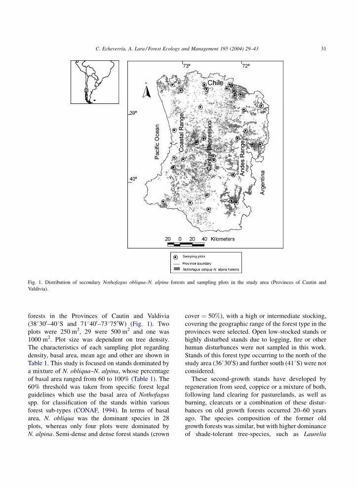
forests in the Provinces of Cautin and Valdivia

(388300–408S and 718400–738750W) (Fig. 1). Two

plots were 250 m2, 29 were 500 m2 and one was

1000 m2. Plot size was dependent on tree density.

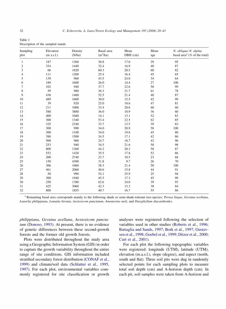
The characteristics of each sampling plot regarding

density, basal area, mean age and other are shown in

Table 1. This study is focused on stands dominated by

a mixture of N. obliqua–N. alpina, whose percentage

of basal area ranged from 60 to 100% (Table 1). The

60% threshold was taken from specific forest legal

guidelines which use the basal area of Nothofagus

spp. for classification of the stands within various

forest sub-types (CONAF, 1994). In terms of basal

area, N. obliqua was the dominant species in 28

plots, whereas only four plots were dominated by

N. alpina. Semi-dense and dense forest stands (crown

cover ¼ 50%), with a high or intermediate stocking,

covering the geographic range of the forest type in the

provinces were selected. Open low-stocked stands or

highly disturbed stands due to logging, fire or other

human disturbances were not sampled in this work.

Stands of this forest type occurring to the north of the

study area (368300S) and further south (418S) were not

considered.

These second-growth stands have developed by

regeneration from seed, coppice or a mixture of both,

following land clearing for pasturelands, as well as

burning, clearcuts or a combination of these distur-

bances on old growth forests occurred 20–60 years

ago. The species composition of the former old

growth forests was similar, but with higher dominance

of shade-tolerant tree-species, such as Laurelia

Fig. 1. Distribution of secondary Nothofagus obliqua–N. alpina forests and sampling plots in the study area (Provinces of Cautin and

Valdivia).

C. Echeverrıa, A. Lara / Forest Ecology and Management 195 (2004) 29–43 31

philippiana, Gevuina avellana, Aextoxicom puncta-

tum (Donoso, 1993). At present, there is no evidence

of genetic differences between these second-growth

forests and the former old growth forests.

Plots were distributed throughout the study area

using a Geographic Information System (GIS) in order

to capture the growth variability throughout the entire

range of site conditions. GIS information included

stratified secondary forest distribution (CONAF et al.,

1999) and climate/soil data (Schlatter et al., 1995,

1997). For each plot, environmental variables com-

monly registered for site classification or growth

analyses were registered following the selection of

variables used in other studies (Roberts et al., 1996;

Battaglia and Sands, 1997; Bork et al., 1997; Gustav-

sen et al., 1998; Goebel et al., 1999; Ditzer et al., 2000;

Curt et al., 2001).

For each plot the following topographic variables

were registered: longitude (UTM), latitude (UTM),

elevation (m.a.s.l.), slope (degree), and aspect (north,

south and flat). Three soil pits were dug in randomly

selected points for each sampling plots to measure

total soil depth (cm) and A-horizon depth (cm). In

each pit, soil samples were taken from A-horizon and

Table 1

Description of the sampled stands

Sampling

plot

Elevation

(m a.s.l.)

Density

(N/ha)

Basal area

(m2/ha)

Mean

DBH (cm)

Mean

age

N. obliqua–N. alpina

basal areaa (% of the total)

1 187 1360 30.8 17.0 29 95

2 354 1440 32.4 16.9 40 87

3 66 1820 60.3 20.5 60 82

4 111 1200 25.4 16.4 45 65

5 139 960 43.5 24.0 34 64

6 189 1600 26.0 14.4 27 100

7 102 940 37.7 22.6 58 99

8 59 980 36.3 21.7 61 78

9 436 1460 52.5 21.4 48 87

10 489 1600 30.0 15.5 42 99

11 39 920 25.0 18.6 47 81

12 211 1000 33.4 20.6 60 60

13 588 3880 36.0 10.9 36 60

14 400 1040 14.1 13.1 52 83

15 300 1340 53.4 22.5 62 85

16 325 2340 33.7 13.5 39 83

17 300 990 34.0 20.9 58 100

18 300 1100 34.0 19.8 45 80

19 388 1500 34.5 17.1 42 86

20 500 900 24.7 18.7 43 96

21 253 940 34.5 21.6 58 98

22 800 1360 44.2 20.3 58 87

23 552 1420 35.5 17.8 52 86

24 200 2740 23.7 10.5 23 68

25 150 4300 31.8 9.7 26 70

26 306 1060 38.3 21.4 58 100

27 461 2060 40.6 15.8 44 91

28 50 990 52.1 25.9 25 94

29 300 1940 45.5 17.3 45 99

30 250 1380 62.6 24.0 39 93

31 425 3060 42.3 13.3 38 84

32 800 1855 40.7 16.7 55 86

a Remaining basal area corresponds mainly to the following shade or semi-shade-tolerant tree-species: Persea lingue, Gevuina avellana,

Laurelia philippiana, Lomatia hirsuta, Aextoxicom punctatum, Amomyrtus meli, and Dasyphyllum diacanthoides.


then mixed up to prepare a representative soil sample

of 500 cm3 for each sampling plot. These soil samples

were analyzed in laboratory to provide data on the

organic matter (%), pH, nitrogen (%), and texture

(percentage of sand, silt and clay in the A horizon).

This field and laboratory information was comple-

mented with local soil information in literature (IREN

and UACH, 1978). Climatic variables included: mean

annual precipitation (mm) (average of annual rainfall

registered in the last 30 years), summer humidity

index (ratio between rainfall and mean potential eva-

potranspiration of the three warmest months), frost-

free period (days per year) (number of consecutive

days without occurrence of frost), and dry period

(months per year) (number of months in which the

rainfall does not represent the 50% of potential eva-

potranspiration) and were obtained from the literature

(Schlatter et al., 1995, 1997).

The selected growth variable was radial increment

(mm per year). One or two increment cores from 15 to

20 dominant or co-dominant N. obliqua and/or N.

alpina trees were obtained from each plot for deter-

mination of radial increment.

2.2. Data processing and analysis

Tree cores were mounted, sanded using sandpaper

of increasingly finer grain, and measured under a

microscope to the nearest 0.001 mm and stored in a

microcomputer (Stokes and Smiley, 1968; Robinson

and Evans, 1980). Then, a validation process was

conducted, comparing each radial-growth with a reg-

ular annual periodic increment (API) curve of an

undisturbed stand (Prodan et al., 1997). This was done

to distinguish those trees in which growth-rates had

been altered by human disturbances (e.g. growth

releases following selective cutting). This validation

was supported by field information on human distur-

bances.

In order to find the period of diameter-growth

(radial increment multiplied by two) that is best

correlated with site factors in each plot, four API

intervals were analyzed. Attempts were made to

include the maximum diameter-growth periods and

a sufficient range of at least 5 years (Espinosa et al.,

1988). The mean diameter API was estimated for the

periods 5–10, 10–15, 5–15, and 15–20 years of age in

each plot.

Multivariate statistical techniques enable the

identification and analysis of the driving factors of

biological and ecological processes. Multiple corre-

spondence factorial analysis was applied (MCFA)

using SPADN12 statistical package for identification

of the driving environmental variables of diameter-

growth. In the MCFA, API in diameter was considered

to be an objective variable and the 17 edaphoclimatic

variables to be active variables. SPADN has the ability

to distinguish a variable of interest (or objective) and

to treat it independently from the set of driving vari-

ables in order to avoid its influence on the definition of

correspondence factors (see footnote 2).

The number of classes for each variable and their

widths were determined using class frequency histo-

grams which were divided into at least five classes

according to the variation range of each variable.

Then, the number of classes that contributed most

importantly to explain the data set variation was fitted

using MCFA reducing the number of classes into two

or three categories (Table 2).

Because of the use of slope aspect, a discrete

variable, the MCFA was chosen as the method of

analysis and the 17 variables were converted into

two or three discrete classes according to the range

of variation of each variable. For the analysis of the

spatial distribution of the driving variables and their

relationship to diameter-growth, we generated Sur-

fer13 contour maps using the MCFA-generated pro-

jection coordinates of each plot for the first three

factors.

We used ascendant hierarchic classification analysis

(AHCA), computed by SPADN1, to classify site

productivity into categories. The AHCA identified

the number of categories based on the analysis of

level indices which were determined from the dis-

tances between plots’ projection coordinates gener-

ated previously by MCFA. The classification used

thresholds to define groups based on SPADN’s statis-

tics, including test value, between-group inertia, and

within-group inertia. The AHCA classified the sam-

pling plots into site productivity categories according

to the driving variables and their correspondence with

diameter-growth.

2 Portable System for Numeric Data Analysis, Version 2.5, 1993.3 Surface Mapping System, Version 6.04. Golden Software, Inc.


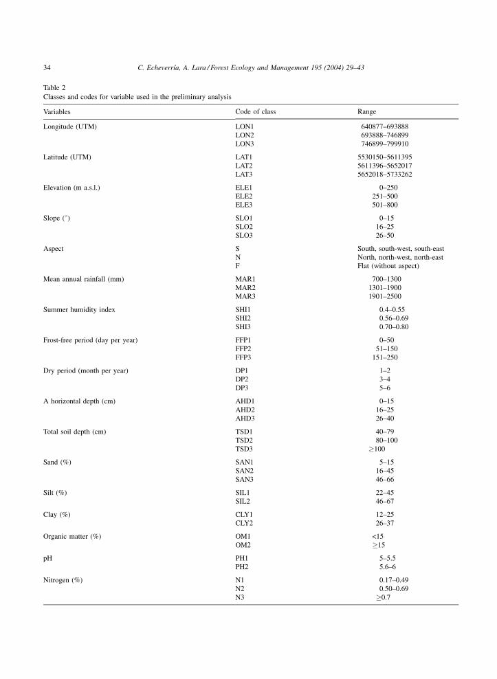
Table 2

Classes and codes for variable used in the preliminary analysis

Variables Code of class Range

Longitude (UTM) LON1 640877–693888LON2 693888–746899LON3 746899–799910

Latitude (UTM) LAT1 5530150–5611395LAT2 5611396–5652017LAT3 5652018–5733262

Elevation (m a.s.l.) ELE1 0–250ELE2 251–500ELE3 501–800

Slope (8) SLO1 0–15SLO2 16–25SLO3 26–50

Aspect S South, south-west, south-eastN North, north-west, north-eastF Flat (without aspect)

Mean annual rainfall (mm) MAR1 700–1300MAR2 1301–1900MAR3 1901–2500

Summer humidity index SHI1 0.4–0.55SHI2 0.56–0.69SHI3 0.70–0.80

Frost-free period (day per year) FFP1 0–50FFP2 51–150FFP3 151–250

Dry period (month per year) DP1 1–2DP2 3–4DP3 5–6

A horizontal depth (cm) AHD1 0–15AHD2 16–25AHD3 26–40

Total soil depth (cm) TSD1 40–79TSD2 80–100TSD3 �100

Sand (%) SAN1 5–15SAN2 16–45SAN3 46–66

Silt (%) SIL1 22–45SIL2 46–67

Clay (%) CLY1 12–25CLY2 26–37

Organic matter (%) OM1 <15OM2 �15

pH PH1 5–5.5PH2 5.6–6

Nitrogen (%) N1 0.17–0.49N2 0.50–0.69N3 �0.7


3. Results

3.1. Driving variables and diameter-growth

The analysis for the initial screening of the inde-

pendent variables considered 17 independent vari-

ables. This number is acknowledged to be small

compared to the number of observations (32 sampling

plots), but it was necessary to assure an adequate

consideration of all the potential variables that could

explain the variation in diameter increment. SPADN

software is recommended in cases when a limiting

number of observations is available or when the

number of independent variables is relatively

large, providing reliability in the results of the initial

screening.

The preliminary analysis using MCFA determined

that 6 out of the 17 variables that were studied sig-

nificantly contributed to the variance explained. At the

same time, these six variables had a high correspon-

dence with the API of 15–20 years, and therefore, this

period was selected as the diameter-growth variable

(Table 3). The classes determined for this API were—

API1: <5.39 mm per year; API2: 5.39–7.00 mm per

year, and API3: �7.01 mm per year.

The six most important variables identified as driv-

ing variables of the API were: longitude, mean annual

rainfall, summer humidity index, frost-free period,

and content of sand and silt in the soil (Table 3).

Using just these driving variables for a new MCFA, the

first three factors accounted for 70.4% of the total

variation (Factor 1: 34.0%, Factor 2: 20.1% and Factor

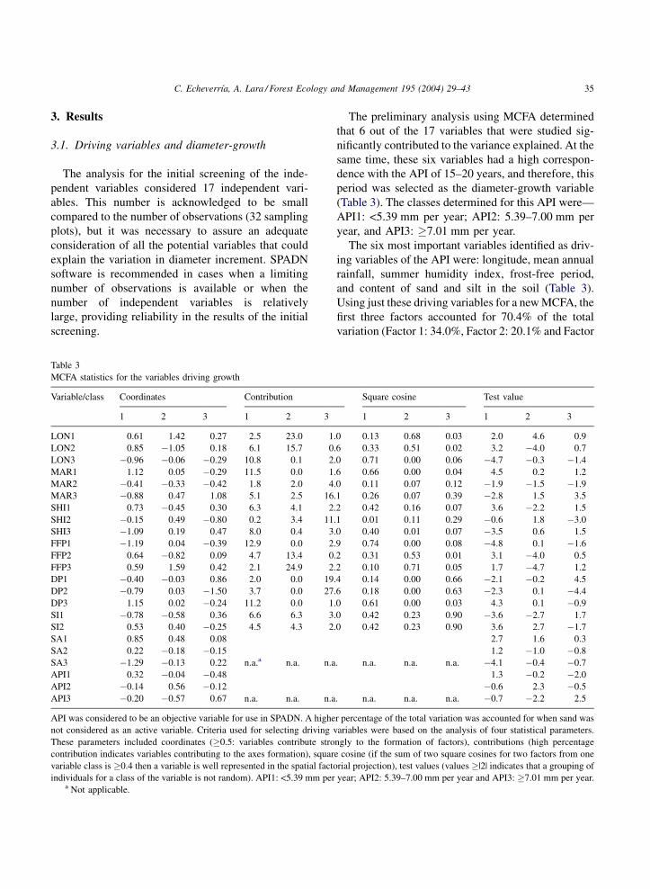
Table 3

MCFA statistics for the variables driving growth

Variable/class Coordinates Contribution Square cosine Test value

1 2 3 1 2 3 1 2 3 1 2 3

LON1 0.61 1.42 0.27 2.5 23.0 1.0 0.13 0.68 0.03 2.0 4.6 0.9

LON2 0.85 �1.05 0.18 6.1 15.7 0.6 0.33 0.51 0.02 3.2 �4.0 0.7

LON3 �0.96 �0.06 �0.29 10.8 0.1 2.0 0.71 0.00 0.06 �4.7 �0.3 �1.4

MAR1 1.12 0.05 �0.29 11.5 0.0 1.6 0.66 0.00 0.04 4.5 0.2 1.2

MAR2 �0.41 �0.33 �0.42 1.8 2.0 4.0 0.11 0.07 0.12 �1.9 �1.5 �1.9

MAR3 �0.88 0.47 1.08 5.1 2.5 16.1 0.26 0.07 0.39 �2.8 1.5 3.5

SHI1 0.73 �0.45 0.30 6.3 4.1 2.2 0.42 0.16 0.07 3.6 �2.2 1.5

SHI2 �0.15 0.49 �0.80 0.2 3.4 11.1 0.01 0.11 0.29 �0.6 1.8 �3.0

SHI3 �1.09 0.19 0.47 8.0 0.4 3.0 0.40 0.01 0.07 �3.5 0.6 1.5

FFP1 �1.19 0.04 �0.39 12.9 0.0 2.9 0.74 0.00 0.08 �4.8 0.1 �1.6

FFP2 0.64 �0.82 0.09 4.7 13.4 0.2 0.31 0.53 0.01 3.1 �4.0 0.5

FFP3 0.59 1.59 0.42 2.1 24.9 2.2 0.10 0.71 0.05 1.7 �4.7 1.2

DP1 �0.40 �0.03 0.86 2.0 0.0 19.4 0.14 0.00 0.66 �2.1 �0.2 4.5

DP2 �0.79 0.03 �1.50 3.7 0.0 27.6 0.18 0.00 0.63 �2.3 0.1 �4.4

DP3 1.15 0.02 �0.24 11.2 0.0 1.0 0.61 0.00 0.03 4.3 0.1 �0.9

SI1 �0.78 �0.58 0.36 6.6 6.3 3.0 0.42 0.23 0.90 �3.6 �2.7 1.7

SI2 0.53 0.40 �0.25 4.5 4.3 2.0 0.42 0.23 0.90 3.6 2.7 �1.7

SA1 0.85 0.48 0.08 2.7 1.6 0.3

SA2 0.22 �0.18 �0.15 1.2 �1.0 �0.8

SA3 �1.29 �0.13 0.22 n.a.a n.a. n.a. n.a. n.a. n.a. �4.1 �0.4 �0.7

API1 0.32 �0.04 �0.48 1.3 �0.2 �2.0

API2 �0.14 0.56 �0.12 �0.6 2.3 �0.5

API3 �0.20 �0.57 0.67 n.a. n.a. n.a. n.a. n.a. n.a. �0.7 �2.2 2.5

API was considered to be an objective variable for use in SPADN. A higher percentage of the total variation was accounted for when sand was

not considered as an active variable. Criteria used for selecting driving variables were based on the analysis of four statistical parameters.

These parameters included coordinates (�0.5: variables contribute strongly to the formation of factors), contributions (high percentage

contribution indicates variables contributing to the axes formation), square cosine (if the sum of two square cosines for two factors from one

variable class is �0.4 then a variable is well represented in the spatial factorial projection), test values (values �|2| indicates that a grouping of

individuals for a class of the variable is not random). API1: <5.39 mm per year; API2: 5.39–7.00 mm per year and API3: �7.01 mm per year.a Not applicable.


3: 16.3%). The variables were well represented in a

two-dimensional projection formed by Factors 1 and

2. More than 70% of the sampling plots were well

represented for the first two factors and this percentage

increases to more than 80% for the first three factors

(not shown). This high representation was revealed by

the statistics used in the SPADN analysis (square

cosine, coordinates and contribution) which also con-

firmed a certain degree of association among the

sampling plots through the study area (not shown).

Due to the high variation explained by the first three

factors and a significant representation of the plots, it

is possible to establish correspondences between

environmental variables and individual plots.

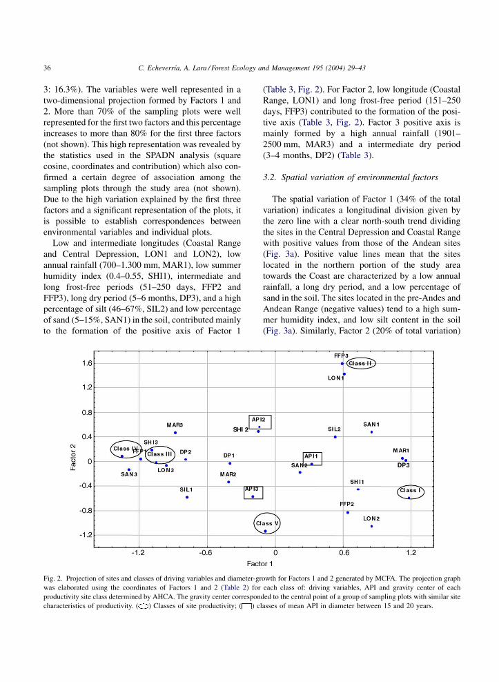
Low and intermediate longitudes (Coastal Range

and Central Depression, LON1 and LON2), low

annual rainfall (700–1.300 mm, MAR1), low summer

humidity index (0.4–0.55, SHI1), intermediate and

long frost-free periods (51–250 days, FFP2 and

FFP3), long dry period (5–6 months, DP3), and a high

percentage of silt (46–67%, SIL2) and low percentage

of sand (5–15%, SAN1) in the soil, contributed mainly

to the formation of the positive axis of Factor 1

(Table 3, Fig. 2). For Factor 2, low longitude (Coastal

Range, LON1) and long frost-free period (151–250

days, FFP3) contributed to the formation of the posi-

tive axis (Table 3, Fig. 2). Factor 3 positive axis is

mainly formed by a high annual rainfall (1901–

2500 mm, MAR3) and a intermediate dry period

(3–4 months, DP2) (Table 3).

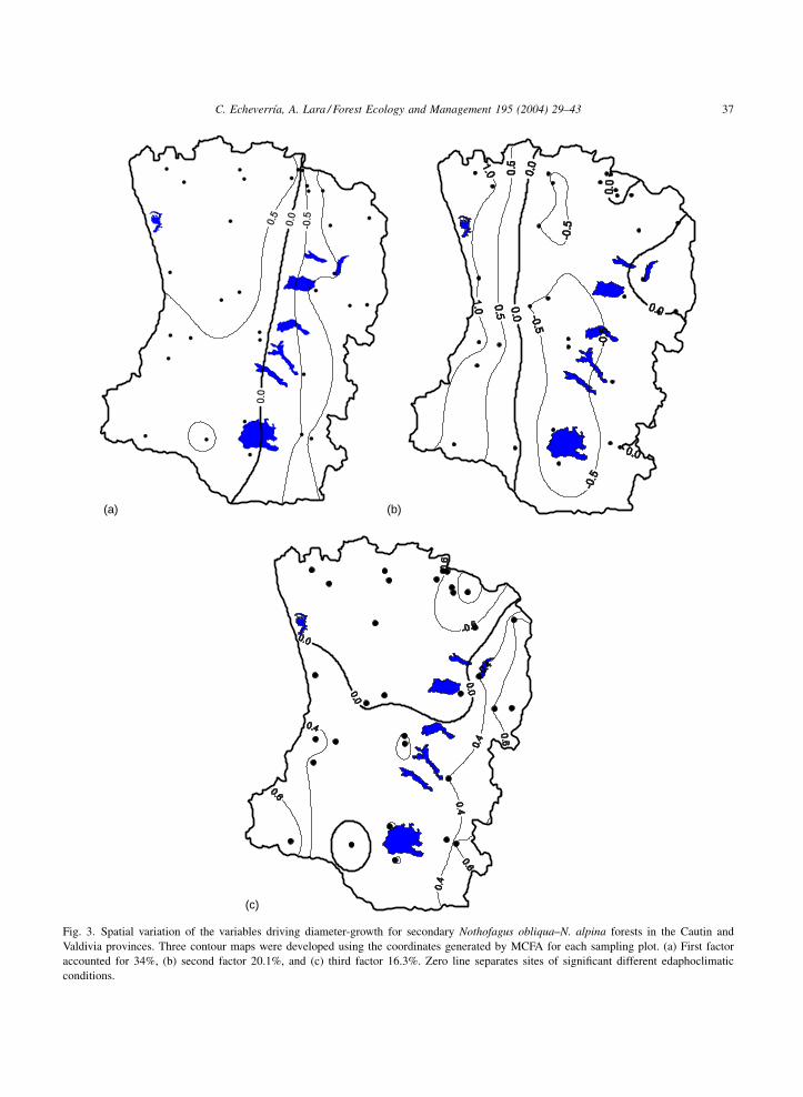
3.2. Spatial variation of environmental factors

The spatial variation of Factor 1 (34% of the total

variation) indicates a longitudinal division given by

the zero line with a clear north-south trend dividing

the sites in the Central Depression and Coastal Range

with positive values from those of the Andean sites

(Fig. 3a). Positive value lines mean that the sites

located in the northern portion of the study area

towards the Coast are characterized by a low annual

rainfall, a long dry period, and a low percentage of

sand in the soil. The sites located in the pre-Andes and

Andean Range (negative values) tend to a high sum-

mer humidity index, and low silt content in the soil

(Fig. 3a). Similarly, Factor 2 (20% of total variation)

Fig. 2. Projection of sites and classes of driving variables and diameter-growth for Factors 1 and 2 generated by MCFA. The projection graph

was elaborated using the coordinates of Factors 1 and 2 (Table 2) for each class of: driving variables, API and gravity center of each

productivity site class determined by AHCA. The gravity center corresponded to the central point of a group of sampling plots with similar site

characteristics of productivity. ( ) Classes of site productivity; ( ) classes of mean API in diameter between 15 and 20 years.


(a)

(c)

(b)

Fig. 3. Spatial variation of the variables driving diameter-growth for secondary Nothofagus obliqua–N. alpina forests in the Cautin and

Valdivia provinces. Three contour maps were developed using the coordinates generated by MCFA for each sampling plot. (a) First factor

accounted for 34%, (b) second factor 20.1%, and (c) third factor 16.3%. Zero line separates sites of significant different edaphoclimatic

conditions.


shows a longitudinal variation of the driving variables,

separating sites located in the Central Depression with

the rest (Fig. 3b). Sites located in the Coastal Range

are characterized by a longer frost-free period than

those located in the Central Depression. Factor 3 (16%

of the total variation) follows a different spatial pattern

compared to Factors 1 and 2, indicating a significant

difference between the northern and southern portions

of the study area, separated by the zero line (Fig. 3c).

3.3. Site productivity classification

The AHCA classified the 32 sampling plots into five

site productivity classes (Table 4). All the classes have

test values >2 or <�2 in Factor 1 or 2. This indicates

that each class has similar ranges of certain edaphocli-

matic driving variables with their corresponding dia-

meter-growth and that each class is not randomly

associated with the variables (Table 4). The higher

value of inter-class inertia compared to intra-class

inertia shows that the partition of sampling plots is

appropriate (Table 4). The homogeneity of the values

of intra-class inertia indicates that the total variation is

distributed proportionally among the various classes.

These statistics demonstrate that both the number of

classes and the classification of the sampling plots

within these classes was objective. Therefore, the

sampling plots can be classified within these five site

productivity categories. The projection of the coordi-

nates of each plot for Factors 1 and 2 computed by

SPADN encircled within their respective site produc-

tivity class shows clear grouping patterns (Fig. 4). This

grouping stresses that the sites within each class are

characterized by a similar range of edaphoclimatic

variables. The location of each sampling plot enabled

us to outline the spatial boundaries of each site

productivity class within the study area (Fig. 4).

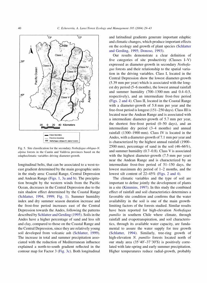
Knowing the location of the sampling plots that

were classified into a specific site by the AHCA, the

boundaries for each type of site (class) were drawn

in the study area (Fig. 5). For each of these classes the

average diameter increment (expressed as API)

between 15 and 20 years old was determined

(Table 5). Classes I, II and IV presented a wide

deviation of the API between 15 and 20 years old,

being Classes I and IV those that have the widest range

of deviation (1.62 mm per year, Table 5). The API of

each plot was used in a non-parametric Kruskal–

Wallis test which revealed a significant difference in

the diameter increment among the classes in the study

area.

4. Discussion

The multiple correspondence factorial analysis

(MFCA) determined that longitude, three climatic

variables (i.e. mean annual rainfall, summer humidity

index, and frost-free period) and two edaphic variables

(i.e. sand and silt contents) were associated with the

diameter-growth in the forest stands studied (Table 3).

These six variables contributed to the formation of the

first three factors accounting for 70.4% of the total

variance. The topographic variables such as elevation,

slope angle and aspect did not explain the variation in

growth in the study area. Similarly, some edaphic

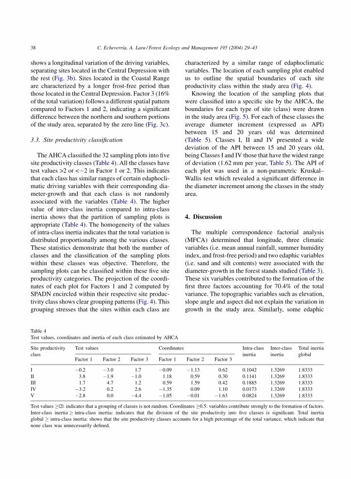
Table 4

Test values, coordinates and inertia of each class estimated by AHCA

Site productivity

class

Test values Coordinates Intra-class

inertia

Inter-class

inertia

Total inertia

globalFactor 1 Factor 2 Factor 3 Factor 1 Factor 2 Factor 3

I �0.2 �3.0 1.7 �0.09 �1.13 0.62 0.1042 1.3269 1.8333

II 3.8 �1.9 �1.0 1.18 0.59 0.30 0.1141 1.3269 1.8333

III 1.7 4.7 1.2 0.59 1.59 0.42 0.1885 1.3269 1.8333

IV �3.2 0.2 2.6 �1.35 0.09 1.10 0.0173 1.3269 1.8333

V �2.8 0.0 �4.4 �1.05 �0.01 �1.63 0.0824 1.3269 1.8333

Test values �|2|: indicates that a grouping of classes is not random. Coordinates �0.5: variables contribute strongly to the formation of factors.

Inter-class inertia � intra-class inertia: indicates that the division of the site productivity into five classes is significant. Total inertia

global � intra-class inertia: shows that the site productivity classes accounts for a high percentage of the total variance, which indicate that

none class was unnecessarily defined.


variables such as the A-horizon depth, total soil depth,

organic matter, pH and Nitrogen were not significant.

This may probably be explained due to their relative

narrow variation ranges in the study area, compared to

the other variables. Nevertheless, these variables

might be significant at a local scale that cannot be

properly identified at the scale used to develop the

MFCA. Similarly, a site classification analysis con-

ducted for Pseudotsuga menziesii plantations in the

northwestern part of the French Massif Central, in

which soil variables were correlated to tree growth,

climatic variables were not significant because of

their low variation within the study area (Curt et al.,

2001).

The use of factorial design techniques for identify-

ing the most important variables has similarly been

conducted in various forest types and geographic areas

(Gomory and Gomoryova, 1997; Goebel et al., 1999;

Canettieri et al., 2001). Different variables, such as

latitude, longitude, elevation, slope, aspect, soil depth,

and texture, were used for developing a growth model

for Eucalyptus globulus in southeastern Tasmania and

in Western Australia (Battaglia and Sands, 1997). In

our study only one of these variables, longitude, was

significant in explaining Nothofagus alpina–N. obli-

qua growth. Other studies have demonstrated the

influence of soil water potential in controlling the

growth of an oak stand in Tennessee, USA (Joslin

et al., 2001). Although the soil chemical variables

analyzed in this study did not explain the variation in

growth, pH, A-horizon depth, and the availability of

minerals have shown to be of particular importance to

determine understory composition in different ecosys-

tems (Goebel et al., 1999; Brosofske et al., 2001;

Weckstrom and Korhola, 2001; Wilson et al., 2001).

Spatial patterns for Factors 1 and 2 of the dri-

ving climatic and edaphic variables follow clear

Fig. 4. Projection of sampling plots for Factors 1 and 2 generated by MCFA. Grouping of sampling plots was determined by AHCA using the

growth driving variables. Each group of sampling plots exhibits similar edaphoclimatic conditions and annual diameter increment.

Table 5

Mean, standard deviation and range of variation to API for each site

productivity class

Site productivity

class

Annual periodic increment, API (mm per year)

Meana S.D. Range

I 5.3 1.62 2.4–7.9

II 5.8 1.19 3.4–7.5

III 5.7 0.88 4.8–6.9

IV 7.1 1.62 4.9–9.0

V 7.5 0.88 6.6–8.9

a Mean annual diameter increment between 15 and 20 year old.


longitudinal belts, that can be associated to a west-to-

east gradient determined by the main geographic units

in the study area: Coastal Range, Central Depression

and Andean Range (Figs. 1, 3a and b). The precipita-

tion brought by the western winds from the Pacific

Ocean, decreases in the Central Depression due to the

rain shadow effect determined by the Coastal Range

(Schlatter, 1994, 1999; Fig. 1). Summer humidity

index and dry summer season duration increase and

the frost-free period increases east of the Central

Depression towards the Andes, following the patterns

described by Schlatter and Gerding (1995). Soils in the

Andes have a higher percentage of sand and less silt

and clay, compared to those on the Coastal Range and

the Central Depression, since they are relatively young

soil developed from volcanic ash (Schlatter, 1999).

The increase in total and summer precipitation asso-

ciated with the reduction of Mediterranean influence

explained a north-to-south gradient reflected in the

contour map for Factor 3 (Fig. 3c). Both longitudinal

and latitudinal gradients generate important edaphic

and climatic changes, which produce important effects

on the ecology and growth of plant species (Schlatter

and Gerding, 1995; Donoso, 1993).

Our results demonstrate a clear definition of

five categories of site productivity (Classes I–V)

expressed as diameter-growth in secondary Nothofa-

gus forests and their relationship to the spatial varia-

tion in the driving variables. Class I, located in the

Central Depression show the lowest diameter-growth

(5.39 mm per year) which is associated with the long-

est dry period (5–6 months), the lowest annual rainfall

and summer humidity (700–1300 mm and 0.4–0.5,

respectively), and an intermediate frost-free period

(Figs. 2 and 4). Class II, located in the Coastal Range

with a diameter-growth of 5.8 mm per year and the

free-frost period is longest (151–250 days). Class III is

located near the Andean Range and is associated with

a intermediate diameter-growth of 5.7 mm per year,

the shortest free-frost period (0–50 days), and an

intermediate dry period (3–4 months) and annual

rainfall (1300–1900 mm). Class IV is located in the

Andes, with a diameter-growth of 7.1 mm per year and

is characterized by the highest annual rainfall (1900–

2500 mm), percentage of sand in the soil (46–66%),

and summer humidity (0.7–0.8). Class V is associated

with the highest diameter-growth (7.5 mm per year)

near the Andean Range and is characterized by an

intermediate frost-free period of 51–150 days, the

lowest maximum dry period of 1–2 months, and the

lowest silt content of 22–45% (Figs. 2 and 4).

The climatic variables and the type of soil are

important to define jointly the development of plants

in a site (Kimmins, 1997). In this study the combined

effect of rainfall and soil characteristics determines a

favorable site condition and confirms that the water

availability in the soil is one of the main growth-

limiting factors of the forests studied. Similar results

have been reported for high-elevation Nothofagus

pumilio in southern Chile where climate, through

rainfall and evapotranspiration, and soil characteris-

tics, through its available water capacity, are funda-

mental to assure the water supply for tree growth

(Schlatter, 1994). Similarly, tree-ring growth of

high-elevation N. pumilio forests located north of

our study area (358400–378300S) is positively corre-

lated with late-spring and early summer precipitation.

Higher temperatures reduce radial-growth, probably

Fig. 5. Site classification for the secondary Nothofagus obliqua–N.

alpina forests in the Cautin and Valdivia provinces based on the

edaphoclimatic variables driving diameter-growth.


because of an increase in evapotranspiration and a

decrease in water availability (Lara et al., 2001).

Although some specific variable classes explain

better the differences and similarities between sites,

the integrated effect of the driving variables enabled

the identification of sites with similar characteristics.

The trend of higher diameter-growth rates for N.

alpina and N. obliqua for sites located near and in

the Andes (site Classes III–V of this study) coincides

with the recognition of volcanic soils as favorable for

vegetation growth (Schmaltz, 1973; INIA, 1985;

Gerding and Schlatter, 1995; Schlatter and Gerding,

1995). A previous study determined growth-zones for

Nothofagus obliqua–N. alpina forest stands along its

entire geographical range also found higher growth

rates for the Andes (Donoso et al., 1993a). Never-

theless, this study did not identified the growth driving

variables using a multivariate analysis.

The understanding of the variation in site productiv-

ity for N. obliqua and N. alpina is a key information for

the design and proposal of sustainable forest manage-

ment schemes. The development and mapping of site

classification based on ecological driving factors will

enable to geographically understand the influence of

abiotic factors on the N. obliqua–N. alpina forests.

Similar ideas have been proposed for the definition

of ecological site classification as a basis for improved

management of the British forests (Wilson et al., 2001)

and in southeastern New Brunswick in Canada (Matson

and Power, 1996). Information on productivity is also

useful for site selection in reforestation and restoration

programs with Nothofagus obliqua and N. alpina. The

success of these programs in high-productivity sites

(Classes III–V) might be assured due to the high rates of

growth expected in these sites.

Due to the high potential of the N. obliqua–N.

alpina secondary stands through sustainable manage-

ment practices, it is important to complement this

work by studying site productivity throughout their

entire geographic range (368300–408300S). Finally, the

approach used in this paper may be applied to deter-

mine the productivity of other forest types in Chile.

Acknowledgements

The authors gratefully thank the information from

sampling plots provided by FONDEF(D97/1065) pro-

ject and Louisiana Pacific Chile. We are also thankful

for CONAFs authorization for the use of the Catastro

digital information on forest cover, and Vıctor Gerd-

ing and Alicia Ortega for their advise and comments,

and Juan Schlatter for providing access to the GIS

edaphoclimatic data base. Silvia Delgado (IANIGLA,

Mendoza, Argentina) and Ana Vianco (U. Nacional de

Rıo Cuarto, Argentina) provided useful guidance with

the statistical analysis. Salvador Gezan, Oscar Thiers

and Emilio Cuq assisted the database, soil description

and dendrochronological analyses, respectively. This

research was supported by the SUCRE (IC18-CT97-

014) and BIOCORES (ICA-CT-2001-10095) projects

funded by the European Commission and WWF grant

(9Z0711/01). A. Lara acknowledges support from

Mideplan, through its Iniciativa Cientıfica Milenio

(ICM), and a Bullard Fellowship from the Harvard

Forest (University of Harvard).

References

Aravena, J.C., Lara, A., Wolodarsky, A., Villalba, R., Cuq, E.,

2002. Tree-ring growth patterns and temperature reconstruction

from Nothofagus pumilio (Fagaceae) forests at the upper tree

line of southern Chilean Patagonia. Revista Chilena de Historia

Natural 75, 361–376.

Battaglia, M., Sands, P., 1997. Modelling site productivity of

Eucalyptus globulus in response to climatic and site factors.

Aust. J. Plant Physiol. 24 (6), 831–850.

Bork, E.W., Hudson, R.J., Bailey, A.W., 1997. Upland plant

community classification in Elk Island National Park, Alberta,

Canada, using disturbance history and physical site factors.

Plant Ecol. 130, 171–190.

Brosofske, K.D., Chen, J., Crow, T.R., 2001. Understory vegetation

and site factors: implications for a managed Wisconsin

landscape. For. Ecol. Manage. 146, 75–87.

Canettieri, E.V., Silva, J.B.A.E., Felipe, M.G.A., 2001. Application

of factorial design to the study of xylitol production from

eucalyptus hemicellulosic hydrolysate. Appl. Biochem. Bio-

technol. 94 (2), 159–168.

CONAF, CONAMA, BIRF, Universidad Austral de Chile,

Pontificia Universidad Catolica de Chile, Universidad Catolica

de Temuco, 1999. Proyecto Catastro y Evaluacion de los

Recursos Vegetacionales Nativos de Chile, Santiago, Chile.

CONAF, 1994. Normas de Manejo para Raleo del Renovales del

Tipo Forestal Roble-Raulı-Coihue. Corporacion Nacional

Forestal. Solicitud de Aplicacion, Santiago, Chile.

Curt, T., Bouchaud, M., Agrech, G., 2001. Predicting site index of

Douglas-Fir plantations from ecological variables in the Massif

Central area of France. For. Ecol. Manage. 149, 61–74.

Damby, N., 1994. Some impressions of Nothofagus in Chile. Quart.

J. For. 88 (2), 112–118.


Daniel, T., Helms, J., Baker, F., 1982. Principios de Silvicultura,

2nd ed. McGraw-Hill, Mexico.

Davel, M., 1998. Identificacion y Caracterizacion de zonas de

crecimiento para Pino Oregon en la Patagonia andina Argentina.

Magister Thesis. Universidad Austral de Chile, Chile.

Ditzer, T., Glauner, R., Forster, M., Kohler, P., Huth, A., 2000. The

process-based stand growth model Formix 3-Q applied in a GIS

environment for growth and yield analysis in a tropical rain

forest. Tree Physiol. 20, 367–381.

Donoso, C., 1981. Tipos Forestales de los bosques nativos de Chile.

Documento de Trabajo No. 38. FAO: DP/CHI/76/003, Chile.

Donoso, P., 1988. Caracterizacion y proposiciones silviculturales

para renovales de Roble (Nothofagus obliqua) y Raulı

(Nothofagus alpina) en el area de proteccion ‘‘Radal 7 Tazas’’,

VII Region. Bosque 9 (2), 103–114.

Donoso, C., 1993. Bosques templados de Chile y Argentina,

variacion, estructura y dinamica. Universitaria, Santiago, Chile.

Donoso, P., Donoso, C., Sandoval, V., 1993a. Proposicion de zonas

de crecimiento de renovales de Roble (Nothofagus obliqua) y

Raulı (Nothofagus alpina) en su rango de distribucion natural.

Bosque 14 (2), 37–55.

Donoso, P., Monfil, T., Otero, L., Barrales, L., 1993b. Estudio de

crecimiento de plantaciones y renovales manejados de especies

nativas en el area andina de las provincias de Cautin y Valdivia.

Ciencia e Investigacion Forestal 7 (2), 253–287.

Espinosa, M., Garcia, J., Pena, E., 1988. Evaluacion del

crecimiento de una plantacion de Raulı [Nothofagus alpina

(Poet. et Endl.) Oerst.] a los 34 anos de edad. Agrociencia 4 (1),

67–74.

Fritts, H., 1976. Tree Rings and Climate. Academic Press, London,

UK.

Gerding, V., Schlatter, J., 1995. Variables y factores del sitio de

importancia para la productividad de Pinus radiata D. Don en

Chile. Bosque 16 (2), 39–56.

Goebel, P.C., Hux, D.M., Olivero, A.M., 1999. Seasonal ground-

flora patterns and site factor relationship of second-growth and

old-growth south-facing forest ecosystems, southeastern Ohio,

USA. Nat. Areas J. 19, 12–29.

Gomory, D., Gomoryova, E., 1997. Comparison of several

multivariate methods for assessing the relationship between

soil properties and height growth of forest stands: a case study.

Ekologia-Bratislava 16, 359–370.

Grosse, H., 1987. Desarrollo de renovales de Raulı raleados.

Ciencia e Investigacion Forestal 1 (2), 31–43.

Grosse, H., Quiroz, I., 1999. Silvicultura de los bosques de segundo

crecimiento de Roble, Raulı y Coihue en la region centro-sur de

Chile. In: Donoso, C., Lara, A. (Eds.), Silvicultura de los

bosques nativos de Chile. Universitaria, Santiago, pp. 95–128.

Gustavsen, H.G., Heinonen, R., Paavilainen, E., Reinikainen, A.,

1998. Growth and yield models for forest stands on drained

peatland sites in southern Finland. For. Ecol. Manage. 107, 1–

17.

Hagglund, B., 1981. Evaluation of forest site productivity. Forestry

abstracts. Review article. Commonwealth Forestry Bureau 42

(11), 515–527.

INIA (Instituto de Investigaciones Agropecuarias), 1985. Suelos

volcanicos de Chile. Ministerio de Agricultura, Santiago.

IREN (Instituto de Investigacion de Recursos Naturales) and

UACH (Universidad Austral de Chile), 1978. Estudio de suelos

de la Provincia de Valdivia, Santiago.

Joslin, J.D., Wolfe, M.H., Hanson, P.J., 2001. Factors controlling

the timing of root elongation intensity in a mature upland oak

stand. Plant and Soil 228, 201–212.

Kimmins, J., 1997. Forest Ecology: A Foundation for Sustainable

Management, 2nd ed. Prentice-Hall, New Jersey, USA.

Lara, A., 1996. Una propuesta general de silvicultura para Chile.

Ambiente y Desarrollo 12 (1), 31–40.

Lara, A., Cortes, M., Echeverrıa, C., 2000. Bosques. In: Sunkel, O.

(Ed.), Informe Paıs: Estado del Medio Ambiente en Chile.

Centro de Analisis de Polıticas Publicas, Universidad de Chile,

Santiago, pp. 131–173.

Lara, A., Donoso, C., Donoso, P., Nunez, P., Cavieres, A., 1999.

Normas de manejo para raleo de renovales del tipo forestal

Roble-Raulı-Coigue. In: Donoso, C., Lara, A. (Eds.), Silvicul-

tura de los bosques nativos de Chile. Universitaria, Santiago,

pp. 129–144.

Lara, A., Aravena, J.C., Villalba, R., Wolodarsky, A., Luckman, B.,

Wilson, R., 2001. Dendroclimatology of high-elevation Notho-

fagus pumilio forests at their northern distribution limit in the

central Andes of Chile. Can. J. For. Res. 31, 925–936.

Le Quesne, C., Aravena, J.C., Alvarez, M., Fernandez, J., 2000.

Dendrocronologıa de Austrocedrus chilensis (Cupressaceae) en

Chile Central. In: ROIG, F. (Ed.), Dendrocronologıa en

America Latina. EDIUNC, Mendoza, Argentina, pp. 159–175.

Martinez, A., 1999. Silvicultura practica en renovales puros y mixtos

y bosques remanentes originales del tipo forestal Roble-Raulı-

Coigue. In: Donoso, C., Lara, A. (Eds.), Silvicultura de los

bosques nativos de Chile. Universitaria, Santiago, pp. 145–176.

Matson, B.E., Power, R.G., 1996. Developing an ecological land

classification for the Fundy Model Forest, southeastern New

Brunswick, Canada. Environ. Monitor. Assess. 39, 149–172.

Otero, L., Monfil, T., 1994. Potencialidad de los bosques nativos en

el desarrollo de la Region de los Lagos. Ambiente y Desarrollo

10(2) 13–20.

Pritchett, W., 1991. Suelos forestales: Propiedades, Conservacion y

Mejoramiento. Limusa, Mexico.

Prodan, M., Peters, R., Cox, F., Real, P., 1997. Mensura Forestal.

Serie Investigacion y Educacion en Desarrollo Sostenible, No.

1. IICA-BMZ/GTZ, San Jose, Costa Rica.

Roberts, B.A., Woodrow, E.F., Bajzak, D., Osmond, S.M., 1996. A

cooperative, integrated project to classify forest sites in

Newfoundland. Environ. Monitor. Assess. 39, 353–364.

Robinson, W.J., Evans, R., 1980. A microcomputer-based tree-ring

measuring system. Tree-Ring Bull. 40, 59–63.

Schlatter, J., 1994. Requerimientos de sitio para lenga, Nothofagus

pumilio (Poepp. Et Endl.) Krasser. Bosque 15 (2), 3–10.

Schlatter, J., 1999. Investigaciones sobre suelos forestales en el

centro y sur de Chile. In: XIV Congreso Latinoamericano de la

Ciencia del Suelo. Pucon, Chile, November 1999.

Schlatter, J., Gerding, V., 1995. Metodo de clasificacion de sitios

para la produccion forestal en Chile. Bosque 16 (2), 13–20.

Schlatter, J., Gerding, V., Adriazola, J., 1997. Sistema de

Ordenamiento de la Tierra. Herramienta para la planificacion

forestal aplicado a las Regiones VII, VIII y IX. Serie Tecnica,


2nd ed. Facultad de Ciencias Forestales, Universidad Austral de

Chile, Valdivia.

Schlatter, J., Gerding, V., Huber, H., 1995. Sistema de Ordena-

miento de la Tierra. Herramienta para la planificacion forestal

aplicado a la X Region. Serie Tecnica. Facultad de Ciencias

Forestales, Universidad Austral de Chile, Valdivia.

Schmaltz, J., 1973. Das wachstum von Pinus radiata in Sudchile.

Forstarchiv 44 (6), 123–128.

Stokes, M., Smiley, T., 1968. An Introduction to Tree-Ring Dating.

University of Chicago Press, Illinois, USA.

Vanclay, J.K., 1994. Modelling Forest Growth and Yield, Applica-

tions to Mixed Tropical Forests. CAB International, Dinamarca.

Vanclay, J., Skovsgaard, J., Pilegaard, C., 1995. Assessing the

quality of permanent sample plot databases for growth

modeling in forest plantations. For. Ecol. Manage. 71, 177–186.

Veblen, T., Ashton, D.H., 1978. Catastrophic influences on the

vegetation of the Valdivian Andes. Vegetatio 36, 149–167.

Veblen, T., Kitzberger, T., Burns, B.R., Rebertus, A.J., 1997.

Perturbaciones y dinamica de regeneracion en bosques andinos

del sur de Chile y Argentina. In: Armesto, J.J., Villagran, C.,

Arroyo, M.K. (Eds.), Ecologıa de los bosques nativos de Chile,

2nd ed. Universitaria, Santiago, pp. 169–198.

Villalba, R., Boinsegna, J.A., Veblen, T.T., Schmelter, A., Rubulis,

S., 1997. Recent trends in tree-ring records from high elevation

sites in the Andes of Northern Patagonia. Climate Change 36,

425–454.

Weckstrom, J., Korhola, A., 2001. Patterns in the distribution,

composition and diversity of diatom assemblages in relation

to ecoclimatic factors in Arctic Lapland. J. Biogeogr. 28,

31–45.

Wilson, S.M., Pyatt, D.G., Malcolm, D.C., Connolly, T., 2001. The

use of ground vegetation and humus type as indicators of soil

nutrient regime for an ecological site classification of British

forests. For. Ecol. Manage. 140, 101–116.


Growth patterns of secondary Nothofagus obliqua– N. alpina forests in southern Chile

Documents

Transcript of Growth patterns of secondary Nothofagus obliqua– N. alpina forests in southern Chile