Group fuzzy AHP approach to embed relevant data on “communicating material”

Group fuzzy AHP approach to embed relevant data on “communicating material”

Sylvain Kublera,∗, Alexandre Voisinb, William Derigentb, Andre Thomasb, Eric Rondeaub, Kary Framlinga

aAlto University, Department of Computer Science and Engineering

P.O. Box 15400, FI-00076 Aalto, FinlandbUniversite de Lorraine, CRAN, UMR 7039, Vandœuvre les Nancy, F-54506, France

CNRS, CRAN, UMR 7039, Vandœuvre les Nancy, F-54506, France

Abstract

The amount of data output into our environment is increasing each day, and the development of new technologies

constantly redefines how we interact with information. In the context of product life cycle management, it is not

uncommon to use intelligent products to ensure an information continuum throughout the product life cycle (e.g.,

for traceability purposes). Integrating intelligence and information into products themselves is now possible through

numerous technologies (RFID, communicating materials). However, these technologies currently have low memory

capacities (several kilobytes or megabytes), whereas to product databases are becoming larger and larger (several gi-

gabytes or terabytes). As a result, a data dissemination process is required to determine the relevant information that

should be stored on the product. This paper proposes a multiple-criteria decision-making (MCDM) method based on a

fuzzy Analytical Hierarchy Process (fuzzy AHP). This method is context-aware and supports the aggregation of opin-

ions from a group of experts. An application is proposed to embed context-sensitive information in a “communicating

textile”.

Keywords: Fuzzy AHP, Group decision-making, Opinion aggregation, Data dissemination, Intelligent product

1. Introduction

Intelligent Products have been introduced as a

concept for transforming physical products into au-

tonomous actors that can optimize their operations, use,

and other behavior in order to fulfill their “mission”,

which may depend on their current context [1, 2, 3]. For

instance, an intelligent vehicle can continuously moni-

tor its own state and environment to optimize the power

delivered versus fuel consumption, while simultane-

ously monitoring itself for upcoming faults and neces-

sary maintenance [4]. Similarly, an intelligent shipment

might optimize its own transportation with the mission

of arriving at its destination on time and with the lowest

possible cost. Modern vehicles contain powerful pro-

cessors and various means of communication, whereas

shipments are usually limited to Radio Frequency Iden-

tification (RFID) or barcode technologies. Intelligent

∗Corresponding author

Email addresses: [email protected] (Sylvain

Kubler), [email protected] (Alexandre

Voisin), [email protected] (William

Derigent), [email protected] (Andre Thomas),

[email protected] (Eric Rondeau),

[email protected] (Kary Framling)

Products can be classified according to many different

criteria and frameworks, such as the one proposed in

[3], in which a classification based on the three crite-

ria of “aggregation level of intelligence”, “location of

intelligence”, and “level of intelligence” is proposed.

After many years of considering a communicating

product to be a physical product associated with an in-

formational product (realized via auto-identifying tech-

nologies such as RFID [2, 5]), a new paradigm has

been proposed in our previous work [6] that drastically

changes the way in which one interacts with the ma-

terial. The concept aims to provide the ability for the

material to be intrinsically and wholly communicating.

In this work, it is not necessary to know how such a

material could be achieved. We just have to accept, as

a hypothesis, that all of the material of the product is

communicating and is able both to embed/convey data

and to communicate it with its environment (see [7, 6]

for more information). A product made of communicat-

ing material could therefore have special abilities, such

as data storage and copy/redundancy/backup informa-

tion on all or part of the product. Obviously, this vi-

sion is far from being possible today, mainly because

of technological limitations, but the current research in

Preprint submitted to Elsevier January 30, 2014

this field is promising. In [6], a prototype of a commu-

nicating textile is designed, in which a large quantity of

RFID µtags is spread throughout the textile.

In this paper, communicating materials are consid-

ered, and the communicating textile prototype is reused.

For such materials, an important challenge is to deter-

mine the information that should be stored in/on the

product during the product life cycle (PLC). Indeed,

many new information systems have been brought to

market, yielding the opportunity to work more effi-

ciently internally and externally with customers, sup-

pliers, and partners. The linkage of product-related

information to the product itself throughout its PLC

may therefore improve product visibility, data inter-

operability between companies, and data sustainability

[8, 9, 10]. Indeed, accessing the appropriate product-

related information at any moment and in any location is

essential (e.g., a car may need to be repaired in any part

of the world) because when data are difficult to access,

users may prefer to re-invent them rather than searching

and waiting to gain access [11]. However, it is not that

easy to identify what information needs be stored on the

product at a given stage of the PLC [12]. To address this

issue, this paper develops a solution based on a multicri-

teria decision-making (MCDM) method to identify the

appropriate data for the expected situation.

Section 2 first explains why the data selection prob-

lem is an MCDM problem. Then, a discussion is pre-

sented that identifies the most appropriate approach to

address our data selection problem, and it is concluded

that the fuzzy AHP (Analytical Hierarchy Process) best

suits to it. From this discussion, a new approach to ag-

gregating opinions from a group of experts is developed

in section 3 based on the fuzzy set theory. The different

stages that compose our “group” fuzzy AHP method are

then detailed in section 4. The group fuzzy AHP is put

into practice in section 5; context-sensitive information

is embedded in the “communicating textile” designed

in our previous work. Finally, the approach to aggregat-

ing opinions that is developed in this paper is compared

with existing approaches in section 6.

2. Method to handle the data selection problem

2.1. Criteria for data selection

During its PLC, a product moves through numerous

companies with various core business sectors and many

information systems. The information required is de-

pendent on a variety of factors at each stage of the PLC,

such as the user concerns, the product environment,

the company core business, and the application features

[11]. Hence, at each stage of the PLC, business actors

may decide to store information on the communicating

material by extracting relevant data from the company’s

database. Thus, they may wonder how to measure this

relevance.

A number of research studies within the framework

of distributed database systems (DDBSs) consider the

data distribution problem [13]. However, few works on

DDBSs propose methods that are sensitive to the con-

text of use of the database and the semantics of the

data [14, 15]. Among these works, Chan and Roddick

[16] proposed an approach that relies on a database,

whose Logical Data Model (LDM) is known, to select

context-sensitive information by formalizing the rela-

tionship between context and data. This approach as-

sesses the relevance of all information using a multicri-

teria evaluation based on 8 weighted criteria expressing

the context of use. A relevance value for each piece of

information is then computed based on a weighted sum.

Finally, a higher relevance value indicates a greater need

to store this information on the product.

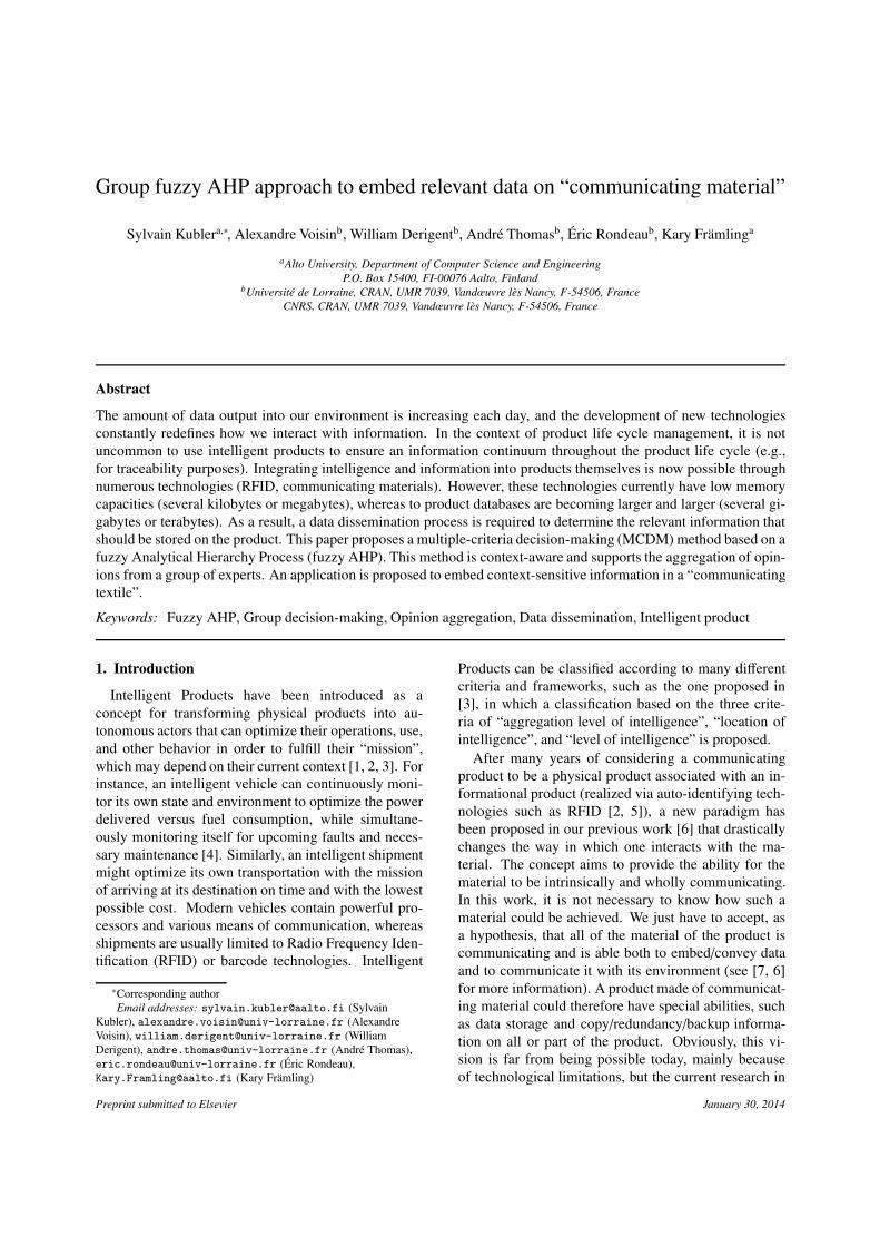
Figure 1 shows part of an LDM in which one

entity corresponds to a relational table, as depicted

in Figure 1(b) with MaterialDefinition. The at-

tributes listed for each entity correspond to the ta-

ble columns, each row is referred to as a tuple, and

a table cell is called a data item. In this example,

MaterialDefinition has 3 attributes and 4 tuples

(i.e., 12 data items). In the approach developed by

Chan and Roddick, the relevance is actually computed

for each data item from each relational table. In Fig-

ure 1(b), the relevance value of the data item located at

row 3, column 1, noted as1 TMD{3, 1}, is equal to 0.2.

To tackle the data selection problem throughout the

PLC, we consider three of the eight criteria defined by

Chan and Roddick:

1. Enumeration (Ce): this criterion allows the user to

enumerate the information that he considers impor-

tant to be stored on the product,

2. Contextual (Cc): experts may not be aware of

all of the data needed by the downstream ac-

tors of the PLC and could omit important classes

of information. Indeed, several information sys-

tems exist over the PLC, e.g., CAD (Computed-

Aided Design), PDM (Product Data Management),

and CRM (Customer Relationship Management),

1Such a notation is used in the rest of the paper to symbolize the

different data items. In this example, MD is used as the abbreviation

of MaterialDefinition.

2

★ : Primary Key (PK)

✩ : Foreign key (SK)

x : relation number

MaterialLot

ID_MatLot★

Description

Status

Quantity

ID_MatDef

ManufacturingBill

ID_ManBill★

Description

Quantity

ID_MatDef✩

ID_ProdDef✩

ProductDefinition

ID_ProdDef★

Description

PublishedDate

MaterialDefinition

ID_MatDef★

Description

Value2

1

3

(a) Example of a Logical Data Model (LDM)

ID Material Description Value

MD44 Wood plank with a nomina... 4m of...1

MD06 Maximum washing temperat.. 15 ˚ C0.2 0.05 0.36

2 MD92 Textile with a high develop... 3mm

3

MD11 Vehicle headrests which co... 2×...4

This corresponds to the data item noted TMD{3, 1}The relevance value of TMD{3, 1} is equal to 0.2

(b) Relational table MaterialDefinition & Data item relevance

Figure 1: View of a Logical Data Model (LDM) and a relational table

which are not concerned with the same data (i.e.,

the same entities from the LDM). The importance

of the entities should therefore change according to

the location of the product in the PLC [17]. This

criterion involves groups of experts drawn from a

consortium of networked enterprises or from stan-

dards organizations, and it aims to assess the im-

portance of different groups of information in the

LDM according to the PLC phases,

3. Data Size (Cs): this criterion favors the storage of

information on the product according to the data

item size. Because products are often memory-

constrained compared with classic databases, the

data relevance should decrease when its size in-

creases [16, 18].

Moreover, unlike Chan and Roddick’s approach,

which assesses all data items from all tables, only tu-

ples related to the individual product (i.e., the product in

question) are assessed in our study. An algorithm is de-

veloped in [6] to identify such tuples from the database.

In this paper, these tuples are referred to as “product-

related tuples”. For instance, in Figure 1(b), only tuple 3

is identified as a product-related tuple (represented with

a dashed background), and thus, only this tuple is as-

sessed in terms of relevancy (not tuples 1, 2, and 4). Fi-

nally, data items are ranked, and in this case, TMD{3, 3}

is the most relevant among the three data items with a

relevance of 0.36.

2.2. Choice of the MCDM method

Chan and Roddick’s model has several limitations.

First, it does not offer the possibility to consider dif-

ferent expert opinions. Moreover, it does not allow one

to consider the uncertainty associated with human judg-

ment. Consequently, this approach may turn out to be

inappropriate according to the context of the study. With

regard to our problem of data selection, several experts

give their opinion at a given stage of the PLC (see Cc).

Each opinion is legitimate and must be considered. Ac-

cordingly, the set of opinions must be formalized in ac-

cordance with a mathematical theory and then synthe-

sized using a suitable aggregation method.

Numerous studies have used MCDM methods, such

as the AHP (Analytical Hierarchy Process), ANP (An-

alytical Network Process), TOPSIS (technique for or-

der preference by similarity to an ideal situation), and

ELECTRE [19]. There are no better or worse tech-

niques, but some techniques are better suited to partic-

ular decision problems than others [20]. For instance,

in our study, it is necessary to implement an MCDM

method that meets our requirements (i.e., consideration

of group opinion, uncertainty,. . . ).

AHP methods have been widely used in the literature

to handle MCDM problems [21]. These methods, orig-

inally proposed by Saaty [22], have the advantage of

organizing the critical aspects of the problem in a hier-

archical structure, thus facilitating the decision-making

process. In these methods, experts use linguistic vari-

ables rather than expressing their judgments in the form

of exact numeric values, which usually makes them

feel more confident and facilitates the valuation process.

Moreover, the use of the AHP does not involve cumber-

some mathematics; thus it is easy to understand, and it

can effectively handle both qualitative and quantitative

data [23, 20]. To tackle the problem of incomplete and

vague information arising from the environment (e.g.,

human judgment, data from sensors), numerous schol-

ars have proposed combining fuzzy set theory with the

AHP, which has become known as the fuzzy AHP.

The fuzzy set theory, introduced by Zadeh [24], mim-

ics human reasoning in its use of approximate informa-

tion and uncertainty to generate decisions. It was specif-

ically designed to mathematically represent uncertainty

and vagueness to provide formalized tools for handling

the imprecision that is intrinsic to many problems. This

3

0

1

0 10a

e, f

b, cg h

d

µA(x) and µB(x)

A = [a, b, c, d]

B = [e, f, g, h]

(a) Trapezoidal fuzzy set A and B

0

1

0 10

Exact form A × B

Approximated form of A × B

µA×B(x)

(b) A × B approximated by a triangular fuzzy set

µA×B(x)

Exact form of A × B

Approximated form of A × B

0

0.2

0.4

0.6

0.8

1

0 10

(c) A × B approximated by 6 α-cuts

Figure 2: Multiplication of two fuzzy sets using two approximation methods

formalization is gradual rather than crisp. In a classi-

cal set A, an element belongs entirely or not to A. In

a fuzzy set A, an element has a degree of membership

in [0, 1]. The kernel of a fuzzy set A is defined as the

set of elements whose membership degree is equal to 1,

as formalized in equation 1, and the support of a fuzzy

set A is defined as the set of elements whose member-

ship degree is different from 0 (see equation 2) [25].

kernel(

A)

= {x ∈ X| µA(x) = 1} (1)

support(

A)

= {x ∈ X| µA(x) > 0} (2)

By combining the advantages of both the AHP and

fuzzy set theory, the fuzzy AHP is an excellent tool to

handle qualitative assessments [20]. As with the AHP

method, the fuzzy AHP has been used in various sectors,

including political [26], social [27], environmental [28],

and product development [23, 29, 30]. Most of the work

uses fuzzy sets to model the uncertainty [31, 32]. The

literature survey made by [33] shows that the vast ma-

jority of the fuzzy AHP applications use the fuzzy ex-

tended AHP (FEAHP) for simplicity [34, 35, 36]. Based

on this review, our attention has turned to the FEAHP

[37] or, to be more exact, to a variant proposed by Deng

[38], which is an improvement over the original FEAHP.

Indeed, the FEAHP is mainly criticized because of the

mechanism used when conducting the computation of

weights. Wang et al. [39] explained that the use of

the possibility degree in this mechanism can lead to un-

true weights and therefore to wrong decisions. The ap-

proach of Deng does not use the same weight computa-

tion mechanism and seems to be free of the drawbacks

described by Wang et al. [39]. To make a clear distinc-

tion between the original and the variant FEAHP, the

term “Deng’s Fuzzy AHP” is used throughout the paper

rather than the FEAHP.

2.3. Adaptation of Deng’s Fuzzy AHP to the context of

use

In this paper, Deng’s Fuzzy AHP is adapted because

the original computation mechanism and the data mod-

eling do not exactly fit our context expectations. First,

the original approach uses triangular fuzzy numbers to

perform the pairwise comparison needed in the AHP.

However, the shape of the fuzzy number is highly re-

lated to the semantics of the information. As a re-

sult, triangular fuzzy numbers are not always appropri-

ate for modeling information. For instance, in our study,

fuzzy numbers are customized based on an aggregation

method that combines the set of expert opinions in ap-

propriate fuzzy forms. These forms are not triangular

but are instead trapezoidal or rectangular. Section 3 in-

troduces the aggregation method and such customiza-

tions. In the literature, some authors develop methods to

perform pairwise comparisons using other shapes, such

as trapezoidal fuzzy sets [40, 41, 42, 20].

Moreover, in Deng’s Fuzzy AHP, computations on

fuzzy numbers are made by only using the limit values

of the kernel and the support, which is a rough approxi-

mation of the exact resulting fuzzy set. Let us illustrate

this problem with two fuzzy sets A and B as given in

Figure 2(a). Figure 2(b) provides the result of the multi-

plication of A and B where the exact form corresponds

to the full line and the approximate form to the dotted

line. It can be observed that a part of the information

is lost when using only the limit values. Another possi-

ble representation of fuzzy sets is the use of crisp inter-

vals, so-called α-cuts. Computations on α-cuts preserve

the form of the membership function as shown in Fig-

ure 2(c). However, the membership function must be

sampled as there are α-cut levels [41].

As a result, Deng’s Fuzzy AHP is adapted as follows:

4

PRO

DU

CTIO

N

EX

PERT

1 1

0 x

v

PRO

DU

CTIO

N

EX

PERT

2 1

0 x

v

PRO

DU

CTIO

N

EX

PERT

3 1

0 x

v

1

0

kernel

x

µv(x)

1 2 3 4 5

(a) Expert consensus a

PRO

DU

CTIO

N

EX

PERT

1

0 x

v

AC

CO

UN

TIN

G

EX

PERT

1

0 x

v

CO

MM

ER

CIA

L

EX

PERT

1

0 x

v

1

0

kernel

x

µv(x)

1 2 3 4 5

(b) Expert consensus b

Figure 3: Aggregation techniques considering two types of expert panels/groups

• the shape of fuzzy numbers, which are used in pair-

wise comparisons, are obtained via clear semantic

rules,

• computations on fuzzy sets are done with the use

of α-cuts to preserve information. One hypoth-

esis of this work is to consider that preserving

the form of fuzzy sets should help obtain a more

precise ranking of the alternatives. Let us note

that 11 α-cut levels are used in our study: α ∈

{0, 0.1, 0.2, . . . , 0.9, 1}.

3. Proposition of an aggregation method based on

fuzzy set theory

The objective of aggregation is to combine individ-

ual sources of information into an overall resource in an

appropriate manner so that the final result of aggrega-

tion can account for all of the individual contributions

[43, 44, 45]. When conflicts occur among experts, an

effective way to manage the conflict involves assigning

weights to the experts (i.e., by assessing their quality).

Such operations are usually performed in the framework

of probability theory [46]. The probabilistic approach,

although it has proven its worth, is once again ill-suited

to model vague opinions and limits the choice of ag-

gregation methods, as claimed by Destercke et al. [47].

Uncertainty theories such as fuzzy set theory make it

possible to overcome these limits [48]. Many fuzzy set

theory proposals have been developed in recent years

[49, 50, 45]. According to [47], an aggregation method

can be characterized by one of the three behaviors item-

ized below. Let us consider a parameter v on a domainX

to be estimated. Two experts e1 and e2 give their opin-

ion e1(v) = A and e2(v) = B with A, B ⊆ X. Let ⋊⋉ be

the aggregation operator:

• conjunctive behavior: e1(v) ⋊⋉ e2(v) ⊆ A ∩ B. The

result is more certain than the expert’s opinion and

can be used when the opinions are not conflicting

(i.e., e1(v) ⋊⋉ e2(v) , ∅),

• disjunctive behavior: e1(v) ⋊⋉ e2(v) ⊇ A ∪ B. The

result is less accurate than it was previously, but all

opinions are taken into account. In fact, the dis-

junction represents the case in which the modeler

does not want to choose among the expert opin-

ions, which might be conflicting,

• “counting” behavior: The result corresponds to a

statistical view of the opinions. A counting behav-

ior could actually be defined at the interface be-

tween the disjunctive and the conjunctive results.

In practice, it makes sense to adapt the aggregation

method according to the context. The accuracy and the

nature of the aggregated result depends on both the pres-

ence of conflicts and the available knowledge on the ex-

pert quality. In the PLC, experts who evaluate alterna-

tives and criteria may originate from the same or differ-

ent core business(es). Two situations involving expert

points of view may be identified:

a) same point of view: experts originate from the same

core business and their concerns about the prod-

uct are similar. As a result, these experts have the

same point of view when evaluating a parameter.

5

Figure 3(a) shows an example of three experts in

production control, i.e., e1, e2, and e3, provide a

crisp evaluation of parameter v on the same scale,

X = {1, 2, 3, 4, 5},

b) different points of view: experts originate from dis-

tinct core businesses, and their concerns about the

product are different. As a result, these experts do

not have the same point of view when evaluating in-

formation. Figure 3(b) shows an example of three

experts from three distinct core businesses: e1 - ex-

pert in production control, e2 - expert in accounting,

and e3 - expert in commercial business. They also

provide a crisp evaluation of parameter v on the same

scale, X = {1, 2, 3, 4, 5},

All of the expert points of view are legitimate and

must be considered. Accordingly, choosing conjunc-

tive behavior for the aggregation is not suitable; rather,

disjunctive or perhaps even counting should be used.

In this sense, a new approach for aggregating multi-

ple points of view from a group of experts is developed

based on the fuzzy set theory. This approach aims at

aggregating crisp evaluations formulated by the experts

through suitable fuzzy set modeling. To consider all ex-

pert points of view, the aggregation method proceeds

by aggregating their evaluations through an information

continuum, namely, a fuzzy interval in which all points

of view form the kernel, as illustrated in Figure 3(a) and

3(b). In case a) in which experts have the same point of

view, the target value might be located outside the ker-

nel because of the small numbers of experts considered

(a new expert could give an evaluation outside the inter-

val). As a result, the support is extended with a linear

slope (i.e., the values decrease when the distance from

the kernel increases) as shown in Figure 3(a). In case

b), in which experts have different points of view, the

fuzzy interval is not extended because the addition of a

new evaluation would mean that a point of view (i.e., a

core business) has been omitted. In this study, we make

the assumption that all core businesses are known at a

given stage of the PLC.

The next section details the different stages of the

group fuzzy AHP method. For each criterion evaluation,

the suitable aggregation is implemented, depending on

the category of points of view of the experts solicited in

each criterion.

4. Data item relevance using the group fuzzy AHP

Our group fuzzy AHP method relies on Deng’s Fuzzy

AHP and consists of five stages as depicted in Figure 4:

➀ AHP structure

➁Information collection +

Aggregation (alternatives)Information collection +

Aggregation (criteria)i ii

➂ Fuzzy judgement matrix A...

A =ai

...

...

...

...

...

...

...

➃ Fuzzy performance matrix H...

H =ai

...

...

...

.

.

.

.

.

.

.

.

.

.

.

.

.

.

.

.

.

.

➄...

R = ai

.

.

.

.

.

.

.

.

.

→Alternative ranking1

ax

Figure 4: Group fuzzy AHP consisting of 5 stages

1. breakdown of the MCDM problem into a hierar-

chical AHP structure: definition of criteria & alter-

natives,

2. collection and aggregation of the expert evalua-

tions regarding i) the evaluations of alternatives

with respect to criteria, and ii) the evaluations of

the importance of criteria. In both cases, the eval-

uations are aggregated in suitable fuzzy sets,

3. creation of the fuzzy judgment matrix A: this ma-

trix is built based on the fuzzy sets of alternatives

with respect to each criterion (fuzzy sets arising

from stage 2),

4. computation of the fuzzy performance matrix H:

this matrix is built by synthesizing A with the rela-

tive criteria importances (importances arising from

stage 2),

5. alternative ranking: multi-criteria performance of

alternatives must be aggregated in a fuzzy vector

R, and then alternatives must be ranked.

These five stages are respectively detailed in sec-

tions 4.1 to 4.5. To make the approach easy to under-

stand, a scenario is considered in the rest of the paper

whose parts are preceded by the symbol “✎”. This sce-

nario relies on 19 entities that come from the LDM of

the B2MML standard. B2MML (Business To Manu-

facturing Markup Language) is meant to be a common

data format to link business enterprise applications with

manufacturing enterprise applications. Figure 1(a) il-

lustrates 4 of them.

4.1. Stage 1: AHP structure

Our MCDM problem is broken down into the AHP

structure depicted in Figure 5. The alternatives are the

data items (cf. Level 3) that must be assessed and ranked

in terms of relevancy to be stored on the communicating

6

s1(ID_Material,MD) = 1s2(ID_Material,MD) = 1s3(ID_Material,MD) = 1

s1(Description,MD) = 0s2(Description,MD) = 0.5s3(Description,MD) = 0

s1(value,MD) = 1s2(value,MD) = 0s3(value,MD) = 0

s(ID_Material,MD) = [min(1, 1, 1) max(1, 1, 1)]= [1, 1]

s(Description,MD) = [min(0, 0.5, 0) max(0, 0.5, 0)]= [0, 0.5]

s(value,MD) = [min(1, 0, 0) max(1, 0, 0)]= [0, 1]

E

E

E

0

0.5

1

0 0.5 1

0

0.5

1

0 0.5 1

0

0.5

1

0 0.5 1

aggregation of the different points of view

Figure 6: Expert evaluations related to Enumeration and fuzzy opinion aggregation

MD06Maxim... 15˚C . . .

data item z

Data item classification (in order of relevance)

Enumeration Contextual Data Size

Level 1

Level 2

Level 3

Figure 5: General architecture of the hierarchy

material (cf. Level 1). The three criteria introduced in

section 2.1 take place at Level 2 and are detailed in the

next stage.

4.2. Stage 2: Information collection and aggregation of

expert points of view

Sections 4.2.1 to 4.2.3 explain the three criteria (Ce,

Cc, Cs), how the experts evaluate each alternative with

respect to each criterion, and how these evaluations are

aggregated. Section 4.2.4 provides the same details but

regarding the evaluations of the criteria importance. The

main variables used in this paper are given in Table 1.

4.2.1. Enumeration - Ce

This criterion allows the user to enumerate the in-

formation that he considers important to store on the

product. To do so, each expert ep enumerates certain

attributes from tables. Let t be a table from the database

(t ∈ T ) and v be an attribute of t. If the attribute v is enu-

merated by ep, the crisp enumeration score sp(v, t) = 0.5

or 1 (depending on the preference intensity, as formu-

lated in equation 3). Experts may come from differ-

ent areas (e.g., production, shipping) and may there-

fore want to store different information on the product

because of their different concerns. Accordingly, the

aggregation method defined in consensus b is used (cf.

Figure 3(b)) to aggregate the set of opinions as formal-

ized in equation 4. Finally, the score of a data item al ∈ v

with respect to Ce, denoted by φe(al), is equal to s(v, t).

sp(v, t) =

1 enumerated (useful attribute)

0.5 enumerated (interesting attribute)

0 not enumerated (useless attribute)

(3)

s(v, t) = [min(sp(v, t)) max(sp(v, t))] (4)

✎ Table 2 shows the attributes enumerated by

three experts e1, e2 and e3. The preference intensities

formulated by each expert for the attributes are also

presented. For instance, e1 judges information from

the attribute Quantity of the table MaterialLot as

“useful” because he gives it a preference of 1 (noted

Quantity+1 in Table 2). e2 judges the same at-

tribute to be “useless” because he does not enumer-

ate it. Attributes not enumerated by experts are not

presented in Table 2, but they take the value of 0.

The aggregation of the three expert opinions regard-

ing each attribute, from each table is then performed

based on Equation 4. Figure 6 shows the aggregation

steps and the fuzzy sets resulting from the aggregation

for the three attributes of MaterialDefinition (i.e.,

ID Material, Description and value), based on the

preferences expressed by experts in Table 2. The fuzzy

scores of data items TMD{3, 1}, TMD{3, 2}, TMD{3, 3}

with respect to Ce, which are noted φe(TMD{3, 1}),

φe(TMD{3, 2}), and φe(TMD{3, 3}), are respectively

equal to s(ID Material, MD), s(Description, MD),

and s(value, M) because they belong to these three at-

tributes.

4.2.2. Contextual - Cc

This criterion more globally evaluates the informa-

tion that should be selected than with Ce. Indeed, ex-

perts may not be aware of all of the data needed by the

downstream actors in the PLC and could omit impor-

tant information. There is thus a need to identify impor-

tant data with regard to the global PLC. This evaluation

cannot be focused on individual data items but should

instead focus on a group of tables. Accordingly, the

7

Table 1: Variable definitions

Variables Description

Cla

ssic

alse

ts&

Cri

spsc

ore

s

T set of tables in the database. Let t be a table ∈ T , a data item from t is noted Tt{u, v} where u corresponds to the row/instance

and v to the column/attribute.

al represents an alternative l (i.e., a data item l) in the AHP structure, with l = {1, 2, .., n}.

ep represents an expert p with p = {1, 2, .., pmax}; pmax varies according to the criterion x.

Cx abbreviation for the criterion x with x = {1, 2, ..,m}. In our study, three criteria are defined in this study, namely: Ce, Cc, Cs.

Gi abbreviation for an entity group i defined in the LDM, with i = {1, 2, .., z}.

k coefficient ∈ R+ used to favor the storage of information on the product according to the data item size (in Cs).

α crisp interval of a fuzzy set, so-called α-cut (11 α-cuts are used in our study: α ∈ {0, 0.1, 0.2, . . . , 0.9, 1}).

x␄ represents the center of gravity (CoG) of a fuzzy set. x␄− and x␄+ are respectively the inferior and superior approximations of

the CoG which are calculated based on the α-cut levels.

rα, rα respectively indicate the minimal and the maximal values of the α-cut on the x-axis.

∆Yrα corresponds to the level difference (y-axis) between the α-cut and α + 1-cut levels.

L list of product-related data items ordered from the most relevant to the lowest (ordered according to their CoG x␄)

Fuzz

ysc

ore

s(v, t) fuzzy score representing the aggregation of the crisp evaluations provided by each expert ep (with p = {1, .., pmax}) in Ce.

The crisp evaluation is noted sp(v, t) and indicates the preference intensity, expressed by ep, about storing on the product

information related to attribute v of table t.

sk represents the aggregation of the crisp evaluations provided by each expert ep (with p = {1, .., pmax}) in Cs. The crisp

evaluation is noted sp

kand corresponds to the value of coefficient k, adjusted by ep.

si j fuzzy score representing the aggregation of pairwise comparisons between element i and j of the pairwise matrix, performed

by all experts. A pairwise comparison between element i and j performed by an expert ep is noted sp

i j(with p = {1, .., pmax}).

Aggregation is based on rules from Table 3.

φ(Gi) fuzzy score representing the relative importance of entity group Gi over the other groups. It can be decomposed in intervals,

on the basis of α-cuts, as φα(Gi).

φ(Cx) fuzzy score representing the relative importance of criterion Cx over the other criteria. It can be decomposed in intervals, on

the basis of α-cuts, as φα(Cx).

φx(al) fuzzy score of alternative al with respect to criterion x, without considering the relative importance of criterion x .

hx(al) fuzzy score of alternative al with respect to criterion x, by considering the relative importance of criterion x.

Fuzz

ym

atri

x/v

ecto

r

G fuzzy matrix synthesizing all fuzzy scores si j (i and j = {1, 2, .., z}) regarding pairwise comparisons between entity groups.

ΦG fuzzy vector synthesizing all fuzzy scores φ(Gi), with i = {1, 2, .., z}.

ρ fuzzy matrix synthesizing all fuzzy scores si j (i and j = {1, 2, ..,m}) regarding pairwise comparisons between criteria.

Φρ fuzzy vector synthesizing all fuzzy scores φ(Cx), with x = {1, 2, ..,m}.

A fuzzy judgment matrix synthesizing all fuzzy scores φx(al) (i.e., the importance of criteria is not considered yet).

H fuzzy performance matrix which synthesizes the judgment matrix A and the fuzzy vector Φρ (i.e., the importance of criteria

is now considered).

R fuzzy vector after multi-criteria aggregation (i.e., after having aggregated scores from the performance matrix H).

Table 2: “Table attributes” enumerated by e1 , e2, and e3

Table name (t) Enumerated attributes (v)+Preference

e1

MaterialLot IDLot+1; Quantity+1

MaterialDefinition IDMaterial+1; Value+1

ProductSegment IDProdSeg+1; Duration+1; Unit+0.5

ProductionOrder IDProdOrd+1; StartTime+1; EndTime+1

e2 MaterialDefinition IDMaterial+1; Description+0.5

e3

MaterialLot Status+0.5

MaterialDefinition IDMaterial+1

ProductSegment IDProdSeg+0.5; Description+0.5

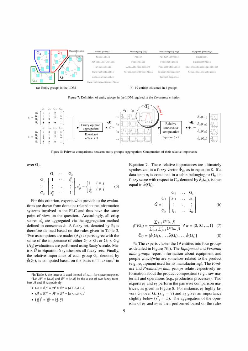
main idea is to cluster all entities of the LDM needed by

the same information systems in “entity groups”. Fig-

ure 7(a) illustrates the definition of four entity groups

in an LDM. Experts then perform pairwise comparisons

among these groups to indicate the utility for the cur-

rent and downstream actors of the PLC to obtain access

to information from the different groups. In our study,

each expert ep performs pairwise comparisons among

entity groups as in equation 5, with z being the num-

ber of groups. The importance of entity group Gi over

group G j, evaluated by ep, is denoted by sp

i j. This evalu-

ation is based on the 1- to 9-point scale from Saaty [51]:

{1, 3, 5, 7, 9}. sp

i j= 1 means that Gi and G j are of equal

importance and sp

i j= 9 means that Gi is strongly favored

8

G1

G2G3

G4

MaterialDefinition

(a) Entity groups in the LDM

Product group (G1) Personal group (G2) Production group (G3) Equipment group (G4)

MaterialLot Person ProductionOrder Equipment

MaterialDefinition PersonClass ProductSegment EquipmentClass

MaterialClass ActualPersonSegment ProductDefinition EquipmentSegmentSpecificat

ManufacturingBill PersonSegmentSpecificat SegmentRequirement ActualEquipmentSegment

ActualMaterialLot SegmentResponse

MaterialSegmentSpecificat

(b) 19 entities clustered in 4 groups

Figure 7: Definition of entity groups in the LDM required in the Contextual criterion

e1 =

G1 G2 G3 G4

G1 1 1 15 7

G2 1 1 13 5

G3 5 3 1 7G4

17

15

17 1

e2 =

G1 G2 G3 G4

G1 1 3 13 5

G213 1 1

3 5G3 3 3 1 7G4

15

15

17 1

Fuzzy opinionaggregation

Equation 6

+ TABLE 3

G1 G2 G3 G4

G1

G =

G2

G3

G4

0

0.5

1

1 3 5 7 9

0

0.5

1

1 3 5 7 9

0

0.5

1

1 3 5 7 9

0

0.5

1

3 5 7 9

0

0.5

1

1 3 5 7 9

0

0.5

1

1 3 5 7 9

0

0.5

1

1 3 5 7 9

0

0.5

1

1 3 5 7 9

0

0.5

1

1 3 5 7 9

0

0.5

1

1 3 5 7 9

0

0.5

1

1 3 5 7 9

0

0.5

1

1 3 5 7 9

0

0.5

1

1 3 5 7 9

0

0.5

1

1 3 5 7 9

0

0.5

1

1 3 5 7 9

0

0.5

1

1 3 5 7 9

3 G4

7 9

0

0.5

1

3 5 7 9

1

E Relativeimportance

computation

Equation 7 - 8

φc(G1)

Φc =

E φc(G2)

φc(G3)

φc(G4)

Zoom1

0

0.5

1

0 0.5 1

0

0.5

1

0 0.5 1

0

0.5

1

0 0.5 1

0

0.5

1

0 0.5 1

Figure 8: Pairwise comparisons between entity groups; Aggregation; Computation of their relative importance

over G j.

G1 · · · Gz

G1 1 · · · sp

1z

....... . .

...

Gz sp

z1· · · 1

, sp

ji=

1 i = j1s

p

i j

i , j(5)

For this criterion, experts who provide to the evalua-

tions are drawn from domains related to the information

systems involved in the PLC and thus have the same

point of view on the question. Accordingly, all crisp

scores sp

i jare aggregated via the aggregation method

defined in consensus b. A fuzzy set, denoted by si j is

therefore defined based on the rules given in Table 3.

Two assumptions are made: (A1) experts agree with the

sense of the importance of either Gi > G j or Gi < G j;

(A2) evaluations are performed using Saaty’s scale. Ma-

trix G in Equation 6 synthesizes all fuzzy sets. Finally,

the relative importance of each group Gi, denoted by

φ(Gi), is computed based on the basis of 11 α-cuts3 in

2In Table 8, the letter q is used instead of pmax for space purposes.3Let Aα = [a, b] and Bα = [c, d] be the α-cut of two fuzzy num-

bers A and B respectively:

• (A⊕ B)α = Aα ⊕ Bα = [a + c, b + d]

• (A⊗ B)α = Aα ⊗ Bα = [a × c, b × d]

•(AB

)α= A

α

Bα= [ a

d, b

c]

Equation 7. These relative importances are ultimately

synthesized in a fuzzy vector ΦG, as in equation 8. If a

data item al is contained in a table belonging to Gi, its

fuzzy score with respect to Cc, denoted by φc(al), is thus

equal to φ(Gi).

G =

G1 . . . Gz

G1 s11 . . . s1z

....... . .

...

Gz sz1 . . . szz

(6)

φα(Gi) =

∑zj=1

Gα(i, j)∑z

k=1

∑zj=1

Gα(k, j)∀ α = {0, 0.1, .., 1} (7)

ΦG = [φ(G1), . . . , φ(Gi), . . . , φ(Gz)] (8)

✎ The experts cluster the 19 entities into four groups

as detailed in Figure 7(b). The Equipment and Personal

data groups report information about equipment and

people which/who are somehow related to the product

(e.g., equipment used for its manufacturing). The Prod-

uct and Production data groups relate respectively in-

formation about the product composition (e.g., raw ma-

terial) and operations (e.g., production processes). Two

experts e1 and e2 perform the pairwise comparison ma-

trices, as given in Figure 8. For instance, e1 highly fa-

vors G1 over G4 (s114= 7) and e2 gives an importance

slightly below (s214= 5). The aggregation of the opin-

ions of e1 and e2 is then performed based on the rules

9

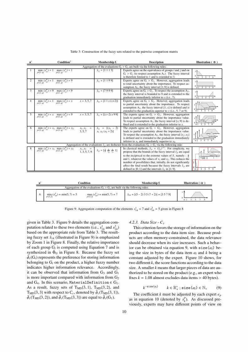
Table 3: Construction of the fuzzy sets related to the pairwise comparison matrix

n˚ Condition2 Membership f. Description Illustration (E)

Aggregation of the evaluations Gi > G j are built via the following rules:

1 minp∈{1..q}

(sp

i j) = 1 max

p∈{1..q}(s

p

i j) = 1 si j = [1 1 1 3] Experts agree on the equivalence of groups i and j and on

Gi > G j (to respect assumption A1). The fuzzy intervalis therefore limited to 1 and is extended to 3.

2 minp∈{1..q}

(sp

i j) = 1 max

p∈{1..q}(s

p

i j) = 9 si j = [1 1 9 9] Experts agree on Gi > G j . However, aggregation leads

to total uncertainty about the importance. To respect as-sumption A2, the fuzzy interval [1; 9] is defined.

3 minp∈{1..q}

(sp

i j) = 9 max

p∈{1..q}(s

p

i j) = 9 si j = [7 9 9 9] Experts agree on Gi > G j . To respect the assumption A2,

the fuzzy interval is bounded to 9 and is extended to thegraduation immediately inferior to x (i.e., 7).

4 minp∈{1..q}

(sp

i j) = 1 max

p∈{1..q}(s

p

i j) = x x = 3, 5, 7 si j = [1 1 x (x+2)] Experts agree on Gi > G j . However, aggregation leads

to partial uncertainty about the importance. To respectassumption A2, the fuzzy interval [1; x] is defined and isextended to the graduation superior to x (i.e., 5, 7 or 9).

5 minp∈{1..q}

(sp

i j) = x max

p∈{1..q}(s

p

i j) = 9 x = 3, 5, 7 si j = [(x−2) x 9 9] The experts agree on Gi > G j . However, aggregation

leads to partial uncertainty about the importance value.To respect assumption A2, the fuzzy interval [x; 9] is de-fined and is extended to the graduation inferior to x.

6 minp∈{1..q}

(sp

i j) = x1 max

p∈{1..q}(s

p

i j) = x2 x1, x2 =

3, 5, 7si j = [(x1 − 2)x1 x2 (x2 + 2)]

The experts agree on Gi > G j . However, aggregationleads to partial uncertainty about the importance value.To respect the assumption A2, the fuzzy interval [x1; x2]is defined and is extended to the graduation immediatelyinferior to x1 and immediately superior to x2.

Aggregation of the evaluations s ji are deducted from the evaluations Gi > G j via the following rule:

8 minp∈{1..q}

(sp

i j) = x1 max

p∈{1..q}(s

p

i j) = x2 x1, x2 =

1, 3, 5, 7, 9s ji = [ 1

91x2

1x1

1]In classical methods, s ji = (si j)

−1 . For simplicity, wepropose that the bounds of the fuzzy interval s ji are equal

to the reciprocal to the extreme values of S , namely : 19

and 1, whatever the values of x1 and x2. This reduces thenumber of possibilities that, initially, do not significantlyaffect the final result because the fuzzy intervals s ji aredefined in ]0; 1] and the intervals si j in ]1; 9].

1

00 1 3 5 7 9

1

00 1 3 5 7 9

1

00 1 3 5 7 9

1

00 1 3 5 7 9

1

00 1 3 5 7 9

1

00 1 3 5 7 9

1

1

1

00 1

917

15

13

1

1

00 1 3 5 7 9

n˚ Condition Membership f. Illustration (E)


6 minp∈{1,2}

(sp

14) = min(5, 7) = 5 max

p∈{1,2}(s

p

14) = min(5, 7) = 7 s14 = [(5 − 2) 3 5 (7 + 2)] = [3 5 7 9]

1

00 1 3 5 7 9

Figure 9: Aggregation computation of the elements s114= 7 and s2

14= 5 given in Figure 8

given in Table 3. Figure 9 details the aggregation com-

putation related to these two elements (i.e., s114

and s214

)

based on the appropriate rule from Table 3. The result-

ing fuzzy set s14 (illustrated in Figure 9) is emphasized

by Zoom 1 in Figure 8. Finally, the relative importance

of each group Gi is computed using Equation 7 and is

synthesized in ΦG in Figure 8. Because the fuzzy set

φc(Gi) represents the preference for storing information

belonging to Gi on the product, a higher fuzzy number

indicates higher information relevance. Accordingly,

it can be observed that information from G3 and G1

is more important compared with information from G2

and G4. In this scenario, MaterialDefinition ∈ G1.

As a result, fuzzy sets of TMD{3, 1}, TMD{3, 2}, and

TMD{3, 3} with respect to Cc, denoted by φc(TMD{3, 1}),

φc(TMD{3, 2}), and φc(TMD{3, 3}) are equal to φc(G1).

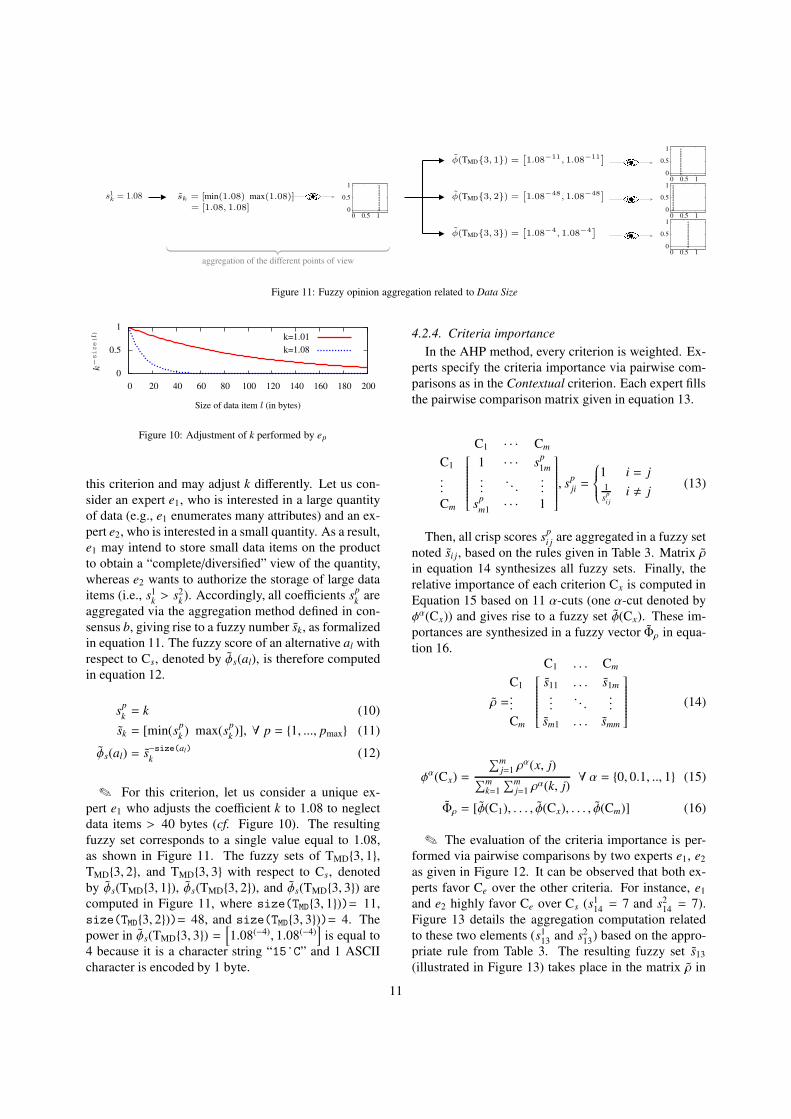
4.2.3. Data Size - Cs

This criterion favors the storage of information on the

product according to the data item size. Because prod-

ucts are often memory-constrained, the data relevance

should decrease when its size increases. Such a behav-

ior can be obtained via equation 9, with size(al) be-

ing the size in bytes of the data item al and k being a

constant adjusted by the expert. Figure 10 shows, for

two different k, the score functions according to the data

size. A smaller k means that larger pieces of data are au-

thorized to be stored on the product (e.g., an expert who

fixes k = 1.08 almost excludes data items > 40 bytes).

k−size(al) k ∈ R∗+ ; size(al) ∈ N+ (9)

The coefficient k must be adjusted by each expert ep

as in equation 10 (denoted by sp

k). As discussed pre-

viously, experts may have different points of view on

10

s1k = 1.08 sk = [min(1.08) max(1.08)]= [1.08, 1.08]

φ(TMD{3, 1}) =[

1.08−11, 1.08−11]

E

φ(TMD{3, 2}) =[

1.08−48, 1.08−48]

E

φ(TMD{3, 3}) =[

1.08−4, 1.08−4]

E

E

0

0.5

1

0 0.5 1

0

0.5

1

0 0.5 1

0

0.5

1

0 0.5 1

0

0.5

1

0 0.5 1

aggregation of the different points of view

Figure 11: Fuzzy opinion aggregation related to Data Size

0

0.5

1

0 20 40 60 80 100 120 140 160 180 200

k−size(l)

Size of data item l (in bytes)

k=1.01

k=1.08

Figure 10: Adjustment of k performed by ep

this criterion and may adjust k differently. Let us con-

sider an expert e1, who is interested in a large quantity

of data (e.g., e1 enumerates many attributes) and an ex-

pert e2, who is interested in a small quantity. As a result,

e1 may intend to store small data items on the product

to obtain a “complete/diversified” view of the quantity,

whereas e2 wants to authorize the storage of large data

items (i.e., s1k> s2

k). Accordingly, all coefficients s

p

kare

aggregated via the aggregation method defined in con-

sensus b, giving rise to a fuzzy number sk, as formalized

in equation 11. The fuzzy score of an alternative al with

respect to Cs, denoted by φs(al), is therefore computed

in equation 12.

sp

k= k (10)

sk = [min(sp

k) max(s

p

k)], ∀ p = {1, ..., pmax} (11)

φs(al) = s−size(al)

k(12)

✎ For this criterion, let us consider a unique ex-

pert e1 who adjusts the coefficient k to 1.08 to neglect

data items > 40 bytes (cf. Figure 10). The resulting

fuzzy set corresponds to a single value equal to 1.08,

as shown in Figure 11. The fuzzy sets of TMD{3, 1},

TMD{3, 2}, and TMD{3, 3} with respect to Cs, denoted

by φs(TMD{3, 1}), φs(TMD{3, 2}), and φs(TMD{3, 3}) are

computed in Figure 11, where size(TMD{3, 1}))= 11,

size(TMD{3, 2}))= 48, and size(TMD{3, 3}))= 4. The

power in φs(TMD{3, 3}) =[

1.08(−4), 1.08(−4)]

is equal to

4 because it is a character string “15˚C” and 1 ASCII

character is encoded by 1 byte.

4.2.4. Criteria importance

In the AHP method, every criterion is weighted. Ex-

perts specify the criteria importance via pairwise com-

parisons as in the Contextual criterion. Each expert fills

the pairwise comparison matrix given in equation 13.

C1 · · · Cm

C1 1 · · · sp

1m

....... . .

...

Cm sp

m1· · · 1

, sp

ji=

1 i = j1s

p

i j

i , j(13)

Then, all crisp scores sp

i jare aggregated in a fuzzy set

noted si j, based on the rules given in Table 3. Matrix ρ

in equation 14 synthesizes all fuzzy sets. Finally, the

relative importance of each criterion Cx is computed in

Equation 15 based on 11 α-cuts (one α-cut denoted by

φα(Cx)) and gives rise to a fuzzy set φ(Cx). These im-

portances are synthesized in a fuzzy vector Φρ in equa-

tion 16.

ρ =

C1 . . . Cm

C1 s11 . . . s1m

....... . .

...

Cm sm1 . . . smm

(14)

φα(Cx) =

∑mj=1 ρ

α(x, j)∑m

k=1

∑mj=1 ρ

α(k, j)∀ α = {0, 0.1, .., 1} (15)

Φρ = [φ(C1), . . . , φ(Cx), . . . , φ(Cm)] (16)

✎ The evaluation of the criteria importance is per-

formed via pairwise comparisons by two experts e1, e2

as given in Figure 12. It can be observed that both ex-

perts favor Ce over the other criteria. For instance, e1

and e2 highly favor Ce over Cs (s114= 7 and s2

14= 7).

Figure 13 details the aggregation computation related

to these two elements (s113

and s213

) based on the appro-

priate rule from Table 3. The resulting fuzzy set s13

(illustrated in Figure 13) takes place in the matrix ρ in

11

e1 =

Ce Cc Cs

Ce 1 7 7Cc

17 1 3

Cs17

13 1

e2 =

Ce Cc Cs

Ce 1 5 7Cc

15 1 5

Cs17

15 1

Fuzzy opinionaggregation

Equation 15

+ TABLE 3

Ce Cc Cs

Ce

ρ =Cc

Cs

0

0.5

1

1 3 5 7 90

0.5

1

1 3 5 7 90

0.5

1

1 3 5 7 9

0

0.5

1

1 3 5 7 90

0.5

1

1 3 5 7 90

0.5

1

1 3 5 7 9

0

0.5

1

1 3 5 7 90

0.5

1

1 3 5 7 90

0.5

1

1 3 5 7 9

Relative

importance

computation

Equation 16 - 17

φρ(Ce)

Φρ = φρ(Cc)

φρ(Cs)

0

0.5

1

0 0.5 1

0

0.5

1

0 0.5 1

0

0.5

1

0 0.5 1

Figure 12: Pairwise comparisons between criteria; Aggregation; Computation of their relative importance

n˚ Condition Membership f. Illustration (E)


6 minp∈{1,2}

(sp

13) = min(7, 7) = 7 max

p∈{1,2}(s

p

13) = min(7, 7) = 7 s13 = [(7 − 2) 7 7 (7 + 2)] = [5 7 7 9]

1

00 1 3 5 7 9

Figure 13: Aggregation computation of the elements s113= 7 and s2

13= 7 given in Figure 12

Figure 12 (cf. row 1, column 3). Finally, the relative im-

portance of each criterion Cx is computed using Equa-

tion 15 and is synthesized in Φρ in Figure 12. The re-

sulting fuzzy sets in Φρ meet the wishes of the experts

because Ce is the most important at this PLC stage. In

other words, the experts give freedom to users to deter-

mine which information must be stored on the product.

4.3. Stage 3: Fuzzy judgment matrix A

After obtaining all alternative scores with respect to

all criteria, the fuzzy judgment matrix A is built as

shown in equation 17, where φx(al) denotes the fuzzy

set of alternative al with respect to criterion x.

A =

C1 C2 . . . Cm

a1 φ1(a1) φ2(a1) . . . φm(a1)

a2 φ1(a2) φ2(a2) . . . φm(a2)...

......

......

an φ1(an) φ2(an) . . . φm(an)

(17)

✎ Throughout the scenario considered in the pre-

vious section, the scores of TMD{3, 1}, TMD{3, 2}, and

TMD{3, 3}with respect to Ce, Cc, and Cs have been com-

puted, which are respectively synthesized in A in Fig-

ure 14.

4.4. Stage 4: Fuzzy performance matrix H

At this stage, only the scores of alternatives with re-

spect to the criteria are considered, without accounting

for relative importance of the criteria. As a result, the

fuzzy matrix A is combined with the criterion impor-

tance Φρ in a fuzzy performance matrix H, as given in

equation 18, where each element hx(al) is computed us-

ing equation 19.

Ce Cc Cs

φe(a1) φc(a1) φs(a1)φe(a2) φc(a2) φs(a2)

......

...

a1a2...

TMD{3, 1}

E A = TMD{3, 2}

TMD{3, 3}

...an−1

an

......

...

φe(an) φc(an) φs(an)φe(an−1) φc(an−1) φs(an−1)

0

0.5

1

0 0.5 1

0

0.5

1

0 0.5 1

0

0.5

1

0 0.5 1

0

0.5

1

0 0.5 1

0

0.5

1

0 0.5 1

0

0.5

1

0 0.5 1

0

0.5

1

0 0.5 1

0

0.5

1

0 0.5 1

0

0.5

1

0 0.5 1

Figure 14: Fuzzy judgment matrix A

H =

C1 C2 . . . Cm

a1 h1(a1) h2(a1) . . . hm(a1)

a2 h1(a2) h2(a2) . . . hm(a2)...

......

......

an h1(an) h2(an) . . . hm(an)

(18)

hx(al) = φx(al) ⊗ φρ(Cx) (19)

✎ The matrix H in our scenario is computed and

depicted in Figure 15. The multiplication related to

he(TMD{3, 1}) is also illustrated in this figure.

4.5. Stage 5: Alternative ranking

This section aims to rank alternatives according to

their evaluations. Until then, each alternative has one

fuzzy set with respect to every criterion, giving a total

12

Ce Cc Cs

he(a1) hc(a1) hs(a1)he(a2) hc(a2) hs(a2)

.

.

....

.

.

.

a1a2...

TMD{3, 1}

E H = TMD{3, 2}

TMD{3, 3}

.

.

.

an−1

an

.

.

....

.

.

.

he(an) hc(an) hs(an)he(an−1) hc(an−1) hs(an−1)

0

0.5

1

0 0.7 1.4

0

0.5

1

0 0.7 1.4

0

0.5

1

0 0.7 1.4

0

0.5

1

0 0.7 1.4

0

0.5

1

0 0.7 1.4

0

0.5

1

0 0.7 1.4

0

0.5

1

0 0.7 1.4

0

0.5

1

0 0.7 1.4

0

0.5

1

0 0.7 1.4

he(TMD{3, 1}) =

0

0.5

1

0 0.5 1

φe(TMD{3, 1})

×0

0.5

1

0 0.5 1

φρ(Ce)

Figure 15: Fuzzy performance matrix H

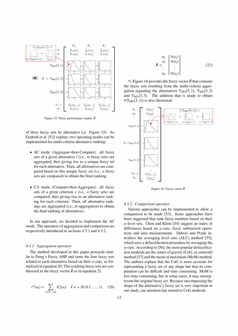
of three fuzzy sets by alternative (cf. Figure 15). As

Grabish et al. [52] explain, two operating modes can be

implemented for multi-criteria alternative ranking:

• AC mode (Aggregate-then-Compare): all fuzzy

sets of a given alternative l (i.e., m fuzzy sets) are

aggregated, thus giving rise to a unique fuzzy set

for each alternative. Then, all alternatives are com-

pared based on this unique fuzzy set (i.e., n fuzzy

sets are compared) to obtain the final ranking,

• CA mode (Compare-then-Aggregate): all fuzzy

sets of a given criterion x (i.e., n fuzzy sets) are

compared, thus giving rise to an alternative rank-

ing for each criterion. Then, all alternative rank-

ings are aggregated (i.e., m aggregation) to obtain

the final ranking of alternatives,

In our approach, we decided to implement the AC

mode. The operators of aggregation and comparison are

respectively introduced in sections 4.5.1 and 4.5.2.

4.5.1. Aggregation operator

The method developed in this paper proceeds simi-

lar to Deng’s Fuzzy AHP and sums the four fuzzy sets

related to each alternative based on their α-cuts, as for-

malized in equation 20. The resulting fuzzy sets are syn-

thesized in the fuzzy vector R as in equation 21.

rα(al) =∑

x∈{1,..,m}

hαx (al) ∀ α = {0, 0.1, . . . , 1} (20)

R =

a1 r(a1)

a2 r(a2)...

...

an r(an)

(21)

✎ Figure 16 provides the fuzzy vector R that contains

the fuzzy sets resulting from the multi-criteria aggre-

gation regarding the alternatives TMD{3, 1}, TMD{3, 2}

and TMD{3, 3}. The addition that is made to obtain

r(TMD{3, 1}) is also illustrated.

r(a1)r(a2)

.

.

.

a1a2

.

.

.

TMD{3, 1}

R =TMD{3, 2}

TMD{3, 3}

.

.

.

an−1

an

.

.

.

r(an)r(an−1)

0

0.5

1

0 1 2 3

0

0.5

1

0 1 2 3

0

0.5

1

0 1 2 3

r(TMD{3, 1}) =

0

0.5

1

0 0.7 1.4

he(TMD{3, 1})

+0

0.5

1

0 0.7 1.4

hc(TMD{3, 1})

+0

0.5

1

0 0.7 1.4

hs(TMD{3, 1})

Figure 16: Fuzzy vector R

4.5.2. Comparison operator

Various approaches can be implemented to allow a

comparison to be made [53]. Some approaches have

been suggested that rank fuzzy numbers based on their

α-level sets. Chen and Klein [54] suggest an index of

differences based on α-cuts, fuzzy subtraction opera-

tions and area measurements. Dubois and Prade in-

troduce the averaging level cuts (ALC) method [55],

which uses a defuzzification procedure by averaging the

α-cuts. According to [56], the most popular defuzzifica-

tion methods are the center of gravity (CoG, or centroid)

method [57] and the mean of maximum (MoM) method.

The authors explain that the CoG is more accurate for

representing a fuzzy set of any shape but that its com-

putation can be difficult and time consuming. MoM is

less time consuming, but in some cases, it may misrep-

resent the original fuzzy set. Because encompassing the

shape of the alternative’s fuzzy set is very important in

our study, our attention has turned to CoG methods.

13

1

µA(x)

xx␄

(a) Computation of Yager’s index

1

µA(x)

x

1

x

f(

µA

(x))

f−1−

(

µA

(x))

f−1+

(

µA

(x))

x␄−x␄+

(b) Computation of Yager’s index based on α-cuts levels

Figure 17: CoG computation: superior and inferior approximation

In our study, the initial approach proposed by Yager

[57] is used for ranking alternatives according to their

α-cut levels. This technique computes an index for each

fuzzy set that is used to compare and to rank alterna-

tives. This index is a crisp value located on the x-axis,

denoted by x␄, and is computed in equation 22.

x␄ =

∫

µA(x) × x dx∫

µA(x) dx(22)

However, because our approach uses α-cut represen-

tations, as illustrated in Figure 17(b) (see the arrow an-

notated f(

µA(y))

), where µA(y) is the fuzzy set and f is

the sampling function (6 α-cuts are considered in this

example), the integral of equation 22 is turning into a

sum over the α-cut levels. Regarding the α-cut, one

considers an inferior and a superior approximation of

the original fuzzy set, as shown in Figure 17(b) (see

the arrows annotated as f −1−

(

µA(y))

and f −1+

(

µA(y))

, re-

spectively). Accordingly, the CoG index can be calcu-

lated either for the inferior or superior approximation

in equations 23 and 24 respectively, which are denoted

by x␄-

and x␄+, with m representing the number of α-cuts

(α = { 0︸︷︷︸

α0

, . . . , 0.9︸︷︷︸

αm-1

, 1︸︷︷︸

αm

} in our case), rα and rα re-

spectively indicating the minimal and the maximal val-

ues of the α-cut on the x-axis, and ∆Yrα corresponding

to the level difference (y-axis) between the α-cut and

α + 1-cut levels. These notations are detailed in Fig-

ure 18, in which the CoG of r(TMD{3, 1}) is computed

based on the superior approximation (x␄+= 1.089).

x␄− =

∑

α={α1 ...αm}

rα + rα

2· ∆Yrα

∑

α={α1 ...αm}

∆Yrα(23)

x␄+=

∑

α={α0 ...αm-1}

rα + rα

2· ∆Yrα

∑

α={α0 ...αm-1}

∆Yrα(24)

0

0.1

0.2

0.3

0.4

0.5

0.6

0.7

0.8

0.9

1

0 0.3 0.6 0.9 1.2 1.5 1.8 2.1 2.4 2.7 3

∆Y r0

r0 r0

r0.1 r0.1

r0.2 r0.2

r0.3 r0.3

r0.4 r0.4

r0.5 r0.5

r0.6 r0.6

r0.7 r0.7

r0.8 r0.8

r0.9 r0.9

∆Y r0.1

∆Y r0.2

∆Y r0.3

∆Y r0.4

∆Y r0.5

∆Y r0.6

∆Y r0.7

∆Y r0.8

∆Y r0.9

x␄+= 1.089

Figure 18: Superior COG computation related to TMD{3, 1}

✎ The CoG based on the superior approximation is

thus computed for each alternative as depicted in Fig-

ure 19. It can be concluded that the CoG of TMD{3, 1} is

higher than the CoG of both TMD{3, 2} (x␄+= 0.672) and

TMD{3, 3} (x␄+= 0.966). TMD{3, 1} thus receives a bet-

ter ranking (cf. podium in Figure 19) and is stored with

priority on the product. Finally, the list of data items

is stored on the “communicating material” from most

relevant to less relevant until no memory is available.

4.6. Synthesis

In summary, when the machine/operator needs to

store data on the product, the relevance of each product-

related data item from the database is computed using

the group fuzzy AHP method. Data items are then

14

r(a1)r(a2)...

a1a2...

TMD{3, 1}

R =TMD{3, 2}

TMD{3, 3}

...an−1

an

...

r(an)r(an−1)

0

0.5

1

0 1 2 3

0

0.5

1

0 1 2 3

0

0.5

1

0 1 2 3

1.089

x␄+

0.672

x␄+

0.966

x␄+

23

Maxim..

115 ˚ C

MD06

ID Material Description Value

MD44 Wooden plank with a nom... 4m of...

MD06 Maximum washing temper... 15 ˚ C

MD92 Textile with a high develo... 3mm...

MD11 Vehicle headrests that con... 2× ...

TMD{3, 1}

TMD{3, 3}

TMD{3, 2}

Figure 19: Alternative ranking according to the superior CoG (x␄+)

ranked in order of relevance and information of the

highest relevance is stored on the product depending on

the available memory space.

5. Application: Information dissemination using a“communicating textile”

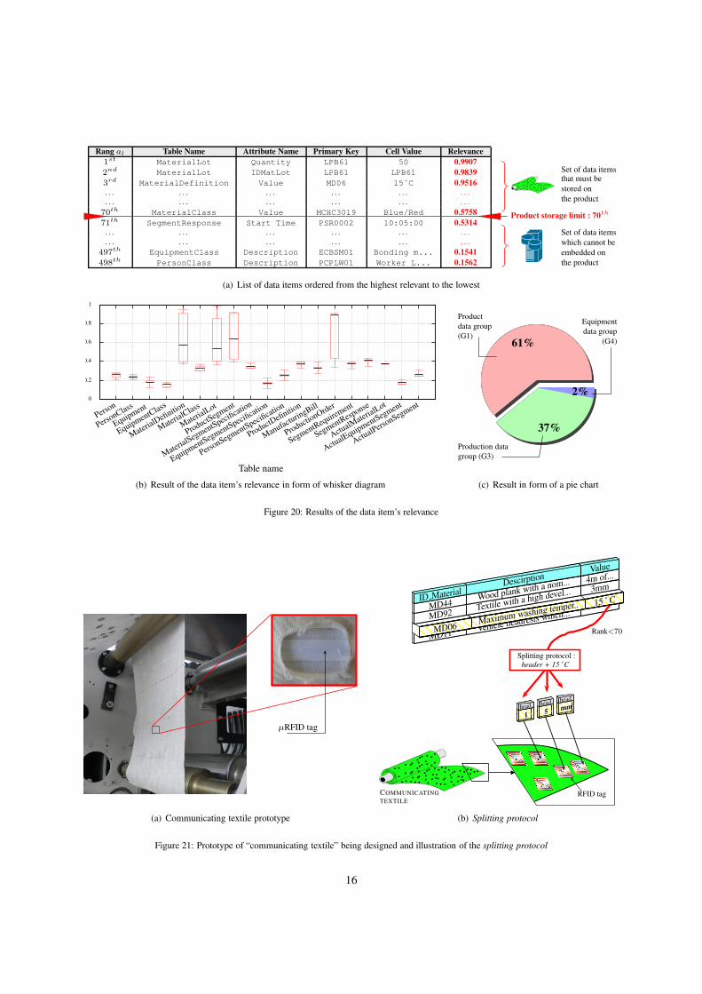
5.1. Data item relevance

The set of computations related to the three alter-

natives/data items TMD{3, 1}, TMD{3, 2} and TMD{3, 3}

have been presented throughout section 4. In our sce-

nario, approximately 500 product-related data items are

ranked (representing ≈ 30 Mbytes). In this section,

results for the final ranking of all data items are com-

mented on, and then a brief view of how data items are

split over the “communicating textile” is presented.

Figure 20(a) provides the resulting list (noted L) of

product-related data items ordered from the most rele-

vant to the least relevant (i.e., ordered according to their

CoG of superior approximation: x␄+). The two most rel-

evant data items come from the table MaterialLot and

have relevances of 0.9907 and 0.9839 respectively. The

third item is TMD{3, 3}. Due to the large number of

data items included in L (498, to be exact), only sta-

tistical results in the form of diagrams are presented

(whisker diagram and pie chart). First, let us exam-

ine the whisker diagram in Figure 20(b). For each ta-

ble t ∈ T , the min, the 1st-3rd quartile, the median, and

the max relevance of the set of data items belonging to t

are given. We can see that the most relevant data items

come from MaterialLot (which includes the two

first data items of L) and from MaterialDefinition,

ProductSegment, and ProductionOrder. The at-

tributes from these four tables have been enumerated by

the experts e1, e2, and e3 in Ce (see Table 2), and Ce

is the most important criterion at this stage of the PLC

(see Figure 12). Moreover, one can note that these four

tables are included in G1 and G3 and that the experts,

concerned by Cc, have highly recommended selecting

information from both groups (cf. vectors in Figure 8).

The “communicating textile” designed is shown in

Figure 21(a). As mentioned, the product-related data

items are stored on the product from the most relevant

to the least relevant, until no more memory is avail-

able. In our study, no more than the first 70 data items

could be stored on the communicating textile (repre-

senting ≈ 4Mbytes when the entire list L represents

≈ 30Mbytes). The pie chart in Figure 20(c) shows the

percentage of data items among the 70 that come from

each entity group. For instance, 61% (i.e., ≈ 43 of the

70 data items) are included in tables for G3, and 37%

are included in tables for G1. It can be noted that no

information related to the personal data group (i.e., G2)

is embedded in the product, which is largely because of

the choices made in the enumeration and contextual cri-

teria. In this respect, these results meet the expert spec-

ifications (note that L, the whisker diagram, and the pie

chart are always displayed to the user and are used as

decision-support tools). The “communicating textile”

is then used to store the first 70 data items. In previous

work, the tools necessary to disseminate/split data items

over a communicating material have been developed.

Figure 21(b) illustrates how the data item TMD{3, 3} is

split and then stored on different RFID µtags. In short,

a specific protocol header is added to each resulting

piece of data item (header represented by the gray back-

ground) to determine in what order information is split,

and then each “piece+header” is stored among the RFID

tags (see Figure 21(b)).

5.2. PLC benefits

With the communicating textile, any actor in a down-

stream PLC stage is able to retrieve the information pre-

liminarily stored on the communicating textile. Fig-

ure 22 illustrates such a scenario considering an typical

PLC that consists of three main phases: Beginning of

Life (BoL), including design and production, Middle of

Life (MoL), including use and maintenance, and End of

Life (EoL), including recycling and disposal [10]. A

writing phase (described in section 5.1) is defined in

BoL and a user (in MoL) then reads and reconstitutes

the set of product-related tuples after reading the mate-

rial. For this to happen, software has been developed,

from which a screenshot is given in Figure 22. It shows

15

Rang al Table Name Attribute Name Primary Key Cell Value Relevance

1st MaterialLot Quantity LPB61 50 0.9907

2ndMaterialLot IDMatLot LPB61 LPB61 0.9839

3rd MaterialDefinition Value MD06 15˚C 0.9516

. . . . . . . . . . . . . . . . . .

. . . . . . . . . . . . . . . . . .

70th MaterialClass Value MCHC3019 Blue/Red 0.5758

71th SegmentResponse Start Time PSR0002 10:05:00 0.5314

. . . . . . . . . . . . . . . . . .

. . . . . . . . . . . . . . . . . .

497th EquipmentClass Description ECBSM01 Bonding m... 0.1541

498th PersonClass Description PCPLW01 Worker L... 0.1562

Product storage limit : 70th

Set of data itemsthat must be

stored on

the product

Set of data items

which cannot be

embedded on

the product

(a) List of data items ordered from the highest relevant to the lowest

0

0.2

0.4

0.6

0.8

1

Person

PersonClass

Equipment

EquipmentClass

MaterialD

efinition

MaterialC

lass

MaterialLot

ProductSegment

MaterialSeg

mentSpecification

EquipmentSegmentSpecificatio

n

PersonSeg

mentSpecification

ProductDefinitio

n

ManufacturingBill

ProductionOrder

SegmentR

equirement

SegmentR

esponse

ActualMateria

lLot

ActualEquipmentSegment

ActualPersonSeg

ment

Table name

(b) Result of the data item’s relevance in form of whisker diagram

61%

37%

2%

Equipment

data group

(G4)

Production data

group (G3)

Product

data group

(G1)

(c) Result in form of a pie chart

Figure 20: Results of the data item’s relevance

µRFID tag

(a) Communicating textile prototype

15 ˚ C

3mm4m of...Value

Vehicle headrests which...Maximum washing temper..Textile with a high devel...Wood plank with a nom...Descirption

MD11MD06MD92MD44

ID Material

Rank<70

Splitting protocol :header + 15 ˚ C

1

head.5

head.mm

head.

COMMUNICATING

TEXTILERFID tag

(b) Splitting protocol

Figure 21: Prototype of “communicating textile” being designed and illustration of the splitting protocol

16

Writing phase Reading phase

Beginning of Life

Designers Manufacturers Warehousers Distributors Dealers

Middle of Life

Users

End of Life

Recyclers

cf. section 5.1 (Fig. 20-21)D

atabase

(s)

➠ ➠ ➠

data items

retrieved from

the textile

Attribute name

Table name

Software screenshot

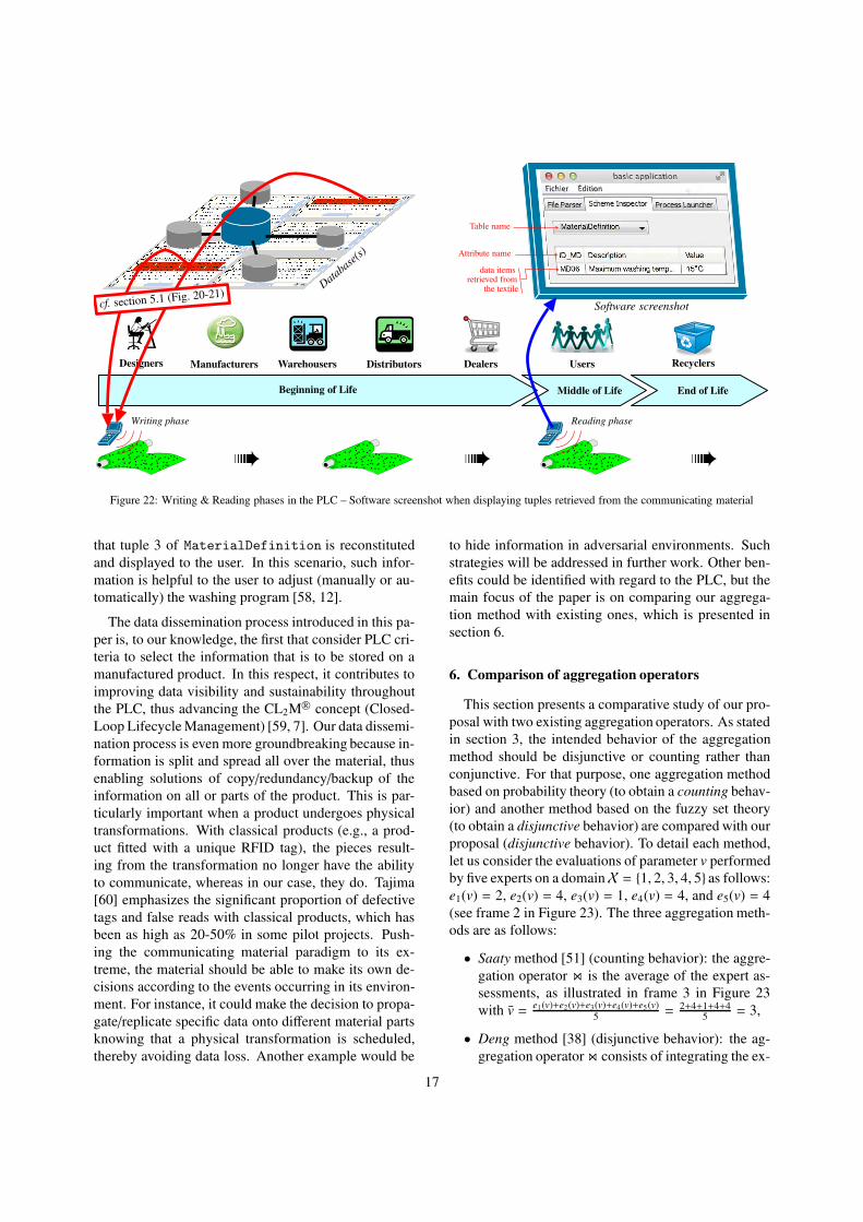
Figure 22: Writing & Reading phases in the PLC – Software screenshot when displaying tuples retrieved from the communicating material

that tuple 3 of MaterialDefinition is reconstituted

and displayed to the user. In this scenario, such infor-

mation is helpful to the user to adjust (manually or au-

tomatically) the washing program [58, 12].

The data dissemination process introduced in this pa-

per is, to our knowledge, the first that consider PLC cri-

teria to select the information that is to be stored on a

manufactured product. In this respect, it contributes to

improving data visibility and sustainability throughout

the PLC, thus advancing the CL2M R© concept (Closed-

Loop Lifecycle Management) [59, 7]. Our data dissemi-

nation process is even more groundbreaking because in-

formation is split and spread all over the material, thus

enabling solutions of copy/redundancy/backup of the

information on all or parts of the product. This is par-

ticularly important when a product undergoes physical

transformations. With classical products (e.g., a prod-

uct fitted with a unique RFID tag), the pieces result-

ing from the transformation no longer have the ability

to communicate, whereas in our case, they do. Tajima

[60] emphasizes the significant proportion of defective

tags and false reads with classical products, which has

been as high as 20-50% in some pilot projects. Push-

ing the communicating material paradigm to its ex-

treme, the material should be able to make its own de-

cisions according to the events occurring in its environ-

ment. For instance, it could make the decision to propa-

gate/replicate specific data onto different material parts

knowing that a physical transformation is scheduled,

thereby avoiding data loss. Another example would be

to hide information in adversarial environments. Such

strategies will be addressed in further work. Other ben-

efits could be identified with regard to the PLC, but the

main focus of the paper is on comparing our aggrega-

tion method with existing ones, which is presented in

section 6.

6. Comparison of aggregation operators

This section presents a comparative study of our pro-

posal with two existing aggregation operators. As stated

in section 3, the intended behavior of the aggregation

method should be disjunctive or counting rather than

conjunctive. For that purpose, one aggregation method

based on probability theory (to obtain a counting behav-

ior) and another method based on the fuzzy set theory

(to obtain a disjunctive behavior) are compared with our

proposal (disjunctive behavior). To detail each method,

let us consider the evaluations of parameter v performed

by five experts on a domainX = {1, 2, 3, 4, 5} as follows:

e1(v) = 2, e2(v) = 4, e3(v) = 1, e4(v) = 4, and e5(v) = 4

(see frame 2 in Figure 23). The three aggregation meth-

ods are as follows:

• Saaty method [51] (counting behavior): the aggre-

gation operator ⋊⋉ is the average of the expert as-

sessments, as illustrated in frame 3 in Figure 23

with v =e1(v)+e2(v)+e3(v)+e4(v)+e5(v)

5= 2+4+1+4+4

5= 3,

• Deng method [38] (disjunctive behavior): the ag-

gregation operator ⋊⋉ consists of integrating the ex-

17

e1

X

v

e2

X

v

e3

X

v

e4

X

v

e5

X

v1

1

1

1

1

0 1 2 3 4 5

avg

Agg. Saaty

X

v

avgAgg. Deng

X

v

Agg. Kubler

X

v1

1

1

0 1 2 3 4 5

2- Expert evaluations

3- Aggregation

➠

➠

Computation steps from Saaty [43]

Computation steps from Deng [16]

Computation steps from section 4

4- AHP Computation

ID_Material Description Value

MD041... Wooden plank with a nomin... 4m of...

MD060... Textile which is provided wit... 15mm

MD993... Textile with a high develope... 3mm...

MD770... Vehicle headrests that confo... 2× ...

MD060..Textile..

15mm . . .data item z


Enumeration Contextual Data Size Model-Based

1- AHP structure

Level 1

Level 2

Level 3

List_Saa

List_Den

List_Kub

5- List :Agg

Figure 23: Illustration of the 3 methods of aggregation of expert opinions based on the scenario of data dissemination

pert opinions through a triangular fuzzy set v. The

kernel of this set is equal to the average evaluation,

and uncertainty is added in a decreasing manner

from this value (i.e., until reaching the minimal and

maximal opinions formulated by the experts), as

depicted in Figure 23. This representation tends to

mean that the “ best/correct” evaluation is consid-

ered as the average evaluation and that uncertainty

arises from the set of evaluations.

• Kubler method (disjunctive behavior – paper pro-

posal): the aggregation operator ⋊⋉ consists of inte-

grating all expert opinions through a uniform fuzzy

set, as described in section 3. In the resulting fuzzy

set, all opinions are of equal importance, unlike the

two previous aggregation methods.

At the end of the process (i.e., after the computations

steps; cf. frame “4-AHP Computation”), the list L of

data items ordered from the most relevant to the low-

est is produced by each aggregation method (similar to

the list presented in Figure 20(a)), denoted respectively

List Saa, List Den, and List Kub in Figure 23 (cf.

frame “5-List:Agg”).

6.1. Comparison process

The assessment of each aggregation method is per-

formed by determining the level of satisfaction of each

expert with regard to the aggregation result. To do

this, for each method (i.e., Saaty, Deng, Kubler), a

performance indicator is defined based on the sim-

ilarity between the aggregated list (e.g., List Saa)

and the list resulting from the specification of a sin-

gle expert k when using the same method (the list is

noted, in this case, List Saa:ek). Figure 24 gives

the example in which only the opinion provided by

expert 4 about parameter v is considered by each ag-

gregation method (cf. frame 2, 3, 4), thus gen-

erating three lists: List Saa:e4, List Den:e4 and

List Kub:e4. Ultimately, if the degree of similarity be-

tween List Saa:ek and List Saa is higher than that

between List Kub:ek and List Kub, the aggregation

method proposed by Saaty better satisfies expert k than

our aggregation method.

The Jaccard similarity coefficient ([61]) can be used

to measure such the similarity between two distinct lists

A and B. It is defined as in equation 25, i.e., the size

of the intersection of the lists divided by the size of the

union of the lists. In our study, the union size is equal to

the number of data items n. A Jaccard similarity coeffi-

cient goes from 0 (no common data items) to 1 (identical

lists).

J(A, B) =|A ∩ B|

|A ∪ B|=|A ∩ B|

n(25)

Let A, B and C be three lists consisting of five data

18

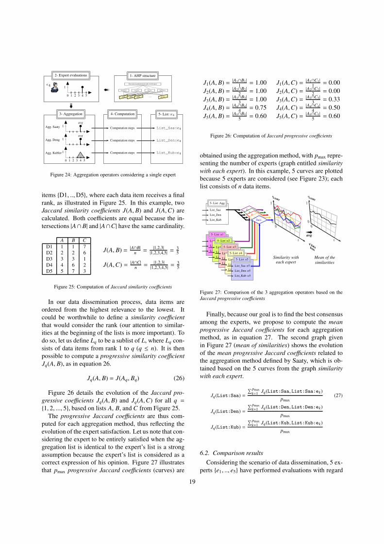
e41

0 1 2 3 4 5

avg

Agg. Saaty

avg

Agg. Deng

Agg. Kubler 1

1

1

0 1 2 3 4 5

2- Expert evaluations

3- Aggregation

➠

➠

Computation steps

Computation steps

Computation steps

4- Computation

MD060..MD060..

MD060.. . . . data item z


Enumeration Contextual Data Size Model-Based

1- AHP structure

List_Saa:e4

List_Den:e4

List_Kub:e4

5- List :e4

Figure 24: Aggregation operators considering a single expert

items {D1, ..,D5}, where each data item receives a final

rank, as illustrated in Figure 25. In this example, two

Jaccard similarity coefficients J(A, B) and J(A,C) are

calculated. Both coefficients are equal because the in-

tersections |A∩B| and |A∩C| have the same cardinality.

A B C

D1 1 1 7

D2 2 2 6

D3 3 3 1

D4 4 6 2

D5 5 7 3

J(A, B) = |A∩B|

n=

|1,2,3||1,2,3,4,5|

= 35

J(A,C) = |A∩C|

n=

|1,2,3||1,2,3,4,5|

= 35

Figure 25: Computation of Jaccard similarity coefficients

In our data dissemination process, data items are

ordered from the highest relevance to the lowest. It

could be worthwhile to define a similarity coefficient

that would consider the rank (our attention to similar-

ities at the beginning of the lists is more important). To

do so, let us define Lq to be a sublist of L, where Lq con-

sists of data items from rank 1 to q (q ≤ n). It is then

possible to compute a progressive similarity coefficient

Jq(A, B), as in equation 26.

Jq(A, B) = J(Aq, Bq) (26)

Figure 26 details the evolution of the Jaccard pro-

gressive coefficients Jq(A, B) and Jq(A,C) for all q =

{1, 2, ..., 5}, based on lists A, B, and C from Figure 25.

The progressive Jaccard coefficients are thus com-

puted for each aggregation method, thus reflecting the

evolution of the expert satisfaction. Let us note that con-

sidering the expert to be entirely satisfied when the ag-

gregation list is identical to the expert’s list is a strong

assumption because the expert’s list is considered as a

correct expression of his opinion. Figure 27 illustrates

that pmax progressive Jaccard coefficients (curves) are

J1(A, B) = |A1∩B1|

1= 1.00 J1(A,C) = |A1∩C1 |

1= 0.00

J2(A, B) = |A2∩B2|

2= 1.00 J2(A,C) = |A2∩C2 |

2= 0.00

J3(A, B) = |A3∩B3|

3= 1.00 J3(A,C) = |A3∩C3 |

3= 0.33

J4(A, B) = |A4∩B4|

4= 0.75 J4(A,C) = |A4∩C4 |

4= 0.50

J5(A, B) = |A5∩B5|

5= 0.60 J5(A,C) = |A5∩C5 |

5= 0.60

Figure 26: Computation of Jaccard progressive coefficients

obtained using the aggregation method, with pmax repre-

senting the number of experts (graph entitled similarity

with each expert). In this example, 5 curves are plotted

because 5 experts are considered (see Figure 23); each

list consists of n data items.

List_Saa

List_Den

List_Kub

5- List :Agg

List_Saa :e1

List_Den :e1

List_Kub :e1

5- List :e1

Jacc.

List_Saa :e2

List_Den :e2

List_Kub :e2

5- List :e2

Jacc.

List_Saa :e3

List_Den :e3

List_Kub :e3

5- List :e3

Jacc.

List_Saa :e4

List_Den :e4

List_Kub :e4

5- List :e4

Jacc.

List_Saa :e5

List_Den :e5

List_Kub :e5

5- List :e5

Jacc.

%corr

n˚dataitem

1

0

0

z

%corr

1

0

0

zavg➟

Similarity witheach expert

Mean of the

similarities

Figure 27: Comparison of the 3 aggregation operators based on the

Jaccard progressive coefficients

Finally, because our goal is to find the best consensus

among the experts, we propose to compute the mean

progressive Jaccard coefficients for each aggregation

method, as in equation 27. The second graph given

in Figure 27 (mean of similarities) shows the evolution

of the mean progressive Jaccard coefficients related to

the aggregation method defined by Saaty, which is ob-

tained based on the 5 curves from the graph similarity

with each expert.

Jq(List:Saa) =

∑pmax

k=1Jq(List:Saa,List:Saa:ek)

pmax(27)

Jq(List:Den) =

∑pmax

k=1Jq(List:Den,List:Den:ek)

pmax

Jq(List:Kub) =

∑pmax

k=1Jq(List:Kub,List:Kub:ek)

pmax

6.2. Comparison results

Considering the scenario of data dissemination, 5 ex-

perts {e1, .., e5} have performed evaluations with regard

19

0

0.5

1

0 50 100 150 200

Sim

ilar

ity

coeff

.

n˚ of data item

Agg. Saaty

0

0.5

1

0 50 100 150 200

n˚ of data item

Agg. Deng

0

0.5

1

0 50 100 150 200

n˚ of data item

Agg. Kubler

Expert 1

Expert 2

Expert 3

Expert 4

Expert 5

(a) Jaccard progressive coefficients in scenario (1)

0

0.5

1

0 50 100 150 200

n˚ of data item

Agg. Saaty

0

0.5

1

0 50 100 150 200

Sim

ilar

ity

coeff

.

n˚ of data item

Agg. Deng

0

0.5

1

0 50 100 150 200

n˚ of data item

Agg. Kubler

Expert 1

Expert 2

Expert 3

Expert 4

Expert 5

(b) Jaccard progressive coefficients in scenario (2)

Figure 28: Computation of Jaccard progressive coefficients for each expert with respect to each aggregation method

to the criteria Enumeration, Contextual, and Data size.

These evaluations are not described in detail but are

commented on throughout this section. Two scenarios

are defined:

(1) Ce favored: Enumeration is strongly favored over

the other criteria,

(2) Equal-importance: the four criteria are of equal im-

portance,

Among the 5 experts, e5 enumerates information that

is not at all enumerated by the 4 other experts. As men-

tioned in section 3, this opinion is as legitimate as the

others, although it is isolated. The Jaccard progressive

coefficients between the lists resulting from each aggre-

gation method (List:Saa, List:Den, List:Kub) and

the lists resulting from each expert k are computed and

plotted in Figure 28 for scenarios (1) and (2).

Considering scenario (1) (see Figure 28(a)), the

curves show that the three aggregation methods have

difficulty satisfying e5 (the Jaccard progressive coef-

ficients of e5 always remain far below the four other

curves, especially for the first 50 data items). This is ex-

plained by the fact that e5 has an isolated point of view

with respect to criterion Ce, which is strongly favored

over the other. As a result, it is particularly difficult to

satisfy every expert. Nonetheless, among the three ag-

gregation methods, the method developed in this paper

(i.e., Agg. Kubler) satisfies e5 the most because meth-

ods Agg. Saaty and Agg. Deng have a similarity of

approximately 0 between data items n˚1 to 30, whereas

our method has a similarity of approximatively 0.3. This

has an impact on the satisfaction rating of the four other

experts, who are less satisfied with Agg. Kubler than

they are with Agg. Saaty and Agg. Deng, but it does

not affect the final consensus because the mean progres-

sive Jaccard coefficients of the three methods (see Fig-

ure 29(a)) are almost identical (the three curves over-

lap). This study shows, in this particular scenario, that

Agg. Kubler better satisfies the disjunctive behavior

than do the two other methods because it tries not to

neglect/to leave out an opinion.

Considering scenario (2) (see Figure 28(b)), it can be

concluded that no expert has been left out or treated un-

fairly. Indeed, unlike scenario (1), no curves are de-

tached from the others, i.e. each aggregation method

equally satisfies the experts. However, it should be

noted that the final consensus is much better when us-

ing Agg. Kubler (see Figure 29(b)) than when using

the two other methods, especially when focusing on the

first 50 data items that are of major importance.

More generally, it can be concluded that the three ag-

gregation methods globally exhibit a similar behavior

in these scenarios because the mean Jaccard progres-

sive coefficients are almost overlapping, whether in sce-

nario (1) or (2) (cf. Figure 29).

20

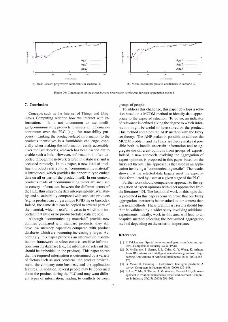
0

0.5

1

0 50 100 150 200

Sim

ilar

ity

coeff

.

n˚ of data item

Agg1

Agg2

Agg3

(a) Mean Jaccard progressive coefficients in scenario (1)

0

0.5

1

0 50 100 150 200

Sim

ilar

ity

coeff

.

n˚ of data item

Agg1

Agg2

Agg3

(b) Mean Jaccard progressive coefficients in scenario (2)

Figure 29: Computation of the mean Jaccard progressive coefficients for each aggregation method

7. Conclusion

Concepts such as the Internet of Things and Ubiq-

uitous Computing redefine how we interact with in-

formation. It is not uncommon to use intelli-

gent/communicating products to ensure an information

continuum over the PLC (e.g., for traceability pur-

poses). Linking the product-related information to the

products themselves is a formidable challenge, espe-

cially when making the information easily accessible.

Over the last decades, research has been carried out to

enable such a link. However, information is often de-

ported through the network (stored in databases) and is

accessed remotely. In this paper, a new kind of intel-

ligent product referred to as “communicating material”

is introduced, which provides the opportunity to embed

data on all or part of the product itself. In our context,

products made of “communicating material” are used

to convey information between the different actors of

the PLC, thus improving data interoperability, availabil-

ity, and sustainability compared with standard products

(e.g., a product carrying a unique RFID tag or barcode).

Indeed, the same data can be copied to several parts of

the material, which is useful in cases in which it is im-

portant that little or no product-related data are lost.

Although “communicating materials” provide new

abilities compared with standard products, they still

have low memory capacities compared with product

databases which are becoming increasingly larger. Ac-

cordingly, this paper proposes an information dissem-

ination framework to select context-sensitive informa-

tion from the database (i.e., the information relevant that

should be embedded in the product). This paper shows

that the required information is determined by a variety

of factors such as user concerns, the product environ-

ment, the company core business, and the application

features. In addition, several people may be concerned

about the product during the PLC and may want differ-

ent types of information, leading to conflicts between

groups of people.

To address this challenge, this paper develops a solu-

tion based on a MCDM method to identify data appro-

priate to the expected situation. To do so, an indicator

of relevance is defined giving the degree to which infor-

mation might be useful to have stored on the product.

This method combines the AHP method with the fuzzy

set theory. The AHP makes it possible to address the

MCDM problem, and the fuzzy set theory makes it pos-

sible both to handle uncertain information and to ag-

gregate the different opinions from groups of experts.

Indeed, a new approach involving the aggregation of

expert opinions is proposed in this paper based on the

fuzzy set theory. This approach is then used in an appli-

cation involving a “communicating textile”. The results

shows that the selected data largely meet the expecta-

tions formulated by users at a given stage of the PLC.

Further work should compare our approach to the ag-

gregation of expert opinions with other approaches from

the literature [45]. The first initial work on this topic that

is presented in this paper seems to prove that our fuzzy

aggregation operator is better suited to our context than

classical methods. These preliminary results should fur-

ther be validated by a wider study involving additional

experiments. Ideally, work in this area will lead to an

adaptive method selecting the best-suited aggregation

method depending on the criterion importance.

References

[1] P. Valckenaers, Special issue on intelligent manufacturing sys-

tems, Computers in Industry 37(3) (1998).

[2] D. McFarlane, S. Sarma, J. L. Chirn, C. Y. Wong, K. Ashton,

Auto ID systems and intelligent manufacturing control, Engi-

neering Applications of Artificial Intelligence 16(4) (2003) 365–

376.

[3] G. Meyer, K. Framling, J. Holmstrom, Intelligent products: A

survey, Computers in Industry 60(3) (2009) 137–148.

[4] S. Lee, Y. Ma, G. Thimm, J. Verstraeten, Product lifecycle man-

agement in aviation maintenance, repair and overhaul, Comput-

ers in Industry 59(2/3) (2008) 296–303.

21

[5] M. Karkkainen, J. Holmstrom, K. Framling, K. Artto, Intelligent

products–a step towards a more effective project delivery chain,

Computers in Industry 50(2) (2013) 141–151.

[6] S. Kubler, W. Derigent, A. Thomas, E. Rondeau, Embedding

data on “communicating materials” from context-sensitive in-

formation analysis, Journal of Intelligent Manufacturing (DOI)

10.1007/s10845-013-0745-y (2013).

[7] S. Kubler, W. Derigent, K. Framling, A. Thomas, E. Ron-

deau, Enhanced product lifecycle information management us-

ing “communicating materials”, Computer-Aided Design (DOI)

10.1016/j.cad.2013.08.009 (2013).

[8] H. Jun, D. Kiritsis, P. Xirouchakis, Research issues on closed-

loop PLM, Computers in Industry 58(8) (2007) 855–868.

[9] S. K. Kwok, J. S. L. Ting, A. H. C. Tsang, W. B. Lee, B. C.

F. Cheung, Design and development of a mobile EPC-RFID-

based self-validation system (MESS) for product authentication,

Computers in Industry 61(7) (2010) 624–635.

[10] D. Kiritsis, Closed-loop PLM for intelligent products in the era

of the Internet of Things, Computer-Aided Design 43(5) (2011)

479–501.

[11] J. Stark, Product lifecycle management: 21st century paradigm

for product realisation, Springer, 2011.

[12] D. McFarlane, V. Giannikas, A. C. Wong, M. Harrison, Product

intelligence in industrial control: Theory and practice, Annual

Reviews in Control 37(1) (2013) 69–88.

[13] M. Ozsu, P. Valduriez, Distributed database systems: where are

we now?, Computer 24(8) (1991) 68–78.

[14] L. Baltrunas, B. Ludwig, S. Peer, F. Ricci, Context relevance

assessment and exploitation in mobile recommender systems,

Personal and Ubiquitous Computing 16(5) (2012) 507–526.

[15] D. Khosroanjom, M. Ahmadzade, A. Niknafs, R. Mavi, Using

fuzzy AHP for evaluating the dimensions of data quality, Inter-

national Journal of Business Information Systems 8(3) (2011)

269–285.

[16] D. Chan, J. Roddick, Context-sensitive mobile database sum-

marisation, in: 26th Australasian computer science conference,

Australia, 2003, pp. 139–149.

[17] S. Terzi, A. Bouras, D. Dutta, M. Garetti, Product lifecycle

management–from its history to its new role, International Jour-

nal of Product Lifecycle Management 4(4) (2010) 360–389.

[18] H.-B. Jun, H.-W. Suh, Decision on the memory size of embed-

ded information systems in an ubiquitous maintenance environ-

ment, Computers & Industrial Engineering 56(1) (2009) 444–

451.

[19] P. Vincke, Multicriteria decision-aid, John Wiley & Sons Inc,

1992.

[20] G. Zheng, N. Zhu, Z. Tian, Y. Chen, B. Sun, Application of

a trapezoidal fuzzy AHP method for work safety evaluation and

early warning rating of hot and humid environments, Safety Sci-

ence 50(2) (2012) 228–240.

[21] O. Vaidya, S. Kumar, Analytic hierarchy process: An overview

of applications, European Journal of operational research 169(1)

(2006) 1–29.

[22] T. Saaty, How to make a decision: the analytic hierarchy pro-

cess, European journal of operational research 48 (1990) 9–26.

[23] G. Buyukozkan, O. Feyzioglu, D. Ruan, Fuzzy group decision-

making to multiple preference formats in quality function de-

ployment, Computers in Industry 58(5) (2007) 392–402.

[24] L. Zadeh, Fuzzy sets, Information and Control 8 (1965) 338–

353.

[25] B. Bouchon-Meunier, La logique floue, Presses universitaires de

France, 2007.

[26] R. Kuo, S. Chi, S. Kao, A decision support system for locating

convenience store through fuzzy AHP, Computers & Industrial

Engineering 37(1/2) (1999) 323–326.

[27] C.-H. Yeh, H. Deng, Y.-H. Chang, Fuzzy multicriteria analysis

for performance evaluation of bus companies, European Journal

of Operational Research 126(3) (2000) 459–473.

[28] K. Anagnostopoulos, C. Petalas, A fuzzy multicriteria benefit–

cost approach for irrigation projects evaluation, Agricultural

Water Management 98(9) (2011) 1409–1416.

[29] M.-C. Lin, C.-C. Wang, M.-S. Chen, C. A. Chang, Using AHP

and TOPSIS approaches in customer-driven product design pro-

cess, Computers in Industry 59(1) (2008) 17–31.

[30] C.-S. Wang, An analysis and evaluation of fitness for shoe lasts

and human feet, Computers in Industry 61(6) (2010) 532–540.

[31] I. N. Durbach, T. J. Stewart, Modeling uncertainty in multi-

criteria decision analysis, European Journal of Operational Re-

search 223(1) (2012) 1–14.

[32] G. Buyukozkan, G. Cifci, A novel fuzzy multi-criteria decision

framework for sustainable supplier selection with incomplete in-

formation, Computers in Industry 62(2) (2011) 164–174.

[33] Y.-M. Wang, K.-S. Chin, Fuzzy analytic hierarchy process: A

logarithmic fuzzy preference programming methodology, Inter-

national Journal of Approximate Reasoning 52(4) (2011) 541–

553.

[34] F. T. Bozbura, A. Beskese, Prioritization of organizational capi-

tal measurement indicators using fuzzy AHP, International Jour-

nal of Approximate Reasoning 44(2) (2007) 124–147.

[35] M. Xia, Z. Xu, Methods for fuzzy complementary preference

relations based on multiplicative consistency, Computers & In-

dustrial Engineering 61(4) (2011) 930–935.

[36] M. B. Javanbarg, C. Scawthorn, J. Kiyono, B. Shahbodaghkhan,

Fuzzy AHP-based multicriteria decision making systems using

particle swarm optimization, Expert Systems with Applications

39(1) (2012) 960–966.

[37] D.-Y. Chang, Applications of the extent analysis method on

fuzzy AHP, European Journal of Operational Research 95(3)

(1996) 649–655.

[38] H. Deng, Multicriteria analysis with fuzzy pairwise comparison,

International Journal of Approximate Reasoning 21(3) (1999)

215–231.

[39] Y.-M. Wang, Y. Luo, Z. Hua, On the extent analysis method

for fuzzy AHP and its applications, European Journal of Opera-

tional Research 186(2) (2008) 735–747.

[40] J. Buckley, Fuzzy hierarchical analysis, Fuzzy Sets and Systems

17 (1985) 233–247.

[41] H.-P. Fu, P. Chao, T.-H. Chang, Y.-S. Chang, The impact of

market freedom on the adoption of third-party electronic mar-

ketplaces: A fuzzy AHP analysis, Industrial Marketing Man-

agement 37(6) (2008) 698–712.

[42] T. Kayaa, C. Kahramanb, A fuzzy approach to e-banking web-

site quality assessment based on an integrated AHP-ELECTRE

method, Technological and Economic Development of Econ-

omy 17(2) (2011) 313–334.

[43] D. Dubois, H. Prade, A review of fuzzy set aggregation connec-

tives, Information sciences 36(1) (1985) 85–121.

[44] M. Delgado, F. Herrera, E. Herrera-Viedma, L. Martinez, Com-

bining numerical and linguistic information in group decision

making, Information Sciences 107(1) (1998) 177–194.

[45] F. Chiclana, J. M. Tapia Garcıa, M. J. del Moral, E. Herrera-

Viedma, A statistical comparative study of different similarity

measures of consensus in group decision making, Information

Sciences 221 (2013) 110–123.

[46] R. Cooke, Experts in uncertainty: opinion and subjective proba-

bility in science, Oxford University Press, USA, 1991.

[47] S. Destercke, D. Dubois, E. Chojnacki, Aggregation of expert

opinions and uncertainty theories, in: Rencontres Francophones

sur la Logique Floue et ses Applications, France, 2006, pp. 295–

302.

22

[48] E. Herrera-Viedma, F. Javier Cabrerizo, J. Kacprzyk, W.

Pedrycz, A review of soft consensus models in a fuzzy environ-

ment, Information Fusion (DOI) 10.1016/j.inffus.2013.04.002.

(2013).

[49] H. Lee, Optimal consensus of fuzzy opinions under group de-

cision making environment, Fuzzy Sets and Systems 132(3)

(2002) 303–315.

[50] Z. Xu, X. Cai, Group consensus algorithms based on preference

relations, Information Sciences 181(1) (2011) 150–162.

[51] T. Saaty, The Analytic Hierarchy Process, New York: McGraw-

Hill, 1980.

[52] M. Grabisch, P. Perny, Agregation multicritere, Utilisations de

la logique floue, Hermes, 1999.

[53] G. Bortolan, R. Degani, A review of some methods for ranking

fuzzy subsets, Fuzzy sets and systems 15(1) (1985) 1–19.

[54] C. Chen, C. Klein, A simple approach to ranking a group of

aggregated fuzzy utilities, IEEE Transactions on Systems, Man,

and Cybernetics, Part B: Cybernetics 27(1) (1997) 26–35.

[55] Y. Wang, Centroid defuzzification and the maximizing set and

minimizing set ranking based on alpha level sets, Computers &

Industrial Engineering 57(1) (2009) 228–236.

[56] J. Cochran, H. Chen, Fuzzy multi-criteria selection of object-

oriented simulation software for production system analysis,

Computers & operations research 32(1) (2005) 153–168.

[57] R. R. Yager, On a general class of fuzzy connectives, Fuzzy sets

and Systems 4(3) (1980) 235–242.

[58] D. Ley, Ubiquitous computing, Ubiquitous Computing, emerg-

ing technologie 2 (2007) 64–79.

[59] K. Framling, J. Holmstrom, J. Loukkola, J. Nyman, A. Kaustell,

Sustainable PLM through Intelligent Products, Engineering Ap-

plications of Artificial Intelligence 26(2) (2013) 789–799.

[60] M. Tajima, Strategic value of RFID in supply chain manage-

ment, Journal of purchasing and supply management 13(4)

(2007) 261–273.

[61] P.-N. Tan, M. Steinbach, V. Kumar, Introduction to data mining,

Addison-Wesley Longman Publishing Co., Inc., 2006.

Sylvain Kubler is postdoctoral researcher

at the department of Computer Science in

Aalto University. He received his M.Sc.

degree and Ph.D. degree in Computer Sci-

ence and Engineering from the University

of lorraine (France) respectively in 2009

and 2012. He has broad expertise in dis-

tributed and intelligent systems, Internet of

Things, Product Lifecycle Management and

communication networks. His main fields

of research are context-aware systems, sys-

tem interoperability, multi-criteria decision making, fuzzy logic and

networked control systems. He was awarded the best Thesis in Auto-

matic Control from the CNRS/IFAC French Workgroup GdR MACS

for his Ph.D thesis in 2012.

Alexandre VOISIN received his Ph. D

degree in Electrical Engineering from the

University of Lorraine in 1999, where he

is currently Assistant Professor. His pri-

mary research was in the field of fuzzy logic

and information processing. Since 2003,

he is involved in e-maintenance research

project. His research deals with depend-

ability, maintenance decision in a proactive

maintenance strategy, prognostics and mon-

itoring, data/information/knowledge reuse

within a fleet of systems and decision making. He is member of

French and International projects/groups on e-maintenance such as the

CNRS MACOD working group (Modeling and Optimization of Dis-

tributed vs. Collaborative Maintenance), the French scientific interest

group 3SGS on “Dependability of Complex Systems” in the project

DEPRADEM (Degradation and Prognosis Modeling for Maintenance

Decision Making), the project BMCI (Report on the Maintenance and

Intelligent Operation of ships), the project CONNEXION, the Euro-

pean Integrated Project DYNAMITE (Dynamic Decision in Mainte-

nance), and the international project DEPEN-IMPRO (Modeling Poli-

cies for the improvement of Production Systems’ Dependability).

William Derigent obtained his Ph.D.

in 2005 from the University of Lorraine

(France). Since 2006, he is an associate

professor at the University of Lorraine and

is working in the ambient intelligent sys-

tems team of the Research Center for Au-

tomatic Control (CRAN-UMR 7039). His

research topics are the internet of things,

product lifecycle management and intelli-

gent products. He focuses in particular on

data dissemination in intelligent environ-

ments while considering the information semantic and application

context. He also designs communicating materials embedding their

own information system by using RFID and wireless sensors.

Andre Thomas received his PhD from

the INPL (National Polytechnic Institute of

Lorraine), France, in 1993. He is cur-

rently Professor at ENSTIB (High School of

wood sciences and Timber engineering) and

in charge of the ISET research department

at CRAN-CNRS – University of Lorraine.

Certified in Value Management and CFPIM,

he works with companies producing man-

ufactured goods for research projects. His

research topic is “Hybrid control” of Sup-

ply Chain. Hybrid control means to use centralised tactical planning

and distributed short term decision-making systems to control mate-

rial flow (thanks to instrumented products) on shop floors and into the

Supply Chains. He is author of books, several papers in scientific and

technical revues. He has developed several training tools in industrial

engineering in the field of improvement and management of produc-

tion systems.

23

Eric Rondeau obtained his Ph.D. in

1993 from the Lorraine University (France).

Since 2002, he is professor at the Univer-

sity of Lorraine and is working in the net-

work research team of the Research Cen-

ter for Automatic Control (CRAN-UMR

7039). His research topics are networked

control systems, real time communications,

pervasive systems and sustainable commu-

nications. He coordinated a FP6 Strep

project named NeCST (Networked Control

Systems Tolerant to faults). He is member of IFAC Technical Com-

mittee 1.5 in Networked Systems. He is the coordinator of Erasmus

Mundus Master in PERCCOM (Pervasive Computing and Commu-

nications for sustainable development) providing original teaching in

the domain of Green ICT and ICT for greening.

Kary Framling received his MSc in Com-

puter Science from Helsinki University of

Technology in 1990 and his PhD from Ecole

Nationale Superieure des Mines de Saint-

Etienne, France, in 1996. He is currently

Professor of Practice in Building Informa-

tion Modeling (BIM) at Aalto University,

Finland. His main research topics are on in-

formation management practices and appli-

cations for BIM and product lifecycle man-

agement in general. His main areas of com-

petence are distributed systems, middleware, multi-agent systems, au-

tonomously learning agents, neural networks and decision support

systems.

24

Group fuzzy AHP approach to embed relevant data on “communicating material”

Documents

Transcript of Group fuzzy AHP approach to embed relevant data on “communicating material”