Group Decision-Making Model With Incomplete Fuzzy Preference Relations Based on Additive Consistency

176 IEEE TRANSACTIONS ON SYSTEMS, MAN, AND CYBERNETICS—PART B: CYBERNETICS, VOL. 37, NO. 1, FEBRUARY 2007

Group Decision-Making Model With IncompleteFuzzy Preference Relations Based on

Additive ConsistencyEnrique Herrera-Viedma, Francisco Chiclana, Francisco Herrera, and Sergio Alonso

Abstract—In decision-making problems there may be cases inwhich experts do not have an in-depth knowledge of the problem tobe solved. In such cases, experts may not put their opinion forwardabout certain aspects of the problem, and as a result they maypresent incomplete preferences, i.e., some preference values maynot be given or may be missing. In this paper, we present a newmodel for group decision making in which experts’ preferencescan be expressed as incomplete fuzzy preference relations. Aspart of this decision model, we propose an iterative procedure toestimate the missing information in an expert’s incomplete fuzzypreference relation. This procedure is guided by the additive-consistency (AC) property and only uses the preference values theexpert provides. The AC property is also used to measure the levelof consistency of the information provided by the experts and alsoto propose a new induced ordered weighted averaging (IOWA)operator, the AC-IOWA operator, which permits the aggregationof the experts’ preferences in such a way that more importanceis given to the most consistent ones. Finally, the selection of thesolution set of alternatives according to the fuzzy majority ofthe experts is based on two quantifier-guided choice degrees: thedominance and the nondominance degree.

Index Terms—Additive consistency (AC), aggregation, choicedegree, group decision making (GDM), incomplete preferencerelations, induced ordered weighted averaging (IOWA) operator.

I. INTRODUCTION

G ROUP decision making (GDM) consists of multiple in-dividuals interacting to reach a decision. Each decision

maker (expert) may have unique motivations or goals and mayapproach the decision process from a different angle, but havea common interest in reaching eventual agreement on selectingthe “best” option(s) [8], [25]. To do this, experts have to expresstheir preferences by means of a set of evaluations over a setof alternatives. It has been a common practice in research tomodel GDM problems in which all the experts express theirpreferences using the same preference representation format.However, in real practice, this is not always possible because

Manuscript received August 16, 2005; revised January 11, 2006 and March10, 2006. This paper was recommended by Associate Editor T. Sudkamp.

E. Herrera-Viedma, F. Herrera, and S. Alonso are with the Departmentof Computer Science and Artificial Intelligence, University of Granada,18071 Granada, Spain (e-mail: [email protected]; [email protected];[email protected]).

F. Chiclana is with the Centre for Computational Intelligence, Schoolof Computing, De Montfort University, LE1 9BH Leicester, U.K. (e-mail:[email protected]).

Digital Object Identifier 10.1109/TSMCB.2006.875872

each expert has their unique characteristics with regard toknowledge, skills, experience, and personality, which impliesthat different experts may express their evaluations by meansof different preference representation formats. In fact, thisis an issue that recently has attracted the attention of manyresearchers in the area of GDM, and as a result, differentapproaches to integrating different preference representationformats have been proposed [1]–[3], [9], [15], [16], [44], [45].In these research papers, many reasons are provided for fuzzypreference relations to be chosen as the base element of thatintegration. Among these reasons, it is worth noting that theyare a useful tool in the aggregation of experts’ preferences intogroup preferences (see also [5], [10], [17], [20], [31], and [32]).

As aforementioned, each expert has his/her own experienceconcerning the problem being studied, which also may implya major drawback, that of an expert not having a perfectknowledge of the problem to be solved [21]–[23], [28], [33].Indeed, there may be cases where an expert would not be ableto efficiently express any kind of preference degree betweentwo or more of the available options. This may be due to anexpert not possessing a precise or sufficient level of knowledgeof part of the problem, or because that expert is unable todiscriminate the degree to which some options are better thanothers. Therefore, it would be of great importance to providethe experts with tools that allow them to express this lack ofknowledge in their opinions. In this paper, we present and usethe concept of an incomplete fuzzy preference relation, i.e., afuzzy preference relation with some of its values missing orunknown, as the tool for modeling situations with incompleteinformation.

Another important issue to bear in mind when information isprovided by experts is that of “consistency” [3], [4], [17]. Dueto the complexity of most decision-making problems, experts’preferences may not satisfy formal properties that fuzzy prefer-ence relations are required to verify. Consistency is one of them,and it is associated with the transitivity property.

Many properties have been suggested to model transitivity offuzzy preference relations and, consequently, consistency maybe measured according to which of these different properties isrequired to be satisfied. One of these properties is the “additivetransitivity,” which, as shown in [17], can be seen as the parallelconcept of Saaty’s consistency property in the case of themultiplicative preference relation.

It is obvious that consistent information, i.e., informa-tion which does not imply any kind of contradiction, is more

1083-4419/$25.00 © 2007 IEEE

HERRERA-VIEDMA et al.: GROUP DECISION-MAKING MODEL WITH INCOMPLETE FUZZY PREFERENCE RELATIONS 177

relevant or important than the information containing some con-tradictions. The general procedure for the inclusion of impor-tance degrees in GDM problems involves the transformation ofthe preference values under the importance degrees to generatenew values [11], [38]. This activity is carried out by means ofa transformation function. Examples of such a function usedin these cases include the minimum operator [11], [38], theexponential function [35], or generally a t-norm operator [46].An alternative way of implementing these importance degreesin the resolution process of a GDM problem is by using themto induce the ordering of the preference values prior to theiraggregation, which is in the definition of an induced orderedweighted averaging (IOWA) operator [40], [42]. In the caseof quantifier-guided IOWA operators, the importance degreescan also be used to calculate their corresponding weightingvector [6], [12].

The aim of this paper is to present a new decision model todeal with GDM problems with the incomplete fuzzy preferencerelations based on the additive-consistency (AC) property. Thisnew model is composed of two steps: the estimation of missingpreference values and the selection of alternatives. To do this,we define a new AC measure for fuzzy preference relations,which is based on the additive transitivity property [31]. Weuse this AC measure to propose a new IOWA operator, whichwe call the AC-IOWA operator. For the first step, we proposean iterative procedure based on AC to estimate the missingvalues of the incomplete fuzzy preference relation. We willshow that under certain conditions the incomplete fuzzy pref-erence relation can be completed, i.e., all its missing valuescan be successfully estimated. The main difference between theapproach we propose and those already proposed [22], [23] isthat the completion of a particular expert’s incomplete fuzzypreference relation is carried out using only the informationhe/she provides and no other expert’s information is needed.It is important to point out that because no information fromexternal sources is used, the estimated information is consistentwith the original expert’s opinions. Finally, following the choicescheme proposed in [10], i.e., aggregation followed by exploita-tion, we will design a selection process for GDM problems withthe incomplete fuzzy preference relations based on the conceptof fuzzy majority and the AC-IOWA operator. The aggregationstep of a GDM problem consists in combining the experts’individual preferences into a group collective one in such away that it summarizes or reflects the properties contained inall the individual preferences. This aggregation is carried outby applying the proposed AC-IOWA operator. The exploitationphase transforms the global information about the alternativesinto a global ranking of them. This can be done in differentways, the most common one being the use of a ranking methodto obtain a score function. To do this, two quantifier-guidedchoice degrees of alternatives are used: the dominance and thenondominance degree.

The rest of the paper is set out as follows. In Section II,we present the GDM problem and its corresponding resolutionprocess when working with the incomplete fuzzy preferencerelations. In Section III, AC measures for both complete and theincomplete fuzzy preference relations are defined. Section IVpresents the iterative procedure to estimate the missing values

of the incomplete fuzzy preference relations and the sufficientconditions to successfully estimate all the missing values. TheAC-IOWA operator and a detailed description of the selectionprocess used to solve GDM problems with the incomplete fuzzypreference relations are presented in Section V. Finally, anexample as to how to apply the new decision-making modelpresented in this paper is given in Section VI and our conclud-ing remarks will be pointed out in Section VII. The Appendixpresents in greater detail the concept of fuzzy quantifiers tomodel the concept of fuzzy majority in the decision process.

II. GDM WITH INCOMPLETE FUZZY

PREFERENCE RELATIONS

The problem we deal with is that of choosing the bestalternative(s) among a finite set, X = {x1, . . . , xn}, (n ≥ 2).The alternatives will be classified from best to worst, usingthe information known according to a set of experts, i.e.,E = {e1, . . . , em}, (m ≥ 2). Each expert ek ∈ E, will providehis/her preferences by means of a fuzzy preference relation:

Definition 1 [20], [29]: A fuzzy preference relation P ona set of alternatives X is a fuzzy set on the product setX ×X , i.e., it is characterized by a membership function µP :X ×X −→ [0, 1].

When cardinality of X is small, the preference relation maybe conveniently represented by the n× n matrix P = (pij),being pij = µP (xi, xj)(∀i, j ∈ {1, . . . , n}) interpreted as thepreference degree or intensity of the alternative xi over xj :pij = 1/2 indicates indifference between xi and xj(xi ∼ xj),pij = 1 indicates that xi is absolutely preferred to xj ,and pij > 1/2 indicates that xi is preferred to xj(xi xj).Based on this interpretation, we have that pii = 1/2 ∀i ∈{1, . . . , n} (xi ∼ xi).

As we have already mentioned, missing information is aproblem that we have to deal with because usual decision-making procedures assume that experts are able to providepreference degrees between any pair of possible alternatives,which is not always possible. We note that a missing valuein a fuzzy preference relation is not equivalent to a lack ofpreference of one alternative over another. A missing value canbe the result of the incapacity of an expert to quantify the degreeof preference of one alternative over another, in which casehe/she may decide not to “guess” to maintain the consistencyof the values already provided. It must be clear then that whenan expert is not able to express the particular value pij , becausehe/she does not have a clear idea of how better alternative xi isover alternative xj , this does not automatically mean that he/sheprefers both options with the same intensity.

In order to model these situations, in the following defini-tions, we express the concept of the incomplete fuzzy prefer-ence relation:

Definition 2: A function f : X −→ Y is partial when notevery element in the set X necessarily maps onto an elementin the set Y . When every element from the set X maps ontoone element of the set Y , then we have a total function.

Definition 3: The incomplete fuzzy preference relation P ona set of alternatives X is a fuzzy set on the product set X ×Xthat is characterized by a partial membership function.


Fig. 1. Resolution process of a GDM with the incomplete fuzzy preferencerelations.

As per this definition, we call a fuzzy preference relationcomplete when its membership function is a total one. Clearly,Definition 1 includes both definitions of complete and theincomplete fuzzy preference relations. However, as there is norisk of confusion between a complete and the incomplete fuzzypreference relation, in this paper, we refer to the first type assimply fuzzy preference relation.

In this context, to obtain a set of solution alternativesXsol ⊂ X , the first step of a resolution process of GDMproblems with the incomplete fuzzy preference relations mightbe the application of some kind of mechanism to infer orestimate the missing values. Therefore, the resolution processpresents the scheme given in Fig. 1. Once the experts providetheir (incomplete) preference relations, two main steps areapplied.

1) Estimation of missing information. In this step, the in-complete fuzzy preference relations are completed. To dothis, an iterative procedure to estimate the missing valuesof the incomplete fuzzy preference relation is presentedin Section IV.

2) Application of a selection process, which is carried out intwo sequential phases.a) Aggregation phase. A collective fuzzy preference

relation is obtained by aggregating all completedindividual fuzzy preference relations. This aggrega-tion is carried out by applying a special type ofIOWA operator [40]–[42], the AC-IOWA operator(Section V-A2), which is based on the concept ofAC [31] (Section III) and that is guided by a lin-guistic quantifier representing the concept of fuzzymajority (of experts) desired to be implemented in theresolution process.

b) Exploitation phase. Using again the concept of fuzzymajority (of alternatives), two choice degrees of al-ternatives are used: the quantifier-guided dominancedegree (QGDD) and the quantifier-guided nondom-inance degree (QGNDD) [1]. These choice degreeswill act over the collective preference relation result-ing in a global ranking of the alternatives, from whichthe set of solution alternatives will be obtained.

The next section presents a new consistency measure forfuzzy preference relations based on the concept of AC. An ex-tended measure for incomplete fuzzy preference is also given.

III. AC MEASURE

The previous Definition 1 of a fuzzy preference relation doesnot imply any kind of consistency property. In fact, preferencevalues of a fuzzy preference relation can be contradictory. Tomake a rational choice, properties to be satisfied by such fuzzypreference relations have been suggested, among which we cancite [17]: triangle condition, weak transitivity, max–min tran-sitivity, max–max transitivity, restricted max–min transitivity,restricted max–max transitivity, and additive transitivity.

As shown in [17], additive transitivity for fuzzy preferencerelations can be seen as the parallel concept of Saaty’s consis-tency property for multiplicative preference relations [30]. Themathematical formulation of the additive transitivity was givenby Tanino in [31]

(pij − 0.5) + (pjk − 0.5)= (pik − 0.5), ∀i, j, k ∈ {1, . . . , n}. (1)

This kind of transitivity has the following interpretation: sup-pose we want to establish a ranking between three alternativesxi, xj , and xk, and that the information available about thesealternatives suggests that we are in an indifference situation,i.e., xi ∼ xj ∼ xk. When giving preferences, this situationwould be represented by pij = pjk = pik = 0.5. Suppose nowthat we have a piece of information that says xi ≺ xj , i.e.,pij < 0.5. This means that pjk or pik have to change; otherwisethere would be a contradiction, because we would have xi ≺xj ∼ xk ∼ xi. If we suppose that pjk = 0.5, then we have thesituation: xj is preferred to xi and there is no difference inpreferring xj to xk. We must then conclude that xk has to bepreferred to xi. Furthermore, as xj ∼ xk then pij = pik, andso (pij − 0.5) + (pjk − 0.5) = (pij − 0.5) = (pik − 0.5). Wehave the same conclusion if pik = 0.5. In the case of pjk < 0.5,then we have that xk is preferred to xj and this to xi, so xk

should be preferred to xi. On the other hand, the value pik hasto be equal to or lower than pij , being equal only in the caseof pjk = 0.5, as we have already shown. Interpreting the valuepji − 0.5 as the intensity of preference of alternative xj over xi,then it seems reasonable to suppose that the intensity of prefer-ence of xi over xk should be equal to the sum of the intensitiesof preferences when using an intermediate alternative xj , thatis, pik − 0.5 = (pij − 0.5) + (pjk − 0.5). The same reasoningcan be applied in the case of pjk > 0.5.

Additive transitivity implies additive reciprocity. Indeed, be-cause pii = 0.5 ∀i, if we make k = i in (1), then we have: pij +pji = 1 ∀i, j ∈ {1, . . . , n}. Therefore, the additive transitivityis the only property that we will assume throughout this paper.

Expression (1) can be rewritten as

pik = pij + pjk − 0.5, ∀i, j, k ∈ {1, . . . , n}. (2)

We will consider a fuzzy preference relation to be “addi-tive consistent” when for every three options in the problemxi, xj , xk ∈ X their associated preference degrees pij , pjk, pik


fulfil (2). An additive consistent fuzzy preference relation willbe referred as consistent throughout the paper, as this is the onlytransitivity property we are considering.

Expression (2) can be used to calculate the value of apreference degree using other preference degrees in a fuzzypreference relation. Indeed, the preference value pik(i = k)can be estimated using an intermediate alternative xj in threedifferent ways.

1) From pik = pij + pjk − 0.5, we obtain the estimate

cp j1ik = pij + pjk − 0.5. (3)

2) From pjk = pji + pik − 0.5, we obtain the estimate

cp j2ik = pjk − pji + 0.5. (4)

3) From pij = pik + pkj − 0.5, we obtain the estimate

cp j3ik = pij − pkj + 0.5. (5)

The values

εp1ik =

n∑j=1

j �=i,k

∣∣∣cp j1ik − pik

∣∣∣n− 2 (6)

εp2ik =

n∑j=1

j �=i,k


∣∣∣n− 2 (7)

εp3ik =

n∑j=1

j �=i,k


∣∣∣n− 2 (8)

represent average deviations of all n− 2 possible estimatescp jl

ik(l ∈ {1, 2, 3}) with respect to the actual value pik. Whenthe information provided in a fuzzy preference relation iscompletely consistent then all cp jl

ik ∈ [0, 1](l ∈ {1, 2, 3}; ∀j ∈{1, . . . , n}) coincide with pik. However, because experts arenot always fully consistent, the information given by an expertmay not verify (2) and some of the estimated preference degreevalues cp jl

ik may not belong to the unit interval [0, 1]. We note,from (3)–(5), what the maximum value of any of the prefer-ence degrees cp jl

ik(l ∈ {1, 2, 3}) is 1.5 while the minimum oneis −0.5, and therefore as pik ∈ [0, 1], |cp jl

ik − pik| ∈ [0, 1.5].The value

εpik =23· εp

1ik + εp2

ik + εp3ik

3(9)

can be used to measure the error in [0, 1] expressed in apreference degree between two alternatives. Thus, it can beused to define the consistency level between the preferencedegree pik and the rest of the preference values of the fuzzypreference relation.

Definition 4: The consistency level associated with a prefer-ence value pik is defined as

CLik = 1− εpik. (10)

When CLik = 1 then εpik = 0 and there is no inconsistencyat all. The lower the value of CLik, the higher the value ofεpik and the more inconsistent is pik with respect to the restof information.

In the following, we define the consistency level of the wholefuzzy preference relation.

Definition 5: The consistency level of a fuzzy preferencerelation P is defined as follows:

CLP =

n∑i,k=1i�=k

CLik

n2 − n(11)

with CLP ∈ [0, 1]. When CLP = 1, the preference relationP is fully consistent; otherwise, the lower CLP the moreinconsistent P .

When working with the incomplete fuzzy preference rela-tion, (6)–(11) cannot be used to estimate its consistency level,and therefore the above definitions of CLik and CLP have tobe extended. To do this, the following sets are introduced:

A = {(i, j) | i, j ∈ {1, . . . , n} ∧ i = j}MV = {(i, j) ∈ A | pij is unknown}EV =A \MV. (12)

MV is the set of pairs of alternatives for which the preferencedegree of the first alternative over the second one is unknownor missing; EV is the set of pairs of alternatives for which theexpert provides preference values. We do not take into accountthe preference value of one alternative over itself as this isalways assumed to be equal to 0.5.

The following sets are also needed:

H1ik = {j = i, k | (i, j), (j, k) ∈ EV} (13)

H2ik = {j = i, k | (j, i), (j, k) ∈ EV} (14)

H3ik = {j = i, k | (i, j), (k, j) ∈ EV} . (15)

H1ik, H2

ik, H3ik are the sets of intermediate alternative xj(j =

i, k) that can be used to estimate the preference valuepik(i = k) using (3)–(5), respectively.

For a particular preference degree pik((i, k) ∈ EV), (6)–(9)can be redefined as

εp1ik =

∑j∈Hl

ik

|cpjlik

−pik|#Hl

ik

, if(#H l

ik = 0) ; l ∈ {1, 2, 3}0, otherwise

(16)and

εpik =23· εp

1ik + εp2

ik + εp3ik

K (17)

with

K =

3, if

(#H1

ik = 0) ∧ (#H2ik = 0) ∧ (#H3

ik = 0)2, if (#Ht

ik = 0) ∧ ((#Hvik = 0) ∧ (#Hw

ik = 0))t, v, w ∈ {1, 2, 3}, t = v = w

1, otherwise.(18)


In decision-making situations with incomplete information,the notion of completeness is also an important factor totake into account when analyzing the consistency. Clearly, thehigher the number of preference values provided by an expertthe higher the chance of inconsistency. Therefore, a degree ofcompleteness associated with the number of preference valuesprovided should also be taken into account to produce a fairermeasure of consistency of the incomplete fuzzy preferencerelation.

Given the incomplete fuzzy preference relation, we caneasily characterize two completeness levels, the completenesslevel of a relation, and the completeness level of an alternative.For the incomplete fuzzy preference relation P , its complete-ness level CPP can be defined as the ratio of the number ofpreference values known #EV to the total possible number ofpreference values n2 − n

CPP =#EVn2 − n

. (19)

For an alternative xi, we can define its completeness levelCPi as the ratio between the actual number of preferencevalues known for xi,#EVi(EVi ⊆ EV), and the total numberof possible preference values in which xi is involved with adifferent alternative 2(n− 1)

CPi =#EVi

2(n− 1) . (20)

The consistency level CLik, associated with a preferencevalue pik, (i, k) ∈ EV, is defined as a linear combination ofits associated error εpik and the average of the completenessvalues associated to the two alternatives involved in that pref-erence degree CPi and CPk using a parameter αik ∈ [0, 1] tocontrol the influence of completeness in the evaluation of theconsistency levels. This parameter αik should decrease withrespect to the number of preference values known, in such away that it takes the value of 0 when all the preference valuesin which xi and xk are involved are known, in which case thecompleteness concept lacks any meaning and, therefore, shouldnot be taken into account; and it takes the value of 1 when novalues are known.

The total number of different preference values involvingthe alternatives xi and xk is equal to 4(n− 1)− 2: the totalnumber of possible preference values involving xi(2(n− 1))plus the total number of possible preference values involvingxk(2(n− 1))minus the common preference value involving xi

and xk, pik and pki. The number of different preference valuesknown for xi and xk is #EVi +#EVk −#(EVi ∩ EVk).Thus, we claim that αik = f(#EVi +#EVk −#(EVi ∩EVk)), being f a decreasing function with f(0) = 1 andf(4(n− 1)− 2) = 0. This is summarized in the followingdefinition.

Definition 6: The consistency level CLik, associated witha preference value pik, (i, k) ∈ EV, is defined as a linearcombination of its associated error εpik and the average of the

completeness values associated to the two alternatives involvedin that preference degree CPi and CPk

CLik=(1−αik) · (1−εpik)+αik · CPi+CPk

2,

αik ∈ [0, 1] (21)

with αik = f(#EVi +#EVk −#(EVi ∩ EVk)), being f adecreasing function with f(0) = 1 and f(4(n− 1)− 2) = 0.

In the above definition, the simple linear solution could beused to obtain the parameter αik

αik = 1− #EVi +#EVk −#(EVi ∩ EVk)4(n− 1)− 2 . (22)

In the following, we define the consistency level of theincomplete fuzzy preference relation.

Definition 7: The consistency level of the incomplete fuzzypreference relation P is defined as follows:

CLP =

∑(i,k)∈EV

CLik

#EV. (23)

Clearly, this redefinition of CLP is an extension of (11),because when P is complete both EV and A coincide andthus: #EV = n2 − n, #H1

ik = #H2ik = #H3

ik = n− 2, andαik = 0 ∀i, k.

IV. ESTIMATING MISSING VALUES IN INCOMPLETE

FUZZY PREFERENCE RELATIONS USING AC

As we have already mentioned, missing information is aproblem that has to be addressed because experts are not alwaysable to provide preference degrees between every pair of possi-ble alternatives. Nevertheless, in this section, we will show thatthese values can be estimated from the existing information.

Usual procedures for GDM problems correct this lack ofknowledge of a particular expert using the information providedby the rest of experts together with aggregation procedures [23].These kind of approaches have several disadvantages. Amongthem, we can cite the requirement of multiple experts in orderto estimate the missing value of a particular expert. Anotherdrawback is that these procedures do not usually take intoaccount the differences between experts’ preferences, whichcould lead to the estimation of a missing value that would notnaturally be compatible with the rest of the preference valuesgiven by that expert. Finally, some of these missing informationretrieval procedures are interactive, that is, they need expertsto collaborate in “real time,” an option which is not alwayspossible.

Our proposal is quite different to the above approaches. Weput forward a procedure that estimates missing information inan expert’s incomplete fuzzy preference relation using onlythe rest of the preference values provided by that particularexpert. By doing this, we assure that the reconstruction of theincomplete fuzzy preference relation is compatible with the restof the information provided by the expert.

Next, we present the iterative procedure to estimate miss-ing values of the incomplete fuzzy preference relations and


sufficient conditions to guarantee the successful estimation ofall the missing values.

A. Iterative Procedure to Estimate Missing Values

In order to develop the iterative procedure to estimatemissing values, the following two different tasks have to becarried out.

1) Establish the elements that can be estimated in each stepof the procedure.

2) Produce the particular expression that will be used toestimate a particular missing value.

1) Elements to Be Estimated in Step h: The subset of miss-ing valuesMV that can be estimated in step h of our procedureis denoted by EMVh (estimated missing values) and defined asfollows:

EMVh =

{(i, k) ∈ MV \

h−1⋃l=0

EMVl |

i = k ∧ ∃j ∈ {Hh1ik ∪Hh2

ik ∪Hh3ik

}}(24)

with

Hh1ik =

{j | (i, j), (j, k) ∈

{EV

h−1⋃l=0

EMVl

}}(25)

Hh2ik =

{j | (j, i), (j, k) ∈

{EV

h−1⋃l=0

EMVl

}}(26)

Hh3ik =

{j | (i, j), (k, j) ∈

{EV

h−1⋃l=0

EMVl

}}(27)

and EMV0 = ∅ (by definition). When EMVmaxIter = ∅ withmaxIter > 0 the procedure will stop as there will not beany more missing values to be estimated. Moreover, if⋃maxIter

l=0 EMVl = MV then all missing values are estimated,and consequently, the procedure is said to be successful in thecompletion of the incomplete fuzzy preference relation.

2) Expression to Estimate a Particular Value pik in Step h:In order to estimate a particular value pik with (i, k) ∈ EMVh,we propose the application of the following function:

function estimate_p(i, k)1) cp1

ik = 0, cp2ik = 0, cp

3ik = 0.

2) cp1ik = ((

∑j∈Hh1

ikcp j1

ik )/#Hh1ik ) if#Hh1

ik = 0.3) cp2

ik = ((∑

j∈Hh2ik

cp j2ik )/#Hh2

ik ) if#Hh2ik = 0.

4) cp3ik = ((

∑j∈Hh3

ikcp j3

ik )/#Hh3ik ) if#Hh3

ik = 0.5) Calculate cpik = (1/K)(cp1

ik + cp2ik + cp3

ik).

end function.

The function estimate_p(i, k) computes the final estimatedvalue of the missing value cpik as the average of all estimatedvalues that can be calculated using all the possible intermediatealternatives xj and using the three possible expressions (3)–(5).

We should point out that some estimated values of the in-complete fuzzy preference relation could lie outside the unit in-terval, i.e., for some (i, k), we may have cpik < 0 or cpik > 1.In order to normalize the expression domains in the decisionmodel, the following function is used

f(y) =

{ 0, if y < 01, if y > 1y, otherwise.

We also point out that the consistency level CLik of anestimated preference value cpik, if necessary, may be defined asthe average of the consistency levels of all the preference valuesused to estimate it and computed easily inside the functionestimate_p(i, k).

The iterative estimation procedure pseudocode is as follows:

ITERATIVE ESTIMATION PROCEDURE0. EMV0 = ∅1. h = 1

2. while EMVh = ∅ {3. for every (i, k) ∈ EMVh {4. estimate_p(i, k)

5. }6. h + +

7. }

B. Sufficient Conditions to Estimate All Missing Values

It is very important to establish conditions that guaranteethat all the missing values of the incomplete fuzzy preferencerelation can be estimated. We assume that experts provide theirjudgements freely by means of the incomplete fuzzy preferencerelations with preferences degrees pik ∈ [0, 1] and pii = 0.5,without any other restriction, as for example, that of imposingthe additive reciprocity property.

In the following, we provide sufficient conditions that guar-antee the success of the above iterative estimation procedure.

1) If for all pik ∈ MV(i = k) there exists at least a j ∈{H1

ik ∪H2ik ∪H3

ik}, then all missing preference valuescan be estimated in the first iteration of the procedure(EMV1 = MV).

2) Under the assumption of AC property, a different suffi-cient condition was given in [17]. This condition statesthat any incomplete fuzzy preference relation can becompleted when the set of n− 1 preference values{p12, p23, . . . , p(n−1)n} is known.

3) A more general condition than the previous one, which in-cludes that when a complete row or column of preferencevalues is known, is given in the following proposition.

Proposition 1: The incomplete fuzzy preference relation canbe completed if a set of n− 1 nonleading diagonal preferencevalues, where each one of the alternatives is compared at leastonce, is known.

Proof: Proof by induction on the number of alternativeswill be used.

1) Basis: For n = 3, we suppose that two preference degreesinvolving the three alternatives are known. These degreescan be provided in three different ways.


a) pij and pjk(i = j = k) are given: In this first case, allthe possible combinations of the two preference val-ues are: {p12, p23}, {p13, p32}, {p21, p13}, {p23, p31},{p31, p12}, and {p32, p21}. In any of these cases,we can find the remaining preference degrees of therelation {pik, pkj , pji, pki} as follows:

pik = pij + pjk − 0.5 pkj = pik − pij + 0.5

pji = pjk − pik + 0.5 pki = pkj − pij + 0.5.

b) pji and pjk(i = j = k) are given: In this second case,all the possible combinations of the two preferencevalues are: {p21, p23}, {p31, p32}, and {p12, p13}. Inany of these cases, we can find the remaining pref-erence degrees of the relation {pik, pki, pkj , pij} asfollows:

pik = pjk − pji + 0.5 pki = pji − pjk + 0.5

pkj = pki − pji + 0.5 pij = pkj − pki + 0.5.

c) pij and pkj(i = j = k) are given: In this third case, allthe possible combinations of the two preference valuesare: {p12, p32}, {p13, p23} and {p21, p31}. In any ofthese cases, we can find the remaining preferencedegrees of the relation {pik, pki, pji, pjk} as follows:

pik = pij − pkj + 0.5 pki = pkj − pij + 0.5

pji = pki − pkj + 0.5 pjk = pik − pij + 0.5.

2) Induction hypothesis: Let us assume that the propositionis true for n = q − 1.

3) Induction step: Let us suppose that the expert providesonly q − 1 preference degrees where each one of the qalternatives is compared at least once.

In this case, we can select a set of q − 2 prefer-ence degrees where q − 1 different alternatives are in-volved. Without loss of generality, we can assume thatthese q − 1 alternatives are x1, x2, . . . , xq−1, and there-fore the remaining preference degree involving the al-ternative xq could be pqi(i ∈ {1, . . . , q − 1}) or piq(i ∈{1, . . . , q − 1}).

By the induction hypothesis, we can estimate all thepreference values of the fuzzy preference relation of order(q − 1)× (q − 1) associated with the set of alternatives{x1, x2, . . . , xq−1}. Therefore, we have estimates for thefollowing set of preference degrees:

{pij , i, j = 1, . . . , q − 1, i = j}.

If the value we know is pqi, i ∈ {1, . . . , q − 1}, then wecan estimate {pqj , j = 1, . . . , q − 1, i = j} and {pjq, j =1, . . . , q − 1} using pqj = pqi + pij − 0.5,∀j and pjq =pji − pqi + 0.5,∀j, respectively. If the value we know ispiq, i ∈ {1, . . . , q − 1} then {pqj , j = 1, . . . , q − 1} and{pjq, j = 1, . . . , q − 1, i = j}, are estimated by means ofpqj = pij − piq + 0.5,∀j and pjq = pji + piq − 0.5,∀j,respectively. �

V. SELECTION PROCESS

The selection process we present consists of two phases:1) aggregation and 2) exploitation. The aggregation phase de-fines a collective fuzzy preference relation, which indicates theglobal preference between every ordered pair of alternatives,while the exploitation phase transforms the global informationabout the alternatives into a global ranking of them, from whicha selection set of alternatives is derived.

A. Aggregation: The Collective Fuzzy Preference Relation

Once we have estimated all the missing values in everyincomplete fuzzy preference relation, we have a set of mindividual fuzzy preference relations {P 1, . . . , Pm}. From thisset, a collective fuzzy preference relation P c = (pc

ik) must bederived by means of an aggregation procedure. In our case, eachvalue pc

ik ∈ [0, 1] will represent the preference of alternativexi over alternative xk according to the majority of the mostconsistent experts’ opinions.

Clearly, a rational assumption in the resolution process ofa GDM is that of associating more importance to the expertswho provide the most consistent information. This assumptionimplies that GDM problems should be viewed as heteroge-neous. Indeed, in any GDM problem with the incomplete fuzzypreference relations, each expert eh can have an importancedegree associated with him/her, which, for example, can behis/her own consistency level of the relation CLP h or consis-tency levels of the preference values CLh

ik in each preferencevalue pik.

Usually, procedures for the inclusion of these importancevalues in the aggregation process involve the transformationof the preference values ph

ik under the importance degree Ih,to generate a new value, ph

ik [11], [14]. This activity is carriedout by means of a transformation function g, ph

ik = g(phik, I

h).Examples of functions g used in these cases include the mini-mum operator [14], the exponential function g(x, y) = xy [35],or generally any t-norm operator. In our case, we apply analternative approach that consists of using importance degreesor consistency levels as the order inducing values of the IOWAoperator [41] to be applied in the aggregation stage of theselection process. In the next sections, we explain how thisis done.

1) Ordered Weighted Averaging (OWA) and IOWA Opera-tors: Yager in [37] introduced the OWA operator, whichis commutative, idempotent, continuous, monotonic, neutral,compensative, and stable for positive linear transformations. Afundamental aspect of the OWA operator is the reordering ofthe arguments to be aggregated, based upon the magnitude oftheir respective values.

Definition 8 [37]: An OWA operator of dimension n is afunction φ : Rn → R, which has a set of weights cor weightingvector associated with it, W = (w1, . . . , wn), with wi ∈ [0, 1],∑n

i=1 wi = 1, and it is defined to aggregate a list of values{p1, . . . , pn} according to the following expression:

φW (p1, . . . , pn) =n∑

i=1

wi · pσ(i) (28)


being σ : {1, . . . , n} → {1, . . . , n} a permutation such thatpσ(i) ≥ pσ(i+1), ∀i = 1, . . . , n− 1, i.e., pσ(i) is the i highestvalue in the set {p1, . . . , pn}.

A natural question in the definition of the OWA operator ishow to obtain the associated weighting vector. In [37], Yagerproposed two ways to obtain it. The first approach is to usesome kind of learning mechanism using some sample data;while the second one tries to give some semantics or meaningto the weights. The latter possibility has allowed multipleapplications in the area we are interested in, quantifier-guidedaggregation [36].

In the process of quantifier-guided aggregation, given acollection of n criteria represented as fuzzy subsets of thealternatives X , the OWA operator is used to implement theconcept of fuzzy majority in the aggregation phase by means ofa fuzzy linguistic quantifier [43], which indicates the proportionof satisfied criteria “necessary for a good solution” [39] (seethe Appendix for more details). This implementation is doneby using the quantifier to calculate the OWA weights. In thecase of a regular increasing monotone (RIM) quantifier Q, theprocedure to evaluate the overall satisfaction of Q criteria (orexperts) (ek) by the alternative xj is carried out calculating theOWA weights as follows:

wi = Q(i/n)−Q ((i− 1)/n) , i = 1, . . . , n. (29)

When a fuzzy quantifier Q is used to compute the weights ofthe OWA operator φ, then it is symbolized by φQ. We make notethat this type of aggregation “is very strongly dependent uponthe weighting vector used” [39], and consequently also uponthe function expression used to represent the fuzzy linguisticquantifier.

In [39], Yager also proposed a procedure to evaluate the over-all satisfaction of Q important (uk) criteria (or experts) (ek)by the alternative xj . In this procedure, once the satisfactionvalues to be aggregated have been ordered, the weighting vectorassociated with an OWA operator using a linguistic quantifier Qare calculated following the expression

wi = Q

(∑ik=1 uσ(k)

T

)−Q

(∑i−1k=1 uσ(k)

T

)(30)

being T =∑n

k=1 uk the total sum of importance, and σ thepermutation used to produce the ordering of the values tobe aggregated. This approach for the inclusion of importancedegrees associates a zero weight to those experts with a zeroimportance degree. In our case, the consistency levels of thefuzzy preference relations are used to derive the “importance”values associated with the experts.

Inspired by the work of Mitchell and Estrakh [26], Yager andFilev in [41] defined the IOWA operator as an extension of theOWA operator to allow a different reordering of the values tobe aggregated.

Definition 9 [41]: An IOWA operator of dimension n is afunction ΦW : (R × R)n → R, to which a set of weights orweighting vector is associated, W = (w1, . . . , wn), with wi ∈[0, 1], Σiwi = 1, and it is defined to aggregate the set of second

arguments of a list of n two-tuples {〈u1, p1〉, . . . , 〈un, pn〉}according to the following expression:

ΦW (〈u1, p1〉, . . . , 〈un, pn〉) =n∑

i=1

wi · pσ(i) (31)

being σ a permutation of {1, . . . , n} such that uσ(i) ≥ uσ(i+1),∀i = 1, . . . , n− 1, i.e., 〈uσ(i), pσ(i)〉 is the two-tuple withuσ(i), the ith highest value in the set {u1, . . . , un}.

In the above definition, the reordering of the set of valuesto be aggregated {p1, . . . , pn} is induced by the reordering ofthe set of values {u1, . . . , un} associated with them, whichis based upon their magnitude. Due to this use of the set ofvalues {u1, . . . , un}, Yager and Filev called them the values ofan order inducing variable and {p1, . . . , pn} the values of theargument variable [40]–[42].

Clearly, the aforementioned approaches to calculate theweighting vector of an OWA operator can also be applied to thecase of IOWA operators. When a fuzzy linguistic quantifier Qis used to compute the weights of the IOWA operator Φ, then itis symbolized by ΦQ.

2) AC-Based IOWA Operator: Definition 9 allows the con-struction of many different operators. Indeed, the set of consis-tency levels of the relations, {CLP 1 , . . . ,CLP m}, or the set ofconsistency levels of the preference values, {CL1

ik, . . . ,CLmik},

may be used not just to associate “importance” values to theexperts E = {e1, . . . , em} but also to define an IOWA operator,i.e., the ordering of the preference values to be aggregated{p1

ik, . . . , pmik} can be induced by ordering the experts from the

most to the least consistent one. In this case, we obtain an IOWAoperator that we call the AC-IOWA operator and denote it asΦAC

W . This new operator can be viewed as an extension of theconsistency IOWA (C-IOWA) operator defined in [4].

Definition 10: The AC-IOWA operator of dimension m,ΦAC

W , is an IOWA operator whose set of order inducing valuesis {CLP 1 , . . . ,CLP m} or {CL1

ik, . . . ,CLmik}.

Because an expert may be consistent in some of his pref-erences and inconsistent in others, our aggregation process iscarried out using an AC-IOWA operator guided by the set ofconsistency levels of preference values, i.e., {CL1

ik, . . . ,CLmik}.

Therefore, the collective fuzzy preference relation is obtainedas follows:

pcik = Φ

ACQ

(⟨CL1

ik, p1ik

⟩, . . . , 〈CLm

ik, pmik〉)

(32)

where Q is the fuzzy quantifier used to implement the fuzzymajority concept and, using (30), to compute the weightingvector of the AC-IOWA operator ΦAC

Q .

B. Exploitation: Choosing the Alternative(s)

At this point, in order to select the alternative(s) “best” ac-ceptable for the majority (Q) of the most consistent experts, wepropose two quantifier-guided choice degrees of alternatives, adominance, and a nondominance degree, which can be appliedaccording to different selection policies.

1) Choice Degrees of Alternatives:QGDDi: The quantifier-guided dominance degree quan-tifies the dominance that one alternative has over all


the others in a fuzzy majority sense and is defined asfollows:

QGDDi = φQ

(pc

i1, pci2, . . . , p

ci(i−1), p

ci(i+1), . . . , p

cin

). (33)

QGNDDi: The quantifier-guided nondominance degreegives the degree in which each alternative is not domi-nated by a fuzzy majority of the remaining alternatives.Its expression being

QGNDDi = φQ

(1− ps

1i, 1− ps2i, . . . , 1− ps

(i−1)i,

1− ps(i+1)i, . . . , 1− ps

ni

)(34)

where psji = max{pc

ji − pcij , 0} represents the degree

in which xi is strictly dominated by xj . When thefuzzy quantifier represents the statement “all,” whosealgebraic aggregation corresponds to the conjunctionoperator min, this nondominance degree coincides withOrlovski’s nondominated alternative concept [29].

2) Selection Policies: The application of the above choicedegrees of alternatives over X may be carried out according totwo different policies.

— Sequential policy: One of the choice degrees is selectedand applied to X according to the preference of theexperts, obtaining a selection set of alternatives. If thereis more than one alternative in this selection set, then theother choice degree is applied to select the alternative ofthis set with the best second choice degree.

— Conjunctive policy: Both choice degrees are applied toX , obtaining two selection sets of alternatives. The finalselection set of alternatives is obtained as the intersectionof these two selection sets of alternatives.

The latter conjunction selection process is more restrictivethan the former sequential selection process because it is possi-ble to obtain an empty selection set. Therefore, in a completeselection process the choice degrees can be applied in threesteps.

Step 1) The application of each choice degree of alternativesover X to obtain the following sets of alternatives:

XQGDD=

{xi ∈ X |QGDDi = sup

xj∈XQGDDj

}(35)

XQGNDD=

{xi ∈ X |QGNDDi = sup

xj∈XQGNDDj

}(36)

whose elements are called maximum dominanceelements on the fuzzy majority of X quantified byQ and maximal nondominated elements by the fuzzymajority of X quantified by Q, respectively.

Step 2) The application of the conjunction selection policy,obtaining the following set of alternatives:

XQGCP = XQGDD⋂

XQGNDD. (37)

If XQGCP = ∅, then End. Otherwise, continue.

Step 3) The application of the one of the two sequentialselection policies, according to either a dominanceor nondominance criterion, i.e., the following.a) Dominance-based sequential selection process

QG-DD-NDD. To apply the quantifier-guideddominance degree over X , and obtain XQGDD.If #(XQGDD) = 1, then End, and this is thesolution set. Otherwise, continue obtaining

XQG−DD−NDD=

{xi∈XQGDD|QGNDDi

= supxj∈XQGDD

QGNDDj

}. (38)

This is the selection set of alternatives.b) Nondominance-based sequential selection pro-

cess QG-NDD-DD. To apply the quantifier-guided nondominance degree over X , andobtain XQGNDD. If #(XQGNDD) = 1, thenEnd, and this is the solution set. Otherwise, con-tinue obtaining

XQG−NDD−DD=

{xi∈XQGNDD|QGDDi

= supxj∈XQGNDD

|QGDDj

}. (39)

This is the selection set of alternatives.

VI. ILLUSTRATIVE EXAMPLE

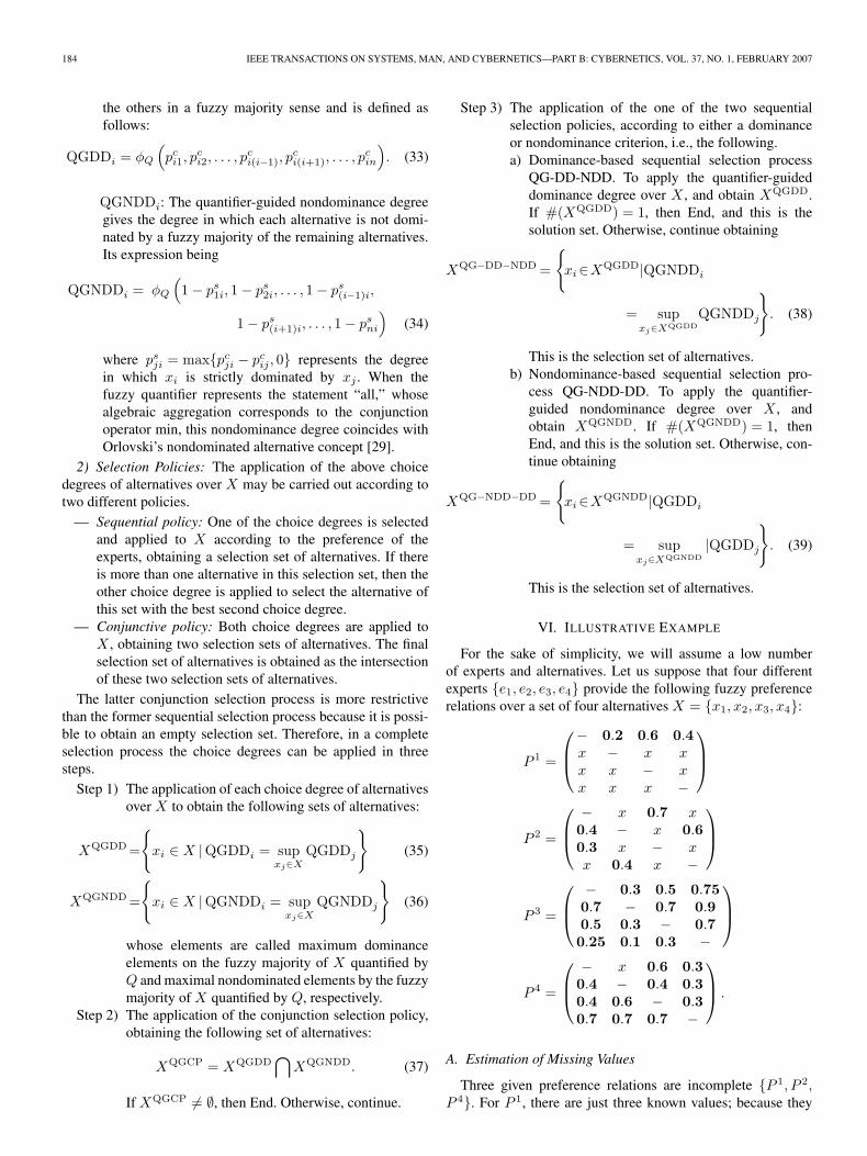
For the sake of simplicity, we will assume a low numberof experts and alternatives. Let us suppose that four differentexperts {e1, e2, e3, e4} provide the following fuzzy preferencerelations over a set of four alternatives X = {x1, x2, x3, x4}:

P 1 =

− 0.2 0.6 0.4x − x xx x − xx x x −

P 2 =

− x 0.7 x0.4 − x 0.60.3 x − xx 0.4 x −

P 3 =

− 0.3 0.5 0.750.7 − 0.7 0.90.5 0.3 − 0.70.25 0.1 0.3 −

P 4 =

− x 0.6 0.30.4 − 0.4 0.30.4 0.6 − 0.30.7 0.7 0.7 −

.

A. Estimation of Missing Values

Three given preference relations are incomplete {P 1, P 2,P 4}. For P 1, there are just three known values; because they


involve all four alternatives, then all the missing values can besuccessfully estimated:

Step 1) The set of elements that can be estimated are

EMV1 = {(2, 3), (2, 4), (3, 2), (3, 4), (4, 2), (4, 3)}} .

After these elements have been estimated, wehave

P 1 =

− 0.2 0.6 0.4x − 0.9 0.7x 0.1 − 0.3x 0.3 0.7 −

.

As an example, to estimate p43, the procedure isas follows:

H1143 = ∅ ⇒ cp1

43 = 0

H1243 = {1} ⇒ cp2

43 = cp1243 = p13 − p14 + 0.5 = 0.7

H2343 = ∅ ⇒ cp3

43 = 0

K =1 ⇒ cp43 =0 + 0.7 + 0

1= 0.7.

Step 2) The set of elements that can be estimated are

EMV1 = {(2, 1), (3, 1), (4, 1)}} .

After these elements have been estimated, wehave the following completed fuzzy preferencerelation:

P 1 =

− 0.2 0.6 0.40.8 − 0.9 0.70.4 0.1 − 0.30.6 0.3 0.7 −

.

As an example, to estimate p41, the procedure isas follows:

H2141 = ∅ ⇒ cp1

41 = 0

H2241 = ∅ ⇒ cp2

41 = 0

H2341 = {2, 3} ⇒ cp23

41 = cp3341 = 0.6⇒ cp3

41 = 0.6

K =1 ⇒ cp41 =0 + 0 + 0.6

1= 0.6.

The corresponding consistency level matrix asso-ciated with the incomplete fuzzy preference relationP 1 is calculated as follows:

EV1 = {(1, 2), (1, 3), (1, 4)}; EV2 = {(1, 2)}EV3 = {(1, 3)}; EV4 = {(1, 4)}CP1 =3/6; CP2 = CP3 = CP4 = 1/6

α12 =α13 = α12 = α12 = 1− 3 + 1− 110

= 0.7.

For p12, we have that there is no intermedi-ate alternative to calculate an estimated value and,consequently, we have

εp12=0⇒ CL112=(1− 0.7) · (1− 0) + 0.7 ·

36 +

16

2≈ 0.53.

The same result is obtained for p13 and p14, i.e.,CL1

13 = CL114 ≈ 0.53. This means that the consis-

tency level for each one of the estimated valuesis also 0.53, as they are calculated as the averageof the consistency values used to estimate them.Consequently, we have

CL1 =

− 0.53 0.53 0.530.53 − 0.53 0.530.53 0.53 − 0.530.53 0.53 0.53 −

.

For P 2, P 3, and P 4, we get

P 2 =

− 0.6 0.7 0.70.4 − 0.6 0.60.3 0.4 − 0.50.3 0.4 0.5 −

CL2 =

− 0.62 0.59 0.670.75 − 0.64 0.590.59 0.67 − 0.620.64 0.59 0.62 −

P 3 =

− 0.3 0.5 0.750.7 − 0.7 0.90.5 0.3 − 0.70.25 0.1 0.3 −

CL3 =

− 0.98 0.98 0.970.98 − 1.0 0.980.98 1.0 − 0.980.97 0.98 0.98 −

P 4 =

− 0.6 0.6 0.30.4 − 0.4 0.30.4 0.6 − 0.30.7 0.7 0.7 −

CL4 =

− 0.93 0.93 0.930.92 − 0.93 0.930.93 0.93 − 0.930.93 0.93 0.93 −

.

As an example of how the iterative estimation pro-cedure has worked over P 4, we show the estimatefor p12, the only missing value in this preferencerelation

H1112 = {3, 4} ⇒ cp31

12 = 0.7 cp4112 = 0.5⇒ cp1

12 = 0.6

H1212 = {3, 4} ⇒ cp32

12 = 0.7 cp4212 = 0.5⇒ cp2

12 = 0.6

H1312 = {3, 4} ⇒ cp33

12 = 0.7 cp4312 = 0.5⇒ cp3

12 = 0.6

cp12 =0.6 + 0.6 + 0.6

3= 0.6.


The following calculations are needed to obtain the consis-tency level CL21.

1) Computation of εp21

H1121 = {3, 4} ⇒ cp31

21 = 0.3 cp4121 = 0.5⇒ εp1

21 = 0.1

H1221 = {3, 4} ⇒ cp32

21 = 0.3 cp4221 = 0.5⇒ εp1

21 = 0.1

H1321 = {3, 4} ⇒ cp33

21 = 0.3 cp4321 = 0.5⇒ εp1

21 = 0.1

εp12 =23· 0.1 + 0.1 + 0.1

3=0.23

.

2) Computation of CP1, CP2, and α21

EV1 = {(1, 3), (1, 4), (2, 1), (3, 1), (4, 1)} ⇒ P1 =56

EV2 = {(2, 1), (2, 3), (2, 4), (3, 2), (4, 2)} ⇒ CP2 =56

EV1 ∩ EV2 = {(2, 1)} ⇒ α21 = 1− 5 + 5− 110

=110

.

3) Computation of CL21

CL21 =(1− 1

10

)·(1− 0.2

3

)+110

·56 +

56

2≈ 0.92.

We should point out that because the third and fourth ex-perts have been very consistent when expressing their pref-erences and have provided an almost complete preferencerelation, the consistency levels for their preference values arevery high.

B. Aggregation Phase

Once the fuzzy preference relations are completed, we ag-gregate them by means of the AC-IOWA operator and usingthe consistency level of the preference values as the order-inducing variable. We make use of the linguistic quantifier“most of,” represented by the RIM quantifier Q(r) = r1/2

(see the Appendix), which applying (30) generates a weight-ing vector of four values to obtain each collective preferencevalue pc

ik.As an example, the collective preference value pc

12 with twodecimal places is obtained as follows:

CL112 = 0.53 CL2

12 = 0.62 CL312 = 0.98 CL4

12 = 0.93

p112 = 0.2 p2

12 = 0.6 p312 = 0.3 p4

12 = 0.6σ(1) = 3 σ(2) = 4 σ(3) = 2 σ(4) = 1

T = CL112 +CL

212 +CL

312 +CL

412

Q(0) = 0 Q

(CL4

12

T

)= 0.57

Q

(CL4

12+CL312

T

)= 0.79 Q

(CL4

12+CL312+CL

212

T

)= 0.91

Q

(CL4

12 +CL312 +CL

212 +CL

112

T

)= Q(1) = 1

w1 = 0.57 w2 = 0.22 w3 = 0.12 w4 = 0.09

pc12 = w1 · p3

12 + w2 · p412 + w3 · p2

12 + w4 · p112

= 0.57 · 0.3 + 0.22 · 0.6 + 0.12 · 0.6 + 0.09 · 0.2= 0.39.

The collective fuzzy preference relation is

P c =

− 0.39 0.55 0.610.6 − 0.64 0.710.45 0.36 − 0.550.39 0.29 0.45 −

.

C. Exploitation Phase

Using again the same fuzzy quantifier “most of,” and (29),we obtain the weighting vector W = (w1, w2, w3)

w1 =Q

(13

)−Q(0) = 0.58− 0 = 0.58

w2 =Q

(23

)−Q

(13

)= 0.82− 0.58 = 0.24

w3 =Q(1)−Q

(23

)= 1− 0.82 = 0.18

and the following quantifier-guided dominance and nondomi-nance degrees of all the alternatives:

x1 x2 x3 x4

QGDDi 0.57 0.67 0.49 0.41QGNDDi 0.96 1.00 0.93 0.81.

Clearly, the maximal sets are

XQGDD = {x2} XQGNDD = {x2}.

Finally, applying the conjunction selection policy, we obtain

XQGCP = XQGDD ∩XQGNDD = {x2}

which means that alternative x2 is the best alternative accordingto “most of” the most consistent experts.

VII. CONCLUSION

We have looked at the issue of GDM problems with theincomplete fuzzy preference relations, and we have presenteda new GDM model based on the AC property to deal withsuch situations. This new model is composed of two phases,the estimation of missing preference values and the selection ofthe best alternatives, both guided by the concept of AC.

To model the estimation phase, we have proposed an iterativeprocedure to estimate missing preference values. We havegiven sufficient conditions to guarantee the direct applicationof our procedure. Our proposal attempts to estimate the missinginformation in an expert’s incomplete fuzzy preference relationusing only the preference values provided by that particularexpert. By doing this, we assure that the reconstruction ofthe incomplete fuzzy preference relation is compatible withthe rest of the information provided by that expert. Becausean important objective in the design of our procedure was tomaintain experts’ consistency levels, the procedure is guided


by the expert’s AC, and this is measured taking into accountonly the available preference values.

Based also on the AC, we have presented a selection processto solve GDM problems with the incomplete fuzzy preferencerelations. To model the selection phase, we have defined a newIOWA operator guided by the AC, the AC-IOWA operator. Thisoperator permits the aggregation of experts’ preferences in acollective fuzzy preference relation and the exploitation of suchcollective relation to achieve the solution set of alternatives ac-cording to the “fuzzy” majority of the most consistent experts’opinions.

In the future, we will address the extension of the manage-ment procedure of incomplete information to the case of lin-guistic preference relations [13], [18], [34] and its applicationto model users’ preferences or desires in different problemslike Internet business [27], technology selection [7], learningevaluation [24], and Web quality evaluation [19].

APPENDIX

FUZZY QUANTIFIERS AND THEIR USE

TO MODEL FUZZY MAJORITY

The majority is traditionally defined as a threshold numberof individuals. Fuzzy majority is a soft majority concept ex-pressed by a fuzzy quantifier, which is manipulated via a fuzzylogic-based calculus of linguistically quantified propositions.Therefore, using fuzzy-majority-guided aggregation operators,we can incorporate the concept of majority into the computationof the solution.

Quantifiers can be used to represent the amount of itemssatisfying a given predicate. Classic logic is restricted to the useof the two quantifiers, there exists and for all, which are closelyrelated, respectively, to the OR and AND connectives. Humandiscourse is much richer and more diverse in its quantifiers,e.g., about five, almost all, a few, many, most of, as many aspossible, nearly half, at least half. In an attempt to bridge thegap between formal systems and natural discourse and, in turn,provide a more flexible knowledge representation tool, Zadehintroduced the concept of fuzzy quantifiers [43].

Zadeh suggested that the semantics of a fuzzy quantifier canbe captured by using fuzzy subsets for its representation. Hedistinguished between two types of fuzzy quantifiers: absoluteand relative. Absolute quantifiers are used to represent amountsthat are absolute in nature such as about two or more thanfive. These absolute linguistic quantifiers are closely relatedto the concept of the count or number of elements. He de-fined these quantifiers as fuzzy subsets of the nonnegative realnumbers, R

+. In this approach, an absolute quantifier can berepresented by a fuzzy subset Q, such that for any r ∈ R

+

the membership degree of r in Q, Q(r), indicates the de-gree in which the amount r is compatible with the quantifierrepresented by Q. Relative quantifiers, such as most, at leasthalf, can be represented by fuzzy subsets of the unit interval[0, 1]. For any r ∈ [0, 1], Q(r) indicates the degree in whichthe proportion r is compatible with the meaning of the quan-tifier it represents. Any quantifier of natural language can berepresented as a relative quantifier or, given the cardinality ofthe elements considered, as an absolute quantifier.

Fig. 2. Examples of relative fuzzy linguistic quantifiers.

A relative quantifier, Q : [0, 1]→ [0, 1], satisfies

Q(0) = 0 ∃r ∈ [0, 1] such that Q(r) = 1.

Yager in [39] distinguishes two categories of these relativequantifiers: RIM quantifiers such as all, most, many, at leastα; and regular decreasing monotone (RDM) quantifiers such asat most one, few, at most α.

A RIM quantifier satisfies

∀a, b if a > b then Q(a) ≥ Q(b).

A widely used membership function for RIM quantifiers is [20]

Q(r) =

0, if r < ar−ab−a , if a ≤ r < b

1, if r ≥ b

(40)

with a, b, r ∈ [0, 1]. Some examples of relative quantifiers areshown in Fig. 2, where the parameters, (a, b) are (0.3, 0.8),(0, 0.5), and (0.5, 1), respectively.

The particular RIM function with parameters (0.3, 0.8) usedto represent the fuzzy linguistic quantifier “most of” when ap-plied with an OWA or IOWA operator associates a low weight-ing value to the most important/consistent experts because itassigns a value of 0 to the first 30% of experts. To overcomethis problem, a different RIM function to represent the fuzzylinguistic quantifier “most of” should be used. To guarantee thatall the important/consistent experts have associated a nonzeroweighting value, and therefore all of them contribute to the finalaggregated value, a strictly increasing RIM function shouldbe used. On the other hand, in order to associate a highweighting value to those values with a high consistency level,a RIM function with a rate of increase in the unit intervalinversely proportional to the value of the variable r seems tobe adequate.

Yager in [39] considers the parameterized family of RIMquantifiers

Q(r) = ra, a ≥ 0and the particular function with a = 2 to represent fuzzy lin-guistic quantifier “most of.” This function is strictly increasingbut, when used with an OWA or IOWA operators, associateshigh weighting values to low consistent values. In order toovercome this drawback, either of the following two approachescould be adopted.

1) The values are ordered using the opposite criteria, i.e., thefirst one being the one with lowest consistency degree.

2) A RIM function with a < 1 is used.


Fig. 3. Relative fuzzy linguistic quantifier “most of.”

We have opted for the second one, and in particular in thispaper, we use RIM function Q(r) = r1/2 given in Fig. 3 torepresent fuzzy linguistic quantifier “most of.”

REFERENCES

[1] F. Chiclana, F. Herrera, and E. Herrera-Viedma, “Integrating three rep-resentation models in fuzzy multipurpose decision making based onfuzzy preference relations,” Fuzzy Sets Syst., vol. 97, no. 1, pp. 33–48,Jul. 1998.

[2] ——, “Integrating multiplicative preference relations in a multipurposedecision-making model based on fuzzy preference relations,” Fuzzy SetsSyst., vol. 122, no. 2, pp. 277–291, Sep. 2001.

[3] ——, “A note on the internal consistency of various preference represen-tations,” Fuzzy Sets Syst., vol. 131, no. 1, pp. 75–78, Oct. 2002.

[4] ——, “Rationality of induced ordered weighted operators based onthe reliability of the source of information in group decision-making,”Kybernetika, vol. 40, no. 1, pp. 121–142, Jan. 2004.

[5] F. Chiclana, F. Herrera, E. Herrera-Viedma, and L. Martínez, “A note onthe reciprocity in the aggregation of fuzzy preference relations using OWAoperators,” Fuzzy Sets Syst., vol. 137, no. 1, pp. 71–83, Jul. 2003.

[6] F. Chiclana, E. Herrera-Viedma, F. Herrera, and S. Alonso, “Inducedordered weighted geometric operators and their use in the aggregationof multiplicative preference relations,” Int. J. Intell. Syst., vol. 19, no. 3,pp. 233–255, Mar. 2004.

[7] A. K. Choudhury, R. Shankar, and M. K. Tiwari, “Consensus-basedintelligent group decision-making model for the selection of advancedtechnology,” Decis. Support Syst. to be published.

[8] T. Evangelos, Multi-Criteria Decision Making Methods: A ComparativeStudy. Dordrecht, The Netherlands: Kluwer, 2000.

[9] Z.-P. Fan, S.-H. Xiao, and G.-H. Hu, “An optimization method for inte-grating two kinds of preference information in group decision-making,”Comput. Ind. Eng., vol. 46, no. 2, pp. 329–335, Apr. 2004.

[10] J. Fodor and M. Roubens, Fuzzy Preference Modelling and MulticriteriaDecision Support. Dordrecht, The Netherlands: Kluwer, 1994.

[11] F. Herrera and E. Herrera-Viedma, “Aggregation operators for linguisticweighted information,” IEEE Trans. Syst., Man, Cybern. A, Syst. Humans,vol. 27, no. 5, pp. 646–656, Sep. 1997.

[12] F. Herrera, E. Herrera-Viedma, and F. Chiclana, “A study of the ori-gin and uses of the ordered weighted geometric operator in multicrite-ria decision making,” Int. J. Intell. Syst., vol. 18, no. 6, pp. 689–707,Jun. 2003.

[13] F. Herrera, E. Herrera-Viedma, and J. L. Verdegay, “A model of consensusin group decision making under linguistic assessments,” Fuzzy Sets Syst.,vol. 78, no. 1, pp. 73–87, Feb. 1996.

[14] ——, “Choice processes for non-homogeneous group decision making inlinguistic setting,” Fuzzy Sets Syst., vol. 94, no. 3, pp. 287–308, Mar. 1998.

[15] F. Herrera, L. Martinez, and P. J. Sánchez, “Managing non-homogeneousinformation in group decision making,” Eur. J. Oper. Res., vol. 166, no. 1,pp. 115–132, Oct. 2005.

[16] E. Herrera-Viedma, F. Herrera, and F. Chiclana, “A consensus model formultiperson decision making with different preference structures,” IEEETrans. Syst., Man, Cybern. A, Syst., Humans, vol. 32, no. 3, pp. 394–402,May 2002.

[17] E. Herrera-Viedma, F. Herrera, F. Chiclana, and M. Luque, “Some issueson consistency of fuzzy preference relations,” Eur. J. Oper. Res., vol. 154,no. 1, pp. 98–109, Apr. 2004.

[18] E. Herrera-Viedma, L. Martinez, F. Mata, and F. Chiclana, “A consensussupport system model for group decision-making problems with multi-granular linguistic preference relations,” IEEE Trans. Fuzzy Syst., vol. 13,no. 5, pp. 644–658, Oct. 2005.

[19] E. Herrera-Viedma, G. Pasi, A. G. López-Herrera, and C. Porcel, “Eval-uating the information quality of Web sites: A qualitative methodologybased on computing with words,” J. Amer. Soc. Inf. Sci. Technol., vol. 57,no. 4, pp. 538–549, Feb. 2006.

[20] J. Kacprzyk, “Group decision making with a fuzzy linguistic majority,”Fuzzy Sets Syst., vol. 18, no. 2, pp. 105–118, Mar. 1986.

[21] S. H. Kim and B. S. Ahn, “Group decision making procedure consideringpreference strength under incomplete information,” Comput. Oper. Res.,vol. 24, no. 12, pp. 1101–1112, Dec. 1997.

[22] ——, “Interactive group decision making procedure under incompleteinformation,” Eur. J. Oper. Res., vol. 116, no. 3, pp. 498–507, Aug. 1999.

[23] S. H. Kim, S. H. Choi, and J. K. Kim, “An interactive procedure formultiple attribute group decision making with incomplete information:Range-based approach,” Eur. J. Oper. Res., vol. 118, no. 1, pp. 139–152,Oct. 1999.

[24] J. Ma and D. Zhou, “Fuzzy set approach to the assessment of student-centered learning,” IEEE Trans. Educ., vol. 43, no. 2, pp. 237–241,May 2000.

[25] G. H. Marakas, Decision Support Systems in the 21th Century, 2nd ed.Upper Saddle River, NJ: Pearson Education, 2003.

[26] H. B. Mitchell and D. D. Estrakh, “A modified OWA operator and itsuse in lossless DPCM image compression,” Int. J. Uncertain., FuzzinessKnowl.-Based Syst., vol. 5, no. 4, pp. 429–436, Aug. 1997.

[27] B. K. Mohanty and B. Bhasker, “Product classification in the Inter-net business—a fuzzy approach,” Decis. Support Syst., vol. 38, no. 4,pp. 611–619, Jan. 2005.

[28] E. A. Ok, “Utility representation of an incomplete preference relation,”J. Econ. Theory, vol. 104, no. 2, pp. 429–449, Jun. 2002.

[29] S. A. Orlovski, “Decision-making with fuzzy preference relations,” FuzzySets Syst., vol. 1, no. 3, pp. 155–167, Jul. 1978.

[30] T. L. Saaty, Fundamentals of Decision Making and Priority Theorywith the AHP. Pittsburg, PA: RWS Publications, 1994.

[31] T. Tanino, “Fuzzy preference orderings in group decision making,” FuzzySets Syst., vol. 12, no. 12, pp. 117–131, Feb. 1984.

[32] ——, “Fuzzy preference relations in group decision making,” in Non-Conventional Preference Relations in Decision Making, J. Kacprzyk andM. Roubens, Eds. Berlin, Germany: Springer-Verlag, 1988, pp. 54–71.

[33] Z. S. Xu, “Goal programming models for obtaining the priority vector ofincomplete fuzzy preference relation,” Int. J. Approx. Reason., vol. 36,no. 3, pp. 261–270, Jul. 2004.

[34] ——, “An approach based on the uncertain LOWG and induced uncertainLOWG operators to group decision making with uncertain multiplica-tive linguistic preference relations,” Decis. Support Syst., vol. 41, no. 2,pp. 488–499, Jan. 2006.

[35] R. R. Yager, “Fuzzy decision making including unequal objectives,”Fuzzy Sets Syst., vol. 1, no. 2, pp. 87–95, Apr. 1978.

[36] ——, “Quantifiers in the formulation of multiple objective decisionfunctions,” Inf. Sci., vol. 31, no. 2, pp. 107–139, Nov. 1983.

[37] ——, “On ordered weighted averaging aggregation operators in multicri-teria decision making,” IEEE Trans. Syst., Man, Cybern., vol. 18, no. 1,pp. 183–190, Jan./Feb. 1988.

[38] ——, “On weighted median aggregation,” Int. J. Uncertain., FuzzinessKnowl.-Based Syst., vol. 2, no. 1, pp. 101–113, Mar. 1994.

[39] ——, “Quantifier guided aggregation using OWA operators,” Int. J. Intell.Syst., vol. 11, no. 1, pp. 49–73, Jan. 1996.

[40] ——, “Induced aggregation operators,” Fuzzy Sets Syst., vol. 137, no. 1,pp. 59–69, Jul. 2003.

[41] R. R. Yager and D. P. Filev, “Operations for granular computing: Mixingwords and numbers,” in Proc. FUZZ-IEEE World Congr. Comput. Intell.,Anchorage, AK, 1998, pp. 123–128.

[42] ——, “Induced ordered weighted averaging operators,” IEEE Trans. Syst.,Man, Cybern. B, Cybern., vol. 29, no. 2, pp. 141–150, Apr. 1999.

[43] L. A. Zadeh, “A computational approach to fuzzy quantifiers in naturallanguages,” Comput. Math. Appl., vol. 9, no. 1, pp. 149–184, 1983.

[44] Q. Zhang, J. C. H. Chen, and P. P. Chong, “Decision consolidation:Criteria weight determination using multiple preference formats,” Decis.Support Syst., vol. 38, no. 2, pp. 247–258, Nov. 2004.

[45] Q. Zhang, J. C. H. Chen, Y.-Q. He, J. Ma, and D.-N. Zhou, “Multi-ple attribute decision making: Approach integrating subjective and ob-jective information,” Int. J. Manuf. Technol. Manage., vol. 5, no. 4,pp. 338–361, 2003.

[46] H.-J. Zimmermann, Fuzzy Set Theory and Its Applications. Dordrecht,The Netherlands: Kluwer, 1991.


Enrique Herrera-Viedma was born in 1969. Hereceived the M.Sc. and Ph.D. degrees in computerscience from the University of Granada, Granada,Spain, in 1993 and 1996, respectively.

Currently, he is a Senior Lecturer of computerscience in the Department of Computer Science andArtificial Intelligence, University of Granada. He hascoedited various journal special issues on Comput-ing with Words and Preference Modeling and SoftComputing in Information Retrieval. His researchinterests include group decision making, decision-

support systems, consensus models, linguistic modeling, aggregation of infor-mation, information retrieval, genetic algorithms, digital libraries, Web qualityevaluation, and recommendation systems.

Francisco Chiclana received the B.Sc. and Ph.D.degrees in mathematics from the University ofGranada, Granada, Spain, in 1989 and 2000, respec-tively.

In August 2003, he left his permanent positionas a Teacher of mathematics in secondary educa-tion in Andalucía, Spain, and joined the Centrefor Computational Intelligence Research Group atDe Montfort University, Leicester, U.K. His re-search interests include fuzzy preference modeling,decision-making problems with heterogeneous fuzzy

information, decision-support systems, the consensus reaching process, ag-gregation of information, modeling situations with missing information, andmodeling variation in automated decision support.

Dr. Chiclana’s thesis “The Integration of Different Fuzzy Preference Struc-tures in Decision Making Problems with Multiple Experts” received the“Outstanding Award for a Ph.D. in Mathematics for the academic year1999/2000” from the University of Granada.

Francisco Herrera received the M.Sc. and Ph.D.degrees in mathematics from the University ofGranada, Granada, Spain, in 1988 and 1991, respec-tively.

He is currently a Professor in the Department ofComputer Science and Artificial Intelligence, Uni-versity of Granada. He has published over 100 papersin international journals, and he is coauthor of thebook Genetic Fuzzy Systems: Evolutionary Tuningand Learning of Fuzzy Knowledge Bases (WorldScientific, 2001). As edited activities, he has coedited

three international books and coedited 15 special issues in international journalson different Soft Computing topics, such as, Preference Modeling, Computingwith Words, Genetic Algorithms, and Genetic Fuzzy Systems. He currentlyserves on the editorial boards of Soft Computing, Mathware and Soft Comput-ing, International Journal of Hybrid Intelligent Systems, and the InternationalJournal of Computational Intelligence Research and Evolutionary Computa-tion. His current research interests include computing with words, preferencemodeling and decision making, data mining and knowledge discovery, geneticalgorithms, and genetic fuzzy systems.

Sergio Alonso was born in Granada, Spain, in 1979.He received the M.Sc. degree in computer sciencefrom the University of Granada, Granada, in 2003.He is currently working toward the Ph.D. degree atthe University of Granada.

His research interests include fuzzy preferencemodeling, modeling missing information situations,consistency properties of preferences, group deci-sion making, decision-support systems, consensusreaching processes, aggregation of information, Webquality evaluation, and recommendation systems. He

was awarded a grant by the Spanish Department for Education and Science toconduct research for a three-month period at the CCI Research Group at DeMontfort University, Leicester, U.K., in 2005.

Group Decision-Making Model With Incomplete Fuzzy Preference Relations Based on Additive Consistency

Documents

Transcript of Group Decision-Making Model With Incomplete Fuzzy Preference Relations Based on Additive Consistency