1 23

Arabian Journal of Geosciences ISSN 1866-7511 Arab J GeosciDOI 10.1007/s12517-012-0700-9

Groundwater resources assessment usingintegrated geophysical techniques in thesouthwestern region of Peninsular Malaysia

Mohamed S. E. Juanah, ShaharinIbrahim, Wan Nor Azmin Sulaiman &Puziah Abdul Latif

1 23

Your article is protected by copyright and all

rights are held exclusively by Saudi Society

for Geosciences. This e-offprint is for personal

use only and shall not be self-archived in

electronic repositories. If you wish to self-

archive your work, please use the accepted

author’s version for posting to your own

website or your institution’s repository. You

may further deposit the accepted author’s

version on a funder’s repository at a funder’s

request, provided it is not made publicly

available until 12 months after publication.

ORIGINAL PAPER

Groundwater resources assessment using integratedgeophysical techniques in the southwestern regionof Peninsular Malaysia

Mohamed S. E. Juanah & Shaharin Ibrahim &

Wan Nor Azmin Sulaiman & Puziah Abdul Latif

Received: 1 June 2012 /Accepted: 23 September 2012# Saudi Society for Geosciences 2012

Abstract Combined geophysical techniques such asmulti-electrode resistivity, induced polarization, andborehole geophysical techniques were carried out onvolcano-sedimentary rocks in the north of Gemas aspart of the groundwater resource’s investigations. Theresult identifies four resistivity units: the tuffaceousmudstone, tuffaceous sandstone, the tuff bed, and theshale layer. Two types of aquifer systems in terms ofstorage were identified within the area: one within afracture system (tuff), which is the leaky area throughwhich vertical flow of groundwater occurs, and an in-tergranular property of the sandy material of the aquiferwhich includes sandstone and tuffaceous sandstone. Theresult also reveals that the aquifer occupies a surfacearea of about 3,250,555 m2 with a mean depth of43.71 m and a net volume of 9.798×107m3. From theapproximate volume of the porous zone (28 %) and thetotal aquifer volume, a usable capacity of (274.339±30.177)×107m3 of water in the study area can be de-duced. This study provides useful information that canbe used to develop a much broader understanding of thenature of groundwater potential in the area and theirrelationship with the local geology.

Keywords Groundwater resources . Electrical resistivity .

Induced polarization . Porosity distribution

Introduction

With Malaysia increasingly becoming an industrialized na-tion, the need for quality water to meet its domestic andindustrial requirements is becoming a major challenge, sincemost of the surface waters are experiencing an increase inpollution and/or contamination due to industrialization andagricultural activities. This has resulted in an increase ingroundwater exploitation as it is often safe from pollution.

The study of groundwater resources in the study area andits surrounding has not been done in detail, and it is amongthe driest areas in Malaysia, recording an average rainfall ofless than 2,000 mm/year and has a history of drought(MINT and JMG 2006). Most of the demand for water inthis area is a result of agricultural activities, mainly paddyplantations. There is also vast increase in demand of watersupply both during the normal and dry seasons because theability to use surface water resources is very minimal.Therefore, the need for quality groundwater to be exploredand to determine the groundwater flow for a database of itsmanagement is vital in assessing the availability of water fordrinking, industrial, and agricultural purposes (Wattanasenand Elming 2008).

Geophysical techniques have been experiencing consid-erable progress in recent years, and their combined applica-tion, together with geological control, is an approach that isgaining widespread acceptance in groundwater exploration.Hence, the need to employ geophysical techniques is vital ingroundwater resource’s mapping as the movement and oc-currence of groundwater are highly localized and unpredict-able, and it has been proven to be the most successful

M. S. E. Juanah (*) : S. Ibrahim :W. N. A. Sulaiman : P. A. LatifFaculty of Environmental Studies, Departmentof Environmental Science, Universiti Putra Malaysia,Serdang, Malaysiae-mail: msejuana@yahoo.co.uk

S. Ibrahime-mail: shaharin@env.upm.edu.my

W. N. A. Sulaimane-mail: wannor@env.upm.edu.my

P. A. Latife-mail: puziah@env.upm.edu.my

Arab J GeosciDOI 10.1007/s12517-012-0700-9

Author's personal copy

techniques. Several integrated geophysical techniques havebeen used for a number of geological and hydrogeologicalpurposes in recent times. Wattanasen and Elming (2008) ap-plied direct and indirect methods of groundwater investigationin southern Sweden using magnetic resonance sounding andvertical electrical sounding; Turesson (2006) carried outground-penetrating radar and resistivity independently to eval-uate their capability to assess water content and porosity forsaturated zone in a sandy section; El Kashouty et al. (2011)used hydrogeophysical techniques to investigate groundwaterpotential in El Bawiti, Northern Bahariya Oasis, WesternDesert Egypt; Marescot et al. (2008) use induced polarization(IP) and resistivity survey to distinguished between low per-meable clay/graphite and permeable water-bearing zone inslope instability studies in Swiss Alps; De Domenico et al.(2006) applied IP and resistivity measurement at archaeologicalsite of Tindary, Italy, and they observed an imperfect agreementof the models.

Hence, a careful appliance or integration of techniques ismost important to become successful technologically, aswell as cost-effectively for any groundwater exploration. Itis an undoubted fact that groundwater cannot be detecteddirectly by any one geophysical method without appropriateknowledge of interpretation and a broader understanding ofthe subsurface hydrogeological condition. Khalil et al.(2012), Van Dam (2010), Soupios et al. (2010), Sinha etal. (2009), Lesmes and Friedman (2005), Yaramanci et al.(2002), and Hubbard and Rubin (2000) emphasize the use oftwo or more complementary geophysical methods to en-hance data interpretation, and according to them, with manyassemblages of geophysical data available, excellent resultswill be produced with significantly better interpretationsthan with a single method. De Domenico et al. (2006), onthe other hand, also state that an integrated approach ofgeophysical techniques is likely to exceed the cost of anysingle method survey; the benefit is so high, such that thecost-to-benefit ratio of the whole operation will be drasti-cally lowered, and this will make the financial effort wellrewarded.

Conventional geophysical methods such as seismic, mag-netics, electrical, and electromagnetic methods have oftenbeen used to map the geometry of aquifers (Wattanasen andElming 2008), particularly for groundwater investigations,geological mapping, contaminant mapping, etc. Thesemethods have been used to estimate location, transmissivity,specific capacity, and other aquifer parameters, despite theambiguity of the interpreted results and also due to limita-tion in each method and the site dependence. However, withthe improvements in geophysical instruments over the years,the development of better methods, such as time domainelectromagnetic (Khalil et al. 2012), transient electromag-netic system (Al-Garni and El-Kaliouby 2011), magneticresonance survey (Perttu et al. 2011), two-dimensional

(2D) multi-electrode resistivity imaging (Ewusi et al.2009), etc., has resulted in the widening of its applications.

The search for groundwater in the study area is a relevantapplied research issue that requires study. It is analternative thatshould be extensively explored and protected so that it can befully utilized when the region is facing a crisis or critical situa-tion of water stress. Hence, this study aims to develop a muchbroader understandingof thenatureof groundwater potential inthe study area and its relations with the local geology and canalso be used to assess the potential of groundwater for thepresent and future based on geophysical information.

The study area

The study area is in the north of Gemas, Negri Sembilan,located between Kampung Londah and Kampung UluLadang (Fig. 1a) with Utm coordinates 292445.3 N,509656.3 E, and 289613.2 N, 511568.6E covering an areaof about 5,419,661 m2. Both Kg Londah and Kg UluLadang are 6–8 km respectively from Gemas which is about165 km from Kuala Lumpur, the capital city. Gemas is amajor transit point for trains moving from the west and eastcoast of Peninsular Malaysia.

The study area is relatively flat with elevation rangingbetween 40 and 70 m above mean sea level. The naturalvegetation within the study area was once an aesthetic rainforest which has been destroyed by man as a result ofagricultural activities. It is mainly rural, and the inhabitantsare farmers who are involved in paddy plantations andperennial crops such as rubber and oil palm plantations. Itis drained in the northwest by Sungai Muar, which forms acontinuous boundary of water around the project area to-wards which a myriad of drainage system flows and in thesouth–southwest is drained by Sungai Gemenche.

The climate of the study area is tropical with relativehumidity of 95 %, and the temperature ranges from 20 °C to30 °C on an average throughout the year. It is characterized bythe northeast and southwesterly monsoons. The northeastmonsoon blows from October to March and forms the wetseason that is responsible for the heavy rainfalls while thesouthwest monsoon occurs between May and September,which is the period of the dry season. The study area is amongthe driest areas in Malaysia, recording an average rainfall ofless than 2,000 mm/year, which is less than the mean averagerainfall of 4,000 mm/year for Malaysia.

Geology of the study area

Understanding the geology of the area is an important aspectin the petrophysical interpretation since different rock forma-tions exist within the area, and each of these formationsgenerally has different petrophysical properties which willinfluence the hydraulic behavior of the studied aquifer system.

Arab J Geosci

Author's personal copy

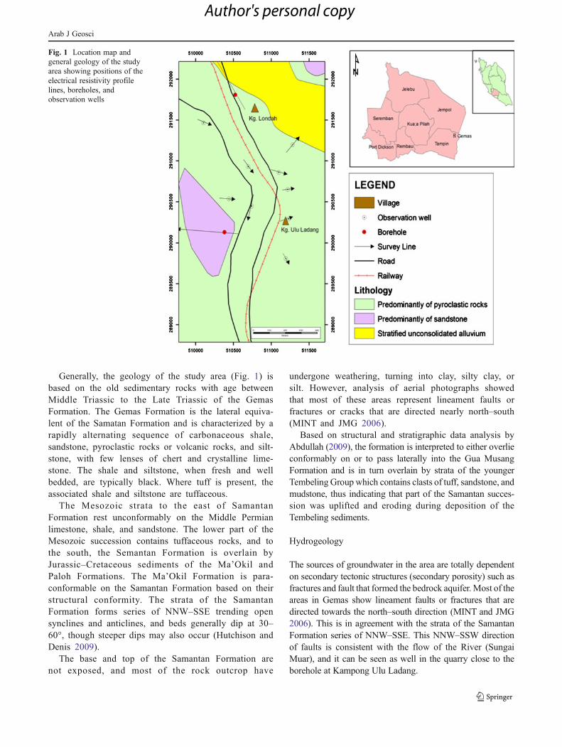
Generally, the geology of the study area (Fig. 1) isbased on the old sedimentary rocks with age betweenMiddle Triassic to the Late Triassic of the GemasFormation. The Gemas Formation is the lateral equiva-lent of the Samatan Formation and is characterized by arapidly alternating sequence of carbonaceous shale,sandstone, pyroclastic rocks or volcanic rocks, and silt-stone, with few lenses of chert and crystalline lime-stone. The shale and siltstone, when fresh and wellbedded, are typically black. Where tuff is present, theassociated shale and siltstone are tuffaceous.

The Mesozoic strata to the east of SamantanFormation rest unconformably on the Middle Permianlimestone, shale, and sandstone. The lower part of theMesozoic succession contains tuffaceous rocks, and tothe south, the Semantan Formation is overlain byJurassic–Cretaceous sediments of the Ma’Okil andPaloh Formations. The Ma’Okil Formation is para-conformable on the Samantan Formation based on theirstructural conformity. The strata of the SamantanFormation forms series of NNW–SSE trending opensynclines and anticlines, and beds generally dip at 30–60°, though steeper dips may also occur (Hutchison andDenis 2009).

The base and top of the Samantan Formation arenot exposed, and most of the rock outcrop have

undergone weathering, turning into clay, silty clay, orsilt. However, analysis of aerial photographs showedthat most of these areas represent lineament faults orfractures or cracks that are directed nearly north–south(MINT and JMG 2006).

Based on structural and stratigraphic data analysis byAbdullah (2009), the formation is interpreted to either overlieconformably on or to pass laterally into the Gua MusangFormation and is in turn overlain by strata of the youngerTembeling Group which contains clasts of tuff, sandstone, andmudstone, thus indicating that part of the Samantan succes-sion was uplifted and eroding during deposition of theTembeling sediments.

Hydrogeology

The sources of groundwater in the area are totally dependenton secondary tectonic structures (secondary porosity) such asfractures and fault that formed the bedrock aquifer. Most of theareas in Gemas show lineament faults or fractures that aredirected towards the north–south direction (MINT and JMG2006). This is in agreement with the strata of the SamantanFormation series of NNW–SSE. This NNW–SSW directionof faults is consistent with the flow of the River (SungaiMuar), and it can be seen as well in the quarry close to theborehole at Kampong Ulu Ladang.

Fig. 1 Location map andgeneral geology of the studyarea showing positions of theelectrical resistivity profilelines, boreholes, andobservation wells

Arab J Geosci

Author's personal copy

Materials and methods

Field survey method

Electrical resistivity technique is a well-established tech-nique for both 2D and three-dimensional (3D) subsurfaceelectrical imaging. The measurements are normally carriedout using computer-controlled system with a large numberof electrodes laid out along straight lines with constantelectrode spacing (Metwaly et al. 2010; Kemna et al. 2002).

In the present work, eleven 2D multi-electrode resistivitysurvey lines (as shown in Table 1 and Fig. 1) were carriedout employing 40–80 electrodes connected to themicroprocessor-driven resistivity meter functional with theWenner configuration. The Wenner configuration was usedbecause it has the strongest signal strength and is good inresolving vertical changes, i.e., horizontal structures (Loke2011). The resistivity data from the profile were invertedusing the RES2DINV to obtain the true 2D resistivity im-age. The ABEM Terrameter SAS 1000/4000, whichemploys the static Lund automatic resistivity imaging sys-tems suitable for high-resolution 2D resistivity surveys andprovides detailed information both laterally and verticallyalong the profile to investigate complex geological struc-tures, was used (Kirsch and Yaramanci 2009). The geophys-ical measurements were designed in such a way that theywere as close as possible to the existing boreholes, in orderto use the latter for calibration purposes.

The process involved positioning electrodes with equalspacing along the profile. A multi-core cable with equaldistant “takeout” for connecting the electrodes was placedalong the profile, and the jumper was used to connect theelectrodes to the takeout. Data acquisition began when thecables were connected to the switching box, and the elec-trode contacts were checked to make sure the electrodesmake good contact (best in quality) (Soupios et al. 2007)with the ground in order to portray the actual resistance ofthe ground. The measurements were controlled by themicroprocessor-driven resistivity meter connected to a lap-top (Kirsch and Yaramanci 2009).

Induced polarization

The induced polarization technique is based on the sameprinciples as the electrical resistivity methods and was car-ried out immediately after the electrical resistivity surveyusing the same setup and electrode arrangements. The maindifference is that an alternating current in the form of asquare wave is injected into the ground instead of DCcurrent, and the transient decay of the applied voltage isrecorded when the transmitter is switched off. Thus, byintegrating the area under the voltage decay curve, thechargeability of the geological formation could be evaluated(Dahlin et al. 2002).

Borehole geophysics

Borehole logging was carried out in an uncased boreholeusing the Mount Sopris portable matrix v.8 logger instru-ment that consisted of 2PGA-1000 Gamma probe and2PFA-1000 poly-fluid resistivity and temperature probe.The borehole measurement is made by lowering the probeinto the borehole with an average speed of 3 m/min andelectrically transmitting data in the form of digital signals tothe surface, and these data are then recorded as a function ofdepth or distance along the borehole. These measurementsare related to the physicochemical properties of the rocksurrounding the boreholes and the properties of the fluidsaturating the pore spaces in the formation.

Laboratory method

In order to quantitatively assess the full potential of anaquifer using geophysical techniques, knowledge about therelationship between the petrophysical properties of the rockformation and hydrogeological characteristics is very im-portant. Understanding this relationship will enable us todetermine properties such as porosity, cementation, density,particle size distribution, clay content, pore water saturation,the quality of pore water, formation factor, etc., as theseproperties are known to affect geophysical measurements

Table 1 Summary of geophysical survey

Survey line Datesurveyed

System used Surveycharacteristics

Lines KGL 001 October2010

ABEMSAS4000

Wenner array

α010.0 m

e040

d0120 m

Line KUL 002 October2010

ABEMSAS4000

Wenner array

α010 m

e040

d0120 m

Lines KUL 003and KUL 004

February2011

ABEMSAS4000

Wenner array

α02.0 m

e080

d024 m

Lines KGL 005,KUL 006, KGL 007,KGL 008, KUL 009,KUL 010, KGL 011

April 2011 ABEMSAS4000

Wenner array

α05.0 m

e040

d028.7 m

Where α is the electrode spacing, e is the electrode spacing, and d is theexpected depth

Arab J Geosci

Author's personal copy

(Taheri Tizro et al. 2012; Mele et al. 2012; Niwas et al.2011; Soupios et al. 2007). These relationships can then beused for the calibration of the electrical resistivity surveyand the geophysical logs response of the logging suite.According to Batte et al. (2010), for any geophysical tech-nique to be successful, calibration of geophysical data withhydrogeological and geological ground truth information isimportant. Furthermore, the use of field measurement to bevalidated by laboratory measurement according to Giao etal. (2003) increases credibility and effectiveness of themethod.

As a result of this, a number of laboratory measurementsusing British Standard Guide, BS 1377–2: 2001 (Cavelieri2001), and American Petroleum Institute guidelines(American Petroleum Institute 1998) were carried out on asuite of near-subsurface soil samples and rock samples todetermine the influence of various factors such as effectiveporosity, soil and rock resistivity, and apparent formationfactor under varying conditions. The resistivities of differentrocks type were determined using the 4284A precisioninductance, conductance, and resistance (LCR) meter withan Angilent 16451 B dielectric material test fixture.

Results and discussion

Borehole geophysical log

The geological borehole log information, together with thenatural gamma ray, fluid resistivity, temperature log, andwater level measurements at the two borehole locationswere used in the interpretations of geophysical result.Lithology profile of each of the two boreholes was basedon natural gamma ray and the local borehole geologicalcross-section while the hydrogeological conditions underambient conditions were determined using fluid resistivityand temperature logs. Detailed studies of the natural gammaand fluid column (temperature and fluid conductivity) havebeen carried out, and the utilization of these logs (particu-larly the natural gamma logs) has enabled the correlation ofthe geophysical logs with the lithostratigraphic units withinthe study area.

The geological borehole description was matched withthe electrical resistivity image at the borehole location, andfrom comparison, the resistivity of each individual type oflithology can be inferred.

In the natural gamma correlation carried out in the twoboreholes, the presence of distinctive marker such as thefractures and with the presence of high natural gammaanomaly associated with shale can be used in defining thelithostratigraphic position of the beds penetrated by theboreholes, as shown below in Fig. 2a, b. Hence, the pres-ence of shale and fracture (due to the possible presence of

clay in the fractures) was detected by the natural gamma ray.The fracture point on the gamma ray log which coincideswith the fluid log is suggestive of the fluid entering (waterinflows) point between the shale and tuff zone.

From the fluid conductivity and temperature log mea-surement, an abrupt shift at 1.2 and at 32.5 m was observedat the conductivity and temperature log in Fig. 2a. Also atFig. 2b, an abrupt shift at 2.4 and 45.5 m was observed atthe conductivity and temperature logs. These abrupt shiftswere confirmed from the water level meter as the waterlevel.

Figure 2a, b shows correlation between the natural gam-ma ray, temperature, fluid resistivity logs, and the lithologicunits of Kampung Londah and Kampung Ulu Ladang.

Electrical resistivity and induced polarization image

Selective 2D inversions of the electrical resistivity andchargeability of the 11 profile lines are shown in Figs. 3,4, 5, and 6; these figures represent the characteristic featuresof the geology and hydrogeology of the study area.

The images were obtained by the end of five iterations.Most of the resistivity sections have an root mean square(RMS) error of less than 8 % with only two having RMSerrors of 11.8 % and 17.2 %, respectively. This high RMSerror is because of high contact resistance of certain electro-des that causes the current penetration to be impeded. Theoverall resistivity range in the images is 10–2,500 ohmmwith most of the multi-electrode resistivity imaging domi-nated by high resistivity (>100 ohmm), although severalimages have low resistivity zones (<100 ohmm).

The IP soundings were carried out simultaneously along-side the resistivity in order to be correlated with the electri-cal resistivity data for the delineation of the groundwateraquifer zone. The interpretation of the IP sounding curvesshows large variations in the chargeability values rangingfrom 0 to 100 ms. The chargeability parameters used in thedelineation of the aquifer are complex and are based on theresistivity result.

The result of the profile KGL 001 was obtained withRMS error of 5.2 % after five iterations. It is located inKampung Londah at about 250 m parallel to the train track.The subsurface resistivity distribution of the profile isshown in Fig. 3a.

Three distinct resistivity zones along the profile can beobserved. At the first layer, an intermediate resistivity(>100 ohmm) can be observed at the top and bottom layersbetween 70 to 190 m along the survey line for a depth ofapproximately 25 m and from 450 to 630 m for a depth ofabout 10 m, respectively. These areas are likely to be dryweathered tuff. Another intermediate resistivity layerextends between the positions of 270 m to 530 m for adepth of approximately 100 m forming a doom shape

Arab J Geosci

Author's personal copy

layering. From borehole investigation, this zone is likely tobe tuff with quartzite. This zone could be the leaky layer asit is associated with fractures through which the localgroundwater systems are connected (Furi et al. 2011).

The second layer has a resistivity between 80 and 90 ohmm and can be observed as a thin layer interbedded with thetuff zone. Results from borehole log shows that this zone islikely to be shale.

The third layer is a saturated zone, and from field obser-vation, the layer at the position between 640 and 800 malong the survey line is observed as very saturated weath-ered soft clay. This zone may probably be the weatheringproduct of tuff. Another saturated zone from field observa-tion is between 200 and 450 m along the profile line.

The high chargeability zone (M>10 ms) that correspondswith the doom shape structure of the intermediate resistivityzone (100–400 ohmm) is probably indicative of tuff while theresistivity of the saturated zone between 160 and 350 m alongthe survey line with depth exceeding 35 m corresponds to thetuffaceous sandstone of high chargeability. The low resistivityzone between 580 and 660 m for a depth of 60 m correspondsto high chargeability zone of possibly tuffaceous sandstone. In

addition, the low resistivity zone between 280 to 360 m alongthe profile line corresponds to low chargeability (M<1 ms).The resistivity pseudo-section shows geophysical unit (prob-ably shale) of low resistivity (<100 ohmm) that corresponds tolower chargeability (M<5 ms) as shown in Fig. 2d.

The potential zones for groundwater resources definedalong the survey line are mainly in three locations as indi-cated by the circles. Though these layers are continuous,preference should be given to the positions already selected.From the record of water level meter, fluid resistivity, andtemperature logs of the borehole, these areas are likely to beassociated with groundwater.

Additionally, the significant correlation of low resistivitywith low chargeability (Fig. 2a) is indicative of groundwa-ter. The zones of low resistivity are located at a depthexceeding 2.5 m; hence, the expected groundwater potentiallayer is located at a depth of more than 20–60 m from thesurface and in some cases can reach up to a depth of 80 m.

The profile KGL 002 is located at Kampung Ulu Ladangwith a survey line of 800 m. A borehole is located at 610 malong the survey line. The subsurface resistivity and charge-ability distribution of the area is shown in Fig. 2c, d with an

Fig. 2 a, b Shows correlation between the natural gamma ray, temperature, fluid resistivity logs, and the lithologic units of Kampung Londah andKampung Ulu Ladang

Arab J Geosci

Author's personal copy

Fig. 3 Showing 2D pseudo-section inverse model and chargeability for KGL 001 and KGL 002

Arab J Geosci

Author's personal copy

Fig. 4 Showing 2D pseudo-section inverse model and chargeability for KGL 003 and KGL 004

Arab J Geosci

Author's personal copy

RMS error of 17.5 % for resistivity and 14.1 % for charge-ability after five iterations.

Two main resistivity zones can be identified from thisprofile. A high resistivity zone (600–2,500 ohmm) along the

Fig. 5 2D pseudo-section inverse model and chargeability for KGL 005 and KGL 006

Arab J Geosci

Author's personal copy

profile from 20 to 590 m can be seen at the top part of theimage for a varying depth of up to 30 m. Based on infor-mation extracted from geological map, borehole log, andfield observation; this zone is found to be sandstone. Alsobased on borehole information, a high resistivity zone from

260 to 360 m for a depth of 40 m is probably highlyfractured tuffaceous sandstone. East of this zone between450 and 520 m along the profile line from the surface is adome-shaped structure that extends up to a depth of about50 m. This zone is probably sandstone interbedded with tuff.

Fig. 6 2D pseudo-section inverse model and chargeability for KGL 007 and KGL 008

Arab J Geosci

Author's personal copy

The second zone from 120 to 800 m is an intermediateresistivity zone of tuff interbedded with thin shale layers.From the borehole log information, the presence of fracturesand high natural gamma signals is observed at this point.

Possible lateral change in facies can be observed in theprofile from 190 to 520 m for a varying depth of up to120 m, in which tuff interbedded with quartzite (tuffaceoussandstone) can be observed at one end in the east and adome-shaped structure of possibly massive sandstone that isnot fractured or consists of more quartzitic content of thesediment or material, observed in the west.

The potential zone for groundwater resources definedalong the survey line can be seen in four areas. This resis-tivity zone corresponds to the borehole log informationbased on fluid conductivity, temperature, and the charge-ability values. The zones of low resistivity are located at adepth exceeding 16 m. Therefore, the expected potentiallayer is located at a depth of more than 16–40 m from thesurface and in some cases can reach up to a depth of 120 m.

The profile KGL 003 displays similar features with pro-file KGL 001, both in geometry and in subsurface resistivitydistribution with an RMS error of 6.7 % and chargeability of14.9 % after five iterations as shown in Fig. 4a, b. This areais located about 500 m south of KGL001.

Three distinct resistivity zones can be observed in the profile,and the profile length is 160m. The first layer in thewestern partof the survey line has high resistivity (>300 ohmm) between 18and 42 m along the profile with an approximate depth of 10 mand at a depth greater 20 m. Field observation indicated that thiszone is weathered sandstone. The second layer has low resistiv-ity (80–90 ohmm) and can be seen forming thin layering withan intermediate resistivity zone. This zone is likely to be shale.While the third layer has intermediate resistivity (>100 ohmm)and extends between 62 and 104mwith an approximate verticalextension of 16 m, forming a dome-shaped structure. This zonecan also be seen on the east end and extends from 126 to 138 mfor an approximate depth of 11 m.

High chargeability zone (M>10 ms) corresponds to thedome-shaped structure of the intermediate resistivity (100–400 ohmm), and this is probably indicative of tuff andtuffaceous sandstone while the resistivity of the saturatedzone between 36 and 128 m along the survey line with depthexceeding 7 m corresponds to the tuffaceous sandstone,some with high chargeability.

The potential zone for groundwater resources definedalong the survey lines is in two locations at a depth of morethan 6–13 m from the surface, though it can reach a depth ofup to 24 m. This is in correlation with the geophysical unitof low resistivity (<100 ohmm) and low chargeability (M<5 ms) of the profile.

Profile KGL 004 is located in a rubber plantation at KgUlu Ladang. The line length is 160 at 2 m electrode spacingand an approximate depth of 24 m. The subsurface electrical

resistivity distribution with 5.8 % and 3.2 % chargeabilityrespectively after five iterations, as shown on Fig. 4c, d.

A thin layering of tuff can be identified across the profilefrom 50 to 148 m for an approximate depth of 2 m. Belowthis zone is a highly fractured resistivity zone (>1,000 ohmm), i.e., zones of high resistivity with a pinch out zone oflow resistivity in between which indicates that it has rela-tively more fissures that cause the resistivity to be lowerthan the rest. This zone can be seen from the surface of theprofile up to a depth of 9 m from 2 to 34 m and increases inintensity from tuffaceous sandstone at the bottom to weath-ered sandstone at the top. This zone from chargeabilityimage is highly saturated with groundwater.

Potential groundwater resources can be identified at thetuffaceous sandstone (98–114 m from the surface up to avertical depth of 12 m) and at the low resistivity zones(<100 ohmm) from 32 to 64 m and 94 to 104 m along theprofile, and these layers correspond to high chargeability(>10 ms) of tuffaceous sandstone as shown in Fig. 4d.

The profile KGL 005 is located in the oil palm farm in KgLondah. The length of the line is 200 m and an electrodespacing of 5 m with an approximate depth of 30 m. Thesubsurface resistivity distribution with RMS error of 2.5 %and 2.7 % chargeability after five iterations are shown onFig. 5a and b, respectively.

A high resistivity zone (>100 ohmm) can be seen runninghorizontally across the profile between 7 and 35 m and be-tween 80 and 170 m for a vertical depth of about 10 m. Fromfield investigation, this zone is the red tuffaceous mud stone.Below this region is an intermediate resistivity zone (100–400 ohmm), and this zone is the tuff bed. A saturated zonewhich is the dominant zone in the image is interbedded withthin layering of shale and extends vertically downwards for anapproximate depth of about 20 m.Within this zone, from boththe resistivity and chargeability image, is a possible fracturetuff saturated with groundwater. Two zones of potentialgroundwater resources were identified from the low resistivityzones, and these areas correlate with low chargeability zones(<1 ms). The zones of low resistivity are located at a depthexceeding 6 m. Therefore, the expected potential layer islocated at a depth of more than 6–30 m from the surface.

The profile KGL 006 is located at a road junction inKampung Londah leading to Pasir Besar. The subsurfaceresistivity distribution with RMS error 3.3 % and 4.8 %chargeability respectively after five iterations are shown inFig. 5c, d. This profile line is about 1–2 m away from astream and runs parallel to it for almost 200 m.

An intermediate resistivity zone (100–300 ohmm) can beseen between 150 and 190 m along the profile for a verticaldepth of about 10 m. The saturated zone which is the dominantzone in the image extends vertically for an approximate depthof up to 30 m. Zones of potential groundwater resources wereidentified from the low resistivity zones, and these areas

Arab J Geosci

Author's personal copy

correlate with high chargeability zones (M>10 ms) of thetuffaceous sandstone interbedded with tuff. The zones of lowresistivity are located at a depth exceeding 2 m. Therefore, theexpected potential layer is located at a depth of more than 2–25 m from the surface and can reach up to depth of 30 m.

The profile KGL 007 runs parallel to KGL 002. The profileline is 200 m with electrode spacing of 5 m. The subsurfaceresistivity distributionwith RMS error 3.3% and chargeability1.5 % respectively after five iterations are shown on Fig. 6a, b.

Two main resistivity zones can be identified. A high resis-tivity zone (100–600 ohmm) can be seen at the surface from 5to 195 m up to a depth of 8 m; this zone is interpreted as thehighly fractured tuffaceous mudstone. An intermediate resistiv-ity zone (100–500 ohmm), possibly tuff can be observed from adepth of about 10 up to 30 m along the profile line (10–165 m).A possible fracture exists in this zone and based on correlationwith the low chargeability zone (M>1 ms); the material presentin the fracture is possibly clay. Two low-resistivity zones(<100 ohmm) can also be seen on the profile between 35 and75 m from the surface up to a depth of 28 m and between 105and 135 m from the surface to a depth of 28 m. These low-resistivity zones (<80 ohmm) are interbedded with thin shalelayer (80–90 ohmm) and correlates with low chargeability asshown in Fig. 6a, b. This correlation is indicative of potentialgroundwater resources. The zones of low resistivity are locatedat a depth exceeding 10 m. Hence, the expected potential layeris located at a depth of more than 10–30 m from the surface.

The profile KGL 008 is located on the main road leadingto Kampung Ulu Ladang with a survey line of 200 m andelectrode spacing of 5 m. The subsurface resistivity andchargeability distribution with RMS error 6.8 % and 8.2 %respectively after five iterations are shown on Fig. 6c, d.

The saturated zone (<100 ohmm) is the dominant zone inthe image. They are observed from a very shallow depth of>6 m up to a depth of 28 m with a thin shale layering asobserved from borehole logs in Kg Londah and Kg UluLadang. These low-resistivity zones are associated withgroundwater potentials and correlate well with the low char-geability zones. An intermediate resistivity (100–300 ohmm)

layer, possibly tuff, can be observed across the top layer of theprofile line from 0–85 and 110–200m. Another resistivity zone(400–600 ohmm) from 85 to 110 m extends down to about8m. This zone is slightly fractured and is likely to be tuffaceoussandstone (Table 2).

Porosity distribution and quantitative estimationof groundwater resources

The results obtained from the inversion of the multi-electroderesistivity, borehole logs, and laboratory techniques are usefulin estimating groundwater resources and defining the subsur-face porosity distribution. Understanding the hydrogeologicalproperties of the formation is very important in determiningporosity distribution of the aquifer. In order to achieve this, alaboratory-established equation (Eq. 2) obtained by fitting acurve-fit regression (Fig. 7) of the apparent formation factor(F) and fractional porosity (ϕ) of the soil and rock sampleswhich is the common form of the Archie equation, Fα0a ϕ

−m,

were used, where α and m are constant and Fα is the apparentformation factor which is given as:

Fa ¼ ρoρw

ð1Þ

Fig. 7 Relationship between apparent formation factor and fractionalporosity

Table 2 Lithology, resistivity, and chargeability range for obtaining potential groundwater in Kg Londah and Kg Ulu Ladang

Lithological unit(Rock type)

Nature/characteristics Resistivity range,ohmm

Chargeability range,ms

Hydrological significance(potential for obtaininggroundwater)

Tuffaceous mudstone Weathered/fractured/cracks

900–2,500 25–60 Poor–moderate groundwaterpotential

Shale Contact with tuff/fractured

80–90 1–5 Moderate–good potential

Tuff Fractured/fissure 100–400 5–25 Good groundwater potential

Tuffaceous sandstone (tuff withquartzite)

Fractured/fissure 500–1,200 25–80 Very good groundwater potential

Sandstone Weathered/fractured/massive

2000–2500 80–100 Excellent groundwater potential

Arab J Geosci

Author's personal copy

Where ρo is the bulk resistivity obtained from the rockand soil samples and ρw is the measured fluid resistivityobtained from the borehole and observation wells.

The power regression obtained from the relationshipbetween apparent formation factor and fractional porosityof the integrated soil and rock samples after taking accountof the clay effect is given by the equation:

Fa ¼ 0:8017f�1:805 ð2Þ

The R200.8843 and standard error estimated of 0.207indicate that 88 % of the total variations in the formationis explained or accounted for by the power fitted regressionequation, Fα00.8017ϕ

−1.805.This equation is then applied to the field resistivity data

to calculate the subsurface porosity distribution of the satu-rated formation (Eq. 3) as shown in column 8 of Table 3.Consequently, understanding the bulk resistivity of the for-mation is very important. The bulk resistivity which is thetrue resistivity is obtained from the inversion of the apparentresistivity of the field data using RES2DINV as shown inFigs. 3, 4, 5, and 6. The RES2DINV is electrical resistivitysoftware used in inverting apparent resistivity of field datato obtain the true resistivity and true depth of the resistivityimage. Thus, as a result of the inversion of the field data, thetrue resistivity, true depth, and the x-position were saved inXYZ format. The calculated true resistivity or bulk resistiv-ity is then divided by the formation water resistivity which isobtained from in situ electrical conductivity measurementfrom the boreholes and observation wells along which thesurvey lines were run to obtain the resistivity formationfactor.

From the information obtained from the subsurface elec-trical resistivity, borehole log data, and the water-bearingzone, the porosity distributions of the subsurface were de-termined from Eq. 3 (Soupios et al. 2007).

∅ ¼ e1mlnðaÞþ 1

mlnð 1FaÞ ð3Þ

The inferred aquifer thickness data was used to determinethe surface area and volume as occupied by pores in thesubsurface using Surfer 9 software (Golden Software Inc.2010). Surfer is a software package used in transformingXYZ data to create contour maps, 3D surface maps(Fig. 8a), shaded relief maps, base maps, etc. It is also usedin the calculations of cross-sections, areas, and volumes. Thebedrock elevation, aquifer thickness, the north of referencecoordinates, and east of reference coordinate were determinedfor each of the data points of the electrical resistivity imagingline. The “easting’s” of each line was considered the X-axis,the “northings” as the Y-axis and the contour, and/or theaquifer thickness elevation considered as Z-axis.

Hence, the volume of the aquifer was obtained from theaquifer elevation thickness data (Fig. 8b). From the appli-cation of Surfer, the total volume of the aquifer is9.7978332×107m3. Mathematically, the usable volume ca-pacity or the theoretical storage capacity was calculatedfrom Eq. 4, (George et al. 2011).

V ¼ VTΘ ð4Þ

Where V is the theoretical usable volume or maxi-mum storage (cubic meters); VT is the total volume ofthe aquifer (9. 7978332×107 m3) calculated fromSurfer; and Θ is the average porosity of the aquiferwhich is 28 %.

However, in order to account for the error in the volume,and based upon Eq. 4, the fractional volume error,

ΔV=V ¼ ΔL=LþΔW=W þΔD=DþΔΘ=Θ ð5ÞWhere ΔV is the error in volume V; ΔL is the error in

length L;ΔW is an error in width w;ΔD is the error in depth

Table 3 Showing porosity distribution of the study area

Location Bulk resistivity, Ωm Aquifer resistivity, Ωm Aquifer thickness, m Apparent formation factor (Fα) a m Porosity (∅)

KGL 001 107.74 34.03 60 3.17 0.80 1.81 0.28

KGL 002 431.33 48 50 8.99 0.80 1.81 0.26

KGL 003 124.27 40.11 17 3.10 0.80 1.81 0.33

KGL 004 596.94 39.01 13 15.30 0.80 1.81 0.20

KGL 005 261.57 30.18 15 8.67 0.80 1.81 0.27

KGL 006 245.21 30.18 23 8.12 0.80 1.81 0.28

KGL 007 158.83 35.61 22 4.46 0.80 1.81 0.39

KGL 008 115.80 28.59 24 4.05 0.80 1.81 0.41

KGL 009 379.01 49.54 16 7.65 0.80 1.81 0.29

KGL 010 797.81 39.5 12 20.20 0.80 1.81 0.17

KGL 011 116.85 22.78 20 5.13 0.80 1.81 0.36

Arab J Geosci

Author's personal copy

d (0.1 m3); andΔΘ is the error in porosity (0.01 %).ΔL andΔw are almost negligible.

Hence,

ΔV=V ¼ 0þ 0þ 0:1þ 0:01ΔV ¼ V 0:11ð Þ ¼ 274:339� 107ð Þ � 0:11ð ÞΔV ¼ 30:177� 107

Thus, from the approximate volume of the porous zonewhich is 28 % of the total aquifer volume, we can concludethat there exist (274.339±30.177)×107m3 or (300±30)×107m3 of water within the study area.

Conclusion

In quantifying groundwater potential in the area, hydro-geological properties of the different rock types such astuffaceous mudstone, shale, the fractured tuff and tuffa-ceous sandstone, the lithological contacts, and fracturingof the various lithologies were obtained from the bore-hole geophysical logs, the electrical resistivity, and in-duced polarization. This information was used todetermine potential groundwater zones, and the inducedpolarization technique was used to distinguish betweenclay and groundwater.

Five main lithologies, tuffaceous mudstone, tuff, tuffwith quartzite (tuffaceous sandstone), sandstone, andshale, were identified based on-field investigation,

borehole logs, electrical resistivity, laboratory method,and induced polarization values (Table 1). The tuffa-ceous sandstone was differentiated based on the highresistivity and chargeability values associated with sand-stone and also through the borehole logs while the highresistivity values associated with tuffaceous mudstonewas based on laboratory analysis and electrical resistiv-ity of the rocks. The resistivity of tuff zone was differ-entiated based on the borehole information and alsobecause it is the dominant rock type in the area. Theshale layer was differentiated based on borehole log,electrical resistivity, and induced polarization.

The resistivity layers in Kg Londah and Kg Ulu Ladangcan be categorized into four resistivity layer units. The firstlayer, tuffaceous mudstone, which is a semi-confined layer,has high resistivity values (800–2,500 Ωm) and can befound at the top. This zone ranges between 0 and 6 m andin some cases can reach up to a depth of 15 m from thesurface.

The second resistivity layer, tuffaceous sandstone (tuffwith quartzite), has moderate to high resistivity of 500–1,200 ohm and is normally found interbedded with the tuff.From borehole log, this zone is highly fractured and, hence,a good groundwater potential zone. Where the sandstone isnot interbedded with tuff, it may be weathered and probablymassive (not fractured or more quartzitic content of thesediment or material) with resistivity between 2,000 and2,500 ohm.

Fig. 8 a Three-dimensionalcontour map of the study areashowing surface elevation andborehole location. b Three-dimensional map showing thespatial distribution of the aqui-fer thickness in the study area

Arab J Geosci

Author's personal copy

The third resistivity layer, the tuff bed, has resistivity thatranges between 100 and 400 ohm. The thickness of thislayer can range from 1 to 60 m, though it can reach up to adepth of 100 m; it is the dominant rock type within the area,and from the borehole log information, this zone consists offractures and/or fissures. The fourth resistivity layer is theshale layer. This layer has a resistivity in the range 80–90 ohm. It is found forming a thin layering with the tuffand hence forms major contact with the tuff.

Therefore, based on the borehole log, electrical resis-tivity data, and induced polarization data, the aquifersystem within the study area can be classified into:

1. Unconfined to semi-confined aquifer trending in W–Edirection: unconfined aquifer, in places where weath-ered sandstone overlies the tuff, shale, and tuffaceoussandstone and semi-confined aquifer when tuffaceousmudstone overlies the fractured tuff interbedded withtuffaceous sandstone and thin shale layers.

2. In terms of storage, the aquifer properties can be con-sidered into two:

(a) One within a fracture system(b) Properties of the sandy material of the aquifer

which includes sandstone and tuffaceoussandstone

3. Although shale can be considered as aquitard, however,the present investigation indicated that fractures do oc-cur within the shale; hence, the shale layer can contrib-ute to the storage within the aquifer system.

Additionally, the results obtained from the profiles showthat the aquifer occupies a surface area of at least3,250,555 m2 and has a mean depth of 43.71 m. Thus, fromthe approximate volume of the porous zone which is 28 %of the total aquifer volume, we can conclude that there exist(274.339±30.177)×107m3 or (300±30)×107 m3 of waterwithin the study area. Although this figure is only an esti-mate, and it is open to further refinement, it, therefore,provides useful information in the exploitation and manage-ment of groundwater resources within the study area.

Finally, results from combined geophysical techniqueshave proven to be useful in delineating groundwater poten-tial zone, locating possible borehole drilling sites, and hasshown geological structures such as fractures and/or fissuresthrough which deep and shallow groundwater can be asso-ciated. This study can therefore be used to develop a muchbroader understanding of the nature of groundwater poten-tial in the area and their relationship with the local geology.Hence, it is hoped that findings from this work will offerreliable background information for future development ofgroundwater resources and its management in KampungLondah and Kampung Ulu Ladang.

Acknowledgments The authors sincerely thank Universiti PutraMalaysia for providing financial assistance through the research uni-versity grant (RUGS), under project number 05-01-11-11216 RU andvote number 9199825. The first Author also wishes to thank theMinistry of Higher Education Malaysia, for providing him with theCommonwealth and Fellowship plan scholarship. We thank anony-mous reviewers and Dr. Mohamed Khalifa (University TechnologyPETRONAS, Malaysia) for their comments, from which the paperhas greatly benefited.

References

Abdullah NT (2009) Geology of peninsular Malaysia (Mesozoic stra-tigraphy). In: Hutchison, CS, Denis NK Tan (ed). University ofMalaya/Geol Soc Malaysia, Kuala Lumpur, Malaysia. p. 107–123

Al-Garni MA, El-Kaliouby HM (2011) Delineation of saline ground-water and sea water intrusion zones using transient electromag-netic (TEM) method, Wadi Thuwal area, Saudi Arabia. Arab JGeosci 4(3):655–668

American Petroleum Institute (1998) Recommended practices for coreanalysis. Recommended practice 40, second edition, February1998. API, Washington, DC

Batte A, Barifaijo E, Kiberu J, Kawule W, Muwanga A, Owor M,Kisekulo J (2010) Correlation of geoelectric data with aquiferparameters to delineate the groundwater potential of hard rockterrain in central Uganda. Pure Appl Geophys 167(12):1549–1559. doi:10.1007/s00024-010-0109-x

Cavelieri G (2001) British standard guide BS 1377–2. British StandardInstitution, London

Dahlin T, Leroux V, Nissen J (2002) Measuring techniques in inducedpolarisation imaging. J Appl Geophys 50(3):279–298.doi:10.1016/s0926-9851(02)00148-9

De Domenico D, Giannino F, Leucci G, Bottari C (2006) Integratedgeophysical surveys at the archaeological site of Tindari (Sicily, Italy).J Archaeol Sci 33(7):961–970. doi:10.1016/j.jas.2005.11.004

El Kashouty M, Aziz A, Soliman M, Mesbah H (2011) Hydrogeo-physical investigation of groundwater potential in the El Bawiti,Northern Bahariya Oasis, Western Desert, Egypt. Arab J Geosci 5(5):953–970. doi:10.1007/s12517-010-0253-8

Ewusi A, Kuma JS, Voigt HJ (2009) Utility of the 2-D multi-electroderesistivity imaging technique in groundwater exploration in theVoltaian sedimentary basin, Northern Ghana. Nat Resour Res 18(4):267–275

Furi W, Razack M, Haile T, Abiye T, Legesse D (2011) The hydro-geology of Adama-Wonji basin and assessment of groundwaterlevel changes in Wonji wetland, Main Ethiopian Rift: results from2D tomography and electrical sounding methods. EnvironmentalEarth Sciences 62(6):1323–1335. doi:10.1007/s12665-010-0619-y

George NJ, Obianwu VI, Obot IB (2011) Estimation of groundwaterreserve in unconfined frequently exploited depth of aquifer usinga combined surficial geophysical and laboratory techniques inThe Niger Delta, South–South, Nigeria. Advances in AppliedScience Research 2(1):163–177

Giao PH, Chung SG, Kim DY, Tanaka H (2003) Electric imaging andlaboratory resistivity testing for geotechnical investigation ofPusan clay deposits. J Appl Geophys 52(4):157–175.doi:10.1016/s0926-9851(03)00002-8

Hubbard SS, Rubin Y (2000) Hydrogeological parameter estimationusing geophysical data: a review of selected techniques. J ContamHydrol 45(1–2):3–34. doi:10.1016/s0169-7722(00)00117-0

Hutchison CST, Denis NK (ed) (2009) Geology of Peninsular Malaysia(Mesozoic stratigraphy): The University of Malaya and The Geo-logical Society of Malaysia, Kuala Lumpur, Malaysia.

Arab J Geosci

Author's personal copy

JMG M (2006) Study of groundwater resources in the valley beef farmsite, Gemas, Negri Sembilan. Mineral Geoscience, MalaysianInstitute for Nuclear Technology Research, Negri Sembilan

Kemna A, Kulessa B, Vereecken H (2002) Imaging and characterisationof subsurface solute transport using electrical resistivity tomography(ERT) and equivalent transport models. J Hydrol 267(3):125–146

Khalil MA, Abbas AM, Santos FM, Masoud U, Salah H (2012)Application of VES and TDEM techniques to investigate seawater intrusion in Sidi Abdel Rahman area, northwestern coastof Egypt. Arab J Geosci 1–9 (in press)

Kirsch R, Yaramanci U (2009) Geoelectrical methods. In: Kirsch R (ed)Groundwater geophysics. Springer, Berlin Heidelberg, pp 85–117

Lesmes DP, Friedman SP (2005) Relationships between the electricaland hydrogeological properties of rocks and soils. In: Rubin Y,Hubbard SS (eds) Hydrogeophysics, vol. 50. Springer, Nether-lands, pp 87–128

Loke, M. H. (2011). A practical guide to 2-D and 3-D electrical imagingsurveys. RES2DINV Manual, IRIS Instruments, Orleans, France

Marescot L, Monnet R, Chapellier D (2008) Resistivity and inducedpolarization surveys for slope instability studies in the Swiss Alps.Eng Geol 98(1–2):18–28. doi:10.1016/j.enggeo.2008.01.010

Mele M, Bersezio R, Giudici M (2012) Hydrogeophysical imaging ofalluvial aquifers: Electrostratigraphic units in the quaternary Poalluvial plain (Italy). Int J Earth Sci 101:2005-2025

Metwaly M, El-Qady G, Massoud U, El-Kenawy A, Matsushima J, Al-Arifi N (2010) Integrated geoelectrical survey for groundwaterand shallow subsurface evaluation: case study at Siliyin spring,El-Fayoum, Egypt. International Journal of Earth Sciences 99(6):1427–1436

Niwas S, Tezkan B, Israil M (2011) Aquifer hydraulic conductivityestimation from surface geoelectrical measurements for Krauthau-sen test site, Germany. Hydrogeol J 19(2):307–315. doi:10.1007/s10040-010-0689-7

Perttu N, Wattanasen K, Phommasone K, Elming S-Å (2011) Charac-terization of aquifers in the Vientiane Basin, Laos, using magneticresonance sounding and vertical electrical sounding. J Appl Geo-phys 73(3):207–220. doi:10.1016/j.jappgeo.2011.01.003

Sinha R, Israil M, Singhal D (2009) A hydrogeophysical model of therelationship between geoelectric and hydraulic parameters of an-isotropic aquifers. Hydrogeol J 17(3):495–503. doi:10.1007/s10040-008-0424-9

Soupios PM, Kalisperi D, Kanta A, Kouli M, Barsukov P, Vallianatos F(2010) Coastal aquifer assessment based on geological and geo-physical survey, northwestern Crete, Greece. Environmental EarthSciences 61(1):63–77

Soupios PM, Kouli M, Vallianatos F, Vafidis A, Stavroulakis G (2007)Estimation of aquifer hydraulic parameters from surficial geo-physical methods: a case study of Keritis Basin in Chania(Crete–Greece). J Hydrol 338(1):122–131

Taheri Tizro A, Voudouris K, Basami Y (2012) Estimation of porosityand specific yield by application of geoelectrical method–a casestudy in western Iran. J Hydrol 454:160-172

Turesson, A (2006) Water content and porosity estimated from ground-penetrating radar and resistivity. J Appl Geophys 58(2):99–111.doi:10.1016/j.jappgeo.2005.04.004

Van Dam RL (2010) Landform characterization using geophysics—recent advances, applications, and emerging tools. Geomorphol-ogy. doi:10.1016/j.geomorph.2010.09.005

Wattanasen K, Elming S-Å (2008) Direct and indirect methods forgroundwater investigations: a case-study of MRS and VES in thesouthern part of Sweden. J Appl Geophys 66(3–4):104–117.doi:10.1016/j.jappgeo.2008.04.005

Yaramanci U, Lange G, Hertrich M (2002) Aquifer characterisationusing surface NMR jointly with other geophysical techniques atthe Nauen/Berlin test site. J Appl Geophys 50(1–2):47–65.doi:10.1016/s0926-9851(02)00129-5

Arab J Geosci

Author's personal copy