Graph coloring inequalities from all-different systems
28
Constraints manuscript No. (will be inserted by the editor) Graph Coloring Inequalities from All-different Systems David Bergman · J. N. Hooker Received: date / Accepted: date Abstract We explore the idea of obtaining valid inequalities for a 0–1 model from a finite-domain constraint programming formulation of the problem. In particular, we formulate a graph coloring problem as a system of all-different constraints. By analyzing the polyhedral structure of all-different systems, we obtain facet- defining inequalities that can be mapped to valid cuts in the classical 0–1 model of the problem. We focus on cuts corresponding to cycles and webs and show that they are stronger than known cuts for these structures. We also identify path cuts and show they do not strengthen the bound. Computational experiments for a set of benchmark instances reveal that finite-domain cycle cuts often deliver tighter bounds, in less time, than classical 0–1 cuts. Keywords graph coloring, finite-domain variables, facet-defining inequalities 1 Introduction The vertex coloring problem is one of the best known optimization problems defined on a graph. It asks how many colors are necessary to color the vertices so that adjacent vertices receive different colors. The minimum number of colors is the chromatic number of the graph. The problem can be given a 0–1 programming model or a constraint pro- gramming (CP) model. The 0–1 model benefits from several known classes of facet-defining inequalities that tighten its continuous relaxation. The CP model consists of all-different constraints and is normally solved without the help of a continuous relaxation. Nonetheless, facet-defining inequalities can be derived for the CP model as well as for the 0–1 model, if its finite-domain variables are interpreted as having This research is partially supported by NSF grant CMMI-1130012 and AFOSR grant FA9550- 11-1-0180. David Bergman School of Business, University of Connecticut, E-mail: [email protected] J. N. Hooker Tepper School of Business, Carnegie Mellon University, E-mail: [email protected]
Transcript of Graph coloring inequalities from all-different systems
Constraints manuscript No.(will be inserted by the editor)
Graph Coloring Inequalities from All-different Systems
David Bergman · J. N. Hooker
Received: date / Accepted: date
Abstract We explore the idea of obtaining valid inequalities for a 0–1 model froma finite-domain constraint programming formulation of the problem. In particular,we formulate a graph coloring problem as a system of all-different constraints.By analyzing the polyhedral structure of all-different systems, we obtain facet-defining inequalities that can be mapped to valid cuts in the classical 0–1 modelof the problem. We focus on cuts corresponding to cycles and webs and show thatthey are stronger than known cuts for these structures. We also identify path cutsand show they do not strengthen the bound. Computational experiments for a setof benchmark instances reveal that finite-domain cycle cuts often deliver tighterbounds, in less time, than classical 0–1 cuts.
Keywords graph coloring, finite-domain variables, facet-defining inequalities
1 Introduction
The vertex coloring problem is one of the best known optimization problemsdefined on a graph. It asks how many colors are necessary to color the vertices sothat adjacent vertices receive different colors. The minimum number of colors isthe chromatic number of the graph.
The problem can be given a 0–1 programming model or a constraint pro-gramming (CP) model. The 0–1 model benefits from several known classes offacet-defining inequalities that tighten its continuous relaxation. The CP modelconsists of all-different constraints and is normally solved without the help of acontinuous relaxation.
Nonetheless, facet-defining inequalities can be derived for the CP model aswell as for the 0–1 model, if its finite-domain variables are interpreted as having
This research is partially supported by NSF grant CMMI-1130012 and AFOSR grant FA9550-11-1-0180.
David BergmanSchool of Business, University of Connecticut, E-mail: [email protected]
J. N. HookerTepper School of Business, Carnegie Mellon University, E-mail: [email protected]

2 David Bergman, J. N. Hooker
numerical values. These inequalities can be mapped into the 0–1 model, usinga simple change of variable, to obtain valid cuts that we call finite-domain cuts.Because the CP model has a very different polyhedral structure than the 0–1model, one might expect the finite-domain cuts to be different from known 0–1cuts. We find that at least some families of finite-domain cuts, corresponding tocyclic structures and webs, are not only different from known cuts associated withcycles [4,13,14,16] but provide tighter bounds.
This is an instance of a general strategy: reformulate a given 0–1 model interms of finite-domain variables, study the resulting polyhedron, and map anycuts back into the 0–1 model. Binary variables frequently encode a choice thatmight just as well be encoded by a single finite-domain variable. For example, a0–1 variable yij might represent whether job j is assigned to worker i, whethertask i begins at time j, or whether stop j follows stop i on a bus route. Thesechoices can be represented by a finite-domain variable xi that indicates which jobis assigned worker i, at what time task i starts, or which stop follows stop i.
The polyhedral structure of some finite-domain CP models, including all-different systems, has been studied. Yet the strength of the resulting cuts hasnot been directly compared with that of cuts in a 0–1 model. Linear inequalitiesderived for a CP model generally remain linear when mapped into a 0–1 model.This allows finite-domain cuts to be combined with 0–1 cuts that may have com-plementary strengths. To our knowledge, such a strategy has not previously beenexamined.
We present here our results for webs, odd cycles, and paths. All bounds men-tioned are bounds on the chromatic number in the vertex coloring problem.
– Finite-domain web cuts, when mapped into the 0–1 model, yield provablytighter bounds for webs than standard web cuts.
– Odd cycles are a generalization of odd holes. We show that in the special caseof odd holes, finite-domain cuts yield provably tighter bounds than standardodd-hole and clique cuts. In the general case of odd cycles, only two finite-domain cuts for a given cycle provide a provably tighter bound than hundredsor thousands of odd-hole and clique cuts that can be generated for that cycle.
– By contrast, we identify finite-domain path cuts that do not improve exist-ing bounds. When mapped into 0–1 space, they have no effect on the boundprovided by the standard 0–1 model.
We make no claim that graph coloring problems are most efficiently solvedusing a purely polyhedral approach, although there have been efforts in this direc-tion [13,14]. Rather, we claim that if relaxation bounds play a role in the solutionmethod, finite-domain cuts can provide tighter bounds than standard 0–1 cuts.
As it happens, the graph coloring problem has a linear objective function inboth the CP and the 0–1 models. Odd-cycle cuts can therefore be added directlyto an LP relaxation of the CP model, if desired. This allows one to obtain a boundby solving this relaxation rather than an LP relaxation of the 0–1 model, and wefind that it is in fact the same bound. If other families of finite-domain cuts aredeveloped, this suggests the possibility of obtaining bounds from a relaxation ofthe CP model rather than from the much larger 0–1 relaxation.
We begin below with a problem statement and a brief literature review. Wethen describe the mapping of finite-domain cuts into the 0–1 space and provesome of its elementary properties. We next derive facet-defining inequalities for
Graph Coloring Inequalities from All-different Systems 3
odd cycles, webs, and paths, and study their properties when mapped into the 0–1space. In addition, we show that each of these inequalities gives rise to a relatedinequality that bounds the chromatic number, a fact that is essential to obtaininggood results. A section on computational results compares the strength of finite-domain cuts and known 0–1 cuts on odd cycles and webs. It also demonstrates theadvantages of odd-cycle cuts on a set of benchmark instances from the DIMACSlibrary. The paper concludes with a summary and suggestions for future research.
2 The Problem
Given an undirected graph G with vertex set V and edge set E, the vertex coloringproblem is to assign a color xi to each vertex i ∈ V so that xi = xj for each(i, j) ∈ E. We seek a solution with the minimum number of colors; that is, asolution that minimizes |{xi | i ∈ V }|.
The vertex coloring problem can be formulated as a system of all-differentconstraints. An all-different constraint alldiff(X) requires that the variables in setX take pairwise distinct values. Let {Vk | k ∈ K} be the vertex sets of the maximalcliques of G, and let Xk be the set of variables xi with i ∈ Vk. Let the colors bedenoted by distinct nonnegative numbers vj for j ∈ J , so that each variable xi hasthe finite domain D = {vj | j ∈ J}. Then the problem of minimizing the numberof colors is
min z
z ≥ xi, i ∈ V
alldiff(Xk), k = 1, . . . ,K
xi ∈ D = {vj | j ∈ J}, i ∈ V
(1)
Note that minimizing∑
i∈V xi does not result in the vertex coloring problem,because an optimal coloring may not minimize
∑i∈V xi.
Any clique cover {Vk | k ∈ K} suffices to formulate the coloring problem.However, in the analysis to follow, we assume that the 0–1 model for a graph thatconsists of a cycle, web, or path is based on covers consisting of maximal cliques. Aclique cover for more general instances can be obtained with a heuristic algorithm,as indicated in Section 7.
It is convenient to assume that |V | = n colors v0, . . . , vn−1 are available. We alsoassume v0 < · · · < vn−1. An initial question is how to select numerical domain val-ues v0, . . . , vn−1, and how polyhedral structure depends on the selection. We notethat this same question arises in 0–1 programming, because the numerical domainof a boolean variable need not be {0, 1}. In the boolean case, polyhedral resultsare valid for any binary domain, after appropriate adjustments in the coefficientsand right-hand sides of valid inequalities.
We will refer to a valid inequality for the convex-hull of feasible solutions to(1) defined only on x variables an x-cut and a valid inequality defined on the x
and z variables a z-cut.The issue is more complicated for general finite domains, but we find that
the x-cuts identified here are valid for arbitrary nonnegative domain values, whilez-cuts are valid for any domain of the form Dδ = {0, δ, 2δ . . . , (n−1)δ}, where δ > 0.In practice, it is convenient to use domain D1, because in this case the minimumcolor number z is one less than the chromatic number.
4 David Bergman, J. N. Hooker
A standard 0–1 model for the coloring problem uses binary variables yij todenote whether vertex i receives color j, and binary variables wj that indicatewhether color j is used. The model is
min∑j∈J
wj∑j∈J
yij = 1, i ∈ V (a)
∑i∈Vk
yij ≤ wj , j ∈ J, k ∈ K (b)
yij ∈ {0, 1}, i ∈ V, j ∈ J
wj ∈ {0, 1}, j ∈ J
(2)
We let PX be the convex hull of feasible solutions in the finite-domain model (1)and PY be the convex hull of feasible solutions in the 0–1 model (2).
The finite-domain variables xi are readily expressed in terms of the 0–1 vari-ables yij :
xi =∑j∈J
vjyij (3)
This allows any valid inequality for model (1) to me mapped to a valid inequalityfor (2) by substituting the expression in (3) for each xi. The facet-defining inequal-ities we identify do not in general map to facet-defining 0–1 inequalities, but theynonetheless yield tighter bounds than known 0–1 cuts.
3 Previous Work
All facets of PX for a single all-different constraint alldiff(X) are given in [7,17].If X = {x1, . . . , xn} and each xi has domain {v1, . . . , vm} with n ≤ m, they are
|J|∑j=1
vj ≤∑i∈J
xi ≤m∑
j=m−|J|+1
vj , all nonempty J ⊆ {1, . . . , n} (4)
where again v1 < · · · < vm. If m = n, (4) defines the affine hull when J = {1, . . . , n}.The facial structure of a system of two all-different constraints is studied in [1,2].
Facets for general all-different systems are derived for combs in [9,10,12] andfor odd holes and webs in [11]. In a conference paper [3], we presented the cycle cutsdescribed here and mapped them into the 0–1 space. The present paper extendsthe computational tests to benchmark instances, introduces additional families ofcuts, and studies the properties of the mapping. Aside from [3], the strategy ofmapping finite-domain cuts into the 0–1 space has, to our knowledge, not beeninvestigated, and the cuts we describe here for cycles and paths have not beenpreviously identified. We also generalize the web cuts in [11] and introduce z-cutsfor webs.
It is natural to ask when all facets of an all-different system are facets ofindividual constraints in the system. It is shown in [12] that this occurs if and onlyif the all-different system has an inclusion property, which means that pairwiseintersections of sets Vk in the alldiff constraints are ordered by inclusion. The
Graph Coloring Inequalities from All-different Systems 5
structures studied here lack the inclusion property and therefore generate newclasses of facets.
Known facets for the 0–1 graph coloring model are discussed in [4,13,14,16].These include cuts based on odd holes, webs, anti-webs, cliques, and paths in thegiven graph G.
Finite-domain cuts have been developed for a few global constraints other thanalldiff systems. These include the element constraint [7], the circuit constraint [5],the cardinality constraint [8], cardinality rules [18], the sum constraint [19], anddisjunctive and cumulative constraints [8].
4 Cycles
We first investigate valid inequalities that correspond to odd cycles. We define acycle in graph G to be a subgraph of G induced by the vertices in V1, . . . , Vq ⊆ V
(for q ≥ 3), where the subgraph induced by each Vk is a clique, and the onlyoverlapping Vk’s are adjacent ones in the cycle V1, . . . , Vq, V1. Thus, (for k < ℓ)
Vk ∩ Vℓ =
{Sk if k + 1 = ℓ or (k, ℓ) = (1, q)∅ otherwise
where Sk = ∅. A feasible vertex coloring on G must therefore satisfy
alldiff(Xk), k = 1, . . . , q (5)
where again Xk = {xi | i ∈ Vk}. The cycle is odd if q is odd. If |Vk| = 2 for each k,an odd cycle is an odd hole.
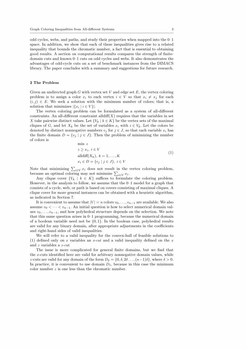
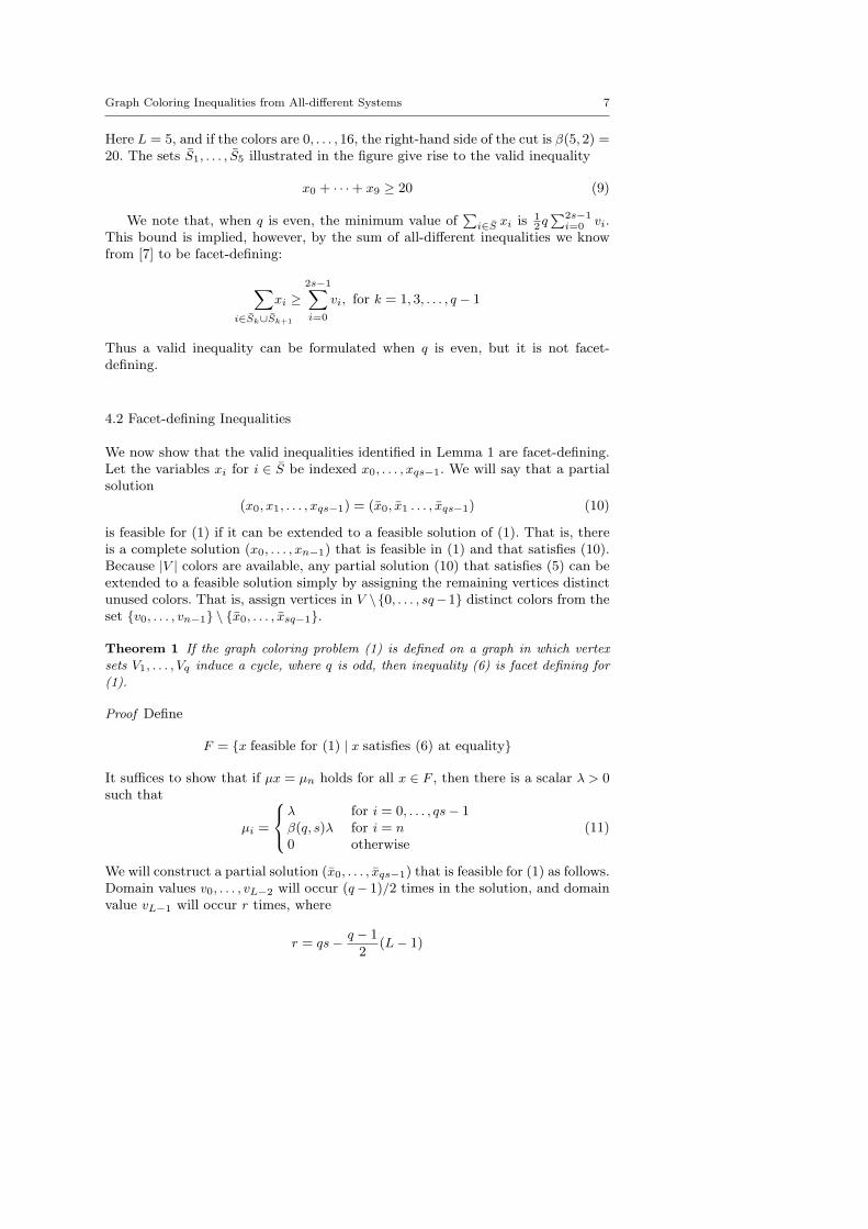
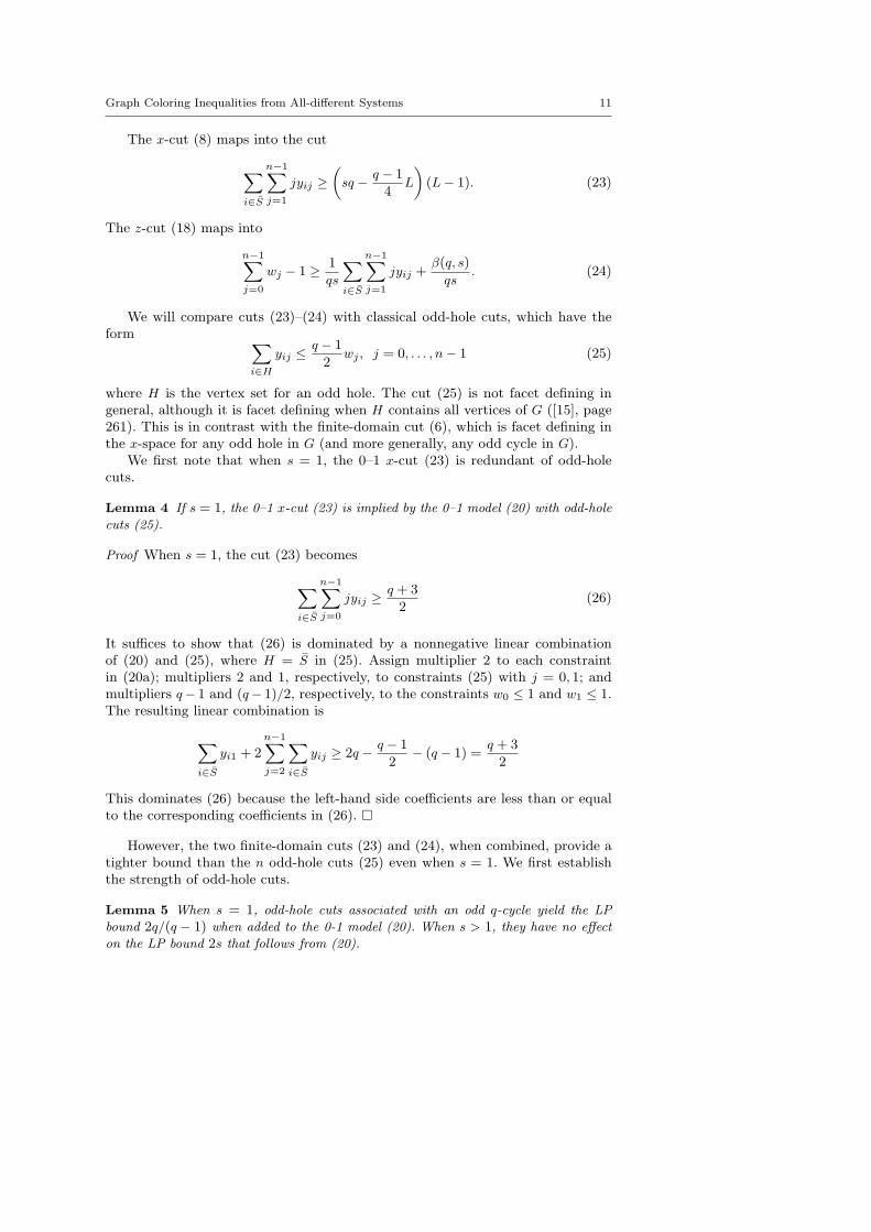
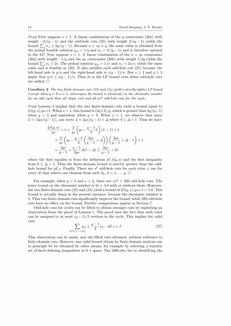
Figure 1 illustrates an odd cycle with q = 5. Each solid oval corresponds toa constraint alldiff(Xk). Thus V1 = {0, 1, 2, 3, 10, 11}, and similarly for V2, . . . , V5.All the vertices in a given Vk are connected by edges in G.
4.1 Valid Inequalities
We first identify valid inequalities that correspond to a given cycle. In the nextsection, we show that they are facet-defining.
Lemma 1 Let V1, . . . , Vq induce a cycle, and let Sk ⊆ Sk and |Sk| = s ≥ 1 for
k = 1, . . . , q. If q is odd and S = S1 ∪ · · · ∪ Sq, the following inequality is valid for (1):∑i∈S
xi ≥ β(q, s) (6)
where
β(q, s) =q − 1
2
L−2∑j=0
vj +
(sq − q − 1
2(L− 1)
)vL−1
and
L =
⌈sq
(q − 1)/2
⌉
6 David Bergman, J. N. Hooker
x0 x1
x10
x2
x3
x11
x12
x4
x5x13x6
x7
x14
x15
x8
x9
x16
.
.
.
.
.
.
.
.
.
.
.
.
.
.
.
.
.
.
.
.
.
.
.
.
.
.
.
.
.
.
.
.
.
.
.
.
.
.
.
.
.
.
..
.
.
..
.
.
..
.
..
.
..
..
.
..............................................................................................................................................................................................................................................................................................................................................
.......................................................................
......................................................................................................................................................................................................................................................................................................................................................................................................................................................
...........................................
...........................................................................................................................................................................................................................................................................................................................................................................................................................................................................................................................................................
........................................................................................................................................................................................................................................................................................................................................................................................................................
.
.
.
.
.
.
.
.
.
.
.
.
.
.
.
.
.
..
.
..
..
...........................................................................................................................................
.................
.........................
..........................................................................................................................................................................................................................................................................................................................................................................................................................................................................................................................................................
............................................................................................................................................................................................................
....................................................................................................................................................................................................................................................................................................................................................................................................................................................................................
...............................................................................................................................................................................................................................................................................................................................................................................................................................................................................................
.
.
.
.
..
..........................................
...................................................................................................................................................................................................................................................................................................................................................................................................................................................................................................................
................................................................................................................................................................................................................................................................................................................................................................................................................
.
.
.
.
.
.
.
.......
.......
.......
.....................
.......
.......
.
.
.
.
.
.
.
.
..
.
..
.
.......
.............. ....... ...
...........
.......
..
.....
.
.......
..
..
..
.
.
.
.
.
.
.
.
.
.
.
.
.
.
.
.
.
.
.
.
.
.
.
.
.
.
.
.
.
.
.
.
.
.
.
.
.
.
.
.
.
.
.
.
.
..
...
..............
.
.
.
.
.
.
.
.
.
.
.
.
.
.
.
.
.
.
.
.
.
.
.
.
.
.
.
.
.
.
.
.
.
.
.
.
.
.
.
.
.
.
.
.
.
.
..
.
.......
.
.
.
..
...
..............
.......
.......
.......
.......
.......
.
.
.
.
.
.
.
.
.
.
.
.
.
.
..............
.......
.......
.......
.......
.......
.
..
.
.
.
.
.
.
.
.
.
.
.
.
.
.
.
.
.
.
.
.
.
.
.
.
.
.
.
.
..
..
.
.......
.......
.......
.......
..............
.......
.
.
.
.
.
.
.
.
.
..
.
.
.
.......
.......
.......
.......
.............. .
......
.
.......
.......
.
.
.
.
.
.
.
.
.
.
.
.
.
.
.
.
.
.
.
.
.
.
.
.
.
.
.
.
.
.
.
.
.
.
.
.
.
.
.
.
.
.
.
.
.
.
.
.
.
.......
.......
.......
.
.
.
.
.
.
.
.
.
.
.
.
.
.
.
.
.
.
.
.
.
.
.
.
.
.
.
.
.
.
.
.
.
.
.
.
.
.
.
.
.
.
.
.
.
.
.
.
.
.
.
..
...
.......
V1
V2
V3
V4
V5
S5
.
.
.
.
.
.
.
.
.
.
.
.
.
.
.
.
.
.
.
.
.
.
.
.
.
.
.
.
.
.
.
.
.
.
.
.
.
.
.
.
.
.
.
.
.
.
.
.
.
.
.
.
.
.
.
.
.
.
.
.
.
.
.
.
.
.
.
.
.
.
.
.
.
.
.
.
.
.
.
.
.
.
.
.
.
.
.
.
..
.
.
.
.
.
.
.
.
.
.
.
.
.
.
.
.
.
.
.
.
.
.
.
.
.
.
.
.
.
.
.
.
.
.
.
.
.
S1
...............................................................................................................................
...................
S2.......................................................................................................
.
.
.
.
.
.
.
.
.
.
.
.
.
.
.
.
.
.
.
S3...............................................................................................
...................
S4
.........................................................................................................................................
...................
Fig. 1 A 5-cycle. The solid ovals correspond to constraints alldiff(Xk) for k = 1, . . . , 5. Thesets S1, . . . , S2 provide the basis for one possible valid cut with s = 2.
Proof Because q is odd, each color can be assigned to at most (q− 1)/2 vertices inthe cycle. This means that the vertices must receive at least L distinct colors, andthe variables in (5) must take at least L different values. Because v0 < · · · < vn−1,we have∑
i∈S
xi ≥q − 1
2(v0 + v1 + · · ·+ vL−2) +
(sq − q − 1
2(L− 1)
)vL−1 = β(q, s)
where the coefficient of vL−1 is the number of vertices remaining to receive colorvL−1 after colors v0, . . . , vL−2 are assigned to (q − 1)/2 vertices each. �
If the cycle is an odd hole, each |Sk| = 1 and L = 3. So (6) becomes∑i∈S
xi ≥q − 1
2(v0 + v1) + v2 (7)
If the domain {v0, . . . , vn−1} of each xi is Dδ = {0, δ, 2δ, . . . , (n − 1)δ} for someδ > 0, inequality (6) becomes∑
i∈S
xi ≥(sq − q − 1
4L
)(L− 1)δ (8)
for a general cycle and ∑i∈S
xi ≥q + 3
2δ
for an odd hole.An example with q = 5 appears in Fig. 1. By setting s = 2 we can obtain 9 valid
inequalities by selecting 2-element subsets S1 and S3 of S1 and S3, respectively.
Graph Coloring Inequalities from All-different Systems 7
Here L = 5, and if the colors are 0, . . . , 16, the right-hand side of the cut is β(5, 2) =20. The sets S1, . . . , S5 illustrated in the figure give rise to the valid inequality
x0 + · · ·+ x9 ≥ 20 (9)
We note that, when q is even, the minimum value of∑
i∈S xi is 12q∑2s−1
i=0 vi.This bound is implied, however, by the sum of all-different inequalities we knowfrom [7] to be facet-defining:
∑i∈Sk∪Sk+1
xi ≥2s−1∑i=0
vi, for k = 1, 3, . . . , q − 1
Thus a valid inequality can be formulated when q is even, but it is not facet-defining.
4.2 Facet-defining Inequalities
We now show that the valid inequalities identified in Lemma 1 are facet-defining.Let the variables xi for i ∈ S be indexed x0, . . . , xqs−1. We will say that a partialsolution
(x0, x1, . . . , xqs−1) = (x0, x1 . . . , xqs−1) (10)
is feasible for (1) if it can be extended to a feasible solution of (1). That is, thereis a complete solution (x0, . . . , xn−1) that is feasible in (1) and that satisfies (10).Because |V | colors are available, any partial solution (10) that satisfies (5) can beextended to a feasible solution simply by assigning the remaining vertices distinctunused colors. That is, assign vertices in V \{0, . . . , sq−1} distinct colors from theset {v0, . . . , vn−1} \ {x0, . . . , xsq−1}.
Theorem 1 If the graph coloring problem (1) is defined on a graph in which vertex
sets V1, . . . , Vq induce a cycle, where q is odd, then inequality (6) is facet defining for
(1).
Proof Define
F = {x feasible for (1) | x satisfies (6) at equality}
It suffices to show that if µx = µn holds for all x ∈ F , then there is a scalar λ > 0such that
µi =
λ for i = 0, . . . , qs− 1β(q, s)λ for i = n
0 otherwise(11)
We will construct a partial solution (x0, . . . , xqs−1) that is feasible for (1) as follows.Domain values v0, . . . , vL−2 will occur (q− 1)/2 times in the solution, and domainvalue vL−1 will occur r times, where
r = qs− q − 1
2(L− 1)
8 David Bergman, J. N. Hooker
This will ensure that (6) is satisfied at equality. We form the partial solution byfirst cycling r times through the values v0, . . . , vL−1, and then by cycling throughthe values v0, . . . , vL−2. Thus
xi =
{vi mod L for i = 0, . . . , rL− 1
v(i−rL) mod (L−1) for i = rL, . . . , qs− 1(12)
To show that this partial solution is feasible for the odd cycle, we must show
alldiff{xi, i ∈ Sk ∪ Sk+1}, for k = 1, . . . , q − 1 (a)
alldiff{xi, i ∈ S1 ∪ Sq} (b)
To show (a), we note that the definition of L implies L − 1 ≥ 2s. Therefore, anysequence of 2s consecutive xi’s are distinct, and (a) is satisfied. To show (b), wenote that the number of values xrL, . . . , xqs−1 is
(qs− 1)− rL+ 1 = (L− 1)
(q − 1
2L− qs
)from the definition of r. Because the number of values is a multiple of L − 1, thevalues xi for i ∈ Sq are (x(q−1)s, . . . , xqs−1) = (vL−s−1, . . . , vL−2), and they are alldistinct. The values xi for i ∈ S1 are (x0, . . . , xs−1) = (v0, . . . , vs−1) and are alldistinct. But L− 1 ≥ 2s implies L− s > s, and (b) follows.
We now construct a partial solution (x0, . . . , xqs−1) from the partial solutionin (12) by swapping any two values xℓ, xℓ′ for ℓ, ℓ′ ∈ Sk ∪ Sk+1, for any k ∈{1, . . . , q − 1}. That is,
xi =
xℓ′ if i = ℓ
xℓ if i = ℓ′
xi otherwise(13)
Extend the partial solutions (12) and (13) to complete solutions x and x, respec-tively, by assigning values with
xi = xi for i ∈ {0, . . . , qs− 1}
such that the values assigned to xi for i ∈ {0, . . . , qs − 1} are all distinct anddo not belong to {v0, . . . , vL−1}. Because x and x are feasible and satisfy (6) atequality, they satisfy µx = µn+1. So we have µx = µx, which implies µℓ = µℓ′ forℓ, ℓ′ ∈ Sk ∪ Sk+1 for any pair ℓ, ℓ′ ∈ Sk ∪ Sk+1 and any k ∈ {1, . . . , q − 1}. Thisimplies
µℓ = µℓ′ for any ℓ, ℓ′ ∈ S (14)
Define x′ by letting x′ = x except that for an arbitrary ℓ ∈ {0, . . . , qs − 1}, x′ℓis assigned a value that does not appear in the tuple x. Since x and x′ are feasibleand satisfy (6) at equality, we have µx = µx′. This and xℓ = x′ℓ imply
µi = 0, i ∈ V \ {0, . . . , qs− 1} (15)
Finally, (14) implies that for some λ > 0,
µi = λ, i = 0, . . . , qs− 1 (16)
Because µx = µn, we have from (16) that µn = β(q, s)λ. This, (15), and (16) imply(11). �
In the example of Fig. 1, suppose that the vertices in V1, . . . , V5 induce a cycleof G. That is, all vertices in each Vk are connected by edges, and there are no otheredges of G between vertices in V1 ∪ · · · ∪ V5. Then (9) is facet-defining for (1).
Graph Coloring Inequalities from All-different Systems 9
4.3 Bounds on the Chromatic Number
We can write a valid inequality involving the objective function variable z if thedomain of each xi is Dδ for δ > 0. To do so we rely on the following, wheree = (1, . . . , 1):
Theorem 2 Suppose ax ≥ β is valid for a graph coloring problem (1) in which each
xi has domain Dδ for δ > 0. Then if ae ≥ 0, the inequality
aez ≥ ax+ β (17)
is also valid for (1).
Proof To show that (17) is valid, note that for any x ∈ Dnδ , z − xi ∈ Dδ for all i,
where z = maxi{xi}. Because ax ≥ β is valid for all x ∈ Dnδ and z−xi ∈ Dδ, ax ≥ β
holds when z − xi is substituted for each xi. Thus (17) holds when z = maxi{xi}.But because z in (1) must satisfy z ≥ xi for each i, and ae ≥ 0, it follows that (17)holds for (1). �
Inequality (6) and Theorem 2 imply
Corollary 1 If the graph coloring problem (1) is defined on a graph in which vertex
sets V1, . . . , Vq induce a cycle, where q is odd and each xi has domain Dδ with δ > 0,then
z ≥ 1
qs
∑i∈S
xi +β(q, s)
qs(18)
is valid for (1), where
β(q, s)
qs=
(1− q − 1
4qsL
)(L− 1)δ
In the case of an odd hole (s = 1), the z-cut is
z ≥ 1
q
∑i∈S
xi +q + 3
2qδ
In the example of Fig. 1, the z-cut is
z ≥ 110 (x0 + · · ·+ x9) + 2 (19)
It is straightforward to deduce the linear programming (LP) bound on thechromatic number that is provided by x-cuts and/or z-cuts in the finite-domainspace, when no other cuts are present. The bound is the minimum of z+1 subjectto the cut(s) and z ≥ xi for all i ∈ V .
Lemma 2 Let the x-cut ax ≥ β and the z-cut z ≥ ax/ae + β/ae be valid for an
arbitrary coloring problem (1) with domain D1, where ae > 0. The x-cut and z-cut
yield the lower bound β/ae+ 1 on the chromatic number when used individually, and
the lower bound 2β/ae+ 1 when used together.
10 David Bergman, J. N. Hooker
Proof The optimal value of the LP that contains the x-cut is z + 1 = β/ae + 1,because this and xi = β/ae for all i is a primal feasible solution, and an assignmentof multiplier 1/ae to the x-cut and ai/ae to each constraint z ≥ xi is dual feasible.The optimal value of the LP with the z-cut is likewise z + 1 = β/ae+ 1, becausethis and xi = 0 for all i is primal feasible, and an assignment of multiplier 1 tothe z-cut and zero to each constraint z ≥ xi is dual feasible. The optimal valuewith both cuts is z+1 = 2β/ae+1, because this and xi = β/ae is primal feasible,and an assignment of multiplier 1/ae to the x-cut, 1 to the z-cut, and zero to eachz ≥ xi is dual feasible. �
For domain D1, the x-cut and z-cut for a cycle provide the bound β(q, s)/qs+1when used individually, and the bound 2β(q, s)/qs+ 1 when used together.
4.4 Mapping to 0–1 Cuts
The 0–1 model for a coloring problem on a cycle has the following continuousrelaxation: ∑
j∈J
yij = 1, i = 0, . . . , n− 1 (a)
∑i∈Vk
yij ≤ wj , j ∈ J, k = 1, . . . , q (b)
0 ≤ yij , wj ≤ 1, all i, j (c)
(20)
Because constraints (b) appear for each maximal clique, the relaxation implies allclique inequalities
∑i∈Vk
yij ≤ 1. Nonetheless, we will see that two finite-domaincuts strengthen the relaxation more than the collection of all odd-hole cuts.
To simplify the discussion, let each xi have domain D1 = {0, 1, . . . , n − 1}. Asnoted earlier, we can map an x-cut ax ≥ β into 0–1 space by substituting
∑j jyij
for each xi, which yields ∑ij
jaiyij ≥ β (21)
Because the minimum color number is zero, minimizing the number of colors∑
j wj
is the same as minimizing z + 1, where z is the largest color number. The z-cutz ≥ ax/ae+ β/ae therefore maps into∑
j
wj ≥ 1
ae
∑ij
jaiyij +β
ae+ 1 (22)
We first note that the x-cut and z-cut, used together, yield an LP bound in0–1 space at least as tight as in finite-domain space. The LP bound in 0–1 spaceis the minimum of
∑j wj subject to (20)–(22).
Lemma 3 Suppose that x-cut ax ≥ β and z-cut z ≥ (ax + β)/ae are valid for an
arbitrary coloring problem (1). If they are mapped into 0–1 space, they yield an LP
bound on the chromatic number of at least 2β/ae+ 1 when used together.
Proof This is seen by taking a linear combination of (21) and (22), with weight1/ae on the former and 1 on the latter. �
Graph Coloring Inequalities from All-different Systems 11
The x-cut (8) maps into the cut
∑i∈S
n−1∑j=1
jyij ≥(sq − q − 1
4L
)(L− 1). (23)
The z-cut (18) maps into
n−1∑j=0
wj − 1 ≥ 1
qs
∑i∈S
n−1∑j=1
jyij +β(q, s)
qs. (24)
We will compare cuts (23)–(24) with classical odd-hole cuts, which have theform ∑
i∈H
yij ≤ q − 1
2wj , j = 0, . . . , n− 1 (25)
where H is the vertex set for an odd hole. The cut (25) is not facet defining ingeneral, although it is facet defining when H contains all vertices of G ([15], page261). This is in contrast with the finite-domain cut (6), which is facet defining inthe x-space for any odd hole in G (and more generally, any odd cycle in G).
We first note that when s = 1, the 0–1 x-cut (23) is redundant of odd-holecuts.
Lemma 4 If s = 1, the 0–1 x-cut (23) is implied by the 0–1 model (20) with odd-hole
cuts (25).
Proof When s = 1, the cut (23) becomes
∑i∈S
n−1∑j=0
jyij ≥ q + 3
2(26)
It suffices to show that (26) is dominated by a nonnegative linear combinationof (20) and (25), where H = S in (25). Assign multiplier 2 to each constraintin (20a); multipliers 2 and 1, respectively, to constraints (25) with j = 0, 1; andmultipliers q− 1 and (q− 1)/2, respectively, to the constraints w0 ≤ 1 and w1 ≤ 1.The resulting linear combination is
∑i∈S
yi1 + 2n−1∑j=2
∑i∈S
yij ≥ 2q − q − 1
2− (q − 1) =
q + 3
2
This dominates (26) because the left-hand side coefficients are less than or equalto the corresponding coefficients in (26). �
However, the two finite-domain cuts (23) and (24), when combined, provide atighter bound than the n odd-hole cuts (25) even when s = 1. We first establishthe strength of odd-hole cuts.
Lemma 5 When s = 1, odd-hole cuts associated with an odd q-cycle yield the LP
bound 2q/(q − 1) when added to the 0-1 model (20). When s > 1, they have no effect
on the LP bound 2s that follows from (20).
12 David Bergman, J. N. Hooker
Proof First suppose s = 1. A linear combination of the q constraints (20a) withweight −2/(q − 1) and the odd-hole cuts (25) with weight 2/(q − 1) yields thebound
∑j wj ≥ 2q/(q − 1). Because n = sq = q, the same value is obtained from
the primal feasible solution yij = 1/q and wj = 2/(q − 1) and is therefore optimalin the LP. Now suppose s > 1. A linear combination of the n = qs constraints(20a) with weight −1/q and the qn constraints (20b) with weight 1/2q yields thebound
∑j wi ≥ 2s. The primal solution yij = 1/n and wj = 2s/n yields the same
value and is feasible in (20). It also satisfies each odd-hole cut (25) because theleft-hand side is q/n and the right-hand side is s(q − 1)/n. But s ≥ 2 and q ≥ 3imply that q/n ≤ s(q − 1)/n. Thus 2s is the LP bound even when odd-hole cutsare added. �
Corollary 2 The two finite-domain cuts (23) and (24) yield a strictly tighter LP bound
(except when q = 3, s = 1, whereupon the bound is identical) on the chromatic number
for an odd cycle than all clique cuts and all nsq odd-hole cuts for the cycle.
Proof Lemma 3 implies that the two finite-domain cuts yield a bound equal to2β(q, s)/qs+1. When s = 1, this bound is (2q+3)/q, which is greater than 2q/(q−1)when q > 3 and equivalent when q = 3. When s > 1, we observe that sinceL = ⌈2qs/(q − 1)⌉, can write L = 2qs/(q − 1) +∆ where 0 ≤ ∆ < 1. Thus we have
2β(q, s)
qs+ 1 =
2
qs
(qs− q − 1
4L
)(L− 1) + 1
=2
qs
(qs− q − 1
4
(2qs
q − 1+∆
))(2qs
q − 1+∆− 1
)+ 1
=2qs
q − 1+
q − 1
2qs∆(1−∆) ≥ 2qs
q − 1> 2s
where the first equality is from the definition of β(q, s) and the first inequalityfrom 0 ≤ ∆ < 1. Thus the finite-domain bound is strictly greater than the odd-hole bound for all s. Finally, There are sq odd-hole cuts for each color j, one forevery H that selects one element from each Sk, k = 1, . . . , q. �
For example, when q = 5 and s = 2, there are nsq = 320 odd-hole cuts. Thelower bound on the chromatic number is 2s = 4.0 with or without them. However,the two finite-domain cuts (23) and (24) yield a bound of 2β(q, s)/qs+1 = 5.0. Thisbound is actually sharp in the present instance, because the chromatic number is5. Thus two finite-domain cuts significantly improve the bound, while 320 odd-holecuts have no effect on the bound. Further comparisons appear in Section 7.
Odd-hole cuts for cycles can be lifted to obtain stronger cuts by exploiting anobservation from the proof of Lemma 1. The proof uses the fact that each colorcan be assigned to at most (q − 1)/2 vertices in the cycle. This implies the validcuts ∑
i∈V1∪···∪Vq
yij ≤ q − 1
2wj , all j ∈ J (27)
This observation can be made, and the lifted cuts obtained, without reference tofinite-domain cuts. However, any valid bound obtain by finite-domain analysis canin principle be be obtained by other means, for example by selecting a suitableset of facet-defining inequalities in 0–1 space. The difficulty lies in identifying the
Graph Coloring Inequalities from All-different Systems 13
inequalities. The advantage of finite-domain analysis is that it may discover validcuts that were previously unknown. To our knowledge, no one has observed thatthe finite-domain cuts (23)–(24) or the lifted odd-hole cuts (27) are valid for graphcoloring.
Furthermore, two finite-domain cuts provide generally tighter bounds in lesstime than the lifted odd-hole cuts. It is easy to show that the lifted cuts (27) yielda bound of 2qs/(q − 1), which has the following relationship to the finite-domainbound:
Lemma 6 The bound 2qs/(q − 1) is strictly weaker than the finite domain bound of
2β(q, s)/qs+1 except when s is an integer multiple of (q−1)/2, in which case the two
bounds are equal.
Proof When s is an integer multiple of (q − 1)/2, we have L = 2qs/(q − 1), anddirect substitution verifies that the two bounds are equal. Otherwise, we haveL = 2qs/(q− 1)+∆ for 0 < ∆ < 1. Substitution of this into the formula for β(q, s)yields the finite-domain bound
2qs
q − 1+
q − 1
2qs∆(1−∆) >
2qs
q − 1
and the lemma follows. �
The difference between the two bounds is never great, but the finite domainbound is achieved with only 2 inequalities, as opposed to n lifted inequalities (27).We will see in Section 7 that this allows the finite-domain bound to be obtainedin substantially less computation time.
5 Webs
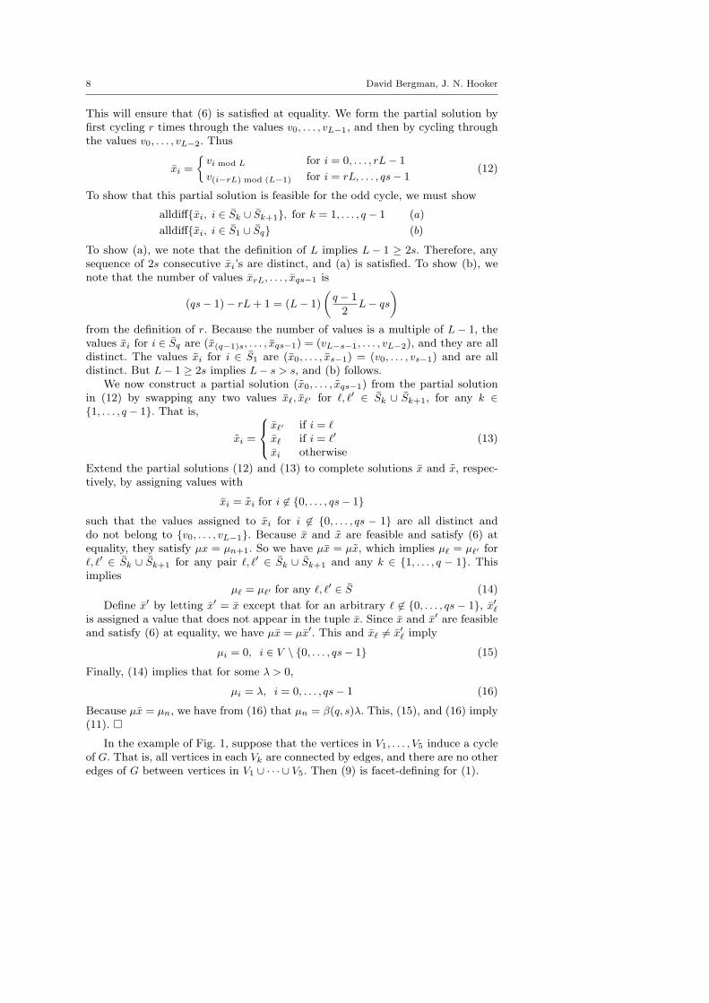
We next study cuts that arise from webs. A web W (q, r) is a graph in which verticescan be arranged cyclically so that the edges connect pairs of vertices separatedby a distance of at least r on the cycle. More formally, given that q ≥ 2r + 1 andr ≥ 1, a web W (q, r) is a graph on vertices 0, . . . , q − 1 whose edges are all (i, i′)such that 0 ≤ i ≤ q− r− 1 and r ≤ i′ − i ≤ q− r. Thus W (q, 1) is a clique. When q
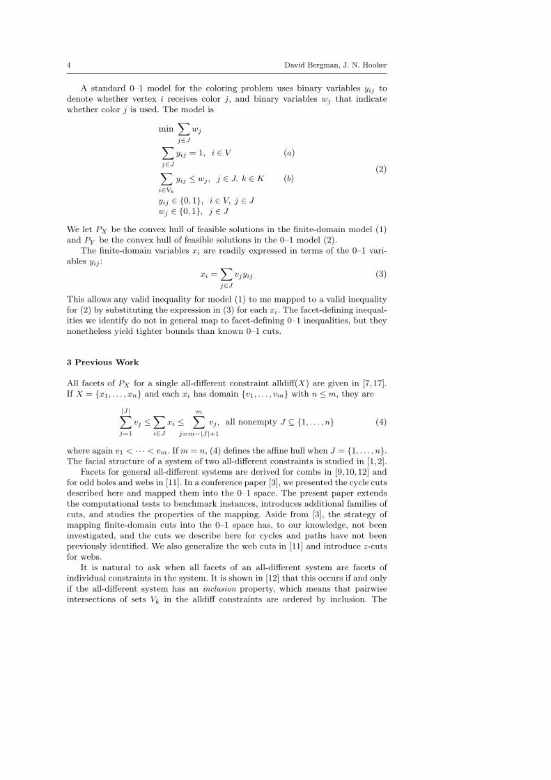
is odd, W (q, q−12 ) is an odd hole, and W (q, 2) is an odd anti-hole (the complement
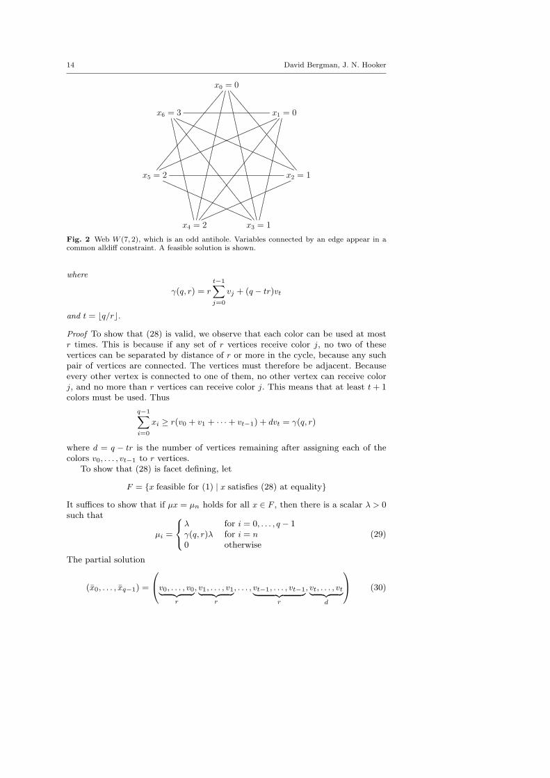
of an odd hole). Figure 2 illustrates W (7, 2).We will focus on webs for which q and d are coprime, where d = q mod r is
the remainder after dividing q by r. This implies, in particular, that q and r arecoprime. Odd holes and odd anti-holes are special cases of these webs. Such websgive rise to 0–1 finite-domain cuts that provide tighter bounds than standard webcuts.
5.1 Facet-Defining Inequalities
Theorem 3 Let vertices 0, . . . , q − 1 of G induce a web W (q, r) , where q and d =q mod r are coprime. The following inequality is facet-defining for (1):
q−1∑i=0
xi ≥ γ(q, r) (28)
14 David Bergman, J. N. Hooker
x0 = 0.................................................................................................................................................................................................................................................................................................................................................................................................................................................................
.
.
.
.
.
.
.
.
.
.
.
.
.
.
.
.
.
.
.
.
.
.
.
.
.
.
.
.
.
.
.
.
.
.
.
.
.
.
.
.
.
.
.
.
.
.
.
.
.
.
.
.
.
.
.
.
.
.
.
.
.
.
.
.
.
.
.
.
.
.
.
.
.
.
.
.
.
.
.
.
.
.
.
.
.
.
.
.
.
.
.
.
.
.
.
.
.
.
.
.
.
.
.
.
.
.
.
.
.
.
.
.
.
.
.
.
.
.
.
.
.
.
.
.
.
.
.
.
.
.
.
.
.
.
.
.
.
.
.
.
.
.
.
.
.
.
.
.
.
.
.
.
.
.
.
.
.
.
.
.
.
.
.
.
.
.
.
.
.
.
.
.
.
.
.
.
.
.
.
.
.
.
.
.
.
.
.
.
.
.
.
.
.
.
.
.
.
.
.
.
.
.
.
.
.
.
.
.
.
.
.
.
.
.
.
.
.
.
.
.
.
.
.
.
.
.
.
.
.
.
.
.
.
.
.
.
.
.
.
.
.
.
.
.
.
.
.
.
.
.
.
.
.
.
.
.
.
.
.
.
.
.
.
.
.
.
.
.
.
.
.
.
.
.
.
.
.
.
.
.
.
.
.
.
.
.
.
.
.
.
.
.
.
.
.
.
.
.
.
.
.
.
.
.
.
.
.
.
.
.
.
.
.
.
.
.
.
.
.
.
.
.
.
.
.
.
.
.
.
.
.
.
.
.
.
.
.
.
.
.
.
.
.
.
.
.
.
.
.
.
.
.
.
.
.
.
.
.
.
.
.
.
.
.
.
.
.
.
.
.
.
.
.
.
.
.
.
.
.
.
.
.
.
.
.
.
.
.
.
.
.
.
.
.
.
.
.
.
.
.
.
.
.
.
.
.
.
.
.
.
.
.
.
.
.
.
.
.
.
.
.
.
.
.
.
.
.
.
.
.
.
.
.
.
.
.
.
.
.
.
.
.
.
.
.
.
.
.
.
..
............................................................................................................................................................................................................................................................................................................................................................
..
..
.
..
..
..
...................................................................................................................................................................................................................................................................................................................................................
x1 = 0.....................................................................................................................................................................................................................................................................................................
.
.
.
.
.
.
.
.
.
.
.
.
.
.
.
.
.
.
.
.
.
.
.
.
.
.
.
.
.
.
.
.
.
.
.
.
.
.
.
.
.
.
.
.
.
.
.
.
.
.
.
.
.
.
.
.
.
.
.
.
.
.
.
.
.
.
.
.
.
.
.
.
.
.
.
.
.
.
.
.
.
.
.
.
.
.
.
.
.
.
.
.
.
.
.
.
.
.
.
.
.
.
.
.
.
.
.
.
.
.
.
.
.
.
.
.
.
.
.
.
.
.
.
.
.
.
.
.
.
.
.
.
.
.
.
.
.
.
.
.
.
.
.
.
.
.
.
.
.
.
.
.
.
.
.
.
.
.
.
.
.
.
.
.
.
.
.
.
.
.
.
.
.
.
.
.
.
.
.
.
.
.
.
.
.
.
.
.
.
.
.
.
.
.
.
.
.
.
.
.
.
.
.
.
.
.
.
.
.
.
.
.
.
.
.
.
.
.
.
.
.
.
.
.
.
.
.
.
.
.
.
.
.
.
.
.
.
.
.
.
.
.
.
.
.
.
.
.
.
.
.
.
.
.
.
.
.
.
.
.
.
.
.
.
.
.
.
.
.
.
.
.
.
.
.
.
.
.
.
.
.
.
.
.
.
.
.
.
.
.
.
.
.
.
.
.
.
.
.
.
.
.
.
.
.
.
.
.
.
.
.
.
.
.
.
.
.
.
.
.
.
.
.
.
.
.
.
.
.
.
.
.
.
.
.
.
.
.
.
.
.
.
.
.
.
.
.
.
.
.
.
.
.
.
..
.
..
.................................................................................................................................................................................................................................................................................................................................................................................................................................................
...................................................................................................................................................................................................................................................................................................................................................................................................................................................
x2 = 1.....................................................................................................................................................................................................................................................................................................................................................................................................
...........................................................................................................................................................................................................................................................................................................................................
x3 = 1x4 = 2
x5 = 2........................................................................................................................................................................................................................................................................................................................................
x6 = 3.................................................................................................................................................................................................................................................................................................................................................................
.
..
.
..
..
.
..
............................................................................................................................................................................................................................................................................................................................................................................................................................................
...................................................................................................................................................................................................................................................................................................................................................................................................................................................
Fig. 2 Web W (7, 2), which is an odd antihole. Variables connected by an edge appear in acommon alldiff constraint. A feasible solution is shown.
where
γ(q, r) = r
t−1∑j=0
vj + (q − tr)vt
and t = ⌊q/r⌋.
Proof To show that (28) is valid, we observe that each color can be used at mostr times. This is because if any set of r vertices receive color j, no two of thesevertices can be separated by distance of r or more in the cycle, because any suchpair of vertices are connected. The vertices must therefore be adjacent. Becauseevery other vertex is connected to one of them, no other vertex can receive colorj, and no more than r vertices can receive color j. This means that at least t+ 1colors must be used. Thus
q−1∑i=0
xi ≥ r(v0 + v1 + · · ·+ vt−1) + dvt = γ(q, r)
where d = q − tr is the number of vertices remaining after assigning each of thecolors v0, . . . , vt−1 to r vertices.
To show that (28) is facet defining, let
F = {x feasible for (1) | x satisfies (28) at equality}
It suffices to show that if µx = µn holds for all x ∈ F , then there is a scalar λ > 0such that
µi =
λ for i = 0, . . . , q − 1γ(q, r)λ for i = n
0 otherwise(29)
The partial solution
(x0, . . . , xq−1) =
v0, . . . , v0︸ ︷︷ ︸r
, v1, . . . , v1︸ ︷︷ ︸r
, . . . , vt−1, . . . , vt−1︸ ︷︷ ︸r
, vt, . . . , vt︸ ︷︷ ︸d
(30)

Graph Coloring Inequalities from All-different Systems 15
is clearly feasible and satisfies (28) at equality. We construct a partial solution(x0, . . . , xq−1) from (30) by swapping the color assignment of the vertices receivingcolor vt with that of the last d vertices receiving color v0. That is, we let
xi =
vt if i ∈ {r − d, . . . , r − 1}v0 if i ∈ {q − d, . . . , q − 1}xi otherwise
Note that (x0, . . . , xq−1) is feasible, because colors v1, . . . , vt−1 are assigned to r
adjacent vertices as before, color v0 is assigned to the r adjacent vertices q −d, . . . , q − 1, 0, . . . , r − d − 1, and color vt is assigned to the remaining adjacentvertices r−d, . . . , r−1. Extend the two partial solutions to feasible solutions x andx of (1). Because x and x satisfy (28) at equality, we have µx = µx, which yields
µr−d + · · ·+ µr−1 = µq−d + · · ·+ µq−1
By symmetry, we conclude
µi + · · ·+ µ(i+d−1) mod q = µ(i−r) mod q + · · ·+ µ(i−r+d−1) mod q
for i = 0, . . . , q − 1. Because q and r are coprime, this implies that the sumsµi + · · ·+ µ(i+d−1) mod q are equal for all i. Thus, in particular, they are equal fori and i+ 1, which yields µi = µ(i+d) mod q for all i. Because q and d are coprime,this implies that µ0 = · · · = µq−1 and
µi = λ, i = 0, . . . , q − 1 (31)
for some λ > 0.
Define x′ by letting x′ = x except that for an arbitrary ℓ ∈ {0, . . . , q − 1}, x′ℓis assigned a value that does not appear in the tuple x. Since x, x′ ∈ F , we haveµx = µx′, which implies
µi = 0, i ∈ V \ {0, . . . , q − 1} (32)
Because µx = µn, we have from (31) that µn = γ(q, r)λ. Thus, (31) and (32) imply(29). �
For domain Dδ with δ > 0, the cut (28) is
q−1∑i=0
xi ≥(q − 1
2 (t+ 1)r)tδ (33)
For an odd antihole W (q, 2) with domain Dδ, the cut simplifies to
q−1∑i=0
xi ≥ 14 (q − 1)2δ (34)
16 David Bergman, J. N. Hooker
5.2 Bounds on the Chromatic Number
Theorems 2 and 3 imply
Corollary 3 If the graph coloring problem (1) is defined on a graph in which the
vertices in a subcollection of the vertex sets Vk induce a web W (q, r), where q and r
are coprime, and each xi has domain Dδ with δ > 0, then
z ≥ 1
q
q−1∑i=0
xi +
(1− r
2q(t+ 1)
)tδ (35)
is valid for (1), where t = ⌊q/r⌋.
Lemma 2 implies that for domain D1, the x-cut (33) and z-cut (35) yield theLP bound t−(rt/2q)(t+1)+1 when used individually, and 2t−(rt/q)(t+1)+1 whenused together. For example, the antihole of Fig. 2 gives rise to the facet-definingcuts
6∑i=0
xi ≥ 9, z ≥ 17
6∑i=0
xi +97
For a graph consisting of this web, these cuts yield the bound 227 when used
individually and 347 when used together.
5.3 Mapping to 0–1 Cuts
If each xi has domain D1 = {0, 1, . . . , n− 1} the x-cut (33) maps into the cut
q−1∑i=0
n−1∑j=1
jyij ≥(q − 1
2 (t+ 1)r)t (36)
when δ = 1. The z-cut (35) maps into
n−1∑j=0
wj − 1 ≥ 1
q
q−1∑i=0
n−1∑j=1
jyij +
(1− r
2q(t+ 1)
)t (37)
We wish to compare these cuts with known cuts for webs. Facet-defining webcuts for a 0–1 model of the coloring problem are given in [16]. These cuts are definedin a space in which the variables correspond to edges and colorings correspond to“admissible star partitions” of the graph. However, the cuts are based on the factthat at most r vertices can be assigned any given color, and we can write analogousweb cuts in the yij-space:
q−1∑i=0
yij ≤ r · wj , all j (38)
We first derive the bound obtained from these cuts. Note that n = q when G is aweb.
Lemma 7 The q web cuts (38) yield the LP bound q/r when added to the 0–1 graph
coloring model (20) for a web W (q, r).
Graph Coloring Inequalities from All-different Systems 17
Proof A linear combination of the q inequalities (20a) with weight −1/r each, andthe q web cuts (38) with weight 1/r each, yields the bound
∑j wj ≥ q/r. It suffices
to show that the primal solution yij = 1/q and wj = 1/r is feasible, because ithas value
∑j wj = q/r. It is clearly feasible in (20a) and the web cuts (38). We
must show that it is feasible in (20b) for each maximal clique Vk in the web. Butbecause every maximal clique Vk in W (q, r) has size ⌊q/r⌋, the left-hand side of(20b) is |Vk|(1/q) < 1/r, and the constraint is satisfied. �
Now we can show that the finite-domain cuts are stronger.
Corollary 4 The two finite-domain cuts (36) and (37) provide a strictly tighter LP
bound on the chromatic number for a web W (q, r) than the n web cuts (38).
Proof By Lemma 3, the two finite-domain cuts (36)–(37) provide bound
2t− rt
q(t+ 1) + 1 =
q
r+
r
qα(1− α) >
q
r
where the equality follows from setting α = q/r− t, and the inequality follows fromthe fact that 0 < α < 1. Because the web cuts yield the bound q/r by Lemma 7,the corollary follows. �
For example, for an antihole W (7, 2), seven 0–1 web cuts (38) give a bound of3.5, while the two finite-domain cuts provide a bound of 3.5714. Further compar-isons appear in Section 7.
6 Paths
Paths present an interesting case because they give rise to finite-domain cuts thatare redundant in the 0–1 model. That is, they have no effect on the bound whenthe problem consists entirely of a path system. However, a few finite-domain cutsmay replace a large number of inequalities in a more complex coloring problem,allowing a substantial reduction in the size of the 0–1 model. In addition, pathcuts are useful in a finite-domain model of the problem.
A path is a subgraph of G induced by the vertices in subsets V1, . . . , Vq ofV , provided the subgraph induced by each Vk is a clique, and only adjacent Vk’soverlap. That is,
Vk ∩ Vℓ =
{Sk if k + 1 = ℓ
∅ otherwise
where Sk = ∅. We let the sets Vk (and Sk) denote both the vertices i in the setsand their corresponding variables xi.
6.1 Facet-defining Inequalities
Facet-defining inequalities can be obtained by selecting one variable from eachoverlap Sk. Valid cuts can be obtained if two or more variables are selected, aswith cycles, but they are redundant of the single-variable cuts.
18 David Bergman, J. N. Hooker
V1
x0......................................................................................................................................................................................................................
.................................................................................................................................................................................................................................
.....................................................................................................................................
.
.
.
.
.
.
.
.
.
.
.
..
.......
..............
.......
..
.
.
.
.
.
.
.
.
.
.
.
.
.
.
.
.
.
.
.
..
.
....
.....................
.
......
.
.
.
.
.
.
.
.
V2
x1
x6
.
.
.
.
.
.
.
.
.
.
.
.
.
.
.
.
.
.
.
.
.
.
.
.
.
.
.
.
.
.
.
.
.
.
.
.
.
.
.
..
.
.
.
..
.
..
.
..............................................................................................................
.......................................................................................................................................
...............................................................................................................................................................................................................................................................................
.......................................................................................................................................................................
.
.
.
.
.
.
.
.
.
.
.
.
.
.
.......
..............
.......
.
.
.
.
.
.
.
.
.
.
.
.
.
.
.
.
.
..
.
.
..
.
....
.....................
.......
.
.
.
.
.
.
.
. x7
x8
V3
x2..................................................................................................................................................
.........................................................................................................................................................................................................................................................................................................................................................
................................................................................................................................................
.
.
.
.
.
.
.
.
.
.
.
.
..
.......
..............
.......
..
.
.
.
.
.
.
.
.
.
.
.
.
.
.
.
.
.
.
.
..
.
....
.....................
.
......
.
.
.
.
.
.
.
.
V4
x3
x9 x10
.
.
.
.
.
.
.
.
.
.
.
.
.
.
.
.
.
.
.
.
.
.
.
.
.
.
.
.
.
.
.
.
.
.
.
..
.
.
.
.
.
.
.
..
.
.
..
.
.
..
.
..
..
..................................................................................................................
...............................................................................................................................................
...................................................................................................................................................................................................................................................................................................
....................................................................................................................................................................................
.
.
.
.
.
.
.
.
.
.
.
.
.
.
.......
..............
.......
.
.
.
.
.
.
.
.
.
.
.
.
.
.
.
.
.
..
.
.
..
.
....
.....................
.......
.
.
.
.
.
.
.
. x11
x12
V5
x4......................................................................................................................................................................................................................
.................................................................................................................................................................................................................................
.....................................................................................................................................
.
.
.
.
.
.
.
.
.
.
.
..
.......
..............
.......
..
.
.
.
.
.
.
.
.
.
.
.
.
.
.
.
.
.
.
.
..
.
....
.....................
.
......
.
.
.
.
.
.
.
.
x5
x13
.
.
.
.
.
.
.
.
.
.
.
.
.
.
.......
..............
.......
.
.
.
.
.
.
.
.
.
.
.
.
.
.
.
.
.
..
.
.
..
.
..
..
.....................
.......
.
.
.
.
.
.
.
.
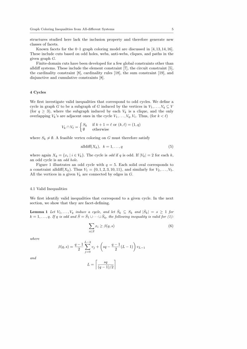
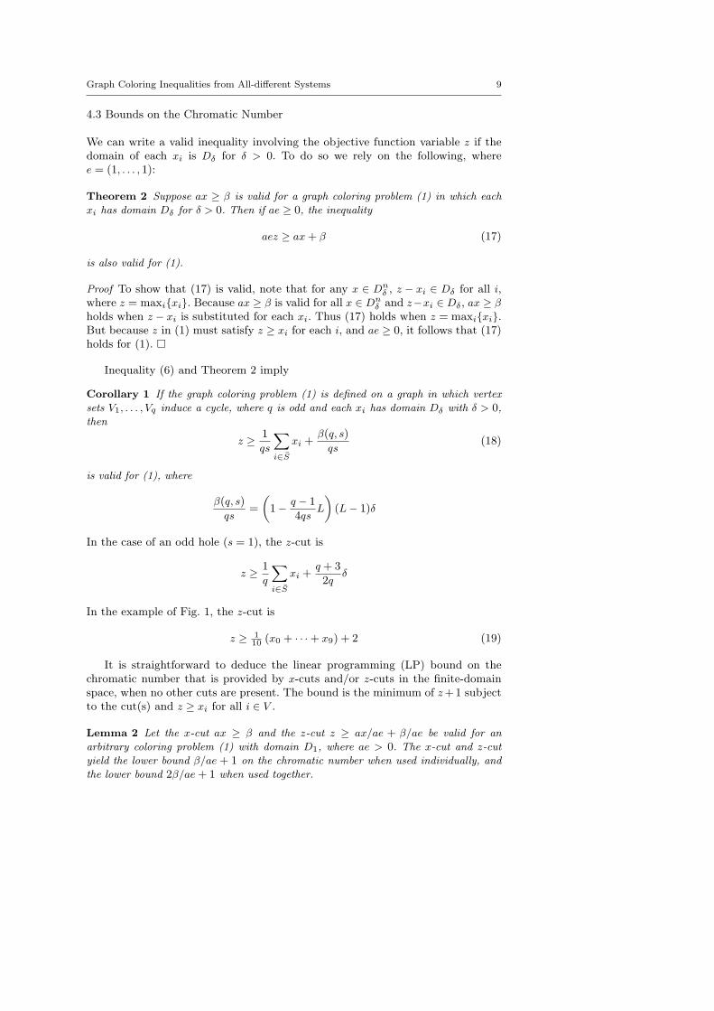
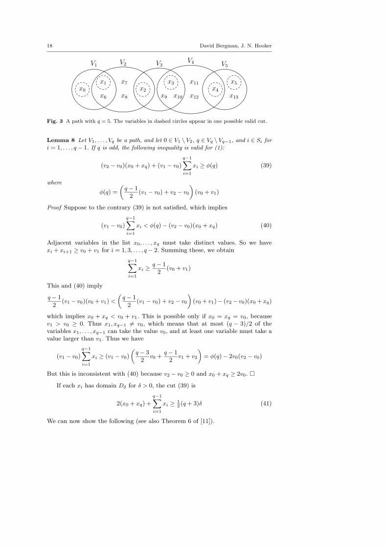
Fig. 3 A path with q = 5. The variables in dashed circles appear in one possible valid cut.
Lemma 8 Let V1, . . . , Vq be a path, and let 0 ∈ V1 \ V2, q ∈ Vq \ Vq−1, and i ∈ Si for
i = 1, . . . , q − 1. If q is odd, the following inequality is valid for (1):
(v2 − v0)(x0 + xq) + (v1 − v0)
q−1∑i=1
xi ≥ ϕ(q) (39)
where
ϕ(q) =
(q − 1
2(v1 − v0) + v2 − v0
)(v0 + v1)
Proof Suppose to the contrary (39) is not satisfied, which implies
(v1 − v0)
q−1∑i=1
xi < ϕ(q)− (v2 − v0)(x0 + xq) (40)
Adjacent variables in the list x0, . . . , xq must take distinct values. So we havexi + xi+1 ≥ v0 + v1 for i = 1, 3, . . . , q − 2. Summing these, we obtain
q−1∑i=1
xi ≥q − 1
2(v0 + v1)
This and (40) imply
q − 1
2(v1 − v0)(v0 + v1) <
(q − 1
2(v1 − v0) + v2 − v0
)(v0 + v1)− (v2 − v0)(x0 + xq)
which implies x0 + xq < v0 + v1. This is possible only if x0 = xq = v0, becausev1 > v0 ≥ 0. Thus x1, xq−1 = v0, which means that at most (q − 3)/2 of thevariables x1, . . . , xq−1 can take the value v0, and at least one variable must take avalue larger than v1. Thus we have
(v1 − v0)
q−1∑i=1
xi ≥ (v1 − v0)
(q − 3
2v0 +
q − 1
2v1 + v2
)= ϕ(q)− 2v0(v2 − v0)
But this is inconsistent with (40) because v2 − v0 ≥ 0 and x0 + xq ≥ 2v0. �
If each xi has domain Dδ for δ > 0, the cut (39) is
2(x0 + xq) +
q−1∑i=1
xi ≥ 12 (q + 3)δ (41)
We can now show the following (see also Theorem 6 of [11]).
Graph Coloring Inequalities from All-different Systems 19
Theorem 4 If the graph coloring problem (1) is defined on a graph in which vertex
sets V0, . . . , Vq induce a path, where q is odd, then inequality (39) is facet defining for
(1).
Proof LetF = {x feasible for (1) | x satisfies (39) at equality}
It suffices to show that if µx ≥ µn+1 holds for all x ∈ F , there is a scalar λ > 0such that
µi =
(v1 − v0)λ for i = 1, . . . , q − 1
(v2 − v0)λ for i = 0, q
ϕ(q)λ for i = n+ 1
0 otherwise
(42)
The following partial solutions are feasible for (1):
(x0, . . . , xq) = (v1, v0, v1, v0, v1, v0, v1, . . . , v1, v0)
(x0, . . . , xq) = (v0, v2, v1, v0, v1, v0, v1, . . . , v1, v0)
(x0, . . . , xq) = (v0, v1, v2, v0, v1, v0, v1, . . . , v1, v0)
They can be extended to complete solutions x, x, x with
xi = xi = xi for i ∈ {0, . . . , q}
in the manner described above. Because x and x satisfy (39) at equality, theysatisfy µx = µn+1, and we have µx = µx = µn+1. This implies µ(x − x) = 0, andtherefore µ1 = µ2.
Note that we obtained x from x by switching the values of x1 and x2. We cansimilarly show that µ2 = µ3 by switching the values of x2 and x3, and so forth,yielding
µ1 = · · · = µq−1 (43)
Also x satisfies (39) at equality, and we have µx = µx = µn+1. This implies(v1 − v0)µ0 = (v2 − v0)µ1. If we define x and x by
(x0, . . . , xq) = (v0, v1, v0, v1, . . . , v0, v1, v0, v1)
(x0, . . . , xq) = (v0, v1, v0, v1, . . . , v0, v1, v2, v0)
then x still satisfies (39) at equality, and we get (v1 − v0)µq = (v2 − v0)µq−1. Thusby (43)
(v1 − v0)µ0 = (v1 − v0)µq = (v2 − v0)µi, i = 1, . . . , q − 1 (44)
Now define x′ by letting x′ = x except that for an arbitrary ℓ ∈ {0, . . . , q}, x′ℓ isassigned a value that does not appear in the tuple x. Since x, x′ are feasible andsatisfy (39) at equality, we have µx = µx′. This and xℓ = x′ℓ imply
µi = 0, i ∈ V \ {0, . . . , q} (45)
Finally, (44) implies that for some λ > 0,
µ0 = µq = (v2 − v0)λ and µi = (v1 − v0)λ, i = 1, . . . , q − 1 (46)
Because µx = µn+1, we have from (46) that µn+1 = ϕ(q)λ. This, (45), and (46)imply (42). �
20 David Bergman, J. N. Hooker
6.2 Bounds on the Chromatic Number
Theorems 2 and 4 imply
Corollary 5 If the graph coloring problem (1) is defined on a graph in which vertex
sets V0, . . . , Vq induce a path, where q is odd and each xi has domain Dδ for δ > 0,then
z ≥ 1
q + 3
(2(x0 + xq) +
q−1∑i=1
xi
)+
δ
2(47)
is valid for (1).
If the colors are 0, 1, . . . , 5, the cuts for the path in Fig. 3 are
2(x0 + x5) +4∑
i=1
xi ≥ 4, z ≥ 14 (x0 + x5) +
18
4∑i=1
xi +12
6.3 Mapping to 0–1 Cuts
Assuming domain D1, the x-cut (39) and z-cut (47) respectively map to 0–1 spaceas follows:
2n−1∑j=1
j(y0j + yqj) +
q−1∑i=1
n−1∑j=1
jyij ≥ 12 (q + 3) (48)
n−1∑j=0
wj − 1 ≥ 2
q + 3
n−1∑j=1
j(y0j + yqj) +1
q + 3
q−1∑i=1
n−1∑j=1
jyij +12 (49)
To simplify notation, we suppose in this section that each Sk = {k}. Thearguments are very similar for the more general case. Given this simplification,the 0–1 path model is
q∑j=0
yij = 1, i = 0, . . . , q (ri)
yij + yi+1,j ≤ wj , i = 0, . . . , q − 1, j = 0, . . . , q (sij)
yij , wj ∈ {0, 1} all i, j
(50)
We first observe as follows that the x-cut (48) is redundant. If the wjs aretreated as constants equal to 1, (50) describes the feasible set in yij-space. We showin the following lemma that the equations and inequalities in (50), so modified,describe the convex hull of the feasible set.
Lemma 9 The coefficient matrix of (50) is totally unimodular when all wjs are set to
1.
Proof Let A be the coefficient matrix, omitting the rows that correspond to theconstraints yij ≤ 1. Because the omitted rows have only one non-zero element, itsuffices to show that A is totally unimodular. We refer to a row of A correspondingto a constraint (ri) in (50) as row ri, and similarly for a row corresponding to aconstraint (sij). It suffices [6] to show that for any subset J of the rows of A, there

Graph Coloring Inequalities from All-different Systems 21
is a partition J0, J1 of J for which every column contains at most one 1 in a row inJ0 and at most one 1 in a row in J1. This is the case if we define J0, J1 inductivelyas follows. If row r1 ∈ J , let r1 ∈ J0 and s1j ∈ J1 for all j, and otherwise lets1j ∈ J0 for all j. Now for any i > 1, suppose si−1,j ∈ Jt (for all j). If ri ∈ J , letri ∈ J1−t and sij ∈ Jt for all j, and otherwise let sij ∈ J1−t for all j. �
Corollary 6 The x-cut (48) is redundant of the equations and inequalities in (50).
Proof Because the coefficient matrix of (50) is totally unimodular when wjs areset to 1, the equations and inequalities in (50) describe the convex hull of thefeasible set in yij-space. Thus any valid inequality in variables yij is redundantof (48) when the wjs are fixed to 1, and therefore redundant for any wj (since0 ≤ wj ≤ 1). In particular, (48) is redundant. �
We cannot use a similar argument to show that the 0–1 z-cut (49) is redundant,because the full model (50) with wjs is not totally unimodular. In fact, the 0–1z-cut is not redundant, because it is not implied by (50) augmented with symmetry-breaking constraints wi ≥ wi+1. The following (extreme point) solution satisfies(50) with q = 3 but violates the cut because it results in a left-hand side of 12
7
and a right-hand side of 1 514 .
y =
0 4
7 0 37
27 0 4
717
27
47 0 1
7
0 0 47
37
, w = (47 ,47 ,
47 ,
47 )
The 0–1 z-cut has no effect on the bound in a problem consisting entirely of apath system, because the relaxation (50) already implies the optimal bound of 2.The sum of the negated constraints (rq−1) and (rq) with constraints (sq−1,j) forj = 0, . . . , q yields the bound
∑j wj ≥ 2.
7 Computational Results
7.1 Cycles
Table 1 shows LP bounds obtained from several families of cuts in 0–1 spacefor odd cycles. Each instance is a graph that consist entirely of one odd cycle,parameterized by s and q. All of the overlap sets Sk have size s, and vertex setVk = Sk ∪ Sk+1 for k = 1, . . . , q − 1 (with Vq = Sq ∪ S1). For each instance, wesolved the linear programming relaxation that minimizes
∑j wj subject to (20)
and various classes of cuts. The x-cuts and z-cuts are generated only for the given s,and not for smaller overlaps. Because we used a clique cover consisting of maximalcliques, the 0–1 model contains all maximal clique cuts.
The table reflects the fact (Corollary 2) that the two finite-domain cuts, whenused together, yield a tighter bound than all odd-hole cuts. In fact, the z-cut aloneyields a better bound when s > 1. The table also reflects the fact (Lemma 5) thatthe odd-hole cuts do not improve the bound beyond that obtained from the cliquecuts. The finite-domain cuts substantially reduce the integrality gap, sometimes to
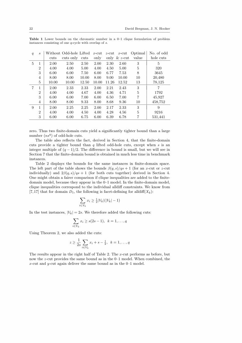
22 David Bergman, J. N. Hooker
Table 1 Lower bounds on the chromatic number in a 0–1 clique formulation of probleminstances consisting of one q-cycle with overlap of s.
q s Without Odd-hole Lifted x-cut z-cut x-cut Optimal No. of oddcuts cuts only cuts only only & z-cut value hole cuts
5 1 2.00 2.50 2.50 2.00 2.30 2.60 3 52 4.00 4.00 5.00 4.00 4.50 5.00 5 3203 6.00 6.00 7.50 6.00 6.77 7.53 8 36454 8.00 8.00 10.00 8.00 9.00 10.00 10 20,4805 10.00 10.00 12.50 10.00 11.26 12.52 13 78,125
7 1 2.00 2.33 2.33 2.00 2.21 2.43 3 72 4.00 4.00 4.67 4.00 4.36 4.71 5 17923 6.00 6.00 7.00 6.00 6.50 7.00 7 45,9274 8.00 8.00 9.33 8.00 8.68 9.36 10 458,752
9 1 2.00 2.25 2.25 2.00 2.17 2.33 3 92 4.00 4.00 4.50 4.00 4.28 4.56 5 92163 6.00 6.00 6.75 6.00 6.39 6.78 7 531,441
zero. Thus two finite-domain cuts yield a significantly tighter bound than a largenumber (nsq) of odd-hole cuts.
The table also reflects the fact, derived in Section 4, that the finite-domaincuts provide a tighter bound than q lifted odd-hole cuts, except when s is aninteger multiple of (q − 1)/2. The difference in bound is small, but we will see inSection 7 that the finite-domain bound is obtained in much less time in benchmarkinstances.
Table 2 displays the bounds for the same instances in finite-domain space.The left part of the table shows the bounds β(q, s)/qs + 1 (for an x-cut or z-cutindividually) and 2β(q, s)/qs + 1 (for both cuts together) derived in Section 4.One might obtain a fairer comparison if clique inequalities are added to the finite-domain model, because they appear in the 0–1 model. In the finite-domain model,clique inequalities correspond to the individual alldiff constraints. We know from[7,17] that for domain D1, the following is facet-defining for alldiff(Xk):∑
i∈Vk
xi ≥ 12 |Vk|(|Vk| − 1)
In the test instances, |Vk| = 2s. We therefore added the following cuts:∑i∈Vk
xi ≥ s(2s− 1), k = 1, . . . , q
Using Theorem 2, we also added the cuts:
z ≥ 1
2s
∑i∈Vk
xi + s− 12 , k = 1, . . . , q
The results appear in the right half of Table 2. The x-cut performs as before, butnow the z-cut provides the same bound as in the 0–1 model. When combined, thex-cut and y-cut again deliver the same bound as in the 0–1 model.
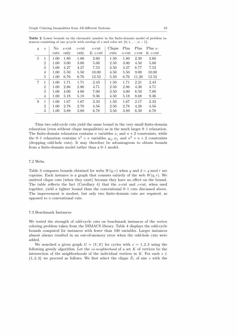
Graph Coloring Inequalities from All-different Systems 23
Table 2 Lower bounds on the chromatic number in the finite-domain model of problem in-stances consisting of one q-cycle with overlap of s and color set {0, 1, . . . , n− 1}.
q s No x-cut z-cut x-cut Clique Plus Plus Plus x-cuts only only & z-cut cuts x-cut z-cut & z-cut
5 1 1.00 1.80 1.80 2.60 1.50 1.80 2.30 2.602 1.00 3.00 3.00 5.00 2.50 3.00 4.50 5.003 1.00 4.27 4.27 7.53 3.50 4.27 6.77 7.534 1.00 5.50 5.50 10.00 4.50 5.50 9.00 10.005 1.00 6.76 6.76 12.52 5.50 6.76 11.26 12.52
7 1 1.00 1.71 1.71 2.43 1.50 1.71 2.21 2.432 1.00 2.86 2.86 4.71 2.50 2.86 4.36 4.713 1.00 4.00 4.00 7.00 3.50 4.00 6.50 7.004 1.00 5.18 5.18 9.36 4.50 5.18 8.68 9.36
9 1 1.00 1.67 1.67 2.33 1.50 1.67 2.17 2.332 1.00 2.78 2.78 4.56 2.50 2.78 4.28 4.563 1.00 3.89 3.89 6.78 3.50 3.89 6.39 6.78
Thus two odd-cycle cuts yield the same bound in the very small finite-domainrelaxation (even without clique inequalities) as in the much larger 0–1 relaxation.The finite-domain relaxation contains n variables xi and n+ 2 constraints, whilethe 0–1 relaxation contains n2 + n variables yij , wj and n2 + n + 2 constraints(dropping odd-hole cuts). It may therefore be advantageous to obtain boundsfrom a finite-domain model rather than a 0–1 model.
7.2 Webs
Table 3 compares bounds obtained for webs W (q, r) when q and d = q mod r arecoprime. Each instance is a graph that consists entirely of the web W (q, r). Weomitted clique cuts (when they exist) because they have no effect on the bound.The table reflects the fact (Corollary 4) that the x-cut and z-cut, when usedtogether, yield a tighter bound than the conventional 0–1 cuts discussed above.The improvement is modest, but only two finite-domain cuts are required, asopposed to n conventional cuts.
7.3 Benchmark Instances
We tested the strength of odd-cycle cuts on benchmark instances of the vertexcoloring problem taken from the DIMACS library. Table 4 displays the odd-cyclebounds computed for instances with fewer than 100 variables. Larger instancesalmost always resulted in an out-of-memory error when the odd-hole cuts wereadded.
We searched a given graph G = (V,E) for cycles with s = 1, 2, 3 using thefollowing greedy algorithm. Let the co-neighborhood of a set K of vertices be theintersection of the neighborhoods of the individual vertices in K. For each s ∈{1, 2, 3} we proceed as follows. We first select the clique S1 of size s with the

24 David Bergman, J. N. Hooker
Table 3 Lower bounds on the chromatic number in a 0–1 formulation of problem instancesconsisting of a web W (q, r). The bound given by the finite-domain formulation is the same asshown below when both cuts are used.
q r Without 0–1 cuts x-cut z-cut x-cut Optimal No. ofcuts only only only & z-cut value 0–1 cuts
5 2 2 2.50 2.00 2.30 2.60 3 5
7 2 2 3.50 2.29 2.79 3.57 4 73 2 2.33 2.00 2.21 2.43 3 7
9 2 2 4.50 2.78 3.28 4.56 5 94 2 2.25 2.00 2.17 2.33 3 9
10 3 2 3.33 2.20 2.70 3.40 4 10
11 2 2 5.50 3.27 3.77 5.55 6 113 2 3.67 2.36 2.86 3.73 4 114 2 2.75 2.00 2.41 2.82 3 115 2 2.20 2.00 2.14 2.27 3 11
largest co-neighborhood (breaking ties arbitrarily). We then progressively build apath S1, S2, . . . by adding cliques Sℓ. For each ℓ, if ℓ is odd, we examine cliquesof size s that have vertices in V \ (S1 ∪ · · · ∪ Sℓ−1) and that continue the path,and select from these a clique Sℓ with the largest co-neighborhood. A clique K
continues the path if all pairs (i, j) ∈ Sℓ−1 × K are edges in E. If ℓ is even, wecheck, for each clique K that continues the path, whether it allows completionof the cycle; that is, whether each pair (i, j) ∈ S1 × K is an edge in E. If so, wegenerate the cycle. (The vertices in S1 ∪ · · · ∪ Sℓ may induce edges that are notin a cycle, but the odd-cycle cuts are still valid.) We then let Sℓ be a clique thatcontinues the path and has the largest co-neighborhood. The process terminateswhen no clique continues the path.
Table 4 compares the bounds obtained from the 0–1 model after adding odd-hole cuts for the cycles found with the bounds obtained after adding 0–1 x-cuts andz-cuts for these same cycles. The 0–1 model in these tests is an edge model withoutclique inequalities, which permits a meaningful comparison of odd-hole and odd-cycle cuts. As noted earlier, odd-hole cuts have little effect in the presence of cliqueinequalities. Thus each set Vk in the 0–1 model (2) consists of the endpoints ofan edge. All odd-hole and odd-cycle cuts are added for each cycle discovered, asopposed to adding only separating cuts. Thus allows us to measure the strengthof the cuts without the complicating effect of a separation algorithm.
The results in Table 4 depend on the problem structure, but the finite-domainodd-cycle cuts obtain tighter bounds in most instances, in some cases substantiallytighter. As one might expect, the advantage is greater when there are cycles withs > 1. The time required to solve the LP relaxation is also consistently less for thefinite-domain cuts (because there are only two of them per cycle), in some casesdramatically less. Additionally, the time required to find the cycles is quite small.
Table 4 also indicates the bounds obtained from lifted odd-hole inequalities(27). The bounds are equal to or somewhat weaker than those obtained from odd-cycle cuts, but the time to solve the LP tends to be much longer. The reason for thisdifference is presumably the number of inequalities, since for each finite-domaincut there are n lifted odd-hole inequalities.
Graph Coloring Inequalities from All-different Systems 25
Table 5 shows results of similar tests using a clique-cover 0–1 model ratherthan an edge model. Here, each set Vk in the 0–1 model (2) consists of the verticesin a clique. Because finding maximal cliques is NP-hard, we used the followingheuristic to generate a clique cover C. Starting with C = ∅, let clique S consistof a single vertex v with the highest positive degree in G. Add to S the vertexwith highest degree in G \ S that is adjacent to all vertices in S, and repeat untilno more additions are possible. At this point, add S to C, remove from G all theedges of the clique induced by S, update the vertex degrees, and repeat the overallprocedure until G has no more edges.
The clique-cover model yields bounds that are sometimes weaker than thoseobtained from the edge model with odd-hole cuts, but often much tighter. Addingodd-cycle cuts to the clique-cover model nonetheless improves the bound in 8 of the23 instances. Interestingly, the presence of odd-cycle cuts almost always reduces theLP solution time, sometimes substantially. This suggests that it is almost alwaysadvantageous to use finite-domain cuts even in a clique-cover model, because theymay improve the bound and are very likely to reduce computation time.
8 Conclusion
We explored the idea of obtaining valid inequalities from a finite-domain formu-lation of a problem that is normally given a 0–1 formulation. We showed thatin the case of graph coloring, this approach yields valid inequalities that providetighter bounds on the chromatic number than known 0–1 cuts for the problem. Inparticular, we identified facet-defining and other valid inequalities for odd cyclesand webs that, when mapped into a 0–1 model, yield a tighter bound than a muchlarger collection of conventional odd-hole and web cuts.
In addition, finite-domain cuts provide the same tight bound in a relaxationof the finite-domain model as in a relaxation of the 0–1 model. If other familiesof finite-domain cuts follow this pattern, there could be advantage in obtainingbounds from a finite-domain relaxation that is much smaller than the 0–1 model.Given that some benchmark instances result in 0–1 models that are too large evento load into a linear solver [14], this could provide a viable alternative for solvinglarge graph coloring and related problems.
The alternate polyhedral perspective afforded by the finite-domain formulationtherefore seems beneficial, at least in the case of graph coloring. The next step isto seek additional families of finite-domain cuts for graph coloring, perhaps corre-sponding to combs, anti-webs, and more general structures. The general strategyof obtaining valid inequalities and tight bounds from finite-domain formulationscan be investigated for other problem classes.
References
1. Appa, G., Magos, D., Mourtos, I.: Linear programming relaxations of multiple all-differentpredicates. In: J.C. Regin, M. Rueher (eds.) Integration of AI and OR Techniques in Con-straint Programming for Combinatorial Optimization Problems (CPAIOR 2004), LectureNotes in Computer Science, vol. 3011, pp. 364–369. Springer (2004)
2. Appa, G., Magos, D., Mourtos, I.: On the system of two all-different predicates. Informa-tion Processing Letters 94, 99–105 (2004)
26 David Bergman, J. N. Hooker
3. Bergman, D., Hooker, J.N.: Graph coloring facets from all-different systems,. In:N. Jussien, T. Petit (eds.) Proceedings of the International Workshop on Integration ofArtificial Intelligence and Operations Research Techniques in Constraint Programming forCombintaorial Optimization Problems (CPAIOR 2012). Springer (to appear)
4. Coll, P., Marenco, J., I. Mendez-Dıaz, Zabala, P.: Facets of the graph coloring polytope.Annals of Operations Research 116, 79–90 (2002)
5. Genc-Kaya, L., Hooker, J.N.: The circuit polytope. Manuscript, Carnegie Mellon Univer-sity (2010)
6. Ghouila-Houri, A.: Caracterisation des matrices totalement unimodulaires. Comptes ren-dus de l’Academie des Sciences de Paris 254, 1192–1194 (1962)
7. Hooker, J.N.: Logic-Based Methods for Optimization: Combining Optimization and Con-straint Satisfaction. Wiley, New York (2000)
8. Hooker, J.N.: Integrated Methods for Optimization, 2nd edition. Springer (2012)9. Kruk, S., Toma, S.: On the system of the multiple all different predicates. Congressus
Numerantium 197, 47–64 (2009)10. Kruk, S., Toma, S.: On the facets of the multiple alldifferent constraint. Congressus
Numerantium 204, 5–32 (2010)11. Magos, D., Mourtos, I.: On the facial structure of the alldifferent system. SIAM Journal
on Discrete Mathematics 25(1), 130–158 (2011)12. Magos, D., Mourtos, I., Appa, G.: A polyhedral approach to the alldifferent system. Math-
ematical Programming 132, 209–260 (2012)13. Mendez-Dıaz, I., Zabala, P.: A polyhedral approach for graph coloring. Electronic Notes
in Discrete Mathematics 7, 178–181 (2001)14. Mendez-Dıaz, I., Zabala, P.: A cutting plane algorithm for graph coloring. Discrete Applied
Mathematics 156, 159–179 (2008)15. Nemhauser, G.L., Wolsey, L.A.: Integer and Combinatorial Optimization. Wiley, New
York (1999)16. Palubeckis, G.: On the graph coloring polytope. Information Technology and Control 37,
7–11 (2008)17. Williams, H.P., Yan, H.: Representations of the all different predicate of constraint satis-
faction in integer programming. INFORMS Journal on Computing 13, 96–103 (2001)18. Yan, H., Hooker, J.N.: Tight representations of logical constraints as cardinality rules.
Mathematical Programming 85, 363–377 (1995)19. Yunes, T.H.: On the sum constraint: Relaxation and applications. In: P. Van Hentenryck
(ed.) Principles and Practice of Constraint Programming (CP 2002), Lecture Notes inComputer Science, vol. 2470, pp. 80–92. Springer (2002)

Graph Coloring Inequalities from All-different Systems 27Table
4Lower
boundson
thech
romaticnumber
ina0–1ed
geform
ulation
ofben
chmark
instanceswith
nverticesand
med
ges,based
on
odd-hole
cuts,lifted
odd-hole
cuts,andfinite-domain
odd-cyclecu
ts.Number
ofodd-hole
cuts
gen
eratedandnumber
ofcy
cles
found(fors=
1,2
,3)are
shown,
asare
thetimein
seco
ndsrequired
tofindth
ecy
cles
andsolveth
eLP
relaxations.
Bound
No.
No.cycles
found
Cycle
LP
Tim
e(sec)
Instance
nm
Odd
Lifted
Odd
Opt
odd
heu
r.Odd
Lifted
Odd
hole
hole
cycle
holes
s=
1s=
2s=
3time
hole
hole
cycle
1-Fulllns3
30
100
2.00
2.00
2.00
3540
18
00
0.00
0.4
1.0
0.1
1-Fulllns4
93
593
2.00
2.00
2.00
45673
61
00
0.09
208.0
23.1
0.4
1-Insertions4
67
232
1.33
1.33
1.43
43216
48
00
0.03
30.3
24.8
2.0
2-Fulllns3
52
201
2.00
2.00
2.00
4936
18
00
0.02
0.9
0.6
0.8
2-Insertions3
37
72
1.25
1.25
1.33
3296
80
00.00
2.9
4.0
0.2
3-Fulllns3
80
346
2.00
2.00
2.00
52000
25
00
0.06
25.8
6.4
0.2
3-Insertions3
56
110
1.20
1.20
1.27
4560
10
00
0.02
11.5
24.1
1.6
4-Insertions3
79
156
1.17
1.17
1.23
3948
12
00
0.05
12.1
91.6
2.6
dav
id87
406
2.00
8.00
8.00
10
74211
103
48
10
0.27
11.0
18.9
0.2
huck
74
301
2.00
8.00
8.00
10
29822
71
28
40.14
7.2
8.0
0.1
jean
80
254
2.00
8.00
8.00
10
19360
26
08
0.17
10.2
21.8
2.1
mug881
88
146
2.00
2.00
2.00
3176
20
00.08
7.8
38.5
1.8
mug8825
88
146
2.00
2.00
2.00
3352
40
00.07
5.3
36.7
2.1
myciel3
11
20
1.50
1.50
1.60
344
40
00.00
0.0
0.0
0.0
myciel4
23
71
1.50
1.50
1.60
4414
18
00
0.00
0.6
0.8
0.0
myciel5
47
236
1.50
1.50
1.60
52115
45
00
0.01
7.9
3.6
0.1
myciel6
95
755
1.50
1.50
1.60
614535
153
00
0.09
1754.7
376.1
0.4
queen55
25
160
2.00
2.00
2.00
41175
47
00
0.00
0.4
0.4
0.1
queen66
36
290
2.00
5.00
5.00
62628
65
10
0.01
1.5
1.3
0.1
queen77
49
476
2.00
3.67
3.71
611417
105
10
0.04
10.6
6.4
0.1
queen88
64
728
*3.33
3.38
8*
133
50
0.08
*68.5
0.3
queen812
96
1368
2.00
8.00
8.00
11
104544
229
31
20
0.41
439.6
272.8
0.9
queen99
81
1056
2.00
8.00
8.00
969660
193
21
0.21
212.4
74.2
0.5
∗LP
solverra
noutofmemory.

28 David Bergman, J. N. Hooker
Table
5Lower
boundsonth
ech
romatic
number
ina0–1cliq
uecover
form
ulatio
nofben
chmark
insta
nces
with
nvertices
andm
edges,
based
onth
ecliq
uecover
model
aloneandth
ecliq
uecover
model
plusfinite-d
omain
odd-cy
clecu
ts.Thenumber
ofcy
clesfound(fo
rs=
1,2
,3)is
shown,asare
the
timein
secondsreq
uired
tofindcliq
ues,
findcy
cles,andsolveth
eLP
relaxatio
ns.
Bound
No.cycles
found
Heu
risticLP
Tim
e(sec)
Insta
nce
nm
Cliq
ue
+Odd
Opt
time(sec)
Cliq
ue
+Odd
model
cycle
s=
1s=
2s=
3cliq
ue
cycle
model
cycle
1-Fullln
s3
30
100
2.00
2.00
318
00
0.00
0.00
0.78
0.3
1-Fullln
s4
93
593
2.00
2.00
461
00
0.02
0.09
101.7
3.8
1-In
sertions4
67
232
1.00
1.43
448
00
0.00
0.03
20.3
2.0
2-Fullln
s3
52
201
3.00
3.00
418
00
0.00
0.02
10.4
2.5
2-In
sertions3
37
72
1.00
1.33
38
00
0.00
0.00
0.8
0.1
3-Fullln
s3
80
346
4.00
4.00
525
00
0.01
0.06
1.7
1.3
3-In
sertions3
56
110
1.00
1.27
410
00
0.00
0.02
7.2
0.6
4-In
sertions3
79
156
1.00
1.23
312
00
0.00
0.05
5.1
5.7
dav
id87
406
10.00
10.00
10
103
48
10
0.00
0.27
9.6
7.6
huck
74
301
10.00
10.00
10
71
28
40.00
0.14
6.6
2.8
jean
80
254
8.00
8.00
10
26
08
0.00
0.17
39.4
12.5
mug881
88
146
2.00
2.00
32
00
0.00
0.08
18.1
14.0
mug8825
88
146
2.00
2.00
34
00
0.00
0.07
33.7
6.9
myciel3
11
20
1.00
1.60
34
00
0.00
0.00
0.0
0.0
myciel4
23
71
1.00
1.60
418
00
0.00
0.00
0.2
0.0
myciel5
47
236
1.00
1.60
545
00
0.00
0.01
1.3
0.1
myciel6
95
755
1.00
1.60
6153
00
0.03
0.09
64.0
0.8
queen
55
25
160
4.00
4.00
447
00
0.00
0.00
0.9
1.4
queen
66
36
290
5.00
5.00
665
10
0.00
0.01
2.3
0.6
queen
77
49
476
6.00
6.00
6105
10
0.00
0.04
4.9
5.8
queen
88
64
728
7.00
7.00
8133
50
0.00
0.08
22.4
16.4
queen
812
96
1368
11.00
11.00
11
229
31
20
0.00
0.41
168.5
275.2
queen
99
81
1056
8.00
8.00
9193
21
0.01
0.21
68.4
15.3