GPU-based Graph Traversal on Compressed GraphsMo Sha

School of Computing

National University of Singapore

sham@comp.nus.edu.sg

Yuchen Li

School of Information System

Singapore Management University

yuchenli@smu.edu.sg

Kian-Lee Tan

School of Computing

National University of Singapore

tankl@comp.nus.edu.sg

ABSTRACTGraph processing on GPUs received much attention in the

industry and the academia recently, as the hardware acceler-

ator offers attractive potential for performance boost. How-

ever, the high-bandwidth device memory on GPUs has lim-

ited capacity that constrains the size of the graph to be loaded

on chip. In this paper, we introduce GPU-based graph tra-

versal on compressed graphs, so as to enable the processing

of graphs having a larger size than the device memory. De-

signed towards GPU’s SIMT architecture, we propose two

novel parallel scheduling strategies Two-Phase Traversal andTask-Stealing to handle thread divergence and workload im-

balance issues when decoding the compressed graph. We

further optimize our solution against power-law graphs by

proposing Warp-centric Decoding and Residual Segmentationto facilitate parallelism on processing skewed out-degree

distribution. Extensive experiments show that with 2x-18x

compression rate, our proposed GPU-based graph traver-

sal on compressed graphs (GCGT) achieves competitive effi-

ciency compared with the state-of-the-art graph traversal

approaches on non-compressed graphs.

ACM Reference Format:Mo Sha, Yuchen Li, and Kian-Lee Tan. 2019. GPU-based Graph Tra-

versal on Compressed Graphs. In 2019 International Conference onManagement of Data (SIGMOD ’19), June 30-July 5, 2019, Amsterdam,Netherlands. ACM, New York, NY, USA, 18 pages.

https://doi.org/10.1145/3299869.3319871

1 INTRODUCTIONGraph analysis is a powerful tool to unveil hidden patterns

and knowledge from complex data with a sparse schema. To

meet the demand for analyzing large-scale graphs emerging

from a wide range of applications, e.g., social networks, web

Permission to make digital or hard copies of all or part of this work for

personal or classroom use is granted without fee provided that copies

are not made or distributed for profit or commercial advantage and that

copies bear this notice and the full citation on the first page. Copyrights

for components of this work owned by others than the author(s) must

be honored. Abstracting with credit is permitted. To copy otherwise, or

republish, to post on servers or to redistribute to lists, requires prior specific

permission and/or a fee. Request permissions from permissions@acm.org.

SIGMOD ’19, June 30-July 5, 2019, Amsterdam, Netherlands© 2019 Copyright held by the owner/author(s).

Publication rights licensed to ACM.

ACM ISBN 978-1-4503-5643-5/19/06. . . $15.00

https://doi.org/10.1145/3299869.3319871

graphs, transaction networks and many others, there is a pre-

vailing interest in developing parallel algorithms to empower

efficient or even real-time graph analysis [18, 25, 47, 51].

Meanwhile, the exceptional advances of General-Purpose

GPUs (GPGPUs) have completely revolutionized the comput-

ing paradigm across multiple fields [34]. Massive number of

cores and ultra memory bandwidth make GPUs a promising

platform for accelerating graph processing. Existing efforts

have shown great success in parallelizing graph algorithms

on GPUs, such as BFS [30, 33, 46], PageRank [15, 37, 49],

Connected Component [2, 42], Betweenness Centrality [44],

Graph Label Propagation [43], etc.

The acceleration enabled by GPUs, however, does not

come for free. When the graph size exceeds the GPU device

memory, costly data transfer between CPUs and GPUs is

inevitable. Unlike the RAM architecture, the device memory

is fixed in the printed circuit board (PCB) and cannot be

extended. The memory size of mainstream GPUs is typically

at most 12 GB, which translates to storing graphs with two

billion edges at best. There have been several strategies pro-

posed to support processing graphs with a size larger than

the device memory: the out-of-core strategy [26, 36, 39] that

divides data into tiles and overlaps the data transfer with

GPU computation to hide the communication overhead, the

multi-GPU strategy [3, 32, 35, 50] as well as the distributed

GPU cluster strategy [17, 21, 46]. In this paper, we propose an

orthogonal approach to further expand the capability of GPU

graph processing. The high level idea is rather intuitive: we

execute the GPU workloads on a compressed graph and only

decode necessary data into caches to limit the memory usage.

Since graph processing tasks are mostly bounded by mem-

ory accesses, we leverage on the massive computing power

of GPUs to hide the decoding cost and retain the perfor-

mance as that in the uncompressed scenario. Given that the

market price of GPU device with a large memory size is ex-

pensive, e.g., GV100 with 32GB device memory costs $9,000

per device, our proposed approach reduces the pressure of

memory usage for single-GPU environment. The benefits

carry over when one resorts to the multi-GPU environment

or the distributed environment.

However, this seemingly intuitive idea brings non-trivial

technical challenges. The key strategy of processing graphs

on GPUs is to evenly distribute the neighbor nodes of an

adjacency list into balanced workloads assigned to multiple

threads. This does not hold if graphs are stored in a com-

pressed manner, since the threads are unable to identify the

neighbor nodes from their compressed form directly. This is

rather challenging for scheduling GPUs’ workloads for three

major reasons. First, it is difficult to estimate the workload

in advance for assigning threads in a balanced manner, in

contrast to processing uncompressed graphs. Second, it is

challenging to dynamically reschedule the workload for mas-

sive GPU threads as compared to the CPU environment since

each single processing unit of GPUs contains minimum num-

ber of control units and is far less powerful as compared to

one CPU core. Third, we need to bound the decoding process

within GPU’s cache to ensure that the performance does not

degrade compared with the uncompressed scenario, as de-

coding into global memory is prohibitively expensive. To ad-

dress the aforementioned challenges, we proposeGPU-basedCompressed Graph Traversal (GCGT), an in-cache scheme to

traverse the compressed graph representation (CGR) storedin GPU’s device memory.

A direct parallel approach assigns a thread to decode a

compressed adjacency list. However, such direct approach

renders severe thread divergence issue since concurrent

threads may end up in diverging control branches when

decoding different segments of the compressed adjacency

lists. Thus, we propose GPU-oriented scheduling strategies

under GCGT: Two-Phase Traversal and Task-Stealing. Two-Phase Traversal explicitly synchronizes thread groups and

ensures the threads entering the same control branch while

decoding their respective adjacency lists.When a few threads

are heavily loaded, we employ Task-Stealing: the working

threads push their extra workload to the shared memory

and the idle threads then steal the workload for better GPU

utilization. Furthermore, we observe that the skewed distri-

bution of power-law graphs leads to the workload imbalance

problem and our proposed scheduling strategies only achieve

sub-optimal results as they are structure-transparent. To sup-

port power-law graphs, we first propose a novelWarp-centricDecoding to effectively parallelize the decoding process. Sec-

ond, we partition long adjacency lists into segments and

devise a Residual Segmentation strategy for threads to better

collaborate under GCGT. To the best of our knowledge, this

is the first study on how to traverse compressed graphs of

its kind on GPUs.

The contributions of this paper are summarized as follows:

• We introduce GCGT, a novel scheme to enable GPUs for

traversing compressed graph representation (CGR) directly.We propose Two-Phase Traversal and Task-Stealing strate-

gies to reduce thread divergence while decoding adjacency

lists in parallel.

• We devise novel Warp-centric Decoding and Residual Seg-mentation optimizations to support efficient power-law

graph processing under GCGT.

• We conduct an extensive experimental study on various

types of graph datasets in different scales. The experimen-

tal results reveal that GCGT achieves 2x-18x compression

rate while producing competitive efficiency against the

state-of-the-art GPU graph traversal approaches.

The rest of this paper is organized as follows. In Section 2,

we review existing related studies. Then in Section 3, we

present the preliminaries. Section 4 demonstrates the pro-

posed GPU-based compressed graph traversal algorithms

and Section 5 discusses the optimizations for power-law

graphs. We discuss how to extend GCGT to other graph ap-

plications in Section 6. Next, we present the experimental

evaluation in Section 7 and finally, we conclude in Section 8.

2 RELATEDWORKWe survey some related studies in this section. First, we

discuss the literature on GPU-based graph processing. Then,

we review existing methods for graph compression.

2.1 GPU-based Graph ProcessingEmerging trends for GPU computing have influenced a wide

range of data-intensive and compute-intensive tasks, includ-

ing large-scale graph processing. There are a plethora of

recent studies which focus on developing efficient parallel

computational frameworks for graph processing on GPUs.

Medusa [51] is the first framework to support general graph

processing on GPUs. It provides a set of user-defined APIs, on

top of which the users express their sequential programs and

Medusa does the automatic scheduling on GPUs. CuSha [25]

is a node-centric graph processing platform and is based on

G-Shards, a static GPU-friendly graph data representation

designed for higher memory access efficiency. GPMA [38]

proposes a dynamic graph analytic framework on GPUs,

where both graph updates and graph processing are effi-

ciently supported. Gunrock [47] offers a higher-level abstrac-

tion than Medusa, which corresponds to an operation on the

nodes or edges in graphs. These GPU-based graph processing

frameworks make it simpler to program GPUs for general

graph computation and at the same time, achieve superior

speedups compared with the multi-core CPU systems.

In addition to the aforementioned general frameworks,

a variety of typical graph problems have been investigated

for GPU acceleration [2, 15, 20, 29, 37, 42, 43, 49]. In particu-

lar, Breath First Search (BFS) has been extensively studied

lately [17, 30, 33, 46]. Parallelizing BFS-style graph traversal

on GPUs mostly follows the expansion - filtering - contractioncomputational pipeline. To be specific, such graph compu-

tation is based on ping-pong frontier queues in an iterative

manner. In each round, the out-degrees of frontiers in in-

Queue are traversed, then filtered by application-specific

requirements and finally placed into outQueue. In this work,

we propose GCGT to parallelize BFS traversal on compressed

graph representations (CGR) stored in GPUs. GCGT is not lim-

ited to BFS since its computation pipeline generalizes to a

wide range of parallel graph algorithms on GPUs, such as

Connected Component [42], Betweenness Centrality [44],

Personalized PageRank [20] and Label Propagation[43].

The main concern of processing BFS on GPU stems from

irregular memory accesses. For one thing, frontiers to be

handled in each iteration are generally distributed randomly,

which leads to uncoalesced memory accesses. For another,

the out-degrees of frontiers are skewed (in most real-world

datasets, they follow the power-law distribution). This gives

rise to thread divergence and results in degradation of the

core utilization [45]. To alleviate these issues, existing studies

rely on adaptively distributing the out-degrees of frontiers

to thread groups of variable sizes [30, 33]. However, traver-

sal on CGR incurs a greater challenge since the workloads

cannot be easily estimated before decompression. One naïve

solution decompresses the out-degrees of frontiers in the

device memory and then employs existing optimizations to

evenly distribute the workloads to threads. However, this

trivial solution not only results in frequent device memory

accesses at a high latency but also potentially takes O(E)space, which defeats the purpose of utilizing CGR in the first

place. Thus, different from this trivial solution, GCGT pro-

poses a set of novel approaches to decompress and process

frontier neighbors entirely in the GPU cache.

2.2 Graph CompressionExisting graph compression techniques can be broadly clas-

sified into two categories: (i) reduce the number of edges

through introducing auxiliary structures; (ii) for a certain

given edge list, use fewer bits in the representation. It is

noted that the categories are orthogonal to each other and

can be applied together.

Category (i). Virtual Node Compression [10] is one of the

most popular graph compression approaches that introduce

auxiliary structures. It searches for frequent patterns of nodes

appearing in the adjacency lists and replaces them with vir-

tual nodes. Such an approach can effectively reduce the num-

ber of edges and retain the equivalent graph topology. Virtual

node compression attracts several follow-up studies on graph

processing [11, 24] due to its good compatibility and proven

effectiveness, especially on web graphs. Similarly, N. Larsson

et al. propose Re-Pair [28], which replaces a frequent pair

of symbols with a new symbol repeatedly as a grammar-

compression approach. Based on this study, F. Claude et

al. [13] introduce Re-Pair to the area of graph compression

to reduce the number of stored edges.

Category (ii). Compressed graph representation (CGR) fo-

cuses on minimizing the number of bits required to represent

a graph. BV [7, 8] is a widely adopted technique to compress

web graphs [31], and it supports general graph data as well.

BV takes advantage of the similarity and locality in graph

data, reuses the redundant information in the areas which

are close to each other in the graph, and then records data via

VLC in order to compress the bits per edge. In the meanwhile,

a number of node reordering techniques have been proposed

to achieve higher compression rate on top of the BV encod-

ing scheme. Apostolico et al. [1] study the encoding and the

compression of graphs based on node indices assigned by

the BFS order. In Shingle [12], it is argued that the algorithm

of finding the optimal encoding scheme so as to achieve the

minimal bits per edge has a high complexity, and then an

approximate optimization algorithm based on MinHash is

proposed. Subsequently, in BP [14], an extension of Shingle,

it is shown that finding the optimal encoding scheme is NP-

hard and an improved, approximate optimization algorithm

on the basis of recursive graph bisection is devised. Slash-

Burn [23] removes the Hub nodes in the graph structure so

that it can obtain an encoding scheme with better locality.

Similarly, LLP [5] aims to obtain clusters with similarity in

the graph structure in a layered label propagation manner.

Furthermore, a fixed-length compression approach [22] is

proposed to represent integers in a tight fixed-length manner.

Specifically, it sets the length of integer as short as possible

on the premise that the number of nodes in a graph does not

overflow. However, its effectiveness is constrained by the

range of the represented values, which renders the approach

unable to scale to large graphs with millions of nodes.

Summary. Existing studies devise optimization specific to

different types of graphs and achieve a satisfactory compres-

sion rate. The proposed GCGT is orthogonal to existing graphcompression techniques since we focus on how to efficiently

process graph traversals on the compressed format directly.

In other words, existing compression techniques may serve

as a preprocessing step for GCGT. Henceforth, we carefullyexamine the trade-off between the compression rate of ex-

isting work and the efficiency of our proposed techniques

working with these compression schemes.

3 PRELIMINARIESIn this section, we start with introducing the background

knowledge of CGR. Next, we present an overview of our GPU-

based compressed graph traversal (GCGT). Readers can get

more information on the computational architecture of GPUs

in Appendix A.

3.1 Compressed Graph Format on GPUsGiven a graph G = (V , E) (either directed or undirected),

V is the node set and E is the edge set. Let OutDeg(u) ={v ∈ V |(u,v) ∈ E} denote node u’s out-degree in G. Ingraph applications, Compressed Sparse Row (CSR) is one of

0 1 2

3 4 5

6 7

0 0 0 1 1 1 2 5 5 61 3 4 2 4 5 5 6 7 7

0 1 2 3 4 5 6 70 3 6 7 7 7 9 10

1 3 4 2 4 5 5 6 7 7

(a) Example Graph

(b) Edge List

(c) CSR

Node IDRow Offset

Col Index

Figure 1: An example of CSR format.

the most frequently used graph format, which is to record

each node’s out-degree neighbors compactly as illustrated

in Figure 1. In CSR, E integers (assuming 32 bit integers) are

needed to represent a graph. To further reduce the storage

usage of the graph, we employ CGR so that each edge takes

fewer than 32 bits.

In this work, graph data is stored in the CGR format, and it

follows the three steps shown below to convert the raw graph

data represented in the traditional adjacency list format into

the CGR format: (i) Intervals and Residuals Representation,

(ii) Gap Transformation, and (iii) VLC Encoding. In the fol-

lowing, we introduce some details about these three steps to

facilitate our presentation on GPU graph traversal on CGR in

subsequent technical sections.

Intervals and Residuals Representation. For many real-

world graphs, the adjacency list of each node exhibits the

locality characteristic to some extent. This means for a cer-

tain node, its neighbors do not distribute uniformly, but tend

to form a number of clusters and the neighbors in the same

cluster tend to have close indices. Hence, it is possible for the

ordered neighbor sequence to form several sub-sequences

with consecutive node indices, called intervals. As a con-

sequence, we can denote a node’s adjacency list with two

sequences, i.e., Intervals and Residuals Representation. For

the neighbors covered in the sub-sequences with consecu-

tive node indices in the adjacency list, we represent them

as an interval with the starting node and the corresponding

length. All intervals compose the interval sequence. For the

neighbors which cannot form intervals, we need to record

them separately in the residual sequence.

Gap Transformation. After Intervals and Residuals Rep-

resentation, each node’s adjacency list is represented as an

interval sequence and a residual sequence. For each sequence,

we transform it into the differential sequence of the original

sequence, that is to denote each element as the difference be-

tween itself and its preceding element. This process is called

Gap Transformation. The target of Gap Transformation is to

decrease the absolute value of each number in the sequence

while maintaining the original information amount. After

such transformation, we can record the equivalent sequence

Original Adjacency List:16: 12, 18, 19, 20, 21, 24, 27, 28, 29, 101

Interval 0 Interval 1Intervals and Residuals Representation:

10, 2, (18, 4), (27, 3), 12, 24, 101degNum itvNum itv0 itv1 res0 res1 res2

Gap Transformation:10, 2, (2, 4), (6, 3), -4, 12, 77

degNum itvNum itv0 itv1 res0 res1 res2

VLC Encoding:0 0 0 1 0 1 0 0 1 0 0 0 1 0 0 0 0 1 0 0 0 0 1 1 0 0 1 1 0 0 0 1 0 0 1 0 0 0 1 1 0 0 0 0 0 0 0 0 1 0 0 1 1 0 1

10 2 2 4 6 3 -4 12 77Figure 2: An example of CGR format.

information with fewer bits via the VLC encoding technique

introduced below.

Variable-Length Code (VLC) Encoding. VLC is widely

used in various data compression scenarios. Compared with

fixed-length encoding, VLC can vary the number of bits

needed to represent an element. VLC works well for com-

pressing power-law graphs [8] since the distribution of ele-

ments in such graphs are skewed, in which case VLC uses a

smaller number of bits to encode the more frequent elements

in order to compress the overall size.We refer interested read-

ers to Appendix B for some more details on VLC Encoding

involved in this work.

To achieve better compression results, we combine the

aforementioned approaches to encode the adjacency lists.

An illustrative example is given as follows.

Example 3.1. In Figure 2, we demonstrate how to com-

press the adjacency list of node16 which has 10 neighbors.

In its sorted form, the adjacency list contains 2 intervals and

3 individual nodes called residuals. We employ the encoding

scheme as follows. First, this scheme stores the number of

neighbors degNum in node16’s adjacency list. Then it records

the number of intervals itvNum. Next, the encoding is fol-

lowed by itvNum tuples and each tuple contains the starting

node’s index and the interval length. In each interval, the

starting node is represented using the gap value from the pre-

vious interval’s ending node, and the first interval’s starting

node is denoted using the gap value from node16. Hence, the

first interval’s starting node is node18 with a corresponding

gap value (from node16) of 2. The second interval’s starting

node is node27, and its gap value from the first interval’s

ending node21 is 6. After these two intervals, this scheme

encodes the remaining residuals (due to degNum, there is no

need to record the number of residuals). Except for the first

residual, which is represented with a gap value from node16,

the other residuals are all described using gap values from

the corresponding preceding residuals. Finally, this scheme

101001101 . . . . 01110Node 1 Node n. . . .

Parallel In-Cache Traversal

GPUMutiple Streaming Processors

CGR in Device Memory101001101 . . . . 01110Node 1

CPU

Node n. . . .

Graph Compression Module

Graph Traversal Queries

PCIeTransfer

PCIeTransfer

Figure 3: GCGT overview.

uses VLC to encode this node16’s adjacency list from the

compressed format explained above into a compressed bit

array1. From this example, we can find that the original ad-

jacency list which requires 10 integers (i.e., 320 bits) in the

representation, can be denoted with only 55 bits on CGR.

Furthermore, the compression rate is highly dependent

on the Node Reordering techniques since they alter the local-

ity property of the graph to be compressed. Given a graph

G = (V , E), node reordering is a bijection σ : V → V ,which assigns a new labelling to all nodes in the graph, i.e.,

G ′ = (V , E ′ = {(σ (v),σ (u))|(v,u) ∈ E}). We employ several

reordering algorithms in this work to improve the locality of

graphs for higher compression rates, which will be discussed

in Section 7 and Appendix D.

3.2 GCGT OverviewThe overview of the proposed GCGT is illustrated in Figure 3.

The graph is compressed in CPU and transferred to GPU’s

device memory. CPU issues graph traversal queries (e.g.,

BFS) by invoking GPU kernels. GCGT allows the storing and

processing of larger graphs on GPUs with the help of com-

pression. Even when the compressed graph cannot entirely

reside in the device memory, CGR reduces the PCIe transfercost since we can directly move the compressed adjacency

lists to GPUs and process themwithout decompression in the

device memory. For graph processing, GCGT effectively hides

the additional overhead of dealing with compressed data

while traversing the graph, by leveraging massive parallel

threads on GPUs. In each iteration of the traversal, a number

of threads collaborate in processing the neighbor list of a

frontier node and outputting qualified neighbors (e.g., unvis-

ited nodes for BFS) to the frontier of the next iteration. It is

noted that, for traversal on the CGR format, we only decode

and process the adjacency lists in the cache of GPU’s cores.

To achieve load balancing, we propose a number of novel

strategies on dynamically assigning threads to collaborate,

which will be extensively discussed in Sections 4 and 5.

1We refer interested readers to Appendix C for the implementation details

of CGR encoding.

4 GPU-BASED COMPRESSED GRAPHTRAVERSAL GCGT

Existing parallel graph traversal approaches on uncompressed

graphs assume all neighbor nodes are immediately available

for parallel processing. Hence, it is rather straightforward for

existing approaches to predict the workload and launch ap-

propriate number of threads that access the neighbor lists of

frontier nodes concurrently. However, such assumption does

not hold if the neighbor lists are encoded in VLC. VLC poses

significant challenges for efficient graph traversal processing

onGPUs since it is difficult to generate balancedworkloads in

the decoding stage (inherently serial) to feed massive threads

on GPUs. Moreover, the architecture of GPUs does not favor

complex scheduling to adjust the workloads dynamically.

Thus, in this section, we first introduce an intuitive solu-

tion which assigns threads to process compressed adjacency

lists independently (Section 4.1). Subsequently, we propose

a Two-Phase Traversal strategy which schedules the pro-

cessing of the interval segments and residual segments into

separate phases, so as to eliminate thread divergence caused

by threads in the same warp entering different control logics

of the interval and residual segments (Section 4.2). Finally,

we devise a Task-Stealing optimization to deal with work-

load imbalance caused by processing in parallel adjacency

lists with skewed lengths of residual segments (Section 4.3).

4.1 Parallel Graph Traversal on CGRTypically, approaches for parallel graph traversal based on

ping-pong frontier queues are executed in an iterative man-

ner. The initial node(s) are placed into inQueue before the

traversal starts. In each iteration, a thread takes its assigned

frontiers from inQueue, inspects all neighbors from a fron-

tier’s adjacency list, and then pushes any unvisited neighbors

to outQueue. outQueue replaces inQueue for the new fron-

tier queue in the next iteration. Intuitively, a natural solution

for GCGT is to assign a thread to process the adjacency list

of a frontier: each thread independently accesses the com-

pressed bit arrays of the CGR-format adjacency lists (of those

frontiers assigned to it), decodes the neighbors one by one

and then pushes unvisited ones to outQueue if necessary.

We present this intuitive solution for GCGT in Algorithm 1.

Procedure BfsBasic is the main procedure which aims to

output the unvisited neighbors of inQueue’s frontiers to

outQueue, and use them as the input frontiers in the next

iteration. Since the algorithm runs in the SIMT manner, the

same instructions are executed in parallel within a threadgroup and each thread’s behavior is characterized by thread-

Num (how many threads in the thread group) and threadId

(the thread’s ID in the thread group). Each thread is assigned

a frontier from inQueue according to its own threadId (i.e., u

in line 4). The thread then decodes u’s compressed adjacency

Algorithm 1 Intuitive Solution for GCGT

1: procedure BfsBasic(inQueue[], outQueue[])2: offset := 0

3: while offset + threadId < inQueue.size do4: u := inQueue[offset + threadId]

5: bitPtr := bitStart[u]

6: degNum = decodeNum(bitPtr)

7: while degNum−− do8: v := getNextNeighbor(u, bitPtr)

9: appendIfUnvisited(v, outQueue)

10: offset += threadNum

11: function getNextNeighbor(u, bitPtr)

12: if first call then13: itvNum := decodeNum(bitPtr)

14: curItvPtr := u

15: curItvLen := 0

16: curRes := u

17: if curItvLen then18: return curItvPtr++, curItvLen -= 1

19: if itvNum then20: curItvPtr += decodeNum(bitPtr)

21: curItvLen := decodeNum(bitPtr)

22: itvNum -= 1, curItvLen -= 1

23: return curItvPtr++

24: return curRes += decodeNum(bitPtr)

25: procedure appendIfUnvisited(v, outQueue[])26: __shared__ outputOffset27: flag := unvisited(v) ? 1 : 0

28: scatter, total := exclusiveScan(flag)

29: if threadId == 0 then30: outOffset := outQueue.atomicAdd(total)

31: if flag then32: outQueue[outputOffset + scatter] := v

list as if it is running in serial. When a neighbor (i.e., v in

line 8) is decoded, the thread appends it to outQueue if the

node is unvisited (line 9).

Function decodeNum maintains the position of the bit

pointer (bitPtr), decodes a number from the compressed bit

array as the returned value and then updates the position of

bitPtr. Function getNextNeighbor demonstrates the pro-

cess of decoding the adjacency list in a serial manner. Specif-

ically, there are three possible scenarios when decoding the

next neighbor: (i) in the middle of an interval (lines 17-18),

(ii) in the beginning of an interval (lines 19-23), and (iii) in

the residual segment (line 24).

The aforementioned functions handle the decoding pro-

cess, where the threads operate on their own without any

conflicts. However, race condition occurs when multiple

threads concurrently append nodes to update outQueue

(line 9). Function appendIfUnvisited is a common tech-

nique to alleviate contention for concurrent frontier updates

on GPUs [33]. The idea is to communicate between threads

in the same CTA so as to reduce the number of atomic oper-

ations when outputting the unvisited nodes to outQueue.

To be specific, each thread first marks its current node vas either visited (0) or unvisited (1) and then invokes ex-clusiveScan2

to obtain the number of unvisited nodes to

push to outQueue in the same CTA (i.e., total) as well the

outputting position in outQueue for each thread (i.e., scat-

ter). The contention is reduced since only one thread from

the CTA calls an atomic operation to allocate the space in

outQueuewhile other threads can safely push their updates

without locking.

4.2 Two-Phase TraversalWe would like to highlight that the intuitive solution pre-

sented in Algorithm 1 is rather expensive to deploy on GPUs

due to severe thread divergence caused by Function get-NextNeighbor. Since all adjacency lists are divided into

interval and residual segments, it is likely that two threads

in the same warp working on different types of segments

try to get their next neighbor decoded simultaneously. As a

consequence, these two threads should end up in diverging

branches of Function getNextNeighbor. Given that any

warp executes instructions in a physically synchronous man-

ner on GPUs, the threads decoding the interval segments

are completely idle waiting for threads decoding the residual

segments to finish. In order to alleviate thread divergence,

we propose a Two-Phase Traversal strategy to decode the

adjacency lists, where we handle the interval segment and

the residual segment in two separate phases.

We present the Two-Phase Traversal strategy in Algo-

rithm 2. The decoding of the interval segment and that of the

residual segment are handled by Procedure handleInter-vals and Procedure handleResiduals respectively. Proce-dure handleIntervals calls Procedure expandIntervalto expand each interval collaboratively by a thread group

(line 16). Algorithm 2 has two distinguishing advantages

over Algorithm 1: (1) better memory access patterns: a thread

group jointly handles consecutive neighbors of one inter-

val at a time, whereas each thread in Algorithm 1 indepen-

dently loads different intervals causing uncoalesced memory

accesses; (2) less thread divergence: Procedure expandIn-terval synchronizes the thread group once an interval is

2Function exclusiveScan is a common primitive on GPUs. When called

by multiple threads, it will see the arguments from each thread as an ar-

ray ordered according to threadId, and then compute the prefix sum of

the array. There are two returned values, scatter and total, representing

sum(input[0..threadId-1]) and sum(input) respectively.

Algorithm 2 GCGT Two-Phase Traversal

1: procedure TwoPhrase(inQueue[], outQueue[])

2: offset := 0

3: while offset + threadId < inQueue.size do4: u := inQueue[offset + threadId]

5: bitPtr := bitStart[u]

6: degNum = decodeNum(bitPtr)

7: handleIntervals(u, degNum, bitPtr)

8: handleResiduals(u, degNum, bitPtr)

9: procedure handleIntervals(u, degNum, bitPtr)

10: itvNum := decodeNum(bitPtr)

11: curItvPtr := u

12: while itvNum−− do13: curItvPtr += decodeNum(bitPtr)

14: curItvLen := decodeNum(bitPtr)

15: degNum -= curItvLen

16: expandInterval(curItvPtr, curItvLen)

17: procedure handleResiduals(u, degNum, bitPtr)

18: curRes := u

19: while degNum−− do20: curRes += decodeNum(bitPtr)

21: appendIfUnvisited(curRes, outQueue)

22: procedure expandInterval(curItvPtr, curItvLen)23: __shared__ winnerId24: while syncAny(curItvLen ≥ threadNum) do25: if curItvLen ≥ threadNum then26: winnerId := threadId

27: winnerItvPtr := shfl(curItvPtr, winnerId)

28: if winnerId == threadId then29: curItvPtr += threadNum

30: curItvLen -= threadNum

31: v := winnerItvPtr + threadId

32: appendIfUnvisited(v, outQueue)

33: __shared__ neighbors[threadNum]

34: scatter, total := exclusiveScan(curItvLen)

35: progress := 0

36: while progress < total do37: while scatter < progress + threadNum do38: if curItvLen == 0 break39: neighbors[scatter - progress] = curItvPtr

40: scatter++, curItvPtr++, curItvLen−−

41: v := neighbors[threadId]

42: appendIfUnvisited(v, outQueue)

43: progress += threadNum

decoded, which protects any threads from entering Proce-dure handleResiduals ahead of other threads in the same

group and causing diverging behavior thereafter.

We further divide Procedure expandInterval into two

stages. In the first stage, a thread group focuses on processing

a long interval (lines 23-32). In the second stage, these threads

collaboratively process multiple short intervals (lines 33-43).

In the first stage, if the length of an interval being discov-

ered by a certain thread exceeds threadNum, we can then

leverage the entire thread group to handle the interval as

there is sufficient workload assigned. Thus, this particular

thread needs to lead its thread group to expand the interval.

The leader election is achieved through Function syncAnyand Function shfl, two thread synchronization primitives

3

on GPUs. To be specific, Function syncAny returns true

if any thread discovers an interval longer than threadNum,

and all threads will enter the first while loop to vote for a

leader. Subsequently, each leader candidate participates in

the resource competition through writing its own threadId to

the shared variable winnerId (lines 25-26). The leader infor-

mation as well as the starting node of the assigned interval is

then broadcast to the thread group through Function shfl(line 27). When the broadcast ends, all threads can now col-

laborate in decoding the interval discovered by the leader

thread. Based on the starting node of the interval, each thread

retrieves the assigned node and outputs unvisited neighbors

to outQueue (lines 31-32).

In the second stage, the remaining length of intervals held

by all threads cannot occupy their corresponding thread

group. To make more threads participate, we need to han-

dle multiple intervals in a collaborative manner. The thread

group synchronizes the interval information for collabora-

tion through Function exclusiveScan, where each thread

notifies others on the remaining length of its interval (line

34). Next, the thread group processes threadNum neighbors

in each round of the second while loop (lines 36-43). Within

the nested loop, the qualified threads exclusively write their

next neighbor based on the offset calculated by the Func-tion exclusiveScan to fill the shared memory buffer with

threadNum neighbors (lines 37-40). This nested loop thus

generates enough workloads for the thread group to output

the decoded neighbors to outQueue (lines 41-42).

In the sequel, we present an example to simulate the exe-

cution of the Two-Phase Traversal strategy, so as to further

clarify its advantages over the intuitive solution described

in Algorithm 1.

Example 4.1. In Figure 4(a), we present a scenario where

a warp consists of 8 threads and each thread is assigned to

a frontier. The compressed format of a frontier’s adjacency

list follows the representation described in Section 3.1. In

3https://devblogs.nvidia.com/using-cuda-warp-level-primitives/

t0 degNum=6 itvNum=1 itv0:len=4 res0 res1t1 degNum=1 itvNum=0 res0t2 degNum=14 itvNum=1 itv0:len=11 res0 res1 res2t3 degNum=2 itvNum=0 res0 res1t4 degNum=1 itvNum=0 res0t5 degNum=11 itvNum=1 itv0:len=7 res0 res1 res2 res3t6 degNum=1 itvNum=0 res0t7 degNum=1 itvNum=0 res0

(a) Compressed Adjacency Lists to be Assigned

step t0 t1 t2 t3 t4 t5 t6 t70 t0:i0 t2:i0 t5:i01 t1:res0 t3:res0 t4:res0 t6:res0 t7:res02 t0:i0:0 t1:res0 t2:i0:0 t3:res0 t4:res0 t5:i0:0 t6:res0 t7:res03 t3:res14 t0:i0:1 t2:i0:1 t3:res1 t5:i0:15 t0:i0:2 t2:i0:2 t5:i0:26 t0:i0:3 t2:i0:3 t5:i0:37 t0:res08 t0:res0 t2:i0:4 t5:i0:49 t0:res1

10 t0:res1 t2:i0:5 t5:i0:511 t2:i0:6 t5:i0:612 t5:res013 t2:i0:7 t5:res014 t5:res115 t2:i0:8 t5:res116 t5:res217 t2:i0:9 t5:res218 t5:res319 t2:i0:10 t5:res320 t2:res021 t2:res022 t2:res123 t2:res124 t2:res225 t2:res2

(b) Intuitive Approach

tX:iY

tX:iY:Z

tX:resY

tX:resY

decoding Y-th interval of the node assigned to thread-Xhandling Z-th neighbour of Y-th interval of the node assigned to thread-Xdecoding Y-th residual of the node assigned to thread-Xhandling Y-th residual of the node assigned to thread-X

idle (warp divergence)

step t0 t1 t2 t3 t4 t5 t6 t70 t0:i0 t2:i0 t5:i01 t2:i0:0 t2:i0:1 t2:i0:2 t2:i0:3 t2:i0:4 t2:i0:5 t2:i0:6 t2:i0:72 t0:i0:0 t0:i0:1 t0:i0:2 t0:i0:3 t2:i0:8 t2:i0:9 t2:i0:10 t5:i0:03 t5:i0:1 t5:i0:2 t5:i0:3 t5:i0:4 t5:i0:5 t5:i0:64 t0:res0 t1:res0 t2:res0 t3:res0 t4:res0 t5:res0 t6:res0 t7:res05 t0:res0 t1:res0 t2:res0 t3:res0 t4:res0 t5:res0 t6:res0 t7:res06 t0:res1 t2:res1 t3:res1 t5:res17 t0:res1 t2:res1 t3:res1 t5:res18 t2:res2 t5:res29 t2:res2 t5:res2

10 t5:res311 t5:res3

(c) Two-Phase Traversal

step t0 t1 t2 t3 t4 t5 t6 t70 t0:i0 t2:i0 t5:i01 t2:i0:0 t2:i0:1 t2:i0:2 t2:i0:3 t2:i0:4 t2:i0:5 t2:i0:6 t2:i0:72 t0:i0:0 t0:i0:1 t0:i0:2 t0:i0:3 t2:i0:8 t2:i0:9 t2:i0:10 t5:i0:03 t5:i0:1 t5:i0:2 t5:i0:3 t5:i0:4 t5:i0:5 t5:i0:64 t0:res0 t1:res0 t2:res0 t3:res0 t4:res0 t5:res0 t6:res0 t7:res05 t0:res0 t1:res0 t2:res0 t3:res0 t4:res0 t5:res0 t6:res0 t7:res06 t0:res1 t2:res1 t3:res1 t5:res17 t2:res2 t5:res28 t5:res39 t0:res1 t2:res1 t2:res2 t3:res1 t5:res1 t5:res2 t5:res3

(d) Task Stealing

Figure 4: Instruction flow sequences of three approaches based on an example.

this particular scenario, the frontiers held by threads t0, t2

and t5 contain an interval whereas the rest of the frontiers

only contain residuals. Figure 4(b) illustrates the instruction

flow sequences of Algorithm 1. To simplify the presentation,

an instruction could be decoding an interval, decoding a

residual or checking whether a node is visited. This simplifi-

cation makes sense because these operations require device

memory accesses, which are the major cost considered in the

context of GPU-based graph processing. Furthermore, we

choose different colors to highlight the types of instructions

executed by a thread at a time. Note that the threads must

execute the same instruction in the SIMT manner thus the

colors will be the same for each step; otherwise, the threads

are idle. As shown in Figure 4(b), if the threads do not collabo-

rate with each other but only divide tasks based on frontiers,

each thread will decode and process one neighbor at a time.

As a consequence, severe thread divergence occurs for two

major reasons: (a) a few threads decode long adjacency lists

resulting in load imbalance (t2 and t5) and unnecessarily

occupy a significant amount of GPU resources, e.g., registers;

(b) threads are running diverging instructions for different

types of operations.

In contrast, we illustrate the instruction flow sequence for

the Two-Phase Traversal strategy in Figure 4(c). In step 0,

t0, t2 and t5 read their respective intervals’ information. As

the length of interval held by t2 is larger than threadNum

(i.e., (itvLen = 11) > (threadNum = 8)), t2 leads all threads to

process the first threadNum neighbors of the interval (Al-

gorithm 2, lines 23-32). After that, the length of the interval

held by t2 is decreased to 3, and there is no thread holding

an interval long enough to occupy all threads. Therefore,

the algorithm finishes processing long intervals and enters

Algorithm 3 GCGT Task Stealing

1: procedure handleResiduals+(u, degNum, bitPtr)

2: curRes := u

3: while syncAll(degNum) do4: curRes += decodeNum(bitPtr)

5: appendIfUnvisited(curRes, outQueue)

6: degNum−−

7: __shared__ neighbors[threadNum]

8: scatter, total := exclusiveScan(degNum)

9: process := 0

10: while progress < total do11: while scatter < progress + threadNum do12: if degNum == 0 break13: curRes += decodeNum(bitPtr)

14: neighbors[scatter - progress] := curRes

15: scatter++, degNum−−

16: v := neighbors[threadId]

17: appendIfUnvisited(v, outQueue)

18: progress += threadNum

the stage to process short intervals. Subsequently, t0, t2, t5

obtain the scatter values 0, 4, 7 respectively so that they can

later push their interval workloads to the shared memory for

all threads to collaborate. In each round, the corresponding

threads put the neighbors in the shared array, and then all

threads retrieve the assigned neighbor for processing. It is

noted that the interval segments are handled in steps 2-3 and

the residual segment are handled in steps 4-11. Apparently,

the Two-Phase Traversal strategy reduces the thread diver-

gence issue, particularly for scheduling the threads to process

the interval segments collaboratively, which results in fewer

execution steps compared with those of Algorithm 1.

4.3 Task StealingOne can observe from Figure 4(c) that, even though the work-

loads of processing interval segments are balanced among

threads, the decoding of residual segments still leads to imbal-

anced workloads. Unlike interval segments where the nodes

in the interval can be immediately calculated according to

the starting node and the length of the interval, the residual

segments have to be decoded one by one serially since the

encoding of a node is strictly dependent on its preceding

nodes. When the distribution w.r.t. the length of the residual

segment held by each thread is skewed, a large number of

threads are idle waiting for the large residual segment to

finish. We thus devise the Task-Stealing strategy to make the

idle threads work on the unfinished residual segments. The

strategy is depicted in Procedure handleResiduals+ of Al-

gorithm 3. We schedule the processing of residual segments

in two stages. In the first stage, all threads process their own

Algorithm 4 Parallel VLC Decoding

1: function parallelDecode(bitPtr, results[])

2: __shared__ vals[threadNum]

3: __shared__ poss[threadNum]

4: __shared__ flags[threadNum]

5: myBitPtr = bitPtr + threadId

6: vals[threadId] := decodeNum(myBitPtr)

7: poss[threadId] := myBitPtr - bitPtr

8: flags[threadId] := threadId ? 0 : 1

9: while true do10: flag := flags[threadId]

11: pos := poss[threadId]

12: if syncNone(flag && pos < threadNum) break13: if pos < threadNum then14: if flag then flag[pos] := 1

15: poss[threadId] := poss[pos]

16: scatter, total := exclusiveSum(flag)

17: if flag then results[scatter] := val

18: return total

workloads until one finishes. In the second stage, the re-

maining threads write their decoded neighbors to the shared

memory so that other threads can steal the workloads and

collaboratively push the updates to outQueue. Figure 4(d)

continues Example 4.1 by demonstrating the effectiveness of

the Task-Stealing strategy. In this example, the idle threads

before processing the residual segments are t1, t4, t6 and t7.

They effectively steal the workloads from other threads and

collaboratively write decoded neighbors to outQueue in

step 9. Compared with Figure 4(c), the Task-Stealing strategy

further saves two execution steps.

5 OPTIMIZATIONS FOR POWER-LAWGRAPHS

We note that most real-world graphs follow the power-law

distribution. Under these circumstances, the residual sequences

of the high-degree nodes are significantly longer than those

of the rest of the nodes. As a consequence, only a small num-

ber of thread groups are scheduled to work on long residual

sequences and the GPU resources are vastly wasted.

In Section 5.1, we propose a novel warp-centric decod-

ing approach to concurrently decode one encoded residual

bit array by falling back on idle threads, with a theoretical

guarantee on the number of scans. In Section 5.2, we intro-

duce the residual segmentation traversal to deal with long

sequences of residuals in power-law graphs. We partition

a long sequence of residuals into multiple segments, which

breaks the sequential dependencies between the residuals

for parallel processing.

5.1 Warp-centric DecodingOne straightforward scheduling for processing multiple en-

coded residual sequences in parallel is to assign a thread

to each node. However, skewed graphs lead to frequent

thread starvation. In the meanwhile, threads in a warp decod-

ing their nodes’ residuals independently incur uncoalesced

memory accesses (reading bit arrays in different memory

locations) and warp divergence (entering different control

branches for VLC decoding). Hence, we introduce a warp-

centric approach. It is challenging to enable parallel decoding

as it is not possible to obtain the position of a residual before

decoding its predecessors in the residual sequence.

To solve this challenge, we consider concurrently decoding

multiple VLCs which are encoded in a bit array with a group

of threads. Since the beginning bit position of each VLC

encoding is unknown in advance, we assign a thread to start

from each bit position. Each thread then decodes a number

according to its beginning bit position. Apparently, only

the decodings of those threads starting from a real VLC

beginning position are valid, so it is required to identify

which decodings are valid among all decoded candidates.

To achieve the best warp efficiency for decoding VLC bit

arrays in parallel, we present the following approach in Al-

gorithm 4. First, a warp of threads tries to conduct decoding

on every position in a consecutive area as the beginning bit

(lines 5-6). Next, for each thread, we can get the decoded

number if we decode from the corresponding bit position,

and the bit position after decoding (i.e., the beginning bit

position of the next encoding, lines 6-7). It is important to

know which threads hold valid decodings. Given that thread-

0 which starts from the first bit position gets a valid decoding

for sure, and the lengths of decoded bits of each thread are

available, we can concatenate all valid decodings starting

from thread-0.

Instead of serially marking valid decodings one at a time,

based on the SIMT execution, we can mark candidates at

an exponential rate, meaning that every marked thread can

mark a new valid decoding at each round. Hence, we can

design an efficient approach of selecting valid decodings

with a complexity of O(log2threadNum) (lines 9-16), which

could possibly yield threadNum decoded nodes in parallel.

We illustrate this process in an example as follows.

Example 5.1. As shown in Figure 5, suppose a thread groupcontains 16 threads and the thread group is used to decode

the bit array (as illustrated in the figure) which is in γ -code4,and the encoded numbers in the bit array are from 1 to 5 in

order. First, 16 threads start to decode from 16 bit positions,

and then obtain the number (decoded starting from the cor-

responding bit position) and the beginning bit position of

4We refer interested readers to Appendix B for details about VLC encoding

including γ -code.

idx 0 1 2 3 4 5 6 7 8 9 10 11 12 13 14 15bit_array 1 0 1 0 0 1 1 0 0 1 0 0 0 0 1 0 1 0 0 …original 1 2 3 4 5

10 1 0

10 0 1 1 0

0 1 11

10 0 1 0 0

0 1 01

0 0 0 0 1 0 1 0 00 0 0 1 0 1 0

0 0 1 0 10 1 0

10 1 0

idx 0 1 2 3 4 5 6 7 8 9 10 11 12 13 14 15vals 1 2 1 6 3 1 1 4 2 1 20 10 5 2 1 2poss 1 4 3 8 7 6 7 12 11 10 19 18 17 16 15 18 Round 0flags 1 0 0 0 0 0 0 0 0 0 0 0 0 0 0 0

poss 4 7 8 11 12 7 12 17 18 19 x x x x 18 x Round 1flags 1 1 0 0 0 0 0 0 0 0 0 0 0 0 0 0

poss 12 17 18 x x 17 x x x x x x x x x x Round 2flags 1 1 0 0 1 0 0 1 0 0 0 0 0 0 0 0

poss x x x x x x x x x x x x x x x x Round 3flags 1 1 0 0 1 0 0 1 0 0 0 0 1 0 0 0

Figure 5: An example of parallel VLC decoding.

the next encoding, i.e., vals and poss in Round 0 as illustrated

in Figure 5. After that, we aim to identify all valid decodings,

i.e., 1, 2, 3, 4, 5 (highlighted in red) which are held by thread-0,1, 4, 7, 12.

In Round 0, only flags[0] is 1 while the others are 0, mean-

ing that, initially, we can only be sure that the number de-

coded by thread-0 is valid. In the next several rounds, each

marked thread will mark a new thread which holds valid

encodings according to pos in each round, and then update

their own pos to the next index of thread to be marked.

For instance, in Round 0, flags[0] is 1 and poss[0] points to

thread-1 so that thread-1 is marked by thread-0. Then, the

pos is assigned to “the pos of pos” which updates indices

of threads to be marked in the next round. Next, in Round

1, thread-0, 1 will respectively mark thread-4, 7 according

to the updated pos. Consequently, in Round n, pos points

to the beginning bit position of the subsequent 2n-th valid

encoding. The threads which have been marked with a valid

encoding, will mark a new valid encoding according to this

pos, unless the pos exceeds the threadNum.

Lemma 5.2. Given a warp composed of K threads to decodeVLCs starting from K consecutive bits in parallel, the compu-tational complexity to identify all valid VLC decodings amongK candidates is O(log

2K).

degNum

itvNum

intervals

residuals

itvNum

intervals

segNum

Unsegmented:

Segmented:

resNum

res0 res1 res2 res3 blank

≥ segLensegLen segLen segLen segLen

seg0 seg1 seg2 seg3 seg4

Figure 6: Compressed data format after segmentingcompressed residuals.

Proof. Let posi denote the position of the next valid de-

coding to be marked by thread-i, if thread-i is marked. Ini-

tially, in Round 0, posi points to the position where thread-i

just finishes its decoding, i.e., the first valid starting position

after thread-i’s decoding. Naturally, thread-0 is marked.

Before Round n starts, the first 2nvalid decodings are

marked. Assume thread-i is the j-th marked thread, then

posi points to the (2n + j)-th valid decoding. Hence, in this

round, the valid decodings from the 2n-th to the 2

n+1-th will

be marked. After that, posposi is assigned to posi , so that posipoints to the (2

n+1 + j)-th valid decoding.

Finally, after Round n, the first 2n+1 valid decodings will

be identified. There are at mostK candidates, so we conclude

that the complexity is O(log2K). □

Given the property that threads in a warp are naturally

synchronized and the corresponding communication cost is

very low, the main bottleneck of the collaboration within the

warp lies in memory accesses. When there are enough active

warps which can fully occupy the memory bandwidth, we

can trade some instruction executions for higher parallelism.

5.2 Residual SegmentationThe proposed GCGT processes graph traversal in a node-

centric parallel manner. However, we note that there exist

some nodes whose residual sequences are remarkably longer

than those of other nodes in real-world graphs. This leads

to low parallelism and degraded performance. To achieve a

better load balancing, we divide a long residual sequence into

smaller segments for a fine-grained workload partitioning.

In Figure 6, we illustrate the compressed data format after

segmenting compressed residuals. We divide a node’s data

into two parts: the first part corresponds to the interval area,

starting with itvNum, followed by the starting nodes and

lengths of itvNum intervals. Then the second part is the

residual area, starting with segNum denoting how many fol-

lowing segments there are. We assume a parameter segLen

as the basis of segmenting the residual area. If the residual

area is long enough, the length of all segments is strictly

segLen, except for the last segment. We try to place as many

residuals as possible in each segment, and if we cannot fully

fill the segment up, we will leave the remaining space as

blank. The advantage of this strategy lies in that, when read-

ing segNum, we immediately know the corresponding bitPtr

of the following segNum residuals according to segNum and

segLen. Therefore, we can proceed with the multi-way pro-

cessing with at most segNum threads. The segLen involved

is an important parameter. Obviously, a smaller segLen leads

to a larger segNum, so that more threads can participate in

processing this super-long residual area in parallel. However,

this will at the same time, cause the sum of each segment’s

blank area to be larger, waste more space, and decrease the

compression rate. Therefore, segLen is a trade-off between

the compression rate and the computational efficiency. We

will explore this trade-off in Appendix D.

For each residual segment, we first record degNum rep-

resenting the number of residuals in the segment. This is

followed by the residuals in order with the corresponding

gap values. When we cannot place more residuals, we leave

the remaining space as blank and these segLen bits compose

a segment. Note that it is unnecessary for the last segment

to have blank area or to be aligned. Specifically, in order to

reduce the space waste as much as possible, we require that

during segmentation, the length of the last segment should

be larger than segLen (its bit length should be 1-2 times of

segLen, instead of dividing the last part to be a segment

shorter than segLen).

6 GCGT EXTENSIONS TO OTHER GRAPHAPPLICATIONS

The proposed techniques of GCGT can be extended to other

graph applications. GCGT falls into the category of node-

centric parallel graph processing, which iteratively executes

a pipeline of expansion - filtering - contraction on the ping-

pong frontier queue (as illustrated in Figure 7(a)). Take BFS

for an example, we first perform expansion for all neigh-

bor nodes connected to one of the frontier nodes, and then

check each neighbor if it is visited (specific for BFS) in the

filtering step. If a neighbor is unvisited, we update the label

of the node and keep it for the next iteration (as shown in

Figure 7(b)). There exists a large number of graph applica-

tions that can fit into the expansion - filtering - contraction

computational pipeline [47]. GCGT can be easily extended to

these applications by adapting the filtering step. We take two

v1 v2 v3 v4 v5frontiers

N11 N12 N21 N31 N32 N33 N41 N42 N51 N52expansion

N12 N33 N41 N52filtering

N12 N33 N41 N52contraction

frontiers

expa

nsio

n

filtering

cont

ract

ion

if unvisited()update_label()

elsefilter_out()

inpu

t

outp

ut

frontiers

expa

nsio

n

filtering

cont

ract

ionhooking

connect componentsbetween edges

pointer-jumpingreduce tree

structure to onelevel (star)

inpu

t

outp

ut

frontiers

expa

nsio

n

filtering

cont

ract

ion

forward pass

calculate distance, shortest path

count (σ-value)

inpu

t

outp

ut

frontiers

expa

nsio

n

filtering

cont

ract

ion

backward pass

calculate !" # =∑ &'(&')

(1 + !" -)-: # ∈ 1234(5,-)

inpu

t

outp

ut

(a) Computational Pipeline (b) BFS (c) Connected Component (d) Betweenness Centrality

Figure 7: Computational pipeline and implementation details of multiple applications.

important graph applications, i.e., CC (Connected Compo-

nent) and BC (Betweenness Centrality), to demonstrate the

generality of GCGT.Connected Component assigns a component ID for each

node, such that the nodes assigned to the same component

ID are connected in the graph. J. Soman et al. [42] propose

the state-of-the-art approach of CC on GPUs, which includes

two kernels, i.e., hooking and pointer-jumping, to achieve

the disjoint-set forests [19] in a parallel manner. These two

kernels can be employed in GCGT pipeline as shown in Fig-

ure 7(c). In the filtering step, we first check if each expanded

neighbor belongs to the same component ID (in the same

component tree) as the corresponding frontier. If not, the

component tree root of one node is linked to that of the

other’s (hooking). Subsequently, we re-direct all nodes on

the tree path to the root to flatten the component tree to one

level only (pointer-jumping). If a node and all its neighbors

belong to the same connected component, it will be excluded

in the filtering step and will not enter the next iteration.

Betweenness Centrality measures the centrality of a par-

ticular node based on the percentage of its occurrences in

shortest paths among all node pairs. A. Sriram et al. [44] pro-

pose a widely-used approach to calculate BC on GPUs, which

needs two passes for traversing the graph. In the forward

traversal pass, the distance label and the shortest path count

(defined as σ -value) between each node in the graph and the

source node are calculated. In the backward traversal pass,

we traverse all nodes based on the distance label (obtained

in the forward pass) in the descending order, to calculate

δ -value and then derive BC value based on the Brandes’s for-

mulation [9]. σ and δ can be easily computed in the filtering

step of two separate kernels as shown in Figure 7(d).

In this paper, we also evaluate the performance of GCGTextensions to CC and BC in Appendix E.

7 EXPERIMENTAL EVALUATIONIn this section, we present the experimental evaluation of

the proposed GCGT scheme. Section 7.1 describes the exper-

imental setup. Section 7.2 presents our main results: com-

paring GCGT with the state-of-the-art CPU-based and GPU-

based parallel graph traversal approaches in order to evaluate

GCGT’s effectiveness on accelerating graph analysis on CGR.Section 7.3 verifies the impact of each proposed technique

on the performance in each dataset. We also evaluate the

sensitivity of the parameters used in GCGT and demonstrate

the efficiency of GCGT extensions to CC and BC. We refer

interested readers to Appendix D and E respectively.

7.1 Experimental SetupDatasets. We collect two web graph datasets (uk-2002 and

uk-2007), two social network graph datasets (ljournal andtwitter) and one biology graph dataset (brain). The detailsof these datasets are described as follows and the statistics

are summarized in Table 1.

• uk-2002 is a web graph dataset obtained in 2002. It is

crawled from the web pages which belong to .uk domain

by UbiCrawler [4].

• uk-2007 is a web graph dataset extracted by DELIS [6]. It

is a monthly snapshot (2017-5) which is also specific to

.uk domain.

• ljournal is a social network graph representing the friend-ship relationship of LiveJournal

5, which is a free online

blog service involving millions of users. This dataset is a

snapshot collected in 2008 [12].

• twitter contains the relationship between users and fol-

lowers in Twitter6. It is a snapshot collected in 2010 via

Twitter API by [27].

• brain is an undirected network representing the link struc-ture among neurons of human beings’ brain. It is collected

by NeuroData7and provided by NetworkRepository

8.

Graph Traversal Approaches. To evaluate our proposal,

we compare it with several state-of-the-art CPU-based and

GPU-based graph traversal approaches.

• Naïve (CPU). The single-threaded implementation, which

provides a basic reference for the traversal performance.

• Ligra [40] (CPU). The state-of-the-art parallel graph pro-

cessing framework for a single multi-core machine.

• Ligra+ [41] (CPU). The subsequent variant of Ligra, whichsupports graph processing on compressed graphs.

• Gunrock [47] (GPU). The state-of-the-art graph analytic

platform designed specifically for GPUs.

5https://www.livejournal.com/

6https://twitter.com/

7https://neurodata.io/data/

8http://networkrepository.com/bn-human-Jung2015-M87113878.php

Traversal Approaches0

10

20

30

40

BFS

Elap

sed

Tim

e (m

s) 594 168 176uk-2002

Traversal Approaches020406080

100 4.6k 923 910

OOM

uk-2007

Traversal Approaches0102030405060 709

ljournal-2008

Traversal Approaches0

200

400

600 12.5k

OOM

twitter

Traversal Approaches020406080

100120 547

brain

03691215

0

5

10

15

0

1

2

3

0

1

2

3

0

3

6

9

Com

pres

sion

Rate

Naïve Ligra Ligra+ Gunrock GPUCSR GCGT

Figure 8: BFS Elapsed Time and Compression Rate comparison between GCGT and multiple baselines.Table 1: Statistics of Datasets

Datasets Category |V | |E | |E |/|V |

uk-2002 Web 18.5M 298M 16.1

uk-2007 Web 105M 3.73B 35.5

ljournal Social Network 5.3M 79M 14.9

twitter Social Network 41.6M 1.46B 35.1

brain Biology 784K 267M 683

• GPUCSR (GPU). The state-of-the-art GPU-based standaloneimplementation on the traditional CSR format for each

particular application. To be specific, it refers to D. Merrill

et al. [33] (BFS), J. Soman et al. [42] (CC), and A. Sriram et

al. [44] (BC) respectively9.

• GCGT (GPU). The proposed approach for GPU-based graph

traversal on compressed graphs.

Experimental Environment.All experiments are conducted

on a two-way Xeon server, with two Intel Xeon Gold 6140

Processors (36 cores, 2.3Hz) and 256GB main memory. The

machine has a NVIDIA TITAN V GPU (5120 Cores and 12GB

device memory). All source codes are compiled by GCC-7.3

and CUDA 10.0 in C++14 standard with -O3. OpenMP is used

to provide parallel primitives for Ligra and Ligra+.

7.2 Comparison Results AnalysisWe demonstrate the main results by comparing GCGT withall baselines introduced in Section 7.1. We configure GCGTwith the parameter setting described in Table 2, as we find

it leads to the best overall performance across datasets. We

discuss the parameter sensitivity in Appendix D.

Evaluation Criterion.We consider two metrics when eval-

uating GCGT: (i) memory usage saved when storing graph

data into the CGR format, (ii) computational overhead caused

by GCGT decoding on the CGR format. A unified preprocessing

is conducted in each dataset before running any experiment,

i.e., restructure the original graph by virtual node compres-

sion [10] and then reorder nodes’ indices [5] to improve the

locality. For each evaluated approach, we execute BFS 100

times starting from a randomly selected node and calculate

the average result to evaluate the elapsed time of the compu-

tation. The results are shown in Figure 8. We use bar plotsto denote each approach’s elapsed time of graph traversal.

9Please note that the experimental results of CC and BC are discussed in

Appendix E.

Table 2: Selected Parameters

Parameter Value

VLC sheme ζ3-codeMin Interval Length 4

Node Reordering LLP [5]Residual Segment Length 32 bytes

The corresponding label is on the left of y-axis with the unit

of millisecond (ms). Meanwhile, the compression rates (i.e.,

32 / bits per edge) are illustrated in line plots with black dots.

A larger compression rate leads to smaller memory usage.

The corresponding label is on the right of y-axis. It is noted

that the purpose of introducing the two metrics into one

plot is to demonstrate the trade-off between efficiency and

memory usage for each compared approach, which is the

main concern of this paper:

• How much device memory will be saved if storing

graphs on CGR which GCGT can operate directly on?

• Compared with approaches traversing on uncom-

pressed graphs, how efficient is GCGT?

Compression Rate Evaluation. For a particular dataset,

Naïve, Ligra, Gunrock, and GPUCSR share the same com-

pression rate, since they all benefit only from virtual node

compression in the dataset preprocessing. It is worth noting

that, Ligra+ further compresses the graph into byte-RLE,

and GCGT further compresses the graph into CGR. The vir-tual node compression only works well on web graphs. In

graphs after virtual node compression, Ligra+ (byte-RLE)

can only further improve the compression rate on brain,mainly because its |V| is smaller than others.

In contrast, CGR demonstrates high compression rates

across datasets. For the web graphs and brain, more than

10x compression rates are achieved, which translates to only

1-2 bits per edge. For the social network datasets, GCGT also

achieves a compression rate of 2x-3x.

Wewould like to highlight that the compression rate varies

across datasets from different domains. A network can be

effectively compressed if it renders good locality character-

istic: neighbors of any node have IDs close to each other.

When considering brain, which shows a hierarchical struc-

ture with distinguishable clusters, it infers better locality

and hence this type of networks is compression-friendly to

Traversal Approaches0

20

40

BFS

Elap

sed

Tim

e (m

s)

3.3x

1.7x1.2x 1.1x 1.0x

uk-2002

Traversal Approaches0

100

200

3003.2x

2.0x1.4x 1.2x 1.0x

uk-2007

Traversal Approaches0

10

20

302.5x

2.1x1.7x

1.3x 1.0x

ljournal-2008

Traversal Approaches0

2000

4000

6000

800034x 32x

14x 12x

1.0x

twitter

Traversal Approaches0

50

1002.3x

1.6x2.1x

1.8x

1.0x

brain

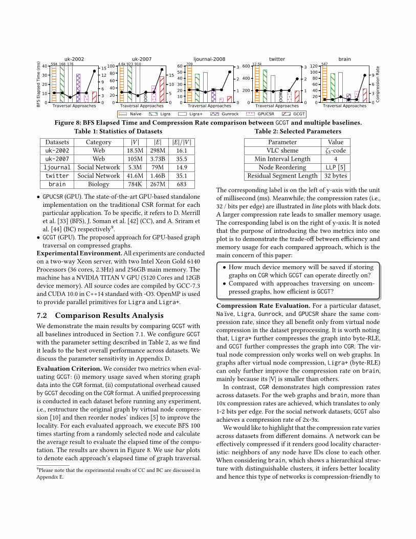
Intuitive TwoPhaseTraversal TaskStealing Warp-centric ResidualSegmentation (GCGT)

Figure 9: Optimization impact analysis results.

the CGR format. For the web graph, on one hand, the neigh-

bors share high similarity (e.g., pages belonging to the same

website); on the other hand, the data of the web graph are

collected with crawlers following hyper-links. Thus the col-

lected data corresponds to a subset of websites with high

locality. In contrast, the data collection of social networks

generally follow the time-line, and the sampling frequency

is constrained by service providers (e.g., Twitter Streaming

API only provides no more than 1% tweets for collection).

Hence, the locality characteristic in the graph structure is

destroyed to a certain extent in the process of data collection.

Hence, poor locality degrades the effectiveness of CGR.Traversal Elapsed Time Evaluation. When comparing

CPU-based and GPU-based approaches, we verify that the

GPU is an appealing accelerator for graph analysis, i.e., GPU-

based approaches (Gunrock, GPUCSR and GCGT) are signifi-cantly faster thanCPU-based approaches (Ligra and Ligra+).

The comparison between GPUCSR and GCGT is interesting

in the sense that it demonstrates the trade-off between per-

formance and device memory usage. Compared with GPUCSRbased on traditional non-compressed graph format, we can

see that GCGT incurs a very low overhead of decoding while

traversing the graph. In the worst case of uk-2007, 18.1xcompression rate is achieved at the expense of introducing

54% latency overhead. Finally, Gunrock faces the out of mem-

ory (OOM) issue on larger datasets (uk-2007 and twitter),because it runs out of the 12GB device memory due to extra

device memory allocated for its platform design.

Summary. These results have validated the motivation of

conducting graph analysis directly on CGR, which signifi-

cantly reduces the device memory pressure for GPU-based

graph processing. Considering the high compression rates

achieved, the performance reduction in terms of latency in-

troduced by GCGT is promising, which is only a few ms in

absolute time. In a nutshell, the compression would not only

enable the analysis on much larger graphs, but also main-

tains the superiority of GPU-accelerated graph analysis over

CPU counterparts.

7.3 Optimization Impact AnalysisIn order to verify the effectiveness of each proposed opti-

mization technique on the performance, we apply the tech-

niques incrementally and illustrate the experimental results

in Figure 9. We have the following interesting observations

through analyzing different datasets. TwoPhaseTraversal aims

to avoid warp divergence when threads fall into different

logic branches: executing either interval or residual decoding.

As a result, the impact of TwoPhaseTraversal is effective inthe web graphs with good locality (with many neighbors rep-

resented by intervals). TaskStealing is useful in the situation

when the residual numbers vary significantly. Warp-Centricshows a relatively stable improvement for its better hard-

ware utilization, and poses a larger impact when the average

bits per edge are fewer, e.g., compared with 9% improvement

achieved in uk-2002 (2.31 bits/edge),Warp-centric acceler-ates 16% in uk-2007 (1.17 bits/edge), and this is the same

case in social network graphs. Note that brain is differentfrom other datasets since its out-degree distribution is rela-

tively uniform and its average out-degree per node is large.

Hence, the overhead in thread collaboration in TaskStealingis not covered by the cycles saved, which results in the perfor-

mance degradation after adding TaskStealing. As mentioned

above, twitter exhibits a severe skewed distribution and

thus, the execution is bottlenecked by several nodes with

an extremely large out-degree. As a consequence, the effec-

tiveness of ResidualSegmentation is significant in twitter.

8 CONCLUSIONIn this paper, we introduce compressed graphs into GPU-

based graph computation for optimized device memory us-

age, and propose GPU-based graph traversal on compressed

graphs. First, we propose GPU-oriented parallel scheduling

strategies, Two-Phase Traversal and Task Stealing, to fully

utilize GPU’s computing resources without explicit decom-

pression into global memory of GPUs. Second, to alleviate

the issue of load imbalance in power-law graphs, we de-

vise novel techniques includingWarp-centric Decoding and

Residual Segmentation. Finally, we evaluate the effectivenessand compatibility of the proposed GCGT through extensive

experiments in representative graphs.

9 ACKNOWLEDGEMENTWe thank the anonymous reviewers for their insightful com-

ments to improve the paper. The project is partially sup-

ported by a MoE Tier 2 grant (MOE2017-T2-1-141) in Singa-

pore. Yuchen’s work is in part supported by a MoE Tier 1

grant (MSS18C001) in Singapore.

REFERENCES[1] Alberto Apostolico and Guido Drovandi. 2009. Graph Compression

by BFS. Algorithms 2, 3 (2009), 1031–1044.[2] Jiri Barnat, Petr Bauch, Lubos Brim, and Milan Ceska Jr. 2011. Comput-

ing Strongly Connected Components in Parallel on CUDA. In IPDPS.544–555.

[3] Tal Ben-Nun, Michael Sutton, Sreepathi Pai, and Keshav Pingali. 2017.

Groute: An Asynchronous Multi-GPU Programming Model for Irregu-

lar Computations. In PPoPP. 235–248.[4] Paolo Boldi, Bruno Codenotti, Massimo Santini, and Sebastiano Vigna.

2004. UbiCrawler: a scalable fully distributed Web crawler. Softw.,Pract. Exper. 34, 8 (2004), 711–726.

[5] Paolo Boldi, Marco Rosa, Massimo Santini, and Sebastiano Vigna. 2011.

Layered label propagation: a multiresolution coordinate-free ordering

for compressing social networks. In WWW. 587–596.

[6] Paolo Boldi, Massimo Santini, and Sebastiano Vigna. 2008. A large

time-aware web graph. SIGIR Forum 42, 2, 33–38.

[7] Paolo Boldi and Sebastiano Vigna. 2004. The webgraph framework I:

compression techniques. In WWW. 595–602.

[8] Paolo Boldi and Sebastiano Vigna. 2004. The WebGraph Framework

II: Codes For The World-Wide Web. In DCC. 528.[9] Ulrik Brandes. 2001. A faster algorithm for betweenness centrality. J.

Math. Sociol. 25, 2 (2001), 163–177.[10] Gregory Buehrer and Kumar Chellapilla. 2008. A scalable pattern

mining approach to web graph compression with communities. In

WSDM. 95–106.

[11] Gregory Buehrer, Roberto L. de Oliveira Jr., David Fuhry, and Srini-

vasan Parthasarathy. 2015. Towards a parameter-free and parallel

itemset mining algorithm in linearithmic time. In ICDE. 1071–1082.[12] Flavio Chierichetti, Ravi Kumar, Silvio Lattanzi, MichaelMitzenmacher,

Alessandro Panconesi, and Prabhakar Raghavan. 2009. On compressing

social networks. In KDD. 219–228.[13] Francisco Claude and Gonzalo Navarro. 2010. Fast and Compact Web

Graph Representations. ACM Trans. Web 4, 4 (2010), 16:1–16:31.[14] Laxman Dhulipala, Igor Kabiljo, Brian Karrer, Giuseppe Ottaviano,

Sergey Pupyrev, and Alon Shalita. 2016. Compressing Graphs and

Indexes with Recursive Graph Bisection. In KDD. 1535–1544.[15] Nhat Tan Duong, Quang Anh Pham Nguyen, Anh Tu Nguyen, and

Huu-Duc Nguyen. 2012. Parallel PageRank computation using GPUs.

In SoICT. 223–230.[16] Peter Elias. 1975. Universal codeword sets and representations of the

integers. IEEE Trans. Inf. Theory 21, 2 (1975), 194–203.

[17] Zhisong Fu, Harish Kumar Dasari, Bradley R. Bebee, Martin Berzins,

and Bryan B. Thompson. 2014. Parallel Breadth First Search on GPU

clusters. In BigData. 110–118.[18] Zhisong Fu, Bryan B. Thompson, and Michael Personick. 2014. Map-

Graph: A High Level API for Fast Development of High Performance

Graph Analytics on GPUs. In GRADES. 2:1–2:6.[19] Bernard A. Galler and Michael J. Fischer. 1964. An improved equiva-

lence algorithm. Commun. ACM 7, 5 (1964), 301–303.

[20] Wentian Guo, Yuchen Li, Mo Sha, and Kian-Lee Tan. 2017. Parallel

Personalized Pagerank on Dynamic Graphs. PVLDB 11, 1 (2017), 93–

106.

[21] Zhihao Jia, Yongkee Kwon, Galen M. Shipman, Patrick S. McCormick,

Mattan Erez, and Alex Aiken. 2017. A Distributed Multi-GPU System

for Fast Graph Processing. PVLDB 11, 3 (2017), 297–310.

[22] Krzysztof Kaczmarski, Piotr Przymus, and Paweł Rzążewski. 2014.

ImprovingHigh-Performance GPUGraph Traversal with Compression.

In ADBIS. 201–214.[23] U. Kang and Christos Faloutsos. 2011. Beyond ’CavemanCommunities’:

Hubs and Spokes for Graph Compression and Mining. In ICDM. 300–

309.

[24] Chinmay Karande, Kumar Chellapilla, and Reid Andersen. 2009. Speed-

ing Up Algorithms on Compressed Web Graphs. Internet Mathematics6, 3 (2009), 373–398.

[25] Farzad Khorasani, Keval Vora, Rajiv Gupta, and Laxmi N. Bhuyan. 2014.

CuSha: vertex-centric graph processing on GPUs. In HPDC. 239–252.

[26] Min-Soo Kim, Kyuhyeon An, Himchan Park, Hyunseok Seo, and Jin-

wook Kim. 2016. GTS: A Fast and Scalable Graph Processing Method

based on Streaming Topology to GPUs. In SIGMOD. 447–461.[27] Haewoon Kwak, Changhyun Lee, Hosung Park, and Sue B. Moon.

2010. What is Twitter, a social network or a news media?. InWWW.

591–600.

[28] N. Jesper Larsson and Alistair Moffat. 1999. Offline Dictionary-Based

Compression. In DCC. 296–305.[29] Xiaojie Lin, Rui Zhang, Zeyi Wen, Hongzhi Wang, and Jianzhong Qi.

2014. Efficient Subgraph Matching Using GPUs. In ADC. 74–85.[30] Hang Liu, H. Howie Huang, and Yang Hu. 2016. iBFS: Concurrent

Breadth-First Search on GPUs. In SIGMOD. 403–416.[31] Sebastian Maneth and Fabian Peternek. 2015. A Survey on Methods

and Systems for Graph Compression. CoRR abs/1504.00616 (2015).

[32] Enrico Mastrostefano and Massimo Bernaschi. 2013. Efficient breadth

first search on multi-GPU systems. J. Parallel Distrib. Comput. 73, 9(2013), 1292–1305.

[33] Duane Merrill, Michael Garland, and Andrew S. Grimshaw. 2015. High-

Performance and Scalable GPU Graph Traversal. ACM Trans. ParallelComput. 1, 2 (2015), 14–30.

[34] NVIDIA. 2018. GPU-accelerated Libraries for Computing. https://

developer.nvidia.com/gpu-accelerated-libraries/. Accessed: 2018-10-

20.

[35] Yuechao Pan, Yangzihao Wang, Yuduo Wu, Carl Yang, and John D.

Owens. 2017. Multi-GPU Graph Analytics. In IPDPS. 479–490.[36] Amitabha Roy, Ivo Mihailovic, and Willy Zwaenepoel. 2013. X-Stream:

edge-centric graph processing using streaming partitions. In SOSP.472–488.

[37] Arnon Rungsawang and Bundit Manaskasemsak. 2012. Fast PageRank

Computation on a GPU Cluster. In PDP. 450–456.[38] Mo Sha, Yuchen Li, Bingsheng He, and Kian-Lee Tan. 2017. Accelerat-

ing Dynamic Graph Analytics on GPUs. PVLDB 11, 1 (2017), 107–120.

[39] Koichi Shirahata, Hitoshi Sato, and Satoshi Matsuoka. 2014. Out-of-

core GPU memory management for MapReduce-based large-scale

graph processing. In CLUSTER. 221–229.[40] Julian Shun and Guy E. Blelloch. 2013. Ligra: a lightweight graph

processing framework for shared memory. In PPoPP. 135–146.[41] Julian Shun, Laxman Dhulipala, and Guy E. Blelloch. 2015. Smaller

and Faster: Parallel Processing of Compressed Graphs with Ligra+. In

DCC. 403–412.[42] Jyothish Soman, Kishore Kothapalli, and P. J. Narayanan. 2010. A fast

GPU algorithm for graph connectivity. In IPDPS Workshops. 1–8.[43] Jyothish Soman and Ankur Narang. 2011. Fast Community Detection

Algorithm with GPUs and Multicore Architectures. In IPDPS. 568–579.[44] Anuroop Sriram, Kollu Gautham, Kishore Kothapalli, P. J. Narayan, and

R. Govindarajulu. 2009. Evaluating Centrality Metrics in Real-World

Networks on GPU. (2009).

[45] John A Stratton, Nasser Anssari, Christopher Rodrigues, I-Jui Sung,

Nady Obeid, Liwen Chang, Geng Daniel Liu, and Wen-mei Hwu. 2012.

Optimization and architecture effects on GPU computing workload

performance. In InPar. 1–10.[46] Koji Ueno and Toyotaro Suzumura. 2013. Parallel distributed breadth

first search on GPU. In HiPC. 314–323.[47] Yangzihao Wang, Yuechao Pan, Andrew A. Davidson, Yuduo Wu, Carl

Yang, Leyuan Wang, Muhammad Osama, Chenshan Yuan, Weitang

Liu, Andy T. Riffel, and John D. Owens. 2017. Gunrock: GPU Graph

Analytics. ACM Trans. Parallel Comput. 4, 1 (2017), 3:1–3:49.[48] HaoWei, Jeffrey Xu Yu, Can Lu, and Xuemin Lin. 2016. Speedup Graph

Processing by Graph Ordering. In SIGMOD. 1813–1828.[49] Tianji Wu, Bo Wang, Yi Shan, Feng Yan, Yu Wang, and Ningyi Xu.

2010. Efficient PageRank and SpMV Computation on AMD GPUs. In

ICPP. 81–89.[50] Xintian Yang, Srinivasan Parthasarathy, and P. Sadayappan. 2011. Fast

Sparse Matrix-Vector Multiplication on GPUs: Implications for Graph

Mining. PVLDB 4, 4 (2011), 231–242.

[51] Jianlong Zhong and Bingsheng He. 2014. Medusa: Simplified Graph

Processing on GPUs. IEEE Trans. Parallel Distrib. Syst. 25, 6 (2014),

1543–1552.

APPENDICESA GPU’S ARCHITECTURE

warp 0

register

warp 1

register

Shared Memorywarp 2

register

warp 3

register

device mem

ory

block 0warp 4

register

warp 5

register

Shared Memorywarp 5

register

warp 7

register

block 1

Figure 10: A sketch of GPU’s architecture.

The superior performance achieved onGPUs inmany com-

putational applications mainly comes from GPU’s two char-

acteristics: (i) Large Number of Cores: A GPU die typically

contains thousands of cores. Compared with CPUs, GPUs

focus on numeric computation and hence, have a relatively

simplified instruction set and manage to simplify the control-

ling logic in order to improve the theoretical computational

performance. (ii) High Memory Bandwidth: Compared

with CPUs, GPUs have a much higher memory bandwidth,

up to hundreds of Gigabyte (GB) per second. In Figure 10,

we illustrate GPU’s computational architecture10. Warp is

the smallest logic control unit on GPUs, and it is composed

of a set of threads (generally 32 threads). The threads be-

longing to the same warp runs in the SIMT mode (i.e., single

instruction multiple threads), and can achieve the fastest

inter-thread communication through accessing each other’s

registers. Multiple warps compose a block (also known as

CTA), which is the synchronization logic unit - only the

threads belonging to the same block can conduct thread syn-

chronization operations, and the cross-block threads cannot.

Each block has its independent shared memory, so that the

threads in the same block can communicate with each other

efficiently. The shared memory and L1 cache have similar

latency. Finally, a GPU card, as a complete subsystem, has

its own memory unit called device memory. The memory

bandwidth of a GPU card accessing its device memory can

achieve hundreds of GB per second. However, if the data

communication between CPU and GPU is needed, the de-

vice memory bandwidth will rely on PCIe transfer, which is

typically below 16GB per second.

The threads in the same warp are synchronized in nature.

Moreover, if multiple threads of the same warp enter into

different condition branches (e.g., if-else), then all condition

branches will be executed in a serial manner and the thread

which enters the condition branch it does not belong to will

10This work is based on the CUDA architecture from NVIDIA and different

versions of the CUDA architectures have some difference in between.

be idle. This is called “warp divergence”, and is a key consid-

eration when evaluating the performance of GPU programs.

From another perspective, GPU’s high device memory ac-

cess bandwidth comes from its relatively long cache line (L1

cache line is generally 128-byte, i.e., 32 single-precision vari-

ables). This means that if the memory access behaviors of all

threads in the warp are aligned, they can achieve high device

memory access bandwidth and thus, can accelerate the com-

putation to a large extent. Otherwise, if such memory access

behaviors are not aligned, a large amount of memory band-

width will be wasted (no matter if it is needed or not, the data

will be loaded into cache in 128-byte). This is called “uncoa-

lesced memory access”, which is another key consideration

when evaluating the performance of GPU programs.

Table 3: Examples of γ -code and ζ -code (bold digits in-dicate unary-code part)

integer γ -code ζ2-code ζ3-code1 1 101 10012 010 110 10103 011 111 10114 00100 010100 11005 00101 010101 11016 00110 010110 111012 0001100 011100 0100110034 00000100010 001100010 01100010

B DETAILS ON VLC ENCODINGMost commonly used encoding schemes for applying VLC

to compress graphs are γ -code [16] and ζ -code [8]. Both

encoding schemes share some similar properties: they are

specific to encoding positive integers, and have two parts in

the encoding. The first half of γ -code uses unary-code11 torepresent the length of the element’s significant bits, and the

second half denotes the element’s significant bits in binary

representation. ζ -code is an extension ofγ -code, which intro-duces a parameter k . If the value of the unary-code part in ζk -code encoding scheme is x , then it means that this element’s

length of significant bits is k × x in binary representation.

Therefore, ζ1-code is equivalent to γ -code theoretically. InTable 3, we illustrate some examples in both the γ -code en-coding scheme and the ζk -code encoding scheme. It should

be noted that for γ -code, the preceding “1” in the second half

can be omitted because it always starts with “1”. However,

for ζk -code (k ≥ 2), this does not hold. For instance, when

encoding the number “6”, whose binary representation is

“110”. In γ -code, we use the unary-code “001” to denote itslength of significant bits is 3, followed by “10” as the signif-

icant bits after omitting the preceding “1”. In ζ2-code andζ3-code, we use the unary-code “01” and “1” to represent the

11https://en.wikipedia.org/wiki/Unary_coding

γ ζ2 ζ3 ζ4 ζ5VLC Encoding scheme

0

5

10

15

BFS

Elap

sed

Tim

e (m

s) uk-2002

γ ζ2 ζ3 ζ4 ζ5VLC Encoding scheme

0

25

50

75

100uk-2007

γ ζ2 ζ3 ζ4 ζ5VLC Encoding scheme

0

5

10

15ljournal-2008

γ ζ2 ζ3 ζ4 ζ5VLC Encoding scheme

0

100

200

twitter

γ ζ2 ζ3 ζ4 ζ5VLC Encoding scheme

0

20

40

60brain

0

5

10

15

0

10

20

0

1

2

3

0

1

2

3

0

5

10

Com

pres

sion

Rate

Figure 11: Results of varying VLC encoding schemes.

2 3 4 5 10 infMinimum Interval Length

0

5

10

15

BFS

Elap

sed

Tim

e (m

s) uk-2002

2 3 4 5 10 infMinimum Interval Length

0

25

50

75

100uk-2007

2 3 4 5 10 infMinimum Interval Length

0

5

10

15ljournal-2008

2 3 4 5 10 infMinimum Interval Length

0

100

200

twitter

2 3 4 5 10 infMinimum Interval Length

0

20

40

60

80brain

0

5

10

15

0

10

20

0

1

2

3

0

1

2

3

0

5

10

Com

pres

sion

Rate

Figure 12: Results of varying Minimum Interval Lengths.

Reordering Method0

5

10

15

20

BFS

Elap

sed

Tim

e (m

s) uk-2002

Reordering Method0

50

100

uk-2007

Reordering Method0

5

10

ljournal-2008

Reordering Method0

100

200

twitter

Reordering Method0

20

40

60brain

0

5

10

15

0

10

20

0

1

2

3

0

1

2

3

0

5

10

15

Com

pres

sion

Rate

Original DegSort BFSOrder Gorder LLP

Figure 13: Results of varying Node Reordering Methods.

length of significant bits as 4 (2 × 2) and 3 (1 × 3), followed

by “0110” and “110” as significant bits respectively.

C DETAILS ON CGR ENCODINGThere are some implementation details on CGR encoding inorder to achieve higher compression rate as follows.

• The gap value between the first interval’s starting node

index or the first residual and the node whose neighbors

are to be encoded can be negative, so a sign bit needs to

be appended to the encoding. In particular, for the first

encoding of both the first interval’s starting node index

and the first residual, assume it is equal to x , then 2x is

encoded if x is non-negative, otherwise, 2x + 1 is encoded.• The gap value is at least 1, and the interval length is no

less than the minimum interval length. Therefore, we can

shift the theoretical minimum to 0 in encoding in order to

increase the compression rate.

• The VLC used in this work cannot represent 0 actually, so

we conduct “+1” shifting for all encodings.

D PARAMETER SENSITIVITY ANALYSISIn this subsection, we examine the influence of various pa-

rameters which are shown in Table 2.

VLC Encoding Scheme. Figure 11 shows the influence ofdifferent VLC encoding schemes with different k settings

(described in Appendix B) on both the computational la-

tency and the compression rate. Varying k settings in VLC

encoding schemes can pose an effect on the distribution of

needed bit numbers of the encoding value range. Therefore,

the tuning of k depends on the distribution of the concrete

graph data structures. At the same time, instead of directly

encoding the adjacency lists, CGR introduces mechanisms

like Intervals and Residuals Representation, and Gap Trans-

formation, which render the modelling of optimizing k more

complicated. In [8], a simplified model is proposed which

establishes a connection between the optimization of k and

the exponent α in the power-law distribution12. Theoreti-

cally, the workload is equal among decoding different VLC

encoding schemes, and the varying of computational latency

is mainly related to memory usage.

Minimum Interval Length. Figure 12 illustrates the ef-

fects of minimum interval length on the compression per-

formance. This parameter indicates the minimum length of

consecutive neighbors which can compose an interval and

“inf” representing no interval. As for the compression rate, all

settings of minimum interval length (except in brain) per-form quite similarly, which means that brain highly benefitsfrom the Interval Representation mechanism. A small mini-

mum interval length leads to a large number of fragmented

intervals and thus, degrades the computational efficiency.

12https://en.wikipedia.org/wiki/Power_law

8 16 32 64 128 infSegment Length (byte)

0

5

10

15

BFS

Elap

sed

Tim

e (m

s) uk-2002

8 16 32 64 128 infSegment Length (byte)

0

25

50

75

100uk-2007

8 16 32 64 128 infSegment Length (byte)

0

5

10

15ljournal-2008

8 16 32 64 128 infSegment Length (byte)

0

100

200

300 2380twitter

8 16 32 64 128 infSegment Length (byte)

0

25

50

75

100brain

0

5

10

15

0

10

20

0

1

2

3

0

1

2

3

0

5

10

Com

pres

sion

Rate

Figure 14: Results of varying Residual Segment Lengths.

CC BC0

20

40

60

Elap

sed

Tim

e (m

s)

uk-2002

CC BC0

200

400

OOM

uk-2007

CC BC0

20

40

60

ljournal-2008

CC BC0

500

1000OO

M

OOM

twitter

CC BC0

50

100

brain

Gunrock GPUCSR GCGT

Figure 15: Experimental results of CC and BC.

This issue is more severe in twitter and brain, due to the

existence of super nodes with too many neighbors for the

former dataset, and relatively larger average out-degrees for

the latter dataset. In the meanwhile, low compression rate of

brain with no interval representation leads to high memory

accesses, which obviously increases the elapsed time.

Node Reordering Methods. We choose several node re-

ordering methods as follows in order to improve the locality

of the original graphs.

• Original. The original order of the raw datasets.

• DegSort. The order provided by a straightforward greedy

strategy, which sorts nodes in a descending order accord-

ing to the frequencies that they are an out-degree node.

• BFSOrder [1]. The order generated by the breadth-first

search traversal.

• Gorder [48]. The order is given based on a defined locality

score Gscore, which is maximized by greedy strategies

and partial maxTSP calculation on sliding windows.

• LLP [5]. The order is determined by the traversal among

these clusters, which are distinguished by the layered label

propagation algorithm.

We illustrate the influence of different node reordering meth-

ods in Figure 13. We first confirm that node reordering

methods affect the compression rate in all datasets. Among

these node reordering methods, LLP and Gorder perform

significantly better than the intuitive strategies DegSort andBFSOrder to a large extent, due to their explicit optimization

of the locality in the processing of reordering. Comparing

LLP and Gorder, they are competitive. Across the datasets,

LLP achieves higher compression rates and Gorder leads to

faster computation. This is because the objective functions of

LLP and Gorder are different: Gorder tends to generate dense

neighbor clusters for better cache performance whereas LLPoptimizes towards global compression rate.

Residual Segment Length. We demonstrate the influence

of various residual segment length settings in Figure 14.

Residual segment length is a parameter to directly trade

off computational latency for compression rate. A smaller

residual segment length will generate more segments so

that more threads can participate in the parallel processing.

Nonetheless, at the same time, a larger blank area in the

rear of each segment will be formed and this will harm the

compression rate.

E EXPERIMENTAL RESULTS OF GCGTEXTENSIONS TO CC AND BC

We compare GCGT extensions to CC and BC with GPU-based

baselines, Gunrock and GPUCSR, as illustrated in Figure 15.

We run each program 100 times to calculate the average

elapsed time and BC’s starting node is randomly selected.

It can be verified that, compared with Gunrock and GPUCSR,GCGT extensions to CC and BC can achieve satisfactory per-

formance, when operating CGR directly in the device memory.

As for CC, it links components via edge traversal which

favors edge-centric implementations. Comparing GCGT andGPUCSR (J. Soman et al. [42], an edge-centric implementa-

tion), we find that in twitter, GCGT introduces relatively

high overhead in terms of elapsed time, which is caused by

the existence of super nodes (with large out-degrees). When

utilizing edge frontiers, such characteristic is not a big prob-

lem, because after being added to a connected component,

subsets of super nodes’ edges can be filtered out gradually

and will not enter subsequent iterations. Nonetheless, this is

not the same case when utilizing node frontiers. As a conse-

quence, the computation of CC in twitter is not friendly to

node-centric implementations.

As for BC, it is quite similar to BFS: deriving the σ -valueand the δ -value through two BFS-like traversals. Thus, GCGTextension to BC exhibits similar performance as in BFS.

In summary, on the premise of incurring moderate cost,

GCGT extensions to other graph applications can work di-

rectly on compressed graphs in order to effectively facilitate

the device memory utilization.