Department of EconomicsGLS Detrending for Nonlinear Unit Root Tests

George Kapetanios and Yongcheol Shin

Working Paper No. 472 November 2002 ISSN 1473-0278

GLS Detrending for Nonlinear Unit Root Tests

George Kapetanios∗

Queen Mary, University of London

Yongcheol ShinDepartment of Economics, University of Edinburgh

November 2002

Abstract

This paper investigates GLS detrending procedures for unit roottests against nonlinear stationary alternative hypotheses where deter-ministic components are assumed present in the series under inves-tigation. It is found that the proposed procedures have considerablepower gains in a majority of cases against both existing nonlinear unitroot tests and standard unit root tests.

JEL Classification: C12, C22, F31.Key Words: Detrending, Nonlinear Unit Root Tests, Nonlinearity, STARModels, SETAR Models.

∗Department of Economics, Queen Mary, University of London, Mile End Rd., LondonE1 4NS. Email: G.Kapetanios@qmul.ac.uk

1

1 Introduction

There is a growing dissatisfaction with the standard linear ARMA frame-

work used to test for unit roots in time series, and increasingly alternative

frameworks within which to test for unit roots are considered. For example,

one alternative focuses on the use of panel data and its role in increasing

the power of standard unit root tests. A good example is Abuaf and Jorion

(1990), who use a panel data test to reject the joint hypothesis of unit roots

in each of a group of real exchange rates against an alternative that they are

all stationary. Another approach is to use an alternative form of stationarity

to simple ARMA models. These include fractional integration and nonlinear

transition dynamics (see e.g. Pesaran and Potter (1997)).

In this paper we extend recent work on testing for unit roots against

particular nonlinear alternatives by Kapetanios, Snell, and Shin (2002) and

Kapetanios and Shin (2002). We focus on a particular aspect of their analysis

which is the detrending procedure they use. It is well known in the literature

on linear unit root testing that inefficient detrending can reduce the power

of the tests significantly and therefore render the tests less useful. We inves-

tigate the ability of efficient detrending procedures used in linear unit root

tests to improve the power performance on nonlinear unit root tests.

The structure of the paper is as follows: Section 2 provides a descrip-

tion of the theoretical framework of nonlinear unit root testing. Section 3

discusses modifications to the existing procedures needed for the implemen-

tation of efficient detrending. Section 4 presents Monte Carlo evidence on

the performance of the new procedures for a variety of experimental setups.

Section 5 discusses an empirical application to real exchange rates. Finally,

[1]

Section 6 concludes.

2 Theoretical Framework

Recently, Kapetanios, Snell, and Shin (2002) and Kapetanios and Shin (2002)

suggested two testing procedures to distinguish between nonstationary unit

root processes and persistent but stationary nonlinear processes. The first

considers the possibility that the alternative model follows a smooth transi-

tion autoregressive model and the second consider the alternative hypothesis

that the nonlinear model belongs to the class of threshold models.

Both testing procedures have been found to be more powerful that stan-

dard unit root tests when the true data generation processes was a persistent

but stationary nonlinear process. However, for the cases where demeaning

or detrending of the data was carried out prior to the test, a significant loss

of power was observed. As a result we investigate whether procedures which

have been found useful in increasing the power of tests based on data whose

deterministic components had been removed in the linear framework, may

be useful in the nonlinear case.

Before proceeding we give a brief account of the alternative nonlinear

models we consider.

2.1 STAR Models

We follow the nonlinear STAR framework considered by Kapetanios, Snell,

and Shin (2002). More specifically, the model they consider is

∆yt = γyt−1

{1− exp (−θy2

t−1

)}+ εt, (1)

[2]

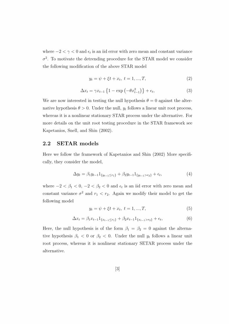
where −2 < γ < 0 and εt is an iid error with zero mean and constant variance

σ2. To motivate the detrending procedure for the STAR model we consider

the following modification of the above STAR model

yt = ψ + ξt+ xt, t = 1, ..., T, (2)

∆xt = γxt−1

{1− exp (−θx2

t−1

)}+ εt, (3)

We are now interested in testing the null hypothesis θ = 0 against the alter-

native hypothesis θ > 0. Under the null, yt follows a linear unit root process,

whereas it is a nonlinear stationary STAR process under the alternative. For

more details on the unit root testing procedure in the STAR framework see

Kapetanios, Snell, and Shin (2002).

2.2 SETAR models

Here we follow the framework of Kapetanios and Shin (2002) More specifi-

cally, they consider the model,

∆yt = β1yt−11{yt−1≤r1} + β2yt−11{yt−1>r2} + εt, (4)

where −2 < β1 < 0, −2 < β2 < 0 and εt is an iid error with zero mean and

constant variance σ2 and r1 < r2. Again we modify their model to get the

following model

yt = ψ + ξt+ xt, t = 1, ..., T, (5)

∆xt = β1xt−11{xt−1≤r1} + β2xt−11{xt−1>r2} + εt, (6)

Here, the null hypothesis is of the form β1 = β2 = 0 against the alterna-

tive hypothesis β1 < 0 or β2 < 0. Under the null yt follows a linear unit

root process, whereas it is nonlinear stationary SETAR process under the

alternative.

[3]

3 Improved Detrending

3.1 The Linear Case

Elliott, Rothenberg, and Stock (1996) investigated the issue of efficient de-

trending for linear unit roor tests following previous work by Dufour and

King (1991), King (1988) and King (1980). Their work was motivated by

asymptotic local power considerations. More specifically, they derived point

optimal unit root tests for trended data for specific local alternative hypothe-

ses. The model they consider is of the form

yt = βzt + xt (7)

xt = αxt−1 + εt (8)

where zt is a deterministic component and εt is an i.i.d. process with finite

zero-frequency spectral density and variance σ2. Since the focus is on lo-

cal alternative hypotheses, the autoregressive parameter is re-expressed as

α = 1 − c/T anticipating the necessary rate of convergence for local power

analysis. They test the null hypothesis, H0 : α = 1, against local alternative

hypotheses of the form Hc : α = α ≡ 1 − c/T , where c is a constant and T

is the number of observations. Note the distinction between c which is the

local alternative parameter and c which is the value under which tests are

constructed. Point optimal likelihood ratio tests of the form

L∗T = minβL(α, β)−min

βL(1, β)

for the null hypothesis against the local alternative, may be constructed

where L(α, β) = (yα − zαβ)′Σ−1(yα − zαβ) is the loglikelihood of the local

alternative hypothesis, yα = (y1, y2 − αy1, . . . , yT − αyT−1), zα = (z1, z2 −αz1, . . . , yT − αzT−1) and Σ is the covariance matrix of ε1, . . . , εT ). The

term (yα − zαβ)′Σ−1(yα − zαβ) may be viewed as a weighted sum of squared

[4]

residuals coming from a constrained GLS regression where the autoregressive

coefficient α has been imposed.

Elliott, Rothenberg, and Stock (1996) suggest modifying the standard

Dickey-Fuller test by applying it to residual data ydt whose deterministic

componenent has been removed. More specifically, ydt = yt − βzt where β

is obtained from a regression of yα on zα. No rigorous theoretical account

of whether this test is close to the point optimal test is given. However,

simulation analysis indicates that the test performs much better than stan-

dard unit root tests. Note that this test is designed with a particular local

alternative in mind represented by the choice of α used for detrending. El-

liott, Rothenberg, and Stock (1996) suggest that choosing α such that the

asymptotic local power of the test, when faced with the local alternative for

which it was designed, is equal to 0.5. This is the test they settle on for their

finite sample analysis.

Clearly the motivation for the modified DF test lies in the fact that the

detrending carried out takes specific account of the local alternative against

which we wish the test to be powerful. We suggest that the same detrending

approach is taken for the nonlinear unit root tests. In particular we suggest

that the nonlinear tests be applied to the residual series ydt obtained following

GLS detrending. Clearly this is not optimal since the nonlinear nature of the

altelnative hypothesis is not taken into account. Take for example the STAR

model in (2)-(3). A local alternative version of it could be constructed by

specifying θ = c/T . A first problem with this is that the T−1 rate involved in

the construction of the local alternative is not neccesarily appropriate since

θ enters in the exponential rather than linearly (see also Park and Phillips

(2001)). Further, it is not clear how to devise a generalised quasi-differencing

[5]

scheme, that does not involve knowledge of xt which would enable the con-

struction of series yθ and zθ comparable to yα and zα for the linear case such

that yθ − βzθ = εt. Another problem is that any detrending taking account

of the nonlinear structure of the alterntive would also involve taking a stance

on the values of the nuisance (in this case) parameters such as γ for STAR

models or r1 and r2 in the case of the SETAR alternative. As a result, the

linear local alternative detrending may provide a useful approximation to the

nonlinear local alternative.

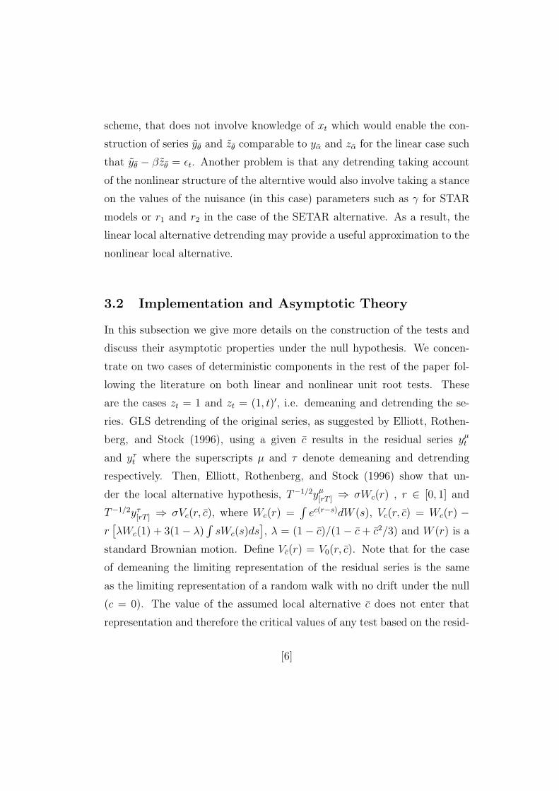
3.2 Implementation and Asymptotic Theory

In this subsection we give more details on the construction of the tests and

discuss their asymptotic properties under the null hypothesis. We concen-

trate on two cases of deterministic components in the rest of the paper fol-

lowing the literature on both linear and nonlinear unit root tests. These

are the cases zt = 1 and zt = (1, t)′, i.e. demeaning and detrending the se-

ries. GLS detrending of the original series, as suggested by Elliott, Rothen-

berg, and Stock (1996), using a given c results in the residual series yµt

and yτt where the superscripts µ and τ denote demeaning and detrending

respectively. Then, Elliott, Rothenberg, and Stock (1996) show that un-

der the local alternative hypothesis, T−1/2yµ[rT ] ⇒ σWc(r) , r ∈ [0, 1] and

T−1/2yτ[rT ] ⇒ σVc(r, c), where Wc(r) =

∫ec(r−s)dW (s), Vc(r, c) = Wc(r) −

r[λWc(1) + 3(1− λ)

∫sWc(s)ds

], λ = (1− c)/(1− c + c2/3) and W (r) is a

standard Brownian motion. Define Vc(r) = V0(r, c). Note that for the case

of demeaning the limiting representation of the residual series is the same

as the limiting representation of a random walk with no drift under the null

(c = 0). The value of the assumed local alternative c does not enter that

representation and therefore the critical values of any test based on the resid-

[6]

ual series will not depend on c. This is not the case for the detrended series

where the critical values will depend on c.

3.3 STAR model

For the STAR model in (2)-(3) we now briefly describe the unit root test.

Once the deterministic components have been removed as described above the

test for the STAR case is constructed as follows. The null hypothesis is H0 :

θ = 0 against the alternative H1 : θ > 0. Testing this null hypothesis directly

is not feasible, since γ is not identified under the null. (See Davies, 1987). To

overcome this problem Kapetanios, Snell, and Shin (2002) follow Luukkonen,

Saikkonen and Terasvirta (1988), and derive a t-type test statistic. The

following auxiliary regression

∆ydt = δyd 3

t−1 + error. (9)

obtained through a Taylor expansion, is used, where the significance of δ is

tested using a t-test. Kapetanios, Snell, and Shin (2002) show that in the

case of no deterministic components the asymptotic distribution of the test

statistic, denoted by NLDF is given by

NLDF ⇒{

14W (1)4 − 3

2

∫ 1

0W (r)2 dr

}√∫

W (r)6dr(10)

As the GLS demeaned series has the same asymptotic representation under

the null as a random walk with no drift the asymptotic distribution of the

test using GLS demeaning and denoted by NLGLSµ, is given by (10). For

the detrended case the arguments of Kapetanios, Snell, and Shin (2002) can

be straightforwardly modified to show that the asymptotic distribution of

[7]

the test using GLS detrending, and denoted by NLGLSτ is given by

NLGLSτ ⇒{

14Vc (1)

4 − 32

∫ 1

0Vc (r)

2 dr}

√∫Vc(r)6dr

(11)

The 95% critical value for NLGLSτ for c = −17.5 which gives asymptoticlocal power1 of 0.5, is -2.93. For the NLDF µ test the relevant value of c is

-9.

3.4 SETAR Model

Following the detrending, the model for testing for nonlinear SETAR sta-

tionarity can be compactly written as

∆ydt = β1y

dt−11{yd

t−1≤r1} + β2ydt−11{yd

t−1>r2} + ut, (12)

where ydt−11{yd

t−1≤r1} and ydt−11{yd

t−1>r2} are orthogonal to each other by con-struction. Kapetanios and Shin (2002) consider the (joint) null hypothesis

of unit root as

H0 : β1 = β2 = 0, (13)

against the alternative hypothesis of threshold stationarity. Writing (12) in

matrix notation gives

∆y = Xβ + u, (14)

where β = (β1, β2)′, and

∆y =

∆yd

1

∆yd2...

∆ydT

; X =

yd01{yd

0≤r1} yd01{yd

0>r2}yd

11{yd1≤r1} yd

11{yd1>r2}

......

ydT−11{yd

T−1≤r1} ydT−11{yd

T−1>r2}

; u =

u1

u2...uT

.

1The local power was obtained via simulations using 5000 replications and processes of1000 observations to discretely approximate the functionals of Brownian motions

[8]

Then, the joint null hypothesis of linear unit root against the nonlinear

threshold stationarity can be tested using the Wald statistic given by

W(r1,r2) = β′[V ar

(β)]−1

β =β′ (X′X) β

σ2u

, (15)

where β is the OLS estimator of β, σ2u ≡ 1

T−2

∑Tt=1 u

2t , and ut are the residuals

obtained from (12).

The test suffers from the Davies (1987) problem since unknown threshold

parameters are not identified under the null. Most solutions to this problem

involve some sort of integrating out unidentified parameters from the test

statistics. This is usually achieved by calculating test statistics for a grid

of possible values of threshold parameters, r1 and r2, and then constructing

the summary statistics. For stationary TAR models this problem has been

studied in Tong (1990) and Hansen (1996). Following Andrews and Ploberger

(1994), Kapetanios and Shin (2002) consider the three most commonly used

statistics such as the supremum, the average and the exponential average of

the Wald statistic defined respectively by

Wsup(r1,r2)

= supi∈#Γ

W(i)(r1,r2)

, Wavg(r1,r2)

=1

#Γ

#Γ∑i=1

W(i)(r1,r2), Wexp

(r1,r2) =1

#Γ

#Γ∑i=1

exp

(W(i)(r1,r2)

2

),

(16)

where W(i)(r1,r2)

is the Wald statistic obtained from the i-th point of the nui-

sance parameter grid, Γ and #Γ is the number of elements of Γ. For more

details on the the selection of the grid of threshold parameters see Kapetanios

and Shin (2002).

The asymptotic distributions ofWsup(r1,r2)

andWavg(r1,r2) are the same and are

given by the distribution of

W ≡{∫ 1

01{W (s)≤0}W (s)dW (s)

}2

∫ 1

01{W (s)≤0}W (s)2ds

+

{∫ 1

01{W (s)>0}W (s)dW (s)

}2

∫ 1

01{W (s)>0}W (s)2ds

,

[9]

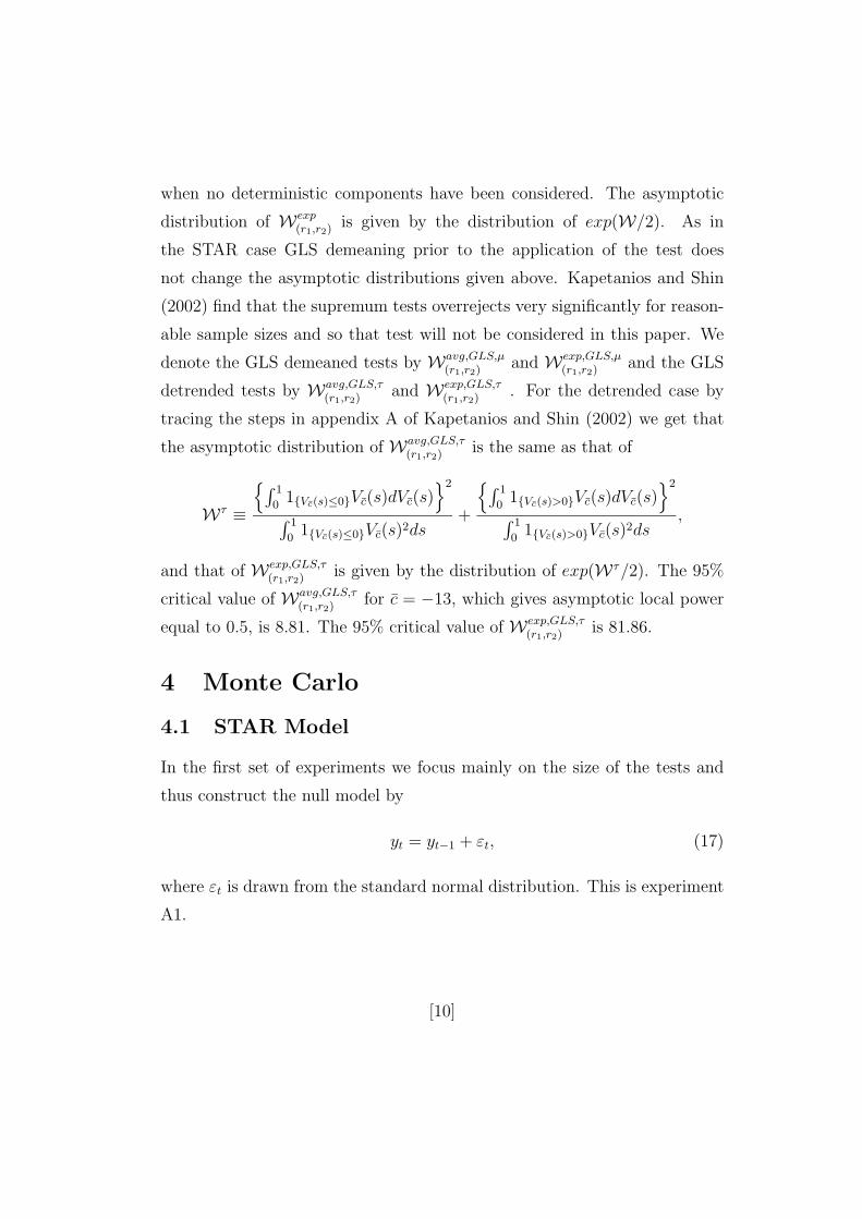
when no deterministic components have been considered. The asymptotic

distribution of Wexp(r1,r2)

is given by the distribution of exp(W/2). As in

the STAR case GLS demeaning prior to the application of the test does

not change the asymptotic distributions given above. Kapetanios and Shin

(2002) find that the supremum tests overrejects very significantly for reason-

able sample sizes and so that test will not be considered in this paper. We

denote the GLS demeaned tests by Wavg,GLS,µ(r1,r2)

and Wexp,GLS,µ(r1,r2)

and the GLS

detrended tests by Wavg,GLS,τ(r1,r2)

and Wexp,GLS,τ(r1,r2)

. For the detrended case by

tracing the steps in appendix A of Kapetanios and Shin (2002) we get that

the asymptotic distribution of Wavg,GLS,τ(r1,r2)

is the same as that of

Wτ ≡{∫ 1

01{Vc(s)≤0}Vc(s)dVc(s)

}2

∫ 1

01{Vc(s)≤0}Vc(s)2ds

+

{∫ 1

01{Vc(s)>0}Vc(s)dVc(s)

}2

∫ 1

01{Vc(s)>0}Vc(s)2ds

,

and that of Wexp,GLS,τ(r1,r2)

is given by the distribution of exp(Wτ/2). The 95%

critical value of Wavg,GLS,τ(r1,r2)

for c = −13, which gives asymptotic local powerequal to 0.5, is 8.81. The 95% critical value of Wexp,GLS,τ

(r1,r2)is 81.86.

4 Monte Carlo

4.1 STAR Model

In the first set of experiments we focus mainly on the size of the tests and

thus construct the null model by

yt = yt−1 + εt, (17)

where εt is drawn from the standard normal distribution. This is experiment

A1.

[10]

Secondly, in order to evaluate the power of alternative tests against glob-

ally stationary processes, we generate the DGP as follows:

∆yt = γyt−1

[1− exp (−θy2

t−1

)]+ εt, (18)

where εt ∼ N (0, 1). In particular, we choose a broad range of parameter val-

ues for γ = {−1.5,−1,−0.5,−0.1} and θ = {0.01, 0.05} for a general powercomparison. For θ = 0.01 we have experiments B1-B4, and for θ = 0.05 we

have experiments B5-B8.

For each of experiments we have computed the rejection probability of

the null hypothesis. The nominal size of each of the tests is set at 0.05,

the number of replications at 1000 and the sample size is considered for

T = 50, 100, 200. In the comparisons we include the nonlinear STAR test

proposed by Chortareas, Kapetanios, and Shin (2002) which uses the Schmidt

and Phillips (1992) detrending. This test is denoted by NLSP . Its linear

version is denoted by SP . We also include the linear DF test and the linear

GLS DF test (denoted by GLS) suggested by Elliott, Rothenberg, and Stock

(1996). Results are presented in Table 1 and 2.

It is clear that the nonlinear GLS detrending procedure improves upon

the performance of the existing tests in a majority of cases and in those cases

where no improvement is achieved the loss in power, compared to the best

performing test, is minimal.

4.2 SETAR Models

In the first set of experiments we examine the size performance of the tests.

Experiment A1 considers the random walk process:

yt = yt−1 + ut, (19)

[11]

where the error term ut is drawn from the independent standard normal

distribution.

The next set of experiments examines the power performance of the tests,

where the data is generated by

yt =

φ1yt−1 + ut if yt−1 ≤ r1

φ0yt−1 + ut if r1 < yt−1 ≤ r2

φ2yt−1 + ut if yt−1 > r2

, t = 1, 2, ..., T, (20)

where ut ∼ N (0, 1). Experiments B and C set φ0 = 1. Experiments B1-B5

consider the symmetric adjustment with φ1 = φ2 = 0.9, whereas we examine

asymmetric adjustments in Experiment C1-C5 with φ1 = 0.85 and φ2 = 0.95.

Experiments D and E are as experiments B and C but with φ0 = 1.3, i.e.

they assume an explosive corridor regime. Within each set of power exper-

iments, we select five different sets of threshold parameter values from 0.90

to 3.90 and -0.90 to -3.90, at steps of 0.75 and -0.75, respectively.2 For each

sample the grid of either lower or upper threshold parameter comprises of

eight equally spaced points between the 10% quantile (lower threshold) or

the 90% quantile (upper threshold) of the sample and the mean of the sample.

All experiments are carried out using the following statistics: the two

version of summary Wald statistics, Wavg(r1,r2)

and Wexp(r1,r2)

, defined by (16)

proposed by Kapetanios and Shin (2002), their GLS detrended counterparts,

the DF and the linear GLS detrending test suggested by Elliott, Rothenberg,

and Stock (1996). For all power experiments, 200 initial observations are

discarded to minimise the effect of initial conditions. All experiments are

based on 1,000 replications, and samples of 100 and 200 are considered.

Empirical size and power of the tests are evaluated at the 5% nominal level.

As the GLS tests overreject we correct for that using empirical critical values

2We also find via simulation that the processes have spent at least 10% of the time ineach of the outer regimes even for the largest threshold parameter values considered.

[12]

obtained from the size experiment, A1. We also correct the nonlinear tests

by Kapetanios and Shin (2002) to enable valid comparisons. Results are

presented in Table 3 and 4. We reach the same conclusion as in the case

of STAR models concerning the performance of the nonlinear detrending

procedures on the existing tests for SETAR models. In particular the GLS

nonlinear tests always outperform the existing nonlinear tests. They also

outperform in the majority of cases the linear unit root tests. Although,

there are some cases where the linear tests perform better, these are not

the majority and in the cases where the nonlinear tests perform better the

difference in performance is much more pronounced.

5 Stationarity of real exchange rates

In this section we apply the new tests to investigate the of stationarity prop-

erties of the Yen and Deutch Mark real exchange rates. Our choice for one of

the data sets reflects previous work in this area by Chortareas, Kapetanios,

and Shin (2002) on Yen real exchange rates using STAR based nonlinear

unit root tests. That paper used nonlinear unit root tests to help explain

the inability of standard unit root tests to reject the null hypothesis of non-

stationarity in accordance with economic theory and the purchasing power

parity hypothesis. We apply the STAR based tests on Yen real exchange

rates and the SETAR based tests on the DM real exchange rates.

We construct bilateral real exchange rates against the i-th currency at

time t (qi,t) as qi,t = si,t + pJ,t − p∗i,t, where si,t is the corresponding nominal

exchange rate (i-th currency per numeraire currency), pJ,t the price level in

the home country, and p∗i,t the price level of the i-th country. Thus, a rise in

qi,t implies a real appreciation against the i-th currency. The price levels are

[13]

consumer price indices for Yen and wholesale price indices for the DM. All

variables are in logs. All data are from the International Monetary Fund’s

International Financial Statistics in CD-ROM. The data are not seasonally

adjusted. All data are quarterly, spanning from 1960Q1 to 2000Q4 and the

bilateral nominal exchange rates against the currencies other than the US

dollar are cross-rates computed using the US dollar rates. We consider a

very large sample of countries in an attempt to make the empirical analy-

sis more comprehensive. Results are presented for the STAR based tests in

Tables 5-6 and for the SETAR based tests in Tables 7-8. Tables 5 and 7

present results for tests with no augmentations to take into account possible

serial correlation, whereas Tables 6 and 8 present results for tests with 4

lags to take into account serial correlation in the series. All tests assume the

presence of a trend under the alternative hypothesis. The empirical critical

values obtained from the Monte Carlo experiments in the previous section

are used for the empirical analysis to minimise the degree of overrejction

under the null hypothesis for the GLS tests.

The results make interesting reading. For the Yen real exchange rates

we see that the nonlinear GLS test based on the ESTAR model rejects the

null hypothesis more often that any other test both for augmented and non-

augmented test regression equations. When we carry out augmentation the

test rejects for 26 out of 39 countries considered. The next best performing

test is the NLDF test with 22 rejections. When there is no augmentation

the nonlinear GLS test rejects less often but still produces twice the number

of rejections compared to any other test examined.

Moving on to the DM real exchange rate and the SETAR model based

tests we see that the nonlinear GLS tests rejects for 24 out of the 31 countries

[14]

considered. This is double the number of rejections of any other test. We note

that we have investigated the Yen real exchange dataset using the SETAR

based tests and the DM real exchange rate dataset using the STAR based

tests and we could not find substantially different performance between the

linear and nonlinear unit root tests. This may be taken to signify the possible

presence of particular forms of nonlinearity which are different between the

two datasets and which can perhaps be picked up more accurately by one or

the other of the two classes of tests. In particular sudden step changes in the

dynamic evolution of the real exchange rate processes may be better picked up

by the SETARmodel based tests whereas smoother adjustments may be more

amenable to investigation through the STAR model based tests. Further this

indicates that the tests may be used complementarily in empirical analysis.

6 Conclusion

In this paper we extend recent work on testing for unit roots against par-

ticular nonlinear alternatives by Kapetanios, Snell, and Shin (2002) and

Kapetanios and Shin (2002). We focus on a particular aspect of their analysis

which is the detrending procedure they use. It is well known in the literature

on linear unit root testing that inefficient detrending can reduce the power

of the tests significantly and therefore render the tests less useful. We inves-

tigate the ability of efficient detrending procedures used in linear unit root

tests to improve the power performance on nonlinear unit root tests.

We find that the GLS detrending procedure can indeed improve the per-

fomance of the existing testing procedures in a majority of cases. This con-

clusion is supported both by extensive Monte Carlo exprimentation and a

comprehensive empirical analysis of Yen and DM real exchange rates.

[15]

References

Abuaf, N., and P. Jorion (1990): “Purchasing Power Parity in the Long

Run,” Journal of Finance, 45, 157–174.

Chortareas, G., G. Kapetanios, and Y. Shin (2002): “Nonlinear Mean

Reversion in Real Exchange Rates,” Economics Letters, Forthcoming.

Dufour, J. M., and M. L. King (1991): “Optimal Invariant Tests for

the Autocorrelation Coefficient in Linear Regression with Stationary or

Nonstationary AR(1) Errors,” Journal of Econometrics, 47, 115–143.

Elliott, G., T. J. Rothenberg, and J. H. Stock (1996): “Efficient

Tests of the Unit Root Hypothesis,” Econometrica, 64, 813–836.

Kapetanios, G., and Y. Shin (2002): “Testing for a Unit Root against

Threshold Nonlinearity,” Working Paper no. 465, Queen Mary, University

of London.

Kapetanios, G., A. Snell, and Y. Shin (2002): “Testing for a Unit Root

in the Nonlinear STAR Framework,” Journal of Econometrics, Forthcom-

ing.

King, M. L. (1980): “Robust Tests for Spherical Symmetry and their Ap-

plication to Least Squares Regression,” Annlas of Statistics, 8, 1265–1271.

(1988): “Towards a Thoery of Point Optimal Testing,” Econometric

Reviews, 6, 169–218.

Park, J. Y., and P. C. B. Phillips (2001): “Nonlinear Regressions with

Integrated Time Series,” Econometrica, 69, 117–161.

[16]

Pesaran, M. H., and S. Potter (1997): “A Floor and Ceiling Model

of U.S. Output,” Journal of Economic Dynamics and Control, 21(4/5),

661–696.

Schmidt, P., and P. C. B. Phillips (1992): “LM Tests for a Unit Root

in the Presence of Determinisitc Trends,” Oxford Bulletin of Economics

and Statistics, 54, 257–287.

[17]

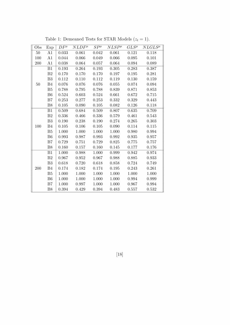
Table 1: Demeaned Tests for STAR Models (zt = 1).

Obs Exp DFµ NLDFµ SPµ NLSPµ GLSµ NLGLSµ

50 A1 0.033 0.061 0.042 0.061 0.121 0.118100 A1 0.044 0.066 0.049 0.066 0.095 0.101200 A1 0.038 0.064 0.057 0.064 0.094 0.089

B1 0.193 0.264 0.193 0.305 0.283 0.387B2 0.170 0.170 0.170 0.197 0.195 0.281B3 0.112 0.110 0.112 0.119 0.130 0.159

50 B4 0.076 0.076 0.076 0.055 0.074 0.094B5 0.788 0.795 0.788 0.839 0.871 0.853B6 0.524 0.603 0.524 0.661 0.672 0.715B7 0.253 0.277 0.253 0.332 0.329 0.443B8 0.105 0.090 0.105 0.082 0.126 0.118B1 0.509 0.684 0.509 0.807 0.635 0.709B2 0.336 0.466 0.336 0.579 0.461 0.543B3 0.190 0.238 0.190 0.274 0.265 0.303

100 B4 0.105 0.106 0.105 0.090 0.114 0.115B5 1.000 1.000 1.000 1.000 0.980 0.994B6 0.993 0.987 0.993 0.992 0.935 0.957B7 0.729 0.751 0.729 0.825 0.775 0.757B8 0.160 0.157 0.160 0.145 0.177 0.176B1 1.000 0.988 1.000 0.999 0.942 0.974B2 0.967 0.952 0.967 0.988 0.885 0.933B3 0.618 0.720 0.618 0.858 0.724 0.749

200 B4 0.174 0.182 0.174 0.195 0.243 0.261B5 1.000 1.000 1.000 1.000 1.000 1.000B6 1.000 1.000 1.000 1.000 0.994 0.999B7 1.000 0.997 1.000 1.000 0.967 0.994B8 0.394 0.429 0.394 0.483 0.557 0.532

[18]

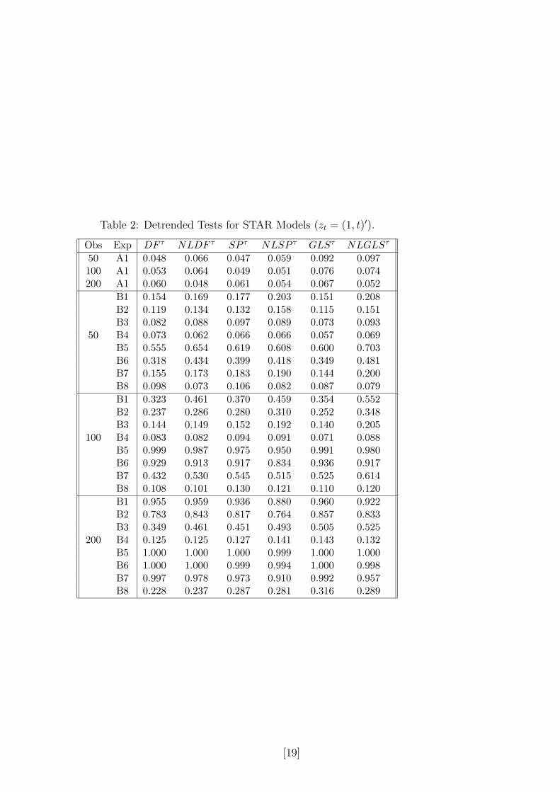
Table 2: Detrended Tests for STAR Models (zt = (1, t)′).

Obs Exp DF τ NLDF τ SP τ NLSP τ GLSτ NLGLSτ

50 A1 0.048 0.066 0.047 0.059 0.092 0.097100 A1 0.053 0.064 0.049 0.051 0.076 0.074200 A1 0.060 0.048 0.061 0.054 0.067 0.052

B1 0.154 0.169 0.177 0.203 0.151 0.208B2 0.119 0.134 0.132 0.158 0.115 0.151B3 0.082 0.088 0.097 0.089 0.073 0.093

50 B4 0.073 0.062 0.066 0.066 0.057 0.069B5 0.555 0.654 0.619 0.608 0.600 0.703B6 0.318 0.434 0.399 0.418 0.349 0.481B7 0.155 0.173 0.183 0.190 0.144 0.200B8 0.098 0.073 0.106 0.082 0.087 0.079B1 0.323 0.461 0.370 0.459 0.354 0.552B2 0.237 0.286 0.280 0.310 0.252 0.348B3 0.144 0.149 0.152 0.192 0.140 0.205

100 B4 0.083 0.082 0.094 0.091 0.071 0.088B5 0.999 0.987 0.975 0.950 0.991 0.980B6 0.929 0.913 0.917 0.834 0.936 0.917B7 0.432 0.530 0.545 0.515 0.525 0.614B8 0.108 0.101 0.130 0.121 0.110 0.120B1 0.955 0.959 0.936 0.880 0.960 0.922B2 0.783 0.843 0.817 0.764 0.857 0.833B3 0.349 0.461 0.451 0.493 0.505 0.525

200 B4 0.125 0.125 0.127 0.141 0.143 0.132B5 1.000 1.000 1.000 0.999 1.000 1.000B6 1.000 1.000 0.999 0.994 1.000 0.998B7 0.997 0.978 0.973 0.910 0.992 0.957B8 0.228 0.237 0.287 0.281 0.316 0.289

[19]

Table 3: Demeaned Tests for SETAR Models (zt = 1).

Obs Exp Wave Wexp DF WaveGLS Wexp

GLS GLS

100 A1 0.048 0.065 0.046 0.079 0.107 0.064200 A1 0.040 0.060 0.041 0.045 0.079 0.051

B1 0.250 0.223 0.318 0.315 0.264 0.455100 B2 0.246 0.216 0.280 0.317 0.281 0.430

B3 0.206 0.200 0.217 0.275 0.250 0.323B4 0.171 0.183 0.155 0.230 0.225 0.271B5 0.159 0.170 0.144 0.195 0.204 0.183C1 0.219 0.204 0.271 0.260 0.236 0.361

100 C2 0.209 0.196 0.225 0.256 0.241 0.296C3 0.189 0.185 0.175 0.230 0.224 0.274C4 0.179 0.204 0.136 0.222 0.230 0.211C5 0.136 0.150 0.106 0.165 0.174 0.147D1 0.267 0.249 0.298 0.341 0.301 0.473

100 D2 0.257 0.245 0.205 0.326 0.309 0.312D3 0.300 0.338 0.207 0.359 0.390 0.215D4 0.486 0.576 0.455 0.553 0.617 0.419D5 0.749 0.826 0.723 0.765 0.828 0.701E1 0.208 0.198 0.233 0.265 0.241 0.344

100 E2 0.231 0.237 0.185 0.285 0.282 0.256E3 0.318 0.370 0.244 0.358 0.400 0.275E4 0.526 0.587 0.485 0.569 0.615 0.499E5 0.759 0.810 0.713 0.779 0.827 0.715B1 0.748 0.738 0.886 0.817 0.789 0.799

200 B2 0.750 0.743 0.839 0.814 0.793 0.778B3 0.722 0.719 0.747 0.826 0.802 0.723B4 0.620 0.650 0.506 0.768 0.742 0.583B5 0.489 0.552 0.355 0.645 0.653 0.507C1 0.604 0.586 0.663 0.703 0.670 0.676

200 C2 0.564 0.569 0.619 0.682 0.650 0.639C3 0.529 0.548 0.546 0.634 0.622 0.586C4 0.512 0.552 0.433 0.635 0.624 0.512C5 0.355 0.419 0.279 0.512 0.524 0.386D1 0.748 0.748 0.847 0.818 0.804 0.796

200 D2 0.770 0.790 0.712 0.846 0.847 0.678D3 0.799 0.860 0.413 0.881 0.894 0.479D4 0.892 0.953 0.362 0.949 0.972 0.397D5 0.958 0.992 0.607 0.986 0.989 0.587E1 0.631 0.632 0.681 0.728 0.698 0.652

200 E2 0.596 0.639 0.530 0.678 0.710 0.613E3 0.576 0.696 0.341 0.669 0.743 0.414E4 0.730 0.834 0.480 0.797 0.853 0.467E5 0.889 0.949 0.701 0.924 0.952 0.657

[20]

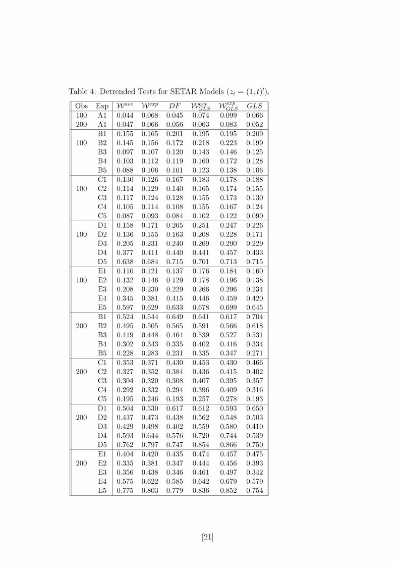
Table 4: Detrended Tests for SETAR Models (zt = (1, t)′).

Obs Exp Wave Wexp DF WaveGLS Wexp

GLS GLS

100 A1 0.044 0.068 0.045 0.074 0.099 0.066200 A1 0.047 0.066 0.056 0.063 0.083 0.052

B1 0.155 0.165 0.201 0.195 0.195 0.209100 B2 0.145 0.156 0.172 0.218 0.223 0.199

B3 0.097 0.107 0.120 0.143 0.146 0.125B4 0.103 0.112 0.119 0.160 0.172 0.128B5 0.088 0.106 0.101 0.123 0.138 0.106C1 0.130 0.126 0.167 0.183 0.178 0.188

100 C2 0.114 0.129 0.140 0.165 0.174 0.155C3 0.117 0.124 0.128 0.155 0.173 0.130C4 0.105 0.114 0.108 0.155 0.167 0.124C5 0.087 0.093 0.084 0.102 0.122 0.090D1 0.158 0.171 0.205 0.251 0.247 0.226

100 D2 0.136 0.155 0.163 0.208 0.228 0.171D3 0.205 0.231 0.240 0.269 0.290 0.229D4 0.377 0.411 0.440 0.441 0.457 0.433D5 0.638 0.684 0.715 0.701 0.713 0.715E1 0.110 0.121 0.137 0.176 0.184 0.160

100 E2 0.132 0.146 0.129 0.178 0.196 0.138E3 0.208 0.230 0.229 0.266 0.296 0.234E4 0.345 0.381 0.415 0.446 0.459 0.420E5 0.597 0.629 0.633 0.678 0.699 0.645B1 0.524 0.544 0.649 0.641 0.617 0.704

200 B2 0.495 0.505 0.565 0.591 0.566 0.618B3 0.419 0.448 0.464 0.539 0.527 0.531B4 0.302 0.343 0.335 0.402 0.416 0.334B5 0.228 0.283 0.231 0.335 0.347 0.271C1 0.353 0.371 0.430 0.453 0.430 0.466

200 C2 0.327 0.352 0.384 0.436 0.415 0.402C3 0.304 0.320 0.308 0.407 0.395 0.357C4 0.292 0.332 0.294 0.396 0.409 0.316C5 0.195 0.246 0.193 0.257 0.278 0.193D1 0.504 0.530 0.617 0.612 0.593 0.650

200 D2 0.437 0.473 0.438 0.562 0.548 0.503D3 0.429 0.498 0.402 0.559 0.580 0.410D4 0.593 0.644 0.576 0.720 0.744 0.539D5 0.762 0.797 0.747 0.854 0.866 0.750E1 0.404 0.420 0.435 0.474 0.457 0.475

200 E2 0.335 0.381 0.347 0.444 0.456 0.393E3 0.356 0.438 0.346 0.461 0.497 0.342E4 0.575 0.622 0.585 0.642 0.679 0.579E5 0.775 0.803 0.779 0.836 0.852 0.754

[21]

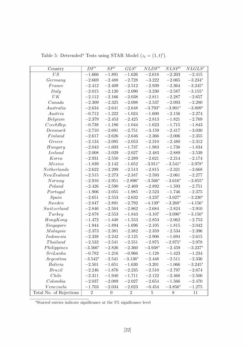
Table 5: Detrendeda Tests using STAR Model (zt = (1, t)′).

Country DF τ SP τ GLSτ NLDF τ NLSP τ NLGLSτ

US −1.666 −1.891 −1.626 −2.618 −2.203 −2.415Germany −2.669 −2.488 −2.728 −3.222 −2.065 −3.234∗France −2.412 −2.409 −2.512 −2.939 −2.364 −3.245∗Italy −2.015 −2.120 −2.090 −3.230 −2.587 −3.155∗UK −2.112 −2.166 −2.038 −2.811 −2.287 −2.657

Canada −2.309 −2.325 −2.098 −2.537 −2.093 −2.280Australia −2.634 −2.641 −2.648 −3.793∗ −3.901∗ −3.809∗Austria −0.712 −1.222 −1.024 −1.600 −2.156 −2.274Belgium −2.379 −2.453 −2.425 −2.813 −1.821 −2.769CzechRep. −0.738 −1.186 −1.044 −1.623 −1.715 −1.843Denmark −2.710 −2.691 −2.751 −3.159 −2.417 −3.030Finland −2.617 −2.626 −2.646 −2.366 −2.006 −2.355Greece −2.134 −2.095 −2.053 −2.310 −2.480 −2.312

Hungary −2.043 −1.693 −1.737 −1.983 −1.738 −1.834Iceland −2.008 −2.029 −2.027 −2.483 −2.889 −2.539Korea −2.931 −2.550 −2.289 −2.621 −2.214 −2.174Mexico −1.839 −2.142 −1.652 −3.911∗ −3.541∗ −3.978∗

Netherlands −2.622 −2.299 −2.513 −2.815 −2.321 −2.668NewZealand −2.515 −2.273 −2.347 −2.593 −2.061 −2.277

Norway −2.916 −2.951 −2.896∗ −3.566∗ −3.616∗ −3.855∗Poland −2.426 −2.590 −2.469 −2.892 −1.593 −2.751Portugal −1.906 −2.055 −1.985 −2.523 −1.746 −2.375Spain −2.651 −2.553 −2.632 −3.237 −3.027∗ −3.230∗Sweden −2.847 −2.891 −2.792 −4.139∗ −3.268∗ −4.156∗

Switzerland −2.846 −2.504 −2.862 −2.684 −2.824 −2.910Turkey −2.878 −2.553 −1.843 −3.107 −3.090∗ −3.150∗

HongKong −1.472 −1.448 −1.553 −2.853 −2.062 −2.753Singapore −1.944 −1.894 −1.696 −2.105 −1.815 −2.042Malaysia −2.373 −2.381 −2.382 −2.359 −2.534 −2.396Indonesia −2.338 −2.242 −2.125 −2.906 −1.694 −2.615Thailand −2.532 −2.541 −2.551 −2.975 −2.975∗ −2.978

Philippines −3.566∗ −2.826 −2.360 −3.938∗ −2.459 −3.237∗SriLanka −0.782 −1.216 −0.966 −1.128 −1.423 −1.234Argentina −3.542∗ −2.541 −3.136∗ −2.448 −2.511 −2.336Bolivia −2.501 −1.651 −1.630 −3.201 −1.066 −3.245∗Brazil −2.246 −1.876 −2.235 −2.510 −2.797 −2.674Chile −2.311 −1.940 −1.711 −2.122 −2.468 −2.500

Colombia −2.037 −2.089 −2.027 −2.654 −1.566 −2.470V enezuela −1.703 −2.034 −2.023 −0.454 −3.856∗ −1.275

Total No. of Rejections 2 0 2 5 8 11

aStarred entries indicate significance at the 5% significance level

[22]

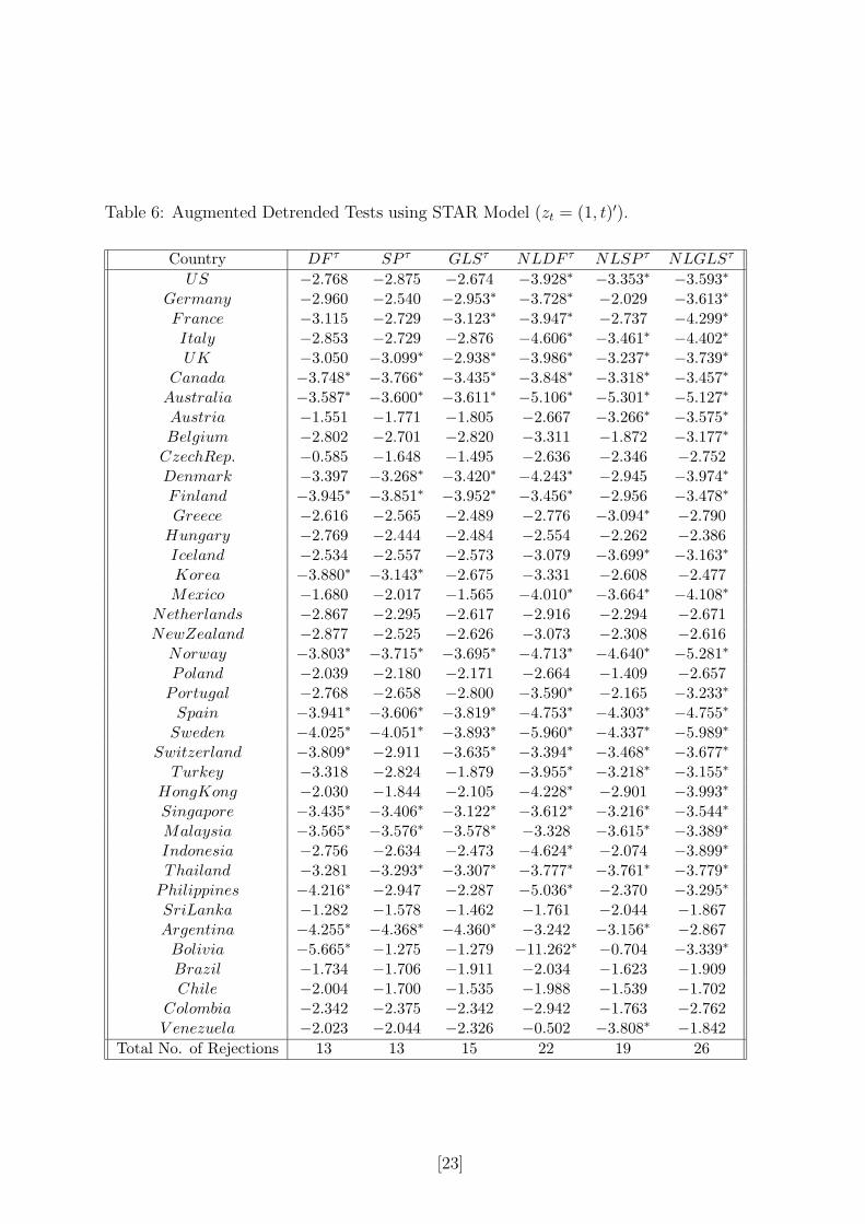
Table 6: Augmented Detrended Tests using STAR Model (zt = (1, t)′).

Country DF τ SP τ GLSτ NLDF τ NLSP τ NLGLSτ

US −2.768 −2.875 −2.674 −3.928∗ −3.353∗ −3.593∗Germany −2.960 −2.540 −2.953∗ −3.728∗ −2.029 −3.613∗France −3.115 −2.729 −3.123∗ −3.947∗ −2.737 −4.299∗Italy −2.853 −2.729 −2.876 −4.606∗ −3.461∗ −4.402∗UK −3.050 −3.099∗ −2.938∗ −3.986∗ −3.237∗ −3.739∗

Canada −3.748∗ −3.766∗ −3.435∗ −3.848∗ −3.318∗ −3.457∗Australia −3.587∗ −3.600∗ −3.611∗ −5.106∗ −5.301∗ −5.127∗Austria −1.551 −1.771 −1.805 −2.667 −3.266∗ −3.575∗Belgium −2.802 −2.701 −2.820 −3.311 −1.872 −3.177∗CzechRep. −0.585 −1.648 −1.495 −2.636 −2.346 −2.752Denmark −3.397 −3.268∗ −3.420∗ −4.243∗ −2.945 −3.974∗Finland −3.945∗ −3.851∗ −3.952∗ −3.456∗ −2.956 −3.478∗Greece −2.616 −2.565 −2.489 −2.776 −3.094∗ −2.790

Hungary −2.769 −2.444 −2.484 −2.554 −2.262 −2.386Iceland −2.534 −2.557 −2.573 −3.079 −3.699∗ −3.163∗Korea −3.880∗ −3.143∗ −2.675 −3.331 −2.608 −2.477Mexico −1.680 −2.017 −1.565 −4.010∗ −3.664∗ −4.108∗

Netherlands −2.867 −2.295 −2.617 −2.916 −2.294 −2.671NewZealand −2.877 −2.525 −2.626 −3.073 −2.308 −2.616

Norway −3.803∗ −3.715∗ −3.695∗ −4.713∗ −4.640∗ −5.281∗Poland −2.039 −2.180 −2.171 −2.664 −1.409 −2.657Portugal −2.768 −2.658 −2.800 −3.590∗ −2.165 −3.233∗Spain −3.941∗ −3.606∗ −3.819∗ −4.753∗ −4.303∗ −4.755∗Sweden −4.025∗ −4.051∗ −3.893∗ −5.960∗ −4.337∗ −5.989∗

Switzerland −3.809∗ −2.911 −3.635∗ −3.394∗ −3.468∗ −3.677∗Turkey −3.318 −2.824 −1.879 −3.955∗ −3.218∗ −3.155∗

HongKong −2.030 −1.844 −2.105 −4.228∗ −2.901 −3.993∗Singapore −3.435∗ −3.406∗ −3.122∗ −3.612∗ −3.216∗ −3.544∗Malaysia −3.565∗ −3.576∗ −3.578∗ −3.328 −3.615∗ −3.389∗Indonesia −2.756 −2.634 −2.473 −4.624∗ −2.074 −3.899∗Thailand −3.281 −3.293∗ −3.307∗ −3.777∗ −3.761∗ −3.779∗

Philippines −4.216∗ −2.947 −2.287 −5.036∗ −2.370 −3.295∗SriLanka −1.282 −1.578 −1.462 −1.761 −2.044 −1.867Argentina −4.255∗ −4.368∗ −4.360∗ −3.242 −3.156∗ −2.867Bolivia −5.665∗ −1.275 −1.279 −11.262∗ −0.704 −3.339∗Brazil −1.734 −1.706 −1.911 −2.034 −1.623 −1.909Chile −2.004 −1.700 −1.535 −1.988 −1.539 −1.702

Colombia −2.342 −2.375 −2.342 −2.942 −1.763 −2.762V enezuela −2.023 −2.044 −2.326 −0.502 −3.808∗ −1.842

Total No. of Rejections 13 13 15 22 19 26

[23]

Table 7: Detrendeda Tests using SETAR Model (zt = (1, t)′).

Country DF τ GLSτ Wexp WexpGLS

US −2.018 −2.001 30.417 31.885Germany −3.029 −2.493 21.617 371.184∗

Italy −1.550 −1.600 4.569 5.281UK −1.368 −1.376 2.611 2.583

Canada −2.309 −2.109 9.049 15.332Australia −2.718 −2.758 26.749 27.129Austria −3.220 −3.132∗ 129.876 182.792∗

Belgium −1.158 −1.289 3.130 3.359Denmark −2.884 −2.882 193.689 179.178∗

Finland −1.976 −2.000 21.031 20.314Greece −3.109 −3.152∗ 483.571 648.997∗

Hungary −1.392 −1.461 27.197 25.501Ireland −2.464 −2.484 71.521 84.536Korea −3.913∗ −1.792 5.764 7196.804∗

Mexico −3.112 −3.139∗ 150.811 140.496Netherlands −1.643 −1.663 16.911 15.533

Norway −1.805 −1.765 5.585 5.105Spain −2.721 −2.579 279.802 656.358∗

Sweden −2.545 −2.551 31.005 36.293Switzerland −3.040 −2.975∗ 255.250 380.021∗

Turkey −2.389 −2.212 15.109 26.186Singapore −1.471 −1.493 4.498 5.483Malaysia −3.583∗ −2.587 76.817 5761.784∗

Indonesia −1.848 −1.420 5.781 11.051Thailand −2.802 −2.677 79.602 160.068∗

Philippines −3.037 −1.685 20.890 144.733SriLanka −2.050 −1.687 7.618 22.242Argentina −5.165∗ −2.407 33.843 4623153∗

Chile −2.909 −2.516 1058.658∗ 16315.06∗

Colombia −2.140 −2.149 16.778 16.885V enezuela −2.022 −2.071 13.117 10.126

Total No. of Rejections 4 5 2 12

aStarred entries indicate significance at the 5% significance level

[24]

Table 8: Augmented Detrended Tests using SETAR Model (zt =(1, t)′).

Country DF τ GLSτ Wexp WexpGLS

US −2.995 −2.982∗ 631.439∗ 702.101∗

Germany −3.249 −2.491 27.803 2943.871∗

Italy −2.238 −2.247 22.700 29.338UK −2.082 −2.079 13.153 8.673

Canada −3.289 −3.085∗ 122.689 282.461∗

Australia −3.690∗ −3.707∗ 302.119 337.048∗

Austria −3.429∗ −3.143∗ 217.976 422.499∗

Belgium −2.530 −2.752 155.902 124.441Denmark −3.528∗ −3.545∗ 3011.942∗ 2492.441∗

Finland −3.311 −3.332∗ 1866.803∗ 1737.248∗

Greece −2.679 −2.744 171.794 246.429∗

Hungary −1.735 −1.790 40.063 42.969Ireland −2.633 −2.647 180.433 211.145∗

Korea −3.059 −1.862 6.843 225.669∗

Mexico −4.747∗ −4.708∗ 315031.4∗ 275743.3∗

Netherlands −2.566 −2.432 371.038 230.185∗

Norway −3.552∗ −3.645∗ 1159.313∗ 878.808∗

Spain −2.825 −2.659 759.037∗ 1615.200∗

Sweden −3.884∗ −3.840∗ 1360.870∗ 1587.833∗

Switzerland −3.063 −2.937∗ 682.176∗ 1605.988∗

Turkey −2.257 −2.302 30.638 37.589Singapore −2.428 −2.462 170.091 255.528∗

Malaysia −3.147 −2.346 41.731 748.718∗

Indonesia −2.290 −1.642 63.976 229.395∗

Thailand −3.416∗ −3.232∗ 848.976∗ 1688.448∗

Philippines −3.833∗ −1.852 59.831 5858.578∗

SriLanka −3.499∗ −2.772 250.551 4455.678∗

Argentina −5.701∗ −1.693 3.985 10064985∗

Chile −1.989 −1.831 97.113 9551.004∗

Colombia −2.269 −2.287 27.936 27.388V enezuela −2.218 −2.281 28.026 21.126

Total No. of Rejections 10 11 9 24

[25]

This working paper has been produced bythe Department of Economics atQueen Mary, University of London

Copyright © 2002 George Kapetanios andYongcheol Shin. All rights reserved.

Department of Economics Queen Mary, University of LondonMile End RoadLondon E1 4NSTel: +44 (0)20 7882 5096 or Fax: +44 (0)20 8983 3580Email: j.conner@qmul.ac.ukWebsite: www.econ.qmul.ac.uk/papers/wp.htm