Volume 29, Issue 2

 

Is Malaysian Stock Market Efficient? Evidence from Threshold Unit Root Tests

 

Qaiser Munir School of Business and Economics, Universiti malaysia

Sabah

Kasim Mansur School of Business and Economics, Universiti Malaysia

Sabah

Abstract

This paper investigates the behavior of Kuala Lumpur Stock Exchange Composite Index (KLCI) for the period from 1980:1 to 2008:8 using a two-regime threshold autoregressive (TAR) model with an autoregressive unit root developed by Caner and Hansen [Threshold autoregression with a unit roots, Econometrics 69 (6) (2001) 1555-1596] which allows testing nonlinearity and nonstationarity simultaneously. Our finding indicates that the KLCI is a nonlinear series that is characterized by a unit root process, consistent with the efficient market hypothesis.

We are grateful to Bruce Hansen for making available his Gauss Programme to estimate and make inferences on the TAR model. The usual disclaimer applies. Citation: Qaiser Munir and Kasim Mansur, (2009) ''Is Malaysian Stock Market Efficient? Evidence from Threshold Unit Root Tests'', Economics Bulletin, Vol. 29 no.2 pp. 1359-1370. Submitted: Apr 29 2009.   Published: June 08, 2009.

 

     

1

1. Introduction

The stock market efficiency hypothesis is among the most popular research topic in the

international macroeconomic literature. Stock market efficiency implies that prices respond

quickly and accurately to relevant information. Information in the efficient market hypothesis is

defined as anything that may affect prices which is unknowable in the present and appears

randomly in the future. This random information is the cause of future price changes. In other

words, an efficient stock market is characterized by a random walk (unit root) process, which

indicates that stock market returns cannot be predicted based on its historical observations. If

stock price follows a random walk process, any shock to stock price is permanent, and there is no

tendency for the price level to return to a trend path over time. In contrast, a mean reverting

process (trend stationary) means that any shock to stock price is transitory and there is tendency

for the price level to return to a trend path over time. The random walk property implies that

future returns are unpredictable based on previous observations and that volatility of stock price

can grow without bound in the long-run. Hence, testing for mean reversion in stock prices is one

avenue for examining market efficiency (see Fama and French, 1988a, 1988b).

There is a large body of the literature that investigates the efficient market hypothesis using a

variety of methodology and found mixed results. Many studies have found that stock indexes are

not characterized by a unit root (see Lo and MacKinlay, 1988; Poterba and Summers, 1988;

Urrutia, 1995; Grieb and Reyes, 1999; Chaudhuri and Wu, 2003; Shively, 2003; Narayan,

2008), while others have found stock indexes to be a unit root process (Huber, 1997; Liu et al.,

1997; Ozdemir, 2008; Narayan, 2005, 2006; Narayan and Smyth, 2004, 2005; Qian et al.,

2008;). Two important features characterize these studies.

First, the majority of these studies are based on univariate unit root tests. However, one strong

criticism of the univariate unit root tests, such as the Dickey and Fuller test used by the most

studies, is that it lacks power if the true data generating process of a series exhibits structural

breaks (Perron, 1989). Therefore, the majority of these studies adopt new developed unit root test

with structural breaks (Zivot and Andrew, 1992; Lumsdaine and Papell, 1997; Lee and

Strazicich, 2003; Im et al., 2005) to investigate the stationary property of stock prices. For

example, Chaudhuri and Wu (2003) investigate mean reversion in stock prices in emerging

markets, including one break unit root tests. Their findings, when compared to previous findings,

show that there is no consensus among economists regarding market efficiency. Narayan and

Smyth (2004) apply the Zivot and Andrews (1992) one break and the Lumsdaine and Papell

(1997) two break unit root tests to examine the random walk hypothesis for stock prices in South

Korea. Their results provide strong evidence that stock prices in South Korea are characterized

by a unit root, which is consistent with the efficient market hypothesis. Lean and Smyth (2007)

apply univariate and panel Lagrange Multiplier (LM) unit root tests with one and two structural

breaks (Lee and Strazicich, 2003; Im et al., 2005) to examine the random walk hypothesis for

stock prices in eight Asian countries. The results from the univariate LM unit root tests and panel

LM unit root test with one structural break suggest that stock prices in each country is characterized by a

random walk, but the findings from the panel LM unit root test with two structural breaks suggest that

stock prices in the eight countries are mean reverting. Narayan (2008) provide evidence on the unit

root hypothesis for G7 stock price indices using the Lagrangian multiplier (LM) panel unit root

2

test that allows for structural breaks. His main finding is that stock prices are stationary

processes, inconsistent with the efficient market hypothesis.

Second, however, following the work of (Abhyankar et al., 1995, 1997; Atchison and White,

1996; Kohers et al., 1997; Schaller and van Norden, 1997; Qi, 1999; Kanas, 2001; Sarantis,

2001; Shively, 2003; Narayan, 2005, 2006; Qian et al., 2008; among others), who find stock

prices to be consistent with a nonlinear data generating process, the reliability of the findings

from existing studies is questionable. Shively (2003) examines the six stock prices (CAC 40,

DAX 30, FTSE 100, Nikkei 225, S&P 500 and TSE 300) for the period 1970:1-2000:12. He

applies Tsay’s (1998) chi-squared test and find that all six stock-price indexes are all highly

consistent with threshold nonlinearity. Then he applies Tsay’s (1998) threshold modeling

technique to partition each stock-price index into three regimes using the corresponding stock-

return series as the stationary threshold variable and finds the series to be a regime reverting

process. This nonlinear regime-reverting process implies a violation of the efficient market

hypothesis. In contrast, Narayan (2006) investigates the behavior of US stock prices using an

unrestricted two-regime threshold model for the period1964:06 to 2003:04. He finds that the

stock prices are nonlinear process and characterized by a unit root process, consistent with the

efficient market hypothesis.

Lean and Symth (2007) suggest that, in terms of future research, there is growing evidence that

univariate unit root tests lack the power to find mean reversion in stock prices. Perhaps a more

promising approach might be to examine whether Asian stock prices are nonlinear with a unit

root. Thus, this paper contributes to the existing literature on the random walk hypothesis, by

providing additional evidence on the Malaysian stock market efficiency, using the threshold

autoregressive (TAR) model developed by Caner and Hansen (2001). Caner and Hansen

methodology is applicable if a nonlinear process has unit root. The main advantage of the TAR

model is that it allows us to discriminate nonstationarity from nonlinearity in data

simultaneously. Furthermore, their methodology allows testing for a partial unit root process in

two regimes1. Our main finding is that the Malaysian stock price is a nonlinear process and is

characterized by unit root. The latter finding is consistent with the efficient market hypothesis.

The rest of the paper is organized as follows: Section 2 outlines the empirical methodology.

Section 3 presents the data and empirical results. Finally, Section 4 provides conclusion.

2. Empirical Methodology

Following the work of Caner and Hansen (2001), we adopt a two-regime TAR (k) model with

an autoregressive unit root as follow:

ttZttZtt eIxIxy } 1{12} 1{11

(1)

Where y is the logarithm of the stock price index for t = 1,. . .,T, ),..., , ,( 111 kttttt yyryx ;

}{I is the indicator function; te is an independently and identically error term; mttt yyZ for

1 Many studies (see, Alba and Park , 2005; Basci and Caner, 2005 and Ho, 2005) have applied this methodology to

test the unit root and threshold effect to exchange rates and Purchasing Power Parity (PPP) .

3

m represents the delay order and some 1 ≤ m ≤ k. tr is a vector of deterministic components

including an intercept and a possible linear time trend. The threshold value λ is unknown and

takes the values in the compact interval ],[ 21 , where λ1 and λ2 are picked according

to 0)( 11 tZP and 1)( 22 tZP . It is convenient to show the components of θ1 and θ2

as follow:

1

1

1

1

and

2

2

2

2

(2)

where ρ1 and ρ2 are slope coefficients on 1ty , β1 and β2 are scalar intercepts, and α1 and α2 are K

x 1 vectors containing the slope coefficients on dynamics regressors (Δyt-1,…, Δyt-k) in the two

regimes. In order to calibrate equation (1), the concentrated least squares (LS) approach is

usually utilized. For each , equation (1) is estimated ordinary least square (OLS) so that

ttZttZtt eIxIxy ˆ )(ˆ )(ˆ} 1{12} 1{11

(3)

Let TteT 1

212 )(ˆ)(ˆ be the OLS estimate of 2 for fixed λ. The LS estimate of threshold

parameter (λ) is found by minimizing the residual variance, )(2 :

)(ˆmin argˆ 2

(4)

Estimating the TAR model in equation (1), the two central issues are whether or not there is a

threshold effect and whether the process yt (stock price index) is stationary or not. In this paper

standard Wald test statistics, ),(sup)ˆ(

TTT WWW

proposed by Caner and Hansen (2001), is

used to test the null hypothesis of no threshold effect (i.e., the process is linear) H0: θ1 = θ2,

against the alternative of threshold effect (i.e., the process is nonlinear). If the null hypothesis

cannot be rejected, there is no threshold effect, in which case the two vectors of coefficients are

identical between the two regimes (θ1 = θ2). Caner and Hansen find that WT has a non-standard

asymptotic null distribution with critical values that cannot be tabulated. Hence they propose a

bootstrap method to compute asymptotic critical values and p-values.

The stationarity of the process yt depends on the parameters ρ1 and ρ2. For regime 1, we can

reject the null hypothesis of unit roots in favor of the alternative hypothesis of level stationarity if

ρ1 is significantly different from zero. We can do the same for regime 2 if ρ2 is significantly

different from zero. If the null hypothesis: H0: ρ1 = ρ2 = 0 holds, the process yt has a unit root and

model (1) can be expressed in terms of the stationary difference Δyt. The obvious alternative to

H0 is H1: ρ1 < 0 and ρ2 < 0, in which case the process yt is stationary in both regimes. We also

have to consider the intermediate partial unit root case H2: ρ1 < 0 and ρ2 = 0 or ρ1 = 0 and ρ2 < 0,

in which case the process yt have a unit root in one regime and is stationary in other showing

mean reversion behavior.

The null hypothesis is tested against the unrestricted alternative ρ1 ≠ 0 or ρ2 ≠ 0 using the Wald

statistics, and expressed as, 22

212 ttR T , where t1 and t2 are the t-ratios for 1̂ and 2̂ respectively

4

from the OLS estimation. However, Caner and Hansen (2001) note that this two-sided Wald

statistics may have less power than a one-sided version of the test. As a result, they recommend

the following one-sided Wald statistics:

}02ˆ{}01ˆ{

22

211 ItItR T (5)

which tests H0 against the one-sided alternative ρ1 <0 or ρ2 <0. A statistically significant R1T

justifies rejecting unit roots in favor of stationarity. However, it does not allow us to discriminate

between the stationary case H1 and the partial unit root case H2. This requires further examining

the individual t statistics t1 and t2. Only one of −t1 or −t2 being significant would be consistent

with the partial unit root case.

3. Data and Empirical Results

The data studied in this paper are the logged values of the KL Composite index (KLCI)2, which

is the main index for Bursa Malaysia (stock exchange). Monthly data over the period from

1980:1 to 2008:8 are utilized for analysis and taken from Bloomberg database. Specifically, we

retrieve the closing prices of the last trading days of all months, which give the time series yt

defined in the preceding section.

Before beginning the tests we consider conventional Augmented Dickey Fuller (ADF) test for

unit root against linear stationary alternative. The results are not reported here to conserve space

but are available from the authors upon request. We find the calculated t-statistics to be –1.8976

(with an intercept) and –2.8588 (with an intercept and a trend), respectively. Given the 10% level

critical value of –2.5712 (for model with no trend) and –3.1344 (for model with trend), we are

unable to reject the unit root null hypothesis. This finding is not surprising since ADF test have

almost no power when alternative is nonlinear process. This implies that KLCI has a unit root3.

To examine the stationarity in the possible presence of nonlinearities, we apply the Caner and

Hansen procedure described above. The first issue we must address is the presence of the

threshold effects. As stated previously, the appropriate test this purpose is the standard Wald

statistic WT. in Table 1, we report the results of the Wald test, bootstrap critical values at three

conventional levels 10%, 5%, and 1%, and bootstrap p-values (using 10000 replications) for

threshold variables of the form Zt = yt – yt-m for different delay parameters m ranging from 1 to

12. The significant bootstrap p-values corresponding to the Wald tests WT (except for m = 4,

which is not statistically significant) indicate that we can reject the null hypothesis of linearity in

favor of the alternative that there is a threshold effect in the monthly KLCI series. According to

2 The Stock Exchange of Malaysia was officially formed in 1964 under the name Stock Exchange of Malaysia and

Singapore (SEMS). In 1973, with the termination of currency interchangeability between Malaysia and Singapore,

the SEMS was separated into The Kuala Lumpur Stock Exchange Bhd (KLSEB). KLSEB became a demutualised

exchange and was re-named Bursa Malaysia in 2004 with total market capitalization of MYR700 billion (US$189

billion). As of 31 December 2007, the Malaysia Exchange had 986 listed companies with a combined market

capitalization of $325 billion.

3 Phillips and Perron (1988) and Kwiatkowski et al. (KPSS, 1992) unit root tests also conducted, and we found the

identical results. All results are available from the author upon request.

5

these results, the linear AR model can be rejected in favour of the TAR model. In order to avoid

the criticism that the results of Table 1 is conditional on m, which is generally unknown, Caner

and Hansen (2001) recommend making m endogenous, which is achieved by selecting an m

value that minimizes the residual variance of the least squares estimates. This is also the value

that maximizes WT since WT is a monotonic function of the residual variance (Alba and Park,

2005). According to Table 1, the Wald statistics is maximized (WT = 46.7, corresponding p-value

= 0.002) when m = 5. Hence we take m̂ = 5 as the preferred model.

Table 1. Threshold Test

m WT Bootstrap critical values Bootstrap p-values

10% 5% 1%

1 35.7 31.3 34.5 41.1 0.029

2 31.2 30.9 33.8 40.9 0.092

3 32.3 30.8 34.0 40.9 0.089

4 22.0 30.7 33.9 40.7 0.514

5 46.7 30.7 33.9 39.7 0.002

6 45.0 30.7 33.7 39.0 0.002

7 39.0 30.7 33.8 40.0 0.014

8 36.8 30.6 33.8 40.0 0.024

9 35.9 30.7 33.4 39.8 0.028

10 41.5 30.6 33.5 39.9 0.007

11 38.9 30.6 33.3 40.0 0.012

12 38.7 30.5 33.3 40.4 0.015

We now examine the unit root properties of the KLCI. We first calculate the one-sided and two-

sided threshold unit root test statistics R1T and R2T along with the bootstrap critical values and p-

values for each delay parameters m, ranging from 1 to 12. The results are reported in Table 2.

The Wald statistic WT obtained from R1T is statistically insignificant at the 10% level for all m.

For the preferred model m = 5, the WT test statistic of 2.80 is less than the 10% critical value

(9.2). We find similar results from the two-sided Wald tests R2T presented in the right panel of

Table 2. For all m, Wald statistics WT are less than the bootstrap critical values at the 10% level

of significance. These results suggest that the null hypothesis of the presence of a unit root in the

monthly KLCI cannot be rejected at the 10% level.

6

Table 2. One and Two sided Unit root Tests

R1T R2T

Bootstrap critical values

Bootstrap critical values

m WT 10% 5% 1% p-values WT 10% 5% 1% p-values

1 3.15 9.1 11.3 16.2 0.571

3.15 9.5 11.6 17.1 0.603

2 2.98 9.1 11.3 16.5 0.594

2.99 9.5 11.8 17.1 0.627

3 1.81 9.1 11.4 16.0 0.751

1.82 9.6 11.8 16.4 0.788

4 1.71 9.3 11.3 16.4 0.754

1.73 9.6 11.8 16.7 0.791

5 2.80 9.2 11.4 16.5 0.606

2.80 9.6 11.9 17.1 0.643

6 1.73 9.3 11.5 16.8 0.762

1.75 9.7 11.9 17.1 0.800

7 1.73 9.2 11.5 16.8 0.761

1.76 9.6 11.9 17.0 0.798

8 3.94 9.3 11.5 16.5 0.472

3.94 9.7 12.1 16.9 0.508

9 7.03 9.4 11.7 16.8 0.205

7.03 9.7 12.2 17.1 0.229

10 6.66 9.5 11.8 17.2 0.234

6.67 9.9 12.2 17.8 0.256

11 4.17 9.6 11.8 17.0 0.458

4.20 9.9 12.2 17.1 0.490

12 3.88 9.4 11.8 17.4 0.495 3.88 9.8 12.1 17.6 0.527

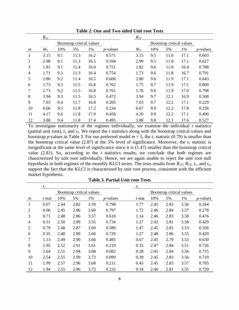
To investigate stationarity of the regimes individually, we examine the individual t statistics

(partial unit root), t1 and t2. We report the t statistics along with the bootstrap critical values and

bootstrap p-values in Table 3. For our preferred model m = 5, the t1 statistic (0.79) is smaller than

the bootstrap critical value (2.87) at the 5% level of significance. Moreover, the t2 statistic is

insignificant at the same level of significance since it is (1.47) smaller than the bootstrap critical

value (2.81). So, according to the t statistics results, we conclude that both regimes are

characterized by unit root individually. Hence, we are again unable to reject the unit root null

hypothesis in both regimes of the monthly KLCI series. The tests results from R1T, R2T, t1, and t2,

support the fact that the KLCI is characterized by unit root process, consistent with the efficient

market hypothesis.

Table 3. Partial Unit root Tests

t1 t2

Bootstrap critical values

Bootstrap critical values

m t-stat 10% 5% 1% p-values t-stat 10% 5% 1% p-values

1 0.07 2.44 2.82 3.59 0.798

1.77 2.45 2.83 3.56 0.264

2 0.06 2.45 2.86 3.60 0.797

1.72 2.46 2.84 3.57 0.278

3 0.71 2.48 2.86 3.57 0.618

1.14 2.46 2.83 3.58 0.476

4 0.31 2.50 2.89 3.55 0.734

1.27 2.42 2.81 3.58 0.429

5 0.79 2.48 2.87 3.60 0.589

1.47 2.45 2.81 3.53 0.356

6 0.35 2.48 2.89 3.66 0.729

1.27 2.48 2.86 3.55 0.429

7 1.13 2.49 2.90 3.66 0.485

0.67 2.45 2.79 3.53 0.630

8 1.95 2.52 2.91 3.61 0.219

0.35 2.47 2.84 3.51 0.726

9 2.64 2.51 2.94 3.68 0.082

0.28 2.45 2.84 3.56 0.755

10 2.54 2.55 2.99 3.72 0.099

0.39 2.45 2.83 3.56 0.710

11 1.99 2.57 2.96 3.68 0.211

0.45 2.45 2.83 3.57 0.705

12 1.94 2.55 2.96 3.72 0.232 0.34 2.46 2.81 3.55 0.729

7

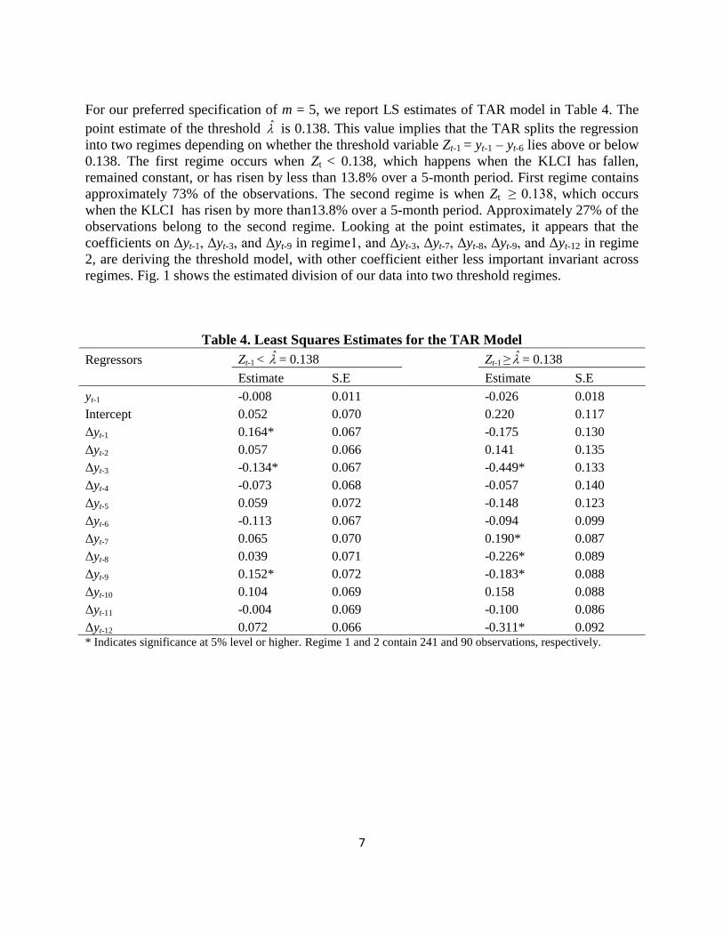
For our preferred specification of m = 5, we report LS estimates of TAR model in Table 4. The

point estimate of the threshold ̂ is 0.138. This value implies that the TAR splits the regression

into two regimes depending on whether the threshold variable Zt-1 = yt-1 – yt-6 lies above or below

0.138. The first regime occurs when Zt < 0.138, which happens when the KLCI has fallen,

remained constant, or has risen by less than 13.8% over a 5-month period. First regime contains

approximately 73% of the observations. The second regime is when Zt ≥ 0.138, which occurs

when the KLCI has risen by more than13.8% over a 5-month period. Approximately 27% of the

observations belong to the second regime. Looking at the point estimates, it appears that the

coefficients on Δyt-1, Δyt-3, and Δyt-9 in regime1, and Δyt-3, Δyt-7, Δyt-8, Δyt-9, and Δyt-12 in regime

2, are deriving the threshold model, with other coefficient either less important invariant across

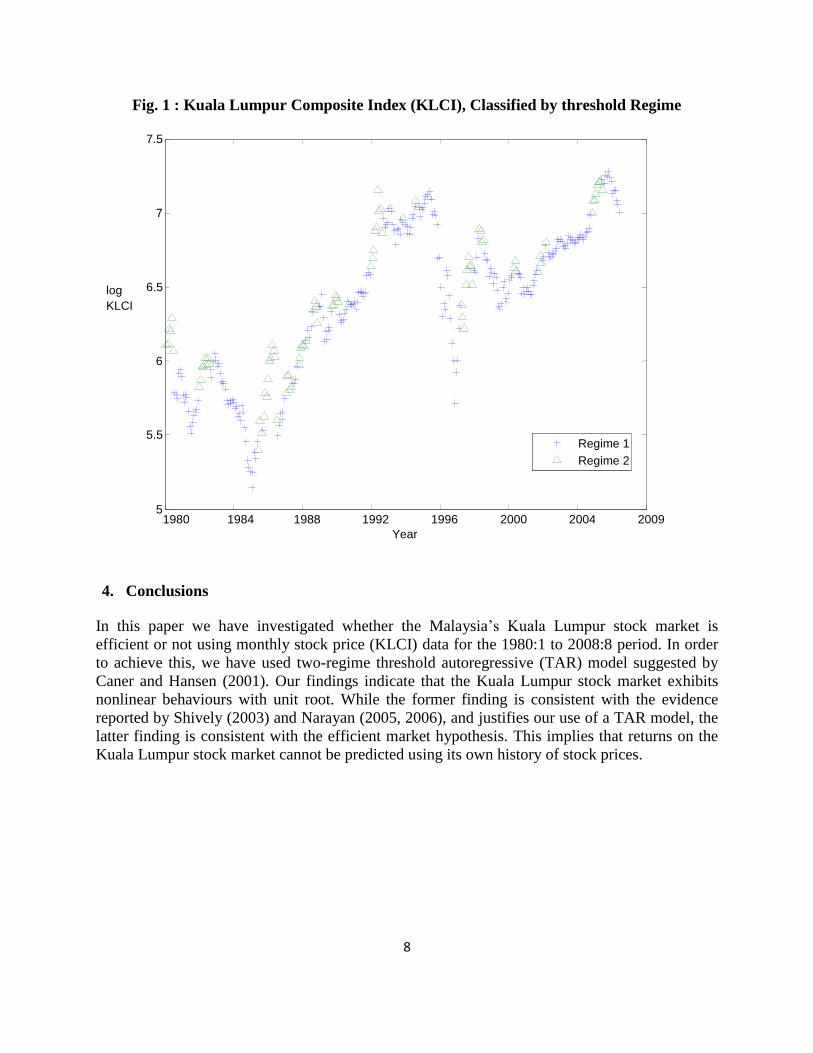
regimes. Fig. 1 shows the estimated division of our data into two threshold regimes.

Table 4. Least Squares Estimates for the TAR Model

Regressors Zt-1 < ̂ = 0.138 Zt-1 ≥ ̂ = 0.138

Estimate S.E Estimate S.E

yt-1

-0.008 0.011

-0.026 0.018

Intercept

0.052 0.070

0.220 0.117

Δyt-1

0.164* 0.067

-0.175 0.130

Δyt-2

0.057 0.066

0.141 0.135

Δyt-3

-0.134* 0.067

-0.449* 0.133

Δyt-4

-0.073 0.068

-0.057 0.140

Δyt-5

0.059 0.072

-0.148 0.123

Δyt-6

-0.113 0.067

-0.094 0.099

Δyt-7

0.065 0.070

0.190* 0.087

Δyt-8

0.039 0.071

-0.226* 0.089

Δyt-9

0.152* 0.072

-0.183* 0.088

Δyt-10

0.104 0.069

0.158 0.088

Δyt-11

-0.004 0.069

-0.100 0.086

Δyt-12 0.072 0.066 -0.311* 0.092 * Indicates significance at 5% level or higher. Regime 1 and 2 contain 241 and 90 observations, respectively.

8

Fig. 1 : Kuala Lumpur Composite Index (KLCI), Classified by threshold Regime

4. Conclusions

In this paper we have investigated whether the Malaysia’s Kuala Lumpur stock market is

efficient or not using monthly stock price (KLCI) data for the 1980:1 to 2008:8 period. In order

to achieve this, we have used two-regime threshold autoregressive (TAR) model suggested by

Caner and Hansen (2001). Our findings indicate that the Kuala Lumpur stock market exhibits

nonlinear behaviours with unit root. While the former finding is consistent with the evidence

reported by Shively (2003) and Narayan (2005, 2006), and justifies our use of a TAR model, the

latter finding is consistent with the efficient market hypothesis. This implies that returns on the

Kuala Lumpur stock market cannot be predicted using its own history of stock prices.

1980 1984 1988 1992 1996 2000 2004 2009 5

5.5

6

6.5

7

7.5

Year

log

KLCI

Regime 1 Regime 2

9

References

Abhyankar, A., Copeland, L. S. and Wong, W. (1995) “Nonlinear dynamics in real-time equity

market indices: evidence from the United Kingdom” Economic Journal 105, 864-880.

Abhyankar, A., Copeland, L. S. and Wong, W. (1997) “Uncovering nonlinear structure in real-

time stock market indexes: the S&P 500, the DAX, the Nikkei 225, and the FTSE-100” Journal

of Business and Economics Statistics 15, 1-14.

Alba, J. D., and Park, D. (2005) “An empirical investigation of purchasing power parity (PPP)

for Turkey”, Journal of policy Modeling, 27, 989-1000.

Atchison, M. D. and White, M. A. (1996) “Disappearing evidence of chaos in security returns: a

Simulation”, Quarterly Journal of Business and Economics, 35, 21–37.

Basci, E and Caner, M. (2005) “Are real exchange rates non-linear or non-stationary? Evidence

from a new threshold unit root test”, Studies in Nonlinear Dynamics and Econometrics, 9, 1-19.

Caner, M. and Hansen, B. (2001) “Threshold autoregression with a unit root”, Econometrica, 69,

1555–1596.

Chaudhuri, K. and Wu, Y. (2003) “Random walk versus breaking trend in stock prices: evidence

from emerging markets”, Journal of Banking and Finance, 27, 575–92.

Dickey, D. A. and Fuller, W. A. (1981) “Likelihood ratio statistics for autoregressive time series

with a unit root”, Econometrica, 49, 1057–72.

Fama, E. F. and French, K. R. (1988a) “Dividend yields and expected stock returns” Journal of

Financial Economics 22, 3-25.

Fama, E. F. and French, K. R. (1988b) “Permanent and temporary components of stock prices”

Journal of Political Economy 96, 246-273.

Grieb, T. A. and Reyes, M. G. (1999) “Random walk tests for Latin American equity indexes

and individual firms”, Journal of Financial Research, 22, 371–83.

Ho, T. (2005) “Investigating the threshold effects of inflation on PPP, Economic Modelling, 22,

926-948.

Huber, P. (1997) “Stock market returns in thin markets: evidence from the Vienna stock

exchange”, Applied Financial Economics, 7, 493-498.

Im,K.S., Lee, J,. and Tieslau, M. (2005) “Panel LM unit root tests with level shifts”, Oxford

Bulletin of Economics & Statistics, 67, 393–419.

10

Kanas, A. and Genius, M. (2005) “Regime (non)stationarity in the US/UK real exchange rate”,

Economics Letters, 87, 407–413.

Kohers, T., Pandey, V. and Kohers, G. (1997) “Using nonlinear dynamics to test for market

efficiency among the major US stock exchanges”, Quarterly Review of Economics and Finance,

37, 523–545.

Lean, H.H and Smyth, R. (2007) “Do Asian Stock Markets Follow a Random Walk? Evidence

from LM Unit Root Tests with One and Two Structural Breaks” Review of Pacific Basin

Financial Markets and Policies, 10, 15-31.

Lee, J. and M. C. Strazicich (2003) “Minimum LM Unit Root Tests with Two Structural Breaks”

The Review of Economics and Statistics 85, 1082-1089.

Lo, A.W. and A.C.MacKinlay (1988) “ Stock market prices do not follow random walks:

evidence from a simple specification test” Review of Financial Studies 1, 41-66.

Liu, C. Y., Song, S. H. and Romilley, P. (1997) “Are Chinese stock markets efficient? A

cointegration and causality analysis”, Applied Economic Letters, 4, 511–5.

Lumsdaine, R. and D. Papell (1997) “Multiple Trend Breaks and the Unit-Root Hypothesis”,

Review of Economics and Statistics, 79, 212–218.

Narayan, P. K. (2005) “Are the Australian and New Zealand stock prices nonlinear with a unit

root?” Applied Economics, 37, 2161-2166.

Narayan, P. K. (2006) “The behavior of US stock prices: evidence from a threshold

autoregressive model, Mathematics and Computers in Simulation 71, 103-108.

Narayan, P. K. (2008) “Do shocks to G7 stock prices have a permanent effect? Evidence from

panel unit root tests with structural change”, Mathematics and Computers in Simulation, 77, 369-

373.

Narayan, P. K. and R. Smyth (2004) “Is South Korea’s stock market efficient?” Applied

Economics Letters 11, 707-710.

Ozdemir, Z.A. (2008) “Efficient market hypothesis: evidence from a small open-economy”,

Applied Economics, 40, 633–641.

Perron, P. (1989) “The Great Crash, the Oil Price Shock, and the Unit Root Hypothesis”,

Econometrica, 57, 1361-1401.

Poterba, J. M. and Summers, L. H. (1988) “Mean reversion in stock prices: evidence and

implications”, Journal of Financial Economics, 22, 27–59.

11

Sarantis, N. (2001) “Nonlinearities, cyclical behavior and predictability in stock markets:

international evidence”, International Journal of Forecasting, 17, 459–482.

Schaller, H. and van Norden, S. (1997) “Regime switching in stock market returns”, Applied

Financial Economics, 7, 177–191.

Shively, P. A. (2003) “The nonlinear dynamics of stock prices”, The Quarterly Review of

Economics and Finance, 43, 505–517.

Qi, M. (1999) “Nonlinear predictability of stock returns using financial and economic variables”,

Journal of Business and Economic Statistics, 17, 419–429.

Qian, Xi-Yuan., Song, Fu-Tie., and Zhou, Wei-Xing. (2008) “Nonlinear behavior of the Chinese

SSEC index with a unit root: Evidence from threshold unit root tests”, Physica A, 387, 503-510.

Tsay,R. (1998) “Testing and modeling multivariate threshold models”, Journal of the American

Statistical Association, 93, 1188–1202.

Urrutia, J. L. (1995) “ Test of random walk and market efficiency for Latin American emerging

equity markets” Journal of Financial Research, 18, 299-309.

Zivot, E. and D.W. K. Andrews. (1992) “Further Evidence on the Great Crash, the Oil-Price

Shock and the Unit Root Hypothesis”, Journal of Business and Economic Statistics, 10, 251–70.