Global_Commercial_Aircrafts_Gas_Turbine_Engine_Market_2012-2016.pdf

UNIVERSITY OF CINCINNATI Date:___________________

I, _________________________________________________________, hereby submit this work as part of the requirements for the degree of:

in:

It is entitled:

This work and its defense approved by:

Chair: _______________________________ _______________________________ _______________________________ _______________________________ _______________________________

Processing & Permeability of Polyimide-Clay Nanocomposite

Membranes

A thesis submitted to the Division of Research and Advanced Studies

University of Cincinnati

In partial fulfillment of the requirements for the degree of

Master of Science

In Department of Chemical and Materials Engineering

At the College of Engineering

University of Cincinnati

Advisor: Dr. Jude O. Iroh

2009

By Wenchao Zhang

B.E.: Materials Science and Engineering,

Shanghai Jiao Tong University, Shanghai, China, 2006

Abstract

Different concentration of Organoclay and PANi-Clay reinforced Polyimide

nanocomposite membranes were studied for the processing and permeation behavior of

water and ethanol. Membranes were prepared by solution casting with 1‐Methyl‐2‐

Pyrrolidone (NMP) as the solvent. The Organoclay used is Cloisite 20 A montmorillonite

containing an alkylated quaternary ammonium ion 2H2T. PANi‐Clay was prepared by

former group member Dr. Yanrong Zhu at year 2002.

The concentration of Organoclay is from 0.01% to 5.00% and 0.01% to 0.50% for PANi‐

Clay. The free standing films were of a thin thickness from 70 to 100 µm. The

imidization temperature varied from 65 ˚C to 250˚C, and related diffusion behaviors were

studied. The permeation set up consisted of a U shaped diffusion cell with two vertical

capillary cylindrical tubes anchored on each cylindrical chamber as a reservoir. One

chamber was filled by pure water and the other was filled by ethanol/water mixture (5:95,

V: V). Chambers were separated by Polyimide nanocomposite membranes.

The effect of concentration of Organoclay and PANi-Clay on permeation was studied in

this study. The diffusion of water from water chamber took place in most membranes and

continued for at least one week. Diffusion did not happen for fully imidized membranesat

high temperature as 250 oC. Small amount of Organoclay will influence the stability and

permeation property. The flux through Organoclay reinforced membranes increased with

increased Organoclay weight percent up to 0.25% loading beyond which a drastic

decrease in the flux occurred for any further increase in the weight percent of

Organoclay. Accordingly, the diffusion coefficient of the Orgnoclay reinforced

membranes increased with increased weight percent of Organoclay from 1.73 x 10-10 cm2

s-1 for the neat PI membrane to 9.57 x 10-10 cm2 s-1 for 0.25 % Organoclay. The

permeability shows the mass transferring in the composite membranes is highly

dependent on the Organoclay loading level but exhibits a nonlinear dependency.

The incorporation of PANi-Clay showed similar behaviors of Organoclay with lower

permeability. However, the dependency of PANi-Clay is more linear comparing to

Organoclay, the diffusion coefficient increases as PANi-Clay load level increases. PANi-

Clay reinforced membranes show longer life than Organoclay modified membranes. Both

permeation results inspire us to separate ethanol from water with optimized polyimide

nanocomposites with proper fillers. The mechanisms of permeation were attempted to be

studied by FTIR and SEM. The different effects of Organoclay and PANi-Clay on

rheological properties were also discussed.

KEYWORDS: Nanotechnology, Separation, Ethanol/Water, Polyimide, Organoclay,

PANi-Clay

I

Acknowledgements

I would like to take this opportunity to express my gratitude to the people who have

helped me for my study over the past two years at University of Cincinnati.

First I would thank my advisor Dr. Jude O. Iroh. I cannot finish my research so quick and

efficient without his kind and wise guide. I learned a lot from him for his patient and

long‐term help. I would like to say “Thank you” sincere to him for not only leading me

into the fascinating area of polyimide nanocomposite research, but also kindly providing

me moral support and academic guidance, which will immensely be of benefit to both

my personal and career development.

Second I would thank my graduate committee: Dr. Steve J. Clarson, Dr. Joo‐Youp Lee,

Dr. Raj. Manglik and Dr. Gregory Beaucage for taking their precious time to be my

committee out of their busy schedules reviewing my thesis and giving suggestions for

my future work.

Special thanks to Dr. Steve J. Clarson. Thank you for your permission using facilities in

your lab and offer me to finish my research for this interesting area. Thank you.

Thank Mary and Jia Wang to continue my work in the future. Also I would thank Dr.

Doug, Dr. Vane Leland, Serhan Oztemiz and Poojari, thank you all for your help with my

research.

II

Table of Contents Processing & Permeability of Polyimide-Clay Nanocomposite Membranes ..................... 1

Abstract ............................................................................................................................... 2

Acknowledgements .............................................................................................................. I

Chapter 1 Introduction ....................................................................................................... 1

1.1 Fermentation Products ............................................................................................. 1

1.2 Membranes ............................................................................................................... 2

1.3 Polyimide................................................................................................................... 3

1.4 Clay ............................................................................................................................ 8

1.5 Polyimide‐Clay nanocomposite ................................................................................ 9

Chapter 2: Experimental ................................................................................................... 11

2.1 Materials ................................................................................................................. 11

2.2 Membranes Preparation ......................................................................................... 12

2.3 Diffusion Test .......................................................................................................... 14

2.4 Characterization Technologies ................................................................................ 15

2.4.1 Brookfield Viscometry .................................................................................................. 15

2.4.2 Fourier Transform Infrared Spectroscopy (FTIR) .......................................................... 16

2.4.3 Scanning Electron Microscopy (SEM) ........................................................................... 16

2.4.4 Concentration Measurement ....................................................................................... 16

Chapter 3 Results and Discussion ..................................................................................... 17

3.0 Temperature of Membranes Synthesis .................................................................. 17

III

3.1 Shear Viscosity ........................................................................................................ 17

3.1.1 Effect of Temperature on Shear Viscosity .................................................................... 18

3.1.2 Effect of Clay on Shear Viscosity .................................................................................. 19

3.1.3 Effect of Shear Rates on Shear Viscosity ...................................................................... 21

3.1.4 Effect of Shear Stress on Shear Viscosity ..................................................................... 22

3.1.5 Effect of Reinforcements .............................................................................................. 22

3.2 Diffusion Model ...................................................................................................... 23

3.2.1 Fick’s Second Law ......................................................................................................... 23

3.2.2 Square‐root relationship[88‐92] ....................................................................................... 24

3.3 Effect of Organoclay and PANi‐Clay on Diffusion ................................................... 26

3.3.1 Stages of Diffusion ........................................................................................................ 26

3.3.2 Diffusion Coefficients ................................................................................................... 35

3.4 Composition and Surface Morphology ................................................................... 41

3.4.1 Fourier Transform Infrared Spectroscopy (FTIR) .......................................................... 41

3.4.2 Scanning Electron Microscopy (SEM) ........................................................................... 45

Chapter 4 Conclusions and Further Work Suggestions. ................................................... 50

Reference .......................................................................................................................... 52

Figure 3.1.1 ln viscosity VS 1/T of Polyimide .................................................................... 66

Figure 3.1.2 ln viscosity VS 1/T of 0.01% Organoclay ....................................................... 66





IV




Figure 3.1.10 ln viscosity VS 1/T of 0.01% PANi‐Clay ....................................................... 71



Figure 3.1.13 ln viscosity VS 1/T of 0. 50% PANi‐Clay ....................................................... 72

Figure 3.1.14 ln viscosity VS ln shear rate of Polyimide ................................................... 73

Figure 3.1.15 ln viscosity VS ln shear rate of 0.01% OC .................................................... 73








Figure 3.1.23 ln viscosity VS ln shear rate of 0.01% PC .................................................... 77



V

Figure 3.1.26 ln viscosity VS ln shear rate of 0. 50% PC ................................................... 79

Figure 3.1.27 Comparison of PC and OC at 0.01% ‐1 ........................................................ 80
















Figure 3.1.43 ln viscosity VS ln shear stress of PI ............................................................. 88

Figure 3.1.44 ln viscosity VS ln shear stress of 0.01% OC ................................................. 88

VI








Figure 3.1.52 ln viscosity VS ln shear stress of 0.01% PC ................................................. 92




Figure 3.3.1 Flux of water with time for PI ....................................................................... 95

Figure 3.3.1‐2 Flux of water with time for PI (Repeated) ................................................. 96

Figure 3.3.1‐3 Comparison of PI vs repeated one ............................................................ 97

Figure 3.3.2 Flux of water with time for 0.05% OC‐PI ...................................................... 98

Figure 3.3.3 Flux of water with time for 0.10% OC‐PI ...................................................... 99

Figure 3.3.4 Flux of water with time for 0.25% OC‐PI .................................................... 100

Figure 3.3.4‐2 Flux of water with time for 0.25% OC‐PI (RP) ......................................... 101

Figure 3.3.4‐3 Comparison of 0.25% OC‐PI VS repeated one ......................................... 102

VII






Figure 3.3.10 Flux of water with time for 0.01% PANiclay‐PI ......................................... 108




Figure 3.4.1.3 FTIR Spectrum of 0.05% Organoclay‐PI membrane before and after

diffusion .......................................................................................................................... 114


diffusion .......................................................................................................................... 115


diffusion .......................................................................................................................... 116


diffusion .......................................................................................................................... 117


diffusion .......................................................................................................................... 119

VIII


diffusion .......................................................................................................................... 120


diffusion .......................................................................................................................... 121

Figure 3.4.1.12 FTIR Spectrum of 0.05% PANiclay‐PI membrane before and after

diffusion .......................................................................................................................... 123


diffusion .......................................................................................................................... 124


diffusion .......................................................................................................................... 125

Figure 3.4.2.1 SEM of PI 10K vs Figure 3.4.2.2 SEM of 0.05% OC‐PI 10K ....................... 126

Figure 3.4.2.3 SEM of 0.10% OC‐PI 10K vs Figure 3.4.2.4 SEM of 0.25% OC‐PI 10K ....... 126

Figure 3.4.2.5 SEM of Polyimide 50K vs Figure 3.4.2.6 SEM of 0.05% OC‐PI 50K .......... 127

Figure 3.4.2.7 SEM of 0.10% OC‐PI 50K vs Figure 3.4.2.8 SEM of 0.25% OC‐PI 50K ..... 127

Figure 3.4.2.9 SEM of PI after diffusion 10K vs Figure 3.4.2.10 SEM of PI after diffusion

50K .................................................................................................................................. 128

1

Chapter 1 Introduction

1.1 Fermentation Products

Fermentation could produce water and bio‐fuel mixtures from organic compounds like

corns. Ethanol is one product of fermentation. Ethanol has been used long in food and

beverage products. It is also used as a disinfectant in the pharmaceutical industry [1].

Also, with the less and less petroleum left as fuel, ethanol’s high heat of combustion

(1365.5 KJ/mol) and its productivity become fascinating [2].

Petroleum reserves are known to be limit resources. The global peak in oil production is

between 1996 and 2035 through different studies. Bio‐fuel technologies catch

researcher’s attention by using waste materials or plant which contains carbohydrate to

produce energy instead of traditional fossil fuel sources [3]. In some developed countries

like USA or Europe, the trend of using bio‐fuel is growing to introduce competitive

various bio‐fuels to replace fossil fuels [4, 5].

Ethanol is one of good substitutes for the gasoline oil which is non‐renewable. It has

been shown that cars on the road today in the U.S. run blends of about 10% ethanol. 1.3

billion gallons of Ethanol was produced in 1997 to 6.5 billion gallons in 2007 in USA [6].

30% or more of the U.S. gasoline could be replaced by biofuels by the year 2030[6].

Ethanol is easily produced from fermentation of cellulose and carbohydrate [7‐9], like

corn. After the fermentation, purification of ethanol needs effort to separate it from

2

residues, especially from its azeotrope‐water. Polymer membranes have shown great

promise as candidate materials for separation of water and ethanol [10, 11].

1.2 Membranes

The technology of membrane becomes one of important industrial applications

nowadays. Separation based on different membranes has been studied and developed

in recent 20 years. More and more countries have put efforts to research and

development of new membranes [12]. For its diversity of operation, usually membranes

are used to separate components as desalinating water, concentrate food or medicine,

or purify chemicals [13].

Membranes are divided by their own specialty: thick or thin, homogeneous or

heterogeneous, natural or synthetic [14, 15]. Based on different principles membranes can

be described as hydrophilic or hydrophobic, neutral or charged, active transport or

passive transport, symmetric or asymmetric[16]. Generally speaking, the structure of the

membranes plays an important role on separation and selection.

The separation processes can be divided into different categories by the principle or

matters as well. Different matters need special separation methods based on the

matters’ size, vapor pressure, electrical affinity, density and chemical properties. Like

microfiltration, untrafiltration, reverse osmosis, dialysis, electrodialysis, liquid

membrane, pervaporation, gas permeation and so on [12,17, 18].

3

1.3 Polyimide

Polyimide refers to heterochain polymers containing an imide group on the backbone

showing below [19]:

Aromatic polyimide became popular since early 1960. Their good mechanical, thermal,

chemical stability and facinating electrical properties [20, 21] are so attractive, a wide

range of applications in advanced materials technology [22‐25].

The literature on the formation reactions and properties of polyimide is really a lot [26‐28].

The first polyimide paper was published by Bogert and Renshw, they used 4‐

aminophthalic anhydride to polycondensate into polyimide in 1908. However, it is

Edwards and Robinson who used pyromellitic acid and aliphatic diamide to synthesis

polyimide and applied patent. By then, polyimide attracted interest from researchers

[29]. Dupont then successfully synthesis aromatic polyimide membranes, polyimide went

to industry. Though other polyheterocycles have better thermal resistance like

polybenzimidazoles, polyquinolines, polyimide has best blend of price‐properties‐

processability so it is still one of star polymers [30].

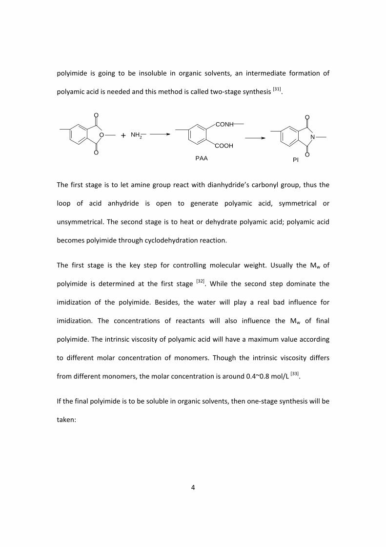
Different polyimides will behave differently according to the different diamines and

dianhydrides reactions. There are two kinds of way to synthesis polyimide. If the final

4

polyimide is going to be insoluble in organic solvents, an intermediate formation of

polyamic acid is needed and this method is called two‐stage synthesis [31].

The first stage is to let amine group react with dianhydride’s carbonyl group, thus the

loop of acid anhydride is open to generate polyamic acid, symmetrical or

unsymmetrical. The second stage is to heat or dehydrate polyamic acid; polyamic acid

becomes polyimide through cyclodehydration reaction.

The first stage is the key step for controlling molecular weight. Usually the Mw of

polyimide is determined at the first stage [32]. While the second step dominate the

imidization of the polyimide. Besides, the water will play a real bad influence for

imidization. The concentrations of reactants will also influence the Mw of final

polyimide. The intrinsic viscosity of polyamic acid will have a maximum value according

to different molar concentration of monomers. Though the intrinsic viscosity differs

from different monomers, the molar concentration is around 0.4~0.8 mol/L [33].

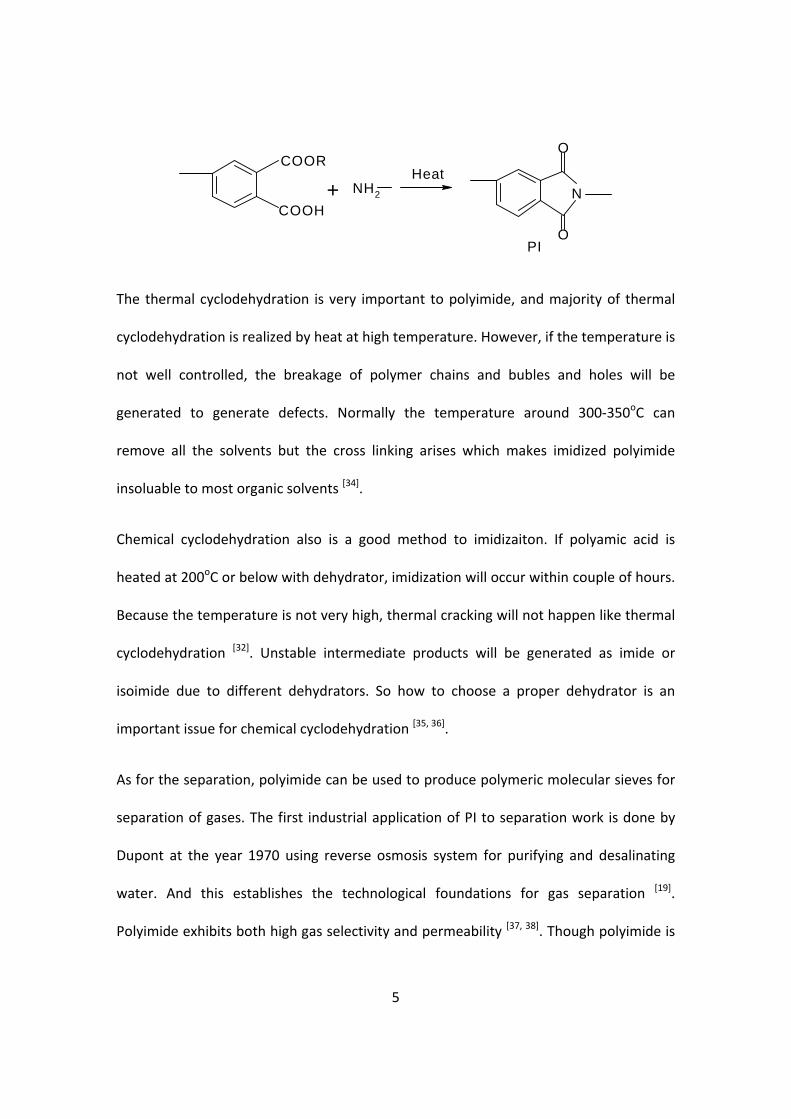
If the final polyimide is to be soluble in organic solvents, then one‐stage synthesis will be

taken:

O

O

O

NH2

CONH

COOHN

O

OPAA PI

+

5

The thermal cyclodehydration is very important to polyimide, and majority of thermal

cyclodehydration is realized by heat at high temperature. However, if the temperature is

not well controlled, the breakage of polymer chains and bubles and holes will be

generated to generate defects. Normally the temperature around 300‐350oC can

remove all the solvents but the cross linking arises which makes imidized polyimide

insoluable to most organic solvents [34].

Chemical cyclodehydration also is a good method to imidizaiton. If polyamic acid is

heated at 200oC or below with dehydrator, imidization will occur within couple of hours.

Because the temperature is not very high, thermal cracking will not happen like thermal

cyclodehydration [32]. Unstable intermediate products will be generated as imide or

isoimide due to different dehydrators. So how to choose a proper dehydrator is an

important issue for chemical cyclodehydration [35, 36].

As for the separation, polyimide can be used to produce polymeric molecular sieves for

separation of gases. The first industrial application of PI to separation work is done by

Dupont at the year 1970 using reverse osmosis system for purifying and desalinating

water. And this establishes the technological foundations for gas separation [19].

Polyimide exhibits both high gas selectivity and permeability [37, 38]. Though polyimide is

NH2 N

O

OPI

COOR

COOH

Heat+

6

a good membrane material and is resistant to high temperature, radiation and chemical,

its mechanical properties is dependent on the extent of imidization. Partially cured PI

membranes have a short lifetime and are easily degraded.

Polyimide membranes can be used to separate organic mixture as well as alcohol and

water. For polyimide has high Tg, so usually the separation process will select water

with high selectivity but low permeability [39]. Polyimide membranes are used to

separate organic solvents by many researchers already.

ODPA‐BISP/PDMS block copolymer was successfully synthesized by improving the

mechanical properties of PDMS with excellent polyimide group [40]. Also, polyimide is

also successfully incorporated with polyurethane by step‐condensation [41, 42].

Polyurethane has segments built by soft and rigid groups which are helpful for

separation.

Incorporation of functional group into polyimide affects the separation process. Many

papers have discussed the relationship between the rigidity, stack density and selectivity

with gas separation [43‐46]. For the flux improvement, CF3 is studied to increase the flux

by restraining marco‐molecules’ stacking and perturbing[45].CH3 group can be found to

increase the flux 10 times while the selectivity remains the same [46]. Selectivity can be

also effected by functional groups: sulfolane group makes the polyimide more

compatible with aromatic solvents thus increases the selectivity [47, 48].

The endurance of polyimide membranes can be improved by introducing phosphonate

ester group [49]. The mechanism is believed that this functional group can increase the

7

appetency with benzene and reduce the wet ability. Improvement is found similarly by

copolymerize with polyethylene oxide [50].

Different ways of synthesis will also affect the separation process [51, 52]. Membranes

through overheating or UV have better separation. For through these methods, the

interaction inside copolyimide groups is strong which reduce the wet ability. Also, the

soft ester group has better toughness which will reduce the brittlity.

Different concentration of polymers, additives, volatilization times and temperatures

were studied to increase the permeability by controlling the thickness of asymmetrical

polyimide membranes [53, 54]. Yanagisita also synthesized thin polyimide membranes to

carry out pervaporation by vapor deposition polymerization [55]. When the thickness is

0.2 μm the selectivity is the same of compact film while the permeability is 14 times

higher[56]. Also spin coating can be used to get super thin film. There might be a slight

decrease of the selectivity but the permeability increase drastically [57]. The factors that

influence the separation are mainly the Mw of polyimide, structure and thickness.

Besides, the imidization and thermal cracking will matter as well [58].

Polymer Ethanol concentration, wt%

Temp., oC

Permeation rate, kg/m2h

Polyetherimide (dry-wet method) 87a 25 2b

Polyamide 6-PEI/PAAc 70a 50 0.5 Polyamide 6-PEI/Alg 88a 50 0.3

BTDA-ODA asymmetry 95 25 0.037 BTDA-ODA symmetry 95 25 0.002

PMDA-p-ODA asymmetry 95 30 0.2 PMDA-p-ODA symmetry 95 30 0.004

HXDA-BMTC 90 40 1.7 BTDA-ODA 8 27 0.18

8

Table 1.3 Pervaporation performance of aliphatic and aromatic polyimide on Ethanol‐

water solution (a: IPA/water. IPA concentration; b. mol/m2‐hr; c. phenol/water. Phenol

concentration.) [39]

1.4 Clay

Layered silicate clays, especially smectite clays, are an interesting class of filler

materials. Among the di‐octahedral smectites, montmorillonite (MMT) is the most

commonly used. [59], mainly layered SiO2 and Al2O3. 1 μm diameter, every unit consists

of hundreds to thousands layers, average number of layers is around 850. It is the

hamburger layer structure as two layers of SiO2 tetrahedral cover one octahedral Al2O3

[60]

Al or Si can be replaced by other metallic ions to form cation exchange clay, anion

exchange clay and neutral exchange clay [61, 62]. The interlayer Van Der Walls gap is

called gallery of just interlayer. The cation and crystal water existing in the galleries can

absorb water in water surrounding to swollen then diffuse water. This can make the

organizing of clay become feasible by the presence of cation and crystal water: to use

proper ions replace cations inside the clay. The ability of ions exchanging for clay is

represented by Cationic Exchange Capacity (CEC). Most montmonrillonite has a CEC

between 70‐150 meq/100 gm [60].

Clay molecules stay together by 50% covalent bond and 50% electrovalent bond plus

few hydrogen bonding. Three clays can be found based on the ratio of tetrahedral over

9

octahedral as 1:1, 2:1 and 2:2. The 2:1 is the most common one, every layer of this clay

built up by a sandwich structure, two tetrahedral clamp one octahedral. Two octahedral

clamp a cation with crystal water [60].

Organizing of clay is pre‐requisite for polyimide‐clay nanocomposite due to its

hydrophilic nature. This can be realized by the cationic exchange capacity; also, more

and more studies are carried out by using the polyimide monomers to modify clay, like

diamine[63,64]. Surface active agents can be also used to improve the compatibility of clay

and polymer like a bridge between them, one side is hydrophilic and the other is

hydrophobic like most polymers. The efficiency of high d‐spacing orgnoclay dependents

on cationic exchange capacity of clay [65].

1.5 PolyimideClay nanocomposite

Nanocomposite has been studied world while both in industry and in academic for

decades. With little addition of reinforcement, the properties of matrix will be changed

drastically [66, 67].

Polyimide‐clay nanocomposites based on PMDA‐ODA polyimide with montmorillonite

has a good thermal and mechanical properties [68]. Also MMT is good reinforcement and

compatible with many polymer matrixes and with the introduction of MMT, the

permeability of PI will be changed [69].

The advantage of using clay to reinforce polyimide is obvious: the improvement of

mechanical properties, like Young’s modulus; the increase of thermal stability, like Tg;

improvement of size stability, it is due to the thermal expansion coefficient is decreased;

10

enhanced anti‐fire behavior due to higher aspect ratio increases the tortuous pathway

so gas will travel longer inside membranes; decrease of dielectric constant and so on [70‐

74].

Dispersion is an important factor that affect improvements. Conventional composite is

believed that the reinforcement is not fully carried out due to the simple stacks of

components. Intercalated nanocomposites will have a better improvement for the

polymer molecules interlude the clay, part of them form a strong bonding, and distance

between silicate layers is around 20‐30A. Exfoliated or delaminated nanocmposite is

believed the best and most uniform nanocomposite. The layer structure disappears and

dispersion reaches its maximum. Properties are greatly improved [75].

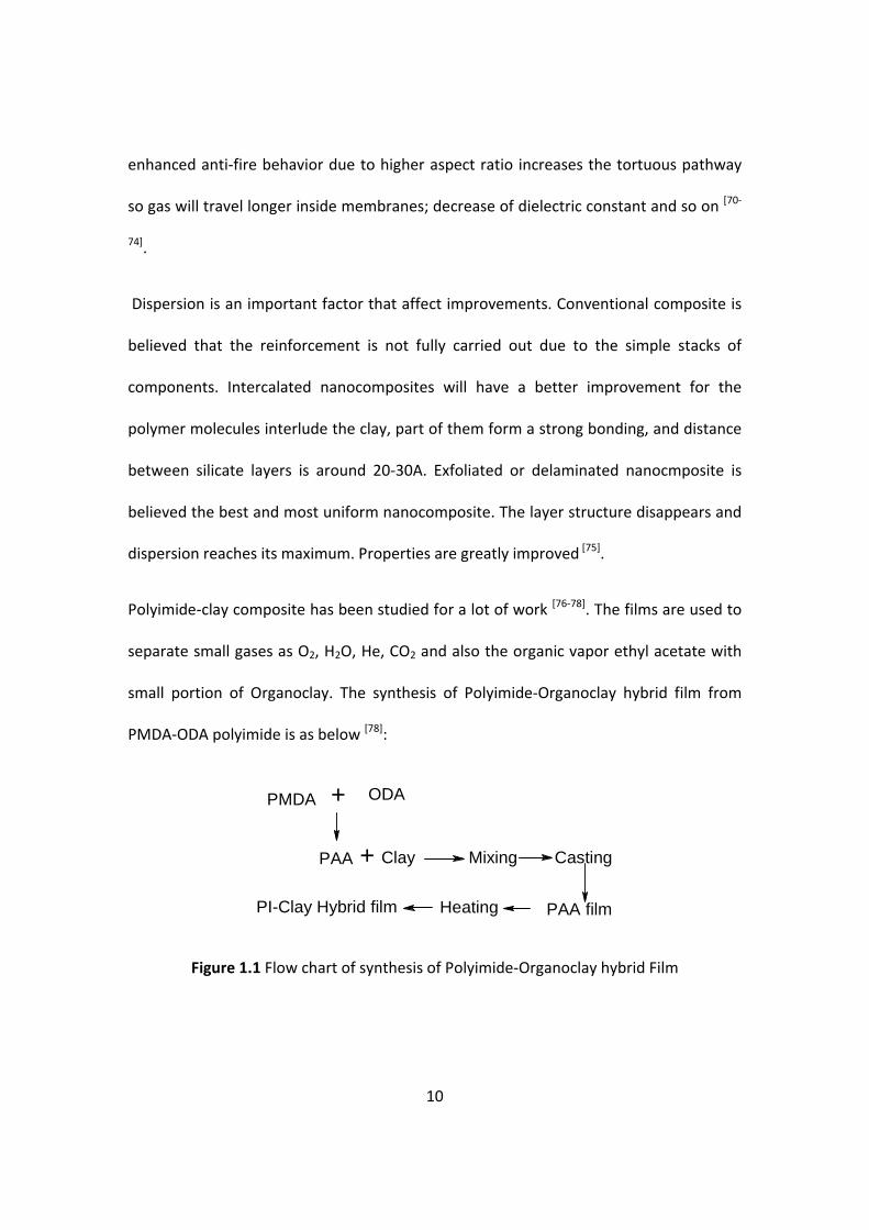
Polyimide‐clay composite has been studied for a lot of work [76‐78]. The films are used to

separate small gases as O2, H2O, He, CO2 and also the organic vapor ethyl acetate with

small portion of Organoclay. The synthesis of Polyimide‐Organoclay hybrid film from

PMDA‐ODA polyimide is as below [78]:

Figure 1.1 Flow chart of synthesis of Polyimide‐Organoclay hybrid Film

PMDA ODA

PAA Clay Mixing Casting

PAA filmHeatingPI-Clay Hybrid film

+

+

2.1

Poly

DuP

Cloi

(PAC

(NM

grea

sho

Cloi

Tex

Tr

1 Material

yamic acid

Pont (PI 254

site® 20A m

CN) are use

MP) purchas

ase purchas

wn in Figur

site ® Na+

as). The typ

reatment/P

Cloisite®

ls

of pyromel

45) is the p

modified w

ed as the fil

sed from A

sed from D

e 2.1

Figure

Clay, 20A

pical proper

roperties:

® 20A

Table 2.1.1

Chapter

litic dianhy

olyimide re

ith a quate

ler separate

Aldrich Che

ow Corning

e 2.1.1 Che

was purch

rties of Na+

OrganicModifier (

2M2HT

1 Typical Pro

11

r 2: Exp

ydride/4, 4‐

esin used in

ernary amm

ely to form

mical Comp

g is used fo

emical Struc

hased from

Clay, 20A C

1)Mo

Conce

95 meq

operties of N

erimen

Oxydianline

this study.

monium salt

nanocompo

pany was u

r sealing. T

ctures of PM

Southern

Clay (Organo

odifier entration

q/100g clay

Na+ 20A Cla

tal

e (PMDA‐O

. Natural m

t ( Organoc

osites. 1‐M

used as the

The structur

MDA‐ODA

Clay Produ

oclay) are sh

% Moisture

< 2%

ay (Organoc

DA) polyme

ontmorillon

lay) and PA

ethy‐2‐Pyrr

e solvent. V

re of PMDA

cts Inc. (Go

hown in Tab

% WeiLoss on Ig

38%

clay)

er, from

nite Na+

ANi‐Clay

rolidone

Vacuum

A‐ODA is

onzales,

ble 2.1.

ght gnition

%

12

Where HT is Hydrogenated Tallow (~65% C18; ~30% C16; ~5% C14) Anion: Chloride

(1) 2M2HT: dimethyl, dihydrogenatedtallow, quaternary ammonium

10% less than: 50% less than: 90% less than:

2µ 6µ 13µ

Table 2.1.2 Typical Dry Particle Sizes of Na+ 20A Clay (Organoclay): (microns, by volume)

PANi –Clay (PACN) was prepared by Yangrong Zhu using in‐situ polymerization

technique at year 2002.

2.2 Membranes Preparation

All the membranes were derived from solution‐casting on a free‐standing glass, at the

Vacuum Oven at 70oC for 8hrs. Solution prepared with 1‐Methyl‐2‐Pyrrolidone (NMP)

as the solvent. For uniform distribution of the filler, all the solutions were vibrated in

Ultra‐Sonic for 5 minutes and then stirred for 2 hours with Magnetic Stir Bar. Before

applying on glass, another 1 minute Ultra‐Sonic vibration was used to get rid of bubbles.

In order to determine the effect of 20A Clay (Organoclay), different concentration of

Organoclay were used in solution casting. The concentration of the components in the

films is shown in Table 2.2.1. Different concentrations of the clay were incorporated into

13

the nanocomposites in order to study the effect of the percentage of clay on the

properties of permeation and separation Ethanol and Water.

Sample ID Polyimide 2545, g Organoclay, g NMP, ml

#0 PI 5 0 5 #1 OC‐1 5 0.0025 5 #2 OC‐2 5 0.005 5 #3 OC‐3 5 0.0125 5 #4 OC‐4 5 0.0251 5 #5 OC‐5 5 0.0505 5 #6 OC‐6 5 0.0761 5 #7 OC‐7 5 0.102 5 #8 OC‐8 5 0.2632 5

Table 2.2.1 Solution Casting Conditions of Polyimide and Organoclay nanocomposites

PANi‐Clay was introduced into our system to study the effect of PANi modification,

continuing Yangrong Zhu’s work in year 2002. Different concentrations of the PANi‐Clay

were incorporated in to the nanocomposites.

Sample ID Polyimide 2545, g PANi –Clay, g NMP, ml

#9 MC‐1 5 0.0005 5 #10 MC‐2 5 0.0025 5 #11 MC‐3 5 0.0125 5 #12 MC‐4 5 0.0251 5

Table 2.2.2 Solution Casting Conditions of Polyimide and PANi –Clay

The thicknesses of the membranes were around 70 µm to 100 µm. Color changed with

the amount of Organoclay and PANi‐Clay. For the both groups, the more clay

inco

than

2.3

Diff

belo

cylin

pos

prev

ioni

of 7

The

and

orporated, t

n Organocla

Diffusion

fusion tests

ow (See Fi

nders cham

ition, the p

venting lea

zed water a

7.9 ml initial

e time of dif

stability.

the deeper

ay’s.

n Test

were carrie

igure 2.3.1

mbers each

eripheral p

king. A pos

and 5.0% (V

lly.

Figure

ffusion test

As the diff

color woul

ed out in U‐

). Two mi

. Size is sh

art of them

sition was h

V:V) Ethano

e 2.3.1 Diag

ts varied fro

usion went

14

ld be. And

‐shaped cel

rrored U s

hown in Fig

m were appl

held with st

ol/Water so

ram of U‐sh

om 60 hrs

t on, there

PANi‐Clay

lls purchase

shaped diff

gure 2.3.2.

lied with Do

trong clips.

lution filled

haped Diffu

to 400 hrs

would be a

membranes

ed from Ken

fusion cells

Membrane

ow Corning

Same volu

d each side

sion Cells.

depends o

a volume d

s had deep

ntucky Glas

s consist o

es were fix

Vacuum gr

ume (95 ml

at the same

n the perm

difference b

er color

s Inc. as

of three

ed in A

rease to

) of de‐

e height

meability

between

15

water side and ethanol/water side due to the difference of diffusion coefficient for

water and ethanol.

2.4 Characterization Technologies

Different technologies were taken to analyze the effect of amount of Organoclay and

PANi‐Clay to composition and morphology of membranes: Brookfield Viscometer (Shear

Viscometer), Fourier Transform Infrared Spectroscopy, Scanning Electron Microscopy

and Refractive Index.

2.4.1 Brookfield Viscometry

Data of materials’ viscosity behavior is of a great importance. Rheological characteristics

are valuable during the processing. Temperature is one of the most obvious factors that

can influence the rheological behavior. And with the introduction of Organoclay and

PANi‐Clay, the amount is another important effect to the shear viscosity. The

relationship between rheological properties and characteristics of the solution will help

us to predict characteristics of sample. For example, with the comparison of viscosity of

different system, we will have a concept of how thick the membrane might be.

Brookfield DV+I viscometer with spindle model‐31 (Brookfield Engineering, Laboratories,

INC.MA) was used to measure the shear viscosity of polyimide and polyimide based

membrane systems. Different temperatures were applied to solutions to study the

influence of temperature. Further comparisons in shear rate and shear stress were

studied.

16

The relationship between viscosity and temperature is given by Arrhenius Equation

below [79]

2.4.2 Fourier Transform Infrared Spectroscopy (FTIR)

Infrared (IR) spectroscopy deals with the recording of the absorption of radiations in the

infrared region of the electromagnetic spectrum. IR spectrum can show important

information of chemical compositions and chemical structures. All the membranes were

analyzed by Fourier Transform Infrared Spectroscopy (FTIR) using Bio‐Rad Excalibur

Series (Bio‐Rad, Richmond, CA). FTIR was used to determine the chemical structure of

Polyimide and the composition of the nanocomposite. With FTIR, the change of the

membranes before diffusion test and after diffusion test was shown. FTIR spectra were

collected at a resolution of 4 cm‐1 and average of 32 scans through 400 to 4000 cm‐1. All

the spectra were analyzed by Bio‐Rad KnowItAll software.

2.4.3 Scanning Electron Microscopy (SEM)

The morphology of the nanoccomposites was observed by using a Hitachi S‐4000 Field

Emission SEM and a Hitachi S‐900 SEM. Membranes were sputtered with a mixture of

Platinum and Gold to improve conductivity.

2.4.4 Concentration Measurement

All the samples concentration is measured by HR100.008 Refractometer (APT

Instrument, IL).

17

Chapter 3 Results and Discussion

3.0 Temperature of Membranes Synthesis

65oC to 250oC has been tried for synthesis of membranes. It took over 15 hours when

the temperature was 65oC before the membrane formed. The higher temperature

applied, the quicker the membrane formed. However, membranes formed and cured

above 100oC showed little water flux during the permeation. 70o, 80 o and 90o formed

and cured membranes showed a relative higher flux. 70 o is selected for the synthesis

temperature for the highest flux.

3.1 Shear Viscosity

Rheological properties of the nanocomposite solution were studied in order to evaluate

the influence of Organoclay and PANi‐Clay concentration on solution viscosity. The data

obtained can be used to predict process ability of the membranes. If the viscosity is too

high, it is difficult to spread solution uniformly on glass, and thick film will it become.

While if the viscosity is too low, solution will spread easily and cannot stay on glass.

Thus, solution will be wasted and much thinner film will it become.

The experimental task had three main objectives. The first objective was to determine

the relationship between viscosity and temperature, and viscosity and shear rate. The

second objective was to evaluate the effect of addition of Organoclay and PANi‐Clay to

the polyimide solution. The information obtained can be used to study the

reinforcement mechanism of clay. The third objective was to evaluate the differences of

effect for Organoclay and PANi‐Clay.

18

The viscosity of shear thinning fluids decreases with the increasing shear rate and

increasing temperature. The dependency of shear viscosity on temperature could be

understood by applying the free volume theory [15]. An increase in temperature would

facilitate thermal motion of molecules by increasing the free volume in the polymer.

Increasing test temperature causes a decrease in the resistance to intermolecular

motion (viscosity).

3.1.1 Effect of Temperature on Shear Viscosity

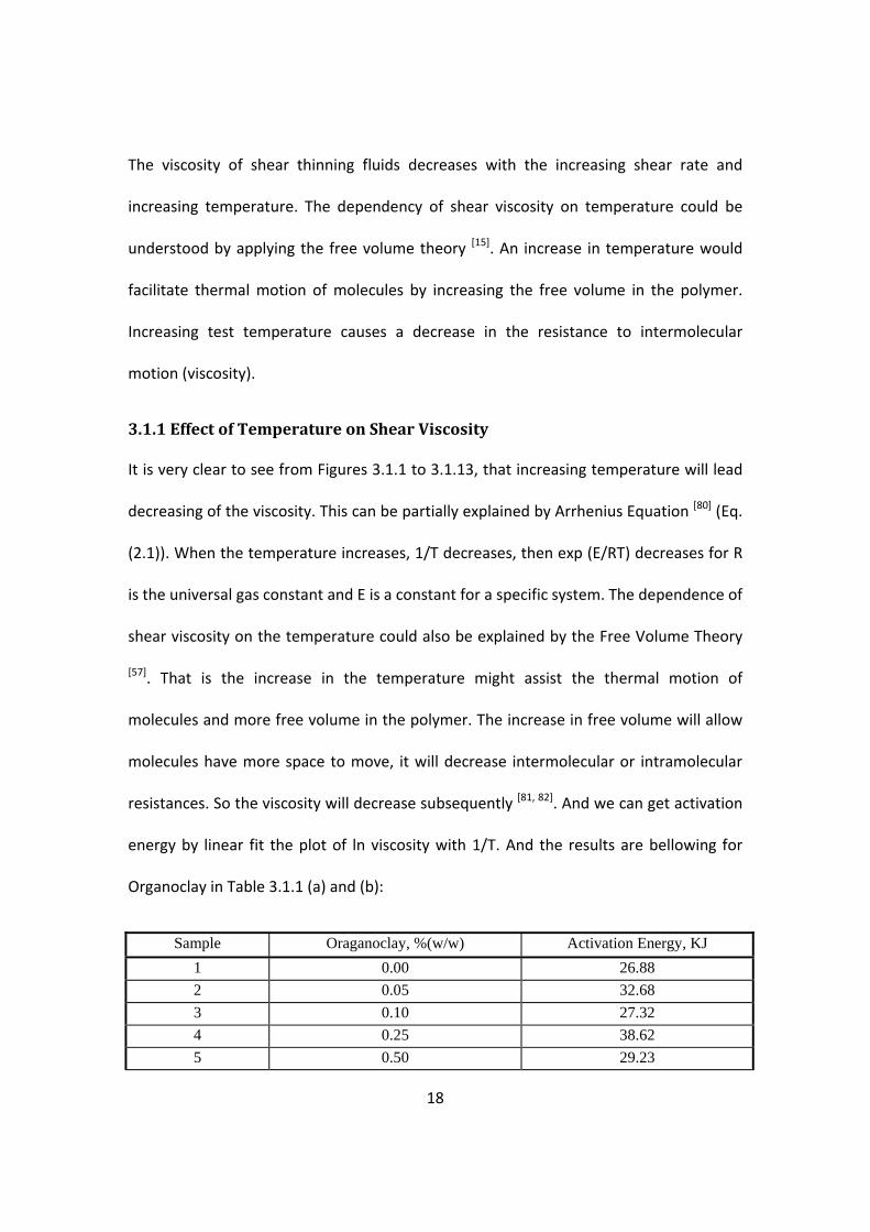
It is very clear to see from Figures 3.1.1 to 3.1.13, that increasing temperature will lead

decreasing of the viscosity. This can be partially explained by Arrhenius Equation [80] (Eq.

(2.1)). When the temperature increases, 1/T decreases, then exp (E/RT) decreases for R

is the universal gas constant and E is a constant for a specific system. The dependence of

shear viscosity on the temperature could also be explained by the Free Volume Theory

[57]. That is the increase in the temperature might assist the thermal motion of

molecules and more free volume in the polymer. The increase in free volume will allow

molecules have more space to move, it will decrease intermolecular or intramolecular

resistances. So the viscosity will decrease subsequently [81, 82]. And we can get activation

energy by linear fit the plot of ln viscosity with 1/T. And the results are bellowing for

Organoclay in Table 3.1.1 (a) and (b):

Sample Oraganoclay, %(w/w) Activation Energy, KJ 1 0.00 26.88 2 0.05 32.68 3 0.10 27.32 4 0.25 38.62 5 0.50 29.23

19

6 1.00 14.27 7 1.50 19.52 8 2.00 18.85

Table 3.1.1 (a) Effect of Organoclay concentration on Activation Energy at RPM=30 r/m

Sample PANi-Clay, %(w/w) Activation Energy, KJ

1 0.00 26.88 9 0.01 27.45 10 0.05 28.36 11 0.25 52.62 12 0.50 49.31

Table 3.1.1 (b) Effect of PANi‐Clay concentration on Activation Energy at RPM=30 r/m

We will see that in both cases, the activation energy reaches a maximum at

concentration of 0.25% filler. The reason caused this phenomena will be discussed in

chapter 3.1.2.

3.1.2 Effect of Clay on Shear Viscosity

By the comparison of activation energy, we will see, with the small amount introduction

of of Organoclay, the activation energy will increase. This indicates that the threshold

energy is increasing from 0.00% to 0.25% Clay, both Organoclay and PANi‐Clay, w/w. So

the viscosity is lower when the concentration is higher. It is believed that good

dispersion of Clay in Dupont PI 2545 can smooth the entanglement of molecular chains

of PI 2545 which results from the exfoliation of Clay. Another possible explanation for

this behavior may involve planar alignment of the clay particles towards the flow

direction under shear [83]. Thus it leads to lower viscosity and higher process ability.

There is a steep rise of the activation energy when the concentration is beyond 0.25%.

The viscosity becomes higher than for the threshold energy increases. It is believed

20

more introduction of Clay will increase the crystalline of solution [84]. And more and

more Clay will become obstacles for themselves for exfoliation. So the shear stress

become noticeable higher thus viscosity increases.

Another theory to explain this behavior is tried by Sinha et al; it is due to planar

alignment of the clay particles towards the flow direction. For low concentration, Clay

particles are easy to attain complete planar alignment along the flow direction with

matrix, so the rheological behavior is not strong. While at high concentration, it takes a

long and hard time for them to align completely. Thus strong rheological behavior

becomes strong. [85]

Sample ID Organoclay%, w/w 20 30 50 60 1001 0.00 27.79 26.88 22.45 21.49 20.552 0.05 32.65 32.68 32.11 26.83 22.493 0.10 26.67 27.32 20.76 15.37 11.074 0.25 43.21 38.62 30.43 26.18 23.645 0.50 33.65 29.23 22.34 20.74 18.586 1.00 16.91 14.27 14.12 12.05 13.847 1.50 21.15 19.52 18.17 16.81 16.358 2.00 21.32 18.85 17.04 15.70 13.33Table 3.1.2 (a) Effect of Organoclay on Activation Energy at Different RPMs

Sample ID PANi-Clay%, w/w 20 30 50 60 1001 0 27.79 26.88 22.45 21.49 20.559 0.05 35.12 27.45 25.18 22.28 20.17

10 0.10 52.98 28.36 26.40 23.77 19.05 11 0.25 - 52.62 31.51 26.84 21.21 12 0.50 83.97 49.31 28.96 26.73 19.45 Table 3.1.2 (b) Effect of PANi‐Clay on Activation Energy at Different RPMs

Same change shows at angular velocity at 30r/m, 50r/m, 60r/m and 100r/m in Table

3.1.2 (a) and (b). Here, we can see the maximum of the activation energy takes place at

21

concentration of 0.25%, we can notice this concentration for other behavior in our later

discussion.

3.1.3 Effect of Shear Rates on Shear Viscosity

For all the samples, there was a trend that viscosity increased as the increase of shear

rate (See Figure 3.1.14 to 3.1.26). But the behaviors at low shear rate and high shear

rate are different. At high shear rate, the shear viscosity seems to reach a plateau

viscosity but it increase as the increase of shear rate at low shear rate. The lower shear

rate goes with Newtonian fluids. This is believed to be caused by the randomly coiled

macromolecule in solution expands during laminar flow [86], saying the expansion of

coiled macromolecule will decrease the average hydrodynamic interaction between

random two segments. So the expansion of coiled macromolecule will lead an addition

influence to the viscosity. Thus, if the shear rate increases, the related shear viscosity

will increase consequently. While at high shear rate, the coiled macromolecules already

finish the expansion, so the increase of shear rate will have little influence on viscosity.

From Figures 3.1.14 to 3.1.26, we could find out the influence of incorporation of both

Organoclay and PANi‐Clay is not so significant to shear viscosity. But the effect of shear

rate on viscosity is lower for the introduction of Clay. It is possible that Clay disrupted

the expansion of randomly coiled macromolecule in solution, so, the viscosity will not

change that much as it should be.

22

3.1.4 Effect of Shear Stress on Shear Viscosity

For all the samples, there was a trend that viscosity increased as the increase of shear

stress. The shear viscosity decreased with the increase of external temperature.

Incorporation of clay would not influence shear viscosity of the mixture significantly.

They were similar to the relationships between viscosity and shear rate. The explanation

is similar to the effect of shear rate. See Figure 3.1.43 to 3.1.55.

3.1.5 Effect of Reinforcements

From the comparison of Organoclay and PANi‐Clay (Figure 3.1.27 to 3.1.42, and Table

3.1.1 to 3.1.2), we will see that the different behaviors from Organoclay and PANi‐Clay.

From 0.01% to 0.50% (Figure 3.1.30, 3.1.34, 3.1.38, 3.1.42), the viscosity of Organoclay

reinforced PI 2545 and PANi‐Clay reinforced PI 2545 shows a transition. At 0.01%,

viscosity of PANi‐Clay solution is greater than Organoclay solution, but they are close at

0.05%. When the concentration of clay increases to and above 0.25%, the viscosity of

Organoclay becomes greater than PANi‐clay.

23

3.2 Diffusion Model

3.2.1 Fick’s Second Law

Separation will be achieved if the diffusivities of Water and Ethanol for membranes are

different. In this system, water was absorbed and then diffused while ethanol was

insulated.

All the diffusion equations can be described by Fick’s first and second laws. Diffusion

coefficient is an important parameter to us because only with this can we know the

diffusivity of water in different membranes. As the concentration in our Ethanol/Water

side changes with time, so Fick’s second law [87] will apply our systems.

wMt

∂∂ =

2

2wMD

x∂∂ (1)

Where Mw is the concentration of water in dimensions of [(amount of substance) length‐

3], [mol m‐3], t is time [s], D is the diffusion coefficient in dimensions of [length2 time‐1],

[m2 s‐1] and x is the position [length], [m]

If we consider the boundary conditions as bellowing: t=0, x=0, Mw = pure water; t>0,

x=0, Mw = pure water. So the boundary value problem of our system will be Figure 1.

(See Below)

WT MB EW

x

X=0 X=L

24

Figure 1: Boundary value problems for diffusion systems.

Applied these boundary conditions to Fick’s Second Law, we will see that it is non‐

homogeneous for T1 and T2 are not zero at the same time. We can get solutions of non‐

homogeneous from homogeneous problem by setting T1=T2=0, and then go back to non‐

homogeneous problem as it is.

3.2.2 Squareroot relationship[8892]

It is too complicated to use this solution calculating diffusion coefficient. In fact, there is

Square‐root relationship for simplification. As in a Semi‐infinite medium having zero

initial concentration and the surface of which is maintained constant, involves only the

single dimensionless parameter2

xDt

.

When applied this into diffusion in a plane sheet. The total amount of diffusing

substance Mt entering or leaving the sheet up to time t, is expressed as a fraction of Minf.

That is:

inf

( , ) 2M x t DtM L π

= (10)

Mt

∂∂

= 2

2

MDx

∂∂

M (0, t) =T1 M (L, t) = T2

x

t

26

3.3 Effect of Organoclay and PANiClay on Diffusion

From the Diffusion Model above, we can make the t1/2 as the X axis, and Mw (x, t)/M inf

as the Y axis. We will get variations of the flux of water with time for membranes.

3.3.1 Stages of Diffusion

Our preliminary results indicate three to four distinct stages for permeation of water

through the membranes composed of: (i) initial instantaneous increase in flux followed

by (ii) an induction period marked by a gradual but constant flux, (iii) a steady‐state

permeation stage marked by a rapid but constant flux and a (iv) final plateau state

where diffusion process takes place very slowly. The diffusion coefficient for each

membrane was calculated from the slope of the third stage of permeation. It should be

noted that the membranes were not swollen prior to the permeation study.

0 5 10 15 20 25

0.0

0.2

0.4

0.6

0.8

1.0

1.50% Organoclay 2.00% Organoclay 5.00% OrganoclayM

w/M

inf)

t1/2, hr1/2

Figure 3.3.1.1 Typical Three Diffusion Stages: 1.50%, 2.00% and 5.00% (w/w) Organoclay

27

The variation of the flux of water with time for membranes plots of 1.50%, 2.00% and

5.00% Organoclay are the most typical of this behavior. (Figure 3.3.1.1) The first stage

occurs in the initial five hours from the beginning of permeation and is marked by a

rapid transport of water through the membrane. The second stage is the induction or

saturation period characterized by a very slow rate of permeation of water. The third

stage is marked by a sharp but constant steady‐state flux. Finally, the fourth stage is

characterized by a gradual and very slow flux and occurs after about 480 h of

permeation in most membranes.

From the Figure 3.3.1.2 and Figure 3.3.1.3, we can see the correlation between diffusion

coefficients and time of stage I and II (The diffusion coefficients will be discussed next

section). Generally speaking, the trend of dependence of concentration on the time is

the same with diffusion coefficient relevantly. All three show a sine wave trend line.

0 2 4 6 8 10 12 140

5

10

15

20

25

30

0.500.25

0.25

0.10

0.10

0.05

0.05

PI

Concentation of Clay, %, w/w

Diff

usio

n C

oeffi

cien

t, 10

-10

cm2 /

s

D, 10-10 cm2/s

PI0

2

4

6

8

10

5.00

5.00

1.50

1.50

1.001.00

0.50

Time, hrs

t, hrs

28

Figure 3.3.1.2 Time of Stage I and relevant Diffusion Coefficient for Organoclay

0 2 4 6 8 10 12 140

5

10

15

20

25

30

PI

0.50

0.25

0.25

0.10

0.10

0.05

0.05

PI

Concentation of Clay, %, w/w

Diff

usio

n C

oeffi

cien

t, 10

-10

cm2 /

s D, 10-10 cm2/s

PI0510152025

30354045505.00

5.00

1.50

1.50

1.00

1.00

0.50

Time, hrs

t2, hrs

Figure 3.3.1.3 Time of Stage II and relevant Diffusion Coefficient for Organoclay

If we put them all together, it is clear that time of stage I is consistent with time of stage

II, and tend to behave similarly as change of diffusion coefficients. But time of stage II

are more stable than stage I which indicates that the induction period of every

membrane are tend to be stable. This properly is depended on a little change will occur

after first stage which is believed to be swollen process. See Figure 3.3.1.4 (a) to (c).

29

0 1 2 3 4 5

0

2

4

6

8

10

Tim

e of

Sta

ge I,

hrs

Organoclay, wt%

Time of Stage I, hrs

(a)

0 1 2 3 4 50

10

20

30

40

50

Tim

e of

Sta

ge II

, hrs

Organoclay, wt%

Time of Stage II, hrs

(b)

30

0 1 2 3 4 5

0

10

20

30

40

50D

, T1,

T2

Organoclay, wt%

Diffusion Coefficient, 10-10 cm2/s Time of Stage I, hrs Time of Stage II, hrs

(c)

Figure 3.3.1.4 Correlation of time of stage I, time of stage II with diffusion coefficients at

different Organoclay concentration

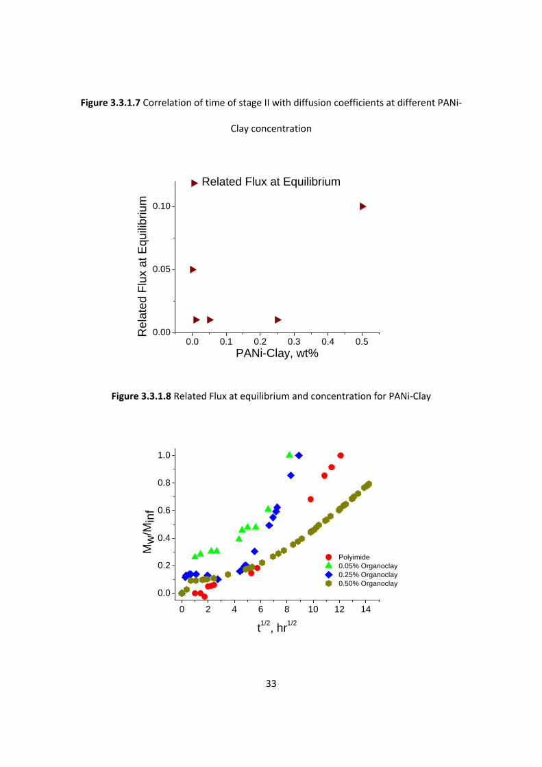
From the Figure 3.3.1.5, we will see the related flux at equilibrium tends to be stable at

low concentration up to 1.00% and it increases when concentration of Organoclay

increases. With a comparison of PANi‐Clay Figure 3.3.1.8, we will notice that PANi‐Clay

reinforced membranes have a lower related flux at quilibrium.

If we compare the low concentration of Organoclay and PANi‐Clay from Figure 3.3.1.1,

3.3.1.9 and 3.3.1.10, we will notice that PANi‐Clay system will blur the border of first

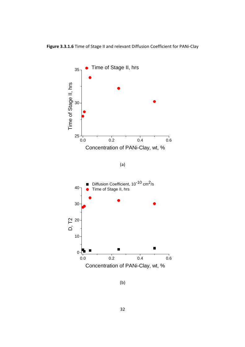
stage and second stage. It is hard to distinguish stage I and stage II except at 0.50%

PANi‐Clay. This is believed that PANi modified clays have the effect of stabilizing

polyimide membrane which minimize the stage I but elongate stage II. This can be

31

noticed from Figure xx to xx, the stage I cannot be noticed in PANi‐ modified clay

system. And the relevant diffusion coefficients are much lower than Organoclay, but

the time of stage II tends to be stable.

0 1 2 3 4 50.0

0.1

0.2

0.3

Rel

ated

Flu

x at

Equ

ilibr

ium

Organoclay, wt%

Related Flux at Equilibrium

Figure 3.3.1.5 Related Flux at equilibrium and concentration for Organoclay

2 4 6 8 100.00

0.05

0.10

0.15

Concentation of PANi-Clay, %, w/w

Diff

usio

n C

oeffi

cien

t, 10

-10

cm2 /

s

D, 10-10 cm2/s

0

5

10

15

20

25

30

35

Time, hrs

0.500.25

0.50

0.25

0.05

0.05

0.01

0.01

PI

PI

T2, hrs

32

Figure 3.3.1.6 Time of Stage II and relevant Diffusion Coefficient for PANi‐Clay

0.0 0.2 0.4 0.625

30

35 Time of Stage II, hrsTi

me

of S

tage

II, h

rs

Concentration of PANi-Clay, wt, %

(a)

0.0 0.2 0.4 0.60

10

20

30

40 Diffusion Coefficient, 10-10 cm2/s Time of Stage II, hrs

D, T

2


(b)

33

Figure 3.3.1.7 Correlation of time of stage II with diffusion coefficients at different PANi‐

Clay concentration

0.0 0.1 0.2 0.3 0.4 0.50.00

0.05

0.10

Rel

ated

Flu

x at

Equ

ilibr

ium

PANi-Clay, wt%

Related Flux at Equilibrium

Figure 3.3.1.8 Related Flux at equilibrium and concentration for PANi‐Clay

0 2 4 6 8 10 12 14

0.0

0.2

0.4

0.6

0.8

1.0

Polyimide 0.05% Organoclay 0.25% Organoclay 0.50% Organoclay

Mw

/Min

f

t1/2, hr1/2

34

Figure 3.3.1.9 Variation of the flux of water with time for membranes Polyimide, 0.05%

,0.25% and 0.50%(w/w) Organoclay

0 2 4 6 8 10 12 14 16 18

0.0

0.2

0.4

0.6

0.8

1.0

0.01% PANi-Clay 0.05% PANi-Clay 0.25% PANi-Clay

Mw

/Min

f

t1/2, hr1/2

Figure 3.3.1.10 Variation of the flux of water with time for membranes 0.01%, 0.05%

and 0.25% (w/w) PANi‐Clay

The concentration is lower for the beginning of second stage and third stage for PANi‐

Clay. The fourth stage is more obvious for PANi‐Clay system. The low concentration of

PANi‐Clay behaves more like high concentration of Organoclay system.

35

3.3.2 Diffusion Coefficients

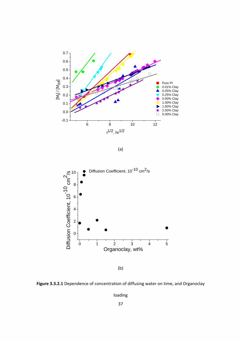
We can calculate the diffusion coefficient from variation of the flux of water with time

for membranes plots. If we make a linear fit at the third stage, we will have different

slope, and the slope is 2 DL π

, so the Diffusion Coefficient will be obtained then.

The diffusion coefficients obtained were compared with that for the neat polyimide

membrane. Nanocomposite membranes containing varying amounts of clay were

studied.

As shown in Figure 3.3.2.1, the relative concentration of diffusing water increases with

permeation time and increases with weight percent of clay up to 0.25% w/w clay. The

relative concentration of diffusing water decreased with any additional increase in clay

concentration Table 3.3.2.1 shows the diffusivity of the membranes as a function of clay

concentration. Accordingly, the diffusion coefficient for the membranes increased with

increasing weight percent of clay up to a clay concentration of 0.25%, beyond which a

sharp decrease in the diffusion coefficient occurred with any further increase in the

concentration of clay.

It is clear that the introduction of Organoclay helped Polyimide membrane increase the

water permeation properties at lower concentration and it did not help a lot that much

at high concentration even showed a reverse effect for permeation. It is believed that

the introduction of Organoclay will help to create or enlarge the pore size of Polyimide

membranes. Organoclay’s layer can exfoliate and “cut” the membrane thus more and

36

more pores shows up, and the size of pores will become larger. However, when more

Organoclay is introduced, it will become an obstacle itself, which means the pores

created by Organoclay will be covered or extrude by strong Organoclay layer. The

mechanism caused this will be studied by FTIR and SEM on composition and surface

morphology later.

Sample ID Organoclay, wt% Diffusion Coefficient, 10‐10cm2/s

0 0.00 1.73 1 0.05 6.43 2 0.10 8.44 3 0.25 9.57 4 0.50 0.71 5 1.00 2.2 6 1.50 0.62 7 2.00 1.77 8 5.00 0.94

Table 3.3.2.1 Dependence of Diffusion Coefficient on Concentration of Organoclay

Neat polyimide membrane and 0.25% Organoclay reinforced polyimide membrane were

repeated by Dr. Iroh’s group. The results were close, see Table 3.3.2.1‐2.

Diffusion Coefficient, 10‐10cm2/s Orginal Repeated Average Standard Deviation

Neat PI 1.75 2.33 2.04 0.41 0.25% OC‐PI 9.57 9.73 9.65 0.11

Table 3.3.2.1‐2Comaprison of Orginal and repeated neat PI and 0.25% OC‐PI, numbers

are Diffusion Coefficients, unit as 10‐10cm2/s

37

6 8 10 12-0.1

0.0

0.1

0.2

0.3

0.4

0.5

0.6

0.7

Pure PI 0.01% Clay 0.05% Clay 0.25% Clay 0.50% Clay 1.00% Clay 1.50% Clay 2.00% Clay 5.00% Clay

[Mt]

/ [M

inf]

t1/2, hr1/2

(a)

0 1 2 3 4 5

0

2

4

6

8

10

Diff

usio

n C

oeffi

cien

t, 10

-10 c

m2 /s

Organoclay, wt%

Diffusion Coefficient, 10-10 cm2/s

(b)

Figure 3.3.2.1 Dependence of concentration of diffusing water on time, and Organoclay

loading

38

With the incorporation of PANi‐Clay, the effect is reversing (See Figure 3.3.2.2. and

Table 3.3.2.2). It decreased the Diffusion Coefficient a lot, which meant the interaction

between Polyimide‐PANi‐Organoclay was strong. Membrane becomes more condense

than before. This is believed that the PANi modified Organoclay changed the

arrangement of Organoclay in the Polyimide. Intercalation became dominant than

exfoliation.

However, the Diffusion Coefficient increased as the concentration of PANi‐Clay leads

difficulty to explain this behavior with intercalation‐exfoliation theory for the D‐spacing

of PANi‐Clay is even bigger than Organoclay. But due to PANi is hydrophobic; it will keep

away water, so the balance of these two forces will lead the final permeation of water

through membrane. It is highly believed that due to the pore creativity from Organoclay,

the effect of PANi‐Clay to permeation will be the results of balance of interactions of

Polyimide‐PANi, Polyimide‐Organoclay, PANi‐Clay and Polyimide‐PANi‐Organoclay. It

becomes more difficult to have a clear concept of the mechanism then.

39

6 8 10 120.0

0.2

0.4

0.6

0.8

1.0

Polyimide 0.01% PANi-Clay 0.05% PANi-Clay 0.25% PANi-Clay 0.50% PANi-Clay

Mw

/Min

f

t1/2, hr1/2

(a)

0.0 0.2 0.4 0.60.0

0.5

1.0

1.5

2.0

2.5

3.0 Diffusion Coefficient, 10-10 cm2/s

Diff

usio

n C

oeffi

cien

t, 10

-10

cm2 /

s


(b)

Figure 3.3.2.2 Dependence of concentration of diffusing water on time, and PANi‐Clay

loading

40

Sample ID PANi‐Clay, wt% Diffusion Coefficient, 10‐10 cm2/s

0 0.00 1.73 9 0.01 0.73 10 0.05 1.3 11 0.25 1.99 12 0.50 2.69

Table 3.3.2.2 Dependence of Diffusion Coefficient on Concentration of PANi‐Clay

41

3.4 Composition and Surface Morphology

In order to study the effect of different concentrations of Organoclay and PANi‐Clay on

composition and surface morphology, Fourier Transform Infrared Spectroscopy (FTIR)

and Scanning Electron Microscopy (SEM) are introduced.

3.4.1 Fourier Transform Infrared Spectroscopy (FTIR)

Fourier Transform Infrared Spectroscopy (FTIR) is a convenient technique for polymer

analysis. It can be used to analysis of liquids, solutions, pastes, powders also our films. In

this work, the effect of different concentrations of Organoclay and PANi‐Clay on

composition was studied by FTIR.

Polyimide FTIR Absorption Peaks

Peak Position, cm‐1 Peak Assignment

1780 asymmetric stretch of C=O

1720 symmetric stretch of C=O, a very strong band 1380 stretch of C‐N , strong

1310‐‐1210 Combined C—N stretching and N—H bending 725 C=O bending

Table 3.4.1.1 Summary of FTIR absorption peaks of Polyimide [93, 94]

The strongest band that occurs at 1720 cm‐1 (C=O symmetrical stretching) also overlaps

with strong carboxylic acid band (1700 cm‐1, C=O) of the poly (amic acid). Some overlap

of the 1780 and 725 cm‐1 is also possible with absorption of anhydrides occurring at

1780 cm‐1 and 720 cm‐1. The carboxylic acid band of 1700 cm‐1 (C=O) abd 2800‐3200 cm‐

1 (OH) and amide bands at 1660 (C=O), 1550 cm‐1 (C‐NH) and 3200‐3300 cm‐1 (N‐H)

42

which often appear as broad peaks also useful for qualitative assessment during

imidization process[95].

The formation of the Polyimide structure was confirmed by FTIR. From the FTIR

spectrum of Neat Polyimide membrane (Figure 3.4.1.1),, we will notice typical imide

bands at 1778 cm‐1 as asymmetric stretch of C=O group, a very strong band at 1719 cm‐1

as symmetric stretch of C=O in the imide group, strong peak at 1381 cm‐1 for C‐N

stretching in the imide group is also shown, and the 721 cm‐1 for C=O bending is also

noticeable (Table 3.4.1.2),. So we succeed to cast Polyimide membrane by our film

casting conditions. The 1300 and 1215 cm‐1 peaks cannot be used to specifying as imide

group, for they are also characteristic peaks for Polyamide.

Polyimide 0 FTIR Absorption Peaks


1778 asymmetric stretch of C=O

1719 symmetric stretch of C=O, a very strong band 1381 stretch of C‐N , strong

1300, 1215 Combined C—N stretching and N—H bending 721 C=O bending

Table 3.4.1.2 Summary of FTIR absorption peaks of Polyimide #0 Membrane

However, since our curing temperature is low, 70oC is definitely lower than common

imidizing temperature [96‐98], so some of Polyamide peaks are shown at the FTIR

spectrum of Polyimide #0 membrane (Figure 3.4.1.1).

43

Polyamide (Secondary) FTIR Absorption Peaks


3300 N–H stretching

1644 C=O stretching, very strong intensity

1550 N–H bending, C–N stretching, strong intensity 1310‐1200 Mixed C‐N stretching and N‐H bending

Table 3.4.1.3 Summary of FTIR absorption peaks of amide [94, 99, 100]

Polyimide 0 FTIR Absorption Peaks


‐ N–H stretching

1645 C=O stretching, very strong intensity

1543 N–H bending, C–N stretching, strong intensity 1300, 1217 Mixed C‐N stretching and N‐H bending

Table 3.4.1.4 Summary of FTIR absorption peaks of Polyimide #0 Membrane

We notice that there is an overlap of 1310 to around 1200 peaks for Polyimide and

Polyamide, so the peak in this area will not be considered as the distinction of Polyimide

or Polyamide. By the comparison of Table 3.4.1.3 and Table 3.4.1.4, we notice that

amine bonds can been seen as the carbonyl vibration of polyamic acid around 1645 cm‐1

and strong amide bands from N‐H bending and C‐N stretching of C‐N‐H group at around

1543 cm‐1 . But the strong amide group at 3300 cm‐1 disappeared which means though

that some of Polyamide groups still exist but majority of them have become Polyimide

group.

If we have a look at the FTIR spectrum after diffusion, we will see Polyimide peaks were

decreased. Though all the peaks were shown at spectrum, their intensities were not as

44

strong as before diffusion. This phenomenon indicates that neat Polyimide membrane is

not so chemical resistant to water and ethanol/water surroundings. Because we dried

the membrane at 70oC which is lower than common imidizing temperature, some of the

solution NMP is possible to stay. And NMP is compatible with water, with the transport

of water through the membrane; some NMP will be taken with water, so some of

Polyimide molecule is possible to be carried away. And this is why further reinforcement

is needed for Polyimide Membrane.

With the introduction of Organoclay, we can see that though the low concentration of

Organoclay from 0.01% to 0.25% will increase the permeation of water for the

membrane, it did limited contribution to stabilize Polyimide (See Figure 3.4.1.2 to

3.4.1.5). At high concentration from 0.50% to 5.00%, the Organoclay is helpful to

stabilize Polyimide (See Figure 3.4.1.6 to 3.4.1.10).

The effect of PANi‐Clay is similar to and better than high concentration of Organoclay.

They have low diffusion coefficients, but the Polyimide is stabilized by even at low

concentration of PANi‐Clay (See Figure 3.4.1.11 to 3.4.1.14).

For the imidization can be realized by two means, one is heating, and the other is

chemical way [19, 34‐36]. Through our results, we believe that both Organoclay and PANi‐

Clay are helpful to cyclodehydration. The mechanism of how it is imidized is not well

known by now.

Here, we can see the dilemma of how to choose the best combination of curing

membrane technique and getting favorable permeation properties. For Polyimide

45

function groups are hydrophobic, the fully imidized polyimide is a good barrier to water

and other little molecule [101, 102].

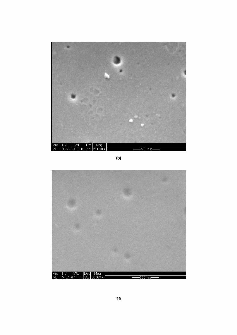
3.4.2 Scanning Electron Microscopy (SEM)

SEM was used to study the surface morphology of Organoclay reinforced Polyimide

membranes.

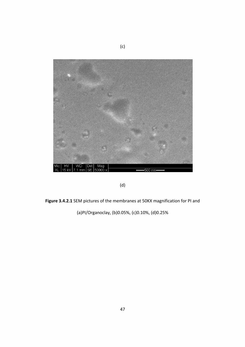
Figure 3.4.2.1 shows the SEM of PI membranes containing varying amount of clay. As

shown in the Figure 3.4.2.1, both the neat PI membrane and the nanocomposite

membranes are highly porous. A close inspection of the SEM pictures, show that the

porosity of the membranes increases with increasing amount of up to 0.25% clay.

(a)

46

(b)

47

(c)

(d)

Figure 3.4.2.1 SEM pictures of the membranes at 50KX magnification for PI and

(a)PI/Organoclay, (b)0.05%, (c)0.10%, (d)0.25%

48

0.00 0.05 0.10 0.15 0.20 0.2540

60

80

100

120

140

160

180

200

0

2

4

6

8

10 Pore Size

Por

e S

ize,

nm

Concentration of Organoclay, wt, %

Diffusion C

oefficient, 10 -10 cm2/s

Diffusion Coefficient

Figure 3.4.2.2 Comparison of pore size and diffusion coefficient for Organoclay

If we have look at the pore size of each sample at low concentration from PI, 0.05%,

0.10%, 0.25%, we will find that the pore size is of a linear relationship with the

concentration. Also, if we look at both pore size and diffusion coefficient, we can see

clearly show that diffusion coefficient increases with increasing pore size. This is

partially proved that the introduction of Organoclay will be helpful to pores and then

benefit for permeation.

49

0.0 0.2 0.4 0.60.5

1.0

1.5

2.0

2.5

3.0


Diffusion Coefficient

Diff

usio

n C

oeffi

cien

t, 10

-10

cm2 /

s

Figure 3.4.2.3 Comparison of concentration and diffusion coefficient for PANi‐Clay

Figure 3.4.2.3 shows the introduction of PANi‐Clay will make a sudden drop of diffusion

coefficient. However, with more PANi‐Clay, it goes back to increase in a similar way for

organoclay. And the diffusion coefficient does not decrease means more PANi‐Clay

might be added into polyimide membranes, this needs further work to understand.

50

Chapter 4 Conclusions and Further Work Suggestions.

The polyimide membranes reinforced with Organoclay have better chemical strengths.

They have a longer life in Ethanol/Water solutions for at least two times longer than

resin membrane. And the higher the concentration is, the more chemical resistant will

be. The effect of PANi‐Clay on chemical resistance is better than Organoclay. Low

concentration of PANi‐Clay will show similar chemical resistance at Ethanol/Water

environment for high concentration of Organoclay.

Polyimide highly cured is not good for permeation. Only partly imidized Polyimide

membranes show good results of permeation. This means fully imidized Polyimide

membranes have a good barrier property and is not appropriate for separation water

and ethanol.

The introduction of Organoclay helped Polyimide membrane increase the water flux at

lower concentration and it did not help that much at high concentration even showed a

reverse effect for permeation. It is believed that the introduction of Organoclay will help

to create or enlarge the pore size of Polyimide membranes. Organoclay’s layer can

exfoliate and “cut” the membrane thus more and more pores shows up, and the size of

pores will become larger. However, when more Organoclay is introduced, it will become

an obstacle itself, which means the pores created by Organoclay will be covered or

extruded by strong Organoclay layer. And the maximum water permeation occurs at the

concentration of 0.25% Organoclay.

51

With the introduction of PANi‐Clay, the effect is reversing. It decreased the diffusion

coefficient a lot, which meant the interaction between Polyimide‐PANi‐Organoclay was

strong. Membrane becomes more condensed than before. This is believed that the PANi

modified Organoclay changed the arrangement of Organoclay in the Polyimide.

Intercalation became dominant than exfoliation. Due to PANi is hydrophobic; it will keep

away water, so the balance of these two forces will lead the final permeation of water

through membrane. It is highly believed that due to the pore creativity from Organoclay,

the effect of PANi‐Clay to permeation will be the results of balance of interactions of

Polyimide‐PANi, Polyimide‐Organoclay, PANi‐Clay and Polyimide‐PANi‐Organoclay. It

becomes more difficult to have a clear concept of the mechanism then.

The Infrared results suggest that polyimide has a weight loss during the diffusion for

neat Polyimide membrane. And this is improved by incorporation of Oragnoclay and

PANi‐Clay. Also, high concentration of Organoclay has a better effect than low

concentration. And PANi‐Clay is also helpful to prevent the loss of polyimide.

However, it is a compromise to choose the right membrane: if the polyimide is kept, the

permeation will be reduced. For future work, how to make the combination of best

chemical resistance and best permeation of water leading to separation is need. Also,

the mechanism of how Organoclay and PANi‐Clay work need a further detailed study.

52

Reference

1. S. A. Parke, G. G. Birch: Solution properties of ethanol in water, Food Chemistry 67

(1999) 241‐246

2. NIST Chemistry WebBook, http://webbook.nist.gov/chemistry/

3. J. Sheehan, V. Cambreco, J. Duffield, M. Garboski, H.Shapouri: An overview of

biodiesel and petroleum diesel life cycles. A report by US Department of Agriculture and

Energy, 1998. p. 1–35

4. S. Puhan, N. Vedaraman, B. V. Rambrahaman, G. Nagarajan. Mahua (Madhuca indica)

seed oil: a source of renewable energy in India, J Sci Ind Res 2005;64:890–6

5. A. Demirbas: Biofuels sources, biofuel policy, biofuel economy and global biofuel

projections, Energy Conversion and Management 49 (2008) 2106–2116

6. RFA, http://www.ethanolrfa.org/resource/facts/

7. K.G. de Carvalho Lima, C.M. Takshashi and F. Alterhum: Ethanol production from corn

cobhydrolysates by Eschierichia coli KO11, Journal of Industrial Microbiology &

Biotechnology (2002) 29, 124‐128

8. B.S. Dien, L.B. Iten and R.J Bothast: Conversion of corn fiber to ethanol by

recombinant E. coli strain FBR3, Journal of Industrial Microbiology & Biotechnology

(1999) 22, 575‐581

53

9. M. Lewandowska, W. Kujawski: Ethanol production from lactose in a

fermentation/pervaporation system, Journal of Food Engineering 79 (2007) 430‐437

10. T. Mohammadi, A. Aroujalian, A. Bakhshi: Pervapoation of dilute alcoholic mixtures

using PDMS membrane, Chemical Engineering Science 60 (2005) 1875‐1880

11. C. Bang‐Xiao: Polymer Membranes for Separating Organic Mixtures, Journal of

Applied Polymer Science, Vol. 101, 1160‐1164 (2006)

12. M. Mulder: Basic principles of membrane technology, Kluwer Academic Publishers,

the Netherlands, 1996

13. S.T. Hwang and K. Kammermeryer: Membrane in separation, John Wiley Sons, New

York, 1975

14. R.Y.M. Huang, R. Pal, G.Y. Moon: Pervaporation dehydration of aqueous ethanol and

isopropanol mixtures through alginate/chitosan two ply composite membranes

supported by poly (vinylidene fluoride) porous membrane, Journal of Membrane

Science, 167 (2000) 275‐289

15. M. Y. Teng, K. R. Lee, D. J. Liaw, J. Y. Lai: Preparation and pervaporation performance

of poly (3‐alkylthiophene) membrane, Polymer 41 (2000) 2047‐2052

16. R.W. Baker: Euromembrane 97, Twente, The Netherlands, 1997

17. P. M. Bungy, H. K. Lonsdale and M.N. de Pinho: Synthetic membranes: science,

engineering and applications, D. Reidel, Dordrecht/Boston/Lancaster/Tokyo, 1986

54

18. R.W. Baker: Membrane technology and application, McGraw‐Hill companies, 2000

19. H. Ohya, V. V. Kudryavtsev, S.I Semenova: Polyimide Membranes Applications,

Fabrications,and Properties, 1996

20. M. I.Bessonov, M. M.Koton, V. V.Kudryavtsev, L. A. Laius: Polyimides: Thermally

Stable Polymers, Consultants Bureau: New York, 1987.

21. D. Wilson, H. D. Stenzenberger, P. M. Hergenrother: Polyimide, Blackie, New York,

1990.

22. K. L. Mittal: Polyimides, Synthesis, Characterization and Applications, Plenum: New

York, 1985.

23. S. H. Goodman: Handbook of Thermoset Plastics, 2nd ed., Noyes Publications: Park

Ridge, NJ, 1998

24. M. Han, H. Bie, D. E. Nikles, G. W. Warren: Amine–Quinone Polyimide: A New High‐

Temperature Polymer and Its Use to Protect Iron Against Corrosion, Published online

25. M. J. M. Abadie, B. Sillion: Polyimides and Other High‐Temperature Polymers,

Elsevier, Amsterdam, 1991.

26. T. Takekoshi: Polyimides, (Wilson D., Hergenrother, P and Stengenberger, H. ed),

Blackie, Chapman and Hall, NY, 1990

27. C.E Sroog: Prog. Polymer Science. 16, 561‐694,1991

55

28. F. W. Harris: Polyimides, (Wilson D., Hergenrother, P and Stengenberger, H. ed),

Blackie, Chapman and Hall, NY, 1990

29. L. Liang, E. Ruckenstein: Polyvinyl alcohol‐Polyacrylamide interpenetrating polymer

network membranes and their pervaporation characteristics for ethanol‐water mixtures,

J. Membrane Sci. 106 (1995) 167‐182

30. H.R. Kricheldorf, Handbook of polymer synthesis, Marcel Dekker, 1991

31. M.T. Bessonov, M.M koton, V.V Kudryavtsev and L.A laius: Polyimide. Thermally

stable polymers, consultants Bureau, NY, 1987

32. C. P. Yang, S.H Hsiao: Effects of various factors on the formation of high molecular

polyamic acid, J. Applied Polymer Sci. 30 (1985) 2883‐2905

33. J. Preston: High‐strength/high‐modulus organic fibres, Polymer Engineering Science,

15 (1975) 199‐206

34. D. Wilson, K. L. Stenzenberger, P. M. Hergenrother: Polyimides, NY, Glasgow, 1‐

37(1990)

35. R.A. Dine‐Hart, W.W. Wright: Preparation and fabrication of aromatic polyimides, J.

Appl. Polym. Sci, 11(1967)609‐627

36. M. J. Brekner, C. Feger: Curing studies of a polyimide precursor. II polyamic acid, J

Polym. Sci. Polym. Chem. Ed. 25 (1987) 2479‐2491

56

37. Yu. N. Sazanov: Applied Significance of Polyimides, Russian Journal of Applied

Chemistry, Vol. 74, No. 8, 2001, 1253‐1259

38. Y. Xu, C. Chen, P. Zhang, B. Sun and J. Li: Pervaporation Properties of Polyimide

Membranes for Separation of Ethanol + Water Mixtures, J. Chem. Eng. Data 2006, 51,

1841‐1845

39. S. Q. Fan: A study of polyamide and polyimide membranes for pervaporation and

vapor permeation, Dissertation of Zhongyuan Univ., 2004

40. J. Schauer, P. Sysel, V. Marousek, Z. Pientka, J. Pokorny and M. Bleha: Pervaporation

and gas separation membranes made from polyimide/polydimethylsiloxande block

copolymer, Journal of Applied Polymer Science, 61 (1996) 1333‐1337

41. A. Jonquiere, C. Dole, R. Clement, P. Lochon: Synthesis and characterization of new

highly permeable polyamideimdes from dianhydride monomers containing amide

functions: an application to the purification of a fuel octane enhancer (ETBE) by

pervaporation, Journal of Polymer Science PT. A‐Polym. Chem. 38 (2000) 614‐630

42. A. Jonquiere, D. Roizard, P. Lochon: Polymer design for pervaporation membrane:

influence of the soft segment size of block copolymers (polyurethaneimides or

polyureaimides) on their pervaporation features, Journal of Membrane Science, 118

(1996) 73‐84

57

43. T.H. Kim, W. J. Koros, G. R. Husk, K.C. O’ Brien: Relationship between gas separation

properties and chemical structures in a series of aromatic polyimides, Journal of

Membrane Science 37 (1988) 45‐62

44. S.A. Stern, Y. Mi, H. Yamamoto, A. K. St. Clair: Structure Permeability relationships of

polyimide membranes: applications to the separation of gas mixtures, Journal of

Polymer Science Pt. B‐Polym. Phys. 27 (1989) 1887‐1909

45. J. Ren, C. S. Bickel, R. N. Lichtenthaler: Separation of aromatics/aliphatics with

crosslinked 6FDA‐based copolyimides, Separation Purification Technology 22‐23 (2001)

31‐43

46. N. Tanihara, K. Tanaka, H. Kita, K. Okamoto: Pervaporation of organic liquid mixtures

through membrane of polyimides containing methyl‐substituted phenylenediamine

moieties, Journal of Membrane Science 95 (1994) 161‐169

47. H. Wang, T. Ugomori, K. Tanaka, H. Kita, K. Okamoto, Y Suma: Sorption and

pervaporation properties of sulfonyl‐containing polyimide membranes to

aromatic/aliphatic hydrocarbon mixtures, Jounal of polymer Science 132 (1997) 97‐108

48. J. Hao, K. Tanaka, H. Kita, K. Okamoto: The pervaporation properties of sulfony‐

containing polyimide membranes to aromatic/aliphatic hydrocarbon mixtures, Journal

of Membrane Science 132 (1997) 97‐108

49. K. Okamoto, h, Wang, T. Ljyuin, S. Fujiwara, K. Tanaka, H. Kita: Pervaporation of

aromatic/non‐aromatic hydrocarbon mixtures through crosslinked membranes of

58

polyimide with pendant phosphonate ester group, Journal of Membranes Science 157

(1999) 97‐105

50. H. Wang, T. Ugomori, Y. Wang, K. Tanaka, H. Kita, K. Okamoto, Y. Suma: Sorption and

pervaporation properties of crosslinked membranes of poly (ethylene oxide imide)

segmented copolymer to aromatic/nonaromatic hydrocarbon mixtures, Journal of

Polymer Science Pt. B‐Polym. Phys. 38 (2000) 1800‐1811

51. J. Fang, K. Tanaka, H. Kita, K. Okamoto: Synthesis of thianthrene‐5,5,10,10‐

tetraoxide‐containing polyimides via Yamazaki‐Higashi phosphorylation method and

their perpaporation properties to aromatic/nonaromatic hydrocarbon mixtures, Journal

of Polymer Science Pt. A‐ Polym. Chem. 38 (2000) 895‐896

52. J. Fang, K. Tanaka, H. Kita, K. Okamoto: Pervaporation properties of ethynyl‐

containing copolyimide membranes to aromatic/nonaromatic hydrocarbon mixtures,

Polymer 40 (1999) 3051‐3059

53. X. Feng, R. Y. M. Huang: Preparation and performance of asymmetric polyetherimide

membranes for isopropanol dehydration by pervaporation, J. Membr. Sci. 109(1996)

165‐172

54．R. Y. M. Huang, X. Feng: Resistance model approach to asymmetric polyetherimide

membranes for pervaporation of isopropanol/water mixtures, Journal of Membrane

Science, 84 (1993) 15‐27

59

55. H. Yanagisita, D. Kitamoto, K. Haraya, T. nakane, T. Tsuchiya, N. Koura: Preparation

and pervaporation performance of polyimide composite membrane by vapor deposition

and polymerization (VDP) , Journal of membrane Science, 136 (1997) 121‐126

56. H. Yanagisita, D. Kitamoto, K. Haraya, T. Nakane, T. Okada, H. Matsuda, Y. Idemoto,

N. Koura: Separation performance of polyimide composite membrane prepared by dip

coating process, Journal of Membrane Science, 188 (2001) 165‐172

57. A. Morioka, H. Yamaguchi, M. Kakimoto, Y. Imai: Formation of interconnected

globulr structure of silica phase in polyimide‐silica hybrid films prepared by the sol‐gel

process, Chem. Mater. , 6 (1994) 913‐917

58. J. H. Kim, K. H. Lee, S. Y. Kim: Pervaporation separation of water from ethanol

through polyimide composite membranes, Journal of Membrane Science, 169 (200) 81‐

93

59. M. Ben‐Hur, M. Malik, J. Letey and U. Mingelgrin, Soil Science, 153: 349‐356, 1992

60. P.D. Kaviratna, T.J. Pinnavaia and P.A. Schroeder, J. Phys.Chem. Solids, 57: 1897‐

1906,1996

61. A. Akelah, A. Moet: Synthesis of organophilic polymer‐clay nanocomposites, Journal

of Applied Polymer Science, Appl.Polym. Symp. 55 (1994) 153‐172

62. C. Depege, F. E. Elmetoui, C. Forano, A. D. Roy: Polymerization of silicates in layered

double hydroxides, Chem. Mater. 8 (1996) 952‐960

60

63. J. J. Lin, I‐J. Cheng, R. Wang, R. J. Lee: Tailoring basal spacing of montmorillonite by

poly (oxyalkylene) diamine intercalation, Macromolecules 24 (2001) 8832‐8834

64. H. L. Tyan, Y. C. Liu, K. H. Wei: Thermally and mechanically enhanced clay/polyimide

nanocomposite via reactive organoclay, Chem. Mater. 11 (1999) 1942‐1947

65. M. Alexandre, P. Dubois: Polymer‐layered silicate nanocomposites: preparation,

properties and sues of a new class of materials, Materials Science and Engineering, R‐

Rep. 28 (2000) 1‐63

66. S. Zhang, D. Sun, Y.Fu, H. Du: Recent advances of superhard nanocomposite

coatings: a review, Surface and Coatings Technology 167 (2003) 113–119

67. L. J. Lee, C. Zeng, X. Cao, X. Han, J. Shen, G. Xu: Polymer nanocomposite foams,

Composites Science and Technology 65 (2005) 2344–2363

68. T. Agag, T. Koga, T. Takeichi: Studies on thermal and mechanical properties of

polyimide‐clay nanocomposites, Polymer 42 (2001) 3399‐3408

69. P. C. LeBaron, Z. Wang, T. J. Pinnavaia: Polymer‐layered silicate nanocomposites: an

overview. Applied Clay Science 15 (1999) 11‐29

70. R. Magaraphan, W. Lilayuthalert, A. Sirivat, J. W. Schwank: Preparation, structure,

properties and thermal behavior of rigid‐rod polyimide/montmorillonite

nanocomposites, Composites Science and Technology 61 (2001) 1253‐1264

61

71. T. Agag, T. Koga, T. Takeichi: Studies on thermal and mechanical properties of

polyimide‐clay nanocomposites, Polymer 42 (2001) 3399‐3408

72. A. gu, S. W. Kuo, F. C. Chang: Syntheses and properties of PI/Clay hybrid, Journal of

Applied Polymer Science 79 (2001) 1902‐1910

73. P. C. Lebaron, Z. Wang, T. J. Pinnavaia: Polymer‐Layered silicate nanocomposites, an

overview, Applied clay science, 15 (1999) 11‐29

74. K. Yano, A. Usuki, A. Okada, T. Kurauchi, O. Kamigaito: Synthesis and properties of

polyimide‐clay hybrid, J. Polym. Sci. Pt. A‐Polym. Chem. 31 (1993) 2493‐2498

75. H.R Dennis, D. L. Hunter, D. Chang, S. Kim. J.L. White, J. W. Cho, D. R. Paul: Effect of

melt processing conditions on the extent of exfoliation in organoclay‐ based

nanocomposties, Polymer 42 (2001) 9513‐9522

76. L. Tie; K. Padmananda D.; P,Thomas J: Mechanism of clay tactoid exfoliation in

epoxy‐clay nanocomposites, Chemistry of Materials, Vol. 7, Issue: 11, 1995. pp. 2144‐

2150

77. P. C. Lebaron, Zhen wang, T. J. Pinnavaia: Polymer‐layered silicate nanocomposites:

an overview, Applied Clay Science 15 (1999) 11‐29

78. Y. Kazuhisa, U. Arimitsu, O. Akane: Synthesis and properties of polyimide‐clay hybrid

films. Journal of Polymer Science Part A: Polymer Chemistry, Vol. 35, Issue: 11, (August

1997) 2289 – 2294

62

79. A. E. Nasrabad, R. Laghaei, and B. C. Eu: Modified Free Volume Theory of Self‐

Diffusion and Molecular Theory of Shear Viscosity of Liquid Carbon Dioxide, J. Phys.

Chem. B 2005, 109, 8171‐8179

80. M.I. Ojovan and W.E. Lee: Viscosity of network liquids within Doremus approach, J.

Appl. Phys. 95 (7): 3803‐3810

81. M.L. Willianms, R.F. Landel, J.D.Ferry, The temperature dependence of relaxation

mechanisms in amorphous polymers and other glass‐forming liquids, J. American Chem.

Society, 77 (1950), 3701

82. Y. S. Song: Rheological characterization of carbon nanotubes/poly9ethylene oxide)

composites, Pheol Acta, 46 (2006), 231

83. S.S. Ray, M. Okamoto: Polymer/layered silicate nanocomposites: a review from

preparation to processing, Prog. Polym. Sci. 28 (2003) 1539–1641

84. K. Wang, S. Y. Yang, L. Fan, M. Sh. Zhan, J. G. Liu: Preparation and Properties of

Molecular‐Weight‐Controlled Polyimides Derived from 1,4‐Bis (4’‐amino‐2’‐

trifluoromethylphenoxy) benzene and 4,4’ Oxydiphthalic Anhydride, Journal of Polymer

Science: Part A: Polymer Chemistry, Vol. 44, 1997–2006 (2006)

85. S. Sinha Ray, K. Okamoto, M. Okamoto: Structure–property relationship in

biodegradable poly(butylene succinate)/ layered silicate nanocomposites.

Macromolecules 2003; 36: 2355–67

63

86. S. Burow, A. Peterlin, D.T. Turner: Increasing viscosity of polymer solutions with

increasing shear stress, Journal of Polymer Science, Part B: Polymer letters, 2, 67, 1964

87. S. Ding, W. T. Petuskey: Solutions to Fick’s second law of diffusion with a sinusoidal

excitation, Solid State Ionics 109 (1998) 101–110

88. W. E. Boyce, R. C. DiPrima: Elementary Differential Equations and Boundary Value

Problems, 8th Edition, Rensselaer Polytechnic Institute, 2005, 612‐615

89. Crank J: The Mathematics of Diffusion, 2nd Edition, 1975, Oxford University Press,

London

90. D. D. Deppe and J. M. Torkelson: Small Molecule Probe Diffusion in Thin Polymer

Films Near the Glass Transition: A Novel Approach using Fluorescence Nonradiative

Energy Tranfer, Polymeric Materials Science and Engineering, Vol. 73, (1995), 388‐389

91. K. E. Miller, R. H. Krueger, J. M. Torkelson: Smart Polymeric Films: Sensing of Cure

and Water Sorption and Diffusion in Multi‐Layered Polymeric Coating by Fluorescence

Spectroscopy, Polymeric Materials Science and Engineering, Vol. 73, (1995), 555‐556

92. G. Giuliana, T. Mariarosaria, V. Vittoria, P. Eric, L. Bénédicte, A. Michael, D. Philippe:

Vapor barrier properties of polycaprolactone montmorillonite nanocomposites: effect of

clay dispersion, Polymer 44 (2003) 2271–2279

93. P. S. Tin, T. S. Chung, Y. Liu, R. Wang: Chemical Cross‐linking Modification on

Polyimide Membrane for Gas Separation, Journal of Membrane Science 189 (2001) 231–

239

64

94. Sadtler Spectral Handbooks: Published by Bio‐Rad Laboratories, Inc., Informatics

Division. © 1978‐2004 Bio‐Rad Laboratories

95. V. Ratta: Crystallization, Morphology, Thermal stability and Adhesive Properties of

Novel High Performance semi crystalline polyimide, Dissertation of Virginia Polytechnic

Institute and State University, 13, 1999

96. H. W. Wang, R. X. Dong, H. C. Chu, K.C. Chang, W. C, Lee: Improvements on the

synthesis and properties of fluorinated polyimide–clay nanocomposites by using double‐

swelling agents, Materials Chemistry and Physics 94 (2005) 42–51

97. O.Khayankarn, R. Magaraphan, J. W. Schwank: Adhesion and Permeability of

Polyimide–Clay

Nanocomposite Films for Protective Coatings, Journal of Applied Polymer Science, Vol.

89, (2003) 2875 – 2881

98. Y.H. Zhang, Z. M. Dang, S. Y. Fu, J. H. Xin, J. G. Deng, J. Wu, S. Yang, L. F. Li, Q. Yan:

Dielectric and dynamic mechanical properties of polyimide–clay nanocomposite films,

Chemical Physics Letters 401 (2005) 553–557

99. B. H. Stuart: Infrared Spectroscopy Fundamentals and Applications, (Analytical

Techniques in the Sciences (AnTs), 2004

100. K.P. Pramoda, T.S. Chung, S.L. Liu, H. Oikawa, A. Yamaguchi: Characterization and

thermal degradation of polyimide and polyamide liquid crystalline polymers, Polymer

Degradation and Stability 67 (2000) 365‐374

65

101. F. Y. Hshieh, D. Hirsch, H. Beeson: Evaluation of Polyimide Foam as a Fire Barrier for

Spacecraft Cushion Materials, Journal of Fire Sciences, Vol. 21, ( 2003) 485‐501

102. V.E. Yudin, J.U. Otaigbe, S. Gladchenko, B.G. Olson, S. Nazarenko, E.N. Korytkova,

V.V. Gusarov: New polyimide nanocomposites based on silicate type nanotubes:

Dispersion, processing and properties, Polymer 48 (2007) 1306‐1315

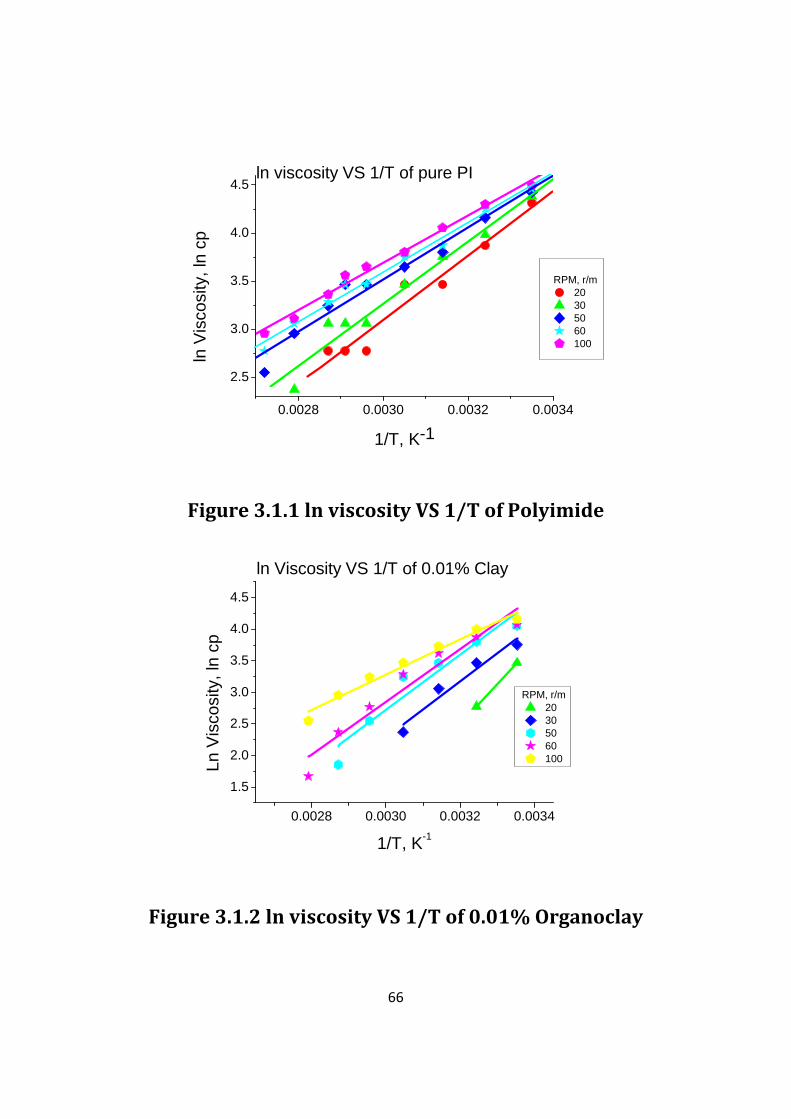
66

0.0028 0.0030 0.0032 0.0034

2.5

3.0

3.5

4.0

4.5

RPM, r/m 20 30 50 60 100

ln V

isco

sity

, ln

cp

1/T, K-1

ln viscosity VS 1/T of pure PI

Figure 3.1.1 ln viscosity VS 1/T of Polyimide

0.0028 0.0030 0.0032 0.0034

1.5

2.0

2.5

3.0

3.5

4.0

4.5

RPM, r/m 20 30 50 60 100Ln

Vis

cosi

ty, l

n cp

1/T, K-1

ln Viscosity VS 1/T of 0.01% Clay

Figure 3.1.2 ln viscosity VS 1/T of 0.01% Organoclay

67

0.0028 0.0030 0.0032 0.0034

2.0

2.5

3.0

3.5

4.0

ln viscosity VS 1/T of 0.05% Clay

RPM, r/m 20 30 50 60 100

ln V

isco

sity

, ln

cp

1/T, K-1


0.0028 0.0030 0.0032 0.0034

2.5

3.0

3.5

4.0

RPM, r/m 20 30 50 60 100ln

Vis

cosi

ty, l

n cp

1/T, K-1



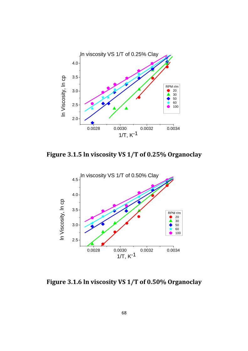
68

0.0028 0.0030 0.0032 0.0034

2.0

2.5

3.0

3.5

4.0

1/T, K-1

ln V

isco

sity

, ln

cp

RPM r/m 20 30 50 60 100



0.0028 0.0030 0.0032 0.0034

2.5

3.0

3.5

4.0

4.5

RPM r/m 20 30 50 60 100

1/T, K-1

ln V

isco

sity

, ln

cp



69

0.0028 0.0030 0.0032 0.0034

2.5

3.0

3.5

4.0

RPM r/m 20 30 50 60 100

1/T, K-1

ln V

isco

sity

, ln

cp



0.0028 0.0030 0.0032 0.0034

3.5

4.0

4.5

5.0

RPM r/m 20 30 50 60 100


ln V

isco

sity

, ln

cp

1/T, K-1


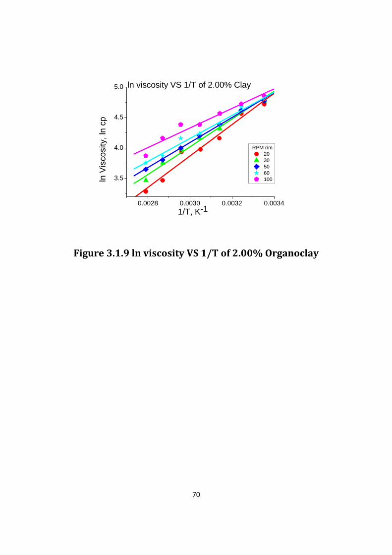
70

0.0028 0.0030 0.0032 0.0034

3.5

4.0

4.5

5.0 ln viscosity VS 1/T of 2.00% Clay

ln V

isco

sity

, ln

cp

RPM r/m 20 30 50 60 100

1/T, K-1


71

0.0028 0.0030 0.0032 0.0034

1.5

2.0

2.5

3.0

3.5

4.0

4.5

RPM, r/m 10 20 30 50 60 100Ln

Vis

cosi

ty, l

n cp

1/T, K-1

ln Viscosity VS 1/T of 0.01% PANi-Clay

Figure 3.1.10 ln viscosity VS 1/T of 0.01% PANiClay

0.0029 0.0030 0.0031 0.0032 0.0033 0.00342.5

3.0

3.5

4.0

4.5

RPM, r/m 20 30 50 60 100Ln

Vis

cosi

ty, l

n cp

1/T, K-1

ln viscosity VS 1/T of 0.05% PANi-Clay


72

0.0030 0.0031 0.0032 0.0033 0.0034

2.5

3.0

3.5

4.0

RPM, r/m 30 50 60 100

Ln V

isco

sity

, ln

cp

1/T, K-1



0.0030 0.0031 0.0032 0.0033 0.0034

2.0

2.5

3.0

3.5

4.0

4.5

RPM, r/m 20 30 50 60 100

1/T, K-1

Ln V

isco

sity

, ln

cp


Figure 3.1.13 ln viscosity VS 1/T of 0. 50% PANiClay

73

3.5 4.0 4.5 5.0 5.5 6.0

2.5

3.0

3.5

4.0

4.5

T, oC 25 35 45 55 65 75 85 95

ln v

isco

sity

, ln

cp

ln shear rate, ln rpm

Pure PI

Figure 3.1.14 ln viscosity VS ln shear rate of Polyimide

4.0 4.5 5.0 5.5 6.01.5

2.0

2.5

3.0

3.5

4.0


T, oC 25 35 45 55 65 75 85ln

vis

cosi

ty

0.01% Clay

Figure 3.1.15 ln viscosity VS ln shear rate of 0.01% OC

74

3.6 4.0 4.4 4.8 5.2 5.6

2.0

2.5

3.0

3.5

4.0


T, oC 25 35 45 55 65 75 85

ln v

isco

sity

, ln

cp

0.05% clay


4.0 4.5 5.0 5.5 6.0

2.5

3.0

3.5

4.0

4.5


T, oC 25 35 45 55 65 75 85

ln v

isco

sity

, ln

cp

0.10% Clay


75

4.2 4.4 4.6 4.8 5.0 5.2 5.4 5.6 5.8

2.0

2.5

3.0

3.5

4.0


T, oC 25 35 45 55 65 75 85ln

vis

cosi

ty

0.25% Clay


4.2 4.4 4.6 4.8 5.0 5.2 5.4 5.6 5.8

2.5

3.0

3.5

4.0

4.5


T, oC 25 35 45 55 65 75 85

ln v

isco

sity

, ln

cp

0.50% Clay


76

4.2 4.4 4.6 4.8 5.0 5.2 5.4 5.6 5.8

2.5

3.0

3.5

4.0


T, oC 25 35 45 55 65 75 85

ln v

isco

sity

, ln

cp

1.00% Clay


4.2 4.4 4.6 4.8 5.0 5.2 5.4 5.6 5.83.0

3.5

4.0

4.5

5.0


25 35 45 55 65 75 85

ln v

isco

sity

, ln

cp

1.50% Clay


77

4.2 4.4 4.6 4.8 5.0 5.2 5.4 5.6 5.8

3.5

4.0

4.5

5.0


T, oC 25 35 45 55 65 75 85

ln v

isco

sity

, ln

cp

2.00% Clay


3.2 3.6 4.0 4.4 4.8 5.2 5.6 6.01.5

2.0

2.5

3.0

3.5

4.0

4.5


T, oC 25 35 45 55 65 75 85 95

ln v

isco

sity

, ln

rpm

0.01% PANi-Clay

Figure 3.1.23 ln viscosity VS ln shear rate of 0.01% PC

78

3.2 3.6 4.0 4.4 4.8 5.2 5.6 6.02.5

3.0

3.5

4.0


T, oC 25 35 45 55 65ln

vis

cosi

ty, l

n cp

0.05% PANi-Clay


4.4 4.8 5.2 5.6 6.0

2.5

3.0

3.5

4.0


T, oC 25 35 45 55

ln v

isco

sity

, ln

cp

0.25% PANi-Clay


79

4.0 4.4 4.8 5.2 5.6 6.02.0

2.5

3.0

3.5

4.0

T, oC 25 35 45 55

ln v

isco

sity

, ln

cp


0.50% PANi-Clay

Figure 3.1.26 ln viscosity VS ln shear rate of 0. 50% PC

80

0 10 20 30 40 50 60 70 80 90 100 1100.0

0.4

0.8

1.2

1.6

2.0

2.4

PANi-Clay Organoclay

Torq

ue %

RPM, r/m

0.01% Clay, T=25oC

Figure 3.1.27 Comparison of PC and OC at 0.01% 1

4.0 4.2 4.4 4.6 4.8 5.0 5.2 5.4 5.6 5.8 6.03.4

3.6

3.8

4.0

4.2

4.4


ln v

isco

sity

, ln

cp


0.01% Clay, T=25oC


81

12.8 13.6 14.4 15.2 16.03.2

3.6

4.0

4.4


ln V

isco

sity

, ln

cp

ln shear stress

0.01% Clay, T=25oC


0.0028 0.0030 0.0032 0.00342.0

2.5

3.0

3.5

4.0

4.5


Ln V

isco

sity

, ln

cp

1/T, K-1

0.01% Clay, RPM=100 r/m


82

10 20 30 40 50 60 70 80 90 100 110

0.0

0.4

0.8

1.2

1.6

2.0


Torq

ue %

RPM, r/m

0.05% Clay, T=25oC


4.0 4.4 4.8 5.2 5.6 6.0

3.6

4.0

4.4


ln v

isco

sity

, ln

cp


0.05% Clay, T=25oC


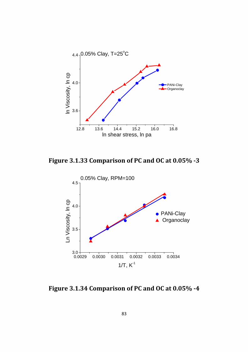
83

12.8 13.6 14.4 15.2 16.0 16.8

3.6

4.0

4.4


ln V

isco

sity

, ln

cp

ln shear stress, ln pa

0.05% Clay, T=25oC


0.0029 0.0030 0.0031 0.0032 0.0033 0.00343.0

3.5

4.0

4.5


Ln V

isco

sity

, ln

cp

1/T, K-1

0.05% Clay, RPM=100


84

20 30 40 50 60 70 80 90 100 1100.0

0.4

0.8

1.2

1.6

2.0


Torq

ue %

RPM, r/m

0.25% Clay, T=25oC


4.0 4.4 4.8 5.2 5.6 6.0

3.0

3.5

4.0


ln v

isco

sity

, ln

cp


0.25% Clay, T=25oC


85

12.8 13.6 14.4 15.2 16.0

2.4

2.8

3.2

3.6

4.0

4.4


ln V

isco

sity

, ln

cp


0.25% Clay, T=25oC


0.0029 0.0030 0.0031 0.0032 0.0033 0.00343.0

3.5

4.0

4.5


Ln V

isco

sity

, ln

cp

1/T, K-1

0.25% Clay, RPM=100 r/m


86

20 30 40 50 60 70 80 90 100 1100.0

0.4

0.8

1.2

1.6

2.0

PANi-Clay OrganoclayTo

rque

%

RPM, r/m

0.50% Clay, T=25oC


4.0 4.4 4.8 5.2 5.6 6.03.0

3.5

4.0

4.5


ln v

isco

sity

, ln

cp


0.50% Clay, T=25oC


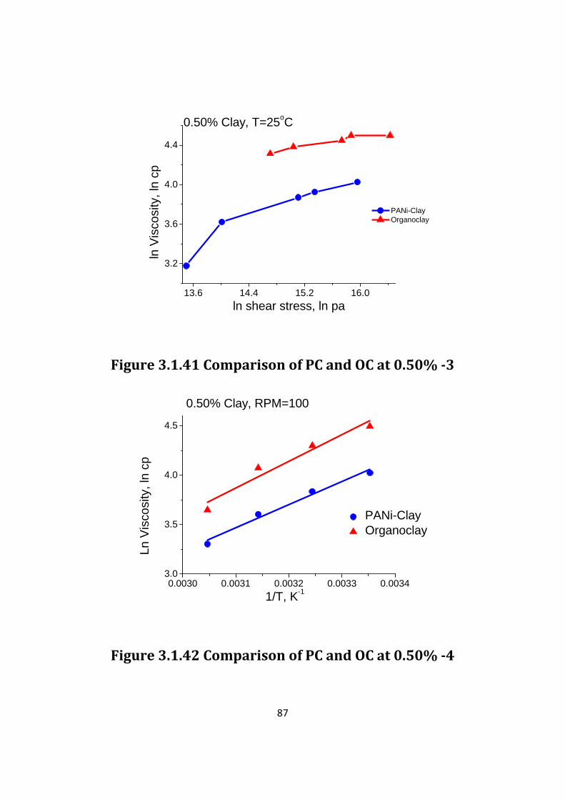
87

13.6 14.4 15.2 16.0

3.2

3.6

4.0

4.4


ln V

isco

sity

, ln

cp


0.50% Clay, T=25oC


0.0030 0.0031 0.0032 0.0033 0.00343.0

3.5

4.0

4.5

Ln V

isco

sity

, ln

cp


1/T, K-1

0.50% Clay, RPM=100


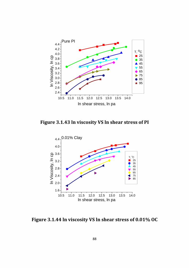
88

10.5 11.0 11.5 12.0 12.5 13.0 13.5 14.0

2.42.62.83.03.23.43.63.84.04.24.4

T, oC2535455565758595ln

Vis

cosi

ty, l

n cp


Pure PI

Figure 3.1.43 ln viscosity VS ln shear stress of PI

10.5 11.0 11.5 12.0 12.5 13.0 13.5 14.01.6

2.0

2.4

2.8

3.2

3.6

4.0

4.4

T, oC 25 35 45 55 65 75 85

ln V

isco

sity

, ln

cp


0.01% Clay

Figure 3.1.44 ln viscosity VS ln shear stress of 0.01% OC

89

10.5 11.0 11.5 12.0 12.5 13.0 13.5 14.0

2.0

2.5

3.0

3.5

4.0

4.5

T, oC25354555657585

ln V

isco

sity

, ln

cp


0.05% clay


10.5 11.0 11.5 12.0 12.5 13.0 13.5 14.0

2.5

3.0

3.5

4.0

4.5

T, oC25354555657585

ln V

isco

sity

, ln

cp


0.10% Clay


90

10.5 11.0 11.5 12.0 12.5 13.0 13.5 14.0

2.0

2.5

3.0

3.5

4.0

T, oC25354555657585

ln V

isco

sity

, ln

cp


0.25% Clay


11.0 11.5 12.0 12.5 13.0 13.5 14.0

2.5

3.0

3.5

4.0

4.5


T, oC25354555657585

ln V

isco

sity

, ln

cp

0.50% Clay


91

11.0 11.5 12.0 12.5 13.0 13.5

2.5

3.0

3.5

4.0

T, oC25354555657585

ln V

isco

sity

, ln

cp


1.00% Clay


11.5 12.0 12.5 13.0 13.5 14.0 14.53.0

3.5

4.0

4.5

5.0

T, oC25354555657585

ln V

isco

sity

, ln

cp


1.50% Clay


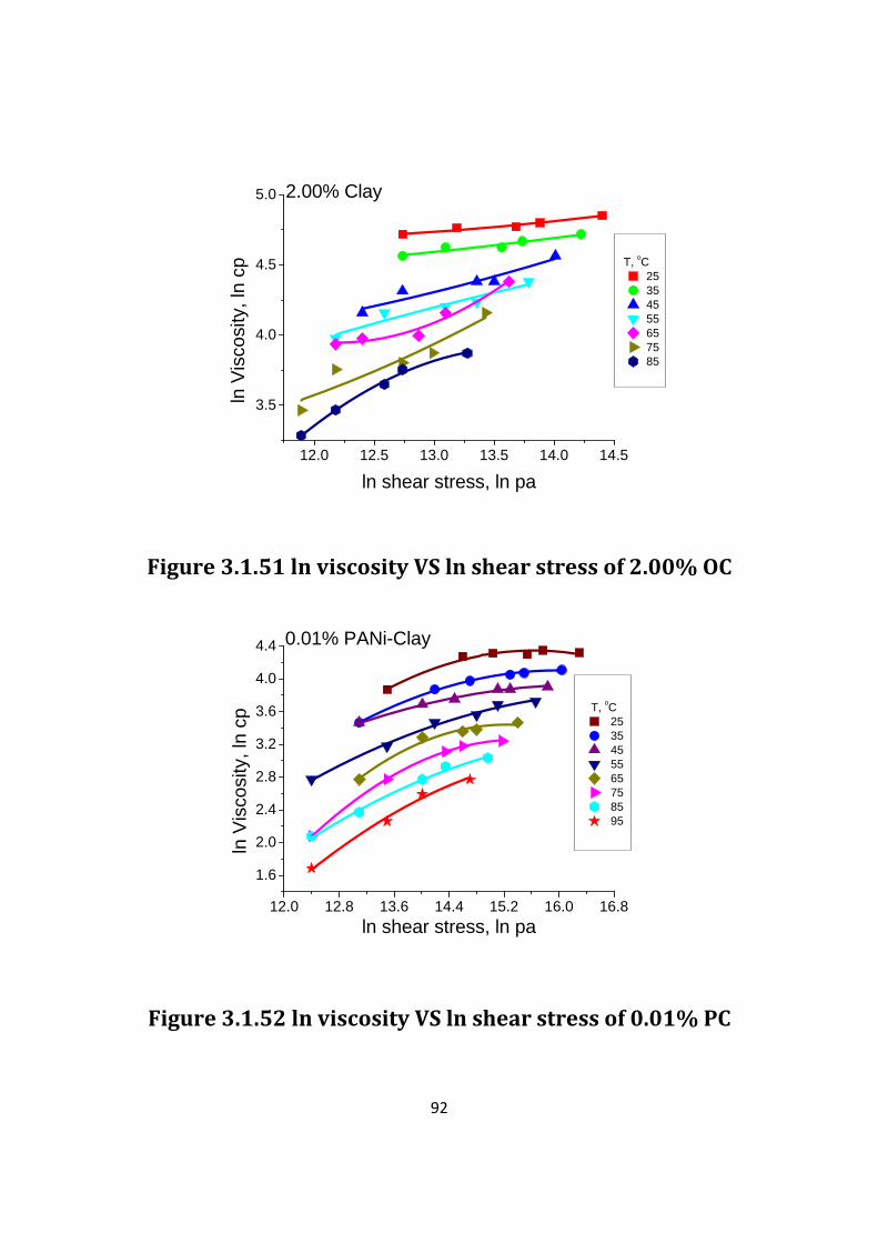
92

12.0 12.5 13.0 13.5 14.0 14.5

3.5

4.0

4.5

5.0

T, oC25354555657585

ln V

isco

sity

, ln

cp


2.00% Clay


12.0 12.8 13.6 14.4 15.2 16.0 16.8

1.6

2.0

2.4

2.8

3.2

3.6

4.0

4.4

T, oC 25 35 45 55 65 75 85 95

ln V

isco

sity

, ln

cp


0.01% PANi-Clay

Figure 3.1.52 ln viscosity VS ln shear stress of 0.01% PC

93

12.8 13.6 14.4 15.2 16.0

2.8

3.2

3.6

4.0

4.4

T, oC 25 35 45 55 65

ln V

isco

sity

, ln

cp


0.05% PANi-Clay


12.8 13.6 14.4 15.2 16.0

2.4

2.8

3.2

3.6

4.0

T, oC 25 35 45 55

ln V

isco

sity

, ln

cp


0.25% PANi-Clay


94

12.8 13.6 14.4 15.2 16.02.0

2.4

2.8

3.2

3.6

4.0

T, oC 25 35 45 55

ln V

isco

sity

, ln

cp


0.50% PANi-Clay


95

0 2 4 6 8 10 12 14

0.0

0.2

0.4

0.6

0.8

1.0[M

w]/[

Min

f]

t1/2, hr1/2

PI

Linear fit for t1/2> 5

4 6 8 10 12

0.0

0.2

0.4

0.6

0.8

1.0

[Mw

]/[M

inf]

t1/2, hr1/2

PI Linear Fit

Figure 3.3.1 Flux of water with time for PI

96

0 2 4 6 8 10 12 14

0.0

0.2

0.4

0.6

0.8

1.0

t1/2, hr1/2

[Mw

]/[M

inf]

PI, repeated


4 6 8 10 12 14

0.0

0.2

0.4

0.6

0.8

1.0

PI, repeated Linear Fit

[Mw

]/[M

inf]

t1/2, hr1/2

Figure 3.3.12 Flux of water with time for PI (Repeated)

97

0 2 4 6 8 10 12 14

0.0

0.2

0.4

0.6

0.8

1.0

t1/2, hr1/2

[Mw

]/[M

inf]

PI, Repeated PI


4 6 8 10 12 14

0.0

0.2

0.4

0.6

0.8

1.0

PI, repeated Linear Fit PI Linear Fit

[Mw

]/[M

inf]

t1/2, hr1/2

Figure 3.3.13 Comparison of PI vs repeated one

98

0 2 4 6 8

0.0

0.2

0.4

0.6

0.8

1.0[M

w]/[

Min

f]

t1/2, hr1/2

0.05%


4 6 8

0.0

0.2

0.4

0.6

0.8

1.0

[Mw

]/[M

inf]

t1/2, hr1/2

0.05% Clay Linear Fit

Figure 3.3.2 Flux of water with time for 0.05% OCPI

99

-2 0 2 4 6 8 10 12 14 16 18

0.0

0.2

0.4

0.6

0.8

1.0[M

w]/[

Min

f]

t1/2, hr1/2

0.1%

Linear Fit for t1/2>5

8 10

0.0

0.2

0.4

0.6

0.8

1.0

[Mw

]/[M

inf]

t1/2, hr1/2



100

0 2 4 6 8 10

0.0

0.2

0.4

0.6

0.8

1.0[M

w]/[

Min

f]

t1/2, hr1/2

0.25% Clay


6 8 10

0.0

0.2

0.4

0.6

0.8

1.0

[Mw

]/[M

inf]

t1/2, hr1/2

0.25 Clay Linear Fit


101

0 2 4 6 8 10

0.0

0.2

0.4

0.6

0.8

1.0

t1/2, hr1/2

[Mw

]/[M

inf]

0.25% Clay, repetead


6 8 10

0.0

0.2

0.4

0.6

0.8

1.0

[Mw

]/[M

inf]

t1/2, hr1/2

0.25 Clay, repeated Linear Fit

102


(RP)

0 2 4 6 8 10

0.0

0.2

0.4

0.6

0.8

1.0

t1/2, hr1/2

[Mw

]/[M

inf]

0.25% Clay, repetead 0.25% Clay


103

6 8 10

0.0

0.2

0.4

0.6

0.8

1.0

1.2[M

w]/[

Min

f]

t1/2, hr1/2

0.25 Clay, repeated Linear Fit 0.25 Clay Linear Fit

Figure 3.3.43 Comparison of 0.25% OCPI VS repeated one

-2 0 2 4 6 8 10 12 14 16 18

0.0

0.2

0.4

0.6

0.8

1.0

[Mw

]/[M

inf]

0.5% Clay

t1/2, hr1/2


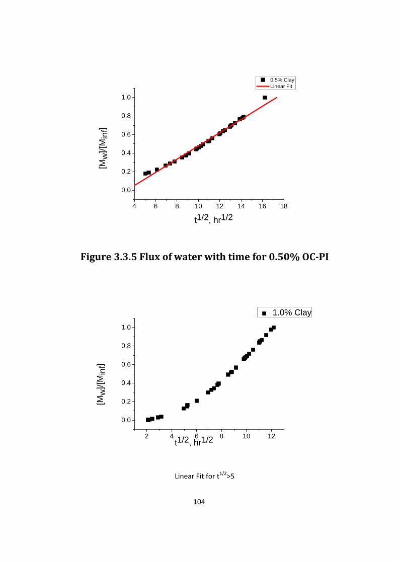
104

4 6 8 10 12 14 16 18

0.0

0.2

0.4

0.6

0.8

1.0[M

w]/[

Min

f]

t1/2, hr1/2



2 4 6 8 10 12

0.0

0.2

0.4

0.6

0.8

1.0

t1/2, hr1/2

[Mw

]/[M

inf]

1.0% Clay


105

4 6 8 10 12

0.0

0.2

0.4

0.6

0.8

1.0

t1/2, hr1/2

[Mt]/

[Min

f]

1.0% Clay Linear FIt


0 2 4 6 8 10 12 14 16 18 20 22

0.0

0.2

0.4

0.6

0.8

1.0

[Mw

]/[M

inf]

t1/2, hr1/2

1.5% Clay

Linear Fit t1/2>5

106

4 6 8 10 12 14 16 18 20 22

0.0

0.2

0.4

0.6

0.8

1.0[M

w]/[

Min

f]

t1/2, hr1/2



0 2 4 6 8 10 12 14 16 18

0.0

0.2

0.4

0.6

0.8

1.0

[Mw

]/[M

inf]

t1/2, hr1/2

2.0% Clay

Linear Fit t1/2>5

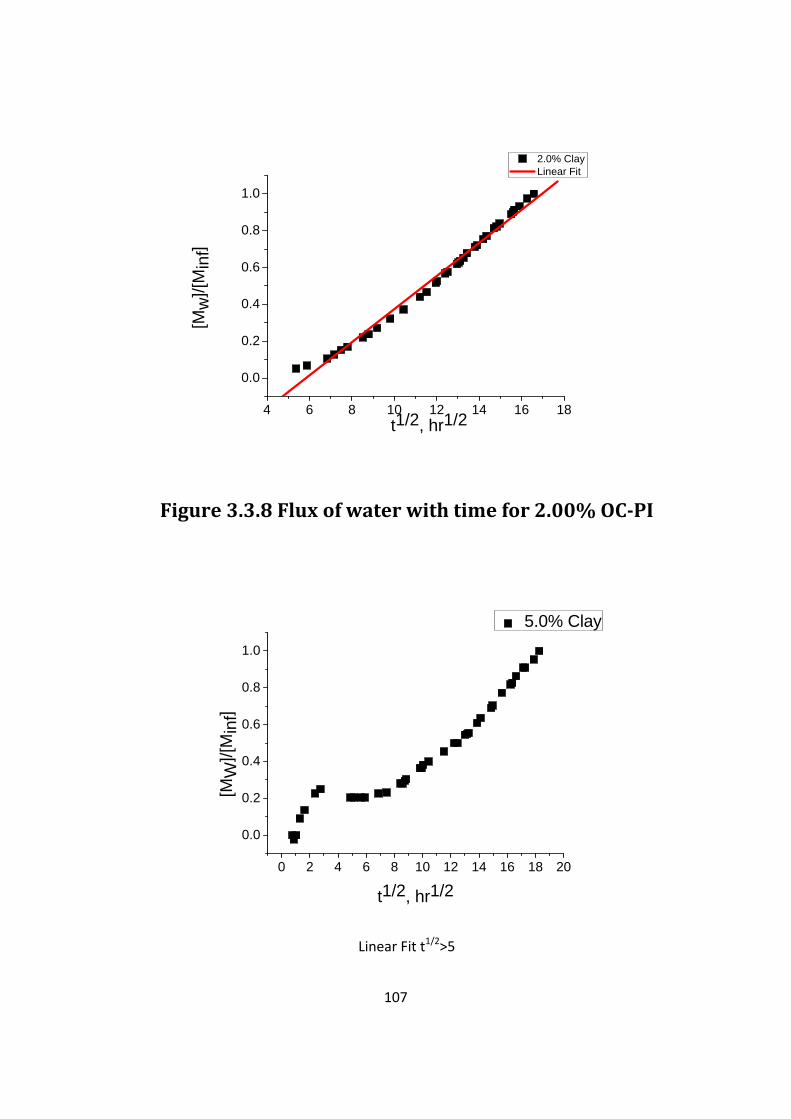
107

4 6 8 10 12 14 16 18

0.0

0.2

0.4

0.6

0.8

1.0

t1/2, hr1/2

[Mw

]/[M

inf]



0 2 4 6 8 10 12 14 16 18 20

0.0

0.2

0.4

0.6

0.8

1.0

[MW

]/[M

inf]

t1/2, hr1/2

5.0% Clay

Linear Fit t1/2>5

108

4 6 8 10 12 14 16 18 20

0.0

0.2

0.4

0.6

0.8

1.0

t1/2, hr1/2

[MW

]/[M

inf]



0 2 4 6 8 10 12 14 16 18 20

0.0

0.2

0.4

0.6

0.8

1.0

0.01% PANi-clay

Mw

/Min

f

t1/2, hr1/2

Linear Fit t1/2 > 5 hr1/2

109

8 12 16 200.0

0.4

0.8

1.2 0.01% PANi-Clay Linear Fit

t1/2, hr1/2

Mw

/Min

f

Figure 3.3.10 Flux of water with time for 0.01% PANiclayPI

-2 0 2 4 6 8 10 12 14 16 18

0.0

0.2

0.4

0.6

0.8

1.0 0.05% PANi-Clay

Mw

/Min

f

t1/2, hr1/2


110

6 7 8 9 10 11 12 13 14 15 160.0

0.2

0.4

0.6

0.8

1.0

0.05% PANi-Clay Linear Fit

t1/2, hr1/2

Mw

/Min

f


0 5 10 15 20

0.0

0.2

0.4

0.6

0.8

1.0 0.25% PANi-Clay

Mw

/Min

f

t1/2, hr1/2


111

6 8 10 12 14 16 18 20

0.0

0.2

0.4

0.6

0.8

1.0


t1/2, hr1/2

Mw

/Min

f


0 2 4 6 8 10 12 14 16

0.0

0.2

0.4

0.6

0.8

1.0 0.50% PANi-Clay

Mw

/Min

f

t1/2, hr1/2


112

6 8 10 12 14 16

0.0

0.2

0.4

0.6

0.8

1.0


t1/2, hr1/2

Mw

/Min

f


Figgure 3.44.1.1 FTI

b

IR Spect

before a

113

trum of

and afte

f neat po

er diffus

olyimide

ion

e membbrane

Figure 3.4.1.2

memb

FTIR Sp

brane be

114

pectrum

efore an

m of 0.01

nd after

1% Orga

diffusio

anoclay

on

PI

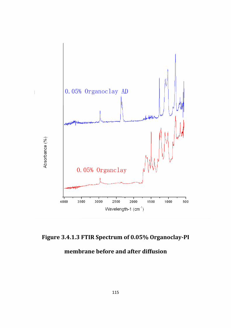
Figure 3.4.1.3

memb

FTIR Sp

brane be

115

pectrum

efore an

m of 0.05

nd after

5% Orga

diffusio

anoclay

on

PI

Figure 3.4.1.4

memb

FTIR Sp

brane be

116

pectrum

efore an

m of 0.10

nd after

0% Orga

diffusio

anoclay

on

PI

Figure 3.4.1.5

memb

FTIR Sp

brane be

117

pectrum

efore an

m of 0.25

nd after

5% Orga

diffusio

anoclay

on

PI

Figure 3.4.1.6

memb

FTIR Sp

brane be

118

pectrum

efore an

m of 0.50

nd after

0% Orga

diffusio

anoclay

on

PI

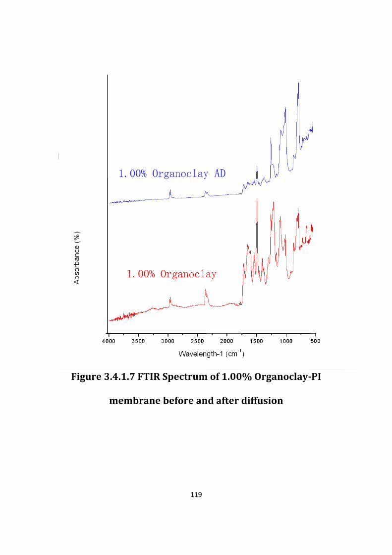
Figure 3.4.1.7

memb

FTIR Sp

brane be

119

pectrum

efore an

m of 1.00

nd after

0% Orga

diffusio

anoclay

on

PI

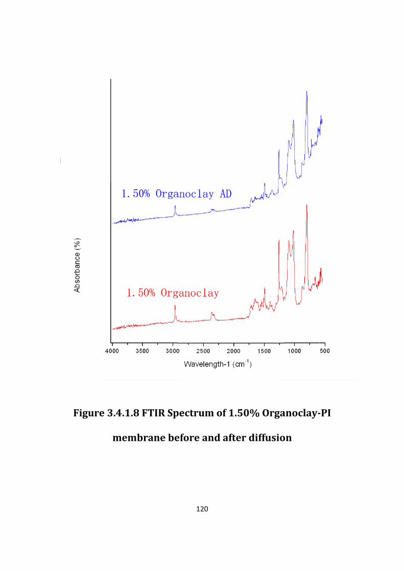
Figure 3.4.1.8

memb

FTIR Sp

brane be

120

pectrum

efore an

m of 1.50

nd after

0% Orga

diffusio

anoclay

on

PI

Figure 3.4.1.9

memb

FTIR Sp

brane be

121

pectrum

efore an

m of 2.00

nd after

0% Orga

diffusio

anoclay

on

PI

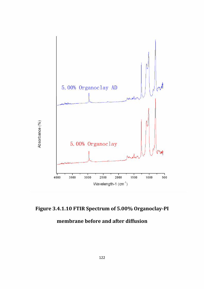
FFigure 3 3.4.1.10

memb

FTIR Sp

brane be

122

pectrum

efore an

m of 5.00

nd after

0% Orga

diffusio

anoclay

on

yPI

Figuree 3.4.1.1

memb

1 FTIR S

brane be

123

Spectru

efore an

um of 0.0

nd after

01% PA

diffusio

ANiclayP

on

PI

Figuree 3.4.1.1

memb

2 FTIR S

brane be

124

Spectru

efore an

um of 0.0

nd after

05% PA

diffusio

ANiclayP

on

PI

Figuree 3.4.1.1

memb

3 FTIR S

brane be

125

Spectru

efore an

um of 0.2

nd after

25% PA

diffusio

ANiclayP

on

PI

Figuree 3.4.1.1

memb

4 FTIR S

brane be

126

Spectru

efore an

um of 0.5

nd after

50% PA

diffusio

ANiclayP

on

PI

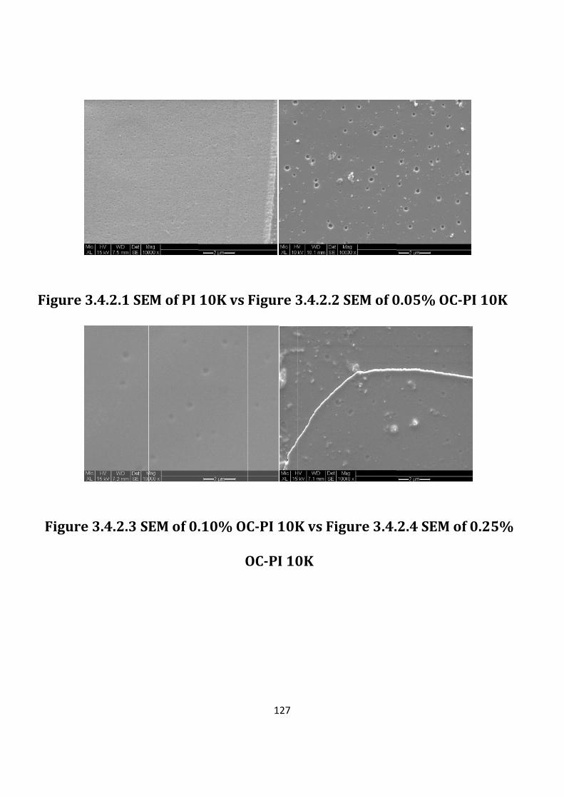
Fi

F

igure 3.4

Figure 3

4.2.1 SE

3.4.2.3 SE

EM of PI

EM of 0.

10K vs

.10% OC

O

127

Figure 3

CPI 10K

OCPI 10

3.4.2.2 S

K vs Figu

0K

SEM of 0

ure 3.4.

0.05% O

2.4 SEM

OCPI 10

M of 0.25

0K

5%

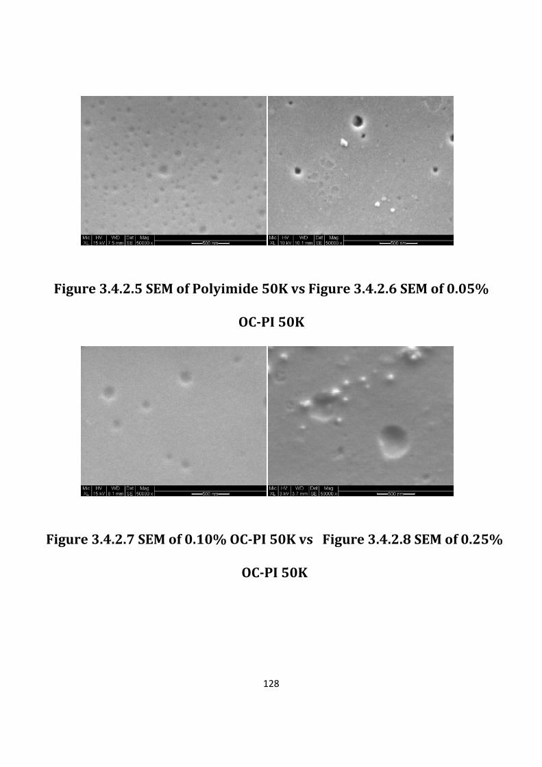
128

Figure 3.4.2.5 SEM of Polyimide 50K vs Figure 3.4.2.6 SEM of 0.05%

OCPI 50K

Figure 3.4.2.7 SEM of 0.10% OCPI 50K vs Figure 3.4.2.8 SEM of 0.25%

OCPI 50K

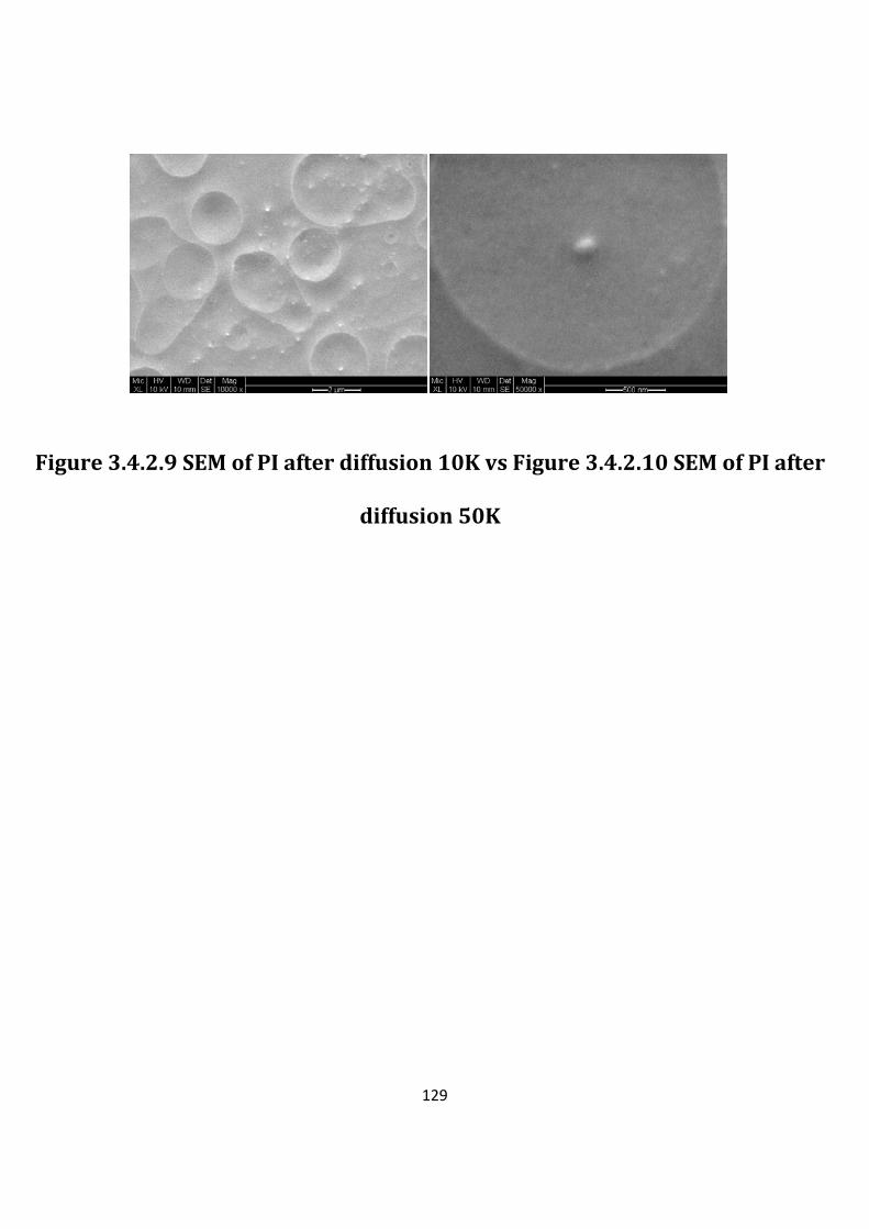
129

Figure 3.4.2.9 SEM of PI after diffusion 10K vs Figure 3.4.2.10 SEM of PI after

diffusion 50K

Global_Commercial_Aircrafts_Gas_Turbine_Engine_Market_2012-2016.pdf

Documents

Transcript of Global_Commercial_Aircrafts_Gas_Turbine_Engine_Market_2012-2016.pdf