Global Techniques for Characterizing Phase Transformations - A Tutorial Review

DOI: 10.1002/adem.201000039

Global Techniques for CharacterizingPhase Transformations – A TutorialReviewBy Michel Perez*, Olivier Lame and Alexis Deschamps

1. Introduction

In order to characterize phase transformations and theirkinetics, one needs to know (i) the nature (crystallography,chemistry, morphology) of each phase, and, (ii) theirdistribution and volume fraction. Phase transformations caninvolve very small volume fractions (e.g. fine precipitation) aswell as the whole sample (e.g. ferrite to austenite transforma-tion).

Presently, no experimental technique can, alone, measureaccurately these two types of information. The nature ofphases is indeed a local data (nano or micrometer scale)whereas their distribution, or volume fraction are more easilyaccessible with global measurements (micrometer to meterscale).

From a local point of view, the most wildly used techniqueis electron microscopy (see Fig. 1, the introductory book ofMurphy[2] and a more specific paper dedicated to precipita-tion[3]). Another rising technique is the tomographic atomprobe (TAP), which gives access to the nature and position of

REVIE

W

Fig. 1. High resolution TEM image of Al3ZrxSc1–x precipitate showing core-shellstructure with Zr rich shell (from Cloue et al.[1]).

[*] Prof. M. Perez, O. LameUniversite de Lyon, INSA LyonMATEIS, UMR CNRS 5510, FranceE-mail: [email protected]. A. DeschampsUniversite de Grenoble, Grenoble INPSIMAP, France

To characterize phase transformations, it is necessary to get both local and global information. Noexperimental technique alone is capable of providing these two types of information. Local techniquesare very useful to get information on morphology and chemistry but fail to deal with global informationlike phase fraction and size distribution since the analyzed volume is very limited. This is why, it isimportant to use, in parallel, global experimental techniques, that investigate the response of the wholesample to a stimulus (electrical, thermal, mechanical. . .). The aim of this paper is not to give anexhaustive list of all global experimental techniques, but to focus on a few examples of recent studiesdealing with the characterization of phase transformations, namely (i) the measurement of thesolubility limit of copper in iron, (ii) the tempering of martensite, (iii) the control of the crystallinitydegree of a ultra high molecular weight polyethylene and (iii) a precipitation sequence in aluminumalloys. Along these examples, it will be emphasized that any global technique requires a calibrationstage and some modeling to connect the measured signal with the investigated information.

ADVANCED ENGINEERING MATERIALS 2010, 12, No. 6 ! 2010 WILEY-VCH Verlag GmbH & Co. KGaA, Weinheim 433

REVIE

W

atoms. The investigated volume is of the order of a fewthousands of nm3 (see Fig. 2 and ref. [4]).

Due to the small analyzed volume, these local techniqueshardly provide global information. They require a largenumber of data and heavy statistical treatment to get, forexample, size distribution of second phase particle. Moreover,estimation of volume fraction of phases is tedious andinaccurate with local techniques.

This is why, in parallel, it is important to perform globalcharacterization that give information averaged on a largeanalyzed volume. Global techniques are based on theresponse of a sample to many kinds of solicitation:(i) thermal: measurement of (i) energy to maintain a

given temperature, or heat a sample (calorimetry), (ii)voltage difference at the extremities of a sample sub-mitted to a temperature gradient [thermoelectricpower (TEP)]

(ii) electric: measurement of electric resistance (resistivity)(iii) mechanical: measurement of the deformation of a sample

submitted to (i) cyclic and low amplitude stress (mech-anical spectroscopy) or (ii) large amplitude stress (tensiletest)

(iv) radiative: measurement of the interaction between radi-ation (X-rays, neutrons, electrons) and matter1.

The aim of this paper is not to give an exhaustive listof all global techniques, but to provide the reader with abrief review on global characterization methods used inmaterial science and underline the potentialities of someof promising techniques through four recent examples:(i) the measure of solubility limit of copper in iron, (ii) thetempering of martensite, (iii) the crystallization of polyethy-lene, and, (iv) a precipitation sequence in an aluminum alloy.The involved global techniques are briefly presented inappendix.

2. Solubility Limit of Copper in Iron

Fe-Cu binary alloys have been extensively studied in thelast 50 years because copper is an excellent candidate forstructural hardening in many alloys: TRIP, HSLA, etc.

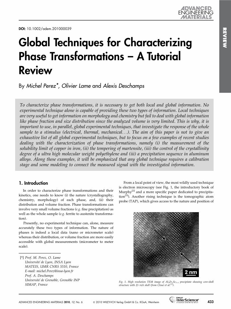
It is paradoxically in the temperature range, within whichcopper is usually precipitated (between 550 and 600 8C) thatvery few experimental data exist on its solubility limit (seeFig. 3). Solubility limit of copper is usually extrapolated fromhigh temperature measurements (>700 8C). Solubility limitsare indeed measured with the diffusion couples technique:two blocks of iron and copper are put in direct contact and thecontent of copper in iron is measured when thermodynamicalequilibrium is reached. Although very convenient at hightemperature, this technique is intractable at temperatureslower than 600 8C, where diffusion is too slow to reachthermodynamic equilibrium during the time scale of theexperiment.

M. Perez et al./Global Techniques for Characterizing Phase . . .

Fig. 2. Reconstructed image from a TAP showing copper precipitates in iron (fromref. [5).

1Techniques involving diffraction and scattering of X-rays arereviewed by A. Deschamps et al [6]

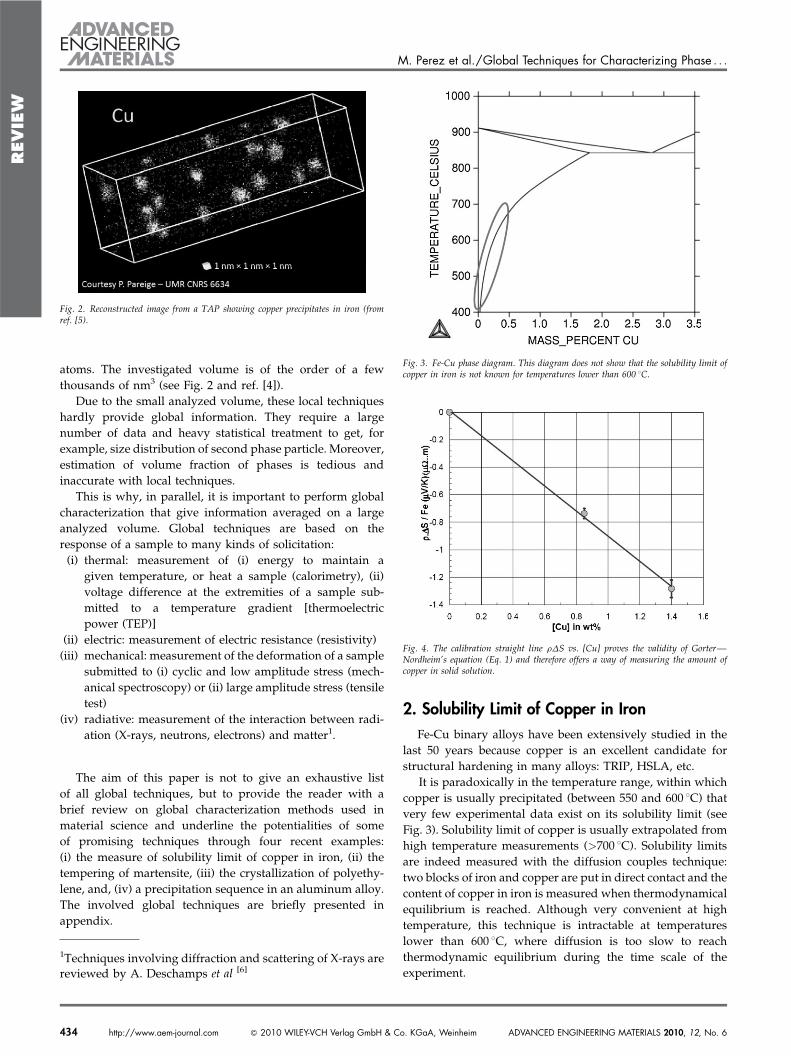
Fig. 3. Fe-Cu phase diagram. This diagram does not show that the solubility limit ofcopper in iron is not known for temperatures lower than 600 8C.

Fig. 4. The calibration straight line rDS vs. [Cu] proves the validity of Gorter—Nordheim’s equation (Eq. 1) and therefore offers a way of measuring the amount ofcopper in solid solution.

434 http://www.aem-journal.com ! 2010 WILEY-VCH Verlag GmbH & Co. KGaA, Weinheim ADVANCED ENGINEERING MATERIALS 2010, 12, No. 6

REVIE

W

2.1. Precipitation Kinetics

To overcome this difficulty, fine precipitation of copperfrom a super saturated solid solution is performed. Indeed,nanometric precipitates induce diffusion of copper within avery limited range (of the order of a few tenth of nanometer)and therefore equilibrium can be reached within a morereasonable isothermal treatment duration (of the order of 1month).

Thermoelectric Power

In order tomeasure the solubility limit of copper in iron, thevariation of thermoelectric power (TEP) can be studied (seeappendix A). The absolute TEP S! of a metallic material isaffected, at different levels, by all the lattice defects (soluteatoms, dislocations, precipitates, etc) which may disturb theelectronic or elastic properties of the material and subse-quently, induce a TEP variation from the defect free TEP S!0.

The contribution of copper on the diffusion component ofTEP is given by the Gorter—Nordheim law[7], which can be

expressed as follows:

rS " r S! # S!0! "

" aCu Cu$ %SCu (1)

where r " r0 & rCu is the resistivity of the considered material(given the Mathiessen’s rule), r0 the resistivity of the pure metal,rCu the increase in resistivity due copper solute atoms(rCu " aCu Cu$ %, where [Cu] is the concentration of copper andaCu is its specific resistivity) and SCu is the specific TEP of copper.

Calibration

To estimate the specific TEP of copper in iron, it is necessaryto check the validity of Gorter—Nordheim’s equation (Eq. (1))by plotting rS versus copper content of the solid solution. Asecond Fe-Cu model alloy has therefore been used(Fe-0.8wt%Cu). The calibration procedure gives an estimationof the specific TEP of copper SCu" 23.4 nV K#1 knowing thespecific resistivity of copper in iron aCu " 3:9 mV.cm/wt%(see Fig. 4).

Results

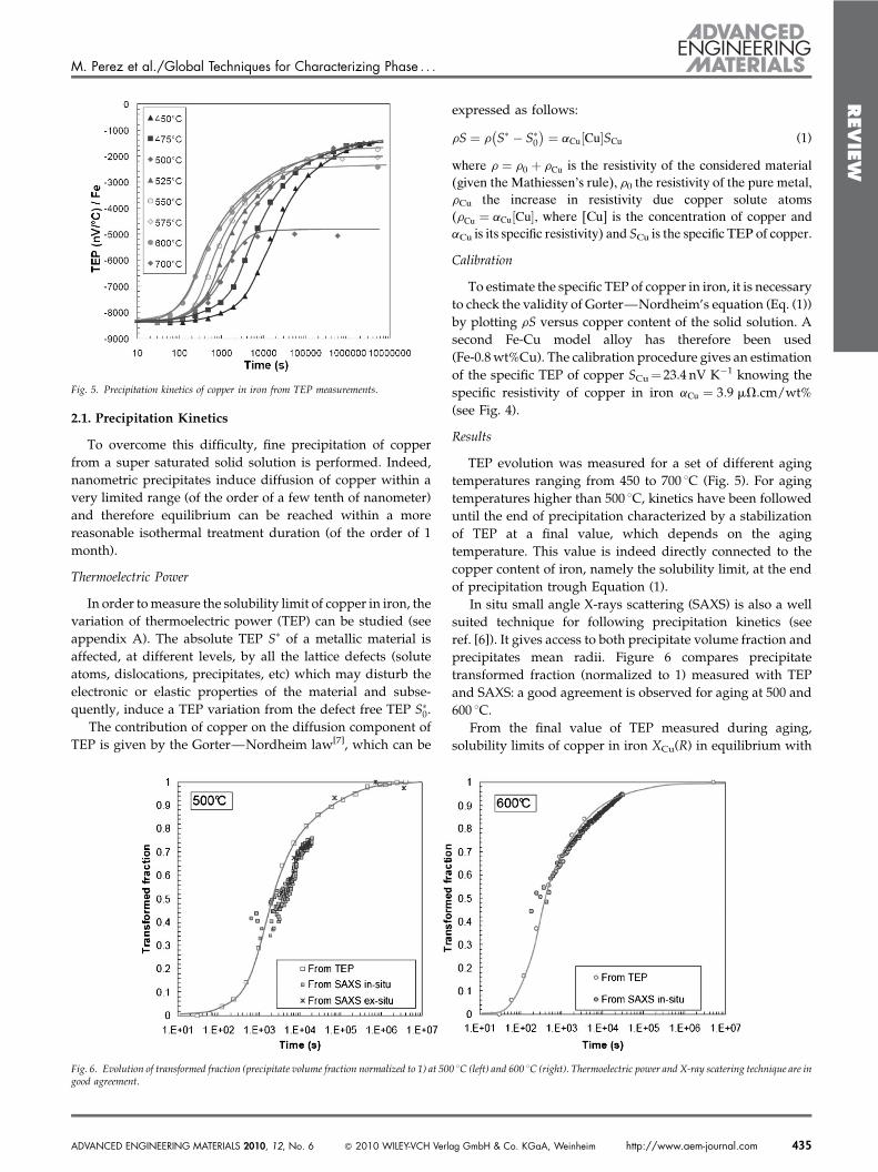
TEP evolution was measured for a set of different agingtemperatures ranging from 450 to 700 8C (Fig. 5). For agingtemperatures higher than 500 8C, kinetics have been followeduntil the end of precipitation characterized by a stabilizationof TEP at a final value, which depends on the agingtemperature. This value is indeed directly connected to thecopper content of iron, namely the solubility limit, at the endof precipitation trough Equation (1).

In situ small angle X-rays scattering (SAXS) is also a wellsuited technique for following precipitation kinetics (seeref. [6]). It gives access to both precipitate volume fraction andprecipitates mean radii. Figure 6 compares precipitatetransformed fraction (normalized to 1) measured with TEPand SAXS: a good agreement is observed for aging at 500 and600 8C.

From the final value of TEP measured during aging,solubility limits of copper in iron XCu(R) in equilibrium with


Fig. 5. Precipitation kinetics of copper in iron from TEP measurements.

Fig. 6. Evolution of transformed fraction (precipitate volume fraction normalized to 1) at 500 8C (left) and 600 8C (right). Thermoelectric power and X-ray scatering technique are ingood agreement.

ADVANCED ENGINEERING MATERIALS 2010, 12, No. 6 ! 2010 WILEY-VCH Verlag GmbH & Co. KGaA, Weinheim http://www.aem-journal.com 435

REVIE

W

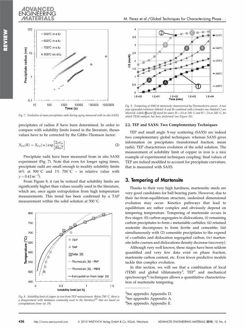
precipitates of radius R have been determined. In order tocompare with solubility limits found in the literature, thesesvalues have to be corrected by the Gibbs–Thomson factor:

XCu R' ( " XCu 1' ( exp 2gvatRkBT

# $(2)

Precipitate radii have been measured from in situ SAXSexperiment (Fig. 7). Note that even for longer aging times,precipitate radii are small enough to modify solubility limits(6% at 500 8C and 1% 700 8C – in relative value withg " 0.4 Jm#2).

From Figure 8, it can be noticed that solubility limits aresignificantly higher than values usually used in the literature,which are, once again extrapolation from high temperaturemeasurements. This trend has been confirmed by a TAPmeasurement within the solid solution at 500 8C.

2.2. TEP and SAXS: Two Complementary Techniques

TEP and small angle X-ray scattering (SAXS) are indeedtwo complementary global techniques: whereas SAXS givesinformation on precipitates (transformed fraction, meanradii), TEP characterizes evolution of the solid solution. Themeasurement of solubility limit of copper in iron is a niceexample of experimental techniques coupling: final values ofTEP are indeed modified to account for precipitate curvature,that is measured with SAXS.

3. Tempering of Martensite

Thanks to their very high hardness, martensitic steels arevery good candidates for ball bearing parts. However, due totheir far-from-equilibrium structure, undesired dimensionalevolution may occur. Kinetics pathways that lead toequilibrium are rather complex and obviously depend ontempering temperature. Tempering of martensite occurs infive stages: (0) carbon segregates to dislocations, (i) remainingcarbon precipitates to form emetastable carbides; (ii) retainedaustenite decomposes to form ferrite and cementite; (iii)simultaneously with (2) cementite precipitates to the expendof e-carbides and dislocation segregated carbon; (iv) marten-site laths coarsen and dislocations density decrease (recovery).

Although very well known, these stages have been seldomquantified and very few data exist on phase fraction,martensite carbon content, etc. Even fewer predictive modelstackle this complex evolution.

In this section, we will see that a combination of local(TEM) and global (dilatometry2, TEP3 and mechanicalspectroscopy4) techniques allows a quantitative characteriza-tion of martensite tempering.


Fig. 8. Solubility limit of copper in iron from TEP measurement. Below 700 8C, there isa disagreement with databases commonly used in the literature[8] that are based onextrapolations from ref. [9].

Fig. 9. Tempering of 100Cr6 martensite characterized by Thermoelectric power. A twostep sigmoidal evolution (labeled A and B) combined with a broader one (labeled C) areobserved. Labels and stand for states H& 4 h at 140 8C and H& 2 h at 240 8C, forwhich TEM analysis has been performed (see Figure 10).

2See appendix Appendix D.3See appendix Appendix A.4See appendix Appendix E.

Fig. 7. Evolution of mean precipitates radii during aging measured with in situ SAXS.


REVIE

W

As ithas been seen in Section 2, TEP is very sensitive tomany microstructural evolutions that may occur duringtempering. Moreover, Abe et al. [10] demonstrated that TEP,like resistivity, is very well adapted to follow the precipitationkinetics of carbides in steels.

3.1. Isothermal Aging of a 100Cr6 Ball Bearing Steel

Samples have been austenitized at 850 8C, quenched in anoil bath and held in hot water (60 8C) for 5min beforeperforming isothermal aging treatments (tempering) atvarious temperatures. Figure 9 shows the change in TEP,DS, as a function of the aging time. From these evolutions,three different stages can be observed:(i) Stage A: a sigmoidal shaped evolution at low aging

temperatures (e.g. 100min at 110 8C).(ii) Stage B: another sigmoidal shaped evolution for higher

temperatures (e.g. 20min at 240 8C).(iii) Stage C: a fairly broad evolution, for the highest inves-

tigated aging temperatures.

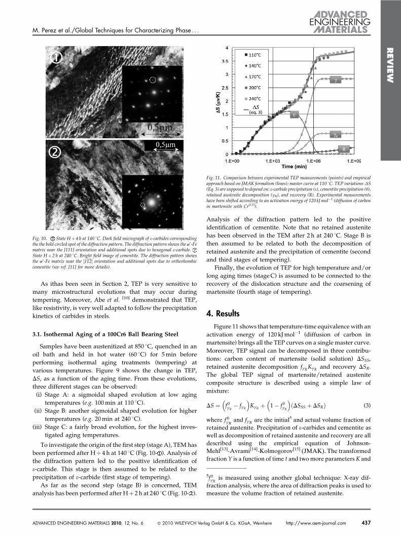
To investigate the origin of the first step (stage A), TEM hasbeen performed after H& 4 h at 140 8C (Fig. 10- ). Analysis ofthe diffraction pattern led to the positive identification ofe-carbide. This stage is then assumed to be related to theprecipitation of e-carbide (first stage of tempering).

As far as the second step (stage B) is concerned, TEManalysis has been performed after H& 2 h at 240 8C (Fig. 10- ).

Analysis of the diffraction pattern led to the positiveidentification of cementite. Note that no retained austenitehas been observed in the TEM after 2 h at 240 8C. Stage B isthen assumed to be related to both the decomposition ofretained austenite and the precipitation of cementite (secondand third stages of tempering).

Finally, the evolution of TEP for high temperature and/orlong aging times (stageC) is assumed to be connected to therecovery of the dislocation structure and the coarsening ofmartensite (fourth stage of tempering).

4. Results

Figure 11 shows that temperature-time equivalence with anactivation energy of 120 kJmol#1 (diffusion of carbon inmartensite) brings all the TEP curves on a single master curve.Moreover, TEP signal can be decomposed in three contribu-tions: carbon content of martensite (solid solution) DSSS,retained austenite decomposition fgRKgR and recovery DSR.The global TEP signal of martensite/retained austenitecomposite structure is described using a simple law ofmixture:

DS " f0gR # fgR

% &KgR & 1# f0gR

% &DSSS & DSR' ( (3)

where f 0gR and fgR are the initial5 and actual volume fraction ofretained austenite. Precipitation of e-carbides and cementite aswell as decomposition of retained austenite and recovery are alldescribed using the empirical equation of Johnson-Mehl[13]-Avrami[14]-Kolmogorov[15] (JMAK). The transformedfraction Y is a function of time t and twomore parameters K and


Fig. 11. Comparison between experimental TEP measurements (points) and empiricalapproach based on JMAK formalism (lines): master curve at 110 8C. TEP variationsDS(Eq. 3) are supposed to depend on: e-carbide precipitation (e), cementite precipitation (u),retained austenite decomposition (gR), and recovery (R). Experimental measurementshave been shifted according to an activation energy of 120 kJmol#1 (diffusion of carbonin martensite with Cr[12]).

5f0gR is measured using another global technique: X-ray dif-fraction analysis, where the area of diffraction peaks is used tomeasure the volume fraction of retained austenite.

Fig. 10. State H& 4 h at 140 8C. Dark field micrograph of e-carbides correspondingthe the bold circled spot of the diffraction pattern. The diffraction pattern shows the a0-Fematrix near the [111] orientation and additional spots due to hexagonal e-carbide.State H& 2 h at 240 8C. Bright field image of cementite. The diffraction pattern showsthe a0-Fe matrix near the $112% orientation and additional spots due to orthorhombiccementite (see ref. [11] for more details).


REVIE

W

n describing the kinetics and rate of the transformation,respectively. Taking into consideration that precipitation ofcementite will destabilize e-carbides, one gets[16]:

Yu t' ( " 1# exp # kut' (nu$ %

Y" t' ( " 1# exp # k"t' (n"$ % # Yu t' ( (4)

where subscripts u and e stand for stable and metastablecarbides, respectively. JMAK parameters has been adjusted togive an accurate description of TEP evolutions at allinvestigated aging temperatures (see Fig. 11). Therefore,analysis of TEP measurements gives the quantities of carbonin martensite as well as the volume fraction of e-carbides,cementite, and retained austenite as a function of time andtemperature. From the knowledge of molar volume of allphases, theses quantities are used to predict dimensionalchanges using classical Voigt and Reuss limits. More detailson this analysis can be found in ref. [17].

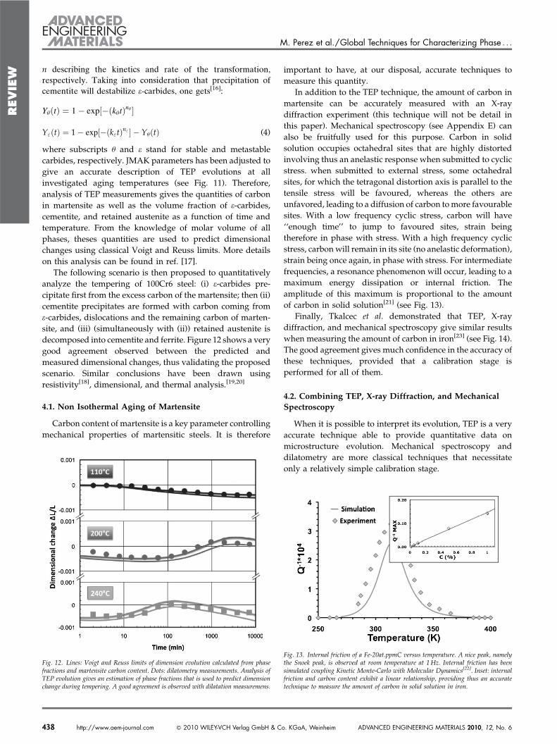
The following scenario is then proposed to quantitativelyanalyze the tempering of 100Cr6 steel: (i) e-carbides pre-cipitate first from the excess carbon of the martensite; then (ii)cementite precipitates are formed with carbon coming frome-carbides, dislocations and the remaining carbon of marten-site, and (iii) (simultaneously with (ii)) retained austenite isdecomposed into cementite and ferrite. Figure 12 shows a verygood agreement observed between the predicted andmeasured dimensional changes, thus validating the proposedscenario. Similar conclusions have been drawn usingresistivity[18], dimensional, and thermal analysis.[19,20]

4.1. Non Isothermal Aging of Martensite

Carbon content of martensite is a key parameter controllingmechanical properties of martensitic steels. It is therefore

important to have, at our disposal, accurate techniques tomeasure this quantity.

In addition to the TEP technique, the amount of carbon inmartensite can be accurately measured with an X-raydiffraction experiment (this technique will not be detail inthis paper). Mechanical spectroscopy (see Appendix E) canalso be fruitfully used for this purpose. Carbon in solidsolution occupies octahedral sites that are highly distortedinvolving thus an anelastic response when submitted to cyclicstress. when submitted to external stress, some octahedralsites, for which the tetragonal distortion axis is parallel to thetensile stress will be favoured, whereas the others areunfavored, leading to a diffusion of carbon tomore favourablesites. With a low frequency cyclic stress, carbon will have‘‘enough time’’ to jump to favoured sites, strain beingtherefore in phase with stress. With a high frequency cyclicstress, carbonwill remain in its site (no anelastic deformation),strain being once again, in phase with stress. For intermediatefrequencies, a resonance phenomenon will occur, leading to amaximum energy dissipation or internal friction. Theamplitude of this maximum is proportional to the amountof carbon in solid solution[21] (see Fig. 13).

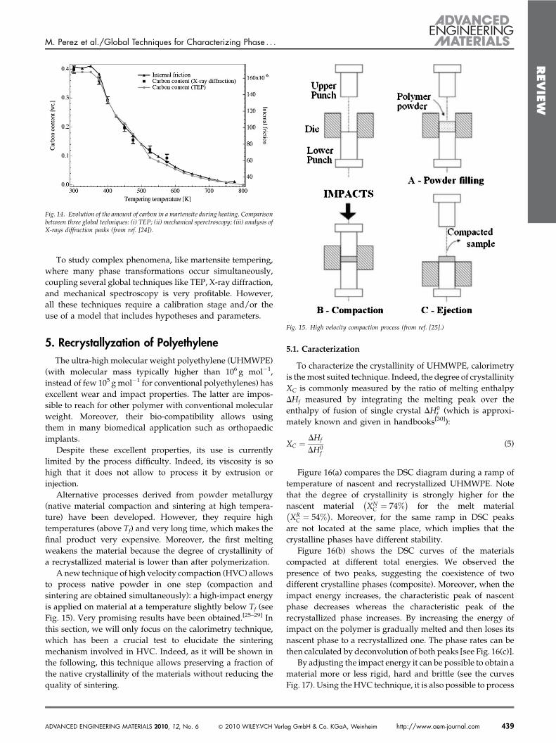
Finally, Tkalcec et al. demonstrated that TEP, X-raydiffraction, and mechanical spectroscopy give similar resultswhen measuring the amount of carbon in iron[23] (see Fig. 14).The good agreement gives much confidence in the accuracy ofthese techniques, provided that a calibration stage isperformed for all of them.

4.2. Combining TEP, X-ray Diffraction, and MechanicalSpectroscopy

When it is possible to interpret its evolution, TEP is a veryaccurate technique able to provide quantitative data onmicrostructure evolution. Mechanical spectroscopy anddilatometry are more classical techniques that necessitateonly a relatively simple calibration stage.


Fig. 13. Internal friction of a Fe-20at.ppmC versus temperature. A nice peak, namelythe Snoek peak, is observed at room temperature at 1Hz. Internal friction has beensimulated coupling Kinetic Monte-Carlo with Molecular Dynamics[22]. Inset: internalfriction and carbon content exhibit a linear relationship, providing thus an accuratetechnique to measure the amount of carbon in solid solution in iron.

Fig. 12. Lines: Voigt and Reuss limits of dimension evolution calculated from phasefractions and martensite carbon content. Dots: dilatometry measurements. Analysis ofTEP evolution gives an estimation of phase fractions that is used to predict dimensionchange during tempering. A good agreement is observed with dilatation measuremens.


REVIE

W

To study complex phenomena, like martensite tempering,where many phase transformations occur simultaneously,coupling several global techniques like TEP, X-ray diffraction,and mechanical spectroscopy is very profitable. However,all these techniques require a calibration stage and/or theuse of a model that includes hypotheses and parameters.

5. Recrystallyzation of Polyethylene

The ultra-high molecular weight polyethylene (UHMWPE)(with molecular mass typically higher than 106 g mol#1,instead of few 105 gmol#1 for conventional polyethylenes) hasexcellent wear and impact properties. The latter are impos-sible to reach for other polymer with conventional molecularweight. Moreover, their bio-compatibility allows usingthem in many biomedical application such as orthopaedicimplants.

Despite these excellent properties, its use is currentlylimited by the process difficulty. Indeed, its viscosity is sohigh that it does not allow to process it by extrusion orinjection.

Alternative processes derived from powder metallurgy(native material compaction and sintering at high tempera-ture) have been developed. However, they require hightemperatures (above Tf) and very long time, which makes thefinal product very expensive. Moreover, the first meltingweakens the material because the degree of crystallinity ofa recrystallized material is lower than after polymerization.

A new technique of high velocity compaction (HVC) allowsto process native powder in one step (compaction andsintering are obtained simultaneously): a high-impact energyis applied on material at a temperature slightly below Tf (seeFig. 15). Very promising results have been obtained.[25–29] Inthis section, we will only focus on the calorimetry technique,which has been a crucial test to elucidate the sinteringmechanism involved in HVC. Indeed, as it will be shown inthe following, this technique allows preserving a fraction ofthe native crystallinity of the materials without reducing thequality of sintering.

5.1. Caracterization

To characterize the crystallinity of UHMWPE, calorimetryis themost suited technique. Indeed, the degree of crystallinityXC is commonly measured by the ratio of melting enthalpyDHf measured by integrating the melting peak over theenthalpy of fusion of single crystal DH0

f (which is approxi-mately known and given in handbooks[30]):

XC "DHf

DH0f

(5)

Figure 16(a) compares the DSC diagram during a ramp oftemperature of nascent and recrystallized UHMWPE. Notethat the degree of crystallinity is strongly higher for thenascent material XN

C " 74%! "

for the melt materialXR

C " 54%! "

. Moreover, for the same ramp in DSC peaksare not located at the same place, which implies that thecrystalline phases have different stability.

Figure 16(b) shows the DSC curves of the materialscompacted at different total energies. We observed thepresence of two peaks, suggesting the coexistence of twodifferent crystalline phases (composite). Moreover, when theimpact energy increases, the characteristic peak of nascentphase decreases whereas the characteristic peak of therecrystallized phase increases. By increasing the energy ofimpact on the polymer is gradually melted and then loses itsnascent phase to a recrystallized one. The phase rates can bethen calculated by deconvolution of both peaks [see Fig. 16(c)].

By adjusting the impact energy it can be possible to obtain amaterial more or less rigid, hard and brittle (see the curvesFig. 17). Using theHVC technique, it is also possible to process


Fig. 15. High velocity compaction process (from ref. [25].)

Fig. 14. Evolution of the amount of carbon in a martensite during heating. Comparisonbetween three global techniques: (i) TEP; (ii) mechanical sperctroscopy; (iii) analysis ofX-rays diffraction peaks (from ref. [24]).


REVIE

W

the polymers below Tf. By preserving a fraction of the nascentcrystalline phase the final properties of the material arestrongly improved.

5.2. DSC: a Key Technique in Polymer Science

Calorimetry is a decisive experimental technique inpolymer science. It allows the detection of Tg, but also themelting peak and the crystallinity degree. Moreover, as themelting temperature depends on crystallites thickness, DSC isparticularly suitable to characterize average crystallite size forsemi-crystalline polymers. It may also be a valuable tool tohighlight the presence of two different crystalline phases inthe same material.

6. Precipitation Sequences in 7xxx Aluminum

Alloying elements and precipitation lead to spectacularimprovement of mechanical properties of aluminum alloys(from 20 for pure aluminum up to 500 MPa). The control ofprecipitation is therefore crucial for the aluminum industry.Unfortunately, these alloys undergo a rather complexprecipitation sequence, involving several metastable phases.

It is therefore essential to combine several experimentaltechniques to characterize precipitates (i) structure (crystal-lography, chemistry and morphology), (ii) size distribution,and (iii) volume fraction. In the following, wewill focus on twoalloys of the 7xxx series (Al-Zn-Mg). It will be demonstratedthat differential scanning calorimetry (DSC), although being avaluable technique, requires an advanced local characteriza-tion investigation, and even modeling, carried out in parallel.

6.1. A Complex Precipitation Sequence

To illustrate the characterization of a precipitation sequencein aluminum alloy, consider a 7150 alloy (Al-6wt%Zn-2wt%-Mg-2wt%Cu) submitted to a T3 treatment (solutionizing and5 days at room temperature maturation).

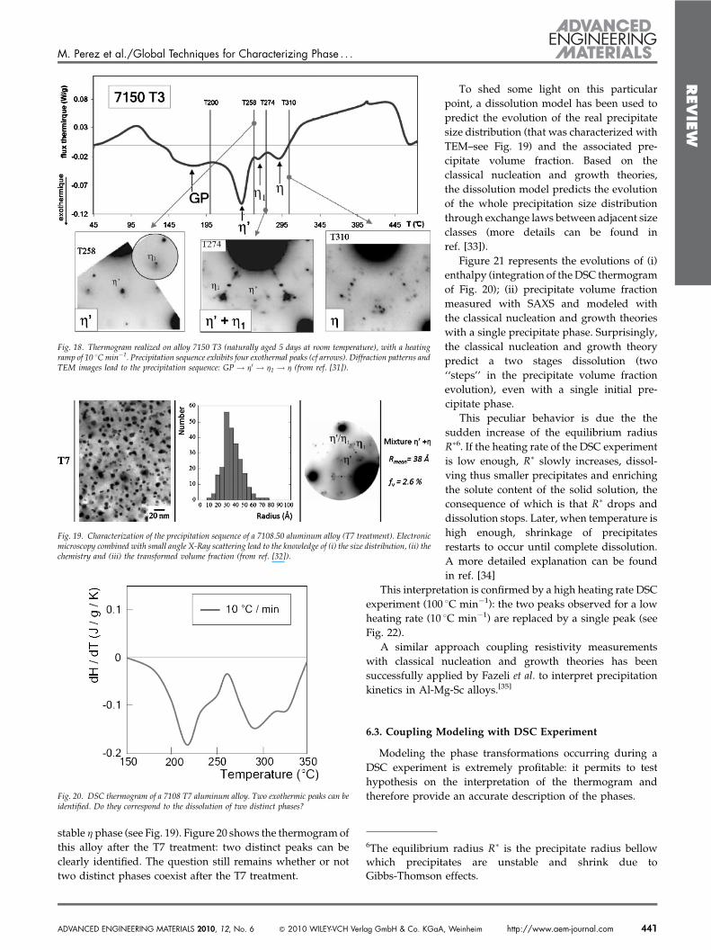
Figure 18 shows the DSC thermogram of this alloy. Fourexothermic peaks can be observed. This thermogram alone isuseless: it is indispensable to perform, in parallel, and aftereach peak, a fine TEM characterization in order to identify theprecipitates. This combined study led the to propose thefollowing precipitation sequence:

GP ! h0 ! h1 ! h (6)

When many metastable phases are involved, coupling aglobal technique with TEM is essential, in order to give acorrect interpretation of the global technique.

6.2. A Model to Interpret DSC Resutls

Let us consider now an (apparently) more simple case: a7108.50 aluminum alloy (Al-5wt%Zn-0.8wt%Mg) submitted toa T7 treatment (overaged 6h at 100 8C, and then 6h at 170 8C).

Thanks to a local characterization stage, it is known that7108.50 (T7) alloy exhibit ametastable h0 and, the predominant


Fig. 16. Analysis by DSC of UHMWPE melting during a heating ramp. (a) Com-parison between the nascent (as-polymerized) material and the material crystallizedfrom the melt. (b) Evolution of the DSC diagram and crystallinity as a function ofimpact energy during process. (c) Measurement of crystallinity by integrating the areaof the DSC peaks.

Fig. 17. Tensile curves of different UHMWPE. It is possible to obtained a ratiomodule-yield strength/hardness desired by adjusting the energy of impact according.


REVIE

W

stable h phase (see Fig. 19). Figure 20 shows the thermogram ofthis alloy after the T7 treatment: two distinct peaks can beclearly identified. The question still remains whether or nottwo distinct phases coexist after the T7 treatment.

To shed some light on this particularpoint, a dissolution model has been used topredict the evolution of the real precipitatesize distribution (that was characterized withTEM–see Fig. 19) and the associated pre-cipitate volume fraction. Based on theclassical nucleation and growth theories,the dissolution model predicts the evolutionof the whole precipitation size distributionthrough exchange laws between adjacent sizeclasses (more details can be found inref. [33]).

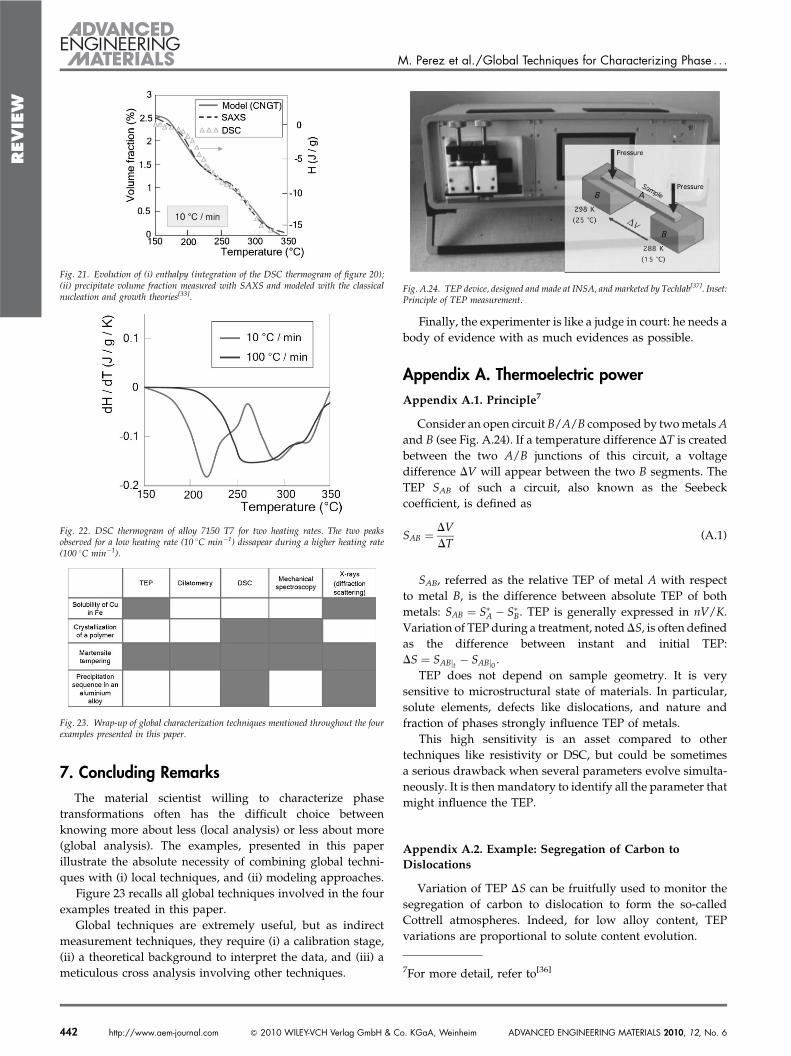
Figure 21 represents the evolutions of (i)enthalpy (integration of the DSC thermogramof Fig. 20); (ii) precipitate volume fractionmeasured with SAXS and modeled withthe classical nucleation and growth theorieswith a single precipitate phase. Surprisingly,the classical nucleation and growth theorypredict a two stages dissolution (two‘‘steps’’ in the precipitate volume fractionevolution), even with a single initial pre-cipitate phase.

This peculiar behavior is due the thesudden increase of the equilibrium radiusR!6. If the heating rate of the DSC experimentis low enough, R! slowly increases, dissol-ving thus smaller precipitates and enrichingthe solute content of the solid solution, theconsequence of which is that R! drops anddissolution stops. Later, when temperature ishigh enough, shrinkage of precipitatesrestarts to occur until complete dissolution.A more detailed explanation can be foundin ref. [34]

This interpretation is confirmed by a high heating rate DSCexperiment (100 8C min#1): the two peaks observed for a lowheating rate (10 8C min#1) are replaced by a single peak (seeFig. 22).

A similar approach coupling resistivity measurementswith classical nucleation and growth theories has beensuccessfully applied by Fazeli et al. to interpret precipitationkinetics in Al-Mg-Sc alloys.[35]

6.3. Coupling Modeling with DSC Experiment

Modeling the phase transformations occurring during aDSC experiment is extremely profitable: it permits to testhypothesis on the interpretation of the thermogram andtherefore provide an accurate description of the phases.


Fig. 18. Thermogram realized on alloy 7150 T3 (naturally aged 5 days at room temperature), with a heatingramp of 10 8Cmin#1. Precipitation sequence exhibits four exothermal peaks (cf arrows). Diffraction patterns andTEM images lead to the precipitation sequence: GP ! h0 ! h1 ! h (from ref. [31]).

Fig. 20. DSC thermogram of a 7108 T7 aluminum alloy. Two exothermic peaks can beidentified. Do they correspond to the dissolution of two distinct phases?

6The equilibrium radius R! is the precipitate radius bellowwhich precipitates are unstable and shrink due toGibbs-Thomson effects.

Fig. 19. Characterization of the precipitation sequence of a 7108.50 aluminum alloy (T7 treatment). Electronicmicroscopy combined with small angle X-Ray scattering lead to the knowledge of (i) the size distribution, (ii) thechemistry and (iii) the transformed volume fraction (from ref. [32]).


https://www.researchgate.net/publication/30513743_Evolution_de_l'etat_de_precipitation_dans_un_alliage_Al-Zn-Mg_lors_de_traitements_thermiques_anisothermes_et_dans_la_zone_affectee_thermiquement_de_joints_soudes?el=1_x_8&enrichId=rgreq-49b82b46b870ef7b1f38dc2c3ca76813&enrichSource=Y292ZXJQYWdlOzIyNzk4NzU3OTtBUzo5ODYwNjk4ODEzNjQ0OEAxNDAwNTIxMTQ2NDQw

REVIE

W

7. Concluding Remarks

The material scientist willing to characterize phasetransformations often has the difficult choice betweenknowing more about less (local analysis) or less about more(global analysis). The examples, presented in this paperillustrate the absolute necessity of combining global techni-ques with (i) local techniques, and (ii) modeling approaches.

Figure 23 recalls all global techniques involved in the fourexamples treated in this paper.

Global techniques are extremely useful, but as indirectmeasurement techniques, they require (i) a calibration stage,(ii) a theoretical background to interpret the data, and (iii) ameticulous cross analysis involving other techniques.

Finally, the experimenter is like a judge in court: he needs abody of evidence with as much evidences as possible.

Appendix A. Thermoelectric power

Appendix A.1. Principle7

Consider an open circuit B/A/B composed by twometalsAand B (see Fig. A.24). If a temperature difference DT is createdbetween the two A/B junctions of this circuit, a voltagedifference DV will appear between the two B segments. TheTEP SAB of such a circuit, also known as the Seebeckcoefficient, is defined as

SAB " DVDT

(A.1)

SAB, referred as the relative TEP of metal A with respectto metal B, is the difference between absolute TEP of bothmetals: SAB " S!A # S!B. TEP is generally expressed in nV/K.Variation of TEP during a treatment, notedDS, is often definedas the difference between instant and initial TEP:DS " SABjt # SABj0 .

TEP does not depend on sample geometry. It is verysensitive to microstructural state of materials. In particular,solute elements, defects like dislocations, and nature andfraction of phases strongly influence TEP of metals.

This high sensitivity is an asset compared to othertechniques like resistivity or DSC, but could be sometimesa serious drawback when several parameters evolve simulta-neously. It is then mandatory to identify all the parameter thatmight influence the TEP.

Appendix A.2. Example: Segregation of Carbon toDislocations

Variation of TEP DS can be fruitfully used to monitor thesegregation of carbon to dislocation to form the so-calledCottrell atmospheres. Indeed, for low alloy content, TEPvariations are proportional to solute content evolution.


Fig. 21. Evolution of (i) enthalpy (integration of the DSC thermogram of figure 20);(ii) precipitate volume fraction measured with SAXS and modeled with the classicalnucleation and growth theories[33].

Fig. 22. DSC thermogram of alloy 7150 T7 for two heating rates. The two peaksobserved for a low heating rate (10 8C min#1) dissapear during a higher heating rate(100 8C min#1).

Fig. A.24. TEP device, designed and made at INSA, and marketed by Techlab[37]. Inset:Principle of TEP measurement.

Fig. 23. Wrap-up of global characterization techniques mentioned throughout the fourexamples presented in this paper.

7For more detail, refer to[36]


REVIE

W

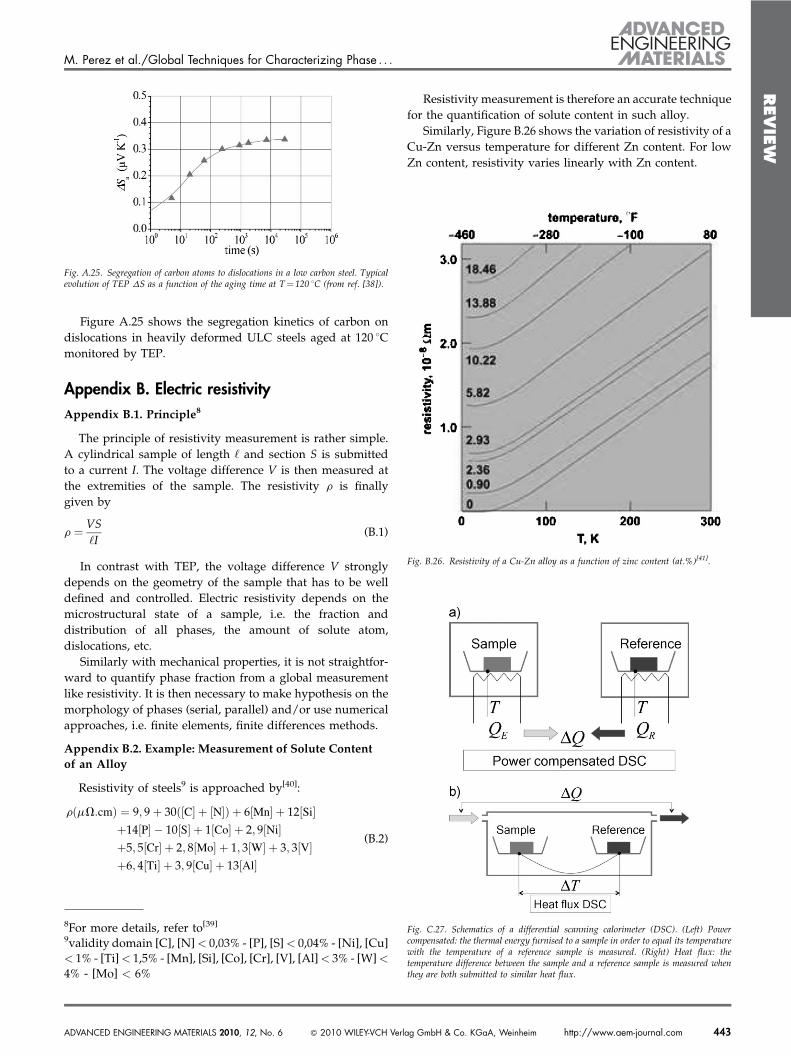
Figure A.25 shows the segregation kinetics of carbon ondislocations in heavily deformed ULC steels aged at 120 8Cmonitored by TEP.

Appendix B. Electric resistivity

Appendix B.1. Principle8

The principle of resistivity measurement is rather simple.A cylindrical sample of length ‘ and section S is submittedto a current I. The voltage difference V is then measured atthe extremities of the sample. The resistivity r is finallygiven by

r " VS‘I

(B.1)

In contrast with TEP, the voltage difference V stronglydepends on the geometry of the sample that has to be welldefined and controlled. Electric resistivity depends on themicrostructural state of a sample, i.e. the fraction anddistribution of all phases, the amount of solute atom,dislocations, etc.

Similarly with mechanical properties, it is not straightfor-ward to quantify phase fraction from a global measurementlike resistivity. It is then necessary to make hypothesis on themorphology of phases (serial, parallel) and/or use numericalapproaches, i.e. finite elements, finite differences methods.

Appendix B.2. Example: Measurement of Solute Contentof an Alloy

Resistivity of steels9 is approached by[40]:

r mV:cm' ( " 9; 9& 30 C$ % & N$ %' ( & 6 Mn$ % & 12 Si$ %&14 P$ % # 10 S$ % & 1 Co$ % & 2; 9 Ni$ %&5; 5 Cr$ % & 2; 8 Mo$ % & 1; 3 W$ % & 3; 3 V$ %&6; 4 Ti$ % & 3; 9 Cu$ % & 13 Al$ %

(B.2)

Resistivity measurement is therefore an accurate techniquefor the quantification of solute content in such alloy.

Similarly, Figure B.26 shows the variation of resistivity of aCu-Zn versus temperature for different Zn content. For lowZn content, resistivity varies linearly with Zn content.


Fig. A.25. Segregation of carbon atoms to dislocations in a low carbon steel. Typicalevolution of TEP DS as a function of the aging time at T" 120 8C (from ref. [38]).

Fig. B.26. Resistivity of a Cu-Zn alloy as a function of zinc content (at.%)[41].

Fig. C.27. Schematics of a differential scanning calorimeter (DSC). (Left) Powercompensated: the thermal energy furnised to a sample in order to equal its temperaturewith the temperature of a reference sample is measured. (Right) Heat flux: thetemperature difference between the sample and a reference sample is measured whenthey are both submitted to similar heat flux.

8For more details, refer to[39]9validity domain [C], [N]< 0,03% - [P], [S]< 0,04% - [Ni], [Cu]< 1% - [Ti]< 1,5% - [Mn], [Si], [Co], [Cr], [V], [Al]< 3% - [W]<4% - [Mo] < 6%


REVIE

W Appendix C. Thermal analysis

Appendix C.1. Principle10

DSC is an accurate technique devoted tothe measurement of thermal characteristicsof a material. The output measure is either (i)the thermal energy furnised to a sample inorder to equal its temperature with thetemperature of a reference sample (powercompensated), or (ii) the temperature differ-ence between the sample and a referencesample is measured when they are bothsubmitted to similar heat flux (heat flux).

First order phase transformations, likefusion, will induce a peak in DSC measure-ment, which surface is proportional to theenthalpy of the transformation. Second ordertransformations will be characterized by astep (change in heat capacity).

Appendix C.2. Example: Crystallization of PEEK

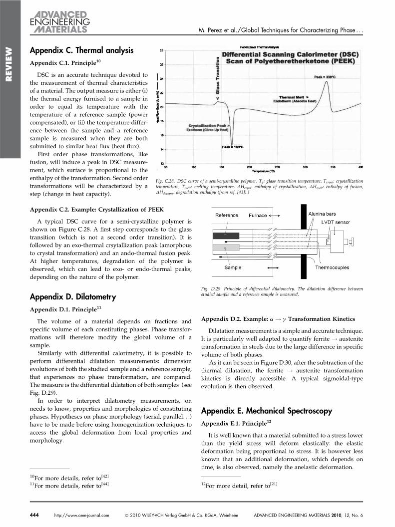
A typical DSC curve for a semi-crystalline polymer isshown on Figure C.28. A first step corresponds to the glasstransition (which is not a second order transition). It isfollowed by an exo-thermal crsytallization peak (amorphousto crystal transformation) and an ando-thermal fusion peak.At higher temperatures, degradation of the polymer isobserved, which can lead to exo- or endo-thermal peaks,depending on the nature of the polymer.

Appendix D. Dilatometry

Appendix D.1. Principle11

The volume of a material depends on fractions andspecific volume of each constituting phases. Phase transfor-mations will therefore modify the global volume of asample.

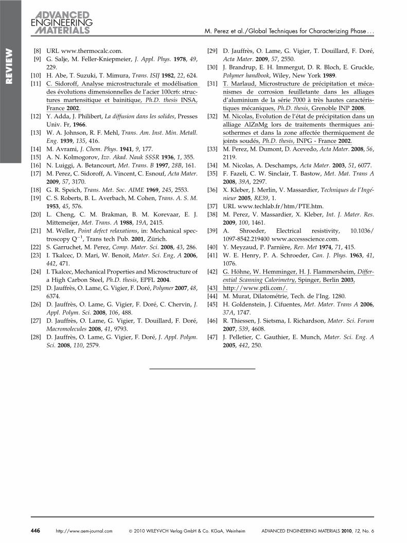
Similarly with differential calorimetry, it is possible toperform differential dilatation measurements: dimensionevolutions of both the studied sample and a reference sample,that experiences no phase transformation, are compared.The measure is the differential dilatation of both samples (seeFig. D.29).

In order to interpret dilatometry measurements, onneeds to know, properties and morphologies of constitutingphases. Hypotheses on phase morphology (serial, parallel. . .)have to be made before using homogenization techniques toaccess the global deformation from local properties andmorphology.

Appendix D.2. Example: a ! g Transformation Kinetics

Dilatationmeasurement is a simple and accurate technique.It is particularly well adapted to quantify ferrite ! austenitetransformation in steels due to the large difference in specificvolume of both phases.

As it can be seen in Figure D.30, after the subtraction of thethermal dilatation, the ferrite ! austenite transformationkinetics is directly accessible. A typical sigmoidal-typeevolution is then observed.

Appendix E. Mechanical Spectroscopy

Appendix E.1. Principle12

It is well known that a material submitted to a stress lowerthan the yield stress will deform elastically: the elasticdeformation being proportional to stress. It is however lessknown that an additional deformation, which depends ontime, is also observed, namely the anelastic deformation.


Fig. C.28. DSC curve of a semi-crystalline polymer. Tg: glass transition temperature, Tcryst: crystallizationtemperature, Tmelt: melting temperature, DHcryst: enthalpy of crystallization, DHmelt: enthalpy of fusion,DHdecomp: degradation enthalpy (from ref. [43]).)

Fig. D.29. Principle of differential dilatometry. The dilatation difference betweenstudied sample and a reference sample is measured.

10For more details, refer to[42]11For more details, refer to[44] 12For more detail, refer to[21]


REVIE

W

All materials exhibit such anelastic deformation, but it isgenerally negligible compared to the elastic deformation.Anelastic deformation is a consequence of defects motion(interstitial atoms, dislocations, gain boundaries, etc) orviscous friction of polymer chains.

This deformation can be quantified by the measurement ofinternal friction: a cyclic stress s " s0 cos vt' ( is applied to asample and strain " " "0 cos vt& f' ( is measured. This straincomprises an elastic part "el cos vt' (' ( and an elastic part"an sin vt' (' (. Internal friction is the ratio of dissipated energy

DW over total elastic energy Wel:

d " DWWel

"R 2p

v0 sd"an

12 s0"el0

" 2p"an0"el0

" 2p tanf (E.1)

Internal friction is measured with the aid of a torsionpendulum (see Figure E.31): forced oscillations at very lowstrain are characterized. Internal friction depends on themobility of defects. It can be measured during heating at agiven frequency or by scanning frequency at constanttemperature. This is why it is called mechanical spectroscopy.

Many phase transformations can be monitored bymechanical spectroscopy because internal friction highlydepends on constituting phases.

Appendix E.2. Example: Crystallization of PET

Figure E.32 show the variations with temperature ofdynamical shear modulus G’ and internal friction of apolymer (PET). The drop in modulus observed at approx-imatively 80 8C is connected to the glass transition, whereasthe rise observed at 130 8C is due to partial recrystallization ofthe polymer.

Received: January 22, 2010Final Version: February 19, 2010Published online: May 20, 2010

[1] E. Clouet, L. Lae, T. Epicier, W. Lefebvre, M. Nastar, A.Deschamps, Nat. Mater. 2006, 5, 482.

[2] D. B. Murphy, Fundamentals of light microscopy andelectronic imaging, Wiley Press, New York 2001.

[3] T. Epicier, Adv. Eng. Mater. 2006, 8, 1.[4] D. Blavette, A. Bostel, J. M. Sarrau, B. Deconihout, A.

Menaud, Nature 1993, 363, 432.[5] URL www.cameca.com.[6] A. Deschamps, L. David, M. Nicolas, F. Bley, F. Livet, R.

Seguela, J. P. Simon, G. Vigier, J. C. Werenskiold, Adv.Eng. Mater. 2001, 3, 579.

[7] L. Nordheim, C. Gorter, Physica 1935, 2, 383.


Fig. D.30. Non-conventional TTT diagram of austenite decomposition in a Fe-Cr-Calloy[45]. Inset: Principle of dilatation measurement performed on a steel sample (heatingrate: 50 K s#1). Linear approximation (parallel-like morphology) lead to ferrite !austenite transformation kinetics[46].

Fig. E.32. Mechanical spectroscopy is a very good tool to study the crystallization ofPET[47].

Fig. E.31. Forced oscillation torsion pendulum used for the measurement of internalfriction[24].)


REVIE

W

[8] URL www.thermocalc.com.[9] G. Salje, M. Feller-Kniepmeier, J. Appl. Phys. 1978, 49,

229.[10] H. Abe, T. Suzuki, T. Mimura, Trans. ISIJ 1982, 22, 624.[11] C. Sidoroff, Analyse microstructurale et modelisation

des evolutions dimensionnelles de l’acier 100cr6: struc-tures martensitique et bainitique, Ph.D. thesis INSA,France 2002.

[12] Y. Adda, J. Philibert, La diffusion dans les solides, PressesUniv. Fr, 1966.

[13] W. A. Johnson, R. F. Mehl, Trans. Am. Inst. Min. Metall.Eng. 1939, 135, 416.

[14] M. Avrami, J. Chem. Phys. 1941, 9, 177.[15] A. N. Kolmogorov, Izv. Akad. Nauk SSSR 1936, 1, 355.[16] N. Luiggi, A. Betancourt, Met. Trans. B 1997, 28B, 161.[17] M. Perez, C. Sidoroff, A. Vincent, C. Esnouf, Acta Mater.

2009, 57, 3170.[18] G. R. Speich, Trans. Met. Soc. AIME 1969, 245, 2553.[19] C. S. Roberts, B. L. Averbach, M. Cohen, Trans. A. S. M.

1953, 45, 576.[20] L. Cheng, C. M. Brakman, B. M. Korevaar, E. J.

Mittemeijer, Met. Trans. A 1988, 19A, 2415.[21] M. Weller, Point defect relaxations, in: Mechanical spec-

troscopy Q#1, Trans tech Pub. 2001, Zurich.[22] S. Garruchet, M. Perez, Comp. Mater. Sci. 2008, 43, 286.[23] I. Tkalcec, D. Mari, W. Benoit, Mater. Sci. Eng, A 2006,

442, 471.[24] I. Tkalcec, Mechanical Properties andMicrosctructure of

a High Carbon Steel, Ph.D. thesis, EPFL 2004.[25] D. Jauffres, O. Lame, G. Vigier, F. Dore, Polymer 2007, 48,

6374.[26] D. Jauffres, O. Lame, G. Vigier, F. Dore, C. Chervin, J.

Appl. Polym. Sci. 2008, 106, 488.[27] D. Jauffres, O. Lame, G. Vigier, T. Douillard, F. Dore,

Macromolecules 2008, 41, 9793.[28] D. Jauffres, O. Lame, G. Vigier, F. Dore, J. Appl. Polym.

Sci. 2008, 110, 2579.

[29] D. Jauffres, O. Lame, G. Vigier, T. Douillard, F. Dore,Acta Mater. 2009, 57, 2550.

[30] J. Brandrup, E. H. Immergut, D. R. Bloch, E. Gruckle,Polymer handbook, Wiley, New York 1989.

[31] T. Marlaud, Microstructure de precipitation et meca-nismes de corrosion feuilletante dans les alliagesd’aluminium de la serie 7000 a tres hautes caracteris-tiques mecaniques, Ph.D. thesis, Grenoble INP 2008.

[32] M. Nicolas, Evolution de l’etat de precipitation dans unalliage AlZnMg lors de traitements thermiques ani-sothermes et dans la zone affectee thermiquement dejoints soudes, Ph.D. thesis, INPG - France 2002.

[33] M. Perez, M. Dumont, D. Acevedo, Acta Mater. 2008, 56,2119.

[34] M. Nicolas, A. Deschamps, Acta Mater. 2003, 51, 6077.[35] F. Fazeli, C. W. Sinclair, T. Bastow, Met. Mat. Trans A

2008, 39A, 2297.[36] X. Kleber, J. Merlin, V. Massardier, Techniques de l’Inge-

nieur 2005, RE39, 1.[37] URL www.techlab.fr/htm/PTE.htm.[38] M. Perez, V. Massardier, X. Kleber, Int. J. Mater. Res.

2009, 100, 1461.[39] A. Shroeder, Electrical resistivity, 10.1036/

1097-8542.219400 www.accessscience.com.[40] Y. Meyzaud, P. Parniere, Rev. Met 1974, 71, 415.[41] W. E. Henry, P. A. Schroeder, Can. J. Phys. 1963, 41,

1076.[42] G. Hohne, W. Hemminger, H. J. Flammersheim, Differ-

ential Scanning Calorimetry, Spinger, Berlin 2003,[43] http://www.ptli.com/.[44] M. Murat, Dilatometrie, Tech. de l’Ing. 1280.[45] H. Goldenstein, J. Cifuentes, Met. Mater. Trans A 2006,

37A, 1747.[46] R. Thiessen, J. Sietsma, I. Richardson, Mater. Sci. Forum

2007, 539, 4608.[47] J. Pelletier, C. Gauthier, E. Munch, Mater. Sci. Eng. A

2005, 442, 250.



https://www.researchgate.net/publication/37813248_Analyse_microstructurale_et_modelisation_des_evolutions_dimensionnelles_de_l'acier_100Cr6_structures_martensitique_et_bainitique?el=1_x_8&enrichId=rgreq-49b82b46b870ef7b1f38dc2c3ca76813&enrichSource=Y292ZXJQYWdlOzIyNzk4NzU3OTtBUzo5ODYwNjk4ODEzNjQ0OEAxNDAwNTIxMTQ2NDQw









https://www.researchgate.net/publication/30516982_Microstructure_de_precipitation_et_mecanismes_de_corrosion_feuilletante_dans_les_alliages_d'aluminium_de_la_serie_7000_a_tres_hautes_caracteristiques_mecaniques?el=1_x_8&enrichId=rgreq-49b82b46b870ef7b1f38dc2c3ca76813&enrichSource=Y292ZXJQYWdlOzIyNzk4NzU3OTtBUzo5ODYwNjk4ODEzNjQ0OEAxNDAwNTIxMTQ2NDQw




https://www.researchgate.net/publication/278639102_Differential_Scanning_Calorimetry?el=1_x_8&enrichId=rgreq-49b82b46b870ef7b1f38dc2c3ca76813&enrichSource=Y292ZXJQYWdlOzIyNzk4NzU3OTtBUzo5ODYwNjk4ODEzNjQ0OEAxNDAwNTIxMTQ2NDQw



Global Techniques for Characterizing Phase Transformations - A Tutorial Review

Documents

Transcript of Global Techniques for Characterizing Phase Transformations - A Tutorial Review