Global properties of pseudospectral methods
38
JOURNAL OF COMPUTATlONAL PHYSICS 81, 239-276 (1989) Global Properties of Pseudospectral Methods A. SOLOMONOFF* ICOMP NASA Lewis Research Center, Cleveland, Ohio AND E. TURKEL' Institute for Computer Applications in Science and Engineering, NASA Lewis Research Center, Cleveland, Ohio and Sackler Faculty of Exact Sciences, Tel-Aviv University, Tel-Aviv, Israel Received January 16, 1987; revised March 16, 1988 We apply polynomial interpolation methods both to the approximation of functions and to the numerical solutions of hyperbolic and elliptic partial differential equations. The derivative matrix for a general sequence of collocation points is explicitly constructed. We explore the effect of several factors on the performance of these methods. We show that global methods cannot be interpreted’in terms of local methods. For example, the accuracy of the approxima- tion differs when large gradients of the function occur near the center of the region or in the vicinity of the boundary. This difference does not depend on the density of the collocation points near the boundaries. Hence, intuition based on finite difference methods can lead to false results. 0 1989 Academic Press, Inc. 1. INTRODUCTION In this study we consider the accuracy of the pseudospectral algorithm both for approximating a function and also for the numerical solution of differential equa- tions. We shall only consider collocation methods, but most of the results shown also apply to Galerkin methods. We approximate the function, f(x), by a polyno- mial, PN(x), that interpolates f(x) at N+ 1 distinct points x0, .. .. xN. f’(x) is approximated by P;(x), which is calculated analytically. In solving differential equa- tions we use an approach similar to finite differences. Thus, all derivatives that appear are replaced by their pseudospectral approximation. The resulting system is * Present address: Brown University, Department of Applied Mathematics. + Research supported by NASA Contracts NASl-17070 and NASl-18107 while he was in residence at NASA Lewis Research Center, Cleveland, OH 44135 and ICASE, NASA Langley Research Center, Hampton, VA 23665. 239 0021-9991/89 $3.00 Copyright 0 1989 by Academic Press, Inc. All rigbts of reproduction in any form mserved.
Transcript of Global properties of pseudospectral methods

JOURNAL OF COMPUTATlONAL PHYSICS 81, 239-276 (1989)
Global Properties of Pseudospectral Methods
A. SOLOMONOFF*
ICOMP NASA Lewis Research Center, Cleveland, Ohio
AND
E. TURKEL'
Institute for Computer Applications in Science and Engineering, NASA Lewis Research Center, Cleveland, Ohio
and Sackler Faculty of Exact Sciences, Tel-Aviv University, Tel-Aviv, Israel
Received January 16, 1987; revised March 16, 1988
We apply polynomial interpolation methods both to the approximation of functions and to the numerical solutions of hyperbolic and elliptic partial differential equations. The derivative matrix for a general sequence of collocation points is explicitly constructed. We explore the effect of several factors on the performance of these methods. We show that global methods cannot be interpreted’in terms of local methods. For example, the accuracy of the approxima- tion differs when large gradients of the function occur near the center of the region or in the vicinity of the boundary. This difference does not depend on the density of the collocation points near the boundaries. Hence, intuition based on finite difference methods can lead to false results. 0 1989 Academic Press, Inc.
1. INTRODUCTION
In this study we consider the accuracy of the pseudospectral algorithm both for approximating a function and also for the numerical solution of differential equa- tions. We shall only consider collocation methods, but most of the results shown also apply to Galerkin methods. We approximate the function, f(x), by a polyno- mial, PN(x), that interpolates f(x) at N+ 1 distinct points x0, . . . . xN. f’(x) is approximated by P;(x), which is calculated analytically. In solving differential equa- tions we use an approach similar to finite differences. Thus, all derivatives that appear are replaced by their pseudospectral approximation. The resulting system is
* Present address: Brown University, Department of Applied Mathematics. + Research supported by NASA Contracts NASl-17070 and NASl-18107 while he was in residence at
NASA Lewis Research Center, Cleveland, OH 44135 and ICASE, NASA Langley Research Center, Hampton, VA 23665.
239 0021-9991/89 $3.00
Copyright 0 1989 by Academic Press, Inc. All rigbts of reproduction in any form mserved.

240 SOLOMONOFF AND TURKEL
solved in space or advanced in time for time-dependent equations. Hence, for an explicit scheme, nonlinearities do not create any special difficulties.
For a collocation method, the coefficients of the series are obtained by demand- ing that the approximation interpolate the function at the collocation points. This requires O(N’) operations. For special sequences of collocation points, e.g., Chebyshev nodes, this can be accomplished by using FFTs and requires only O(N log N) operations. Every collocation method has two interpretations: one in terms of interpolation at the collocation points and one in terms of a series expan- sion but with different coefficients than a Galerkin expansion. In the past, this has lead to some confusion. As an example we consider the case of a Chebyshev collocation method with xi= cos(rrj/N). From an approximation viewpoint, we know [ll, 15-181 that the maximum error for interpolation at the zeros of T,,,(x) is within a factor of (4 + 2/7c log N) of the minimax error and converges to zero as N-+ co for all functions in C’. The bound for the error based on the points xi, given above, is even smaller than this [13]. There also exist sharp estimates in Sobolev spaces [3]. Since the minimax approximation has an error which is equi- oscillatory, we expect the Chebyshev interpolant to be nearly equi-oscillatory. Indeed, Remez suggests using these xj as a first guess in finding the zeros off - P, in this algorithm for the minimax approximation. Thus, we would expect that when Chebyshev points are used to solve differential equations the error will be essentially uniform throughout the domain.
On the other hand, considered as a finite difference type scheme with N+ 1 nodes, one expects the scheme to be more accurate near the boundaries where the collocation points are clustered. At the center of the domain the distance between points is approximately n/2N, while near the boundary the smallest distance between two points is approximately 7r2/2N2. Hence, the spacing at the center is about n/2 times coarser than an equivalent equally spaced mesh and near the boundary it is about 4N/7r2 times liner. Thus, one expects the accuracy and resolv- ing power of the scheme to be better near the boundaries. However, the bunching of points near the boundaries only serves to counter the tendency of polynomials to oscillate with large amplitude near the boundary. We shall also consider colloca- tion based on uniformly spaced points. Since we consider polynomial interpolation on the interval ( - 1, l), we get qualitatively different results than those obtained by Fourier or finite difference methods even for the same collocation points. In fact, we shall see that the boundaries exert a strong influence in this case just as with Chebyshev nodes. In addition, we shall examine the influence of boundary condi- tions on the accuracy and stability of pseudospectral methods. In general, global methods are more sensitive to the boundary treatment than local methods. We also consider the effect of the location of the collocation points on both the accuracy and the stability of the scheme and its effect on the allowable time step for an explicit time integration algorithm.

GLOBALPROPERTIESOFPSEUDOSPECTRALMETHODS 241
2. APPROXIMATION AND DIFFERENTIATION
We assume that we are given N + 1 distinct points x,, < x1 c . . . < x,,,. Given a functionf(x) it is well known how to interpolatef(x) by a polynomial PN(x) such that PN(xj) = f(xj), j = 0, . . . . N. We define a function ek(x) which is a polynomial of degree N and satisfies ek(xj) = Sjk. Explicitly,
ek(xl=$o (x-x,) Ifk
ak= ;I @k-x,). I=0 l#k
(2.la)
(2.lb)
Then the approximating polynomial is given by the Lagrange interpolation formula,
PN(X) = 5 ftxk) ek(X). k=O
(2.2)
We now construct an approximation to the derivative by analytically differentiat- ing (2.2). The value of the approximate derivative at the collocation points is a linear functional of the value of the function itself at the collocation points. Hence, given the N + 1 values f(xj) we can find the values PA(x) by a matrix multiplying the original vector (f(x,), . . . . f(xN)). We denote this matrix by D = (djk). By con- struction, DP, = Pk is exact for all polynomials of degree N or less. In fact, an alter- native way of characterizing D is by demanding that it give the analytic derivative for all such polynomials P. In particular, we shall explicitly construct D by demanding that,
Dek(Xj) = e;(Xj), j, k = 0, . . . . N; (2.3)
i.e.,
D

242 SOLOMONOFF AND TURKEL
Performing the matrix multiply, it is obvious that
djk = 2 (Xj). (2.4)
We next explicitly evaluate djk in terms of the collocation points xj. Taking the logarithm of (2.1) we have
log(e,) = f log(x - x,) - log(+). I=0 Ifk
Differentiating, we have
e;(x) = ek(x) 5 l/(x-x,). I=0 I#k
(2.5)
In order to evaluate (2.5) at x = xi, j # k, we need to eliminate the zero divided by zero expression. We therefore rewrite (2.5) as
e;(x)=ek(x)/(x-xj)+e,(x) fj l/(x-x,). I=0
I# j,k
Since, ek(xj) = 0 for j # k we have that
e;(xj) = liy ek(x)/(x - x,). I
Using the definition of e,(x), (2.1), we have
djk=$ ,fio (xj-X/)=a cx~~xk) see (2.lb)). k I
I#j,k
(2.7)
While the formulas (2.5), (2.7) are computationally useable, it is sometimes preferable to express the formulas slightly differently. We therefore rederive these formulas using a slightly different notation. Define
N #N+I(X)= n (x-x,). (2.8) I=0
Then,
&v+,(x)= g l?i (x-x,) k-0 I=0
Ifk
(2.9)
GLOBAL PROPERTIES OF PSEUDOSPECTRAL METHODS 243
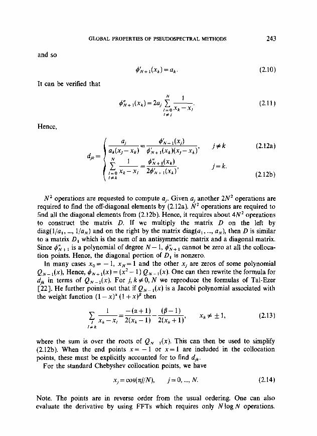
and so
&‘+ ltxk) =ak.
It can be verified that
d~+l(xk)=2uj,$o&. I
I#i
Hence,
djk
(2.10)
(2.11)
j#k
j=k.
(2.12a)
(2.12b)
N* operations are requested to compute aj. Given aj another 2N2 operations are required to find the off-diagonal elements by (2.12a). N* operations are required to find all the diagonal elements from (2.12b). Hence, it requires about 4N2 operations to construct the matrix D. If we multiply the matrix D on the left by diag( l/a,, . . . . l/a,) and on the right by the matrix diag(a,, . . . . a,,,), then D is similar to a matrix D, which is the sum of an antisymmetric matrix and a diagonal matrix. Since &,+ i is a polynomial of degree N - 1, di+, cannot be zero at all the colloca- tion points. Hence, the diagonal portion of D, is nonzero.
In many cases x0 = - 1, xN = 1 and the other xj are zeros of some polynomial QN- ,(x), Hence, #N+ i(x) = (x2 - 1) QN- i(x). One can then rewrite the formula for djk in terms of Q,+,(x). For j, k # 0, N we reproduce the formulas of Tal-Ezer [22]. He further points out that if QN- i(x) is a Jacobi polynomial associated with the weight function (1 -x)’ (1 + x)~ then
(2.13) I#k
where the sum is over the roots of QN-,(x). This can then be used to simplify (2.12b). When the end points x = - 1 or x = 1 are included in the collocation points, these must be explicitly accounted for to find djk.
For the standard Chebyshev collocation points, we have
xi = cos(nj/N), j = 0, . . . . N. (2.14)
Note. The points are in reverse order from the usual ordering. One can also evaluate the derivative by using FFTs which requires only N log N operations.

244 SOLOMONOFFAND TURKEL
Computationally it is found that for N? 100 the matrix multiplication is faster than the FFT approach; see, e.g., [23]. The exact crossover point depends on the computer and the efficiency of the software for computing FFTs and matrix multi- plications. Multiplying by a matrix has the advantage that it is more flexible and vectorizable. For example, both the location and the number of the collocation points is arbitrary. In order to use the FFT approach, it is required that the collocation points be related to the Fourier collocation points, e.g., Chebyshev. Furthermore, the total number of collocation points needs to be factorizable into powers of 2 and 3 for efficiency. The efficiency of these factors depends on the memory allocation scheme of the computer. Other collocation nodes than (2.14) are considered in [3, 7, 131. The matrix D for the Chebyshev points (2.14) is given in [7]. An alternative to using matrix multiplication is to find the derivative by using finite differences and Newton’s interpolation formula based on xj, j = 0, . . . . N.
Similarly for the second derivative we have
D’2’e,(xj) = ei(x,), j, k = 0, . . . . N,
and so
=2djk [dH-&], j#k
(,F,&,-,, (&‘x,)’ I#k I#k
N
=d :k 1
-,;o (xk-xl)” j=k.
\ I#k
I# j,k
= 2d, c -!- I=0 xj-xI
I#j,k
In Appendix A, we consider the problem when we have N collocation nodes and wish the derivative matrix to be exact (in least squares sense) for M> N functions which need not be polynomials.
3. PARTIAL DIFFERENTIAL EQUATIONS
In this study we consider three applications of collocation methods: (1) approximation theory, (2) hyperbolic equations, and (3) elliptic equations. For approximation theory we need only discuss accuracy. We first need some way to measure the approximation error that can be used on a computer. We cannot use

GLOBAL PROPERTIES OF PSEUDOSPECTRAL METHODS 245
the error at the collocation points since, by construction, this error is zero. Instead, we use
(3.1)
where
17t and 1, I#% N w/E--
CI N Cl =
2, I=O, N
for some sequence of points x1 which are not the collocation points. In general, we shall choose N’ much larger than N, the number of collocation points. If the original points are chosen as Chebyshev nodes, then we again choose the x1, as Chebyshev nodes based on this larger number, N’. Because of this selection of nodes the sum in (3.1) approximates the Chebyshev integral norm; i.e.,
(3.2)
When the collocation points are uniformly spaced, we can choose the nodes of the integration formula to be also uniformly spaced. In this case
llf-P,112=~~, C”fw-W~)12~~. (3.3)
For general collocation points it is not clear how to choose the weights w, in the norm. An alternative possibility is to measure the error in some Sobolev norm. In this case, the finite sum can be based on the original collocation points, and the norm is the L2 norm of the derivative. In this study all errors will be given by (3.2) regardless of the distribution of the collocation nodes.
For hyperbolic problems we need to be concerned with stability in addition to accuracy. For simplicity we shall only consider the model equation
u, =4x) UC?, -l<x<l, t > 0. (3.4)
We will solve the differential equation (3.4) by a pseudo-spectral algorithm. Thus, we will consider the solution only at the collocation points. We then replace the derivative in (3.4) by a matrix multiplication as described in Section 2. We next multiply a(x) at each collocation point by the approximate derivative at that point. We now have a system of ordinary differential equations in time. To advance the solution in time we could use any ODE solver. In particular, we shall use a standard 4-stage fourth-order Runge-Kutta formula. This formula has several advantages. First, since it is fourth-order in time (for both linear and nonlinear problems), it is closer to the high spatial accuracy of the spectral method than a
246 SOLOMONOFF AND TURKEL
second-order formula. Also, the region of stability includes a significant portion of the left half-plane and so is appropriate for Chebyshev methods which have eigen- values in the left half-plane. Finally, if we look along the imaginary axis it has a comparatively large stability region. An alternative method is to use a spectral method in time [21]. However, it is difficult to generalize such methods to non- linear problems while Runge-Kutta methods extend trivially to nonlinear problems.
Since the Runge-Kutta method is an explicit method (even though all the points are connected every time step), it is easy to impose boundary conditions after any stage of the algorithm. Whenever we wish we can let the pseudo-spectral method advance the solution at the boundary also. Since the method is explicit, there is a limit on the allowable At because of stability considerations. Heuristically, one can consider this stability limit as arising from two different considerations. One is based on the minimum spacing between mesh points, which usually occurs near the boundary. This is heuristic since the domain of influence of each point is the entire interval. Alternatively, one can derive a stability limit by finding the spectral radius of a(x) times the derivative matrix. This is also heuristic since the derivative matrix is not a normal matrix. When a(x) is constant both methods indicate that At varies with l/N’. The exact constant varies with the particular Runge-Kutta metod used. For a two stage Runge-Kutta method, At/max(a) is about three times the minimum spacing. For further details, the reader is referred to [S, 73 and the result section. In Appendix B, we present the proof of the stability of Chebyshev collocation at the points (2.14) for u, = u,.
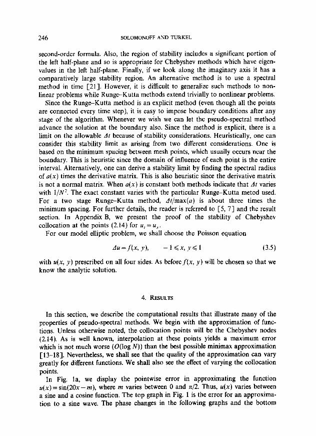
For our model elliptic problem, we shall choose the Poisson equation
Au = Ax, Y), -l<x,y<l (3.5)
with u(x, y) prescribed on all four sides. As before,f(x, y) will be chosen so that we know the analytic solution.
4. RESULTS
In this section, we describe the computational results that illustrate many of the properties of pseudo-spectral methods. We begin with the approximation of func- tions. Unless otherwise noted, the collocation points will be the Chebyshev nodes (2.14). As is well known, interpolation at these points yields a maximum error which is not much worse (O(log N)) than the best possible minimax approximation [ 13-181. Nevertheless, we shall see that the quality of the approximation can vary greatly for different functions. We shall also see the effect of varying the collocation points.
In Fig. la, we display the pointwise error in approximating the function U(X) = sin(20x - m), where m varies between 0 and n/2. Thus, u(x) varies between a sine and a cosine function. The top graph in Fig. 1 is the error for an approxima- tion to a sine wave. The phase changes in the following graphs and the bottom


248 SOLOMONOFF AND TURKEL
graph is the error for a cosine function. In this case we chose 28 Chebyshev colloca- tion points. For m = 0, i.e., a sine function, the amplitude of the error is largest. This occurs since sin(x) is an odd function and hence the coefficient of T, is zero, so in essence we are only using 27 polynomials. This is verified in Fig. lb by using N= 29; for this case the error of the cosine function is larger. Nevertheless, this result is pertinent for time-dependent problems when the solution may vary between a sine and cosine function. In addition, we also notice that for m = 0 the largest errors occur in the middle of the domain while for m = n/2 the largest errors are near the boundaries. Thus, for smooth functions the maximum error can occur anywhere in the domain. It is not necessary for the error to be smaller near the boundaries where the collocation points are bunched together.
In Fig. 2 we show the pointwise error in approximating the function U(X) = Ix - x,,I which has a discontinuous derivative at x = x0. We define a point as being halfway between two nodes in the Chebyshev sense when
Xj+ l/z E COS(7C(j + $)/N).
The top of the graph displays the error when the discontinuous derivative is located halfway between nodes, while the center of the graph shows the error when the dis- continuity in the derivative occurs at a node. The other graphs show other locations of xi. Thus, we see that when the discontinuous derivative occurs halfway between
FIG. 2. The error for pseudospectral approximation to (x - x,,l, 0.05 <x0 < 0.05 with 29 nodes. The error is plotted as a function of x.

GLOBAL PROPERTIES OF PSEUDOSPECTRAL METHODS 249
nodes in the Chebyshev sense, the error has a sharp peak near the discontinuity but is close to zero elsewhere. When the discontinuity occurs near a node, the error is more spread out and several peaks may occur but the maximum error is decreased. Gottlieb has observed similar phenomena in other problems. For other values of x the error goes smoothly between these extremes.
We next examine the effect of the aliasing error in the approximation of a function. Gottlieb and Orszag [S] show that one needs at least n points per wave length when using a Galerkin-Chebyshev approximation. In Fig. 3a, we approximate sin(Mrcx) with N Chebyshev nodes in a pseudospectral approxima- tion. We plot the L* error, (3.2), as a function of the number of points. As expected, the error begins to decrease exponentially when there are rr points per wave length. We further see that in order to reach a fixed error the number of collocation points, N, should vary (approximately) as the (N- nM)/M’13. Hence the error depends on both and N and M. Computationally, it is hard to find the exact exponent, but it seems to be between $J and f. In Fig. 3b, we see that for j(x) = tanh(Mx) there is no sudden limit. Rather there is a gradual reduction in the error as N increases. This analysis is not limited to the function tanh(x). In general, we expect the estimate of x points per wavelength to be accurate only for entire functions. The behavior of M/N is different for the various functions.
For a Fourier method, it can be shown that one only needs two points per wavelength rather than II points per wavelength. It might be speculated that this is due to the larger spacing of the Chebyshev method near the middle of the domain. In fact, asymptotically, the largest spacing between Chebyshev nodes is exactly 7c/2 times as large as for Fourier nodes. In Fig. 4, we consider the same case as in Fig. 3, but where the collocation points are evenly spaced. We now need more than 2 points per wavelength. Computationally, it is hard to determine exactly what is the dependence. In Fig. 4a we plot the L2 error as a function of (N - 5.5M)/Mo2, for f(x) = sin(M?rx), M= 1, 2, 4, 6, 8, 10, and N collocation points, N going from 5 to 55. For comparison we plot, in Fig. 4b, the same data as a function of (N- rcM)/M’.‘. There is a theorem [ 143 that interpolation based on uniformly spaced points converges for analytic functions in a certain lens shaped region. Nevertheless, we see in Fig. 4 that the approximation begins to diverge if N is suf- ficiently large with respect to M. The calculations for these case were carried out on a CRAY computer with about 15 significant figures. Using double precision (about 30 significant digits) one stabilizes the procedure until larger N are reached at which point the approximation again diverges. Hence, even though the function is analytic, nevertheless roundoff errors eventually contaminate the approximation. Hence, collocation based on uniformly spaced nodes is risky even for analytic func- tions because of the great sensitivity of these collocation methods to any noise level.
In Fig. 5a, we study the resolving power of Chebyshev methods when there are sharp gradients. It is often stated that Chebyshev methods are ideal for boundary layer flows since they naturally bunch points in the boundary layer. In Fig. 5a, we plot the L* error when approximating the function u(x) = tanh(M(x-x0)), for M = 8, 32, 128, 512, and 2048 and N = 3 1. As M increases, the slope becomes

(N-Pl*M)I(M*+.333)
b IO*- 0
FIG.
.- ‘O*--10 FI ” ” ” ” ” ”
0 I 2 3 Y 5 b 7 8 9 IO II 12 13 I+ ,Y 15 16
graphs several 32. We
ur., I . , I ”
3.(a) Lz error of the pseudospectral Chebyshev approximation to sin(Mnx). The diNere represent M= 2, 4, 8, 16, and 32. The Lz error is plotted as a function of (N-~nM)/kf”~ wi N. (b) Lz error of the pseudospectral Chebyshev approximation to tanhlMx1 for M= plot normalized L2 error as a function of N/M for several M.
mt Ith
: 2, 8, 16,
250

b I
(N-PI* M)/0.4+*.5)
FIG. 4.(a) L* error of the approximation obtained by collocation based on uniformly spaced points for J(x) =sin(Mrx), h4= 1, 2, 4, 6, 8, 10 and N nodes. The error is measured as a function of (N- 5.5M)/,14°.2. (b) Same as Fig. 4a but the error is plotted versus (N - xM)/M~.~.
251

2048 512
I I I I I 1 I I \a -60.0 Il., 0.2 0.3 0.Y 0.5 0.6 0.7 0.8 0.9 I.0
XZERO
b
FIG. 5.(a) L2 error of the approximation obtained by pseudospectral collocation with 31 Chebyshev nodes for f(x) = tanh(M(x - q,)) with M = 8, 32, 512, 2048. x0 varies between the center, x0 = 0, and the edge, xc = 1. (b) Same case as Fig. 5a but using uniformly spaced collocation points. Now M = 2, 4, 8, 16, and 32. The Lz error is the same Chebyshev norm as in Fig. 5a. (c) Same as Fig. 5a for the function f(x) = tanh(Q(x-xx,)), Q = (MI/~) J(M’+ l)/(M2(1 -x$ + l), M= 1, . . . . 5.
252
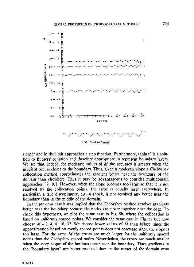
GLOBAL PROPERTIES OF PSEUDOSPECTRAL METHODS 253
XZERO
FIG. 5-Continued.
steeper and in the limit approaches a step function. Furthermore, tanh(x) is a solu- tion to Burgers’ equation and therefore appropriate to represent boundary layers. We see that, indeed, for moderate values of A4 the accuracy is greater when the gradient occurs closer to the boundary. Thus, given a moderate slope a Chebyshev collocation method approximates the gradient better near the boundary of the domain than elsewhere. Thus it may be advantageous to consider multidomain approaches [9, lo]. However, when the slope becomes too large so that it is not resolved by the collocation points, the error is equally large everywhere. In particular, a true discontinuity, e.g., a shock, is not resolved any better near the boundary than in the middle of the domain.
In the previous case it was implied that the Chebyshev method resolves gradients better near the boundary because the nodes are closer together near the edge. To check this hypothesis, we plot the same case in Fig. 5b, where the collocation is based on uniformly spaced points. We consider the same case in Fig. 5a but now choose M= 2, 4, 8, 16, 32. We choose lower values of M than before, since the approximation based on evenly spaced points does not converge when the slope is too large. For the same A4 the errors are much larger for the uniformly spaced nodes than the Chebyshev spaced nodes. Nevertheless, the errors are much smaller when the steep slopes of the funtions occur near the boundary. Thus, gradients in the “boundary layer” are better resolved than in the center of the domain even
581/81/Z-2

254 SOLOMONOFF AND TURKEL
though we are using interpolation based on uniformly spaced points. In fact, the ratio of the L* error when the steep slope is at the center to the L* error when the slope is near the edge is even larger for uniformly spaced nodes than for a Chebyshev distribution of nodes (of course, one would not use uniformly spaced nodes in practice). In both cases, we used the Chebyshev norm (3.2). However, the results do not depend on the details of the norm.
In order to explain this phenomenon we examine the singularity of the function in the complex plane. To simplify the discussion we consider the expansion of a function in Chebyshev polynomials. In this case it is known [14] that the approximation converges in the largest ellipse with foci at + 1 and - 1 that does not contain any singularities. The equation of an ellipse with foci at f 1 is
x2 Y2 * 7+jq= ’
where I> 2 measures the size of the ellipse. Let, r = 1+ m. Then r is the sum of the semi-major and semi-minor axes. It is known [12, 163 that the convergence rate of the scheme is bounded by r- “‘. Hence, as I increases the approximation converges faster. I is determined by the closest singularity. Suppose that this singularity occurs at X, J. Then
For f(x) = tanh(M(x - x,)), we have X = x0 and jj = ni/2M. Thus, as x0 varies, jj is fixed while X changes. It is easily shown that (8/8%‘)([‘) > 0. Thus, for fixed 7, I2 is a minimum at X = 0 and 1 increases as JXJ = lx,,1 increases. Hence, as x0 approaches the boundaries, + 1, the rate of convergence increases. Also, as M increases, i.e., the function has a larger gradient, jj decreases, and 1 decreases and so the rate of convergence decreases. For interpolation approximations, both at Chebyshev and uniformly spaced points, a similar phenomenon occurs but the quantitative analysis is more complex [12].
For uniformly spaced collocation points in [0, 11, the ellipses are replaced by the curves u(x, y) = constant, where
u(x, y) = 1 - x In JY - (1 - x) In Jm + y arc tan Y x-g- y2’
(4.1)
By examining graphs of this curve (Fig. 6; see also [ 11, p. 2491) one sees that if the first singularity is at x,, + ijj the size of the region increases as x0 moves toward the boundaries. As before, this increases the rate of convergence. We also see that outside (0, 1) the contours resemble ellipses. However, for U(X, y) > 1 the level curves are no longer convex.

GLOBAL PROPERTIES OF PSEUDOSPECTRAL METHODS
FIG. 6. Level curves for (4.1) for evenly spaced nodes.
255
In Fig. 5c, we consider the same case as Fig. 5a for the function f(x) = tanh[Q(x - x0)]. Here, Q is a function of M and x,; specifically
a=?/=, M=2, 4, 8, 15, 32.
At the center, x,, = 0, Q = Mn/2, while near the boundary x,, N 1 and Q N- M*x/2. With this scaling the L* error is essentially independent of x,,. This indicates that an adaptive collocation method could be useful [2, 83.
In order to further investigate the resolving power of the schemes, we repeat the experiment of Fig. 5 but for a function that is not analytic. In this case, our previous analysis is no longer valid. We choose
where q = M(x - x,,). Hence, f(x) = - 1 when x < x0 - l/M, f(x) = + 1 when x > x0 + l/M, and f(M) is a quintic polynomial in between. Furthermore, f(x) has two continuous derivatives, but the third derivative is discontinuous at x = x,, f l/M. Thus, as before, x0 denotes the center of the “jump” and the gradient
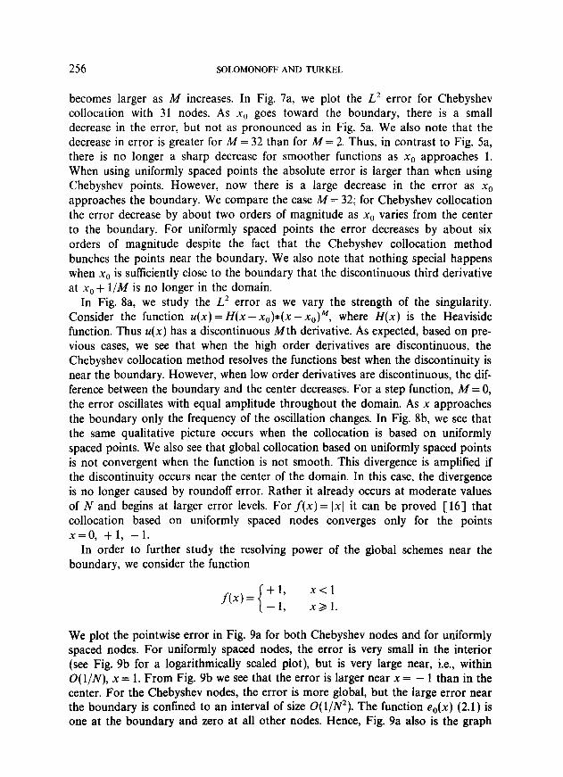
256 SOLOMONOFF AND TURKEL
becomes larger as M increases. In Fig. 7a, we plot the L2 error for Chebyshev collocation with 31 nodes. As x0 goes toward the boundary, there is a small decrease in the error, but not as pronounced as in Fig. 5a. We also note that the decrease in error is greater for M = 32 than for M = 2. Thus, in contrast to Fig. 5a, there is no longer a sharp decrease for smoother functions as x0 approaches 1. When using uniformly spaced points the absolute error is larger than when using Chebyshev points. However, now there is a large decrease in the error as x0 approaches the boundary. We compare the case M= 32; for Chebyshev collocation the error decrease by about two orders of magnitude as x0 varies from the center to the boundary. For uniformly spaced points the error decreases by about six orders of magnitude despite the fact that the Chebyshev collocation method bunches the points near the boundary. We also note that nothing special happens when x0 is sufficiently close to the boundary that the discontinuous third derivative at x0 + l/M is no longer in the domain.
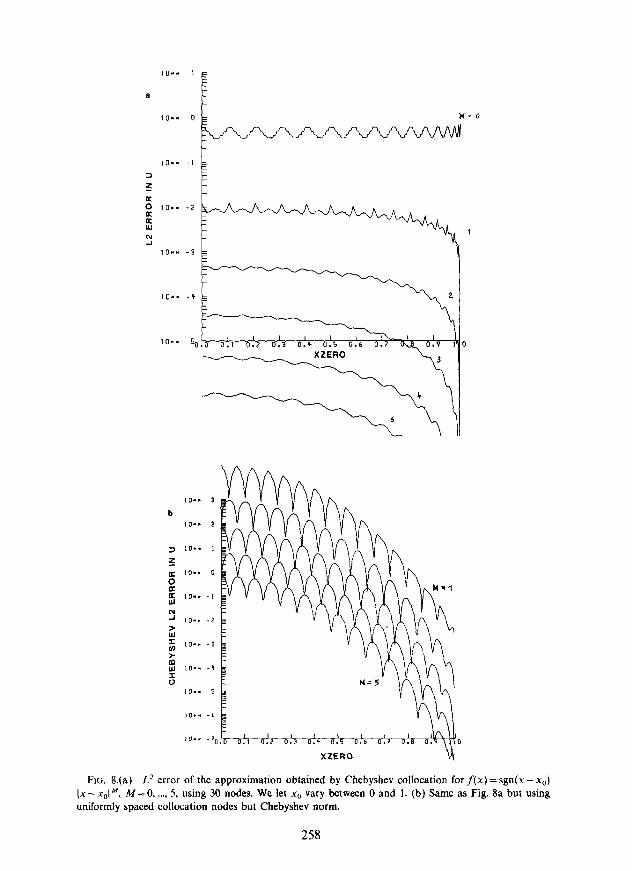
In Fig. 8a, we study the L2 error as we vary the strength of the singularity. Consider the function U(X) = H(x-x,)*(x -x~)~, where H(x) is the Heaviside function. Thus U(X) has a discontinuous Mth derivative. As expected, based on pre- vious cases, we see that when the high order derivatives are discontinuous, the Chebyshev collocation method resolves the functions best when the discontinuity is near the boundary. However, when low order derivatives are discontinuous, the dif- ference between the boundary and the center decreases. For a step function, M = 0, the error oscillates with equal amplitude throughout the domain. As x approaches the boundary only the frequency of the oscillation changes. In Fig. 8b, we see that the same qualitative picture occurs when the collocation is based on uniformly spaced points. We also see that global collocation based on uniformly spaced points is not convergent when the function is not smooth. This divergence is amplified if the discontinuity occurs near the center of the domain. In this case, the divergence is no longer caused by roundoff error. Rather it already occurs at moderate values of N and begins at larger error levels. For f(x) = 1x1 it can be proved [ 161 that collocation based on uniformly spaced nodes converges only for the points x=0, + 1, - 1.
In order to further study the resolving power of the global schemes near the boundary, we consider the function
We plot the pointwise error in Fig. 9a for both Chebyshev nodes and for uniformly spaced nodes, For uniformly spaced nodes, the error is very small in the interior (see Fig. 9b for a logarithmically scaled plot), but is very large near, i.e., within O( l/N), x = 1. From Fig. 9b we see that the error is larger near x = - 1 than in the center. For the Chebyshev nodes, the error is more global, but the large error near the boundary is confined to an interval of size O(1/N2). The function e,,(x) (2.1) is one at the boundary and zero at all other nodes. Hence, Fig. 9a also is the graph

a
IO*- t I I I -70.0 0.’ 0.2 0.3
I I I I 0.Y 0 5 XZiRO 0.6 - 0.7 . . 1.0
lO*m 2
IO** t -50.0
I I I I I I I 0.’ 0.2 0.3 0.4 I 0.5 I 0.6 0.7 0.8 0.9 I!0
XZERO
FIG. 7.(a) L2 error of the approximation obtained by Chebyshev collocation using 31 nodes for the function given in (4.1). (b) Same as Fig. 7a but using uniformly spaced nodes and M= 2, 4, 8, 16, 32.
257
IO..
b IO..
10..
XZERO VI
FIG. 8.(a) L’ error of the approximation obtained by Chebyshev collocation for f(x) = sgn(x - x,,) (.x-qJ”, M=O, . . . . 5, using 30 nodes. We let x0 vary between 0 and 1. (b) Same as Fig. 8a but using uniformly spaced collocation nodes but Chebyshev norm.
258

10”” I
b IO.. 0
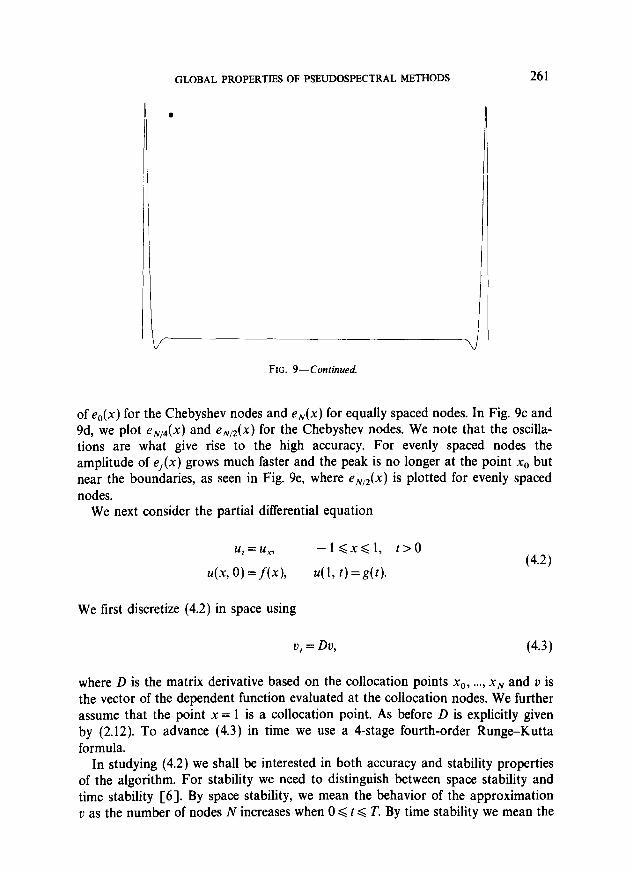
I; FIG. 9.(a) We consider the function f(x) = 1 except at x = 1 when j(x) = 0. We graph the error for
(solid line) Chebyshev nodes and (dotted line) uniformly spaced nodes, both using 31 collocation points. This is also the graph of the first basis function e,(x). (b) The case of uniformly spaced nodes of Fig. 9a plotted on a logarithmic scale. (c) Basis function e N,2(~) for the Chebyshev nodes with N = 33. (d) Basis function e&x) for the Chebyshev nodes with N = 33. (e) Basis function e N,Z(~) for evenly spaced nodes with N = 33.

3 P
D
GLOBAL PROPERTIES OF PSEUDOSPECTRAL METHODS 261
I/ ” FIG. 9-Continued.
v
u, = u,, -l<x<l, t>o
4x3 0) =.0x), 41, t) =g(t). (4.2)
of eO(x) for the Chebyshev nodes and eN(x) for equally spaced nodes. In Fig. 9c and 9d, we plot e,,,,*(x) and e,,,,Jx) for the Chebyshev nodes. We note that the oscilla- tions are what give rise to the high accuracy. For evenly spaced nodes the amplitude of ej(x) grows much faster and the peak is no longer at the point x0 but near the boundaries, as seen in Fig. 9e, where e&x) is plotted for evenly spaced nodes.
We next consider the partial differential equation
We first discretize (4.2) in space using
vt=Dv, (4.3)
where D is the matrix derivative based on the collocation points x,,, . . . . xN and v is the vector of the dependent function evaluated at the collocation nodes. We further assume that the point x = 1 is a collocation point. As before D is explicitly given by (2.12). To advance (4.3) in time we use a 4-stage fourth-order Runge-Kutta formula.
In studying (4.2) we shall be interested in both accuracy and stability properties of the algorithm. For stability we need to distinguish between space stability and time stability [6]. By space stability, we mean the behavior of the approximation v as the number of nodes N increases when 0 < t d T. By time stability we mean the
262 SOLOMONOFF AND TURKEL
behavior of u as time increases, for fixed N. Since D can be diagonalized, the scheme is time stable whenever all the eigenvalues of At. D lie in the stability region of the Runge-Kutta scheme. This does not necessarily prove space stability since the norm of the matrix that diagonalizes D depends itself on N. Obviously, both the spectral radius of D and the maximum allowable time step depend on the implementation of the boundary conditions.
Since the temporal accuracy is lower than the spatial accuracy, the maximum At allowed by stability considerations will not yield very accurate approximations. However, by decreasing the time step we can increase the accuracy of the solution. This general technique works equally well for nonlinear problems. When the model equation (4.1) is replaced by a more realistic system with several wave speeds, the stability limit will also give approximations that are accurate [I]. Also, when one is only interested in the steady state, frequently the time step can be chosen by stability considerations alone. An alternative which will not be persued in this study is to use spectral methods also in the time domain, e.g., [4, 213.
In order to measure the accuracy of the approximation, we shall choose u(x, t) =f(x- t) for some f(x). Hence, the approximation can be compared pointwise with the analytic solution. The boundary data is then given by g(t) =f( 1 - t). We shall measure the error either pointwise or else in a weighted L2 norm given by (3.2).
We first study the effect of the boundary treatment on the stability and accuracy of (4.3). One property of global methods is that the approximation is automatically updated at all collocation points including the boundaries. Thus, if one wished, the scheme could be advanced without ever imposing the given boundary data; but this would be an unstable scheme. For a multistage time scheme, one can impose the boundary conditions at any stage one wishes. We now consider (4.1) with f(x)= sin(rrx). In Fig. lOa, we impose the given boundary condition after each stage, while in Fig. lob we impose the boundary condition only after the fourth stage. We define the Courant number, CFL, by
CFL = N2 At.
In both plots, 10a and b, we display the error for several values of the Courant number. We see that imposing boundary conditions after each stage allows a larger maximum stable CFL number. For the four stage scheme, the maximum CFL is about 35. However, for smaller time steps the error is slightly larger than when one imposes the boundary condition only at the end of all the stages. One also sees that for a given error level that the approximate solution is essentially independent of the time step below some critical time step. As one demands more accuracy, the CFL number decreases. The largest stable At does not give accurate solutions at any error level. We also found that the error grows in time if the solution is not sufftciently resolved in either space or time. There was no growth when N was large enough and At was sufficiently small.

10-m 1
a
IO-= 0
lO** -I E
- IO.” -2 E
;
FIG. 10.(a) Pseudospectral approximation to (4.1) with f(x) = sin xx. A 4-stage fourth-order Runge-Kutta formula is used and boundary conditions are imposed after every stage. The L* error at T= 1 is given as a function of N. Each graph represents a different time step, i.e., CFL number with an increase of 3 between graphs. (b) L2 error of the pseudospectral approximation to (4.1) with f(x) = sin xx at time T= 1. A 4-stage fourth-order Rung+Kutta formula is used but with the boundary condition imposed only once after the completion of the four Runge-Kutta stages.

264 SOLOMONOFF AND TURKEL
In Fig. lla and b, we again plot the L2 error for approximating (4.2) as N increases with f(x) = sin(x) and for several time steps. In these plots, we choose a different sequence of collocation points given by
xi= -(l --l)cos;+or 3 >
-1+2j N'
j = 0, . . . . N,
so x0 = - 1 and xN = 1. These points are a convex combination of Chebyshev nodes and uniformly spaced nodes. Let
&P-1)(1--W) 2/N-(l-cosn/N)
We find
a_n2wl) 1 4N 'I-n2f4N
when B=O(l),
and
B= new spacing at edge
Chebyshev spacing at edge’ (4.6 )
We solve (4.2) by using the derivative matrix (2.12). We do not use a mapping to Chebyshev collocation nodes. In Fig. lla, we choose B= 2, i.e., a spacing at the boundary twice the usual Chebyshev spacing. We see that in this case we cannot increase the allowable time step beyond the stability condition for the Chebyshev nodes. Hence, the stability condition is not directly related to the minimum spacing. In Fig. 1 lb, we display the error for /? = $, i.e., a spacing half the Chebyshev spacing near the boundary. In this case the largest stable time step is reduced compared with the Chebyshev nodes. In this example, we have considered constant coef- ficients. For a problem with variable coefficients it is possible that coarsening the mesh near the boundary will allow a larger time step. This is because the coarser mesh near the boundary may counteract the behavior of the variable coeffkients near the boundary.
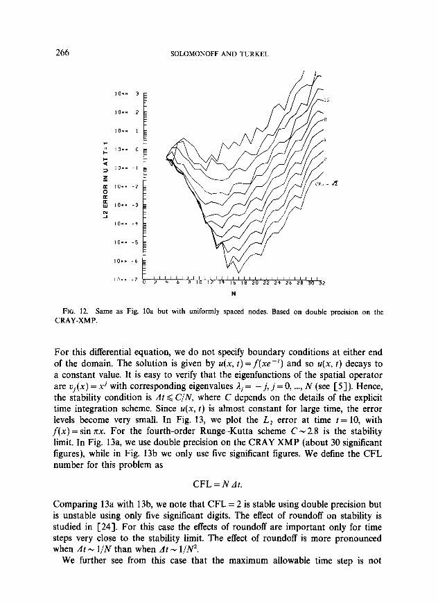
In Fig. 12, we consider uniformly spaced nodes, i.e., CI = 0. From Fig. 12, we see that even for small CFL numbers the error first decreases but then increases as N gets larger. These calculations were carried out in double precision on the CRAY. Nevertheless, it is difficult to distinguish between nonconvergence and an instability caused by rounding errors on the computer.
In Fig. 13, we consider the differential equation
u,= -xxu I 9 -l<x<l,
4x7 0) = f(x). (4.7)

; IO.” -2
t = IO.. -3
I LT IO.. -9 0
E w IO-. -5 E
Y IO.. -6 E
IO.” -7 E
IO.” -8
IO.. I
b
IO*= 0 r
IO-. -I E
r IO”. -2 E
; 2 10.. -3 c
3 z 10.. -Y a
5 E IO.. -5 Ill cu J IO.. -6
IO.. -7
IO.. -8
FIG. 1 l.(a) L2 error of the pseudospectral Chebyshev approximation to (4.1) with f(x) = sin BX, at time T= 1. Four applications of the boundary conditions and /3 = 2, i.e., the mesh is twice as coarse as a Chebyshev grid near the boundary. Each graph represents a different CFL number, increasing by a factor of fi. (b) L* error of the pseudospectral Chebyshev approximation to (4.1) with f(x) = sin n[x, at time T= 1. Four applications of the boundary conditions and /?= f, i.e., twice the density of Chebyshev spacing near the boundary. Each graph represents a different CFL number, increasing by a factor of Ji.
265
266 SOLOMONOFF AND TURKEL
N
FIG. 12. Same as Fig. 10a but with uniformly spaced nodes. Based on double precision on the CRAY-XMP.
For this differential equation, we do not specify boundary conditions at either end of the domain. The solution is given by U(X, t) =f(xe-‘) and so U(X, t) decays to a constant value. It is easy to verify that the eigenfunctions of the spatial operator are vj(x) = xj with corresponding eigenvalues lj = -j, j = 0, . . . . N (see [S]). Hence, the stability condition is At < C/N, where C depends on the details of the explicit time integration scheme. Since U(X, t) is almost constant for large time, the error levels become very small. In Fig. 13, we plot the L, error at time t = 10, with f(x) = sin KX. For the fourth-order Runge-Kutta scheme C- 2.8 is the stability limit. In Fig. 13a, we use double precision on the CRAY XMP (about 30 significant figures), while in Fig. 13b we only use live significant figures. We define the CFL number for this problem as
CFL = N At.
Comparing 13a with 13b, we note that CFL = 2 is stable using double precision but is unstable using only five significant digits. The effect of roundoff on stability is studied in [24]. For this case the effects of roundoff are important only for time steps very close to the stability limit. The effect of roundoff is more pronounced when At w l/N than when At - l/N’.
We further see from this case that the maximum allowable time step is not

L
CFL < t2
FIG. 13.(a) L* error of the pseudospectral Chebyshev approximation to the equation u, = - xu at time T= 10. Uses double precision on the CRAY-XMP, CFL = N At. (b) Same as Fig. 13a but u&g only 5 significant digits.
267
268 SOLOMONOFF AND TURKEL
necessarily related to the minimum spacing in the grid. In this case, the fact that no boundary conditions were specified allowed At to vary with l/N rather than the usual l/N’. We also observe a similar phenomenon where coarsening the mesh near the boundary does not allow a larger maximum time step. A similar conclusion was found by Tal-Ezer [22] for the Legendre-Tau method, which has a time step limitation that depends on l/N even though the minimum grid spacing is l/N*. Thus, to find the stability limit, one must analyse the derivative matrix appropriate for each case rather than using a heuristic approach based on the spacing between collocation nodes.
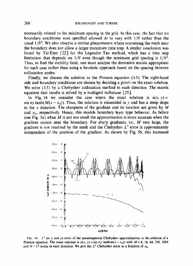
Finally, we discuss the solution to the Poisson equation (3.5). The right-hand side and boundary conditions are chosen by deciding a priori on the exact solution. We solve (3.5) by a Chebyshev collocation method in each direction. The matrix equation that results is solved by a multigrid technique [25].
In Fig. 14 we consider the case where the exact solution is u(x, y) = sin rcy tanh(M(x -x0)). Thus, the solution is sinusoidal in y and has a steep slope in the x direction. The sharpness of the gradient and its location are given by it4 and x,,, respectively. Hence, this models boundary layer type behavior. As before (see Fig. 5a) when M is not too small the approximation is more accurate when the gradient occurs near the boundary. For sharp gradients, i.e., M very large, the gradient is not resolved by the mesh and the Chebyshev L* error is approximately independent of the position of the gradient. As shown by Fig. 5b, this increased
10". t I I -70.0 0.1 0.2 0
I I 1 I .3 0.Y 0.5 0.6 Y?rd--J . . 0.9’ 1.u
XZERO
FIG. 14. L2 (in x and y) error of the pseudospectral Chebyshev approximation to the solution of a Poisson equation. The exact solution is u(x, y) = sin xy tanh(m(x - x0)) with M = 4, 16, 64, 256, 1024 and N= 17 nodes in each direction. We plot the I,* Chebyshev error as a function of x0.

GLOBAL PROPERTIES OF PSEUDOSPECTRAL METHODS 269
accuracy in the boundary layer is not only due to the increased number of collocation points in the “boundary layer.” Rather it is due to properties of global approximation techniques. It is of interest to note that for M= 1024, i.e., a discontinuity, the error is almost constant. However, for M = 64 and 256, i.e., a sharp gradient, there are peaks in the error as x0 approaches a collocation node.
5. CONCLUSIONS
We have considered the properties of global collocation methods for problems in approximation theory and partial differential equations. In particular, we study concepts that have been used by many authors without verification.
In order to be able to study differential equations for a general sequence of collocation nodes we calculate the approximate derivative by multiplying a matrix and a vector. For Fourier or Chebyshev methods one could also use a FFT [S]. Several authors, e.g., [23], have compared the efficiency of using a matrix multi- plication or a fast Fourier transform. In this study, we have only used the matrix approach because of its greater generality. In particular we wish to investigate the effect of the distribution of the collocation points on properties of the scheme. Hence, we construct the derivative matrix for general collocation points.
It follows from the results presented in Section 4 that a global collocation method must be distinguished from a local finite difference or finite element approximation. In particular, for a smooth function the greater density of points, for a Chebyshev collocation method, near the boundary does not give increased accuracy near the boundary. The extra density near the boundary is needed to counteract the tendency of polynomial approximation to give large errors near the edges of the domain.
Chebyshev collocation methods have lower errors when sharp gradients or dis- continuous derivatives occur near the boundary than when they are in the center of the domain. However, qualitatively similar results are obtained using uniformly spaced nodes. Thus, the increased resolution near the boundary is due to the global nature of the approximation and not the bunching of collocation nodes. Explana- tions should be based on complex variable theory rather than on intuition from finite differencing. Of course, in terms of absolute error, it is preferable to use Chebyshev collocation rather than uniform collocation. This indicates that domain decomposition methods should be advantageous [9, lo] but not for shocks. In fact, even in cases where collocation based on a uniform mesh should converge the actual interpolation process on a computer eventually diverges due to roundoff errors. These roundoff errors contaminate the results for relatively small iV.
As a further distinction between global and local techniques we consider the aliasing limit. For a Fourier (periodic) method we need 2 points per wavelength to resolve a sine wave. For a Chebyshev method we need A points per wavelength. The difference between 2 and 71 is not due to the different distribution of points in these techniques. Polynomial collocation based on uniformly spaced points again needs
581/81/2-3
270 SOLOMONOFF AND TURKEL
at least rc points per wavelength. Furthermore, for other functions, e.g., tanh x, one does not observe any sharp aliasing limit, Thus, one cannot speak of the number of points per wavelength for general functions on nonperiodic domains.
An alternative for improving the accuracy of an approximation is to map the x domain [ - 1, l] onto another computational domain s, for simplicity again [ - 1, 11. The above conclusions do not extend to such mappings. First, a polyno- mial in s is no longer a polynomial in x. Hence, in the physical space x we are not considering polynomial collocation methods. In addition, the L2 norm in s-space corresponds to a weighted L' norm in x-space. Hence, it is difficult to measure the effectiveness of such mappings. In practice [2] has shown that in some cases adaptive mesh mappings can be effective for spectral methods.
The results obtained for approximating solutions to elliptic partial differential equations seem to correspond to the results for the approximation problem. Again one cannot interpret the properties of a Chebyshev collocation method in terms of finite difference properties. Such concepts as the number of points in a local region are not meaningful. If one chooses another set of collocation points, there are two ways of implementing the method. One can map one set of points to the other and then use a Chebyshev method in the computational space. This introduces metrics into the equation. Alternatively, one can solve the equation in physical space using the general derivative matrix (2.12). We have not investigated the differences between these two approaches.
For a time-dependent partial differential equation, the study is more complicated. First, there is an accumulation of errors as time progresses. Thus, for example, for a stationary problem one can distinguish between the discontinuity being at a node or in between nodes. For a time dependent problem the discontinuity is moving and so all effects are combined. This is especially true for systems with variable coefftcients where there is coupling between all the components. In addition to accuracy, there is the question of stability. We have found that the implementation of boundary conditions influences both the maximum time step allowed and the accuracy. At times an implementation which increases the stability will decrease the accuracy.
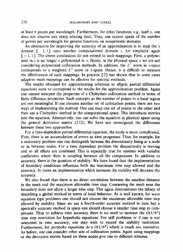
We also found that there is no direct correlation between the smallest distance in the mesh and the maximum allowable time step. Coarsening the mesh near the boundary does not allow a larger time step. This again demonstrates the fallacy of describing a global method in terms of local behavior. As is well known, for wave equation type problems one should not choose the maximum allowable time step allowed by stability. Since we use a fourth-order accurate method in time but a spectrally accurate method in space one should choose a smaller time step to com- pensate. Thus to achieve time accuracy there is no need to increase the 0(1/N2) time step restriction for hyperbolic equations. For stiff problems or if one is not interested in time accuracy, one may wish to exceed the stability restriction. Furthermore, for parabolic equations dt N 0( 1/N4) which is much too restrictive. As before, one can consider other sets of collocation points. Again using mappings or the derivative matrix based on these nodes give rise to different schemes.

GLOBAL PROPERTIES OF PSEUDOSPECTRAL METHODS 271
APPENDIX A
In Section 2, we saw that given the collocation points x0, . . . . xN and N+ 1 func- tions uJx), the derivative matrix, D, is determined by demanding that D times (+,i(xo), . . . . dj(x,))’ give the exact derivative at the collocation points. Let D = (d,) and define the matrix U by Ujk = Uj(X,), j, k = 0, . . . . N. Given the matrices D and U we denote the jth column of these matrices as d, and ui. Then each column of D is determined by the equation
Udj = u; at all collocation points xk, k = 0, . . . . N. (AlI
If we wish D to be exact for M> N+ 1 functions, then in general there is no solution. Instead we can demand that D give the smallest L2 error over these M functions. Intuitively if D is almost exact for many functions, it should be a good approximation to the derivative. In particular, one may choose functions that are more appropriate to a given problem than polynomials. Choosing D to give the least sqares minimization is equivalent to demanding that
U’Ud, = UTu; (42)
instead of (Al ). It is easy to verify that
(uTu)j/r= f ui(xj) ui(xk)
i=O
and
(u’u;), = f Idi Ui(Xi), j, k = 0, . . . . N. i=O
We now define
U,(X)= f Ui(Xk) Ui(X)y k=O, . . . . N, i=O
(A3)
(A4)
then
l$(Xj) = ( u’u;), .
Assuming det U # 0 then the uk(t) are linearly independent. It also follows that D is exact for the N+ 1 functions uk(x) at the collocation points. Hence, demanding least square minimization for ui(x), i =0, .,., M, is equivalent to demanding exactness for ui(x), i = 0, . . . . N, given in (A4).
We next extend this by letting M become infinite and replacing the sums by integrals. Thus, given the continuum of function ui(x) and demanding that D be

272 SOLOMONOFF AND TURKEL
the best least squares approximation to the derivative at the collocation points is equivalent to demanding that D be exact for the N+ 1 functions
vr(x) = lorn ui(xk) z+(x) di. 645)
To demonstrate this, we consider a specific example. Let uk(x) be the functions sin(kx) and cos(kx) for 0 < k < N7r/2 and choose N + 1 uniformly spaced colloca- tion points, xj. Since k < N7c/2 we are always below the aliasing limit. It follows from (A5) that
U/((Xj) = Jby* [sin(ixj) sin(ix,) + cos(ixj) cos(ix,)] di
sin N7r/2 (xi - xk) xj-xk ’ j#k
= (‘46)
\ NIT/~, j=k.
These functions, vi(x) are known as SINC functions and have been used for inter- polation formulae [19]. Demanding that D be exact for vi(x), j= 0, . . . . N, yields the derivative matrix
(-I)‘+& j#k
djk = xj-xk ’
0, j=k,
which is an antisymmetric matrix. We also note that this matrix resembles the derivative matrix for the Chebyshev nodes [7].
APPENDIX B
In this section, we present the proof that Chebyshev collocation at the standard Gauss-Lobatto points is stable for solving scalar hyperbolic equations. This result was given in [7] without proof.
Consider the collocation points
xi = cos nj/N, j = 0, . . . . N. 031)
Let ZJ be the solution to
u, = u,, U(1, t)=O, 4x9 0) = f(x). 032)
GLOBAL PROPERTIES OF PSEUDOSPECTRAL METHODS 273
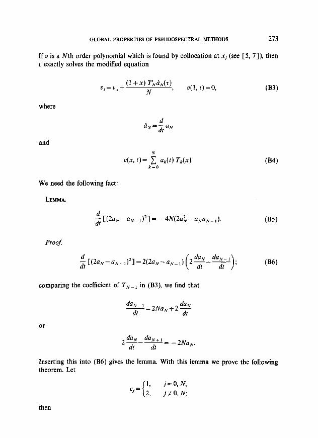
If u is a Nth order polynomial which is found by collocation at Xj (see [S, 7]), then v exactly solves the modified equation
u = u + (1 +x) TN&N(T) I x N ’ u(1, t)=O, (B3)
where
d aN=-&aN
and
k=O
We need the following fact:
LEMMA.
i [@aNmaN-,)*] = -4N(2ai-aNaN-,).
(B4)
Proof:
W)
comparing the coefficient of TN-, in (B3), we find that
da,v- 1 daN -=2NaN+2x dt
or
2d‘% da,+, ---= -2NaN. dt dt
Inserting this into (B6) gives the lemma. With this lemma we prove the following theorem. Let
then
1, j=O, N, cj =
2, j#O, N,

214 SOLOMONOFF AND TURKEL
THEOREM. Let v solve (A2.3) then if N/(3N- 1) <p< + then
~~~(1+Xj)(l-Bi,)~‘(~j,r)+~B(N-~)(2o,-~,~,)’)60 (B7)
and so the solution v is stable.
Proof: We multiply (B3) by (rc/NCj)( 1 + xj)( collocation nodes. We then have
1 -fixi) v(xj, t) and sum over the
$$~~(l+Xj)(l-Bx,)V,f
CI J
+$~~~(l+Xj)2(l-PXj)T:V(xj)v(xj). I J
038)
However, the last term is zero since Y,(xj) = 0 at interior points, 1 + xi= 0 at xi = - 1, and u(s) = 0 at xi = + 1. Furthermore, if
f(X) = C bj T’ (x)3 fEP4N--13
then
~~~f(xj)=J$$$dx+nb2,. J
By algebra, it can be verified that the 2Nth Chebyshev coefficient of (1 +x)(1 -/?x)vu, is b,,= (1 -fi)N&2-/3((2N- 1)/4)aNuN-,, where, as before, aj are the Chebyshev coefficients of v. Therefore, (B8) can be rewritten as
&fzi(l +Xj)(l-PXj)Vj2 J
(B9)
Integrating by parts and using the fact that v( 1, t) = 0, we find that

GLOBAL PROPERTIESOFPSEUDOSPECTRALMETHODS 275
1 1 (1-B-lIx+Px2)u2(x t)du =z -1 (lmx)Jn ’ s
@lo)
Using the lemma, this is equivalent to
~{~~~(l+~,)(l-Bx,)v’(x,, I)+&B(N--f) @a,--o,,)‘} J J
1 ’ 1-/3-fix+px2 = -- 2 f -1 (l-x)$7
u’(x, t)dx-F [(3fl- l)N-p]aL. (Bll)
If /I 6 $ then the integral term is negative while if /I 2 N/(3N - 1) N $ then the second term on the right-hand side is also negative. Hence, when N/(3N- 1) < /I < 2, then the right-hand side of (Bll) is negative and the theorem is proven.
If we choose the special case p = 3 then (Bll) becomes
~{~~~(l+Xj)(1-~xj)~2(Xj,I)+~(2a,-a,-,)2 J J
1 1 (l-2x)2 =-- 10 f -1 (l-x)&T
u2(x, t)dx-fi(7N-4)aZ,. O-312)
As a corollary, this theorem implies that all the eigenvalues of D lie in the left half of the complex plane.
ACKNOWLEDGMENTS
The authors thank A. Bayliss of Northwestern University for the use of his code to find adaptive points and critically reading the paper. We also thank C. Street of NASA Langley for the use of his spectral multigrid package to solve the Poisson equation. The second author also thanks D. Gottlieb of Tel-Aviv University for many discussions on the paper.
REFERENCBS
1. A. BAYLISS, K. E. JORDAN, B. J. LEMFSJRIER, AND E. TURKEL, Bull. Seismol. Sot. Amer. 76, 1115 (1986).
2. A. BAYLISS AND B. J. MATKOWSKY, J. Comput. Phys. 71, 147 (1987). 3. C. CANUTO AND A. QUARTERONI, Math. Comput. 38, 67 (1982).

276 SOLOMONOFF AND TURKEL
4. M. DEVILLE, P. HALDENWANG, AND G. LABROSSE, in Proceedings 4th GAMM-Conference Numerical Methods in Fluid Dynamics, (Friedrich Vieweg, BraunschweigWiesbaden, 1982).
5. D. GO~LIEB AND S. Z. ORSZAG, Numerical Analysis of Spectral Methods: Theory and Applications (SIAM, Philadelphia, 1977).
6. D. GOTTLIEB, S. Z. ORSZAG, AND E. TURKEL, Math. Compur. 37, 293 (1981). 7. D. GOTTLIEB AND E. TURKEL, Lecture Nofes in Mafhemafics Vol. 1127 (Springer-Verlag,
New York/Berlin, 1985), p. 115. 8. H. GUILLARD AND R. PEYRET, University of Nice, Dept. of Math. Report 108, 1986 (unpublished). 9. D. KOPRIVA, Appl. Numer. Math. 2, 221 (1986).
10. K. Z. KORCZAK AND A. T. PATERA, J. Compuf. Phys. 62, 361 (1986). 11. P. P. KOROVKIN, Linear Operafors and Approximation Theory, transl. from Russian (Hindustan
Publ., Delhi, 1960). 12. V. I. KRYLOV, Approximate Calculation of Integrals, transl. by A. H. Stroud (Macillan Co.,
New York, 1962). 13. J. H. MCCABE AND G. M. PHILIPS, BIT 13, 434 (1973). 14. A. I. MARKUSHEVICH, Theory of Functions of a Complex Variable, Vol. III, transl. by R. A. Silverman
(Prentice-Hall, Englewood Cliffs, NJ, 1967). 15. G. MEINARDUS, Approximation of Functions: Theory and Numerical Methods, (Springer-Verlag,
Berlin, 1967). 16. I. P. NATANSON, Constructive Function Theory, Vol. III (Ungar, New York, 1965). 17. M. J. D. POWELL, Approximation Theory and Metho& (Cambridge Univ. Press, Cambridge, 1975). 18. T. J. RIVLIN, An introduction to the Approximation of Functions (Blaisdell, Waltham, MA, 1979). 19. F. STENGER, SIAM Rev. 23, 165 (1981). 20. E. TADMOR, SIAM J. Numer. Anal. 23, 1 (1986). 21. H. TAL-EZER, SIAM J. Numer. Anal. 23, 11 (1986). 22. H. TAL-EZER, J. Compuf. Phys. 67, 145 (1986). 23. T. D. TAYLOR, R. S. HIRSH, AND M. M. NADWORNY, Comput. & FIuidr 12, 1 (1984). 24. L. N. TREFETHEN AND M. R. TRUMMER, J. SIAM Numer. Anal. 24, 1008 (1987). 25. T. A. ZANG, Y. S. WONG, AND M. Y. HUSSAINI, J. Comput. Phys. 54, 489 (1984). 26. A. ZYGMUND, Trigonmetric Series, Vol. I (Cambridge Univ. Press, Cambridge, 1968).