Global Dynamics of a General Class of Multistage Models for Infectious Diseases

Copyright © by SIAM. Unauthorized reproduction of this article is prohibited.

SIAM J. APPL. MATH. c© 2012 Society for Industrial and Applied MathematicsVol. 72, No. 1, pp. 261–279

GLOBAL DYNAMICS OF A GENERAL CLASS OF MULTISTAGEMODELS FOR INFECTIOUS DISEASES∗

HONGBIN GUO† , MICHAEL Y. LI‡ , AND ZHISHENG SHUAI§

Abstract. We propose a general class of multistage epidemiological models that allow possibledeterioration and amelioration between any two infected stages. The models can describe diseaseprogression through multiple latent or infectious stages as in the case of HIV and tuberculosis.Amelioration is incorporated into the models to account for the effects of antiretroviral or antibiotictreatment. The models also incorporate general nonlinear incidences and general nonlinear forms ofpopulation transfer among stages. Under biologically motivated assumptions, we derive the basicreproduction number R0 and show that the global dynamics are completely determined by R0: ifR0 ≤ 1, the disease-free equilibrium is globally asymptotically stable, and the disease dies out;if R0 > 1, then the disease persists in all stages and a unique endemic equilibrium is globallyasymptotically stable.

Key words. infectious disease progression, amelioration, multiple stages, antiretroviral treat-ment, HIV, TB, global stability, Lyapunov function

AMS subject classifications. 34D23, 92D30

DOI. 10.1137/110827028

1. Introduction. For infectious diseases that progress through a long infectiousperiod, infectivity or infectiousness can vary significantly in time. Progression of HIVinfection can take eight to ten years before the clinical syndrome (AIDS) occurs,and go through several distinct stages, marked by drastically different CD4+ T-cellcounts and viral RNA levels. Infectivity of an infected host is determined by twomain factors: the transmission fitness (or transmissibility) of the pathogen inside thehost and the frequency at which the host is in contact with others. Transmissibilityof the pathogen can vary at different stages of the disease progression according toboth the quantity and location of the pathogens inside the host’s body. For HIVinfection, the first few weeks after seroconversion see an extremely high level of viralload and high transmissibility. This initial stage is followed by a long chronic stageduring which viral load is controlled by the immune system and the transmissibilityis relatively low. The final stage will see exhaustion of host immune resources and theHIV virus escape from immune control, viral load will explode, and transmissibilitywill increase. For tuberculosis (TB) infection, the TB bacteria need to develop in thelung to be transmissible through coughing, and their transmissibility depends on theirprogression in the lung as well as the strength of a host’s immune system. Active TBhas the highest possibility of developing within the first 2–5 years of infection, while

∗Received by the editors March 10, 2011; accepted for publication (in revised form) December 7,2011; published electronically February 2, 2012. This research was supported in part by grants fromthe Natural Science and Engineering Research Council of Canada (NSERC) and Canada Foundationfor Innovation (CFI) and by the NCE-MITACS project “Transmission Dynamics and Spatial Spreadof Infectious Diseases: Modelling, Prediction and Control.”

http://www.siam.org/journals/siap/72-1/82702.html†Department of Mathematics and Statistics, York University, Toronto, ON, M3J 1P3, Canada

([email protected], [email protected]).‡Department of Mathematical and Statistical Sciences, University of Alberta, Edmonton, AB,

T6G 2G1, Canada ([email protected]). This author’s work was supported by a McCalla ResearchProfessorship at the University of Alberta.

§Department of Mathematics and Statistics, University of Victoria, Victoria, BC, V8W 3R4,Canada ([email protected]). This author’s work was supported by an NSERC Postdoctoral Fellowship.

261


262 HONGBIN GUO, MICHAEL Y. LI, AND ZHISHENG SHUAI

most TB infections remain latent for a long period of time until immune compromiseoccurs due to aging or co-infection with other illnesses such as HIV [5, 28]. It is worthyto note that an infected host’s overall infectivity is also impacted significantly by thefrequency of the host’s contact. During a period of high pathogen transmissibility, ahost’s infectivity may be low if the host remain isolated or inactive, as may be thecase during the late stage of the HIV infection. On the other hand, an asymptomaticdisease carrier may have a low pathogen load while maintaining a high infectivity dueto risky behaviors.

Medical interventions such as antiretroviral (ART) therapies for HIV and otherviral infections and antibiotic treatments for TB and STDs can revert and stop thedisease progression. HAART treatment can effectively suppress HIV replication andrestore a host’s CD4 count. WHO DOTS programs can completely cure patients withactive TB. Nonadherence to treatment programs, however, often renders the diseasesuppression incomplete and results in only partial reverse of the disease progression.Co-infection with other diseases or drug-resistant mutations may lead to much fasterdisease progression. Medical interventions can reduce the transmissibility factor of anindividual host; they may, however, increase the host’s infectivity if partial ameliora-tion leads to risky behaviors and more contacts. The overall effect at the populationlevel of individual amelioration brought by medical interventions needs to be carefullyinvestigated using mathematical models.

Variability of infectiousness in time has been described in the literature by Markovchain models or staged progression (SP) models; see, e.g., [19, 21, 22, 24, 34, 36, 42]and the references therein. Progression through long latency is also modelled in theliterature using multistage models [2, 10, 11, 23, 37, 47]. In [9], multistage models witha general distribution function for infectious stages were formulated using systems ofdifferential-integral equations. When the distribution of infectious periods is given byan exponential function, the resulting models are described by systems of ordinarydifferential equations (ODEs). If the distributions are of Gamma type, the resultingmodels are described as larger systems of ODEs using the “linear chain trick” [10, 35].Derivation of SP models directly from ODEs can be found in [22]. In [36], ameliorationwas first incorporated into an SP model for HIV/AIDS with standard incidence. In[15], the global dynamics of an n-stage SP model with bilinear incidence were analyzed.The effects of vaccine and amelioration on the progression of HIV were discussed inan SP model in [14]. Global dynamics for an SP model with amelioration were furtheranalyzed in [16].

In the present paper, we formulate a general class of multistage models thatincorporate disease progression and amelioration of individual hosts to account formore realistic situations. A key new feature in our models is that we allow individualhosts to move with certain probability from any stage of the disease to any other stageeither forward (progression) or backward (amelioration). We have also incorporatedgeneral nonlinear forms of disease incidence, host demography, and disease progressionand amelioration. Our models contain earlier SP models in [15, 16, 22, 29] as specialcases. In our models, an infectious stage can be regarded as a latent stage or aquarantine stage if the transmission from that stage is set to zero. Therefore, ourmodels also contain as special cases earlier models with multiple latent stages [2, 13,23, 37], as well as models with quarantine and relapses [8, 20, 44].

Our main objective is to rigorously establish the global dynamics of this generalclass of multistage models. Under very general and biologically plausible assumptionson the incidence, birth, and progression functions, we prove that the dynamics ofmultistage model are completely determined by the basic reproduction number R0: if


GLOBAL DYNAMICS OF MULTISTAGE EPIDEMIC MODELS 263

R0 ≤ 1, the disease-free equilibrium is globally asymptotically stable, and the diseasedies out from all stages; if R0 > 1, then the disease-free equilibrium is unstable,and the disease persists in all stages. Furthermore, a unique endemic equilibriumis globally asymptotically stable. As is the case for many other complex epidemicmodels, establishing the uniqueness and global stability of the endemic equilibriumposes a significant mathematical challenge. For earlier models, the proof heavily relieson the bidiagonal or tridiagonal nature of the progression matrix, so that constants forthe global Lyapunov functions can be explicitly expressed by inverting the progressionmatrix. In our model, the progression/amelioration matrix is a full matrix. Thisfact makes earlier proofs nonapplicable. We demonstrate that a new graph-theoreticapproach to the construction of Lyapunov functions developed by the authors [17, 18,32] allows us to avoid inversion of the progression matrix and successfully establishthe global stability. This approach has been shown to work well for complex modelswith group structures or spatial structures [17, 18, 31, 32, 33, 41, 45, 46]. Our resultin this paper is the first to show that the approach also works well for models withgeneral discrete stage structures. While the graph-theoretic approach may be a usefulalternative for multistage models in the literature, it is the only approach that isknown to work for the general class of models considered in this paper.

We derive our general class of multistage models in section 2. The basic reproduc-tion number is derived in section 3. In section 4, the global stability of the disease-freeequilibrium is established. Our main result on global stability of the endemic equilib-rium appears in section 5. Two special cases are considered in section 6 to illustrateour main results. A summary and brief discussion are given in section 7.

2. Model formulation. To formulate a general multistage disease progressionmodel, we partition the host population into the following compartments: a suscepti-ble compartment S, a succession of infectious compartments Ii, i = 1, 2, . . . , n, whosemembers are in the ith stage of the disease progression, and a removed compartmentR for individuals who are neglected from the infection process, either because theyare in the terminal stage of the disease, such as the stage of AIDS in the case of HIVinfection, or they are permanently protected from infection by acquired immunity.Then, N = S+ I1+ · · ·+ In denotes the total number of individuals who are active inthe infection process or the total at-risk population. For any given 1 ≤ i, j ≤ n, thetransfer rate from the jth stage to the ith stage is given by a function φij(Ij): wheni > j, φij(Ij) represents the rate of disease progression or immune deterioration; wheni < j, φij(Ij) represents amelioration or immune restoration; assume that φii ≡ 0.For any given 1 ≤ i ≤ n, the transfer rate from the ith stage to the terminal stage ofthe disease R is given by φn+1,i.

The disease transmission happens when susceptible individuals contact infectiveindividuals at an infectious stage. The incidence term is of the following general form:

(2.1)

n∑j=1

f(N)gj(S, Ij).

Here function f(N), N ∈ (0,∞), describes density dependence of the incidence. Atypical form of function f is f(N) = N−α, 0 ≤ α ≤ 1. Functions gj describe theincidence for infections occurred among contacts of S and Ij . Possible forms of gj arenonlinear incidences gj(S, Ij) = βjS

pIqjj with constants βj , p, qj > 0, and saturation

incidences gj(S, Ij) =βjS

pj Ij1+κjS

pj or gj(S, Ij) =βjSI

qjj

1+κjIqjj

with constants βj , pj , qj > 0



and κj ≥ 0. When f(N) = N−α and gj(S, Ij) = βjSIj , the incidence term in (2.1)

becomesβjSIjNα , which includes the standard incidence when α = 1 and the bilinear

incidence when α = 0.For demographics of the host population, we assume that, without the disease,

the dynamics of the host population is described by the following differential equation:

S′ = θ(S).

Here function θ(S) is any typical growth function with a carrying capacity. Letζi(Ii), 1 ≤ i ≤ n, denote the removal rates of the Ii compartment, which can includeboth natural death and death due to the disease infection. When ζi = diIi, the removalterm is customarily called exponential death. Based on the above assumptions andignoring the removed population in R, a general multistage model for the populationat risk can be formulated as the following system of n+ 1 ODEs:

S′ = θ(S)− f(N)

n∑j=1

gj(S, Ij),

I ′1 = f(N)n∑j=1

gj(S, Ij) +n∑j=1

φ1j(Ij)−n+1∑j=1

φj1(I1)− ζ1(I1),(2.2)

I ′i =n∑j=1

φij(Ij)−n+1∑j=1

φji(Ii)− ζi(Ii), i = 2, 3, . . . , n.

The population transfer among compartments is schematically depicted in the transferdiagram in Figure 1.

Fig. 1. The transfer diagram for model (2.2). Forward arrows between Ij compartments indi-cate disease progression and backward arrows indicate disease amelioration.

Functions f(N), gj(S, Ij), ζi(Ii), and φij(Ij) are assumed to be sufficiently smoothso that solutions to (2.2) with nonnegative initial conditions exist and are unique.Throughout the paper, we make the following basic and biologically motivated as-sumptions:

(H1) There exists S > 0 such that θ(S) = 0 and θ(S)(S − S) < 0 for all S ≥ 0 andS �= S.

(H2) For all N > 0, f(N) > 0 and f(N) is nonincreasing.(H3) For 1 ≤ j ≤ n, gj(S, Ij) ≥ 0 for all S, Ij ≥ 0, and gj(0, Ij) = gj(S, 0) = 0.



(H4) For 1 ≤ i, j ≤ n, φij(Ij) ≥ 0 for Ij ≥ 0;∑nj=1 φji(Ii) = 0 if and only if Ii = 0.

(H5) For 1 ≤ i ≤ n, ζi(0) = 0; there exists constant di > 0 such that ζi(Ii) ≥ diIifor all Ii ≥ 0.

Assumption (H1) ensures that the host population has carrying capacity S > 0when the disease is absent. A common form of θ is

θ(S) = Λ + rS(1− S

K

)− dS,

in which case S is the positive root of the quadratic equation

rS2

K− (r − d)S − Λ = 0.

This form of θ(S) includes many simple demographic functions: immigration withexponential death, Λ − dS, and logistic growth in the host population, which maybe more realistic for animal diseases. For biological considerations, we are interestedin solutions that are nonnegative and bounded. It can be verified that solutionsof (2.2) starting with nonnegative initial conditions stay nonnegative for all t ≥ 0.Furthermore, from the first equations of (2.2), we know that S′(t) ≤ θ(S), and thus,lim supt→∞ S(t) ≤ S by assumption (H1). Assumption (H5) is required to ensure thetotal population remains bounded. In fact, adding all equations of (2.2) yields that(S + I1 + · · ·+ In)

′ = θ(S)− ζ1(I1)− · · · − ζn(In). Let

d∗ = min{di : 1 ≤ i ≤ n} > 0

and choose M sufficiently large such that M ≥ d∗S + maxS∈[0,S] θ(S). Then, weobtain

(S + I1 + · · ·+ In)′ ≤ max

S∈[0,S]θ(S)− d1I1 − · · · − dnIn ≤M − d∗(S + I1 + · · ·+ In),

which implies that lim supt→∞(S + I1 + · · · + In) ≤ Md∗ . Therefore, all solutions are

bounded and the feasible region for model (2.2) can be taken as

(2.3) Γ ={(S, I1, · · · , In) ∈ Rn+1

+ | S ≤ S, S + I1 + · · ·+ In ≤ M

d∗

}.

It can be verified that Γ is positively invariant with respect to (2.2).Assumption (H2) is satisfied by the class of functions f(N) = N−α, 0 ≤ α ≤ 1.

Assumption (H3) allows the possibility of gi ≡ 0 for some stages while requiring thatoverall transmission is nonzero. With this generality, some stages can be interpretedas latent or quarantined. Assumption (H4) implies that transfers out of a stage i isnonzero while transfers into the stage may be zero. This ensures the disease progressesthrough all the Ij stages and the only terminal stage is R.

Disease progression and amelioration are described in our model by the transfermatrix {φij}. In the special case when the progression is given by φij(Ij) = γijIj ,i > j, and the amelioration given by φij(Ij) = δijIj , i < j, the transfer matrix can berepresented by

(2.4) A =

⎛⎜⎜⎜⎜⎝

0 δ12 · · · δ1n

γ21. . .

. . ....

.... . .

. . . δ(n−1)n

γn1 · · · γn(n−1) 0

⎞⎟⎟⎟⎟⎠ .



In earlier multistage models in the literature, disease progression or ameliorationproceeds only to the next or previous stage. Correspondingly, transfer matrix A istypically tridiagonal [2, 14, 15, 16, 22, 23, 36, 39]. In our model, we allow the transfermatrix to be a full matrix.

For notational convenience, we set

(2.5) ψi(Ii) =

n+1∑j=1

φji(Ii) + ζi(Ii), 1 ≤ i ≤ n.

Then, assumption (H4) implies that ψi(Ii) = 0 if and only if Ii = 0, for i = 1, . . . , n.We can rewrite model (2.2) in the following form:

S′ = θ(S)− f(N)

n∑j=1

gj(S, Ij),

I ′1 = f(N)

n∑j=1

gj(S, Ij) +

n∑j=1

φ1j(Ij)− ψ1(I1),(2.6)

I ′i =n∑j=1

φij(Ij)− ψi(Ii), i = 2, 3, . . . , n.

3. Equilibria and the basic reproduction number. Since θ(S) = 0 has a

unique positive solution S and gj(S, 0) = 0, φij(0) = 0, ψi(0) =∑n+1j=1 φji(0)+ ζi(0) =

0 for all i, j, system (2.6) has a unique disease-free equilibrium P0 = (S, 0, . . . , 0).A positive equilibrium of (2.6), if one exists, is called an endemic equilibrium, anddenoted by P ∗ = (S∗, I∗1 , . . . , I

∗n), where S

∗, I∗1 , . . . , I∗n > 0 satisfy the following equi-

librium equations:

(3.1)

θ(S∗) = f(N∗)n∑j=1

gj(S∗, I∗j ),

ψ1(I∗1 ) = f(N∗)

n∑j=1

gj(S∗, I∗j ) +

n∑j=1

φ1j(I∗j ),

ψi(I∗i ) =

n∑j=1

φij(I∗j ), i = 2, 3, . . . , n,

N∗ = S∗ +n∑j=1

I∗j .

In order to derive the basic reproduction number, we make the following assump-tions on the behaviors of functions gi(S, Ii), φij(Ii), and ψi(Ii) near Ii = 0.

(H6) There exist constants 0 ≤ ci ≤ ∞, 1 ≤ i ≤ n, and maxi{ci} > 0 such that

limIi→0+gi(S,Ii)ψi(Ii)

= ci.

(H7) There exist constants 0 ≤ bij <∞, 1 ≤ i, j ≤ n, such that limIj→0+φij(Ij)ψj(Ij)

=

bij .(H8) For 1 ≤ i ≤ n, lim infIi→0+

Iiψi(Ii)

> 0.



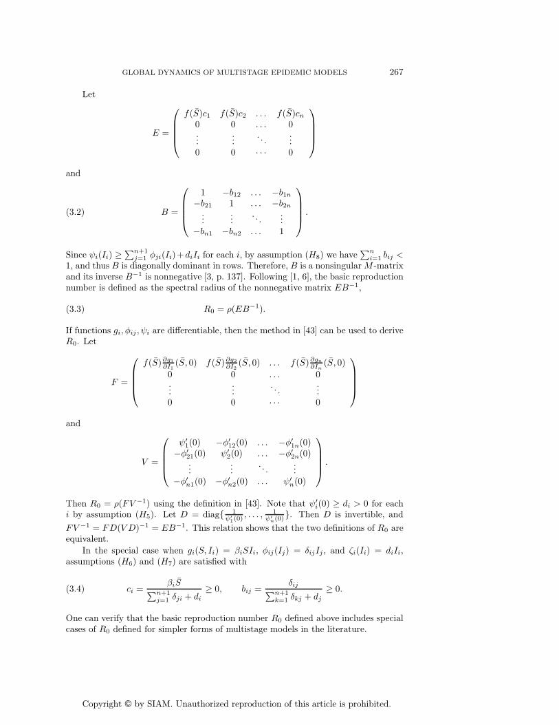
Let

E =

⎛⎜⎜⎜⎝

f(S)c1 f(S)c2 . . . f(S)cn0 0 . . . 0...

.... . .

...0 0 · · · 0

⎞⎟⎟⎟⎠

and

(3.2) B =

⎛⎜⎜⎜⎝

1 −b12 . . . −b1n−b21 1 . . . −b2n...

.... . .

...−bn1 −bn2 . . . 1

⎞⎟⎟⎟⎠ .

Since ψi(Ii) ≥∑n+1

j=1 φji(Ii)+diIi for each i, by assumption (H8) we have∑n

i=1 bij <1, and thus B is diagonally dominant in rows. Therefore, B is a nonsingularM -matrixand its inverse B−1 is nonnegative [3, p. 137]. Following [1, 6], the basic reproductionnumber is defined as the spectral radius of the nonnegative matrix EB−1,

(3.3) R0 = ρ(EB−1).

If functions gi, φij , ψi are differentiable, then the method in [43] can be used to deriveR0. Let

F =

⎛⎜⎜⎜⎝

f(S)∂g1∂I1(S, 0) f(S)∂g2∂I2

(S, 0) . . . f(S)∂gn∂In(S, 0)

0 0 . . . 0...

.... . .

...0 0 · · · 0

⎞⎟⎟⎟⎠

and

V =

⎛⎜⎜⎜⎝

ψ′1(0) −φ′12(0) . . . −φ′1n(0)

−φ′21(0) ψ′2(0) . . . −φ′2n(0)

......

. . ....

−φ′n1(0) −φ′n2(0) . . . ψ′n(0)

⎞⎟⎟⎟⎠ .

Then R0 = ρ(FV −1) using the definition in [43]. Note that ψ′i(0) ≥ di > 0 for each

i by assumption (H5). Let D = diag{ 1ψ′

1(0), . . . , 1

ψ′n(0)

}. Then D is invertible, and

FV −1 = FD(V D)−1 = EB−1. This relation shows that the two definitions of R0 areequivalent.

In the special case when gi(S, Ii) = βiSIi, φij(Ij) = δijIj , and ζi(Ii) = diIi,assumptions (H6) and (H7) are satisfied with

(3.4) ci =βiS∑n+1

j=1 δji + di≥ 0, bij =

δij∑n+1k=1 δkj + dj

≥ 0.

One can verify that the basic reproduction number R0 defined above includes specialcases of R0 defined for simpler forms of multistage models in the literature.



4. Global dynamics when R0 ≤ 1. In this section, we show that the diseasedies out when the basic reproduction number R0 ≤ 1, and that the disease persistsotherwise. We make the following assumptions.

(A1) For 1 ≤ i ≤ n, f(S)gi(S, Ii) ≤ f(S)gi(S, Ii) holds for all 0 ≤ S ≤ S, Ii ≥ 0; if

f(S)gi(S, Ii) = f(S)gi(S, Ii) �≡ 0, then S = S; for Ii > 0, gi(S,Ii)ψi(Ii)≤ ci.

(A2) For all Ij > 0, 1 ≤ i, j ≤ n, supIj>0φij(Ij)ψj(Ij)

= bij .

Theorem 4.1. Suppose that assumptions (H1)–(H8) hold. If R0 ≤ 1 and as-sumptions (A1) and (A2) hold, then the disease-free equilibrium P0 is globally asymp-totically stable in Γ; if R0 > 1, then P0 is unstable and system (2.6) is uniformly

persistent in the interior◦Γ of Γ.

Proof. Let matrix B be as defined in (3.2) and

(w1, w2, . . . , wn) = f(S)(c1, c2, . . . , cn)B−1 ≥ 0.

Then, by (3.2) and (3.3), w1 = R0 ≤ 1. Define a Lyapunov function

L =n∑i=1

wiIi.

The derivative of L along solutions of system (2.6) is

•L = w1f(N)

n∑j=1

gj(S, Ij) +n∑i=1

wi

( n∑j=1

φij(Ij)− ψi(Ii)

)

= w1f(N)

(g1(S, I1)

ψ1(I1),g2(S, I2)

ψ2(I2), . . . ,

gn(S, In)

ψn(In)

)(ψ1(I1), . . . , ψn(In))

T

−(w1, . . . , wn)

⎛⎜⎜⎜⎜⎝

1 −φ12(I2)ψ2(I2)

. . . −φ1n(In)ψn(In)

−φ21(I1)ψ1(I1)

1 . . . −φ2n(In)ψn(In)

......

. . ....

−φn1(I1)ψ1(I1)

−φn2(I2)ψ2(I2)

. . . 1

⎞⎟⎟⎟⎟⎠ (ψ1(I1), . . . , ψn(In))

T

≤ w1f(S)(c1, . . . , cn)(ψ1(I1), . . . , ψn(In))T − (w1, . . . , wn)B(ψ1(I1), . . . , ψn(In))

T

= (w1 − 1)f(S)(c1, . . . , cn)(ψ1(I1), . . . , ψn(In))T ≤ 0, since w1 = R0 ≤ 1.

Therefore, all limit points are contained in the largest invariant subset K of

G = {(S, I1, . . . , In) ∈ Γ |•L = 0}.

Suppose that R0 < 1. Then•L = 0 implies that

∑ni=1 ciψi(Ii) = 0. Using assumption

(A1), this implies that∑n

j=1 gj(S, Ij) = 0 holds along solutions in K. Using the S

equation in (2.6) we obtain that S = S in K. Furthermore, from equations of Ii, wehave (

n∑i=1

Ii

)′

= −n∑i=1

ζi(Ii)−n∑j=1

φ(n+1)j(Ij) ≤ −d∗n∑i=1

Ii.

Therefore, along any solution in K, we necessarily have S = S and I1 = · · · = In = 0.As a consequence, K = {P0} if R0 < 1.



If R0 = 1, then•L = 0 implies

f(S)(g1(S, I1)ψ1(I1)

,g2(S, I2)

ψ2(I2), . . . ,

gn(S, In)

ψn(In)

)(ψ1(I1), . . . , ψn(In))

T

= f(S)(c1, . . . , cn)(ψ1(I1), . . . , ψn(In))T .

Therefore, there exists 1 ≤ i ≤ n such that

f(S)gi(S, Ii)

ψi(Ii)=f(S)gi(S, Ii)

ψi(Ii)= ci > 0, namely,

f(S)gi(S, Ii) = f(S)gi(S, Ii) �= 0 for all Ii > 0.

By assumption (A1), we have S = S. Using the S equation in (2.6), we know that∑nj=1 gj(S, Ij) = 0 holds along any solution in K. The same argument as in the

previous case shows that K = {P0} if R0 = 1 as well. By LaSalle’s invarianceprinciple [27], P0 is globally asymptotically stable in Γ if R0 ≤ 1.

If R0 > 1, then, by continuity,•L > 0 in a neighborhood of P0 in

◦Γ. Solutions in

Rn+1+ sufficiently close to P0 move away from P0, except those on the invariant S-axis.

This implies that P0 is unstable. Using a uniform persistence result from [12] and asimilar argument as in the proof of Proposition 3.3 of [30], we can show that, whenR0 > 1, the instability of P0 implies the uniform persistence of (2.6). This completesthe proof of Theorem 4.1.

Uniform persistence of (2.6) and the positive invariance of compact set Γ imply

the existence of an equilibrium of (2.6) in◦Γ (see Theorem D.3 in [40] or Theorem

2.8.6 in [4]).Proposition 4.2. Suppose that assumptions (H1)–(H8) hold. If R0 > 1, then

there exists at least one endemic equilibrium for system (2.6).Theorem 4.1 and Proposition 4.2 imply that the disease always dies out from

all stages if the basic reproduction number R0 ≤ 1, irrespective of the size of theinitial outbreak. If R0 > 1, then the disease persists in all stages and it can persistat a constant endemic state. This establishes R0 as a sharp threshold for the diseasepersistence.

5. Global dynamics when R0 > 1. In this section, for the special case f(N) ≡1, we show that the endemic equilibrium is unique and is globally asymptotically stablein the interior of the feasible region Γ. Biologically, this implies that the diseasealways becomes endemic and persists at a unique endemic equilibrium, no matterhow small the size of the initial outbreak is. Suppose that assumptions (H1)–(H8)hold. By Proposition 4.2, an endemic equilibrium P ∗ = (S∗, I∗1 , . . . , I

∗n) exists. Here

S∗, I∗1 , . . . , I∗n are positive and satisfy the equilibrium equations (3.1).

Assume that there exists a function Φ : R+ → R+ such that the following as-sumptions hold.

(B1) For S �= S∗,

(θ(S)− θ(S∗))(Φ(S)− Φ(S∗)) < 0.

(B2) For 0 ≤ S ≤ S, Ij > 0, 1 ≤ j ≤ n,

(gj(S, Ij)Φ(S)

−gj(S

∗, I∗j )

Φ(S∗)

)( gj(S, Ij)

Φ(S)ψj(Ij)−

gj(S∗, I∗j )

Φ(S∗)ψj(I∗j )

)≤ 0.



(B3) For Ij > 0, 1 ≤ i, j ≤ n,

(φij(Ij)− φij(I∗j )) ·

(φij(Ij)ψj(Ij)

−φij(I

∗j )

ψj(I∗j )

)≤ 0.

We also make the following monotonicity assumption.

(B4) For each 1 ≤ i ≤ n, one of the functions gi(S∗, Ii),

∑nj=1 φij(Ij), ψi(Ii) is

strictly monotone in Ii.

We define a matrix M = (mij), where

(5.1) mij =

{φ1j(I

∗j ) + gj(S

∗, I∗j ) if i = 1,

φij(I∗j ) if i ≥ 2.

We regard matrix M as a weight matrix for the infection-transfer graph G of ourmodel, as shown in Figure 2. In the weighted graph G, solid arrows indicate transfersof individuals between compartments, and dashed arrows indicate infection. For ournext result, we will require thatM be an irreducible matrix. In graph-theoretic terms,irreducibility of M is equivalent to weighted graph (G,M) being strongly connected[3].

Fig. 2. The infection-transfer graph G at the endemic equilibrium P ∗ of model (2.2). Solidarrows indicate transfers of individuals between compartments, and dashed arrows indicate infection.

Theorem 5.1. Suppose that assumptions (H1)–(H8) hold and that f(N) ≡ 1.Assume that matrix M defined in (5.1) is irreducible, and that assumptions (B1)–(B4) hold. Then, when R0 > 1, there exists a unique endemic equilibrium P ∗ and it

is globally asymptotically stable in◦Γ.

Proof. For system (2.6), we consider the following Lyapunov function:

(5.2) V = τ1

∫ S

S∗

Φ(ξ)− Φ(S∗)

Φ(ξ)dξ +

n∑i=1

τi

∫ Ii

I∗i

ψi(ξ)− ψi(I∗i )

ψi(ξ)dξ.

Here τi > 0, i = 1, . . . , n, are constants to be specified later. Differentiating V alongsolutions of (2.6) and using equilibrium equations (3.1) to simplify, we obtain



(5.3)•V = τ1

(θ(S)− θ(S)

Φ(S∗)

Φ(S)+

n∑j=1

gj(S, Ij)Φ(S∗)

Φ(S)+

n∑j=1

φij(Ij)− ψ1(I1)

−n∑j=1

gj(S, Ij)ψ1(I

∗1 )

ψ1(I1)−

n∑j=1

φij(Ij)ψ1(I

∗1 )

ψ1(I1)+ ψ1(I

∗1 )

)

+

n∑i=2

τi

( n∑j=1

φij(Ij)− ψi(Ii)−n∑j=1

φij(Ij)ψi(I

∗i )

ψi(Ii)+ ψi(I

∗i )

)

= τ1(θ(S)− θ(S∗))

(1− Φ(S∗)

Φ(S)

)

+ τ1

n∑j=1

gj(S∗, I∗j )

(2 +

gj(S, Ij)Φ(S∗)

gj(S∗, I∗j )Φ(S)− Φ(S∗)

Φ(S)− ψ1(I1)

ψ1(I∗1 )− gj(S, Ij)ψ1(I

∗1 )

gj(S∗, I∗j )ψ1(I1)

)

+

n∑i=1

τi

n∑j=1

φij(I∗j )

(φij(Ij)

φij(I∗j )− ψi(Ii)

ψi(I∗i )− φij(Ij)ψi(I

∗i )

φij(I∗j )ψi(Ii)+ 1

).

By assumption (B1), we have

(5.4) (θ(S) − θ(S∗))

(1− Φ(S∗)

Φ(S)

)≤ 0.

Using assumption (B3) we obtain(5.5)

φij(Ij)

φij(I∗j )− ψi(Ii)

ψi(I∗i )− φij(Ij)ψi(I

∗i )

φij(I∗j )ψi(Ii)+ 1 =

(φij(Ij)

φij(I∗j )− 1

)(1−

φij(I∗j )ψj(Ij)

φij(Ij)ψj(I∗j )

)

+

(1− φij(Ij)ψi(I

∗i )

φij(I∗j )ψi(Ii)+ ln

φij(Ij)ψi(I∗i )

φij(I∗j )ψi(Ii)

)

+

(1−

φij(I∗j )ψj(Ij)

φij(Ij)ψj(I∗j )+ ln

φij(I∗j )ψj(Ij)

φij(Ij)ψj(I∗j )

)

+ψj(Ij)

ψj(I∗j )− ln

ψj(Ij)

ψj(I∗j )− ψi(Ii)

ψi(I∗i )+ ln

ψi(Ii)

ψi(I∗i )

≤ 1− φij(Ij)ψi(I∗i )


φij(Ij)ψi(I∗i )

φij(I∗j )ψi(Ii)

+ 1−φij(I

∗j )ψj(Ij)


φij(I∗j )ψj(Ij)

φij(Ij)ψj(I∗j )

+ψj(Ij)

ψj(I∗j )− ln

ψj(Ij)


ψi(I∗i )+ ln

ψi(Ii)

ψi(I∗i ).

Similarly, using inequality (B2), we obtain



(5.6)

2 +gj(S, Ij)Φ(S

∗)

gj(S∗, I∗j )Φ(S)− Φ(S∗)

Φ(S)− ψ1(I1)

ψ1(I∗1 )− gj(S, Ij)ψ1(I

∗1 )

gj(S∗, I∗j )ψ1(I1)

=( gj(S, Ij)Φ(S∗)

gj(S∗, I∗j )Φ(S)− 1)(

1−gj(S

∗, I∗j )Φ(S)ψj(Ij)

gj(S, Ij)Φ(S∗)ψj(I∗j )

)+(1− Φ(S∗)

Φ(S)+ ln

Φ(S∗)

Φ(S)

)+(1− gj(S, Ij)ψ1(I

∗1 )

gj(S∗, I∗j )ψ1(I1)+ ln

gj(S, Ij)ψ1(I∗1 )

gj(S∗, I∗j )ψ1(I1)

)

+(1−

gj(S∗, I∗j )Φ(S)ψj(Ij)

gj(S, Ij)Φ(S∗)ψj(I∗j )+ ln



)+ψj(Ij)

ψj(I∗j )− ln

ψj(Ij)

ψj(I∗j )− ψ1(I1)

ψ1(I∗1 )+ ln

ψ1(I1)

ψ1(I∗1 )

≤(1− Φ(S∗)

Φ(S)+ ln

Φ(S∗)

Φ(S)

)+(1− gj(S, Ij)ψ1(I

∗1 )



gj(S∗, I∗j )ψ1(I1)

)+(1−





)+ψj(Ij)

ψj(I∗j )− ln

ψj(Ij)

ψj(I∗j )− ψ1(I1)

ψ1(I∗1 )+ ln

ψ1(I1)

ψ1(I∗1 ).

Combining (5.3)–(5.6) and using the definition of mij in (5.1), we obtain

(5.7)

•V ≤

n∑i=1

τi

n∑j=1

φij(I∗j )[1− φij(Ij)ψi(I

∗i )


φij(Ij)ψi(I∗i )

φij(I∗j )ψi(Ii)

]

+n∑i=1

τi

n∑j=1

φij(I∗j )[1−

φij(I∗j )ψj(Ij)


φij(I∗j )ψj(Ij)

φij(Ij)ψj(I∗j )

]

+ τ1

n∑j=1

gj(S∗, I∗j )

[1− Φ(S∗)

Φ(S)+ ln

Φ(S∗)

Φ(S)

]

+ τ1

n∑j=1

gj(S∗, I∗j )

[1− gj(S, Ij)ψ1(I

∗1 )



gj(S∗, I∗j )ψ1(I1)

]

+ τ1

n∑j=1

gj(S∗, I∗j )

[1−





]

+

n∑i=1

τi

n∑j=1

mij

(ψj(Ij)ψj(I∗j )

− lnψj(Ij)


ψi(I∗i )+ ln

ψi(Ii)

ψi(I∗i )

).

Note that function s(x) = 1−x+lnx is nonpositive for x > 0 and s(x) = 0 if and onlyif x = 1. We see that expressions enclosed in the square brackets in (5.7) are negative

definite. To show that•V negative definite, we choose constants τi > 0 such that the

last expression in (5.7) vanishes. Let M be the infection-transfer matrix defined in(5.1) and let

L(M) = diag

⎛⎝ n∑j=1

m1j , . . . ,

n∑j=1

mnj

⎞⎠−M

be the algebraic Laplacian matrix of M . We choose τi as the co-factor of the ithdiagonal entry of L(M). By Kirchhoff’s matrix tree theorem (see the appendix), since



M is irreducible, we know that τi > 0. Furthermore, using the tree cycle identity andits corollary in the appendix, we obtain the following identity:

n∑i=1

τi

n∑j=1

mij

(ψj(Ij)ψj(I∗j )

− lnψj(Ij)


ψi(I∗i )+ ln

ψi(Ii)

ψi(I∗i )

)≡ 0.

Therefore, we conclude that•V ≤ 0 for all (S, I1, . . . , In) ∈

◦Γ. Furthermore,

•V = 0

implies that

(5.8) (θ(S)− θ(S∗))(1− Φ(S∗)

Φ(S)

)= 0

by (5.4), and thus S = S∗ by assumption (B1). Furthermore,•V = 0 implies that

(5.9)gj(S, Ij)

gj(S∗, I∗j )=φij(Ij)

φij(I∗j )=ψj(Ij)

ψj(I∗j )= λ, i, j = 1, . . . , n,

using properties of s(x) = 1− x+ lnx and strong connectivity of the weighted graph

(G,M). Along any solution that stays in the set where•V = 0, we necessarily have

S = S∗, gj(S, Ij) = λ gj(S∗, I∗j ), j = 1, . . . , n.

Substituting these relations into the first equation of (2.2), we obtain

0 = θ(S∗)− λ

n∑j=1

gj(S∗, I∗j ).

Since the expression on the right-hand side is linear in λ, the equation holds only atλ = 1, namely at P ∗. Letting λ = 1 in (5.4) we know that

gj(S, Ij) = gj(S∗, I∗j ),

n∑i=1

φij(Ij) =n∑i=1

φij(I∗j ), ψj(Ij) = ψj(I

∗j ),

and it follows from monotonicity assumption (B4) that Ij = I∗j , j = 1, . . . , n. There-

fore, the only invariant set in the set {•V = 0} is the singleton {P ∗}. By LaSalle’s

invariance principle, P ∗ is globally asymptotically stable in◦Γ. As a consequence, P ∗

is also unique.Assumptions (B1)–(B4) are more general and more flexible than earlier conditions

on nonlinear incidences. For instance, if the nonlinear incidence gi(S, Ii) takes theseparable form gi(S, Ii) = p(S)qi(Ii) and if p(S) is strictly increasing, then we can takeΦ(S) = p(S) in assumption (B2) and obtain the following assumption for functionqi(Ii):

(5.10) (qi(Ii)− qi(I∗i ))(qi(Ii)ψ(Ii)

− qi(I∗i )

ψ(I∗i )

)≤ 0, Ii �= I∗i .

Apart from difference in notations, this condition is the same as condition (5.1) in[13]. Furthermore, if ψi(Ii) = δiIi, then condition (5.10) becomes

(5.11) (qi(Ii)− qi(I∗i ))(qi(Ii)

Ii− qi(I

∗i )

I∗i

)≤ 0, Ii �= I∗i .



A sufficient condition for (5.11) is that if qi(Ii) is monotonically increasing and concavedown, which is satisfied by classes of nonlinear functions

qi(Ii) = Ipii and qi(Ii) =Ipii

1 + κiIpi, 0 < pi ≤ 1, κi ≥ 0,

commonly used in the literature of epidemic modeling. We also remark that, whengi(S, Ii) = p(S)qi(Ii) and θ(S) = Λ−dS, if p(S) is strictly increasing, then assumption(B1) is automatically satisfied. In this case, conditions like (5.10) are subjected onlyon qi(Ii), not on p(S).

6. Two special cases. To illustrate our main results in sections 4 and 5, weconsider two special cases. Throughout the section, we assume that f(N) ≡ 1.

6.1. Separable incidence and linear transfer among compartments. Weassume that the nonlinear incidence is in separable form, gj(S, Ij) = p(S)qj(Ij), and

that transfer and mortality functions are linear, φij(Ij) = φijIj and ζi(Ii) = ζiIi,for 1 ≤ i, j ≤ n. Then, system (2.6) becomes

S′ = θ(S)− p(S)

n∑j=1

qj(Ij),

I ′1 = p(S)

n∑j=1

qj(Ij) +

n∑j=1

φ1jIj − ψ1I1,(6.1)

I ′i =n∑j=1

φijIj − ψiIi, i = 2, 3, . . . , n,

where ψi =∑n+1

j=1 φji + ζi, i = 1, . . . , n.With these special classes of functions, assumptions (H1)–(H8) are reduced to

the following:(H ′

1) There exists S > 0 such that θ(S) = 0 and θ(S)(S − S) < 0 for all S ≥ 0 andS �= S.

(H ′2) For 1 ≤ j ≤ n, qj(Ij) ≥ 0 for all Ij ≥ 0, and qj(0) = 0; p(S) ≥ 0 for S ≥ 0

and p(0) = 0.(H ′

3) For 1 ≤ i, j ≤ n, φij ≥ 0, and∑n

j=1 φji > 0 for each i.

(H ′4) For 1 ≤ i ≤ n, ζi > 0.

(H ′5) For 1 ≤ i ≤ n, there exists ci ≥ 0, such that limIi→0+

qi(Ii)Ii

= ci, andmaxi{ci} > 0.

It can be verified that functions of the form θ(S) = Λ − dS + rS(1 − SK ), qi(Ii) =

βiIpii and qi(Ii) =

βiIpii

1+κiIpii

satisfy assumptions (H ′1)–(H

′5). Furthermore, the basic

reproduction number is given as

R0 = ρ(E1B−11 ),

where

E1 = p(S)

⎛⎜⎜⎜⎝

c1ψ1

c2ψ2

. . . cnψn

0 0 . . . 0...

.... . .

...0 0 · · · 0

⎞⎟⎟⎟⎠ , B1 =

⎛⎜⎜⎜⎝

1 −b12 . . . −b1n−b21 1 . . . −b2n...

.... . .

...−bn1 −bn2 . . . 1

⎞⎟⎟⎟⎠ ,



with bij =φij

ψj.

Assumptions (A1) and (A2) are now reduced to the following two assumptions.

(A′1) Function p(S) is monotonically increasing for 0 ≤ S ≤ S, and p(S) = p(S) if

and only if S = S.

(A′2) For 1 ≤ i ≤ n, ci = supIi>0

qi(Ii)Ii

.

Following Theorem 4.1 we have the following result.

Theorem 6.1. Suppose that assumptions (H ′1)–(H

′5) hold. If R0 ≤ 1 and as-

sumptions (A′1) and (A′

2) hold, then the disease-free equilibrium P0 is globally asymp-totically stable in Γ.

By choosing Φ(S) = p(S), assumptions (B1)–(B4) reduce to the following twoconditions.

(B′1) For S �= S∗, (S − S∗)(θ(S) − θ(S∗)) < 0.

(B′2) For 0 ≤ S ≤ S, p(S) is strictly increasing; for Ij > 0, 1 ≤ j ≤ n,

(qj(Ij)− qj(I∗j ))(qj(Ij)

Ij−qj(I

∗j )

I∗j

)≤ 0.

As we commented at the end of section 5, condition (B′2) is satisfied if qj(Ij) is

strictly increasing and concave down. Such properties are satisfied by functions of the

forms qj(Ij) = βjIpjj and qj(Ij) =

βjIpjj

1+κjIpjj

, with 0 < pj ≤ 1, κj ≥ 0.

The weight matrix M = (mij) in (5.1) becomes

(6.2) mij =

{φ1jI

∗j + p(S∗)qj(I

∗j ) if i = 1,

φijI∗j if i ≥ 2.

The following result follows from Theorem 5.1.

Theorem 6.2. Suppose that assumptions (H ′1)–(H

′5) hold. Assume that matrix

M defined in (6.2) is irreducible, and that assumptions (B′1) and (B′

2) hold. Then,when R0 > 1, there exists a unique endemic equilibrium P ∗ to system (6.1) and it is

globally asymptotically stable in◦Γ.

6.2. Bilinear incidence and nonlinear transfer among compartments.We consider bilinear incidence gj(S, Ij) = βjIjS. System (2.6) becomes

S′ = θ(S)−n∑j=1

βjIjS,

I ′1 =

n∑j=1

βjIjS +

n∑j=1

φ1j(Ij)− ψ1(I1),(6.3)

I ′i =n∑j=1

φij(Ij)− ψi(Ii), i = 2, 3, . . . , n.

Assumptions (H2) and (H3) are automatically satisfied. Assumption (H6) becomesthe following:

(H ′′6 ) There exist constants 0 ≤ ci ≤ ∞, 1 ≤ i ≤ n, and maxi{ci} > 0, such that

limIi→0+Ii

ψi(Ii)= ci.



The basic reproduction number R0 is defined as R0 = ρ(E2B−12 ) with

E2 =

⎛⎜⎜⎜⎝

β1Sc1 β2Sc2 . . . βnScn0 0 . . . 0...

.... . .

...0 0 · · · 0

⎞⎟⎟⎟⎠ , B2 =

⎛⎜⎜⎜⎝

1 −b12 . . . −b1n−b21 1 . . . −b2n...

.... . .

...−bn1 −bn2 . . . 1

⎞⎟⎟⎟⎠ .

Assumption (A1) simplifies to(A′′

1 ) For 1 ≤ i ≤ n, ci = sup Iiψi(Ii)

.

Assumption (B2) simplifies to (by choosing Φ(S) = S)

(B′′2 ) (Ij − I∗j )

( Ijψj(Ij)

− I∗jψj(I∗j )

)≤ 0, 1 ≤ j ≤ n.

We note that assumption (B′′2 ) holds if ψj is linear.

Then, with the bilinear incidence, assumptions (H1)–(H7) are replaced by (H1),(H4), (H5), and (H ′′

6 ), (H7), and (H8). If R0 ≤ 1, then Theorem 4.1 holds under (A′′1 )

and (A2), while if R0 > 1, Theorem 5.1 holds under assumptions (B1), (B′′2 ), and

(B3).

7. Summary and discussions. In this paper, we have formulated a generalclass of multistage epidemic models with disease progression and amelioration. Amongthe new features is that individuals are allowed to move from one stage of the infec-tion to any other stage either forward (progression) or backward (amelioration) withcertain transfer rates. We have also incorporated general classes of nonlinear demo-graphic functions for the host population, nonlinear incidence functions that are alsodensity dependent, as well as nonlinear transfer and removal functions from each dis-ease stage. Under biologically motivated conditions, we have derived the basic repro-duction number R0 and proved that the global dynamics are completely determinedby the value of R0; if R0 ≤ 1, then the disease-free equilibrium is globally asymptoti-cally stable, and the disease always dies out from all stages. If R0 > 1, then the diseasepersists in all stages. In the special case that the incidence is density-independent, wehave proved that a unique endemic equilibrium P ∗ is globally asymptotically stableif R0 > 1.

Our models contain many important classes of epidemic models with multiplestages and multiple compartments in the literature. Hyman, Li, and Stanley [22]formulated a class of staged progression (SP) models for the progression of HIV.Similar structures in the SP models have appeared in earlier works of Jacquez and hiscollaborators (see [24, 39]) on HIV/AIDS modelling. SP models are further extendedto SP and amelioration models in McCluskey [14, 36], Guo and Li [15, 16], and inrecent works of Sallet and his collaborators [2, 7, 23]. In these earlier models, transferof individuals is to the adjacent stage either forward (disease progression) or backward(amelioration). As a result, the transfer matrix is tridiagonal. This allows explicitconstruction of global Lyapunov functions using matrix techniques. In our model, thetransfer matrix is a full matrix, and previous construction of Lyapunov functions isnot applicable. This makes the application of the graph-theoretic technique developedin our earlier work [17, 18, 31, 32] essential in our proof of the uniqueness and globalstability of the endemic equilibrium. Our results in the present paper mark the firsttime that the graph-theoretic technique is shown to work for epidemic models withgeneral discrete stage structures.

We have allowed infectivity at an infectious stage to be zero, so that these stagescan be regarded as latent or quarantined. Our results and proof are applicable to



earlier models with multiple latent stages [2, 23] and epidemic models of SIQR typewith quarantined compartment [20]. In the special case when n = 2 and g1 = 0, ourmodel reduces to the well-known SEIR model. Our results and proof generalize thosein [25, 26].

Nonlinear functions are used in our models to describe incidence, disease pro-gression, disease amelioration, and host population demography. These nonlinearelements have been used in the literature, and the methods of Lyapunov functionshave been used for models that incorporate some of these nonlinearities [13, 26, 45];none of these earlier models have the degree of generality in our model.

One limitation in our model is that we have used exponential distributions forresidence time for individuals in a compartment Ij . Further extension of the model canincorporate general distributions for disease progression or amelioration as discussedin [9, 10].

Appendix. Some combinatorial identities.Given a weighted digraph G with n vertices (n ≥ 2), define the weight matrix

A = (aij)n×n whose entry aij equals the weight of arc (j, i) if it exists, and 0 otherwise.For our purpose, we denote a weighted digraph as (G, A). The Laplacian matrix of(G, A) is defined as

(A.1) L =

⎛⎜⎜⎜⎜⎜⎝

∑k =1 a1k −a12 · · · −a1n−a21

∑k =2 a2k · · · −a2n

......

. . ....

−an1 −an2 · · ·∑k =n ank

⎞⎟⎟⎟⎟⎟⎠ .

Let ci denote the co-factor of the ith diagonal element of L. Then (c1, . . . , cn)T is a

right eigenvector of L with respect to the eigenvalue 0. The following result gives agraph-theoretic description of ci and is customarily referred to as Kirchhoff’s matrixtree theorem. We refer the reader to [38] for its proof.

Proposition A.1 (Kirchhoff’s matrix tree theorem). Assume n ≥ 2. Then

(A.2) ci =∑T ∈Ti

w(T ), i = 1, 2, . . . , n,

where Ti is the set of all spanning trees T of (G, A) that are rooted at vertex i, andw(T ) is the weight of T . In particular, if (G, A) is strongly connected, then ci > 0 for1 ≤ i ≤ n.

The following tree cycle identity was first proved in [32]. We refer the reader to[32] for its proof.

Proposition A.2 (tree cycle identity). Assume n ≥ 2. Let ci be given inProposition A.1. Then the following identity holds:

(A.3)

n∑i,j=1

ci aij Fij(x) =∑Q∈Q

w(Q)∑

(s,r)∈E(CQ)

Frs(x).

Here Fij(x), 1 ≤ i, j ≤ n, x ∈ Rm, are arbitrary functions, Q is the set of all spanningunicyclic graphs of (G, A), w(Q) is the weight of Q, and CQ denotes the directed cycleof Q.

The following identity was first established in [32] and follows directly from thetree cycle identity.



Corollary A.3. Let ci be given in Kirchhoff’s matrix tree theorem, and let{Gi(xi)}ni=1 be any family of functions. Then the following identity holds:

(A.4)

n∑i,j=1

ci aij Gi(xi) =

n∑i,j=1

ci aij Gj(xj).

REFERENCES

[1] R. M. Anderson and R. M. May, Infectious Diseases of Humans: Dynamics and Control,Oxford University Press, Oxford, UK, 1992.

[2] N. Bame, S. Bowong, J. Mbang, G. Sallet, and J.-J. Tewa, Global stability analysis forSEIS models with n latent classes, Math. Biosci. Eng., 5 (2008), pp. 20–33.

[3] A. Berman and R. J. Plemmons, Nonnegative Matrices in the Mathematical Sciences, Aca-demic Press, New York, 1979.

[4] N. P. Bhatia and G. P. Szego, Dynamical Systems: Stability Theory and Applications,Lecture Notes in Math. 35, Springer-Verlag, Berlin, New York, 1967.

[5] E. Corbett, C. Watt, N. Walker, D. Maher, B. Williams, M. Raviglione, and C. Dye,The growing burden of tuberculosis: Global trends and interactions with the HIV epidemic,Arch. Intern. Med., 163 (2003), pp. 1009–1021.

[6] O. Diekmann, J. A. P. Heesterbeek, and J. A. J. Metz, On the definition and the compu-tation of the basic reproduction ratio R0 in models for infectious diseases in heterogeneouspopulations, J. Math. Biol., 28 (1990), pp. 365–382.

[7] A. Fall, A. Iggidr, G. Sallet, and J. J. Tewa, Epidemiological models and Lyapunovfunctions, Math. Model. Nat. Phenom., 2 (2007), pp. 55–73.

[8] Z. Feng, Final and peak epidemic sizes for SEIR models with quarantine and isolation, Math.Biosci. Eng., 4 (2007), pp. 675–686.

[9] Z. Feng and H. R. Thieme, Endemic models with arbitrarily distributed periods of infection.I. Fundamental properties of the model, SIAM J. Appl. Math., 61 (2000), pp. 803–833.

[10] Z. Feng, D. Xu, and H. Zhao, Epidemiological models with non-exponentially distributeddisease stages and applications to disease control, Bull. Math. Biol., 69 (2007), pp. 1511–1536.

[11] Z. Feng, W. Huang, and C. Castillo-Chavez, On the role of variable latent periods inmathematical models for tuberculosis, J. Dynam. Differential Equations, 13 (2001), pp.425–452.

[12] H. I. Freedman, S. G. Ruan, and M. X. Tang, Uniform persistence and flows near a closedpositively invariant set, J. Dynam. Differential Equations, 6 (1994), pp. 583–600.

[13] P. Georgescu and Y.-H. Hsieh, Global stability for a virus dynamics model with nonlinearincidence of infection and removal, SIAM J. Appl. Math., 67 (2006), pp. 337–353.

[14] A. B. Gumel, C. C. McCluskey, and P. van den Driessche, Mathematical study of a staged-progression HIV model with imperfect vaccine, Bull. Math. Biol., 68 (2006), pp. 2105–2128.

[15] H. Guo and M. Y. Li, Global dynamics of a staged progression model for infectious diseases,Math. Biosci. Eng., 3 (2006), pp. 513–525.

[16] H. Guo and M. Y. Li, Global dynamics of a staged-progression model with amelioration forinfectious diseases, J. Biol. Dyn., 2 (2008), pp. 154–168.

[17] H. Guo, M. Y. Li, and Z. Shuai, Global stability of the endemic equilibrium of multigroupSIR epidemic models, Can. Appl. Math. Q., 14 (2006), pp. 259–284.

[18] H. Guo, M. Y. Li, and Z. Shuai, A graph-theoretic approach to the method of global Lyapunovfunctions, Proc. Amer. Math. Soc., 136 (2008), pp. 2793–2802.

[19] J. C. M. Hendriks, G. A. Satten, I. M. Longini, H. A. M. van Druten, P. T. A.

Schellekens, R. A. Coutinho, and G. J. P. van Griensven, Use of immunologicalmarkers and continuous-time Markov models to estimate progression of HIV infection inhomosexual men, AIDS, 10 (1996), pp. 649–656.

[20] H. W. Hethcote, Z. Ma, and S. Liao, Effects of quarantine in six endemic models forinfectious diseases, Math. Biosci., 180 (2002), pp. 141–160.

[21] H. W. Hethcote and J. W. Van Ark, Modeling HIV Transmission and AIDS in the UnitedStates, Springer-Verlag, Berlin, 1992.

[22] J. M. Hyman, J. Li, and E. A. Stanley, The differential infectivity and staged progressionmodels for the transmission of HIV, Math. Biosci., 155 (1999), pp. 77–109.



[23] A. Iggidr, J. Mbang, G. Sallet, and J.-J. Tewa, Multi-compartment models, Discrete Con-tin. Dyn. Syst., suppl. (2007), 506–519.

[24] J. A. Jacquez, C. P. Simon, J. Koopman, L. Sattenspiel, and T. Perry, Modeling andanalyzing HIV transmission: The effect of contact patterns, Math. Biosci., 92 (1988), pp.119–199.

[25] A. Korobeinikov, Lyapunov functions and global properties for SEIR and SEIS epidemicmodels, Math. Med. Biol., 21 (2004), pp. 75–83.

[26] A. Korobeinikov, Global properties of infectious disease models with nonlinear incidence,Bull. Math. Biol., 69 (2007), pp. 1871–1886.

[27] J. P. LaSalle, The Stability of Dynamical Systems, CBMS-NSF Regional Conf. Ser. in Appl.Math. 25, SIAM, Philadelphia, 1976.

[28] S. Lawn, R. Wood, and R. Wilkinson, Changing concepts of “latent tuberculosis infection”in patients living with HIV infection, Clin. Dev. Immunol., 2011 (2011), 980594.

[29] G. Li and Z. Jin, Global stability of a SEIR epidemic model with infectious force in latent,infected and immune period, Chaos Solitons Fractals, 25 (2005), pp. 1177–1184.

[30] M. Y. Li, J. R. Graef, L. Wang, and J. Karsai, Global dynamics of a SEIR model withvarying total population size, Math. Biosci., 160 (1999), pp. 191–213.

[31] M. Y. Li and Z. Shuai, Global stability of an epidemic model in a patchy environment, Can.Appl. Math. Q., 17 (2009), pp. 175–187.

[32] M. Y. Li and Z. Shuai, Global-stability problem for coupled systems of differential equationson networks, J. Differential Equations, 248 (2010), pp. 1–20.

[33] M. Y. Li, Z. Shuai, and C. Wang, Global stability of multi-group epidemic models withdistributed delays, J. Math. Anal. Appl., 361 (2010), pp. 38–47.

[34] X. Lin, H. W. Hethcote, and P. van den Driessche, An epidemiological model forHIV/AIDS with proportional recruitment, Math. Biosci., 118 (1993), pp. 181–195.

[35] N. MacDonald, Time Lags in Biological Models, Lecture Notes in Biomath. 27, Springer-Verlag, Berlin, 1978.

[36] C. C. McCluskey, A model of HIV/AIDS with staged progression and amelioration, Math.Biosci., 181 (2003), pp. 1–16.

[37] C. C. McCluskey, Global stability for a class of mass action systems allowing for latency intuberculosis, J. Math. Anal. Appl., 338 (2008), pp. 518–535.

[38] J. W. Moon, Counting Labelled Trees, William Clowes and Sons, London, 1970.[39] C. P. Simon and J. A. Jacquez, Reproduction numbers and the stability of equilibria of SI

models for heterogeneous populations, SIAM J. Appl. Math., 52 (1992), pp. 541–576.[40] H. L. Smith and P. Waltman, The Theory of the Chemostat: Dynamics of Microbial Com-

petition, Cambridge University Press, Cambridge, UK, 1995.[41] R. Sun, Global stability of the endemic equilibrium of multigroup SIR models with nonlinear

incidence, Comput. Math. Appl., 60 (2010), pp. 2286–2291.[42] H. R. Thieme and C. Castillo-Chavez, How may infection-age-dependent infectivity affect

the dynamics of HIV/AIDS?, SIAM J. Appl. Math., 53 (1993), pp. 1447–1479.[43] P. van den Driessche and J. Watmough, Reproduction numbers and sub-threshold endemic

equilibria for compartmental models of disease transmission, Math. Biosci., 180 (2002),pp. 29–48.

[44] P. van den Driessche, L. Wang, and X. Zou, Modeling diseases with latency and relapse,Math. Biosci. Eng., 4 (2007), pp. 205–219.

[45] Z. Yuan and L. Wang, Global stability of epidemiological models with group mixing andnonlinear incidence rates, Nonlinear Anal. Real World Appl., 11 (2010), pp. 995–1004.

[46] Z. Yuan and X. Zou, Global threshold property in an epidemic model for disease with latencyspreading in a heterogeneous host population, Nonlinear Anal. Real World Appl., 11 (2010),pp. 3479–3490.

[47] E. Ziv, C. L. Daley, and S. M. Blower, Early therapy for latent tuberculosis infection, Amer.J. Epidemiol., 153 (2001), pp. 381–385.

Global Dynamics of a General Class of Multistage Models for Infectious Diseases

Documents

Transcript of Global Dynamics of a General Class of Multistage Models for Infectious Diseases