GLACE survey: OSIRIS/GTC Tuneable Filter Hα imaging of the rich galaxy cluster ZwCl 0024.0+1652 at...
23
Astronomy & Astrophysics manuscript no. glace˙paper1˙v6 c ESO 2015 February 11, 2015 GLACE survey: OSIRIS/GTC Tuneable Filter Hα imaging of the rich galaxy cluster ZwCl 0024.0+1652 at z = 0.395 Part I – Survey presentation, TF data reduction techniques and catalogue M. S´ anchez-Portal 1,2 , I. Pintos-Castro 3,4,8,2 , R. P´ erez-Mart´ ınez 1,2 , J. Cepa, 4,3 , A. M. P´ erez Garc´ ıa 3,4 , H. Dom´ ınguez-S´ anchez 29 , A. Bongiovanni 3,4 , A. L. Serra 23 , E. Alfaro 5 , B. Altieri 1 , A. Arag ´ on-Salamanca 6 , C. Balkowski 7 , A. Biviano 9 , M. Bremer 10 , F. Castander 11 , H. Casta ˜ neda 12 , N. Castro-Rodr´ ıguez 3,4 , A. L. Chies-Santos 25 , D. Coia 1 , A. Diaferio 23,24 , P.A. Duc 13 , A. Ederoclite 21 , J. Geach 14 , I. Gonz´ alez-Serrano 15 , C. P. Haines 16 , B. McBreen 17 , L. Metcalfe 1 , I. Oteo 26,27 , I. P´ erez-Fourn´ on 4,3 , B. Poggianti 18 , J. Polednikova 3,4 , M. Ram ´ on-P´ erez 3,4 , J. M. Rodr´ ıguez-Espinosa 4,3 , J. S. Santos 28 , I. Smail 19 , G. P. Smith 17 , S. Temporin 20 , and I. Valtchanov 1 (Affiliations can be found after the references) Received; accepted ABSTRACT Context. The cores of clusters at 0 . z . 1 are dominated by quiescent early-type galaxies, whereas the field is dominated by star-forming late-type galaxies. Clusters grow through the accretion of galaxies/groups from the surrounding field, which implies that galaxy properties, notably the star formation ability, are altered as they fall into overdense regions. The critical issues to understand this evolution are how the truncation of star formation is connected to the morphological transformation and what physical mechanism is responsible for these changes. The GaLAxy Cluster Evolution Survey (GLACE) is conducting a thorough study on the variation of galaxy properties (star formation, AGN activity and morphology) as a function of environment in a representative and well-studied sample of clusters. Aims. To address these questions, the GLACE survey is performing a deep panoramic survey of emission line galaxies (ELG), mapping a set of optical lines ([O ii], [O iii], Hβ and Hα/[N ii] when possible) in several galaxy clusters at z ∼ 0.40, 0.63 and 0.86. Methods. Using the Tunable Filters (TF) of the OSIRIS instrument at the 10.4m GTC telescope, the GLACE survey applies the technique of TF tomography: for each line, a set of images are taken through the OSIRIS TF, each image tuned at a different wavelength (equally spaced), to cover a rest frame velocity range of several thousands km/s centred at the mean cluster redshift is scanned for the full TF field of view of 8 arcmin diameter. Results. Here we present the first results of the GLACE project, targeting the Hα/[N ii] lines in the intermediate redshift cluster ZwCl 0024.0+1652 at z = 0.395. Two pointings, covering ∼ 2 × r vir have been performed. We discuss the specific techniques devised to process the TF tomogra- phy observations in order to generate the catalogue of cluster Hα emitters, that contains more than 200 sources down to a star formation rate (SFR) . 1M /yr. An ancillary broadband catalogue is constructed, allowing us to discriminate line interlopers by means of colour diagnostics. The final catalog contains 174 unique cluster sources. The AGN population is discriminated using different diagnostics and found to be ∼ 37% of the ELG population. The median SFR of the star-forming population is 1.4 M /yr. We have studied the spatial distribution of ELG, confirming the existence of two components in the redshift space. Finally, we have exploited the outstanding spectral resolution of the TF, attempting to estimate the cluster mass from ELG dynamics, finding M 200 = (4.1 ± 0.2) × 10 14 M h -1 , in agreement with previous weak-lensing estimates. Key words. galaxies: clusters: individual: ZwCl 0024.0+1652 – galaxies: photometry – galaxies: star formation – galaxies: active 1. Introduction It is well known that, while the cores of nearby clusters are dom- inated by red early-type galaxies, a significant increase in the fraction of blue cluster galaxies is observed at z > 0.2 (the so- called Butcher-Oemler -BO- effect; Butcher & Oemler 1984). An equivalent increase in obscured star formation (SF) activity has also been seen in mid- and far- IR surveys of distant clus- ters (Coia et al. 2005; Geach et al. 2006; Haines et al. 2009; Altieri et al. 2010) as well as a growing population of AGN (e.g. Martini et al. 2009, 2013). In general, a strong evolution (i.e. in- crease of the global cluster star formation rate –SFR) is observed (e.g. Webb et al. 2013; Koyama et al. 2011). Even focusing on a single epoch, aspects of this same evo- lutionary trend have been discovered in the outer parts of clus- ters where significant changes in galaxy properties can be clearly identified such as gradients in typical colour or spectral proper- ties with clustercentric distance (Balogh et al. 1999; Pimbblet et al. 2001) and in the morphology-density relation (Dressler 1980; Dressler et al. 1997). In a hierarchical model of structure formation, galaxies assemble into larger systems, namely galaxy clusters, as time progresses. It is quite likely that this accretion process is responsible for a transformation of the properties of cluster galaxies both as a function of redshift and as a function of environment (Balogh et al. 2000; Kodama & Bower 2001). Haines et al. (2013) measured the mid-IR BO effect over the redshift range 0.0–0.4, finding a rapid evolution in the fraction of cluster massive ( M K < -23.1) luminous IR galaxies within r 200 and SFR > 3M /yr that can be modeled as f SF ∝ (1+z) n , with n = 7.6 ± 1.1. The authors investigate the origin of the BO ef- fect, finding that can be explained as a combination of a ∼ 3× decline in the mean specific-SFR of star-forming cluster galax- ies since z ∼ 0.3 with a ∼ 1.5× decrease in number density. Two- thirds of this reduction in the specific-SFRs of star-forming clus- 1 arXiv:1502.03020v1 [astro-ph.GA] 10 Feb 2015
Transcript of GLACE survey: OSIRIS/GTC Tuneable Filter Hα imaging of the rich galaxy cluster ZwCl 0024.0+1652 at...
Astronomy & Astrophysics manuscript no. glace˙paper1˙v6 c© ESO 2015February 11, 2015
GLACE survey: OSIRIS/GTC Tuneable Filter Hα imaging of the richgalaxy cluster ZwCl 0024.0+1652 at z = 0.395
Part I – Survey presentation, TF data reduction techniques and catalogue
M. Sanchez-Portal1,2, I. Pintos-Castro3,4,8,2, R. Perez-Martınez1,2, J. Cepa,4,3, A. M. Perez Garcıa3,4, H.Domınguez-Sanchez29, A. Bongiovanni3,4, A. L. Serra23, E. Alfaro5, B. Altieri1, A. Aragon-Salamanca6, C.
Balkowski7, A. Biviano9, M. Bremer10, F. Castander11, H. Castaneda12, N. Castro-Rodrıguez3,4, A. L. Chies-Santos25,D. Coia1, A. Diaferio23,24, P.A. Duc13, A. Ederoclite21, J. Geach14, I. Gonzalez-Serrano15, C. P. Haines16, B.
McBreen17, L. Metcalfe1, I. Oteo26,27, I. Perez-Fournon4,3, B. Poggianti18, J. Polednikova3,4, M. Ramon-Perez3,4, J. M.Rodrıguez-Espinosa4,3, J. S. Santos28, I. Smail19, G. P. Smith17, S. Temporin20, and I. Valtchanov1
(Affiliations can be found after the references)
Received; accepted
ABSTRACT
Context. The cores of clusters at 0. z. 1 are dominated by quiescent early-type galaxies, whereas the field is dominated by star-forming late-typegalaxies. Clusters grow through the accretion of galaxies/groups from the surrounding field, which implies that galaxy properties, notably the starformation ability, are altered as they fall into overdense regions. The critical issues to understand this evolution are how the truncation of starformation is connected to the morphological transformation and what physical mechanism is responsible for these changes. The GaLAxy ClusterEvolution Survey (GLACE) is conducting a thorough study on the variation of galaxy properties (star formation, AGN activity and morphology)as a function of environment in a representative and well-studied sample of clusters.Aims. To address these questions, the GLACE survey is performing a deep panoramic survey of emission line galaxies (ELG), mapping a set ofoptical lines ([O ii], [O iii], Hβ and Hα/[N ii] when possible) in several galaxy clusters at z∼ 0.40, 0.63 and 0.86.Methods. Using the Tunable Filters (TF) of the OSIRIS instrument at the 10.4m GTC telescope, the GLACE survey applies the technique ofTF tomography: for each line, a set of images are taken through the OSIRIS TF, each image tuned at a different wavelength (equally spaced), tocover a rest frame velocity range of several thousands km/s centred at the mean cluster redshift is scanned for the full TF field of view of 8 arcmindiameter.Results. Here we present the first results of the GLACE project, targeting the Hα/[N ii] lines in the intermediate redshift cluster ZwCl 0024.0+1652at z = 0.395. Two pointings, covering ∼ 2× rvir have been performed. We discuss the specific techniques devised to process the TF tomogra-phy observations in order to generate the catalogue of cluster Hα emitters, that contains more than 200 sources down to a star formation rate(SFR). 1 M/yr. An ancillary broadband catalogue is constructed, allowing us to discriminate line interlopers by means of colour diagnostics. Thefinal catalog contains 174 unique cluster sources. The AGN population is discriminated using different diagnostics and found to be ∼ 37% of theELG population. The median SFR of the star-forming population is 1.4 M/yr. We have studied the spatial distribution of ELG, confirming theexistence of two components in the redshift space. Finally, we have exploited the outstanding spectral resolution of the TF, attempting to estimatethe cluster mass from ELG dynamics, finding M200 = (4.1± 0.2)× 1014 M h−1, in agreement with previous weak-lensing estimates.
Key words. galaxies: clusters: individual: ZwCl 0024.0+1652 – galaxies: photometry – galaxies: star formation – galaxies: active
1. Introduction
It is well known that, while the cores of nearby clusters are dom-inated by red early-type galaxies, a significant increase in thefraction of blue cluster galaxies is observed at z> 0.2 (the so-called Butcher-Oemler -BO- effect; Butcher & Oemler 1984).An equivalent increase in obscured star formation (SF) activityhas also been seen in mid- and far- IR surveys of distant clus-ters (Coia et al. 2005; Geach et al. 2006; Haines et al. 2009;Altieri et al. 2010) as well as a growing population of AGN (e.g.Martini et al. 2009, 2013). In general, a strong evolution (i.e. in-crease of the global cluster star formation rate –SFR) is observed(e.g. Webb et al. 2013; Koyama et al. 2011).
Even focusing on a single epoch, aspects of this same evo-lutionary trend have been discovered in the outer parts of clus-ters where significant changes in galaxy properties can be clearlyidentified such as gradients in typical colour or spectral proper-
ties with clustercentric distance (Balogh et al. 1999; Pimbbletet al. 2001) and in the morphology-density relation (Dressler1980; Dressler et al. 1997). In a hierarchical model of structureformation, galaxies assemble into larger systems, namely galaxyclusters, as time progresses. It is quite likely that this accretionprocess is responsible for a transformation of the properties ofcluster galaxies both as a function of redshift and as a functionof environment (Balogh et al. 2000; Kodama & Bower 2001).
Haines et al. (2013) measured the mid-IR BO effect over theredshift range 0.0–0.4, finding a rapid evolution in the fraction ofcluster massive (MK < −23.1) luminous IR galaxies within r200and SFR> 3 M/yr that can be modeled as fS F ∝ (1+z)n, withn = 7.6± 1.1. The authors investigate the origin of the BO ef-fect, finding that can be explained as a combination of a ∼ 3×decline in the mean specific-SFR of star-forming cluster galax-ies since z∼ 0.3 with a ∼ 1.5× decrease in number density. Two-thirds of this reduction in the specific-SFRs of star-forming clus-
1
arX
iv:1
502.
0302
0v1
[as
tro-
ph.G
A]
10
Feb
2015
M. Sanchez-Portal et al.: GLACE: OSIRIS/GTC TF Hα imaging of ZwCl 0024.0+1652. Part I
ter galaxies is due to the steady cosmic decline in the specific-SFRs among those field galaxies accreted into the clusters. Theremaining one-third reflects an accelerated decline in the SF ac-tivity of galaxies within clusters. The slow quenching of SF incluster galaxies is consistent with a gradual shut down of SF ininfalling spiral galaxies as they interact with the cluster medium.
Possible physical processes that have been proposed to trig-ger or inhibit the SF include (e.g. Treu et al. 2003): (i) Galaxy-ICM interactions: ram-pressure stripping, thermal evaporation ofthe ISM, turbulent and viscous stripping, pressure-triggered SF.When a slow decrease of the SF is produced, these mechanismsare collectively labelled as starvation. (ii) Galaxy-cluster gravita-tional potential interactions: tidal compression, tidal truncation.(iii) Galaxy-galaxy interactions: mergers (low-speed interac-tions), harassment (high-speed interactions). Nevertheless, it isstill largely unknown whether the correlations of star-formationhistories and large-scale structure are due to the advanced evo-lution in overdense regions, or to a direct physical effect on thestar formation capability of galaxies in dense environments (e.g.Popesso et al. 2007). This distinction can be made reliably if onehas an accurate measurement of star formation rate (or history),for galaxies spanning a range of stellar mass and redshift, in dif-ferent environments.
The physical processes proposed above act on the clusterpopulation of emission line galaxies (ELG; comprising both SFand AGN population); narrow-band imaging surveys are very ef-ficient to identify all the ELGs in a cluster. For instance, Koyamaet al. (2010) performed a MOIRCS narrow-band Hα and Akarimid-IR survey of the cluster RX J1716.4+6708 at z = 0.81,showing that both Hα and mid-IR emitters avoid the centralcluster regions. A population of red SF galaxies (comprisingboth Hα and mid-IR emitters) is found in medium-density en-vironments like outskirts, groups and filaments, suggesting thatdusty SF is triggered in the infall regions of clusters, implyinga probable link between galaxy transition and dusty SF. Theauthors found that the mass-normalised cluster SFR declinesrapidly since z∼ 1 as ∝ (1+z)6 (i.e. consistent with the resultsfrom Haines et al. 2013, outlined above). “Classical” narrow-band imaging surveys have therefore demonstrated to be a pow-erful tool, but suffer from ambiguity about the true fluxes of de-tected sources and do not provide neither accurate membershipnor dynamical information about the population. Attempting toovercome these limitations, but taking advantage of the powerof narrow-band imaging, the GaLAxy Cluster Evolution Survey(GLACE) has been designed as an innovative survey of ELGsand AGNs in a well-studied and well-defined sample of clus-ters, exploiting the novel capabilities of tunable filters (TF) ofthe OSIRIS instrument (Optical System for Imaging and low-Resolution Integrated Spectroscopy; Cepa et al. 2003, 2005)at the 10.4m GTC telescope, to map a set of important opticalemission lines by means of the technique of “TF tomography”,scanning a range of the spectrum, i.e. a range of radial velocitiesaround the cluster nominal redshift, at a fixed wavelength step.
The main purpose of this paper is to present the GLACEproject, along with some specific techniques devised to processTF data and the results of several simulations performed to as-sess the quality and performance of the observations and pro-cedures developed. In addition, results from the Hα/[N ii] sur-vey performed in the galaxy cluster ZwCl 0024+1652 (hereafterreferred as Cl0024) at z = 0.395 are presented. In sect. 2, theGLACE survey is outlined, including its main objectives, tech-nical implementation and intended targets. Then, sect. 3 reportson the observations performed towards Cl0024, along with theprocedures developed to reduce TF data within the GLACE sur-
vey. The method for flux calibration is also addressed, as wellas Cl0024 ancillary broadband data and spectroscopic redshifts.In sect. 4 the methods to derive the catalogue of ELG, includingline wavelength estimation and rejection of contaminants (lineemitters at different redshifts) are described. sect. 5 addressesthe derivation of the Hα and [N ii] fluxes and possible expla-nations to the absorption-like features observed in some casesin the spectral data. In sect. 6 we discuss the spatial and red-shift distribution of the cluster galaxies. sect. 7 is dedicated tothe Hα luminosity function of Cl0024 and its comparison withprevious work (Kodama et al. 2004). In sect. 8, the discrimina-tion between star-forming (SF) galaxies and AGNs is discussed.Finally, sect. 9 investigates the possibility of studying the dy-namical properties of clusters of galaxies by means of emission(rather than absorption) lines.
This is the first of a series of papers on the GLACE targets.A thorough discussion on the SF properties of Cl0024 derivedfrom the Hα line and their comparison with mid- and far-IR re-sults, as well as discussion on the results derived from the restof lines targeted will be addressed in forthcoming papers (Perez-Martınez et al., in preparation). The infrared-derived SF proper-ties of the young galaxy cluster RX J1257.2+4738 at z = 0.866(see GLACE target list below) have been discussed in Pintos-Castro et al. (2013). The GLACE [O ii] OSIRIS TF survey ofthis cluster and the morphological properties of the SF and AGNpopulation are being addressed in Pintos-Castro et al. (in prepa-ration).
Unless otherwise specified, throughout this paper we assumea Universe with H0 = 70 km s−1 Mpc−1 , ΩΛ = 0.7 and Ωm = 0.3.
2. The GLACE Project
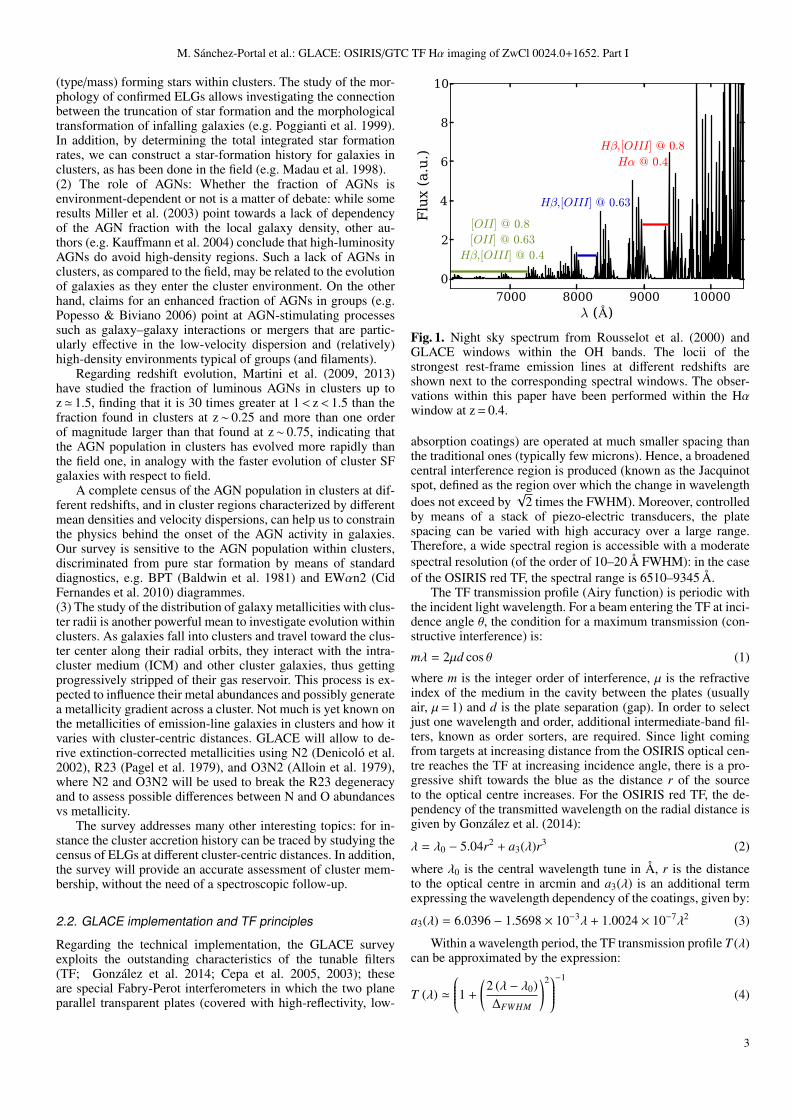
The GLACE programme (PIs. Miguel Sanchez-Portal & JordiCepa) is undertaking a panoramic census of the star formationand AGN activity within a sample of clusters at three redshiftbins defined by windows relatively free of strong atmosphericOH emission lines (Fig. 1): z∼0.40, 0.63 and 0.86, mapping thestrongest rest-frame optical emission lines: Hα (only at z∼ 0.4),Hβ, [Oii]3727 and [Oiii]5007; the sections below describe themain goals of the GLACE project and the technical implemen-tation of the project.
2.1. GLACE goals
The GLACE project is aimed at comparing the maps of ELGswith the structures of the targeted clusters (as traced by galaxies,gas and dark matter) to address several crucial issues:(1) Star formation in clusters: We will determine how the starformation properties of galaxies relate to their position in thelarge scale structure. This will provide a key diagnostic to testbetween different models for the environmental influence ongalaxy evolution. Each mechanism is most effective in a dif-ferent environment (generally depending on the cluster-centricdistance, e.g. Treu et al. 2003), leaving a footprint in the data.We are mapping the extinction-corrected star formation throughHα and [Oii], over a large and representative region in a statis-tically useful sample of clusters. The survey has been designedto reach SFR ∼2 M/yr (i.e. below that of the Milky Way) with1 magnitude of extinction at Hα1. Our first results (see sect. 4)show that we are achieving this goal. Another important ques-tion that can be addressed is related with the kind of galaxies
1 fHα = 1.89× 10⁻¹⁶ erg s−1 at z = 0.4 using standard SFR−luminosityconversion factors (Kennicutt 1998)
2
M. Sanchez-Portal et al.: GLACE: OSIRIS/GTC TF Hα imaging of ZwCl 0024.0+1652. Part I
(type/mass) forming stars within clusters. The study of the mor-phology of confirmed ELGs allows investigating the connectionbetween the truncation of star formation and the morphologicaltransformation of infalling galaxies (e.g. Poggianti et al. 1999).In addition, by determining the total integrated star formationrates, we can construct a star-formation history for galaxies inclusters, as has been done in the field (e.g. Madau et al. 1998).(2) The role of AGNs: Whether the fraction of AGNs isenvironment-dependent or not is a matter of debate: while someresults Miller et al. (2003) point towards a lack of dependencyof the AGN fraction with the local galaxy density, other au-thors (e.g. Kauffmann et al. 2004) conclude that high-luminosityAGNs do avoid high-density regions. Such a lack of AGNs inclusters, as compared to the field, may be related to the evolutionof galaxies as they enter the cluster environment. On the otherhand, claims for an enhanced fraction of AGNs in groups (e.g.Popesso & Biviano 2006) point at AGN-stimulating processessuch as galaxy–galaxy interactions or mergers that are partic-ularly effective in the low-velocity dispersion and (relatively)high-density environments typical of groups (and filaments).
Regarding redshift evolution, Martini et al. (2009, 2013)have studied the fraction of luminous AGNs in clusters up toz' 1.5, finding that it is 30 times greater at 1< z< 1.5 than thefraction found in clusters at z∼ 0.25 and more than one orderof magnitude larger than that found at z∼ 0.75, indicating thatthe AGN population in clusters has evolved more rapidly thanthe field one, in analogy with the faster evolution of cluster SFgalaxies with respect to field.
A complete census of the AGN population in clusters at dif-ferent redshifts, and in cluster regions characterized by differentmean densities and velocity dispersions, can help us to constrainthe physics behind the onset of the AGN activity in galaxies.Our survey is sensitive to the AGN population within clusters,discriminated from pure star formation by means of standarddiagnostics, e.g. BPT (Baldwin et al. 1981) and EWαn2 (CidFernandes et al. 2010) diagrammes.(3) The study of the distribution of galaxy metallicities with clus-ter radii is another powerful mean to investigate evolution withinclusters. As galaxies fall into clusters and travel toward the clus-ter center along their radial orbits, they interact with the intra-cluster medium (ICM) and other cluster galaxies, thus gettingprogressively stripped of their gas reservoir. This process is ex-pected to influence their metal abundances and possibly generatea metallicity gradient across a cluster. Not much is yet known onthe metallicities of emission-line galaxies in clusters and how itvaries with cluster-centric distances. GLACE will allow to de-rive extinction-corrected metallicities using N2 (Denicolo et al.2002), R23 (Pagel et al. 1979), and O3N2 (Alloin et al. 1979),where N2 and O3N2 will be used to break the R23 degeneracyand to assess possible differences between N and O abundancesvs metallicity.
The survey addresses many other interesting topics: for in-stance the cluster accretion history can be traced by studying thecensus of ELGs at different cluster-centric distances. In addition,the survey will provide an accurate assessment of cluster mem-bership, without the need of a spectroscopic follow-up.
2.2. GLACE implementation and TF principles
Regarding the technical implementation, the GLACE surveyexploits the outstanding characteristics of the tunable filters(TF; Gonzalez et al. 2014; Cepa et al. 2005, 2003); theseare special Fabry-Perot interferometers in which the two planeparallel transparent plates (covered with high-reflectivity, low-
7000 8000 9000 10000λ ( )
0
2
4
6
8
10
Flu
x (a
.u.)
Hβ,[OIII] @ 0.8
Hα @ 0.4
Hβ,[OIII] @ 0.63
[OII] @ 0.8
[OII] @ 0.63
Hβ,[OIII] @ 0.4
Fig. 1. Night sky spectrum from Rousselot et al. (2000) andGLACE windows within the OH bands. The locii of thestrongest rest-frame emission lines at different redshifts areshown next to the corresponding spectral windows. The obser-vations within this paper have been performed within the Hαwindow at z = 0.4.
absorption coatings) are operated at much smaller spacing thanthe traditional ones (typically few microns). Hence, a broadenedcentral interference region is produced (known as the Jacquinotspot, defined as the region over which the change in wavelengthdoes not exceed by
√2 times the FWHM). Moreover, controlled
by means of a stack of piezo-electric transducers, the platespacing can be varied with high accuracy over a large range.Therefore, a wide spectral region is accessible with a moderatespectral resolution (of the order of 10–20 Å FWHM): in the caseof the OSIRIS red TF, the spectral range is 6510–9345 Å.
The TF transmission profile (Airy function) is periodic withthe incident light wavelength. For a beam entering the TF at inci-dence angle θ, the condition for a maximum transmission (con-structive interference) is:
mλ = 2µd cos θ (1)
where m is the integer order of interference, µ is the refractiveindex of the medium in the cavity between the plates (usuallyair, µ= 1) and d is the plate separation (gap). In order to selectjust one wavelength and order, additional intermediate-band fil-ters, known as order sorters, are required. Since light comingfrom targets at increasing distance from the OSIRIS optical cen-tre reaches the TF at increasing incidence angle, there is a pro-gressive shift towards the blue as the distance r of the sourceto the optical centre increases. For the OSIRIS red TF, the de-pendency of the transmitted wavelength on the radial distance isgiven by Gonzalez et al. (2014):
λ = λ0 − 5.04r2 + a3(λ)r3 (2)
where λ0 is the central wavelength tune in Å, r is the distanceto the optical centre in arcmin and a3(λ) is an additional termexpressing the wavelength dependency of the coatings, given by:
a3(λ) = 6.0396 − 1.5698 × 10⁻³λ + 1.0024 × 10⁻⁷λ2 (3)
Within a wavelength period, the TF transmission profile T (λ)can be approximated by the expression:
T (λ) '
1 +
(2 (λ − λ0)∆FWHM
)2−1
(4)
3
M. Sanchez-Portal et al.: GLACE: OSIRIS/GTC TF Hα imaging of ZwCl 0024.0+1652. Part I
where λ0 is the wavelength at which the TF is tuned and ∆FWHMis the TF FWHM bandwidth.
Within the GLACE survey, we have applied the techniqueof TF tomography (Jones & Bland-Hawthorn 2001; Cepa et al.2013): for each line, a set of images are taken through theOSIRIS TF, each image tuned at a different wavelength (equallyspaced), so that a rest frame velocity range of several thousandskm/s (6500 km/s for our first target) centred at the mean clus-ter redshift is scanned for the full TF field of view of 8 arcminin diameter. Additional images are taken to compensate forthe blueshift of the wavelength from centre to the edge of thefield of view (as given in Eq. 2). Finally, for each pointing andwavelength tuned, three dithered exposures allow correcting foretalon diametric ghosts, using combining sigma clipping algo-rithms.
The TF FWHM and sampling (i.e.: the wavelength intervalbetween consecutive exposures) at Hα are of 12 and 6 Å, re-spectively, to allow deblending Hα from [Nii]λ6584. with an ac-curacy better than 20% (Lara-Lopez et al. 2010). For the rest ofthe lines, the largest available TF FWHM, 20 Å is applied, withsampling interval of 10 Å. These parameters also allow a pho-tometric accuracy better than 20% according to simulations per-formed within the OSIRIS team. The same pointing positions areobserved at every emission line. In order to trace the relation be-tween SF and environment in a wide range of local densities, Wehave required to cover '2 Virial radii (some 4 Mpc) within thetargeted clusters. This determines the number of OSIRIS point-ings (two pointings at 0.40 and 0.63 and just one at 0.86).
The intended GLACE sample includes nine clusters, threein each redshift bin. Currently we have been awarded with ob-serving time and completed the observations of clusters: ZwCl0024.0+1652 and RX J1257.2+4738. Tab. 1 outlines the sampleand the current status of the observations.
3. Observations and data reduction
Two OSIRIS/GTC pointings using the red TF were planned anexecuted towards Cl0024. The first one (carried out in GTCsemesters 09B, 10A and 13B; hereafter referred as “centre posi-tion”) targeted the Hα/[N ii], Hβ and [O iii] lines. The observa-tions were planned to keep the cluster core well centered withinCCD12. The second pointing (hereafter referred as “offset posi-tion”) was carried out in semesters 10B and 13B and targeted thesame emission lines. This second pointing was offset by ∆α= -2.3 arcmin, ∆δ= +2.5 arcmin (i.e. some 3.4 arcmin in the NWdirection). A summary of the observations is presented in Tab. 2.Within the scope of this paper, we shall present the results fromthe Hα/[N ii] observations. The total on-source exposure time is5.1 and 2.9 hours at the central and offset pointings, respectively.
The Hα/[N ii] spectral range 9047–9341 Å was covered by50 evenly spaced scan steps3 (∆λ= 6 Å). Taking into accountthe radial wavelength shift described by Eq. 2, the spectral rangesampled over the entire field of view (of 8 arcmin diameter) issomewhat smaller, 9047–9267 Å (the ranges 9267–9341 Å and8968–9047 Å are partially covered in the central and external re-gions of the field of view, respectively). At each TF tune, three
2 The OSIRIS detector mosaic is composed of two 2048× 4096pixel CCDs abutted, with a plate scale of 0.125 arcsec/pixel.See Cepa et al. (2005) and the OSIRIS Users’ manual athttp://www.gtc.iac.es/instruments/osiris/media
3 three scan steps, at 9317.4 and 9323.4 and 9341.4 Å were acciden-tally omitted in the observations of the offset positions; hence only 47slices are available for that pointing.
individual exposures with an “L” shaped dithering pattern of10 arcsec amplitude were taken (in order to allow the removalof fringes and to ease the identification of diametric ghosts;the amplitude was chosen similar to the gap between the de-tectors). While this observing strategy has revealed useful forremoving the fringing patterns that are specially evident beyondλ' 9300 Å, it introduces an additional complexity since the po-sition of a source within the CCD varies in each dither position,and therefore, the wavelength at which it is observed due to theradial wavelength shift experienced in TFs.
3.1. TF data reduction procedures
The data reduction was performed using a version of thetfred package Jones et al. (2002) modified for OSIRIS by A.Bongiovanni (Ramon-Perez et al. in prep.) and private iraf4 andidl scripts written by our team. The basic reduction steps werecarried out using standard iraf procedures and included bias sub-traction and flat-field normalization; the next reduction step wasa TF-specific one, namely the removal of the diffuse, optical-axiscentred sky rings produced by atmospheric OH emission linesas a consequence of the radial-dependent wavelength shift de-scribed by Eqs. 2 and 3; to this end, the tfred task tringSub2was used. It corrects each individual exposure by means of abackground map created by computing the median of severaldithered copies of the object-masked image. Fringing was alsoremoved when required using the dithered images taken withthe same TF tune. Then, the frames were aligned and a deepimage obtained by combining all individual exposures of ev-ery scan step. This combination was done by applying a me-dian filter. While this could potentially lead to the loss of lineemitters with very low-continuum level, it is the best methodto remove spurious features as ghosts. When compared with thedeep image obtained adding up all the individual scans, applyinga simple minimum-maximum rejection filter, we have observedthat, at most, one line emitter per CCD gets lost but more thanone-hundred spurious features are effectively removed. The as-trometry was performed in the resulting deep image, using irafstandard tasks (ccxymatch and ccmap). The sky position of ref-erence objects were gathered from the USNO B1.0 catalogue(Monet et al. 2003) in the centre position, while for the offset onewe obtained better results using the 2MASS catalogue (Skrutskieet al. 2006); the achieved precision was in both cases equal orbetter than 0.3 arcsec r.m.s. (i.e. of the order of the binned pixelsize). The deep images were used to extract the sources by meansof the SExtractor package (Bertin & Arnouts 1996). The numberof sources detected above 3σ are 931 and 925 in the centre andoffset positions, respectively (after removing a number of clearlyspurious sources appearing at the edges of the detectors). Sincethere is a quite large overlap between both positions, we found374 common sources after matching both source catalogues us-ing topcat (Taylor 2005). These common sources were used asa test of the relative consistency of our astrometry: 245 sources(65%) were found within a match radius of 0.5 arcsec (i.e. con-sistent with the quoted accuracy), 88 (24%) within 0.75 arcsecand 15 (4%) within 1.0 arsec radius. A number of sources (26objects, i.e. 7%) were matched at larger radii (around 1.5 arcsec)but these sources were always found at the edges of the images,were the OSIRIS field suffers a larger distortion.
4 iraf is distributed by the National Optical Astronomy Observatory,which is operated by the Association of Universities for Research inAstronomy (AURA) under cooperative agreement with the NationalScience Foundation.
4
M. Sanchez-Portal et al.: GLACE: OSIRIS/GTC TF Hα imaging of ZwCl 0024.0+1652. Part I
Table 1. GLACE sample and status of the observations
Name RA(J2000) Dec(J2000) z StatusZwCl 0024.0+1652 00 26 35.7 +17 09 45 0.395 Completed; programmes GTC63-09B, GTC8-
10AGOS, GTC47-10B & GTC75-13BAbell 851 09 42 56.6 +46 59 22 0.407 PlannedRX J1416.4+4446 14 16 28.7 +44 46 41 0.40 PlannedXMMLSS-XLSSC 001 02 24 57.1 -03 48 58 0.613 PlannedMACS J0744.8+3927 07 44 51.8 +39 27 33 0.68 PlannedCl J1227.9-1138 12 27 58.9 -11 35 13 0.636 PlannedXLSSC03 02 27 38.2 -03 17 57.0 0.839 PlannedRX J1257.2+4738 12 57 12.2 +47 38 07 0.866 Completed; ESO/GTC programme 186.A-2012Cl 1604+4304 16 04 23.7 +43 04 51.9 0.89 Planned; Cl 1604 supercluster
Table 2. Log of the OSIRIS/TF observations of the region centred around the Hα emission line in the Cl0024 cluster.
Centre Positionλ0,i OS Filter Date Seeing N Steps N Exp. Exp. Time
(nm) (′′) (s)904.74 f893/50 2009 Dec 05 0.7 – 0.9 6 3 53
2010 Aug 17 0.8 6 3 85908.34 f902/40 2010 Aug 21 0.8 11 3 60908.74 f902/40 2009 Dec 05 0.7 – 0.9 2 3 53909.54 f902/40 2009 Nov 25 0.9 – 1.1 9 3 53914.94 f910/40 2009 Nov 25 0.9 – 1.1 9 3 53
2010 Aug 01 0.8 14 3 60920.34 f910/40 2009 Dec 05 0.6 – 0.8 5 3 53923.34 f919/41 2009 Dec 05 0.6 – 0.8 4 3 53
2010 Aug 18 0.8 3 3 60925.14 f919/41 2010 Aug 18 0.8 5 3 100928.14 f919/41 2010 Aug 18 0.8 3 3 120929.94 f919/41 2010 Aug 19 0.9 3 3 190931.74 f923/34 2010 Aug 19 0.9 2 3 170932.94 f923/34 2010 Aug 21 0.8 3 3 120
Offset Positionλ0,i OS Filter Date Seeing N Steps N Exp. Exp. Time
(nm) (′′) (s)904.74 f893/50 2010 Oct 01 <1.0 6 3 60908.34 f902/40 2010 Nov 08 1.0 – 1.2 11 3 60914.94 f910/40 2010 Sep 20 <0.8 14 3 60923.34 f919/41 2010 Nov 08 0.9 – 1.2 3 3 60925.14 f919/41 2010 Nov 08 0.9 – 1.2 5 3 100928.14 f919/41 2010 Nov 08 0.9 – 1.2 3 3 120929.94 f919/41 2010 Nov 08 1.0 – 1.2 3 3 120932.94 f923/34 2010 Oct 01 <1.0 2 3 120
The catalogue of detections contains 1482 unique sources.For each detected source and scan step, the best possible combi-nation of individual images, i.e. the best combinations of TF tuneand dither position at the location of the source was computed.In practice, we deemed as “best combination” algorithm the se-lection of all the images for which the TF wavelength at the posi-tion of the source lies within a range of ±3 Å (i.e. half scan step)of the given one. For each of these combinations, a syntheticequivalent filter transmission profile was derived by adding upthe transmission profiles of all the images entering the combina-tion and fitting to the result the function given in Eq. 4. Thesesynthetic profiles allowed us to verify that our combination ap-proach does not introduce a significant error neither in the wave-length of the central position (less than 1 Å maximum) nor in theFWHM (the average equivalent FWHM is 12.7 Å with a devia-tion of 0.4 Å). The output combined image is used to determinethe flux at this specific scan step and source position by means
of SExtractor. The resulting “pseudo-spectra” consist of 50 (47)tuples (λ at source position, flux). The FWHM of the equiva-lents (synthetic) TF Airy transmission profiles derived at eachsource position and TF tune were also included in each pseudo-spectrum file. A pseudo-spectrum should not be confused witha standard spectrum produced by a dispersive system: the fluxat each point of the pseudo-spectrum is that integrated withina filter passband centred at the wavelength of the point; there-fore, mathematically a pseudo-spectrum is the convolution of thesource spectrum with the TF transmission profile.
3.2. Flux calibration
The flux calibration of each TF tune has been carried out in twosteps: first, the total efficiency ε(λ) of the system (telescope, op-tics and detector) should be derived; it is computed as the ratioof the measured to published flux Fm(λ)/Fp(λ) for a set of ex-
5
M. Sanchez-Portal et al.: GLACE: OSIRIS/GTC TF Hα imaging of ZwCl 0024.0+1652. Part I
Table 3. Spectrophotometric standard stars
Name m(λ) Reference PositionG157–34 15.35(5400) Filippenko &
Greenstein (1984)offset
G191–B2B 11.9(5556) Oke (1990) offsetRoss 640 13.8(5556) Oke (1974) centre
Table 4. Efficiencies for Cl0024 observations
Position λ≤ 9270 Å λ> 9270 Å〈ε〉 Zero point Slope
Centre 0.1779± 0.0236 10.2497± 1.2181 -0.0011± 0.0001Offset 0.1993± 0.0035 12.8566± 0.9074 -0.0014± 0.0001
posures of spectrophotometric standard stars (Tab. 3) taken inphotometric conditions within a range of tunes compatible withthat of the cluster observation (ideally at the same tunes). Thefluxes of the standards are measured by aperture photometry,and the exact wavelengths at the positions of the star are derivedfrom Eqs. 2 and 3. The published fluxes are also derived at thesewavelengths by means of a polynomial fit to the tabulated fluxes(see references in Tab. 3). Then, measured fluxes in engineeringunits (ADU) are converted to physical units (ergs s−1 cm−2 Å −1)using the expression:
Fm(λ) =g K(λ) Eγ(λ)
t Atel δλeFADU(λ) (5)
where g is the CCD gain in e−ADU−1, Eγ(λ) is the energy ofa photon in ergs, t is the exposure time in seconds, Atel is thearea of the telescope primary mirror in cm2, δλe is the effectivepassband width5 in Å, and K(λ) is the correction for atmosphericextinction,
K(λ) = 100.4 k(λ) 〈χ〉 (6)
dependent on the extinction coefficient k(λ) and the mean air-mass 〈χ〉 of the observations. In our case, we estimated k(λ) byfitting the extinction curve of La Palma6. in the wavelength rangeof interest.
The uncertainty in the efficiency has been computed by er-ror propagation, taking into account the errors in the measuredfluxes (that in turn include terms to cope with the error of theaperture photometry and the uncertainty of the wavelength tune)and those of the published ones.
The efficiency ε(λ) (sampled with 9 tunes at position A and19 tunes at position B) must be then fitted to an analytical func-tion of λ in order to perform the calibration at the wavelength ofeach tune and source. In both cases, the best solution has beena constant efficiency for λ≤ 9270 Å and a linear decreasing de-pendency at longer wavelengths (Tab. 4).
The second step is to convert the measured flux in ADU ofeach source at each tune i to physical units (ergs s−1 cm−2 Å −1)by means of the expression:
f (λ)i =g K(λ) Eγ(λ)t Atel δλe ε(λ)
fADU,i (7)
where ε(λ) is the total efficiency computed above and the re-maining terms are as in Eq. 5. The flux errors are computed again
5 δλe = π2 FWHMT F
6 http://www.ing.iac.es/Astronomy/observing/manuals/ps/tech notes/tn031.pdf
by propagation, taking into account the efficiency errors derivedabove and the source flux measurement uncertainty computed bythe tfred tspect task as:
∆ f =
√Apixσ2 + f /g (8)
where Apix is the measurement aperture area in pixels, σ is thestandard deviation of the background noise and g is the gain inin e−ADU−1.
3.3. Ancillary data
Within the process of generation of the catalogue of line emittersand further data analysis, we have made use of public Cl0024catalogues7 from the collaboration “A Wide Field Survey ofTwo z=0.5 Galaxy Clusters” (Treu et al. 2003; Moran et al.2005, hereafter M05) that include photometric data for 73318sources detected and extracted in the HST WFPC2 sparse mo-saic covering 0.5 × 0.5 degrees (Treu et al. 2003) and in ground-based CFHT CFH12k BVRI and Palomar WIRC JKs imag-ing. Visually determined morphological types are given for allsources brighter than I=22.5. In addition, thousands of photo-metric and spectroscopic redshift estimates are available. Thecatalogue of spectroscopically confirmed objects within the field(including foreground, cluster and background sources) com-prises 1632 sources (see Moran et al. 2007, and referencestherein).
4. The Catalogue of ELGs
In order to produce a catalogue of ELGs we start by selectingthe line emitters The first step to get the catalogue of ELGs isto perform the selection of line emitters (either Hα at the red-shift of the cluster, or other lines in the case of backgroundcontaminants). In many cases, the emission line showed veryclear, and even in a fraction of the emitters the Hα and [N ii]lines appeared clearly resolved, but given the number of in-put sources, an automated or semi-automated procedure wasrequired. The tfred package provides with a task, tscale,that outputs the putative ELGs from the source catalogue, butwhen applied to our input catalogue, it did not yield reliableresults: it was designed for a reduced number of scans andsparse spectral sampling and frequently failed to classify eventhe most obvious ELGs from our densely sampled pseudo-spectra. Instead, we have followed a different approach, creatingan automatic selection tool, implementing the following steps:(i) Define a “pseudo-continuum” (hereafter referred as pseudoc)as the subset of pseudo-spectrum points resulting from discard-ing “high/low” outlier values, defined as those above/below themedian value f luxalldata ± 2×σalldata; the “pseudo-continuum”level, f luxpseudoc, will be defined as its median and the “pseudo-continuum” noise, σpseudoc, as its standard deviation. (ii) The“upper” value will be defined as f luxpseudoc + 2×σpseudoc. Then,the criteria to determine a reliable ELG candidate have beendefined as: a) either two consecutive values above “upper” arefound, or b) or one point above “upper” is found and, in addition,one contiguous point above f luxpseudoc +σpseudoc and one con-tiguous point above f luxpseudoc. These criteria have been chosensince we have observed in our simulations (see below) that evenvery narrow lines (0.7 Å) always produce a high positive signalin at least two scan slices around the maximum. Single-point
7 http://www.astro.caltech.edu/∼smm/clusters/
6
M. Sanchez-Portal et al.: GLACE: OSIRIS/GTC TF Hα imaging of ZwCl 0024.0+1652. Part I
peaks in the pseudo-spectrum are attributed to noise or artefacts.On the other hand, the criteria above can cope with broad-lineAGNs (see sect. 8).
In order to investigate the reliability of this automatic clas-sifier, we have created a number of simulated spectra compris-ing an emission line with a Gaussian profile and a flat contin-uum (a good approximation within our relatively small spectralrange). This simple spectrum is convolved with an Airy pro-file with FWHM = 12 Å and sampled at steps of 6 Å to pro-duce a noiseless pseudo-spectrum. Finally, a noise componentis built drawing random values from a normal distribution withzero mean and varying standard deviation and added to thepseudo-spectrum signal. We have built a collection of 800 suchpseudo-spectra varying different input parameters, namely: (i)the range of intrinsic line widths of the lines has been adoptedfrom the typical limiting values of the integrated line profilesof giant extragalactic Hii regions from Roy et al. (1986), fromsome 20 km s−1 to about 40 km s−1 that corresponds to a rangeFWHMline = 0.7–1.5 Å (rest frame) with 0.4 Å step; this rangehas been further extended by one additional step up to 2.3 Å(65 km s−1) in order to cope with blending of several Hii re-gions within the galaxy; (ii) the range of shifts of the peak of theline with respect to the maximum filter transmission has beenset to 0–3 Å with 1 Å step (i.e. consistent with the scan step of6 Å); (iii) the equivalent width (EW) of the emission line hasbeen varied in the range 5–15 Å with steps of 1 Å (this range ex-plores our detection sensitivity threshold; at larger EW we do notexpect line identification problems) (iv) and finally, the ampli-tude (standard deviation) of the added random noise component,σnoise, has ben set in the range 0.1 to 0.4 times the maximum ofthe line, with steps of 0.1.
The automatic classifier has identified as line emitters 726out of the 800 simulated pseudo-spectra (i.e. more than 90%).From those, only in two cases the classifier chose the sourcebased in a noise feature rather than the correct line. As expected,the 74 pseudo-spectra not classified as ELG are in the high noiserange (0.3 or 0.4).
Moreover, in order to determine the possibility of automat-ically classifying as ELG a passive galaxy, we have generatedin a similar way a set of pseudo-spectra based on a flat contin-uum and σnoise in the range 0.1 to 0.3 times the continuum fluxvalue, with steps of 0.01 (a finer step was chosen in order to cre-ate a sufficient large number of instances, given that the noise isthe only variable parameter). At each noise step, we have gener-ated 21 instances yielding a total number of 420 pseudo-spectra.From these, 316 (i.e. more than 75%) have been classifed as pas-sive, while the remaining 104 (i.e. less than 25%) have been clas-sified as ELG.
The results of the simulations indicate that our simple clas-sification algorithm is quite effective to classify true ELGs asa line emitters, but can also pick a non-negligible amount ofnoisy pseudo-spectra of passive galaxies as emission-line ob-jects. Therefore, we have added an additional step, filtering thesample produced by the selection tool by a careful visual inspec-tion of the pseudo-spectra and also of the thumbnails of all scanslices for every source of this output sample (this was done bythree collaborators separately). After applying these two steps,we have extracted a sample of 210 very robust (i.e. high S/N)ELGs, comprising both star-forming galaxies and AGNs.
4.1. Line wavelength estimation
Estimating the wavelength of the Hα line is possible with TFtomography, but it is generally a complex issue, since on theone hand, we have a blend of three lines (the Hα line plus thetwo components of the [N ii] doublet), convolved with the trans-mission profile of the TF and, as will be described in sect. 5,in many cases the pseudo-spectrum line “profile” (hereafter re-ferred as line pseudo-profile) is affected by absorption-like fea-tures. We have attempted to derive the Hα line position con-sidering a model comprising three Gaussian lines plus a lin-ear continuum; the rest-frame wavelength relative positions arefixed, as is the ratio of the two [N ii] doublet components (setto f6548/ f6583 = 0.3). Free parameters of the model are: the ob-served wavelength of the Hα line, the line width (constrained tobe the same for the three lines), the [N ii] λ 6583 and Hα fluxesand the continuum level. This model spectrum has been con-volved with the TF transmission profile and fitted by means ofnon-linear least squares to the pseudo-spectra profiles. For some30% of the sources, the result of the fit reproduces accurately thepseudo-spectrum profile, but in a vast majority of the cases thefit either fails or provides inaccurate results due to noise in thepseudo-continuum, absorption-like features in the line pseudo-profile, etc. Eventually, we have decided to derive the position ofthe line by manually fitting the pseudo-spectrum using the IRAFsplot task and either a Gaussian or a Lorentzian profile, choos-ing after inspection the appropriate range to avoid continuumnoise and contaminant lines. There is a very good agreement be-tween the line positions computed by splot and those resultingfrom the trustful, accurate model fits (∼ 1 Å). In a minority of thecases, where the line profile showed very asymmetric (e.g. whenabsorption-like features are present, most likely due to randomnoise as shown in sect. 5 below), the position of the line waschosen to be the peak value of the pseudo-spectrum. Given thedifficulty of providing a trustful uncertainty figure, we have as-sumed a constant error value of 3 Å for the fit to the peak of theline, i.e. half of a scan step; this error is square-added to the tun-ing uncertainty of 1 Å and to the wavelength error introducedby the combination of images performed in order to producethe pseudo-spectrum (see sect. 3.1), also considered to be 1 Åat most; hence, σpos ' 3.3 Å.
4.2. Identification of Hα emitters: rejection of interlopers
The observations presented here target a single emission line;therefore, a number of interlopers can be present; these are ex-pected to be ELGs at other redshifts. When observing Hα atz = 0.40, [O iii]λ 5007 Å emitters at z = 0.83 and [O ii]λ 3727 Åemitters at z = 1.46 can be detected as well. However, at the lim-iting fluxes considered here these contaminants are not expectedto be very abundant and can be easily discriminated via colour-colour diagrammes. We have implemented such colour-colourdiagnostic diagrams following Kodama et al. (2004) accordingto the following steps: first, we have matched our initial cata-logue of 210 robust candidates with the photometric and spectro-scopic catalogue from M05 and a matching radius of 1.0 arcsec(i.e. compatible with the accuracy of our astrometry). A coun-terpart with at least photometric data has been found for 202sources. Using the CFHT CFH12k aperture photometry, we havecomputed the B − V , V − R and R − I colours. The diagnose gridhas been built by deriving synthetic colours for COSMOS tem-plates Ilbert et al. (2009) of Sa, Sc, and starburst (SB) galaxiesat redshifts ranging from z = 0 to z = 1.0 with steps of 0.1, in-
7
M. Sanchez-Portal et al.: GLACE: OSIRIS/GTC TF Hα imaging of ZwCl 0024.0+1652. Part I
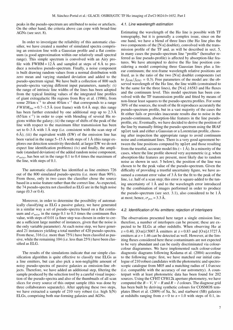
tegrated to the CFH12k B, V , R and I passbands. Also, modelsfrom from Kodama et al. (1999) at z = 0.4 and z = 0.5 have beenincluded in the grid. The diagrammes for B − V vs. V − R andV − R vs. R − I are shown in Fig. 2. A source has been deemedas interloper if: (i) the source is outside the cluster region (as de-picted in Fig. 2) in both colour diagrammes and does not have aspectroscopic redshift from M05 within the cluster range (set as0.35≤ z≤ 0.45); (ii) the source has a spectroscopic redshift fromM05 outside the cluster range, independent of its colours.
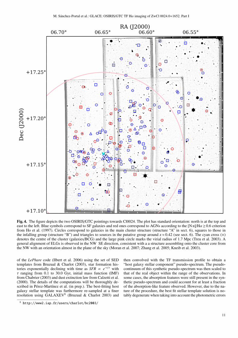
Based on the first criterion, we have deemed 19 sources ascontaminants. These are in a vast majority of the cases locatedin the locus of the colour-colour diagram occupied by galaxiesat z = 0.8–1.0, i.e. consistent with being [O iii]λ 5007 Å emitters.Moreover, 97% of the ELGs with a redshift from M05 within thecluster range have been also catalogued as cluster members bythe colour-colour diagnostic described above. The second crite-rion added 9 additional sources as interlopers (two sources havebeen discarded by both colours and redshift criteria). Hence, 28objects have been classified as contaminants at a different red-shift. In addition, 8 sources do not have a counterpart in the M05catalogue and therefore have been excluded from the cluster list.Therefore, our final catalogue consists of 174 robust cluster Hαemitters (see the distribution of sources in the sky in Fig. 4), 28putative interlopers (ELGs at a different redshift, mostly oxy-gen emitters at z∼ 0.9) and 8 sources without ancillary data toperform the assessment. Future analysis of additional spectralranges (centred at the [O iii] and Hβ wavelengths at the nominalredshift of Cl0024) will refine this rejection criterion. The 174sources in our final catalogue of unique robust cluster emittersare listed in Tab. 5. From these, 112 have spectroscopic redshiftsin the M05 catalogue.
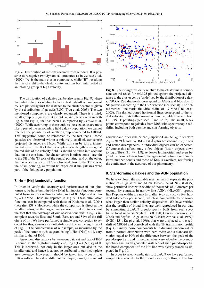
Fig. 3 shows a selection of high signal-to-noise pseudo-spectra. In many cases, the strongest [N ii] doublet component(at 6583 Å) is clearly separated from the Hα line in a visual in-spection. Sometimes the line is observed as a “shoulder” at thelong wavelength side of the Hα line.
5. Derivation of line fluxes
From the pseudo-spectra described in sect. 4, it is possible to de-rive the Hα and [N ii] fluxes following several approaches. Wehave applied a straightforward procedure derived from the stan-dard narrow-band on-band/off-band technique, using for eachsource the flux in the scan slice closest to the computed posi-tion of the Hα line (see sect. 4) and that of the slice closest to the[N ii] line; as will be shown below, this method, though simple,produces acceptable results when compared to the more sophis-ticated procedure based on least-squares fitting of the pseudo-spectrum to a model spectrum convolved with the transmissionprofile of the TF described in sect. 4.1 with the advantage thatthe former method is always applicable while the latter can beonly used in a minority of cases.
We start by subtracting a linear continuum. This can be eas-ily done by applying a linear fit to the regions of the pseudo-spectrum excluding the emission line. Then, assuming infinitelythin lines, the Hα and [N ii] line fluxes, denoted by f (Hα) andf ([N ii]) respectively, are given by the expressions (Cepa, priv.comm.):
fon,Hα = THα (Hα) f (Hα) + THα ([N ii]) f ([N ii])fon,[N ii] = T[N ii] (Hα) f (Hα) + T[N ii] ([N ii]) f ([N ii]) (9)
where fon,Hα and fon,[N ii] are the continuum-subtracted fluxes inthe chosen Hα and [N ii] slices and T<slice> (< line >) denotesthe TF transmission of a given slice at a given line wavelength.The different transmission values can be easily derived from theapproximate expression given in Eq. 4. From Eq. 9 we can easilyderive the flux in the Hα line:
f (Hα) =fon,HαT[N ii] ([N ii]) − fon,[N ii]THα ([N ii])
THα (Hα) T[N ii] ([N ii]) − THα ([N ii]) T[N ii] (Hα)(10)
And a similar expresion for the [N ii] line. The errors in thelines have been derived by propagation, taking into account notonly the errors in the Hα and [N ii] “on” bands, but also the con-tinuum noise (i.e. the noise around the zero-level continuum af-ter removing the linear fit explained above). Hence, the line errorhas been computed as:
∆ f (Hα) = ((T[N ii] ([N ii]) ∆ fon,Hα
)2 (11)
+(THα ([N ii]) ∆ fon,[N ii]
)2)
+((
T[N ii] ([N ii]) − THα ([N ii]))σcont
)2)1/2
/(THα (Hα) T[N ii] ([N ii]) − THα ([N ii]) T[N ii] (Hα)
)where ∆ fon,Hα and ∆ fon,[N ii] are the flux errors in the “on” Hαand [N ii] bands computed as indicated in sect. 3.2 and σcont isthe continuum error measured as the standard deviation of thepoints within the region of the pseudo-spectrum excluding theemission lines. The contribution of the continuum noise to thetotal error is important, on average ∼ 30% at the central positionand much larger at the offset position where the exposure timesare smaller, on average 60–70%.
The median fractional error in the Hα fluxes is ≈ 24%. A70% of the sample objects have relative errors below 30%. Thiserrors are compatible with those quoted by Lara-Lopez et al.(2010) (see sect. 2.2), though somewhat larger than those de-rived from their simulations due to our larger continuum errors.However, since the [N ii] line is usually fainter than the Hα line,its flux errors are in general notably larger: the average fractionalerror is ≈ 54% and only 15% of the sample objects have a relativeerror below 30%. This was of course expected since the detec-tion/selection algorithm is driven by the strongest line presentin the pseudo-spectrum. Hence, in many cases the Hα line actsas a “prior” and the nitrogen flux is extracted at the expectedwavelength of the (otherwise barely detected) [N ii] line.
As mentioned above, the line flux estimation is based inan infinitely thin line approximation which assumes that theline can be well represented by δ(λ − λz), where λz = λ0(1+ z). According to Pascual et al. (2007), for star-forminggalaxies, emission line widths are mass-related and typicallyFWHM. 10 Å× (1 + z), and, for narrow-band filters of some50 Å width, it is possible to recover ∼ 80% of the line flux upto z∼ 4. We have investigated the impact of applying such ap-proximation to our very narrow TF scans (∼ 12 Å). To this end,we have performed several simulations using Gaussian line pro-files of several widths peaking at different offsets with respect tothe maximum of the filter transmission profile (Eq. 4). The emis-sion line broadening is given by the relation (Fernandez Lorenzoet al. 2009):
2Vmax =∆λc
λ0 sin(i)(1 + z)(12)
where Vmax is the maximum rotation velocity, λ0 is the linewavelength at z = 0 and ∆λ is the line width at 20% of peak
8
M. Sanchez-Portal et al.: GLACE: OSIRIS/GTC TF Hα imaging of ZwCl 0024.0+1652. Part I
Fig. 2. B − V vs. V − R (left) and V − R vs. R − I (right) diagnostic diagrams. The sample, comprising 202 unique objects withcounterparts in the M05 catalogue is denoted by cross symbols (+). The red triangles (4) mark objects with spectroscopic redshiftzs > 0.5 in the M05 catalogue. The control grid has been built using synthetic colours from COSMOS templates for Sa, Sc and SBgalaxies in the range z = 0.0–1.0 with steps of ∆z = 0.1. The thick, black dashed line connects the three templates at z = 0.4. The bluedashed line depicts the Kodama et al. (1999) models at z = 0.4 and z = 0.5. The thick, black solid line box marks the approximateregion used for selecting the cluster candidates.
intensity. For a Gaussian line, ∆λ= 1.524×FWHM. AssumingVmax = 200 km s−1 as a safe upper limit (see for instanceFernandez Lorenzo et al. 2009), the Hα line FWHM' 8 Å (herewe assume that the line is unresolved. The possibility that theline appears resolved in our pseudo-spectra due to kinematicalsplit is investigated below). For narrow lines, FWHM = 2 Å, weare able to recover 96–98% of the flux (from 0 to 2 Å offset),while for the widest simulated lines, FWHM = 8 Å, the fractionof recovered flux is in the range 73–76%. In order to comparethe simulations with real results, we have used the small set ofpseudo-spectra for which a reliable fit to the model spectrum wasachieved, finding that the average ratio between the flux derivedfrom the infinitely thin line approximation and that derived fromthe best fit is 0.81 and 0.88 for the Hα and [N ii] lines, respec-tively, i.e. well aligned with the results of our simulations.
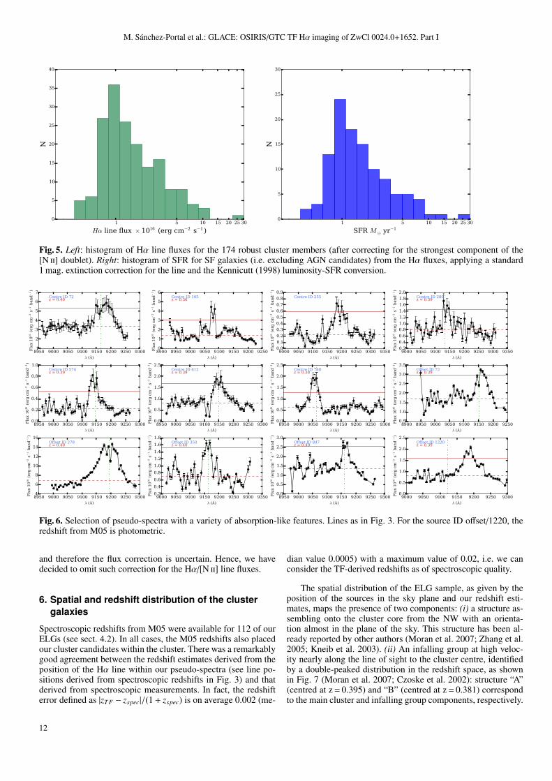
The completeness limit of the ELG sample, as given by themaximum of the flux histogram depicted in Fig. 5 (left panel)is ∼ 0.9× 10⁻¹⁶ erg s−1cm−2, i.e. better than the GLACE require-ments.
5.1. Absorption-like features in the pseudo-spectra
In a large number of cases, we have observed in the pseudo-spectra absorption-like features affecting the (putative) Hα emis-sion line. This affects around 50% of the galaxies, and showsvery clear in about 25% of the cases, as those depicted in Fig. 6.We have explored a number of possible explanations: first, andperhaps most obvious, that the absorption-like features are due
to random noise. These characteristics have been observed inthe simulations described in the preceding sections, in approxi-mately 20% of the cases (some 146 out of 726 simulated pseudo-spectra classified as ELGs). This is therefore a very probableexplanation in an ample fraction of cases. In addition, we haveexplored two potential physical explanations: either an emissionline split due to the galaxy rotation or the presence of under-lying stellar absorption. In order to investigate the first possi-ble cause, we have performed a series of simulations similarto those described in the preceding section but starting with aspectrum comprising two identical Gaussian lines with separa-tion 2λ0(1 + z)Vmax/c and a flat continuum in order to re-createthe effect of the rotational split in TF pseudo-spectra. We havebuilt our collection of pseudo-spectra varying the range of intrin-sic line widths in the range FWHMline = 0.7–2.3 Å (rest frame)with 0.4 Å step; the range of shifts of the peak of the line withrespect to the maximum filter transmission has been set to 0–3 Åwith 1 Å step and finally the galaxy rotational speed has been letto vary in the range Vmax = 100–200 km s−1 with 10 km s−1 step,in agreement with Fernandez Lorenzo et al. (2009); hence, theseparation between the two line peaks ranges from some 6.1 Åto about 12.3 Å; and finally the amplitude of the added randomnoise component (σnoise) has ben set in the range 0.1 to 0.3 timesthe maximum of the line, with steps of 0.1.
After inspecting 1320 pseudo-spectra simulated as describedabove, we have observed that the fraction of absorption-like fea-tures observed in the pseudo-spectra is relatively low at rota-tional speeds ≤ 160 km s−1, ranging from approximately 10% at
9

M. Sanchez-Portal et al.: GLACE: OSIRIS/GTC TF Hα imaging of ZwCl 0024.0+1652. Part I
Fig. 3. Selection of 28 pseudo-spectra with high signal-to-noise. The green dashed-dotted lines correspond to spectroscopic or securephotometric redshifts from M05 (when available). The dashed red line corresponds to the approximate pseudo-spectrum continuumlevel, and the solid red line to the 3σcont level, where σcont is the pseudo-continuum noise. For the source ID offset/686, the redshiftfrom M05 is photometric.
100 km s−1 to some 26% at 160 km s−1 and therefore consistentwith noise-induced features. However, the fraction of featuresobserved raises notably for Vmax ≥ 170 km s−1, being of 45% at170 km s−1 and 58%–60% above that speed. Therefore, a kine-matical line split due to galaxy rotation is a plausible mechanismto induce a fraction of the absorption-like features observed.Nevertheless, it should be taken into account that the fraction ofsuch fast-rotating galaxies is reduced (around 14% in the sampleof Fernandez Lorenzo et al. 2009, in the range 0.3< z< 0.8) and
moreover that we are assuming sin i = 1, i.e. edge-on or nearlyedge-on galaxies so the actual fraction of objects fulfilling theconditions is probably on the order of 14% at most.
We have finally explored the possibility that theseabsorption-like features are caused by true absorption due tothe underlying host galaxy stellar component. To this end, themost likely host galaxy stellar population was derived by fit-ting the public photometric information from M05 (B, V, R,I from CFHT; J, Ks from WIRC at Palomar 200”) by means
10
M. Sanchez-Portal et al.: GLACE: OSIRIS/GTC TF Hα imaging of ZwCl 0024.0+1652. Part I
Fig. 4. The figure depicts the two OSIRIS/GTC pointings towards Cl0024. The plot has standard orientation: north is at the top andeast to the left. Blue symbols correspond to SF galaxies and red ones correspond to AGNs according to the [N ii]/Hα≥ 0.6 criterionfrom Ho et al. (1997). Circles correspond to galaxies in the main cluster structure (structure “A” in sect. 6), squares to those inthe infalling group (structure “B”) and triangles to sources in the putative group around z≈ 0.42 (see sect. 6). The cyan cross (×)denotes the centre of the cluster (galaxies/BCG) and the large pink circle marks the virial radius of 1.7 Mpc (Treu et al. 2003). Ageneral alignment of ELGs is observed in the NW SE direction, consistent with a a structure assembling onto the cluster core fromthe NW with an orientation almost in the plane of the sky (Moran et al. 2007; Zhang et al. 2005; Kneib et al. 2003).
of the LePhare code (Ilbert et al. 2006) using the set of SEDtemplates from Bruzual & Charlot (2003), star formation his-tories exponentially declining with time as SFR ∝ e−t/τ withτ ranging from 0.1 to 30.0 Gyr, initial mass function (IMF)from Chabrier (2003) and dust extinction law from Calzetti et al.(2000). The details of the computations will be thoroughly de-scribed in Perez-Martınez et al. (in prep.). The best-fitting hostgalaxy stellar template was furthermore re-sampled at a finerresolution using GALAXEV8 (Bruzual & Charlot 2003) and
8 http://www2.iap.fr/users/charlot/bc2003/
then convolved with the TF transmission profile to obtain a“host galaxy stellar component” pseudo-spectrum. The pseudo-continuum of this synthetic pseudo-spectrum was then scaled tothat of the real object within the range of the observations. Insome cases, the absorption features were still present in the syn-thetic pseudo-spectrum and could account for at least a fractionof the absorption-like feature observed. However, due to the na-ture of the procedure, the best fit stellar template solution is no-tably degenerate when taking into account the photometric errors
11
M. Sanchez-Portal et al.: GLACE: OSIRIS/GTC TF Hα imaging of ZwCl 0024.0+1652. Part I
1 5 10 15 20 25 30
Hα line flux × 1016 (erg cm−2 s−1 )
0
5
10
15
20
25
30
35
40
N
1 5 10 15 20 25 30
SFR M¯ yr−1
0
5
10
15
20
25
30
N
Fig. 5. Left: histogram of Hα line fluxes for the 174 robust cluster members (after correcting for the strongest component of the[N ii] doublet). Right: histogram of SFR for SF galaxies (i.e. excluding AGN candidates) from the Hα fluxes, applying a standard1 mag. extinction correction for the line and the Kennicutt (1998) luminosity-SFR conversion.
Fig. 6. Selection of pseudo-spectra with a variety of absorption-like features. Lines as in Fig. 3. For the source ID offset/1220, theredshift from M05 is photometric.
and therefore the flux correction is uncertain. Hence, we havedecided to omit such correction for the Hα/[N ii] line fluxes.
6. Spatial and redshift distribution of the clustergalaxies
Spectroscopic redshifts from M05 were available for 112 of ourELGs (see sect. 4.2). In all cases, the M05 redshifts also placedour cluster candidates within the cluster. There was a remarkablygood agreement between the redshift estimates derived from theposition of the Hα line within our pseudo-spectra (see line po-sitions derived from spectroscopic redshifts in Fig. 3) and thatderived from spectroscopic measurements. In fact, the redshifterror defined as |zT F − zspec|/(1 + zspec) is on average 0.002 (me-
dian value 0.0005) with a maximum value of 0.02, i.e. we canconsider the TF-derived redshifts as of spectroscopic quality.
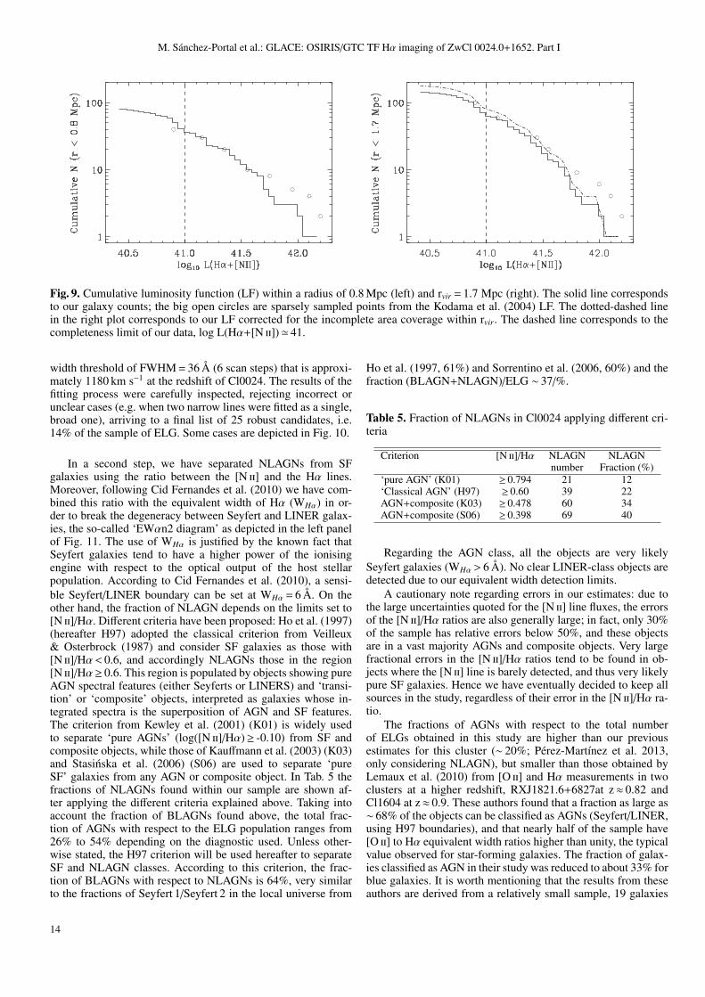
The spatial distribution of the ELG sample, as given by theposition of the sources in the sky plane and our redshift esti-mates, maps the presence of two components: (i) a structure as-sembling onto the cluster core from the NW with an orienta-tion almost in the plane of the sky. This structure has been al-ready reported by other authors (Moran et al. 2007; Zhang et al.2005; Kneib et al. 2003). (ii) An infalling group at high veloc-ity nearly along the line of sight to the cluster centre, identifiedby a double-peaked distribution in the redshift space, as shownin Fig. 7 (Moran et al. 2007; Czoske et al. 2002): structure “A”(centred at z = 0.395) and “B” (centred at z = 0.381) correspondto the main cluster and infalling group components, respectively.
12
M. Sanchez-Portal et al.: GLACE: OSIRIS/GTC TF Hα imaging of ZwCl 0024.0+1652. Part I
Fig. 7. Distribution of redshifts derived from our data. It is pos-sible to recognize two dynamical structures as in Czoske et al.(2002): “A” is the main cluster component, while “B” lies alongthe line of sight to the cluster centre and has been interpreted asan infalling group at high velocity.
The distribution of galaxies can be also seen in Fig. 8, wherethe radial velocities relative to the central redshift of component“A” are plotted against the distance to the cluster centre as givenby the distribution of galaxies/BGC (Treu et al. 2003). The twomentioned components are clearly separated. There is a third,small group of 8 galaxies at z≈ 0.41–0.42 (clearly seen in bothFig. 8 and Fig. 7) that has been also reported by Czoske et al.(2002). While according to these authors these galaxies are mostlikely part of the surrounding field galaxy population, we cannotrule out the possibility of another group connected to Cl0024.This suggestion could be reinforced by the fact that all thesegalaxies are observed within a relatively small cluster-centricprojected distance, r< 1 Mpc. While this can be just a instru-mental effect, result of the incomplete wavelength coverage atthe red side of the velocity field, is should be taken into accountthat, on the one hand, the cluster centre is offset some 1 arcminto the SE of the TF axis of the central pointing, and on the other,that no other excess of ELG is observed close to the TF axis ofthe offset pointing, as would be expected if the galaxies werepart of the field galaxy population.
7. Hα+ [N ii] luminosity function
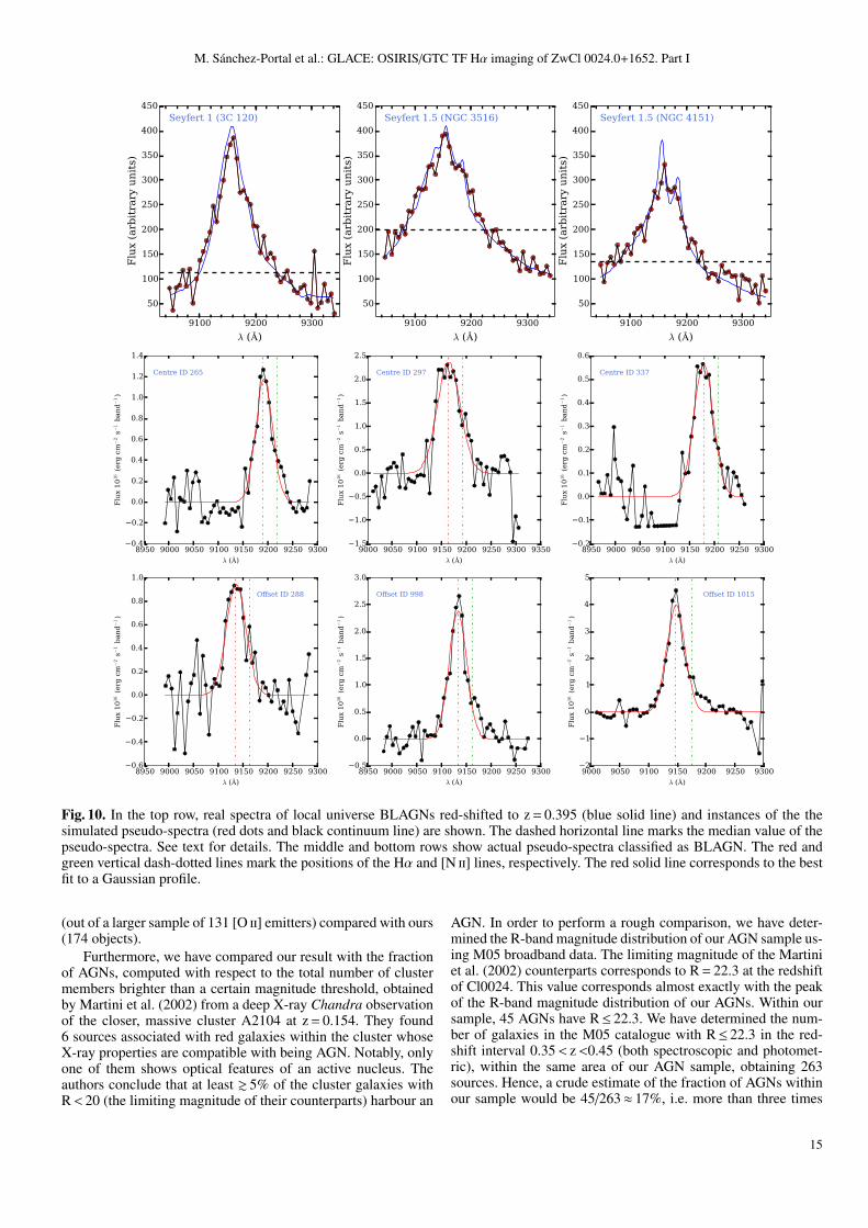
In order to verify the accuracy and performance of our pho-tometry, we have built the Hα+ [N ii] luminosity functions com-puted from sources within a central area of 0.8 Mpc and withinrvir = 1.7 Mpc. These are depicted in Fig. 9. These cumulativefunctions can be compared with those of Kodama et al. (2004)(hereafter K04). However, while the comparison is direct at thesmaller radius, at the larger one we need to take into accountthe fact that the coverage of our observations within rvir is in-complete towards East and South–East, around 81% of the fullcircle of rvir. We have performed a simple area correction to ac-count for this, shown as a dotted-dashed line in the right panelof Fig. 9. The completeness of our sample, as measured by thepeak of the luminosity histogram, is log L(Hα+[N ii])' 41, verysimilar to that of K04.
An evident discrepancy between our data set and that of K04is found at the high-luminosity end, log L(Hα+[N ii])& 41.8.This is observed, not only in the larger area but also in thesmaller one, and hence it cannot be attributed to our incompletearea coverage. However, it should be taken into account thatK04 results are based on different technique, namely a standard
0.0 0.5 1.0 1.5 2.0 2.5 3.0
Cluster-centric projected distance (Mpc)
6000
4000
2000
0
2000
4000
6000
rad
ial
velo
city
(km
s−
1)
Fig. 8. Line-of-sight velocity relative to the cluster main compo-nent central redshift z = 0.395 plotted against the projected dis-tance to the cluster centre (as defined by the distribution of galax-ies/BCG). Red diamonds correspond to AGNs and blue dots toSF galaxies according to the H97 criterion (see sect. 8). The dot-ted vertical line marks the virial radius of 1.7 Mpc (Treu et al.2003). The dashed-dotted horizontal lines correspond to the ra-dial velocity limits fully covered within the field of view of bothOSIRIS TF pointings (see sect. 3 and Eq. 2). The small, blackpoints correspond to galaxies from M05 with spectroscopic red-shifts, including both passive and star-forming objects.
narrow-band filter (the Subaru/Suprime-Cam NB912 filter withλe f f = 9139 Å and FWHM = 134 Å) plus broad-band BRz′ filtersand hence discrepancies in individual objects can be expected.Of course this affects only a few objects (just 4 objects downto log L(Hα+[N ii])' 41.8). At lower luminosities and even be-yond the completeness limit, the agreement between our cumu-lative number counts and those of K04 is excellent, reinforcingthe confidence in the accuracy of our photometry.
8. Star-forming galaxies and the AGN population
We have explored the available mechanisms to separate the pop-ulation of SF galaxies and AGNs. Broad-line AGNs (BLAGN)show permitted lines with widths of thousands of kilometers persecond. By contrast, in narrow-line AGNs (NLAGN), spectraline Doppler widths are much smaller, typically only a few hun-dred kilometers per second, which is comparable to or some-what larger than stellar velocity dispersions. We have verifiedthat the profiles of broad lines are well reproduced in our databy simulating BLAGN pseudo-spectra built from real spec-tra of local universe Seyfert 1 (3C 120, Garcıa-Lorenzo et al.2005) and Seyfert 1.5 galaxies (NGC 3516; Arribas et al. 1997),(NGC 4151; Kaspi et al. 1996), that were displaced to the red-shift of Cl0024 and convolved with the TF transmission profile(Eq. 4). Finally, noise components built drawing random valuesfrom a normal distribution with zero mean and a standard de-viation equal to 10% of the difference between the peak of thepseudo-spectrum and its median value were added to the pseudo-spectra signal. In all generated instances of such pseudo-spectra,the broad component of the Hα line was clearly traced as de-picted in Fig. 10.
In order to select candidates to BLAGN we have performedsimple Gaussian fits to the pseudo-spectra, setting a low line
13
M. Sanchez-Portal et al.: GLACE: OSIRIS/GTC TF Hα imaging of ZwCl 0024.0+1652. Part I
Fig. 9. Cumulative luminosity function (LF) within a radius of 0.8 Mpc (left) and rvir = 1.7 Mpc (right). The solid line correspondsto our galaxy counts; the big open circles are sparsely sampled points from the Kodama et al. (2004) LF. The dotted-dashed linein the right plot corresponds to our LF corrected for the incomplete area coverage within rvir. The dashed line corresponds to thecompleteness limit of our data, log L(Hα+[N ii])' 41.
width threshold of FWHM = 36 Å (6 scan steps) that is approxi-mately 1180 km s−1 at the redshift of Cl0024. The results of thefitting process were carefully inspected, rejecting incorrect orunclear cases (e.g. when two narrow lines were fitted as a single,broad one), arriving to a final list of 25 robust candidates, i.e.14% of the sample of ELG. Some cases are depicted in Fig. 10.
In a second step, we have separated NLAGNs from SFgalaxies using the ratio between the [N ii] and the Hα lines.Moreover, following Cid Fernandes et al. (2010) we have com-bined this ratio with the equivalent width of Hα (WHα) in or-der to break the degeneracy between Seyfert and LINER galax-ies, the so-called ‘EWαn2 diagram’ as depicted in the left panelof Fig. 11. The use of WHα is justified by the known fact thatSeyfert galaxies tend to have a higher power of the ionisingengine with respect to the optical output of the host stellarpopulation. According to Cid Fernandes et al. (2010), a sensi-ble Seyfert/LINER boundary can be set at WHα = 6 Å. On theother hand, the fraction of NLAGN depends on the limits set to[N ii]/Hα. Different criteria have been proposed: Ho et al. (1997)(hereafter H97) adopted the classical criterion from Veilleux& Osterbrock (1987) and consider SF galaxies as those with[N ii]/Hα< 0.6, and accordingly NLAGNs those in the region[N ii]/Hα≥ 0.6. This region is populated by objects showing pureAGN spectral features (either Seyferts or LINERS) and ‘transi-tion’ or ‘composite’ objects, interpreted as galaxies whose in-tegrated spectra is the superposition of AGN and SF features.The criterion from Kewley et al. (2001) (K01) is widely usedto separate ‘pure AGNs’ (log([N ii]/Hα)≥ -0.10) from SF andcomposite objects, while those of Kauffmann et al. (2003) (K03)and Stasinska et al. (2006) (S06) are used to separate ‘pureSF’ galaxies from any AGN or composite object. In Tab. 5 thefractions of NLAGNs found within our sample are shown af-ter applying the different criteria explained above. Taking intoaccount the fraction of BLAGNs found above, the total frac-tion of AGNs with respect to the ELG population ranges from26% to 54% depending on the diagnostic used. Unless other-wise stated, the H97 criterion will be used hereafter to separateSF and NLAGN classes. According to this criterion, the frac-tion of BLAGNs with respect to NLAGNs is 64%, very similarto the fractions of Seyfert 1/Seyfert 2 in the local universe from
Ho et al. (1997, 61%) and Sorrentino et al. (2006, 60%) and thefraction (BLAGN+NLAGN)/ELG ∼ 37/%.
Table 5. Fraction of NLAGNs in Cl0024 applying different cri-teria
Criterion [N ii]/Hα NLAGN NLAGNnumber Fraction (%)
‘pure AGN’ (K01) ≥ 0.794 21 12‘Classical AGN’ (H97) ≥ 0.60 39 22AGN+composite (K03) ≥ 0.478 60 34AGN+composite (S06) ≥ 0.398 69 40
Regarding the AGN class, all the objects are very likelySeyfert galaxies (WHα > 6 Å). No clear LINER-class objects aredetected due to our equivalent width detection limits.
A cautionary note regarding errors in our estimates: due tothe large uncertainties quoted for the [N ii] line fluxes, the errorsof the [N ii]/Hα ratios are also generally large; in fact, only 30%of the sample has relative errors below 50%, and these objectsare in a vast majority AGNs and composite objects. Very largefractional errors in the [N ii]/Hα ratios tend to be found in ob-jects where the [N ii] line is barely detected, and thus very likelypure SF galaxies. Hence we have eventually decided to keep allsources in the study, regardless of their error in the [N ii]/Hα ra-tio.
The fractions of AGNs with respect to the total numberof ELGs obtained in this study are higher than our previousestimates for this cluster (∼ 20%; Perez-Martınez et al. 2013,only considering NLAGN), but smaller than those obtained byLemaux et al. (2010) from [O ii] and Hα measurements in twoclusters at a higher redshift, RXJ1821.6+6827at z≈ 0.82 andCl1604 at z≈ 0.9. These authors found that a fraction as large as∼ 68% of the objects can be classified as AGNs (Seyfert/LINER,using H97 boundaries), and that nearly half of the sample have[O ii] to Hα equivalent width ratios higher than unity, the typicalvalue observed for star-forming galaxies. The fraction of galax-ies classified as AGN in their study was reduced to about 33% forblue galaxies. It is worth mentioning that the results from theseauthors are derived from a relatively small sample, 19 galaxies
14
M. Sanchez-Portal et al.: GLACE: OSIRIS/GTC TF Hα imaging of ZwCl 0024.0+1652. Part I
9100 9200 9300
λ ( )
50
100
150
200
250
300
350
400
450
Flu
x (a
rbit
rary
un
its)
Seyfert 1 (3C 120)
9100 9200 9300
λ ( )
50
100
150
200
250
300
350
400
450
Flu
x (a
rbit
rary
un
its)
Seyfert 1.5 (NGC 3516)
9100 9200 9300
λ ( )
50
100
150
200
250
300
350
400
450
Flu
x (a
rbit
rary
un
its)
Seyfert 1.5 (NGC 4151)
Fig. 10. In the top row, real spectra of local universe BLAGNs red-shifted to z = 0.395 (blue solid line) and instances of the thesimulated pseudo-spectra (red dots and black continuum line) are shown. The dashed horizontal line marks the median value of thepseudo-spectra. See text for details. The middle and bottom rows show actual pseudo-spectra classified as BLAGN. The red andgreen vertical dash-dotted lines mark the positions of the Hα and [N ii] lines, respectively. The red solid line corresponds to the bestfit to a Gaussian profile.
(out of a larger sample of 131 [O ii] emitters) compared with ours(174 objects).
Furthermore, we have compared our result with the fractionof AGNs, computed with respect to the total number of clustermembers brighter than a certain magnitude threshold, obtainedby Martini et al. (2002) from a deep X-ray Chandra observationof the closer, massive cluster A2104 at z = 0.154. They found6 sources associated with red galaxies within the cluster whoseX-ray properties are compatible with being AGN. Notably, onlyone of them shows optical features of an active nucleus. Theauthors conclude that at least & 5% of the cluster galaxies withR< 20 (the limiting magnitude of their counterparts) harbour an
AGN. In order to perform a rough comparison, we have deter-mined the R-band magnitude distribution of our AGN sample us-ing M05 broadband data. The limiting magnitude of the Martiniet al. (2002) counterparts corresponds to R = 22.3 at the redshiftof Cl0024. This value corresponds almost exactly with the peakof the R-band magnitude distribution of our AGNs. Within oursample, 45 AGNs have R≤ 22.3. We have determined the num-ber of galaxies in the M05 catalogue with R≤ 22.3 in the red-shift interval 0.35< z<0.45 (both spectroscopic and photomet-ric), within the same area of our AGN sample, obtaining 263sources. Hence, a crude estimate of the fraction of AGNs withinour sample would be 45/263≈ 17%, i.e. more than three times
15
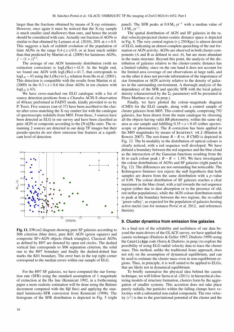
M. Sanchez-Portal et al.: GLACE: OSIRIS/GTC TF Hα imaging of ZwCl 0024.0+1652. Part I
larger than the fractions obtained by means of X-ray estimates.However, once again it must be noticed that the X-ray sampleis much smaller (and shallower) than ours, and hence the resultshould be considered with care. Actually our fraction of AGNs issimilar to that obtained by Lemaux et al. (2010), 20% at z≈ 0.9.This suggests a lack of redshift evolution of the population offaint AGNs in the range 0.4. z. 0.9, or at least much milderthan that predicted by Martini et al. (2009) for luminous AGNs,f ∼ (1 + z)5.3.
The average of our AGN luminosity distribution (with noextinction correction) is logL(Hα)' 41.0. At the bright end,we found one AGN with logL(Hα)' 41.7, that corresponds tologLX ∼ 43 using the L(Hα) to LX relation from Ho et al. (2001).This detection is compatible with the results from Martini et al.(2009) in the 0.3< z< 0.6 bin (four AGNs in ten clusters withlogLX ≥ 43).
We have cross-matched our ELG catalogue with a list ofsource detection positions from a Chandra ACIS-S observationof 40 ksec performed in FAINT mode, kindly provided to us byP. Tozzi. Five sources (out of 37) have been ascribed to the clus-ter after cross-matching the X-ray emitter list with the catalogueof spectroscopic redshifts from M05. From these, 3 sources havebeen detected as ELG in our survey and have been classified aspure AGN or composite according to the [N ii]/Hα ratio. The re-maining 2 sources are detected in our deep TF images but theirpseudo-spectra do not show emission line features at a signifi-cant level of detection.
0.5 1.0 1.5 2.0 2.5
[NII]/Hα
10.0
20.0
30.0
40.0
50.0
60.0
70.0
80.0
90.0
100.0
WHα
()
Fig. 11. EWαn2 diagram showing pure SF galaxies according toS06 criterion (blue dots), pure K01 AGN (green squares) andcomposite SF+AGN objects (black triangles). Classical AGNsas defined by H97 are denoted by open red circles. The dashedvertical line corresponds to S06 separation criterion, the solidone to the H97 boundary and finally the dashed-dotted linemarks the K01 boundary. The error bars in the top right cornercorrespond to the median errors within our sample of ELG.
For the H97 SF galaxies, we have computed the star forma-tion rate (SFR) using the standard assumption of 1 magnitudeof extinction at the Hα line (Kennicutt 1992, in a forthcomingpaper a more realistic estimation will be done using the Balmerdecrement computed with the Hβ flux) and applying the stan-dard luminosity-SFR conversion from Kennicutt (1998). Thehistogram of the SFR distribution is depicted in Fig. 5 (right
panel). The SFR peaks at 0.8 M yr−1 with a median value of1.4 M yr−1.
The spatial distribution of AGN and SF galaxies in the ra-dial velocity/projected cluster-centric distance space is depictedin Fig. 8. The very central region (r. 250 Kpc) is almost devoidof ELG, indicating an almost complete quenching of the star for-mation or AGN activity. AGNs are observed in both cluster com-ponents (A and B as defined in sect. 6), but are more abundantin the main structure. Beyond this point, the analysis of the dis-tribution of galaxies relative to the cluster-centric distance hasa limited validity, since on the one hand it does not account forthe limited area coverage of our observations at large radii, andon the other it does not provide information of the importance ofstar formation or AGN activity relative to the density of galax-ies in the surrounding environment. A thorough analysis of thedependency of the SFR and specific SFR with the local galaxydensity (characterised by the Σ5 parameter) will be presented inPerez-Martınez et al. (in prep.).
Finally, we have plotted the colour–magnitude diagram(CMD) for the ELG sample, along with a control sample ofcluster galaxies from M05. This control sample, comprising 792galaxies, has been drawn from the main catalogue by choosingall the objects having valid BR photometry, within the same skyarea as our sample and fulfilling 0.35< z< 0.45 (either spectro-scopic or photometric). The K-correction has been applied tothe M05 magnitudes by means of kcorrect v4 2 (Blanton &Roweis 2007). The rest-frame B − R vs. R CMD is depicted inFig. 12. The bi-modality in the distribution of optical colours isclearly noticed, with a red sequence well developed. We havedefined a boundary between the red sequence and the blue cloudas the intersection of the Gaussian functions resulting from thefit to each colour peak ( B − R = 1.39). We have investigatedthe colour distributions of AGNs and SF galaxies (right panel inFig. 12). The differences are not outstanding but noticeable. TheKolmogorov-Smirnov test rejects the null hypothesis that bothsamples are drawn from the same distribution with a p–valueof 0.09. The colour distribution of SF galaxies reaches a clearmaximum in the blue cloud, with a tail towards the red sequenceregion (either due to dust absorption or to the presence of old,red stellar populations), while the AGN colour distribution tendsto peak at the boundary between the two regions, the so-called‘green valley’, as expected for the population of galaxies hostingactive nuclei (see for instance Povic et al. 2012, and referencestherein).
9. Cluster dynamics from emission line galaxies
As a final test of the reliability and usefulness of our data be-yond the main drivers of the GLACE survey, we have applied thecaustic technique (Diaferio & Geller 1997; Diaferio 1999) usingthe CausticApp code (Serra & Diaferio, in prep.) to explore thepossibility of using ELG radial velocity data to trace the clustermass. This method, unlike the traditional Jeans approach, doesnot rely on the assumption of dynamical equilibrium, and canbe used to estimate the cluster mass even in non-equilibrium re-gions. Thus, in principle, it is well suited to be applied to ELGs,that are likely not in dynamical equilibrium.
To briefly summarise the physical idea behind the caustictechnique, we will follow Serra et al. (2011): in hierarchical clus-tering models of structure formation, clusters form by the aggre-gation of smaller systems. This accretion does not take placepurely radially, but particles within the falling clumps have ve-locities with a substantial non-radial component. The rms veloc-ity 〈v2〉 is due to the gravitational potential of the cluster and the
16
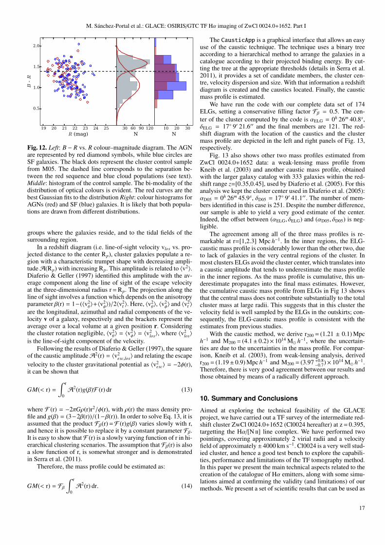
M. Sanchez-Portal et al.: GLACE: OSIRIS/GTC TF Hα imaging of ZwCl 0024.0+1652. Part I
19 20 21 22 23 24 25
R (mag)
0.5
1.0
1.5
2.0
B-R
30 60 90 120
N10 20 30
N
Fig. 12. Left: B − R vs. R colour–magnitude diagram. The AGNare represented by red diamond symbols, while blue circles areSF galaxies. The black dots represent the cluster control samplefrom M05. The dashed line corresponds to the separation be-tween the red sequence and blue cloud populations (see text).Middle: histogram of the control sample. The bi-modality of thedistribution of optical colours is evident. The red curves are thebest Gaussian fits to the distribution Right: colour histograms forAGNs (red) and SF (blue) galaxies. It is likely that both popula-tions are drawn from different distributions.
groups where the galaxies reside, and to the tidal fields of thesurrounding region.
In a redshift diagram (i.e. line-of-sight velocity vlos vs. pro-jected distance to the center Rp), cluster galaxies populate a re-gion with a characteristic trumpet shape with decreasing ampli-tudeA(Rp) with increasing Rp. This amplitude is related to 〈v2〉.Diaferio & Geller (1997) identified this amplitude with the av-erage component along the line of sight of the escape velocityat the three-dimensional radius r = Rp. The projection along theline of sight involves a function which depends on the anisotropyparameter β(r) = 1−(〈v2
θ〉+〈v2φ〉)/2〈v
2r 〉. Here, 〈v2
θ〉, 〈v2φ〉 and 〈v2
r 〉
are the longitudinal, azimuthal and radial components of the ve-locity v of a galaxy, respectively and the brackets represent theaverage over a local volume at a given position r. Consideringthe cluster rotation negligible, 〈v2
θ〉 = 〈v2φ〉 = 〈v2
los〉, where 〈v2los〉
is the line-of-sight component of the velocity.Following the results of Diaferio & Geller (1997), the square
of the caustic amplitudeA2(r) = 〈v2esc,los〉 and relating the escape
velocity to the cluster gravitational potential as 〈v2esc〉 = −2φ(r),
it can be shown that
GM(< r) =
∫ r
0A2(r)g(β)F (r) dr (13)
where F (r) = −2πGρ(r)r2/φ(r), with ρ(r) the mass density pro-file and g(β) = (3−2β(r))/(1−β(r)). In order to solve Eq. 13, it isassumed that the product Fβ(r) =F (r)g(β) varies slowly with r,and hence it is possible to replace it by a constant parameter Fβ.It is easy to show that F (r) is a slowly varying function of r in hi-erarchical clustering scenarios. The assumption that Fβ(r) is alsoa slow function of r, is somewhat stronger and is demonstratedin Serra et al. (2011).
Therefore, the mass profile could be estimated as:
GM(< r) = Fβ
∫ r
0A2(r) dr. (14)
The CausticApp is a graphical interface that allows an easyuse of the caustic technique. The technique uses a binary treeaccording to a hierarchical method to arrange the galaxies in acatalogue according to their projected binding energy. By cut-ting the tree at the appropriate thresholds (details in Serra et al.2011), it provides a set of candidate members, the cluster cen-tre, velocity dispersion and size. With that information a redshiftdiagram is created and the caustics located. Finally, the causticmass profile is estimated.
We have run the code with our complete data set of 174ELGs, setting a conservative filling factor Fβ = 0.5. The cen-ter of the cluster computed by the code is αELG = 0h 26m 40.8s,δELG = 17 9′ 21.6′′ and the final members are 121. The red-shift diagram with the location of the caustics and the clustermass profile are depicted in the left and right panels of Fig. 13,respectively.
Fig. 13 also shows other two mass profiles estimated fromZwCl 0024.0+1652 data: a weak-lensing mass profile fromKneib et al. (2003) and another caustic mass profile, obtainedwith the larger galaxy catalog with 333 galaxies within the red-shift range z=[0.35,0.45], used by Diaferio et al. (2005). For thisanalysis we kept the cluster center used in Diaferio et al. (2005):αD05 = 0h 26m 45.9s, δD05 = 17 9′ 41.1′′. The number of mem-bers identified in this case is 251. Despite the number difference,our sample is able to yield a very good estimate of the center.Indeed, the offset between (αELG, δELG) and (αD05, δD05) is neg-ligible.
The agreement among all of the three mass profiles is re-markable at r=[1,2.3] Mpc h−1. In the inner regions, the ELG-caustic mass profile is considerably lower than the other two, dueto lack of galaxies in the very central regions of the cluster. Inmost clusters ELGs avoid the cluster center, which translates intoa caustic amplitude that tends to underestimate the mass profilein the inner regions. As the mass profile is cumulative, this un-derestimate propagates into the final mass estimates. However,the cumulative caustic mass profile from ELGs in Fig 13 showsthat the central mass does not contribute substantially to the totalcluster mass at large radii. This suggests that in this cluster thevelocity field is well sampled by the ELGs in the outskirts; con-sequently, the ELG-caustic mass profile is consistent with theestimates from previous studies.
With the caustic method, we derive r200 = (1.21 ± 0.1) Mpch−1 and M200 = (4.1± 0.2)× 1014 M h−1, where the uncertain-ties are due to the uncertainties in the mass profile. For compar-ison, Kneib et al. (2003), from weak-lensing analysis, derivedr200 = (1.19± 0.9) Mpc h−1 and M200 = (3.97 +0.8
−0.7)× 1014 M h−1.Therefore, there is very good agreement between our results andthose obtained by means of a radically different approach.
10. Summary and Conclusions
Aimed at exploring the technical feasibility of the GLACEproject, we have carried out a TF survey of the intermediate red-shift cluster ZwCl 0024.0+1652 (Cl0024 hereafter) at z = 0.395,targetting the Hα/[N ii] line complex. We have performed twopointings, covering approximately 2 virial radii and a velocityfield of approximately ± 4000 km s−1. Cl0024 is a very well stud-ied cluster, and hence a good test bench to explore the capabili-ties, performance and limitations of the TF tomography method.In this paper we present the main technical aspects related to thecreation of the catalogue of Hα emitters, along with some simu-lations aimed at confirming the validity (and limitations) of ourmethods. We present a set of scientific results that can be used as
17
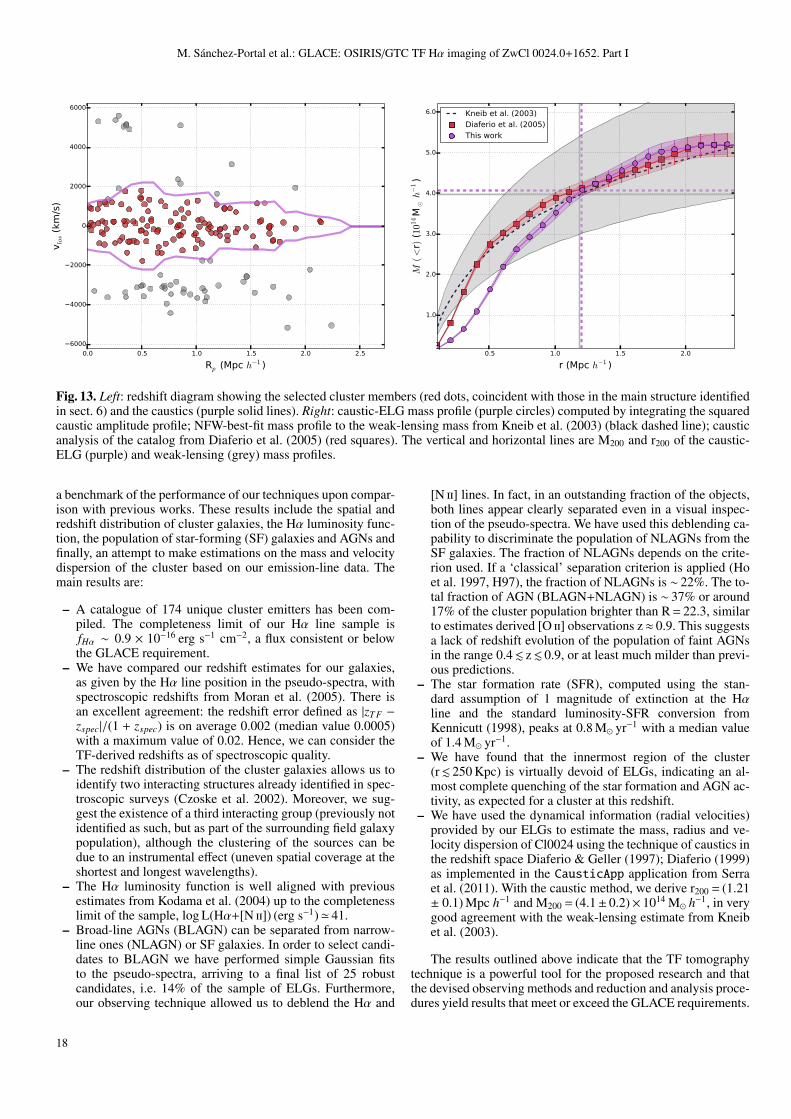
M. Sanchez-Portal et al.: GLACE: OSIRIS/GTC TF Hα imaging of ZwCl 0024.0+1652. Part I
0.0 0.5 1.0 1.5 2.0 2.5
Rp (Mpc h−1 )
6000
4000
2000
0
2000
4000
6000
v los
(km
/s)
0.5 1.0 1.5 2.0
r (Mpc h−1 )
1.0
2.0
3.0
4.0
5.0
6.0
M(<
r) (1
014M¯h−
1)
Kneib et al. (2003)Diaferio et al. (2005)This work
Fig. 13. Left: redshift diagram showing the selected cluster members (red dots, coincident with those in the main structure identifiedin sect. 6) and the caustics (purple solid lines). Right: caustic-ELG mass profile (purple circles) computed by integrating the squaredcaustic amplitude profile; NFW-best-fit mass profile to the weak-lensing mass from Kneib et al. (2003) (black dashed line); causticanalysis of the catalog from Diaferio et al. (2005) (red squares). The vertical and horizontal lines are M200 and r200 of the caustic-ELG (purple) and weak-lensing (grey) mass profiles.
a benchmark of the performance of our techniques upon compar-ison with previous works. These results include the spatial andredshift distribution of cluster galaxies, the Hα luminosity func-tion, the population of star-forming (SF) galaxies and AGNs andfinally, an attempt to make estimations on the mass and velocitydispersion of the cluster based on our emission-line data. Themain results are:
– A catalogue of 174 unique cluster emitters has been com-piled. The completeness limit of our Hα line sample isfHα ∼ 0.9 × 10⁻¹⁶ erg s−1 cm−2, a flux consistent or belowthe GLACE requirement.
– We have compared our redshift estimates for our galaxies,as given by the Hα line position in the pseudo-spectra, withspectroscopic redshifts from Moran et al. (2005). There isan excellent agreement: the redshift error defined as |zT F −
zspec|/(1 + zspec) is on average 0.002 (median value 0.0005)with a maximum value of 0.02. Hence, we can consider theTF-derived redshifts as of spectroscopic quality.
– The redshift distribution of the cluster galaxies allows us toidentify two interacting structures already identified in spec-troscopic surveys (Czoske et al. 2002). Moreover, we sug-gest the existence of a third interacting group (previously notidentified as such, but as part of the surrounding field galaxypopulation), although the clustering of the sources can bedue to an instrumental effect (uneven spatial coverage at theshortest and longest wavelengths).
– The Hα luminosity function is well aligned with previousestimates from Kodama et al. (2004) up to the completenesslimit of the sample, log L(Hα+[N ii]) (erg s−1)' 41.
– Broad-line AGNs (BLAGN) can be separated from narrow-line ones (NLAGN) or SF galaxies. In order to select candi-dates to BLAGN we have performed simple Gaussian fitsto the pseudo-spectra, arriving to a final list of 25 robustcandidates, i.e. 14% of the sample of ELGs. Furthermore,our observing technique allowed us to deblend the Hα and
[N ii] lines. In fact, in an outstanding fraction of the objects,both lines appear clearly separated even in a visual inspec-tion of the pseudo-spectra. We have used this deblending ca-pability to discriminate the population of NLAGNs from theSF galaxies. The fraction of NLAGNs depends on the crite-rion used. If a ‘classical’ separation criterion is applied (Hoet al. 1997, H97), the fraction of NLAGNs is ∼ 22%. The to-tal fraction of AGN (BLAGN+NLAGN) is ∼ 37% or around17% of the cluster population brighter than R = 22.3, similarto estimates derived [O ii] observations z≈ 0.9. This suggestsa lack of redshift evolution of the population of faint AGNsin the range 0.4. z. 0.9, or at least much milder than previ-ous predictions.
– The star formation rate (SFR), computed using the stan-dard assumption of 1 magnitude of extinction at the Hαline and the standard luminosity-SFR conversion fromKennicutt (1998), peaks at 0.8 M yr−1 with a median valueof 1.4 M yr−1.
– We have found that the innermost region of the cluster(r. 250 Kpc) is virtually devoid of ELGs, indicating an al-most complete quenching of the star formation and AGN ac-tivity, as expected for a cluster at this redshift.
– We have used the dynamical information (radial velocities)provided by our ELGs to estimate the mass, radius and ve-locity dispersion of Cl0024 using the technique of caustics inthe redshift space Diaferio & Geller (1997); Diaferio (1999)as implemented in the CausticApp application from Serraet al. (2011). With the caustic method, we derive r200 = (1.21± 0.1) Mpc h−1 and M200 = (4.1± 0.2)× 1014 M h−1, in verygood agreement with the weak-lensing estimate from Kneibet al. (2003).
The results outlined above indicate that the TF tomographytechnique is a powerful tool for the proposed research and thatthe devised observing methods and reduction and analysis proce-dures yield results that meet or exceed the GLACE requirements.
18
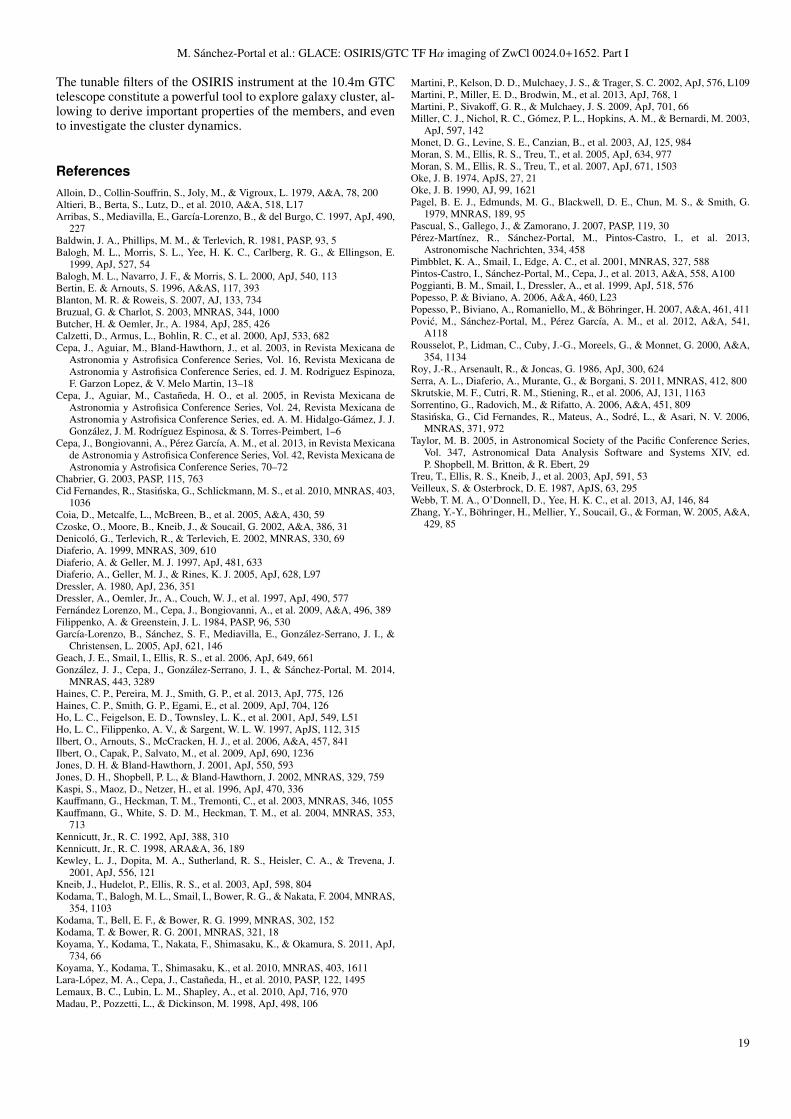
M. Sanchez-Portal et al.: GLACE: OSIRIS/GTC TF Hα imaging of ZwCl 0024.0+1652. Part I
The tunable filters of the OSIRIS instrument at the 10.4m GTCtelescope constitute a powerful tool to explore galaxy cluster, al-lowing to derive important properties of the members, and evento investigate the cluster dynamics.
ReferencesAlloin, D., Collin-Souffrin, S., Joly, M., & Vigroux, L. 1979, A&A, 78, 200Altieri, B., Berta, S., Lutz, D., et al. 2010, A&A, 518, L17Arribas, S., Mediavilla, E., Garcıa-Lorenzo, B., & del Burgo, C. 1997, ApJ, 490,
227Baldwin, J. A., Phillips, M. M., & Terlevich, R. 1981, PASP, 93, 5Balogh, M. L., Morris, S. L., Yee, H. K. C., Carlberg, R. G., & Ellingson, E.
1999, ApJ, 527, 54Balogh, M. L., Navarro, J. F., & Morris, S. L. 2000, ApJ, 540, 113Bertin, E. & Arnouts, S. 1996, A&AS, 117, 393Blanton, M. R. & Roweis, S. 2007, AJ, 133, 734Bruzual, G. & Charlot, S. 2003, MNRAS, 344, 1000Butcher, H. & Oemler, Jr., A. 1984, ApJ, 285, 426Calzetti, D., Armus, L., Bohlin, R. C., et al. 2000, ApJ, 533, 682Cepa, J., Aguiar, M., Bland-Hawthorn, J., et al. 2003, in Revista Mexicana de
Astronomia y Astrofisica Conference Series, Vol. 16, Revista Mexicana deAstronomia y Astrofisica Conference Series, ed. J. M. Rodriguez Espinoza,F. Garzon Lopez, & V. Melo Martin, 13–18
Cepa, J., Aguiar, M., Castaneda, H. O., et al. 2005, in Revista Mexicana deAstronomia y Astrofisica Conference Series, Vol. 24, Revista Mexicana deAstronomia y Astrofisica Conference Series, ed. A. M. Hidalgo-Gamez, J. J.Gonzalez, J. M. Rodrıguez Espinosa, & S. Torres-Peimbert, 1–6
Cepa, J., Bongiovanni, A., Perez Garcıa, A. M., et al. 2013, in Revista Mexicanade Astronomia y Astrofisica Conference Series, Vol. 42, Revista Mexicana deAstronomia y Astrofisica Conference Series, 70–72
Chabrier, G. 2003, PASP, 115, 763Cid Fernandes, R., Stasinska, G., Schlickmann, M. S., et al. 2010, MNRAS, 403,
1036Coia, D., Metcalfe, L., McBreen, B., et al. 2005, A&A, 430, 59Czoske, O., Moore, B., Kneib, J., & Soucail, G. 2002, A&A, 386, 31Denicolo, G., Terlevich, R., & Terlevich, E. 2002, MNRAS, 330, 69Diaferio, A. 1999, MNRAS, 309, 610Diaferio, A. & Geller, M. J. 1997, ApJ, 481, 633Diaferio, A., Geller, M. J., & Rines, K. J. 2005, ApJ, 628, L97Dressler, A. 1980, ApJ, 236, 351Dressler, A., Oemler, Jr., A., Couch, W. J., et al. 1997, ApJ, 490, 577Fernandez Lorenzo, M., Cepa, J., Bongiovanni, A., et al. 2009, A&A, 496, 389Filippenko, A. & Greenstein, J. L. 1984, PASP, 96, 530Garcıa-Lorenzo, B., Sanchez, S. F., Mediavilla, E., Gonzalez-Serrano, J. I., &
Christensen, L. 2005, ApJ, 621, 146Geach, J. E., Smail, I., Ellis, R. S., et al. 2006, ApJ, 649, 661Gonzalez, J. J., Cepa, J., Gonzalez-Serrano, J. I., & Sanchez-Portal, M. 2014,
MNRAS, 443, 3289Haines, C. P., Pereira, M. J., Smith, G. P., et al. 2013, ApJ, 775, 126Haines, C. P., Smith, G. P., Egami, E., et al. 2009, ApJ, 704, 126Ho, L. C., Feigelson, E. D., Townsley, L. K., et al. 2001, ApJ, 549, L51Ho, L. C., Filippenko, A. V., & Sargent, W. L. W. 1997, ApJS, 112, 315Ilbert, O., Arnouts, S., McCracken, H. J., et al. 2006, A&A, 457, 841Ilbert, O., Capak, P., Salvato, M., et al. 2009, ApJ, 690, 1236Jones, D. H. & Bland-Hawthorn, J. 2001, ApJ, 550, 593Jones, D. H., Shopbell, P. L., & Bland-Hawthorn, J. 2002, MNRAS, 329, 759Kaspi, S., Maoz, D., Netzer, H., et al. 1996, ApJ, 470, 336Kauffmann, G., Heckman, T. M., Tremonti, C., et al. 2003, MNRAS, 346, 1055Kauffmann, G., White, S. D. M., Heckman, T. M., et al. 2004, MNRAS, 353,
713Kennicutt, Jr., R. C. 1992, ApJ, 388, 310Kennicutt, Jr., R. C. 1998, ARA&A, 36, 189Kewley, L. J., Dopita, M. A., Sutherland, R. S., Heisler, C. A., & Trevena, J.
2001, ApJ, 556, 121Kneib, J., Hudelot, P., Ellis, R. S., et al. 2003, ApJ, 598, 804Kodama, T., Balogh, M. L., Smail, I., Bower, R. G., & Nakata, F. 2004, MNRAS,
354, 1103Kodama, T., Bell, E. F., & Bower, R. G. 1999, MNRAS, 302, 152Kodama, T. & Bower, R. G. 2001, MNRAS, 321, 18Koyama, Y., Kodama, T., Nakata, F., Shimasaku, K., & Okamura, S. 2011, ApJ,
734, 66Koyama, Y., Kodama, T., Shimasaku, K., et al. 2010, MNRAS, 403, 1611Lara-Lopez, M. A., Cepa, J., Castaneda, H., et al. 2010, PASP, 122, 1495Lemaux, B. C., Lubin, L. M., Shapley, A., et al. 2010, ApJ, 716, 970Madau, P., Pozzetti, L., & Dickinson, M. 1998, ApJ, 498, 106
Martini, P., Kelson, D. D., Mulchaey, J. S., & Trager, S. C. 2002, ApJ, 576, L109Martini, P., Miller, E. D., Brodwin, M., et al. 2013, ApJ, 768, 1Martini, P., Sivakoff, G. R., & Mulchaey, J. S. 2009, ApJ, 701, 66Miller, C. J., Nichol, R. C., Gomez, P. L., Hopkins, A. M., & Bernardi, M. 2003,
ApJ, 597, 142Monet, D. G., Levine, S. E., Canzian, B., et al. 2003, AJ, 125, 984Moran, S. M., Ellis, R. S., Treu, T., et al. 2005, ApJ, 634, 977Moran, S. M., Ellis, R. S., Treu, T., et al. 2007, ApJ, 671, 1503Oke, J. B. 1974, ApJS, 27, 21Oke, J. B. 1990, AJ, 99, 1621Pagel, B. E. J., Edmunds, M. G., Blackwell, D. E., Chun, M. S., & Smith, G.
1979, MNRAS, 189, 95Pascual, S., Gallego, J., & Zamorano, J. 2007, PASP, 119, 30Perez-Martınez, R., Sanchez-Portal, M., Pintos-Castro, I., et al. 2013,
Astronomische Nachrichten, 334, 458Pimbblet, K. A., Smail, I., Edge, A. C., et al. 2001, MNRAS, 327, 588Pintos-Castro, I., Sanchez-Portal, M., Cepa, J., et al. 2013, A&A, 558, A100Poggianti, B. M., Smail, I., Dressler, A., et al. 1999, ApJ, 518, 576Popesso, P. & Biviano, A. 2006, A&A, 460, L23Popesso, P., Biviano, A., Romaniello, M., & Bohringer, H. 2007, A&A, 461, 411Povic, M., Sanchez-Portal, M., Perez Garcıa, A. M., et al. 2012, A&A, 541,
A118Rousselot, P., Lidman, C., Cuby, J.-G., Moreels, G., & Monnet, G. 2000, A&A,
354, 1134Roy, J.-R., Arsenault, R., & Joncas, G. 1986, ApJ, 300, 624Serra, A. L., Diaferio, A., Murante, G., & Borgani, S. 2011, MNRAS, 412, 800Skrutskie, M. F., Cutri, R. M., Stiening, R., et al. 2006, AJ, 131, 1163Sorrentino, G., Radovich, M., & Rifatto, A. 2006, A&A, 451, 809Stasinska, G., Cid Fernandes, R., Mateus, A., Sodre, L., & Asari, N. V. 2006,
MNRAS, 371, 972Taylor, M. B. 2005, in Astronomical Society of the Pacific Conference Series,
Vol. 347, Astronomical Data Analysis Software and Systems XIV, ed.P. Shopbell, M. Britton, & R. Ebert, 29
Treu, T., Ellis, R. S., Kneib, J., et al. 2003, ApJ, 591, 53Veilleux, S. & Osterbrock, D. E. 1987, ApJS, 63, 295Webb, T. M. A., O’Donnell, D., Yee, H. K. C., et al. 2013, AJ, 146, 84Zhang, Y.-Y., Bohringer, H., Mellier, Y., Soucail, G., & Forman, W. 2005, A&A,
429, 85
19
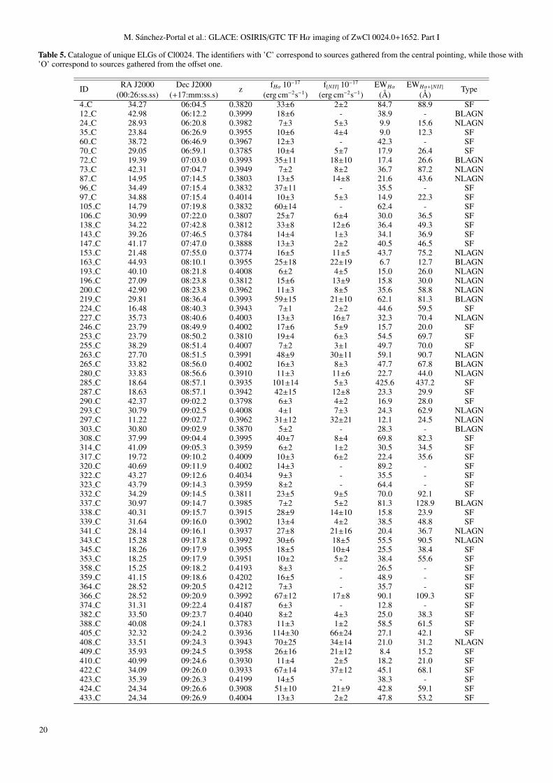
M. Sanchez-Portal et al.: GLACE: OSIRIS/GTC TF Hα imaging of ZwCl 0024.0+1652. Part I
Table 5. Catalogue of unique ELGs of Cl0024. The identifiers with ’C’ correspond to sources gathered from the central pointing, while those with’O’ correspond to sources gathered from the offset one.
ID RA J2000 Dec J2000 z fHα 10−17 f[NII] 10−17 EWHα EWHα+[NII] Type(00:26:ss.ss) (+17:mm:ss.s) (erg cm−2s−1) (erg cm−2s−1) (Å) (Å)
4 C 34.27 06:04.5 0.3820 33±6 2±2 84.7 88.9 SF12 C 42.98 06:12.2 0.3999 18±6 - 38.9 - BLAGN24 C 28.93 06:20.8 0.3982 7±3 5±3 9.9 15.6 NLAGN35 C 23.84 06:26.9 0.3955 10±6 4±4 9.0 12.3 SF60 C 38.72 06:46.9 0.3967 12±3 - 42.3 - SF70 C 29.05 06:59.1 0.3785 10±4 5±7 17.9 26.4 SF72 C 19.39 07:03.0 0.3993 35±11 18±10 17.4 26.6 BLAGN73 C 42.31 07:04.7 0.3949 7±2 8±2 36.7 87.2 NLAGN87 C 14.95 07:14.5 0.3803 13±5 14±8 21.6 43.6 NLAGN96 C 34.49 07:15.4 0.3832 37±11 - 35.5 - SF97 C 34.88 07:15.4 0.4014 10±3 5±3 14.9 22.3 SF105 C 14.79 07:19.8 0.3832 60±14 - 62.4 - SF106 C 30.99 07:22.0 0.3807 25±7 6±4 30.0 36.5 SF138 C 34.22 07:42.8 0.3812 33±8 12±6 36.4 49.3 SF143 C 39.26 07:46.5 0.3784 14±4 1±3 34.1 36.9 SF147 C 41.17 07:47.0 0.3888 13±3 2±2 40.5 46.5 SF153 C 21.48 07:55.0 0.3774 16±5 11±5 43.7 75.2 NLAGN163 C 44.93 08:10.1 0.3955 25±18 22±19 6.7 12.7 BLAGN193 C 40.10 08:21.8 0.4008 6±2 4±5 15.0 26.0 NLAGN196 C 27.09 08:23.8 0.3812 15±6 13±9 15.8 30.0 NLAGN200 C 42.90 08:23.8 0.3962 11±3 8±5 35.6 58.8 NLAGN219 C 29.81 08:36.4 0.3993 59±15 21±10 62.1 81.3 BLAGN224 C 16.48 08:40.3 0.3943 7±1 2±2 44.6 59.5 SF227 C 35.73 08:40.6 0.4003 13±3 16±7 32.3 70.4 NLAGN246 C 23.79 08:49.9 0.4002 17±6 5±9 15.7 20.0 SF253 C 23.79 08:50.2 0.3810 19±4 6±3 54.5 69.7 SF255 C 38.29 08:51.4 0.4007 7±2 3±1 49.7 70.0 SF263 C 27.70 08:51.5 0.3991 48±9 30±11 59.1 90.7 NLAGN265 C 33.82 08:56.0 0.4002 16±3 8±3 47.7 67.8 BLAGN280 C 33.83 08:56.6 0.3910 11±3 11±6 22.7 44.0 NLAGN285 C 18.64 08:57.1 0.3935 101±14 5±3 425.6 437.2 SF287 C 18.63 08:57.1 0.3942 42±15 12±8 23.3 29.9 SF290 C 42.37 09:02.2 0.3798 6±3 4±2 16.9 28.0 SF293 C 30.79 09:02.5 0.4008 4±1 7±3 24.3 62.9 NLAGN297 C 11.22 09:02.7 0.3962 31±12 32±21 12.1 24.5 NLAGN303 C 30.80 09:02.9 0.3870 5±2 - 28.3 - BLAGN308 C 37.99 09:04.4 0.3995 40±7 8±4 69.8 82.3 SF314 C 41.09 09:05.3 0.3959 6±2 1±2 30.5 34.5 SF317 C 19.72 09:10.2 0.4009 10±3 6±2 22.4 35.6 SF320 C 40.69 09:11.9 0.4002 14±3 - 89.2 - SF322 C 43.27 09:12.6 0.4034 9±3 - 35.5 - SF323 C 43.79 09:14.3 0.3959 8±2 - 64.4 - SF332 C 34.29 09:14.5 0.3811 23±5 9±5 70.0 92.1 SF337 C 30.97 09:14.7 0.3985 7±2 5±2 81.3 128.9 BLAGN338 C 40.31 09:15.7 0.3915 28±9 14±10 15.8 23.9 SF339 C 31.64 09:16.0 0.3902 13±4 4±2 38.5 48.8 SF341 C 28.14 09:16.1 0.3937 27±8 21±16 20.4 36.7 NLAGN343 C 15.28 09:17.8 0.3992 30±6 18±5 55.5 90.5 NLAGN345 C 18.26 09:17.9 0.3955 18±5 10±4 25.5 38.4 SF353 C 18.25 09:17.9 0.3951 10±2 5±2 38.4 55.6 SF358 C 15.25 09:18.2 0.4193 8±3 - 26.5 - SF359 C 41.15 09:18.6 0.4202 16±5 - 48.9 - SF364 C 28.52 09:20.5 0.4212 7±3 - 35.7 - SF366 C 28.52 09:20.9 0.3992 67±12 17±8 90.1 109.3 SF374 C 31.31 09:22.4 0.4187 6±3 - 12.8 - SF382 C 33.50 09:23.7 0.4040 8±2 4±3 25.0 38.3 SF388 C 40.08 09:24.1 0.3783 11±3 1±2 58.5 61.5 SF405 C 32.32 09:24.2 0.3936 114±30 66±24 27.1 42.1 SF408 C 33.51 09:24.3 0.3943 70±25 34±14 21.0 31.2 NLAGN409 C 35.93 09:24.5 0.3958 26±16 21±12 8.4 15.2 SF410 C 40.99 09:24.6 0.3930 11±4 2±5 18.2 21.0 SF422 C 34.09 09:26.0 0.3933 67±14 37±12 45.1 68.1 SF423 C 35.39 09:26.3 0.4199 14±5 - 38.3 - SF424 C 24.34 09:26.6 0.3908 51±10 21±9 42.8 59.1 SF433 C 24.34 09:26.9 0.4004 13±3 2±2 47.8 53.2 SF
20
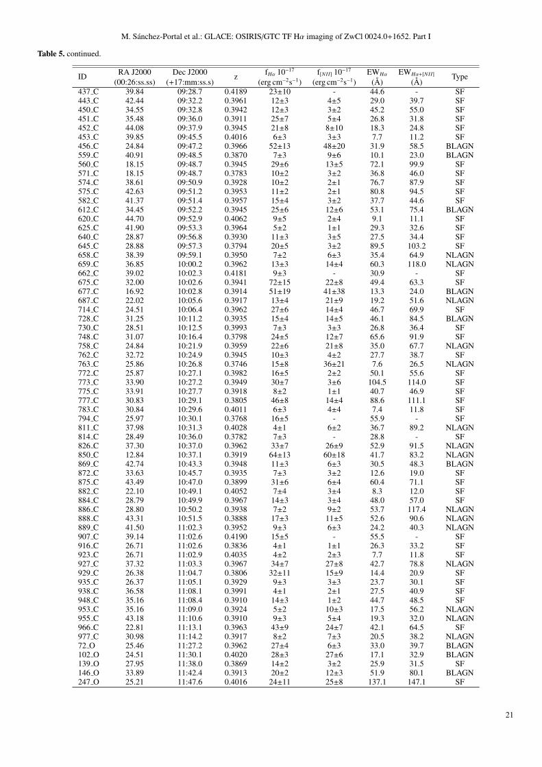
M. Sanchez-Portal et al.: GLACE: OSIRIS/GTC TF Hα imaging of ZwCl 0024.0+1652. Part I
Table 5. continued.
ID RA J2000 Dec J2000 z fHα 10−17 f[NII] 10−17 EWHα EWHα+[NII] Type(00:26:ss.ss) (+17:mm:ss.s) (erg cm−2s−1) (erg cm−2s−1) (Å) (Å)
437 C 39.84 09:28.7 0.4189 23±10 - 44.6 - SF443 C 42.44 09:32.2 0.3961 12±3 4±5 29.0 39.7 SF450 C 34.55 09:32.8 0.3942 12±3 3±2 45.2 55.0 SF451 C 35.48 09:36.0 0.3911 25±7 5±4 26.8 31.8 SF452 C 44.08 09:37.9 0.3945 21±8 8±10 18.3 24.8 SF453 C 39.85 09:45.5 0.4016 6±3 3±3 7.7 11.2 SF456 C 24.84 09:47.2 0.3966 52±13 48±20 31.9 58.5 BLAGN559 C 40.91 09:48.5 0.3870 7±3 9±6 10.1 23.0 BLAGN560 C 18.15 09:48.7 0.3945 29±6 13±5 72.1 99.9 SF571 C 18.15 09:48.7 0.3783 10±2 3±2 36.8 46.0 SF574 C 38.61 09:50.9 0.3928 10±2 2±1 76.7 87.9 SF575 C 42.63 09:51.2 0.3953 11±2 2±1 80.8 94.5 SF582 C 41.37 09:51.4 0.3957 15±4 3±2 37.7 44.6 SF612 C 34.45 09:52.2 0.3945 25±6 12±6 53.1 75.4 BLAGN620 C 44.70 09:52.9 0.4062 9±5 2±4 9.1 11.1 SF625 C 41.90 09:53.3 0.3964 5±2 1±1 29.3 32.6 SF640 C 28.87 09:56.8 0.3930 11±3 3±5 27.5 34.4 SF645 C 28.88 09:57.3 0.3794 20±5 3±2 89.5 103.2 SF658 C 38.39 09:59.1 0.3950 7±2 6±3 35.4 64.9 NLAGN659 C 36.85 10:00.2 0.3962 13±3 14±4 60.3 118.0 NLAGN662 C 39.02 10:02.3 0.4181 9±3 - 30.9 - SF675 C 32.00 10:02.6 0.3941 72±15 22±8 49.4 63.3 SF677 C 16.92 10:02.8 0.3914 51±19 41±38 13.3 24.0 BLAGN687 C 22.02 10:05.6 0.3917 13±4 21±9 19.2 51.6 NLAGN714 C 24.51 10:06.4 0.3962 27±6 14±4 46.7 69.9 SF728 C 31.25 10:11.2 0.3935 15±4 14±5 46.1 84.5 BLAGN730 C 28.51 10:12.5 0.3993 7±3 3±3 26.8 36.4 SF748 C 31.07 10:16.4 0.3798 24±5 12±7 65.6 91.9 SF758 C 24.84 10:21.9 0.3959 22±6 21±8 35.0 67.7 NLAGN762 C 32.72 10:24.9 0.3945 10±3 4±2 27.7 38.7 SF763 C 25.86 10:26.8 0.3746 15±8 36±21 7.6 26.5 NLAGN772 C 25.87 10:27.1 0.3982 16±5 2±2 50.1 55.6 SF773 C 33.90 10:27.2 0.3949 30±7 3±6 104.5 114.0 SF775 C 33.91 10:27.7 0.3918 8±2 1±1 40.7 46.9 SF777 C 30.83 10:29.1 0.3805 46±8 14±4 88.6 111.1 SF783 C 30.84 10:29.6 0.4011 6±3 4±4 7.4 11.8 SF794 C 25.97 10:30.1 0.3768 16±5 - 55.9 - SF811 C 37.98 10:31.3 0.4028 4±1 6±2 36.7 89.2 NLAGN814 C 28.49 10:36.0 0.3782 7±3 - 28.8 - SF826 C 37.30 10:37.0 0.3962 33±7 26±9 52.9 91.5 NLAGN850 C 12.84 10:37.1 0.3919 64±13 60±18 41.7 83.2 NLAGN869 C 42.74 10:43.3 0.3948 11±3 6±3 30.5 48.3 BLAGN872 C 33.63 10:45.7 0.3935 7±3 3±2 12.6 19.0 SF875 C 43.49 10:47.0 0.3899 31±6 6±4 60.4 71.1 SF882 C 22.10 10:49.1 0.4052 7±4 3±4 8.3 12.0 SF884 C 28.79 10:49.9 0.3967 14±3 3±4 48.0 57.0 SF886 C 28.80 10:50.2 0.3938 7±2 9±2 53.7 117.4 NLAGN888 C 43.31 10:51.5 0.3888 17±3 11±5 52.6 90.6 NLAGN889 C 41.50 11:02.3 0.3952 9±3 6±3 24.2 40.3 NLAGN907 C 39.14 11:02.6 0.4190 15±5 - 55.5 - SF916 C 26.71 11:02.6 0.3836 4±1 1±1 26.3 33.2 SF923 C 26.71 11:02.9 0.4035 4±2 2±3 7.7 11.8 SF927 C 37.32 11:03.3 0.3967 34±7 27±8 42.7 78.8 NLAGN929 C 26.38 11:04.7 0.3806 32±11 15±9 14.4 20.9 SF935 C 26.37 11:05.1 0.3929 9±3 3±3 23.7 30.1 SF938 C 36.58 11:08.1 0.3991 4±1 2±1 27.5 40.9 SF948 C 35.16 11:08.4 0.3910 14±3 1±2 44.7 48.5 SF953 C 35.16 11:09.0 0.3924 5±2 10±3 17.5 56.2 NLAGN955 C 43.18 11:10.6 0.3910 9±3 5±4 19.3 32.0 NLAGN966 C 22.81 11:13.1 0.3963 43±9 24±7 42.1 64.5 SF977 C 30.98 11:14.2 0.3917 8±2 7±3 20.5 38.2 NLAGN72 O 25.46 11:27.2 0.3962 27±4 6±3 33.0 39.7 BLAGN102 O 24.51 11:30.1 0.4020 28±3 27±6 17.1 32.9 BLAGN139 O 27.95 11:38.0 0.3869 14±2 3±2 25.9 31.5 SF146 O 33.89 11:42.4 0.3913 20±2 12±3 51.9 80.1 BLAGN247 O 25.21 11:47.6 0.4016 24±11 25±8 137.1 147.1 SF
21
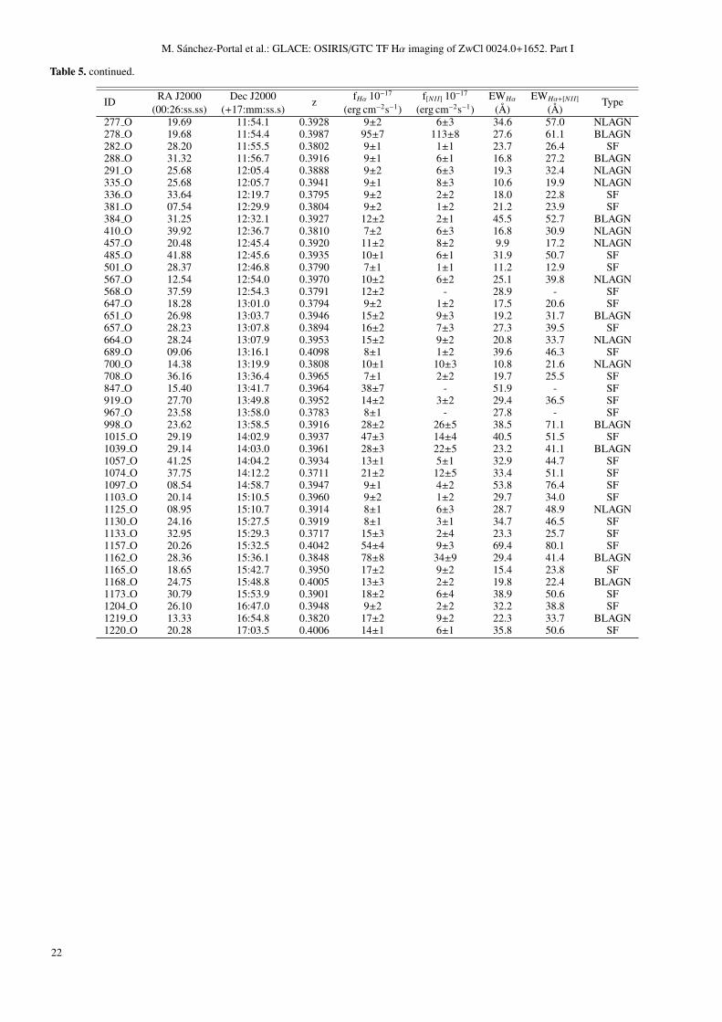
M. Sanchez-Portal et al.: GLACE: OSIRIS/GTC TF Hα imaging of ZwCl 0024.0+1652. Part I
Table 5. continued.
ID RA J2000 Dec J2000 z fHα 10−17 f[NII] 10−17 EWHα EWHα+[NII] Type(00:26:ss.ss) (+17:mm:ss.s) (erg cm−2s−1) (erg cm−2s−1) (Å) (Å)
277 O 19.69 11:54.1 0.3928 9±2 6±3 34.6 57.0 NLAGN278 O 19.68 11:54.4 0.3987 95±7 113±8 27.6 61.1 BLAGN282 O 28.20 11:55.5 0.3802 9±1 1±1 23.7 26.4 SF288 O 31.32 11:56.7 0.3916 9±1 6±1 16.8 27.2 BLAGN291 O 25.68 12:05.4 0.3888 9±2 6±3 19.3 32.4 NLAGN335 O 25.68 12:05.7 0.3941 9±1 8±3 10.6 19.9 NLAGN336 O 33.64 12:19.7 0.3795 9±2 2±2 18.0 22.8 SF381 O 07.54 12:29.9 0.3804 9±2 1±2 21.2 23.9 SF384 O 31.25 12:32.1 0.3927 12±2 2±1 45.5 52.7 BLAGN410 O 39.92 12:36.7 0.3810 7±2 6±3 16.8 30.9 NLAGN457 O 20.48 12:45.4 0.3920 11±2 8±2 9.9 17.2 NLAGN485 O 41.88 12:45.6 0.3935 10±1 6±1 31.9 50.7 SF501 O 28.37 12:46.8 0.3790 7±1 1±1 11.2 12.9 SF567 O 12.54 12:54.0 0.3970 10±2 6±2 25.1 39.8 NLAGN568 O 37.59 12:54.3 0.3791 12±2 - 28.9 - SF647 O 18.28 13:01.0 0.3794 9±2 1±2 17.5 20.6 SF651 O 26.98 13:03.7 0.3946 15±2 9±3 19.2 31.7 BLAGN657 O 28.23 13:07.8 0.3894 16±2 7±3 27.3 39.5 SF664 O 28.24 13:07.9 0.3953 15±2 9±2 20.8 33.7 NLAGN689 O 09.06 13:16.1 0.4098 8±1 1±2 39.6 46.3 SF700 O 14.38 13:19.9 0.3808 10±1 10±3 10.8 21.6 NLAGN708 O 36.16 13:36.4 0.3965 7±1 2±2 19.7 25.5 SF847 O 15.40 13:41.7 0.3964 38±7 - 51.9 - SF919 O 27.70 13:49.8 0.3952 14±2 3±2 29.4 36.5 SF967 O 23.58 13:58.0 0.3783 8±1 - 27.8 - SF998 O 23.62 13:58.5 0.3916 28±2 26±5 38.5 71.1 BLAGN1015 O 29.19 14:02.9 0.3937 47±3 14±4 40.5 51.5 SF1039 O 29.14 14:03.0 0.3961 28±3 22±5 23.2 41.1 BLAGN1057 O 41.25 14:04.2 0.3934 13±1 5±1 32.9 44.7 SF1074 O 37.75 14:12.2 0.3711 21±2 12±5 33.4 51.1 SF1097 O 08.54 14:58.7 0.3947 9±1 4±2 53.8 76.4 SF1103 O 20.14 15:10.5 0.3960 9±2 1±2 29.7 34.0 SF1125 O 08.95 15:10.7 0.3914 8±1 6±3 28.7 48.9 NLAGN1130 O 24.16 15:27.5 0.3919 8±1 3±1 34.7 46.5 SF1133 O 32.95 15:29.3 0.3717 15±3 2±4 23.3 25.7 SF1157 O 20.26 15:32.5 0.4042 54±4 9±3 69.4 80.1 SF1162 O 28.36 15:36.1 0.3848 78±8 34±9 29.4 41.4 BLAGN1165 O 18.65 15:42.7 0.3950 17±2 9±2 15.4 23.8 SF1168 O 24.75 15:48.8 0.4005 13±3 2±2 19.8 22.4 BLAGN1173 O 30.79 15:53.9 0.3901 18±2 6±4 38.9 50.6 SF1204 O 26.10 16:47.0 0.3948 9±2 2±2 32.2 38.8 SF1219 O 13.33 16:54.8 0.3820 17±2 9±2 22.3 33.7 BLAGN1220 O 20.28 17:03.5 0.4006 14±1 6±1 35.8 50.6 SF
22
M. Sanchez-Portal et al.: GLACE: OSIRIS/GTC TF Hα imaging of ZwCl 0024.0+1652. Part I
Acknowledgements. We acknowledge the support provided by M. Balogh dur-ing the preparation of the GLACE proposal to ESO, as well as his useful sug-gestions to improve the quality of this paper. We also acknowledge the anony-mous referee. We acknowledge financial support from Spanish MINECO un-der grant AYA2014-29517-C03-01 and AYA2011-29517-C03-02. EJA acknowl-edges support from MINECO under grant AYA2013-40611-P. JMRE acknowl-edges support from MINECO under grant AYA2012-39168-C03-01. We ac-knowledge support from the Faculty of the European Space Astronomy Centre(ESAC). IRS acknowledges support from STFC GT/I001573/1, a EuropeanResearch Council Advanced Programme Dustygal (321334) and a RoyalSociety/Wolfson Research Merit Award. Based on observations made with theGran Telescopio Canarias (GTC), instaled in the Spanish Observatorio del Roquede los Muchachos of the Instituto de Astrofsica de Canarias, in the island ofLa Palma. This publication makes use of data products from the Two MicronAll Sky Survey, which is a joint project of the University of Massachusetts andthe Infrared Processing and Analysis Center/California Institute of Technology,funded by the National Aeronautics and Space Administration and the NationalScience Foundation.
1 European Space Astronomy Centre (ESAC)/ESA, P.O. Box 78,28690 Villanueva de la Canada, Madrid, Spaine-mail: [email protected]
2 ISDEFE, Beatriz de Bobadilla 3, 28040 Madrid, Spain3 Instituto de Astrofısica de Canarias, E38205, La Laguna, Tenerife,
Spain4 Universidad de La Laguna, Tenerife, Spain5 Instituto de Astrofısica de Andalucıa, CSIC, Granada, Spain6 School of Physics and Astronomy, University of Nottingham, U.K.7 GEPI, Observatoire de Paris & CNRS, Meudon, France8 Centro de Astrobiologıa, INTA-CSIC, Madrid, Spain9 INAF, Osservatorio Astronomico di Trieste, Italy
10 Department of Physics, University of Bristol, U.K.11 Institut de Ciencies de l’Espai (CSIC), Barcelona, Spain12 Instituto Polictecnico Nacional, Mexico D.F., Mexico13 Laboratoire AIM Saclay, CEA/IRFU, CNRS/INSU, Universite Paris
Diderot, France14 Department of Physics, McGill University, Montreal, Quebec,
Canada15 Instituto de Fısica de Cantabria, CSIC-Univ. de Cantabria,
Santander, Spain16 Departamento de Astronomıa, Universidad de Chile, Casilla 36-D,
Correo Central, Santiago, Chile17 University College, Belfield, Dublin, Ireland18 INAF, Osservatorio Astronomico di Padova, Italy19 Institute for Computational Cosmology, Durham University,
Durham DH1 3LE, U.K.20 Institute of Astro- and Particle Physics, University of Innsbruck,
Austria21 Centro de Estudios de Fısica del Cosmos de Aragon, Teruel, Spain22 Dipartimento di Fisica, Universita degli Studi di Milano, Milano,
Italy23 Dipartimento di Fisica, Universita di Torino, Torino, Italy24 Istituto Nazionale di Fisica Nucleare (INFN), sezione di Torino,
Torino, Italy25 Departamento de Astronomia, Instituto de Astronomia, Geofısica e
Ciencias Atmosfericas da USP, Sao Paulo, Brazil26 Institute for Astronomy, University of Edinburgh, Royal
Observatory, Blackford Hill, Edinburgh27 European Southern Observatory, Garching, Germany28 INAF-Osservatorio Astrofisico di Arcetri, Florence, Italy29 Departamento de Astrofısica, Facultad de CC. Fısicas, Universidad
Complutense de Madrid, 28040, Madrid, Spain
23