Gibbs Sampling Based Bayesian Analysis of Mixtures with Unknown Number of Components

Sankhya : The Indian Journal of Statistics2008, Volume 70-B, Part 1, pp. 133-155c© 2008, Indian Statistical Institute

Gibbs Sampling Based Bayesian Analysis of Mixtures withUnknown Number of Components

Sourabh BhattacharyaIndian Statistical Institute, Kolkata, INDIA

Abstract

For mixture models with unknown number of components, Bayesian ap-proaches, as considered by Escobar and West (1995) and Richardson andGreen (1997), are reconciled here through a simple Gibbs sampling approach.Specifically, we consider exactly the same direct set up as used by Richard-son and Green (1997), but put Dirichlet process prior on the mixture com-ponents; the latter has also been used by Escobar and West (1995) albeitin a different set up. The reconciliation we propose here yields a simpleGibbs sampling scheme for learning about all the unknowns, including theunknown number of components. Thus, we completely avoid complicatedreversible jump Markov chain Monte Carlo (RJMCMC) methods, yet tacklevariable dimensionality simply and efficiently. Moreover, we demonstrate,using both simulated and real data sets, and pseudo-Bayes factors, that ourproposed model outperforms that of Escobar and West (1995), while enjoy-ing, at the same time, computational superiority over the methods proposedby Richardson and Green (1997) and Escobar and West (1995). We alsodiscuss issues related to clustering and argue that in principle, our approachis capable of learning about the number of clusters in the sample as well asin the population, while the approach of Escobar and West (1995) is suitablefor learning about the number of clusters in the sample only.

AMS (2000) subject classification. Primary .Keywords and phrases. Bayesian analysis, cross-validation, Dirichlet pro-cess, leave-one-out posterior, Markov chain Monte Carlo, pseudo-Bayes fac-tor

1 Introduction

Mixture models are noted for their flexibility and are widely used in thestatistical literature. Such models constitute a natural framework for model-ing heterogeneity with strong connections with cluster analysis. The entireliterature on mixture models have been almost exhaustively discussed by

134 Sourabh Bhattacharya

Titterington et al. (1985) and McLachlan and Basford (1988). However, aparticularly challenging situation arises when the number of mixture compo-nents, which we denote by k, can not be determined based on the availabledata set in a straightforward manner. Escobar and West (1995) (henceforthEW) were the first to propose a modeling style, involving Dirichlet processes,to introduce uncertainty within the number of components. Gibbs samplingis then used to learn about all the unknowns involved. However, the mix-ture model of EW does not resemble the traditional mixture models, whichare often mixtures of normal distributions. For instance, conditional on theparameters, the predictive distribution in the case of EW is a mixture of non-central Student’s t and normal distributions. In contrast, Richardson andGreen (1997) (henceforth RG) consider a mixture of normal distributionsassuming k unknown. But acknowledgment of uncertainty about k makesthe dimension of the parameter space a random variable in the case of RG.They use sophisticated, but quite complicated MCMC methods, known asreversible jump MCMC (RJMCMC), introduced in the literature by Green(1995).

In this paper, we propose another alternative model for mixture anal-ysis when the number of components is unknown. Broadly, as in RG, weconsider a mixture of normal distributions, but instead of complicated (andoften inefficient) RJMCMC methods, view the parameters of the componentsas samples from a Dirichlet process. We propose a simple Gibbs samplingalgorithm, thus freeing ourselves of the burden of implementing RJMCMC,while maintaining the same variable dimensional framework as RG. This isthe implementation advantage of our proposed methodology. On the con-ceptual side, we demonstrate with simulated and real data sets that ourmodel is better supported by the data than that of EW. We argue tenta-tively that the unconventional mixture of the thick-tailed Student’s t withthe normal distributions of the predictive distributions of EW is the reasonfor its relatively poor performance compared to our conventional mixture ofnormal distributions. Moreover, the implementation time of our model isfar less than that of EW and RG. For example, with the largest of the threereal data sets that we consider, the MCMC algorithm for the implementa-tion of EW’s method does about 93 iterations per second on a Mac OS Xlaptop, RG’s RJMCMC does 160 iterations per second (see Richardson andGreen (1997), page 755), but the MCMC algorithm for implementation ofour proposed model does about 715 iterations per second.

The remainder of our paper is structured as follows. In Section 2 we intro-duce our proposed methodology for mixture analysis with unknown number

Gibbs sampling based bayesian analysis of mixtures withunknown number of components 135

of components. A simple Gibbs sampling approach for implementing ourmodel and methodology is proposed in Section 3. Details on the advantagesof our approach as compared to the approaches of RG and EW are providedin Sections 4 and 5 respectively. Model comparison using pseudo-Bayes fac-tor is outlined in Section 6. Illustration of our methodology and comparisonswith the proposal of EW using simulated data, are carried out in Section7. Applications of our methodology to three real data sets are discussed inSection 8. We summarize the main points and provide directions for futureresearch in Section 9.

2 Dirichlet Process for Learning Unknown Number ofParameters

Generically denoting by Θp the set of parameters {θj ; 1 ≤ j ≤ p}, forany p, where θj = (µj , λj), we show that the mixture of the form

[yi | Θp] =p∑j=1

πj

√λj2π

exp{−λj

2(yi − µj)

2

}, (2.1)

although a mixture of a random number of components, may be expressedsimply as an average of a fixed (but perhaps, large) number of components.To this end, we first express the distribution of yi as the following:

[yi | Θm] =1m

m∑j=1

√λj2π

exp{−λj

2(yi − µj)

2

}(2.2)

In the above, m(≥ p) can be interpreted as the maximum number of distinctmixture components of [yi | Θm], with πj = 1/m for each j. We now showthat, under an interesting nonparametric prior assumption for {(µj , λj); ` =1, . . . ,m}, (2.2) boils down to the form of (2.1).

In Θm, the parameters {θ1, . . . ,θm} are samples drawn from a Dirichletprocess (see Ferguson (1974), Escobar and West (1995)). In other words, weassume that, (θ1, . . . ,θm) are samples from some unknown prior distributionG(·) on <×<+. We further suppose that forG ∼ D(αG0), a Dirichlet processdefined by α, a positive scalar, and G0(·), a specified bivariate distributionfunction over <× <+. Put more simply, we assume that

[θ1, . . . ,θm | G] ∼ iid G

andG ∼ D(αG0)


A crucial feature of our modelling style concerns the discreteness of the priordistributionG, given the assumption of Dirichlet process; that is, under theseassumptions, the parameters θ` are coincident with positive probability. Infact, this is the property that we exploit to show that (2.2) reduces to (2.1)under the above modelling assumptions. The main points regarding this aresketched below.

On marginalising over G we obtain,

[θj | Θ−jm] ∼ αam−1G0(θj) + am−1

m∑l=1,l 6=j

δθl(θj) (2.3)

In the above, Θ−jm = (θ1, . . . ,θj−1,θj+1, . . . ,θm) and δθl(·) denotes a unit

point mass at θl and al = 1/(α+ l) for positive integers l.

The above expression shows that the θj follow a general Polya urnscheme. In other words, it follows that the joint distribution of Θm isgiven by the following: θ1 ∼ G0, and, for j = 2, . . . ,m, [θj | θ1, . . . ,θj−1] ∼αaj−1G0(θj)+aj−1

∑j−1l=1 δθl

(θj). Thus, given a sample {θ1, . . . ,θj−1}, θj−1

is drawn from G0 with probability αaj−1 and is otherwise drawn uniformlyfrom among the sample {θ1, . . . ,θj−1}. In the former case, θj is a new, dis-tinct realisation and in the latter case, it coincides with one of the realisationsalready obtained. Thus, there is a positive probability of coincident values.For more on the relationship between a generalized Polya urn scheme andthe Dirichlet process prior, see Blackwell and McQueen (1973) and Ferguson(1974).

Now, supposing that a sample from the joint distribution of θ1, . . . ,θmyields p∗ distinct realisations given by θ∗

1, . . . ,θ∗p∗ , and if m` denotes the

number of times θ∗` appears in the sample, then π∗

` = m`/m. Certainly, itholds that

∑p∗

`=1 π∗` = 1. Hence, (2.2) reduces to the form (2.1).

With our modelling style using Dirichlet process, the prior for m` is im-plicitly induced; for more details, see Antoniak (1974), Escobar and West(1995). For recent use of Dirichlet process to estimate many arbitraryfunctions in the context of palaeo environmental reconstruction, see Bhat-tacharya (2006).


2.1. Choice of G0. It is now necessary to specify the prior mean G0(·) ofG(·). Following EW, we assume that under G0(·), θj = (µj , λj) is normal-gamma. In other words, we assume that, under G0,

[λj ] ∼ Gamma(s/2, S/2) (2.4)

[µj | λj ] ∼ N

(µ0,

ψ

λj

)(2.5)

In the above, we define Gamma(a, b) to mean a Gamma distribution withmean a/b and variance a/b2. The choices of the prior parameters s, S, µ0, ψwill generally depend upon the application at hand. Hence, at this moment,we leave them unspecified. One may also specify prior distributions on µ0

and ψ; following EW it is possible to consider that, a priori, µ0 ∼ N(a,A)and ψ−1 ∼ Gamma(w/2,W/2), for specified hyperparameters a,A,w, andW . In the applications, our choices will closely follow those of EW and RG.The choice of the maximum number of components, m, will also dependupon the given problem; however, following RG, who chose 30 as the maxi-mum number of components for all their illustrations, we will generally takem = 30. In the applications we present in this paper, almost all posteriorprobability mass is concentrated on less than 30 components. We also needto either specify a value for α or put a prior distribution on it. Because ofour ignorance of the actual value of α, we resort to quantify the uncertaintyabout α by assigning to it a Gamma(aα, bα) prior distribution; the values ofaα and bα will be chosen based on the values used by EW.

We have thus defined a semiparametric model with priors on the pa-rameters Θm = {θ1, . . . ,θm} being non-parametric, viewed as samples fromthe Dirichlet process, but the distribution of [yi | Θm] has a parametricform, given by (2.2). In the next section we discuss implementation of ourmethodology by Gibbs sampling.

3 Markov Chain Monte Carlo Implementation of the ProposedModel

3.1. Representation of the mixture using allocation variables and asso-ciated full conditional distributions. The distribution of [yi | Θm] given by(2.2) can be represented by introducing the allocation variables zi, as follows:


For i = 1, . . . , n and j = 1, . . . ,m,

[yi | zi = j,Θm] =

√λj2π

exp{−λj

2(yi − µj)2

}(3.1)

[Zi = j] =1m

(3.2)

It follows that the full conditional distribution of zi (i = 1, . . . , n) given therest is given by

[zi = j | Y,Θm,Z−i, ] ∝√λj exp

{−λj

2(yi − µj)2

}; j = 1, . . . ,m (3.3)

In the above, Z−i = (z1, . . . , zi−1, zi+1, . . . , zn)′. Note that the allocationvariables play the role of clustering the observation vector Y, into maximumm components, assuming initially that all the parameters are distinct.

Next we use the allocation variables Z to determine the full conditionaldistributions of θj = (µj , λj) given the rest.

3.1.1. Full conditionals of θj. To write down the full conditional dis-tribution of θj given the rest, we first define nj = # {i : zi = j} and yj =∑

i:zi=jyi/nj . Then, using the Polya urn scheme given by (2.3) and the dis-

cussion in Section 3.1 it can be shown that the full conditional distributionof θj given the rest is given by

[θj | Y,Z,Θ−jm] = q0jGj(θj) +m∑

`=1,` 6=jq`jδθ`

(θj) (3.4)

In the above, Gj(θj) is a bivariate normal/gamma distribution such thatunder Gj(θj):

[λj ] ∼ Gamma

s+ nj2

,12

S +nj(yj − µ0)2

njψ + 1+

∑i:zi=j

(yi − yj)2

(3.5)

[µj | λj ] ∼ N

(nj yjψ + µ0

njψ + 1,

ψ

λj(njψ + 1)

)(3.6)


In (3.4) q0j and q`j are given by the following:

q0j ∝ α

(S2

) s2

Γ( s2)× 1√

njψ + 1×

(12π

)nj2

×2

s+nj2 Γ( s+nj

2 ){S + nj(yj−µ0)2

njψ+1 +∑

i:zi=j(yi − yj)2

} s+nj2

(3.7)

and,

q`j ∝(λ`2π

)nj2

exp

−λ`2

nj(µ` − yj)2 +∑i:zi=j

(yi − yj)2

(3.8)

The proportionality constant is chosen such that q0j +∑

`=1,` 6=j q`j = 1.

Note that the full conditional distribution of θj , given by (3.4) is a mix-ture of normal-gamma distribution and point masses δθ`

, where δθ`(θj) = 1

if θj = θ` and zero otherwise. The mixing probability of the former is q0jand that of the latter are q`j . Thus, to sample from (3.4) one must eitherchoose with probability q0j the normal-gamma distribution jointly given by(3.5) and (3.6), and draw a realization from it or draw an already observedvalue, say, θ` (` 6= j) with probability q`j .

We note that the approach we have provided so far is applicable wheneach of the data points y1, . . . , yn, are univariate. The reader might wonderif our approach will be applicable in case the observations are multivariate.We assure that our approach is, of course, applicable even when each ofthe data points y1, . . . ,yn are vectors, consisting of d components. Also,configuration indicators (see, for example, MacEachern (1994), Muller et el(1996)) may be used for updating only the distinct parameters; this methodhas the additional advantage of being applicable even when the base measureG0 is not conjugate with (3.1). The full conditional distributions of α, µ0

and ψ have forms that are similar to those corresponding to the approach ofEW. Due to reasons of space, we omit details on these interesting facts, butthese are available from the author on request.

4 Comparison With the Approach of RG

In fixed dimensional problems, sampling from a non-standard posteriordistribution is usually carried out via Metropolis-Hastings algorithms. For


instance, if the posterior of a fixed-dimensional parameter φ ∈ Φ is propor-tional to prior times the likelihood, given by π(φ)L(φ), then staring withan initial value φ(0), a new iterate φ(1) may be obtained by proposing froman arbitrary distribution q(· | φ(0)), and accepting the proposed value withprobability

min

{π(φ(1))L(φ(1))q(φ(0) | φ(1))π(φ(0))L(φ(0))q(φ(1) | φ(0))

, 1

}(4.1)

In this way, under very mild conditions, a Markov chain {φ(0), φ(1), . . .} isgenerated, which converges to the stationary distribution, which is also theposterior distribution of interest. However, construction of a Markov chainwhich converges to the posterior distribution is not straightforward in thecase of varying dimensional model, since the ratio in the acceptance proba-bility (4.1) would not make sense when the numerator and denominator areassociated with parameters of different dimensionalities. Green (1995) wasthe first to propose “dimension-matching” transformations to circumvent theproblem. We briefly illustrate the ideas below.

Defining a collection of models by Mp = {f(· | φp);φp ∈ Φp}; p =1, . . . , P , the prior distribution of (p, φp) may be represented as π(p, φp) =π(p)π(φp | p). The latter is a density with respect to the Lebesgue measureon the union of spaces Φ = ∪p{p}×Φp. In our set up, Mp is the p-componentnormal mixture distribution (2.1). Following Robert and Casella (2004) wemotivate MCMC for general variable dimensional models, such as (2.1), fromthe perspective of fixed dimension MCMC. In other words, when consideringa move from Mp1 to Mp2 , where dp1 = dimΦp1 < dimΦp2 = dp2 , it ispossible to describe an equivalent move in a fixed dimensional setting.

The crux of the RJMCMC algorithms described in Green (1995) (seealso RG), lies in adding an auxiliary variable up1p2 ∈ Up1p2 to φp1 so thatΦp1 × Up1p2 and Φp2 are in bijection relation. Observe that, proposing amove from (φp1 , up1p2) to φp2 is the same as the fixed dimensional proposalwhen the corresponding stationary distributions are π(p1, φp1)π(up1p2) andπ(p2, φp2) respectively. As for the proposal distribution, consider that themove from (φp1 , up1p2) to φp2 proceeds by generating

φp2 ∼ Ndp2(Tp1p2(φp1 , up1p2), εI); ε > 0 (4.2)

and that the reverse proposal is to take (φp1 , up1p2) as the Tp1p2-inversetransform of the normal distribution Ndp2

(Tp1p2(φp1 , up1p2), εI). Taking intoaccount the Jacobian of the aforementioned transformations and probabili-ties of the moves between Mp1 and Mp2 , we obtain, after taking ε→ 0, the


Metropolis-Hastings acceptance probability from a fixed dimensional per-spective, as

min(

π(p1, φp1)πp2p1π(p1, φp1)π(up1p2)πp1p2

∣∣∣∣∂Tp1p2(φp1 , up1p2)∂(φp1 , up1p2)

∣∣∣∣ , 1)(4.3)

In the above, πij is the probability of choosing a jump to Mpj while in Mpi .

The efficiency of the algorithm very much depends upon the dimensionmatching transformation selected. Indeed, this is a potential cause for inef-ficiency of the algorithm and requires extremely demanding tuning steps. Inthe words of Robert and Casella (2004), “. . .this is a setting where wealth isa mixed blessing, if only the total lack of direction in the choice of the jumpsmay result in a lengthy or even impossible calibration of the algorithm”. In-deed, the analysis of (2.1) using RJMCMC as described by RG is extremelycomplicated even for univariate data, so much so that an error crept intothe analysis of RG (the corrigendum of the error is provided in Richardsonand Green (1998)). Obviously, the computational complexity increases a lotwith increasing dimensionality making the method extremely inefficient anderror-prone. In contrast, the Gibbs sampling algorithm we proposed in thispaper retains its efficiency in all dimensions.

5 Comparison With the Approach of EW

EW proceed by assuming a hierarchical model for the data Y: fori = 1, . . . , n, yi ∼ N

(µi, λ

−1i

); θi = (µi, λi) ∼ G; G ∼ D(αG0), where

G0 is normal/inverse Gamma. Observe that, unlike our model, yi in theapproach of EW are not iid. Note that the literature on modelling based onDirichlet processes invariably refers to the set up where the observed dataset is clustered into number of clusters less than or equal to the total num-ber of observations. In other words, in the approach of EW, the number ofdistinct components in the mixture, denoted by k is less than or equal to n,the total number of observations. But this set up is not appropriate in caseswhere the true model is a mixture of many distributions, but a relativelyless number of data are obtained. To clarify, suppose that, for i = 1, . . . , n,data yi ∼

∑kj=1 πjfj where

∑kj=1 πj = 1, and fj ; j = 1, . . . are the mixture

components. Now if n < k, then all components of the mixture are not rep-resented in the data, and one must use prior information to learn about allthe mixture components, and the mixing probabilities πj . But approachesavailable in the literature do not allow for using such prior information. Our


approach to mixture modelling using Dirichlet processes allow for incorpo-ration of prior knowledge by assuming the mixture model yi ∼ 1

m

∑mj=1 fj ,

for typically large m, allowing for m >> n, and modelling the parametersof fj as samples from an unknown distribution G, which is modelled as aDirichlet process. Coincidences among the m parameters will then reducethe effective number of parameters, taking the resulting mixture close tothe truth. In practice, m may be elicited using prior opinion of experts.For instance, to classify vegetation of a forest, the collected data may notinclude all possible vegetation, so classification based on the data only willbe misleading. Experts can, however, provide some information, at leastan upper bound, of the actual number of distinct vegetation in the forest.In our approach, we might take m to be the upper bound provided by theexpert. To summarize, the traditional approaches that use Dirichlet processfor clustering, are only appropriate for learning sample number of clusters,but they can never learn about the population number of clusters. In ourapproach, however, it is possible in principle to learn about the populationnumber of clusters using available prior information. We will illustrate thiswith an example.

We also note that the upper bound provided by the expert may evenbe much smaller than the number of observations collected. This can againbe utilised by our approach to rule out minor, unimportant clusters, thatmay get significant probabilities in the traditional approaches as of EW,that gives positive probabilities to all possible clusters associated with theobservations.

A technical point related to the approach of EW must also be taken intoaccount. The predictive distribution of yn+1, a new observation, given Θn

(note that, n 6= m), is a mixture of a Student’s t distribution and n normaldistributions, given by (see equations (4) and (5) of EW)

[yn+1 | Θn] =∫

[yn+1 | θn+1] [θn+1 | Θn] dθn+1

= αanΓ

(s+12

)Γ

(s2

) (1

Msπ

) 12 1{

1 + (yn+1−µ0)2

Ms

} s+12

+ an

n∑i=1

√λi2π

exp{−λi

2(yi − µi)2

}(5.1)


where an = 1/(α+n) and M = (1+ψ)S/s. It may be pointed out that whena normal component can fit the data, it will perform better than a thick-tailed Student’s t component. As a result, it is arguable that our mixturemodel, which consists of normal components only, will perform better thanthe model of EW. We demonstrate with both simulation studies and realdata examples that this is indeed the case.

6 Model Comparison Using Pseudo-Bayes Factor

The pseudo Bayes factor (PBF) owes its origin to Geisser and Eddy(1979). Using cross-validation ideas (Stone (1974), Geisser (1975)), PBFhas been proposed as a surrogate for the Bayes factor by Geisser and Eddy(1979). Before discussing the advantages of PBF over Bayes factor (BF), itis useful to briefly touch upon the latter.

6.1. Bayes factor. The Bayes factor is given by

BF =[Y |M1][Y |M2]

(6.1)

where [Y | Mj ]; j = 1, 2 are the marginals of the data under the competingmodels Mj . In particular, denoting by Φ the entire set of model parameters,and letting [Φ] denote the prior for Φ, we note that,

[Y |Mj ] =∫

[Y | Φ][Φ]dΦ (6.2)

In the above, [Y | Φ] is simply the likelihood under the observed data set Y.Jeffreys (1961) recommends selection of model M1 if BF > 2. A well-knownproperty of the Bayes factor is that it tends to put too much weight onparsimonious models; this is also known as Lindley’s paradox. Also observethat the above marginal is improper if the prior [Φ] is improper. Sinceimproper priors are used very widely in realistic problems, it is useful toseek alternatives to the traditional Bayes factor.

6.2. Pseudo Bayes factor. The pseudo Bayes factor, which is based oncross-validation, can be defined as

PBF (M1/M2) =n∏i=1

[yi | Y−i,M1][yi | Y−i,M2]

(6.3)


In the above, Y−i = {y1, . . . , yi−1, yi+1, . . . , yn}. The factors [yi | Y−i,Mj ]; j =1, 2 are the cross-validation predictive densities, given by

[yi | Y−i,Mj ] =∫

[yi | Φ][Φ | Y−i,Mj ]dΦ (6.4)

Note that the cross-validation predictive density [yi | Y−i,Mj ] is properwhenever the posterior [Φ | Y−i,Mj ] is proper. Thus, (6.4) avoids theimpropriety problem generally encountered by the traditional Bayes factorgiven by (6.1). Another point worth mentioning is, it follows from Brook’slemma (see Brook (1964)) that the set of cross-validation predictive densities{[yi | Y−i,Mj ]; i = 1, . . . , n} is equivalent to the marginal [Y | Mj ], givenby (6.2) whenever the latter exists. Gelfand and Dey (1994) show thatasymptotically,

PBF (M1/M2) ≈ log(νn) +p2 − p1

2(6.5)

where

νn =L(Φ1;Y,M1)L(Φ2;Y,M2)

(6.6)

is the likelihood ratio, Φ1, Φ2 being maximum likelihood estimates of modelparameters Φ1 and Φ2, of dimensionalities p1 and p2, respectively. Veryimportantly, unlike BF, PBF does not suffer from Lindley’s paradox (Gelfandand Dey (1994)).

6.3. Computation of pseudo Bayes factor. Computation of all n cross-validation predictive densities must preceed computation of PBF . However,this is a very challenging task, since it requires computation of n leave-one-out posteriors [Φ | Y−i,Mj ]; i = 1, . . . , n. In order to handle this computa-tional challenge, Gelfand (1996) proposed an importance sampling strategy.In this paper, we arrive at the same result as Gelfand (1996), but in a moredirect manner.

Note that

[yi | Y−i,Mj ] =∫

[yi | Φ][Φ | Y−i,Mj ]dΦ

=∫

[yi | Φ][Φ | Y−i,Mj ][Φ | Y,Mj ]

[Φ | Y,Mj ]dΦ

= E[Φ|Y,Mj ]

([yi | Φ,Mj ]

[Φ | Y−i,Mj ][Φ | Y,Mj ]

)(6.7)


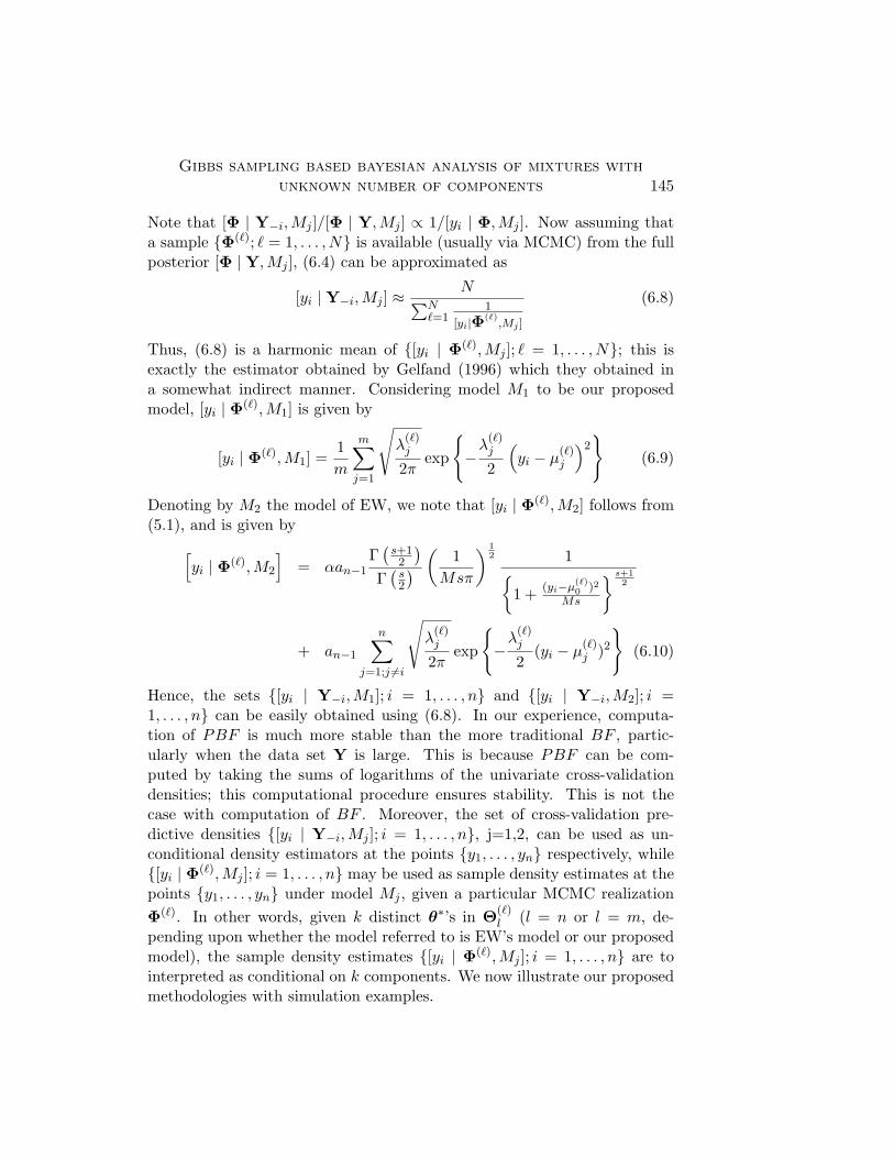
Note that [Φ | Y−i,Mj ]/[Φ | Y,Mj ] ∝ 1/[yi | Φ,Mj ]. Now assuming thata sample {Φ(`); ` = 1, . . . , N} is available (usually via MCMC) from the fullposterior [Φ | Y,Mj ], (6.4) can be approximated as

[yi | Y−i,Mj ] ≈N∑N

`=11

[yi|Φ(`),Mj ]

(6.8)

Thus, (6.8) is a harmonic mean of {[yi | Φ(`),Mj ]; ` = 1, . . . , N}; this isexactly the estimator obtained by Gelfand (1996) which they obtained ina somewhat indirect manner. Considering model M1 to be our proposedmodel, [yi | Φ(`),M1] is given by

[yi | Φ(`),M1] =1m

m∑j=1

√λ

(`)j

2πexp

{−λ

(`)j

2

(yi − µ

(`)j

)2}

(6.9)

Denoting by M2 the model of EW, we note that [yi | Φ(`),M2] follows from(5.1), and is given by[

yi | Φ(`),M2

]= αan−1

Γ(s+12

)Γ

(s2

) (1

Msπ

) 12 1{

1 + (yi−µ(`)0 )2

Ms

} s+12

+ an−1

n∑j=1;j 6=i

√λ

(`)j

2πexp

{−λ

(`)j

2(yi − µ

(`)j )2

}(6.10)

Hence, the sets {[yi | Y−i,M1]; i = 1, . . . , n} and {[yi | Y−i,M2]; i =1, . . . , n} can be easily obtained using (6.8). In our experience, computa-tion of PBF is much more stable than the more traditional BF , partic-ularly when the data set Y is large. This is because PBF can be com-puted by taking the sums of logarithms of the univariate cross-validationdensities; this computational procedure ensures stability. This is not thecase with computation of BF . Moreover, the set of cross-validation pre-dictive densities {[yi | Y−i,Mj ]; i = 1, . . . , n}, j=1,2, can be used as un-conditional density estimators at the points {y1, . . . , yn} respectively, while{[yi | Φ(`),Mj ]; i = 1, . . . , n} may be used as sample density estimates at thepoints {y1, . . . , yn} under model Mj , given a particular MCMC realizationΦ(`). In other words, given k distinct θ∗’s in Θ(`)

l (l = n or l = m, de-pending upon whether the model referred to is EW’s model or our proposedmodel), the sample density estimates {[yi | Φ(`),Mj ]; i = 1, . . . , n} are tointerpreted as conditional on k components. We now illustrate our proposedmethodologies with simulation examples.


7 Simulation Study

Since our modelling ideas are similar to that of RG, the major differencebeing implementation issues, we confine ourselves to comparing our proposedmodel and methodology with that of EW.

Based upon simulated data, we chose to simulate just 5 observationsfrom a mixture distribution with 10 mixture components. Very obviously,EW will now always put zero posterior probability on 10 components, sincethe model is based upon clustering of the data only, and the data size isonly 5. For our model, instead of putting a prior on α, we set it equalto 5. This choice of α implies a relatively strong belief in G0. We ranMCMC algorithms for our proposed model as well as for the model of EWfor a burn-in of 300,000 iterations, and a further 15,00,000 iterations, storingone in 150 iterations, thus obtaining a total of 10,000 realizations from theposterior distribution. Convergence of our MCMC algorithms have beenconfirmed by Kolmogorov-Smirnov tests as described in pages 466–470 ofRobert and Casella (2004).

The posterior probabilities of the possible number of clusters rangingfrom 1 to 30 are given by {0.0000, 0.0003, 0.0022, 0.0091, 0.0274, 0.0497,0.0727, 0.0965, 0.1232, 0.1275, 0.1230, 0.1088, 0.0876, 0.0651, 0.0412, 0.0309,0.0176, 0.0091, 0.0052, 0.0017, 0.0006, 0.0001, 0.0004, 0.0001, 0.0000, 0.0000,0.0000, 0.0000, 0.0000, 0.0000}. Thus, the true number of components, 10,get the highest posterior probability.

Apart from the above simulation study, we also compared our modelwith that of EW using a different simulated data set, where the data size,15, is greater than the true number of components, 10. Brief results fol-low. With a relatively weak prior on α, taken to be Gamma(5, 1), theposterior probabilities of the number of clusters with respect to our model,are given by {0.0000, 0.0000, 0.0003, 0.0017, 0.0063, 0.0186, 0.0335, 0.0650,0.0899, 0.1260, 0.1315, 0.1352, 0.1167, 0.0958, 0.0698, 0.0507, 0.0300, 0.0140,0.0082, 0.0046, 0.0013, 0.0008, 0.0001, 0.0000, 0.0000, 0.0000, 0.0000, 0.0000,0.0000, 0.0000}. Thus 10 components gets very significant posterior proba-bility, 0.1260, which is close to the highest posterior probability. For EW’smodel, these are given by {0.0000, 0.0011, 0.0100, 0.0388, 0.0906, 0.1550,0.1765, 0.1913, 0.1570, 0.0987, 0.0521, 0.0214, 0.0057, 0.0017, 0.0001}; 10components getting posterior probability 0.0987, which is close that of ourmodel. However, PBF (M1/M2) = 335.6571 still says that our model is sup-ported by the data much better than EW’s model. This is accordance with


the discussion in Section 5. Several other simulation studies supported thesame conclusion.

8 Application to Real Data Problems

We now illustrate our methodologies on the three real data sets usedby RG, and available at http://www.stats.bris.ac.uk/∼peter/mixdata.The first data set concerns the distribution of enzymatic activity in theblood, for an enzyme involved in the metabolism of carcinogenic substances,among a group of 245 unrelated individuals. The second data set, the ‘aciditydata’, concerns an acidity index measured in a sample of 155 lakes in north-central Wisconsin. The third and the last data set, the ‘galaxy data’, hasbeen analysed under different mixture models by several researchers. It con-sists of the velocities of 82 distant galaxies, diverging from our own galaxy.For details on these data sets, see RG. We remind the reader again that sinceour set up is the same as in RG, it is not meaningful to compare our modelwith theirs, the only important difference being that our implementation ismuch more straightforward and simple, as compared to RJMCMC used byRG. We, however, compare our model with that of EW and demonstratethat our model performs much better. As in the case of simulation studies,in the real data situation also we ran MCMC algorithms for our proposedmodel as well as for the model of EW for a burn-in of 300,000 iterations, anda further 15,00,000 iterations, storing one in 150 iterations, thus obtaininga total of 10,000 realizations from the posterior distribution.

8.1 Enzyme data. Following both RG and EW, we chose the prior pa-rameters as s = 4.0;S = 2× (0.2/1.22) = 0.3278689;µ0 = 1.45; aα = 2; bα =4;ψ = 33.3. In the value of S, the factor 0.2/1.22 is actually the expec-tation of a Gamma-distributed hyperparameter considered by RG. We donot think that the extra level of hierarchy is necessary; in fact, it only addsto the computational burden. Hence, in all the applications we consid-ered, we fixed the value of the hyperparameter as the expected value of theprior distribution of the hyperparameter. Following RG, we chose m = 30.Apart from fixing the values of µ0 and ψ above, we also experimented withvaguely informative and non-informative priors on the hyperparameters asdescribed in EW. In particular, we assigned that, a priori, µ0 ∼ N(a,A) andψ−1 ∼ Gamma (w/2,W/2), where A−1 → 0, w → 0 and W → 0. However,the results remained almost exactly same as in the case of fixed values of µ0

and ψ, in all three applications we discuss below.


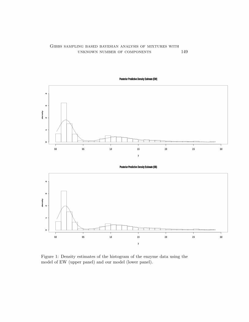
According to the model of EW, the posterior probability of the num-ber of components {1,2,3,4,5,6,7,8,9,10} are given, respectively, by {0.0000,0.0006, 0.2721, 0.3417, 0.2287, 0.1016, 0.0354, 0.0141, 0.0043, 0.0015}, therest having zero posterior probabilities. In our contrast, our model gives therespective probabilities as {0.0000, 0.0010, 0.4483, 0.4026, 0.1228, 0.0226,0.0023, 0.0004, 0.0000, 0.0000}, the rest having zero posterior probabilities.These are not exactly same as the results obtained by RG, but broadly theresults are similar, the posterior of number of components, k, favouring 3–5components (see page 743 of RG). That our model performs much betterthan EW is reflected in PBF (M1/M2) = 3656.644. Figure 1 shows thedensity estimates of the histogram of the enzyme data using EW’s modeland our model. The density estimates look similar. It is however, worthmentioning in this context, that the density estimates we present in thisapplication and other two applications below, are not the same as presentedby RG or EW (the latter consider the galaxy data only), as they did not usecross-validation to obtain the density estimates or sample density estimates.It is apparent from the papers by RG and EW that their densities were notevaluated at the observed data points, but all the observed data points wereused to estimate the densities at arbitrary points on the sample space (theY -space). As a result, our figures are different from theirs. In our opinion,for the purpose of model comparison, use of our cross-validation predictivedensity estimates makes more sense.

It is important to note that while implementation of our approach took42 minutes, implementation of that of EW took 5 hours and 24 minutes ona Mac OS X laptop.

8.2 Acidity data. Based on the priors of RG and EW we take s = 4;S =2× (0.2/0.573) = 0.6980803;µ0 = 5.02; aα = 2; bα = 4;ψ = 33.3;m = 30.

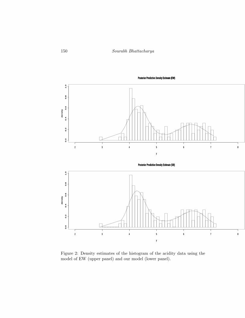
In this case, according to the model of EW, the posterior probabilitiesof the number of components {1,2,3,4,5,6,7,8,9,10,11} are {0.0000, 0.1620,0.3185, 0.2761, 0.1470, 0.0651, 0.0212, 0.0078, 0.0019, 0.0001 0.0003}, therest having zero posterior probabilities. With our model these are {0.0000,0.1091, 0.3444, 0.3092, 0.1628, 0.0564, 0.0147, 0.0028, 0.0003, 0.0002, 0.0001}.In this example as well, 3–5 components are favoured by our model, a resultwhich is once gain in agreement with the analysis of RG. The model of EWseems to favour 2–5 components. The pseudo Bayes factor again prefers ourmodel to that of EW; PBF (M1/M2) = 38.97128. Figure 2 shows the densityestimates of the histogram of the acidity data using EW’s model and ourmodel; again, the density estimates look similar.


Posterior Predictive Density Estimate (EW)

y

de

nsity

0.0 0.5 1.0 1.5 2.0 2.5 3.0

01

23

4

0.0 0.5 1.0 1.5 2.0 2.5 3.0

01

23

4


y

de

nsity

Posterior Predictive Density Estimate (SB)

y

de

nsity

0.0 0.5 1.0 1.5 2.0 2.5 3.0

01

23

4

0.0 0.5 1.0 1.5 2.0 2.5 3.0

01

23

4


y

de

nsity

Figure 1: Density estimates of the histogram of the enzyme data using themodel of EW (upper panel) and our model (lower panel).



y

de

nsity

2 3 4 5 6 7 8

0.0

0.2

0.4

0.6

0.8

1.0

2 3 4 5 6 7 8

0.0

0.2

0.4

0.6

0.8

1.0


y

de

nsity


y

de

nsity

2 3 4 5 6 7 8

0.0

0.2

0.4

0.6

0.8

1.0

2 3 4 5 6 7 8

0.0

0.2

0.4

0.6

0.8

1.0


y

de

nsity

Figure 2: Density estimates of the histogram of the acidity data using themodel of EW (upper panel) and our model (lower panel).


In this case, implementation of our approach took 29 minutes, while thatof EW took 2 hours and 4 minutes.

8.3 Galaxy data. Following EW we consider the following values of theprior parameters: s = 4;S = 2;µ0 = 20; aα = 2; bα = 4;ψ = 33.3;m = 30.

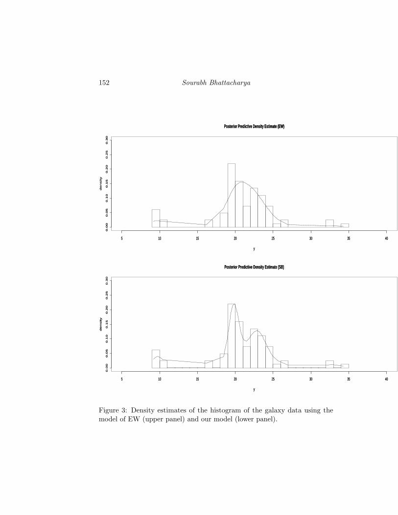
For the galaxy data, under EW’s model, the posterior probabilities ofthe number of components {1,2,3,4,5,6,7,8,9,10,11,12,13,14,15,16} are givenby {0.0000, 0.0000, 0.0893, 0.1760, 0.2148, 0.1951, 0.1495, 0.0891, 0.0487,0.0233, 0.0091, 0.0035, 0.0008, 0.0006, 0.0001, 0.0001} and the others havezero posterior probabilities. So, in this example, k = 4, 5, 6, 7 are well sup-ported by the model of EW. For our model, the posterior probabilities of kare given by {0.0000, 0.0000, 0.0035, 0.0322, 0.1210, 0.2072, 0.2354, 0.1895,0.1210, 0.0574, 0.0247, 0.0055, 0.0021, 0.0004, 0.0001}, thus putting mostposterior mass on k = 5, 6, 7; RG too mention that 5–7 components are in-dicated by the galaxy data with their RJMCMC analysis. PBF (M1/M2) =495439.7 shows that our model is much better supported by the data, ascompared to the model of EW. Figure 3 displays the density estimates ofthe histogram of the galaxy data using the model of EW and the model weproposed. However, unlike in the cases of enzyme and acidity data, in thiscase, our density estimate, even in the naked eye, looks much accurate thanthat of EW.

Again, our approach turned out to be much faster than that of EW, therespective implementation time being 18 minutes and 36 minutes.

9 Conclusion

We have proposed a new and simple approach for Bayesian modelling andinference on mixture models, and argued that our proposal is better thanthat of RG implementation-wise, and is better than that of EW model-wise(in terms of pseudo Bayes factors) and in terms of the ability to take accountof prior information about the number of mixture components in the popu-lation. Moreover, computationally of our approach is much less demandingthan the approaches of EW and RG. Numerical experiments, conducted withsimulated as well as real data sets, have demonstrated considerable powerand flexibility of our approach, and confirmed the arguments we put forwardin support of our proposal.

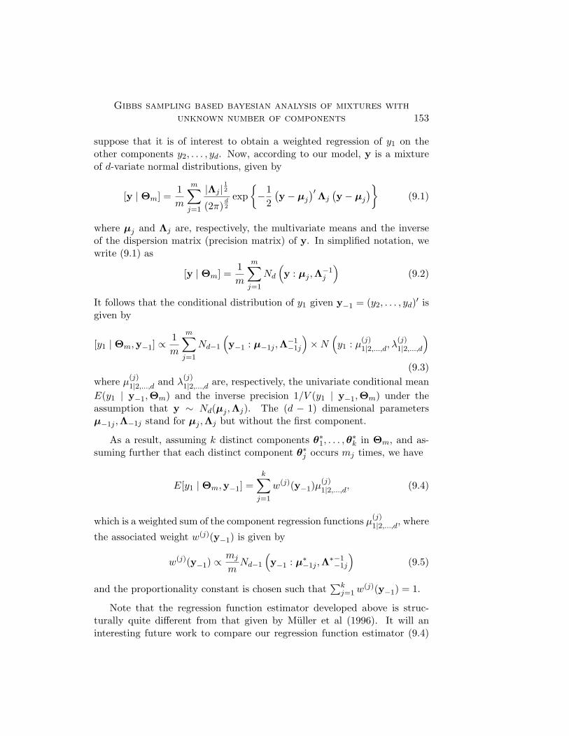
Another advantage of our proposed methodology is the ease with whichregression function estimation can be done. Suppose, for example, thatwe have d-variate data, {yi; i = 1, . . . , n}, where yi = (y1i, . . . , ydi)′. Now



y

de

nsity

5 10 15 20 25 30 35 40

0.0

00

.05

0.1

00

.15

0.2

00

.25

0.3

0

5 10 15 20 25 30 35 40

0.0

00

.05

0.1

00

.15

0.2

00

.25

0.3

0


y

de

nsity


y

de

nsity

5 10 15 20 25 30 35 40

0.0

00

.05

0.1

00

.15

0.2

00

.25

0.3

0

5 10 15 20 25 30 35 40

0.0

00

.05

0.1

00

.15

0.2

00

.25

0.3

0


y

de

nsity

Figure 3: Density estimates of the histogram of the galaxy data using themodel of EW (upper panel) and our model (lower panel).


suppose that it is of interest to obtain a weighted regression of y1 on theother components y2, . . . , yd. Now, according to our model, y is a mixtureof d-variate normal distributions, given by

[y | Θm] =1m

m∑j=1

|Λj |12

(2π)d2

exp{−1

2(y− µj

)′ Λj

(y− µj

)}(9.1)

where µj and Λj are, respectively, the multivariate means and the inverseof the dispersion matrix (precision matrix) of y. In simplified notation, wewrite (9.1) as

[y | Θm] =1m

m∑j=1

Nd

(y : µj ,Λ

−1j

)(9.2)

It follows that the conditional distribution of y1 given y−1 = (y2, . . . , yd)′ isgiven by

[y1 | Θm,y−1] ∝1m

m∑j=1

Nd−1

(y−1 : µ−1j ,Λ

−1−1j

)×N

(y1 : µ(j)

1|2,...,d, λ(j)1|2,...,d

)(9.3)

where µ(j)1|2,...,d and λ(j)

1|2,...,d are, respectively, the univariate conditional meanE(y1 | y−1,Θm) and the inverse precision 1/V (y1 | y−1,Θm) under theassumption that y ∼ Nd(µj ,Λj). The (d − 1) dimensional parametersµ−1j ,Λ−1j stand for µj ,Λj but without the first component.

As a result, assuming k distinct components θ∗1, . . . ,θ

∗k in Θm, and as-

suming further that each distinct component θ∗j occurs mj times, we have

E[y1 | Θm,y−1] =k∑j=1

w(j)(y−1)µ(j)1|2,...,d, (9.4)

which is a weighted sum of the component regression functions µ(j)1|2,...,d, where

the associated weight w(j)(y−1) is given by

w(j)(y−1) ∝mj

mNd−1

(y−1 : µ∗

−1j ,Λ∗−1−1j

)(9.5)

and the proportionality constant is chosen such that∑k

j=1w(j)(y−1) = 1.

Note that the regression function estimator developed above is struc-turally quite different from that given by Muller et al (1996). It will aninteresting future work to compare our regression function estimator (9.4)


with that of Muller et al (1996) after subjecting both the methodologies tovarious challenging applications.

Acknowledgements. We are grateful to Mr. Mriganka Chatterjee forhis assistance in the preparation of this manuscript, and to an anonymousreferee, whose comments have led to an improved presentation of the paper.

References

Antoniak, C. E. (1974). Mixtures of Dirichlet Processes With Applications to Non-parametric Problems., Ann. Statist,, 2, 1152–1174.

Bhattacharya, S. (2006). A Bayesian semiparametric model for organism based envi-ronmental reconstruction, Environmetrics, 17 , 763–776.

Blackwell, D. and McQueen, J. B. (1973). Ferguson distributions via Polya urnschemes, Ann. Statist,, 1, 353–355.

Brook, D. (1964). On the distinction between the conditional probability and the jointprobability approaches in the specification of nearest-neighbour systems, Biometrika,51, 481–483.

Escobar, M. D. and West, M. (1995). Bayesian Density Estimation and Inferenceusing Mixtures, J. Amer. Statist. Assoc., 90, 577–588.

Ferguson, T. S. (1973). A Bayesian Analysis of some Nonparametric Problems, Ann.Statist., 1, 209–230.

Geisser, S. (1975). The predictive sample reuse method with applications, J. Amer.Statist. Assoc., 70, 320–328.

Geisser, S. and Eddy, W. F. (1979). A predictive approach to model selection. J.Amer. Statist. Assoc., 74, 153–160.

Gelfand, A. E. (1996). Model determination using sampling-based methods. In W. Gilks,S. Richardson, and D. Spiegelhalter, editors, Markov Chain Monte Carlo in Prac-tice, Interdisciplinary Statistics, pages 145–162, London. Chapman and Hall.

Gelfand, A. E. and Dey, D. K. (1994). Bayesian model choice: Asymptotics and exactcalculations, J. Roy. Statist. Soc. B, 56, 501–514.

Green, P. J. (1995). Reversible jump Markov chain Monte Carlo computation andBayesian model determination, Biometrika, 82, 711–732.

Jeffreys, H. (1961). Theory of Probability. 3rd edition. Oxford University Press,Oxford.

MacEachern, S. N. (1994). Estimating normal means with a conjugate-style Dirichletprocess prior, Communications in Statistics: Simulation and Computation, 23, 727–741.

McLachlan, G. J. and Basford, K. E. (1988). Mixture Models: Inference and Appli-cations to Clustering, New York: Dekker.

Muller, P., Erkanli, A. and West, M. (1996). Bayesian curve fitting using multi-variate normal mixtures. Biometrika, 83, 67–79.

Richardson, S. and Green, P. J. (1997). On Bayesian analysis of mixtures with anunknown number of components (with discussion), J. Roy. Statist. Soc. B, 59,731–792.


Richardson, S. and Green, P. J. (1998). Corrigendum: On Bayesian analysis ofmixtures with an unknown number of components (with discussion), J. Roy. Statist.Soc. B, 560, 661.

Robert, C. P. and Casella, G. (2004). Monte Carlo Statistical Methods. Springer-Verlag, New York.

Stone, M. (1974). Cross-validatory choice and assessment of statistical predictions (withdiscussion), J. Roy. Statist. Soc. B, 36, 111–147.

Titterington, D. M., Smith, A. F. M. and Makov, U. E. (1985). Statistical Analysisof Finite Mixture Distributions. New York: John Wiley & Sons.

Sourabh BhattacharyaBayesian and Interdisciplinary Research UnitIndian Statistical Institute203, B. T. RoadKolkata 700108INDIAE-mail: [email protected]

Paper received March 2008; revised November 2008.

Gibbs Sampling Based Bayesian Analysis of Mixtures with Unknown Number of Components

Documents

Transcript of Gibbs Sampling Based Bayesian Analysis of Mixtures with Unknown Number of Components