Fluid Phase Equilibria, 1 (1977) 113-135 113 Q Elsevier Scientific Publishing Company, Amsterdam - Printed in The Netherlands

A QUASI LATTICE-LOCAL COMPOSITION MODEL FOR THE EXCESS GIBBS FREE ENERGY OF LIQUID MIXTURES

J.H. VERA, S.G. SAYEGH and G.A. RATCLIFF *

Department of Chemical Engineering, McGill University, Montreal, Quebec (Canada)

(Received October 26th, 1976)

ABSTRACT

Vera, J.H., Sayegh, S.G. and Ratcliff, G.A., 1977. A quasi lattice-local composition model for the excess Gibbs free energy of liquid mixtures. Fluid Phase Equilibria, 1: 113-135.

Two new expressions for the excess Gibbs energy of liquid mixtures are derived from Guggenheim’s quasi-lattice model and Wilson’s local composition concept. These are called the Local Surface Guggenheim equation (LSG) and the Local Composition Guggen- heim equation (LCG). The LSG equation is similar, but not identical to UNIQUAC. The new equations require only two adjustable parameters per binary, and no higher-order parameters for extension to multicomponent systems.

A critical discussion is given of Guggenheim’s quasi-lattice expression for the excess Gibbs energy of athermal mixtures. This expression gives the combinatorial contribution to the new equations.

A new method is proposed in the evaluation of the pure component structural param- eters, independent of particular assumptions about the lattice parameters.

The application of the LSG and the LCG equations to practical problems of phase- equilibria is considered in detail.

INTRODUCTION

The activity coefficients used to express the deviations from ideality of liquid mixtures are related to the molar excess Gibbs energy by the exact thermodynamic equations

gE = C x. ln y.

RT i ’ ’

and

In Ti = (an:;;T)*,P,“;ii

(1)

(2)

l Deceased July 1976.

114

Several analytical expressions giving the functional dependence of the molar excess Gibbs energy on composition and temperature have been presented in the literature. One of the most successful was obtained by Wilson (1964) by introducing the concept of local composition into the Flory-Huggins equa- tion for the excess Gibbs energy of athermal mixtures. Orye and Prausnitz (1965) proposed that the Wilson equation be written as

gE __ = - C Xi In C X, A,i RT I j

where Aij # Aji and Aij = 1 for i = j. This equation has proved to be extreme- ly useful for engineering applications (Prausnitz et al., 1967; Hudson and Van Winkle, 1973; Holmes and Van Winkle, 1970). The major drawback of the Wilson equation is its inability to predict separation into two or more liquid phases. Thus, the prediction of liquid-liquid equilibria has become a critical test for analytical expressions of the excess Gibbs energy.

Wilson (1964) proposed the introduction of a third parameter in his equa- tion in order to predict liquid-liquid immiscibility. Other authors (Nitta and Katayama, 1974; Novak et al., 1974; Tsuboka and Katayama, 1975) have proposed various expressions to be added to the original Wilson equation. Furthermore, other three-parameter expressions have appeared in the litera- ture (Renon and Prausnitz, 1968; Nagata et al., 1975). The local composi- tion concept and the quasi-chemical model have also been used to derive other two-parameter equations able to predict phase instability (Palmer and Smith, 1972; Hiranuma, 1974; Abrams and Prausnitz, 1975).

In this work we develop new expressions for the excess Gibbs energy of liquid mixtures by using Guggenheim’s equation for athermal mixtures and Wilson’s local composition concept. Of the three possible equations that may be obtained, two are considered in detail: the Local Surface Guggenheim equation (LSG) and the Local Composition Guggenheim equation (LCG), the first because of its similarity with a previous equation called UNIQUAC (Abrams and Prausnitz, 1975) and the latter because of its greater consis- tency with the local composition concept. We also propose a method for the evaluation of the pure-component structural parameters required by the quasi-lattice model. This method does not require an explicit description of the lattice geometry. The advantages of the new equations over UNIQUAC are mostly formal. They require fewer assumptions in their derivations and the final expressions, when coupled with the proposed method for evalua- tion of the pure-component parameters, are independent of assumptions about the geometric nature of the lattice.

QUASI-LATTICE MODEL AND LOCAL COMPOSITION CONCEPT

In general, the molar excess Gibbs energy is related to the molar Gibbs energy change of mixing by

gE A&” -= __ - C xi In xi RT RT i

115

For athermal mixtures, i.e., hE = Ah” = 0, we may write

(5)

where the subscript c denotes an athermal mixture (combinatorial contribu- tion). The quasi-lattice model of liquids, through the use of the combina- torial factor, gives expressions for the composition-dependence of the entropy of an athermal mixture and hence for its excess Gibbs energy. The pure-component structural parameters of this model are, for each molecule of species i, the number of segments ri and a parameter qi defined such that zqi is the number of nearest neighbour sites to molecule i, z being the coor- dination number of the lattice. For straight or branched open-chain mole- cules, Guggenheim (1944a) showed that zqi is related to ri by

Zq; = (2 - 2)ri + 2 (6)

In order to generalize eqn. (6) for more complex molecules (aromatics, cycle components, etc.) we will employ the nomenclature introduced previously by Abrams and Prausnitz (1975) and define the bulk factor Ii, by

li =%(ri--qi)-(t--l) (7)

or

Zqi = (2 - 2)ri + 2(1 - Zi) (7a)

Thus, according to Guggenheim, for straight or branched open-chained mol- ecules, Ii = 0.

The final equations for athermal mixtures obtained from the quasi-lattice model can be conveniently written in terms of the overall volume fraction @i and the overall area fraction 8i of component i in a mixture, defined by

and

ei = x,(aq,)

cxj(zgj) j

(9)

For the treatment of non-athermal mixtures, Guggenheim introduced the quasi-chemical approach, leading to a set of simultaneous non-linear equa- tions that must be solved numerically for mixtures other than binary (Hage- mark, 1968). An alternative empirical modification of the equations for athermal mixtures can be obtained using the local composition concept

116

introduced by Wilson (1964). The latter, as demonstrated by the Wilson equation, has proved to be of practical importance in engineering applica- tions and will be used here.

The basic feature of Wilson’s treatment is the definition of the local mole fractions xii and xii. These represent the mole fraction of components j and i, respectively, in the element of volume surrounding a central molecule of species i, and are proportional to the probabilities of finding molecules of type j or type i immediately adjacent to the central molecule. Wilson relates these quantities to the overall mole fractions in the solution by

xji _ “j (10)

x,i Xi ” with

7ij = f?Xp(-Tlij/T) (11)

ajj being a parameter related to the difference between the potential energies of the pairs i-j and i-i. In general aij Z Uji and Qij = 0 for i = j. By defining a local volume fraction by analogy with eqn. (8) and introducing it in place of the overall volume fraction in the Flory-Huggins equation for athermal mixtures, eqn. (3) is obtained. The relationship between Aij and rij is given

by

Aij = 2 Tij

I (12)

When using the local composition concept with Guggenheim’s equation for athermal mixtures, we have found it convenient to introduce a similar nomen- clature for the area-related term, namely

(13)

In the rest of this section we discuss some features of the quasi-lattice equations for athermal mixtures and the various ways in which they may be extended to non-athermal mixtures by applying the local composition con- cept.

Practically-oriented readers may procede directly to the section “Evalua- tion of Pure-Component Structural Parameters”.

Quasi-lattice models for athermal mixtures

Our intention here is not to develop a new lattice model for athermal mix- tures but to critically discuss the existing equations and their interrelations. We first consider the interrelation between the approximations of Guggen- heim and Staverman, and then establish the conditions under which the

117

Guggenheim-Staverman expression for the excess Gibbs energy reduces to the Flory-Huggins equation.

For athermal mixtures of open-chain molecules, branched or unbranched, Guggenheim (1952) presented explicit equations for the change in thermo- dynamic properties in the process of mixing. The equations were presented “not much for their practical importance but rather to emphasize their existence”. His equation for the entropy change of mixing can be written as

(14) l

Equation (14) was obtained with the assumption that eqn. (6) is valid for all molecules in the mixture. Staverman (1950) developed an expression for the combinatorial factor, and thus for the entropy of an athermal mixture, that is free from the restriction of eqn. (6). However, the striking fact that has not been fully realized in the literature is that when Staverman’s combina- torial factor is used to obtain the entropy change of mixing, eqn. (14) is recovered. This fact can be easily explained since the same condition of bulkiness of a molecule (ring formation, branching, etc.) is allowed in both the pure component and the mixture. The excess Gibbs energy of an ather- ma1 mixture of molecules of any size and shape can be then obtained by combining equations (4)) (5) and (14) as

(15)

This equation will be called the Athermal Guggenheim-Staverman equation since it can be obtained either from Guggenheim’s or from Staverman’s expressions for the combinatorial factor. The activity coefficients obtained by combining eqns. (2) and (15) can be written in a remarkably simple form:

(16)

If the restrictive relation between Zqi and ri given by eqn. (6) is applied to eqn. (16), the following expression is obtained:

(restricted form) (17)

As expected, when either eqn. (16) or (17) is combined with eqn. (l), eqn. (15) is regenerated. This fact supports the arguments about the generality of eqn. (15).

* Equation 10.10.4, Guggenheim, 1952.

118

It has long been recognized that the Flory-Huggins equation for athermal mixtures of polymers can be obtained directly from eqn. (15) by assuming that ri = qi for all i, leading to

gE (-) = Cxiln* RTFH i xi

and

(In ?i)FH = >

(18)

(19)

The basic assumption underlying this simplification has usually been justified in the literature using the physically unrealistic condition that z + m in eqn. (6). This drastic condition, which tends to destroy the physical significance of the quasi-lattice model, is not, in fact, necessary. A more general condition is that the ratios ri/qi have the same value for all mole- cules in the mixture. In practice this situation may be found, for example, for mixtures of open-chain r-mers with large ri. In this case eqn. (6) is valid but the effect of the constant term tends to be negligible. Similarly, for molecules with bulk factors close to unity, the constant term in eqn. (7a) tends to cancel out.

For the treatment of non-athermal mixtures with the local composition concept, the use of eqn. (15) allows us to obtain a correction term that over- comes the inability of the Wilson equation to describe liquid-liquid equi- libria.

Local composition concept and equations for non-athermal mixtures

Using the local composition concept as introduced by Wilson (1964), we define the total volume fraction Ev and the local area fraction [A of compo- nent i, by

(20)

and

.g = xii(zqi) ei =

C ~ji(Zqj) C 8j Tij

j j

(21)

When the Flory-Huggins equation, eqn. (18), is chosen as the basic equation for non-athermal mixtures there is no ambiguity on how to apply the local

119

composition concept. Replacing the overall volume fraction in the Flory Huggins equation by the local volume fraction, we obtain

This form of the Wilson equation clearly shows two contributions to the excess Gibbs energy. The first term on the right hand side represents the combinatorial contribution, since it is identical to the Flory-Huggins equa- tion. The second term is the residual contribution arising from the inter- molecular potentials. The more familiar form of the Wilson equation, eqn. (3), is obtained by grouping both terms of the right hand side of eyn. (22) and using eqn. (12).

When the Athermal Guggenheim-Staverman equation is considered, three distinct possibilities arise. Following Abrams and Prausnitz (1975), we may use the local area fraction as the principal variable. If the overall area frac- tion in eqn. (15) is replaced by the local area fraction, we obtain

Xi(Zqi) In C 8j7iJ j

(23)

where (g”/RT), is given by eqn. (15) and represents the combinatorial con- tribution. Equation (23) is almost identical to the UNIQUAC equation (Abrams and Prausnitz, 1975) except for the factor z/2 multiplying the residual contribution. The indices of T are also interchanged with respect to UNIQUAC but this arises from the use of a convention different from that employed by Wilson. Equation (23) can be written in a more compact form as

Pa)

This equation will be called the Local Surface Guggenheim equation (LSG). A second modification of the Athermal Guggenheim-Staverman equation

would be to use the overall area fraction and the local volume fraction. From the point of view of this analysis, however, there seems to be no reason for applying local mole fractions to surface terms and not to volume terms or vice versa. The third alternative modification would then be to simultaneous- ly use eqns. (20) and (21) for the local volume and surface fractions in place of their respective overall terms in the Athermal Guggenheim-Staverman equation. The resulting expression may be written in compact form as,

C Xj Aij

(24)

120

-2

-.l M

E & RT

.2 4 6 .a

x1

2 4 6 -8

Xl,

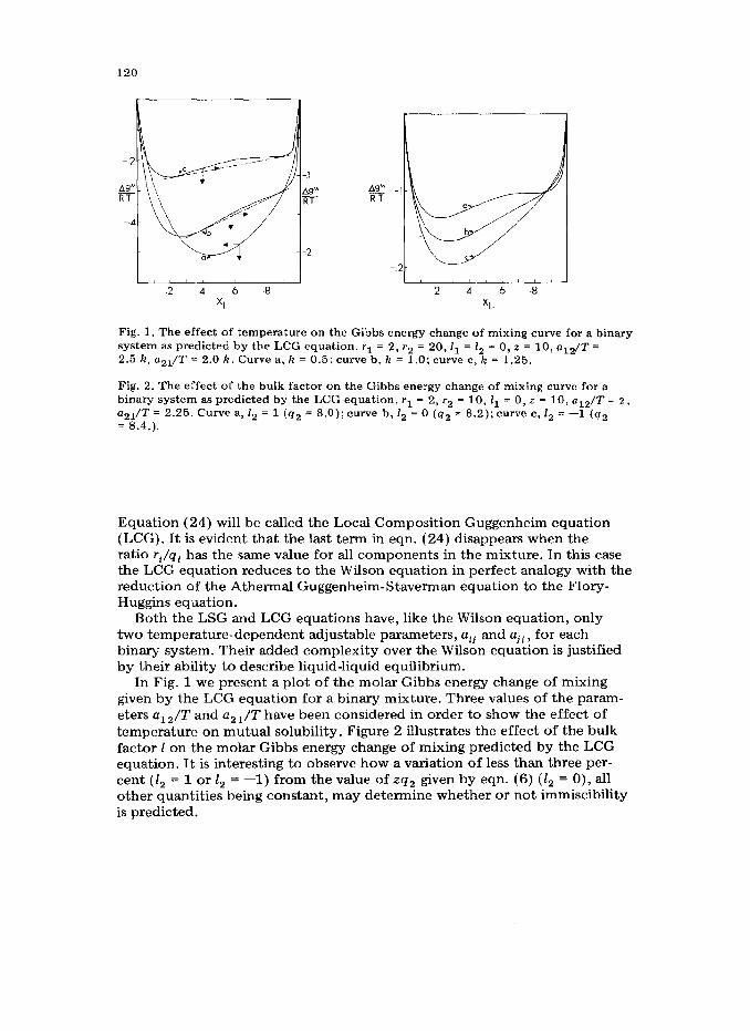
Fig. 1. The effect of temperature on the Gibbs energy change of mixing curve for a binary system as predicted by the LCG equation. rI = 2, r2 = 20,1, = 1, = 0, z = 10, ala/T = 2.5 k, azl/T = 2.0 k. Curve a, k = 0.5; curve b, k = 1.0; curve c, k = 1.25.

Fig. 2. The effect of the bulk factor on the Gibbs energy change of mixing curve for a binary system as predicted by the LCG equation. r1 = 2, r2 = 10, 1, = 0, z = 10, Q/T = 2,

a,,/T = 2.25. Curve a, 1, = 1 (qa = 8.0); curve b, I, = 0 (qa = 8.2); curve c, I, = -1 (q2 = 8.4.).

Equation (24) will be called the Local Composition Guggenheim equation (LCG). It is evident that the last term in eqn. (24) disappears when the ratio ri/qi has the same value for all components in the mixture. In this case the LCG equation reduces to the Wilson equation in perfect analogy with the reduction of the Athermal Guggenheim-Staverman equation to the Flory- Huggins equation.

Both the LSG and LCG equations have, like the Wilson equation, only two temperature-dependent adjustable parameters, aij and uji , for each binary system. Their added complexity over the Wilson equation is justified by their ability to describe liquid-liquid equilibrium.

In Fig. 1 we present a plot of the molar Gibbs energy change of mixing given by the LCG equation for a binary mixture. Three values of the param- eters a, .JT and a2 1/T have been considered in order to show the effect of temperature on mutual solubility. Figure 2 illustrates the effect of the bulk factor 1 on the molar Gibbs energy change of mixing predicted by the LCG equation. It is interesting to observe how a variation of less than three per- cent (& = 1 or 1, = -1) from the value of zq, given by eqn. (6) (& = 0), all other quantities being constant, may determine whether or not immiscibility is predicted.

121

EVALUATION OF PURE COMPONENT STRUCTURAL PARAMETERS

In the previous section two new expressions for the molar excess Gibbs energy have been derived; i.e., the Local Surface Guggenheim equation (LSG), eqn. (23a), and the Local Composition Guggenheim equation, eqn. (24). The most critical problem that confronts any equation based on the quasi-lattice model is the evaluation of the structural parameters r and 4. There has also been some arbitrariness associated with the selection of a value for 2.

Previous works (Lichtenthaler, Abrams and Prausnitz, 1973; Donohue and Prausnitz, 1975; Abrams and Prausnitz, 1975) suggest considering

and

qi =A!!. a* (26)

where ui is a quantity related to some measure of the volume (or size) of the molecule and ai is a quantity related to its surface (shape). u* and a* are some arbitrarily-chosen reducing factors which can be associated with the volume and area, respectively, of a unit cell or a unit segment.

For the Flory-Huggins or Wilson type of equations, the value of u* is immaterial since it cancels out. Furthermore, for these equations, the use of ui as given by the molar volume or the Van der Waals volume as calculated by Bondi (1968), gives almost the same results. In fact, the Van der Waals vol- ume is closely proportional to the molar volume at 20°C. A least square fit over 33 compounds, including alkanes, alcohols, esters, ketones, alkylchlo- rides and aromatics, gives

Ui = 0.554Vm (20°C) (27)

with a mean absolute relative deviation of 2.78%. The proportionality con- stant corresponds to an average value of the packing density at 20°C as defined by Bondi (1968). Since the parameters z and qi do not appear in these equations, they are independent of any lattice assumption (Longuett- Higgins, 1953; Silberberg, 1970).

For the LSG and LCG equations (and also for the Athermal Guggenheim- Staverman equation), the term zqi appears explicitly. In order to obtain this quantity similarly independent of any assumption regarding the lattice parameters we proceed as follows. We retain eqn. (6) for open-chain mole- cules, branched or not, Zi = 0, and assume eqns. (25) and (26) to be valid. Combining these equations, we obtain

(28)

122

or

ai = h,ui + kz (284

Following Abrams and Prausnitz (1975), we use the Van der Waals areas and volumes for ai and ui as calculated by Bondi (1968). As shown in the Appendix, the relation between ai and ui is in fact theoretically linear with a common slope for all families of compounds, but a unique intercept for each family. This would result in the choice of a different value of a*, and hence of u*, for each family, making the application of the model awkward. However, a compensatory effect can be expected in the intercept of eqn. (A.3). In fact, a least-squares fit over forty-three of the more common open- chain compounds, branched or unbranched (including alkanes, alcohols, aldehydes, ketones, nitriles, acids and esters), for which it is presumed that eqn. (6) applies, yields

z-2 a* kl = --- - = 1.323 * lo* cm-i

z v*

2a’ k, = - = 6.259 * lo8 cm2/mole

Z (30)

with a mean absolute relative deviation of 1.24%. This small deviation justifies eqn. (28) and its underlying assumptions, eqns. (6), (25) and (26).

Combining eqns. (28a), (29) and (30) we obtain

Zqi = 0.4228~i + 2 (31)

An alternative expression for zqi can be obtained combining eqns. (26) and (30), as

ai

zqi = ~>l~>.l@ (32)

For open-chain molecules, eqns. (31) and (32) are virtually equivalent. Although no particular assumptions about z, v* and a* are required by

this method, for any assumed z, a value for a* can be obtained from eqn. (30) and then a value of u* from eqn. (29). Sets of self-consistent values are presented in Table 1. For convenience only, we will use the set corre- sponding to z = 10, but it should be clear that any self-consistent set gives the same values for Gi, ei and zq, to be used in the LSG and LCG equations. For molecules with more complex geometry eqn. (7a) should be used instead of eqn. (6). Thus, generalizing eqn. (31) for molecules of any size and shape we write

zqi = 0.4228~~ + 2(1 - ri) (33)

No a priori method for the evaluation of the bulk factor li is known, but a knowledge of the geometry of the molecule may serve as a guide, cf. Prigo-

123

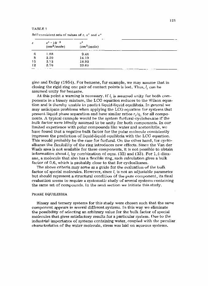
TABLE I

Self-consistent sets of values of z, a* and u*

.z a* - 10-g u* (cm2/mole) (cm3/mole)

6 1.88 9.46 8 2.50 14.19

10 3.13 18.92 12 3.76 23.65

gine and Defay (1954). For benzene, for example, we may assume that in closing the rigid ring one pair of contact points is lost. Thus, Zi can be assumed unity for benzene.

At this point a warning is necessary. If li is assumed unity for both com- ponents in a binary mixture, the LCG equation reduces to the Wilson equa- tion and is thereby unable to predict liquid-liquid equilibria. In general we may anticipate problems when applying the LCG equation for systems that present liquid phase separation and have similar ratios ri/qi for all compo- nents. A typical example would be the system furfural-cyclohexane if the bulk factor were blindly assumed to be unity for both components. In our limited experience with polar compounds like water and acetonitrile, we have found that a negative bulk factor for the polar molecule consistently improves the prediction of liquid-liquid equilibria with the LCG equation. This would probably be the case for furfural. On the other hand, for cyclo- alkanes the flexibility of the ring introduces new effects. Since the Van der Waals area is not available for these components, it is not possible to obtain information about Zi by combination of eqns. (32) and (33). For 1,4-diox- ane, a molecule that also has a flexible ring, such calculation gives a bulk factor of 0.6, which is probably close to that for cycloalkanes.

The above criteria may serve as a guide for the evaluation of the bulk factor of special molecules. However, since Zi is not an adjustable parameter but should represent a structural condition of the pure component, its final evaluation seems to require a systematic study of several systems containing the same set of compounds. In the next section we initiate this study.

PHASE EQUILIBRIA

Binary and ternary systems for this study were chosen such that the same component appears in several different systems. In this way we eliminate the possibility of selecting an arbitrary value for the bulk factor of special molecules that gives satisfactory results for a particular system. Due to the industrial importance of systems containing water, coupled with the peculiar characteristics of the water molecule, stress was laid on aqueous systems.

TA

BL

E

2

Val

ues

of t

he s

truc

tura

l pa

ram

eter

s r

and

q

Com

pone

nt

“i

ai ’

lo-

’ L

SG o

r L

CG

equ

atio

ns

z =

10

Uni

quac

2

= 1

0 (c

m3

/mol

e)

(cm

2/m

ole)

r

4 1

P 9

I

Ace

tone

39

.04

5.84

2.

06

1.85

0

2.57

2.

34

-0.4

2 C

hlor

ofor

m

43.5

4 6.

03

2.30

2.

04

0 2.

87

2.41

0.

43

Eth

anol

31

.94

4.93

1.

69

1.55

0

2.11

a

1.97

a

*.41

E

thyl

ac

etat

e 52

.77

7.79

2.

79

2.43

0

3.48

a

3.12

a

-0.6

8 n-

Hep

tane

78

.49

10.9

9 4.

15

3.52

0

5.17

a

4.40

a

-0.3

2 M

ethy

l ac

etat

e 42

.54

6.44

2.

25

2.00

0

2.80

2.

58

-0.7

0 B

enze

ne

48.3

9 6.

00

2.56

2.

05

1 3.

19

2.40

1.

76

Ace

toni

trile

28

.37

4.31

1.

50

1.50

-0

.5

1.87

a

1.72

=

-0.1

2 W

ater

13

.91

22.2

3 0.

73

1.19

-2

0.

92

1.40

-2

.32

a V

alue

s fo

r U

NIQ

UA

C

obta

ined

fr

om

ri =

uJ1

5.17

an

d qi

= O

i/(2.

5 10

’).

Oth

er

valu

es

for

UN

IQU

AC

ar

e th

ose

repo

rted

by

Abr

ams

and

Prau

snitz

(1

97 5

).

125

Furthermore since Abrams and Prausnitz (1975) have observed that the pre- diction of liquid-liquid equilibria for plait-point ternary systems present the most difficult cases, such systems were chosen.

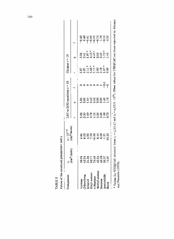
The pure component structural parameters r and q to be used with the LSG and the LCG equations are presented in Table 2. These parameters were obtained by the method described in the previous section. For con- venience only, we present their values for z = 10. The parameters to be used with UNIQUAC are also included in Table 2.

Evaluation of binary parameters

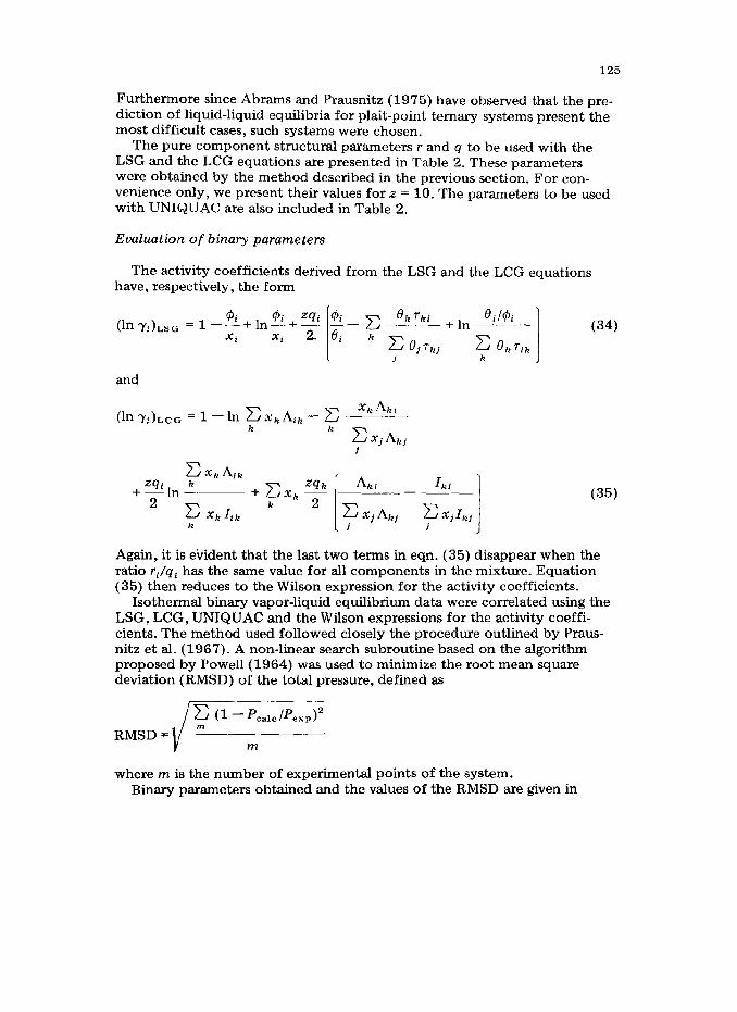
The activity coefficients derived from the LSG and the LCG equations have, respectively, the form

(ln Yi)LSG = 1__‘+ln’+Z9, &_ C ekrki +ln_ *i/@i

xi xi 2 ei ’ C OjTkj

c OkTik j k

and

(hyi)LcG -1-h CXkAik-C xk Aki

k

’ c”jI\kj

i

c xk bk

+ 24’In J._ +cxkF Aki I .

2 c xk Ii, k k

C XjAkj - c:jlkj

1 j

(34)

i

(35)

Again, it is evident that the last two terms in eqn. (35) disappear when the ratio ri/qi has the same value for all components in the mixture. Equation (35) then reduces to the Wilson expression for the activity coefficients.

Isothermal binary vapor-liquid equilibrium data were correlated using the LSG, LCG, UNIQUAC and the Wilson expressions for the activity coeffi- cients. The method used followed closely the procedure outlined by Praus- nitz et al. (1967). A non-linear search subroutine based on the algorithm proposed by Powell (1964) was used to minimize the root mean square deviation (RMSD) of the total pressure, defined as

where m is the number of experimental points of the system. Binary parameters obtained and the values of the RMSD are given in

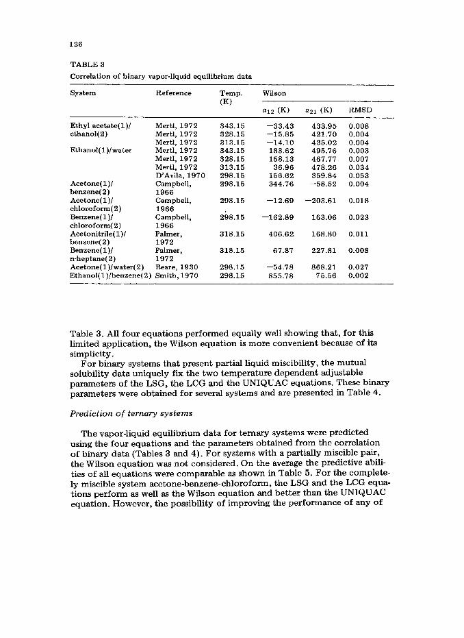
126

TABLE 3

Correlation of binary vapor-liquid equilibrium data

System Reference Temp.

(R)

Wilson

a12 W) *21 W RMSD

Ethyl acetate(l)/ Mertl, 1972 ethanol(2) Mertl, 1972

Mertl, 1972 Ethanol(l)/water Mertl, 1972

Mertl, 1972 Mertl, 1972 D’Avila, 1970

Acetone(l)/ Campbell, benzene( 2) 1966 Acetone(l)/ Campbell, chloroform( 2) 1966 Benzene( 1 )/ Campbell, chloroform(2) 1966 Acetonitrile( l)/ Palmer, benzene( 2) 1972 Benzene(l)/ Palmer, n-heptane(2) 1972 Acetone(l)/water(2) Beare, 1930 Ethanol(l)/benzene(2) Smith, 1970

343.15 -33.43 433.95 0.008 328.15 -15.85 421.70 0.004 313.15 -14.10 435.02 0.004 343.15 183.62 495.76 0.003 328.15 158.13 467.77 0.007 313.15 36.96 478.26 0.034 298.15 156.62 359.84 0.053 298.15 344.76 -58.52 0.004

298.15

298.15 -162.89

318.15 406.62

318.15 67.87

298.15 -54.73 868.21 0.027 298.15 855.78 75.56 0.002

-12.69 -203.61 0.018

163.06 0.023

168.80 0.011

227.81 0.008

Table 3. All four equations performed equally well showing that, for this limited application, the Wilson equation is more convenient because of its simplicity.

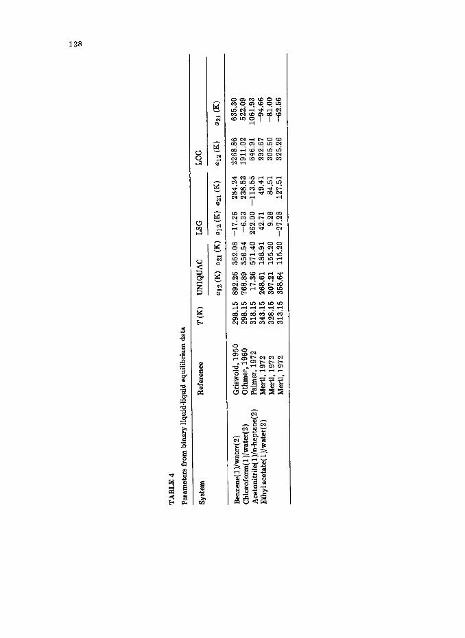
For binary systems that present partial liquid miscibility, the mutual solubility data uniquely fix the two temperature dependent adjustable parameters of the LSG, the LCG and the UNIQUAC equations. These binary parameters were obtained for several systems and are presented in Table 4.

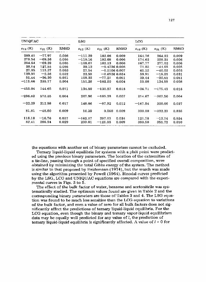
Prediction of ternary systems

The vapor-liquid equilibrium data for ternary systems were predicted using the four equations and the parameters obtained from the correlation of binary data (Tables 3 and 4). For systems with a partially miscible pair, the Wilson equation was not considered. On the average the predictive abili- ties of all equations were comparable as shown in Table 5. For the complete- ly miscible system acetone-benzene-chloroform, the LSG and the LCG equa- tions perform as well as the Wilson equation and better than the UNIQUAC equation. However, the possibility of improving the performance of any of

127

UNIQUAC LSG LCG

~12 WI ~21 W) RMSD ~12 WI ~21 W RMSD ~12 WI (121 (K) RMSD

289.41 -77.97 0.008 -111.39 182.06 0.009 164.76 264.22 0.009 278.54 -69.36 0.005 -110.16 182.08 0.006 174.62 258.21 0.006 284.64 -69.39 0.005 -108.67 182.13 0.006 167.77 277.02 0.006 28.14 127.55 0.005 30.12 -0.4736 0.008 71.85 -44.55 0.005 27.05 115.37 0.003 27.54 -0.5106 0.007 65.53 -40.03 0.003

129.91 -2.36 0.032 22.59 -0.6526 0.034 59.91 -18.05 0.031 51.44 -36.30 0.051 108.22 -77.21 0.051 39.44 -30.51 0.061

-111.66 235.17 0.004 151.28 -102.50 0.004 55.08 134.59 0.008

-455.04 144.65 0.011

0.004

134.59

267.96

-130.27 0.018

-185.38 0.007

-36.71 -175.42 0.018

214.67 -362.50 0.004 -286.69 573.35

-22.29 212.98 0.017

0.009

148.06

16.39

-87.92 0.012

-0.060 0.009

-167.94 300.00 0.037

300.00 -332.23 0.035 81.81 -48.60

118.18 -16.76 0.037 -162.17 297.03 0.034 121.78 -13.74 0.034 82.41 286.24 0.029 239.01 -121.88 0.009 380.50 351.72 0.010

the equations with another set of binary parameters cannot be excluded. Ternary liquid-liquid equilibria for systems with a plait point were predict-

ed using the previous binary parameters. The location of the extremities of a tie-line, passing through a point of specified overall composition, were obtained by minimizing the total Gibbs energy of the system. The method is similar to that proposed by Heidemann (1974)) but the search was made using the algorithm presented by Powell (1964). Binodal curves predicted by the LSG, LCG and UNIQUAC equations are compared with the experi- mental curves in Figs. 3 to 5.

The effect of the bulk factor of water, benzene and acetonitrile was sys- tematically studied. The optimum values found are given in Table 2 and the corresponding binary parameters are those of Tables 3 and 4. The LSG equa- tion was found to be much less sensitive than the LCG equation to variatfons of the bulk factor, and even a value of zero for all bulk factors does not sig- nificantly affect the predictions of ternary liquid-liquid equilibria. For the LCG equation, even though the binary and ternary vapor-liquid equilibrium data may be equally well predicted for any value of 1, the prediction of ternary liquid-liquid equilibria is significantly affected. A value of 1 = 0 for

128

129

TABLE 5

Prediction of ternary vapor-liquid equilibrium

System Reference Temp.

(R)

RMSD

Wilson UNIQUAC LSG LCG

Acetone( 1 )/ benzene( 2)/ chloroform(3) Acetonitrile( l)/ benzene( 2)/ n-heptane( 3) Ethyl acetate(l) ethanol( 2)/ water( 3)

Campbell, 1966 298.15 0.021 0.147 0.024 0.031

Palmer, 1972 318.15 - 0.039 0.025 0.045

Mertl, 1972 343.15 - 0.042 0.039 0.048 Mertl, 1972 328.15 - 0.061 0.061 0.052 Mertl, 1972 313.15 - 0.051 0.056 0.051

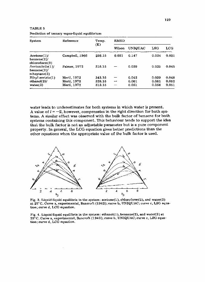
water leads to underestimates for both systems in which water is present. A value of I= -2, however, compensates in the right direction for both sys- tems. A similar effect was observed with the bulk factor of benzene for both systems containing this component. This behaviour tends to support the idea that the bulk factor is not an adjustable parameter but is a pure component property. In general, the LCG equation gives better predictions than the other equations when the appropriate value of the bulk factor is used.

.2 .A .6

x3

2 A -6 8

x3

Fig. 3. Liquid-liquid equilibria in the system: acetone(l), chloroform(2), and water(3) at 25°C. Curve a, experimental, Bancroft (1942); curve b, UNIQUAC; curve c, LSG equa- tion; curve d, LCG equation.

Fig. 4. Liquid-liquid equilibria in the system: ethanol(l), benzene(2), and water(3) at 25°C. Curve a, experimental, Bancroft (1942); curve b, UNIQUAC; curve c, LSG equa- tion; curve d, LCG equation.

2 .4 .6 8 x3

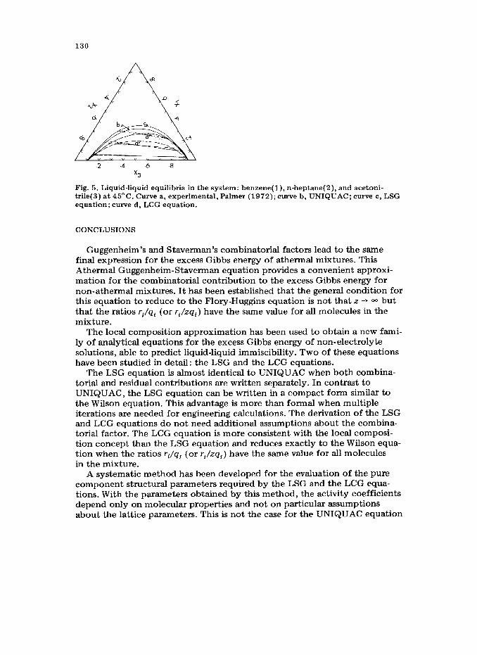
Fig. 5. Liquid-liquid equilibria in the system: benzene(l), n-heptane(2), and acetoni- trile(3) at 45°C. Curve a, experimental, Palmer (1972); curve b, UNIQUAC; curve c, LSG equation; curve d, LCG equation.

CONCLUSIONS

Guggenheim’s and Staverman’s combinatorial factors lead to the same final expression for the excess Gibbs energy of athermal mixtures. This Athermal Guggenheim-Staverman equation provides a convenient approxi- mation for the combinatorial contribution to the excess Gibbs energy for non-athermal mixtures. It has been established that the general condition for this equation to reduce to the Flory-Huggins equation is not that z -+ - but that the ratios ri/qi (or ri/zqi) have the same value for all molecules in the mixture.

The local composition approximation has been used to obtain a new fami- ly of analytical equations for the excess Gibbs energy of non-electrolyte solutions, able to predict liquid-liquid immiscibility. Two of these equations have been studied in detail: the LSG and the LCG equations.

The LSG equation is almost identical to UNIQUAC when both combina- torial and residual contributions are written separately. In contrast to UNIQUAC, the LSG equation can be written in a compact form similar to the Wilson equation. This advantage is more than formal when multiple iterations are needed for engineering calculations. The derivation of the LSG and LCG equations do not need additional assumptions about the combina- torial factor. The LCG equation is more consistent with the local composi- tion concept than the LSG equation and reduces exactly to the Wilson equa- tion when the ratios ri/qi (or rj/zqi) have the same value for all molecules in the mixture.

A systematic method has been developed for the evaluation of the pure component structural parameters required by the LSG and the LCG equa- tions. With the parameters obtained by this method, the activity coefficients depend only on molecular properties and not on particular assumptions about the lattice parameters. This is not the case for the UNIQUAC equation

131

since qi (and not zqi) appears explicitly in the final expressions. In order to generalize the method for molecules of any size and shape, an

operational parameter Ei, introduced by Abrams and Prausnitz (19’75), has been interpreted as a “bulk factor” by comparison with the relation between ri and zqi given by Guggenheim (1944) for open-chain molecules, branched or unbranched. For these simple molecules, according to Guggenheim, Zi = 0. Only certain molecules, like cyclic, aromatic or highly polar molecules, require a non-zero value of the bulk factor. Some preliminary guidelines for evaluating the bulk factor for these special molecules are presented.

The prediction of liquid-liquid equilibria with the LCG equation, in con- trast to the prediction with the LSG equation, is particularly sensitive to the values of the bulk factor. This is a major drawback of the LCG equation for systems for which reliable values of the bulk factor for all special molecules are not available.

In terms of practical performance, there seems to be no definite superior- ity of one of the proposed equations over the other, nor of either over the UNIQUAC equation.

In addition to the results presented here, a complete study was performed using a method similar to that proposed by Abrams and Prausnitz (1975), to evaluate r and q. The values of the reducing volume and surface were those of the CH, group given by Bondi (1968). For z a value of ten was used. The results were similar to those presented here. We consider the present method for evaluating r and q more fundamental since it avoids assumptions of the lattice parameters.

ACKNOWLEDGEMENT

The authors are grateful for financial assistance from the National Research Council of Canada and to the McConnell Memorial Foundation for the award of a McConnell Fellowship to S. Sayegh. The first two authors gratefully acknowledge their debt to the late Professor G.A. Ratcliff, whose contribution during the first stages of this work was determinant for its com- pletion. They are also grateful to Professor J.M. Prausnitz for valuable com- ments and to Professor J.R. Grace for his help in the editing of this manu- script.

APPENDIX

A linear correlation between Van der Waals volumes and surfaces in a family of compounds

A family of compounds may be represented as

R” - (CH,), - H

where R” is a characteristic radical defining the family. Following Bondi’s

132

method (Bondi 1968), the Van der Waals volume and surface of any member of the family can be written in terms of the volumes and surfaces of the con- stituents groups as

Vi = Usa + nv, + VH (A-1)

lZi = aRO + na2 + aH (-4-z)

where the subscripts 2 and H indicate the property of the CHs group and the H atom, respectively.

Eliminating n from equations (A.l) and (A.2), we obtain

q z(z) vi + (aRoa’,aH -!fIE$!E)a2 (A-3)

or

ai = hlvi +h2 (A.3a)

Equation (A.3) shows that for any family of compounds there is a linear correlation between ai and ui. A plot of ai vs. ui for different families should yield a series of parallel straight lines of slopes (a,&) and a characteristic intercept depending on R" . For the straight-chain alkane family (R” = CH,) we obtain, analytically, h, = 1.320 .lOs cm-r and h, = 6.321 . 10s ems/ mole. These values are close to those given in eqns. (29) and (30) of the text. The latter represent an average for different families of open-chain com- pounds.

NOTATION

‘i

'ij

;:

AiP Ahm

Iii 4 k2

4

n

ni

P

41 R R”

‘i

Van der Waals surface of molecule i binary interaction parameter reducing area excess Gibbs energy per mole Gibbs energy change of mixing per mole enthalpy change of mixing per mole see eqn. (13) see eqn. (29) see eqn. (30) bulk factor of component i, see eqn. (7) total number of moles number of moles of component i

total pressure surface parameter of component i

Gas constant characteristic radical (Appendix) volume parameter of component i

133

As” T

‘i

V*

VIII xi

3cii

z

entropy change of mixing per mole absolute temperature Van der Waals volume of component i reducing volume molar volume mole fraction of component i local mole fraction of component j in the element of volume sur- rounding a central molecule of species i coordination number of the lattice

Greek letters

Yi

ei

hj

$

activity coefficient of component i

overall surface fraction of component i Wilson-type binary interaction parameters, see eqn. (12) local surface fraction of component i, see eqn. (21) local volume fraction of component i, see eqn. (20)

7ij binary interaction parameter, see eqn. (11)

6 overall volume fraction of component i

Subscripts

ij,k components C combinatorial contribution FH Flory-Huggins term for athermal mixture res. residual contribution

REFERENCES

Abrams, D.S. and Prausnitz, J.M., 1975. Statistical thermodynamics of liquid mixtures: A new expression for the excess Gibbs energy of partly or completely miscible sys- tems. AIChE J., 21: 116-128.

Bancroft, W.D. and Hubard, S.S., 1942. A new method for determining dineric distribu- tion. J. Am. Chem. Sot., 64: 347-353.

Beare, W.G., McVicar, G.A. and Ferguson, J.B., 1930. The determination of vapour and liquid compositions in binary systems. II. Acetone-water at 25°C. J. Phys. Chem., 34: 1310-1318.

Bondi, A., 1968. Physical properties of molecular crystals, liquids and glasses. Wiley, New York.

Campbell, A.N., Kartzmark, EM. and Chatterjee, R.M., 1966. Excess volumes, vapour pressures, and related thermodynamic properties of the system acetone-chloroform- benzene, and its component binary systems. Can. J. Chem., 44: 1183-1189.

D’Avila, S.G. and Silva, R.F., 1970. Isothermal vapour-liquid equilibrium data by total pressure method. Systems acetaldehyde-ethanol, acetaldehyde-water, and ethanol- water. J. Chem. Eng. Data, 15: 421-424.

Donohue, M.D. and Prausnitz, J.M., 1975. Combinatory entropy of mixing molecules that differ in size and shape. A simple approximation for binary and multicomponent mixtures. Can. J. Chem., 53: 1586-1592.

134

Griswold, J., Chew, J.N. and Klecka, M.E., 1950. Pure hydrocarbons from petroleum. Recovery of Aniline solvent from Distex hydrocarbon products by water extraction. Ind. Eng. Chem., 42 (6): 1246-1251.

Guggenheim, E.A., 1944. (a) Statistical thermodynamics of mixtures with zero energies of mixing. Proc. Roy. Sot. A, 183: 203-212; (b) Ibid. 213-227.

Guggenheim, E.A., 1952. Mixtures. Clarendon Press, Oxford. Hagemark, K., 1968. Thermodynamics of ternary systems. The quasi-chemical approxi-

mation. J. Phys. Chem., 72: 2316-2322. Heidemann, R.A., 1974. Three phase equilibria using equations of state. AIChE J., 20:

847-855. Hiranuma. N., 1974. A new expression similar to the three parameter Wilson equation.

Ind. Eng. Chem., Fundamentals, 13 : 219-222. Holmes, M.J. and Van Winkle, M., 1970. Prediction of ternary vapor-liquid equilibria

from binary data. Wilson equation used to predict vapour compositions. Ind. Eng. Chem., 62 (1): 21-31.

Hudson, J.W. and Van Winkle, M,, 1973. Multicomponent vapor-liquid equilibria in miscible systems from binary parameters. Ind. Eng. Chem. Process Design Develop., 9 : 466-472.

Lichtenthaler, R.N., Abrams, D.S. and Prausnitz, J.M., 1973. Combinatorial entropy of mixing for molecules differing in size and shape. Can. J. Chem., 51: 3071-3080.

Longuett-Higgins, H.C., 1953. Solutions of chain molecules -A new statistical theory. Discuss. Faraday Sot., 15: 73-80.

Mertl, I., 1972. Liquid-vapour equilibrium IL. Phase equilibria in the ternary system ethyl acetate-ethanol-water. Coll. Czech. Chem. Comm., 37 : 366-374.

Nagata, I., Yamada, T., Gotoh, K. and Kazuma, K., 1975. A modification of the Wilson equation in vapor-liquid data reduction. J. Chem. Eng. Japan, 8: 71-72.

Nagata, I., Ogura, M. and Nagashima, M., 1975. An extension of the Wilson equation to partially miscible systems. Ind. Eng. Chem., Process Design Develop., 14: 500-502.

Nitta, T. and Katayama, T., 1974. A new interpretation of the Wilson equation, As a shortcut form of the associated solutions theory. J. Chem. Eng. Japan, 7: 381-382.

Novak, J.P., Vonka, P., Suska, J., Matous, J. and Pick, J., 1974. Applicability of the three-constant Wilson equation to correlations of strongly non-ideal systems. II. Coll. Czech. Chem. Comm., 39: 3593-3598.

@ye, R.V. and Prausnitz, J.M., 1965. Multicomponent equilibria with the Wilson equa- tion. Ind. Eng. Chem., 67 (5): 18-26. Gthmer, D.S. and Ku, P.L., 1960. Solubility data for ternary liquid systems. Acetic acid

and formic acid distributed between chloroform and water. J. Chem. En% Data, 5 : 42-44.

Palmer, D.A. and Smith, D.B., 1972. Thermodynamic excess property measurements for acetonitrile-benzene-n-heutane system at 45’C. J. Chem. Eng. Data, 17: 71-76.

Palmer, D.A. and Smith, D.B., 1972. New two-parameter local composition equation capa- ble of correlating partial miscibility. Ind. Eng. Chem., Process Design Develop., 11: 114-119.

Powell, M.J.D., 1964/5. A method for minimizing a sum of squares of non-linear func- tions without calculating derivatives. The Computer J., 7 : 303-307.

Prausnitz, J.M., Eckert, C.A., Orye, R.V. and O’Connell, J.P., 1967. Computer Calcula- tions for Multicomponent Vapor-Liquid Equilibria. Prentice-Hall, New Jersey.

Prigogine, I. and Defay, R., 1954. Chemical Thermodynamics. Translated by Everett, D.H., Longmans, Green and Co. Ltd., London.

Renon, H. and Prausnitz, J.M., 1968. Local compositions in thermodynamic excess func- tions for liquid mixtures. AIChE J., 14: 135-144.

Silberberg, A., 1970. Discuss. Faraday Sot., 49: 162-163. Smith, V.C. and Robinson, R.L., 1970. Vapor-liquid equilibria at 25°C in the binary

mixtures formed by hexane, benzene and ethanol. J. Chem. Eng. Data, 15: 391-395.

135

Staverman, A.J., 1950. The entropy of high polymer solutions. Generalisation of for- mulae. Rec. Trav. Chim. Pays-Bas, 69: 163-174.

Tsuboka, T. and Katayama, T., 1975. Modified Wilson equation for vapor-liquid and liquid-liquid equilibria. J. Chem. Eng. Japan, 8: 181-187.

Wilson, G.M., 1964. Vaporliquid equilibrium. XI. A new expression for the excess free energy of mixing. J. Am. Chem. Sot., 86: 127-130.