GHS+LEM: Global-best Harmony Search using Learnable Evolution

Models

Carlos Cobos a,b

, Dario Estupiñán a, José Pérez

a

a Information Technology Research Group (GTI) members, Electronic and Telecommunications Engineering Faculty, University of Cauca, Colombia

b Full time professor, Computer Science Department, Electronic and Telecommunications Engineering Faculty, University of Cauca, Colombia

Abstract

This paper presents a new optimization algorithm called GHS+LEM, which is based on the Global-best Harmony Search algorithm (GHS)

and techniques from the Learnable Evolution Models (LEM) to improve convergence and accuracy of the algorithm. The performance of

the algorithm is evaluated with fifteen optimization functions commonly used by the optimization community. In addition, the results

obtained are compared against the original Harmony Search algorithm, the Improved Harmony Search algorithm and the Global-best

Harmony Search algorithm. The assessment shows that the proposed algorithm (GHS+LEM) improves the accuracy of the results obtained

in relation to the other options, producing better results in most situations, but more specifically in problems with high dimensionality,

where it offers a faster convergence with fewer iterations.

© 2014 Elsevier Ltd. All rights reserved.

Keywords: Harmony search; Meta-heuristics; Evolutionary algorithms; Optimization, Learnable evolution models; Machine Learning; Prism

1. Introduction

Meta-heuristics are defined as high-level strategies that guide other heuristics in the search for feasible solutions and are

generally used in problems for which it is not possible to obtain an optimal solution using complex mathematical methods [1,

2]. Within the realm of meta-heuristic we find Harmony Search algorithms, which are based on the musical improvisation

process [3, 4]. Harmony Search (HS) has been successfully applied in many optimization problems [5-27] and has undergone

several changes in combination with other optimization techniques, among which we highlight the Improved Harmony

Search algorithm (IHS) [28] and the Global-best Harmony Search (GHS) [29].

In 2000, Learnable Evolution Model (LEM) was presented as a new optimization technique. In the Darwinian method of

evolutionary computation, the populations evolve based on processes of selection, combination, and mutation. In LEM,

machine learning techniques are also employed to generate new populations. On using the machine learning mode, LEM can

determine which individuals in a population (or a group of individuals from previous populations) are superior to others in

performing certain tasks. This reasoning, expressed as inductive hypotheses are used to generate new populations. Then,

when the algorithm runs in the Darwinian evolution mode, it uses random or semi-random operations for the generation of

new individuals (using traditional combination and/or mutations techniques) [30].

This paper proposes a new version of GHS, called GHS+LEM, which makes use of the concepts of LEM in order to

improve the accuracy of the original GHS algorithm. LEM was adapted to function in a simple way, to locate promising areas

where the global optimum is to be found and work with discrete and continuous variables. The performance of GHS+LEM

was compared with ten well-known optimization functions and which were originally used in testing the GHS algorithm [29].

C. Cobos, D. Estupiñán, J.Perez/ Applied Mathemathics and Computation 2

The performance of the algorithm was then studied by changing the number of dimensions of the problems proposed and the

variation of the algorithm parameters.

This paper is organized as follows: Section 2, 3 and 4 are a summary of the algorithms HS, IHS and GHS. Section 5

presents the new algorithm, GHS+LEM. Section 6 presents the results of the algorithm against the optimization functions

used and the impact of changes in the values of the algorithm parameters. Finally section 7 presents conclusions and future

work that the research group hopes to undertake.

2. Harmony Search

HS is a meta heuristic algorithm, i.e. a general purpose algorithm that consists of iterative procedures that guide a

heuristic, combining in an intelligent way different concepts to explore and properly exploit the search space [1]. The

discrete-variable version of this algorithm was originally proposed by Zong Woo Geem et al [1] in 2001, then in 2005 Geem

and Lee [31] proposed the continuous-variable version of the algorithm. HS simulates the process of musical improvisation in

which musicians attempt to produce an agreeable harmony determined by the aural aesthetic standard [4]. Table 1 shows the

actions performed by a musician when improvising and its corresponding representation (formalized in [1]) in the HS

algorithm.

Table 1 Relationship of the components of the HS algorithm to the actions in musical improvisation

Actions Components

Plays a tune learned previously Use of harmonic memory

Play something similar to the above tune, gradually adjusting to reach the desired pitch Pitch adjustment

Composes a new melody based on his musical knowledge from randomly selected notes Randomness

"In musical improvisation, each musician plays a note within a possible range, forming an array of harmonies. If all the

notes played by musicians are considered a good harmony, this is stored in the memory of each musician, increasing the

possibility of producing a good harmony next time. Similarly, in the process of optimization in engineering, each decision

variable takes values initially randomized within the possible range, forming a solution vector. If this set of values that make

up the vector are a good solution, this is stored in the memory of each variable, enhancing the chances of finding better

solutions in the next iteration" [31]. These three operations are summarized using the following formulas ([32]):

Pitch

Memory

Random

i

HMSiiii

iiiii

Newi

Ppw

Ppw

Ppw

mkx

xxxkx

Kxxxkx

x

.

.

..

)(

,,,)(

)(,),2(),1()(21

(1)

The steps that indicate the operation of the HS algorithm (for continuous-variables) and its description are described

below:

2.1. Initialize the problem and HS parameters

The optimization problem is defined as . Where f (x) is the

objective function, x is a candidate solution consisting of N decision variables ( ), and and are the lowest and

highest decision limit for each decision variable, respectively. The HS parameters are specified in this step and these are:

harmonic memory size (HMS), the harmony memory consideration rate (HMCR), the pitch adjustment rate (PAR), the pitch

adjustment bandwidth (bw) and the number of improvisations (NI).

2.2. Initialize the harmonic memory

The initial harmonic memory is generated from a uniform distribution in the ranges [ , ], where .This is

done as follows: The variable r refers to a random

number and to the function generating the uniform random number between 0 and 1.

C. Cobos, D. Estupiñán, J.Perez/ Applied Mathemathics and Computation 3

2.3. Improvise a new harmony

Generating a new harmony is called improvisation. The new harmony vector, , is generated using

the following rules: memory consideration, pitch adjustment and random selection. The value of BW is a bandwidth

arbitrary distance for continuous variables and r is a uniform random number between 0 and 1 [31]. This procedure is shown

below in Figure 1.

for each do

if then /*memory consideration*/

begin

, where

if then /*pitch adjustment*/

where end_if

end

else /*random selection*/

end_if

done Fig.1. Improvisation of a new harmony in HS

2.4. Update harmony memory

The new harmony vector generated, , replaces the worst harmony stored in the harmony memory

(HM), only if its fitness (or fitness value of the new harmony, measured in terms of the objective function) is better than that

of the worst harmony.

2.5. Check the stopping criterion

The execution of the algorithm ends when the maximum number of improvisations (NI) is reached; otherwise steps 2.3

and 2.4 are repeated.

HS is generally less sensitive to the parameter values [3, 4], therefore, the algorithm does not require an exhaustive tuning

of these to obtain good results. Despite this, it should be noted that the parameters HMCR and PAR help the method in

searching for globally and locally improved solutions, respectively. PAR and bw have a profound effect on the performance

of the algorithm and that is why the adjustment of these two parameters is very important.

3. Improved Harmony Search

Improved Harmony Search is a new harmony algorithm proposed in 2007 by Mahdavi et al [28]. It uses a method for

generating new solution vectors based on the dynamic adjustment of the PAR (pitch adjustment rate) and bw (pitch

adjustment bandwidth) parameters, thus achieving improved accuracy and convergence speed. In this variant only the step

that creates a new harmony is adjusted. PAR and bw change dynamically with the number of generations and are calculated

using the following formulas:

Where,

Pitch adjustment rate for each improvisation (iteration).

Minimum pitch adjustment rate.

Maximum pitch adjustment rate.

Total number of improvisations (Maximum iteration).

Current iteration

(2)

C. Cobos, D. Estupiñán, J.Perez/ Applied Mathemathics and Computation 4

,

Where,

Bandwidth for each iteration

Minimum bandwidth

Maximun bandwidth

(3)

The PAR parameter increases linearly with the number of generations (although some papers claim otherwise with

numerical simulation results [33]), while bw decreases exponentially (for better bw, Das et al. [34] provided a theoretical

background of the exploratory power of HS). Given this change in the parameters, IHS does improve the performance of HS,

since it finds better solutions both globally and locally. “A major drawback of the IHS is that the user needs to specify the

values for bwmin and bwmax which are difficult to guess and problem dependent” [29].

4. Global-best Harmony Search

Global-best Harmony Search (GHS) is a stochastic optimization algorithm proposed in 2008 by Mahamed G.H. Omran

and Mehrdad Mahdavi [29], which hybridizes the original Harmony Search with the concept of swarm intelligence proposed

in PSO (Particle Swarm Optimization) [29], in which a swarm of individuals (called particles) fly through the search space.

Each particle represents a candidate solution to the optimization problem. The position of a particle is influenced by the best

position visited by itself (own experience) and the position of the best particles in the swarm (swarm experience). GHS

modifies the pitch adjustment step in HS in such a way that the newly-produced harmony can mimic the best one in the

harmony memory. This allows GHS to work efficiently in continuous and discrete problems. GHS is generally better than

IHS and HS when applied to problems of high dimensionality and when noise is present [29], but there are different

simulation results [35]. For the water network design, while GHS is better than HS in small (n=8) and medium (n=34) sized

problems, GHS is worse than HS in large (n=454) sized problems.

GHS has exactly the same steps as the IHS and the HS algorithms with the exception of the modification of step 3, which

corresponds to the improvisation of a new harmony, modified according to Figure 2.

for each do

if then /*memory consideration*/

begin

, where

If then /*pitch adjustment with PSO*/

, where is the index of the best harmony in and

end_if

end

else /*random selection*/

end_if

done Fig.2. Improvisation in the Global-best Harmony Search algorithm (GHS)

5. Proposed algorithm: GHS+LEM

Inspired by the concept of the Learnable Evolution Model (LEM) proposed by Michalsky [30] , this paper proposes a new

variation of the GHS algorithm. In LEM, machine learning techniques are used to generate new populations along with the

Darwinian method, applied in evolutionary computation and based on mutation and natural selection. This method can

determine which individuals in a population (or set of individuals from previous populations) are better than others in

performing certain tasks. This reasoning, expressed as an inductive hypotheses, is used to generate new populations. Then,

when the algorithm is run in Darwinian evolution mode, it uses random or semi-random operations for the generation of new

C. Cobos, D. Estupiñán, J.Perez/ Applied Mathemathics and Computation 5

individuals (using traditional mutation and/or recombination techniques). The LEM process can be summarized in the

following steps:

1. Generate a population

2. Run the machine learning mode

3. Run the Darwinian learning mode

4. Alternate between the two modes until the stop criterion is reached.

The machine learning mode (item 2 listed above) also comprises the following four steps [30].

A. Derive extreme: select from the current population of two groups: High performance group, (H-group), and Low

performance group (L-group), based on the values of the fitness function.

B. Create a hypothesis: apply a machine learning method to create a description of the H-group that differentiates it from

the L-group. Consideration of previous populations is also an option.

C. Generate a new population: Generate new individuals by the rules learned from the description of the H-group.

D. Go to Step A and repeat until the stop criterion of the machine learning process is reached.

In our research, the machine learning process in the new algorithm uses a variation of the PRISM algorithm proposed by

Cendrowska [36, 37]. PRISM takes as input a training set given as a file of ordered sets of attribute values, each one

determined by a classification. Information on attributes and classifications (name, number of possible values, list of possible

values, etc.) is the input of a file separated at the beginning of the program, and the results are issued as individual rules for

each of the classifications that figure in terms of the attributes described.

The approximation that is used from the PRISM algorithm in the proposed algorithm is designed to mimic the simple

handled by the Harmonic family and can work with both continuous and discrete variables. To this end, it has a set of

conjunctive rules ( ), which delineate the regions about which there is a greater chance of finding a

better value for each (for example , where LV and HV are the lower and upper limits of the rules for the

value ). Given the combination of rules (R) for each dimension the search space is limited to regions most likely to generate

a global optimum. The rule inference algorithm is run for the first time immediately after the creation of the initial harmony

memory. The steps of the rule inference procedure and related routines are summarized in Figure 3.

/// The resulting rule is of type , where P is a conjunction of the rules that have the highest probability for

each attribute, and Q corresponds to class 1 (high-performance group). ///

Rule_Inference_Procedure (Harmony_Memory HM, integer HLGS)

begin

Use the Derive_Extreme_Procedure to generate E instances based on HM and HLGS

Initialize R as an empty rules set

while E contains instances do

Use the Single_Rule_Procedure to generate the best perfect rule r based on E

Add the rule r to R

Remove instances and attributes covered by r from E

end_while

return R (one rule by each attribute in HM)

end

/// From the current harmony memory, the high performance group and low performance group are chosen using the

following formula: where i = HLGS, HMS is the

size of the harmony memory (HM) and HLGS is the size of high and low performance groups. A matrix is returned

for this routine. This matrix stores the attributes values and the corresponding fitness as follows, if it is Hgroup it is

assigned 1, otherwise 0 is assigned. ///

Derive_Extreme_Procedure (Harmony_Memory HM, integer HLGS)

begin

Sort (from highest to lowest) HM based on fitness values

Copy first HLGS instances (rows) from HM into E and assign fitness value equal to 1 to each instance

Copy last HLGS instances from HM into E and assign fitness value equal to 0 to each instance

return E

end

C. Cobos, D. Estupiñán, J.Perez/ Applied Mathemathics and Computation 6

/// This is a rule learner routine based on a covering approach. Accuracy in this routine is the probability of

occurrence of each value in a specific range (number of ones in fitness function -high-performance instances- over

total number of instances). ///

Single_Rule_Procedure (Instances E)

begin

Create an empty list of rules (PR)

for each attribute A in E do

Sort E based on values of A from lowest to highest

Create continuous Ranges of highest values and store accuracy of each range

Select Range RE which maximize the accuracy

Add RE to PR

done

Select the best rule generated from PR (the one with the highest accuracy)

return the best rule

end Fig.3. Rule inference procedure and related routines

Next in Figure 4 a sample of the rule inference procedure is shown. In this sample, an Initial Harmony Memory of five (5)

vector solutions is used. The HLGS parameter is fixed to 2, so, Hgroup and Lgroup have two vector solutions each of them at

the end of the derive extreme procedure. These groups are joined in the matrix E. Matrix E is reduced when finished the first

execution of the Single Rule Procedure.

Initial Harmony Memory (HM)

x1 x2 Fitness

9.009928237185779 5.0302307098313381 208.45984614156086

5.1580518834097546 3.8518099458198112 83.752645840308276

4.4178110335105139 -4.0427427711164308 85.590708763858316

-2.2681191620734147 -0.81956197080181958 5.6948494127811582

-5.7056648543596573 9.2243086822444162 817.4313955621659

Derive Extreme Procedure:

Sort (from highest to lowest) HM based on fitness values

x1 x2 Fitness

-2.2681191620734147 -0.81956197080181958 5.6948494127811582

5.1580518834097546 3.8518099458198112 83.752645840308276

4.4178110335105139 -4.0427427711164308 85.590708763858316

9.009928237185779 5.0302307098313381 208.45984614156086

-5.7056648543596573 9.2243086822444162 817.4313955621659

Matrix (E) resulting of the procedure: 1 for Hgroup and 0 for Lgroup.

x1 x2 Fitness

-2.2681191620734147 -0.81956197080181958 1

5.1580518834097546 3.8518099458198112 1

9.009928237185779 5.0302307098313381 0

-5.7056648543596573 9.2243086822444162 0

First Execution of the Single Rule Procedure:

First attribute:

Sort E based on values of x1

x1 x2 Fitness

-5.7056648543596573 9.2243086822444162 0

-2.2681191620734147 -0.81956197080181958 1

5.1580518834097546 3.8518099458198112 1

9.009928237185779 5.0302307098313381 0

Possible rules (PR) for x1 based on continuous ranges

Min x1 Max x1 Accuracy

-2.2781191620734145 5.1680518834097544 0.5 (2/4)

Second attribute:

Sort E based on values of x2

x1 x2 Fitness

-2.2681191620734147 -0.81956197080181958 1

5.1580518834097546 3.8518099458198112 1

9.009928237185779 5.0302307098313381 0

-5.7056648543596573 9.2243086822444162 0

Possible rules (PR) for x2 based on continuous ranges

Min x2 Max x2 Accuracy

-0.82956197080181959 3.861809945819811 0.5 (2/4)

Select the best rule generated from PR (When rules have same accuracy take decision based on minimum range):

Attribute Min Max

x2 -0.82956197080181959 3.861809945819811

Remove instances and attributes covered by r from E:

x1 Fitness

-2.2681191620734147 1

5.1580518834097546 1

C. Cobos, D. Estupiñán, J.Perez/ Applied Mathemathics and Computation 7

Second Execution of the Single Rule Procedure:

First (and unique) attribute for current matrix E:

Matrix E sorted by x1

x1 Fitness

-2.2681191620734147 1

5.1580518834097546 1

Possible rules (PR) for x1 based on continuous ranges

Min x1 Max x1 Accuracy

-2.2781191620734145 5.1680518834097544 1

Select the best rule generated from PR (When rules have same accuracy take decision based on minimum range):

Attribute Min Max

x1 -2.2781191620734145 5.1680518834097544

Remove instances and attributes covered by r from E: Empty

All generated rules are:

Attribute Min Max

x2 -0.82956197080181959 3.861809945819811

x1 -2.2781191620734145 5.1680518834097544

Fig.4. Sample of the rule inference procedure and related routines

The new proposal is named Global-best Harmony Search using Learnable Evolution Models (GHS+LEM) and the steps of

the algorithm are presented below:

5.1. Initialize the problem and the GHS+LEM parameters

This step is similar to that proposed in GHS and adds three parameters that are explained later, namely the rate of rule

update (RRU), the size of high performance and low performance groups (HLGS) and the rate of consideration of rules

(RCR).

5.2. Initialize the harmonic memory

The process of initialization proposed in HS is carried out without any changes.

5.3. Run the rule inference procedure for the first time

The rule inference procedure is executed for the first time based on the initial harmony memory and the HLGS parameter.

This parameter (HLGS) indicates the size of high performance and low performance groups, this value must be .

5.4. Improvise a new harmony

This step presents the use of the rules generated in the previous step for defining the values of the dimension of the new

improvise (see Figure 5). This is executed based on the parameter called rate of consideration of rules (RCR). This parameter

(RCR) decides what percentage of the time the rules are used. It will otherwise run the traditional method based on random

generation (based in the general search space, original in HS).

for each do

if then /*memory consideration*/

begin

, where

if then /*pitch adjustment with PSO*/

, where is the index of the best harmony in and

end_if

end

else

if then /*rule consideration rate*/

,where best is the best set of rules for

C. Cobos, D. Estupiñán, J.Perez/ Applied Mathemathics and Computation 8

else /* random selection */

end_if

end_if

done Fig.5. Improvisation in the algorithm GHS+LEM

5.5. Update harmonic memory

The new harmony vector generated, replaces the worst harmony stored in the harmony memory

(HM), only if its fitness (or fitness value of the new harmony, measured in terms of the objective function) is better than that

of the worst harmony.

5.6. Check the rule update criteria

This is done through the RRU parameter, which specifies in what percentage of occasions the rules need to be updated. If

a random number generated uniformly between 0 and 1 is less than the value of RRU, the rule inference procedure is

executed again (see Figure 6).

if then /*rule update*/

Run the rule inference procedure

end_if Fig. 6. Rule update procedure in GHS+LEM

5.7. Check the stopping criterion

The execution of the algorithm ends when the maximum number of improvisations (NI) is reached; otherwise steps 5.4,

5.5 and 5.6 are repeated.

6. Experimental Results

This section shows the performance of the GHS+LEM algorithm compared to the original harmony search (HS), the

Improved harmony search (IHS) and the Global-best harmony search (GHS). The parameters used to execute the algorithms

in each experiment are presented before each table of results, but Table 2 shows the parameter settings generally used.

Table 2 General settings for the tests

Variable HS IHS GHS GHSLEM

HMS 5 5 5 5

HCMR 0.9 0.9 0.9 0.9

PAR 0.3 N.A. N.A. N.A.

PARmin N.A. 0.01 0.01 0.01

PARmax N.A. 0.99 0.99 0.99

Bw 0.01 N.A. N.A. N.A.

bwmin N.A. 0.0001 N.A. N.A.

bwmax N.A. N.A. N.A.

HLGS N.A. N.A. N.A. RCR N.A. N.A. N.A. 0.9

RRU N.A. N.A. N.A. 0.2

All functions, except the Six-Hump Camel-Back, which is bi-dimensional, were implemented for 2, 3, 5, 10, 15, 20, 30, 40

and 50 dimensions. For each of the dimensions we used 50, 500, 5,000 and 50,000 iterations. In each case, we specify how

many dimensions were used in this specific test and the number of iterations. The initial harmony memory is generated

randomly within ranges specified for each function.

C. Cobos, D. Estupiñán, J.Perez/ Applied Mathemathics and Computation 9

6.1. Test functions used in the evaluation

For comparison we used the functions listed in Table 3 of unimodal and multimodal functions. These are based on the

functions proposed in the article on GHS [29] that provides an adequate balance between unimodal and multimodal

functions. For each of the functions, the global minimum is searched, defined as:

Given

Find such that , where is the number of dimensions

Table 3 Test Functions

1. Sphere (DeJong´s first function) [38]

Where and

for

F1 in CEC 2005 competition [39].

2. Schwefel’s Problem 2.22 [40]

Where and

for

3. Step

Where and

for

C. Cobos, D. Estupiñán, J.Perez/ Applied Mathemathics and Computation 10

4. Rosenbrock [38]

Where and

for

Similar to F6 in CEC 2005 competition [39].

5. Rotated Hyper-Ellipsoid [29]

Where and

for

F2 in CEC 2005 competition [39].

6. Generalized Schwefel 2.26 [40]

Where and

for

7. Rastrigin [38]

Where and

for

F9 in CEC 2005 competition [39].

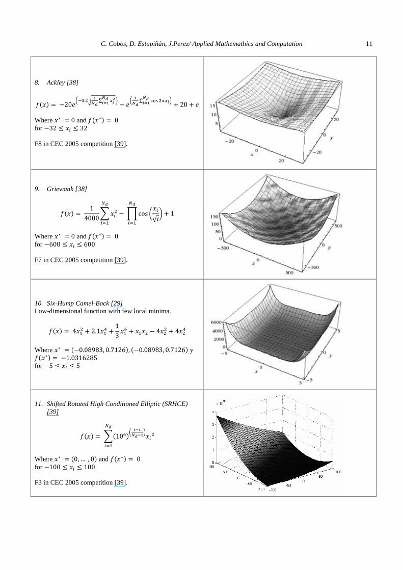
C. Cobos, D. Estupiñán, J.Perez/ Applied Mathemathics and Computation 11

8. Ackley [38]

Where and

for

F8 in CEC 2005 competition [39].

9. Griewank [38]

Where and

for

F7 in CEC 2005 competition [39].

10. Six-Hump Camel-Back [29]

Low-dimensional function with few local minima.

Where y

for

11. Shifted Rotated High Conditioned Elliptic (SRHCE)

[39]

Where and for

F3 in CEC 2005 competition [39].

C. Cobos, D. Estupiñán, J.Perez/ Applied Mathemathics and Computation 12

12. Shifted Schwefel’s Problem 1.2 with Noise in

Fitness(Schwefel’s with Noise) [39]

Where and for

F4 in CEC 2005 competition [39].

13. Shifted Rotated Expanded Scaffer’s F6 (SRESF6)[39]

Where and for

F14 in CEC 2005 competition [39].

14. Shifted Rotated Weierstrass [39]

Where a=0.5, b=3, kmax=20, and for

F11 in CEC 2005 competition [39].

15. Sum of Different Power [40]

Where and

for

C. Cobos, D. Estupiñán, J.Perez/ Applied Mathemathics and Computation 13

6.2. Results of the comparison

Table 4 presents the results of comparative tests applied to the GHS+LEM algorithm in order to measure its accuracy

against other algorithms in the harmony family. The number of iterations for the test was set at 50,000 and the number of

dimensions was set at 30 for all functions except for the Six-Hump Camel-Back which is defined in two dimensions. The

algorithms were run 100 times to ensure a reliable average deviation.

Table 4 Mean and standard deviation ( of the optimization tests (Nd = 30, NI=50.000).

HS IHS GHS GHS+LEM

Sphere Media 0.000684005 0.017838978 4.0457E-05 2.09647E-10

(±SD) 9.67781E-05 0.00710319 7.29366E-05 3.60168E-10

Schwefel’s Problem 2.22 Media 0.143656975 0.997096357 0.040860755 5.70121E-05

(±SD) 0.047911784 0.200329207 0.037067055 4.49754E-05

Rosenbrock Media 312.2431152 423.9427774 72.47196696 15.77537882

(±SD) 486.5124844 330.6943507 103.3253058 22.43722786

Step Media 11.56 11.22 0 0

(±SD) 4.608555943 3.945538332 0 0

Rotated Hyper-Ellipsoid Media 4200.19364 4444.37734 6636.76182 162.758505

(±SD) 1319.27706 1338.22348 7763.48957 294.309443

Schwefel’s Problem 2.26 Media -12545.01282 -12540.34846 -12569.46257 -12569.48662

(±SD) 9.274118296 10.54344883 0.03971048 3.40336E-11

Rastrigin Media 1.266797341 2.722732645 0.009457309 3.81653E-08

(±SD) 1.023021844 1.130249802 0.014012005 6.06791E-08

Ackley Media 0.981392208 1.584674315 0.024746761 5.83147E-06

(±SD) 0.485630315 0.331393069 0.026603311 4.86194E-06

Griewank Media 1.085396028 1.087082117 0.091022469 2.1722E-11

(±SD) 0.035098647 0.031926489 0.192952247 4.5967E-11

Six-Hump Camel- Back Media -1.031600318 -1.031628428 -1.031568182 -1.031628452

(±SD) 3.48248E-05 5.53445E-09 8.34751E-05 1.45999E-09

SRHCE Media 2641376.45 2736608.87 2639715.92 2638638.74

(±SD) 2123.26009 84608.4261 2365.63557 0.00134496

Schwefel’s with Noise Media 10734.2988 10822.5744 9606.13828 2900.82884

(±SD) 4207.32949 3978.9036 9516.94576 3964.44543

SRESF6 Media 1.96830452 2.48652905 3.20171518 0.71929327

(±SD) 0.58544715 0.52748454 1.57984035 0.62934122

Shifted Rotated Weierstrass Media 4.6535775 1.96625309 0.34992759 0.27805826

(±SD) 0.38824192 0.4172199 0.24911012 0.03101279

Sum of Different Power Media 8.0773E-06 0.00104216 6.6663E-05 3.5302E-11

(±SD) 7.3632E-06 0.00258109 0.00014128 7.426E-11

The results of the applied tests suggest that GHS+LEM exceed the accuracy obtained by HS, IHS and GHS in all

optimization functions performed. The standard deviation of the tests is also lower for all functions in which the algorithm

was applied, except SRESF6 in which IHS rates lower. But even in the worst case, the result obtained with GHS+LEM

exceed the best result obtained by IHS.

Table 5 presents the results of scalability tests to which the algorithm GHS+LEM was subjected. The number of iterations

was defined as 50000, the number of dimensions set at 50 and the number of executions of each algorithm was set at 100.

The results for the Six-Hump Camel-Back are not included but presented in Table 4. GHS+LEM improves accuracy in each

of the optimization functions used, proving to be better than HS, IHS and GHS in conditions of high dimensionality.

Moreover, in discontinuous functions such as Step, GHS+LEM maintains its optimum performance unlike other options,

which suffer under conditions of higher dimensionality.

C. Cobos, D. Estupiñán, J.Perez/ Applied Mathemathics and Computation 14

Table 5 Mean and standard deviation ( of the optimization tests (Nd = 50, NI=50.000).

HS IHS GHS GHS+LEM

Sphere Media 1.231713634 1.36689254 0.005550663 2.58528E-08

(±SD) 0.287760963 0.308892735 0.00776301 5.5786E-08

Schwefel’s Problem 2.22 Media 9.594968369 10.03102019 0.411417885 0.000441435

(±SD) 1.080214642 1.361876185 0.397066313 0.000376589

Rosenbrock Media 28119.05942 27416.72832 357.7255365 39.49848422

(±SD) 10535.26342 9607.338888 726.1644056 59.9930843

Step Media 513.92 535.07 0.09 0

(±SD) 101.4288505 112.1655752 0.637149587 0

Rotated Hyper-Ellipsoid Media 29509.5846 28901.7791 66423.751 9698.04483

(±SD) 5773.08368 5338.41442 22022.3762 7340.12668

Schwefel’s Problem 2.26 Media -20065.84929 -20055.73906 -20944.1766 -20949.14436

(±SD) 183.3728874 187.2603852 8.953405915 3.8441E-09

Rastrigin Media 35.35722669 45.97323267 0.407654111 4.13742E-06

(±SD) 4.955395824 5.414365656 0.622184354 8.94894E-06

Ackley Media 5.259876609 5.382419569 0.324365569 6.09717E-05

(±SD) 0.384154298 0.38808497 0.444545366 5.45021E-05

Griewank Media 5.701261605 5.887341775 0.700857354 5.35254E-09

(±SD) 1.080435525 1.108359613 0.368310151 1.198E-08

Six-Hump Camel- Back Media -1.031600318 -1.031628428 -1.031568182 -1.031628452

(±SD) 3.48248E-05 5.53445E-09 8.34751E-05 1.45999E-09

SRHCE Media 4849016.47 5112265.38 4323424.84 4070199.91

(±SD) 321380.054 477042.762 382439.522 0.00843488

Schwefel’s with Noise Media 44173.8891 44978.9758 77200.6744 23470.0405

(±SD) 9303.92094 9664.43851 19279.3161 11482.3296

SRESF6 Media 7.53326153 7.56787837 8.2040702 1.27372272

(±SD) 0.91845325 0.73623798 4.45743971 1.20134079

Shifted Rotated Weierstrass Media 13.1610808 12.7139825 1.73347675 1.25572551

(±SD) 1.03368193 1.16549521 1.02389123 0.1074032

Sum of Different Power Media 11.8118627 9.55819903 0.03464226 7.1917E-11

(±SD) 14.739244 36.363862 0.07923361 1.0876E-10

6.3. Effects of varying the parameters HCMR, HMS, PAR and RCR

To study the variation of the parameters HCMR, HMS, PAR and RCR, the values specified in Table 2 were used. The

number of dimensions is 30, the number of iterations is 50000 and the number of executions for each test is 30. Table 6

shows the effects of varying the HCMR parameter in the proposed algorithm. The accuracy of the algorithm is seen to

improve with higher values of HCMR. A high HCMR (≥ 0.9) favors convergence. For Six-Hump Camel-Back, Rotated

Hyper-Ellipsoid, and Schwefel’s with Noise functions a lower value of HCMR is required to increase the capacity of the

algorithm for exploration. In other words, a lower HCMR (0.7 for example) favors optimal search in those functions in which

greater exploration is required.

Table 6

Mean and standard deviation ( with varying HCMR (Nd = 30, NI=50000)

HCMR 0.5 0.7 0.9 0.95

C. Cobos, D. Estupiñán, J.Perez/ Applied Mathemathics and Computation 15

Sphere Media 0.000197381 2.16632E-05 2.46402E-10 3.33277E-11

(±SD) 3.46488E-05 8.90181E-06 4.85473E-10 6.94329E-11

Schwefel’s Problem 2.22 Media 0.046732628 0.008995544 4.78127E-05 1.67511E-05

(±SD) 0.00547272 0.003419191 3.78919E-05 1.41968E-05

Rosenbrock Media 23.02466444 16.02993218 26.47111615 32.26301449

(±SD) 32.03192831 14.24846561 32.66147183 108.4442821

Step Media 0 0 0 0

(±SD) 0 0 0 0

Rotated Hyper-Ellipsoid Media 0.00127694 0.00117081 149.42678 624.776002

(±SD) 0.00065481 0.00246363 205.003201 732.55286

Schwefel’s Problem 2.26 Media -12569.48659 -12569.48662 -12569.48662 -12569.48662

(±SD) 5.24351E-06 1.07255E-06 4.07439E-11 1.62063E-11

Rastrigin Media 0.677007539 0.00421244 3.39398E-08 4.2067E-09

(±SD) 3.47513999 0.001785797 7.24178E-08 7.68495E-09

Ackley Media 0.010563105 0.003265899 8.99544E-06 3.70719E-06

(±SD) 0.001000305 0.000749123 9.99327E-06 3.20833E-06

Griewank Media 9.62872E-06 9.92445E-07 2.79283E-11 2.95602E-12

(±SD) 2.24672E-06 4.86263E-07 3.46684E-11 4.3954E-12

Six-Hump Camel- Back Media -1.031628453 -1.031628453 -1.031628453 -1.031628448

(±SD) 3.15616E-10 2.0307E-10 1.36426E-09 1.88262E-08

SRHCE Media 2638639.61 2638638.81 2638638.74 2638638.74

(±SD) 0.23388803 0.03133231 0.0011759 0.00068605

Schwefel’s with Noise Media 0.00183615 1.93310742 3514.66702 7329.6367

(±SD) 0.00291021 7.89363197 3937.72542 5220.25806

SRESF6 Media 1.15749862 0.47597451 0.81255243 0.49298221

(±SD) 1.38547041 0.48806422 0.72467993 0.43153488

Shifted Rotated Weierstrass Media 2.76053748 1.45427489 0.28669758 0.17334889

(±SD) 0.18666743 0.13396875 0.03304307 0.02110725

Sum of Different Power Media 7.8452E-11 5.2276E-11 2.9351E-11 1.0869E-10

(±SD) 1.4035E-10 8.9653E-11 6.208E-11 1.5017E-10

Table 7 presents the results of HMS parameter variation on the proposed algorithm. The best results for the proposed

algorithm are seen to be located between the values 5 and 10 (60%). The next best results are values equal to 20 (27 %) and

50 (33%). The proposed algorithm obtains better results with small harmony memory sizes as recommended in the original

HS algorithm, but some functions -Rotated Hyper-Ellipsoid, Griewank, Six-Hump Camel- Back, Schwefel’s with Noise,

SRESF6, and Sum of Different Power- need larger values of harmony memory sizes in order to favors a greater exploration

of search space. The Step function, being discontinuous, seems not to be affected by this parameter. A future work should try

to determine whether or not by using a history of the rules the accuracy of the algorithm can be improved even if using a

smaller harmonic memory size.

Table 7

Mean and standard deviation ( with varying HMS (Nd = 30, NI=50000)

HMS 5 10 20 50

Sphere Media 1.09049E-08 9.42334E-09 4.56347E-08 6.10931E-08

(±SD) 1.97455E-08 1.21108E-08 8.98288E-08 1.00668E-07

Schwefel’s Problem 2.22 Media 0.00058248 0.000613678 0.000721842 0.000857497

(±SD) 0.000568687 0.000648931 0.00074417 0.000758539

Rosenbrock Media 31.0074059 48.32958186 39.0007948 31.84389228

(±SD) 51.12983659 57.16531525 47.41503805 35.13859472

Step Media 0 0 0 0

(±SD) 0 0 0 0

C. Cobos, D. Estupiñán, J.Perez/ Applied Mathemathics and Computation 16

Rotated Hyper-Ellipsoid Media 4482.80339 4028.15389 3177.56436 840.301105

(±SD) 205.003201 285.078399 165.933003 58.0258614

Schwefel’s Problem 2.26 Media -12569.48662 -12569.48662 -12569.48662 -12569.48596

(±SD) 4.53706E-08 1.32036E-07 7.77143E-08 0.00362494

Rastrigin Media 2.95253E-06 5.09339E-06 2.9867E-06 1.61558E-05

(±SD) 3.63668E-06 1.01325E-05 4.88117E-06 2.98689E-05

Ackley Media 7.03661E-05 8.6753E-05 7.74663E-05 0.000163219

(±SD) 5.66978E-05 0.000139645 6.64779E-05 0.000179311

Griewank Media 0.030470641 0.010369382 0.002829622 0.021107642

(±SD) 0.157625199 0.037402693 0.014132011 0.050745481

Six-Hump Camel- Back Media -1.031628349 -1.031628331 -1.031628381 -1.031628382

(±SD) 1.22241E-07 1.37004E-07 7.88387E-08 1.01315E-07

SRHCE Media 79159162.3 79159162.3 79159162.3 79159162.3

(±SD) 0.0011759 0.00095803 0.00086158 0.00133169

Schwefel’s with Noise Media 3715.24708 1597.31424 464.521089 64.6658585

(±SD) 4967.42551 2352.99565 850.102275 116.587692

SRESF6 Media 0.81255243 0.61550188 0.61462859 0.60094146

(±SD) 0.72467993 0.56970373 0.49020067 0.36547509

Shifted Rotated Weierstrass Media 0.28669758 0.29544614 0.29098197 0.29226029

(±SD) 0.03304307 0.03894089 0.03032137 0.03896236

Sum of Different Power Media 2.9351E-11 6.5673E-11 5.9275E-11 2.8704E-11

(±SD) 6.208E-11 1.7835E-10 8.3191E-11 4.1108E-11

Table 8 deals with the results of the PAR parameter variation in the proposed algorithm. In the original proposal of GHS

[29] the PAR is dynamically adjusted with respect to the number of iterations [28, 29]. The HS algorithm proposed by Geem

[1] establishes that the PAR parameter has to be fixed and a value of 0.3 is recommended. In this group of tests a constant

PAR value of 0.1, 0.3, 0.5, 0.7, 0.9 is set along with a dynamic one, as in IHS. It is noted that the best performances of the

proposed algorithm are obtained when the PAR is dynamic for all the optimization functions. In non-continuous functions the

PAR parameter seems not to affect the accuracy of the algorithm. Even in functions whose convergence is slow (Rotated

Hyper-Ellipsoid) the best choice is a dynamic PAR. The difference between the results of Schwefel’s Problem 2.26 for the

selected PAR and the dynamic PAR is 0.003%, making it statistically irrelevant.

Table 8

Mean and standard deviation ( with varying PAR (Nd = 30, NI=50000)

PAR 0.1 0.3 0.5 0.7 0.9 Dynamic

Sphere Media 3.16E-09 2.43E-09 1.06E-08 1.55E-08 2.05E-08 2.46402E-10

(±SD) 7.21E-09 6.07E-09 2.73E-08 2.94E-08 3.23E-08 4.85473E-10

Schwefel’s Problem

2.22 Media 1.45E-04 2.19E-04 2.41E-04 4.29E-04 5.84E-04 4.78127E-05

(±SD) 1.05E-04 1.94E-04 2.80E-04 3.92E-04 5.55E-04 3.78919E-05

Rosenbrock Media 2.67E+01 4.97E+01 5.35E+01 5.82E+01 2.55E+01 2.65 E+01

(±SD) 4.16E+01 7.67E+01 7.03E+01 6.29E+01 4.82E+01 3.27 E+01

Step Media 0.0 0.0 0.0 0.0 0.0 0.0

(±SD) 0.0 0.0 0.0 0.0 0.0 0.0

Rotated Hyper-Ellipsoid

Media 1.49E+02 1.49E+02 1.49E+02 1.49E+02 1.49E+02 1.49E+02

(±SD) 2.05E+02 2.05E+02 2.05E+02 2.05E+02 2.05E+02 2.05E+02

Schwefel’s Problem 2.26

Media -1.26E+04 -1.26E+04 -1.26E+04 -1.26E+04 -1.26E+04 -1.26E+04

(±SD) 1.16E-09 1.08E-09 8.46E-10 5.13E-09 6.67E-09 4.07439E-11

Rastrigin Media 5.75E-07 7.07E-07 1.23E-06 1.41E-06 2.71E-06 3.39E-08

(±SD) 8.04E-07 1.20E-06 2.06E-06 2.43E-06 5.04E-06 7.24E-08

Ackley Media 2.37E-05 2.87E-05 3.51E-05 5.17E-05 9.03E-05 9.00E-06

C. Cobos, D. Estupiñán, J.Perez/ Applied Mathemathics and Computation 17

(±SD) 2.40E-05 2.43E-05 3.35E-05 5.68E-05 7.93E-05 9.99E-06

Griewank Media 4.79E-02 3.85E-10 9.14E-10 4.92E-09 3.46E-09 2.79E-11

(±SD) 1.62E-01 5.39E-10 1.80E-09 1.94E-08 5.65E-09 3.47E-11

Six-Hump Camel-

Back Media -1.03E+00 -1.03E+00 -1.03E+00 -1.03E+00 -1.031E+00 -1.03E+00

(±SD) 1.30E-06 1.76E-06 3.99E-07 4.35E-07 1.90E-07 1.36E-09

SRHCE Media 2.64E+06 2.64E+06 2.64E+06 2.64E+06 2.64E+06 2.64E+06

(±SD) 1.18E-03 1.18E-03 1.18E-03 1.18E-03 1.18E-03 1.18E-03

Schwefel’s with Noise Media 2.97E+03 3.71E+03 2.58E+03 3.55E+03 2.82E+03 3.51E+03

(±SD) 3.74E+03 6.09E+03 2.38E+03 5.19E+03 3.20E+03 3.94E+03

SRESF6 Media 8.13E-01 8.13E-01 8.13E-01 8.13E-01 8.13E-01 8.13E-01

(±SD) 7.25E-01 7.25E-01 7.25E-01 7.25E-01 7.25E-01 7.25E-01

Shifted Rotated

Weierstrass Media 2.87E-01 2.87E-01 2.87E-01 2.87E-01 2.87E-01 2.87E-01

(±SD) 3.30E-02 3.30E-02 3.30E-02 3.30E-02 3.30E-02 3.30E-02

Sum of Different Power

Media 2.94E-11 2.94E-11 2.94E-11 2.94E-11 2.94E-11 2.94E-11

(±SD) 6.21E-11 6.21E-11 6.21E-11 6.21E-11 6.21E-11 6.21E-11

The results of varying the RCR parameter are shown in Table 9. The RCR parameter determines in what percentage of the

times the inferred rules (result of the PRISM adapted algorithm) are used in generating a new harmony. A clear tendency to

use a large value for RCR is observed ( ). The recommended setting for RCR by default in the proposed

algorithm is 0.9, at which the highest level of effectiveness is shown. The possibility is left open for a study with a RCR

factor varying between 0.7 and 1.0 (it is similar to the PAR parameter).

Table 9 Mean and standard deviation ( with varying RCR (Nd = 30, NI=50000)

RCR 1.0 0.9 0.8 0.7 0.6 0.5 0.4 0.3 0.2 0.1

Sphere 2.161E-10 2.352E-10 2.453E-10 3.132E-10 2.729E-10 4.625E-10 1.399E-09 2.230E-09 4.838E-09 1.011E-08

5.040E-10 4.509E-10 4.745E-10 5.985E-10 4.207E-10 7.560E-10 2.929E-09 4.419E-09 9.146E-09 1.561E-08

Schwefel’s

Problem

2.22

3.607E-05 4.470E-05 5.970E-05 6.989E-05 7.995E-05 9.629E-05 1.086E-04 1.732E-04 2.777E-04 5.493E-04

4.350E-05 3.848E-05 7.632E-05 7.082E-05 8.713E-05 7.975E-05 1.053E-04 1.367E-04 3.002E-04 4.912E-04

Rosenbrock 2.101E+01 1.861E+01 1.476E+01 3.032E+01 1.994E+01 2.617E+01 2.719E+01 7.098E+01 4.208E+01 6.856E+01

3.121E+01 3.042E+01 2.344E+01 3.910E+01 3.451E+01 3.375E+01 4.439E+01 1.682E+02 8.332E+01 1.333E+02

Step 1.20 0.00 0.00 0.00 0.00 0.00 0.00 0.00 0.00 0.00

5.94 0.00 0.00 0.00 0.00 0.00 0.00 0.00 0.00 0.00

Rotated

Hyper-

Ellipsoid

635.279583 149.42678 166.249878 235.400082 426.184667 572.885247 1036.88623 1819.2857 2980.20403 3225.82524

943.517838 205.003201 232.271253 267.291022 511.991995 591.857973 695.852484 879.099952 973.000542 1156.0523

Schwefel’s Problem

2.26

-1.250E+04 -1.257E+04 -1.257E+04 -1.257E+04 -1.257E+04 -1.257E+04 -1.257E+04 -1.257E+04 -1.257E+04 -1.257E+04

5.025E+02 3.855E-11 5.829E-11 5.530E-11 6.038E-11 2.142E-10 7.002E-10 3.531E-10 5.424E-10 5.673E-04

Rastrigin 1.194E+00 6.038E-08 5.753E-08 5.499E-08 8.028E-08 1.356E-07 2.565E-07 2.105E-07 7.543E-07 5.055E-06

5.909E+00 1.366E-07 1.132E-07 9.368E-08 1.141E-07 3.275E-07 3.396E-07 4.158E-07 1.073E-06 1.152E-05

Ackley 1.430E-01 7.612E-06 7.243E-06 9.316E-06 1.307E-05 9.818E-06 1.325E-05 2.711E-05 3.759E-05 5.917E-05

7.076E-01 6.617E-06 6.937E-06 1.132E-05 1.028E-05 1.205E-05 1.479E-05 2.417E-05 3.438E-05 6.534E-05

Griewank 2.272E-11 1.208E-11 1.400E-11 2.154E-11 8.018E-11 5.236E-11 1.672E-10 1.272E-02 2.786E-03 5.095E-02

3.142E-11 1.542E-11 2.240E-11 3.105E-11 2.327E-10 8.748E-11 4.402E-10 8.994E-02 1.957E-02 1.551E-01

Six-Hump

Camel- Back

-9.500E-01 -1.032E+00 -1.032E+00 -1.032E+00 -1.032E+00 -1.032E+00 -1.032E+00 -1.032E+00 -1.032E+00 -1.032E+00

2.473E-01 1.645E-09 2.202E-09 3.530E-09 3.106E-09 6.871E-09 1.025E-08 8.118E-09 4.938E-08 9.653E-08

SRHCE 2638638.74 2638638.74 2638638.74 2638638.74 2638638.74 2638638.75 2638638.76 2638638.79 2638638.92 2638642.6

C. Cobos, D. Estupiñán, J.Perez/ Applied Mathemathics and Computation 18

0.00064421 0.0011759 0.00226699 0.00199823 0.00223534 0.01068915 0.01420785 0.04666398 0.22487547 8.10863555

Schwefel’s with Noise

1711.30168 2458.47163 3037.39566 4055.39407 5332.82446 7432.53838 7040.69871 9545.10601 8802.23788 11530.1239

2607.64288 3243.75066 3543.72205 3941.58669 3765.86402 4362.01585 4431.63942 4254.99433 3531.34188 4924.39438

SRESF6 1.01717905 0.81255243 0.61587394 0.82358984 0.83525756 0.83516347 0.92880128 0.89577229 1.36191868 1.59949269

1.14063446 0.72467993 0.55317585 0.61607082 0.59695425 0.69573287 0.67341881 0.55251217 0.78662756 0.66011548

Shifted

Rotated Weierstrass

0.25688648 0.28669758 0.29982573 0.32922784 0.362599 0.42054823 0.46084905 0.57014011 0.70368141 1.06326949

0.02942249 0.03304307 0.04379959 0.03585728 0.03978034 0.05615239 0.05870615 0.04996005 0.07453427 0.14235103

Sum of

Different

Power

4.0421E-11 2.9351E-11 5.7058E-11 5.5714E-11 1.6194E-10 3.0699E-09 9.4552E-09 3.2809E-08 9.1628E-08 1.3382E-06

1.0258E-10 6.208E-11 1.1399E-10 9.6809E-11 2.275E-10 5.7561E-09 1.8955E-08 5.4911E-08 1.579E-07 2.3263E-06

Other tests were performed by varying the number of iterations as shown in Table 10. The number of iterations for this test

is 5000. It is noted that the GHS+LEM algorithm outperforms other proposals when the number of iterations is low. The

proposed algorithm maintains an acceptable level of approximation to the optimal solution, despite the low number of

iterations proposed. The differences in the function of Six-Hump Camel-Back are not statistically significant.

Table 10 Mean and standard deviation ( with varying number of iterations (Nd = 30, NI=5000)

Functions HMS IHS GHS GHS+LEM

Sphere Media 1.391113338 1.492336778 0.008490508 5.93279E-08

(±SD) 0.442516349 0.429375922 0.015014868 9.80204E-08

Schwefel’s Problem 2.22 Media 7.343708198 7.942415139 0.38849092 0.000681506

(±SD) 1.298620467 1.376467735 0.392227894 0.000587781

Rosenbrock Media 44801.42361 44335.30705 365.8780006 35.91286497

(±SD) 27087.38846 25827.36583 988.1136926 68.65861969

Step Media 577.17 599.34 3.25 0

(±SD) 178.0053373 181.6569761 8.62738768 0

Rotated Hyper-Ellipsoid Media 18648.2804 19114.2613 22845.7019 9742.75094

(±SD) 4664.11977 5576.63382 12812.2556 5923.66993

Schwefel’s Problem 2.26 Media -11723.5473 -11734.68475 -12561.42156 -12569.4597

(±SD) 194.1725169 182.3846445 16.70991705 0.248116333

Rastrigin Media 29.46075697 36.89200558 0.881408659 1.17383E-05

(±SD) 5.461732931 6.233664508 1.594135534 1.89959E-05

Ackley Media 6.335464888 6.480145971 0.535233079 0.000125684

(±SD) 0.620693868 0.686288345 0.701961543 0.000103427

Griewank Media 6.277931588 6.370436585 0.795212512 0.006467333

(±SD) 1.494900647 1.816294084 0.350711873 0.054165186

Six-Hump Camel- Back Media -1.03155243 -1.031628431 -1.026283458 -1.030628257

(±SD) 5.65151E-05 7.41828E-09 0.008075092 0.004327667

SRHCE Media 4949527.45 5272015.41 3257133.71 2638638.87

(±SD) 1549998.56 2003255.08 1000322.75 0.17113924

Schwefel’s with Noise Media 25859.5942 25706.8318 33126.0056 16884.5567

(±SD) 6127.04081 6656.33665 14920.4074 8512.95715

SRESF6 Media 5.40555247 5.66821959 3.73505659 1.38260315

(±SD) 0.74702013 0.57290456 2.6546381 1.1580235

Shifted Rotated Weierstrass Media 8.1876236 9.14968576 1.62251403 0.9166651

C. Cobos, D. Estupiñán, J.Perez/ Applied Mathemathics and Computation 19

(±SD) 1.08444438 1.03659385 1.09541355 0.08870444

Sum of Different Power Media 56.7816376 70.2377894 0.04011324 8.4062E-09

(±SD) 84.9067592 135.452682 0.06083117 2.4547E-08

The results of GHS+LEM with 5000 iterations were compared with the results obtained by other methods (HS, IHS and

GHS) with 50000 iterations (see Table 11). It is noted that even with a low number of iterations (5000) the proposed

algorithm improves the results in almost all the optimization functions used. In cases such as Schwefel’s Problem 2.26 the

difference is not statistically significant (0.000023%). For functions with slow convergence, as Rotated Hyper-Ellipsoid, a

greater number of iterations are required to improve the accuracy of the proposed algorithm.

Table 11 Mean and standard deviation ( comparing accuracy with different numbers of iterations (Nd = 30; GHS+LEM with

NI=5000; HS, IHS y GHS with NI=50000)

Functions HMS IHS GHS GHS+LEM (5000 NI)

Sphere Media 0.000684005 0.017838978 4.0457E-05 5.93279E-08

(±SD) 9.67781E-05 0.00710319 7.29366E-05 9.80204E-08

Schwefel’s Problem 2.22 Media 0.143656975 0.997096357 0.040860755 0.000681506

(±SD) 0.047911784 0.200329207 0.037067055 0.000587781

Rosenbrock Media 312.2431152 423.9427774 72.47196696 35.91286497

(±SD) 486.5124844 330.6943507 103.3253058 68.65861969

Step Media 11.56 11.22 0 0

(±SD) 4.608555943 3.945538332 0 0

Rotated Hyper-Ellipsoid Media 4234.47788 4183.56875 6880.91826 9742.75094

(±SD) 1140.43614 1040.33435 7812.23325 5923.66993

Schwefel’s Problem 2.26 Media -12545.01282 -12540.34846 -12569.46257 -12569.4597

(±SD) 9.274118296 10.54344883 0.03971048 0.248116333

Rastrigin Media 1.266797341 2.722732645 0.009457309 1.17383E-05

(±SD) 1.023021844 1.130249802 0.014012005 1.89959E-05

Ackley Media 0.981392208 1.584674315 0.024746761 0.000125684

(±SD) 0.485630315 0.331393069 0.026603311 0.000103427

Griewank Media 1.085396028 1.087082117 0.091022469 0.006467333

(±SD) 0.035098647 0.031926489 0.192952247 0.054165186

Six-Hump Camel- Back Media -1.031600318 -1.031628428 -1.031568182 -1.030628257

(±SD) 3.48248E-05 5.53445E-09 8.34751E-05 0.004327667

SRHCE Media 2641799.17 2741995.37 2639726.35 2638638.87

(±SD) 2878.93967 89375.4964 2506.22217 0.17113924

Schwefel’s with Noise Media 10045.7637 11298.1914 10638.4058 16884.5567

(±SD) 2605.17481 3410.50321 10996.5284 8512.95715

SRESF6 Media 1.82019811 2.55920064 3.45257774 1.38260315

(±SD) 0.61530057 0.54004037 1.40491917 1.1580235

Shifted Rotated Weierstrass Media 4.65605359 1.89005574 0.28266306 0.9166651

(±SD) 0.36447473 0.39416867 0.19571374 0.08870444

Sum of Different Power Media 8.3165E-06 0.0015714 8.6639E-05 8.4062E-09

(±SD) 6.9039E-06 0.00344916 0.00022289 2.4547E-08

C. Cobos, D. Estupiñán, J.Perez/ Applied Mathemathics and Computation 20

In addition tests were performed to evaluate the performance of the algorithm in integer programming problems. The tests

implemented were defined in the article on GHS [29] and correspond to five problems identified as F1, F2, F3, F4 and F5.

The results can be seen in Table 12. In these results it can also be seen that GHS+LEM improves the accuracy for high-

dimensional function F1 with respect to the other proposals. For all other functions implemented it is seen that GHS+LEM

performs in a similar way against the other algorithms, improving the performance shown by GHS in F2, F3 and F5.

Table 12 Integer programming problems

HS IHS GHS GHS+LEM

F1 (N=5) Media 0 0 0 0

(±SD) 0 0 0 0

F1 (N=15) Media 0 0.833333333 0 0

(±SD) 0 0.461133037 0 0

F1 (N=30) Media 6.266666667 11.26666667 0.433333333 0

(±SD) 1.387961376 1.964044619 0.504006933 0

F2 Media 0 0 0.3 0

(±SD) 0 0 0.70221325 0

F3 Media 0 9 0.133333333 0

(±SD) 0 16.29258346 0.434172485 0

F4 Media -7 -7 -6.933333333 -6.933333333

(±SD) 0 0 0.253708132 0.253708132

F5 Media -3880 -3880 -3879.633333 -3880

(±SD) 0 0 0.556053417 0

6.4. Convergence vs. iterations

The results of the algorithms were compared in relation to the convergence speed to the optimal solution and the number

of iterations to reach such solutions. As an example, Table 13 shows a graphic of the convergence on the test functions taking

30 dimensions into account. It can be seen that the convergence to the global optimum in the GHS+LEM algorithm is

achieved with a smaller number of iterations. The process of inference rules and their application in the generation of new

harmonies allows GHS+LEM to execute qualitative jump towards the global optimum, so that optimal results are achieved in

an average of 500 iterations over all test functions, while other algorithms need over 3000 iterations, and even 5000

iterations.

Table 13 Convergence curves for all algorithms in test functions

Sphere with 500 iterations

Schwefel’s Problem 2.22 with 500 iterations

0

20

40

60

80

100

120

140

160

180

200

1

28

55

82

10

9

13

6

16

3

19

0

21

7

24

4

27

1

29

8

32

5

35

2

37

9

40

6

43

3

46

0

48

7

GHS+LEM

GHS

IHS

HS

0

20

40

60

80

100

120

1

28

55

82

10

9

13

6

16

3

19

0

21

7

24

4

27

1

29

8

32

5

35

2

37

9

40

6

43

3

46

0

48

7

GHS+LEM

GHS

IHS

HS

C. Cobos, D. Estupiñán, J.Perez/ Applied Mathemathics and Computation 21

Rosenbrock with 1000 iterations (logarithmic scale)

Step with 600 iterations (logarithmic scale)

Rotated Hyper-Ellipsoid with 500 iterations

Schwefel’s Problem 2.26 with 500 iterations

Rastrigin with 500 iterations

Ackley with 1000 iterations

Griewank with 500 iterations

Shifted Rotated High Conditioned Elliptic with 500

iterations

1

10

100

1000

10000

100000

1000000

10000000

100000000

1E+091

64

12

7

19

0

25

3

31

6

37

9

44

2

50

5

56

8

63

1

69

4

75

7

82

0

88

3

94

6

GHS+LEM

GHS

IHS

HS

1

10

100

1000

10000

100000

1

35

69

10

3

13

7

17

1

20

5

23

9

27

3

30

7

34

1

37

5

40

9

44

3

47

7

51

1

54

5

57

9

GHS+LEM

GHS

IHS

HS

0

200000

400000

600000

800000

1000000

1200000

1400000

1600000

1800000

1

31

61

91

12

1

15

1

18

1

21

1

24

1

27

1

30

1

33

1

36

1

39

1

42

1

45

1

48

1

GHS+LEM

GHS

IHS

HS

-14000

-12000

-10000

-8000

-6000

-4000

-2000

0

1

29

57

85

11

3

14

1

16

9

19

7

22

5

25

3

28

1

30

9

33

7

36

5

39

3

42

1

44

9

47

7

GHS+LEM

GHS

IHS

HS

0

100

200

300

400

500

600

1

28

55

82

10

9

13

6

16

3

19

0

21

7

24

4

27

1

29

8

32

5

35

2

37

9

40

6

43

3

46

0

48

7

GHS+LEM

GHS

IHS

HS

0

5

10

15

20

25

1

54

10

7

16

0

21

3

26

6

31

9

37

2

42

5

47

8

53

1

58

4

63

7

69

0

74

3

79

6

84

9

90

2

95

5GHS+LEM

GHS

IHS

HS

0

100

200

300

400

500

600

700

800

900

1000

1

28

55

82

10

9

13

6

16

3

19

0

21

7

24

4

27

1

29

8

32

5

35

2

37

9

40

6

43

3

46

0

48

7

GHS+LEM

GHS

IHS

HS

0

500000000

1E+09

1,5E+09

2E+09

2,5E+09

3E+09

1

33

65

97

12

9

16

1

19

3

22

5

25

7

28

9

32

1

35

3

38

5

41

7

44

9

48

1

GHS+LEM

GHS

IHS

HS

C. Cobos, D. Estupiñán, J.Perez/ Applied Mathemathics and Computation 22

Shifted Schwefel’s Problem 1.2 with Noise in Fitness

with 500 iterations

Shifted Rotated Expanded Scaffer’s F6 with 500

iterations

Shifted Rotated Weierstrass with 500 iterations

Sum of Different Power with 250 iterations (logarithmic

scale)

7. Conclusions and future work

This paper presents a new version of the GHS algorithm called GHS+LEM. The proposed algorithm uses LEM techniques

to create a set of rules that allows the inferring of new candidates in the population that emerge not only from the random

scan. The amendment allows the new algorithm to perform efficiently in both discrete and continuous functions. The

algorithm was subjected to ten classic optimization features and in most cases improved the results against other methods

(HS, IHS, and GHS). It was also concluded following a scalability test that the algorithm maintains its accuracy even in high

dimensions ( . We investigated the effects of the HCMR, HMS, PAR and RCR parameters on the performance of the

proposed algorithm. It resulted that in HCMR ≥ 0.9 the algorithm generally improves its efficiency. Moreover, with regard to

the size of the harmony memory, tests show that the proposed algorithm generally performs better when the size is between 5

and 10, which is consistent with the recommendations of the original HS algorithm. It can also be seen too that better results

are obtained when the PAR value is dynamic, as proposed in IHS. With respect to variation in the RCR parameter, a better

overall performance of the algorithm was achieved when the rule procedure application is carried out using a probability of

between 0.7 and 1. The algorithm also was shown to maintain a higher accuracy than the other algorithms even when the

number of iterations is 10 times lower than used by those other harmony algorithms.

As future work, the research group proposes a study of the performance of the algorithm with other functions [39] and

real-world problems; introducing variations in the inference rules procedure that allow manage harmony memory history to

be taken into account and modify the inference rules procedure to update each time a change in the harmonic memory is

made in order to evaluate the algorithm’s performance under these new conditions. A study for improving the parameter

setting process in GHS+LEM or a study to bypass this process should be conducted. Generalize the algorithm to work with

attributes with different range of values (with different upper and lower bounds on each dimension). Use non-parametric

statistical tests to validate results of the present paper [41].

0

100000

200000

300000

400000

500000

6000001

29

57

85

11

3

14

1

16

9

19

7

22

5

25

3

28

1

30

9

33

7

36

5

39

3

42

1

44

9

47

7

GHS+LEM

GHS

IHS

HS

0

2

4

6

8

10

12

14

16

1

28

55

82

10

9

13

6

16

3

19

0

21

7

24

4

27

1

29

8

32

5

35

2

37

9

40

6

43

3

46

0

48

7

GHS+LEM

GHS

IHS

HS

0

10

20

30

40

50

60

1

28

55

82

10

9

13

6

16

3

19

0

21

7

24

4

27

1

29

8

32

5

35

2

37

9

40

6

43

3

46

0

48

7

GHS+LEM

GHS

IHS

HS

1,00E+00

1,00E+02

1,00E+04

1,00E+06

1,00E+08

1,00E+10

1,00E+12

1,00E+14

1,00E+16

1,00E+18

1,00E+20

1,00E+22

1,00E+24

1

16

31

46

61

76

91

10

6

12

1

13

6

15

1

16

6

18

1

19

6

21

1

22

6

24

1

GHS+LEM

GHS

IHS

HS

C. Cobos, D. Estupiñán, J.Perez/ Applied Mathemathics and Computation 23

Acknowledgements

This research work was supported by a Research Grant from the University of Cauca under project VRI-2560. The authors

would like to thank the anonymous reviewers for helpful comments and suggestions.

References

1. Geem, Z., J. Kim, and G.V. Loganathan, A New Heuristic Optimization Algorithm: Harmony Search. Simulation, 2001.

76(2): p. 60-68.

2. Garcia, E. RSJ-PM Tutorial: A Tutorial on the Robertson-Sparck Jones Probabilistic Model for Information Retrieval.

2009; Available from: http://www.miislita.com/information-retrieval-tutorial/information-retrieval-probabilistic-model-

tutorial.pdf.

3. Yang, X.-S., Harmony Search as a Metaheuristic Algorithm, in Music-Inspired Harmony Search Algorithm. 2009,

Springer Berlin / Heidelberg. p. 1-14.

4. Geem, Z.W., Music-Inspired Harmony Search Algorithm: Theory and Applications. Studies in Computational

Intelligence. Vol. 191. 2009, Rockville, Maryland: Springer Publishing Company, Incorporated. 206.

5. Geem, Z.W., Recent Advances In Harmony Search Algorithm. Studies in Computational Intelligence. Vol. 270. 2010,

Annandale,Virginia: Springer

6. Geem, Z.W., et al., Recent Advances in Harmony Search. Advances in Evolutionary Algorithms, 2008: p. 16.

7. Tangpattanakul, P., A. Meesomboon, and P. Artrit, Optimal Trajectory of Robot Manipulator Using Harmony Search

Algorithms, in Recent Advances In Harmony Search Algorithm. 2010, Springer Berlin / Heidelberg. p. 23-36.

8. Panigrahi, B., et al., Population Variance Harmony Search Algorithm to Solve Optimal Power Flow with Non-Smooth

Cost Function, in Recent Advances In Harmony Search Algorithm. 2010, Springer Berlin / Heidelberg. p. 65-75.

9. Mohsen, A., A. Khader, and D. Ramachandram, An Optimization Algorithm Based on Harmony Search for RNA

Secondary Structure Prediction, in Recent Advances In Harmony Search Algorithm. 2010, Springer Berlin / Heidelberg.

p. 163-174.

10. Fourie, J., S. Mills, and R. Green, Visual Tracking Using Harmony Search, in Recent Advances In Harmony Search

Algorithm. 2010, Springer Berlin / Heidelberg. p. 37-50.

11. Forsati, R. and M. Mahdavi, Web Text Mining Using Harmony Search, in Recent Advances In Harmony Search

Algorithm. 2010, Springer Berlin / Heidelberg. p. 51-64.

12. dos Santos Coelho, L. and D. de A. Bernert, A Harmony Search Approach Using Exponential Probability Distribution

Applied to Fuzzy Logic Control Optimization, in Recent Advances In Harmony Search Algorithm. 2010, Springer Berlin

/ Heidelberg. p. 77-88.

13. Ayvaz, M., Solution of Groundwater Management Problems Using Harmony Search Algorithm, in Recent Advances In

Harmony Search Algorithm. 2010, Springer Berlin / Heidelberg. p. 111-122.

14. Geem, Z., State-of-the-Art in the Structure of Harmony Search Algorithm, in Recent Advances In Harmony Search

Algorithm. 2010, Springer Berlin / Heidelberg. p. 1-10.

15. Jaberipour, M. and E. Khorram, Solving the sum-of-ratios problems by a harmony search algorithm. Journal of

Computational and Applied Mathematics, 2010. 234(3): p. 733-742.

16. Zou, D., et al., A novel global harmony search algorithm for reliability problems. Computers & Industrial Engineering,

2009. 58(2): p. 307-316.

17. Geem, Z.W., Optimal Design of Water Distribution Networks Using Harmony Search. 2009: p. 112.

18. Saka, M., Optimum Design of Steel Skeleton Structures, in Music-Inspired Harmony Search Algorithm. 2009, Springer

Berlin / Heidelberg. p. 87-112.

19. Panchal, A., Harmony Search in Therapeutic Medical Physics, in Music-Inspired Harmony Search Algorithm. 2009,

Springer Berlin / Heidelberg. p. 189-203.

20. Mahdavi, M., Solving NP-Complete Problems by Harmony Search, in Music-Inspired Harmony Search Algorithm. 2009,

Springer Berlin / Heidelberg. p. 53-70.

21. Fesanghary, M., Harmony Search Applications in Mechanical, Chemical and Electrical Engineering, in Music-Inspired

Harmony Search Algorithm. 2009, Springer Berlin / Heidelberg. p. 71-86.

22. Geem, Z.W. and J.C. Williams, Ecological optimization using harmony search, in Proceedings of the American

Conference on Applied Mathematics. 2008, World Scientific and Engineering Academy and Society (WSEAS):

Cambridge, Massachusetts.

23. Prasad, B. and Z. Geem, Harmony Search Applications in Industry, in Soft Computing Applications in Industry. 2008,

Springer Berlin / Heidelberg. p. 117-134.

C. Cobos, D. Estupiñán, J.Perez/ Applied Mathemathics and Computation 24

24. Geem, Z.W. and J.-Y. Choi, Music Composition Using Harmony Search Algorithm. Applications of Evolutionary

Computing, 2007. 4448/2007: p. 7.

25. Geem, Z.W., Optimal cost design of water distribution networks using harmony search. Engineering Optimization,

2006. 38.

26. Geem, Z.W., Harmony search algorithms for structural design optimization, in Studies in computational intelligence,

v.239. 2009, Springer Berlin Heidelberg: Berlin, Heidelberg. p. 228.

27. Cobos, C., et al. Web document clustering based on Global-Best Harmony Search, K-means, Frequent Term Sets and

Bayesian Information Criterion. in 2010 IEEE Congress on Evolutionary Computation (CEC). 2010. Barcelona, Spain:

IEEE.

28. Mahdavi, M., M. Fesanghary, and E. Damangir, An improved harmony search algorithm for solving optimization

problems. Applied Mathematics and Computation, 2007. 188(2): p. 1567-1579.

29. Omran, M.G.H. and M. Mahdavi, Global-best harmony search. Applied Mathematics and Computation, 2008. 198(2): p.

643-656.

30. Michalski, R.S., LEARNABLE EVOLUTION MODEL: Evolutionary Processes Guided by Machine Learning. Machine

Learning, 2000-01-01. 38(1): p. 9-40.

31. Lee, K. and Z. Geem, A new meta-heuristic algorithm for continuous engineering optimization: harmony search theory

and practice. Computer Methods in Applied Mechanics and Engineering, 2005. 194(36-38): p. 3902-3933.

32. Geem, Z.W., Novel derivative of harmony search algorithm for discrete design variables. Applied Mathematics and

Computation, 2008. 199(1): p. 223-230.

33. Geem, Z.W. and K.-B. Sim, Parameter-setting-free harmony search algorithm. Applied Mathematics and Computation,

2010. 217(8): p. 3881-3889.

34. Das, S., et al., Exploratory Power of the Harmony Search Algorithm: Analysis and Improvements for Global Numerical

Optimization. Systems, Man, and Cybernetics, Part B: Cybernetics, IEEE Transactions on. 41(1): p. 89-106.

35. Geem, Z.W., Particle-swarm harmony search for water network design. Engineering Optimization, 2009. 41: p. 297-

311.

36. Cendrowska, J., PRISM: An algorithm for inducing modular rules. International Journal of Man-Machine Studies, 1987.

27(4): p. 349-370.

37. Witten, I.H. and E. Frank, Data mining: practical machine learning tools and techniques with Java implementations.

SIGMOD Rec., 2002. 31(1): p. 76-77.

38. M. Molga, C.S., Test functions for optimization needs. available at www.zsd.ict.pwr.wroc.pl/files/docs/functions.pdf

2005.

39. Suganthan, P.N., et al., Problem definitions and evaluation criteria for the CEC 2005 Special Session on Real Parameter

Optimization. 2005.

40. Xin, Y., L. Yong, and L. Guangming, Evolutionary programming made faster. Evolutionary Computation, IEEE

Transactions on, 1999. 3(2): p. 82-102.

41. Garcia, S., et al., A study on the use of non-parametric tests for analyzing the evolutionary algorithms' behaviour: a case

study on the CEC'2005 Special Session on Real Parameter Optimization. Journal of Heuristics, 2009. 15(6): p. 617-644.