GHG Inventory for South Africa: 2000 – 2012 | i

GHG National

Inventory Report

South Africa 2000 – 2012

March 2016

GHG Inventory for South Africa: 2000 – 2012 | ii

PREFACE

This report has been compiled for the Department of Environmental Affairs (DEA) in response to South

Africa’s obligation to report its greenhouse (GHG) emissions to international climate change bodies.

The report is prepared in accordance with the United Nations Framework Convention on Climate

Change (UNFCCC). This inventory was compiled by making use of the Intergovernmental Panel on

Climate Change (IPCC) 2006 Excel spread sheet guidelines and the Good Practice Guidance.

This report is published by the DEA, South Africa. An electronic version will be available on the website

of the DEA (http://www.saaqis.org.za/) once the review process is completed. Information from this

report may be reproduced, provided the source is acknowledged.

ACKNOWLEDGEMENTS

Many people and institutes were involved in the compilation of this National Inventory Report for

2012. The main information on the energy and industrial processes and product use (IPPU) sectors

was provided by the Department of Energy (DoE), the Department of Mineral Resources (DMR),

Business Unity South Africa (BUSA) members, the Chamber of Mines, Eskom, Sasol, and PetroSA. The

agriculture, forestry and other land use (AFOLU) sector was prepared by North West University (NWU)

and Gondwana Environmental Solutions, with the major data suppliers being Tshwane University of

Technology (TUT), the DEA, the Department of Agriculture, Forestry and Fisheries (DAFF),

GeoTerraImage (GTI), the Food and Agricultue Organization (FAO), Forestry SA and the Agricultural

Research Council (ARC). The waste sector was compiled by the DEA with the main data providers being

Statistics South Africa (StatsSA), the DEA, the World Resources Institute (WRI) and the Council for

Scientific and Industrial Research (CSIR).

We greatly appreciate all the contributions from organizations and individuals who were involved in

the process of completing this NIR. Special thanks to the Department for International Development

(DFID) for providing funding for the land change mapping and updating of the agriculture, forestry and

land-use sector, as well as funds for the compilation of this national inventory report (NIR). We would

also like to thank all reviewers of the various sector sections as well as the reviewers of the completed

NIR.

GHG Inventory for South Africa: 2000 – 2012 | iii

MAIN AUTHORS

General responsibility: Jongikhaya Witi

Individual chapters:

Executive summary - Luanne Stevens, Jongikhaya Witi

Chapter 1: Introduction - Luanne Stevens, Jongikhaya Witi

Chapter 2: Trends in GHG Emissions - Luanne Stevens, Jongikhaya Witi

Chapter 3: Energy Sector - Lungile Manzini

Chapter 4: Industrial Processes and Product Use - Jongikhaya Witi

Chapter 5: Agriculture, Forestry and Land Use - Luanne Stevens, Lindeque Du Toit

Chapter 6: Waste - Jongikhaya Witi

Report compilation: Luanne Stevens

Report quality check:

Report editor:

External report reviewers:

GHG Inventory for South Africa: 2000 – 2012 | iv

CONTENTS

Preface ........................................................................................................................................ ii Main authors .............................................................................................................................. iii Executive Summary ................................................................................................................... xvii

ES1 Background information on South Africa’s GHG inventories ............................................. xvii ES2 Summary of South Africa’s GHG emissions ......................................................................... xxii ES3 South Africa’s indicators .................................................................................................... xxvi ES4 Other information ............................................................................................................. xxvii ES5 Conclusions and recommendations ........................................................................................ xxxii

1 Introduction ....................................................................................................................... 34 1.1 Climate change and GHG inventories ................................................................................... 34 1.2 Country background ............................................................................................................. 34

1.2.1 National circumstances ................................................................................................. 34 1.2.2 Institutional arrangements for inventory preparation ................................................. 39

1.3 Inventory preparation ........................................................................................................... 41 1.3.1 Data collection procedures and plans........................................................................... 42 1.3.2 Data archiving and storage ........................................................................................... 44 1.3.3 Brief description of methodologies and data sources .................................................. 46 1.3.4 Brief description of key categories ............................................................................... 52

1.4 Information on QA/QC plan .................................................................................................. 57 1.4.1 Quality control .............................................................................................................. 57 1.4.2 Quality assurance (QA) ................................................................................................. 59

1.5 Evaluating uncertainty .......................................................................................................... 61 1.6 General assessment of completeness .................................................................................. 62

2 Trends in GHG emissions..................................................................................................... 65 2.1 Trends for aggregated GHG emissions ................................................................................. 65 2.2 Emission trends by gas .......................................................................................................... 67

2.2.1 Carbon dioxide .............................................................................................................. 67 2.2.2 Methane ........................................................................................................................ 69 2.2.3 Nitrous oxide ................................................................................................................. 70 2.2.4 Fluorinated gases .......................................................................................................... 72

2.3 Emission trends specified by source category ...................................................................... 73 2.4 Emission trends for indirect GHG.......................................................................................... 75

3 Energy sector ...................................................................................................................... 77 3.1 An overview of the energy sector ......................................................................................... 77

3.1.1 Energy demand ............................................................................................................. 78 3.1.2 Energy reserves and production ................................................................................... 78 3.1.3 Transport ....................................................................................................................... 81

3.2 GHG Emissions from the energy sector ................................................................................ 82 3.2.1 Overview of shares and trends in emissions................................................................. 83 3.2.2 Key sources ................................................................................................................... 89

3.3 Fuel combustion activities [1A] ............................................................................................. 89 3.3.1 Comparison of the sectoral approach with the reference approach ........................... 90 3.3.2 Feed stocks and non-energy use of fuels ...................................................................... 90 3.3.3 Energy industries [1A1] ................................................................................................. 91 3.3.4 Manufacturing industries and construction [1A2] ...................................................... 100 3.3.5 Transport [1A3] ........................................................................................................... 104 3.3.6 Other sectors [1A4] ..................................................................................................... 117 3.3.7 Non-specified [1A5] .................................................................................................... 124

3.4 Fugitive emissions from fuels [1B] ...................................................................................... 126

GHG Inventory for South Africa: 2000 – 2012 | v

3.4.1 Solid fuels [1B1] .......................................................................................................... 127 3.4.2 Oil and natural gas [1B2] ............................................................................................. 130 3.4.3 Other emissions from energy production [1B3] ......................................................... 132

4 Industrial processes and other product use ....................................................................... 134 4.1 An overview of the IPPU sector .......................................................................................... 134

4.1.1 Overview of shares and trends in emissions............................................................... 134 4.1.2 Key sources ................................................................................................................. 136 4.1.3 Completeness .............................................................................................................. 136

4.2 Mineral production [2A] ..................................................................................................... 138 4.2.1 Source category description ....................................................................................... 138 4.2.2 Overview of shares and trends in emissions............................................................... 139 4.2.3 Methodological issues................................................................................................. 141 4.2.4 Data sources ................................................................................................................ 142 4.2.5 Uncertainty and time-series consistency .................................................................... 144 4.2.6 Source specific QA/QC and verification ...................................................................... 144 4.2.7 Source-specific recalculations ..................................................................................... 144 4.2.8 Source-specific planned improvements and recommendations ................................ 145

4.3 Chemical industry [2B] ........................................................................................................ 145 4.3.1 Source category description ....................................................................................... 146 4.3.2 Trends in emissions ..................................................................................................... 147 4.3.3 Methodological issues................................................................................................. 148 4.3.4 Data sources ................................................................................................................ 148 4.3.5 Uncertainty and time-series consistency .................................................................... 150 4.3.6 Source-specific QA/QC and verification ...................................................................... 151 4.3.7 Source-specific recalculations ..................................................................................... 151 4.3.8 Source-specific planned improvements and recommendations ................................ 151

4.4 Metal industry [2C] ............................................................................................................. 151 4.4.1 Source category description ....................................................................................... 151 4.4.2 Overview of shares and trends in emissions............................................................... 153 4.4.3 Methodology ............................................................................................................... 155 4.4.4 Data sources ................................................................................................................ 156 4.4.5 Uncertainty and time-series consistency .................................................................... 158 4.4.6 Source-specific QA/QC and verification ...................................................................... 159 4.4.7 Source-specific recalculations ..................................................................................... 159 4.4.8 Source-specific planned improvements and recommendations ................................ 160

4.5 Non-energy use of fuels and solvent use [2D] .................................................................... 160 4.5.1 Source-category description ....................................................................................... 160 4.5.2 Overview of shares and trends in emissions............................................................... 160 4.5.3 Methodological issues................................................................................................. 160 4.5.4 Data sources ................................................................................................................ 160 4.5.5 Uncertainty and time-series consistency ......................... Error! Bookmark not defined. 4.5.6 Source-specific QA/QC and verification ...................................................................... 162 4.5.7 Source-specific recalculations ..................................................................................... 162 4.5.8 Source-specific planned improvements and recommendations ................................ 162

4.6 Production uses as substitutes for ozone-depleting substances [2F] ................................. 163 4.6.1 Overview of shares and trends in emissions............................................................... 163 4.6.2 Methodological issues................................................................................................. 163 4.6.3 Data sources ................................................................................................................ 164 4.6.4 Uncertainty and time-series consistency .................................................................... 164 4.6.5 Source-specific QA/QC and verification ...................................................................... 164 4.6.6 Source-specific recalculations ..................................................................................... 165

GHG Inventory for South Africa: 2000 – 2012 | vi

4.6.7 Source-specific planned improvements and recommendations ................................ 165 5 Agriculture, forestry and other land use ............................................................................ 166

5.1 Overview of the sector ........................................................................................................ 166 5.2 GHG emissions from the AFOLU sector .............................................................................. 167

5.2.1 Overview of shares and trends in emissions............................................................... 167 5.2.2 Key sources ...................................................................... Error! Bookmark not defined. 5.2.3 Recalculations ............................................................................................................. 169

5.3 Livestock [3A] ...................................................................................................................... 169 5.3.1 Overview of shares and trends in emissions............................................................... 169 5.3.2 Overview of trends in activity data ............................................................................. 170 5.3.3 Enteric fermentation [3A1] ......................................................................................... 171 5.3.4 Manure management [3A2]........................................................................................ 184

5.4 Land [3B] ............................................................................................................................. 195 5.4.1 Overview of the sub-sector ......................................................................................... 195 5.4.2 Overview of shares and trends ................................................................................... 196 5.4.3 General methodology ................................................................................................. 200 5.4.4 Method for obtaining land-cover matrix .................................................................... 201 5.4.5 Land use definitions and classifications ...................................................................... 207 5.4.6 Recalculations ............................................................................................................. 211 5.4.7 Forest land [3B1] ......................................................................................................... 212 5.4.8 Cropland [3B2] ............................................................................................................ 224 5.4.9 Grassland [3B3] ........................................................................................................... 230 5.4.10 Wetlands [3B4]............................................................................................................ 233 5.4.11 Settlements [3B5] ....................................................................................................... 235 5.4.12 Other land [3B6] .......................................................................................................... 237

5.5 Aggregated sources and non-CO2 emission sources on land [3C] ...................................... 239 5.5.1 Overview of shares and trends in emissions............................................................... 239 5.5.2 Biomass burning [3C1] ................................................................................................ 240 5.5.3 Liming and urea application [3C2 and 3C3] ................................................................ 245 5.5.4 Direct N2O emissions from managed soils [3C4] ........................................................ 248 5.5.5 Indirect N2O emissions from managed soils [3C4] ...................................................... 255 5.5.6 Indirect N2O emissions from manure management [3C6] .......................................... 257 5.5.7 Harvested wood products ........................................................................................... 260

6 Waste sector .................................................................................................................... 264 6.1 Overview of sector .............................................................................................................. 264 6.2 Overview of shares and trends in emissions ...................................................................... 264 6.3 Solid waste disposal on land [4A] ....................................................................................... 265

6.3.1 Source-category description ....................................................................................... 265 6.3.2 Overview of shares and trends in emissions............................................................... 266 6.3.3 Methodological issues................................................................................................. 266 6.3.4 Data sources ................................................................................................................ 266 6.3.5 Uncertainty and time-series consistency .................................................................... 267 6.3.6 Source-specific QA/QC and verification ...................................................................... 268 6.3.7 Source-specific recalculations ..................................................................................... 268 6.3.8 Source-specific planned improvements and recommendations ................................ 268

6.4 Wastewater treatment and discharge [4D] ........................................................................ 269 6.4.1 Source category description ....................................................................................... 269 6.4.2 Overview of shares and trends in emissions............................................................... 270 6.4.3 Methodological issues................................................................................................. 271 6.4.4 Data sources ................................................................................................................ 271 6.4.5 Uncertainties and time-series consistency ................................................................. 272

GHG Inventory for South Africa: 2000 – 2012 | vii

6.4.6 Source-specific QA/QC and verification ...................................................................... 273 6.4.7 Source-specific recalculations ..................................................................................... 273 6.4.8 Source-specific planned improvements and recommendations ................................ 273

7 References ....................................................................................................................... 274 8 Appendix A: Summary Tables ............................................................................................ 285 9 Appendix B: Key category analysis .................................................................................... 298

9.1 Level assessment: 2000 (including FOLU) ........................................................................... 298 9.2 Level assessment: 2000 (excluding FOLU) .......................................................................... 300 9.3 Level assessment: 2012 (including FOLU) ........................................................................... 301 9.4 Level assessment: 2012 (excluding FOLU) .......................................................................... 303 9.5 Trend assessment: 2000 – 2012 (including FOLU) .............................................................. 305 9.6 Trend assessment: 2000 – 2012 (excluding FOLU) ............................................................. 307

10 Appendix C: Uncertainty analysis ...................................................................................... 312 10.1 Energy sector uncertainty ................................................................................................... 312 10.2 IPPU sector uncertainty ...................................................................................................... 318

11 Appendix D: Energy sector – Comparison of the Reference vs Sectoral Approach ............... 322 12 Appendix E: Agricultural activity data ................................................................................ 328

12.1 Livestock sub-categories for sheep, goats and swine ......................................................... 328 12.2 Livestock population data ................................................................................................... 329

13 Appendix F: Land sector activity data ................................................................................ 332 13.1 Land cover by climate ......................................................................................................... 332 13.2 Land cover by soil type........................................................................................................ 332 13.3 Biomass and soil data .......................................................................................................... 333

14 Appendix G: Methodology for land cover and land use change matrix................................ 335 14.1 South African 2013-14 National Land-cover dataset .......................................................... 335 14.2 1990 – 2013-14 Land use change report .............................................................................. 49

GHG Inventory for South Africa: 2000 – 2012 | viii

LIST OF FIGURES

Figure A: Information flow in NAEIS. .......................................................................................................... xviii Figure B: Overview of the phases of the GHG inventory compilation and improvement process. .................. xx Figure C: Institutional arrangements for the compilation of the 2000 – 2012 inventories. ............................ xxi Figure D: GHG emissions for South Africa between 2000 and 2012 by sector with FOLU excluded (top) and

included (bottom). ...................................................................................................................... xxiv Figure E: The highest emitting categories in the South African GHG inventory (excl. FOLU) in 2000 (top) and

2012 (bottom). ............................................................................................................................ xxv Figure F: Gas contribution to the GHG emissions from South Africa between 2000 and 2012...................... xxvi Figure G: South Africa’s emissions intensity between 2000 and 2012 (Department of Environmental Affairs,

2014) ......................................................................................................................................... xxvii

Figure 1.1: GHG inventory data collection procedure .................................................................................... 44 Figure 1.2: Configuration and files contained in the GHG Inventory database. .............................................. 46 Figure 1.3: The independent review process for the 2000 – 2012 inventory. ................................................. 60

Figure 2.1: Greenhouse gases: Trend and emission levels (excl. FOLU), 2000 – 2012. .................................... 66 Figure 2.2: Greenhouse gases: Trend and emission levels (including FOLU sub-sectors), 2000 – 2012. .......... 67 Figure 2.3: CO2: Trend and emission levels of sectors (excl. FOLU), 2000 – 2012. ........................................... 68 Figure 2.4: CH4: Trend and emission levels of sectors (excl. FOLU), 2000 – 2012 ............................................ 70 Figure 2.5: N2O: Trend and emission levels of sectors, 2000 – 2012. .............................................................. 71 Figure 2.6: F-Gases: Trend and emission levels of sectors, 2000 – 2012. ........................................................ 73 Figure 2.7: Total GHG: Trend and levels from sectors (excl. FOLU), 2000 – 2012. .......................................... 74

Figure 3.1: Sector 1 Energy: Trend in the primary energy consumption in South Africa, 2000 – 2010. ........... 80 Figure 3.2: Sector 1 Energy: Average contribution of source categories to the total energy sector GHG

emissions between 2000 and 2012. ............................................................................................... 84 Figure 3.3: Sector 1 Energy: Trend and emission levels of source categories, 2000 – 2012. ............................ 85 Figure 3.4: Sector 1 Energy: Annual change in total GHG emissions between 2000 and 2012. ....................... 86 Figure 3.5: Sector 1 Energy: Trend and emission levels of total GHG’s from the energy sector, 1990 – 2012. 88 Figure 3.6: Sector 1 Energy: Trend in sources of total GHG emissions from fuel used in manufacturing industries

and construction category (1A2), 2000 - 2012. ............................................................................. 101 Figure 3.7: Sector 1 Energy: Percentage contribution of the various fuel types to fuel consumption in the road

transport category (1A3b), 2000 – 2012. ...................................................................................... 106 Figure 3.8: Sector 1 Energy: Trend in total GHG emissions from the transport sector, 2000 – 2012. ............ 108 Figure 3.9: Sector 1 Energy: Percentage contribution of CO2, CH4 and N2O from the transport sector, average

over 2000 – 2012 period. ............................................................................................................. 108 Figure 3.10: Sector 1 Energy: Fuel consumption in the commercial/institutional category, 2000 – 2012. .... 117 Figure 3.11: Sector 1 Energy: Trend in fuel consumption in the residential category, 2000 – 2012. ............. 118 Figure 3.12: Sector 1 Energy: Trend in fuel consumption in the agriculture/forestry/fishing category, 2000 –

2012. ........................................................................................................................................... 119 Figure 3.13: Sector 1 Energy: Trend in total GHG emissions from other sectors, 2000 – 2012. ..................... 120

Figure 4.1: Sector 2 IPPU: Trend and emission levels of source categories, 2000 – 2012. ............................. 135 Figure 4.2: Sector 2 IPPU: Trends and emission levels of the various greenhouse gases, 2000 – 2012. ........ 136 Figure 4.3: Sector 2 IPPU: Trend and emission levels in the Mineral Industries, 2000 – 2012. ...................... 140 Figure 4.4: Sector 2 IPPU: Trend and emission levels in the chemical industries between 2000 and 2012. .. 147 Figure 4.5: Sector 2 IPPU: Percentage contribution from the various industries and gases to the total

accumulated GHG emissions from the metal industries between 2000 and 2012. ....................... 154 Figure 4.6: Sector 2 IPPU: Trend and emission levels in the metal industry, 2000 – 2012............................. 155 Figure 4.7: Sector 2 IPPU: Trends and emission levels from the non-energy products from fuels and solvent

use category, 2000 – 2012. .......................................................................................................... 161 Figure 4.8: Sector 2 IPPU: Trends and emission levels of HFC’s, 2005 – 2012. .............................................. 164

GHG Inventory for South Africa: 2000 – 2012 | ix

Figure 5.1: Sector 3 AFOLU: Percentage contribution of the various GHG to the total AFOLU inventory, 2000 –

2012. ........................................................................................................................................ 168

Figure 5.2: Sector 3 AFOLU: Trends in GHG emissions from the livestock category, 2000 – 2012. ................ 170

Figure 5.3: Sector 3 AFOLU - Livestock: Trends in livestock population numbers, 2000 – 2012. ................... 171

Figure 5.4: Sector 3 AFOLU - Livestock: Trend and emission levels of enteric fermentation emissions in the

livestock categories, 2000 – 2012. ............................................................................................ 173

Figure 5.5: Sector 3 AFOLU - Livestock: Trend in cattle herd composition, 2000 – 2012. .............................. 173

Figure 5.6: Sector 3 AFOLU – Livestock: Contribution of the livestock categories to the enteric fermentation

emissions in 2012. .................................................................................................................... 174

Figure 5.7: Sector 3 AFOLU – Livestock: Total manure management trend and emission levels from source

categories, 2000 – 2012. ........................................................................................................... 186

Figure 5.8: Sector 3 AFOLU – Livestock: Manure management CH4 trend and emission levels from source

categories, 2000 – 2012. ........................................................................................................... 187

Figure 5.9: Sector 3 AFOLU – Livestock: Manure management N2O trend an emission levels from source

categories, 2000 – 2012. ........................................................................................................... 187

Figure 5.10: Sector 3 AFOLU - Land: Comparison of land areas and the change between 1990 and 2013-2014.

................................................................................................................................................. 197

Figure 5.11: Sector 3 AFOLU – Land: Trend in emissions and sinks (in Gg CO2) in the Land sub-sector between

2000 and 2012, differentiated by sub-category. ....................................................................... 198

Figure 5.12: Sector 3 AFOLU – Land: Trend in emissions and sinks (in Gg CO2) in the Land sub-sector between

2000 and 2012, differentiated by source category. ................................................................... 198

Figure 5.13: Sector 3 AFOLU – Land: Trend in emissions and sinks (in Gg CO2) in the forest land between 2000

and 2012, differentiated by sub-category. ................................................................................ 213

Figure 5.14: Sector 3 AFOLU – Land: Trend in emissions and sinks (in Gg CO2) in the forest land between 2000

and 2012, differentiated by source category. ........................................................................... 213

Figure 5.15: Sector 3 AFOLU – Land: Trend in emissions and sinks (in Gg CO2) in Croplands between 2000 and

2012, differentiated by sub-category. ....................................................................................... 225

Figure 5.16: Sector 3 AFOLU – Land: Trend in emissions and sinks (in Gg CO2) in Croplands between 2000 and

2012, differentiated by source category. .................................................................................. 225

Figure 5.17: Sector 3 AFOLU – Land: Trend in CH4 emissions (in Gg CO2eq) in wetlands between 2000 and 2012.

................................................................................................................................................. 233

Figure 5.18: Sector 3 AFOLU – Aggregated and non-CO2 sources: Trend and emission levels, 2000 – 2012. MM

= Manure management; MS = Managed soils; BB = Biomass burning. ...................................... 239

Figure 5.19: Sector 3 AFOLU – Aggregated and non-CO2 sources: Contribution of the various land categories to

the biomass burning emissions, 2000 – 2012. ........................................................................... 241

Figure 5.20: Sector 3 AFOLU – Aggregated and non-CO2 sources: Trends and emission levels from liming and

urea application, 2000 – 2012. .................................................................................................. 246

Figure 5.21: Sector 3 AFOLU – Aggregated and non-CO2 sources: Annual amount of lime and urea applied to

soils, 2000 – 2012. .................................................................................................................... 246

Figure 5.22: Sector 3 AFOLU – Aggregated and non-CO2 sources: Trend and emission levels of direct N2O from

managed soils, 2000 – 2012 ...................................................................................................... 250

Figure 5.23: Sector 3 AFOLU – Aggregated and non-CO2 sources: Trend and emission level estimates of indirect

N2O losses from managed soils, 2000 – 2012. ........................................................................... 256

Figure 6.1: Sector 4 Waste: Trends and emission levels of source categories, 2000 – 2012. ......................... 265

LIST OF TABLES

Table A: Trends in the national GHG emissions, including and excluding FOLU, between 2000 and 2012. ... xxii

GHG Inventory for South Africa: 2000 – 2012 | x

Table B: Trends and levels in GHG emissions for 2000 and 2012 classified by sector ................................... xxii Table C: Activities in the 2012 inventory which are not estimated (NE), included elsewhere (IE) or not occurring

(NO). ..........................................................................................................................................xxviii Table D: Recalculated sector GHG emission estimates for 2000 and 2010 for South Africa. ..........................xxx Table E: DEA driven GHGIP projects ............................................................................................................. xxxi Table F: Donor funded GHGIP projects ........................................................................................................ xxxi

Table 1.1: The GDP percentage growth in South Africa between 2000 and 2012 (source: Statistics SA, 2014).

...................................................................................................................................................... 36 Table 1.2: Institutional arrangements in the energy sector ............................................................................ 39 Table 1.3: Institutional arrangements in the IPPU sector ............................................................................... 40 Table 1.4: Institutional arrangements in the AFOLU sector ............................................................................ 40 Table 1.5: Institutional arrangements in the waste sector ............................................................................. 41 Table 1.6: Tier method (TM) and emission factor (EF) used in this inventory in the estimation of the emissions

from the various sectors. ............................................................................................................... 48 Table 1.7: Global warming potential (GWP) of greenhouse gases used in this report (Source: IPCC 2001). .... 49 Table 1.8: Level assessment results for 2012, excluding FOLU contributions. Only key categories are shown.

...................................................................................................................................................... 53 Table 1.9: Level assessment results for 2012, including FOLU contributions. Only key categories are shown.53 Table 1.10: Trend assessment results for 2012 (with 2000 as the base year), excluding FOLU contributions.

Only the key categories are shown. ............................................................................................... 54 Table 1.11: Trend assessment results for 2012 (with 2000 as the base year), including FOLU contributions.

Only the key categories are shown. ............................................................................................... 55 Table 1.12: QC activity and procedures applied in this inventory .................................................................. 57 Table 1.13: Activities in the 2012 inventory which are not estimated (NE), included elsewhere (IE) or not

occurring (NO). .............................................................................................................................. 62

Table 2.1: Trends and levels in GHG emissions for South Africa between 2000 and 2012. ............................. 75 Table 2.2: Precursor GHG: Trend and emission levels in CO and NOx (Gg of gas) from biomass burning, 2000 –

2012. ............................................................................................................................................. 76

Table 3. 1: Sector 1 Energy: Contribution of the various sources to the total energy GHG emissions. ............ 86 Table 3.2: Sector 1 Energy: Summary of electricity users in South Africa (Source: DoE, 2009a)...................... 91 Table 3.3: Sector 1 Energy: Net electricity generation capacity and associated consumption (Source: ESKOM,

2005, 2007, 2011). ......................................................................................................................... 92 Table 3.4: Sector 1 Energy: Summary of GHG emissions from the public electricity producer........................ 94 Table 3.5: Sector 1 Energy: Summary of GHG emissions from the auto electricity producer, 2000 - 2012. ..... 95 Table 3.6: Sector 1 Energy: Summary of consumption and GHG emissions in the petroleum refining category

(1A1b), 2000 - 2012........................................................................................................................ 95 Table 3.7: Sector 1 Energy: Contribution of CO2, CH4 and N2O to the total emissions from the manufacture of

solid fuels and other energy industries category (1A1c), 2000 - 2012. ........................................... 96 Table 3.8: Sector 1 Energy: Emission factors for GHG emissions (Source: 2006 IPCC Guidelines, Vol 2 and Zhou

et al., 2009). .................................................................................................................................. 98 Table 3.9: Sector 1 Energy: Emission factor for the calculation of GHG emissions from petroleum refining

(Source: 2006 IPCC Guidelines). ..................................................................................................... 98 Table 3.10: Sector 1 Energy: Fuel consumption (TJ) in the manufacturing industries and construction category,

2000 – 2012. ................................................................................................................................ 102 Table 3.11: Sector 1 Energy: Emission factors used in the manufacturing industries and construction category

(Source: 2006 IPCC Guidelines). ................................................................................................... 103 Table 3.12: Sector 1 Energy: Summary of GHG emissions from International aviation (International bunkers),

2000 – 2012. ................................................................................................................................ 110 Table 3.13: Net Calorific Values for the transport Sector (Source: DoE 2009a) ............................................. 111 Table 3.14: Sector 1 Energy: Fuel consumption (TJ) in the transport sector, 2000 – 2012. ........................... 112 Table 3.15: Sector 1 Energy: Fuel consumption (TJ) in the international aviation category, 2000 – 2012. .... 114

GHG Inventory for South Africa: 2000 – 2012 | xi

Table 3.16: Sector 1 Energy: Emission factors used for the transport sector emission calculations (Source: 2006 IPCC Guidelines). ......................................................................................................................... 114

Table 3.17: Sector 1 Energy: Emission factors used for all other sectors (Source: 2006 IPCC Guidelines). .... 122 Table 3.18: Sector 1 Energy: Trend in consumption and GHG emissions from the non-Specified sector, 2000 –

2012. ........................................................................................................................................... 125 Table 3.19: Sector 1 Energy: Emission factors for calculating emissions from the Non-Specified sector (Source:

2006 IPCC Guidelines). ................................................................................................................. 125 Table 3.20: Sector 1 Energy: Fugitive emissions from coal mining for the period 2000 to 2012. .................. 128 Table 3.21: Sector 1 Energy: Coal mining activity data for the period 2000 to 2010. .................................... 129 Table 3.22: Sector 1 Energy: Comparison of country-specific and IPCC 2006 default emission factors for coal

mining. ........................................................................................................................................ 129 Table 3.23: Sector 1 Energy: Total GHG emissions from venting and flaring for the period 2000 – 2012. ..... 131 Table 3.24: Sector 1 Energy: Total GHG emissions from the category other emissions from energy production

(1B3), 2000 – 2012. ...................................................................................................................... 132

Table 4.1: Sector 2 IPPU: Classification of categories of emissions excluded from this inventory. ............... 137 Table 4.2: Sector 2 IPPU: Activity data for Cement, Lime and Glass Production, 2000 – 2012. ..................... 142 Table 4.3: Sector 2 IPPU: Clinker fraction for the period 2000 – 2012. ......................................................... 143 Table 4.4: Sector 2 IPPU: Activity data for the various metal industries, 2000 – 2012. ................................. 157 Table 4.5: Sector 2 IPPU: Comparison of the country-specific emission factors for iron and steel production

and the IPCC 2006 default values (Source: Iron and Steel Company; IPCC 2006 Guidelines). ....... 158 Table 4.6: Sector 2 IPPU: Emission factors for ferroalloy production (Source: 2006 IPCC Guidelines). ......... 159 Table 4.7: Sector 2 IPPU: Emission factors for aluminium production (Source: 2006 IPCC Guidelines). ........ 159 Table 4.8: Sector 2 IPPU: Total fuel consumption in the Non-energy use of Fuels and Solvent Use category,

2000 – 2010. ................................................................................................................................ 162

Table 5.1: Sector 3 - AFOLU: Trends in emissions and removals (Gg CO2eq) from AFOLU sector, 2000 – 2010.

.................................................................................................................................................... 168 Table 5.2: Sector 3 AFOLU – Livestock: Livestock categories used in the determination of livestock emissions.

.................................................................................................................................................... 179 Table 5.3: Sector 3 AFOLU – Livestock: Livestock weights, methane EF’s and IPCC 2006 default EF’s. .......... 181 Table 5.4: Sector 3 AFOLU – Livestock: Weights and methane EF’s for game animals. ................................. 182 Table 5.5: Sector 3 AFOLU – Livestock: Comparison between the productivity data used and EF calculated in

this inventory and the IPCC 2006 Guideline default values. ......................................................... 183 Table 5.6: Sector 3 AFOLU – Livestock: Manure management system usage (%) for different livestock

categories, 2000 – 2012 (Source: DAFF, 2010; Du Toit et al., 2013a and 2013b). .......................... 191 Table 5.7: Sector 3 AFOLU – Livestock: CH4 manure EF’s for the various livestock compared to the IPCC 2006

default factors and the Australian EF’s (Source: Du Toit et al., 2013a, b, c; IPCC 2006 Guidelines; ANIR, 2009). ................................................................................................................................ 193

Table 5.8: Sector 3 AFOLU – Land: The six IPCC land classes and the South African sub-categories within each land class. .................................................................................................................................... 201

Table 5.9: Sector 3 AFOLU – Land: Land-use matrix for the change between 1990 and 2013-14 (ha) with highlighted numbers on the diagonal showing the area (ha) remaining in the same category and the other cells show the relevant land-use changes (including the transitions since 1990). ............... 203

Table 5.10: Sector 3 AFOLU – Land: Land-use matrix for 2012 with highlighted numbers on the diagonal showing the area (ha) remaining in the same category and the other cells show the relevant land-use changes from 2011 to 2012 (including the transitions since 1990). ........................................ 203

Table 5.11: Sector 3 AFOLU – Land: Comparison between the land areas from the 2010 inventory and the updated areas in this 2012 inventory. ......................................................................................... 206

Table 5.12: Sector 3 AFOLU – Land: Annual wood harvest data (m3/yr) from plantations between 2000 and 2012 (source: FSA, 2012). ............................................................................................................. 219

Table 5.13: Sector 3 AFOLU – Land: Annual removal of fuelwood (m3/yr) from plantations between 2000 and 2012 (source: FSA, 2012). ............................................................................................................ 220

Table 5.14: Sector 3 AFOLU – Land: Relative stock change factors (± error) for different management activities on croplands. ............................................................................................................................... 221

Table 5.15: Sector 3 AFOLU – Land: Above ground biomass for the various land classes. ............................ 229

GHG Inventory for South Africa: 2000 – 2012 | xii

Table 5.16: Sector 3 AFOLU – Aggregated and non-CO2 sources: Percentage area burnt within each land class between 2000 and 2012. ............................................................................................................. 243

Table 5.17: Sector 3 AFOLU – Aggregated and non-CO2 sources: Limestone, dolomite and urea use between 2000 and 2012 (source: Fertilizer Association of SA; FAOSTAT). .................................................. 247

Table 5.18: Sector 3 AFOLU – Aggregated and non-CO2 sources: Indirect emissions of N2O (Gg CO2eq) due to volatilization from manure management between 2000 and 2012. ............................................. 258

Table 5.19: Sector 3 AFOLU – Aggregated and non-CO2 sources: Default values used for N loss due to volatilization of NH3 and NOx from manure management (%). The value in the brackets indicates the range. .................................................................................................................................... 258

Table 5.20: Sector 3 AFOLU – Other: Trend in the HWP CO2 sink (Gg) between 2000 and 2012. .................. 260

Table 6.1: Sector 4 Waste: CH4 and N2O emissions from domestic and industrial wastewater treatment, 2000

– 2010. ...................................................................................................................................... 270 Table 6.2: Sector 4 Waste: Emission factors for different wastewater treatment and discharge systems (Source:

DEAT, 2009). .............................................................................................................................. 271 Table 6.3: Sector 4 Waste: Distribution and utilization of different treatment and discharge systems (Source:

DEAT, 2009). .............................................................................................................................. 272

GHG Inventory for South Africa: 2000 – 2012 | xiii

ABBREVIATIONS

AFOLU Agriculture, Forestry and Other Land Use

AGB Above-ground biomass

Bbl/d Barrels per day

BCEF Biomass conversion and expansion factor

BEF Biomass expansion factor

BNF Biological nitrogen fixing

BOD Biological oxygen demand

C Carbon

C2F6 Carbon hexafluoroethane

CF4 Carbon tetrafluoromethane

CFC Chlorofluorocarbons

CH4 Methane

CO Carbon monoxide

CO2 Carbon dioxide

CO2eq Carbon dioxide equivalent

CRF Common reporting format

DAFF Department of Agriculture Affairs, Forestry and Fisheries

DEA Department of Environmental Affairs

DFID Department for International Development

DM Dry matter

DMD Dry matter digestibility

DMR Department of Mineral Resources

DoE Department of Energy

DOM Dead organic matter

DTI Department of Trade and Industry

DWA Department of Water Affairs

DWAF Department of Water Affairs and Forestry

EF Emission factor

F-gases Flourinated gases: e.g., HFC, PFC, SF6 and NF3

FOD First order decay

FOLU Forestry and Other Land Use

FSA Forestry South Africa

GDP Gross domestic product

GEI Gross energy intake

GFRSA Global Forest Resource Assessment for South Africa

Gg Gigagram

GHG Greenhouse gas

GHGI Greenhouse Gas Inventory

GIS Geographical Information Systems

GPG Good Practice Guidance

GWH Gigawatt hour

GWP Global warming potential

HFC Hydrofluorocarbons

GHG Inventory for South Africa: 2000 – 2012 | xiv

HWP Harvested wood products

IEF Implied emission factor

INC Initial National Communication

IPCC Intergovernmental Panel on Climate Change

IPPU Industrial Processes and Product Use

ISO International Organization for Standardization

LPG Liquefied petroleum gas

LTO Landing/take off

MCF Methane conversion factor

MEF Manure emission factor

MW Megawatt

MWH Megawatt hours

MWTP Municipal wastewater treatment plant

NAEIS National Atmospheric Emissions Inventory System

N2O Nitrous oxide

NCCC National Climate Change Committee

NE Not estimated

NERSA National Energy Regulator of South Africa

NGHGIS National Greenhouse Gas Inventory System

NIR National Inventory Report

NIU National Inventory Unit

NMVOC Non-methane volatile organic compound

NOx Oxides of nitrogen

NTCSA National Terrestrial Carbon Sinks Assessment

NWBIR National Waste Baseline Information Report

PFC Perfluorocarbons

PPM Parts per million

PRP Pastures, rangelands and paddocks

QA/QC Quality assurance/quality control

RSA Republic of South Africa

SAAQIS South African Air Quality Information System

SAISA South African Iron and Steel Institute

SAMI South African Minerals Industry

SAPIA South African Petroleum Industry Association

SAR Second Assessment Report

SASQF South African Statistical Quality Assurance Framework

SADC Southern African Development Community

SF6 Sulphur hexafluoride

SNE Single National Entity

TAM Typical animal mass

TAR Third Assessment Report (IPCC)

TJ Terajoule

TM Tier method

TMR Total mixed ratio

TOW Total organics in wastewater

GHG Inventory for South Africa: 2000 – 2012 | xv

UN United Nations

UNEP United Nations Environmental Programme

UNFCCC United Nations Framework Convention on Climate Change

WRI World Resources Institute

WWTP Wastewater treatment plant-derived

VS Volatile solids

GHG Inventory for South Africa: 2000 – 2012 | xvi

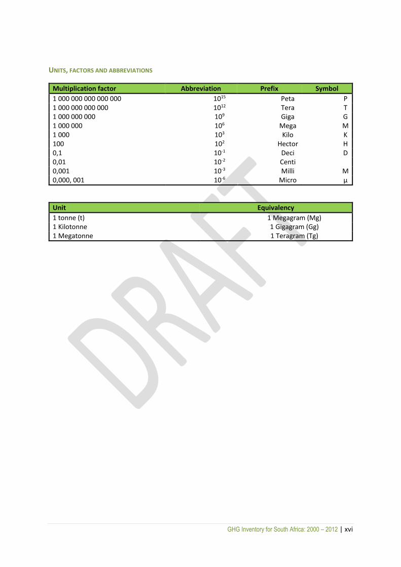
UNITS, FACTORS AND ABBREVIATIONS

Multiplication factor Abbreviation Prefix Symbol

1 000 000 000 000 000 1015 Peta P 1 000 000 000 000 1012 Tera T 1 000 000 000 109 Giga G 1 000 000 106 Mega M 1 000 103 Kilo K 100 102 Hector H 0,1 10-1 Deci D 0,01 10-2 Centi 0,001 10-3 Milli M 0,000, 001 10-6 Micro µ

Unit Equivalency

1 tonne (t) 1 Megagram (Mg) 1 Kilotonne 1 Gigagram (Gg) 1 Megatonne 1 Teragram (Tg)

GHG Inventory for South Africa: 2000 – 2012 | xvii

EXECUTIVE SUMMARY

ES1 Background information on South Africa’s GHG inventories

In August 1997 the Republic of South Africa joined the majority of countries in the international

community in ratifying the UNFCCC. The first national GHG inventory in South Africa was prepared in

1998, using 1990 data. It was updated to include 1994 data and published in 2004. It was developed

using the 1996 IPCC Guidelines for National Greenhouse Gas Inventories. For the 2000 national

inventory, a decision was made to use the recently published 2006 IPCC Guidelines to enhance

accuracy and transparency, and also to familiarise researchers with the latest inventory preparation

guidelines. Following these guidelines, in 2014 the GHG inventory for the years 2000 to 2010 were

compiled.

This report documents South Africa’s submission of its national greenhouse gas inventory for the year

2012. It also reports on the GHG trends for the period 2000 to 2012. It is in accordance with the

guidelines provided by the UNFCCC and follows the 2006 IPCC Guidelines and IPCC Good Practice

Guidance (GPG). The Common Reporting Format (CRF) spread sheet files were used in the compilation

of this inventory. This report provides an explanation of the methods (Tier 1 and Tier 2 approaches),

activity data and emission factors used to develop the inventory. In addition, it assesses the

uncertainty and describes the quality assurance and quality control (QA/QC) activities. Quality

assurance for this GHG inventory was undertaken by independent reviewers.

Development of the National GHG Inventory System (NGHGIS)

During the compilation of the 2010 inventory there were several challenges that affected the accuracy

and completeness of the inventory, such as application of lower tier methods as a result of the

unavailability of disaggregated activity data, lack of well-defined institutional arrangements, and

absence of legal and formal procedures for the compilation of GHG emission inventories. South Africa

is currently in the process of creating a national GHG inventory system that will manage and simplify

its climate change obligations to the UNFCCC process. This system will ensure: a) the sustainability of

the inventory preparation in the country, b) consistency of reported emissions and c) the standard

quality of results. The NGHGIS will ensure that the country prepares and manages data collection and

analysis, as well as all relevant information related to climate change in the most consistent,

transparent and accurate manner for both internal and external reporting. Reliable GHG emission

inventories are essential for the following reasons:

To fulfil the international reporting requirements such as the National Communications and

Biennial Update Reports;

To evaluate mitigation options;

To assess the effectiveness of policies and mitigation measures;

To develop long term emission projections; and

To monitor and evaluate the performance of South Africa in the reduction of GHG emissions.

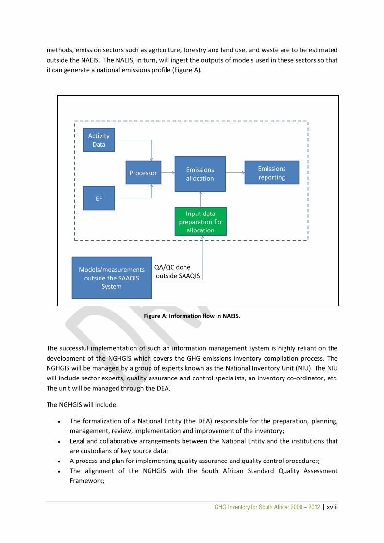
South Africa is developing a National Atmospheric Emissions Inventory System (NAEIS) that will

manage the mandatory reporting of GHG emissions. Due to their complex emission estimating

GHG Inventory for South Africa: 2000 – 2012 | xviii

methods, emission sectors such as agriculture, forestry and land use, and waste are to be estimated

outside the NAEIS. The NAEIS, in turn, will ingest the outputs of models used in these sectors so that

it can generate a national emissions profile (Figure A).

Figure A: Information flow in NAEIS.

The successful implementation of such an information management system is highly reliant on the

development of the NGHGIS which covers the GHG emissions inventory compilation process. The

NGHGIS will be managed by a group of experts known as the National Inventory Unit (NIU). The NIU

will include sector experts, quality assurance and control specialists, an inventory co-ordinator, etc.

The unit will be managed through the DEA.

The NGHGIS will include:

The formalization of a National Entity (the DEA) responsible for the preparation, planning,

management, review, implementation and improvement of the inventory;

Legal and collaborative arrangements between the National Entity and the institutions that

are custodians of key source data;

A process and plan for implementing quality assurance and quality control procedures;

The alignment of the NGHGIS with the South African Standard Quality Assessment

Framework;

Activity Data

EF

Processor

Input data preparation for

allocation

Models/measurements outside the SAAQIS

System

Emissions allocation

Emissions reporting

QA/QC doneoutside SAAQIS

GHG Inventory for South Africa: 2000 – 2012 | xix

A process to ensure that the national inventory meets the standard inventory data quality

indicators of accuracy, transparency, completeness, consistency and comparability; and

A process for continual improvement of the national inventory.

Current inventory process

In the 1990, 1994 and 2000 GHG inventories for South Africa activity and emission factor data were

reported in the IPCC worksheets and the reports were compiled from this data. Supporting data and

methodological details were not recorded, which made updating the inventory a very difficult and

lengthy process. In the 2000 – 2010 GHG inventory more emphasis was placed on building up the

annual data sheets and creating improved trend information. This led to better data records, but still

very little supporting data and method details were kept. Also, in all previous inventories the quality

control procedures and uncertainty estimates were limited. As South Africa moves forward, more

emphasis has been placed on improving the documentation of inventory data and documents, as well

as on uncertainty and quality control so as to improve the transparency of the inventory. The 2012

inventory has come a long way in addressing some of these issues.

The stages of the inventory update and improvement process (Figure B) were:

Data collection, which involved:

o assessing data requirements;

o sourcing data from various stakeholders;

o screening data and selecting the appropriate data sets; and

o data quality control.

Data input into the inventory database.

Metadata input into the inventory database, which included:

o documentation of people responsible for inputting the data;

o specific data calculations;

o data sources;

o recalculations undertaken; and

o links to data or reference files.

Uncertainty analysis.

Compilation of the inventory report.

Quality control and quality assurance involving:

o assessment of the quality of the inventory;

o routine and consistent checks to ensure data integrity, correctness and completeness;

o identification of errors and omissions both in the calculations and report compilation;

o a public commenting process; and

o an external review.

o

GHG Inventory for South Africa: 2000 – 2012 | xx

Stak

eh

old

ers

Data collation

Energy

IPPU

AFOLU

Waste QC/QA database

QC1

QC4

QC5

Sector input data

Energy

IPPU

AFOLU

Waste

Uncertainty data

Energy

IPPU

AFOLU

Waste

Metadata

Energy

IPPU

AFOLU

Waste

Tre

nd

an

d o

vera

ll su

mm

ary

dat

a

Data input

Data collection

Data output

Key

cat

ego

ry a

nd

un

cert

ain

ty a

na

lysi

s

Inve

nto

ry d

ata

ba

se

Inve

nto

ry r

ep

ort

co

mp

ilati

on

Fin

al d

raft

GH

G in

ven

tory

re

po

rt

Fin

al G

HG

inve

nto

ry

QA

GH

G In

ven

tory

re

po

rt

QC2

QC3

Figure B: Overview of the phases of the GHG inventory compilation and improvement process.

Institutional arrangements for inventory preparation

The DEA is responsible for the co-ordination and management of all climate change-related

information, including mitigation, adaption, monitoring and evaluation, and GHG inventories.

Although the DEA takes a lead role in the compilation, implementation and reporting of the national

GHG inventories, other relevant agencies and ministries play supportive roles in terms of data

provision across relevant sectors. Figure C gives an overview of the institutional arrangements for the

compilation of the 2000 – 2012 GHG emissions inventory.

GHG Inventory for South Africa: 2000 – 2012 | xxi

Figure C: Institutional arrangements for the compilation of the 2000 – 2012 inventories.

Organisation of report

This report follows a standard NIR format in line with the UNFCCC Reporting Guidelines. Chapter 1 is

the introductory chapter which contains background information for South Africa, the country’s

inventory preparation and reporting process, key categories, a description of the methodologies,

activity data and emission factors, and a description of the QA/QC process. A summary of the

aggregated GHG trends by gas and emission source is provided in Chapter 2. Chapters 3 to 6 deal with

detailed explanations of the emissions in the energy, IPPU, AFOLU and waste sectors, respectively.

They include an overall trend assessment, methodology, data sources, recalculations, uncertainty and

time-series consistency, QA/QC and planned improvements and recommendations.

DEA (National Entity)

Chief Directorate: Monitoring and Evaluation (GHG Inventory Unit)

Energy

DoE

DMR

Eskom

Coaltech

SAPIA

Chamber of Mines

NERSA

DoT

IPPU

BUSA

SAISI

ACMP

FAPA

DMR

AFOLU

GTI

ARC

FSA

CSIR

AgriSA

SAPA

UP/TUT

NWU

DAFF

StatsSA

DEA-GIS unit

Waste

CSIR

DEA Waste Unit

StatsSA

GHG Inventory for South Africa: 2000 – 2012 | xxii

ES2 Summary of South Africa’s GHG emissions

Overview of national emission and removal trends

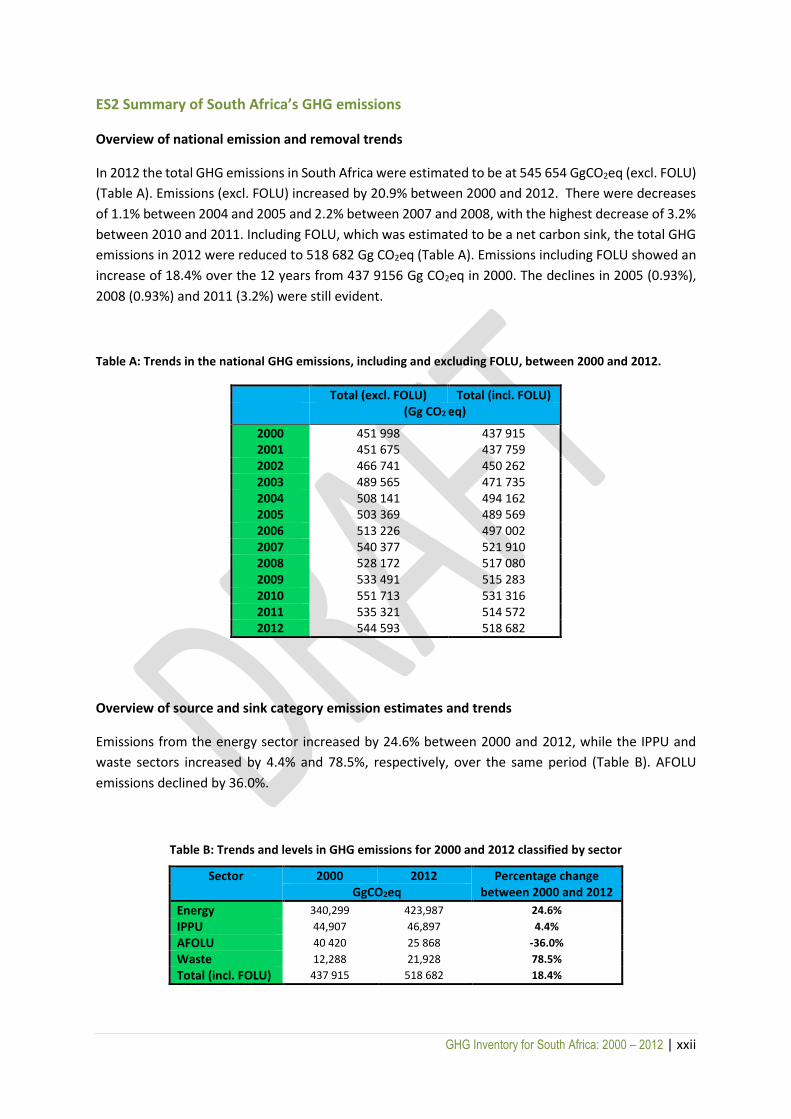
In 2012 the total GHG emissions in South Africa were estimated to be at 545 654 GgCO2eq (excl. FOLU)

(Table A). Emissions (excl. FOLU) increased by 20.9% between 2000 and 2012. There were decreases

of 1.1% between 2004 and 2005 and 2.2% between 2007 and 2008, with the highest decrease of 3.2%

between 2010 and 2011. Including FOLU, which was estimated to be a net carbon sink, the total GHG

emissions in 2012 were reduced to 518 682 Gg CO2eq (Table A). Emissions including FOLU showed an

increase of 18.4% over the 12 years from 437 9156 Gg CO2eq in 2000. The declines in 2005 (0.93%),

2008 (0.93%) and 2011 (3.2%) were still evident.

Table A: Trends in the national GHG emissions, including and excluding FOLU, between 2000 and 2012.

Total (excl. FOLU) Total (incl. FOLU)

(Gg CO2 eq)

2000 451 998 437 915 2001 451 675 437 759 2002 466 741 450 262 2003 489 565 471 735 2004 508 141 494 162 2005 503 369 489 569 2006 513 226 497 002 2007 540 377 521 910 2008 528 172 517 080 2009 533 491 515 283 2010 551 713 531 316 2011 535 321 514 572 2012 544 593 518 682

Overview of source and sink category emission estimates and trends

Emissions from the energy sector increased by 24.6% between 2000 and 2012, while the IPPU and

waste sectors increased by 4.4% and 78.5%, respectively, over the same period (Table B). AFOLU

emissions declined by 36.0%.

Table B: Trends and levels in GHG emissions for 2000 and 2012 classified by sector

Sector 2000 2012 Percentage change between 2000 and 2012 GgCO2eq

Energy 340,299 423,987 24.6%

IPPU 44,907 46,897 4.4%

AFOLU 40 420 25 868 -36.0%

Waste 12,288 21,928 78.5%

Total (incl. FOLU) 437 915 518 682 18.4%

GHG Inventory for South Africa: 2000 – 2012 | xxiii

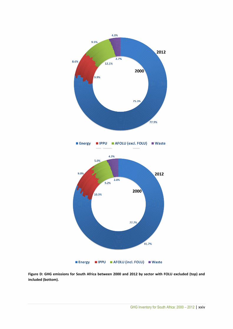
The energy sector contributed 75.3% to the total GHG inventory (excl. FOLU) in 2000 and this

increased to 77.9% in 2012 (Figure D). There was a general increase in the energy sector contribution;

however slight declines were evident in 2001, 2005 and 2006. The AFOLU sector (excl. FOLU) is the

second-largest contributor, followed closely by the IPPU sector. AFOLU (excl. FOLU) contributed 12.1%

in 2000, which declined to 9.5% in 2012, while in 2000 IPPU contributed 9.9%, which declined to 8.6%

in 2012. The IPPU sector showed annual increases in emissions between 2000 and 2006, followed by

a decline between 2007 and 2009. There was also a decline between 2011 and 2012. The AFOLU sector

(excl. FOLU) showed a general decline with small annual increases (of less than 5%) in 2002, 2006,

2008, 2010 and 2011. The waste sector showed a steady increase in its contribution from 2.7% in 2000

to 4.0% in 2012. Including the FOLU component in the AFOLU sector decreased the total GHG

emissions to 518 682 Gg CO2eq in 2012. This also changed the contribution from the energy, IPPU,

AFOLU and waste sectors to 81.7%, 9.0%, 5.0% and 4.2%, respectively, in 2012 (Figure D).

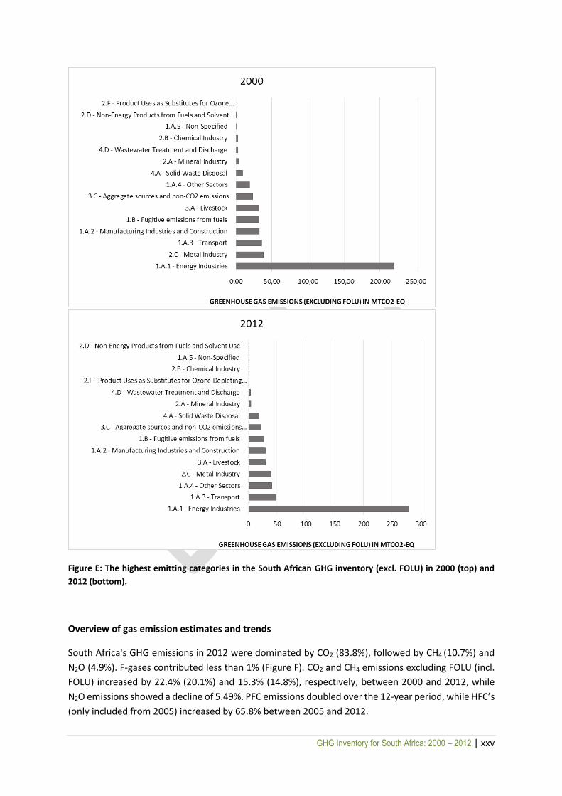
The top-emitting categories in 2000 and 2012 (excl. FOLU) are shown in Figure E.

GHG Inventory for South Africa: 2000 – 2012 | xxiv

Figure D: GHG emissions for South Africa between 2000 and 2012 by sector with FOLU excluded (top) and

included (bottom).

GHG Inventory for South Africa: 2000 – 2012 | xxv

Figure E: The highest emitting categories in the South African GHG inventory (excl. FOLU) in 2000 (top) and

2012 (bottom).

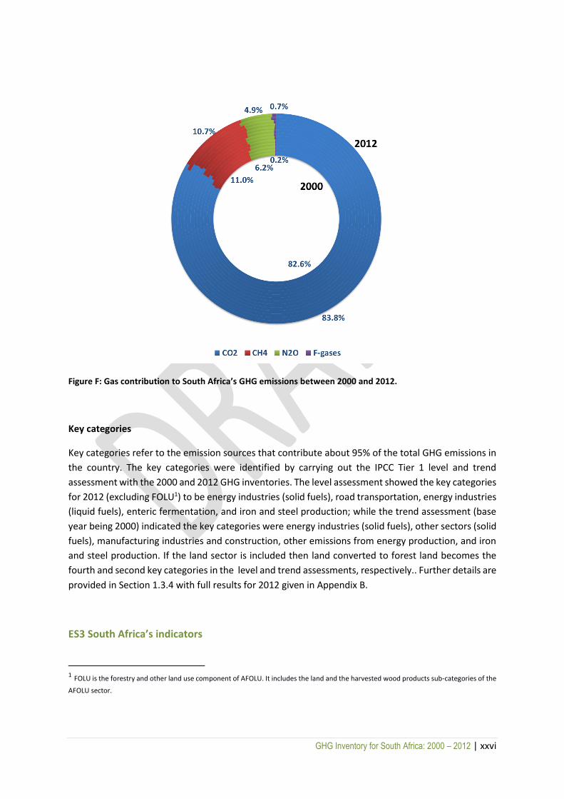
Overview of gas emission estimates and trends

South Africa's GHG emissions in 2012 were dominated by CO2 (83.8%), followed by CH4 (10.7%) and

N2O (4.9%). F-gases contributed less than 1% (Figure F). CO2 and CH4 emissions excluding FOLU (incl.

FOLU) increased by 22.4% (20.1%) and 15.3% (14.8%), respectively, between 2000 and 2012, while

N2O emissions showed a decline of 5.49%. PFC emissions doubled over the 12-year period, while HFC’s

(only included from 2005) increased by 65.8% between 2005 and 2012.

GHG Inventory for South Africa: 2000 – 2012 | xxvi

Figure F: Gas contribution to South Africa’s GHG emissions between 2000 and 2012.

Key categories

Key categories refer to the emission sources that contribute about 95% of the total GHG emissions in

the country. The key categories were identified by carrying out the IPCC Tier 1 level and trend

assessment with the 2000 and 2012 GHG inventories. The level assessment showed the key categories

for 2012 (excluding FOLU1) to be energy industries (solid fuels), road transportation, energy industries

(liquid fuels), enteric fermentation, and iron and steel production; while the trend assessment (base

year being 2000) indicated the key categories were energy industries (solid fuels), other sectors (solid

fuels), manufacturing industries and construction, other emissions from energy production, and iron

and steel production. If the land sector is included then land converted to forest land becomes the

fourth and second key categories in the level and trend assessments, respectively.. Further details are

provided in Section 1.3.4 with full results for 2012 given in Appendix B.

ES3 South Africa’s indicators

1 FOLU is the forestry and other land use component of AFOLU. It includes the land and the harvested wood products sub-categories of the

AFOLU sector.

GHG Inventory for South Africa: 2000 – 2012 | xxvii

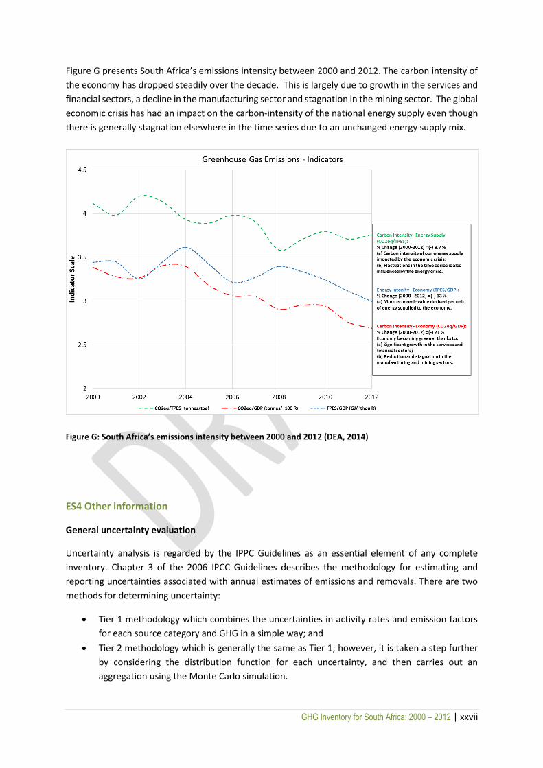
Figure G presents South Africa’s emissions intensity between 2000 and 2012. The carbon intensity of

the economy has dropped steadily over the decade. This is largely due to growth in the services and

financial sectors, a decline in the manufacturing sector and stagnation in the mining sector. The global

economic crisis has had an impact on the carbon-intensity of the national energy supply even though

there is generally stagnation elsewhere in the time series due to an unchanged energy supply mix.

Figure G: South Africa’s emissions intensity between 2000 and 2012 (DEA, 2014)

ES4 Other information

General uncertainty evaluation

Uncertainty analysis is regarded by the IPPC Guidelines as an essential element of any complete

inventory. Chapter 3 of the 2006 IPCC Guidelines describes the methodology for estimating and

reporting uncertainties associated with annual estimates of emissions and removals. There are two

methods for determining uncertainty:

Tier 1 methodology which combines the uncertainties in activity rates and emission factors

for each source category and GHG in a simple way; and

Tier 2 methodology which is generally the same as Tier 1; however, it is taken a step further

by considering the distribution function for each uncertainty, and then carries out an

aggregation using the Monte Carlo simulation.

GHG Inventory for South Africa: 2000 – 2012 | xxviii

The reporting of uncertainties requires a complete understanding of the processes of compiling the

inventory, so that potential sources of inaccuracy can be qualified and possibly quantified. The 2010

inventory (DEA, 2014) did not incorporate an overall uncertainty assessment due to a lack of

quantitative and qualitative uncertainty data. In this inventory there has been an attempt to

incorporate an overall uncertainty assessment through the utilization of the IPCC uncertainty spread

sheet. A trend uncertainty between the base year and 2012, as well as a combined uncertainty of

activity data and emission factor uncertainty was determined using an Approach 1. This inventory

includes uncertainty assessment for the energy and IPPU sectors only, but the other sectors will be

included in the next inventory. The total uncertainty for the energy sector was determined to be 6.5%,

with a trend uncertainty of 6.3%. The IPPU sector has an uncertainty of 30.6% (8.83% excluding section

2.F).

Quality control and quality assurance

In accordance with IPCC requirements, the national GHG inventory preparation process must include

quality control and quality assurance (QC/QA) procedures. The objective of quality checking is to

improve the transparency, consistency, comparability, completeness, and accuracy of the national

greenhouse gas inventory. QC procedures, performed by the compilers, were carried out at various

stages throughout the inventory compilation process (Figure B). Quality checks were completed at

four different levels, namely (a) inventory data (activity data, EF data, uncertainty, and recalculations),

(b) database (data transcriptions and aggregations), (c) metadata (documentation of data, experts and

supporting data), and (d) inventory report. Quality assurance was completed through a public review

process as well as an independent review. The inventory was finalized once all comments from the

quality assurance process were addressed.

Completeness of the national inventory

The GHG emission inventory for South Africa is not complete, mainly due to data unavailability, and

lack of data and estimation methodologies. Table C describes the activities identified by the IPCC 2006

Guidelines that were not estimated (NE), included elsewhere (IE) or not occurring (NO).

Table C: Activities in the 2012 inventory which were not estimated (NE), included elsewhere (IE) or not occurring (NO).

NE, IE or NO

Activity Comments

NE

CO2 and CH4 fugitive emissions from oil and natural gas operations

Emissions from this source category will be included in the next inventory submission covering the period 2000-2014

CO2, CH4 and N2O from spontaneous combustion of coal seams

New research work on sources of emissions from this category will be used to report in the next emission inventory submission

CH4 emissions from abandoned mines New research work on sources of emissions from this category will be used to report emissions in the next inventory submission

GHG Inventory for South Africa: 2000 – 2012 | xxix

Other process use of carbonates

Electronics industry A study was to be undertaken in 2015 to understand emissions from this source category

Indirect N2O emission due to nitrogen deposition

HWP from solid waste This will be included in the next inventory

CO2, CH4 and N2O emissions from combined heat and power (CHP) combustion systems

CH4, N2O emissions from biological treatment of waste

CO2, CH4 and N2O emissions from incineration and open burning of waste

DOM emissions from croplands, grasslands, settlements and other lands

IE

CO2, CH4 and N2O emissions from water-borne navigation

Fuel consumption for this source-category is included elsewhere. Accurate quantification of fuel consumption attributed to water-borne navigation was to be undertaken in 2015 and a progress report will be included in the next inventory submission

CO2, CH4 and N2O emissions from off-road vehicles and other machinery

Fuel use associated with this source category is included in road transportation. A new study that was to be finalised in October 2015 on fuel apportionment to all demand sectors will help with accurate allocation of fuels.

Ozone depleting substance replacements for fire protection and aerosols

Emissions from these sources are assumed to be accounted for in the Tier 1 methodology for quantification of HFC emissions

NO

Other product manufacture and use

Rice cultivation This activity does not occur in South Africa

CO2, CH4 and N2O emissions from Soda Ash Production

This activity does not occur in South Africa

CO2 from Carbon Capture and Storage This activity does not occur in South Africa

CO2, CH4 and N2O emissions from Adipic acid production

This activity does not occur in South Africa

CO2, CH4 and N2O Caprolactam, Glyoxal and Glyoxylic acid production

This activity does not occur in South Africa

Precursor emissions have only been estimated for biomass burning, and only for CO and NOx

Precursor emissions from all sources will be included in the next inventory

Methodological changes, recalculations and improvements

In the past year various improvements have been made to the GHG inventory due to the incorporation

of more detailed activity data, updated emission factors and more consistent land-cover maps. For

the energy sector, country-specific CO2 emission factors were incorporated, while for the IPPU sector

the calculations made used more accurate activity data acquired from actual process analysis. No

major recalculations were done in the IPPU sector.

Significant updates were made in the AFOLU sector. In the agriculture sector small corrections were

made to beef cattle and poultry population data, and emissions from game on privately owned parks

was included. In the section on land use, new land-cover maps with a higher resolution were

GHG Inventory for South Africa: 2000 – 2012 | xxx

introduced, and emissions from DOM in forest lands and emissions from other lands were included.

Updates to some of the biomass data were also made so as to incorporate data from the recent

National Terrestrial Carbon Sinks report (DEA, 2015). The soil carbon methodology was updated to

incorporate soil types, while the HWP data was updated based on the new KP Supplementary GP

guidelines.

For the purpose of this report, the GHG emissions for the period 2000 to 2012 were recalculated using

the updated activity data and emission factors so as to form a more consistent time series. In this way,

the trends over time can be assessed. All the updates and recalculation methods and procedures are

discussed in detail in Chapters 3 to 6 of this report.

The recalculations for the AFOLU sector had the largest impact on the total emissions (Table D) with a

32.5% and 29.2% increase on the sector estimates in 2000 and 2010, respectively. The majority of this

change was due to the corrected HWP estimates (this falls under the IPCC category 3D other) and the

updated land change maps. The increases in the AFOLU sector impacted the national total by 2.2%

and 1.4% in 2000 and 2010, respectively (Table D). Small adjustments and recalculations were made

in the energy, IPPU and waste sectors, which contributed 0.7%, 0.3% and 0.1% to the increase in the

national total, respectively.

Table D: Recalculated sector GHG emission estimates for 2000 and 2010 for South Africa.

Initial emissions

Recalculated emissions

% change

% impact on national total (incl.

FOLU)

(Gg CO2eq.)

Energy 2000 337 381 340 300 0.9% 0.65%

2010 428 368 431 994 0.8% 0.67%

IPPU 2000 44 907 44 907 0.0% 0.00%

2010 44 350 45 736 3.1% 0.25%

Total AFOLU 2000 30 496 40 420 32.5% 2.22%

2010 25 713 33 230 29.2% 1.41%

3A Livestock 2000 31 118 31 162 0.1% 0.13%

2010 28 986 29 412 1.5% 0.004%

3B Land 2000 -18 492 -13 770 -25.54% 1.08%

2010 -33 224 -19 904 -40.09% 2.51%

3C Aggregated sources and non-CO2 emissions on land

2000 23 656 23 340 -1.343% -0.07%

2010 22 802 23 381 2.53% 0.11%

3D Other 2000 -5 785 -312 -94.6% 1.23%

2010 -6 204 -491 -92.1% 1.10%

Waste 2000 12 433 12 288 -1.2% -0.03%

2010 19 806 20 354 2.8% 0.10%

The Greenhouse Gas Improvement Programme (GHGIP)

The main challenge in the compilation of South Africa’s GHG inventory remains the availability of

accurate activity data. The DEA is in the process of implementing a project that will ensure easy

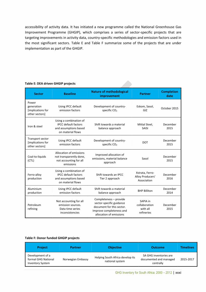
GHG Inventory for South Africa: 2000 – 2012 | xxxi

accessibility of activity data. It has initiated a new programme called the National Greenhouse Gas

Improvement Programme (GHGIP), which comprises a series of sector-specific projects that are

targeting improvements in activity data, country-specific methodologies and emission factors used in

the most significant sectors. Table E and Table F summarize some of the projects that are under

implementation as part of the GHGIP.

Table E: DEA driven GHGIP projects

Sector Baseline Nature of methodological

improvement Partner

Completion date

Power generation [implications for other sectors]

Using IPCC default emission factors

Development of country-specific CO2

Eskom, Sasol, GIZ

October 2015

Iron & steel

Using a combination of IPCC default factors

and assumptions based on material flows

Shift towards a material balance approach

Mittal Steel, SAISI

December 2015

Transport sector [implications for other sectors]

Using IPCC default emission factors

Development of country-specific CO2

DOT December

2015

Coal-to-liquids (CTL)

Allocation of emissions not transparently done,

not accounting for all emissions

Improved allocation of emissions, material balance

approach Sasol

December 2015

Ferro-alloy production

Using a combination of IPCC default factors

and assumptions based on material flows

Shift towards an IPCC Tier 2 approach

Xstrata, Ferro-Alloy Producers'

Association

December 2016

Aluminium production

Using IPCC default emission factors

Shift towards a material balance approach

BHP Billiton December

2014

Petroleum refining

Not accounting for all emission sources. Data time series inconsistencies

Completeness – provide sector-specific guidance

document for this sector. Improve completeness and

allocation of emissions

SAPIA in collaboration

with all refineries

December 2015

Table F: Donor funded GHGIP projects

Project Partner Objective Outcome Timelines

Development of a formal GHG National Inventory System

Norwegian Embassy Helping South Africa develop its

national system

SA GHG inventories are documented and managed

centrally 2015-2017

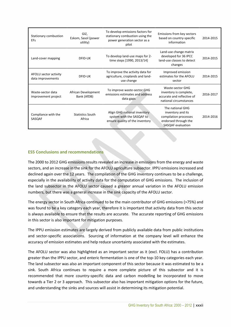
GHG Inventory for South Africa: 2000 – 2012 | xxxii

Stationary combustion EFs

GIZ, Eskom, Sasol (power

utility)

To develop emissions factors for stationary combustion using the

power generation sector as a pilot

Emissions from key sectors based on country-specific

information 2014-2015

Land-cover mapping DFID-UK To develop land-use maps for 2-

time steps [1990, 2013/14]

Land-use change matrix developed for 36 IPCC

land-use classes to detect changes

2014-2015

AFOLU sector activity data improvements

DFID-UK To improve the activity data for agriculture, croplands and land-

use change

Improved emission estimates for the AFOLU

sector 2014-2015

Waste-sector data improvement project

African Development Bank (AfDB)

To improve waste-sector GHG emissions estimates and address

data gaps

Waste-sector GHG inventory is complete,

accurate and reflective of national circumstances

2016-2017

Compliance with the SASQAF

Statistics South Africa

Align GHG national inventory system with the SASQAF to

ensure quality of the inventory

The national GHG inventory and its

compilation processes endorsed through the

SASQAF evaluation

2014-2016

ES5 Conclusions and recommendations

The 2000 to 2012 GHG emissions results revealed an increase in emissions from the energy and waste

sectors, and an increase in the sink for the AFOLU agriculture subsector. IPPU emissions increased and

declined again over the 12 years. The compilation of the GHG inventory continues to be a challenge,

especially in the availability of activity data for the computation of GHG emissions. The inclusion of

the land subsector in the AFOLU sector caused a greater annual variation in the AFOLU emission

numbers, but there was a general increase in the sink capacity of the AFOLU sector.

The energy sector in South Africa continued to be the main contributor of GHG emissions (>75%) and

was found to be a key category each year, therefore it is important that activity data from this sector

is always available to ensure that the results are accurate. The accurate reporting of GHG emissions

in this sector is also important for mitigation purposes.

The IPPU emission estimates are largely derived from publicly available data from public institutions

and sector-specific associations. Sourcing of information at the company level will enhance the

accuracy of emission estimates and help reduce uncertainty associated with the estimates.

The AFOLU sector was also highlighted as an important sector as it (excl. FOLU) has a contribution

greater than the IPPU sector, and enteric fermentation is one of the top-10 key categories each year.

The land subsector was also an important component of this sector because it was estimated to be a

sink. South Africa continues to require a more complete picture of this subsector and it is

recommended that more country-specific data and carbon modelling be incorporated to move

towards a Tier 2 or 3 approach. This subsector also has important mitigation options for the future,

and understanding the sinks and sources will assist in determining its mitigation potential.

GHG Inventory for South Africa: 2000 – 2012 | xxxiii

In the waste sector the emission estimates from both the solid waste and wastewater sources were

largely computed using default values suggested in the IPCC 2006 Guidelines, which could lead to large

margins of error for South Africa. South Africa needs to improve the data capture of the quantities of

waste disposed into managed and unmanaged landfills, as well as update waste composition

information and the mapping of all the wastewater discharge pathways. This sector would also benefit

from the inclusion of more detailed economic data (e.g. annual growth) broken down by the different

population groups. The assumption that GDP growth is evenly distributed across the different

populations groups is highly misleading and exacerbates the margins of error.

1 INTRODUCTION

1.1 Climate change and GHG inventories

The Republic of South Africa ratified the UNFCCC and is therefore required to undertake several projects related to climate change. These include the

preparation of greenhouse gas inventories, one of the outputs for the National Communications to the UNFCCC.

South Africa's first national GHG inventory was compiled in 1998 using activity data for 1990. The second national GHG inventory used 1994 data and was

published in 2004. Both the 1990 and 1994 inventories were compiled based on the 1996 IPCC Guidelines.

The third national GHG inventory was compiled in 2009 using activity data from 2000. For that inventory the 2006 IPCC Guidelines were introduced. Those

guidelines ensured accuracy, transparency and consistency. The 2006 IPCC Guidelines made significant changes, particularly on the restructuring of inventory

sectors. Countries are not required by the UNFCCC to report their GHG emissions using the updated guidelines; however, it was decided to use the latest

IPCC Guidelines to avoid difficulties converting from the 1996 to the 2006 guidelines in the future. In 2014 South Africa prepared its fourth national inventory,

which included annual emission estimates for 2000 to 2010.

1.2 Country background

1.2.1 National circumstances

South Africa is a culturally diverse developing country with 11 official languages. It is a significant industrial and economic power in Africa and has the largest

economy in southern Africa. The country has well-developed mining, transport, energy, manufacturing, tourism, agriculture, commercial timber and pulp

production, and service sectors. It is a net exporter of energy, food, and telecommunications and other services to neighbouring countries. South Africa shares

borders with six countries: Namibia, Botswana, Zimbabwe and Mozambique, which lie to the north, and Lesotho and Swaziland, which are landlocked within

South Africa.

GHG Inventory for South Africa: 2000 – 2012 | 35

There are various factors that can influence a nation’s GHG emissions, including governments (infra-) structure, population growth, geography, economic

growth, energy consumption, technological development, climate and soils, agriculture, and land use management. South Africa contributes to global climate

change and, as a result, has taken steps to formulate measures to mitigate and adapt to a changing climate.

1.2.1.1 GOVERNMENT STRUCTURE

South Africa is a multiparty democracy, with three tiers of government: national, provincial and local. Responsibilities affecting economic development,

energy and natural resources, among others, are shared across the three tiers.

1.2.1.2 POPULATION PROFILE

South Africa's population in 2013 was 52.98 million (Statistics SA, 2013). It had grown by 11.54% between 2001 to 2010 and the projected growth rate for

2010 to 2015 was 0.5% (DEA, 2011). International immigration is currently the main driving force of South Africa’s population growth (DEA, 2014). Strong

socio-economic and policy drivers of migration to urban centres have been at play, as indicated by the urban population increase from 52% to 62% over the

past two decades (UNDP, 2010). South Africa is one of the most urbanised countries in Africa. There are nine provinces: Eastern Cape, Free State, Gauteng,

KwaZulu-Natal, Limpopo, Mpumalanga, Northern Cape, North West and Western Cape. Gauteng is the most populated, with 24% of residents (DEA, 2014),

followed by KwaZulu-Natal with 19.7%. The Northern Cape has the smallest population (2.2%) (Statistics SA, 2013). South Africa has 11 official languages,

which displays its cultural diversity.

1.2.1.3 GEOGRAPHIC PROFILE

South Africa is a medium-sized country, which covers roughly 124 929 847 hectares of the southernmost part of the African continent. It measures

approximately 1 600 km from north to south, and is about the same from east to west. It lies between 22° and 35° south, flanked on the west by the Atlantic

Ocean and on the east by the Indian Ocean (GCSI, 2009). The coastline is more than 2 500 km long, extending southwards from the desert border with

Namibia in the northwest to Cape Agulhas, and then northwards to the Indian Ocean until it reaches the subtropical border with Mozambique in the northeast

(GCSI, 2009). It has narrow coastal plateaus in the south and west which are edged by coastal mountain ranges. Further into the interior, an escarpment

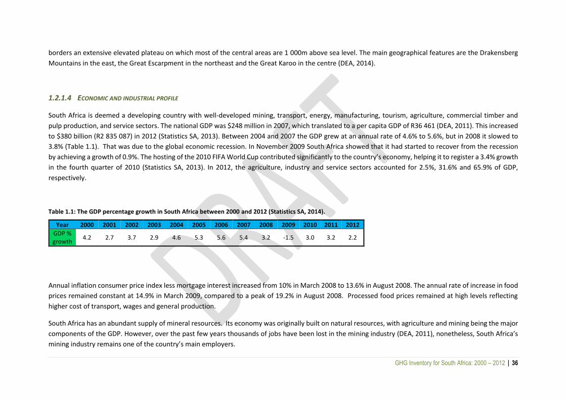
GHG Inventory for South Africa: 2000 – 2012 | 36

borders an extensive elevated plateau on which most of the central areas are 1 000m above sea level. The main geographical features are the Drakensberg

Mountains in the east, the Great Escarpment in the northeast and the Great Karoo in the centre (DEA, 2014).

1.2.1.4 ECONOMIC AND INDUSTRIAL PROFILE

South Africa is deemed a developing country with well-developed mining, transport, energy, manufacturing, tourism, agriculture, commercial timber and

pulp production, and service sectors. The national GDP was $248 million in 2007, which translated to a per capita GDP of R36 461 (DEA, 2011). This increased

to $380 billion (R2 835 087) in 2012 (Statistics SA, 2013). Between 2004 and 2007 the GDP grew at an annual rate of 4.6% to 5.6%, but in 2008 it slowed to

3.8% (Table 1.1). That was due to the global economic recession. In November 2009 South Africa showed that it had started to recover from the recession

by achieving a growth of 0.9%. The hosting of the 2010 FIFA World Cup contributed significantly to the country’s economy, helping it to register a 3.4% growth

in the fourth quarter of 2010 (Statistics SA, 2013). In 2012, the agriculture, industry and service sectors accounted for 2.5%, 31.6% and 65.9% of GDP,

respectively.

Table 1.1: The GDP percentage growth in South Africa between 2000 and 2012 (Statistics SA, 2014).

Year 2000 2001 2002 2003 2004 2005 2006 2007 2008 2009 2010 2011 2012

GDP % growth

4.2 2.7 3.7 2.9 4.6 5.3 5.6 5.4 3.2 -1.5 3.0 3.2 2.2

Annual inflation consumer price index less mortgage interest increased from 10% in March 2008 to 13.6% in August 2008. The annual rate of increase in food

prices remained constant at 14.9% in March 2009, compared to a peak of 19.2% in August 2008. Processed food prices remained at high levels reflecting

higher cost of transport, wages and general production.

South Africa has an abundant supply of mineral resources. Its economy was originally built on natural resources, with agriculture and mining being the major

components of the GDP. However, over the past few years thousands of jobs have been lost in the mining industry (DEA, 2011), nonetheless, South Africa’s

mining industry remains one of the country’s main employers.

GHG Inventory for South Africa: 2000 – 2012 | 37

The transport sector is dominated by road travel. South Africa's car ownership ratio is higher than the world average, which is attributed to the large distances

between settlements and places of employment. Within the road transport sector 19% is due to private vehicle trips, and 11.5% due to minibus taxis. Sixty-

three percent of the country's commuters use minibus taxis, 22% use buses and 15% use trains (DEA, 2011). The minibus-taxi industry continues to grow

annually.

With the growing population and economy, waste processing and disposal continue to be significant challenges. Households with adequate refuse removal

services have remained at about 60% since 2006, but over 80% of these households are in urban areas. In rural areas, as little as 20% of households have

access to these services.

1.2.1.5 NATURAL RESOURCES PROFILE

South Africa is located in a subtropical region, making it a warm and sunny country. Its climate is moderated by oceanic influences along the extensive

coastline and by the altitude of the interior plateau. Its climate is generally warm temperate dry, however, there are exceptions, which create climatic

diversity. There is a temperate Mediterranean-type climate in the southwest, a warm subtropical climate in the northeast, and a warm, dry desert

environment in the central west and northwest. South Africa is a semi-arid region with an east-west rainfall gradient ranging from less than 250 mm to over

1000 mm per year (State of Environment Report, 2006). Most of the rainfall occurs in summer; however, the Western Cape receives most of its rainfall in

winter (GCSI, 2009).

The relatively young geology in South African gives rise to high-nutrient soils. The Nama-Karoo biome of the central region comprises predominantly

mudstones and sandstones of the Karoo Supergroup, while the Highveld grasslands are associated with high-nutrient soils of basalt and dolerite origin (Palmer

& Ainslie, 2002). The savannas of the Mpumalanga Lowveld are associated with gabbros and granites (sandy, moderate-nutrient status) of the Bushveld

Igneous Complex. The Cape Fold Mountains are siliceous rocks giving rise to litholic soils, while the Lesotho Highlands are basaltic giving rise to mollisols

(Partridge, 1997).

The land cover in South Africa is dominated by low shrublands (33%), grasslands (20%) and woodlands or open bush (10%) (GeoTerraImage, 2015; see

Appendix G). Natural forests are very small in South Africa, covering less than 0.5% of the land area. Settlements occupy approximately 2% of the land area

(GeoTerraImage, 2015). Although 80% of South Africa’s land surface area is used for agriculture and subsistence livelihoods, only about 11% has arable

potential. The remaining 69% is used for grazing. Areas of moderate to high arable potential occur mainly in the eastern part of the country, in Mpumalanga

and Gauteng, with scattered patches in KwaZulu-Natal, the Eastern Cape, and Limpopo. The agricultural sector is very diverse, ranging from intensive, large-

GHG Inventory for South Africa: 2000 – 2012 | 38

scale commercial agricultural to low-intensity, small-scale subsistence farming. Roughly 11% of the land is formally cultivated, with a further 1.6% under

subsistence farming. Maize and wheat are the dominant annual crops by area. Plantations are based on non-native trees, with the dominant species being

Eucalyptus grandis.

Land in South Africa has enormous economic, social and environmental value, but a large proportion of the country’s land surface is susceptible to

degradation. Schoeman et al. (2013) showed that there was a 1.2% increase in transformed land between 1994 and 2005. Cultivation and degradation of

natural cover contributed 10.5% and 4.5%, respectively, to this transformation. The rest was due to urban land use and forestry. Cultivated areas over this

period declined from 12.4% to 11.9%.

1.2.1.6 AGRICULTURE, FORESTRY AND FISHERIES PROFILE

Agriculture, forestry and fisheries together accounted for less than 3% of GDP in 2006 (DEA, 2011). The agriculture sector is dominated, in economic output

terms, by large-scale commercial farming, but there is a very important small-scale and subsistence sector. The total contribution of agriculture to the

economy increased from R27 billion in 2001 to R36 billion in 2007. During the period 2008 to 2009 the sale of animals and animal products accounted for

48.2% of the income, 26.7% was from field crops and 25.1% was from horticulture (DST, 2010). South Africa’s largest agricultural commodity by mass in 2007

was sugar cane, followed by cattle meat, chicken meat, grapes and dairy.

South Africa’s timber plantations are based on non-native trees and cover 1.3% of the land area (GeoTerraImage, 2015). Timber contributes more than R16

billion to South Africa’s economy, with an annual production of 2.2 million m3 of commercial round wood (DEA, 2011). Exports are mainly converted, value-

added products, with raw material exports making up only 1.8% of the total. The main products exported are pulp and paper (73%), saw timber, wood chips

and wattle extract.

The commercial and recreational fishing industries are a relatively small economic sector, contributing about 1% of GDP and valued at approximately R4

billion to 5 billion annually (DEA, 2011).

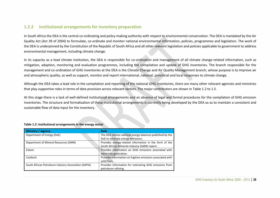
GHG Inventory for South Africa: 2000 – 2012 | 39

1.2.2 Institutional arrangements for inventory preparation

In South Africa the DEA is the central co-ordinating and policy-making authority with respect to environmental conservation. The DEA is mandated by the Air

Quality Act (Act 39 of 2004) to formulate, co-ordinate and monitor national environmental information, policies, programmes and legislation. The work of

the DEA is underpinned by the Constitution of the Republic of South Africa and all other relevant legislation and policies applicable to government to address

environmental management, including climate change.

In its capacity as a lead climate institution, the DEA is responsible for co-ordination and management of all climate change-related information, such as

mitigation, adaption, monitoring and evaluation programmes, including the compilation and update of GHG inventories. The branch responsible for the

management and co-ordination of GHG inventories at the DEA is the Climate Change and Air Quality Management branch, whose purpose is to improve air

and atmospheric quality, as well as support, monitor and report international, national, provincial and local responses to climate change.

Although the DEA takes a lead role in the compilation and reporting of the national GHG inventories, there are many other relevant agencies and ministries

that play supportive roles in terms of data provision across relevant sectors. The major contributors are shown in Table 1.2 to 1.5.

At this stage there is a lack of well-defined institutional arrangements and an absence of legal and formal procedures for the compilation of GHG emission

inventories. The structure and formalization of these institutional arrangements is currently being developed by the DEA so as to maintain a consistent and

sustainable flow of data input for the inventory.

Table 1.2: Institutional arrangements in the energy sector

Ministry / Agency Role Department of Energy (DoE) The DEA utilises national energy balances published by the

DoE to estimate energy emissions. Department of Mineral Resources (DMR) Provides energy-related information in the form of the

South African Minerals Industry (SAMI) report. Eskom Provides information on GHG emissions associated with

electricity generation. Coaltech Provides information on fugitive emissions associated with

solid fuels. South African Petroleum Industry Association (SAPIA) Provides information for estimating GHG emissions from

petroleum refining.

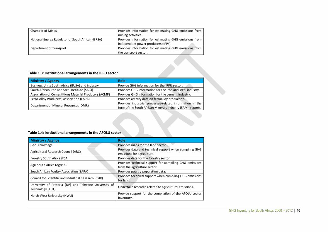
GHG Inventory for South Africa: 2000 – 2012 | 40

Chamber of Mines Provides information for estimating GHG emissions from mining activities.

National Energy Regulator of South Africa (NERSA) Provides information for estimating GHG emissions from independent power producers (IPPs).

Department of Transport Provides information for estimating GHG emissions from the transport sector.

Table 1.3: Institutional arrangements in the IPPU sector

Ministry / Agency Role Business Unity South Africa (BUSA) and industry Provide GHG information for the IPPU sector. South African Iron and Steel Institute (SAISI) Provides GHG information for the iron and steel industry. Association of Cementitious Material Producers (ACMP) Provides GHG information for the cement industry. Ferro-Alloy Producers' Association (FAPA) Provides activity data on ferroalloy production.

Department of Mineral Resources (DMR) Provides industrial processes-related information in the form of the South African Minerals Industry (SAMI) reports.

Table 1.4: Institutional arrangements in the AFOLU sector

Ministry / Agency Role GeoTerraImage Provides maps for the land sector.

Agricultural Research Council (ARC) Provides data and technical support when compiling GHG emissions for agriculture.

Forestry South Africa (FSA) Provides data for the forestry sector.

Agri South Africa (AgriSA) Provides technical support for compiling GHG emissions from the agriculture sector.

South African Poultry Association (SAPA) Provides poultry population data.

Council for Scientific and Industrial Research (CSIR) Provides technical support when compiling GHG emissions for land.

University of Pretoria (UP) and Tshwane University of Technology (TUT)

Undertake research related to agricultural emissions.

North-West University (NWU) Provide support for the compilation of the AFOLU sector inventory.

GHG Inventory for South Africa: 2000 – 2012 | 41

Department of Agriculture, Forestry and Fisheries (DAFF) Provides data, statistics and information on the AFOLU sector.

Statistics South Africa (Stats SA) Provides statistical data for the AFOLU sector. Department of Environmental Affairs (DEA) Geographic Information System (GIS) Unit

Provides an archiving system for forestry maps.

Table 1.5: Institutional arrangements in the waste sector

Ministry / Agency Role Council for Scientific and Industrial Research (CSIR) Provides technical support when compiling GHG emissions

for the waste sector. DEA Waste Unit Provides information on the waste sector. Statistics South Africa (StatsSA) Provides statistical parameters that can be applied when

estimating GHG emissions from the waste sector Department of Water Affairs (DWA) Provides information on the country’s wastewater

treatment works.

1.3 Inventory preparation

It was decided before the preparation of the 2000 inventory that the 2006 IPCC Guidelines would be used to prepare South Africa’s GHG inventory so as to

ensure consistency, accuracy and transparency. To be consistent with previous inventories, this GHG inventory for 2012 was also prepared using the principles

of the 2006 IPCC Guidelines. The method chosen for each source category is guided by the decision trees provided in the IPCC Guidelines. In general, the

method selected depended on whether or not the source category was considered as the main category, and on the availability of data.

The collection of data and information is still a challenge when compiling the GHG inventory for South Africa. The data and information are often collected

from national aggregated levels rather than from point or direct sources. That makes the use of higher-tier methods difficult. Where more disaggregated

data and emission factors were available, a higher-tier method was used to improve on the previous inventory. South Africa’s aim is to incorporate more

country-specific data and move towards a Tier 2 or 3 approach for the key categories in particular.

GHG Inventory for South Africa: 2000 – 2012 | 42

The DEA is in the process of implementing a data management system that will manage all aspects of the inventory compilation process. The NGHGIS will

include:

The formalization of a National Entity (the DEA), which will include an inventory co-ordinator, sector-specific experts and an inventory compiler. This

group will be responsible for the preparation, planning, management, review, implementation and improvement of the inventory;

Legal and collaborative arrangements between the National Entity and the institutions that are custodians of key source data and that will provide

the required data for each sector;

A process and plan for implementing QA and QC procedures, including ensuring that the UNFCCC reporting and IPCC Guidelines have been properly

implemented;

The alignment of the NGHGIS with the South African Standard Quality Assessment Framework;

A process to ensure that the national inventory meets the standard inventory data quality indicators of accuracy, transparency, completeness,

consistency and comparability; and

A process for continual improvements of the national inventory.

1.3.1 Data collection procedures and plans

A variety of data suppliers provide basic input data for emission estimates. Data collection and documentation were the responsibility of individual experts

in each sector. Data came mostly from government institutions, local and international literature, and, to a lesser extent, from individual industrial plants and

professional associations. Data access continues to be a challenge for South Africa; therefore this inventory is not complete. Some sources or sinks have been

omitted due to lack of appropriate data (see Section 1.6).

The DEA is in the process of developing a data collection plan that will improve the accessibility of activity data. The data collection procedures will include

guidance on collection, collation and processing existing data, as well as providing guidance for the generation of new data. A data collection plan is required

to meet data quality objectives regarding timeliness, consistency, completeness, comparability, accuracy and transparency. It is also good practice to

periodically review the data collection process to maintain the quality and to guide progressive and efficient inventory improvement.

The data collection plan will focus on providing guidance for three main aspects (Figure 1.1):

Collection and collation of existing data:

GHG Inventory for South Africa: 2000 – 2012 | 43

o focus data collection on improving estimates for key categories which:

are the largest,

have the greatest potential to change, or

have the greatest uncertainty;

o choose data collection procedures that iteratively improve the quality of the inventory in line with the data quality objectives; and

o collect data at a level of detail appropriate to the method used;

Generation of new data:

o identify data gaps and work towards filling these gaps; and

o put in place data collection activities that lead to the continual improvement of data sets used in the inventory;

Maintenance of data supply and collection procedures:

o introduce agreements with data suppliers to support consistent and continuing information flows; and

o review data collection activities and methodological needs on a regular basis.

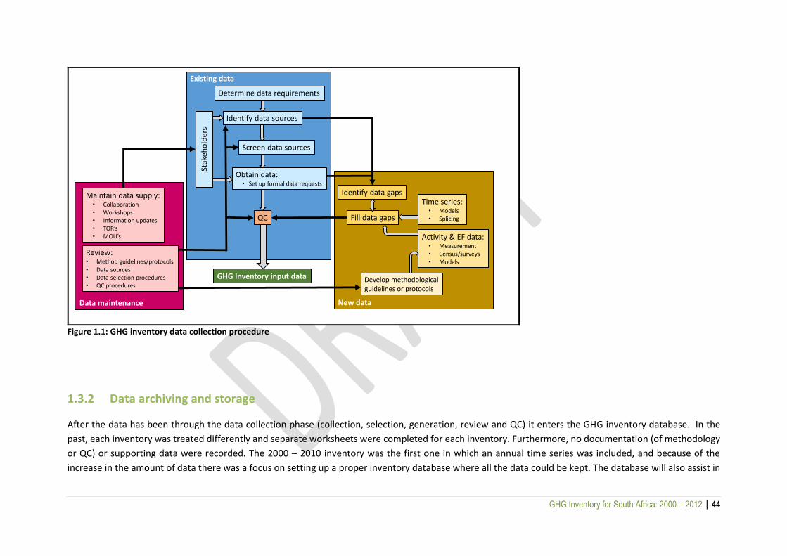
GHG Inventory for South Africa: 2000 – 2012 | 44

Determine data requirements

Identify data sources

QC

Maintain data supply:• Collaboration• Workshops• Information updates• TOR’s• MOU’s

Identify data gaps

Activity & EF data:• Measurement• Census/surveys• Models

Time series:• Models• Splicing

Develop methodological guidelines or protocols

Fill data gaps

Obtain data:• Set up formal data requests

GHG Inventory input data

Existing data

Stak

eho

lder

s

New dataData maintenance

Review:• Method guidelines/protocols• Data sources• Data selection procedures• QC procedures

Screen data sources

Figure 1.1: GHG inventory data collection procedure

1.3.2 Data archiving and storage

After the data has been through the data collection phase (collection, selection, generation, review and QC) it enters the GHG inventory database. In the

past, each inventory was treated differently and separate worksheets were completed for each inventory. Furthermore, no documentation (of methodology

or QC) or supporting data were recorded. The 2000 – 2010 inventory was the first one in which an annual time series was included, and because of the

increase in the amount of data there was a focus on setting up a proper inventory database where all the data could be kept. The database will also assist in

GHG Inventory for South Africa: 2000 – 2012 | 45

streamlining future GHG inventory updates. In this 2000 – 2012 inventory there has been a focus on documentation, transparency and quality control.

Additional spreadsheets for metadata and supporting documents, as well as quality control and uncertainty files have been added to the database.

The database consists of a series of Excel spreadsheets which are linked to ensure consistency and easy updating. The GHG Inventory database contains five

folders (Figure 1.2):

General sectoral data;

GHG inventory data sheets;

GHG metadata;

GHG inventory QC; and

GHG inventory report.

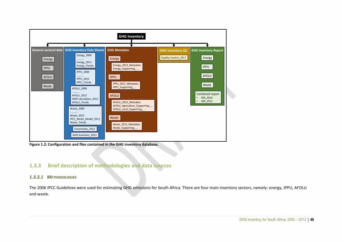
GHG Inventory for South Africa: 2000 – 2012 | 46

GHG Inventory

GHG Inventory Data Sheets

Energy_2000……….Energy_2012Energy_Trends

IPPU_2000………IPPU_2012IPPU_Trends

AFOLU_2000……….AFOLU_2012HWP calculation_2012AFOLU_Trends

Waste_2000………..Waste_2012IPCC_Waste_Model_2012Waste_Trends

GHG Metadata

Energy_2012_MetadataEnergy_Supporting_...

IPPU_2012_MetadataIPPU_Supporting_...

AFOLU_2012_MetadataAFOLU_Agriculture_Supporting_...AFOLU_Land_Supporting_...

Waste_2012_MetadataWaste_Supporting_...Uncertainty_2012

GHG Inventory QC

Quality Control_2012

GHG Summary_2012

GHG Inventory Report

Combined report• NIR_2010• NIR_2012

General sectoral data

Energy

IPPU

AFOLU

Waste

Energy

IPPU

AFOLU

Waste

Energy

IPPU

AFOLU

Waste

Figure 1.2: Configuration and files contained in the GHG inventory database.

1.3.3 Brief description of methodologies and data sources

1.3.3.1 METHODOLOGIES

The 2006 IPCC Guidelines were used for estimating GHG emissions for South Africa. There are four main inventory sectors, namely: energy, IPPU, AFOLU

and waste.

GHG Inventory for South Africa: 2000 – 2012 | 47

Table 1.6 This section provides an overview of the methods used to estimate GHG emissions in South Africa. In January 2015 all countries will be mandated

to use the 2006 IPCC Guidelines for the compilation and reporting of national GHG inventories under the UNFCCC reporting guidelines. In addition, non-

annex I countries that are party to the convention shall use the GWP from the IPCC Second Assessment Report (SAR). In this current inventory, South Africa

has chosen to use GWPs from the IPCC Third Assessment Report (TAR) (Table 1.7) so as to align with the 2006 IPCC Guidelines. Discussions are underway

domestically to consider the possibility of using GWPs from the IPCC Fourth Assessment Report (FAR).

After data were collected, the sources quality assured, and the unit conversions completed, the GHG emissions were calculated by inventory experts using

the following basic principle (IPCC 2006 Guidelines):

Emission = activity data x emission factor

As required by the 2006 IPCC Guidelines, the AFOLU and waste sectors made use of more complex calculations and models which are described in Chapters

5 and 6.

When calculating emissions, the expert is responsible for quality assurance and checks, but the calculations are also checked by external parties to ensure

accuracy and consistency. Emission factors from national sources are the most accurate, but, where national emission factors are not available, default IPCC

emission factors should be used. In most cases default factors where used where disaggregated data could not be obtained and the Tier 1 approach was

applied. More detailed methodologies for each sector and source category are presented in later chapters.

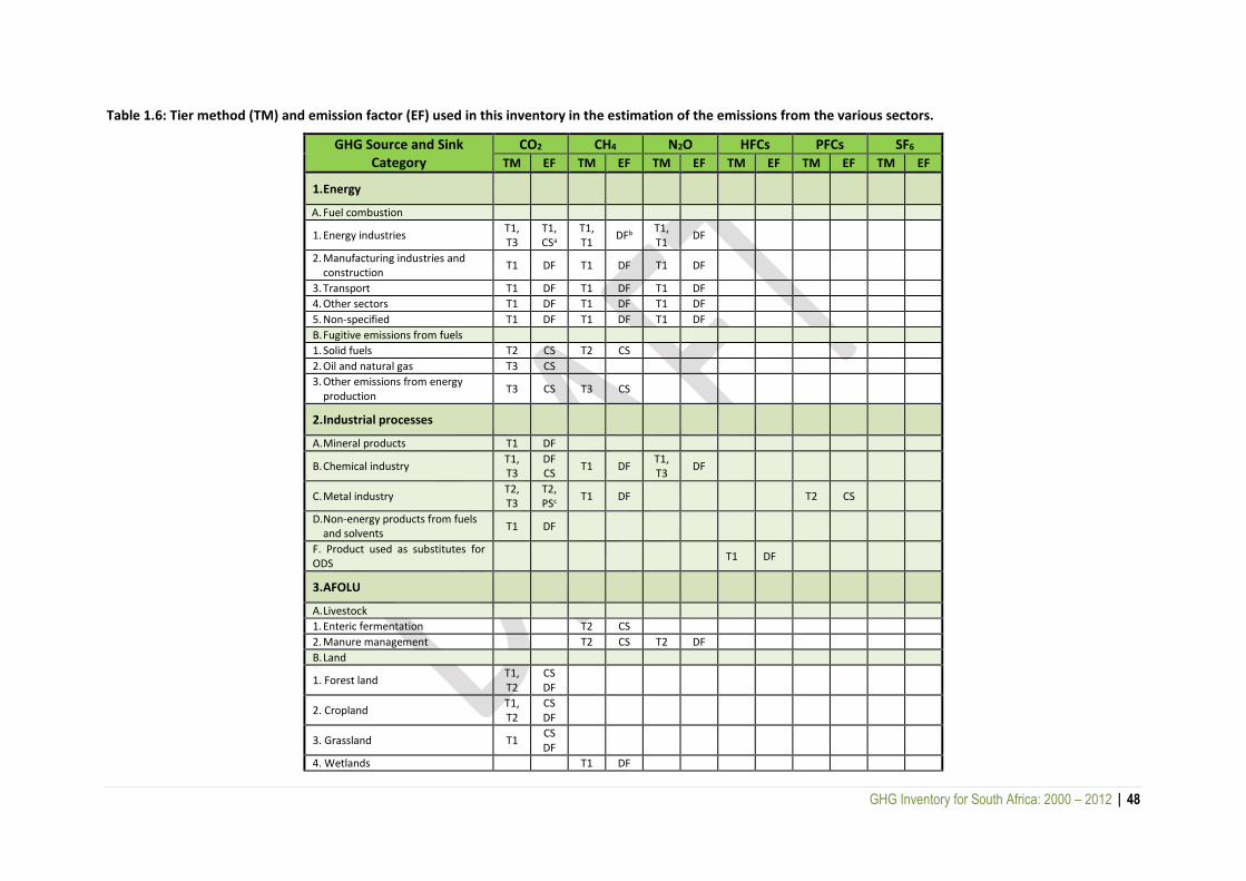
GHG Inventory for South Africa: 2000 – 2012 | 48

Table 1.6: Tier method (TM) and emission factor (EF) used in this inventory in the estimation of the emissions from the various sectors.

GHG Source and Sink Category

CO2 CH4 N2O HFCs PFCs SF6 TM EF TM EF TM EF TM EF TM EF TM EF

1. Energy

A. Fuel combustion

1. Energy industries T1, T3

T1, CSa

T1, T1

DFb T1, T1

DF

2. Manufacturing industries and construction

T1 DF T1 DF T1 DF

3. Transport T1 DF T1 DF T1 DF

4. Other sectors T1 DF T1 DF T1 DF

5. Non-specified T1 DF T1 DF T1 DF

B. Fugitive emissions from fuels

1. Solid fuels T2 CS T2 CS

2. Oil and natural gas T3 CS

3. Other emissions from energy production

T3 CS T3 CS

2. Industrial processes

A. Mineral products T1 DF

B. Chemical industry T1, T3

DF CS

T1 DF T1, T3

DF

C. Metal industry T2, T3

T2, PSc

T1 DF T2 CS

D. Non-energy products from fuels and solvents

T1 DF

F. Product used as substitutes for ODS

T1 DF

3. AFOLU

A. Livestock

1. Enteric fermentation T2 CS

2. Manure management T2 CS T2 DF

B. Land

1. Forest land T1, T2

CS DF

2. Cropland T1, T2

CS DF

3. Grassland T1 CS DF

4. Wetlands T1 DF

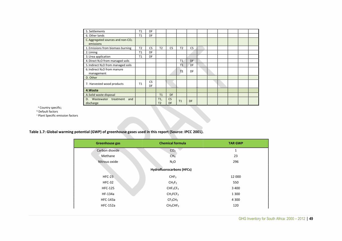
GHG Inventory for South Africa: 2000 – 2012 | 49

5. Settlements T1 DF

6. Other lands T1 DF

C. Aggregated sources and non-CO2 emissions

1. Emissions from biomass burning T2 CS T2 CS T2 CS

2. Liming T1 DF

3. Urea application T1 DF

4. Direct N2O from managed soils T1 DF

5. Indirect N2O from managed soils T1 DF

6. Indirect N2O from manure management

T1 DF

D. Other

7. Harvested wood products T1 CS DF

4.Waste

A. Solid waste disposal T1 DF

D. Wastewater treatment and discharge

T1, T2

CS DF

T1 DF

a Country specific; b Default factors c Plant Specific emission factors

Table 1.7: Global warming potential (GWP) of greenhouse gases used in this report (Source: IPCC 2001).

Greenhouse gas Chemical formula TAR GWP

Carbon dioxide CO2 1

Methane CH4 23

Nitrous oxide N2O 296

Hydrofluorocarbons (HFCs)

HFC-23 CHF3 12 000

HFC-32 CH2F2 550

HFC-125 CHF2CF3 3 400

HF-134a CH2FCF3 1 300

HFC-143a CF3CH3 4 300

HFC-152a CH3CHF2 120

GHG Inventory for South Africa: 2000 – 2012 | 50

Greenhouse gas Chemical formula TAR GWP

Perfluorocarbons (PFCs)

PFC-14 CF4 5 700

PF-116 C2F6 11 900

PFC-218 C3F8 8 600

PFC-31-10 C4F10 8 600

PFC-318 c-C4F8 10 000

PFC-4-1-12 C5F12 8 900

PFC-5-1-14 C6F14 9 000

Sulphur hexafluoride

Sulphur hexafluoride SF6 23 900

For the current inventory, data were gathered for the following gases: CO2, CH4, and N2O. Certain HFCs and PFCs were reported on in the IPPU sector and NOx

and CO were estimated for biomassburning emissions.

1.3.3.2 DATA SOURCES

In general, the following primary data sources supplied the annual activity data used in the emission calculations:

Energy data:

o Department of Mineral Resources (DMR);

o Department of Energy (DoE);

o Power utility plants;

o Chevron;

o SAPREF;

o Engen;

GHG Inventory for South Africa: 2000 – 2012 | 51

o Energy balances and the periodically published Digests of South African Energy Statistics provided an overview of the interrelations within

South Africa’s energy sector, by providing a breakdown of the different fuels and category sources;

o South African Petroleum Industry Association (SAPIA) provided other energy data, transport fuel data and crude oil production;

o PetroSA;

o Sasol;

o Eskom;

o Food and Agriculture Organization (FAO);

o Chamber of Mines provided information associated with GHG emissions from mining activities;

o Statistics South Africa;

o National Energy Regulator of South Africa (NERSA);

o Government Communications and Information Systems (GCIS); and

o South African Reserve Bank.

Industrial processes and product use:

o Business Unity South Africa;

o Chemical and Allied Industries Association (CAIA);

o Industry associations;

o South African Minerals Industry (SAMI) report;

o Department of Mineral Resources (DMR);

o Department of Energy (DoE);

o South African Iron and Steel Institute (SAISI);

o Association of Cementitious Material Producers (ACMP); and

o Direct communication with various industrial production plants.

AFOLU:

o Department of Agriculture, Forestry and Fisheries (DAFF);

o Forest Resource Assessment (from DAFF and FAO);

o Department of Environmental Affairs (DEA);

o Forestry South Africa (FSA);

o GeoTerraImage (GTI);

o National Terrestrial Carbon Sinks Assessment (NTCSA) (DEA, 2015);

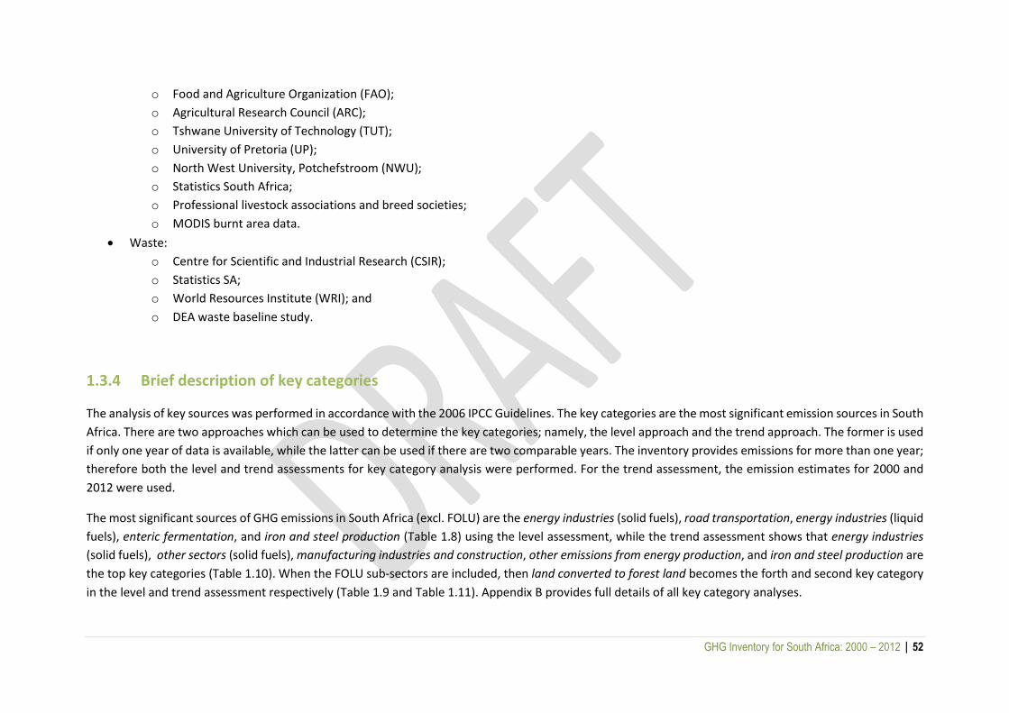
GHG Inventory for South Africa: 2000 – 2012 | 52

o Food and Agriculture Organization (FAO);

o Agricultural Research Council (ARC);

o Tshwane University of Technology (TUT);

o University of Pretoria (UP);

o North West University, Potchefstroom (NWU);

o Statistics South Africa;

o Professional livestock associations and breed societies;

o MODIS burnt area data.

Waste:

o Centre for Scientific and Industrial Research (CSIR);

o Statistics SA;

o World Resources Institute (WRI); and

o DEA waste baseline study.

1.3.4 Brief description of key categories

The analysis of key sources was performed in accordance with the 2006 IPCC Guidelines. The key categories are the most significant emission sources in South

Africa. There are two approaches which can be used to determine the key categories; namely, the level approach and the trend approach. The former is used

if only one year of data is available, while the latter can be used if there are two comparable years. The inventory provides emissions for more than one year;

therefore both the level and trend assessments for key category analysis were performed. For the trend assessment, the emission estimates for 2000 and

2012 were used.

The most significant sources of GHG emissions in South Africa (excl. FOLU) are the energy industries (solid fuels), road transportation, energy industries (liquid

fuels), enteric fermentation, and iron and steel production (Table 1.8) using the level assessment, while the trend assessment shows that energy industries

(solid fuels), other sectors (solid fuels), manufacturing industries and construction, other emissions from energy production, and iron and steel production are

the top key categories (Table 1.10). When the FOLU sub-sectors are included, then land converted to forest land becomes the forth and second key category

in the level and trend assessment respectively (Table 1.9 and Table 1.11). Appendix B provides full details of all key category analyses.

GHG Inventory for South Africa: 2000 – 2012 | 53

Table 1.8: Level assessment results for 2012, excluding FOLU contributions. Only key categories are shown.

IPCC code

IPCC Category GHG 2012 (Ex,t) (Gg CO2 eq)

Lx,t Cumulative

Total

1.A.1 Energy industries - solid fuels CO2 242 154 0.4444 0.4444

1.A.3.b Road transportation CO2 42 930 0.0788 0.5232

1.A.1 Energy industries - liquid fuels CO2 34 534 0.0634 0.5866

3.A.1 Enteric fermentation CH4 27 198 0.0499 0.6365

2.C.1 Iron and steel production CO2 25 009 0.0459 0.6824

1.A.2 Manufacturing industries and construction - solid fuels

CO2 24 473 0.0449 0.7273

1.A.4 Other sectors - solid fuels CO2 21 897 0.0402 0.7675

1.B.3 Other emissions from energy production

CO2 21 800 0.0400 0.8075

4.A Solid waste disposal CH4 18 412 0.0338 0.8413

1.A.4 Other sectors - liquid fuels CO2 18 260 0.0335 0.8748

3.C.4 Direct N2O emissions from managed soils

N2O 14 702 0.0270 0.9018

2.C.2 Ferroalloy production CO2 11 405 0.0209 0.9227

3.C.5 Indirect N2O emissions from managed soils

N2O 4 559 0.0084 0.9311

2.A.1 Cement production CO2 3 845 0.0071 0.9382

1.A.3.a Civil aviation CO2 3 466 0.0064 0.9445

4.D Wastewater treatment and discharge CH4 2 828 0.0052 0.9497

1.B.3 Other emissions from energy production

CH4 2 526 0.0046 0.9543

Table 1.9: Level assessment results for 2012, including FOLU contributions. Only key categories are shown.

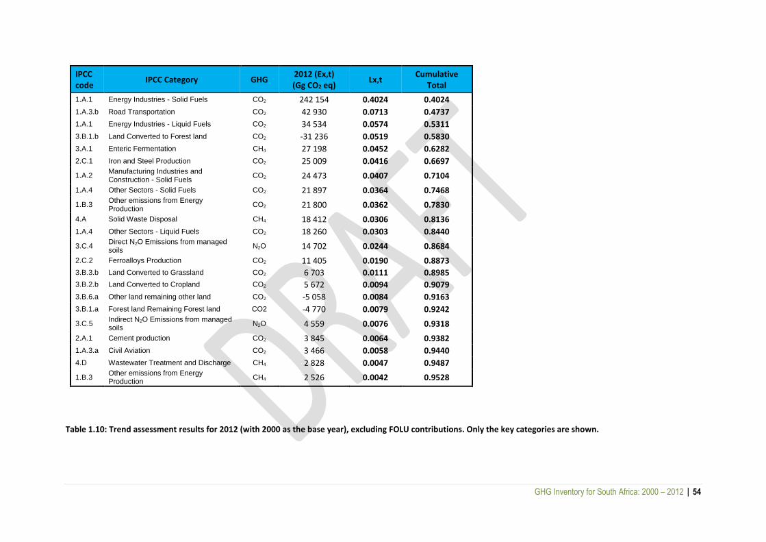
GHG Inventory for South Africa: 2000 – 2012 | 54

IPCC code

IPCC Category GHG 2012 (Ex,t) (Gg CO2 eq)

Lx,t Cumulative

Total

1.A.1 Energy Industries - Solid Fuels CO2 242 154 0.4024 0.4024

1.A.3.b Road Transportation CO2 42 930 0.0713 0.4737

1.A.1 Energy Industries - Liquid Fuels CO2 34 534 0.0574 0.5311

3.B.1.b Land Converted to Forest land CO2 -31 236 0.0519 0.5830

3.A.1 Enteric Fermentation CH4 27 198 0.0452 0.6282

2.C.1 Iron and Steel Production CO2 25 009 0.0416 0.6697

1.A.2 Manufacturing Industries and Construction - Solid Fuels

CO2 24 473 0.0407 0.7104

1.A.4 Other Sectors - Solid Fuels CO2 21 897 0.0364 0.7468

1.B.3 Other emissions from Energy Production

CO2 21 800 0.0362 0.7830

4.A Solid Waste Disposal CH4 18 412 0.0306 0.8136

1.A.4 Other Sectors - Liquid Fuels CO2 18 260 0.0303 0.8440

3.C.4 Direct N2O Emissions from managed soils

N2O 14 702 0.0244 0.8684

2.C.2 Ferroalloys Production CO2 11 405 0.0190 0.8873

3.B.3.b Land Converted to Grassland CO2 6 703 0.0111 0.8985

3.B.2.b Land Converted to Cropland CO2 5 672 0.0094 0.9079

3.B.6.a Other land remaining other land CO2 -5 058 0.0084 0.9163

3.B.1.a Forest land Remaining Forest land CO2 -4 770 0.0079 0.9242

3.C.5 Indirect N2O Emissions from managed soils

N2O 4 559 0.0076 0.9318

2.A.1 Cement production CO2 3 845 0.0064 0.9382

1.A.3.a Civil Aviation CO2 3 466 0.0058 0.9440

4.D Wastewater Treatment and Discharge CH4 2 828 0.0047 0.9487

1.B.3 Other emissions from Energy Production

CH4 2 526 0.0042 0.9528

Table 1.10: Trend assessment results for 2012 (with 2000 as the base year), excluding FOLU contributions. Only the key categories are shown.

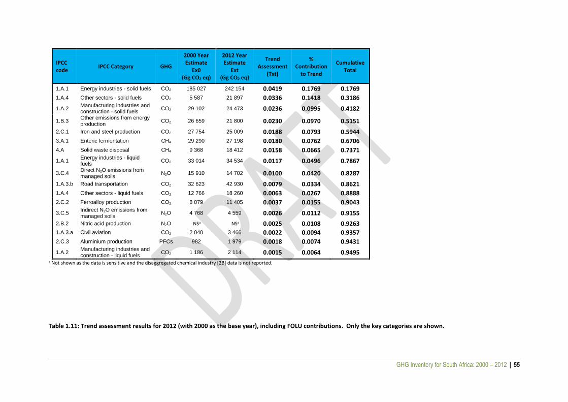
GHG Inventory for South Africa: 2000 – 2012 | 55

IPCC code

IPCC Category GHG

2000 Year Estimate

Ex0 (Gg CO2 eq)

2012 Year Estimate

Ext (Gg CO2 eq)

Trend Assessment

(Txt)

% Contribution

to Trend

Cumulative Total

1.A.1 Energy industries - solid fuels CO2 185 027 242 154 0.0419 0.1769 0.1769

1.A.4 Other sectors - solid fuels CO2 5 587 21 897 0.0336 0.1418 0.3186

1.A.2 Manufacturing industries and construction - solid fuels

CO2 29 102 24 473 0.0236 0.0995 0.4182

1.B.3 Other emissions from energy production

CO2 26 659 21 800 0.0230 0.0970 0.5151

2.C.1 Iron and steel production CO2 27 754 25 009 0.0188 0.0793 0.5944

3.A.1 Enteric fermentation CH4 29 290 27 198 0.0180 0.0762 0.6706

4.A Solid waste disposal CH4 9 368 18 412 0.0158 0.0665 0.7371

1.A.1 Energy industries - liquid fuels

CO2 33 014 34 534 0.0117 0.0496 0.7867

3.C.4 Direct N2O emissions from managed soils

N2O 15 910 14 702 0.0100 0.0420 0.8287

1.A.3.b Road transportation CO2 32 623 42 930 0.0079 0.0334 0.8621

1.A.4 Other sectors - liquid fuels CO2 12 766 18 260 0.0063 0.0267 0.8888

2.C.2 Ferroalloy production CO2 8 079 11 405 0.0037 0.0155 0.9043

3.C.5 Indirect N2O emissions from managed soils

N2O 4 768 4 559 0.0026 0.0112 0.9155

2.B.2 Nitric acid production N2O NSa NSa 0.0025 0.0108 0.9263

1.A.3.a Civil aviation CO2 2 040 3 466 0.0022 0.0094 0.9357

2.C.3 Aluminium production PFCs 982 1 979 0.0018 0.0074 0.9431

1.A.2 Manufacturing industries and construction - liquid fuels

CO2 1 186 2 114 0.0015 0.0064 0.9495

a Not shown as the data is sensitive and the disaggregated chemical industry [2B] data is not reported.

Table 1.11: Trend assessment results for 2012 (with 2000 as the base year), including FOLU contributions. Only the key categories are shown.

GHG Inventory for South Africa: 2000 – 2012 | 56

IPCC code

IPCC Category GHG

2000 Year Estimate

Ex0 (Gg CO2 eq)

2012 Year Estimate

Ext (Gg CO2 eq)

Trend Assessment

(Txt)

% Contribution

to Trend

Cumulative Total

1.A.1 Energy Industries - Solid Fuels

CO2 185027 242154 0.0455 0.1730 0.1730

3.B.1.b Land Converted to Forest land

CO2 -17115 -31236 0.0349 0.1324 0.3054

1.A.4 Other Sectors - Solid Fuels CO2 5587 21897 0.0307 0.1168 0.4221

1.A.2 Manufacturing Industries and Construction - Solid Fuels

CO2 29102 24473 0.0202 0.0769 0.4990

1.B.3 Other emissions from Energy Production

CO2 26659 21800 0.0198 0.0752 0.5742

2.C.1 Iron and Steel Production CO2 27754 25009 0.0159 0.0606 0.6348

3.A.1 Enteric Fermentation CH4 29290 27198 0.0152 0.0578 0.6925

4.A Solid Waste Disposal CH4 9368 18412 0.0147 0.0558 0.7483

1.A.1 Energy Industries - Liquid Fuels

CO2 33014 34534 0.0093 0.0354 0.7838

1.A.3.b Road Transportation CO2 32623 42930 0.0085 0.0323 0.8161

3.C.4 Direct N2O Emissions from managed soils

N2O 15910 14702 0.0084 0.0319 0.8480

1.A.4 Other Sectors - Liquid Fuels CO2 12766 18260 0.0063 0.0238 0.8718

2.C.2 Ferroalloys Production CO2 8079 11405 0.0037 0.0139 0.8857

3.B.3.b Land Converted to Grassland CO2 6735 6703 0.0026 0.0099 0.8956

2.B.2 Nitric Acid Production N2O NSa NSa 0.0023 0.0085 0.9041

3.C.5 Indirect N2O Emissions from managed soils

N2O 4768 4559 0.0022 0.0084 0.9125

3.B.2.b Land Converted to Cropland CO2 5673 5672 0.0021 0.0081 0.9206

1.A.3.a Civil Aviation CO2 2040 3466 0.0021 0.0080 0.9286

3.B.6.a Other land remaining other land

CO2 -5058 -5058 0.0019 0.0072 0.9358

3.B.2.a Cropland Remaining Cropland

CO2 -1242 -105 0.0018 0.0069 0.9427

2.C.3 Aluminium production CO2 982 1979 0.0016 0.0062 0.9490

1.A.2 Manufacturing Industries and Construction - Liquid Fuels

CO2 1186 2114 0.0014 0.0054 0.9544 a Not shown as the data is sensitive and the disaggregated chemical industry [2B] data is not reported.

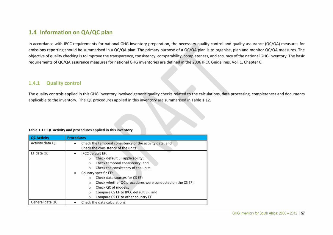
GHG Inventory for South Africa: 2000 – 2012 | 57

1.4 Information on QA/QC plan

In accordance with IPCC requirements for national GHG inventory preparation, the necessary quality control and quality assurance (QC/QA) measures for

emissions reporting should be summarised in a QC/QA plan. The primary purpose of a QC/QA plan is to organise, plan and monitor QC/QA measures. The

objective of quality checking is to improve the transparency, consistency, comparability, completeness, and accuracy of the national GHG inventory. The basic

requirements of QC/QA assurance measures for national GHG inventories are defined in the 2006 IPCC Guidelines, Vol. 1, Chapter 6.

1.4.1 Quality control

The quality controls applied in this GHG inventory involved generic quality checks related to the calculations, data processing, completeness and documents

applicable to the inventory. The QC procedures applied in this inventory are summarised in Table 1.12.

Table 1.12: QC activity and procedures applied in this inventory

QC Activity Procedures

Activity data QC Check the temporal consistency of the activity data; and Check the consistency of the units.

EF data QC IPCC default EF: o Check default EF applicability; o Check temporal consistency; and o Check the consistency of the units.

Country specific EF: o Check data sources for CS EF; o Check whether QC procedures were conducted on the CS EF; o Check QC of models; o Compare CS EF to IPCC default EF; and o Compare CS EF to other country EF

General data QC Check the data calculations:

GHG Inventory for South Africa: 2000 – 2012 | 58

o Reproduce a set of emission/removal calculations; and o Check calculations with an approximation method.

Check any recalculation data;

Check the emission and removal data are correctly aggregated from lower reporting levels;

Check that the data is compared to previous estimates;

Check for consistency in the trend; and Check for completeness of each subcategory

Uncertainty QC Check that expert judgement is recorded; and Check uncertainty calculations

Database QC Check that the data is in the database;

Check for transcription errors;

Check uncertainty is in the database;

Check for transcription errors in uncertainty data;

Check the correct units have been used in the database;

Check the labels in the database are correct;

Check for common data consistency between sectors and categories;

Check the correct conversion factors are used; Check data aggregations are correct; and Check the uncertainty aggregations are correct.

Metadata QC Check all data details are documented;

Check all uncertainty details are documented;

Check all recalculation details are recorded; Check all supporting data and documents are attached; and Check details regarding experts are documented.

Report QC Check that the relevant activity data details are incorporated into the report;

Check that the relevant EF data details are incorporated into the report;

Check for data transcription errors between the database and the report;

Check the references are properly cited;

Check that expert judgements are reported;

Check that uncertainty data in incorporated into the report;

Check that completeness is documented;

Check that comparisons have been made with previous estimates;

Check that explanations are provided for any data differences; and

Check that the QC/QA procedures have been documented.

GHG Inventory for South Africa: 2000 – 2012 | 59

1.4.2 Quality assurance (QA)

The QA process was done by external reviewers who have a different technical perspective and who were not involved in the compilation process of the

inventory, so they could conduct an unbiased review of the inventory. The external reviewers ensured that the inventory’s results, assumptions and methods

were reasonable. Furthermore, a public review process was undertaken to supplement the external review. The independent review process is demonstrated

in Figure 1.3.

Essentially, the draft GHG inventory report was published for public comment in a Government Gazette. Parallel to the publication for public comment, an

independent technical review of activity data, emission factors and methodologies used was undertaken by an independent company. Comments that were

submitted during the public commenting process were incorporated in the independent review process. Findings and recommendations from the

independent review process were then used to refine the draft GHG inventory report. Currently, the DEA is preparing a revised three-year supplementary

improvement plan to address recommendations from the independent review process. Some of the projects that are currently listed in the Greenhouse Gas

Improvement Programme (GHGIP) are as a result of the findings of the previous review undertaken for the 2000 – 2010 GHG inventory.

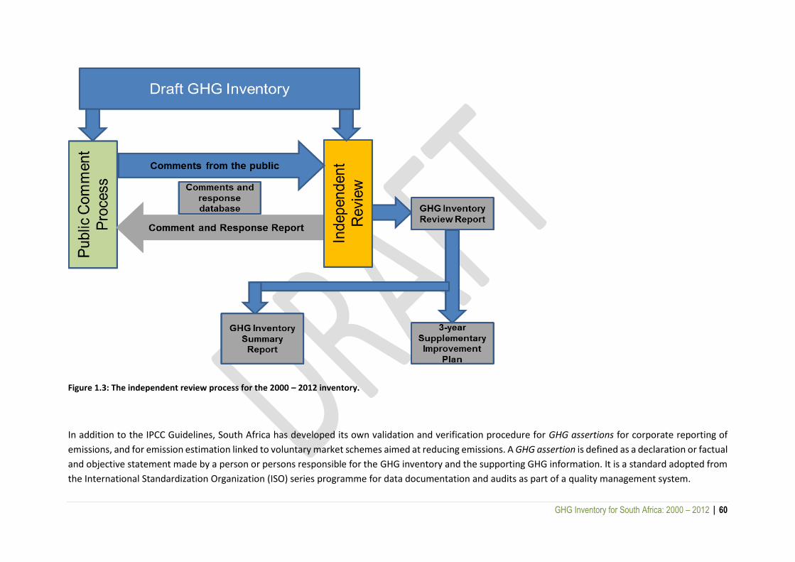
GHG Inventory for South Africa: 2000 – 2012 | 60

Figure 1.3: The independent review process for the 2000 – 2012 inventory.

In addition to the IPCC Guidelines, South Africa has developed its own validation and verification procedure for GHG assertions for corporate reporting of

emissions, and for emission estimation linked to voluntary market schemes aimed at reducing emissions. A GHG assertion is defined as a declaration or factual

and objective statement made by a person or persons responsible for the GHG inventory and the supporting GHG information. It is a standard adopted from

the International Standardization Organization (ISO) series programme for data documentation and audits as part of a quality management system.

GHG Inventory for South Africa: 2000 – 2012 | 61

In the South African context, QA/QC measures are defined by Part 3 of the South African National Standard for Greenhouse Gases, SANS 14064-3:2006

(Specification with guidance for the validation and verification of GHG gas assertions). This standard specifies the requirements for selecting GHG

validators/verifiers, establishing the level of assurance, objectives, criteria and scope, determining the validation/verification approach, assessing GHG data,

information, information systems and controls, evaluating assertions, and preparing validation/verification statements.

1.5 Evaluating uncertainty

Uncertainty analysis is regarded by the IPCC Guidelines as an essential element of any complete GHG inventory. Uncertainty reporting is important for

suggesting methods of compiling uncertainty estimates and for identifying approaches that would enable the prioritisation of national efforts to reduce future

uncertainties. It identifies areas of further improvement in the inventory preparation process and will guide methodological choices in future inventories to

improve accuracy, reduce bias, and transparently report on the presence and levels of uncertainty. Uncertainty can also be used to determine appropriate

methods for carrying out recalculations for previous inventories. The overall objective is to minimise uncertainties to the greatest possible degree.

Chapter 3 of the 2006 IPCC Guidelines for National Greenhouse Gas Inventories describes the need and methodology for estimating and reporting

uncertainties associated with annual estimates of emissions and removals, including emission and removal trends over time. Broadly speaking, the approach

involves combining the category uncertainties into estimates of uncertainty for total national net emissions and their associated trends.

Uncertainty analysis for the South Africa inventory involved quantifying the uncertainties for all source categories and sinks where data were available. The

main sources for the uncertainty in activity and emission factor data are the IPCC default uncertainty estimates (particularly for the emission factors), scientific

literature and reported variances, expert judgement and comparisons with uncertainty ranges reported by other countries.

There is a lack of quantitative uncertainty data in many source categories, which makes it difficult to determine and assess the uncertainty of these emission

sources. In many cases more detailed data collection is required to speculate about levels of quantitative uncertainty. Where sufficient data were available,

the analysis involved the determination of a probability-density function for a number of parameters, using approaches and values provided in the 2006 IPCC

Guidelines. Thus the uncertainty analysis included a statistical evaluation of individual data items, and experts' assessments as guided by the IPCC Good

Practice Guidelines.

For this inventory an Approach 1 uncertainty analysis (assuming no correlation between the activity data) was applied to the energy and the IPPU sectors and

the IPCC uncertainty tables were used. There were insufficient data to include AFOLU and waste sector uncertainties, however these will be included in the

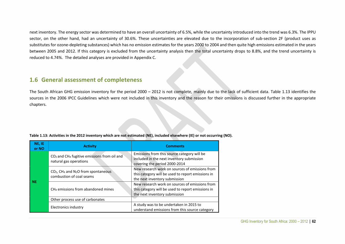
GHG Inventory for South Africa: 2000 – 2012 | 62

next inventory. The energy sector was determined to have an overall uncertainty of 6.5%, while the uncertainty introduced into the trend was 6.3%. The IPPU

sector, on the other hand, had an uncertainty of 30.6%. These uncertainties are elevated due to the incorporation of sub-section 2F (product uses as

substitutes for ozone-depleting substances) which has no emission estimates for the years 2000 to 2004 and then quite high emissions estimated in the years

between 2005 and 2012. If this category is excluded from the uncertainty analysis then the total uncertainty drops to 8.8%, and the trend uncertainty is

reduced to 4.74%. The detailed analyses are provided in Appendix C.

1.6 General assessment of completeness

The South African GHG emission inventory for the period 2000 – 2012 is not complete, mainly due to the lack of sufficient data. Table 1.13 identifies the

sources in the 2006 IPCC Guidelines which were not included in this inventory and the reason for their omissions is discussed further in the appropriate

chapters.

Table 1.13: Activities in the 2012 inventory which are not estimated (NE), included elsewhere (IE) or not occurring (NO).

NE, IE or NO

Activity Comments

NE

CO2 and CH4 fugitive emissions from oil and natural gas operations

Emissions from this source category will be included in the next inventory submission covering the period 2000-2014

CO2, CH4 and N2O from spontaneous combustion of coal seams

New research work on sources of emissions from this category will be used to report emissions in the next inventory submission

CH4 emissions from abandoned mines New research work on sources of emissions from this category will be used to report emissions in the next inventory submission

Other process use of carbonates

Electronics industry A study was to be undertaken in 2015 to understand emissions from this source category

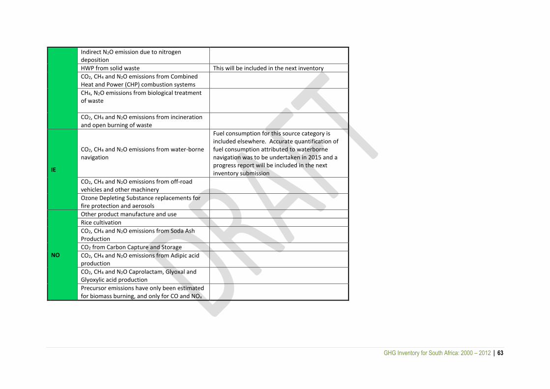
GHG Inventory for South Africa: 2000 – 2012 | 63

Indirect N2O emission due to nitrogen deposition

HWP from solid waste This will be included in the next inventory

CO2, CH4 and N2O emissions from Combined Heat and Power (CHP) combustion systems

CH4, N2O emissions from biological treatment of waste

CO2, CH4 and N2O emissions from incineration and open burning of waste

IE

CO2, CH4 and N2O emissions from water-borne navigation

Fuel consumption for this source category is included elsewhere. Accurate quantification of fuel consumption attributed to waterborne navigation was to be undertaken in 2015 and a progress report will be included in the next inventory submission

CO2, CH4 and N2O emissions from off-road vehicles and other machinery

Ozone Depleting Substance replacements for fire protection and aerosols

NO

Other product manufacture and use

Rice cultivation

CO2, CH4 and N2O emissions from Soda Ash Production

CO2 from Carbon Capture and Storage

CO2, CH4 and N2O emissions from Adipic acid production

CO2, CH4 and N2O Caprolactam, Glyoxal and Glyoxylic acid production

Precursor emissions have only been estimated for biomass burning, and only for CO and NOx

GHG Inventory for South Africa: 2000 – 2012 | 64

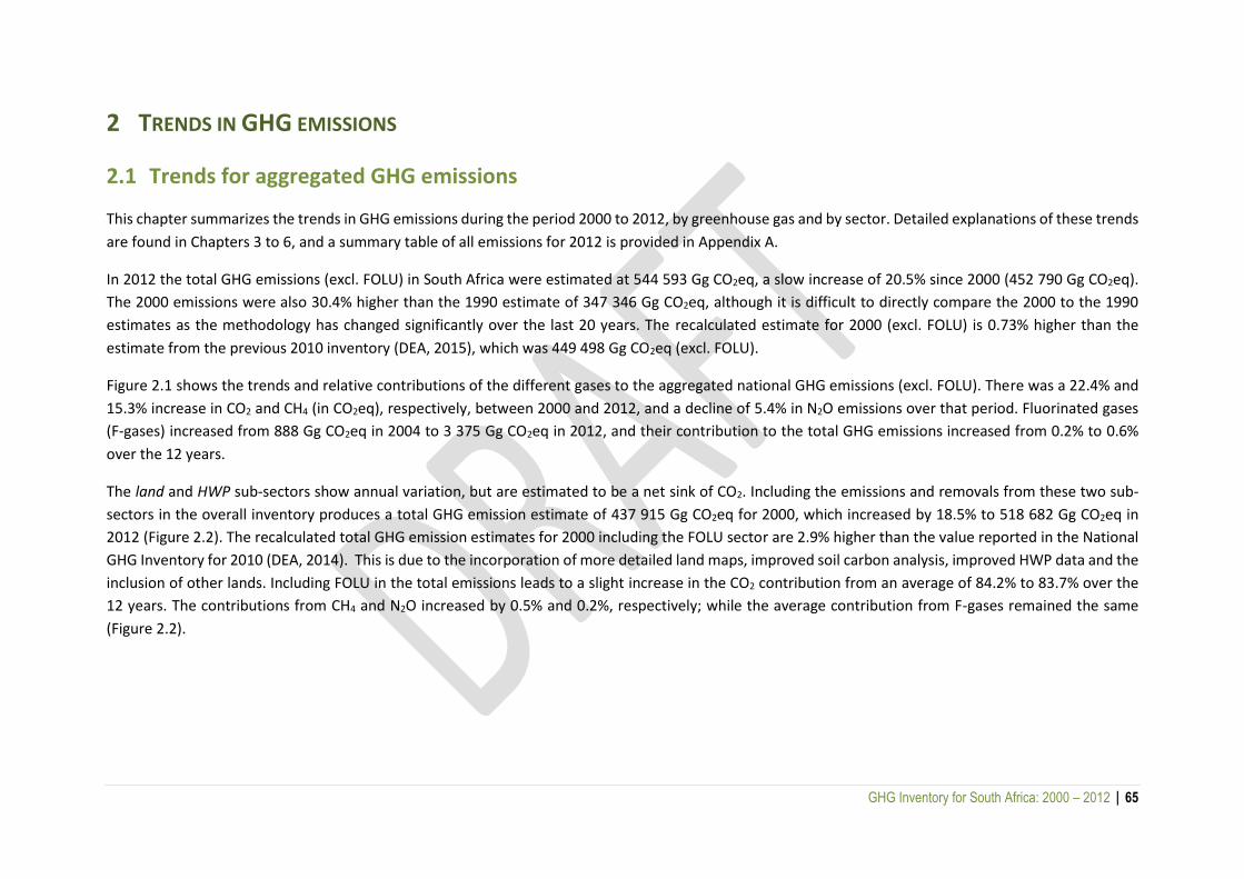
GHG Inventory for South Africa: 2000 – 2012 | 65

2 TRENDS IN GHG EMISSIONS

2.1 Trends for aggregated GHG emissions

This chapter summarizes the trends in GHG emissions during the period 2000 to 2012, by greenhouse gas and by sector. Detailed explanations of these trends

are found in Chapters 3 to 6, and a summary table of all emissions for 2012 is provided in Appendix A.

In 2012 the total GHG emissions (excl. FOLU) in South Africa were estimated at 544 593 Gg CO2eq, a slow increase of 20.5% since 2000 (452 790 Gg CO2eq).

The 2000 emissions were also 30.4% higher than the 1990 estimate of 347 346 Gg CO2eq, although it is difficult to directly compare the 2000 to the 1990

estimates as the methodology has changed significantly over the last 20 years. The recalculated estimate for 2000 (excl. FOLU) is 0.73% higher than the

estimate from the previous 2010 inventory (DEA, 2015), which was 449 498 Gg CO2eq (excl. FOLU).

Figure 2.1 shows the trends and relative contributions of the different gases to the aggregated national GHG emissions (excl. FOLU). There was a 22.4% and

15.3% increase in CO2 and CH4 (in CO2eq), respectively, between 2000 and 2012, and a decline of 5.4% in N2O emissions over that period. Fluorinated gases

(F-gases) increased from 888 Gg CO2eq in 2004 to 3 375 Gg CO2eq in 2012, and their contribution to the total GHG emissions increased from 0.2% to 0.6%

over the 12 years.

The land and HWP sub-sectors show annual variation, but are estimated to be a net sink of CO2. Including the emissions and removals from these two sub-

sectors in the overall inventory produces a total GHG emission estimate of 437 915 Gg CO2eq for 2000, which increased by 18.5% to 518 682 Gg CO2eq in

2012 (Figure 2.2). The recalculated total GHG emission estimates for 2000 including the FOLU sector are 2.9% higher than the value reported in the National

GHG Inventory for 2010 (DEA, 2014). This is due to the incorporation of more detailed land maps, improved soil carbon analysis, improved HWP data and the

inclusion of other lands. Including FOLU in the total emissions leads to a slight increase in the CO2 contribution from an average of 84.2% to 83.7% over the

12 years. The contributions from CH4 and N2O increased by 0.5% and 0.2%, respectively; while the average contribution from F-gases remained the same

(Figure 2.2).

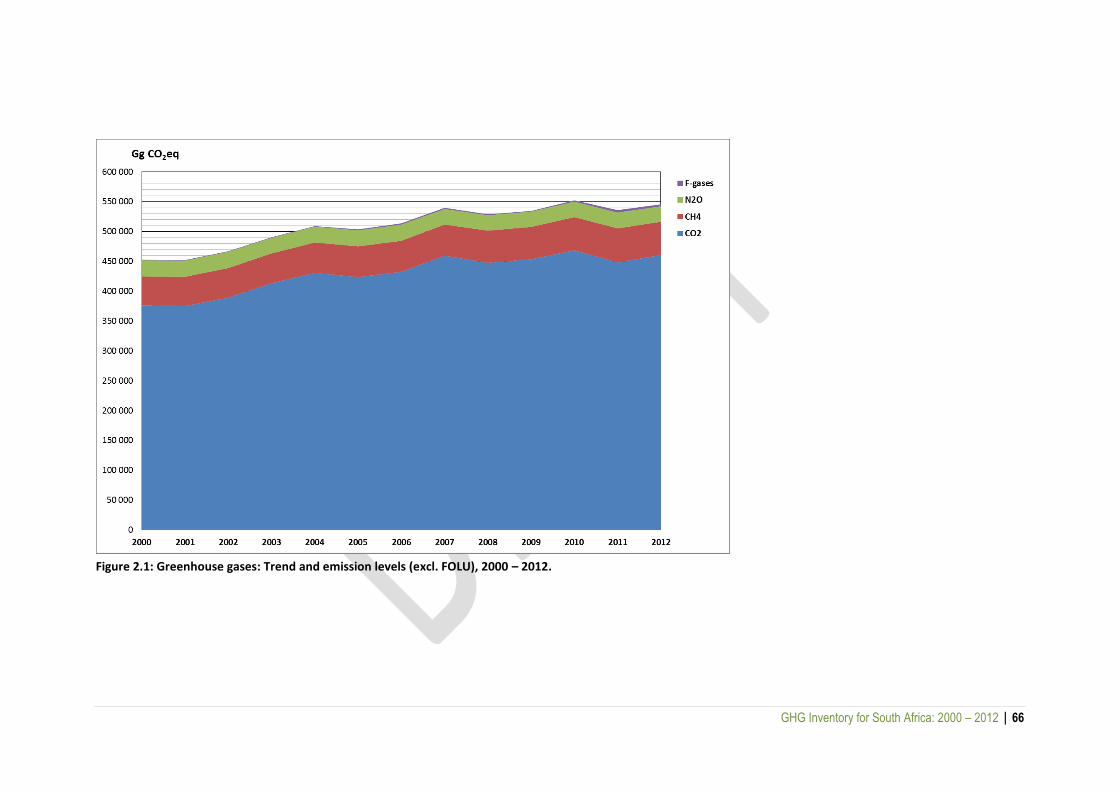
GHG Inventory for South Africa: 2000 – 2012 | 66

Figure 2.1: Greenhouse gases: Trend and emission levels (excl. FOLU), 2000 – 2012.

GHG Inventory for South Africa: 2000 – 2012 | 67

Figure 2.2: Greenhouse gases: Trend and emission levels (including FOLU sub-sectors), 2000 – 2012.

2.2 Emission trends by gas

2.2.1 Carbon dioxide

Figure 2.3 presents the contribution of the main sectors to the trend in national CO2 emissions (excl. FOLU). The energy sector is by far the largest contributor

to CO2 emissions in South Africa, contributing an average of 89.3% between 2000 and 2012, and 90.5% in 2012. The categories 1A1 energy industries (60.2%),

GHG Inventory for South Africa: 2000 – 2012 | 68

1A3 transport (10.1%) and 1A4 other sectors (8.7%) were the major contributors to CO2 emissions in 2012. The IPPU sector contribution declined from 11.3%

in 2000 to 9.3% in 2012. The AFOLU sector (excl. FOLU) contributed an average of 0.2% towards the CO2 emission budget over the 12 years.

Figure 2.3: CO2: Trend and emission levels of sectors (excl. FOLU), 2000 – 2012.

GHG Inventory for South Africa: 2000 – 2012 | 69

2.2.2 Methane

The sector contributions to the total CH4 emissions (excl. FOLU) in South Africa are shown in Figure 2.4. National CH4 emissions increased from 47 755 Gg

CO2eq (2 076 Gg CH4) in 2000 to 55 053 Gg CO2eq (2 394 Gg CH4) in 2012 (a 15.3% increase). The AFOLU livestock category and waste sectors were the major

contributors, providing 56.1% and 31.9%, respectively, to the total CH4 emissions in 2012. The contribution from livestock declined by 12.2%, while the

contribution from the waste sector increased by a similar amount (13.8%) over the period 2000 to 2012.

GHG Inventory for South Africa: 2000 – 2012 | 70

Figure 2.4: CH4: Trend and emission levels of sectors (excl. FOLU), 2000 – 2012

2.2.3 Nitrous oxide

Figure 2.5 shows the contribution from the major sectors to the national N2O emissions in South Africa. The emissions declined by 5.4% over the 2000 to 2012

period from 26 960 Gg CO2 eq ( 91.1 Gg N2O) to 25 510 Gg CO2 eq (86.2 Gg N2O). The category 3C aggregated and non-CO2 sources on land (which includes

GHG Inventory for South Africa: 2000 – 2012 | 71

emissions from managed soils and biomass burning) contributed an average of 80.1% to the total N2O emissions over the period 2000 to 2012, while the

energy sector and livestock subsector (which includes manure management) contributed an average of 8.8% and 4.4%, respectively.

Figure 2.5: N2O: Trend and emission levels of sectors, 2000 – 2012.

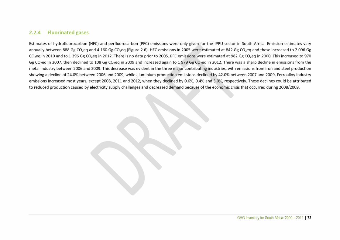
GHG Inventory for South Africa: 2000 – 2012 | 72

2.2.4 Fluorinated gases

Estimates of hydrofluorocarbon (HFC) and perfluorocarbon (PFC) emissions were only given for the IPPU sector in South Africa. Emission estimates vary

annually between 888 Gg CO2eq and 4 160 Gg CO2eq (Figure 2.6). HFC emissions in 2005 were estimated at 842 Gg CO2eq and these increased to 2 096 Gg

CO2eq in 2010 and to 1 396 Gg CO2eq in 2012. There is no data prior to 2005. PFC emissions were estimated at 982 Gg CO2eq in 2000. This increased to 970

Gg CO2eq in 2007, then declined to 108 Gg CO2eq in 2009 and increased again to 1 979 Gg CO2eq in 2012. There was a sharp decline in emissions from the

metal industry between 2006 and 2009. This decrease was evident in the three major contributing industries, with emissions from iron and steel production

showing a decline of 24.0% between 2006 and 2009, while aluminium production emissions declined by 42.0% between 2007 and 2009. Ferroalloy Industry

emissions increased most years, except 2008, 2011 and 2012, when they declined by 0.6%, 0.4% and 3.0%, respectively. These declines could be attributed

to reduced production caused by electricity supply challenges and decreased demand because of the economic crisis that occurred during 2008/2009.

GHG Inventory for South Africa: 2000 – 2012 | 73

Figure 2.6: F-Gases: Trend and emission levels of sectors, 2000 – 2012.

2.3 Emission trends specified by source category

Figure 2.7 provides an overview of emission trends per IPCC sector in Gg CO2eq (excl. FOLU). The energy sector is the largest contributor to the total GHG

emissions, providing 75.3% in 2000 and 77.9% in 2012. The AFOLU sector (excl. FOLU) and the IPPU sector contributed 9.5% and 8.6%, respectively, to the

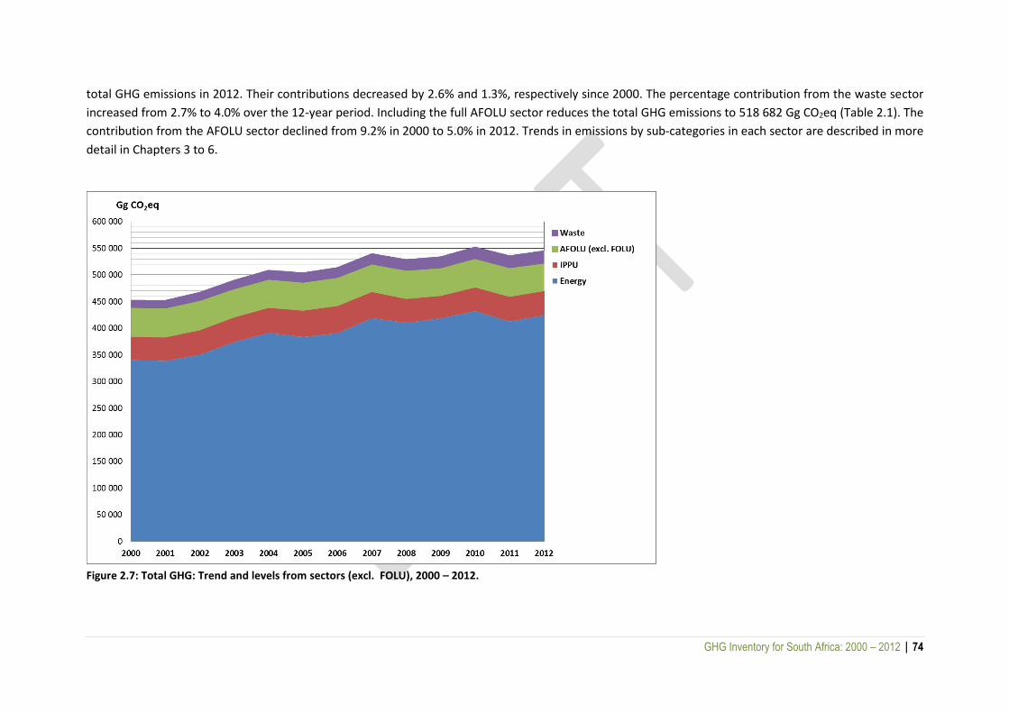
GHG Inventory for South Africa: 2000 – 2012 | 74

total GHG emissions in 2012. Their contributions decreased by 2.6% and 1.3%, respectively since 2000. The percentage contribution from the waste sector

increased from 2.7% to 4.0% over the 12-year period. Including the full AFOLU sector reduces the total GHG emissions to 518 682 Gg CO2eq (Table 2.1). The

contribution from the AFOLU sector declined from 9.2% in 2000 to 5.0% in 2012. Trends in emissions by sub-categories in each sector are described in more

detail in Chapters 3 to 6.

Figure 2.7: Total GHG: Trend and levels from sectors (excl. FOLU), 2000 – 2012.

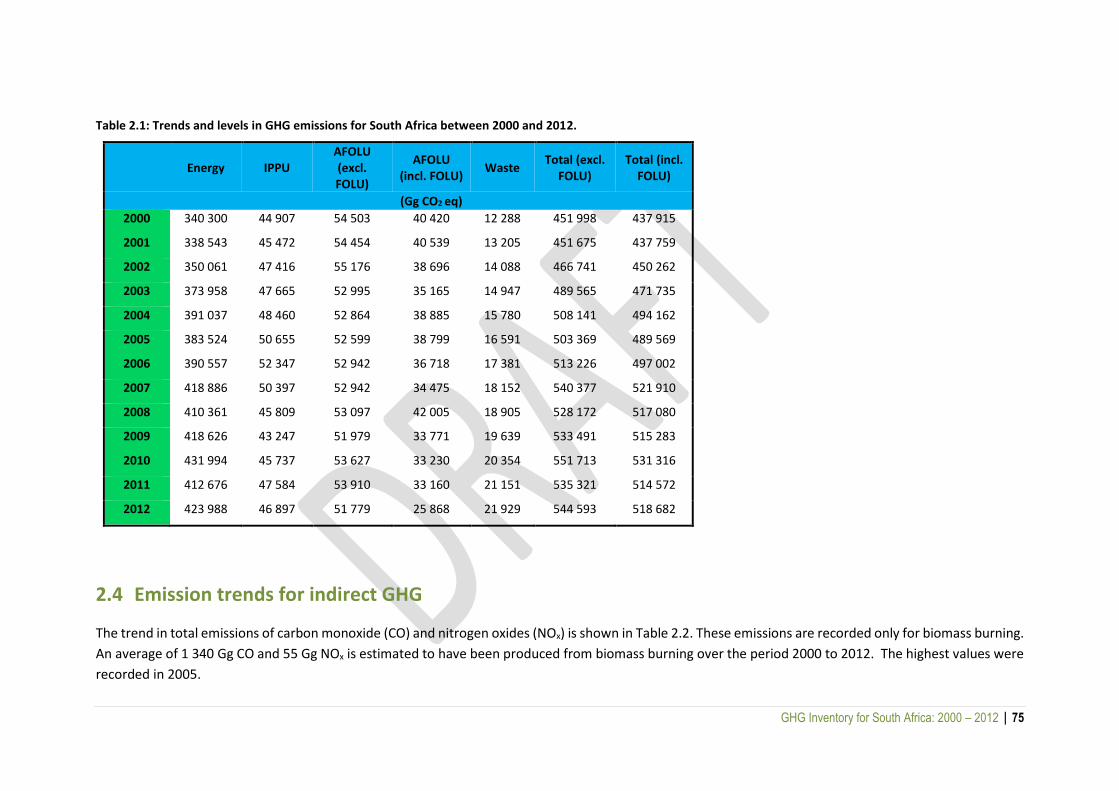
GHG Inventory for South Africa: 2000 – 2012 | 75

Table 2.1: Trends and levels in GHG emissions for South Africa between 2000 and 2012.

Energy IPPU

AFOLU (excl. FOLU)

AFOLU (incl. FOLU)

Waste Total (excl.

FOLU) Total (incl.

FOLU)

(Gg CO2 eq)

2000 340 300 44 907 54 503 40 420 12 288 451 998 437 915

2001 338 543 45 472 54 454 40 539 13 205 451 675 437 759

2002 350 061 47 416 55 176 38 696 14 088 466 741 450 262

2003 373 958 47 665 52 995 35 165 14 947 489 565 471 735

2004 391 037 48 460 52 864 38 885 15 780 508 141 494 162

2005 383 524 50 655 52 599 38 799 16 591 503 369 489 569

2006 390 557 52 347 52 942 36 718 17 381 513 226 497 002

2007 418 886 50 397 52 942 34 475 18 152 540 377 521 910

2008 410 361 45 809 53 097 42 005 18 905 528 172 517 080

2009 418 626 43 247 51 979 33 771 19 639 533 491 515 283

2010 431 994 45 737 53 627 33 230 20 354 551 713 531 316

2011 412 676 47 584 53 910 33 160 21 151 535 321 514 572

2012 423 988 46 897 51 779 25 868 21 929 544 593 518 682

2.4 Emission trends for indirect GHG

The trend in total emissions of carbon monoxide (CO) and nitrogen oxides (NOx) is shown in Table 2.2. These emissions are recorded only for biomass burning.

An average of 1 340 Gg CO and 55 Gg NOx is estimated to have been produced from biomass burning over the period 2000 to 2012. The highest values were

recorded in 2005.

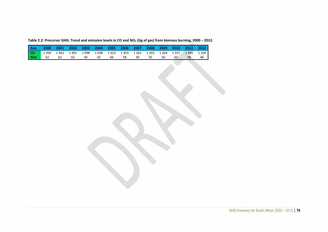
GHG Inventory for South Africa: 2000 – 2012 | 76

Table 2.2: Precursor GHG: Trend and emission levels in CO and NOx (Gg of gas) from biomass burning, 2000 – 2012.

Gas 2000 2001 2002 2003 2004 2005 2006 2007 2008 2009 2010 2011 2012 CO 1 269 1 462 1 491 1 098 1 038 1 623 1 453 1 261 1 355 1 264 1 557 1 445 1 104 NOx 52 61 62 45 42 66 58 50 55 50 63 58 46

GHG Inventory for South Africa: 2000 – 2012 | 77

3 ENERGY SECTOR

3.1 An overview of the energy sector

South Africa’s GDP is the 26th highest in the world, but in primary energy consumption South Africa is ranked 16th in the world. South Africa’s energy intensity

is high mainly because the economy is dominated by large-scale, energy-intensive primary minerals beneficiation industries and mining industries.

Furthermore, there is a heavy reliance on fossil fuels for the generation of electricity and significant proportion of the liquid fuels consumed in the country.

The energy sector is critical to the South African economy because it accounts for a total of 15% in the GDP.

In May 2009, the Department of Minerals and Energy was divided into two separate departments, namely, the Department of Mineral Resources and the

Department of Energy (DoE). The DoE is responsible for the management, processing, exploration, utilisation and development of South Africa’s energy

resources.

The DoE’s Energy Policy is mainly focused on the following key objectives:

Diversifying primary energy sources and reducing dependency on coal;

Good governance, which must also facilitate and encourage private-sector investments in the energy sector;

Environmentally responsible energy provision;

Attaining universal access to energy by 2014;

Achieving a final energy demand reduction of 12% by 2015; and

Providing accessible, affordable and reliable energy, to the poorer communities of South Africa.

The energy sector in South Africa is highly dependent on coal as the main primary energy resource. The largest source of energy sector emissions in

South Africa is the combustion of fossil fuels. Emission products of the combustion process include CO2, N2O, CH4 and H2O. A large quantity of liquid

fuels is imported in the form of crude oil. Renewable energy comprises biomass and natural processes that can be used as energy sources. Biomass

is used commercially in industry to produce process heat and in households for cooking and heating.

The 2004 White Paper on Renewable Energy indicated that the target for renewable energy should be 10 000 GWh by 2013. The DoE recently

developed a biofuel strategy to contribute towards the production of renewable energy and to minimize South Africa’s reliance on imported crude

oil.

GHG Inventory for South Africa: 2000 – 2012 | 78

3.1.1 Energy demand

In terms of energy demand, South Africa is divided into six sectors: industry, agriculture, commerce, residential, transport and other. The industrial sector

(which includes mining, iron and steel, chemicals, non-ferrous metals, non-metallic minerals, pulp and paper, food and tobacco, and other) is the largest user

of energy in South Africa.

3.1.2 Energy reserves and production

The primary energy supply in South Africa is dominated by coal (65.7%), followed by crude oil (21.6%), renewable and waste (7.6%) and natural gas (2.8%)

(DoE, 2010) (Figure 3.1).

3.1.2.1 COAL

The majority of the country’s primary energy needs is provided by coal (approximately 77%). South African coal is nearly all bituminous, with very little

anthracite. It is generally of low quality with a high ash content. The contribution of coal to the total primary energy supply decreased by 8% between 2000

and 2006, but then it increased by 5% between 2006 and 2009. South Africa produces an average of 224 Mt of marketable coal annually, making it the fifth

largest coal-producing country in the world (GCSI, 2009). South Africa has coal reserves of 48 Gt, representing 5.7% of total global reserves.

3.1.2.2 NUCLEAR

Nuclear power contributes a small amount (1.9%) to South Africa’s energy supply (DoE, 2010). The Koeberg Nuclear Power Station, which is the only nuclear

power station in Africa, has two 900 MW units supplying 1 800 MW to the national grid. It therefore provides a significant amount of South Africa’s electricity

GHG Inventory for South Africa: 2000 – 2012 | 79

(GCSI, 2009). The National Nuclear Regulator, as the main safety regulator responsible for protecting persons, property and the environment against nuclear

damage, provides safety standards and regulations. Low- and intermediate-level waste from Koeberg is transported by road in steel and concrete containers

to a remote disposal site at Vaalputs, 600 km away in the Kalahari Desert. High-level waste, the spent fuel, is stored on-site in special pools equipped with

high-density racking (Eskom, 2012). The total consumption of nuclear energy decreased by 1.4% for the period 2000 to 2009.

3.1.2.3 RENEWABLE ENERGY

Renewable energy sources, other than biomass (the energy from plants and plant-derived materials), have not yet been exploited optimally in South Africa.

Renewable energy and waste contribute a total of 7.6% to the energy supply (DoE, 2010). Wind as an energy source contributes more than 4 GWh annually.

Hydro and geothermal solar contribute a total of 0.2% and 0.1%, respectively, to the primary energy supply. Their contribution increased by 0.2% and 2.0%,

respectively, between 2000 and 2009.

3.1.2.4 LIQUID FUELS

In the third quarter of 2008 the demand for petrol decreased by 10% compared with the same period in 2007, while the demand for diesel increased by 3.0%

as industries scaled down operations because of the global economic recession (GCSI, 2009). The petrol price in South Africa is linked to international petrol

markets in which use the United States dollar. This means the supply and demand of petroleum products on the international markets, combined with the

rand-dollar exchange rate influence the domestic price.

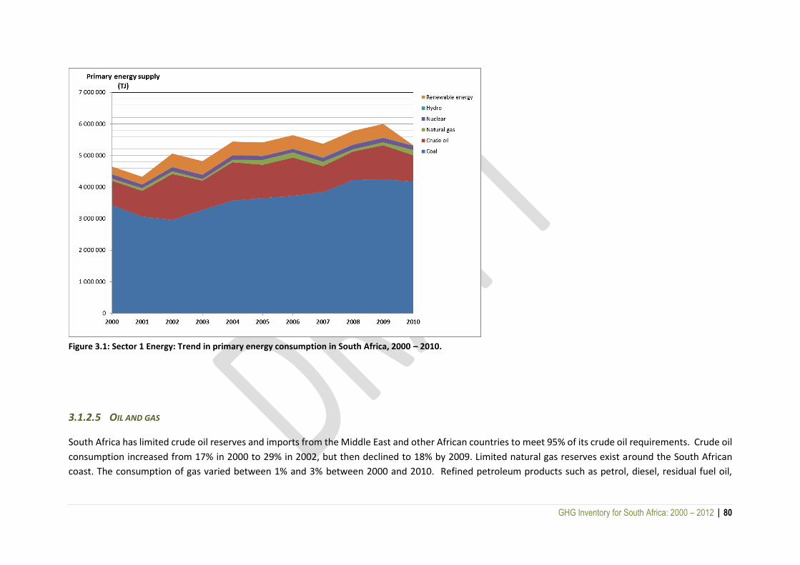
GHG Inventory for South Africa: 2000 – 2012 | 80

Figure 3.1: Sector 1 Energy: Trend in primary energy consumption in South Africa, 2000 – 2010.

3.1.2.5 OIL AND GAS

South Africa has limited crude oil reserves and imports from the Middle East and other African countries to meet 95% of its crude oil requirements. Crude oil

consumption increased from 17% in 2000 to 29% in 2002, but then declined to 18% by 2009. Limited natural gas reserves exist around the South African

coast. The consumption of gas varied between 1% and 3% between 2000 and 2010. Refined petroleum products such as petrol, diesel, residual fuel oil,

GHG Inventory for South Africa: 2000 – 2012 | 81

paraffin, jet fuel, aviation gasoline, liquefied petroleum gas and refinery gas are produced by refining crude oil (in oil refineries), converting coal to liquid fuels

and gas to liquid fuels, and turning natural gas into liquid fuels. Industry is the largest customer of refined petroleum products.

3.1.2.6 ELECTRICITY

South Africa’s largest power producer, Eskom, generates 95% of the electricity in South Africa and about 45% of Africa's electricity (GCSI, 2009). Approximately

88% of South Africa’s electricity is generated from coal-fired power stations, 6.5% from Koeberg Nuclear Power Station, and 2.3% from hydroelectric and

other renewables (GCSI, 2009).

3.1.3 Transport

South Africa has roads, rail and air facilities (both domestic and international). In 2010, the South African transport sector employed 392 381 people,

representing a total of 0.8% of the population (Statistics SA, 2011). South Africa invested R170 billion in the transport system in the five-year period from

2005/06 to 2009/10, with R13.6 billion of the total allocated to improve public transport systems for the 2010 FIFA World Cup.

3.1.3.1 RAIL

State-owned Transnet is a freight transport and logistics company. Transnet Freight Rail (TFR) has a 20 247 km rail network, of which about 1 500 km is heavy-

haul lines. TFR's infrastructure represents about 80% of Africa’s rail infrastructure. The Gautrain Rapid Rail Link commenced operation in 2010. It has 80 km

of routes, linking Sandton to OR Tambo International Airport, Johannesburg to Pretoria, and Rosebank to Johannesburg's Park Station. The aim of the Gautrain

was to reduce the congestion along the Johannesburg-Pretoria traffic route, which accommodates approximately 300 000 vehicles per day.

GHG Inventory for South Africa: 2000 – 2012 | 82

3.1.3.2 ROAD TRANSPORT

South Africa has the longest road network of any country in Africa. The Bus Rapid Transit (BRT) system implements high-quality public transport networks

that operate on exclusive right of way and which incorporates existing bus and minibus operators.

3.1.3.3 CIVIL AVIATION

South Africa is home to more than 70% of the aviation activities in the SADC region. South Africa’s aviation industry has experienced a significant growth in

the past 10 years. The Airports Company of South Africa (ACSA) owns and operates the 10 principal airports, including the three major international airports

located in Johannesburg, Durban and Cape Town.

3.1.3.4 PORTS

Transnet National Ports Authority (TNPA) is the largest port authority on the African continent. It owns and manages South Africa’s ports. Commercial ports

play a crucial role in South Africa’s transport, logistics and socio-economic development. Approximately 98% of South Africa’s exports are conveyed by sea.

3.2 GHG Emissions from the energy sector

The energy sector in South Africa is highly dependent on coal as the main primary energy provider. The largest source of energy sector emissions in South

Africa is the combustion of fossil fuels. Emission products of the combustion process include CO2, N2O, CH4 and H2O.

The energy sector includes:

Exploration and exploitation of primary energy sources;

Conversion of primary energy sources into more useable energy forms in refineries and power plants;

Transmission and distribution of fuels; and

Final use of fuels in stationary and mobile applications.

GHG Inventory for South Africa: 2000 – 2012 | 83

3.2.1 Overview of shares and trends in emissions

Total GHG emissions for the energy sector increased by 27% between 2000 and 2012, and produced a total accumulated GHG estimate of 5 084 940 Gg CO2eq

over the 12 year period. An analysis of key categories was completed in order to determine the most significant emission sources in the energy sector. The

majority of emissions are from energy industries (63.6%) (Figure 3.2), followed by 10.8% from transport and 9.8% from manufacturing industries and

construction.

The main source of emissions in this sector is CO2 from fossil fuel combustion. The largest source of emissions for the period 2000 to 2012 is the main activity

electricity producer, which accounted for 56% (2 736 658 Gg CO2eq) of the total accumulated emissions. The second largest emitting subcategory was

manufacturing industries and construction which accounted for 467 855 Gg CO2eq over the period 2000 to 2012. The transport sector and fugitive emissions

from energy production accounted for 315 235 Gg CO2eq and 357 517 Gg CO2eq (7.4% of the total emissions), respectively, between 2000 and 2012. The

manufacture of solid fuels and other energy industries accounts for an accumulated 386 264 Gg CO2eq of the total GHG emissions in the energy sector for the

period 2000 to 2012. The residential and commercial sectors are both heavily reliant on electricity for meeting energy needs, contributing a total of 212 888

Gg CO2eq and 189 488 Gg CO2eq of emissions, respectively.

The total GHG emissions in the energy sector increased from 340 711 GgCO2eq in 2000 to 395 0888 Gg CO2eq in 2012 (Figure 3.3). The majority of emissions

were from electricity production, which accounted for a total of 61.9% of the total GHG emissions from the energy sector in 2012. Total GHG emissions

increased between 2001 and 2004, mainly because of economic growth and development, which led to increased demand for electricity and fossil fuels. An

expansion of industrial production during that period increased the demand for electricity and fossil fuels. Economic growth also increased the amount people

travelled, leading to higher rates of consumption of petroleum fuels. GHG emissions decreased by 2.5% in 2005, which was followed by a linear increase in

emissions until 2008 when there was a slight decrease (Figure 3.4). In 2009 emissions began to increase again minimally by 2.1%. Table 3. 1 shows the

contribution of the source categories in the energy sector to the total national GHG inventory.

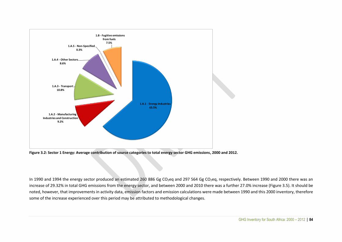
GHG Inventory for South Africa: 2000 – 2012 | 84

Figure 3.2: Sector 1 Energy: Average contribution of source categories to total energy sector GHG emissions, 2000 and 2012.

In 1990 and 1994 the energy sector produced an estimated 260 886 Gg CO2eq and 297 564 Gg CO2eq, respectively. Between 1990 and 2000 there was an

increase of 29.32% in total GHG emissions from the energy sector, and between 2000 and 2010 there was a further 27.0% increase (Figure 3.5). It should be

noted, however, that improvements in activity data, emission factors and emission calculations were made between 1990 and this 2000 inventory, therefore

some of the increase experienced over this period may be attributed to methodological changes.

1.A.1 - Energy Industries 63.5%

1.A.2 - Manufacturing Industries and Construction

9.2%

1.A.3 - Transport 10.8%

1.A.4 - Other Sectors 8.6%

1.A.5 - Non-Specified 0.3%

1.B - Fugitive emissions

from fuels 7.5%

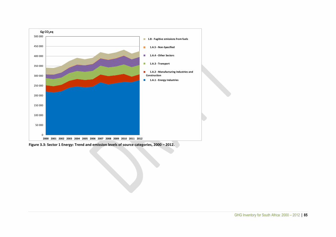
GHG Inventory for South Africa: 2000 – 2012 | 85

Figure 3.3: Sector 1 Energy: Trend and emission levels of source categories, 2000 – 2012.

0

50 000

100 000

150 000

200 000

250 000

300 000

350 000

400 000

450 000

500 000

2000 2001 2002 2003 2004 2005 2006 2007 2008 2009 2010 2011 2012

Gg CO2eq

1.B - Fugitive emissions from fuels

1.A.5 - Non-Specified

1.A.4 - Other Sectors

1.A.3 - Transport

1.A.2 - Manufacturing Industries and

Construction

1.A.1 - Energy Industries

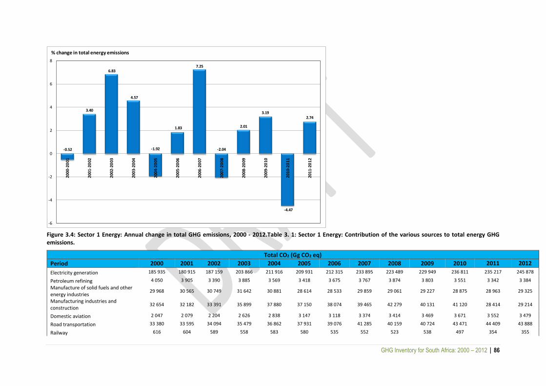
GHG Inventory for South Africa: 2000 – 2012 | 86

Figure 3.4: Sector 1 Energy: Annual change in total GHG emissions, 2000 - 2012.Table 3. 1: Sector 1 Energy: Contribution of the various sources to total energy GHG emissions.

Total CO2 (Gg CO2 eq)

Period 2000 2001 2002 2003 2004 2005 2006 2007 2008 2009 2010 2011 2012

Electricity generation 185 935 180 915 187 159 203 866 211 916 209 931 212 315 233 895 223 489 229 949 236 811 235 217 245 878

Petroleum refining 4 050 3 905 3 390 3 885 3 569 3 418 3 675 3 767 3 874 3 803 3 551 3 342 3 384

Manufacture of solid fuels and other energy industries

29 968 30 565 30 749 31 642 30 881 28 614 28 533 29 859 29 061 29 227 28 875 28 963 29 325

Manufacturing industries and construction

32 654 32 182 33 391 35 899 37 880 37 150 38 074 39 465 42 279 40 131 41 120 28 414 29 214

Domestic aviation 2 047 2 079 2 204 2 626 2 838 3 147 3 118 3 374 3 414 3 469 3 671 3 552 3 479

Road transportation 33 380 33 595 34 094 35 479 36 862 37 931 39 076 41 285 40 159 40 724 43 471 44 409 43 888

Railway 616 604 589 558 583 580 535 552 523 538 497 354 355

-0.52

3.40

6.83

4.57

-1.92

1.83

7.25

-2.04

2.01

3.19

-4.47

2.74

-6

-4

-2

0

2

4

6

8

2000

-20

01

2001

-20

02

2002

-20

03

2003

-20

04

2004

-20

05

2005

-20

06

2006

-20

07

2007

-20

08

2008

-20

09

2009

-20

10

2010

-20

11

2011

-20

12

% change in total energy emissions

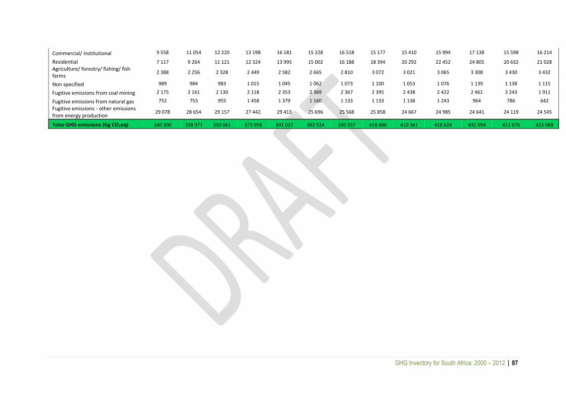
GHG Inventory for South Africa: 2000 – 2012 | 87

Commercial/ institutional 9 558 11 054 12 220 13 198 16 181 15 228 16 518 15 177 15 410 15 994 17 138 15 598 16 214

Residential 7 117 9 264 11 121 12 324 13 995 15 002 16 188 18 394 20 292 22 452 24 805 20 632 21 028

Agriculture/ forestry/ fishing/ fish farms

2 388 2 256 2 328 2 449 2 582 2 665 2 810 3 072 3 021 3 065 3 308 3 430 3 432

Non specified 989 984 983 1 015 1 045 1 062 1 073 1 100 1 053 1 076 1 139 1 138 1 115

Fugitive emissions from coal mining 2 175 2 161 2 130 2 118 2 353 2 369 2 367 2 395 2 438 2 422 2 461 3 243 1 911

Fugitive emissions from natural gas 752 753 955 1 458 1 379 1 160 1 133 1 133 1 138 1 243 964 786 642

Fugitive emissions - other emissions from energy production

29 078 28 654 29 157 27 442 29 413 25 696 25 568 25 858 24 667 24 985 24 641 24 119 24 545

Total GHG emissions (Gg CO2eq) 340 300 338 971 350 061 373 958 391 037 383 524 390 557 418 886 410 361 418 626 431 994 412 676 423 988

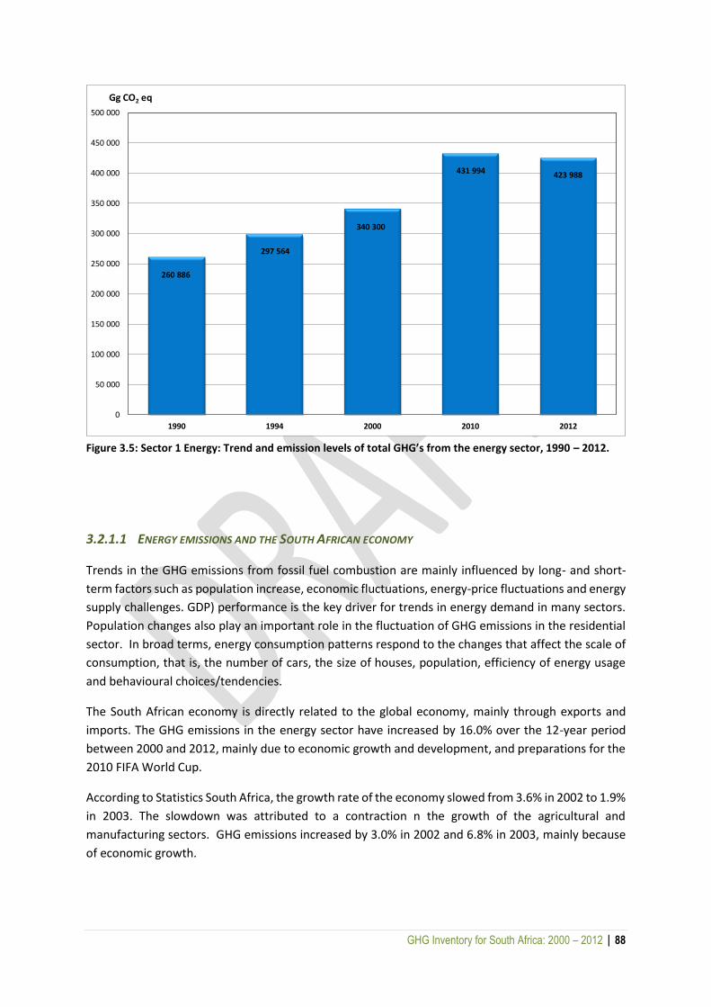
GHG Inventory for South Africa: 2000 – 2012 | 88

Figure 3.5: Sector 1 Energy: Trend and emission levels of total GHG’s from the energy sector, 1990 – 2012.

3.2.1.1 ENERGY EMISSIONS AND THE SOUTH AFRICAN ECONOMY

Trends in the GHG emissions from fossil fuel combustion are mainly influenced by long- and short-

term factors such as population increase, economic fluctuations, energy-price fluctuations and energy

supply challenges. GDP) performance is the key driver for trends in energy demand in many sectors.

Population changes also play an important role in the fluctuation of GHG emissions in the residential

sector. In broad terms, energy consumption patterns respond to the changes that affect the scale of

consumption, that is, the number of cars, the size of houses, population, efficiency of energy usage

and behavioural choices/tendencies.

The South African economy is directly related to the global economy, mainly through exports and

imports. The GHG emissions in the energy sector have increased by 16.0% over the 12-year period

between 2000 and 2012, mainly due to economic growth and development, and preparations for the

2010 FIFA World Cup.

According to Statistics South Africa, the growth rate of the economy slowed from 3.6% in 2002 to 1.9%

in 2003. The slowdown was attributed to a contraction n the growth of the agricultural and

manufacturing sectors. GHG emissions increased by 3.0% in 2002 and 6.8% in 2003, mainly because

of economic growth.

260 886

297 564

340 300

431 994 423 988

0

50 000

100 000

150 000

200 000

250 000

300 000

350 000

400 000

450 000

500 000

1990 1994 2000 2010 2012

Gg CO2 eq

GHG Inventory for South Africa: 2000 – 2012 | 89

In 2004 GDP growth increased again to 3.7% and to 5% in 2005. GHG emissions increased by only 1.8%

between 2005 and 2006. The reason for the slower rate of increase in emissions between 2004 and

2005 is unknown.

The annual rate of increase in GHG emissions was significantly lower between 2007 and 2009, with an

increase of only 2.0% in 2009. In May 2009 South Africa officially entered an economic recession – the

first in 17 years – sparked by the global economic recession that started towards the end of 2008.

Until then, the country's economic growth and development had been stable and consistent.

According to Statistics South Africa, the GDP increased by 2.7% in 2001, 3.7% in 2002, 3.1% in 2003,

4.9% in 2004, 5.0% in 2005, 5.4% in 2006, 5.1% in 2007 and 3.1% in 2008. As a result of the recession,

GHG emissions decreased enormously almost across all categories in the energy sector.

By November 2009, the economy had recovered, achieving a 0.9% growth, primarily because of

growth in the manufacturing sector. Hosting the 2010 FIFA World Cup in June and July 2010 also

contributed positively to the economy and, as a result, GHG emissions increased by 3.5% that year.

South Africa's economy is highly dependent on a reliable electricity supply. A decline in emissions

between November 2007 and the end of January 2008 can be attributed to substantial disruptions in

the electricity supply caused by a lack of adequate generating capacity.

In January 2006 the main power producer, Eskom, started experiencing difficulties meeting customer

demand (NERSA, 2008). This situation deteriorated in late 2007 and early 2008 and Eskom resorted

to load shedding. The extent of the load shedding had a disruptive impact on business operations,

traffic, industry, mining operations, commerce, hospitals, clinics, schools and other institutions, and

households. The situation deteriorated to the extent that major mining operations had to close down

on 24 January 2008 for safety considerations (NERSA, 2008).

3.2.2 Key sources

Level and trend key category analyses were completed for 2012 using 2000 as the base year. The level

assessment shows that energy industries (solid fuels), road transportation, manufacturing industries

and construction (solid fuels), and other sectors (solid fuels) are the top subcategories in the energy

sector. In the trend assessment, it is other sectors (solid fuels), other emissions from energy

production, and energy industries (liquid and solid fuels) that top the list (see Table 1.8 and Table 1.10).

This differs from the 2000 inventory which showed fugitive emissions from coal mining (1B1) to be the

second most important emitter, whereas in this inventory these emissions are not seen as a key

category. Also, emissions from road transportation have move much higher up the key categories list

in this inventory.

3.3 Fuel combustion activities [1A]

The combustion of fuels includes both mobile and stationary sources with their respective

combustion-related emissions. GHG emissions from the combustion of fossil fuels in this inventory

will include the following categories and subcategories:

GHG Inventory for South Africa: 2000 – 2012 | 90

1A1 Energy industries

o 1A1a Main activity electricity and heat production

o 1A1b Petroleum activity

o 1A1c Manufacture of solid fuels and other energy industries

1A2 Manufacturing industries and construction

o 1A2c Chemicals

o 1A2m Non-specified sectors

1A3Transport sector

o 1A3a Civil aviation

o 1A3b Road transportation

o 1A3c Railways

o 1A3d Waterborne navigation

o 1A3e Other transportation

1A4 Other sectors

o 1A4a Commercial/ institutional

o 1A4b Residential

o 1A4c Agriculture / forestry/ fishing/ fish farms

3.3.1 Comparison of the sectoral approach with the reference approach

The reference approach is a quick estimate of the total CO2 emitted in a country using a first-order

estimate of national GHG emissions based on the energy supplied to a country. The reference

approach can be used to estimate a country’s CO2 emissions from fuel combustion and can be

compared with the results of the sectoral emission estimates. That was done for this inventory. Over

the period 2000 to 2012 the CO2 emissions were higher using the reference approach. Reporting has

improved over the 12-year period and, as a result, the difference between the two approaches has

declined from 56% in 2000 to 20% in 2012. There are a number of possible reasons for the discrepancy:

Net calorific values (NCVs) used in the sectoral approach differ from those used in the

reference approach. In power generation, NCVs in the sectoral approach vary over the 2000–

2012 time series based on the information provided by industry;

Activity data on liquid fuels in the sectoral approach, particularly for energy industries, is

sourced directly from the companies involved and has been reconciled with other publicly

available datasets;

Allocation of solid fuels between energy use, non-energy use as well as use for synfuels

production remains one of the key drivers of the differences observed between the two

datasets.

3.3.2 Feed stocks and non-energy use of fuels

There are cases where fuels are used as raw materials in production processes. For example, in iron

and steel production, coal is used as a feedstock in the manufacture of steel. The 2006 IPCC Guidelines

emphasize the significance of separating energy and process emissions to prevent double counting

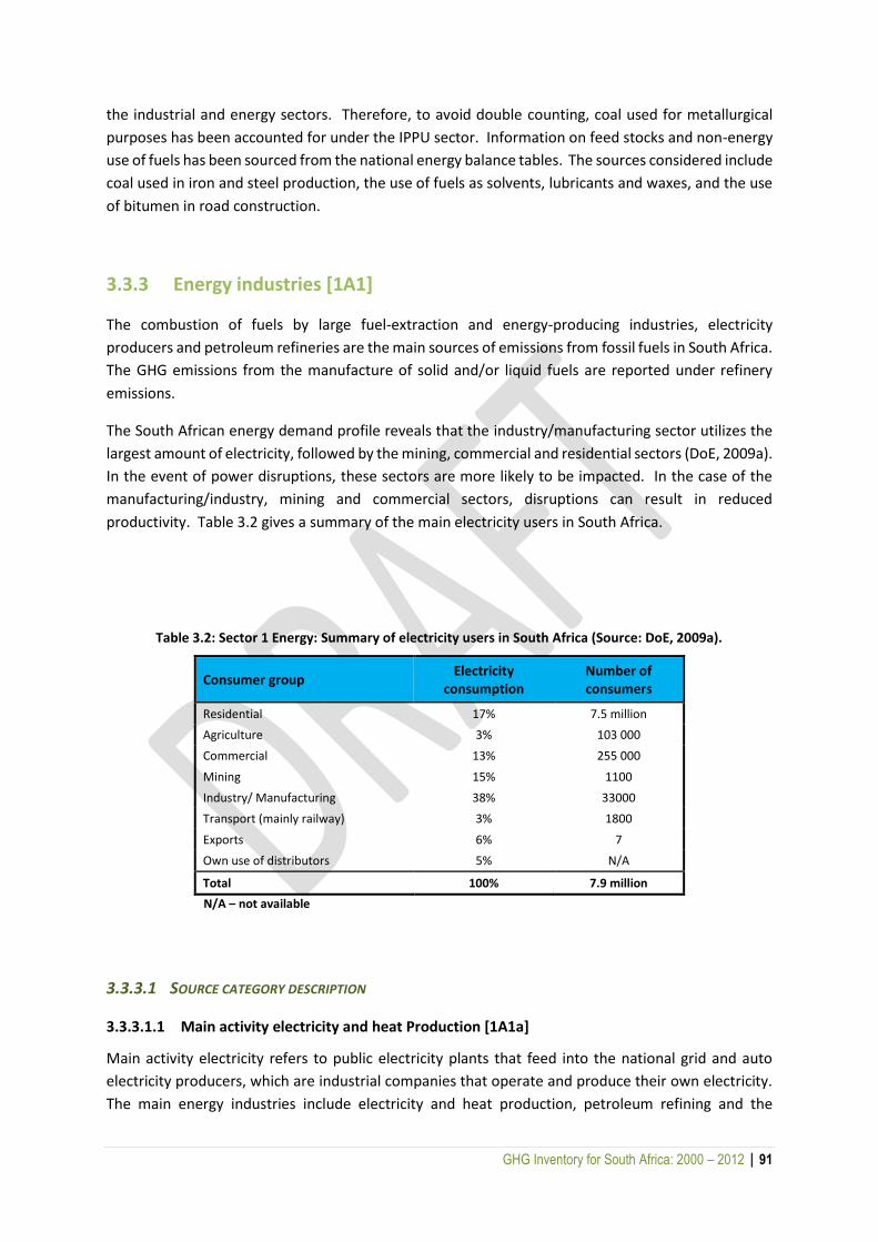
GHG Inventory for South Africa: 2000 – 2012 | 91

the industrial and energy sectors. Therefore, to avoid double counting, coal used for metallurgical

purposes has been accounted for under the IPPU sector. Information on feed stocks and non-energy

use of fuels has been sourced from the national energy balance tables. The sources considered include

coal used in iron and steel production, the use of fuels as solvents, lubricants and waxes, and the use

of bitumen in road construction.

3.3.3 Energy industries [1A1]

The combustion of fuels by large fuel-extraction and energy-producing industries, electricity

producers and petroleum refineries are the main sources of emissions from fossil fuels in South Africa.

The GHG emissions from the manufacture of solid and/or liquid fuels are reported under refinery

emissions.

The South African energy demand profile reveals that the industry/manufacturing sector utilizes the

largest amount of electricity, followed by the mining, commercial and residential sectors (DoE, 2009a).

In the event of power disruptions, these sectors are more likely to be impacted. In the case of the

manufacturing/industry, mining and commercial sectors, disruptions can result in reduced

productivity. Table 3.2 gives a summary of the main electricity users in South Africa.

Table 3.2: Sector 1 Energy: Summary of electricity users in South Africa (Source: DoE, 2009a).

Consumer group Electricity

consumption Number of consumers

Residential 17% 7.5 million

Agriculture 3% 103 000

Commercial 13% 255 000

Mining 15% 1100

Industry/ Manufacturing 38% 33000

Transport (mainly railway) 3% 1800

Exports 6% 7

Own use of distributors 5% N/A

Total 100% 7.9 million

N/A – not available

3.3.3.1 SOURCE CATEGORY DESCRIPTION

3.3.3.1.1 Main activity electricity and heat Production [1A1a]

Main activity electricity refers to public electricity plants that feed into the national grid and auto

electricity producers, which are industrial companies that operate and produce their own electricity.

The main energy industries include electricity and heat production, petroleum refining and the

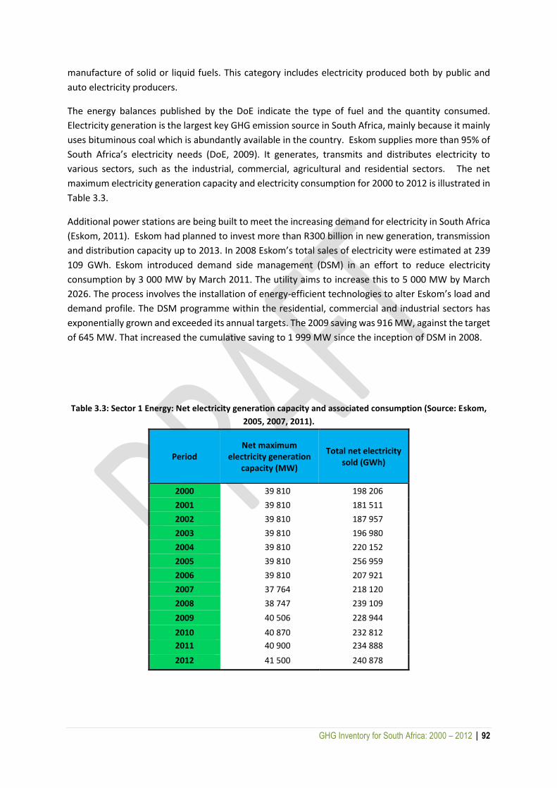
GHG Inventory for South Africa: 2000 – 2012 | 92

manufacture of solid or liquid fuels. This category includes electricity produced both by public and

auto electricity producers.

The energy balances published by the DoE indicate the type of fuel and the quantity consumed.

Electricity generation is the largest key GHG emission source in South Africa, mainly because it mainly

uses bituminous coal which is abundantly available in the country. Eskom supplies more than 95% of

South Africa’s electricity needs (DoE, 2009). It generates, transmits and distributes electricity to

various sectors, such as the industrial, commercial, agricultural and residential sectors. The net

maximum electricity generation capacity and electricity consumption for 2000 to 2012 is illustrated in

Table 3.3.

Additional power stations are being built to meet the increasing demand for electricity in South Africa

(Eskom, 2011). Eskom had planned to invest more than R300 billion in new generation, transmission

and distribution capacity up to 2013. In 2008 Eskom’s total sales of electricity were estimated at 239

109 GWh. Eskom introduced demand side management (DSM) in an effort to reduce electricity

consumption by 3 000 MW by March 2011. The utility aims to increase this to 5 000 MW by March

2026. The process involves the installation of energy-efficient technologies to alter Eskom’s load and

demand profile. The DSM programme within the residential, commercial and industrial sectors has

exponentially grown and exceeded its annual targets. The 2009 saving was 916 MW, against the target

of 645 MW. That increased the cumulative saving to 1 999 MW since the inception of DSM in 2008.

Table 3.3: Sector 1 Energy: Net electricity generation capacity and associated consumption (Source: Eskom,

2005, 2007, 2011).

Period Net maximum

electricity generation capacity (MW)

Total net electricity sold (GWh)

2000 39 810 198 206

2001 39 810 181 511

2002 39 810 187 957

2003 39 810 196 980

2004 39 810 220 152

2005 39 810 256 959

2006 39 810 207 921

2007 37 764 218 120

2008 38 747 239 109

2009 40 506 228 944

2010 40 870 232 812

2011 40 900 234 888

2012 41 500 240 878

GHG Inventory for South Africa: 2000 – 2012 | 93

3.3.3.1.2 Petroleum refining [1A1b]

This source category includes combustion emissions from crude oil refining and excludes emissions

from the manufacture of synthetic fuels from coal and natural gas. Combustion-related emissions

from the manufacture of synthetic fuels from coal and natural gas are accounted for under 1A1c.

South Africa has limited oil reserves and approximately 95% of its crude oil requirements are met by

imports. Refined petroleum products such as petrol, diesel, fuel oil, paraffin, jet fuel and LPG are

produced by crude oil refining, and the production of coal-to-liquid fuels and gas-to-liquid fuels.

In 2000 and 2010 the total crude oil distillation capacity of South Africa’s petroleum refineries was 700

000 bbl/d- and 703 000 bbl/d, respectively (SAPIA, 2006 & 2011). The production of oil was 689 000

tonnes in 2000 and 684 000 tonnes in 2006 (SAPIA, 2011). Activity data on the fuel consumed by

refineries is sourced directly from refineries. National energy balance data from the DoE is used to

verify data reported by the petroleum industry.

3.3.3.1.3 Manufacture of solid fuels and other energy industries [1A1c]

This category refers to combustion emissions from solid fuels used during the manufacture of

secondary and tertiary products, including the production of charcoal. The GHG emissions from the

various industrial plants’ own on-site fuel use, and emissions from the combustion of fuels for the

generation of electricity and heat for their own use is also included in this category.

3.3.3.2 OVERVIEW OF SHARES AND TRENDS IN EMISSIONS

3.3.3.2.1 Main activity electricity and heat Production [1A1a]

Public electricity producer

The total estimated cumulative coal consumption of the public electricity producer, Eskom, for the

period 2000 to 2012 was 28 229 590 TJ. Consumption increased by 38.6% over this period (Table 3.4).

The total estimated of cumulative GHG emissions from the public electricity producer was 2 736 658

Gg CO2 eq between 2000 and 2012.

In 2000, GHG emissions from the public electricity producer totalled 174 762 Gg CO2eq. The main

source of emissions in this category was the combustion of coal for electricity generation. The

consumption of electricity increased marginally between 2000 and 2007 (DoE, 2009a). The GHG

emissions steadily increased throughout the same period from 174 762 Gg CO2eq to 229 252 Gg

CO2eq in 2007. The main reason for the increase in GHG emissions during that period was robust

economic growth, which increased the demand for electricity and fossil fuel consumption.

During 2003, Eskom's total electricity sales increased by 196 980 GWh. The peak demand on the

integrated system amounted to 31 928 MW and the total GHG emissions during that period were

equivalent to 195 Mt CO2eq. These figures demonstrate the growth of the South African economy

and the importance of energy as a key driver of the country’s economic growth and development.

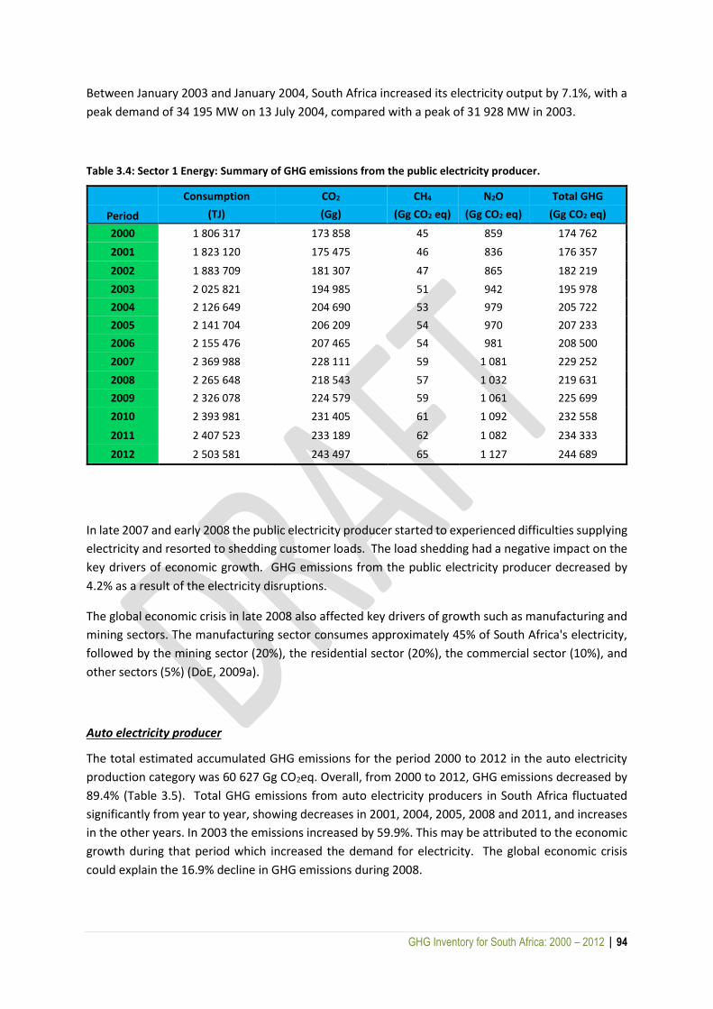
GHG Inventory for South Africa: 2000 – 2012 | 94

Between January 2003 and January 2004, South Africa increased its electricity output by 7.1%, with a

peak demand of 34 195 MW on 13 July 2004, compared with a peak of 31 928 MW in 2003.

Table 3.4: Sector 1 Energy: Summary of GHG emissions from the public electricity producer.

Consumption CO2 CH4 N2O Total GHG

Period (TJ) (Gg) (Gg CO2 eq) (Gg CO2 eq) (Gg CO2 eq)

2000 1 806 317 173 858 45 859 174 762

2001 1 823 120 175 475 46 836 176 357

2002 1 883 709 181 307 47 865 182 219

2003 2 025 821 194 985 51 942 195 978

2004 2 126 649 204 690 53 979 205 722

2005 2 141 704 206 209 54 970 207 233

2006 2 155 476 207 465 54 981 208 500

2007 2 369 988 228 111 59 1 081 229 252

2008 2 265 648 218 543 57 1 032 219 631

2009 2 326 078 224 579 59 1 061 225 699

2010 2 393 981 231 405 61 1 092 232 558

2011 2 407 523 233 189 62 1 082 234 333

2012 2 503 581 243 497 65 1 127 244 689

In late 2007 and early 2008 the public electricity producer started to experienced difficulties supplying

electricity and resorted to shedding customer loads. The load shedding had a negative impact on the

key drivers of economic growth. GHG emissions from the public electricity producer decreased by

4.2% as a result of the electricity disruptions.

The global economic crisis in late 2008 also affected key drivers of growth such as manufacturing and

mining sectors. The manufacturing sector consumes approximately 45% of South Africa's electricity,

followed by the mining sector (20%), the residential sector (20%), the commercial sector (10%), and

other sectors (5%) (DoE, 2009a).

Auto electricity producer

The total estimated accumulated GHG emissions for the period 2000 to 2012 in the auto electricity

production category was 60 627 Gg CO2eq. Overall, from 2000 to 2012, GHG emissions decreased by

89.4% (Table 3.5). Total GHG emissions from auto electricity producers in South Africa fluctuated

significantly from year to year, showing decreases in 2001, 2004, 2005, 2008 and 2011, and increases

in the other years. In 2003 the emissions increased by 59.9%. This may be attributed to the economic

growth during that period which increased the demand for electricity. The global economic crisis

could explain the 16.9% decline in GHG emissions during 2008.

GHG Inventory for South Africa: 2000 – 2012 | 95

Table 3.5: Sector 1 Energy: Summary of GHG emissions from auto electricity producers, 2000 - 2012.

Consumption CO2 CH4 N2O Total GHG

(TJ) (Gg) (Gg CO2 eq) (Gg CO2 eq) (Gg CO2 eq)

2000 116 046 11 169 2.90 51.87 11 224

2001 47 346 4 557 1.18 21.16 4 579

2002 51 311 4 939 1.28 22.94 4 963

2003 82 036 7 896 2.05 36.67 7 935

2004 64 333 6 192 1.61 28.76 6 222

2005 28 029 2 698 0.70 12.53 2 711

2006 39 627 3 814 0.99 17.71 3 833

2007 48233 4 642 1.21 21.56 4 665

2008 40 066 3 856 1.00 17.91 3 875

2009 44 149 4 294 1.10 19.73 4 270

2010 44 171 4 251 1.10 19.74 4 272

2011 9 164 882 0.23 4.10 886

2012 12 305 1 184 0.31 5.50 1 190

3.3.3.2.2 Petroleum refining [1A1b]

The total cumulative consumption of fuels for petroleum refining for the period 2000 to 2012 was

estimated at 709 696 TJ, with refinery gas contributing 76.6% in 2010. The total GHG emissions from

petroleum refining was estimated at 4 050 Gg CO2eq in 2000, decreasing to 3 384 Gg CO2 eq in 2012

(Table 3.6).

In 2000 refinery gas contributed 50.7% to the total GHG emissions in this category and this increased

to 82.5% in 2012. Emissions from residual fuel oil decreased from contributing 45.3% in 2000 to only

5.2% in 2012. A shift from residual fuel oil to refinery gas in most refineries is the main driver of

emissions reduction in this source category.

Table 3.6: Sector 1 Energy: Summary of consumption of fuels and GHG emissions in the petroleum refining category (1A1b), 2000 - 2012.

Consumption CO2 CH4 N2O Total GHG

Period (TJ) Gg (Gg CO2 eq) (Gg CO2 eq) (Gg CO2 eq)

2000 59 637 4 043 2.47 4.7 4 050

2001 57 599 3 898 2.43 4.65 3 905

2002 50 679 3 385 1.97 3.6 3 390

2003 57 486 3 879 2.12 4.27 3 885

2004 53 292 3 563 2.05 3.72 3 569

2005 51 609 3 413 1.92 3.43 3 418

2006 55 122 3 669 2.14 3.90 3 675

2007 56 073 3 761 2.21 4.07 3 767

2008 57 870 3 868 2.26 4.14 3 874

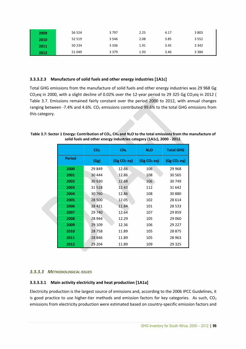
GHG Inventory for South Africa: 2000 – 2012 | 96

2009 56 524 3 797 2.25 4.17 3 803

2010 52 519 3 546 2.08 3.85 3 552

2011 50 234 3 336 1.91 3.45 3 342

2012 51 049 3 379 1.93 3.46 3 384

3.3.3.2.3 Manufacture of solid fuels and other energy industries [1A1c]

Total GHG emissions from the manufacture of solid fuels and other energy industries was 29 968 Gg

CO2eq in 2000, with a slight decline of 0.02% over the 12-year period to 29 325 Gg CO2eq in 2012 (

Table 3.7. Emissions remained fairly constant over the period 2000 to 2012, with annual changes

ranging between -7.4% and 4.6%. CO2 emissions contributed 99.6% to the total GHG emissions from

this category.

Table 3.7: Sector 1 Energy: Contribution of CO2, CH4 and N2O to the total emissions from the manufacture of solid fuels and other energy industries category (1A1c), 2000 - 2012.

CO2 CH4 N2O Total GHG

Period (Gg) (Gg CO2 eq) (Gg CO2 eq) (Gg CO2 eq)

2000 29 849 12.66 106 29 968

2001 30 444 12.86 108 30 565

2002 30 630 12.68 106 30 749

2003 31 518 12.43 112 31 642

2004 30 760 12.86 108 30 880

2005 28 500 12.05 102 28 614

2006 28 421 11.84 101 28 533

2007 29 740 12.64 107 29 859

2008 28 944 12.29 105 29 060

2009 29 109 12.36 106 29 227

2010 28 758 11.89 105 28 875

2011 28 846 11.89 105 28 963

2012 29 204 11.89 109 29 325

3.3.3.3 METHODOLOGICAL ISSUES

3.3.3.3.1 Main activity electricity and heat production [1A1a]

Electricity production is the largest source of emissions and, according to the 2006 IPCC Guidelines, it

is good practice to use higher-tier methods and emission factors for key categories. As such, CO2

emissions from electricity production were estimated based on country-specific emission factors and

GHG Inventory for South Africa: 2000 – 2012 | 97

plant-specific activity data. Hence, net caloric values (NCVs) reported on an annual basis by the power

utility and activity data for each power plant were used in these estimations.

3.3.3.3.2 Petroleum refining [1A1b]

GHG emissions from petroleum refining were estimated based on a Tier 1 approach and IPCC default

emission factors.

3.3.3.3.3 Manufacture of solid fuels and other energy industries [1A1c]

A country-specific methodology was applied for the calculation of GHG emissions from the

manufacture of solid fuels and energy industries. The GHG emissions from this category were

calculated based on actual process material balance analysis.

3.3.3.4 DATA SOURCES

3.3.3.4.1 Main activity electricity and heat production [1A1a]

Data on fuel consumption for public electricity generation was obtained directly from the national

power producer for the period 2000 to 2012. Activity data for auto electricity producers for the period

2000 to 2006 was sourced from the DoE Energy Digest and for the period 2007 to 2012 the data was

extrapolated using the technique recommended by the 2006 IPCC Guidelines from the SAMI annual

publications on total coal consumption. To convert fuel quantities into energy units for public

electricity generation, the net calorific values estimated by the national utility annually were applied.

A country-specific average NCV of 0.0192 TJ/tonne was used to convert fuel quantities into energy

units and this was sourced from Eskom's annual report for 2010 (Eskom, 2010) for auto electricity

producers.

A Tier 2 approach with country-specific emission factors was used to estimate CO2 emissions from coal

consumption (Table 3.8).

For the calculation of CH4 and N2O emissions, a Tier 1 approach was used with default emission factors

sourced from the 2006 IPCC Guidelines. Furthermore, default factors from these guidelines were

applied for the estimation of GHG emissions from other fuels such as other kerosene and diesel oil.

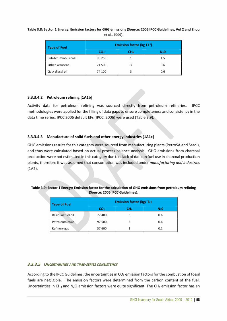
GHG Inventory for South Africa: 2000 – 2012 | 98

Table 3.8: Sector 1 Energy: Emission factors for GHG emissions (Source: 2006 IPCC Guidelines, Vol 2 and Zhou

et al., 2009).

Type of Fuel Emission factor (kg TJ-1)

CO2 CH4 N20

Sub-bituminous coal 96 250 1 1.5

Other kerosene 71 500 3 0.6

Gas/ diesel oil 74 100 3 0.6

3.3.3.4.2 Petroleum refining [1A1b]

Activity data for petroleum refining was sourced directly from petroleum refineries. IPCC

methodologies were applied for the filling of data gaps to ensure completeness and consistency in the

data time series. IPCC 2006 default EFs (IPCC, 2006) were used (Table 3.9).

3.3.3.4.3 Manufacture of solid fuels and other energy industries [1A1c]

GHG emissions results for this category were sourced from manufacturing plants (PetroSA and Sasol),

and thus were calculated based on actual process balance analysis. GHG emissions from charcoal

production were not estimated in this category due to a lack of data on fuel use in charcoal production

plants, therefore it was assumed that consumption was included under manufacturing and industries

(1A2).

Table 3.9: Sector 1 Energy: Emission factor for the calculation of GHG emissions from petroleum refining (Source: 2006 IPCC Guidelines).

Type of Fuel Emission factor (kg/ TJ)

CO2 CH4 N20

Residual fuel oil 77 400 3 0.6

Petroleum coke 97 500 3 0.6

Refinery gas 57 600 1 0.1

3.3.3.5 UNCERTAINTIES AND TIME-SERIES CONSISTENCY

According to the IPCC Guidelines, the uncertainties in CO2 emission factors for the combustion of fossil

fuels are negligible. The emission factors were determined from the carbon content of the fuel.

Uncertainties in CH4 and N2O emission factors were quite significant. The CH4 emission factor has an

GHG Inventory for South Africa: 2000 – 2012 | 99

uncertainty of between 50 and 150%, while the uncertainty on the N2O emission factor can range from

one-tenth of the mean value to ten times the mean value. With regards to activity data, statistics of

fuel combusted at large sources obtained from direct measurement or obligatory reporting are likely

to be within 3% of the central estimate (IPCC, 2006). Those default IPCC uncertainty values have been

used to report uncertainty for energy industries.

Activity data time series for the period 2000 to 2012 were sourced directly from energy industries. In

cases where data gaps were observed, the IPCC methodologies for filling data gaps were used. That

was mostly the case in petroleum refining (1A1b) as some refineries did not record fuel consumption

in the first four years of the time series. To ensure consistency in time-series emission estimates, IPCC

default emission factors were used for the entire time series for all energy industries. In some cases

(e.g. 1A1c), mass balances methods were applied consistently across the time series. The national

power utility changed its annual reporting planning cycle from a calendar year to an April-March

financial year from 2006 onwards. . That affected the time-series consistency, therefore, the national

power utility was asked to prepare calendar-year fuel consumption estimates using its monthly fuel

consumption statistics.

3.3.3.6 SOURCE-SPECIFIC QA/QC AND VERIFICATION

For the quality control of the activity data used to compile emission estimates in energy industries,

various publications were used to verify facility-level activity data. The DMR's SAMI publication was

used to verify fuel used for electricity generation (SAMI, 2010). Similarly, a combination of crude oil

input reported in the SAPIA reports and in the energy balances applied with the IPCC default

assumptions on fuel input in refineries was used to verify fuel consumption data reported by refineries

(SAPIA 2010). An independent reviewer was appointed to assess the quality of the inventory,

determine the conformity of the procedures followed for the compilation of this inventory and identify

areas of improvements.

3.3.3.7 SOURCE-SPECIFIC RECALCULATIONS

In the previous 2000 GHG inventory, the activity data was sourced mainly from publicly available

publications, such as the national energy balances and SAPIA reports. For this inventory report

improvements were made by collecting data directly from the national utility and the petroleum

refineries. As more accurate activity data was collected for all sources the emissions within the energy

industries sector had to be recalculated back to 2000. The recalculation improved the accuracy of the

2000 GHG emissions result for the energy sector.

3.3.3.8 SOURCE-SPECIFIC PLANNED IMPROVEMENTS AND RECOMMENDATIONS

3.3.3.8.1 Main activity electricity and heat production [1A1a]

The electricity generation sector is a key category and its estimate has a significant influence on the

country’s total inventory of GHGs. Therefore increasing the accuracy of GHG calculations by applying

country-specific emission factors for this sector will improve the national GHG inventory estimate.

GHG Inventory for South Africa: 2000 – 2012 | 100

Another improvement for this category would be to formalise the data collection process to ensure

continuous collection of data and time-series consistency. A further improvement would be for the

national power producer to provide the DEA with information that would assist in the explanation of

the trends throughout the reporting period.

3.3.3.8.2 Petroleum refining [1A1b]

To improve the reporting of GHG emissions in this category it is important that the petroleum

refineries provide plant-specific activity data, such as net caloric and carbon content values, and also

develop country-specific emission factors that can be used for the calculation of GHG emissions.

3.3.3.8.3 Manufacture of solid fuels and other energy industries [1A1c]

To improve the estimation of GHG emissions from the manufacture of solid fuels and energy

industries, a more regular collection of activity data would be useful. That would improve the time

series and consistency of the data. Another improvement would be to monitor the cause of

fluctuations in the manufacture of solid fuels and other energy industries regularly, to enable the

inventory compilers to elaborate on the fluctuations.

3.3.4 Manufacturing industries and construction [1A2]

3.3.4.1 SOURCE CATEGORY DESCRIPTION

According to the 2006 IPCC Guidelines, this category comprise a variety of fuel combustion emission

sources, mainly in the industrial sector. In manufacturing industries, raw materials are converted into

products using fuels as the main source of energy. The industrial sector consumes 40.8% of the final

energy supplied in South Africa. The manufacturing industries and construction subsector can be

divided into mining, iron and steel, chemicals, non-ferrous metals, non-metallic minerals, pulp and

paper, food and tobacco and other productions (includes manufacturing, construction, textiles, wood

products etc.) categories. The largest category is iron and steel which consumes 27.4% of the total

energy utilized by the industrial sector (DoE, 2009a). Emissions from the combustion of fossil fuels in

the construction sector are also included in this category. According to the energy balances compiled

by the DoE, fossil fuels used in the construction sector include LPG, gas/diesel oil, residual fuel oil,

other kerosene, bitumen, sub-bituminous coal and natural gas.

3.3.4.2 OVERVIEW OF SHARES AND TRENDS IN EMISSIONS

The estimated cumulative total GHG emissions in the category manufacturing industries and

construction for the 12-year period was 467 855 Gg CO2eq. GHG emissions were estimated to be 32

654 Gg CO2eq in 2000 and these decreased by 0.11% to 29 214 Gg CO2eq in 2012 (Figure 3.6).

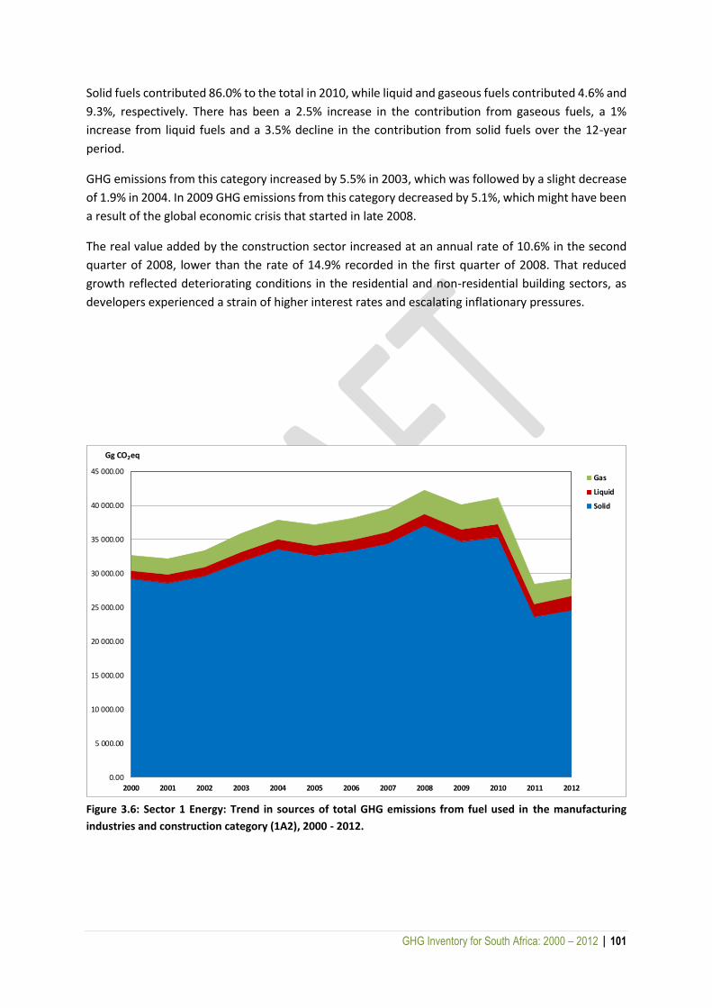
GHG Inventory for South Africa: 2000 – 2012 | 101

Solid fuels contributed 86.0% to the total in 2010, while liquid and gaseous fuels contributed 4.6% and

9.3%, respectively. There has been a 2.5% increase in the contribution from gaseous fuels, a 1%

increase from liquid fuels and a 3.5% decline in the contribution from solid fuels over the 12-year

period.

GHG emissions from this category increased by 5.5% in 2003, which was followed by a slight decrease

of 1.9% in 2004. In 2009 GHG emissions from this category decreased by 5.1%, which might have been

a result of the global economic crisis that started in late 2008.

The real value added by the construction sector increased at an annual rate of 10.6% in the second

quarter of 2008, lower than the rate of 14.9% recorded in the first quarter of 2008. That reduced

growth reflected deteriorating conditions in the residential and non-residential building sectors, as

developers experienced a strain of higher interest rates and escalating inflationary pressures.

Figure 3.6: Sector 1 Energy: Trend in sources of total GHG emissions from fuel used in the manufacturing

industries and construction category (1A2), 2000 - 2012.

0.00

5 000.00

10 000.00

15 000.00

20 000.00

25 000.00

30 000.00

35 000.00

40 000.00

45 000.00

2000 2001 2002 2003 2004 2005 2006 2007 2008 2009 2010 2011 2012

Gg CO2eq

Gas

Liquid

Solid

GHG Inventory for South Africa: 2000 – 2012 | 102

3.3.4.3 METHODOLOGICAL ISSUES

GHG emissions included in this subsector are mainly from fuel combusted for heating purposes. Fuels

used as feed stocks and other non-energy uses are accounted for under the IPPU sector. For the

manufacturing industries and construction subsector, a Tier 1 methodology was applied by multiplying

activity data (fuel consumed) with IPCC default emission factors. In future, facility-level data has to

be sourced and country-specific emission factors need to be developed in order to move towards a

Tier 2 methodology.

3.3.4.4 DATA SOURCES

For the manufacturing industries and construction sector data for solid fuels for the period 2000 to

2007 were sourced from the DoE's energy digest, for the period 2007 to 2010 the SAMI report was

used to extrapolate the fuel consumption. The activity data on liquid fuels for this category was

sourced from SAPIA. Data from industries were also acquired and used to compare the figures in the

energy digest and the SAMI report. Table 3.10 shows the total fuel consumption in this category for

the period 2000 to 2012. An NCV of 0.0243 TJ/tonne was used to convert fuel quantities into energy

units (DoE, 2009a). To avoid double counting fuel activity data, the fuel consumption associated with

petroleum refining (1A1b) was subtracted from the fuel consumption activity data sourced for 1A2.

Table 3.10: Sector 1 Energy: Fuel consumption (TJ) in the manufacturing industries and construction category, 2000 – 2012.

Period Other

Kerosene (TJ)

Gas/Diesel

Oil (TJ)

Residual Fuel Oil

(TJ)

LPG

(TJ)

Bitumen

(TJ)

Sub-Bituminous

Coal (TJ)

Natural Gas (TJ)

Total

(TJ)

2000 698 9 531 194 109 5 053 302 354 39 532 357 471

2001 640 9 888 194 115 5 584 295 804 41 241 353 465

2002 606 10 410 187 113 6 161 306 401 43 048 366 927

2003 626 11 069 185 107 6 276 328 424 48 749 395 436

2004 649 11 702 199 108 6 382 347 344 50 361 416 745

2005 619 12 367 171 106 7 038 337 162 53 166 410 629

2006 601 13 271 166 116 7 245 344 183 56 038 421 621

2007 567 14 870 164 122 7 707 355 304 58 908 437 643

2008 433 14 877 164 118 7 475 383 032 61 778 467 877

2009 444 14 877 207 105 7 602 359 011 64 645 446 892

2010 469 16 129 219 111 8 044 365 687 68 406 459 066

2011 473 17 107 167 138 7 536 243 904 51 382 320 707

2012 383 17 163 198 126 9 807 254 262 44 518 326 458

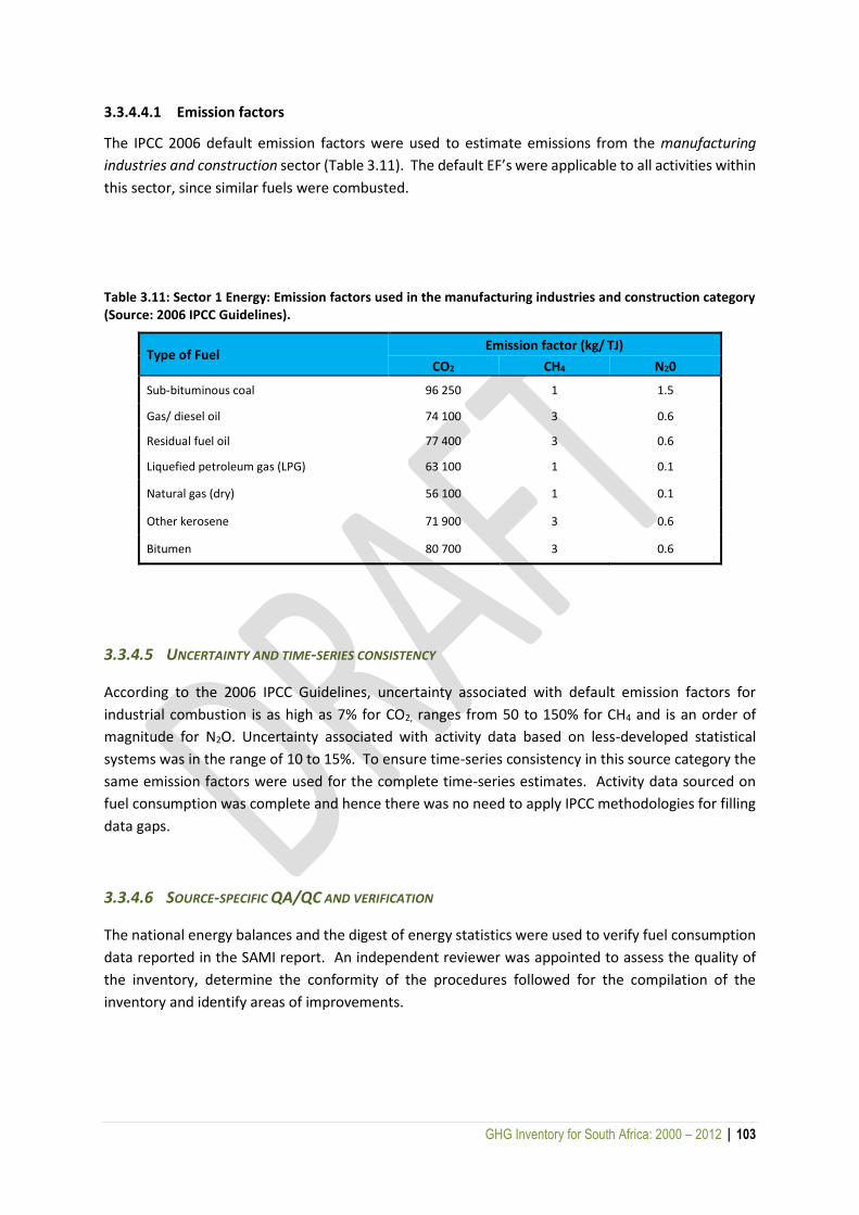
GHG Inventory for South Africa: 2000 – 2012 | 103

3.3.4.4.1 Emission factors

The IPCC 2006 default emission factors were used to estimate emissions from the manufacturing

industries and construction sector (Table 3.11). The default EF’s were applicable to all activities within

this sector, since similar fuels were combusted.

Table 3.11: Sector 1 Energy: Emission factors used in the manufacturing industries and construction category (Source: 2006 IPCC Guidelines).

Type of Fuel Emission factor (kg/ TJ)

CO2 CH4 N20

Sub-bituminous coal 96 250 1 1.5

Gas/ diesel oil 74 100 3 0.6

Residual fuel oil 77 400 3 0.6

Liquefied petroleum gas (LPG) 63 100 1 0.1

Natural gas (dry) 56 100 1 0.1

Other kerosene 71 900 3 0.6

Bitumen 80 700 3 0.6

3.3.4.5 UNCERTAINTY AND TIME-SERIES CONSISTENCY

According to the 2006 IPCC Guidelines, uncertainty associated with default emission factors for

industrial combustion is as high as 7% for CO2, ranges from 50 to 150% for CH4 and is an order of

magnitude for N2O. Uncertainty associated with activity data based on less-developed statistical

systems was in the range of 10 to 15%. To ensure time-series consistency in this source category the

same emission factors were used for the complete time-series estimates. Activity data sourced on

fuel consumption was complete and hence there was no need to apply IPCC methodologies for filling

data gaps.

3.3.4.6 SOURCE-SPECIFIC QA/QC AND VERIFICATION

The national energy balances and the digest of energy statistics were used to verify fuel consumption

data reported in the SAMI report. An independent reviewer was appointed to assess the quality of

the inventory, determine the conformity of the procedures followed for the compilation of the

inventory and identify areas of improvements.

GHG Inventory for South Africa: 2000 – 2012 | 104

3.3.4.7 SOURCE-SPECIFIC RECALCULATIONS

In the previous 2000 GHG inventory, activity data for this category were sourced from the energy

balances published by the DoE. For this inventory a combination of the energy digest and the SAMI

report was used as a source of activity data for solid fuels, and SAPIA was the source of activity data

from liquid fuels. The combination of a variety of publicly available information has improved the

accuracy of the activity data for this category.

3.3.4.8 SOURCE-SPECIFIC PLANNED IMPROVEMENTS AND RECOMMENDATIONS

In future, facility-level data needs to be sourced and country-specific emission factors have to be

developed in order to move towards a Tier 2 methodology. The reliance on energy balances and other

publications for the compilation of emissions needs to be reduced by sourcing facility-level activity

data. This would help to reduce the uncertainty associated with the activity data.

3.3.5 Transport [1A3]

According to the 2006 IPCC Guidelines, estimates of GHG emissions from mobile combustion refers to

major transport activities such as road, off-road, air, railways and waterborne navigation. This

category only includes direct emissions from transport activities, mainly from liquid fuels (gasoline,

diesel, aviation gas and jet fuel). Secondary fuels, such as electricity used by trains, are reported under

the main activity electricity and heat production category and not under the transport category. The

diversity of sources and combustion takes into consideration the age of the fleet, maintenance, the

sulphur content of the fuel used and patterns of use of the various transport modes. The GHG

inventory includes emissions from combustion and evaporation of fuels for all transport activity.

The 2006 IPCC Guidelines indicate that, where possible, activities such as agricultural machinery,

fishing boats and military transport should be recorded separately under the appropriate sectors and

not in the transport sector (IPCC 2006, p.3.8). Furthermore, GHG emissions from fuels sold to any air

or marine vessels engaged in international transport are excluded from the national total emissions

and are reported separately under the memo items.

3.3.5.1 SOURCE CATEGORY DESCRIPTION

3.3.5.1.1 Civil aviation [1A3a]

Civil aviation emissions are produced from the combustion of jet fuel (jet kerosene and jet gasoline)

and aviation gasoline. Aircraft engine emissions (ground emissions and cruise emissions) are roughly

composed of 70% CO2, less than 30% water and 1.0% of other components (NOx, CO, SOx, NMVOCs,

particulates, and trace components). Civil aviation data were sourced from both domestic and

international aircrafts, including departures and arrivals. That also included civil commercial use of

airplanes, scheduled and charter traffic for passengers and freight, air taxing, agricultural airplanes,

GHG Inventory for South Africa: 2000 – 2012 | 105

private jets and helicopters. The GHG emissions from military aviation are reported separately under

the other category or the memo item multilateral operations.

International aviation (international bunkers) [1A3aI]

GHG emissions from aircraft that returned from an international destination or were going to an

international airport were included under this sub-category. That included civil commercial use of

airplanes, scheduled and charter traffic for passengers and freight, air taxiing, agricultural airplanes,

private jets and helicopters. The GHG emissions from military aviation were reported separately under

the other category or under the memo item multilateral operations.

3.3.5.1.2 Road transport [1A3b]

According to the 2006 IPCC Guidelines, road transport emissions include fuel consumption by light-

duty vehicles (cars and light delivery vehicles), heavy-duty vehicles (trucks, buses and tractors) and

motorcycles (including mopeds, scooters and three-wheelers). Fuels used by agricultural vehicles on

paved roads are also included in this category. The DoE’s energy balances list the fuels under road

transport as diesel, gasoline, other kerosene, residual fuel oil and LPG. Road transport was responsible

for the largest fuel consumed in the transport sector (79.1% in 2012). Motor gas contributed 64.9% of

the road transport fuel consumption in 2010, followed by gas/diesel oil (35%). Between 2000 and

2012 there was an increase in the percentage contribution of gas/diesel oil to road transport

consumption (80.1%), and a corresponding decline of 12.7% in the contribution from motor gasoline

(Figure 3.7). This can be attributed to the efficiency and affordability of diesel compared with motor

gasoline.

GHG Inventory for South Africa: 2000 – 2012 | 106

Figure 3.7: Sector 1 Energy: Percentage contribution of the various fuel types to fuel consumption in the road

transport category (1A3b), 2000 – 2012.

3.3.5.1.3 Railways [1A3c]

Railway locomotives are mostly one of three types: diesel, electric or steam. Diesel locomotives

generally use engines in combination with a generator to produce the energy required to power the

locomotive. Electric locomotives are powered by electricity generated at power stations and other

sources. Steam locomotives are generally used for local operations, primarily as tourist attractions

and their GHG emissions are very low (DME, 2002). Both freight and passenger railway traffic

generates emissions. South Africa’s railway sector uses electricity as its main source of energy, with

diesel being the only other energy source (DME, 2002).

3.3.5.1.4 Water-borne navigation [1A3d]

According to the 2006 IPCC Guidelines, waterborne navigation sources include emissions from the use

of fossil fuels in all waterborne transport, from recreational craft to large ocean cargo ships, but

exclude fishing vessels. Fishing vessels are accounted for under the other sector, in the fishing

subcategory. The vessels are driven primarily by large, medium to slow diesel engines and sometimes

by steam or gas turbines.

0%

10%

20%

30%

40%

50%

60%

70%

80%

90%

100%

2000 2001 2002 2003 2004 2005 2006 2007 2008 2009 2010 2011 2012

LPG

Residual Fuel Oil

Gas / Diesel Oil

Other Kerosene

Motor Gasoline

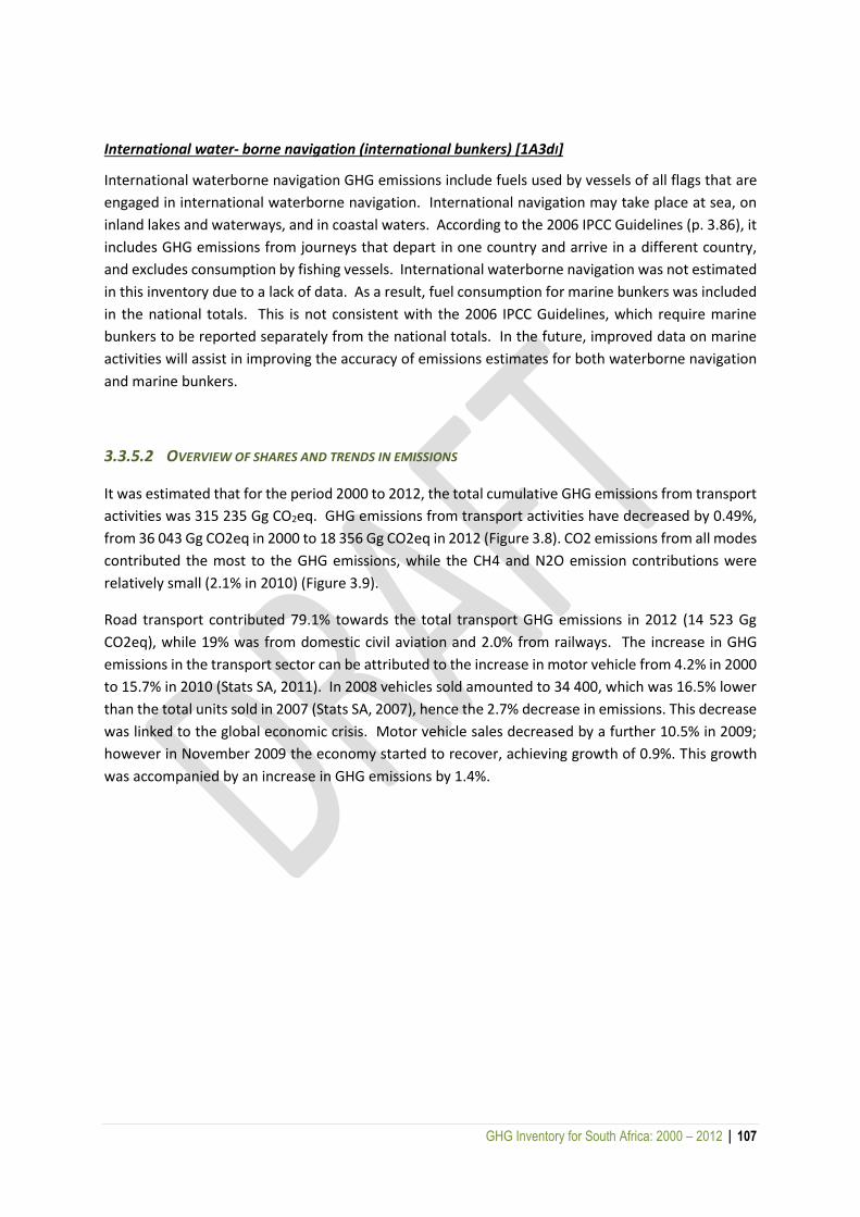
GHG Inventory for South Africa: 2000 – 2012 | 107

International water- borne navigation (international bunkers) [1A3dI]

International waterborne navigation GHG emissions include fuels used by vessels of all flags that are

engaged in international waterborne navigation. International navigation may take place at sea, on

inland lakes and waterways, and in coastal waters. According to the 2006 IPCC Guidelines (p. 3.86), it

includes GHG emissions from journeys that depart in one country and arrive in a different country,

and excludes consumption by fishing vessels. International waterborne navigation was not estimated

in this inventory due to a lack of data. As a result, fuel consumption for marine bunkers was included

in the national totals. This is not consistent with the 2006 IPCC Guidelines, which require marine

bunkers to be reported separately from the national totals. In the future, improved data on marine

activities will assist in improving the accuracy of emissions estimates for both waterborne navigation

and marine bunkers.

3.3.5.2 OVERVIEW OF SHARES AND TRENDS IN EMISSIONS

It was estimated that for the period 2000 to 2012, the total cumulative GHG emissions from transport

activities was 315 235 Gg CO2eq. GHG emissions from transport activities have decreased by 0.49%,

from 36 043 Gg CO2eq in 2000 to 18 356 Gg CO2eq in 2012 (Figure 3.8). CO2 emissions from all modes

contributed the most to the GHG emissions, while the CH4 and N2O emission contributions were

relatively small (2.1% in 2010) (Figure 3.9).

Road transport contributed 79.1% towards the total transport GHG emissions in 2012 (14 523 Gg

CO2eq), while 19% was from domestic civil aviation and 2.0% from railways. The increase in GHG

emissions in the transport sector can be attributed to the increase in motor vehicle from 4.2% in 2000

to 15.7% in 2010 (Stats SA, 2011). In 2008 vehicles sold amounted to 34 400, which was 16.5% lower

than the total units sold in 2007 (Stats SA, 2007), hence the 2.7% decrease in emissions. This decrease

was linked to the global economic crisis. Motor vehicle sales decreased by a further 10.5% in 2009;

however in November 2009 the economy started to recover, achieving growth of 0.9%. This growth

was accompanied by an increase in GHG emissions by 1.4%.

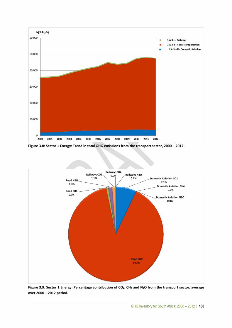
GHG Inventory for South Africa: 2000 – 2012 | 108

Figure 3.8: Sector 1 Energy: Trend in total GHG emissions from the transport sector, 2000 – 2012.

Figure 3.9: Sector 1 Energy: Percentage contribution of CO2, CH4 and N2O from the transport sector, average

over 2000 – 2012 period.

0

10 000

20 000

30 000

40 000

50 000

60 000

2000 2001 2002 2003 2004 2005 2006 2007 2008 2009 2010 2011 2012

Gg CO2eq

1.A.3.c - Railways

1.A.3.b - Road Transportation

1.A.3.a.ii - Domestic Aviation

Domestic Aviation CO27.1%

Domestic Aviation CH40.0%

Domestic Aviation N2O

0.0%

Road CO289.7%

Road CH4

0.7%

Road N2O1.3%

Railways CO21.1%

Railways CH4

0.0% Railways N2O0.1%

GHG Inventory for South Africa: 2000 – 2012 | 109

3.3.5.2.1 Transport emissions and the economy

In the transport sector 92% of the GHG emissions were generated from road transport. There is a

strong linkage between vehicle population and energy demand. It was estimated that the purchase

of motor vehicles increased from 4.81% in 2000 to 10.23% in 2006 (Statistics SA, 2007).

Energy fuels from transport activities consist mainly of liquid fuels. The most dominant fuel is motor

gasoline (53.3%), followed by diesel (34%) and then jet fuel (10.9%). The demand for petrol and diesel

has remained relatively static over the years. The demand for jet fuel has grown steadily, however,

as a result of increased business and tourism activities. In 2001, total liquid-fuel sales grew by 0.3%

to 20 934 million litres (Ml). These figures demonstrate the growth of the South African economy and

the importance of energy as a key driver of the economy.

The primary driver for the transport sector is GDP growth. For road passenger travel, GDP growth

means an increase in the number of commuters and an increase in personal wealth, both in terms of

the number of wealthier people and the size of people's expendable incomes. This results in more

money being available to purchase cars and for leisure activities, which, in turn, increases the demand

for transport and transport fuel.

In terms of civil aviation, there has been an in increase in the number of passengers who disembarked

from international scheduled flights in past years. In 2008 the total number of passengers decreased

by 7.3% (7.8 million) in the 08/09 financial year compared to the 07/08 financial year. However,

passenger activity rose by 5% in the 10/11 financial year amounting to 8.2 million passengers (ACSA,

2013).

Passengers travelling by commuter rail increased to 646.2 million in the financial year 2008/09, a 9%

increase on 2008/09 (Stats SA, 2007). Passenger kilometres travelled by trains also increased by 9% to

16.9 billion kilometres in 2008/09.

Annual growth in GHG emissions from the transport sector slowed between 2003 and 2004, from 4.9%

to 4.1%. This was mainly because the price of oil was at the narrow range of approximately

$22/28/bbl, however in the year 2005 the price of oil escalated significantly.

According to SAPIA, the factors that influenced the escalating crude oil price in 2005 were the

following:

o Feared shortages due to limited surplus crude oil production and refining capacity at

a time of strongly rising world demand for petroleum products, notably in the United

States and China;

o A particular shortage of sweet (low-sulphur) crudes due to a lack of refining capacity

to process sour (high-sulphur) crudes into the requisite product qualities needed by

world markets;

o Political tensions in certain crude oil-producing countries; and

o The petrol price in South Africa is linked to the price of petrol in US dollars and to

certain other international petrol markets.

The local prices of petroleum products are affected by the ZAR-USD exchange rate and the dollar price

of crude oil. It is important to note that in late 2001 when the exchange rate rose above R12 to the

GHG Inventory for South Africa: 2000 – 2012 | 110

dollar and the oil price was about $20/bbl, crude oil cost some R240/bbl, and in 2004 when the rand

strengthened to R6 to the dollar and the crude oil price was $40/bbl, oil still cost some R240/bbl. That

meant, despite some fluctuations, the rand price of crude oil was relatively stable until the dollar price

increased above $40/bbl. At a price of $65/bbl and at a rate of R6,5 to the dollar, the cost became

R423/bbl, a very significant rise.

In 2007, aggregate sales of major petroleum products showed a strong increase of 7.3% in the first

quarter compared with the first quarter of 2006. The most significant increases were in diesel (13.1%),

bitumen (36.3%) and LPG (15%). Petrol sales grew by 4.4% and jet fuel sales by 4.6%. Paraffin sales

declined by 13.4%, indicating that the product was being used less frequently for household energy.

In the first quarter of 2007, the percentage split of petrol sales between unleaded petrol (ULP) and

lead replacement petrol (LRP) was 64% and 36%, respectively.

In 2008 GHG emissions from the transport sector decreased by 2.5%, which was attributed to the

global economic crisis that occurred in 2008 and 2009. Total sales of major petroleum products

showed an increase of 4% in the first quarter of 2008 compared with the first quarter of 2007. The

most significant increases were in diesel (9.5%) and industrial heating fuels (35.6%). Petrol and

paraffin sales declined by 0.9% and 3.2%, respectively, affected by price increases, while jet fuel sales

grew by 3.3%. LPG volumes were the same as in 2007 and bitumen volumes increased by 7.6%.

In November 2009 South Africa's economy recovered from the recession and in 2010 the country

successfully hosted the FIFA World Cup.

International aviation (international bunkers) [1A3aI]

It was estimated that for the period 2000 to 2012 the total cumulative GHG emissions from

international aviation activities was 33 078 Gg CO2eq. Table 3.12 provides a summary of GHG

emissions for the period 2000 to 2012 from international aviation. Over the 12-year assessment

period, GHG emissions emanating from international aviation have decreased by 19%. However in

2005 and 2010 GHG emissions increased by 11% and 6%, respectively. The increase in 2010 could be

attributed to the fact that South Africa hosted the FIFA World Cup and international travel increased

as a result.

Table 3.12: Sector 1 Energy: Summary of GHG emissions from international aviation (international bunkers), 2000 – 2012.

CO2 CH4 N2O Total GHG

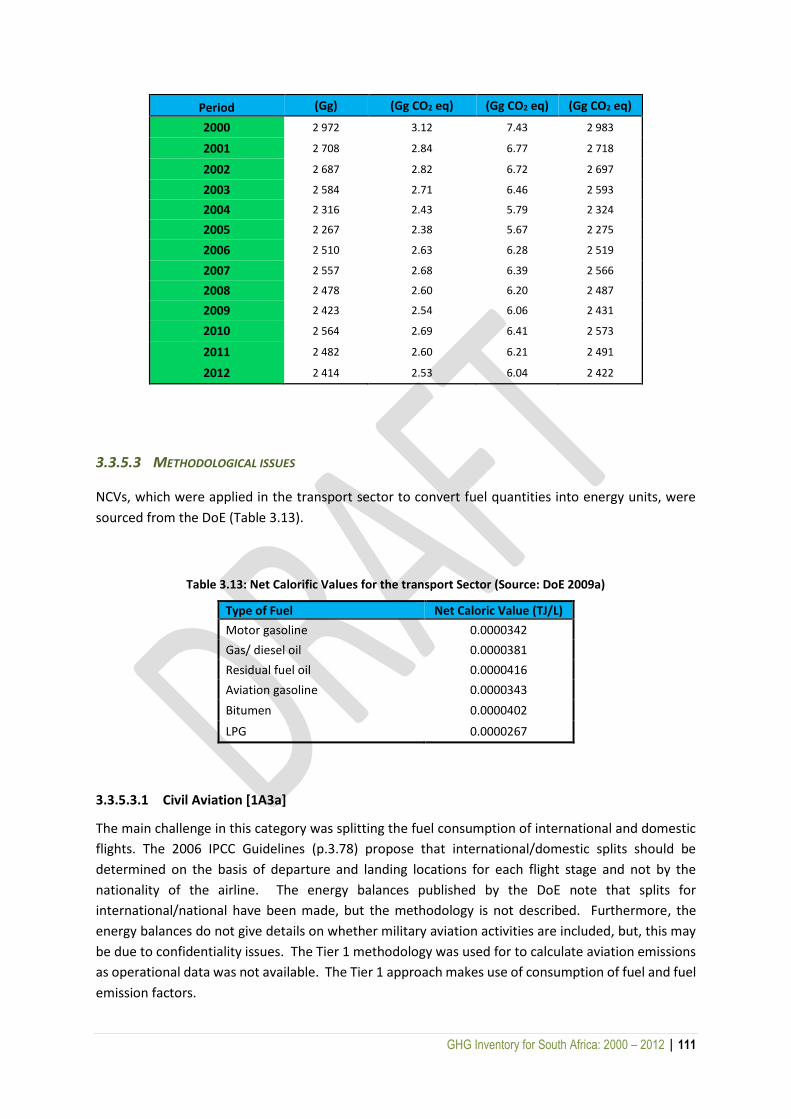
GHG Inventory for South Africa: 2000 – 2012 | 111

Period (Gg) (Gg CO2 eq) (Gg CO2 eq) (Gg CO2 eq)

2000 2 972 3.12 7.43 2 983

2001 2 708 2.84 6.77 2 718

2002 2 687 2.82 6.72 2 697

2003 2 584 2.71 6.46 2 593

2004 2 316 2.43 5.79 2 324

2005 2 267 2.38 5.67 2 275

2006 2 510 2.63 6.28 2 519

2007 2 557 2.68 6.39 2 566

2008 2 478 2.60 6.20 2 487

2009 2 423 2.54 6.06 2 431

2010 2 564 2.69 6.41 2 573

2011 2 482 2.60 6.21 2 491

2012 2 414 2.53 6.04 2 422

3.3.5.3 METHODOLOGICAL ISSUES

NCVs, which were applied in the transport sector to convert fuel quantities into energy units, were

sourced from the DoE (Table 3.13).

Table 3.13: Net Calorific Values for the transport Sector (Source: DoE 2009a)

Type of Fuel Net Caloric Value (TJ/L)

Motor gasoline 0.0000342

Gas/ diesel oil 0.0000381

Residual fuel oil 0.0000416

Aviation gasoline 0.0000343

Bitumen 0.0000402

LPG 0.0000267

3.3.5.3.1 Civil Aviation [1A3a]

The main challenge in this category was splitting the fuel consumption of international and domestic

flights. The 2006 IPCC Guidelines (p.3.78) propose that international/domestic splits should be

determined on the basis of departure and landing locations for each flight stage and not by the

nationality of the airline. The energy balances published by the DoE note that splits for

international/national have been made, but the methodology is not described. Furthermore, the

energy balances do not give details on whether military aviation activities are included, but, this may

be due to confidentiality issues. The Tier 1 methodology was used for to calculate aviation emissions

as operational data was not available. The Tier 1 approach makes use of consumption of fuel and fuel

emission factors.

GHG Inventory for South Africa: 2000 – 2012 | 112

3.3.5.3.2 Road transport [1A3b]

The 2006 IPCC Guidelines suggest that the fuel consumption approach is appropriate for CO2 emissions

as it depends entirely on the carbon content of the fuel combusted, whereas the kilometre approach

(distance travelled by vehicle type) is appropriate for CH4 and N2O. Hence, in order to use a higher-

tier approach for calculating road transport emissions, a better understanding of the fuel sold and

vehicle kilometres travelled is required for the entire South African vehicle fleet. This data was not

available for the entire 12-year period, therefore, a Tier 1 approach based on fuel consumption and

2006 IPCC emission factors was used to calculate the emissions.

3.3.5.3.3 Railways [1A3c]

The Tier 1 approach was used for the calculation of railway emissions. Default emissions factors from

the 2006 IPCC Guidelines were used. The use of a higher-tier approach depends on the availability of

fuel consumption data by locomotive type and/or country-specific emission factors.

3.3.5.4 DATA SOURCES

3.3.5.4.1 Civil aviation [1A3a]

Activity data on fuel consumption was sourced from SAPIA's annual reports (Table 3.14). The 2006

IPCC Guidelines (p. 3.78) require only domestic aviation to be included in the national totals. Hence,

in order to separate international from domestic aviation, the DoE energy balances were used to

estimate the ratio of domestic to international consumption. Furthermore, according to the 2006 IPCC

Guidelines, it is good practice to separate military aviation from domestic aviation. However, based

on the SAPIA data and national energy balances, it is not possible to estimate the amount of fuel used

for military aviation activities. It is not indicated in data sources, therefore, military aviation emissions

are thought to be accounted for under domestic aviation. In the D0E's energy balances civil aviation

fuels include gasworks gas, aviation gasoline and jet kerosene.

International aviation (international bunkers) [1A3aI]

The energy balances published by the DoE were the main source of data for the amount of fuel

consumed (Table 3.14). They did not indicate whether aviation fuel consumption figures included

military aviation activities (these might have been excluded for security reasons).

Table 3.14: Sector 1 Energy: Fuel consumption (TJ) in the transport sector, 2000 – 2012.

Domestic Aviation Road Transportation Railways

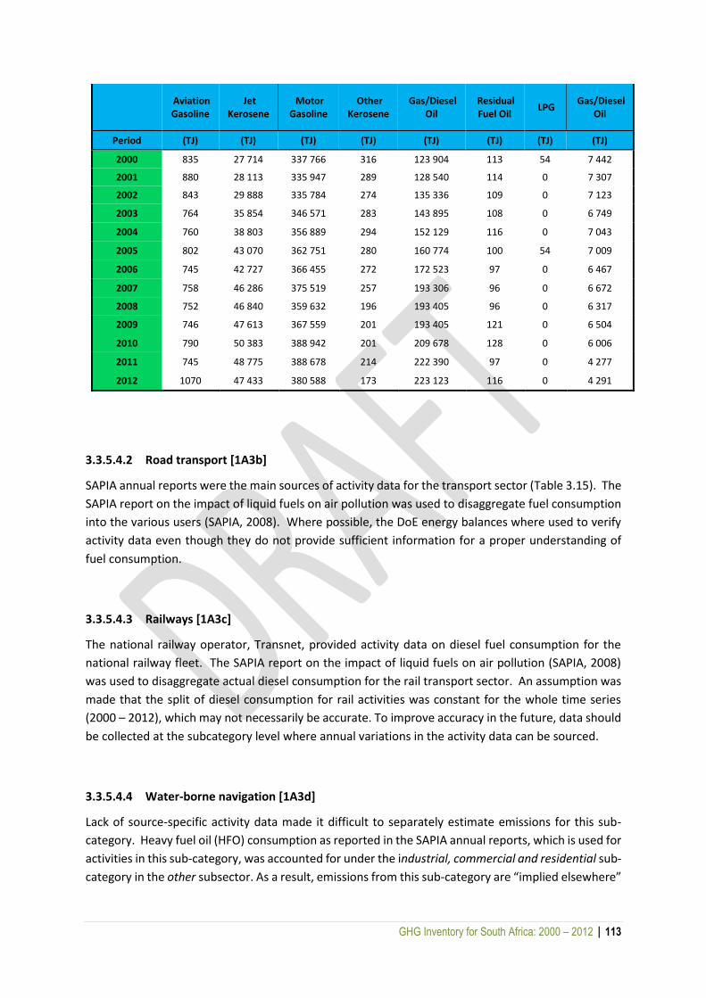
GHG Inventory for South Africa: 2000 – 2012 | 113

Aviation Gasoline

Jet Kerosene

Motor Gasoline

Other Kerosene

Gas/Diesel Oil

Residual Fuel Oil

LPG Gas/Diesel

Oil

Period (TJ) (TJ) (TJ) (TJ) (TJ) (TJ) (TJ) (TJ)

2000 835 27 714 337 766 316 123 904 113 54 7 442

2001 880 28 113 335 947 289 128 540 114 0 7 307

2002 843 29 888 335 784 274 135 336 109 0 7 123

2003 764 35 854 346 571 283 143 895 108 0 6 749

2004 760 38 803 356 889 294 152 129 116 0 7 043

2005 802 43 070 362 751 280 160 774 100 54 7 009

2006 745 42 727 366 455 272 172 523 97 0 6 467

2007 758 46 286 375 519 257 193 306 96 0 6 672

2008 752 46 840 359 632 196 193 405 96 0 6 317

2009 746 47 613 367 559 201 193 405 121 0 6 504

2010 790 50 383 388 942 201 209 678 128 0 6 006

2011 745 48 775 388 678 214 222 390 97 0 4 277

2012 1070 47 433 380 588 173 223 123 116 0 4 291

3.3.5.4.2 Road transport [1A3b]

SAPIA annual reports were the main sources of activity data for the transport sector (Table 3.15). The

SAPIA report on the impact of liquid fuels on air pollution was used to disaggregate fuel consumption

into the various users (SAPIA, 2008). Where possible, the DoE energy balances where used to verify

activity data even though they do not provide sufficient information for a proper understanding of

fuel consumption.

3.3.5.4.3 Railways [1A3c]

The national railway operator, Transnet, provided activity data on diesel fuel consumption for the

national railway fleet. The SAPIA report on the impact of liquid fuels on air pollution (SAPIA, 2008)

was used to disaggregate actual diesel consumption for the rail transport sector. An assumption was

made that the split of diesel consumption for rail activities was constant for the whole time series

(2000 – 2012), which may not necessarily be accurate. To improve accuracy in the future, data should

be collected at the subcategory level where annual variations in the activity data can be sourced.

3.3.5.4.4 Water-borne navigation [1A3d]

Lack of source-specific activity data made it difficult to separately estimate emissions for this sub-

category. Heavy fuel oil (HFO) consumption as reported in the SAPIA annual reports, which is used for

activities in this sub-category, was accounted for under the industrial, commercial and residential sub-

category in the other subsector. As a result, emissions from this sub-category are “implied elsewhere”

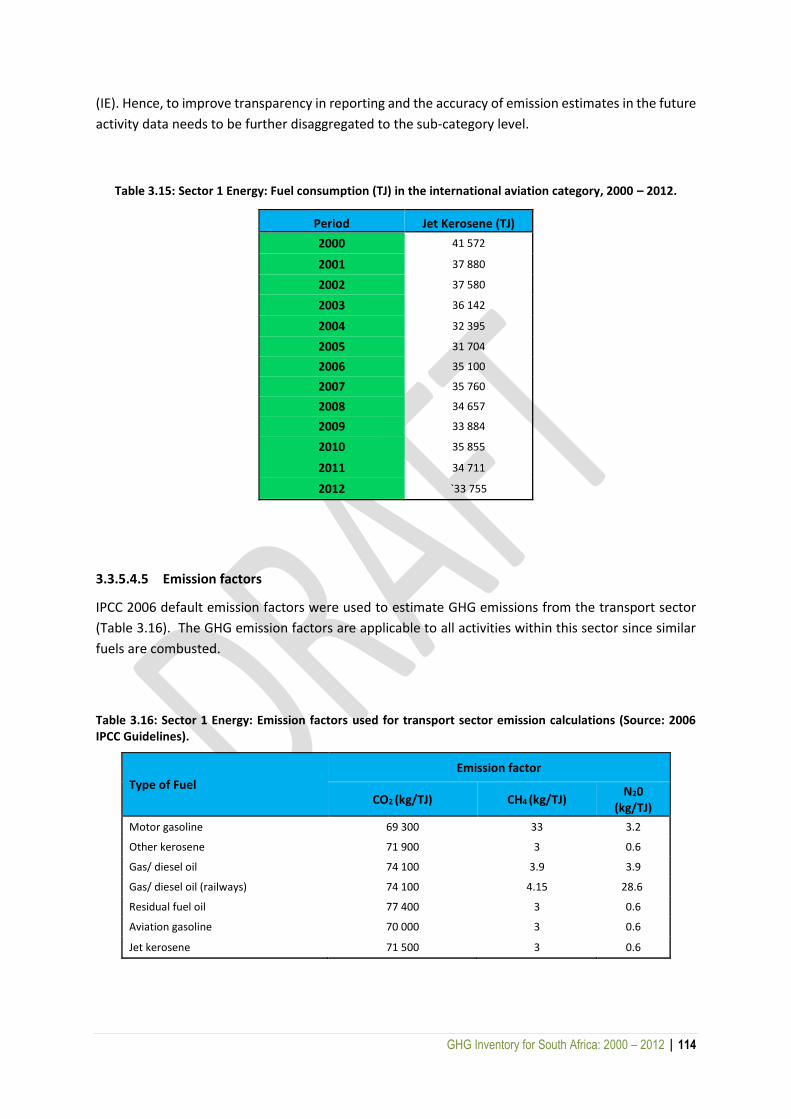
GHG Inventory for South Africa: 2000 – 2012 | 114

(IE). Hence, to improve transparency in reporting and the accuracy of emission estimates in the future

activity data needs to be further disaggregated to the sub-category level.

Table 3.15: Sector 1 Energy: Fuel consumption (TJ) in the international aviation category, 2000 – 2012.

Period Jet Kerosene (TJ)

2000 41 572

2001 37 880

2002 37 580

2003 36 142

2004 32 395

2005 31 704

2006 35 100

2007 35 760

2008 34 657

2009 33 884

2010 35 855

2011 34 711

2012 `33 755

3.3.5.4.5 Emission factors

IPCC 2006 default emission factors were used to estimate GHG emissions from the transport sector

(Table 3.16). The GHG emission factors are applicable to all activities within this sector since similar

fuels are combusted.

Table 3.16: Sector 1 Energy: Emission factors used for transport sector emission calculations (Source: 2006 IPCC Guidelines).

Type of Fuel

Emission factor

CO2 (kg/TJ) CH4 (kg/TJ) N20

(kg/TJ)

Motor gasoline 69 300 33 3.2

Other kerosene 71 900 3 0.6

Gas/ diesel oil 74 100 3.9 3.9

Gas/ diesel oil (railways) 74 100 4.15 28.6

Residual fuel oil 77 400 3 0.6

Aviation gasoline 70 000 3 0.6

Jet kerosene 71 500 3 0.6

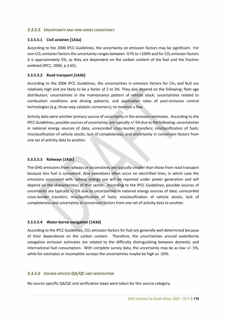
GHG Inventory for South Africa: 2000 – 2012 | 115

3.3.5.5 UNCERTAINTY AND TIME-SERIES CONSISTENCY

3.3.5.5.1 Civil aviation [1A3a]

According to the 2006 IPCC Guidelines, the uncertainty on emission factors may be significant. For

non-CO2 emission factors the uncertainty ranges between -57% to +100% and for CO2 emission factors

it is approximately 5%, as they are dependent on the carbon content of the fuel and the fraction

oxidized (IPCC, 2006, p.3.65).

3.3.5.5.2 Road transport [1A3b]

According to the 2006 IPCC Guidelines, the uncertainties in emission factors for CH4 and N2O are

relatively high and are likely to be a factor of 2 to 3%. They also depend on the following: fleet age

distribution; uncertainties in the maintenance pattern of vehicle stock; uncertainties related to

combustion conditions and driving patterns; and application rates of post-emission control

technologies (e.g. three-way catalytic converters), to mention a few.

Activity data were another primary source of uncertainty in the emission estimates. According to the

IPCC Guidelines, possible sources of uncertainty, are typically +/-5% due to the following: uncertainties

in national energy sources of data; unrecorded cross-border transfers; misclassification of fuels;

misclassification of vehicle stocks; lack of completeness; and uncertainty in conversion factors from

one set of activity data to another.

3.3.5.5.3 Railways [1A3c]

The GHG emissions from railways or locomotives are typically smaller than those from road transport

because less fuel is consumed. Also operations often occur on electrified lines, in which case the

emissions associated with railway energy use will be reported under power generation and will

depend on the characteristics of that sector. According to the IPCC Guidelines, possible sources of

uncertainty are typically +/-5% due to uncertainties in national energy sources of data; unrecorded

cross-border transfers; misclassification of fuels; misclassification of vehicle stocks; lack of

completeness and uncertainty in conversion factors from one set of activity data to another.

3.3.5.5.4 Water-borne navigation [1A3d]

According to the IPCC Guidelines, CO2 emission factors for fuel are generally well determined because

of their dependence on the carbon contenl. Therefore, the uncertainties around waterborne

navigation emission estimates are related to the difficulty distinguishing between domestic and

international fuel consumption. With complete survey data, the uncertainty may be as low +/- 5%,

while for estimates or incomplete surveys the uncertainties maybe be high as -50%.

3.3.5.6 SOURCE-SPECIFIC QA/QC AND VERIFICATION

No source-specific QA/QC and verification steps were taken for this source category.

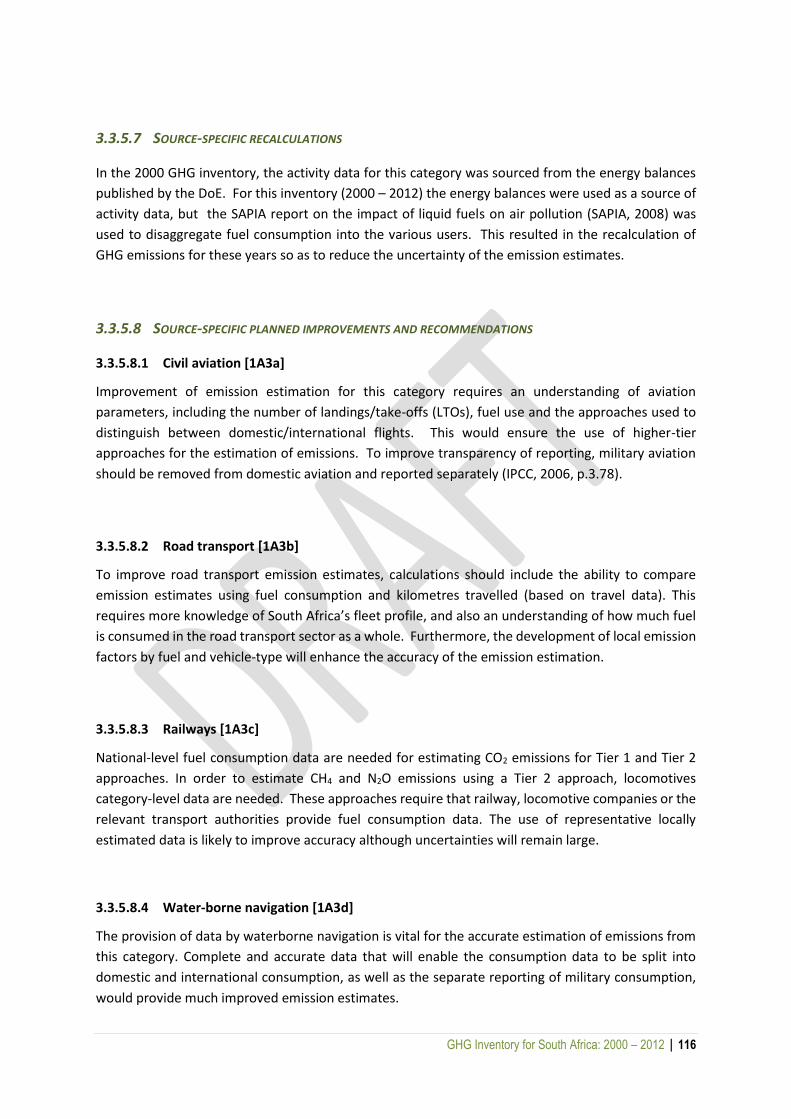
GHG Inventory for South Africa: 2000 – 2012 | 116

3.3.5.7 SOURCE-SPECIFIC RECALCULATIONS

In the 2000 GHG inventory, the activity data for this category was sourced from the energy balances

published by the DoE. For this inventory (2000 – 2012) the energy balances were used as a source of

activity data, but the SAPIA report on the impact of liquid fuels on air pollution (SAPIA, 2008) was

used to disaggregate fuel consumption into the various users. This resulted in the recalculation of

GHG emissions for these years so as to reduce the uncertainty of the emission estimates.

3.3.5.8 SOURCE-SPECIFIC PLANNED IMPROVEMENTS AND RECOMMENDATIONS

3.3.5.8.1 Civil aviation [1A3a]

Improvement of emission estimation for this category requires an understanding of aviation

parameters, including the number of landings/take-offs (LTOs), fuel use and the approaches used to

distinguish between domestic/international flights. This would ensure the use of higher-tier

approaches for the estimation of emissions. To improve transparency of reporting, military aviation

should be removed from domestic aviation and reported separately (IPCC, 2006, p.3.78).

3.3.5.8.2 Road transport [1A3b]

To improve road transport emission estimates, calculations should include the ability to compare

emission estimates using fuel consumption and kilometres travelled (based on travel data). This

requires more knowledge of South Africa’s fleet profile, and also an understanding of how much fuel

is consumed in the road transport sector as a whole. Furthermore, the development of local emission

factors by fuel and vehicle-type will enhance the accuracy of the emission estimation.

3.3.5.8.3 Railways [1A3c]

National-level fuel consumption data are needed for estimating CO2 emissions for Tier 1 and Tier 2

approaches. In order to estimate CH4 and N2O emissions using a Tier 2 approach, locomotives

category-level data are needed. These approaches require that railway, locomotive companies or the

relevant transport authorities provide fuel consumption data. The use of representative locally

estimated data is likely to improve accuracy although uncertainties will remain large.

3.3.5.8.4 Water-borne navigation [1A3d]

The provision of data by waterborne navigation is vital for the accurate estimation of emissions from

this category. Complete and accurate data that will enable the consumption data to be split into

domestic and international consumption, as well as the separate reporting of military consumption,

would provide much improved emission estimates.

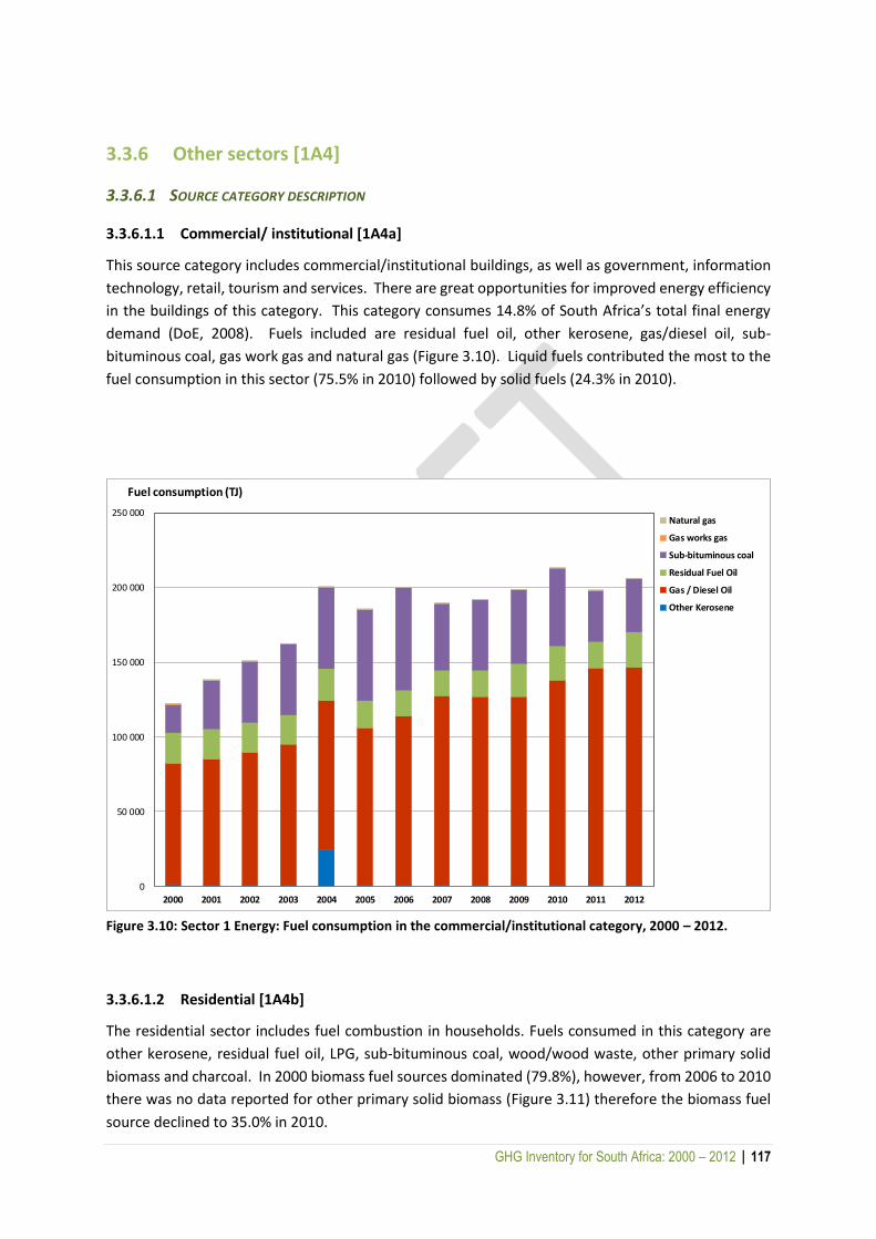
GHG Inventory for South Africa: 2000 – 2012 | 117

3.3.6 Other sectors [1A4]

3.3.6.1 SOURCE CATEGORY DESCRIPTION

3.3.6.1.1 Commercial/ institutional [1A4a]

This source category includes commercial/institutional buildings, as well as government, information

technology, retail, tourism and services. There are great opportunities for improved energy efficiency

in the buildings of this category. This category consumes 14.8% of South Africa’s total final energy

demand (DoE, 2008). Fuels included are residual fuel oil, other kerosene, gas/diesel oil, sub-

bituminous coal, gas work gas and natural gas (Figure 3.10). Liquid fuels contributed the most to the

fuel consumption in this sector (75.5% in 2010) followed by solid fuels (24.3% in 2010).

Figure 3.10: Sector 1 Energy: Fuel consumption in the commercial/institutional category, 2000 – 2012.

3.3.6.1.2 Residential [1A4b]

The residential sector includes fuel combustion in households. Fuels consumed in this category are

other kerosene, residual fuel oil, LPG, sub-bituminous coal, wood/wood waste, other primary solid

biomass and charcoal. In 2000 biomass fuel sources dominated (79.8%), however, from 2006 to 2010

there was no data reported for other primary solid biomass (Figure 3.11) therefore the biomass fuel

source declined to 35.0% in 2010.

0

50 000

100 000

150 000

200 000

250 000

2000 2001 2002 2003 2004 2005 2006 2007 2008 2009 2010 2011 2012

Fuel consumption (TJ)

Natural gas

Gas works gas

Sub-bituminous coal

Residual Fuel Oil

Gas / Diesel Oil

Other Kerosene

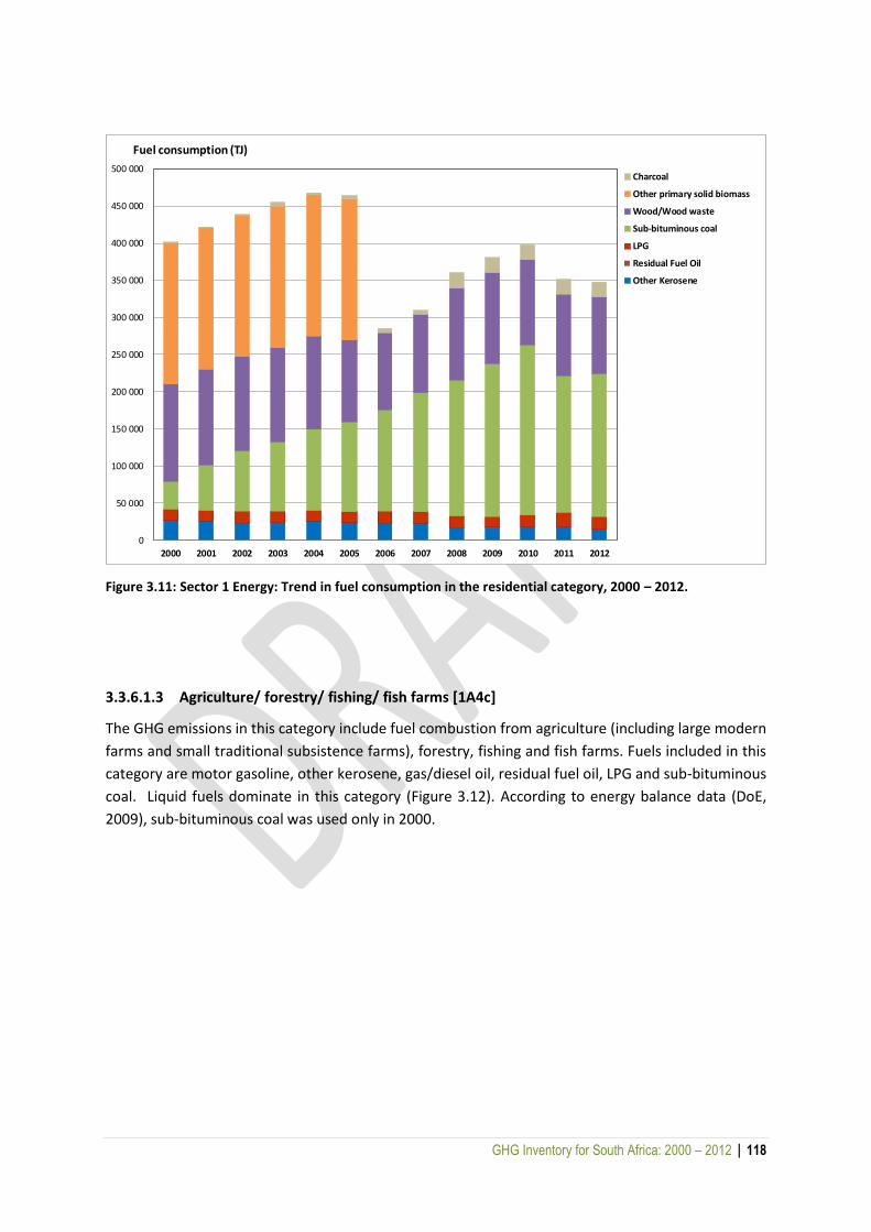
GHG Inventory for South Africa: 2000 – 2012 | 118

Figure 3.11: Sector 1 Energy: Trend in fuel consumption in the residential category, 2000 – 2012.

3.3.6.1.3 Agriculture/ forestry/ fishing/ fish farms [1A4c]

The GHG emissions in this category include fuel combustion from agriculture (including large modern

farms and small traditional subsistence farms), forestry, fishing and fish farms. Fuels included in this

category are motor gasoline, other kerosene, gas/diesel oil, residual fuel oil, LPG and sub-bituminous

coal. Liquid fuels dominate in this category (Figure 3.12). According to energy balance data (DoE,

2009), sub-bituminous coal was used only in 2000.

0

50 000

100 000

150 000

200 000

250 000

300 000

350 000

400 000

450 000

500 000

2000 2001 2002 2003 2004 2005 2006 2007 2008 2009 2010 2011 2012

Fuel consumption (TJ)

Charcoal

Other primary solid biomass

Wood/Wood waste

Sub-bituminous coal

LPG

Residual Fuel Oil

Other Kerosene

GHG Inventory for South Africa: 2000 – 2012 | 119

Figure 3.12: Sector 1 Energy: Trend in fuel consumption in the agriculture/forestry/fishing category, 2000 –

2012.

3.3.6.2 OVERVIEW OF SHARES AND TRENDS IN EMISSIONS

3.3.6.2.1 Commercial/ institutional [1A4a]

The estimation of total cumulative GHG emissions in the commercial/institutional category for the

period 2000 to 2012 was 189 488 Gg CO2 eq. Emissions increased by 70 % over the 12 year period

from 9 558 Gg CO2 eq in 2000 to 16 214 Gg CO2 eq in 2012 (Figure 3.13). Emissions were dominated

by CO2 emissions, with a small percentage of CH4 and N2O.

In 2001 GHG emissions in this category increased by 11% compared with the previous year, and

continued to increase annually from 2002 to 2003. That might have been as a result of economic

growth and development during that period. The increase in 2003 (23%) was linked to the increased

used of other kerosene. There was a slight decline in emissions in 2007 which was due to a reduction

in sub-bituminous coal consumption that year. That was possibly linked to boiler-fuel switching from

coal to gas in small-to-medium enterprises. GHG emissions in 2010 decreased by 9%, followed by an

increase of 4% in 2012.

0

5 000

10 000

15 000

20 000

25 000

30 000

35 000

40 000

45 000

50 000

2000 2001 2002 2003 2004 2005 2006 2007 2008 2009 2010 2011 2012

Fuel consumption (TJ)

Sub-bituminous coal

LPG

Residual Fuel Oil

Gas / Diesel Oil

Other Kerosene

Motor Gasoline

GHG Inventory for South Africa: 2000 – 2012 | 120

Figure 3.13: Sector 1 Energy: Trend in total GHG emissions from other sectors, 2000 – 2012.

3.3.6.2.2 Residential [1A4b]

The estimation of total GHG emissions in the residential category for the period 2000 to 2012 was 212

888 Gg CO2eq. Emissions in the residential sector have increased more than three fold from 7 121 Gg

CO2eq in 2000 to 21 073 Gg CO2eq in 2012 (Figure 3.13). The increase was attributed mainly to

population growth and economic growth (70.44% in 2000 to 75% in 2009). The GHG emissions in this

category increased annually. The South African residential category consumes 20% of the total energy

supply; this includes gas, electricity, candles, wood, dung, coal, LPG, paraffin, gas and other vegetable

matter. In 2006, 72.8% of energy consumed by South African households was in the form of electricity,

29.1% in the form of coal, and 7.4% in the form of petroleum products (such as LPG and paraffin) (DoE,

2009b). By 2009, 75% of households (9 245 357 households) were electrified (DoE, 2009b).

It has been recorded that more than 10 million electrified households in South Africa have been fitted

with eight incandescent lights per household. In 2008 Eskom rolled out compact fluorescent lamps

(CFLs), which resulted in a saving of 800 MW of electricity. By September 2009, more than 30 million

lamps had been replaced. Energy consumed by households represented 17% of the country’s net use.

Most of household energy was obtained from fuel wood (50% of the net household energy), primarily

in the rural areas, with the remainder being obtained from coal (18%), illuminating paraffin (7%) and

a small amount from LPG. The estimated number of households with access to electricity increased

from 4.5 million (50.9%) in 1994 to 9.1 million (73%) in 2008. Coal is used by approximately 950 000

households countrywide.

0

5 000

10 000

15 000

20 000

25 000

30 000

35 000

40 000

45 000

50 000

2000 2001 2002 2003 2004 2005 2006 2007 2008 2009 2010 2011 2012

Gg CO2eq

1.A.4.c -Agriculture/Forestry/Fishing/Fish Farms

1.A.4.b - Residential

1.A.4.a - Commercial/Institutional

GHG Inventory for South Africa: 2000 – 2012 | 121

GHG emissions in this category increased annually, however in 2011 there was a decline of 16.77%.

This could have been due to an increase of more than 10% in the food price. The price of basic

foodstuffs, such as maize, wheat, soya beans and rice, increased as a result of changing climatic

conditions and rising demand. In 2007 GHG emissions in the residential category increased by 13.6%

compared with the previous year.

3.3.6.2.3 Agriculture/ forestry/ fishing/ fish farms [1A4c]

Primary agriculture contributes approximately 3.2% to the GDP of South Africa and provides almost

9% of formal employment. The majority of the energy for agriculture is sourced from diesel and

vegetable waste (DoE, 2010). In 2006 approximately 69% of energy for use in agriculture was sourced

from petroleum products, 29.9% from electricity and 1.1% from coal (DoE, 2010). The estimated total

GHG emissions of the agriculture/forestry/fishing/fish farms category for the period 2000 to 2012 was

36 805 Gg CO2eq. GHG emissions increased from 2 388 Gg CO2eq in 2000 to 3 432 Gg CO2 eq in 2012,

with annual increases of between 1.5% and 9.3% (Figure 3.13).

GHG emissions in 2008, during the global economic crisis, decreased by 1.66%, while in 2010 GHG

emissions peaked, increasing by 7.93%.

There was a decline in emissions between 2000 and 2001. The contribution of the

agriculture/forestry/fishing/fish farms category to the GDP also decreased by 3.3% during the same

period. In 2008 the sector's GHG emissions decreased by 1.7%, accompanied by a massive GDP

contribution of 16.1% in the same period. However, in 2009 its contribution to the GDP decreased to

0.3% and the GHG emissions increased by 1.46%., mainly because of the global economic crisis in

2008/09.

3.3.6.3 METHODOLOGICAL ISSUES

The Tier 1 approach was used to estimate emissions from all the other sectors. To estimate the total

GHG emissions of this sector, the amount of fuel combusted was multiplied with the default emission

factors from the 2006 IPCC Guidelines (Table 3.17).

3.3.6.4 DATA SOURCES

3.3.6.4.1 Commercial/ institutional [1A4a]

Data on fuel consumption in the commercial/institutional buildings category was sourced from the

DoE's energy digest reports, the DMR's SAMI report (solid fuels and natural gas) and SAPIA (liquid

fuels). The DoE energy reports were used to source solid fuels for the period 2000 to 2006, for the

period 20007 to 2010, the SAMI report was used to extrapolate the consumption of solid fuels for this

category. An NCV of 0.0243 TJ/tonne was used to convert fuel quantities into energy units (DoE,

2009a).

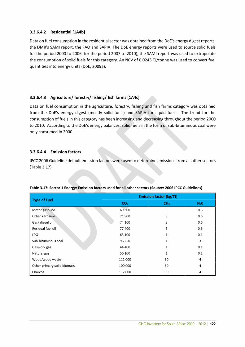
GHG Inventory for South Africa: 2000 – 2012 | 122

3.3.6.4.2 Residential [1A4b]

Data on fuel consumption in the residential sector was obtained from the DoE's energy digest reports,

the DMR's SAMI report, the FAO and SAPIA. The DoE energy reports were used to source solid fuels

for the period 2000 to 2006, for the period 2007 to 2010), the SAMI report was used to extrapolate

the consumption of solid fuels for this category. An NCV of 0.0243 TJ/tonne was used to convert fuel

quantities into energy units (DoE, 2009a).

3.3.6.4.3 Agriculture/ forestry/ fishing/ fish farms [1A4c]

Data on fuel consumption in the agriculture, forestry, fishing and fish farms category was obtained

from the DoE's energy digest (mostly solid fuels) and SAPIA for liquid fuels. The trend for the

consumption of fuels in this category has been increasing and decreasing throughout the period 2000

to 2010. According to the DoE's energy balances, solid fuels in the form of sub-bituminous coal were

only consumed in 2000.

3.3.6.4.4 Emission factors

IPCC 2006 Guideline default emission factors were used to determine emissions from all other sectors

(Table 3.17).

Table 3.17: Sector 1 Energy: Emission factors used for all other sectors (Source: 2006 IPCC Guidelines).

Type of Fuel Emission factor (kg/TJ)

CO2 CH4 N20

Motor gasoline 69 300 3 0.6

Other kerosene 71 900 3 0.6

Gas/ diesel oil 74 100 3 0.6

Residual fuel oil 77 400 3 0.6

LPG 63 100 1 0.1

Sub-bituminous coal 96 250 1 3

Gaswork gas 44 400 1 0.1

Natural gas 56 100 1 0.1

Wood/wood waste 112 000 30 4

Other primary solid biomass 100 000 30 4

Charcoal 112 000 30 4

GHG Inventory for South Africa: 2000 – 2012 | 123

3.3.6.5 UNCERTAINTY AND TIME-SERIES CONSISTENCY

The uncertainties in CO2 emissions are relatively low in fossil fuel combustion. These emission factors

are determined by the carbon content of the fuel. Emission factors for CH4 and more specifically N2O

are highly uncertain. The uncertainty on the CH4 emission factor is 50 to 150%, while for N2O it is an

order of magnitude. This high uncertainty is due to the lack of relevant and accurate measurements

and/or insufficient understanding of the emission generating process.

3.3.6.6 SOURCE-SPECIFIC QA/QC AND VERIFICATION

An independent reviewer was appointed to assess the quality of the inventory, determine the

conformity of the procedures followed for the compilation of this inventory and to identify areas of

improvements.

3.3.6.7 SOURCE-SPECIFIC RECALCULATIONS

In the previous 2000 GHG inventory, the activity data for this category was sourced from the energy

balances published by the DoE. For this inventory a combination of sources of activity data were used,

including the DoE's energy digest, the DMR's SAMI report, SAPIA and the FAO. The inclusion of various

sources of data has improved the accuracy of the GHG inventory which led to a recalculation of

emissions for these categories. The results for the published 2000 GHG inventory had to be

recalculated as a result of the availability of more robust activity data.

3.3.6.8 SOURCE-SPECIFIC PLANNED IMPROVEMENTS AND RECOMMENDATIONS

3.3.6.8.1 Commercial/ institutional [1A4a]

The Tier 1 approach is used for the simplest calculation methods or methods that require the least

data; therefore this approach provides the least accurate estimates of emissions. The Tier 2 and Tier

3 approaches require more detailed data and resources to produce accurate estimates of emissions.

The commercial/institutional sector should be willing to co-operate in the provision of data for the

purposes of inventories. A regulatory framework should be established and implemented to ensure

that sectors provide the data necessary for the compilation of the inventory.

3.3.6.8.2 Residential [1A4b]

Investigations and studies of the residential sector in South Africa are necessary for the accurate

estimation of emissions. Due to the many households, uniform reporting would be possible if data

were collected by local government.

GHG Inventory for South Africa: 2000 – 2012 | 124

3.3.6.8.3 Agriculture/ forestry/ fishing/ fish farms [1A4c]

A regulatory framework should be established and implemented to ensure that sectors provide the

data necessary for the compilation of the inventory.

3.3.7 Non-specified [1A5]

3.3.7.1 SOURCE CATEGORY DESCRIPTION

This category refers to all remaining emissions from fuel combustion that were not specified

elsewhere in this document. It should include emissions from fuel delivered to the military in the

country and delivered to the military of other countries that are not engaged in multilateral

operations.

3.3.7.1.1 Stationary [1A5a]

This section includes emissions from fuel combustion in stationary sources that are not specified

elsewhere. The only fuel reported under this category was the consumption of motor gasoline.

3.3.7.2 OVERVIEW OF SHARES AND TRENDS IN EMISSIONS

The non-specified stationary category showed a steady increase of 12.68% in total GHG emissions

between 2000 and 2012. Emissions were estimated at 989 Gg CO2 eq in 2000 and 1 114 Gg CO2 eq in

2012 (Table 3.18). There was a slight decline of 0.71% between 2000 and 2002 and a 4.23% decline in

2008.

3.3.7.3 METHODOLOGICAL ISSUES

The Tier 1 approach was used for the calculation of emissions in the non-specified sector. To estimate

the total GHG emissions for this sector, the activity data (fuel consumed) was multiplied by the default

emission factor from the 2006 IPCC Guidelines.

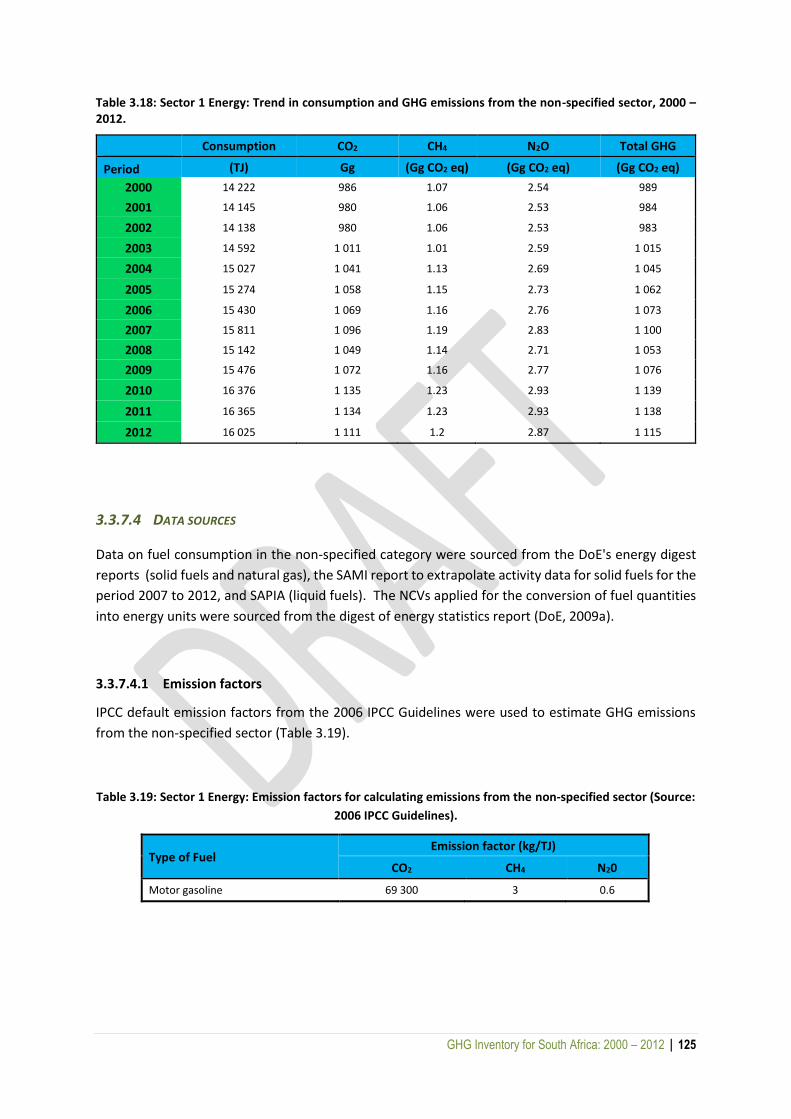
GHG Inventory for South Africa: 2000 – 2012 | 125

Table 3.18: Sector 1 Energy: Trend in consumption and GHG emissions from the non-specified sector, 2000 – 2012.

Consumption CO2 CH4 N2O Total GHG

Period (TJ) Gg (Gg CO2 eq) (Gg CO2 eq) (Gg CO2 eq)

2000 14 222 986 1.07 2.54 989

2001 14 145 980 1.06 2.53 984

2002 14 138 980 1.06 2.53 983

2003 14 592 1 011 1.01 2.59 1 015

2004 15 027 1 041 1.13 2.69 1 045

2005 15 274 1 058 1.15 2.73 1 062

2006 15 430 1 069 1.16 2.76 1 073

2007 15 811 1 096 1.19 2.83 1 100

2008 15 142 1 049 1.14 2.71 1 053

2009 15 476 1 072 1.16 2.77 1 076

2010 16 376 1 135 1.23 2.93 1 139

2011 16 365 1 134 1.23 2.93 1 138

2012 16 025 1 111 1.2 2.87 1 115

3.3.7.4 DATA SOURCES

Data on fuel consumption in the non-specified category were sourced from the DoE's energy digest

reports (solid fuels and natural gas), the SAMI report to extrapolate activity data for solid fuels for the

period 2007 to 2012, and SAPIA (liquid fuels). The NCVs applied for the conversion of fuel quantities

into energy units were sourced from the digest of energy statistics report (DoE, 2009a).

3.3.7.4.1 Emission factors

IPCC default emission factors from the 2006 IPCC Guidelines were used to estimate GHG emissions

from the non-specified sector (Table 3.19).

Table 3.19: Sector 1 Energy: Emission factors for calculating emissions from the non-specified sector (Source:

2006 IPCC Guidelines).

Type of Fuel Emission factor (kg/TJ)

CO2 CH4 N20

Motor gasoline 69 300 3 0.6

GHG Inventory for South Africa: 2000 – 2012 | 126

3.3.7.5 UNCERTAINTY AND TIME-SERIES CONSISTENCY

The uncertainties in CO2 emissions are relatively low in fossil fuel combustion. These emission factors

are determined by the carbon content of the fuel. Emission factors for CH4 and, more specifically, N2O

are highly uncertain. This high uncertainty is due to the lack of relevant and accurate measurements

and/or an insufficient understanding of the emission-generating process.

3.3.7.6 SOURCE-SPECIFIC QA/QC AND VERIFICATION

An independent reviewer was appointed to assess the quality of the inventory, determine the

conformity of the procedures followed for the compilation of this inventory and identify areas of

improvements.

3.3.7.7 SOURCE-SPECIFIC RECALCULATIONS

In the 2000 GHG inventory, the non-specified category was excluded from the estimations. For this

inventory the DoE's energy digest and SAPIA were used as sources of data for this category to ensure

completeness by including all categories as recommended by the IPCC Guidelines. The results for the

published 2000 GHG inventory had to be recalculated as a result of availability of more robust activity

data.

3.3.7.8 SOURCE-SPECIFIC PLANNED IMPROVEMENTS AND RECOMMENDATIONS

The Tier 1 approach is used for the simplest calculation methods or methods that require the least

data; therefore this approach provides the least accurate estimates of emissions. The Tier 2 and Tier

3 approaches require more detailed data and resources to produce accurate estimates of emissions.

Sourcing of activity data for pipeline transport, and fuel consumption associated with ground activities

at airports and harbours is planned for the next inventory compilation cycle.

3.4 Fugitive emissions from fuels [1B]

Fugitive emissions refer to the intentional and unintentional release of GHGs that occur during the

extraction, processing and delivery of fossil fuels to the point of final use. Methane is the most

important emission sourced from solid fuels fugitive emissions.

In coal mining activities, the fugitive emissions considered were from the following sources:

Coal mining, including both surface and underground mining;

Coal processing;

The storage of coal and wastes; and

The processing of solid fuels (mostly coal)

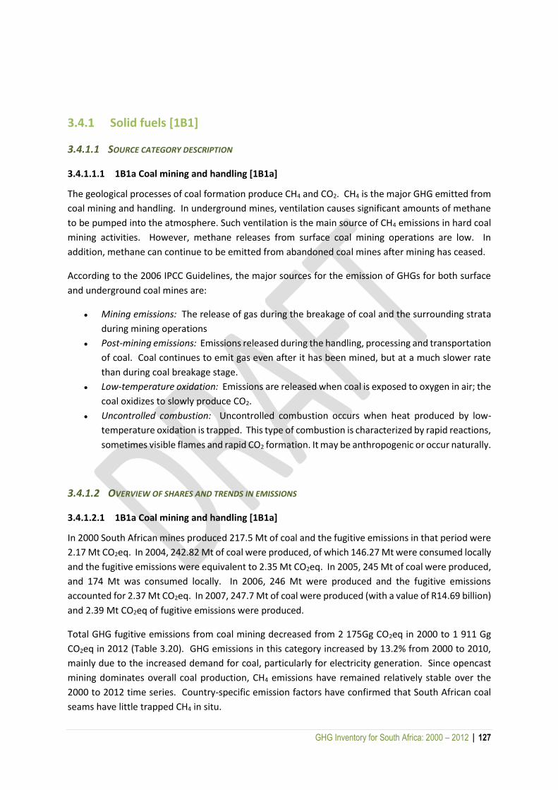
GHG Inventory for South Africa: 2000 – 2012 | 127

3.4.1 Solid fuels [1B1]

3.4.1.1 SOURCE CATEGORY DESCRIPTION

3.4.1.1.1 1B1a Coal mining and handling [1B1a]

The geological processes of coal formation produce CH4 and CO2. CH4 is the major GHG emitted from

coal mining and handling. In underground mines, ventilation causes significant amounts of methane

to be pumped into the atmosphere. Such ventilation is the main source of CH4 emissions in hard coal

mining activities. However, methane releases from surface coal mining operations are low. In

addition, methane can continue to be emitted from abandoned coal mines after mining has ceased.

According to the 2006 IPCC Guidelines, the major sources for the emission of GHGs for both surface

and underground coal mines are:

Mining emissions: The release of gas during the breakage of coal and the surrounding strata

during mining operations

Post-mining emissions: Emissions released during the handling, processing and transportation

of coal. Coal continues to emit gas even after it has been mined, but at a much slower rate

than during coal breakage stage.

Low-temperature oxidation: Emissions are released when coal is exposed to oxygen in air; the

coal oxidizes to slowly produce CO2.

Uncontrolled combustion: Uncontrolled combustion occurs when heat produced by low-

temperature oxidation is trapped. This type of combustion is characterized by rapid reactions,

sometimes visible flames and rapid CO2 formation. It may be anthropogenic or occur naturally.

3.4.1.2 OVERVIEW OF SHARES AND TRENDS IN EMISSIONS

3.4.1.2.1 1B1a Coal mining and handling [1B1a]

In 2000 South African mines produced 217.5 Mt of coal and the fugitive emissions in that period were

2.17 Mt CO2eq. In 2004, 242.82 Mt of coal were produced, of which 146.27 Mt were consumed locally

and the fugitive emissions were equivalent to 2.35 Mt CO2eq. In 2005, 245 Mt of coal were produced,

and 174 Mt was consumed locally. In 2006, 246 Mt were produced and the fugitive emissions

accounted for 2.37 Mt CO2eq. In 2007, 247.7 Mt of coal were produced (with a value of R14.69 billion)

and 2.39 Mt CO2eq of fugitive emissions were produced.

Total GHG fugitive emissions from coal mining decreased from 2 175Gg CO2eq in 2000 to 1 911 Gg

CO2eq in 2012 (Table 3.20). GHG emissions in this category increased by 13.2% from 2000 to 2010,

mainly due to the increased demand for coal, particularly for electricity generation. Since opencast

mining dominates overall coal production, CH4 emissions have remained relatively stable over the

2000 to 2012 time series. Country-specific emission factors have confirmed that South African coal

seams have little trapped CH4 in situ.

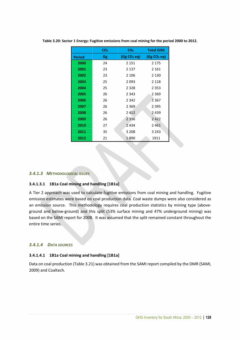
GHG Inventory for South Africa: 2000 – 2012 | 128

Table 3.20: Sector 1 Energy: Fugitive emissions from coal mining for the period 2000 to 2012.

CO2 CH4 Total GHG

Period Gg (Gg CO2 eq) (Gg CO2 eq)

2000 24 2 151 2 175

2001 23 2 137 2 161

2002 23 2 106 2 130

2003 25 2 093 2 118

2004 25 2 328 2 353

2005 26 2 343 2 369

2006 26 2 342 2 367

2007 26 2 369 2 395

2008 26 2 412 2 439

2009 26 2 396 2 422

2010 27 2 434 2 461

2011 35 3 208 3 243

2012 21 1 890 1911

3.4.1.3 METHODOLOGICAL ISSUES

3.4.1.3.1 1B1a Coal mining and handling [1B1a]

A Tier 2 approach was used to calculate fugitive emissions from coal mining and handling. Fugitive

emission estimates were based on coal production data. Coal waste dumps were also considered as

an emission source. This methodology requires coal production statistics by mining type (above-

ground and below-ground) and this split (53% surface mining and 47% underground mining) was

based on the SAMI report for 2008. It was assumed that the split remained constant throughout the

entire time series.

3.4.1.4 DATA SOURCES

3.4.1.4.1 1B1a Coal mining and handling [1B1a]

Data on coal production (Table 3.21) was obtained from the SAMI report compiled by the DMR (SAMI,

2009) and Coaltech.

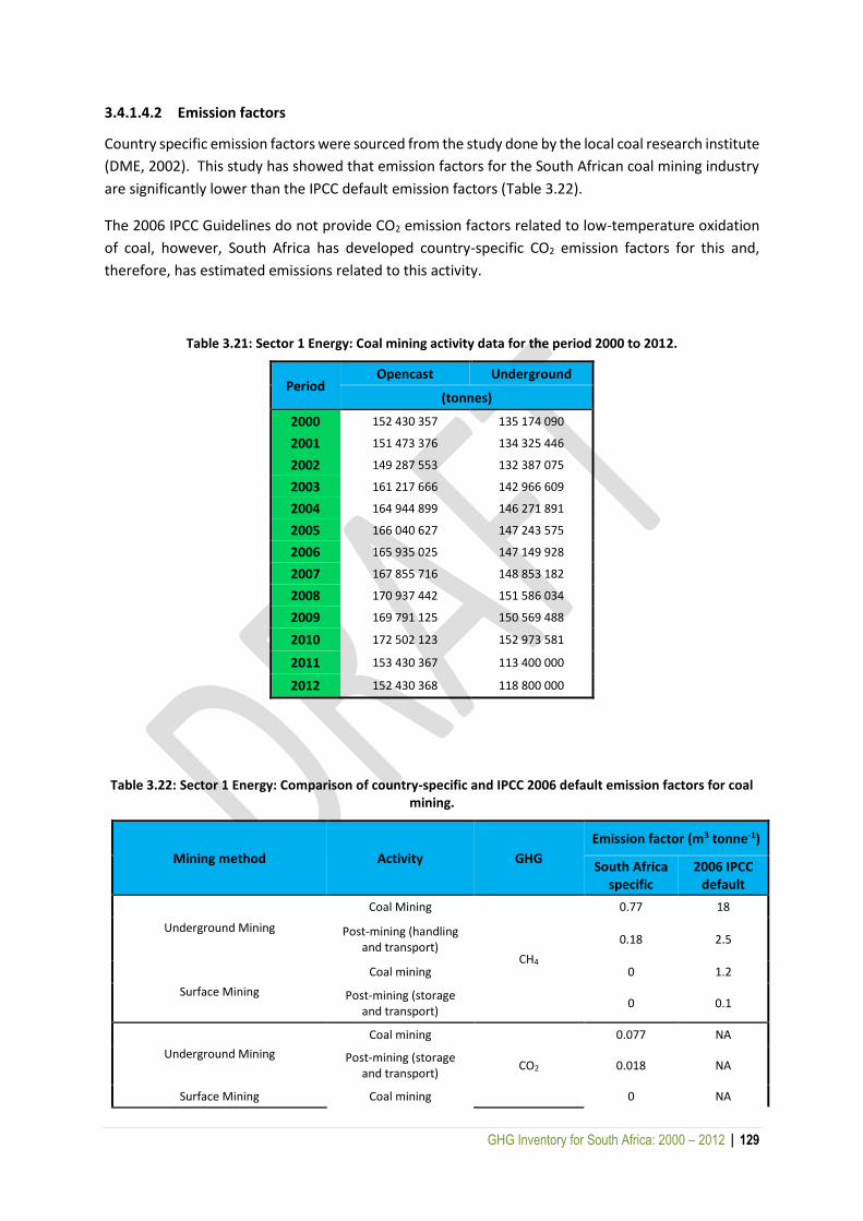
GHG Inventory for South Africa: 2000 – 2012 | 129

3.4.1.4.2 Emission factors

Country specific emission factors were sourced from the study done by the local coal research institute

(DME, 2002). This study has showed that emission factors for the South African coal mining industry

are significantly lower than the IPCC default emission factors (Table 3.22).

The 2006 IPCC Guidelines do not provide CO2 emission factors related to low-temperature oxidation

of coal, however, South Africa has developed country-specific CO2 emission factors for this and,

therefore, has estimated emissions related to this activity.

Table 3.21: Sector 1 Energy: Coal mining activity data for the period 2000 to 2012.

Period Opencast Underground

(tonnes)

2000 152 430 357 135 174 090

2001 151 473 376 134 325 446

2002 149 287 553 132 387 075

2003 161 217 666 142 966 609

2004 164 944 899 146 271 891

2005 166 040 627 147 243 575

2006 165 935 025 147 149 928

2007 167 855 716 148 853 182

2008 170 937 442 151 586 034

2009 169 791 125 150 569 488

2010 172 502 123 152 973 581

2011 153 430 367 113 400 000

2012 152 430 368 118 800 000

Table 3.22: Sector 1 Energy: Comparison of country-specific and IPCC 2006 default emission factors for coal mining.

Mining method Activity GHG

Emission factor (m3 tonne-1)

South Africa specific

2006 IPCC default

Underground Mining

Coal Mining

CH4

0.77 18

Post-mining (handling and transport)

0.18 2.5

Surface Mining

Coal mining 0 1.2

Post-mining (storage and transport)

0 0.1

Underground Mining

Coal mining

CO2

0.077 NA

Post-mining (storage and transport)

0.018 NA

Surface Mining Coal mining 0 NA

GHG Inventory for South Africa: 2000 – 2012 | 130

Post-mining (storage and transport)

0 NA

3.4.1.5 UNCERTAINTY AND TIME-SERIES CONSISTENCY

The major source of uncertainty in this category is activity data on coal production statistics. According

to the 2006 IPCC Guidelines, country-specific tonnages are likely to have an uncertainty in the 1 to 2%

range, but if raw coal data are not available, then the uncertainty will increase to about ±5%, when

converting from saleable coal production data. The data are also influenced by moisture content,

which is usually present at levels between 5 and 10 %, and may not be determined with great accuracy.

3.4.1.6 SOURCE-SPECIFIC QA/QC AND VERIFICATION

An inventory compilation manual documenting sources of data, data preparation and sources of

emission factors was used to compile emission estimates for this source category. Emission estimates

were also verified with emission estimates produced by the coal mining industry. An independent

reviewer was appointed to assess the quality of the inventory, determine the conformity of the

procedures followed for the compilation of this inventory and identify areas of improvements.

3.4.1.7 SOURCE-SPECIFIC RECALCULATIONS

Emissions were recalculated for 2000 using country-specific EFs. The recalculation resulted in the

reduction of emissions from 40 Mt CO2eq to 2 Mt CO2eq, resulting in a 95% reduction in the emission

estimate.

3.4.1.8 SOURCE-SPECIFIC PLANNED IMPROVEMENTS AND RECOMMENDATIONS

More attention needs to be placed on the collection of fugitive emissions from abandoned mines and

the spontaneous combustion of underground coal seams.

3.4.2 Oil and natural gas [1B2]

3.4.2.1 SOURCE CATEGORY DESCRIPTION

The sources of fugitive emissions from oil and natural gas included, but were not limited to, equipment

leaks, evaporation and flashing losses, venting, flaring, incineration and accidental losses (e.g. tank,

seal, well blow-outs and spills) as well as transformation of natural gas into petroleum products.

GHG Inventory for South Africa: 2000 – 2012 | 131

3.4.2.2 OVERVIEW OF SHARES AND TRENDS IN EMISSIONS

The total estimation of cumulative GHG emissions from flaring was equivalent to 13 496 Gg CO2 for

the period 2000 to 2012. Emissions decreased by 20% from 752 Gg CO2eq in 2000 to 641 Gg CO2eq in

2012 (Table 3.23).

Table 3.23: Sector 1 Energy: Total GHG emissions from venting and flaring for the period 2000 – 2012.

Period 2000 2001 2002 2003 2004 2005 2006 2007 2008 2009 2010 2011 2012

Gg CO2eq

752 753 955 1 458 1 379 1 160 1 133 1 133 1 138 1 243 964 786 642

3.4.2.3 METHODOLOGICAL ISSUES

Fugitive emissions are a direct source of GHGs due to the release of CH4 and formation CO2 (CO2

produced in oil and gas when it leaves the reservoir). Use of facility-level production data and facility-

level gas composition and vent flow rates has facilitated the use of Tier 3 methodology. Hence, CO2

emissions from venting and flaring have been estimated using real continuous monitoring results and

therefore no emission factors were used.

3.4.2.4 DATA SOURCES

This is the first time this subcategory has been accounted for in the national GHG inventory. Data on

oil and natural gas emissions were obtained directly from refineries and, to a lesser extent, from the

energy digest reports (DoE, 2009a).

3.4.2.5 UNCERTAINTY AND TIME-SERIES CONSISTENCY

According to the 2006 IPCC Guidelines, gas compositions are usually accurate to within ±5 % on

individual components. Flow rates typically have errors of ±3% or less for sales volumes and ±15% or

more for other volumes. Given that the activity data used is sourced at facility level, the uncertainty

is expected to be less than 3%.

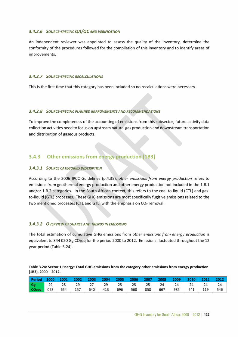
GHG Inventory for South Africa: 2000 – 2012 | 132

3.4.2.6 SOURCE-SPECIFIC QA/QC AND VERIFICATION

An independent reviewer was appointed to assess the quality of the inventory, determine the

conformity of the procedures followed for the compilation of this inventory and to identify areas of

improvements.

3.4.2.7 SOURCE-SPECIFIC RECALCULATIONS

This is the first time that this category has been included so no recalculations were necessary.

3.4.2.8 SOURCE-SPECIFIC PLANNED IMPROVEMENTS AND RECOMMENDATIONS

To improve the completeness of the accounting of emissions from this subsector, future activity data

collection activities need to focus on upstream natural gas production and downstream transportation

and distribution of gaseous products.

3.4.3 Other emissions from energy production [1B3]

3.4.3.1 SOURCE CATEGORIES DESCRIPTION

According to the 2006 IPCC Guidelines (p.4.35), other emissions from energy production refers to

emissions from geothermal energy production and other energy production not included in the 1.B.1

and/or 1.B.2 categories. In the South African context, this refers to the coal-to-liquid (CTL) and gas-

to-liquid (GTL) processes. These GHG emissions are most specifically fugitive emissions related to the

two mentioned processes (CTL and GTL) with the emphasis on CO2 removal.

3.4.3.2 OVERVIEW OF SHARES AND TRENDS IN EMISSIONS

The total estimation of cumulative GHG emissions from other emissions from energy production is

equivalent to 344 020 Gg CO2eq for the period 2000 to 2012. Emissions fluctuated throughout the 12

year period (Table 3.24).

Table 3.24: Sector 1 Energy: Total GHG emissions from the category other emissions from energy production (1B3), 2000 – 2012.

Period 2000 2001 2002 2003 2004 2005 2006 2007 2008 2009 2010 2011 2012

Gg CO2eq

29 078

28 654

29 157

27 640

29 413

25 696

25 568

25 858

24 667

24 985

24 641

24 119

24 546

GHG Inventory for South Africa: 2000 – 2012 | 133

3.4.3.3 METHODOLOGICAL ISSUES

The use of facility-level production data and facility-level gas composition and vent flow rates enabled

the use of Tier 3 methodology. Hence, CO2 emissions from other emissions from energy production

have been estimated using real continuous monitoring results and material balances.

3.4.3.4 DATA SOURCES

Data on other emissions from energy production were obtained from both Sasol and PetroSA.

3.4.3.5 UNCERTAINTY AND TIME-SERIES CONSISTENCY

No source-specific uncertainty analysis has been performed for this source category. Currently,

uncertainty data does not form part of the data collection and measurement programme. This is an

area that will require improvement in future inventories. Facilities are to be encouraged to collect

uncertainty data as part of data collection and measurement programmes. Time-series activity data

was validated using information on mitigation projects that have been implemented in the past 10

years and other factors such as economic growth and fuel supply and demand.

3.4.3.6 SOURCE-SPECIFIC QA/QC AND VERIFICATION

Quality assurance is currently done in an ad-hoc manner: the department reviews the material

balance and measurement data supplied by facilities. An independent reviewer was appointed to

assess the quality of the inventory, determine the conformity of the procedures which were followed

for the compilation of this inventory and identify areas of improvement.

3.4.3.7 SOURCE-SPECIFIC RECALCULATIONS

No source-specific recalculations were done for this section.

3.4.3.8 SOURCE-SPECIFIC PLANNED IMPROVEMENTS AND RECOMMENDATIONS

No improvements are planned for this section.

GHG Inventory for South Africa: 2000 – 2012 | 134

4 INDUSTRIAL PROCESSES AND OTHER PRODUCT USE

4.1 An overview of the IPPU sector

The IPPU sector includes GHG emissions sourced from industrial processes, the use of GHG emissions

in products and the use of fossil fuels (non-energy uses). The main emission sources are releases from

industrial processes that chemically or physically transform raw material (e.g. ammonia products

manufactured from fossil fuels). GHG emissions released during these processes are CO2, CH4, N2O,

HFCs, SF6 and PFCs. Also included in the IPPU sector are GHG emissions used in products such as

refrigerators, foams and aerosol cans.

The estimation of GHG emissions from non-energy sources is often difficult because they are

widespread and diverse. The difficulties in the allocation of GHG emissions between fuel combustion

and industrial processes arise when by-product fuels or waste gases are transferred from the

manufacturing site and combusted elsewhere in different activities. The largest source of emissions

in the IPPU sector in South Africa is the production of iron and steel.

4.1.1 Overview of shares and trends in emissions

Major GHGs generated by the IPPU sector include CO2, N2O, CH4 and PFCs. The main emissions sources

for this category are as follows:

Manufacture of mineral products, mainly cement;

Manufacture of chemical products, such as nitric acid and adipic acid; and

Metal production, mainly iron and steel.

The performance of the economy is the key driver for trends in the IPPU sector. The South African

economy is directly related to the global economy, mainly through exports and imports. South Africa

officially entered an economic recession in May 2009, which was the first in 17 years. Until the global

economic recession affected South Africa in late 2008, economic growth had been stable and

consistent. According to Statistics South Africa, the GDP increased annually by 2.7%, 3.7%, 3.1%, 4.9%,

5.0%, 5.4%, 5.1% and 3.1% between 2001 and 2008, respectively. However in the third and fourth

quarters of 2008, the economy experienced enormous recession, and this continued into the first and

second quarters of 2009. As a result of the recession, GHG emissions during that period decreased

enormously across almost all categories in the IPPU sector.

In 1990 IPPU GHG emissions accounted for 8.9% of South Africa’s total GHG emissions (excl. FOLU),

whereas in 1994 and 2000 it contributed 8.0% and 6.5%, respectively. When analysing the recalculated

IPPU sector emissions for 2000, there was an increase of 4.6% when compared to 1990. Between 2000

and 2010 there was a 1.2% decrease in overall emissions from the IPPU sector, although there were

increases during this period.

The GHG emissions in the IPPU sector fluctuated during the 12-year reporting period (Figure 4.1).

Accumulated emissions totalled 616 593 Gg CO2eq. IPPU sector emissions increased annually by an

average of 2.6% between 2000 and 2006 due to robust economic growth during this time, which led

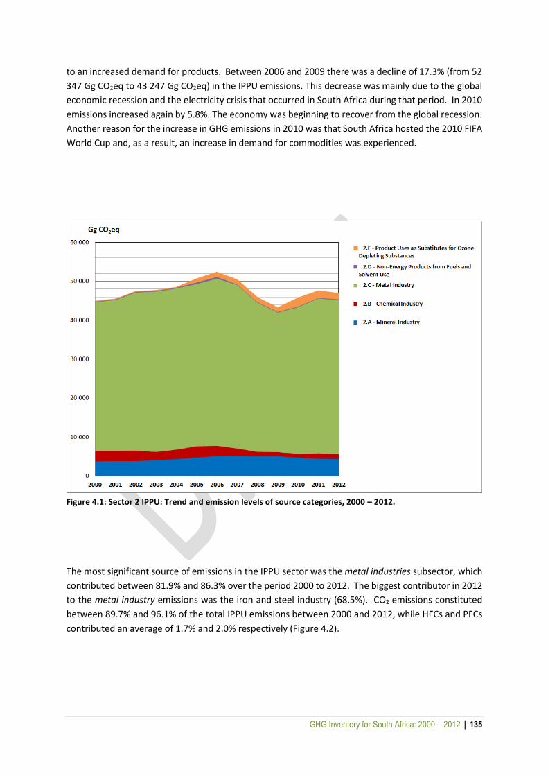
GHG Inventory for South Africa: 2000 – 2012 | 135

to an increased demand for products. Between 2006 and 2009 there was a decline of 17.3% (from 52

347 Gg CO2eq to 43 247 Gg CO2eq) in the IPPU emissions. This decrease was mainly due to the global

economic recession and the electricity crisis that occurred in South Africa during that period. In 2010

emissions increased again by 5.8%. The economy was beginning to recover from the global recession.

Another reason for the increase in GHG emissions in 2010 was that South Africa hosted the 2010 FIFA

World Cup and, as a result, an increase in demand for commodities was experienced.

Figure 4.1: Sector 2 IPPU: Trend and emission levels of source categories, 2000 – 2012.

The most significant source of emissions in the IPPU sector was the metal industries subsector, which

contributed between 81.9% and 86.3% over the period 2000 to 2012. The biggest contributor in 2012

to the metal industry emissions was the iron and steel industry (68.5%). CO2 emissions constituted

between 89.7% and 96.1% of the total IPPU emissions between 2000 and 2012, while HFCs and PFCs

contributed an average of 1.7% and 2.0% respectively (Figure 4.2).

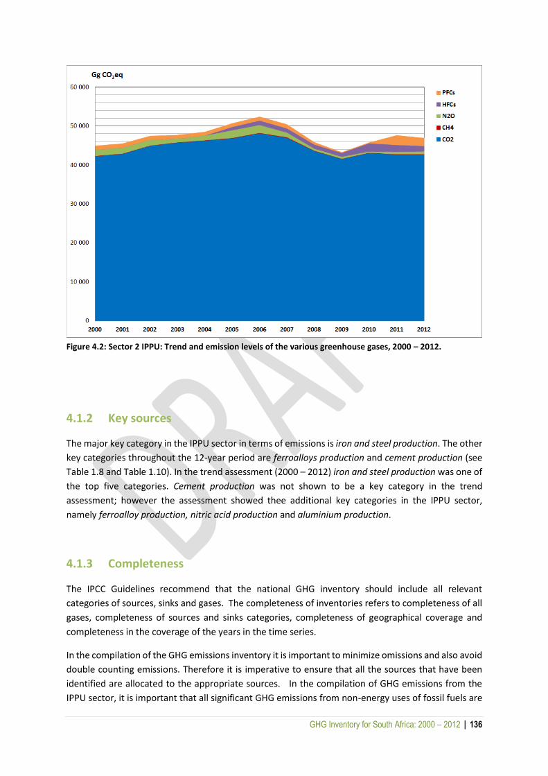
GHG Inventory for South Africa: 2000 – 2012 | 136

Figure 4.2: Sector 2 IPPU: Trend and emission levels of the various greenhouse gases, 2000 – 2012.

4.1.2 Key sources

The major key category in the IPPU sector in terms of emissions is iron and steel production. The other

key categories throughout the 12-year period are ferroalloys production and cement production (see

Table 1.8 and Table 1.10). In the trend assessment (2000 – 2012) iron and steel production was one of

the top five categories. Cement production was not shown to be a key category in the trend

assessment; however the assessment showed thee additional key categories in the IPPU sector,

namely ferroalloy production, nitric acid production and aluminium production.

4.1.3 Completeness

The IPCC Guidelines recommend that the national GHG inventory should include all relevant

categories of sources, sinks and gases. The completeness of inventories refers to completeness of all

gases, completeness of sources and sinks categories, completeness of geographical coverage and

completeness in the coverage of the years in the time series.

In the compilation of the GHG emissions inventory it is important to minimize omissions and also avoid

double counting emissions. Therefore it is imperative to ensure that all the sources that have been

identified are allocated to the appropriate sources. In the compilation of GHG emissions from the

IPPU sector, it is important that all significant GHG emissions from non-energy uses of fossil fuels are

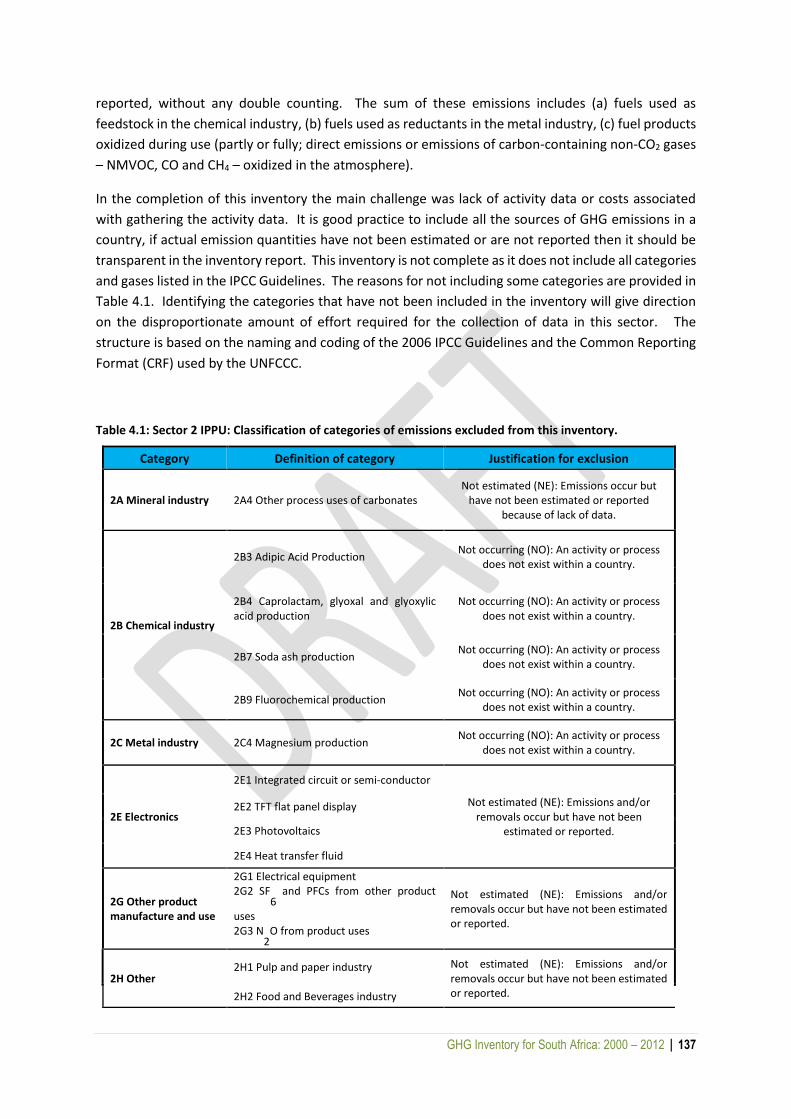
GHG Inventory for South Africa: 2000 – 2012 | 137

reported, without any double counting. The sum of these emissions includes (a) fuels used as

feedstock in the chemical industry, (b) fuels used as reductants in the metal industry, (c) fuel products

oxidized during use (partly or fully; direct emissions or emissions of carbon-containing non-CO2 gases

– NMVOC, CO and CH4 – oxidized in the atmosphere).

In the completion of this inventory the main challenge was lack of activity data or costs associated

with gathering the activity data. It is good practice to include all the sources of GHG emissions in a

country, if actual emission quantities have not been estimated or are not reported then it should be

transparent in the inventory report. This inventory is not complete as it does not include all categories

and gases listed in the IPCC Guidelines. The reasons for not including some categories are provided in

Table 4.1. Identifying the categories that have not been included in the inventory will give direction

on the disproportionate amount of effort required for the collection of data in this sector. The

structure is based on the naming and coding of the 2006 IPCC Guidelines and the Common Reporting

Format (CRF) used by the UNFCCC.

Table 4.1: Sector 2 IPPU: Classification of categories of emissions excluded from this inventory.

Category Definition of category Justification for exclusion

2A Mineral industry 2A4 Other process uses of carbonates Not estimated (NE): Emissions occur but

have not been estimated or reported because of lack of data.

2B Chemical industry

2B3 Adipic Acid Production Not occurring (NO): An activity or process

does not exist within a country.

2B4 Caprolactam, glyoxal and glyoxylic acid production

Not occurring (NO): An activity or process does not exist within a country.

2B7 Soda ash production Not occurring (NO): An activity or process

does not exist within a country.

2B9 Fluorochemical production Not occurring (NO): An activity or process

does not exist within a country.

2C Metal industry 2C4 Magnesium production Not occurring (NO): An activity or process

does not exist within a country.

2E Electronics

2E1 Integrated circuit or semi-conductor

Not estimated (NE): Emissions and/or removals occur but have not been

estimated or reported.

2E2 TFT flat panel display

2E3 Photovoltaics

2E4 Heat transfer fluid

2G Other product manufacture and use

2G1 Electrical equipment 2G2 SF

6 and PFCs from other product

uses 2G3 N

2O from product uses

Not estimated (NE): Emissions and/or removals occur but have not been estimated or reported.

2H Other 2H1 Pulp and paper industry Not estimated (NE): Emissions and/or

removals occur but have not been estimated or reported. 2H2 Food and Beverages industry

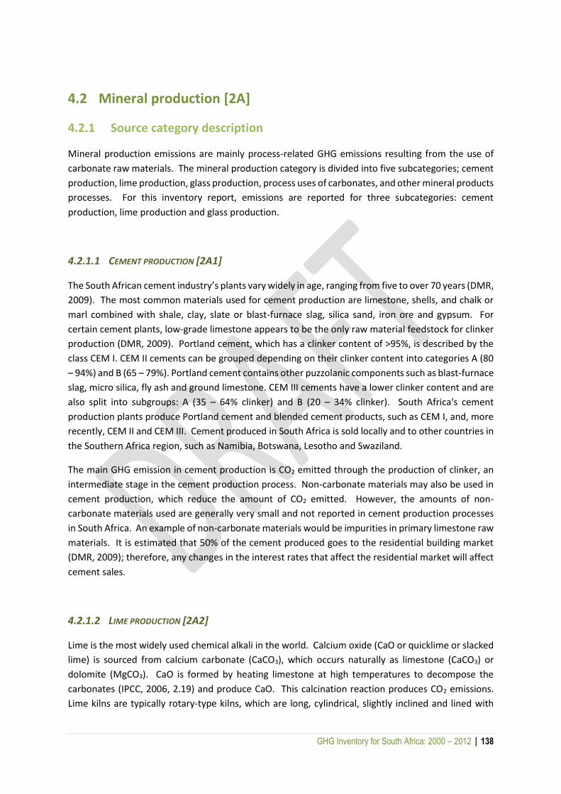
GHG Inventory for South Africa: 2000 – 2012 | 138

4.2 Mineral production [2A]

4.2.1 Source category description

Mineral production emissions are mainly process-related GHG emissions resulting from the use of

carbonate raw materials. The mineral production category is divided into five subcategories; cement

production, lime production, glass production, process uses of carbonates, and other mineral products

processes. For this inventory report, emissions are reported for three subcategories: cement

production, lime production and glass production.

4.2.1.1 CEMENT PRODUCTION [2A1]

The South African cement industry’s plants vary widely in age, ranging from five to over 70 years (DMR,

2009). The most common materials used for cement production are limestone, shells, and chalk or

marl combined with shale, clay, slate or blast-furnace slag, silica sand, iron ore and gypsum. For

certain cement plants, low-grade limestone appears to be the only raw material feedstock for clinker

production (DMR, 2009). Portland cement, which has a clinker content of >95%, is described by the

class CEM I. CEM II cements can be grouped depending on their clinker content into categories A (80

– 94%) and B (65 – 79%). Portland cement contains other puzzolanic components such as blast-furnace

slag, micro silica, fly ash and ground limestone. CEM III cements have a lower clinker content and are

also split into subgroups: A (35 – 64% clinker) and B (20 – 34% clinker). South Africa's cement

production plants produce Portland cement and blended cement products, such as CEM I, and, more

recently, CEM II and CEM III. Cement produced in South Africa is sold locally and to other countries in

the Southern Africa region, such as Namibia, Botswana, Lesotho and Swaziland.

The main GHG emission in cement production is CO2 emitted through the production of clinker, an

intermediate stage in the cement production process. Non-carbonate materials may also be used in

cement production, which reduce the amount of CO2 emitted. However, the amounts of non-

carbonate materials used are generally very small and not reported in cement production processes

in South Africa. An example of non-carbonate materials would be impurities in primary limestone raw

materials. It is estimated that 50% of the cement produced goes to the residential building market

(DMR, 2009); therefore, any changes in the interest rates that affect the residential market will affect

cement sales.

4.2.1.2 LIME PRODUCTION [2A2]

Lime is the most widely used chemical alkali in the world. Calcium oxide (CaO or quicklime or slacked

lime) is sourced from calcium carbonate (CaCO3), which occurs naturally as limestone (CaCO3) or

dolomite (MgCO3). CaO is formed by heating limestone at high temperatures to decompose the

carbonates (IPCC, 2006, 2.19) and produce CaO. This calcination reaction produces CO2 emissions.

Lime kilns are typically rotary-type kilns, which are long, cylindrical, slightly inclined and lined with

GHG Inventory for South Africa: 2000 – 2012 | 139

refractory material. At some facilities, the lime may be subsequently reacted (slaked) with water to

produce hydrated lime.

In South Africa the market for lime is divided into pyrometallurgical and chemical components.

Hydrated lime is divided into three sectors: chemical, water purification and other sectors (DMR,

2010). Quicklime and hydrated lime contributed an average of 92% and 8%, respectively (DMR Report

R85/2010). Lime has wide applications, e.g., it is used as a neutralizing and coagulating agent in

chemical, hydrometallurgical and water treatment processes and a fluxing agent in pyrometallurgical

processes. Pyrometallurgical quicklime sales have been increasing, while the demand for quicklime in

the chemical industry has been decreasing (DMR, 2010).

4.2.1.3 GLASS PRODUCTION [2A3]

There are many types of glass and compositions used commercially, however the glass industry is

divided into four categories: containers, flat (window) glass, fibre glass and speciality glass. When

other materials (including metal) solidify, they become crystalline, whereas glass (a super cool liquid)

is non-crystalline. The raw materials used in glass production are sand, limestone, soda ash, dolomite,

feldspar and saltcake. The major glass raw materials which emit CO2 during the melting process are

limestone (CaCO3), dolomite CaMg(CO3)2 and soda ash (Na2CO3). Glass makers do not produce glass

only from raw materials, they also use a certain amount of recycled scrap glass (cullet). The chemical

composition of glass is silica (72%), iron oxide (0.075%), alumina (0.75%), magnesium oxide (2.5%),

sodium oxide (14.5%), potassium oxide (0.5%), sulphur trioxide (0.25%) and calcium oxide (7.5%) (PFG

glass, 2010).

4.2.2 Overview of shares and trends in emissions

The cumulative GHG emissions from the mineral industry for the reporting period 2000 to 2012 were

59 472 Gg CO2eq. Emissions increased by 35% between 2000 and 2007 to 5 217 Gg CO2eq, after which

emissions slowly declined (by 15.8%) to 4 411 Gg CO2eq in 2012 (Figure 4.3: ). Over the 12-year period

the emissions from the mineral industries increased by 14.7%. The most significant GHG emission

sources in 2012 were cement production (contributing 87.2% of total GHG emissions), followed by

lime production (10.3%). GHG emissions from glass production accounted for only 2.6% of the total

emissions.

4.2.2.1 CEMENT PRODUCTION [2A1]

The GHG emissions from cement production increased from 3 347 Gg CO2eq in 2000 to 4 583 Gg CO2eq

in 2007, after which emissions declined to 3 845 Gg CO2eq in 2012. Cement production in South Africa

increased significantly from the period 2000 to 2007 as a result of economic growth. There was a

2.0%, 7.1%, 5.8% and 2.5% decrease in emissions in 2008, 2010, 2011 and 2012, respectively. In 2009

the South African economy went into recession and the GDP decreased by 1.8% in that year. Cement

demand in the residential market and construction industry in 2009/2010 decreased due to higher

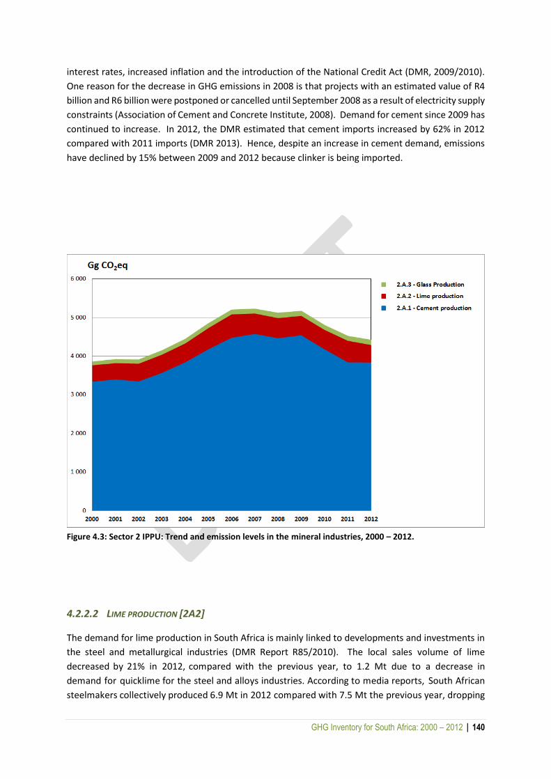
GHG Inventory for South Africa: 2000 – 2012 | 140

interest rates, increased inflation and the introduction of the National Credit Act (DMR, 2009/2010).

One reason for the decrease in GHG emissions in 2008 is that projects with an estimated value of R4

billion and R6 billion were postponed or cancelled until September 2008 as a result of electricity supply

constraints (Association of Cement and Concrete Institute, 2008). Demand for cement since 2009 has

continued to increase. In 2012, the DMR estimated that cement imports increased by 62% in 2012

compared with 2011 imports (DMR 2013). Hence, despite an increase in cement demand, emissions

have declined by 15% between 2009 and 2012 because clinker is being imported.

Figure 4.3: Sector 2 IPPU: Trend and emission levels in the mineral industries, 2000 – 2012.

4.2.2.2 LIME PRODUCTION [2A2]

The demand for lime production in South Africa is mainly linked to developments and investments in

the steel and metallurgical industries (DMR Report R85/2010). The local sales volume of lime

decreased by 21% in 2012, compared with the previous year, to 1.2 Mt due to a decrease in

demand for quicklime for the steel and alloys industries. According to media reports, South African

steelmakers collectively produced 6.9 Mt in 2012 compared with 7.5 Mt the previous year, dropping

GHG Inventory for South Africa: 2000 – 2012 | 141

in the world steel-production rankings from 21 to 22. The total sales volume of quicklime for

pyrometallurgical and chemical applications decreased by 22% to 1.11 Mt owing to subdued demand

from the steel industry, and sales value decreased by 14% to R1.1 billion (DMR 2013). The total

cumulative estimation of GHG emissions from lime production for the period 2000 to 2012 was 6 480

Gg CO2eq.

The fluctuations in lime production were directly linked to developments and investments in the steel

and metallurgical industries. In 2009 the lime industry declined as a result of the economic recession,

hence, in that year, GHG emissions from lime production decreased by 3.4%. Overall, the GHG

emissions from this category increased by 6.3% between 2000 and 2012, which is mainly due to an

increase in the number of infrastructure projects and the 2010 FIFA World Cup preparation.

4.2.2.3 GLASS PRODUCTION [2A3]

South Africa’s glass production emissions increased consistently from 2001 to 2005 and again in 2007

to 2008. In 2009 and 2010 GHG emissions from glass production declined by 6.6% and 5.3%,

respectively. This decline in emissions was mainly because of the global economic crisis which affected

the glass-manufacturing market. GHG emissions picked up again in 2011 (1.9%) and 2012 (7.5%). Over

the 12-year period there was a 53.2% increase in emissions from glass production. The glass-

manufacturing market is largely influenced by consumer behaviour and consumer spending; therefore

any negative changes in the economy will affect the glass manufacturing industry. The total

cumulative estimation of GHG emissions from glass production for the period 2000 to 2012 was 1 295

Gg CO2eq.

4.2.3 Methodological issues

4.2.3.1 CEMENT PRODUCTION [2A1]

As a key emission source, cement production requires higher-tier level emission estimation; The Tier

2 method stipulates that if sufficient country-specific data on the calcium oxide (CaO) content of

clinker and inputs of non-carbonate CaO sources are available, a country-specific CO2 emission factor

for clinker should be calculated. This was, however, not possible due to the lack of country specific

emission factors. A Tier 1 approach was used to estimate emissions.

4.2.3.2 LIME PRODUCTION [2A2]

The production of lime involves various steps, which include the quarrying of raw materials, crushing

and sizing, calcining the raw materials to produce lime, and (if required) hydrating the lime to calcium

hydroxide. The Tier 1 approach was used for the calculation of GHG emissions from lime production.

This report estimated the total lime production based on the aggregate national value of the quantity

of limestone produced, using the breakdown of the types of lime published in the SAMI report

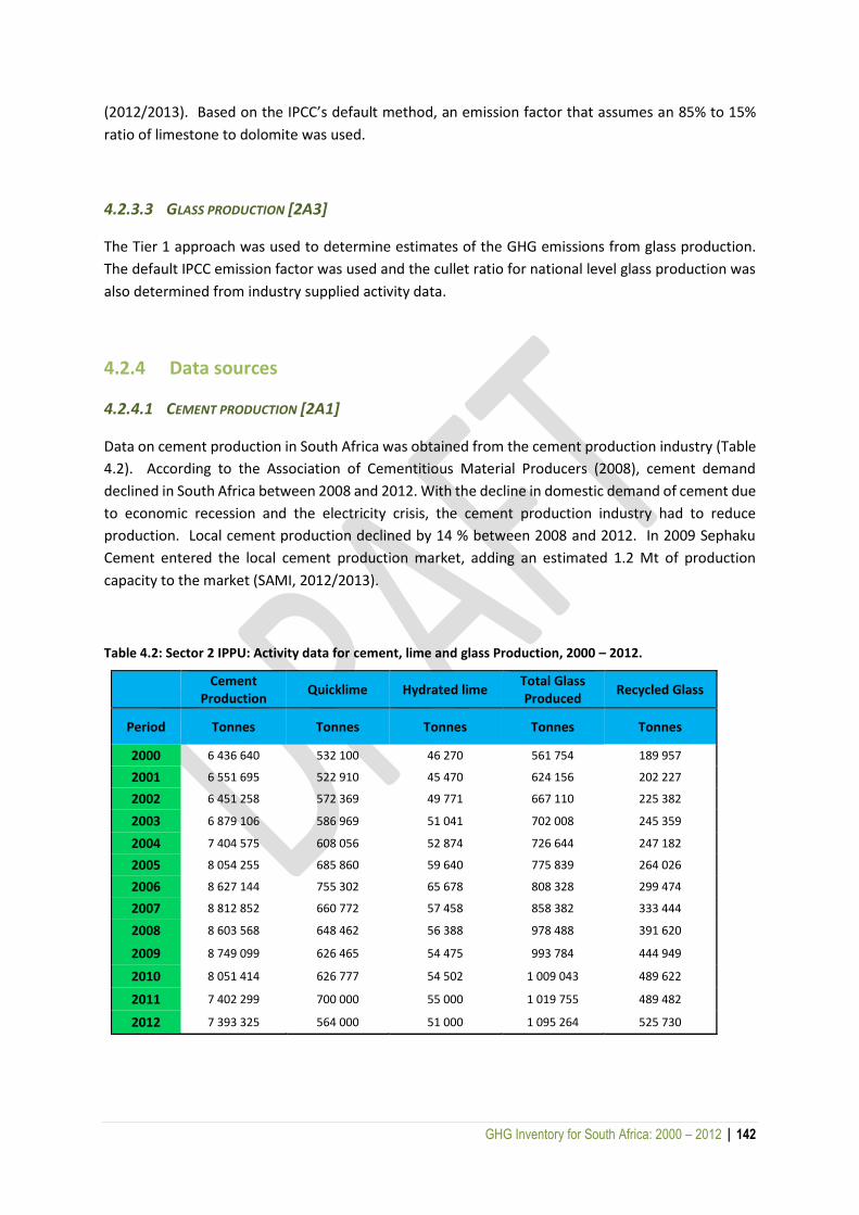
GHG Inventory for South Africa: 2000 – 2012 | 142

(2012/2013). Based on the IPCC’s default method, an emission factor that assumes an 85% to 15%

ratio of limestone to dolomite was used.

4.2.3.3 GLASS PRODUCTION [2A3]

The Tier 1 approach was used to determine estimates of the GHG emissions from glass production.

The default IPCC emission factor was used and the cullet ratio for national level glass production was

also determined from industry supplied activity data.

4.2.4 Data sources

4.2.4.1 CEMENT PRODUCTION [2A1]

Data on cement production in South Africa was obtained from the cement production industry (Table

4.2). According to the Association of Cementitious Material Producers (2008), cement demand

declined in South Africa between 2008 and 2012. With the decline in domestic demand of cement due

to economic recession and the electricity crisis, the cement production industry had to reduce

production. Local cement production declined by 14 % between 2008 and 2012. In 2009 Sephaku

Cement entered the local cement production market, adding an estimated 1.2 Mt of production

capacity to the market (SAMI, 2012/2013).

Table 4.2: Sector 2 IPPU: Activity data for cement, lime and glass Production, 2000 – 2012.

Cement

Production Quicklime Hydrated lime

Total Glass Produced

Recycled Glass

Period Tonnes Tonnes Tonnes Tonnes Tonnes

2000 6 436 640 532 100 46 270 561 754 189 957

2001 6 551 695 522 910 45 470 624 156 202 227

2002 6 451 258 572 369 49 771 667 110 225 382

2003 6 879 106 586 969 51 041 702 008 245 359

2004 7 404 575 608 056 52 874 726 644 247 182

2005 8 054 255 685 860 59 640 775 839 264 026

2006 8 627 144 755 302 65 678 808 328 299 474

2007 8 812 852 660 772 57 458 858 382 333 444

2008 8 603 568 648 462 56 388 978 488 391 620

2009 8 749 099 626 465 54 475 993 784 444 949

2010 8 051 414 626 777 54 502 1 009 043 489 622

2011 7 402 299 700 000 55 000 1 019 755 489 482

2012 7 393 325 564 000 51 000 1 095 264 525 730

GHG Inventory for South Africa: 2000 – 2012 | 143

4.2.4.1.1 Emission factors

For the calculation of GHG emissions in cement production, CO2 emission factors were sourced from

the 2006 IPCC Guidelines. It was assumed that the CaO composition (one tonne of clinker) contains

0.65 tonnes of CaO from CaCO3. This carbonate is 56.03% of CaO and 43.97% of CO2 by weight (IPCC,

2006, p. 2.11). The emission factor for CO2, provided by IPCC 2006 Guidelines, is 0.52 tonnes of CO2

per tonne clinker. The IPCC default emission factors were used to estimate the total emissions. The

country-specific clinker fraction for the period 2000 to 2012 ranged between 69% - 76% (Table 4.3).

Table 4.3: Sector 2 IPPU: Clinker fraction for the period 2000 – 2012.

Period 2000 2001 2002 2003 2004 2005 2006 2007 2008 2009 2010 2011 2012

Country specific clinker fraction

0.76 0.75 0.73 0.73 0.73 0.72 0.73 0.71 0.7 0.71 0.69 0.69 0.69

4.2.4.2 LIME PRODUCTION [2A2]

The DMR publishes data on limestone and dolomite production in South Africa in the SAMI report

(DMR, 2012/2013). The SAMI provides a breakdown of limestone demand; 80% goes to cement

manufacturing and the remaining 20% goes to metallurgical, agricultural and other uses. No data was

provided for lime production, therefore it was assumed that the ‘other’ (6.0%) in the breakdown of

limestone demand goes to lime production. .

4.2.4.2.1 Emission factors

For the calculation of GHG emissions from lime production, GHG emission factors were sourced from

the 2006 IPCC Guidelines. In South Africa data was acquired for high-calcium lime, which has a range

of 93 to 98% CaO content, and hydraulic lime, which has a range of 62 to 92% CaO. The GHG emission

factor for high-calcium lime (0.75 tonnes CO2/tonne CaO) and hydraulic lime (0.59 tonnes CO2 per

tonne CaO) were used for quicklime and hydrated lime, respectively (IPCC 2006 Guidelines).

4.2.4.3 GLASS PRODUCTION [2A3]

Data on glass production was obtained from the glass production industry.

4.2.4.3.1 Emission factors

For the calculation of GHG emissions from glass production, the emission factor (0.2 tonnes CO2 per

tonne glass) was sourced from the 2006 IPCC Guidelines based on a typical raw material mixture,

according to national glass production statistics. A typical soda-lime batch might consist of sand (56.2

weight percent), feldspar (5.3%), dolomite (9.8%), limestone (8.6%) and soda ash (20.0%). Based on

GHG Inventory for South Africa: 2000 – 2012 | 144

this composition, one metric tonne of raw materials yields approximately 0.84 tonnes of glass, losing

about 16.7% of its weight as volatiles, in this case virtually entirely CO2 (IPCC, 2006).

4.2.5 Uncertainty and time-series consistency

4.2.5.1 CEMENT PRODUCTION [2A1]

According to the 2006 IPCC Guidelines, if a 95% clinker fraction in Portland cement is assumed then

the uncertainty is in the range of 2 to 7%.

4.2.5.2 LIME PRODUCTION [2A2]

The only available data for lime production was sourced from the SAMI report; therefore there was

no comparison of data across different plants. According to the IPCC 2006 Guidelines, the uncertainty

of the activity data for a Tier 1 emission estimation methodology is within the range of 4 to 8%.

4.2.5.3 GLASS PRODUCTION [2A3]

The only available data for glass production was sourced from the glass production industry; therefore

there was no comparison of data across different plants. The uncertainty associated with use of the

Tier 1 emission factor and cullet ratio is significantly high at +/- 60% (IPCC, 2006, Vol 3).

4.2.6 Source specific QA/QC and verification

For cement production, facility-level activity data submitted by facilities was compared with data

published by the cement association as well as data reported in the SAMI reports. A comparison was

made between facility-level data and the SAMI data and it was evident that there are discrepancies

between the two sources of data. To give a few examples; for 2000, SAMI reported the total cement

production as 3 742 126 tonnes and industry reported the production for the same year as 6 436 640

tonnes; for 2009 SAMI reported production as 5 027 293 tonnes and the industry reported production

as 8 749 099 tonnes. These differences lead to increased uncertainty and the reasons for the

discrepancies need to be further investigated before the next inventory. Corrections were made in

facility-level data to ensure that emissions were categorised according to IPCC categorization. An

independent reviewer was appointed to assess the quality of the inventory, determine the conformity

of the procedures followed for the compilation of this inventory and identify areas of improvement.

4.2.7 Source-specific recalculations

No recalculations were performed for cement production, lime production or glass production.

GHG Inventory for South Africa: 2000 – 2012 | 145

4.2.8 Source-specific planned improvements and recommendations

4.2.8.1 CEMENT PRODUCTION [2A1]

An improvement would be the collection of activity data from all cement production plants in South

Africa. The activity data has to include the CaO content of the clinker and the fraction of this CaO from

carbonate. According to the 2006 IPCC Guidelines, it is good practice to separate CaO from non-

carbonate sources (e.g. slag and fly ash) and CaO content of the clinker when calculating emissions. It

is evident that there are discrepancies between the cement production data from industry and the

cement production data published by the DMR, as a recommendation, the DMR should work with the

cement production industry to ensure accuracy and consistency between the two data sources.

4.2.8.2 LIME PRODUCTION [2A2]

It is recommended that activity data be collected from all lime production plants in South Africa.

Another improvement would be the development of country-specific emission factors.

4.2.8.3 GLASS PRODUCTION [2A3]

Determining country-specific emission factors is recommended for the improvement of emission

estimates from this category. One of the largest sources of uncertainty in the emissions estimate (Tier

1 and Tier 2) for glass production is the cullet ratio. The amount of recycled glass used can vary across

facilities in a country and in the same facility over time. The cullet ratio might be a good candidate for

more in-depth investigation.

4.3 Chemical industry [2B]

This category estimates GHG emissions from the production of both organic and inorganic chemicals

in South Africa. The chemical industry in South Africa is mainly developed through the gasification of

coal because the country has no significant oil reserves. GHG emissions from the following chemical

production processes were reported: ammonia production, nitric acid production, carbide production,

titanium dioxide production and carbon black. The chemical industry in South Africa contributes

approximately 5% to the GDP and 23% of its manufacturing sales. The chemical products in South

Africa can be divided into four categories: base chemicals, intermediate chemicals, chemical end-

products, and speciality end-products. Chemical products include ammonia, waxes, solvents, plastics,

paints, explosives and fertilizers.

GHG Inventory for South Africa: 2000 – 2012 | 146

4.3.1 Source category description

4.3.1.1 AMMONIA PRODUCTION [2B1]

Ammonia production is the most important nitrogenous material produced and is a major industrial

chemical. According to the 2006 IPCC Guidelines (p.3.11), ammonia gas can be used directly as a

fertilizer, in heat treating, paper pulping, nitric acid and nitrates manufacture, nitric acid ester and

nitro compound manufacture, in explosives of various types and as a refrigerant.

4.3.1.2 NITRIC ACID PRODUCTION [2B2]

Nitric acid is a raw material used mainly in the production of nitrogenous-based fertilizer. According

to the 2006 IPCC Guidelines (p.3.19), during the production of nitric acid, nitrous oxide is generated

as an unintended by-product of high-temperature catalytic oxidation of ammonia.

4.3.1.3 CARBIDE PRODUCTION [2B5]

Carbide production can result in GHG emissions such as CO2 and CH4. According to the 2006 IPCC

Guidelines (p.3.39), calcium carbide is manufactured by heating calcium carbonate (limestone) and

subsequently reducing CaO with carbon (e.g. petroleum coke).

4.3.1.4 TITANIUM DIOXIDE PRODUCTION [2B6]

Titanium dioxide (TiO2) is a white pigment used mainly in paint manufacture, paper, plastics, rubber,

ceramics, fabrics, floor coverings, printing ink, among others. According 2006 IPCC Guidelines (p.

3.47), there are three processes in titanium dioxide production that result in GHG emissions, namely,

a) titanium slag production in electric furnaces; b) synthetic rutile production using the Becher Process

and c) rutile TiO2 production through the chloride route.

4.3.1.5 CARBON BLACK [2B8F]

Carbon black is produced from petroleum-based or coal-based feed stocks using the furnace black

process (IPCC, 2006). Primary fossil fuels in carbon black production include natural gas, petroleum

and coal. The use of these fossil fuels may involve the combustion of hydrocarbon content for heat

rising and the production of secondary fuels (IPCC, 2006, p.3.56). GHG missions from the combustion

of fuels obtained from feed stocks should be allocated to the source category in the IPPU sector,

however, where the fuels are not used within the source category but are transferred out of the

process for combustion elsewhere, these emissions should be reported in the appropriate energy

sector source category (IPCC, 2006, p. 3.56). Commonly, the largest percentage of carbon black is

used in the tyre and rubber industry, and the rest is used as pigment in applications such as ink and

carbon dry-cell batteries.

GHG Inventory for South Africa: 2000 – 2012 | 147

4.3.2 Trends in emissions

The chemical industries subsector contains confidential information, so, following the IPCC Guidelines

for reporting confidential information, no disaggregated source-category level emission data are

reported; only the emissions at the sector scale are discussed. Emission estimates are, however, based

on bottom-up activity data and methodologies.

The chemical industries contributed emissions totalling 26 034 Gg CO2eq over the period 2000 to 2012.

Emissions from this category fluctuated considerably over the 12-year period, with a maximum of 2

889 Gg CO2eq in 2005 and a minimum of 1 011 Gg CO2eq in 2010 (Figure 4.4: Sector 2 IPPU: Trend and

emission levels in the chemical industries between 2000 and 2012.

). Overall there was a 50.8% decline in GHG emissions from this category over the 12-year period,

largely due to N2O emission reductions in nitric acid production.

Figure 4.4: Sector 2 IPPU: Trend and emission levels in the chemical industries between 2000 and 2012.

GHG Inventory for South Africa: 2000 – 2012 | 148

4.3.3 Methodological issues

4.3.3.1 AMMONIA PRODUCTION [2B1]

GHG emission estimates from ammonia production were obtained through the Tier 3 approach; the

GHG emissions from this category were calculated based on actual process balance analysis. The

emission factors will not be provided, for the reason that there is only one company that produces

ammonia and therefore the total consumption is confidential.

4.3.3.2 NITRIC ACID PRODUCTION [2B2]

A Tier 3 approach was used for the calculation of GHG emissions from nitric acid production, using

production data and relevant emission factors. The GHG emissions in this category were calculated

based on actual process balance analysis.

4.3.3.3 CARBIDE PRODUCTION [2B5]

Emission estimates for carbide production were obtained by using the Tier 1 approach. Default IPCC

2006 emission factors were used. The GHG emissions from carbide production were estimated from

activity data on petroleum coke consumption, which is in line with the 2006 IPCC Guidelines.

4.3.3.4 TITANIUM DIOXIDE PRODUCTION [2B6]

The Tier 1 approach was used for calculating GHG emissions from titanium dioxide production, using

2006 IPCC default emission factors.

4.3.3.5 CARBON BLACK [2B8F]

Tier 1 was the main approach used in calculating GHG emissions from carbon black production, using

production data and relevant emission factors. IPCC 2006 default emission factors were used in all

GHG emission estimations.

4.3.4 Data sources

4.3.4.1 AMMONIA PRODUCTION [2B1]

Activity data from ammonia production were not provided, but rather the total emission estimates

were obtained from the ammonia production plants. The emissions were calculated based on actual

process balance analysis. The total GHG emissions for 2000 were not provided for; therefore it was

assumed that the GHG emissions for 2001 were similar to the GHG emissions for 2000.

GHG Inventory for South Africa: 2000 – 2012 | 149

4.3.4.2 NITRIC ACID PRODUCTION [2B2]

The amount of nitric acid emissions released was sourced from the nitric acid production plants. The

GHG emissions were calculated based on a combination of emission factors and process material

balance analysis. Sasol emissions were added to the total emissions using the emission factor

approach.

4.3.4.2.1 Emission factors

For the calculation of GHG emissions from nitric acid production, the N2O emission factor of 2.0 kg

N2O per tonne nitric acid was sourced from the 2006 IPCC Guidelines. This excluded Sasol emission

estimates, which are based on a mass-balance approach.

4.3.4.3 CARBIDE PRODUCTION [2B5]

The carbide production values were sourced from the carbide production plants and emissions were

calculated based on actual process balance analysis.

4.3.4.3.1 Emission factors

For the calculation of GHG emissions from carbide production, the IPCC 2006 CO2 emission factor

(1.090 tonnes CO2 per tonne carbide production) was used.

4.3.4.4 TITANIUM DIOXIDE PRODUCTION [2B6]

The titanium dioxide emissions data were sourced from the titanium dioxide production plants.

Emission estimates were based on a mass-balance approach.

4.3.4.5 CARBON BLACK [2B8F]

Carbon black activity data was sourced directly from industry.

4.3.4.5.1 Emission factors

For the calculation of GHG emissions from carbon black production, the IPCC 2006 default CO2 and

CH4 emission factors were used (p. 3.80). It was assumed that carbon black is produced through the

furnace black process.

GHG Inventory for South Africa: 2000 – 2012 | 150

4.3.5 Uncertainty and time-series consistency

4.3.5.1 AMMONIA PRODUCTION [2B1]

According to the 2006 IPCC Guidelines (p. 3.16), the plant-level activity data required for the Tier 3

approach are the total fuel requirement classified by fuel type; CO2 recovered for downstream use or

other applications; and ammonia production. It is recommended that uncertainty estimates are

obtained at the plant level, which should be lower than the uncertainty values associated with the

IPCC default emission factors.

4.3.5.2 NITRIC ACID PRODUCTION [2B2]

According to the 2006 IPCC Guidelines (p. 3.24) the plant-level activity data required for the Tier 3

approach include production data disaggregated by technology and abatement system type.

According the 2006 IPCC Guidelines (p. 3.24), default emission factors have very high uncertainties for

two reasons: a) N2O may be generated in the gauze reactor section of nitric acid production as an

unintended reaction by-product; and b) the exhaust gas may or may not be treated for NOx control

and the NOx abatement system may or may not reduce the N2O concentration of the treated gas. The

uncertainty measures of default emission factors are +/- 2%. For the uncertainty estimates of the

country-specific emission factors it is good practice that the uncertainty values are lower than the

default emission factors.

4.3.5.3 CARBIDE PRODUCTION [2B5]

The total GHG emissions were sourced from the specific carbide production plants therefore there

was no comparison of data across different plants. The default emission factors are generally

uncertain because industrial-scale carbide production processes differ from the stoichiometry of

theoretical chemical reactions (IPCC, 2006, p. 3.45). According to the IPCC 2006 Guidelines (p. 3.45),

the uncertainty of the activity data that accompanies the method used here is approximately 10%.

4.3.5.4 TITANIUM DIOXIDE PRODUCTION [2B6]

The total GHG emissions were sourced from the specific titanium dioxide production plants therefore,

no comparison of data across different plants was made. According to the IPCC 2006 Guidelines (p.

3.50), the uncertainty of the activity data that accompanies the method used here is approximately

5%.

4.3.5.5 CARBON BLACK [2B8F]

The activity data was sourced from disaggregated national totals; therefore QC measures were not

applied. According to the IPCC 2006 Guidelines, the uncertainty of the activity data that accompanies

GHG Inventory for South Africa: 2000 – 2012 | 151

the method used here is in the range of -15% to +15% for CO2 emission factors and between -85% to

+85% for CH4 emission factors.

4.3.6 Source-specific QA/QC and verification

4.3.6.1 CHEMICAL INDUSTRY [2B]

No source-specific QA/QC was performed for the chemical industry. However, activity data and

material balance data was verified with industry sectors.

4.3.7 Source-specific recalculations

No recalculations were performed.

4.3.8 Source-specific planned improvements and recommendations

For ammonia, nitric acid, carbide and titanium production it is recommended that the country-specific

emission factors which were applied by the industry be made transparent. This would allow efficient

quality assurance and control of the emission factors used. There is high uncertainty on many of the

default emission factors, so having country-specific emission factors would reduce this uncertainty.

Development of country-specific emission factors and/or moving to a material approach will improve

emission estimates for the carbon black source category.

4.4 Metal industry [2C]

This subcategory relates to emissions resulting from the production of metals. Processes covered for

this inventory report include the production of iron and steel, ferroalloys, aluminium, lead, and zinc.

Estimates were made for emissions of CO2 from the manufacture of all the metals, CH4 from ferroalloy

production, and perfluorocarbons (CF4 and C2F6) from aluminium production.

4.4.1 Source category description

4.4.1.1 IRON AND STEEL PRODUCTION [2C1]

Iron and steel production results in the emission of CO2, CH4 and N2O. According to the 2006 IPCC

Guidelines (p. 4.9), the iron and steel industry broadly consists of primary facilities that produce both

iron and steel; secondary steel-making facilities; iron production facilities; and offsite production of

metallurgical coke. According to the World Steel Association (2010), South Africa is the 21st-largest

crude steel producer in the world. The range of primary steel products and semi-finished products

GHG Inventory for South Africa: 2000 – 2012 | 152

manufactured in South Africa includes: billets; blooms; slabs; forgings; light-, medium- and heavy

sections and bars; reinforcing bar; railway track material; wire rod; seamless tubes; plates; hot- and

cold-rolled coils and sheets; electrolytic galvanised coils and sheets; tinplate; and pre-painted coils

and sheets. The range of primary stainless steel products and semi-finished products manufactured

in South Africa include slabs, plates, and hot- and cold-rolled coils and sheets.

4.4.1.2 FERROALLOY PRODUCTION [2C2]

Ferroalloy refers to concentrated alloys of iron and one or more metals such as silicon, manganese,

chromium, molybdenum, vanadium and tungsten. Ferroalloy plants manufacture concentrated

compounds that are delivered to steel production plants to be incorporated in alloy steels. Ferroalloy

production involves a metallurgical reduction process that results in significant carbon dioxide

emissions (IPCC, 2006, p. 4.32). South Africa is the world’s largest producer of chromium and

vanadium ores, and the leading supplier of their alloys (SAMI, 2013). South Africa is also the largest

producer of iron and manganese ores, and an important supplier of ferromanganese, ferrosilicon and

silicon metal (SAMI, 2013).

4.4.1.3 ALUMINIUM PRODUCTION [2C3]

According to the 2006 IPCC Guidelines, aluminium production is realised via the Hall-Heroult

electrolytic process. In this process, electrolytic reduction cells differ in the form and configuration of

the carbon anode and alumina feed system.

The most significant process emissions are (IPCC, 2006, p. 4.43):

Carbon dioxide (CO2) emissions from the consumption of carbon anodes in the reaction to

convert aluminium oxide to aluminium metal;

Perfluorocarbon (PFC) emissions of CF4 and C2F6 during anode effects. Also emitted are

smaller amounts of process emissions, CO, SO2, and NMVOCs. SF6 is not emitted during the

electrolytic process and is only rarely used in the aluminium manufacturing process, where

small quantities are emitted when fluxing specialized high-magnesium aluminium alloys.

4.4.1.4 LEAD PRODUCTION [2C5]

According to the 2006 IPCC Guidelines, there are two primary processes for the production of lead

bullion from lead concentrates:

Sintering/smelting, which consists of sequential sintering and smelting steps and constitutes

approximately 7% of the primary production; and

Direct smelting, which eliminates the sintering step and constitutes 22% of primary lead

production.

GHG Inventory for South Africa: 2000 – 2012 | 153

4.4.1.5 ZINC PRODUCTION [2C6]

According to the 2006 IPCC Guidelines, there are three primary processes for the production of zinc:

Electro-thermic distillation; this is a metallurgical process that combines roasted concentrate

and secondary zinc products into sinter that is combusted to remove zinc, halides, cadmium

and other impurities. The reduction results in the release of non-energy CO2 emissions.

The pyrometallurgical process: this involves the utilization of an Imperial Smelting Furnace,

which allows for the simultaneous treatment of zinc and zinc concentrates. The process

results in the simultaneous production of lead and zinc and the release of non-energy CO2

emissions.

The electrolytic: this is a hydrometallurgical technique, during which zinc sulphide is

calcinated, resulting in the production of zinc oxide. The process does not result in non-energy

CO2 emissions.

4.4.2 Overview of shares and trends in emissions

Emissions from the metal industry totalled 517 251 Gg CO2eq between 2000 and 2012. The major

contributor over this period was iron and steel production (68.4%), followed by ferroalloy production

(25.5%) and aluminium production (5.7%) (Figure 4.5). In 2000 almost half (47.1%) of the total GHG

emissions (in Gg CO2eq) from aluminium production were PFC emissions. This rose to 65.0% in 2011

and 2012 due to the closure of the Soderberg and Side-Worked Pre-Bake processes in 2009.

GHG Inventory for South Africa: 2000 – 2012 | 154

Figure 4.5: Sector 2 IPPU: Percentage contribution from the various industries and gases to the total

accumulated GHG emissions from the metal industries between 2000 and 2012.

Total emissions in the metal industry increased between 2000 and 2006, with a sharp decline (16.5%)

between 2006 and 2009 (Figure 4.6).

This decrease was evident in the three major contributing industries, with emissions from iron and

steel production showing a decline of 24.0% between 2006 and 2009, while aluminium production

emissions declined by 42.0% between 2007 and 2009. Ferroalloy industry emissions increased in most

years, except in 2008, 2011 and 2012, when they declined by 0.6%, 0.4% and 3.0% respectively. These

declines could be attributed to reduced production caused by electricity supply challenges and

decreased demand following the economic crisis that occurred during 2008/2009. Between 2009 and

2012 total GHG emissions from the metal industries increased by 10.3%, from 35 808 Gg CO2eq in

2009 to 39 490 Gg CO2eq in 2012. Although emissions from zinc production were relatively small,

emissions decreased by 100% between 2009 and 2012 due to the closure of zinc production facilities

in South Africa.

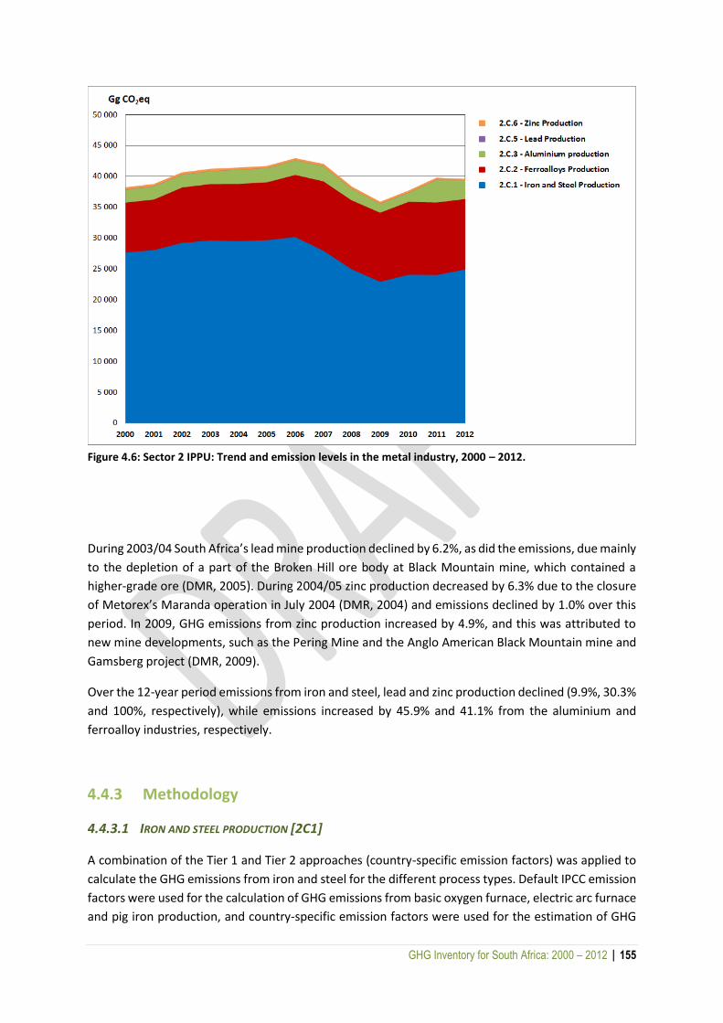
GHG Inventory for South Africa: 2000 – 2012 | 155

Figure 4.6: Sector 2 IPPU: Trend and emission levels in the metal industry, 2000 – 2012.

During 2003/04 South Africa’s lead mine production declined by 6.2%, as did the emissions, due mainly

to the depletion of a part of the Broken Hill ore body at Black Mountain mine, which contained a

higher-grade ore (DMR, 2005). During 2004/05 zinc production decreased by 6.3% due to the closure

of Metorex’s Maranda operation in July 2004 (DMR, 2004) and emissions declined by 1.0% over this

period. In 2009, GHG emissions from zinc production increased by 4.9%, and this was attributed to

new mine developments, such as the Pering Mine and the Anglo American Black Mountain mine and

Gamsberg project (DMR, 2009).

Over the 12-year period emissions from iron and steel, lead and zinc production declined (9.9%, 30.3%

and 100%, respectively), while emissions increased by 45.9% and 41.1% from the aluminium and

ferroalloy industries, respectively.

4.4.3 Methodology

4.4.3.1 IRON AND STEEL PRODUCTION [2C1]

A combination of the Tier 1 and Tier 2 approaches (country-specific emission factors) was applied to

calculate the GHG emissions from iron and steel for the different process types. Default IPCC emission

factors were used for the calculation of GHG emissions from basic oxygen furnace, electric arc furnace

and pig iron production, and country-specific emission factors were used for the estimation of GHG

GHG Inventory for South Africa: 2000 – 2012 | 156

emissions from direct reduced iron production. The separation of energy and process emissions

emanating from the use of coke was not done due to a lack of disaggregated information on coke

consumption. Hence, energy-related emissions from iron and steel production have been accounted

for through the application of default IPCC emission factors.

4.4.3.2 FERROALLOY PRODUCTION [2C2]

The Tier 1 approach was used to calculate the GHG emissions from ferroalloy production.

4.4.3.3 ALUMINIUM PRODUCTION [2C3]

The Tier 1 approach was used to calculate the GHG emissions from aluminium production. It was

assumed that the activity data was mainly for primary aluminium only, without any resmelting.

4.4.3.4 LEAD PRODUCTION [2C5]

Emissions from lead production were estimated using a Tier 1 approach. It was assumed that that lead

production was 80% Imperial Smelting Furnace and 20% direct smelting.

4.4.3.5 ZINC PRODUCTION [2C6]

Emissions from zinc production were calculated with the Tier 1 approach.

4.4.4 Data sources

Metal industry emission estimates were based on data from two main sources: the SAISI (2008)

provided data for iron and steel production, while production data for all the other metals were

obtained from the SAMI report (Department of Minerals and Energy, 2001).

4.4.4.1 IRON AND STEEL PRODUCTION [2C1]

The SAISI provided data for iron and steel production (Table 4.4).

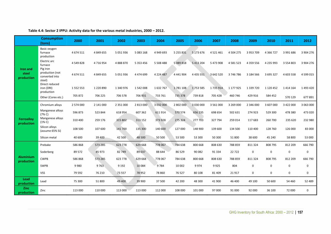
GHG Inventory for South Africa: 2000 – 2012 | 157

Table 4.4: Sector 2 IPPU: Activity data for the various metal industries, 2000 – 2012.

Consumption (tons)

2000 2001 2002 2003 2004 2005 2006 2007 2008 2009 2010 2011 2012

Iron and steel

production

Basic oxygen furnace production

4 674 511 4 849 655 5 051 936 5 083 168 4 949 693 5 255 831 5 173 676 4 521 461 4 504 275 3 953 709 4 366 727 3 991 686 3 904 276

Electric arc furnace

4 549 828 4 716 954 4 888 870 5 353 456 5 508 488 5 089 818 5 413 204 5 473 908 4 581 523 4 359 556 4 235 993 3 554 803 3 904 276

Pig iron production (not converted into steel)

4 674 511 4 849 655 5 051 936 4 474 699 4 224 487 4 441 904 4 435 551 3 642 520 3 746 786 3 184 566 3 695 327 4 603 558 4 599 015

Direct reduced iron (DRI) production

1 552 553 1 220 890 1 340 976 1 542 008 1 632 767 1 781 108 1 753 585 1 735 914 1 177 925 1 339 720 1 120 452 1 414 164 1 493 420

Other (Corex etc.) 705 872 706 225 706 578 706 931 733 761 735 378 739 818 705 428 460 746 429 916 584 452

570 129 677 891

Ferroalloy production

Chromium alloys 2 574 000 2 141 000 2 351 000 2 813 000 3 032 000 2 802 000 3 030 000 3 561 000 3 269 000 2 346 000 3 607 000 3 422 000 3 063 000

Manganese alloys (7% C)

596 873 523 844 618 954 607 362 611 914 570 574 656 235 698 654 502 631 274 923 529 300 478 380 473 020

Manganese alloys (1% C)

310 400 259 176 315 802 313 152 373 928 275 324 277 703 327 794 259 014 117 683 260 700 235 620 232 980

Silicon alloys (assume 65% Si)

108 500 107 600 141 700 135 300 140 600 127 000 148 900 139 600 134 500 110 400 128 760 126 000 83 000

Silicon metal 40 600 39 400 42 500 48 500 50 500 53 500 53 300 50 300 51 800 38 600 45 240 58 800 53 000

Aluminium production

Prebake 586 868 573 285 623 778 629 668 778 067 784 638 800 668 808 630 788 859 811 324 808 795 812 209 666 790

Soderberg 89 572 85 973 82 749 89 037 88 644 86 529 90 082 91 334 22 722 0 0 0 0

CWPB 586 868 573 285 623 778 629 668 778 067 784 638 800 668 808 630 788 859 811 324 808 795 812 209 666 790

SWPB 9 980 9 763 9 192 10 084 9 784 10 002 9 974 9 925 804 0 0 0 0

VSS 79 592 76 210 73 557 78 952 78 860 76 527 80 108 81 409 21 917 0 0 0 0

Lead production

Lead 75 300 51 800 49 400 39 900 37 500 42 200 48 300 41 900 46 400 49 100 50 600 54 460 52 489

Zinc production

Zinc 113 000 110 000 113 000 113 000 112 000 108 000 101 000 97 000 91 000 92 000 36 100 72 000 0

GHG Inventory for South Africa: 2000 – 2012 | 158

4.4.4.1.1 Emission factors

A combination of country-specific emission factors and IPCC default emission factors were applied for

the calculation of GHG emissions from iron and steel. Country-specific emission factors were sourced

from one of the iron and steel companies in South Africa (Table 4.5) and these were based on actual

process analysis at the respective plants. The country-specific emission factor for electric arc furnace

(EAF) production is slightly higher than the IPCC default value; this emission factor was not used for

the estimation of GHG emissions from EAF because it needs to be investigated further. The country-

specific emission factor for Ddirect reduced iron production is more than twice the default factor

(Table 4.5) and it was used for the estimation of GHG emissions from this process. Differences in

feedstock material and origin results in higher emission factors compared with the IPCC default

emission factor values, which assume consistent feedstock conditions across countries.

Table 4.5: Sector 2 IPPU: Comparison of the country-specific emission factors for iron and steel production

and the IPCC 2006 default values (Source: iron and steel Companies; IPCC 2006 Guidelines).

Type of Technology

CO2 Emission factor

(tones CO2 per tonne iron and steel)

Country-specific

IPCC 2006 default

Basic Oxygen Furnace 1.46

Electric Arc Furnace 1.1 0.08

Pig Iron Production (not converted into steel) - 1.35

Direct Reduced Iron (DRI) Production 1.525 0.7

Sinter Production 0.34 0.2

4.4.4.2 FERROALLOY, ALUMINIUM, LEAD AND ZINC PRODUCTION

The source of activity data for these categories was sourced from the SAMI report (Table 4.4). IPCC

default emission factors were used (Table 4.6 and Table 4.7). The emission factor of 0.52 tonnes CO2

per tonne lead and 1.72 tonnes CO2 per tonne zinc were sourced from the IPCC 2006 Guidelines.

4.4.5 Uncertainty and time-series consistency

The necessary quality-control measures were used to minimise estimation errors. The Tier 1 approach

for metal production emission estimates generates a number of uncertainties. For example, the IPCC

2006 Guidelines explain that applying Tier 1 to default emission factors for iron and steel production

may have an uncertainty of ± 25%. The same range of uncertainty is associated with the Tier 1

approach for ferroalloy production emission factors.

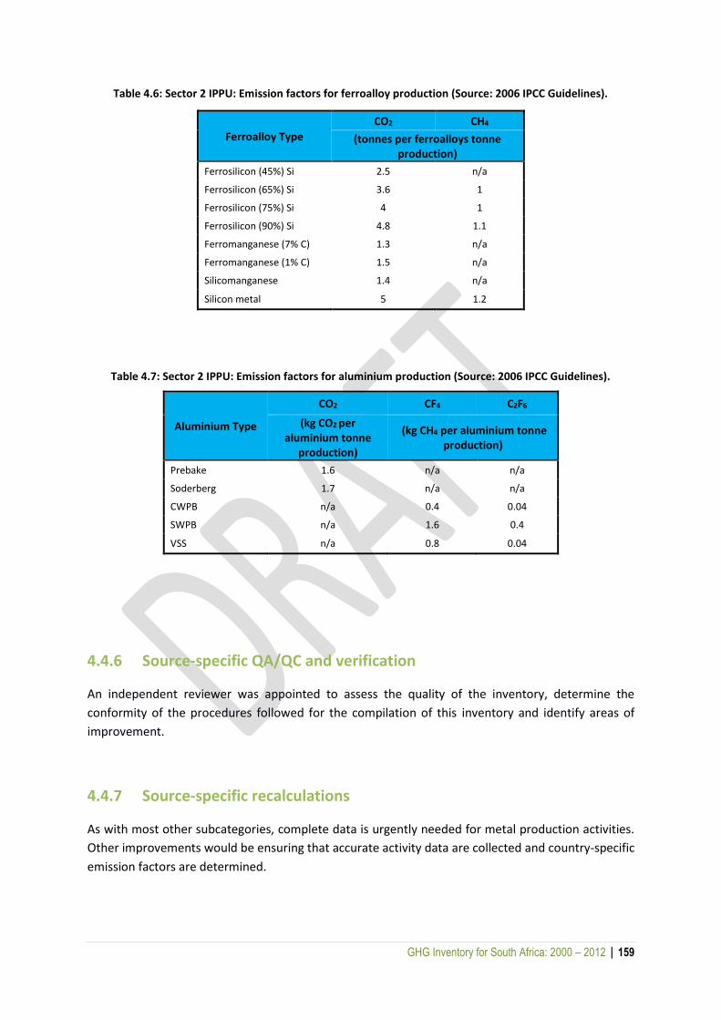
GHG Inventory for South Africa: 2000 – 2012 | 159

Table 4.6: Sector 2 IPPU: Emission factors for ferroalloy production (Source: 2006 IPCC Guidelines).

Ferroalloy Type

CO2 CH4

(tonnes per ferroalloys tonne production)

Ferrosilicon (45%) Si 2.5 n/a

Ferrosilicon (65%) Si 3.6 1

Ferrosilicon (75%) Si 4 1

Ferrosilicon (90%) Si 4.8 1.1

Ferromanganese (7% C) 1.3 n/a

Ferromanganese (1% C) 1.5 n/a

Silicomanganese 1.4 n/a

Silicon metal 5 1.2

Table 4.7: Sector 2 IPPU: Emission factors for aluminium production (Source: 2006 IPCC Guidelines).

Aluminium Type

CO2 CF4 C2F6

(kg CO2 per aluminium tonne

production)

(kg CH4 per aluminium tonne production)

Prebake 1.6 n/a n/a

Soderberg 1.7 n/a n/a

CWPB n/a 0.4 0.04

SWPB n/a 1.6 0.4

VSS n/a 0.8 0.04

4.4.6 Source-specific QA/QC and verification

An independent reviewer was appointed to assess the quality of the inventory, determine the

conformity of the procedures followed for the compilation of this inventory and identify areas of

improvement.

4.4.7 Source-specific recalculations

As with most other subcategories, complete data is urgently needed for metal production activities.

Other improvements would be ensuring that accurate activity data are collected and country-specific

emission factors are determined.

GHG Inventory for South Africa: 2000 – 2012 | 160

4.4.8 Source-specific planned improvements and recommendations

As with most other subcategories, completeness of data is urgently needed for metal production

activities. Other improvements would be ensuring that accurate activity data are collected and

country specific emission factors are determined.

4.5 Non-energy use of fuels and solvent use [2D]

4.5.1 Source-category description

Non-energy use of fuels and solvents includes lubricants and paraffin wax. The use of solvents can

result in evaporative emissions of various NMVOCs, which can be oxidized and released into the

atmosphere. According to the 2006 IPCC Guidelines (p. 5.16), white spirit is used as an extraction

solvent, cleaning solvent, degreasing solvent and as a solvent in aerosols, paints, wood preservatives,

varnishes and asphalt products. Lubricants are used in industrial and transport applications.

Lubricants are divided into two types, namely, motor and industrial oils, and greases that differ in

physical characteristics. Paraffin wax is used in products such as petroleum jelly, paraffin waxes and

other waxes (saturated hydrocarbons). Paraffin waxes are used in applications such as candles,

corrugated boxes, paper coating, board sizing, food production, wax polishes, surfactants (as used in

detergents) and many others (IPCC, 2006, p.5.11).

4.5.2 Overview of shares and trends in emissions

Total GHG emissions from the non-energy products from fuels and solvent use category fluctuated

between 196 Gg CO2eq and 246 Gg CO2eq between 2000 and 2004, and hovered around 234 Gg CO2eq

between 2007 and 2010, with a peak in emissions occurring in 2006 (Figure 4.7).

Emissions from lubricant use contributed between 93.5% and 99.1% of the total emissions from this

category.

4.5.3 Methodological issues

Emissions for this category were estimated using a Tier 1 approach. In line with the 2006 IPCC

Guidelines (p.5.9), it was assumed that 90% of the mass of lubricants is oil and 10% is grease.

4.5.4 Data sources

The source of activity data for solvents was the energy balance tables published annually by the DoE

(Table 4.8).

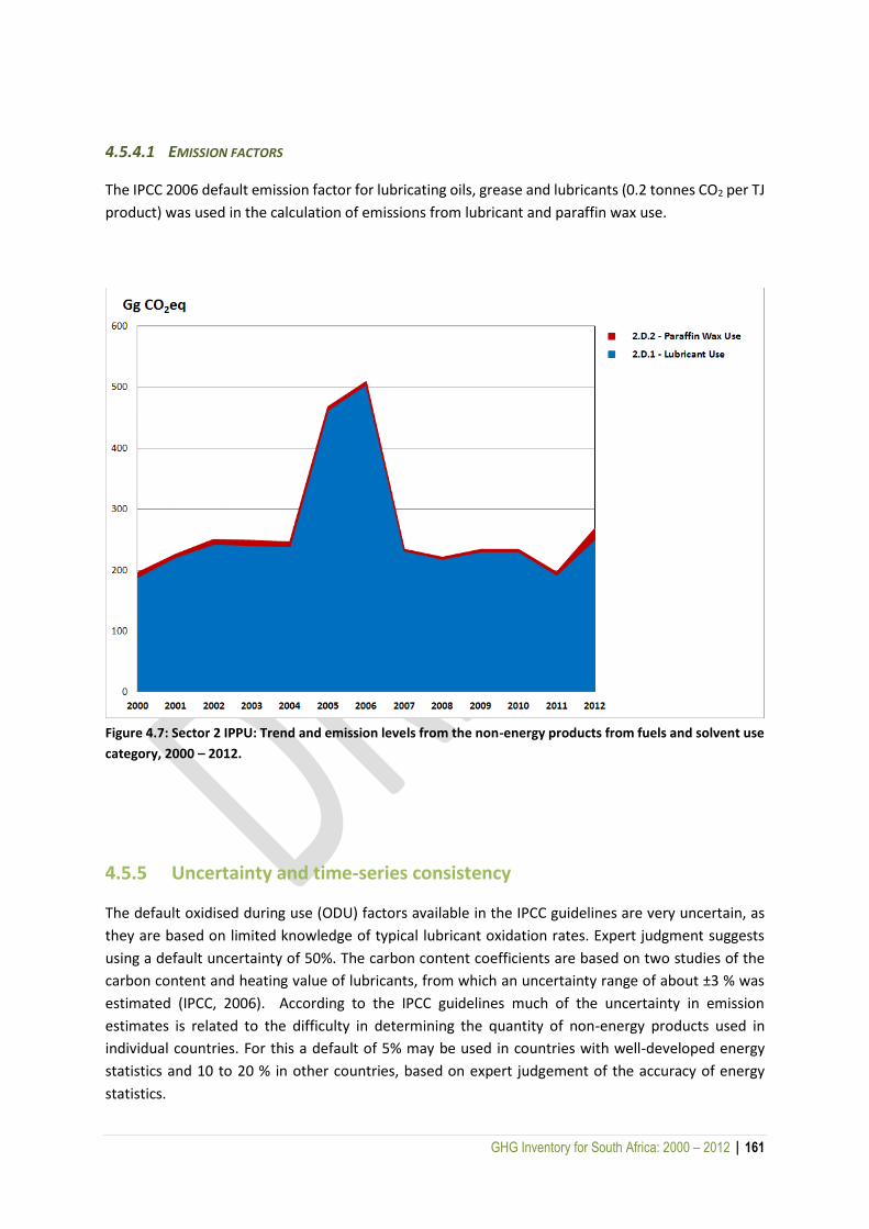
GHG Inventory for South Africa: 2000 – 2012 | 161

4.5.4.1 EMISSION FACTORS

The IPCC 2006 default emission factor for lubricating oils, grease and lubricants (0.2 tonnes CO2 per TJ

product) was used in the calculation of emissions from lubricant and paraffin wax use.

Figure 4.7: Sector 2 IPPU: Trend and emission levels from the non-energy products from fuels and solvent use

category, 2000 – 2012.

4.5.5 Uncertainty and time-series consistency

The default oxidised during use (ODU) factors available in the IPCC guidelines are very uncertain, as

they are based on limited knowledge of typical lubricant oxidation rates. Expert judgment suggests

using a default uncertainty of 50%. The carbon content coefficients are based on two studies of the

carbon content and heating value of lubricants, from which an uncertainty range of about ±3 % was

estimated (IPCC, 2006). According to the IPCC guidelines much of the uncertainty in emission

estimates is related to the difficulty in determining the quantity of non-energy products used in

individual countries. For this a default of 5% may be used in countries with well-developed energy

statistics and 10 to 20 % in other countries, based on expert judgement of the accuracy of energy

statistics.

GHG Inventory for South Africa: 2000 – 2012 | 162

Table 4.8: Sector 2 IPPU: Total fuel consumption in the non-energy use of fuels and solvent use category, 2000 – 2010.

Fuel consumption

Period Lubricants (TJ)

Paraffin Wax (TJ)

2000 12 851 507

2001 15 092 314

2002 16 561 506

2003 16 430 521

2004 16 295 490

2005 31 549 350

2006 34 391 324

2007 15 819 141

2008 14 891 182

2009 15 707 231

2010 15 715 231

2011 13 130 260

2012 17 085 1 188

4.5.6 Source-specific QA/QC and verification

An independent reviewer was appointed to assess the quality of the inventory, determine the

conformity of the procedures followed for the compilation of this inventory and to identify areas of

improvement.

4.5.7 Source-specific recalculations

No source-specific recalculations were performed.

4.5.8 Source-specific planned improvements and recommendations

Energy balances remain the source of activity data for this source category and, therefore, no source-

specific improvements are planned in the future. However, improvements in data collection for

energy balances would reduce uncertainty in fuel use data.

GHG Inventory for South Africa: 2000 – 2012 | 163

4.6 Production uses as substitutes for ozone-depleting substances

[2F]

The Montreal Protocol on Substances that Deplete the Ozone Layer (a protocol to the Vienna

Convention for the Protection of the Ozone Layer) is an international treaty designed to protect the

ozone layer by phasing out the production of numerous substances believed to be responsible for

ozone depletion. Hydrofluorocarbons (HFCs) and, to a limited extent, perfluorocarbons (PFCs) are

serving as alternatives to ozone-depleting substances (ODS) being phased out under this protocol.

According to the 2006 IPCC Guidelines, current application areas of HFCs and PFCs include

refrigeration and air conditioning; fire suppression and explosion protection; aerosols; solvent

cleaning; foam blowing; and other applications (equipment sterilisation, tobacco expansion

applications, and as solvents in the manufacture of adhesives, coatings and inks).

4.6.1 Overview of shares and trends in emissions

Total CO2eq emissions from HFC’s increased from 842 Gg CO2eq in 2005 to 2 096 Gg CO2eq in 2010,

then declined again to 1 396 in 2012 (Figure 4.8). There was no available data for the years prior to

2005. HFC-134a is the biggest contributor (average contribution of 80.8%) and HFC-143a contributing

an average of 8.9%.

4.6.2 Methodological issues

The Tier 1 approach was used to estimate emissions from substitutes for ozone-depleting substances.

The calculation of GHG emissions was done through a calculator provided by the IPCC. It was assumed

that the equipment lifespan was 15 years and the emission factor from the installed base was 15%.

These assumptions were based on the defaults from the 2006 IPCC Guidelines.

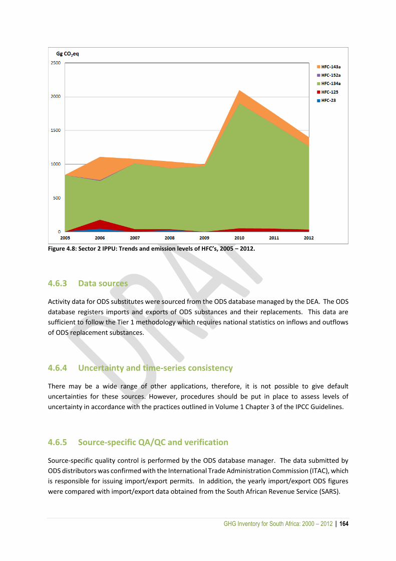
GHG Inventory for South Africa: 2000 – 2012 | 164

Figure 4.8: Sector 2 IPPU: Trends and emission levels of HFC’s, 2005 – 2012.

4.6.3 Data sources

Activity data for ODS substitutes were sourced from the ODS database managed by the DEA. The ODS

database registers imports and exports of ODS substances and their replacements. This data are

sufficient to follow the Tier 1 methodology which requires national statistics on inflows and outflows

of ODS replacement substances.

4.6.4 Uncertainty and time-series consistency

There may be a wide range of other applications, therefore, it is not possible to give default

uncertainties for these sources. However, procedures should be put in place to assess levels of

uncertainty in accordance with the practices outlined in Volume 1 Chapter 3 of the IPCC Guidelines.

4.6.5 Source-specific QA/QC and verification

Source-specific quality control is performed by the ODS database manager. The data submitted by

ODS distributors was confirmed with the International Trade Administration Commission (ITAC), which

is responsible for issuing import/export permits. In addition, the yearly import/export ODS figures

were compared with import/export data obtained from the South African Revenue Service (SARS).

GHG Inventory for South Africa: 2000 – 2012 | 165

4.6.6 Source-specific recalculations

No source-specific recalculations were performed.

4.6.7 Source-specific planned improvements and recommendations

According to the IPCC Guidelines, it is good practice to estimate emissions from ODS replacement use

by end-use sector (e.g., foam blowing, refrigeration etc.). Future improvements would involve the

collection of data at the sector level such that default emission factors can be applied at sectoral level.

GHG Inventory for South Africa: 2000 – 2012 | 166

5 AGRICULTURE, FORESTRY AND OTHER LAND USE

5.1 Overview of the sector

This section includes GHG emissions and removals from agriculture as well as land use and forestry.

Based on the IPCC 2006 Guidelines, the following categories are included in the emission estimates:

Livestock

o Enteric fermentation (IPCC Section 3A1)

o Manure management (IPCC Section 3A2)

Land

o Forest land (IPCC Section 3B1)

o Cropland (IPCC Section 3B2)

o Grassland (IPCC Section 3B3)

o Wetlands (IPCC Section 3B4)

o Settlements (IPCC Section 3B5)

o Other land (IPCC Section 3B6)

Aggregate sources and non-CO2 emissions on land

o Biomass burning (IPCC Section 3C1)

o Liming (IPCC Section 3C2)

o Urea application (IPCC Section 3C3)

o Direct N2O emission from managed soils (IPCC Section 3C4)

o Indirect N2O emission from managed soils (IPCC Section 3C5)

o Indirect N2O emission from manure management (IPCC Section 3C6)

Other

o Harvested wood products (IPCC Section 3D1)

Emissions from fuel combustion in this sector are not included here as these fall under the

agriculture/forestry/fisheries subsector (see Section 3.3.6.1.3) in the energy sector. Categories not

included in this report are rice cultivation (3C7), and other (3C8, 3D2), as they are not applicable to

South Africa. The land use component includes land remaining in the same land use as well as land

converted to another land use. This section includes a Tier 1 approach to the mineral soil carbon pool,

while organic soils are not reported on as the area of organic soils in South Africa was estimated to be

insignificant.

Emissions from ruminants in privately owned game parks has been included as these are suggested to

be managed lands as the game a fed. Game in national parks are not included as they are considered

unmanaged.

Manure management includes all emissions from confined, managed animal waste systems. Methane

emissions from livestock manure produced in the field during grazing are included under manure

management (3A2); however, the N2O emissions from this source are included under category 3C4

direct N2O emissions from managed soils. This is in accordance with IPCC 2006 Guidelines. Methane

emissions from managed soils are regarded as non-anthropogenic and are, according to the

guidelines, not included.

GHG Inventory for South Africa: 2000 – 2012 | 167

Losses of CO2 emissions from biomass burning of forest land are included under losses due to

disturbance in the forest land section (3B1) and not in the biomass burning (3C1) section. Section 3C1

deals with non-CO2 emissions from biomass burning in all land use types.

5.2 GHG emissions from the AFOLU sector

5.2.1 Overview of shares and trends in emissions

The AFOLU sector was a source of CO2 (Table 5.1). The source fluctuated over the 12 year period, but

overall there appeared to be an increase in the sink. Total GHG emissions from livestock declined by

5.6%, from 31 162 Gg CO2eq in 2000 to 29 413 Gg CO2eq in 2012. The decline was attributed mainly

to the decreasing cattle, sheep and goat populations. The land component is estimated to be a sink,

varying between 10 309 Gg CO2eq and 20 830 Gg CO2eq (Table 5.1). The variation was caused mainly

by changes in carbon stocks in forest lands due to variation in carbon losses (fire and fuelwood losses).

Emissions from aggregated and non-CO2 emission sources varied by a maximum of 9.1% over the 12

year period. The fluctuations in this category are driven mainly by changes in biomass burning, liming

and urea application. HWP estimates indicate that this subsector is a small sink of CO2, varying

between a minimum of 312 Gg CO2eq (2000) and a maximum of 1 187 Gg CO2eq (2004). In 2011 this

subsector was a small source of CO2. As with the land and aggregated and non-CO2 emission sources,

the sink does not show any trend.

The recalculated 2010 estimate in this inventory was 29.2% higher than the previous inventory

estimate of 25 713 Gg CO2eq (DEA, 2014). The change was attributed mainly to the use of updated

land cover change maps and corrected HWP estimates. The HWP estimates were reduced by an

average of 94% compared with the 2010 inventory due to corrections and improved methodology.

In all years CH4 emissions contributed the most to the total AFOLU emissions (Figure 5.1: Sector 3

AFOLU: Percentage contribution of the various GHG to the total AFOLU inventory, 2000 – 2012.

), but this contribution declined from 46.32% in 2000 to 38.5% in 2012. Enteric fermentation

contributed an average of 92.4% of the CH4. The contribution from N2O fluctuated annually but was

in the range of 32.5% to 38.9% with an average of 68.8% of this coming from direct N2O emissions

from managed soils.

5.2.2 Key sources

A level and trend key category analysis including the AFOLU sector was carried out on the 2012 data

(Appendix B). Both of these assessments showed that the main key categories in this sector are land

converted to forest land, enteric fermentation and direct N2O from managed soils. It should be noted

that the key category assessment is incomplete due to the incomplete reporting of all sources.

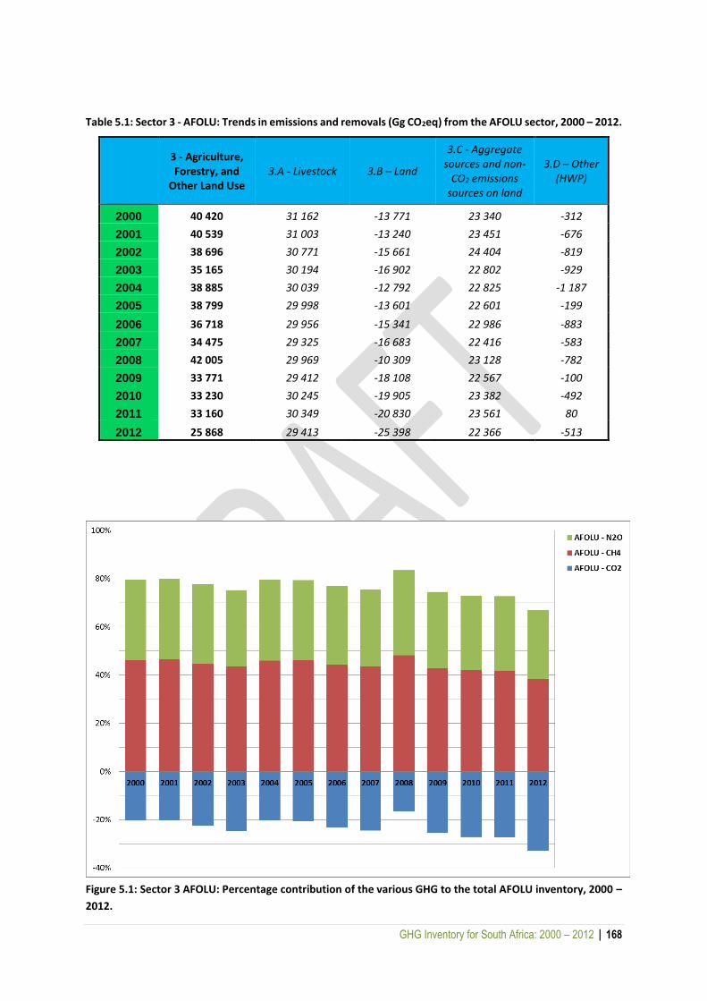
GHG Inventory for South Africa: 2000 – 2012 | 168

Table 5.1: Sector 3 - AFOLU: Trends in emissions and removals (Gg CO2eq) from the AFOLU sector, 2000 – 2012.

3 - Agriculture, Forestry, and

Other Land Use 3.A - Livestock 3.B – Land

3.C - Aggregate sources and non-

CO2 emissions sources on land

3.D – Other (HWP)

2000 40 420 31 162 -13 771 23 340 -312

2001 40 539 31 003 -13 240 23 451 -676

2002 38 696 30 771 -15 661 24 404 -819

2003 35 165 30 194 -16 902 22 802 -929

2004 38 885 30 039 -12 792 22 825 -1 187

2005 38 799 29 998 -13 601 22 601 -199

2006 36 718 29 956 -15 341 22 986 -883

2007 34 475 29 325 -16 683 22 416 -583

2008 42 005 29 969 -10 309 23 128 -782

2009 33 771 29 412 -18 108 22 567 -100

2010 33 230 30 245 -19 905 23 382 -492

2011 33 160 30 349 -20 830 23 561 80

2012 25 868 29 413 -25 398 22 366 -513

Figure 5.1: Sector 3 AFOLU: Percentage contribution of the various GHG to the total AFOLU inventory, 2000 –

2012.

GHG Inventory for South Africa: 2000 – 2012 | 169

5.2.3 Recalculations

In the livestock subsector, minor corrections were made to the beef and dairy cattle population

numbers, as well as the poultry population numbers. Also emissions from game on privately owned

game parks were included using activity data and emission factors supplied by Du Toit et al. (2013d).

Due to these updated activity data and emission factors the annual livestock emissions since 2000

were recalculated.

In the land category there were several updates:

New land-use change maps were incorporated (for 1990 and 2013/2014);

Biomass data was updated;

DOM was incorporated for forest lands;

Estimates from other lands were included;

Changes in soil carbon methodology to include soil type; and

Corrected and updated HWP methodology.

These recalculations were completed for all yeas since 2000 and all updates and improvements are

discussed in the sections below.

5.3 Livestock [3A]

5.3.1 Overview of shares and trends in emissions

The GHG emissions from livestock produced a total of 29 412 Gg CO2eq in 2012. This was a 5.6%

decline from the 2000 emissions (31 162 Gg CO2eq) (Figure 5.2: Sector 3 AFOLU: Trends in GHG

emissions from the livestock category, 2000 – 2012.

). The total accumulated emissions since 2000 stand at 332 075 Gg CO2eq. Emissions declined

annually between 2000 and 2007, and increased by 2.2% in 2008. There was also an increase of 3.0%

between 2009 and 2011. Enteric fermentation accounted for an average of 93.3% of the GHG

emissions from livestock, while the rest was from manure management. Emissions from manure

management showed a 18.2% increase in emissions between 2000 (1 872 Gg CO2eq) and 2012 (2 214

Gg CO2eq). This increase was mainly due to the increase in the poultry population with all of the

manure from this livestock category being managed. If poultry manure is excluded then there is a

slight decline in manure emissions from all other livestock, with little annual variation.

GHG Inventory for South Africa: 2000 – 2012 | 170

Figure 5.2: Sector 3 AFOLU: Trends in GHG emissions from the livestock category, 2000 – 2012.

5.3.2 Overview of trends in activity data

The total annual livestock population increased by 29.8% between 2000 and 2012, mainly due to

growth in the poultry industry. If poultry numbers are excluded, then there was a general decline (of

6.1%) in the remaining livestock population over the 12-year period (Figure 5.3: Sector 3 AFOLU -

Livestock: Trends in livestock population numbers, 2000 – 2012.

). The commercial beef cattle population fluctuated slightly around an average of 7 million (with a low

of 6.85 million in 2002, and a high of 7.34 million in 2001), while the communal beef population

fluctuated around 5.4 million (± 0.27 million). The dairy cattle population declined between 2000 and

2004 (25.6%), increased between 2004 and 2010 (31.4%), and declined by 7.5% between 2010 and

2012. Sheep and goat populations declined by 9.2% and 13.9%, respectively, and swine by 4.1%

between 2000 and 2012. The annual average poultry population increased by 48.4%, from 100 million

in 2000 to 149 million in 2012 (Figure 5.3: Sector 3 AFOLU - Livestock: Trends in livestock population

numbers, 2000 – 2012.

).

Generally, the commercial population numbers were higher than the communal numbers, except for

goats, where the communal goat population was approximately twice that of the commercial

population. The game population in privately owned game parks was estimated at 2 285 000 (Du Toit

et al., 2013d). This was kept constant each year due to a lack of data.

GHG Inventory for South Africa: 2000 – 2012 | 171

Figure 5.3: Sector 3 AFOLU - Livestock: Trends in livestock population numbers, 2000 – 2012.

5.3.3 Enteric fermentation [3A1]

5.3.3.1 SOURCE-CATEGORY DESCRIPTION

Methane is the main greenhouse gas produced from agricultural livestock production. CH4 from

enteric fermentation is produced in herbivores as a by-product of the digestive process, and is

released mainly through eructation and normal respiration, and a small quantity as flatus (Bull et al.,

2005; Chhabra et al., 2009; Baggot et al., 2006; IPCC, 1997; IPCC, 2006). The amount of CH4 produced

and emitted by an individual animal depends primarily on the animal’s digestive system and the

amount and type of feed it consumes (IPCC, 1997; Garcia-Apaza et al., 2008). South Africa’s animal

data are divided into three main groups according to their different methane-producing abilities,

namely ruminants (cattle, sheep, and goats), pseudo-ruminants (horses, donkeys) and monogastric

animals (pigs) (DAFF, 2010).

South Africa does not have any managed camels or ilamas so these were excluded from the emissions.

Buffalo and other game are not managed per say, but are found in significant numbers in game parks

(both national and private). This inventory includes a first estimate of emissions from game in private

GHG Inventory for South Africa: 2000 – 2012 | 172

parks. This number is not complete as not all ruminant species were included due to a lack of emission

factor data. Furthermore, an estimate from the game population kept in national parks has not been

included due to a lack of population data.

Enteric fermentation emissions from poultry were not estimated as the amount produced is

considered negligible (IPCC, 2006). No default emission factors are provided in the IPCC Guidelines as

it states that there is insufficient data for the calculation. This exclusion of poultry from enteric

fermentation emissions is in line with the IPCC 2006 Guidelines, however, there are some reports of

CH4 emissions from poultry (Wang and Huang, 2005; Burns, 2012). These emissions are small, but in

light of South Africa’s growing poultry population it should be investigated further in future

inventories.

5.3.3.2 OVERVIEW OF SHARES AND TRENDS IN EMISSIONS

Enteric fermentation emissions from livestock declined from 29 290 Gg CO2eq in 2000 to 27 198 Gg

CO2eq in 2012 (Figure 5.4: Sector 3 AFOLU - Livestock: Trend and emission levels of enteric

fermentation emissions in the livestock categories, 2000 – 2012.

), mainly due to a decline in population numbers. Emissions declined in most years except for an

increase of 2.3% between 2007 and 2008, as well as a 3.0% increase between 2009 and 2010. In these

years there was an increase in enteric fermentation emissions from cattle, which was attributed to an

increase in the number of mature cows and heifers and a reduction in the calf population (Figure 5.5:

Sector 3 AFOLU - Livestock: Trend in cattle herd composition, 2000 – 2012.

). Mature cows and heifers have a higher emission factor than calves due to a well-developed gut.

Cattle are the largest contributors to the enteric fermentation emissions (78.1% in 2012), with 9.2%

from dairy cattle, 13.9% from sheep and 3.2% from goats in 2012 (Figure 5.6: Sector 3 AFOLU –

Livestock: Contribution of the livestock categories to the enteric fermentation emissions in 2012.

).

GHG Inventory for South Africa: 2000 – 2012 | 173

Figure 5.4: Sector 3 AFOLU - Livestock: Trend and emission levels of enteric fermentation emissions in the

livestock categories, 2000 – 2012.

Figure 5.5: Sector 3 AFOLU - Livestock: Trend in cattle herd composition, 2000 – 2012.

GHG Inventory for South Africa: 2000 – 2012 | 174

Figure 5.6: Sector 3 AFOLU – Livestock: Contribution of the livestock categories to the enteric fermentation

emissions in 2012.

5.3.3.3 METHODOLOGICAL ISSUES

The proportion of intake that is converted into methane is dependent on the characteristics of the

animal, feed and the amount eaten. Given the heterogeneity of available feed types within South

Africa it was considered important to use methodologies that could reflect such differences,

developed under similar conditions as in Australia. A detailed description of the methods, data sources

and emission factors is found in Du Toit et al. (2013a, 2013b), and are summarized below.

Emissions from enteric fermentation are calculated from activity data on animal numbers and the

appropriate emission factor:

CH4 emission = ΣEFi (kg CH4 animal-1) * [number of animals for livestock category i] (Eq. 5.1)

5.3.3.3.1 Dairy cattle [3A1AI]

EFs for the various sub-categories of dairy cattle were taken from Du Toit et al. (2013a). These EF’s

were calculated using a Tier 2 approach following the equation:

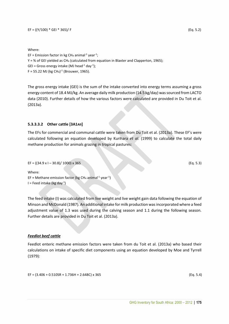
GHG Inventory for South Africa: 2000 – 2012 | 175

EF = ((Y/100) * GEI * 365)/ F (Eq. 5.2)

Where:

EF = Emission factor in kg CH4 animal-1 year-1;

Y = % of GEI yielded as CH4 (calculated from equation in Blaxter and Clapperton, 1965);

GEI = Gross energy intake (MJ head-1 day-1);

F = 55.22 MJ (kg CH4)-1 (Brouwer, 1965).

The gross energy intake (GEI) is the sum of the intake converted into energy terms assuming a gross

energy content of 18.4 MJ/kg. An average daily milk production (14.5 kg/day) was sourced from LACTO

data (2010). Further details of how the various factors were calculated are provided in Du Toit et al.

(2013a).

5.3.3.3.2 Other cattle [3A1AII]

The EFs for commercial and communal cattle were taken from Du Toit et al. (2013a). These EF’s were

calculated following an equation developed by Kurihara et al. (1999) to calculate the total daily

methane production for animals grazing in tropical pastures:

EF = ((34.9 x I – 30.8)/ 1000) x 365 (Eq. 5.3)

Where:

EF = Methane emission factor (kg CH4 animal-1 year-1)

I = Feed intake (kg day-1)

The feed intake (I) was calculated from live weight and live weight gain data following the equation of

Minson and McDonald (1987). An additional intake for milk production was incorporated where a feed

adjustment value of 1.3 was used during the calving season and 1.1 during the following season.

Further details are provided in Du Toit et al. (2013a).

Feedlot beef cattle

Feedlot enteric methane emission factors were taken from du Toit et al. (2013a) who based their

calculations on intake of specific diet components using an equation developed by Moe and Tyrrell

(1979):

EF = (3.406 + 0.510SR + 1.736H + 2.648C) x 365 (Eq. 5.4)

GHG Inventory for South Africa: 2000 – 2012 | 176

Where:

SR = Intake of soluble residue (kg day-1);

H = Intake of hemicellulose (kg day-1);

C = Intake of cellulose (kg day-1).

Soluble residue intake, hemicellulose intake and cellulose intake were calculated from feedlot diet

analysis (ANIR, 2009) and average dry matter intake (DMI) taken as 8.5 kg DM per day (South African

feedlot association and industry experts).

Total annual methane production (EF, kg CH4 head-1 year-1) was calculated as:

EF = (Y / F) x 365 (Eq. 5.5)

Where:

F = 55.22 MJ (kg CH4)-1 (Brouwer, 1965)

The total feedlot calculations are based on the assumption that an animal will stay in the feedlot for approximately 110 days (3 cycles per year).

5.3.3.3.3 Sheep [3A1C]

Sheep CH4 emission factors were taken from Du Toit et al. (2013b) which are based on the equations

of Howden et al. (1994):

EF = (I x 0.0188 + 0.00158) x 365 (Eq. 5.6)

Where:

EF = Emission factor (kg CH4 head-1 year-1);

I = Feed intake (kg DM day-1).

The actual feed intake by sheep was calculated from the potential feed intake (determined by body

size and the proportion of the diet that was able to be metabolised by the animal), relative intake

(based on dry matter availability) and an additional intake for milk production.

5.3.3.3.4 Goats [3A1D]

The CH4 emission factors for the various goat sub-categories were taken from Du Toit et al. (2013b).

These calculations followed the same methodology as for sheep. Goats are browsers they are also

selective feeders and will select for quality. It was assumed that lactating milk goats will receive a

higher quality diet with a DMD of 70% throughout the year.

GHG Inventory for South Africa: 2000 – 2012 | 177

5.3.3.3.5 Swine [3A2H]

CH4 emission factors for the pig sub-categories were taken from Du Toit et al. (2013c) which were

based on the methodology described in the Australian National Inventory (ANIR, 2009):

EF = I x 18.6 x 0.007 / F (Eq. 5.7)

Where:

EF = Emission factor (kg CH4 head-1 year-1)

I = Feed intake (kg DM day-1);

F = 55.22 MJ (kg CH4)-1 (Brouwer, 1965);

18.6 = MJ GE per kg feed DM.

A methane conversion factor of 0.7% was used in the calculation for pigs, based on the ANIR (2009).

5.3.3.3.6 Horses and donkeys [3A1F and 3A1G]

The contribution of horses and donkeys to the total methane emissions was relatively small, and given

the lack of data on methane production from these animals, a complex methodology, incorporating

relationships between feed intake and methane production, is inappropriate. Therefore the emissions

from horses and donkeys were based on the Tier 1 methodology and IPCC default emission factors.

5.3.3.3.7. Game [3A1J]

EF's for ruminant game species were taken directly from Du Toit et al. (2013d). For hippopotamus and

rhinoceros, the EFs were based on the daily methane emissions of elephants (0.1 g CH4/kg LW/day)

as was done in Du Toit et al. (2013).

5.3.3.4 DATA SOURCES

5.3.3.4.1 Livestock categorization and population numbers

The first step in estimating CH4 emissions from enteric fermentation and CH4 and N2O emissions from

manure management involves dividing the farmed animal population into the livestock categories and

sub-categories. The livestock categories and sub-categories used in this inventory update are shown

in Table 5.2. The sub-categories for sheep, goats and swine were obtained by combining some of the

more detailed sub-categories given in Du Toit et al. (2013a, 2013b, 2013c) (see Appendix E) as some

of the populations were small and EF’s didn’t vary significantly. The inclusion of all the detailed sub-

categories should be considered in future inventories.

The commercial cattle (dairy and other), sheep, goat and swine population data were obtained from

the Abstracts of Agricultural Statistics 2012. The population numbers for these animals has a

consistent time-series dating back to 1970. For other cattle the feedlot cattle need to be separated

GHG Inventory for South Africa: 2000 – 2012 | 178

out as feedlot cattle have a different emission factor. Annual feedlot cattle numbers were obtained

from the South African Feedlot Association (SA Feedlot Association, 2013; Ford, Dave, 2013. Pers.

Comm.). Data was only available for the years 2008 to 2012, so an average of 420 000 was used for

each year between 2000 and 2007. The number of cattle in feedlots fluctuates by at most 20 000

around this number and this number is not expected to change much over a 10 year period (Ford,

Dave, 2013). The feedlot population was assumed to consist of calves, heifers and young oxen in an

equal split. Therefore the total commercial calf, young oxen and heifer population numbers from the

Abstracts of Agricultural Statistics (DAFF, 2012) were reduced by a third of the feedlot population for

that year and then the feedlot category was added into the population.

The herd composition data from Du Toit et al. (2013a, 2013b, 2013c) was applied to the national dairy,

sheep and goat population numbers to obtain the herd composition sub-categories for these livestock.

The average annual herd composition for swine was assumed to be 1.9% boars, 32.2% sows, 33%

piglets, 4.9% porkers and 28% baconers (Du Toit et al., 2013c).

Due to a lack of data over time on herd composition it was assumed that the composition remained

constant between 2000 and 2010. In future this assumption needs to be addressed by improving the

monitoring of livestock herd composition. Altering the composition of the herd is a possible, although

small, mitigation action therefore improved monitoring of herd composition is required in the future

to address this assumption.

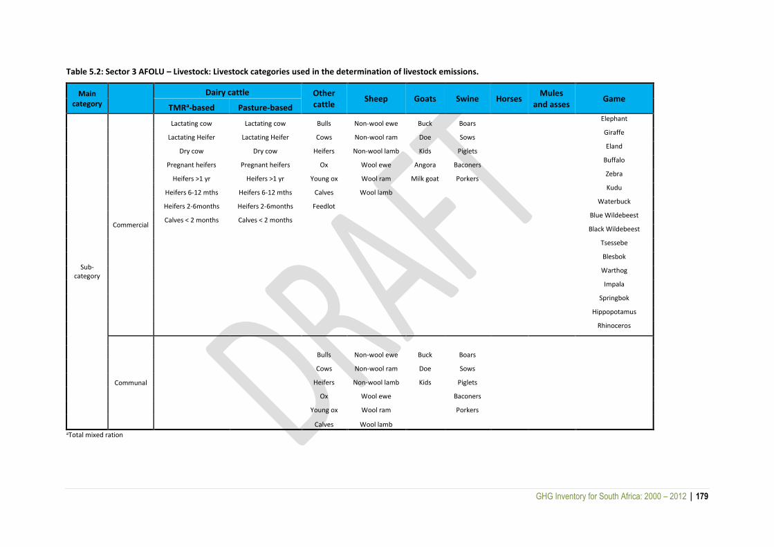
GHG Inventory for South Africa: 2000 – 2012 | 179

Table 5.2: Sector 3 AFOLU – Livestock: Livestock categories used in the determination of livestock emissions.

Main category

Dairy cattle Other cattle

Sheep Goats Swine Horses Mules

and asses Game

TMRa-based Pasture-based

Sub-category

Commercial

Lactating cow Lactating cow Bulls Non-wool ewe Buck Boars Elephant

Lactating Heifer Lactating Heifer Cows Non-wool ram Doe Sows Giraffe

Dry cow Dry cow Heifers Non-wool lamb Kids Piglets Eland

Pregnant heifers Pregnant heifers Ox Wool ewe Angora Baconers Buffalo

Heifers >1 yr Heifers >1 yr Young ox Wool ram Milk goat Porkers Zebra

Heifers 6-12 mths Heifers 6-12 mths Calves Wool lamb Kudu

Heifers 2-6months Heifers 2-6months Feedlot Waterbuck

Calves < 2 months Calves < 2 months Blue Wildebeest

Black Wildebeest

Tsessebe

Blesbok

Warthog

Impala

Springbok

Hippopotamus

Rhinoceros

Communal

Bulls Non-wool ewe Buck Boars

Cows Non-wool ram Doe Sows

Heifers Non-wool lamb Kids Piglets

Ox Wool ewe Baconers

Young ox Wool ram Porkers

Calves Wool lamb

aTotal mixed ration

GHG Inventory for South Africa: 2000 – 2012 | 180

The total communal cattle population was determined from the difference in the total cattle

population data provided in Table 58 of the Abstracts of Agricultural Statistics (2013) and the total

commercial dairy and other cattle provided in Table 59 of the Abstracts. All the communal cattle were

assumed to be other cattle. The communal population was assumed to have the same herd

composition (excluding feedlot cattle) as the commercial population. The total communal population

numbers for sheep, goats and swine was obtained by using the ratio of commercial to communal

population from the quarterly census numbers which have been recorded by DAFF from 1996

onwards. The ratios were 0.1396 for sheep, 1.9752 for goats and 0.1306 for swine. The communal

livestock numbers were given as a total so to determine the number in each livestock sub-category

the same herd composition as that of commercial livestock was assumed.

Data on horse and donkey populations in South Africa are very scarce and the data that is available

varies greatly. Census data obtained from DAFF showed there were 20 588 horses in 2002 and 21 431

in 2007. However, a detailed report by Simalenga et al. (2002) indicated the horse population to be

180 000, while the donkey population was at 1 million. This was however based on 1995 data. FAO

data (http://faostat.fao.org/site/573/default.aspx#ancor; accessed on 14 April 2014) gives a constant

value of 270 000 for horses and 164 000 mules/asses in South Africa between 2000 and 2005. After

which the numbers increase slightly. The population data varies quite widely, and it was decided to

use the more consistent FAO data set for horses, mules and asses. Population data for all game

animals was taken from Du Toit et al. (2013d). All livestock population numbers are provided in

Appendix E.

5.3.3.4.2 Live weight data

The live weight (or typical animal mass [TAM]) data of the various livestock categories and sub-

categories was taken from Du Toit et al. (2013a, 2013b, 2013c) (Table 5.3). For sheep, goats and swine

where some of the subcategories were combined a weighted average TAM (based on population

numbers) was calculated for the livestock subcategories used in this inventory. For game the live

weight data was taken from Du Toit et al. (2013d) except for hippo and rhino. The live weight for hippo

and rhino were taken to be the average weight provided in Clauss et al. (2003). For rhino it was the

average weight of both black and white rhino.

5.3.3.4.3 Methane emission factors

South Africa has identified enteric fermentation as a key source category; therefore, Tier 2 methods

were used to determine enteric fermentation emissions from the major livestock categories, as well

for game. The EFs were taken from Du Toit et al. (2013a, 2013b, 2013c, 2013d) (Table 5.3 and Table

5.4), who developed country-specific methodologies based on the methods developed by Australia

and described in detail in their National Inventory Reports (ANIR, 2009). In the 2004 Agricultural

Inventory (DAFF, 2010) it was determined that the EFs for South African livestock were similar to those

of Australia, a country which has similar climatic conditions. This was one of the reasons for adopting

the Australian methodology. The EF takes into account the climate, feed digestibility and energy intake

of the various livestock. In some cases there were more detailed subcategories, so in these cases a

weighted average EF was calculated for the livestock subcategories used in this inventory. Du Toit et

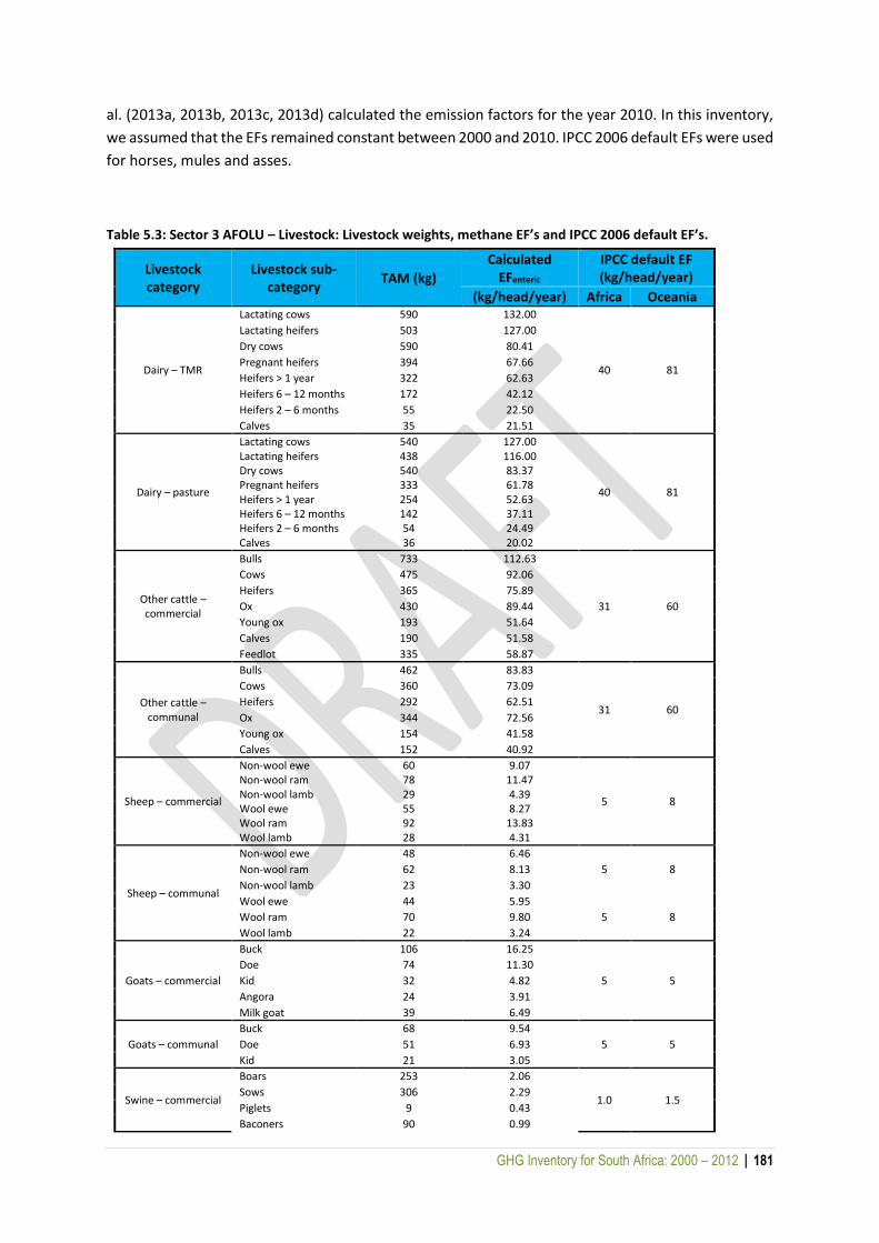
GHG Inventory for South Africa: 2000 – 2012 | 181

al. (2013a, 2013b, 2013c, 2013d) calculated the emission factors for the year 2010. In this inventory,

we assumed that the EFs remained constant between 2000 and 2010. IPCC 2006 default EFs were used

for horses, mules and asses.

Table 5.3: Sector 3 AFOLU – Livestock: Livestock weights, methane EF’s and IPCC 2006 default EF’s.

Livestock category

Livestock sub-category

TAM (kg)

Calculated EFenteric

IPCC default EF (kg/head/year)

(kg/head/year) Africa Oceania

Dairy – TMR

Lactating cows 590 132.00

40 81

Lactating heifers 503 127.00

Dry cows 590 80.41

Pregnant heifers 394 67.66

Heifers > 1 year 322 62.63

Heifers 6 – 12 months 172 42.12

Heifers 2 – 6 months 55 22.50

Calves 35 21.51

Dairy – pasture

Lactating cows 540 127.00

40 81

Lactating heifers 438 116.00 Dry cows 540 83.37 Pregnant heifers 333 61.78 Heifers > 1 year 254 52.63 Heifers 6 – 12 months 142 37.11 Heifers 2 – 6 months 54 24.49 Calves 36 20.02

Other cattle – commercial

Bulls 733 112.63

31 60

Cows 475 92.06

Heifers 365 75.89

Ox 430 89.44

Young ox 193 51.64

Calves 190 51.58

Feedlot 335 58.87

Other cattle – communal

Bulls 462 83.83

31 60

Cows 360 73.09

Heifers 292 62.51

Ox 344 72.56

Young ox 154 41.58

Calves 152 40.92

Sheep – commercial

Non-wool ewe 60 9.07

5 8

Non-wool ram 78 11.47 Non-wool lamb 29 4.39 Wool ewe 55 8.27 Wool ram 92 13.83 Wool lamb 28 4.31

Sheep – communal

Non-wool ewe 48 6.46

5 8 Non-wool ram 62 8.13

Non-wool lamb 23 3.30

Wool ewe 44 5.95

5 8 Wool ram 70 9.80

Wool lamb 22 3.24

Goats – commercial

Buck 106 16.25

5 5

Doe 74 11.30

Kid 32 4.82

Angora 24 3.91

Milk goat 39 6.49

Goats – communal

Buck 68 9.54

5 5 Doe 51 6.93

Kid 21 3.05

Swine – commercial

Boars 253 2.06

1.0 1.5 Sows 306 2.29

Piglets 9 0.43

Baconers 90 0.99

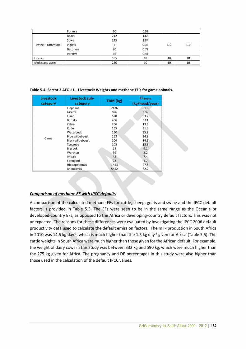
GHG Inventory for South Africa: 2000 – 2012 | 182

Porkers 70 0.51

Swine – communal

Boars 212 1.65

1.0 1.5

Sows 245 1.84

Piglets 7 0.34

Baconers 70 0.79

Porkers 56 0.41

Horses 595 18 18 18

Mules and asses 250 10 10 10

Table 5.4: Sector 3 AFOLU – Livestock: Weights and methane EF’s for game animals.

Livestock category

Livestock sub-category

TAM (kg) EFenteric

(kg/head/year)

Game

Elephant 2436 81.0 Giraffe 826 136 Eland 528 93.7 Buffalo 466 113 Zebra 266 13.9 Kudu 155 31.3 Waterbuck 150 35.9 Blue wildebeest 153 24.8 Black wildebeest 106 14.3 Tsessebe 105 13.8 Blesbok 62 9.1 Warthog 59 2.2 Impala 42 7.4 Springbok 28 4.7 Hippopotamus 1453 47.5 Rhinoceros 5452 62.2

Comparison of methane EF with IPCC defaults

A comparison of the calculated methane EFs for cattle, sheep, goats and swine and the IPCC default

factors is provided in Table 5.5. The EFs were seen to be in the same range as the Oceania or

developed-country EFs, as opposed to the Africa or developing-country default factors. This was not

unexpected. The reasons for these differences were evaluated by investigating the IPCC 2006 default

productivity data used to calculate the default emission factors. The milk production in South Africa

in 2010 was 14.5 kg day-1, which is much higher than the 1.3 kg day-1 given for Africa (Table 5.5). The

cattle weights in South Africa were much higher than those given for the African default. For example,

the weight of dairy cows in this study was between 333 kg and 590 kg, which were much higher than

the 275 kg given for Africa. The pregnancy and DE percentages in this study were also higher than

those used in the calculation of the default IPCC values.

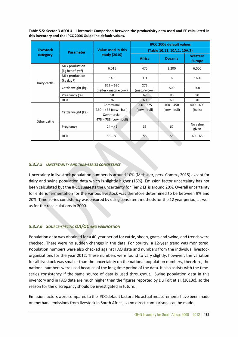
GHG Inventory for South Africa: 2000 – 2012 | 183

Table 5.5: Sector 3 AFOLU – Livestock: Comparison between the productivity data used and EF calculated in this inventory and the IPCC 2006 Guideline default values.

Livestock category

Parameter Value used in this

study (2010)

IPCC 2006 default values

(Table 10.11, 10A.1, 10A.2)

Africa Oceania Western Europe

Dairy cattle

Milk production 6,015 475 2,200 6,000

(kg head-1 yr-1)

Milk production 14.5 1.3 6 16.4

(kg day-1)

Cattle weight (kg) 322 – 590 275

500 600 (heifer - mature cow) (mature cow)

Pregnancy (%) 58 67 80 90

DE% 76 60 60 70

Other cattle

Cattle weight (kg)

Communal: 200 – 275 400 – 450 400 – 600

360 – 462 (cow - bull); (cow - bull) (cow - bull) (bulls)

Commercial:

475 – 733 (cow - bull)

Pregnancy 24 – 49 33 67 No value

given

DE% 55 – 80 55 55 60 – 65

5.3.3.5 UNCERTAINTY AND TIME-SERIES CONSISTENCY

Uncertainty in livestock population numbers is around 10% (Meissner, pers. Comm., 2015) except for

dairy and swine population data which is slightly higher (15%). Emission factor uncertainty has not

been calculated but the IPCC suggests the uncertainty for Tier 2 EF is around 20%. Overall uncertainty

for enteric fermentation for the various livestock was therefore determined to be between 9% and

20%. Time-series consistency was ensured by using consistent methods for the 12 year period, as well

as for the recalculations in 2000.

5.3.3.6 SOURCE-SPECIFIC QA/QC AND VERIFICATION

Population data was obtained for a 40-year period for cattle, sheep, goats and swine, and trends were

checked. There were no sudden changes in the data. For poultry, a 12-year trend was monitored.

Population numbers were also checked against FAO data and numbers from the individual livestock

organizations for the year 2012. These numbers were found to vary slightly, however, the variation

for all livestock was smaller than the uncertainty on the national population numbers, therefore, the

national numbers were used because of the long time period of the data. It also assists with the time-

series consistency if the same source of data is used throughout. Swine population data in this

inventory and in FAO data are much higher than the figures reported by Du Toit et al. (2013c), so the

reason for the discrepancy should be investigated in future.

Emission factors were compared to the IPCC default factors. No actual measurements have been made

on methane emissions from livestock in South Africa, so no direct comparisons can be made.

GHG Inventory for South Africa: 2000 – 2012 | 184

An independent reviewer was appointed to assess the quality of the inventory, determine the

conformity of the procedures followed for the compilation of this inventory and identify areas of

improvement.

5.3.3.7 SOURCE-SPECIFIC RECALCULATIONS

The other cattle population data was recalculated for all years between 2000 and 2012, as it was

determined that feedlot cattle were already incorporated into the commercial population data. Also,

the ratio of communal to commercial cattle was adjusted based on data from the Abstracts of

Agricultural Statistics (2013). In this inventory, emissions from ruminant game in privately owned

game parks were estimated. There were not in the previous inventory. Due to limited population data

the numbers and emissions for game were kept constant between 2000 and 2012, so a constant

emission from game was added to all years.

5.3.3.8 SOURCE-SPECIFIC PLANNED IMPROVEMENTS AND RECOMMENDATIONS

There are no planned improvements, however it is recommended that if sufficient data is available

annual emission factors, incorporating changes in feed quality and milk production, should be

considered instead of assuming a constant emission factor across all years. It is also recommended

that a more thorough uncertainty analysis be completed, following the IPCC 2006 Uncertainty

Guidelines and Good Practice Guidelines.

5.3.4 Manure management [3A2]

5.3.4.1 SOURCE-CATEGORY DESCRIPTION

Manure management includes the storage and treatment of manure, before using it as farm manure

or burning it as fuel. Methane (CH4) and nitrous oxide (N2O) are produced during different storage and

treatment stages of manure. The term “manure” includes both dung and urine produced by livestock.

Camels and Ilamas do not occur in South Africa and were therefore not included in the report. There

is a large population of game in South Africa, but a lack of data hinders the inclusion of their emissions.

National population data for ruminant game is lacking, however, there is population data for game

kept in privately owned parks. Du Toit et al. (2013) determined that manure CH4 emissions from game

were very low and therefore no emission factors were reported. This inventory thus assumes zero

manure CH4 emissions from game.

The majority of manure in South Africa is produced and left in the pastures while grazing, with only a

small amount of manure is being managed in South Africa. N2O manure emissions are reported for

managed manure on dairy, swine, feedlot and poultry. In accordance with IPCC Guidelines, N2O

emissions from the manure left in pastures and daily spread are not taken into account in this source

category (manure management), but are included in the source category for managed soils.

GHG Inventory for South Africa: 2000 – 2012 | 185

5.3.4.2 OVERVIEW OF SHARES AND TRENDS IN EMISSIONS

Manure management produced a total of 2 214 Gg CO2eq in 2012, which was an increase from the 1

872 Gg CO2eq produced in 2000 (Figure 5.7: Sector 3 AFOLU – Livestock: Total manure management

trend and emission levels from source categories, 2000 – 2012.

).

Manure emissions showed the greatest increase between 2004 and 2007, with annual increases of

4.0%, 2.6% and 2.8% during this period. There was also another large increase between 2010 and

2011. Emissions generally increased annually, with the only decline (0.5%) occurring between 2002

and 2003. These increases are due to increased N2O emissions from poultry manure, but N2O emission

from feedlot manure also contributed to the increase between 2010 and 2011. This was mostly related

to increases in population numbers during that time.

Methane emissions accounted for 38.5% of manure emissions in 2012, with its contribution slowly

declining from 46.2% in 2000. Manure CH4 emissions showed peaks in 2001 (875 Gg CO2eq) and in

2009 (870 Gg CO2eq) (Figure 5.8: Sector 3 AFOLU – Livestock: Manure management CH4 trend and

emission levels from source categories, 2000 – 2012.

). The largest contributor to the CH4 emissions were swine (68.9% in 2012), followed by dairy cattle

(18.1% in 2012). The contribution of CH4 from dairy cattle manure management decreased by 1.6%

since 2000, while the contribution from swine manure declined by 1.9% over the same period.

N2O dominated the manure emissions, contributing 57.5% in 2012. The contribution has slowly

increased since 2000 (when it contributed 53.8%). N2O emissions from manure management

increased from 1 007 Gg CO2eq (2000) to 1 362 Gg CO2eq (2012), mainly due to the increased manure

from poultry. Poultry contribution has increased from 63.8% in 2000 to 70.1% in 2012, while the

contribution from cattle feedlots declined by 4.4% over the same period (Figure 5.9: Sector 3 AFOLU

– Livestock: Manure management N2O trend an emission levels from source categories, 2000 – 2012.

). Swine manure N2O emissions declined by 4.1% between 2000 and 2012.

The total emissions from poultry manure increased by 48.6% between 2000 and 2012, and their

contribution to manure emissions increased from 36.2% to 45.7%.

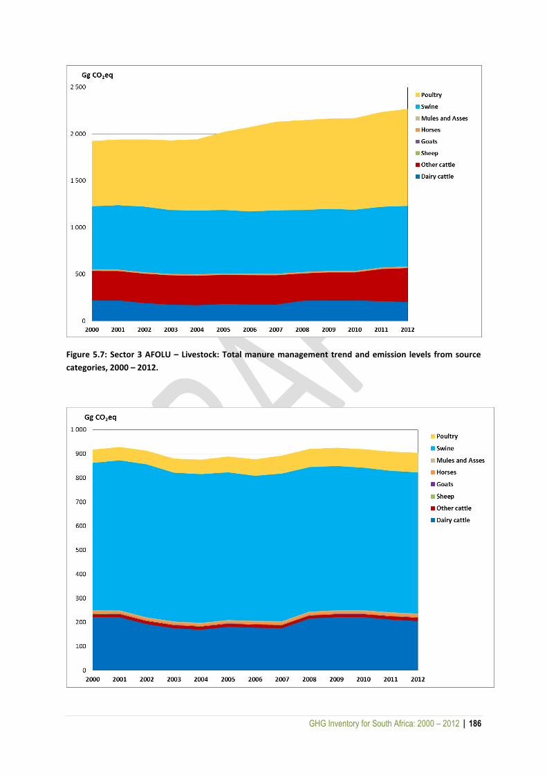
GHG Inventory for South Africa: 2000 – 2012 | 186

Figure 5.7: Sector 3 AFOLU – Livestock: Total manure management trend and emission levels from source

categories, 2000 – 2012.

GHG Inventory for South Africa: 2000 – 2012 | 187

Figure 5.8: Sector 3 AFOLU – Livestock: Manure management CH4 trend and emission levels from source categories, 2000 – 2012.

Figure 5.9: Sector 3 AFOLU – Livestock: Manure management N2O trend an emission levels from source categories, 2000 – 2012.

5.3.4.3 METHODOLOGICAL ISSUES

The methane produced from manure management of dairy cattle, beef cattle and feedlot cattle was

calculated based on the approach of the IPCC (2006), using a combination of default IPCC and country-

specific input values. Due to the similarity in environmental and climatic conditions, the Australian

methodology was used to calculate the manure emission factor (MEF) of range-kept cattle in

environments with an average temperature of 21oC. This was determined to be 1.4 x 10-5 kg CH4 (kg

DM manure)-1 based on Gonzalez-Avalos and Ruiz-Suarez (2001).

5.3.4.3.1 CH4 emissions from animal manure

Dairy cattle [3A2ai]

Methane emissions from manure originate from the organic fraction of the manure (volatile solids).

Manure CH4 emissions were taken from Du Toit et al. (2013a). A Tier 2 approach was used and the

emissions (kg head-1 year-1) were determined using the equation:

GHG Inventory for South Africa: 2000 – 2012 | 188

EF = (VS x Bo x MCF x p) x 365 (Eq. 5.8)

Where:

Bo = emissions potential (0.24 m3 CH4 (kg VS)-1; IPCC, 2006);

MCF = integrated methane conversion factor – based on the proportion of the different manure management

systems;

p = density of methane (0.662 kg m-3)

Using the methane conversion factor (MCF) from the IPCC 2006 Guidelines for the various manure

management systems the integrated MCF for lactating dairy cattle in total mixed ration (TMR) based

production systems was calculated as 10% and 1% for all other classes of dairy cattle. In pasture based

production systems the integrated MCF for lactating cattle was calculated as 4.57% and 1% for all

other classes of cattle. Volatile solids (VS, kg head-1 day-1) were calculated according to ANIR (2009)

as:

VS = I x (1 – DMD) x (1 – A) (Eq. 5.9)

Where:

I = dry matter intake calculated as described above;

DMD = Dry matter digestibility expressed as a fraction;

A = ash content of manure expressed as a fraction (assumed to be 8% of faecal DM, IPCC 2006 Guidelines).

Other cattle, sheep and goats [3A2aii, 3A2c and 3A2d]

Methane emissions from manure (kg head-1 year-1) of all categories of beef cattle, sheep and goats were taken from Du Toit et al. (2013a and 2013b) who followed the methods used in the Australian inventory (ANIR, 2009):

EF = (I x (1 – DMD) x MEF) x 365 (Eq. 5.10)

Where:

I = Intake as calculated under enteric emissions (Section 5.3.3.3);

MEF = Manure emissions factor (kg CH4 (kg DM manure)-1).

Feedlot cattle

The IPCC default methane conversion factor for drylot (1.5%) was used. The volatile solid production

for feedlot cattle was estimated based on data developed under the enteric methane emission

calculations. The volatile solid production and methane emission factor was calculated as for dairy

cattle (Eq. 5.9), but assuming a DMD of 80% for feedlot diets and a B0 of 0.17 m3 CH4 (kg VS)-1 (IPCC,

2006).

GHG Inventory for South Africa: 2000 – 2012 | 189

Swine [3A2h]

Commercial pig production systems in South Africa are housed systems and a large proportion of

manure and waste is managed in lagoon systems. The CH4 emission factors for pig manure (kg head-1

year-1) were taken from Du Toit et al. (2013c) and calculated following the equations provided in ANIR

(2009):

EF = (VS x Bo x MCF x p) x 365 (Eq. 5.11)

Where:

VS = Volatile solid production (kg head-1 year-1);

Bo = emissions potential (0.45 m3 CH4 (kg VS)-1) (IPCC 2006);

MCF = Integrated methane conversion factor calculated from IPCC 2006 MCF for each manure management

system;

P = density of methane (0.622 kg m-3).

Du Toit calculated the volatile solid production from South African pigs by using the following equation

provided in the IPCC 2006 Guidelines:

VS = [GE x (1 – (DE%/100)) + (UE x GE)] x [(1 – ASH)/18.45] (Eq. 5.12)

Where:

VS = volatile solid excretion (kg VS day-1);

GE = Gross energy intake (MJ day-1);

DE% = digestibility of feed (%);

(UE x GE) = urinary energy expressed as a fraction of GE. Typically 0.02GE for pigs (IPCC 2006);

ASH = Ash content of manure (17%, Siebrits, 2012);

18.45 = conversion factor for dietary GE per kg of DM (MJ kg-1).

Poultry [3A2i]

As for the other manure CH4 emission factors, the poultry emission factors were calculated according

to Equation 5.8, using an integrated MCF of 1.5% (IPCC, 2006; Du Toit et al., 2013c). Volatile solid

production from poultry production systems was calculated using the same equation as for dairy cattle

(Eq. 5.9), but assuming a dry matter intake of 0.11 kg day-1, a DMD of 80% and an ash content of 8%

of faecal DM (ANIR, 2009).

Game [Other - 3A2j]

CH4 emissions from game manure were assumed to be zero as Du Toit et al. (2013d) indicated that

emissions were minimal and did not report any EFs.

GHG Inventory for South Africa: 2000 – 2012 | 190

5.3.4.3.2 N2O emissions from animal manure

Du Toit et al. (2013a) calculated nitrogen excretion from the various livestock categories using crude

protein inputs and storage, and from this the output of nitrogen in faeces and urine (following the

methodology provided in ANIR, 2009). Unfortunately, there were insufficient data to extend these

calculations from 2010 to the period 2000 to 2009, therefore a Tier 1 approach was used, as in the

2004 Agricultural inventory (DAFF, 2010). N2O emissions from manure management are not a key

source of emissions so the Tier 1 methodology is sufficient.

Direct N2O emissions from manure management were calculated from animal population data, activity

data and manure management system data using Equation 10.25 and 10.30 from the IPCC 2006

Guidelines.

5.3.4.4 DATA SOURCES

Population data sources for all livestock except poultry are described in Section 5.3.3.4.1 and the

typical animal aasses (TAMs) are provided in Table 5.3: Sector 3 AFOLU – Livestock: Livestock weights,

methane EF’s and IPCC 2006 default EF’s. Poultry were also included in the manure management

emission calculations. The total number of layers and slaughtered broilers was obtained from the

South African Poultry Association (Prinsloo, Magda, 2014, Pers. Comm.). The layer population

numbers were used as they were provided, but, for broilers, the annual average population (AAP) was

calculated, as a broiler is not alive for 365 days a year. The AAP was determined using the average

number of broiler growing cycles (per annum), using an equation similar to that used by New Zealand

(Ministry of Agriculture and Forestry, 2011):

AAP = NAPA/R (Eq. 5.13)

NAPA is the number of animals produced annually, which was taken to be the number of broilers

slaughtered; and R is the average number of broiler growing cycles per annum (R = 8, Du Toit et al.,

2013). It has been noted that New Zealand changed their methodology from using the growing cycle

to using the number of days alive. It indicated that the former method was leading to an

overestimation. However, for South Africa, using the growing cycle brings the population numbers

more in line with data from the census that was carried out between 2000 and 2013. Communal

layers and broilers were calculated as 4.2% of the commercial population (Prinsloo, Magda, 2014,

Pers. Comm.). The TAM for poultry was 1.8kg for commercial broilers, 2 kg for layers and 0.9 kg for

communal broilers (DAFF, 2010; IPCC, 2006). Population data is provided in Appendix D.

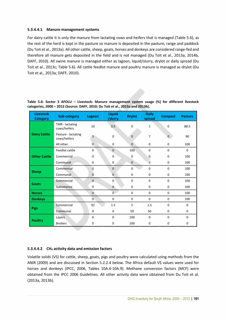
GHG Inventory for South Africa: 2000 – 2012 | 191

5.3.4.4.1 Manure management systems

For dairy cattle it is only the manure from lactating cows and heifers that is managed (Table 5.6), as

the rest of the herd is kept in the pasture so manure is deposited in the pasture, range and paddock

(Du Toit et al., 2013a). All other cattle, sheep, goats, horses and donkeys are considered range-fed and

therefore all manure gets deposited in the field and is not managed (Du Toit et al., 2013a, 2014b,

DAFF, 2010). All swine manure is managed either as lagoon, liquid/slurry, drylot or daily spread (Du

Toit et al., 2013c; Table 5.6). All cattle feedlot manure and poultry manure is managed as drylot (Du

Toit et al., 2013a; DAFF, 2010).

Table 5.6: Sector 3 AFOLU – Livestock: Manure management system usage (%) for different livestock categories, 2000 – 2012 (Source: DAFF, 2010; Du Toit et al., 2013a and 2013b).

Livestock Category

Sub-category Lagoon Liquid /slurry

Drylot Daily

spread Compost Pasture

Dairy Cattle

TMR - lactating cows/heifers

10 0.5 0 1 0 88.5

Pasture - lactating cows/heifers

3 0 0 7 0 90

All other 0 0 0 0 0 100

Other Cattle

Feedlot cattle 0 0 100 0 0 0

Commercial 0 0 0 0 0 100

Communal 0 0 0 0 0 100

Sheep Commercial 0 0 0 0 0 100

Communal 0 0 0 0 0 100

Goats Commercial 0 0 0 0 0 100

Subsistence 0 0 0 0 0 100

Horses 0 0 0 0 0 100

Donkeys 0 0 0 0 0 100

Pigs Commercial 92 1.5 5 1.5 0 0

Communal 0 0 50 50 0 0

Poultry Layers 0 0 100 0 0 0

Broilers 0 0 100 0 0 0

5.3.4.4.2 CH4 activity data and emission factors

Volatile solids (VS) for cattle, sheep, goats, pigs and poultry were calculated using methods from the

ANIR (2009) and are discussed in Section 5.2.2.4 below. The Africa default VS values were used for

horses and donkeys (IPCC, 2006, Tables 10A.4-10A.9). Methane conversion factors (MCF) were

obtained from the IPCC 2006 Guidelines. All other activity data were obtained from Du Toit et al.

(2013a, 2013b).

GHG Inventory for South Africa: 2000 – 2012 | 192

Emission factors for cattle, sheep, goats, swine and poultry (Table 5.7) were taken from Du Toit et al.

(2013a, 2013b, 2013c) and the methods are described in Section 5.3.3.3. In the case of sheep, goats

and swine there were additional livestock subcategories in Du Toit et al. (2013a, 2013b, 2013c) (see

Appendix E) and in these cases a weighted average emission factor was calculated. IPCC 2006 Africa

default values were used for horses and donkeys.

Comparison of manure EF’s and IPCC defaults

A comparison of the calculated manure emission factors with IPCC default values is given in Table 5.7.

For dairy cattle the EF for lactating cows and heifers was much higher than the Africa default, while

the rest of the dairy cattle were only slightly higher. If an average dairy cattle EF was calculated from

this data the EF would be close to the Australian EF. For other cattle the EF are lower than the Africa

default values, but are in a similar range to the Australian EF. All cattle EF are lower than the Oceania

IPCC 2006 default values. Swine EF were much higher than the Africa default values and are in a similar

range to those of Oceania and Australia. Poultry manure EF for N2O was lower than all default values.

5.3.4.4.3 N2O activity data and Emission factors

Nitrogen excretion rates (Nrate) were obtained from the Africa default values (IPCC, 2006, Table 10.19)

while the annual N excretion for livestock Nex was estimated using Equation 10.30 from the guidelines

(IPCC, 2006). The typical animal mass (TAM) for the various livestock categories is given in Table 5.3.

The manure management system usage data (Table 5.6) was used to produce the fraction of total

annual nitrogen excretion for each livestock category managed in the various manure management

systems.

IPCC 2006 default N2O emission factors were used for the various manure management systems (IPCC

2006, Table 10.21).

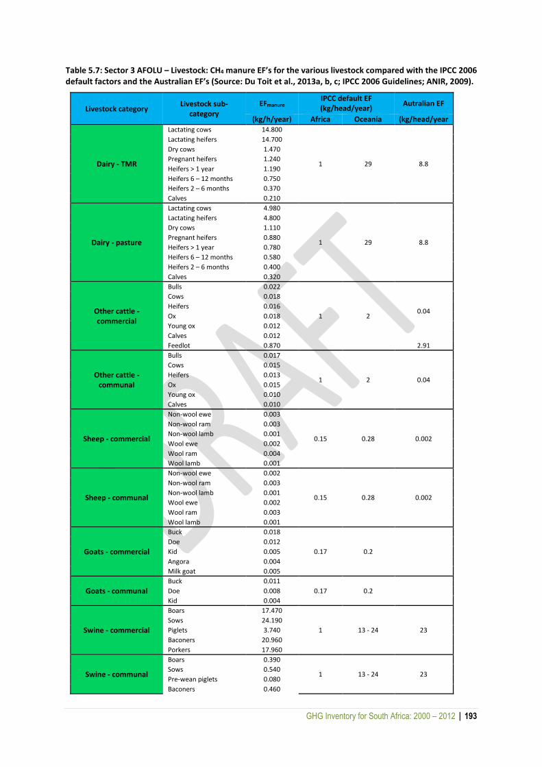
GHG Inventory for South Africa: 2000 – 2012 | 193

Table 5.7: Sector 3 AFOLU – Livestock: CH4 manure EF’s for the various livestock compared with the IPCC 2006 default factors and the Australian EF’s (Source: Du Toit et al., 2013a, b, c; IPCC 2006 Guidelines; ANIR, 2009).

Livestock category Livestock sub-

category

EFmanure IPCC default EF (kg/head/year)

Autralian EF

(kg/h/year) Africa Oceania (kg/head/year

Dairy - TMR

Lactating cows 14.800

1 29 8.8

Lactating heifers 14.700

Dry cows 1.470

Pregnant heifers 1.240

Heifers > 1 year 1.190

Heifers 6 – 12 months 0.750

Heifers 2 – 6 months 0.370

Calves 0.210

Dairy - pasture

Lactating cows 4.980

1 29 8.8

Lactating heifers 4.800

Dry cows 1.110

Pregnant heifers 0.880

Heifers > 1 year 0.780

Heifers 6 – 12 months 0.580

Heifers 2 – 6 months 0.400

Calves 0.320

Other cattle - commercial

Bulls 0.022

1 2 0.04

Cows 0.018

Heifers 0.016

Ox 0.018

Young ox 0.012

Calves 0.012

Feedlot 0.870 2.91

Other cattle - communal

Bulls 0.017

1 2 0.04

Cows 0.015

Heifers 0.013

Ox 0.015

Young ox 0.010

Calves 0.010

Sheep - commercial

Non-wool ewe 0.003

0.15 0.28 0.002

Non-wool ram 0.003

Non-wool lamb 0.001

Wool ewe 0.002

Wool ram 0.004

Wool lamb 0.001

Sheep - communal

Non-wool ewe 0.002

0.15 0.28 0.002

Non-wool ram 0.003

Non-wool lamb 0.001

Wool ewe 0.002

Wool ram 0.003

Wool lamb 0.001

Goats - commercial

Buck 0.018

0.17 0.2

Doe 0.012

Kid 0.005

Angora 0.004

Milk goat 0.005

Goats - communal Buck 0.011

0.17 0.2

Doe 0.008

Kid 0.004

Swine - commercial

Boars 17.470

1 13 - 24 23

Sows 24.190

Piglets 3.740

Baconers 20.960

Porkers 17.960

Swine - communal

Boars 0.390

1 13 - 24 23 Sows 0.540

Pre-wean piglets 0.080

Baconers 0.460

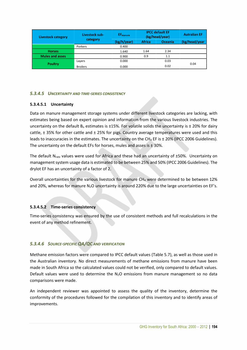
GHG Inventory for South Africa: 2000 – 2012 | 194

Livestock category Livestock sub-

category

EFmanure IPCC default EF (kg/head/year)

Autralian EF

(kg/h/year) Africa Oceania (kg/head/year Porkers 0.400

Horses 1.640 1.64 2.34

Mules and asses 0.900 0.9 1.1

Poultry Layers 0.000 0.03

0.04 Broilers 0.000 0.02

5.3.4.5 UNCERTAINTY AND TIME-SERIES CONSISTENCY

5.3.4.5.1 Uncertainty

Data on manure management storage systems under different livestock categories are lacking, with

estimates being based on expert opinion and information from the various livestock industries. The

uncertainty on the default Bo estimates is ±15%. For volatile solids the uncertainty is ± 20% for dairy

cattle, ± 35% for other cattle and ± 25% for pigs. Country average temperatures were used and this

leads to inaccuracies in the estimates. The uncertainty on the CH4 EF is ± 20% (IPCC 2006 Guidelines).

The uncertainty on the default EFs for horses, mules and asses is ± 30%.

The default Nrate values were used for Africa and these had an uncertainty of ±50%. Uncertainty on

management system usage data is estimated to be between 25% and 50% (IPCC 2006 Guidelines). The

drylot EF has an uncertainty of a factor of 2.

Overall uncertainties for the various livestock for manure CH4 were determined to be between 12%

and 20%, whereas for manure N2O uncertainty is around 220% due to the large uncertainties on EF’s.

5.3.4.5.2 Time-series consistency

Time-series consistency was ensured by the use of consistent methods and full recalculations in the

event of any method refinement.

5.3.4.6 SOURCE-SPECIFIC QA/QC AND VERIFICATION

Methane emission factors were compared to IPCC default values (Table 5.7), as well as those used in

the Australian inventory. No direct measurements of methane emissions from manure have been

made in South Africa so the calculated values could not be verified, only compared to default values.

Default values were used to determine the N2O emissions from manure management so no data

comparisons were made.

An independent reviewer was appointed to assess the quality of the inventory, determine the

conformity of the procedures followed for the compilation of this inventory and to identify areas of

improvements.

GHG Inventory for South Africa: 2000 – 2012 | 195

5.3.4.7 SOURCE-SPECIFIC RECALCULATIONS

Recalculations were completed for all years between 2000 and 2012 with the updated population data

for other cattle and poultry. Poultry data were adjusted for all years based on new information and to

bring the numbers more in line with the annual census data. Game manure emissions were considered

for all years, but the emissions were assumed to be zero, so no changes were made for this.

5.3.4.8 SOURCE-SPECIFIC PLANNED IMPROVEMENTS AND RECOMMENDATIONS

No specific improvements are planned, however, it is suggested that in order to improve the accuracy

and reduce the uncertainty of the manure management emission data it would be important to

improve the monitoring of manure management systems. Another improvement would be to stratify

the livestock population by climate, or even provincial data, so that a more accurate weighted average

emission factor can be determined.

N2O emission data from manure management systems would also be improved if N excretion rates

for cattle in South Africa were determined so that actual data could be used instead of the value

calculated using IPCC 2006 default values.

5.4 Land [3B]

5.4.1 Overview of the sub-sector

The land component of the AFOLU sector includes CO2 emissions and sinks of the carbon pools above-

ground and below-ground biomass, and soils from the categories forest land (3.B.1), croplands (3.B.2),

grasslands (3.B.3), wetlands (3.B.4), settlements (3.B.5), other lands (3.B.6), and the relevant land-use

change categories. The N2O emissions from the land sector were estimated in the aggregated and

non-CO2 emission sources on land section and CH4 emissions from wetlands were also included,

following the methodology in the previous inventories (DEAT, 2009; DEA, 2014). All other emissions

in the land category were assumed to be negligible.

According to the maps developed in section 5.4.4 (GeoTerraImage, 2015) the land cover in South

Africa in 2014 was dominated by low shrubland (33.5%) and grasslands (20.7%). Natural forests are

very small in South Africa covering less than 0.5% of the land area, while settlements occupy

approximately 2.3%. Agricultural activities cover about 11.2% of the land area, with maize and wheat

being the dominant annual crops by area. Perennial crops (orchards and viticulture) contribute less

than 0.5% towards the cropland land area. Plantations are based on non-native trees, the dominant

species being Eucalyptus grandis, and they cover about 1.5% of the land area (Forestry South Africa,

2012).

Classifying the South African soils into the six main types provided by the IPCC shows that the high-

activity clay mineral soil dominates (>60%) (Moeletsi et al., 2013). This soil type consists of lightly to

GHG Inventory for South Africa: 2000 – 2012 | 196

moderately weathered soils, dominated by 2:1 silicate clay minerals, including vertisols, mollisols,

calcareous soils, shallow soils and various others. The other two main soil types are sandy mineral soil

and low-activity clay mineral soil. Sandy minerals predominate over the Northern Cape, North West

and Western Cape. The low-activity clay soils are found mainly in the warmer, higher rainfall areas,

such as KwaZulu-Natal and Mpumalanga. Organic soils are considered negligible.

Long-term (1920 – 1999) climate data for South Africa were used to categorize the climate into the

IPCC climate classes. Over 95% of South Africa is categorised under the “warm temperate dry” climate

class. There are a few very small patches over the Limpopo ranges, along the KwaZulu-Natal coast, in

some parts of Mpumalanga and over the Western Cape, which fall into the “warm temperate moist”

class. The other exception is the “cool temperate dry” regions in the ranges of the Eastern Cape that

are close to Lesotho.

5.4.2 Overview of shares and trends

5.4.2.1 LAND COVER TRENDS

Land-cover change was determined as discussed in Section 5.4.4 and results show that between 1990

and 2014 the Forest land (which includes woodlands and open bush) and settlements increased by

15.4% and 6.7% respectively. Wetlands decreased by 17.6%, while grasslands and croplands declined

by 6.2% and 1.6% respectively (Figure 5.10).2 These numbers, however, should be considered in light

of the limitations discussed in Section 5.4.4.4.

2 A cautionary note: there are three basic factors that may have influenced land-cover change results and associated statistics, namely land-

cover mapping accuracies, seasonal / climatic conditions under which the original source imagery was acquired, and the level of (landscape)

detail that is being compared over time. These influencing factors are discussed in detail in Appendix G (section 14.2).

GHG Inventory for South Africa: 2000 – 2012 | 197

Figure 5.10: Sector 3 AFOLU - Land: Comparison of land areas and the change between 1990 and 2013-2014.

5.4.2.2 TRENDS IN CO2

The Land sector was estimated to be a net sink of CO2, but this sink fluctuated over the 12 year period

(Figure 5.11). The biomass and soil carbon pools contribute the most to the Land sector (Figure 5.12).

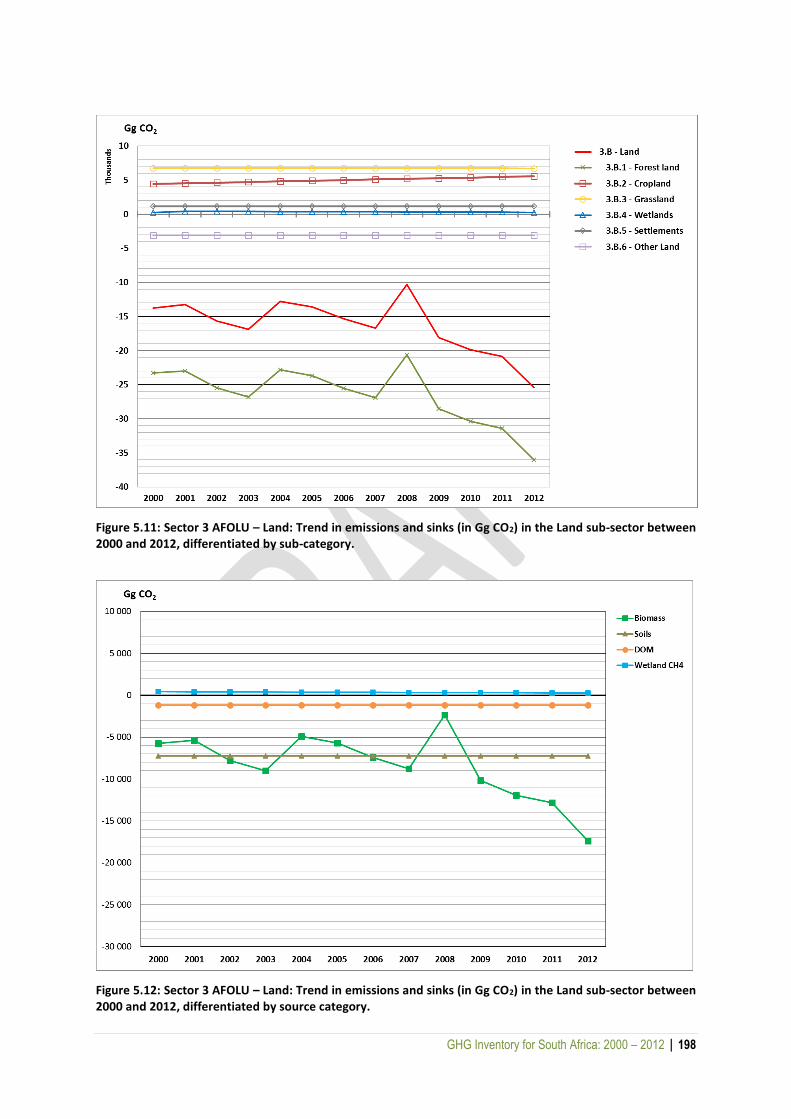
GHG Inventory for South Africa: 2000 – 2012 | 198

Figure 5.11: Sector 3 AFOLU – Land: Trend in emissions and sinks (in Gg CO2) in the Land sub-sector between 2000 and 2012, differentiated by sub-category.

Figure 5.12: Sector 3 AFOLU – Land: Trend in emissions and sinks (in Gg CO2) in the Land sub-sector between 2000 and 2012, differentiated by source category.

GHG Inventory for South Africa: 2000 – 2012 | 199

Forest land (3B1) comprised emissions and removals from the above and below ground, soil carbon

and DOM pools for the forest land remaining forest land and land converted to forest land sub-

categories. Forest lands include plantations, natural forests, thickets, and woodland/open bush.

Carbon stock changes due to wood harvesting, fuelwood consumption, and disturbance (including

fires) were all included. The forest land category was estimated to be a net sink for CO2 in all years

between 2000 and 2012, varying between a low of 10 309 Gg CO2 (2008) and a high of 25 397 Gg CO2.

The land converted to forest land subcategory accounted for 86.8% of the forest land CO2 in 2012 and

this is mainly due to the land conversions accumulating in this category until the 23 year period is

reached. Furthermore, due to a lack of data the carbon losses could not be separated between land

remaining land and converted land. Therefore all losses were allocated to land remaining land, leading

to the converted lands having a higher sink.

Croplands (3B2) comprised emissions and removals from the biomass and soil carbon pools in the

croplands remaining croplands and the land converted to croplands sub-categories. Croplands include

annual crops, perennial crops (viticulture, orchards), and cultivated subsistence crops. Cropland had

an emission of 4 431 Gg CO2 in 2000 and this increased to 5 567 Gg CO2 in 2012. Croplands remaining

croplands are generally assumed to be in balance, however there were some conversions between

the different crop types which lead to a sink in this category whichdeclined to 104 Gg CO2 from 1 241

Gg CO2 in 2000.

Grasslands (3B3) comprised emissions and removals from the biomass and soil carbon pools for

grasslands remaining grasslands and land converted to grasslands subcategories. The grassland

category only includes grassland vegetation. The grassland remaining grasslands subcategory,

following the Tier 1 methodology, are assumed to be in balance, while land converted to grasslands

were a sink of 6 735 Gg CO2 annually.

Wetlands (3B4) were estimated not to have any emissions or removals of CO2, but CH4 emissions were

estimated. Wetlands were therefore estimated to be a weak source of emissions which declined from

429 Gg CO2eq in 2000 to 267 Gg CO2eq in 2012. Wetlands included wetlands and waterbodies.

The Settlements category (3B5) comprises the settlements remaining settlements and land converted

to settlements subcategories. This category includes settlements and mines. Settlements remaining

settlements do not have any CO2 emissions or uptakes, but land conversions to settlements produced

a small source (1 160 Gg CO2 per year).

Other lands (3B6) comprised emissions and removals from the biomass and soil carbon pools for other

lands remaining other lands and land converted to other lands subcategories. The other lands category

includes low shrublands, bare ground and degraded land. Other lands remaining other lands do not

generally have any CO2 emissions or uptakes, however there are large conversions between low

shrublands, degraded lands and bare ground which leads to a soil sink of 5 057 Gg CO2 eq. Land

converted to other lands was shown to be a source of 1 675 Gg CO2 per year.

GHG Inventory for South Africa: 2000 – 2012 | 200

5.4.3 General methodology

South Africa followed a Tier 1 approach and in Forest lands a Tier 2 approach of the IPCC 2006

Guidelines to determine the effects of land use and land-use change on the GHG inventory. The gain-

loss method was used, where the inventory data was subdivided into the appropriate pools and land-

use types.

It was assumed that no conversions occurred before 1990, so land converted to another land category

would remain, and accumulate, in the converted category for 23 years. The IPCC default period is 20

years, but it is stated that if the change period extends beyond this then the time period can be

adjusted. In this inventory the maps spanned a 23 year period therefore D = T = 23 years.

The inventory comprises the six land classes recommended by the IPCC (forest land, grassland,

cropland, settlements, wetlands and Other) as well as all the land-conversion categories. Due to the

diverse nature of South Africa’s vegetation, the six land classes had several subdivisions (Table 5.8).

These divisions are further explained in Section 5.4.5.

The sub-divisions in this inventory differ slightly from those in the 2010 inventory. The main reason

for this change was because in the previous inventory the maps suggested large changes between

bare ground and Nama-Karoo and Succulent-Karoo vegetation. The fact that the biome borders used

to identify these areas are static may have had an influence on these numbers and led to errors in

change over time. In this current inventory, the map resolution was increased from 1 km to 30m and

the biome categories were removed. More detail on the classification is provided in Section 5.4.5.

Area per category was estimated using a wall-to-wall approach, where the entire land surface of South

Africa was classified into one of the six land class. Land areas were determined from the maps

described in Section 5.4.4.

Annual carbon stock changes in biomass were estimated using the process-based (gain-loss) approach

where gains are attributed to growth and losses are due to decay, harvesting, burning, disease, etc.

For the land remaining in the same land-use category annual increases in biomass carbon stocks were

estimated using Equation 2.9 of the IPCC 2006 Guidelines, where the mean annual biomass growth

was estimated using the Tier 1 approach of Equation 2.10 in the IPCC 2006 Guidelines. For plantations

the Tier 2 approach was applied. The annual decrease in carbon stocks due to biomass losses were

estimated from Equations 2.11 to 2.14 and 2.27 of the IPCC 2006 Guidelines. For the land converted

to another land category, the Tier 2 approach was used. Changes in biomass carbon stocks were

estimated from IPCC 2006 Equations 2.15 and 2.16. Carbon stock changes in dead organic matter were

estimated with the stock-difference method (Tier 1), according to Equation 2.19 and 2.23 of the IPCC

2006 Guidelines. Changes in mineral soil carbon stocks for both land remaining land and land

converted to a new land use were estimated from the formulation B of Equation 2.25 (IPCC, 2006

Guidelines, volume 4, p. 2.34).

If an IPCC default factor is required, the climate zone often plays a part in the selection process. For

the purpose of this inventory all land classes were assumed to be within the warm temperate dry

climate category as this is the dominant IPCC category for South Africa based on long term climate

data (Moeletsi et al., 2013).

GHG Inventory for South Africa: 2000 – 2012 | 201

Table 5.8: Sector 3 AFOLU – Land: The six IPCC land classes and the South African sub-categories within each

land class.

IPCC Land Class SA Sub-category in 2010 inventory Reclassification in this inventory

Forest Land

Natural Forests Indigenous Forests Plantations (Eucalyptus, Softwoods, Acacia, Other sp.)

Plantations/woodlots

Thicket Thicket/ Dense bush Woodland/savannas Woodland/ Open bush

Cropland

Annual commercial crops Cultivated commercial annual crops (pivot, non-pivot)

Perennial crops (viticulture, orchards) Cultivated commercial perennial crops (viticulture, orchards)

Annual semi-commercial/subsistence crops Cultivated subsistence crops Sugarcane

Grassland Grassland Fynbos

Grasslands

Settlements Settlements Settlements Mines Mines

Wetlands Wetlands Wetlands Waterbodies Waterbodies

Other Lands

Nama karoo Succulent karoo Bare ground

Low shrublands Bare ground Degraded land

Other

5.4.4 Method for obtaining land-cover matrix

The South African National Land-Cover Dataset 19903 and 2013-144, developed by GeoTerraImage

(GTI), were used for this study to determine long-term changes in land cover and their associated

impacts. The 1990 and 2013-14 National Land-Cover Datasets were derived from multi-seasonal

Landsat 5 and Landsat 8 imagery with 30 x 30 m raster cells, respectively. The 1990 National Land-

Cover Dataset made use of imagery from 1989 to 1991, while the 2013-14 National Land-Cover

Dataset used 2013 to 2014 imagery. Both datasets were developed as 35 and 17 classes. The 35-class

land cover, which included biome-level information (fynbos, Nama-Karoo and Succulent-Karoo, where

applicable) for indigenous forest, thicket/dense bush, Woodland/open bush, shrubland, grasslands

3 © GEOTERRAIMAGE - 2015

4 © GEOTERRAIMAGE - 2014

GHG Inventory for South Africa: 2000 – 2012 | 202

and bare ground was further summarised into 17 classes to remove the biomes (see Table 5.7 above).

Details of the land-cover datasets can be found in (Appendix G).

The accuracy of the 2013-14 Land-Cover Dataset was calculated at 83% based on 6 415 sample points.

It was determined that the accuracy is unlikely to be the result of chance occurrence, with a high

Kappa score of 80.87. The 1990 dataset did not have an accuracy assessment conducted on it as there

was no historical reference to use. The assumption was that the same modelling procedures were

used to compile the 1990 dataset as was used for the 2013-14 dataset, therefore, the accuracy

assessment calculated for the 2013-14 dataset would apply to the 1990 dataset.

Landsat 5 and 8 imagery with a 30m resolution was acquired for the 1990 and 2013-14 datasets from

the United States Geological Survey (USGS, http://glovis.usgs.gov/). Seasonal images were acquired

to characterise seasonal variations of foundation-based landscapes, which include; trees, grass, water

and bare ground. Spectral indices were derived from existing algorithms including, the Normalised

Difference Vegetation Index (NDVI), Normalised Difference Water Index (NDWI) and GTI custom-

derived algorithms. ERDAS Imagine © was used for all modelling. All modelling was conducted using

the foundation classes. Terrain modifications were conducted to minimise terrain-shadowing effects

resulting from seasonal variations. Thereafter, the spectrally-modified dataset was merged into a

single national dataset with the various classes. A detailed description of the modelling process can

be obtained from the GTI report (2014, 2015) in Appendix G.

5.4.4.1 DATA SOURCES

Details of the source imagery used to develop the land cover maps for South Africa for 1990 and 2013-

2014 are given in the GTI report (2014, 2015) provided in Appendix G.

5.4.4.2 LAND COVER AND MODELLING GRID RESOLUTION

The Landsat 5 and 8 modelling was based on 30 x 30 m pixels, while the geographic masks were pre-

defined in the GTI data libraries.

5.4.4.3 LAND MATRIX APPROACH

The IPCC provides detailed guidelines for the three approaches to spatial data use (IPCC 2006, Vol. 4,

Chapter 3.3.1):

Approach 1 identifies the total area for each category of land use within a country, but does

not provide detailed information on conversions between different categories of land use;

Approach 2 incorporates Approach 1, but introduces the tracking of conversions between land

use categories; and

Approach 3 extends the information available from Approach 2 by allowing land use

conversions to be tracked in a spatially explicit way.

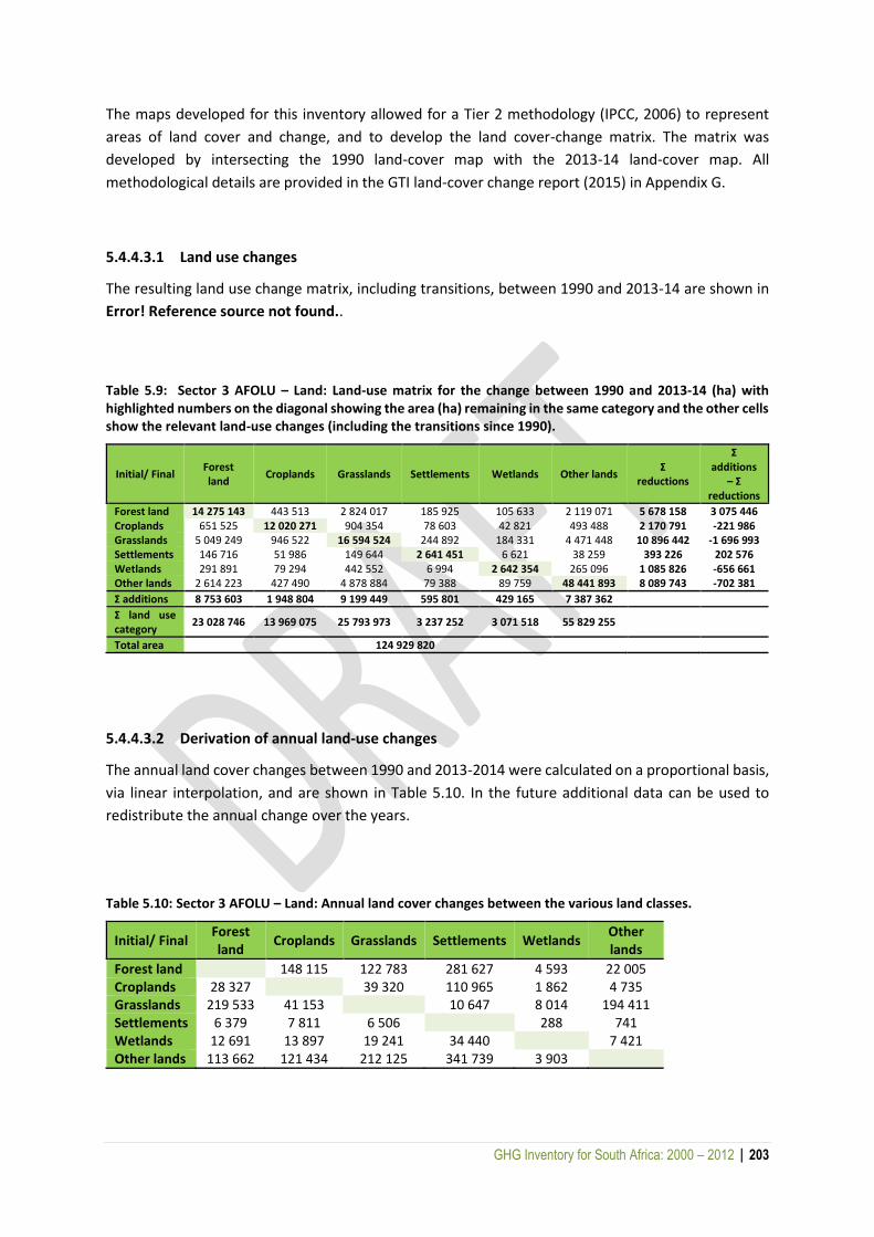
GHG Inventory for South Africa: 2000 – 2012 | 203

The maps developed for this inventory allowed for a Tier 2 methodology (IPCC, 2006) to represent

areas of land cover and change, and to develop the land cover-change matrix. The matrix was

developed by intersecting the 1990 land-cover map with the 2013-14 land-cover map. All

methodological details are provided in the GTI land-cover change report (2015) in Appendix G.

5.4.4.3.1 Land use changes

The resulting land use change matrix, including transitions, between 1990 and 2013-14 are shown in

Error! Reference source not found..

Table 5.9: Sector 3 AFOLU – Land: Land-use matrix for the change between 1990 and 2013-14 (ha) with highlighted numbers on the diagonal showing the area (ha) remaining in the same category and the other cells show the relevant land-use changes (including the transitions since 1990).

Initial/ Final Forest land

Croplands Grasslands Settlements Wetlands Other lands Σ

reductions

Σ additions

– Σ reductions

Forest land 14 275 143 443 513 2 824 017 185 925 105 633 2 119 071 5 678 158 3 075 446 Croplands 651 525 12 020 271 904 354 78 603 42 821 493 488 2 170 791 -221 986 Grasslands 5 049 249 946 522 16 594 524 244 892 184 331 4 471 448 10 896 442 -1 696 993 Settlements 146 716 51 986 149 644 2 641 451 6 621 38 259 393 226 202 576 Wetlands 291 891 79 294 442 552 6 994 2 642 354 265 096 1 085 826 -656 661 Other lands 2 614 223 427 490 4 878 884 79 388 89 759 48 441 893 8 089 743 -702 381

Σ additions 8 753 603 1 948 804 9 199 449 595 801 429 165 7 387 362

Σ land use category

23 028 746 13 969 075 25 793 973 3 237 252 3 071 518 55 829 255

Total area 124 929 820

5.4.4.3.2 Derivation of annual land-use changes

The annual land cover changes between 1990 and 2013-2014 were calculated on a proportional basis,

via linear interpolation, and are shown in Table 5.10. In the future additional data can be used to

redistribute the annual change over the years.

Table 5.10: Sector 3 AFOLU – Land: Annual land cover changes between the various land classes.

Initial/ Final Forest land

Croplands Grasslands Settlements Wetlands Other lands

Forest land 148 115 122 783 281 627 4 593 22 005 Croplands 28 327 39 320 110 965 1 862 4 735 Grasslands 219 533 41 153 10 647 8 014 194 411 Settlements 6 379 7 811 6 506 288 741 Wetlands 12 691 13 897 19 241 34 440 7 421 Other lands 113 662 121 434 212 125 341 739 3 903

GHG Inventory for South Africa: 2000 – 2012 | 204

5.4.4.4 LIMITATIONS AND CAUTIONARY NOTES ON CHANGE ASSESSMENT

Cloud-free images from Landsat were used as far as possible. Where this was not possible, regions

were corrected by merging cloud affected YoA with cloud free ToA. The process of masking was found

to be acceptable by GTI.

The seasonal representation and range of monthly acquisition dates is generally better for the 1990

land-cover dataset, than used for the 2013-14 dataset, despite the same average number of

acquisition dates per frame for the two datasets. This is because the 2013-14 dataset was limited to

what cloud free imagery was recorded between April 2013 and the designated March 2014 cut-off,

whereas the 1990 dataset had access to a wider range of imagery from 1989 to 1993. This greater

seasonal representation may have influenced the modelling results in terms of the distribution and

extent of some of the natural vegetation classes (excluding indigenous forests), since a better seasonal

profile was often possible in 1990 compared to 2014 in some image frame locations.

The 1990 period appears to have been generally wetter than the 2013-14 period in most regions, as

observed through the increase in observable surface water features in 1990. This is especially evident

in the pans across the central regions of the Free State and Northern Cape, where many pans are

water filled in 1990 and dry in 2013-14. These differences will reflect as changes between the two

assessment periods but do not necessarily represent a permanent loss of water bodies over the ± 24

year period, but rather a seasonal (or climatic) induced difference. This fact needs to be noted during

modelling and interpretation of land-cover change results.

The wetter conditions prevalent in the 1990 dataset have allowed the wetland modelling to be

extended across the full national coverage, unlike the drier 2013-14 image data which restricted

wetland modelling to the wetter eastern and southern regions. These differences will reflect as

changes between the two assessment periods but do not necessarily represent a permanent loss of

wetlands over the ± 24 year period, but rather a seasonal (or climatic) induced difference. This fact

needs to be noted during modelling and interpretation of land-cover change results.

The wetter conditions prevalent in the 1990 dataset may have influenced the boundary between low-

shrub (i.e. karoo type) and highveld grassland vegetation, since the 1990 grassland/low shrub

transition in the western Free State region appears to have shifted generally to the west compared to

2013-14, which may be a result of a greater grass component being present in the karoo/grass

transition zone in 1990.

The (highveld, montane and coastal) grassland correction procedures applied to the 1990 dataset are

considered to be slightly more accurate than those applied to the 2013-14 data, as a result of both

modified procedures used and better image seasonal representation in 1990. It is therefore potentially

possible that some of the 'grassland' to 'open woody vegetation' changes in these regions may be a

result of the improved grassland delineation in 1990 and not actual bush cover increases in 2013-14.

Changes in the extent of urban areas between 1990 and 2013-14 may not be as locally significant as

maybe expected, since the total built-up footprint defined in the "settlements" class in both the 1990

GHG Inventory for South Africa: 2000 – 2012 | 205

and 2013-14 datasets includes peripheral smallholding areas around the main built-up areas; and

these tend to be the first land-use that is converted to formal urban areas, before further expansion

into natural and cultivated lands.

It should also be noted that all land conversions as provided by the land change map were included

due to the limited time period to assess the change maps. In the next inventory a full assessment of

the land change classes will be completed.

5.4.4.5 COMPARISON WITH LAND COVER DATA FOR 2010 INVENTORY

For the purpose of this inventory a comparison was made between the 2010 national land cover data

from the previous inventory (DEA, 2014) and the new 2013-14 land cover map used in this inventory

(Table 5.11). Croplands, settlements and other land areas were much larger in the 2010 classification,

while forest land area was reduced by 44.3%. Indigenous forest area remained fairly consistent, while

the thicket/dense bush and woodland/open bush varied significantly. This is partly because of the re-

classification of the classes and the removal of the biome boundaries. Plantation areas were reduced,

which was expected as plantations were overestimated in the 2010 map. The map area for plantations

is now more consistent with areas reported by Forestry South Africa (FSA, 2012). Grassland areas are

consistent, but the removal of the fynbos boundary resulted in the fynbos being reclassified into the

other land classes and it was thus moved out of the grassland category. A portion of the fynbos was

classified into low shrubland, which is partly the reason for the increase in the Other land category.

5.4.4.6 QA/QC AND VERIFICATION

GTI calculated the accuracy of the 2013-14 land-cover dataset with the multi-seasonal Landsat 8

imagery. The results indicated an overall map and mean map accuracy of 82.53% and 88.36%,

respectively. A total of 6 415 sample points were used to determine the accuracy. In addition, the

Kappa Index of 80.87 indicates that results are unlikely to be from a chance occurrence. All classes

recorded above 70% user accuracy (UA) and producer accuracy (PA) except for dense bush/Tthicket

(53.74% UA), woodland/open bush (60.84% UA; 54.13 PA), low shrubland/other (61.82 PA) and

grasslands (69.82 PA). Detailed results can be found in the GTI report (Appendix G).

GHG Inventory for South Africa: 2000 – 2012 | 206

Table 5.11: Sector 3 AFOLU – Land: Comparison between the land areas from the 2010 inventory and the updated areas in this 2012 inventory.

5.4.4.7 TIME-SERIES CONSISTENCY

It is important that there is a consistent time-series in the preparation of the land-use category and

conversion data so that any artefact from method change is not included as an actual land-use

conversion. When using land-use data it is important to harmonize definitions between the existing

independent data sources; ensure that data acquisition methods are reliable and well documented;

ensure the consistent application of category definitions between time periods; prepare uncertainty

estimates; and ensure that the national land area is consistent across the inventory time series. This

inventory has tried to address these issues.

Landsat imagery was used for both the 1990 and 2013-14 datasets to specifically ensure time-series

consistency. In addition, the resolution of Landsat imagery was improved compared to the MODIS

datasets used in previous studies. The methods and procedures used to develop the 1990 and 2013-

IPCC category

Vegetation class (2010) Area (ha) Vegetation class (2013-14) Area (ha)

Change relative to 2010

(%)

Forest land

Indigenous Forest 477 889 Indigenous Forest 428 444 Thicket 2 876 607 Thicket /Dense bush 8 291 669 Woodlands/Savanna 35 854 791 Woodland/Open bush 12 434 932 Plantations 2 146 347 Plantations / Woodlots 1 873 701

Sub-total 41 355 634 23 028 746 -44.32%

Cropland

Annual commercial crops non-pivot 6 445 523

Commercial annual crops non-pivot 10 610 838

Annual commercial crops pivot 426 973 Commercial annual crops pivot 782 049 Permanent crops orchard 181 835 Commercial permanent orchards 346 950 Permanent crops viticulture 235 113 Commercial permanent vines 188 711 Annual semi-commercial / subsistence crops 1 020 776 Cultivated subsistence crops 2 040 527 Sugarcane 313 613

Sub-total 8 623 833 13 969 075 61.98%

Grassland Grassland 24 852 654 Grasslands 25 793 973 Fynbos 5 909 183

Sub-total 30 761 837 25 793 973 -16.15%

Settlements Settlements 1 822 753 Settlements (incl smallholdings) 2 908 280 Mines 179 324 Mines 328 973

Sub-total 2 002 077 3 237 252 61.69%

Wetlands Wetlands 1 138 322 Wetlands 1 025 900 Water Bodies 1 716 648 Waterbodies 2 045 618

Sub-total 2 854 970 3 071 518 7.58%

Other lands

Bare Ground 22 663 354 Bare Ground 13 057 933 Other 922 077 Nama-karoo 9 280 573 Low shrubland 41 827 260 Succulent karoo 3 598 410 Degraded 944 061

Sub-total 36 464 414 55 829 255 53.11%

GHG Inventory for South Africa: 2000 – 2012 | 207

14 datasets remained consistent. The main variation in the development of the two land-cover

datasets was the use of Landsat 5 and Landsat 8. All other aspects in this development remained

consistent.

5.4.4.8 PLANNED IMPROVEMENTS

The land-cover maps were developed as a desktop only modelling exercise, the results of which are

directly dependent on the validity and accuracy of the modelling data inputs, theoretical assumptions

and associated modelling rules. As such, no statistical verification of final land-cover change detection

accuracy can or has been be provided. The DEA has a GHG Inventory Improvement Programme and,

although there are no specific plans in place currently, it is recommended that under this programme

a stratified sampling approach which can be used to validate these, and future, land-cover maps be

investigated for future inventory updates.

5.4.5 Land use definitions and classifications

5.4.5.1 FOREST LAND

The forest land category included all land with woody vegetation consistent with thresholds used to

define forest land in the national greenhouse gas inventory. It also included systems with a vegetation

structure that currently falls below, but in situ could potentially reach the threshold values used by a

country to define the forest land category. According to the Kyoto Protocol and the Marrakesh Accord,

a forest is defined as having a minimum area of 0.05 to 1.0 hectares with tree crown cover (or

equivalent stocking level) of more than 10 to 30%, with trees with the potential to reach a minimum

height of 2 to 5 metres at maturity in situ. A forest may consist either of closed forest formations

where trees of various storeys and undergrowth cover a high proportion of the ground or open forest.

Young natural stands and all plantations which have yet to reach a crown density of 10 to 30% or tree

height of 2 to 5 metres are included under forest.

The FAO defines indigenous forests as forests with a tree canopy cover of more than 10%, trees should

be able to reach a height of 5 m and the forest area must be greater than 0.5 hectares. Under this

definition, indigenous forests include woodlands which have a tree canopy cover of 10 to 70%. In the

Global Forest Resources Assessment Report for South Africa (GFRASA, 2005) forests include (a) forests

with a tree canopy cover >70%, (b) forest and woodlands which have a tree cover of between 10% to

70%, and (c) plantations. This report therefore classifies all woodlands and savannas under forest land.

The previous inventory differed in that it separated out the woody savannas from other woodlands

by their geographical distribution, and excluded woody savannas from forest lands.

A further addition to forest land in this inventory was thickets. Typically thickets are not classed as

forest lands as the trees do not reach the height requirement. In the GFRASA (2005) they were

classified as other woodlands, however, for the purpose of this inventory, thickets were classed as

forest land, since they are more like forests than grasslands.

GHG Inventory for South Africa: 2000 – 2012 | 208

The following vegetation subcategories were therefore included within forest land:

Natural forests:

o Natural/semi-natural indigenous forest, dominated by tall trees, where tree canopy

heights are typically > ± 5m and tree canopy densities are typically > ± 75 %, often

with multiple understory vegetation canopies.

Plantations:

o All areas of systematically planted man-managed tree resources, composed of

primarily exotic species, including hybrids. This category includes all plantations from

young to mature which have been established for commercial timber production

seedling trials or woodlots (Thompson, 1999; GeoTerraImage, 2013);

o It includes clear-felled stands;

o It excludes all non-timber-based plantations, as well as orchards.

Thickets/dense bush:

o Natural/semi-natural tree- and/or bush-dominated areas, where typically canopy

heights are between 2 –and 5 m, and canopy density is typically > ± 75%, but may

include localised sparser areas down to ± 60%. Includes dense bush, thicket, closed

woodland, tall, dense shrubs, scrub forest and mangrove swamps. Can include self-

seeded bush encroachment areas if sufficient canopy density.

Woodland/open bush:

o Natural/semi-natural tree- and/or bush-dominated areas, where typically canopy

heights are between ± 2 and 5 m, and canopy densities typically between 40 and 75%,

but may include localised sparser areas down to ± 15 to 20%. Includes sparse, open

bushland and woodland, including transitional wooded grassland areas. Can include

self-seeded bush encroachment areas if canopy density is within indicated range.

5.4.5.2 CROPLAND

This category included cropped land and agro-forestry systems where the vegetation structure falls

below the thresholds used for the forest land category. The subcategories in croplands were:

Annual commercial crops:

o Commercial annuals (rainfed or non-pivot) - Cultivated lands used primarily for the

production of rain-fed, annual crops for commercial markets. Typically represented

by large field units, often in dense local or regional clusters. In most cases the defined

cultivated extent represents the actual cultivated or potentially extent. Includes

Sugarcane crops.

o Commercial pivot (irrigated or pivot) - Cultivated lands used primarily for the

production of centre pivot irrigated, annual crops for commercial markets. In most

cases the defined cultivated extent represents the actual cultivated or potentially

extent. Includes sugarcane crops.

Perennial crops:

o Permanent orchards - Cultivated lands used primarily for the production of both rain-

fed and irrigated permanent orchard crops for commercial markets. Includes both

tree, shrub and non-woody crops, such as citrus, tea, coffee, grapes, lavender and

pineapples etc. In most cases the defined cultivated extent represents the actual

cultivated or potentially extent.

GHG Inventory for South Africa: 2000 – 2012 | 209

o Permanent vines - Cultivated lands used primarily for the production of both rain-fed

and irrigated permanent vine (grape) crops for commercial markets. In most cases the

defined cultivated extent represents the actual cultivated or potential extent.

Subsistence crops:

o Those that do not meet the threshold for annual commercial crops and are found in

and around local housing areas;

o Cultivated lands used primarily for the production of rain-fed, annual crops for local

markets and / or home use. Typically represented by small field units, often in dense

local or regional clusters. The defined area may include intra-field areas of non-

cultivated land, which may be degraded or use-impacted, if the individual field units

are too small to be defined as separate features.

5.4.5.3 GRASSLAND

The grassland category included range and pasture lands that were not considered cropland. The

category also included all grassland from wild lands to recreational areas as well as agricultural and

silvi-pastural systems, consistent with national definitions. It is defined as natural/semi-natural grass-

dominated areas, where typically the tree and/or bush canopy densities are < ± 20 %, but may include

localised denser areas up to ± 40%, (regardless of canopy heights). Includes open grassland, and sparse

bushland and woodland areas, including transitional wooded grasslands. May include planted pasture

(i.e. grazing) if not irrigated. “Planted grassland‟ is defined in the same way except that it is grown

under human-managed (including irrigated) conditions for grazing hay or turf production or

recreation. Planted grassland can be either indigenous or exotic species. Irrigated pastures will

typically be classified as cultivated, and urban parks and golf courses etc under urban.

5.4.5.4 SETTLEMENTS

Settlements are defined as all developed land, including transportation infrastructure and human

settlements of any size, unless they are already included under other categories. They essentially

comprise all formal built-up areas in which people reside on a permanent or near-permanent basis

identifiable by the high density of residential and associated infrastructure. Includes both towns

villages and where applicable the central nucleus of more open rural clusters. This category also

includes mines. The mining activity footprint includes extraction pits, tailings, waste dumps, flooded

pits and associated surface infrastructure such as roads and buildings (unless otherwise indicated), for

both active and abandoned mining activities. This class may also include open cast pits, sand mines,

quarries and borrow pits etc.

5.4.5.5 WETLANDS

Wetlands are areas of land that are covered or saturated by water for all or part of the year and that

do not fall into the fForest land, cropland, grassland or settlements categories. They include reservoirs

as a managed sub-division and natural rivers and lakes as unmanaged sub-divisions. Wetlands include

two sub-divisions:

Waterbodies:

GHG Inventory for South Africa: 2000 – 2012 | 210

o Areas occupied by (generally permanent) open water. The category includes both

natural and man-made waterbodies that are either static or flowing and fresh brackish

and salt-water conditions (Thompson, 1999). This category includes features such as

rivers, major reservoirs, farm-level irrigation dams, permanent pans lakes and

lagoons;

Wetlands:

o Natural or artificial areas where the water level is permanently or temporarily at (or

very near) the land surface typically covered in either herbaceous or woody

vegetation cover. The vegetation can be either rooted or floating. Wetlands may be

either daily (i.e. coastal), temporarily seasonal or permanently wet and/or saturated.

Vegetation is predominately herbaceous. Includes, but is not limited to, wetlands

associated with seeps/springs, marshes, floodplains, lakes / pans, swamps, estuaries,

and some riparian areas.

5.4.5.6 OTHER LAND

This category includes bare soil, rock, ice, and all land areas that did not fall into any of the other five

categories. It allowed the total of identified land areas to match the national area, where data were

available. This category included the following:

Bare ground:

o Bare, non-vegetated ground, with little or very sparse vegetation cover (i.e. typically

< ± 5 to 10 % vegetation cover), occurring as a result of either natural or man-induced

processes. Includes, but is not limited to, natural rock exposures, dry river beds, dry

pans, coastal dunes and beaches, sand and rocky desert areas, very sparse low

shrublands and grasslands, erosion areas, and major road networks etc. May also

include long-term wildfire scars in some mountainous areas in the Western Cape.

Degraded land:

o Sparsely vegetated areas, occurring as a result of man-induced processes, which

show significantly lower overall vegetation cover compared to surrounding, natural

undisturbed areas. Includes, but is not limited to, natural rock exposures, dry river

beds, dry pans, coastal dunes and beaches, sand and rocky desert areas, very sparse

low shrublands and grasslands, erosion areas, and major road networks etc.

Low shrublands:

o Natural/semi-natural low shrub-dominated areas, typically with ≤ 2m canopy height.

Includes a range of canopy densities encompassing sparse to dense canopy covers.

Very sparse covers may be associated with the bare ground class. Typically associated

with low, woody shrub, Karoo-type vegetation communities, although can also

represent locally degraded vegetation areas where there is a significantly reduced

vegetation cover in comparison to surrounding, less impacted vegetation cover,

including long-term wildfire scars in some mountainous areas in the Western Cape.

Note that taller tree/bush/shrub communities within this vegetation type are

typically classified separately as one of the other tree- or bush-dominated cover

classes.

GHG Inventory for South Africa: 2000 – 2012 | 211

5.4.5.7 MANAGED AND UNMANAGED LANDS

According to the IPCC definition of the AFOLU sector, anthropogenic GHG emissions and removals

take place on “managed land”. Most land in South Africa is managed to some degree, so all land

classes were included in the biomass growth and loss calculations, except other lands. Inclusion of the

other land category may be considered in the future.

5.4.6 Recalculations

There were several changes and thus recalculations for the land-use sector since the last inventory:

New land-cover maps:

o These were developed specifically for this inventory to cover the period 1990 – 2013-

14;

o The resolution of the maps was increased from 1km to 30m.

Reclassification of land classes:

o In this inventory the biome boundaries were removed so that Karoo and fynbos

vegetation were not distinguished. Instead all vegetation from these classes were

classified into the other vegetation categories.

o In the previous inventory fynbos vegetation was classed in the grassland category, but

with the new reclassification and distribution of fynbos into the other land categories,

the grassland category consisted only of grasslands.

o Sugar cane was incorporated into annual crops.

o A small degraded land category was included.

Land-conversion data:

o The category other lands was also included and sinks and removals from this category

were incorporated in this inventory.

o Converted land was accumulated over the 23 year period.

Activity data:

o Updated biomass data for indigenous forests, woodland/open bush, orchards and

vineyards were incorporated;

o Cropland methodology was corrected and updated with new biomass data;

o DOM was included for forest lands; and

o Soil type was included into the soil carbon data.

HWP:

o Emissions and removals from the HWP category were corrected and the methodology

was updated following the recent KP Supplementary GPG.

Specific recalculations completed for each land class are discussed in detail under the specific sections

below. All recalculations were completed for the years 2000 to 2012.

GHG Inventory for South Africa: 2000 – 2012 | 212

5.4.7 Forest land [3B1]

5.4.7.1 SOURCE-CATEGORY DESCRIPTION

Reporting in this category covers emissions and removals from above-ground and below-ground

biomass, DOM and mineral soils. The category included indigenous forests, plantations/woodlots,

thickets/dense bush, and woodlands/open bush. As in the previous inventory the plantations were

sub-divided into Eucalyptus sp., softwood sp., acacia (wattle) and other plantation species. Softwoods

were further divided into sawlogs, pulp and other as the growth and expansion factors of these

plantations differed. The majority of the Eucalyptus plantations are used for pulp so the Eucalyptus

species were not split by use, but Eucalyptus grandis and Other Eucalyptus species were separated.

Changes in biomass include wood removal, fuelwood collection, and losses due to disturbance.

Harvested wood was included for plantations, while fuelwood collection was estimated for all forest

land subcategories. In plantations, disturbance from fires and other disturbances was included, while

for all other subcategories only disturbance from fire was included due to a lack of data on other

disturbances. It should be noted that only CO2 emissions from fires were included in this section as all

other non-CO2 emissions were included under section 3C1. Also all emissions from the burning of

fuelwood for energy or heating purposes were reported as part of the energy sector.

This category reports emissions and removals from the categories forest land remaining forest land

and land converted to forest land (new forest established, via afforestation or natural succession, on

areas previously used for other land-use classes). In 2012 the total sink from forests amounted to 36

006 Gg CO2, which was up from the 23 269 Gg CO2 in 2000. Land converted to forest land contributed

the largest portion to the forest category (Figure 5.13) due to changes in biomass and soil carbon. The

annual fluctuations in this category are due mainly to changes in biomass losses (due to harvesting,

fuelwood removals and disturbance losses). In 2004 there was a reduction in the sink compared to

2003 and this was due mainly to an increase in disturbance losses that year. Harvested wood was also

higher in 2004 compared to 2003. During 2008 and 2009 there was an economic recession and this

could be responsible for the increased fuelwood use during this period. There was also an increase in

losses due to disturbance in 2007 and 2008, which declined in 2009. These increases in carbon losses

led to a sink in the forest land remaining forest land during 2008. This sink is however also partly due

to the inability to allocate carbon losses between land remaining land and converted land. The

increased sink in 2012 is due to a combination of reduced harvested wood, fuelwood and disturbance.

Conversion of grasslands and other lands to forest lands are estimated to be the largest contributors

to the land converted to forest land CO2 sink. Of the 2012 sink, 90.2% was contributed by the biomass

pool, while the rest was from the SOC and DOM pools (Figure 5.14).

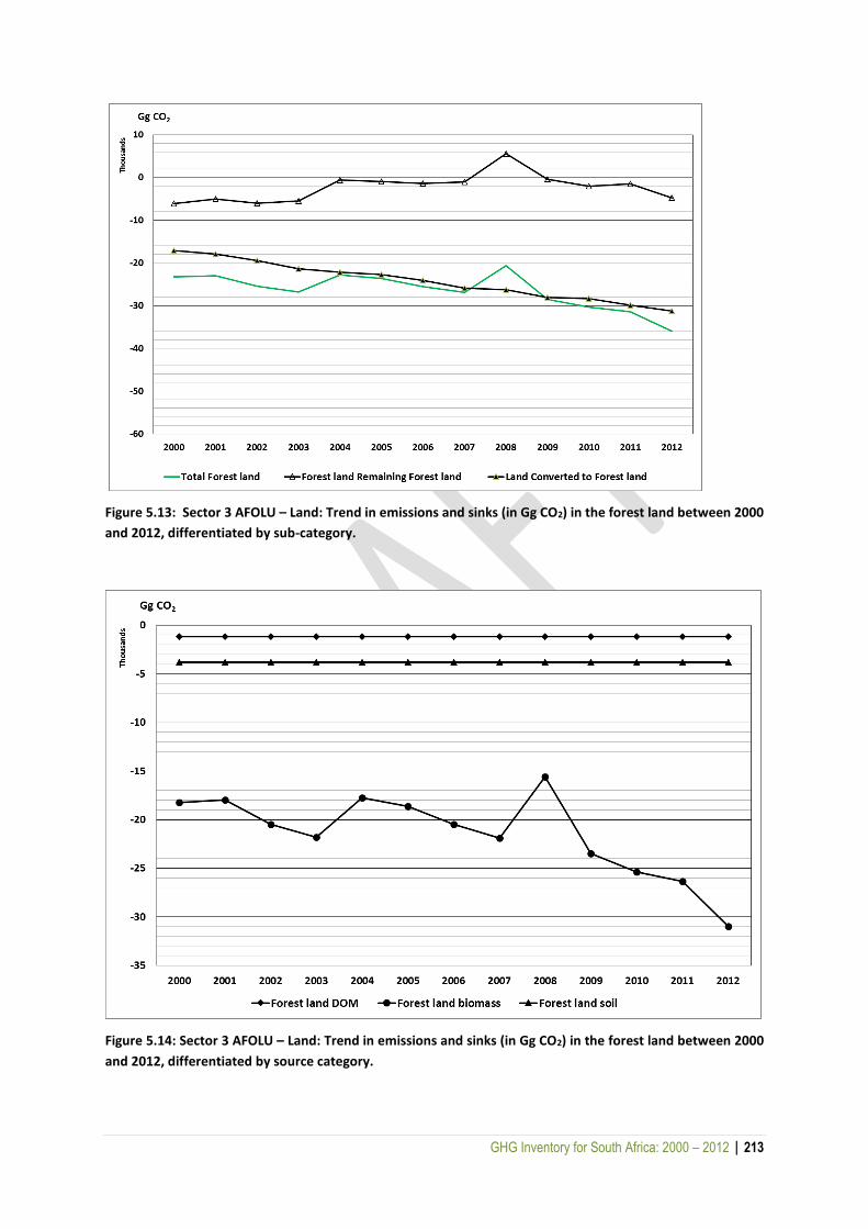
GHG Inventory for South Africa: 2000 – 2012 | 213

Figure 5.13: Sector 3 AFOLU – Land: Trend in emissions and sinks (in Gg CO2) in the forest land between 2000

and 2012, differentiated by sub-category.

Figure 5.14: Sector 3 AFOLU – Land: Trend in emissions and sinks (in Gg CO2) in the forest land between 2000

and 2012, differentiated by source category.

GHG Inventory for South Africa: 2000 – 2012 | 214

5.4.7.2 METHODOLOGICAL ISSUES

5.4.7.2.1 Biomass

Forest land remaining forest land

Removals and emissions of CO2 from changes in above- and below-ground biomass are estimated

using the Tier 1 gain-loss Method in the 2006 IPCC Guidelines. The gains in biomass stock growth were

calculated using the following equations (Equation 2.9 and 2.10 from IPCC 2006 Guidelines):

ΔCG = ∑(Ai * GTOTALi * CFi) (Eq. 5.14)

where for GTOTAL a Tier 1 approach was used for natural vegetation classes ( Eq. 5.15), while a Tier 2/3

approach was applied to the plantations (Eq. 5.16)

GTOTALi = Σ[GWi * (1+R)] (Eq. 5.15)

GTOTALi = Σ[Iv * BCEFI * (1+R)] (Eq. 5.16)

And:

Ai = Area of forest category i remaining in the same land-use category GWi = Average annual above-ground biomass growth for forest category i (t dm ha-1 a-1) Ri = Ratio of below-ground biomass to above-ground biomass for forest category i (t dm below-ground biomass (t dm above-ground biomass)-1) Iv = average net annual increment for specific vegetatio type (m3 ha-1 yr-1); BCEFI = biomass conversion and expansion factor for conversion of net annual increment in volume to above-ground biomass growth ((t AG biomass growth (m3 net annual increment)-1); CFi = Carbon fraction of dry matter for forest category i (t C (t dm)-1)

In the previous inventory a dead wood component was included in Eq. 5.15 as it was indicated that

the carbon losses from the live biomass would be overestimated as the fuel wood removals include

dead wood. In this inventory estimates for the DOM pool were included therefore, instead of including

a dead wood component in the carbon gains the fuelwood removals were adjusted for dead wood so

only removals of live wood were included here.

The losses were calculated for three components:

Loss of carbon from harvested wood;

Loss of carbon from fuelwood removals; and

Loss of carbon from disturbance.

Loss of carbon from harvested wood was calculated for plantations only as follows (Equation 2.12 IPCC

2006 Guidelines):

Lwood-removals = [H * BCEFS * (1+R) * CF (Eq. 5.17)

Where:

GHG Inventory for South Africa: 2000 – 2012 | 215

H = annual wood removals (m3 yr-1) BCEFS = biomass conversion and expansion factor for conversion of removals in merchantable volume to total biomass removals (including bark), (t biomass removed (m3 of removals)-1) R = ratio of below-ground biomass to above-ground biomass (t dm below-ground (t dm above-ground)-1). CF = Carbon fraction of dry matter (t C (t dm)-1)

Loss of carbon from fuelwood removals was calculated using the following equation (Equation 2.13 of

IPCC 2006 Guidelines):

Lfuelwood = [FGtrees *BCEFR * (1+R) + FGpart * D] * CF (Eq. 5.18)

Where: FGtrees = annual volume of fuelwood removal of whole trees (m3 yr-1) FGpart = annual volume of fuelwood removal as tree parts (m3 yr-1) BCEFR = biomass conversion and expansion factor for conversion of removals in merchantable volume to biomass removals (including bark), (t biomass removal (m3 of removals)-1) R = ratio of below-ground biomass to above-ground biomass (t dm below-ground (t dm above-ground)-1) D = basic wood density (t dm m-3) CF = carbon fraction of dry matter (t C (t dm)-1)

Finally, the loss of carbon from disturbance in plantations was calculated following IPCC Equation 2.14:

Ldisturbances = Adisturbance * BW * (1+R) * CF * fd (Eq. 5.19)

Where: Adisturbance = area affected by disturbances (ha yr-1) BW = average above-ground biomass of areas affected by disturbance (t dm ha-1) R = ratio of below-ground biomass to above-ground biomass (t dm below-ground (t dm above-ground)-1). CF = carbon fraction of dry matter (t C (t dm)-1) fd = fraction of biomass lost in disturbance; a stand-replacing disturbance will kill all (fd = 1) biomass while an insect disturbance may only remove a portion (e.g. fd = 0.3) of the average biomass C density

For woodlands/ open bush the loss of carbon from disturbance (fires only) was calculated using the

biomass burning equation (IPCC 2006, Equation 2.27, p. 2.42):

Lfire = A * MB * Cf * Gef *10-3 * (12/44) (Eq. 5.20)

Where: Lfire = mass of carbon emissions from fire (t C); A = area burnt (ha) MB = mass of fuel available for combustion (t ha-1) Cf = combustion factor Gef = emission factor (g CO2 (kg dm burnt)-1)

This ensured that the disturbance estimates were consistent with the biomass burning estimates.

GHG Inventory for South Africa: 2000 – 2012 | 216

The total carbon flux (ΔC ) was then calculated as follows (IPCC 2006 Equations 2.7 and 2.11):

ΔC= ΔCG – Lwood-removals – Lfuelwood – Ldisturbances (Eq. 5. 21)

Land converted to forest land

The land converted to plantations could not be split into the various plantation types due to a lack of

data so the values for Eucalyptus were used as this is the dominant species. Annual increase in biomass

carbon stocks were calculated in the same way as for forest land remaining forest land. If a land area

is converted to a plantation then it is unlikely wood would be harvested in the year following the

conversion, therefore it was assumed that no wood was harvested or removed for fuel wood from the

converted land in the first year of conversion. All annual harvested wood and fuel wood losses were

therefore allocated to the forest land remaining forest land category. There was insufficient data to

determine how much of the annual disturbance in a plantation occurred on the converted land. For

the purpose of this inventory it was assumed that no disturbance occurred on converted land, but this

assumption will need to be corrected in future inventories. Losses due to fire disturbance were

calculated for land converted to woodlands/open bush using Equation 2.27 in the IPCC 2006

Guidelines. A detailed description of the methodology for calculating losses due to fire is given in

Section 5.5.2. As with forest land remaining forest land, indigenous forests and thickets were assumed

not to burn.

5.4.7.2.2 Dead organic matter

Forest land remaining forest land

The dead organic matter (DOM) pool comprises deadwood and litter. For this inventory a Tier 1

approach was introduced as the DOM pool is not a key category. Under the Tier 1 method the DOM

pool in land remaining in the same land use category are reported to have zero changes in carbon

stocks or carbon emissions (IPCC, 2006, Chapter 2, p 2.21).

Land converted to forest land

For the Tier 1 approach it is assumed that on land converted to forest land the build-up of litter and

deadwood occurs linearly from zero (in the non-forest land-use categories) over a transition period.

The transition period for this inventory was taken as 23 years (transition period of the land-cover

maps), as IPCC Guidelines indicate that if the transition time (T) is longer than the default 20 years (D)

then the value for T should be used. Annual change in carbon stocks in deadwood or litter (tonnes C

yr-1) was calculated using the following equation (Equation 2.23 in the IPCC 2006 Guidelines):

GHG Inventory for South Africa: 2000 – 2012 | 217

ΔCDOM = [(Cn – Co) * Aon] / Ton (Eq. 5.22)

Where:

Cn = dead wood/litter stock under the new land-use category (tonnes C ha-1); Co = dead wood/litter stock under the old land-use category (tonnes C ha-1); Aon = area under going conversion from old to new-land use category (ha); Ton = time period of the transition from old to new land-use category (yr) (23 years for this inventory).

5.4.7.2.3 Mineral soils

Land converted to forest land

Annual change in carbon stocks in mineral soils were calculated by applying a Tier 1 method with

Equation 2.25 of the IPCC 2006 Guidelines (IPCC, 2006, Volume 4, p. 2.30). Land areas were stratified

by default soil types (see Section 5.4.1) in order to obtain SOC reference values (for warm temperate

dry conditions). These were then multiplied by stock change factors by using formulation B of Equation

2.25:

ΔCMineral = Σ[{(SOCREF*FLU*FMG*Fl)0 – (SOCREF*FLU*FMG*FI*A)(0-T)}*A]/D (Eq. 5.23)

Where: SOCREF = the reference carbon stock (t C ha-1) for each soil type; FLU = stock change factor for land-use system for a particular land-use (dimensionless); FMG = stock change factor for management regime (dimensionless); FI = stock change factor for input of organic matter (dimensionless); Time 0 = last year of inventory time period; Time (0-T) = beginning of the inventory time period; A = land area (ha); D = time dependence of stock change factor (transition period of 23 years was used for this inventory).

5.4.7.3 DATA SOURCES

The land areas for forest land remaining forest land and land converted to forest land were obtained

from the land use maps discussed in section 5.4.4.

5.4.7.3.1 Biomass

Biomass gains

Annual biomass growth data for plantations was calculated from mean annual increment (MAI) data

provided by Forestry SA. These values were multiplied by the BCEF’s from Dovey and Smith (2005)

GHG Inventory for South Africa: 2000 – 2012 | 218

(0.522 for softwoods; 0.558 for Eucalyptus grandis; 0.741 for other Eucalyptus species; 0.909 for

Acacia species; and an average of 0.68 for other species) to obtain the increment in t dm ha-1. These

BCEFI values fall within the IPCC 2006 default range of 0.4 – 0.9 t biomass (m3 wood volume)-1 for dry

subtropical plantations with a growing stock between 100 and 200 m3 (IPCC 2006, Table 4.5).

Midgley and Seydack (2006, 2007) reported that growth was 1% of AGB for indigenous forests. The

AGB value in the previous inventory was 81 t dm ha-1 (IPCC GPG 2003), however in this inventory a

value of 150 t dm ha-1 was applied based on the outputs of the recently completed NTCSA (DEA, 2015)

(see Appendix F). The report provided validation for these data outputs. This value is at the upper limit

of the IPCC default values for subtropical systems in Africa (20 – 200 t dm ha-1) with the subtropical

dry forest having a value of 130-140 t dm ha-1 (IPCC, 2003). The 1% growth rate of 1.5 t dm ha-1 yr-1 is

also much more in line with IPCC default values for subtropical systems (Table 4.12; IPCC 2006

Guidelines) than the 0.8 t dm ha-1 from the previous inventory.

Data for thickets remain unchanged from the previous inventory. Carbon sequestration rates of some

thicket species have been estimated to be between 1.2 and 5.1 t C ha-1 yr-1 (2.4 to 10.2 t dm ha-1 yr-1)

(Aucamp and Howe, 1979; Mills and Cowling, 2006; Van der Vyver, 2011). Mills and Cowling (2006)

reported growth rates for above ground biomass of 0.04 to 0.131 g C m-2 yr-1 (or 0.85 to 2.76 t dm ha-

1) in thickets which provides an average estimate of 1.8 t dm ha yr-1 as used in the previous inventory.

For woodland/open bush a growth value of 0.9 t ha-1 yr-1 was also taken from the previous inventory

(DEA, 2013).

A root-to-shoot ratio of 0.24 for woodland/open shrubs and forests taken from the Global Forest

Resource Assessment for South Africa (GFRASA, 2005), as was the 0.34 for acacia and other plantation

species. For Eucalyptus and softwoods the value of 0.15 was taken from Christie and Scholes (1995).

All of these are consistent with the values used in the 2010 inventory (DEA, 2014). In the GFRASA

(2010) thickets are classed as other woodlands and these are indicated to have a root-to-shoot ratio

of 0.48.

The IPCC 2006 default value of 0.47 t C per t dm-1 (IPCC 2006, Table 4.3) was used for the carbon

fraction of dry matter of all Forest lands.

Losses due to wood harvesting

Loss of carbon due to wood harvesting was only determined for plantations using FSA data (FSA, 2012)

(Table 5.12) as wood harvesting does not occur in woodlands/open bush, thickets or indigenous

forests. The wood harvested for fuelwood was not included here as it was included under fuelwood

removals. The industry conversion factors provided were used to convert between tonnes and m3.

The BCEFS were taken to be the same as the BCEFI values described above Section as the IPCC 2006

default values (IPCC 2006, Table 4.5) indicate this to be the case.

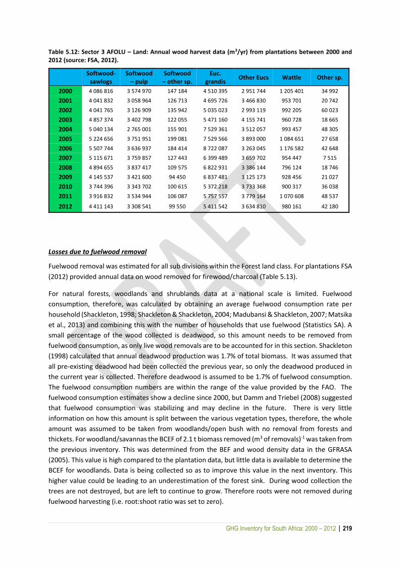
GHG Inventory for South Africa: 2000 – 2012 | 219

Table 5.12: Sector 3 AFOLU – Land: Annual wood harvest data (m3/yr) from plantations between 2000 and 2012 (source: FSA, 2012).

Softwood-sawlogs

Softwood – pulp

Softwood – other sp.

Euc. grandis

Other Eucs Wattle Other sp.

2000 4 086 816 3 574 970 147 184 4 510 395 2 951 744 1 205 401 34 992

2001 4 041 832 3 058 964 126 713 4 695 726 3 466 830 953 701 20 742

2002 4 041 765 3 126 909 135 942 5 035 023 2 993 119 992 205 60 023

2003 4 857 374 3 402 798 122 055 5 471 160 4 155 741 960 728 18 665

2004 5 040 134 2 765 001 155 901 7 529 361 3 512 057 993 457 48 305

2005 5 224 656 3 751 951 199 081 7 529 566 3 893 000 1 084 651 27 658

2006 5 507 744 3 636 937 184 414 8 722 087 3 263 045 1 176 582 42 648

2007 5 115 671 3 759 857 127 443 6 399 489 3 659 702 954 447 7 515

2008 4 894 655 3 837 417 109 575 6 822 931 3 386 144 796 124 18 746

2009 4 145 537 3 421 600 94 450 6 837 481 3 125 173 928 456 21 027

2010 3 744 396 3 343 702 100 615 5 372 218 3 733 368 900 317 36 038

2011 3 916 832 3 534 944 106 087 5 757 557 3 779 164 1 070 608 48 537

2012 4 411 143 3 308 541 99 550 5 411 542 3 634 810 980 161 42 180

Losses due to fuelwood removal

Fuelwood removal was estimated for all sub divisions within the Forest land class. For plantations FSA

(2012) provided annual data on wood removed for firewood/charcoal (Table 5.13).

For natural forests, woodlands and shrublands data at a national scale is limited. Fuelwood

consumption, therefore, was calculated by obtaining an average fuelwood consumption rate per

household (Shackleton, 1998; Shackleton & Shackleton, 2004; Madubansi & Shackleton, 2007; Matsika

et al., 2013) and combining this with the number of households that use fuelwood (Statistics SA). A

small percentage of the wood collected is deadwood, so this amount needs to be removed from

fuelwood consumption, as only live wood removals are to be accounted for in this section. Shackleton

(1998) calculated that annual deadwood production was 1.7% of total biomass. It was assumed that

all pre-existing deadwood had been collected the previous year, so only the deadwood produced in

the current year is collected. Therefore deadwood is assumed to be 1.7% of fuelwood consumption.

The fuelwood consumption numbers are within the range of the value provided by the FAO. The

fuelwood consumption estimates show a decline since 2000, but Damm and Triebel (2008) suggested

that fuelwood consumption was stabilizing and may decline in the future. There is very little

information on how this amount is split between the various vegetation types, therefore, the whole

amount was assumed to be taken from woodlands/open bush with no removal from forests and

thickets. For woodland/savannas the BCEF of 2.1 t biomass removed (m3 of removals)-1 was taken from

the previous inventory. This was determined from the BEF and wood density data in the GFRASA

(2005). This value is high compared to the plantation data, but little data is available to determine the

BCEF for woodlands. Data is being collected so as to improve this value in the next inventory. This

higher value could be leading to an underestimation of the forest sink. During wood collection the

trees are not destroyed, but are left to continue to grow. Therefore roots were not removed during

fuelwood harvesting (i.e. root:shoot ratio was set to zero).

GHG Inventory for South Africa: 2000 – 2012 | 220

Table 5.13: Sector 3 AFOLU – Land: Annual removal of fuelwood (m3/yr) from plantations between 2000 and 2012 (source: FSA, 2012).

Softwoods

Euc. grandis

Other Eucs

Wattle Other sp.

2000 18 855 42 082 18 933 80 944 5 165

2001 21 523 95 890 21 093 94 991 6 268

2002 22 356 56 000 34 234 113 718 2 427

2003 20 148 53 439 36 821 101 730 2 822

2004 24 333 78 488 61 713 99 400 998

2005 39 772 51 053 37 221 134 037 2 289

2006 42 661 82 002 35 939 130 150 292

2007 26 537 93 077 51 850 132 358 1 674

2008 28 396 75 649 44 144 122 114 0

2009 38 669 105 093 43 624 123 065 1 727

2010 21 051 94 642 37 541 127 498 0

2011 25 448 139 666 18 019 116 852 0

2012 23 654 144 275 18 568 118 228 0

Losses due to disturbance

The only disturbance losses that were estimated for all forest land classes were those from fire, but

for plantations the loss due to other disturbances was also included. The FSA provides data on the

area damaged during fire and other disturbances. For the year 1979 to 2000 the FSA also recorded

whether the plantations in a disturbed area were slightly damaged, seriously damage (in terms of

timber sold) or seriously damaged in that there was a total loss of vegetation. This data was used to

determine the weighted average fraction of biomass lost in the disturbance (by assuming a slight

damage had an fd = 0.3 and serious damage with total loss had a fd = 1) for hardwood (fd = 0.636) and

softwood (fd = 0.489) species. These averages were kept constant over the 10-year period as the FSA

stop reporting this data in 2000. The AGB (BW) data obtained from the NTCSA (DEA, 2015) only

provided a value for plantations as a whole (97 t dm ha-1). To estimate biomass data for each

plantation type the growing stock (by volume) data from GFRASA (2010) was combined with the BCEFS

(Chhabra et al., 2002). The values ranged between 70 t dm ha-1 and 132 t dm ha-1 which are within the

range estimated in the NTCSA (DEA, 2015).

The amount of carbon lost due to fire disturbance in woodlands/open bush was determined as

discussed in Section 5.4.7.2.1. Natural forests and thickets were assumed not to burn. The MB and Cf

factors were taken from the previous inventory (DEA, 2014) and are discussed further in Section 5.5.2.

A Gef of 1650 g CO2 (kg dm burnt)-1 was taken from the IPCC Guidelines.

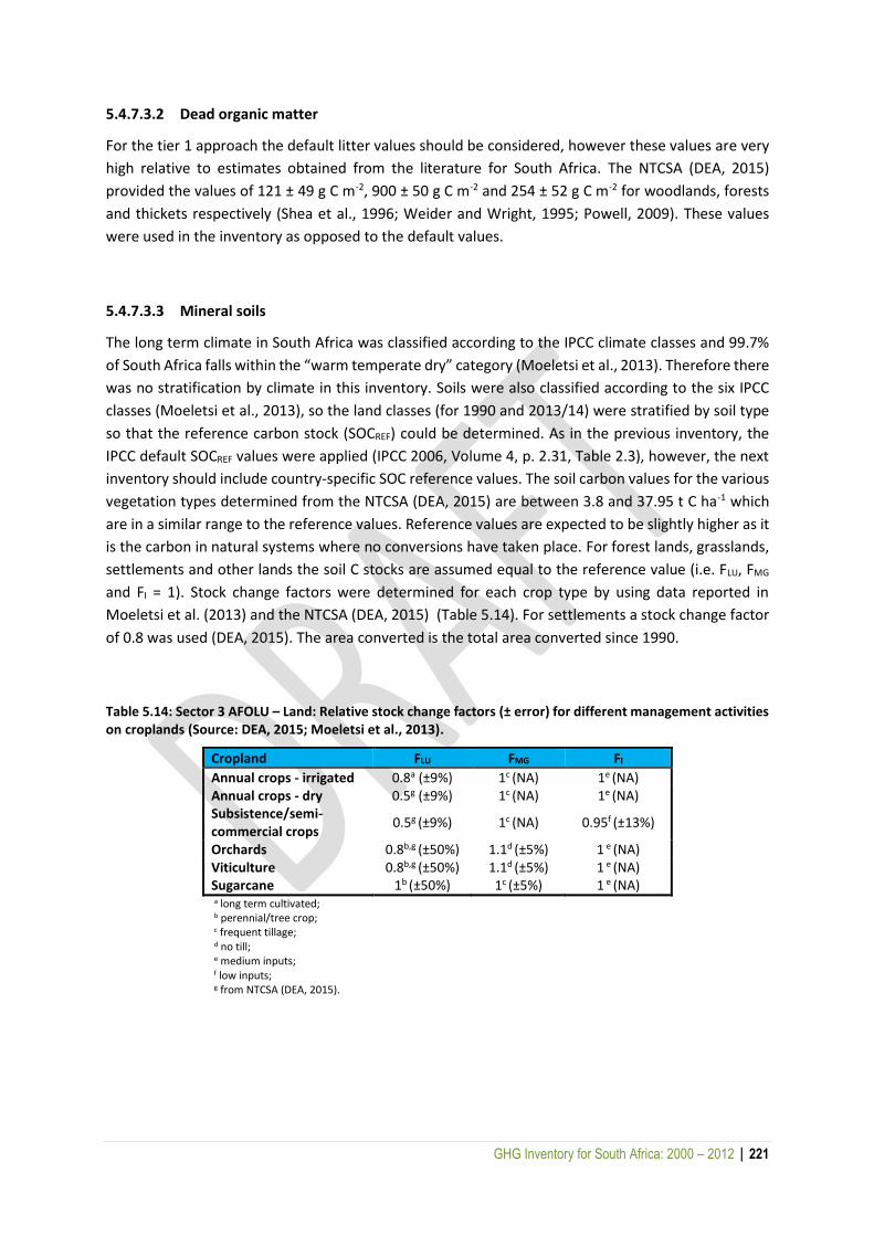
GHG Inventory for South Africa: 2000 – 2012 | 221

5.4.7.3.2 Dead organic matter

For the tier 1 approach the default litter values should be considered, however these values are very

high relative to estimates obtained from the literature for South Africa. The NTCSA (DEA, 2015)

provided the values of 121 ± 49 g C m-2, 900 ± 50 g C m-2 and 254 ± 52 g C m-2 for woodlands, forests

and thickets respectively (Shea et al., 1996; Weider and Wright, 1995; Powell, 2009). These values

were used in the inventory as opposed to the default values.

5.4.7.3.3 Mineral soils

The long term climate in South Africa was classified according to the IPCC climate classes and 99.7%

of South Africa falls within the “warm temperate dry” category (Moeletsi et al., 2013). Therefore there

was no stratification by climate in this inventory. Soils were also classified according to the six IPCC

classes (Moeletsi et al., 2013), so the land classes (for 1990 and 2013/14) were stratified by soil type

so that the reference carbon stock (SOCREF) could be determined. As in the previous inventory, the

IPCC default SOCREF values were applied (IPCC 2006, Volume 4, p. 2.31, Table 2.3), however, the next

inventory should include country-specific SOC reference values. The soil carbon values for the various

vegetation types determined from the NTCSA (DEA, 2015) are between 3.8 and 37.95 t C ha-1 which

are in a similar range to the reference values. Reference values are expected to be slightly higher as it

is the carbon in natural systems where no conversions have taken place. For forest lands, grasslands,

settlements and other lands the soil C stocks are assumed equal to the reference value (i.e. FLU, FMG

and FI = 1). Stock change factors were determined for each crop type by using data reported in

Moeletsi et al. (2013) and the NTCSA (DEA, 2015) (Table 5.14). For settlements a stock change factor

of 0.8 was used (DEA, 2015). The area converted is the total area converted since 1990.

Table 5.14: Sector 3 AFOLU – Land: Relative stock change factors (± error) for different management activities on croplands (Source: DEA, 2015; Moeletsi et al., 2013).

Cropland FLU FMG FI

Annual crops - irrigated 0.8a (±9%) 1c (NA) 1e (NA) Annual crops - dry 0.5g (±9%) 1c (NA) 1e (NA) Subsistence/semi-commercial crops

0.5g (±9%) 1c (NA) 0.95f (±13%)

Orchards 0.8b,g (±50%) 1.1d (±5%) 1 e (NA) Viticulture 0.8b,g (±50%) 1.1d (±5%) 1 e (NA) Sugarcane 1b (±50%) 1c (±5%) 1 e (NA) a long term cultivated; b perennial/tree crop; c frequent tillage; d no till; e medium inputs; f low inputs; g from NTCSA (DEA, 2015).

GHG Inventory for South Africa: 2000 – 2012 | 222

5.4.7.4 UNCERTAINTIES AND TIME-SERIES CONSISTENCY

5.4.7.4.1 Uncertainties

A full assessment of the uncertainties in the forest land category have not yet been completed, and

will be undertaken in the next inventory. Much of the uncertainty associated with the land component

relates to the mapping and area of each land type. These are discussed in Section 5.4.4. The statistics

from the FSA have a high confidence rating (80%) with an uncertainty range from -11% to 3% based

on a comparison with the RSA yearbook (DEAT, 2009). Uncertainty on a lot of the activity data for the

other vegetation sub-categories was difficult to estimate due to a lack of data. Uncertainty would,

however, be higher than that for the forestry industry. Uncertainty of AGB growth increment in natural

forests and woodlands could not be determined, but for thickets the uncertainty is 1.8 ± 0.96 t dm ha-

1. The uncertainty in BCEF could not be determined; however, IPCC 2006 Guidelines suggest that it

can reach up to 30%. Default root-to-shoot ratios for forests and woodlands have a range of 0.28 –

0.68; while thicket ratios had a variance of about 5%. The uncertainty on the fuel wood harvest

numbers from the FAO were not provided, but it is expected to be high.

For default soil organic C stocks for mineral soils there is a nominal error estimate of ±90% (IPCC 2006

Guidelines, p 2.31). The error on the stock change factors is indicated in Table 5.13.

The uncertainty on the burnt area, MB and Cf factors is discussed in Section 5.5.2.5.

The forest land category covers a wide span of vegetation types, from closed forests to open

woodlands, so the variation on the activity data was large (see Appendix F) and requires more vigorous

analysis to determine the uncertainty. It is suggested that a more detailed uncertainty analysis be

done on the data.

5.4.7.4.2 Time-series consistency

The same sources of data and land-cover maps were used throughout the 12-year period so as to

provide a consistent time series of data.

5.4.7.5 SOURCE-SPECIFIC QA/QC AND VERIFICATION

The land area in the land-cover maps were compared to previous data sets and explanations for the

various changes have been provided. The land areas were checked and summed across all land-use

categories to ensure that the total area in the inventory remained constant over the time series.

Where possible, the activity data was compared to literature, previous inventories and to default

values. The biomass data was compared to the biomass and NPP data from the NTCSA (DEA, 2015)

outputs. It was noted that the inventory produces biomass growth values at the low end of the NPP

range and that savannas are estimated to have a higher NPP than thickets, however as more detail is

included in the next inventory so these differences are expected to be reduced. Further assessments

will be completed in the next inventory. Soil carbon data was also compared to the NTCSA outputs.

GHG Inventory for South Africa: 2000 – 2012 | 223

As validation the plantation data was compared to a more detailed study by Alembong (2015). This

inventory overestimates the gains and also the losses from plantations. This could be due to a

difference in plantation areas being used. However Alembong (2015) estimated the overall carbon

gains in plantations in 2011 to be 857 300 t C, while the inventory estimates 558 223 t C. These values

are within a similar range and more detailed will be incorporated into the next inventory to reduce

these differences.

Wood removed due to harvesting were cross-checked with the input data for HWP. There was also a

cross-check between the wood removed for fuelwood and the fuelwood consumption data used in

the energy sector. The amount of wood harvested was compared to the FAO data. All general QC

procedures discussed in Section 1.4.1 were carried out on this category to ensure consistency in the

data. An independent reviewer provided comment on the forest land category and the inventory was

improved accordingly.

5.4.7.6 SOURCE-SPECIFIC RECALCULATIONS

Recalculations were made for 2000 to 2012 as new higher resolution maps were incorporated. There

was also a reclassification of the woodland/open bush category. These changes impacted the area of

forest land remaining forest land as well as land converted to forest land. Minor updates were made

to the activity data and the DOM pool was included. Land classes were also stratified by soil type to

improve the soil carbon data.

5.4.7.7 CATEGORY-SPECIFIC PLANNED IMPROVEMENTS AND RECOMMENDATIONS

The most important update that will be made in the next inventory is the BCEF for fuelwood data. A

reduction in uncertainty in this area would lead to improved data for the forest land category.

The next inventory plans to make use of the recently released IPCC 2006 version of the Agriculture

and Land Use (ALU) software. This software allows spatial data to be integrated with ground based

data. For the forest land category the plan is to incorporate more detail regarding the forests and their

age classes and management. Data from Alembong (2015) will be obtained and incorporated where

possible. A complete uncertainty analysis on the land data is also planned for the next inventory and

the ALU software will also be able to assist with this. The other advantage of the ALU software is that

it provide a place for all the metadata and data sources to be stored. Although the NTCSA (DEA, 2015)

study did not provide reference carbon stocks, reference carbon stocks could be determined from this

data in future and incorporated into the inventory. This is not planned for the next inventory but is

something which could be considered in future.

GHG Inventory for South Africa: 2000 – 2012 | 224

5.4.8 Cropland [3B2]

5.4.8.1 SOURCE CATEGORY DESCRIPTION

Reporting in the cropland category covers emissions and removals of CO2 from mineral soils, and from

above- and below-ground biomass. Croplands include annual commercial crops, annual semi-

commercial or subsistence crops, orchards, and viticulture. This category reports emissions and

removals from the category cropland remaining cropland (cropland that remains cropland during the

period covered by the report) and the land converted to cropland category. Calculations are carried

out on the basis of a 23-year transition period in that once a land area is converted it remains in the

converted land category for 20 years. In this inventory transition data was only available from 1990

(see section Error! Reference source not found.) therefore all calculations include transitions since

1990.

For Cropland remaining cropland, the Tier 1 assumption is that for annual cropland there is no change

in biomass carbon stocks after the first year (GPG-AFOLU, section 5.2.1, IPCC, 2006a). The rationale is

that the increase in biomass stocks in a single year is equal to the biomass losses from harvest and

mortality in that same year. For perennial cropland, there is a change in carbon stocks associated with

a land-use change. Where there has been land-use change between the Cropland subcategories,

carbon stock changes are reported under Cropland remaining cropland. Cropland remaining cropland

was estimated to be a sink of CO2, declining from 1 241 Gg CO2 in 2000 to 104 Gg CO2 in 2012 (Figure

5.15). The sink is due to conversions between annual and perennial cropland categories and changes

in soil carbon. Land converted to cropland was a source of CO2 (5 672 Gg CO2 per year) (Figure 5.16).

The source remained constant as a constant annual change was derived over the mapping period

between 2000 and 2013-14. It is assumed that equilibrium is reached after a year of conversion

therefore even though the land converted to cropland area increased every year the change in

biomass is only determined for the annual area converted. The largest contributors to the CO2 source

in this category were conversions from grasslands to croplands. SOC was the largest contributor to

this category (Figure 5.16). For Croplands the DOM was not estimated, but is not considered as a major

contributor to this category. .

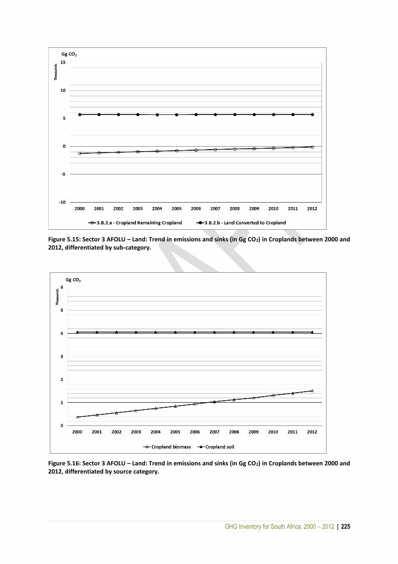
GHG Inventory for South Africa: 2000 – 2012 | 225

Figure 5.15: Sector 3 AFOLU – Land: Trend in emissions and sinks (in Gg CO2) in Croplands between 2000 and 2012, differentiated by sub-category.

Figure 5.16: Sector 3 AFOLU – Land: Trend in emissions and sinks (in Gg CO2) in Croplands between 2000 and 2012, differentiated by source category.

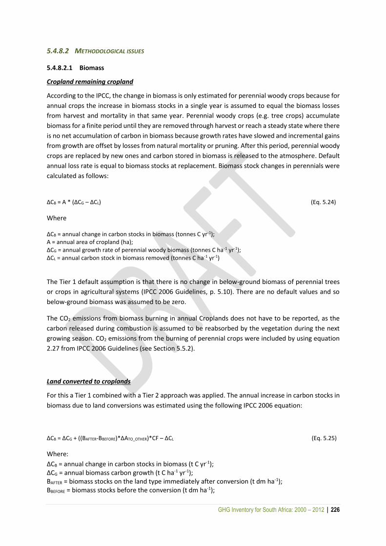
GHG Inventory for South Africa: 2000 – 2012 | 226

5.4.8.2 METHODOLOGICAL ISSUES

5.4.8.2.1 Biomass

Cropland remaining cropland

According to the IPCC, the change in biomass is only estimated for perennial woody crops because for

annual crops the increase in biomass stocks in a single year is assumed to equal the biomass losses

from harvest and mortality in that same year. Perennial woody crops (e.g. tree crops) accumulate

biomass for a finite period until they are removed through harvest or reach a steady state where there

is no net accumulation of carbon in biomass because growth rates have slowed and incremental gains

from growth are offset by losses from natural mortality or pruning. After this period, perennial woody

crops are replaced by new ones and carbon stored in biomass is released to the atmosphere. Default

annual loss rate is equal to biomass stocks at replacement. Biomass stock changes in perennials were

calculated as follows:

ΔCB = A * (ΔCG – ΔCL) (Eq. 5.24)

Where

ΔCB = annual change in carbon stocks in biomass (tonnes C yr-1); A = annual area of cropland (ha); ΔCG = annual growth rate of perennial woody biomass (tonnes C ha-1 yr-1); ΔCL = annual carbon stock in biomass removed (tonnes C ha-1 yr-1)

The Tier 1 default assumption is that there is no change in below-ground biomass of perennial trees

or crops in agricultural systems (IPCC 2006 Guidelines, p. 5.10). There are no default values and so

below-ground biomass was assumed to be zero.

The CO2 emissions from biomass burning in annual Croplands does not have to be reported, as the

carbon released during combustion is assumed to be reabsorbed by the vegetation during the next

growing season. CO2 emissions from the burning of perennial crops were included by using equation

2.27 from IPCC 2006 Guidelines (see Section 5.5.2).

Land converted to croplands

For this a Tier 1 combined with a Tier 2 approach was applied. The annual increase in carbon stocks in

biomass due to land conversions was estimated using the following IPCC 2006 equation:

ΔCB = ΔCG + ((BAFTER-BBEFORE)*ΔATO_OTHER)*CF – ΔCL (Eq. 5.25)

Where:

ΔCB = annual change in carbon stocks in biomass (t C yr-1); ΔCG = annual biomass carbon growth (t C ha-1 yr-1); BAFTER = biomass stocks on the land type immediately after conversion (t dm ha-1); BBEFORE = biomass stocks before the conversion (t dm ha-1);

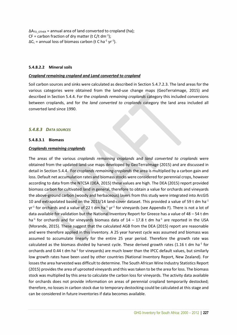
GHG Inventory for South Africa: 2000 – 2012 | 227

ΔATO_OTHER = annual area of land converted to cropland (ha); CF = carbon fraction of dry matter (t C/t dm-1); ΔCL = annual loss of biomass carbon (t C ha-1 yr-1).

5.4.8.2.2 Mineral soils

Cropland remaining cropland and Land converted to cropland

Soil carbon sources and sinks were calculated as described in Section 5.4.7.2.3. The land areas for the

various categories were obtained from the land-use change maps (GeoTerraImage, 2015) and

described in Section 5.4.4. For the croplands remaining croplands category this included conversions

between croplands, and for the land converted to croplands category the land area included all

converted land since 1990.

5.4.8.3 DATA SOURCES

5.4.8.3.1 Biomass

Croplands remaining croplands

The areas of the various croplands remaining croplands and land converted to croplands were

obtained from the updated land-use maps developed by GeoTerraImage (2015) and are discussed in

detail in Section 5.4.4. For croplands remaining croplands the area is multiplied by a carbon gain and

loss. Default net accumulation rates and biomass stocks were considered for perennial crops, however

according to data from the NTCSA (DEA, 2015) these values are high. The DEA (2015) report provided

biomass carbon for cultivated land in general, therefore to obtain a value for orchards and vineyards

the above-ground carbon (woody and herbaceous) layers from this study were integrated into ArcGIS

10 and extrapolated based on the 2013/14 land-cover dataset. This provided a value of 59 t dm ha-1

yr-1 for orchards and a value of 22 t dm ha-1 yr-1 for vineyards (see Appendix F). There is not a lot of

data available for validation but the National Inventory Report for Greece has a value of 48 – 54 t dm

ha-1 for orchards and for vineyards biomass data of 14 – 17.8 t dm ha-1 are reported in the USA

(Morande, 2015). These suggest that the calculated AGB from the DEA (2015) report are reasonable

and were therefore applied in this inventory. A 25 year harvest cycle was assumed and biomass was

assumed to accumulate linearly for the entire 25 year period. Therefore the growth rate was

calculated as the biomass divided by harvest cycle. These derived growth rates (1.16 t dm ha-1 for

orchards and 0.44 t dm ha-1 for vineyards) are much lower than the IPCC default values, but similarly

low growth rates have been used by other countries (National Inventory Report, New Zealand). For

losses the area harvested was difficult to determine. The South African Wine Industry Statistics Report

(2015) provides the area of uprooted vineyards and this was taken to be the area for loss. The biomass

stock was multiplied by this area to calculate the carbon loss for vineyards. The activity data available

for orchards does not provide information on areas of perennial cropland temporarily destocked;

therefore, no losses in carbon stock due to temporary destocking could be calculated at this stage and

can be considered in future inventories if data becomes available.

GHG Inventory for South Africa: 2000 – 2012 | 228

Land converted to cropland

It is assumed that land is cleared before it is converted to a crop, therefore the biomass stock

immediately after conversion is assumed to be zero. Indigenous forest AGB are provided in section

5.4.7.3.1. For thickets and dense bush the 60 t dm ha-1 (Mills et al., 2005; Mills and Cowling, 2006;

Lechmere-Oertel, 2003) used in the previous inventory was applied. This was within the range

provided by the NTCSA (DEA, 2015). This study reported an average value of 50 t dm ha-1, and if this

carbon data is overlaid with the updated 2014 land cover map then a value of 68 t dm ha-1 is obtained

(see Appendix F). Therefore the value identified from the literature is within this range. The

woodland/dense bush AGB values were adjusted from the previous inventory due to data from the

NTCSA (DEA, 2015), but also due to changes in classification. This vegetation class is very large and

covers savannas and woodlands so the variation and uncertainty on the average value is large.

Intersecting the new land cover map (2014) with the woody and herbaceous carbon data from the

DEA (2015) report provided a value of 14.86 t dm ha-1. This is within the range of 3.4 – 57.8 t dm ha-1

sourced from the literature (Scholes and Hall, 1996; Rutherford, 1982; Shackelton and Scholes, 2011;

Colgan et al., 2012). The average AGB value of 18 t dm ha-1 provided by Scholes and Hall (1996) was

used in this inventory. The biomass data for other land classes before conversions are provided in

Table 5.15. The IPCC default values for annual cropland and grassland AGB were used as in the

previous inventory as the data from the NTCSA (DEA, 2015) are in the same range (see Appendix F).

A default carbon gain of 5 t C ha-1 was applied for annual croplands. Gains and losses for phase 2 of

the equation were determined as for cropland remaining cropland. The carbon fraction was the

default of 0.5 t C/t dm-1.

5.4.8.3.2 Mineral soils

Data are as described in Section 5.4.7.3.3.

5.4.8.4 UNCERTAINTIES AND TIME-SERIES CONSISTENCY

5.4.8.4.1 Uncertainties

The main uncertainties were associated with the area estimates of the croplands and this is discussed

in Section 5.4.4. Uncertainty on the biomass carbon stocks for forest land categories was not

determined, but default biomass carbon stocks have an error of ±75%. IPCC default values for carbon

stocks after one year of growth in crops planted after conversion also have an error of ±75% (IPCC,

2006, p. 5.28).

For default soil organic C stocks for mineral soils there is a nominal error estimate of ±90% (IPCC 2006

Guidelines, p 2.31). The error on the stock change factors is indicated in Table 5.13. The biomass and

DOM activity data is highly variable and the standard deviation on these data sets are shown in

Appendix F.

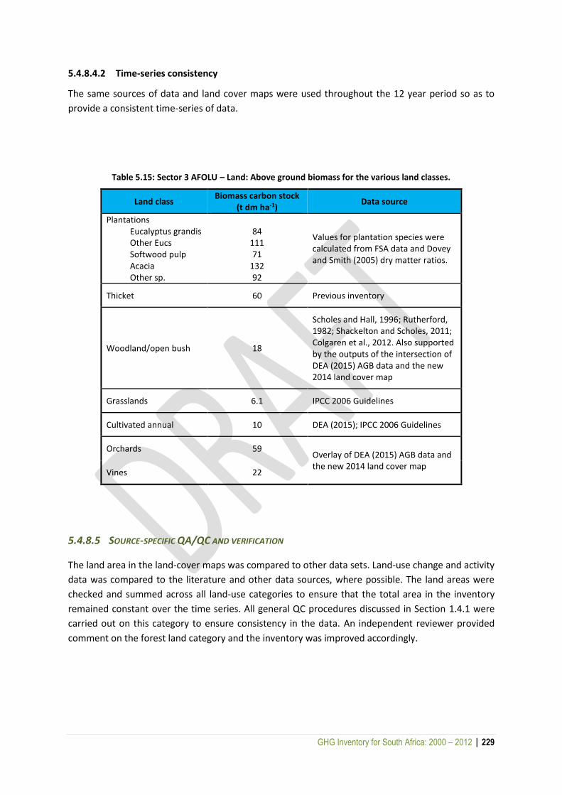
GHG Inventory for South Africa: 2000 – 2012 | 229

5.4.8.4.2 Time-series consistency

The same sources of data and land cover maps were used throughout the 12 year period so as to

provide a consistent time-series of data.

Table 5.15: Sector 3 AFOLU – Land: Above ground biomass for the various land classes.

Land class Biomass carbon stock

(t dm ha-1) Data source

Plantations Eucalyptus grandis Other Eucs Softwood pulp Acacia Other sp.

84

111 71

132 92

Values for plantation species were calculated from FSA data and Dovey and Smith (2005) dry matter ratios.

Thicket 60 Previous inventory

Woodland/open bush 18

Scholes and Hall, 1996; Rutherford, 1982; Shackelton and Scholes, 2011; Colgaren et al., 2012. Also supported by the outputs of the intersection of DEA (2015) AGB data and the new 2014 land cover map

Grasslands 6.1 IPCC 2006 Guidelines

Cultivated annual 10 DEA (2015); IPCC 2006 Guidelines

Orchards 59 Overlay of DEA (2015) AGB data and the new 2014 land cover map

Vines 22

5.4.8.5 SOURCE-SPECIFIC QA/QC AND VERIFICATION

The land area in the land-cover maps was compared to other data sets. Land-use change and activity

data was compared to the literature and other data sources, where possible. The land areas were

checked and summed across all land-use categories to ensure that the total area in the inventory

remained constant over the time series. All general QC procedures discussed in Section 1.4.1 were

carried out on this category to ensure consistency in the data. An independent reviewer provided

comment on the forest land category and the inventory was improved accordingly.

GHG Inventory for South Africa: 2000 – 2012 | 230

5.4.8.6 SOURCE-SPECIFIC RECALCULATIONS

The updated land cover maps meant that recalculations had to be done for all years between 2000

and 2012. Updated activity and soil carbon data were also incorporated.

5.4.8.7 CATEGORY-SPECIFIC PLANNED IMPROVEMENTS AND RECOMMENDATIONS

Under the GHG Improvement Programme initiated by the DEA, a project was recently completed by

the Agricultural Research Council (ARC) which provides more detailed cropland data. Due to the timing

of the project the data could not be incorporated into this inventory but will be considered in the next

one. The next inventory will make use of the ALU software which will enable a more detailed

categorization of croplands, and also allow for the integration of the detailed crop management data

(irrigation, fertilization, rotations). The improved management data will also assist in improving the

soil carbon data. Detailed categorization of crops will also allow more crop specific biomass and

growth data to be included which can aid in reducing uncertainty. It is important for South Africa to

move towards a Tier2 for croplands.

5.4.9 Grassland [3B3]

5.4.9.1 SOURCE CATEGORY DESCRIPTION

The Grassland remaining grassland category includes all grasslands, managed pastures and

rangelands. The IPCC does recommend separating out improved grassland; however, there was

insufficient information at the national scale to enable this division so all grasslands were classified

together. This section deals with emissions and removals of CO2 in the biomass and mineral soil carbon

pools, but there was insufficient data to include the DOM pool. CO2 emissions from biomass burning

were not reported since they are largely balanced by the CO2 that is reincorporated back into the

biomass via photosynthetic activity.

Grasslands remaining grasslands were assumed to be in balance so there were no emissions from this

sub-category. Land converted to grasslands were estimated to be a sink of CO2 (6 735 Gg CO2 per year)

because of land use conversions. The sink remained constant, as a constant annual change was derived

over the mapping period between 2000 and 2013-14. It is assumed that equilibrium is reached after

a year of conversion, therefore, even though the land converted to grassland area increased every

year, the change is only determined for the annual area converted. DOM was not estimated for

grasslands.

GHG Inventory for South Africa: 2000 – 2012 | 231

5.4.9.2 METHODOLOGICAL ISSUES

5.4.9.2.1 Biomass

Grassland remaining grassland

A Tier 1 approach assumes no change in biomass in grassland remaining grassland, as carbon

accumulation through plant growth is roughly balanced by losses through grazing, decomposition and

fire.

Land converted to grassland

Annual change in biomass carbon stocks on land converted to grasslands was estimated using

equation 5.25 above. The average carbon stock change is equal to the carbon stock change due to the

removal of biomass from the initial land use plus carbon stocks for biomass growth. Tier 1 method

assumes that biomass is cleared when preparing a site for grassland use, so the default for biomass

immediately after conversion is zero. The other assumption is that grasslands achieve their steady

state biomass during the first year following conversion so there are no stock changes associated with

Phase 2. The carbon fraction was the default of 0.5 t C /t dm-1.

5.4.9.2.2 Mineral soils

Grasslands remaining grasslands and Land converted to grasslands

Soil carbon sources and sinks were calculated as described in Section 5.4.7.2.2. The land areas for the

various categories were obtained from the land-use change maps (GeoTerraImage, 2015). For Land

converted to grasslands the land area includes all converted land since 1990.

5.4.9.3 DATA SOURCES

5.4.9.3.1 Biomass

The areas of grassland remaining grassland and annual area of land converted to grassland were

obtained from the updated land use maps developed by GeoTerraImage (2015) and are discussed in

detail in section 5.4.4. The BBEFORE AGB values are provided in Table 5.15 and in the relevant biomass

sections.

5.4.9.3.2 Mineral soils

Data are as described in Section 5.4.7.3.3.

GHG Inventory for South Africa: 2000 – 2012 | 232

5.4.9.4 UNCERTAINTY AND TIME-SERIES CONSISTENCY

5.4.9.4.1 Uncertainties

The main uncertainties were associated with the area estimates of the grassland categories (discussed

in Section 5.4.4). Grasslands achieved a user accuracy of 85% but a producers accuracy of 70%, which

resulted from the confusion between grasslands, woodland/open bush and low shrubland (GTI 2013).

A full uncertainty assessment has not been conducted, but is this will be done in the next inventory.

Uncertainty on the biomass carbon stocks for the various land classes is given in Appendix F. Default

biomass carbon stocks for the various land categories have an error of ±75%. IPCC default values for

carbon stocks after one year of growth in crops planted after conversion also have an error of ±75%

(IPCC, 2006, p. 5.28).

For default soil organic C stocks for mineral soils there is a nominal error estimate of ±90% (IPCC 2006

Guidelines, p 2.31). The error on the stock change factors is indicated in Table 5.13.

5.4.9.4.2 Time-series consistency

The same sources of data and land-cover maps were used throughout the 12-year period to provide

a consistent time series of data.

5.4.9.5 SOURCE-SPECIFIC QA/QC AND VERIFICATION

The land area in the land-cover maps was compared to other data sets. Land-use change and activity

data were compared to the literature and other data sources where possible; otherwise no other

source-specific QA/QC procedures were carried out on this subcategory. The land areas were checked

and summed across all land-use categories to ensure that the total area in the inventory remained

constant over the time series. All general QC procedures discussed in Section 1.4.1 were carried out

on this category to ensure consistency in the data. An independent reviewer provided comment on

the forest land category and the inventory was improved accordingly.

5.4.9.6 SOURCE-SPECIFIC RECALCULATIONS

Due to the updated land-cover maps and improved soils data recalculations were done for all years

between 2000 and 2012.

5.4.9.7 CATEGORY-SPECIFIC PLANNED IMPROVEMENTS AND RECOMMENDATIONS

No specific improvements are planned for this category.

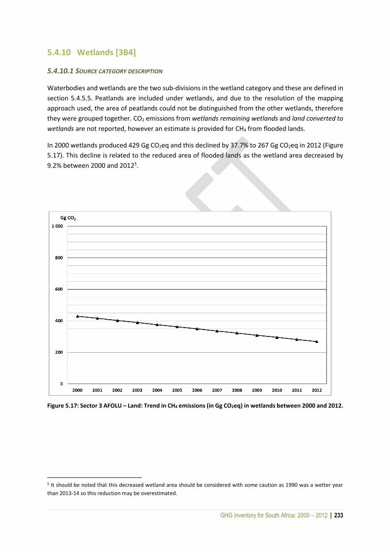
GHG Inventory for South Africa: 2000 – 2012 | 233

5.4.10 Wetlands [3B4]

5.4.10.1 SOURCE CATEGORY DESCRIPTION

Waterbodies and wetlands are the two sub-divisions in the wetland category and these are defined in

section 5.4.5.5. Peatlands are included under wetlands, and due to the resolution of the mapping

approach used, the area of peatlands could not be distinguished from the other wetlands, therefore

they were grouped together. CO2 emissions from wetlands remaining wetlands and land converted to

wetlands are not reported, however an estimate is provided for CH4 from flooded lands.

In 2000 wetlands produced 429 Gg CO2eq and this declined by 37.7% to 267 Gg CO2eq in 2012 (Figure

5.17). This decline is related to the reduced area of flooded lands as the wetland area decreased by

9.2% between 2000 and 20125.

Figure 5.17: Sector 3 AFOLU – Land: Trend in CH4 emissions (in Gg CO2eq) in wetlands between 2000 and 2012.

5 It should be noted that this decreased wetland area should be considered with some caution as 1990 was a wetter year

than 2013-14 so this reduction may be overestimated.

GHG Inventory for South Africa: 2000 – 2012 | 234

5.4.10.2 METHODOLOGICAL ISSUES

CH4 emissions from wetlands were calculated as in the previous inventory following the equation:

CH4 emissionsWWFlood = P * E(CH4)diff * A * 10-6 (Eq. 5.26)

Where:

CH4 emissions WWFlood = total CH4 emissions from flooded land (Gg CH4 yr-1); P = ice-free period (days yr-1); E(CH4)diff = average daily diffusive emissions (kg CH4 ha-1 day-1); A = area of flooded land (ha).

5.4.10.3 DATA SOURCES

The area of waterbodies was taken from the GeoTerraImage (2014) land use maps. For South Africa

the ice-free period is taken as 365 days. The emission factor (E(CH4)diff) was selected to be a median

average for the warm temperate dry climate values provided in Table 3.A2 (IPCC 2006, volume 3). This

emission factor is the lowest of all climates and therefore provides a conservative estimate.

5.4.10.4 UNCERTAINTY AND TIME-SERIES CONSISTENCY

The main uncertainties were associated with the area estimates of the wetland categories (discussed

in Section 5.4.4). The same sources of data and land-cover maps were used throughout the 12-year

period to provide a consistent time series of data.

5.4.10.5 SOURCE-SPECIFIC RECALCULATIONS

The 2000 to 2012 emissions were recalculated using the updated wetland area.

5.4.10.6 SOURCE-SPECIFIC PLANNED IMPROVEMENTS AND RECOMMENDATIONS

No improvements are planned for this category.

GHG Inventory for South Africa: 2000 – 2012 | 235

5.4.11 Settlements [3B5]

5.4.11.1 SOURCE CATEGORY DESCRIPTION

Settlements include all formal built-up areas, in which people reside on a permanent or near-

permanent basis. It includes transportation infrastructure as well as mines. The population of South

Africa in 2010 was just under 50 million (Statistics South Africa, 2010), with the urban population

increasing from 52% to 62% over the past two decades (DEA, 2011). The surface area of settlements

provided by the land cover map developed for this inventory was 3 228 445 ha (2 901 090 ha of

settlements and 327 354 ha under mines) in 2012. This area was higher than the area used in the 2010

inventory. Changes in the extent of urban areas between 1990 and 2013-14 (increase of 6.7%) may

not be as locally significant as expected as the settlements category includes peripheral smallholding

areas around the main built-up areas; and these tend to be the first land-use that is converted to

formal urban areas, before further expansion into natural and cultivated lands.

This category assumes there are no emissions from settlements remaining settlements, but includes

emissions and sinks from biomass and soil carbon pools for land converted to settlements. This

category was found to be a source of CO2 (1 160 Gg CO2) due to land conversions. The soil source is

approximately a third of the carbon, with the rest being from biomass.

5.4.11.2 METHODOLOGICAL ISSUES

5.4.11.2.1 Biomass

Land converted to settlements

Annual change in biomass carbon stocks on land converted to settlements was estimated using

Equation 5.25 above. A Tier 1 method assumes that all biomass is cleared when preparing a site for

settlements, thus the default for biomass immediately after conversion is zero. Above-ground biomass

of the various land categories was taken from Table 5.15 as the biomass value before conversion. It is

also assumed that there is no additional growth or loss of carbon on the land after it becomes a

settlement. The carbon fraction was the default of 0.5 t C/t dm-1.

5.4.11.2.2 Mineral soils

Land converted to settlements

Soil carbon sources and sinks were calculated as described in Section 5.4.7.2.3.

5.4.11.3 DATA SOURCES

5.4.11.3.1 Biomass

The area of Land converted to settlements was obtained from the updated land use maps developed

by GeoTerraImage (2015) and are discussed in detail in section 5.4.4. Biomass carbon stocks before

GHG Inventory for South Africa: 2000 – 2012 | 236

conversion for the various vegetation types are provided in Table 5.15 and the relevant biomass

sections.

5.4.11.3.2 Mineral soils

The land areas for the various categories were obtained from the land-use change maps

(GeoTerraImage, 2015) and described in Section 5.4.4. For land converted to settlements the land area

includes all converted land since 1990. All other data are described in Section 5.4.7.3.3. A stock change

factor of 0.8 was applied to settlements.

5.4.11.4 UNCERTAINTIES AND TIME-SERIES CONSISTENCY

5.4.11.4.1 Uncertainties

The main uncertainties were associated with the area estimates of settlements and this is discussed

in Section 5.4.4.

5.4.11.4.2 Time-series consistency

The same sources of data and land-cover maps were used throughout the 12-year period so as to

provide a consistent time series of data.

5.4.11.5 SOURCE-SPECIFIC QA/QC AND VERIFICATION

The land area in the land-cover maps was compared to other data sets. Land-use change and activity

data were compared to the literature and other data sources, where possible, otherwise no other

source-specific QA/QC procedures were carried out on this subcategory.

5.4.11.6 SOURCE-SPECIFIC RECALCULATIONS

Due to new land areas from the updated land-cover maps, recalculations were done for all years

between 2000 and 2012.

5.4.11.7 CATEGORY-SPECIFIC PLANNED IMPROVEMENTS AND RECOMMENDATIONS

There are no planned improvements for this category, particularly since it is not a key category.

However carbon stock changes could be improved if land conversions and country-specific data on

biomass in settlements could be included.

GHG Inventory for South Africa: 2000 – 2012 | 237

5.4.12 Other land [3B6]

5.4.12.1 SOURCE CATEGORY DESCRIPTION

Other land includes bare soil, rock, and all other land areas that do not fall into the other land classes

(including low shrublands). This category includes emissions and sinks for other land remaining other

land and land converted to other lands. For the former only soil carbon pools are included as it was

assumed there is no change in biomass. However with the low shrublands in this category there are

likely biomass changes through conversion to bare ground or degraded land. The biomass component

will be included in the next inventory. For the land converted to other land category both the biomass

and soil carbon changes are included. This category was found to have an annual sink of 3 081 Gg CO2,

with changes within the land remaining land category being a sink of 5 057 Gg CO2 eq due to large

changes between low shrubland and bare ground. On the other hand the land converted to other land

is a source of carbon (1 975 Gg CO2 eq per year) due to carbon losses in biomass and soil carbon

changes. Soils were the largest contributors to this category although biomass has not been fully

incorporated.

5.4.12.2 METHODOLOGICAL ISSUES

5.4.12.2.1 Biomass

Land converted to other lands

Annual change in biomass carbon stocks on land converted to other lands was estimated using

equation 5.25 above. Carbon stocks before the conversion are provided in Table 5.15 and in the

relevant biomass sections. Following the Tier 1 approach, it was assumed that other lands achieved

their steady-state biomass during the first year following conversion so no stock changes were

associated with phase 2 (i.e. no change due to growth or losses). The carbon fraction was the default

of 0.5 t C/t dm-1.

5.4.12.2.2 Mineral soils

Other land remaining other land

There are conversions between bare ground, degraded land and low shrubland which lead to changes

in soil carbon. Tier 1 assumes that the reference C stock at the end of the default transition period is

zero and this was assumed to be true for bare ground, but for low shrubland and degraded land the

default reference carbon stocks were applied. The other assumption in this category, based on the

Tier 1 assumption, is that the starting soil reference carbon for bare ground is zero, and carbon is

accumulated at a linear rate to the reference carbon stock of the land it is being converted to.

Land converted to other lands

Soil carbon sources and sinks were calculated as described in Section 5.4.7.2.3. Tier 1 also assumes

that the reference C stock at the end of the 23 year transition period, is assumed to be zero. This was

GHG Inventory for South Africa: 2000 – 2012 | 238

assumed to be the case for bare ground but for low shrublands and degraded land the pre-conversion

soil organic C stocks were assumed.

5.4.12.3 DATA SOURCES

5.4.12.3.1 Biomass

The area of Land converted to settlements was obtained from the updated land use maps developed

by GeoTerraImage (2015) and are discussed in detail in section 5.4.4. Biomass carbon stocks before

conversion for the various vegetation types are shown in Table 5.15 and in the relevant biomass

sections.

5.4.12.3.2 Mineral soils

The land areas for the various categories was obtained from the land-use change maps

(GeoTerraImage, 2015) and described in Section 5.4.4. For land converted to other lands the land area

includes all converted land since 1990. All other data are described in Section 5.4.7.3.2.

5.4.12.4 UNCERTAINTIES AND TIME-SERIES CONSISTENCY

5.4.12.4.1 Uncertainties

The main uncertainties were associated with the area estimates of other lands and this is discussed in

Section 5.4.4. Standard deviations on biomass activity data are provided in Appendix F.

5.4.12.4.2 Time-series consistency

The same sources of data and land-cover maps were used throughout the 12-year period to provide

a consistent time series of data.

5.4.12.5 SOURCE-SPECIFIC QA/QC AND VERIFICATION

The land area in the land-cover maps was compared to other data sets. No source-specific QA/QC

procedures were carried out on this sub-category.

5.4.12.6 SOURCE-SPECIFIC RECALCULATIONS

Recalculations were completed for all years between 2000 and 2012 due to updated land areas.

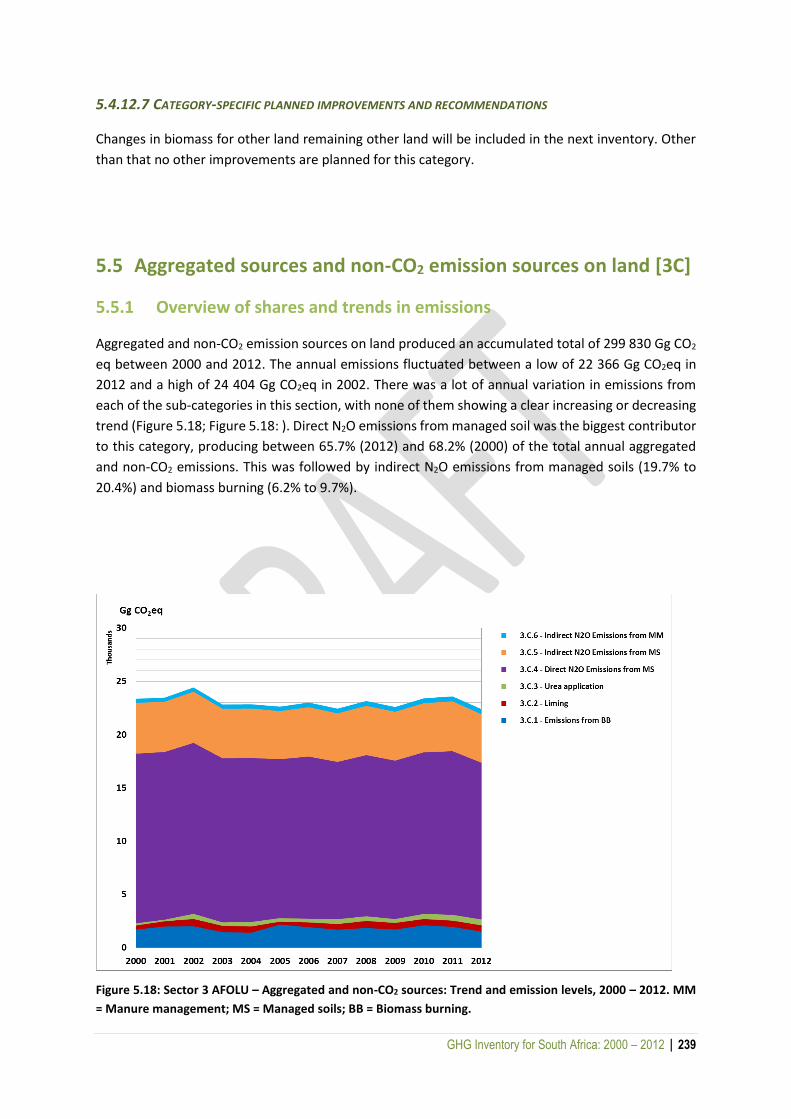
GHG Inventory for South Africa: 2000 – 2012 | 239

5.4.12.7 CATEGORY-SPECIFIC PLANNED IMPROVEMENTS AND RECOMMENDATIONS

Changes in biomass for other land remaining other land will be included in the next inventory. Other

than that no other improvements are planned for this category.

5.5 Aggregated sources and non-CO2 emission sources on land [3C]

5.5.1 Overview of shares and trends in emissions

Aggregated and non-CO2 emission sources on land produced an accumulated total of 299 830 Gg CO2

eq between 2000 and 2012. The annual emissions fluctuated between a low of 22 366 Gg CO2eq in

2012 and a high of 24 404 Gg CO2eq in 2002. There was a lot of annual variation in emissions from

each of the sub-categories in this section, with none of them showing a clear increasing or decreasing

trend (Figure 5.18; Figure 5.18: ). Direct N2O emissions from managed soil was the biggest contributor

to this category, producing between 65.7% (2012) and 68.2% (2000) of the total annual aggregated

and non-CO2 emissions. This was followed by indirect N2O emissions from managed soils (19.7% to

20.4%) and biomass burning (6.2% to 9.7%).

Figure 5.18: Sector 3 AFOLU – Aggregated and non-CO2 sources: Trend and emission levels, 2000 – 2012. MM

= Manure management; MS = Managed soils; BB = Biomass burning.

GHG Inventory for South Africa: 2000 – 2012 | 240

5.5.2 Biomass burning [3C1]

5.5.2.1 SOURCE CATEGORY DESCRIPTION

Biomass burning is an important ecosystem process in Southern Africa, with significant implications

for regional and global atmospheric chemistry and biogeochemical cycles (Korontzi et al., 2003).

According to the National Inventory Report (DEAT, 2009), fire plays an important role in South African

biomes, where grassland, savanna and fynbos fires maintain ecological health. In addition to carbon

dioxide, the burning of biomass results in the release of other GHGs or precursors of GHGs that

originate from incomplete combustion of the fuel. The key GHGs are CO2, CH4, and N2O; however, NOx,

NH3, NMVOC and CO are also produced and these are precursors for the formation of GHG in the

atmosphere (IPCC, 2006).

Although the IPCC Guidelines only require the calculation of emissions from savanna burning, South

Africa reports emissions of non-CO2 gases (CH4, CO, N2O and NOx) from all land categories, as explained

in the 2000 inventory (DEAT, 2009). The burning of biomass is classified into the six land-use categories

defined in the 2006 Guidelines, namely, forest land, cropland, grassland, wetlands, settlements and

other land. The IPCC Guidelines suggest that emissions from savanna burning should be included

under the grassland category; however, since, in this inventory woodlands and open bush have been

classified as forest land, their emissions were dealt with under forest land.

Although the burning of croplands might be limited, burning has been shown to occur on cultivated

land (Archibald et al., 2010), mainly due to the spread of fires from surrounding grassland areas. The

croplands category was sub-divided into annual and perennial crops; there was also a sub-division for

sugarcane as residue burning is still an acceptable practice in South Africa (Hurly et al., 2003).

The CO2 net emissions should be reported when CO2 emissions and removals from the biomass pool

are not equivalent in the inventory year. For grasslands and annual croplands the annual CO2 removals

(through growth) and emissions (whether by decay or fire) are in balance. CO2 emissions are therefore

assumed to be zero for these categories.

Non-CO2 emissions from biomass burning in all land categories were dealt with in this section. For

forest land the CO2 emissions from biomass burning were not included in this section but rather in the

forest land section (see Section 5.4.7).

5.5.2.2 OVERVIEW OF SHARES AND TRENDS IN EMISSIONS

Biomass burning contributed between 1 4218 Gg CO2eq (2004) and 2 188 Gg CO2eq (2005) to the

overall emissions in the AFOLU sector. Of this, about 63% was CH4 and 37% N2O. Grasslands

contributed the most to biomass-burning emissions (52.1% to 63.1%), followed by forest lands (16.2%

to 20.7%) and croplands (10.5% to 22.5%) (Figure 5.19). In the previous inventory (DEA, 2014),

grasslands contributed about 52% and forest lands 28% in 2010, compared with the 52.0% and 17.9%,

respectively, in 2010 in this inventory. This change was likely due to changes in land area that were

brought about by the incorporation of the new land-cover maps.

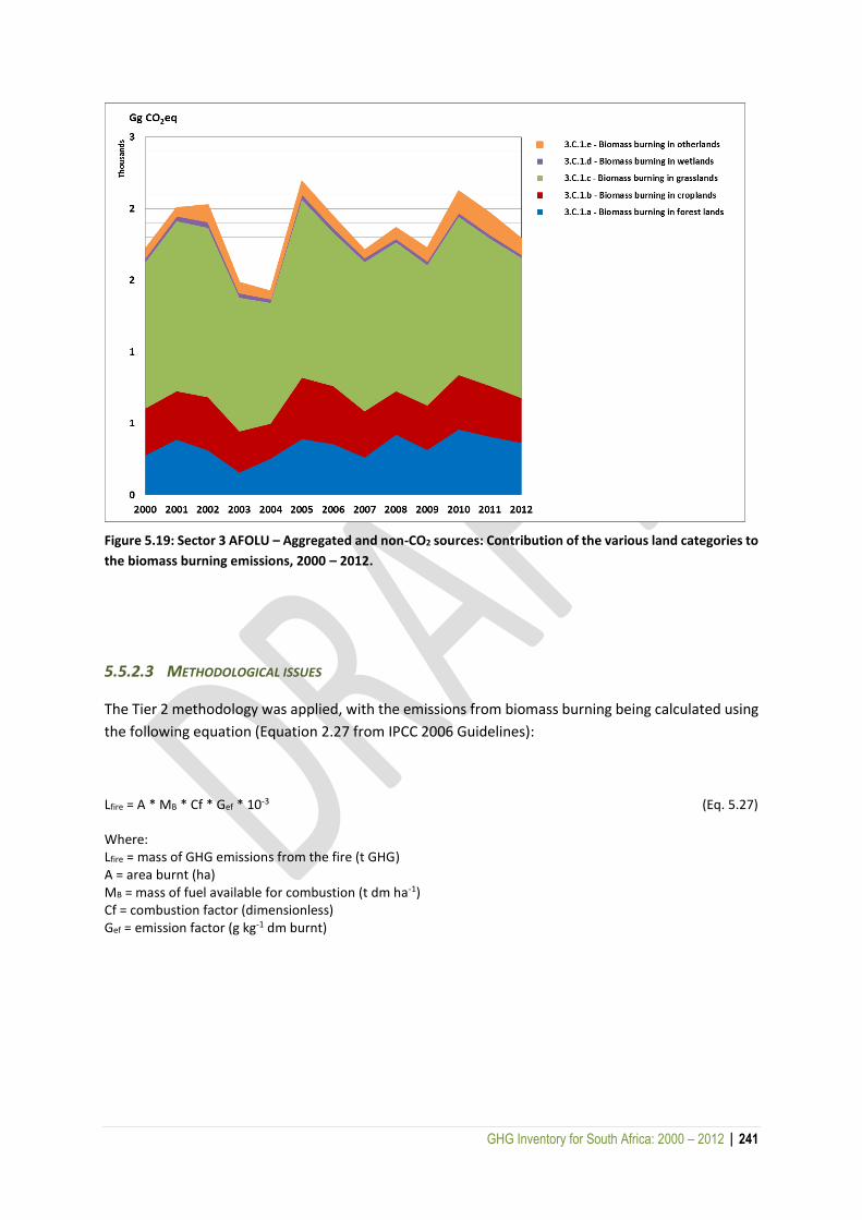
GHG Inventory for South Africa: 2000 – 2012 | 241

Figure 5.19: Sector 3 AFOLU – Aggregated and non-CO2 sources: Contribution of the various land categories to

the biomass burning emissions, 2000 – 2012.

5.5.2.3 METHODOLOGICAL ISSUES

The Tier 2 methodology was applied, with the emissions from biomass burning being calculated using

the following equation (Equation 2.27 from IPCC 2006 Guidelines):

Lfire = A * MB * Cf * Gef * 10-3 (Eq. 5.27)

Where: Lfire = mass of GHG emissions from the fire (t GHG) A = area burnt (ha) MB = mass of fuel available for combustion (t dm ha-1) Cf = combustion factor (dimensionless) Gef = emission factor (g kg-1 dm burnt)

GHG Inventory for South Africa: 2000 – 2012 | 242

5.5.2.4 DATA SOURCES

5.5.2.4.1 Burnt area data

Annual burnt-area maps were produced from the MODIS monthly burnt-area product for each year

of the inventory (2000 to 2012). The MODIS Collection 5 Burned Area Product (MCD45) Geotiff version

from the University of Maryland (ftp://ba1.geog.umd.edu) was used. This is a level 3 gridded 500 m

product and the quality of the information is described in Boschetti et al. (2012). Every month of data

was reprojected into the UTM 35S projection to remain consistent with the 2013-14 land-cover

dataset project. All the monthly maps were then merged into an annual map by adding the valid burnt

areas in each map. This was done for each year between 2000 and 2012. These burnt-area maps were

then overlaid with the 2013-14 land-cover maps to determine the burnt area in each land class. The

percentage of burnt area in each land class is shown in

Table 5.16.

Some burnt area corrections were applied to the data. It was assumed that there was no burning in

indigenous forests and thickets, so any burnt area under these categories was allocated to grasslands.

The FSA reports burnt area for plantations so these figures were used and any difference between the

FSA and MODIS burnt area was added or subtracted from grasslands. Any burning on bare ground was

allocated to low shrublands, and any burning under water bodies was allocated to wetlands.

5.5.2.4.2 Mass of fuel available for combustion

The values for fuel density were sourced from the 2000 inventory (DEAT, 2009), except for croplands

where a value of 7.0 t ha-1 was taken from the 2004 Agricultural Inventory (DAFF, 2010).

5.5.2.4.3 Combustion factor

The combustion factors (Cf) were taken from the 2000 GHG inventory (DEAT, 2009).

5.5.2.4.4 Emission factors

Emission factors were also sourced from the 2000 GHG inventory (DEAT, 2009).

GHG Inventory for South Africa: 2000 – 2012 | 243

Table 5.16: Sector 3 AFOLU – Aggregated and non-CO2 sources: Percentage area burnt within each land class between 2000 and 2012.

2000 2001 2002 2003 2004 2005 2006 Indigenous forest 0.00 0.00 0.00 0.00 0.00 0.00 0.00 Thicket 0.00 0.00 0.00 0.00 0.00 0.00 0.00 Woodland / Open bush 5.88 8.46 6.54 2.51 4.69 7.92 6.87 Plantations 1.08 0.92 0.89 1.55 1.51 1.20 1.54 Annual crops: pivot 3.91 3.05 3.96 3.67 4.62 5.08 3.81 Annual crops: non-pivot 3.88 3.59 4.40 3.28 2.77 4.69 4.78 Orchard 0.60 1.15 0.84 0.86 0.47 1.06 0.74 Viticulture 0.54 0.35 0.28 0.44 0.11 0.31 0.61 Subsistence crops 5.44 8.14 6.41 5.44 4.34 9.40 7.37 Settlements 1.94 2.15 1.90 1.64 1.28 2.90 2.54 Mines 3.30 2.97 4.26 2.90 3.31 4.85 4.71 Wetlands 7.37 8.90 10.07 8.24 7.06 10.45 9.28 Grasslands 10.89 12.70 12.69 9.84 8.49 13.44 11.62 Water bodies 0.00 0.00 0.00 0.00 0.00 0.00 0.00 Low shrublands 0.36 0.30 0.73 0.46 0.28 0.48 0.37 Degraded 7.19 6.51 8.72 2.56 7.70 9.43 13.98

2007 2008 2009 2010 2011 2012

Indigenous forest 0.00 0.00 0.00 0.00 0.00 0.00 Thicket 0.00 0.00 0.00 0.00 0.00 0.00 Woodland / Open bush 3.95 7.14 4.71 8.09 6.94 6.97 Plantations 3.77 3.78 1.06 0.84 0.82 0.51 Annual crops: pivot 3.82 2.70 2.80 4.18 3.19 2.32 Annual crops: non-pivot 2.70 3.13 3.09 3.90 4.31 2.70 Orchard 1.28 1.64 0.70 1.46 0.97 1.34 Viticulture 0.29 0.22 0.33 0.12 0.29 0.01 Subsistence crops 11.41 6.86 8.12 9.88 5.98 4.62 Settlements 2.81 1.73 2.08 2.76 1.52 1.83 Mines 2.31 2.42 1.96 3.09 2.71 2.01 Wetlands 8.17 7.45 8.37 8.41 8.32 5.72 Grasslands 11.34 10.73 10.65 12.12 11.32 9.14 Water bodies 0.00 0.00 0.00 0.00 0.00 0.00 Low shrublands 0.32 0.38 0.51 0.88 0.86 0.44 Degraded 2.13 9.95 6.46 9.91 10.47 3.35

5.5.2.5 UNCERTAINTY AND TIME-SERIES CONSISTENCY

5.5.2.5.1 Uncertainty

The MODIS burnt area products have been shown to identify about 75% of the burnt area in Southern

Africa (Roy and Boschetti, 2009a & b). The MCD45 product produces a finer resolution (500 m) than

the other products (1 km) and uses a more sophisticated change-detection process to identify a burn

scar (Roy et al., 2005). It also provides ancillary data on the quality of the burn-scar detection. The

MCD45 product has been shown to have the lowest omission and commission errors compared to the

L3JRC and GlobCarbon products (Anaya and Chuvieco, 2012). Much of the uncertainty lies with the

land-cover maps (Section 5.4.4) and some corrections for misclassified pixels were made. Since the

values for fuel density, combustion fraction and emission factors were taken from the 2000 GHG

GHG Inventory for South Africa: 2000 – 2012 | 244

inventory, the uncertainties discussed in Section 5.5.1.6 of the 2000 inventory (DEAT, 2009) still apply

to this data set.

5.5.2.5.2 Time-series consistency

The MODIS burnt area product was used for all 12 years to maintain consistency.

5.5.2.6 SOURCE-SPECIFIC QA/QC

The burnt area data derived in this inventory were compared to the data from the previous inventories

(DEAT, 2009; DEA, 2014) using the data from the same years. Direct comparisons are difficult,

however, due to the changes in the land-class definitions.

In terms of the amount of fuel burnt and the combustion factors, South Africa is one of the leaders in

research on biomass burning. The methods used to derive the data were very comprehensive and

locally relevant.

All general QC procedures to check data, transcriptions and spreadsheets, as detailed in Section 1.4.1,

were also conducted.

An independent reviewer was appointed to assess the quality of the inventory, determine the

conformity of the procedures followed for the compilation of this inventory and identify areas of

improvement.

5.5.2.7 SOURCE-SPECIFIC RECALCULATIONS

Recalculations were done for all years between 2000 and 2012 due to the introduction of new land

cover data.

5.5.2.8 SOURCE-SPECIFIC PLANNED IMPROVEMENTS AND RECOMMENDATIONS

There are no specific planned improvements for this category; however, there are plans to develop

higher-resolution land-use maps. These could be overlaid with the appropriate burnt-area data to

improve estimates for those years. Higher-resolution land-use maps will reduce the need for

corrections.

GHG Inventory for South Africa: 2000 – 2012 | 245

5.5.3 Liming and urea application [3C2 and 3C3]

5.5.3.1 SOURCE CATEGORY DESCRIPTION

Liming is used to reduce soil acidity and improve plant growth in managed systems. Adding carbonates

to soils in the form of lime (limestone or dolomite) leads to CO2 emissions as the carbonate limes

dissolve and release bicarbonate.

Adding urea to soils during fertilization leads to a loss of CO2 that was fixed in the industrial production

process. Similar to the soil reaction following the addition of lime, bicarbonate that is formed evolves

into CO2 and water.

5.5.3.2 OVERVIEW OF SHARES AND TRENDS IN EMISSIONS

The CO2 from liming showed a high annual variability, with the highest emissions being in 2002 (684

Gg CO2) and the lowest in 2005 (267 Gg CO2) (Figure 5.20:). The variation was directly linked to

limestone and dolomite consumption (Figure 5.20). The CO2 emissions from urea application showed

a similar annual variability (Figure 5.21). Urea application produced an accumulated amount of 5 156

Gg CO2 between 2000 and 2012, with the lowest emissions (147 Gg CO2) occurring in 2001 and the

highest (555 Gg CO2) in 2012. There was a sharp decline in emissions from both liming and urea

application in 2005.

5.5.3.3 METHODOLOGICAL ISSUES

A Tier 1 approach of the IPCC 2006 Guidelines was used to calculate annual C emissions from lime

application (Equation 11.12, IPCC 2006) and CO2 emissions from urea fertilization (Equation 11.13,

IPCC 2006).

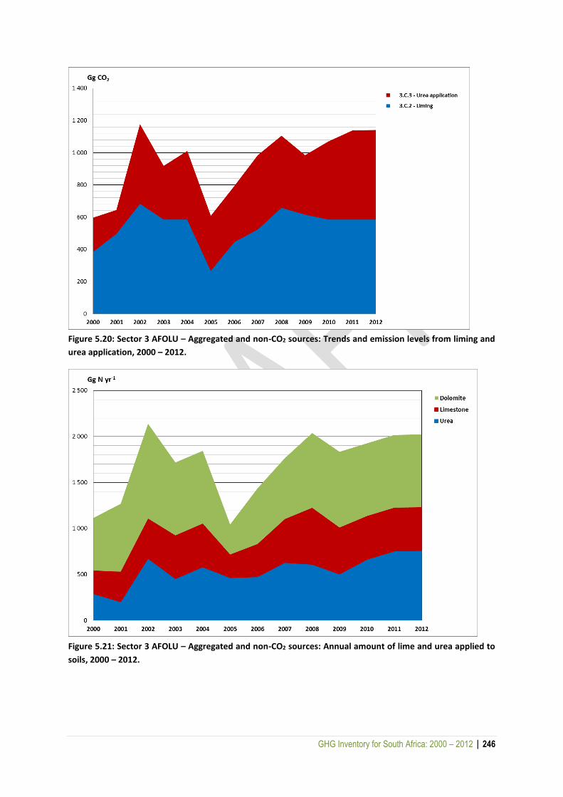
GHG Inventory for South Africa: 2000 – 2012 | 246

Figure 5.20: Sector 3 AFOLU – Aggregated and non-CO2 sources: Trends and emission levels from liming and

urea application, 2000 – 2012.

Figure 5.21: Sector 3 AFOLU – Aggregated and non-CO2 sources: Annual amount of lime and urea applied to

soils, 2000 – 2012.

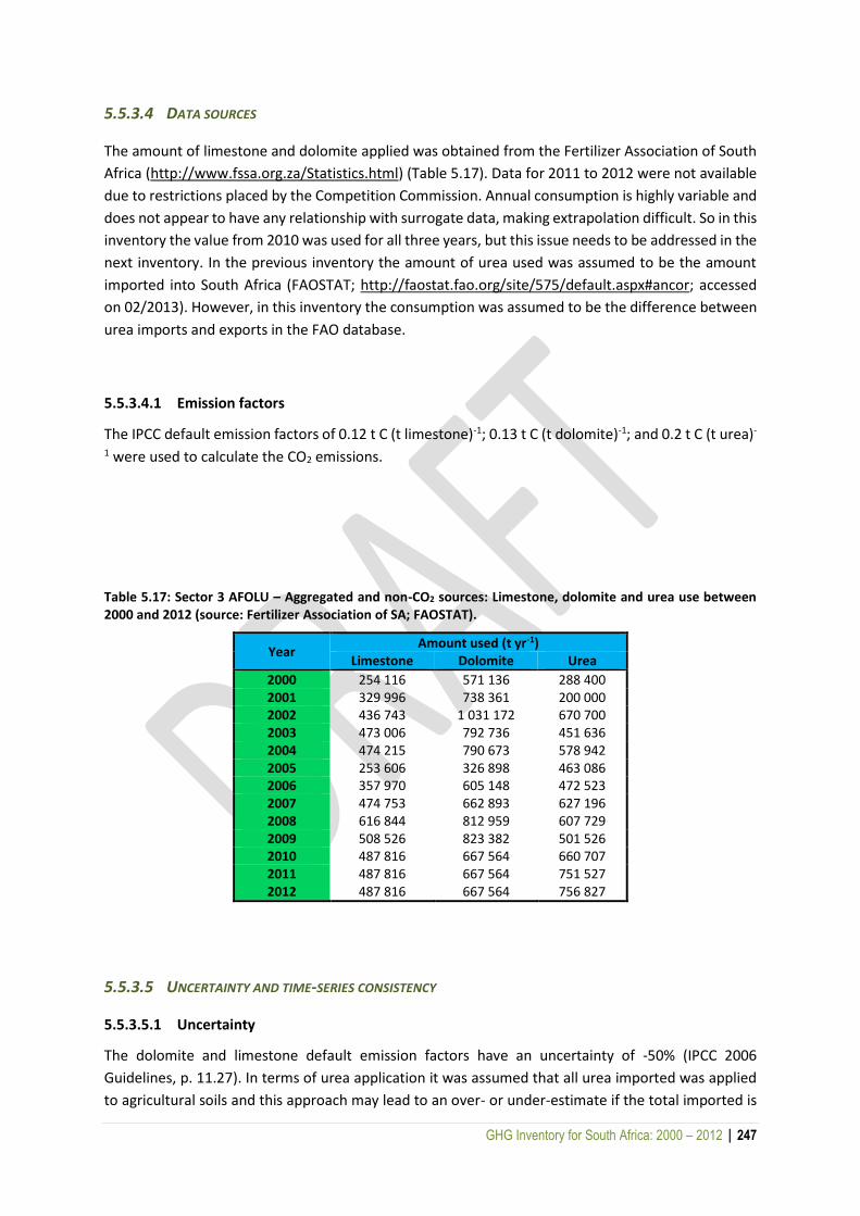
GHG Inventory for South Africa: 2000 – 2012 | 247

5.5.3.4 DATA SOURCES

The amount of limestone and dolomite applied was obtained from the Fertilizer Association of South

Africa (http://www.fssa.org.za/Statistics.html) (Table 5.17). Data for 2011 to 2012 were not available

due to restrictions placed by the Competition Commission. Annual consumption is highly variable and

does not appear to have any relationship with surrogate data, making extrapolation difficult. So in this

inventory the value from 2010 was used for all three years, but this issue needs to be addressed in the

next inventory. In the previous inventory the amount of urea used was assumed to be the amount

imported into South Africa (FAOSTAT; http://faostat.fao.org/site/575/default.aspx#ancor; accessed

on 02/2013). However, in this inventory the consumption was assumed to be the difference between

urea imports and exports in the FAO database.

5.5.3.4.1 Emission factors

The IPCC default emission factors of 0.12 t C (t limestone)-1; 0.13 t C (t dolomite)-1; and 0.2 t C (t urea)-

1 were used to calculate the CO2 emissions.

Table 5.17: Sector 3 AFOLU – Aggregated and non-CO2 sources: Limestone, dolomite and urea use between 2000 and 2012 (source: Fertilizer Association of SA; FAOSTAT).

Year Amount used (t yr-1)

Limestone Dolomite Urea

2000 254 116 571 136 288 400 2001 329 996 738 361 200 000 2002 436 743 1 031 172 670 700 2003 473 006 792 736 451 636 2004 474 215 790 673 578 942 2005 253 606 326 898 463 086 2006 357 970 605 148 472 523 2007 474 753 662 893 627 196 2008 616 844 812 959 607 729 2009 508 526 823 382 501 526 2010 487 816 667 564 660 707 2011 487 816 667 564 751 527 2012 487 816 667 564 756 827

5.5.3.5 UNCERTAINTY AND TIME-SERIES CONSISTENCY

5.5.3.5.1 Uncertainty

The dolomite and limestone default emission factors have an uncertainty of -50% (IPCC 2006

Guidelines, p. 11.27). In terms of urea application it was assumed that all urea imported was applied

to agricultural soils and this approach may lead to an over- or under-estimate if the total imported is

GHG Inventory for South Africa: 2000 – 2012 | 248

not applied in that particular year. However, over the long-term this bias should be negligible (IPCC,

2006). As for the liming emission factors, the urea emission factor also has an uncertainty of -50%

(IPCC 2006 Guidelines, p. 11.32).

5.5.3.5.2 Time-series consistency

For liming the same source of activity data was used for 2000 to 2009, and for 2010 numbers were

estimated based on this data so as to try and maintain the time-series consistency. The same activity

data source for urea was applied to all 12 years.

5.5.3.6 SOURCE-SPECIFIC QA/QC AND VERIFICATION

Quality control of the activity data was limited for this section as very little comparative data was

available. Data, calculations and spreadsheets were all checked to ensure data was carried through

properly and that there were no transcription errors. An external reviewer provided the quality

assurance.

5.5.3.7 SOURCE-SPECIFIC RECALCULATIONS

Emission data for urea were recalculated for all years between 2000 and 2012 due to the adjustment

made to the urea consumption data.

5.5.3.8 SOURCE-SPECIFIC PLANNED IMPROVEMENTS AND RECOMMENDATIONS

At this stage there are no improvements planned for CO2 emissions from liming and urea application.

However, more accurate urea application data would improve the emission estimates.

5.5.4 Direct N2O emissions from managed soils [3C4]

5.5.4.1 SOURCE CATEGORY DESCRIPTION

Agricultural soils contribute to GHGs in three ways (Desjardins et al., 1993):

CO2 through the loss of soil organic matter. This is a result of land-use change, and is, therefore,

dealt with in the land sector, not in this section;

CH4 from anaerobic soils. Anaerobic cultivation, such as rice paddies, is not practised in South

Africa, and therefore CH4 emissions from agricultural soils are not included in this inventory; and

N2O from fertilizer use and intensive cultivation. This is a significant fraction of non-carbon

emissions from agriculture and is the focus of this section of the inventory.

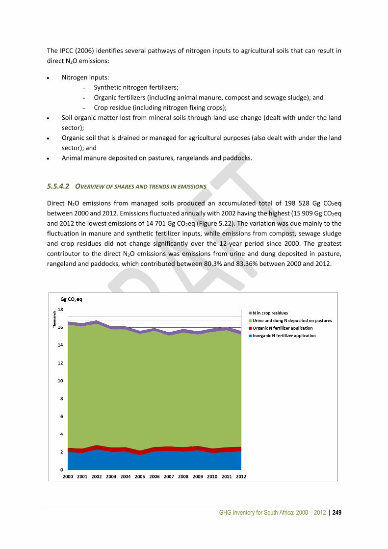
GHG Inventory for South Africa: 2000 – 2012 | 249

The IPCC (2006) identifies several pathways of nitrogen inputs to agricultural soils that can result in

direct N2O emissions:

Nitrogen inputs:

- Synthetic nitrogen fertilizers;

- Organic fertilizers (including animal manure, compost and sewage sludge); and

- Crop residue (including nitrogen fixing crops);

Soil organic matter lost from mineral soils through land-use change (dealt with under the land

sector);

Organic soil that is drained or managed for agricultural purposes (also dealt with under the land

sector); and

Animal manure deposited on pastures, rangelands and paddocks.

5.5.4.2 OVERVIEW OF SHARES AND TRENDS IN EMISSIONS

Direct N2O emissions from managed soils produced an accumulated total of 198 528 Gg CO2eq

between 2000 and 2012. Emissions fluctuated annually with 2002 having the highest (15 909 Gg CO2eq

and 2012 the lowest emissions of 14 701 Gg CO2eq (Figure 5.22). The variation was due mainly to the

fluctuation in manure and synthetic fertilizer inputs, while emissions from compost, sewage sludge

and crop residues did not change significantly over the 12-year period since 2000. The greatest

contributor to the direct N2O emissions was emissions from urine and dung deposited in pasture,

rangeland and paddocks, which contributed between 80.3% and 83.36% between 2000 and 2012.

GHG Inventory for South Africa: 2000 – 2012 | 250

Figure 5.22: Sector 3 AFOLU – Aggregated and non-CO2 sources: Trend and emission levels of direct N2O from

managed soils, 2000 – 2012

5.5.4.3 METHODOLOGICAL ISSUES

The N2O emissions from managed soils were calculated by using the Tier 1 method from the IPCC 2006

Guidelines (Equation 11.1). As in the 2004 agricultural inventory (DAFF, 2010), the contribution of N

inputs from FSOM (N mineralization associated with loss of SOM resulting from change of land use or

management) and FOS (N from managed organic soils) was assumed to be minimal and was therefore

excluded from the calculations. Furthermore, since there are no flooded rice fields in South Africa

these emissions were also excluded. The simplified equation for direct N2O emissions from soils is

therefore as follows:

N2ODirect-N = N2O-NN inputs + N2O-NPRP (Eq. 5.28)

Where:

N2O-NN inputs = [(FSN +FON + FCR) * EF1] (Eq. 5.29)

N2O-NPRP = [(FPRP,CPP * EF3PRP,CPP) + (FPRP,SO * EF3PRP,SO)] (Eq. 5.30)

Where: N2ODirect-N = annual direct N2O-N emissions produced from managed soils (kg N2O-N yr-1); N2O-NN inputs = annual direct N2O-N emissions from N inputs to managed soils (kg N2O-N yr-1); N2O-NPRP = annual direct N2O-N emissions from urine and dung inputs to grazed soils (kg N2O-N yr-1); FSN = annual amount of synthetic fertilizer N applied to soils (kg N yr-1); FON = annual amount of animal manure, compost, sewage sludge and other organic N additions applied to soils

(kg N yr-1); FCR = annual amount of N in crop residues, including N-fixing crops, and from forage/pasture renewal, returned

to soils (kg N yr-1); FPRP = annual amount of urine and dung N deposited by grazing animals on pasture, range and paddock (kg N yr-

1), CPP = Cattle, Poultry and Pigs, SO = Sheep and Other; EF1 = emission factor for N2O emissions from N inputs (kg N2O-N (kg N input)-1); EF3PRP = emission factor for N2O emissions from urine and dung N deposited on pasture, range and paddock by

grazing animals (kg N2O-N (kg N input)-1), CPP = Cattle, Poultry and Pigs, SO = Sheep and Other.

Most of the country specific data was obtained from national statistics from the Department of

Agriculture (Abstracts of Agricultural Statistics, 2012), and supporting data was obtained through

scientific articles, guidelines, reports or personal communications with experts as discussed below.

5.5.4.3.1 Nitrogen inputs

Synthetic fertilizer use (FSN) was recorded by the Fertilizer Association of South Africa, but organic

nitrogen (FON) and crop residue (FCR) inputs needed to be calculated. FON is composed of N inputs from

managed manure (FAM), compost and sewage sludge. FAM includes inputs from manure which is

GHG Inventory for South Africa: 2000 – 2012 | 251

managed in the various manure management systems (i.e. lagoons, liquid/slurries, or as drylot, daily

spread, or compost). The amount of animal manure N, after all losses, applied to managed soils or for

feed, fuel or construction was calculated using Equations 10.34 and 11.4 in the IPCC 2006 guidelines.

The amount of compost used on managed soils each year was calculated in the same way as in the

2004 inventory (DAFF, 2010). The synthetic fertilizer input changed each year, while the rest of the

factors were assumed to remain unchanged over the 12 year period.

Application of sewage sludge to agricultural land is common practice in South Africa; however, no

national data of total production of sewage sludge for South Africa exists, therefore estimates were

made from wastewater treatment plant data (DAFF, 2010). To estimate total sewage sludge

production, a list of wastewater treatment plants (WWTP) was obtained from the Department of

Water Affairs (DWA, 2009) and an average capacity for each province was used to calculate the volume

of wastewater treated in South Africa each year. Supporting references show that 0.03% of

wastewater typically could be precipitated as sewage sludge (0.1% of wastewater is solids, of which

30% is suspended) (Environment Canada, 2009; Van der Waal, 2008). Snyman et al. (2004) reported

several end uses for sewage sludge and from this it was estimated that about 30% is for agricultural

use. Due to limited data, for the years 2000 to 2004 the amount of sewage sludge used for agriculture

was kept constant.

The 2004 report (DAFF, 2010), however, indicated that this amount was probably an overestimate, as

the use of sewage sludge for agricultural purposes had reduced significantly due to contamination.

There are no figures on how much this has been reduced by, so an estimated 15% reduction each year

between 2004 and 2012 was assumed.

Actual data for crop residue left on land was not available so the amount was calculated as described

in DAFF (2010). The principal biological nitrogen fixing (BNF) crops in South Africa are soyabeans,

groundnuts and lucerne. The addition of N through BNF crops were included in the default values for

crop-residue calculations.

5.5.4.3.2 Nitrogen inputs from urine and dung

Manure deposited in pastures, rangelands and paddocks include all the open areas where animal

excretions are not removed or managed. This fraction remains on the land, where it is returned to

the soil, and also contributes to GHG emissions. In South Africa the majority of animals spend most

or part of their lives on pastures and rangelands. The annual amount of urine and dung N deposited

on pastures, ranges or paddocks and by grazing animals (FPRP) was calculated as in the 2004 inventory

using Equation 11.5 in the IPCC 2006 Guidelines (Chapter 11, Volume 4).

5.5.4.4 DATA SOURCES

5.5.4.4.1 Synthetic fertilizer inputs (FSN)

National consumption data for N fertilizer was obtained from the Fertilizer Society of South Africa

(http://www.fssa.org.za).

GHG Inventory for South Africa: 2000 – 2012 | 252

5.5.4.4.2 Organic nitrogen inputs (FON)

Managed manure inputs (FAM)

The calculation of FAM required the following activity data:

Population data (Section 5.3.3.4.1);

Nex data (Section 5.3.4.3.2);

Manure management system usage data (Section 5.3.4.4.1);

Amount of managed manure nitrogen that is lost in each manure management system

(FracLossMS). IPCC 2006 default values were used here (Table 10.23, Chapter 10, Volume 4 , IPCC

2006);

Amount of nitrogen from bedding. There were no data available for this so the value was

assumed to be zero; and

The fraction of managed manure used for feed, fuel, or construction. Again there were

insufficient data and thus FAM was not adjusted for these fractions (IPCC 2006 Guidelines, p.

11.13).

Compost

To estimate N inputs from compost FSN data were used. It was estimated that a total of 5% of all

farmers use compost. Compost is seldom, if ever, used as the only nutrient source for crops or

vegetables. It is used as a supplement for synthetic fertilizers, and it is estimated that farmers would

supply about a third (33%) of nutrient needs through compost. All of this was taken into account when

estimating N inputs from compost (details provided in DAFF (2010) and Otter (2011)).

Sewage sludge

Waste water treatment data was obtained from the DWA (2009) and the end users of sewage sludge

were determined from Snyman et al. (2004). Calculations follow those described in DAFF (2010) and

outputs are given in Otter (2011).

5.5.4.4.3 Nitrogen inputs from crop residue (FCR)

Actual data for crop residue left on land was not available so the amount was calculated as described

in DAFF (2010) using the following activity data:

Crop production data from the Abstract of Agricultural Statistics (2012). For some of the crops

the data was for a split year (i.e. July 2005/June 2006), while for others it was for a year

(January to December). In order to standardize the data it was assumed that the production

was evenly split between the two years and thus production per full year (January to

GHG Inventory for South Africa: 2000 – 2012 | 253

December) was calculated. For dry peas production declined until there were no reported

data between 2007 and 2012, so dry pea production was assumed to be zero for those years.

The same applied to lentil production between 2006 and 2012. Rye production data were not

recorded between 2003 and 2009, but the data for these years were calculated by fitting a

linear regression to the data collected since 1970.

IPCC 2006 default values for above- and below-ground residues. In the absence of IPCC default

values, external references were used to calculate the biomass by using the harvest index of

crops;

Above-ground biomass removal from grazing and burning. As in the previous inventory it was

assumed that all below-ground plant material remains in the soil, and that most (80%) above-

ground plant material is removed by grazing. Removal of above-ground biomass includes

grazing (for all field crops) and burning (assumed only to occur with sugarcane).

5.5.4.4.4 Nitrogen inputs from Manure deposited by livestock on pastures, rangelands and

paddocks (FPRP)

The activity data required for this calculation were population data (Section 5.3.3.4.1), Nex data

(Section 5.3.4.3.2) and the fraction of total annual N excretion for each livestock species that is

deposited on pastures, rangelands and paddocks (PRP).

5.5.4.4.5 Emission factors

The IPCC 2006 default emission factors (Chapter 11, Volume 4, Table 11.1) were used to estimate

direct N2O emissions from managed soils. EF1 was used to estimate direct N2O-N emissions from FSN,

FON and FCR N inputs; while EF3PRP was used to estimate direct N2O-N emissions from urine and dung N

inputs to soil from cattle, poultry and pigs (CPP), and sheep and other animals (SO).

For game the default factor for other animals (i.e. the SO EF) was used.

The IPCC 2006 default EFs for PRP were thought to be overestimated for South Africa, as grazing areas

in South Africa are mostly in the drier parts of the country where water content is low. Even though

the N is available as a potential source of N2O, this is not the most likely pathway. The 2004 inventory

(DAFF, 2010) suggests that emissions from PRP are probably more towards the lower range of the

default values provided by the IPCC (2006).

5.5.4.5 UNCERTAINTY AND TIME-SERIES CONSISTENCY

5.5.4.5.1 Uncertainty

The uncertainty ranges for EF1, EF3PRP,CPP and EF3PRP,SO are 0.003 to 0.03, 0.007 to 0.06, and 0.003 to

0.03, respectively (IPCC 2006 Guidelines, Table 11.1).

The uncertainty on the amount of compost applied was high due to the high variability across the

region. No quantitative data was available, so estimates were based on expert opinion. Most

GHG Inventory for South Africa: 2000 – 2012 | 254

estimates indicated a use of 20% animal manure in producing compost, while some indicated as much

as 80%. Most vegetable production is estimated to use compost for about 33% of the nutrient

requirements. The data could be improved if more information on organic matter use in agriculture

were available.

Sewage sludge use in agriculture is also uncertain due to a lack of actual data. In this inventory, data

from 72 WWTPs were used as representative of all 1 697 WWTPs in South Africa. A calculated value

based on estimated capacity ranges for wastewater treatment was used to determine the total

quantity of sewage sludge produced. Ranges of WWTP capacity varied between 1 776 ML and 8 580

ML per day, with an average of 5 177 ML per plant. The end use of sewage sludge could also be

improved. It was estimated that 30% of total sewage sludge is used in the agricultural sector, but this

number could vary between 10 and 80%. The N content for sludge, from the 72 WWTPs data, varied

between 1.5% and 6.5%. The average of 3.8% was used in the calculations.

The main source of data for crop residue was the Abstract of Agricultural Statistics (2012), and one of

the main limitations was that it only included commercial crops, not subsistence agriculture. For the

rest of the calculation, the default values were mostly used, or estimates of the fraction of crop

removal. These estimates were often area-specific but applied on a broad scale. In future, each

province or area could be documented separately to give more accurate data input.

5.5.4.5.2 Time-series consistency

The same data sources and emission factors were used for the 12 year period to maintain the time-

series consistency over the inventory period.

5.5.4.6 SOURCE-SPECIFIC QA/QC AND VERIFICATION

It was difficult to verify a lot of the data in this section due to there being very limited data available

to cross-check the numbers against. An independent reviewer was appointed to assess the quality of

the inventory, determine the conformity of the procedures followed for the compilation of this

inventory and identify areas of improvement.

5.5.4.7 SOURCE-SPECIFIC RECALCULATIONS

The livestock population data were adjusted for other cattle and poultry, therefore recalculations

were done for 2000 to 2012 due to the associated change in manure production. An estimate for game

manure emissions was included (which was not in previous inventories) and this amount was included

in the emissions for each year since 2000.

GHG Inventory for South Africa: 2000 – 2012 | 255

5.5.4.8 SOURCE-SPECIFIC PLANNED IMPROVEMENTS AND RECOMMENDATIONS

No source-specific improvements are planned, but suggestions are given as to how estimates could

be improved in future. The major component of N2O emissions from managed soils was from the

inputs of animal manure and manure deposited on pastures, rangelands and paddocks. It is,

therefore, very important for South Africa to determine country-specific EFs for these emissions,

instead of using the IPCC default values. Furthermore, as with the CH4 emissions from manure

management, the manure-management system usage data needs to be better quantified in order to

improve the accuracy of the emission estimates in this category.

5.5.5 Indirect N2O emissions from managed soils [3C4]

5.5.5.1 SOURCE CATEGORY DESCRIPTION

Indirect emissions of N2O-N can take place in two ways: i) volatilization of N as NH3 and oxides of N,

and the deposition of these gases onto water surfaces, and ii) through runoff and leaching from land

where N was applied (IPCC, 2006). Due to limited data a Tier 1 approach was used to calculate the

indirect N2O emissions.

5.5.5.2 OVERVIEW OF SHARES AND TRENDS IN EMISSIONS

The total accumulated amount of indirect N2O lost over the period 2000 to 2012 was estimated at 60

358 Gg CO2eq and 4 558 Gg CO2eq was produced in 2012. There was a decreasing trend over this

period with losses due to atmospheric deposition of N volatilised from managed soils decreasing by

7.5% and losses due to leaching and run-off declining by 6.0% between 2000 and 2012 (Figure 5.23).

Indirect N2O losses due to leaching and run-off accounted for 56.5% of the indirect emissions in 2012.

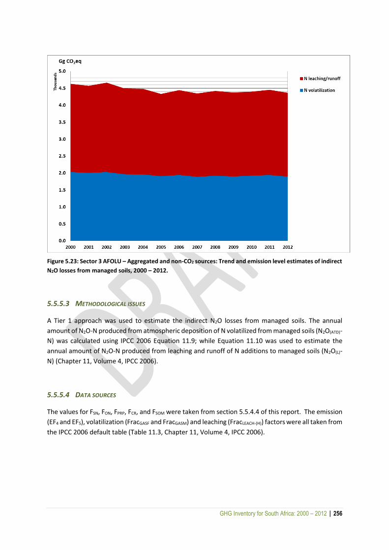
GHG Inventory for South Africa: 2000 – 2012 | 256

Figure 5.23: Sector 3 AFOLU – Aggregated and non-CO2 sources: Trend and emission level estimates of indirect

N2O losses from managed soils, 2000 – 2012.

5.5.5.3 METHODOLOGICAL ISSUES

A Tier 1 approach was used to estimate the indirect N2O losses from managed soils. The annual

amount of N2O-N produced from atmospheric deposition of N volatilized from managed soils (N2O(ATD)-

N) was calculated using IPCC 2006 Equation 11.9; while Equation 11.10 was used to estimate the

annual amount of N2O-N produced from leaching and runoff of N additions to managed soils (N2O(L)-

N) (Chapter 11, Volume 4, IPCC 2006).

5.5.5.4 DATA SOURCES

The values for FSN, FON, FPRP, FCR, and FSOM were taken from section 5.5.4.4 of this report. The emission

(EF4 and EF5), volatilization (FracGASF and FracGASM) and leaching (FracLEACH-(H)) factors were all taken from

the IPCC 2006 default table (Table 11.3, Chapter 11, Volume 4, IPCC 2006).

GHG Inventory for South Africa: 2000 – 2012 | 257

5.5.5.5 UNCERTAINTY AND TIME-SERIES CONSISTENCY

5.5.5.5.1 Uncertainty

There is uncertainty in the activity data; nevertheless emission factor uncertainty is likely to dominate.

The uncertainty ranges on EF4 and EF5 are 0.002 to 0.05, and 0.0005 to 0.025, respectively. For FracGASF,

FracGASM and FracLEACH-(H), the uncertainty ranges are 0.03 to 0.3, 0.05 to 0.5 and 0.1 to 0.8, respectively

(IPCC 2006 Guidelines, Table 11.3, p. 11.24).

5.5.5.5.2 Time-series consistency

The same data sources were used throughout the 12 year period to reduce uncertainties due to

inconsistent data sources.

5.5.5.6 SOURCE-SPECIFIC QA/QC AND VERIFICATION

No source-specific QA/QC and verification procedures were carried out in this section.

5.5.5.7 SOURCE-SPECIFIC RECALCULATIONS

No source specific recalculations were necessary.

5.5.5.8 SOURCE-SPECIFIC PLANNED IMPROVEMENTS AND RECOMMENDATIONS

No specific improvements have been planned for this source.

5.5.6 Indirect N2O emissions from manure management [3C6]

5.5.6.1 SOURCE CATEGORY DESCRIPTION

Indirect N2O losses from manure management due to volatilization were calculated using the Tier 1

method. Throughout the world, data on leaching and run-off losses from various management

systems is extremely limited, therefore, there are no IPCC 2006 default values and no Tier 1 method.

The equation given in the IPCC 2006 Guidelines can only be used where there is country-specific

information on the fraction of nitrogen loss due to leaching and run-off from manure management

systems available, i.e. there is only a Tier 2 method. There was insufficient data for South Africa to do

the Tier 2 calculation, so there is no estimate for manure management N losses due to leaching and

run-off.

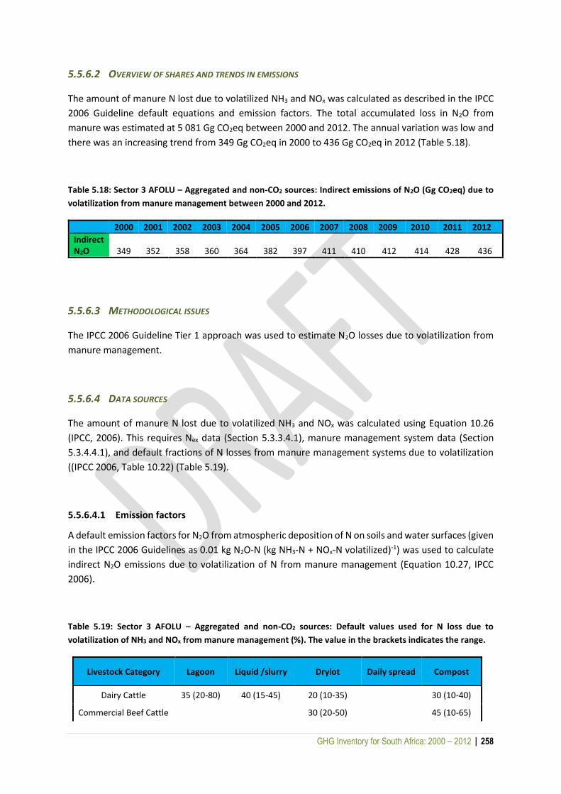
GHG Inventory for South Africa: 2000 – 2012 | 258

5.5.6.2 OVERVIEW OF SHARES AND TRENDS IN EMISSIONS

The amount of manure N lost due to volatilized NH3 and NOx was calculated as described in the IPCC

2006 Guideline default equations and emission factors. The total accumulated loss in N2O from

manure was estimated at 5 081 Gg CO2eq between 2000 and 2012. The annual variation was low and

there was an increasing trend from 349 Gg CO2eq in 2000 to 436 Gg CO2eq in 2012 (Table 5.18).

Table 5.18: Sector 3 AFOLU – Aggregated and non-CO2 sources: Indirect emissions of N2O (Gg CO2eq) due to

volatilization from manure management between 2000 and 2012.

2000 2001 2002 2003 2004 2005 2006 2007 2008 2009 2010 2011 2012

Indirect N2O 349 352 358 360 364 382 397 411 410 412 414 428 436

5.5.6.3 METHODOLOGICAL ISSUES

The IPCC 2006 Guideline Tier 1 approach was used to estimate N2O losses due to volatilization from

manure management.

5.5.6.4 DATA SOURCES

The amount of manure N lost due to volatilized NH3 and NOx was calculated using Equation 10.26

(IPCC, 2006). This requires Nex data (Section 5.3.3.4.1), manure management system data (Section

5.3.4.4.1), and default fractions of N losses from manure management systems due to volatilization

((IPCC 2006, Table 10.22) (Table 5.19).

5.5.6.4.1 Emission factors

A default emission factors for N2O from atmospheric deposition of N on soils and water surfaces (given

in the IPCC 2006 Guidelines as 0.01 kg N2O-N (kg NH3-N + NOx-N volatilized)-1) was used to calculate

indirect N2O emissions due to volatilization of N from manure management (Equation 10.27, IPCC

2006).

Table 5.19: Sector 3 AFOLU – Aggregated and non-CO2 sources: Default values used for N loss due to

volatilization of NH3 and NOx from manure management (%). The value in the brackets indicates the range.

Livestock Category Lagoon Liquid /slurry Drylot Daily spread Compost

Dairy Cattle 35 (20-80) 40 (15-45) 20 (10-35) 30 (10-40)

Commercial Beef Cattle 30 (20-50) 45 (10-65)

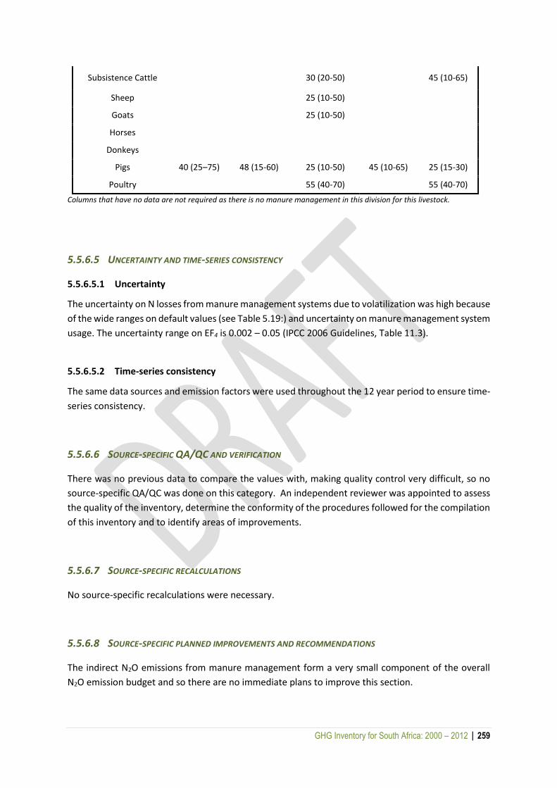
GHG Inventory for South Africa: 2000 – 2012 | 259

Subsistence Cattle 30 (20-50) 45 (10-65)

Sheep 25 (10-50)

Goats 25 (10-50)

Horses

Donkeys

Pigs 40 (25–75) 48 (15-60) 25 (10-50) 45 (10-65) 25 (15-30)

Poultry 55 (40-70) 55 (40-70)

Columns that have no data are not required as there is no manure management in this division for this livestock.

5.5.6.5 UNCERTAINTY AND TIME-SERIES CONSISTENCY

5.5.6.5.1 Uncertainty

The uncertainty on N losses from manure management systems due to volatilization was high because

of the wide ranges on default values (see Table 5.19:) and uncertainty on manure management system

usage. The uncertainty range on EF4 is 0.002 – 0.05 (IPCC 2006 Guidelines, Table 11.3).

5.5.6.5.2 Time-series consistency

The same data sources and emission factors were used throughout the 12 year period to ensure time-

series consistency.

5.5.6.6 SOURCE-SPECIFIC QA/QC AND VERIFICATION

There was no previous data to compare the values with, making quality control very difficult, so no

source-specific QA/QC was done on this category. An independent reviewer was appointed to assess

the quality of the inventory, determine the conformity of the procedures followed for the compilation

of this inventory and to identify areas of improvements.

5.5.6.7 SOURCE-SPECIFIC RECALCULATIONS

No source-specific recalculations were necessary.

5.5.6.8 SOURCE-SPECIFIC PLANNED IMPROVEMENTS AND RECOMMENDATIONS

The indirect N2O emissions from manure management form a very small component of the overall

N2O emission budget and so there are no immediate plans to improve this section.

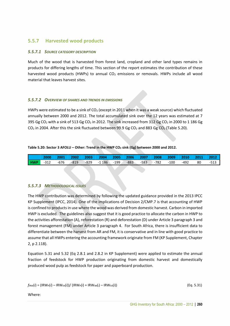
GHG Inventory for South Africa: 2000 – 2012 | 260

5.5.7 Harvested wood products

5.5.7.1 SOURCE CATEGORY DESCRIPTION

Much of the wood that is harvested from forest land, cropland and other land types remains in

products for differing lengths of time. This section of the report estimates the contribution of these

harvested wood products (HWPs) to annual CO2 emissions or removals. HWPs include all wood

material that leaves harvest sites.

5.5.7.2 OVERVIEW OF SHARES AND TRENDS IN EMISSIONS

HWPs were estimated to be a sink of CO2 (except in 2011 when it was a weak source) which fluctuated

annually between 2000 and 2012. The total accumulated sink over the 12 years was estimated at 7

395 Gg CO2 with a sink of 513 Gg CO2 in 2012. The sink increased from 312 Gg CO2 in 2000 to 1 186 Gg

CO2 in 2004. After this the sink fluctuated between 99.9 Gg CO2 and 883 Gg CO2 (Table 5.20).

Table 5.20: Sector 3 AFOLU – Other: Trend in the HWP CO2 sink (Gg) between 2000 and 2012.

2000 2001 2002 2003 2004 2005 2006 2007 2008 2009 2010 2011 2012

HWP -312 -676 -819 -929 -1 186 -199 -883 -583 -782 -100 -492 80 -513

5.5.7.3 METHODOLOGICAL ISSUES

The HWP contribution was determined by following the updated guidance provided in the 2013 IPCC

KP Supplement (IPCC, 2014). One of the implications of Decision 2/CMP.7 is that accounting of HWP

is confined to products in use where the wood was derived from domestic harvest. Carbon in imported

HWP is excluded. The guidelines also suggest that it is good practice to allocate the carbon in HWP to

the activities afforestation (A), reforestation (R) and deforestation (D) under Article 3 paragraph 3 and

forest management (FM) under Article 3 paragraph 4. For South Africa, there is insufficient data to

differentiate between the harvest from AR and FM, it is conservative and in line with good practice to

assume that all HWPs entering the accounting framework originate from FM (KP Supplement, Chapter

2, p 2.118).

Equation 5.31 and 5.32 (Eq 2.8.1 and 2.8.2 in KP Supplement) were applied to estimate the annual

fraction of feedstock for HWP production originating from domestic harvest and domestically

produced wood pulp as feedstock for paper and paperboard production.

fIRW(i) = (IRWP(i) – IRWEX(i))/ (IRWP(i) + IRWIM(i) – IRWEX(i)) (Eq. 5.31)

Where:

GHG Inventory for South Africa: 2000 – 2012 | 261

fIRW(i) = share of industrial roundwood for the domestic production og HWP originating from domestic forests in year i; IRWP(i) = production of industrial roundwood in year i (Gg C yr-1); IRWIM(i) = import of industrial roundwood in year i (Gg C yr-1); IRWEX(i) = export of industrial roundwood in year i (Gg C yr-1).

fPULP(i) = (PULPP(i) – PULPEX(i))/ (PULPP(i) + PULPIM(i) – PULPEX(i)) (Eq. 5.32)

where:

fPULP(i) = share of domestically produced pulp for the domestic production of paper and paperboard in year i; PULPP(i) = production of wood pulp in year i (Gg C yr-1); PULPIM(i) = import of wood pulp in year i (Gg C yr-1); PULPEX(i) = export of wood pulp in year i (Gg C yr-1).

The resulting feedstock factors were applied to Equation 5.33 (Eq 2.8.4 KP Supplement) to estimate

the HWP contribution of the aggregate commodities sawnwood, wood-based panels and paper and

paperboard.

HWPj(i) = HWPP(i) * fDP(i) * fj(i) (Eq. 5.33)

where:

HWPj(i) = HWP amounts produced from domestic harvest associated with activity j in year i (m3 yr-1 or Mt yr-1); HWPP(i) = production of the particular HWP commodities (i.e. sawnwood, wood-based panels and paper and paperboard) in year i (m3 yr-1 or Mt yr-1); fDP(i) = share of domestic feedstock for the production of the particular HWP category originating from domestic forests in year i, with:

fDP(i) = fIRW(i) for HWP categories ‘sawnwood’ and ‘wood-based panels’; and fDP(i) = fIRW(i) * fPULP(i) for HWP category ‘paper and paperboard’; and

fIRW(i) = 0 if fIRW(i) < 0 and fPULP(i) = 0 if fPULP(i) < 0. fj(i) = share of harvest originating from the particular activity j (FM or AR or D) in year i. For SA this was

assumed to be 1 as all the harvest was allocated to FM.

First order decay

Transparent and verifiable data were available for sawnwood, wood-based panels and paper and

paperboard, but no country-specific information for Tier 3 was available so a Tier 2 first order decay

approach (Eq 5.34 (Eq 12.1 in 2006 IPCC Guidelines)) was applied to estimate the HWP contribution:

C(i+1) = e-k * C(i) + ((1 – e-k)/k) * Inflow(i) (Eq. 5.34)

Where:

GHG Inventory for South Africa: 2000 – 2012 | 262

C(i) = the carbon stock in the particular HWP category at the beginning of year i (Gg C); k = decay constant of FOD for each HWP category (units yr-1) (k = ln(2)/HL where HL is the half life of the HWP pool in years; Inflow(i) = the inflow to the particular HWP category during year i (Gg C yr-1); ΔC(i) = C(i+1) – C(i) = carbon stock change of the HWP category during year i (Gg C yr-1).

As a proxy in the Tier 2 method it is assumed that the HWP pools are in steady state at the initial time

(t0) from which the activity data start. This means that as a proxy ΔC(t0) is assumed to be equal to 0

and this steady state for each HWP commodity category is approximated using the following equation

(Eq 2.8.6 KP Supplement):

C(t0) = Inflowaverage/k (Eq. 5.35)

where:

Inflowaverage = ( ∑ 𝑰𝒏𝒇𝒍𝒐𝒘(𝒊)𝒕𝟒𝒊=𝒕𝟎 )/5 (Eq. 5.36)

C(t0) was taken to be 1990 (S. Ruter, pers. comm.) and was substituted into Eq 5.34 so that C(i) and

ΔC(i) in the sequential time instants can be calculated.

5.5.7.4 DATA SOURCES

All the data on production, imports and exports of roundwood, sawnwood, wood-based panels, paper

and paperboard, and wood pulp were obtained from the FAOSTAT database (http://faostat.fao.org/).

5.5.7.5 UNCERTAINTY AND TIME-SERIES CONSISTENCY

The activity data was obtained from the FAO and the same data set, dating back to 1961, was applied

throughout to maintain consistency. Uncertainties for activity data and parameters associated with

HWP variables are provided in the IPCC Guidelines (IPCC 2006, Volume 4, p. 12.22). Production and

trade data have an uncertainty of 50% since 1961, while the product volume to product weight factors

and oven-dry product weight to carbon weight have uncertainties of ±25% and ±10%, respectively.

There was also a ±50% uncertainty on the half-life values.

5.5.7.6 SOURCE-SPECIFIC QA/QC AND VERIFICATION

As part of the quality control the data was run through the WoodCarbonMonitor model and the IPCC

HWP model and the outputs were compared. Although there were some slight differences the data

were all within a similar range.

GHG Inventory for South Africa: 2000 – 2012 | 263

5.5.7.7 SOURCE-SPECIFIC RECALCULATIONS

Recalculations were necessary as the recent KP Supplement guidelines were applied, so as to reduce

uncertainty, and there were several changes to the methodology. Data was recalculated for all years

between 2000 and 2012. Recalculations resulted in a significant reduction in the CO2 sink of the HWP

category.

5.5.7.8 SOURCE-SPECIFIC PLANNED IMPROVEMENTS AND RECOMMENDATIONS

Due to the recent improvements made to this subsector there are no further source-specific

improvements planned.

GHG Inventory for South Africa: 2000 – 2012 | 264

6 WASTE SECTOR

6.1 Overview of sector

Climate change caused by greenhouse gas (GHG) emissions, mainly from anthropogenic sources, is

one of the most significant challenges defining human history over the past few decades. Among the

sectors that contribute to the increasing quantities of GHGs into the atmosphere is the waste sector.

This report highlights the GHG emissions into the atmosphere from managed landfills and wastewater

treatment systems in South Africa, estimated using the IPCC 2006 Guidelines.

The waste sector in the national inventory of South Africa comprises two sources:

4A Solid waste disposal; and

4D Wastewater treatment and discharge.

The results were derived by either using available data or estimates based on accessible surrogate

data sourced from the scientific literature. For the waste sector, among the chief limitations of

quantifying the GHG emissions from different waste streams was the lack of a periodically updated

national inventory on: the quantities of organic waste deposited in well-managed landfills; the annual

recovery of methane from landfills; quantities generated from anaerobically decomposed organic

matter from wastewater treated; and per capita annual protein consumption in South Africa.

To contextualize the findings presented herein and provide a sound basis for interpreting them, the

assumptions used in estimating the 2000 – 2010 GHG emissions from the waste sector (DEAT, 2014)

were adopted for this 2000 – 2012 inventory. Therefore, the entire set of assumptions will not be

reproduced in this report. However, even though a large percentage of the GHG emissions from waste

sources are expected to come from managed solid waste landfills and wastewater treatment systems,

future inventories should address completeness in this sector by quantifying emissions from the

following sources:

the open burning of waste, as these emissions also have potential impacts for air-quality

management;

the biological treatment of organic waste, where a clear and unambiguous link with

agricultural practices can be made; and

the incineration of solid waste and biological waste.

6.2 Overview of shares and trends in emissions

The total estimated GHG emissions from the waste sector were estimated to have increased by 78.5%

from 12 288 Gg CO2eq in 2000 to 21 928 Gg CO2eq in 2012 (Figure 6.1:). The annual increase declined

from 7.5% to 3.7% between these years. Emissions from solid waste disposal dominated (Figure 6.1:)

with its contribution to the total GHG emissions from the waste sector increasing steadily from 76.2%

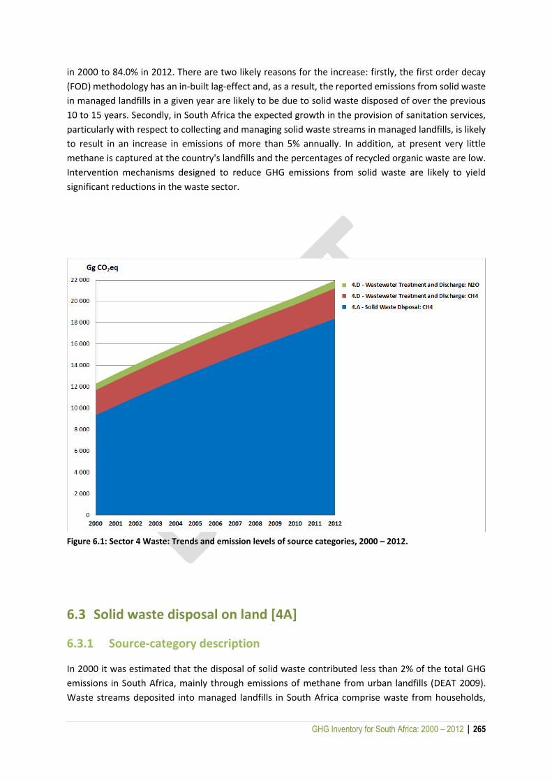
GHG Inventory for South Africa: 2000 – 2012 | 265

in 2000 to 84.0% in 2012. There are two likely reasons for the increase: firstly, the first order decay

(FOD) methodology has an in-built lag-effect and, as a result, the reported emissions from solid waste

in managed landfills in a given year are likely to be due to solid waste disposed of over the previous

10 to 15 years. Secondly, in South Africa the expected growth in the provision of sanitation services,

particularly with respect to collecting and managing solid waste streams in managed landfills, is likely

to result in an increase in emissions of more than 5% annually. In addition, at present very little

methane is captured at the country's landfills and the percentages of recycled organic waste are low.

Intervention mechanisms designed to reduce GHG emissions from solid waste are likely to yield

significant reductions in the waste sector.

Figure 6.1: Sector 4 Waste: Trends and emission levels of source categories, 2000 – 2012.

6.3 Solid waste disposal on land [4A]

6.3.1 Source-category description

In 2000 it was estimated that the disposal of solid waste contributed less than 2% of the total GHG

emissions in South Africa, mainly through emissions of methane from urban landfills (DEAT 2009).

Waste streams deposited into managed landfills in South Africa comprise waste from households,

GHG Inventory for South Africa: 2000 – 2012 | 266

commercial businesses, institutions, and industry. In this report only the organic fraction of the waste

in solid disposal sites was considered as other waste stream components were assumed to generate

insignificant quantities in landfills. Furthermore only GHG’s generated from managed disposal landfills

in South Africa were included, as data on unmanaged sites are not documented and the sites are

generally shallow. A periodic survey is still needed to assess the percentage share of unmanaged sites

and semi-managed sites. Generating this information is central to understanding methane generation

rates for different solid waste disposal pathways.

6.3.2 Overview of shares and trends in emissions

The total accumulated GHG emissions from solid waste disposal between 2000 and 2010 was

estimated at 183 048 Gg CO2eq, increasing from 9 368 Gg CO2eq in 2000 to 18 412 Gg CO2eq in 2012

(Figure 6.1: above). This is an increase of 78.5% over the 12 year period.

6.3.3 Methodological issues

The FOD model was used to estimate GHG emissions from this source category for the period 1950 to

2012 using the following input activity data: population, waste generation rates, income per capita,

annual waste generation and population growth rates, emission rates, half-lives of bulk waste stream

(default value for the half-live is 14 years), rate constants, methane correction factor (MCF),

degradable carbon fraction (DCF), as well as other factors described in the IPPC Guidelines, Volume 5,

Chapter (IPPC, 2006). Notably, due to a lack of published specific-activity data for many of these

parameters in South Africa, the default values suggested in the IPCC Guidelines were applied. In

addition, the inventory compilers noted that the information on national waste composition

presented in the National Waste Baseline Information Report (NWIBR, 2012) was not compatible with

the approach set out in the 2006 IPCC Guidelines, therefore, even though domestic information on

waste composition was available, it could not be used for the purposes of this inventory. Instead,

default IPCC waste composition values where used. The NWIBR, however, does provide information

on the percentage of the waste generated that is disposed of in solid waste disposal sites. This value

was estimated at 91% for 2011. It was assumed that this value was constant throughout the time

series due to a lack of data for the previous years.

6.3.4 Data sources

For the FOD methodology, the model required historical data with at least three to five half-lives.

Therefore, the activity data used comprised waste quantities disposed of into managed landfills from

1950 to 2010, covering a period of about 70 years (satisfying the condition for a period of five half-

lives). Population data for the period 1950- to 2001 was sourced from United Nations population

statistics (UN, 2012). Statistics South Africa population data was used for the period 2002 to 2012

(StatsSA, 2013). Waste Generation rates for industrial waste were estimated using GDP values

sourced from StatsSA (StatsSA, 2013) and tonnages of industrial waste reported in the NWIBR for

GHG Inventory for South Africa: 2000 – 2012 | 267

2011. A value of 8 tonnes/per unit of GDP in US dollars was derived and assumed constant throughout

the time series.

Among the chief limitations of the FOD methodology is that even if activity data improved

considerably, the limitations of the data, or lack thereof, of previous years will still introduce a

considerable degree of uncertainty. On the other hand, the estimated waste generations derived from

previous years, back to 1950, will remain useful in future estimations of GHGs as they will aid in taking

into account half-lives.

No detailed analysis of the methane recovery from landfills was accounted for between 2000 and

2010. As noted in the previous inventory (DEA, 2009), the recovery of methane from landfills

commenced on a large-scale after 2000, with some sites having a lifespan of about 21 years (DME,

2008). To address these data limitations, the DEA has implemented the National Climate Change

Response Database, which captures valuable data from mitigation and adaptation projects for future

GHG estimates from landfills. This tool will be used in the future to identify and implement methane

recovery projects. However, at present there are limited publicly accessible data on the quantities of

methane recovered annually from managed landfills in South Africa.

6.3.5 Uncertainty and time-series consistency

6.3.5.1 UNCERTAINTY

Uncertainty in this category is due mainly to the lack of data on the characterization of landfills, as

well as of the quantities of waste disposed in them over the medium to long term. An uncertainty of

30% is typical for countries that collect waste-generation data on a regular basis (IPCC 2006 Guidelines,

Table 3.5). Another source of uncertainty is that methane production is calculated using bulk waste

because of a lack of data on waste composition, therefore, uncertainty is more than a factor of two

(DEAT, 2009). For the purpose of the bulk waste estimates, the whole of South Africa is classified as

a “warm dry temperate” climate zone, even though some landfills are located in dry tropical climatic

conditions. Other uncertainties are the fraction of MSWT sent to SWDS (more than a factor of two),

DOCf (±20%), MCF (-10%-0%), F (±5%), methane recovery (can be as much as ±50%) and the oxidation

factor (IPCC 2006 Guidelines, Table 3.5).

6.3.5.2 TIME-SERIES CONSISTENCY

The FOD methodology for estimating methane emissions from solid waste requires a minimum of 48

years’ worth of historical waste disposal data. However, in South Africa, waste disposal statistics are

not available. In addition, periodic waste baseline studies do not build time-series data. Hence,

population statistics sourced from the UN secretariat provided consistent time-series activity data for

solid waste disposal.

GHG Inventory for South Africa: 2000 – 2012 | 268

6.3.6 Source-specific QA/QC and verification

A review of the waste sector emission estimates has been performed by experts from various

universities. The review resulted in major changes to emission estimates. For example, assumptions

about the percentage of waste that ends in waste disposal sites, GDP values for estimating emissions

from industrial waste, as well as waste generation rates were all reviewed and updated. Verification

focused on waste generation rates, population statistics and GDP values using Statistics SA datasets

and the DEA’s waste baseline study.

An independent reviewer was appointed to assess the quality of the inventory, determine the

conformity of the procedures followed for the compilation of this inventory and identify areas of

improvement.

6.3.7 Source-specific recalculations

Source-specific recalculations have been performed for the period 2000 to 2010 in this source

category because of the following:

Population statistics for the period 2002 to 2010 based on new information available in the

2011 national census conducted by Statistics South Africa.

The percentage of waste generated that is disposed in solid waste disposal sites was reviewed

and updated based on the NWIBR.

A waste generation rate for municipal solid waste was reviewed based on new information

sourced from the NWIBR. The new waste generation rate is based on provincial weighted

average waste generation rates. This rate was assumed constant for the entire time period.

A waste generation rate for industrial waste was reviewed based on GDP data reported by

StatsSA as well as industrial waste tonnage rates available from the NWIBR for 2011. This rate

was assumed constant for the entire time period.

6.3.8 Source-specific planned improvements and recommendations

The most challenging task in estimating GHG emissions in South Africa was the lack of specific-activity

and emissions factor data. As a result, estimations of GHG emissions from both solid waste and

wastewater sources were largely computed using default values suggested in IPCC 2006 Guidelines

and, as a consequence, margins of error were large. Therefore, several recommendations for

improving the activity and emission factors data are suggested. These include:

(i) advance data capturing, particularly the quantities of waste disposed of into managed and

unmanaged landfills. Other activities that merit improvement are the MCF and rate constants, owing

to their impact on the computed methane emissions from landfills; and

GHG Inventory for South Africa: 2000 – 2012 | 269

(ii) improve the reporting of economic data (e.g. annual growth) to include different population

groups. The assumption that GDP growth is evenly distributed (using a computed mean) across all the

population groups is highly misleading and leads to exacerbated margins of error.

6.4 Wastewater treatment and discharge [4D]

6.4.1 Source category description

Wastewater treatment contributes to anthropogenic emissions, mainly CH4 and N2O. The generation

of CH4 is due to anaerobic degradation of organic matter in wastewater from domestic, commercial

and industrial sources. The organic matter can be quantified using biological oxygen demand (BOD)

values.

Wastewater can be treated on site (mostly industrial sources), or treated in septic systems and

centralised systems (mostly for urban domestic sources), or disposed of untreated (mostly in rural and

peri-urban settlements). Most domestic wastewater CH4 emissions are generated from centralised

aerobic systems that are not well managed, or from anaerobic systems (anaerobic lagoons and

facultative lagoons), or from anaerobic digesters where the captured biogas is not completely

combusted.

Unlike in the case of solid waste, organic carbon in wastewater sources generates comparatively low

quantities of CH4. This is because even at very low concentrations, oxygen considerably inhibits the

functioning of the anaerobic bacteria responsible for the generation of CH4.

N2O is produced from nitrification and denitrification of sewage nitrogen, which results from human

protein consumption and discharge.

The Revised 1996 IPCC Guidelines (IPCC 1997) included one equation to estimate emissions from

wastewater and another to estimate emissions from sludge removed from wastewater. This

distinction was removed in the 2006 IPCC Guidelines (IPCC 2006, Vol.5, p 6.9), so both emissions are

now calculated by the same equation.

In South Africa, most of the wastewater generated from domestic and commercial sources is treated

through municipal wastewater treatment systems (MWTPs).

For wastewater generated by industrial processes, the IPCC 2006 Guidelines list the industry

categories which use large quantities of organic carbon that generate wastewater (IPCC 2006 Vol.5,

p.6.22). The IPCC 2006 Guidelines require the development of consistent data for estimating emissions

from wastewater in a given industrial sector (IPCC 2006, Vol.5, p 6.22). Once an industrial sector is

included in an inventory, it should be included in all future inventories.

The South African data on industrial categories with high organic content are very limited. Some data

exist on wastewater in sectors such as vegetables, fruits and juices, and the wine industry, but these

are available only for a specific year, making it impossible to extrapolate such statistics accurately over

any period. Therefore, in this inventory, only CH4 emissions from domestic sources are presented.

However, wastewater from commercial and industrial sources discharged into sewers is accounted

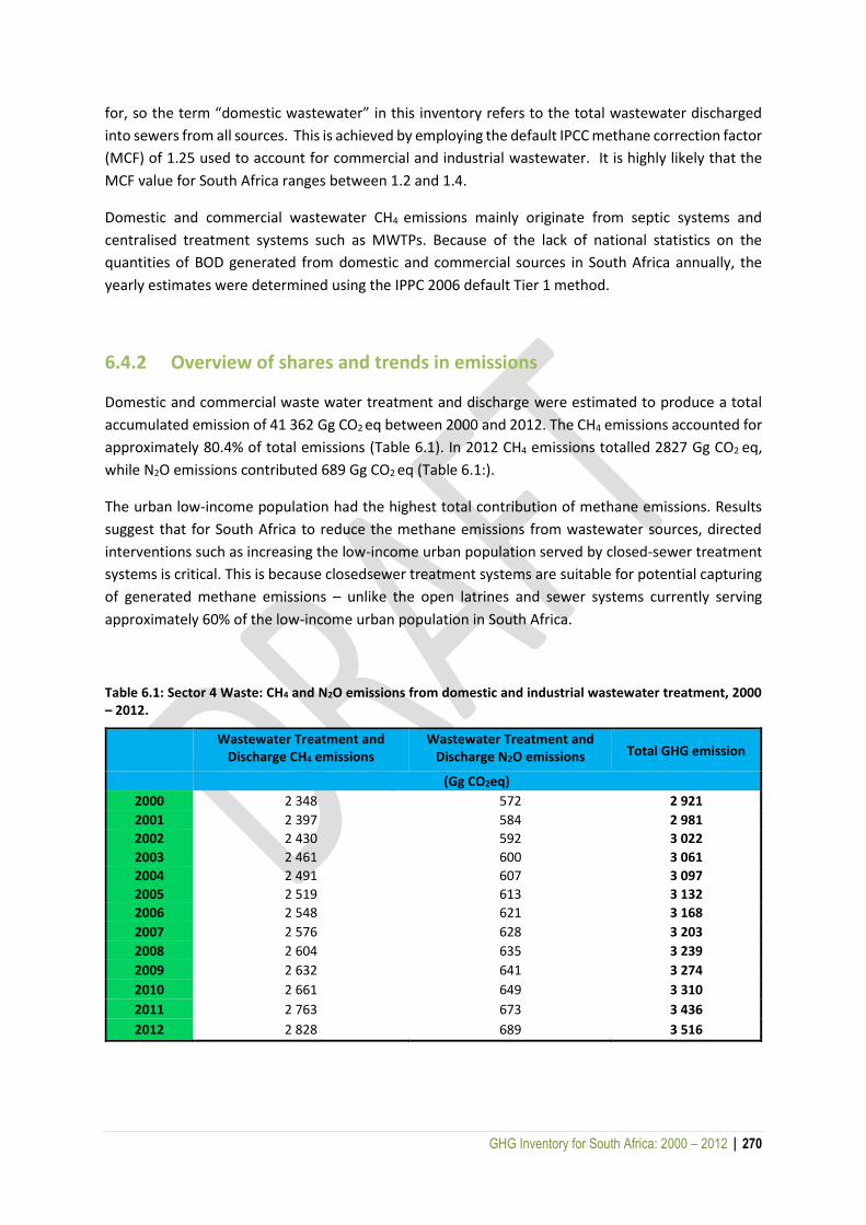
GHG Inventory for South Africa: 2000 – 2012 | 270

for, so the term “domestic wastewater” in this inventory refers to the total wastewater discharged

into sewers from all sources. This is achieved by employing the default IPCC methane correction factor

(MCF) of 1.25 used to account for commercial and industrial wastewater. It is highly likely that the

MCF value for South Africa ranges between 1.2 and 1.4.

Domestic and commercial wastewater CH4 emissions mainly originate from septic systems and

centralised treatment systems such as MWTPs. Because of the lack of national statistics on the

quantities of BOD generated from domestic and commercial sources in South Africa annually, the

yearly estimates were determined using the IPPC 2006 default Tier 1 method.

6.4.2 Overview of shares and trends in emissions

Domestic and commercial waste water treatment and discharge were estimated to produce a total

accumulated emission of 41 362 Gg CO2 eq between 2000 and 2012. The CH4 emissions accounted for

approximately 80.4% of total emissions (Table 6.1). In 2012 CH4 emissions totalled 2827 Gg CO2 eq,

while N2O emissions contributed 689 Gg CO2 eq (Table 6.1:).

The urban low-income population had the highest total contribution of methane emissions. Results

suggest that for South Africa to reduce the methane emissions from wastewater sources, directed

interventions such as increasing the low-income urban population served by closed-sewer treatment

systems is critical. This is because closedsewer treatment systems are suitable for potential capturing

of generated methane emissions – unlike the open latrines and sewer systems currently serving

approximately 60% of the low-income urban population in South Africa.

Table 6.1: Sector 4 Waste: CH4 and N2O emissions from domestic and industrial wastewater treatment, 2000 – 2012.

Wastewater Treatment and Discharge CH4 emissions

Wastewater Treatment and Discharge N2O emissions Total GHG emission

(Gg CO2eq)

2000 2 348 572 2 921

2001 2 397 584 2 981

2002 2 430 592 3 022

2003 2 461 600 3 061

2004 2 491 607 3 097

2005 2 519 613 3 132

2006 2 548 621 3 168

2007 2 576 628 3 203

2008 2 604 635 3 239

2009 2 632 641 3 274

2010 2 661 649 3 310

2011 2 763 673 3 436

2012 2 828 689 3 516

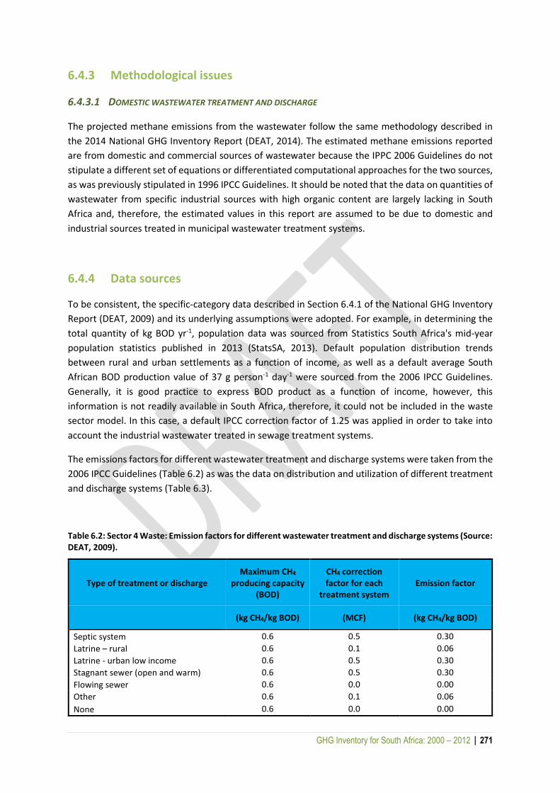
GHG Inventory for South Africa: 2000 – 2012 | 271

6.4.3 Methodological issues

6.4.3.1 DOMESTIC WASTEWATER TREATMENT AND DISCHARGE

The projected methane emissions from the wastewater follow the same methodology described in

the 2014 National GHG Inventory Report (DEAT, 2014). The estimated methane emissions reported

are from domestic and commercial sources of wastewater because the IPPC 2006 Guidelines do not

stipulate a different set of equations or differentiated computational approaches for the two sources,

as was previously stipulated in 1996 IPCC Guidelines. It should be noted that the data on quantities of

wastewater from specific industrial sources with high organic content are largely lacking in South

Africa and, therefore, the estimated values in this report are assumed to be due to domestic and

industrial sources treated in municipal wastewater treatment systems.

6.4.4 Data sources

To be consistent, the specific-category data described in Section 6.4.1 of the National GHG Inventory

Report (DEAT, 2009) and its underlying assumptions were adopted. For example, in determining the

total quantity of kg BOD yr-1, population data was sourced from Statistics South Africa's mid-year

population statistics published in 2013 (StatsSA, 2013). Default population distribution trends

between rural and urban settlements as a function of income, as well as a default average South

African BOD production value of 37 g person-1 day-1 were sourced from the 2006 IPCC Guidelines.

Generally, it is good practice to express BOD product as a function of income, however, this

information is not readily available in South Africa, therefore, it could not be included in the waste

sector model. In this case, a default IPCC correction factor of 1.25 was applied in order to take into

account the industrial wastewater treated in sewage treatment systems.

The emissions factors for different wastewater treatment and discharge systems were taken from the

2006 IPCC Guidelines (Table 6.2) as was the data on distribution and utilization of different treatment

and discharge systems (Table 6.3).

Table 6.2: Sector 4 Waste: Emission factors for different wastewater treatment and discharge systems (Source: DEAT, 2009).

Type of treatment or discharge Maximum CH4

producing capacity (BOD)

CH4 correction factor for each

treatment system Emission factor

(kg CH4/kg BOD) (MCF) (kg CH4/kg BOD)

Septic system 0.6 0.5 0.30

Latrine – rural 0.6 0.1 0.06

Latrine - urban low income 0.6 0.5 0.30

Stagnant sewer (open and warm) 0.6 0.5 0.30

Flowing sewer 0.6 0.0 0.00

Other 0.6 0.1 0.06

None 0.6 0.0 0.00

GHG Inventory for South Africa: 2000 – 2012 | 272

Table 6.3: Sector 4 Waste: Distribution and utilization of different treatment and discharge systems (Source: DEAT, 2009).

Income group Type of treatment or discharge

pathway Degree of utilization

(Tij)

Rural

Septic tank 0.10

Latrine – rural 0.28

Sewer stagnant 0.10

Other 0.04

None 0.48

Urban high-income

Sewer closed 0.70

Septic tank 0.15

Other 0.15

Urban low-income

Latrine - urban low income 0.24

Septic tank 0.17

Sewer (open and warm) 0.34

Sewer (flowing) 0.20

Other 0.05

6.4.4.1 DOMESTIC WASTEWATER N2O EMISSIONS

The default values provided by the IPCC Guidelines were used in estimating the potential growing

trends of N2O emissions from the wastewater treatment systems. This was due to the lack of specific-

activity data for South Africa. For instance, a default value for per capita protein consumption of 27.96

kg yr-1 was applied in the model.

6.4.5 Uncertainties and time-series consistency

6.4.5.1 UNCERTAINTIES

An analysis of the results for methane emissions suggest that the likely sources of uncertainties may

be due to the input data. These include uncertainties associated with South African population

estimates provided by the United Nations, the presumed constant country BOD production of about

37 g person-1 day-1 from 2001 to 2020, and the lack of data on the distribution of wastewater

treatment systems in South Africa. It is recommended that, in future inventories, a detailed study on

the input parameters merits careful consideration to minimize the uncertainty level. In turn, this

approach would improve the reliability of the projected methane estimates from wastewater sources.

GHG Inventory for South Africa: 2000 – 2012 | 273

6.4.5.2 TIME-SERIES CONSISTENCY

Time-series consistency was achieved by using population datasets obtained from the UN secretariat.

Assumptions about wastewater streams were assumed to be constant over the 12-year time series

and default IPCC emission factors used.

6.4.6 Source-specific QA/QC and verification

Internal and external reviews of this source category were included in the review of solid waste

disposal. Hence, changes to population statistics, the percentage split of wastewater pathways, total

organics in wastewater and methane correction factors were all reviewed.

6.4.7 Source-specific recalculations

One correction was made to the calculations since the 2000 inventory. In the previous inventory

individual TOW (total organics in wastewater) values for each income group were used to calculate a

CH4 emission from each income group which were then summed together to obtain the total

emissions. Whereas in this inventory the total TOW (of all the income groups) was used in the emission

calculation. This correction was made following equation 6.1 in the IPCC 2006 Guidelines.

6.4.8 Source-specific planned improvements and recommendations

The biggest challenge in estimating GHG emissions in South Africa is the lack of specific-activity and

emissions factor data. As a result, estimations of GHGs from both solid waste and wastewater sources

were largely computed using default values suggested in the IPCC 2006 Guidelines and, as a

consequence, margins of error were high. Therefore, several recommendations are suggested to

improve the activity and emission factors data. These include: (i) advance data capturing, particularly

the quantities of waste disposed of into managed and unmanaged landfills. Other activities that merit

improvement are the MCF and rate constants, owing to their impact on the computed methane

emissions from landfills; and (ii) improve the reporting of economic data (e.g. annual growth) to

include different population groups. The assumption that GDP growth is evenly distributed (using a

computed mean) across all the population groups is highly misleading, and leads to exacerbated

margins of error.

GHG Inventory for South Africa: 2000 – 2012 | 274

7 REFERENCES

Abstract of Agricultural Statistics, 2012. Department of Agriculture, Forestry and Fisheries, Pretoria,

RSA.

Abstracts of Agricultural Statistics, 2012. Department of Agriculture, Forestry and Fisheries, Pretoria, RSA. Can be downloaded from www.daff.gov.za.

Airports Company South Africa (ACSA), 2013. Passenger travel Statistics. http://www.acsa.co.za/home.asp?pid=137. [Accessed April 2013]

Alembong, OA., 2015. Carbon flow analysis in the South African Forest and the Forestry Sector, MSC thesis, University of Kwazulu-Natal.

Anaya, J.A. and Chuvieco, E., 2012. Accuracy Assessment of Burned Area Products in the Orinoco Basin, Photogrammetric Engineering & Remote Sensing, 78: 53 – 60.

Anglo American 2011: The South African Iron and Steel Value Chain. http://www.angloamericankumba.com/ [Accessed July 2012]

Anton Eberhard, 2009. South African Coal: market, investment and policy challenges. South African coal paper, University of Cape Town.

Archibald, S., Roy, D.P., Van Wilgen, B.W, Scholes, R.J., 2010. What limits fire? An examination of the drivers of burnt area in southern Africa. Global Change Biology.

Archibald, S., Scholes, R.J., Roy, D., Roberts, G. and Boscheti, L., 2009. Southern African fire regimes as revealed by remote sensing. African Journal of Ecology.

Association of Cementitious Material Producers, 2008. Sustainability Report. http://www.acmp.co.za/climate_change.htm [Accessed March 2013

Association of Cementitious Material Producers, 2009. Cement Manufacturing Process. http://www.acmp.co.za/cement_manufacturing_process.htm. [Accessed March 2013].

Aucamp, A.J. and Howe, L.G., 1979. The production potential of the Eastern Cape Valley Bushveld. Proc. Grassl. Soc. S Afr. 14: 115 – 117.

Australian National Inventory Report (ANIR), 2009. Australian national greenhouse accounts: National inventory report. Department of climate change and energy efficiency, Commonwealth of Australia, Canberra, ACT.

Baggott, S.L., Brown, L., Cardenas, L., Downes, M.K., Garnett, E., Hobson, M., Jackson, J., Milne, R., Mobbs, D.C., Passant, N., Thistlethwaite, G., Thomson, A. and Watterson, J., 2006. Greenhouse Gas Inventory, 1990 to 2004.

Bessinger, D., 2000. Cooling Characteristics of High Titania Slags, MSc dissertation, University of Pretoria, Pretoria. http://upetd.up.ac.za/thesis/available/etd-07212006-102324 [Accessed 30 January 2013].

Bexley, J., 2013. A perspective on the Glass Manufacturing Industry. (Personal communication, February, 2013).

GHG Inventory for South Africa: 2000 – 2012 | 275

Blaxter, K.L. and Clapperton, J.L., 1965. Prediction of the amount of methane produced by ruminants. Brit. J. Nutr. 19: 511 – 522.

Boschetti, L., Roy, D., Hoffman, A.A. and Humber, M., 2012. MODIS Collection 5.1 burned area product – MCD45: User’s guide version 3.

Brouwer, 1965. Report of sub-committee on constants and factors. In: Proceedings of the 3rd symposium on energy metabolism, pp. 441 – 443. K.L Blaxter (Edt). London: Academic Press.

Bull, P., McMillan, C. and Yamamoto, A., 2005. Michigan Greenhouse Gas Inventory 1990 and 2002. Centre for Sustainable Systems, University of Michigan, Report No. CSS05-07.

Bull, P., McMillan, C. and Yamamoto, A., 2005. Michigan Greenhouse Gas Inventory 1990 and 2002. Centre for Sustainable Systems, University of Michigan, Report No. CSS05-07.

Burns, R., 2012. Poultry production and climate change. XXIV World’s poultry Congress, Salvador, Brazil.

Cement and Concrete Institute, 2008. Cement and Concrete Institute Review 2008. http://www.cnci.org.za/Uploads/Overall_Review%202008.pdf. [Accessed October 2012].

CHAPOPSA, 2002. Charcoal potential in southern Africa. INCO_DEV: International cooperation with developing countries (1998 – 2002).

Chhabra, A., Manjunath, K.R., Panigrahy, S. and Parihar, J.S., 2009. Spatial pattern of methane emissions from Indian livestock. Current Science, 96 (5), 683 – 689.

Chidumayo, E.N., 1993. Response of miombo to harvesting: ecology and management. Stockholm Environmental Institute, Stockholm.

Christie, S.I. and Scholes, R.J. 1995. Carbon storage in Eucalyptus and Pine plantations in South Africa. Environmental Monitoring and Assessment, 38: 231 – 241.

Clauss, M., Frey, R., Kiefer, B., Lechner-Doll, M., Loehlein,W., Polster, C., Rössner, G.E., Streich, W.J., 2003. The maximum attainable body size of herbivorous mammals: morphophysiological constraints on foregut, and adaptations of hindgut fermenters. Oecologia, 136, 14–27.

Colgan, M.S., Asner, G.P., Levick, S.R., Martin, R.E. and Chadwick, O.A., 2012. Topo-edaphic controls over woody plant biomass in South African savannas. Biogeosciences, 9: 1809-1821.

Cowling, R.M., Richardson, D.M. and Mustart, P.J., 1997. Fynbos. In: Cowling, R.M., Richardson, D.M. and Pierce, S.M. (eds), Vegetation of Southern Africa. Cambridge University Press, Cambridge, UK, pp 99 – 130.

Damm, O. and Triebel, R., 2008. A Synthesis Report on Biomass Energy Consumption and Availability in South Africa. A report prepared for ProBEC.

Department of Agriculture, Forestry and Fisheries, 2010. The South African Agricultural GHG Inventory for 2004. Department of Agriculture, Forestry and Fisheries, ISBN: 978-1-86871-321-9, DAFF, Pretoria, RSA.

Department of Environmental Affairs (DEA), 2004: National Climate Change Response, White Paper. Department of Environmental Affairs, Pretoria.

GHG Inventory for South Africa: 2000 – 2012 | 276

Department of Environmental Affairs (DEA), 2011. South Africa’s Second National Communication under the United Nations Framework Convention on Climate Change. Department of Environmental Affairs, Republic of South Africa, Pretoria.

Department of Environmental Affairs (DEA), 2012. Atmospheric Emissions Licenses, Department of

Environmental Affairs, Pretoria.

Department of Environmental Affairs (DEA), 2014. South Africa’s 1st Biennial Update Report. Department of Environmental Affairs, Pretoria.Draft, Published for public comment.

DEA, 2015. National Terrestrial Carbon Sinks Assessment, Department of Environmental Affairs,

Pretoria.

DEAT, 2006. South Africa Environment Outlook. A report on the state of the environment. Executive

summary and key findings. Department of Environmental Affairs and Tourism, Pretoria. 42pp.

Department of Environment Affairs and Tourism (DEAT), 2009. Greenhouse Gas Inventory South

Africa, 1990 to 2000. National Inventory Report, May 2009. Pretoria: Department of

Environmental Affairs and TourismEAT.

Department of Energy (DoE), 2000. Digest of South African Energy Statistics. Pretoria.

Department of Minerals and Resources, 2001a. Department of Minerals and Resources Annual Report

2001/2002. Pretoria

Department of Minerals and Resources, 2001b. South Africa’s mineral industry (SAMI) 2001/2002.

Pretoria

Department of Minerals and Resources, 2004. South Africa’s mineral industry (SAMI) 2004/2005.

Pretoria

Department of Minerals and Resources, 2005. South Africa’s mineral industry (SAMI) 2005/2006.

Pretoria

Department of Minerals and Resources, 2006. South Africa’s mineral industry (SAMI) 2006/2007.

Pretoria

Department of Minerals and Resources, 2006. South African Ferroalloy Production Trends 1995- 2004.

Directorate: Mineral Economics, Report 52/2006, Pretoria.

Department of Minerals and Resources, 2008. South Africa’s mineral industry (SAMI) 2007/2008.

Pretoria

Department of Minerals and Resources, 2009. South Africa’s mineral industry (SAMI) 2009/2010.

Pretoria

Department of Minerals and Resources, 2010c. Lime Industry SA 2010. Directorate: Mineral

Economics, Report 85, Pretoria.

Department of Minerals and Resources, 2010d. Operating and Developing Coal Mines in the Republic

of South Africa 2010. Directorate: Mineral Economics, Directory D2/2010, Pretoria.

GHG Inventory for South Africa: 2000 – 2012 | 277

Department of Minerals and Resources, 2010e. Producers of Industrial Mineral Commodities in South

Africa. Directorate: Mineral Economics, Directory D11/2010, Pretoria.

Department of Minerals and Resources, 2010f. South Africa’s mineral industry (SAMI) 2009/2010.

Pretoria

Department of Minerals and Resources, 2010g. Statistical Tables, 1988 -2009. Directorate: Mineral

Economics, Bulletin B1/2010, Pretoria.

Department of Minerals and Resources, 2010h. Dolomites and Limestone in South Africa: Supply and

Demand. Directorate: Mineral Economics, Report R49/2005, Pretoria.

Department of Minerals and Resources, 2011. Operating Mines and Quarries and Mineral Processing

Plants in the Republic of South Africa, 2011. Directorate: Mineral Economics, Directory

D1/2011, Pretoria

Department of Transport 2001: Statistics, Pretoria. http://www.dot.gov.za [Accessed October 2012].

Department of Transport, 2009. Transport Statistics 2008. Annual Transport Statistics Bulletin, Pretoria. http://www.dot.gov.za, [Accessed 11 July 2012].

Department of Water Affairs (DWA), 2009. Directorate: Resource Protection and Waste. Inventory of Waste Water Treatment Works, Department of Water Affairs, Pretoria, RSA.

Desjardins, R., Rochette, P., Pattey, E. and MacPherson, I., 1993. Measurements of Greenhouse Gas Fluxes using Aircraft and Tower-based Techniques. In: Harper, L.A., Mosier, A.R. and Duxbury, J.M. (eds), Agricultural ecosystems effects on trace gases and global climate change: proceedings of a symposium / sponsored by Divisions A-3 and S-3 of the American Society of Agronomy and Soil Science Society of America. ASA Special Publication Number 55, USA.

Dingaan, M.N.V and du Preez, P.J., 2013. Grassland communities of urban open spaces in Bloemfontein, Free State, South Africa. Koedoe 55: 1-8, http://www.koedoe.co.za, doi:10.4102/koedoe.v55i1.1075.

Department of Minerals and Energy (DME), 2000. Hydrocarbons and Energy Planning Branch – Liquid

Fuel, Department of Minerals and Energy, Pretoria.

Department of Minerals and Energy (DDME), 2001. National Electrification Programme NEP. Summary

evaluation Report, Department of Minerals and Energy, Pretoria.

Department of Minerals and Energy (DMEDME), 2002. South African National Energy Database:

Energy Prices, Department of Minerals and Energy, Pretoria.

Department of Minerals and Energy (DME), 2008. National Efficiency Strategy of the Republic of South

Africa, Report 32342, Department of Minerals and Energy, Pretoria.

Department of Minerals and Energy (DME), 2010a. Department of Minerals and Energy annual reports

2009/2010, Department of Minerals and Energy, Pretoria.

Department of Minerals and Energy (DME), 2010b. Department of Minerals and Energy annual reports

2009/2010, Department of Minerals and Energy, Pretoria.

GHG Inventory for South Africa: 2000 – 2012 | 278

Department of Minerals and EnergyDME, Eskom, Energy Research Institute and University of Cape

Town 2002: Energy Outlook for South Africa 2002.

http://www.info.gov.za/view/DownloadFileAction [Accessed August 2012].

Department of Energy (DoE), 2005. Digest of South African Energy Statistics, Department of Energy,

Pretoria.

Department of Energy (DoE), 2005. Energy Price Report. Directorate: Energy Planning and

Development, Department of Energy, Pretoria.

Department of Energy (DoE), 2007. Biofuels Industrial Strategy of the Republic of South Africa,

Department of Energy,Pretoria.

http://www.energy.gov.za/files/esources/petroleum/biofuels_indus_strat.pdf(2).pdf

[Accessed October 2012].

Department of Energy (DoE), 2008. Energy Balances Statistics. Department of Energy,

http://www.energy.gov.za/files/energyStats_frame.html. [Accessed November 2012].

Department of Energy (DoE), 2009a. Digest of South African Energy Statistics, Depertment of Energy,

Pretoria.

Department of Energy (DoE), 2009b. Electrification Statistics. Electrification Policy Development and

Management Directorate, Department of Energy, Pretoria.

Department of Energy (DoE), 2010. South Africa National energy Balance (2000-2010). Department of

Energy, Pretoria, DOE. http://www.energy.gov.za/files/energyStats_frame.html

Department of Energy (DoE), 2010. South African Energy Synopsis 2010. Department of Energy,

http://www.energy.gov.za [Accessed June 2012].

Donaldson, R.A., 2009. Season effects on the potential biomass and sucrose accumulation of some commercial cultivars of sugarcane, PhD Thesis, University of KwaZulu-Natal, Pietermaritzburg, RSA.

Donaldson, R.A., Redshaw, K.A., Rhodes, R. and Van Antwerpen, R., 2008. Season effects on productivity of some commercial South African sugarcane cultivars, 1: Biomass and radiation use efficiency. Proc. S Afr. Sug. Technol. Ass. 81: 517 – 527.

Dovey, S.B. and Smith, C.W., 2005. Simple ratios to estimate bark and branch biomass and nutrient contents of commercial plantations. ICFR Bulletin Series 13/2005, ICFR, Pietermaritzburg, RSA.

Du Toit, C.J.L., Meissner, H.H. and van Niekerk, W.A., 2013a. Direct methane and nitrous oxide emissions of South African dairy and beef cattle. South African Journal of Animal Science, 43 (3): 320 – 339.

Du Toit, C.J.L., Meissner, H.H. and van Niekerk, W.A., 2013d. Direct greenhouse gas emissions of the game industry in South Africa. South African Journal of Animal Science, 43 (3): 376 – 393.

Du Toit, C.J.L., van Niekerk, W.A. and Meissner, H.H., 2013b. Direct greenhouse gas emissions of the South African small stock sectors. South African Journal of Animal Science, 43 (3): 340 – 361.

GHG Inventory for South Africa: 2000 – 2012 | 279

Du Toit, C.J.L., van Niekerk, W.A. and Meissner, H.H., 2013c. Direct methane and nitrous oxide emissions of monogastric livestock in South Africa. South African Journal of Animal Science, 43 (3): 362 - 375.

Engelbrecht, A., Golding, A., Hietkamp, S. and Scholes, R.J., 2004. The potential for sequestration of carbon dioxide in South Africa. Council for Scientific and Industrial Research (CSIR), Pretoria, RSA.

Environment Canada, 2009. Municipal Waste Water sources and characteristics. http://www.atl.ec.gc.ca/epb/issues/wstewtr.html

Eskom 2005: Eskom Annual Report, 2005. http://www.eskom.co.za/c/article/289/publications/

[Accessed February 2012]

Eskom 2007: Eskom Annual Report, 2007. http://www.eskom.co.za/c/article/289/publications/

[Accessed February 2012]

Eskom 2008: Eskom Annual Report, 2008. http://www.eskom.co.za/c/article/289/publications/

[Accessed February 2012]

Eskom 2010: Eskom Annual Report, 2010. http://www.eskom.co.za/c/article/289/publications/

[Accessed February 2012]

Eskom 2011: Eskom Annual Report, 2011. http://www.eskom.co.za/c/article/289/publications/ [Accessed February 2012]

FAOSTAT, 2012. Food and Agriculture Organization of the United Nations: Statistics. 2012. http://faostat.fao.org/site/605/default.aspx#ancor; accessed on 11/2012.

Fertilizer Society of SA (FSSA), 2009. Fertilizer Society of South Africa, http://www.fssa.org.za.

Ford, Dave, 2013. Personal communication with Dave Ford, Executive Director, SA Feedlot Association. Telephone +27 12 667 1189, Pretoria.

Forestry South Africa, 2012. Forestry and FP Industry Facts, 1980 – 2011. Forestry South Africa.

Garcia-Apaza, E., Paz, O. and Arana, I., 2008. Greenhouse gas emissions from enteric fermentation of livestock in Bolivia: values for 1990–2000 and future projections. Australian Journal of Experimental Agriculture, 48: 255–259.

GCIS, 2008. South African Year Book on Transport 2007/2008. Government Communication and

Information System, http://www.gcis.gov.za/content/resource-centre/sa-

info/yearbook/2009-10. [Accessed November 2012]

GCIS, 2009. South African Year Book on Economy 2008/2009. Government Communication and

Information System, http://www.gcis.gov.za/content/resource-centre/sa-

info/yearbook/2009-10. [Accessed November 2012]

GCIS, 2010. South African Year Book on Energy 2009/2010. Government Communication and

Information System, http://www.gcis.gov.za/content/resource-centre/sa-

info/yearbook/2009-10http://www.gcis.gov.za. [Accessed November 2012]

GHG Inventory for South Africa: 2000 – 2012 | 280

GeoTerraImage (GTI) Pty Ltd., 2015. 1990 – 2013-14 South African National Land-cover change. Department of Environmental Affairs, Pretoria.

GeoTerraImage (GTI) Pty Ltd., 2015. 2013-2014 South African National Land-cover dataset. Department of Environmental Affairs, Pretoria.

Global Forest Resource Assessment SA (GFRASA), 2005. Global Forest Resources Assessment: Country Reports – South Africa. FAO, Rome, Italy.

Gonzalez-Avalos, E. and Ruiz-Suarez, L.G., 2001. Methane emission factors from cattle manure in Mexico. Biosecure Technology, 80(1): 63 – 71.

Government Communication and Information System (GCIS), 2009. 2009/10 Year South African Year Book. http://www.gcis.gov.za/content/resource-centre/sa-info/yearbook/2009-10 [Accessed: February 2013].

Hély, C., Dowty, P.R., Alleane, S., Caylor, K.K., Korontzi, S., Swap, R.J., Shugart, H.H. and Justice, C.O., 2003. Regional fuel load for two climatically contrasting years in southern Africa. Journal of Geophysical Research, 108.

Howden, S.M., White, D.H., McKeon, G.M., Scanlan, J.C and Carter J.O., 1994. Methods for Exploring Management Options to Reduce Greenhouse Gas Emissions from Tropical Grazing Systems, Climatic Change, vol 27 pp 49–70.

Hurly, K.M., Lynsky, R.J. and Stranack, R.A., 2003. Protecting the Privilege of Burning Sugarcane at Harvest le International Farm Management Congress http://ageconsearch.umn.edu/bitstream/24381/1/ cp03hu02.pdf

International Energy Agency (IEA), 2012. CO2 emissions from fuel combustion: Highlights. (http://www.iea.org/co2highlights/co2highlights.pdf)

IPCC, 1997. Greenhouse Gas Inventory Reporting Instructions. Revised 1996 IPCC Guidelines for National Greenhouse Gas Inventories. UNEP, WMO, OECD and IEA, Bracknell United Kingdom.

IPCC, 2001. IPCC Third Assessment Report (TAR): Climate Change 2001. Cambridge: Intergovernmental Panel on Climate Change. Cambridge University Press.

IPCC, 2003. Good Practice Guidance for Land Use, Land-Use Change and Forestry.

IPCC, 2006. 2006 IPCC Guidelines for National Greenhouse Gas Inventories. The National Greenhouse Gas Inventories Programme, Eggleston H S, Buenida L, Miwa K, Ngara T, and Tanabe K, eds; Institute for Global Environmental Strategies (IGES). Hayama, Kanagawa, Japan.

IPCC, 2014. 2013 Revised Supplementary Methods and Good Practice Guidance Arising from the Kyoto Protocol, Hiraishi, T., Krug, T., Tanabe, K., Srivastava, N., Baasansuren, J., Fukuda, M. and Troxler, T.G. (eds), Published: IPCC, Switzerland.

Korontzi, S., Justice, C.O. and Scholes, R.J., 2003. Influence of timing and spatial extent of Savanna fires in Southern Africa on atmospheric emissions. Journal of Arid Environments, 54: 395 - 404.

Kurihara, M., Magner, T., Hunter, R.A. and McCrabb, G.J., 1999. Methane production and energy partition of cattle in the tropics. British J. Nutr. 81, 227 – 234.

LACTO data, 2010. Milk producers statistics, MPO, Pretoria. Vol 14 (1).

GHG Inventory for South Africa: 2000 – 2012 | 281

Lambers, H., Raven, J.A., Shaver, G.R. and Smith, S.E., 2008. Plant nutrient-acquisition strategies change with soil age. Trends Ecol Evol 23: 95–103.

Lechmere-Oertel, R.G., 2003. The effects of goat browsing on ecosystem patterns and processes in succulent thicket, South Africa. PhD thesis, Nelson Mandela Metropolitan University.

Lloyd P.J.D., 2001. The South African Petroleum Industry: A Review. Prepared for the Automobile Association of South Africa. Energy Research Institute: University of Cape Town.

Low, A.B. and Rebelo, A.G., 1996. Vegetation of South Africa, Lesotho and Swaziland, Department of Environmental Affairs and Tourism, Pretoria. 0-621-17316-9 ISBN.

Malimbwi, R.E. and Zahabu, E., 2009. The analysis of sustainable charcoal production systems in Tanzania. In: Simmone, S., Remedio, E. and Trossero, M.A. (eds), Criteria and Indicators for Sustainable Woodfuels: Case studies from Brazil, Guyana, Nepal, Philippines and Tanzania. FAO, Rome, Italy.

McGinn, S.M., Chen, D., Loh, Z., Hill, J., Beauchemin, K.A. and Denmead, O.T., 2008. Methane emissions from feedlot cattle in Australia and Canada. Australian Journal of Experimental Agriculture, 48: 183–185.

Midgley, J.J. and Seydack, A.H.W., 2006. No adverse signs of the effect of environmental change on tree biomass in the Knysna forest during the 1990s. S A J Science 102: 96-97.

Mills, A.J. and Cowling, R.M., 2006. Rate of carbon sequestration at two thicket restoration sites in the Eastern Cape, South Africa. Restoration Ecology, 14 (1):38 – 49.

Mills, A.J., Birch, S.C., Stephenson, J.D. and Bailey, R.V., 2012. Carbon stocks in fynbos, pastures and vineyards on the Agulhas Plain, South Africa: a preliminary assessment. S A J Plant. Soil, iFirst: 1-3.

Mills, A.J., Cowling, R.M., Fey, M.V., Kerley, G.I.H., Donaldson, J.S., Lechmere-Oertel, R.G., Sigwela, A.M., Skowno, A.L. and Rundel, P., 2005. Effects of goat pastoralism on ecosystem carbon storage in semiarid thicket, Easern Cape, South Africa. Austral Ecology 30: 797 – 804.

Milton, S.J., 1990. Above-ground biomass and plant cover in a succulent shrubland in the southern Karoo, South Africa. S A J Bot. 56: 587-589.

Milton, S.J., Yeaton, R., Dean, W.R.J. and Vlok, J.H.J., 1997. Succulent Karoo. In: Cowling, R.M., Richardson, D.M. and Pierce, S.M. (Eds.), Vegetation of Southern Africa. Cambridge: Cambridge University Press, Cambridge, UK.

Minson, D.J. and McDonald, C.K., 1987. Estimating forage intake from growth of cattle. Tropical grasslands, 21(3): 116 – 121.

Moe, P.W. and Tyrell, H.F., 1979. Methane production in dairy cows. J. Dairy Sci. 62: 1583 – 1586.

Moeletsi, M., Paterson, G.. Van Der Walt, M., Malherbe, J., Nape, M., Nkambule, V. and Malaka, S., 2013. ARC Contribution to ALU GHG Project, ARC-ISCW, unpublished report no. GW/A/2013/19, Pretoria, RSA.

Mucina, L. and Rutherford, M.C. (eds), 2006. The Vegetation of South Africa, Lesotho and Swaziland. Strelitzia 19. South African National Biodiversity Institute, Pretoria.

GHG Inventory for South Africa: 2000 – 2012 | 282

National Electricity Regulator, 2000. Electricity Supply Statistics for South Africa. http://www.ner.org.za. [Accessed July 2012].

National Electricity Regulator, 2004. Electricity Supply Statistics for South Africa. http://www.ner.org.za. [Accessed July 2012].

National Electricity Regulator, 2006. Electricity Supply Statistics for South Africa. http://www.ner.org.za. [Accessed July 2012].

NERSA, National Energy Regulator of South Africa (NERSA), 2006. 2006 Electricity statistics for South Africa. National Energy Regulator of South Africa, http://www.nersa.org.za [Accessed February 2012]

NERSA, 2008. 2008 Electricity statistics for South Africa. National Energy Regulator of South Africa, http://www.nersa.org.za [Accessed February 2012]

NERSA, 2008. The national electricity supply shortage and load shedding. National Energy Regulator of South Africa, http://www.eepublishers.co.za/article/nersa-enquiry-into-the-national-

electricity-supply-shortage-and-load-shedding.html [Accessed February 2012]

O’Connor, T.G. and Bredenkamp, G.J., 1997. Grassland. In: Cowling, R.M., Richardson, D.M. and Pierce, S.M. (eds), Vegetation of Southern Africa. Cambridge University Press, Cambridge, UK.

O’Connor, T.G., 2008. Influence of land use on phytomass accumulation in Highland Sourveld grassland in the southern Drakensberg, South Africa. Afr. J. Range & Forage Sci. 25: 17 – 27.

Otter, L. and Scholes, M., 2000. Methane sources and sinks in a periodically flooded South African savannah. Glob. Biogeochem. Cycles, vol 14: 97 – 111.

Otter, L. B., 2011. Agricultural GHG Inventory: 2000 to 2009 and forward projections to 2020. Unpublished report prepared for Department of Environmental Affairs, Pretoria.

Palmer, T. and Ainslie, A., 2002. South Africa: FAO Country Profile – Country Pasture/Forage Resource Profile, Rome: FAO. http://www.fao.org/ag/agp/agpc/doc/counprof/southafrica/southafrica.htm ; accessed on 15/03/2013.

PFG Glass, 2010. Chemical composition of glass. http://www.pfg.co.za/all-about-glass.aspx [Accessed February 2013]

Prinsloo, Magda, 2014. Statistician for the South African Poultry Association, personal communication

via email. Email: Magda@sapoultry.co.za

Research Unit of Creamer Media (Pty) Ltd, 2009. South Africa’s Steel Industry 2009. Creamer media,

Johannesburg.

Roy, D.P. and Boschetti, L., 2009b. Southern Africa validation of the MODIS, L3JRC and GlobCarbon Burned-Area Products, IEEE Transactions on Geoscience and Remote Sensing, 47(4):1–13.

Roy, D.P., Jin, Y., Lewis, P.E. and Justice, C.O., 2005. Prototyping a global algorithm for systematic fire-affected area mapping using MODIS time series data. Remote Sensing of Environment 97(2), pp.137-162

Rutherford, M.C., 1982. Aboveground biomass categories of woody plants in a Burkea africana - Ochna pulchra Savanna. Bothalia, 14: 131-138.

GHG Inventory for South Africa: 2000 – 2012 | 283

SA Feedlot Association, 2013. http://www.safeedlot.co.za/index.asp?Content=90 [Accessed 10 June 2013]

Scholes, R.J. and Walker, B.H., 1993. An African Savanna: Synthesis of the Nylsvley study. Cambridge University Press, Cambridge, UK.

Scholes R.J. and Hall D.O., 1996. The carbon budget of tropical savannas, woodlands and grasslands. In: Breymeyer A.I., Hall D.O., Melillo J.M. and Agren G.I. (Eds.) Global Change: Effects on Coniferous Forests and Grasslands, SCOPE Volume 56. Wiley, Chichester. pp. 69-100.

Shackleton, C.M. and Scholes, R.J., 2011. Above ground woody community attributes, biomass and carbon stocks along a rainfall gradient in the savannas of the central lowveld, South Africa. S A J Bot 77: 184 -192.

Siebrits, F., 2012. Report to authors on pig diets in South Africa. Pretoria.

Simalenga, T.E., Joubert, A.B.D. and Hanekom, D., 2002. Agricultural Mechanization in South Africa: Status, Trend and Challenges, ARC-All, Pretoria.

Singh, J.S. and Joshi, M.C., 1979. Primary Production. Chapter 17 in: Coupland, R.T. (ed), Grassland ecosystems of the world: Analysis of grasslands and their uses. Cambridge University Press, Cambridge, UK.

Snyman, H.A., 2005. Influence of fire on root distribution, seasonal root production and root/shoot ratios in grass species in a semi-arid grassland of South Africa. S A J Bot. 71: 133-144.

Snyman, H.A., 2011. Root studies in a semi-arid climate. In: Grassroots, The Grassland Society of Southern Africa, http://www.grassland.org.za.

Snyman, H.G., Herselman, J.E. and Kasselman, G., 2004. A metal content survey of South African Sewage Sludge and an Evaluation of Analytical Methods for their Determination in Sludge. WRC Report No 1283/1/04. Water Research Commission, Pretoria, RSA.

South Africa Iron and Steel Institute (SAISI), 2009. Local Sales of Iron and Crude Steel Production in South Africa. http://www.saisi.co.za/localsales.php. [Accessed September 2012].

South Africa Iron and Steel Institute (SAISI), 2009. Local Sales of Iron and Crude Steel Production in South Africa. http://www.saisi.co.za/localsales.php. [Accessed September 2012].

South Africa Iron and Steel Institute (SAISI), 2012. Iron and Crude Steel Production in South Africa. http://www.saisi.co.za/ironsteelproduction.php. [Accessed September 2012].

South Africa Iron and Steel Institute (SAISI), 2012. Overview of Iron and Crude Steel Production in South Africa. http://www.saisi.co.za/primover.php. [Accessed September 2012].

South African Iron and Steel Institute (SAISI), 2008. Steel Stats. http://www.saisi.co.za/index.php/steel-stats [Accessed May 2012]

South African Petroleum Industry Association (SAPIA), 2006. SAPIA Annual Report 2006. http://www.sapia.co.za. [Accessed September 2011].

South African Petroleum Industry Association (SAPIA), 2008. Petrol and Diesel in South Africa and the Impact on Air Quality. http://www.sapia.co.za. [Accessed September 2011].

South African Petroleum Industry Association (SAPIA), 2010. SAPIA Annual Report 2010. http://www.sapia.co.za. [Accessed September 2011].

GHG Inventory for South Africa: 2000 – 2012 | 284

South African Petroleum Industry Association (SAPIA), 2011. SAPIA Annual Report 2011. http://www.sapia.co.za. [Accessed September 2012].

South African Statistics Council, 2006. South African Statistics Council Annual Report 2005/2006, Report 174/2006. http://www.statssa.gov.za/publications/StatsCouncilAnnualReport0506.pdf. [Accessed February 2012].

South African Statistics Council, 2007. South African Statistics Council Annual Report 2006/2007, Report.http://www.statssa.gov.za/publications/statsdownload.asp?PPN=AnnualReport&SCH=4026 [Accessed February 2012].

South African Statistics Council, 2011. South African Statistics Council Annual Report 2011/11, Report 174/2011. http://www.statssa.gov.za/publications/StatsCouncilAnnualReport0506.pdf. [Accessed February 2012].

South African Wine Industry Statistics, 2012. www.sawis.co.za. Paarl, South Africa.

Standards South Africa (SSA), 2004. SANS 1877:2004 - A standard land-cover classification scheme for

remote-sensing applications in South Africa. Edition 1. Pretoria, RSA.

Statistics South Africa (Statistics SA), 2006. Statistics South Africa Annual Report 2005/2006.

http://www.statssa.gov.za/annual reports. [Accessed September 2012]

Statistics South Africa, 2010. Mid-year population estimates: 2010. Statistical release P0302.

Thompson, M.W., 1999. South African National Land-cover database project. Data users manual, Final report. CSIR-ARC Contract Report. ENV/P/C 98136, Pretoria.

United Nations (UN), 2012. Population Division of the Department of Economic and Social

Affairs of the Secretariat, World Population Prospects:

http://esa.un.org/unpd/wpp/index.htm [Accessed April 2013]

Van den Berg, E.C., Plarre, C., Van den Berg, H.M. and Thompson, M.W., 2008. The South African National Land-Cover 2000. Agricultural Research Council-Institute for Soil, Climate and Water, Unpublished Report No. GW/A/2008/86.

Van der Merwe, M. and Scholes, R. J., 1998. Greenhouse Gas Emissions Inventory of 1990 for South Africa, Phase 1. Council for Scientific and Industrial Research (CSIR), Pretoria: National Research Foundation, RSA.

Van der Vyver, M.L., 2011. Restoring the biodiversity of canopy species within degraded Spekboom thicket. MSc thesis, Nelson Mandela Metropolitan University.

Van der Waal, C., 2008. Guidelines for the Utilization and Disposal of Wastewater Sludge, Volume 1-5: Impact Assessment. WRC Report No TT 370/08. Water Research Commission, Pretoria, RSA.

Van Dyk J.P., 2006. An overview of the Zincor Process, Southern African Pyrometallurgy 2006. South African Institute of Mining and Metallurgy, Johannesburg

Van Heerden, P.D.R., Donaldson, R.A., Watt, D.A. and Singels, A., 2010. Biomass accumulation in sugarcane: unravelling the factors underpinning reduced growth phenomena. J Exp. Bot., June 13, 2010, p 1 – 11; doi:10.1093/jeb/erq144.

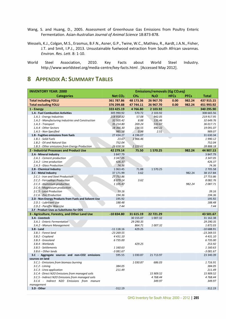
GHG Inventory for South Africa: 2000 – 2012 | 285

Wang, S. and Huang, D., 2005. Assessment of Greenhouse Gas Emissions from Poultry Enteric Fermentation. Asian-Australian Journal of Animal Science 18:873-878.

Wessels, K.J., Colgan, M.S., Erasmus, B.F.N., Asner, G.P., Twine, W.C., Mathieu, R., Aardt, J.A.N., Fisher, J.T. and Smit, I.P.J., 2013. Unsustainable fuelwood extraction from South African savannas. Environ. Res. Lett. 8: 1-10.

World Steel Association, 2010. Key Facts about World Steel Industry. http://www.worldsteel.org/media-centre/key-facts.html . [Accessed May 2012].

8 APPENDIX A: SUMMARY TABLES

INVENTORY YEAR: 2000 Emissions/removals (Gg CO2eq) Categories Net CO2 CH4 N2O HFCs PFCs Total

Total including FOLU 361 787.86 48 173.36 26 967.70 0.00 982.24 437 915.15 Total excluding FOLU 376 299.88 47 744.11 26 967.70 0.00 982.24 451 993.92

1 - Energy 333 425.19 4 766.80 2 103.92 340 295.90 1.A - Fuel Combustion Activities 305 990.92 570.72 2 103.92 308 665.56 1.A.1 - Energy Industries 218 918.82 57.08 942.05 219 917.95 1.A.2 - Manufacturing Industries and Construction 32 505.42 8.88 135.46 32 649.76 1.A.3 - Transport 35 214.80 269.24 533.67 36 017.71 1.A.4 - Other Sectors 18 366.30 234.55 490.22 19 091.07 1.A.5 - Non-Specified 985.58 0.98 2.51 989.07 1.B - Fugitive emissions from fuels 27 434.27 4 196.07 31 630.34 1.B.1 - Solid Fuels 23.67 1 966.46 1 990.12 1.B.2 - Oil and Natural Gas 752.04 752.04 1.B.3 - Other emissions from Energy Production 26 658.56 2 229.61 28 888.18

2 - Industrial Processes and Product Use 42 279.14 75.50 1 570.25 982.24 44 907.13 2.A - Mineral Industry 3 847.79 3 847.79 2.A.1 - Cement production 3 347.05 3 347.05 2.A.2 - Lime production 426.37 426.37 2.A.3 - Glass Production 74.36 74.36 2.B - Chemical Industry 1 063.45 71.88 1 570.25 2 705.58 2.C - Metal Industry 37 171.99 3.62 982.24 38 157.84 2.C.1 - Iron and Steel Production 27 753.86 27 753.86 2.C.2 - Ferroalloys Production 8 079.14 3.62 8 082.76 2.C.3 - Aluminium production 1 105.47 982.24 2 087.71 2.C.4 - Magnesium production 2.C.5 - Lead Production 39.16 39.16 2.C.6 - Zinc Production 194.36 194.36 2.D - Non-Energy Products from Fuels and Solvent Use 195.92 195.92 2.D.1 - Lubricant Use 188.48 188.48 2.D.2 - Paraffin Wax Use 7.44 7.44 2.F - Product Uses as Substitutes for ODS

3 - Agriculture, Forestry, and Other Land Use -10 834.80 31 615.19 22 721.29 43 501.67 3.A - Livestock 30 155.07 1 007.32 31 162.38 3.A.1 - Enteric Fermentation 29 290.35 29 290.35 3.A.2 - Manure Management 864.71 1 007.32 1 872.03 3.B - Land -11 118.16 429.25 -10 688.91 3.B.1 - Forest land -23 269.55 -23 269.55 3.B.2 - Cropland 4 431.10 4 431.10 3.B.3 - Grassland 6 735.00 6 735.00 3.B.4 - Wetlands 429.25 253.92 3.B.5 - Settlements 1 160.63 1 160.63 3.B.6 – Other lands -3 081.67 -3 081.67 3.C - Aggregate sources and non-CO2 emissions sources on land

595.55 1 030.87 21 713.97 23 340.39

3.C.1 - Emissions from biomass burning 1 030.87 686.03 1 716.91 3.C.2 - Liming 384.05 384.05 3.C.3 - Urea application 211.49 211.49 3.C.4 - Direct N2O Emissions from managed soils 15 909.52 15 909.52 3.C.5 - Indirect N2O Emissions from managed soils 4 768.44 4 768.44 3.C.6 - Indirect N2O Emissions from manure management

349.97 349.97

3.D - Other -312.19 -312.19

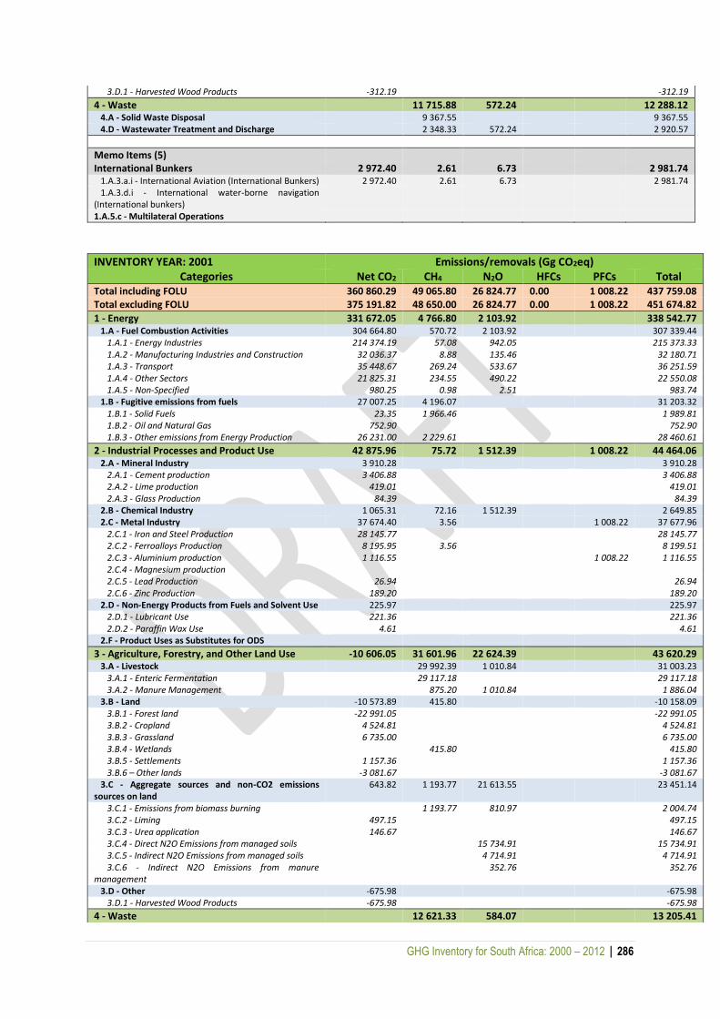
GHG Inventory for South Africa: 2000 – 2012 | 286

3.D.1 - Harvested Wood Products -312.19 -312.19

4 - Waste 11 715.88 572.24 12 288.12 4.A - Solid Waste Disposal 9 367.55 9 367.55 4.D - Wastewater Treatment and Discharge 2 348.33 572.24 2 920.57

Memo Items (5)

International Bunkers 2 972.40 2.61 6.73 2 981.74 1.A.3.a.i - International Aviation (International Bunkers) 2 972.40 2.61 6.73 2 981.74 1.A.3.d.i - International water-borne navigation (International bunkers)

1.A.5.c - Multilateral Operations

INVENTORY YEAR: 2001 Emissions/removals (Gg CO2eq) Categories Net CO2 CH4 N2O HFCs PFCs Total

Total including FOLU 360 860.29 49 065.80 26 824.77 0.00 1 008.22 437 759.08 Total excluding FOLU 375 191.82 48 650.00 26 824.77 0.00 1 008.22 451 674.82

1 - Energy 331 672.05 4 766.80 2 103.92 338 542.77 1.A - Fuel Combustion Activities 304 664.80 570.72 2 103.92 307 339.44 1.A.1 - Energy Industries 214 374.19 57.08 942.05 215 373.33 1.A.2 - Manufacturing Industries and Construction 32 036.37 8.88 135.46 32 180.71 1.A.3 - Transport 35 448.67 269.24 533.67 36 251.59 1.A.4 - Other Sectors 21 825.31 234.55 490.22 22 550.08 1.A.5 - Non-Specified 980.25 0.98 2.51 983.74 1.B - Fugitive emissions from fuels 27 007.25 4 196.07 31 203.32 1.B.1 - Solid Fuels 23.35 1 966.46 1 989.81 1.B.2 - Oil and Natural Gas 752.90 752.90 1.B.3 - Other emissions from Energy Production 26 231.00 2 229.61 28 460.61

2 - Industrial Processes and Product Use 42 875.96 75.72 1 512.39 1 008.22 44 464.06 2.A - Mineral Industry 3 910.28 3 910.28 2.A.1 - Cement production 3 406.88 3 406.88 2.A.2 - Lime production 419.01 419.01 2.A.3 - Glass Production 84.39 84.39 2.B - Chemical Industry 1 065.31 72.16 1 512.39 2 649.85 2.C - Metal Industry 37 674.40 3.56 1 008.22 37 677.96 2.C.1 - Iron and Steel Production 28 145.77 28 145.77 2.C.2 - Ferroalloys Production 8 195.95 3.56 8 199.51 2.C.3 - Aluminium production 1 116.55 1 008.22 1 116.55 2.C.4 - Magnesium production 2.C.5 - Lead Production 26.94 26.94 2.C.6 - Zinc Production 189.20 189.20 2.D - Non-Energy Products from Fuels and Solvent Use 225.97 225.97 2.D.1 - Lubricant Use 221.36 221.36 2.D.2 - Paraffin Wax Use 4.61 4.61 2.F - Product Uses as Substitutes for ODS

3 - Agriculture, Forestry, and Other Land Use -10 606.05 31 601.96 22 624.39 43 620.29 3.A - Livestock 29 992.39 1 010.84 31 003.23 3.A.1 - Enteric Fermentation 29 117.18 29 117.18 3.A.2 - Manure Management 875.20 1 010.84 1 886.04 3.B - Land -10 573.89 415.80 -10 158.09 3.B.1 - Forest land -22 991.05 -22 991.05 3.B.2 - Cropland 4 524.81 4 524.81 3.B.3 - Grassland 6 735.00 6 735.00 3.B.4 - Wetlands 415.80 415.80 3.B.5 - Settlements 1 157.36 1 157.36 3.B.6 – Other lands -3 081.67 -3 081.67 3.C - Aggregate sources and non-CO2 emissions sources on land

643.82 1 193.77 21 613.55 23 451.14

3.C.1 - Emissions from biomass burning 1 193.77 810.97 2 004.74 3.C.2 - Liming 497.15 497.15 3.C.3 - Urea application 146.67 146.67 3.C.4 - Direct N2O Emissions from managed soils 15 734.91 15 734.91 3.C.5 - Indirect N2O Emissions from managed soils 4 714.91 4 714.91 3.C.6 - Indirect N2O Emissions from manure management

352.76 352.76

3.D - Other -675.98 -675.98 3.D.1 - Harvested Wood Products -675.98 -675.98

4 - Waste 12 621.33 584.07 13 205.41

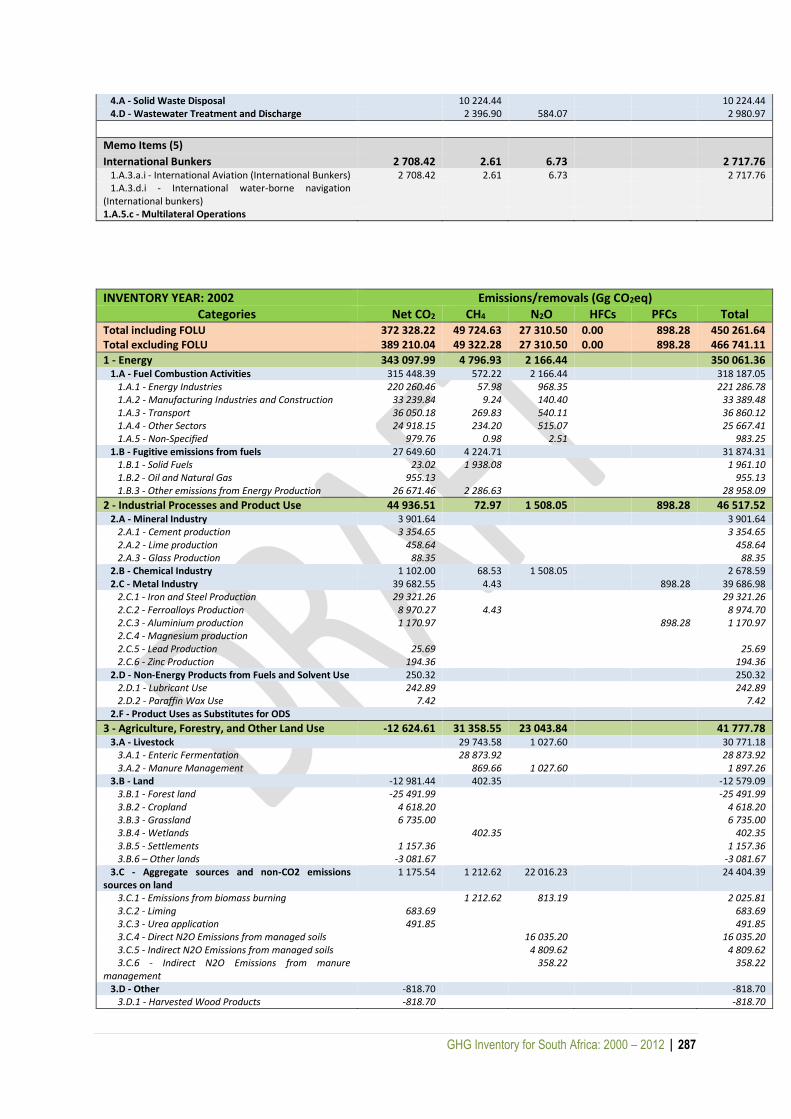
GHG Inventory for South Africa: 2000 – 2012 | 287

4.A - Solid Waste Disposal 10 224.44 10 224.44 4.D - Wastewater Treatment and Discharge 2 396.90 584.07 2 980.97

Memo Items (5) International Bunkers 2 708.42 2.61 6.73 2 717.76 1.A.3.a.i - International Aviation (International Bunkers) 2 708.42 2.61 6.73 2 717.76 1.A.3.d.i - International water-borne navigation (International bunkers)

1.A.5.c - Multilateral Operations

INVENTORY YEAR: 2002 Emissions/removals (Gg CO2eq) Categories Net CO2 CH4 N2O HFCs PFCs Total

Total including FOLU 372 328.22 49 724.63 27 310.50 0.00 898.28 450 261.64 Total excluding FOLU 389 210.04 49 322.28 27 310.50 0.00 898.28 466 741.11

1 - Energy 343 097.99 4 796.93 2 166.44 350 061.36 1.A - Fuel Combustion Activities 315 448.39 572.22 2 166.44 318 187.05 1.A.1 - Energy Industries 220 260.46 57.98 968.35 221 286.78 1.A.2 - Manufacturing Industries and Construction 33 239.84 9.24 140.40 33 389.48 1.A.3 - Transport 36 050.18 269.83 540.11 36 860.12 1.A.4 - Other Sectors 24 918.15 234.20 515.07 25 667.41 1.A.5 - Non-Specified 979.76 0.98 2.51 983.25 1.B - Fugitive emissions from fuels 27 649.60 4 224.71 31 874.31 1.B.1 - Solid Fuels 23.02 1 938.08 1 961.10 1.B.2 - Oil and Natural Gas 955.13 955.13 1.B.3 - Other emissions from Energy Production 26 671.46 2 286.63 28 958.09

2 - Industrial Processes and Product Use 44 936.51 72.97 1 508.05 898.28 46 517.52 2.A - Mineral Industry 3 901.64 3 901.64 2.A.1 - Cement production 3 354.65 3 354.65 2.A.2 - Lime production 458.64 458.64 2.A.3 - Glass Production 88.35 88.35 2.B - Chemical Industry 1 102.00 68.53 1 508.05 2 678.59 2.C - Metal Industry 39 682.55 4.43 898.28 39 686.98 2.C.1 - Iron and Steel Production 29 321.26 29 321.26 2.C.2 - Ferroalloys Production 8 970.27 4.43 8 974.70 2.C.3 - Aluminium production 1 170.97 898.28 1 170.97 2.C.4 - Magnesium production 2.C.5 - Lead Production 25.69 25.69 2.C.6 - Zinc Production 194.36 194.36 2.D - Non-Energy Products from Fuels and Solvent Use 250.32 250.32 2.D.1 - Lubricant Use 242.89 242.89 2.D.2 - Paraffin Wax Use 7.42 7.42 2.F - Product Uses as Substitutes for ODS

3 - Agriculture, Forestry, and Other Land Use -12 624.61 31 358.55 23 043.84 41 777.78 3.A - Livestock 29 743.58 1 027.60 30 771.18 3.A.1 - Enteric Fermentation 28 873.92 28 873.92 3.A.2 - Manure Management 869.66 1 027.60 1 897.26 3.B - Land -12 981.44 402.35 -12 579.09 3.B.1 - Forest land -25 491.99 -25 491.99 3.B.2 - Cropland 4 618.20 4 618.20 3.B.3 - Grassland 6 735.00 6 735.00 3.B.4 - Wetlands 402.35 402.35 3.B.5 - Settlements 1 157.36 1 157.36 3.B.6 – Other lands -3 081.67 -3 081.67 3.C - Aggregate sources and non-CO2 emissions sources on land

1 175.54 1 212.62 22 016.23 24 404.39

3.C.1 - Emissions from biomass burning 1 212.62 813.19 2 025.81 3.C.2 - Liming 683.69 683.69 3.C.3 - Urea application 491.85 491.85 3.C.4 - Direct N2O Emissions from managed soils 16 035.20 16 035.20 3.C.5 - Indirect N2O Emissions from managed soils 4 809.62 4 809.62 3.C.6 - Indirect N2O Emissions from manure management

358.22 358.22

3.D - Other -818.70 -818.70 3.D.1 - Harvested Wood Products -818.70 -818.70

GHG Inventory for South Africa: 2000 – 2012 | 288

4 - Waste 13 496.19 592.17 14 088.37 4.A - Solid Waste Disposal 11 066.05 11 066.05 4.D - Wastewater Treatment and Discharge 2 430.15 592.17 3 022.32

Memo Items (5) International Bunkers 2 686.97 2.59 6.67 2 696.24 1.A.3.a.i - International Aviation (International Bunkers) 2 686.97 2.59 6.67 2 696.24 1.A.3.d.i - International water-borne navigation (International bunkers)

1.A.5.c - Multilateral Operations

INVENTORY YEAR: 2003 Emissions/removals (Gg CO2eq) Categories Net CO2 CH4 N2O HFCs PFCs Total

Total including FOLU 395 147.45 49 818.38 25 872.64 0.00 896.23 471 734.70 Total excluding FOLU 413 366.94 49 429.48 25 872.64 0.00 896.23 489 565.30

1 - Energy 366 692.62 4 963.99 2 301.41 373 958.03 1.A - Fuel Combustion Activities 340 047.81 591.40 2 301.41 342 940.62 1.A.1 - Energy Industries 238 277.97 63.04 1 052.16 239 393.17 1.A.2 - Manufacturing Industries and Construction 35 738.40 9.93 150.49 35 898.82 1.A.3 - Transport 37 825.84 279.15 558.09 38 663.08 1.A.4 - Other Sectors 27 194.38 238.28 538.07 27 970.74 1.A.5 - Non-Specified 1 011.23 1.01 2.59 1 014.82 1.B - Fugitive emissions from fuels 26 644.81 4 372.59 31 017.40 1.B.1 - Solid Fuels 24.85 2 092.96 2 117.81 1.B.2 - Oil and Natural Gas 1 457.99 1 457.99 1.B.3 - Other emissions from Energy Production 25 161.97 2 279.63 27 441.60

2 - Industrial Processes and Product Use 45 757.13 75.65 936.31 896.23 46 769.09 2.A - Mineral Industry 4 138.81 4 138.81 2.A.1 - Cement production 3 577.14 3 577.14 2.A.2 - Lime production 470.34 470.34 2.A.3 - Glass Production 91.33 91.33 2.B - Chemical Industry 1 123.51 71.20 936.31 2 131.02 2.C - Metal Industry 40 246.20 4.45 896.23 40 250.65 2.C.1 - Iron and Steel Production 29 692.63 29 692.63 2.C.2 - Ferroalloys Production 9 156.40 4.45 9 160.85 2.C.3 - Aluminium production 1 182.06 896.23 1 182.06 2.C.4 - Magnesium production 2.C.5 - Lead Production 20.75 20.75 2.C.6 - Zinc Production 194.36 194.36 2.D - Non-Energy Products from Fuels and Solvent Use 248.61 248.61 2.D.1 - Lubricant Use 240.97 240.97 2.D.2 - Paraffin Wax Use 7.64 7.64 2.F - Product Uses as Substitutes for ODS

3 - Agriculture, Forestry, and Other Land Use -14 220.63 30 431.98 22 035.16 38 246.51 3.A - Livestock 29 143.08 1 050.50 30 193.58 3.A.1 - Enteric Fermentation 28 306.34 28 306.34 3.A.2 - Manure Management 836.74 1 050.50 1 887.24 3.B - Land -14 208.87 388.90 -13 819.97 3.B.1 - Forest land -26 816.21 -26 816.21 3.B.2 - Cropland 4 711.72 4 711.72 3.B.3 - Grassland 6 735.00 6 735.00 3.B.4 - Wetlands 388.90 388.90 3.B.5 - Settlements 1 160.63 1 160.63 3.B.6 – Other lands -3 081.67 -3 081.67 3.C - Aggregate sources and non-CO2 emissions sources on land

917.19 899.99 20 984.66 22 801.85

3.C.1 - Emissions from biomass burning 899.99 583.02 1 483.02 3.C.2 - Liming 585.99 585.99 3.C.3 - Urea application 331.20 331.20 3.C.4 - Direct N2O Emissions from managed soils 15 395.78 15 395.78 3.C.5 - Indirect N2O Emissions from managed soils 4 645.23 4 645.23 3.C.6 - Indirect N2O Emissions from manure management

360.63 360.63

3.D - Other -928.95 -928.95

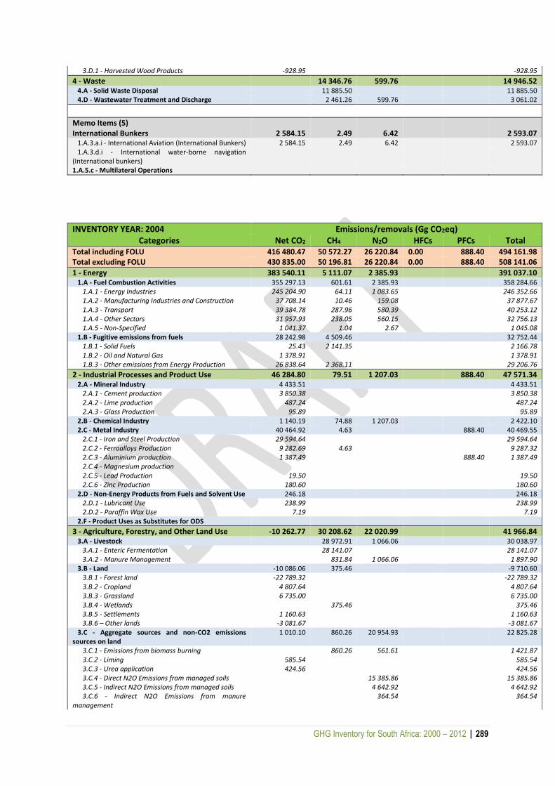
GHG Inventory for South Africa: 2000 – 2012 | 289

3.D.1 - Harvested Wood Products -928.95 -928.95

4 - Waste 14 346.76 599.76 14 946.52 4.A - Solid Waste Disposal 11 885.50 11 885.50 4.D - Wastewater Treatment and Discharge 2 461.26 599.76 3 061.02

Memo Items (5) International Bunkers 2 584.15 2.49 6.42 2 593.07 1.A.3.a.i - International Aviation (International Bunkers) 2 584.15 2.49 6.42 2 593.07 1.A.3.d.i - International water-borne navigation (International bunkers)

1.A.5.c - Multilateral Operations

INVENTORY YEAR: 2004 Emissions/removals (Gg CO2eq) Categories Net CO2 CH4 N2O HFCs PFCs Total

Total including FOLU 416 480.47 50 572.27 26 220.84 0.00 888.40 494 161.98 Total excluding FOLU 430 835.00 50 196.81 26 220.84 0.00 888.40 508 141.06

1 - Energy 383 540.11 5 111.07 2 385.93 391 037.10 1.A - Fuel Combustion Activities 355 297.13 601.61 2 385.93 358 284.66 1.A.1 - Energy Industries 245 204.90 64.11 1 083.65 246 352.66 1.A.2 - Manufacturing Industries and Construction 37 708.14 10.46 159.08 37 877.67 1.A.3 - Transport 39 384.78 287.96 580.39 40 253.12 1.A.4 - Other Sectors 31 957.93 238.05 560.15 32 756.13 1.A.5 - Non-Specified 1 041.37 1.04 2.67 1 045.08 1.B - Fugitive emissions from fuels 28 242.98 4 509.46 32 752.44 1.B.1 - Solid Fuels 25.43 2 141.35 2 166.78 1.B.2 - Oil and Natural Gas 1 378.91 1 378.91 1.B.3 - Other emissions from Energy Production 26 838.64 2 368.11 29 206.76

2 - Industrial Processes and Product Use 46 284.80 79.51 1 207.03 888.40 47 571.34 2.A - Mineral Industry 4 433.51 4 433.51 2.A.1 - Cement production 3 850.38 3 850.38 2.A.2 - Lime production 487.24 487.24 2.A.3 - Glass Production 95.89 95.89 2.B - Chemical Industry 1 140.19 74.88 1 207.03 2 422.10 2.C - Metal Industry 40 464.92 4.63 888.40 40 469.55 2.C.1 - Iron and Steel Production 29 594.64 29 594.64 2.C.2 - Ferroalloys Production 9 282.69 4.63 9 287.32 2.C.3 - Aluminium production 1 387.49 888.40 1 387.49 2.C.4 - Magnesium production 2.C.5 - Lead Production 19.50 19.50 2.C.6 - Zinc Production 180.60 180.60 2.D - Non-Energy Products from Fuels and Solvent Use 246.18 246.18 2.D.1 - Lubricant Use 238.99 238.99 2.D.2 - Paraffin Wax Use 7.19 7.19 2.F - Product Uses as Substitutes for ODS

3 - Agriculture, Forestry, and Other Land Use -10 262.77 30 208.62 22 020.99 41 966.84 3.A - Livestock 28 972.91 1 066.06 30 038.97 3.A.1 - Enteric Fermentation 28 141.07 28 141.07 3.A.2 - Manure Management 831.84 1 066.06 1 897.90 3.B - Land -10 086.06 375.46 -9 710.60 3.B.1 - Forest land -22 789.32 -22 789.32 3.B.2 - Cropland 4 807.64 4 807.64 3.B.3 - Grassland 6 735.00 6 735.00 3.B.4 - Wetlands 375.46 375.46 3.B.5 - Settlements 1 160.63 1 160.63 3.B.6 – Other lands -3 081.67 -3 081.67 3.C - Aggregate sources and non-CO2 emissions sources on land

1 010.10 860.26 20 954.93 22 825.28

3.C.1 - Emissions from biomass burning 860.26 561.61 1 421.87 3.C.2 - Liming 585.54 585.54 3.C.3 - Urea application 424.56 424.56 3.C.4 - Direct N2O Emissions from managed soils 15 385.86 15 385.86 3.C.5 - Indirect N2O Emissions from managed soils 4 642.92 4 642.92 3.C.6 - Indirect N2O Emissions from manure management

364.54 364.54

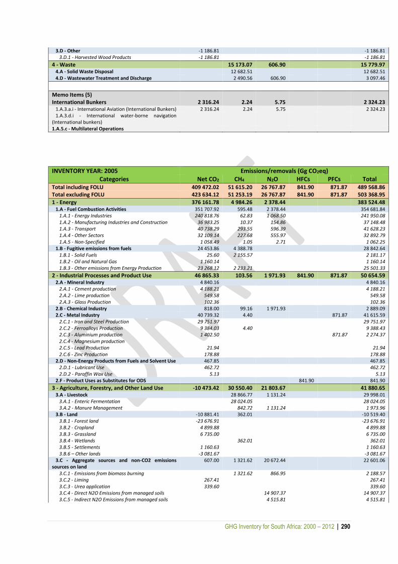
GHG Inventory for South Africa: 2000 – 2012 | 290

3.D - Other -1 186.81 -1 186.81 3.D.1 - Harvested Wood Products -1 186.81 -1 186.81

4 - Waste 15 173.07 606.90 15 779.97 4.A - Solid Waste Disposal 12 682.51 12 682.51 4.D - Wastewater Treatment and Discharge 2 490.56 606.90 3 097.46

Memo Items (5) International Bunkers 2 316.24 2.24 5.75 2 324.23 1.A.3.a.i - International Aviation (International Bunkers) 2 316.24 2.24 5.75 2 324.23 1.A.3.d.i - International water-borne navigation (International bunkers)

1.A.5.c - Multilateral Operations

INVENTORY YEAR: 2005 Emissions/removals (Gg CO2eq) Categories Net CO2 CH4 N2O HFCs PFCs Total

Total including FOLU 409 472.02 51 615.20 26 767.87 841.90 871.87 489 568.86 Total excluding FOLU 423 634.12 51 253.19 26 767.87 841.90 871.87 503 368.95

1 - Energy 376 161.78 4 984.26 2 378.44 383 524.48 1.A - Fuel Combustion Activities 351 707.92 595.48 2 378.44 354 681.84 1.A.1 - Energy Industries 240 818.76 62.83 1 068.50 241 950.08 1.A.2 - Manufacturing Industries and Construction 36 983.25 10.37 154.86 37 148.48 1.A.3 - Transport 40 738.29 293.55 596.39 41 628.23 1.A.4 - Other Sectors 32 109.14 227.68 555.97 32 892.79 1.A.5 - Non-Specified 1 058.49 1.05 2.71 1 062.25 1.B - Fugitive emissions from fuels 24 453.86 4 388.78 28 842.64 1.B.1 - Solid Fuels 25.60 2 155.57 2 181.17 1.B.2 - Oil and Natural Gas 1 160.14 1 160.14 1.B.3 - Other emissions from Energy Production 23 268.12 2 233.21 25 501.33

2 - Industrial Processes and Product Use 46 865.33 103.56 1 971.93 841.90 871.87 50 654.59 2.A - Mineral Industry 4 840.16 4 840.16 2.A.1 - Cement production 4 188.21 4 188.21 2.A.2 - Lime production 549.58 549.58 2.A.3 - Glass Production 102.36 102.36 2.B - Chemical Industry 818.00 99.16 1 971.93 2 889.09 2.C - Metal Industry 40 739.32 4.40 871.87 41 615.59 2.C.1 - Iron and Steel Production 29 751.97 29 751.97 2.C.2 - Ferroalloys Production 9 384.03 4.40 9 388.43 2.C.3 - Aluminium production 1 402.50 871.87 2 274.37 2.C.4 - Magnesium production 2.C.5 - Lead Production 21.94 21.94 2.C.6 - Zinc Production 178.88 178.88 2.D - Non-Energy Products from Fuels and Solvent Use 467.85 467.85 2.D.1 - Lubricant Use 462.72 462.72 2.D.2 - Paraffin Wax Use 5.13 5.13 2.F - Product Uses as Substitutes for ODS 841.90 841.90

3 - Agriculture, Forestry, and Other Land Use -10 473.42 30 550.40 21 803.67 41 880.65 3.A - Livestock 28 866.77 1 131.24 29 998.01 3.A.1 - Enteric Fermentation 28 024.05 28 024.05 3.A.2 - Manure Management 842.72 1 131.24 1 973.96 3.B - Land -10 881.41 362.01 -10 519.40 3.B.1 - Forest land -23 676.91 -23 676.91 3.B.2 - Cropland 4 899.88 4 899.88 3.B.3 - Grassland 6 735.00 6 735.00 3.B.4 - Wetlands 362.01 362.01 3.B.5 - Settlements 1 160.63 1 160.63 3.B.6 – Other lands -3 081.67 -3 081.67 3.C - Aggregate sources and non-CO2 emissions sources on land

607.00 1 321.62 20 672.44 22 601.06

3.C.1 - Emissions from biomass burning 1 321.62 866.95 2 188.57 3.C.2 - Liming 267.41 267.41 3.C.3 - Urea application 339.60 339.60 3.C.4 - Direct N2O Emissions from managed soils 14 907.37 14 907.37 3.C.5 - Indirect N2O Emissions from managed soils 4 515.81 4 515.81

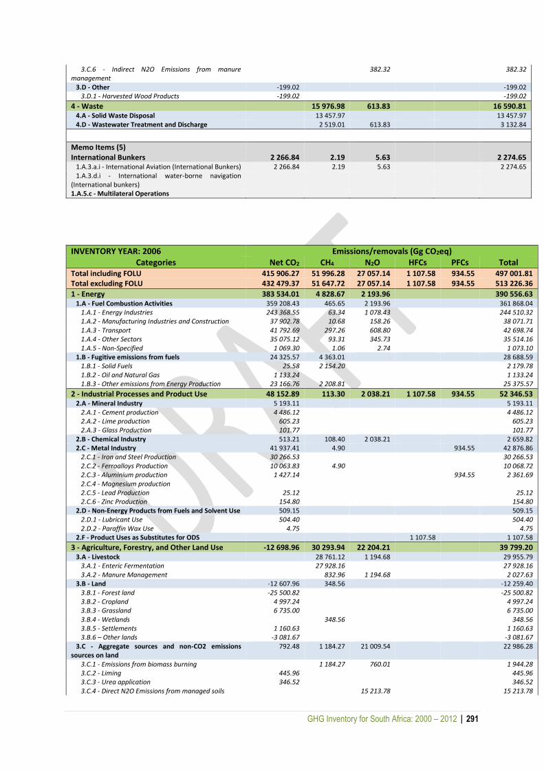
GHG Inventory for South Africa: 2000 – 2012 | 291

3.C.6 - Indirect N2O Emissions from manure management

382.32 382.32

3.D - Other -199.02 -199.02 3.D.1 - Harvested Wood Products -199.02 -199.02

4 - Waste 15 976.98 613.83 16 590.81 4.A - Solid Waste Disposal 13 457.97 13 457.97 4.D - Wastewater Treatment and Discharge 2 519.01 613.83 3 132.84

Memo Items (5) International Bunkers 2 266.84 2.19 5.63 2 274.65 1.A.3.a.i - International Aviation (International Bunkers) 2 266.84 2.19 5.63 2 274.65 1.A.3.d.i - International water-borne navigation (International bunkers)

1.A.5.c - Multilateral Operations

INVENTORY YEAR: 2006 Emissions/removals (Gg CO2eq) Categories Net CO2 CH4 N2O HFCs PFCs Total

Total including FOLU 415 906.27 51 996.28 27 057.14 1 107.58 934.55 497 001.81 Total excluding FOLU 432 479.37 51 647.72 27 057.14 1 107.58 934.55 513 226.36

1 - Energy 383 534.01 4 828.67 2 193.96 390 556.63 1.A - Fuel Combustion Activities 359 208.43 465.65 2 193.96 361 868.04 1.A.1 - Energy Industries 243 368.55 63.34 1 078.43 244 510.32 1.A.2 - Manufacturing Industries and Construction 37 902.78 10.68 158.26 38 071.71 1.A.3 - Transport 41 792.69 297.26 608.80 42 698.74 1.A.4 - Other Sectors 35 075.12 93.31 345.73 35 514.16 1.A.5 - Non-Specified 1 069.30 1.06 2.74 1 073.10 1.B - Fugitive emissions from fuels 24 325.57 4 363.01 28 688.59 1.B.1 - Solid Fuels 25.58 2 154.20 2 179.78 1.B.2 - Oil and Natural Gas 1 133.24 1 133.24 1.B.3 - Other emissions from Energy Production 23 166.76 2 208.81 25 375.57

2 - Industrial Processes and Product Use 48 152.89 113.30 2 038.21 1 107.58 934.55 52 346.53 2.A - Mineral Industry 5 193.11 5 193.11 2.A.1 - Cement production 4 486.12 4 486.12 2.A.2 - Lime production 605.23 605.23 2.A.3 - Glass Production 101.77 101.77 2.B - Chemical Industry 513.21 108.40 2 038.21 2 659.82 2.C - Metal Industry 41 937.41 4.90 934.55 42 876.86 2.C.1 - Iron and Steel Production 30 266.53 30 266.53 2.C.2 - Ferroalloys Production 10 063.83 4.90 10 068.72 2.C.3 - Aluminium production 1 427.14 934.55 2 361.69 2.C.4 - Magnesium production 2.C.5 - Lead Production 25.12 25.12 2.C.6 - Zinc Production 154.80 154.80 2.D - Non-Energy Products from Fuels and Solvent Use 509.15 509.15 2.D.1 - Lubricant Use 504.40 504.40 2.D.2 - Paraffin Wax Use 4.75 4.75 2.F - Product Uses as Substitutes for ODS 1 107.58 1 107.58

3 - Agriculture, Forestry, and Other Land Use -12 698.96 30 293.94 22 204.21 39 799.20 3.A - Livestock 28 761.12 1 194.68 29 955.79 3.A.1 - Enteric Fermentation 27 928.16 27 928.16 3.A.2 - Manure Management 832.96 1 194.68 2 027.63 3.B - Land -12 607.96 348.56 -12 259.40 3.B.1 - Forest land -25 500.82 -25 500.82 3.B.2 - Cropland 4 997.24 4 997.24 3.B.3 - Grassland 6 735.00 6 735.00 3.B.4 - Wetlands 348.56 348.56 3.B.5 - Settlements 1 160.63 1 160.63 3.B.6 – Other lands -3 081.67 -3 081.67 3.C - Aggregate sources and non-CO2 emissions sources on land

792.48 1 184.27 21 009.54 22 986.28

3.C.1 - Emissions from biomass burning 1 184.27 760.01 1 944.28 3.C.2 - Liming 445.96 445.96 3.C.3 - Urea application 346.52 346.52 3.C.4 - Direct N2O Emissions from managed soils 15 213.78 15 213.78

GHG Inventory for South Africa: 2000 – 2012 | 292

3.C.5 - Indirect N2O Emissions from managed soils 4 637.90 4 637.90 3.C.6 - Indirect N2O Emissions from manure management

397.84 397.84

3.D - Other -883.48 -883.48 3.D.1 - Harvested Wood Products -883.48 -883.48

4 - Waste 16 760.37 620.76 17 381.13 4.A - Solid Waste Disposal 14 212.91 0.00 14 212.91 4.D - Wastewater Treatment and Discharge 2 547.46 620.76 3 168.22

Memo Items (5) International Bunkers 2 509.65 2.42 6.23 2 518.31 1.A.3.a.i - International Aviation (International Bunkers) 2 509.65 2.42 6.23 2 518.31 1.A.3.d.i - International water-borne navigation (International bunkers)

1.A.5.c - Multilateral Operations

INVENTORY YEAR: 2007 Emissions/removals (Gg CO2eq) Categories Net CO2 CH4 N2O HFCs PFCs Total

Total including FOLU 441 954.84 52 120.92 25 786.70 1 077.88 970.11 521 910.46 Total excluding FOLU 459 556.11 51 785.81 25 786.70 1 077.88 970.11 539 176.62

1 - Energy 411 570.89 4 970.80 2 344.64 418 886.32 1.A - Fuel Combustion Activities 387 062.72 483.81 2 344.64 389 891.16 1.A.1 - Energy Industries 266 254.35 69.28 1 183.91 267 507.54 1.A.2 - Manufacturing Industries and Construction 39 287.73 11.14 163.64 39 462.51 1.A.3 - Transport 44 230.25 306.27 643.74 45 180.26 1.A.4 - Other Sectors 36 194.68 96.03 350.54 36 641.25 1.A.5 - Non-Specified 1 095.70 1.09 2.81 1 099.60 1.B - Fugitive emissions from fuels 24 508.17 4 486.99 28 995.16 1.B.1 - Solid Fuels 25.88 2 179.14 2 205.01 1.B.2 - Oil and Natural Gas 1 132.69 1 132.69 1.B.3 - Other emissions from Energy Production 23 349.60 2 307.86 25 657.46

2 - Industrial Processes and Product Use 47 000.41 152.84 1 195.78 1 077.88 970.11 50 397.03 2.A - Mineral Industry 5 217.15 5 217.15 2.A.1 - Cement production 4 582.68 4 582.68 2.A.2 - Lime production 529.48 529.48 2.A.3 - Glass Production 104.99 104.99 2.B - Chemical Industry 581.39 148.25 1 195.78 1 925.41 2.C - Metal Industry 40 967.79 4.60 970.11 41 942.50 2.C.1 - Iron and Steel Production 28 038.77 28 038.77 2.C.2 - Ferroalloys Production 11 245.95 4.60 11 250.55 2.C.3 - Aluminium production 1 487.57 970.11 2 457.68 2.C.4 - Magnesium production 2.C.5 - Lead Production 21.79 21.79 2.C.6 - Zinc Production 173.72 173.72 2.D - Non-Energy Products from Fuels and Solvent Use 234.08 234.08 2.D.1 - Lubricant Use 232.01 232.01 2.D.2 - Paraffin Wax Use 2.07 2.07 2.F - Product Uses as Substitutes for ODS 1 077.88 1 077.88

3 - Agriculture, Forestry, and Other Land Use -13 534.78 29 473.12 21 618.68 37 557.02 3.A - Livestock 28 088.53 1 236.93 29 325.46 3.A.1 - Enteric Fermentation 27 238.59 27 238.59 3.A.2 - Manure Management 849.94 1 236.93 2 086.87 3.B - Land -13 936.56 335.11 -13 601.45 3.B.1 - Forest land -26 929.62 -26 929.62 3.B.2 - Cropland 5 097.44 5 097.44 3.B.3 - Grassland 6 735.00 6 735.00 3.B.4 - Wetlands 335.11 335.11 3.B.5 - Settlements 1 160.63 1 160.63 3.B.6 – Other lands -3 081.67 -3 081.67 3.C - Aggregate sources and non-CO2 emissions sources on land

984.81 1 049.48 20 381.76 22 416.05

3.C.1 - Emissions from biomass burning 1 049.48 659.30 1 708.78 3.C.2 - Liming 524.87 524.87 3.C.3 - Urea application 459.94 459.94

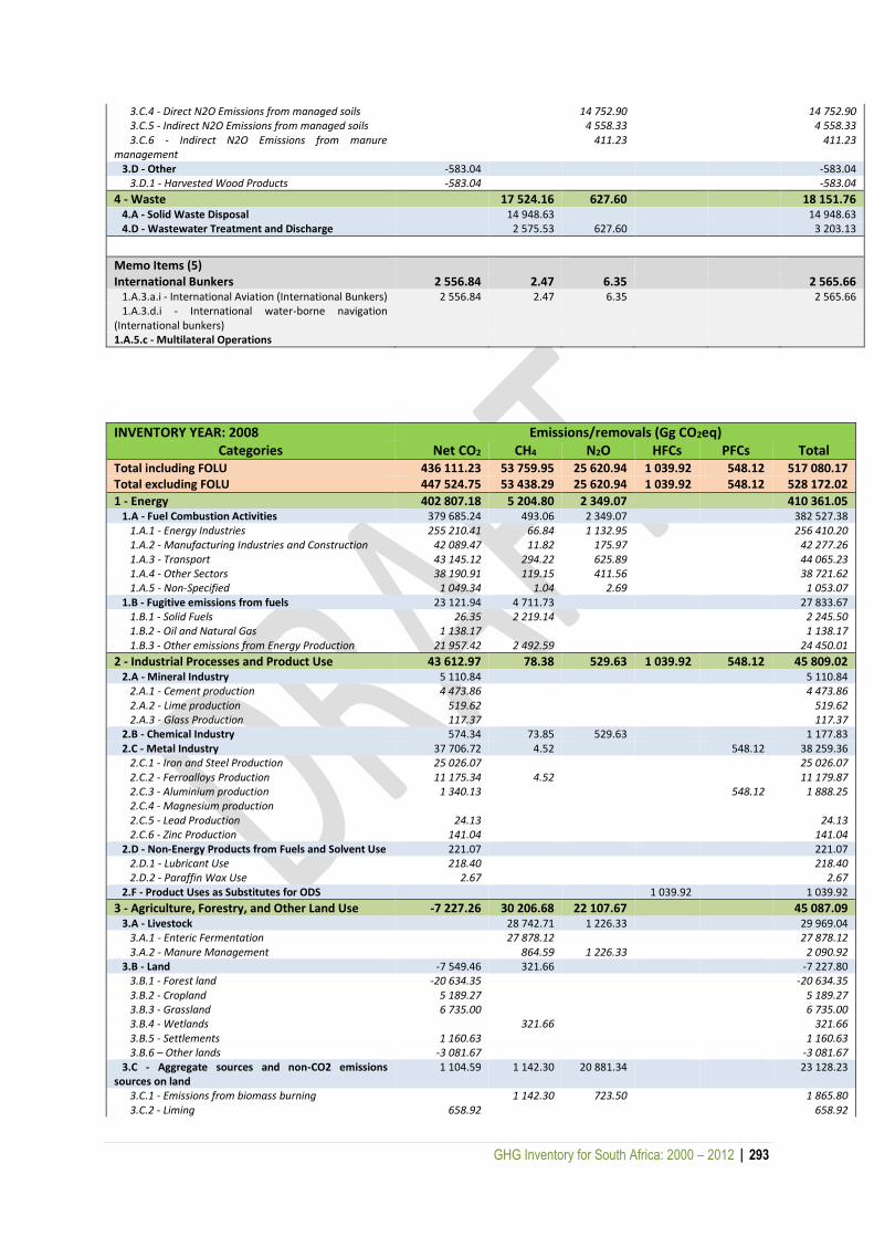
GHG Inventory for South Africa: 2000 – 2012 | 293

3.C.4 - Direct N2O Emissions from managed soils 14 752.90 14 752.90 3.C.5 - Indirect N2O Emissions from managed soils 4 558.33 4 558.33 3.C.6 - Indirect N2O Emissions from manure management

411.23 411.23

3.D - Other -583.04 -583.04 3.D.1 - Harvested Wood Products -583.04 -583.04

4 - Waste 17 524.16 627.60 18 151.76 4.A - Solid Waste Disposal 14 948.63 14 948.63 4.D - Wastewater Treatment and Discharge 2 575.53 627.60 3 203.13

Memo Items (5) International Bunkers 2 556.84 2.47 6.35 2 565.66 1.A.3.a.i - International Aviation (International Bunkers) 2 556.84 2.47 6.35 2 565.66 1.A.3.d.i - International water-borne navigation (International bunkers)

1.A.5.c - Multilateral Operations

INVENTORY YEAR: 2008 Emissions/removals (Gg CO2eq) Categories Net CO2 CH4 N2O HFCs PFCs Total

Total including FOLU 436 111.23 53 759.95 25 620.94 1 039.92 548.12 517 080.17 Total excluding FOLU 447 524.75 53 438.29 25 620.94 1 039.92 548.12 528 172.02

1 - Energy 402 807.18 5 204.80 2 349.07 410 361.05 1.A - Fuel Combustion Activities 379 685.24 493.06 2 349.07 382 527.38 1.A.1 - Energy Industries 255 210.41 66.84 1 132.95 256 410.20 1.A.2 - Manufacturing Industries and Construction 42 089.47 11.82 175.97 42 277.26 1.A.3 - Transport 43 145.12 294.22 625.89 44 065.23 1.A.4 - Other Sectors 38 190.91 119.15 411.56 38 721.62 1.A.5 - Non-Specified 1 049.34 1.04 2.69 1 053.07 1.B - Fugitive emissions from fuels 23 121.94 4 711.73 27 833.67 1.B.1 - Solid Fuels 26.35 2 219.14 2 245.50 1.B.2 - Oil and Natural Gas 1 138.17 1 138.17 1.B.3 - Other emissions from Energy Production 21 957.42 2 492.59 24 450.01

2 - Industrial Processes and Product Use 43 612.97 78.38 529.63 1 039.92 548.12 45 809.02 2.A - Mineral Industry 5 110.84 5 110.84 2.A.1 - Cement production 4 473.86 4 473.86 2.A.2 - Lime production 519.62 519.62 2.A.3 - Glass Production 117.37 117.37 2.B - Chemical Industry 574.34 73.85 529.63 1 177.83 2.C - Metal Industry 37 706.72 4.52 548.12 38 259.36 2.C.1 - Iron and Steel Production 25 026.07 25 026.07 2.C.2 - Ferroalloys Production 11 175.34 4.52 11 179.87 2.C.3 - Aluminium production 1 340.13 548.12 1 888.25 2.C.4 - Magnesium production 2.C.5 - Lead Production 24.13 24.13 2.C.6 - Zinc Production 141.04 141.04 2.D - Non-Energy Products from Fuels and Solvent Use 221.07 221.07 2.D.1 - Lubricant Use 218.40 218.40 2.D.2 - Paraffin Wax Use 2.67 2.67 2.F - Product Uses as Substitutes for ODS 1 039.92 1 039.92

3 - Agriculture, Forestry, and Other Land Use -7 227.26 30 206.68 22 107.67 45 087.09 3.A - Livestock 28 742.71 1 226.33 29 969.04 3.A.1 - Enteric Fermentation 27 878.12 27 878.12 3.A.2 - Manure Management 864.59 1 226.33 2 090.92 3.B - Land -7 549.46 321.66 -7 227.80 3.B.1 - Forest land -20 634.35 -20 634.35 3.B.2 - Cropland 5 189.27 5 189.27 3.B.3 - Grassland 6 735.00 6 735.00 3.B.4 - Wetlands 321.66 321.66 3.B.5 - Settlements 1 160.63 1 160.63 3.B.6 – Other lands -3 081.67 -3 081.67 3.C - Aggregate sources and non-CO2 emissions sources on land

1 104.59 1 142.30 20 881.34 23 128.23

3.C.1 - Emissions from biomass burning 1 142.30 723.50 1 865.80 3.C.2 - Liming 658.92 658.92

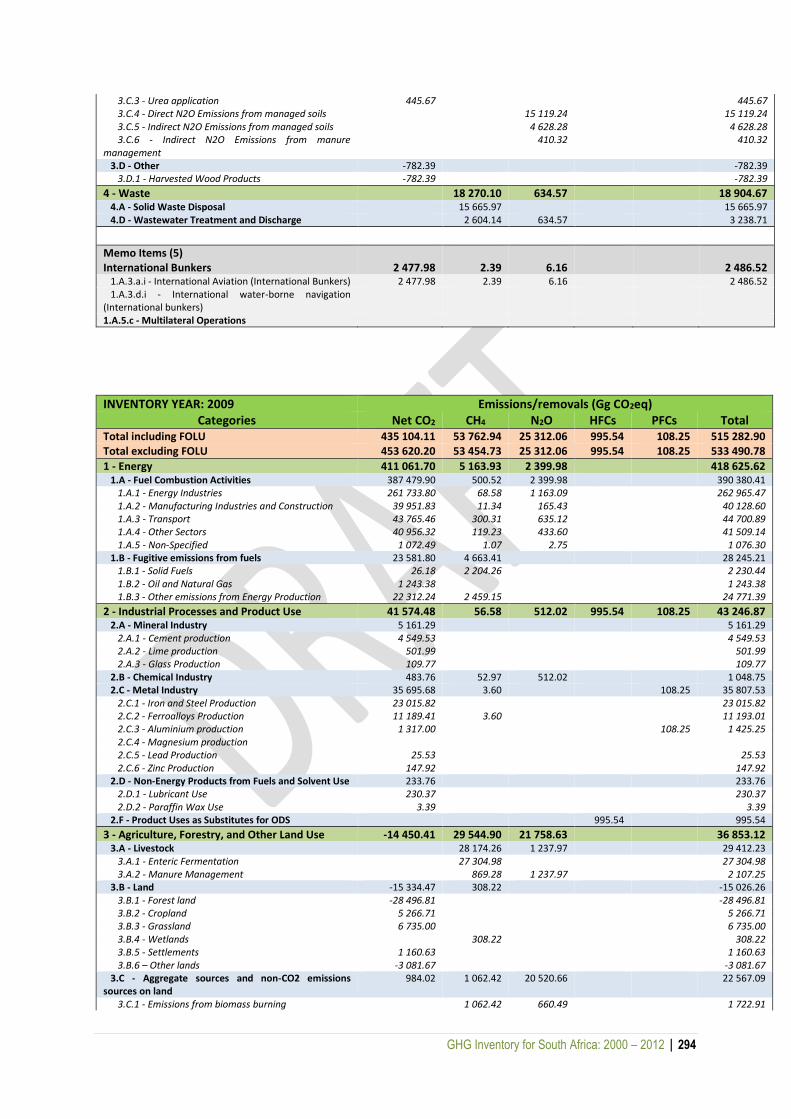
GHG Inventory for South Africa: 2000 – 2012 | 294

3.C.3 - Urea application 445.67 445.67 3.C.4 - Direct N2O Emissions from managed soils 15 119.24 15 119.24 3.C.5 - Indirect N2O Emissions from managed soils 4 628.28 4 628.28 3.C.6 - Indirect N2O Emissions from manure management

410.32 410.32

3.D - Other -782.39 -782.39 3.D.1 - Harvested Wood Products -782.39 -782.39

4 - Waste 18 270.10 634.57 18 904.67 4.A - Solid Waste Disposal 15 665.97 15 665.97 4.D - Wastewater Treatment and Discharge 2 604.14 634.57 3 238.71

Memo Items (5) International Bunkers 2 477.98 2.39 6.16 2 486.52 1.A.3.a.i - International Aviation (International Bunkers) 2 477.98 2.39 6.16 2 486.52 1.A.3.d.i - International water-borne navigation (International bunkers)

1.A.5.c - Multilateral Operations

INVENTORY YEAR: 2009 Emissions/removals (Gg CO2eq) Categories Net CO2 CH4 N2O HFCs PFCs Total

Total including FOLU 435 104.11 53 762.94 25 312.06 995.54 108.25 515 282.90 Total excluding FOLU 453 620.20 53 454.73 25 312.06 995.54 108.25 533 490.78

1 - Energy 411 061.70 5 163.93 2 399.98 418 625.62 1.A - Fuel Combustion Activities 387 479.90 500.52 2 399.98 390 380.41 1.A.1 - Energy Industries 261 733.80 68.58 1 163.09 262 965.47 1.A.2 - Manufacturing Industries and Construction 39 951.83 11.34 165.43 40 128.60 1.A.3 - Transport 43 765.46 300.31 635.12 44 700.89 1.A.4 - Other Sectors 40 956.32 119.23 433.60 41 509.14 1.A.5 - Non-Specified 1 072.49 1.07 2.75 1 076.30 1.B - Fugitive emissions from fuels 23 581.80 4 663.41 28 245.21 1.B.1 - Solid Fuels 26.18 2 204.26 2 230.44 1.B.2 - Oil and Natural Gas 1 243.38 1 243.38 1.B.3 - Other emissions from Energy Production 22 312.24 2 459.15 24 771.39

2 - Industrial Processes and Product Use 41 574.48 56.58 512.02 995.54 108.25 43 246.87 2.A - Mineral Industry 5 161.29 5 161.29 2.A.1 - Cement production 4 549.53 4 549.53 2.A.2 - Lime production 501.99 501.99 2.A.3 - Glass Production 109.77 109.77 2.B - Chemical Industry 483.76 52.97 512.02 1 048.75 2.C - Metal Industry 35 695.68 3.60 108.25 35 807.53 2.C.1 - Iron and Steel Production 23 015.82 23 015.82 2.C.2 - Ferroalloys Production 11 189.41 3.60 11 193.01 2.C.3 - Aluminium production 1 317.00 108.25 1 425.25 2.C.4 - Magnesium production 2.C.5 - Lead Production 25.53 25.53 2.C.6 - Zinc Production 147.92 147.92 2.D - Non-Energy Products from Fuels and Solvent Use 233.76 233.76 2.D.1 - Lubricant Use 230.37 230.37 2.D.2 - Paraffin Wax Use 3.39 3.39 2.F - Product Uses as Substitutes for ODS 995.54 995.54

3 - Agriculture, Forestry, and Other Land Use -14 450.41 29 544.90 21 758.63 36 853.12 3.A - Livestock 28 174.26 1 237.97 29 412.23 3.A.1 - Enteric Fermentation 27 304.98 27 304.98 3.A.2 - Manure Management 869.28 1 237.97 2 107.25 3.B - Land -15 334.47 308.22 -15 026.26 3.B.1 - Forest land -28 496.81 -28 496.81 3.B.2 - Cropland 5 266.71 5 266.71 3.B.3 - Grassland 6 735.00 6 735.00 3.B.4 - Wetlands 308.22 308.22 3.B.5 - Settlements 1 160.63 1 160.63 3.B.6 – Other lands -3 081.67 -3 081.67 3.C - Aggregate sources and non-CO2 emissions sources on land

984.02 1 062.42 20 520.66 22 567.09

3.C.1 - Emissions from biomass burning 1 062.42 660.49 1 722.91

GHG Inventory for South Africa: 2000 – 2012 | 295

3.C.2 - Liming 616.23 616.23 3.C.3 - Urea application 367.79 367.79 3.C.4 - Direct N2O Emissions from managed soils 14 860.12 14 860.12 3.C.5 - Indirect N2O Emissions from managed soils 4 587.21 4 587.21 3.C.6 - Indirect N2O Emissions from manure management

412.83 412.83

3.D - Other -99.95 -99.95 3.D.1 - Harvested Wood Products -99.95 -99.95

4 - Waste 18 997.54 641.43 19 638.96 4.A - Solid Waste Disposal 16 365.27 16 365.27 4.D - Wastewater Treatment and Discharge 2 632.26 641.43 3 273.69

Memo Items (5) International Bunkers 2 422.71 2.34 6.02 2 431.06 1.A.3.a.i - International Aviation (International Bunkers) 2 422.71 2.34 6.02 2 431.06 1.A.3.d.i - International water-borne navigation (International bunkers)

1.A.5.c - Multilateral Operations

INVENTORY YEAR: 2010 Emissions/removals (Gg CO2eq) Categories Net CO2 CH4 N2O HFCs PFCs Total

Total including FOLU 447 801.66 55 555.25 25 724.59 2 096.25 138.26 531 316.01 Total excluding FOLU 468 493.12 55 260.48 25 724.59 2 096.25 138.26 551 712.70

1 - Energy 424 313.26 5 195.55 2 485.42 431 994.23 1.A - Fuel Combustion Activities 401 333.61 516.31 2 485.42 404 335.34 1.A.1 - Energy Industries 267 960.07 69.82 1 193.33 269 223.23 1.A.2 - Manufacturing Industries and Construction 40 936.94 11.70 168.81 41 117.45 1.A.3 - Transport 46 617.91 318.14 670.45 47 606.50 1.A.4 - Other Sectors 44 683.84 115.51 449.93 45 249.27 1.A.5 - Non-Specified 1 134.86 1.13 2.91 1 138.90 1.B - Fugitive emissions from fuels 22 979.64 4 679.24 27 658.88 1.B.1 - Solid Fuels 26.59 2 239.46 2 266.05 1.B.2 - Oil and Natural Gas 964.25 964.25 1.B.3 - Other emissions from Energy Production 21 988.80 2 439.79 24 428.59

2 - Industrial Processes and Product Use 43 109.80 67.13 325.54 2 096.25 138.26 45 736.97 2.A - Mineral Industry 4 792.86 4 792.86 2.A.1 - Cement production 4 186.74 4 186.74 2.A.2 - Lime production 502.24 502.24 2.A.3 - Glass Production 103.88 103.88 2.B - Chemical Industry 622.89 62.88 325.54 1 011.31 2.C - Metal Industry 37 460.18 4.24 138.26 37 602.68 2.C.1 - Iron and Steel Production 24 146.87 24 146.87 2.C.2 - Ferroalloys Production 11 810.79 4.24 11 815.03 2.C.3 - Aluminium production 1 330.00 138.26 1 468.26 2.C.4 - Magnesium production 2.C.5 - Lead Production 26.31 26.31 2.C.6 - Zinc Production 146.20 146.20 2.D - Non-Energy Products from Fuels and Solvent Use 233.87 233.87 2.D.1 - Lubricant Use 230.49 230.49 2.D.2 - Paraffin Wax Use 3.39 3.39 2.F - Product Uses as Substitutes for ODS 2 096.25 2 096.25

3 - Agriculture, Forestry, and Other Land Use -16 539.73 30 586.77 22 265.05 36 312.10 3.A - Livestock 28 996.25 1 249.22 30 245.47 3.A.1 - Enteric Fermentation 28 132.82 28 132.82 3.A.2 - Manure Management 863.44 1 249.22 2 112.65 3.B - Land -17 117.93 294.77 -16 823.16 3.B.1 - Forest land -30 387.13 -30 387.13 3.B.2 - Cropland 5 373.58 5 373.58 3.B.3 - Grassland 6 735.00 6 735.00 3.B.4 - Wetlands 294.77 294.77 3.B.5 - Settlements 1 160.63 1 160.63 3.B.6 – Other lands -3 081.67 -3 081.67 3.C - Aggregate sources and non-CO2 emissions sources on land

1 070.06 1 295.75 21 015.84 23 381.65

GHG Inventory for South Africa: 2000 – 2012 | 296

3.C.1 - Emissions from biomass burning 1 295.75 826.07 2 121.83 3.C.2 - Liming 585.54 585.54 3.C.3 - Urea application 484.52 484.52 3.C.4 - Direct N2O Emissions from managed soils 15 162.46 15 162.46 3.C.5 - Indirect N2O Emissions from managed soils 4 612.45 4 612.45 3.C.6 - Indirect N2O Emissions from manure management

414.85 414.85

3.D - Other -491.86 -491.86 3.D.1 - Harvested Wood Products -491.86 -491.86

4 - Waste 19 705.80 648.58 20 354.38 4.A - Solid Waste Disposal 17 044.19 17 044.19 4.D - Wastewater Treatment and Discharge 2 661.62 648.58 3 310.20

Memo Items (5) International Bunkers 2 563.63 2.47 6.37 2 572.47 1.A.3.a.i - International Aviation (International Bunkers) 2 563.63 2.47 6.37 2 572.47 1.A.3.d.i - International water-borne navigation (International bunkers)

1.A.5.c - Multilateral Operations

INVENTORY YEAR: 2011 Emissions/removals (Gg CO2eq) Categories Net CO2 CH4 N2O HFCs PFCs Total

Total including FOLU 427 189.30 56 997.92 26 223.72 1 749.86 2 410.85 514 571.65 Total excluding FOLU 448 220.19 56 716.60 26 223.72 1 749.86 2 410.85 535 321.22

1 - Energy 404 395.67 5 919.61 2 360.72 412 676.00 1.A - Fuel Combustion Activities 382 128.92 509.11 2 360.72 384 998.76 1.A.1 - Energy Industries 266 253.47 69.62 1 184.55 267 507.64 1.A.2 - Manufacturing Industries and Construction 28 289.72 8.54 114.31 28 412.56 1.A.3 - Transport 47 293.87 318.80 669.94 48 282.61 1.A.4 - Other Sectors 39 157.78 111.02 389.01 39 657.81 1.A.5 - Non-Specified 1 134.09 1.13 2.91 1 138.13 1.B - Fugitive emissions from fuels 22 266.75 5 410.49 27 677.24 1.B.1 - Solid Fuels 35.05 2 951.32 2 986.37 1.B.2 - Oil and Natural Gas 785.76 785.76 1.B.3 - Other emissions from Energy Production 21 445.93 2 459.17 23 905.10

2 - Industrial Processes and Product Use 42 687.86 92.45 643.36 1 749.86 2 410.85 47 584.38 2.A - Mineral Industry 4 512.70 4 512.70 2.A.1 - Cement production 3 849.20 3 849.20 2.A.2 - Lime production 557.45 557.45 2.A.3 - Glass Production 106.05 106.05 2.B - Chemical Industry 671.58 87.93 643.36 1 402.87 2.C - Metal Industry 37 307.19 4.52 2 410.85 39 722.56 2.C.1 - Iron and Steel Production 24 097.08 24 097.08 2.C.2 - Ferroalloys Production 11 758.45 4.52 11 762.97 2.C.3 - Aluminium production 1 299.50 2 410.85 3 710.35 2.C.4 - Magnesium production 0.00 2.C.5 - Lead Production 28.32 28.32 2.C.6 - Zinc Production 123.84 123.84 2.D - Non-Energy Products from Fuels and Solvent Use 196.39 268.00 2.D.1 - Lubricant Use 192.57 250.58 2.D.2 - Paraffin Wax Use 3.81 17.42 2.F - Product Uses as Substitutes for ODS 1 749.86 1 749.86

3 - Agriculture, Forestry, and Other Land Use -19 894.23 30 508.12 22 546.34 33 160.23 3.A - Livestock 29 024.32 1 324.46 30 348.78 3.A.1 - Enteric Fermentation 28 168.96 28 168.96 3.A.2 - Manure Management 855.35 1 324.46 2 179.82 3.B - Land -21 111.22 281.32 -20 829.89 3.B.1 - Forest land -31 394.21 -31 394.21 3.B.2 - Cropland 5 469.05 5 469.05 3.B.3 - Grassland 6 735.00 6 735.00 3.B.4 - Wetlands 281.32 281.32 3.B.5 - Settlements 1 160.63 1 160.63 3.B.6 – Other lands -3 081.67 -3 081.67 3.C - Aggregate sources and non-CO2 emissions sources on land

1 136.66 1 202.48 21 221.88 23 561.02

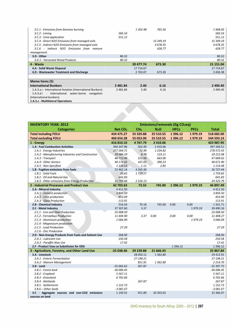
GHG Inventory for South Africa: 2000 – 2012 | 297

3.C.1 - Emissions from biomass burning 1 202.48 765.56 1 968.05 3.C.2 - Liming 585.54 585.54 3.C.3 - Urea application 551.12 551.12 3.C.4 - Direct N2O Emissions from managed soils 15 349.19 15 349.19 3.C.5 - Indirect N2O Emissions from managed soils 4 678.35 4 678.35 3.C.6 - Indirect N2O Emissions from manure management

428.77 428.77

3.D - Other 80.32 80.32 3.D.1 - Harvested Wood Products 80.32 80.32

4 - Waste 20 477.74 673.30 21 151.04 4.A - Solid Waste Disposal 17 714.67 17 714.67 4.D - Wastewater Treatment and Discharge 2 763.07 673.30 3 436.38

Memo Items (5) International Bunkers 2 481.84 2.40 6.16 2 490.40 1.A.3.a.i - International Aviation (International Bunkers) 2 481.84 2.40 6.16 2 490.40 1.A.3.d.i - International water-borne navigation (International bunkers)

1.A.5.c - Multilateral Operations

INVENTORY YEAR: 2012 Emissions/removals (Gg CO2eq) Categories Net CO2 CH4 N2O HFCs PFCs Total

Total including FOLU 434 475.27 55 320.88 25 510.55 1 396.12 1 979.19 518 682.00 Total excluding FOLU 460 654.28 55 053.00 25 510.55 1 396.12 1 979.19 544 593.14

1 - Energy 416 810.10 4 767.79 2 410.06 423 987.95 1.A - Fuel Combustion Activities 394 347.96 502.49 2 410.06 397 260.51 1.A.1 - Energy Industries 277 264.71 72.90 1 234.82 278 572.43 1.A.2 - Manufacturing Industries and Construction 29 084.19 8.78 119.11 29 212.08 1.A.3 - Transport 46 713.90 312.66 663.06 47 689.62 1.A.4 - Other Sectors 40 174.62 107.05 390.23 40 671.90 1.A.5 - Non-Specified 1 110.53 1.11 2.85 1 114.48 1.B - Fugitive emissions from fuels 22 462.14 4 265.30 26 727.44 1.B.1 - Solid Fuels 20.65 1 739.17 1 759.83 1.B.2 - Oil and Natural Gas 641.83 641.83 1.B.3 - Other emissions from Energy Production 21 799.66 2 526.13 24 325.79

2 - Industrial Processes and Product Use 42 703.63 73.55 745.00 1 396.12 1 979.19 46 897.49 2.A - Mineral Industry 4 411.50 4 411.50 2.A.1 - Cement production 3 844.50 3 844.50 2.A.2 - Lime production 453.09 453.09 2.A.3 - Glass Production 113.91 113.91 2.B - Chemical Industry 516.54 70.18 745.00 0.00 0.00 1 331.71 2.C - Metal Industry 37 507.60 3.37 1 979.19 39 490.16 2.C.1 - Iron and Steel Production 25 008.50 25 008.50 2.C.2 - Ferroalloys Production 11 404.90 3.37 0.00 0.00 0.00 11 408.27 2.C.3 - Aluminium production 1 066.90 1 979.19 3 046.09 2.C.4 - Magnesium production 2.C.5 - Lead Production 27.29 27.29 2.C.6 - Zinc Production 2.D - Non-Energy Products from Fuels and Solvent Use 268.00 268.00 2.D.1 - Lubricant Use 250.58 250.58 2.D.2 - Paraffin Wax Use 17.42 17.42 2.F - Product Uses as Substitutes for ODS 1 396.12 1 396.12

3 - Agriculture, Forestry, and Other Land Use -25 038.46 29 239.88 21 666.43 25 867.84 3.A - Livestock 28 050.11 1 362.80 29 412.91 3.A.1 - Enteric Fermentation 27 198.21 27 198.21 3.A.2 - Manure Management 851.91 1 362.80 2 214.70 3.B - Land -25 665.62 267.87 -25 397.75 3.B.1 - Forest land -36 006.45 -36 006.45 3.B.2 - Cropland 5 567.11 5 567.11 3.B.3 - Grassland 6 702.66 6 702.66 3.B.4 - Wetlands 267.87 267.87 3.B.5 - Settlements 1 152.73 1 152.73 3.B.6 – Other lands -3 081.67 -3 081.67 3.C - Aggregate sources and non-CO2 emissions sources on land

1 140.55 921.89 20 303.63 22 366.07

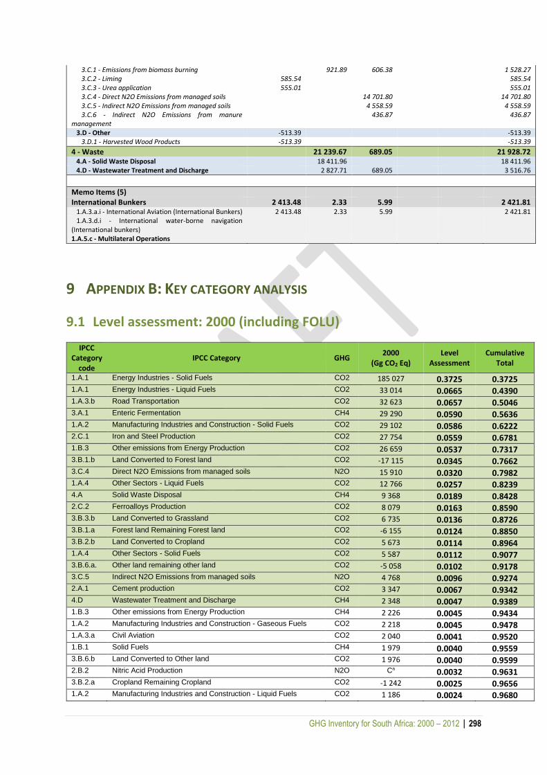
GHG Inventory for South Africa: 2000 – 2012 | 298

3.C.1 - Emissions from biomass burning 921.89 606.38 1 528.27 3.C.2 - Liming 585.54 585.54 3.C.3 - Urea application 555.01 555.01 3.C.4 - Direct N2O Emissions from managed soils 14 701.80 14 701.80 3.C.5 - Indirect N2O Emissions from managed soils 4 558.59 4 558.59 3.C.6 - Indirect N2O Emissions from manure management

436.87 436.87

3.D - Other -513.39 -513.39 3.D.1 - Harvested Wood Products -513.39 -513.39

4 - Waste 21 239.67 689.05 21 928.72 4.A - Solid Waste Disposal 18 411.96 18 411.96 4.D - Wastewater Treatment and Discharge 2 827.71 689.05 3 516.76

Memo Items (5) International Bunkers 2 413.48 2.33 5.99 2 421.81 1.A.3.a.i - International Aviation (International Bunkers) 2 413.48 2.33 5.99 2 421.81 1.A.3.d.i - International water-borne navigation (International bunkers)

1.A.5.c - Multilateral Operations

9 APPENDIX B: KEY CATEGORY ANALYSIS

9.1 Level assessment: 2000 (including FOLU)

IPCC Category

code IPCC Category GHG

2000 (Gg CO2 Eq)

Level Assessment

Cumulative Total

1.A.1 Energy Industries - Solid Fuels CO2 185 027 0.3725 0.3725 1.A.1 Energy Industries - Liquid Fuels CO2 33 014 0.0665 0.4390 1.A.3.b Road Transportation CO2 32 623 0.0657 0.5046 3.A.1 Enteric Fermentation CH4 29 290 0.0590 0.5636 1.A.2 Manufacturing Industries and Construction - Solid Fuels CO2 29 102 0.0586 0.6222 2.C.1 Iron and Steel Production CO2 27 754 0.0559 0.6781 1.B.3 Other emissions from Energy Production CO2 26 659 0.0537 0.7317 3.B.1.b Land Converted to Forest land CO2 -17 115 0.0345 0.7662 3.C.4 Direct N2O Emissions from managed soils N2O 15 910 0.0320 0.7982 1.A.4 Other Sectors - Liquid Fuels CO2 12 766 0.0257 0.8239 4.A Solid Waste Disposal CH4 9 368 0.0189 0.8428 2.C.2 Ferroalloys Production CO2 8 079 0.0163 0.8590 3.B.3.b Land Converted to Grassland CO2 6 735 0.0136 0.8726 3.B.1.a Forest land Remaining Forest land CO2 -6 155 0.0124 0.8850 3.B.2.b Land Converted to Cropland CO2 5 673 0.0114 0.8964 1.A.4 Other Sectors - Solid Fuels CO2 5 587 0.0112 0.9077 3.B.6.a. Other land remaining other land CO2 -5 058 0.0102 0.9178 3.C.5 Indirect N2O Emissions from managed soils N2O 4 768 0.0096 0.9274 2.A.1 Cement production CO2 3 347 0.0067 0.9342 4.D Wastewater Treatment and Discharge CH4 2 348 0.0047 0.9389 1.B.3 Other emissions from Energy Production CH4 2 226 0.0045 0.9434 1.A.2 Manufacturing Industries and Construction - Gaseous Fuels CO2 2 218 0.0045 0.9478 1.A.3.a Civil Aviation CO2 2 040 0.0041 0.9520 1.B.1 Solid Fuels CH4 1 979 0.0040 0.9559 3.B.6.b Land Converted to Other land CO2 1 976 0.0040 0.9599 2.B.2 Nitric Acid Production N2O Ca 0.0032 0.9631 3.B.2.a Cropland Remaining Cropland CO2 -1 242 0.0025 0.9656 1.A.2 Manufacturing Industries and Construction - Liquid Fuels CO2 1 186 0.0024 0.9680

GHG Inventory for South Africa: 2000 – 2012 | 299

IPCC Category

code IPCC Category GHG

2000 (Gg CO2 Eq)

Level Assessment

Cumulative Total

3.B.5.b Land Converted to Settlements CO2 1 161 0.0023 0.9703 2.C.3 Aluminium production CO2 1 105 0.0022 0.9725 3.C.1 Emissions from biomass burning CH4 1 031 0.0021 0.9746 3.A.2 Manure Management N2O 1 007 0.0020 0.9766 1.A.5 Non-Specified - Liquid Fuels CO2 986 0.0020 0.9786 2.C.3 Aluminium production PFCs 982 0.0020 0.9806 3.A.2 Manure Management CH4 865 0.0017 0.9823 1.A.1 Energy Industries - Solid Fuels N2O 854 0.0017 0.9840 1.B.2.a Oil CO2 752 0.0015 0.9856 3.C.1 Emissions from biomass burning N2O 686 0.0014 0.9869 4.D Wastewater Treatment and Discharge N2O 572 0.0012 0.9881 1.A.3.c Railways CO2 551 0.0011 0.9892 2.B.1 Ammonia Production CO2 Ca 0.0010 0.9902 1.A.3.b Road Transportation N2O 463 0.0009 0.9911 2.B.6 Titanium Dioxide Production CO2 Ca 0.0009 0.9920 2.A.2 Lime production CO2 426 0.0009 0.9929 3.C.2 Liming CO2 384 0.0008 0.9936 3.C.6 Indirect N2O Emissions from manure management N2O 350 0.0007 0.9943 3.D.1 Harvested Wood Products CO2 -312 0.0006 0.9950 1.A.3.a Civil Aviation CH4 270 0.0005 0.9955 1.A.3.b Road Transportation CH4 268 0.0005 0.9960 3.B.4.a.ii Flooded land remaining flooded land CH4 254 0.0005 0.9966 3.C.3 Urea application CO2 211 0.0004 0.9970 2.D Non-Energy Products from Fuels and Solvent Use CO2 196 0.0004 0.9974 2.C.6 Zinc Production CO2 194 0.0004 0.9978 1.A.4 Other Sectors - Biomass N2O 168 0.0003 0.9981 2.B.8 Petrochemical and Carbon Black Production CO2 Ca 0.0003 0.9984 1.A.2 Manufacturing Industries and Construction - Solid Fuels N2O 134 0.0003 0.9987 1.A.1 Energy Industries - Liquid Fuels N2O 109 0.0002 0.9989 1.A.4 Other Sectors - Biomass CH4 98 0.0002 0.9991 2.A.3 Glass Production CO2 74 0.0001 0.9992 2.B.1 Ammonia Production CH4 Ca 0.0001 0.9994 1.A.3.c Railways N2O 63 0.0001 0.9995 1.A.4 Other Sectors - Solid Fuels N2O 51 0.0001 0.9996 1.A.1 Energy Industries - Solid Fuels CH4 44 0.0001 0.9997 2.C.5 Lead Production CO2 39 0.0001 0.9998 1.A.4 Other Sectors - Liquid Fuels N2O 29 0.0001 0.9998 1.B.1 Solid Fuels CO2 24 0.0000 0.9999 1.A.1 Energy Industries - Liquid Fuels CH4 13 0.0000 0.9999 1.A.4 Other Sectors - Gaseous Fuels CO2 13 0.0000 0.9999 1.A.4 Other Sectors - Liquid Fuels CH4 11 0.0000 0.9999 1.A.2 Manufacturing Industries and Construction - Solid Fuels CH4 7 0.0000 1.0000 1.A.3.a Civil Aviation N2O 5 0.0000 1.0000 2.C.2 Ferroalloys Production CH4 4 0.0000 1.0000 1.A.2 Manufacturing Industries and Construction - Liquid Fuels N2O 3 0.0000 1.0000 1.A.5 Non-Specified - Liquid Fuels N2O 3 0.0000 1.0000 2.B.5 Carbide Production CO2 Ca 0.0000 1.0000 1.A.4 Other Sectors - Solid Fuels CH4 1 0.0000 1.0000 1.A.2 Manufacturing Industries and Construction - Gaseous Fuels N2O 1 0.0000 1.0000 1.A.2 Manufacturing Industries and Construction - Liquid Fuels CH4 1 0.0000 1.0000 1.A.5 Non-Specified - Liquid Fuels CH4 1 0.0000 1.0000 1.A.2 Manufacturing Industries and Construction - Gaseous Fuels CH4 1 0.0000 1.0000

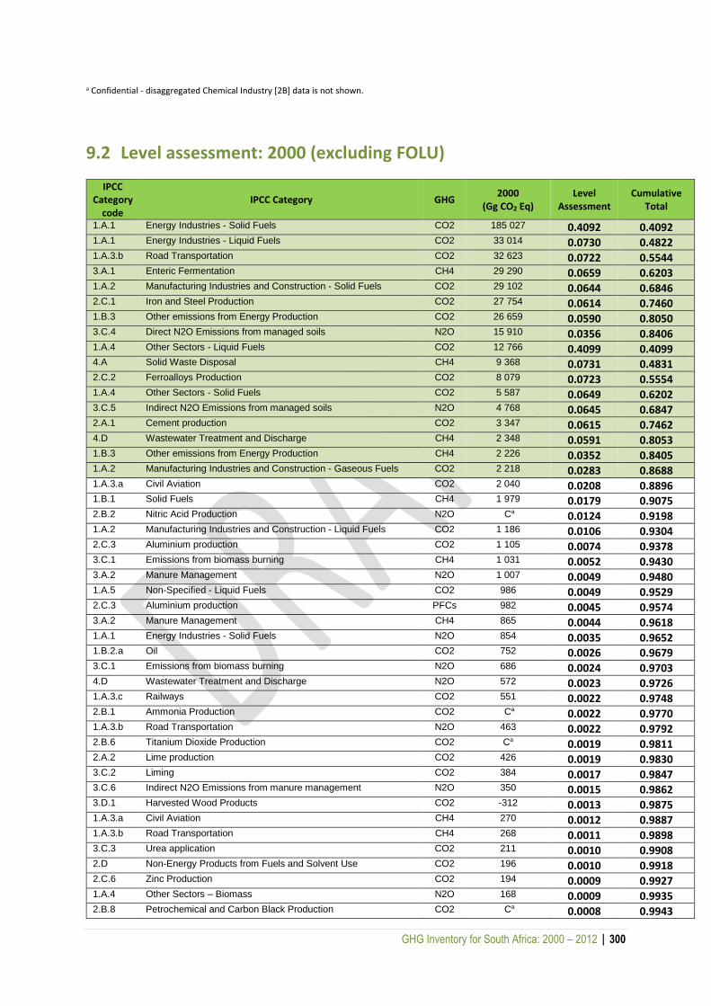
GHG Inventory for South Africa: 2000 – 2012 | 300

a Confidential - disaggregated Chemical Industry [2B] data is not shown.

9.2 Level assessment: 2000 (excluding FOLU)

IPCC Category

code IPCC Category GHG

2000 (Gg CO2 Eq)

Level Assessment

Cumulative Total

1.A.1 Energy Industries - Solid Fuels CO2 185 027 0.4092 0.4092 1.A.1 Energy Industries - Liquid Fuels CO2 33 014 0.0730 0.4822 1.A.3.b Road Transportation CO2 32 623 0.0722 0.5544 3.A.1 Enteric Fermentation CH4 29 290 0.0659 0.6203 1.A.2 Manufacturing Industries and Construction - Solid Fuels CO2 29 102 0.0644 0.6846 2.C.1 Iron and Steel Production CO2 27 754 0.0614 0.7460 1.B.3 Other emissions from Energy Production CO2 26 659 0.0590 0.8050 3.C.4 Direct N2O Emissions from managed soils N2O 15 910 0.0356 0.8406 1.A.4 Other Sectors - Liquid Fuels CO2 12 766 0.4099 0.4099 4.A Solid Waste Disposal CH4 9 368 0.0731 0.4831 2.C.2 Ferroalloys Production CO2 8 079 0.0723 0.5554 1.A.4 Other Sectors - Solid Fuels CO2 5 587 0.0649 0.6202 3.C.5 Indirect N2O Emissions from managed soils N2O 4 768 0.0645 0.6847 2.A.1 Cement production CO2 3 347 0.0615 0.7462 4.D Wastewater Treatment and Discharge CH4 2 348 0.0591 0.8053 1.B.3 Other emissions from Energy Production CH4 2 226 0.0352 0.8405 1.A.2 Manufacturing Industries and Construction - Gaseous Fuels CO2 2 218 0.0283 0.8688 1.A.3.a Civil Aviation CO2 2 040 0.0208 0.8896 1.B.1 Solid Fuels CH4 1 979 0.0179 0.9075 2.B.2 Nitric Acid Production N2O Ca 0.0124 0.9198 1.A.2 Manufacturing Industries and Construction - Liquid Fuels CO2 1 186 0.0106 0.9304 2.C.3 Aluminium production CO2 1 105 0.0074 0.9378 3.C.1 Emissions from biomass burning CH4 1 031 0.0052 0.9430 3.A.2 Manure Management N2O 1 007 0.0049 0.9480 1.A.5 Non-Specified - Liquid Fuels CO2 986 0.0049 0.9529 2.C.3 Aluminium production PFCs 982 0.0045 0.9574 3.A.2 Manure Management CH4 865 0.0044 0.9618 1.A.1 Energy Industries - Solid Fuels N2O 854 0.0035 0.9652 1.B.2.a Oil CO2 752 0.0026 0.9679 3.C.1 Emissions from biomass burning N2O 686 0.0024 0.9703 4.D Wastewater Treatment and Discharge N2O 572 0.0023 0.9726 1.A.3.c Railways CO2 551 0.0022 0.9748 2.B.1 Ammonia Production CO2 Ca 0.0022 0.9770 1.A.3.b Road Transportation N2O 463 0.0022 0.9792 2.B.6 Titanium Dioxide Production CO2 Ca 0.0019 0.9811 2.A.2 Lime production CO2 426 0.0019 0.9830 3.C.2 Liming CO2 384 0.0017 0.9847 3.C.6 Indirect N2O Emissions from manure management N2O 350 0.0015 0.9862 3.D.1 Harvested Wood Products CO2 -312 0.0013 0.9875 1.A.3.a Civil Aviation CH4 270 0.0012 0.9887 1.A.3.b Road Transportation CH4 268 0.0011 0.9898 3.C.3 Urea application CO2 211 0.0010 0.9908 2.D Non-Energy Products from Fuels and Solvent Use CO2 196 0.0010 0.9918 2.C.6 Zinc Production CO2 194 0.0009 0.9927 1.A.4 Other Sectors – Biomass N2O 168 0.0009 0.9935 2.B.8 Petrochemical and Carbon Black Production CO2 Ca 0.0008 0.9943

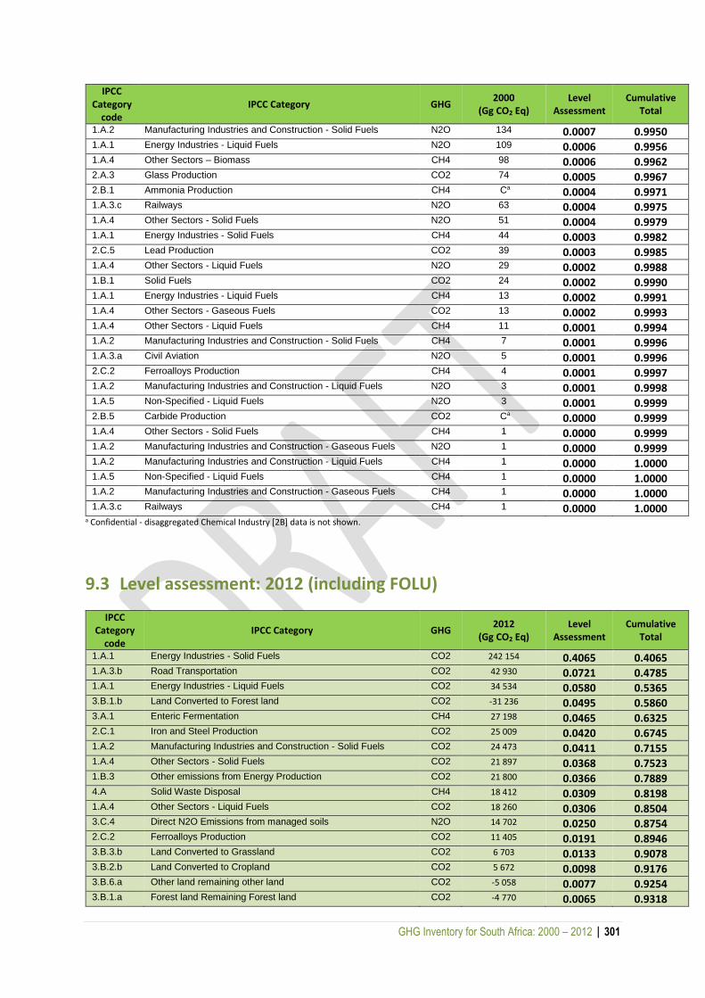
GHG Inventory for South Africa: 2000 – 2012 | 301

IPCC Category

code IPCC Category GHG

2000 (Gg CO2 Eq)

Level Assessment

Cumulative Total

1.A.2 Manufacturing Industries and Construction - Solid Fuels N2O 134 0.0007 0.9950 1.A.1 Energy Industries - Liquid Fuels N2O 109 0.0006 0.9956 1.A.4 Other Sectors – Biomass CH4 98 0.0006 0.9962 2.A.3 Glass Production CO2 74 0.0005 0.9967 2.B.1 Ammonia Production CH4 Ca 0.0004 0.9971 1.A.3.c Railways N2O 63 0.0004 0.9975 1.A.4 Other Sectors - Solid Fuels N2O 51 0.0004 0.9979 1.A.1 Energy Industries - Solid Fuels CH4 44 0.0003 0.9982 2.C.5 Lead Production CO2 39 0.0003 0.9985 1.A.4 Other Sectors - Liquid Fuels N2O 29 0.0002 0.9988 1.B.1 Solid Fuels CO2 24 0.0002 0.9990 1.A.1 Energy Industries - Liquid Fuels CH4 13 0.0002 0.9991 1.A.4 Other Sectors - Gaseous Fuels CO2 13 0.0002 0.9993 1.A.4 Other Sectors - Liquid Fuels CH4 11 0.0001 0.9994 1.A.2 Manufacturing Industries and Construction - Solid Fuels CH4 7 0.0001 0.9996 1.A.3.a Civil Aviation N2O 5 0.0001 0.9996 2.C.2 Ferroalloys Production CH4 4 0.0001 0.9997 1.A.2 Manufacturing Industries and Construction - Liquid Fuels N2O 3 0.0001 0.9998 1.A.5 Non-Specified - Liquid Fuels N2O 3 0.0001 0.9999 2.B.5 Carbide Production CO2 Ca 0.0000 0.9999 1.A.4 Other Sectors - Solid Fuels CH4 1 0.0000 0.9999 1.A.2 Manufacturing Industries and Construction - Gaseous Fuels N2O 1 0.0000 0.9999 1.A.2 Manufacturing Industries and Construction - Liquid Fuels CH4 1 0.0000 1.0000 1.A.5 Non-Specified - Liquid Fuels CH4 1 0.0000 1.0000 1.A.2 Manufacturing Industries and Construction - Gaseous Fuels CH4 1 0.0000 1.0000 1.A.3.c Railways CH4 1 0.0000 1.0000

a Confidential - disaggregated Chemical Industry [2B] data is not shown.

9.3 Level assessment: 2012 (including FOLU)

IPCC Category

code IPCC Category GHG

2012 (Gg CO2 Eq)

Level Assessment

Cumulative Total

1.A.1 Energy Industries - Solid Fuels CO2 242 154 0.4065 0.4065

1.A.3.b Road Transportation CO2 42 930 0.0721 0.4785

1.A.1 Energy Industries - Liquid Fuels CO2 34 534 0.0580 0.5365

3.B.1.b Land Converted to Forest land CO2 -31 236 0.0495 0.5860

3.A.1 Enteric Fermentation CH4 27 198 0.0465 0.6325

2.C.1 Iron and Steel Production CO2 25 009 0.0420 0.6745

1.A.2 Manufacturing Industries and Construction - Solid Fuels CO2 24 473 0.0411 0.7155

1.A.4 Other Sectors - Solid Fuels CO2 21 897 0.0368 0.7523

1.B.3 Other emissions from Energy Production CO2 21 800 0.0366 0.7889

4.A Solid Waste Disposal CH4 18 412 0.0309 0.8198

1.A.4 Other Sectors - Liquid Fuels CO2 18 260 0.0306 0.8504

3.C.4 Direct N2O Emissions from managed soils N2O 14 702 0.0250 0.8754

2.C.2 Ferroalloys Production CO2 11 405 0.0191 0.8946

3.B.3.b Land Converted to Grassland CO2 6 703 0.0133 0.9078

3.B.2.b Land Converted to Cropland CO2 5 672 0.0098 0.9176

3.B.6.a Other land remaining other land CO2 -5 058 0.0077 0.9254

3.B.1.a Forest land Remaining Forest land CO2 -4 770 0.0065 0.9318

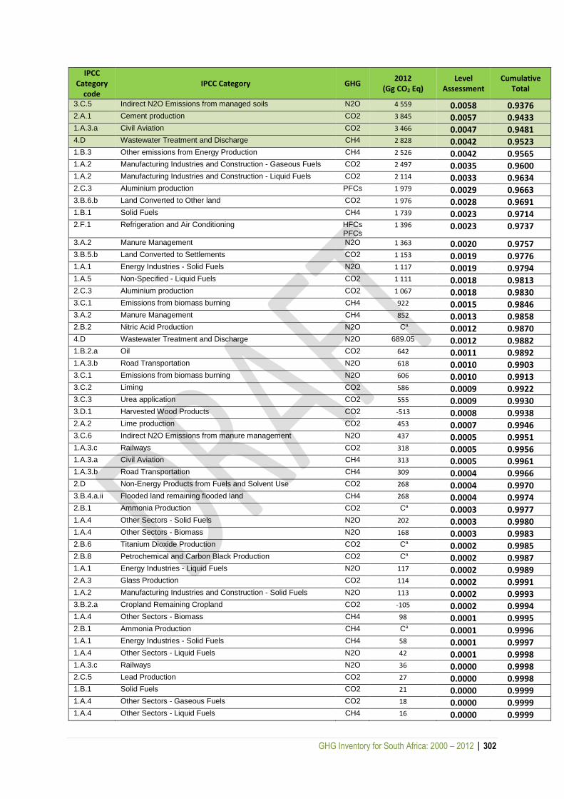
GHG Inventory for South Africa: 2000 – 2012 | 302

IPCC Category

code IPCC Category GHG

2012 (Gg CO2 Eq)

Level Assessment

Cumulative Total

3.C.5 Indirect N2O Emissions from managed soils N2O 4 559 0.0058 0.9376

2.A.1 Cement production CO2 3 845 0.0057 0.9433

1.A.3.a Civil Aviation CO2 3 466 0.0047 0.9481

4.D Wastewater Treatment and Discharge CH4 2 828 0.0042 0.9523

1.B.3 Other emissions from Energy Production CH4 2 526 0.0042 0.9565 1.A.2 Manufacturing Industries and Construction - Gaseous Fuels CO2 2 497 0.0035 0.9600

1.A.2 Manufacturing Industries and Construction - Liquid Fuels CO2 2 114 0.0033 0.9634

2.C.3 Aluminium production PFCs 1 979 0.0029 0.9663

3.B.6.b Land Converted to Other land CO2 1 976 0.0028 0.9691

1.B.1 Solid Fuels CH4 1 739 0.0023 0.9714

2.F.1 Refrigeration and Air Conditioning HFCsPFCs

1 396 0.0023 0.9737

3.A.2 Manure Management N2O 1 363 0.0020 0.9757

3.B.5.b Land Converted to Settlements CO2 1 153 0.0019 0.9776

1.A.1 Energy Industries - Solid Fuels N2O 1 117 0.0019 0.9794

1.A.5 Non-Specified - Liquid Fuels CO2 1 111 0.0018 0.9813

2.C.3 Aluminium production CO2 1 067 0.0018 0.9830

3.C.1 Emissions from biomass burning CH4 922 0.0015 0.9846

3.A.2 Manure Management CH4 852 0.0013 0.9858

2.B.2 Nitric Acid Production N2O Ca 0.0012 0.9870

4.D Wastewater Treatment and Discharge N2O 689.05 0.0012 0.9882 1.B.2.a Oil CO2 642 0.0011 0.9892

1.A.3.b Road Transportation N2O 618 0.0010 0.9903

3.C.1 Emissions from biomass burning N2O 606 0.0010 0.9913

3.C.2 Liming CO2 586 0.0009 0.9922

3.C.3 Urea application CO2 555 0.0009 0.9930

3.D.1 Harvested Wood Products CO2 -513 0.0008 0.9938

2.A.2 Lime production CO2 453 0.0007 0.9946

3.C.6 Indirect N2O Emissions from manure management N2O 437 0.0005 0.9951

1.A.3.c Railways CO2 318 0.0005 0.9956 1.A.3.a Civil Aviation CH4 313 0.0005 0.9961

1.A.3.b Road Transportation CH4 309 0.0004 0.9966

2.D Non-Energy Products from Fuels and Solvent Use CO2 268 0.0004 0.9970

3.B.4.a.ii Flooded land remaining flooded land CH4 268 0.0004 0.9974

2.B.1 Ammonia Production CO2 Ca 0.0003 0.9977

1.A.4 Other Sectors - Solid Fuels N2O 202 0.0003 0.9980

1.A.4 Other Sectors - Biomass N2O 168 0.0003 0.9983

2.B.6 Titanium Dioxide Production CO2 Ca 0.0002 0.9985

2.B.8 Petrochemical and Carbon Black Production CO2 Ca 0.0002 0.9987 1.A.1 Energy Industries - Liquid Fuels N2O 117 0.0002 0.9989

2.A.3 Glass Production CO2 114 0.0002 0.9991

1.A.2 Manufacturing Industries and Construction - Solid Fuels N2O 113 0.0002 0.9993

3.B.2.a Cropland Remaining Cropland CO2 -105 0.0002 0.9994

1.A.4 Other Sectors - Biomass CH4 98 0.0001 0.9995

2.B.1 Ammonia Production CH4 Ca 0.0001 0.9996

1.A.1 Energy Industries - Solid Fuels CH4 58 0.0001 0.9997

1.A.4 Other Sectors - Liquid Fuels N2O 42 0.0001 0.9998

1.A.3.c Railways N2O 36 0.0000 0.9998

2.C.5 Lead Production CO2 27 0.0000 0.9998 1.B.1 Solid Fuels CO2 21 0.0000 0.9999

1.A.4 Other Sectors - Gaseous Fuels CO2 18 0.0000 0.9999

1.A.4 Other Sectors - Liquid Fuels CH4 16 0.0000 0.9999

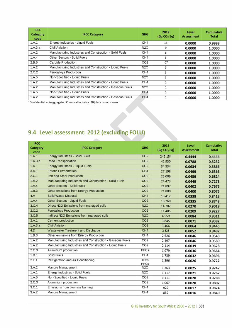
GHG Inventory for South Africa: 2000 – 2012 | 303

IPCC Category

code IPCC Category GHG

2012 (Gg CO2 Eq)

Level Assessment

Cumulative Total

1.A.1 Energy Industries - Liquid Fuels CH4 15 0.0000 0.9999

1.A.3.a Civil Aviation N2O 9 0.0000 1.0000

1.A.2 Manufacturing Industries and Construction - Solid Fuels CH4 6 0.0000 1.0000

1.A.4 Other Sectors - Solid Fuels CH4 5 0.0000 1.0000

2.B.5 Carbide Production CO2 Ca 0.0000 1.0000 1.A.2 Manufacturing Industries and Construction - Liquid Fuels N2O 5 0.0000 1.0000

2.C.2 Ferroalloys Production CH4 3 0.0000 1.0000

1.A.5 Non-Specified - Liquid Fuels N2O 3 0.0000 1.0000

1.A.2 Manufacturing Industries and Construction - Liquid Fuels CH4 2 0.0000 1.0000

1.A.2 Manufacturing Industries and Construction - Gaseous Fuels N2O 1 0.0000 1.0000

1.A.5 Non-Specified - Liquid Fuels CH4 1 0.0000 1.0000

1.A.2 Manufacturing Industries and Construction - Gaseous Fuels CH4 1 0.0000 1.0000 a Confidential - disaggregated Chemical Industry [2B] data is not shown.

9.4 Level assessment: 2012 (excluding FOLU)

IPCC Category

code IPCC Category GHG

2012 (Gg CO2 Eq)

Level Assessment

Cumulative Total

1.A.1 Energy Industries - Solid Fuels CO2 242 154 0.4444 0.4444

1.A.3.b Road Transportation CO2 42 930 0.0788 0.5232

1.A.1 Energy Industries - Liquid Fuels CO2 34 534 0.0634 0.5866

3.A.1 Enteric Fermentation CH4 27 198 0.0499 0.6365

2.C.1 Iron and Steel Production CO2 25 009 0.0459 0.6824

1.A.2 Manufacturing Industries and Construction - Solid Fuels CO2 24 473 0.0449 0.7273

1.A.4 Other Sectors - Solid Fuels CO2 21 897 0.0402 0.7675

1.B.3 Other emissions from Energy Production CO2 21 800 0.0400 0.8075

4.A Solid Waste Disposal CH4 18 412 0.0338 0.8413

1.A.4 Other Sectors - Liquid Fuels CO2 18 260 0.0335 0.8748

3.C.4 Direct N2O Emissions from managed soils N2O 14 702 0.0270 0.9018

2.C.2 Ferroalloys Production CO2 11 405 0.0209 0.9227

3.C.5 Indirect N2O Emissions from managed soils N2O 4 559 0.0084 0.9311

2.A.1 Cement production CO2 3 845 0.0071 0.9382

1.A.3.a Civil Aviation CO2 3 466 0.0064 0.9445

4.D Wastewater Treatment and Discharge CH4 2 828 0.0052 0.9497

1.B.3 Other emissions from Energy Production CH4 2 526 0.0046 0.9543

1.A.2 Manufacturing Industries and Construction - Gaseous Fuels CO2 2 497 0.0046 0.9589

1.A.2 Manufacturing Industries and Construction - Liquid Fuels CO2 2 114 0.0039 0.9628

2.C.3 Aluminium production PFCs 1 979 0.0036 0.9664

1.B.1 Solid Fuels CH4 1 739 0.0032 0.9696

2.F.1 Refrigeration and Air Conditioning HFCs, PFCs

1 396 0.0026 0.9722

3.A.2 Manure Management N2O 1 363 0.0025 0.9747

1.A.1 Energy Industries - Solid Fuels N2O 1 117 0.0021 0.9767

1.A.5 Non-Specified - Liquid Fuels CO2 1 111 0.0020 0.9788

2.C.3 Aluminium production CO2 1 067 0.0020 0.9807

3.C.1 Emissions from biomass burning CH4 922 0.0017 0.9824

3.A.2 Manure Management CH4 852 0.0016 0.9840

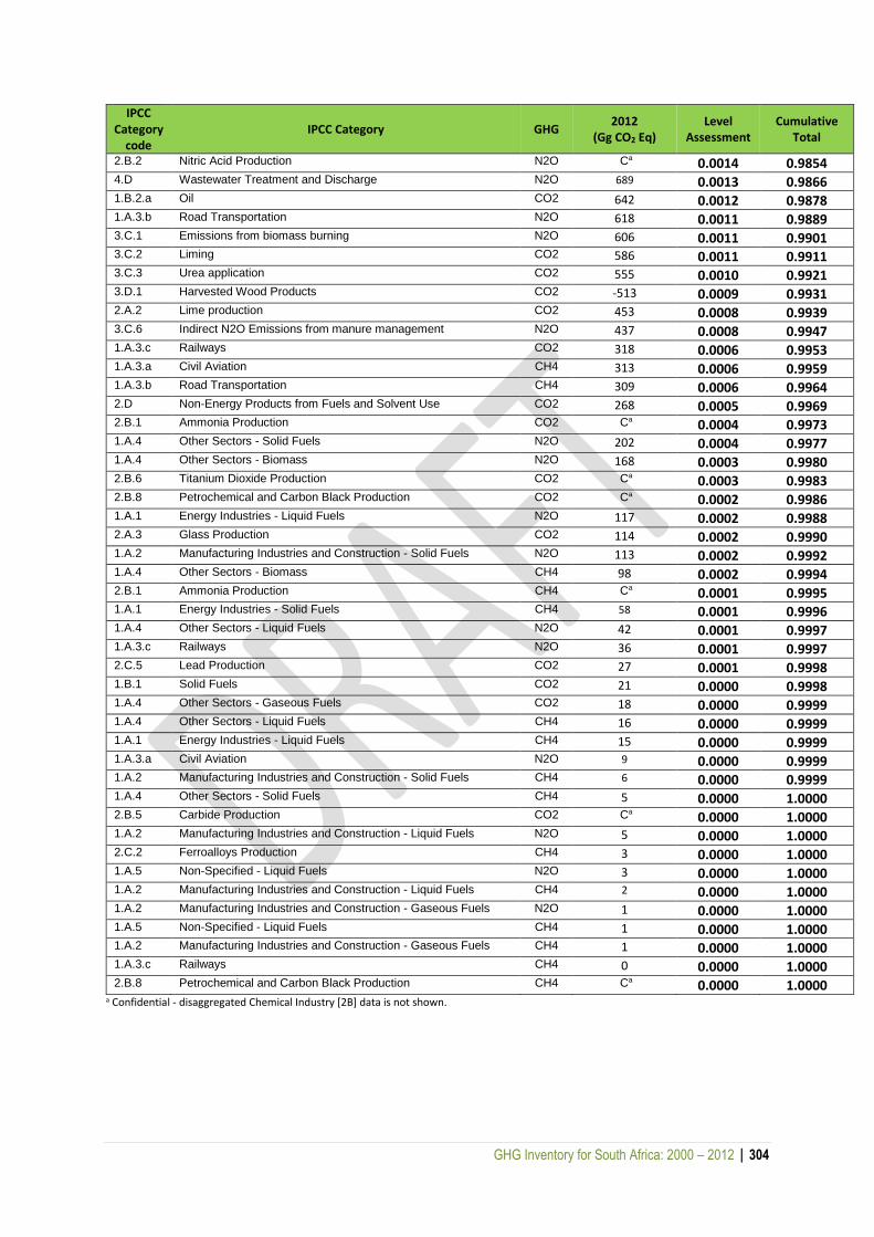
GHG Inventory for South Africa: 2000 – 2012 | 304

IPCC Category

code IPCC Category GHG

2012 (Gg CO2 Eq)

Level Assessment

Cumulative Total

2.B.2 Nitric Acid Production N2O Ca 0.0014 0.9854

4.D Wastewater Treatment and Discharge N2O 689 0.0013 0.9866

1.B.2.a Oil CO2 642 0.0012 0.9878

1.A.3.b Road Transportation N2O 618 0.0011 0.9889

3.C.1 Emissions from biomass burning N2O 606 0.0011 0.9901

3.C.2 Liming CO2 586 0.0011 0.9911

3.C.3 Urea application CO2 555 0.0010 0.9921

3.D.1 Harvested Wood Products CO2 -513 0.0009 0.9931

2.A.2 Lime production CO2 453 0.0008 0.9939

3.C.6 Indirect N2O Emissions from manure management N2O 437 0.0008 0.9947

1.A.3.c Railways CO2 318 0.0006 0.9953

1.A.3.a Civil Aviation CH4 313 0.0006 0.9959

1.A.3.b Road Transportation CH4 309 0.0006 0.9964

2.D Non-Energy Products from Fuels and Solvent Use CO2 268 0.0005 0.9969

2.B.1 Ammonia Production CO2 Ca 0.0004 0.9973

1.A.4 Other Sectors - Solid Fuels N2O 202 0.0004 0.9977

1.A.4 Other Sectors - Biomass N2O 168 0.0003 0.9980

2.B.6 Titanium Dioxide Production CO2 Ca 0.0003 0.9983

2.B.8 Petrochemical and Carbon Black Production CO2 Ca 0.0002 0.9986

1.A.1 Energy Industries - Liquid Fuels N2O 117 0.0002 0.9988

2.A.3 Glass Production CO2 114 0.0002 0.9990

1.A.2 Manufacturing Industries and Construction - Solid Fuels N2O 113 0.0002 0.9992

1.A.4 Other Sectors - Biomass CH4 98 0.0002 0.9994

2.B.1 Ammonia Production CH4 Ca 0.0001 0.9995

1.A.1 Energy Industries - Solid Fuels CH4 58 0.0001 0.9996

1.A.4 Other Sectors - Liquid Fuels N2O 42 0.0001 0.9997

1.A.3.c Railways N2O 36 0.0001 0.9997

2.C.5 Lead Production CO2 27 0.0001 0.9998

1.B.1 Solid Fuels CO2 21 0.0000 0.9998

1.A.4 Other Sectors - Gaseous Fuels CO2 18 0.0000 0.9999

1.A.4 Other Sectors - Liquid Fuels CH4 16 0.0000 0.9999

1.A.1 Energy Industries - Liquid Fuels CH4 15 0.0000 0.9999

1.A.3.a Civil Aviation N2O 9 0.0000 0.9999

1.A.2 Manufacturing Industries and Construction - Solid Fuels CH4 6 0.0000 0.9999

1.A.4 Other Sectors - Solid Fuels CH4 5 0.0000 1.0000

2.B.5 Carbide Production CO2 Ca 0.0000 1.0000

1.A.2 Manufacturing Industries and Construction - Liquid Fuels N2O 5 0.0000 1.0000

2.C.2 Ferroalloys Production CH4 3 0.0000 1.0000

1.A.5 Non-Specified - Liquid Fuels N2O 3 0.0000 1.0000

1.A.2 Manufacturing Industries and Construction - Liquid Fuels CH4 2 0.0000 1.0000

1.A.2 Manufacturing Industries and Construction - Gaseous Fuels N2O 1 0.0000 1.0000

1.A.5 Non-Specified - Liquid Fuels CH4 1 0.0000 1.0000

1.A.2 Manufacturing Industries and Construction - Gaseous Fuels CH4 1 0.0000 1.0000

1.A.3.c Railways CH4 0 0.0000 1.0000

2.B.8 Petrochemical and Carbon Black Production CH4 Ca 0.0000 1.0000 a Confidential - disaggregated Chemical Industry [2B] data is not shown.

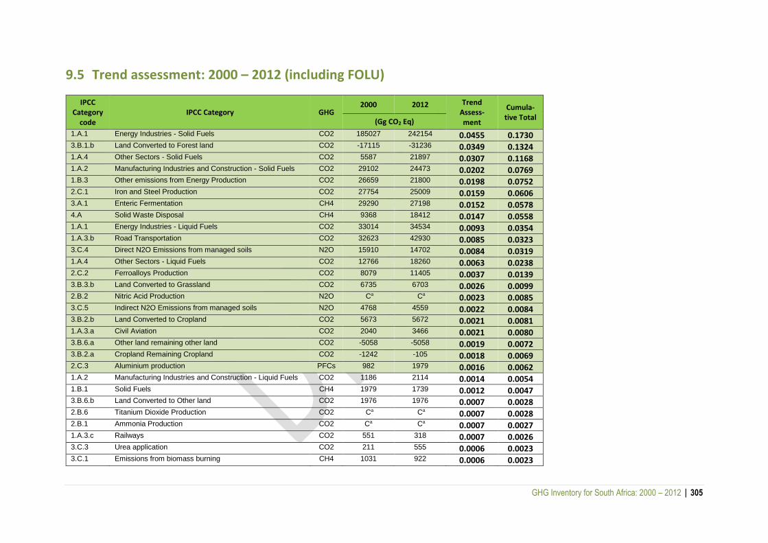
GHG Inventory for South Africa: 2000 – 2012 | 305

9.5 Trend assessment: 2000 – 2012 (including FOLU)

IPCC Category

code IPCC Category GHG

2000 2012 Trend Assess-ment

Cumula-tive Total

(Gg CO2 Eq)

1.A.1 Energy Industries - Solid Fuels CO2 185027 242154 0.0455 0.1730

3.B.1.b Land Converted to Forest land CO2 -17115 -31236 0.0349 0.1324

1.A.4 Other Sectors - Solid Fuels CO2 5587 21897 0.0307 0.1168

1.A.2 Manufacturing Industries and Construction - Solid Fuels CO2 29102 24473 0.0202 0.0769

1.B.3 Other emissions from Energy Production CO2 26659 21800 0.0198 0.0752

2.C.1 Iron and Steel Production CO2 27754 25009 0.0159 0.0606

3.A.1 Enteric Fermentation CH4 29290 27198 0.0152 0.0578

4.A Solid Waste Disposal CH4 9368 18412 0.0147 0.0558

1.A.1 Energy Industries - Liquid Fuels CO2 33014 34534 0.0093 0.0354

1.A.3.b Road Transportation CO2 32623 42930 0.0085 0.0323

3.C.4 Direct N2O Emissions from managed soils N2O 15910 14702 0.0084 0.0319

1.A.4 Other Sectors - Liquid Fuels CO2 12766 18260 0.0063 0.0238

2.C.2 Ferroalloys Production CO2 8079 11405 0.0037 0.0139

3.B.3.b Land Converted to Grassland CO2 6735 6703 0.0026 0.0099

2.B.2 Nitric Acid Production N2O Ca Ca 0.0023 0.0085

3.C.5 Indirect N2O Emissions from managed soils N2O 4768 4559 0.0022 0.0084

3.B.2.b Land Converted to Cropland CO2 5673 5672 0.0021 0.0081

1.A.3.a Civil Aviation CO2 2040 3466 0.0021 0.0080

3.B.6.a Other land remaining other land CO2 -5058 -5058 0.0019 0.0072

3.B.2.a Cropland Remaining Cropland CO2 -1242 -105 0.0018 0.0069

2.C.3 Aluminium production PFCs 982 1979 0.0016 0.0062

1.A.2 Manufacturing Industries and Construction - Liquid Fuels CO2 1186 2114 0.0014 0.0054

1.B.1 Solid Fuels CH4 1979 1739 0.0012 0.0047 3.B.6.b Land Converted to Other land CO2 1976 1976 0.0007 0.0028

2.B.6 Titanium Dioxide Production CO2 Ca Ca 0.0007 0.0028

2.B.1 Ammonia Production CO2 Ca Ca 0.0007 0.0027

1.A.3.c Railways CO2 551 318 0.0007 0.0026

3.C.3 Urea application CO2 211 555 0.0006 0.0023

3.C.1 Emissions from biomass burning CH4 1031 922 0.0006 0.0023

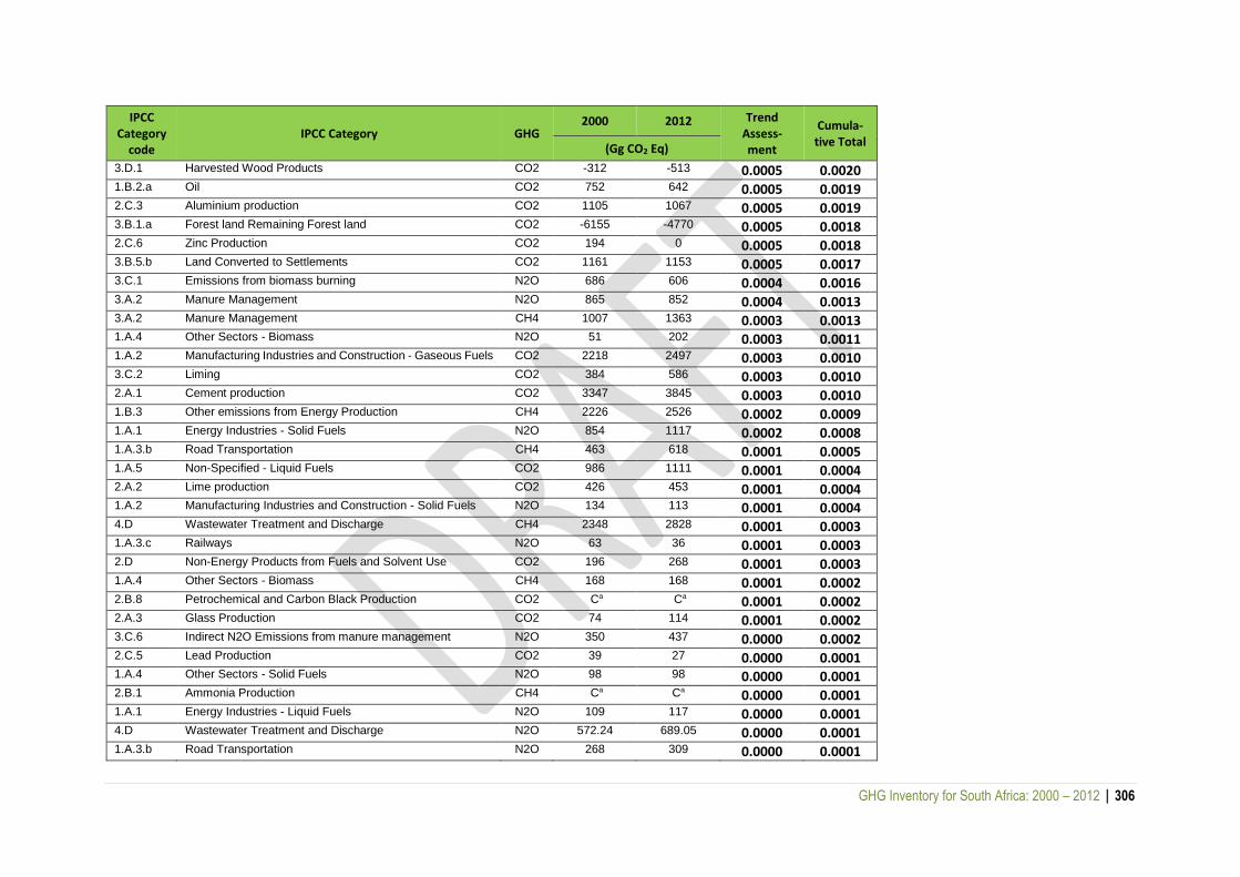
GHG Inventory for South Africa: 2000 – 2012 | 306

IPCC Category

code IPCC Category GHG

2000 2012 Trend Assess-ment

Cumula-tive Total

(Gg CO2 Eq)

3.D.1 Harvested Wood Products CO2 -312 -513 0.0005 0.0020

1.B.2.a Oil CO2 752 642 0.0005 0.0019

2.C.3 Aluminium production CO2 1105 1067 0.0005 0.0019

3.B.1.a Forest land Remaining Forest land CO2 -6155 -4770 0.0005 0.0018

2.C.6 Zinc Production CO2 194 0 0.0005 0.0018

3.B.5.b Land Converted to Settlements CO2 1161 1153 0.0005 0.0017

3.C.1 Emissions from biomass burning N2O 686 606 0.0004 0.0016

3.A.2 Manure Management N2O 865 852 0.0004 0.0013

3.A.2 Manure Management CH4 1007 1363 0.0003 0.0013 1.A.4 Other Sectors - Biomass N2O 51 202 0.0003 0.0011

1.A.2 Manufacturing Industries and Construction - Gaseous Fuels CO2 2218 2497 0.0003 0.0010

3.C.2 Liming CO2 384 586 0.0003 0.0010

2.A.1 Cement production CO2 3347 3845 0.0003 0.0010

1.B.3 Other emissions from Energy Production CH4 2226 2526 0.0002 0.0009

1.A.1 Energy Industries - Solid Fuels N2O 854 1117 0.0002 0.0008

1.A.3.b Road Transportation CH4 463 618 0.0001 0.0005

1.A.5 Non-Specified - Liquid Fuels CO2 986 1111 0.0001 0.0004

2.A.2 Lime production CO2 426 453 0.0001 0.0004 1.A.2 Manufacturing Industries and Construction - Solid Fuels N2O 134 113 0.0001 0.0004

4.D Wastewater Treatment and Discharge CH4 2348 2828 0.0001 0.0003

1.A.3.c Railways N2O 63 36 0.0001 0.0003

2.D Non-Energy Products from Fuels and Solvent Use CO2 196 268 0.0001 0.0003

1.A.4 Other Sectors - Biomass CH4 168 168 0.0001 0.0002

2.B.8 Petrochemical and Carbon Black Production CO2 Ca Ca 0.0001 0.0002

2.A.3 Glass Production CO2 74 114 0.0001 0.0002

3.C.6 Indirect N2O Emissions from manure management N2O 350 437 0.0000 0.0002

2.C.5 Lead Production CO2 39 27 0.0000 0.0001 1.A.4 Other Sectors - Solid Fuels N2O 98 98 0.0000 0.0001

2.B.1 Ammonia Production CH4 Ca Ca 0.0000 0.0001

1.A.1 Energy Industries - Liquid Fuels N2O 109 117 0.0000 0.0001

4.D Wastewater Treatment and Discharge N2O 572.24 689.05 0.0000 0.0001

1.A.3.b Road Transportation N2O 268 309 0.0000 0.0001

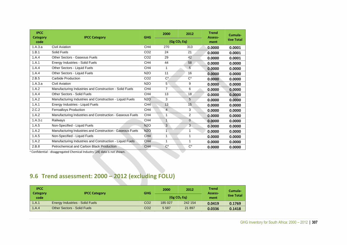
GHG Inventory for South Africa: 2000 – 2012 | 307

IPCC Category

code IPCC Category GHG

2000 2012 Trend Assess-ment

Cumula-tive Total

(Gg CO2 Eq)

1.A.3.a Civil Aviation CH4 270 313 0.0000 0.0001

1.B.1 Solid Fuels CO2 24 21 0.0000 0.0001

1.A.4 Other Sectors - Gaseous Fuels CO2 29 42 0.0000 0.0001

1.A.1 Energy Industries - Solid Fuels CH4 44 58 0.0000 0.0000

1.A.4 Other Sectors - Liquid Fuels CH4 1 5 0.0000 0.0000

1.A.4 Other Sectors - Liquid Fuels N2O 11 16 0.0000 0.0000

2.B.5 Carbide Production CO2 Ca Ca 0.0000 0.0000

1.A.3.a Civil Aviation N2O 5 9 0.0000 0.0000

1.A.2 Manufacturing Industries and Construction - Solid Fuels CH4 7 6 0.0000 0.0000 1.A.4 Other Sectors - Solid Fuels CH4 13 18 0.0000 0.0000

1.A.2 Manufacturing Industries and Construction - Liquid Fuels N2O 3 5 0.0000 0.0000

1.A.1 Energy Industries - Liquid Fuels CH4 13 15 0.0000 0.0000

2.C.2 Ferroalloys Production CH4 4 3 0.0000 0.0000

1.A.2 Manufacturing Industries and Construction - Gaseous Fuels CH4 1 2 0.0000 0.0000

1.A.3.c Railways CH4 1 0 0.0000 0.0000

1.A.5 Non-Specified - Liquid Fuels N2O 3 3 0.0000 0.0000

1.A.2 Manufacturing Industries and Construction - Gaseous Fuels N2O 1 1 0.0000 0.0000

1.A.5 Non-Specified - Liquid Fuels CH4 1 1 0.0000 0.0000 1.A.2 Manufacturing Industries and Construction - Liquid Fuels CH4 1 1 0.0000 0.0000

2.B.8 Petrochemical and Carbon Black Production CH4 Ca Ca 0.0000 0.0000 a Confidential - disaggregated Chemical Industry [2B] data is not shown.

9.6 Trend assessment: 2000 – 2012 (excluding FOLU)

IPCC Category

code IPCC Category GHG

2000 2012 Trend Assess-ment

Cumula-tive Total

(Gg CO2 Eq)

1.A.1 Energy Industries - Solid Fuels CO2 185 027 242 154 0.0419 0.1769

1.A.4 Other Sectors - Solid Fuels CO2 5 587 21 897 0.0336 0.1418

GHG Inventory for South Africa: 2000 – 2012 | 308

IPCC Category

code IPCC Category GHG

2000 2012 Trend Assess-ment

Cumula-tive Total

(Gg CO2 Eq)

1.A.2 Manufacturing Industries and Construction - Solid Fuels CO2 29 102 24 473 0.0236 0.0995

1.B.3 Other emissions from Energy Production CO2 26 659 21 800 0.0230 0.0970

2.C.1 Iron and Steel Production CO2 27 754 25 009 0.0188 0.0793

3.A.1 Enteric Fermentation CH4 29 290 27 198 0.0180 0.0762

4.A Solid Waste Disposal CH4 9 368 18 412 0.0158 0.0665

1.A.1 Energy Industries - Liquid Fuels CO2 33 014 34 534 0.0117 0.0496

3.C.4 Direct N2O Emissions from managed soils N2O 15 910 14 702 0.0100 0.0420

1.A.3.b Road Transportation CO2 32 623 42 930 0.0079 0.0334

1.A.4 Other Sectors - Liquid Fuels CO2 12 766 18 260 0.0063 0.0267

2.C.2 Ferroalloys Production CO2 8 079 11 405 0.0037 0.0155

3.C.5 Indirect N2O Emissions from managed soils N2O 4 768 4 559 0.0026 0.0112

2.B.2 Nitric Acid Production N2O Ca Ca 0.0025 0.0108

1.A.3.a Civil Aviation CO2 2 040 3 466 0.0022 0.0094

2.C.3 Aluminium production PFCs 982 1 979 0.0018 0.0074

1.A.2 Manufacturing Industries and Construction - Liquid Fuels CO2 1 186 2 114 0.0015 0.0064

1.B.1 Solid Fuels CH4 1 979 1 739 0.0014 0.0061

2.B.6 Titanium Dioxide Production CO2 Ca Ca 0.0008 0.0035

2.B.1 Ammonia Production CO2 Ca Ca 0.0008 0.0034

1.A.3.c Railways CO2 551 318 0.0008 0.0032

3.C.1 Emissions from biomass burning CH4 1 031 922 0.0007 0.0030

3.C.3 Urea application CO2 211 555 0.0007 0.0028

2.C.3 Aluminium production CO2 1 105 1 067 0.0006 0.0025

3.D.1 Harvested Wood Products CO2 -312 -513 0.0006 0.0025

1.B.2.a Oil CO2 752 642 0.0006 0.0025

2.C.6 Zinc Production CO2 194 0 0.0005 0.0022

3.C.1 Emissions from biomass burning N2O 686 606 0.0005 0.0021

2.A.1 Cement production CO2 3 347 3 845 0.0004 0.0018

3.A.2 Manure Management N2O 865 852 0.0004 0.0018

1.A.2 Manufacturing Industries and Construction - Gaseous Fuels CO2 2 218 2 497 0.0004 0.0017

1.B.3 Other emissions from Energy Production CH4 2 226 2 526 0.0004 0.0015

3.A.2 Manure Management CH4 1 007 1 363 0.0003 0.0014

1.A.4 Other Sectors - Biomass N2O 51 202 0.0003 0.0013

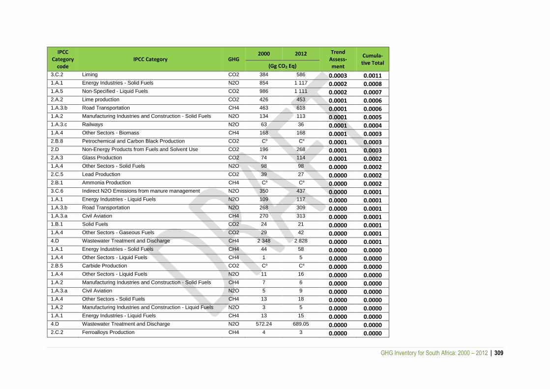
GHG Inventory for South Africa: 2000 – 2012 | 309

IPCC Category

code IPCC Category GHG

2000 2012 Trend Assess-ment

Cumula-tive Total

(Gg CO2 Eq)

3.C.2 Liming CO2 384 586 0.0003 0.0011

1.A.1 Energy Industries - Solid Fuels N2O 854 1 117 0.0002 0.0008

1.A.5 Non-Specified - Liquid Fuels CO2 986 1 111 0.0002 0.0007

2.A.2 Lime production CO2 426 453 0.0001 0.0006

1.A.3.b Road Transportation CH4 463 618 0.0001 0.0006

1.A.2 Manufacturing Industries and Construction - Solid Fuels N2O 134 113 0.0001 0.0005

1.A.3.c Railways N2O 63 36 0.0001 0.0004

1.A.4 Other Sectors - Biomass CH4 168 168 0.0001 0.0003

2.B.8 Petrochemical and Carbon Black Production CO2 Ca Ca 0.0001 0.0003

2.D Non-Energy Products from Fuels and Solvent Use CO2 196 268 0.0001 0.0003

2.A.3 Glass Production CO2 74 114 0.0001 0.0002

1.A.4 Other Sectors - Solid Fuels N2O 98 98 0.0000 0.0002

2.C.5 Lead Production CO2 39 27 0.0000 0.0002

2.B.1 Ammonia Production CH4 Ca Ca 0.0000 0.0002

3.C.6 Indirect N2O Emissions from manure management N2O 350 437 0.0000 0.0001

1.A.1 Energy Industries - Liquid Fuels N2O 109 117 0.0000 0.0001

1.A.3.b Road Transportation N2O 268 309 0.0000 0.0001

1.A.3.a Civil Aviation CH4 270 313 0.0000 0.0001

1.B.1 Solid Fuels CO2 24 21 0.0000 0.0001

1.A.4 Other Sectors - Gaseous Fuels CO2 29 42 0.0000 0.0001

4.D Wastewater Treatment and Discharge CH4 2 348 2 828 0.0000 0.0001

1.A.1 Energy Industries - Solid Fuels CH4 44 58 0.0000 0.0000

1.A.4 Other Sectors - Liquid Fuels CH4 1 5 0.0000 0.0000

2.B.5 Carbide Production CO2 Ca Ca 0.0000 0.0000

1.A.4 Other Sectors - Liquid Fuels N2O 11 16 0.0000 0.0000

1.A.2 Manufacturing Industries and Construction - Solid Fuels CH4 7 6 0.0000 0.0000

1.A.3.a Civil Aviation N2O 5 9 0.0000 0.0000

1.A.4 Other Sectors - Solid Fuels CH4 13 18 0.0000 0.0000

1.A.2 Manufacturing Industries and Construction - Liquid Fuels N2O 3 5 0.0000 0.0000

1.A.1 Energy Industries - Liquid Fuels CH4 13 15 0.0000 0.0000

4.D Wastewater Treatment and Discharge N2O 572.24 689.05 0.0000 0.0000

2.C.2 Ferroalloys Production CH4 4 3 0.0000 0.0000

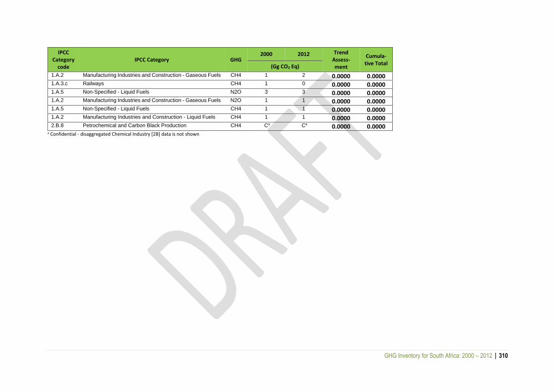
GHG Inventory for South Africa: 2000 – 2012 | 310

IPCC Category

code IPCC Category GHG

2000 2012 Trend Assess-ment

Cumula-tive Total

(Gg CO2 Eq)

1.A.2 Manufacturing Industries and Construction - Gaseous Fuels CH4 1 2 0.0000 0.0000

1.A.3.c Railways CH4 1 0 0.0000 0.0000

1.A.5 Non-Specified - Liquid Fuels N2O 3 3 0.0000 0.0000

1.A.2 Manufacturing Industries and Construction - Gaseous Fuels N2O 1 1 0.0000 0.0000

1.A.5 Non-Specified - Liquid Fuels CH4 1 1 0.0000 0.0000

1.A.2 Manufacturing Industries and Construction - Liquid Fuels CH4 1 1 0.0000 0.0000

2.B.8 Petrochemical and Carbon Black Production CH4 Ca Ca 0.0000 0.0000 a Confidential - disaggregated Chemical Industry [2B] data is not shown

GHG Inventory for South Africa: 2000 – 2012 | 311

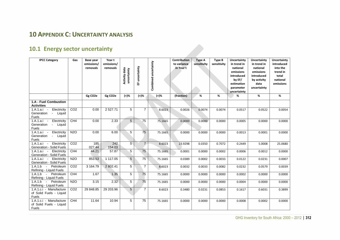
GHG Inventory for South Africa: 2000 – 2012 | 312

10 APPENDIX C: UNCERTAINTY ANALYSIS

10.1 Energy sector uncertainty

IPCC Category Gas Base year emissions/ removals

Year t emissions/ removals

Act

ivit

y d

ata

un

cert

ain

ty

EF u

nce

rtai

nty

Co

mb

ine

d u

nce

rtai

nty

Contribution to variance

in Year t

Type A sensitivity

Type B sensitivity

Uncertainty in trend in national

emissions introduced

by EF/ estimation parameter uncertainty

Uncertainty in trend in national

emissions introduced by activity

data uncertainty

Uncertainty introduced

into the trend in

total national

emissions

Gg CO2e Gg CO2e (+)% (+)% (+)% (fraction) % % % % %

1.A - Fuel Combustion Activities

1.A.1.a.i - Electricity Generation - Liquid Fuels

CO2 0.00 2 527.71 5 7 8.6023 0.0026 0.0074 0.0074 0.0517 0.0522 0.0054

1.A.1.a.i - Electricity Generation - Liquid Fuels

CH4 0.00 2.33 5 75 75.1665 0.0000 0.0000 0.0000 0.0005 0.0000 0.0000

1.A.1.a.i - Electricity Generation - Liquid Fuels

N2O 0.00 6.00 5 75 75.1665 0.0000 0.0000 0.0000 0.0013 0.0001 0.0000

1.A.1.a.i - Electricity Generation - Solid Fuels

CO2 185 027.44

242 154.03

5 7 8.6023 23.9298 0.0350 0.7072 0.2449 5.0008 25.0680

1.A.1.a.i - Electricity Generation - Solid Fuels

CH4 44.21 57.87 5 75 75.1665 0.0001 0.0000 0.0002 0.0006 0.0012 0.0000

1.A.1.a.i - Electricity Generation - Solid Fuels

N2O 853.53 1 117.05 5 75 75.1665 0.0389 0.0002 0.0033 0.0122 0.0231 0.0007

1.A.1.b - Petroleum Refining - Liquid Fuels

CO2 3 164.79 2 802.41 5 7 8.6023 0.0032 0.0033 0.0082 0.0232 0.0579 0.0039

1.A.1.b - Petroleum Refining - Liquid Fuels

CH4 1.67 1.35 5 75 75.1665 0.0000 0.0000 0.0000 0.0002 0.0000 0.0000

1.A.1.b - Petroleum Refining - Liquid Fuels

N2O 3.15 2.32 5 75 75.1665 0.0000 0.0000 0.0000 0.0004 0.0000 0.0000

1.A.1.c.i - Manufacture of Solid Fuels - Liquid Fuels

CO2 29 848.85 29 203.96 5 7 8.6023 0.3480 0.0231 0.0853 0.1617 0.6031 0.3899

1.A.1.c.i - Manufacture of Solid Fuels - Liquid Fuels

CH4 11.64 10.94 5 75 75.1665 0.0000 0.0000 0.0000 0.0008 0.0002 0.0000

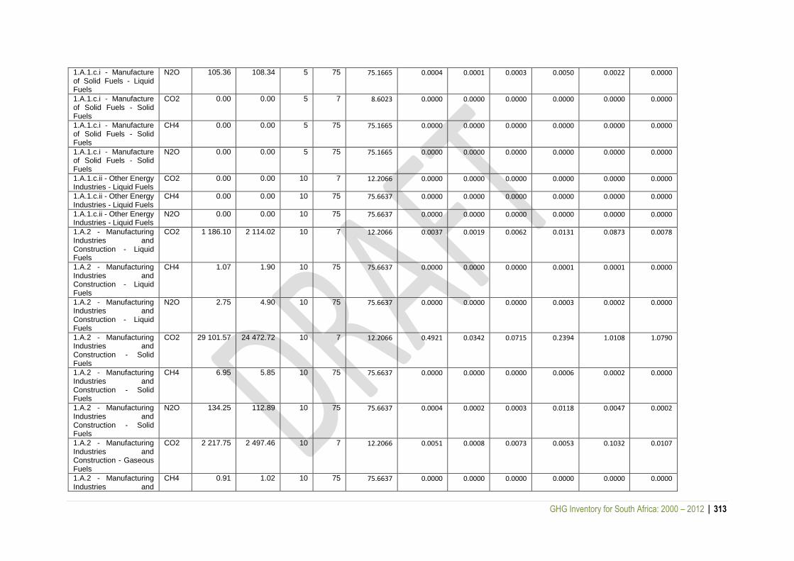
GHG Inventory for South Africa: 2000 – 2012 | 313

1.A.1.c.i - Manufacture of Solid Fuels - Liquid Fuels

N2O 105.36 108.34 5 75 75.1665 0.0004 0.0001 0.0003 0.0050 0.0022 0.0000

1.A.1.c.i - Manufacture of Solid Fuels - Solid Fuels

CO2 0.00 0.00 5 7 8.6023 0.0000 0.0000 0.0000 0.0000 0.0000 0.0000

1.A.1.c.i - Manufacture of Solid Fuels - Solid Fuels

CH4 0.00 0.00 5 75 75.1665 0.0000 0.0000 0.0000 0.0000 0.0000 0.0000

1.A.1.c.i - Manufacture of Solid Fuels - Solid Fuels

N2O 0.00 0.00 5 75 75.1665 0.0000 0.0000 0.0000 0.0000 0.0000 0.0000

1.A.1.c.ii - Other Energy Industries - Liquid Fuels

CO2 0.00 0.00 10 7 12.2066 0.0000 0.0000 0.0000 0.0000 0.0000 0.0000

1.A.1.c.ii - Other Energy Industries - Liquid Fuels

CH4 0.00 0.00 10 75 75.6637 0.0000 0.0000 0.0000 0.0000 0.0000 0.0000

1.A.1.c.ii - Other Energy Industries - Liquid Fuels

N2O 0.00 0.00 10 75 75.6637 0.0000 0.0000 0.0000 0.0000 0.0000 0.0000

1.A.2 - Manufacturing Industries and Construction - Liquid Fuels

CO2 1 186.10 2 114.02 10 7 12.2066 0.0037 0.0019 0.0062 0.0131 0.0873 0.0078

1.A.2 - Manufacturing Industries and Construction - Liquid Fuels

CH4 1.07 1.90 10 75 75.6637 0.0000 0.0000 0.0000 0.0001 0.0001 0.0000

1.A.2 - Manufacturing Industries and Construction - Liquid Fuels

N2O 2.75 4.90 10 75 75.6637 0.0000 0.0000 0.0000 0.0003 0.0002 0.0000

1.A.2 - Manufacturing Industries and Construction - Solid Fuels

CO2 29 101.57 24 472.72 10 7 12.2066 0.4921 0.0342 0.0715 0.2394 1.0108 1.0790

1.A.2 - Manufacturing Industries and Construction - Solid Fuels

CH4 6.95 5.85 10 75 75.6637 0.0000 0.0000 0.0000 0.0006 0.0002 0.0000

1.A.2 - Manufacturing Industries and Construction - Solid Fuels

N2O 134.25 112.89 10 75 75.6637 0.0004 0.0002 0.0003 0.0118 0.0047 0.0002

1.A.2 - Manufacturing Industries and Construction - Gaseous Fuels

CO2 2 217.75 2 497.46 10 7 12.2066 0.0051 0.0008 0.0073 0.0053 0.1032 0.0107

1.A.2 - Manufacturing Industries and

CH4 0.91 1.02 10 75 75.6637 0.0000 0.0000 0.0000 0.0000 0.0000 0.0000

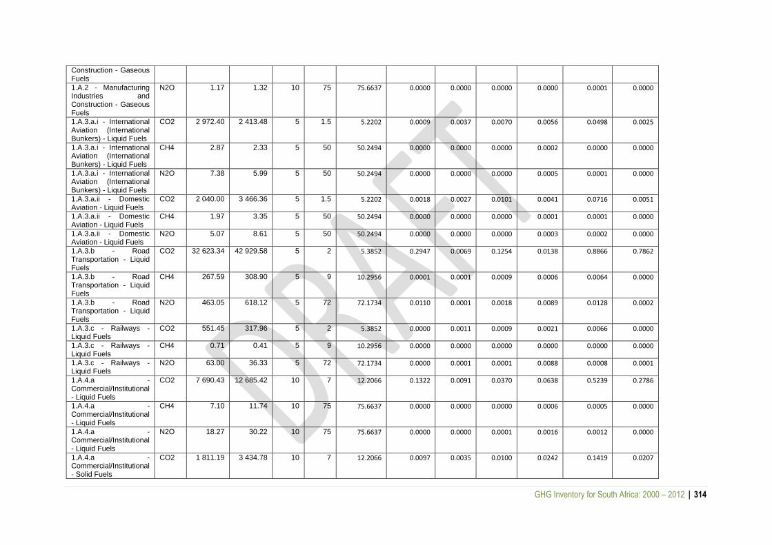
GHG Inventory for South Africa: 2000 – 2012 | 314

Construction - Gaseous Fuels

1.A.2 - Manufacturing Industries and Construction - Gaseous Fuels

N2O 1.17 1.32 10 75 75.6637 0.0000 0.0000 0.0000 0.0000 0.0001 0.0000

1.A.3.a.i - International Aviation (International Bunkers) - Liquid Fuels

CO2 2 972.40 2 413.48 5 1.5 5.2202 0.0009 0.0037 0.0070 0.0056 0.0498 0.0025

1.A.3.a.i - International Aviation (International Bunkers) - Liquid Fuels

CH4 2.87 2.33 5 50 50.2494 0.0000 0.0000 0.0000 0.0002 0.0000 0.0000

1.A.3.a.i - International Aviation (International Bunkers) - Liquid Fuels

N2O 7.38 5.99 5 50 50.2494 0.0000 0.0000 0.0000 0.0005 0.0001 0.0000

1.A.3.a.ii - Domestic Aviation - Liquid Fuels

CO2 2 040.00 3 466.36 5 1.5 5.2202 0.0018 0.0027 0.0101 0.0041 0.0716 0.0051

1.A.3.a.ii - Domestic Aviation - Liquid Fuels

CH4 1.97 3.35 5 50 50.2494 0.0000 0.0000 0.0000 0.0001 0.0001 0.0000

1.A.3.a.ii - Domestic Aviation - Liquid Fuels

N2O 5.07 8.61 5 50 50.2494 0.0000 0.0000 0.0000 0.0003 0.0002 0.0000

1.A.3.b - Road Transportation - Liquid Fuels

CO2 32 623.34 42 929.58 5 2 5.3852 0.2947 0.0069 0.1254 0.0138 0.8866 0.7862

1.A.3.b - Road Transportation - Liquid Fuels

CH4 267.59 308.90 5 9 10.2956 0.0001 0.0001 0.0009 0.0006 0.0064 0.0000

1.A.3.b - Road Transportation - Liquid Fuels

N2O 463.05 618.12 5 72 72.1734 0.0110 0.0001 0.0018 0.0089 0.0128 0.0002

1.A.3.c - Railways - Liquid Fuels

CO2 551.45 317.96 5 2 5.3852 0.0000 0.0011 0.0009 0.0021 0.0066 0.0000

1.A.3.c - Railways - Liquid Fuels

CH4 0.71 0.41 5 9 10.2956 0.0000 0.0000 0.0000 0.0000 0.0000 0.0000

1.A.3.c - Railways - Liquid Fuels

N2O 63.00 36.33 5 72 72.1734 0.0000 0.0001 0.0001 0.0088 0.0008 0.0001

1.A.4.a - Commercial/Institutional - Liquid Fuels

CO2 7 690.43 12 685.42 10 7 12.2066 0.1322 0.0091 0.0370 0.0638 0.5239 0.2786

1.A.4.a - Commercial/Institutional - Liquid Fuels

CH4 7.10 11.74 10 75 75.6637 0.0000 0.0000 0.0000 0.0006 0.0005 0.0000

1.A.4.a - Commercial/Institutional - Liquid Fuels

N2O 18.27 30.22 10 75 75.6637 0.0000 0.0000 0.0001 0.0016 0.0012 0.0000

1.A.4.a - Commercial/Institutional - Solid Fuels

CO2 1 811.19 3 434.78 10 7 12.2066 0.0097 0.0035 0.0100 0.0242 0.1419 0.0207

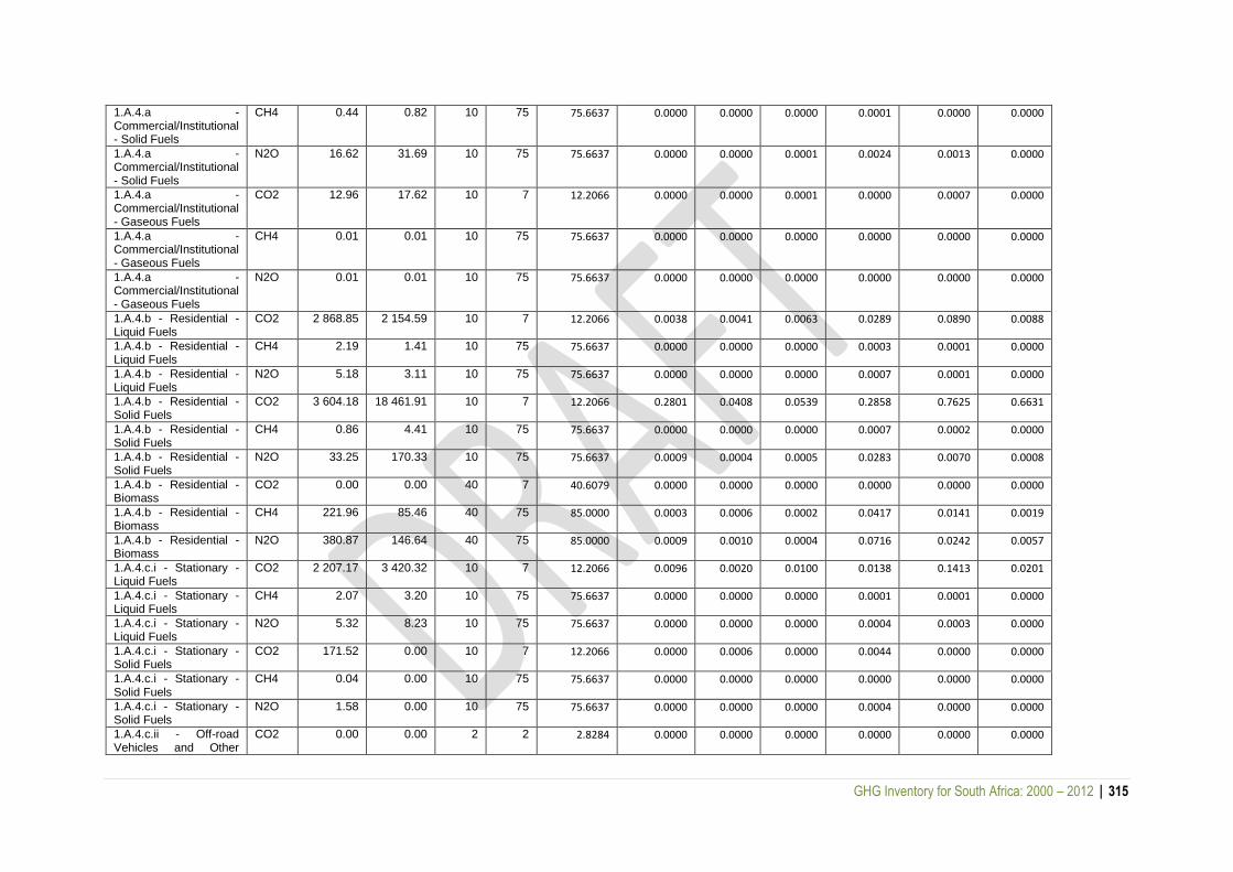
GHG Inventory for South Africa: 2000 – 2012 | 315

1.A.4.a - Commercial/Institutional - Solid Fuels

CH4 0.44 0.82 10 75 75.6637 0.0000 0.0000 0.0000 0.0001 0.0000 0.0000

1.A.4.a - Commercial/Institutional - Solid Fuels

N2O 16.62 31.69 10 75 75.6637 0.0000 0.0000 0.0001 0.0024 0.0013 0.0000

1.A.4.a - Commercial/Institutional - Gaseous Fuels

CO2 12.96 17.62 10 7 12.2066 0.0000 0.0000 0.0001 0.0000 0.0007 0.0000

1.A.4.a - Commercial/Institutional - Gaseous Fuels

CH4 0.01 0.01 10 75 75.6637 0.0000 0.0000 0.0000 0.0000 0.0000 0.0000

1.A.4.a - Commercial/Institutional - Gaseous Fuels

N2O 0.01 0.01 10 75 75.6637 0.0000 0.0000 0.0000 0.0000 0.0000 0.0000

1.A.4.b - Residential - Liquid Fuels

CO2 2 868.85 2 154.59 10 7 12.2066 0.0038 0.0041 0.0063 0.0289 0.0890 0.0088

1.A.4.b - Residential - Liquid Fuels

CH4 2.19 1.41 10 75 75.6637 0.0000 0.0000 0.0000 0.0003 0.0001 0.0000

1.A.4.b - Residential - Liquid Fuels

N2O 5.18 3.11 10 75 75.6637 0.0000 0.0000 0.0000 0.0007 0.0001 0.0000

1.A.4.b - Residential - Solid Fuels

CO2 3 604.18 18 461.91 10 7 12.2066 0.2801 0.0408 0.0539 0.2858 0.7625 0.6631

1.A.4.b - Residential - Solid Fuels

CH4 0.86 4.41 10 75 75.6637 0.0000 0.0000 0.0000 0.0007 0.0002 0.0000

1.A.4.b - Residential - Solid Fuels

N2O 33.25 170.33 10 75 75.6637 0.0009 0.0004 0.0005 0.0283 0.0070 0.0008

1.A.4.b - Residential - Biomass

CO2 0.00 0.00 40 7 40.6079 0.0000 0.0000 0.0000 0.0000 0.0000 0.0000

1.A.4.b - Residential - Biomass

CH4 221.96 85.46 40 75 85.0000 0.0003 0.0006 0.0002 0.0417 0.0141 0.0019

1.A.4.b - Residential - Biomass

N2O 380.87 146.64 40 75 85.0000 0.0009 0.0010 0.0004 0.0716 0.0242 0.0057

1.A.4.c.i - Stationary - Liquid Fuels

CO2 2 207.17 3 420.32 10 7 12.2066 0.0096 0.0020 0.0100 0.0138 0.1413 0.0201

1.A.4.c.i - Stationary - Liquid Fuels

CH4 2.07 3.20 10 75 75.6637 0.0000 0.0000 0.0000 0.0001 0.0001 0.0000

1.A.4.c.i - Stationary - Liquid Fuels

N2O 5.32 8.23 10 75 75.6637 0.0000 0.0000 0.0000 0.0004 0.0003 0.0000

1.A.4.c.i - Stationary - Solid Fuels

CO2 171.52 0.00 10 7 12.2066 0.0000 0.0006 0.0000 0.0044 0.0000 0.0000

1.A.4.c.i - Stationary - Solid Fuels

CH4 0.04 0.00 10 75 75.6637 0.0000 0.0000 0.0000 0.0000 0.0000 0.0000

1.A.4.c.i - Stationary - Solid Fuels

N2O 1.58 0.00 10 75 75.6637 0.0000 0.0000 0.0000 0.0004 0.0000 0.0000

1.A.4.c.ii - Off-road Vehicles and Other

CO2 0.00 0.00 2 2 2.8284 0.0000 0.0000 0.0000 0.0000 0.0000 0.0000

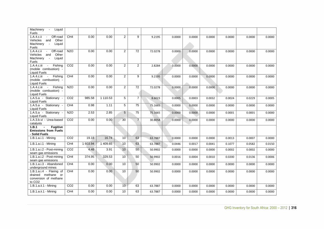
GHG Inventory for South Africa: 2000 – 2012 | 316

Machinery - Liquid Fuels

1.A.4.c.ii - Off-road Vehicles and Other Machinery - Liquid Fuels

CH4 0.00 0.00 2 9 9.2195 0.0000 0.0000 0.0000 0.0000 0.0000 0.0000

1.A.4.c.ii - Off-road Vehicles and Other Machinery - Liquid Fuels

N2O 0.00 0.00 2 72 72.0278 0.0000 0.0000 0.0000 0.0000 0.0000 0.0000

1.A.4.c.iii - Fishing (mobile combustion) - Liquid Fuels

CO2 0.00 0.00 2 2 2.8284 0.0000 0.0000 0.0000 0.0000 0.0000 0.0000

1.A.4.c.iii - Fishing (mobile combustion) - Liquid Fuels

CH4 0.00 0.00 2 9 9.2195 0.0000 0.0000 0.0000 0.0000 0.0000 0.0000

1.A.4.c.iii - Fishing (mobile combustion) - Liquid Fuels

N2O 0.00 0.00 2 72 72.0278 0.0000 0.0000 0.0000 0.0000 0.0000 0.0000

1.A.5.a - Stationary - Liquid Fuels

CO2 985.58 1 110.53 5 7 8.6023 0.0005 0.0003 0.0032 0.0024 0.0229 0.0005

1.A.5.a - Stationary - Liquid Fuels

CH4 0.98 1.11 5 75 75.1665 0.0000 0.0000 0.0000 0.0000 0.0000 0.0000

1.A.5.a - Stationary - Liquid Fuels

N2O 2.53 2.85 5 75 75.1665 0.0000 0.0000 0.0000 0.0001 0.0001 0.0000

1.A.3.b.vi - Urea-based catalysts

CO2 0.00 0.00 30 7 30.8058 0.0000 0.0000 0.0000 0.0000 0.0000 0.0000

1.B.1 - Fugitive Emissions from Fuels - Solid Fuels

1.B.1.a.i.1 - Mining CO2 19.18 16.74 10 63 63.7887 0.0000 0.0000 0.0000 0.0013 0.0007 0.0000

1.B.1.a.i.1 - Mining CH4 1 603.94 1 409.65 10 63 63.7887 0.0446 0.0017 0.0041 0.1077 0.0582 0.0150

1.B.1.a.i.2 - Post-mining seam gas emissions

CO2 4.48 3.91 10 50 50.9902 0.0000 0.0000 0.0000 0.0002 0.0002 0.0000

1.B.1.a.i.2 - Post-mining seam gas emissions

CH4 374.95 329.53 10 50 50.9902 0.0016 0.0004 0.0010 0.0200 0.0136 0.0006

1.B.1.a.i.3 - Abandoned underground mines

CH4 0.00 0.00 10 50 50.9902 0.0000 0.0000 0.0000 0.0000 0.0000 0.0000

1.B.1.a.i.4 - Flaring of drained methane or conversion of methane to CO2

CH4 0.00 0.00 10 50 50.9902 0.0000 0.0000 0.0000 0.0000 0.0000 0.0000

1.B.1.a.ii.1 - Mining CO2 0.00 0.00 10 63 63.7887 0.0000 0.0000 0.0000 0.0000 0.0000 0.0000

1.B.1.a.ii.1 - Mining CH4 0.00 0.00 10 63 63.7887 0.0000 0.0000 0.0000 0.0000 0.0000 0.0000

GHG Inventory for South Africa: 2000 – 2012 | 317

1.B.1.a.ii.2 - Post-mining seam gas emissions

CO2 0.00 0.00 10 50 50.9902 0.0000 0.0000 0.0000 0.0000 0.0000 0.0000

1.B.1.a.ii.2 - Post-mining seam gas emissions

CH4 0.00 0.00 10 50 50.9902 0.0000 0.0000 0.0000 0.0000 0.0000 0.0000

1.B.2 - Fugitive Emissions from Fuels - Oil and Natural Gas

1.B.2.a.i - Venting CO2 0.00 0.00 25 75 79.0569 0.0000 0.0000 0.0000 0.0000 0.0000 0.0000

1.B.2.a.i - Venting CH4 0.00 0.00 25 75 79.0569 0.0000 0.0000 0.0000 0.0000 0.0000 0.0000

1.B.2.a.i - Venting N2O 0.00 0.00 25 75 79.0569 0.0000 0.0000 0.0000 0.0000 0.0000 0.0000

1.B.2.a.ii - Flaring CO2 752.04 641.83 25 75 79.0569 0.0142 0.0009 0.0019 0.0643 0.0663 0.0085

1.B.2.a.ii - Flaring CH4 0.00 0.00 25 75 79.0569 0.0000 0.0000 0.0000 0.0000 0.0000 0.0000

1.B.3 - Other emissions from Energy Production

CO2 26 658.56 21 799.66 25 75 79.0569 16.3796 0.0331 0.0637 2.4852 2.2510 11.2428

1.B.3 - Other emissions from Energy Production

CH4 2 226.04 2 526.13 25 75 79.0569 0.2199 0.0007 0.0074 0.0531 0.2608 0.0709

1.C - CO2 Transport Injection and Storage

TOTAL

Sum 342 402.3510

425 831.6207

42.23 39.70

Uncertainty in total inventory

6.50 Trend uncertainty

6.30

GHG Inventory for South Africa: 2000 – 2012 | 318

10.2 IPPU sector uncertainty

IPCC Category Gas Base year emissions/ removals

Year t emissions/ removals

Act

ivit

y d

ata

un

cert

ain

ty

EF u

nce

rtai

nty

Co

mb

ine

d

un

cert

ain

ty

Contribution to

variance in Year t

Type A sensitivity

Type B sensitivity

Uncertainty in trend in national

emissions introduced by EF/ estimation

parameter uncertainty

Uncertainty in trend in national

emissions introduced by activity data uncertainty

Uncertainty introduced

into the trend in

total national

emissions

Gg CO2e Gg CO2e (+)% (+)% (+)% (fraction) % % % % %

2.A - Mineral Industry

2.A.1 - Cement production CO2 3 347.05 3 844.50 1 4.5 4.6098 0.0001 2.5046 0.0853 11.2707 0.1206 127.0438

2.A.2 - Lime production CO2 426.37 453.09 1 6 6.0828 0.0000 0.3201 0.0101 1.9205 0.0142 3.6884

2.A.3 - Glass Production CO2 74.36 113.91 5 60 60.2080 0.0000 0.0551 0.0025 3.3031 0.0179 10.9107

2.A.4.a - Ceramics CO2 0.00 0.00 43 2.5 43.0726 0.0000 0.0000 0.0000 0.0000 0.0000 0.0000

2.A.4.b - Other Uses of Soda Ash

CO2 0.00 0.00 43 2.5 43.0726 0.0000 0.0000 0.0000 0.0000 0.0000 0.0000

2.A.4.c - Non Metallurgical Magnesia Production

CO2 0.00 0.00 43 2.5 43.0726 0.0000 0.0000 0.0000 0.0000 0.0000 0.0000

2.A.4.d - Other (please specify) CO2 0.00 0.00 43 2.5 43.0726 0.0000 0.0000 0.0000 0.0000 0.0000 0.0000

2.B - Chemical Industry

2.B.1 - Ammonia Production CO2 485.28 217.80 5 6 7.8102 0.0000 0.3709 0.0048 2.2254 0.0342 4.9536

2.B.1 - Ammonia Production CH4 71.81 70.10 5 6 7.8102 0.0000 0.0540 0.0016 0.3243 0.0110 0.1053

2.B.2 - Nitric Acid Production N2O 1 570.25 745.00 2 10 10.1980 0.0000 1.1990 0.0165 11.9897 0.0468 143.7547

2.B.3 - Adipic Acid Production N2O 0.00 0.00 2 10 10.1980 0.0000 0.0000 0.0000 0.0000 0.0000 0.0000

2.B.4 - Caprolactam, Glyoxal and Glyoxylic Acid Production

N2O 0.00 0.00 2 40 40.0500 0.0000 0.0000 0.0000 0.0000 0.0000 0.0000

2.B.5 - Carbide Production CO2 1.98 5.20 5 10 11.1803 0.0000 0.0014 0.0001 0.0142 0.0008 0.0002

2.B.5 - Carbide Production CH4 0.00 0.00 5 10 11.1803 0.0000 0.0000 0.0000 0.0000 0.0000 0.0000

2.B.6 - Titanium Dioxide Production

CO2 437.62 158.66 5 10 11.1803 0.0000 0.3353 0.0035 3.3531 0.0249 11.2441

2.B.7 - Soda Ash Production CO2 0.00 0.00 5 10 11.1803 0.0000 0.0000 0.0000 0.0000 0.0000 0.0000

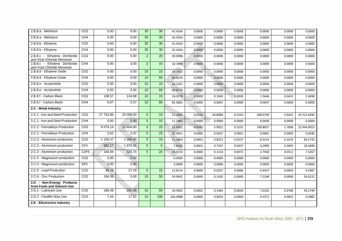
GHG Inventory for South Africa: 2000 – 2012 | 319

2.B.8.a - Methanol CO2 0.00 0.00 30 30 42.4264 0.0000 0.0000 0.0000 0.0000 0.0000 0.0000

2.B.8.a - Methanol CH4 0.00 0.00 30 30 42.4264 0.0000 0.0000 0.0000 0.0000 0.0000 0.0000

2.B.8.b - Ethylene CO2 0.00 0.00 30 30 42.4264 0.0000 0.0000 0.0000 0.0000 0.0000 0.0000

2.B.8.b - Ethylene CH4 0.00 0.00 30 30 42.4264 0.0000 0.0000 0.0000 0.0000 0.0000 0.0000

2.B.8.c - Ethylene Dichloride and Vinyl Chloride Monomer

CO2 0.00 0.00 2 20 20.0998 0.0000 0.0000 0.0000 0.0000 0.0000 0.0000

2.B.8.c - Ethylene Dichloride and Vinyl Chloride Monomer

CH4 0.00 0.00 2 10 10.1980 0.0000 0.0000 0.0000 0.0000 0.0000 0.0000

2.B.8.d - Ethylene Oxide CO2 0.00 0.00 10 10 14.1421 0.0000 0.0000 0.0000 0.0000 0.0000 0.0000

2.B.8.d - Ethylene Oxide CH4 0.00 0.00 10 60 60.8276 0.0000 0.0000 0.0000 0.0000 0.0000 0.0000

2.B.8.e - Acrylonitrile CO2 0.00 0.00 10 10 14.1421 0.0000 0.0000 0.0000 0.0000 0.0000 0.0000

2.B.8.e - Acrylonitrile CH4 0.00 0.00 10 60 60.8276 0.0000 0.0000 0.0000 0.0000 0.0000 0.0000

2.B.8.f - Carbon Black CO2 138.57 134.88 10 15 18.0278 0.0000 0.1043 0.0030 1.5646 0.0423 2.4498

2.B.8.f - Carbon Black CH4 0.07 0.07 10 85 85.5862 0.0000 0.0001 0.0000 0.0047 0.0000 0.0000

2.C - Metal Industry

2.C.1 - Iron and Steel Production CO2 27 753.86 25 008.50 5 10 11.1803 0.0316 20.8080 0.5550 208.0799 3.9241 43 312.6496

2.C.1 - Iron and Steel Production CH4 0.00 0.00 5 10 11.1803 0.0000 0.0000 0.0000 0.0000 0.0000 0.0000

2.C.2 - Ferroalloys Production CO2 8 079.14 11 404.90 5 25 25.4951 0.0342 5.9922 0.2531 149.8057 1.7896 22 444.9653

2.C.2 - Ferroalloys Production CH4 3.62 3.37 5 25 25.4951 0.0000 0.0027 0.0001 0.0681 0.0005 0.0046

2.C.3 - Aluminium production CO2 1 105.47 1 066.90 5 10 11.1803 0.0001 0.8321 0.0237 8.3214 0.1674 69.2733

2.C.3 - Aluminium production CF4 982.17 1 970.91 5 6 7.8102 0.0001 0.7167 0.0437 4.2999 0.3093 18.5848

2.C.3 - Aluminium production C2F6 156.94 325.74 5 24 24.5153 0.0000 0.1143 0.0072 2.7430 0.0511 7.5267

2.C.4 - Magnesium production CO2 0.00 0.00 0.0000 0.0000 0.0000 0.0000 0.0000 0.0000 0.0000

2.C.4 - Magnesium production SF6 0.00 0.00 0.0000 0.0000 0.0000 0.0000 0.0000 0.0000 0.0000

2.C.5 - Lead Production CO2 39.16 27.29 5 15 15.8114 0.0000 0.0297 0.0006 0.4457 0.0043 0.1987

2.C.6 - Zinc Production CO2 194.36 0.00 10 50 50.9902 0.0000 0.1505 0.0000 7.5248 0.0000 56.6222

2.D - Non-Energy Products from Fuels and Solvent Use

2.D.1 - Lubricant Use CO2 188.48 250.58 10 50 50.9902 0.0001 0.1404 0.0056 7.0192 0.0786 49.2749

2.D.2 - Paraffin Wax Use CO2 7.44 17.42 10 100 100.4988 0.0000 0.0054 0.0004 0.5371 0.0055 0.2885

2.E - Electronics Industry

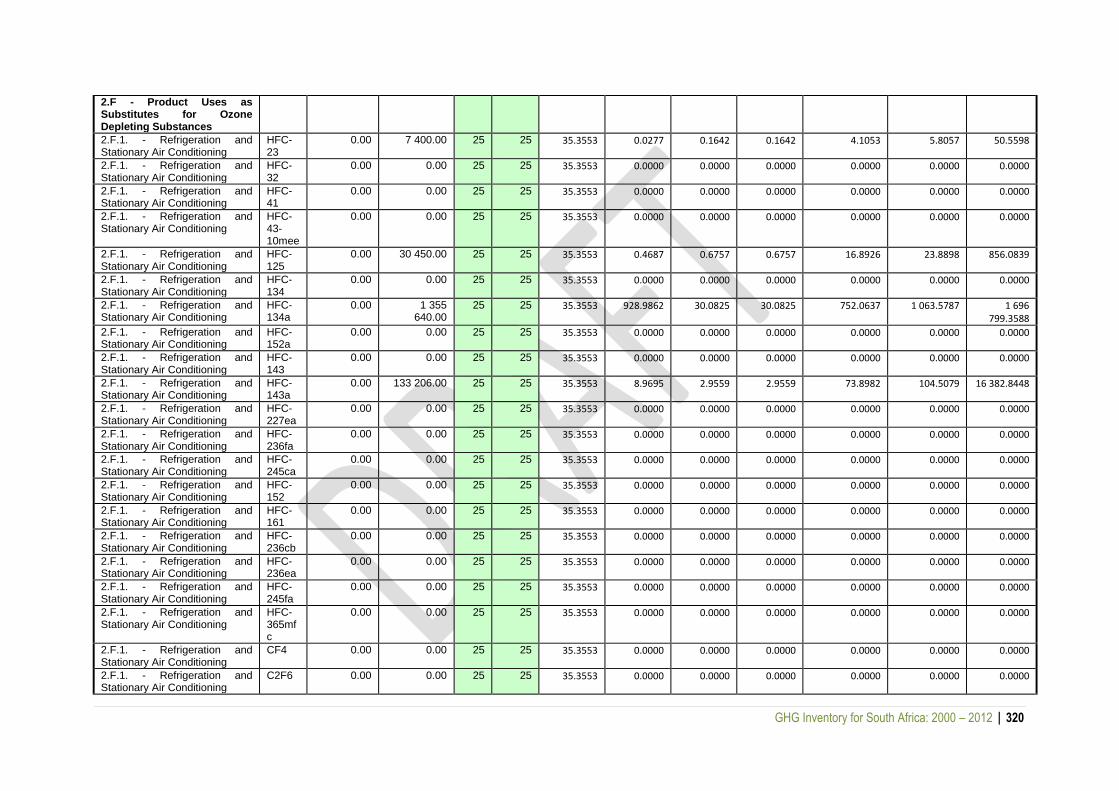
GHG Inventory for South Africa: 2000 – 2012 | 320

2.F - Product Uses as Substitutes for Ozone Depleting Substances

2.F.1. - Refrigeration and Stationary Air Conditioning

HFC-23

0.00 7 400.00 25 25 35.3553 0.0277 0.1642 0.1642 4.1053 5.8057 50.5598

2.F.1. - Refrigeration and Stationary Air Conditioning

HFC-32

0.00 0.00 25 25 35.3553 0.0000 0.0000 0.0000 0.0000 0.0000 0.0000

2.F.1. - Refrigeration and Stationary Air Conditioning

HFC-41

0.00 0.00 25 25 35.3553 0.0000 0.0000 0.0000 0.0000 0.0000 0.0000

2.F.1. - Refrigeration and Stationary Air Conditioning

HFC-43-10mee

0.00 0.00 25 25 35.3553 0.0000 0.0000 0.0000 0.0000 0.0000 0.0000

2.F.1. - Refrigeration and Stationary Air Conditioning

HFC-125

0.00 30 450.00 25 25 35.3553 0.4687 0.6757 0.6757 16.8926 23.8898 856.0839

2.F.1. - Refrigeration and Stationary Air Conditioning

HFC-134

0.00 0.00 25 25 35.3553 0.0000 0.0000 0.0000 0.0000 0.0000 0.0000

2.F.1. - Refrigeration and Stationary Air Conditioning

HFC-134a

0.00 1 355 640.00

25 25 35.3553 928.9862 30.0825 30.0825 752.0637 1 063.5787 1 696 799.3588

2.F.1. - Refrigeration and Stationary Air Conditioning

HFC-152a

0.00 0.00 25 25 35.3553 0.0000 0.0000 0.0000 0.0000 0.0000 0.0000

2.F.1. - Refrigeration and Stationary Air Conditioning

HFC-143

0.00 0.00 25 25 35.3553 0.0000 0.0000 0.0000 0.0000 0.0000 0.0000

2.F.1. - Refrigeration and Stationary Air Conditioning

HFC-143a

0.00 133 206.00 25 25 35.3553 8.9695 2.9559 2.9559 73.8982 104.5079 16 382.8448

2.F.1. - Refrigeration and Stationary Air Conditioning

HFC-227ea

0.00 0.00 25 25 35.3553 0.0000 0.0000 0.0000 0.0000 0.0000 0.0000

2.F.1. - Refrigeration and Stationary Air Conditioning

HFC-236fa

0.00 0.00 25 25 35.3553 0.0000 0.0000 0.0000 0.0000 0.0000 0.0000

2.F.1. - Refrigeration and Stationary Air Conditioning

HFC-245ca

0.00 0.00 25 25 35.3553 0.0000 0.0000 0.0000 0.0000 0.0000 0.0000

2.F.1. - Refrigeration and Stationary Air Conditioning

HFC-152

0.00 0.00 25 25 35.3553 0.0000 0.0000 0.0000 0.0000 0.0000 0.0000

2.F.1. - Refrigeration and Stationary Air Conditioning

HFC-161

0.00 0.00 25 25 35.3553 0.0000 0.0000 0.0000 0.0000 0.0000 0.0000

2.F.1. - Refrigeration and Stationary Air Conditioning

HFC-236cb

0.00 0.00 25 25 35.3553 0.0000 0.0000 0.0000 0.0000 0.0000 0.0000

2.F.1. - Refrigeration and Stationary Air Conditioning

HFC-236ea

0.00 0.00 25 25 35.3553 0.0000 0.0000 0.0000 0.0000 0.0000 0.0000

2.F.1. - Refrigeration and Stationary Air Conditioning

HFC-245fa

0.00 0.00 25 25 35.3553 0.0000 0.0000 0.0000 0.0000 0.0000 0.0000

2.F.1. - Refrigeration and Stationary Air Conditioning

HFC-365mfc

0.00 0.00 25 25 35.3553 0.0000 0.0000 0.0000 0.0000 0.0000 0.0000

2.F.1. - Refrigeration and Stationary Air Conditioning

CF4 0.00 0.00 25 25 35.3553 0.0000 0.0000 0.0000 0.0000 0.0000 0.0000

2.F.1. - Refrigeration and Stationary Air Conditioning

C2F6 0.00 0.00 25 25 35.3553 0.0000 0.0000 0.0000 0.0000 0.0000 0.0000

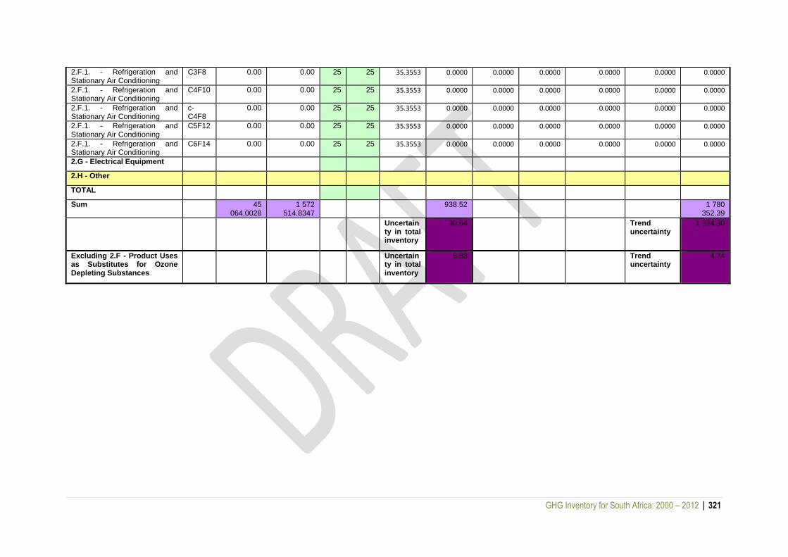
GHG Inventory for South Africa: 2000 – 2012 | 321

2.F.1. - Refrigeration and Stationary Air Conditioning

C3F8 0.00 0.00 25 25 35.3553 0.0000 0.0000 0.0000 0.0000 0.0000 0.0000

2.F.1. - Refrigeration and Stationary Air Conditioning

C4F10 0.00 0.00 25 25 35.3553 0.0000 0.0000 0.0000 0.0000 0.0000 0.0000

2.F.1. - Refrigeration and Stationary Air Conditioning

c-C4F8

0.00 0.00 25 25 35.3553 0.0000 0.0000 0.0000 0.0000 0.0000 0.0000

2.F.1. - Refrigeration and Stationary Air Conditioning

C5F12 0.00 0.00 25 25 35.3553 0.0000 0.0000 0.0000 0.0000 0.0000 0.0000

2.F.1. - Refrigeration and Stationary Air Conditioning

C6F14 0.00 0.00 25 25 35.3553 0.0000 0.0000 0.0000 0.0000 0.0000 0.0000

2.G - Electrical Equipment

2.H - Other

TOTAL

Sum 45 064.0028

1 572 514.8347

938.52 1 780 352.39

Uncertainty in total inventory

30.64 Trend uncertainty

1 334.30

Excluding 2.F - Product Uses as Substitutes for Ozone Depleting Substances

Uncertainty in total inventory

8.83 Trend uncertainty

4.74

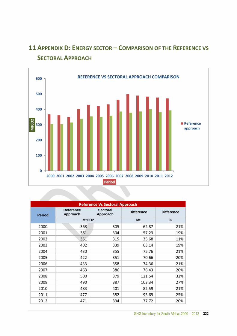
GHG Inventory for South Africa: 2000 – 2012 | 322

11 APPENDIX D: ENERGY SECTOR – COMPARISON OF THE REFERENCE VS

SECTORAL APPROACH

Reference Vs Sectoral Approach

Period

Reference approach

Sectoral Approach

Difference Difference

MtCO2 Mt %

2000 368 305 62.87 21%

2001 361 304 57.23 19%

2002 351 315 35.68 11%

2003 402 339 63.14 19%

2004 430 355 75.76 21%

2005 422 351 70.66 20%

2006 433 358 74.36 21%

2007 463 386 76.43 20%

2008 500 379 121.54 32%

2009 490 387 103.34 27%

2010 483 401 82.59 21%

2011 477 382 95.69 25%

2012 471 394 77.72 20%

0

100

200

300

400

500

600

2000 2001 2002 2003 2004 2005 2006 2007 2008 2009 2010 2011 2012

MtC

O2

Period

REFERENCE VS SECTORAL APPROACH COMPARISON

Referenceapproach

GHG Inventory for South Africa: 2000 – 2012 | 323

Average 76.69 21%

The Reference Approach is a top-down approach, using a country’s energy supply data to calculate

the emissions of CO2 from combustion of mainly fossil fuels. The Reference Approach was applied on

the basis of relatively easily available energy supply statistics. It is good practice to apply both a

sectoral approach and the reference approach to estimate a country’s CO2 emissions from fuel

combustion and to compare the results of these two independent estimates. Significant differences

may indicate possible problems with the activity data, net calorific values, carbon content, excluded

carbon calculation etc.

The Reference Approach and the Sectoral Approach often have different results because the

Reference Approach is a top-down approach using a country’s energy supply data and has no detailed

information on how the individual fuels are used in each sector. The average difference in the

reference and sectoral approach is approximately 21% which is quite significant. The main reasons for

the differences were mainly from the gaseous fuels and solid fuels which had an average difference

of 124% and 43% respectively. The generic reasons for the difference in reference and sectoral

approach are as follows:

Missing information on stock changes that may occur at the final consumer level. The

relevance of consumer stocks depends on the method used for the Sectoral Approach.

High distribution losses for gas will cause the Reference Approach to be higher than the

Sectoral Approach,

Unrecorded consumption of gas or other fuels may lead to an underestimation of the Sectoral

Approach.

The treatment of transfers and reclassifications of energy products may cause a difference in

the Sectoral Approach estimation since different net calorific values and emission factors may

be used depending on howthe fuel is classified.

Net Calorific Values (NCV) used in the sectoral approach differs from those used in the

reference approach. In power generation, NCV values in the sectoral approach vary over the

2000-2010 time series based on the information provided by industry;

Activity data on Liquid fuels in the sectoral approach particularly for energy industries is

sourced directly from the companies involved and has been reconciled with other publicly

available datasets;

Allocation of solid fuels between energy use, non-energy use as well use for synfuels

production remains one of the key drives for the differences observed between the two

datasets.

Inconsistencies on the sources of activity data within the time series and in some cases the

application of extrapolation

The misallocation of the quantities of fuels used for conversion into derived products (other

than power or heat) or quantities combusted in the energy sector.

Simplifications in the Reference Approach. There are small quantities of carbon which should

be included in the Reference Approach because their emissions fall under fuel combustion.

These quantities have been excluded where the flows are small or not represented by a major

statistic available within energy data.

GHG Inventory for South Africa: 2000 – 2012 | 324

Examples of quantities not accounted for in the Reference Approach include lubricants used

in two-stroke e.g. natural gas leakage from pipelines, emissions from energy transformation,

etc. Likely to be <5% of the reference approach.

Solid Fuels

SOLID FUELS

Period

Reference approach

Sectoral Approach

Difference Difference

TJ TJ %

2000 3 386 284 2 282 887 1 103 396.84 48%

2001 3 380 674 2 258 656 1 122 017.53 50%

2002 3 314 815 2 363 553 951 262.16 40%

2003 3 687 775 2 576 732 1 111 043.31 43%

2004 3 886 355 2 702 932 1 183 423.23 44%

2005 3 849 218 2 689 024 1 160 194.32 43%

2006 3 918 677 2 744 792 1 173 885.33 43%

2007 4 039 592 2 978 118 1 061 474.11 36%

2008 4 417 995 2 918 928 1 499 067.10 51%

2009 4 503 950 2 984 812 1 519 138.10 51%

2010 4 227 203 3 085 055 1 142 147.62 37%

2011 4 122 114 2 878 821 1 243 292.94 43%

2012 4 063 666 2 997 646 1 066 020.21 36%

Average 1 179 720.22 43%

0

500 000

1 000 000

1 500 000

2 000 000

2 500 000

3 000 000

3 500 000

4 000 000

4 500 000

5 000 000

2000 2001 2002 2003 2004 2005 2006 2007 2008 2009 2010 2011 2012

TJ

Period

REF VS SEC APPROACH COMPARISON FOR SOLID FUELS

Referenceapproach

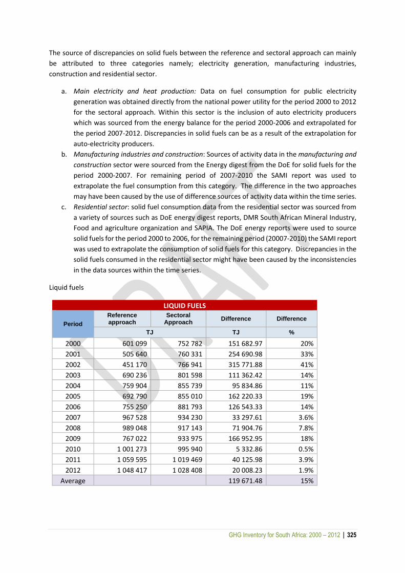
GHG Inventory for South Africa: 2000 – 2012 | 325

The source of discrepancies on solid fuels between the reference and sectoral approach can mainly

be attributed to three categories namely; electricity generation, manufacturing industries,

construction and residential sector.

a. Main electricity and heat production: Data on fuel consumption for public electricity

generation was obtained directly from the national power utility for the period 2000 to 2012

for the sectoral approach. Within this sector is the inclusion of auto electricity producers

which was sourced from the energy balance for the period 2000-2006 and extrapolated for

the period 2007-2012. Discrepancies in solid fuels can be as a result of the extrapolation for

auto-electricity producers.

b. Manufacturing industries and construction: Sources of activity data in the manufacturing and

construction sector were sourced from the Energy digest from the DoE for solid fuels for the

period 2000-2007. For remaining period of 2007-2010 the SAMI report was used to

extrapolate the fuel consumption from this category. The difference in the two approaches

may have been caused by the use of difference sources of activity data within the time series.

c. Residential sector: solid fuel consumption data from the residential sector was sourced from

a variety of sources such as DoE energy digest reports, DMR South African Mineral Industry,

Food and agriculture organization and SAPIA. The DoE energy reports were used to source

solid fuels for the period 2000 to 2006, for the remaining period (20007-2010) the SAMI report

was used to extrapolate the consumption of solid fuels for this category. Discrepancies in the

solid fuels consumed in the residential sector might have been caused by the inconsistencies

in the data sources within the time series.

Liquid fuels

LIQUID FUELS

Period

Reference approach

Sectoral Approach

Difference Difference

TJ TJ %

2000 601 099 752 782 151 682.97 20%

2001 505 640 760 331 254 690.98 33%

2002 451 170 766 941 315 771.88 41%

2003 690 236 801 598 111 362.42 14%

2004 759 904 855 739 95 834.86 11%

2005 692 790 855 010 162 220.33 19%

2006 755 250 881 793 126 543.33 14%

2007 967 528 934 230 33 297.61 3.6%

2008 989 048 917 143 71 904.76 7.8%

2009 767 022 933 975 166 952.95 18%

2010 1 001 273 995 940 5 332.86 0.5%

2011 1 059 595 1 019 469 40 125.98 3.9%

2012 1 048 417 1 028 408 20 008.23 1.9%

Average 119 671.48 15%

GHG Inventory for South Africa: 2000 – 2012 | 326

The source of discrepancies on liquid fuels between the reference and sectoral approach can mainly

be attributed to three categories namely; road transportation, commercial sector and

Agriculture/Forestry/Fishing/Fish Farms

a) The main consuming sector of liquid fuels is the road transportation. The main source of

activity data for liquid fuel consumption in the transportation sector, was the SAPIA annual

reports. The discrepancies between the sectoral and reference approach might be attributed

to the fact that SAPIA reports liquid fuel consumption at a disaggregated level various users.

b) Commercial sector: The commercial sector refers to institutional or commercial building. The

main source of activity data for liquid fuels for this category was the SAPIA for the period 2000-

2006. An extrapolation method was applied to estimate activity data for the period 2007-

2012, this might have also contributed to the differences in the reference and sectoral

approach.

c) Agriculture/Forestry/Fishing/Fish Farms: Data on fuel consumption in the agriculture,

forestry, fishing and fish farms was obtained from the Energy digest by the DoE (mostly solid

fuels) and SAPIA for liquid fuels. Discrepancies might have been attributed by the application

of different sources of activity data for the time series.

Gaseous Fuels

0

200 000

400 000

600 000

800 000

1 000 000

1 200 000

2000 2001 2002 2003 2004 2005 2006 2007 2008 2009 2010 2011 2012

TJ

Period

REF VS SEC APPROACH COMPARISON FOR LIQUID FUELS

Referenceapproach

GHG Inventory for South Africa: 2000 – 2012 | 327

GASEOUS FUELS

Period

Reference approach

Sectoral Approach

Difference Difference

TJ TJ %

2000 58 490 39 763 18 726.60 47%

2001 75 990 41 482 34 508.42 83%

2002 75 362 43 299 32 063.40 74%

2003 45 176 48 844 -3 668.43 7.5%

2004 116 393 50 671 65 722.04 130%

2005 115 472 53 541 61 930.94 116%

2006 112 039 56 433 55 605.77 99%

2007 160 103 59 323 100 780.23 170%

2008 163 578 62 213 101 365.28 163%

2009 128 702 65 101 63 601.23 98%

2010 162 155 68 888 93 266.76 135%

2011 160 982 51 744 109 238.46 211%

2012 168 979 44 832 124 147.25 277%

Average 65 945.23 124%

The source of discrepancies on gaseous fuels between the reference and sectoral approach can mainly

be attributed to the manufacturing industries and construction mainly in the production of synfuels.

0

20 000

40 000

60 000

80 000

100 000

120 000

140 000

160 000

180 000

2000 2001 2002 2003 2004 2005 2006 2007 2008 2009 2010 2011 2012

TJ

Period

REF VS SEC APPROACH COMPARISON FOR GASEOUS FUELS

Referenceapproach

GHG Inventory for South Africa: 2000 – 2012 | 328

12 APPENDIX E: AGRICULTURAL ACTIVITY DATA

12.1 Livestock sub-categories for sheep, goats and swine

Livestock category Livestock sub-category from

Du Toit et al. (2013b)

Livestock sub-category in this

inventory

Sheep

Non-wool breeding ewe Non-wool ewe

Non-wool young ewe

Non-wool breeding ram Non-wool ram

Non-wool young ram

Non-wool weaners Non-wool lamb

Non-wool lamb

Merino breeding ewe

Wool ewe

Merino young ewe

Other wool breeding ewe

Other wool young ewe

Karakul breeding ewe

Karakul young ewe

Merino breeding ram

Wool ram

Merino young ram

Other wool breeding ram

Other wool young ram

Karakul breeding ram

Karakul young ram

Merino weaner

Wool lamb

Merino lamb

Other wool weaner

Other wool lamb

Karakul weaner

Karakul lamb

Goats

Breeding buck Buck

Young buck

Breeding doe Doe

Young doe

Weaner Kid

Kid

Breeding buck

Angora

Young buck

Breeding doe

Young doe

Weaner

Kid

Breeding buck

Milk goat

Young buck

Breeding doe

Young doe

Weaner

Kid

Swine

Boars

Boars Replacement boars

Cull boars

Dry gestating sow

Sows Lactating sow

Replacement sow

Cull sow

Pre-wean piglets Piglets

Baconers Baconers

Porkers Porkers

GHG Inventory for South Africa: 2000 – 2012 | 329

12.2 Livestock population data

Category Sub-category Population

2000 2001 2002 2003 2004 2005 2006 2007 2008 2009 2010

Dairy (Commercial - TMR)

Lactating cow 437 637 437 637 375 749 349 226 340 385 362 487 353 646 349 226 433 217 442 058 442 058 Dry cow 106 452 106 452 91 398 84 947 82 796 88 173 86 022 84 947 105 377 107 528 107 528 Lactating heifer 42 092 40 985 39 877 31 015 27 692 31 015 31 015 32 123 35 446 37 662 37 662 Pregnant heifer 56 663 55 172 53 680 41 751 37 278 41 751 41 751 43 243 47 716 50 698 50 698 Heifer >1yr 19 427 18 916 18 405 14 315 12 781 14 315 14 315 14 826 16 360 17 382 17 382 Heifer 6-12mths 38 854 37 832 36 809 28 630 25 562 28 630 28 630 29 652 32 720 34 764 34 764 Heifer 2-6mths 25 903 25 221 24 540 19 086 17 041 19 086 19 086 19 768 21 813 23 176 23 176 Calves <6mths 25 903 25 221 24 540 19 086 17 041 19 086 19 086 19 768 21 813 23 176 23 176 Total TMR 752 932 747 436 664 998 588 056 560 577 604 544 593 552 593 552 714 461 736 445 736 445

Dairy (Commercial - Pasture)

Lactating cow 358 667 358 667 307 946 286 209 278 963 297 078 289 832 286 209 355 044 362 290 362 290

Dry cow 87 243 87 243 74 906 69 618 67 856 72 262 70 500 69 618 86 362 88 125 88 125

Lactating heifer 34 497 33 589 32 681 25 419 22 695 25 419 25 419 26 327 29 050 30 866 30 866

Pregnant heifer 46 438 45 216 43 994 34 218 30 551 34 218 34 218 35 440 39 106 41 550 41 550

Heifer >1yr 15 922 15 503 15 084 11 732 10 475 11 732 11 732 12 151 13 408 14 246 14 246

Heifer 6-12mths 31 843 31 005 30 167 23 463 20 950 23 463 23 463 24 301 26 815 28 491 28 491

Heifer 2-6mths 21 229 20 670 20 112 15 642 13 966 15 642 15 642 16 201 17 877 18 994 18 994

Calves <6mths 21 229 20 670 20 112 15 642 13 966 15 642 15 642 16 201 17 877 18 994 18 994

Total Pasture 617 068 612 564 545 002 481 944 459 423 495 456 486 448 486 448 585 539 603 555 603 555

Total Dairy 1 370 000 1 360 000 1 210 000 1 070 000 1 020 000 1 100 000 1 080 000 1 080 000 1 300 000 1 340 000 1 340 000

Other cattle (Commercial)

Feedlot 420 000 420 000 420 000 420 000 420 000 420 000 391 148 400 819 399 822 461 800 484 274 Bulls 200 000 190 000 190 000 190 000 200 000 190 000 180 000 150 000 160 000 180 000 200 000 Cows 3 540 000 3 600 000 3 430 000 3 080 000 2 840 000 3 140 000 3 080 000 2 460 000 2 710 000 2 390 000 2 980 000 Heifers 1 050 000 1 040 000 1 020 000 950 000 1 390 000 920 000 900 000 850 000 770 000 700 000 910 000 Ox 230 000 240 000 200 000 260 000 280 000 210 000 200 000 170 000 240 000 280 000 170 000 Young ox 660 000 660 000 540 000 570 000 520 000 510 000 500 000 1 080 000 1 140 000 860 000 630 000 Calves 1 630 000 1 610 000 1 470 000 1 910 000 1 770 000 2 110 000 2 070 000 2 400 000 1 960 000 2 490 000 1 990 000 Total commercial 7 730 000 7 760 000 7 270 000 7 380 000 7 420 000 7 500 000 7 350 000 7 530 000 7 371 148 7 300 819 7 279 822

Other cattle (Cummunal)

Bulls 137 359 130 491 130 491 130 491 137 359 130 491 123 623 103 019 109 887 123 623 137 359

Cows 2 431 256 2 472 464 2 355 709 2 115 330 1 950 499 2 156 538 2 115 330 1 689 517 1 861 216 1 641 441 2 046 651

Heifers 721 135 714 267 700 531 652 456 954 646 631 852 618 116 583 776 528 833 480 757 624 984

Ox 157 963 164 831 137 359 178 567 192 303 144 227 137 359 116 755 164 831 192 303 116 755

Young ox 453 285 453 285 370 870 391 473 357 134 350 266 343 398 741 739 782 947 590 644 432 681

Calves 1 119 477 1 105 741 1 009 589 1 311 779 1 215 628 1 449 138 1 421 667 1 648 309 1 346 119 1 710 121 1 366 723

Total communal 5 020 475 5 041 079 4 704 549 4 780 097 4 807 568 4 862 512 4 759 493 4 883 116 4 793 833 4 738 889 4 725 153

Total Other cattle 12 750 475 12 801 079 11 974 549 12 160 096 12 227 569 12 362 512 12 109 493 12 413 115 12 164 981 12 039 708 12 004 975

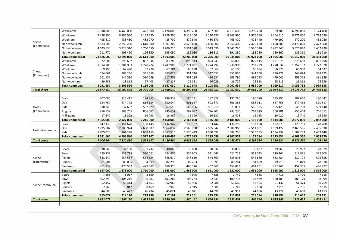
GHG Inventory for South Africa: 2000 – 2012 | 330

Sheep (Commercial)

Wool lamb 6 610 800 6 446 000 6 427 600 6 476 000 6 395 200 6 407 600 6 219 600 6 299 200 6 389 200 6 296 000 6 174 400

Wool ewe 9 420 390 9 185 550 9 159 330 9 228 300 9 113 160 9 130 830 8 862 930 8 976 360 9 104 610 8 971 800 8 798 520

Wool ram 495 810 483 450 482 070 485 700 479 640 480 570 466 470 472 440 479 190 472 200 463 080

Non-wool lamb 2 823 600 2 753 200 2 618 000 2 601 200 2 520 400 2 486 800 2 558 400 2 470 400 2 408 800 2 470 800 2 422 800

Non-wool ewe 4 023 630 3 923 310 3 730 650 3 706 710 3 591 570 3 543 690 3 645 720 3 520 320 3 432 540 3 520 890 3 452 490

Non-wool ram 211 770 206 490 196 350 195 090 189 030 186 510 191 880 185 280 180 660 185 310 181 710

Total commercial 23 586 000 22 998 000 22 614 000 22 693 000 22 289 000 22 236 000 21 945 000 21 924 000 21 995 000 21 917 000 21 493 000

Sheep (Communal)

Wool lamb 922 602 899 602 897 034 903 789 892 513 894 243 868 006 879 115 891 675 878 668 861 698

Wool ewe 1 314 708 1 281 933 1 278 274 1 287 900 1 271 831 1 274 297 1 236 909 1 252 739 1 270 637 1 252 102 1 227 920

Wool ram 69 195 67 470 67 278 67 784 66 938 67 068 65 100 65 934 66 876 65 900 64 627

Non-wool lamb 394 061 384 236 365 368 363 023 351 746 347 057 357 050 344 768 336 172 344 824 338 125

Non-wool ewe 561 537 547 536 520 649 517 308 501 239 494 557 508 796 491 295 479 045 491 375 481 829

Non-wool ram 29 555 28 818 27 403 27 227 26 381 26 029 26 779 25 858 25 213 25 862 25 359

Total communal 3 291 657 3 209 596 3 156 005 3 167 030 3 110 648 3 103 251 3 062 639 3 059 709 3 069 617 3 058 732 2 999 558

Total sheep 26 877 657 26 207 596 25 770 005 25 860 030 25 399 648 25 339 251 25 007 639 24 983 709 25 064 617 24 975 732 24 492 558

Goats (Commercial)

Buck 207 086 213 417 194 863 189 939 190 291 187 828 191 786 186 070 185 894 182 640 180 442

Doe 654 760 674 778 616 114 600 544 601 657 593 872 606 383 588 311 587 755 577 468 570 517

Kids 618 749 637 667 582 229 567 515 568 566 561 210 573 033 555 955 555 429 545 708 539 140

Angora 856 557 882 745 806 001 785 632 787 087 776 903 793 270 769 629 768 901 755 444 746 351

Milk goats 17 847 18 392 16 793 16 369 16 399 16 187 16 528 16 035 16 020 15 740 15 550

Total commercial 2 355 000 2 427 000 2 216 000 2 160 000 2 164 000 2 136 000 2 181 000 2 116 000 2 114 000 2 077 000 2 052 000

Goats (Communal)

Buck 147 130 151 628 138 445 134 947 135 197 133 447 136 259 132 198 132 073 129 761 128 200

Doe 2 795 507 2 880 974 2 630 507 2 564 032 2 568 780 2 535 542 2 588 960 2 511 801 2 509 427 2 465 506 2 435 830

Kids 1 709 028 1 761 278 1 608 155 1 567 516 1 570 419 1 550 099 1 582 756 1 535 585 1 534 134 1 507 283 1 489 140

Total communal 4 651 664 4 793 880 4 377 107 4 266 494 4 274 395 4 219 089 4 307 974 4 179 584 4 175 634 4 102 550 4 053 170

Total goats 7 006 664 7 220 880 6 593 107 6 426 494 6 438 395 6 355 089 6 488 974 6 295 584 6 289 634 6 179 550 6 105 170

Swine (commercial)

Boars 30 563 31 138 31 732 30 860 30 860 30 637 30 099 30 637 29 969 29 932 29 579

Sows 529 757 539 728 550 021 534 903 534 903 531 043 521 715 531 043 519 464 518 821 512 709

Piglets 543 340 553 567 564 124 548 619 548 619 544 660 535 093 544 660 532 784 532 124 525 856

Porkers 81 501 83 035 84 619 82 293 82 293 81 699 80 264 81 699 79 918 79 819 78 878

Baconers 461 839 470 532 479 505 466 326 466 326 462 961 454 829 462 961 452 866 452 305 446 977

Total commercial 1 647 000 1 678 000 1 710 000 1 663 000 1 663 000 1 651 000 1 622 000 1 651 000 1 615 000 1 613 000 1 594 000

Swine (communal)

Boars 7 868 8 017 8 169 7 945 7 945 7 888 7 749 7 888 7 716 7 706 7 615

Sows 102 290 104 216 106 203 103 284 103 284 102 539 100 738 102 539 100 303 100 179 98 999

Piglets 52 457 53 444 54 463 52 966 52 966 52 584 51 660 52 584 51 437 51 374 50 769

Porkers 7 868 8 017 8 169 7 945 7 945 7 888 7 749 7 888 7 716 7 706 7 615

Baconers 44 588 45 427 46 294 45 021 45 021 44 696 43 911 44 696 43 722 43 668 43 153

Total communal 215 072 219 120 223 299 217 161 217 161 215 594 211 807 215 594 210 893 210 632 208 151

Total swine 1 862 072 1 897 120 1 933 299 1 880 161 1 880 161 1 866 594 1 833 807 1 866 594 1 825 893 1 823 632 1 802 151

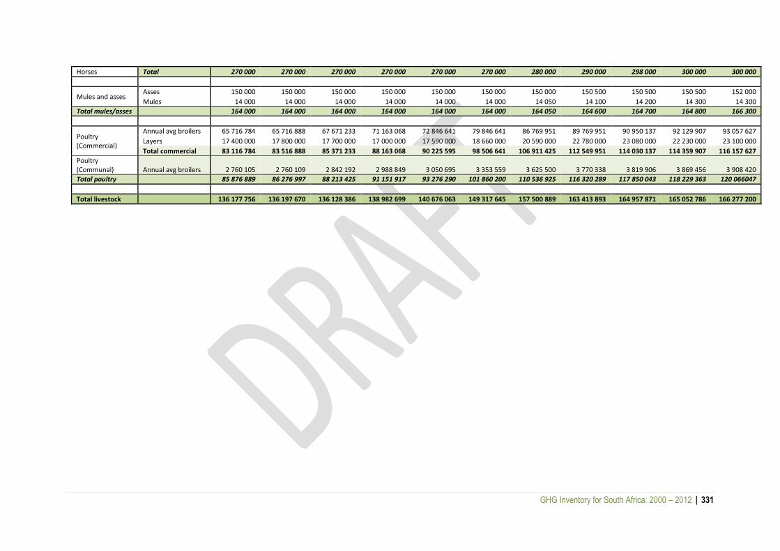
GHG Inventory for South Africa: 2000 – 2012 | 331

Horses Total 270 000 270 000 270 000 270 000 270 000 270 000 280 000 290 000 298 000 300 000 300 000

Mules and asses Asses 150 000 150 000 150 000 150 000 150 000 150 000 150 000 150 500 150 500 150 500 152 000

Mules 14 000 14 000 14 000 14 000 14 000 14 000 14 050 14 100 14 200 14 300 14 300

Total mules/asses 164 000 164 000 164 000 164 000 164 000 164 000 164 050 164 600 164 700 164 800 166 300

Poultry (Commercial)

Annual avg broilers 65 716 784 65 716 888 67 671 233 71 163 068 72 846 641 79 846 641 86 769 951 89 769 951 90 950 137 92 129 907 93 057 627

Layers 17 400 000 17 800 000 17 700 000 17 000 000 17 590 000 18 660 000 20 590 000 22 780 000 23 080 000 22 230 000 23 100 000

Total commercial 83 116 784 83 516 888 85 371 233 88 163 068 90 225 595 98 506 641 106 911 425 112 549 951 114 030 137 114 359 907 116 157 627

Poultry (Communal) Annual avg broilers 2 760 105 2 760 109 2 842 192 2 988 849 3 050 695 3 353 559 3 625 500 3 770 338 3 819 906 3 869 456 3 908 420

Total poultry 85 876 889 86 276 997 88 213 425 91 151 917 93 276 290 101 860 200 110 536 925 116 320 289 117 850 043 118 229 363 120 066047

Total livestock 136 177 756 136 197 670 136 128 386 138 982 699 140 676 063 149 317 645 157 500 889 163 413 893 164 957 871 165 052 786 166 277 200

332

13 APPENDIX F: LAND SECTOR ACTIVITY DATA

13.1 Land cover by climate

The 2013-14 land cover map (GeoTerraImage, 2015) was intersected with the long term climate map

provided by the ARC.

Description Climate Type Area [ha] WTD WTM CTD CTM Total (ha)

Indigenous Forest 365 000 11 100 100 0 376 200

Thicket /Dense bush 7 460 300 24 800 1 800 400 7 487 300

Woodland/Open bush 11 422 900 14 600 3 400 200 11 441 100

Low shrubland 38 197 100 60 300 6 500 7 300 38 271 200

Plantations / Woodlots 1 707 500 26 900 0 0 1 734 400

Cultivated commercial annual crops pivot 720 900 0 0 0 720 900

Cultivated commercial annual crops non-pivot 9 811 600 500 0 0 9 812 100

Cultivated commercial permanent orchards 312 200 2 200 0 0 314 400

Cultivated commercial permanent vines 174 800 400 0 0 175 200

Cultivated subsistence crops 1 875 600 700 0 0 1 876 300

Settlements 2 663 400 1 000 0 0 2 664 400

Wetlands 936 700 2 100 1 100 300 940 200

Grasslands 23 610 500 63 400 68 100 19 500 23 761 500

Mines 302 000 100 0 0 302 100

Waterbodies (incl coastal sea extent) 447 900 700 0 0 448 600

Bare Ground 11 753 000 3 300 1 800 2 600 11 760 700

Degraded 868 400 100 0 0 868 500

13.2 Land cover by soil type

Description Area on each IPCC soil type [ha]

Sandy

mineral soils

Wetland mineral

soils

Spodic mineral

soils

Rocky areas

Low activity

clay mineral

soils

High activity

clay mineral

soils

Water body

Indigenous Forest 96 696 226 0 30 403 91 295 203 150 1 863

Thicket /Dense bush 658 937 924 2 200 1 185 382 562 013 5 817 654 9 370

Woodland/Open bush 2 135 567 161 518 1 424 284 576 444 8 243 359 4 073

Low shrubland 15 748 119 124 2 063 4 634 043 24 304 20 955 223 7 588

Plantations / Woodlots 164 824 36 52 23 253 1 121 099 561 068 568

Cultivated commercial annual crops pivot

162 477 540 0 1 117 50 719 565 961 71

Cultivated commercial annual crops non-pivot

1 167 966 1 252 1 501 57 126 712 547 8 669 075 658

Cultivated commercial permanent orchards

75 632 0 22 6 955 57 575 206 523 242

Cultivated commercial permanent vines

55 978 0 0 4 672 0 128 053 8

Cultivated subsistence crops 110 808 720 0 11 934 175 470 1 737 450 169

Settlements 349 109 539 0 55 124 300 620 2 201 493 394

Wetlands 62 972 1 861 118 28 006 149 993 766 409 9 770

Grasslands 1 644 147 3 601 50 1 724 952 2 210 455 20 142 593 15 568

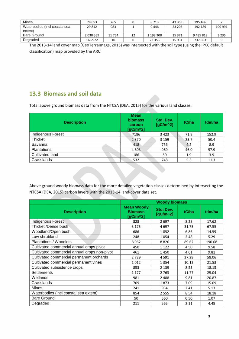
333

The 2013-14 land cover map (GeoTerraImage, 2015) was intersected with the soil type (using the IPCC default

classification) map provided by the ARC.

13.3 Biomass and soil data

Total above ground biomass data from the NTCSA (DEA, 2015) for the various land classes.

Description

Mean biomass carbon

[gC/m^2]

Std. Dev. [gC/m^2]

tC/ha tdm/ha

Indigenous Forest 7186 3 423 71.9 152.9

Thicket 2 370 3 159 23.7 50.4

Savanna 418 756 4.2 8.9 Plantations 4 603 969 46.0 97.9

Cultivated land 186 50 1.9 3.9

Grasslands 532 748 5.3 11.3

Above ground woody biomass data for the more detailed vegetation classes determined by intersecting the

NTCSA (DEA, 2015) carbon layers with the 2013-14 land-cover data set.

Woody biomass

Description Mean Woody

Biomass [gC/m^2]

Std. Dev. [gC/m^2]

tC/ha tdm/ha

Indigenous Forest 828 2 697 8.28 17.62 Thicket /Dense bush 3 175 4 697 31.75 67.55

Woodland/Open bush 686 1 852 6.86 14.59

Low shrubland 248 1 054 2.48 5.29

Plantations / Woodlots 8 962 8 826 89.62 190.68

Cultivated commercial annual crops pivot 450 1 122 4.50 9.58

Cultivated commercial annual crops non-pivot 461 1 450 4.61 9.81

Cultivated commercial permanent orchards 2 729 4 591 27.29 58.06

Cultivated commercial permanent vines 1 012 1 354 10.12 21.53

Cultivated subsistence crops 853 2 139 8.53 18.15 Settlements 1 177 2 763 11.77 25.04

Wetlands 981 2 488 9.81 20.87

Grasslands 709 1 873 7.09 15.09

Mines 241 934 2.41 5.13

Waterbodies (incl coastal sea extent) 854 2 555 8.54 18.18

Bare Ground 50 560 0.50 1.07

Degraded 211 565 2.11 4.48

Mines 78 653 265 0 8 713 43 353 195 486 7

Waterbodies (incl coastal sea extent)

29 812 983 1 9 446 23 205 192 189 199 991

Bare Ground 2 038 559 11 754 12 1 198 308 15 371 9 485 819 3 235

Degraded 166 972 10 0 23 355 15 931 737 663 9

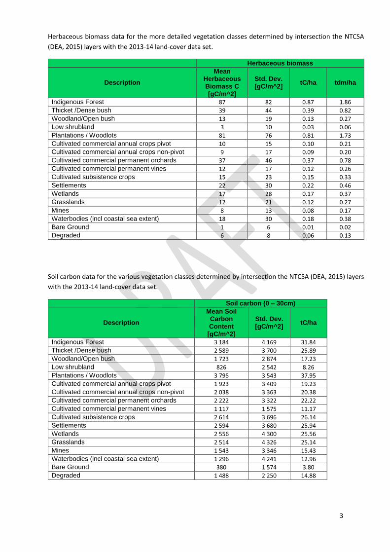
334

Herbaceous biomass data for the more detailed vegetation classes determined by intersection the NTCSA

(DEA, 2015) layers with the 2013-14 land-cover data set.

Herbaceous biomass

Description

Mean Herbaceous Biomass C [gC/m^2]

Std. Dev. [gC/m^2]

tC/ha tdm/ha

Indigenous Forest 87 82 0.87 1.86

Thicket /Dense bush 39 44 0.39 0.82

Woodland/Open bush 13 19 0.13 0.27

Low shrubland 3 10 0.03 0.06

Plantations / Woodlots 81 76 0.81 1.73

Cultivated commercial annual crops pivot 10 15 0.10 0.21 Cultivated commercial annual crops non-pivot 9 17 0.09 0.20

Cultivated commercial permanent orchards 37 46 0.37 0.78

Cultivated commercial permanent vines 12 17 0.12 0.26

Cultivated subsistence crops 15 23 0.15 0.33

Settlements 22 30 0.22 0.46

Wetlands 17 28 0.17 0.37

Grasslands 12 21 0.12 0.27

Mines 8 13 0.08 0.17

Waterbodies (incl coastal sea extent) 18 30 0.18 0.38

Bare Ground 1 6 0.01 0.02 Degraded 6 8 0.06 0.13

Soil carbon data for the various vegetation classes determined by intersection the NTCSA (DEA, 2015) layers

with the 2013-14 land-cover data set.

Soil carbon (0 – 30cm)

Description

Mean Soil Carbon Content [gC/m^2]

Std. Dev. [gC/m^2]

tC/ha

Indigenous Forest 3 184 4 169 31.84

Thicket /Dense bush 2 589 3 700 25.89

Woodland/Open bush 1 723 2 874 17.23

Low shrubland 826 2 542 8.26

Plantations / Woodlots 3 795 3 543 37.95

Cultivated commercial annual crops pivot 1 923 3 409 19.23 Cultivated commercial annual crops non-pivot 2 038 3 363 20.38

Cultivated commercial permanent orchards 2 222 3 322 22.22

Cultivated commercial permanent vines 1 117 1 575 11.17

Cultivated subsistence crops 2 614 3 696 26.14

Settlements 2 594 3 680 25.94

Wetlands 2 556 4 300 25.56

Grasslands 2 514 4 326 25.14

Mines 1 543 3 346 15.43

Waterbodies (incl coastal sea extent) 1 296 4 241 12.96 Bare Ground 380 1 574 3.80

Degraded 1 488 2 250 14.88

335

14 APPENDIX G: METHODOLOGY FOR LAND COVER AND LAND USE CHANGE

MATRIX

14.1 South African 2013-14 National Land-cover dataset

2013 - 2014 South African National

Land-Cover Dataset.

DEA/CARDNO SCPF002: Implementation of Land-Use Maps for South Africa

Project Specific Data User Report and MetaData

DATA PRODUCT CREATED BY GEOTERRAIMAGE (South Africa),

www.geoterraimage.com July 2015, version 05b (pivot code corrected data)

336

OPEN ACCESS LICENCE

337

LICENSE AND COPYRIGHT

The data supplied are licensed by GEOTERRAIMAGE to the Client, but remains the property

of GEOTERRAIMAGE as is protected by copyright laws. The data can be used by the client

as per the conditions set forth in the offer. The client does not obtain any ownership or

intellectual property rights in the data. “Client” refers to the South African Department of

Environmental Affairs.

The following shall always be clearly mentioned: (© GEOTERRAIMAGE - 2014).

OPEN DATA LICENSING (PERMITTED & INTENDED DATA USE)

The Department is granted an Open Data User license, which allows the Department

unrestricted access to and use the supplied data. The data is defined as the 72 Class GTI

South African National Land Cover Dataset (2013/2014). The Open Data License allows the

Department to distribute the data unrestricted to third parties with the full understanding that

the Department and third parties may not use the data to develop new products that will

compete directly with GEOTERRAIMAGE existing or “in-progress” commercial data products;

and that the Department and third parties accept and understand the stated Data Copyright,

Licensing and Liability conditions.

LIABILITY

The Client has to verify prior to his commitment, the adequacy of GEOTERRAIMAGE

datasets and products to the specific data and analyses needs as set out by the client.

GEOTERRAIMAGE will in no event be liable for any direct, indirect, incidental or

consequential damages including lost savings or profit, legal fees, lost data, lost sales, loss

of commitments, business interruption, including loss of or other damage, resulting from its

datasets and products, whether or not GEOTERRAIMAGE has been advised of the

possibility of such damage. This includes damages incurred by the client or any

third party.

GEOTERRAIMAGE datasets and products are processed from sources like topographic

maps and satellite images. The quality of these sources is not the responsibility of

GEOTERRAIMAGE. The data and data products are provided “as is”, without warranty of

any kind, either express or implied, including, but not limited to, the implied warranties of

merchantability and fitness for a particular purpose.

338

Whilst all possible care and attention has been taken in the production of the data, neither

GEOTERRAIMAGE or any of its respective sub-organisations or employees, accept any liability

whatsoever for any perceived or actual inaccuracies or misrepresentations in the supplied data or

accompanying report(s), as a result of the nature of mapping from coarse and medium scale

satellite imagery. Any mapped boundaries either implied or inferred within the data do not have any

legal status whatsoever.

All rights not specifically granted or specified in this agreement, pertaining to this data are

reserved to GEOTERRAIMAGE Pty Ltd.

339

CONTENTS

COPY OF DATA LICENCE AGREEMENT

1. INTRODUCTION

2. BACKGROUND

3. OBJECTIVE

4. PRODUCT DESCRIPTION

4.1 Land-Cover Legend

5. OVERVIEW OF THE AUTOMATED MODELLING APPROACH

5.1 Model Portability to other Geographical Areas and Sensors

5.2 Use of Object Based Modelling

6. LANDSAT IMAGERY

6.1 Landsat Image Sourcing

6.2 Landsat Data Preparation

7. LAND-COVER MODELLING

7.1 Spectral Modelling

7.2 Terrain Modifications

7.3 Individual Frame Spectral Models

7.3.1 Spectral Modelling of Water

7.3.2 Spectral Modelling of Bare Ground

7.3.3 Spectral Modelling of Tree / Bush Cover

7.3.4 Spectral Modelling of Grass

7.3.5 Spectral Modelling of Burnt Areas

7.4 Seasonally Defined Spectral Land-Cover per Image Frame

7.5 Generation of Full South African Spectral Class Mosaic

7.5.1 Grassland Corrections: Inland

7.5.2 Grassland Corrections: Coastal

8. LAND-COVER INFORMATION GENERATION

8.1 Conversion from Spectral to Information Classes

8.2 Creating Base Vegetation Land-Cover Classes

8.2.1 Fynbos

8.2.2 Indigenous Forests

8.2.3 Wetlands

8.2.4 Nama and Succulent Karoo

8.3 Creating Land-Use Classes

8.3.1 Cultivated Lands

340

8.3.1.1 NDVI-based Cultivated Land Sub-Classes

8.3.2 Plantations

8.3.3 Mines

8.3.4 Built-up / Settlements

8.3.5 Erosion

8.3.5.1 Degraded

9. ACCURACY ASSESSMENT

9.1 Design and Approach

9.2 Results

9.3 Analysis and Conclusions

9.3.1 Dense Bush / Thicket

9.3.2 Woodland / Open Bushland

9.3.3 Grassland

9.3.4 Low Shrubland (Fynbos and Other Sub-Classes combined)

9.3.5 Bare Ground

9.3.6 Conclusion

10. DATA USE

11. METADATA

APPENDIX A 2013-14 South African National Land-cover Legend

APPENDIX B List of accompanying documents and files.

APPENDIX C 51 x Class Seasonally Defined Spectral Foundation Class Legend.

APPENDIX D Visual representation of canopy cover density percentages per unit area.

APPENDIX E 33 x Verified Land-Cover / Use Classes.

PLEASE NOTE

This report provides information on the specific version of the 2013-14

GEOTERRAIMAGE South African National Land-Cover Dataset supplied to the South

African Department of Environmental Affairs under the DEA / CARDNO Project:

SCPF002:"Implementation of Land Use Maps for South Africa".

The supplied dataset referred to in this report represents a subset of the full 2013-14

GEOTERRAIMAGE South African National Land-Cover Dataset, in terms of supplied

land-cover / land-use categories and associated class legend.

Use of this DEA / CARDNO data version is governed by the LICENCE AGREEMENT shown

previously.

341

1. INTRODUCTION

Land-cover is a key information requirement for a wide range of landscape planning,

inventory and management activities, ranging from environmental resource management to

telecommunication planning. The recent global availability of Landsat 8 satellite imagery

offered the opportunity to create a new, national land-cover dataset1 for South Africa, circa

2013-14, replacing and updating the previous 1994 and 2000 South African National Land-

cover datasets. The 2013-14 national land-cover dataset is based on 30x30m raster cells,

and is ideally suited for ± 1:75,000 - 1:250,000 scale GIS-based mapping and modelling

applications.

The dataset has been derived from multi-seasonal Landsat 8 imagery, using operationally

proven, semi-automated modelling procedures developed specifically for the generation of

this dataset, based on repeatable and standardised modelling routines. The dataset has

been created by GEOTERRAIMAGE (GTI) and is available as a commercial data product.

The production of a comparable 1990 land-cover product is also in progress that will provide,

for the very first time, a standardised and directly comparable set of national land-cover

datasets that can be used to determine landscape change in South Africa over a 20+ year

period2.

2. BACKGROUND

The recent global availability of Landsat 8 imagery (April 2013), was the primary catalyst

behind the development of new, innovative automated land-cover modelling procedures,

which allowed the creation of the 2013-14 South African National Land-Cover dataset.

Primarily because Landsat 8 offered a free, and regular supply of radiometrically and

geometrically standardised, medium resolution, multi-spectral imagery, suitable for medium

to large area mapping. Collectively, this offered an ideal opportunity for GTI to re-look at

using automated land-cover mapping techniques as a more efficient alternative to

conventional, analyst-assisted per-pixel classifiers, allowing rapid production of

standardised, yet informative land-cover information.

1

Note that the term "land-cover" is used loosely to incorporate both land-cover and land-use information in the context of the GTI 2013-14 South African National Land-Cover dataset.

2

The existing 1994 and 2000 South African National Land-cover datasets were generated independently, using very

different source image formats (i.e. paper versus digital), and end-product formats (i.e. 1:250,000 scale digital vector versus 1:50,000 digital raster), despite being derived from equivalent Landsat imagery. See Thompson MW, 1991. South

African National Land-Cover Database Project. Data Users Manual. Final Report (Phases 1,2, & 3). CSIR Project Report ENV/P/C 98136, February 1999; and Thompson MW et al, 2001. Guideline Procedures for National Land-Cover Mapping

and Change Monitoring. CSIR Client Project Report ENV/P/C 2001-006, March 2001.

342

3. OBJECTIVE

The primary objective was to generate a new, national land-cover dataset for the whole of

South Africa, and to be able to release this as a commercial data product within ±1 year of

image data acquisition to ensure that the dataset is up-to-date and current. In support of this

primary objective was the requirement to develop operational procedures based on semi-

automated (spectral) modelling techniques that would facilitate the rapid production of

consistent, standardised land-cover information from multi-seasonal Landsat 8 imagery.

4. PRODUCT DESCRIPTION

The 2013-14 South African National Land-cover dataset produced by GEOTERRAIMAGE as

a commercial data product has been generated from digital, multi-seasonal Landsat 8

multispectral imagery, acquired between April 2013 and March 2014. In excess of 600

Landsat images were used to generate the land-cover information, based on an average of 8

different seasonal image acquisition dates, within each of the 76 x image frames required to

cover South Africa. The land-cover dataset, which covers the whole of South Africa, is

presented in a map-corrected, raster format, based on 30x30m cells equivalent to the image

resolution of the source Landsat 8 multi-spectral imagery. The full dataset contains 72 x

land-cover / use information classes, covering a wide range of natural and man-made

landscape characteristics. The DEA / CARDNO dataset contains a summarised 35 x class

legend. Each data cell contains a single code representing the dominant land-cover class

(by area) within that 30x30m unit, as determined from analysis of the multi-date imagery

acquired over that image frame. The original land-cover dataset was processed in UTM

(north) / WGS84 map projection format based on the Landsat 8 standard map projection

format as provided by the USGS3. The final product is available in UTM35(north) and

(south), WGS84 map projections and Geographic Coordinates, WGS84.

4.1 Land-Cover Legend

The 2013-14 SA National Land-cover legend is aligned with SANS 18774 South African

National Land-cover Classification Standard in terms of class definitions and hierarchical

format. The complete list of information classes that have been mapped and supplied as part

of the DEA / CARDNO land-cover dataset, and the associated class definitions are supplied

in Appendix A.

3 United States Geological Survey.

4

SANS 1877: SA Bureau of Standards designated national land-cover classification standard for South Africa.

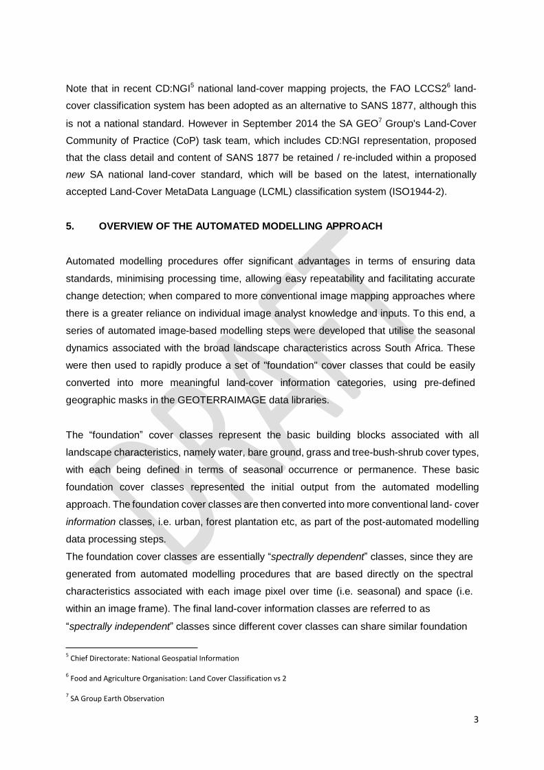
343

Note that in recent CD:NGI5 national land-cover mapping projects, the FAO LCCS26 land-

cover classification system has been adopted as an alternative to SANS 1877, although this

is not a national standard. However in September 2014 the SA GEO7 Group's Land-Cover

Community of Practice (CoP) task team, which includes CD:NGI representation, proposed

that the class detail and content of SANS 1877 be retained / re-included within a proposed

new SA national land-cover standard, which will be based on the latest, internationally

accepted Land-Cover MetaData Language (LCML) classification system (ISO1944-2).

5. OVERVIEW OF THE AUTOMATED MODELLING APPROACH

Automated modelling procedures offer significant advantages in terms of ensuring data

standards, minimising processing time, allowing easy repeatability and facilitating accurate

change detection; when compared to more conventional image mapping approaches where

there is a greater reliance on individual image analyst knowledge and inputs. To this end, a

series of automated image-based modelling steps were developed that utilise the seasonal

dynamics associated with the broad landscape characteristics across South Africa. These

were then used to rapidly produce a set of "foundation" cover classes that could be easily

converted into more meaningful land-cover information categories, using pre-defined

geographic masks in the GEOTERRAIMAGE data libraries.

The “foundation” cover classes represent the basic building blocks associated with all

landscape characteristics, namely water, bare ground, grass and tree-bush-shrub cover types,

with each being defined in terms of seasonal occurrence or permanence. These basic

foundation cover classes represented the initial output from the automated modelling

approach. The foundation cover classes are then converted into more conventional land- cover

information classes, i.e. urban, forest plantation etc, as part of the post-automated modelling

data processing steps.

The foundation cover classes are essentially “spectrally dependent” classes, since they are

generated from automated modelling procedures that are based directly on the spectral

characteristics associated with each image pixel over time (i.e. seasonal) and space (i.e.

within an image frame). The final land-cover information classes are referred to as

“spectrally independent” classes since different cover classes can share similar foundation

5 Chief Directorate: National Geospatial Information

6

Food and Agriculture Organisation: Land Cover Classification vs 2

7 SA Group Earth Observation

344

class spectral characteristics in a one-to-many type relationship. For example, the “bare

ground” spectrally dependent cover classes could represent non-vegetated built-up urban

areas, natural rock exposures, beach sand or a mine pit and tailings dump. Similarly the

tree-bush classes could represent a natural vegetation cover, a timber plantation or a fruit

orchard. The advantage of this approach is that the conversion of the initial, spectrally

dependent foundation cover classes into the final, spectrally independent land-cover

information classes can be tailored to suit a variety of end-user information requirements;

simply by using a different set of pre-determined masks and foundation class sub-divisions

and amalgamations.

5.1 Model Portability to other Geographical Areas and Sensors

Although model development was focussed on using Landsat 8 imagery within South Africa,

the same models have also been proven to work with equivalent success on Landsat 8 imagery

over sites in Sudan, Zimbabwe, Botswana, Namibia and Mozambique; as well as using

comparable Landsat 5 archive imagery over South Africa; all of which indicate a high level of

model portability. This should allow and support the production of directly

comparable historical land-cover datasets for change detection, assuming of course that the

required level of seasonal image coverage is available in the data archives.

5.2 Use of Object Based Modelling

No attempt was made to include or use object-based modelling in the automated mapping

process, primarily because the medium resolution format of multi-spectral Landsat 8 imagery

does not lend it self to this type of modelling; since pixel resolution typically precludes the

identification of true landscape “objects” in comparison to high and ultra high resolution

image formats. The 30 metre Landat resolution pixels typically represent a mix of land-cover

characteristics rather than a pure cover surface, i.e. an urban pixel is typically a composite of

building roofs, garden vegetation and / or road surfaces etc. However, object-based modelling

may be useful approach for helping to generate 2nd level information classes from the primary

level "foundation" class dataset, such as for example, separating water in rivers (i.e. natural)

from water in dams (i.e. artificial), based on size, shape and context etc.

6. LANDSAT IMAGERY

The primary imagery source used in the generation of the 2013-14 SA National Land-cover

dataset was 30m resolution Landsat 8 imagery, acquired between April 2013 and March

2014. Within each image frame, a range of seasonal image acquisition dates were used

(within the automated modelling procedures), to characterise the seasonal dynamics across

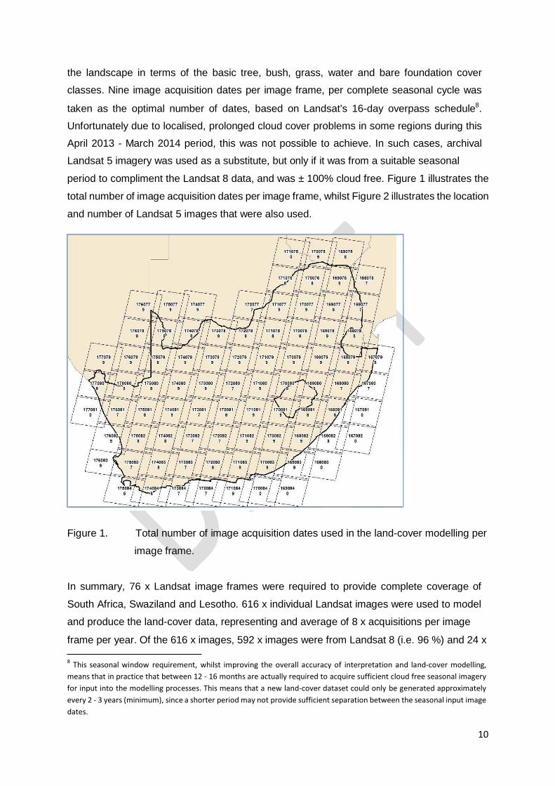
1010

the landscape in terms of the basic tree, bush, grass, water and bare foundation cover

classes. Nine image acquisition dates per image frame, per complete seasonal cycle was

taken as the optimal number of dates, based on Landsat's 16-day overpass schedule8.

Unfortunately due to localised, prolonged cloud cover problems in some regions during this

April 2013 - March 2014 period, this was not possible to achieve. In such cases, archival

Landsat 5 imagery was used as a substitute, but only if it was from a suitable seasonal

period to compliment the Landsat 8 data, and was ± 100% cloud free. Figure 1 illustrates the

total number of image acquisition dates per image frame, whilst Figure 2 illustrates the location

and number of Landsat 5 images that were also used.

Figure 1. Total number of image acquisition dates used in the land-cover modelling per

image frame.

In summary, 76 x Landsat image frames were required to provide complete coverage of

South Africa, Swaziland and Lesotho. 616 x individual Landsat images were used to model

and produce the land-cover data, representing and average of 8 x acquisitions per image

frame per year. Of the 616 x images, 592 x images were from Landsat 8 (i.e. 96 %) and 24 x

8 This seasonal window requirement, whilst improving the overall accuracy of interpretation and land-cover modelling,

means that in practice that between 12 - 16 months are actually required to acquire sufficient cloud free seasonal imagery

for input into the modelling processes. This means that a new land-cover dataset could only be generated approximately

every 2 - 3 years (minimum), since a shorter period may not provide sufficient separation between the seasonal input image

dates.

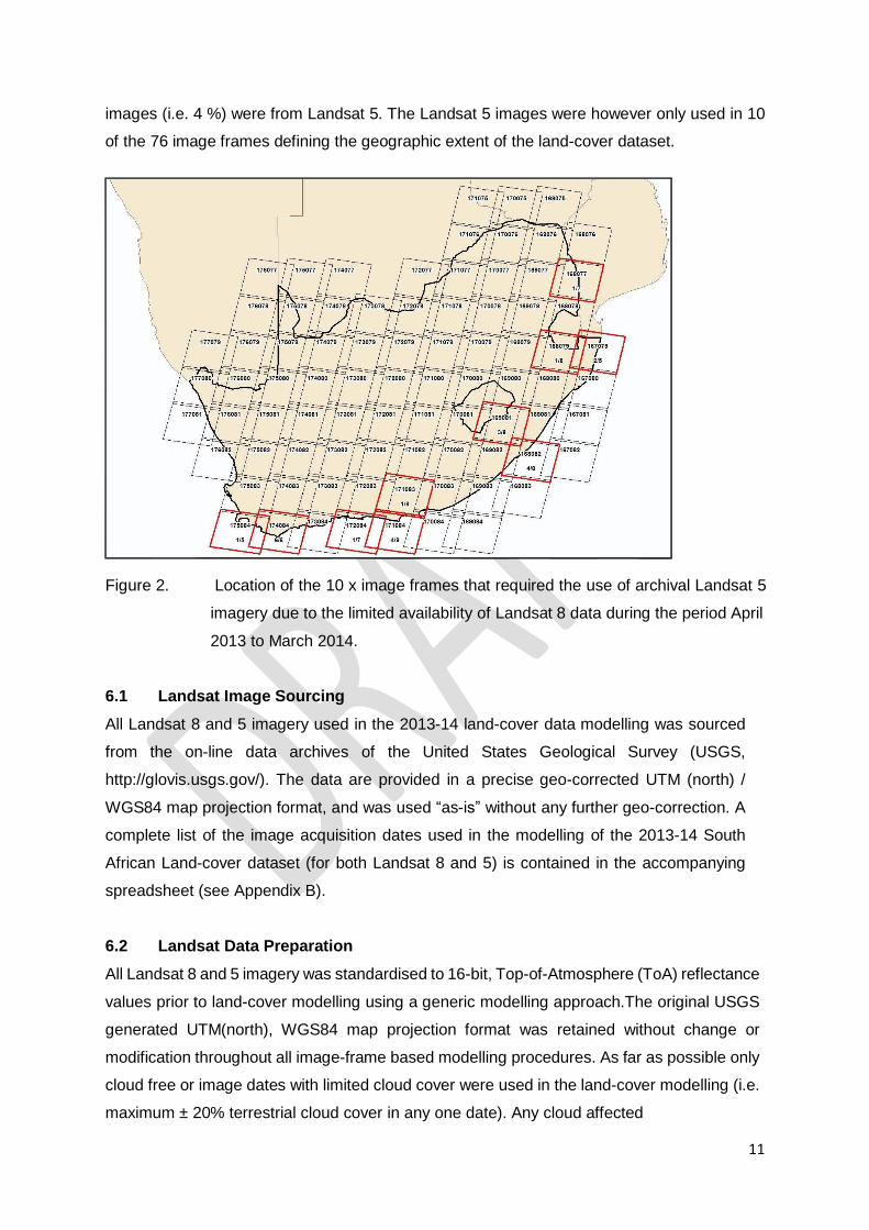
1111

images (i.e. 4 %) were from Landsat 5. The Landsat 5 images were however only used in 10

of the 76 image frames defining the geographic extent of the land-cover dataset.

Figure 2. Location of the 10 x image frames that required the use of archival Landsat 5

imagery due to the limited availability of Landsat 8 data during the period April

2013 to March 2014.

6.1 Landsat Image Sourcing

All Landsat 8 and 5 imagery used in the 2013-14 land-cover data modelling was sourced

from the on-line data archives of the United States Geological Survey (USGS,

http://glovis.usgs.gov/). The data are provided in a precise geo-corrected UTM (north) /

WGS84 map projection format, and was used “as-is” without any further geo-correction. A

complete list of the image acquisition dates used in the modelling of the 2013-14 South

African Land-cover dataset (for both Landsat 8 and 5) is contained in the accompanying

spreadsheet (see Appendix B).

6.2 Landsat Data Preparation

All Landsat 8 and 5 imagery was standardised to 16-bit, Top-of-Atmosphere (ToA) reflectance

values prior to land-cover modelling using a generic modelling approach.The original USGS

generated UTM(north), WGS84 map projection format was retained without change or

modification throughout all image-frame based modelling procedures. As far as possible only

cloud free or image dates with limited cloud cover were used in the land-cover modelling (i.e.

maximum ± 20% terrestrial cloud cover in any one date). Any cloud affected

1212

regions were corrected by merging cloud affected ToA corrected imagery with cloud free ToA

corrected data from preferably the preceding or following overpass date; so that as far as

possible, the final cloud-free merged imagery composite only represented a maximum

difference of ± 16 days. Cloud masks were created using either using conventional pixel

classification procedures (within analyst defined sub-image areas), or spectral based

modelling using generic thermal and blue light reflectance thresholds9; depending on cloud

characteristics. This was deemed acceptable in terms of minimising any changes in local

vegetation cover growth changes. Approximately 35% of the 616 x images used in the land-

cover modelling were cloud-masked composites. No external atmospheric correction was

applied to the image data.

7. LAND-COVER MODELLING

7.1 Spectral Modelling

Derived spectral indices, generated from the ToA corrected imagery were used as the only

inputs into the land-cover models. No original spectral (i.e. ToA reflectance) data was used

as an input, although collectively, 5 out of the 8 available non-thermal spectral bands were

used in the various spectral indices10. A standardised set of spectral indices were identified

from which the required foundation cover classes, namely (1) tree dominated, (2) bush

dominated, (3) grass dominated, (4) water and (5) bare ground could be modelled, using

pre-determined, generic spectral threshold values. The generic threshold values associated

with each indices and cover type were tested over several landscapes and seasons before

being confirmed and accepted as such.

The spectral indices included both existing algorithms such as the Normalised Difference

Vegetation Index (NDVI) and Normalised Difference Water Index (NDWI), as well as

algorithms developed in-house specifically for the GTI land-cover modelling requirements.

All models were developed in ERDAS Imagine © image processing software using the

Model Maker function.

The modelling and generation of each foundation cover class was undertaken as a separate

modelling exercise, i.e. water was modelled separately from bare ground, which was modelled

separately from tree and bush cover etc. This approach simplified the modelling

steps and facilitated easier desk-top quality control of outputs; compared to attempting to

9 The spectral modelling approach could only be applied to Landsat 8 imagery (if applicable) due to its enhanced spectral

band range, compared to Landsat 5.

10 (2) Green, (3) Red, (4) Red, (5) NIR, (6) SWIR-1 and (7) SWIR-2 Landsat 8 spectral bands.

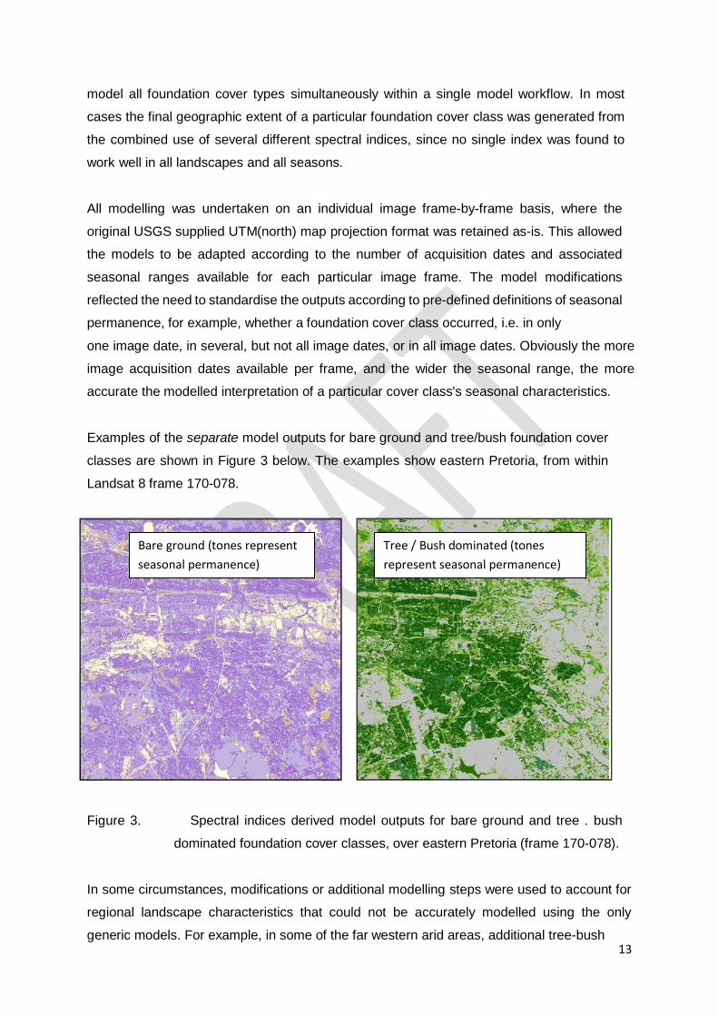
1313

model all foundation cover types simultaneously within a single model workflow. In most

cases the final geographic extent of a particular foundation cover class was generated from

the combined use of several different spectral indices, since no single index was found to

work well in all landscapes and all seasons.

All modelling was undertaken on an individual image frame-by-frame basis, where the

original USGS supplied UTM(north) map projection format was retained as-is. This allowed

the models to be adapted according to the number of acquisition dates and associated

seasonal ranges available for each particular image frame. The model modifications

reflected the need to standardise the outputs according to pre-defined definitions of seasonal

permanence, for example, whether a foundation cover class occurred, i.e. in only

one image date, in several, but not all image dates, or in all image dates. Obviously the more

image acquisition dates available per frame, and the wider the seasonal range, the more

accurate the modelled interpretation of a particular cover class's seasonal characteristics.

Examples of the separate model outputs for bare ground and tree/bush foundation cover

classes are shown in Figure 3 below. The examples show eastern Pretoria, from within

Landsat 8 frame 170-078.

Bare ground (tones represent

seasonal permanence)

Tree / Bush dominated (tones

represent seasonal permanence)

Figure 3. Spectral indices derived model outputs for bare ground and tree . bush

dominated foundation cover classes, over eastern Pretoria (frame 170-078).

In some circumstances, modifications or additional modelling steps were used to account for

regional landscape characteristics that could not be accurately modelled using the only

generic models. For example, in some of the far western arid areas, additional tree-bush

1414

modelling steps were taken using a slightly modified modelling approach in order to better

detect and separate between the sparse, low bush and shrub covers in these landscapes.

7.2 Terrain Modifications

Terrain based modifications were included within some of the foundation cover class modelling

procedures (i.e. water, bare and tree-bush classes), in order to minimise seasonally induced

terrain shadowing effects, using a combination of solar illumination and slope parameters.

These parameters were modelled independently using the 90m resolution SRTM dataset11,

with outputs being re-sampled to a Landsat comparable 30m resolution format, prior to being

incorporated into the foundation cover class models. For example,

solar illumination and DEM slope masks were used to minimise any spectral confusion

between dark terrain shadow areas and comparable water body reflectance levels. Note that

when creating the DEM derived parameters, such as shadow extents, modelling was based

on the full range of seasonal solar azimuth and zenith angles and not a specific date or season,

in order to better align with seasonal differences evident across the any given range of image

acquisition dates.

7.3 Individual Frame Spectral Models

The basic modelling parameters used to create each of the "foundation" cover classes are

described below. In each case the modelled output would typically represent a (qualitative)

gradient of spatial densities and as well as temporal, i.e. seasonal occurrence. For example

the bare ground model output consisted of a set of classes that represented a range of

conditions from "pure bare" to "mixed bare / sparsely vegetated", with each described in terms

of seasonal permanent or temporary occurrence. The foundation water class modelling was

the only exception to this, with the model output describing water extent in terms of only

permanent or seasonal occurrence.

7.3.1 Spectral Modelling of Water

Water was modelled using a combination of 5 spectral indices, including a burn index, and

DEM derived solar illumination and slope masks. The burn index was used to minimise any

spectral confusion between dark burnt areas and comparable water body reflectance. The

solar illumination and slope masks were used to minimise any spectral confusion between

dark terrain shadow areas and comparable water body reflectance. Generic spectral water

models were developed for both flat (standard) and hilly terrain, and for shallow water (pan)

dominated landscapes.

11

Although the 30m SRTM terrain dataset would have been more preferable it did not become publically accessible until after the completion of the bulk of the 2013-14 land-cover modelling had been completed.

1515

7.3.2 Spectral Modelling of Bare Ground

Bare ground was modelled using a combination of 2 spectral indices, and DEM derived solar

illumination and slope masks. The solar illumination and slope masks were used to minimise

any spectral confusion between dark terrain shadow areas and comparable bare ground

reflectance. The output represented a gradient of bare ground from pure bare to sparsely

vegetated cover.

7.3.3 Spectral Modelling of Tree / Bush Cover

Tree and bush cover was generated within the same spectral model. Both woody covers were

modelled using a combination of 4 spectral indices, and DEM derived slope mask. The slope

mask was used to minimise any spectral confusion between dark terrain shadow areas and

comparable woody cover in two of the 4 spectral indices. "Trees" refers to dense, typically tall

woody cover, such as natural and planted forests, dense woodland and thickets, etc; whereas

"bush" refers to more open, often lower mixed tree / bush communities such as typical bushveld

or open woodland. The spectral modelling procedure also separated woody cover spectral

classes that showed similar characteristics to other vegetated covers such as crops, sports

fields, golf fields (especially if irrigated), from those that didn't. An additional "desert" tree / bush

model was developed as an extra model to be run in addition to the standard model in more

arid areas, in increase the representation of bush cover in these regions where the modelling

thresholds used in the standard model were not sensitive enough.

7.3.4 Spectral Modelling of Grass

Grass cover was modelled using only a single spectral indices. No DEM derived solar

illumination and slope mask modifiers were used.

7.3.5 Spectral Modelling of Burnt Areas

Burnt cover was modelled using only a single spectral indices. No DEM derived solar

illumination and slope mask modifiers were used.

7.4 Seasonally Defined Spectral Land-Cover per Image Frame

The modelled outputs for each foundation cover class were combined into a single composite

dataset for each frame, in a pre-determined hierarchical order, in order that the final output

cover class combinations reflected the dominant and sub-dominant cover types in terms of

seasonal occurrence. For example:

water in all dates (permanent),

water in many dates (seasonal),

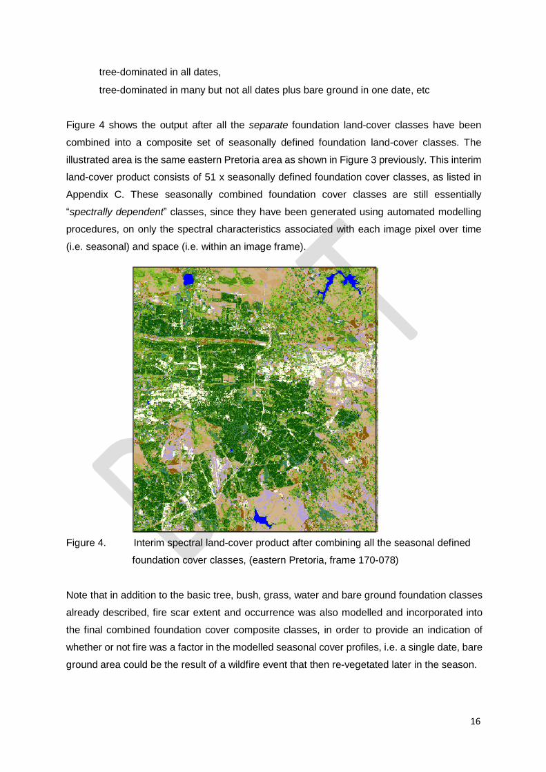
1616

tree-dominated in all dates,

tree-dominated in many but not all dates plus bare ground in one date, etc

Figure 4 shows the output after all the separate foundation land-cover classes have been

combined into a composite set of seasonally defined foundation land-cover classes. The

illustrated area is the same eastern Pretoria area as shown in Figure 3 previously. This interim

land-cover product consists of 51 x seasonally defined foundation cover classes, as listed in

Appendix C. These seasonally combined foundation cover classes are still essentially

“spectrally dependent” classes, since they have been generated using automated modelling

procedures, on only the spectral characteristics associated with each image pixel over time

(i.e. seasonal) and space (i.e. within an image frame).

Figure 4. Interim spectral land-cover product after combining all the seasonal defined

foundation cover classes, (eastern Pretoria, frame 170-078)

Note that in addition to the basic tree, bush, grass, water and bare ground foundation classes

already described, fire scar extent and occurrence was also modelled and incorporated into

the final combined foundation cover composite classes, in order to provide an indication of

whether or not fire was a factor in the modelled seasonal cover profiles, i.e. a single date, bare

ground area could be the result of a wildfire event that then re-vegetated later in the season.

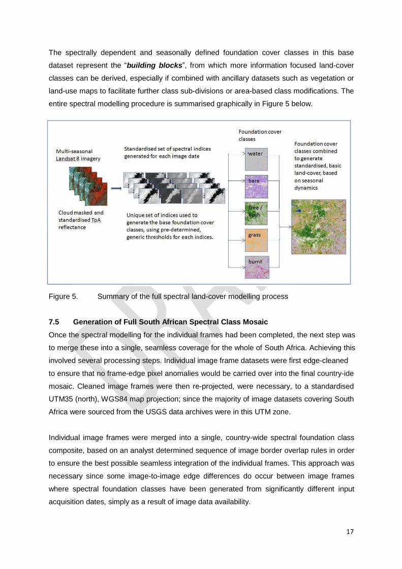
1717

The spectrally dependent and seasonally defined foundation cover classes in this base

dataset represent the “building blocks”, from which more information focused land-cover

classes can be derived, especially if combined with ancillary datasets such as vegetation or

land-use maps to facilitate further class sub-divisions or area-based class modifications. The

entire spectral modelling procedure is summarised graphically in Figure 5 below.

Figure 5. Summary of the full spectral land-cover modelling process

7.5 Generation of Full South African Spectral Class Mosaic

Once the spectral modelling for the individual frames had been completed, the next step was

to merge these into a single, seamless coverage for the whole of South Africa. Achieving this

involved several processing steps. Individual image frame datasets were first edge-cleaned

to ensure that no frame-edge pixel anomalies would be carried over into the final country-ide

mosaic. Cleaned image frames were then re-projected, were necessary, to a standardised

UTM35 (north), WGS84 map projection; since the majority of image datasets covering South

Africa were sourced from the USGS data archives were in this UTM zone.

Individual image frames were merged into a single, country-wide spectral foundation class

composite, based on an analyst determined sequence of image border overlap rules in order

to ensure the best possible seamless integration of the individual frames. This approach was

necessary since some image-to-image edge differences do occur between image frames

where spectral foundation classes have been generated from significantly different input

acquisition dates, simply as a result of image data availability.

1818

Although the standardised modelling approach used to generate the es supported generation

of spatial and content comparable land-cover data in adjacent image frames (if both frames

utilised comparable input image acquisition dates), if there was a significant difference in the

number or seasonal range of input images, then adjacent images often showed edge

matching differences. In such cases, the adjacent images were often spatially comparable,

but not necessarily content comparable. In these cases, the edge matching process was set-

up, as far as possible so that the most prominent and spatially extensive landscape pattern

was maintained across the image borders, in order to provide a more visually seamless image

frame overlap.

Note that for water ("seasonal" and "permanent") and bare ground ("pure bare, all dates")

country-wide coverages, the maximum extent of each class, from all images, was transferred

across to the final country-wide spectral class composite; regardless of any frame overlap edge

matching applied to other spectral classes.

7.5.1 Grassland Corrections: Inland

Persistent cloud cover problems on several image acquisition dates during the 2013-14 wet

season period over the Highveld region resulted in the unavailability of usable, early wet

season imagery for modelling inputs. This resulted in the standard spectral models under-

estimating the grassland extent. In order to correct this, an alternative grassland model was

developed, based on a single, rather than multiple, image acquisition date. The optimal single

date representing the best, dry season image for visually separating green woody vegetation

from senescent grassland vegetation, with minimal burn scars. For image frames covering

areas of significant topographical relief, such as over the escarpment, the single- date grass

corrective model included use of solar illumination and slope parameters to improve modelling

outputs. For standardisation purposes, the inland grassland corrective model was applied to

all image frames overlapping or contained within the SANBI grassland Biome boundary. The

resultant grassland extents for each image frame where then merged into a composite

geographical mask and integrated back into the original county-wide spectral class dataset to

improve the overall grassland delineation.

7.5.2 Grassland Corrections: Coastal

In some high rainfall coastal regions, the standard spectral models were unable to accurately

distinguish between grassland and woody cover, where the grass biomass was exceptionally

high as a result of high local rainfall during the 2013-14 wet season, even if suitable image

acquisition dates were available. This was especially the case around Pondoland (E Cape)

and Zululand and Maputoland (KZN). To correct this another grassland correction model

1919

was developed with alternate spectral thresholds to better delineate the correct grassland

extent in these areas. The resultant frame specific outputs were then merged into a

composite geographical mask and integrated back into the original county-wide spectral

class dataset to improve the overall grassland delineation.

8. LAND-COVER INFORMATION GENERATION

Multi-seasonal Landsat imagery has been used to generate a comprehensive set of spectrally-

based outputs that describe the seasonal characteristics of tree, bush, grass, bare and water

cover characteristics within each image pixel, as represented by the 51 x spectral foundation

classes. These were converted into more meaningful and informative land-cover and land-use

information classes, aligned with the SANS 1877 South African National Land- cover

Classification Standard (see Section 4.1). For example a pixel may be described as having a

detectable tree cover on more than one image acquisition date, but not all dates; and grass

covered for several but not all dates. This would then be interpreted as an open, deciduous

tree covered woody community, (i.e. woodland), where the grass cover became evident when

the tree canopy showed less than maximum foliage cover.

8.1 Conversion from Spectral to Information Classes

The creation of both land-cover and land-use information classes involves the recoding and

re-grouping of selected spectral foundation classes either in a controlled or uncontrolled

geographic area. In a controlled re-coding, independently sourced and / or generated

geographical masks are used to define the location and extent of the recode process. This is

required because in many situations different landscape features can be represented by

similar spectral characteristics. For example a spectrally modelled area of permanent bare

ground (i.e. spectral characteristics are representative of a non-vegetated surface in all image

acquisition dates), could be representative of a beach, a mine, or a large building. By using an

appropriate geographic mask (essentially an independently defined or sourced polygon

coverage), it is then possible to code all bare ground pixels within the mask to, for example,

mining, whilst allowing all other bare areas outside the mask to represent other bare ground

surfaces, which can then be further re-coded as and where required.

The key to this process is that the spectral modelling defines the exact footprint of the spectral

cover class (in a user independent manner), whereas the geographic mask defines the

information content (based on user expertise and knowledge). This approach overcomes

problems where spectral characteristics are shared between two or more separate land-

cover/use classes, which is self-evident in many image-based mapping

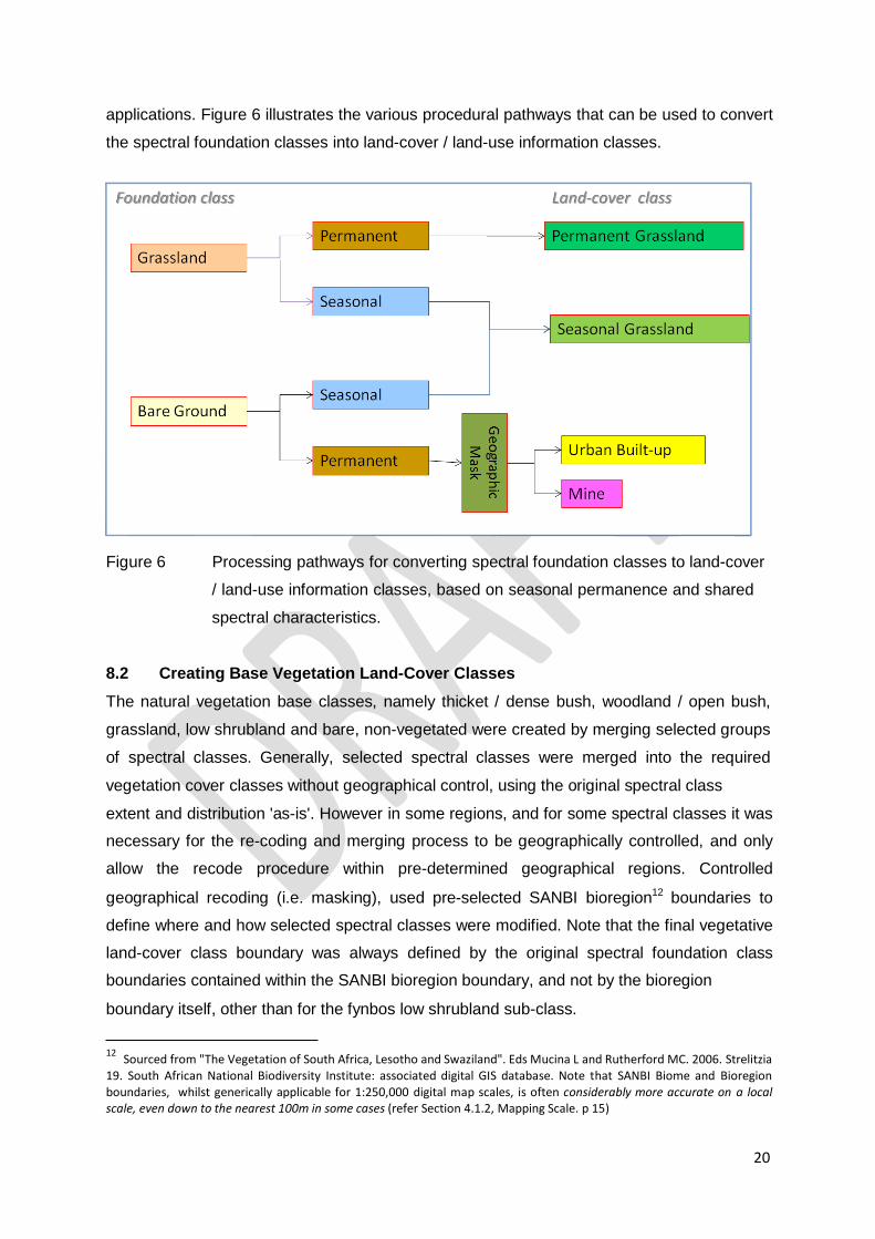
2020

applications. Figure 6 illustrates the various procedural pathways that can be used to convert

the spectral foundation classes into land-cover / land-use information classes.

Figure 6 Processing pathways for converting spectral foundation classes to land-cover

/ land-use information classes, based on seasonal permanence and shared

spectral characteristics.

8.2 Creating Base Vegetation Land-Cover Classes

The natural vegetation base classes, namely thicket / dense bush, woodland / open bush,

grassland, low shrubland and bare, non-vegetated were created by merging selected groups

of spectral classes. Generally, selected spectral classes were merged into the required

vegetation cover classes without geographical control, using the original spectral class

extent and distribution 'as-is'. However in some regions, and for some spectral classes it was

necessary for the re-coding and merging process to be geographically controlled, and only

allow the recode procedure within pre-determined geographical regions. Controlled

geographical recoding (i.e. masking), used pre-selected SANBI bioregion12 boundaries to

define where and how selected spectral classes were modified. Note that the final vegetative

land-cover class boundary was always defined by the original spectral foundation class

boundaries contained within the SANBI bioregion boundary, and not by the bioregion

boundary itself, other than for the fynbos low shrubland sub-class.

12

Sourced from "The Vegetation of South Africa, Lesotho and Swaziland". Eds Mucina L and Rutherford MC. 2006. Strelitzia

19. South African National Biodiversity Institute: associated digital GIS database. Note that SANBI Biome and Bioregion

boundaries, whilst generically applicable for 1:250,000 digital map scales, is often considerably more accurate on a local scale, even down to the nearest 100m in some cases (refer Section 4.1.2, Mapping Scale. p 15)

2121

8.2.1 Fynbos

The sensitivity of the automated spectral models was insufficient to determine the transition

between structurally similar fynbos low shrub communities and non-fynbos low shrub

communities, except for the boundary with the structurally different Namaqualand (SKn and

SKs) and Knersvlakte (Skk) Bioregions. In these areas the boundary between the fynbos

and non-fynbos low shrub communities has been defined on the basis of the original spectral

class boundaries13.

8.2.2 Indigenous Forests

The indigenous forest land-cover class was generated in a similar manner to the previously

described base vegetation classes, although the geographical masks used to control the

recoding of the selected spectral foundation classes were derived from a combination of

independent datasets. These included the SANBI forest biome boundaries, higher detail

regional masks created in-house in support of previous provincial-level land-cover mapping,

shadow and altitude terrain parameters modelled from the higher resolution 30m resolution

SRTM DEM terrain data14, and NDVI15 spectral datasets. The NDVI dataset represented a

nation-wide summary of the seasonal maximum NDVI recorded in each pixel, calculated from

all image acquisition dates used in the spectral land-cover modelling. Note that separate

models were required to recode the different Forest vegetation types (i.e. Northern

Afromontane, Sand, Scarp etc), with each one being based on different geographical mask

combinations and associated data thresholds, in order to correctly model the forest patch

distributions in these regions. The final, modelled forest extents were then integrated into the

base vegetation land-cover classes.

8.2.3 Wetlands

The wetland class was created using independent and separate modelling routines that did

not include reference to, or recoding of any of the original 51 x class spectral foundation

classes. Depending on the available image acquisition dates per frame, wetland extent was

modelled using either a dual or single image acquisition date process. The single date

13

The is primarily because satellite imagery such as Landsat, with its combination of medium spatial resolution and limited

spectral capabilities (compared to hyper-spectral sensors), is primarily responsive to structural vegetation characteristics

rather than community floristics. Accurate delineation of Biome-related boundaries, especially if the boundary is a transition

zone, rather than distinct border, is at best, challenging with imagery such as Landsat. Especially if floristic differences play

a greater role than structural differences in defining the border. This is likely to be the case between the Fynbos, Succulent

Karoo, Nama Karoo and surrounding Grassland and Desert Biomes.

14

The 30m resolution SRTM terrain data for Africa was available for use at this time within the 2013-14 SA Land-Cover project, despite not having been available for the initial spectral modelling phase.

15

Normalised Difference Vegetation Index (NDVI)

2222

approach used the best "wettest" image date, whereas the. The dual date approach was

based on the difference between wettest and driest image dates whereas the single

(wettest) date modelling was only used as an alternative approach if the available acquisition

dates did not provide suitable seasonal differences for the dual date, wet-dry date approach.

Both modelling approaches only used inputs from multiple spectral indices, and not use the

51 x spectral foundation cover classes as used in the other vegetation class generation. A

combination eight indices were used in the dual-date approach, with each being applied to

both dates; whereas only four spectral indices were used in the single, wettest date approach.

Both modelling approaches generated a dataset that represented the likelihood of wetlands

occurring in the landscape, within which a threshold was determined on a frame-

by-frame basis in order to best represent actual wetland extent.

The single (wettest) date modelling approach used terrain shadow masking to minimise

spectral confusion with non-wetland regions, whereas the dual-date approach used more

complex slope and floodplain modelling to limit the topographic areas within which wetlands

were likely to occur. Both approaches used the 90m SRTM terrain data as the source for

topographic modelling.

The slope and floodplain model generated potential flooding zones, based on potential flood

heights, which were taken to be indicative of areas most likely to be wet, and thus contain the

highest probability of having wetlands. The flood heights were created by estimating the water

expansion level in river channels against a modelled stream surface height layer, (in

comparison to actual terrain surface). The modelling provides an indication of potential lateral

water extent at a range of heights above the stream base height in relation to the stream

channel profile at that location, irrespective of flood duration or time periods. The

modelling does not take account of the surface roughness or flow blockage which may result

in additional lateral extension of flood waters through backup etc. The accuracy of the output

is directly dependent on the scale, resolution and detail contained within the DEM. The

modelled potential flooding zones were then used to restrict the dual-date wetland modelling

where wetlands are most likely to occur.

Note that in some localised areas, the results of both single and dual-date wetland modelling

approaches required post-modelling edits to improve the wetland delineation, especially if

wetlands were not showing saturation or significant (vegetation) flushes. In such cases,

analyst assisted conventional unsupervised classifications were used to locally improve the

modelled wetland output.

2323

The modelled wetland extents were then integrated into the base vegetation land-cover

classes.

8.2.4 Nama and Succulent Karoo

The Nama and Succulent Karoo categories and associated sub-classes are included as a

result of a specific DEA information requirement in the DEA / CARDNO land-cover data

product. Since the sensitivity of the automated spectral models was insufficient to determine

these Biome boundaries, they have been defined solely on the SANBI Biome boundaries, as

per the previous Fynbos explanation.

However within these SANBI boundaries the original level of modelled land-cover detail has

been retained, in terms of forest, dense bush, open bush, low shrubland, grassland and bare

ground sub-classes. This is because each Biome can contain a wide range of structural

vegetation types, over and above the dominant structural form. For example, localised patches

of thicket, tall bush and grass-like structural communities all occur within the general low shrub

matrix that comprises the Nama Karoo Biome, according to local species composition, terrain

location and fire history, etc

8.3 Creating Land-Use Classes

Land-use classes such as cultivated lands, forest plantations, mines and settlements were

all derived as separate modelling procedures, typically using independently sourced and

generated geographical masks to control where and how the original 51 x seasonally

defined, spectral foundation classes were re-coded and modified into the final land-use

classes. The masking process allowed

8.3.1 Cultivated Lands

The Department of Agriculture, Forestry and Fisheries's (DAFF) public domain 2013 national

field boundary dataset (captured from 2.5m resolution, pan-merge SPOT5 imagery), was the

initial source of the cultivated land-use classes. This existing dataset was updated nationally

to represent the latest cultivated land patterns present on the latest 2014 Landsat 8 imagery

used in each image frame. This typically involved capturing the distribution of new,

commercially cultivated fields, especially centre pivot irrigation units, although all field types,

were included in the 2014 updating process, including subsistence cultivation areas, if

clearly apparent.

In addition, the location, extent and distribution of all commercial pineapple and sugar cane

crops were mapped from the same 2014 Landsat 8 imagery, to increase the level of crop

2424

specific sub-class detail, in-line with several of the previous Provincial land-cover datasets

generated by GEOTERRAIMAGE.

All new cultivated lands (and crop types) mapped from the 2014 Landsat 8 imagery were

captured manually using on-screen photo-interpretation techniques; since this facilitated and

maintained similar interpretation accuracies to the source SPOT5 derived field boundary data.

Furthermore it also eliminated post-classification editing necessities typically associated with

field boundary (as opposed to crop type), classification attempts.

The final cultivated land boundaries were used 'as-is' to define the final geographical extent

of all the cultivated land-use classes incorporated into the land-cover dataset. No use of, or

reference to, the original 51 x class, seasonally defined, spectral foundation classes was

made.

8.3.2 Plantations

Forestry plantations were derived from selected classes from within the 51 x spectral

foundation cover dataset, which were re-coded and re-grouped within controlled

geographical areas, using independently sourced and generated geographic masks. The

plantation area masks were sourced from several in-house provincial mapping projects,

updated nationally to the plantation extent visible on the 2014 Landsat imagery.

Note that the final plantation class boundaries were always defined by the original spectral

foundation class boundaries contained within the geographical masks, and not by the

geographical mask boundaries themselves.

The geographical masks used to define the areas to be recoded for the clearfelled plantation

sub-class were only mapped off the latest 2014 Landsat imagery, in order to ensure that the

representation and interpretation was current.

8.3.3 Mines

Mines were derived from selected classes from within the 51 x spectral foundation cover

dataset, which were re-coded and re-grouped within controlled geographical areas, using

independently sourced and generated geographic masks. The mine area masks were

sourced from previous in-house, provincial mapping projects and national 1:50,000 scale

map datasets16, all of which were then updated nationally to the mine activity extent visible

16 Geographic masks from the national 1:50,000 scale topographic digital map data were created by extracting

the relevant vector features and buffering them by 1 x Landsat pixel extent. These were integrated with the in- house provincial mine masks, before updating to 2014 geographic extents off the 2014 Landsat 8 imagery.

2525

on the 2014 Landsat imagery. Note that mine water sub-classes were generated by

identifying water classes that were located within the final mine geographical masks.

Note that major road and rail features were excluded from the mine area footprint if it

intersected the mine mask.

Note that the final mine class boundaries were always defined by the original spectral

foundation class boundaries contained within the geographical masks, and not by the

geographical mask boundaries themselves.

8.3.4 Built-Up / Settlements

Built-up areas generated independently of the spectral foundation cover dataset. The primary

source for the cover class were several, internally developed GEOTERRAIMAGE urban map

products and associated databases. These provided detailed information on the extent,

distribution and land-use for all settlements nationally. This was verified in rural areas with the

national Dwelling Frame dataset, available from STATS SA17. This information was then

spatially re-modelled to represent built-up area outlines, which were then further updated and

corrected nationally, using the 2014 Landsat imagery for visual reference. This was especially

so in terms of rural village outlines.

The independently generated Built-up area class boundaries were used 'as-is' to define the

final geographical extent of the settlement patterns incorporated into the land-cover dataset.

No use of, or reference to, the original 51 x class, seasonally defined, spectral foundation

classes was made.

8.3.5 Erosion

The erosion (donga) class was derived from selected classes (representative of bare ground)

from within the 51 x spectral foundation cover dataset, which were re-coded and re- grouped

within controlled geographical areas, using independently sourced and generated geographic

masks. The erosion area masks were sourced from previous in-house, provincial mapping

projects and other national erosion datasets, all of which were then updated nationally to

represent the current extent of major donga's visible on the 2014 Landsat imagery. Note that

as a result of spectral modelling sensitivities, and the need to be able to

separate the bare ground within donga features from the surrounding non-eroding areas, the

17 Statistics South Africa (Department of)

2626

final modelled extent of erosion features is significantly better represented both spatially and

numerically in the wetter, more vegetatively lush regions of the country, where the non-

vegetated erosion surface are significantly different from the surrounding vegetation cover

(i.e. bushveld and grassland regions). Donga feature detection in the drier more arid region

is not as accurate.

As with previous land-use classes, the final donga / erosion class boundaries were always

defined by the original spectral foundation class boundaries contained within the

geographical masks, and not by the geographical mask boundaries themselves.

8.3.5.1 Degraded

As part of the Department of Environment Affairs commissioned version of the 2014

GEOTERRAIMAGE South African Land-Cover dataset, and additional sub-class, defining

'Degraded' areas was also generated. This sub-class is however not part of the standard

land-cover data product. Degraded areas are defined in terms of this dataset as areas of

significantly reduced vegetation cover compared to immediately adjacent pristine or semi-

pristine natural areas. Degraded areas were modelled from selected classes from within the

51 x spectral foundation cover dataset, which were re-coded and re-grouped within

controlled geographical areas, using independently generated geographic masks. The basic

degraded area mask was created from image derived, seasonally summarised NDVI

maximum and standard deviation datasets. The extent of this mask allocation was limited to

areas outside of formally protected (conservation) areas18, within non-arid Biome regions19, on

terrain slopes < 21 degrees20, and not overlapping major roads, dry river beds, beaches and

dune fields21.

This modelling approach, whilst relevant in terms of practical available input data, excluded

the identification of cover rich, species poor degraded areas, as well as degraded low

vegetation areas within naturally occurring low vegetation regions. In the latter case alternate

modelling options were considered, based on buffered threshold distances around

18 As defined in the DEA Protected Areas 2014 PACA database.

19

To ensure that degraded areas were clearly identifiable as having a lower vegetation cover than the

surrounding non-degraded areas, unless they were in located within former TBVC state boundaries and closely

associated areas of dense rural settlements.

20 To exclude natural rocky slopes and cliff faces with similar non-vegetated spectral characteristics.

21

To exclude other land-cover and land-use features with similar non-vegetated spectral characteristics

2727

settlements and mines etc, but the generic outputs were not considered universally reliable

nor accurate.

As with previous land-use classes, the final degraded area boundaries were always defined

by the original spectral foundation class boundaries contained within the geographical masks,

and not by the geographical mask boundaries themselves.

9. ACCURACY ASSESSMENT

The 2013-14 South African National Land-Cover dataset has been verified in terms of

mapping accuracy in order to provide a measure of end user confidence in data use. The

satellite image generated land-cover / land-use information was verified visually, as part of a

desk-top only procedure, against equivalent date, high resolution imagery and photography

in Google Earth ©. Accuracies are reported using industry standard error (confusion) matrices,

and include Producer, User and Kappa values.

9.1 Design and Approach

Sample points for verification were selected using two separate approaches, that considered

the validity of statistical representation, the spatial resolution of Landsat imagery in relation

to landscape features, the national reporting frame extent, and the structure of the mapped

land-cover information. Note that 33 x land-cover / land-use classes were verified,

representing in some cases primary rather than sub-class land- cover or land-use

characteristics. Were necessary these were then amalgamated into the broader DEA /

CARDNO land-cover / use classes for statistical reporting. For example, water, mines and

plantations were all verified at the primary level since sub-class detail was linked to short

term temporal effects that could not be verified on the single Google Earth imagery.

Selection of samples representing potential commission errors was achieved by selecting ±

150 x samples for each of the 33 x classes to be verified, given a total of ± 3500 points. Points

were selected randomly across the full national land-cover dataset. Typically ± 100 samples

were selected from thematic class units < 100 ha, and ± 50 samples were selected from

thematic class units > 100 ha, in order to ensure a balanced representation of thematic unit

areas. In all cases, the actual sample point represented the centre of the selected thematic

unit, with placement set to exclude areas within 50 m of thematic unit boundary, to minimise

class edge effects.

2828

Selection of samples representing potential omission errors was achieved by selecting

approximately ± 2500 samples, without reference to class type, on initially a stratified

approach using the image frame extents, and then randomly, within the selected frames,

randomly across the original spectral foundation class dataset (as opposed to the final land-

cover dataset). The boundaries of the spectral foundation classes were just used as a

sampling frame. Points represented the centre of the selected thematic spectral unit, with

placement set to exclude areas within 50 m of thematic unit boundary, to minimise class

edge effects. This approach was deemed appropriate since it ensured that the sample points

at least reflected the spatial variability of the multi-date input imagery, which in turn reflected

the seasonal landscape characteristics. Approximately 1000 samples were selected from

thematic class units between 100 - 200 ha in size, ± 1000 samples from thematic class units

between 200 - 500 ha, ± 400 samples from thematic class units between 500 - 1000 ha, and

± 100 samples from thematic class units > 1000 ha, in order to ensure a balanced

representation of thematic unit areas.

Note that the results presented below represent the DEA / CARDNO land-cover legend

content and not the full land-cover legend from which it has been derived.

Note that no map accuracy statistics are provided at the Biome Level, other than for the

Fynbos: Low Shrubland class, since the Biome defined boundaries have been derived from

fixed, independent data and simply overlaid on the spectrally modelled structural vegetation

categories. The Low Shrubland: Fynbos class is retained within the accuracy assessment

since its delineation has, in part, been defined on modelled spectral characteristics.

Note that no map accuracy is provided for the Degraded class due to the difficulty of reliably

determining, visually, that the vegetation at a specific sample point is significantly lower than

that in surrounding, undisturbed natural vegetation areas, without in-field observation over

wider areas. It is suggested that the calculated accuracy for bare ground and erosion are

taken as indicative of the degraded mapping accuracy, since the degraded class is a modelled

derivative of these classes.

Figure 7 illustrates the number and distribution of sample points across the full country

extent.

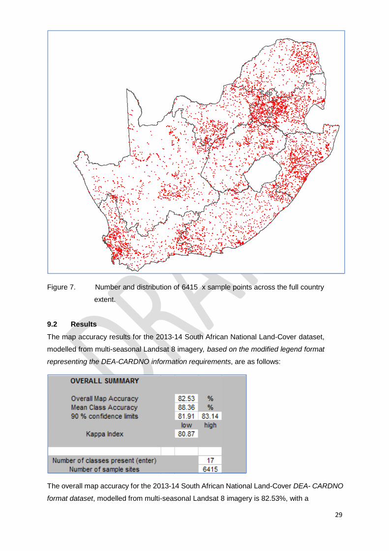
2929

Figure 7. Number and distribution of 6415 x sample points across the full country

extent.

9.2 Results

The map accuracy results for the 2013-14 South African National Land-Cover dataset,

modelled from multi-seasonal Landsat 8 imagery, based on the modified legend format

representing the DEA-CARDNO information requirements, are as follows:

The overall map accuracy for the 2013-14 South African National Land-Cover DEA- CARDNO

format dataset, modelled from multi-seasonal Landsat 8 imagery is 82.53%, with a

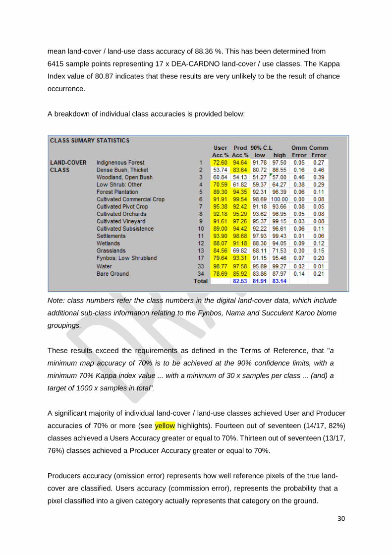
3030

mean land-cover / land-use class accuracy of 88.36 %. This has been determined from

6415 sample points representing 17 x DEA-CARDNO land-cover / use classes. The Kappa

Index value of 80.87 indicates that these results are very unlikely to be the result of chance

occurrence.

A breakdown of individual class accuracies is provided below:

Note: class numbers refer the class numbers in the digital land-cover data, which include

additional sub-class information relating to the Fynbos, Nama and Succulent Karoo biome

groupings.

These results exceed the requirements as defined in the Terms of Reference, that "a

minimum map accuracy of 70% is to be achieved at the 90% confidence limits, with a

minimum 70% Kappa index value ... with a minimum of 30 x samples per class ... (and) a

target of 1000 x samples in total".

A significant majority of individual land-cover / land-use classes achieved User and Producer

accuracies of 70% or more (see yellow highlights). Fourteen out of seventeen (14/17, 82%)

classes achieved a Users Accuracy greater or equal to 70%. Thirteen out of seventeen (13/17,

76%) classes achieved a Producer Accuracy greater or equal to 70%.

Producers accuracy (omission error) represents how well reference pixels of the true land-

cover are classified. Users accuracy (commission error), represents the probability that a

pixel classified into a given category actually represents that category on the ground.

3131

Producers accuracy therefore represents the accuracy of the sample points whereas the

Users accuracy represents what the data user will experience when using the land-cover

data. The Kappa Index is measure of statistical chance, with higher values (>0.7) typically

representing repeatable and reliable results.

The contingency matrix showing the per-cover class breakdown of these map accuracy

statistics is shown in Appendix E.

9.3 Analysis and Conclusions

Overall the map accuracies for the 2013-14 South African National Land-Cover dataset are

very good and indicate that the dataset is accurate and that data users can have confidence

in the information contained within. There are however some individual classes, with less than

80% User and / or Producer accuracies that need further analysis and comment. All of these,

bar one, are associated with spectrally modelled base vegetation classes, rather than the

post-modelling derived land-use classes.:

9.3.1 Dense Bush / Thicket

The Dense Bush / Thicket class achieved a 83.64% Producers Accuracy but only a 53.86%

Users Accuracy. This appears to be primarily result of confusion with Woodland / Open Bush

(76/428 samples), Grassland (51/428 samples), and Low Shrubland22 (45/428 samples). There

is no clear regional pattern associated with this misclassification.

Within the Woodland / Open Bush confused samples, 52 of the 76 samples had a woody cover

≥ 55%, and 26 of the 76 samples had a woody cover ≥ ± 65%, which may explain this inter-

class confusion, since the (Google Earth) observed canopy cover amounts could be

considered close to the transition to dense bush cover. The confusion with observed

Grassland areas is difficult to explain since there is very little woody cover observed in these

samples. A possible explanation may be that localised areas of extremely high grassland

biomass are (spectrally) being confused in the modelling process with woody cover. The

Dense Bush / Thicket confusion with Low Shrubland may associated, in some cases, with the

tall woody cover density of the Low Shrubland23, since 24/45 of the incorrect sample

sites have an observed woody cover of ≥ ± 15%, 15/45 have an observed woody cover of ≥

22 Low Shrubland Fynbos and Other sub-classes combined.

23

The observed woody cover percentage for Low Shrubland (Fynbos and Other) as indicated in the accuracy spreadsheet represents the tall woody cover and not the general low matrix of woody shrubs.

25 Low Shrubland Fynbos and Other sub-classes combined.

3232

± 25%, 9/45 have an observed woody cover of ≥ ± 35%, and 5/45 have an observed woody

cover of ≥ ± 45%.

If all the Dense Bush / Thicket samples are grouped into tall woody versus non-woody (or low

woody shrub) cover24, then 349/428 (81%) samples have a tall woody canopy cover ≥ ±

15%, regardless of observed land-cover type, 331/428 (77%) samples have a tall woody

canopy cover ≥ ± 25%, 323/428 (75%) samples have a tall woody canopy cover ≥ ± 35%,

310/428 (72%) samples have a tall woody canopy cover ≥ ± 45%, and 197/428 (46%)

samples have a tall woody canopy cover ≥ ± 65%.

9.3.2 Woodland / Open Bushland

The Woodland / Open Bushland class achieved a 60.84% Users Accuracy and Producers

Accuracy of 54.13% Users Accuracy. This appears to be primarily result of confusion with

Grassland (59/452 samples), and Low Shrubland25 (80/452 samples). There is no clear

regional pattern associated with this misclassification.

The confusion with Grassland is difficult to explain, other than as a result of modelling and

interpretation errors associated with lower woody canopy cover densities and associated

spectral characteristics, with 14/59 (23%) of the observed Grassland samples having a woody

cover of ≥ 15%. Similar confusion was found with Low Shrubland, with 17/80 (21%) of the

observed Low Shrubland samples having an tall woody cover of ≥ 15% cover,

irrespective of the background low woody shrub matrix.

If all the Woodland / Open Bushland samples are grouped into tall woody versus non-woody

(or low woody shrub) cover, then 320/452 (70%) samples have a tall woody canopy cover ≥

± 15%, regardless of observed land-cover type, 289/452 (63%) samples have a tall woody

canopy cover ≥ ± 25%, 284/452 (62%) samples have a tall woody canopy cover ≥ ± 35%,

221/452 (48%) samples have a tall woody canopy cover ≥ ± 45%, and 80/452 (17%)

samples have a tall woody canopy cover ≥ ± 65%.

24

Note that Forest Plantations do not have a woody canopy cover value recorded for either observed or mapped

plantation sample sites, so it is likely that the accuracy of the modelled extent of dense woody cover is actually higher, since there are 8 x Dense Bush / Thicket sample points that were observed to be Plantation Forests.

27 Low Shrubland Fynbos and Other sub-classes combined.

3333

9.3.3 Grassland

The Grassland class achieved a 84.56% User Accuracy but only a 69.82% Producers

Accuracy. This appears to be primarily result of confusion with Woodland / Open Bush

(82/1004 samples), and Low Shrubland26 (55/1004 samples). There is no clear regional

pattern associated with this misclassification.

The confusion with Woodland / Open Bush is difficult to explain, other than as a result of

modelling and interpretation errors associated, since the majority of observed Woodland /

Open Bush sample sites all have tall woody cover densities ≥ ± 55%. However on the

majority of observed Low Shrubland sites, the woody cover density was less than ± 5 %

cover, irrespective of the background low woody shrub matrix, which is probably

representative of a transitional zone..

If all the Grassland samples are grouped into tall woody versus non-woody cover, then

813/1004 (80%) samples have a tall woody canopy cover ≤ ± 15%, regardless of observed

land-cover type and 711/1004 (70%) samples have a tall woody canopy cover ≤ ± 5%,

regardless of observed land-cover type.

9.3.4 Low Shrubland (Fynbos and Other Sub-Classes combined)

The Low Shrubland classes for Fynbos and Other respectively achieved User Accuracies of

79.64% and 70.59%; and Producers Accuracies of 93.31% and 61.82%. These two classes

have been assessed in combination since they are only differentiated on the basis of the

overlaid SANBI Biome boundary. In both cases confusion was primarily with Grassland

(142/858 samples). There is no clear regional pattern associated with this misclassification.

If all the Low Shrubland samples are grouped into (tall) woody versus non-woody cover, then

791/858 (92%) samples have a tall woody canopy cover less than ± 15%, regardless of

observed land-cover type and 691/858 (80%) samples have a tall woody canopy cover less

than ± 5%, regardless of observed land-cover type.

9.3.5 Bare Ground

The Bare Ground class achieved a User Accuracy of 73.54% and a Producers Accuracy of

77.54%. This appears to be primarily result of confusion with Grassland (26/378 samples),

and Low Shrubland27 (65/378 samples). There is no clear regional pattern associated with

this misclassification. The confusion with Low Shrubland is difficult to explain, other than as

26 Low Shrubland Fynbos and Other sub-classes combined.

3434

a result of modelling and interpretation errors associated, since the 57 / 65 observed Low

Shrubland sample sites all have tall woody cover densities between ± 5 - 55%, with the

majority being between ± 15 - 25%. However these percentages, as indicated, only refer to

the tall woody cover component, and not the low woody shrub component, which may have

been very sparse. The confusion with Grassland may be due a comparable, overall low

vegetation base cover, although unlike with the observed Low Shrubland samples, the

observed Grassland samples all had, bar one, zero % tall woody cover densities.

9.3.6 Conclusion

In conclusion it would seem that the majority of mapping errors associated with the base

natural vegetation cover classes can be broadly associated with transitional vegetation

conditions, represented by structural vegetation gradients, within which the spectral based

modelling has defined a fixed boundary.

10. DATA USE

The digital raster data is supplied without any post modelling or classification spatial filtering.

Data users may wish to consider applying spatial cleaning techniques, for example, such as

applying a moving 3 x 3 pixel window filter to remove isolated single class pixels from the

dataset, especially if the raster data is to be converted to vector format.

3535

11. METADATA

2013-14 GEOTERRAIMAGE SOUTH AFRICAN NATIONAL LAND-COVER DATASET

DEA / CARDNO 35 x CLASS LEGEND :

CORE METADATA ELEMENTS (SANS1878)

1(M) Dataset title: 2013-14 GTI SA National Land-Cover (DEA / CARDNO version)

(dea_cardno_2014_sa_lcov_utm35n_vs2b_pivot-corr.img)

2(M) Dataset reference date: April 2013 - March 2014

3(O) Dataset responsible party: Produced by GeoTerra Image (GTI) Pty Ltd, South Africa

4(C) Geographic location of the dataset. MBR

WestBoundLongitude: -717294.00 (Upper Left X)

EastBoundLongitude: 1301256.00 (Lower Right X)

NorthBoundLongitude: -2239230.00 (Upper Left Y)

SouthBoundLongitude: -4046670.00 (Lower Right Y)

Projection coordinates based on Universal Transverse Mercator UTM 35 North, WGS84

(datum), meters.

5(M) Dataset language : “English” (eng)

6(C) Dataset character set: UTF8 (8-bit data)

7(M)Dataset topic category: 010 = Base Map earth coverage

8(O) Scale of the dataset: Land-cover mapped from 30 metre resolution Landsat satellite

imagery, therefore recommended for ±1:75,000 - 1: 90,000 scale or coarse mapping &

modelling applications.

9(M) Abstract describing the dataset: The 2013-14 South African National Land-cover dataset

produced by GEOTERRAIMAGE as a commercial data product has been generated from

digital, multi-seasonal Landsat 8 multispectral imagery, acquired between April 2013 and

March 2014. In excess of 600 Landsat images were used to generate the land-cover

information, based on an average of 8 different seasonal image acquisition dates, within each

of the 76 x image frames required to cover South Africa. The land-cover dataset, which

3636

covers the whole of South Africa, is presented in a map-corrected, raster format, based on

30x30m cells equivalent to the image resolution of the source Landsat 8 multi-spectral

imagery. This specific version of the 2013-14 GEOTERRAIMAGE South African National

Land-Cover Dataset is supplied to the South African Department of Environmental Affairs

under the DEA / CARDNO Project: SCPF002:"Implementation of Land Use Maps for South

Africa". The supplied dataset referred to in this report represents a subset of the full 2013-14

GEOTERRAIMAGE South African National Land-Cover Dataset, in terms of supplied land-

cover / land-use categories. Use of this DEA / CARDNO data version is governed by the

LICENCE AGREEMENT contained on this report. The DEA / CARDNO dataset contains 35

x land-cover / use information classes, covering a wide range of natural and man-made

landscape characteristics. The original land-cover dataset was processed in UTM (north) /

WGS84 map projection format based on the Landsat 8 standard map projection format as

provided by the USGS. The data remains the property of GEOTERRAIMAGE, and is

protected by copyright laws. All Intellectual Property rights pertaining to the data remain with

GEOTERRAIMAGE at all times. This updated 2013-14 dataset corrects the coding error for DEA - CARDNO classes #6 and

#7 (cultivated fields and pivot cultivated fields) which was inadvertently swapped in the

previous version. Apart from the recoding of the two field-type classes, all other details and

class codes etc remain exactly the same as the previously delivered datasets.

10(O) Dataset format name: ERDAS Imagine *img raster formats

11(O) Dataset format version: version 01 (file # 22)

12(O) Additional extent information for the dataset: (vertical and temporal)

Vertical Extent:

Minimum Value: n/a

Maximum Value: n/a

Unit Of Measure: n/a

Vertical Datum: n/a

Temporal Extent: Land-cover datasets generated in January 2015, based on April 2013 -

March 2014 multi-seasonal Landsat 8 and 5 satellite imagery.

14(O) Reference system: Universal Transverse Mercator (UTM) 35 North

CRS:

Projection Used: Universal Transverse Mercator (UTM) 35 North

Spheroid used: WGS84

3737

Datum used: WGS 84

Ellipsoid parameters:

Ellipsoid semimajor axis

axis units

denominator of flattening ratio

Projection Parameters:

UTM Zone: 35 (North)

Standard parallel

Longitude of central meridian: 27:00:00.00 East

Latitude of projection origin: 00:00:00.00 East

False easting: 500000.00 meters

False northing: 0.00 meters

Scale factor at equator: 0.999600

Projection units: meters

15(O) Lineage statement: Land-cover dataset generated in-house by GeoTerraImage

(Pretoria) in January 2015, based on primarily multi-date Landsat 8 imagery acquired

between April 2013 and March 2014.

16(O) On-line resource: n/a

17(O) Metadata file identifier: n/a

18(O) Metadata standard name: SANS I878

19(O) Metadata standard version: version 01

20(C) Metadata language: English (eng)

21(C) Metadata character set: 021 (UsAscii)

22(M) Metadata point of contact:

Name: Mark Thompson

Position Name: Director Remote Sensing

3838

Organisation Name: GeoTerraImage Pty Ltd

Physical Address:

Building Grain Building (1st Floor)

Street Witherite

Street_Suffix Street

Street_Nr 477

Suburb Die Wilgers

City Pretoria

Zip 0041

State Gauteng

Country South Africa

Postal Address :

Box 295

Suburb Persequor Park

City Pretoria

Zip 0020

State Gauteng

Country South Africa

23(M) Metadata time stamp: 31 July 2015

3939

APPENDIX A 2013-14 South African National Land-cover Legend (DEA / CARDNO legend)

The table below describes the 35 x land-cover / use classes contained in the DEA / CARDNO supplied subset of the 2013-14 South African

National Land-cover dataset, generated from multi-seasonal Landsat 8 imagery. See Appendix D for visual examples of percent cover densities

per unit area.

PARENT DEA Class Name (and digital code) Definition

WATER

Water (33)

Areas of open, surface water, that are detectable on all image dates used in the Landsat 8

based water modelling processes. The mapped extent represents the maximum detectable

water extent from all available imagery acquired within the 2013-14 assessment period.

Includes both natural and man-made water features. WETLAND

Wetland (12)

Wetland areas that are primarily vegetated on a seasonal or permanent basis. Defined on the

basis of seasonal image identifiable surface vegetation patterns (not subsurface soil

characteristics),. The vegetation can be either rooted or floating. Wetlands may be either daily

(i.e. coastal), temporarily, seasonal or permanently wet and/or saturated. Vegetation is

predominately herbaceous. Includes but not limited to wetlands associated with seeps/springs,

marshes, floodplains, lakes / pans, swamps, estuaries, and some riparian areas. Wetlands

associated with riparian zones represent image identified vegetation along the edges of

watercourses that show similar spectral characteristics to nearby wetland vegetation. Excludes

Mangrove swamps. Permanent or seasonal open water areas within the wetlands are classified

separately. Seasonal wetland occurrences within commercially cultivated field boundaries are not

shown, although they have been retained within subsistence level cultivation fields. FOREST

Indigenous Forest (1)

Natural / semi-natural indigenous forest, dominated by tall trees, where tree canopy heights are

typically > ± 5m and tree canopy densities are typically > ± 75 %, often with multiple

understory vegetation canopies. Note this class refers to Grassland areas not within the

Fynbos, Nama Karoo and Succulent Karoo Biome boundaries (as defined in the SANBI 2006

"Vegetation of South Africa, Swaziland and Lesotho" map data). THICKET &

DENSE BUSH

Dense Bush, Thicket & Tall Dense

Shrubs (2)

Natural / semi-natural tree and / or bush dominated areas, where typically canopy heights are

between 2 - 5 m, and canopy density is typically > ± 75%, but may include localised sparser

areas down to ± 60%22

. Includes dense bush, thicket, closed woodland, tall, dense shrubs,

4040

scrub forest and mangrove swamps. Can include self-seeded bush encroachment areas if

sufficient canopy density. Note this class refers to Grassland areas not within the Fynbos,

Nama Karoo and Succulent Karoo Biome boundaries (as defined in the SANBI 2006

"Vegetation of South Africa, Swaziland and Lesotho" map data).

WOODLAND /

OPEN-BUSH

Woodland and Open Bushland (3)

Natural / semi-natural tree and / or bush dominated areas, where typically canopy heights are

between ± 2 - 5 m, and canopy densities typically between 40 - 75%, but may include localised

sparser areas down to ± 15 - 20 %28

. Includes sparse - open bushland and woodland, including

transitional wooded grassland areas. Can include self-seeded bush encroachment areas if

canopy density is within indicated range. In the arid western regions (i.e. Northern Cape), this

cover class may be associated with a transitional bush / shrub cover that is lower than typical

Open Bush / Woodland cover but higher and/or more dense than typical Low Shrub cover. Note

this class refers to Grassland areas not within the Fynbos, Nama Karoo and Succulent

Karoo Biome boundaries (as defined in the SANBI 2006 "Vegetation of South Africa, Swaziland

and Lesotho" map data). GRASSLAND

Grassland (13)

Natural / semi-natural grass dominated areas, where typically the tree and / or bush canopy

densities are typically < ± 20 %, but may include localised denser areas up to ± 40 %,

(regardless of canopy heights)7. Includes open grassland, and sparse bushland and woodland

areas, including transitional wooded grasslands. May include planted pasture (i.e. grazing) if

not irrigated. Irrigated pastures will typically be classified as cultivated, and urban parks and

golf courses etc under urban. Note this class refers to Grassland areas not within the Fynbos,

Nama Karoo and Succulent Karoo Biome boundaries (as defined in the SANBI 2006

"Vegetation of South Africa, Swaziland and Lesotho" map data).

28 Normally it is preferred that land-cover class definitions are mutually exclusive in terms of content and associated landscape characteristics. Due to the nature of the multi-

seasonal spectral modelling approach used in compiling the land-cover dataset, it seems that there is some transitional overlap between "bushy / woody grassland" and

"grassy woodland / bushland" in terms of woody cover densities. For this reason the class definitions for both "Woodland / Open Bush" and "Grassland" include both a class

specific core woody cover definition, and a shared transitional woody cover definition. The sample points used to verify the map accuracy record the observed woody cover percentage for these vegetation types should the user wish to undertake further analysis.

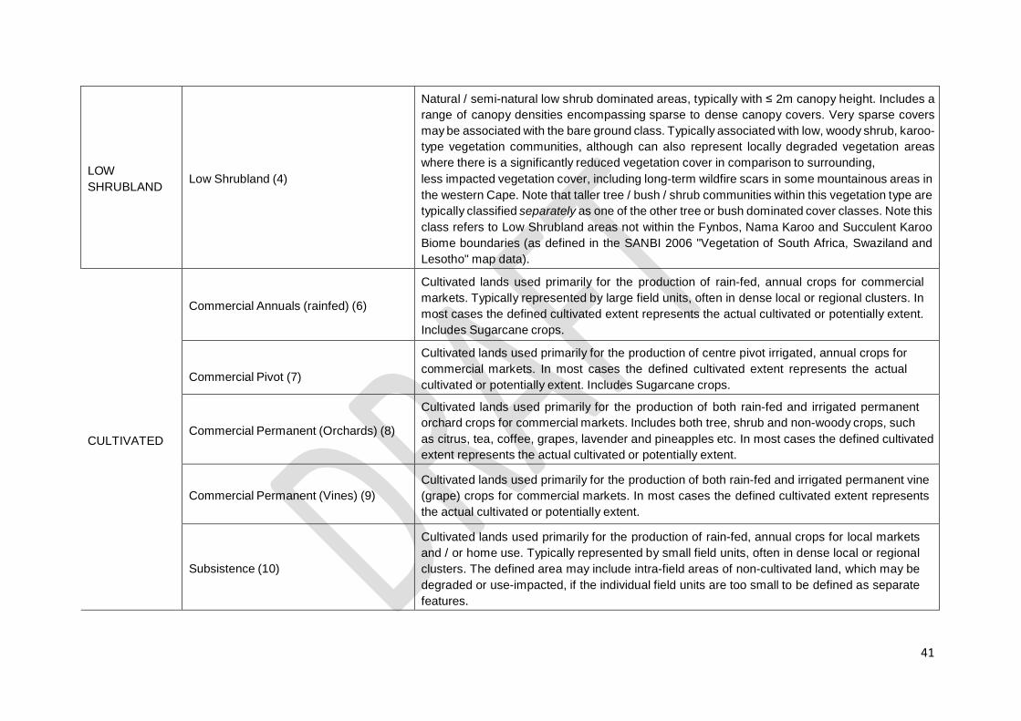
LOW

SHRUBLAND

Low Shrubland (4)

Natural / semi-natural low shrub dominated areas, typically with ≤ 2m canopy height. Includes a

range of canopy densities encompassing sparse to dense canopy covers. Very sparse covers

may be associated with the bare ground class. Typically associated with low, woody shrub, karoo-

type vegetation communities, although can also represent locally degraded vegetation areas

where there is a significantly reduced vegetation cover in comparison to surrounding,

less impacted vegetation cover, including long-term wildfire scars in some mountainous areas in

the western Cape. Note that taller tree / bush / shrub communities within this vegetation type are

typically classified separately as one of the other tree or bush dominated cover classes. Note this

class refers to Low Shrubland areas not within the Fynbos, Nama Karoo and Succulent Karoo

Biome boundaries (as defined in the SANBI 2006 "Vegetation of South Africa, Swaziland and

Lesotho" map data).

CULTIVATED

Commercial Annuals (rainfed) (6)

Cultivated lands used primarily for the production of rain-fed, annual crops for commercial

markets. Typically represented by large field units, often in dense local or regional clusters. In

most cases the defined cultivated extent represents the actual cultivated or potentially extent.

Includes Sugarcane crops.

Commercial Pivot (7)

Cultivated lands used primarily for the production of centre pivot irrigated, annual crops for

commercial markets. In most cases the defined cultivated extent represents the actual

cultivated or potentially extent. Includes Sugarcane crops.

Commercial Permanent (Orchards) (8)

Cultivated lands used primarily for the production of both rain-fed and irrigated permanent

orchard crops for commercial markets. Includes both tree, shrub and non-woody crops, such

as citrus, tea, coffee, grapes, lavender and pineapples etc. In most cases the defined cultivated

extent represents the actual cultivated or potentially extent. Commercial Permanent (Vines) (9)

Cultivated lands used primarily for the production of both rain-fed and irrigated permanent vine

(grape) crops for commercial markets. In most cases the defined cultivated extent represents

the actual cultivated or potentially extent.

Subsistence (10)

Cultivated lands used primarily for the production of rain-fed, annual crops for local markets

and / or home use. Typically represented by small field units, often in dense local or regional

clusters. The defined area may include intra-field areas of non-cultivated land, which may be

degraded or use-impacted, if the individual field units are too small to be defined as separate

features.

41

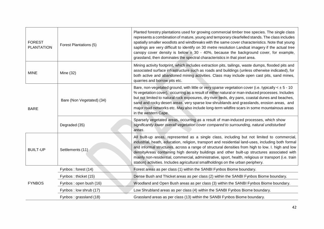
FOREST

PLANTATION

Forest Plantations (5)

Planted forestry plantations used for growing commercial timber tree species. The single class

represents a combination of mature, young and temporary clearfelled stands. The class includes

spatially smaller woodlots and windbreaks with the same cover characteristics. Note that young

saplings are very difficult to identify on 30 metre resolution Landsat imagery if the actual tree

canopy cover density is below ± 30 - 40%, because the background cover, for example,

grassland, then dominates the spectral characteristics in that pixel area.

MINE

Mine (32)

Mining activity footprint, which includes extraction pits, tailings, waste dumps, flooded pits and

associated surface infrastructure such as roads and buildings (unless otherwise indicated), for

both active and abandoned mining activities. Class may include open cast pits, sand mines,

quarries and borrow pits etc. BARE

Bare (Non Vegetated) (34)

Bare, non-vegetated ground, with little or very sparse vegetation cover (i.e. typically < ± 5 - 10

% vegetation cover), occurring as a result of either natural or man-induced processes. Includes

but not limited to natural rock exposures, dry river beds, dry pans, coastal dunes and beaches,

sand and rocky desert areas, very sparse low shrublands and grasslands, erosion areas, and

major road networks etc. May also include long-term wildfire scars in some mountainous areas

in the western Cape.

Degraded (35)

Sparsely vegetated areas, occurring as a result of man-induced processes, which show

significantly lower overall vegetation cover compared to surrounding, natural undisturbed

areas.

BUILT-UP

Settlements (11)

All built-up areas, represented as a single class, including but not limited to commercial,

industrial, heath, education, religion, transport and residential land-uses, including both formal

and informal structures, across a range of structural densities from high to low. I. high and low

densityAreas containing high density buildings and other built-up structures associated with

mainly non-residential, commercial, administrative, sport, health, religious or transport (i.e. train

station) activities. Includes agricultural smallholdings on the urban periphery. FYNBOS

Fynbos : forest (14) Forest areas as per class (1) within the SANBI Fynbos Biome boundary.

Fynbos : thicket (15) Dense Bush and Thicket areas as per class (2) within the SANBI Fynbos Biome boundary.

Fynbos : open bush (16) Woodland and Open Bush areas as per class (3) within the SANBI Fynbos Biome boundary.

Fynbos : low shrub (17) Low Shrubland areas as per class (4) within the SANBI Fynbos Biome boundary.

Fynbos : grassland (18) Grassland areas as per class (13) within the SANBI Fynbos Biome boundary.

42

4343

Fynbos : bare ground (19) Bare Ground areas as per class (14) within the SANBI Fynbos Biome boundary.

NAMA

KAROO

Nama Karoo : forest (20) Forest areas as per class (1) within the SANBI Nama Karoo Biome boundary. Nama Karoo : thicket (21)

Dense Bush and Thicket areas as per class (2) within the SANBI Nama Karoo Biome

boundary. Nama Karoo : open bush (22)

Woodland and Open Bush areas as per class (3) within the SANBI Nama Karoo Biome

boundary.

Nama Karoo : low shrub (23) Low Shrubland areas as per class (4) within the SANBI Nama Karoo Biome boundary.

Nama Karoo : grassland (24) Grassland areas as per class (13) within the SANBI Nama Karoo Biome boundary.

Nama Karoo : bare ground (25) Bare Ground areas as per class (14) within the SANBI Nama Karoo Biome boundary.

SUCCULENT

KAROO

Succulent Karoo : forest (26) Forest areas as per class (1) within the SANBI Succulent Karoo Biome boundary. Succulent Karoo : thicket (27)

Dense Bush and Thicket areas as per class (2) within the SANBI Succulent Karoo Biome

boundary. Succulent Karoo : open bush (28)

Woodland and Open Bush areas as per class (3) within the SANBI Succulent Karoo Biome

boundary.

Succulent Karoo : low shrub (29) Low Shrubland areas as per class (4) within the SANBI Succulent Karoo Biome boundary.

Succulent Karoo : grassland (30) Grassland areas as per class (13) within the SANBI Succulent Karoo Biome boundary.

Succulent Karoo : bare ground (31) Bare Ground areas as per class (14) within the SANBI Succulent Karoo Biome boundary.

Note: the Fynbos, Nama Karoo and Succulent Karoo vegetation sub-classes are provided with additional class codes representing the parent

primary vegetation class,in order that different levels of class detail can be used and accessed by data users. This is illustrated below

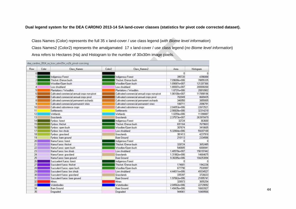
4444

Dual legend system for the DEA CARDNO 2013-14 SA land-cover classes (statistics for pivot code corrected dataset).

Class Names (Color) represents the full 35 x land-cover / use class legend (with Biome level information)

Class Names2 (Color2) represents the amalgamated 17 x land-cover / use class legend (no Biome level information)

Area refers to Hectares (Ha) and Histogram to the number of 30x30m image pixels.

4545

APPENDIX B List of accompanying documents and files.

Excel spreadsheet containing full list of Landsat 8 and 5 acquisition dates, per image

frame, as used in the generation of the 2013-14 South African National Land-Cover

dataset29.

ESRI ArcGIS point coverage (UTM35 north) representing the sample points used to verify

the 2013-14 South African National Land-Cover dataset (version 4), and calculate the

DEA-CARDNO legend format mapping accuracies.

29 Note that the listed acquisition dates represent the primary dates used in the land-cover modelling, and not

any additional image dates that were only used for localised cloud masking on the primary image date. Additional image dates are however listed if they themselves were also considered primary acquisition dates

and used as modelling inputs.

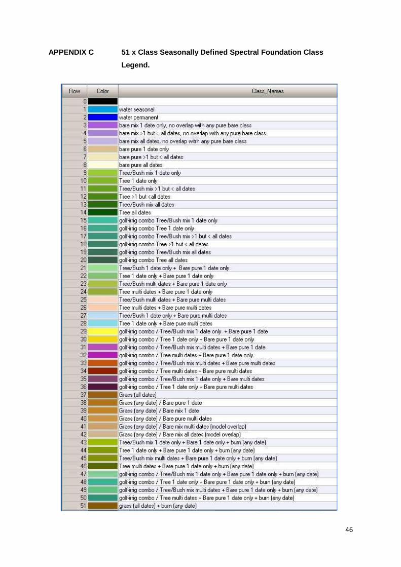
4646

APPENDIX C 51 x Class Seasonally Defined Spectral Foundation Class

Legend.

4747

APPENDIX D Visual representation of canopy cover density

percentages per unit area.

Adapted from Paine, D.P., 1981, Aerial photography and image interpretation for resource management: New York, John Wiley & Sons, 422 p.

APPENDIX E Contingency Matrix representing the Map Accuracy Results for all 33 x Land-Cover / Use Classes.

48

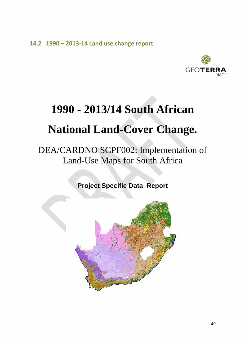
49

14.2 1990 – 2013-14 Land use change report

1990 - 2013/14 South African

National Land-Cover Change.

DEA/CARDNO SCPF002: Implementation of

Land-Use Maps for South Africa

Project Specific Data Report

50

DATA PRODUCT CREATED BY

GEOTERRAIMAGE (South Africa),

www.geoterraimage.com

August 2015, version 01

LIABILITY

The Client has to verify prior to his commitment, the adequacy of GEOTERRAIMAGE datasets

and products to the specific data and analyses needs as set out by the client.

GEOTERRAIMAGE will in no event be liable for any direct, indirect, incidental or consequential

damages including lost savings or profit, legal fees, lost data, lost sales, loss of commitments,

business interruption, including loss of or other damage, resulting from its datasets and

products, whether or not GEOTERRAIMAGE has been advised of the possibility of such

damage. This includes damages incurred by the client or any

third party.

GEOTERRAIMAGE datasets and products are processed from sources like topographic maps

and satellite images. The quality of these sources is not the responsibility of

GEOTERRAIMAGE. The data and data products are provided “as is”, without warranty of any

kind, either express or implied, including, but not limited to, the implied warranties of

merchantability and fitness for a particular purpose.

Whilst all possible care and attention has been taken in the production of the data, neither

GEOTERRAIMAGE or any of its respective sub-organisations or employees, accept any liability

whatsoever for any perceived or actual inaccuracies or misrepresentations in the supplied data or

accompanying report(s), as a result of the nature of mapping from coarse and medium scale

satellite imagery. Any mapped boundaries either implied or inferred within the data do not have

any legal status whatsoever.

All rights not specifically granted or specified in this agreement, pertaining to this data are

reserved to GEOTERRAIMAGE Pty Ltd.

51

52

CONTENTS

1.BACKGROUND

2.COMMENTS ON 1990 - 2014 SA LAND-COVER CHANGE ASSESSMENT

2.1Influence of Land-Cover Mapping Accuracies

2.2Influence of Seasonal / Climatic Differences on Land-Cover Change

2.3Influence of Mapping Detail on Land-Cover Change

3.QUALITATIVE EXAMPLES OF LAND-COVER CHANGE 1990 - 2013/14

4.QUANTITATIVE ASSESSMENT OF LAND-COVER CHANGE 1990 - 2013/14

4.1 National Level Land-Cover Change Results

4.2 Provincial Level Land-Cover Change Results

4.3 Inter-Class Land-Cover Change Results

5.1990 - 2013/14 CHANGE RESULTS ANALYSIS

5.1Indigenous Forest

5.2Thicket / Dense Bush

5.3Woodland/ Open Bush

5.4Low Shrubland

5.5 Plantations / Woodlots

5.6Cultivated Commercial Annual Crops Non-Pivot

5.7 Cultivated Commercial Annual Crops Pivots

5.8Cultivated Commercial Permanent Orchards

5.9Cultivated Commercial Permanent Vines

5.10Cultivated Subsistence Crops

5.11 Settlements (including Smallholdings)

5.12Wetlands

5.13Grasslands

53

5.14Mines

5.15Waterbodies

5.16Bare Ground

5.17Degraded

PLEASE NOTE

This report provides information on the land-cover change statistics derived from a

comparison of the specific versions of the 1990 and 2013/14 GEOTERRAIMAGE South

African National Land-Cover Dataset supplied to the South African Department of

Environmental Affairs under the DEA / CARDNO Project: SCPF002:"Implementation of

Land Use Maps for South Africa". These datasets represent information subsets of the

full 1990 and 2013/14 GEOTERRAIMAGE South African National Land-Cover Datasets, in

terms of supplied land-cover / land-use categories and associated class legend.

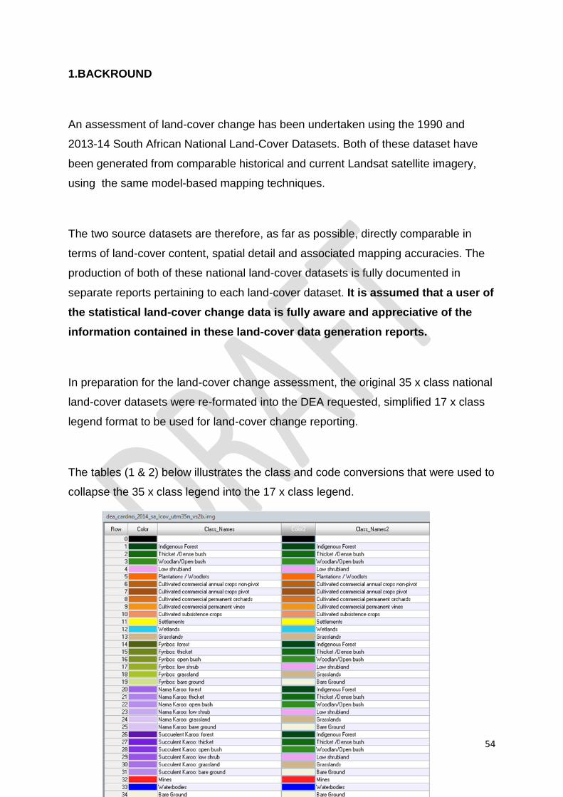
54

1.BACKROUND

An assessment of land-cover change has been undertaken using the 1990 and

2013-14 South African National Land-Cover Datasets. Both of these dataset have

been generated from comparable historical and current Landsat satellite imagery,

using the same model-based mapping techniques.

The two source datasets are therefore, as far as possible, directly comparable in

terms of land-cover content, spatial detail and associated mapping accuracies. The

production of both of these national land-cover datasets is fully documented in

separate reports pertaining to each land-cover dataset. It is assumed that a user of

the statistical land-cover change data is fully aware and appreciative of the

information contained in these land-cover data generation reports.

In preparation for the land-cover change assessment, the original 35 x class national

land-cover datasets were re-formated into the DEA requested, simplified 17 x class

legend format to be used for land-cover change reporting.

The tables (1 & 2) below illustrates the class and code conversions that were used to

collapse the 35 x class legend into the 17 x class legend.

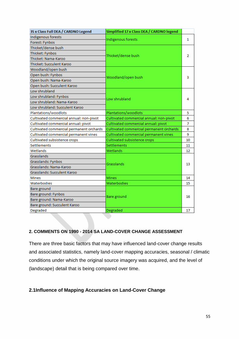
55

2. COMMENTS ON 1990 - 2014 SA LAND-COVER CHANGE ASSESSMENT

There are three basic factors that may have influenced land-cover change results

and associated statistics, namely land-cover mapping accuracies, seasonal / climatic

conditions under which the original source imagery was acquired, and the level of

(landscape) detail that is being compared over time.

2.1Influence of Mapping Accuracies on Land-Cover Change

56

Mapping accuracies have been calculated for the 2013-14 land-cover dataset and

are reported in the 2013-14 Data User's report. The results of the 2013-14 map

accuracy assessment are assumed to be representative of the 1990 accuracies,

since comparable image data and modelling / mapping techniques were used for

both datasets. No independent map accuracy assessment was undertaken for the

1990 dataset due to the unavailability of suitable reference data. The reliability of

(land-cover) change statistics are greatly influenced by the accuracy of the input data

against which change is determined. In simplistic terms, the sum of the known

mapping error associated with a particular land-cover class over two time periods

can indicate the level of 'statistical change' that is in fact a result of compounded

mapping errors over time, and not actual land-cover change. For this reason all

statistical (land-cover) change values must be interpreted and evaluated in the

context of the reported land-cover class mapping accuracy, especially the User (as

opposed to the Producers) accuracy. Class specific mapping accuracies are

included in the land-cover change results reported below and in the accompanying

spreadsheet.

2.2Influence of Seasonal / Climatic Differences on Land-Cover Change

It is important to understand the influence that seasonal, and possible climatic

differences between 1990 and 2013-14 may have had on the generation of each

land-cover dataset in terms of landscape characteristics, and the possible effect of

such differences on the change assessment results and associated spatial statistics.

The seasonal representation and range of monthly acquisition dates is generally better for the

1990 land-cover dataset, than used for the 2013-14 dataset, despite the same average

number of acquisition dates per frame for the two datasets. This is because the 2013-14

dataset was limited to what cloud free imagery was recorded between April 2013 and the

designated March 2014 cut-off, whereas the 1990 dataset had access to a wider range of

imagery from 1989 - 1993. This greater seasonal representation may have influenced the

modelling results in terms of the distribution and extent of some of the natural vegetation

classes (excluding indigenous forests), since a better seasonal profile was often possible in

1990 compared to 2014 in some image frame locations.

57

The 1990 period appears to have been generally wetter than the 2013-14 period in most

regions, as observed through the increase in observable surface water features in 1990. This

is especially evident in the pans across the central regions of the Free State and Northern

Cape, where many pans are water filled in 1990 and dry in 2013-14. These differences will

reflect as changes between the two assessment periods but do not necessarily represent a

permanent loss of water bodies over the ± 24 year period, but rather a seasonal (or climatic)

induced difference. This fact needs to be noted during modelling and the interpretation of land-

cover change results and associated statistics.

The wetter conditions prevalent in the 1990 dataset have allowed the wetland modelling to be

extended across the full national coverage, unlike the drier 2013-14 image data which

restricted wetland modelling to the wetter eastern and southern regions. These differences

will reflect as changes between the two assessment periods but do not necessarily represent

a permanent loss of wetlands over the ± 24 year period, but rather a seasonal (or climatic)

induced difference. This fact needs to be noted during modelling and interpretation of land-

cover change results.

The wetter conditions prevalent in the 1990 dataset may have influenced the boundary

between low-shrub (i.e. karoo type) and highveld grassland vegetation, since the 1990

grassland / low shrub transition in the western Free State region appears to have shifted

generally to the west compared to 2013-14, which may be a result of a greater grass

component being present in the karoo / grass transition zone in 1990.

The (highveld, montane and coastal) grassland correction procedures applied to the 1990

dataset are considered to be slightly more accurate than those applied to the 2013-14 data,

as a result of both modified procedures used and better image seasonal representation in

1990. It is therefore potentially possible that some of the 'grassland' to 'open woody vegetation'

changes in these regions may be a result of the improved grassland delineation in 1990 and

not actual bush cover increases in 2013-14.

2.3Influence of Mapping Detail on Land-Cover Change

The ability to determine change is obviously dependent on the level of detail that is

being observed and compared. For example, changes in the extent of urban areas

between 1990 and 2013-14 may not be as locally significant as maybe expected,

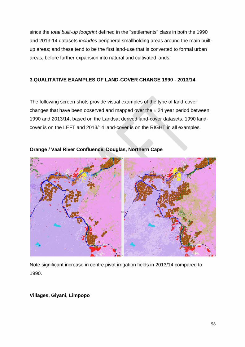
58

since the total built-up footprint defined in the "settlements" class in both the 1990

and 2013-14 datasets includes peripheral smallholding areas around the main built-

up areas; and these tend to be the first land-use that is converted to formal urban

areas, before further expansion into natural and cultivated lands.

3.QUALITATIVE EXAMPLES OF LAND-COVER CHANGE 1990 - 2013/14.

The following screen-shots provide visual examples of the type of land-cover

changes that have been observed and mapped over the ± 24 year period between

1990 and 2013/14, based on the Landsat derived land-cover datasets. 1990 land-

cover is on the LEFT and 2013/14 land-cover is on the RIGHT in all examples.

Orange / Vaal River Confluence, Douglas, Northern Cape

Note significant increase in centre pivot irrigation fields in 2013/14 compared to

1990.

Villages, Giyani, Limpopo

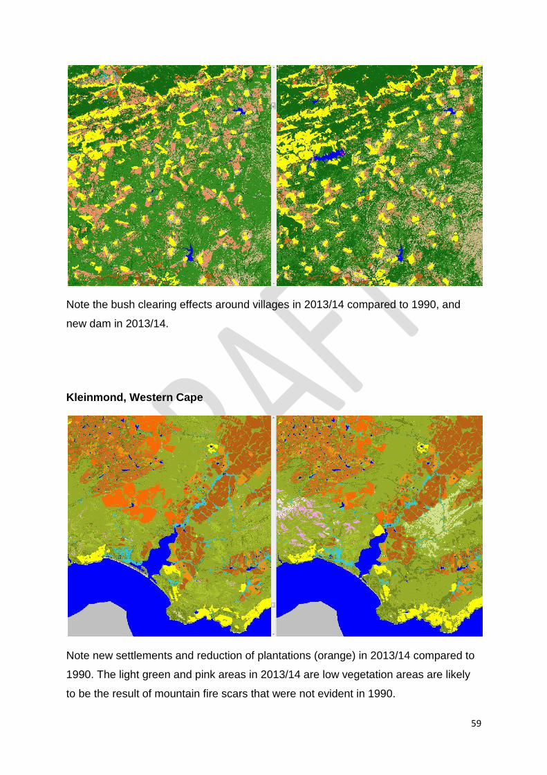
59

Note the bush clearing effects around villages in 2013/14 compared to 1990, and

new dam in 2013/14.

Kleinmond, Western Cape

Note new settlements and reduction of plantations (orange) in 2013/14 compared to

1990. The light green and pink areas in 2013/14 are low vegetation areas are likely

to be the result of mountain fire scars that were not evident in 1990.

60

Kosi Bay, KwaZulu Natal

Note the increase in plantation forestry (orange) in 2013/14 and the greater extent of

wetlands (light blue) in 1990 as a result of the (generally) wetter conditions.

KZN Midlands, KwaZulu Natal

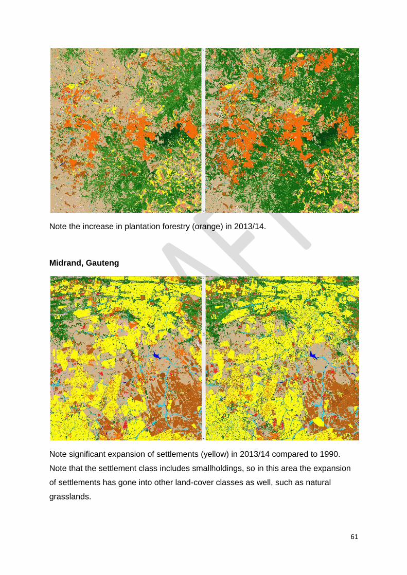
61

Note the increase in plantation forestry (orange) in 2013/14.

Midrand, Gauteng

Note significant expansion of settlements (yellow) in 2013/14 compared to 1990.

Note that the settlement class includes smallholdings, so in this area the expansion

of settlements has gone into other land-cover classes as well, such as natural

grasslands.

62

Pan (wetlands), Northern Cape

Note significantly greater extent and number of water features evident in the pans in

1990 as result of the wetter conditions compared to 2013/14.

Olifants River, Western Cape

63

Note significant increase in centre pivot irrigation fields in 2013/14 compared to

1990.

Rustenburg, North West

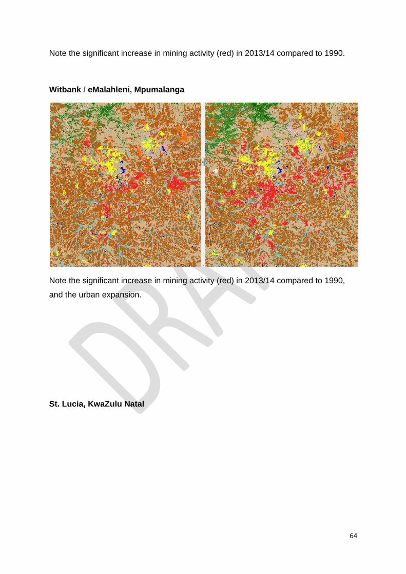
64

Note the significant increase in mining activity (red) in 2013/14 compared to 1990.

Witbank / eMalahleni, Mpumalanga

Note the significant increase in mining activity (red) in 2013/14 compared to 1990,

and the urban expansion.

St. Lucia, KwaZulu Natal

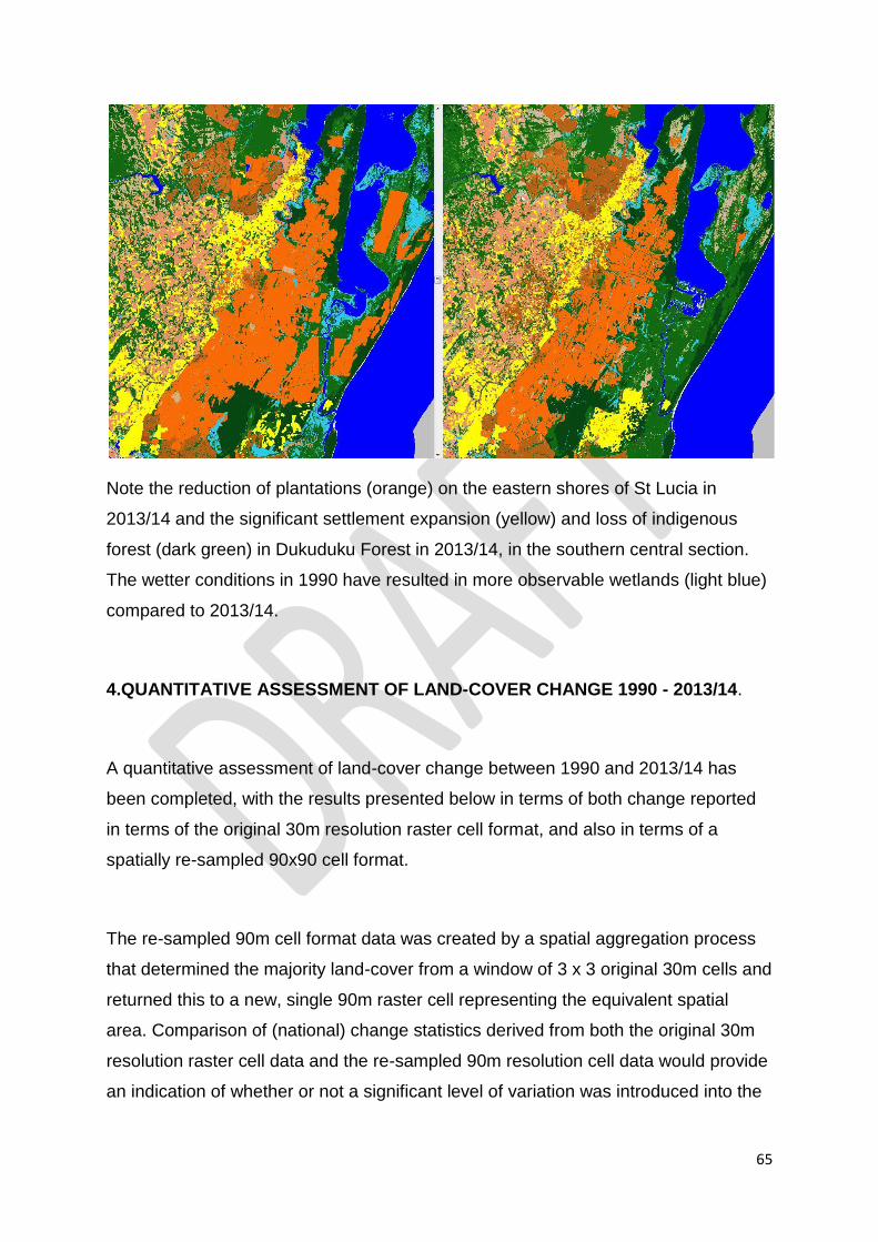
65

Note the reduction of plantations (orange) on the eastern shores of St Lucia in

2013/14 and the significant settlement expansion (yellow) and loss of indigenous

forest (dark green) in Dukuduku Forest in 2013/14, in the southern central section.

The wetter conditions in 1990 have resulted in more observable wetlands (light blue)

compared to 2013/14.

4.QUANTITATIVE ASSESSMENT OF LAND-COVER CHANGE 1990 - 2013/14.

A quantitative assessment of land-cover change between 1990 and 2013/14 has

been completed, with the results presented below in terms of both change reported

in terms of the original 30m resolution raster cell format, and also in terms of a

spatially re-sampled 90x90 cell format.

The re-sampled 90m cell format data was created by a spatial aggregation process

that determined the majority land-cover from a window of 3 x 3 original 30m cells and

returned this to a new, single 90m raster cell representing the equivalent spatial

area. Comparison of (national) change statistics derived from both the original 30m

resolution raster cell data and the re-sampled 90m resolution cell data would provide

an indication of whether or not a significant level of variation was introduced into the

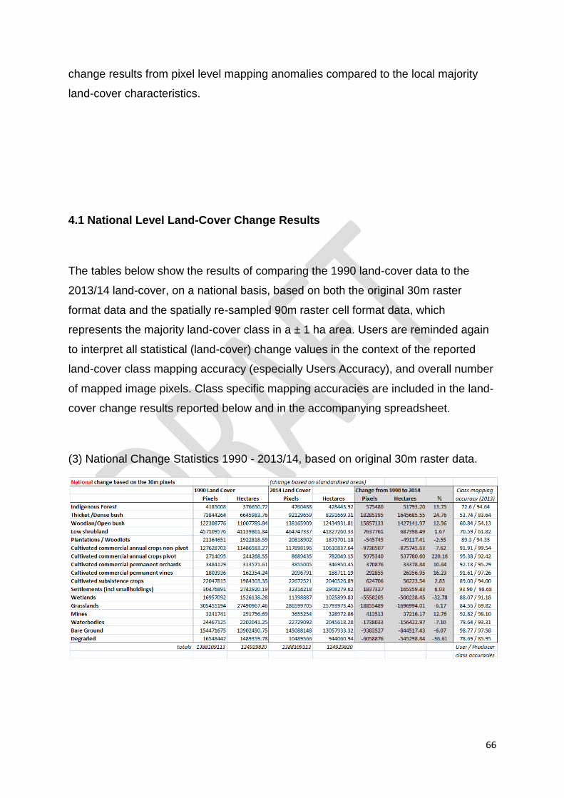
66

change results from pixel level mapping anomalies compared to the local majority

land-cover characteristics.

4.1 National Level Land-Cover Change Results

The tables below show the results of comparing the 1990 land-cover data to the

2013/14 land-cover, on a national basis, based on both the original 30m raster

format data and the spatially re-sampled 90m raster cell format data, which

represents the majority land-cover class in a ± 1 ha area. Users are reminded again

to interpret all statistical (land-cover) change values in the context of the reported

land-cover class mapping accuracy (especially Users Accuracy), and overall number

of mapped image pixels. Class specific mapping accuracies are included in the land-

cover change results reported below and in the accompanying spreadsheet.

(3) National Change Statistics 1990 - 2013/14, based on original 30m raster data.

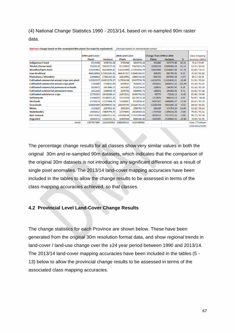
67

(4) National Change Statistics 1990 - 2013/14, based on re-sampled 90m raster

data.

The percentage change results for all classes show very similar values in both the

original 30m and re-sampled 90m datasets, which indicates that the comparison of

the original 30m datasets is not introducing any significant difference as a result of

single pixel anomalies. The 2013/14 land-cover mapping accuracies have been

included in the tables to allow the change results to be assessed in terms of the

class mapping accuracies achieved, so that classes.

4.2 Provincial Level Land-Cover Change Results

The change statistics for each Province are shown below. These have been

generated from the original 30m resolution format data, and show regional trends in

land-cover / land-use change over the ±24 year period between 1990 and 2013/14.

The 2013/14 land-cover mapping accuracies have been included in the tables (5 -

13) below to allow the provincial change results to be assessed in terms of the

associated class mapping accuracies.

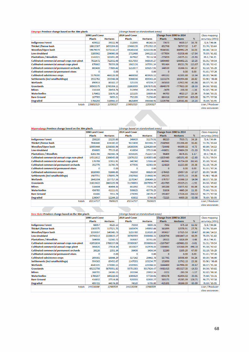
68

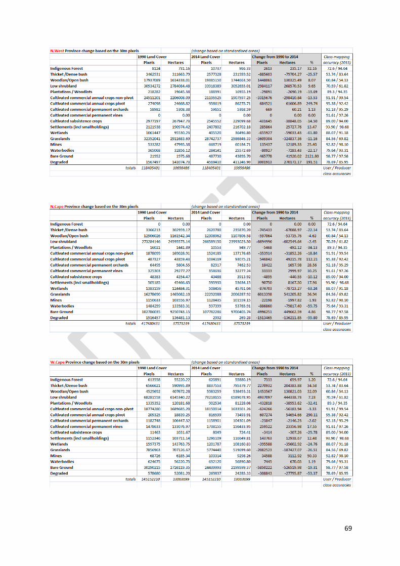
69

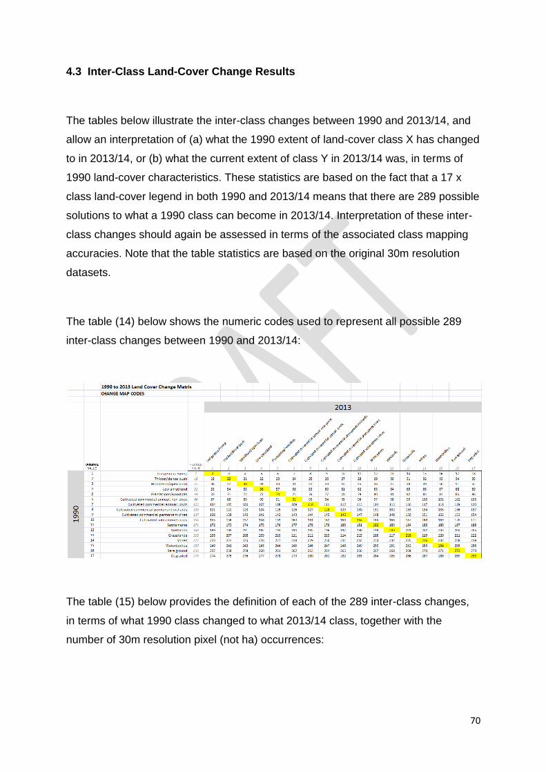
70

4.3 Inter-Class Land-Cover Change Results

The tables below illustrate the inter-class changes between 1990 and 2013/14, and

allow an interpretation of (a) what the 1990 extent of land-cover class X has changed

to in 2013/14, or (b) what the current extent of class Y in 2013/14 was, in terms of

1990 land-cover characteristics. These statistics are based on the fact that a 17 x

class land-cover legend in both 1990 and 2013/14 means that there are 289 possible

solutions to what a 1990 class can become in 2013/14. Interpretation of these inter-

class changes should again be assessed in terms of the associated class mapping

accuracies. Note that the table statistics are based on the original 30m resolution

datasets.

The table (14) below shows the numeric codes used to represent all possible 289

inter-class changes between 1990 and 2013/14:

The table (15) below provides the definition of each of the 289 inter-class changes,

in terms of what 1990 class changed to what 2013/14 class, together with the

number of 30m resolution pixel (not ha) occurrences:

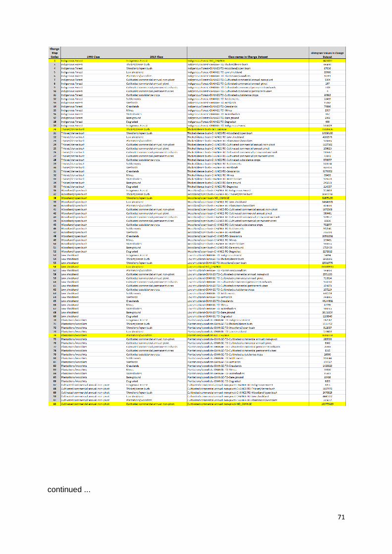
71

continued ...

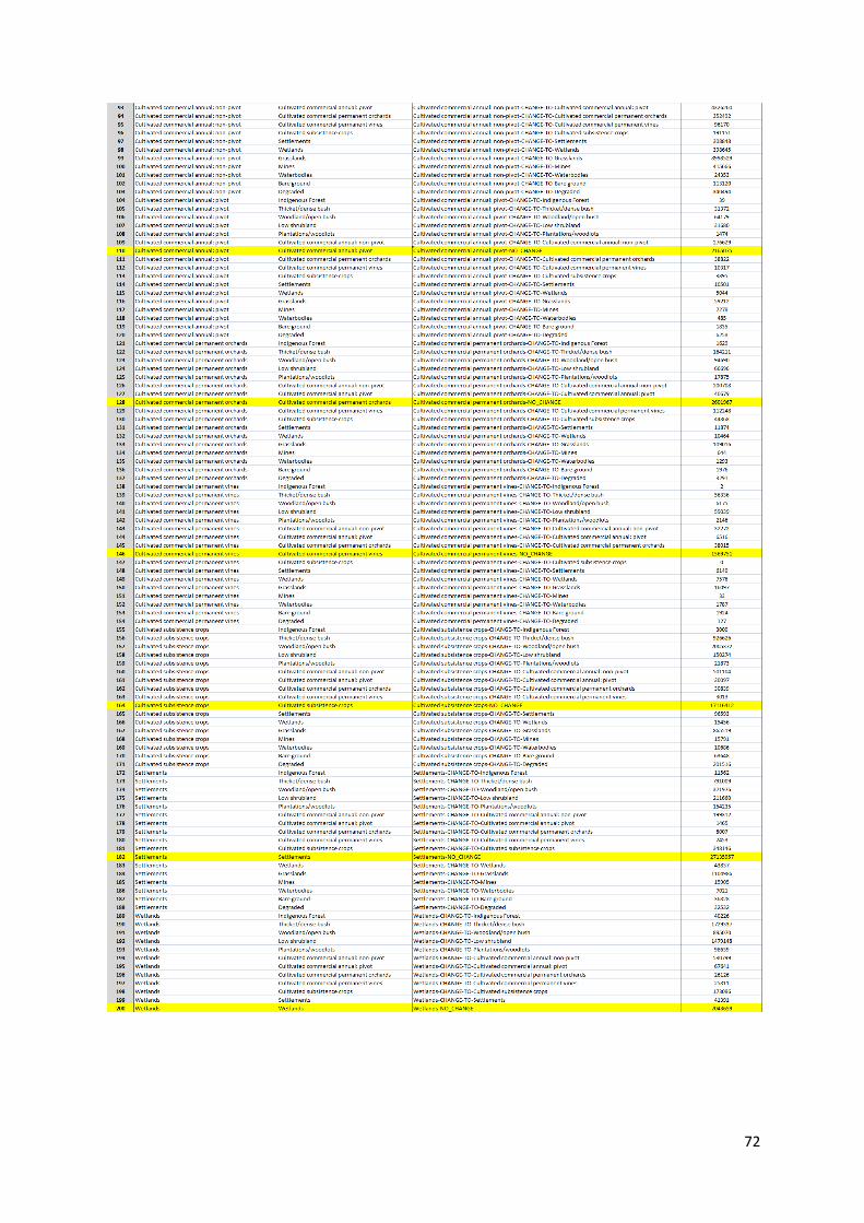
72

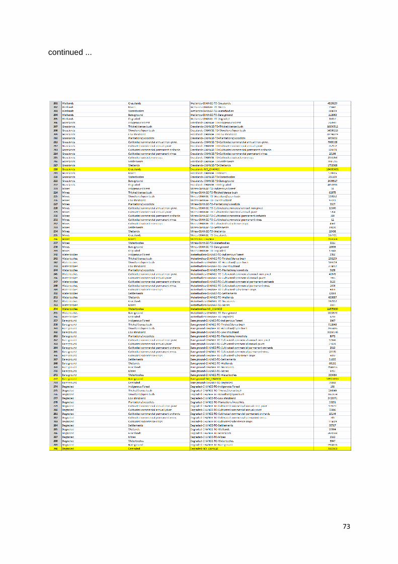
73

continued ...

74

The table (16) below describes the actual 1990 - 2013/14 inter-class land-cover changes for the whole of South Africa, in terms of

Hectares (Ha):

75

The table (17) below describes the actual 1990 - 2013/14 inter-class land-cover changes for the whole of South Africa, expressed

in terms of the percentage of the original 1990 class extent and what it has become in 2013/14. For example, 81.84 % of what was

mapped as indigenous forest in 1990 is still indigenous forest in 2013/14, and 11.85% of what was indigenous forest in 1990 is now

mapped as thicket / dense bush in 2013/14:

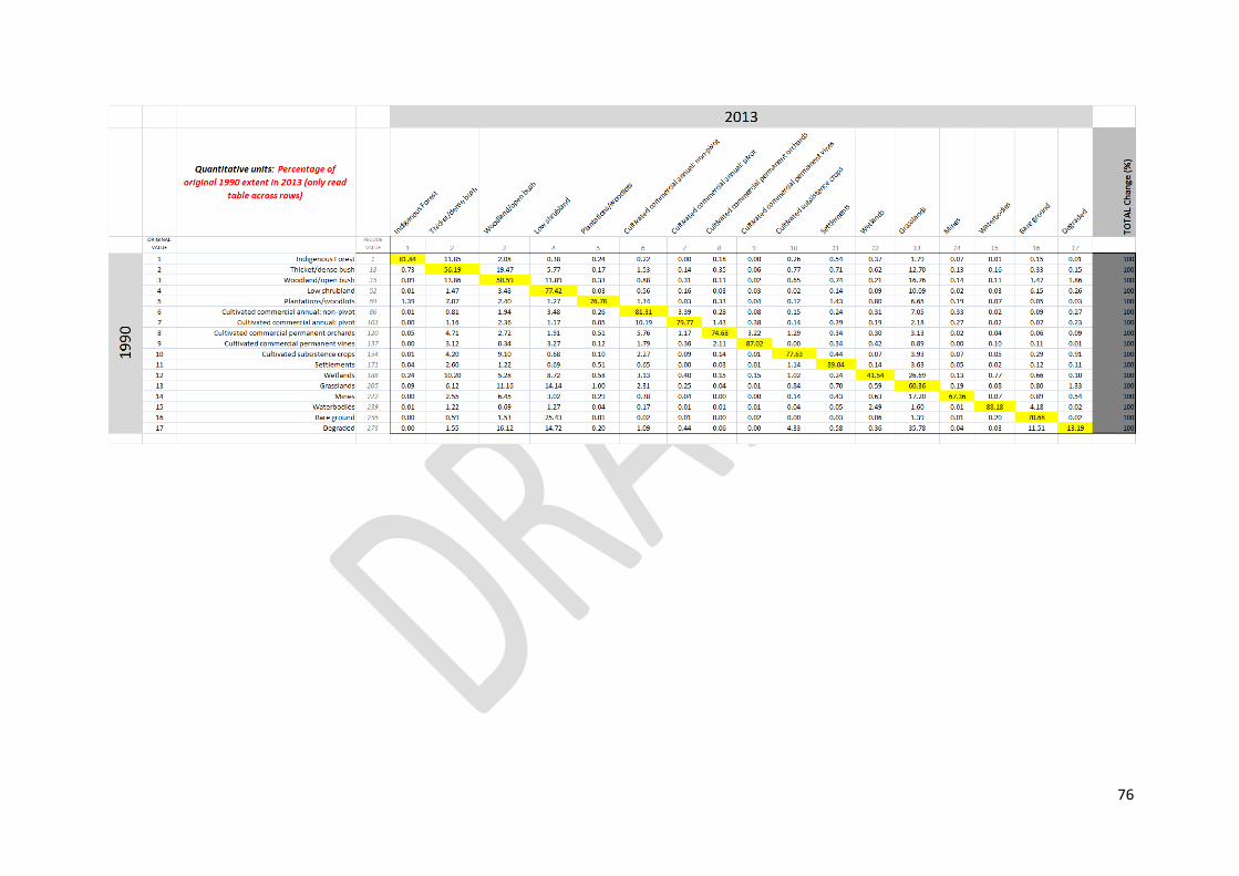
76

77

The table (18) below describes the actual 1990 - 2013/14 inter-class land-cover changes for the whole of South Africa, expressed

in terms of the percentage of the current 2013/14 class extent and what it was originally in 1990. For example, 71.95 % of what was

mapped as indigenous forest in 2013/14 was also indigenous forest in 1990, and 11.26% of what is indigenous forest in 2013/14

was mapped as thicket / dense bush in 1990:

.

78

79

5.1990 - 2013/14 CHANGE RESULTS ANALYSIS

5.1Indigenous Forest

According to the land-cover data there was nationally a 13.75% increase in the

indigenous forest class extent between 1990 and 2013/14. However the 2013/14

map accuracy results indicate a 72.6 % Users Accuracy, which may mean that in

many cases the reported change is a result of mapping error between true forest and

the spectrally similar woody vegetation classes such as 'thicket / dense bush', as

indicated in the 2013/14 accuracy report. In Gauteng Province there is a 1350% (!)

statistical increase in the extent of indigenous forest in 2013/14, but this is simply

due to the fact that in 1990 2 pixels were mapped as forest whereas in 2013/14 29

pixels were mapped. This difference is likely to be a result of the reported mapping

inaccuracies; with 29 pixels representing only 0.0006 % of the total mapped area of

indigenous forest in 2013/14. National and provincial statistics should not however

detract from the very relevant and real changes in indigenous forest cover change

that are contained within the land-cover datasets in a local basis, such as around

Dukuduku, St Lucia (see previous picture example).

5.2Thicket / Dense Bush

According to the land-cover data there was nationally a 24.76% increase in the

thicket / dense bush class extent between 1990 and 2013/14. However the 2013/14

map accuracy results indicate only a 53.74 % Users Accuracy, which may mean that

in many cases the reported change will be a result of mapping error between this

class and other spectrally similar woody vegetation classes, as indicated in the

2013/14 accuracy report. Provincial changes, in the woody dominated areas vary

from +16.03% in Limpopo, +18.77% in KZN, +36.46% in Mpumalanga, +79.52% in

Eastern Cape and -25.57 % in North West. It is recommended that such statistical

changes are treated with caution unless validated by corroborating evidence of

plausible local change within the actual land-cover map datasets.

5.3Woodland/ Open Bush

80

According to the land-cover data there was nationally a 12.96% increase in the

woodland / open bush class extent between 1990 and 2013/14. However the

2013/14 map accuracy results indicate only a 60.84 % Users Accuracy, which may

mean that in many cases the reported change will be a result of mapping error

between this class and other spectrally similar woody vegetation classes, as

indicated in the 2013/14 accuracy report. Provincial changes, in the woody

dominated areas vary from +3.47% in Limpopo, +20.57% in KZN, - 4.73% in

Mpumalanga, +115.79% in Eastern Cape and +8.07% in North West. It is

recommended that such statistical changes are treated with caution unless validated

by corroborating evidence of plausible local change within the actual land-cover map

datasets.

5.4Low Shrubland

According to the land-cover data there was nationally a 1.67% increase in the low

shrub class extent between 1990 and 2013/14. The 2013/14 map accuracy results

indicate a 70.59 % Users Accuracy, which may mean that the limited amount of

change is a function of both increasing map accuracy and the extremely large

national class footprint within which any local change is insignificant in terms of total

area affected. Provincial changes low shrub / karoo / fynbos dominated areas vary

from +48.59% in Free State, -2.45% in Northern Cape and +7.23% in Western Cape.

In most cases the changes in low shrub extent seem to be along a transitional

gradient with grasslands, and may be reflecting local annual changes in grass

component cover in response to different annual rainfall conditions, as is evident in

the difference in open water / wetland areas between 1990 and 2013/14. It is

recommended that such statistical changes are treated with caution unless validated

by corroborating evidence of plausible local change within the actual land-cover map

datasets.

5.5 Plantations / Woodlots.

According to the land-cover data there was nationally a 2.55% decrease in the

plantation / woodlot class extent between 1990 and 2013/14. The 2013/14 map

accuracy results indicate a 89.3 % Users Accuracy, which should mean that both

81

the mapped and statistical representations of change are plausible and likely to be

accurate. The national statistic does not however reflect provincial or local area

changes over the same ± 24 year period, with some areas definately showing losses

and others expansion. Provincial changes in traditional forestry areas vary from -

23.93% in Limpopo, +1.1% in Mpumalanga, +1.02% in Eastern Cape and +3.57% in

KZN.

5.6Cultivated Commercial Annual Crops Non-Pivot.

According to the land-cover data there was nationally a 7.62% decrease in the

cultivated commercial annual crop non-pivot class extent between 1990 and

2013/14. The 2013/14 map accuracy results indicate a 91.91 % Users Accuracy,

which should mean that both the mapped and statistical representations of change

are plausible and likely to be accurate. The national statistic does not however reflect

provincial or local area changes over the same ± 24 year period, with some areas

definately showing losses and others expansion. Provincial changes in traditional

forestry areas vary from -20.25% in Limpopop, -12.65% in Mpumalanga, +11.64% in

KZN, -10.30% in Eastern Cape and -3.33% in Western Cape for example. On a local

scale, many of these losses and expansions also appear to relate to associated

increases in other cultivation land-uses, such as orchards, vines and pivots, and

losses due to new mining and urban areas.

5.7 Cultivated Commercial Annual Crops Pivots

According to the land-cover data there was nationally a 220.16% increase in the

cultivated commercial annual crop pivot class extent between 1990 and 2013/14.

This is by far the biggest increase in any land-cover class extent over the ±24 year

period and represents a huge increase in irrigation activities and associated water

consumption. The 2013/14 map accuracy results indicate a 95.381 % Users

Accuracy, which should mean that both the mapped and statistical representations of

change are plausible and very likely to be accurate. The national statistic does not

however reflect provincial or local area changes over the same ± 24 year period, with

provincial changes in pivot class extent varying from +113.87% in Limpopop,

+262.41% in Mpumalanga, +261.41% in KZN, +413.66% in Eastern Cape and

82

+290.11% in Western Cape for example. All provinces showed increases in pivot

class extent since 1990. On a local scale this expansion appears to have resulted in

losses to both other cultivated land-uses and natural vegetation types, depending on

location.

5.8Cultivated Commercial Permanent Orchards.

According to the land-cover data there was nationally a 10.64% increase in the

cultivated commercial permanent orchard class extent between 1990 and 2013/14.

The 2013/14 map accuracy results indicate a 92.18 % Users Accuracy, which should

mean that both the mapped and statistical representations of change are plausible

and likely to be accurate. The national statistic does not however reflect provincial or

local area changes over the same ± 24 year period, with some areas definately

showing losses and others expansion. Provincial changes in traditional orchard

areas vary from +40.27% in Limpopo, +35.38% in Mpumalanga, +28.56% in

Northern Cape, and -18.18 in Eastern Cape for example. On a local scale, many of

these losses and expansions also appear to relate to associated increases in other

cultivation land-uses, such as orchards, vines and pivots, and losses due to new

mining and urban areas.

5.9Cultivated Commercial Permanent Vines.

According to the land-cover data there was nationally a 16.23% increase in the

cultivated commercial permanent vines class extent between 1990 and 2013/14. The

2013/14 map accuracy results indicate a 91.61% Users Accuracy, which should

mean that both the mapped and statistical representations of change are plausible

and likely to be accurate. The national statistic does reflect provincial level changes

over the same ± 24 year period,, with similar percent increases being reported in

both the Western and Northern Cape. All provinces with vines in 1990 show an

increase in 2013/14.

5.10Cultivated Subsistence Crops

83

According to the land-cover data there was nationally only a 2.83% increase in the

cultivated subsistence crop class extent between 1990 and 2013/14. The 2013/14

map accuracy results indicate a 89.00 % Users Accuracy, which should mean that

both the mapped and statistical representations of change are plausible and likely to

be accurate. It is important to note however that unlike commercial fields which were

(originally) mapped on a individual field unit basis, subsistence fields were mapped

according to the outer extent of clusters of subsistence fields, as necessitated by

their characteristically small areas compared to image resolution. This resulted in

varies levels and patterns of inter-field non-crop land being included in the

subsistence cluster boundaries. During the land-cover mapping these inter-field non-

crop areas have been re-classified, where possible, into their basic vegetation cover

types, i.e. grass, dense bush etc. Since this was based on a generic modelling

procedure as opposed to image-specific classification routines, it is possible that the

extent and coverage of such inter-field non-crop areas has been influenced by (a)

the accuracies associated with these vegetation classes, and (b) any modifying

effect resulting from 1990 conditions appearing to be generally wetter than those in

2013/14. Furthermore, the actual intensity of land-use (i.e. subsistence crop yield)

cannot be gauged from the single 'subsistence class' defined in the 17x class

legend format, since all subsistence fields have been included within one

amalgamated class on the basis of (image) observable field boundaries, regardless

of whether such fields were cultivated, temporary or long term fallow (i.e.

abandoned) in the assessment year. A subdivision of land-use activity intensity

(a.k.a. cropping), based on annual Normalised Difference Vegetation Index (NDVI)

profiles is available as part of the associated 72 x class DEA / GTI national land-

cover dataset for 2013/14, but not presently for 1990. This may be a consideration

for future work and analysis since it will allow the historical and current extents of

high intensity subsistence cropping units to be compared, as opposed to just the

overall extent of image observable field cluster boundaries.

The national statistic does not however reflect provincial or local area changes over

the same ± 24 year period, with areas showing losses and others expansion.

Provincial changes in subsistence cropping vary from -13.34% in Limpopop, -27.27%

in Mpumalanga, and +30.29% in KZN. . It is recommended that until such time that

84

that subsistence changes can be validated in terms of land-use intensity changes

(i.e. productive-to-productive, productive-to-fallow,, fallow-to-productive etc), such

statistical changes are treated with caution unless validated by corroborating

evidence of plausible local change within the actual land-cover map datasets.

5.11 Settlements (including Smallholdings)

According to the land-cover data there was nationally only a 6.03% increase in the

settlement class extent between 1990 and 2013/14. The 2013/14 map accuracy

results indicate a 93.90 % Users Accuracy, which should mean that both the mapped

and statistical representations of change are plausible and likely to be accurate. The

national statistic does not however reflect provincial or local area changes over the

same ± 24 year period, with some areas definately showing losses and others

expansion, ranging from +28.82% in Limpopo to (surprisingly) -2.93% in KZN.

Gauteng only shows a +10.58% increase, which from an anecdotal perspective may

be lower than expected, but this is potentially explained by the fact that the

settlement footprint defined in the two land-cover datasets includes a variety of urban

sub-classes, including commercial, residential, village, schools etc, as well as

smallholdings. Peripheral smallholdings around urban centres are typically the first

land-use class to convert to formal urban areas under urban expansion. Thus the

total settlement footprint as defined in terms of the DEA / CARDNO national land-

cover datasets will not change over time when smallholdings are converted to formal

residential or industrial areas. Settlement sub-classes defining separate commercial,

industrial, residential, informal, village and smallholding categories are available

within the full 72 x class DEA / GTI national land-cover dataset for 2013/14, but not

presently for 1990. This may be a consideration for future work and analysis since it

will allow a more representative interpretation of urban expansion to be evaluated.

5.12Wetlands

According to the land-cover data there was nationally a 32.78% decrease in the

wetland class extent between 1990 and 2013/14. The 2013/14 map accuracy results

indicate a 88.07 % Users Accuracy, which should mean that both the mapped and

statistical representations of change are plausible and likely to be accurate. However

85

wetlands is one specific land-cover class that has been significantly affected by the

general wetter landscape conditions in 1990 compared to 2013/14, especially in the

more conventionally drier western areas. The generally wetter landscape conditions

in 1990 allowed wetland modelling to be undertaken across the entire country,

whereas in 2013/14, because of drier conditions, wetland modelling was restricted to

the southern and eastern regions. Thus any wetlands in the normally drier western

regions that were mapped in 1990 have not been re-mapped in 2013/14 simply

because they were not visible as such on the imagery under these drier conditions.

This does not mean that such wetlands have been 'lost' but rather are temporary

absent in terms of surface representation in 2013/14. This must be noted when

interpreting the statistics. A possible solution may be to take the combined area of

wetlands from 1990 and 2013/14 and subtract appropriate non-wetland land-use

class extents from this for both 1990 and 2013/14 landscapes in order to derive a

more accurate picture of wetland loss, irrespective of whether the wetlands

The national statistic does not however reflect provincial or local area changes over

the same ± 24 year period, with losses ranging from -63.24% in Northern Cape to -

12.13% in Gauteng, where the Northern Cape difference is likely to be a result of

the landscape wetness differences already discussed, and the Gauteng difference

probably being more representative of actual loss. All provinces showed a loss in

wetland extent between 1990 and 2013/14. It is therefore recommended that such

statistical changes are treated with caution unless validated by corroborating

evidence of plausible local change within the actual land-cover map datasets.

5.13Grasslands

According to the land-cover data there was nationally a 6.17% decrease in the

grassland class extent between 1990 and 2013/14. The 2013/14 map accuracy

results indicate a 84.56% Users Accuracy, which should mean that both the mapped

and statistical representations of change are plausible and likely to be accurate. As

indicated in the 1990 DEA / CARDNO SA land-cover data report the post-modelling

grassland correction edits are potentially more accurate than those applied to the

2013/14 land-cover dataset, as a result of better image dates and modified

86

correction procedures. This may mean that the actual grassland extent as

represented in the 1990 dataset is slightly more accurate than that represented in

the 2013/14 dataset, and that there could be a corresponding increase in the level of

grassland / woody vegetation cover confusion in 2013/14. It is recommended that

such statistical changes are treated with caution unless validated by corroborating

evidence of plausible local change within the actual land-cover map datasets.

The generally wetter landscape conditions in 1990, especially in the more typically

arid karoo regions may also have experienced a regional annual increase in the

grass component in the low shrub / grassland transition zone, also increasing the

extent of the grassland class mapped in 1990.

The national statistic does not however reflect provincial or local area changes over

the same ± 24 year period, with some areas showing losses and others expansion.

Provincial changes vary from -28.33% in Limpopo, +1.93% in Mpumalanga, and

+36.94% in Northern Cape.

5.14Mines

According to the land-cover data there was nationally a 12.76% increase in the

mining class extent between 1990 and 2013/14. The 2013/14 map accuracy results

indicate a 92.82% Users Accuracy, which should mean that both the mapped and

statistical representations of change are plausible and very likely to be accurate. The

national statistic does not however reflect provincial or local area changes over the

same ± 24 year period, with both losses and increases being recorded, ranging from

-46.22% in Eastern Cape to +66.84% in Mpumalanga (as would be expected due to

the expansion of open cast coal mining in this area). Since mapping accuracies are

high for this class, interpretation of the statistical changes must be made in the

context of the original and current spatial extents.

5.15Waterbodies

87

According to the land-cover data there was nationally a -7.10% decrease in the

water class extent between 1990 and 2013/14, which includes both natural, man-

made, seasonal and permanent water features. The 2013/14 map accuracy results

indicate a 79.64% Users Accuracy, which should mean that both the mapped and

statistical representations of change are plausible and likely to be accurate. The

national statistic does not however reflect provincial or local area changes over the

same ± 24 year period, with both losses and increases being recorded, ranging from

+25.34% in Limpopo, 11.35% in Mpumalanga, and -59.75% in Northern Cape.

These regional differences are likely to have been influenced by a combination of

both the generally wetter landscape conditions in 1990, especially in the typically

drier western regions, and by the construction of several new major dams after 1990

that are observable in 2013/14. Since mapping accuracies are high for this class,

interpretation of the statistical changes must be made in the context of the original

and current spatial extents, so that small spatial features do not become over-

represented statistically if they have shown significant statistical but not necessarily

spatial growth.

5.16Bare Ground

According to the land-cover data there was nationally a -6.07% decrease in the bare

ground class extent between 1990 and 2013/14. The 2013/14 map accuracy results

indicate a 98.77% Users Accuracy, which should mean that both the mapped and

statistical representations of change are plausible and very likely to be accurate. The

national statistic does not however reflect provincial or local area changes over the

same ± 24 year period, with both losses and increases being recorded, ranging from

+635.08% in Limpopo, 2121.80% in North West and -63.01% in Eastern Cape. Since

mapping accuracies are high for this class, interpretation of the statistical changes

must be made in the context of the original and current spatial extents in any given

area, so that small spatial features do not become over-represented statistically if

they have shown significant statistical but not necessarily spatial growth. The

2013/14 dataset may have been influenced by the generally drier conditions in some

areas, perhaps resulting in lower vegetative cover, although in some regions human

activity will have increased the bare ground extent.

88

5.17Degraded

According to the land-cover data there was nationally a -36.61% decrease in the

degraded class extent between 1990 and 2013/14. The 2013/14 map accuracy

results indicate a 78.69 % Users Accuracy, which should mean that both the mapped

and statistical representations of change are plausible and likely to be accurate.

However, degraded is defined as areas showing significant lower total vegetation

cover to surrounding non-impacted areas, in terms of the viewed landscape. It is

feasible therefore that a significant portion of the difference in degraded areas

between 1990 and 2013/14 could be attributed to the generally wetter conditions in

1990 compared to the drier 2013/14 conditions. The provincial results show a

significantly higher area of bare ground in 1990 than 2013/14, apart from North

West. This would appear to be the opposite of what would be expected give that

1990 was the wetter period, and thus the vegetation cover would be assumed to be

more extensive. However an alternative suggestion maybe that, in terms of the

generic modelling procedures used to define this class, when all the vegetation is

generally lower (as in a drier period) then the difference between impacted (i.e.

degraded) land and non-impacted land is harder to determine; compared to when

non-impacted land is much greener in wetter conditions.

It is recommended that such statistical changes are treated with caution unless validated by

corroborating evidence of plausible local change within the actual land-cover map datasets.

ADDITIONAL INFORMATION

PLEASE NOTE THAT THIS IS NOT A LAND-COVER MAP DATASET BUT A

SPATIAL REPRESENTATION OF 1990 TO 2013/14 LAND-COVER CHANGE ON

A PER-PIXEL BASIS.