This article was downloaded by: [Manjit S. Kang]On: 29 August 2014, At: 16:50Publisher: Taylor & FrancisInforma Ltd Registered in England and Wales Registered Number: 1072954 Registeredoffice: Mortimer House, 37-41 Mortimer Street, London W1T 3JH, UK

Journal of Crop ImprovementPublication details, including instructions for authors andsubscription information:http://www.tandfonline.com/loi/wcim20

GGE Biplot Analysis for Cane and SugarYield from Advanced-Stage SugarcaneTrials in Subtropical IndiaSurinder K. Sandhua, Sawanpreet S. Brara, R. S. Singhb, PritpalSingha, I. Bhagatc & Manjit S. Kangd

a Department of Plant Breeding and Genetics, Punjab AgriculturalUniversity, Ludhiana, Punjab, Indiab Regional Research Station, Punjab Agricultural University, Faridkot,Punjab, Indiac Regional Research Station, Punjab Agricultural University,Gurdaspur, Punjab, Indiad Former Vice Chancellor, Punjab Agricultural University, LudhianaPublished online: 26 Aug 2014.

To cite this article: Surinder K. Sandhu, Sawanpreet S. Brar, R. S. Singh, Pritpal Singh, I.Bhagat & Manjit S. Kang (2014) GGE Biplot Analysis for Cane and Sugar Yield from Advanced-Stage Sugarcane Trials in Subtropical India, Journal of Crop Improvement, 28:5, 641-659, DOI:10.1080/15427528.2014.925025

To link to this article: http://dx.doi.org/10.1080/15427528.2014.925025

PLEASE SCROLL DOWN FOR ARTICLE

Taylor & Francis makes every effort to ensure the accuracy of all the information (the“Content”) contained in the publications on our platform. However, Taylor & Francis,our agents, and our licensors make no representations or warranties whatsoever as tothe accuracy, completeness, or suitability for any purpose of the Content. Any opinionsand views expressed in this publication are the opinions and views of the authors,and are not the views of or endorsed by Taylor & Francis. The accuracy of the Contentshould not be relied upon and should be independently verified with primary sourcesof information. Taylor and Francis shall not be liable for any losses, actions, claims,proceedings, demands, costs, expenses, damages, and other liabilities whatsoever orhowsoever caused arising directly or indirectly in connection with, in relation to or arisingout of the use of the Content.

This article may be used for research, teaching, and private study purposes. Anysubstantial or systematic reproduction, redistribution, reselling, loan, sub-licensing,systematic supply, or distribution in any form to anyone is expressly forbidden. Terms &

Conditions of access and use can be found at http://www.tandfonline.com/page/terms-and-conditions

Dow

nloa

ded

by [

Man

jit S

. Kan

g] a

t 16:

50 2

9 A

ugus

t 201

4

Journal of Crop Improvement, 28:641–659, 2014Copyright © Taylor & Francis Group, LLCISSN: 1542-7528 print/1542-7536 onlineDOI: 10.1080/15427528.2014.925025

GGE Biplot Analysis for Cane and Sugar Yieldfrom Advanced-Stage Sugarcane Trials in

Subtropical India

SURINDER K. SANDHU1, SAWANPREET S. BRAR1, R. S. SINGH2,PRITPAL SINGH1, I. BHAGAT3, and MANJIT S. KANG4*

1Department of Plant Breeding and Genetics, Punjab Agricultural University,Ludhiana, Punjab, India

2Regional Research Station, Punjab Agricultural University, Faridkot, Punjab, India3Regional Research Station, Punjab Agricultural University, Gurdaspur, Punjab, India

4Former Vice Chancellor, Punjab Agricultural University, Ludhiana

The performance of quantitative traits in sugarcane (Saccharumspp. complex) often varies across diverse environments because ofsignificant genotype-by-environment interaction (GEI). Our objec-tive was to assess performance stability of 20 advanced sugarcanegenotypes across six environments, including two crop seasonsin Punjab. Data were obtained on cane yield (t/ha), sucrose %juice, and commercial cane sugar % at harvest and subjected toGGE [genotype (G) plus genotype-environment (GE)] biplot analy-sis, which revealed high positive correlations between spring andautumn crop seasons at all locations for all measured traits. Thisimplied that genotypes could be evaluated in either crop sea-son, which should reduce testing cost and time. Test environmentFaridkot (FDK) spring, being both discriminating and representa-tive, was an ideal test environment for selecting generally adaptedgenotypes for cane yield. Similarly, Ludhiana (LDH) autumn wasan ideal test environment for selecting generally adapted genotypesfor quality traits. Co 0238 and CoPb 08214, having high mean

Received 3 March 2014; accepted 12 May 2014.∗Current affiliation: Department of Plant Pathology, Kansas State University, Manhattan,

Kansas, USA.

Address correspondence to Surinder K. Sandhu, Department of Plant Breeding andGenetics, Punjab Agricultural University, Ludhiana-141004, Punjab, India. E-mail: surindersandhu@pau.edu

Color versions of one or more of the figures in the article can be found online at www.tandfonline.com/wcim.

641

Dow

nloa

ded

by [

Man

jit S

. Kan

g] a

t 16:

50 2

9 A

ugus

t 201

4

642 S. K. Sandhu et al.

performance and stability across environments for cane yield andquality traits, were identified as ideal genotypes. These genotypescan be exploited commercially for the entire state of Punjab. TheGGE biplot helped identify a specifically adapted genotype, CoH119, which was the best performer in Gurdaspur (GDSP) in bothcrop seasons.

KEYWORDS cane yield, sucrose content, commercial cane sugar,principal components, stability analysis

ABBREVIATIONS. (AEA) average environment axis; (AEC) average environ-ment coordinate; (AMMI) additive main effects and multiplicative interaction;(ANOVA) analysis of variance; (CCS %) Commercial cane sugar percent;(DNMRT) Duncan’s new multiple range test; (PC) principal component;(FDK) Faridkot; (GDSP) Gurdaspur; (GEI) genotype x environment inter-action; (GGE) genotype; (G) plus genotype-environment interaction (GE);(LDH) Ludhiana; (MET) multi-environmental trial; (SAS) statistical analysissystem; (SVD) singular value decomposition; (TCH) tons of cane per hectare;(TSS) total soluble solids.

INTRODUCTION

Sugarcane breeding is highly complex because of the highly heterozygousnature of sugarcane and high ploidy level. In multi-year yield trials, ranksof genotypes often vary from one location to another for yield and qual-ity, thereby indicating a strong genotype x environment interaction (GEI).Differential performance of genotypes evaluated across a wide range ofenvironments results in crossover (rank changes) or non-crossover (changein magnitude of performance but no rank changes) GEI (Kang 1998). TheGEI is of major concern to plant breeders because a large interaction canreduce gains from selection and make the identification of superior culti-vars difficult. Measuring GEI is important to determine an optimum strategyfor selecting genotypes adapted to target environments (Annicchiarico 1997).When GEI is significant, its causes, nature, and implications must be carefullyconsidered in breeding programs (Kang and Martin 1987). Kang (1998) dis-cussed extensively the causes of GEI and ways to exploit or minimize GEI.An understanding of the causes of GEI is essential for the implementation ofefficient selection and evaluation networks (Ramburan et al. 2011).

The success of crop improvement activities largely depends on the iden-tification of superior genotypes for cultivation. In plant breeding programs,many new genotypes are usually evaluated in different environments (loca-tions and years) to identify and advance desirable ones towards release.

Dow

nloa

ded

by [

Man

jit S

. Kan

g] a

t 16:

50 2

9 A

ugus

t 201

4

GGE Biplot Analysis for Cane & Sugar Yield 643

A genotype or cultivar is considered stable if it has adaptability for a traitof economic importance across diverse environments. The environmentalcomponent (E) generally represents the largest component in analyses ofvariance, but it is not relevant to cultivar selection; only G and GE arerelevant to meaningful cultivar evaluation and must be considered simul-taneously for making selection decisions (Yan and Kang 2003). Variousstatistical methods have been developed for the analysis of GEI. One ofthese methods is GGE biplot analysis developed by Yan et al. (2000). Thisis a GEI pattern-visualization tool, which graphically displays GE data (Yan2001; Yan and Kang 2003). It is based on two concepts, the biplot conceptof Gabriel (1971) and the GGE concept (Yan et al. 2000), and is used tovisually analyze multi-environmental trial (MET) data. The GGE explains ahigher proportion of GEI sum of squares and is said to be more informativewith regards to environments and cultivar performance than AMMI (additivemain effects and multiplicative interaction) analysis (Yan et al. 2007). TheGGE biplot technique has been used to assess GEI in a variety of cropspecies (Ma et al. 2004; Casanoves et al. 2005; Kang et al. 2005; Blancheand Myers 2006; Fan et al. 2007). Glaz and Kang (2008) used GGE biplotanalysis to improve efficiency of sugarcane MET by identifying organic-soillocations that could be replaced by a sand-soil location without compro-mising superior-cultivar selection on Florida’s organic soils. Ramburan andZhou (2011) evaluated genotype stability and magnitude of GEI in the rain-fed parts of the South African sugar industry to improve selection efficiencyand evaluation methodology via GGE biplot. Sandhu et al. (2012) also usedthe GGE biplot technique in sugarcane to assess the stability of advancedsugarcane genotypes tested across a wide range of zonal locations of Indiaand characterized the discriminating ability of test location for economictraits.

The importance of GEI in sugarcane selection has long been recognizedaround the globe (Kang and Miller 1984; Milligan et al. 1990; Bull et al. 1992;Jackson et al. 2007; Chen et al. 2012). The presence of GEI in sugarcaneMET networks complicates the identification and selection of superior cul-tivars (Ramburan et al. 2012). Consequently, MET networks must include arange of locations, years, and management regimes. Ramburan et al. (2010)categorized post-release cultivar evaluation trials in South Africa based onage and time of harvest and demonstrated highly significant genotype x ageand genotype x time of harvest interactions using restricted maximum likeli-hood (REML). These results were subsequently used to characterize varietiesfor inclusion into a decision support system. This ensured genotype selectionfor production in environments with varying biotic and abiotic stresses, withthe expectation of superior performance being repeated after cultivar release.Such an empirical approach is the basis of most crop improvement programs,which are consequently highly dependent on the representativeness of testsites.

Dow

nloa

ded

by [

Man

jit S

. Kan

g] a

t 16:

50 2

9 A

ugus

t 201

4

644 S. K. Sandhu et al.

In Punjab state (India), sugarcane crop is grown across different agro-climatic zones, viz., arid, sub-humid, and semi-arid, which differ widelyin rainfall, soil texture, and other environmental conditions. Three testlocations—Faridkot (FDK), Gurdaspur (GDSP), and Ludhiana (LDH)—represent different sugarcane environments in Punjab. There have been fewstudies on GEI in sugarcane in Punjab. In sugarcane, traits such as yieldexhibit a large amount of GEI (Kang and Miller 1984; Milligan et al.1990),and tools such as GGE biplot can be used effectively to identify stablegenotypes (Yan and Kang 2003). Thus, the objectives of this investigationwere to explore GEI using sugarcane yield trial data from Punjab, evaluatethe discriminating ability of the test locations, and assess the interaction ofgenotypes with crop seasons (spring and autumn) via GGE biplot analyses.

MATERIALS AND METHODS

Genotype Evaluation Trials

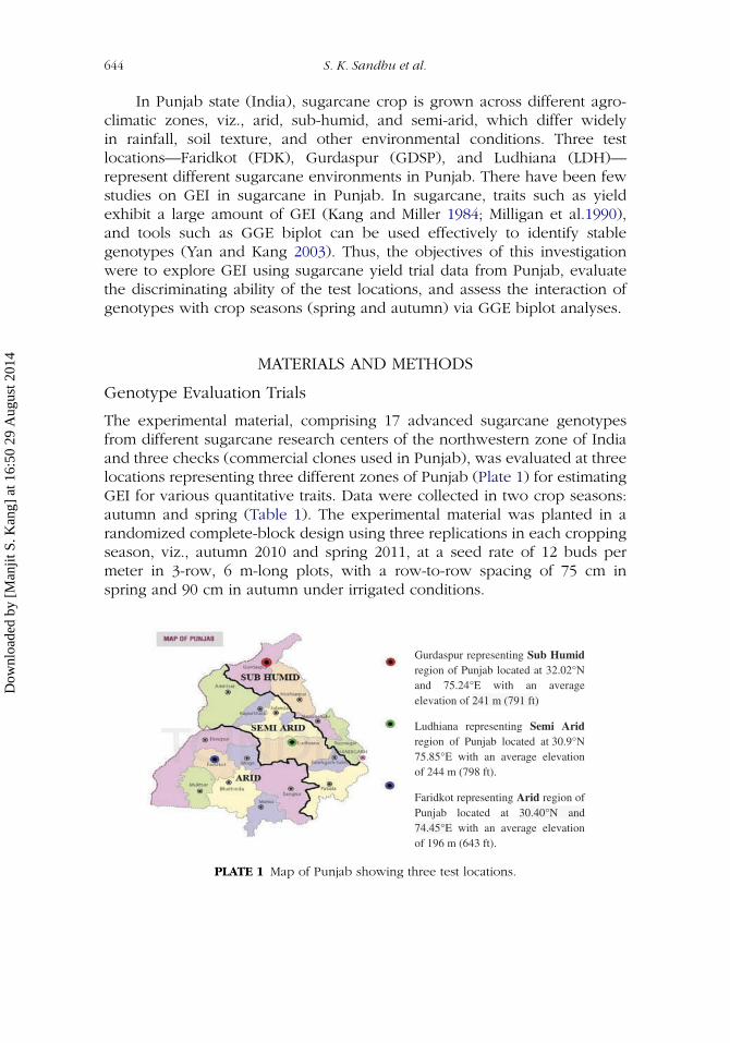
The experimental material, comprising 17 advanced sugarcane genotypesfrom different sugarcane research centers of the northwestern zone of Indiaand three checks (commercial clones used in Punjab), was evaluated at threelocations representing three different zones of Punjab (Plate 1) for estimatingGEI for various quantitative traits. Data were collected in two crop seasons:autumn and spring (Table 1). The experimental material was planted in arandomized complete-block design using three replications in each croppingseason, viz., autumn 2010 and spring 2011, at a seed rate of 12 buds permeter in 3-row, 6 m-long plots, with a row-to-row spacing of 75 cm inspring and 90 cm in autumn under irrigated conditions.

Gurdaspur representing Sub Humidregion of Punjab located at 32.02°N and 75.24°E with an average elevation of 241 m (791 ft)

Ludhiana representing Semi Aridregion of Punjab located at 30.9°N 75.85°E with an average elevation of 244 m (798 ft).

Faridkot representing Arid region of Punjab located at 30.40°N and 74.45°E with an average elevation of 196 m (643 ft).

PLATE 1 Map of Punjab showing three test locations.

Dow

nloa

ded

by [

Man

jit S

. Kan

g] a

t 16:

50 2

9 A

ugus

t 201

4

GGE Biplot Analysis for Cane & Sugar Yield 645

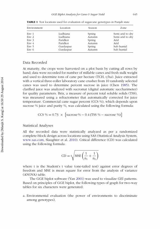
TABLE 1 Test locations used for evaluation of sugarcane genotypes in Punjab state

Environment Location Season Zone

Env 1 Ludhiana Spring Semi arid to dryEnv 2 Ludhiana Autumn Semi arid to dryEnv 3 Faridkot Spring AridEnv 4 Faridkot Autumn AridEnv 5 Gurdaspur Spring Sub humidEnv 6 Gurdaspur Autumn Sub humid

Data Recorded

At maturity, the crops were harvested on a plot basis by cutting all rows byhand; data were recorded for number of millable canes and fresh stalk weightand used to determine tons of cane per hectare (TCH, t/ha). Juice extractedwith a vertical three-roller laboratory cane crusher from 10 randomly selectedcanes was used to determine percent sucrose in juice (Chen 1985). Theclarified juice was analyzed with sucromat (digital automatic saccharimeter)for quality parameters. Brix, a measure of percent total soluble solids (TSS),was measured using a refractometer that automatically corrected for juicetemperature. Commercial cane sugar percent (CCS %), which depends uponsucrose % juice and purity %, was calculated using the following formula:

CCS % = 0.73 × [sucrose % − 0.4 (TSS % − sucrose %)

]

Statistical Analyses

All the recorded data were statistically analyzed as per a randomizedcomplete-block design across locations using SAS (Statistical Analysis System,www.sas.com, Slaughter et al. 2010). Critical difference (CD) was calculatedusing the following formula:

CD = t

√MSE

(1

n1+ 1

n2

)

where t is the Student’s t value (one-tailed test) against error degrees offreedom and MSE is mean square for error from the analysis of variance(ANOVA) table.

The GGE biplot software (Yan 2001) was used to visualize GEI patterns.Based on principles of GGE biplot, the following types of graph for two-waytables for six characters were generated:

a. Environmental evaluation (the power of environments to discriminateamong genotypes),

Dow

nloa

ded

by [

Man

jit S

. Kan

g] a

t 16:

50 2

9 A

ugus

t 201

4

646 S. K. Sandhu et al.

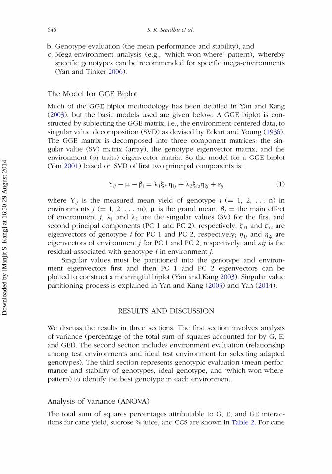
b. Genotype evaluation (the mean performance and stability), andc. Mega-environment analysis (e.g., ‘which-won-where’ pattern), whereby

specific genotypes can be recommended for specific mega-environments(Yan and Tinker 2006).

The Model for GGE Biplot

Much of the GGE biplot methodology has been detailed in Yan and Kang(2003), but the basic models used are given below. A GGE biplot is con-structed by subjecting the GGE matrix, i.e., the environment-centered data, tosingular value decomposition (SVD) as devised by Eckart and Young (1936).The GGE matrix is decomposed into three component matrices: the sin-gular value (SV) matrix (array), the genotype eigenvector matrix, and theenvironment (or traits) eigenvector matrix. So the model for a GGE biplot(Yan 2001) based on SVD of first two principal components is:

Yij − μ − βj = λ1ξi1η1j + λ2ξi2η2j + εij (1)

where Yij is the measured mean yield of genotype i (= 1, 2, . . . n) inenvironments j (= 1, 2, . . . m), μ is the grand mean, β j = the main effectof environment j, λ1 and λ2 are the singular values (SV) for the first andsecond principal components (PC 1 and PC 2), respectively, ξ i1 and ξ i2 areeigenvectors of genotype i for PC 1 and PC 2, respectively; η1j and η2j areeigenvectors of environment j for PC 1 and PC 2, respectively, and εij is theresidual associated with genotype i in environment j.

Singular values must be partitioned into the genotype and environ-ment eigenvectors first and then PC 1 and PC 2 eigenvectors can beplotted to construct a meaningful biplot (Yan and Kang 2003). Singular valuepartitioning process is explained in Yan and Kang (2003) and Yan (2014).

RESULTS AND DISCUSSION

We discuss the results in three sections. The first section involves analysisof variance (percentage of the total sum of squares accounted for by G, E,and GEI). The second section includes environment evaluation (relationshipamong test environments and ideal test environment for selecting adaptedgenotypes). The third section represents genotypic evaluation (mean perfor-mance and stability of genotypes, ideal genotype, and ‘which-won-where’pattern) to identify the best genotype in each environment.

Analysis of Variance (ANOVA)

The total sum of squares percentages attributable to G, E, and GE interac-tions for cane yield, sucrose % juice, and CCS are shown in Table 2. For cane

Dow

nloa

ded

by [

Man

jit S

. Kan

g] a

t 16:

50 2

9 A

ugus

t 201

4

GGE Biplot Analysis for Cane & Sugar Yield 647

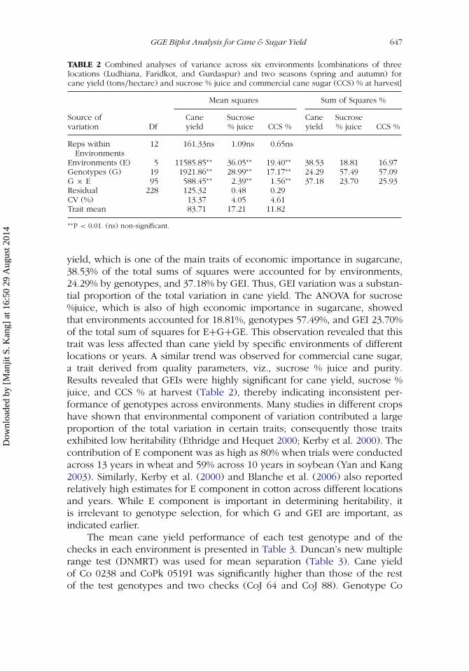
TABLE 2 Combined analyses of variance across six environments [combinations of threelocations (Ludhiana, Faridkot, and Gurdaspur) and two seasons (spring and autumn) forcane yield (tons/hectare) and sucrose % juice and commercial cane sugar (CCS) % at harvest]

Mean squares Sum of Squares %

Source ofvariation Df

Caneyield

Sucrose% juice CCS %

Caneyield

Sucrose% juice CCS %

Reps withinEnvironments

12 161.33ns 1.09ns 0.65ns

Environments (E) 5 11585.85∗∗ 36.05∗∗ 19.40∗∗ 38.53 18.81 16.97Genotypes (G) 19 1921.86∗∗ 28.99∗∗ 17.17∗∗ 24.29 57.49 57.09G × E 95 588.45∗∗ 2.39∗∗ 1.56∗∗ 37.18 23.70 25.93Residual 228 125.32 0.48 0.29CV (%) 13.37 4.05 4.61Trait mean 83.71 17.21 11.82

∗∗P < 0.01. (ns) non-significant.

yield, which is one of the main traits of economic importance in sugarcane,38.53% of the total sums of squares were accounted for by environments,24.29% by genotypes, and 37.18% by GEI. Thus, GEI variation was a substan-tial proportion of the total variation in cane yield. The ANOVA for sucrose%juice, which is also of high economic importance in sugarcane, showedthat environments accounted for 18.81%, genotypes 57.49%, and GEI 23.70%of the total sum of squares for E+G+GE. This observation revealed that thistrait was less affected than cane yield by specific environments of differentlocations or years. A similar trend was observed for commercial cane sugar,a trait derived from quality parameters, viz., sucrose % juice and purity.Results revealed that GEIs were highly significant for cane yield, sucrose %juice, and CCS % at harvest (Table 2), thereby indicating inconsistent per-formance of genotypes across environments. Many studies in different cropshave shown that environmental component of variation contributed a largeproportion of the total variation in certain traits; consequently those traitsexhibited low heritability (Ethridge and Hequet 2000; Kerby et al. 2000). Thecontribution of E component was as high as 80% when trials were conductedacross 13 years in wheat and 59% across 10 years in soybean (Yan and Kang2003). Similarly, Kerby et al. (2000) and Blanche et al. (2006) also reportedrelatively high estimates for E component in cotton across different locationsand years. While E component is important in determining heritability, itis irrelevant to genotype selection, for which G and GEI are important, asindicated earlier.

The mean cane yield performance of each test genotype and of thechecks in each environment is presented in Table 3. Duncan’s new multiplerange test (DNMRT) was used for mean separation (Table 3). Cane yieldof Co 0238 and CoPk 05191 was significantly higher than those of the restof the test genotypes and two checks (CoJ 64 and CoJ 88). Genotype Co

Dow

nloa

ded

by [

Man

jit S

. Kan

g] a

t 16:

50 2

9 A

ugus

t 201

4

648 S. K. Sandhu et al.

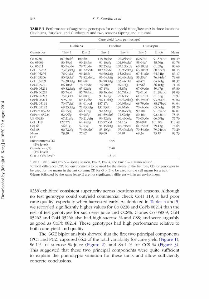
TABLE 3 Performance of sugarcane genotypes for cane yield (tons/hectare) in three locations(Ludhiana, Faridkot, and Gurdaspur) and two seasons (spring and autumn)

Cane yield (tons per hectare)

Ludhiana Faridkot Gurdaspur

Genotypes †Env 1 Env 2 Env 3 Env 4 Env 5 Env 6 Mean

Co 0238 107.58ab§ 100.60a 118.38abc 107.23bcde 82.97bc 91.57abc 101.39Co 05009 86.55cd 90.23abc 91.16efg 102.93cdef 55.04ef 58.76g 80.78Co 05011 83.94cde 78.71cde 92.25efg 107.13bcde 60.18def 61.39g 80.60CoH 05262 73.63defg 81.22bcde 109.34cde 90.96cdefg 63.10def 68.67efg 81.15CoH 05265 76.91def 96.26ab 96.60defg 115.09bcd 67.51cde 64.64fg 86.17CoH 05266 80.93def 73.82cdefg 95.04defg 96.49cdefg 55.35ef 76.44def 79.68CoH 05269 74.38defg 101.60a 94.90defg 103.44cdef 49.47f 64.46fg 81.37CoLk 05201 86.40cd 78.74cde 76.50gh 69.18fg 49.96f 66.18fg 71.16CoPb 05211 69.32defg 65.92efg 67.15h 65.87g 67.09cde 59.47g 65.80CoPb 06219 85.74cd 85.78abcd 99.56cdef 110.74bcd 73.01cd 91.38abc 91.03CoPb 07213 75.03def 61.80fg 91.14efg 122.68bc 61.57def 61.57g 78.97CoPb 08214 99.91bc 89.43abc 96.11defg 97.49cdefg 63.39def 93.80ab 90.02CoPk 05191 76.97def 84.01bcd 137.17a 109.03bcd 68.79cde 88.27bcd 94.04CoPk 05192 69.25defg 71.03defg 131.93ab 138.67ab 70.66cde 65.66fg 91.20CoPant 05222 64.75fg 66.11efg 92.32efg 83.02defg 99.10a 91.55abc 82.81CoPant 05224 62.95fg 59.96fg 101.69cdef 72.52efg 80.46c 92.42abc 78.33UP 05233 67.31efg 70.21defg 93.52efg 86.43defg 70.05cde 66.69fg 75.70CoH 119 122.77a 64.44efg 115.97bcd 161.15a 96.89ab 101.70a 110.49CoJ 64 56.61g 57.53g 94.15defg 118.75bcd 61.75def 59.13g 74.65CoJ 88 66.72efg 76.00cdef 85.10fgh 97.46cdefg 70.54cde 79.94cde 79.29Mean 79.38 77.67 99.00 102.81 68.34 75.19 83.73CD‡

Environments (E)(1% level)

4.05

Genotypes (G)(1% level)

7.40

G × E (1% level) 18.14

†Env 1, Env 3, and Env 5 = spring season; Env 2, Env 4, and Env 6 = autumn season.‡Critical difference (CD) for environments to be used for the means in the last row; CD for genotypes tobe used for the means in the last column; CD for G × E to be used for the cell means for a trait.§Means followed by the same letter(s) are not significantly different within an environment.

0238 exhibited consistent superiority across locations and seasons. Althoughno test genotype could outyield commercial check CoH 119, it had poorcane quality, especially when harvested early. As depicted in Tables 4 and 5,we recorded significantly higher values for Co 0238 and CoPb 08214 than therest of test genotypes for sucrose% juice and CCS%. Clones Co 05009, CoH05262 and CoH 05266 also had high sucrose % and CSS; and were arguablyas good as CoPb 08214. These genotypes had high performance relative toboth cane yield and quality.

The GGE biplot analysis showed that the first two principal components(PC1 and PC2) captured 66.2 of the total variability for cane yield (Figure 1),86.1% for sucrose % juice (Figure 2), and 84.4 % for CCS % (Figure 3).This suggested that these two principal components were quite sufficientto explain the phenotypic variation for these traits and allow sufficientlyconcrete conclusions.

Dow

nloa

ded

by [

Man

jit S

. Kan

g] a

t 16:

50 2

9 A

ugus

t 201

4

GGE Biplot Analysis for Cane & Sugar Yield 649

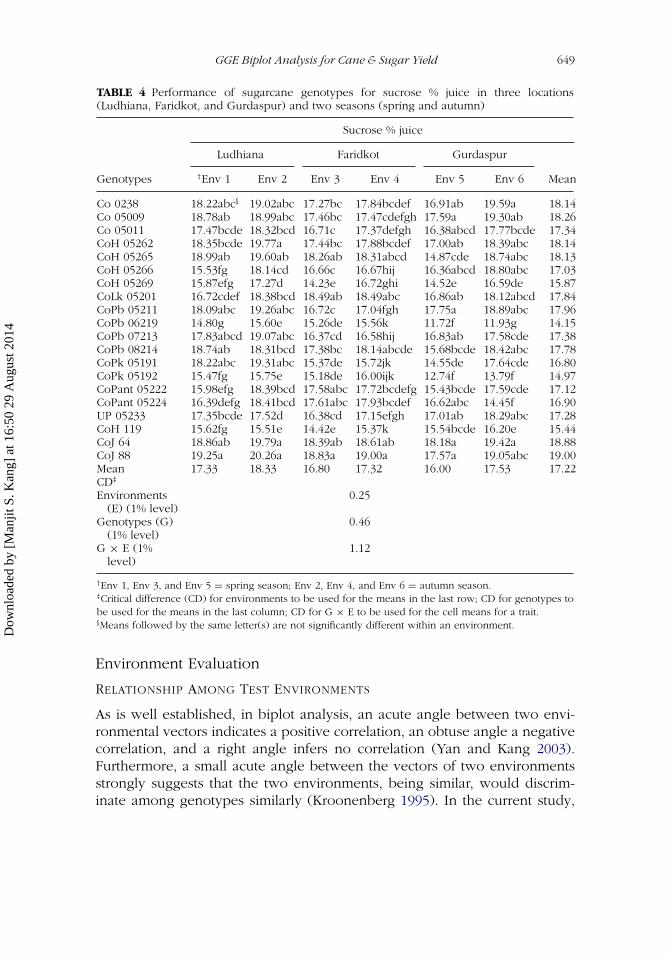
TABLE 4 Performance of sugarcane genotypes for sucrose % juice in three locations(Ludhiana, Faridkot, and Gurdaspur) and two seasons (spring and autumn)

Sucrose % juice

Ludhiana Faridkot Gurdaspur

Genotypes †Env 1 Env 2 Env 3 Env 4 Env 5 Env 6 Mean

Co 0238 18.22abc§ 19.02abc 17.27bc 17.84bcdef 16.91ab 19.59a 18.14Co 05009 18.78ab 18.99abc 17.46bc 17.47cdefgh 17.59a 19.30ab 18.26Co 05011 17.47bcde 18.32bcd 16.71c 17.37defgh 16.38abcd 17.77bcde 17.34CoH 05262 18.35bcde 19.77a 17.44bc 17.88bcdef 17.00ab 18.39abc 18.14CoH 05265 18.99ab 19.60ab 18.26ab 18.31abcd 14.87cde 18.74abc 18.13CoH 05266 15.53fg 18.14cd 16.66c 16.67hij 16.36abcd 18.80abc 17.03CoH 05269 15.87efg 17.27d 14.23e 16.72ghi 14.52e 16.59de 15.87CoLk 05201 16.72cdef 18.38bcd 18.49ab 18.49abc 16.86ab 18.12abcd 17.84CoPb 05211 18.09abc 19.26abc 16.72c 17.04fgh 17.75a 18.89abc 17.96CoPb 06219 14.80g 15.60e 15.26de 15.56k 11.72f 11.93g 14.15CoPb 07213 17.83abcd 19.07abc 16.37cd 16.58hij 16.83ab 17.58cde 17.38CoPb 08214 18.74ab 18.31bcd 17.38bc 18.14abcde 15.68bcde 18.42abc 17.78CoPk 05191 18.22abc 19.31abc 15.37de 15.72jk 14.55de 17.64cde 16.80CoPk 05192 15.47fg 15.75e 15.18de 16.00ijk 12.74f 13.79f 14.97CoPant 05222 15.98efg 18.39bcd 17.58abc 17.72bcdefg 15.43bcde 17.59cde 17.12CoPant 05224 16.39defg 18.41bcd 17.61abc 17.93bcdef 16.62abc 14.45f 16.90UP 05233 17.35bcde 17.52d 16.38cd 17.15efgh 17.01ab 18.29abc 17.28CoH 119 15.62fg 15.51e 14.42e 15.37k 15.54bcde 16.20e 15.44CoJ 64 18.86ab 19.79a 18.39ab 18.61ab 18.18a 19.42a 18.88CoJ 88 19.25a 20.26a 18.83a 19.00a 17.57a 19.05abc 19.00Mean 17.33 18.33 16.80 17.32 16.00 17.53 17.22CD‡

Environments(E) (1% level)

0.25

Genotypes (G)(1% level)

0.46

G × E (1%level)

1.12

†Env 1, Env 3, and Env 5 = spring season; Env 2, Env 4, and Env 6 = autumn season.‡Critical difference (CD) for environments to be used for the means in the last row; CD for genotypes tobe used for the means in the last column; CD for G × E to be used for the cell means for a trait.§Means followed by the same letter(s) are not significantly different within an environment.

Environment Evaluation

RELATIONSHIP AMONG TEST ENVIRONMENTS

As is well established, in biplot analysis, an acute angle between two envi-ronmental vectors indicates a positive correlation, an obtuse angle a negativecorrelation, and a right angle infers no correlation (Yan and Kang 2003).Furthermore, a small acute angle between the vectors of two environmentsstrongly suggests that the two environments, being similar, would discrim-inate among genotypes similarly (Kroonenberg 1995). In the current study,

Dow

nloa

ded

by [

Man

jit S

. Kan

g] a

t 16:

50 2

9 A

ugus

t 201

4

650 S. K. Sandhu et al.

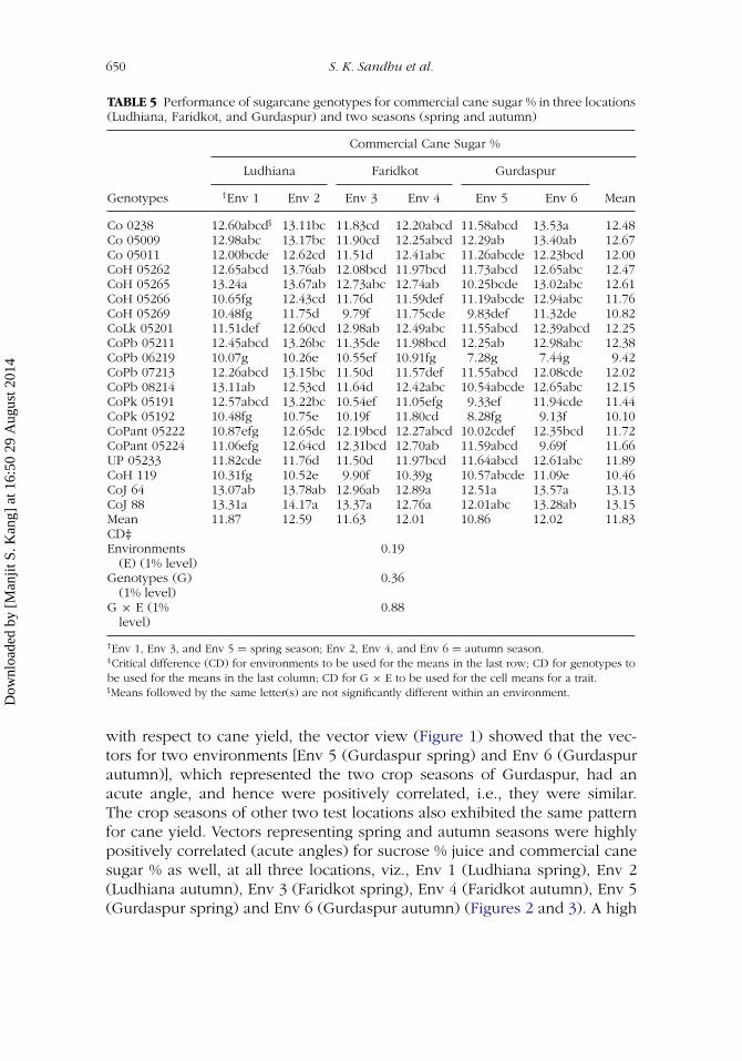
TABLE 5 Performance of sugarcane genotypes for commercial cane sugar % in three locations(Ludhiana, Faridkot, and Gurdaspur) and two seasons (spring and autumn)

Commercial Cane Sugar %

Ludhiana Faridkot Gurdaspur

Genotypes †Env 1 Env 2 Env 3 Env 4 Env 5 Env 6 Mean

Co 0238 12.60abcd§ 13.11bc 11.83cd 12.20abcd 11.58abcd 13.53a 12.48Co 05009 12.98abc 13.17bc 11.90cd 12.25abcd 12.29ab 13.40ab 12.67Co 05011 12.00bcde 12.62cd 11.51d 12.41abc 11.26abcde 12.23bcd 12.00CoH 05262 12.65abcd 13.76ab 12.08bcd 11.97bcd 11.73abcd 12.65abc 12.47CoH 05265 13.24a 13.67ab 12.73abc 12.74ab 10.25bcde 13.02abc 12.61CoH 05266 10.65fg 12.43cd 11.76d 11.59def 11.19abcde 12.94abc 11.76CoH 05269 10.48fg 11.75d 9.79f 11.75cde 9.83def 11.32de 10.82CoLk 05201 11.51def 12.60cd 12.98ab 12.49abc 11.55abcd 12.39abcd 12.25CoPb 05211 12.45abcd 13.26bc 11.35de 11.98bcd 12.25ab 12.98abc 12.38CoPb 06219 10.07g 10.26e 10.55ef 10.91fg 7.28g 7.44g 9.42CoPb 07213 12.26abcd 13.15bc 11.50d 11.57def 11.55abcd 12.08cde 12.02CoPb 08214 13.11ab 12.53cd 11.64d 12.42abc 10.54abcde 12.65abc 12.15CoPk 05191 12.57abcd 13.22bc 10.54ef 11.05efg 9.33ef 11.94cde 11.44CoPk 05192 10.48fg 10.75e 10.19f 11.80cd 8.28fg 9.13f 10.10CoPant 05222 10.87efg 12.65dc 12.19bcd 12.27abcd 10.02cdef 12.35bcd 11.72CoPant 05224 11.06efg 12.64cd 12.31bcd 12.70ab 11.59abcd 9.69f 11.66UP 05233 11.82cde 11.76d 11.50d 11.97bcd 11.64abcd 12.61abc 11.89CoH 119 10.31fg 10.52e 9.90f 10.39g 10.57abcde 11.09e 10.46CoJ 64 13.07ab 13.78ab 12.96ab 12.89a 12.51a 13.57a 13.13CoJ 88 13.31a 14.17a 13.37a 12.76a 12.01abc 13.28ab 13.15Mean 11.87 12.59 11.63 12.01 10.86 12.02 11.83CD‡Environments

(E) (1% level)0.19

Genotypes (G)(1% level)

0.36

G × E (1%level)

0.88

†Env 1, Env 3, and Env 5 = spring season; Env 2, Env 4, and Env 6 = autumn season.‡Critical difference (CD) for environments to be used for the means in the last row; CD for genotypes tobe used for the means in the last column; CD for G × E to be used for the cell means for a trait.§Means followed by the same letter(s) are not significantly different within an environment.

with respect to cane yield, the vector view (Figure 1) showed that the vec-tors for two environments [Env 5 (Gurdaspur spring) and Env 6 (Gurdaspurautumn)], which represented the two crop seasons of Gurdaspur, had anacute angle, and hence were positively correlated, i.e., they were similar.The crop seasons of other two test locations also exhibited the same patternfor cane yield. Vectors representing spring and autumn seasons were highlypositively correlated (acute angles) for sucrose % juice and commercial canesugar % as well, at all three locations, viz., Env 1 (Ludhiana spring), Env 2(Ludhiana autumn), Env 3 (Faridkot spring), Env 4 (Faridkot autumn), Env 5(Gurdaspur spring) and Env 6 (Gurdaspur autumn) (Figures 2 and 3). A high

Dow

nloa

ded

by [

Man

jit S

. Kan

g] a

t 16:

50 2

9 A

ugus

t 201

4

GGE Biplot Analysis for Cane & Sugar Yield 651

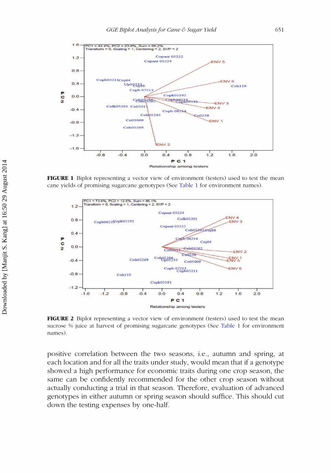
FIGURE 1 Biplot representing a vector view of environment (testers) used to test the meancane yields of promising sugarcane genotypes (See Table 1 for environment names).

FIGURE 2 Biplot representing a vector view of environment (testers) used to test the meansucrose % juice at harvest of promising sugarcane genotypes (See Table 1 for environmentnames).

positive correlation between the two seasons, i.e., autumn and spring, ateach location and for all the traits under study, would mean that if a genotypeshowed a high performance for economic traits during one crop season, thesame can be confidently recommended for the other crop season withoutactually conducting a trial in that season. Therefore, evaluation of advancedgenotypes in either autumn or spring season should suffice. This should cutdown the testing expenses by one-half.

Dow

nloa

ded

by [

Man

jit S

. Kan

g] a

t 16:

50 2

9 A

ugus

t 201

4

652 S. K. Sandhu et al.

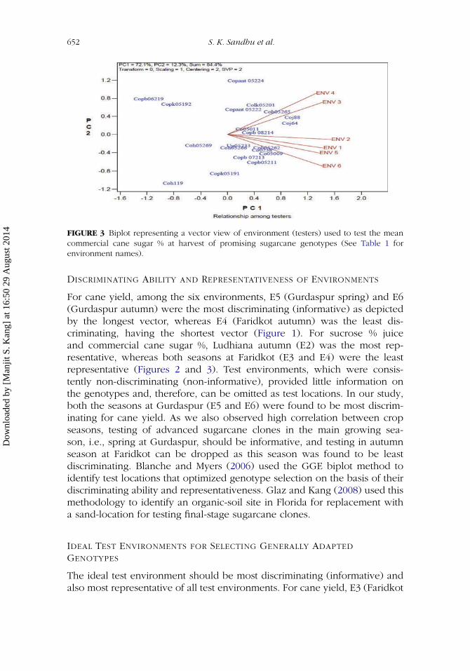
FIGURE 3 Biplot representing a vector view of environment (testers) used to test the meancommercial cane sugar % at harvest of promising sugarcane genotypes (See Table 1 forenvironment names).

DISCRIMINATING ABILITY AND REPRESENTATIVENESS OF ENVIRONMENTS

For cane yield, among the six environments, E5 (Gurdaspur spring) and E6(Gurdaspur autumn) were the most discriminating (informative) as depictedby the longest vector, whereas E4 (Faridkot autumn) was the least dis-criminating, having the shortest vector (Figure 1). For sucrose % juiceand commercial cane sugar %, Ludhiana autumn (E2) was the most rep-resentative, whereas both seasons at Faridkot (E3 and E4) were the leastrepresentative (Figures 2 and 3). Test environments, which were consis-tently non-discriminating (non-informative), provided little information onthe genotypes and, therefore, can be omitted as test locations. In our study,both the seasons at Gurdaspur (E5 and E6) were found to be most discrim-inating for cane yield. As we also observed high correlation between cropseasons, testing of advanced sugarcane clones in the main growing sea-son, i.e., spring at Gurdaspur, should be informative, and testing in autumnseason at Faridkot can be dropped as this season was found to be leastdiscriminating. Blanche and Myers (2006) used the GGE biplot method toidentify test locations that optimized genotype selection on the basis of theirdiscriminating ability and representativeness. Glaz and Kang (2008) used thismethodology to identify an organic-soil site in Florida for replacement witha sand-location for testing final-stage sugarcane clones.

IDEAL TEST ENVIRONMENTS FOR SELECTING GENERALLY ADAPTED

GENOTYPES

The ideal test environment should be most discriminating (informative) andalso most representative of all test environments. For cane yield, E3 (Faridkot

Dow

nloa

ded

by [

Man

jit S

. Kan

g] a

t 16:

50 2

9 A

ugus

t 201

4

GGE Biplot Analysis for Cane & Sugar Yield 653

spring) had a small acute angle with AEA (average environment axis). TheAEA serves as the abscissa of the average environment coordinate (AEC).Because E3 was both discriminating and representative, it was an idealtest environment. Thus, testing of advanced sugarcane genotypes duringspring season at Faridkot would be appropriate for selecting high-yieldinggenotypes having wide adaptability. The Gurdaspur spring season (E5) wasdiscriminating but non-representative; it was useful for selecting specificallyadapted genotypes. For quality traits, among the six environments, test envi-ronment E2, i.e., autumn season at Ludhiana, being both discriminating andrepresentative, was an ideal test environment, whereas E3 (Faridkot spring)and E4 (Faridkot autumn) were discriminating but non-representative envi-ronments, which can be used for selecting specifically adapted genotypes.These observations informed that a single test location couldn’t be used forevaluation of all the traits. As in the present case, E3 (Faridkot spring) wasthe ideal environment for cane yield, but E2 (Ludhiana autumn) was theideal test environment for quality traits.

Genotypic Evaluation

MEAN PERFORMANCE AND STABILITY OF THE GENOTYPES

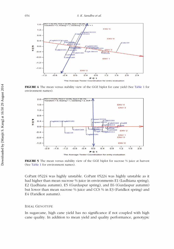
Unlike the AEC abscissa, which has one direction, with the arrow pointingto greater genotype main effect, the AEC ordinate is indicated by doublearrows, and either direction away from the biplot origin indicates greaterGEI effect and reduced stability. The genotypes are ranked according to theirprojections on to the AEC ordinate. Yan (2001) studied performance and sta-bility of genotypes for yield via the AEC method. The AEC ordinate separatesgenotypes with below-average means from those with above-average means.In the present study, CoH 119 had the highest mean cane yield because itis located on positive side of the AEC ordinate (Figure 4), followed by Co0238, CoH 05191, and CoPb 08214. CoH 05265 had a mean cane yield similarto the grand mean, and CoPb 05211 had the lowest mean yield. High caneyield is only important if it is coupled with stability. Thus, CoPb 06219, CoPk05191, Co 0238, and CoPb 08214 were highly stable because these genotypehad relatively short projections on the AEC and showed consistent yieldacross environments, whereas CoPant 05222 was highly unstable becauseit had higher than mean yield in environments E5 (Gurdaspur spring), E6(Gurdaspur autumn), and E3 (Faridkot Spring) but lower than mean yieldin E4 (Faridkot autumn), E1 (Ludhiana spring), and E2 (Ludhiana autumn).Similarly, quality trait ordinate of AEC (Figures 5 and 6) showed that CoJ88 had the highest mean sucrose % juice and CCS %, followed by CoJ 64,CoH 05265, Co 05009, CoH 05262, Co 0238, CoPb 08214. UP 05233 hadmean sucrose % juice and CCS % similar to the grand mean; and CoPb06219 had the lowest mean sucrose % juice and CCS %. The AEC showed thatCoH 05262, Co 0238, and CoPb 08214 were highly stable cultivars, whereas

Dow

nloa

ded

by [

Man

jit S

. Kan

g] a

t 16:

50 2

9 A

ugus

t 201

4

654 S. K. Sandhu et al.

FIGURE 4 The mean versus stability view of the GGE biplot for cane yield (See Table 1 forenvironment names).

FIGURE 5 The mean versus stability view of the GGE biplot for sucrose % juice at harvest(See Table 1 for environment names).

CoPant 05224 was highly unstable. CoPant 05224 was highly unstable as ithad higher than mean sucrose % juice in environments E1 (Ludhiana spring),E2 (Ludhiana autumn), E5 (Gurdaspur spring), and E6 (Gurdaspur autumn)but lower than mean sucrose % juice and CCS % in E3 (Faridkot spring) andE4 (Faridkot autumn).

IDEAL GENOTYPE

In sugarcane, high cane yield has no significance if not coupled with highcane quality. In addition to mean yield and quality performance, genotypic

Dow

nloa

ded

by [

Man

jit S

. Kan

g] a

t 16:

50 2

9 A

ugus

t 201

4

GGE Biplot Analysis for Cane & Sugar Yield 655

FIGURE 6 The mean versus stability view of the GGE biplot for commercial cane sugar % atharvest (See Table 1 for environment names).

stability is quite crucial. From this study, two genotypes, Co 0238 and CoPb08214, were identified as ideal genotypes because of their above-averagemean performance (Figures 4, 5, and 6) for economic traits and were judgedas absolutely stable across environments. Such genotypes possessing wideadaptability and high mean performance can be commercially utilized for allmajor sugarcane-growing areas of Punjab state.

WHICH-WON-WHERE PATTERN

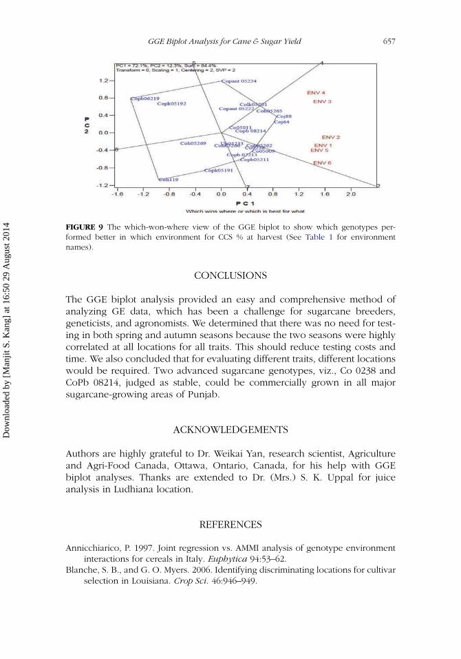
One of the most attractive features of a GGE biplot is its ability to showthe ‘which-won-where’ pattern in a genotype-by-environment dataset, asit graphically addresses important concepts (Yan and Tinker 2006). Formechanics of drawing a polygon and interpreting data, refer to Yan andKang (2003). The ‘which-won-where’ feature of GGE biplot revealed thatpolygon view of cane yield (Figure 7) had three sectors, where commer-cial check CoH 119 was the winner in environments E5 (Gurdaspur spring)and E6 (Gurdaspur autumn); CoH 05269 was the winner in E2 (Ludhianaautumn); and Co 0238 was the winner in environments E1 (Ludhiana spring),E3 (Faridkot spring), and E4 (Faridkot autumn). For quality traits (Figures 8and 9), six environments fell into three sectors. CoJ 88 was winner in envi-ronments E3 (Faridkot spring) and E4 (Faridkot autumn); CoJ 64 was winnerin E1 (Ludhiana spring) and E2 (Ludhiana autumn); and Co 0238 was win-ner in E5 (Gurdaspur spring) and E6 (Gurdaspur autumn), revealing theirspecific adaptation to these locations. The genotype ranking done on thebasis of performance values of a trait for each genotype using DNMRT(Tables 1, 2, and 3) was parallel to the results for winning genotypes based

Dow

nloa

ded

by [

Man

jit S

. Kan

g] a

t 16:

50 2

9 A

ugus

t 201

4

656 S. K. Sandhu et al.

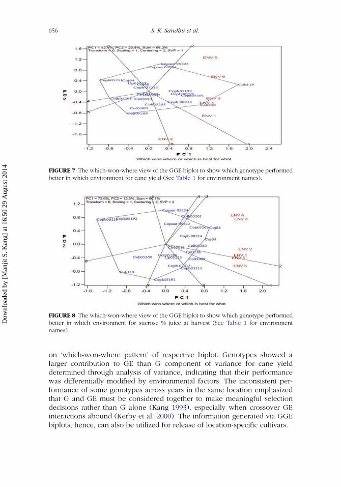
FIGURE 7 The which-won-where view of the GGE biplot to show which genotype performedbetter in which environment for cane yield (See Table 1 for environment names).

FIGURE 8 The which-won-where view of the GGE biplot to show which genotype performedbetter in which environment for sucrose % juice at harvest (See Table 1 for environmentnames).

on ‘which-won-where pattern’ of respective biplot. Genotypes showed alarger contribution to GE than G component of variance for cane yielddetermined through analysis of variance, indicating that their performancewas differentially modified by environmental factors. The inconsistent per-formance of some genotypes across years in the same location emphasizedthat G and GE must be considered together to make meaningful selectiondecisions rather than G alone (Kang 1993), especially when crossover GEinteractions abound (Kerby et al. 2000). The information generated via GGEbiplots, hence, can also be utilized for release of location-specific cultivars.

Dow

nloa

ded

by [

Man

jit S

. Kan

g] a

t 16:

50 2

9 A

ugus

t 201

4

GGE Biplot Analysis for Cane & Sugar Yield 657

FIGURE 9 The which-won-where view of the GGE biplot to show which genotypes per-formed better in which environment for CCS % at harvest (See Table 1 for environmentnames).

CONCLUSIONS

The GGE biplot analysis provided an easy and comprehensive method ofanalyzing GE data, which has been a challenge for sugarcane breeders,geneticists, and agronomists. We determined that there was no need for test-ing in both spring and autumn seasons because the two seasons were highlycorrelated at all locations for all traits. This should reduce testing costs andtime. We also concluded that for evaluating different traits, different locationswould be required. Two advanced sugarcane genotypes, viz., Co 0238 andCoPb 08214, judged as stable, could be commercially grown in all majorsugarcane-growing areas of Punjab.

ACKNOWLEDGEMENTS

Authors are highly grateful to Dr. Weikai Yan, research scientist, Agricultureand Agri-Food Canada, Ottawa, Ontario, Canada, for his help with GGEbiplot analyses. Thanks are extended to Dr. (Mrs.) S. K. Uppal for juiceanalysis in Ludhiana location.

REFERENCES

Annicchiarico, P. 1997. Joint regression vs. AMMI analysis of genotype environmentinteractions for cereals in Italy. Euphytica 94:53–62.

Blanche, S. B., and G. O. Myers. 2006. Identifying discriminating locations for cultivarselection in Louisiana. Crop Sci. 46:946–949.

Dow

nloa

ded

by [

Man

jit S

. Kan

g] a

t 16:

50 2

9 A

ugus

t 201

4

658 S. K. Sandhu et al.

Blanche, S. B., G. O. Myers, J. Z. Zumba, D. Caldwell, and J. Hayes. 2006. Stabilitycomparisons between conventional and near–isogenic transgenic cotton culti-vars. J. Cotton Sci. 10:17–28.

Bull, J.K., D.M. Hogarth, and K.E. Basford. 1992. Impact of genotype x environ-ment interaction on response to selection in sugarcane. Aust. J. Exp. Agric.32:731–737.

Casanoves, F., J. Baldessari, and M. Balzarini. 2005. Evaluation of multienvironmenttrials of peanut cultivars. Crop Sci. 45:18–26.

Chen X., P. Jackson, W. Shen, H. Deng, Y. Fan, Q. Li, F. Hu, X. Wei and J. Liu.2012. Genotype × environment interactions in sugarcane between China andAustralia. Crop and Pasture Sci. 63:459–66.

Chen, J. C. P. 1985. Cane sugar handbook. New York, NY: Wiley Interscience.Eckart, C., and G. Young. 1936. The approximation of one matrix by another of

lower rank. Psychometrika 1:211–218.Ethridge, M. D., and E. F. Hequet. 2000. Fiber properties and textile performance

of transgenic cotton versus parent varieties. In Proc. Beltwide Cotton Conf., SanAntonio, TX . 4–8 January 2000, 488–494. Memphis, TN: National Cotton Councilof America.

Fan, X. M., M. S. Kang, H. Chen., Y. Zhang, J. Tan, and C. Xu. 2007. Yield stabilityof maize hybrids evaluated in multienvironment trials in Yunnan, China. AgronJ . 99: 220–228.

Gabriel, K. R. 1971. The biplot graphic of matrices with application to principalcomponent analysis. Biometrics 58:453–467.

Glaz, B., and M. S. Kang. 2008. Location contributions determined via GGE biplotanalysis of multi-environment sugarcane genotype-performance trials. Crop Sci.48:941–950.

Jackson P., S. Chapman, A. Rattey, W. X. Ming, and M. Cox. 2007. Genotype x regioninteractions, and implications for sugarcane breeding programs. Sugarcane Int.25:3–7.

Kang, M. S. 1993. Simultaneous selection for yield and stability in crop performancetrials: Consequences for growers. Agron J . 85:754–757.

Kang, M. S. 1998. Using genotype-by-environment interaction for crop cultivardevelopment. Adv Agron. 62:199–252.

Kang, M. S., V. D. Aggarwal, and R. M. Chirwa. 2005. Adaptability and stability ofbean cultivars as determined via yield-stability statistic and GGE Biplot analysis.J. Crop Improv. 15:97–120.

Kang, M. S., and F. A. Martin. 1987. A review of important aspects of genotype-environmental interactions and practical suggestions for sugarcane breeders. J.Am. Soc. Sugar Cane Technol. 7:36–38.

Kang, M. S., and J. D. Miller. 1984. Genotype x environment interaction for cane andsugar yield, and their implications in sugarcane breeding. Crop Sci. 24:435–440.

Kerby, T., J. Burgess, M. Bates, D. Albers, and K. Lege. 2000. Partitioning variety andenvironment contribution to variation in yield, plant growth, and fiber quality.In Proc. Belt wide Cotton Conf., New Orleans, LA, 7–10 January 2000, 528–532.Memphis, TN: National Cotton Council of America.

Dow

nloa

ded

by [

Man

jit S

. Kan

g] a

t 16:

50 2

9 A

ugus

t 201

4

GGE Biplot Analysis for Cane & Sugar Yield 659

Kroonenberg, P. M. 1995. Introduction to biplots for G x E tables. Departmentof Mathematics. Research Report 51. Queensland, Australia: University ofQueensland, Australia.

Ma, B. L., W. Yan, L. M. Dwyer, J. Fregeau-Reid, H. D. Voldeng, Y. Dion, and H.Nass. 2004. Graphic analysis of genotype, environment, nitrogen fertilizer, andtheir interactions on spring wheat yield. Agron J . 96:169–180.

Milligan, S. B., K. A. Gravois, K. P. Birchoff, and F. A. Martin. 1990. Crop effects onbroad-sense heritabilities and genetic variances of sugarcane yield components.Crop Sci. 30:344–349.

Ramburan, S., A. Paraskavopoulos, G. Saville, and M. Jones. 2010. A decision supportsystem for sugarcane variety selection in South Africa based on genotype-by-environment analysis. Exp. Agric. 46:243–257.

Ramburan, S., and M. Zhou. 2011. Investigating sugarcane genotype x environmentinteractions under rainfed conditions in South Africa using variance componentsand biplot analysis. In Proc. South Afr. Sugar Technol. Assoc., 17–19 August,2011, Durban, South Africa. 84:345–358.

Ramburan, S., M. Zhou, and M. Labuschagne. 2011. Interpretation of genotype xenvironment interactions of sugarcane: Identifying significant environmentalfactors. Field Crops Res. 124:392–399.

Ramburan, S., M. Zhou, and M. Labuschagne. 2012. Investigating test site similar-ity, trait relations, and causes of genotype x environment interactions in theMidlands region of South Africa. Field Crops Res. 129:71–80.

Sandhu, S. K., B. Ram, S. Kumar, R. S. Singh, S. K. Uppal, K. S. Brar, P. Singh andN. V. Nair. 2012. GGE biplot analysis for visualization of performance rank andstability of sugarcane genotypes. Int. Sugar J . 114:810–820

Slaughter, J. S., and L. D. Delwiche. 2010. The little SAS book for enterprise guide 4.2.Cary, NC: SAS Institute.

Yan, W. 2001. GGE biplot: A Windows application for graphical analysis of multienvironment trial data and other types of two-way data. Agron J . 93:1111–1118.

Yan, W. 2014. Crop variety trials: Data management and analysis. New York, NY:John Wiley and Sons.

Yan, W., L. A. Hunt, Q. Sheng, and Z. Szlavnics. 2000. Cultivar evaluation and mega-environment investigation based on the GGE biplot. Crop Sci. 40:597–605.

Yan, W., and M.S. Kang. 2003. GGE biplot analysis: A graphical tool for breeders,geneticists, and agronomists. Boca Raton, FL: CRC Press.

Yan, W., M. S. Kang, B. Ma, S. Woods, and P. L. Cornelius. 2007. GGE biplot vs.AMMI analysis of genotype by environment data. Crop Sci. 47:643–655.

Yan, W., and N. A. Tinker. 2006. Biplot analysis of multi-environment trial data:Principles and applications. Can. J. Plant Sci. 86:623–45.

Dow

nloa

ded

by [

Man

jit S

. Kan

g] a

t 16:

50 2

9 A

ugus

t 201

4