Please do not remove this page

Subtropical Atlantic Climate Variability Record inSpeleothems from the BahamasArienzo, Monicahttps://scholarship.miami.edu/discovery/delivery/01UOML_INST:ResearchRepository/12355474580002976?l#13355504900002976

Arienzo. (2014). Subtropical Atlantic Climate Variability Record in Speleothems from the Bahamas[University of Miami].https://scholarship.miami.edu/discovery/fulldisplay/alma991031448070502976/01UOML_INST:ResearchRepository

Downloaded On 2022/01/13 21:21:43 -0500Free to read

Please do not remove this page

UNIVERSITY OF MIAMI

SUBTROPICAL ATLANTIC CLIMATE VARIABILITY RECORD IN SPELEOTHEMS FROM THE BAHAMAS

By

Monica Arienzo

A DISSERTATION

Coral Gables, Florida

December 2014

©2014 Monica Arienzo

All Rights Reserved

UNIVERSITY OF MIAMI

A dissertation submitted in partial fulfillment of the requirements for the degree of

Doctor of Philosophy

SUBTROPICAL ATLANTIC CLIMATE VARIABILITY RECORD IN SPELEOTHEMS FROM THE BAHAMAS

Monica Arienzo Approved: ________________ _________________ Peter K. Swart, Ph.D. Kenneth Broad, Ph.D. Lewis G. Weeks Professor Professor of Marine Affairs of Marine Geology and Geophysics and Policy ________________ _________________ Amy Clement, Ph.D. Philip (Flip) Froelich, Ph.D. Associate Dean and Professor Froelich Education Services of Marine Physical Oceanography Tallahassee, Florida ________________ ________________ Larry C. Peterson, Ph.D. M. Brian Blake, Ph.D. Professor of Marine Geology Dean of the Graduate School and Geophysics ________________ Ali Pourmand, Ph.D. Assistant Professor of Marine Geology and Geophysics

ARIENZO, MONICA (Ph.D., Marine Geology and Geophysics) Subtropical Atlantic Climate Variability Record (December 2014) in Speleothems from the Bahamas Abstract of a dissertation at the University of Miami. Dissertation supervised by Professor Peter K. Swart. No. of pages in text. (331)

The last 100,000 years of climate consist of numerous abrupt millennial scale

climate variations. Of interest to this study are Heinrich stadials which are extreme cold

events in the North Atlantic. While a comprehensive picture of climate across Heinrich

events is emerging for the North Atlantic, very few studies have been conducted in the

subtropical western Atlantic, which may be important for the global propagation of these

events. This study is the first study to determine paleoclimate of the Bahamas across

Heinrich stadials.

Cave deposits, in particular stalagmites, offer the opportunity to obtain high

resolution records of past climate. Typically, stable oxygen and carbon isotopes of the

calcite are analyzed. However, when interpreting the oxygen isotope record of

carbonates there are several climatic factors which can lead to changes in the oxygen

isotopes. The hydrogen and oxygen isotopic analysis (δ2H and δ18O) of water trapped

within speleothem carbonate (fluid inclusions) can shed light on the drivers of the

carbonate oxygen isotopes. The application of cavity ring-down spectroscopy to the δ2H

and δ18O analysis of water in fluid inclusions was investigated at the University of Miami

(this study) as an alternative to traditional δ2H and δ18O methods and results demonstrate

acceptable precision and good agreement with previous results.

In order to ascertain the climate expression across Heinrich events in the sub-

tropical Atlantic, carbon and oxygen isotopes, fluid inclusion isotopes and minor

elements have been measured on a series of U-Th dated speleothems from Dan’s Cave,

Abaco Island, Bahamas. The analyses suggest that during Heinrich stadials 1-6

temperatures decreased by ~3 °C. These findings support previous work in other areas of

the North Atlantic and are consistent with the climate response to a weakening of the

Atlantic meridional overturning circulation.

To support the findings in the ancient stalagmites, a monitoring study has been

conducted. The goal of the monitoring study is to better understand the drivers of kinetic

isotope fractionation. In particular, the focus of this study was the carbonate clumped

isotope methodology which is a relatively recent geochemical development and therefore

more calibration studies are necessary. Nearly 2 years of monitoring a currently active

cave in the Bahamas has been conducted and results demonstrate that clumped isotope

fractionation increases during periods of increased ventilation and growth rate.

Modern studies of atmospheric dust demonstrate that currently there is seasonal

deposition to the Caribbean derived from Africa. Iron concentrations within the cave in

the modern are found to be heterogeneous in drip waters and calcite both temporally and

spatially. The temporal variation is thought to be due annual variations in dust delivery

and the amount of precipitation. Additionally, two stalagmites collected from the

Bahamas exhibit iron concentrations which increase concurrently with Heinrich stadials,

suggesting increased dust deposition to the Bahamas during these events.

ACKNOWLEDGEMENT

First I would like to thank my advisor Dr. Peter K. Swart. I have been extremely luckily

to work with Peter, who taught me how to ask scientifically relevant questions, to write

scientifically, and who also taught me how to solder. I also am grateful for his advice, in

particular his rule of threes. I am extremely luckily to have had a committee which has

pushed me, and supported me. Ali Pourmand provided me with the opportunity to utilize

the Neptune, which has become extremely helpful in my post-doctoral research. I would

also like to thank Amy Clement, who has helped me to better understand the climate as a

system and to think about my paleoclimate reconstructions in a global perspective. I

would also like to than Kenneth Broad, who I had the opportunity to work with in the

field and at RSMAS. I am greatly appreciative of all of the numerous dives which were

required to create such a unique collection of stalagmite samples. I would also like to

thank Larry Peterson, who helped me understand the paleoclimate of the last glacial

period and link my records to other records from around the world. Finally I would like

to thank Flip Froelich, for pushing me to better understand speleothem geochemistry.

This work could not have been conducted without the help from many others. In

particular, I would like to thank Huber Vonhof, who allowed me to visit his laboratory,

utilize his machine for fluid inclusion analysis and has provided insightful comments to

our publications. I would also like to thank Brian Kakuk who acquired permits necessary

for sampling in the Bahamas and who has also conducted numerous dives to collect

samples as part of this project. The Cape Eleuthera Institute in particular I would like to

thank Ron and Karen, who have provided me with help while I am in the Bahamas,

allowed me to store materials in their house, and who made sure I returned after visiting

iii

the cave. I am also grateful for Carol DeWet, my undergraduate advisor, who first

showed me the incredible world of carbonate geochemistry and encouraged me to pursue

a Ph. D. Carol has continued to provide me with advice and support over the last six

years which I am greatly appreciative of.

Funding for this project was provided by numerous sources, including the

Rosenstiel Fellowship, Cave Research Foundation Student Research Grant, Geological

Society of America Student Research Grant, RSMAS Alumni Award Research Grant, a

NSF P2C2 grant awarded to P. Swart and others, and the CSL.

I would also like to thank my family for their support over the last six year. My

parents, who have emotionally supported me, my brother and his wife who have been an

excellent voice of reason. I’d like to thank my fellow SILers (past and present)

including (but not limited too) Corey, Amel, Chris K., Amanda O. and Quinn, who have

helped me immensely in the lab and have listened to me talk through issues, as well as

Sean Murray who helped solve the dark secrets of clumped isotopes and Sevag

Mehterian who was critical to me finishing. I would also like to thank Greta and Karen

for their help over the years, as well as Grey Horwitz, Sevag and Kimberly Chamales

who traveled with me to Hatchet Bay Cave. I’d also like to thank the rest of my RSMAS

family, my Miami family, my roommates, Frisbee team members and Chico, who make

the days always better. Lastly, I am greatly indebted to Gareth Blakemore, who cooked

many meals for me, listened to me, and told me when I was being unreasonable, thank

you.

iv

TABLE OF CONTENTS

Page

LIST OF FIGURES ..................................................................................................... ix LIST OF TABLES ....................................................................................................... xiv Chapter

1 INTRODUCTION ......................................................................................... 1 1.1 Background of Millennial Scale Climate Variability………… ................ 1 1.2 Application of Speleothems to Paleoclimate Studies ................................ 2 1.3 Oxygen and Carbon Isotopes…………………………………………… . 3 1.4 Fluid Inclusion Isotopes ............................................................................. 5 1.5 Minor and Trace Elements ......................................................................... 6 1.6 Clumped Isotopes....................................................................................... 8 1.6.1 Analysis of Δ47 ......................................................................................................................... 9 1.6.2 Application of Δ47 to carbonates ....................................................... 10 1.7 U-Th Dating ............................................................................................... 11 1.8 Sample for Study........................................................................................ 14 1.9 Conclusion ................................................................................................. 17 2 MEASUREMENT OF δ18O AND δ2H VALUES OF FLUID INCLUSION

WATER IN SPELEOTHEMS USING CAVITY RING-DOWN SPECTROSCOPY COMPARED TO ISOTOPE RATIO MASS SPECTROMETRY ........................................................................................ 18

2.1 Background ................................................................................................ 19 2.2 Design of the System: The Miami Device ................................................. 21 2.3 Protocol for Analysis ................................................................................. 24 2.3.1 Calibration......................................................................................... 27 2.3.2 Data reduction ................................................................................... 28 2.4 Results ........................................................................................................ 28 2.4.1 Reproducibility ................................................................................. 29 2.4.2 Crushes .............................................................................................. 29 2.4.3 Comparison between laboratories ..................................................... 30 2.5 Discussion .................................................................................................. 34 2.5.1 Difference between Amsterdam and Miami Device ......................... 34 2.5.2 Possible fractionation during injection and crushing ........................ 34 2.5.3 Possible interferences using CRDS .................................................. 37 2.6 Conclusion ................................................................................................. 38 3 BAHAMIAN SPELEOTHEM REVEALS TEMPERATURE DECREASE

ASSOCIATED WITH HEINRICH STADIALS ............................................. 40 3.1 Background ................................................................................................ 40

v

3.1.1 Speleothems as paleoclimate archives .............................................. 42 3.1.2 Previous work on Bahamian speleothems ........................................ 44 3.2 Sample Locality and Methods ................................................................... 45 3.2.1 Regional setting ................................................................................ 45 3.2.2 Geochemical methods ....................................................................... 46 3.3 Results ........................................................................................................ 50 3.3.1 Age model ......................................................................................... 50 3.3.2 Tests for kinetic fractionation ........................................................... 54 3.3.3 Carbon and oxygen isotopes of carbonate ........................................ 55 3.3.4 Fluid inclusions ................................................................................. 56 3.4 Discussion .................................................................................................. 58 3.4.1 Climate interpretation of the oxygen isotope record ......................... 58 3.4.2 Climate interpretation of the carbon isotope record ......................... 60 3.4.3 Climate variability in the context of the Atlantic basin .................... 61 3.5 Conclusion ................................................................................................. 67 4 MULTI-PROXY EVIDENCE OF MILLENNIAL SCALE CLIMATE

VARIABILITY FROM MULTIPLE BAHAMIAN SPELEOTHEMS .......... 68 4.1 Background ................................................................................................ 69 4.1.1 Speleothem geochemistry ................................................................. 69 4.1.2 Millennial scale climate variability ................................................... 71 4.2 Sample Specimens for Study ..................................................................... 73 4.2.1 Ancient stalagmites ........................................................................... 73 4.2.2 Modern .............................................................................................. 73 4.3 Methods...................................................................................................... 77 4.3.1 Stalagmite samples: Abaco Island cave ............................................ 77 4.3.2 Modern samples: Hatchet Bay Cave ................................................. 80 4.4 Results ........................................................................................................ 84 4.4.1 Abaco Island stalagmites .................................................................. 84 4.4.2 Modern samples ................................................................................ 96 4.5 Discussion .................................................................................................. 109 4.5.1 Oxygen and carbon isotopes: records of temperature? ..................... 109 4.5.2 Minor elements: records of precipitation? ........................................ 115 4.6 Interpretation of Paleoclimate Results: Comparison with Atlantic Proxies........................................................................................................ .. 121 4.6.1 Heinrich stadials................................................................................ 122 4.6.2 Interstadials ....................................................................................... 123 4.7 Conclusion ................................................................................................. 124 5 DETERMINING THE CAUSES OF OXYGEN, CARBON AND CLUMPED

ISOTOPE FRACTIONATION IN MODERN AND ANCIENT BAHAMIAN SPELEOTHEMS ............................................................................................. 126

5.1 Background ................................................................................................ 127 5.2 Samples ...................................................................................................... 133 5.2.1 Modern samples: Hatchet Bay Cave ................................................. 133 5.2.2 Ancient stalagmite ............................................................................ 137

vi

5.3 Methods...................................................................................................... 137 5.3.1 Hatchet Bay Cave ............................................................................. 137 5.3.2 Clumped isotopes .............................................................................. 141 5.3.3 AB-DC-09 ......................................................................................... 144 5.4 Results ........................................................................................................ 145 5.4.1 Environmental variation in Hatchet Bay Cave ................................. 145 5.4.2 HBC slides ........................................................................................ 153 5.4.3 Kinetic isotope fractionation ............................................................. 154 5.4.4 Stalagmite AB-DC-09 ....................................................................... 167 5.5 Discussion .................................................................................................. 172 5.5.1 Modern: Environment of the cave .................................................... 172 5.5.2 Modern: Carbon isotopes .................................................................. 173 5.5.3 Modern: Oxygen isotopes of calcite ................................................. 177 5.5.4 Modern: What drives clumped isotope offset? ................................. 177 5.5.5 Clumped isotope versus fluid inclusions: Stalagmite AB-DC-09 .... 180 5.5.6 Correction of clumped data ............................................................... 187 5.6 Conclusion ................................................................................................. 191 6 SPELEOTHEMS FROM BAHAMAS BLUE HOLES: GEOCHEMICAL ARCHIVES OF PAST DUST EVENTS ............................................................... 193 6.1 Background ................................................................................................ 194 6.2 Study Site ................................................................................................... 195 6.2.1 Dust delivery to the Bahamas: Past and present ............................... 196 6.3 Speleothems as Archives of Dust .............................................................. 198 6.4 Methods...................................................................................................... 198 6.4.1 Modern samples ................................................................................ 198 6.4.2 Ancient samples ................................................................................ 203 6.5 Results ........................................................................................................ 205 6.5.1 Modern samples ................................................................................ 205 6.5.2 Ancient samples ................................................................................ 209 6.6 Discussion .................................................................................................. 214 6.6.1 Sources of Iron .................................................................................. 214 6.6.2 Modern samples ................................................................................ 217 6.6.3 Ancient samples ................................................................................ 219 6.6.4 Comparison with other dust records ................................................. 221 6.6.5 Potential sources of dust ................................................................... 224 6.6.6 Climatic influence of atmospheric dust ............................................ 228 6.7 Conclusion ................................................................................................. 229 7 REVIEW OF MILLENNIAL SCALE CLIMATE VARIABILITY ..................... 231 7.1 Background ................................................................................................ 231 7.2 Northern Hemisphere Records of Heinrich and D/O Events ..................... 232 7.2.1 High latitudes .................................................................................... 232 7.2.2 Mid-latitudes ..................................................................................... 235 7.2.3 Subtropics and tropics ....................................................................... 239 7.3 Southern Hemisphere ................................................................................. 245

vii

7.3.1 Tropics .............................................................................................. 246 7.3.2 Mid to high latitudes ......................................................................... 248 7.4 Evidence of Heinrich Stadials Beyond the Last 100,000 Years ................ 250 7.5 Forcing of Millennial Scale Climate .......................................................... 253 7.5.1 Freshwater forcing ............................................................................ 253 7.5.2 Tropical ocean/atmosphere forcing................................................... 254 7.5.3 Sea-ice forcing .................................................................................. 255 7.6 Summary and Conclusion .......................................................................... 256 References .............................................................................................................. 257 Appendix A U-Th dating of Bahamas speleothems at the NIL…………… ........... 283 Appendix B Water standards .................................................................................... 289 Design of the Miami Device ................................................................ 289 Sample variation with time .................................................................. 291 Appendix C Overview of the U-Th dating mechanisms for sample AB-DC-09 ..... 300 Determination of the 3.7 initial 230Th/232Th activity ratio .................... 301 Appendix D Monitoring and clumped isotopes ........................................................ 306 Results from cave monitoring at HBC ................................................. 306 Sample preparation for clumped isotopes ............................................ 323 Water equilibrated and heated gases preparation ................................. 324 Appendix E Fingerprinting dust to the Bahamas ..................................................... 329 Appendix F Bahamas samples not included in Chapters 1-6 .................................. 330

viii

List of Figures

Chapter 1 .................................................................................................. Page

Figure 1.1 Dissolution and precipitation of the karst system ................................ 6

Figure 1.2 Decay chain for 238U to 230Th for the U-Th geochronometry .......... 12

Figure 1.3 Map of the Bahamas showing the localities of samples collected ....... 15

Figure 1.4 Samples which have been dated using U-Th methods from the Bahamas ............................................................................................... 16

Chapter 2

Figure 2.1 The design of the Miami Device .......................................................... 22

Figure 2.2 Standard water injections at variable injection amounts ...................... 26

Figure 2.3 Water concentration, oxygen and hydrogen isotopes from a typical injection................................................................................................ 35

Figure 2.4 Average oxygen and hydrogen isotopes plotted for all fluid inclusion .... 36

Chapter 3

Figure 3.1 Sample AB-DC-09 was collected from Abaco Island in the Bahamas ............................................................................................... 46

Figure 3.2 Photo of sample AB-DC-09 showing the sampling locations ............. 47

Figure 3.3 Derived age model from U-Th ages ..................................................... 53

Figure 3.4 Geochemical results ............................................................................. 57

Figure 3.5 δ18Ow and δ2Hw values from fluid inclusion with GMWL .................. 58

Figure 3.6 Compilation of paleoclimate studies from throughout the Atlantic..... 63

Chapter 4

Figure 4.1 Map of the Western Atlantic ................................................................ 75

Figure 4.2 Schematic of HBC ............................................................................... 76

Figure 4.3 Photos of samples from submerged caves ........................................... 79

Figure 4.4 Photos of the slide set up in the MS, ES and WS locations ................. 82

Figure 4.5 Age model for samples utilized in this study ....................................... 86

Figure 4.6 Hendy tests for the three stalagmites ................................................... 89

Figure 4.7 Geochemical results for stalagmites AB-DC-01, AB-DC-03 and AB-DC-12 ............................................................................................ 90

Figure 4.8 Cross plots of Mg/Ca versus δ13Cc values ........................................... 93

Figure 4.9 Fluid inclusion results for stalagmite AB-DC-12 ................................ 94

ix

Figure 4.10 Fluid inclusion results from sample AB-DC-12 plotted with GMWL ................................................................................................. 96

Figure 4.11 Keeling plot for air samples ................................................................. 97

Figure 4.12 δ18Ow and δ2Hw for drip water samples ............................................... 98

Figure 4.13 Relationship between rainfall and drip waters ..................................... 99

Figure 4.14 Mg/Ca versus Sr/Ca results for drip water samples ............................. 102

Figure 4.15 Mg/Ca versus Sr/Ca results for drip water samples with PCP vector.. 103

Figure 4.16 Sr/Mg versus δ18Ow for drip water ....................................................... 104

Figure 4.17 Mg/Ca and Sr/Ca for the cave calcites ................................................. 106

Figure 4.18 Mg/Ca versus δ18Oc for the cave calcites ............................................. 107

Figure 4.19 Mg/Ca versus δ13Cc for the cave calcites ............................................. 107

Figure 4.20 Sr/Mg versus δ18Oc for the cave calcites .............................................. 108

Figure 4.21 Sr/Mg versus δ13Cc for the cave calcites .............................................. 108

Figure 4.22 Compilation of Atlantic paleo-records ................................................. 113

Figure 4.23 Summary of findings from the monitoring study of HBC ................... 120

Chapter 5

Figure 5.1 The Δ47 to temperature relationship with different acid temperatures from Fernandez et al. (2014) ................................................................ 132

Figure 5.2 Map of the Bahamas showing the location of Abaco Island and Eleuthera Island ................................................................................... 135

Figure 5.3 Map of Hatchet Bay Cave, Eleuthera, Bahamas .................................. 136

Figure 5.4 Example of the slides from HBC monitoring ...................................... 141

Figure 5.5 Temperature from HBC and Govenor’s Harbor airport ...................... 147

Figure 5.6 Carbon isotopes of cave air δ13CCO2 .................................................... 148

Figure 5.7 Keeling plot of HBC samples .............................................................. 149

Figure 5.8 Keeling plot divided by sample location ............................................. 150

Figure 5.9 δ13CDIC of the drip waters for HBC ...................................................... 150

Figure 5.10 Results from calcite saturation state for HBC ...................................... 151

Figure 5.11 Growth rate of the slides plotted by date collected .............................. 154

Figure 5.12 Geochemical results (δ18Oc, δ13Cc, Δ47) from slides ............................. 156

Figure 5.13 Temperature observed versus 1000ln(α) and versus Δ47 ..................... 162

Figure 5.14 Δ47 by location plotted versus the date removed from the cave........... 163

x

Figure 5.15 Saturation state of HBC waters (log(Q/K)) versus Δ47 offset .............. 164

Figure 5.16 Growth rate of HBC versus Δ47 offset ................................................. 164

Figure 5.17 Growth rate of HBC versus Δ47 offset grouped by location ................ 165

Figure 5.18 Hatchet Bay Cave carbon isotope value of calcite versus Δ47 offset ... 166

Figure 5.19 Oxygen isotope of the HBC calcite versus Δ47 offset .......................... 167

Figure 5.20 Clumped isotope and fluid inclusions AB-DC-09 plotted with the age scale .................................................................................................. 171

Figure 5.21 1000ln (α) versus temperature for calcite from theoretical studies and cave studies ................................................................................... 179

Figure 5.22 HBC results plot of the Δ47 and δ18Oc offset with Kim and O’Neil ..... 184

Figure 5.23 HBC results plot of the Δ47 and δ18Oc offset with Tremaine

et al. 2011 ............................................................................................. 185

Figure 5.24 HBC results plot of the Δ47 and δ13Cc offset ........................................ 186

Figure 5.25 Correction of clumped isotope results ................................................. 189

Figure 5.26 Temperature from Δ47 after correction using the slope from HBC modern data, compared with fluid inclusion results ............................ 190 Chapter 6

Figure 6.1 Time-averaged map of subtropical/tropical Atlantic Aerosol Optical Depth (AOD) from the MISR satellite and map of the stud area ........ 197

Figure 6.2 Map of Hatchet Bay Cave, Eleuthera, Bahamas .................................. 202

Figure 6.3 Photos and sampling of samples AB-DC-09 and AB-DC-12 .............. 204

Figure 6.4 Results from the water samples in ppb for Iron ................................... 206

Figure 6.5 Results from the water samples in ppb for Iron for each sampling period shown by location with the cave ............................................... 206

Figure 6.6: Mg/Ca versus Sr/Ca results for drip water samples ............................. 207

Figure 6.7 δ18Ow and δ2Hw for drip water samples ............................................... 207

Figure 6.8 Results from calcite farmed for Iron .................................................... 208

Figure 6.9 Box and whisker plot of the results from the calcite Iron shown by location in the cave .............................................................................. 209

Figure 6.10 Geochemical results for samples AB-DC-09 and AB-DC-12 ............. 213

Figure 6.11 High resolution δ18O and Fe/Ca data for samples AB-DC-09 and AB-DC-12 ............................................................................................ 214

Figure 6.12 Model for the deposition of dust to the precipitation of Fe in the Cave .................................................................................................. 216

xi

Figure 6.13 Growth rate vs Fe/Ca for AB-DC-09 ................................................... 222

Figure 6.14 Growth rate vs Fe/Ca for AB-DC-12 ................................................... 222

Figure 6.15 Northern hemisphere records of dust ................................................... 225

Figure 6.16 Modeling results from Murphy et al. (2014) demonstrating the flux of dust to the surface for Heinrich stadials compared to LGM dust flux .................................................................................................. 227

Chapter 7

Figure 7.1 High latitude records of millennial scale climate variations ................ 232

Figure 7.2 North Atlantic AMOC reconstruction from McManus et al. (2004) ... 235

Figure 7.3 Figure from Wagner et al. (2010) demonstrating the relationship between US paleoclimate proxies for 30 to 54 ka BP ......................... 238

Figure 7.4 Color reflectance of Cariaco Basin sediment core from Peterson et al. (2000) .................................................................................................. 240

Figure 7.5 Widespread tropical aridity for Africa and Asia associated with Heinrich stadial 1compiled by Stager et al. (2011).............................. 242

Figure 7.6 Paleoclimate records from China compared to other global climate records figure is from Cai et al. (2006) ................................................ 246

Figure 7.7 Paleoclimate record compilation of the last 65,000 years from South America from Cheng et al. (2013) ............................................. 247

Figure 7.8: Records from Western Australia and Indonesia from (Denniston et al., 2013a). .................................................................... 249

Figure 7.9 Oxygen isotopes from NGRIP ice core (Greenland) compared with Deuterium isotopes from Epica Dome C for the past 100 ka BP

from Wolff et al. (2010) ...................................................................... 250

Figure 7.10 Sample AB-DC-07 δ18Oc, δ13Cc results from 366 to 378 ka BP .......... 252

Figure 7.11 Sample AB-DC-08 δ18Oc, δ13Cc results from 218 to 264 ka BP .......... 252

Appendix B

Figure B.1 Various alternative designs of the Miami Device ................................ 295

Figure B.2 Results for a standard water injection utilizing the set up depicted in Figure B.1c ........................................................................................... 296

Figure B.3 Comparison between the resultant ppm of H2O, δ18O and δ2H values (machine scale) using a) the Miami Device and b) the Picarro

vaporizer unit ....................................................................................... 297

Figure B.4 The resultant ppm H2O, δ18O and δ2H values (machine scale) over 700 seconds ................................................................................................. 298

Appendix C

xii

Figure C.1 Propagation of the age model with an 230Th/232Th activity ratio of 7, 7.5 and 7.8 ±0.6 .................................................................................... 304

Figure C.2 The carbon isotopic record plotted with various initial 230Th/232Th activity ratios ........................................................................................ 305

Appendix D

Figure D.1 Extraction line for sample preparation ................................................. 325

Appendix F

Figure F.1 Oxygen (blue) and carbon (green) isotopes from AB-DC-14 (top) And AB-DC-16 (bottom). .................................................................. 331

xiii

List of Tables

Chapter 1 Page

Table 1.1 Isotopologues of CO2, their relative stochastic abundances and mass ............................................................................................... 9 Chapter 2 ..................................................................................................

Table 2.1 Description of speleothem samples analyzed for fluid inclusion Isotopes ................................................................................................ 29

Table 2.2 Reproducibility tests of repeated analysis of fluid inclusion

isotopes ................................................................................................ 31

Table 2.3 Comparison of fluid inclusion isotopic results between speleothems measured both at UM and VU ............................................................. 33 Chapter 3

Table 3.1 U-Th ages for sample AB-DC-09 230Th dating results ........................ 52

Table 3.2 Fluid inclusion oxygen and hydrogen isotope values .......................... 59

Chapter 4

Table 4.1 Summary table for each of the slides deployed in the cave ................. 83

Table 4.2a 230Th dating results for samples AB-DC-01, AB-DC-03..................... 87

Table 4.2b 230Th dating results for samples AB-DC-12 ........................................ 88

Table 4.3 Fluid inclusion results for sample AB-DC-12 ..................................... 95

Table 4.4 Annual average water geochemical results .......................................... 100

Table 4.5 Annual average calcite results ............................................................. 105 Chapter 5

Table 5.1 Summary of the average results from the Hatchet Bay Cave Monitoring ........................................................................................... 152

Table 5.2 Summary table for growth rate for each of the slides deployed in the cave ............................................................................................ 153

Table 5.3 Results for each of the 16 slides center and outside ............................ 159

Table 5.4 Data from the center of the slides ........................................................ 161

Table 5.5 Results from sample AB-DC-09 for clumped isotopes and fluid inclusion analyses ........................................................................ 169

Table 5.6 δ18Oc and δ13Cc offset for the Hatchet Bay Cave samples ................... 176

Table 5.7 Average summer and winter results for δ13CCO2 for HBC ................... 177

Chapter 6

Table 6.1 230Th dating results for samples AB-DC-09 and AB-DC-12 ............... 211

xiv

Appendix A

Table A.1 Results from 230Th dating of samples which are not presented in Chapters 1-7 ......................................................................................... 283

Appendix B

Table B.1 Reproducibility test for 4 standard waters utilizing the 100 cm3 volume 289......................................................................................... 292

Table B.2 Average ppm H2O, δ18O and δ2H values (machine scale) from over Figure B.4 different time intervals ....................................................... 299 Appendix C

Table C.1 The results from the analysis of the modern cave deposits from the Bahamas ............................................................................................... 303

Table C.2 Timing of the isotopic shifts based on various initial Th values ......... 303

Appendix D

Table D.1 δ13CCO2 of air results relative to VPDB (‰) ........................................ 306

Table D.2 Water Sr/Ca, Mg/Ca, δ18O, δ13CDIC from HBC monitoring .............. 309

Table D.3 Water pH, Alkalinity and Cl- results from HBC monitoring............... 307

Table D.4 Slides Sr/Ca, Mg/Ca, Fe/Ca and Sr/Mg ratios and δ13C and δ18O ....... 311

Table D.5 XRD results for select slides from HBC .............................................. 316

Table D.6 Long term average for Carrara Marble ................................................ 326

Table D.7 Data for samples plotted with Tremaine et al. 2011 ............................ 327

xv

Chapter 1

Introduction

Summary

The primary objective of this dissertation is to determine the climatic response to

millennial scale changes in the Bahamas using the geochemical records contained in

stalagmites. The last 100,000 years have been characterized by millennial scale climate

events, which are well expressed in the high latitudes, however little work has been

conducted on the western subtropical Atlantic. To fill this gap, this study will elucidate

the climatic responses to these events. The geochemical tools utilized for this study will

aid in the reconstruction of both temperature and amount of precipitation. Below follows

a brief overview of the background of the millennial scale climate events and the

geochemical tools utilized during this study.

1.1 Background of Millennial Scale Climate Variability

Millennial scale climate variability as supported by marine, sediment, ice core,

speleothem and lake records is a pervasive feature of climate during the last million years

(Blunier and Brook, 2001; Bond et al., 1993; Bond et al., 1992). The last 70,000 years are

characterized by 25 abrupt temperature changes known as Dansgaard/Oeschger (D/O)

cycles and 6 cold (stadial) event known as Heinrich events (Dansgaard et al., 1984;

Dansgaard et al., 1993). These cycles are alternations between warm interstadials and

cold stadials, best expressed in the Greenland ice core record (Bond et al., 1997) and

North Atlantic sediment records (Bond et al., 1993; Bond et al., 1992; Bond et al., 1997).

Paleoclimate data support that D/O cycles and Heinrich stadials are global in their scale,

1

2

abrupt in their nature and a pervasive feature of climate (Clement and Peterson, 2008;

McManus, 1999; Zhang and Delworth, 2005).

In order to understand the climatic expression of millennial scale climate change in

the subtropical Atlantic, other paleoclimate proxies such as marine and lake sediments,

and speleothems can be used (Keigwin and Jones, 1994; Peterson et al., 2000; Sachs and

Lehman, 1999). A study conducted on a Florida sediment core from Lake Tulane

indicates that stadials periods correlate with warm, wet periods (Grimm et al., 2006). The

warm and wet Heinrich stadials in Florida are attributed to the reduction in northerly heat

transport, creating warm and wet subtropics (Donders et al., 2009; Grimm et al., 2006).

However, the Grimm et al. (2006) study was contrary to many other paleoclimate

proxies, which supported a southerly shifted ITCZ and increased aridity in the Northern

Hemisphere subtropics and tropics (Escobar et al., 2012; Hodell et al., 2012; Kanner et

al., 2012; Peterson et al., 2000; Stager et al., 2011). By analyzing speleothems from the

Bahamas, the aim of this study has been to continue to build upon the current knowledge

of climate in the subtropical western Atlantic across Heinrich stadials and D/O

interstadials. This was achieved through the geochemical analyses of speleothems from

the Bahamas which formed over the last 70,000 years. Below follows a brief outline of

the geochemical tools which were utilized, followed by a description of the samples

available for this study.

1.2 Application of Speleothems to Paleoclimate Studies

Speleothems (cave calcites) have proven to be valuable archives for paleoclimate

reconstructions. Speleothems can be accurately dated using U-Th techniques, easily

analyzed for carbon and oxygen isotopes (δ13C and δ18O) and elemental concentration,

3

and can be studied at a range of time scales from sub-annual to 100,000 years (Fairchild

et al., 2006; Gordon et al., 1989). For paleoclimate studies, stalagmites, which form from

the bottom of the cave, are typically used. Stalagmites form as a result of the precipitation

of CaCO3 in the form of aragonite or calcite (generally calcite). Cave drip waters become

saturated with respect to low-Magnesium calcite (LMC) or aragonite through dissolution

of the CaCO3 overlying the cave (Figure 1.1). Aragonite forms when the Mg2+ content of

the groundwater is high. When drip waters reach on open cave area, CO2 degassing

occurs leading to the precipitation of calcite (McDermott, 2004) (Figure 1.1):

Ca2+ + 2HCO3- CaCO3(s) + H2O + CO2 (g) (1)

Drip waters are elevated in dissolved CO2 as a result of the high pCO2 in the soil above

the cave and karst and limestone dissolution. Carbonate precipitation occurs through thin

(approximately 100 µm) layers of drip water (equation 1) (Fairchild et al., 2006).

Speleothem growth is dependent on the magnitude and duration of groundwater

recharge, the calcium concentration of the drip water, the drip rate and cave ventilation

(Fairchild et al., 2006; Richards et al., 1994). Layering is visible when organics, clay

particles or fluid inclusions are incorporated in crystal formation. Crystal growth is

generally not affected by these incorporations; however, growth hiatuses and large

influxes of organic material can affect crystal growth (White, 1976). The cessation of

growth can be driven by a significant decrease in the supply of water to the cave

(Richards et al., 1994).

1.3 Oxygen and Carbon Isotopes

Carbon and oxygen isotopes are the most often used geochemical tool in

paleoclimate studies. Oxygen and carbon isotope analyses rely on the determination of

4

the ratio of the less abundant isotope to the more plentiful one (i.e. 18O/16O and 13C/12C)

in the sample. Isotopic abundances are measured using mass spectrometer techniques

and reported using the conventional delta notation as expressed for oxygen in equation 2:

(2)

Oxygen isotopes in carbonates are reported relative to Vienna Pee Dee Belemnite (V-

PDB), while in waters relative to Vienna Standard Ocean Mean Water (VSMOW)

standards. Oxygen isotope analysis in carbonates is generally used to determine

temperature at the time of formation (Craig, 1965; Epstein et al., 1953) as temperature is

dependent on the calcite δ18O value and the δ18O value of the water at the time of

formation. Paleotemperature reconstructions from δ18O measurements of speleothem

calcite have proven to be problematic. The issue lies in accurately determining δ18O of

the formation water. Variations in the δ18O of the drip water is driven by the source

water, evaporation and amount of rainfall (Dansgaard, 1964; Lachniet, 2009), making it

difficult to make assumptions about the water from which the carbonate precipitated

from. This requires either the monitoring of a currently active cave to determine the

isotopic composition of the drip waters, or the isotopic analysis of water trapped within

speleothem calcite, known as fluid inclusion isotopic analysis (Dublyansky and Spotl,

2009; Feng et al., 2012; Genty et al., 2014; Harmon et al., 1979; Matthews et al., 2000;

Riechelmann et al., 2011; Schwarcz et al., 1976; Tremaine et al., 2011; Vonhof et al.,

2006; Wainer et al., 2011). For many tropical speleothems, temperature is not thought to

be the primary driver of the δ18O of the calcite, rather δ18O of the calcite is driven by

changes in the amount of rainfall (Carolin et al., 2013; Kanner et al., 2012).

δ18Ο =18Ο/16 Οsample−

18Ο/16 Οstandard18Ο/16 Οstandard

×1000

5

Carbon isotopes (δ13C) are also reported relative to VPDB, but are not as

commonly used in speleothem studies because the environmental drivers are not as well

understood (Lambert and Aharon, 2011). The δ13C of the carbonate is dependent on the

dissolved inorganic carbon of the drip waters. Carbon sources to the drip waters include

atmospheric CO2, soil biological components, overlying bedrock, cave atmosphere CO2

and cave ventilation (Fairchild et al., 2006; Tremaine et al., 2011). These factors may

vary with the seasons, temperature and rainfall amount (Fairchild et al., 2006). By

combining multiple geochemical proxies a better interpretation of δ13C in speleothems

can be developed (Fairchild et al., 2006).

In order for the speleothems to accurately record environmental changes, the

calcite must be precipitated in isotopic equilibrium (Hendy, 1971). Caves that precipitate

stalagmites in equilibrium generally consist of a high relative humidity and a slow and

constant drip rate (Lachniet, 2009).

1.4 Fluid Inclusion Isotopes

The analysis of microscopic water trapped in a mineral (or fluid inclusion) has

been utilized as a method to understand the geologic history of the deposits (Goldstein,

1986, 2001; Lecuyer and Oneil, 1994; Schwarcz et al., 1976; Shepherd, 1977). This

method has been successfully applied to speleothem studies for the reconstruction of

paleotemperature and past oxygen isotope value of paleoprecipitation (Dublyansky and

Spotl, 2009; van Breukelen et al., 2008; Vonhof et al., 2006; Wainer et al., 2011). The

δ2H and δ18O analysis of water from fluid inclusions is a direct measurement of the

oxygen isotopic value of the water the speleothem formed in. For example, determining

6

Figure 1.1: Dissolution and precipitation of the karst system. The dissolution zone (I) is where the drip water becomes saturated with Ca2+ and bicarbonate. When the drip water enters the cave environment (II), CO2 degassing leads to the formation of CaCO3. Figure from Fairchild et al. (2006)

the δ18O values of both the trapped fluid and that of the accompanying mineral, and

assuming that the δ18O of the trapped water represents that of the fluids at the time of

formation, allows the temperature of mineral formation to be determined. This method

has been applied to stalagmites from Israel to determine changes in source water during

the LGM versus the modern (Matthews et al., 2000) and to a speleothem from Oman

which supports that modern day fluid inclusions are consistent with precipitation

expectations (Fleitmann et al., 2003).

1.5 Minor and Trace Elements

Elemental concentration of speleothem carbonate may also provide paleoclimate

information. Minor and trace elements are precipitated by substitution with Ca2+,

between lattice planes, at site defects or as adsorbed cations (Moore, 1989). Typically

I II

7

Ca2+ is substituted by Mg2+, Sr2+, Ba2+, Mn2+, and Fe2+ (Fairchild and Treble, 2009). The

distribution or partition coefficient (Doner and Hoskins, 1925) can be defined by

equation 3 (Fairchild and Treble, 2009; Moore, 1989):

� 𝑇𝑇𝑇𝑇𝑇𝑇𝑇𝑇𝑇𝑇𝐶𝐶𝑇𝑇𝐶𝐶𝐶𝐶𝐶𝐶𝐶𝐶3

� = 𝐷𝐷𝑇𝑇𝑇𝑇𝑇𝑇𝑇𝑇𝑇𝑇 �𝑇𝑇𝑇𝑇𝑇𝑇𝑇𝑇𝑇𝑇𝐶𝐶𝑇𝑇

�𝑠𝑠𝑠𝑠𝑠𝑠𝑠𝑠𝑠𝑠𝑠𝑠𝑠𝑠𝑠𝑠

(3)

Where Trace is the concentration of the trace ion of interest and Dtrace is the distribution

coefficient for the element. The left side of the equation indicates the concentration of the

element relative to calcium of the solid, while the right is the concentration in fluid phase

(Moore, 1989). Of primary interest for cave studies is the incorporation of magnesium

and strontium in the speleothem calcite.

The incorporation of trace and minor elements into the speleothem calcite is

dependent on the elemental concentrations in the drip waters and temperature. Other

factors that impact the incorporation of trace and minor elements into the calcite are the

drip rate, type and amount of overlying bedrock, routing path of the water, and kinetic

effects (Cruz et al., 2007). Coupling trace element concentrations with δ18O and δ13C

analysis of speleothems can aid in the interpretation of the geochemical signature

(Fairchild and Treble, 2009). For speleothems, the incorporation of Sr in stalagmites can

be influenced by temperature, growth rate and bedrock type (Fairchild et al., 2000; Huang

and Fairchild, 2001; Lorens, 1981). While enrichment in both Sr and Mg is thought to be

driven by prior calcite precipitation (PCP) which is the precipitation of calcite prior to the

drip water reaching the stalagmite (Fairchild and Treble, 2009). Increased PCP can occur

during periods of increased residence times in the epikarst (Fairchild and Treble, 2009;

Tremaine and Froelich, 2013).

8

1.6 Clumped Isotopes

Clumped isotope geochemistry is the study of multiply substituted isotopologues

of CO2, or CO2 molecules that contain one or more rare isotope. The most abundant

multiply substituted isotopologue (containing two or more rare isotopes) for CO2 is

13C18O16O (Table 1.1) and for CO32- is 13C18O16O2

2- (Dennis, 2011).

The substitution of either heavy or light isotopes impacts the bond strength within

the molecule. A bond between a heavy and light isotope is more stable than a bond

between two light isotopes because the vibrational frequency decreases and the bond’s

zero point energy decreases (Bigeleisen and Mayer, 1947; Eiler, 2007, 2011; Urey,

1947). This is also true with two heavy isotopes (i.e. 2H-2H will have the lowest zero

point energy, then 2H-1H followed by 1H-1H) (Eiler, 2007, 2011). Therefore, there is a

thermodynamic preference for doubly substituted bonds (the bonding of two heavy

bonds) and with decreasing temperatures the amount of doubly-substituted bonds

increases. At high temperatures, entropy promotes a random distribution of bonds and a

stochastic distribution is reached (Dennis, 2011). For CO32- the exchange reaction is:

12C18O16O22− + 13C16O3

2− ↔ 13C18O16O22− + 12C16O3

2− (4)

And for CO2:

12C18O16O + 13C16O2 ↔ 13C18O16O + 12C16O2 (5)

The equilibrium constants for these reactions are in fact temperature dependent and

increased ‘clumping’ will be favored at lower temperatures (Ghosh et al., 2006; Wang et

al., 2004b). Considering that clumping is an isotope exchange and is only a single phase,

prior knowledge of the isotopic composition of the water or the dissolved inorganic

9

Mass Relative Abundance 12C16O2 44 98.40% 13C16O2 45 1.10% 12C16O17O 45 761 ppm 12C16O18O 46 0.40% 13C16O17O 46 8.6 ppm 12C17O2 46 147 ppb 13C16O18O 47 46.3 ppm 12C17O18O 47 1.6 ppm 13C17O2 47 2 ppb 12C18O2 48 4.2 ppm 13C17O18O 48 18 ppb 13C18O2 49 48 ppb

Table 1.1: Isotopologues of CO2, their relative stochastic abundances and mass. Adapted from Dennis (2011). The most abundant multiply substituted isotopologue of CO2 is 13C16O18O with a relative abundance at the ppm level (shown in bold).

carbon is not necessary, which is a huge advantage over the oxygen isotope

paleothermometer. This allows for paleotemperature reconstructions from carbonates

which previously could not be studied due to a lack of knowledge of the oxygen isotopic

composition of the formation water.

1.6.1 Analysis of Δ47

Analysis of multiply substituted isotopologues in carbonates is not directly

possible, however it is possible to analyze the evolved CO2 from acid digestion. The Δ47

of the evolved CO2 is calculated using equation 6 and represents the deviation of CO2

from the stochastic distribution of isotopologues. Mass 47 is dominated by the 13C18O16O

species.

𝛥𝛥47 = �� 𝑅𝑅47

𝑅𝑅47∗− 1� − �𝑅𝑅

46

𝑅𝑅46∗− 1� − �𝑅𝑅

45

𝑅𝑅45∗− 1�� ∗ 1000 (6)

10

In equation 6, R47 is the ratio of mass 47 to 44, R46 is the ratio of mass 46 to 44 and R45 is

the ratio of mass 45 to 44 from CO2 of the sample while R47* , R46* and R45* are the

stochastic distribution of the ratios expected in the sample based on the sample’s

measured δ47, δ46 and δ45 values (Eiler, 2007; Huntington et al., 2009; Wang et al.,

2004b).

1.6.2 Application of Δ47 to carbonates

Since the first theoretical proposal of the temperature dependence of Δ47 to

temperature, there have been a series of studies which have attempted to calibrate this

relationship in carbonates (Ghosh et al., 2006; Passey et al., 2010; Thiagarajan et al.,

2011; Tripati et al., 2010; Wang et al., 2004b). The first Δ47 to temperature relationship

for carbonates was developed by Ghosh et al. (2006):

(7)

where T is the absolute temperature (kelvin) and ∆47 is the measured ratio of mass 47/44

of the sample relative to the stochastic distribution (equation 6). The application of the

clumped isotope methodology for paleotemperature determination has been applied to a

range of biogenic and inorganic calcites (Came et al., 2007; Dennis and Schrag, 2010;

Ferry et al., 2011; Ghosh et al., 2006; Henkes et al., 2013; Hough et al., 2014; Passey et

al., 2010; Thiagarajan et al., 2011; Tripati et al., 2010; Zaarur et al., 2011) and most

carbonates appear to agree well with the Δ47 to temperature relationship found in Ghosh

et al. (2006). Although clumped isotope geochemistry is still a relatively new area of

study, it has been applied to the study of cave calcites (Affek et al., 2008; Daëron et al.,

2011; Kluge and Affek, 2012; Kluge et al., 2012; Wainer et al., 2011) and cryogenic cave

carbonates (Kluge et al., 2014). Studies of clumped isotopes in speleothems reveal a

∆ 47 =0.0059 *106

T 2 − 0.02

11

deviation from the Δ47 to temperature relationship, with speleothem temperatures being

warmer than expected (Affek et al., 2008; Daëron et al., 2011; Kluge and Affek, 2012;

Kluge et al., 2012). Currently, this offset has been shown to be greatest among carbonates

which have been studied. There is one important distinction between carbonate

precipitated in speleothems and carbonate precipitation in other systems as carbonate

precipitation in speleothems is a three phase system. During the process of carbonate

precipitation in speleothems, the degassing of CO2 from the dripwater (equation 1), is

thought to lead to kinetic isotope fractionation depending on the rate of degassing and

CaCO3 precipitiation (Affek, 2013).

Clumped isotope studies demonstrate the potential of this methodology to

determine paleotemperature, however there is still much to be learned about the kinetic

fractionation of isotopes in particular for in speleothems. Further work is needed to

accurately determine the calibration of absolute temperature reconstructions in

speleothems (Affek et al., 2008; Wainer et al., 2011).

Not only does clumped isotope analysis allow for the determination of

temperature at the time of formation, it additionally provides information of the δ18O of

the water from which the speleothem precipitated from. By analyzing samples from the

same intervals for both fluid inclusion and clumped isotopes, paleotemperature can be

independently determined using two different proxies, potentially aiding in calibration of

the clumped isotope paleothermometer (Schauble et al., 2006; Wainer et al., 2011).

1.7 U-Th Dating

Age dating of speleothems is typically conducted by U-Th methods. This method

relies on the decay of 238U to 230Th to determine the age of the sample. The decay

12

reaction for 238U is shown in Figure 1.2. The half-lives for 234Th and 234Pa are relatively

short compared to 238U, 234U and 230Th and are therefore not included in the age

calculations. There are certain assumptions which must be met in order for a sample to

dated using U-Th methods. The sample must be within the dating limits of the

methodology (i.e. less than 600,000 years) and changes in the isotope ratios must be

driven by isotope decay (i.e. parent and daughter cannot be added and/or removed from

the system).

Figure 1.2: Decay chain for 238U to 230Th for the U-Th geochronometry. The isotopes of interest for U-Th dating are 238U, 230Th and 234U. Also shown are the decay rates for each isotope, modified from Bourdon et al. (2003).

The equation utilized for age determination is:

�� 𝑇𝑇ℎ230

𝑈𝑈238 � − � 𝑇𝑇ℎ232

𝑈𝑈238 � � 𝑇𝑇ℎ230

𝑇𝑇ℎ232 �𝑠𝑠�𝑒𝑒−𝜆𝜆230𝑠𝑠�� − 1 = −𝑒𝑒−𝜆𝜆230𝑠𝑠 + �𝛿𝛿

234𝑈𝑈𝑚𝑚1000

� � 𝜆𝜆230𝜆𝜆230−𝜆𝜆234

� �1 − 𝑒𝑒−(𝜆𝜆230−𝜆𝜆234)𝑠𝑠� (8)

The 234U is produced from alpha decay, and alpha emissions can damage bonds

surrounding the nuclide. This causes 234U to be susceptible to leaching and not in secular

equilibrium (Edwards et al., 2003) and thus variation in the 234U must be accounted for.

13

Therefore, in equation (8) the term δ234Um is utilized to account for variations in the 234U,

where:

𝛿𝛿234𝑈𝑈𝑚𝑚 = �� 𝑈𝑈234

𝑈𝑈238 � − 1� ∗ 1000 (9)

One of the primary hurdles to overcome with U-Th age dating in speleothems is

the initial Thorium fraction which is deposited with the speleothem calcite as the sample

is forming (Richards and Dorale, 2003). This thorium fraction is often referred to as

initial or unsupported thorium and can be monitored through the measurement of 232Th

which is a long lived isotope of Th (1.401 X 1010 a) (Richards and Dorale, 2003). When

232Th concentration is high, initial 230Th is also high (Richards and Dorale, 2003).

Considering that the unsupported Th fraction is deposited initially, it also decays with

time and therefore must be accounted for. The calculation of the proportion of 230Th

which is unsupported is calculated from the initial 230Th, measured 232Th/238U, 230Th/238U

and the decay of 230Th as shown in equation (8).

Without accounting for the initial 230Th fraction, ages would be older than the true

age as it would appear that more Th has decayed from U. Typically for speleothems an

initial 230Th/232Th activity ratio of 0.6 ±0.2 (2σ) is utilized as this value represents the

average ratio in the upper crust (Richards and Dorale, 2003). For samples with low

232Th, there is minimal initial 230Th and therefore if the initial 230Th/232Th activity ratio is

not accurately known, impacts on the error of the age is small (Edwards et al., 2003).

Methods to account for initial Thorium include the measurement of actively forming

samples (zero-age samples). By measuring an actively forming stalagmite sample, the

age is assumed to be zero and therefore the Th present is derived from the detrital

component and not from the decay of Uranium (Richards and Dorale, 2003). Also

14

measurement of drip water 230Th/232Th has been successfully used to account for initial

Thorium (Richards and Dorale, 2003).

Issues with U-Th methods for dating speleothems can arise if the samples can be

affected by post-depositional alteration or high detrital Th making dating difficult if not

impossible to date (Richards and Dorale, 2003). For all speleothems, multiple ages are

conducted to determine if there is the presence of age reversals which is indicative that

isotope ratios are not solely due to decay. Additionally, it is common practice to utilize

multiple U-Th ages per stalagmite to account for any variations in growth rate.

1.8 Samples for Study

To date, a suite of speleothem samples (n=53) have been collected from

throughout the Bahamas platform from submerged caves (‘Blue Holes’) or from dry

caves (Figure 1.3). Of the 53 samples, 32 have been dated using U-Th dating methods.

The samples were collected by Brian Kakuk and Dr. Kenny Broad from submerged caves

of Abaco Island, Andros Island, Grand Bahama, Eleuthera and Great Exuma, Bahamas

using advanced diving technology (Figure 1.3). The age ranges for the dated stalagmites

fall into three major categories: 13,000-100,000 yr BP, 200,000 to 250,000 yr BP and

300,000 to 375,000 yr BP (Figure 1.4). This includes the last four major sea level low

stands. Samples chosen for this study are from Dan’s Cave in Abaco Island, Bahamas and

were forming over the last 100,000 years. A complete list of dated samples is provided in

Appendix A.

15

Figure 1.3: Map of the Bahamas showing the localities of samples collected for this study. Samples have been collected from Blue Holes and above ground caves from Grand Bahama, Abaco Island, Andros Island, Eleuthera, and the Exumas. Samples from Blue Holes are currently not forming, rather the samples were forming when sea level was low, and the cave was exposed to air. The bathymetric line is the 120 m water depth, which represents sea level during the Last Glacial Maximum. During sea level low stands, the bank top would have been exposed.

16

Figure 1.4: Samples which have been dated using U-Th methods from the Bahamas. a) Sea-level over the last 500,000 years shown in blue from Lisiecki (2005). Green bars represent the various stalagmite samples which have been dated, plotted at the depth the samples were collected. The length of bar is dependent on the time the stalagmite sample was forming over. Samples were forming over stage 2/3, 6/7 and stage 10/11. B) Close up of the last 120,000 years for the same samples in (a). The grey vertical bars represent the timing of Heinrich stadials 1-6. The colored bars represent the stalagmite samples which were focused on for this study. The samples include stalagmites AB-DC-09 (yellow), AB-DC-12 (purple), AB-DC-03 (red) and AB-DC-01 (blue).

a. b.

17

To compare with the ancient stalagmites, since June of 2012, a cave monitoring

project has been undertaken. This monitoring project has been conducted at Hatchet Bay

Cave, on the island of Eleuthera, located on the eastern edge of the Bahamas platform

(Figure 1.3). The goal of the cave monitoring project is to better characterize the modern

drivers of speleothem geochemical variations through the analysis of the modern

environment of the cave such as temperature, relative humidity, oxygen isotopes of the

drip water and carbon isotopes of the dissolved inorganic carbon. These results are

compared to results from calcite precipitated in situ. The precipitated calcite is analyzed

for carbon, oxygen and clumped isotopes and elemental abundances. This project was

based on the cave monitoring projects of Tremaine et al. (2011) and Banner et al. (2007).

1.9 Conclusion

Through the geochemical study of multiple stalagmites from the same cave,

variations in climate conditions associated with millennial scale events can be

ascertained. This dissertation will focus on climate reconstructions over the last 70,000

years from Dan’s Cave, Abaco Island, Bahamas and additionally the relationship of the

ancient to the modern through a cave monitoring study of Hatchet Bay Cave, Eleuthera,

Bahamas.

Chapter 2

Measurement of δ18O and δ2H values of fluid inclusion water in speleothems using cavity ring-down spectroscopy compared to isotope ratio mass spectrometry 1 Summary

The hydrogen and oxygen isotopic analyses (δ2H and δ18O) of water trapped within

speleothem carbonate (fluid inclusions) have traditionally been conducted utilizing dual-

inlet isotope ratio mass spectrometry (IRMS) or continuous flow IRMS (CF-IRMS)

methods. The application of cavity ring down spectroscopy (CRDS) to the δ2H and δ18O

analysis of water in fluid inclusions was investigated at the University of Miami as an

alternative method to CF-IRMS.

An extraction line was developed to recover water from the fluid inclusions

consisting of a crusher, sample injection port and an expansion volume (either 100 or 50

cm3) directly connected to the CRDS instrument (L2130-i Picarro). Tests were

conducted to determine the reproducibility of standard water injections and crushes. In

order to compare results with conventional analytical methods, samples were analyzed

both at the University of Miami (CRDS method) and Vrije Universiteit Amsterdam (CF-

IRMS method).

Analytical reproducibility of speleothem samples crushed on the Miami Device

demonstrates an average external standard deviation of 0.5 and 2.0 ‰ for δ18O and δ2H

respectively. Sample data are shown to fall near the global meteoric water line

supporting the validity of the method. Three different samples were analyzed at Vrije

Universiteit Amsterdam and the University of Miami in order to compare the

1 Arienzo, M. M., Swart, P. K., Vonhof, H. B. 2013. Measurement of δ18O and δ2H of fluid inclusion water in speleothems using cavity ring-down spectroscopy compared with isotope ratio mass spectrometry, Rapid Communications in Mass Spectrometry, vol 27, 2616–2624, DOI: 10.1002/rcm.6723.

18

19

performance of each laboratory. The average offset between the two laboratories is 0.7 ‰

for δ18O and 2.5 ‰ for δ2H.

The advantage of CRDS is that the system offers a low cost alternative to CF-IRMS

for fluid inclusion isotope analysis. The CRDS method demonstrates acceptable

precision and good agreement with results from the CF-IRMS method. These are

promising results for the future application of CRDS to fluid inclusion isotope analysis.

2.1 Background

The δ2H and δ18O analyses of waters obtained from fluid inclusions are able to

provide additional insights into the conditions prevalent at the time of mineral formation

when combined with conventional δ18O analysis of the solid phase. For example,

determining the δ18O values of both the trapped fluid and that of the accompanying

mineral, and assuming that the δ18O of the trapped water represents that of the fluids at

the time of formation, allows the temperature of mineral formation to be determined

(Schwarcz et al., 1976).

The δ2H and δ18O measurement of fluid inclusions is a two-step process, (i) the

extraction of water from the sample, and (ii) the actual O and H isotopic analysis. The

first step can be achieved either through thermal decrepitation or by crushing the sample.

Thermal decrepitation releases trapped water by heating the fluid bearing sample to a

high temperature (Dallai et al., 2004). While this method has proven to be effective in

speleothem studies (Cisneros et al., 2011), there are limitations to this technique

including inter laboratory offsets (Dallai et al., 2004; Matthews et al., 2000) arising from

variations in the extraction temperature (Matthews et al., 2000), isotopic exchange at high

temperature and fractionation during the thermal decrepitation process. Crushing of the

20

sample under vacuum or a flow of a carrier gas such as He also allows the H2O to be

released and is considered to be the preferred method, as it potentially avoids some of the

problems associated with thermal decrepitation (Dennis et al., 2001; Harmon et al.,

1979).

For the isotopic analysis of the released water, previous speleothem fluid inclusion

isotopic studies relied first on dual inlet isotope ratio mass spectrometry (Dallai et al.,

2004; Dennis et al., 2001; Matthews et al., 2000) and more recently on continuous flow

isotope ratio mass spectrometry (CF-IRMS) (Dublyansky and Spotl, 2009; Vonhof et al.,

2006; Wainer et al., 2011). Both methods require conversion of the water vapor to

molecular species suitable for O and H isotopic analysis. The development of CF-IRMS

allowed for faster analysis on smaller samples and a precision similar to that achieved

using dual inlet methods (Dublyansky and Spotl, 2009; Sharp et al., 2001; Vonhof et al.,

2006). One of the first successful systems which combines crushing with CF-IRMS was

developed by Vonhof et al. (2006) at Vrije Univeristeit (VU) in Amsterdam. The

Amsterdam Device consists of a crusher, cold trap and a flash heater to heat the trapped

water, subsequently directed by the carrier gas to the inlet of the Finnigan TC-EA furnace

(High Temperature Conversion-Elemental Analyzer, Thermo Scientific, Bremen,

Germany). Within the TC-EA, the water vapor is converted to CO and H2 by reaction

with glassy carbon and the products then separated using a packed gas chromatographic

column before analysis using an isotope ratio mass spectrometer (Sharp et al., 2001). A

similar method was employed by Dublyansky and Spotl (2009) also using CF-IRMS

and both laboratories are capable of analyzing small amounts of water (0.1-0.2 μL) with

typical standard deviations of 0.5 ‰ for δ18O and 1.5‰ for δ2H (Wainer et al., 2011).

21

Although these systems have been applied to paleoclimate studies, (Dublyansky and

Spotl, 2009; Griffiths et al., 2010; van Breukelen et al., 2008; Wainer et al., 2011) there is

an observed inter laboratory offset of 1‰ for δ18O and 3‰ for δ2H (Wainer et al., 2011).

This paper describes the first application of cavity ring down spectroscopy (CRDS) to

fluid inclusion isotopic analysis. We have constructed a fluid inclusion water extraction

device (Miami Device) based on the Amsterdam Device and interfaced to a L2130-i

Picarro water isotope analyzer. The important difference between the IRMS method and

the CRDS method is that the latter does not require conversion of the water to other

molecular species; rather the CRDS technique utilizes the absorption of a specific

wavelength of laser light corresponding to the vibrational frequency of the H216O,

H2H16O and H218O molecules. The precision of water isotopic analysis utilizing the

CRDS systems has demonstrated to be superior to traditional IRMS systems (Brand et al.,

2009). The motivation to conduct fluid inclusion isotopic analysis with CRDS is driven

by the potential this system offers for faster analysis, less maintenance arising from

simpler sample processing, and comparable precision.

2.2 Design of the System: The Miami Device

The Miami Device consists of a piston to crush the calcite and release the water from

within the sample, a stainless steel line and a volume reservoir which is connected to the

CRDS instrument (Figure 2.1). This design utilizes aspects of the Amsterdam Device as

outlined in Vonhof et al. (2006) as well as the Picarro vaporizer unit (A0211, Picarro

Inc., Santa Clara, CA, USA). The Picarro vaporizer unit consists of a heated 150 cm3

volume reservoir through which N2 gas has been flushed. The liquid water sample is

22

Figure 2.1: The design of the Miami Device. a) Schematic of the ‘Miami Device’. The entire line is heated (~115oC) to minimize absorption of water. Alternative designs which were tested are presented in Appendix B. b) Photograph of the modified valve unit showing the steel piston and the valve body which has been drilled to accommodate the piston. The piston is raised and lowered using the valve stem. Also shown is a typical calcite cube to be crushed, the sample weighed 0.4 grams. The crusher assembly can accommodate samples up to 1.3 cm3 and can be disconnected for sample exchange. c) Photograph of the 100 cm3 volume, made by Quality Float Works, Inc. The 50 cm3 volume is similar in shape and length. directly injected into the volume. After injection the volume is opened to the CRDS

analyzer and the water enters the instrument. The large volume provides a continuous

stable signal of water on which the δ18O and δ2H can be measured.

The Miami Device extraction line is constructed entirely of stainless steel (Swagelok

SS-T2-S-6ME, Swagelok Florida Fluid System Technologies, Inc., Mulberry, Florida,

USA), 1/8” external diameter tubing with the exception of ¼” stainless steel tubing

(Swagelok SS-T4-S-6ME) connecting the volume to the crusher. The entire extraction

line is heated with nickel-chromium resistance heating wire with fiberglass sleeving

23

(NI80-015, FBGS-N-22, OMEGA Engineering, Stamford, CT, USA) which ensures that

there are no cold spots where water vapor can condense. Heating of the crusher unit is

accomplished by a 100 W cartridge heater inserted into a base plate on which the crusher

valve rests. Temperature is monitored throughout the line and at the crusher unit to

ensure uniform heating throughout. The temperature is maintained at 115°C during

analysis which represents the ideal temperature to limit adsorption of fluid inclusion

water on calcite directly after crushing (Dublyansky and Spotl, 2009; Vonhof et al.,

2006).

Crusher: The crusher consists of a modified 3/8” Nupro vacuum valve (Swagelok SS-

6BG) (Figure 2.1 b) with the valve seat replaced by a steel piston which slides into a

customized valve body milled to accommodate it. In order to crush the sample, the valve

stem is turned to lower the piston to release the water within the calcite. A 0.5 μm pore

size (Swagelok SS-2F-05) Swagelok in-line filter is located adjacent to the crusher to

prevent particles of the crushed calcite sample from contaminating the downstream line

and potentially entering the CRDS analyzer.

Water Injection Port: An injection port consisting of a septa (Swaglok SS-4-T) is

fitted before the crusher and allows for the introduction of 0.1 to 1.2 μL standard water

from a 5 μL syringe (Figure 2.1).

Expansion Volume: In order to mimic the design of the Picarro vaporizer, a 100 cm3

or 50 cm3 stainless steel expansion volume (Quality Float Works, Inc., Schaumburg, IL,

USA) (Figure 2.1c) is placed downstream of the crusher. The volume can be isolated

from the CRDS instrument and the crusher utilizing two Nupro SS-4H valves (Florida

Fluid System Technologies, Inc., Mulberry, Florida, USA, valves 4 and 5).

24

Vacuum and Vent Connections: Between the crusher and the expansion volume a

vacuum pump connection (KNF 84.4, KNF Neuberger, Inc., Trenton, NJ, USA) allows

residual water vapor to be removed from the extraction line between crushed samples or

injections of standard waters. The carrier gas can be isolated during line maintenance

using a Swagelok SS-2P4T valve (valve 1, Figure 2.1) and the carrier gas can be vented

to prevent excess pressure from entering the CRDS instrument (valve 2, Figure 2.1).

2.3 Protocol for Analysis

For a typical analysis, the sample (in the case of this paper, a stalagmite specimen) is

subsampled utilizing a diamond band saw producing a calcite chip typically between 0.2

and 0.8 g, with the size dependent on the amount of water present in the sample (ideally

between 0.3 to 1.0 μL). The calcite chip is then loaded and the crusher is connected to

the N2 supply. A crush is initiated once the temperature of the extraction line reaches

115°C and the background water concentration in the CRDS isotope analyzer is <150

ppm. The sample is then crushed to a fine powder. After the crush, water is carried to

the expansion volume and into the analyzer (L2130-i, Picarro, Santa Clara, CA, USA).

Once the concentration reaches 1,000 ppm H2O as measured using the CRDS instrument,

the valve between the volume and the crusher (valve 4, Figure 2.1) is closed. Water

vapor continues to enter the analyzer from the expansion volume, and the concentration

rises to values between 4,000 to 20,000 ppm depending upon the size of the sample

crushed and its water concentration. If valve 4 is closed when the concentration of H2O

exceeds 1,000 ppm, the sample would flush through the CRDS water isotope analyzer too

quickly and a stable measurement would not be attained. After at least 250 seconds of

measurement, the valve closest to the CRDS analyzer is closed (valve 5, Figure 2.1), the

25

valve between the crusher and the volume (valve 4) is opened and the N2 gas isolated

(valve 1). This allows the crusher and volume to be evacuated to remove residual water

vapor between samples. After pumping the line for approximately 60 seconds, the

extraction line and the CRDS instrument is purged with the carrier gas. The next

injection or crush can start once the background reaches <150 ppm H2O, thereby

allowing for five or six individual analyses per hour.

For standard water injections, water is injected through the water injection port

(Swaglok SS-4-T) allowing for the introduction of 0.1 to 1.2 μL standard water through a

septum (Figure 2.1). The procedure for a standard water injection is the same as the

procedure described above for a sample crush.

For each individual rock sample analyzed there is a set protocol involving a series of

standard injections before and after the rock is crushed. Prior to crushing the sample, the

extraction line is first conditioned with 2 to 4 standard water injections (0.5 μL) with the

isotopic compositions of the waters ideally not being too far from that expected in the

crushed sample. The sample is then crushed, followed by two or more standard water

injections in which the injection amount matches that released by the crush. This is

because, as observed in other systems, the raw δ2H and δ18O values vary with the amount

of water introduced, with a marked decrease in δ2H and δ18O values for smaller samples

(Figure 2.2 a & b) (Dublyansky and Spotl, 2009) . In the case of oxygen and hydrogen,

for both the 100 and 50 cm3 volumes, a decrease in isotopic value is associated with

26

Figure 2.2: Standard water injections at variable injection amounts. For information on the standard waters, see Appendix B. a) Oxygen (filled black triangles) and hydrogen (grey open triangles) isotope values for standard water LS at variable water injection amounts using the 100 cm3 volume. b) Oxygen (filled triangles) and hydrogen (grey open triangles) isotope values for standard water LS4 at variable water injection amounts using the 50 cm3 volume. Regression lines are logarithmic fit to the data with r2 values. Grey r2 values correspond to hydrogen isotope data, black r2 values correspond to oxygen isotope data. c) Oxygen (filled triangles) and hydrogen (grey open triangles) isotope values for standard water LS using the 100 cm3 volume plotted versus 1/concentration of water in ppm. d) Oxygen (filled triangles) and hydrogen (grey open triangles) isotope values for standard water LS4 using the 50 cm3 volume plotted versus 1/concentration of water in ppm. Regression lines are linear fit to the data with r2 values. Grey r2 values correspond to hydrogen isotope data, black r2 values correspond to oxygen isotope data. All isotope ratios are relative to VSMOW. Vertical error bars represent standard deviation associated with the sample isotopic value.

27

smaller sample size (Figure 2.2), although the decrease is not as pronounced for δ18O.

Plotting the δ2H or δ18O values versus 1/concentration, the data falls on a linear

relationship (Figure 2.2 c & d), which has been observed for other CRDS instruments

(Johnson et al., 2011). In order to correct for the size offset, directly after a crush,

between two to four standard waters close in size to that of the crush are injected. The

isotope crush data are then corrected for any offset as a result of size. In addition, this

procedure allows us to assess whether any water adhered to the freshly crushed calcite

(Vonhof et al., 2006). This correction method is similar to that followed at VU. In total,

with two to four injections prior to the crush, followed by the crush and two or more

injections after the crush, the entire process takes between one to two hours.

After the measurement cycle, the crusher is removed from the line and the contents

exchanged for a new sample, and the crusher reconnected to the extraction line. The line

is purged with dry N2 for approximately 30 to 60 minutes to remove adhered water vapor

before the next measurement cycle.

2.3.1 Calibration

Calibration is conducted utilizing a series of four laboratory standard waters,

previously calibrated using the Vienna Standard Mean Ocean Water scale (VSMOW),

Greenland Ice Sheet Precipitation (GISP), and Standard Light Antarctic Precipitation

(SLAP). This injection size was chosen because smaller samples exhibit a larger

standard deviation in their δ2H and δ18O values (Figure 2.2). Johnson et al. (2011) noted a

significant increase in measurement errors below 2,500 ppm corresponding to

approximately 0.1 μL for the Picarro water vapor analyzer, similar to what has been

observed with the Miami Device.

28

2.3.2 Data reduction

The Picarro software continually collects data when the instrument is operating

regardless of whether there is a sample being measured and hence data reduction consists

of accessing the appropriate data file and averaging the signal for each crush or injection.

A typical output from the data file of the concentration of water and the corresponding

δ18O and δ2H signal is shown in Figure 2.3. For the purposes of this paper, data (H2O

ppm, δ18O and δ2H values) are averaged 2 minutes after the crushed or injected sample is

introduced, as this is the amount of time for the sample to reach the water analyzer and

stabilize. Integration continues up to 1 minute before the sample is flushed away.

Integration of data over longer periods produced no significant change in the δ18O and

δ2H values (the results are provided in Appendix B). This data reduction scheme has

been compared with a water injection introduced through the Picarro vaporizer unit in

Appendix B and demonstrates similar results for both the Picarro vaporizer unit and the

Miami Device. Raw data are then corrected to VSMOW using the calibration line

established between known and measured values of the injected waters. In the case of a

crush, the data have been corrected for any size effects (see previous discussion).

2.4 Results

In this section, results for standard water injections and crushed samples for both the

100 and the 50 cm3 volume are presented. In addition, data are presented of an inter

laboratory comparison based on the same speleothem samples analyzed at the University

of Miami utilizing CRDS (UM) and at Vrije Universiteit Amsterdam utilizing IRMS

(VU).

29

2.4.1 Reproducibility

For calibration, four standard waters with a range of δ18O and δ2H values are each

injected two or three times. The average standard deviation for all injections is 0.4‰ for

δ18O and 1.1‰ for δ2H (see Appendix B). Injection sizes are approximately 0.5 μL,

yielding an apparent concentration of ~ 6,000 and 9,000 ppm of water in the 100 and 50

cm3 volumes. Similar results are obtained for the raw δ18O and δ2H values using the two

volumes. As a result of the higher concentration of water using the 50 cm3 volume,

better precisions are achievable in the case of smaller samples (0.1-0.3 µL) for both

δ18O and δ2H (Figure 2.2).

2.4.2 Crushes

In order to determine the precision of fluid inclusion isotopic analyses, repeated

crushes have been conducted for both the 100 and 50 cm3 volumes using the samples

described in Table 2.1. Although all of the samples analyzed in this study are calcite

speleothems, the method can also be applied to aragonite materials. For the 100 cm3

Sample ID Type of Speleothem Cave Location

DCF Flowstone Dan’s Cave Abaco, Bahamas

HBC2 Flowstone Hatchet Bay

Eleuthera, Bahamas

SCF Flowstone Scladina Belgium

DC-S Stalagmite Dan’s Cave Abaco, Bahamas

HS Stalagmite Huagapo Peruvian Andes

Table 2.1: Description of speleothem samples analyzed for fluid inclusion isotopes. Samples chosen for this study are from a range of localities and are both stalagmites and flowstones.

30

volume, samples DCF and HBC2 were analyzed. The average δ18O and δ2H values for

these samples are similar, and not unexpected considering the samples were collected

from closely situated islands on the Bahamas platform (Table 2.2a). On average, for 0.5 g

of calcite analyzed, the samples yielded about 0.4 μL of H2O.

For the 50 cm3 volume, DCF, Scladina, and Huagapo samples were analyzed. The

average δ18O and δ2H values for the DCF sample are within error of the results from the

100 cm3 volume for the same sample (Table 2.2b). The average δ18O and δ2H values for

sample HS are -14.5 ‰ (±0.5 ‰) and -105.3 ‰ (±0.4 ‰) (n=4) respectively (Table 2.2b)

with an average sample size of 0.3 g yielding approximately 1.1 μL of H2O. The SCF

fluid inclusion average value for δ18O is -8.9 ‰ (±0.5 ‰) and -58.9 ‰ (±1.6‰) for δ2H

(n=7). The water content per crush is calculated from the amount of water released and

the weight of the sample, demonstrating that the amount of water varied per sample

(Table 2.2).

2.4.3 Comparison between laboratories

In order to compare the Amsterdam and Miami devices a series of samples have been

crushed and analyzed in both laboratories (Table 2.3). The offset is found to be 0.7 and

2.5 ‰ respectively for δ18O and δ2H with the Miami data being more negative in both

δ18O and δ2H values than the VU data.

Table 2.2(following page): a) Reproducibility tests of repeated analysis of fluid inclusion isotopes from 2 flowstones (DCF and HBC2) utilizing the 100 cm3 volume. The δ18O and δ2H values are corrected to VSMOW and have been corrected for size as outlined in the text. The DCF sample analyzed on 2/13/2013 is an outlier due to low water content. The amount of water released from the sample was 0.1 μL. b) Reproducibility tests of repeated analysis of fluid inclusion water from 3 speleothems (DCF, HS and SCF) utilizing the 50 cm3volume. The δ18O and δ2H values are corrected to VSMOW and have been corrected for size. Also shown are averages and standard deviations for each sample, sample size and water content.

31

Ta

ble

2.2

a:

D

ate

Sam

ple

ID

Sam

ple

size

δ18

O

δ2 H

outli

er

outli

er

Wat

er C

onte

nt

(g)

(‰)

(‰)

δ18O

(‰)

δ2 H (‰

) (μ

L/g

CaC

O3)

1/21

/201

3 D

CF

0.7

-3.6

-1

3.7

0.9

1/22

/201

3 D

CF

0.6

-3.8

-1

1.8

1.0

1/30

/201

3 D

CF

0.5

-3.8

-1

8.6

1.3

2/7/

2013

D

CF

0.4

-3.1

-1

3.6

0.6

2/13

/201

3 D

CF

0.4

-3.5

-1

0.7

0.2

2/12

/201

3 D

CF

0.5

-4.6

-2

7.3

0.3

Av

erag

e 0.

5 -3

.6

-14.

4

0.

7

SD

0.4

2.9

1/

21/2

013

HB

C2

0.8

-4.8

-1

0.2

0.6

1/24

/201

3 H

BC

2 0.

5 -4

.2

-18.

4

0.

5 1/

28/2

013

HB

C2

0.6

-3.2

-1

6.3

0.8

2/6/

2013

H

BC

2 0.

5 -4

.4

-11.

9

1.

2 2/

8/20

13

HB

C2

0.3

-4.0

-1

3.7

1.0

2/13

/201

3 H

BC

2 0.

5 -5

.3

-16.

3

0.

8 2/

18/2

013

HB

C2

0.3

-4.2

-1

5.7

1.0

Av

erag

e 0.

5 -4

.3

-14.

7

0.

8

SD

0.7

2.9

32

Ta

ble

2.2

b:

D

ate

Sam

ple

ID

Sam

ple

size

δ18

O

δ2 H

outli

er

outli

er

Wat

er C

onte

nt

(g)

(‰)

(‰)

δ18O

(‰

) δ2 H

(‰

) (μ

L/g

CaC

O3)

2/19

/201

3 D

CF

0.6

-3.5

-1

6.1

0.8

2/23

/201

3 D

CF

0.4

-4.6

-1

9.8

0.3

2/27

/201

3 D

CF

0.5

-3.3

-1

5.5

0.6

Av

erag

e 0.

5 -3

.8

-17.

1

0.

6

SD

0.7

2.4

2/

23/2

013

HS

0.4

-14.

8 -1

05.2

3.

0 2/

25/2

013

HS

0.3

-14.

5 -1

04.9

3.

2 2/

28/2

013

HS

0.3

-14.

7 -1

05.9

3.

9 5/

8/20

13

HS

0.2

-13.

8 -1

05.3

3.

5

Av

erag

e 0.

3 -1

4.5

-105

.3

3.4

SD

0.5

0.4

2/

19/2

013

SCF

0.5

-9.4

-5

6.4

2.0

2/20

/201

3 SC

F 0.

3 -8

.3

-57.

5

1.

1 2/

20/2

013

SCF

0.3

-9.8

-6

1.0

1.2

2/26

/201

3 SC

F 0.

3 -8

.5

-60.

5

0.

9 2/

27/2

013

SCF

0.5

-10.

4 -7

0.6

0.9

2/28

/201

3 SC

F 0.

4 -9

.0

-58.

6

0.

8 4/

28/2

013

SCF

0.3

-8.6

-5

9.2

1.0

5/8/

2013

SC

F 0.

3 -8

.9

-59.

4

1.

0

Av

erag

e 0.

4 -8

.9

-58.

9

1.

1

SD

0.5

1.6

33

M

easu

red

at V

U A

mst

erda

m

Mea

sure

d at

UM

SA

MPL

E ID

A

vera

ge O

A

vera

ge

H

n A

vera

ge

wat

er

Ave

rage

O

A

vera

ge

H

n A

vera

ge

wat

er

Diff

eren

ce

O

Diff

eren

ce

H

‰

‰

μL/g

‰

‰

μL/g

U

M-V

U

UM

-VU

D

C-S

10

-1.3

-2

.1

2 0.

7 -1

.3

-6.9

1

2.1

0.0

-4.9

D

C-S

12

-1.3

-6

.3

1 0.

2 -2

.5

-12.

0 1

1.3

-1.2

-5

.7

DC

-S 1

4 -1

.5

-6.0

2

0.9

-1.3

-5

.0

2 1.

4 0.

2 1.

1 D

C-S

18

-1.8

-4

.2

2 0.

7 -1

.6

-7.2

1

2.0

0.2

-3.0

D

C-S

24

-2.1

-7

.4

2 1.

4 -2

.2

-8.4

2

1.8

0.0

-1.0

D

C-S

27

-2.3

-6

.4

3 2.

1 -1

.8

-8.0

1

3.0

0.6

-1.6

D

C-S

28

-2.0

-8

.1

2 2.

7 -3

.3

-12.

1 1

1.0

-1.3

-3

.9

DC

-S 3

0 -1

.7

-4.6

2

1.5

-1.8

-5

.5

1 3.

6 -0

.1

-0.9

D

C-S

33

-1.0

-0

.6

2 0.

8 -2

.3

-8.2

1

2.6

-1.3

-7

.6

DC

-S 3

6 -2

.2

-5.1

2

3.1

-1.5

-7

.1

2 3.

1 0.

7 -2

.0

DC

-S 3

8 -1

.5

-8.2

1

0.3

-2.5

-1

2.5

2 1.

5 -1

.0

-4.3

D

C-S

39

-1.6

-5

.4

3 1.

2 -2

.5

-9.0

1

1.4

-0.9

-3

.5

DC

-S 4

2 -1

.7

-5.7

2

1.3

-2.0

-1

1.8

2 1.

6 -0

.3

-6.1

HS

-14.

0 -1

05.0

-1

4.5

-105

.3

4 3.

4 -0

.5

-0.3

SCF

-7.5

-5

5.0

-8.9

-5

8.9

7 1.

1 -1

.4

-3.9

Av

erag

e of

fset

(UM

- VU

) -0

.7

-2.5

Ta

ble

2.3:

Com

paris

on o

f flu

id in

clus

ion

isot

opic

resu

lts b

etw

een

spel

eoth

ems m

easu

red

both

at U

M a

nd V

U.

Res

ults

ar

e fo

r spe

leot

hem

s DC

-S, H

S an

d SC

F. A

vera

ge δ

18O

and

δ2 H

val

ues f

or b

oth

labo

rato

ries c

orre

cted

to V

SMO

W. A

lso

show

n is

the

num

ber o

f ana

lyse

s con

duct

ed p

er sa

mpl

e an

d th

e av

erag

e am

ount

of w

ater

ext

ract

ed.

34

2.5 Discussion

We have demonstrated the precision and accuracy of the Miami Device as well as

its versatility in analyzing a range of sample types and sizes. Through repeated analysis

of cave calcites, an average standard deviation of ±0.5 and ±2.0 ‰ for δ18O and δ2H in

waters from fluid inclusions was determined.

2.5.1 Difference between Amsterdam and Miami Device

An inter laboratory offset of 1‰ for δ18O and 3‰ for δ2H was previously

observed between the VU and Innsbruck University (IU), with the IU results being more

depleted in δ18O and δ2H (Wainer et al., 2011). The average offset between the

Amsterdam and Miami laboratories is found to be similar; with the data from the Miami

Device also being more depleted in both δ18O and δ2H values.

2.5.2 Possible fractionation during injection and crushing

Although it is possible that some fractionation might have taken place during

crushing (or injection) and subsequent expansion, it was observed that once a stable

concentration of gas was attained within the analyzer, both the δ18O and δ2H values did

not vary significantly (Figure 2.3) indicating that little fractionation occurred during this

process. Furthermore, all samples analyzed with the Miami Device fall within 5‰ of the

GMWL, the exception being sample HBC2 (Figure 2.4), suggesting that the δ18O and δ2H

values have not been affected by fractionation and that the data therefore reflect a value

representative of the original meteoric water composition.

As two of the samples (DCF and the HBC2) were collected from Pleistocene aged

material in the Bahamas, it is possible to compare modern cave temperatures and

δ18Owater (δ18Ow) values of drip waters with values obtained from fluid inclusion

35

isotopic analysis. The oxygen isotope values of the calcite (+26.8‰ VSMOW for DCF;

+25.8‰ VSMOW for HBC2) were determined and temperatures were calculated using

Figure 2.3: Water concentration, oxygen and hydrogen isotopes from a typical injection. a) The concentration of water (black triangles) with the corresponding δ18O values (black diamonds, instrument scale) and δ2H values (black squares, instrument scale) from a typical injection, demonstrating the time for the sample to reach the water isotope analyzer, stabilize and be pumped out using the method outlined in the text. Time represents seconds since injection. b) Close up of the water concentration, δ18O and δ2H data from the dashed square in a. The standard deviation of the concentration of H2O during the analysis is ~ 150 ppm and close to that expected in this instrument.

36

Figure 2.4: Average oxygen and hydrogen isotopes (VSMOW) plotted for all fluid inclusion isotope sample data. Black line represents the global meteoric water line and grey lines are ±5 ‰ δ18O. Open data symbols are sample data from VU, while black data symbols represent results from UM. Squares are DC-S data, triangles are HS data, circles are SCF results, black rectangle is DCF sample data and the black diamond is from HBC2.

the water-calcite oxygen isotope fractionation equation from Tremaine et al. (2011)

Although it is not possible to know the precise δ18Ow and temperature of formation as

these samples are Pleistocene in age, the derived temperatures (+20.9oC and +22.9oC)

and the measured δ18Ow values of the fluid inclusions (-3.7 ‰ VSMOW for DCF and -

4.3 ‰ VSMOW for HBC2), are close to that which we have observed in a modern cave

in the in the Bahamas where stalagmites are currently forming (average annual

37

temperature = 23.2°C and drip water = -3.8 ‰ for δ18Ow VSMOW). These data further

support the accuracy of the analyses.

2.5.3 Possible interferences using CRDS

One of the potential drawbacks of utilizing CRDS is the possibility of interferences

over the range of wavelengths used for measurement. In particular, interferences have

been observed in the presence of ethanol and methanol (Brand et al., 2009) and dissolved

organic carbon (DOC), such as organic contaminates from leaf (Schmidt et al., 2012;

West et al., 2010) and soil extracts (Schmidt et al., 2012). Offsets as high as 15.4 ‰ for

δ18O and 46 ‰ for δ2H have been observed when comparing CRDS to IRMS data,

however, lower offsets have also been observed (Schmidt et al., 2012; West et al., 2010).

The offset driven by these contaminants does not appear to be linear, and therefore is

difficult to correct for (Schmidt et al., 2012; West et al., 2010). Although in an IRMS

system such contaminants have the potential to be converted to either CO or H2 gas, the

concentrations are usually insignificant relative to the amount of water present and

therefore their importance is minor and does not significantly impact the results (West et

al., 2010). In order to alleviate the issues of interferences in CRDS systems, Picarro now

offers a post-processing software, Chemcorrect™ (Picarro, Santa Clara, CA, USA) that

flags samples for contamination. The software detects contaminations by monitoring the

wavelength spectrum of the instrument for irregularities and comparing with known

spectral features of water contaminates and the software also monitors the spectral

baseline and the slope of the spectral baseline which are also indicators of potential

contamination (West et al., 2011). Another potential solution from Munksgaard et al.

(2011) is to diffuse the water through porous PTFE tubing which is shown to reduce the

38

interferences from DOC. For stalagmites, organic matter, which is typically comprised

of humic and fulvic acid compounds, (Meyer et al., 2012) can be trapped in the

speleothem calcite and can be useful for identifying environmental change through UV

fluorescence (Perrette et al., 2005). Dissolved organic carbon is found in cave drip

waters (Cruz et al., 2005), but it is not known if this extends to fluid inclusions and

whether this is a potential source of contamination for fluid inclusion isotopic analysis.

Future work combining UV fluorescence and fluid inclusion isotope analysis may shed

light on these questions. Through careful observation of sample data, the use of

correction software and the analysis of sample spectra, it is possible to identify samples

which are affected by interferences.

2.6 Conclusion

Cavity ring-down spectroscopy is a lower cost and mechanically simpler alternative

to the continuous flow IRMS method for the analysis of δ18O and δ2H values in fluid

inclusions. For water extraction, we have developed a hybrid system utilizing aspects of

the Amsterdam Device and the Picarro vaporizer unit. Through repeated crushes of cave

calcites, the standard deviation of fluid inclusion isotope data from the Miami Device is

shown to be comparable to errors reported by Dublyansky and Spotl (2009) and Vonhof

et al. (2006) both which utilize IRMS based systems. Comparison of fluid inclusion

isotope data between the Amsterdam Device and the Miami Device demonstrates that the

Miami Device measurements accurately reflect the values of the water trapped in the

mineral. Also the samples analyzed with the Miami Device fall near the GMWL, further

supporting this conclusion. While we do observe offsets between the data from VU and

UM, we attribute this offset to differences in the laboratory set up, considering that

39

similar inter-laboratory offsets have been observed between IRMS systems. As more

fluid inclusion work is conducted, the ability to correct for inter laboratory biases must be

addressed through the development of standards.

Chapter 3

Bahamian speleothem reveals temperature decrease associated with Heinrich stadials Summary

Temperature reconstructions across Heinrich stadials 1-3 are presented from an

absolute-dated speleothem from Abaco Island in the Bahamas to understand the nature of

climate change across these intervals in the subtropical Atlantic. The stalagmite carbonate

record, dated by the U-Th geochronometry technique, includes higher δ18O and δ13C

values within Heinrich stadials 1, 2, and 3 followed by rapid declines at the end of the

stadials. To aid in the interpretation of these results, the δ18O of fluid inclusions within

the same intervals were also analyzed. These measurements, which allowed for the

relative influence of temperature and δ18O of precipitation to be distinguished, suggest

that changes in the δ18O values of the speleothem carbonate associated with Heinrich

stadials 1 – 3 are principally driven by an average ~3 °C temperature decrease, rather

than a change in the δ18O of the rainfall. These findings support previous work in other

areas of the North Atlantic and are consistent with the climate response to a weakening of

the Atlantic meridional overturning circulation.

3.1 Background

Ice core and deep sea sediment records of the last 65,000 years show 18 periods

of abrupt climatic events known as the Dansgaard/Oeschger (D/O) cycles and 6 Heinrich

stadials (Dansgaard et al., 1984). Dansgaard/Oeschger events are millennial scale

alternations between warm (interstadial) and cold (stadial) periods (Bond et al., 1997).

Heinrich stadials are characterized in the North Atlantic by cold periods, and are

recognized in the sedimentary record as eroded terrigenous materials (Ice Rafted Debris,

40

41

IRD) deposited in the North Atlantic by ice bergs upon melting (Bond et al., 1997;

Heinrich, 1988). Heinrich stadials are associated with a slowdown of the Atlantic

meridional overturning circulation (AMOC) and an inter-hemispheric climate response

(Wolff et al., 2010; McManus et al., 2004). Observations and models (Zhang and

Delworth, 2005) support reduction in sea surface temperatures (SSTs) associated with

Heinrich stadials, thought to be a result of the reduced northward heat transport, driven

by the slowdown of the AMOC (Clement and Peterson, 2008) or the increase in sea/land

ice (Chiang and Bitz, 2005). Reduced northern hemisphere SSTs lead to the meridional

shift in the intertropical convergence zone (ITCZ) and drier conditions in the tropical

northern hemisphere (Chiang and Bitz, 2005; Stager et al., 2011). During interstadial

periods (i.e. D/O interstadial events), the inverse occurs with a poleward shift of the

northern hemisphere summer ITCZ and the jet streams (Asmerom et al., 2010).

However, the exact mechanisms driving these events are still not well understood

(Clement and Peterson, 2008).

Various types of paleoclimate data support the global response to North Atlantic

Heinrich stadials, as well as the abrupt nature of the events (Clement and Peterson, 2008).

Paleoclimate records suggest that the global signature of Heinrich stadials includes: a

drier Europe (Genty et al., 2003), weaker Asian monsoon (Wang et al., 2001), wetter

southwestern North America (Asmerom et al., 2010; McGee et al., 2012), drier northern

South America (Peterson et al., 2000), wetter southern South America (Kanner et al.,

2012), an overall drier tropical Asia and Africa (Stager et al., 2011), and a gradually

warming Antarctica (Wolff et al., 2010) (for a review of paleoclimate data across

Heinrich stadials see Clement and Peterson, 2008). While a comprehensive picture of

42

climate across North Atlantic Heinrich stadials is emerging from records in both

hemispheres, very few studies have been conducted in the subtropical western Atlantic

(Grimm et al., 2006; Lachniet et al., 2013; Sachs and Lehman, 1999), which may be an

important area for detecting the global propagation of these events and constraining

climate models. In this study, geochemical data obtained from a speleothem spanning

Heinrich stadials 1-3 is presented from a cave in Abaco Island, Bahamas. Each Heinrich

stadial event exhibited unique characteristics, which is in agreement with other studies

that have shown Heinrich stadial 1 is the strongest event (Stager et al., 2011), with almost

complete shutdown in AMOC (McManus et al., 2004) and the provenance of Heinrich

stadial 3 IRDs were different than the IRDs for Heinrich stadials 1 or 2 (Martins et al.,

2013).

3.1.1 Speleothems as paleoclimate archives

Speleothems have proven to be valuable archives for paleoclimate

reconstructions, particularly for the study of climate variability on millennial timescales

(Asmerom et al., 2010; Wang et al., 2001). Stable isotope ratios of oxygen and carbon

(δ18O and δ13C) of the carbonate are the most common geochemical proxies analyzed

within speleothems. There are several climatic factors that can lead to changes in the

δ18O values of the carbonate record (Lachniet 2004). In the case of tropical speleothems,

the δ18O of the carbonate is typically interpreted to be driven primarily by the δ18O of the

rainfall and/or the temperature of the cave (Kanner et al., 2012; van Breukelen et al.,

2008) and some studies have shown that cave drip water has δ18O values similar to local

precipitation (Tremaine et al., 2011; van Breukelen et al., 2008). In the Bahamas and

throughout the Caribbean and south Florida, there is an inverse relationship between the

43

amount of rainfall and the δ18O of the rainwater (Baldini et al., 2007; van Breukelen et

al., 2008), and therefore the amount of rainfall is considered to exert the main control on

the δ18O composition of the precipitation (the amount effect) (Dansgaard, 1964).

However, distinguishing the competing influences of temperature and δ18O of the

rainwater is inherently complex when interpreting the carbonate δ18O results. One

approach to address the confounding influences of temperature and water δ18O is through

the δ18O analysis of fluid inclusions. These inclusions are microscopic water filled

cavities located within the speleothem calcite mineral structure which contain drip water

trapped at the time of the stalagmite formation. As suggested above, the drip water is

thought to directly represent precipitation, and therefore the isotopic analysis of the

trapped water provides a direct measure of the temporal changes in the δ18O of rainfall

(hence rainfall amount). Determining the δ18O value of both the trapped fluid and that of

the accompanying mineral allows for the calculation of temperature at the time of

speleothem formation (van Breukelen et al., 2008).

In contrast, the δ13C of the carbonate is a function of the type and amount of

vegetation above the cave, root respiration, organic material decomposition and the

amount of water/rock interactions (Fairchild et al., 2006). Variation in the biogenic CO2

component of the carbon is in turn influenced by precipitation amount and temperature

(Genty et al., 2003). Generally the partial pressure of CO2 (pCO2) is expected to show an

inverse correlation with δ13C values in the soil horizon. Changes in the amount of

rainfall or temperature could also alter the ratio of C3 and C4 plants, further causing

isotopic changes, particularly over longer timescales (Fairchild et al., 2006). Cave

ventilation may also exert control over the δ13C of the CO2 in the cave and therefore

44

ultimately the δ13C in the cave fluids (Kowalczk and Froelich, 2010). Through the

combination of both δ18O and δ13C of the carbonate as well as δ18O of the fluid

inclusions, variations in the temperature and amount of rainfall can be estimated over the

sample time period.

1.2 Previous work on Bahamian speleothems

Several studies have been conducted on the formation, growth, age, and

geochemistry of Bahamian speleothems, with most of the work carried out on samples

from caves currently submerged in seawater (e.g., Richards et al., 1994 and references

therein). These speleothems formed during previous sea level low-stands and stopped

forming when rising sea level flooded the caves, making the speleothems potential

archives of paleo-sea level, however, it has also been shown in some instances that the

speleothems ceased forming prior to seawater flooding, presumably as a result of drier

conditions (Richards et al., 1994). Richards et al. (1994) also found no geochemical

evidence of alteration in samples from submerged caves. Stalagmites from the Bahamas

have been additionally utilized as recorders of past atmospheric ∆14C concentration for

radiocarbon calibrations (Hoffmann et al., 2010, Beck et al., 2001).

The aim of this work is to determine the paleoclimatic changes associated with

Heinrich stadials over the last ~32,000 years by applying multiple geochemical tools.

This study represents the first high resolution paleoclimate reconstruction utilizing a

Bahamian speleothem and the first muti-collector ICP-MS dated speleothem from this

region. Additionally, the combination of both stable isotope analyses of the carbonate

and fluid inclusions is unique and the resolution of the fluid inclusion analyses for a

stalagmite record from this time period is unprecedented. Finally, considering that

45

relatively few studies have been conducted in the subtropical western Atlantic (Escobar et

al., 2012; Grimm et al., 2006; Hagen and Keigwin, 2002; Hodell et al., 2012; Keigwin

and Jones, 1994; Sachs and Lehman, 1999), and even fewer studies are from terrestrial

records, this study offers the opportunity to better understand abrupt climate change at

this location during the Pleistocene.

3.2. Sample Locality and Methods

3.2.1 Regional setting

The modern climate of the Bahamas is primarily controlled by the easterly trade

winds and winds from the west are limited to frontal passages (Baldini et al., 2007). The

annual variation in air temperature ranges from 22 to 28 °C (Baldini et al., 2007). There

are distinct wet and dry seasons with the wetter period between April to December driven

by the Bermuda high.

The stalagmite (sample AB-DC-09) was collected from a currently submerged

cave located in the middle of southern Abaco Island, Bahamas (N26°14, W77°10) in July

of 2007 from a depth of 16.5 m below current sea level (Figure 3.1). The cave is

accessed through a collapsed sinkhole and consists of three laterally extensive levels at

~22, 33.5 and 45 meters below sea level. The overlying bedrock of the cave is composed

of Pleistocene limestone aeolianites and marine limestones (Walker et al., 2008). After

collection, the speleothem was sectioned along the main growth axis (Figure 3.2 a) and

sampled in the central region for U-Th geochronometry, stable C and O isotopes (δ13Cc

and δ18Oc), and δ18Ow of fluid inclusions. Sample AB-DC-09 has a total length of 23 cm

and is comprised of dense milky white calcite with no evidence of post-depositional

diagenesis (Figure 3.2 a).

46

2.2 Geochemical methods

U-Th geochronometry: Twenty-three U-Th dates (Table 3.1) were measured at

the Neptune Isotope Laboratory of the University of Miami - RSMAS utilizing a

ThermoFisher-Neptune Plus multi-collector ICP-MS. Details of the U-Th

geochronometry technique and propagation of random and systematic uncertainties are

discussed elsewhere (Pourmand et al., 2014). Briefly, 100-200 mg of the sample was

hand-drilled. Samples were then completely digested in 5 mL of 6 mol L-1 HNO3

followed by the addition of 0.5 g of a previously calibrated 229Th-233U-236U spike mixture

(Pourmand et al., 2014). The concentrations of U and Th in the spike mixture were

determined by isotope dilution mass spectrometry against a mixture of U and Th mono-

elemental standard solutions and gravimetrically prepared U standard from ~1g of U

Figure 3.1: Sample AB-DC-09 was collected from Abaco Island in the Bahamas (N26°14, W77°10). Cave location is indicated by the star. Contours show 120 m bathymetry.

47

Figure 3.2: a) Photo of sample AB-DC-09 showing the sampling locations. Dashed line: low resolution analysis. Black bars: High resolution analysis. Horizontal dotted lines: location of Hendy tests. b) Photo of thin section after sampling for geochemical analysis of the upper most section of the speleothem. This demonstrates areas of both high and low resolution δ18Oc & δ13Cc analyses. Along the center axis, millimeter scale laminations of the speleothem calcite are found. Microscopic analysis displays no evidence of post depositional alteration or evidence of a hiatus in the center. However along the outer most portion of the stalagmite, blocky calcite is observed with minimal layering, suggesting this area may be affected by post-depositional diagenesis. c) Hendy test results from 3 cm from the top showing variation in carbon and oxygen isotopes (black circles and open squares respectively) from the center of the growth axis outward along a growth band, showing little variation in both carbon and oxygen isotopes. Also shown is low correlation between carbon and oxygen isotopes. d) Hendy test results from 23 cm from the top showing carbon and oxygen isotopes (black circles and open squares respectively) from the center of the growth axis outward, with little variation and low correlation across a growth band.

48

metal (full details on spike calibration are provided in Pourmand et al. (2014)). To

separate U and Th from matrix elements (mainly Ca, Sr and Mg), the sample and spike

mixture were loaded on to pre-packed 2-mL cartridges of U/TEVA resin (particle size

50–100 µm) from Eichrom Inc. After removal of the matrix elements, Th and U were

quantitatively separated from each other in 10 mL of 3 and 0.1 mol L-1 HCl,

respectively.

Higher abundance U (233U, 235U, 236U and 238U) and Th (229Th, 232Th) isotopes

were measured in Faraday collectors while 234U and 230Th isotopes were measured in the

secondary electron multiplier (SEM) after the ion beams passed through a Retardation

Potential Quadrupole (RPQ) filter to reduce the abundance sensitivity effect. Each U and

Th measurement was bracketed by two measurements of inlet system memory and

measurements of CRM-112A and IRMM-035 standard solution spiked with IRMM-

3636a 233U-236U spike, respectively. Data acquisition for U and Th isotopes and the half-

masses were exported to Excel spreadsheet templates and processed using an open-source

algorithm in Mathematica as presented in Pourmand et al. (2014) for calculating the U

and Th concentrations, age and uncertainties (reported here as 95% confidence interval).

A significant advantage of this technique is consideration for U and Th isotope

covariance and propagation of uncertainties on decay constants and other sources of

random and systematic uncertainties on corrected ages. The half-life values used are

those presented in Edwards et al. (2003) and Fietzke et al. (2008).

The concentration of U and Th in procedural blanks, which were processed every

five samples, were below 1 and 10 pg respectively and therefore no blank corrections

were necessary. All ages are reported in years before present (yr BP).

49

Isotopic sampling on the carbonate: Sampling of the speleothem carbonate for

δ13Cc and δ18Oc (calcite) was carried out using a New-Wave computerized micromill at

both high and low resolution. Low resolution sampling consisted of one sample every

1000 μm throughout the length of the stalagmite (Figure 3.2 a & b). The low resolution

analysis revealed three areas of rapid and significant isotopic shifts. These areas were

subsequently analyzed at a higher resolution (20 μm sampling interval) (Figure 3.2 b).

Isotopic measurements were made using a Kiel III interfaced with a Thermo-Finnigan

Delta Plus Mass Spectrometer at the University of Miami. All data have been corrected

for isobaric inferences at mass 45 and 46 and are reported relative to Vienna Pee Dee

Belemnite (VPDB). The precision of the δ13Cc and δ18Oc values, determined by repeated

measurement of a standard, is less than 0.1‰.

Fluid inclusions: Thirty-one oxygen and hydrogen isotopic analyses of the fluids

trapped within inclusions (δ18Ow and δ2Hw) were carried out at the University of Miami

using a cavity ring-down spectroscopy instrument (L2130-i Picarro) as outlined in

Arienzo et al. (2013). This system allowed for the determination of δ18O of the water

(δ18Ow) and δ2Hw of the fluid inclusions from approximately 0.2 g samples, which on

average yielded 0.4 µL of water from AB-DC-09 speleothem. Sampling for fluid

inclusion analysis was conducted along the center of the growth axis, utilizing a band saw

to extract 0.6 – 1.0 g cubes of calcite which were subsequently divided into ~0.2 g cubes

for replicate analysis. The isotopic compositions of the fluid inclusions are reported

relative to the Vienna Standard Mean Ocean Water (VSMOW). Each sample was

analyzed 1-3 times with an average error of 0.5 ‰ for δ18Ow and 2.0 ‰ for δ2Hw values

(Arienzo et al., 2013). As a result of the larger sample size, average sampling was

50

conducted at every 0.75 cm. The δ18Oc of the calcite hosting the inclusion was measured

on the crushed residue at the University of Miami using a Thermo-Finnigan Delta Plus

mass spectrometer (see above).

3.3. Results

3.3.1 Age model

An important variable in U-Th geochronometry is the contribution of excess

(unsupported) 230Th to the U series equilibrium clock (Edwards et al., 2003). Isochron

techniques and direct measurements from modern cave deposits provide estimates of the

initial 230Th. Previous studies of Bahamian speleothems forming over the last glacial

maximum (LGM) utilizing isochrons suggested relatively high initial 230Th/232Th activity

ratios, ranging from 7.8 ±4.0 (Hoffmann et al., 2010) to 18.7± 2.9 (Beck et al., 2001).

These samples were collected from Grand Bahama Island, located to the north of Abaco

Island and were forming over the LGM. To determine a representative 230Th detrital

activity ratio for this study, modern cave calcites from an actively forming cave in

Eleuthera, Bahamas were analyzed. The results measured in the depositional slides

yielded an average initial 230Th/232Th activity ratio of 2.2 ± 0.6 (for a full description of

how the value was calculated, see supplementary material). These findings from

speleothems suggest that for the Bahamas, there is a wide range of measured initial

230Th/232Th activity ratios from 2.2 to 18.7. The published data from samples with higher

initial 230Th/232Th activity ratios were samples that were forming over the LGM,

suggesting the cave had a higher Th input during the LGM than the modern samples from

Eleuthera. Other studies have focused on characterizing the U and Th concentrations in

carbonates and waters of the Bahamas, and these studies demonstrate wide variability in

51

concentrations and several potential sources of detrital Th, including aeolian inputs (e.g.,

Robinson et al., 2004).

Considering that stalagmites from Abaco Island have yet to be studied, there are

no available values to compare to for this island. Therefore, from the results outlined

above (and the supplementary information), the activity ratio of 3.7 ± 0.6 for initial

230Th/232Th is considered a reasonable estimate. It must be noted that we make the

assumption that the initial Th activity ratio was unchanging throughout the deposition of

the stalagmite. Three U-Th ages resulted in age reversals and were not considered in the

age model (Figure 3.3). Two of the ages located ~5 cm from the top were younger than

the previous ages (Table 3.1), which may be driven by a reduction in the initial

230Th/232Th component during this time period (see supplementary Figure 3.1).

Considering the disagreement between these two ages and the surrounding ages, we do

not utilize these two ages as part of the age model. One U-Th age 11 cm from the top

was older than the previous ages, possibly suggesting an increase in the initial 230Th/232Th

component at this time. Considering the good agreement between surrounding ages, we

discount this age as well and do not include it in the final age model.

An additional source of error may reside in the uncertainty of the initial

230Th/232Th activity ratio value. However, the age model does not significantly change

with varying initial Th value for the younger interval of the sample (supplementary

Figure 3.2). The initial 230Th/232Th activity ratio does impact the calculated age on the

oldest U-Th ages, and these ages do consist of the largest errors. The final age model for

the speleothem was therefore developed utilizing twenty U-Th ages through linear

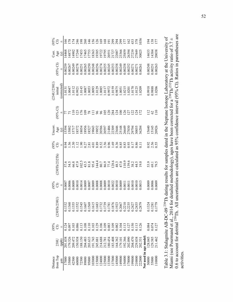
52

D

ista

nce

from

Top

23

8U

(95%

C

I)

(230

Th/2

38U

) (9

5%

CI)

(2

30Th

/232

Th)

(95%

C

I)

Unc

orr.

Age

(9

5% C

I) (2

34U

/238

U)

initi

al

(95%

CI)

Cor

r. A

ge

(95%

C

I)

µm

(ppb

) ±

±

±

(y)

± (c

orre

cted

) ±

(y)

± 17

000

201.

838

0.12

4 0.

1332

0.

0007

57

.6

0.94

15

394

77

1.01

31

0.00

259

1446

8 16

6 35

000

179.

526

0.09

7 0.

1360

0.

0006

54

.5

1.56

15

882

71

1.00

47

0.00

267

1487

2 17

8 42

500

209.

472

0.10

3 0.

1355

0.

0009

66

.8

2.30

15

717

110

1.01

12

0.00

249

1490

2 17

4 60

000

150.

938

0.08

6 0.

1552

0.

0010

47

.9

1.12

18

572

123

0.99

21

0.00

278

1724

4 24

6 72

500

188.

150

0.11

3 0.

1545

0.

0014

10

2.5

1.90

18

054

176

1.01

45

0.00

251

1745

3 19

8 89

000

204.

483

0.10

8 0.

1607

0.

0009

43

.5

0.27

18

956

109

1.00

87

0.00

265

1746

5 26

0 95

000

203.

633

0.11

0 0.

1569

0.

0007

81

.8

2.81

18

527

78

1.00

53

0.00

250

1775

3 14

6 10

3000

19

1.74

3 0.

103

0.16

15

0.00

09

95.4

4.

01

1904

3 11

1 1.

0093

0.

0024

8 18

363

156

1150

00

245.

881

0.12

9 0.

1683

0.

0008

14

4.4

8.89

19

852

96

1.01

29

0.00

256

1938

5 12

6 12

4000

21

4.68

8 0.

106

0.17

32

0.00

08

80.7

0.

52

2058

6 96

1.

0085

0.

0027

4 19

722

169

1250

00

212.

781

0.10

9 0.

1739

0.

0009

86

.9

3.56

20

597

105

1.01

17

0.00

255

1979

5 16

8 13

3000

18

0.45

4 0.

083

0.17

81

0.00

10

77.4

0.

96

2148

6 12

0 0.

9972

0.

0024

5 20

551

191

1370

00

183.

408

0.10

9 0.

1876

0.

0022

12

8.6

1.69

22

309

284

1.01

59

0.00

253

2172

7 29

9 14

5000

16

4.36

2 0.

082

0.19

23

0.00

10

48.3

0.

36

2364

6 12

4 0.

9875

0.

0025

8 22

007

294

1490

00

179.

101

0.10

4 0.

2067

0.

0009

47

.0

0.85

25

148

100

1.00

51

0.00

249

2336

6 29

9 15

6000

19

2.36

6 0.

113

0.22

10

0.00

11

110.

9 0.

83

2664

9 12

6 1.

0215

0.

0025

8 25

859

177

1780

00

202.

090

0.12

7 0.

2235

0.

0011

13

9.6

0.93

27

030

127

1.02

01

0.00

252

2639

4 16

2 19

9000

20

4.47

0 0.

150

0.24

27

0.00

10

38.2

0.

17

2979

4 12

2 1.

0170

0.

0027

1 27

239

433

2100

00

229.

838

0.11

3 0.

2435

0.

0010

44

.5

0.86

30

055

124

1.01

25

0.00

271

2784

9 37

8 22

2000

20

2.53

1 0.

126

0.28

79

0.00

13

19.0

0.

11

3620

4 17

2 1.

0209

0.

0026

1 30

025

1036

N

ot u

sed

in a

ge m

odel

:

50

000

128.

045

0.08

4 0.

1324

0.

0009

53

.9

0.92

15

640

112

0.99

18

0.00

248

1463

3 19

4 55

000

129.

585

0.07

4 0.

1281

0.

0006

69

.1

2.56

15

145

62

0.98

88

0.00

251

1438

4 13

8 11

0000

21

1.46

2 0.

127

0.17

79

0.00

09

79.5

0.

55

2092

6 11

0 1.

0206

0.

0026

3 20

038

177

Tabl

e 3.

1: S

tala

gmite

AB

-DC

-09

230 Th

dat

ing

resu

lts fo

r sam

ples

dat

ed in

the

Nep

tune

Isot

ope

Labo

rato

ry a

t the

Uni

vers

ity o

f M

iam

i (se

e Po

urm

and

et a

l., 2

014

for d

etai

led

met

hodo

logy

), ag

es h

ave

been

cor

rect

ed fo

r a 23

0 Th/23

2 Th a

ctiv

ity ra

tio o

f 3.7

±

0.6

to a

ccou

nt fo

r det

rital

230 Th

. A

ll un

certa

intie

s are

cal

cula

ted

as 9

5% c

onfid

ence

inte

rval

(95%

CI)

. Rat

ios i

n pa

rent

hese

s are

ac

tiviti

es.

53

interpolation between nearest ages (Figure 3.3). When plotting the age model with other

paleoproxies from the region, we find good agreement in the timing of isotopic shifts

between records, (discussed in detail in section 4.4), which further validates the decision

to utilize a value of 3.7± 0.6 for initial 230Th/232Th activity ratio.

The results for U-series geochronometry (Table 3.1) indicate that the stalagmite

formed between 14.1 to 31.3 ka before present with a weighted average growth rate of 13

µm/year (Figure 3.3 & 3.4). There is no evidence for any growth hiatuses throughout the

sample from either the age measurements or petrographic thin section analysis, however

there is evidence for periods of decreased growth rate from the U-Th geochronometry.

The lowest growth rate occurred from 22 to 26 ka BP (~ 14.5-15.5 cm from top) with an

Figure 3.3: Age model (black) based on twenty U-Th ages, years before present (yr BP). Random and systematic sources of uncertainty, including the uncertainties on decay constants, are propagated and reported at 95% confidence interval (see Pourmand et al. (2014) for details). The age model was developed by linear interpolation between adjacent ages. Red triangles indicate U-Th results not included in the age model.

54

average growth rate of 3 μm/year. There are two additional periods of decreased growth

rate from 14.9 to 17.3 ka BP (~ 4.2 to 6 cm from the top) and 27.8 to 30 ka BP (~ 21 to

23 cm from the top). There is evidence of three small layers of darker laminations at ~5,

14.5 and 22 cm from the top (Figure 3.2 a & b) which correlate with the three short

periods of reduced calcite precipitation. Based on the age model, however, there is no

evidence for a hiatus at these three locations of darker lamina.

3.3.2 Tests for kinetic fractionation

Several studies have shown that the δ18O and δ13C can be affected by kinetically

driven fractionations during the deposition of the carbonate which can overwhelm

environmental and climatic signals (Hendy, 1971; Lachniet, 2009). An approach often

used to examine the role of kinetic effects is known as the “Hendy test” (Hendy, 1971) in

which the lateral variation in a chemical parameter within the speleothem is measured.

Assuming that sampling can be carried out along a growth band, the following criteria

must be met for the Hendy test: i) an absence of lateral increases in δ18Oc and δ13Cc

values, and ii) a low correlation between δ18Oc and δ13Cc values. If these conditions are

met, then it is assumed that minimal kinetic fraction has taken place. However, studies

have demonstrated that this test may not be sufficient to rule out kinetic fraction

(Mühlinghaus et al., 2009). Other authors have suggested a more robust method is to

conduct replication tests, in which multiple stalagmites from the same cave are measured

and if the δ13Cc and δ18Oc trends are replicated, this supports kinetic fractionation not

having occurred (Dorale and Liu, 2009). We present two locations across which lateral

variation of δ18Oc and δ13Cc values were measured. Sampling for kinetic fractionation

was conducted at one millimeter increments from the center of the growth axis sampling

55

outward along a growth band. As shown in Figure 3.2 c and d, tests for kinetic

fractionation demonstrate low correlation and no significant increase for both δ13Cc and

δ18Oc across a lamina. This demonstrates that significant fractionation for δ13Cc and

δ18Oc has not occurred for this speleothem. Additionally, in the currently active cave

from Eleuthera Island, the measured δ18O of the calcite, temperature of the cave, and drip

water δ18O support the calcite is precipitated in equilibrium (see supplementary material).

For fluid inclusions, isotopic fractionation after deposition can occur through

fractionation between the water and the surrounding calcite, thereby altering the isotopic

composition of the trapped water, however, such a fractionation in the humid subtropics

should be minimal (van Breukelen et al., 2008). The fluid inclusions are representative

of paleoprecipitation, therefore results should fall on the global meteoric water line

(GMWL), which defines the linear δ18Ow versus δ2Hw relationship for all meteoric waters

(Craig, 1961). Fluid inclusion results plot near the GMWL suggesting that the δ18Ow and

δ2Hw values have not been affected by fractionation and the data therefore are

representative of the original meteoric water composition (Figure 3.5).

3.3.3 Carbon and oxygen isotopes of carbonate

The speleothem AB-DC-09 was sampled at both high (one sample every ~2

years) and low resolution (one sample every ~50 years). To aid with the analysis of the

data, the δ13C and δ18O carbonate isotope results are plotted with a 50 year rectangular

interpolation (Figure 3.4 a & b). A comparison of the δ13C and δ18O of the speleothem

calcite (δ18Oc and δ13Cc) with the derived age model demonstrates significant variations in

the isotopic value of the calcite (Figure 3.4 a & b). The variation in the δ13Cc results are

6.2 ‰ for the sample, with the most positive δ13Cc value of +3.2 ‰ V-PDB occurring at

56

30.9±1 ka BP. Above average δ13Cc values are also found at 15±0.2 ka and 24.7±0.2 ka

BP (Figure 3.4 a). Similar results are found in the δ18Oc record with the most positive

δ18Oc value of -0.2 ‰ V-PDB at 15 ±0.2 ka and above average δ18Oc values at 24.1±0.2

ka and 30.9±1 ka BP (Figure 3.4 b). Overall, a total of 3.5 ‰ variation is observed in the

δ18Oc results. A similar trend for each positive C and O isotope event is observed, with a

gradual increase leading to a maximum, followed by a more rapid decline. For the 15 ka

event, the gradual increase begins at 17.4 ka BP and reaches a maximum at ~15 ka BP,

followed by a rapid decrease (~200 years) in δ18Oc and δ13Cc. The trend is also observed

across the 24.5 ka event with an increase beginning at 25.5 ka BP to a maximum,

followed by a decrease. For the oldest event, maximum δ18Oc and δ13Cc values occurred

at ~31 ka and declined over ~200 years after the maximum. In summary, the carbonate

results support three unique shifts, of which the least significant in both δ13Cc and δ18Oc is

the 24.5 ka BP event (Figure 3.4 a & b).

3.3.4 Fluid inclusions

A comparison of the δ18Ow measured on the fluid inclusions with the derived age

model from U-Th geochronometry demonstrates minimal variations in the isotopic value

of the fluids (Figure 3.4 c). The δ2Hw and δ18Ow measured on the fluid inclusions support

variations of 11.7 ‰ and 1.6 ‰ over the studied interval with average values of -8.6 ‰

and -2.5 ‰ V-SMOW in δ2Hw and δ18Ow (Table 3.2). The variability in δ18Ow value is

relatively small compared to the changes in the δ18Oc value (~3.5 ‰, Figure 3.4 c). The

data support a minimum δ18Ow value at 25 ka BP and a maximum δ18Ow value at 30.3 ka

BP.

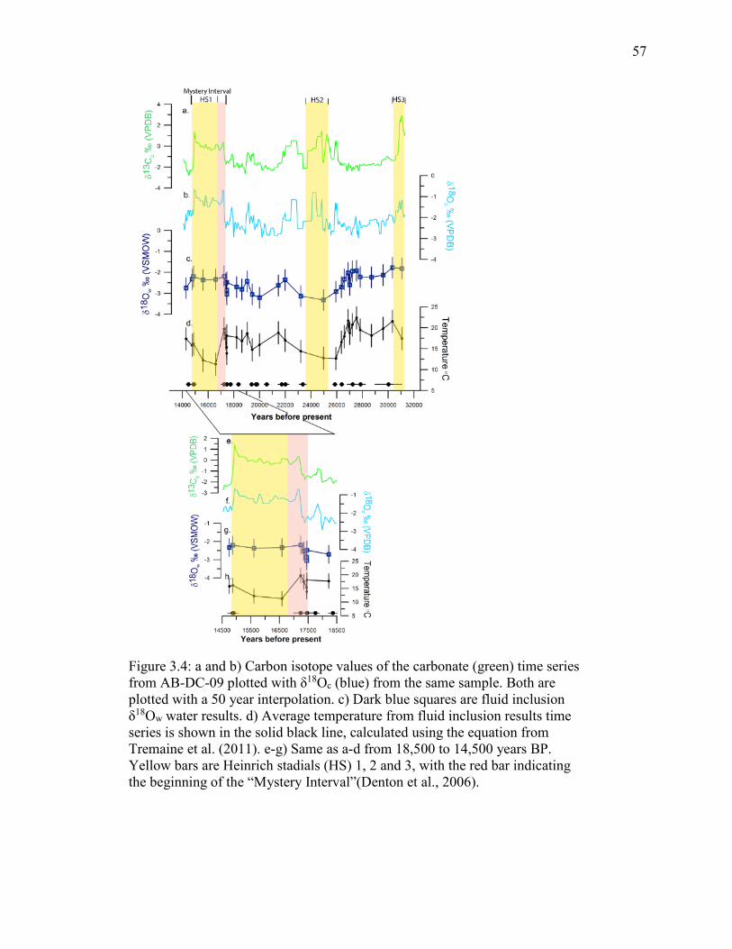
57

Figure 3.4: a and b) Carbon isotope values of the carbonate (green) time series from AB-DC-09 plotted with δ18Oc (blue) from the same sample. Both are plotted with a 50 year interpolation. c) Dark blue squares are fluid inclusion δ18Ow water results. d) Average temperature from fluid inclusion results time series is shown in the solid black line, calculated using the equation from Tremaine et al. (2011). e-g) Same as a-d from 18,500 to 14,500 years BP. Yellow bars are Heinrich stadials (HS) 1, 2 and 3, with the red bar indicating the beginning of the “Mystery Interval”(Denton et al., 2006).

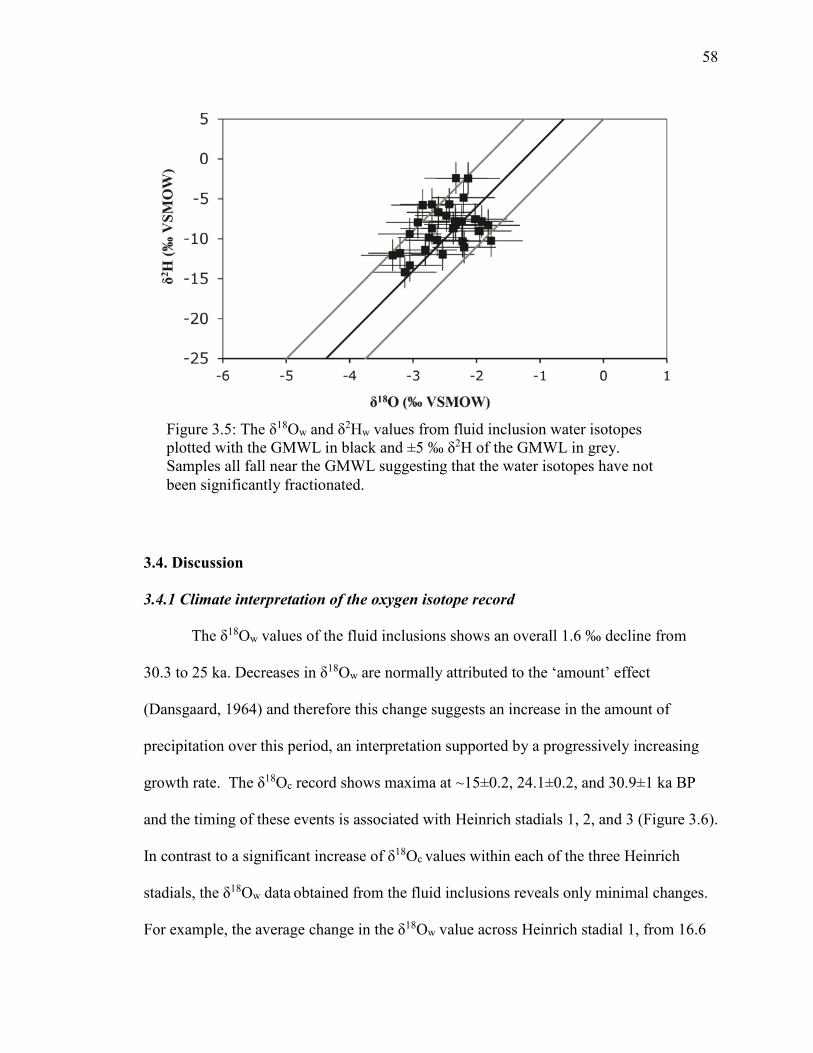
58

3.4. Discussion

3.4.1 Climate interpretation of the oxygen isotope record

The δ18Ow values of the fluid inclusions shows an overall 1.6 ‰ decline from

30.3 to 25 ka. Decreases in δ18Ow are normally attributed to the ‘amount’ effect

(Dansgaard, 1964) and therefore this change suggests an increase in the amount of

precipitation over this period, an interpretation supported by a progressively increasing

growth rate. The δ18Oc record shows maxima at ~15±0.2, 24.1±0.2, and 30.9±1 ka BP

and the timing of these events is associated with Heinrich stadials 1, 2, and 3 (Figure 3.6).

In contrast to a significant increase of δ18Oc values within each of the three Heinrich

stadials, the δ18Ow data obtained from the fluid inclusions reveals only minimal changes.

For example, the average change in the δ18Ow value across Heinrich stadial 1, from 16.6

Figure 3.5: The δ18Ow and δ2Hw values from fluid inclusion water isotopes plotted with the GMWL in black and ±5 ‰ δ2H of the GMWL in grey. Samples all fall near the GMWL suggesting that the water isotopes have not been significantly fractionated.

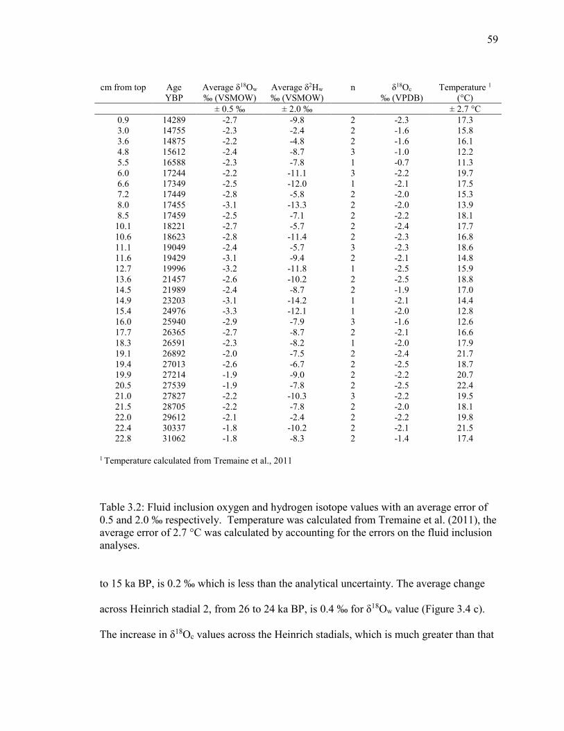
59

Table 3.2: Fluid inclusion oxygen and hydrogen isotope values with an average error of 0.5 and 2.0 ‰ respectively. Temperature was calculated from Tremaine et al. (2011), the average error of 2.7 °C was calculated by accounting for the errors on the fluid inclusion analyses.

to 15 ka BP, is 0.2 ‰ which is less than the analytical uncertainty. The average change

across Heinrich stadial 2, from 26 to 24 ka BP, is 0.4 ‰ for δ18Ow value (Figure 3.4 c).

The increase in δ18Oc values across the Heinrich stadials, which is much greater than that

cm from top Age Average δ18Ow Average δ2Hw n δ18Oc Temperature 1

YBP ‰ (VSMOW) ‰ (VSMOW)

‰ (VPDB) (°C)

± 0.5 ‰ ± 2.0 ‰

± 2.7 °C

0.9 14289 -2.7 -9.8 2 -2.3 17.3 3.0 14755 -2.3 -2.4 2 -1.6 15.8 3.6 14875 -2.2 -4.8 2 -1.6 16.1 4.8 15612 -2.4 -8.7 3 -1.0 12.2 5.5 16588 -2.3 -7.8 1 -0.7 11.3 6.0 17244 -2.2 -11.1 3 -2.2 19.7 6.6 17349 -2.5 -12.0 1 -2.1 17.5 7.2 17449 -2.8 -5.8 2 -2.0 15.3 8.0 17455 -3.1 -13.3 2 -2.0 13.9 8.5 17459 -2.5 -7.1 2 -2.2 18.1

10.1 18221 -2.7 -5.7 2 -2.4 17.7 10.6 18623 -2.8 -11.4 2 -2.3 16.8 11.1 19049 -2.4 -5.7 3 -2.3 18.6 11.6 19429 -3.1 -9.4 2 -2.1 14.8 12.7 19996 -3.2 -11.8 1 -2.5 15.9 13.6 21457 -2.6 -10.2 2 -2.5 18.8 14.5 21989 -2.4 -8.7 2 -1.9 17.0 14.9 23203 -3.1 -14.2 1 -2.1 14.4 15.4 24976 -3.3 -12.1 1 -2.0 12.8 16.0 25940 -2.9 -7.9 3 -1.6 12.6 17.7 26365 -2.7 -8.7 2 -2.1 16.6 18.3 26591 -2.3 -8.2 1 -2.0 17.9 19.1 26892 -2.0 -7.5 2 -2.4 21.7 19.4 27013 -2.6 -6.7 2 -2.5 18.7 19.9 27214 -1.9 -9.0 2 -2.2 20.7 20.5 27539 -1.9 -7.8 2 -2.5 22.4 21.0 27827 -2.2 -10.3 3 -2.2 19.5 21.5 28705 -2.2 -7.8 2 -2.0 18.1 22.0 29612 -2.1 -2.4 2 -2.2 19.8 22.4 30337 -1.8 -10.2 2 -2.1 21.5 22.8 31062 -1.8 -8.3 2 -1.4 17.4

1 Temperature calculated from Tremaine et al., 2011

60

found in the δ18Ow results, most likely arises from lower temperatures, rather than a

significant change in the δ18Ow or precipitation amount. The δ18Ow values, when

combined with δ18Oc values, allows for the calculation of the temperature at the time of

mineral formation. While caves generally maintain a constant temperature throughout

the year (representative of mean annual temperature), over longer time periods,

speleothems can record decadal to centennial scale changes in temperature. Utilizing the

equation presented in Tremaine et al. (2011), which defines the temperature dependent

fractionation relationship for stalagmites, temperature variations on the order of 11 °C

(Figure 3.4 d, Table 3.2) for the sample were calculated. The average temperature, 17.2

±2.7 °C, is cooler than the average modern annual temperature for the Bahamas (average

annual temperature = 22 to 28 °C (Baldini et al., 2007)) and typical temperatures within

modern dry caves in the area (average annual cave temperature = 23.2°C (Arienzo et al.,

2013)). Heinrich stadials 1, 2, and 3 are represented by cooler temperatures, with the

average temperature across Heinrich stadials 1, 2 and 3 of 14.6 ±2.7 ºC, and Heinrich

stadial 1 being the coolest event (Figure 3.4 d).

3.4.2 Climate interpretation of the carbon isotope record

Both the δ13Cc and δ18Oc results consists of increased values around 15±0.2,

24.1±0.2, and 30.9±1 ka BP suggesting that similar environmental factors influenced the

δ13Cc and δ18Oc composition of the stalagmite during Heinrich stadials. As the δ18Oc

value across Heinrich stadial events is primarily driven by changes in the cave

temperature, we suggest that the increases in the δ13Cc values are indirectly driven by

cooling during these Heinrich stadials. Potentially, the increased δ13Cc values are a result

of a decline in soil microbial activity which increases the δ13CDIC ratio of the drip water

61

during periods of cooler temperatures. Assuming changes in cave ventilation did not

occur during sample deposition, the δ13Cc ratio of the speleothem is most likely driven by

changes in the soil zone or the vegetation above the cave. Support for this notion comes

from similar results found in a cave in France, where lower δ13Cc values during warm

periods were driven by drip water having a greater biogenic CO2 component (Genty et al.,

2003). Nevertheless, it is not possible to rule out the potential influence of changes in the

amount of precipitation on the δ13Cc record, as is possibly supported by the decreases in

growth rates during the periods of increased δ13Cc values. An increase in the δ13Cc ratio

of the carbonate can be driven by aridity, which leads to a reduction in soil microbial

activity, or a greater proportion of C4 versus C3 plants.

3.4.3 Climate variability in the context of the Atlantic basin

Proxy records from throughout the Atlantic not only support climatic shifts

associated with Heinrich stadials, but are in good agreement with the timing of Heinrich

stadials 1-3 in the sample studied here (Figure 3.6). These reconstructions support the

global scale response to Heinrich stadials. The difference in climatic expression between

northern hemisphere records (e.g., Hulu Cave, Cariaco Basin, and the Bahamas)

compared to southern hemisphere records (e.g., Pacupahuain Cave) demonstrates the

anti-phased response across Heinrich stadials (Broecker, 1998; Kanner et al., 2012;

Peterson et al., 2000; Wang et al., 2001)(Figure 3.6). This anti-phased relationship

between the hemispheres is in part due to a meridional shift in climate across Heinrich

stadials and is well documented in the ice core records with the Greenland ice core

records supporting cooling and the ice cores from Antarctica supporting warming during

Heinrich stadials (Broecker, 1998; Wolff et al., 2010).

62

The Bahamian speleothem record, along with other proxies from the

subtropical/tropical western Atlantic, support overall drying and/or cooling associated

with Heinrich stadials (Escobar et al., 2012; Lachniet et al., 2013; Peterson et al.,

2000)(Figure 3.6). This coherence in climate expression among the North Atlantic

tropical records across Heinrich stadials can be explained by a meridional shift in climate.

An alkenone-derived SST record from the Bermuda rise across Heinrich stadials 4 and 5

supports a ~3-5 °C decrease in SSTs (Sachs and Lehman, 1999) suggesting SSTs also

may have declined during earlier Heinrich stadials. Further south, a lake record from

Guatemala supports increased aridity and a 6-10 °C cooling associated with Heinrich

stadial 1 (Escobar et al., 2012; Hodell et al., 2012). The temperatures observed during

Heinrich stadial 1 are lower than modern mean annual temperature for Guatemala (mean

annual temperature = 26 °C) (Hodell et al., 2012). The increased aridity and cooling in

Guatemala is thought to be driven by a southerly shifted ITCZ and decreased tropical

Atlantic SSTs (Escobar et al., 2012; Hodell et al., 2012). The amount of cooling

observed in the Guatemala and the Bermuda records across Heinrich stadials is similar to

the cooling observed in the Bahamas record. Modeling results also support decreased

temperatures for the tropical northern hemisphere coincident with Heinrich stadials,

however the modeled temperature changes are much less (Murphy et al., 2014; Zhang

and Delworth, 2005).

As suggested above, while the geochemical data in the speleothem record from

the Bahamas supports a decrease in temperature, it does not rule out the possibility of

enhanced aridity across these events, which potentially may drive the variability in the

63

Figure 3.6: Compilation of paleoclimate studies from throughout the Atlantic. a) δ18O time series from NGRIP ice core (black) data from Wolff et al. (2010) plotted with a 5 point running average. b) In orange, δ18O time series from Hulu Cave, data from PD and MSD samples from Wang et al. (2001) note the axis is reversed. c) Oxygen isotope time series from this study (sample AB-DC-09) plotted with a 50 year interpolation. Note the axis is reversed. d) Cariaco Basin reflectance (red) at 550 nm, axis reversed from Peterson et al. (2000) with a 5 point smoothing. e) Green is δ18O record from Pacupahuain cave, Peru from Kanner et al. (2012).

64

carbon isotopic record. A speleothem record from southwestern Mexico demonstrates a

reduction in the North American Monsoon associated with Heinrich stadial 1 driven by

the southerly shifted ITCZ and reduced AMOC (Lachniet et al., 2013). A southerly shift

in the ITCZ would be accompanied by an expanded Bermuda high, which could have led

to an increased aridity in the Bahamas across Heinrich stadials (Hodell et al., 2000).

In contrast to the data presented here, a record based on pollen from Lake Tulane,

Florida in the southeastern U.S. suggests warmer and wetter Heinrich stadials (Grimm et

al., 2006). These authors attributed the warming and increased rainfall to a slowdown of

the AMOC leading to a reduction in the transport of heat from the Gulf of Mexico and

thereby forcing the observed warmer and wetter climate in Florida (Grimm et al., 2006).

Nevertheless the same climatic response may not be observed in the Bahamas as a result

of the location of Abaco Island, on the eastern edge of the Bahamas platform, and

therefore this study site may not have been influenced by changes in the Gulf of Mexico.

Furthermore, the postulated warming of the Gulf of Mexico from the Florida record is not

consistent with the simulated climate response to an AMOC shut down (Clement and

Peterson, 2008 and references therein) rather, most climate models suggest a cooling of

the entire North Atlantic, including the Gulf of Mexico.

In many paleoclimate proxy reconstructions, Heinrich stadial 1 is a larger

magnitude event compared to stadials 2 and 3 (Stager et al., 2011) (Figure 3.6). In the

record presented here, Heinrich stadial 1 is characterized by the greatest change in δ18Oc

and temperature (observed ~ 5 º C temperature decrease), while Heinrich stadial 2

exhibits minimal changes and Heinrich stadial 3 demonstrates a larger shift in δ13Cc

value. The reduced geochemical change across Heinrich stadial 2 may be due to a

65

minimal change in the AMOC during this event (Lynch-Stieglitz et al., 2014; McManus

et al., 2004).

Based on paleoclimate reconstructions, Heinrich stadial 1 has been shown to be

the strongest event and a period punctuated with climatic changes. Heinrich stadial 1 has

also been considered a part of the so-called “Mystery Interval”, from 17.5 to 14.5 ka BP

(Denton et al., 2006) and corresponding to a period of prolonged hydrologic changes

(Broecker et al., 2009; McGee et al., 2012). In this speleothem record from the Bahamas,

there is evidence for climate variations associated with the “Mystery Interval” (Figure

3.4, e-h). Fluid inclusion results suggest a temperature increase and/or precipitation

change from ~17.5 to ~16.9 ka BP followed by a progressively cooler period from ~16.9

to 15 ka BP (Table 3.2, Figure 3.4 g & h). The cooler period is identified as Heinrich

stadial 1. Similarly, in Guatemala, a lake record indicates a cold and dry period

beginning around 18 ka BP, interrupted by a wetter and warmer period around 17 ka BP,

followed by a return to drier and cooler temperatures at approximately 16.1 ka BP

(Escobar et al., 2012; Hodell et al., 2012). The authors suggest the two cold and dry

periods observed in Guatemala are driven by two separate North Atlantic IRD events

(Escobar et al., 2012). A multi-proxy study of a core from the Cariaco Basin of the

“Mystery Interval” supports the drier climate associated with Heinrich stadial 1 is

interrupted by a shift to wetter climate conditions (Escobar et al., 2012; Yurco, 2010).

While the exact timing of these climatic shifts varies between the various records, these

records do support that the “Mystery Interval” is a period of climate variability for the

subtropical/tropical Atlantic.

66

Additional to the observed geochemical variability associated with the last three

Heinrich stadials and the “Mystery Interval”, there are observed increases in the δ18Oc

and δ13Cc of the carbonate at 19±0.2 and 22.6±0.2 ka before present. The magnitude of

the isotopic shifts at 19 and 22.6 ka BP are less than the isotopic shifts observed during

Heinrich stadial events (at 19 ka BP, a 1.7‰ decrease in the δ13Cc value and at 22.6 ka

BP a 2 ‰ decrease for δ13Cc). This may suggest these isotopic variations are driven by

climatic changes which are not as significant. Similarly, Bond et al. (1997) observed

increased IRD deposits at similar time periods. Therefore these may also be periods of

decreased temperatures and/or precipitation.

The resumption of AMOC at the end of Heinrich stadial 1 is believed to have

caused an increase in SSTs in the North Atlantic (McManus et al., 2004), leading to the

northward shift of the ITCZ and the observed shift to wetter and warmer conditions in the

northern tropics and the start of the Bolling-Allerod period (Peterson et al., 2000). This is

also supported by the increase in temperatures by ~ 4 ºC after Heinrich stadial 1 from the

fluid inclusion results (Figure 3.4 d).

While other climate records for the same time period from nearby localities such

as Cariaco Basin (Peterson et al., 2000) and stalagmites from the Peruvian Andes

(Kanner et al., 2012) have recorded millennial scale variations (e.g., Dansgaard/Oeschger

(D/O) events) there is no evidence of D/O variability in the isotopic record of sample

AB-DC-09. A similar observation was made from speleothems collected from Borneo in

which the geochemistry of the speleothems recorded Heinrich stadials, but not the D/O

events (Carolin et al., 2013). The lack of evidence for D/O events suggests that D/O

events are different than Heinrich stadials either in the forcing mechanism, the global

67

propagation, the geographic expression, or how these events are recorded in the

speleothems (Carolin et al., 2013).

3.5. Conclusion

The stalagmite record reported in this paper reveals three distinctive climatic

changes during the last glacial period, each coincident with a Heinrich stadial. The δ18Oc

and δ13Cc data support significant shifts within the Heinrich stadials, while minimal

changes occur in the δ18O of the water contained in fluid inclusions. The geochemical

results demonstrate that Heinrich stadials 1- 3 are characterized by a temperature

decrease and are in good agreement with regional paleoclimate data for Heinrich stadials.

The observed temperature changes for the Bahamas speleothem across Heinrich stadials

are consistent with paleoclimate records from the Western Atlantic. We propose the

average temperature decline of ~3 ºC during Heinrich stadials, to an average temperature

of 14.6 ±2.7 ºC, is due to the meridional shift in the climate that led to cooler subtropics.

The results suggest variable geochemical responses to each of the events, with Heinrich

stadial 1 being the most extreme event, with up to a 5 ºC temperature decline is observed.

Finally, the results presented here support the teleconnection between the subtropical

Atlantic and cooling in the North Atlantic and the sensitivity of the Bahamas temperature

to changes in AMOC.

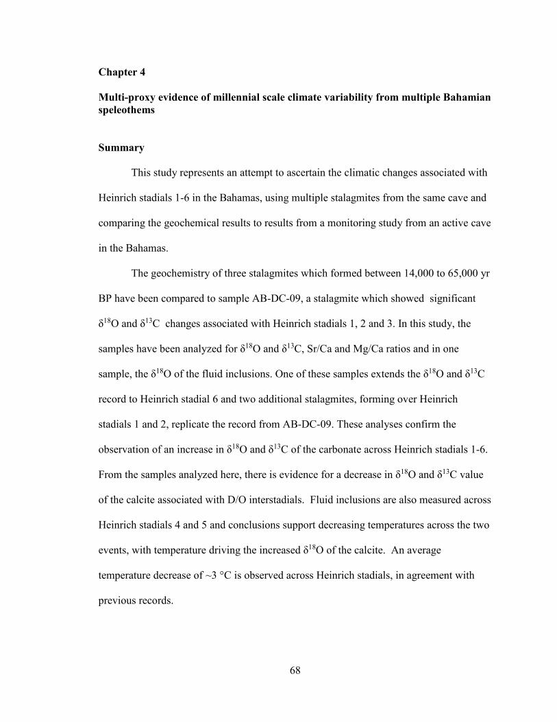
Chapter 4

Multi-proxy evidence of millennial scale climate variability from multiple Bahamian speleothems

Summary

This study represents an attempt to ascertain the climatic changes associated with

Heinrich stadials 1-6 in the Bahamas, using multiple stalagmites from the same cave and

comparing the geochemical results to results from a monitoring study from an active cave

in the Bahamas.

The geochemistry of three stalagmites which formed between 14,000 to 65,000 yr

BP have been compared to sample AB-DC-09, a stalagmite which showed significant

δ18O and δ13C changes associated with Heinrich stadials 1, 2 and 3. In this study, the

samples have been analyzed for δ18O and δ13C, Sr/Ca and Mg/Ca ratios and in one

sample, the δ18O of the fluid inclusions. One of these samples extends the δ18O and δ13C

record to Heinrich stadial 6 and two additional stalagmites, forming over Heinrich

stadials 1 and 2, replicate the record from AB-DC-09. These analyses confirm the

observation of an increase in δ18O and δ13C of the carbonate across Heinrich stadials 1-6.

From the samples analyzed here, there is evidence for a decrease in δ18O and δ13C value

of the calcite associated with D/O interstadials. Fluid inclusions are also measured across

Heinrich stadials 4 and 5 and conclusions support decreasing temperatures across the two

events, with temperature driving the increased δ18O of the calcite. An average

temperature decrease of ~3 °C is observed across Heinrich stadials, in agreement with

previous records.

68

69

4.1 Background

4.1.1 Speleothem geochemistry

The geochemistry of speleothems (normally δ13C and δ18O) has proven to be a

valuable archive of modern, Holocene and millennial scale climate events (Fairchild et

al., 2006; McDermott, 2004). Considering that the interpretation of δ18O values of

carbonates is inherently complex, studies have taken various approaches including the

measurement of the δ18O value of drip water from within the cave, the measurement of

the δ18O of the rainfall from a nearby monitoring station, modeling the δ18O value of

rainfall and/or measuring the fluid inclusion δ18O values, representative of the local

rainfall (Baker and Bradley, 2010; Carolin et al., 2013; Kanner et al., 2012; van

Breukelen et al., 2008).

In the case of the δ13C of the carbonate, biological soil activity, the type of

vegetation (C3 versus C4) and amount, as well as the amount of water/rock interaction can

impact the δ13C of the dissolved inorganic carbon (DIC) (Fairchild et al., 2006;

McDermott, 2004). These factors can be influenced by changes in temperature and

amount of precipitation. The biogenic component of the CO2 in the soil zone increases as

a result of root respiration, organic material decomposition, and the amount of vegetation

cover (Couchoud et al., 2009; Genty et al., 2003). Within the cave, studies have

demonstrated that ventilation may influence the δ13C of the CO2 and hence δ13C of the

speleothem (Kowalczk and Froelich, 2010; Lambert and Aharon, 2011; Tremaine et al.,

2011).

Elemental abundances have proven to be important for understanding the

environment of formation of the carbonate minerals. In biogenic carbonates, particularly

70

corals, Sr/Ca ratios can be utilized as indicators of temperature change (Beck et al.,

1992). In speleothems, minor elements have been utilized to reconstruct paleoclimate

and are able to aid with the interpretation of δ13C and δ18O results (Cruz et al., 2007;

Oster et al., 2010; Tremaine and Froelich, 2013). Factors that can influence the

incorporation of minor elements into drip water include the type of overlying bedrock

(Fairchild et al., 2000), the hydrologic conditions (Cruz et al., 2007), the routing path of

the water (Fairchild and Treble, 2009), the amount of water/rock interaction (Fairchild et

al., 2000), cave ventilation (Wong et al., 2011), and calcite precipitation rate (Lorens,

1981). During periods of enhanced aridity, prior calcite precipitation (PCP) can occur

through evaporation or CO2 degassing in the epikarst or within the cave ceiling. With

increasing PCP, drip waters become enriched in Mg and Sr as these elements are

excluded from the diagenetic solid phase. Evidence of PCP, and hence increased aridity,

have been attributed to a positively correlated Mg to Sr variation in speleothems

(Fairchild and Treble, 2009). In addition, during periods of low flow, increased residence

time of waters in the epikarst leads to increased water/rock interaction and hence minor

element concentrations will reflect the overlying bedrock (Fairchild and Treble, 2009).

Studies have demonstrated that changes in the δ13C and δ18O values in the

speleothems may not be solely driven by climatic factors, but rather by kinetics. Kinetic

isotope fraction results in disequilibrium and a test used to suggest that kinetic effects are

not important is the ‘Hendy’ test (Hendy, 1971) which measures lateral δ13C and δ18O

variation within a speleothem. Assuming that sampling can be carried out along a growth

band, the following criteria must be met for the Hendy test: i) an absence of lateral

increases in δ18Oc and δ13Cc values, and ii) a low correlation between δ18Oc and δ13Cc

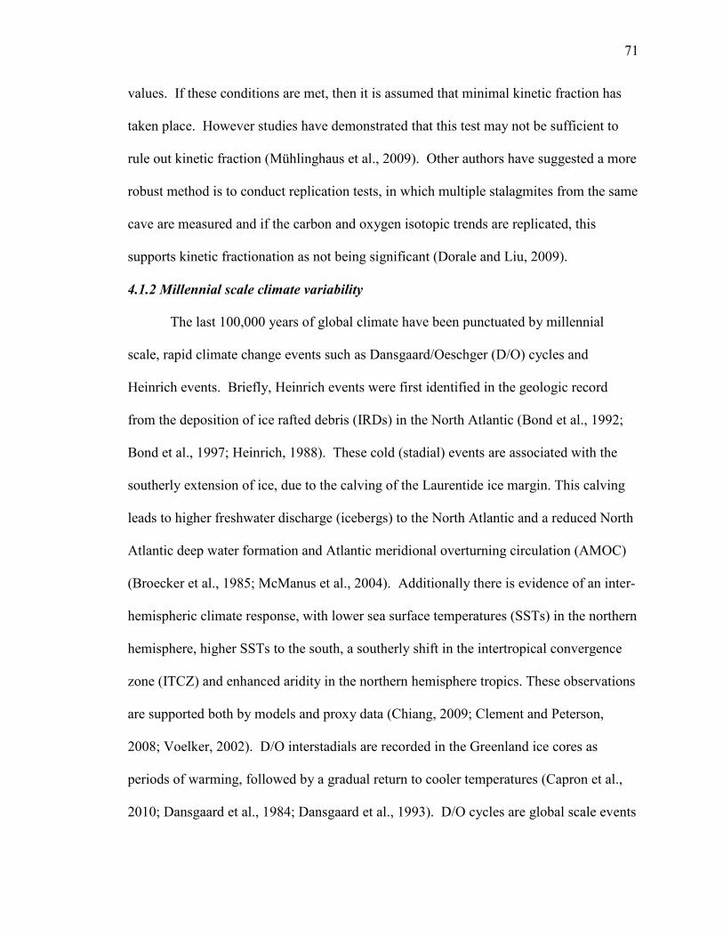
71

values. If these conditions are met, then it is assumed that minimal kinetic fraction has

taken place. However studies have demonstrated that this test may not be sufficient to

rule out kinetic fraction (Mühlinghaus et al., 2009). Other authors have suggested a more

robust method is to conduct replication tests, in which multiple stalagmites from the same

cave are measured and if the carbon and oxygen isotopic trends are replicated, this

supports kinetic fractionation as not being significant (Dorale and Liu, 2009).

4.1.2 Millennial scale climate variability

The last 100,000 years of global climate have been punctuated by millennial

scale, rapid climate change events such as Dansgaard/Oeschger (D/O) cycles and

Heinrich events. Briefly, Heinrich events were first identified in the geologic record

from the deposition of ice rafted debris (IRDs) in the North Atlantic (Bond et al., 1992;

Bond et al., 1997; Heinrich, 1988). These cold (stadial) events are associated with the

southerly extension of ice, due to the calving of the Laurentide ice margin. This calving

leads to higher freshwater discharge (icebergs) to the North Atlantic and a reduced North

Atlantic deep water formation and Atlantic meridional overturning circulation (AMOC)

(Broecker et al., 1985; McManus et al., 2004). Additionally there is evidence of an inter-

hemispheric climate response, with lower sea surface temperatures (SSTs) in the northern

hemisphere, higher SSTs to the south, a southerly shift in the intertropical convergence

zone (ITCZ) and enhanced aridity in the northern hemisphere tropics. These observations

are supported both by models and proxy data (Chiang, 2009; Clement and Peterson,

2008; Voelker, 2002). D/O interstadials are recorded in the Greenland ice cores as

periods of warming, followed by a gradual return to cooler temperatures (Capron et al.,

2010; Dansgaard et al., 1984; Dansgaard et al., 1993). D/O cycles are global scale events

72

(Denniston et al., 2007; Fletcher et al., 2010; Jiménez-Moreno et al., 2010; Jouzel et al.,

2007; Siddall et al., 2010), however the mechanisms driving D/O cycles and the global

propagation are still not well understood (Clement and Peterson, 2008; Timmermann et

al., 2003). Several theories have been suggested including AMOC changes (Broecker et

al., 1985), sea ice changes (Li et al., 2010; Petersen et al., 2013), and tropical processes

(Clement and Cane, 1999) to name a few. There is some evidence of IRD deposits

associated with D/O stadials which suggests that D/O cycles are possibly driven by ice

sheet mechanisms (Menviel et al., 2014). Modeling studies suggest D/O cycles are

forced both by ice-sheet and AMOC variations (Menviel et al., 2014).

The goal of this study is to build upon a previous stalagmite record (AB-DC-09)

(Chapter 3), by analyzing three additional stalagmites from the same cave to reconstruct

millennial scale climate variations using multiple geochemical proxies. These four

stalagmites from the Bahamas formed over the last 65,000 years. In Chapter 3 it was

concluded that the main cause of increasing δ18O of the speleothem carbonate was lower

temperature, with lower temperature associated with Heinrich stadials 1 to 3. Also

observed was higher δ13C of the carbonate during Heinrich stadials, due to either a

decrease in temperature or increase in aridity. Both a decrease in temperature and an

increase in aridity can lead to a reduced biogenic CO2 component of the DIC and heavier

δ13C values. Using these additional speleothems from the Bahamas, the climatic change

across Heinrich stadials 1-6 was studied utilizing δ13C and δ18O, minor elements and the

δ18O of fluid inclusions. The results from these stalagmites will be compared to results

from a modern cave. The modern cave monitoring study consists of the measurement of

drip waters and calcite samples δ13C and δ18O and minor elements, to aid with the

73

interpretation of the geochemical results from the ancient stalagmites. This study is of

significance as it extends the original record to Heinrich stadial 6 and combines multiple

geochemical proxies to determine the drivers of geochemical changes. Finally, combining

both geochemical analyses of ancient stalagmites with a modern monitoring study is

significant as it validates the interpretation of our results.

4.2 Sample Specimens for Study

The three main types of data presented in this report are: 1) a geochemical time

series from four stalagmites over the last 65,000 years before present, 2) a spatial and

temporal geochemical data from drip waters from a currently active cave, 3) geochemical

dataset from calcites from the currently active cave.

4.2.1 Ancient stalagmites

For this study, four stalagmites (AB-DC-01, 03, 09 and 12) were selected from a

currently submerged cave from Abaco Island, Bahamas (Figure 4.1). Samples were

collected from a water depth of 33.5, 34.4, 16.5 and 11.9 meters, respectively, below sea

level. Stalagmite sample AB-DC-09 has been previously analyzed for U-Th ages, δ13C

and δ18O values of the carbonate, and δ18O and δ2H values of the fluid inclusions. All

samples were analyzed for the presence of kinetic fractionation through the ‘Hendy’ test.

Samples from the surrounding cave walls were not collected.

4.2.2 Modern

Samples were collected from Hatchet Bay Cave (HBC), a currently active cave in

Eleuthera, the Bahamas (Figure 4.1). Monitoring was initiated in June of 2012.

Overlying the cave is grasses and small Metopium toxiferum (poison wood) and trees of

the Fabaceae family with well-developed soils (greater than 15 cm depth). Most of the

74

grasses are located near the entrance and at lower elevations around the cave, with the

small trees located on the Aeolian ridge. HBC was accessed through a small ~1.7 m. by

0.9 m. opening located 10 to 15 m above sea level and exhibits an extremely linear

pattern particularly west of the main entrance (Mylroie and Mylroie, 2009). The opening

is immediately surrounded by thick grasses with larger trees (as described above) located

3 meters to the west, approximately following the cave direction and well developed soils

(as described above). The first level exhibits evidence of phreatic dissolution (Mylroie

and Mylroie, 2009). There is no evidence of cave breathing holes through the roof as

suggested by the lack of changes in the overlying vegetation and soil. The cave is divided

into three levels with the first level being the shallowest and the smallest level. The

second level is a tubular passage accessed by a 1.6 m. ladder down from the first level

and again contains evidence of phreatic dissolution (Mylroie and Mylroie, 2009). The

second level is more extensive (300 m long) with active drip water and stalagmite

formation (Mylroie and Mylroie, 2009). The 2nd level is thought to follow a thick, terra

rossa paleosol, leading to the creation of the linear and tubular shape following the

aeolian ridge (Mylroie and Mylroie, 2009). The third level is the deepest level and is

accessed by another 1.8 m ladder from the second level. However continuing on the

second floor lies a smaller passage which after several meters leads to a 7 m shaft to the

surface, which may have been carved out for guano mining (Mylroie and Mylroie, 2009).

The third level is partially filled with water, with active stalagmite formation occurring

on raised rock ledges above the water, ~1.2 m above the water level. This water is tidally

influenced and of marine salinity (Mylroie and Mylroie, 2009). There is no evidence of

water flooding the rock ledges nor is there any evidence of calcite deposits forming from

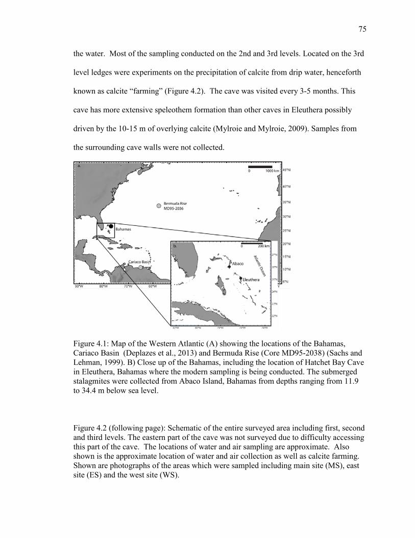
75

the water. Most of the sampling conducted on the 2nd and 3rd levels. Located on the 3rd

level ledges were experiments on the precipitation of calcite from drip water, henceforth

known as calcite “farming” (Figure 4.2). The cave was visited every 3-5 months. This

cave has more extensive speleothem formation than other caves in Eleuthera possibly

driven by the 10-15 m of overlying calcite (Mylroie and Mylroie, 2009). Samples from

the surrounding cave walls were not collected.

Figure 4.1: Map of the Western Atlantic (A) showing the locations of the Bahamas, Cariaco Basin (Deplazes et al., 2013) and Bermuda Rise (Core MD95-2038) (Sachs and Lehman, 1999). B) Close up of the Bahamas, including the location of Hatchet Bay Cave in Eleuthera, Bahamas where the modern sampling is being conducted. The submerged stalagmites were collected from Abaco Island, Bahamas from depths ranging from 11.9 to 34.4 m below sea level. Figure 4.2 (following page): Schematic of the entire surveyed area including first, second and third levels. The eastern part of the cave was not surveyed due to difficulty accessing this part of the cave. The locations of water and air sampling are approximate. Also shown is the approximate location of water and air collection as well as calcite farming. Shown are photographs of the areas which were sampled including main site (MS), east site (ES) and the west site (WS).

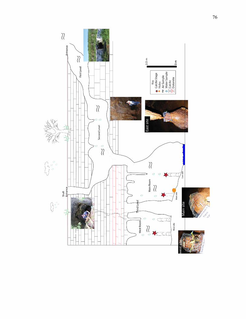
76

77

4.3 Methods

4.3.1 Stalagmite samples: Abaco Island cave

Uranium-Thorium:

For age dating of the speleothems, a total of 27 U-Th age dates were acquired at

the Neptune Isotope Laboratory of the University of Miami - RSMAS utilizing a

ThermoFisher-Neptune Plus multi-collection ICP-MS for stalagmites AB-DC-01, 03 and

12. Previously, 20 ages were acquired for sample AB-DC-09 and are reported elsewhere

(Chapter 3). The U-Th geochronometry method and the propagation of random and

systematic uncertainties is provided in Chapter 3 and in Pourmand et al. (2014b). For all

samples, an initial 230Th/232Th activity ratio of 3.7± 0.6 was used to account for excess

(unsupported) 230Th (Chapter 3).

Calcite isotopes:

Sampling of the speleothem carbonate for δ13Cc and δ18Oc (calcite) was carried out

using a New-Wave computerized micromill at both high and low resolution. Low

resolution sampling consisted of one sample every 1000 μm throughout the length of the

stalagmite (Figure 4.3 a-c). Two areas were analyzed at high resolution (20 μm sampling

interval) for sample AB-DC-12 (Figure 4.3 a) and three areas from sample AB-DC-09

(Chapter 3). The areas were chosen because the low resolution analysis demonstrated

areas of rapid and significant isotopic shifts in these intervals. C and O isotopic

measurements were made using a Kiel III interfaced with a Thermo-Finnigan Delta Plus

Mass Spectrometer at the University of Miami. All data have been corrected for the usual

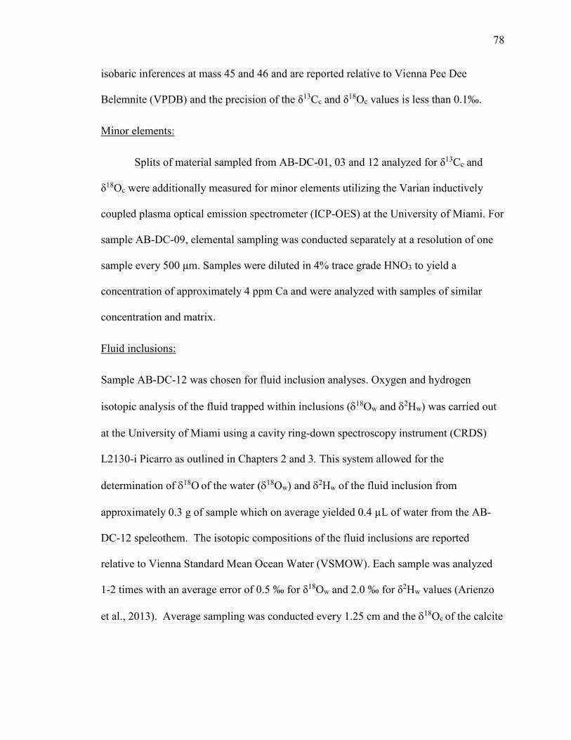
78

isobaric inferences at mass 45 and 46 and are reported relative to Vienna Pee Dee

Belemnite (VPDB) and the precision of the δ13Cc and δ18Oc values is less than 0.1‰.

Minor elements:

Splits of material sampled from AB-DC-01, 03 and 12 analyzed for δ13Cc and

δ18Oc were additionally measured for minor elements utilizing the Varian inductively

coupled plasma optical emission spectrometer (ICP-OES) at the University of Miami. For

sample AB-DC-09, elemental sampling was conducted separately at a resolution of one

sample every 500 μm. Samples were diluted in 4% trace grade HNO3 to yield a

concentration of approximately 4 ppm Ca and were analyzed with samples of similar

concentration and matrix.

Fluid inclusions:

Sample AB-DC-12 was chosen for fluid inclusion analyses. Oxygen and hydrogen

isotopic analysis of the fluid trapped within inclusions (δ18Ow and δ2Hw) was carried out

at the University of Miami using a cavity ring-down spectroscopy instrument (CRDS)

L2130-i Picarro as outlined in Chapters 2 and 3. This system allowed for the

determination of δ18O of the water (δ18Ow) and δ2Hw of the fluid inclusion from

approximately 0.3 g of sample which on average yielded 0.4 µL of water from the AB-

DC-12 speleothem. The isotopic compositions of the fluid inclusions are reported

relative to Vienna Standard Mean Ocean Water (VSMOW). Each sample was analyzed

1-2 times with an average error of 0.5 ‰ for δ18Ow and 2.0 ‰ for δ2Hw values (Arienzo

et al., 2013). Average sampling was conducted every 1.25 cm and the δ18Oc of the calcite

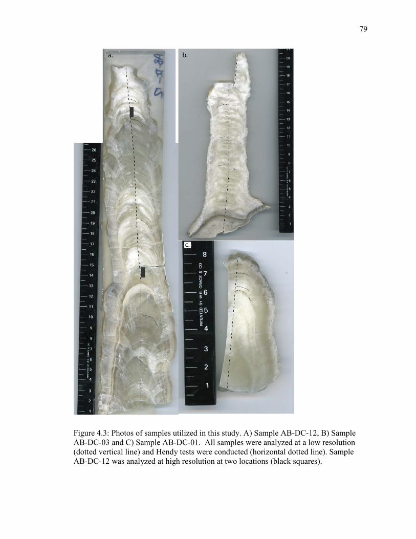
79

Figure 4.3: Photos of samples utilized in this study. A) Sample AB-DC-12, B) Sample AB-DC-03 and C) Sample AB-DC-01. All samples were analyzed at a low resolution (dotted vertical line) and Hendy tests were conducted (horizontal dotted line). Sample AB-DC-12 was analyzed at high resolution at two locations (black squares).

80

hosting the inclusion was measured on the carbonate using the Thermo-Finnigan Delta

Plus mass spectrometer (see above).

4.3.2 Modern samples: Hatchet Bay Cave

Sampling within HBC began in June of 2012 and continued to November of 2013.

Geochemical analyses of samples from HBC include the analyses of the CO2 of air, drip

waters and the precipitated calcite.

Air samples:

Air samples for carbon isotopes of the CO2 (δ13CCO2) were collected into 30 mL

glass vials sealed with a septa, in a transect through the cave. Every visit to the cave an

air sample was taken outside of the cave in an open field within 3 meters of the cave

entrance prior to entering the cave. Carbon isotopes of the CO2 were analyzed at the

University of Miami on a gas bench coupled to a Thermo-Delta plus Advantage isotope

ratio mass spectrometer (IRMS) and calibrated against internal standards. Data are

reported relative to Vienna Pee Dee Belemnite (V-PDB). To determine CO2

concentration, carbon peak intensity data were calibrated utilizing air samples with CO2

concentrations of atmospheric condition using only one standard of atmospheric air.

Water samples:

Unfiltered water samples were collected throughout the second and third levels of

the cave by holding clean plastic vials under dripping stalactites. Vials were filled

completely (where possible) to avoid head space equilibration, then capped with a screw

top cap the cap was then wrapped in either parafilm or electrical tape to prevent leaking

during travel and stored until analysis. The waters were filtered (Whatman 0.2 µm pore

filter) upon return to the laboratory (within 2-3 days) and transferred to a separate clean

81

plastic container, which was sealed with a screw cap. The filtered water was subsequently

measured for minor elements and oxygen and hydrogen isotopes (δ18Ow & δ2Hw). For

minor element analyses, filtered samples were acidified and analyzed using the Varian

ICP-OES. For δ18Ow & δ2Hw of the drip water, samples were measured using the Picarro

Cavity Ring-Down Spectroscopy (CRDS). Four standard waters were analyzed with

each set of samples and the standards used were previously calibrated to the VSMOW-

GISP-SLAP scale. Data are reported relative to VSMOW with an average

reproducibility of 0.05 ‰ for δ18Ow and 0.1 ‰ for δ2Hw from repeated analysis of a

standard.

Chloride concentration was determined by titration with silver nitrate using dilute

potassium chromate solution as the indicator. International Association for the Physical

Science of the Oceans (IAPSO) seawater standard was utilized as a standard solution for

Chloride and the average error was 5 ppm.

Calcite farming:

In June of 2012, collection of recently formed calcite began in Hatchet Bay Cave.

Standard glass microscope slides (Figure 4.4) were placed on top of currently forming

stalagmites and held in place by securing wire to the top of the stalagmite. The slides

were fixed at a slight angle, similar to the methods of Tremaine et al. (2011) and Banner

et al. (2007). Prior to installing the slides in the cave, the slides were pre-weighed in the

laboratory. For the calcite farming, two farming set ups were installed in the main room

(sites: middle (MS) and east (ES)), with a total of three slides deployed, and additionally

a set up was installed in the west room (site: west (WS)) with one microscope slide

82

Figure 4.4: Photos of the calcite “farming” slide set up in the MS, ES and WS locations, with photos of two representative slides, slides #20 and 10.

(Figure 4.4). The microscope slides were left in the cave for 3-5 months between visits

(Table 4.1). Drip rates were not measured in the cave.

The slides were recovered from the cave, brought back to the laboratory, dried at

40ºC and weighed (slides were not rinsed with DI water prior to drying, therefore may be

contaminated with sea salt aerosols). For geochemical analyses, the calcite was removed

Slide 20 Slide 10

WS

ES MS

83

from the slides using a cleaned dental tool. For minor element analyses of the microscope

slides, samples were dissolved in 4% HNO3 and analyzed using the Varian ICP-OES as

described above. Carbon and oxygen isotopic measurements were made using a Kiel III

interfaced with a Thermo-Finnigan Delta Plus Mass Spectrometer (see above).

Slide# Slide Weight (mg) no calcite

Location Date

removed # days in

cave

Calcite Precipitated

(mg)

μmoles CaCO3/cm2/day

1 5833.1 Main Room 8/21/2012 79 140.3 1.8 3 5744.7 East Main Room 8/21/2012 79 228.7 2.9 4 5868.2 Main Room 8/21/2012 79 118.3 1.5 6 5803.7 West Room 8/21/2012 79 470.6 6.0 8 5853.3 Main Room 12/11/2012 110 80 0.7 9 5874.4 Main Room 5/1/2013 250 333.5 1.3

10 5853.5 East Main Room 12/11/2012 110 314.6 2.9 11 5857.3 West Room 12/11/2012 110 345.8 3.1 12 5808.5 Main Room 5/1/2013 140 40.2 0.3 13 5858.8 East Main Room 5/1/2013 140 245.3 1.8 14 5867.2 West Room 5/1/2013 140 790.7 5.6 15 5773.9 Main Room 8/6/2013 95 165.6 1.7 16 5817.4 Main Room 8/6/2013 95 Broken Broken 17 5866.5 East Main Room 8/6/2013 95 214.5 2.3 18 5940.2 West Room 8/6/2013 95 491.2 5.2 19 5810.7 Main Room 11/21/2013 105 366.4 3.5 20 5777 Main Room 11/21/2013 105 262.5 2.5 21 5862.8 East Main Room 11/21/2013 105 160.3 1.5 22 5802.6 West Room 11/21/2013 105 609 5.8

Table 4.1: Summary table for each of the slides deployed in the cave. Growth rate is calculated from the weight of the slide before and after deployment in the cave. Slides 2 and 7 were destroyed in transport to the cave and therefore were not deployed. Slide 16 was broken after collection and therefore growth rate was not calculated.

84

Statistics:

Data were considered to be normally distributed and using a Pearson correlation

coefficient, correlations were performed. Statistically significant relationships are

reported at the 95% confidence limits.

4.4 Results

Results for the ancient stalagmite samples will be discussed first, followed by a

discussion of the modern results. Comparisons between the two data sets will be made in

order to aid with the interpretation of the results.

4.4.1 Abaco Island stalagmites

U-Th geochronometry:

Relevant data from the U-series analyses are shown in Figure 4.5 and Table 4.2

and b. Errors on ages were on average ±250 years. The age model for each speleothem

was developed through linear interpolation between adjacent ages and each speleothem is

plotted on its own independent time series (Figure 4.5). Results from U-series ages

suggest the stalagmites were continuously forming from 14.1 to 63.5 ka before present

(BP) with the only gap in the record between 31.3 and 35.9 ka BP, at which point of the

sampled stalagmites, none were growing (Figure 4.5). Results demonstrate sample AB-

DC-01 was forming from 22.9 to 29 ka BP and sample AB-DC-03 was forming from

14.4 to 15.6 ka BP. Sample AB-DC-09 overlaps with stalagmites AB-DC-01 and 03 and

was forming from 14.1 to 31.3 ka BP. Finally sample AB-DC-12 was the oldest sample

analyzed, forming from 35.9 to 63.5 ka BP (Figure 4.5).

85

Kinetic fractionation:

A test often used to suggest that kinetic effects are not important is the ‘Hendy’

test (Hendy, 1971) which measures lateral variation in a chemical parameter within the

speleothem and has been widely used to examine kinetic effects. For speleothems AB-

DC-01, -03 and -12, sampling was conducted at one millimeter increments using a hand

drill to sample laterally outwards from the central growth axis and results are plotted in

Figure 4.6 a-c. Results demonstrate only a minimal increase from the center of the

stalagmite outwards for δ13Cc and δ18Oc values, suggesting minimal kinetic fractionation

is driving δ13Cc and δ18Oc values for all three stalagmites.

Calcite isotopes:

When plotting the δ18O record of the carbonate (δ18Oc) with the age model (Figure

4.7), the results support a decreasing trend (from -3 to -4.1 ‰) over the time period from

62 to 38 ka BP followed by an increase between 30 to 17 ka BP (to 0.7 ‰). Both AB-

DC-03 and -09, which overlap, exhibit an approximate 3 ‰ δ18Oc increase at ~15.5 and

14.9±0.2 ka BP, respectively. AB-DC-01 and -09 also overlap and both samples have

maximum δ18Oc values at ~25.5 and 24.8±0.2 ka BP, respectively, with a ~2 ‰ higher

value in the δ18Oc value (Figure 4.7). Similar results were observed for the δ13Cc record

with higher carbon isotope values for stalagmites AB-DC-01 and 03 occurring

synchronously with the observed δ13Cc changes in AB-DC-09 (Figure 4.7 b). Stalagmite

AB-DC-09 also exhibits higher δ13Cc and δ18Oc values at 30.9±1 ka BP. Stalagmite

sample AB-DC-12 has a maximum δ13Cc and δ18Oc value at 62.4±0.3 ka BP with distinct

more positive δ13Cc and δ18Oc values at 38.8±0.2 and from 48 to 46.6±0.2 ka BP. In

summary, both the δ13Cc and δ18Oc records for a composite of the four records yield

86

Figure 4.5: Age-depth plots for samples utilized in this study. a) Sample AB-DC-01 in blue, (b) sample AB-DC-03 in red, (c) sample AB-DC-12 in purple.

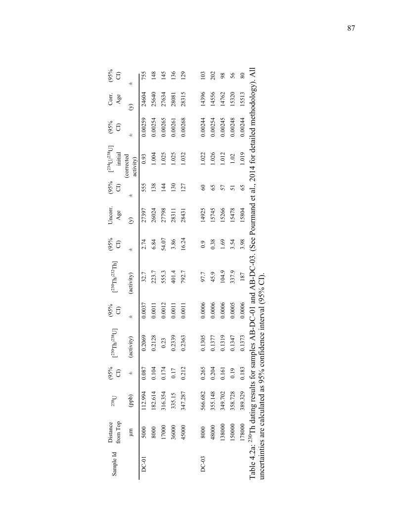
87

Sam

ple

Id

Dis

tanc

e fro

m T

op

238 U

(9

5%

CI)

[23

0 Th/23

8 U]

(95%

C

I)

[230 Th

/232 Th

] (9

5%

CI)

U

ncor

r. A

ge

(95%

C

I)

[234 U

/238 U

] in

itial

(9

5%

CI)

C

orr.

Age

(9

5%

CI)

µm

(p

pb)

± (a

ctiv

ity)

± (a

ctiv

ity)

± (y

) ±

(cor

rect

ed

activ

ity)

± (y

) ±

DC

-01

5000

11

2.99

4 0.

087

0.20

69

0.00

37

32.7

2.

74

2739

7 55

5 0.

93

0.00

259

2460

4 75

5

80

00

182.

614

0.10

4 0.

2128

0.

0011

22

3.7

6.84

26

024

138

1.00

4 0.

0025

4 25

640

148

17

000

316.

354

0.17

4 0.

23

0.00

12

555.

3 54

.07

2779

8 14

4 1.

025

0.00

265

2763

4 14

5

36

000

335.

15

0.17

0.

2339

0.

0011

40

1.4

3.86

28

311

130

1.02

5 0.

0026

1 28

081

136

45

000

347.

287

0.21

2 0.

2363

0.

0011

79

2.7

16.2

4 28

431

127

1.03

2 0.

0026

8 28

315

129

DC

-03

8000

56

6.68

2 0.

265

0.13

05

0.00

06

97.7

0.

9 14

925

60

1.02

2 0.

0024

4 14

396

103

48

000

355.

148

0.20

4 0.

1377

0.

0006

45

.9

0.38

15

745

65

1.02

6 0.

0025

4 14

556

202

13

8000

34

9.70

2 0.

161

0.13

19

0.00

06

104.

9 1.

69

1526

6 57

1.

012

0.00

245

1476

2 98

15

0000

35

8.72

8 0.

19

0.13

47

0.00

05

337.

9 3.

54

1547

8 51

1.

02

0.00

248

1532

0 56

17

8000

38

9.32

9 0.

183

0.13

73

0.00

06

187

3.98

15

804

65

1.01

9 0.

0024

4 15

513

80

Tabl

e 4.

2a: 23

0 Th d

atin

g re

sults

for s

ampl

es A

B-D

C-0

1 an

d A

B-D

C-0

3. (S

ee P

ourm

and

et a

l., 2

014

for d

etai

led

met

hodo

logy

). A

ll un

certa

intie

s are

cal

cula

ted

as 9

5% c

onfid

ence

inte

rval

(95%

CI)

.

88

Dis

tanc

e fro

m T

op

238 U

(9

5% C

I) [23

0 Th/23

8 U]

(95%

C

I)

[230 Th

/232 Th

] (9

5%

CI)

U

ncor

r. A

ge

(95%

CI)

[234 U

/238 U

] in

itial

(9

5%

CI)

C

orr.

Age

(9

5%

CI)

µm

(ppb

) ±

(act

ivity

) ±

(act

ivity

) ±

(y)

± (c

orre

cted

ac

tivity

) ±

(y)

±

1400

0 77

5.20

4 0.

422

0.29

14

0.00

11

268.

1 1.

92

3714

8 14

4 1.

011

0.00

264

3671

2 15

9

5300

0 26

0.53

5 0.

163

0.30

22

0.00

14

490.

8 2.

88

3924

7 19

0 1.

001

0.00

27

3899

9 19

1

8400

0 36

1.55

6 0.

174

0.32

04

0.00

12

249.

3 3.

48

4205

9 16

4 1.

003

0.00

263

4153

9 18

0

1010

00

395.

053

0.35

1 0.

3261

0.

0014

12

66.5

9.

18

4250

0 19

2 1.

012

0.00

29

4239

7 19

1

1330

00

624.

8 0.

29

0.33

09

0.00

13

2330

.9

58.9

2 43

035

164

1.01

7 0.

0026

7 42

979

164

1670

00

301.

034

0.19

2 0.

336

0.00

15

792

8.53

44

287

219

1.00

8 0.

0028

1 44

117

219

1930

00

612.

42

0.27

5 0.

3395

0.

0013

26

54.1

72

.22

4444

4 17

4 1.

017

0.00

263

4439

4 17

4

2150

00

330.

759

0.2

0.35

32

0.00

14

646.

8 36

.18

4703

1 20

6 1.

01

0.00

282

4681

2 20

9

2250

00

537.

129

0.29

5 0.

3648

0.

0014

48

0.3

5.73

48

713

205

1.01

5 0.

0027

9 48

410

211

2280

00

319.

361

0.15

9 0.

3762

0.

0015

92

1.8

18.7

8 50

999

213

1.00

9 0.

0027

6 50

836

215

2300

00

300.

241

0.19

1 0.

384

0.00

17

420.

8 16

.65

5232

7 26

9 1.

009

0.00

287

5196

0 27

4

2350

00

224.

135

0.12

2 0.

4072

0.

0017

11

18.4

10

1.68

56

846

276

1.00

4 0.

0029

8 56

699

277

2400

00

375.

277

0.21

9 0.

4202

0.

0022

51

4.2

3.2

5777

1 36

8 1.

025

0.00

285

5744

9 37

1

2560

00

209.

07

0.10

4 0.

4249

0.

0017

39

3.2

10.8

6 60

592

295

0.99

7 0.

0029

2 60

153

302

2720

00

262.

334

0.16

4 0.

4445

0.

002

1247

.8

61.5

2 62

474

334

1.02

2 0.

0029

3 62

333

335

2880

00

338.

949

0.15

5 0.

4485

0.

0018

12

86.4

23

.23

6316

4 29

9 1.

023

0.00

288

6302

6 30

0

3090

00

535.

342

0.25

5 0.

4554

0.

0018

11

08.7

17

.08

6354

0 27

7 1.

036

0.00

276

6337

9 27

6

Tabl

e 4.

2b: 23

0 Th d

atin

g re

sults

for s

ampl

es A

B-D

C-1

2. (S

ee P

ourm

and

et a

l., 2

014

for d

etai

led

met

hodo

logy

). A

ll un

certa

intie

s are

cal

cula

ted

as 9

5% c

onfid

ence

inte

rval

(95%

CI)

.

89

Figu

re 4

.6: H

endy

test

s for

the

thre

e st

alag

mite

s pre

sent

ed in

this

stud

y. R

esul

ts in

clud

e: a

) thr

ee H

endy

test

s for

sam

ples

A

B-D

C-0

1, b

) thr

ee H

endy

test

s sam

ple

AB

-DC

-03

and

c) fo

ur H

endy

test

s for

sam

ple

AB

-DC

-12.

The

δ13

C v

alue

s are

re

pres

ente

d by

ope

n sq

uare

s, δ18

O v

alue

s by

clos

ed c

ircle

s. R

esul

ts a

re sh

own

as m

m fr

om c

ente

r axi

s. Fo

r the

loca

tion

of

each

of t

he H

endy

test

s, se

e Fi

gure

4.2

.

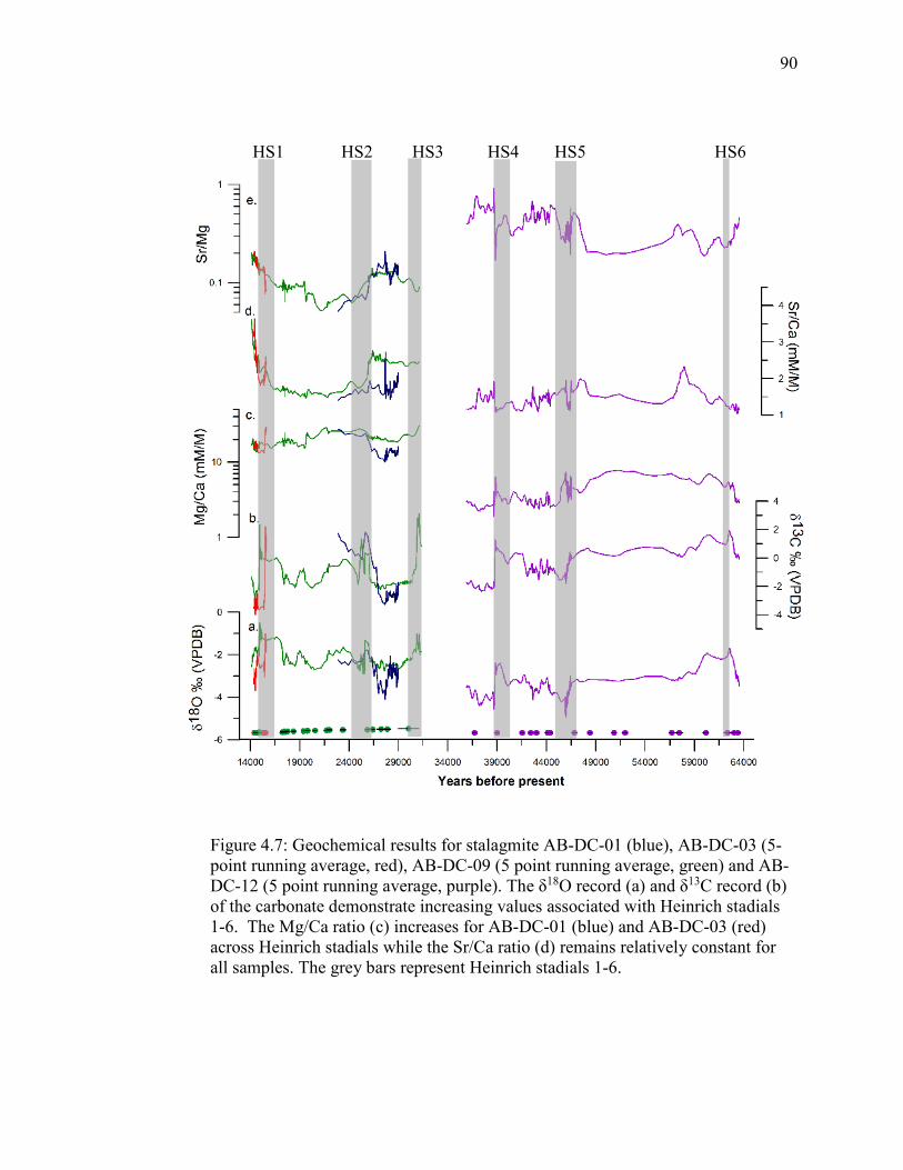
90

HS1 HS2 HS3 HS4 HS5 HS6

Figure 4.7: Geochemical results for stalagmite AB-DC-01 (blue), AB-DC-03 (5-point running average, red), AB-DC-09 (5 point running average, green) and AB-DC-12 (5 point running average, purple). The δ18O record (a) and δ13C record (b) of the carbonate demonstrate increasing values associated with Heinrich stadials 1-6. The Mg/Ca ratio (c) increases for AB-DC-01 (blue) and AB-DC-03 (red) across Heinrich stadials while the Sr/Ca ratio (d) remains relatively constant for all samples. The grey bars represent Heinrich stadials 1-6.

91

positive isotopic shifts at approximately 14.9 to 15.3 ±0.2, 24.8 to 25.5±0.2, 31.1 to 30.9

±1, 38.8 to 40.2±0.2, 46.8 to 47.4 to ±0.2 and 62.2 to 62.8±0.3 ka BP (Figure 4.7 a & b).

Minor elements:

Similar to δ13Cc and δ18Oc results the minor elements are plotted with the age

model in Figure 4.7 c and d. The Mg/Ca values varied between 10 to 34 mM/M with the

exception of sample AB-DC-12 which had a range from 1.8 to 12 mM/M (Figure 4.7 c).

For Sr/Ca the range of values for all samples was between 0.87 to 4.3 mM/M (Figure 4.7

d). There is no evidence from any of the stalagmites for a significant correlation between

Sr/Ca and Mg/Ca. For samples AB-DC-01 and AB-DC-03 there is a positive correlation

between Mg/Ca and δ13Cc (r2 = 0.8, p<0.01), but no other significant correlations were

found (Figure 4.8). For sample AB-DC-09, a maximum Mg/Ca ratio was found at 31 ka

BP and for sample AB-DC-12 a maximum Mg/Ca ratio was found at 46.0 ka BP (Figure

4.7 c). For Sr/Mg ratios, there are relatively minimal changes in the Sr/Mg ratios for

samples AB-DC-01, 03 and 09 (Figure 4.7 e). For Sr/Mg ratio, the variability is 0.15 for

samples AB-DC-01, -03, -09 observed, with AB-DC-12 exhibiting much greater

variability of 0.88 for Sr/Mg.

Fluid inclusions:

In the case of sample AB-DC-12, the δ18Ow of the fluid inclusions was measured

to help with the interpretation of the variability in the δ18Oc values. Periods of higher

δ18Oc values were targeted (Figure 4. 9 a). A comparison of the δ18Ow measured on the

fluid inclusions with the derived age model from U-Th geochronometry demonstrates

minimal variations in the isotopic value of the fluids (Figure 4. 9 b). The δ2Hw and δ18Ow

measured on the fluid inclusions show variations of 10.3 ‰ and 1.7 ‰ over the studied

92

interval with average values of -10.6 ‰ and -2.3 ‰ V-SMOW for δ2Hw and δ18Ow

(Table 4.3, Figure 4.9 b). The variability in δ18Ow value (~1.7 ‰) is relatively small

compared to the changes in the δ18Oc (~3.5 ‰, Figure 4.9 a). The data support a

minimum δ18Ow value at 35.9 ka BP and a maximum δ18Ow value at 39.4 ka BP. The

large break in sampling after 46.5 ka BP is due to there being no water present in the

stalagmite until the sample at 57.5 ka BP.

Comparison of the fluid inclusion results to the global meteoric water line (GMWL) may

shed light on the factors influencing the fluid inclusion data. The GMWL defines the

linear δ18Ow versus δ2Hw relationship for precipitation (Craig, 1961) (Figure 4.10). The

data from the fluid inclusions plot near the GMWL which suggests that samples have not

been significantly fractionated (Figure 4.10). If samples had been significantly

fractionated, then the results would not fall near the GMWL, and rather would fall below

the GMWL. One potential source of contamination is from the stalagmites having been

submerged since the deglaciation. One potential mechanism to determine if seawater has

contaminated the fluid inclusions would be to measure the salt content of the inclusions.

Unfortunately, this was unable to be measured in this stalagmite. However given the

dense crystalline nature of the stalagmite and the lack of any evidence of seawater

infiltration, it is not thought that seawater has contaminated this speleothem.

Additionally, Richards et al. (1994) demonstrated minimal impact of submersion on

geochemistry.

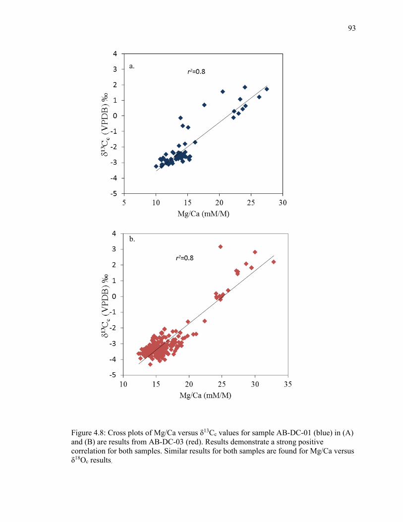
93

Figure 4.8: Cross plots of Mg/Ca versus δ13Cc values for sample AB-DC-01 (blue) in (A) and (B) are results from AB-DC-03 (red). Results demonstrate a strong positive correlation for both samples. Similar results for both samples are found for Mg/Ca versus δ18Oc results.

a. b.

94

HS4

HS5

H

S6

Figu

re 4

.9: F

luid

incl

usio

n re

sults

for s

tala

gmite

AB

-DC

-12.

The

δ18

Oc r

ecor

d (a

) is s

how

n in

ligh

t blu

e, w

ith a

5 p

oint

runn

ing

aver

age

in p

urpl

e, d

emon

stra

ting

incr

easi

ng δ

18O

c for

Hei

nric

h st

adia

ls 4

and

5. B

) Th

e flu

id in

clus

ion

isot

ope

reco

rd δ

18O

w

dem

onst

rate

s min

imal

cha

nge

in th

e δ18

Ow

acro

ss th

e tim

e in

terv

al.

C) T

empe

ratu

res v

arie

d, w

ith d

ecre

asin

g te

mpe

ratu

res a

ssoc

iate

d w

ith in

crea

sed

δ18O

c val

ues.

Tem

pera

ture

was

cal

cula

ted

usin

g th

e eq

uatio

n fr

om T

rem

aine

et a

l. (2

011)

. Gre

y ba

rs in

dica

te th

e tim

ing

of H

einr

ich

stad

ials

4 5

and

6

95

cm from top Age

Average δ18Ow

Average δ2Hw n δ18Oc Temperature

YBP ‰

(VSMOW) ‰

(VSMOW) ‰ (VPDB) (°C) ± 0.5 ‰ ± 2.0 ‰ ± 2.7 °C 0 35892 -3.2 -9.2 2 -3.3 19.8

0.8 36332 -2.5 -13.1 2 -3.7 25.9 2.3 37257 -2.1 -8.4 1 -2.5 21.6 4.0 38254 -2.4 -12.5 2 -3.7 26.5 4.6 38605 -2.1 -6.7 2 -2.8 23.4 5.7 39354 -1.6 -9.5 1 -2.8 26.1 6.8 40256 -2.2 -8.6 1 -3.2 24.8 9.0 41834 -1.7 -13.3 1 -3.1 26.8

18.0 44252 -3.1 -16.5 1 -4.1 24.6 18.4 44290 -3.0 -10.0 1 -4.0 25.0 18.8 44332 -1.9 -11.3 1 -3.6 28.2 20.3 45433 -2.6 -14.8 1 -4.2 28.1 21.3 46532 -1.9 -6.2 2 -2.9 24.7 24.0 57451 -2.0 -8.0 1 -3.2 25.5

Table 4.3: Fourteen fluid inclusion results for sample AB-DC-12. Temperature is calculated using the equation from Tremaine et al. (2011).

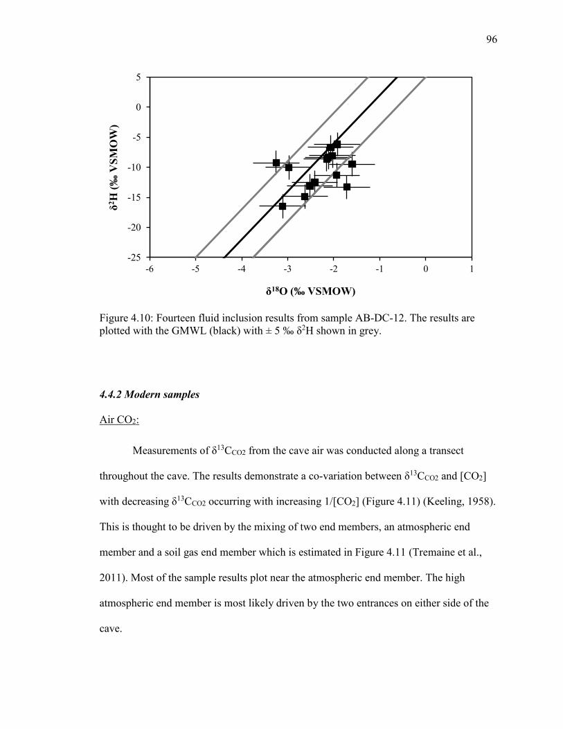
96

Figure 4.10: Fourteen fluid inclusion results from sample AB-DC-12. The results are plotted with the GMWL (black) with ± 5 ‰ δ2H shown in grey. 4.4.2 Modern samples

Air CO2:

Measurements of δ13CCO2 from the cave air was conducted along a transect

throughout the cave. The results demonstrate a co-variation between δ13CCO2 and [CO2]

with decreasing δ13CCO2 occurring with increasing 1/[CO2] (Figure 4.11) (Keeling, 1958).

This is thought to be driven by the mixing of two end members, an atmospheric end

member and a soil gas end member which is estimated in Figure 4.11 (Tremaine et al.,

2011). Most of the sample results plot near the atmospheric end member. The high

atmospheric end member is most likely driven by the two entrances on either side of the

cave.

-25

-20

-15

-10

-5

0

5

-6 -5 -4 -3 -2 -1 0 1

δ2 H (‰

VSM

OW

)

δ18O (‰ VSMOW)

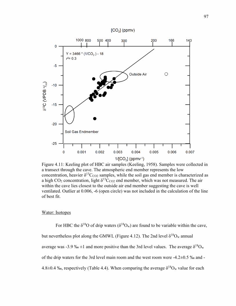
97

Figure 4.11: Keeling plot of HBC air samples (Keeling, 1958). Samples were collected in a transect through the cave. The atmospheric end member represents the low concentration, heavier δ13CCO2 samples, while the soil gas end member is characterized as a high CO2 concentration, light δ13CCO2 end member, which was not measured. The air within the cave lies closest to the outside air end member suggesting the cave is well ventilated. Outlier at 0.006, -6 (open circle) was not included in the calculation of the line of best fit. Water: Isotopes

For HBC the δ18O of drip waters (δ18Ow) are found to be variable within the cave,

but nevertheless plot along the GMWL (Figure 4.12). The 2nd level δ18Ow annual

average was -3.9 ‰ ±1 and more positive than the 3rd level values. The average δ18Ow

of the drip waters for the 3rd level main room and the west room were -4.2±0.5 ‰ and -

4.8±0.4 ‰, respectively (Table 4.4). When comparing the average δ18Ow value for each

98

location by sample month, the August 2012 results from the second level are the most

positive (Figure 4.13). These findings are compared to modeled rainfall δ18Ow values

from Baldini et al. (2007) for San Salvador, Bahamas in Figure 4.13a. The results

demonstrate seasonality in the second floor drip water results as well as a possible 2

month residence time when compared to the San Salvador data (Figure 4.13 a). Also

observed on the 2nd level was an inverse correlation between rainfall amount and drip

water δ18Ow value (Figure 4.13 a & b). While there is observed variability on the 2nd

level, the drip water δ18Ow values of the third level are annually very stable and do not

exhibit seasonality (Figure 4.13 a).

Figure 4.12: δ18Ow and δ2Hw for drip water samples from the 2nd level (light blue), 3rd level main (dark blue) and 3rd level west (green triangles). Results are plotted on the GMWL (black) with ± 5 ‰ δ2H shown in grey. Average errors are shown in the upper left corner in black.

-40

-35

-30

-25

-20

-15

-10

-5

-6.5 -5.5 -4.5 -3.5 -2.5

δ2H

‰ V

SMO

W

δ18O ‰ VSMOW

GMWL2nd Level3rd Level Main

99

Figure 4.13: Relationship between rainfall and drip waters. A) Monthly rainfall δ18Ow value from San Salvador, Bahamas shown in black. Precipitation oxygen isotope data are from Baldini et al. (2007). Light blue is 2nd level δ18Ow drip water results. Dark blue squares are 3rd level main room and green triangles are 3rd level west room. Note the preliminary 2nd level seasonal changes in δ18Ow drip water particularly when compared to the San Salvador results. B) Amount of precipitation by month for the Bahamas. Precipitation amount data are from San Salvador, Bahamas from Baldini et al. (2007). C) δ18Ow of precipitation versus precipitation amount demonstrating the relationship between the two.

100

δ1

8Ow

σ

δ2Hw

σ

Sr/C

a σ

Mg/

Ca

σ C

l-

‰ V

SMO

W

‰

VSM

OW

ppm

2n

d Le

vel

-3.9

1.

0 -2

1.3

7.1

2.2

0.4

509

132.

0 53

9 3r

d Le

vel M

ain

-4.2

0.

5 -2

4.9

2.9

2.4

0.6

956

280.

4 20

25

3rd

Leve

l Wes

t -4

.8

0.4

-29.

6 2.

0 2.

2 0.

2 10

05

76.9

28

11

Tabl

e 4.

4: A

nnua

l ave

rage

wat

er re

sults

from

the

2nd,

3rd

leve

l mai

n an

d 3r

d le

vel w

est l

ocat

ions

. R

esul

ts

incl

ude

both

isot

opic

and

min

or e

lem

ent r

esul

ts.

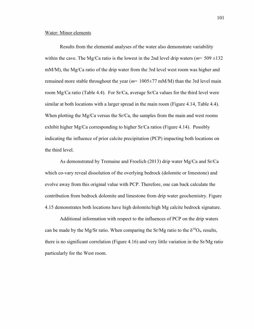
101

Water: Minor elements

Results from the elemental analyses of the water also demonstrate variability

within the cave. The Mg/Ca ratio is the lowest in the 2nd level drip waters (m= 509 ±132

mM/M), the Mg/Ca ratio of the drip water from the 3rd level west room was higher and

remained more stable throughout the year (m= 1005±77 mM/M) than the 3rd level main

room Mg/Ca ratio (Table 4.4). For Sr/Ca, average Sr/Ca values for the third level were

similar at both locations with a larger spread in the main room (Figure 4.14, Table 4.4).

When plotting the Mg/Ca versus the Sr/Ca, the samples from the main and west rooms

exhibit higher Mg/Ca corresponding to higher Sr/Ca ratios (Figure 4.14). Possibly

indicating the influence of prior calcite precipitation (PCP) impacting both locations on

the third level.

As demonstrated by Tremaine and Froelich (2013) drip water Mg/Ca and Sr/Ca

which co-vary reveal dissolution of the overlying bedrock (dolomite or limestone) and

evolve away from this original value with PCP. Therefore, one can back calculate the

contribution from bedrock dolomite and limestone from drip water geochemistry. Figure

4.15 demonstrates both locations have high dolomite/high Mg calcite bedrock signature.

Additional information with respect to the influences of PCP on the drip waters

can be made by the Mg/Sr ratio. When comparing the Sr/Mg ratio to the δ18Ow results,

there is no significant correlation (Figure 4.16) and very little variation in the Sr/Mg ratio

particularly for the West room.

102

Figure 4.14 Mg/Ca versus Sr/Ca results for drip water samples from the 3rd floor main (dark blue) and 3rd floor west (green triangles).

0

0.5

1

1.5

2

2.5

3

3.5

4

0 200 400 600 800 1000 1200 1400

Sr/C

a (m

M/M

)

Mg/Ca (mM/M)

3rd Fl Main3rd Fl West

103

Figure 4.15: Drip water Sr/Ca and Mg/Ca data plotted with PCP vector in orange. The PCP vector is modeled after (Tremaine and Froelich, 2013) using dissolved limestone bedrock mixtures. For this study, the bedrock limestone was assumed to have a Mg/Ca of 9 mM/M, dolomite 1000 mM/M. The Sr/Ca value was assumed to be 1.99 mM/M, and it was assumed that the contribution from sea salts was negligible. Data in (a) are from the Main room drip waters, and data in (b) are from the West room drip waters. Results demonstrate a greater dolomite contribution to the West room (90%) versus the Main room (80%), however overall the samples demonstrate a high dolomite or Mg calcite bedrock. Future work will measure the Sr/Ca and Mg/Ca of bedrock around the cave. The greatest Mg/Ca and Sr/Ca values for both the Main and West rooms were found in November 2013, which was the beginning of the dry season. Further work is needed to verify the seasonality of the trace elements.

0

1

2

3

4

5

0 500 1000 1500

Sr/C

a (m

Mol

/Mol

)

Mg/Ca (mM/M)

PCP Vector: 80% Dolomite; Lowest [Sr]

0

1

2

3

4

5

0 500 1000 1500

Sr/C

a (m

M/M

)

Mg/Ca (mM/M))

PCP Vector: 90% Dolomite; Lowest [Sr]

a.

b.

104

Figure 4.16: Drip water Sr/Mg versus δ18Ow for drip water. Sr/Mg relationship is relatively unchanging particularly for the West room. Calcite: Elements and isotopes

For the precipitated calcite from the modern, the concentration of minor elements

varied amongst different sites. The average Sr/Ca ratio from WS location was 0.3 and for

Mg/Ca was 23.2 ±1.5 mM/M (Table 4.5). The values from ES and MS locations were

similar, with the MS containing higher Mg/Ca ratios (Tale 4.5). The results from the WS

and ES sites fell on a positive co-varying trend for Sr/Ca versus Mg/Ca (r2=0.8, n=10,

p<0.01) while results from the MS location exhibited a much greater minor element

variability (Figure 4.17).

A complete interpretation of the δ13Cc and δ18Oc from the slides are provided in

Chapter 5 and for this study the δ13Cc and δ18Oc will be considered in terms of the

relationship with minor element results only. The Mg/Ca versus δ18Oc results

105

δ18

Oc

σ δ13

Cc

σ Sr

/Ca

σ M

g/C

a σ

‰

VPD

B

‰

VPD

B

m

M/M

mM

/M

ES

-4

.6

0.6

-9.4

7.

1 0.

4 0.

03

28.6

1.

5 M

S -3

.9

0.6

-8.8

2.

9 0.

5 0.

07

37.5

3.

9 W

S -5

.1

0.3

-10.

9 2.

0 0.

3 0.

01

23.2

1.

5

Tabl

e 4.

5: A

nnua

l ave

rage

cal

cite

resu

lts fr

om th

e ES

, MS

and

WS

loca

tions

. R

esul

ts in

clud

e bo

th is

otop

ic a

nd

min

or e

lem

ent r

esul

ts.

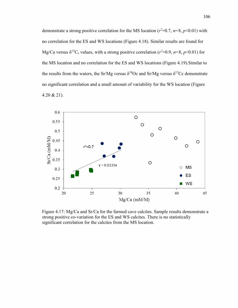
106

demonstrate a strong positive correlation for the MS location (r2=0.7, n=8, p<0.01) with

no correlation for the ES and WS locations (Figure 4.18). Similar results are found for

Mg/Ca versus δ13Cc values, with a strong positive correlation (r2=0.9, n=8, p<0.01) for

the MS location and no correlation for the ES and WS locations (Figure 4.19).Similar to

the results from the waters, the Sr/Mg versus δ18Oc and Sr/Mg versus δ13Cc demonstrate

no significant correlation and a small amount of variability for the WS location (Figure

4.20 & 21).

Figure 4.17: Mg/Ca and Sr/Ca for the farmed cave calcites. Sample results demonstrate a strong positive co-variation for the ES and WS calcites. There is no statistically significant correlation for the calcites from the MS location.

107

Figure 4.18: Mg/Ca versus δ18Oc for the cave calcites. Results demonstrate a positive co-variation for the MS location. There is no statistically significant correlation for the calcites from the WS or ES location.

Figure 4.19: Mg/Ca versus δ13Cc for the cave calcites. Sample results demonstrate a high positive co-variation for the MS location. There is no statistically significant correlation for the calcites from the WS or ES location.

108

Figure 4.20: Sr/Mg versus δ18Oc demonstrating no significant correlation for MS location and the least amount of spread for the WS location.

Figure 4.21: Sr/Mg versus δ13Cc demonstrating no significant correlation for MS location and the least amount of spread for the WS location.

109

4.5 Discussion

4.5.1 Oxygen and carbon isotopes: records of temperature?

Ancient:

The higher δ13Cc and δ18Oc values at ~15.2±0.2, 25±0.2, 30.9±1, 38.8±0.2, 47±0.2

and 62.4±0.3 ka BP are associated with Heinrich stadials 1-6 as supported by the good

agreement between the timing of Heinrich stadials in the Bahamas record and other

paleoproxies (Figure 4.22) (Deplazes et al., 2013; Peterson et al., 2000; Wang et al.,

2001). In addition, there is evidence for more negative δ13Cc and δ18Oc values associated

with D/O interstadials 3, 4, 8, 9, 11 and 12 and the timing of these negative changes are

shown to correlate with other records (Figure 4.22). The isotopic shifts associated with

D/O interstadials are not as significant as the shifts associated with Heinrich stadials and

are on the order of ~0.5 ‰ (3, 4, 8, 9, 11 ) to ~1‰ (12) for δ18Oc and δ13Cc (Figure 4.22).

The interpretation that the changes in the δ13Cc and δ18Oc values are due to by climatic

events is geochemically supported by the fact that multiple speleothems from the same

cave record similar changes over time intervals which overlap. This validates that the

geochemistry records climatic changes and is not influenced by kinetic isotope effects.

As previously suggested, the interpretation of δ13Cc and δ18Oc of the carbonate is

inherently complex and therefore the carbon and oxygen results will be summarized

below with the interpretation of the minor elements and fluid inclusion isotope results.

Fluid inclusion isotopes:

The δ18Oc record for stalagmite AB-DC-12 exhibits maximum values at ~38.8

and 46.6 ka BP associated with Heinrich stadials 4 and 5 (Figure 4.9). The higher δ18Oc

values are either due to higher δ18Ow values or a lower temperature. Changes in the

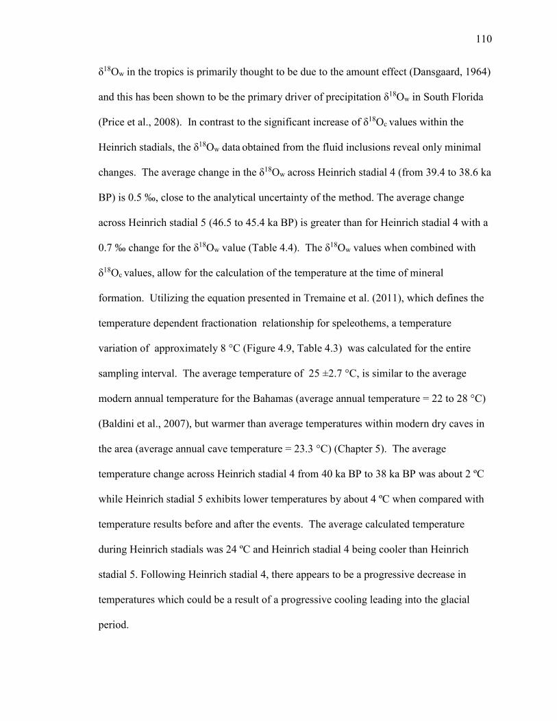
110

δ18Ow in the tropics is primarily thought to be due to the amount effect (Dansgaard, 1964)

and this has been shown to be the primary driver of precipitation δ18Ow in South Florida

(Price et al., 2008). In contrast to the significant increase of δ18Oc values within the

Heinrich stadials, the δ18Ow data obtained from the fluid inclusions reveal only minimal

changes. The average change in the δ18Ow across Heinrich stadial 4 (from 39.4 to 38.6 ka

BP) is 0.5 ‰, close to the analytical uncertainty of the method. The average change

across Heinrich stadial 5 (46.5 to 45.4 ka BP) is greater than for Heinrich stadial 4 with a

0.7 ‰ change for the δ18Ow value (Table 4.4). The δ18Ow values when combined with

δ18Oc values, allow for the calculation of the temperature at the time of mineral

formation. Utilizing the equation presented in Tremaine et al. (2011), which defines the

temperature dependent fractionation relationship for speleothems, a temperature

variation of approximately 8 °C (Figure 4.9, Table 4.3) was calculated for the entire

sampling interval. The average temperature of 25 ±2.7 °C, is similar to the average

modern annual temperature for the Bahamas (average annual temperature = 22 to 28 °C)

(Baldini et al., 2007), but warmer than average temperatures within modern dry caves in

the area (average annual cave temperature = 23.3 °C) (Chapter 5). The average

temperature change across Heinrich stadial 4 from 40 ka BP to 38 ka BP was about 2 ºC

while Heinrich stadial 5 exhibits lower temperatures by about 4 ºC when compared with

temperature results before and after the events. The average calculated temperature

during Heinrich stadials was 24 ºC and Heinrich stadial 4 being cooler than Heinrich

stadial 5. Following Heinrich stadial 4, there appears to be a progressive decrease in

temperatures which could be a result of a progressive cooling leading into the glacial

period.

111

Overall the temperatures calculated from sample AB-DC-12 are higher than

previously reported for sample AB-DC-09, by approximately 8 °C (Chapter 3). As

sample AB-DC-12 was collected from a shallower depth (11.9 m versus 16.5 m) than

stalagmite AB-DC-09, it is possible that the cave environment between the two samples

was different. Since sample AB-DC-12 was a shallower sample, it is possible that the

sample was impacted by increased ventilation, which has been shown to influence

speleothem geochemistry via evaporation (Kowalczk and Froelich, 2010; Tremaine et al.,

2011). Additionally there may be variations in the residence time of the water in the

epikarst between the two stalagmites, which may cause one stalagmite to be offset from

the other. As shown in HBC, there is a 0.5 up to 1.0 ‰ difference in the δ18Ow of the drip

water within the cave. If we assume the drip water δ18Ow values for AB-DC-12 are

systematically higher relative to the drip water of AB-DC-09, and apply a correction of 1

‰ to the δ18Ow value, the average temperature difference between the two stalagmites

decreases to ~2.4 °C, which is within the uncertainty of the measurements. Finally,

sample AB-DC-09 formed during the LGM which may have been cooler, and in the

youngest portion of sample AB-DC-12, temperatures begin to decline.

Even with the temperature differences between the two stalagmites, there are

many similarities in the two fluid inclusion records. Overall the average temperature

change across Heinrich stadials 4 and 5 for sample AB-DC-12 is similar (~3 °C) to the

average temperature changes observed in sample AB-DC-09 for Heinrich stadials 1 -3

(~3 °C). The fluid inclusion results from samples AB-DC-09 and AB-DC-12 do not

suggest a significant change in the δ18Ow across Heinrich stadials, but rather both records

agree that Heinrich stadials are characterized by lower temperature and higher δ18Oc

112

values. These results support the main driver of the higher δ18Oc values at 15.2±0.2,

25±0.2, 30.9±1, 38.8±0.2, 47±0.2 and 62.4±0.3 ka BP associated with Heinrich stadials

1-6 are due to temperature decreases.

Oxygen isotopes of modern drip water:

There are variations observed within the oxygen isotopes of HBC drip water

including: 1) second level potentially exhibits greater variation, 2) the 2nd level

potentially consists of overall higher δ18Ow values and 3) the west room may exhibit a

lower average δ18Ow value compared to the main room. In contrast to the ancient, there is

no evidence from the modern for a temperature control on the δ18Oc values. Rather, the

δ18Ow of the modern drip water for the 2nd level negatively correlates with rainfall

amount, as would be expected for the ‘amount effect’ driving isotope variability

(Dansgaard, 1964). Also there appears to be seasonality to the δ18Ow of the modern drip

water however, more data is needed to verify this. Variations in the δ18Ow of the modern

drip water samples from throughout the cave were approximately <1‰, lower than the

range observed in modern rainfall of South Florida and San Salvador, Bahamas (Baldini

et al., 2007; Price et al., 2008) as would be expected due to longer residence times in the

epikarst. The third level δ18Ow is characterized by less annual variability than the second

level, which suggests that the waters feeding the third level undergo an even longer

residence time allowing for the homogenization and integration of the δ18Ow seasonal

signal. When compared with the δ18Ow of precipitation model results (Baldini et al.,

2007), the δ18Ow value of the drip waters feeding the third level are primarily derived

from wet season precipitation, which is the most negative δ18Ow value (Tremaine and

Froelich, 2013)(Figure 4.13). Other studies of cave drip waters demonstrate more

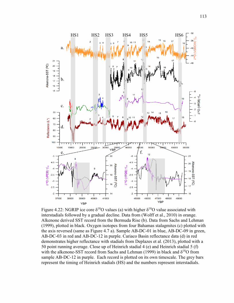
113

Figure 4.22: NGRIP ice core δ18O values (a) with higher δ18O value associated with interstadials followed by a gradual decline. Data from (Wolff et al., 2010) in orange. Alkenone derived SST record from the Bermuda Rise (b). Data from Sachs and Lehman (1999), plotted in black. Oxygen isotopes from four Bahamas stalagmites (c) plotted with the axis reversed (same as Figure 4.7 a). Sample AB-DC-01 in blue, AB-DC-09 in green, AB-DC-03 in red and AB-DC-12 in purple. Cariaco Basin reflectance data (d) in red demonstrates higher reflectance with stadials from Deplazes et al. (2013), plotted with a 50 point running average. Close up of Heinrich stadial 4 (e) and Heinrich stadial 5 (f) with the alkenone-SST record from Sachs and Lehman (1999) in black and δ18O from sample AB-DC-12 in purple. Each record is plotted on its own timescale. The grey bars represent the timing of Heinrich stadials (HS) and the numbers represent interstadials.

a. b. c. d.

e. f.

HS1 HS2 HS3 HS4 HS5 HS6

114

negative δ18Ow values of the water deeper in the cave, also due to the deeper parts of the

cave being fed when rainfall is high and δ18Ow value is low (Baldini et al., 2007;

Dansgaard, 1964; Genty et al., 2014).

An additional factor that may lead to the higher δ18Ow values in the main room

versus the west room is higher evaporation in the epikarst, soil zone or within the cave

during calcite precipitation, which may result in heavier δ18Ow values. The increasing Cl-

concentration (as well as the other ions) within the cave with depth suggests that

evapotranspiration is occurring. The third level west room exhibits the highest Cl-

concentrations (discussed further in section 4.5.2) suggesting these waters maybe

impacted by evapotranspiration (Tremaine and Froelich, 2013). Direct evaporation with

in the cave can occur via ventilation and as shown in Figure 4.11, the CO2 concentration

of the cave air represents a mixture between the outside atmospheric air and a soil gas

end member. Most of the air samples plot near the atmospheric end member suggesting

that the cave is well ventilated and heavily impacted by atmospheric air, via ventilation.

Increased ventilation and hence lower [CO2] can lead to enhanced evaporation (Tremaine

et al., 2011). If evaporation is a significant contributor to the δ18Ow value, the δ18Ow and

δ2Hw data of the drip water would not fall on the GMWL at this location, rather the drip

waters would fall below the GMWL (Gat, 1996). Therefore, it does not appear that

evaporation is significantly impacting the δ18Ow value.

The drip water results from the modern also may explain the difference in the

δ18Ow values between sample AB-DC-09 and DC-12 from the fluid inclusion analyses.

Sample AB-DC-09 was collected from a deeper section of the cave, therefore may lead to

an overall more annually homogenized and hence lower δ18Ow value.

115

4.5.2 Minor elements: records of precipitation amount?

In interpreting the trace element concentration of the cave, it is important to

understand the various factors that can influence the drip water chemistry including: (1)

bedrock dissolution, and bedrock type, (2) mixing of waters from different bedrocks and

(3) Prior Calcite Precipitation.

Ancient speleothems: Magnesium

Changes in Mg concentration in stalagmites have been suggested to arise from

variations in Mg concentration of the bedrock, water/rock interactions, the amount of

PCP and temperature (Fairchild and Treble, 2009). Two stalagmites (AB-DC-01 and 03)

collected from the deepest depths (33.5 and 34.4 m below sea level) contain a high

correlation between the concentration of Mg and δ13Cc values. Typically, co-variation in

Sr/Ca and Mg/Ca ratios are associated with PCP and therefore PCP is not thought to be

driving the high correlation between Mg and δ13Cc values. Rather, the higher Mg

concentration may be a result of two factors: i) increased dolomite in the bedrock, and ii)

slower flow rates in the epikarst. Studies show that on Abaco Island, there is dolomite

present ~24.3 m below the surface (Kaldi and Gidman, 1982) and the two samples (AB-

DC-01 and -03) with a high correlation between Mg and δ13Cc values are located within

the dolomitized interval. Other studies which have been conducted on speleothems

forming within dolomitic bedrock observed elevated Mg/Ca ratios and periods of

lowered flow rates further elevated Mg/Ca ratios (Fairchild et al., 2000), as the dolomite

provides a source for Mg. The associated higher δ13Cc values is also impacted by lower

flow rates, leading to lower biogenic CO2 component of the DIC (Cruz et al., 2006). The

periods of higher Mg/Ca and δ13Cc values for stalagmites AB-DC-01 and 03 are

116

associated with Heinrich stadials 1 and 2 suggesting that Heinrich stadials in the

Bahamas are characterized by increased aridity (Figure 4.7). Possibly the higher Mg/Ca

ratio observed at 31 ka BP for stalagmite AB-DC-09 is due to increased aridity and a

greater bedrock component.

The overall lower Mg/Ca ratio in speleothem AB-DC-12 may be due to the fact

that this stalagmite was the shallowest sample, and therefore contained lower

concentrations of Mg relative to Ca. Previous studies have also demonstrated lower

minor element concentrations shallower in the cave (Verheyden, 2004). Similarly, in the

modern, the shallowest drip water samples (second floor) also exhibited the lowest

Mg/Ca ratios.

Ancient speleothems: Strontium

The concentration of Sr remains relatively invariant in most of the stalagmites

across Heinrich and D/O events. There are, however, periods of higher Sr/Ca ratios,

which are not associated with changes in Mg/Ca ratio. Both stalagmites AB-DC-09 and

AB-DC-03 exhibit higher Sr/Ca ratio starting at approximately 14.6 ka BP. This period

is characterized by higher amounts of rainfall (based on fluid inclusion δ18Ow results and

δ18Oc results), which may lead to the higher Sr/Ca values and the low Mg/Ca values. This

possibly suggests that during wetter periods, the flow paths for the drip water change,

leading to a greater Sr bedrock signature driving the variations in minor elements (Tooth

and Fairchild, 2003). Studies also demonstrate that the incorporation of Sr in stalagmites

can be influenced by growth rates (Huang and Fairchild, 2001; Lorens, 1981). Both of

these factors may influence the higher Sr/Ca ratio of AB-DC-09 and -03 at 14.6 ka BP.

117

Comparing the Sr/Mg ratio can be useful for identifying the factors influencing

elemental concentrations in speleothems. Constant Sr/Mg ratio would be expected if PCP

was driving the elemental concentration. Non-constant Sr/Mg was shown by (Tremaine

and Froelich, 2013) to be driven by changes in bedrock mixing, cave morphology,

temperature changes, growth rate, mineralogy, and incongruent dissolution of bedrock. It

appears that stalagmite AB-DC-12 contains largest changes in the Sr/Mg ratio than the

other stalagmites (Figure 4.7) possibly driven by the overall lower Mg/Ca ratio in this

sample compared to the other samples. However, all of the stalagmites exhibit variability

in Sr/Mg ratios, supporting that PCP is not the primary driver of the elemental variations

in these stalagmites.

Modern minor elements: Water and calcite

Elemental variability of drip waters within the same cave has been observed in

several studies (Fairchild et al., 2000; Genty et al., 2014; Partin et al., 2013; Tremaine

and Froelich, 2013; Verheyden et al., 2000). Such variability within cave water has been

suggested to be due to the variations in the routing path and the residence time of the

water (Tooth and Fairchild, 2003). From a cave in Borneo PCP influences minor

elements at one location, while minor elements at other sites are influenced by residence

time at other sites (Partin et al., 2013). In HBC, a similar variability is found suggesting

that two different processes are occurring within the same cave.

Prior calcite precipitation is the primary driver of minor element variability in

calcites from many caves (Fairchild and Treble, 2009; Partin et al., 2013; Tremaine and

Froelich, 2013). The observed positive co-varying trend between Sr/Ca and Mg/Ca in the

drip waters and calcites of HBC supports that PCP is the primary driver of the elemental

118

variability of the calcite precipitated at the WS and ES sites. The lower Sr/Ca and Mg/Ca

ratios observed in the WS compared with the ES site calcite may be indicative of less

PCP occurring, as with increasing PCP, Sr and Mg concentrations will be higher

(Tremaine and Froelich, 2013). As shown by Tremaine and Froelich (2013) with

increased evapotranspiration (lower net rainfall, drier epikarst) there is an increase in

PCP. The extent of PCP in the karst is controlled by fluctuations in net rainfall amount

(Precipitation minus Evapotranspiration) which can affect the amount of PCP (Tremaine

and Froelich, 2013). With decreasing net rainfall, there will be a decrease in hydrologic

head and therefore a reduction in drip rate. Considering the Bahamas rainfall seasonality,

this would create a generally lower net rainfall during the dry season. Evapotranspiration

is shown in a cave in Florida to lead to increased concentration of Cl- (Tremaine and

Froelich, 2013) while transpiration is not shown to impact the δ18Ow or δ2Hw of soil

water. Therefore the increased Cl- deeper in the cave may be due to evapotranspiration

processes influencing the water in this region in the overlying karst, and hence the

increased ionic concentrations. Considering the close proximity of the cave to the ocean,

there is the possibility of increased Cl- in the drip waters due to sea spray. The West

room is an interesting location as this location not only has slightly higher Cl-

concentration and the lowest δ18Ow values, suggesting the drip waters here are driven by

either increased evapotranspiration or a pool of saline water above it, both which could

account for the increased ionic concentration and the lowest δ18Ow values. The Wet

room is thought to have the highest water throughput and the stalagmites were

precipitating from active stalactites. The Sr/Ca and Mg/Ca ratios suggest that the West

119

room exhibits the least amount of evaporation and hence the lowest Sr/Ca and Mg/Ca

ratios.

Opposite to the ES and WS sites, at the MS site, calcite does not exhibit co-

varying Mg/Ca and Sr/Ca ratios. At the MS location, Mg and Sr concentrations are

characterized by much greater variability of both, due to an increased bedrock signature

feeding this location. This interpretation is supported by the strong relationship between

Mg/Ca and δ18Oc and δ13Cc values (Fairchild et al., 2000; Tremaine and Froelich, 2013).

Fairchild et al. (2000) demonstrated that higher Mg/Ca ratio occurred during periods of

increased water-rock interactions and during periods of increased aridity. In fact, at the

MS location, the periods of higher Mg/Ca, δ18O and δ13C values are during the dry season

(January to May) when residence time is thought to be greatest due to a decrease in the

amount of precipitation (Figure 4.23).

These interpretations are supported by the Sr/Mg ratio of the calcite results, which

demonstrate the least amount of spread in the Sr/Mg for the WS location (variability =

0.0035 Sr/Mg) and the greatest spread in the MS results (variability = 0.008 Sr/Mg)

(Figure 4.20 & 21). These results support PCP driven variability for the WS location, and

hence limited Sr/Mg spread (Tremaine and Froelich, 2013). While the MS location

exhibits increased Sr/Mg variability due to increased water-rock interaction at this

location. This observed variability in the modern is much less than the Sr/Mg variability

observed in the ancient stalagmites.

120

Figure 4.23: Summary of findings from the monitoring study of HBC. Results suggest the 3rd level west room is characterized by PCP, the MS location is characterized by greater water/rock interactions and the ES contains evidence of increased PCP. In contrast the second level exhibits lower Mg/Ca and higher δ18Ow values. The increased PCP at the East Site may be due to increased ventilation, evaporation in the soil zone, or increased residence time in the epikarst.

121

As demonstrated by Tremaine and Froelich (2013) drip water Mg/Ca and Sr/Ca

which co-vary are impacted by dissolution of the overlying bedrock (dolomite or

limestone) and evolve away from this original value with increasing PCP. Therefore, one

can back calculate the contribution from bedrock dolomite and limestone from drip water

geochemistry which has been impacted by prior calcite precipitation. The results

demonstrate a significant contribution of dolomite to both the West and Main locations.

However this was conducted with assumptions of the bedrock minor element

concentrations and future studies will analyze the bedrock trace elements.

To summarize, evaporative processes are thought to impact the ionic

concentrations of the third floor drip waters. PCP has been demonstrated to occur in two

of the three site and is found to be the most severe in the East Main site. The difference

in PCP in the East versus West sites is thought to be a result of a greater residence time of

the waters in the East site or due to ventilation differences. In contrast to the East and

West site, the Main site is dominated by bedrock mixing. When comparing with the

results from the ancient stalagmites, there is no evidence of PCP driving the elemental

variability of the past, as is supported by the lack of Mg/Ca versus Sr/Ca correlation and

the variable Sr/Mg ratio.

4.6 Interpretation of Paleoclimate Results: Comparison with Atlantic Proxies

Below follows a brief interpretation of the regional paleoclimate across millennial

scale climate events, to place the Bahamas records in a regional context. The

geochemistry of stalagmites AB-DC-01, -03, -09 and 12 are compared to published

paleoclimate records from the Atlantic.

122

4.6.1 Heinrich stadials

The geochemical records from stalagmites presented in this paper, and from other

proxies from the subtropical/tropical western Atlantic indicate cooling associated with

Heinrich stadials as a result of lowered SSTs in the North Atlantic (Hagen and Keigwin,

2002; Hodell et al., 2012; Keigwin and Jones, 1994). This cooling is observed in an

alkenone-derived SST record from the Bermuda rise (MD95-2038), located north of the

Bahamas (Sachs and Lehman, 1999) (Figure 4.1). The alkenone derived SST record

supports a 4-5 ºC decline in SSTs during Heinrich stadials 4 and 5 (Sachs and Lehman,

1999). When comparing the Bermuda Rise record to the Bahamian speleothem record,

the two records agree with the timing of Heinrich stadial 4 and 5 within the error of the

age models. The shift to cooler temperatures across Heinrich stadials in the Bermuda

Rise record is greater for Heinrich stadial 4 than for Heinrich stadial 5 (Figure 4.22) and

in the Bahamas record, Heinrich stadial 5 is characterized by a smaller isotopic change in

δ13Cc and δ18Oc values (Figure 4.22 e & f). However, the fluid inclusion results support a

greater decline in temperatures associated with Heinrich stadial 5 than Heinrich stadial 4

(Figure 4.9). One important consideration is that the Bahamas is dominated by seasonal

rainfall (Figure 4.13), there may be enhanced precipitation of calcite during the rainy

season, which may bias results to a rainy season signal. This however should not impact

the temperature record as temperature of the cave is thought to reflect mean annual

temperature. Sea surface temperatures in the northern hemisphere are thought to decline

during these events as a result of the shutdown of the AMOC, possibly driving the lower

temperature observed in the Bahamas (Deplazes et al., 2013; McManus et al., 2004).

123

For the δ13Cc results, the interpretation is more complex. As previously suggested,

the biogenic CO2 component of the soil will decrease during periods of lowered

biological activity. Lowered soil biological activity can occur during periods of lowered

temperatures or increased aridity (Genty et al., 2003). The minor element results from the

modern and ancient suggest that during Heinrich stadials not only may temperatures have

declined; precipitation amount may have also declined, leading to a greater bedrock

signature (Couchoud et al., 2009; Genty et al., 2006).

Further south of the Bahamas, there is evidence for climate variations associated

with Heinrich stadials. Records from Cariaco Basin support an increased aridity (Figure

4.1 & 4.22 d) (Deplazes et al., 2013; Peterson et al., 2000) and records from Guatemala

support lowered temperatures and increased aridity (Escobar et al., 2012; Hodell et al.,

2012). The increased aridity associated with Heinrich stadials is thought to be impacted

by a southerly shifted ITCZ and reduced SSTs (Deplazes et al., 2013; Hodell et al.,

2012). Therefore for the Bahamas, the increased aridity may be caused by an expansion

of the Bermuda high associated with a southerly shifted ITCZ (Hodell et al., 2000).

4.6.2 Interstadials

Both the NGRIP and Bermuda Rise records contain evidence for D/O events and

are expressed in the Bermuda Rise record as periods of warmer SSTs (reaching 19 to 21

ºC) (Sachs and Lehman 1999) (Figure 4.22 a & b). The NGRIP and Bermuda Rise

records demonstrate a characteristic saw-tooth pattern, with rapidly increasing

temperatures followed by a steady decline (Figure 4.22 a & b). In the case of samples

AB-DC-01 and 12, D/O interstadials are expressed as more negative δ13Cc and δ18Oc

values (Figure 4.22 c) and the isotopic shifts across interstadials are not as significant as

124

those associated with Heinrich stadials. The lower δ13Cc and δ18Oc values supports

warmer and/or wetter conditions for the Bahamas during interstadials. Further south,

proxy data from the Cariaco Basin sediments support a wetter climate across D/O

interstadials, due to the northerly shift in the ITCZ associated with higher SSTs (Figure

4.22 d) (Deplazes et al., 2013; Peterson et al., 2000). Similar to the Cariaco Basin record,

the Bahamas record does not contain the saw-tooth pattern for D/O cycles as observed in

the Greenland ice core record (Deplazes et al., 2013). Modeling studies suggest the large

temperature change observed in Greenland during D/O stadial to interstadial transitions is

a local effect and thought to be impacted by feedbacks related to sea-ice extent (Deplazes

et al., 2013; Li et al., 2010; Menviel et al., 2014). This may explain the reduced response

of the tropics relative to the North Atlantic during D/O interstadials. In addition, there

are some D/O interstadials which do not appear in the geochemistry of sample AB-DC-

12 while other speleothem samples from the Bahamas (AB-DC-03 and -09) do not

contain evidence for isotopic shifts associated with D/O interstadials (Figure 4.22). This

may be driven by variable strength of D/O interstadials or a minimal climate response in

the Bahamas to D/O warming. Cave records from Borneo also do not contain

geochemical evidence for D/O interstadials, but contain evidence for Heinrich stadials

(Carolin et al., 2013), which possibly suggests that the mechanisms driving D/O

interstadials are different than the mechanisms driving the global propagation of Heinrich

stadials.

4.7 Conclusions

Through the application of δ13C and δ18O and minor element analyses on multiple

speleothems from stalagmites forming over the last 65,000 years, millennial scale climate

125

variations have been resolved. From analysis of the δ13C and δ18O values of the

carbonate, there is evidence of higher isotopic ratios associated with Heinrich stadials 1-

6. This is thought to be due to lower temperature across these events as supported by

fluid inclusion work from two Bahamas stalagmites. The minor elements support higher

water/rock interactions during Heinrich stadials based on co-varying Mg/Ca and δ13Cc

values from two stalagmites. Covariation is driven by reduced flow rates in the epikarst

and higher aridity associated with Heinrich stadials. Similarly, in the modern, the MS

location results demonstrate a strong correlation between Mg/Ca and δ18Oc and Mg/Ca

and δ13Cc supporting the interpretation of increased water/rock interactions driving the

geochemistry at this location. This additionally provides confidence in our interpretation

of the ancient speleothem record. Also observed in the modern is the influence of PCP

on the minor elements of the precipitated calcites, with no evidence of PCP on minor

element variability in the past. Finally, analysis of fluid inclusions from a stalagmite over

Heinrich stadials 4 and 5 supports the previous observations that temperatures lowered

during Heinrich stadials.

In conclusion, the robust relationship between Bermuda SSTs and the Bahamas

speleothem records supports the influence of decreased northern hemisphere

temperatures on the climate of the Bahamas. During D/O interstadials, lowered δ13C and

δ18O values are thought to be a result of warmer and/or wetter climate; however the

isotopic shifts are not as significant as the isotopic excursions associated with Heinrich

stadials, possibly indicating D/O events are not significant climate events in the Bahamas

or the events are not well recorded in speleothem geochemistry.

Chapter 5

Determining the causes of oxygen, carbon and clumped isotope fractionation in modern and ancient Bahamian speleothems Summary

This study attempts to improve the understanding of oxygen, carbon and clumped

isotopes using modern cave calcites and ancient stalagmites from the Bahamas. Recent

studies of caves from around the world indicate that the temperature dependent oxygen

isotopic fractionation of carbonate in cave calcites may be greater than previous

laboratory studies indicated. Additionally, recent work applying the clumped isotope

method to cave calcites produces temperatures which are too warm.

This study sheds light on the environmental causes of the δ18O and Δ47 offsets

using results from a monitoring study. This monitoring study includes the analyses of

temperature, relative humidity, drip waters, cave air and the chemical composition of

modern calcite (δ18O, δ13C, Δ47, and minor elements). The results from the modern

demonstrate the least ventilated portion of the cave is characterized by the highest growth

rate, the lowest δ13C of the CO2 of the air and produces calcites which are closest to

equilibrium for both δ18O and Δ47 value when compared to the rest of the cave. This

suggests that growth rate and ventilation may be primary causes of the decreased

fractionation. Results from all locations in the cave demonstrate an increasing Δ47 offset

correlated with an increased oxygen isotope offset, similar to the observations from other

cave studies. This suggests that the processes driving kinetic fractionation in clumped

isotopes are also driving fractionation in the oxygen isotopes.

The results from the modern are compared with δ18Ow of fluid inclusions and Δ47

values from an ancient stalagmite collected from a currently submerged cave in Abaco

126

127

Island, Bahamas. This allows for a direct comparison of the temperature records from

both methods. The Δ47 results demonstrate that periods with the greatest Δ47 offset (when

compared to fluid inclusion temperatures) are associated with lower fluid inclusion

temperatures, suggesting a climatic control on the kinetics. Using the methods outlined

in Wainer et al. (2011), the clumped isotope results have been corrected to equilibrium.

To correct to equilibrium, the relationship observed in the modern for the fractionation

between water and calcite oxygen isotopes (expressed as 1000ln(α)) offset from expected

versus Δ47 offset from expected was utilized. With α representing the fractionation factor

between two substances (in this case water and calcite oxygen isotopes) and 1000ln(α)

representing the per mil fractionation (Sharp, 2007). The Δ47 results after correction are

closer to the fluid inclusion results, however offset between the two records are greatest

during Heinrich stadial events 1 and 2. This suggests that the offset between oxygen

isotopes and clumped isotopes may change with time and between various cave systems.

5.1 Background

Traditionally carbon and oxygen isotope analyses of speleothems have been used

to unravel paleoclimate history (Fairchild et al., 2006; Lachniet, 2009) from decadal scale

climatic changes (Mattey et al., 2008), to centennial scale (Lachniet, 2004) and to

interglacial/glacial time scales (Carolin et al., 2013; Fleitmann et al., 2003). However,

interpretation of the δ18O of the carbonate is complex as the δ18O of the carbonate is

dependent both on the variations in temperature and the δ18O of the water. The oxygen

isotope paleotemperature proxy relies on the determination of the temperature of

formation from the δ18O of the calcite and the δ18O of the formation water and numerous

studies have been conducted to determine this fractionation (Craig, 1965; Epstein et al.,

128

1953; Kim and O'Neil, 1997; O'Neil et al., 1969). The resulting temperature dependent

fractionation equations were determined from laboratory experiments in which inorganic

calcite was precipitated under controlled laboratory conditions with an average

fractionation of ~ -0.2 ‰/°C. For example the O'Neil et al. (1969) experiment was

conducted in the laboratory at a range of temperatures (0-500 °C) and the temperature

dependent fractionation equation as modified by Friedman and O'Neil (1977) is:

1000ln(α) =2.78*106/T2 – 2.89 (1)

Contrary to this earlier study, the Kim and O'Neil (1997) equation was developed using

the precipitation of synthetic carbonates at temperatures from 10-40°C. The Kim and

O’Neil 1997 equation utilized in this study is the modified equation by Kim et al. 2007:

1000ln(α)calcite-H2O = 18.03*103/T – 32.17 (2)

A recent cave monitoring experiment demonstrated a slightly lower fractionation factor

for speleothems at -0.177 ‰/°C and this relationship was found to be applicable to cave

environments around the globe (Tremaine et al., 2011):

1000ln(α) =16.1(103/T) – 24.6 (3)

The difference between the laboratory and cave findings may be driven by kinetic

isotope effects during the precipitation of cave calcites.

Without prior knowledge of the δ18O of the water at the time of formation,

temperature cannot be accurately calculated, therefore requiring an additional method to

estimate one of the two unknowns. For ancient speleothems, this typically includes fluid

inclusion isotopic analysis. Fluid inclusion isotope analysis is the isotopic analysis of

water filled cavities in the speleothem calcite which is assumed to preserve drip water at

the time of formation. Isotopic analysis provides information on the formation water

129

(δ18Ow) and temperature can be calculated utilizing one of the temperature dependent

oxygen isotope fractionation equations (Chapter 2, 3 and 4) (Arienzo et al., 2013; van

Breukelen et al., 2008; Vonhof et al., 2006; Wainer et al., 2011). When fluid inclusion

analyses is not possible, temperature can only be determined through the measurement of

modern cave drip waters or by making assumptions of past δ18Ow values.

Several studies have shown that kinetic isotopic fractionation can occur during the

deposition of the carbonate in speleothems and can overwhelm any environmental signals

present in the carbon and oxygen isotopes (Hendy, 1971; Lachniet, 2009; Mickler et al.,

2006). Studies have analyzed variability in carbon and oxygen isotopes of cave calcites

(Lambert and Aharon, 2011; Mickler et al., 2004; Riechelmann et al., 2011; Tremaine et

al., 2011) and found that isotope enrichment of both carbon and oxygen isotopes is in part

driven by the mechanisms of CO2 degassing and CaCO3 precipitation (Guo, 2008;

Mickler et al., 2004). The production of CaCO3 in caves is through the degassing of CO2:

Ca2++2HCO3-CaCO3+H2O+CO2 (g) (4)

and during fast degassing, one mole of carbonate is precipitated for every mole of CO2

degassed (Guo, 2008). Degassing of CO2 proceeds through two mechanisms (Guo, 2008;

Mickler et al., 2004):

CO2 Dehydration:

HCO3-(aq) + H+↔ CO2 + H2O (5)

CO2 Dehydroxylation:

HCO3-(aq) ↔ CO2 + OH - (6)

Rate limiting step:

2HCO3- ↔H2O+CO2+CO3

2- (7)

130

At the pH of cave drip waters, the dominant mechanism is dehydration (equation 5) (Guo,

2008; Mickler et al., 2004). Dehydration has been documented to be accompanied by

significant kinetic isotope effects both of the degassed CO2 and the precipitated carbonate

mineral (Mickler et al., 2006). This fractionation has been attributed to the HCO3-(aq) not

undergoing re-equilibration with the water. This results in the isotopic composition of the

HCO3-(aq) to follow Rayleigh distillation (Guo, 2008). However, studies suggest that the

kinetic isotope fractionation driven by degassing can be minimal with varying

environmental parameters such as saturation state and degassing rate (Tremaine et al.,

2011). It is important to note that water is the main oxygen species during the

precipitation of CaCO3. For carbon, during the process of degassing the DIC of the water

can undergo requilibration with the CO2 air.

Clumped isotope analysis (reported as Δ47) provides an additional method of

constraining the mechanisms driving δ18O of the carbonate. The Δ47 clumping method

relies on the determination of the proportion of 13C and 18O bonds within a carbonate

mineral as increased ‘clumping’ will be favored at lower temperatures (Ghosh et al.,

2006). The Δ47 value has been shown to be dependent only upon the temperature of

formation, and therefore prior knowledge of the δ18O of the water is not necessary. By

combining conventional δ18O measurement of the carbonate with the Δ47 value, it is possible

to determine the δ18O of the fluid. Ghosh et al. (2006) present the original calibration of

the Δ47 to temperature relationship utilizing inorganically precipitated calcite at known

temperatures following the methods of Kim and O'Neil (1997). Since the publication of

the original relationship between temperatures and Δ47 (Ghosh et al., 2006) other

laboratories have established their own empirical and theoretical calibrations. These

131

include a theoretical equation developed by Guo et al. (2009), an equation proposed by

Dennis and Schrag (2010) determined through inorganic calcite precipitation by passive

degassing, and an equation of Zaarur et al. (2013) which utilized an active degassing

method similar to Ghosh et al. (2006). All of these calibrations were conducted at Earth

surface temperatures, while Passey and Henkes (2012) developed a high temperature

calibration equation. The Δ47 to temperature equations which have been published can be

divided into two main groups based on the slope between Δ47 and temperature: (1) a

greater slope as observed in Ghosh et al. (2006), Ghosh et al. (2007), Tripati et al. (2010)

and Zaarur et al. (2013) and (2) a lower slope as seen in Guo et al. (2009), Dennis and

Schrag (2010), Eagle et al. (2010), Passey and Henkes (2012), Henkes et al. (2013), Hill

et al. (2014), Tang et al. (2014) and Fernandez et al. (2014). Each equation produces

variable temperature results, an issue which still remains to be addressed, and possible

explanations for these discrepancies are well outlined in Fernandez et al. (2014) and Tang

et al. (2014) (Figure 5.1).

Temperature determination from clumped isotopes has been ‘successfully’ applied to a

range of biogenic and inorganic calcites including deep-sea corals, mollusks,

brachiopods, foraminifera, dolomites and paleosols (Came et al., 2007; Dennis and

Schrag, 2010; Ferry et al., 2011; Ghosh et al., 2006; Henkes et al., 2013; Hough et al.,

2014; Passey et al., 2010; Thiagarajan et al., 2011; Tripati et al., 2010; Zaarur et al.,

2011) (For a review on the application of clumped isotopes see Eiler, (2011)) and the Δ47

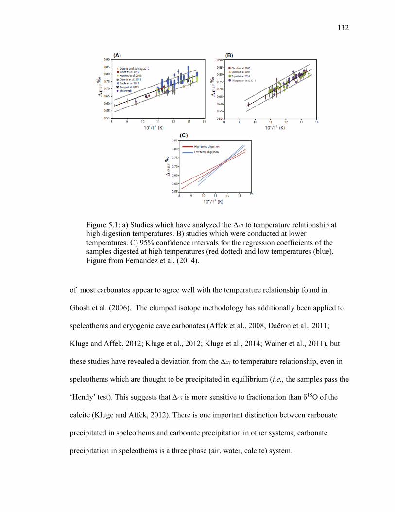
132

of most carbonates appear to agree well with the temperature relationship found in

Ghosh et al. (2006). The clumped isotope methodology has additionally been applied to

speleothems and cryogenic cave carbonates (Affek et al., 2008; Daëron et al., 2011;

Kluge and Affek, 2012; Kluge et al., 2012; Kluge et al., 2014; Wainer et al., 2011), but

these studies have revealed a deviation from the Δ47 to temperature relationship, even in

speleothems which are thought to be precipitated in equilibrium (i.e., the samples pass the

‘Hendy’ test). This suggests that Δ47 is more sensitive to fractionation than δ18O of the

calcite (Kluge and Affek, 2012). There is one important distinction between carbonate

precipitated in speleothems and carbonate precipitation in other systems; carbonate

precipitation in speleothems is a three phase (air, water, calcite) system.

Figure 5.1: a) Studies which have analyzed the Δ47 to temperature relationship at high digestion temperatures. B) studies which were conducted at lower temperatures. C) 95% confidence intervals for the regression coefficients of the samples digested at high temperatures (red dotted) and low temperatures (blue). Figure from Fernandez et al. (2014).

133

The first speleothem Δ47 isotope measurements were conducted on a stalagmite from

Soreq Cave and reconstructed temperatures were found to be greater than modern

expected temperatures by ~8 °C (Δ47 was lower) (Affek et al., 2008). Similar results have

been found in other caves (Daëron et al., 2011; Kluge and Affek, 2012; Wainer et al.,

2011) and in laboratory precipitation experiments which mimicked the cave environment

(Daëron et al., 2011). Studies have also found a strong correlation between δ18O and Δ47

offsets, with Δ47 exhibiting more negative values than predicted and δ18O values more

positive than predicted (Affek, 2013; Daëron et al., 2011; Kluge and Affek, 2012). A

study focusing on stalagmites from Bunker Cave, Germany found reduced kinetic isotope

fractionation occurred across periods with a reduced super saturation of drip water (Kluge

and Affek, 2012). The preciptiation of calcite occurs through the degassing of CO2 from

very high pCO2 drip water to a low CO2 cave and it is thought that during the degassing

process, fractionation can occur.

This study represents an additional attempt to determine the causes of kinetic fraction

from speleothems through a cave monitoring experiment from the subtropical Bahamas.

In addition, by also sampling an ancient speleothem sample from the Bahamas for

clumped isotopes and fluid inclusion isotopes, a direct comparison between the two

temperature methods demonstrates that the causes of kinetic fractionation in speleothems

may vary between cave systems and with space and time.

5.2 Samples

5.2.1 Modern samples: Hatchet Bay Cave

Samples were collected from Hatchet Bay Cave (HBC), a currently active cave in

Eleuthera, the Bahamas (Figure 5.1). Monitoring was initiated in June of 2012.

134

Overlying the cave is grasses and small Metopium toxiferum (poison wood) and trees of

the Fabaceae family with well-developed soils (greater than 15 cm depth). Most of the

grasses are located near the entrance and at lower elevations around the cave, with the

small trees located on the Aeolian ridge. HBC was accessed through a small ~1.7 m. by

0.9 m. opening located 10 to 15 m above sea level and exhibits an extremely linear

pattern particularly west of the main entrance (Mylroie and Mylroie, 2009). The opening

is immediately surrounded by thick grasses with larger trees (as described above) located

3 meters to the west, approximately following the cave direction and well developed soils

(as described above). The first level exhibits evidence of phreatic dissolution (Mylroie

and Mylroie, 2009). There is no evidence of cave breathing holes through the roof as

suggested by the lack of changes in the overlying vegetation and soil. The cave is divided

into three levels with the first level being the shallowest and the smallest level. The

second level is a tubular passage accessed by a 1.6 m. ladder down from the first level

and again contains evidence of phreatic dissolution (Mylroie and Mylroie, 2009). The

second level is more extensive (300 m long) with active drip water and stalagmite

formation (Mylroie and Mylroie, 2009). The 2nd level is thought to follow a thick, terra

rossa paleosol, leading to the creation of the linear and tubular shape following the

aeolian ridge (Mylroie and Mylroie, 2009). The third level is the deepest level and is

accessed by another 1.8 m ladder from the second level. However continuing on the

second floor lies a smaller passage which after several meters leads to a 7 m shaft to the

surface, which may have been carved out for guano mining (Mylroie and Mylroie, 2009).

The third level is partially filled with water, with active stalagmite formation occurring

on raised rock ledges above the water, ~1.2 m above the water level. This water is tidally

135

influenced and of marine salinity (Mylroie and Mylroie, 2009). There is no evidence of

water flooding the rock ledges nor is there any evidence of calcite deposits forming from

the water. Most of the sampling was conducted on the 2nd and 3rd levels. Located on the

3rd level ledges were experiments on the precipitation of calcite from drip water,

henceforth known as calcite “farming” (Figure 5.2). The cave was visited every 3-5

months. This cave has more extensive speleothem formation than other caves in

Eleuthera possibly driven by the 10-15 m of overlying calcite (Mylroie and Mylroie,

2009). Samples from the surrounding cave walls were not collected.

Figure 5.2: Map of the Bahamas showing the location of Abaco Island and Eleuthera Island, both islands located on the eastern edge of the Bahamas platform. Figure 5.3: (following page): Schematic of the entire surveyed area including first, second and third levels. The eastern part of the cave was not surveyed due to difficulty accessing this part of the cave. The locations of water and air sampling are approximate. Also shown is the approximate location of water and air collection as well as calcite farming. Shown are photographs of the areas which were sampled including main site (MS), east site (ES) and the west site (WS).

136

137

5.2.2 Ancient stalagmite

The stalagmite (sample AB-DC-09) was collected from a currently submerged

cave on Abaco Island, Bahamas, in July of 2007 from a depth of 16.5 m. The stalagmite

was not currently forming, but rather formed when sea-level was low and the cave was

exposed to air (Figure 5.2).

5.3 Methods

5.3.1 Hatchet Bay Cave

Analyses were conducted on the air (δ13C of CO2, CO2 concentration), drip water

(δ18Ow, δ2Hw, δ13C of DIC and minor elements) and the farmed calcite (δ13Cc, δ18Oc, Δ47,

and trace elements) deposited on microscope slides which were deployed in the cave. A

description of the monitoring methods is included in the following.

HBC Environmental:

Hatchet Bay Cave was continuously monitored for temperature and relative

humidity from June 2012 to November of 2013. Temperature and relative humidity were

measured every two hours utilizing a HOBO U23 Pro v2 Temperature/Relative Humidity

Data Logger from Onset. The manufacturer specifications are for temperature: ±0.21°C

from 0° to 50°C and for relative humidity: ±2.5% from 10% to 90% relative humidity, to

a maximum of ±3.5%, therefore for humidity levels above 90%, errors increase. The

temperature and relative humidity sensor was located in the main room (Figure 5.3). Air

samples for carbon isotopes of the CO2 (δ13CAIR) and CO2 concentration were collected

into 30 mL glass vials sealed with a septa, in a transect through the cave. Every visit to

the cave an air sample was taken outside of the cave in an open field prior to entering the

cave. Air samples for carbon isotopes of the CO2 (δ13CCO2) were collected into 30 mL

138

glass vials sealed with a septa, in a transect through the cave. Every visit to the cave an

air sample was taken outside of the cave in an open field within 3 meters of the cave

entrance prior to entering the cave. Carbon isotopes of the CO2 were analyzed at the

University of Miami on a gas bench coupled to a Thermo-Delta plus Advantage isotope

ratio mass spectrometer (IRMS) and calibrated against internal standards. Data are

reported relative to Vienna Pee Dee Belemnite (V-PDB). To determine CO2

concentration, carbon peak intensity data were calibrated utilizing air samples with CO2

concentrations of atmospheric condition using only one standard of atmospheric air of

CO2 concentration. Unfortunately, CO2 concentration was only measured for a subset of

the sample analyzed for δ13CCO2 value.

Unfiltered water samples were collected throughout the second and third levels of

the cave by holding clean acid washed vials under dripping stalactites. Vials were filled

completely (where possible) to avoid head space equilibration, then capped and stored

until analysis. Samples were filtered using a Whatman 0.2 µm pore filter upon return to

the laboratory and stored in clean vials (within 2-3 days). Water samples were measured

for oxygen and hydrogen isotopes (δ18Ow and δ2Hw), carbon isotopes of the dissolved

inorganic carbon (DIC) (δ13CDIC), pH, Chloride concentration and total alkalinity.

For oxygen and hydrogen isotopes of the water samples, samples were measured

using a L2130-i Picarro cavity ring down spectroscopy (CRDS) instrument. In house

standards are analyzed with the samples which have been previously calibrated to the

VSMOW-GISP-SLAP scale. One milliliter of each sample or standard is measured into a

glass vial and sealed with a rubber septum. Each sample or standard is injected into the

Picarro A0211 vaporizer unit at 0.2 ml per injection six times into the vaporizer. The

139

vaporizer is held at 110ºC for the duration of the sample run. The injection port of the

A0211 is fitted with a fine stainless steel mesh for trapping salt crystals to minimize

interferences and clogging downstream. The mesh basket is periodically removed,

rinsed, dried and reinserted into the injection port. The vaporized water gas is transferred

to the Picarro CRDS analyzer in a stream of N2 gas. The measurement cycle of each

sample lasts about 8 minutes and data are reported relative to VSMOW.

For δ13CDIC measurements, samples were injected in a previously evacuated 30

mL glass vial sealed with septa which contained 0.5 mL of 103% phosphoric acid

(H3PO4) previously flushed with Helium. Samples were then mixed utilizing a vortex

mixer producing CO2 from the reaction between DIC and the phosphoric acid. The CO2

was sampled using a gas bench and measured on a Thermo-Delta V Advantage IRMS.

The δ13C was calibrated to three reference pulses of CO2, two at the start of the sample

and two at the end. In house reagent grade NaHCO3 standards were also utilized for

standardization and consist of a similar molarity to the samples and were analyzed in the

same manner as the samples. The δ13C of the in house standards have been previously

standardized using a dual inlet mass spectrometer (Finnigan MAT 251), calibrated

relative to Vienna Pee Dee Belemnite (V-PDB). The reproducibility determined from

multiple replicates of standards is < 0.1‰ and data are reported relative to Vienna Pee

Dee Belemnite (V-PDB).

Alkalinity was measured utilizing a double endpoint auto titrator using 0.01 N

HCl. Average error determined from the repeated measurement of a standard was 0.02

mM. Chloride concentration was determined by titration with silver nitrate using dilute

potassium chromate solution as the indicator. International Association for the Physical

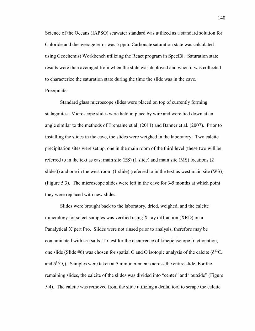
140

Science of the Oceans (IAPSO) seawater standard was utilized as a standard solution for

Chloride and the average error was 5 ppm. Carbonate saturation state was calculated

using Geochemist Workbench utilizing the React program in SpecE8. Saturation state

results were then averaged from when the slide was deployed and when it was collected

to characterize the saturation state during the time the slide was in the cave.

Precipitate:

Standard glass microscope slides were placed on top of currently forming

stalagmites. Microscope slides were held in place by wire and were tied down at an

angle similar to the methods of Tremaine et al. (2011) and Banner et al. (2007). Prior to

installing the slides in the cave, the slides were weighed in the laboratory. Two calcite

precipitation sites were set up, one in the main room of the third level (these two will be

referred to in the text as east main site (ES) (1 slide) and main site (MS) locations (2

slides)) and one in the west room (1 slide) (referred to in the text as west main site (WS))

(Figure 5.3). The microscope slides were left in the cave for 3-5 months at which point

they were replaced with new slides.

Slides were brought back to the laboratory, dried, weighed, and the calcite

mineralogy for select samples was verified using X-ray diffraction (XRD) on a

Panalytical X’pert Pro. Slides were not rinsed prior to analysis, therefore may be

contaminated with sea salts. To test for the occurrence of kinetic isotope fractionation,

one slide (Slide #6) was chosen for spatial C and O isotopic analysis of the calcite (δ13Cc

and δ18Oc). Samples were taken at 5 mm increments across the entire slide. For the

remaining slides, the calcite of the slides was divided into “center” and “outside” (Figure

5.4). The calcite was removed from the slide utilizing a dental tool to scrape the calcite

141

off of the slide, homogenized, and analyzed for clumped isotopes (Δ47) as well as C and

O isotopes (Figure 5.4). The C and O isotopic measurements were made using a Kiel III

interfaced with a Thermo-Finnigan Delta Plus IRMS at the University of Miami. All data

have been corrected for isobaric inferences at mass 45 and 46 and are reported relative to

Vienna Pee Dee Belemnite (V-PDB). The precision of the δ13Cc and δ18Oc values is

better than ±0.1‰. The method for the clumped isotope analysis is discussed in section

5.3.2.

Statistics:

Data were considered to be normally distributed and using a Pearson correlation

coefficient, correlations were performed. Statistically significant relationships are

reported at the 95% confidence limits.

5.3.2 Clumped isotopes

The calcite from sample AB-DC-09 and from the HBC slides were both analyzed

for clumped isotopes (Δ47 value). The methods for clumped isotope analyses at the

University of Miami are outlined in Murray et al. (Submitted) and Swart et al. (In Prep).

Figure 5.4: Example of the slides from HBC monitoring. Slide #10 after collection and drying in 40 ºC oven. Sampling of the slide was conducted at the center of the slide and along the outside of the slide for δ18Oc, δ13Cc and Δ47 value. The calcite was removed using a dental tool, homogenized with a mortar and pestle and stored in Eppendorf vials until analysis.

142

Briefly, 8 mg of sample were weighed into copper boats and reacted at 90 °C for 30

minutes in 103% H3PO4 using the common acid bath method (Swart et al., 1991). After

reaction, CO2 was purified utilizing two H2O removal traps held at -80 to -90 °C and a

PoraPak Q trap held at -25 to -30 °C to remove contaminants. The CO2 gas was

cryogenically frozen into a sealed vessel and transferred to the IRMS for analysis. The

entire process from reaction to the IRMS takes approximately 90 minutes. In between

samples, the entire line is evacuated through two turbo molecular pumps and the line is

heated up to 200 °C for 30 minutes. A complete description of the extraction line can be

found in Appendix D.

Sample CO2 gas was measured on the Thermo MAT 253 IRMS. The δ13C and

δ18O of the CO2 reference gas was calibrated using NBS-19 and results reported relative

to Vienna Pee Dee Belemnite (VPDB). Samples were analyzed for 10-20 acquisitions

and run at 12 V on mass 44 with peak centering and pressure balancing before each

acquisition. The sample δ45, δ46, δ47 and δ48 values were measured to obtain a

standard error of ~±0.008‰ for the Δ47 value.

Calculation of Δ47 was conducted utilizing the methods outlined in Affek and

Eiler (2006) and Huntington et al. (2009). All data are reported in the reference

framework outlined in Dennis et al. (2011) utilizing both heated and water equilibrated

gases (1000, 50 and 25 °C). All data have been corrected for an acid fractionation factor

of -0.00141 ‰/°C for reaction at 90°C as reported in Henkes et al. (2013).

A typical set of sample analyses includes an internal carbonate Carrara marble

standard, followed by 2-4 samples. Monthly, heated and water equilibrated gases were

analyzed and the data corrected to account for long term drift in the machine. Samples

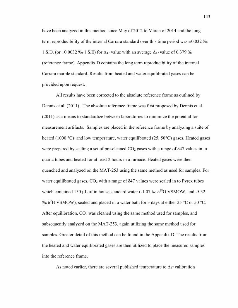
143

have been analyzed in this method since May of 2012 to March of 2014 and the long

term reproducibility of the internal Carrara standard over this time period was ±0.032 ‰

1 S.D. (or ±0.0032 ‰ 1 S.E) for Δ47 value with an average Δ47 value of 0.379 ‰

(reference frame). Appendix D contains the long term reproducibility of the internal

Carrara marble standard. Results from heated and water equilibrated gases can be

provided upon request.

All results have been corrected to the absolute reference frame as outlined by

Dennis et al. (2011). The absolute reference frame was first proposed by Dennis et al.

(2011) as a means to standardize between laboratories to minimize the potential for

measurement artifacts. Samples are placed in the reference frame by analyzing a suite of

heated (1000 °C) and low temperature, water equilibrated (25, 50°C) gases. Heated gases

were prepared by sealing a set of pre-cleaned CO2 gases with a range of δ47 values in to

quartz tubes and heated for at least 2 hours in a furnace. Heated gases were then

quenched and analyzed on the MAT-253 using the same method as used for samples. For

water equilibrated gases, CO2 with a range of δ47 values were sealed in to Pyrex tubes

which contained 150 μL of in house standard water (-1.07 ‰ δ18O VSMOW, and -5.32

‰ δ2H VSMOW), sealed and placed in a water bath for 3 days at either 25 °C or 50 °C.

After equilibration, CO2 was cleaned using the same method used for samples, and

subsequently analyzed on the MAT-253, again utilizing the same method used for

samples. Greater detail of this method can be found in the Appendix D. The results from

the heated and water equilibrated gases are then utilized to place the measured samples

into the reference frame.

As noted earlier, there are several published temperature to Δ47 calibration

144

equations. For this project, the results will be expressed using the equation from Ghosh

et al., 2006 in the reference frame as reported by Dennis et al., 2011:

Δ47 = 0.0636*106/T2 – 0.0047 (8)

This equation was chosen as it has been utilized in most speleothem studies to date.

Considering this is a relatively new field of geochemistry all raw data and heated gas

results can be provided. For the HBC slides and samples from the AB-DC-09 stalagmite,

samples were each run 2 to 5 times and the data collected include δ47, Δ47, δ13Cc and

δ18Oc values. Results for δ13Cc and δ18Oc are reported relative to V-PDB while Δ47 values

are reported in the reference frame of Dennis et al. (2011).

5.3.3 AB-DC-09

Fluid Inclusion Isotopes:

Oxygen and hydrogen isotopes (δ18Ow and δ2Hw) were measured on 31 fluid

inclusion samples from AB-DC-09 (Chapter 3). Fluid inclusion data are reported relative

to Vienna Standard Mean Ocean Water (VSMOW) with an average error of 0.5 ‰ for

δ18Ow and 2.0 ‰ for δ2Hw values (Arienzo et al., 2013). The δ18Oc of the calcite hosting

the inclusion was measured at the University of Miami using a Thermo-Finnigan Delta

Plus IRMS as described above. Stalagmite AB-DC-09 was also radiometrically dated

using U-Th dating methodologies for a total of 20 U-Th dates, as described in Chapter 3.

Clumped Isotopes:

For stalagmite AB-DC-09, the same 31 water samples which were analyzed for

fluid inclusions were also measured for clumped isotopes utilizing the methods described

in section 5.3.2. An additional 7 samples were measured for Δ47 value only.

145

5.4 Results

5.4.1 Environmental variation in Hatchet Bay Cave

Below follows a summary of the findings of the monitoring project at HBC. All

of the individual sample results, are provided in Appendix D.

Temperature, humidity and air:

Throughout the duration of the experiment (June 2012 to November 2013), the

relative humidity remained at >90 % ±2.5. Temperature varied from 22.8 °C to 23.8 °C at

as reported by the temperature logger, with an average value of 23.3 °C. The maximum

temperature occurred at the end of October to beginning of November of 2013 (Figure

5.5). Minimum temperature was found in mid-April of 2013.

The δ13C of cave air CO2 (δ13CCO2) demonstrates a progressive depletion in

δ13CCO2 value from the outside of the cave to the third level west room (Figure 5.6). On

average, the 3rd level west room is 1.5 ‰ more negative than the 3rd level main room.

δ13C of the soil or soil CO2 concentration was not measured. The results demonstrate a

co-variation between δ13CCO2 and 1/[CO2] with decreasing δ13CCO2 occurring with

increasing [CO2] (Figure 5.7)(Keeling, 1958). This is thought to be driven by the mixing

of two end members, an atmospheric end member and a soil gas end member which is

estimated in Figure 5.6 (Tremaine et al., 2011). Most of the sample results plot near the

atmospheric end member and the line of best fit has a y-intercept at -18 ±2‰ which is

thought to be the soil gas value. The deeper in the cave, the lower contribution from

atmospheric air (Figure 5.8).

146

Water:

Isotopic analyses of the drip waters include the analyses of δ13CDIC, δ18Ow and

δ2Hw values. Overall the δ13CDIC results decrease with increasing depth within the cave

(Figure 5.9) similar to the trend observed in the δ13CCO2 results (Figure 5.6). The δ18Ow

of the drip waters were also more negative in the 3rd level west room when compared

with the 2nd level or the 3rd level main room (Table 5.1). The average δ18Ow of the drip

waters for the 3rd level main room was -4.2±0.5 ‰ while the west room was -4.8±0.4 ‰.

Total alkalinity and pH were relatively invariant (Alkalinity = 3.5 to 4.0 mM and pH 7.8

to 8.0) within the cave, with a slight increase from the 2nd to 3rd level. Chloride

concentration was greater in the 3rd level drip waters than the 2nd level (538 ppm) and

within the third level, the west room waters contained the highest Cl- concentrations

(2811 ppm in West Room, with 2025 ppm in Main room) (Table 5.1). Evapotranspiration

is shown in a cave in Florida to lead to increased concentration of Cl- (Tremaine and

Froelich, 2013) while transpiration is not shown to impact the δ18Ow or δ2Hw of soil

water. Therefore the increased Cl- deeper in the cave may be due to evapotranspiration

processes influencing the water in this region in the overlying karst, and hence the

increased ionic concentrations. Considering the close proximity of the cave to the ocean,

there is the possibility of increased Cl- in the drip waters due to sea spray. Results

demonstrate that for May, August and November, saturation state was higher in the 3rd

level than the 2nd level (Figure 5.10), and saturation state does not significantly change

within the third level (Saturation state 1.1 to 1.0 for Main and West rooms respectively)

(Table 5.1, Figure 5.10). Chloride is known to be a conservative element. However

increasing Cl- concentration deeper in the cave is thought to be in part driven by

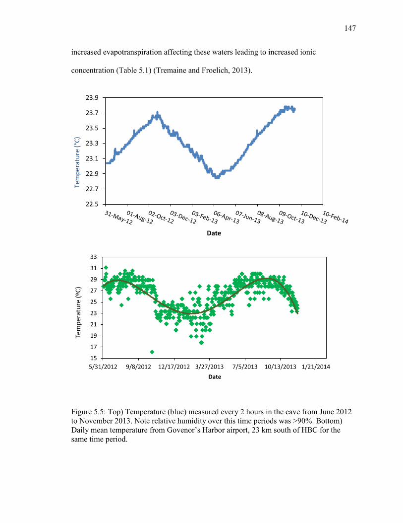
147

increased evapotranspiration affecting these waters leading to increased ionic

concentration (Table 5.1) (Tremaine and Froelich, 2013).

Figure 5.5: Top) Temperature (blue) measured every 2 hours in the cave from June 2012 to November 2013. Note relative humidity over this time periods was >90%. Bottom) Daily mean temperature from Govenor’s Harbor airport, 23 km south of HBC for the same time period.

22.5

22.7

22.9

23.1

23.3

23.5

23.7

23.9

Tem

pera

ture

(°C)

Date

15

17

19

21

23

25

27

29

31

33

5/31/2012 9/8/2012 12/17/2012 3/27/2013 7/5/2013 10/13/2013 1/21/2014

Tem

pera

ture

(ºC)

Date

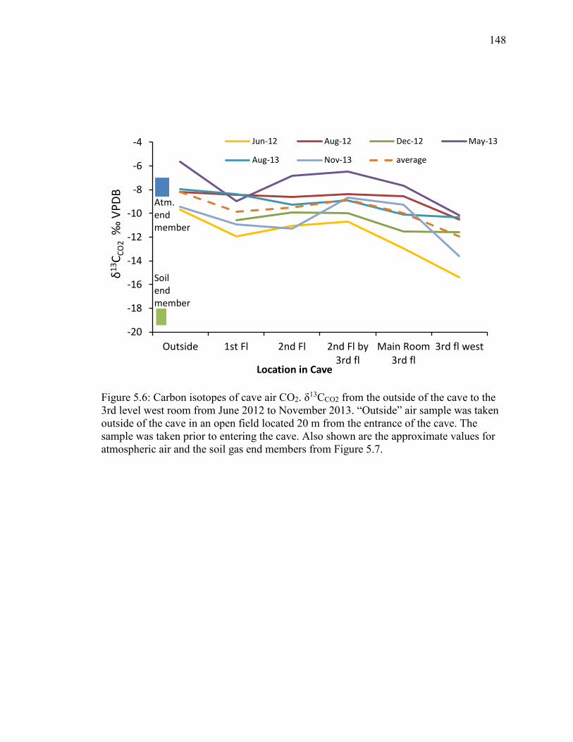
148

Figure 5.6: Carbon isotopes of cave air CO2. δ13CCO2 from the outside of the cave to the 3rd level west room from June 2012 to November 2013. “Outside” air sample was taken outside of the cave in an open field located 20 m from the entrance of the cave. The sample was taken prior to entering the cave. Also shown are the approximate values for atmospheric air and the soil gas end members from Figure 5.7.

-20

-18

-16

-14

-12

-10

-8

-6

-4

Outside 1st Fl 2nd Fl 2nd Fl by3rd fl

Main Room3rd fl

3rd fl west

δ13C C

O2

‰ V

PDB

Location in Cave

Jun-12 Aug-12 Dec-12 May-13

Aug-13 Nov-13 average

Atm. endmember

Soilendmember

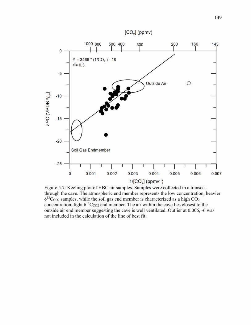
149

Figure 5.7: Keeling plot of HBC air samples. Samples were collected in a transect through the cave. The atmospheric end member represents the low concentration, heavier δ13CCO2 samples, while the soil gas end member is characterized as a high CO2 concentration, light δ13CCO2 end member. The air within the cave lies closest to the outside air end member suggesting the cave is well ventilated. Outlier at 0.006, -6 was not included in the calculation of the line of best fit.

150

Figure 5.8: Same as Figure 5.7, however results are grouped by sampling location. This demonstrates that overall, the 3rd Level West are closest to the soil gas end member, while the 1st floor samples plot closer to the atmospheric end member.

Figure 5.9: δ13CDIC of the drip waters for the 2nd level (light blue), 3rd level main (dark blue) and 3rd level west (dark green) from August 2012 to November 2013.

-12

-11

-10

-9

-8

-7

-6

-5

-4

Aug-12 Nov-12 Feb-13 May-13 Aug-13 Nov-13

δ13 C

DIC

‰ V

PDB

Sampling Month

2nd Level

3rd Level Main

3rd Level West

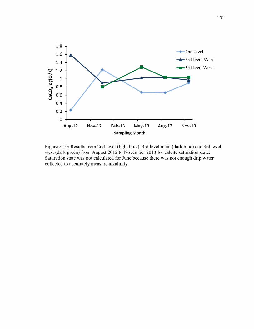
151

Figure 5.10: Results from 2nd level (light blue), 3rd level main (dark blue) and 3rd level west (dark green) from August 2012 to November 2013 for calcite saturation state. Saturation state was not calculated for June because there was not enough drip water collected to accurately measure alkalinity.

0

0.2

0.4

0.6

0.8

1

1.2

1.4

1.6

1.8

Aug-12 Nov-12 Feb-13 May-13 Aug-13 Nov-13

CaCO

3 lo

g(Q

/K)

Sampling Month

2nd Level

3rd Level Main

3rd Level West

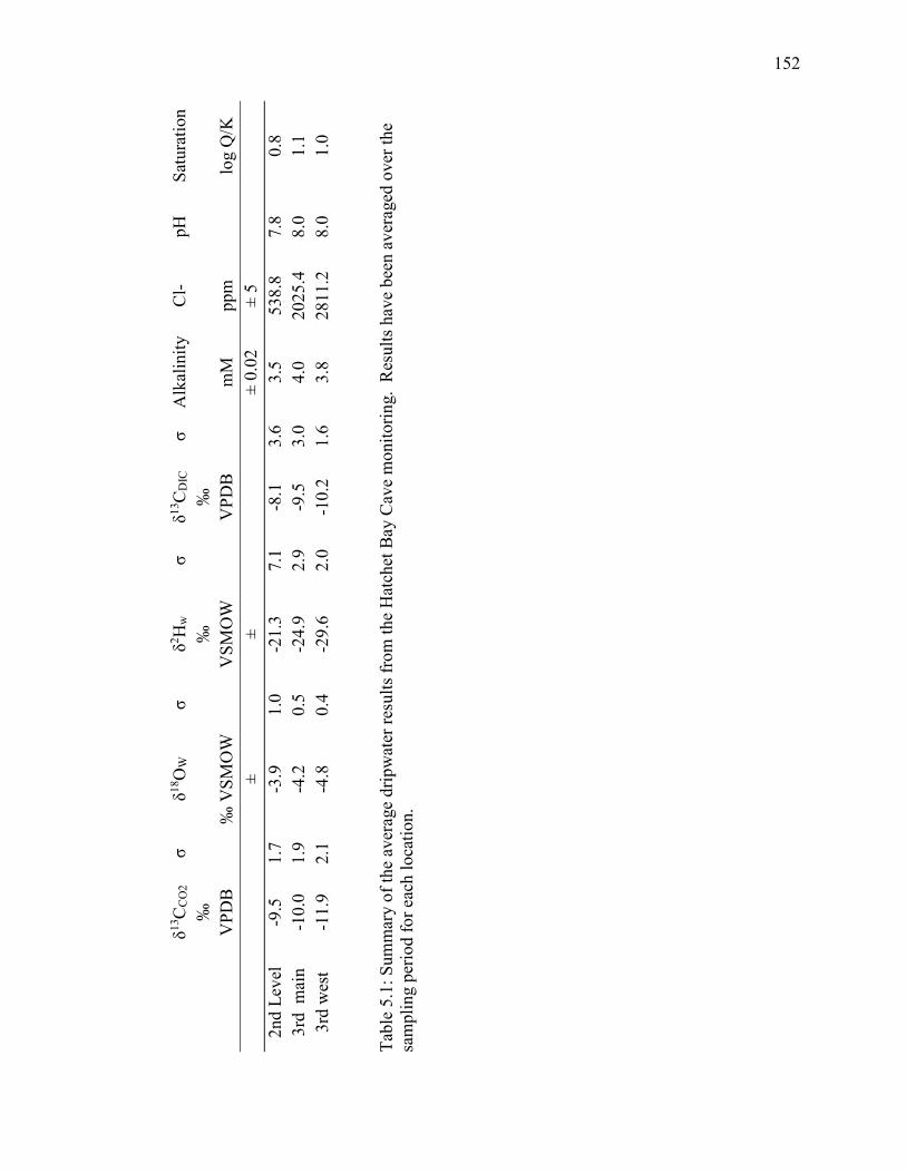
152

δ13

CC

O2

σ δ18

OW

σ

δ2 Hw

σ

δ13C

DIC

σ

Alk

alin

ity

Cl-

pH

Satu

ratio

n

‰

V

PDB

‰ V

SMO

W

‰

V

SMO

W

‰

V

PDB

mM

pp

m

lo

g Q

/K

±

±

±

0.02

±

5

2n

d Le

vel

-9.5

1.

7 -3

.9

1.0

-21.

3 7.

1 -8

.1

3.6

3.5

538.

8 7.

8 0.

8 3r

d m

ain

-10.

0 1.

9 -4

.2

0.5

-24.

9 2.

9 -9

.5

3.0

4.0

2025

.4

8.0

1.1

3rd

wes

t -1

1.9

2.1

-4.8

0.

4 -2

9.6

2.0

-10.

2 1.

6 3.

8 28

11.2

8.

0 1.

0 Ta

ble

5.1:

Sum

mar

y of

the

aver

age

drip

wat

er re

sults

from

the

Hat

chet

Bay

Cav

e m

onito

ring.

Res

ults

hav

e be

en a

vera

ged

over

the

sam

plin

g pe

riod

for e

ach

loca

tion.

153

Slide# Slide Weight (mg) no calcite

Location Date removed

# days in cave

Calcite Precipitated

(mg)

μmoles CaCO3/cm2/day

1 5833.1 Main Room 8/21/2012 79 140.3 1.8 3 5744.7 East Main Room 8/21/2012 79 228.7 2.9 4 5868.2 Main Room 8/21/2012 79 118.3 1.5 6 5803.7 West Room 8/21/2012 79 470.6 6.0 8 5853.3 Main Room 12/11/2012 110 80 0.7 9 5874.4 Main Room 5/1/2013 250 333.5 1.3

10 5853.5 East Main Room 12/11/2012 110 314.6 2.9 11 5857.3 West Room 12/11/2012 110 345.8 3.1 12 5808.5 Main Room 5/1/2013 140 40.2 0.3 13 5858.8 East Main Room 5/1/2013 140 245.3 1.8 14 5867.2 West Room 5/1/2013 140 790.7 5.6 15 5773.9 Main Room 8/6/2013 95 165.6 1.7 16 5817.4 Main Room 8/6/2013 95 Broken Broken 17 5866.5 East Main Room 8/6/2013 95 214.5 2.3 18 5940.2 West Room 8/6/2013 95 491.2 5.2 19 5810.7 Main Room 11/21/2013 105 366.4 3.5 20 5777 Main Room 11/21/2013 105 262.5 2.5 21 5862.8 East Main Room 11/21/2013 105 160.3 1.5 22 5802.6 West Room 11/21/2013 105 609 5.8

Table 5.2: Summary table for growth rate for each of the slides deployed in the cave. Slides 2 and 7 were destroyed in transport and therefore were not deployed. Slide 16 was broken after collection and therefore growth rate was not able to be calculated. 5.4.2 HBC slides

Summary of when each slide was recovered and the length of time in the cave are

found in Table 5.2.

XRD:

X-ray diffraction was conducted for select slides. Results demonstrate the slides

are comprised of low magnesium calcite (LMC). With no other significant minerals

found. Results are provided in Appendix D.

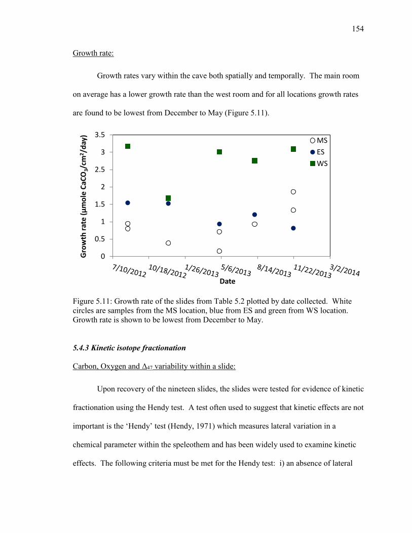
154

Growth rate:

Growth rates vary within the cave both spatially and temporally. The main room

on average has a lower growth rate than the west room and for all locations growth rates

are found to be lowest from December to May (Figure 5.11).

Figure 5.11: Growth rate of the slides from Table 5.2 plotted by date collected. White circles are samples from the MS location, blue from ES and green from WS location. Growth rate is shown to be lowest from December to May.

5.4.3 Kinetic isotope fractionation

Carbon, Oxygen and Δ47 variability within a slide:

Upon recovery of the nineteen slides, the slides were tested for evidence of kinetic

fractionation using the Hendy test. A test often used to suggest that kinetic effects are not

important is the ‘Hendy’ test (Hendy, 1971) which measures lateral variation in a

chemical parameter within the speleothem and has been widely used to examine kinetic

effects. The following criteria must be met for the Hendy test: i) an absence of lateral

0

0.5

1

1.5

2

2.5

3

3.5

Gro

wth

rate

(μm

ole

CaCO

3/cm

2 /da

y)

Date

MSESWS

155

increases in δ18Oc and δ13Cc values, and ii) a low correlation between δ18Oc and δ13Cc

values along a growth band. If these conditions are met, then it is assumed that minimal

kinetic fraction has taken place. The slides were analyzed for δ18Oc, δ13Cc and Δ47 values

at the center and at the outside of the slide (Figure 5.4). Two slides did not have sufficient

material to analyze both the center and the outside for (Slides # 3 and 15) therefore, these

samples were not analyzed further. Slide 1 was not analyzed as it was utilized for the

initial Th measurements (see Chapter 3).

For this study, the Hendy test was conducted on each of the slides for which there

was enough material present. This test was conducted by scraping off calcite utilizing a

clean dental tool to remove calcite from the center and the outside of the slide. These

sub-samples were then analyzed for δ18Oc , δ13Cc and Δ47 values utilizing the methods

provided above. The results for the δ18Oc and δ13Cc from the center compared with the

outside for the16 slides are shown in Figures 5.12 a & b. Of the 16 slides analyzed for

δ18Oc and δ13Cc, three slides consisted of increased C and O isotopes on the outside of the

slide relative to the center and therefore were not considered further (Slides # 8, 9 and

14). These results demonstrate minimal enrichment from the center to the outside for C

and O isotopes. Maximum enrichment of δ18Oc of 0.36 ‰ was found for Slide 10 and for

carbon isotopes there is a maximum enrichment of 0.8 ‰ also for Slide 10 (Figures 5.12

a & b, Table 5.3). One additional sample was not considered further (Slide #12) as this

slide exhibited higher than average Δ47 variability for three replicates. However the

results from all 16 slides analyzed for δ18Oc, δ13Cc and Δ47 value are provided in Figure

5.12 and Table 5.3, however slides 8, 9, 12 and 14 will not be included in figures beyond

this point, as these samples are thought to be kinetically fractionated. For the remaining

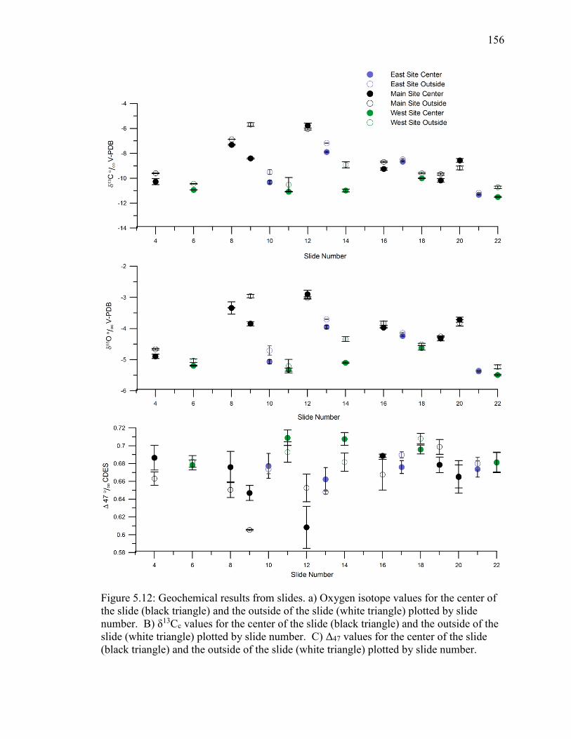
156

Figure 5.12: Geochemical results from slides. a) Oxygen isotope values for the center of the slide (black triangle) and the outside of the slide (white triangle) plotted by slide number. B) δ13Cc values for the center of the slide (black triangle) and the outside of the slide (white triangle) plotted by slide number. C) Δ47 values for the center of the slide (black triangle) and the outside of the slide (white triangle) plotted by slide number.

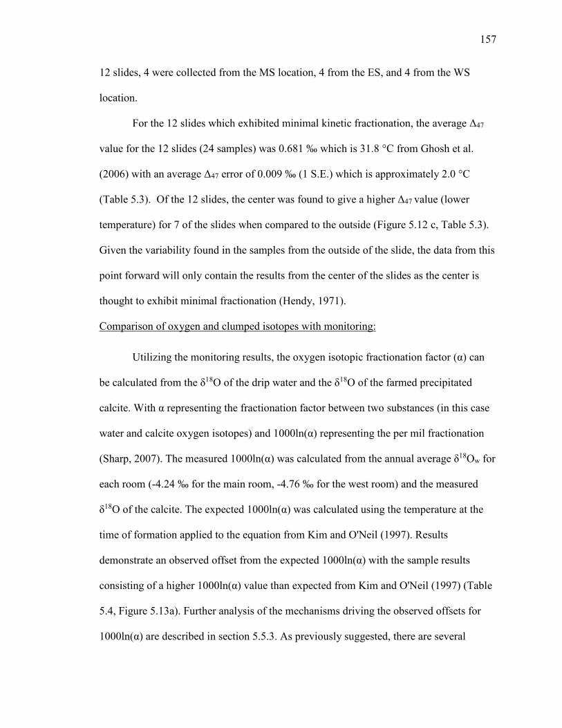
157

12 slides, 4 were collected from the MS location, 4 from the ES, and 4 from the WS

location.

For the 12 slides which exhibited minimal kinetic fractionation, the average Δ47

value for the 12 slides (24 samples) was 0.681 ‰ which is 31.8 °C from Ghosh et al.

(2006) with an average Δ47 error of 0.009 ‰ (1 S.E.) which is approximately 2.0 °C

(Table 5.3). Of the 12 slides, the center was found to give a higher Δ47 value (lower

temperature) for 7 of the slides when compared to the outside (Figure 5.12 c, Table 5.3).

Given the variability found in the samples from the outside of the slide, the data from this

point forward will only contain the results from the center of the slides as the center is

thought to exhibit minimal fractionation (Hendy, 1971).

Comparison of oxygen and clumped isotopes with monitoring:

Utilizing the monitoring results, the oxygen isotopic fractionation factor (α) can

be calculated from the δ18O of the drip water and the δ18O of the farmed precipitated

calcite. With α representing the fractionation factor between two substances (in this case

water and calcite oxygen isotopes) and 1000ln(α) representing the per mil fractionation

(Sharp, 2007). The measured 1000ln(α) was calculated from the annual average δ18Ow for

each room (-4.24 ‰ for the main room, -4.76 ‰ for the west room) and the measured

δ18O of the calcite. The expected 1000ln(α) was calculated using the temperature at the

time of formation applied to the equation from Kim and O'Neil (1997). Results

demonstrate an observed offset from the expected 1000ln(α) with the sample results

consisting of a higher 1000ln(α) value than expected from Kim and O'Neil (1997) (Table

5.4, Figure 5.13a). Further analysis of the mechanisms driving the observed offsets for

1000ln(α) are described in section 5.5.3. As previously suggested, there are several

158

equations for the temperature dependent fractionation for δ18O of calcite. Here, the

1000ln(α) offset value has been calculated using the Kim and O'Neil (1997) equation as

other speleothem studies have reported 1000ln(α) offset values using this equation. This

allows for the offsets to be compared between studies.

The Δ47 values from the farmed calcite average of 0.6810 ‰ (Table 5.4, Figure

5.13 b) which is an average temperature of 31.4 ºC utilizing the Ghosh et al. (2006)

equation. This is an average ~8 ºC warmer than expected, with the measured average

temperature of the cave being 23.3 °C. However, there is variability in the Δ47 value

between the various rooms within the cave (Figure 5.14). The WS location (n=4) average

Δ47 value (0.691 ‰) is higher than the ES location Δ47 value (0.679 ‰ n=4), and the MS

location contains the lowest average Δ47 value (0.669 ‰ n=4) (Figure 5.14). The greatest

offset from the expected (black cross, Figure 5.14) was observed in May of 2013 for

Slide 13 collected from ES location and the lowest offset was observed on December of

2012 for Slide11 from the WS location (Figure 5.14). Expected Δ47 value was

calculated using the Ghosh et al., (2006) equation and the temperature for that time

period from the HOBO logger.

The Δ47 value can be expressed as an offset from the expected Δ47 value. Expected

Δ47 value was calculated using the Ghosh et al., (2006) equation and the temperature for

that time period from the HOBO logger. In Figure 5.15 this offset is plotted versus

saturation state for the period the sample was in the cave. The results suggest increased

saturation state may be associated with a decreased Δ47 offset (r2= 0.7, p<0.05) (Figure

5.15). As described earlier, saturation state was averaged between slide deployment and

159

Tabl

e 5.

3a: R

esul

ts fr

om th

e ce

nter

of t

he sl

ide

for e

ach

of th

e 16

slid

es fo

r the

cen

ter o

f the

slid

es in

clud

ing

the

slid

e nu

mbe

r, lo

catio

n in

the

cave

, the

num

ber o

f rep

licat

es, δ

13C

c, δ18

Oc ,

δ47

, and

Δ47

resu

lts.

Slid

e #

Loc

n δ1

3Cc

1 S.

D.

δ18O

c 1

S.

D.

δ47

‰

SE

Δ47

‰

SE

‰

VPD

B

‰

V

PDB

RF

4

Mai

n 3

-10.

3 0.

24

-4.9

0.

07

1.56

0.

29

0.68

7 0.

014

6 W

est

3 -1

0.9

0.01

-5

.2

0.02

0.

57

0.02

0.

678

0.00

6 8

Mai

n 2

-7.3

0.

04

-3.3

0.

20

6.18

0.

19

0.67

6 0.

018

9 M

ain

3 -8

.4

0.04

-3

.8

0.07

4.

53

0.13

0.

647

0.00

8 10

Ea

st M

ain

4 -1

0.3

0.14

-5

.1

0.07

1.

33

0.18

0.

677

0.01

4 11

W

est

3 -1

1.1

0.03

-5

.3

0.05

0.

31

0.05

0.

709

0.00

9 12

M

ain

3 -5

.8

0.20

-2

.9

0.13

8.

15

0.30

0.

608

0.02

4 13

Ea

st M

ain

3 -7

.9

0.05

-4

.0

0.06

4.

95

0.09

0.

662

0.01

3 14

W

est

4 -1

1.0

0.11

-5

.1

0.02

0.

64

0.11

0.

708

0.00

7 16

M

ain

2 -9

.3

0.09

-4

.0

0.02

3.

57

0.11

0.

689

0.00

2 17

Ea

st M

ain

3 -8

.7

0.04

-4

.2

0.02

3.

86

0.05

0.

676

0.00

7 18

W

est

3 -1

0.0

0.02

-4

.6

0.07

2.

12

0.08

0.

696

0.00

5 19

M

ain

3 -1

0.2

0.15

-4

.3

0.07

2.

26

0.23

0.

679

0.00

9 20

M

ain

4 -8

.6

0.14

-3

.7

0.08

4.

52

0.23

0.

665

0.01

8 21

Ea

st M

ain

3 -1

1.3

0.03

-5

.4

0.02

-0

.03

0.03

0.

674

0.00

9 22

W

est

4 -1

1.5

0.04

-5

.5

0.02

-0

.32

0.06

0.

681

0.01

1

160

Tabl

e 5.

3b: R

esul

ts fo

r eac

h of

the

16 sl

ides

for t

he sa

mpl

e fr

om th

e ou

tsid

e of

the

slid

e in

clud

ing

the

slid

e nu

mbe

r, lo

catio

n in

the

cave

, the

num

ber o

f rep

licat

es, δ

13C

c, δ18

Oc ,

δ47

, and

Δ47

resu

lts.

Slid

e #

Loc

Rep

licat

es

δ13C

c 1 S.D

. δ1

8Oc

1 S

. D

. δ4

7 ‰

SE

Δ4

7 ‰

SE

‰ V

PDB

‰ V

PDB

RF

4

Mai

n 3

-9.6

0.

03

-4.7

0.

03

2.47

0.

05

0.66

3 0.

008

6 W

est

5 -1

0.4

0.03

-5

.0

0.06

1.

25

0.09

0.

682

0.00

7 8

Mai

n 1

-6.9

0.

01

-3.3

0.

01

6.61

0.

09

0.65

1 0.

009

9 M

ain

3 -5

.7

0.15

-3

.0

0.05

8.

19

0.21

0.

605

0.00

1 10

Ea

st M

ain

4 -9

.5

0.19

-4

.7

0.15

2.

53

0.34

0.

674

0.00

5 11

W

est

3 -1

0.5

0.57

-5

.2

0.22

0.

99

0.80

0.

693

0.01

2 12

M

ain

3 -6

.1

0.08

-3

.0

0.04

8.

15

0.30

0.

653

0.01

6 13

Ea

st M

ain

2 -7

.2

0.02

-3

.7

0.00

5.

92

0.02

0.

648

0.00

2 14

W

est

4 -8

.9

0.24

-4

.3

0.08

3.

52

0.33

0.

682

0.01

0 16

M

ain

2 -8

.7

0.06

-3

.8

0.07

4.

27

0.14

0.

668

0.01

7 17

Ea

st M

ain

3 -8

.5

0.06

-4

.1

0.02

4.

16

0.07

0.

690

0.00

4 18

W

est

3 -9

.6

0.05

-4

.5

0.04

2.

67

0.11

0.

708

0.00

6 19

M

ain

3 -9

.7

0.08

-4

.3

0.02

2.

85

0.07

0.

699

0.00

8 20

M

ain

4 -9

.2

0.15

-3

.8

0.10

3.

78

0.26

0.

666

0.01

3 21

Ea

st M

ain

3 -1

1.2

0.03

-5

.4

0.03

0.

15

0.01

0.

680

0.00

7 22

W

est

4 -1

0.7

0.10

-5

.2

0.06

0.

75

0.14

0.

682

0.01

1

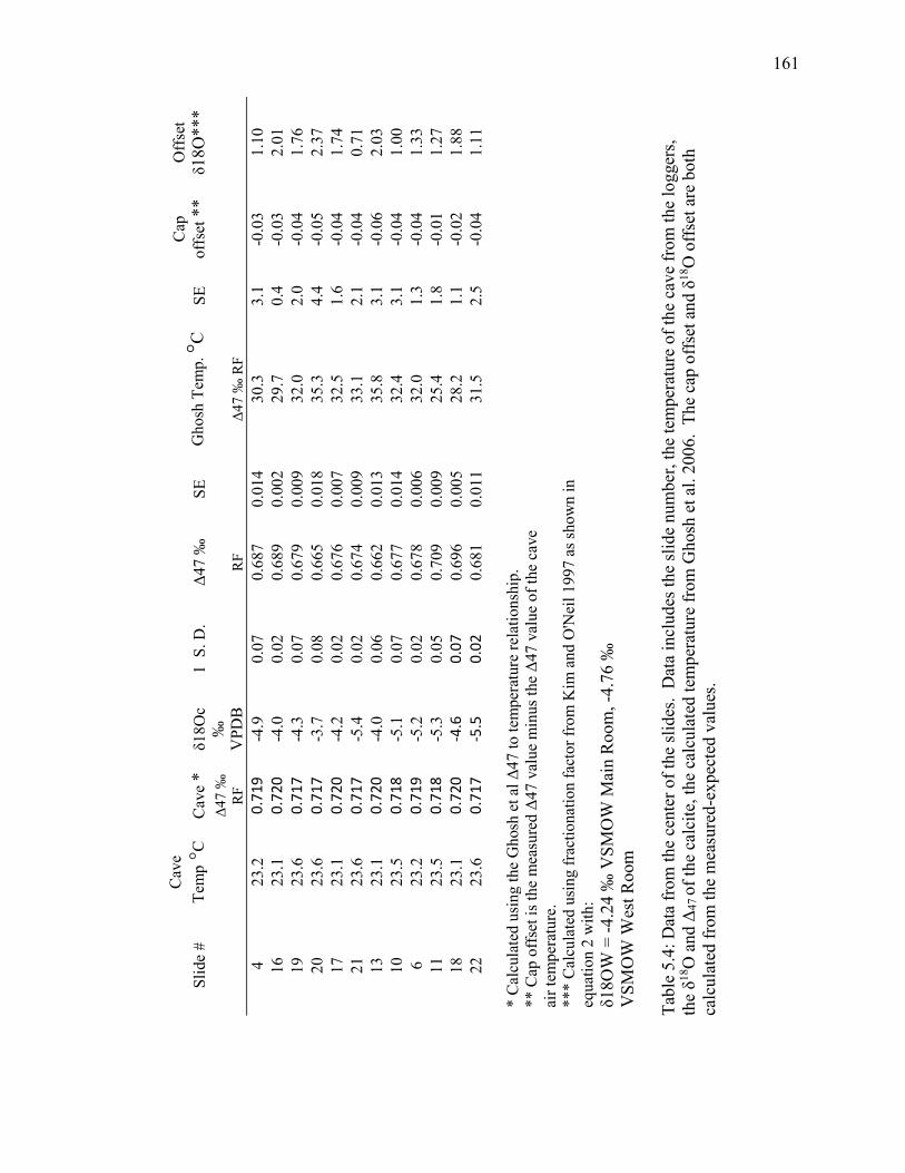
161

Slid

e #

Cav

e Te

mp °

C

Cav

e *

δ18O

c 1

S. D

. Δ4

7 ‰

SE

G

hosh

Tem

p. °C

SE

C

ap

offs

et *

* O

ffse

t δ1

8O**

*

Δ47

‰

RF

‰

VPD

B

R

F

Δ47

‰ R

F

4 23

.2

0.71

9 -4

.9

0.07

0.

687

0.01

4 30

.3

3.1

-0.0

3 1.

10

16

23.1

0.

720

-4.0

0.

02

0.68

9 0.

002

29.7

0.

4 -0

.03

2.01

19

23

.6

0.71

7 -4

.3

0.07

0.

679

0.00

9 32

.0

2.0

-0.0

4 1.

76

20

23.6

0.

717

-3.7

0.

08

0.66

5 0.

018

35.3

4.

4 -0

.05

2.37

17

23

.1

0.72

0 -4

.2

0.02

0.

676

0.00

7 32

.5

1.6

-0.0

4 1.

74

21

23.6

0.

717

-5.4

0.

02

0.67

4 0.

009

33.1

2.

1 -0

.04

0.71

13

23

.1

0.72

0 -4

.0

0.06

0.

662

0.01

3 35

.8

3.1

-0.0

6 2.

03

10

23.5

0.

718

-5.1

0.

07

0.67

7 0.

014

32.4

3.

1 -0

.04

1.00

6

23.2

0.

719

-5.2

0.

02

0.67

8 0.

006

32.0

1.

3 -0

.04

1.33

11

23

.5

0.71

8 -5

.3

0.05

0.

709

0.00

9 25

.4

1.8

-0.0

1 1.

27

18

23.1

0.

720

-4.6

0.

07

0.69

6 0.

005

28.2

1.

1 -0

.02

1.88

22

23

.6

0.71

7 -5

.5

0.02

0.

681

0.01

1 31

.5

2.5

-0.0

4 1.

11

*

Cal

cula

ted

usin

g th

e G

hosh

et a

l Δ47

to te

mpe

ratu

re re

latio

nshi

p.

**

Cap

off

set i

s the

mea

sure

d Δ4

7 va

lue

min

us th

e Δ4

7 va

lue

of th

e ca

ve

air t

empe

ratu

re.

**

* C

alcu

late

d us

ing

frac

tiona

tion

fact

or fr

om K

im a

nd O

'Nei

l 199

7 as

show

n in

eq

uatio

n 2

with

:

δ1

8OW

= -4

.24

‰ V

SMO

W M

ain

Roo

m, -

4.76

‰

VSM

OW

Wes

t Roo

m

Tabl

e 5.

4: D

ata

from

the

cent

er o

f the

slid

es.

Dat

a in

clud

es th

e sl

ide

num

ber,

the

tem

pera

ture

of t

he c

ave

from

the

logg

ers,

the

δ18O

and

Δ47

of t

he c

alci

te, t

he c

alcu

late

d te

mpe

ratu

re fr

om G

hosh

et a

l. 20

06.

The

cap

offs

et a

nd δ

18O

off

set a

re b

oth

calc

ulat

ed fr

om th

e m

easu

red-

expe

cted

val

ues.

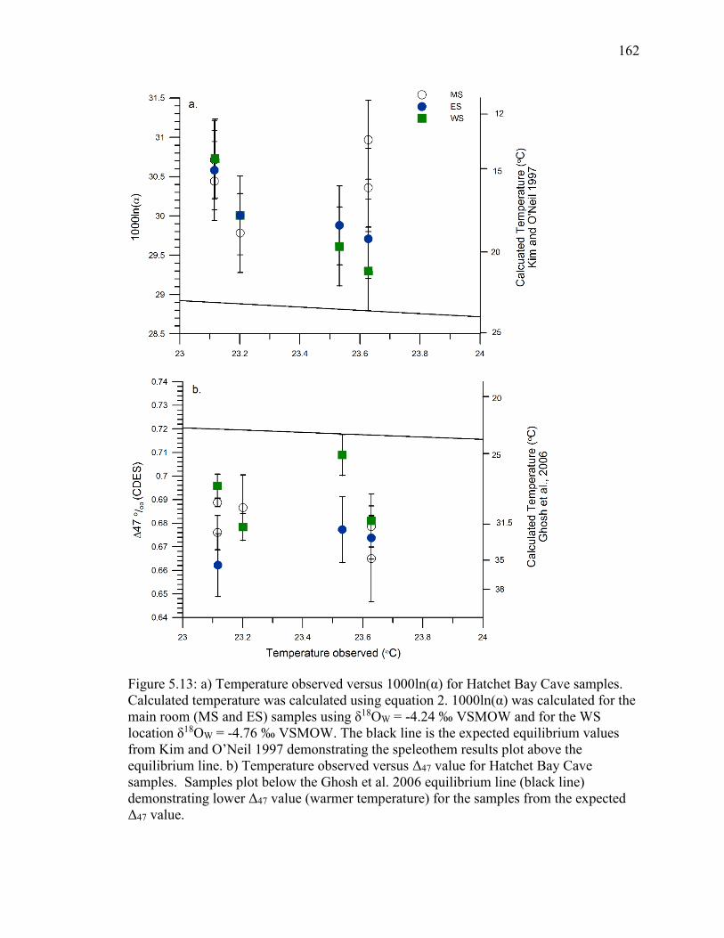
162

Figure 5.13: a) Temperature observed versus 1000ln(α) for Hatchet Bay Cave samples. Calculated temperature was calculated using equation 2. 1000ln(α) was calculated for the main room (MS and ES) samples using δ18OW = -4.24 ‰ VSMOW and for the WS location δ18OW = -4.76 ‰ VSMOW. The black line is the expected equilibrium values from Kim and O’Neil 1997 demonstrating the speleothem results plot above the equilibrium line. b) Temperature observed versus Δ47 value for Hatchet Bay Cave samples. Samples plot below the Ghosh et al. 2006 equilibrium line (black line) demonstrating lower Δ47 value (warmer temperature) for the samples from the expected Δ47 value.

163

its recovery; therefore there are fewer data points as calculating the saturation state was

not possible in June (as described above).

Of further significance may be the relationship between growth rate and Δ47 offset

(Figure 5.16). In the west room, where growth rates are higher than the rest of the cave,

there is a significant relationship between growth rate and Δ47 offset, with lower growth

rate correlating with a lower Δ47 offset (r2=0.9, p<0.05) (Figure 5.17). Conversely, in the

main room there is no relationship between growth rate and Δ47 offset for either the MS

or ES location (Figure 5.16 & 17).

A weak relationship was found between δ18Oc value and Δ47 offset as well as

δ13Cc value and Δ47 offset (r2=0.2, p<0.1) (Figure 5.18 and 19).

Figure 5.14: Plot for Δ47 by location plotted versus the date removed from the cave. Note all samples fall below the expected Δ47 value. Results demonstrate increased Δ47 values for the WS location compared to the MS and ES locations. Expected cap value (black cross) is the Δ47 value expected for each month.

164

Figure 5.15: Results from Hatchet Bay Cave for saturation state (log(Q/K)) versus Δ47 offset. Log(Q/K) defines the saturation index and when the saturation index is above 1, saturation has been reached. Samples demonstrate a trend of decreasing Δ47 offset with increasing saturation state. Saturation state was not calculated for June because there was not enough drip water collected to accurately measure alkalinity. The point at 1.17 has minimal influence on the r2 value, with the value with the point is r2=0.7 and without the point is r2=0.6.

Figure 5.16: Results from Hatchet Bay Cave for growth rate versus Δ47 offset for all locations, demonstrating no statistically significant relationship. If the data point at 1.6 and -0.009 is removed, the relationship is slightly improved with a r2 value of 0.2.

165

Figure 5.17: Results from Hatchet Bay Cave for growth rate versus Δ47 offset grouped by location in the cave. Samples demonstrate an increased Δ47 offset with increasing growth rate for the WS location. No statistically significant relationship was found for the MS or ES locations. For the West Room, there is a significant negative correlation between growth rate and Δ47 offset, with decreasing Δ47 offset occurring with a decrease in growth rate. The relationship for the WS location is robust even if the data point at 1.6 and -0.009 is removed.

166

Figure 5.18: Results from Hatchet Bay Cave for carbon isotope value of the calcite versus Δ47 offset. Samples demonstrate a larger Δ47 offset with higher carbon isotope value of the calcite. The y intercept of the regression line is at -16.5 ‰ for δ13C, which is a similar value to the soil gas end member found in Figure 5.6. This suggests that the carbon isotopes of the water (hence calcite) are heavier than the original value, this is most likely driven by degassing processes which lead to heavier isotopic values.

r2 = 0.3

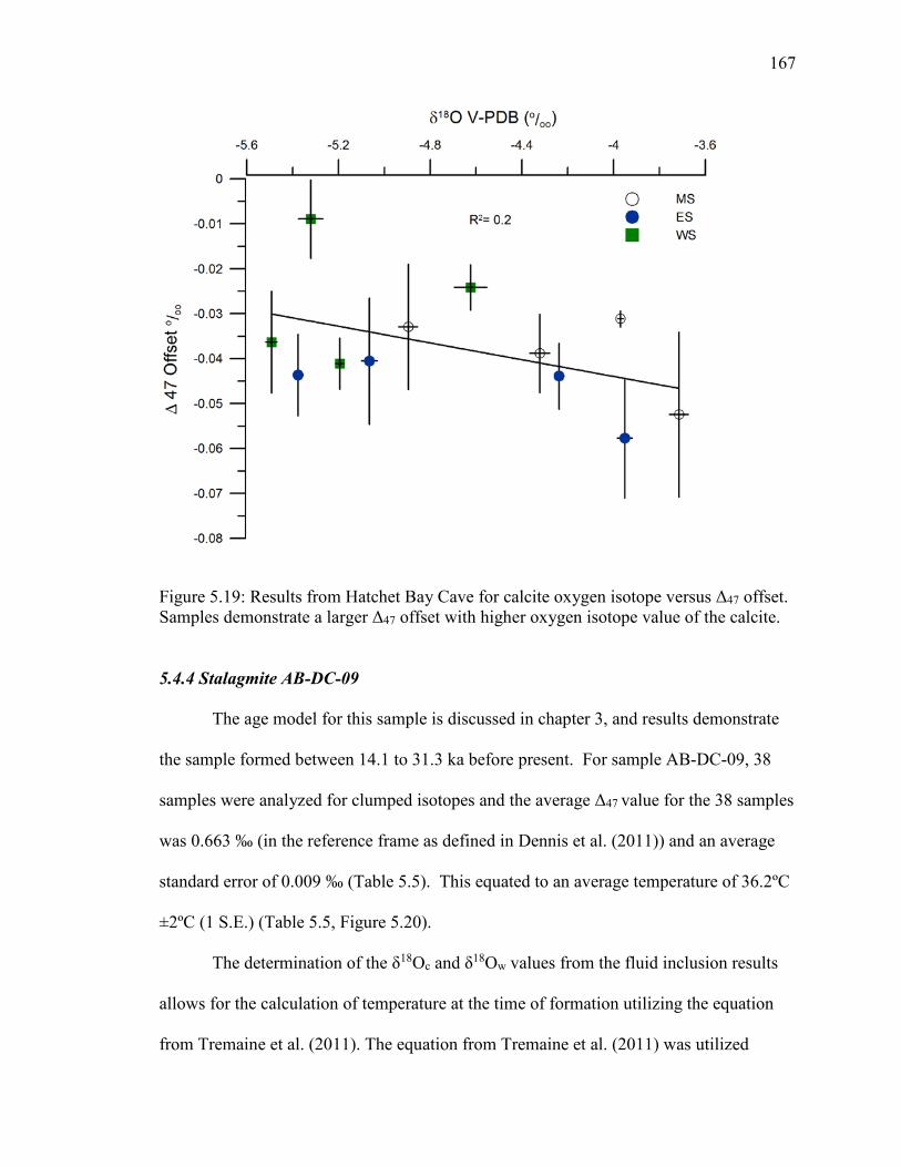
167

Figure 5.19: Results from Hatchet Bay Cave for calcite oxygen isotope versus Δ47 offset. Samples demonstrate a larger Δ47 offset with higher oxygen isotope value of the calcite. 5.4.4 Stalagmite AB-DC-09

The age model for this sample is discussed in chapter 3, and results demonstrate

the sample formed between 14.1 to 31.3 ka before present. For sample AB-DC-09, 38

samples were analyzed for clumped isotopes and the average Δ47 value for the 38 samples

was 0.663 ‰ (in the reference frame as defined in Dennis et al. (2011)) and an average

standard error of 0.009 ‰ (Table 5.5). This equated to an average temperature of 36.2ºC

±2ºC (1 S.E.) (Table 5.5, Figure 5.20).

The determination of the δ18Oc and δ18Ow values from the fluid inclusion results

allows for the calculation of temperature at the time of formation utilizing the equation

from Tremaine et al. (2011). The equation from Tremaine et al. (2011) was utilized

168

because this equation was determined from cave studies from around the world. Thirty

one of the 38 samples analyzed for clumped isotopes were previously analyzed for fluid

inclusion isotopes (see Chapter 3). This allowed for a direct comparison between the fluid

inclusion and clumped isotope results as shown in Figure 5.20 and Table 5.5. Similar to

the modern, the clumped isotope values from AB-DC-09 demonstrate warmer

temperatures than expected from the fluid inclusion results. The average temperature

from the fluid inclusion isotope results was 17.2 ±2.7 °C which is 18 °C cooler than the

average temperature derived from the clumped isotopes (Figure 5.20).

The temperatures calculated using the clumped isotope method demonstrate

higher variability than the results from fluid inclusions (Figure 5.20). A minimum

clumped temperature was at 26.2 ka BP and a maximum temperature at 14.9 ka BP. The

largest offsets are observed at 15.6 ka and 17.5 ka, corresponding with periods of lowered

temperatures from fluid inclusions (Figure 5.20, Table 5.5).

Table 5.5 (following page): Results from sample AB-DC-09 for clumped isotopes and fluid inclusion analyses. Age was determined from U-Th methods as described in Chapter 3. δ13C, δ18O and Δ47 values were determined from clumped isotope analyses. Δ47 values are reported in the reference frame of Dennis et al. (2011) using the methods outlined above. Temperature from fluid inclusions were determined using the equation from Tremaine et al. (2011) as described in chapter 3. Temperature offset represents the temperature difference between clumped isotopes and fluid inclusion temperatures.

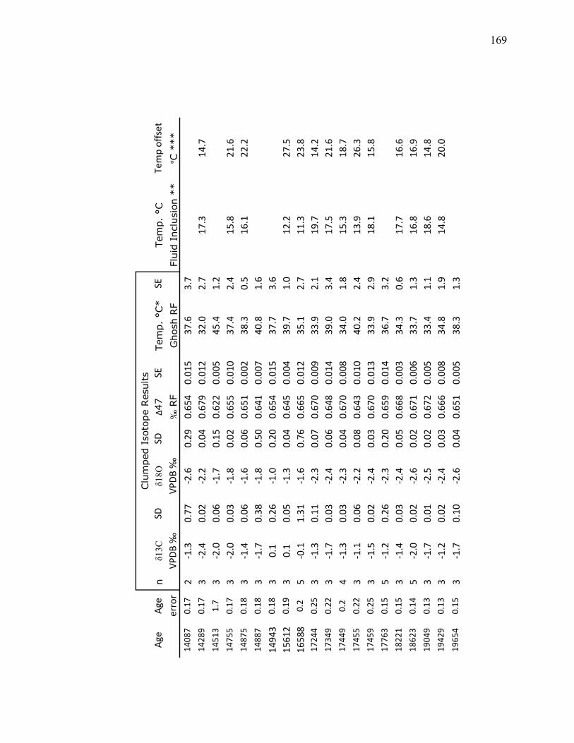
169

Clu

mpe

d Is

otop

e R

esul

ts

Age

Age

n

δ13C

SD

δ1

8O

SD

Δ47

SE

Tem

p. °

C*

SE

Te

mp.

°C

Tem

p of

fset

erro

r

VPDB

‰

VP

DB ‰

‰ R

F

Gho

sh R

F

Fl

uid

Incl

usio

n **

°C

***

14

087

0.17

2

-1.3

0.

77

-2.6

0.

29

0.65

4 0.

015

37.6

3.

7

14

289

0.17

3

-2.4

0.

02

-2.2

0.

04

0.67

9 0.

012

32.0

2.

7 17

.3

14.7

14

513

1.7

3 -2

.0

0.06

-1

.7

0.15

0.

622

0.00

5 45

.4

1.2

1475

5 0.

17

3 -2

.0

0.03

-1

.8

0.02

0.

655

0.01

0 37

.4

2.4

15.8

21

.6

1487

5 0.

18

3 -1

.4

0.06

-1

.6

0.06

0.

651

0.00

2 38

.3

0.5

16.1

22

.2

1488

7 0.

18

3 -1

.7

0.38

-1

.8

0.50

0.

641

0.00

7 40

.8

1.6

1494

3 0.

18

3 0.

1 0.

26

-1.0

0.

20

0.65

4 0.

015

37.7

3.

6

15

612

0.19

3

0.1

0.05

-1

.3

0.04

0.

645

0.00

4 39

.7

1.0

12.2

27

.5

1658

8 0.

2 5

-0.1

1.

31

-1.6

0.

76

0.66

5 0.

012

35.1

2.

7 11

.3

23.8

17

244

0.25

3

-1.3

0.

11

-2.3

0.

07

0.67

0 0.

009

33.9

2.

1 19

.7

14.2

17

349

0.22

3

-1.7

0.

03

-2.4

0.

06

0.64

8 0.

014

39.0

3.

4 17

.5

21.6

17

449

0.2

4 -1

.3

0.03

-2

.3

0.04

0.

670

0.00

8 34

.0

1.8

15.3

18

.7

1745

5 0.

22

3 -1

.1

0.06

-2

.2

0.08

0.

643

0.01

0 40

.2

2.4

13.9

26

.3

1745

9 0.

25

3 -1

.5

0.02

-2

.4

0.03

0.

670

0.01

3 33

.9

2.9

18.1

15

.8

1776

3 0.

15

5 -1

.2

0.26

-2

.3

0.20

0.

659

0.01

4 36

.7

3.2

1822

1 0.

15

3 -1

.4

0.03

-2

.4

0.05

0.

668

0.00

3 34

.3

0.6

17.7

16

.6

1862

3 0.

14

5 -2

.0

0.02

-2

.6

0.02

0.

671

0.00

6 33

.7

1.3

16.8

16

.9

1904

9 0.

13

3 -1

.7

0.01

-2

.5

0.02

0.

672

0.00

5 33

.4

1.1

18.6

14

.8

1942

9 0.

13

3 -1

.2

0.02

-2

.4

0.03

0.

666

0.00

8 34

.8

1.9

14.8

20

.0

1965

4 0.

15

3 -1

.7

0.10

-2

.6

0.04

0.

651

0.00

5 38

.3

1.3

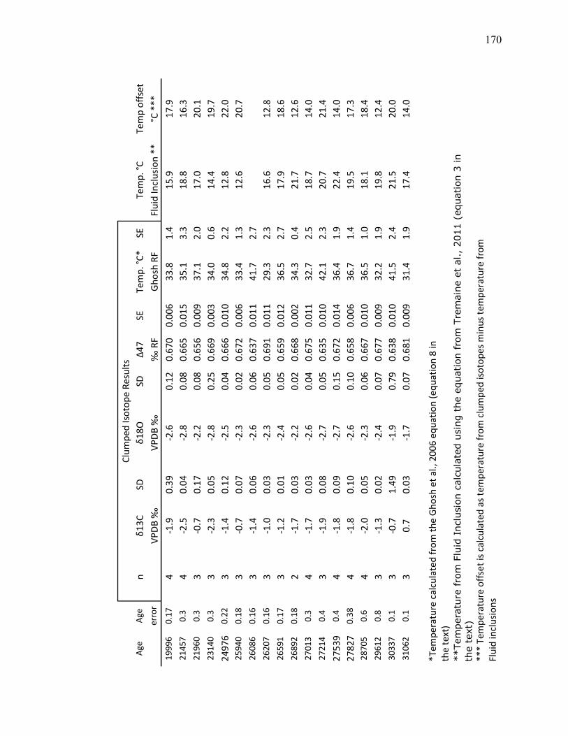
170

Clum

ped

Isoto

pe R

esul

ts

Age

Age

n

δ13C

SD

δ1

8O

SD

Δ47

SE

Tem

p. °C

*

SE

Tem

p. °C

Te

mp

offs

et

er

ror

VP

DB ‰

VPDB

‰

‰

RF

Gh

osh

RF

Fl

uid

Incl

usio

n **

°C

***

19

996

0.17

4

-1.9

0.

39

-2.6

0.

12

0.67

0 0.

006

33.8

1.

4 15

.9

17.9

21

457

0.3

4 -2

.5

0.04

-2

.8

0.08

0.

665

0.01

5 35

.1

3.3

18.8

16

.3

2196

0 0.

3 3

-0.7

0.

17

-2.2

0.

08

0.65

6 0.

009

37.1

2.

0 17

.0

20.1

23

140

0.3

3 -2

.3

0.05

-2

.8

0.25

0.

669

0.00

3 34

.0

0.6

14.4

19

.7

2497

6 0.

22

3 -1

.4

0.12

-2

.5

0.04

0.

666

0.01

0 34

.8

2.2

12.8

22

.0

2594

0 0.

18

3 -0

.7

0.07

-2

.3

0.02

0.

672

0.00

6 33

.4

1.3

12.6

20

.7

2608

6 0.

16

3 -1

.4

0.06

-2

.6

0.06

0.

637

0.01

1 41

.7

2.7

2620

7 0.

16

3 -1

.0

0.03

-2

.3

0.05

0.

691

0.01

1 29

.3

2.3

16.6

12

.8

2659

1 0.

17

3 -1

.2

0.01

-2

.4

0.05

0.

659

0.01

2 36

.5

2.7

17.9

18

.6

2689

2 0.

18

2 -1

.7

0.03

-2

.2

0.02

0.

668

0.00

2 34

.3

0.4

21.7

12

.6

2701

3 0.

3 4

-1.7

0.

03

-2.6

0.

04

0.67

5 0.

011

32.7

2.

5 18

.7

14.0

27

214

0.4

3 -1

.9

0.08

-2

.7

0.05

0.

635

0.01

0 42

.1

2.3

20.7

21

.4

2753

9 0.

4 4

-1.8

0.

09

-2.7

0.

15

0.67

2 0.

014

36.4

1.

9 22

.4

14.0

27

827

0.38

4

-1.8

0.

10

-2.6

0.

10

0.65

8 0.

006

36.7

1.

4 19

.5

17.3

28

705

0.6

4 -2

.0

0.05

-2

.3

0.06

0.

667

0.01

0 36

.5

1.0

18.1

18

.4

2961

2 0.

8 3

-1.3

0.

02

-2.4

0.

07

0.67

7 0.

009

32.2

1.

9 19

.8

12.4

30

337

0.1

3 -0

.7

1.49

-1

.9

0.79

0.

638

0.01

0 41

.5

2.4

21.5

20

.0

3106

2 0.

1 3

0.7

0.03

-1

.7

0.07

0.

681

0.00

9 31

.4

1.9

17.4

14

.0

*T

empe

ratu

re c

alcu

late

d fr

om th

e Gh

osh

et a

l., 2

006

equa

tion

(equ

atio

n 8

in

the

text

)

**Te

mpe

ratu

re f

rom

Flu

id I

nclu

sion

cal

cula

ted

usin

g th

e eq

uation

fro

m T

rem

aine

et

al.,

201

1 (e

quat

ion

3 in

th

e te

xt)

**

* Te

mpe

ratu

re o

ffset

is c

alcu

late

d as

tem

pera

ture

from

clu

mpe

d iso

tope

s min

us te

mpe

ratu

re fr

om

Flui

d in

clus

ions

171

Figure 5.20: Results from clumped isotope analysis of sample AB-DC-09 plotted with the age scale. A) Clumped isotope values for all samples analyzed. B) Carbon and oxygen isotopes of the carbonate determined during the clumped isotope analysis. C) Fluid inclusion temperature results from Chapter 3. D) Temperature offset reported as the difference in temperature from clumped and from fluid inclusions. Blue bars represent Heinrich stadials which are global climatic events and are shown to be periods of temperature decrease in the Bahamas.

HS1 HS2 HS3

172

5.5 Discussion

5.5.1 Modern: Environment of the cave

Published records suggest modern annual variation in air temperature ranges from

22 to 28 °C in the Bahamas, with the coldest month being January and the warmest in

July and August (Baldini et al., 2007). Relative humidity averages ~77%, with little

annual variation (Yanes and Romanek, 2013). There are distinct wet and dry seasons with

the wetter period between May to November driven by the Bermuda high and an

observed break in the wet season in July due to the westward expansion of the Bermuda

high (Magana et al., 1999). Growth rates are found to be lowest corresponding to the dry

season, suggesting that there is not a significant lag for the rainfall to reach the cave

(Figure 5.11). The pH, δ13CDIC and δ13CCO2 results are similar to observations from cave

monitoring studies (Lambert and Aharon, 2011; Mattey et al., 2008; Tremaine et al.,

2011) and the total alkalinity results are similar to the calculated results from Tremaine et

al. (2011).

Fluctuations in net rainfall amount (Precipitation minus Evapotranspiration: P-

ET) can affect drip water. With decreasing net rainfall, there will be a decrease in

hydrologic head and therefore a reduction in drip rate and with the Bahamas rainfall

seasonality, this would create a generally negative net rainfall during the dry season.

Evapotranspiration is shown in a cave in Florida to lead to increased concentration of Cl-

with no effect on the δ18Ow or δ2Hw of the drip water (Tremaine and Froelich, 2013).

Therefore the increased Cl- deeper in the cave may be due to evapotranspiration

processes influencing the water in this region, leading to increased Cl- water.

173

5.5.2 Modern: Carbon isotopes

The DIC of the drip water reflects bedrock carbon, soil gas CO2 and a component

of atmospheric CO2 (Fohlmeister et al., 2011; Lambert and Aharon, 2011; Tremaine et

al., 2011). Carbon isotopic ratio from the soil zone is dependent on the type of overlying

vegetation (C3 vs C4), the amount of vegetation, the soil microbial activity and the

ventilation processes occurring (Genty et al., 2003; Lambert and Aharon, 2011). In HBC,

it appears that the soil zone end member is approximately -18 ‰ VPDB (Figure 5.7).

Within the epikarst, the DIC can be impacted by prior calcite precipitation (PCP) in

which calcite precipitates prior to the drip water reaching the cave. This occurs through

degassing of CO2 being present in the epikarst, particularly during dry events when the

groundwater table is depressed. Prior calcite precipitation leads to the CO2 exchange

with the epikarst air, and an opportunity for the carbon isotopes of the DIC to be altered

(Tremaine and Froelich, 2013). Once the drip waters reach the cave environment, the

difference of the pCO2 of the water and the cave air leads to the exchange and degassing

of CO2 and precipitation of CaCO3 (equation 4). This can again lead to prior calcite

precipitation. The rate of CO2 degassing varies with drip water flow rates and the pCO2

of the cave environment and drip water. Variation of the pCO2 of the cave is typically

thought to be related to ventilation changes, with increased ventilation decreasing the

pCO2 of the cave and hence increasing the rate of degassing and calcite precipitation

(Kowalczk and Froelich, 2010; Lambert and Aharon, 2011).

Several cave studies have demonstrated that δ13Cc values in cave calcites are

enriched relative to the expected equilibrium values based on δ13CDIC measurements

(Mickler et al., 2004; Riechelmann et al., 2013; Tremaine et al., 2011). Carbon isotopic

174

fractionation from HCO3-(aq) to carbonate has been suggested to be minimal, with some

studies suggesting fractionation of up to 1 ‰ (Romanek et al., 1992; Rubinson and

Clayton, 1969; Tremaine et al., 2011). The observed δ13Cc enrichment in caves relative

to the δ13CDIC value has been attributed to ventilation driven CO2 degassing causing an

enhanced enrichment of the δ13CDIC or as CO2 exchange between gas phase and aqueous

phase is more rapid than net degassing. Periods of increased ventilation is associated

increased net degassing of CO2 and calcite precipitation via dehydration (equation 5).

Increased rate of degassing leads the remaining HCO3-(aq) to become progressively

enriched in 13C resulting in an increased calcite δ13Cc value (Lambert and Aharon, 2011;

Mickler et al., 2004; Tremaine et al., 2011). During degassing processes the carbon

isotope of the drip water will become progressively will be heavier also due to the DIC-

CO2 exchange with ventilated cave air (Tremaine et al., 2011). In HBC, the cave air is

heavily influenced by atmospheric air, and therefore a much greater δ13C value and hence

driving the increased δ13Cc value of the precipitated calcite.

In HBC, there is evidence of some enrichment of δ13Cc value from the center to

the outside of the slide. This may in part be driven by degassing processes which leads to

increased δ13Cc from the center and due to exchange with the heavier cave air.

As suggested above, ventilation changes and degassing processes can greatly

impact the degassing rate of CO2 and hence kinetic isotope fractionation. In this study,

results from the δ13CC of the slides are shown to be more positive than the original soil

zone carbon isotopic value (Figure 5.18) suggesting that isotopic exchange has occurred

since the soil zone, most likely due to degassing and exchange with the air. The δ13CCO2

value is lowest in the west room suggesting that this is the least ventilated room (Mattey

175

et al., 2008; Spotl et al., 2005; Tremaine et al., 2011), which is supported by the [CO2]

data, however other measurements (e.g. radon) are needed to verify that this room is in

fact the least ventilated. This interpretation is also supported by the lower δ13Cc and

δ13CDIC of the west room (Figure 5.9) (Lambert and Aharon, 2011; Spotl et al., 2005).

When comparing the δ13CDIC to the δ13Cc results, there appears to be minimal offset

between the carbonate and DIC for the main room, while the west room δ13Cc values are

lower than the average δ13CDIC values (Figure 5.9, Table 5.6a). However the δ13CDIC

values are highly variable for all locations (Table 5.9a).

Studies have also shown that ventilation may vary seasonally as processes in the

soil zone change (Lambert and Aharon, 2011; Tremaine et al., 2011) In order to better

understand seasonalilty of ventilation, a longer sampling period is necessary in HBC.

However, the limited sampling suggests that the summer may be characterized by

increased δ13CCO2 value for both locations on the third level, while winter is characterized

by decreased δ13CCO2 values, suggesting decreased ventilation in the winter (Table 5.7).

This is similar to the ventilation regime observed in a cave in Gibraltar, where cave pCO2

increases in the winter and decreases in the summer (ventilation decreases in the winter

and increases in the summer) (Mattey et al., 2008). As previously demonstrated,

ventilation can impact degassing with periods of increased ventilation associated with

increased degassing rates and ventilation will bring heavy 13CO2 from outside air into the

cave. HBC is a well-ventilated cave therefore the impacts of ventilation are thought to be

driving the δ13Cc results.

176

Table 5.6: δ18Oc (A) and δ13Cc (B) differences for the Hatchet Bay Cave samples. A) Measured δ13Cc values compared to measured δ13CDIC results from the drip waters. The results demonstrate limited fractionation between the DIC and the calcite δ13Cc values, which may be due to the large errors of the δ13CDIC results. B) Measured δ18Ow of drip waters and cave temperature were used to calculate the predicted δ18Oc values based on the Kim and O'Neil (1997) (equation 2), O'Neil et al. (1969) (equation 1), and Tremaine et al. (2011) (equation 3) equations. Predicted δ18Oc values were then compared to the measured δ18Oc values (measured – observed). Results demonstrate increased difference in the MS location compared to ES and WS.

A.

Location δ13CC S.D. δ13CDIC S.D. δ13C

difference (VPDB ‰) (VPDB ‰) calcite - DIC

MS -9.57 0.8 -9.47 3.0 -0.09 ES -9.54 1.5 -9.47 3.0 -0.07 WS -10.88 0.6 -10.16 1.6 -0.72

B.

Corrected Kim and O’Neil 1997 S.D. O’Neil et al. 1969 S.D.

Tremaine et al. 2011 S.D.

Location offset (VPDB ‰) offset (VPDB ‰) offset (VPDB

‰) MS 1.81 0.53 1.72 0.54 0.76 0.53 ES 1.38 0.61 1.29 0.61 0.32 0.62 WS 1.15 0.64 1.31 0.33 0.34 0.34

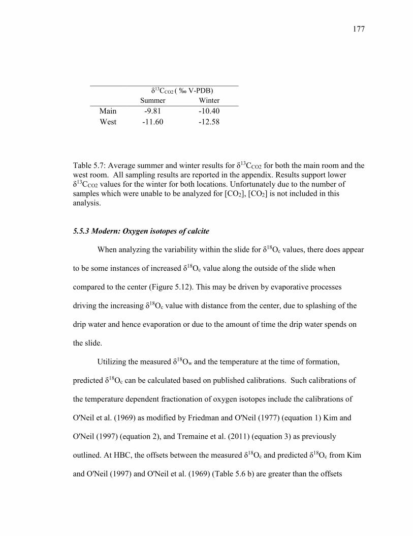
177

Table 5.7: Average summer and winter results for δ13CCO2 for both the main room and the west room. All sampling results are reported in the appendix. Results support lower δ13CCO2 values for the winter for both locations. Unfortunately due to the number of samples which were unable to be analyzed for [CO2], [CO2] is not included in this analysis.

5.5.3 Modern: Oxygen isotopes of calcite

When analyzing the variability within the slide for δ18Oc values, there does appear

to be some instances of increased δ18Oc value along the outside of the slide when

compared to the center (Figure 5.12). This may be driven by evaporative processes

driving the increasing δ18Oc value with distance from the center, due to splashing of the

drip water and hence evaporation or due to the amount of time the drip water spends on

the slide.

Utilizing the measured δ18Ow and the temperature at the time of formation,

predicted δ18Oc can be calculated based on published calibrations. Such calibrations of

the temperature dependent fractionation of oxygen isotopes include the calibrations of

O'Neil et al. (1969) as modified by Friedman and O'Neil (1977) (equation 1) Kim and

O'Neil (1997) (equation 2), and Tremaine et al. (2011) (equation 3) as previously

outlined. At HBC, the offsets between the measured δ18Oc and predicted δ18Oc from Kim

and O'Neil (1997) and O'Neil et al. (1969) (Table 5.6 b) are greater than the offsets

δ13CCO2 ( ‰ V-PDB)

Summer Winter

Main -9.81 -10.40 West -11.60 -12.58

178

observed during the monitoring study of Tremaine et al. (2011). Results demonstrate the

greatest offset is observed in the MS location, while ES and WS calcites agree best with

the temperature dependent fractionation equation from Tremaine et al. (2011) (Figure

5.21,Table 5.6 b). This suggests either there is enhanced fractionation occurring at MS

through evaporation or the limited sampling has not captured the full δ18Ow of the drip

waters for this site and therefore has offset the calculations of the expected δ18Oc values.

From the drip water δ18Ow results, the residence time of the water is thought to be

long enough that the δ18Ow of the drip water should not be affected by rapid short lived

events, such as hurricanes, which are known to have isotopically light δ18Ow values (Price

et al., 2008).

The observed δ18Oc results for HBC are compared to published cave monitoring

results in Figure 5.21. These results demonstrate the large variability for the oxygen

isotope fractionation in the cave, with a majority of the samples falling near the equation

from Tremaine et al. (2011). These results further support that the temperature dependent

fractionation is offset for speleothems from previously published laboratory studies and

agree well with the findings by Tremaine et al. (2011).

Factors that can influence the fractionation of oxygen isotopes during

precipitation include the rate of net precipitation as demonstrated in the δ13Cc system

and/or evaporative processes. Evaporative processes can lead to the oxygen isotopes of

the water and hence calcite to become progressively heavier (Tremaine et al., 2011).

This can occur as a result of evaporative processes in the soil zone or in the cave.

Precipitation rate can influence the kinetic fractionation if the rate of precipitation

is faster than the rate of HCO3-(aq) re-equilibration. Studies have also demonstrated the

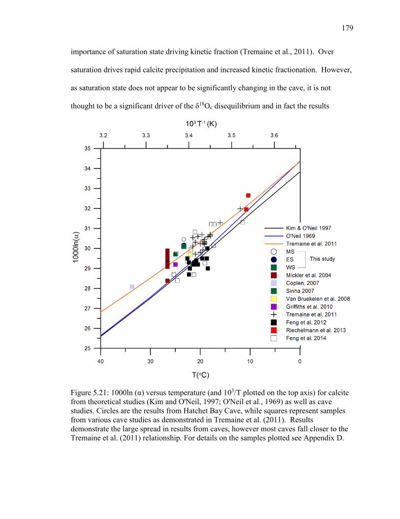
179

importance of saturation state driving kinetic fraction (Tremaine et al., 2011). Over

saturation drives rapid calcite precipitation and increased kinetic fractionation. However,

as saturation state does not appear to be significantly changing in the cave, it is not

thought to be a significant driver of the δ18Oc disequilibrium and in fact the results

Figure 5.21: 1000ln (α) versus temperature (and 103/T plotted on the top axis) for calcite from theoretical studies (Kim and O'Neil, 1997; O'Neil et al., 1969) as well as cave studies. Circles are the results from Hatchet Bay Cave, while squares represent samples from various cave studies as demonstrated in Tremaine et al. (2011). Results demonstrate the large spread in results from caves, however most caves fall closer to the Tremaine et al. (2011) relationship. For details on the samples plotted see Appendix D.

180

do not support a statistically significant relationship between δ18Oc and saturation state.

Rather, the primary driver of fractionation for δ18Oc and δ13Cc isotopes is thought to be

the CO2 exchange between drip water and cave air during degassing fractionation.

Additionally it has been proposed that during the process of dehydration, when CO2

degassing occurs rapidly, can lead to δ18Oc and δ13Cc isotope fractionation.

5.5.4 Modern: What drives clumped isotope offset?

Previous studies demonstrate that the temperatures calculated using the clumped

isotope value in speleothems are consistently warmer than expected (Δ47 values are lower

than expected) (Affek et al., 2008; Daëron et al., 2011; Kluge and Affek, 2012). This

would suggest that certain mechanisms unique to speleothems may be causing Δ47 to be

out of equilibrium. As demonstrated above, samples may pass the Hendy test, but may

still exhibit Δ47 value variability within a slide. This suggests that clumped isotopes may

be more sensitive to kinetic effects, as also found in Kluge and Affek (2012).

The offset observed in the modern is similar to the observations by Affek et al.

(2008) with an average offset of 8 ºC, Kluge and Affek (2012) observed a mean offset of

10 ºC and Daëron et al. (2011) observed offsets ranging from 3.5-22 ºC. The results of

HBC clumped isotopes will be utilized to better understand clumped isotope offsets and

variability.

Temporal and spatial variability:

Studies have shown that saturation state can impact the Δ47 offset with

supersaturation driving an increased Δ47 offset, as increased saturation is driven by higher

degassing rates, hence the degree of kinetic fractionation (Kluge and Affek, 2012).

However, in HBC the reverse is observed with increasing saturation being correlated with

181

decreasing Δ47 offset (Figure 5.15). Given the limited number of datasets for which

saturation state is available, further studies are necessary to validate these results.

Growth rate variability is found within HBC, with increased growth rate in the

WS, compared to the MS and ES locations. The strong relationship between growth rate

and Δ47 offset observed in the WS location may be due to degassing rates. The sample

with the lowest offset was found in December 2012, when ventilation was the lowest and

hence the degassing rate was the lowest. Conversely, no relationship is observed between

growth rate and Δ47 offset at either the ES or MS locations. Kluge and Affek (2012) also

observed no significant relationship between growth rate and Δ47 offset.

The relationship between increasing δ18Oc disequilibrium and Δ47 offset (Figure

5.22) may be driven by the degassing rate and exchange rates of CO2 and/or evaporative

processes (Affek et al., 2008; Daëron et al., 2011). During fast degassing, the product

CO2 may have a greater Δ47 value than the HCO3-(aq) and if the residual HCO3

- does not

re-equilibrate with the remaining water, fractionation of the isotopic composition follows

a Rayleigh type distillation (Guo, 2008). However, with slow degassing, re-equilibration

can occur, and the Δ47 value will remain in equilibrium (Affek et al., 2008; Kluge and

Affek, 2012). Guo (2008) theoretically calculated the impacts of dehydration and

dehydroxylation on the δ13C, δ18O, and Δ47 values and found that for every 1 ‰ increase

in δ18O, the δ13C value increases by 1.1-3.2 ‰ and the Δ47 value decreases by 0.017 to

0.026 ‰. The variability of fractionation is dependent upon the pathway of the CO2

degassing and how much carbonate forms (Guo, 2008). Evaporative processes can also

drive δ18O offset in HBC, while CO2 degassing and exchange processes can lead to offset

182

in Δ47 value, resulting in a linear relationship between the two, however it is unclear if

should influences were considered in Guo (2008).

The trend shown in Figure 5.22 demonstrates the relationship between increasing

δ18O offset and Δ47 offset for HBC, for the study by Kluge and Affek (2012) and for

theoretical modeling (Guo, 2008) utilizing Kim and O'Neil (1997) as equilibrium to

calculate the δ18O offset. The theoretical model plotted assumes the primary pathway for

degassing is dehydration, with a 1:1 precipitation rate and assuming for a 1 ‰ increase in

δ18Oc, a -0.0175 ‰ decrease in Δ47 and a +2.34 ‰ increase in δ13Cc value (Figure 5.22).

The slope for HBC (-0.023 ‰) is shallower than the slope from Kluge and Affek (2012)

(-0.047 ‰) and from Daëron et al. (2011) (not shown) suggesting that disequilibrium

may vary by cave and with time. However the results from HBC fall closer to the

fractionation predicted from Guo (2008) for degassing processes driving the offset for

δ18Oc and Δ47 (Figure 5.22).

The trend shown in Figure 5.23 demonstrates the relationship between increasing

δ18O offset and Δ47 offset for this study, utilizing Tremaine et al. (2011) as equilibrium.

Since the data from Kluge and Affek (2012) were calculated using Kim and O'Neil

(1997), the data cannot be plotted on Figure 5.23. The slope for the HBC data is steeper (-

0.042 ‰) when calculated using the Tremaine et al. (2011) equation.

The above mentioned explanation for the drivers of the observed Δ47 offset relies

heavily on the influences of degassing processes (and subsequent dehydration) in driving

the observed offsets. However, the exchange between the heavier cave air (Figure 5.7)

and the drip water may also lead the observed Δ47 offset. When comparing the δ13Cc

results to the Δ47 value, the δ13Cc value is offset from the soil gas end member (Figure

183

5.18). This is thought to be due the exchange between the heavier cave air (Figure 5.7)

and the drip water. This exchange leads to the increasing δ13Cc value and Δ47 value

observed in Figure 5.18 and would be expected to occur in a well-ventilated cave such as

HBC. This also accounts for the strong relationship between δ13Cc value and the Δ47

value, while conversely there is a weak relationship between δ18Oc and Δ47 value. When

comparing the δ13Cc to the δ13CDIC values, (Figure 5.24) the δ13CDIC values are more

negative suggesting the drip water has not yet equilibrated with the cave air, but rather

during the precipitation of CaCO3 there has been exchange, hence increased δ13Cc values.

When compared to the expected results from Guo (2008), the HBC results plot below the

Guo (2008) line (Figure 5.24). However the errors on the δ13CDIC are large. With

increased sampling for δ13CDIC and a better characterization, in the future a greater

understanding of the factors driving δ13Cc and Δ47 offset can be developed.

Summary of HBC observations:

Overall, geochemical results suggest variation in kinetic fractionation for different

parts of the cave. Fractionation is enhanced in the main room compared with the west

room for both δ18Oc and Δ47 values (Figure 5.13 & 5.19). The two clear differences

between the main room and west room are growth rate and ventilation (Figure 5.8 &

5.11). The west room overall has a higher growth rate and an observed decreased Δ47

offset during periods of slower growth. In addition, the period of decreased growth rate

(winter) is also the period of decreased ventilation and therefore a decreased degassing

rate. This suggests that a combination of these factors may drive the Δ47 towards

equilibrium.

184

The main room is considered to be more ventilated and based on the δ13Cc and

δ18Oc data, more fractionated. The greater fractionation in this part of the cave may be a

result of increased ventilation or an increase in evaporation.

5.5.5 Clumped isotopes versus fluid inclusions: Stalagmite AB-DC-09

The average offset between the clumped isotope temperature and the temperature

determined from fluid inclusions in sample AB-DC-09 is 18 ºC. This value is much larger

than the temperature offset observed in the modern between clumped isotope and

measured temperature (8.6 ºC). This suggests that either the temperatures (based on the

δ18Ow of the fluid inclusions and the δ18Oc of the calcite) are lower than expected,

possibly driven by fractionation, or that the clumped isotopes are more fractionated

thereby leading to an increased offset. Based on the fluid inclusion data, there does not

Figure 5.22: Results from Hatchet Bay Cave (circles) demonstrating the systematic offset from the expected value for both Δ47 and δ18Oc values. Also plotted are results from Kluge and Affek (2012), demonstrating a positive δ18Oc offset and a negative Δ47 offset. The purple line represents the average slope of -0.023 ‰ observed for HBC, the blue line is the -0.047 ‰ slope for Kluge and Affek results and red is the theoretical slope from Guo, 2008 as described in the text. The correlation between both Δ47 and δ18Oc supports similar factors drive both. Average error from the HBC results is represented by the black circle.

185

Figure 5.23: Results from Hatchet Bay Cave demonstrating the systematic offset from the expected value for both Δ47 and δ18Oc values. Δ47 offset was determined as the offset from the temperature measured in the cave and the δ18Oc offset was determined as the offset from the expected from Tremaine et al. (2011). The orange line represents the average slope of -0.042 ‰ observed for HBC and red is the theoretical slope from Guo, 2008 as described in the text. The correlation between both Δ47 and δ18Oc supports similar factors drive both. Average error from the HBC results is represented by the black circle.

186

Figure 5.24: Results from Hatchet Bay Cave (circles) demonstrating the systematic offset from the expected value for both Δ47 and δ13Cc values. The red line represents the theoretical slope from Guo, 2008 as described in the text, with an intercept at the origin as this plot represents offsets. The results from HBC plot below the expected from Guo, 2008 and have large errors suggesting additional work is necessary. Average error from the HBC results is represented by the black circle.

appear to be any indication of significant fractionation taking place (see Chapter 3), and

therefore we propose that differences arise as a result of increased Δ47 kinetic

fractionation. The periods with the greatest offset between the clumped isotope and fluid

inclusion records are found at 15.6 and 17.5 ka BP (Figure 5.20). This is a period

characterized by decreasing temperatures in the fluid inclusion results, reflecting the

impact of a global scale climate event, known as a Heinrich stadial. In the Bahamas,

Heinrich stadials have been shown to be periods of lower temperature and lower

precipitation (Chapters 3 and 4). Therefore, it is possible that during these events there

was an associated change in the rate of degassing leading to the observed enhanced Δ47

187

offset. This change in the degassing rate can be driven by changes in the amount of water

in the overlying limestone. With less water in the epikarst (due to aridity) there is the

potential for increased cave ventilation through the passages which are normally filled

with water. Increased ventilation could lead to a decrease in the pCO2 and hence

increased rate of degassing and Δ47 fractionation.

5.5.6 Correction of clumped data

A method for correcting Δ47 values has been proposed by Wainer et al. (2011)

utilizing the fluid inclusion results and monitoring data. As demonstrated from the

modern data from HBC, the 1000ln(α) and Δ47 offset correlates with a slope of -0.042 ‰

(Figure 5.23) when utilizing Tremaine et al. (2011) as equilibrium. As proposed by

Wainer et al. (2011), the slope of this disequilibrium line can be utilized to project the Δ47

results back to equilibrium allowing for the calculation of a “corrected” temperature.

This assumes the sample was offset from the original temperature along a kinetic isotope

fractionation vector with a known slope. Four clumped isotope samples were chosen to

demonstrate this method and are presented in Figure 5.25. Utilizing the fluid inclusion

results to correct the clumped isotope results is circular reasoning; however, as is

described below, a worthwhile exercise as this may shed light on kinetic fractionation

over time.

The four samples chosen to demonstrate this correction method are from a range

of 1000ln(α) values and are plotted as 1000ln(α) versus Δ47 value in Figure 5.25. The

1000ln(α) value was calculated from the δ18Oc of the carbonate and the δ18Ow of the fluid

inclusion water and the Δ47 value is the measured value. From this original point, the

1000ln(α) and Δ47 values are transformed along the slope of the 1000ln(α) versus Δ47

188

offset previously determined (i.e. -0.042 ‰ from HBC). The values are corrected to the

point of equilibrium, using Tremaine et al. (2011) for equilibrium. At the point of

equilibrium, the Δ47 and 1000ln(α) values have been corrected such that temperature

calculated using Ghosh et al. (2006) and the temperature calculated by Tremaine et al.

(2011) are equal. Figure 5.25 transforms the Δ47 and 1000ln(α) along the slope

determined from the modern Hatch Bay Cave from Figure 5.23. Since we have defined

equilibrium as the Tremaine et al. (2011) equation, we cannot utilize the slopes calculated

in Figure 5.22 (calculated using Kim and O'Neil (1997)).

This same transformation was applied to all samples which were analyzed for

clumped isotopes and fluid inclusions and the results are presented in Figures 5.26.

Utilizing the slope observed in the modern produces samples which are on average 6 ºC

±3 warmer than indicated by the fluid inclusion data (Figure 5.26).

The offset between the corrected clumped isotope and fluid inclusion data is the

greatest from 15 to 16.8 ka BP. This indicates a steeper Δ47 offset to 1000ln(α)

characterizes these two time periods. Overall the trend for the corrected samples is

similar to the trend from the original fluid inclusion results, with both the corrected Δ47

and the fluid inclusion temperature records demonstrating decreased temperatures

associated with Heinrich stadials. These results indicate that fractionation of both the Δ47

and δ18Oc occurs and also that fractionation varies between with time, with the Heinrich

stadials 1 and 2 exhibiting the greatest offset after correction, suggesting a steeper δ18Oc

offset versus Δ47 offset at these time periods.

In the modern cave, the results from the Bahamas support the conclusion that

factors such as growth rate and ventilation drives kinetic isotope fractionation.

189

Figure 5.25: Samples from AB-DC-09 plot below the equilibrium line defined by Tremaine et al., 2011 and Ghosh et al., 2006 as outlined above. Using the modern slope for disequilibrium from Figure 5.23, samples can be corrected back to equilibrium using the observed slope. A) Four samples projected back to the equilibrium line of Tremaine et al. (2011) using the observed slope of HBC from Figure 5.23, with a slope of -0.042. The new equilibrium temperatures are shown for each sample. The original fluid inclusion data was calculated using the Tremaine equation (see chapter 3).

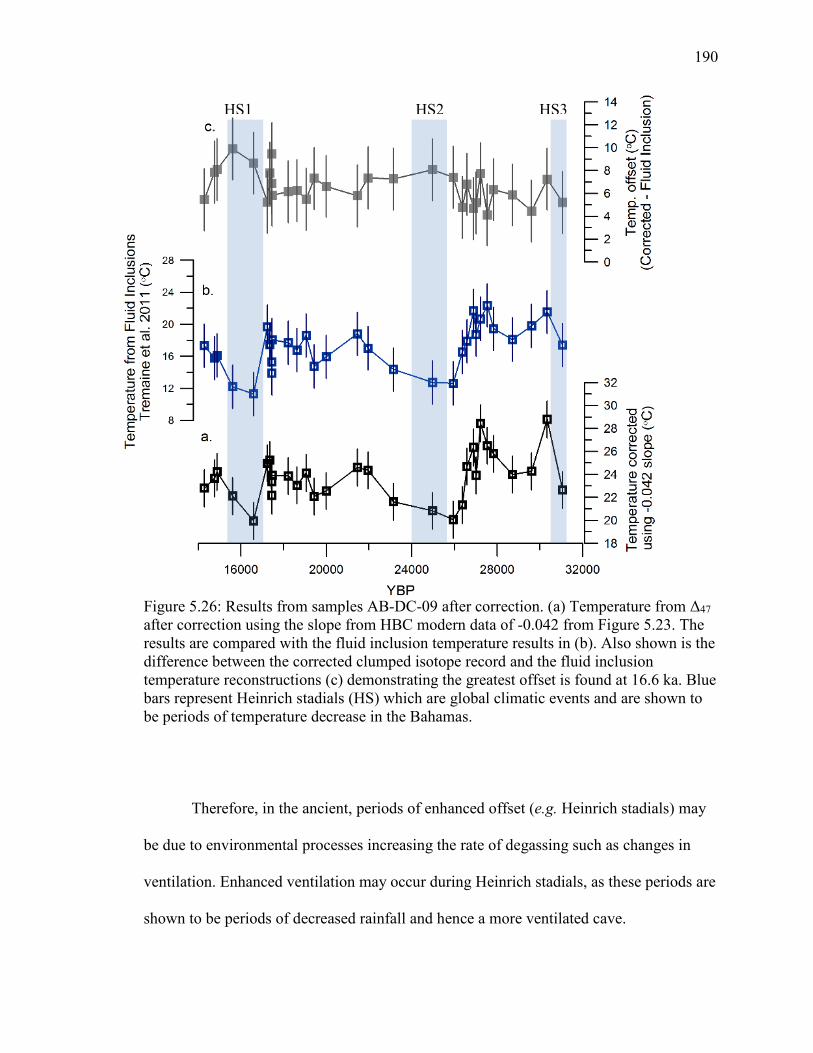
190

.

Figure 5.26: Results from samples AB-DC-09 after correction. (a) Temperature from Δ47 after correction using the slope from HBC modern data of -0.042 from Figure 5.23. The results are compared with the fluid inclusion temperature results in (b). Also shown is the difference between the corrected clumped isotope record and the fluid inclusion temperature reconstructions (c) demonstrating the greatest offset is found at 16.6 ka. Blue bars represent Heinrich stadials (HS) which are global climatic events and are shown to be periods of temperature decrease in the Bahamas.

Therefore, in the ancient, periods of enhanced offset (e.g. Heinrich stadials) may

be due to environmental processes increasing the rate of degassing such as changes in

ventilation. Enhanced ventilation may occur during Heinrich stadials, as these periods are

shown to be periods of decreased rainfall and hence a more ventilated cave.

HS1 HS2 HS3

191

5.6 Conclusion

This study represent an attempt to better understand carbon, oxygen and clumped

isotope fractionation in a cave using modern and ancient cave carbonates. The results

from the modern demonstrate enhanced fractionation for carbon and oxygen isotopes of

the calcite for the Main site compared to the East and West locations. The west room is

thought to be less fractionated with respect to carbon and oxygen isotopes as a result of

the reduced ventilation. For the clumped isotope results, the temperatures calculated

from the clumped isotope data are 6 °C warmer than the monitored temperature in the

cave. The growth rate and ventilation appear to be driving the clumped isotope offset for

the west room as both processes influence the degassing process. Overall, for the three

locations, fractionation driven by either DIC-CO2 of the cave air equilibration or

hydration processes appears to be primarily driving both δ18Oc and Δ47 offset.

For speleothem sample AB-DC-09, the temperatures calculated from the clumped

isotope method are offset from those estimated using the δ18Ow from the fluid inclusions

and the carbonate of the same samples. The difference in temperature between these two

methods is greater than that observed in the modern farmed calcite. When the Δ47 value is

compared to the fluid inclusion results, periods with the lowest temperatures from fluid

inclusions are the periods with the greatest offset, suggesting a climatic control on the

kinetic isotope fractionation. One possibility is that the periods with the lowest

temperatures are also the periods with decreased precipitation, hence increased

ventilation, which would lead to greater degassing and evaporation, which would further

fractionate the clump isotopes, driving the greater offset at this time period. Using the

methods outlined in Wainer et al. (2011) the clumped isotope results have been corrected

192

to equilibrium using the relationship observed in the modern for 1000ln(α) offset versus

Δ47 offset. The corrected clumped isotope results suggest a greater Δ47 offset for every 1

‰ δ18O offset for sample AB-DC-09 particularly from 16.8 to 15 ka BP.

Chapter 6

Speleothems from Bahamas Blue Holes: Geochemical archives of past dust events

Summary

Modern studies of atmospheric dust demonstrate that there is seasonal deposition

today in the Caribbean derived from Africa. There is however a paucity of data on the

deposition of dust during past time periods in the Bahamas. This study represents an

attempt to understand modern and ancient deposition of dust in the Bahamas utilizing

speleothems. The isolated Bahamas platform represents an ideal location to study the

deposition of dust as its pristine limestone bedrock restricts the detrital source of trace

and minor elements to atmospheric deposition. In this study, iron will be utilized as a

proxy for atmospheric dust. Results from the study of a modern cave demonstrate good

agreement between the trace element concentrations of the water and that in the

associated precipitated calcite. Iron concentrations are found to be heterogeneous in drip

waters and calcite both temporally and spatially. The temporal variation is thought to be

due to annual variations in dust delivery and amount of precipitation. The spatial

variability within the cave is thought to be due to variations in drip water flow rates and

flow paths within the soil zone and limestone bedrock.

In order to supplement the work in the modern, two stalagmites collected from the

Bahamas which formed from 64,000 to 14,000 years before present were analyzed for

their Fe/Ca ratios. The Fe/Ca ratios of the ancient stalagmites are shown to increase

concurrently with changes in the oxygen and carbon isotopes that are associated with

Heinrich stadials. Other paleoclimate records from the Northern Hemisphere support the

notion that Heinrich stadials are dusty events, the increased Fe/Ca ratios in speleothems

193

194

associated with the Heinrich stadial terminations can potentially be explained by an

increase in precipitation at the end of each Heinrich stadial, bringing into the cave Fe rich

waters derived from prior deposited dust. The periods of the Fe increases in the Bahamas

are in good agreement with other Heinrich stadial dust records from Africa and

Greenland. This study supports the scenario that Heinrich stadials are dusty events in the

Northern Hemisphere and that dust is transported and deposited in the Bahamas.

6.1. Background

Atmospheric dust has been shown to impact sea surface temperatures (SSTs)

(Evan et al., 2011; Evan et al., 2009), precipitation (Yoshioka et al., 2007) and primary

productivity (Martinez-Garcia et al., 2011) both in the modern and in the past, making

dust an important component of the climate system (Mahowald et al., 2010; Mahowald

et al., 2006). Studies suggest decrease SSTs and precipitation with increasing

atmospheric dust (Evan et al., 2011; Evan et al., 2009; Yoshioka et al., 2007) and the

global scale impact of dust on the climate system supports the importance of studying

dust fluxes of the past.

Evidence recorded in ice and sediment cores suggests increased concentrations of

dust in the atmosphere during glacial periods. Overall, studies support that atmospheric

mineral dust was approximately 2-4 times higher worldwide during glacial periods than

interglacial periods (McGee et al., 2010), and up to 7 times higher over Africa (Just et al.,

2012). An even greater amount of dust in the atmosphere occurs synchronously with

millennial scale climate events, particularly during Heinrich stadials. Cores from the

western coast of Africa indicate increased dust originating from Africa during Heinrich

stadials (Jullien et al., 2007; Mulitza et al., 2008; Tjallingii et al., 2008) with estimates of

195

dust fluxes ranging from a 2.5 (McGee et al., 2013) to an 80 fold increase (Just et al.,

2012). Other evidence of increased aridity in the Northern Hemisphere during these

events is from sediment cores from the Arabian Sea (Pourmand et al., 2004) and records

from Eastern Europe (Sima et al., 2013). The increased Northern Hemisphere aridity

during stadials is thought to be driven by a reduction in Atlantic meridional overturning

circulation (AMOC), a decrease in Northern Hemisphere SSTs and a southerly shift in

the ITCZ (Bond et al., 1992; Clement and Peterson, 2008; Peterson et al., 2000).

6.2. Study Site

The Bahamas platform is an isolated carbonate platform approximately 80 km

east of South Florida (Figure 6.1) that includes low lying islands comprised of relatively

pure carbonate with no terrigenous input from rivers (Swart et al., 2014). The isolated

nature of the platform and the pure nature of the carbonate should be reflected in the

geochemistry of stalagmite calcite and the concentrations of minor and trace elements

should therefore remain low. Any departure from these low concentrations should reflect

an increase in dust delivery to the Bahamas. To understand modern dust fluxes to the

Bahamas, drip waters and calcites have been collected from a currently active cave from

Hatchet Bay Cave, Eleuthera Island, Bahamas. For the study of the past deposition of

dust to the Bahamas, stalagmite samples forming over the last six Heinrich stadials have

been collected from Abaco Island, Bahamas from a currently submerged cave. Both

Eleuthera and Abaco Islands are on the eastern edge of the Bahamas platform (Figure

6.1).

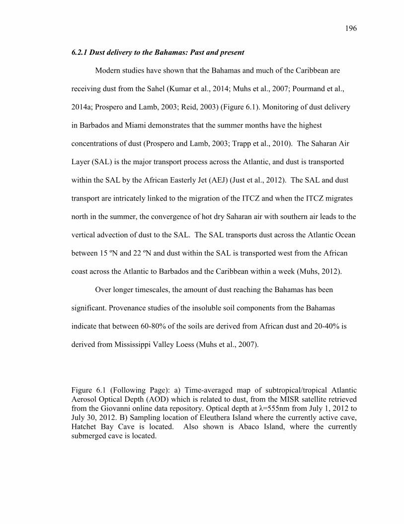
196

6.2.1 Dust delivery to the Bahamas: Past and present

Modern studies have shown that the Bahamas and much of the Caribbean are

receiving dust from the Sahel (Kumar et al., 2014; Muhs et al., 2007; Pourmand et al.,

2014a; Prospero and Lamb, 2003; Reid, 2003) (Figure 6.1). Monitoring of dust delivery

in Barbados and Miami demonstrates that the summer months have the highest

concentrations of dust (Prospero and Lamb, 2003; Trapp et al., 2010). The Saharan Air

Layer (SAL) is the major transport process across the Atlantic, and dust is transported

within the SAL by the African Easterly Jet (AEJ) (Just et al., 2012). The SAL and dust

transport are intricately linked to the migration of the ITCZ and when the ITCZ migrates

north in the summer, the convergence of hot dry Saharan air with southern air leads to the

vertical advection of dust to the SAL. The SAL transports dust across the Atlantic Ocean

between 15 ºN and 22 ºN and dust within the SAL is transported west from the African

coast across the Atlantic to Barbados and the Caribbean within a week (Muhs, 2012).

Over longer timescales, the amount of dust reaching the Bahamas has been

significant. Provenance studies of the insoluble soil components from the Bahamas

indicate that between 60-80% of the soils are derived from African dust and 20-40% is

derived from Mississippi Valley Loess (Muhs et al., 2007).

Figure 6.1 (Following Page): a) Time-averaged map of subtropical/tropical Atlantic Aerosol Optical Depth (AOD) which is related to dust, from the MISR satellite retrieved from the Giovanni online data repository. Optical depth at λ=555nm from July 1, 2012 to July 30, 2012. B) Sampling location of Eleuthera Island where the currently active cave, Hatchet Bay Cave is located. Also shown is Abaco Island, where the currently submerged cave is located.

197

Cai

cos

Isla

nds

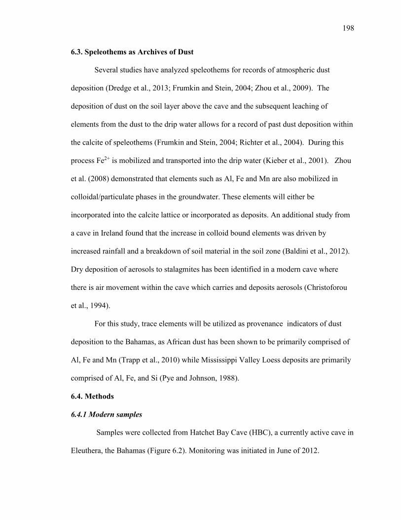
198

6.3. Speleothems as Archives of Dust

Several studies have analyzed speleothems for records of atmospheric dust

deposition (Dredge et al., 2013; Frumkin and Stein, 2004; Zhou et al., 2009). The

deposition of dust on the soil layer above the cave and the subsequent leaching of

elements from the dust to the drip water allows for a record of past dust deposition within

the calcite of speleothems (Frumkin and Stein, 2004; Richter et al., 2004). During this

process Fe2+ is mobilized and transported into the drip water (Kieber et al., 2001). Zhou

et al. (2008) demonstrated that elements such as Al, Fe and Mn are also mobilized in

colloidal/particulate phases in the groundwater. These elements will either be

incorporated into the calcite lattice or incorporated as deposits. An additional study from

a cave in Ireland found that the increase in colloid bound elements was driven by

increased rainfall and a breakdown of soil material in the soil zone (Baldini et al., 2012).

Dry deposition of aerosols to stalagmites has been identified in a modern cave where

there is air movement within the cave which carries and deposits aerosols (Christoforou

et al., 1994).

For this study, trace elements will be utilized as provenance indicators of dust

deposition to the Bahamas, as African dust has been shown to be primarily comprised of

Al, Fe and Mn (Trapp et al., 2010) while Mississippi Valley Loess deposits are primarily

comprised of Al, Fe, and Si (Pye and Johnson, 1988).

6.4. Methods

6.4.1 Modern samples

Samples were collected from Hatchet Bay Cave (HBC), a currently active cave in

Eleuthera, the Bahamas (Figure 6.2). Monitoring was initiated in June of 2012.

199

Overlying the cave is grasses and small Metopium toxiferum (poison wood) and trees of

the Fabaceae family with well-developed soils (greater than 15 cm depth). Most of the

grasses are located near the entrance and at lower elevations around the cave, with the

small trees located on the Aeolian ridge. HBC was accessed through a small ~1.7 m. by

0.9 m. opening located 10 to 15 m above sea level and exhibits an extremely linear

pattern particularly west of the main entrance (Mylroie and Mylroie, 2009). The opening

is immediately surrounded by thick grasses with larger trees (as described above) located

3 meters to the west, approximately following the cave direction and well developed soils

(as described above). The first level exhibits evidence of phreatic dissolution (Mylroie

and Mylroie, 2009). There is no evidence of cave breathing holes through the roof as

suggested by the lack of changes in the overlying vegetation and soil. The cave is divided

into three levels with the first level being the shallowest and the smallest level. The

second level is a tubular passage accessed by a 1.6 m. ladder down from the first level

and again contains evidence of phreatic dissolution (Mylroie and Mylroie, 2009). The

second level is more extensive (300 m long) with active drip water and stalagmite

formation (Mylroie and Mylroie, 2009). The 2nd level is thought to follow a thick, terra

rossa paleosol, leading to the creation of the linear and tubular shape following the

aeolian ridge (Mylroie and Mylroie, 2009). The third level is the deepest level and is

accessed by another 1.8 m ladder from the second level. However continuing on the

second floor is a smaller passage which after several meters leads to a 7 m shaft to the

surface, which may have been carved out for guano mining (Mylroie and Mylroie, 2009).

The third level is partially filled with water, with active stalagmite formation occurring

on raised rock ledges above the water, ~1.2 m above the water level. This water is tidally

200

influenced and of marine salinity (Mylroie and Mylroie, 2009). There is no evidence of

water flooding the rock ledges nor is there any evidence of calcite deposits forming from

the water. Most of the sampling was conducted on the 2nd and 3rd levels. Located on the

3rd level ledges were experiments on the precipitation of calcite from drip water,

henceforth known as calcite “farming” (Figure 6.2). The cave was visited every 3-5

months. This cave has more extensive speleothem formation than other caves in

Eleuthera possibly driven by the 10-15 m of overlying calcite (Mylroie and Mylroie,

2009). Samples from the surrounding cave walls were not collected.

Analyses were conducted on the air ([CO], δ13C of CO2), drip water (δ18Ow, δ2Hw,

δ13C of DIC and minor elements) and the farmed calcite (δ13Cc, δ18Oc, Δ47, and trace

elements) deposited on microscope slides which were deployed in the cave. For this

study, results will focus on the drip water δ18Ow, δ2Hw, and minor elements and for the

farmed calcite trace and minor elements. A description of the monitoring methods is

included in the following.

Waters:

Unfiltered water samples were collected throughout the second and third levels of

the cave by holding clean (10% HCl clean) vials under dripping stalactites. Vials were

filled completely (where possible) to avoid head space equilibration, then capped and

stored until analysis. The waters were filtered (Whatman 0.2 µm pore filter) upon return

to the laboratory (within 2-3 days) into unused 10% HCl clean vials. For δ18Ow & δ2Hw of

the drip water, samples were measured using the Picarro cavity ring-down spectroscopy

instrument (CRDS). Four standard waters were analyzed with each set of samples and

the standards used were previously calibrated to the VSMOW-GISP-SLAP scale. Data

201

are reported relative to VSMOW with an average reproducibility of 0.05 ‰ for δ18Ow and

0.1 ‰ for δ2Hw from repeated analysis of a standard. One milliliter of each sample or

standard is measured into a glass vial and sealed with a rubber septum. Each sample or

standard is injected into the Picarro A0211 vaporizer unit at 0.2 ml per injection six times

into the vaporizer. The vaporizer is held at 110oC for the duration of the sample run. The

injection port of the A0211 is fitted with a fine stainless steel mesh ideal for trapping salt

crystals to minimize interferences and clogging downstream. The mesh basket is

periodically removed, rinsed, dried and reinserted into the injection port. The vaporized

water gas is transferred to the Picarro CRDS analyzer in a stream of N2 gas. The

measurement cycle of each sample lasts about 8 minutes and data are reported relative to

VSMOW.

For trace and minor elements, samples were acidified using OmniTrace® HNO3

and then analyzed using a Varian Vista Pro inductively coupled optical emissions

spectrometer (ICP-OES) at the University of Miami within 2-3 days of returning. For

long term storage, the waters were acidified. Results from procedural blanks were below

detection limits.

Figure 6.2 (following page): Map of Hatchet Bay Cave, Eleuthera, Bahamas. The cave is divided into three levels and the locations of water sampling are approximate. Also shown is the approximate location of water collection and calcite farming. Also included are photographs of the areas which were sampled.

202

203

Calcite:

Standard glass microscope slides were placed on top of currently forming

stalagmites. Microscope slides were held in place by wire and were tied down at an

angle similar to the methods of Tremaine et al. (2011) and Banner et al. (2007). Prior to

installing the slides in the cave, the slides were weighed in the laboratory. Two calcite

precipitation sites were set up, one in the main room of the third level (these two will be

referred to in the text as east main site (1 slide) and main site locations (2 slides)) and one

in the west room (1 slide) (referred to in the text as west site) (Figure 4.2). The

microscope slides were left in the cave for 3-5 months.

Slides were brought back to the laboratory, dried in a 40 ºC oven overnight and

weighed, slides were not rinsed with DI therefore may be contaminated with sea salts.

Sampling of the slide was conducted by removing the calcite using a dental tool. The

calcite was then homogenized with a mortar and pestle and stored in Eppendorf vials

until analysis. Calcite samples were dissolved in OmniTrace® 4 % HNO3 to give a

concentration of 4 ppm Ca and were analyzed using the ICP-OES.

6.4.2 Ancient samples

Two stalagmite samples (samples AB-DC-09 and AB-DC-12) were collected

from a currently submerged cave from Abaco Island, Bahamas (16.5 and 11.9 meters

below sea level) (Figure 6.3). A total of 37 U-Th age dates were acquired at the Neptune

Isotope Laboratory of the University of Miami utilizing a ThermoFisher-Neptune Plus

multi-collection ICP-MS. Details of the U-Th geochronometry technique and

propagation of random and systematic uncertainties are discussed in Pourmand et al.

204

Figure 6.3: Reflected light photos of samples AB-DC-09 (a) and AB-DC-12 (b). For both a and b: Dotted line is the location of low resolution (1000 μm) sampling and black squares are the sampling locations for the high resolution (20 μm) analysis.

a. b.

205

(2014b). For all samples, an initial 230Th/232Th activity ratio of 3.7 ± 0.6 was used to

account for excess (unsupported) 230Th (see Chapter 3). The age models for the

stalagmites were determined through linear interpolation between ages and the results are

presented in Chapters 3 and 4.

Stalagmite sample AB-DC-09 was sampled every 0.5 mm for trace elements and

AB-DC-12 was sampled every 1 mm (Figure 6.3) utilizing a computerized NewWave

micromill. Five locations (3 for AB-DC-09 and 2 for AB-DC-12) were additionally

sampled at a high resolution (1 sample every 20 µm) (Figure 6.3) utilizing a

computerized NewWave micromill. These areas were chosen as the initial δ18O and δ13C

of the calcite results demonstrated these are intervals of rapid isotopic shifts (Chapter 4).

Trace element samples were analyzed on the Varian ICP-OES for trace and minor

elements as previously described for calcite samples.

6.5. Results

6.5.1 Modern samples

Waters:

For drip waters collected from Hatchet Bay Cave, an increase in the trace element

concentration (in particular Fe) was observed in June 2012 and again in August 2013

(Figure 6.4). The concentration of Fe was lower in the 3rd level west room than the main

room (Figure 6.5). The drip waters also demonstrate variability in the Sr/Ca and Mg/Ca

values (Figure 6.6) and the δ18O value of the drip water (δ18Ow) (Figure 6.7). In particular

the West room exhibits more negative δ18O value of the drip water (Figure 6.7) and

decreased Sr/Ca and Mg/Ca values (Figure 6.6) when compared to the values observed in

the Main room.

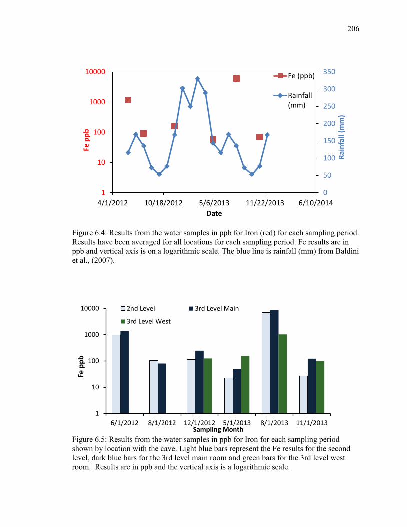
206

Figure 6.4: Results from the water samples in ppb for Iron (red) for each sampling period. Results have been averaged for all locations for each sampling period. Fe results are in ppb and vertical axis is on a logarithmic scale. The blue line is rainfall (mm) from Baldini et al., (2007).

Figure 6.5: Results from the water samples in ppb for Iron for each sampling period shown by location with the cave. Light blue bars represent the Fe results for the second level, dark blue bars for the 3rd level main room and green bars for the 3rd level west room. Results are in ppb and the vertical axis is a logarithmic scale.

0

50

100

150

200

250

300

350

1

10

100

1000

10000

4/1/2012 10/18/2012 5/6/2013 11/22/2013 6/10/2014

Rain

fall

(mm

)

Fe p

pb

Date

Fe (ppb)

Rainfall(mm)

1

10

100

1000

10000

6/1/2012 8/1/2012 12/1/2012 5/1/2013 8/1/2013 11/1/2013

Fe p

pb

Sampling Month

2nd Level 3rd Level Main

3rd Level West

207

Figure 6.6: Mg/Ca versus Sr/Ca results for drip water samples from the 3rd level main (dark blue) and 3rd level west (green triangles).

Figure 6.7: δ18Ow and δ2Hw for drip water samples from the 2nd level (light blue), 3rd level main (dark blue) and 3rd level west (green triangles). Results are plotted on the GMWL (black) with ± 5 ‰ δ2H shown in grey. Average errors are shown in the upper left corner in black.

y = 0.0024x

y = 0.0022x

0

0.5

1

1.5

2

2.5

3

3.5

4

0 200 400 600 800 1000 1200 1400

Sr/C

a (m

M/M

)

Mg/Ca (mM/M)

3rd Level Main

3rd Level West

-40

-35

-30

-25

-20

-15

-10

-5

-6.5 -5.5 -4.5 -3.5 -2.5

δ2H

‰ V

SMO

W

δ18O ‰ VSMOW

GMWL2nd Level3rd Level Main3rd Level West

208

Calcite:

For the precipitated calcite in 2012 and 2013, the slides which were deployed and

collected between August and November showed the highest Fe concentrations (Figure

6.8). The calcite precipitated in the main room overall had a higher Fe/Ca ratio, while the

west room contained a significantly lower Fe/Ca ratio (Figure 6.9).

Figure 6.8: Results from the calcite farming precipitation experiment for Iron shown by sampling month. The average of each sampling location for each month is shown as a ratio of Fe/Ca (µM/M).

0

500

1000

1500

2000

2500

3000

3500

Aug 2012 Dec 2012 May 2013 Aug 2013 Nov 2013

Fe/C

a (µ

mol

/mol

)

Sampling Month

209

Figure 6.9: Box and whisker plot of the results from the calcite Iron shown by location in the cave. The results include all of the sampling periods. This demonstrates the higher Fe/Ca ratio in the main room when compared to the west room. Results are shown as a ratio of Fe/Ca (µM/M). 6.5.2 Ancient samples

The U-Th age dating of the speleothems demonstrate the stalagmites were formed

from 14.2 to 63.5 ka before present with a gap in the record between 31.3 and 35.9 ka.

During this time period, neither of the two stalagmite samples was forming (Table 6.1,

6.2, Figure 6.10). Weighted average growth rates are approximately 13 μm/year for

sample AB-DC-09 and 11 μm/year for sample AB-DC-12.

The periods which were sampled at high resolution were approximately at 4 cm,

15.3 cm and 22.6 cm from the top for sample AB-DC-09, which correspond to ages 14.9,

24.9 and 31 ka BP. While for DC-12, areas of high resolution were conducted at ~5 cm

and 21 cm from the top, corresponding to ages of ~38.8 and 46.4 ka BP. For samples AB-

DC-09 and – 12, high Fe/Ca values were found at 15.0±0.2, 31.2±1.1, 38.8±0.2 and

210

46.0±0.2 ka before present, with highest values during the 15 and 46 ka BP events

(Figure 6.10 a). Therefore not all periods which were sampled at a high resolution

resulted in increased Fe/Ca values. Additionally it is important to note that the average

five point smooth utilized in Figures 6.10 and 6.11 is an average smoothing of ~ 100

years for sample AB-DC-09 and ~ 150 years for sample AB-DC-12. These higher Fe/Ca

values corresponded with increased δ13C and δ18O values in the carbonate found at

14.9±0.2, 30.9±1, 38.8±0.2, and 48±0.2 ka BP (Figure 6.10 b and c) suggesting a

relationship between increased isotopic values of the calcite and Fe/Ca ratios for the 15,

30.9, 38.8 and 47.0 ka events. For the isotopic events at 14.9, 25 and 62.4 ka BP, there is

a decline in the growth rate, but for the other events (30.9, 38.8 and 48 ka BP) there does

not appear to be any change in growth rate (Figure 6.10 d).

The high resolution results support abrupt increases in Fe/Ca ratios (Figure 6.11

a-d). For the 15 ±0.2 ka BP event, there appears to be two pulses of increased iron, one at

15.0 which occurs with increasing δ18O values and a second at 14.8±0.2 ka BP associated

with a rapid decline in δ18O value (Figure 6.11 a). For the 31.2 ka BP event, there is

elevated Fe/Ca associated with declining δ18O values. For the 38.8 and 46 ka BP events,

the increased Fe/Ca ratio is associated with a decreasing δ18O and δ13C values (Figure

6.11 c and d). Also shown is the [232Th/230Th] activity ratio which is a good proxy for

detrital contribution again demonstrating minimal relationship between [232Th/230Th] and

increased Fe/Ca.

211

Sam

ple

Id

Dis

tanc

e fro

m

Top

238 U

(9

5%

CI)

[230 T

h/23

8 U]

(95%

CI)

[230 T

h/23

2 Th]

(9

5%

CI)

Unc

orr.

Age

(9

5%

CI)

[234 U

/238 U

] in

itial

(9

5%

CI)

Cor

r. A

ge

(95%

CI)

µm

(p

pb)

± (a

ctiv

ity)

± (a

ctiv

ity)

± (y

) ±

(cor

rect

ed

activ

ity)

± (y

) ±

DC

-09

1800

0 20

1.83

9 0.

125

0.13

32

0.00

07

57.6

0.

96

1539

4 77

1.

013

0.00

262

1454

4 16

8

37

000

179.

526

0.09

7 0.

136

0.00

06

54.5

1.

54

1588

2 72

1.

005

0.00

264

1495

6 18

0

60

000

150.

938

0.08

5 0.

1552

0.

001

47.9

1.

11

1857

3 12

5 0.

992

0.00

273

1735

4 24

5

72

500

188.

15

0.11

3 0.

1545

0.

0014

10

2.5

1.95

18

054

174

1.01

4 0.

0025

2 17

501

200

85

000

204.

482

0.10

9 0.

1607

0.

0009

43

.5

0.28

18

955

109

1.00

9 0.

0026

1 17

588

260

11

0000

21

1.46

2 0.

125

0.17

79

0.00

09

79.5

0.

56

2092

5 11

0 1.

021

0.00

265

2011

0 18

1

12

7000

18

3.40

8 0.

109

0.18

76

0.00

22

128.

6 1.

67

2231

0 28

2 1.

016

0.00

255

2177

5 29

5

13

7000

16

4.36

1 0.

082

0.19

23

0.00

1 48

.3

0.36

23

648

123

0.98

7 0.

0025

2 22

141

288

14

5000

19

2.36

6 0.

114

0.22

1 0.

0011

11

0.9

0.81

26

649

127

1.02

2 0.

0025

8 25

921

180

15

6000

20

2.09

0.

129

0.22

35

0.00

11

139.

6 0.

9 27

028

126

1.02

0.

0025

6 26

445

161

17

8000

20

4.47

1 0.

15

0.24

27

0.00

1 38

.2

0.17

29

796

123

1.01

7 0.

0027

7 27

447

431

22

2500

20

2.53

1 0.

127

0.28

79

0.00

13

19

0.11

36

203

169

1.02

1 0.

0026

4 30

526

1008

Tabl

e 6.

1: 23

0 Th d

atin

g re

sults

for s

ampl

e A

B-D

C-0

9. R

esul

ts fr

om b

oth

sam

ples

are

pro

paga

ted

with

an

initi

al 23

0 Th/23

2 Th

activ

ity ra

tio o

f 3.7

±0.6

.

212

Sam

ple

Id

Dis

tanc

e fro

m T

op

238 U

(9

5% C

I) [23

0 Th/

238

U]

(95%

CI)

[230 T

h/23

2

Th]

(95%

C

I) U

ncor

r. A

ge

(95%

C

I) [23

4 U/23

8 U] i

nitia

l (9

5% C

I) C

orr.

Age

(95 %

CI)

µm

(p

pb)

± (a

ctiv

ity)

± (a

ctiv

ity)

± (y

) ±

(cor

rect

ed

activ

ity)

± (y

) ±

DC

-12

1400

0 77

5.20

5 0.

423

0.29

14

0.00

12

268.

1 1.

97

3715

0 14

4 1.

011

0.00

265

3674

9 15

7

53

000

260.

535

0.16

7 0.

3022

0.

0014

49

0.8

2.85

39

247

188

1.00

1 0.

0026

8 39

018

193

84

000

361.

556

0.17

9 0.

3204

0.

0012

24

9.3

3.47

42

057

161

1.00

3 0.

0026

6 41

580

184

10

1000

39

5.05

1 0.

346

0.32

61

0.00

14

1266

.5

9.08

42

500

193

1.01

2 0.

0029

1 42

405

193

13

3000

62

4.80

2 0.

287

0.33

09

0.00

13

2330

.9

58.8

5 43

036

162

1.01

7 0.

0026

1 42

984

161

16

7000

30

1.03

4 0.

189

0.33

60

0.00

15

792.

0 8.

45

4428

8 22

2 1.

008

0.00

278

4413

1 22

5

19

3000

61

2.42

3 0.

278

0.33

95

0.00

13

2653

.8

73.6

3 44

445

172

1.01

7 0.

0026

4 44

398

172

21

5000

33

0.75

9 0.

200

0.35

32

0.00

14

646.

8 36

.61

4703

0 20

8 1.

010

0.00

281

4682

9 20

9

22

5000

53

7.12

8 0.

292

0.36

48

0.00

14

480.

2 5.

79

4871

2 20

5 1.

015

0.00

285

4843

4 21

0

22

8000

31

9.36

1 0.

159

0.37

62

0.00

15

921.

8 18

.67

5100

0 21

7 1.

009

0.00

274

5084

9 21

7

23

5000

22

4.13

5 0.

121

0.40

72

0.00

17

1118

.1

99.8

5 56

845

275

1.00

4 0.

0029

7 56

710

275

24

0000

37

5.27

4 0.

214

0.42

02

0.00

22

514.

2 3.

19

5777

1 36

6 1.

025

0.00

277

5747

4 36

6

25

6000

20

9.07

1 0.

104

0.42

49

0.00

17

393.

1 10

.64

6059

2 29

1 0.

997

0.00

293

6018

8 30

0

27

2000

26

2.33

7 0.

163

0.44

45

0.00

19

1247

.4

60.4

7 62

470

328

1.02

2 0.

0029

4 62

341

327

28

8000

33

8.94

9 0.

155

0.44

85

0.00

18

1286

.3

23.6

9 63

165

300

1.02

3 0.

0028

5 63

038

300

30

9000

53

5.34

3 0.

257

0.45

54

0.00

18

1108

.7

16.6

6 63

539

281

1.03

6 0.

0028

3 63

392

282

Tabl

e 6.

2: 23

0 Th d

atin

g re

sults

for s

ampl

e A

B-D

C-1

2. R

esul

ts fr

om b

oth

sam

ples

are

pro

paga

ted

with

an

initi

al 23

0 Th/23

2 Th

activ

ity ra

tio o

f 3.7

±0.6

.

213

Figure 6.10: Geochemical results for samples AB-DC-09 (from ~14 to 32 ka BP) and AB-DC-12 (from ~36 to 65 ka BP), each sample plotted with its own age model. A) Fe/Ca ratio in orange shown for samples AB-DC-09 and AB-DC-12. Data are both at high and low resolution, with a 5 point running average, plotted on a logarithmic scale. B & C) Black line represents δ18O values of the carbonate and green line represents δ13C of the carbonate plotted with a 50 year interpolation forAB-DC-09 and a 5 point running average for sample AB-DC-12. D) Growth rate calculated using the U-Th ages from Table 6.1 shown in blue. E) 230Th/232Th activity ratio shown in purple. Grey bars represent the timing of Heinrich stadials (HS) 1-6.

HS1 HS2 HS3 HS4 HS5 HS6

214

Figure 6.11: Expanded view of δ18O and Fe/Ca data from Figure 6.8. a) Data from Heinrich stadial 1, showing elevated Fe/Ca from 14.8 to 15.0 ka before present. B) Data from Heinrich stadials 3, demonstrating elevated Fe/Ca from 31.3 to 31.0 ka BP, c) Increased at 38.8 ka BP, associated with Heinrich stadial 4 and d) increase Fe/Ca from 46.3 to 46.0 ka BP associated with Heinrich stadial 5. Both Fe/Ca and δ18O are plotted with a 5 point running average. Fe is plotted on a logarithmic scale.

6.6. Discussion

6.6.1 Source of Iron

Considering the lack of local sources of iron, the iron must be allochthonous and

derived from atmospheric dust deposited on the soil zone (Swart et al., 2014). As already

described, the Bahamas annually receives dust from Africa associated with the seasonal

215

migration of the ITCZ. Once the dust is deposited on the soil surface, to mobilize the Fe

in the dust, rainfall is necessary to leach the Fe or to transport colloidally bound Fe.

Similar to the dust, rainfall in the Bahamas varies seasonally with the rainy season

typically occurring from May to November. These observations are supported by results

from a study of calcretes in Caicos Island. Similar to the Bahamas, Caicos Island (located

to the south of the Bahamas) is geologically analogous, comprised of relatively pure

carbonate with few contaminants. Caicos Island is characterized by red soils up to a

meter thick with high levels of iron (~16000 ppm Fe), while the underlying host

limestone contains very low concentrations of iron of about 100 ppm Fe (Rossinsky and

Wanless, 1992). Considering that there are few local sources of iron in Caicos, the

authors suggest the insoluble red calcrete soils on Caicos Island must have originated

from aerosols from Africa (Rossinsky and Wanless, 1992). The authors also showed that

the surface of the soil is directly affected by aerosol inputs and contains very high Fe

concentrations, while Fe is not present 1.5 m into the limestone bedrock, supporting the

importance of aerosol input (Rossinsky et al., 1992).

In the Bahamas, an additional source of iron may be recycled Fe from the soil as

the soils have been shown to be derived from dust (Muhs et al., 2007). However, the soil

layer in the Bahamas is thin in most areas and was also thin in the past (Muhs et al.,

2007). The soil is therefore most likely not a significant contributor of Fe. Nonetheless in

HBC the soil layer is more developed above this cave and therefore cannot be ruled out

as a potential source of iron. The various factors driving aerosol inputs to stalagmites, as

described above, are outlined and summarized in Figure 6.12.

216

Figure 6.12: Model for the deposition of dust to the precipitation of Fe in the cave. I) Dust is deposited on the soil layer either through rain out and/or the settling of dust on the soil layer. From studies, it has been demonstrated that dust deposition to the Bahamas varies seasonally (Prospero and Lamb, 2003) as does precipitation (Baldini et al., 2007) (annual variations shown here are schematics). II) The rate of percolation of water through the soil zone and into the limestone bedrock varies by site. III) The water from precipitation flows rapidly through the limestone bed rock as shown in (a) leading to a lower residence time of the water in the soil zone or the bedrock, resulting in lower Fe concentrations in the precipitated calcite as shown in (b). Slower flow rates through the soil and bedrock as shown in (c) would lead to greater leaching of Fe into the drip waters and therefore more Fe deposited in the stalagmite (d). This is discussed in the text in section (6.6.2).This model is based on the assumption that the Fe is dissolved or colloidal in the drip water.

217

6.6.2 Modern samples

Drip waters:

In the modern samples, the highest concentrations of iron found in drip waters

were during the wet summer months. The seasonality in the concentration of trace

elements in the water is possibly driven both by the changes in dust deposition to the

Bahamas (considering the greatest dust deposition in Miami and Barbados is found in

June and July (Trapp et al., 2010)) and higher amounts of rainfall from May to November

(the rainy season) in the Bahamas (Baldini et al., 2007) (Figure 6.12). Considering the

samples were filtered prior to analysis, the water samples represent fine phase particulate

and colloidal Fe.

Calcites:

Similar to the water results, the carbonate results demonstrate seasonal variation

as well as heterogeneity within the cave. The slides deployed in June of 2012 and

collected in August 2012 contain above average Fe/Ca ratios, reflecting the increased Fe

observed in the drip waters of June 2012. Similarly, the slides deployed in August 2013

and removed in November of 2013 show an increased Fe/Ca ratio (Figure 6.8) reflecting

the observed increase in Fe/Ca of the waters in August of 2013 (Figure 6.5). The periods

of increased Fe/Ca (June – August) are coincident with the rainy season and dust

deposition to the Bahamas. The rainfall allows for the leaching of Fe or the transport of

collodially bounded Fe into the cave which is deposited with the calcite.

There is also observed heterogeneity in the Fe concentration within the cave, with

the main room containing higher Fe/Ca ratios than the west room. Trace and minor

element variations have also been observed within HBC, particularly for Mg and Sr

218

concentrations (Chapter 4). This spatial variation has been suggested to be driven by

changes in the routing path or the residence time of the water in the overlying bedrock as

modifications in the routing path of the water or the residence time may impact the

incorporation of trace and minor elements into the drip water (Fairchild and Treble,

2009). In HBC, as demonstrated above and in Chapter 4, the Mg/Ca and Sr/Ca results

show higher Mg/Ca and Sr/Ca ratios of the calcite precipitated in the main room

compared to the west room (Figure 6.6). This is additionally supported by the results of

the isotopic analysis of the drip waters. The west room drip waters on average consist of

a δ18Owater value 0.5 ‰ more depleted than the main room δ18Owater value (Figure 6.7).

The results from both elemental and isotopic analyses suggest that the waters feeding the

main room undergo a longer residence time in the soil zone and the epikarst resulting in

increased elemental concentrations. Variations in the residence time would primarily

drive the incorporation of Fe leached from the dust, not the collodially bounded Fe.

The incorporation of Fe into the drip waters (hence calcite) may also vary with

drip rate and drip path length. Variations in drip rate are primarily driven by residence

time, which can potentially influence the incorporation of Fe into drip waters. Future

work in HBC should also measure drip rate.

Finally, an additional source of Fe to the calcite may be aerosols. This spatial

variability may also be driven by ventilation of the cave. As the cave ventilates,

atmospheric air enters the cave which can carry with it aerosols. Additionally, the cave is

accessible to the public, who may kick up dust in the cave, and additionally since the

cave is ventilated, air flow through the cave can move particulates (Dredge et al., 2013).

219

One way to address if aerosols within the cave are a major contributor to Fe deposition is

through the collection and monitoring of aerosols throughout the cave.

6.6.3 Ancient samples

From the ancient samples, increased Fe/Ca occurs synchronously with the

changes in the δ18O and δ13C record. Previous studies support that the timing of the

increased δ18O and δ13C values of the carbonate from both stalagmite samples (AB-DC-

09 and -12) correlates well with the timing of Heinrich stadials (see Chapters 3 and 4).

The paleoclimate interpretation of the δ18O and δ13C record have been previously

discussed, but briefly, the geochemical results support the interpretation that increases in

the δ18O of the carbonate associated with Heinrich stadials are primarily driven by a

temperature decrease associated with the events. The associated increase in the δ13C

record is thought to be driven by a likely combination of lower temperatures and higher

aridity during Heinrich stadials and/or higher ventilation of the cave. The terminations of

Heinrich stadials are characterized as periods of enhanced rainfall, higher temperatures

and/or less ventilation as supported by lower carbon and oxygen isotopes of the

carbonate. Paleoclimate records suggest that the abrupt terminations of Heinrich stadials

are driven by resumption of the AMOC, leading to an increase in SSTs in the North

Atlantic (McManus et al., 2004), and a northward shift of the ITCZ (Peterson et al., 2000)

(Chapters 3 and 4). The paleoclimatic interpretations of the Bahamas records have been

developed through isotopic analysis of the fluid inclusions and coupled trace element and

stable isotopic analysis of the carbonate and are consistent with this scenario.

The high resolution data presented here demonstrate that the increase in iron is

abrupt and occurs near the termination of the Heinrich events, not during the onset. This

220

was observed during Heinrich stadial 1 (Figure 6.11 a) which shows an increased Fe/Ca

associated with the termination of the event at 14.9 ka BP and elevated Fe/Ca ratios

persisting until 14.8 ka. Similar results are seen for HS 3 -5. Therefore, considering that

the modern data suggest that precipitation amount is important for the leaching of Fe into

the drip water; this mechanism is applicable to the past. Heinrich stadials are known to

be dusty events (Jullien et al., 2007; McGee et al., 2013; Murphy et al., 2014). However,

geochemical results suggest that Heinrich stadials are also dry in the Bahamas and

therefore the leaching of soil Fe may not have been significant during the stadial itself.

Therefore, the proposed process is 1) Heinrich stadials result in the deposition of dust to

the soil layer, 2) the iron is leached out of the dust during increased rainfall events

associated with the termination of the Heinrich stadial, and 3) the iron is deposited within

the calcite (Baldini et al., 2007; Zhou et al., 2008). This supports both the timing and the

rapid nature of the increased Fe/Ca ratio. It is important to note that while stadials may

have been drier, there was still rain that could mobilize Fe as stalagmite growth continues

during the stadials supports that there was clearly enough rain to supply carbonate

precipitation inside the cave.

The growth rate of a speleothem is dependent on the drip rate, temperature, calcite

saturation and pCO2 of the cave (Banner et al., 2007; Oster et al., 2014) and therefore

may be a good indicator of environmental conditions at the time of speleothem formation.

Hence another possible explanation for the increase in iron associated with Heinrich

stadials is a significant decrease in growth rate, allowing for the accumulation of iron on

the stalagmite surface (Dredge et al., 2013). When comparing the Fe/Ca record with

growth rate, there is minimal evidence of growth rate controlling the deposition of Fe for

221

either stalagmite (Figure 6.13 & 6.14). While the 25 ka and 62 ka events both

demonstrate a decreased growth rate (Figure 6.10 d), these events consist of little to no

change in the Fe/Ca ratio of the speleothem calcite (Figure 6.10 a). Therefore growth rate

is not a significant driver of the increased Fe/Ca ratio, but rather it is possible the

increased iron is driven by an increased supply (e.g. more dust and/or more rainfall).

The [230Th/232Th] ratio demonstrates that the ratio is larger for sample AB-DC-12,

supporting a decreased detrital component to sample, when compared to sample AB-DC-

09 (Figure 6.10 e). Additionally it is important to note that there is not a significant

decrease in the [230Th/232Th] ratio associated with Heinrich stadials (Figure 6.10 e), with

the possible exceptions of Heinrich stadial 1 and 3.

6.6.4 Comparison with other dust records

Numerous studies have suggested that Heinrich stadials are associated with

increased dust deposition to Greenland, while the warm interstadials are represented by a

reduction of atmospheric detrital dust (Fuhrer et al., 1999; McGee et al., 2010; Ruth et

al., 2007). Ruth et al. (2007) demonstrated a relationship between NGRIP dust and China

loess deposits, suggesting that dust increases in Greenland are driven by Asian aridity

during Heinrich stadials (Figure 6.15 a). NGRIP dust concentration was calculated by

Laser particle counter (Ruth et al., 2007). During Heinrich stadials, the Sahel region of

Africa was drier and cooler as supported by paleoclimate records (Stager et al., 2011;

Tjallingii et al., 2008) which may in turn have created more dust sources (Figure 6.15).

222

Figure 6.13: Growth rate versus Fe/Ca for sample AB-DC-09 demonstrating minimal relationship between growth rate and Fe/Ca ratio.

Figure 6.14: Growth rate versus Fe/Ca for sample AB-DC-12 demonstrating minimal relationship between growth rate and Fe/Ca ratio.

There is evidence from modeling studies that the AEJ was intensified during this period,

potentially transporting more dust from western Africa to the eastern Atlantic Ocean (Just

et al., 2012; Mulitza et al., 2008; Murphy et al., 2014) as increased dust deposition has

been observed in the eastern Atlantic associated with Heinrich stadials (Jullien et al.,

0

5000

10000

15000

20000

25000

30000

35000

0 200 400 600 800 1000 1200 1400 1600

Fe/C

a (m

M/M

)

Growth Rate (μm/yr)

0

5000

10000

15000

20000

25000

30000

0 20 40 60 80 100

Fe/C

a (m

M/M

)

Growth rate (μm/yr)

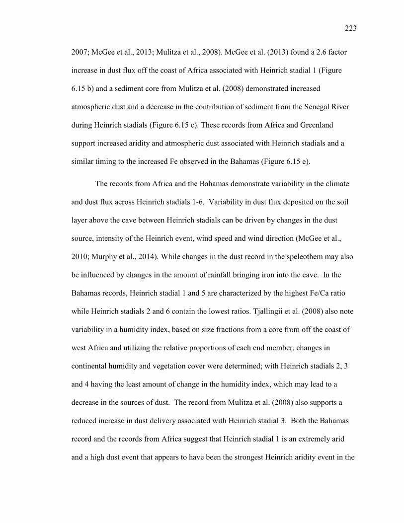
223

2007; McGee et al., 2013; Mulitza et al., 2008). McGee et al. (2013) found a 2.6 factor

increase in dust flux off the coast of Africa associated with Heinrich stadial 1 (Figure

6.15 b) and a sediment core from Mulitza et al. (2008) demonstrated increased

atmospheric dust and a decrease in the contribution of sediment from the Senegal River

during Heinrich stadials (Figure 6.15 c). These records from Africa and Greenland

support increased aridity and atmospheric dust associated with Heinrich stadials and a

similar timing to the increased Fe observed in the Bahamas (Figure 6.15 e).

The records from Africa and the Bahamas demonstrate variability in the climate

and dust flux across Heinrich stadials 1-6. Variability in dust flux deposited on the soil

layer above the cave between Heinrich stadials can be driven by changes in the dust

source, intensity of the Heinrich event, wind speed and wind direction (McGee et al.,

2010; Murphy et al., 2014). While changes in the dust record in the speleothem may also

be influenced by changes in the amount of rainfall bringing iron into the cave. In the

Bahamas records, Heinrich stadial 1 and 5 are characterized by the highest Fe/Ca ratio

while Heinrich stadials 2 and 6 contain the lowest ratios. Tjallingii et al. (2008) also note

variability in a humidity index, based on size fractions from a core from off the coast of

west Africa and utilizing the relative proportions of each end member, changes in

continental humidity and vegetation cover were determined; with Heinrich stadials 2, 3

and 4 having the least amount of change in the humidity index, which may lead to a

decrease in the sources of dust. The record from Mulitza et al. (2008) also supports a

reduced increase in dust delivery associated with Heinrich stadial 3. Both the Bahamas

record and the records from Africa suggest that Heinrich stadial 1 is an extremely arid

and a high dust event that appears to have been the strongest Heinrich aridity event in the

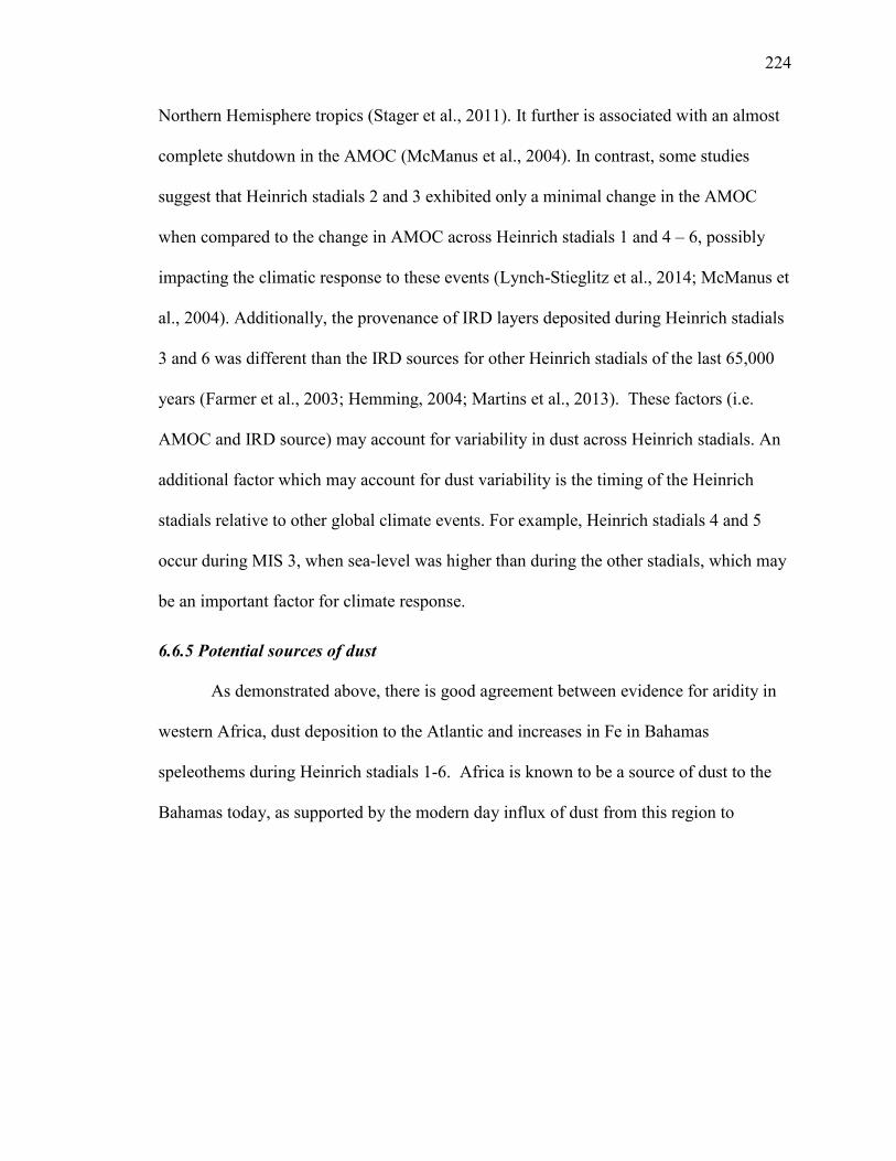
224

Northern Hemisphere tropics (Stager et al., 2011). It further is associated with an almost

complete shutdown in the AMOC (McManus et al., 2004). In contrast, some studies

suggest that Heinrich stadials 2 and 3 exhibited only a minimal change in the AMOC

when compared to the change in AMOC across Heinrich stadials 1 and 4 – 6, possibly

impacting the climatic response to these events (Lynch-Stieglitz et al., 2014; McManus et

al., 2004). Additionally, the provenance of IRD layers deposited during Heinrich stadials

3 and 6 was different than the IRD sources for other Heinrich stadials of the last 65,000

years (Farmer et al., 2003; Hemming, 2004; Martins et al., 2013). These factors (i.e.

AMOC and IRD source) may account for variability in dust across Heinrich stadials. An

additional factor which may account for dust variability is the timing of the Heinrich

stadials relative to other global climate events. For example, Heinrich stadials 4 and 5

occur during MIS 3, when sea-level was higher than during the other stadials, which may

be an important factor for climate response.

6.6.5 Potential sources of dust

As demonstrated above, there is good agreement between evidence for aridity in

western Africa, dust deposition to the Atlantic and increases in Fe in Bahamas

speleothems during Heinrich stadials 1-6. Africa is known to be a source of dust to the

Bahamas today, as supported by the modern day influx of dust from this region to

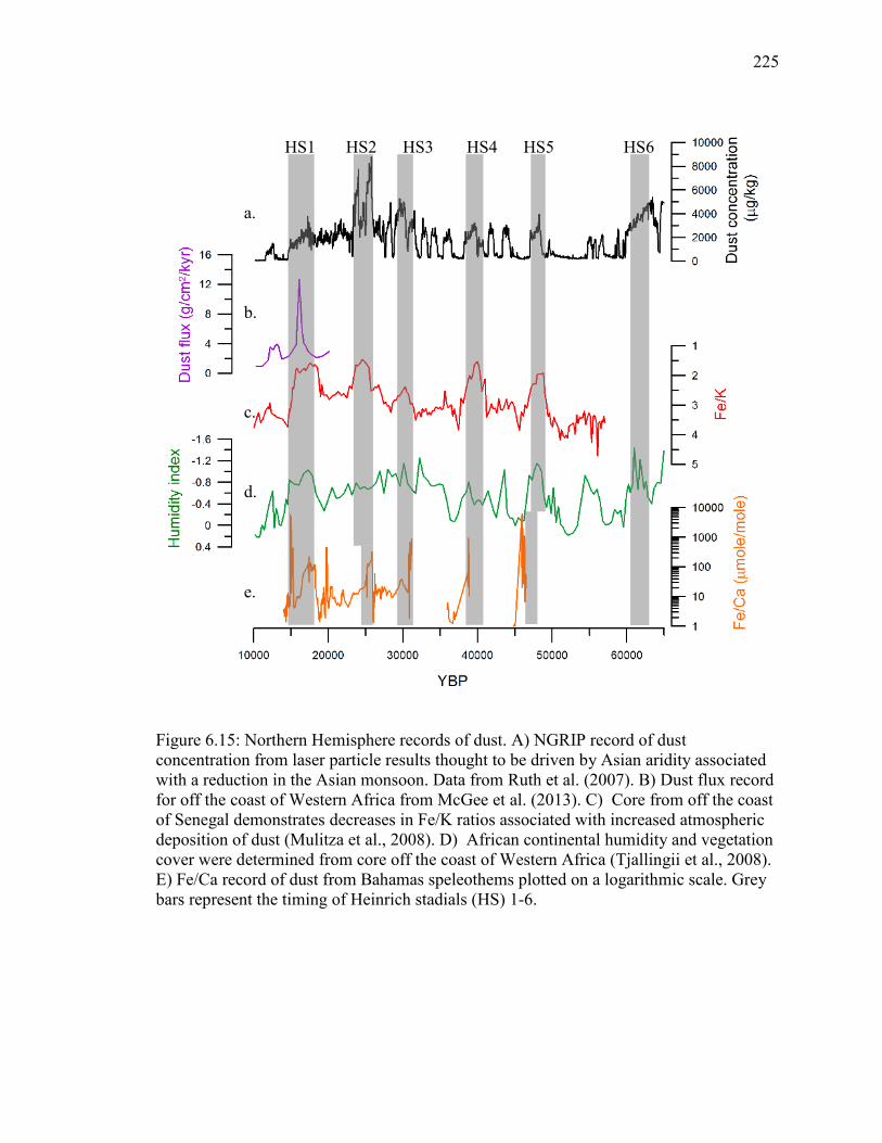
225

Figure 6.15: Northern Hemisphere records of dust. A) NGRIP record of dust concentration from laser particle results thought to be driven by Asian aridity associated with a reduction in the Asian monsoon. Data from Ruth et al. (2007). B) Dust flux record for off the coast of Western Africa from McGee et al. (2013). C) Core from off the coast of Senegal demonstrates decreases in Fe/K ratios associated with increased atmospheric deposition of dust (Mulitza et al., 2008). D) African continental humidity and vegetation cover were determined from core off the coast of Western Africa (Tjallingii et al., 2008). E) Fe/Ca record of dust from Bahamas speleothems plotted on a logarithmic scale. Grey bars represent the timing of Heinrich stadials (HS) 1-6.

a. b. c. d. e.

HS1 HS2 HS3 HS4 HS5 HS6

226

Barbados and Florida and from soil studies (Muhs et al., 2007; Prospero and Lamb, 2003;

Prospero et al., 2010). However, one modeling study predicts a southerly shift in the AEJ

with consequent reduction in dust transport form Africa to the Bahamas during Heinrich

stadials (Murphy et al., 2014) (Figure 6.16 a and b). This model also supports increased

North American aridity leading to increased dust deposition to the east coast of North

America, the Bahamas and the North Atlantic (Murphy et al., 2014). This suggests that

during Heinrich stadials sources of dust to the Bahamas may have instead been the

Mississippi River Valley loess deposits. There are several loess deposits in the

Mississippi Valley from the LGM (Muhs, 2012) and studies have shown that mass

accumulation rates of mid-continent loess during the LGM were an order of magnitude

higher than in the Holocene (Bettis et al., 2003). However, it is unknown if these sources

were greater during Heinrich stadials.

One tantalizing idea is that by conducting Sr isotopic measurements on the

speleothem, a comparison of the Sr isotopic composition from within the Heinrich stadial

and outside of the Heinrich stadial would shed light on the provenance of the dust.

Studies have effectively determined the provenance of dust by analyzing for a unique

geochemical “finger print” (Grousset and Biscaye, 2005). As a feasibility test, the

87Sr/86Sr variability has been utilized in speleothem studies for the identification of Sr

source and source variability with time (Ayalon et al., 1999; Bar-Matthews et al., 1999;

Frumkin and Stein, 2004; Goede et al., 1998; Li et al., 2005; Zhou et al., 2009) and

periods of increased aridity (Banner et al., 1996). The 87Sr/86Sr isotopic values were

measured within the Heinrich stadial and outside the Heinrich stadial of the calcite;

however the 87Sr/86Sr results were invariant (Appendix E). In addition, the speleothem

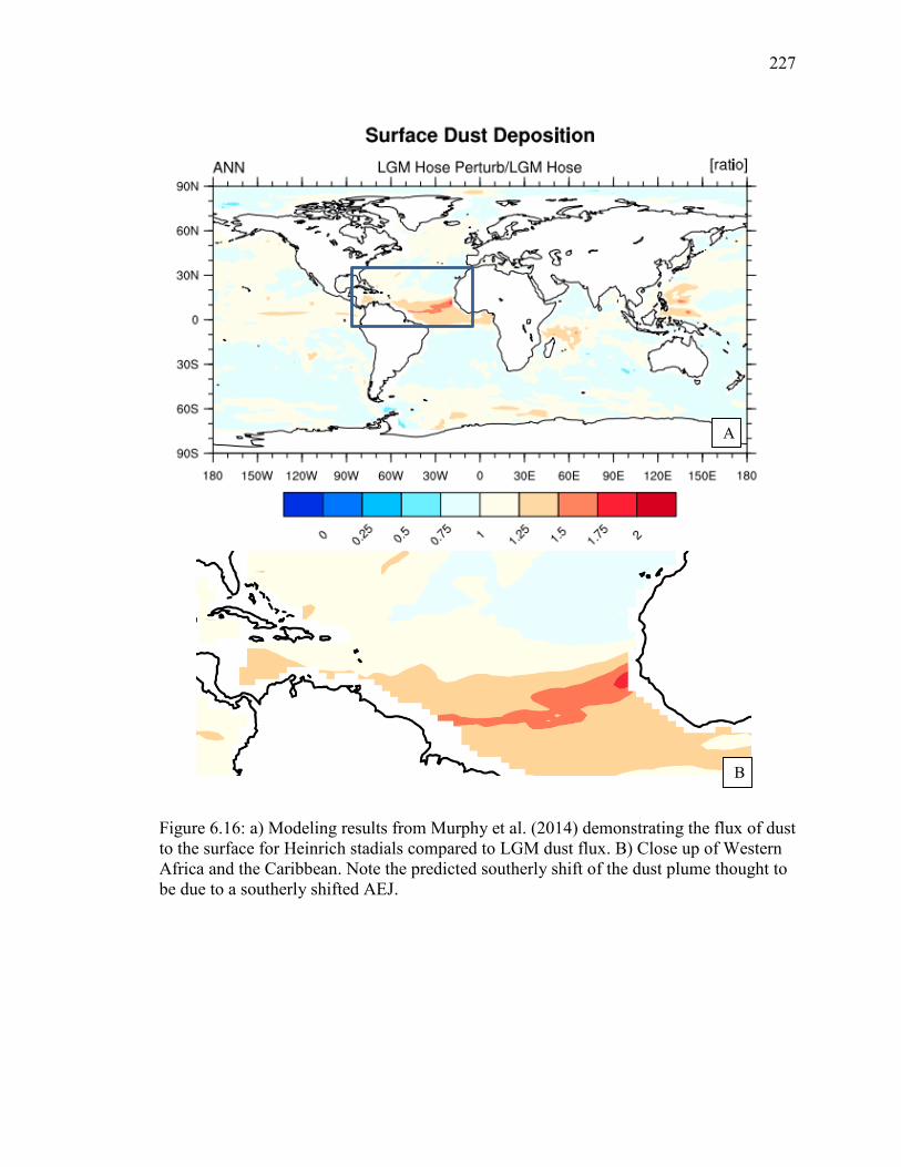
227

Figure 6.16: a) Modeling results from Murphy et al. (2014) demonstrating the flux of dust to the surface for Heinrich stadials compared to LGM dust flux. B) Close up of Western Africa and the Caribbean. Note the predicted southerly shift of the dust plume thought to be due to a southerly shifted AEJ.

B

A

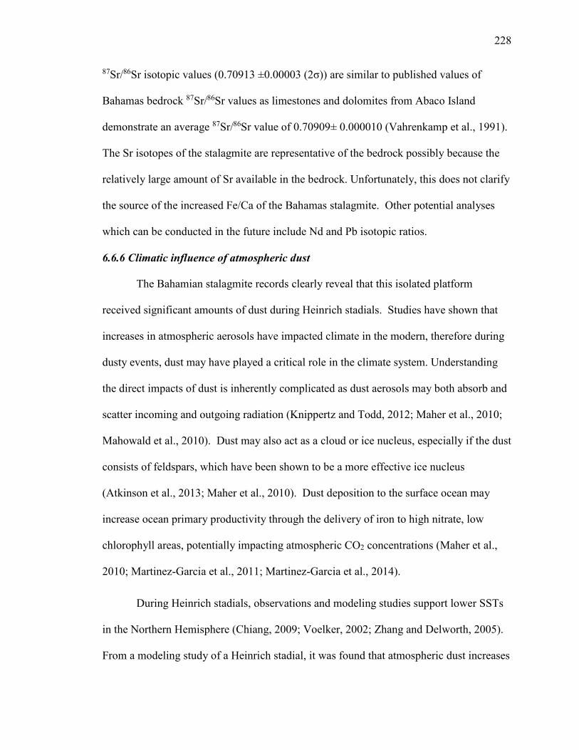
228 87Sr/86Sr isotopic values (0.70913 ±0.00003 (2σ)) are similar to published values of

Bahamas bedrock 87Sr/86Sr values as limestones and dolomites from Abaco Island

demonstrate an average 87Sr/86Sr value of 0.70909± 0.000010 (Vahrenkamp et al., 1991).

The Sr isotopes of the stalagmite are representative of the bedrock possibly because the

relatively large amount of Sr available in the bedrock. Unfortunately, this does not clarify

the source of the increased Fe/Ca of the Bahamas stalagmite. Other potential analyses

which can be conducted in the future include Nd and Pb isotopic ratios.

6.6.6 Climatic influence of atmospheric dust

The Bahamian stalagmite records clearly reveal that this isolated platform

received significant amounts of dust during Heinrich stadials. Studies have shown that

increases in atmospheric aerosols have impacted climate in the modern, therefore during

dusty events, dust may have played a critical role in the climate system. Understanding

the direct impacts of dust is inherently complicated as dust aerosols may both absorb and

scatter incoming and outgoing radiation (Knippertz and Todd, 2012; Maher et al., 2010;

Mahowald et al., 2010). Dust may also act as a cloud or ice nucleus, especially if the dust

consists of feldspars, which have been shown to be a more effective ice nucleus

(Atkinson et al., 2013; Maher et al., 2010). Dust deposition to the surface ocean may

increase ocean primary productivity through the delivery of iron to high nitrate, low

chlorophyll areas, potentially impacting atmospheric CO2 concentrations (Maher et al.,

2010; Martinez-Garcia et al., 2011; Martinez-Garcia et al., 2014).

During Heinrich stadials, observations and modeling studies support lower SSTs

in the Northern Hemisphere (Chiang, 2009; Voelker, 2002; Zhang and Delworth, 2005).

From a modeling study of a Heinrich stadial, it was found that atmospheric dust increases

229

the climate response to the Heinrich state (Murphy et al., 2014). Increased atmospheric

dust was demonstrated to increase cooling in the North Atlantic SSTs and amplify aridity

in Africa, the Arabian Sea and India (Murphy et al., 2014). The dust-climate feedback on

a high-albedo surface, such as ice, is still not well understood (Maher et al., 2010). A

study of the radiative effects of mineral dust in the high latitudes during LGM conditions

demonstrates increased dust leads to decreased radiative forcings and amplification of

surface cooling (Lambert et al., 2013). This is due to dust creating a cooling in the lower

troposphere. Recent studies have demonstrated the importance of light absorbing

aerosols, primarily black carbon, as significant contributors to warming in the Arctic

(Hegg et al., 2010). The deposition of light absorbing aerosols on ice sheets can lead to a

reduction of surface albedo and warming of temperatures which is critical if future

anthropogenic black carbon emissions increase (Lee et al., 2013). Future work focused

on dust variability in the atmosphere in the present and the past is important for the

determination of climate-dust feedbacks, impacts on the global climate and predictions

for future climate (Lambert et al., 2013; Lee et al., 2013; Mahowald et al., 2010).

6.7 Conclusion

Today the Bahamas seasonally receives dust from Africa. This study

demonstrates modern dust delivery to the cave and has shown that in the past, there were

increases in the amount of dust delivered to the Bahamas during Heinrich stadials.

To summarize the findings, in the modern, results support temporal and spatial

variability in the concentration of Fe within the cave. The temporal variability is thought

to be driven both by annual changes in the amount of available dust Fe and the amount of

precipitation. The variability between sites within the cave is driven by variations in flow

230

rates in the epikarst and soil zone as supported by other geochemical tools. The transport

of the iron from the dust to the cave is dependent on the amount of precipitation to leach

the iron and/or the transport of the colloid-bound Fe.

From the ancient stalagmites, the Fe/Ca ratios are found to increase concurrently

with changes in oxygen and carbon isotopes. An increased Fe/Ca ratio is associated with

Heinrich stadials and is thought to be driven by the leaching of Fe from the dust. From

the high resolution data, the increased Fe/Ca ratios are associated with the Heinrich

stadial termination, suggesting that increased Fe/Ca may be the result of an increase in

precipitation associated with the end of the Heinrich stadial. The washing of Fe rich

waters into the cave leads to an increase of iron at the termination. The increase in dust to

the Bahamas across Heinrich stadials is shown to be in good agreement with the timing

of other Heinrich stadial dust records from Africa and Greenland. Additionally,

variability in dust records between Heinrich stadials may provide insights into the relative

strength of each event. This study is the first study to demonstrate increased dust

deposition to the Bahamas associated with Heinrich stadials. It supports the view that

Heinrich stadials are dusty events; given the importance of dust to the climate system,

further studies should consider the climatic feedbacks of atmospheric dust.

Chapter 7

Review of millennial scale climate variability Summary

In this chapter, an overview of recent paleoclimate data will be utilized to provide

a review of the timing and nature of millennial scale climate and driving mechanisms.

When possible, the hitherto unpublished Bahamian records will be compared to published

data. The discussion of paleoclimate proxies will be followed by a review of the

mechanisms driving Dansgaard/Oeschger and Heinrich stadials and the global

propagation of these events.

7.1 Background

Global climate variations at the millennial scale are dominated by

Dansgaard/Oeschger (D/O) cycles and Heinrich stadial events (Denniston et al., 2007;

Fletcher et al., 2010; Jiménez-Moreno et al., 2010; Jouzel et al., 2007; Siddall et al.,

2010). Over the last 100,000 years, there have been 25 D/O cycles and 6 Heinrich

stadials (Figure 7.1). This chapter will primarily focus on these Heinrich stadials and D/O

cycles and the climatic expression in various regions of the world. However a brief

review of older events will be included in section 7.4. Several previous studies have

reviewed the paleoclimate and mechanisms associated with millennial scale climate

(Alley et al., 1999; Chiang, 2009; Clement and Peterson, 2008; Seager and Battisti, 2007;

Voelker, 2002), therefore this study will primarily focus on recently published archives.

This study is by no means a complete review of paleoclimate reconstructions for

millennial scale climate variability; rather the goal is to shed light on questions which

remain.

231

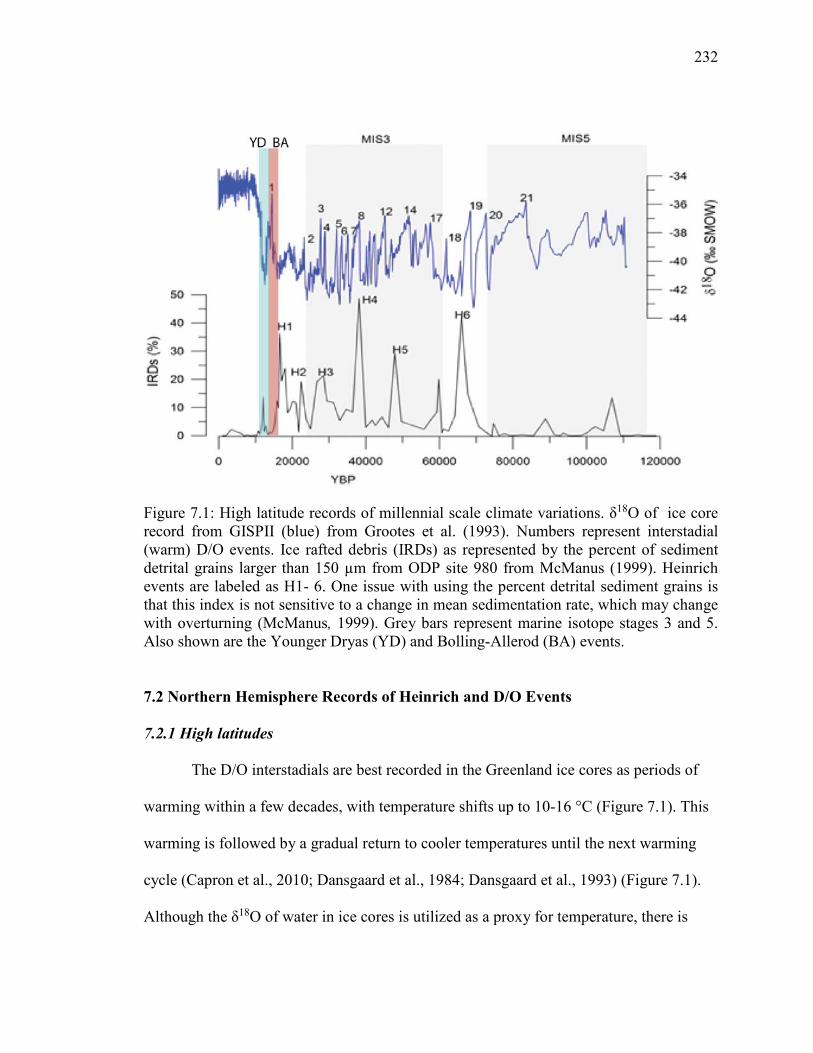
232

Figure 7.1: High latitude records of millennial scale climate variations. δ18O of ice core record from GISPII (blue) from Grootes et al. (1993). Numbers represent interstadial (warm) D/O events. Ice rafted debris (IRDs) as represented by the percent of sediment detrital grains larger than 150 µm from ODP site 980 from McManus (1999). Heinrich events are labeled as H1- 6. One issue with using the percent detrital sediment grains is that this index is not sensitive to a change in mean sedimentation rate, which may change with overturning (McManus, 1999). Grey bars represent marine isotope stages 3 and 5. Also shown are the Younger Dryas (YD) and Bolling-Allerod (BA) events.

7.2 Northern Hemisphere Records of Heinrich and D/O Events

7.2.1 High latitudes

The D/O interstadials are best recorded in the Greenland ice cores as periods of

warming within a few decades, with temperature shifts up to 10-16 °C (Figure 7.1). This

warming is followed by a gradual return to cooler temperatures until the next warming

cycle (Capron et al., 2010; Dansgaard et al., 1984; Dansgaard et al., 1993) (Figure 7.1).

Although the δ18O of water in ice cores is utilized as a proxy for temperature, there is

233

some evidence that seasonal distribution of precipitation and atmospheric processes may

cause oxygen isotopes to be driven by other processes (Wolff et al., 2010). Other proxies

such as the δ15N of trapped N2 can also be utilized to support increased temperature

across D/O cycles (Capron et al., 2010; Guillevic et al., 2013). There is additional

evidence that D/O events 8 – 10 in eastern Greenland exhibit the greatest temperature

increases (Guillevic et al., 2013; Wolff et al., 2010).

In addition to warming, there are several other environmental factors which change in

response to millennial scale climate events in the high latitudes. Methane concentrations

increase in the ice cores of Greenland during interstadials and decrease during stadial

events (Wolff et al., 2010). Records demonstrate nearly synchronous increases of

methane in both Greenland and Antarctic ice cores supporting rapid interhemispheric

atmospheric response (Blunier and Brook, 2001; Wolff et al., 2010). Ruth et al. (2007)

demonstrated a relationship between NGRIP dust and China loess deposits, suggesting

that dust increases in Greenland are driven by Asian aridity during Heinrich stadials

(HS).

The clearest record of Heinrich stadial (HS) events is in sediment cores from the

North Atlantic (Figure 1). Cold (stadial) events are associated with the southerly

extension of ice and an increase in freshwater discharge in to the North Atlantic

(Broecker et al., 1985; McManus et al., 2004). Heinrich stadials are characterized in the

North Atlantic by cold periods, and are recognized in the sedimentary record as eroded

terrigenous materials (Ice Rafted Debris IRD) deposited in the North Atlantic by ice

234

bergs upon melting (Bond et al., 1997; Heinrich, 1988).

Not only are there records of a decrease in temperature and collapse of ice sheets

associated with Heinrich stadials, but there is additional evidence in the North Atlantic

for changes in oceanic circulation. With the introduction of melt water to the surface of

the North Atlantic, decreasing the sea surface salinity of the North Atlantic leads to a

reduction of the Atlantic meridional overturning circulation (AMOC) (McManus et al.,

2004)(Figure 7.2). This was well supported by McManus et al. (2004) in which

231Pa/230Th was utilized as a proxy for the AMOC from a North Atlantic sediment core.

As demonstrated in figure 7.2, the shutdown of the AMOC into HS 1 was not abrupt;

rather it slowed over about 1,000 years which has implications for the forcing

mechanism. Similar results were found off the Iberian margin by Gherardi et al. (2005),

however the 231Pa/230Th of sediments from the Bermuda Rise may not reflect AMOC

reconstructions alone as it was determined that biogenic silica and 231Pa/230Th were

highly correlated and therefore may reflect an upwelling signal and not a proxy for

overturning at this location (Lippold et al., 2009).

As regards the origins of D/O cycles, there are conflicting interpretations from the

North Atlantic. There is some evidence from sediment cores of IRDs associated with D/O

interstadials, with peak iceberg calving associated with stadials (Broecker et al., 1985;

Bond et al., 1997; Menviel et al., 2014). This possibly suggests an associated AMOC

variation associated with D/O cycles, driven by iceberg calving (Menviel et al., 2014).

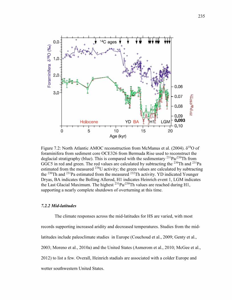
235

Figure 7.2: North Atlantic AMOC reconstruction from McManus et al. (2004). δ18O of foraminifera from sediment core OCE326 from Bermuda Rise used to reconstruct the deglacial stratigraphy (blue). This is compared with the sedimentary 231Pa/230Th from GGC5 in red and green. The red values are calculated by subtracting the 230Th and 231Pa estimated from the measured 238U activity; the green values are calculated by subtracting the 230Th and 231Pa estimated from the measured 232Th activity. YD indicated Younger Dryas, BA indicates the Bolling Allerod, H1 indicates Heinrich event 1, LGM indicates the Last Glacial Maximum. The highest 231Pa/230Th values are reached during H1, supporting a nearly complete shutdown of overturning at this time.

7.2.2 Mid-latitudes

The climate responses across the mid-latitudes for HS are varied, with most

records supporting increased aridity and decreased temperatures. Studies from the mid-

latitudes include paleoclimate studies in Europe (Couchoud et al., 2009; Genty et al.,

2003; Moreno et al., 2010a) and the United States (Asmerom et al., 2010; McGee et al.,

2012) to list a few. Overall, Heinrich stadials are associated with a colder Europe and

wetter southwestern United States.

236

Europe:

Several millennial scale studies have been conducted on sediment cores from off

the Iberian Margin and cave records from France. The marine records support decreased

sea surface temperatures (SSTs) associated with Heinrich stadials (Moreno et al., 2010a)

and are supported by terrestrial lake records (Moreno et al., 2010b), speleothem records

from France (Genty et al., 2003; Genty et al., 2010) and a lake record from the Balkans

(Panagiotopoulos et al., 2014). Sea surface temperature decreases during HS range

between 5-10 ºC across the Iberian Margin (Martrat et al., 2007; Patton et al., 2011) and

similar results were found in the Alboran Sea (northern Morocco), across the Straits of

Gibraltar (Cacho et al., 1999). The decreased SSTs during HS events in this region are

thought to be driven by the influx of cold surface water to the Mediterranean, due to a

reduction in AMOC.

In contrast to the findings during stadials, the D/O interstadials are periods of

increased humidity (Moreno et al., 2010a), up to a 10°C increase in temperature in the

Mediterranean (Genty et al., 2010) and a shift to more C3 plants versus C4 plants and

hence a wetter climate (Fleitmann et al., 2009).

Contrary to the results from Western Europe, a speleothem record from eastern

Turkey reveals increased aridity associated with stadials and increased humidity during

interstadials (Rowe et al., 2012). This is supported by a lake low stand at 15,000 yr BP

also possibly suggesting increased aridity associated with HS 1, however a higher dating

resolution is necessary (Landmann and Reimer, 1996). Rowe et al. (2012) proposed that

increased aridity during stadials in northeastern Turkey was driven by a reduction in the

export of winter moisture from the Mediterranean.

237

Further to the south several speleothem stable C and O isotopic studies conducted

from Soreq Cave and Peqiin Cave (Israel) reflect a decrease in precipitation associated

with Heinrich stadials (Bar-Matthews et al., 2003; Bar-Matthews et al., 1997). A more

recent, high resolution ion microprobe and confocal laser fluorescent microscope imaging

study of a Soreq Cave speleothem supports decreased temperatures, decreased seasonal

rainfall and changes in the vegetation type during HS1 (Orland et al., 2012). These

changes are thought to be driven by southerly shifted westerlies leading to an overall

decreased rainfall (Orland et al., 2012).

United States:

In the United States (US), variability to the response to millennial scale climate

events is observed with the west coast of the US exhibiting a decrease in temperatures

and an increase in precipitation (Hendy and Kennett, 2000; Oster et al., 2014). In the

southwestern United States, modern precipitation is in part driven by the North American

monsoon (NAM) however this does not appear to be a significant driver at the millennial

scale. Periods of increased precipitation have been observed in records of Heinrich

stadials from the southwest of the US (Asmerom et al., 2010; McGee et al., 2012;

Wagner et al., 2010) and as far east as Alabama (Lambert, 2010), while interstadials have

been shown to be periods of increased aridity (Wagner et al., 2010) (Figure 7.3).

However, not all studies agree, with some studies suggesting increased aridity associated

HS events in the southwest of the US (Benson et al., 2011). This suggests that western

US may not be a significant dust source during stadial events.

Increased precipitation to the west coast of the US is thought to be driven by increased

storms associated with a strengthened Aleutian Low (Hendy and Kennett, 2000; Oster et

238

al., 2014). While the mechanisms driving the climate response in the southwestern

United States is primarily attributed to the strengthening of the subtropical jet and storm

track (McGee et al., 2012), and southerly shift in the jet stream which may bring

increased winter precipitation from the Pacific Ocean (Asmerom et al., 2010; Wagner et

al., 2010). Conversely, periods of warming are associated with a weakening Aleutian

low, northward storm track and hence reduced precipitation (Wagner et al., 2010).

Figure 7.3: Figure from Wagner et al. (2010) demonstrating the relationship between oxygen isotopes from a speleothem from Arizona (red) and Santa Barbra Basin oxygen isotopes (green and blue) (Hendy and Kennett, 2000), Hulu cave oxygen isotopes from China (brown) (Wang et al., 2001) and NGRP ice core oxygen isotopes (dark blue) (Svensson et al., 2008). These records demonstrate the increased aridity in Arizona associated with D/O interstadials and warmer temperatures in Santa Barbara Basin.

239

7.2.3 Subtropics and tropics

Similar to the findings from the mid-latitudes, many tropical records reflect increased

aridity and cooling associated with Heinrich stadials in the Northern Hemisphere.

Conversely, D/O interstadial periods are typically associated with a warmer and wetter

climate.

Western Atlantic:

Records from Western Atlantic provide evidence for both increased aridity associated

with stadials and decreasing temperatures. Decreasing temperature is observed from an

alkenone-derived SST record from the Bermuda rise during stadials, with increasing

temperatures during interstadials (Sachs and Lehman, 1999). Further south, increased

aridity and decreased temperatures are observed during stadials from speleothem records

from the Bahamas (this study) and a lake record from Guatemala (Escobar et al., 2012;

Hodell et al., 2012). While some records from this region solely suggest increased aridity

during stadials, including a record in southwestern Mexico (driven by a reduction in the

NAM) and Cariaco Basin (driven by a southerly shifted ITCZ) (Lachniet et al., 2013;

Peterson et al., 2000) (Figure 7.4). These observations are also supported by records from

the Caribbean Sea, with increased salinity driven by a reduction in the AMOC or a

reduction in rainfall (Schmidt et al., 2004). Records from the Straits of Florida support

decreased northerly flow during Heinrich stadials due to reduction in AMOC (Lynch-

Stieglitz et al., 2014).

Interestingly, not all the D/O cycles are found in the stalagmite geochemistry from the

Bahamas and some stalagmites do not exhibit any geochemical change associated with

D/O cycles (discussed in Chapter 4). In addition, two stalagmites (AB-DC-14 and AB-

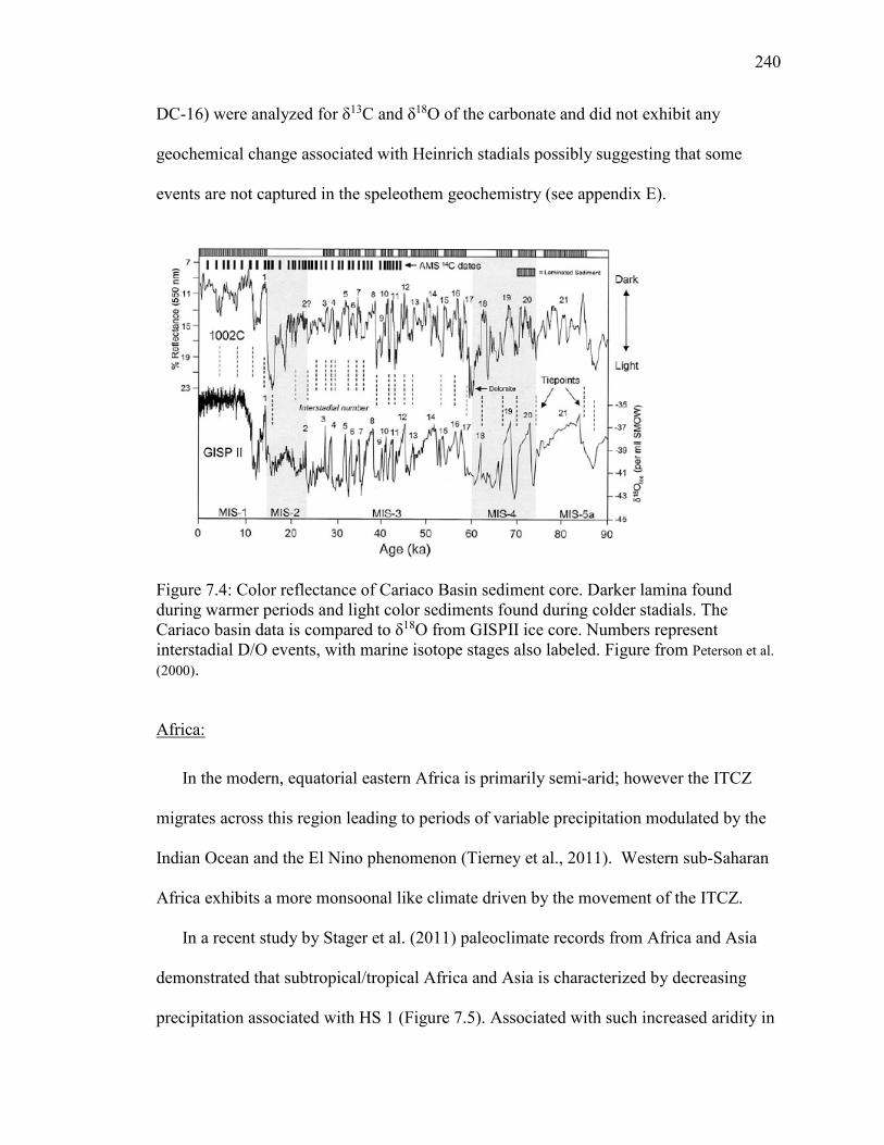
240

DC-16) were analyzed for δ13C and δ18O of the carbonate and did not exhibit any

geochemical change associated with Heinrich stadials possibly suggesting that some

events are not captured in the speleothem geochemistry (see appendix E).

Figure 7.4: Color reflectance of Cariaco Basin sediment core. Darker lamina found during warmer periods and light color sediments found during colder stadials. The Cariaco basin data is compared to δ18O from GISPII ice core. Numbers represent interstadial D/O events, with marine isotope stages also labeled. Figure from Peterson et al. (2000). Africa:

In the modern, equatorial eastern Africa is primarily semi-arid; however the ITCZ

migrates across this region leading to periods of variable precipitation modulated by the

Indian Ocean and the El Nino phenomenon (Tierney et al., 2011). Western sub-Saharan

Africa exhibits a more monsoonal like climate driven by the movement of the ITCZ.

In a recent study by Stager et al. (2011) paleoclimate records from Africa and Asia

demonstrated that subtropical/tropical Africa and Asia is characterized by decreasing

precipitation associated with HS 1 (Figure 7.5). Associated with such increased aridity in

241

Africa are records of increased atmospheric dust emission from western Africa (See

Chapter 6) (McGee et al., 2013; Multiza et al., 2008). Further evidence of increased

aridity for Western Africa is present in relic sand dunes and indicates that the Sahel-

Sahara boundary reached it most southerly position during HS 1-5 (Collins et al., 2013).

Off the coast of West Africa, results from a sediment core supports a reduction in glacial

North Atlantic intermediate water during HS 1 (Meckler et al., 2013) possibly driven by

the reduction in AMOC.

What are the mechanisms driving the widespread aridity associated with HS 1 in

tropical Africa? Stager et al. (2011) proposed that the widespread aridity cannot be solely

attributed to the southerly shifted ITCZ, but aridity may be enhanced as a result of

reduced SSTs in the Atlantic and in the Indian Ocean. A recent modeling study of the

ITCZ demonstrates the mean ITCZ shift during HS1 is likely less than 1 º latitude

supporting that the regional response in Africa may not be solely due to a shifted ITCZ,

but rather a response to different forcing mechanisms (McGee et al., 2014). One

interesting point is that the widespread aridity observed in the paleoclimate records has

been difficult to reconstruct in models (Murphy et al., 2014).

Asia:

Climate variation of the subtropical/tropical region of the Asian continent today is

dominated by monsoonal systems including both the Indian and Asian monsoons. During

HS events, there is significant evidence that the monsoonal systems weakened.

Sediment cores from the Arabian Sea exhibit lighter colored, bioturbated intervals during

HS 1 through HS 6, while dark organic carbon rich layers were deposited during

interstadials. However, the mechanism driving these sedimentological changes is not

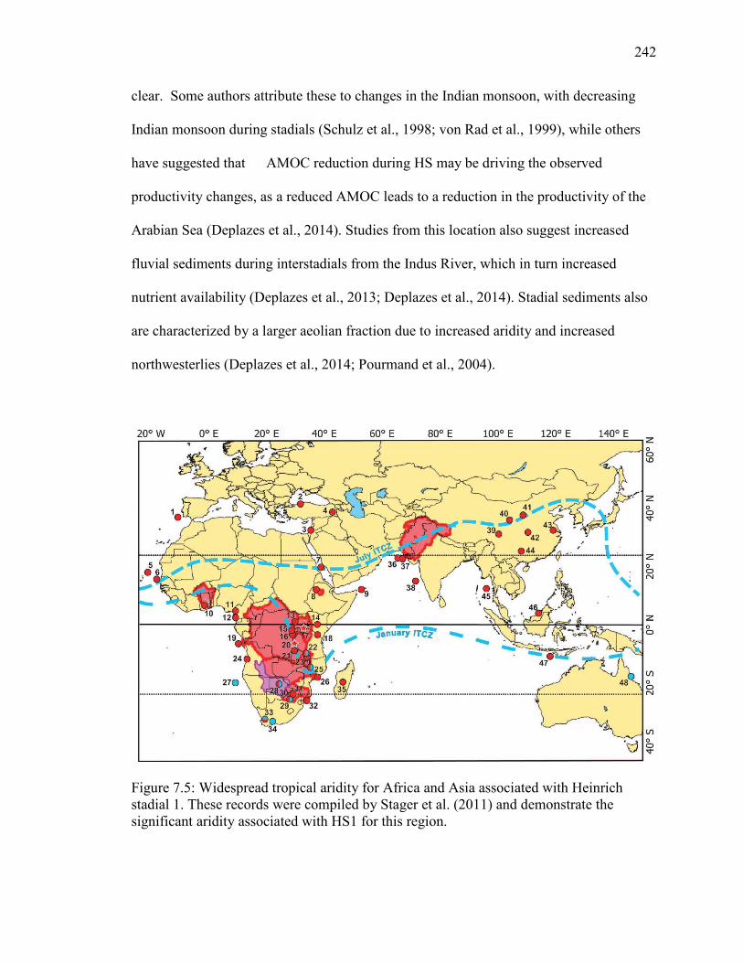
242

clear. Some authors attribute these to changes in the Indian monsoon, with decreasing

Indian monsoon during stadials (Schulz et al., 1998; von Rad et al., 1999), while others

have suggested that AMOC reduction during HS may be driving the observed

productivity changes, as a reduced AMOC leads to a reduction in the productivity of the

Arabian Sea (Deplazes et al., 2014). Studies from this location also suggest increased

fluvial sediments during interstadials from the Indus River, which in turn increased

nutrient availability (Deplazes et al., 2013; Deplazes et al., 2014). Stadial sediments also

are characterized by a larger aeolian fraction due to increased aridity and increased

northwesterlies (Deplazes et al., 2014; Pourmand et al., 2004).

Figure 7.5: Widespread tropical aridity for Africa and Asia associated with Heinrich stadial 1. These records were compiled by Stager et al. (2011) and demonstrate the significant aridity associated with HS1 for this region.

243

Several studies have been conducted on speleothems from China, as this area is

influenced both by the Indian and East Asian monsoons. The southwest of China is

characterized as a transition zone between the East Asian Monsoon and Indian Summer

Monsoon, while more northerly Hulu and Sanbao Caves are dominated by the East Asian

Monsoon (Zhao et al., 2010)(Figure 7.6). Good agreement was found between northern

and southern Chinese speleothem records across millennial scale climate events,

suggesting both monsoonal systems are responding similarly to these events with a

decrease in the monsoons during stadials and an increase during interstadials (Cai et al.,

2006; Wang et al., 2001; Zhao et al., 2010). Isotope records from speleothems from

China also support changes in the monsoon associated with summer insolation at 65 °N

(Wang et al., 2008).

Using an isotope enabled model, Pausata et al. (2011) modeled changes in the

δ18O of precipitation during Heinrich stadials in India and China. Pausata et al. (2011)

suggest that during stadials, precipitation changes in Asia are primarily driven by changes

in the Indian Summer Monsoon, rather than changes in the East Asian Monsoon and the

speleothem records from China reflect these changes. A study analyzing the drivers of

Holocene δ18O increases from speleothems from across China also found the drivers of

speleothem δ18O values to be primarily changes in the summer rainfall source and not a

change in the amount of rainfall (Maher and Thompson, 2012).

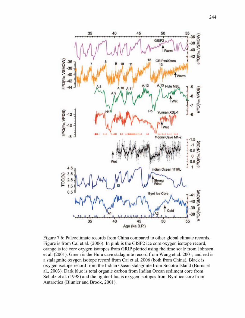
244

Figure 7.6: Paleoclimate records from China compared to other global climate records. Figure is from Cai et al. (2006). In pink is the GISP2 ice core oxygen isotope record, orange is ice core oxygen isotopes from GRIP plotted using the time scale from Johnsen et al. (2001). Green is the Hulu cave stalagmite record from Wang et al. 2001, and red is a stalagmite oxygen isotope record from Cai et al. 2006 (both from China). Black is oxygen isotope record from the Indian Ocean stalagmite from Socotra Island (Burns et al., 2003). Dark blue is total organic carbon from Indian Ocean sediment core from Schulz et al. (1998) and the lighter blue is oxygen isotopes from Byrd ice core from Antarctica (Blunier and Brook, 2001).

245

Pacific:

In the Pacific, the ITCZ is situated over northern Borneo year round with minimal

annual variation. Several studies have been conducted from speleothems from Borneo

and records from this location support a decrease in precipitation associated with HS

(Carolin et al., 2013; Partin et al., 2007) and minimal geochemical response across D/O

cycles (Carolin et al., 2013). Additionally the records support a precessional (21 ka)

insolation forcing (Carolin et al., 2013; Partin et al., 2007).

From the tropical eastern Indian Ocean located to the west of the Borneo records,

results from geochemical analysis of foraminifera support drier conditions across HS 1

(Mohtadi et al., 2014). This is supported by longer records from sediment cores from the

west coast of Sumatra, Indonesia (Russell et al., 2014), a speleothem record from West

Flores, Indonesia (Lewis et al., 2011) and reduced precipitation in the eastern Indian

Ocean is supported by increased sea surface salinity from sediment cores (Gibbons et al.,

2014). Mechanisms which have been proposed for the resulting climatic response include

sea surface cooling driving precipitation decrease, decrease in Indo-Austral Summer

Monsoon (IASM) intensity due to ITCZ migration or the changes in ocean fronts

(Mohtadi et al., 2014), and a reorganization of Hadley circulation (Gibbons et al., 2014;

Mohtadi et al., 2014). These findings are well summarized in Mohtadi et al. (2014) and

Denniston et al. (2013b).

7.3 Southern Hemisphere

The climatic response across millennial scale climate events in the Southern

Hemisphere is often expressed as periods of increased precipitation and temperatures

during stadials, with decreased precipitation during interstadials.

246

7.3.1 Tropics

The South American summer monsoon (SASM) is primarily driven by seasonal

migration in the ITCZ. During the Northern Hemisphere winter, the ITCZ is shifted

further south over Brazil, and easterly winds transport moisture across from the Amazon

Basin (Kanner et al., 2012). During the Northern Hemisphere summer, the ITCZ shifts

further north, bringing rains to northern South America.

Stalagmites from the Peruvian Andes support intensified SASM across Heinrich

stadials while D/O interstadials are characterized by a reduction in precipitation amount

(Kanner et al., 2012) (Figure 7.7). Several records from Brazil also exhibit similar

changes across Heinrich and D/O cycles, supporting good coherence in the climatic

response to HS (Cheng et al., 2013; Cruz et al., 2009; Kanner et al., 2012; Mosblech et

al., 2012)(Figure 7.7).The increased SASM is primarily thought to be driven by a

southward shift in the mean position of the ITCZ, possibly due to the strengthening in

Hadley cell circulation and decreased SSTs (Cheng et al., 2013; Cheng et al., 2012).

Studies have demonstrated an anti-phase relationship over the last precession

cycle between eastern/northeastern Brazil and western/southern Brazil, contrary to the

good agreement during millennial scale climate events (Cheng et al., 2013; Mosblech et

al., 2012). Eastern/northeastern Brazil records demonstrate an antiphased relationship

with insolation due to high insolation intensifying the SASM leading to increased

precipitation in south/west of Brazil and decreased precipitation in the east/north (Cheng

et al., 2013).

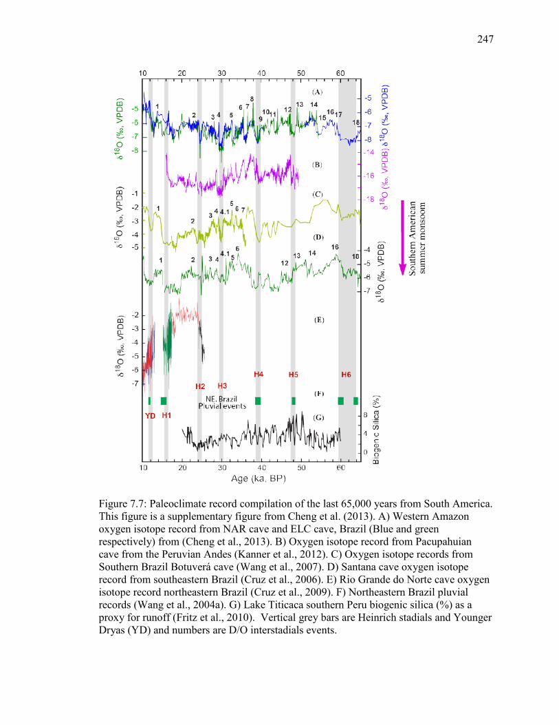
247

Figure 7.7: Paleoclimate record compilation of the last 65,000 years from South America. This figure is a supplementary figure from Cheng et al. (2013). A) Western Amazon oxygen isotope record from NAR cave and ELC cave, Brazil (Blue and green respectively) from (Cheng et al., 2013). B) Oxygen isotope record from Pacupahuian cave from the Peruvian Andes (Kanner et al., 2012). C) Oxygen isotope records from Southern Brazil Botuverá cave (Wang et al., 2007). D) Santana cave oxygen isotope record from southeastern Brazil (Cruz et al., 2006). E) Rio Grande do Norte cave oxygen isotope record northeastern Brazil (Cruz et al., 2009). F) Northeastern Brazil pluvial records (Wang et al., 2004a). G) Lake Titicaca southern Peru biogenic silica (%) as a proxy for runoff (Fritz et al., 2010). Vertical grey bars are Heinrich stadials and Younger Dryas (YD) and numbers are D/O interstadials events.

248

Pacific:

In the Southern Hemisphere Pacific, there is evidence for increased Indo-

Australian Summer Monsoon (IASM) associated with HS (Ayliffe et al., 2013) from

southern Indonesia and from Western Australia (Denniston et al., 2013b) (Figure 7.8).

The record from northwestern Australia provides evidence of a weakened IASM during

D/O interstadials (Denniston et al., 2013b), however the U-Th dating is not at a resolution

which can exactly determine the timing of the D/O interstadials in this record. Further

south in Western Australia there is evidence for minimal geochemical changes across HS

2, suggesting that HS 2 was not a significant event (Denniston et al., 2013a). The

increased IASM during stadials is thought to be due to a steepening north-south

interhemispheric gradient driving a southward shift of the IASM during stadials (Ayliffe

et al., 2013) and additionally stadials are thought to exhibit increased tropical cyclone

activity (Denniston et al., 2013a).

7.3.2 Mid to high latitudes

Antarctic cores preserve much longer records (to 800,000 years before present)

than the Greenland ice cores providing a long record of millennial and orbital scale

climate (Jouzel et al., 2007). For every Greenland interstadial, there is a corresponding

Antarctic event. Antarctica exhibits cooling during Greenland interstadials and warming

during Greenland stadials, however the magnitude of change is much smaller in

Antarctica (Blunier and Brook, 2001; Jouzel et al., 2007; Wolff et al., 2010) (Figure 7.9).

Additionally the response to millennial scale climate events varies by location on

Antarctica, with the Atlantic sector exhibiting a much more rapid temperature rise than

those found in the Indian/Pacific ocean sector (Buiron et al., 2012). With the recently

249

acquired WAIS ice core, results will aid in the understanding of such differences (Buiron

et al., 2012).

Figure 7.8: comparison of the record from (Denniston et al., 2013a) from coastal Western Australia in blue to records from Flores Sea (black) (a) from (Muller et al., 2012). The Flores Sea record is from a sediment core which supports increased precipitation associated with Heinrich stadial 1 (Muller et al., 2012). (b) Red is a record from Northern Australia (Denniston et al., 2013b) demonstrating an increased IASM associated with Heinrich stadial 1 and 2. Figure (c) red is from (De Deckker et al., 2012) from offshore Western Australia, supports increased Leeuwin Current during Heinrich stadial 1 and 2.

250

Two sediment cores from the Weddell Sea support eight periods of increased IRD

deposition during the past 20 ka BP, derived from Antarctica (Weber et al., 2014). The

IRD deposits exhibit a pacing similar to the observations from the North Atlantic,

suggesting the Antarctic ice sheet also exhibited similar abrupt ice-sheet instability

(Weber et al., 2014).

Figure 7.9: Oxygen isotopes from NGRIP ice core (Greenland) compared with Deuterium isotopes from Epica Dome C. The numbers indicate D/O cycle 8 and 12 which are two very large interstadials in the ice core records. This figure from Wolff et al. (2010) demonstrates the good agreement in the timing of events between the two hemispheres. 7.4 Evidence of Heinrich Stadials beyond Last 100,000 Years

Evidence of sub-orbital millennial scale climate variability has been identified

well beyond the last 100,000 years and has been demonstrated to be a pervasive feature

of the climate state over longer periods of times (Johnsen et al., 2001; Jouzel et al., 2007;

McManus, 1999; Weirauch et al., 2008). Sedimentary records demonstrate that climate

instability is the norm rather than the exception in both high latitude and low latitude

251

records (Gibson and Peterson, 2014; McManus, 1999). McManus (1999) demonstrated

fewer IRDs during interglacial periods in the North Atlantic and those IRDs are

associated with benthic δ18O values greater than +3.5 ‰, suggesting that a minimum

amount of ice is required. A molybdenum record from Cariaco basin (proxy for anoxic

conditions) also supports that millennial scale climate variations are persistent over the

last 600,000 years, although this record does not suggest a minimum ice sheet size is

required (Gibson and Peterson, 2014). This record suggests that either a non-Laurentide

ice sheet melt water source or glacial sea-ice extent may drive millennial scale climate

variations, however questions still remain about the forcing mechanisms, particularly

during periods of minimal ice sheet volume (Gibson and Peterson, 2014). Potentially,

developing records from the subtropical Bahamas may aid in the understanding of

millennial scale climate variations during older glacial periods, in particular if older

samples forming from above water caves can be acquired, these samples may provide

information on millennial scale climate variations in the subtropical Atlantic during

interglacials.

Two older stalagmite samples from the Bahamas have been analyzed. One

sample, AB-DC-07 was dated at 367,880 yr BP (Figures 7.10 and 7.11). Only one age

date was acquired and more are necessary, however preliminary C and O isotopes suggest

possible millennial scale variations (Figure 7.10). Sample AB-DC-08 was dated at

231,660, 249,470 and 258,820 yr BP and may support increases in C and O isotopes

associated with the IRD deposit at 241,000 yr BP (Figure 7.11). Future work focusing on

establishing a reliable age model for these samples may be of interest.

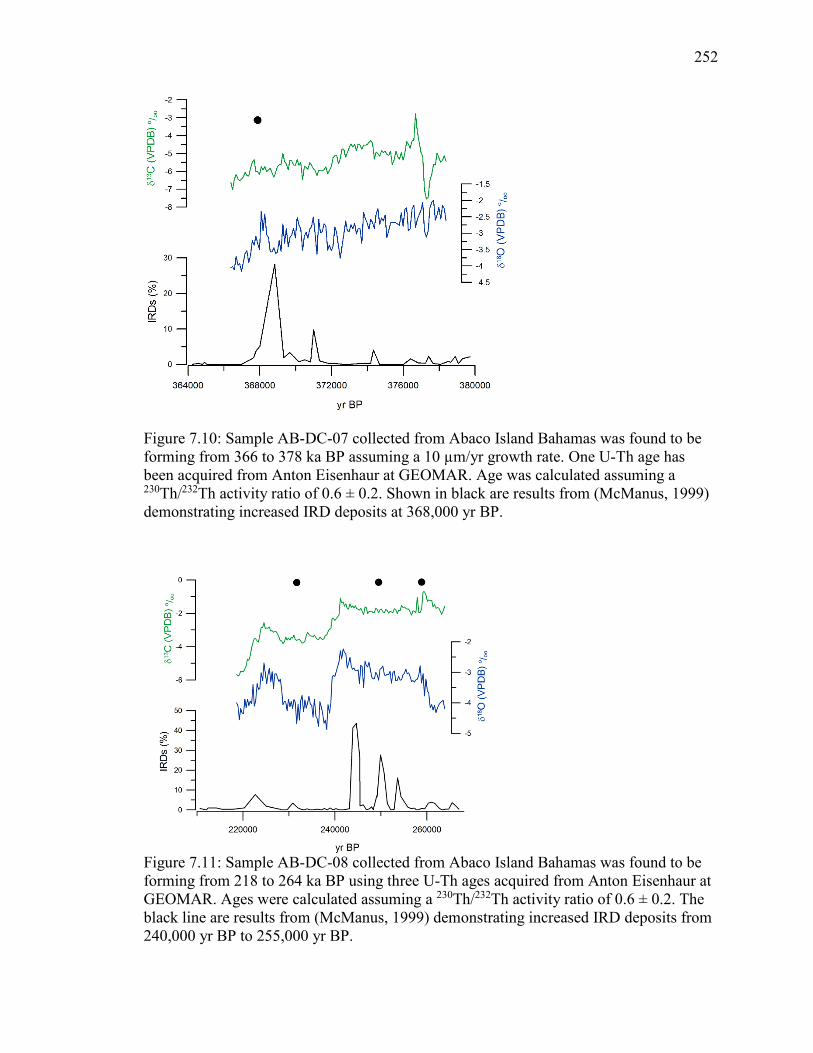
252

Figure 7.10: Sample AB-DC-07 collected from Abaco Island Bahamas was found to be forming from 366 to 378 ka BP assuming a 10 µm/yr growth rate. One U-Th age has been acquired from Anton Eisenhaur at GEOMAR. Age was calculated assuming a 230Th/232Th activity ratio of 0.6 ± 0.2. Shown in black are results from (McManus, 1999) demonstrating increased IRD deposits at 368,000 yr BP.

Figure 7.11: Sample AB-DC-08 collected from Abaco Island Bahamas was found to be forming from 218 to 264 ka BP using three U-Th ages acquired from Anton Eisenhaur at GEOMAR. Ages were calculated assuming a 230Th/232Th activity ratio of 0.6 ± 0.2. The black line are results from (McManus, 1999) demonstrating increased IRD deposits from 240,000 yr BP to 255,000 yr BP.

253

7.5 Forcing of Millennial Scale Climate

Critical to understanding subtropical climate during Heinrich events and Bond

cycles is the forcing mechanisms of these events. Several forcing mechanisms have been

proposed including, but not limited to: freshwater forcing, tropical forcing and sea-ice

feedback forcing. These mechanisms are well reviewed in papers such as Clement and

Peterson (2008), Hemming (2004), Chiang (2009), Seager and Battisti (2007), and

Overpeck and Cole (2006). The mechanisms driving D/O cycles and the global

propagation are still not well understood (Clement and Peterson, 2008; Timmermann et

al., 2003).

7.5.1 Freshwater forcing

The forcing mechanism of millennial scale climate must be 1) abrupt and 2)

enable a global scale climate response (Clement and Peterson, 2008). The freshwater

forcing mechanism invokes a decrease in the AMOC as a driver for the observed climate.

The reduction or shut down of the AMOC is thought to lead to the formation of the

“bipolar seesaw” or the antiphased relationship between the North Atlantic and Antarctic

climate (Blunier and Brook, 2001; Overpeck and Cole, 2006). This antiphased

relationship is seen across Heinrich stadials and D/O cycles between the Antarctic and

the Greenland ice core records. AMOC resumes once salinities in the North Atlantic are

restored by a decrease in the freshwater influx. Many models have been built using the

freshwater forcing mechanism and agree reasonably well with the observed paleoclimate

response across Heinrich stadials with the major exception being the tropics (Menviel et

al., 2011; Vellinga and Wood, 2002; Zhang and Delworth, 2005).

254

The freshwater forcing mechanism relies on the buildup and subsequent melting

of the ice sheets as a driver for reduction in AMOC. There have been several theories

proposed for the mechanisms driving the ice sheet dynamics, including the binge-purge

model, geothermal heating (Macayeal, 1993), insolation driven ice sheet dynamics (Bond

et al., 2001) and others, however uncertainties still remain. The binge-purge model

suggests that large ice sheets buildup gradually (binge phase) until it reaches a phase of

destabilization.

D/O cycles and the evidence for IRDs:

There is some recent evidence that all D/O stadials between 30-50 ka BP are

associated with IRD deposits in the North Atlantic (Menviel et al., 2014). Records

support that iceberg calving occurred during interstadials and peaked during stadial

periods (Menviel et al., 2014). It has been suggested that therefore the forcing for D/O

cycles is very similar to the forcing mechanisms of Heinrich stadials (Menviel et al.,

2014).

7.5.2 Tropical ocean/atmosphere forcing

The antiphased relationship between the AMOC and the southern hemisphere

supports the global importance of the AMOC in climate modulation. Change of the

thermohaline circulation is the current favorite explanation for abrupt climate change.

However, this mechanism does not explain all of the observed paleoclimate variability.

Seager and Battisti (2007) argue that the degree of winter cooling must be caused by a

change in the atmospheric heat transport potentially driven by wind changing the

movement of water northward. This change would lead to a southward extension of the

255

ice sheets and an increased aridity in the tropics (Seager and Battisti, 2007). However, it

is still unclear how such a change in the wind field would occur.

The tropics may serve as a critical point in the global propagation of these events

because the tropics act as a barrier between the two hemispheres. As demonstrated by El

Nino Southern Oscillation events, the tropics can play a very large role in the global

climate (Cane and Clement, 1999). Mechanisms that have been proposed for AMOC and

tropical climate are outlined in Clement and Peterson, 2008.

Tropical dust:

As suggested previously, tropical paleoclimate records support increased aridity

during HS, a feature which is not resolved in many models of these events (Murphy et al.,

2014). One potential source of this offset is the impacts of dust on climate. From a

modeling study of a Heinrich stadial, it was found that dust increases the climate

response to the Heinrich stadials and increased atmospheric dust was demonstrated to

increase cooling in the North Atlantic SSTs and amplify aridity in Africa, the Arabian

Sea and India (Murphy et al., 2014). Future studies should consider aerosol-sea ice

feedbacks in the North Atlantic for HS, however studies have demonstrated, models have

difficulty capturing accurate dust emissions, based on modern analysis of dust as well as

paleo dust measurements (Evan et al., 2014; Lambert et al., 2013; Lee et al., 2013;

Mahowald et al., 2010; Murphy et al., 2014; Pourmand et al., 2014a).

7.5.3 Sea-ice forcing

The D/O cycles are associated with an increased accumulation for the Greenland ice

sheet, difficult to explain based on the mechanisms discussed thus far (Li et al., 2010). It

has been proposed that D/O cycles may be driven by a different forcing mechanism

256

which accounts for this increase in accumulation (Li et al., 2010). For D/O cycles

(interstadials), there is minimal evidence for changes in overturning, therefore it has been

proposed that sea ice changes may be an important mechanism driving climate responses

(Petersen et al., 2013). This mechanism supports the changes in accumulation as well as

the saw-tooth pattern of the oxygen isotopes of Greenland across D/O events (Petersen et

al., 2013). This hypothesis is supported by evidence of IRD deposits associated with D/O

events in particular during interstadials and modeling studies suggest D/O events are

forced both by ice-sheet and AMOC variations (Menviel et al., 2014).

7.6 Summary and Conclusion

This chapter has provided an overview of the recent paleoclimate studies on

millennial scale climate variability and the driving mechanisms of these events. To

summarize, there are several global scale changes associated with millennial scale

climate variations, including in the Northern Hemisphere, decreased SSTs, increased

aridity in many locations (in particular in the tropics), reduction of the IASM, Asian

monsoons and NAM, while interstadials are often expressed as periods of rapid warming

(in particular in Greenland) and SST increase, and increased rainfall. Contrary, in the

Southern Hemisphere stadials are characterized by increased SASM and IASM which are

thought to be driven by increased SSTs and a southerly shifted ITCZ. Future research

efforts on millennial scale climate events which would be of importance includes

continued research on the NAM during these events, continued research on millennial

scale climate variation during interglacial periods and paleoclimate research to continue

to quantify dust emissions during Heinrich stadials for the production of reliable dust

models.

References

Affek, H., Barmatthews, M., Ayalon, A., Matthews, A., and Eiler, J., 2008, Glacial/interglacial temperature variations in Soreq cave speleothems as recorded by ‘clumped isotope’ thermometry: Geochimica et Cosmochimica Acta, v. 72, no. 22, p. 5351-5360.

Affek, H. P., 2013, Clumped Isotopic Equilibrium and the Rate of Isotope Exchange between CO2 and Water: American Journal of Science, v. 313, no. 4, p. 309-325.

Affek, H. P., and Eiler, J. M., 2006, Abundance of mass 47 CO2 in urban air, car exhaust, and human breath: Geochimica Et Cosmochimica Acta, v. 70, no. 1, p. 1-12.

Alley, R. B., Clark, P. U., Keigwin, L. D., and Webb, R. S., 1999, Making sense of millennial-scale climate change, Mechanisms of Global Climate Change at Millennial Time Scales, Volume Geophysical Monograph 112, American Geophyisical Union.

Arienzo, M. M., Swart, P. K., and Vonhof, H. B., 2013, Measurement of δ18O and δ2H values of fluid inclusion water in speleothems using cavity ring-down spectroscopy compared with isotope ratio mass spectrometry: Rapid Communications in Mass Spectrometry, v. 27, no. 23, p. 2616-2624.

Asmerom, Y., Polyak, V. J., and Burns, S. J., 2010, Variable winter moisture in the southwestern United States linked to rapid glacial climate shifts: Nature Geoscience, v. 3, no. 2, p. 114-117.

Atkinson, J. D., Murray, B. J., Woodhouse, M. T., Whale, T. F., Baustian, K. J., Carslaw, K. S., Dobbie, S., O'Sullivan, D., and Malkin, T. L., 2013, The importance of feldspar for ice nucleation by mineral dust in mixed-phase clouds: Nature, v. 498, no. 7454, p. 355-358.

Ayalon, A., Bar-Matthews, M., and Kaufman, A., 1999, Petrography, strontium, barium and uranium concentrations, and strontium and uranium isotope ratios in speleothems as palaeoclimatic proxies: Soreq Cave, Israel: The Holocene, v. 9, no. 6, p. 715-722.

Ayliffe, L. K., Gagan, M. K., Zhao, J. X., Drysdale, R. N., Hellstrom, J. C., Hantoro, W. S., Griffiths, M. L., Scott-Gagan, H., St Pierre, E., Cowley, J. A., and Suwargadi, B. W., 2013, Rapid interhemispheric climate links via the Australasian monsoon during the last deglaciation: Nat Commun, v. 4, p. 2908.

Baker, A., and Bradley, C., 2010, Modern stalagmite δ18O: Instrumental calibration and forward modelling: Global and Planetary Change, v. 71, no. 3-4, p. 201-206.

Baldini, J. U. L., McDermott, F., Baldini, L. M., Ottley, C. J., Linge, K. L., Clipson, N., and Jarvis, K. E., 2012, Identifying short-term and seasonal trends in cave drip water trace element concentrations based on a daily-scale automatically collected drip water dataset: Chemical Geology, v. 330, p. 1-16.

257

258

Baldini, L. M., Walker, S. E., Railsback, L. B., Baldini, J. U. L., and Crowe, D. E., 2007, Isotopic ecology of the modern land snail Cerion, San Salvador, Bahamas: Preliminary advances toward establishing a low-latitude island paleoenvironmental proxy: Palaios, v. 22, no. 2, p. 174-187.

Banner, J. L., Guilfoyle, A., James, E. W., Stern, L. A., and Musgrove, M., 2007, Seasonal variations in modern speleothem calcite growth in Central Texas, U.S.A: Journal of Sedimentary Research, v. 77, no. 8, p. 615-622.

Banner, J. L., Musgrove, M. L., Asmerom, Y., Edwards, R. L., and Hoff, J. A., 1996, High-resolution temporal record of Holocene ground-water chemistry: Tracing links between climate and hydrology: Geology, v. 24, no. 11, p. 1049-1053.

Bar-Matthews, M., Ayalon, A., Gilmour, M., Matthews, A., and Hawkesworth, C. J., 2003, Sea-land oxygen isotopic relationships from planktonic foraminifera and speleothems in the Eastern Mediterranean region and their implication for paleorainfall during interglacial intervals: Geochimica Et Cosmochimica Acta, v. 67, no. 17, p. 3181-3199.

Bar-Matthews, M., Ayalon, A., and Kaufman, A., 1997, Late Quaternary paleoclimate in the eastern Mediterranean region from stable isotope analysis of speleothems at Soreq Cave, Israel: Quaternary Research, v. 47, no. 2, p. 155-168.

Bar-Matthews, M., Ayalon, A., Kaufman, A., and Wasserburg, G. J., 1999, The Eastern Mediterranean paleoclimate as a reflection of regional events: Soreq cave, Israel: Earth and Planetary Science Letters, v. 166, no. 1-2, p. 85-95.

Beck, J. W., Edwards, R. L., Ito, E., Taylor, F. W., Recy, J., Rougerie, F., Joannot, P., and Henin, C., 1992, Sea-surface temperature from coral skeletal strontium calcium ratios: Science, v. 257, no. 5070, p. 644-647.

Benson, L. V., Lund, S. P., Smoot, J. P., Rhode, D. E., Spencer, R. J., Verosub, K. L., Louderback, L. A., Johnson, C. A., Rye, R. O., and Negrini, R. M., 2011, The rise and fall of Lake Bonneville between 45 and 10.5 ka: Quaternary International, v. 235, p. 57-69.

Bettis, E. A., Muhs, D. R., Roberts, H. M., and Wintle, A. G., 2003, Last Glacial loess in the conterminous USA: Quaternary Science Reviews, v. 22, no. 18-19, p. 1907-1946.

Bigeleisen, J., and Mayer, M. G., 1947, Calculation of equilibrium constants for isotopic exchange reactions: Journal of Chemical Physics, v. 15, no. 5, p. 261-267.

Blunier, T., and Brook, E. J., 2001, Timing of millennial-scale climate change in Antarctica and Greenland during the last glacial period: Science, v. 291, no. 5501, p. 109-112.

Bond, G., Broecker, W., Johnsen, S., Mcmanus, J., Labeyrie, L., Jouzel, J., and Bonani, G., 1993, Correlations between climate records from North-Atlantic sediments and Greenland ice: Nature, v. 365, no. 6442, p. 143-147.

259

Bond, G., Heinrich, H., Broecker, W., Labeyrie, L., Mcmanus, J., Andrews, J., Huon, S., Jantschik, R., Clasen, S., Simet, C., Tedesco, K., Klas, M., Bonani, G., and Ivy, S., 1992, Evidence for massive discharges of icebergs into the North-Atlantic Ocean during the Last Glacial Period: Nature, v. 360, no. 6401, p. 245-249.

Bond, G., Kromer, B., Beer, J., Muscheler, R., Evans, M. N., Showers, W., Hoffmann, S., Lotti-Bond, R., Hajdas, I., and Bonani, G., 2001, Persistent solar influence on north Atlantic climate during the Holocene: Science, v. 294, no. 5549, p. 2130-2136.

Bond, G., Showers, W., Cheseby, M., Lotti, R., Almasi, P., deMenocal, P., Priore, P., Cullen, H., Hajdas, I., and Bonani, G., 1997, A pervasive millennial-scale cycle in North Atlantic Holocene and glacial climates: Science, v. 278, no. 5341, p. 1257-1266.

Bourdon, B., Turner, S., Henderson, G. M., and Lundstrom, C. C., 2003, Introduction to U-series geochemistry, in Bourdon, B., ed., Reviews in Mineralogy and Geochemistry: Uranium-series Geochemistry, Volume 52: Washington, DC, Mineralogical Society of America.

Brand, W. A., Geilmann, H., Crosson, E. R., and Rella, C. W., 2009, Cavity ring-down spectroscopy versus high-temperature conversion isotope ratio mass spectrometry; a case study on δ2H and δ18O of pure water samples and alcohol/water mixtures: Rapid Communications in Mass Spectrometry, v. 23, no. 12, p. 1879-1884.

Broecker, W. S., 1994, Massive iceberg discharges as triggers for global climate change: Nature, v. 372, no. 6505, p. 421-424.

Broecker, W. S., Peteet, D. M., and Rind, D., 1985, Does the ocean-atmosphere system have more than one stable mode of operation: Nature, v. 315, no. 6014, p. 21-26.

Buiron, D., Stenni, B., Chappellaz, J., Landais, A., Baumgartner, M., Bonazza, M., Capron, E., Frezzotti, M., Kageyama, M., Lemieux-Dudon, B., Masson-Delmotte, V., Parrenin, F., Schilt, A., Selmo, E., Severi, M., Swingedouw, D., and Udisti, R., 2012, Regional imprints of millennial variability during the MIS 3 period around Antarctica: Quaternary Science Reviews, v. 48, p. 99-112.

Burns, S. J., Fleitmann, D., Matter, A., Kramers, J., and Al-Subbary, A. A., 2003, Indian Ocean climate and an absolute chronology over Dansgaard/Oeschger events 9 to 13: Science, v. 301, no. 5638, p. 1365-1367.

Cacho, I., Grimalt, J. O., Pelejero, C., Canals, M., Sierro, F. J., Flores, J. A., and Shackleton, N., 1999, Dansgaard-Oeschger and Heinrich event imprints in Alboran Sea paleotemperatures: Paleoceanography, v. 14, no. 6, p. 698-705.

Cai, Y., An, Z., Cheng, H., Edwards, R. L., Kelly, M. J., Liu, W., Wang, X., and Shen, C.-C., 2006, High-resolution absolute-dated Indian Monsoon record between 53 and 36 ka from Xiaobailong Cave, southwestern China: Geology, v. 34, no. 8, p. 621.

260

Came, R. E., Eiler, J. M., Veizer, J., Azmy, K., Brand, U., and Weidman, C. R., 2007, Coupling of surface temperatures and atmospheric CO2 concentrations during the Palaeozoic era: Nature, v. 449, no. 7159, p. 198-U193.

Capron, E., Landais, A., Chappellaz, J., Schilt, A., Buiron, D., Dahl-Jensen, D., Johnsen, S. J., Jouzel, J., Lemieux-Dudon, B., Loulergue, L., Leuenberger, M., Masson-Delmotte, V., Meyer, H., Oerter, H., and Stenni, B., 2010, Millennial and sub-millennial scale climatic variations recorded in polar ice cores over the last glacial period: Climate of the Past, v. 6, no. 3, p. 345-365.

Carolin, S. A., Cobb, K. M., Adkins, J. F., Clark, B., Conroy, J. L., Lejau, S., Malang, J., and Tuen, A. A., 2013, Varied response of western Pacific hydrology to climate forcings over the last glacial period: Science, v. 340, no. 6140, p. 1564-1566.

Cheng, H., Sinha, A., Cruz, F. W., Wang, X., Edwards, R. L., d'Horta, F. M., Ribas, C. C., Vuille, M., Stott, L. D., and Auler, A. S., 2013, Climate change patterns in Amazonia and biodiversity: Nat Commun, v. 4, p. 1411.

Cheng, H., Sinha, A., Wang, X. F., Cruz, F. W., and Edwards, R. L., 2012, The Global Paleomonsoon as seen through speleothem records from Asia and the Americas: Climate Dynamics, v. 39, no. 5, p. 1045-1062.

Chiang, J. C. H., 2009, The tropics in paleoclimate: Annual Review of Earth and Planetary Sciences, v. 37, no. 1, p. 263-297.

Christoforou, C. S., Salmon, L. G., and Cass, G. R., 1994, Deposition of atmospheric particles within the Buddhist Cave Temples at Yungang, China: Atmospheric Environment, v. 28, no. 12, p. 2081-2091.

Cisneros, C. J., Caballero, E., Vera, J. A., and Andreo, B., 2011, An optimized thermal extraction system for preparation of water from fluid inclusions in speleothems: Geologica Acta, v. 9, no. 2, p. 9.

Clement, A. C., and Cane, M. A., 1999, A role for the tropical pacific coupled ocean-atmosphere system on Milankovitch and millennial timescales, in Clark, P. U., Webb, R. S., and Keigwin, L. D., eds., Mechanisms of Global Climate Change at Millennial Time Scales, Volume 112: Washington, D.C., AGU, p. 363-371.

Clement, A. C., and Peterson, L. C., 2008, Mechanisms of abrupt climate change of the last glacial period: Reviews of Geophysics, v. 46, no. 4.

Collins, J. A., Govin, A., Mulitza, S., Heslop, D., Zabel, M., Hartmann, J., Rohl, U., and Wefer, G., 2013, Abrupt shifts of the Sahara-Sahel boundary during Heinrich stadials: Climate of the Past, v. 9, no. 3, p. 1181-1191.

Coplen, T. B., 2007, Calibration of the calcite-water oxygen-isotope geothermometer at Devils Hole, Nevada, a natural laboratory: Geochimica Et Cosmochimica Acta, v. 71, no. 16, p. 3948-3957.

Couchoud, I., Genty, D., Hoffmann, D., Drysdale, R., and Blamart, D., 2009, Millennial-scale climate variability during the Last Interglacial recorded in a speleothem from south-western France: Quaternary Science Reviews, v. 28, no. 27-28, p. 3263-3274.

261

Craig, H., 1961, Isotopic variations in meteoric waters: Science, v. 133, no. 3465, p. 1702-1703.

-, 1965, The measurement of oxygen isotope paleotemperatures, in Tongiorgi, E., ed., Stable Isotopes in Oceanographic Studies and Paleotemperatures: Pisa, Italy, Consiglio Nazionale delle Ricerche, Laboratorio de Geologia Nucleare, p. 161-182.

Cruz, F., Burns, S., Jercinovic, M., Karmann, I., Sharp, W., and Vuille, M., 2007, Evidence of rainfall variations in Southern Brazil from trace element ratios (Mg/Ca and Sr/Ca) in a Late Pleistocene stalagmite: Geochimica et Cosmochimica Acta, v. 71, no. 9, p. 2250-2263.

Cruz, F. W., Burns, S. J., Karmann, I., Sharp, W. D., Vuille, M., and Ferrari, J. A., 2006, A stalagmite record of changes in atmospheric circulation and soil processes in the Brazilian subtropics during the Late Pleistocene: Quaternary Science Reviews, v. 25, no. 21-22, p. 2749-2761.

Cruz, F. W., Karmann, I., Magdaleno, G. B., Coichev, N., and Viana, O., 2005, Influence of hydrological and climatic parameters on spatial-temporal variability of fluorescence intensity and DOC of karst percolation waters in the Santana Cave System, Southeastern Brazil: Journal of Hydrology, v. 302, no. 1-4, p. 1-12.

Cruz, F. W., Vuille, M., Burns, S. J., Wang, X., Cheng, H., Werner, M., Edwards, R. L., Karmann, I., Auler, A. S., and Nguyen, H., 2009, Orbitally driven east-west antiphasing of South American precipitation: Nature Geoscience, v. 2, no. 3, p. 210-214.

Daëron, M., Guo, W., Eiler, J., Genty, D., Blamart, D., Boch, R., Drysdale, R., Maire, R., Wainer, K., and Zanchetta, G., 2011, 13C18O clumping in speleothems: Observations from natural caves and precipitation experiments: Geochimica et Cosmochimica Acta, v. 75, no. 12, p. 3303-3317.

Dallai, L., Lucchini, R., and Sharp, Z. D., 2004, Techniques for stable isotope analysis of fluid and gaseous inclusions, in de Groot, P. A., ed., Handbook of stable isotope analytical techniques: Amsterdam, Elsevier, p. v.

Dansgaard, W., 1964, Stable isotopes in precipitation: Tellus, v. 16, no. 4, p. 436-468.

Dansgaard, W., Johnsen, S. J., Clausen, H. B., Dahl-Jensen, D., Gundestrup, N., Hammer, C. U., and Oeschger, H., 1984, North Atlantic climatic oscillations revealed by deep Greenland ice cores, Climate Processes and Climate Sensitivity, Volume 29, AGU, p. 10.

Dansgaard, W., Johnsen, S. J., Clausen, H. B., Dahljensen, D., Gundestrup, N. S., Hammer, C. U., Hvidberg, C. S., Steffensen, J. P., Sveinbjornsdottir, A. E., Jouzel, J., and Bond, G., 1993, Evidence for general instability of past climate from a 250-Kyr ice-core record: Nature, v. 364, no. 6434, p. 218-220.

De Deckker, P., Moros, M., Perner, K., and Jansen, E., 2012, Influence of the tropics and southern westerlies on glacial interhemispheric asymmetry: Nature Geoscience, v. 5, no. 4, p. 266-269.

262

Dennis, K. J., 2011, Clumped isotope paleothermometry and its application to Earth's history [PhD: Harvard University].

Dennis, K. J., Affek, H. P., Passey, B. H., Schrag, D. P., and Eiler, J. M., 2011, Defining an absolute reference frame for ‘clumped’ isotope studies of CO2: Geochimica et Cosmochimica Acta, v. 75, no. 22, p. 7117-7131.

Dennis, K. J., and Schrag, D. P., 2010, Clumped isotope thermometry of carbonatites as an indicator of diagenetic alteration: Geochimica et Cosmochimica Acta, v. 74, no. 14, p. 4110-4122.

Dennis, P. F., Rowe, P. J., and Atkinson, T. C., 2001, The recovery and isotopic measurement of water from fluid inclusions in speleothems: Geochimica et Cosmochimica Acta, v. 65, no. 6, p. 871-884.

Denniston, R. F., Asmerom, Y., Lachniet, M., Polyak, V. J., Hope, P., An, N., Rodzinyak, K., and Humphreys, W. F., 2013a, A Last Glacial Maximum through middle Holocene stalagmite record of coastal Western Australia climate: Quaternary Science Reviews, v. 77, p. 101-112.

Denniston, R. F., Asmerom, Y., Polyak, V., Dorale, J. A., Carpenter, S. J., Trodick, C., Hoye, B., and González, L. A., 2007, Synchronous millennial-scale climatic changes in the Great Basin and the North Atlantic during the last interglacial: Geology, v. 35, no. 7, p. 619.

Denniston, R. F., Wyrwoll, K.-H., Asmerom, Y., Polyak, V. J., Humphreys, W. F., Cugley, J., Woods, D., LaPointe, Z., Peota, J., and Greaves, E., 2013b, North Atlantic forcing of millennial-scale Indo-Australian monsoon dynamics during the Last Glacial period: Quaternary Science Reviews, v. 72, p. 159-168.

Deplazes, G., Luckge, A., Peterson, L. C., Timmermann, A., Hamann, Y., Hughen, K. A., Rohl, U., Laj, C., Cane, M. A., Sigman, D. M., and Haug, G. H., 2013, Links between tropical rainfall and North Atlantic climate during the last glacial period: Nature Geoscience, v. 6, no. 3, p. 213-217.

Deplazes, G., Lückge, A., Stuut, J.-B. W., Pätzold, J., Kuhlmann, H., Husson, D., Fant, M., and Haug, G. H., 2014, Weakening and strengthening of the Indian monsoon during Heinrich events and Dansgaard-Oeschger oscillations: Paleoceanography, v. 29, no. 2, p. 99-114.

Donders, T. H., Boer, H. J., Finsinger, W., Grimm, E. C., Dekker, S. C., Reichart, G. J., and Wagner-Cremer, F., 2009, Impact of the Atlantic Warm Pool on precipitation and temperature in Florida during North Atlantic cold spells: Climate Dynamics, v. 36, no. 1-2, p. 109-118.

Doner, H. A., and Hoskins, W. M., 1925, Coprecipitation of radium and barium sulphates: Journal of the American Chemical Society.

Dorale, J. A., and Liu, Z. H., 2009, Limitations of Hendy Test criteria in judging the paleoclimatic suitability of speleothems and the need for replication: Journal of Cave and Karst Studies, v. 71, no. 1, p. 73-80.

263

Dredge, J., Fairchild, I. J., Harrison, R. M., Faernandez-Cortes, A., Sanchez-Moral, S., Jurado, V., Gunn, J., Smith, A., Spotl, C., Mattey, D., Wynn, P. M., and Grassineau, N., 2013, Cave aerosols: distribution and contirbuton to speleothem geochemistry: Quaternary Science Reviews, no. 63, p. 23-41.

Dublyansky, Y. V., and Spotl, C., 2009, Hydrogen and oxygen isotopes of water from inclusions in minerals: design of a new crushing system and on-line continuous-flow isotope ratio mass spectrometric analysis: Rapid Communincations in Mass Spectrometry, v. 23, no. 17, p. 2605-2613.

Edwards, R. L., Gallup, C. D., and Cheng, H., 2003, U-series dating of marine and lacustrine carbonates, in Bourdon, B., ed., Reviews in Mineralogy and Geochemistry: Uranium Series Geochemistry, Volume 52: Washington, DC, Mineralogical Society of America.

Eiler, J. M., 2007, “Clumped-isotope” geochemistry—The study of naturally-occurring, multiply-substituted isotopologues: Earth and Planetary Science Letters, v. 262, no. 3-4, p. 309-327.

-, 2011, Paleoclimate reconstruction using carbonate clumped isotope thermometry: Quaternary Science Reviews, v. 30, no. 25-26, p. 3575-3588.

Epstein, S., Buchsbaum, R., Lowenstam, H. A., and Urey, H. C., 1953, Revised carbonate-water isotopic temperature scale: Geological Society of America Bulletin, v. 64, no. 11, p. 1315-1325.

Escobar, J., Hodell, D. A., Brenner, M., Curtis, J. H., Gilli, A., Mueller, A. D., Anselmetti, F. S., Ariztegui, D., Grzesik, D. A., Perez, L., Schwalb, A., and Guilderson, T. P., 2012, A similar to 43-ka record of paleoenvironmental change in the Central American lowlands inferred from stable isotopes of lacustrine ostracods: Quaternary Science Reviews, v. 37, p. 92-104.

Evan, A. T., Flamant, C., Fiedler, S., and Doherty, O., 2014, An analysis of aeolian dust in climate models: Geophysical Research Letters, v. 41, no. 16, p. 5996-6001.

Evan, A. T., Foltz, G. R., Zhang, D. X., and Vimont, D. J., 2011, Influence of African dust on ocean-atmosphere variability in the tropical Atlantic: Nature Geoscience, v. 4, no. 11, p. 762-765.

Evan, A. T., Vimont, D. J., Heidinger, A. K., Kossin, J. P., and Bennartz, R., 2009, The role of aerosols in the evolution of tropical North Atlantic Ocean temperature anomalies: Science, v. 324, no. 5928, p. 778-781.

Fairchild, I. J., Borsato, A., Tooth, A. F., Frisia, S., Hawkesworth, C. J., Huang, Y. M., McDermott, F., and Spiro, B., 2000, Controls on trace element (Sr-Mg) compositions of carbonate cave waters: implications for speleothem climatic records: Chemical Geology, v. 166, no. 3-4, p. 255-269.

Fairchild, I. J., Smith, C. L., Baker, A., Fuller, L., Spötl, C., Mattey, D., McDermott, F., and E.I.M.F, 2006, Modification and preservation of environmental signals in speleothems: Earth-Science Reviews, v. 75, no. 1-4, p. 105-153.

264

Fairchild, I. J., and Treble, P. C., 2009, Trace elements in speleothems as recorders of environmental change: Quaternary Science Reviews, v. 28, no. 5-6, p. 449-468.

Farmer, G. L., Barber, D., and Andrews, J., 2003, Provenance of Late Quaternary ice-proximal sediments in the North Atlantic: Nd, Sr and Pb isotopic evidence: Earth and Planetary Science Letters, v. 209, no. 1-2, p. 227-243.

Feng, W. M., Banner, J. L., Guilfoyle, A. L., Musgrove, M., and James, E. W., 2012, Oxygen isotopic fractionation between drip water and speleothem calcite: A 10-year monitoring study, central Texas, USA: Chemical Geology, v. 304, p. 53-67.

Feng, W. M., Casteel, R. C., Banner, J. L., and Heinze-Fry, A., 2014, Oxygen isotope variations in rainfall, drip-water and speleothem calcite from a well-ventilated cave in Texas, USA: Assessing a new speleothem temperature proxy: Geochimica Et Cosmochimica Acta, v. 127, p. 233-250.

Fernandez, A., Tang, J. W., and Rosenheim, B. E., 2014, Siderite 'clumped' isotope thermometry: A new paleoclimate proxy for humid continental environments: Geochimica Et Cosmochimica Acta, v. 126, p. 411-421.

Ferry, J. M., Passey, B. H., Vasconcelos, C., and Eiler, J. M., 2011, Formation of dolomite at 40-80 C in the Latemar carbonate buildup, Dolomites, Italy, from clumped isotope thermometry: Geology, v. 39, no. 6, p. 571-574.

Fleitmann, D., Burns, S. J., Neff, U., Mangini, A., and Matter, A., 2003, Changing moisture sources over the last 330,000 years in Northern Oman from fluid-inclusion evidence in speleothems: Quaternary Research, v. 60, no. 2, p. 223-232.

Fleitmann, D., Cheng, H., Badertscher, S., Edwards, R. L., Mudelsee, M., Gokturk, O. M., Fankhauser, A., Pickering, R., Raible, C. C., Matter, A., Kramers, J., and Tuysuz, O., 2009, Timing and climatic impact of Greenland interstadials recorded in stalagmites from northern Turkey: Geophysical Research Letters, v. 36.

Fletcher, W. J., Sánchez Goñi, M. F., Allen, J. R. M., Cheddadi, R., Combourieu-Nebout, N., Huntley, B., Lawson, I., Londeix, L., Magri, D., Margari, V., Müller, U. C., Naughton, F., Novenko, E., Roucoux, K., and Tzedakis, P. C., 2010, Millennial-scale variability during the last glacial in vegetation records from Europe: Quaternary Science Reviews, v. 29, no. 21-22, p. 2839-2864.

Fohlmeister, J., Scholz, D., Kromer, B., and Mangini, A., 2011, Modelling carbon isotopes of carbonates in cave drip water: Geochimica Et Cosmochimica Acta, v. 75, no. 18, p. 5219-5228.

Friedman, I., and O'Neil, J. R., 1977, Compilation of stable isotope fractionation factors of geochemical interest: Geolog. Surv. Prof. Paper, v. 440-KK, p. 11.

Fritz, S. C., Baker, P. A., Ekdahl, E., Seltzer, G. O., and Stevens, L. R., 2010, Millennial-scale climate variability during the Last Glacial period in the tropical Andes: Quaternary Science Reviews, v. 29, no. 7-8, p. 1017-1024.

Frumkin, A., and Stein, M., 2004, The Sahara–East Mediterranean dust and climate connection revealed by strontium and uranium isotopes in a Jerusalem speleothem: Earth and Planetary Science Letters, v. 217, no. 3-4, p. 451-464.

265

Fuhrer, K., Wolff, E. W., and Johnsen, S. J., 1999, Timescales for dust variability in the Greenland Ice Core Project (GRIP) ice core in the last 100,000 years: Journal of Geophysical Research-Atmospheres, v. 104, no. D24, p. 31043-31052.

Gat, J. R., 1996, Oxygen and hydrogen isotopes in the hydrologic cycle: Annual Review of Earth and Planetary Sciences, v. 24, p. 225-262.

Genty, D., Blamart, D., Ouahdi, R., Gilmour, M., Baker, A., Jouzel, J., and Van-Exter, S., 2003, Precise dating of Dansgaard-Oeschger climate oscillations in western Europe from stalagmite data: Nature, v. 421, no. 6925, p. 833-837.

Genty, D., Combourieu-Nebout, N., Peyron, O., Blamart, D., Wainer, K., Mansuri, F., Ghaleb, B., Isabello, L., Dormoy, I., von Grafenstein, U., Bonelli, S., Landais, A., and Brauer, A., 2010, Isotopic characterization of rapid climatic events during OIS3 and OIS4 in Villars Cave stalagmites (SW-France) and correlation with Atlantic and Mediterranean pollen records: Quaternary Science Reviews, v. 29, no. 19-20, p. 2799-2820.

Genty, D., Labuhn, I., Hoffmann, G., Danis, P. A., Mestre, O., Bourges, F., Wainer, K., Massault, M., Exter, S. V., Regnier, E., Orengo, P., Farlourd, S., and Minster, B., 2014, Rainfall and cave water isotopic relationships in two South-France sites: Geochimica et Cosmochimica Acta, v. 131, p. 3233-3343.

Gherardi, J. M., Labeyrie, L., McManus, J. F., Francois, R., Skinner, L. C., and Cortijo, E., 2005, Evidence from the Northeastern Atlantic basin for variability in the rate of the meridional overturning circulation through the last deglaciation: Earth and Planetary Science Letters, v. 240, no. 3-4, p. 710-723.

Ghosh, P., Adkins, J., Affek, H., Balta, B., Guo, W., Schauble, E., Schrag, D., and Eiler, J., 2006, 13C–18O bonds in carbonate minerals: A new kind of paleothermometer: Geochimica et Cosmochimica Acta, v. 70, no. 6, p. 1439-1456.

Gibbons, F. T., Oppo, D. W., Mohtadi, M., Rosenthal, Y., Cheng, J., Liu, Z., and Linsley, B. K., 2014, Deglacial δ18O and hydrologic variability in the tropical Pacific and Indian Oceans: Earth and Planetary Science Letters, v. 387, p. 240-251.

Gibson, K. A., and Peterson, L. C., 2014, A 0.6 million year record of millennial-scale climate variability in the tropics: Geophysical Research Letters, v. 41, no. 3, p. 2013GL058846.

Goede, A., McCulloch, M., McDermott, F., and Hawkesworth, C., 1998, Aeolian contribution to strontium and strontium isotope variations in a Tasmanian speleothem: Chemical Geology, v. 149, no. 1-2, p. 37-50.

Goldstein, R. H., 1986, Reequilibration of fluid inclusions in low-temperature calcium-carbonate cement: Geology, v. 14, no. 9, p. 792-795.

-, 2001, Fluid inclusions in sedimentary and diagenetic systems: Lithos, v. 55, no. 1–4, p. 159-193.

266

Gordon, D., Smart, P. L., Ford, D. C., Andrews, J. N., Atkinson, T. C., Rowe, P. J., and Christopher, N. S. J., 1989, Dating of Late Pleistocene interglacial and interstadial periods in the United-Kingdom from speleothem growth frequency: Quaternary Research, v. 31, no. 1, p. 14-26.

Griffiths, M. L., Drysdale, R. N., Vonhof, H. B., Gagan, M. K., Zhao, J.-x., Ayliffe, L. K., Hantoro, W. S., Hellstrom, J. C., Cartwright, I., and Frisia, S., 2010, Younger Dryas–Holocene temperature and rainfall history of southern Indonesia from δ18O in speleothem calcite and fluid inclusions: Earth and Planetary Science Letters, v. 295, no. 1-2, p. 30-36.

Grimm, E. C., Watts, W. A., Jacobson Jr, G. L., Hansen, B. C. S., Almquist, H. R., and Dieffenbacher-Krall, A. C., 2006, Evidence for warm wet Heinrich events in Florida: Quaternary Science Reviews, v. 25, no. 17-18, p. 2197-2211.

Grootes, P. M., Stuiver, M., White, J. W. C., Johnsen, S., and Jouzel, J., 1993, Comparison of oxygen isotope records from the GISP2 and GRIP Greenland ice cores: Nature, v. 366, no. 6455, p. 552-554.

Grousset, F. E., and Biscaye, P. E., 2005, Tracing dust sources and transport patterns using Sr, Nd and Pb isotopes: Chemical Geology, v. 222, no. 3-4, p. 149-167.

Guillevic, M., Bazin, L., Landais, A., Kindler, P., Orsi, A., Masson-Delmotte, V., Blunier, T., Buchardt, S. L., Capron, E., Leuenberger, M., Martinerie, P., Prié, F., and Vinther, B. M., 2013, Spatial gradients of temperature, accumulation and δ18O ice in Greenland over a series of Dansgaard Oeschger events: Climate of the Past, v. 9, no. 3, p. 1029-1051.

Guo, W., 2008, Carbonate clumped isotope thermometry: Application to carbonaceous chondrites & effects of kinetic isotope fractionation [Ph. D. : California Institute of Technology].

Guo, W., Mosenfelder, J. L., Goddard, W. A., III, and Eiler, J. M., 2009, Isotopic fractionations associated with phosphoric acid digestion of carbonate minerals: Insights from the first principles theoretical modeling and clumped isotope measurements: Geochimica et Cosmochimica Acta, v. 73, p. 7203-7225.

Hagen, S., and Keigwin, L. D., 2002, Sea-surface temperature variability and deep water reorganisation in the subtropical North Atlantic during Isotope Stage 2-4: Marine Geology, v. 189, no. 1-2, p. 145-162.

Harmon, R. S., Schwarcz, H. P., and Oneil, J. R., 1979, D-H Ratios in speleothem fluid inclusions - Guide to variations in the isotopic composition of meteoric precipitation: Earth and Planetary Science Letters, v. 42, no. 2, p. 254-266.

Hegg, D. A., Warren, S. G., Grenfell, T. C., Doherty, S. J., and Clarke, A. D., 2010, Sources of light-absorbing aerosol in arctic snow and their seasonal variation: Atmospheric Chemistry and Physics, v. 10, no. 22, p. 10923-10938.

Heinrich, H., 1988, Origin and consequences of cyclic ice rafting in the Northeast Atlantic-Ocean during the past 130,000 Years: Quaternary Research, v. 29, no. 2, p. 142-152.

267

Hemming, S. R., 2004, Heinrich events: Massive Late Pleistocene detritus layers of the North Atlantic and their global climate imprint: Reviews of Geophysics, v. 42, no. 1.

Hendy, C. H., 1971, The isotopic geochemistry of speleothems—I. The calculation of the effects of different modes of formation on the isotopic composition of speleothems and their applicability as palaeoclimatic indicators: Geochimica et Cosmochimica Acta, v. 35, no. 8, p. 801-824.

Hendy, I. L., and Kennett, J. P., 2000, Dansgaard-Oeschger cycles and the California Current System: Planktonic foraminiferal response to rapid climate change in Santa Barbara Basin, Ocean Drilling Program hole 893A: Paleoceanography, v. 15, no. 1, p. 30-42.

Henkes, G. A., Passey, B. H., Wanamaker, A. D., Grossman, E. L., Ambrose, W. G., and Carroll, M. L., 2013, Carbonate clumped isotope compositions of modern marine mollusk and brachiopod shells: Geochimica Et Cosmochimica Acta, v. 106, p. 307-325.

Hill, P. S., Tripati, A. K., and Schauble, E. A., 2014, Theoretical constraints on the effects of pH, salinity, and temperature on clumped isotope signatures of dissolved inorganic carbon species and precipitating carbonate minerals: Geochimica Et Cosmochimica Acta, v. 125, p. 610-652.

Hodell, D. A., Brenner, M. K., and Curtis, J. H., 2000, Climate change in the northern American tropics and subtropics since the last ice age: Implications for environment and culture, in Lentz, D. L., ed., An Imperfect Balance : Landscape Transformations in the Pre-Columbian Americas: New York, Columbia University Press, p. 547 p.

Hodell, D. A., Turchyn, A. V., Wiseman, C. J., Escobar, J., Curtis, J. H., Brenner, M., Gilli, A., Mueller, A. D., Anselmetti, F., Ariztegui, D., and Brown, E. T., 2012, Late Glacial temperature and precipitation changes in the lowland Neotropics by tandem measurement of δ18O in biogenic carbonate and gypsum hydration water: Geochimica et Cosmochimica Acta, v. 77, p. 352-368.

Hough, B. G., Fan, M., and Passey, B., 2014, Calibration of the clumped isotope geothermometer in soil carbonate in Wyoming and Nebraska, USA: Implications for paleoelevation and paleoclimate reconstruction: Earth and Planetary Science Letters, v. 391, p. 110-120.

Huang, Y. M., and Fairchild, I. J., 2001, Partitioning of Sr2+ and Mg2+ into calcite under karst-analogue experimental conditions: Geochimica Et Cosmochimica Acta, v. 65, no. 1, p. 47-62.

Huntington, K. W., Eiler, J. M., Affek, H. P., Guo, W., Bonifacie, M., Yeung, L. Y., Thiagarajan, N., Passey, B., Tripati, A., Daeron, M., and Came, R., 2009, Methods and limitations of 'clumped' CO2 isotope (Δ47) analysis by gas-source isotope ratio mass spectrometry: J Mass Spectrom, v. 44, no. 9, p. 1318-1329.

268

Jiménez-Moreno, G., Anderson, R. S., Desprat, S., Grigg, L. D., Grimm, E. C., Heusser, L. E., Jacobs, B. F., López-Martínez, C., Whitlock, C. L., and Willard, D. A., 2010, Millennial-scale variability during the last glacial in vegetation records from North America: Quaternary Science Reviews, v. 29, no. 21-22, p. 2865-2881.

Jochum, K. P., Wilson, S. A., Abouchami, W., Amini, M., Chmeleff, J., Eisenhauer, A., Hegner, E., Iaccheri, L. M., Kieffer, B., Krause, J., McDonough, W. F., Mertz-Kraus, R., Raczek, I., Rudnick, R. L., Scholz, D., Steinhoefel, G., Stoll, B., Stracke, A., Tonarini, S., Weis, D., Weis, U., and Woodhead, J. D., 2011, GSD-1G and MPI-DING reference glasses for in situ and bulk isotopic determination: Geostandards and Geoanalytical Research, v. 35, no. 2, p. 193-226.

Johnsen, S. J., DahlJensen, D., Gundestrup, N., Steffensen, J. P., Clausen, H. B., Miller, H., Masson-Delmotte, V., Sveinbjornsdottir, A. E., and White, J., 2001, Oxygen isotope and palaeotemperature records from six Greenland ice-core stations: Camp Century, Dye-3, GRIP, GISP2, Renland and NorthGRIP: Journal of Quaternary Science, v. 16, no. 4, p. 299-307.

Johnson, L. R., Sharp, Z. D., Galewsky, J., Strong, M., Van Pelt, A. D., Dong, F., and Noone, D., 2011, Hydrogen isotope correction for laser instrument measurement bias at low water vapor concentration using conventional isotope analyses: application to measurements from Mauna Loa Observatory, Hawaii: Rapid Communications in Mass Spectrometry, v. 25, no. 5, p. 608-616.

Jouzel, J., Masson-Delmotte, V., Cattani, O., Dreyfus, G., Falourd, S., Hoffmann, G., Minster, B., Nouet, J., Barnola, J. M., Chappellaz, J., Fischer, H., Gallet, J. C., Johnsen, S., Leuenberger, M., Loulergue, L., Luethi, D., Oerter, H., Parrenin, F., Raisbeck, G., Raynaud, D., Schilt, A., Schwander, J., Selmo, E., Souchez, R., Spahni, R., Stauffer, B., Steffensen, J. P., Stenni, B., Stocker, T. F., Tison, J. L., Werner, M., and Wolff, E. W., 2007, Orbital and millennial Antarctic climate variability over the past 800,000 years: Science, v. 317, no. 5839, p. 793-796.

Jullien, E., Grousset, F., Malaizé, B., Duprat, J., Sanchez-Goni, M. F., Eynaud, F., Charlier, K., Schneider, R., Bory, A., Bout, V., and Flores, J. A., 2007, Low-latitude “dusty events” vs. high-latitude “icy Heinrich events”: Quaternary Research, v. 68, no. 3, p. 379-386.

Just, J., Heslop, D., von Dobeneck, T., Bickert, T., Dekkers, M. J., Frederichs, T., Meyer, I., and Zabel, M., 2012, Multiproxy characterization and budgeting of terrigenous end-members at the NW African continental margin: Geochemistry Geophysics Geosystems, v. 13.

Kaldi, J., and Gidman, J., 1982, Early diagenetic dolomite cements - Examples from the Permian Lower Magnesian limestone of England and the Pleistocene carbonates of the Bahamas: Journal of Sedimentary Petrology, v. 52, no. 4, p. 1073-1085.

Kanner, L. C., Burns, S. J., Cheng, H., and Edwards, R. L., 2012, High-latitude forcing of the South American summer monsoon during the Last Glacial: Science, v. 335, no. 6068, p. 570-573.

269

Keeling C., 1958, The concentration and isotopic abundances of atmospheric carbon dioxide in rural areas. Geochimica Et Cosmochimica Acta, v. 13, p. 322–334.

Keigwin, L. D., and Jones, G. A., 1994, Western North-Atlantic evidence for millennial-scale changes in ocean circulation and climate: Journal of Geophysical Research-Oceans, v. 99, no. C6, p. 12397-12410.

Kieber, R. J., Williams, K., Willey, J. D., Skrabal, S., and Avery, G. B., 2001, Iron speciation in coastal rainwater: concentration and deposition to seawater: Marine Chemistry, v. 73, no. 2, p. 83-95.

Kim, S. T., and O'Neil, J. R., 1997, Equilibrium and nonequilibrium oxygen isotope effects in synthetic carbonates: Geochimica et Cosmochimica Acta, v. 61, no. 16, p. 3461-3475.

Kluge, T., and Affek, H. P., 2012, Quantifying kinetic fractionation in Bunker Cave speleothems using Δ47: Quaternary Science Reviews, v. 49, p. 82-94.

Kluge, T., Affek, H. P., Marx, T., Aeschbach-Hertig, W., Riechelmann, D. F. C., Scholz, D., Riechelmann, S., Immenhauser, A., Richter, D. K., Fohlmeister, J., Wackerbarth, A., Mangini, A., and Spötl, C., 2012, Reconstruction of drip-water δ18O based on calcite oxygen and clumped isotopes of speleothems from Bunker Cave (Germany): Climate of the Past Discussions, v. 8, no. 4, p. 2853-2892.

Kluge, T., Affek, H. P., Zhang, Y. G., Dublyansky, Y., Spotl, C., Immenhauser, A., and Richter, D. K., 2014, Clumped isotope thermometry of cryogenic cave carbonates: Geochimica Et Cosmochimica Acta, v. 126, p. 541-554.

Knippertz, P., and Todd, M. C., 2012, Mineral dust aerosols over the Sahara: meteorological controls on emission and transport and implications for modeling: Reviews of Geophysics, v. 50.

Kowalczk, A. J., and Froelich, P. N., 2010, Cave air ventilation and CO2 outgassing by radon-222 modeling: How fast do caves breathe?: Earth and Planetary Science Letters, v. 289, no. 1-2, p. 209-219.

Kumar, A., Abouchami, W., Galer, S. J. G., Garrison, V. H., Williams, E., and Andreae, M. O., 2014, A radiogenic isotope tracer study of transatlantic dust transport from Africa to the Caribbean: Atmospheric Environment, v. 82, p. 130-143.

Lachniet, 2004, A 1500-year El Niño/Southern Oscillation and rainfall history for the Isthmus of Panama from speleothem calcite: Journal of Geophysical Research, v. 109, no. D20.

-, 2009, Climatic and environmental controls on speleothem oxygen-isotope values: Quaternary Science Reviews, v. 28, no. 5-6, p. 412-432.

Lachniet, M. S., Asmerom, Y., Bernal, J. P., Polyak, V. J., and Vazquez-Selem, L., 2013, Orbital pacing and ocean circulation-induced collapses of the Mesoamerican monsoon over the past 22,000 y: Proceedings of the National Academy of Sciences of the United States of America, v. 110, no. 23, p. 9255-9260.

270

Lambert, F., Kug, J. S., Park, R. J., Mahowald, N., Winckler, G., Abe-Ouchi, A., O'ishi, R., Takemura, T., and Lee, J. H., 2013, The role of mineral-dust aerosols in polar temperature amplification: Nature Climate Change, v. 3, no. 5, p. 487-491.

Lambert, W. J., 2010, High Resolution, U/Th Dated (32,000 to 11,000 Years), Oxygen and Carbon Isotope Proxy Climate Records from a Stalagmite in DeSoto Caverns, Alabama, USA [PhD: University of Alabama].

Lambert, W. J., and Aharon, P., 2011, Controls on dissolved inorganic carbon and δ13C in cave waters from DeSoto Caverns: Implications for speleothem δ13C assessments: Geochimica et Cosmochimica Acta, v. 75, no. 3, p. 753-768.

Landmann, G., and Reimer, A., 1996, Climatically induced lake level changes at Lake Van, Turkey, during the Pleistocene/Holocene transition: Global Biogiochemical Cycles, v. 10, no. 4, p. 797-808.

Lecuyer, C., and Oneil, J. R., 1994, Stable isotope compositions of fluid inclusions in biogenic carbonates: Bulletin De La Societe Geologique De France, v. 165, no. 6, p. 573-581.

Lee, Y. H., Lamarque, J. F., Flanner, M. G., Jiao, C., Shindell, D. T., Berntsen, T., Bisiaux, M. M., Cao, J., Collins, W. J., Curran, M., Edwards, R., Faluvegi, G., Ghan, S., Horowitz, L. W., McConnell, J. R., Ming, J., Myhre, G., Nagashima, T., Naik, V., Rumbold, S. T., Skeie, R. B., Sudo, K., Takemura, T., Thevenon, F., Xu, B., and Yoon, J. H., 2013, Evaluation of preindustrial to present-day black carbon and its albedo forcing from Atmospheric Chemistry and Climate Model Intercomparison Project (ACCMIP): Atmospheric Chemistry and Physics, v. 13, no. 5, p. 2607-2634.

Lewis, S. C., Gagan, M. K., Ayliffe, L. K., Zhao, J.-x., Hantoro, W. S., Treble, P. C., Hellstrom, J. C., LeGrande, A. N., Kelley, M., Schmidt, G. A., and Suwargadi, B. W., 2011, High-resolution stalagmite reconstructions of Australian–Indonesian monsoon rainfall variability during Heinrich stadial 3 and Greenland interstadial 4: Earth and Planetary Science Letters, v. 303, no. 1-2, p. 133-142.

Li, C., Battisti, D. S., and Bitz, C. M., 2010, Can North Atlantic sea ice anomalies account for Dansgaard-Oeschger climate signals: Journal of climate, v. 23, p. 5457-5475.

Li, H.-C., Ku, T.-L., You, C.-F., Cheng, H., Edwards, R. L., Ma, Z.-B., Tsai, W.-s., and Li, M.-D., 2005, 87Sr/86Sr and Sr/Ca in speleothems for paleoclimate reconstruction in Central China between 70 and 280 kyr ago: Geochimica et Cosmochimica Acta, v. 69, no. 16, p. 3933-3947.

Lippold, J., Grützner, J., Winter, D., Lahaye, Y., Mangini, A., and Christl, M., 2009, Does sedimentary 231Pa/230Th from the Bermuda Rise monitor past Atlantic Meridional Overturning Circulation?: Geophysical Research Letters, v. 36, no. 12.

Lisiecki, L. E., 2005, A Pliocene-Pleistocene stack of 57 globally distributed benthic δ18O records: Paleoceanography, v. 20, no. 1.

271

Lorens, R. B., 1981, Sr, Cd, Mn and Co distribution coefficients in calcite as a function of calcite precipitation rate: Geochimica Et Cosmochimica Acta, v. 45, no. 4, p. 553-561.

Lynch-Stieglitz, J., Schmidt, M. W., Henry, L. G., Curry, W. B., Skinner, L. C., Mulitza, S., Zhang, R., and Chang, P., 2014, Muted change in Atlantic overturning circulation over some glacial-aged Heinrich events: Nature Geoscience.

Macayeal, D. R., 1993, A low-order model of the Heinrich event cycle: Paleoceanography, v. 8, no. 6, p. 767-773.

Magana, V., Amador, J. A., and Medina, S., 1999, The midsummer drought over Mexico and Central America: Journal of Climate, v. 12, no. 6, p. 1577-1588.

Maher, B. A., Prospero, J. M., Mackie, D., Gaiero, D., Hesse, P. P., and Balkanski, Y., 2010, Global connections between aeolian dust, climate and ocean biogeochemistry at the present day and at the last glacial maximum: Earth-Science Reviews, v. 99, no. 1-2, p. 61-97.

Maher, B. A., and Thompson, R., 2012, Oxygen isotopes from Chinese caves: records not of monsoon rainfall but of circulation regime: Journal of Quaternary Science, v. 27, no. 6, p. 615-624.

Mahowald, N. M., Kloster, S., Engelstaedter, S., Moore, J. K., Mukhopadhyay, S., McConnell, J. R., Albani, S., Doney, S. C., Bhattacharya, A., Curran, M. A. J., Flanner, M. G., Hoffman, F. M., Lawrence, D. M., Lindsay, K., Mayewski, P. A., Neff, J., Rothenberg, D., Thomas, E., Thornton, P. E., and Zender, C. S., 2010, Observed 20th century desert dust variability: impact on climate and biogeochemistry: Atmospheric Chemistry and Physics, v. 10, no. 22, p. 10875-10893.

Mahowald, N. M., Muhs, D. R., Levis, S., Rasch, P. J., Yoshioka, M., Zender, C. S., and Luo, C., 2006, Change in atmospheric mineral aerosols in response to climate: Last glacial period, preindustrial, modern, and doubled carbon dioxide climates: Journal of Geophysical Research-Atmospheres, v. 111, no. D10.

Martinez-Garcia, A., Rosell-Mele, A., Jaccard, S. L., Geibert, W., Sigman, D. M., and Haug, G. H., 2011, Southern Ocean dust-climate coupling over the past four million years: Nature, v. 476, no. 7360, p. 312-315.

Martinez-Garcia, A., Sigman, D. M., Ren, H., Anderson, R. F., Straub, M., Hodell, D. A., Jaccard, S. L., Eglinton, T. I., and Haug, G. H., 2014, Iron fertilization of the Subantarctic Ocean during the last ice age: Science, v. 343, no. 6177, p. 1347-1350.

Martins, V. A., Santos, J. F., Mackensen, A., Dias, J. A., Ribeiro, S., Moreno, J. C., Soares, A. M., Frontalini, F., Rey, D., and Rocha, F., 2013, The sources of the glacial IRD in the NW Iberian Continental Margin over the last 40 ka: Quaternary International, v. 318, p. 128-138.

Martrat, B., Grimalt, J. O., Shackleton, N. J., de Abreu, L., Hutterli, M. A., and Stocker, T. F., 2007, Four climate cycles of recurring deep and surface water destabilizations on the Iberian margin: Science, v. 317, no. 5837, p. 502-507.

272

Mattey, D., Lowry, D., Duffet, J., Fisher, R., Hodge, E., and Frisia, S., 2008, A 53 year seasonally resolved oxygen and carbon isotope record from a modem Gibraltar speleothem: Reconstructed drip water and relationship to local precipitation: Earth and Planetary Science Letters, v. 269, no. 1-2, p. 80-95.

Matthews, A., Ayalon, A., and Bar-Matthews, M., 2000, D/H ratios of fluid inclusions of Soreq cave (Israel) speleothems as a guide to the Eastern Mediterranean Meteoric Line relationships in the last 120 ky: Chemical Geology, v. 166, no. 3-4, p. 183-191.

McDermott, F., 2004, Palaeo-climate reconstruction from stable isotope variations in speleothems: a review: Quaternary Science Reviews, v. 23, no. 7-8, p. 901-918.

McGee, D., Broecker, W. S., and Winckler, G., 2010, Gustiness: The driver of glacial dustiness?: Quaternary Science Reviews, v. 29, no. 17-18, p. 2340-2350.

McGee, D., deMenocal, P. B., Winckler, G., Stuut, J. B. W., and Bradtmiller, L. I., 2013, The magnitude, timing and abruptness of changes in North African dust deposition over the last 20,000 yr: Earth and Planetary Science Letters, v. 371, p. 163-176.

McGee, D., Donohoe, A., Marshall, J., and Ferreira, D., 2014, Changes in ITCZ location and cross-equatorial heat transport at the Last Glacial Maximum, Heinrich Stadial 1, and the mid-Holocene: Earth and Planetary Science Letters, v. 390, p. 69-79.

McGee, D., Quade, J., Edwards, R. L., Broecker, W. S., Cheng, H., Reiners, P. W., and Evenson, N., 2012, Lacustrine cave carbonates: Novel archives of paleohydrologic change in the Bonneville Basin (Utah, USA): Earth and Planetary Science Letters, v. 351, p. 182-194.

McManus, J. F., 1999, A 0.5 million year record of millennial scale climate variability in the North Atlantic: Science, v. 283, no. 5404, p. 971-975.

McManus, J. F., Francois, R., Gherardi, J. M., Keigwin, L. D., and Brown-Leger, S., 2004, Collapse and rapid resumption of Atlantic meridional circulation linked to deglacial climate changes: Nature, v. 428, no. 6985, p. 834-837.

Meckler, A. N., Sigman, D. M., Gibson, K. A., Francois, R., Martinez-Garcia, A., Jaccard, S. L., Rohl, U., Peterson, L. C., Tiedemann, R., and Haug, G. H., 2013, Deglacial pulses of deep-ocean silicate into the subtropical North Atlantic Ocean: Nature, v. 495, no. 7442, p. 495.

Menviel, L., Timmermann, A., Friedrich, T., and England, M. H., 2014, Hindcasting the continuum of Dansgaard&ndash;Oeschger variability: mechanisms, patterns and timing: Climate of the Past, v. 10, no. 1, p. 63-77.

Menviel, L., Timmermann, A., Timm, O. E., and Mouchet, A., 2011, Deconstructing the Last Glacial termination: the role of millennial and orbital-scale forcings: Quaternary Science Reviews, v. 30, no. 9-10, p. 1155-1172.

273

Meyer, M. C., Spotl, C., Mangini, A., and Tessadri, R., 2012, Speleothem deposition at the glaciation threshold - An attempt to constrain the age and paleoenvironmental significance of a detrital-rich flowstone sequence from Entrische Kirche Cave (Austria): Palaeogeography Palaeoclimatology Palaeoecology, v. 319, p. 93-106.

Mickler, P. J., Banner, J. L., Stern, L., Asmerom, Y., Edwards, R. L., and Ito, E., 2004, Stable isotope variations in modern tropical speleothems: Evaluating equilibrium vs. kinetic isotope effects: Geochimica Et Cosmochimica Acta, v. 68, no. 21, p. 4381-4393.

Mickler, P. J., Stern, L. A., and Banner, J. L., 2006, Large kinetic isotope effects in modern speleothems: Geological Society of America Bulletin, v. 118, no. 1-2, p. 65-81.

Mohtadi, M., Prange, M., Oppo, D. W., De Pol-Holz, R., Merkel, U., Zhang, X., Steinke, S., and Luckge, A., 2014, North Atlantic forcing of tropical Indian Ocean climate: Nature, v. 509, no. 7498, p. 76-80.

Moore, C. E., 1989, Carbonate diagenesis and porosity, New York, NY, Elsevier, Developments in Sedimentology.

Moreno, A., Stoll, H., Jiménez-Sánchez, M., Cacho, I., Valero-Garcés, B., Ito, E., and Edwards, R. L., 2010a, A speleothem record of glacial (25–11.6 kyr BP) rapid climatic changes from northern Iberian Peninsula: Global and Planetary Change, v. 71, no. 3-4, p. 218-231.

Moreno, A., Valero-Garces, B. L., Jimenez-Sanchez, M., Dominguez-Cuesta, M. J., Mata, M. P., Navas, A., Gonzalez-Samperiz, P., Stoll, H., Farias, P., Morellon, M., Corella, J. P., and Rico, M., 2010b, The last deglaciation in the Picos de Europa National Park (Cantabrian Mountains, northern Spain): Journal of Quaternary Science, v. 25, no. 7, p. 1076-1091.

Mosblech, N. A. S., Bush, M. B., Gosling, W. D., Hodell, D., Thomas, L., van Calsteren, P., Correa-Metrio, A., Valencia, B. G., Curtis, J., and van Woesik, R., 2012, North Atlantic forcing of Amazonian precipitation during the last ice age: Nature Geoscience, v. 5, no. 11, p. 817-820.

Mühlinghaus, C., Scholz, D., and Mangini, A., 2009, Modelling fractionation of stable isotopes in stalagmites: Geochimica et Cosmochimica Acta, v. 73, no. 24, p. 7275-7289.

Muhs, D. R., 2012, The geologic records of dust in the Quaternary: Aeolian Research.

Muhs, D. R., Budahn, J. R., Prospero, J. M., and Carey, S. N., 2007, Geochemical evidence for African dust inputs to soils of western Atlantic islands: Barbados, the Bahamas, and Florida: Journal of Geophysical Research, v. 112, no. F2.

Mulitza, S., Prange, M., Stuut, J.-B., Zabel, M., von Dobeneck, T., Itambi, A. C., Nizou, J., Schulz, M., and Wefer, G., 2008, Sahel megadroughts triggered by glacial slowdowns of Atlantic meridional overturning: Paleoceanography, v. 23, no. 4.

274

Muller, J., McManus, J. F., Oppo, D. W., and Francois, R., 2012, Strengthening of the Northeast Monsoon over the Flores Sea, Indonesia, at the time of Heinrich event 1: Geology, v. 40, no. 7, p. 635-638.

Munksgaard, N. C., Wurster, C. M., and Bird, M. I., 2011, Continuous analysis of δ18O and δD values of water by diffusion sampling cavity ring-down spectrometry: a novel sampling device for unattended field monitoring of precipitation, ground and surface waters: Rapid Communications in Mass Spectrometry, v. 25, no. 24, p. 3706-3712.

Murphy, L. N., Clement, A. C., Albani, S., Mahowald, N. M., Swart, P. K., and Arienzo, M. M., 2014, Simulated changes in atmospheric dust in response to a Heinrich stadial: Paleoceanography, v. 29, no. 1, p. 30-43.

Murray, S. T., Arienzo, M. M., and Swart, P. K., Submitted, Applications of the clumped isotopic method to the study of dolomitization in the Bahamas: Implications for the interpretation of clumped isotopes in dolomites: Geochimica et Cosmochimica Acta.

Mylroie, J. E., and Mylroie, J. R., 2009, Caves of the Bahamas, Guidebook for Excursion No. 82, 15th International Congress of Speleology: Huntsville, Alabama, National Speleological Society, p. 76

O'Neil, J. R., Clayton, R. N., and Mayeda, T. K., 1969, Oxygen isotope fractionation in divalent metal carbonates: Journal of Chemical Physics, v. 51, no. 12, p. 5547-&.

Orland, I. J., Bar-Matthews, M., Ayalon, A., Matthews, A., Kozdon, R., Ushikubo, T., and Valley, J. W., 2012, Seasonal resolution of Eastern Mediterranean climate change since 34 ka from a Soreq Cave speleothem: Geochimica et Cosmochimica Acta, v. 89, p. 240-255.

Oster, J. L., Montañez, I. P., Guilderson, T. P., Sharp, W. D., and Banner, J. L., 2010, Modeling speleothem δ13C variability in a central Sierra Nevada cave using 14C and 87Sr/86Sr: Geochimica et Cosmochimica Acta, v. 74, no. 18, p. 5228-5242.

Oster, J. L., Montañez, I. P., Mertz-Kraus, R., Sharp, W. D., Stock, G. M., Spero, H. J., Tinsley, J., and Zachos, J. C., 2014, Millennial-scale variations in western Sierra Nevada precipitation during the last glacial cycle MIS 4/3 transition: Quaternary Research.

Overpeck, J. T., and Cole, J. E., 2006, Abrupt change in Earth's climate system: Annual Review of Environment and Resources, v. 31, no. 1, p. 1-31.

Panagiotopoulos, K., Bohm, A., Leng, M. J., Wagner, B., and Schabitz, F., 2014, Climate variability over the last 92 ka in SW Balkans from analysis of sediments from Lake Prespa: Climate of the Past, v. 10, no. 2, p. 643-660.

Partin, J. W., Cobb, K. M., Adkins, J. F., Clark, B., and Fernandez, D. P., 2007, Millennial-scale trends in west Pacific warm pool hydrology since the Last Glacial Maximum: Nature, v. 449, no. 7161, p. 452-455.

275

Partin, J. W., Cobb, K. M., Adkins, J. F., Tuen, A. A., and Clark, B., 2013, Trace metal and carbon isotopic variations in cave dripwater and stalagmite geochemistry from northern Borneo: Geochemistry Geophysics Geosystems, v. 14, no. 9, p. 3567-3585.

Passey, B. H., and Henkes, G. A., 2012, Carbonate clumped isotope bond reordering and geospeedometry: Earth and Planetary Science Letters, v. 351, p. 223-236.

Passey, B. H., Levin, N. E., Cerling, T. E., Brown, F. H., and Eiler, J. M., 2010, High-temperature environments of human evolution in East Africa based on bond ordering in paleosol carbonates: Proceedings of the National Academy of Sciences of the United States of America, v. 107, no. 25, p. 11245-11249.

Patton, G. M., Martin, P. A., Voelker, A., and Salgueiro, E., 2011, Multiproxy comparison of oceanographic temperature during Heinrich Events in the eastern subtropical Atlantic: Earth and Planetary Science Letters, v. 310, no. 1-2, p. 45-58.

Pausata, F. S. R., Battisti, D. S., Nisancioglu, K. H., and Bitz, C. M., 2011, Chinese stalagmite δ18O controlled by changes in the Indian monsoon during a simulated Heinrich event: Nature Geoscience, v. 4, no. 7, p. 474-480.

Perrette, Y., Delannoy, J. J., Desmet, M., Lignier, V., and Destombes, J. L., 2005, Speleothem organic matter content imaging. The use of a Fluorescence Index to characterise the maximum emission wavelength: Chemical Geology, v. 214, no. 3-4, p. 193-208.

Petersen, S. V., Schrag, D., and Clark, P. U., 2013, A new mechanism for Dansgaard-Oeschger cycels: Paleoceanography, v. 28, p. 24-30.

Peterson, L. C., Haug, G. H., Hughen, K. A., and Rohl, U., 2000, Rapid changes in the hydrologic cycle of the tropical Atlantic during the last glacial: Science, v. 290, no. 5498, p. 1947-1951.

Pourmand, A., Marcantonio, F., and Schulz, H., 2004, Variations in productivity and eolian fluxes in the northeastern Arabian Sea during the past 110 ka: Earth and Planetary Science Letters, v. 221, no. 1-4, p. 39-54.

Pourmand, A., Prospero, J. M., and Sharfi, A., 2014a, Geochemical fingerprinting of trans-Atlantic African dust based on radiogenic Sr-Nd-Hf isotopes and rare earth element anomalies: Geology, v. 42, no. 8, p. 675-678.

Pourmand, A., Tissot, F. L. H., Arienzo, M. M., and Sharifi, A., 2014b, Introducing a comprehensive data reduction and uncertainty propagation algorithm for U-Th geochronometry with extraction chromatography and isotope dilution MC-ICP-MS: Geostandards and Geoanalytical Research, v. 38, no. 2, p. 129-148.

Price, R. M., Swart, P. K., and Willoughby, H. E., 2008, Seasonal and spatial variation in the stable isotopic composition (δ18O and δD) of precipitation in south Florida: Journal of Hydrology, v. 358, no. 3-4, p. 193-205.

Prospero, J. M., and Lamb, P. J., 2003, African droughts and dust transport to the Caribbean: climate change implications: Science, v. 302, no. 5647, p. 1024-1027.

276

Prospero, J. M., Landing, W. M., and Schulz, M., 2010, African dust deposition to Florida: Temporal and spatial variability and comparisons to models: Jornal of Geophysical Research, v. 115.

Pye, K., and Johnson, R., 1988, Stratigraphy, geochemistry and thermoluminescence ages of lower Mississippi Valley loess: Earth Surface Processes and Landforms, v. 13, p. 103-124.

Reid, E. A., 2003, Characterization of African dust transported to Puerto Rico by individual particle and size segregated bulk analysis: Journal of Geophysical Research, v. 108, no. D19.

Richards, D. A., and Dorale, J. A., 2003, Uranium-series chronology and environmental applications of speleothems, in Bourdon, B., ed., Reviews in Mineralogy and Geophysics: Uranium-series Geochemistry, Volume 52: Washington, DC, Mineralogical Society of America.

Richards, D. A., Smart, P. L., and Edwards, R. L., 1994, Maximum sea levels for the Last Glacial Period from U-series ages of submerged speleothems: Nature, v. 367, no. 6461, p. 357-360.

Richter, D. K., Gotte, T., Niggemann, S., and Wurth, G., 2004, REE3+ and Mn2+ activated cathodoluminescence in lateglacial and Holocene stalagmites of central Europe: evidence for climatic processes?: Holocene, v. 14, no. 5, p. 759-767.

Riechelmann, D. F. C., Deininger, M., Scholz, D., Riechelmann, S., Schroder-Ritzrau, A., Spotl, C., Richter, D. K., Mangini, A., and Immenhauser, A., 2013, Disequilibrium carbon and oxygen isotope fractionation in recent cave calcite: Comparison of cave precipitates and model data: Geochimica Et Cosmochimica Acta, v. 103, p. 232-244.

Riechelmann, D. F. C., Schroder-Ritzrau, A., Scholz, D., Fohlmeister, J., Spotl, C., Richter, D. K., and Mangini, A., 2011, Monitoring Bunker Cave (NW Germany): A prerequisite to interpret geochemical proxy data of speleothems from this site: Journal of Hydrology, v. 409, no. 3-4, p. 682-695.

Romanek, C. S., Grossman, E. L., and Morse, J. W., 1992, Carbon isotopic fractionation in synthetic aragonite and calcite - effects of temperature and precipitation rate: Geochimica Et Cosmochimica Acta, v. 56, no. 1, p. 419-430.

Rossinsky, V., and Wanless, H. R., 1992, Topographic and vegetative controls on calcrete formation, Turks and Caicos Islands, British West Indies: Journal of Sedimentary Petrology, v. 62, no. 1, p. 84-98.

Rossinsky, V., Wanless, H. R., and Swart, P. K., 1992, Penetrative calcretes and their stratigraphic implications: Geology, v. 20, no. 4, p. 331-334.

Rowe, P. J., Mason, J. E., Andrews, J. E., Marca, A. D., Thomas, L., van Calsteren, P., Jex, C. N., Vonhof, H. B., and Al-Omari, S., 2012, Speleothem isotopic evidence of winter rainfall variability in northeast Turkey between 77 and 6 ka: Quaternary Science Reviews, v. 45, p. 60-72.

277

Rubinson, M., and Clayton, R. N., 1969, Carbon-13 fractionation between aragonite and calcite: Geochimica et Cosmochimica Acta, v. 33, no. 8, p. 997-1002.

Russell, J. M., Vogel, H., Konecky, B. L., Bijaksana, S., Huang, Y. S., Melles, M., Wattrus, N., Costa, K., and King, J. W., 2014, Glacial forcing of central Indonesian hydroclimate since 60,000 y BP: Proceedings of the National Academy of Sciences of the United States of America, v. 111, no. 14, p. 5100-5105.

Ruth, U., Bigler, M., Rothlisberger, R., Siggaard-Andersen, M. L., Kipfstuhl, S., Goto-Azuma, K., Hansson, M. E., Johnsen, S. J., Lu, H. Y., and Steffensen, J. P., 2007, Ice core evidence for a very tight link between North Atlantic and east Asian glacial climate: Geophysical Research Letters, v. 34, no. 3.

Sachs, J. P., and Lehman, S. J., 1999, Subtropical North Atlantic temperatures 60,000 to 30,000 years ago: Science, v. 286, no. 5440, p. 756-759.

Schauble, E. A., Ghosh, P., and Eiler, J. M., 2006, Preferential formation of C-13-O-18 bonds in carbonate minerals, estimated using first-principles lattice dynamics: Geochimica Et Cosmochimica Acta, v. 70, no. 10, p. 2510-2529.

Schmidt, M., Maseyk, K., Lett, C., Biron, P., Richard, P., Bariac, T., and Seibt, U., 2012, Reducing and correcting for contamination of ecosystem water stable isotopes measured by isotope ratio infrared spectroscopy: Rapid Communications in Mass Spectrometry, v. 26, no. 2, p. 141-153.

Schmidt, M. W., Spero, H. J., and Lea, D. W., 2004, Links between salinity variation in the Caribbean and North Atlantic thermohaline circulation: Nature, v. 428, no. 6979, p. 160-163.

Schulz, H., Von Rad, U., and Erlenkeuser, H., 1998, Correlation between Arabian Sea and Greenland climate oscillations of the past 110,000 years: Nature, v. 393.

Schwarcz, H. P., Harmon, R. S., Thompson, P., and Ford, D. C., 1976, Stable isotope studies of fluid inclusions in speleothems and their paleoclimatic significance: Geochimica et Cosmochimica Acta, v. 40, no. 6, p. 657-665.

Seager, R., and Battisti, D., 2007, Challenges to our understanding of the general circulation: Abrupt climate change, in T., S., and Sobel, A. H., eds., The Global Circulation of the Atmosphere: Princeton, N. J., Princeton Univ. Press, p. 331–371.

Sharp, Z. D., Atudorei, V., and Durakiewicz, T., 2001, A rapid method for determination of hydrogen and oxygen isotope ratios from water and hydrous minerals: Chemical Geology, v. 178, no. 1-4, p. 197-210.

Shepherd, T. J., 1977, Fluid inclusion study of gold-uranium ores: Philosophical Transactions of the Royal Society a-Mathematical Physical and Engineering Sciences, v. 286, no. 1336, p. 549.

Siddall, M., Rohling, E. J., Blunier, T., and Spahni, R., 2010, Patterns of millennial variability over the last 500 ka: Climate of the Past, v. 6, no. 3, p. 295-303.

278

Sima, A., Kageyama, M., Rousseau, D. D., Ramstein, G., Balkanski, Y., Antoine, P., and Hatte, C., 2013, Modeling dust emission response to North Atlantic millennial-scale climate variations from the perspective of East European MIS 3 loess deposits: Climate of the Past, v. 9, no. 4, p. 1385-1402.

Sinha, A., Cannariato, K. G., Stott, L. D., Cheng, H., Edwards, R. L., Yadava, M. G., Ramesh, R., and Singh, I. B., 2007, A 900-year (600 to 1500 A. D.) record of the Indian summer monsoon precipitation from the core monsoon zone of India: Geophysical Research Letters, v. 34, no. 16.

Spotl, C., Fairchild, I. J., and Tooth, A. F., 2005, Cave air control on dripwater geochemistry, Obir Caves (Austria): Implications for speleothem deposition in dynamically ventilated caves: Geochimica et Cosmochimica Acta, v. 69, no. 10, p. 2451-2468.

Stager, J. C., Ryves, D. B., Chase, B. M., and Pausata, F. S., 2011, Catastrophic drought in the Afro-Asian monsoon region during Heinrich event 1: Science, v. 331, no. 6022, p. 1299-1302.

Svensson, A., Andersen, K. K., Bigler, M., Clausen, H. B., Dahl-Jensen, D., Davies, S. M., Johnsen, S. J., Muscheler, R., Parrenin, F., Rasmussen, S. O., Roethlisberger, R., Seierstad, I., Steffensen, J. P., and Vinther, B. M., 2008, A 60 000 year Greenland stratigraphic ice core chronology: Climate of the Past, v. 4, no. 1, p. 47-57.

Swart, P., Oehlert, A., Mackenzie, G., Eberli, G., and Reijmer, J., 2014, The fertilization of the Bahamas by Saharan dust: A trigger for carbonate precipitation?: Geology.

Swart, P. K., Burns, S. J., and Leder, J. J., 1991, Fractionation of the stable isotopes of oxygen and carbon in carbon-dioxide during the reaction of calcite with phosphoric acid as a function of temperature and technique: Chemical Geology, v. 86, no. 2, p. 89-96.

Swart, P. K., Cantrell, D. L., Murray, S. T., and Arienzo, M. M., In Prep, Dolomitization in the Ghawar field: An update based on the clumped isotope technique: Geochimica et Cosmochimica Acta.

Tang, J., Dietzel, M., Fernandez, A., Tripati, A. K., and Rosenheim, B. E., 2014, Evaluation of kinetic effects on clumped isotope fractionation (Δ47) during inorganic calcite precipitation: Geochimica et Cosmochimica Acta, v. 134, p. 120-136.

Thiagarajan, N., Adkins, J., and Eiler, J., 2011, Carbonate clumped isotope thermometry of deep-sea corals and implications for vital effects: Geochimica et Cosmochimica Acta, v. 75, no. 16, p. 4416-4425.

Tierney, J. E., Russell, J. M., Sinninghe Damste, J. S., Huang, Y., and Verschuren, D., 2011, Late Quaternary behavior of the East African monsoon and the importance of the Congo Air Boundary: Quaternary Science Reviews, v. 30, p. 798-807.

Timmermann, A., Gildor, H., Schulz, M., and Tziperman, E., 2003, Coherent resonant millennial-scale climate oscillations triggered by massive meltwater pulses: Journal of Climate, v. 16, no. 15, p. 2569-2585.

279

Tjallingii, R., Claussen, M., Stuut, J.-B. W., Fohlmeister, J., Jahn, A., Bickert, T., Lamy, F., and Röhl, U., 2008, Coherent high- and low-latitude control of the northwest African hydrological balance: Nature Geoscience, v. 1, no. 10, p. 670-675.

Tooth, A. F., and Fairchild, I. J., 2003, Soil and karst aquifer hydrological controls on the geochemical evolution of speleothem-forming drip waters, Crag Cave, southwest Ireland: Journal of Hydrology, v. 273, no. 1-4, p. 51-68.

Trapp, J. M., Millero, F. J., and Prospero, J. M., 2010, Temporal variability of the elemental composition of African dust measured in trade wind aerosols at Barbados and Miami: Marine Chemistry, v. 120, no. 1-4, p. 71-82.

Tremaine, D. M., and Froelich, P. N., 2013, Speleothem trace element signatures: A hydrologic geochemical study of modern cave dripwaters and farmed calcite: Geochimica Et Cosmochimica Acta, v. 121, p. 522-545.

Tremaine, D. M., Froelich, P. N., and Wang, Y., 2011, Speleothem calcite farmed in situ: Modern calibration of δ18O and δ13C paleoclimate proxies in a continuously-monitored natural cave system: Geochimica et Cosmochimica Acta, v. 75, no. 17, p. 4929-4950.

Tripati, A. K., Eagle, R. A., Thiagarajan, N., Gagnon, A. C., Bauch, H., Halloran, P. R., and Eiler, J. M., 2010, 13C–18O isotope signatures and ‘clumped isotope’ thermometry in foraminifera and coccoliths: Geochimica et Cosmochimica Acta, v. 74, no. 20, p. 5697-5717.

Urey, H. C., 1947, The thermodynamic properties of isotopic substances: Journal of the Chemical Society, no. May, p. 562-581.

Vahrenkamp, V. C., Swart, P. K., and Ruiz, J., 1991, Episodic dolomitization of Late Cenozoic carbonates in the Bahamas - Evidence from strontium isotopes: Journal of Sedimentary Petrology, v. 61, no. 6, p. 1002-1014.

van Breukelen, M. R., Vonhof, H. B., Hellstrom, J. C., Wester, W. C. G., and Kroon, D., 2008, Fossil dripwater in stalagmites reveals Holocene temperature and rainfall variation in Amazonia: Earth and Planetary Science Letters, v. 275, no. 1-2, p. 54-60.

Vellinga, M., and Wood, R. A., 2002, Global climatic impacts of a collapse of the Atlantic thermohaline circulation: Climatic Change, v. 54, no. 3, p. 251-267.

Verheyden, S., Keppens, E., Fairchild, I., McDermott, F., and Weis, D., 2000, Mg, Sr and Sr isotope geochemistry of a Belgian Holocene speleothem: implications for paleoclimate reconstructions: Chemical Geology, v. 169, no. 1-2, p. 131-144.

Verheyden, V., 2004, Trace elements in speleothems: A short review of the state of the art: International Journal of Speleology, v. 33, p. 6.

Voelker, A. H. L., 2002, Global distribution of centennial-scale records for Marine Isotope Stage (MIS) 3: a database: Quaternary Science Reviews, v. 21, no. 10, p. 1185-1212.

280

von Rad, U., Schulz, H., Riech, V., den Dulk, M., Berner, U., and Sirocko, F., 1999, Multiple monsoon-controlled breakdown of oxygen-minimum conditions during the past 30,000 years documented in laminated sediments off pakistan: Palaeogeography, Palaeoclimatology, Palaeoecology, v. 152, p. 129-161.

Vonhof, H. B., van Breukelen, M. R., Postma, O., Rowe, P. J., Atkinson, T. C., and Kroon, D., 2006, A continuous-flow crushing device for on-line delta2H analysis of fluid inclusion water in speleothems: Rapid Communications in Mass Spectrometry, v. 20, no. 17, p. 2553-2558.

Wagner, J. D. M., Cole, J. E., Beck, J. W., Patchett, P. J., Henderson, G. M., and Barnett, H. R., 2010, Moisture variability in the southwestern United States linked to abrupt glacial climate change: Nature Geoscience, v. 3, no. 2, p. 110-113.

Wainer, K., Genty, D., Blamart, D., Daëron, M., Bar-Matthews, M., Vonhof, H., Dublyansky, Y., Pons-Branchu, E., Thomas, L., van Calsteren, P., Quinif, Y., and Caillon, N., 2011, Speleothem record of the last 180 ka in Villars cave (SW France): Investigation of a large δ18O shift between MIS6 and MIS5: Quaternary Science Reviews, v. 30, no. 1-2, p. 130-146.

Wang, Auler, A. S., Edwards, R. L., Cheng, H., Cristalli, P. S., Smart, P. L., Richards, D. A., and Shen, C. C., 2004a, Wet periods in northeastern Brazil over the past 210 kyr linked to distant climate anomalies: Nature, v. 432, no. 7018, p. 740-743.

Wang, X., Auler, A. S., Edwards, R. L., Cheng, H., Ito, E., Wang, Y., Kong, X., and Solheid, M., 2007, Millennial-scale precipitation changes in southern Brazil over the past 90,000 years: Geophysical Research Letters, v. 34, no. 23.

Wang, Y., Cheng, H., Edwards, R. L., Kong, X., Shao, X., Chen, S., Wu, J., Jiang, X., Wang, X., and An, Z., 2008, Millennial- and orbital-scale changes in the East Asian monsoon over the past 224,000 years: Nature, v. 451, no. 7182, p. 1090-1093.

Wang, Y. J., Cheng, H., Edwards, R. L., An, Z. S., Wu, J. Y., Shen, C. C., and Dorale, J. A., 2001, A high-resolution absolute-dated late Pleistocene Monsoon record from Hulu Cave, China: Science, v. 294, no. 5550, p. 2345-2348.

Wang, Z. G., Schauble, E. A., and Eiler, J. M., 2004b, Equilibrium thermodynamics of multiply substituted isotopologues of molecular gases: Geochimica Et Cosmochimica Acta, v. 68, no. 23, p. 4779-4797.

Weber, M. E., Clark, P. U., Kuhn, G., Timmermann, A., Sprenk, D., Gladstone, R., Zhang, X., Lohmann, G., Menviel, L., Chikamoto, M. O., Friedrich, T., and Ohlwein, C., 2014, Millennial-scale variability in Antarctic ice-sheet discharge during the last deglaciation: Nature, v. 510, no. 7503, p. 134.

Weirauch, D., Billups, K., and Martin, P., 2008, Evolution of millennial-scale climate variability during the mid-Pleistocene: Paleoceanography, v. 23, no. 3, p. PA3216.

281

West, A. G., Goldsmith, G. R., Brooks, P. D., and Dawson, T. E., 2010, Discrepancies between isotope ratio infrared spectroscopy and isotope ratio mass spectrometry for the stable isotope analysis of plant and soil waters: Rapid Communications in Mass Spectrometry, v. 24, no. 14, p. 1948-1954.

West, A. G., Goldsmith, G. R., Matimati, I., and Dawson, T. E., 2011, Spectral analysis software improves confidence in plant and soil water stable isotope analyses performed by isotope ratio infrared spectroscopy (IRIS): Rapid Communications in Mass Spectrometry, v. 25, no. 16, p. 2268-2274.

White, W. B., 1976, Cave minerals and speleothems, in Ford, T. D., ed., The Science of Speleology: London, Academic Press, p. 267-327.

Wolff, E. W., Chappellaz, J., Blunier, T., Rasmussen, S. O., and Svensson, A., 2010, Millennial-scale variability during the last glacial: The ice core record: Quaternary Science Reviews, v. 29, no. 21-22, p. 2828-2838.

Wong, C. I., Banner, J. L., and Musgrove, M., 2011, Seasonal dripwater Mg/Ca and Sr/Ca variations driven by cave ventilation: Implications for and modeling of speleothem paleoclimate records: Geochimica Et Cosmochimica Acta, v. 75, no. 12, p. 3514-3529.

Yanes, Y., and Romanek, C. S., 2013, Quaternary interglacial environmental stability in San Salvador Island (Bahamas): A land snail isotopic approach: Palaeogeography Palaeoclimatology Palaeoecology, v. 369, p. 28-40.

Yoshioka, M., Mahowald, N. M., Conley, A. J., Collins, W. D., Fillmore, D. W., Zender, C. S., and Coleman, D. B., 2007, Impact of desert dust radiative forcing on Sahel precipitation: Relative importance of dust compared to sea surface temperature variations, vegetation changes, and greenhouse gas warming: Journal of Climate, v. 20, no. 8, p. 1445-1467.

Zaarur, S., Affek, H. P., and Brandon, M. T., 2013, A revised calibration of the clumped isotope thermometer: Earth and Planetary Science Letters, v. 382, p. 47-57.

Zaarur, S., Olack, G., and Affek, H. P., 2011, Paleo-environmental implication of clumped isotopes in land snail shells: Geochimica et Cosmochimica Acta, v. 75, no. 22, p. 6859-6869.

Zhang, R., and Delworth, T. L., 2005, Simulated tropical response to a substantial weakening of the Atlantic thermohaline circulation: Journal of Climate, v. 18, no. 12, p. 1853-1860.

Zhao, K., Wang, Y., Edwards, R. L., Cheng, H., and Liu, D., 2010, High-resolution stalagmite δ18O records of Asian monsoon changes in central and southern China spanning the MIS 3/2 transition: Earth and Planetary Science Letters, v. 298, no. 1-2, p. 191-198.

Zhou, H., Chi, B., Lawrence, M., Zhao, J., Yan, J., Greig, A., and Feng, Y., 2008, High-resolution and precisely dated record of weathering and hydrological dynamics recorded by manganese and rare-earth elements in a stalagmite from Central China: Quaternary Research, v. 69, no. 3, p. 438-446.

282

Zhou, H., Feng, Y.-x., Zhao, J.-x., Shen, C.-C., You, C.-F., and Lin, Y., 2009, Deglacial variations of Sr and 87Sr/86Sr ratio recorded by a stalagmite from Central China and their association with past climate and environment: Chemical Geology, v. 268, no. 3-4, p. 233-247.

APPENDIX A

U-Th dating of Bahamas speleothems at the NIL

Below follows a list of samples and the results from 230Th dating. These samples

are all from the Bahamas and were all propagated with the initial 230Th/232Th value of 0.6

±0.2, which represents the average crustal value.

Table A.1 (following page): Results from 230Th dating of samples which are not presented in Chapters 1-7 from samples which were analyzed at the Neptune Isotope Laboratory, Miami, FL.

283

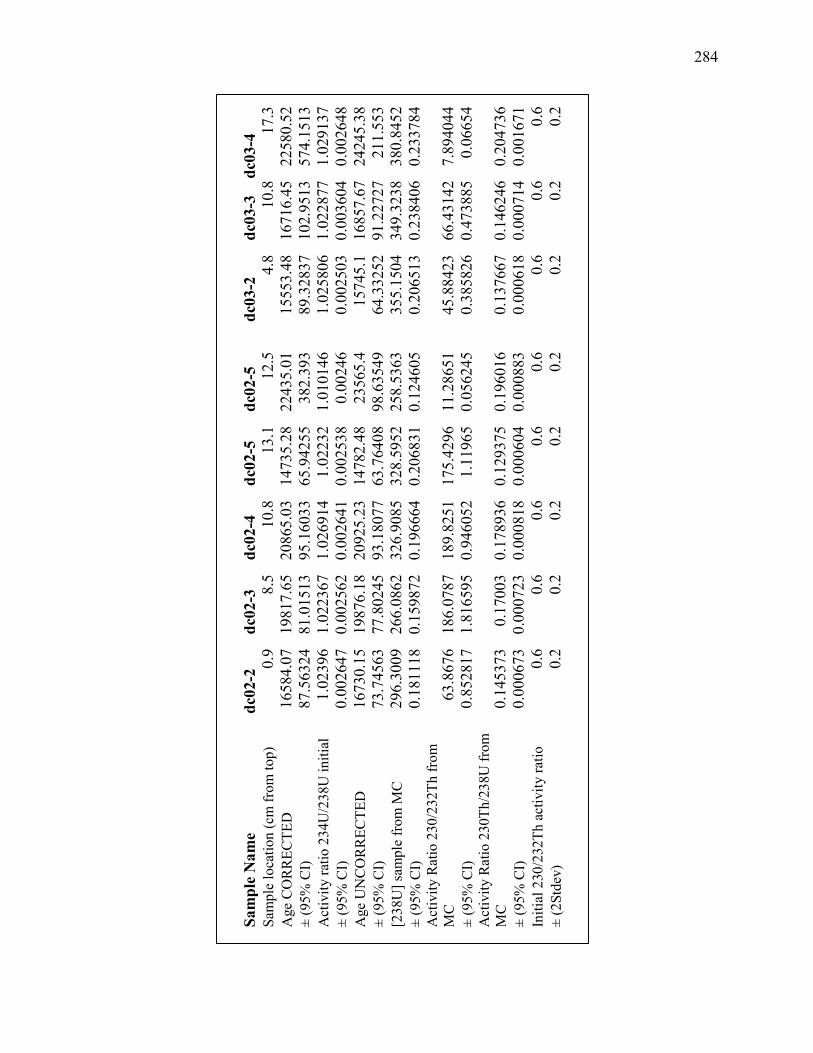
284

Sam

ple

Nam

e dc

02-2

dc

02-3

dc

02-4

dc

02-5

dc

02-5

dc03

-2

dc03

-3

dc03

-4

Sam

ple

loca

tion

(cm

from

top)

0.

9 8.

5 10

.8

13.1

12

.5

4.

8 10

.8

17.3

A

ge C

OR

REC

TED

16

584.

07

1981

7.65

20

865.

03

1473

5.28

22

435.

01

15

553.

48

1671

6.45

22

580.

52

± (9

5% C

I) 87

.563

24

81.0

1513

95

.160

33

65.9

4255

38

2.39

3

89.3

2837

10

2.95

13

574.

1513

A

ctiv

ity ra

tio 2

34U

/238

U in

itial

1.

0239

6 1.

0223

67

1.02

6914

1.

0223

2 1.

0101

46

1.

0258

06

1.02

2877

1.

0291

37

± (9

5% C

I) 0.

0026

47

0.00

2562

0.

0026

41

0.00

2538

0.

0024

6

0.00

2503

0.

0036

04

0.00

2648

A

ge U

NC

OR

REC

TED

16

730.

15

1987

6.18

20

925.

23

1478

2.48

23

565.

4

1574

5.1

1685

7.67

24

245.

38

± (9

5% C

I) 73

.745

63

77.8

0245

93

.180

77

63.7

6408

98

.635

49

64

.332

52

91.2

2727

21

1.55

3 [2

38U

] sam

ple

from

MC

29

6.30

09

266.

0862

32

6.90

85

328.

5952

25

8.53

63

35

5.15

04

349.

3238

38

0.84

52

± (9

5% C

I) 0.

1811

18

0.15

9872

0.

1966

64

0.20

6831

0.

1246

05

0.

2065

13

0.23

8406

0.

2337

84

Act

ivity

Rat

io 2

30/2

32Th

from

M

C

63.8

676

186.

0787

18

9.82

51

175.

4296

11

.286

51

45

.884

23

66.4

3142

7.

8940

44

± (9

5% C

I) 0.

8528

17

1.81

6595

0.

9460

52

1.11

965

0.05

6245

0.38

5826

0.

4738

85

0.06

654

Act

ivity

Rat

io 2

30Th

/238

U fr

om

MC

0.

1453

73

0.17

003

0.17

8936

0.

1293

75

0.19

6016

0.13

7667

0.

1462

46

0.20

4736

±

(95%

CI)

0.00

0673

0.

0007

23

0.00

0818

0.

0006

04

0.00

0883

0.00

0618

0.

0007

14

0.00

1671

In

itial

230

/232

Th a

ctiv

ity ra

tio

0.6

0.6

0.6

0.6

0.6

0.

6 0.

6 0.

6 ±

(2St

dev)

0.

2 0.

2 0.

2 0.

2 0.

2

0.2

0.2

0.2

285

Sam

ple

Nam

e dc

03-5

dc

03-6

dc

03-7

dc

03-1

5cm

dc

05-5

.1

dc05

-0.2

dc

05-4

Sa

mpl

e lo

catio

n (c

m fr

om to

p)

8000

13

.8

17.8

15

5.1

0.2

4.7

Age

CO

RR

ECTE

D

1483

9.13

15

183.

87

1575

6.93

15

452.

26

18

385.

54

1504

1.84

14

823.

38

± (9

5% C

I)

66.5

8032

62

.311

76

68.3

5129

51

.393

98

19

5.29

8 11

2.40

06

97.4

9437

A

ctiv

ity ra

tio 2

34U

/238

U in

itial

1.

0220

48

1.01

155

1.01

9289

1.

0196

7

1.01

3058

1.

0076

36

1.00

489

± (9

5% C

I)

0.00

2439

0.

0025

29

0.00

2397

0.

0025

26

0.

0025

75

0.00

2444

0.

0024

92

Age

UN

CO

RR

ECTE

D

1492

4.66

15

265.

38

1580

4.06

15

477.

86

18

530.

5 15

342.

64

1488

4.52

±

(95%

CI)

60

.603

94

56.6

0762

66

.834

71

51.0

6552

190.

1065

53

.945

89

95.9

7227

[2

38U

] sam

ple

from

MC

56

6.68

57

349.

7033

38

9.32

68

358.

7275

304.

1965

33

5.29

52

298.

7335

±

(95%

CI)

0.

2602

81

0.16

1298

0.

1845

24

0.18

8898

0.18

5268

0.

1586

06

0.15

2538

A

ctiv

ity R

atio

230

/232

Th fr

om

MC

97

.746

25

104.

8963

18

7.00

52

337.

8824

70.7

4647

28

.589

91

136.

5694

±

(95%

CI)

0.

9005

08

1.69

7674

4.

0823

34

3.58

1503

3.43

2085

0.

1780

61

3.14

8813

A

ctiv

ity R

atio

230

Th/2

38U

from

M

C

0.13

0505

0.

1319

41

0.13

7283

0.

1346

96

0.

1580

62

0.13

206

0.12

8034

±

(95%

CI)

0.

0005

8 0.

0005

48

0.00

0634

0.

0005

26

0.

0015

2 0.

0005

29

0.00

0828

In

itial

230

/232

Th a

ctiv

ity ra

tio

0.6

0.6

0.6

0.6

0.

6 0.

6 0.

6 ±

(2St

dev)

0.

2 0.

2 0.

2 0.

2

0.2

0.2

0.2

286

Sa

mpl

e N

ame

dc05

-3

dc05

-3c

m

dc

11-1

dc13

-1

dc

16-1

dc

16-2

dc

16-3

Sa

mpl

e lo

catio

n (c

m fr

om to

p)

3 3

38

.1

16

.2

10

3 6.

03

19.9

A

ge C

OR

REC

TED

21

451

1442

2.72

1404

23.6

5262

9.58

2866

2.97

15

461.

28

1560

4.54

±

(95%

CI)

269.

3009

61

.091

42

13

64.4

22

28

3.78

74

16

1.05

99

.972

8 66

.841

24

Act

ivity

ratio

234

U/2

38U

initi

al

1.02

2201

1.

0087

75

1.

0333

67

1.

0158

55

1.

0075

14

1.00

9554

1.

0037

72

± (9

5% C

I) 0.

0027

3 0.

0024

36

0.

0036

29

0.

0027

86

0.

0026

0.

0025

18

0.00

2476

A

ge U

NC

OR

REC

TED

22

205.

15

1449

5.86

1404

52.7

5266

2.63

2880

1.72

15

483.

95

1563

3.11

±

(95%

CI)

98.8

779

56.3

2941

1365

.363

283.

068

15

4.95

5 99

.723

76

66.4

1775

[2

38U

] sam

ple

from

MC

23

4.23

65

278.

6228

282.

4661

176.

1576

342.

022

352.

6139

43

3.45

49

± (9

5% C

I) 0.

1597

21

0.12

854

0.

1810

81

0.

1077

18

0.

1976

14

0.21

9898

0.

2041

71

Act

ivity

Rat

io 2

30/2

32Th

from

MC

16

.056

89

111.

5517

1614

.365

757.

2033

109.

7123

38

2.00

28

305.

6376

±

(95%

CI)

0.07

9647

0.

5530

53

12

.014

06

16

.785

01

0.

7440

11

3.38

6422

6.

3987

84

Act

ivity

Rat

io 2

30Th

/238

U fr

om

MC

0.

1879

69

0.12

5384

0.74

2803

0.38

8221

0.23

3508

0.

1334

35

0.13

3879

±

(95%

CI)

0.00

0851

0.

0005

51

0.

0036

47

0.

0017

99

0.

0011

98

0.00

0862

0.

0006

09

Initi

al 2

30/2

32Th

act

ivity

ratio

0.

6 0.

6

0.6

0.

6

0.6

0.6

0.6

± (2

Stde

v)

0.2

0.2

0.

2

0.2

0.

2 0.

2 0.

2

287

Sa

mpl

e N

ame

dc16

-4

dc16

-5

dc16

-6

dc16

-7

dc16

-8

hb

c02-

1

hbc0

4-1

Sam

ple

loca

tion

(cm

from

top)

40

.2

49.5

60

.5

70.5

84

.2

49

.8

8.

89

Age

CO

RR

ECTE

D

1716

4.62

18

574.

89

1938

6.8

2153

1.17

22

808.

42

54

780.

52

50

180.

07

± (9

5% C

I) 65

.935

36

67.7

4371

77

.810

69

96.4

9976

11

2.16

88

33

6.30

89

77

6.85

64

Act

ivity

ratio

234

U/2

38U

initi

al

1.00

456

1.01

2736

1.

0033

01

1.00

8978

1.

0058

88

1.

0410

21

0.

9708

86

± (9

5% C

I) 0.

0024

41

0.00

2443

0.

0024

41

0.00

2459

0.

0025

01

0.

0029

92

0.

0031

4 A

ge U

NC

OR

REC

TED

17

209.

16

1860

0.82

19

413.

88

2154

8.54

22

923.

22

55

016.

93

52

179.

38

± (9

5% C

I) 64

.553

16

66.8

5597

77

.047

16

96.7

6672

10

6.84

39

32

5.52

47

39

5.88

04

[238

U] s

ampl

e fr

om M

C

374.

9951

45

2.49

62

302.

9372

36

7.66

34

322.

7952

63.6

7839

27.6

1215

±

(95%

CI)

0.16

9057

0.

2183

38

0.13

8883

0.

1717

35

0.15

092

0.

0394

01

0.

0187

84

Act

ivity

Rat

io 2

30/2

32Th

from

MC

21

4.30

73

395.

5017

39

4.35

62

675.

7478

10

8.28

16

10

9.36

89

12

.598

42

± (9

5% C

I) 2.

2924

12

11.0

3496

14

.405

63

20.7

4765

1.

0955

14

0.

6392

81

0.

0861

71

Act

ivity

Rat

io 2

30Th

/238

U fr

om M

C

0.14

6453

0.

1585

64

0.16

3407

0.

1806

41

0.19

0431

0.41

0733

0.36

9597

±

(95%

CI)

0.00

0625

0.

0006

37

0.00

0716

0.

0008

39

0.00

0904

0.00

2066

0.00

2265

In

itial

230

/232

Th a

ctiv

ity ra

tio

0.6

0.6

0.6

0.6

0.6

0.

6

0.6

± (2

Stde

v)

0.2

0.2

0.2

0.2

0.2

0.

2

0.2

288

Sam

ple

Nam

e hi

w01

-1

rc

01-1

rc02

-1

rc

05-1

kb03

-1

kb

04-1

Sam

ple

loca

tion

(cm

from

top)

2.

5

13.7

5

22.4

79

21

.6

4.

2

Age

CO

RR

ECTE

D

4495

5.4

14

319.

98

58

682.

2

3431

4.25

1465

2.3

15

090.

69

±

(95%

CI)

373.

4271

179.

2481

412.

8213

371.

1514

72.3

4122

104.

509

A

ctiv

ity ra

tio 2

34U

/238

U in

itial

1.

0211

01

1.

0820

48

1.

0182

26

1.

0749

31

1.

0331

98

1.

0411

12

±

(95%

CI)

0.00

2774

0.00

271

0.

0028

47

0.

0029

52

0.

0033

77

0.

0026

17

A

ge U

NC

OR

REC

TED

45

548.

43

14

358.

56

58

855.

54

34

371.

68

14

733.

35

15

239.

26

±

(95%

CI)

323.

9113

177.

9126

408.

4609

370.

6424

66.5

0342

91.0

3338

[238

U] s

ampl

e fr

om M

C

374.

3235

211.

6801

114.

7779

135.

4045

367.

6253

391.

9998

± (9

5% C

I) 0.

2427

45

0.

1314

58

0.

0711

01

0.

0818

26

0.

2507

89

0.

2540

2

Act

ivity

Rat

io 2

30/2

32Th

from

M

C

37.6

8319

209.

1717

157.

3033

307.

124

10

2.26

26

57

.505

37

±

(95%

CI)

0.24

9085

2.93

612

1.

7607

54

4.

6509

39

0.

4982

1

0.36

3664

Act

ivity

Rat

io 2

30Th

/238

U fr

om

MC

0.

3477

97

0.

1331

17

0.

4236

04

0.

2892

7

0.13

0319

0.13

5494

± (9

5% C

I) 0.

0021

19

0.

0015

83

0.

0023

74

0.

0027

1

0.00

0562

0.00

0814

Initi

al 2

30/2

32Th

act

ivity

ratio

0.

6

0.6

0.

6

0.6

0.

6

0.6

±

(2St

dev)

0.

2

0.2

0.

2

0.2

0.

2

0.2

APPENDIX B

The Miami Device

Provided in Appendix B is an overview of the water standards used for calibration

of the Miami Device and the various alternative designs which were tested for the Miami

Device. The final design of the Miami Device is similar to the design of the Picarro

vaporizer unit; therefore we compared results of the Miami Device to results from the

Picarro vaporizer unit. Finally, we have provided data which demonstrates the long term

stability of a sample introduced through the Miami Device. We allowed a sample to be

continually measured for 700 seconds to demonstrate variability in the water

concentration and oxygen and hydrogen isotopes over time.

Water Standards

In order to correct to VSMOW scale, four standard waters were analyzed which

have been previously calibrated to the VSMOW-GISP-SLAP scale. For the 100 cm3

volume, 0.5 μL of each water standard was injected twice at the beginning of each day

(Supplementary Table 1). Supplementary table 1 demonstrates the average for each

standard over a period of approximately a month. Also shown is the oxygen and

hydrogen isotope value after correction to VSMOW scale. The average external standard

deviation for the injections was ±0.4‰ for δ18O and ±1.1‰ for δ2H.

Design of the Miami Device

In the development of the Miami Device, a series of alternative designs were

tested (Figure B.1). The original design is primarily based on the design of the

Amsterdam Device (Vonhof et al., 2006) with a cold trap to freeze out the water (Figure

289

290

B.1a) rather than the final design which does not utilize a trap, but instead a large volume

reservoir. However, issues were encountered when utilizing a water trap.

For the original design of the Miami Device (Figure B.1a), the method for sample

extraction included freezing the water into the trap utilizing either liquid nitrogen or a

methanol /liquid nitrogen trap (temperature at -70 to -90 °C). The water was allowed to

freeze for on average 5 minutes after injection or crush to ensure all of the water froze

down while the nitrogen carrier gas was flowing to the L2130-i Picarro. After 5 minutes,

valve 4 and 5 were closed and the trap was heated for 5 minutes, at which point valve 5 is

opened and the water was released to the Picarro CRDS instrument for analysis (Figure

B.1a). We conducted tests at various time intervals (2 to 10 minutes) for both freezing

and heating and found similar results.

The set up in supplementary figure 1a was not utilized because (1) the system had

large blanks which we believed resulted from freezing water which was in the carrier gas,

(2) the CRDS instrument experienced large pressure increases which we believe is the

result of the condensation of N2 when liquid nitrogen was used. In order to reduce the

blank, we inserted a water trap before valve 1 to trap any water from the carrier gas

(Figure B.1 b), but this was not found to make any significant difference. The large

pressure increases resulted in inconsistent data because the CRDS cavity is sensitive to

pressure changes. To reduce the pressure effect, we increased the volume of the line

between the cold trap and the Picarro by utilizing 3/8” outer diameter tubing to reduce the

pressure to the Picarro, (Figure B.1 c) however this did not significantly reduce the

pressure and the resulting oxygen and hydrogen isotope values were unstable, as shown

in Figure B.2.

291

As stated in the text, the final design was based on aspects of the Amsterdam

Device and the Picarro vaporizer unit. The implementation of the volume reservoir

reduced the pressure effects and eliminated the blank issues, as observed with the original

designs. Figure B.3 compares data between the vaporizer introductory system and the

Miami Device. The resulting oxygen and hydrogen isotope values and water

concentration from the Miami Device and the Picarro vaporizer unit demonstrate minimal

difference between the two introductory systems. The change in the water concentration,

δ18O and δ2H values over 300 seconds is similar for both introductory systems. This

system works well because all of the water from the injection or crush is transferred to

the reservoir and the reservoir provides a stable signal to the instrument for analysis.

Sample variation with time

When averaging data, data was averaged 2 minutes after the crushed or injected

sample was introduced, up to 1 minute before the sample was flushed away, as described

in the text. Tests were conducted to determine how the water concentration, δ18O and

δ2H values change over time. To conduct this test, the sample was expanded into the

volume reservoir and the sample was pumped away after 700 seconds. Figure B.4

demonstrates the resulting oxygen and hydrogen isotopes as well as water concentration

over 700 seconds. Table B.2 demonstrates the change in oxygen and hydrogen isotope

values and water concentration over various integration periods, demonstrating minimal

difference between integrating over 250 seconds compared with 650 seconds. This

validates the stability of the system when conducting measurements.

292

Table B.1: Reproducibility test for 4 standard waters utilizing the 100 cm3 volume. Each standard was injected (0.5 μL) twice per day and the average of the two injections is shown. The average δ18O and δ2H data have not been corrected to VSMOW. Also shown is the average corrected to VSMOW and the reported value for the standard.

Date analyzed Standard water δ18O (‰)

δ2H (‰)

1/18/2013 LS4 -1.4 -12.6 1/21/2013 LS4 -0.5 -13.2 1/22/2013 LS4 -0.7 -11.6 1/24/2013 LS4 -1.5 -14.2 1/28/2013 LS4 -1.8 -14.5 1/30/2013 LS4 -1.6 -16.3 1/31/2013 LS4 -1.7 -14.8 2/10/2013 LS4 -1.4 -12.4 2/14/2013 LS4 -2.0 -14.5

Average -1.4 -13.8

Standard deviation 0.5 1.4

Average Corrected to VSMOW -2.9 -19.2

Reported Value -2.9 -16.0

1/18/2013 LS 0.4 -1.8 1/21/2013 LS 0.9 -1.1 1/22/2013 LS 0.6 -1.3 1/24/2013 LS 0.1 -2.4 1/28/2013 LS 0.2 -1.7 1/30/2013 LS 0.3 -0.7 1/31/2013 LS 0.4 -2.1 2/4/2013 LS 0.3 -1.9 2/10/2013 LS 0.0 -1.4

Average 0.3 -1.6

Standard deviation 0.3 0.5

Average Corrected to VSMOW -1.1 -4.0

Reported Value -1.1 -5.3

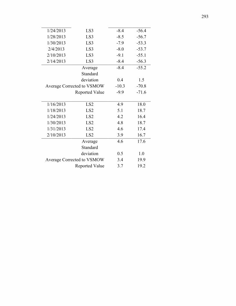
293

1/24/2013 LS3 -8.4 -56.4 1/28/2013 LS3 -8.5 -56.7 1/30/2013 LS3 -7.9 -53.3 2/4/2013 LS3 -8.0 -53.7 2/10/2013 LS3 -9.1 -55.1 2/14/2013 LS3 -8.4 -56.3

Average -8.4 -55.2

Standard deviation 0.4 1.5

Average Corrected to VSMOW -10.3 -70.8

Reported Value -9.9 -71.6

1/16/2013 LS2 4.9 18.0 1/18/2013 LS2 5.1 18.7 1/24/2013 LS2 4.2 16.4 1/30/2013 LS2 4.8 18.7 1/31/2013 LS2 4.6 17.4 2/10/2013 LS2 3.9 16.7

Average 4.6 17.6

Standard deviation 0.5 1.0

Average Corrected to VSMOW 3.4 19.9

Reported Value 3.7 19.2

294

Figure B.1 (following page): Various alternative designs of the Miami Device. a) Schematic of original extraction line design with a cold trap to freeze out water rather than the current design which implements the volume reservoir. The sample method was the same, with the exception that the water was frozen in the trap utilizing either liquid nitrogen or a methanol /liquid nitrogen trap (temperature at -70 to -90 °C). The water was allowed to freeze for on average 5 minutes after injection to ensure all of the water froze down while nitrogen carrier gas was flowing to the Picarro. After 5 minutes, valve 4 and 5 were closed and the trap was heated for another 5 minutes, at which point valve 5 was opened. b) The second design implemented a cold trap prior to valve one in order to eliminate any water in the carrier gas. c) The volume of the line between the cold trap and the Picarro CRDS instrument was increased by utilizing 3/8” outer diameter tubing to reduce the pressure reaching the Picarro, however this did not significantly reduce the pressure to the CRDS instrument.

295

296

Figure B.2: Results for a standard water injection utilizing the set up depicted in Figure B.1c a) Oxygen and hydrogen isotope values (machine scale) for an injection with the resulting water concentration. b) Close up of the water concentration, δ18O and δ2H data from the dashed square in a. The sharp decline in water concentration from 200 to 400 seconds is due to the large pulse of water from the trap and the decline in the δ2H signal and the increase in the δ18O signal is also due to the pulse of water coming off of the trap.

297

Figure B.3: Comparison between the resultant ppm of H2O, δ18O and δ2H values (machine scale) using a) the Miami Device and b) the Picarro vaporizer unit. There is minimal difference between the two. For a 300 second integration (represented by the dashed rectangles), there was a maximum rise in the water concentration in (a) of approximately 1,600 ppm, while for the data acquired using the vaporizer unit (b) the rise is about 1,400 ppm. For oxygen isotopes the standard deviation of δ18O values over 300 seconds was 0.3 ‰ for both the Miami Device (a) and the vaporizer unit (b). For δ2H the standard deviation over 300 seconds was 0.9 ‰ for both introductory systems.

298

Figure B.4: The resultant ppm H2O, δ18O and δ2H values (machine scale) over 700 seconds. The dashed rectangles represent the data which were averaged in supplementary table 2.

299

Table B.2: Average ppm H2O, δ18O and δ2H values (machine scale) from supplementary figure 4 over different time intervals (represented in supplementary figure 4 by the rectangles). There is minimal difference between 250 second integration compared with integration over 650 seconds for δ18O values with higher variability for δ2H results.

ppm H2O δ18O (‰) δ2H (‰) Average over 250 seconds 10758.7 -7.6 -49.6

SD over 250 seconds 473.9 0.3 1.4

Average over 350 seconds 11079.3 -7.5 -48.9 SD over 350 seconds 652.6 0.3 1.7

Average over 450 seconds 11346.3 -7.5 -48.4 SD over 450 seconds 763.9 0.3 1.9

Average over 550 seconds 11558.0 -7.5 -47.9 SD over 550 seconds 824.8 0.3 2.1

Average over 650 seconds 11725.8 -7.5 -47.4 SD over 650 seconds 855.1 0.3 2.3

Average 11293.6 -7.5 -48.4 SD 384.6 0.0 0.9

APPENDIX C

Overview of the U-Th dating mechanisms for sample AB-DC-09

Provided in the supplementary material is an overview of results from the modern

samples collected from Eleuthera, Bahamas which were used to calculate initial,

unsupported (230Th/232Th) ratio. The modern samples were also analyzed for oxygen

isotopes and were utilized to demonstrate that minimal kinetic fractionation occurs in the

modern. Also provided is an overview of some of the potential sources of error in the

development of the age model for sample AB-DC-09.

Modern samples: Determination of initial (230Th/232Th) ratio from modern (zero age)

cave calcites

To determine the initial (230Th/232Th) ratio, modern calcite was collected from a

cave with actively forming stalagmites in Eleuthera, Bahamas (Figure 1). Modern cave

deposits were collected by placing standard glass microscope slides on top of currently

forming stalagmites similar to the methods of Tremaine et al. (2011) and Banner et al.

(2007). The slides were left in the cave for 3-5 months, then brought back to the

laboratory and dried at 40 °C for 24 hours. The calcite was scraped off the slides, and

145-185 mg of calcite was weighed and dissolved for U-Th separation using the methods

presented in the text and outlined in Pourmand et al. (2014). The samples were spiked

prior to analysis in the Neptune Isotope Laboratory of the University of Miami - RSMAS

utilizing a ThermoFisher-Neptune Plus multi-collection ICP-MS to determine Th

concentrations. Considering that these are modern precipitates, the entire 230 Th

contribution (after spike correction) can be attributed to unsupported Th from the

300

301

epikarst, rather than the decay of uranium equilibrium series. Therefore, the mass-bias

corrected 230Th/232Th ratio in these modern samples can be used to calculate the

unsupported (detrital) activity ratio by assuming a zero-age for these samples

(Supplementary Table 1).

Determination of the initial (230Th/232Th) ratio

As described in the text, the sample ages were corrected for contribution of initial,

unsupported 230Th using an initial (230Th/232Th) ratio of 3.7 ±0.6. This initial

(230Th/232Th) ratio falls in the range of values for the Bahamas, and additionally results

in good agreement with previously published records. Provided below is an assessment of

potential sources of error to the age model for sample AB-DC-09.

We have chosen to utilize a single (230Th/232Th) ratio for the propagation of ages for

the sample, which is a reasonable assumption given that this ratio cannot be realistically

determined for every interval at which an age determination was made. Nevertheless we

acknowledge the possibility that the detrital activity ratio may have changed with time.

Two of the ages located ~5 cm from the top resulted in age reversals. These ages were

younger than the previous ages. This is thought be due to a reduction in the initial

230Th/232Th component during this time period, leading to ages which appear to be

younger. This is demonstrated in supplementary figure 1. If the age model is propagated

with a much greater (230Th/232Th) ratio, the older ages become younger, resulting in a

significant age reversal. Here we utilize an activity ratio of 7.8±0.6 to demonstrate this

(supplementary figure 1). No reversal is observed when the ages are propagated with

lower activity ratios. We conclude that the two samples located ~5 cm from the top are

younger than would be expected due to a reduced initial (230Th/232Th) ratio at this

302

period. Considering the disagreement between these two ages and the surrounding ages,

we do not consider these ages as part of the age model. Similarly, one U-Th age at 11 cm

from the top was older than the previous ages, possibly suggesting an increased the initial

230Th/232Th component at this time period as shown in supplementary figure 2.

Supplementary figure 2 demonstrates that with increasing 230Th/232Th activity ratio,

propagated ages become younger. Considering the good agreement between surrounding

ages, we discount this age and do not include it in the final age model.

We further assess the contribution of variable initial, unsupported 230Th by a sensitivity

test whereby the resultant age models propagated at various initial (230Th/232Th) ratios.

Supplementary figure 2 demonstrates the carbon isotopic record with varying initial Th

activity ratios (0.6, 2.2, 3.4 and 3.7) to demonstrate the effect of the initial Th values on

the age model and the timing of the isotopic shifts. As is demonstrated in supplementary

figure 2, when propagated at a higher activity ratio, the oldest ages become younger.

This causes the timing of Heinrich stadial 3 to become unreasonable younger in

comparison to other records from the region. However, we would like to note that the

timing of the isotopic shifts for Heinrich stadial 1 and 2 do not significantly change when

propagating at 2.2 or 3.7 (supplementary Table 2). Therefore the initial value chosen

most significantly impacts the timing of Heinrich stadial 3, but neither the younger two

events.

Modern samples: Oxygen isotopes

Not only was the modern calcite analyzed for Th concentrations, additionally, the

oxygen isotopes of the drip waters and the calcites were measured. The temperature of

the cave was measured every 2 hours using a HOBO U23 Pro v2 Temperature/Relative

303

Humidity Data Logger from Onset. Predicted δ18Oc values were calculated using the

equation from Tremaine et al. (2011) using the results from the drip water oxygen isotope

measurements (annual average = -4.8 ± 0.05 ‰ VSMOW ) and the temperature

(23.2±0.2 °C). When compared to the measured δ18Oc values, an average offset of 0.3

‰ was found for the location from which these samples were collected from. We

therefore conclude that these samples were precipitated very close to equilibrium. As

cave studies have shown that cave drip water has δ18O values similar to local

precipitation (Yonge et al., 1985).

Table C.1: The results from the analysis of the modern cave deposits from the Bahamas. The samples were collected from an actively forming cave in Eleuthera, Bahamas.

Sample ID Th-232 Th-230 Detrital [Th-230/Th-232]*

ug/g ug/g dpm/dpm

Slide 1 0.2654 2.07E-06 1.46 Slide 3 0.0095 1.35E-07 2.66 Slide 10 0.0117 1.48E-07 2.37

Average 2.16

SD 0.6

*Activity ratios are calculated assuming a zero age

Table C.2: Timing of the isotopic shifts based on various initial Th values as shown in supplementary Figure 2. Results demonstrate that with decreasing initial Th value, ages become older with the timing of Heinrich stadial 3 being impacted the most by changing initial Th value.

Timing of even (ka BP)

Initial Th value HS1 HS2 HS3

3.7 14.9 24.8 30.9 3.4 15 25 31 2.2 16 25.3 34.4 0.6 16.5 25.8 37.8

304

.

Figure C.1: Propagation of the age model with an 230Th/232Th activity ratio of 7, 7.5 and 7.8 ±0.6. This demonstrates the impact on the ages when propagating with a much greater 230Th/232Th activity ratio. With increasing initial, the bottom of the stalagmite yields ages which are younger than those to the top of the stalagmite.

305

Figure C.2: The carbon isotopic record plotted with various initial 230Th/232Th activity ratios. The age models were propagated at 0.6 (black), 2.2 (blue), 3.4 (purple) and 3.7 (green) 230Th/232Th activity ratio. Overall the timing of Heinrich stadial 3 is the most impacted. Note the carbon isotopic record has not undergone the 50 year interpolation as is shown in the main text.

APPENDIX D

Provided in Appendix D is the results from air and water analysis from the HBC

monitoring, followed by a description of the extraction line for the preparation of samples

for clumped isotope analysis, followed by the heated and water equilibrated gas results,

the long term reproducibility of the Carrara marble standard, the results of samples which

were not included in the text of chapter 5 and the data used in the compilation Figure

5.18.

Results from cave monitoring at HBC

Table D.1: A) δ13CCO2 of air results relative to VPDB (‰).

Sample Location δ13C AIR (VPDB)

‰ 6/2/12 HBC outside -9.7 6/2/12 HBC 3rd Level 1 -11.6 6/2/12 HBC 3rd Level 2 -11.3 6/2/12 HBC west room -12.2 6/4/12 HBC 1 Level -11.9 6/4/12 HBC 2 Level -1 -11.1 6/4/12 HBC 2 Level -2 -10.7 6/4/12 HBC 3 Level -15.9 6/4/12 HBC WEST ROOM -15.4 8/21/12 Outside -8.2 8/21/12 Outside -55.8 8/21/12 1st Level -8.9 8/21/12 1st Level -8.0 8/21/12 2nd Level -1 -9.2 8/21/12 2nd Level -1 -8.0 8/21/12 2nd Level-2 -9.1 8/21/12 2nd Level-2 -7.7 8/21/12 3rd Level - -9.2 8/21/12 3rd Level- -7.9 8/21/12 3rd Level West- -11.8 8/21/12 3rd Level West- -9.2

306

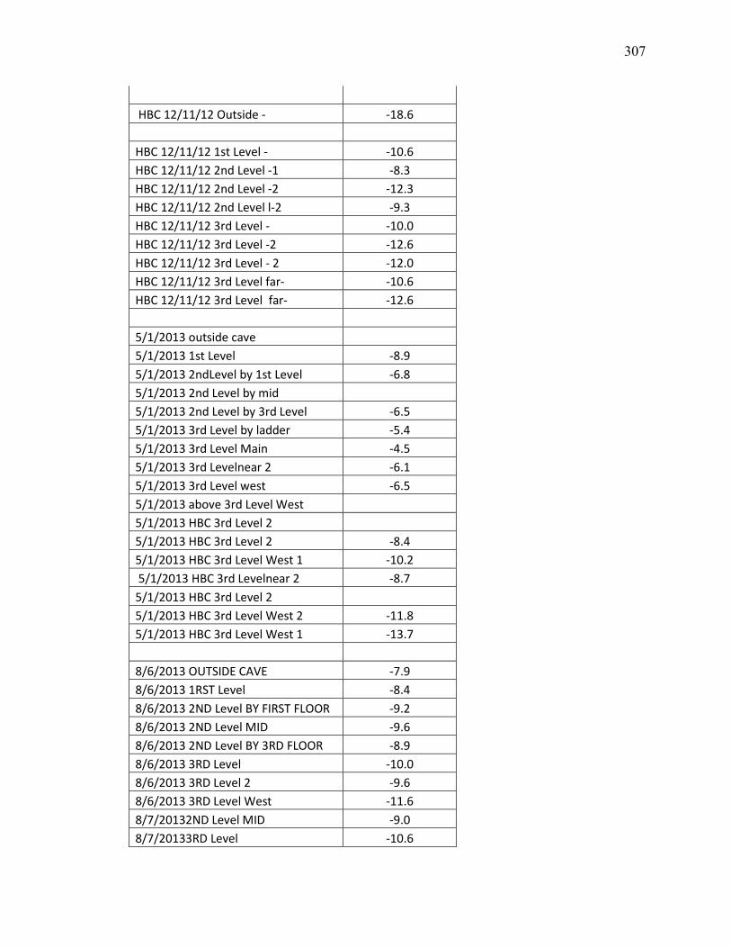
307

HBC 12/11/12 Outside - -18.6 HBC 12/11/12 1st Level - -10.6 HBC 12/11/12 2nd Level -1 -8.3 HBC 12/11/12 2nd Level -2 -12.3 HBC 12/11/12 2nd Level l-2 -9.3 HBC 12/11/12 3rd Level - -10.0 HBC 12/11/12 3rd Level -2 -12.6 HBC 12/11/12 3rd Level - 2 -12.0 HBC 12/11/12 3rd Level far- -10.6 HBC 12/11/12 3rd Level far- -12.6 5/1/2013 outside cave 5/1/2013 1st Level -8.9 5/1/2013 2ndLevel by 1st Level -6.8 5/1/2013 2nd Level by mid 5/1/2013 2nd Level by 3rd Level -6.5 5/1/2013 3rd Level by ladder -5.4 5/1/2013 3rd Level Main -4.5 5/1/2013 3rd Levelnear 2 -6.1 5/1/2013 3rd Level west -6.5 5/1/2013 above 3rd Level West 5/1/2013 HBC 3rd Level 2 5/1/2013 HBC 3rd Level 2 -8.4 5/1/2013 HBC 3rd Level West 1 -10.2 5/1/2013 HBC 3rd Levelnear 2 -8.7 5/1/2013 HBC 3rd Level 2 5/1/2013 HBC 3rd Level West 2 -11.8 5/1/2013 HBC 3rd Level West 1 -13.7 8/6/2013 OUTSIDE CAVE -7.9 8/6/2013 1RST Level -8.4 8/6/2013 2ND Level BY FIRST FLOOR -9.2 8/6/2013 2ND Level MID -9.6 8/6/2013 2ND Level BY 3RD FLOOR -8.9 8/6/2013 3RD Level -10.0 8/6/2013 3RD Level 2 -9.6 8/6/2013 3RD Level West -11.6 8/7/20132ND Level MID -9.0 8/7/20133RD Level -10.6

308

8/7/20133RD Level West -9.1 outside cave 11/21/2013 -9.4 1st Level 11/21/2013 -13.4 1st Level by ladder 11/21/2013 -8.4 2nd Level by 1st 11/21/2013 -7.1 2nd Level mid 1 11/21/2013 -12.6 2nd Level mid 2 11/21/2013 -12.3 2nd Level mid 3 11/21/2013 -13.0 3rd Level by ladder 1 11/21/2013 -8.7 3rd Level ladder 2 11/21/2013 -12.2 3RD Level 11/21/2013 -8.7 3rd Level near mud room 11/21/2013 -9.8 3rd Level West 11/21/2013 -13.3 3rd Level West 2 11/21/2013 -13.8

Table D.1: B) CO2 concentration (ppm) from HBC

Location date [CO2] ppm

outside cave 11/21/2013 517.4949 HBC 12/11/12 Outside 582.5152 8/6/2013 OUTSIDE CAVE 435.2595 outside cave 11/21/2013 517.4949 8/6/2013 OUTSIDE CAVE 435.2595 1st level by ladder 11/21/2013 603.2793 1st level 11/21/2013 677.0985 8/6/2013 1RST level 433.8399 HBC 12/11/12 1st level 381.7503 2nd level by 1st 11/21/2013 176.2839 HBC 12/11/12 2nd Fl-1 level 358.9998 2nd levelmid 1 11/21/2013 658.086 2nd level mid 2 11/21/2013 609.3633 2nd levelmid 3 11/21/2013 578.0814 8/6/2013 2ND level MID 450.2667 8/7/20132ND level MID 436.4763 8/6/2013 2ND FLOOR BY 3RD level 444.7911 8/6/2013 2ND FLOOR BY FIRST level 468.2652 HBC 12/11/12 2nd level-2 355.0949 HBC 12/11/12 2ndlevel 2 441.428

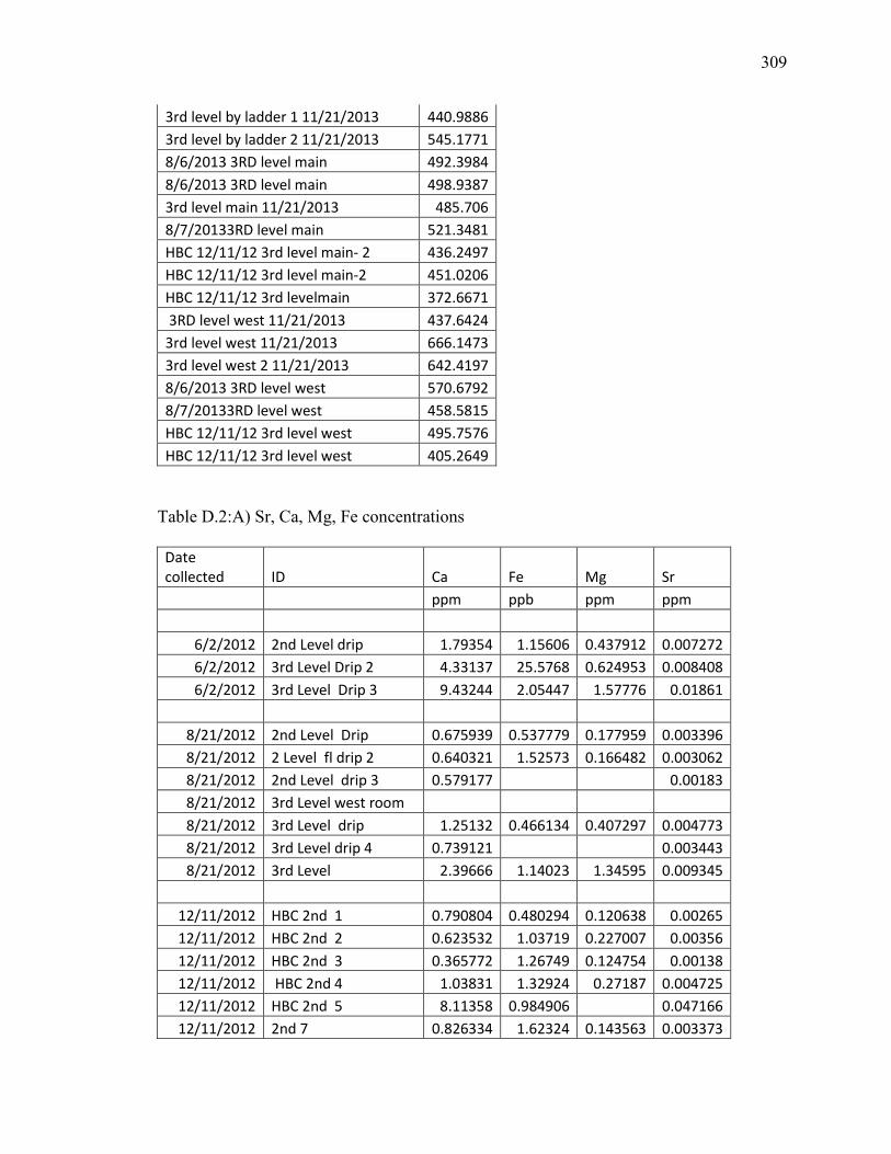
309

3rd level by ladder 1 11/21/2013 440.9886 3rd level by ladder 2 11/21/2013 545.1771 8/6/2013 3RD level main 492.3984 8/6/2013 3RD level main 498.9387 3rd level main 11/21/2013 485.706 8/7/20133RD level main 521.3481 HBC 12/11/12 3rd level main- 2 436.2497 HBC 12/11/12 3rd level main-2 451.0206 HBC 12/11/12 3rd levelmain 372.6671 3RD level west 11/21/2013 437.6424 3rd level west 11/21/2013 666.1473 3rd level west 2 11/21/2013 642.4197 8/6/2013 3RD level west 570.6792 8/7/20133RD level west 458.5815 HBC 12/11/12 3rd level west 495.7576 HBC 12/11/12 3rd level west 405.2649

Table D.2:A) Sr, Ca, Mg, Fe concentrations

Date collected ID Ca Fe Mg Sr ppm ppb ppm ppm

6/2/2012 2nd Level drip 1.79354 1.15606 0.437912 0.007272 6/2/2012 3rd Level Drip 2 4.33137 25.5768 0.624953 0.008408 6/2/2012 3rd Level Drip 3 9.43244 2.05447 1.57776 0.01861

8/21/2012 2nd Level Drip 0.675939 0.537779 0.177959 0.003396 8/21/2012 2 Level fl drip 2 0.640321 1.52573 0.166482 0.003062 8/21/2012 2nd Level drip 3 0.579177 0.00183 8/21/2012 3rd Level west room 8/21/2012 3rd Level drip 1.25132 0.466134 0.407297 0.004773 8/21/2012 3rd Level drip 4 0.739121 0.003443 8/21/2012 3rd Level 2.39666 1.14023 1.34595 0.009345

12/11/2012 HBC 2nd 1 0.790804 0.480294 0.120638 0.00265 12/11/2012 HBC 2nd 2 0.623532 1.03719 0.227007 0.00356 12/11/2012 HBC 2nd 3 0.365772 1.26749 0.124754 0.00138 12/11/2012 HBC 2nd 4 1.03831 1.32924 0.27187 0.004725 12/11/2012 HBC 2nd 5 8.11358 0.984906 0.047166 12/11/2012 2nd 7 0.826334 1.62324 0.143563 0.003373

310

12/11/2012 HBC 3rd Level West 1 2.14704 0.570163 1.25126 0.009628 12/11/2012 HBC 3rd Level West 2 2.44131 1.91824 1.48595 0.011412 12/11/2012 HBC 3rd Level 1 0.60043 1.19141 0.374708 0.004197 12/11/2012 HBC 3rd Level 2 1.57894 0.739818 0.850473 0.007605 12/11/2012 HBC 3rd Level 3 1.73386 3.03546 0.200492 0.003814 12/11/2012 HBC 3rd Level 4 1.7177 4.84415 0.006772

5/1/2013 2nd fl 0.645008 0.222884 0.254392 0.00254 5/1/2013 HBC 3rd Level 1 1.91653 0.351921 1.24336 0.011014 5/1/2013 HBC 3rd Level 2 5/1/2013 3rd fl near stage 8 0.876632 0.300236 0.595703 0.004838 5/1/2013 3rd fl mud room 2.31349 0.84831 1.53962 0.010592 5/1/2013 HBC 3rd Level West 1 2.6086 0.401615 1.58459 0.011985 5/1/2013 HBC 3rd Level West 2 5/1/2013 HBC 3rd Level West 3 2.8401 2.68225 1.62327 0.012399

8/6/2013 HBC 2nd 1 1.16728 17.0356 0.246752 0.004128 8/6/2013 HBC 2nd 2 1.4871 150.746 0.645135 0.008933 8/6/2013 HBC 2nd 3 1.32128 84.6662 0.417187 0.006486 8/6/2013 HBC 2nd 4 1.41932 84.884 0.420204 0.006603 8/6/2013 HBC 2nd 5 1.09314 17.7423 0.254513 0.004554 8/6/2013 HBC 2nd 6 8/6/2013 3rd FL Main 1 2.88088 84.9245 1.8307 0.01552 8/6/2013 3rd FL Main 2 2.44664 167.466 1.47475 0.011345 8/6/2013 3rd FL Main 3 1.93025 162.864 1.04777 0.010311 8/6/2013 3rd FL Main 4 2.60993 3.97104 1.61358 0.013171 8/6/2013 3rd FL Main 5 1.28243 11.8357 0.842939 0.007537 8/6/2013 HBC 3rd Level West 1 3.80283 14.1296 2.09007 0.016632 8/6/2013 HBC 3rd Level West 2 3.58177 14.0606 2.00054 0.015895 8/6/2013 HBC 3rd Level West 3 3.30466 3.25754 1.97489 0.015456 8/6/2013 HBC 3rd Level West 4 3.96447 5.83269 2.18722 0.017427 8/6/2013 HBC 3rd Level West 5 3.82176 14.291 2.07997 0.01664

11/21/2013 2nd fl 1 0.978275 0.129658 0.386143 0.005886 11/21/2013 2nd fl 2 0.747408 0.078609 0.28364 0.003951 11/21/2013 2nd fl 3 2.08551 0.625428 0.692697 0.011902 11/21/2013 2nd fl 4 1.06842 0.286015 0.355851 0.006212 11/21/2013 2nd fl 5 0.744487 0.209525 0.25517 0.004019 11/21/2013 3rd fl Near 1 stage 8 1.69821 1.14286 0.009986 11/21/2013 3rd FL Main 2 0.730079 0.107232 0.402868 0.004744 11/21/2013 3rd FL Main 3 0.915639 0.164336 0.496756 0.006812

311

11/21/2013 3rd FL Main 4 1.5341 0.896502 1.04867 0.0083 11/21/2013 3rd FL Main 5 2.67771 0.341416 2.0865 0.014808 11/21/2013 3rd FL Main 6 1.98214 0.863804 1.36726 0.010517 11/21/2013 3rd FL Main 7 1.8398 0.071312 1.19571 0.0114 11/21/2013 3rd FL Main 8 1.30878 0.768036 0.79296 0.009135 11/21/2013 3rd FL Main 9 2.30306 0.60739 1.47483 0.011908

11/21/2013 3rd fl Main 10 stage 11 2.0881 0.273899 1.24717 0.012244

11/21/2013 3rd fl Main 11 2.68919 0.069551 2.04636 0.014895 11/21/2013 3rd fl Main 12 stage 4 2.32302 0.112393 1.46809 0.011733

11/21/2013 3rd fl Main 13 stage 11 1.65039 0.337736 1.10251 0.008902

11/21/2013 3rd fl Main 15 1.59193 1.64523 1.07211 0.010116 11/21/2013 3rd fl Main 16 4.88354 10.777 2.46993 0.020628 11/21/2013 HBC 3rd Level West 1 2.832395 0.085373 1.812855 0.014263 11/21/2013 HBC 3rd Level West 2 2.966515 0.061276 1.89106 0.014695 11/21/2013 HBC 3rd Level West 3 2.897595 0.290907 1.76002 0.013894 11/21/2013 HBC 3rd Level West 4 3.44612 0.865279 2.11208 0.016501 11/21/2013 HBC 3rd Level West 5 2.53614 0.196662 1.4197 0.01242 11/21/2013 HBC 3rd Level West 6 1.89597 0.943537 1.39023 0.011203 11/21/2013 HBC 3rd Level West 7 3.2012 5.97452 2.01566 0.019889 11/21/2013 HBC 3rd Level West 8 2.89601 0.172938 1.85592 0.014328 11/21/2013 HBC 3rd Level West 8 2.3987 0.549486 1.44568 0.011987

Table D.2:B) Water Sr/Ca, Mg/Ca, δ18O, δ13CDIC from HBC monitoring.

Date collected ID Sr/Ca Mg/Ca δ18O δ2H

δ13C DIC

mM/M mM/M 6/2/2012 2nd Level drip 1.9 407.7 6/2/2012 3rd Level Drip 2 0.9 241.0 1.7 6/2/2012 3rd Level Drip 3 0.9 279.3 -2.9 -19.6 2.6

8/21/2012 2nd Level Drip 2.3 439.7 -1.2 -5.5 -6.8 8/21/2012 2 Level fl drip 2 2.2 434.2 -4.9 -29.9 -6.7 8/21/2012 2nd Level drip 3 1.4 -2.6 -10.2 8/21/2012 3rd Level west room -4.8 -30.3 8/21/2012 3rd Level drip 1.7 543.6 -4.5 -27.2 -7.9 8/21/2012 3rd Level drip 4 2.1 -8.7 8/21/2012 3rd Level 1.8 937.9 -10.0

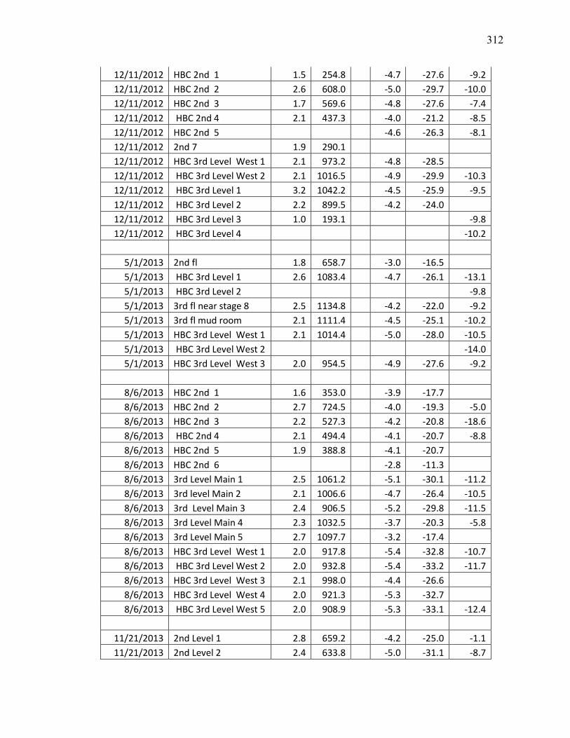
312

12/11/2012 HBC 2nd 1 1.5 254.8 -4.7 -27.6 -9.2 12/11/2012 HBC 2nd 2 2.6 608.0 -5.0 -29.7 -10.0 12/11/2012 HBC 2nd 3 1.7 569.6 -4.8 -27.6 -7.4 12/11/2012 HBC 2nd 4 2.1 437.3 -4.0 -21.2 -8.5 12/11/2012 HBC 2nd 5 -4.6 -26.3 -8.1 12/11/2012 2nd 7 1.9 290.1 12/11/2012 HBC 3rd Level West 1 2.1 973.2 -4.8 -28.5 12/11/2012 HBC 3rd Level West 2 2.1 1016.5 -4.9 -29.9 -10.3 12/11/2012 HBC 3rd Level 1 3.2 1042.2 -4.5 -25.9 -9.5 12/11/2012 HBC 3rd Level 2 2.2 899.5 -4.2 -24.0 12/11/2012 HBC 3rd Level 3 1.0 193.1 -9.8 12/11/2012 HBC 3rd Level 4 -10.2

5/1/2013 2nd fl 1.8 658.7 -3.0 -16.5 5/1/2013 HBC 3rd Level 1 2.6 1083.4 -4.7 -26.1 -13.1 5/1/2013 HBC 3rd Level 2 -9.8 5/1/2013 3rd fl near stage 8 2.5 1134.8 -4.2 -22.0 -9.2 5/1/2013 3rd fl mud room 2.1 1111.4 -4.5 -25.1 -10.2 5/1/2013 HBC 3rd Level West 1 2.1 1014.4 -5.0 -28.0 -10.5 5/1/2013 HBC 3rd Level West 2 -14.0 5/1/2013 HBC 3rd Level West 3 2.0 954.5 -4.9 -27.6 -9.2

8/6/2013 HBC 2nd 1 1.6 353.0 -3.9 -17.7 8/6/2013 HBC 2nd 2 2.7 724.5 -4.0 -19.3 -5.0 8/6/2013 HBC 2nd 3 2.2 527.3 -4.2 -20.8 -18.6 8/6/2013 HBC 2nd 4 2.1 494.4 -4.1 -20.7 -8.8 8/6/2013 HBC 2nd 5 1.9 388.8 -4.1 -20.7 8/6/2013 HBC 2nd 6 -2.8 -11.3 8/6/2013 3rd Level Main 1 2.5 1061.2 -5.1 -30.1 -11.2 8/6/2013 3rd level Main 2 2.1 1006.6 -4.7 -26.4 -10.5 8/6/2013 3rd Level Main 3 2.4 906.5 -5.2 -29.8 -11.5 8/6/2013 3rd Level Main 4 2.3 1032.5 -3.7 -20.3 -5.8 8/6/2013 3rd Level Main 5 2.7 1097.7 -3.2 -17.4 8/6/2013 HBC 3rd Level West 1 2.0 917.8 -5.4 -32.8 -10.7 8/6/2013 HBC 3rd Level West 2 2.0 932.8 -5.4 -33.2 -11.7 8/6/2013 HBC 3rd Level West 3 2.1 998.0 -4.4 -26.6 8/6/2013 HBC 3rd Level West 4 2.0 921.3 -5.3 -32.7 8/6/2013 HBC 3rd Level West 5 2.0 908.9 -5.3 -33.1 -12.4

11/21/2013 2nd Level 1 2.8 659.2 -4.2 -25.0 -1.1 11/21/2013 2nd Level 2 2.4 633.8 -5.0 -31.1 -8.7

313

11/21/2013 2nd Level 3 2.6 554.7 -4.4 -27.4 -7.6 11/21/2013 2nd Level 4 2.7 556.2 -4.1 -22.9 -8.6 11/21/2013 2nd Level 5 2.5 572.4 -3.1 -14.6 -5.9

11/21/2013 3rd Level Near 1 stage 8 2.7 1123.9 -4.5 -27.4 -9.5

11/21/2013 3rd Level Main 2 3.0 921.5 -4.4 -26.1 -9.9 11/21/2013 3rd Level Main 3 3.4 906.0 -8.4 11/21/2013 3rd Level Main 4 2.5 1141.6 -4.2 -24.5 -10.3 11/21/2013 3rd Level Main 5 2.5 1301.3 -4.2 -25.8 -11.3 11/21/2013 3rd Level Main 6 2.4 1151.9 -4.1 -24.4 -10.8 11/21/2013 3rd Level Main 7 2.8 1085.4 -4.2 -24.8 -10.0 11/21/2013 3rd Level Main 8 3.2 1011.8 -4.0 -23.5 -8.0 11/21/2013 3rd Level Main 9 2.4 1069.4 -4.3 -25.6 -10.9

11/21/2013 3rd Level Main 10 stage 11 2.7 997.4 -4.3 -24.9 -11.5

11/21/2013 3rd Level Main 11 2.5 1270.8 -4.1 -25.2 -12.7

11/21/2013 3rd Level Main 12 stage 4 2.3 1055.4 -4.3 -25.9 -10.9

11/21/2013 3rd Level Main 13 stage 11 2.5 1115.6 -4.2 -24.3 -9.9

11/21/2013 3rd Level Main 15 2.9 1124.7 11/21/2013 3rd Level Main 16 1.9 844.6 -8.2 11/21/2013 HBC 3rd Level West 1 2.3 1068.9 -4.5 -29.2 -9.0 11/21/2013 HBC 3rd Level West 2 2.3 1064.6 -4.5 -29.4 -9.0 11/21/2013 HBC 3rd Level West 3 2.2 1014.4 -4.4 -28.8 -8.2 11/21/2013 HBC 3rd Level West 4 2.2 1023.5 -4.4 -27.6 -9.3 11/21/2013 HBC 3rd Level West 5 2.2 934.8 -4.6 -29.6 -10.5 11/21/2013 HBC 3rd Level West 6 2.7 1224.5 -4.6 -29.3 -11.3 11/21/2013 HBC 3rd Level West 7 2.8 1051.5 -4.6 -29.5 -9.2 11/21/2013 HBC 3rd Level West 8 2.3 1070.2 -4.3 -27.8 -8.7 11/21/2013 HBC 3rd Level West 8 2.3 1006.5 -4.5 -29.3 -8.6

Table D.3: Water pH, Alkalinity and Cl- results from HBC monitoring.

Date collected ID pH Alkalinity Cl- Mmoles/L ppm

6/2/2012 2nd Level drip 6/2/2012 3rd Level Drip 2 6/2/2012 3rd Level Drip 3 7.3 1.2

8/21/2012 2nd Level Drip 7.2 0.6

314

8/21/2012 2 Level fl drip 2 8.4 2.8 8/21/2012 2nd Level drip 3 8/21/2012 3rd Level west room 8.2 5.1 8/21/2012 3rd Level drip 8.3 6.0 8/21/2012 3rd Level drip 4 8/21/2012 3rd Level

12/11/2012 HBC 2nd 1 7.8 3.9 542.6293 12/11/2012 HBC 2nd 2 8.2 4.6 546.2212 12/11/2012 HBC 2nd 3 12/11/2012 HBC 2nd 4 12/11/2012 HBC 2nd 5 12/11/2012 2nd 7 12/11/2012 HBC 3rd Level West 1 7.8 4.3 12/11/2012 HBC 3rd Level West 2 3.3 2048.887 12/11/2012 HBC 3rd Level 1 813.006 12/11/2012 HBC 3rd Level 2 12/11/2012 HBC 3rd Level 3 12/11/2012 HBC 3rd Level 4

5/1/2013 2nd fl 5/1/2013 HBC 3rd Level 1 8.2 4.9 2755.056 5/1/2013 HBC 3rd Level 2 813.006 5/1/2013 3rd Level near stage 8 7.9 4.7 1767.785 5/1/2013 3rd Level mud room 5/1/2013 HBC 3rd Level West 1 8.1 3.7 5/1/2013 HBC 3rd Level West 2 5/1/2013 HBC 3rd Level West 3

8/6/2013 HBC 2nd 1 8.1 5.5 470.0044 8/6/2013 HBC 2nd 2 7.3 2.2 8/6/2013 HBC 2nd 3 6.8 4.2 8/6/2013 HBC 2nd 4 7.9 5.3 8/6/2013 HBC 2nd 5 7.8 4.7 8/6/2013 HBC 2nd 6 8/6/2013 3rd Level Main 1 7.9 4.1 2811.369 8/6/2013 3rd Level Main 2 8.0 5.5 2148.309 8/6/2013 3rd Level Main 3 8.0 5.3 8/6/2013 3rd Level Main 4 7.8 3.1 8/6/2013 3rd Level Main 5 8/6/2013 HBC 3rd Level West 1 7.6 3.7 3055.505

315

8/6/2013 HBC 3rd Level West 2 7.8 3.5 3036.815 8/6/2013 HBC 3rd Level West 3 7.8 1.9 8/6/2013 HBC 3rd Level West 4 8.3 3.7 8/6/2013 HBC 3rd Level West 5 7.8 4.0 3074.442

11/21/2013 2nd Level 1 7.9 4.7 634.4709 11/21/2013 2nd Level l 2 8.3 2.2 376.0226 11/21/2013 2nd Level 3 8.0 1.9 594.3647 11/21/2013 2nd Level 4 607.627 11/21/2013 2nd Level 5

11/21/2013 3rd Level Near 1 stage 8 8.1 4.0 1608.824

11/21/2013 3rd Level Main 2 7.9 3.6 743.383 11/21/2013 3rd Level Main 3 7.7 2.9 1107.954 11/21/2013 3rd Level Main 4 8.4 4.7 1777.778 11/21/2013 3rd Level Main 5 8.4 5.5 3227.354 11/21/2013 3rd Level Main 6 8.4 4.0 2051.573 11/21/2013 3rd Level Main 7 8.2 2.5 1949.731 11/21/2013 3rd Level Main 8 7.9 3.7 11/21/2013 3rd Level Main 9 2377.915

11/21/2013 3rd Level Main 10 stage 11 2266.227

11/21/2013 3rd Level l Main 11 3333.38

11/21/2013 3rd Level Main 12 stage 4 2396.019

11/21/2013 3rd Level Main 13 stage 11

11/21/2013 3rd Level Main 15 11/21/2013 3rd Level Main 16 11/21/2013 HBC 3rd Level West 1 7.8 4.4 2936.728 11/21/2013 HBC 3rd Level West 2 7.5 4.3 3377.554 11/21/2013 HBC 3rd Level West 3 8.0 2.8 2955.777 11/21/2013 HBC 3rd Level West 4 7.5 4.6 2872.603 11/21/2013 HBC 3rd Level West 5 8.4 3.8 11/21/2013 HBC 3rd Level West 6 1938.66 11/21/2013 HBC 3rd Level West 7 8.3 3.8 11/21/2013 HBC 3rd Level West 8 2814.758 11/21/2013 HBC 3rd Level West 8

Table D.4: Slides Sr/Ca, Mg/Ca, Fe/Ca and Sr/Mg ratios and δ13C and δ18O of the carbonate.

Slide # Location Sr/Ca Mg/Ca Fe/Ca Sr/Mg δ13C δ18O

316

mM/M mM/M uM/M ‰ VPDB

‰ VPDB

3 East Main 0.37 28.85 135.39 0.01 -8.90 -4.23 4 Main 0.33 35.27 511.23 0.01 -10.27 -4.90 6 West 0.26 21.58 170.00 0.01 -10.94 -5.19 8 Main 0.42 41.75 56.72 0.01 -7.31 -3.34 9 Main 0.46 39.83 1076.43 0.01 -8.41 -3.85

10 East Main 0.50 29.40 2143.00 0.02 -11.33 -5.38 11 West 0.30 24.78 43.32 0.01 -11.08 -5.32 12 Main 0.44 43.73 2849.45 0.01 -6.00 -3.05 13 East Main 0.43 30.12 124.90 0.01 -7.89 -3.95 14 West 0.28 22.40 263.97 0.01 -10.99 -5.10 15 Main 0.53 33.91 1475.53 0.02 -10.04 -4.39 16 Main 0.48 35.63 86.59 0.01 -9.25 -3.97 17 East Main 0.41 29.85 -98.97 0.01 -8.67 -4.24 18 West 0.29 24.88 129.64 0.01 -10.00 -4.62 19 Main 0.57 32.78 4563.94 0.02 -10.17 -4.32 20 Main 0.51 37.06 2234.61 0.01 -8.58 -3.72 21 East Main 0.37 27.17 86.06 0.01 -10.31 -5.07 22 West 0.27 22.37 69.11 0.01 -11.50 -5.49

Table D.5: XRD results for select slides from HBC. Results are shown with the slide number and the location of peaks within the results. The results are followed by photos. Slide #9 Pos. [°2Th.] Area [cts*°2Th.] Id 23.2248 2.15 2ndary 29.5964 22.82 LMC

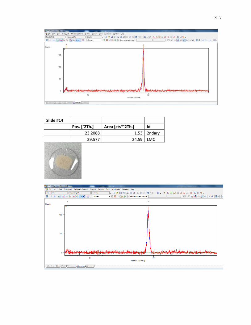
317

Slide #14 Pos. [°2Th.] Area [cts*°2Th.] Id 23.2088 1.53 2ndary 29.577 24.59 LMC

318

Slide #15

Pos. [°2Th.]

Area [cts*°2Th.] Id

23.1562 1.68 2ndary 29.5434 20.19 LMC

Slide #17 Pos. [°2Th.] Area [cts*°2Th.] Id 23.1373 1.6 2ndary 29.5274 26.23 LMC 31.5986 1.07 2ndary

319

Slide #10 Pos. [°2Th.] Area [cts*°2Th.] Id 23.1643 5.63 calcite 2ndary 29.515 105.65 LMC 36.1006 8.76 calcite 2ndary 39.5603 17.55 calcite 2ndary 43.3294 13.42 calcite 2ndary 47.2664 8.99 flourite? 47.6624 22.83 calcite 2ndary 48.6793 20.13 calcite 2ndary 56.7574 3.77 Halite ? 57.5871 11.54 calcite 2ndary 60.8741 7.04 Talc ? 64.8929 7.6 Mica ?

320

Slide #18

Pos. [°2Th.]

Area [cts*°2Th.] Id

23.1821 3.92 2ndary 29.5135 61.22 LMC 31.5666 3.23 2ndary 36.1252 12.88 2ndary 39.562 13.84 2ndary 43.3447 22.24 2ndary 47.32 3.94 flourite? 47.7157 15.77 2ndary 48.7051 17.64 2ndary 56.7735 2.14 Halite ? 57.6387 9.25 2ndary 60.9233 4.32 Talc ? 64.9344 4.89 Mica ? 65.9095 4.24 ?

321

Slide #19

Pos. [°2Th.]

Area [cts*°2Th.] Id

23.2412 3.61 2ndary 29.5588 89.27 LMC 36.1839 17.57 2ndary 39.6328 14.27 2ndary 43.4364 6.45 2ndary 47.4034 4.57 flourite? 47.6959 20.56 2ndary 48.7653 12.03 2ndary 56.868 4.73 Halite ? 60.98 4.09 Talc ? 64.9943 4.95 Mica ? 65.935 3.26 ?

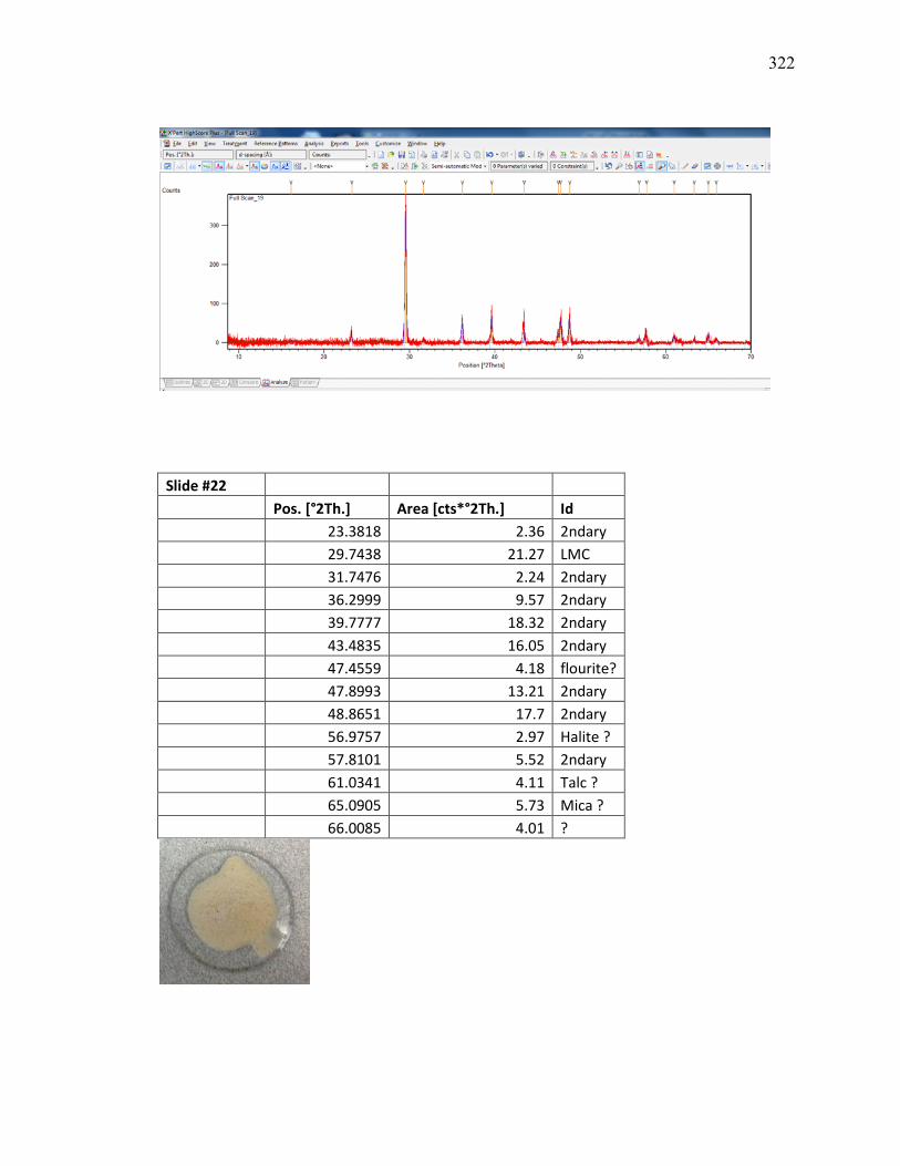
322

Slide #22 Pos. [°2Th.] Area [cts*°2Th.] Id 23.3818 2.36 2ndary 29.7438 21.27 LMC 31.7476 2.24 2ndary 36.2999 9.57 2ndary 39.7777 18.32 2ndary 43.4835 16.05 2ndary 47.4559 4.18 flourite? 47.8993 13.21 2ndary 48.8651 17.7 2ndary 56.9757 2.97 Halite ? 57.8101 5.52 2ndary 61.0341 4.11 Talc ? 65.0905 5.73 Mica ? 66.0085 4.01 ?

323

Sample preparation for clumped isotopes

Below follows an outline of sampling for clumped isotopes. Samples for clumped

isotopes are reacted in the modified Fairbanks device using the common acid bath

method (Figure D.1). The samples are cryogenically frozen in the first trap during

reaction, which takes approximately 30 minutes. Sample in trap one is then heated

between -90 to -70 ºC using a methanol/liquid nitrogen slush. The amount of CO2 gas

which is released is monitored on a capacitance manometer (MKS 220). The CO2 is then

frozen into trap two, using liquid nitrogen. The remaining non-condensables are removed

using a turbo molecular pump using the methanol slush to protect the sample CO2 gas.

The sample is then sealed off from the turbo molecular pump and the liquid nitrogen is

removed to release the CO2 gas. The sample is transferred to trap three via the Porapak

(Type Q 50-80 mesh packing material). The Porapak is held between -30 to -20 ºC, and

this transfer takes approximately 45 minutes. While the sample is being transferred

through the Porapak, trap 1 is heated and evacuated. Once ~99.99% of all CO2 has

transferred through the Porapak, the sample is sealed off from the Porapak and again a

methanol trap replaces the liquid nitrogen on trap three. The sample is then transferred to

324

the cold finger, and again the CO2 pressure is measured on a capacitance manometer to

ensure proper sample yield. The CO2 gas is then transferred to a sample vial using liquid

nitrogen, the CO2 gas is sealed and transferred to the MAT 253. Upon completion of a

sample, the entire line is pumped to background pressure using the Penning gauge to

monitor the pressure. The line and Porapak are heated to 200 ºC using insulated nichrome

wire for at least 30 minutes. Additionally provided throughout the line are a suite of

thermocouple gauges to monitor the movement of CO2 throughout the entire system.

Water equilibrated and heated gases preparation

Water equilibrated and heated gases are composed of three CO2 gases, with a

suite of δ13C and δ18O values. These gases are stored in sealed bulbs (2000 cm3) at

atmospheric pressure attached to the extraction line (Figure D.1). All gases were

precleaned through a H2O removal trap and all non-condensable gases were evacuated.

For the water equilibrated gases, 500 μL of in house ultrapure water was frozen

into a Pyrex tube and evacuated using the extraction line. The water was heated and

frozen several times to ensure no residual CO2 was in the Pyrex tube. An aliquot of the

tank gas was then frozen into the evacuated Pyrex tube. The tube was sealed and placed

in either a 25.0°C ± 1.0°C or 50.0°C ± 1.0°C, temperature controlled, water bath for at

least 120 hours. The tubes were then removed from the baths, the water was frozen using

a methanol slush held at -90 to -70 °C. Prior to breaking the tube, the tube was evacuated

and then broken to release the equilibrated CO2. The CO2 gas was then purified using the

methods outlined above for a sample and then analyzed on the MAT-253.

The heated gases also utilize the same CO2 tank gases as the water equilibrated

gases. However, the CO2 is purified first, using the same method as for the samples.

325

Contrary to the samples, the CO2 for the heated gases are frozen into a quartz tube and

flame sealed. This is followed by heating at 1000 °C in the furnace for over two hours.

The tube is quenched and transferred to the MAT-253 mass spectrometer where the tube

is cracked and the gas released into the IRMS.

Figure D.1: Extraction line for sample preparation. The line is made up of 3/8” o.d. stainless steel tubing, with the exception of the area between trap 2, the modified Fairbanks device and the high vacuum which is comprised of 1/4” o.d. stainless steel tubing. All valves are Swagelok valves (SS-6BK) which are able to be heated. Evacuation from atmosphere is through a dedicated roughing line (Edwards E2M2). Samples are loaded into the modified Fairbanks device, evacuated through the roughing line, and then pumped further using the Turbo molecular pumps (Balzer TPU 170 and Edwards 50EX). Overnight the samples are evacuated to < 0.001 mbar.

326

Table D.6: Long term averages for Carrara Marble in-house standard.

Carrara

May, 11 2012 to March 6, 2014

δ13C VPDB ‰ 1.84 s.d. 0.18

δ18O VPDB ‰ -1.70 s.d. 0.15

δ47CO2 WG ‰ 16.93 s.e. 0.04

δ48CO2 WG ‰ 32.807 s.e. 0.130

Δ47CO2 WG ‰ -0.084 s.e. 0.007

Δ48CO2 WG ‰ 8.091 s.e. 0.117

Δ47CO2 RF ‰* 0.287 s.e. 0.003

Δ47CO2 RF ‰** 0.379 s.e. 0.003

Temp. Ghosh 134.89 s.e. 1.67

* Results in Reference frame (RF) but not corrected for acid fractionation ** Results in Reference frame (RF) AND corrected for acid fractionation

327

Table D.7: Data for samples shown similar to the data utilized in Tremaine et al., 2011

Study: Tremaine 2011 Study: Feng et al. 2014 Study: Feng et al. 2012 Location: Lucky Room, Florida

Location: WC-1, Texas Location: NBCT, Texas

Temp 1000ln(α)

Temp 1000ln(α)

Temp 1000ln(α) 19.2 30.26

26.5 29.27

22.3 29.3

19.7 30.68

22.6 29.36

22.3 28.7 19.5 29.93

19.6 30.34

21.4 29.2

21.5 30.12

17.2 31.21

20.5 29.2 21.5 30.53

17.8 31.21

20.8 29.4

20.5 30.60

21.1 30.82

22.1 29 19.5 29.92

21.9 29.95

18.5 30.58

19.1 29.27 19.2 30.36

25.3 28.68

16 31.29

24.6 28.39 21 30.31

21.3 28.68

20 30.23

20 29.75 20 29.79

17.3 30.14

18 30.69

11.5 31.30 18 30.62

24.8 29.75

21 29.72 19.2 30.19 19.2 30.32 19.2 30.23 12 31.99 19.2 30.45

Study: Feng et al. 2012 Study: Riechelmann et al. 2013 Study: Griffiths et al. 2010 Location: NBWS, Texas

Location: Bunker Cave, Germany

Location: Liang Luar Cave, Indonesia

Temp 1000ln(α)

Temp 1000ln(α)

Temp 1000ln(α) 22.6 29.5

10.8 31.95

25 29.196

19.6 29.5

10.4 32.66 18.7 29.5

20.6 29.2 21.2 29.3 18.6 30 18.5 29

328

Study: Van Bruekelen et al. 2008 Study: Sinha et al. 2007 Location: Cueva del Tigre Perdido, Peru Location: Dandak Cave, India Temp 1000ln(α)

Temp 1000ln(α)

22 29.689

25 29.711

Study: Coplen et al. 2007 Study: Mickler et al. 2004 Location: Devils Hole, Nevada Location: Harrison's Cave, Barbados Temp 1000ln(α)

Temp 1000ln(α)

33.7 28.09

26.6 29.49

26.6 29.892

26.6 29.691

26.6 29.289

26.6 29.088

26.6 28.385

APPENDIX E

Fingerprinting dust to the Bahamas

87Sr/86Sr isotope results

Utilizing the ThermoFisher Neptune Plus laser ablation ICP-MS at the Neptune

Laboratory at the University of Miami, the provenance of the dust could be determined.

Sr isotopes were measured to determine if the Heinrich layers within the speleothem

contained a different isotopic ratio than the non Heinrich layers. The average Sr isotope

ratio was 0.70913 ±0.00003 (2σ) for both Heinrich and non Heinrich layers. These

results were normalized to MACS-3 with an 87Sr/86Sr value of 0.70755 (Jochum et al.,

2011). The results demonstrate no significant change in the 87Sr/86Sr value associated

with Heinrich layers. Strontium isotopic studies which were conducted on the limestones

and dolomites from Abaco Island, Bahamas demonstrate an average 87Sr/86Sr value of

0.70909± 0.000010 for the samples from the upper 28 meters of the core (for this study,

the authors measured NBS 987 with87Sr/86Sr = 0.710250 ± 0.000005) (Vahrenkamp et

al., 1991). These values are within error of each other; suggesting the 87Sr/86Sr of the

speleothem was reflective of the bedrock.

329

APPENDIX F

Additional Bahamas samples

Provided in Appendix F is the samples which were analyzed from the Bahamas

which did not exhibit significant isotopic changes associated with Heinrich events. Two

stalagmites (AB-DC-14 and AB-DC-16) were analyzed for carbon and oxygen isotopes

of the carbonate and did not exhibit any change in δ13C and δ18O values associated with

Heinrich stadials (Figure F.1). Both samples AB-DC-16 and AB-DC-14 exhibit

variability in the carbon and oxygen isotopes, however there is not a clear climatic driver

of the isotopic variability. This suggests these samples may have undergone post-

depositional alteration, which may have resulted in changes in the isotopic records.

Therefore care must be taken when selecting speleothems for sampling.

330

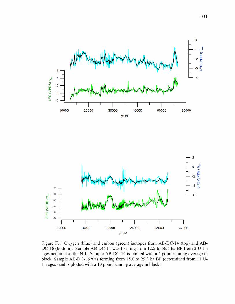
331

Figure F.1: Oxygen (blue) and carbon (green) isotopes from AB-DC-14 (top) and AB-DC-16 (bottom). Sample AB-DC-14 was forming from 12.5 to 56.5 ka BP from 2 U-Th ages acquired at the NIL. Sample AB-DC-14 is plotted with a 5 point running average in black. Sample AB-DC-16 was forming from 15.0 to 29.3 ka BP (determined from 11 U-Th ages) and is plotted with a 10 point running average in black.