PROCEEDINGS OF THE INTERNATIONAL GEOTECHNICAL CONFERENCE

GEOTECHNICAL CHALLENGES IN MEGACITIES

Moscow, 7-10 June 2010

Volume 1

Edited by V.P. Petrukhin, V.M. Ulitsky, I.V. Kolybin, M.B. Lisyuk, M.L. Kholmyansky

Moscow 2010

1

. . , . . , . . , . . , . .

, 7-10 2010 .

2010 .

ii

Proceedings of the International geotechnical conference “Geotechnical challenges in megaci-ties”.

In 1st volume of the Proceedings the lectures presented by the authors in English and Russian are published.

In 2nd and 3rd volumes of the Proceedings the papers presented by the authors in English are pub-lished.

In 4th and 5th volumes of the Proceedings the papers presented by the authors in Russian are pub-lished.

The responsibility for content and editing is placed upon the authors of the lectures of this volume.

All rights reserved. No part of this publication may be reproduced, stored or transmitted in any form without the written permission of the Publisher.

Published by: GRF 190005, 4 Izmaylovsky prosp., St. Petersburg, Russia

ISBN 978-5-9902005-2-4

© NIIOSP, 2010 © GRF, 2010

Printed in printing house ‘MST’, Russia, St. Petersburg

iii

«» , .

. 2, 3 -, , 4, 5 – .

.

. -- , ,

, .

: “ ”190005, . 4, - ,

ISBN 978-5-9902005-2-4

© , 2010 © “ ”, 2010

‘ ’, , -

iv

PREFACE

Nowadays the humanity encounters unprecedented increase of urbanisation rate. One of its striking manifestations is the formation of large cities. In 2005 there were 27 cities with population above 3 millions, and by 2025 the number is forecasted to be a hundred and fifty.

Modern megacity is the concentration point of productive and creative power of human-ity and at the same time – the source of severe problems: ecology, transportation, preventing of disasters and minimization of their consequences.

Megacity poses the most complicated problems for geotechnical engineers. Existing buildings, underground structures and lifelines must be considered along with geotechnical conditions in the restrained urban environment, often complicated by bad environmental conditions, arose as a consequence of habitation and activity of millions of people.

Attempts to provide as many apartments and workplaces as possible have led to such a characteristic feature of megacities as high-rise buildings. They form the appearance of large city, at the same time challenging engineers of all branches. Problem of significantly increased loads bearing by soil with providing admissibility of deformations for existing structures should be in a focus. Therefore foundations for high-rise buildings are one of the most popular objects of research for geotechnical engineers. Other means of solving the problem of the space shortage are placing of city bridges and elevated roads in the above-ground space; that creates special problems of foundation engineering.

One more way of solving the problem of megacities is underground space development: construction of complex underground parts in the newly erected buildings, deepening of basements under existing buildings in course of their reconstruction, building underground thoroughfares. The most difficult problem is stated by interaction of existing and new struc-tures, especially within large-scale multifunctional complexes. One of the effective means for solution of corresponding geotechnical problems is soil improvement.

Generally, problems of interaction are relevant for geotechnics of megacities. Interaction of foundations, effect of new buildings and constructions on underground structures along with an effect of new underground structures on existing buildings and networks – all that problems are already within the range of interests of geotechnical engineers and must attract even more attention in the future. Systems approach to these problems dictates the necessity to both geofailures and geological risks assessment in urban planning. The latter is often related with construction on problematic soils.

Many megacities were formed around the centuries-old cities. The need to preserve his-torical buildings is an additional factor causing difficulties for geotechnical engineers. Strengthening and reconstruction of existing foundations is one of the most important branches of their work.

Another feature of prolonged human activity in built-up areas is pollution of the envi-ronment, giving rise to geoecological problems of construction on contaminated soils. Preservation of hydrogeological situation in course of underground space development, water pumping and other man-caused effects lies within the same range of problems.

v

-. . 2005

3 27, 2025 , ,.

: ,, .

- . -,,

,.

-,

. ,.

,. -

-. -

, --

. – -

: ,, -

., -

.

..

,,

– -.

, ..

vi

Being a product of modern civilisation, megacities at the same time state the problem of its future. Preservation of natural resources when supporting megacities’ life has attracted the attention of geotechnical engineers already, forcing search of solution for sustainable development.

The understanding of existing difficulties by the professional community led to organiza-tion of International conference “Geotechnical challenges in megacities”. Unprecedented number of ISSMGE Technical Committees united their efforts so that the interaction of professionals of different specialization may advance to the sound and balanced reduction of risks and expenses of construction in the most important inhabited localities, being homes for significant part of mankind.

Publication of this five-volume edition including fourteen lectures and more than two hundred papers of the leading world professionals in the field of geotechnics must record state-of-the-art and design the ways of solution of principal existing problems. The editors hope that these targets are at least partly achieved.

V.P. Petrukhin Chairman of the Organizing Committee

V.M. Ulitsky Co-chairman of the Organizing Committee

vii

.-

, . -.

-, -

.-

, .,

. -- ,

.-

«». -

ISSMGE , -

-, -

.,

- , -. -

, .

. .

. .

viii

ORGANIZERS

International Society for Soil Mechanics and Geotechnical Engineering (ISSMGE) and

five its technical committees:

• Technical Committee 18 “Deep Foundations”

• Technical Committee 28 “Underground Construction in Soft Ground”

• Technical Committee 32 “Engineering Practice of Risk Assessment and Management”

• Technical Committee 38 “Soil-Structure Interaction”

• Technical Committee 41 “Geotechnical Infrastructure for Mega Cities and New Capitals”

Gersevanov Research Institute of Bases and Underground Structures (NIIOSP), Moscow

NPO “Georeconstruction-Fundamentproject (GRF), Saint-Petersburg

ORGANIZING COMMITTEE

V.P. Petrukhin, Chairman of the Organizing Committee, Professor, Director, NIIOSP, Russia

V.M. Ulitsky, Co-Chairman of the Organizing Committee, Professor, Head of Department, Saint-Petersburg State Transport University, Chairman TC 38, Russia

I.V. Kolybin, Deputy Director, NIIOSP, Russia

A.G. Shashkin, Director General, GRF, Russia

M.B. Lisyuk, Deputy Director, GRF, Member of ISSMGE IDC, Russia

M.L. Kholmyansky, Leading Researcher, NIIOSP, Russia — Secretary General of the Conference

ix

(ISSMGE)

:

• 18 “ ”

• 28 ” ”

• 32 “ ”

• 38 “ ”

• 41 “ -

”

- , - -

. . ( . . . ), .

“ - ”, -

. . , , ,. . . ,

. . , , , -- ,

38,

. . , . . . ,

. . , « - »,.

. . , « - », ISSMGE,

. . , . . . , –

x

INTERNATIONAL SCIENTIFIC COMMITTEE

P. Seko e Pinto, Portugal

N. Taylor, UK

R. Frank, France

W. Van Impe, Belgium

J.-L. Briaud, USA

V.A. Ilyichev, Russia

R. Kastner, France

R. Katzenbach, Germany

A. Negro, Brazil

F. Nadim, Norway

A.Zh. Zhussupbekov, Kazakhstan

A.B. Fadeev , Russia

M.Yu. Abelev, Russia

Z.G. Ter-Martirosyan, Russia

V.I. Sheinin, Russia

V.G. Fedorovsky, Russia

CONFERENCE SECRETARIAT

M.L. Kholmyansky – Secretary General, NIIOSP, Moscow

G.K. Fursova, NIIOSP, RSSMGFE, Moscow

E.V. Dubinin, GRF, Saint-Petersburg

xi

,

. ,

. ,

. ,

.- . ,

. . ,

. ,

. ,

. ,

. ,

. . ,

. . ,

. . ,

. . - ,

. . ,

. . ,

. . – ,. . . ,

. . , . . . , ,

. . , “ - ”, -

xii

Table of contents

Volume 1 1

Keynote and invited lectures

H. Brandl Cyclic preloading of piles and box-shaped deep foundations ................................................. 3

J.-L. Briaud, C. J. Rutherford Excavation support using deep mixing technology ............................................................... 29

A. Burghignoli, F. Di Paola, M. Jamiolkowski, G. Simonacci New Rome metro line C: approach for safeguarding ancient monuments ............................ 55

R. Frank, F. Schlosser Some lessons learnt from ‘FOREVER’:the French national research project on micropiles ............................................................... 79

R. Kastner, F. Emeriault, D. Dias Assessment and control of ground movements related to tunnelling .................................... 92

R. Katzenbach, S. Leppla, M. Vogler, R. Dunaevskiy, H. Kuttig State of practice for the cost-optimized foundation of high-rise buildings ......................... 120

P. Simão Sêco e Pinto, J. Barradas Railway Old Station Building: Enlargement and Underpinning ......................................... 130

K. Pitilakis, G. Tsinidis Seismic design of large, long underground structures:Metro and parking stations, highway tunnels ...................................................................... 158

P.I.B. Queiroz, A. Negro Geo-environmental Conditions Impact on Underground Projects ...................................... 198

H.F. Schweiger Numerical analysis of deep excavations and tunnelsin accordance with EC7 design approaches......................................................................... 206

xiii

I. Vaní ekUrban Environmental Geotechnics Construction on Brownfields ...................................... 218

G.M.B. Viggiani, A. Mandolini, A. Flora, G. Russo Excavations in the urban environment:examples from the construction of Napoli underground ..................................................... 236

. . –

...................................................................................... 259

. . , . . , . .

.............................................................................. 321

xiv

Key-note and invited lectures

Cyclic preloading of piles and box-shaped deep foundations

H. Brandl Vienna University of Technology, Austria

ABSTRACT: Pre-loading and cyclic un- and re-loading of piles is a proven method to reduce total and differential settlements of high-rise buildings and/or statically sensitive structures. It is performed by using the piled raft or capping structure as counter weight. This is demonstrated for a Danubebridge and the 202 m high Millennium Tower in Vienna. Another settlement-minimizing method are box-shaped deep foundations which primarily consist of pile walls or diaphragm walls (but also ofdeep-mixing walls or jet grouting walls). Such foundations have several advantages over conven-tional deep foundations due to the composite effect between walls and enclose soil.

1. PRELOADING AND LOAD CYCLING OF PILES

1.1. Introduction

From numerous full-scale tests it is known that the bearing behaviour of individual piles on a site usually differs clearly. This may cause stress constraints within the structure, stress-redistribution with local overloading, and differential settlements. To avoid this and to also reduce absolute settlement, a preloading and load cycling technique was developed which comprises all structural piles of a build-ing without hindering construction work. The piles are preloaded as single elements or in groups by imposing a load which exceeds the design load by at least 20%. Flat jacks have to be placed on the upper end of the piles, and an equipment for post-grouting should be installed if the jacks remain within the structure. This provides the final bond between piles and raft after finishing the complete building.

The basic idea is not only to minimize the total settlement of the pile foundation or of the piled raft foundation but also to achieve uniform load-movement behaviour of all piles. Experi-ence has shown that this requires in most cases hysteresis loops with at least two to three cycles of (re-)loading - unloading. The aim is, to have rather similar gradients along the statically relevant section of the final load-settlement curves under service conditions.

1.2. Strengthening of bridge foundation

One of Vienna’s main bridges, 30 years old, had to be strengthened and widened as a result of rapid traffic increase since the extension of the European Union. Moreover, the construction of a nearby hydropower plant required a lifting of the bridge deck of up to 1.8 m. The 1022 m long structure exhibits field lengths between 40 m and 210 m. The statically sensitive superstruc-ture comprises hollow box girders (one for each traffic direction) which consist of steel in the 413 m long central part and of prestressed reinforced concrete in the other parts of the bridge. The bridge deck should be widened by one lane in each direction, thus finally provid-ing eight lanes to transport 230.000 cars per day.

The old foundation consisted of large diame-ter bored piles (d = 1.8 m) which were embed-ded in tertiary sediments (sandy silt to clay), overlain by a thin cover of quaternary sandy gravel. It could no longer meet the increased loads and the requirements of modern codes and standards. Moreover, the statically indetermi-nate superstructure was very sensitive towards differential settlements during the various construction phases of bridge lifting and widen-ing, which involved repeated changes of the statical system.

Strengthening of the old foundation was achieved by installing six additional piles on each side of the bridge piers and then by com-

3

Figure 1. View of a highway bridge which had to be lifted and strengthened.

Figure 2. Ground plan to Figure 1 with new piles which were cyclically loaded before bridge lifting.

bining them with a capping structure. Before creating a statically compound system, the piles were preloaded up to 120% of the working load under service conditions of the widened bridge deck and under maximum traffic. Figures 1, 2 show the view and the ground plan of one of the

bridge piers, illustrating the pattern of the new piles which were required for strengthening the old foundation. The cross sections are given in Figures 3, 4, thus illustrating the preloading equipment to impose load cycles on the piles before connecting the entire system to a statical

4

Figure 3. Cross section A A to Figure 1. Construc-tion phase with hydraulic jacks for pile preloading and load cycling.

Figure 4. Cross section B B to Figure 1.

Figure 5. Detail to Figure 3.

Figure 6. Detail to Figures 3,5, but in the transversal direction.

unit. Preloading was performed in steps on twin-piles symmetrically to the bridge axis, and it involved cyclic un- and reloading to achieve, in the end, similar load - settlement curves within the relevant range of service loads of all piles of a pier. Figures 5, 6 give some details to Figure 3 regarding the openings in the raft and the reinforcement.

5

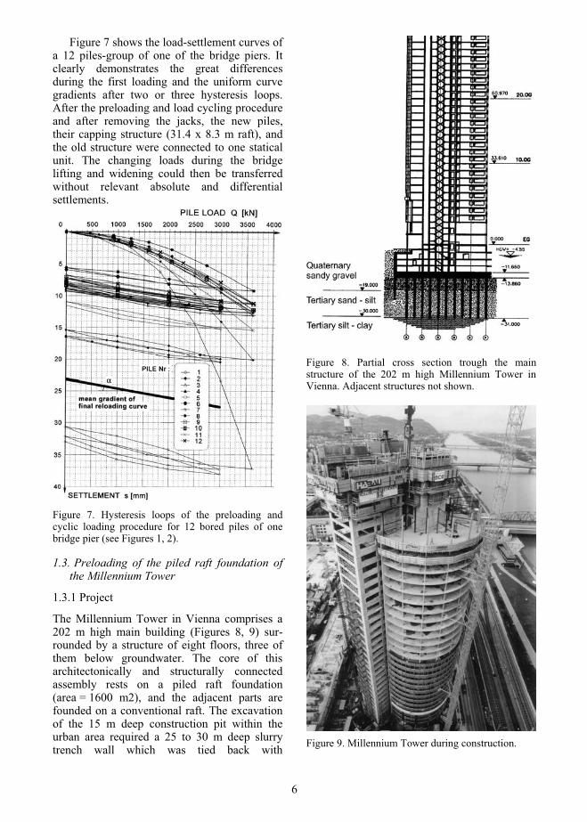
Figure 7 shows the load-settlement curves of a 12 piles-group of one of the bridge piers. It clearly demonstrates the great differences during the first loading and the uniform curve gradients after two or three hysteresis loops. After the preloading and load cycling procedure and after removing the jacks, the new piles, their capping structure (31.4 x 8.3 m raft), and the old structure were connected to one statical unit. The changing loads during the bridge lifting and widening could then be transferred without relevant absolute and differential settlements.

Figure 7. Hysteresis loops of the preloading and cyclic loading procedure for 12 bored piles of one bridge pier (see Figures 1, 2).

1.3. Preloading of the piled raft foundation of the Millennium Tower

1.3.1 Project

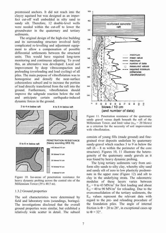
The Millennium Tower in Vienna comprises a 202 m high main building (Figures 8, 9) sur-rounded by a structure of eight floors, three of them below groundwater. The core of this architectonically and structurally connected assembly rests on a piled raft foundation (area = 1600 m2), and the adjacent parts are founded on a conventional raft. The excavation of the 15 m deep construction pit within the urban area required a 25 to 30 m deep slurry trench wall which was tied back with

Figure 8. Partial cross section trough the main structure of the 202 m high Millennium Tower in Vienna. Adjacent structures not shown.

Figure 9. Millennium Tower during construction.

6

prestressed anchors. It did not reach into the clayey aquitard but was designed as an imper-fect cut-off wall embedded in silty sand to sandy silt. Therefore, 12 double-level wells were needed within the cut-off to lower the groundwater in the quaternary and tertiary sediments.

The original design of the high-rise building and its surrounding structure involved fairly complicated re-levelling and adjustment equip-ment to allow a compensation of possible differential settlements between the structural units. This would have required long-term monitoring and continuous adjusting. To avoid this, an alternative was developed: Local soil improvement by deep vibrocompaction and preloading (overloading and load cycling) of all piles. The main purpose of vibroflotation was to homogenise and densify the near-surface cohesionless subsoil and to increase the portion of load directly transferred from the raft into the ground. Furthermore, vibroflotation should improve the subgrade reaction below the raft and anticipate certain earthquake-induced dynamic forces in the ground.

Figure 10. Iso-areas of penetration resistance for heavy dynamic probing across the central site of the Millennium Tower (39 x 40.5 m).

1.3.2 Ground properties

The soil characteristics were determined by field and laboratory tests (soundings, borings). The investigations disclosed that the overall ground properties were similar, but exhibited a relatively wide scatter in detail. The subsoil

Figure 11. Penetration resistance of the quaternary sandy gravel versus depth beneath the raft of the Millennium Tower, and limit value (n10 = 20 blows) as a criterion for the necessity of soil improvement with vibroflotation.

consists of young fills (made ground) and fine-grained river deposits underlain by quaternary sandy-gravel which reaches 3 to 9 m below the raft (6 – 8 m within the perimeter of the core structure). Figures 10, 11 illustrate the hetero-geneity of the quaternary sandy gravels as it was found by heavy dynamic probing.

The lying tertiary sediments vary from uni-form silty sands to silty clay, whereby silty sand and sandy silt of zero to low plasticity predomi-nate in the upper zone (Figure 12) and silt to clay in the underlying strata. The odeometric modulus of these layers varies between Es1 = 8 to 43 MN/m2 for first loading and about Es2 = 40 to 90 MN/m2 for reloading. Due to the overconsolidation of the tertiary sediments, the Es2 values represent the relevant data with regard to the pre- and reloading procedure of the foundation piles. The angle of internal friction is = 20 to 28 , in exceptional cases up to = 32°.

7

The groundwater level was originally close to the ground surface, corresponding with the water level of the nearby river Danube. After cut-off wall installation, it now lies 6 m below surface.

Figure 12. Range of grain size distribution of the tertiary sediments along the piled zone.

Figure 13. Scheme of the piled raft foundation of the Millennium Tower with local vibroflotation to gain a quasi-composite body, and flat jacks on top of the piles for subsequent preloading and load cycling.

1.3.3 Local soil improvement; pile installation, preloading, and loading cycling

The 202 m high core structure of the Millen-nium Tower was founded on 151 continuous flight auger piles (d = 0.88m) of 13 to 16 m length. Before piling, the hetergeneous sandy gravel was locally improved by vibroflotation if the penetration resistance of heavy dynamic probing was less than n10 = 20 (Figure 11).

Figure 14. Detail to Figure 13. Pile preloading and load cycling system.

Figure 15. Detail to Figures 13, 14: Flat jack that is installed on top of each pile.

Vibroflotation was performed on a working level 1.2 m above the pile heads (Figure 13). The mean spacing of the vibroflotation points was 2.5 x 2.5 m. After homogenising the near-surface ground, the piles were installed from a working level which was protected by 0.2 m sub-concrete (reinforced with wire mesh). Experience from several sites has disclosed that

8

such a surface protection improves the load-bearing behaviour of pile groups: On several sites an increase of 10 to 20% in bearing capac-ity could be measured under comparative conditions.

Figure 16. Detail to Figures 13, 14: Sub-concrete for the raft is cast. Sleeve-coverpipes to enable post-grouting of the pile heads are being installed.

The 2.2 m thick raft of the high-rise core structure was constructed without joints. The steel reinforcement was 185 kg/m³ and the concrete quality C30/40. The jointless raft required a casting of 3520 m3 concrete without interruption within 15 hours.

Preloading of the piles started about three months after their installation, when the second sub-floor of the building was already under construction. Until then no relevant load trans-fer into the piles had occurred: the loads were running from the raft directly into the ground. This could be achieved by an open space between pile head and raft, into which flat jacks were placed (Figures 14 to 16).

Preloading of the piles required flat jacks of 600 tons capacity and 50 mm vertical lift range; their diameter corresponded to the pile diameter minus concrete cover and reinforcement, hence 700 mm. Each of the 151 piles was preloaded, either as single element or in groups with maximal 10 piles. The space between the piles which underwent simultaneous loading was 7.5 m to 10 m in order to prevent mutual influenc-ing. This procedure did not hinder any on-going construction work, and it did not require addi-tional counterweight besides the dead load of the raft. In total, it was performed within 15 working days, i.e. within only three weeks. About three weeks after preloading, the hydrau-lic oil in most of the flat jacks was replaced by high pressure cement injection. This provided a stiff connection between raft and piles. Eleven

Figure 17. . Load settlement curves for two relevant piles of the Vienna Millennium Tower, illustrating the locally different pile behaviour. Preloading and load cycling procedure until uniform gradients of the final reloading curves are achieved. Qw,calc = calcu-lated working load (under service conditions).

Figure 18. Similar to 17, but two other piles with different length and Qw,calc.

pile heads have been left as measuring piles to collect as much data as possible under the total load of the building.

Preloading of the piles involved a first load-ing up to 1.2 QW,calc, whereby QW,calc is the calculated working load under service condi-tions of the building (design load). This tempo-rary over-loading was followed by unloading - reloading cycles until the gradients of the reloading curves were practically equal. Figures 17, 18 show this for four piles, each with a rather different load-settlement behaviour during first loading. The conventional founda-tion technique without any preloading would

9

Figure 19. Histograms for pile head settlements of 151 piles of the Tower under first loading.

have caused strong constraints within the piled raft under building loads, because the pile characteristics differed so much. This could now be eliminated by means of preloading and load cycling.

Preloading of each pile disclosed very clearly that there is a relatively great difference in the load-settlement behaviour of the individ-ual piles on the same site, despite rather similar ground conditions, the same type and dimension of piles, and the same rig and crew. There are no identical piles, and the scattering of their deformation behaviour increases with load, as illustrated in Figures 19a (Q = 0.8 QW,calc), 19b (Q = 1.0 QW,calc) and 19c (Q = 1.2 QW,calc).

Figure 20 shows that the scatter of pile load-settlement behaviour increases over-proportion-ally with load. A semi-normalized diagram provides a straight line (Figure 21) which could be also found on other construction sites. The gradient of the line depends on the dimensions, system and installation of the piles, and on the ground parameters. Most reliable values can be

gained for pile loads exceeding 50 % of the total working load.

The scheme of Figures 20,21 can be used to optimize pile design for conventional pile groups or piled rafts respectively, considering parametric studies and most plausible assump-tions for pile behaviour scatter and global performance of the foundations. Thus, stress constraints in the structure can also be assessed.

y = 3.581x2 + 0.1045x + 0.0017

0

1

2

3

4

5

6

0 0.2 0.4 0.6 0.8 1 1.2Percentage of working load Qw,calc

Stan

dard

dev

iatio

n s x

of p

ile

load

dis

plac

emen

t [m

m]

General model: f(x) = p1*x^2 + p2*x + p3Coefficients (with 95% confidence bounds): p1 = 3.581 (3.159, 4.003) p2 = 0.1045 (-0.4139, 0.623) p3 = 0.0017 (-0.1383, 0.1417)Goodness of fit: SSE: 0.002174 R-square: 0.9999 Adjusted R-square: 0.9998 RMSE: 0.03297

Figure 20. Standard deviation sx of pile head dis-placement (in mm) versus percentage of calculated working load Qw,calc for 151 piles.

10

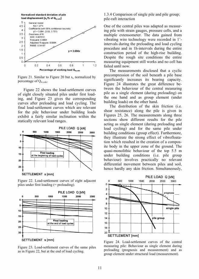
Figure 21. Similar to Figure 20 but sx normalized by percentage of Qw,calc.

Figure 22 shows the load-settlement curves of eight closely situated piles under first load-ing, and Figure 23 gives the corresponding curves after preloading and load cycling. The final load-settlement curves which are relevant for the pile behaviour under building loads exhibit a fairly similar inclination within the statically relevant load ranges.

Figure 22. Load-settlement curves of eight adjacent piles under first loading (= preloading).

Figure 23. Load-settlement curves of the same piles as in Figure 22, but at the end of load cycling.

1.3.4 Comparison of single pile and pile group; pile-raft interaction

One of the central piles was adapted as measur-ing pile with strain gauges, pressure cells, and a multiple extensometer. The data gained from vibrating wire technology were recorded in 1’-intervals during the preloading and load cycling procedure and in 1h-intervals during the entire construction period of the high-rise building. Despite the rough site conditions the entire measuring equipment still works and no cell has failed until now.

The measurements disclosed that a cyclic precompression of the soil beneath a pile base significantly increases its bearing capacity. Figure 24 illustrates the great difference be-tween the behaviour of the central measuring pile as a single element (during preloading) on the one hand and as group element (under building loads) on the other hand.

The distribution of the skin friction (i.e. shear resistance) along the pile is given in Figures 25, 26. The measurements along three sections show different results for the pile acting as single element (during preloading and load cycling) and for the same pile under building conditions (group effect). Furthermore, they illustrate the strong effect of vibrofloata-tion which resulted in the creation of a compos-ite body in the upper zone of the ground. The quasi-monolithic behaviour of the top 5.5 m under building conditions (i.e. pile group behaviour) involves practically no relevant differential movement between piles and soil, hence hardly any skin friction. Simultaneously,

Figure 24. Load-settlement curves of the central measuring pile: Behaviour as single element during preloading (prognosis and measurement) and as group element under structural load (measurement).

11

Figure 25. Normal pile force (Q) versus depth of the central measuring pile at different construction stages (0.5 and 0.8 Qw,calc). At first, single pile behaviour during preloading, then group behaviour under construction conditions. Dotted line indicates the base of a widely “quasi-monolithic” body beneath the pile raft.

load is transferred more directly from the raft into the ground, and the deeper zones of the piles are more intensively mobilised for load transfer than in the case of the single pile state.

Figure 25 shows the decrease of normal force, Q, in the pile with depth, measured for a pile load of 0.5 QW,calc and 0.8 QW,calc. The curves clearly disclose that the load transfer from the pile into the ground (by skin friction) occurs in greater depth under group condition. The load transfer from raft to ground occurs mainly in the topmost 5 to 6 m where negative skin friction (from the raft) and positive skin friction (shear resistance) widely compensate each other (Figure 26). Pile-raft interaction grows with load, whereby the soil improvement due to vibroflotation increases the direct load transfer via raft into the ground. Thus, the top zone finally acts like a “quasi-monolith”. The composite-like foundation system (raft + piles + improved ground) behaves as if its base were about 5.5 m below the raft. This can also be deduced from the gradients of the tangents of the curves in Figure 25: they are practically equal for the single pile state below raft base on the one hand and the group pile state 5.5 m below the raft base on the other hand. The pile

load has no influence on this basic behaviour. Furthermore, the thickness of the “quasi-monolith” remains constant. Only the gradient of the curves decreases with increasing loads. This means that skin friction below the quasi-monolithic body increases with load.

Figure 27 illustrates exemplarily how the pile loads changed during the construction period of the Tower and during the subsequent construction of an adjacent building (annex). A reliable interpretation is only possible if observ-ing the settlements and groundwater level as well. The measurements confirmed the self-regulating behaviour of the interacting members of a piled raft foundation.

During the initial construction stage the ex-ternal loads were nearly fully transferred from the raft into the subsoil. But the load transfer mechanism changed significantly after the spaces between flat jacks and raft were injected step by step. This measure activated increas-ingly the piles which during the quick construc-tion of the high-rise structure finally reached a maximum of about 75% (edge piles) to 95% (central piles) of the total design load depending on pile location and local load transfer from the high-rise structure. With ongoing settlement, the load portion directly running from the raft into the subsoil increased, thus causing a gradual decrease in the pile load portion. The percent-age of the load taken by the raft increased from originally 10 – 20% to about 25 – 35% of the specific total load.

Figure 26. Load transfer from the piled raft founda-tion into the ground. Schematic.

12

Figure 27. Influence of groundwater lowering and re-rising on the settlement of the Tower edge and on a pile opposite to the annex.

1.3.5 Settlements

The construction pits for the high-rise core and the lower structures were excavated simultane-ously as one unit to a depth of 15 m below surface. The excavation of 180,000 m³ of soil caused a heave which reached about 40 m below the pit base: During excavation between 6 m to 15 m depth, ground heaving up to 30 mm was measured by geodetic levelling survey and 60 m deep multiple extensometers (Figure 28). From the recorded time-heave curve, an addi-tional heave of nearly 10 mm could be deduced for the initial construction phase before meas-urements started, thus resulting in about 40 mm total heave. After casting the raft, the loads of the high-rise building were transferred very quickly into the ground: Because of the short construction period, two floors had to be erected weekly. A building height of 170 m was already reached after 7 months. Therefore, the fresh concrete of the 2.2 m thick piled raft behaved

very flexible, undergoing trough-shaped settle-ment.

The total settlements were reached in the year 2002 (38 mm), and they correspond fully with the prognosis. They can be widely consid-ered an elastic re-deformation of the ground after heaving during deep pit excavation. The

Figure 28. Ground heave due to the excavation of the 15 m deep construction pit.

13

maximum differential settlement between the centre of the high-rise core structure and the edges of the building is s 23 mm, and it occurred early, i.e. during the very flexible and statically non-critical phase of construction. Therefore, no compensation levelling was necessary during the construction of the high-rise structure, and the joints along the contact areas between core tower and the adjacent 8-floor structures have remained fully watertight. Furthermore, the convex settlement curve compensated the concave deformation curve of the structural members within the high-rise structure above ground. The latter occurred because the compressive strains in the outer zone of the core were greater than those in the inner part. Consequently, the floors now exhibit horizontal slabs.

Figure 29 shows the settlement curves along the cross section of the building, derived from 20 measuring points between centre point and edge. It should be noted that there was exclu-sively a raft-soil contact at the beginning before the piles were gradually activated by injecting the open space on their top. Figure 29 also indicates that the pile resistance was not mobi-lised from the beginning of load transfer. At first, a direct load transfer from the raft into the ground occurred, and the portion of pile load transfer was negligible. The piles were increas-ingly activated then by injecting, in steps, the spacing between pile head, flat jack, and raft. The settlement trough developed due to the deep-seated overall ground deformation beneath the pile toes and not because of differential pile behaviour.

The time-settlement behaviour is illustrated in Figure 30, showing mean values of geodetic

levelling and extensometer readings below the core structure. The influence of groundwater lowering and raising within the cut-off walls of the excavation pit is also visible. The time-settlement curve exhibits an increasing flatten-ing since the dead load of the building has been reached. This is typical for deep foundations in overconsolidated fine soils (Figure 12) where the settlements occur more quickly than in normally consolidated soil. Moreover the relevant subsoil zone contributing to settlements reaches not as deep as in the case of normally consolidated soil.

The building was opened at the end of April 1999, and no measures to compensate differen-tial settlements have been required since, though the subsequent construction of an adjacent building caused an additional settle-ment of up to 5 mm (Figure 27). Moreover, no joint between the high-rise core and lower structure opened in the basement which re-mained watertight. Usually proper serviceability is in such cases much more sensitive than structural stability.

Figure 30. Partial time-settlement curves for typical measuring points of the Millennium Tower.

Figure 29. Settlement curves duringconstruction of the Millennium Towerin Vienna. Gradual mobilization of pileresistance by injecting the spacingbetween pile heads, flat jacks, and raft.

14

2. BOX-SHAPED DEEP FOUNDATIONS

2.1. Introduction

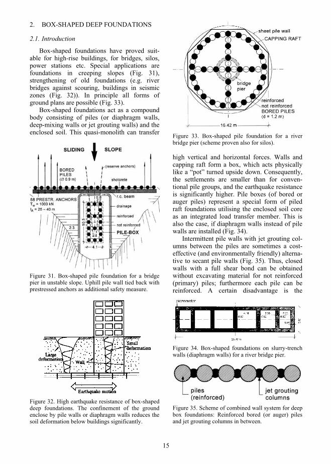
Box-shaped foundations have proved suit-able for high-rise buildings, for bridges, silos, power stations etc. Special applications are foundations in creeping slopes (Fig. 31), strengthening of old foundations (e.g. river bridges against scouring, buildings in seismic zones (Fig. 32)). In principle all forms of ground plans are possible (Fig. 33).

Box-shaped foundations act as a compound body consisting of piles (or diaphragm walls, deep-mixing walls or jet grouting walls) and the enclosed soil. This quasi-monolith can transfer

Figure 31. Box-shaped pile foundation for a bridge pier in unstable slope. Uphill pile wall tied back with prestressed anchors as additional safety measure.

Figure 32. High earthquake resistance of box-shaped deep foundations. The confinement of the ground enclose by pile walls or diaphragm walls reduces the soil deformation below buildings significantly.

Figure 33. Box-shaped pile foundation for a river bridge pier (scheme proven also for silos).

high vertical and horizontal forces. Walls and capping raft form a box, which acts physically like a “pot” turned upside down. Consequently, the settlements are smaller than for conven-tional pile groups, and the earthquake resistance is significantly higher. Pile boxes (of bored or auger piles) represent a special form of piled raft foundations utilising the enclosed soil core as an integrated load transfer member. This is also the case, if diaphragm walls instead of pile walls are installed (Fig. 34).

Intermittent pile walls with jet grouting col-umns between the piles are sometimes a cost-effective (and environmentally friendly) alterna-tive to secant pile walls (Fig. 35). Thus, closed walls with a full shear bond can be obtained without excavating material for not reinforced (primary) piles; furthermore each pile can be reinforced. A certain disadvantage is the

Figure 34. Box-shaped foundations on slurry-trench walls (diaphragm walls) for a river bridge pier.

Figure 35. Scheme of combined wall system for deep box foundations: Reinforced bored (or auger) piles and jet grouting columns in between.

15

requirement of an additional site equipment. The optimum clear pile spacing lies typically between 0.2 to 0.5 m depending on the soil properties, required lengths of piles and jet grouting columns, on the jet grouting technique and on static requirements.

2.2. Model tests

Comprehensive model tests were performed to investigate parameters influencing the bearing-settlement behaviour of box-shaped pile founda-tions. The research program comprised 70 tests including the following test series (Hofmann 2001, Brandl 2001, Brandl & Hofmann 2002):

Pile boxes with inner piles (according to general design practice); Pile boxes without inner piles; Pile boxes without soil infill (simulating zero-stiffness of the enclosed soil); Pile boxes filled with “concrete” (simulating a monolithic block); Conventional pile groups (axial spacing a 2d); Close contact or free gap between raft and soil beneath; Single piles. Tests with conventional pile groups and sin-

gle piles were conducted to compare the load-settlement behaviour of the different pile patterns. Furthermore, pile diameter (d), pile length (l) and density of soil ( ) were varied to check their influence. The “standard” test series were performed with uniform quartzitic sand: d50 = 0.75 mm, dmax = 2 mm, Cu = 3. Figure 36 shows two standard types of investigated box-foundations. The pile pattern was similar to the design of foundation alternatives for a long river bridge.

During the tests the load-settlement curves until failure, the settlement troughs and the pile forces in five or six measuring levels were registered.

Figures 37 and 38 show some test results in normalized diagrams. The data are given di-mensionless to enable a direct comparison with results gained for conventional pile groups or from in situ measurements on construction sites. Moreover, dimensionless diagrams can be applied more easily to larger scales.

The diagrams demonstrate the effect of pile arrangement and intensity of bond within the pile box. The installation of inner piles reduces the settlement, which can be expressed by a

Figure 36. Two examples of box-foundations used for the standard model tests (scale 1:50). Equivalent diameter D for a circular box-foundation for box S.

Figure 37. Dimensionless load-settlement curves for the pile box S. Pile length l = 40 cm. s = settlement, Q = total load on the foundation, d = pile diameter, A = foundation area (cross sectional area within circumference of pile box), = density of soil.

Figure 38. Similar to Fig. 37, but pile box L.

cell-factor c 1.0 (see Fig. 43). A comparison of these two figures shows that the Q/(Ad )ratio – hence the geotechnical “efficiency” of

16

Figure 39. Influence of stiffness of enclosed soil or bond effect between piles and enclosed soil of the box-foundation S; pile length l = 40 cm.

small boxes is relatively greater, whereby, of course, large box-foundations as a whole can take higher total loads due to their larger area and pile number. Figure 39 illustrates the composite effect: The hatched zone between pile box without infill and full monolith de-pends on the bond factor.

The influence of the ratio of box area A to box circumference U increases with the limit pile load. This ratio corresponds to the “hydrau-lic radius” R = A/U. Hence, boxes with a small hydraulic radius (i.e. long-stretched) can trans-fer higher loads than those with a square or circular shape. This coincides well with the theory, because square or circular foundations cause a higher stress concentration in the ground.

The portion of external load directly taken by the soil core increases with increasing hydraulic radius of the pile box, assuming a similar pile arrangement. From the model tests, a “box-factor” could be deduced:

totalsoil QQ , (1)

hence totalpile QQ )1( , (2)

whereby 4.00 , (3) The box-factor increases with the stiffness

of the soil core. Usually it lies below 0.4. A higher value can be obtained if the soil core is improved by jet grouting or deep mixing.

Figure 40 shows the box-factor for limit loads, which characterise a beginning steepen-ing of the load-settlement curve. The -linesshould not be extrapolated linearly to values higher than A/U/d = 2. It is rather recommended

Figure 40. Box-factor of deep box-foundations versus ratio A/U/d, where A = area of pile box, U = circumference of pile box, d = pile diameter. Derived from model tests.

to design piles with a box-factor that then is kept constant (for safety reasons). When ap-proaching failure load the forces concentrate in the piles, because the ratio of stiffness of piles to plastified soil increases. But due to a self-regulating behaviour box-foundations do not have a clear ultimate load. Figure 40 demon-strates the great influence of the cell size(s) on the load transfer via the soil core(s). The portion of external load directly taken by the enclosed soil of the box-foundation increases with the “hydraulic radius” A/U or A/U/d. A cohesion of the soil has no significant effect on the ratio Qsoil/Qtotal, but it influences the load transfer mechanism of the piles, hence the percentage of skin friction force and base resistance force.

Figure 40 represents only one among vari-ous correlations because the box-factor depends on a series of parameters:

Ratio A/U/d; Slenderness of the box-foundation, l/D; Ratio of stiffness of concrete members (Econcrete) to soil (Esoil);Multi-cellular pattern of the box foundation; Ratio of service load to limit or rupture load; Settlement. The portion of external load directly trans-

ferred from the raft into the soil (Qsoil/Qtotal)decreases with pile length l and box slenderness l/D respectively. The main reduction occurs between l/D = 0 (i.e. flat foundation where the raft takes 100 % of Qtotal) and l/D = 0.5 to 0.75 where the raft usually takes about 60 to 30% of Qtotal.

The transfer of vertical loads by a box-shaped pile foundation concentrates rather on

17

Figure 41. Base pressure of the piles versus settle-ment of the pile box S (Fig. 36). Pile length l = 50cm.

the inner piles than on the outer ones. This effect increases with increasing total load (e.g. Fig. 41) and is caused by a silo pressure within the cells (Brandl 2001).

The base pressure of the piles increases with the size of the soil cells because larger cells facilitate higher silo pressures. In the upper zone of the box, the ring walls are subjected to a lateral earth pressure difference that is directed outward. With increasing depth, the horizontal silo pressure is widely compensated by the earth pressure at rest acting on the outer face of the box-foundation. Therefore, adjacent piles should exhibit sufficient bond along their connecting line (mainly in the upper zone), i.e. secant piles are advantageous over tangent piles. In the case of contiguous or even intermittent pile walls, a load transferring closure can be obtained by jet grouting between the spandrels.

The effectiveness of piles forming cross walls in a deep box-foundation can be quanti-fied by dividing the settlement reduction by the increase of the proportional pile number when adding inner piles to form a multi-cellular pattern. The model tests exhibited that piles forming cross walls in long-stretched boxes have a larger effect than those in square-shaped or circular cells.

2.3. Theory and calculation

2.3.1 General

In conventional design practice, the bearing capacity of the capping raft of deep foundations is usually neglected. But box-shaped deep foundations behave as a compound body: the enclosed soil cannot move laterally and takes part in bearing external loads. Consequently, the capping raft can be designed to take a signifyc-

Figure 42. Design charts for deep box-foundations. Settlement curves for a cylindrical box foundation under a unit load of Q = 1 kN. Slenderness l/D of the foundation as parameter, whereby l = depth of pile or diaphragm wall foundation. Unit modulus of soil Es = 20 MN/m², d = wall thickness. For non-cylindrical foundations: D = equivalent diameter.

cant percentage of the forces from the structure above by transferring it directly into the ground. Comprehensive model tests and in-situ meas-urements have shown that the settlement of such box-foundations is smaller than it would be in the case of conventional groups of piles or diaphragm wall panels. Avoiding the lateral deformation of the soil core and minimizing its shear deformation leads to a significant reduc-tion of settlements, because the foundation system acts like a pot turned upside down. For the design and calculation of such deep box-foundations, several hypotheses have proved suitable:

Half-space hypothesis Limit case hypotheses Subgrade reaction models Numerical models.

2.3.2 Elastic-isotropic half-space hypothesis

Figure 42 shows a design chart for the de-termination of the unit-settlement of a cylindri-cal box-foundation depending on its diameter and slenderness. It is based on the half-space hypothesis (Brandl 1987, 2001). Originally, the integration of Mindlin’s equations was per-

18

formed for a circular diameter referring to the axis of the circumference wall (Hazivar, 1979). Therefore, if the box has a rectangular or polygonal shape, an equivalent diameter must be chosen (see also Figure 57). The theoretical diameter should be somewhat smaller than the outline of the cell (e.g. minus d/2), depending on the pile spacing (intermittent, contiguous or secant). This is an allowable approximation that has proven suitable in practice, especially for commonly designed and utilised rectangular box-foundations. In the case of a rectangular foundation box, the transformation into an equivalent diameter means a theoretically stronger stress concentration – especially in the case of long-stretched boxes (e.g. Figure 36, Box S). This effect justifies an equivalent diameter somewhat larger than the axial wall spacing and fits better to that area where friction forces are transferred in reality.

Single elements within the enclosed soil core reduce the settlement, but not significantly. Transverse walls have a greater effect. Another purpose of such additional inner elements is to stiffen the foundation-box and to gain a stati-cally optimal support for the capping raft. Furthermore, the bearing capacity for horizontal loads and moments increases, and the earth-quake resistance is improved significantly.

The settlement assessment curves of Figures 42 and 57 were developed for cylindrical box-foundations without stiffening elements inside. But comprehensive model tests on box-shaped pile foundations with and without inner piles disclosed that the installation of inner walls increases the bearing capacity and reduces the settlement. From model tests and in situ meas-urements on numerous sites a cell-factor ccould be deduced, which describes the effect of a multi-cellular shape of the box-foundation (Figure 43). It was determined for service loads corresponding to about 50% of the limit loads. Commonly it varies between

0.15.0 c , (4)

The maximum value occurs if no inner piles are installed, the minimum refers to a multi-cellular pattern with relatively small cells. In the latter case the pile (or diaphragm wall) founda-tion behaves increasingly like an idealized quasi-monolithic block foundation with a deep-lying foundation base.

Figure 43 illustrates that the cell-factor de-pends on the “hydraulic radius” A/U of the box-

Figure 43. Cell-factor c of (multi-cellular) deep box-foundations versus the ratio A/U/d. Number of cells, n, of the box-foundation as parameter.

foundation, on the pile diameter d (or wall thickness d), and on the number of cells within the box. The relatively greatest settlement-reducing and stiffening effect is gained with two or three cells. Usually, large foundations should exhibit at least three cells. The theoretical minimum of c is obtained if the entire box is filled with concrete elements (or jet grouting columns or deep mixing columns). But this is uneconomical. A cost-effective compromise, however, could be a local soil core improve-ment by (jet) grouting. Nevertheless, experience has shown that the cell-factor used for practical settlement assessment should not be assumed smaller than c = 0.5.

From Figures 42 and 43 the settlement s of a box-shaped deep foundation with an equivalent diameter D can be calculated as follows:

zEE

QQ

ss

stotc

1,

1

, (5)

c = cell factor of the deep box-foundation (from Figure 43)

totQ [kN] = settlement-effective total load on top of the pile group (or diaphragm wall group)

1Q = unit load, i.e. 1Q = 1 kN

sE [kN/m²] = modulus of soil (mean value)

1,sE = unit modulus, i.e. = 20 MN/m²

z = unit settlement from Figure 42 Equation (5) is primarily valid for a wall

thickness of about d = 1m, but may be used for d = 0.8 to 1.5m with sufficient accuracy. (In the

19

case of diaphragm walls even for d = 0.6 m). It is – strictly speaking – based on a Poisson’s ratio of = 0.3 and on a modulus ratio of structural members to soil of about 103. But values of 0.2 0.5 have no relevant influ-ence on the result. Furthermore, a variation of the ratio Epile : Esoil between 5.102 to 5.103 is allowable if the soil modulus is properly cho-sen. Hence equation (5) and Figure 42 have proved suitable for a wide range of different soils. Only for very soft clays too large settle-ments are calculated, and for very stiff overcon-solidated clays the cell-factor should be ne-glected (hence approximately c = 1 also for multi-cellular boxes). Furthermore, this formula is usually limited to soils with a modulus of about Es 100 MN/m2.

2.3.3 Limit case hypotheses

Limit case hypotheses and analyses refer to theoretically idealized limit assumptions (upper and lower bound approaches) and are not necessarily identical with limit load analyses or ultimate load conditions of deep foundations.

For assessing the bearing capacity of box-shaped foundations, two methods have proved successful in design practice:

Calculating the bearing capacity of the single pile or single diaphragm element (Figs. 44, 45) safety factor F1.Calculating the bearing capacity and settle-ment of the box-foundation as a quasi-block according to the monolith theory (Fig. 46)

safety factor F2.Evaluating the bearing capacity of single

elements provides only fictitious limit case values because the bond effect between con-crete elements and enclosed soil core is ne-glected. Thus, maximum pile or diaphragm wall loads are calculated. But actually, single ele-ments cannot fail because of the composite effect and the rigid (reinforced) connection of the piles or diaphragm panels with the capping raft. Moreover, deep box-foundations exhibit a self-regulating bearing behaviour, especially if the boxes are stiffened with inner walls: in the case of a local overloading of the soil around a pile, stress redistribution is possible. Therefore, very low safety factors are sufficient for this theoretical model: usually F1 1.15. For short construction stages or catastrophic conditions even values of F1 = 1.05 have been allowed.

Figure 44. Scheme of load transfer in a box-shaped deep foundation with inner pile- or diaphragm walls.

Contrary to the monolith-theory, skin friction may be taken into consideration along the outside and inside face of the foundation-box, but not between the single elements.

The other limit case hypothesis is an ideal-ised “monolith-theory”. According to Fig. 46, a full bond effect between deep foundation elements and the closed soil is assumed. This compound body comprises the outer circumfer-ence of the foundation if secant piles or dia-phragm walls are installed. In the case of contiguous piles, the theoretical area should be reduced by at least half a pile diameter. For the quasi-monolith, only skin friction along the outside surface of the foundation box may be taken into account.

The monolith-theory provides minimum pile or diaphragm wall loads. However, a full composite effect occurs only theoretically but hardly in practice. Therefore, relatively high safety factors are required: about F2 3.0 if conventional calculation methods for evaluating the base failure of equivalent “shallow” founda-tions are used. Short-term traffic loads do not reach the toe of the deep box-foundations but

20

Figure 45. Subgrade reaction model for a strength-ened foundation of the central river pier of an old Vienna Danube bridge showing soil responses to superimposed loads. Box-shaped new pile foundation consisting of secant piles and soil improvement in the upper part. Hatching on the diagram (below) indi-cates the difference between actual settlement and idealised model in the case of load increase.

are more or less directly transferred into the upper soil zone, unless the box has an exclu-sively end-bearing character.

For settlement analyses, the monolith-theory has proved practicable and sufficiently accurate in engineering practice by assuming the base of the box-foundation as the fictitious surface of the half space. The theoretical contact pressure includes the reduction of the total load Q by the skin friction Qs.

2.4. Case histories

2.4.1 General

Numerous data from in-situ measurements have been collected over a period of about 35 years. They comprise stress and deforma-tion/settlement measurements of box-shaped deep foundations of bridges, hydropower plants,

Figure 46. Box-shaped foundation (consisting of bored piles or diaphragm walls and the enclosed soil core) loaded by vertical and horizontal forces and moments: Idealised model “quasi – monolith” of the limit case hypothesis for determining the safety factor F2 against ground failure and evaluating the settlements.

industrial buildings and high-rise buildings. The ground plan of the box-foundations was rectan-gular, circular, elliptical or polygonal and mostly stiffened by transversal and/or longitu-dinal wall elements. Sometimes single piles or diaphragm wall panels were additionally in-stalled within the cells (for static reasons; to compensate installation failures, etc.). The ground conditions varied from very soft clay to stiff overconsolidated clay, from loose to dense sands, gravel, heterogeneous colluvium, from weathered slope deposits to decomposed rock.

The wall systems and the way of installation were also different. Both have an influence on the load-settlement behaviour of the box-shaped foundations. Diaphragm walls, for instance, provide a better transfer of shear forces between the concrete panels than contiguous pile walls, but on the other hand have frequently a smaller skin friction.

The in-situ measurements confirmed that the percentage of load taken either by the capping raft or by the piles (or diaphragm walls) de-pends on various parameters, such as:

Cross section (incl. pile pattern etc.) and slenderness of the foundation-box;

21

Ratio of stiffness of concrete elements and soil; Magnitude and distribution of external loads (V,H,M); Ratio of service load to ultimate (failure) load; Ground properties; Vertical and horizontal soil displacement; Magnitude and distribution of the contact stress between raft and soil; Foundation depth; Depth of excavation (construction pit); Installation factors.

2.4.2 Highway bridge

Consequently, the results of in-situ meas-urements scatter relatively widely, including several changes also during the construction period. In the following, a case history is selected which represents rather weak soil conditions.

The piers of a highway bridge had to be founded in deep-reaching young river sedi-ments: Sandy gravel of about 4 m thickness, underlain by weak silts (sandy to clayey); the natural water content varied between the plastic and liquid limit, the dry density was

d = 1,6 - 1,7 t/m³. Figure 47 shows the pile arrangement, thus forming a box-shaped foun-dation. The enveloping piles are secant, there-fore only every second one is reinforced. The interior piles are throughout reinforced and improve the load transfer from the bridge pier to the deep foundation. The construction was exe-

cuted in the year 1971. Nowadays the inner piles would be rather installed in a secant form to increase the stiffness of the box.

For the bridge design, the (differential) set-tlements were assessed rather cautiously, because this was one of the first box founda-tions. The measured value of s = 55 mm for the central bridge pier lies clearly below the prog-nosticated maximum of s = 100 mm, but coin-cides very well with the result derived from Figure 42 and Equation (5):

ground area of the box-foundation, A = 155.6m² circumference of box-foundation, U = 50.7m equivalent diameter of a cylindrical founda-tion, D = 14m pile length, l = 11m pile diameter, d = 0.88m slenderness of the foundation box, 1 : D = 0.8 total load (life load reduced), Q’tot = 55000 kN modulus of subsoil (mean value), Es = 8 MN/m²

From Figure 43 a cell factor of c = 0.5 is derived (for 6 cells) and provides a unit settle-ment of z’ = 0.8 10-3 mm. This leads to a total settlement of

3108.0820

1550005.0s

mm55s , (6)

Figure 47. Ground plan of a box-shapedfoundation for a highway bridge in silty river sediments. Bored piles, diameterd = 0.9 m. Single piles (hatched) only additional to overcome constructiondifficulties and local inhomogenities inthe subsoil. Black piles: reinforced; white piles: not reinforced.

22

2.4.3 Hydro-power plants

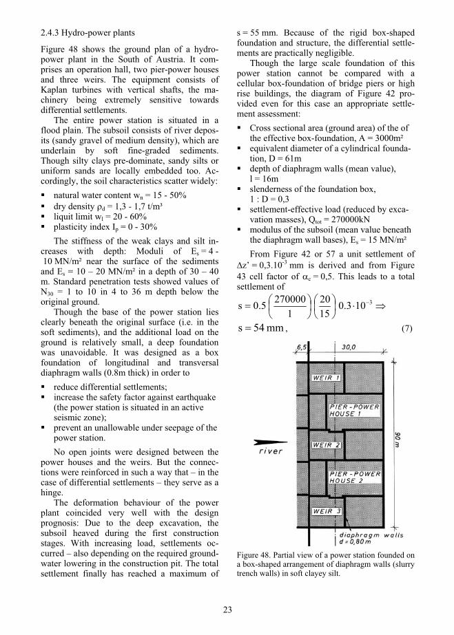
Figure 48 shows the ground plan of a hydro-power plant in the South of Austria. It com-prises an operation hall, two pier-power houses and three weirs. The equipment consists of Kaplan turbines with vertical shafts, the ma-chinery being extremely sensitive towards differential settlements.

The entire power station is situated in a flood plain. The subsoil consists of river depos-its (sandy gravel of medium density), which are underlain by soft fine-graded sediments. Though silty clays pre-dominate, sandy silts or uniform sands are locally embedded too. Ac-cordingly, the soil characteristics scatter widely:

natural water content wn = 15 - 50% dry density d = 1,3 - 1,7 t/m³ liquit limit wl = 20 - 60% plasticity index Ip = 0 - 30% The stiffness of the weak clays and silt in-

creases with depth: Moduli of Es = 4 - 10 MN/m² near the surface of the sediments and Es = 10 – 20 MN/m² in a depth of 30 – 40 m. Standard penetration tests showed values of N30 = 1 to 10 in 4 to 36 m depth below the original ground.

Though the base of the power station lies clearly beneath the original surface (i.e. in the soft sediments), and the additional load on the ground is relatively small, a deep foundation was unavoidable. It was designed as a box foundation of longitudinal and transversal diaphragm walls (0.8m thick) in order to

reduce differential settlements; increase the safety factor against earthquake (the power station is situated in an active seismic zone); prevent an unallowable under seepage of the power station. No open joints were designed between the

power houses and the weirs. But the connec-tions were reinforced in such a way that – in the case of differential settlements – they serve as a hinge.

The deformation behaviour of the power plant coincided very well with the design prognosis: Due to the deep excavation, the subsoil heaved during the first construction stages. With increasing load, settlements oc-curred – also depending on the required ground-water lowering in the construction pit. The total settlement finally has reached a maximum of

s = 55 mm. Because of the rigid box-shaped foundation and structure, the differential settle-ments are practically negligible.

Though the large scale foundation of this power station cannot be compared with a cellular box-foundation of bridge piers or high rise buildings, the diagram of Figure 42 pro-vided even for this case an appropriate settle-ment assessment:

Cross sectional area (ground area) of the of the effective box-foundation, A = 3000m² equivalent diameter of a cylindrical founda-tion, D = 61m depth of diaphragm walls (mean value), l = 16m slenderness of the foundation box, 1 : D = 0,3 settlement-effective load (reduced by exca-vation masses), Qtot = 270000kN modulus of the subsoil (mean value beneath the diaphragm wall bases), Es = 15 MN/m² From Figure 42 or 57 a unit settlement of

z’ = 0,3.10-3 mm is derived and from Figure 43 cell factor of c = 0,5. This leads to a total settlement of

3103.01520

12700005.0s

mm54s , (7)

Figure 48. Partial view of a power station founded on a box-shaped arrangement of diaphragm walls (slurry trench walls) in soft clayey silt.

23

Figure 49. Cross section (in river flow direction) through a partition pier of the river Danube hydropower plant in Vienna (14 000 m3/s flood capacity). Box-shaped foundation on diaphragm walls arranged as stiffening cells.

Figure 49 shows a cross section through the hydropower plant Vienna at the river Danube (designed for 14 000 m3/s, width = 450 m). This is the first facility constructed in a densely populated area, situated on a geological fault and in a seismic area. Consequently, a deep box-shaped foundation consisting of slurry trench walls forming stiffening cells was exe-cuted. Such foundation schemes have proved suitable for all kinds of buildings with high vertical and/or horizontal loads.

2.4.4 Box-shaped foundations with raked piles

In rivers with shipping, high flow velocity and danger of scouring bridge piers (including their foundation) should be as small as possible and hydraulically friendly. Consequently, truncated cone box foundations are an interesting alterna-tive to the classical prismatic shape. Figure 50 shows a vertical cross section of such a founda-tion, and Figure 51 illustrates the horizontal sections on top and toe of the piles. The Figures 52 and 53 show a smaller box foundation.

In both cases the piles were excavated through a fly ash body which was filled into the box of precast elements placed on the river bed (and fixed by the pilot piles).

This measure facilitated a precise installa-tion of the raked piles and increased the com-posite behaviour of the box foundation. The pilot piles were installed before (from ships) in order to have fixing points for further equip-ment and for sinking the r.c. precast elements

on the river bed. Therefore the steel casing was not withdrawn near their head zone. Moreover, the pilot piles were excavated to a greater depth than the standard piles in order to gain detailed additional information about the in-situ ground properties beneath the bottom of the box-

Figure 50. Vertical section through a box foundation with raked piles – for a pier of a river bridge.

24

Figure 51. Horizontal section through the pile heads of Figure 50. Position of pile toes indicated by broken line circles.

Figure 52. Horizontal sections through a box founda-tion with raked piles: Example of a small box. Section 1-1 is in the level of pile heads, section 3-3 in the level of pile toes.

foundation. The installation of raked piles for a box foundation like a frustum of a cone or pyramid is rather difficult, especially if they have to be excavated from a ship or swimming platform.

Consequently, but also for geometrical rea-sons, the box effect decreases with depth. Such a foundation may be considered a structure behaving between a box-foundation and a piled raft foundation.

Figure 53. To Figure 52: View of the longer side of the pile box.

3. COMPARISON OF DEEP FOUNDATIONS

In order to prove the reliability of geotech-nical theories and the general application of test results to the practice, in-situ measurements on construction sites and on completed structures are essential. Figures 54 to 56 show some examples of deep foundations in tertiary sedi-ments, overlain by quaternary river deposits (in Vienna and Lower Austria). The tertiary layers are over-consolidated and consist of sandy to clayey silt (locally silty sand and silty clay). The ground properties, of course, scatter in spite of the same geological genesis along the river Danube in Vienna and nearby. Nevertheless, the site conditions of the structures can be fairly compared. The deep foundations elements were large diameter bored or auger piles (d = 0.9 to 1.2 m) or diaphragms walls (thickness, d = 0.6 to 0.8 m).

The data are again plotted in dimensionless diagrams – similar to the results from the model tests. The normalized graphs enable a direct comparison.

Figure 54 shows the results from some high- rise buildings in Vienna. All buildings have

25

Figure 54. Normalized load-settlement behaviour of some high-rise buildings in Vienna, founded on bored or auger piles. s = settlement, d = pile diameter, Q = total load on the foundation, A = foundation area (horizontal sectional area within circumference of pile box), = density of soil, H = height of building, l = pile length

deep basements, i.e. the top of the foundation lies clearly below original surface, and the foundations are below groundwater level. The pile lengths are of about similar magnitude; differences are only local, depending on statical or structural reasons. The diagram illustrates very clearly the advantage of piled raft founda-tions over a conventional pile foundation (Business Park). The optimum behaviour of the Millennium Tower can be explained by pile preloading and a soil improvement in the top zone of the foundation: loose sandy gravel, overlying the tertiary silt was densified by vibroflotation.

Figure 55 shows normalized load-settlement curves of several box-shaped foundations with diaphragm walls. A comparison underlines the following interacting influence factors:

Length (depth) of wall elements: Widely superimposed by other factors, because l = 18 – 22 m is roughly of a similar magni-tude. Hence of secondary influence in this special case. Level of foundation head: The high-rise building without deep basement (Mischek Tower) settled more than the others. Way of installation: The installation from a higher working level improves the bearing- deformation behaviour of diaphragm walls

Figure 55. Normalized load-settlement behaviour of some high-rise buildings in Vienna, founded on diaphragm walls. s = settlement, d = thickness of diaphragm wall, Q = total load on the foundation, A = foundation area (horizontal sectional area within circumference of diaphragm wall box), = density of soil, H = height of building, l = depth of diaphragm wall

(e.g. IZD-Tower) - and bored or auger piles likewise. The positive effect of an uncast pile length or uncast diaphragm wall depth could be observed on many construction sites. It is achieved because the soil along the top zone of the deep foundation is less disturbed during the installation procedure. Influence of geological overconsolidation: The Twin Tower is situated in an area of less overconsolidation than the other build-ings. Arrangement of diaphragm walls: The buildings of the UNO-City Vienna are founded on box-shaped as well as on cross-shaped diaphragm wall elements. The latter settled more, because the composite effect between single barrettes or cross-shaped concrete panels and soil is clearly smaller than for box-foundations. Figure 56, finally, compares high-rise build-

ings and bridges, whereby the following influ-ence factors played a relevant role:

Load area and total load, hence depth and extent of stress bulb in the ground: Millen-nium Tower and UNO-City create a deep reaching stress field. Magnitude of geological overconsolidation: This is greater for both bridges (crossing the

26

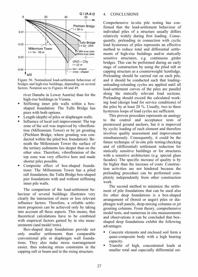
Figure 56. Normalized load-settlement behaviour of bridges and high-rise buildings, depending on several factors. Notation see to Figures 48 and 49.

river Danube in Lower Austria) than for the high-rise buildings in Vienna. Stiffening inner pile walls within a box-shaped foundation: The Tulln Bridge has piers with both options. Length (depth) of piles or diaphragm walls. Influence of local soil improvement: The top zone of the soil was improved by vibroflota-tion (Millennium Tower) or by jet grouting (Pöchlarn Bridge, where grouting was con-ducted within the piled box foundation). Be-neath the Millennium Tower the surface of the tertiary sediments lies deeper than on the other sites. Therefore, vibroflotation of the top zone was very effective here and made shorter piles possible. Composite effect of box-shaped founda-tions: The Millennium Tower has a piled raft foundation, the Tulln Bridge box-shaped pier foundations with and without stiffening inner pile walls. The comparison of the load-settlement be-

haviour of several buildings illustrates very clearly the interaction of more or less relevant influence factors. Therefore, a reliable settle-ment prognosis can be achieved only by taking into account all these aspects. This means, that theoretical calculations have to be combined with empirical factors gained by in situ meas-urements (and model tests).

Box-shaped deep foundations provide not only smaller settlements than comparable conventional pile or diaphragm wall founda-tions. They also make stress rearrangement easier, thus reducing stress constraints in the capping raft or beam and in the rising structure.

4. CONCLUSIONS

Comprehensive in-situ pile testing has con-firmed that the load-settlement behaviour of individual piles of a structure usually differs relatively widely during first loading. Conse-quently, preloading in connection with cyclic load hystereses of piles represents an effective method to reduce total and differential settle-ments of high-rise buildings and/or statically sensitive structures, e.g. continuous girder bridges. This can be performed during an early stage of construction by using the piled raft or capping structure as a counterweight/ kentledge. Preloading should be carried out on each pile, and it should be conducted such that loading-unloading-reloading cycles are applied until all load-settlement curves of the piles are parallel along the statically relevant load sections. Preloading should exceed the calculated work-ing load (design load for service conditions) of the piles by at least 20 %. Usually, two to three hysteresis loops of load cycles are sufficient.

This proven procedure represents an analogy to the control and acceptance tests of prestressed ground anchors, but it is improved by cyclic loading of each element and therefore involves quality assessment and improvement simultaneously. Consequently, it could be the future technique of in-situ pile testing/checking and of (differential) settlement reduction for statically sensitive buildings or for structures with a sensitive architecture (e.g. special glass facades). The specific increase of quality is by far higher than the increase of costs. Construc-tion activities are not hindered because the preloading procedure can be performed com-pletely independently from other construction work.

The second method to minimize the settle-ment of pile foundations that can be used also for other deep foundations is a box-shaped arrangement of (bored or auger) piles or dia-phragm wall panels, deep-mixing columns or jet grouting columns. From theory, comprehensive model tests, and numerous in situ measurements and observations it can be concluded that box-shaped deep foundations exhibit the following advantages:

Concrete elements and enclosed soil form a quasi-composite body with a high bearing capacity.Transfer of high, concentrated loads at smaller total and especially differential set-

27

tlements than in the case of conventional groups of piles or diaphragm wall panels. Smaller foundation area required than in the case of conventional pile groups with axial pile spacing of a 2d to 3d (d = pile diame-ter). This is especially important for bridge piers situated in rivers. High resisting moment against lateral forces from high embankments on soft soil (acting on bridge abutments) or from unstable slopes (e.g. creeping pressure). Very suitable in the case of strongly hetero-geneous and anisotropy ground. High resistance to earthquake and soil liquefaction. High resistance to scouring (foundations in rivers, torrents, harbours). Very suitable in the case of dynamic loading processes: E.g. ship impact, dynamic loads due to waves and unstable currents, (turbu-lent) wind loading of tall structures, shock loads due to unstable silo flow. Suitable for post-strengthening existing buildings, for instance piers of river bridges: Increase of stability against ground failure in the case of scouring. Very suitable in the case of fluctuating and cyclic loading processes: E.g. cycles of (ground-)water level, storage level fluctua-tions (oil tank farms, storage silos) or wave induced cyclic loads.

5. REFERENCES

Brandl, H. 1987. Deep box-foundations with piles and diaphragm walls in weak soils. Proceedings of 9th Southeast Asian Geotechnical Conference. Bangkok.

Brandl, H. 2001. Box-shaped pile and diaphragm wall foundations for high loads. Proceedings of the 15th ICSMGE. Istanbul.

Brandl, H. & Hofmann, R. 2002. Tragfähigkeits- und Setzungsverhalten von Kastenfundierungen. Re-search Report, Volume 528. Federal Ministry for Traffic, Innovation and Technology. Vienna.

Hazivar, W. 1979. Tragverhalten von Brunnen-gründungen, Volume 14, Institute for Soil Me-chanics and Geotechnical Engineering, Vienna University of Technology.

Hofmann, R. 2001. Trag- und Setzungsverhalten von Pfahlkästen. Doctoral Thesis, Vienna University of Technology.

Japanese Geotechnical Society, 1998. Remedial measures against soil liquefaction. A.A. Balkema, Rotterdam.

Mindlin, R.D. 1936. Force at a Point in the Interior of a Semi Infinite Solid. Physics, Vol. 7.

6. APPENDIX

Figure 57 represents an additional design chart for box-shaped deep foundations (to Figure 42) considering more detailed the equivalent diame-ter D.

Figure 57. Settlement curves for a cylindrical box foundation under a unit load of Q = 1 kN. Slenderness l/D of the foundation as parameter, whereby l = depth of pile or diaphragm wall foundation. Unit modulus of soil Es = 20 MN/m², d = wall thickness. For non-cylindrical foundations: D = equivalent diameter.

28

Excavation support using deep mixing technology J.-L. Briaud Professor and Holder of the Buchanan Chair Zachry Department of Civil Engineering Texas A&M University

C. J. Rutherford Doctoral Research Assistant Zachry Department of Civil Engineering Texas A&M University

ABSTRACT: Deep Soil Mixing (DSM) for excavation support is a relatively recent technique which can be veryhelpful and economical when used in the right circumstances. In a first part DSM is compared with other typesof excavation walls and wall supports such as structural diaphragm walls, sheet-pile walls, soldier pile andlagging walls, tiebacks and internal struts. A design flow chart is presented and each step is discussed. One of theadvantages of such walls is that the engineer can control movements by choosing the support loads. Six casehistories are briefly described to illustrate the statements made in the paper. They include (1) EBMUD StorageBasin, Oakland, CA; (2) Lake Parkway Project, Milwaukee, WI; (3) Central Artery/Tunnel Project, Boston, MA;(4) Honolulu Excavation, Honolulu, HI; (5) Oakland Airport Roadway Project, Oakland, CA; and (6) VERTWall, Texas A&M University.

1. BACKGROUND

Deep soil mixing (DSM) for excavation support involves constructing a support wall by mixing in situ soils with a stabilizing agent. Some of the other common names used to describe this method are Cement Deep Soil Mixing (CDSM), Deep Mixing Method (DMM), or Soil Mix Wall (SMW) method (Porbaha, 1998). The mixed-in-place excavation support walls are well suited for urban areas with high groundwater levels since the placement of DSM columns causes little disturbance to the surroundings and gener-ates low vibration and noise pollution. Numer-ous projects have incorporated deep mixing for excavation support and cutoff walls. One of the first major applications of deep soil mixing for excavation support in the United States was the Wet Weather Storage Basin for the East Bay Municipal Utility District (EDMUD) project in Oakland, California constructed in 1990 (Taki and Yang, 1991). One of the largest projects in the United States involving DSM technology is the Boston Central Artery and Tunnel (CA/T) project (O’Rourke and O’Donnell, 1997a and 1997b; O’Rourke et al., 1998, O’Rourke and McGinn, 2004).

The implementation of deep mixing technol-ogy into American excavation support design and construction practices is growing due to the various advantages it offers over traditional support systems. Although the design process

for DSM walls is similar to traditional walls, there are steps that are unique to DSM walls. This paper discusses DSM technology for DSM walls and compares them to other top down wall types. A design flowchart and the steps recom-mended for design of deep soil mixed walls for excavation support are presented.

Deep mixing has become a general term used to describe a number of soil improvement and soil mixing techniques. The most common method of deep mixing for excavations involves overlapping soil cement columns that are either installed using a multi–auger rotary shaft or a drilling tool. The stabilizing agent is usually a slurry mixture of cement, water, and sometimes bentonite. The material resulting from mixing the natural soil with small amounts of cement has the advantage of improved soil strength and stiffness

Deep mixing technology is effectively used in excavations both in conjunction with and in substitution of traditional techniques. It gener-ally results in economical and convenient solutions for the stability of the system and the prevention of seepage. Deep mixed walls constructed as part of a soldier pile and tie-backs system act also as temporary support, prevent seepage like a sheet pile wall, but require a lower amount of steel (Figure 1). The deep mixed treatment can also contribute to the stability of the wall system against deep-seated failures.

29

Figure 1. Typical Arrangement of Soil Cement Columns

1.1 Types of walls and wall supports used in urban excavations

A variety of excavation walls and wall support systems are currently used. The prevalence of one system over the others in a certain region depends on several factors including: local experience, site conditions, availability and cost of materials and the amount of support required for the project. The advantages and limitations of common types of excavation walls were compiled based on general knowledge and the opinion of experts (Table 1).

Information regarding the advantages and limitations of various types of supports used for excavation walls was compiled based on general knowledge and expert opinion (Table 2). Site conditions often control the use of tie-back/anchors compared to internal struts.

1.2 Advantages and limitations of deep soil mixing

There are many advantages of DSM walls compared to other walls types and traditional techniques. The placement of DSM columns causes little disturbance to the surrounding soil, and, allows installation close to an adjacent building’s foundation. Unlike driving sheet piles, DSM construction generates low vibration and noise pollution. The construction is also typically faster than other traditional methods. One advantage over slurry (diaphram) walls is a decrease in the volume of spoils generated.

The ability to create soil cement columns to stabilize the base against deep rotational failure is also an important advantage. Soil cement buttresses (continuous grid of columns installed in the base of the excavation) are used to stabi-lize deep excavations and improve bearing capacity, prevent deep rotational failures and decrease ground deformation. Another advan-tage of DSM walls is that steel wide flange beams, which are very efficient in resisting

Table 1. Comparison of Types of Excavation Walls ExcavationSupportSystem

Advantages Limitations

Deep Soil Mixing(DSM)

Installation causes little disturbance to surrounding soil. Constructiongenerates low vibration and noise pollution. Decreased volume of spoils. Spoil can be handled as solid waste. In situ quality verifi-able through wet sampling and cores.

Need large space for equipment and overhead restrictions. Spoils generated and disposals of excess soil and soil cement required. Cannot be installed through complex fills, boulders or other obstructions. Limited depth.

StructuralDiaphram(Slurry)Wall

Constructed before excavation and below ground water, good water seal, can be used forpermanent wall and can be used in most soils. Relatively high stiffness.

Large volume of spoils generated and disposal of slurry required. Costly compared to other methods.

SheetpileWall

Constructed before excavation and below ground water.Can be used only in soft to medium stiff soils. Quickly constructed and easily removed.Low initial cost.

Cannot be driven through complex fills, boulders or other obstructions.Vibration and noise with installation.Possible problems with joints. Limited depth and stiffness.Relatively large lateral movements.

SoldierPile and LaggingWall

Low initial cost. Easy to handle and construct.

Lagging cannot bepractically installed below groundwater. Cannot be used in soils that do not have arching or that exhibit baseinstability.

SecantWall/Tangent Pile Wall(similar to DSMwalls)

Constructed before excavation and below ground water.Low vibration and noise. Can use wide flange beams for reinforcement.

Equipment cannot penetrate boulders, requires pre–drilling. Continuity can be a problem if piles drilled one at a time.

Micro–pileWall

Constructed before excavation and below ground water.Useful when limited right of way.

Large number required. Continuity a problem, low bending resistance.

30

bending, can be placed in the soil cement columns as reinforcement. The strength of the soil cement columns can be changed based on project requirements by varying the ratio of cement and water to the in situ soil. Typical soil cement mixes have a cement-slurry to soil volume ratio varying from 0.15 to 0.40. This range allows the designer to control deforma-tions through soil cement specifications and system stiffness (anchors or struts). Due to advances in mixing equipment, real–time monitoring, and alignment control, deep mixing has become an efficient method for excavation support.

Table 2. Comparison of Types of Supports for Excavation Walls

Type of Support

Advantages Limitations

Tiebacks Reduces depth of embedmentbelow bottom of excavation, keeps overhead clear during excava-tion. Can be permanent under limitedconditions.

Difficult to install tiebacks below groundwater, Ease-ments required if outside property limits.

InternalStruts

Does not extend beyond excava-tion walls, reduces depth of embedmentbelow bottom of excavation.

Overhead and lateral obstruction for excavation of trench. Subjected to tempera-ture changes, requires internal vertical support for wideexcavations.

The initial feasibility of the application of DSM to excavations is dependent on site condi-tions and economics. Sites with ground settle-

ment sensitivity, vibration sensitivity, high groundwater table, and/or soft soils are often good candidates for the use of deep soil mixing. Economic considerations for determining the advantage of deep mixing versus traditional techniques differ 1) regionally, due to many factors such as availability of equipment, mate-rials, labor; and 2) based on the details of the project. As with all other excavation support techniques, the presence of utilities, subways, or other underground structures may determine whether or not deep mixing is viable at a site. DSM is likely to produce the least amount of disruption and adverse impacts compared to other methods.

Some limitations of DSM walls include the following. Stiff layers of soil may require pre–drilling to ensure homogenous soil cement columns. Spoils are generated and disposal of excess soil and soil cement is required. Soil cement columns cannot be installed through complex fills, boulders or other obstructions. There is a limited depth of installation which is dependent upon the DSM equipment. Due to the large equipment required, there are both space and overhead restrictions.

2. DEEP MIXING TECHNOLOGY

2.1 Historical Background

Excavation support using deep soil mixing technology evolved from the early 1970’s Japanese practice, in which single soil-cement columns were created to support excavations and act as cut-off walls. Examples of events which took place in the second half of the 20th century are shown in Figure 2.

Figure 2. Some Deep Mixing for Excavation Support Events

31

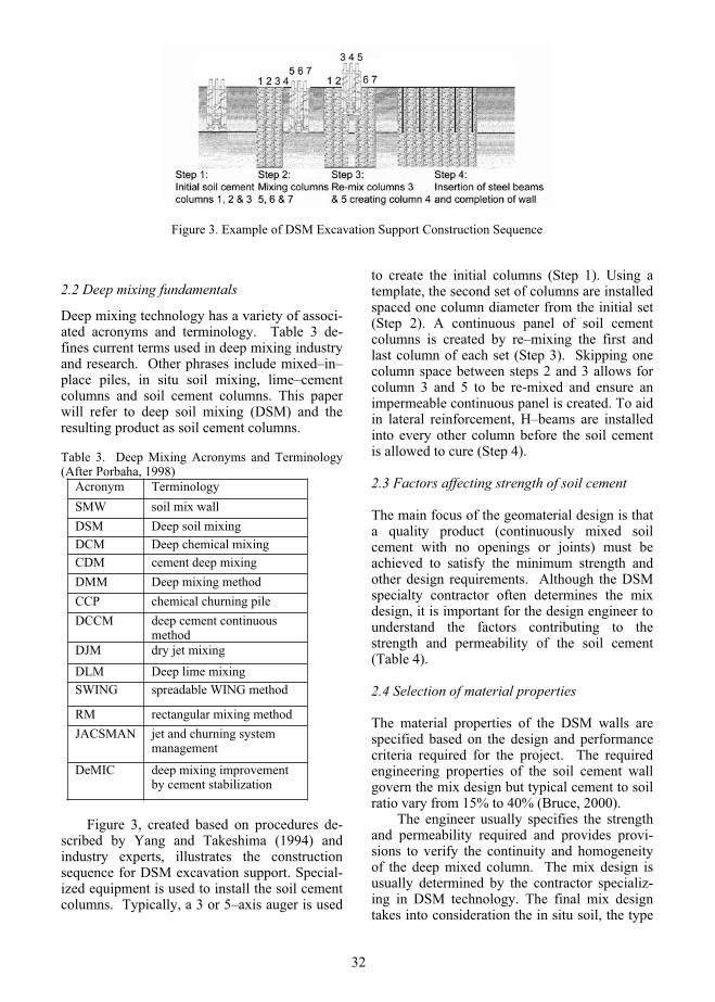
Figure 3. Example of DSM Excavation Support Construction Sequence

2.2 Deep mixing fundamentals

Deep mixing technology has a variety of associ-ated acronyms and terminology. Table 3 de-fines current terms used in deep mixing industry and research. Other phrases include mixed–in–place piles, in situ soil mixing, lime–cement columns and soil cement columns. This paper will refer to deep soil mixing (DSM) and the resulting product as soil cement columns.

Table 3. Deep Mixing Acronyms and Terminology (After Porbaha, 1998)

Acronym Terminology SMW soil mix wall DSM Deep soil mixing DCM Deep chemical mixing CDM cement deep mixing DMM Deep mixing method CCP chemical churning pile DCCM deep cement continuous

methodDJM dry jet mixing DLM Deep lime mixing SWING spreadable WING method

RM rectangular mixing method JACSMAN jet and churning system

management

DeMIC deep mixing improvement by cement stabilization

Figure 3, created based on procedures de-scribed by Yang and Takeshima (1994) and industry experts, illustrates the construction sequence for DSM excavation support. Special-ized equipment is used to install the soil cement columns. Typically, a 3 or 5–axis auger is used

to create the initial columns (Step 1). Using a template, the second set of columns are installed spaced one column diameter from the initial set (Step 2). A continuous panel of soil cement columns is created by re–mixing the first and last column of each set (Step 3). Skipping one column space between steps 2 and 3 allows for column 3 and 5 to be re-mixed and ensure an impermeable continuous panel is created. To aid in lateral reinforcement, H–beams are installed into every other column before the soil cement is allowed to cure (Step 4).

2.3 Factors affecting strength of soil cement

The main focus of the geomaterial design is that a quality product (continuously mixed soil cement with no openings or joints) must be achieved to satisfy the minimum strength and other design requirements. Although the DSM specialty contractor often determines the mix design, it is important for the design engineer to understand the factors contributing to the strength and permeability of the soil cement (Table 4).

2.4 Selection of material properties

The material properties of the DSM walls are specified based on the design and performance criteria required for the project. The required engineering properties of the soil cement wall govern the mix design but typical cement to soil ratio vary from 15% to 40% (Bruce, 2000).

The engineer usually specifies the strength and permeability required and provides provi-sions to verify the continuity and homogeneity of the deep mixed column. The mix design is usually determined by the contractor specializ-ing in DSM technology. The final mix design takes into consideration the in situ soil, the type

32

of equipment used, the installation procedure, the required quality, and the economics of the project (Taki and Yang, 1991).

Table 4. Factors Affecting Soil Cement Strength (After Terashi, 1997)

1. Type of stabilizing agent

2. Quality

I. Characteristics of stabilizing agent

3. Mixing water and additives1. Physical chemical and mineralogical properties of soil

2. Organic content

3. pH of pore water

II. Characteristics and conditions of soil (especially important for clays)

4. Water content

1. Degree of mixing

2. Timing of mixing/re–mixing3. Quantity of stabilizing agent

III. Mixingconditions

4. Soil cement ratio

1. Temperature

2. Curing time

3. Humidity

IV. Curingconditions

4. Wetting and dry-ing/freezing and thawing

For the Fort Point Channel deep mixing project for example, during the pre-construction soil cement testing program, eight mixes were used for the clay ranging in cement factor from 1.12 to 4.65 kN/m3. The cement factor is the total weight of dry cement divided by the total volume of treated soil. For the organic silt, the three mixes cement factors ranged from 0.94 to 2.14 kN/m3. A water to cement ratio equal to 1.25 was used for the each of the mixes (McGinn and O’Rourke, 2003).

2.5 Strength, permeability and Young’s modulus

Unconfined compression tests are usually conducted in the laboratory on specimens prepared from wet grab samples and specimens trimmed from core samples. As described by McGinn and O’Rourke (2003), a database of unconfined compression tests was compiled for

the Fort Point Channel deep mixing project. Statistical analysis was conducted to find trends. Tests results demonstrated that the unconfined compressive strength data could be reasonably characterized by a lognormal distribution to a 5% significance level.

Although the data was for a specific loca-tion, there was considerable variability in the unconfined compressive strength results. Varia-tions in soil conditions, mixing process and sampling procedures contributed to the variabil-ity of data. Bias in the data reflected in both lower unit weight and higher unconfined com-pressive strength for the wet grab samples compared with the core samples was determined to be due to the relatively small opening of the wet grab sampler. Unconfined compression strength specified for an excavation support cutoff wall is usually greater than 700 kPa (Taki and Yang, 1991). Figure 4 gives example values of the unconfined compression strengths of a soil, a soil cement mixture and concrete.

Figure 4. Strength Comparisons (Example Values)

Soil type, quantity of cement, water cement ratio, age, and injection ratio of cement affect the permeability of the soil cement (Taki and Yang, 1991). The permeability of the soil cement is also affected by pore size distribution (Kunito et al., 1988). The higher percentage of fine pores reduces the soil cement permeability. Hydraulic conductivity usually ranges from 10–5

to 10–6 cm/s for soil-cement (Taki and Yang, 1991).

The modulus of a soil is a complex parame-ter which requires a precise definition when quoted. The modulus depends on the stress level, the strain level, the rate of loading, the number of cycles and other factors. The range of Young’s moduli in soils is approximately 5 to 1000 MPa. Table 5 presents the approximate ranges of various materials. The addition of cement grout in soils increases the modulus but this increase is not well docu-mented. Briaud et al. (2000) present results from a full scale, extensively instrumented DSMproject at Texas A&M University (Figure

33

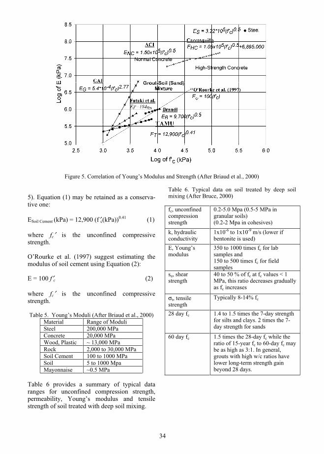
Figure 5. Correlation of Young’s Modulus and Strength (After Briaud et al., 2000)

5). Equation (1) may be retained as a conserva-tive one:

ESoil Cement (kPa) = 12,900 (f′c(kPa))0.41 (1)

where fc′ is the unconfined compressive strength.

O’Rourke et al. (1997) suggest estimating the modulus of soil cement using Equation (2):

E = 100 f′c (2)

where fc′ is the unconfined compressive strength.

Table 5. Young’s Moduli (After Briaud et al., 2000) Material Range of Moduli Steel 200,000 MPa Concrete 20,000 MPa Wood, Plastic ~ 13,000 MPa Rock 2,000 to 30,000 MPa Soil Cement 100 to 1000 MPa Soil 5 to 1000 Mpa Mayonnaise ~0.5 MPa

Table 6 provides a summary of typical data ranges for unconfined compression strength, permeability, Young’s modulus and tensile strength of soil treated with deep soil mixing.

Table 6. Typical data on soil treated by deep soil mixing (After Bruce, 2000)

fc, unconfined compressionstrength

0.2-5.0 Mpa (0.5-5 MPa in granular soils) (0.2-2 Mpa in cohesives)

k, hydraulic conductivity

1x10-6 to 1x10-9 m/s (lower if bentonite is used)

E, Young’s modulus

350 to 1000 times fc for lab samples and150 to 500 times fc for field samples

su, shear strength

40 to 50 % of fc at fc values < 1 MPa, this ratio decreases gradually as fc increases

σt, tensile strength

Typically 8-14% fc

28 day fc 1.4 to 1.5 times the 7-day strength for silts and clays. 2 times the 7-day strength for sands

60 day fc 1.5 times the 28-day fc while the ratio of 15-year fc to 60-day fc may be as high as 3:1. In general, grouts with high w/c ratios have lower long-term strength gain beyond 28 days.

34

3. DESIGN OF EXCAVATION USING DEEP MIXING TECHNOLOGY

3.1 Modes of failure

A variety of possible modes of failure exist for both supported walls and gravity walls. Al-though DSM wall components differ from traditional wall elements in construction tech-niques and materials, they essentially perform the same function. For this reason the discus-sion of modes of failures for deep mixed walls follows closely the list of mechanisms estab-lished in the literature for traditional construc-tion. In general, failure modes can be divided into four main categories: (1) instability due to seepage; (2) global instability; (3) geotechnical failure; and (4) structural failure.

3.1.1 Instability due to seepage

Seepage instability can occur due to boil-ing/piping or base heave when the water level is lower inside the excavation than outside the excavation causing water to flow under the wall into the excavation (McNab, 2002). The effec-tive stress in the volume of soil below the bottom of the excavation, extending to the embedment depth of the wall – referred to as plug – can be reduced significantly by the pore water pressures. As a result there can be a loss of horizontal passive resistance leading to inward failure of the retaining wall. The seep-age forces may decrease the effective stresses, causing a “quick” condition. A “cork” effect or “plug” heave occurs when the excavation site consists of sand underlying a clay layer.

3.1.2 Global instability

Global instability occurs when a failure surface develops and can be analyzed using a variety of slope stability approaches. An inverted bearing capacity failure occurs when the overburden pressure outside the excavation overcomes the shear strength of the soil, causing soil to flow into the excavation under the wall (McNab, 2002). Inverted bearing capacity failures not only cause instability to the excavation due to the decrease in bearing capacity, but can cause lateral movement and damage to adjacent facilities.

3.1.3 Geotechnical failures

Geotechnical failures occur when the imposed loads are greater than the strength of the soil (McNab, 2002). Figure 6(a) illustrates a case of the settlement of the soil cement columns. Settlement of the toe can occur if the downward component of the anchor and downdrag on the column is larger than the bearing capacity of the soil. As the column settles the anchor rotates.

This movement can cause lateral deforma-tions and damage to adjacent facilities. Figure 6(b) illustrates passive resistance failure at the base of the excavation allowing the wall to rotate. Other geotechnical failures include failure by overturning, sliding or translation, and rotational failure of the ground mass. Raker failures are illustrated in Figure 6(c) and Figure 6 (d). Column toe uplift can cause a failure in tension allowing the wall to rotate up and forward. A bearing capacity failure under the raker would cause large lateral deformations of the wall.

3.1.4 Structural failures

Structural failure occurs when a portion of the shoring system cannot withstand imposed loads (McNab, 2002) which include failure of the wall above a tieback, failure of the wall at mid–span, failure of a tieback tendon or connection fail-ures. As in the case as base instability, struc-tural failures result in large displacements which can cause damage to nearby facilities.

Figure 6. Geotechnical Failures (After McNab, 2002)

35

3.2 Design flowchart

Deep mixing walls are designed following techniques similar to those used for traditional excavation support methods. Three major approaches to design and analyze excavation support walls exist: (a) the hand calculation approach; (b) the beam–column approach; and (c) the finite element approach. This paper will outline hand and chart methods and make recommendations for computer-aided ap-proaches.

A step-by-step design procedure (Figure 7) for the use of deep mixing for excavation control was developed. A flowchart of the following steps is presented in the manual(https://ceprofs.civil.tamu.edu/briaud/DSM%20Manual.pdf): (1) Site investigation, (2) Wall type, (3) Performance criteria, (4) Seepage analysis, (5) External stability, (6) Wall compo-nent design, (7) Vertical capacity of wall, (8) Structural resistance of retaining elements, (9) Wall deflections and soil deformation, and (10) Specifications and other considerations.

Once the feasibility of DSM technology is determined, the function and design criteria for the wall must be established. Following this step, the soil properties are collected and design soil parameters are selected. The type of retain-ing wall system is decided based on cost, site conditions, required wall height, speed of construction, and other project specific require-ments. A seepage analysis is carried out using initial wall geometry. The external stability is evaluated, followed by the retaining wall design. The vertical capacity of the wall is calculated and the structural resistance of the retaining elements checked. Finally, other considerations such as settlement, freeze–thaw, and seismic conditions are analyzed.

3.2.1 Seepage analysis

For temporary retaining systems, the wall should be designed to resist water forces associ-ated with seepage behind and beneath the wall. Piping occurs when the water head is sufficient to produce critical velocities in cohesionless soils causing a “quick” condition at the bottom of the excavation. “Quick” condition in coarse grain soils occurs when the effective stress becomes zero. Methods to decrease instability are dewatering, application of a surcharge on the bottom of the excavation, or extending the embedment of the wall. Bottom

Figure 7. Design Flowchart

heave should be evaluated for clay soils under seepage conditions. Bottom heave can also occur in cohesionless soils, although rare.

Vertical ground displacements at the base of the excavation can lead to lateral displace-ments behind the wall. The impermeable layer should be depressurized if heave is expected. The wall embedment should also be extended if heave failure is possible. Soil improvement of the base of the excavation such as buttressing is also possible to strengthen the base against heave.

A variety of finite element software exists that can be used to model seepage and pore–water pressure distributions. Some programs allow both saturated and unsaturated flow modeling and the ability to model the dissipa-tion of excess pore–water pressure. Common required inputs include geometry, material properties (coefficient of hydraulic conductivity, unit weight), and boundary conditions. Program output includes pore pressures, velocity vectors, flow paths, flux values, phreatic surface lines and flownets. Example programs include SEEP–W, GEOFLOW, FLONET and PLAXIS.

36

3.2.2. External stability analysis

An overall or global stability analysis looks at rotational or compound failure mechanisms. A classical slope stability analysis is used to determine the external stability of the retaining system. Classical methods include the method of slices such as Bishop’s method and Janbu’s method as well as the wedge method, and others. Typical potential failure surfaces in-clude circular failure surface, noncircular failure surface and sliding block failure surface. An inverted bearing capacity failure occurs when the difference in overburden pressures between the outside and the inside of the excavation overcomes the shear strength of the soil, causing the soil to flow into the excavation under the wall (McNab, 2002).

Global stability analysis can be performed using programs such as G–Slope, STABLE, GEOSLOPE, U-TEXAS and XSLOPE that evaluate potential slip surfaces or failure planes and perform Bishop and Janbu methods of analysis. Typical input includes geometry, soil properties (shear strength parameters, unit weight), loading and surcharge conditions and water conditions. Output includes factors of safety and potential failure surfaces.

3.2.3 Wall component design and vertical capacity

The geometry of the wall including the embed-ment and support locations is calculated based on the type of wall. The earth pressures, support loads and bending moments are calculated using traditional wall techniques. Earth pressure diagrams for the design of single sup-port/tieback walls have been a topic of much debate. Some recommend that a triangular earth pressure diagram (as with cantilever walls) be

used for single row anchored walls. Weatherby, (1998) and Mueller et al. (1998) recommend that the same apparent earth pressure diagrams used to design walls with multiple sup-port/tiebacks be used to design single sup-port/tieback walls.

The apparent total earth pressure or total horizontal pressure above the excavation, σh,can also be determined using a deformation control approach (Briaud and Lim, 1999) and is calculated using Equation 3. Deformation control design is discussed in more detail in section 3.2.5.

σh = k σ′ov + αu (3)

where σh is the constant total horizontal pressure above the excavation, k is the coefficient of apparent earth pressure (Figures 8 and 9), σ′ov is the effective vertical stress on the retained side at the excavation level, α is the ratio of water pore cross section area over the total pore cross section area. (α = 1 for saturated soils under the GWT and α = 0 for soils with no water), and uis the water stress (pore water pressure).

The earth pressure coefficient, k, is deter-mined using Figures 8 and 9 which link k and deflection. In the figures, Utop is the deflection at the top of the wall, Umean is the mean deflec-tion of the wall and H is the height of the exca-vation. These figures were generated using multiple case histories and finite element me-thod (FEM) simulations (Briaud and Lim, 1999). The graphs allow for the earth pressure coefficient to be determined using specified deflection criteria. The application of these recommendations is limited by the range of parameters studied.

37

Figure 8. Earth Pressure Coefficient Versus Top Defection (Briaud and Lim, 1999) (note: Earth pressure coefficient = mean pressure behind wall divided by unit weight times wall height;

Wall deflection = deflection at the top of the wall divided by the wall height)

Figure 9. Earth Pressure Coefficient Versus Mean Wall Deflection (Briaud and Lim, 1999) (Note: Earth pressure coefficient = mean pressure behind wall divided by unit weight times wall height; Wall

deflection = mean deflection of the wall divided by the wall height)

Two computer based methods, the bound-ary element method, BEM, and finite element method, FEM, are growing in popularity over the pressure diagram/hand calculation method. BEM is also called the beam–column method

(BMCOL), finite difference method or p–y/t–zcurve method.

The vertical capacity of the wall is deter-mined by summing the forces acting on the column. At the preliminary design stage, the

38

length of wall over which the downdrag, qn, acts may be taken equal to the excavation height. More accurate analysis require a computer aided analysis.

3.2.4 Structural resistance

The wall elements and anchor elements are designed in this step. The soil cement is de-signed to span between soldier beams similar to the lagging in the soldier beam/lagging walls (Taki and Yang, 1991). The stress analysis for the soil cement between the reinforcement beams includes evaluation of internal shear and compression stress of the soil cement (Figure 10). Based on finite element studies by Taki and Yang (1991), an empirical design criteria was developed to avoid bending failure in the soil-cement. Bending failure is checked by ensuring that Equation (4) is verified.

L2 D+h 2e (4)

where L2 is the distance between the end of the wide flange beams, D is the diameter of the soil-cement column, h is the height of the wide flange beam, and e is the eccentricity defined as the distance between the center of the wide flange beam and the center of the soil-cement column after trimming.

The spacing between the reinforcement members is determined by ensuring safety against failure in bending and shear of both the steel beam and the soil cement (Pearlman and Himick, 1993). The shear strength at the section where columns intersect and at the flange of the beams is checked (Figure 10). Pearlman and Himick (1993) recommend that the shear strength of the mixed soil be estimated as 1/3 of the unconfined compressive strength and a factor of safety of 2 or more be applied.

Richards (2008) suggests that for beam spac-ing of approximately 1.2 m, calculations of the shear resistance and the compressive arch produce similar required soil cement compres-sive strengths. However, the compressive arch governs for larger beam spacing whereas the shear failure governs for smaller beam spacing (Richards, 2008). The shear resistance can be estimated by using Equation (5).

Vmax = p•L2•bw (5)

where p is the maximum earth pressure, L2 the clear distance between flanges, bw is a unit

depthUsing the American Concrete Institute

(ACI) for nominal shear strength Equation (6):

Vc = λ•2•fc0.5•bw•d (6)

where λ for lightweight concrete is estimated as 0.75, fc for compressive strength of soil cement, bw is a unit depth and d is the height of the block.

From the sum of forces, Equations 7 thru 11 can be obtained,.

2•Vc>Vmax (7)

2•(λ•2•fc0.5•bw•d)> p•L2•bw (8)

fc0.5= (p•L2•bw)/( 2•(λ•2•bw•d)) (9)

Canceling bw:

fc0.5=(p•L2)/(2•(λ•2•d)) (10)

Therefore,

fc=[(p•L2)/(2•λ•2•d)]2 (11)

The compressive stresses inside the soil cement block between the soldier beams are also calcu-lated. Anchor design elements such as anchor type, corrosion protection, length, spacing, anchor resistance, bond length, and connection to retaining systems are determined following typical anchored wall design methodologies (Weatherby, 1998).

3.2.5 Deflections and soil deformation

The design of excavation support systems is evolving towards a deflection based design. Movements of in situ wall systems are related to the stiffness of the system. Briaud and Lim (1999) illustrate how anchor load magnitude directly influence deflection and bending mo-ments of tieback walls. Using the proposed kversus (utop /H) relationships in Figure 7 and 8, the engineer can select the anchor lock–off loads that will approximately generate a chosen deflection.

39

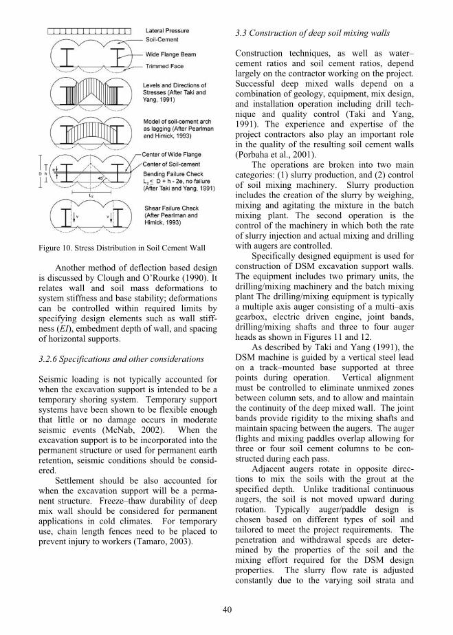
Figure 10. Stress Distribution in Soil Cement Wall

Another method of deflection based design is discussed by Clough and O’Rourke (1990). It relates wall and soil mass deformations to system stiffness and base stability; deformations can be controlled within required limits by specifying design elements such as wall stiff-ness (EI), embedment depth of wall, and spacing of horizontal supports.

3.2.6 Specifications and other considerations

Seismic loading is not typically accounted for when the excavation support is intended to be a temporary shoring system. Temporary support systems have been shown to be flexible enough that little or no damage occurs in moderate seismic events (McNab, 2002). When the excavation support is to be incorporated into the permanent structure or used for permanent earth retention, seismic conditions should be consid-ered.

Settlement should be also accounted for when the excavation support will be a perma-nent structure. Freeze–thaw durability of deep mix wall should be considered for permanent applications in cold climates. For temporary use, chain length fences need to be placed to prevent injury to workers (Tamaro, 2003).

3.3 Construction of deep soil mixing walls

Construction techniques, as well as water–cement ratios and soil cement ratios, depend largely on the contractor working on the project. Successful deep mixed walls depend on a combination of geology, equipment, mix design, and installation operation including drill tech-nique and quality control (Taki and Yang, 1991). The experience and expertise of the project contractors also play an important role in the quality of the resulting soil cement walls (Porbaha et al., 2001).

The operations are broken into two main categories: (1) slurry production, and (2) control of soil mixing machinery. Slurry production includes the creation of the slurry by weighing, mixing and agitating the mixture in the batch mixing plant. The second operation is the control of the machinery in which both the rate of slurry injection and actual mixing and drilling with augers are controlled. Specifically designed equipment is used for construction of DSM excavation support walls. The equipment includes two primary units, the drilling/mixing machinery and the batch mixing plant The drilling/mixing equipment is typically a multiple axis auger consisting of a multi–axis gearbox, electric driven engine, joint bands, drilling/mixing shafts and three to four auger heads as shown in Figures 11 and 12. As described by Taki and Yang (1991), the DSM machine is guided by a vertical steel lead on a track–mounted base supported at three points during operation. Vertical alignment must be controlled to eliminate unmixed zones between column sets, and to allow and maintain the continuity of the deep mixed wall. The joint bands provide rigidity to the mixing shafts and maintain spacing between the augers. The auger flights and mixing paddles overlap allowing for three or four soil cement columns to be con-structed during each pass. Adjacent augers rotate in opposite direc-tions to mix the soils with the grout at the specified depth. Unlike traditional continuous augers, the soil is not moved upward during rotation. Typically auger/paddle design is chosen based on different types of soil and tailored to meet the project requirements. The penetration and withdrawal speeds are deter-mined by the properties of the soil and the mixing effort required for the DSM design properties. The slurry flow rate is adjusted constantly due to the varying soil strata and

40

changes in penetration speed. Some spoils are produced during the con-

struction of the excavation support wall due to the loosening and mixing of in situ soil. Be-cause most of the slurry is used in the wall construction, the volume of spoils is smaller than those of other types of excavation construc-tion methods (Taki and Yang, 1991). Often the spoils are allowed to harden to facilitate in transportation from the site. Compared to traditional techniques, the cost of transporting the spoils decreases because the soil is mixed in situ rather than replaced, and the net quantity of excess material is considerably less (Porbaha et al., 2001).

Test columns can be constructed at project locations to calibrate the construction procedure and to obtain more accurate design parameters. The mix design can also be calibrated with pre-construction laboratory and site testing. Ando et al. (1995) found that the environ-mental impacts during the construction of deep mixing are minimal compared with other soil improvement methods. Both vibration and noise disturbances are minimized as well as ground displacement during construction. This is a distinct advantage of deep mixing over other

types of excavation support methods.

Figure 11. Three Auger DSM Equipment (After Taki and Yang, 1991)

Figure 12. DSM Equipment at CA/T Project, Boston, MA (After McGinn and O’Rourke, 2003)

41

3.4 Quality assessment and performance monitoring

Quality assessment of mixing and construction is of great importance to ensure the continuity and homogeneity of the excavation support wall. Strength and permeability tests are also per-formed to ensure the wall meets design specifi-cations. The slurry mixture condition, vertical alignment, penetration/withdrawal speeds, and flow of slurry contribute to the quality of the final DSM wall. Multiple methods of quality assessment have been developed for deep mixing construc-tion. Examination of the documentation of cement source and quality, records of cement mixing quantities and results of on–site tests for compressive strength of partially cured soil cement samples should always be included in the quality assessment program (Sabatini et al., 1997). During installation of the wall, the following mixing and positioning parameters should be monitored (1) Shaft rotation during penetration and withdrawal, (2) Velocity of shaft withdrawal, (3) Cement content of soil cement mixture, (4) Pumping rate of soil cement slurry mixture, (5) Amount of overlap between adjacent piles, and (6) Horizontal and vertical alignment (Sabatini et al., 1997). Both laboratory and field testing are used to determine and control the design parameters for the wall. Prior to construction of the soil cement wall, testing is performed on the samples pre-pared in the laboratory using in situ soil. Labo-ratory testing should be performed when no previous data is available or where the in situ soils contain material deleterious to soil cement (Taki and Yang, 1991). Selection of mixing equipment, installation parameters and proce-dures can be left to the Contractor. Field samples from the soil cement columns are obtained to insure the wall meets strength and permeability requirements. A sampler can be used at the designated depth to retrieve a soil cement bulk sample immediately after column installation. The test cylinders are prepared from the bulk samples retrieved from the col-umns. Unconfined compressive strength tests, direct shear tests, and triaxial compression tests are used to evaluate the strength characteristics of the soil cement mixture (Taki and Yang, 1991). Another method of testing the columns is the use of a reversed column penetrometer with

a probe or the standard cone penetrometer test (CPT). The Legeon Test Technique (also known as the Packer test – an in-situ method for deter-mining rock permeability) can be used to per-form the in situ permeability test (Holm, 2000). After the installation of the soil cement columns, monitoring techniques during the excavation are very important. Instrumentation should be used to verify the alignment and wall deformations of the excavation support. During the excavation, lateral wall movements, poten-tial bottom heave and settlement of areas behind the wall should be inspected and monitored carefully. Conventional techniques include the use of surveying, heave points, settlement plates, extensometers, inclinometers and other sophisticated measurement tools. Field instru-mentation is important for accurate monitoring of DM excavation support.

4. CASE HISTORIES OF DEEP MIXING FOR EXCAVATION SUPPORT

The following case histories (Table 7) are presented as innovative solutions to unique excavation problems: (1) EBMUD Storage Basin, Oakland, CA; (2) Lake Parkway, Mil-waukee, WI; (3) Bird Island Flats Boston, MA; (4) Marin Tower, Honolulu, HI; (5) Oakland Airport Roadway, Oakland, CA; and (6) VERT Wall, Texas A&M University.

Table 7. Case History Summary

CaseHistoryTitle

Excav.depth(m)

Embed.depth(m)

Max.Defl.(mm)

WallType

EBMUDStorageBasin

12 - 14

10.38 -12.38

57 Excav. support/cutoff

LakeParkwayProject

2.3 -9.9

7.3 -10.7

25 Excav.support/cutoff

BirdIslandFlatsCentralArtery

12.5-25.9

10 215 Excav. support/groundimprov.

MarinTower

16.7 6.4 - Excav. support/cutoff

OaklandAirportRoadway

4.8 1.22 - Gravity retainingwall/cutoff

VERTWall,

8 0.5 23.1 Gravity retainingwall

42

4.1 Case History 1 – EBMUD Storage Basin, Oakland, CA

The East Bay Municipal Utility District’s (EBMUD) Wet Weather Storage Basin was constructed in 1990 and was the first major application of deep soil mixing for excavation support in the United States (Taki and Yang, 1991). This case, designed in 1988, was also one of the first excavations designed specifically using deformation control methodologies.

EBMUD Wet Weather Storage Basin re-quired an excavation of 82 m by 67 m in foot-print, and 12 m to 14 m deep. The site was located within 9 m of an existing effluent channel. The channel had to remain operational and required a shoring system to minimize lateral movement and settlement. The excava-tion was also within 10.7 to 15 m of other facilities, including an existing energy building and multiple above ground storage tanks. Impacts to the adjacent structures and settlement due to dewatering were of major concern (Taki and Yang, 1991; Koutsoftas, 1999).

4.1.1 Site conditions

The surface layer is a very loose sandy fill approximately 2.4 m thick. The sand fill is underlain by a layer of soft to medium stiff, highly plastic silty clay also known as San Francisco Bay Mud, which extends to a depth of 9 m. In some parts of the site, thin very loose marine sand lenses are present between the layers of Bay Mud. A layer of very stiff clay, extending to depths of 35 m and greater, is directly below the Bay Mud. The water table is approximately 1.5 m below the surface.

4.1.2 Design

The excavation was designed specifically for deformation control to minimize lateral move-ment and settlement to an adjacent fifty year-old concrete channel structure. Shoring specifica-tions required that the maximum lateral dis-placement should not exceed 70 mm. A soil cement mixed wall design was chosen to func-tion as both excavation support and groundwater

control. The 0.6 m thick soil cement wall was reinforced by W21x57 wide–flange beams spaced 0.91 m in alternating soil cement col-umns. The internal bracing system consisted of three levels of struts with an average vertical and horizontal spacing of 3.66 m. An uncon-fined compressive strength of 427 kPa was required based on a stress analysis of the soil cement column using the lateral pressure speci-fied. A factor of safety of 2 was used.

4.1.3 Construction

Construction started in April 1990 on the DSM wall using three–axis soil mixing equipment. A total of 5797 m2 of wall were completed in June 1990. The average daily construction rate was approximately 139 m2. Wet field samples were taken for quality control of the soil cement mix.

4.1.4 Performance

The results of unconfined compressive test and permeability test on field wet samples indicated the soil cement met the specified requirements. Inclinometers installed behind the support wall reported a maximum displacement of 57 mm, as shown in Figure 13.

4.2 Case History 2 – Lake Parkway Project, Milwaukee, Wisconsin

Prior to 1996, deep mixing had been used in the United States for only groundwater cutoff and temporary earth retention. The Lake Parkway project was the first time deep mixing technol-ogy was incorporated in a permanent highway retaining wall design. The wall was made of a combination of tieback soldier beam and deep mixed cutoff wall system with an architectural concrete facing.

The Lake Parkway project required the con-struction of a depressed roadway located in a railway/utility corridor of a residential area (Figure 14). The roadway was 912 m long and in some areas as much as 9 m below grade. The alignment extended a distance

43

Figure 13. Lateral Deformation Profiles (After Koutsoftas, 1999)

of approximately 4.8 km from Interstate High-way 794 to E. Layton Ave. along north side of General Mitchell International Airport.Construction considerations included existing rail lines, an existing street, an overhead high voltage electrical line, buried high–pressure sludge, sewer and water lines. One major concern was a 2.1 m diameter water pipe line that carried most of Milwaukee’s drinking water. The utilities had to be either avoided or grouted to prevent potential leakage paths if they passed through the cut off walls (Anderson, 1998; Bahner and Naguib, 1998; Andromalos and Bahner, 2003).

4.2.1 Site Conditions

The site is underlain by layers of silt, silty clay, and clean fine sands to depths of 4.6 m to 18.3 m below existing grade. Stiff to hard silty clay/clayey silt with interbedded layers of medium dense to dense silty sand and silt underlie the upper layers. The ground water is typically at a depth of 2.4 m below the ground surface.

Figure 14. Lake Parkway Project (Picture from Schnabel Foundation Company, www.schnabel.com)

4.2.2 Design

The design criteria included 1) a minimum design life of 75 years; 2) a maximum ground-water infiltration rate of 6.2 m3/day/m; 3) a maximum groundwater table drop of 152 mm at a distance of 15 m behind the cutoff wall; 4) a maximum lateral wall movements of 25 mm; and 5) a minimum facing wall thickness of 610 mm at the base of the wall (Andromalos and Bahner, 2003). Sheet piles walls were deter-

44

mined to be unacceptable due to the potential for leakage through joints.

SEEP/W, a 2D FEM flow analysis, was used to determine the depths of the cutoff walls. The expected groundwater inflow was calcu-lated to be 2.48 to 30 x10-3 m3/day/m and drawdown was estimated on the order of 25 mm for wall permabilities of 10–9 m/s to 10–8 m/s were found. When a wall permeability of 10–7

m/s was assumed, the inflow rate increased to 62 to 86 x10-3 m3/day/m with drawdowns of 76 to 229 mm. The cutoff walls were keyed into the shallow till layer south of St. Francis Ave-nue and penetrated the shallower low permeabil-ity sediments north of St. Francis Avenue. Figure 15 illustrates a typical section of the wall.

Figure 15. Typical Wall Plan (After Bahner and Naguib, 1998)

4.2.3 Construction

The construction of the excavation was con-ducted in stages to maintain traffic flow. The cutoff walls were constructed first. Then, the traffic was diverted to complete the second stage which was the construction of the structural support walls. Following mixing, steel soldier beams were inserted in the DSM columns at 1.37 m spacing. A total of 1.2 m of cover (0.6 m of concrete wall facing and 0.6 m thick DSM wall) was used as frost protection on the walls that extended below the ground water level 2.4 m depth. Some 20,900 m2 of DSM cutoff wall were installed. Three–day cylinder tests re-sulted in strengths typically equal to 2 to 4 times

the design strength and flexible wall permeabil-ity tests gave hydraulic conductivity values ranging from 10–8 and 9x10–10 m/s.

4.2.4 Performance

Three inclinometer readings were taken and the measurements show that the lateral movement was below the 25 mm maximum allowed lateral movement limit. During construction, the excavation support wall was exposed to re-peated freezing and thawing conditions. Super-ficial crumbing occurred at some of the exposed areas. In areas with the most pronounced deterioration, shotcrete was used as replacement cover. Ground water monitoring wells were installed at a distance of 9 m from the wall at a spacing of 120 m. Well measurements show normal seasonal water level fluctuations. No measureable seepage has been observed (Ander-son, 1998).

4.3 Case History 3 – Central Artery/Tunnel Project: Bird Island Flats, Boston, Massa-chusetts

The Central Artery/Tunnel project is the largest single contract deep mixing project in the Western Hemisphere to date with approximately 420,000 m3 of soil stabilization performed (Jakiel, 2000). DSM was used as excavation support, protection against deep rotational failure of the clay, control of ground deforma-tion and to provide a stable base for construction of permanent structures.

The CA/T project located at Bird Island Flats (BIF) required the design of a cut–and–cover tunnel to connect the Logan International Airport and the immersed twin steel tube tunnel crossing the Boston Harbor (O’Rourke and O’Donnell, 1997a,b; O’Rourke et al., 1998; McGinn and O’Rourke, 2004). The excavation was 1,128 m long ranging in depth from 12.5 to 25.9 m. The excavation was supported by a combination of DSM walls and concrete slurry walls (Figure 16).

4.3.1 Site Conditions

The subsurface conditions, from the surface down, consisted of fill, organic deposits, marine deposits, glaciomarine deposits, and bedrock. The fill material was 6 m thick and consisted of granular fill, miscellaneous fill and cohesive fill. The organic deposits varied in thickness from 1

45

Figure 16. Bird Island Flats CA/T Project, Boston, MA (Picture from Jenny Engineering Corp., www.jennyengineering.com)

to 3 m consisting of organic silt with sand, silt and clay. The marine deposits were Boston Blue Clay, with lenses of sand and silt varying in thickness from 12 m to 26.5 m along the length of the excavation site. The upper gla-ciomarine deposit consists of silt with little sand, clay, gravel and cobbles. The lower glaciomarine deposit was a silt with little gravel, sand, clay, cobbles, and boulders. The primary distinctions between the two deposits are the cohesion and N–values (O’Rourke and McGinn, 2004).4.3.2 Design

The excavation support system using tieback anchors was reinforced with W21x50 H–piles spaced at 1.2 m intervals. The soil cement was designed with an unconfined compressive

strength of 620 kPa to resist the lateral stresses (Yang and Takeshima, 1994). Extensive instru-mentation including inclinometers, extensom-eters, settlement points and water-level observa-tion wells was installed.

4.3.3 Construction

During excavation, large deformations were recorded along the east wall after the installation of the three level tiebacks and first stage grout-ing. A maximum lateral movement of 215 mm was recorded adjacent to the wall. Soil was backfilled to the elevation of the second-level tiebacks to stabilize the excavation and stop the wall deformation (McGinn and O’Rourke, 2000). The wall deformations and ground movements were shown to be related to deep rotational instability (O’Rourke and O’Donnell, 1997). Field lift-off tests of the tiebacks were performed before back filling. Figure 17 shows the cross-section of the wall, soil profile, hori-zontal and vertical movements.

4.3.4 Performance

The mean unit weight of 775 core samples and 3319 wet grab samples were 16.3 kN/m3 and 15.2 kN/m3, respectively. The mean unconfined compressive strengths for 823 core samples and 3545 wet grab samples were 2.68 MPa and 3.95 MPa, respectively (McGinn and O’Rourke, 2003).

Figure 17. Bird Island Flats Excavation Cross-Section (After McGinn and O’Rourke, 2000)

46

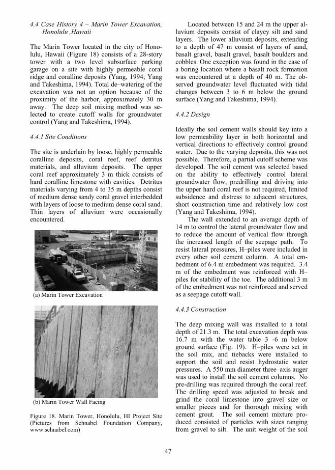
4.4 Case History 4 – Marin Tower Excavation, Honolulu ,Hawaii

The Marin Tower located in the city of Hono-lulu, Hawaii (Figure 18) consists of a 28-story tower with a two level subsurface parking garage on a site with highly permeable coral ridge and coralline deposits (Yang, 1994; Yang and Takeshima, 1994). Total de–watering of the excavation was not an option because of the proximity of the harbor, approximately 30 m away. The deep soil mixing method was se-lected to create cutoff walls for groundwater control (Yang and Takeshima, 1994).

4.4.1 Site Conditions

The site is underlain by loose, highly permeable coralline deposits, coral reef, reef detritus materials, and alluvium deposits. The upper coral reef approximately 3 m thick consists of hard coralline limestone with cavities. Detritus materials varying from 4 to 35 m depths consist of medium dense sandy coral gravel interbedded with layers of loose to medium dense coral sand.Thin layers of alluvium were occasionally encountered.

(a) Marin Tower Excavation

(b) Marin Tower Wall Facing

Figure 18. Marin Tower, Honolulu, HI Project Site (Pictures from Schnabel Foundation Company, www.schnabel.com)

Located between 15 and 24 m the upper al-luvium deposits consist of clayey silt and sand layers. The lower alluvium deposits, extending to a depth of 47 m consist of layers of sand, basalt gravel, basalt gravel, basalt boulders and cobbles. One exception was found in the case of a boring location where a basalt rock formation was encountered at a depth of 40 m. The ob-served groundwater level fluctuated with tidal changes between 3 to 6 m below the ground surface (Yang and Takeshima, 1994).

4.4.2 Design

Ideally the soil cement walls should key into a low permeability layer in both horizontal and vertical directions to effectively control ground water. Due to the varying deposits, this was not possible. Therefore, a partial cutoff scheme was developed. The soil cement was selected based on the ability to effectively control lateral groundwater flow, predrilling and driving into the upper hard coral reef is not required, limited subsidence and distress to adjacent structures, short construction time and relatively low cost (Yang and Takeshima, 1994).

The wall extended to an average depth of 14 m to control the lateral groundwater flow and to reduce the amount of vertical flow through the increased length of the seepage path. To resist lateral pressures, H–piles were included in every other soil cement column. A total em-bedment of 6.4 m embedment was required. 3.4 m of the embedment was reinforced with H–piles for stability of the toe. The additional 3 m of the embedment was not reinforced and served as a seepage cutoff wall.

4.4.3 Construction

The deep mixing wall was installed to a total depth of 21.3 m. The total excavation depth was 16.7 m with the water table 3 -6 m below ground surface (Fig. 19). H–piles were set in the soil mix, and tiebacks were installed to support the soil and resist hydrostatic water pressures. A 550 mm diameter three–axis auger was used to install the soil cement columns. No pre-drilling was required through the coral reef. The drilling speed was adjusted to break and grind the coral limestone into gravel size or smaller pieces and for thorough mixing with cement grout. The soil cement mixture pro-duced consisted of particles with sizes ranging from gravel to silt. The unit weight of the soil

47

cement slurry was approximately 16.0 kN/m3.In situ water was prevented from entering

the soil cement columns because a higher pressures was maintained in the borehole during construction. The soil cement mixture flowed in to fill and stabilize the cavities and prevent further loss of soil–cement mixture. One side of the soil cement columns was shaved off using a backhoe to create a flat surface. Mix designs with cement dosages ranging from 3 to 5 kN/m3

(dry cement weight over volume of treated soil) were used providing 28–day unconfined com-pressive strengths ranging from 833 to 1431 kPa. A total of eleven dewatering wells were installed of which five were constantly used to control the bottom flow of groundwater. The wall was completed in March, 1994.

Figure 19. Marin Tower, Honolulu, HI Site Profile and Wall Cross Sections

4.4.4 Performance

A total of 4,015 m2 of soil cement wall was constructed, of which approximately 80% served the dual function of excavation support and groundwater control. The horizontal flow of water through the wall was negligible. The construction of the basement of the Marin Tower was enabled due to the control of the horizontal flow of groundwater through the use of deep mixing technology.

4.5 Case History 5 – Oakland Airport Roadway Project, Oakland California

The Oakland Airport Roadway project consisted of three grade separation structures at two roadway interchanges and the intersection of a roadway and taxiway (Yang et al., 2001; Yang, 2003). Deep soil mixing was used for founda-tion improvement, construction of a soil cement gravity retaining wall and groundwater control using two cutoff walls. A block–type gravity structure was constructed at the Air Cargo Road/Taxiway intersection to function both as a permanent retaining structure and temporary shoring. Cutoff walls were used as permanent seepage control and to reduce dewatering requirements during construction.

4.5.1 Site Conditions

The subsurface conditions consist of three strata including artificial fill, Young Bay Mud, and the San Antonio Formation. The artificial fill is generally less than 4.5 m thick and includes hydraulically placed, dredged, loose or very loose sand materials. Underlying the fill, the Young Bay Mud is soft to very soft silty clay generally less than 3 m deep and is absent in some areas. The San Antonio Formation con-sists of competent clays and sands. Due to the airport pumping activities, the ground water levels at the site vary from 1.5 m to 3 m below the existing ground surface (Yang, 2003).

4.5.2 Design

The project location is divided into three distinct areas: (1) Doolittle Drive/Airport Cargo Road interchange; (2) Airport Drive/ Air Cargo Road interchange and (3) Air Cargo Road/Taxiway B intersection. A DSM cutoff was constructed at the Doolittle Drive/Airport Cargo Road inter-change to provide permanent seepage control and to minimize dewatering requirements during construction. The soil beneath the new soil embankment was improved using DSM to increase the soil strength and reduce the poten-tial for lateral spreading of the embankment in case of seismic loading at the Airport Drive/ Air Cargo Road interchange.

At the Air Cargo Road/Taxiway B intersec-tion, a gravity structure including soil nails for reinforcement was constructed as a permanent retaining structure and as a temporary shoring system during construction. Design criteria

48

limited the permanent lateral deformation of the embankment to 150 mm during a design earth-quake with a probability of exceedance of 20 percent in 50 years. Permanent ground defor-mations were evaluated using pseudo–static stability methods, Newmark–type displacement analyses incorporating peak horizontal ground acceleration, and estimated duration of strong ground shaking for the design event. The cutoff walls were designed for a maximum permanent deformation of about 90 mm during a design earthquake with a probability of exceedance of 5 percent in 50 years.

4.5.3 Construction

The construction of the DSM gravity wall began in March 2001 and was completed in December 2001 with approximately 34,405 m3 of soil cement. The construction of the DSM cutoff wall at the Airport Drive Undercrossing at Doolittle Drive began in May 2000 and was completed in July 2000. The DSM foundation treatment for the Airport Drive Overcrossing and the Taxiway B Overcrossing at Air Cargo Road began in March and April 2001, respec-

tively. The gravity wall had a minimum width equal to the maximum depth of the excavation during construction and extended to a minimum of 1.22 m below the excavation (Yang, et al., 2001).

For additional resistance against sliding, the soil cement panels were keyed into the layer below the gravity wall. Geocomposite drain strips were used to release the water pressure behind the permanent wall facing of the gravity wall. As illustrated in Figure 20, a DSM cutoff wall was incorporated in the center of the soil cement gravity wall and extended beneath the bottom of the gravity wall to reduce the seepage under the gravity wall (Yang 2003).

4.5.4 Performance

The unconfined compressive strength of the DSM cutoff wall material ranged from 870 to 3865 kPa at 28 days with an average of 2064 kPa. Permeability tests gave hydraulic conduc-tivity values ranging from 5.3 x 10–7 to 5.9 x 10–

9 cm/s with an average of 1.9 x 10–7 cm/sec

Figure 20. Design of Gravity Wall (After Yang, 2003)

49

4.6 Case History 6- VERT Wall, Texas A&M University, College Station, Texas

The VERT wall is a new type of top–down gravity retaining structures deriving its name from the vertical reinforcement used to stabilize the structure (Figure 21). Three to four rows of 1 m diameter soil cement columns are installed in the in situ soil to the depth of the excavation. To study the behavior of the retaining wall system, Geo–Con built and instrumented a full–scale VERT wall at the National Geotechnical Experimentation site (NGES) at Texas A&M University (TAMU) (Briaud et al., 2000).

4.6.1 Site Conditions

The site of the VERT wall consists of sand deposits (Fig 22). The sand, a floodplain deposit of Plesitocene age, has a high fine content with occasional clay layers due to the relatively low energy depositional environment. A hard clay shale is found approximately 10 m below the ground surface. This dark gray clay shale was deposited in a series of marine transgressions and regressions. The water table is 7.2 m below the ground surface.

4.6.2 Design

The design strength for the soil cement was 690 kPa at 28 days before starting the excavation. Design guidelines are similar to those used for gravity retaining walls. There is a need for further development of VERT walls design guidelines. The construction of this research wall indicated the importance of two design features: 1) it is important to have a DSM platform at the top of the wall to connect all the columns together, and 2) it is important to reinforce the front row of column to resist bending beyond the tensile strength of the cement soil mixture.

4.6.3 Construction

Prior to construction, a 1 m thick fill was placed on top of the original ground surface to ensure that the final excavation level would remain above the water table. The fill consisted of compacted sand from the site. Soil cement columns were installed using a drilling rig equipped with a 0.91 m diameter cutting and mixing head. The drilling fluid consisted of a water and cement slurry with a ratio of 1.75 to 1

while the cement slurry to soil ratio by weight was 0.55. Therefore, there was 15% dry cement or 33% slurry per 1 m3 of soil-water-cement of DSM material.

The soil cement columns were installed to a depth of 8.5 m below the top of the fill. A front row (Row A) of 43 contiguous columns was constructed (Fig. 23 and Fig. 24). Immediately behind this row was a second row (Row B) with center–to–center spacing of 1.82 m. A third row (Row C) and a fourth row (Row D) were con-structed to maintain the 1.82 m spacing. On top of the first half of the wall, a 1 m thick platform was built using the soil slurry spoils ejected from each hole. The global volume of soil cement installed was 9.5 m high, 5.6 m wide and 40 m long.

4.6.4 Performance

Compressive strength tests were performed on soil cement samples from various depths at 3, 7, 28 and 56 day increments. The lowest value of the unconfined strength at 28 days before construction was twice the design value. Core samples were also taken and tested. The best coring process of the soil cement column was achieved when using a triple-tub core barrel and coring 28 days or more after column construc-tion. Compression testing at 28-days of repre-sentative samples showed an average uncon-fined compression strength of 2,069 kN/m2.

The relieving platform had a very beneficial effect because it decreased the maximum deflection of the wall by a factor of 2. One and a half years after construction, the horizontal deflection at the top of the 10 m high wall was 23.1 mm and the vertical settlement of the same point was 9.2 mm (Figure 25).

5. CONCLUSIONS

Deep Soil Mixing (DSM) for excavation support is a relatively recent technique which can be very helpful and economical when used in the right circumstances. In a first part DSM is compared with other types of excavation walls and wall supports such as structural diaphragm walls, sheet-pile walls, soldier pile and lagging walls, tiebacks and internal struts. Some DSM historical background is then presented followed by a discussion of the engineering properties of soil cement mixtures. The percent cement to soil ratio by volume is typically in the range of 15 to 50%. On a log scale the typical compression

50

strength of soil cement mixtures used in DSM fits in the middle between soil and concrete. Stiffness and hydraulic conductivity are two other very important properties for DSM walls.

DSM walls can fail by seepage instability, global instability, geotechnical failure including excessive settlement, passive failure of the embedment, anchor failure, and structural failure. A design flow chart is presented and each step is discussed. One of the advantages of such walls is that the engineer can control settlement by choosing the support loads. Charts are given to relate the wall pressures to the likely settlement based on case histories and

numerical simulations. Construction issues and equipment are discussed as well as quality assessment and performance monitoring.

Six case histories are briefly described to il-lustrate the statements made in the paper. They include (1) EBMUD Storage Basin, Oakland, CA; (2) Lake Parkway Project, Milwaukee, WI; (3) Bird Island Flats Central Artery/Tunnel Project, Boston, MA; (4) Honolulu Excavation, Honolulu, HI; (5) Oakland Airport Roadway Project, Oakland, CA; and (6) VERT Wall, Texas A&M University.

Figure 21. Completed VERT Wall (After Briaud et al., 2000)

Figure 22. VERT Wall Section View

51

Figure 23. VERT Wall Layout (After Briaud et al., 2000)

Figure 24. VERT Wall Front View (After Briaud et al., 2000)

Figure 25. VERT Wall Displacements (After Briaud et al., 2000)

52

6. REFERENCES

Anderson, T. C. 1998. Anchored Deep Soil Mixed Cutoff/Retaining Walls for Lake Parkway Project in Milwaukee, WI. Design and Construction of Earth Retaining Systems, ASCE, Geotechnical Special Publication No. 83, pp 1–13.

Ando, Y., Tsuboi, H., Yamamoto, M., Harada, K., and Nozu, N. 1995. Recent Soil Improvement Methods for Preventing Liquefaction. Proceedingof Earthquake Geotechnical Engineering,Balkema, Rotterdam, The Netherlands, pp. 1011–1016.

Andromalos, K. B., and Bahner, E. W. 2003. The Application of Various Deep Mixing Methods for Excavation Support Systems. Grouting and Ground Treatment, ASCE, Geotechnical Special Publication No. 120, pp. 515–526.

Bahner, E. W. and Naguib, A. M. 1998. Design and Construction of a Deep Soil Mix Retaining Wall for the Lake Parkway Freeway Extension. SoilImprovement for Big Digs, ASCE, Geotechnical Special Publication No. 81, pp. 41–58.

Briaud, J.–L., and Lim, Y. 1999. Tieback Walls in Sand: Numerical Simulation and Design Implica-tions. Journal of Geotechnical and Geoenviron-mental Engineering, Vol. 125, No. 2, pp. 101–111.

Briaud, J.–L., Nicholson P., Lee J. 2000. Behavior of a Full–Scale VERT Wall in Sand. Journal of Geotechnical and Geoenvironmental Engineer-ing, Vol. 126, No. 9, pp. 808–818.

Bruce, D. A. 2000. An Introduction to the Deep Soil Mixing Method as Used in Geotechnical Applica-tions, Federal Highway Administration¸ FHWD-99-138.

Holm, G. 2000. Deep Mixing. Soft Ground Technol-ogy, ASCE, Geotechnical Special Publication, No. 112, pp. 105–122.

Jakiel, R. 2000. Case History: Deep Soil–Cement Mixing at the I–90/I–93 NB Interchange on the Central Artery/Tunnel Project, Contract C09A7 at Fort Point Channel Site, Boston, MA. Proceed-ings 25th Annual Meeting and 8th International Conference and Exhibition, New York, NY, Oct., Deep Foundations Institute, Englewood Cliffs, NY, pp. 569–593.

Koutsoftas, D. 1999. Excavation in San Francisco Bay Mud: Design for Deformation Control. Pro-ceedings of the Conference American Society of Civil Engineers, University of Illinois, Urbana-Champaign, IL, pp. 337–392.

Kunito, T. Honda, A., Mashima, M., and Hamasato, S. 1988. A Study of The Relationship between Pore Structure and Coefficient of Permeability of Soil Stabilized with Cement. Pore Structure and Permeability of Cementitious Materials, Materi-als Research Society Symposium Proceedings, Boston, MA, pp. 314-325.

McGinn, A.J. and O’Rourke, T.D. 2000. Case Study of Excavation Base Stability in Deep Marine

Clay. ASCE, Geotechnical Special Publication, No. 94, pp. 480–495.

McGinn, A.J. and O’Rourke, T.D. 2003. Perform-ance of Deep Mixing Methods at Fort Point Channel. report prepared for Bechtel/Parsons Brinckerhoff, the Massachusetts Turnpike Au-thority, and the Federal Highway Administration at Cornell University, Ithaca, NY.

McNab, A. 2002. Earth Retention Systems Handbook,McGraw–Hill Publishers, New York, NY.

Mueller, C.G., Long, L.H., Weatherby, D.E., Cord-ing, E.J., Powers III, W.F., and Briaud, J.–L. 1998. Summary Report of Research on Perma-nent Ground Anchor Walls, “Volume III: Model–scale Wall Tests and Ground Anchor Tests,” Report No. FHWA–RD–98–067, Federal Highway Administration, McLean, VA.

O’Rourke, T.D. and McGinn, A.J. 2004. Case History of Deep Mixing Soil Stabilization for Boston Central Artery, Proceedings of Geo-Trans 2004 Geotechnical engineering transportation projects,Los Angeles, CA, Vol. 2, No. 126, pp. 77-136.

O’Rourke, T.D., McGinn, A.J., Dewsnap, J. and Stewart, H.E. 1997. Performance of Excavations Stabilized by Deep Soil Mixing, report prepared for Bechtel/Parsons Brinckerhoff, the Massachu-setts Highway Department, and the Federal Highway Administration at Cornell University, Ithaca, NY.

O’Rourke, T.D., McGinn, A.J. and Dewsnap, J. 1998. Case History of Excavation Stabilized by Deep Mixing Methods. Design and Construction of Earth Retaining Systems ASCE, Geotechnical Special Publication No. 83, pp. 41–61.

O’Rourke, T.D. and O’Donnell, C.J. 1997a. Deep Rotational Stability of Tiedback Excavations in Clay. Journal of Geotechnical Engineering, Vol. 123, No. 6, pp. 506–515.

O’Rourke, T. D and O’Donnell, C.J. 1997b. Field Behavior of Excavation Stabilized by Deep Soil Mixing. Journal of Geotechnical and Geoenvi-ronmental Engineering, Vol. 123, No. 6, pp. 516–524.

Pearlman, S.L. and Himick, D.E. 1993. Anchored Excavation Support Using SMW. Deep Founda-tion Institute, 18th Annual Conference, Pitts-burgh, PA, pp. 101-120.

Porbaha, A. 1998. State of the Art in Deep Mixing Technology: Basic Concepts. Ground Improve-ment, Vol. 2, No. 2, pp. 81–92.

Porbaha, A. 2000. State of the Art in Deep Mixing Technology. Part IV: Design Considerations. Ground Improvement, Vol. 4, No. 3, pp. 111–125.

Porbaha, A., Raybaut, J.–L., and Nicholson, P. (2001). State of the Art in Construction Aspects of Deep Mixing Technology. Ground Improve-ment, Vol. 5, No. 3, pp. 123–140.

Sabatini, P.J., Elias, V., Schmertmann, G.R., and Bonaparte, R. 1997. Earth Retaining Systems.FHWA–SA–96–038, Federal Highway Admini-stration, Washington, DC.

53

Taki, O. and Yang, D.S. 1991. Soil–Cement Mixed Wall Technique. ASCE Special Conference, Denver, CO, pp. 298–309.

Weatherby D. 1998. Design Manual for Permanent Ground Anchor Walls, FHWA report no. FHWA–RD–97–130, Federal Highway Administration, Washington, DC.

Yang, D.S. 1994. The Applications of Soil Mix Walls in the United States. Geotechnical News, Decem-ber, pp. 44–47.

Yang, D.S. 2003. Soil–Cement Walls for Excavation Support. Earth Retention Systems 2003: A Joint Conference presented by ASCE Metropolitan Sec-tion of Geotechnical Group, The Deep Founda-tions Institute, and The International Association of Foundation Drilling, New York City, NY.

Yang, D.S., Scheibel, L.L., Lobedan, F. and Nagata, C. 2001. Oakland Airport Roadway Project. Deep Foundations Institute Specialty Seminar–Soil Mixing, St. Louis, MI, pp. 55–71.

Yang, D.S. and Takeshima, S. 1994. Soil Mix Walls in Difficult Ground. In situ Ground Improvement Case Histories, ASCE Convention, Atlanta, GA, pp. 106–120.

7. ACKNOWLEDGEMENTS

This research was sponsored by the National Deep Mixing (NDM) pooled fund program and the Federal Highway Administration (FHWA). Mr. Ali Porbaha (CALTRANS) was the techni-cal contact for NDM. Mr. Al DiMillio was the technical contact for FHWA. The authors thank their board of consultants namely Mr. Demetri-ous Koutsoftas of Ove Arup and Partners, Mr. George Tamaro of Mueser Rutledge Consulting Engineers, Dr. Tom O'Rourke of Cornell Uni-versity and Mr. Dave Weatherby of Schnabel Foundations for their valuable contributions towards this project. The authors also wanted to thank the contributions of Dr. David Yang of Raito, Inc.

54

New Rome metro line C: approach for safeguarding ancient monuments

Burghignoli A. Professor, Università di Roma La Sapienza, alberto.burghignoli@uniroma1.it

Di Paola F. Project Manager, ASTALDI Ltd. Roma, f.dipaola@metrocspa.com

Jamiolkowski M. Professor Emeritus, Technical University of Torino, Michele.jamiolkowski@polito.it

Simonacci G. General Director, Metropolitane di Roma Ltd., g.simonacci@romametropolitane.it

ABSTRACT: The new Rome Metro C line, whose central lots T2 and T3 are under design, poses a tremendous challenge with respect to the conservation of buildings. In fact, the line will be crossing the entire segment lying below the Roman historical centre, thus beneath some sites inscribed on UNESCO’s World Heritage List.

A serious concern is also the presence of man-made ground, 6 to 12 m thick, with a huge amount of archaeo-logical remains, dating back to BC centuries.

In the circumstances the owner, Metropolitane di Roma Ltd, set up a special multidisciplinary Steering Technical Committee (STC) to operate alongside the General Contractor (GC) and the Metro C Ltd with the assignment to implement the procedures to safeguard the historical buildings. The paper describes the STC organizational scheme to accomplish the task, identifying the buildings at risk and suggesting appropriate mitigation interventions.

1. INTRODUCTION

The construction of an underground line raises always some geotechnical problems, due to the unavoidable interaction of the line with the existing urban environment. The problems originate from the surface settlements induced by the tunnel excavation and the construction of stations. The width and depth of the settlement trough above the tunnels and the extension of the induced settlements around the open exca-vations for the stations can be more or less pronounced, depending on their dimensions, on the mechanical properties of the surrounding soils and on the excavation technique and sequence.

The interaction phenomena between the soils and the existing buildings are especially important and delicate when tunnels run through weak soils and the existing structures are particularly vulnerable. Also, when the structures have exceptional archaeological and historical value, the design necessarily must include an in-depth study of said interaction phenomenon to construct the line without threatening the buildings at surface.

This is the case for the new C line of Roma underground, [Burghignoli et al (2007),

Viggiani and De Sanctis, (2009)], crossing the entire city along the SE-NW direction and that, within its lots lying below the Roman historical centre between San Giovanni da Laterano and Piazza Cavour, passes beneath the Aurelian Walls, the area of the Colosseum and of the Fori Romani, and the Roman Renaissance area from Piazza Venezia to the Tiber river. A layout of the whole line C and a zooming on the monu-mental lots T3 and T2 are shown in Fig.1.

Fig.2 shows, to an enlarged scale, the layouts of T3 and T2 with clues and a list of the main monuments and historical buildings, whose location suggests that their integrity might be jeopardized by the subway construction. The situation is worsened because the monuments are generally packed with valuable mosaics and frescos, extremely at risk in relation to the induced settlements. Moreover, virtually along the entire extension of the T3 and T2 lots, the man-made ground with a thickness ranging from 8 and 17 meters is embedded within an incredible amount of archaeological remains. These valu-able vestiges entail other constraints on the geotechnical design, truly limiting the applica-tions of the soil improvement and the founda-tions methods that during their implementation might damage them.

55

Figure 1. New Metro Line C Route.

Twin subway tunnels will be excavated using TBMs with an outer diameter of about 6.7m. Along the route they run at depths varying between 20 to 40 m below ground level. The choice of rather deep tunnels was mandatory, to avoid direct interferences with the archaeologi-cal subsurface layer and to reduce interaction effects on the buildings and monuments present along the line. The stations located along the lots T3 and T2, see Fig.2, will require a deep open excavations supported by the diaphragm walls reaching a depth exceeding 60 to 70 m.

Given the circumstances, the owner, Metro-politane di Roma Ltd, in the tender phase, appointed a special multidisciplinary Steering Technical Committee (STC) to operate together with the General Contractor (GC) and the Metro C Ltd, with the assignment to develop and implement, in the design, the procedures to safeguard the monuments and the historical buildings.

In the next sections of the paper, after de-scribing the local geology and the site charac-terization of the soils encountered along the two monumental lots, it is illustrated the STC approach scheme.

2. GEOLOGY ALONG T2 AND T3 ROUTES

In Fig. 3 are shown the geological cross section of lot T3 and the tunnels position. The subsoil consists of man-made ground of varying thick-ness, overlaying Pleistocene sandy and clayey soils in the upper part and sandy gravel in the lower part.

A thick stiff OC clay of the Pliocene age is encountered beneath the Quaternary deposits at a depth ranging between 30 and 40 m. In some cases the Pleistocene deposits contain old erosion ditches filled with softer fine grained soils. The ground water level (GWL) is located at a depth ranging between 10 and 15 below the existing ground level (GL). The pore pressure distribution with depth results close to hydrostatic. Similar pieces of information regarding the geology of the lot T2 are reported in Fig. 4. In this case, the Pliocene very stiff OC clay is overlaid by 10 to 20 m thick deposits of the Pleistocene 30 to 40 m, followed by the Holocene Tiber river allu-vium and covered by man-made ground having thickness ranging between 7 and 11 m. The GWL encountered at the depth of 6 to 8 m below the GL, exhibits the hydrostatic pressure distribu-tion with depth and is subject to periodic fluctua-tions according to the variation of the Tiber hydrometric level.

56

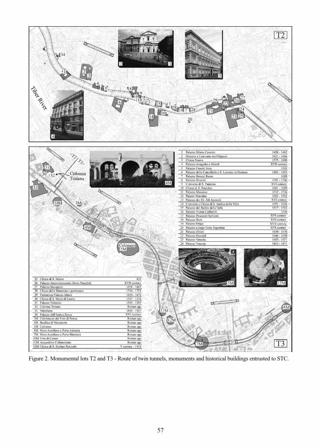
Figure 2. Monumental lots T2 and T3 - Route of twin tunnels, monuments and historical buildings entrusted to STC.

57

Figure 3. Geological profile between S. Giovanni and Piazza Venezia.

Figure 4. Geological profile between Tiber river and Piazza Venezia.

3. HINTS ABOUT GEOTECHNICAL SITE CHARACTERIZATION

The site characterization along the lots T3 and T2 focused at soil-structure interaction studies has been carried out by means of a number of geo-technical investigation campaigns between 1999 and 2009. Their programmes and the technical oversight were steered by the Working Group Geotechnical Engineering (WG-GE), coordinated by prof. S. Rampello1 assisted by Dr. L. Callisto1,Dr. C. Soccodato2 and Prof. G. Viggiani3; for details see section 4.1 of the paper.

The field investigation consisted in several deep borings during which a large number of undis-turbed samples of fine grained soils were re-trieved using the Osterberg’s hydraulic piston sampler having a diameter of 90mm.

Furthermore, a large variety of insitu tests were performed, of particular relevance to the modelling and design are the following: cross-hole (CH) and down-hole (CH) seismic tests, static cone penetration tests with pore pressure measurements (CPTU), standard penetration tests (SPT) and seismic CPTU (S-CPTU).

In a number of borings, piezometers were in-stalled to monitor the GWL.

As to laboratory tests, classification and index properties tests have been performed on both fine grained and coarse grained geomaterials;

( * ) ( 1) Università di Roma, La Sapienza; ( 2) Università di Cagliari; ( 3) Università di Roma, Tor Vergata.

58

in the latter case using disturbed sampling having integral, thus representative grading.

The mechanical properties of the fine grained soil were assessed via the following tests: incremental (IL) and constant rate of strain (CRS) oedometer; resonant column (RC), unconsolidated-undrained triaxial compression (TX-UU), consolidated-undrained compression with the excess pressure measurements (TX-CIU and TX-CAU) and drained triaxial com-pression (TX-CID and TX-CAD). During the latter ones, the shear wave velocity was meas-ured (Vs) using bender elements.

The above laboratory tests results combined with in situ seismic tests results allowed assess-ing the parameters of fine grained soils needed for the constitutive relations adopted in model-ling soil-structure interaction phenomena.

As to coarse grained soils the relevant geo-technical parameters were established based on in situ tests. The initial small strain stiffness was evaluated from Vs measured during seismic tests other parameters such as stiffness at larger strains, shear strength, from semi-empirical correlations with the CPTU’s and SPT’s results.

The mass of geotechnical testing carried out, the number of monuments and historical build-ings involved, do not allow presenting thor-oughly the efforts made for the site characteri-zation.

For the lot T3, considering the relatively li-mited number of monuments encountered (3M, 4M, 5M, 6M, 7M, 10M, 11M, and 12M in Fig.2) and their scattered distribution along the route, the presentation will be limited to the area of Basilica di Massenzio (4M).

This important monument is, in fact, quite representative for the entire lot and required special efforts in the soil-structure analyses, not only in relation to its historical relevance but

also due to the complexity of engineering problems deriving from the future construction of the deep Fori Imperiali station, located very close to it.

Fig.5 shows the soil profile across the area of the Basilica perpendicular to Fori Imperiali. The relevant strata, which can be also identified on the geological profile shown in Fig.3, are: man-made ground (R)**, succession of sandy and clayey silts (Tb)**, sandy gravel (SG)**, over-laying the thick deposit of the very stiff OC Pliocene marine clay.

The figure reports also the results of some SPT’s and of cone resistance qc measured by means of CPTU’s.

Fig.6 gives the results of the initial small strain ( s 10-5) shear modulus Go computed from the Vs measured during CH tests.

Figure 6. Basilica di Massenzio - Initial small strain shear modulus.

Figure 5. Basilica Basilica di Massenzio - Representative soil profile.

( **) Letters referred to symbols of the geologicprofiles, Figs.3 and 4.

59

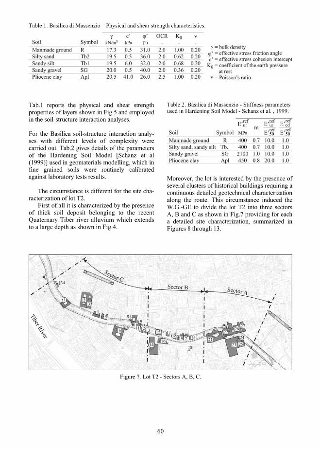
Table 1. Basilica di Massenzio – Physical and shear strength characteristics.

Tab.1 reports the physical and shear strength properties of layers shown in Fig.5 and employed in the soil-structure interaction analyses.

For the Basilica soil-structure interaction analy-ses with different levels of complexity were carried out. Tab.2 gives details of the parameters of the Hardening Soil Model [Schanz et al (1999)] used in geomaterials modelling, which in fine grained soils were routinely calibrated against laboratory tests results.

The circumstance is different for the site cha-racterization of lot T2.

First of all it is characterized by the presence of thick soil deposit belonging to the recent Quaternary Tiber river alluvium which extends to a large depth as shown in Fig.4.

Table 2. Basilica di Massenzio - Stiffness parameters used in Hardening Soil Model - Schanz et al. , 1999.

Moreover, the lot is interested by the presence of several clusters of historical buildings requiring a continuous detailed geotechnical characterization along the route. This circumstance induced the W.G.-GE to divide the lot T2 into three sectors A, B and C as shown in Fig.7 providing for each a detailed site characterization, summarized in Figures 8 through 13.

Figure 7. Lot T2 - Sectors A, B, C.

60

Figure 8. Lot T2, Sector A: Grading and index properties.

Figure 9. Lot T2, Sector A: Mechanical properties. CH = cross-hole tests, DH = down-hole tests.

Figure 10. Lot T2, Sector B: Grading and index properties.

61

Figure 11. Lot T2, Sector B: Mechanical properties.

Figure 12. Lot T2, Sector C: Grading and index properties.

Figure 13. Lot T2, Sector C: Mechanical properties.

62

Tabs. 3, 4 and 5 summarize the mean value of the key geotechnical parameters as obtained from laboratory tests for fine grained and for coarse grained soils, as inferred from the semi-empirical correlations with CPTU cone resis-tance (qc) and with the SPT blow count (NSPT).

All the gathered data confirm that along the T2 route prevails soft slightly OC fine grained deposits exhibiting quite pronounced spatial heterogeneity.

With this respect, it is worth observing that many oedometer tests on clay/silt samples yields OCR<1 which can be attributed to slight specimens disturbance.

Also deserving some comments are the quite high values of the effective stress cohesion intercept c’ (1<OCR<1.2) which, because in this occurrence do not deal with significantly structured soils, should be close to nil.

Table 3. Lot T2, Sector A: Mean values of geotechnical parameters.

Table 4. Lot T2, Sector B: Mean values of geotechnical parameters.

Table 5. Lot T2, Sector C: Mean values of geotechnical parameters.

63

4. INTERACTION OF THE NEW LINE WITH THE EXISTING BUILDINGS

4.1. Steering Technical Committee and Working Groups

STC has been entrusted with the supervision of all activities aimed at safeguarding the monu-mental and architectural heritage.

To sum up, the Committee’s main tasks are the following:

Evaluate, through numerical analyses, the influence of the line C construction on the monuments and historical buildings, see a list in Fig.2. Suggest mitigation interventions of geotech-nical or/and structural nature congruent with the restoration and conservation principles of the historical and architectural heritage in relation to monuments/buildings for which the analyses yield a displacement field en-dangering their structural, architectonic and artistic integrity. Develop a comprehensive and redundant monitoring scheme allowing, in real time, to follow the response of the buildings to tunnel-ling and to open excavations. When requested, assist GC, during construc-tion, in the evaluation of the monitoring data to optimize the construction sequence or/and procedures as well as to advise on the needs to activate the mitigation interventions.

To accomplish said tasks, the Owner and the GC have appointed a multidisciplinary STC including experts in Preservation and Restora-tion of Monuments, in Art of Tunnelling, in Geology and in Structural and Geotechnical Engineering. The overall role of the STC within the GC organization scheme is illustrated in Fig.14.

The STC activities are undertaken by four Working Groups (W.G.) each covering the following areas:

Assessment of history and state of the building (W.G.-HS) This W.G. activities are focused on the follow-ing issues:

- State of conservation. - History of construction and of restoration

interventions. - Structural features, including foundations. - Mechanical properties of the construction

materials.

Geology (W.G.-G) This W.G. provides the following information along the route of the lots T3 and T2:

- Depositional history and features of the encountered geomaterials.

- Characteristics and spatial distribution of the man-made ground.

- History of landscape modifications. - Hydrogeological site characterization.

Figure 14. Response of existing constructions to tunneling - Organization scheme.

64

Geotechnical Engineering (W.G.GE) This W.G. multiple tasks can be summarized as follows:

- Site characterization of soil deposits along the route and definition of the design pa-rameters of interest.

- In cooperation with the Structural Engi-neering W.G., identify the methodological approach, in the soil-structure interaction analyses, to quantify how the construction of stations and the tunnelling works will affect the existing historical buildings un-der the STC competence.

- Predict the displacement field affecting the pre-existing buildings listed in Fig.2, dur-ing and after construction.

- Investigate the feasibility of different miti-gation interventions when the soil-structure analysis yields displacements field, induced by the construction works, which affects the ground surface in an un-acceptable manner.

- Develop the geotechnical monitoring scheme, allowing to watch in real time, the response of monuments and historical buildings to the construction works.

Structural Engineering (WG-SE) The W.G.-SE activity, in close teamwork with GE group, focuses on:

- Harmonizing the methodology of the soil-structure interaction analyses to the struc-tural models of buildings using the input provided by the W.G.-GE.

- Performing the soil-structure interaction aimed at defining the stresses and strains, in the masonry, thus assessing the possible damage category [Boscardin and Cording (1989), Burland (1995)].

- Suggesting, when needed, non invasive and if possible, temporary structural inter-ventions to mitigate the impact of the dis-placements induced by the construction activities.

- Developing the project of structural moni-toring instrumentation to be installed on the building elevations.

Geomatics (W.G. -GM) The W.G. has been entrusted with the following activities:

- Design and implement the geomatic moni-toring system to measure, before starting

construction, the long period low fre-quency of the baseline movements of the city area adjacent to the lots T3 and T2 route. This has been accomplished by us-ing the Synthetic Aperture Radar which has permitted, since 1992, to obtain the pe-riodical seasonal series of the reflectors movements.

- Design and implement the geomatic moni-toring system to measure, before the con-struction, short period, high frequency, baseline movements of buildings and mo-numents existing along the T3 and T2 route. To accomplish this task, a series of motorized total stations together with the installation of a large number of mini mir-rors were placed on monuments and his-torical buildings along the route. The sta-bility of the total stations is constantly controlled by the GPS receiver and by the automatic biaxial inclinometer. Such ar-rangement will produce a daily move-ments cycle of mini mirrors at least for a period ranging between 1 and 2 years be-fore starting the construction.

- Devise and run geodetic measurements of the buildings entrusted to the STC, during the entire construction period and for at least two years beyond. This will be ac-complished by means of the mentioned to-tal stations assisted by the conventional geodetic survey at spots difficult to be cov-ered only by the total stations operations.

- Setup and manage a Relational Data Base Management, incorporating all geomatic monitoring data as well as those obtained by means of metereologic, geotechnical and structural monitoring instrumentation.

4.2. Analyses of Soil-Structure Interaction

The interaction between the activities involving the construction of Line C and the monumental and architectonic heritage located along the routes of lots T3 and T2 are carried out along with three levels of analysis, of increasing complexity.

The first level is applied to all the historical buildings and monuments entrusted to STC and listed in Fig.2. It employs the semi-empirical method allowing to compute the surface and the near surface settlement through in greenfield

65

conditions i.e., without considering the presence of the buildings [Attewell and Woodman (1982), Attewell and al (1986)].

The resulting displacement field is then im-posed under the 3D linear-elastic finite element model (FEM) of the considered structure, computing stresses and strains due to induced subsidence.

Supported by a well consolidated field evi-dence, the settlement through at the ground surface, in absence of buildings (greenfield) in sandy and clayey geomaterials above the tunnel axis, at some distance behind its face, can be approximated by the Gaussian function see Fig.15 [Attewell and Woodman (1982), At-tewell et al (1986)] given by the formula:

wz = wzmax exp(-y2/2i2) (1)

where: wz = vertical displacement wzmax = maximum vertical displacement

above tunnel axis i = distance y from the tunnel axis to

the inflexion point in Fig.15

The value of i is assumed to vary linearly with depth zo of the tunnel axis according to i=Kzo , being K the width through parameter depending on the soil type and position of the GWL [O’Reilly and New (1982), Mair et al (1993), Mair and Taylor (2001)]. K is usually consid-ered constant with depth when the assessment of the surface settlement through is of interest.

Integrating the plane-strain settlement through,

2

2

max 2exp

iywV zw (2)

the value of wzmax can be computed by means of the following formula:

wzmax = 0,313 VL D2/i (2a)

where: D = tunnel diameter VL = defined as volume loss parameter

corresponding to the volume of the settlement through (Vw) divided by the nominal volume of the excavated tunnel (Vo). Both Vw and Vo are re-ferred to unit length of tunnel.

Figure 15. Surface settlement profile after Attewell et al. , 1986.

66

VL results a crucial parameter when evaluating how the underground works affect the existing buildings, it is strongly dependent on soil type, tunnelling method and quality of the contractor performance. The main sources generating the magnitude of the VL are referred to Leca et al (2000).

When the subsurface settlement through is of interest, it still can be approximated by the Gaussian function as long as the variation of i with depth z can be defined.

This can be accomplished [Mair et al (1993) Moh and Huang (1996) and Mair and Taylor (2001)] by means of eq. (1) considering the trend of K and i vs. depth given by the follow-ing relationships:

i= K(zo-z) (3)

i/zo = 0.175 + 0.325(1-z/zo) (4)

Eq. (4) holds for fine grained soils. Combining eqs. (3) and (4) one gets:

o

o

zz1

zz1325.0175.0

K (5)

Concerning the type of soils, more general relationship to evaluate i of subsurface settle-ment through has been proposed by Moh and Huang (1996);

i(z)= i(z=0)[ (zo-z)/zo]m (6)

with the value of exponent m ranging from 0.4, recommended for silt-sand and 0.8 for silt-clay geomaterials.

In eqs. (4), (5) and (6), the z corresponds to depth at which the settlements are evaluated.

The value of wz max for a subsurface settlement through can be computed from the following relationship;

o

L

o

2

maxz

zz1325.0175.0

V25.1z4

Dw (7)

being : z = depth at which the wz max is evaluated.

Then introducing into eq (1) the value of i resulting from eq. (3) and the value of K ob-tained from eq (5) one gets the settlement through transversal to the tunnel axes, for depth z, at some distance from the tunnel face, where plane strain conditions holds.

The extension of the shape and magnitude of the surface/subsurface settlements at the front of the advancing tunnel and ahead of it can be evaluated assuming that the settlement through along the x axis in Fig.15 is well approximated by the cumulative probability function [Attewell et al (1986)]:

wx = wxmax · (x,i) (8)

being :

xi2xerf1

21 (8a)

,dt)texp(2)A(erfA

o

(8b)

where xi2

xA

assuming i (x) = i (y), and being t = internal variable.

The value of wx max can be obtained by means of the following formula:

y

L2

maxx iVD

82w (9)

being: D = tunnel diameter VL = volume loss as fraction of one,

Combining the settlements computed by means of eqs. (1) and (8) and assuming i (x) i (y)

K= f (zo-z), it can be obtained the pattern of the induced greenfield subsidence at surface and subsurface planes, this latter as long as it is done sufficiently far, let’s say 0.5D, from the crown of the excavated tunnel. Using the same

67

approach and superposition principle the settle-ment field can be extended to twin tunnels.

The mentioned procedure to compute wz =f (x,y,z) can be extended to assess also the horizontal displacements uy=f(x,y,z), see At-tewell et al (1986) and Pickhaver (2006).

As already mentioned, the greenfield dis-placement field is imposed under the base of the 3D structural FEM to evaluate how the tunnel-ling works affect the stresses and strains in the building.

Differentiating the displacements of the structural components resulting from the finite element analysis it is possible to obtain, in first approximation, the vertical and horizontal strains in the masonry from which, in turn, it can be estimated in first approximation, the principal tensile strain t.

It is worthy to recall the readers’ attention on the circumstance that the greenfield dis-placements computed by means of the exposed semi-empirical equations, implies that all the deformation processes occur at a constant volume. This holds in saturated fine grained soils immediately after completion of the tunnels but can differ in coarse grained geoma-terial where the tunnelling operation occurs in virtually drained condition. Moreover, in long term, especially in low permeability soils, the near surface settlement can increase as result of consolidation and creep.

The consolidation occurring when the tunnel acts as a drain with respect to the surrounding soil is controlled primarily by the ratio of the lining to the soil hydraulic conductivity [Mair (2008)] and can be responsible for an increase of both settlements and of the width of the settlement through. As to creep very little is known, it can manifest in structured fine grained soils where the tunnelling and associ-ated works cause the phenomenon of destructu-ration. An example of the observed increase of wz after the TBM passage measured during metro line construction, possibly imputable to creep, is shown in Fig.16 [Rocchi et al (2010)].

The outcome of the 1st level interaction ana-lyses allows, in first approximation, to predict the expected damage category of historical buildings and monuments using the criteria proposed by Burland (1995) for masonry structures. Tab.6 reports the damage classifica-tion based on the fissures opening and magni-tude of t , adapted after Burland (1995) by introducing more conservative criteria in order to account for the age and conditions of the monuments and historical buildings encoun-tered along route of T3 and T2.

When the greenfield analysis suggests that the settlement induced by the tunnelling works endangers the monument/building, the 2nd level of analysis is undertaken. It consists in selecting few planar elements of the structure, a façade or an alignment of the shear walls, for which the equivalent linear-elastic 2D solid (ES) is com-puted, see Pickhaver (2006).

Figure 16. Greenfield settlement through - Observed vs. computed. Rocchi, 2009.

68

Table 6. Classification of damage for the buildings of ancient Roman age (adapted after Burland 1995).

The equivalent solid (ES), by applying the homogenization procedure, preserves the dimensions in plane, the weight and the stiff-ness of the prototype and is assessed via linear-elastic finite element analysis (FEA) taking into account the boundary conditions at its extremes.

Once the characteristics of ES are defined, the corresponding displacement field is com-puted by means of 2D FEA, simulating, for the given value of VL, the construction of the tunnel following the approach used by Venturini and Viggiani (2003).

In the evaluation of the settlement through, the underlying soil is modelled as a coupled two-phase (soil skeleton pore fluid) elastic-plastic work hardening material. The resulting displacements field is then imposed under the corresponding 2D linear-elastic ES FEM, computing the induced stresses and strains. The results of analysis allow estimating the magni-tude of strains in the masonry element and deliberating on the expected damage level.

An example of the 2nd level analyses carried out using above approach is exposed in the next section of the paper.

The approach to the 2nd level analysis con-sists in the steps summarized in the following, referring to the twin tunnels excavated by TBM’s:

- calibration of the geotechnical model si-mulating TBM tunnel excavation [Sa-gaseta (1998), Venturi and Viggiani (2003) in order to compare the obtained settlement through with that corresponding to the greenfield condition generated for the design value of VL , see example in Fig.17,

- generation of the site topography and im-plementation of the geostatic stresses in the foundation soils,

- modelling the presence of the ES,

- modelling excavation of the first tunnel, including construction of the lining,

- modelling excavation of the second tunnel including construction of the lining.

When the 2nd level analysis cannot suitably pick up the 3D nature of soil-structure interaction phenomena, the 3rd level of analysis is carried out.

This is the case for the cluster of historical buildings in Piazza Venezia (nn°21, 22, 23, 24, 25, 26, 27 in Fig.2), modelled performing geotechnical analyses to assess the displacement field under 3D ES’s, which then is applied under 3D linear-elastic model of the buildings to evaluate the expected damage level.

Basically, the procedure followed in the 3rd

level analysis is conceptually similar to that of 2nd level as to the involved constitutive model-ling of materials (soil, masonry) and of its objectives.

The only relevant difference is that the 3rd level analysis makes reference to 3D model of the ES representing the entire building.

The attempt to perform such complex analy-sis for cluster of buildings of great historical value such the ones in question was also trig-gered by the circumstance that the area of Piazza Venezia is interested by deep deposits of soft lightly OC clays, see Figs.7 to 9 represent-ing the most critical portion of the T2 route.

Figure 17. Settlement through - greenfield vs. FE simulation.

69

As to the stations of Fori Imperiali in front of Basilica di Massenzio (n° 4M in Fig.2), in Piazza Venezia and the one close to Chiesa Nuova (nn°2 and 3 in Fig.2), planned along the lots T3 and T2 and involving large and deep open excavations, their modelling to estimate the settlements of the surroundings terrain, requires 3D FEA. The analyses are performed adopting a two-phase elastic-plastic work hardening constitutive model for soils providing the coupling between soil skeleton and pore fluid. During the analysis all construction phases are modelled including those related to the execution of 50 to 60 meters deep dia-phragm walls.

4.3. Worked Example

Palazzo della Cancelleria.

Palazzo della Cancelleria is located along the route of the T2 lot, in corso Vittorio Emanuele II, see building n°6 shown in Fig.2.

The palazzo's façade incorporates the Basilica of S. Lorenzo in Damaso, whose origin dates back to end of the IV century when its construction started on the ground of an old church. It was completed around 1514 and ever since the building has undergone many trans-formations to recent times (1940) when the works to enlarge the existing foundation on the internal colonnade courtyard were completed.

Figs. 18 and 19 show respectively the pro-spective view of the Palazzo della Cancelleria in Corso Vittorio Emanuele II and the above mentioned internal courtyard.

The building, of trapezoidal in shape, covers an area of 2700 m2 and its position with respect to the route of the line C is shown in Fig 20. The distance between the twin tunnels 6.7 m in diameter each can be summarized as follows. The odd tunnel does not underpass the building being located 24 and 9 m from its NE and NW corners respectively. The even tunnel alignment passes beneath the building. along the nave of the Basilica. Table 7. Palazzo della Cancelleria, tunnels location and geometry.

Figure 18. Palazzo della Cancelleria - View from Corso Vittorio Emanuele II.

Figure 19. Palazzo della Cancelleria - Palazzo della Cancelleria - Internal courtyard.

Figure 20. Plan view of Palazzo della Cancelleria.

Moreover, in the vicinity, two ventilation shafts, shown in Fig.20 are planned, whose construc-tion, especially that named Cancelleria shaft, can affect the response of the building.

The altimetry and the geometrical features of the tunnels can be inferred from Tab.7.

70

The soil profile in the surroundings of Palazzo della Cancelleria can be summarized as follows:

- Man-made ground (R) is encountered from the existing ground level (elev. +17.5 to +17.0) to a depth ranging between 8 to 9 m. The man-made ground contains ar-chaeological remains and parts of old con-structions dating back to the II century BC.

- Lightly OC clayey silts (LAv) on average, 4.5m thick.

- Medium to fine silty sand (SL), 7.0m thick. - Medium sand (S), 8.0m thick. - Soft NC clays (Ag) with thickness of

around 30m. This formation in its lower part can contain a thin layer of silty sand marking the transition to coarse grained deposit present underneath.

- Sandy gravel (SG) circa 6m thick. - Deposit of medium plasticity OC Pliocene

silty clay (Apl) extending to a large depth.

The above soil profile can be considered repre-sentative of Sector C (Fig.7) of the T2 lot whose geotechnical characterization is given in the section 3 of the paper.

Referring to the outlined subsoil profile, the W.G.-GE has carried out the 1st level greenfield analyses evaluating the subsidence induced by the construction works by means of the semi - empirical approach summarized in section 4.2.

The analyses have been performed assum-ing, for the tunnels excavated using TBM’s, the values of VL equal to 0.5% (design value) and 1.0% (upper bound).

The effect of the excavation of the tunnels connecting the metro line with the ventilation shafts, by traditional methods, has also been investigated within the 1st level approach assuming the value of VL=2.5%.

The depth of the building foundations adopted in the calculations was 9.0m below the G.L. in agreement with the records obtained during the works on the foundation on the internal courtyard colonnade performed in 1940.

The evaluation of the subsurface settlement through has been carried out adopting the input parameters reported in Tab.8. As to the varia-tion of i vs. depth, the eq. (5) suggested by Moh and Huang (1996) has been employed introduc-ing values of m and b corresponding to an average within the range suggested by the authors.

Table 8. Palazzo della Cancelleria, input for greenfield analysis.

The evaluation of the settlement through at the foundation depth (9m, elev.+17.5 a.msl) has been computed simulating the first construction of the odd tunnel, followed by the excavation of the even tunnel.

In both simulations, the route has been di-vided in a number of stretches, evaluating at the end of each the induced settlement, obtaining the influence of the TBM location on the induced settlements when tunnelling is in progress.

Examples of the analyses carried out are il-lustrated in the following figures, showing the projection of the settlement through (wz , mm) on the foundation plan:

- Fig.21, odd tunnel completed (VL=0.5%) - Fig.22, odd and even tunnels completed

(VL=0.5%) - Fig.23, as above but including the effects

of the tunnelling of connections (VL=2.5%) to the ventilation shafts

The settlements profiles induced by all tunnel-ling works along the facade of Piazza della Cancelleria (section A-A’ in Fig.20), for the values of VL 0.5 and 1.0 percent are shown in Fig.24.

Figure 21. Settlements in mm at the foundation level. VL=0.5%, odd tunnel completed.

71

Figure 22. Settlements in mm at the foundation level. VL=0.5%, twin tunnels completed.

Figure 23. Settlements at the foundation level. VL=0.5%, twin tunnels completed VL=2.5%, access tunnels to the ventilation shafts completed

Figure 25. Deflection ratio and tensile strain from greenfield analysis.

The data such as those shown above allow estimating the values of the principal tensile strain ( t) and of the deflection ratio ( /L), see Burland and Wroth (1974) and Burland (1995), along any desired masonry alignment of the building. The meaning of the above terms and of the related symbols as referred to greenfield settlement through, together with the values of

t , obtained for the A-A’ alignment (Fig.20) of the Palazzo della Cancelleria as shown in Fig.25 and Tab.9.

The data exposed in Fig.25 have been ob-tained for two scenarios, twin tunnels completed and the situation after the execution of the access tunnels to the ventilation shafts.

The results of the 1st level analyses, summa-rized above, according to the damage categories exposed in Tab.6 yield satisfactory response as risk of the damage is concerned. Facades and masonry alignments of the Palazzo della Can-celleria, evaluated similarly to the alignment A-A’, fall into the damage category 0.

Figure 24. Settlements through along alignment A-A’ - Twin tunnels completed.

72

Table 9. Palazzo della Cancelleria, alignment A-A’- Results of the greenfield analysis.

Only alignment A-A’, the most critical one, exhibits for the VL=1.0%, a damage category 1 according to the classification given in Tab.6. Despite this positive result, in consideration of the high historical and artistic value of the Palazzo della Cancelleria, the 2nd level of the analysis has been undertaken performing the soil-structure interaction analysis of the ES corresponding to the facade at the front of Piazza della Cancelleria which coincides with the mentioned alignment A-A’.

The ES of this façade worked out by the joint effort of the W.G’s of GE and SE, adopt-ing the principles of homogenization, led to the ES having the following characteristics:

- Wall 90m long, 1,7 m thick, 9m high completely embedded in the subsoil. The geometry of 2D ES implies that it incorpo-rates the effects of presence of the other masonry walls parallel to the considered façade with a spacing of 8.5m extending to a very large distance in the perpendicular direction.

- The structural ES masonry elements are modelled as an elastic-perfectly plastic purely cohesive ( f=c) material with tensile strength t=0. The complete set of the pa-rameters characterizing the mechanical properties of the ES is given in Tab.10.

- The pressure p transmitted by the ES to the soil as estimated by the W.G.-SE resulted equal to 250 kPa.

- At the contact between the ES and founda-tion soil, it has been considered a friction coefficient equal to 70% of that of the un-derlying soil.

- To simulate more realistically the stresses in the ES when undergoing the settlements induced by the underground works, its structure was modelled as a three layers system composed two different materials

having equivalent moduli of elasticity (Eeq) which after the homogenization re-duces to values Emod used in the FEM. Both the mentioned values of moduli are given in Tab.10 together with bulk density ( ), Poisson ratio ( ) of the masonry as well the homogenization factor f.

The response of the ES to the tunnelling has been computed by FEA referring to the previ-ously mentioned soil profile. The stress-strain-strength behaviour of different geomaterials present, has been described adopting the Hard-ening Soil model [Schanz et al (1999)], Tab.11.

The tunnels excavation process has been si-mulated by means of FEA, imposing, along the tunnel crown, an inward vertical displacement field of such magnitude and distribution to yield, after the trial and error process, the desired value of VL , see Venturi and Viggiani (2003).

Table 10. Palazzo della Cancelleria, alignment A-A’. Material paramenters of equivalent solid.

Table 11. Palazzo della Cancelleria, alignment A-A’- Second level analysis, Paramenters for Hardening Soil Model , Schanz et al. ,1999.

73

The geometry of the ES for the façade in question and the corresponding FEM are shown in Fig. 26.

The evaluation of the displacement field to which ES is subject, has been carried out following all the steps listed in the section 4.2, with the reference to the 2nd level analysis, assuming drained response of all the strata present in the subsoil, except for the soft clayey formation Ag, for which undrained conditions have been modelled.

The results of the 2nd level analysis and its comparison with the 1st level semi-empirical analysis can be summarized as follows:

- In Fig. 27, the settlement troughs, at the foundation level, as obtained from semi-empirical approach is compared against the results of the numerical modelling. The two analyses yield quite similar settlement troughs. The numerical model displays slightly smaller wzmax and almost identical troughs width.

- The settlement induced by tunnelling un-der the ES for the two considered values of VL is presented in Fig.28.

- Tab.12 summarizes, for the twin tunnels, the end of construction values of /L , the

1 max. as well as the average value of the strain 1 resulting from the numerical analysis for sagging and hogging respec-tively.

- In the examined case, the comparison of the results of greenfield analysis vs ES, show the advantages, in terms of masonry damages indices [D/L, t( 1)], when per-forming the soil-structure analysis. This is quite common but cannot be generalized. Indeed, when the soil-structure analysis re-fers to heavy loaded buildings and em-ploys a non-linear stress-strain for soils re-lationship, the opposite is true indicating that not necessarily the greenfield yields an answer on the safe side. This holds for analyses carried out for the Basilica di Massenzio, not reported in this paper, where the loads transmitted to the founda-tion soils mobilize around 60% of the available shear strength.

Figure 26. Palazzo della Cancelleria - Equivalent Solid.

74

Figure 27. Palazzo della Cancelleria, alignment A-A’. Settlement throughs from semiempirical and numerical analyses.

Table 12. Palazzo della Cancelleria, alignment A-A’- Results of the second level analysis.

75

Figure 28. Equivalent Solid, settlement field from numerical analyses.

4.4. Mitigation Interventions

Despite T3 and T2 tunnels are located at large depth (2.6 > H*/D > 6.0, being H = depth to the tunnel crown) and that in most of the examined cases the soil-structure analyses yield, 0 or 1 damage level, refer to Tab.6, the uniqueness of the buildings as well as their vulnerability to differential settlements, have led the designers to device a series of measures aimed at mitigat-ing the tunnelling induced displacements.

The possible mitigation interventions - both geotechnical and structural - are limited to avoid too invasive measures which could endanger the monumental and architectonic integrity of the structure.

The compensation grouting [Mair and Height (1994)], when applicable, is one of the most effective measure to keep the tunnelling induced displacement within reasonable limits. It consists in highly controlled grouting under the building to counteract the ongoing settle-ments, see Fig. 29.

To be effective, the compensation grouting, should meet some strict requirements such as: a highly experienced contractor, a reliable high precision monitoring system, a preliminary field trial and a rigorous application of the observa-tional method, see Peck (1969).

This measure is feasible in many soil types, but its application presents some restraints in soft to medium saturated fine grained deposits, where the grouting induces pore pressure excess which, when dissipates, causes settlement

making, to a large extent, unproductive the compensation grouting and/or requiring its repetition in time.

The international geotechnical literature re-ports many well documented examples illustrat-ing compensation grouting procedures and applications. [Harris et al (1994, 1996), Boone et al (1997), Essler et al (1998) Harris et al (1999), Harris (2001), Chambosse and Otterbein (2001), Burland and Standing(2001), Au et al (2003), Hassnoot et al (2003), Liu (2003), Mair (2008)].

When the soil condition and the building structural features permit, by no means the compensation grouting appears as the most effective and almost non invasive means to correct the settlements caused to the surround-ing buildings by excavations and tunnelling.

Another kind of intervention directly involv-ing structural engineering, consists in jacking the structural components undergoing tunnel-ling induced settlements, see for example [Harris (2001), Di Stefano (1990), Macchi (2009) and Macchi, G. and Macchi, S. (2007)].

The intervention consists in separating the structure in elevation from the foundation, by performing thin horizontal cut in the masonry, where a series of flat jacks are inserted. The flat jacks assisted by an adequate monitoring system allow raising the superstructure to compensating the settlement manifested by foundations.

In the case described by Harris (2001) and Mair at al (2009), this intervention, which can be named mechanical compensation, was associated with compensation grouting.

Figure 29. Principle of compensation grouting, adapted from Mair et al. , 2009.

76

This kind of mitigation is presently considered for the Chiesa Nuova station (building n°2 in Fig.2), Macchi (2009), where the excavations and tunnelling, based on the analyses available so far are expected to cause displacements of an unbearable magnitude.

As to deep open excavations supported by diaphragm walls, the mitigation of displace-ments induced at the surrounding surface can be effectively mitigated by installing, before starting the excavation, a series of transversal panels of lean concrete, having compression strength between 5 and 10 Mpa. The panels named sacrificial crosswalls, see Figs.30 and 31, have generally the same length of the outside diaphragm panels and are demolished while proceeding with the excavation.

Overall, the crosswalls allow minimizing the inward movements of the outside diaphragm walls which occur during installation of props, resulting especially effective in controlling deep seated displacements below the excavation bottom. Figs 30 and 31 illustrate in a qualita-tive manner the horizontal displacement ( ) of the perimeter diaphragm panels in absence and in presence of crosswalls.

Figure 30. Open excavation - Crosswall panel, Mair and Menkiti, 2009.

Figure 31. Open deep excavation - Role of cross-walls, Mair and Menkiti, 2009.

For lots T3 and T2 of the Metro C, the use of the sacrificial crosswalls is foreseen in the design of boxes for the deep stations Basilica di Massenzio and Chiesa Nuova.

For more details on the design and use of crosswalls see Osborn et al (2009) and Meritt et al (2010).

5. CLOSING REMARKS

Although the construction of the monumental lots T3 and T2 will start in 2012, their design is in an advanced stage of development and will be completed in the next 8 to 12 months, per-forming many advanced 2D and 3D soil-structure analyses of the monuments and the historical buildings entrusted to the SCT.

In the circumstances this paper represents a kind of progress report introducing the readers into the methodological approach and organiza-tion setup to safeguard the Roman archaeologi-cal heritage during the subway construction.

The writers and their colleagues of the W.G.’s presented in section 4.1 will inform of the activities progresses. A good opportunity will be the next Symposium of the ISSMGE Technical Committee 204 “Underground Construction in Soft Ground” to be held in Rome in April 2011. By that time we will be able to give more com-prehensive details on this project.

6. REFERENCESAttewell. P.B., Woodman, J.P. (1982). Predicting the

dynamics of ground settlement and its derivates caused by tunnelling in soil. Ground Engineering, Vo. 15 (8), pp. 13-22

Attewell, P.B., Yeates, J. and Selby, A.R. (1986). Soil movements induced by tunnelling and their effects on pipelines and structures, Blackie and Son Ltd, Glasgow

Au, S.K.A., Soga, K., Jafari, M.R., Bolton, M. D. and Komiya, K. (2003). Factors affecting long-tern efficiency of compensation grouting in clays. ASCE Journal of Geotechnical Geoenvironmental Engineering. 129 (3), pp. 254-262

Boscardin, M.D., Cording, E.J. (1989). Building response to excavation – induced settlement ASCE Journal of Geotechnical Geoenvironmental Engi-neering. 115 (1). pp. 1-21

Burland, J.B., Wroth, C.P. (1974). Settlement of buildings and associated damage. BGS Conf. Set-tlement of Structures, Cambridge UK, pp. 611-654

Burland, J.B. (1995). Assessment of risk damage to buildings due to tunnelling and excavation. 1st Conf. Earthquake Geotechnical Engineering, To-kyo, Japan vol. 3, pp. 1189-1201

77

Burghignoli, A., Jamiolkowski, M. and Viggiani, C.(2007) Geotechnics for the preservation of his-toric cities and monuments: components of a mul-tidisciplinary approach. XIV ECSMGE, Madrid, vol. 1, pp.3-38

Chambosse, G., Otterbein, R. (2001). State of the art compensation grouting in Germany. XV ICSMGE, Istanbul, Turkey vol. 2, pp. 1511-1514

Di Stefano, R., (1990) Spostamento del portale di S. Chiara in Napoli. Il consolidamento strutturale nel restauro architettonico. Edizioni Scientifiche ital-iane, Napoli.

Essler, R.D. (1998). Control of settlement in compensa-tion grouting: Jubilee Line in London. ASCE GSP 86 Big Digs around the world Lambrechts, J.R. Hwang, R. Urzua, A. (eds) pp. 398-417

Haasnoot, J. K., Van der Stoel, A.E.C. and Kaalberg. F.J. (2003). Full-scale compensation grouting trial North/South line Amsterdam; spatial relationships of fracture grouting injection pressures. XIII ECSMFE , Prague. vol. 2, pp. 589-594

Harris, D.I. Mair, R. J. Love, J. P., Taylor, R. N. and Henderson, T.O., (1994). Observation of ground and structure movements for compensation grouting during tunnel excavation at Waterloo Station, Geo-technique, 44, ( 4), pp. 691-713

Harris, D.I, Menkiti, C.O., Pooley, A.J. and Stephenson, J.A. (1996). Construction of low-level tunnels below Waterloo Station with compensation grouting for the Julibee Line extension. Int. Symp.Geotechnical aspects of underground construction in soft ground, London, UK Mair, R. J. and Taylor, R. N.(eds) pp. 361-366

Harris, D.I. Mair, R.J. Burland, J,B, and Standing, J. R.(1999). Compensation grouting to control tilt of Big Ben Clock Tower. Int. Symp. Geotechnical as-pects of underground construction in soft ground. Tokyo Kusakabe,O., Fujita,K. and Miyazaki, Y. (eds) pp. 225-232

Harris, D. (2001). Protective measures. Chapter 11 in Building response to tunnelling – case studies from construction of the Jubilee Line extension, London, Vol. 1 Projects and Methods, Thomas Telford, Lon-don, 135-176

Leca, E., Leblais, Y. and Kuhnhenn, K. (2000). Under-ground works in soils and soft rock tunnelling, GeoEng 2000. Proc. Int. Con. Geotechnical and Geological Engineering, Melbourne

Liu, J.(2003). Compensation grouting to reduce settle-ment of buildings during an adjacent deep excava-tion, ASCE GSP 120 Johnsen,L.; Bruce,D.A.; Byle,M.J. (eds) Vol. 2, pp. 837-844

Macchi, G. and Macchi, S., 2007. Consolidamento del Duomo di Pavia. Ruolo dell’innovazione nella diag-nosi e nell’intervento. Quale sicurezza per il patri-monio architettonico? ARCO, Nuova Argos, Roma.

Macchi, G. (2009). Compensazione meccanica. Personal communication

Mair,R. J,., Taylor, R.N. and Bracegirdle, A. (1993). Sub-surface settlement profiles above tunnels in clays. Geotechnique 43, (2) pp. 315-320

Mair. R.J. and Taylor, R.N. (1997). Bored tunnelling in the urban environment, SOA report and theme lec-ture. XIV ICSMFE, Hamburg, Germany Vol. 4, pp. 2353-2385

Mair, R.J. (2008). Tunnelling and geotechnics: new horizons. 46th Ranking Lecture, Geotechnique 58 ( 9) pp. 695-736

Mair, R.J., and Menkiti, C.O. (2009). Personal commu-nication

Mair, R.J., Viggiani, G. and Menkiti, C.O. (2009). Reduction of control of surface settlement induced by shallow and deep excavation. XXII CGT Mitiga-zione del rischio mediante interventi di consolida-mento e rinforzo dei terreni, Torino

Meritt, A.S. Menkiti, C.O., Harris, D.I., Zdravkovic, L., Potts, D.M. and Mair, R.J. (2010). 3D finite element analysis of diaphragm wall excavation with sacrifi-cial crosswalls.GeoMos 2010, in print

Moh, Z.C. and Hwang, R.N. (1996). Ground move-ments around tunnels in soft ground. Geotechnical aspects of underground constructions in soft ground. Int. Symp. Geotechnical aspects of underground construction in soft ground, London, UK Mair, R. J. and Taylor, R.N.(eds) pp. 725-730

O’Reilly, M.P. and New, B.M. (1982). Settlements above tunnels in the UK, their magnitude and pre-diction Tunnelling ’82, pp. 173-181

Osborne, N.H., Ng, C.C. and Cheah, C.K. (2009). Geotechnical aspects of underground construction in soft ground. Int. Symp. Geotechnical aspects of un-derground construction in soft ground. Shanghai, China Ng, C. W.W., Huang, H. W. and Liu, G. B. (eds) pp- 447-452

Peck, R.B. (1969). Advantages and limitations of the Observational Method in applied soil mechanics, Geotechnique, 19 (2) pp. 171-187

Pickhaver, J.A. (2006). Numerical modelling of build-ings response to tunnelling, Ph.D. Thesis, University of Oxford. Oxford UK

Rocchi, G.F. (2010) Personal communication Sagaseta, C. (1998). On the role of analytical solutions

for the evaluation of soil deformations around tun-nels. IV NUMGE Application of numerical methods to geotechnical problems. Udine Italy, Cividini, A. (Ed.) CISM Courses and Lectures, N° 397, pp. 3-24

Shanz, T., Vermeer, P.A., Bonnier, P.G. (1999). Formulation and verification of the hardening – soil model. Plaxis Symp. Beyond 2000 in computational geotechnics, Amsterdam, The Netherlands pp. 281-296

Venturi, C. and Viggiani, G. (2003). Analisi numerica tridimensionale della realizzazione di gallerie TBM, IARG, Incontro annuale dei ricercatori di geotec-nica, Potenza Italy

Viggiani, G. and De Sanctis, L. (2009). Geotechnical aspects of underground railway construction in the urban environment: the examples of Rome and Naples. Engng Geol. Sp. Publ. Vol 22 Engineering Geology for tomorrow’s cities. Culshaw, M.G., Reeves, H.J, Jefferson, I., and Spinl, T.W. (eds) pp. 215-240.

78

Some lessons learnt from ‘FOREVER’: the French nationalresearch project on micropiles

R. Frank Université Paris-Est, Ecole des Ponts ParisTech, Navier-CERMES, Marne-la-Vallée, France

F. Schlosser Université Paris-Est, Ecole des Ponts ParisTech, Navier-CERMES, Marne-la-Vallée, France

ABSTRACT: This paper gives some of the main results, as well as the conclusions and recommendations, of the‘FOREVER’ French National Research Project on Micropiles performed mainly experimentally from 1993 to2001 (Cyna et al. 2004 and Forever, 2008). The behaviour of vertical micropile groups and of micropile net-works was studied under vertical and horizontal loadings, mostly in sand. A positive group effect has beenobserved with a large number of slender micropiles and a negative one with a small number. The prediction ofthe displacements of such groups has also been investigated using t-z and p-y approaches. Micropile networksappear to withstand lateral loading better than equivalent micropile groups.

1. INTRODUCTION

The ‘FOREVER’ French National Research Project on Micropiles (FOundations REinforced VERtically), an operation of RGCU, the Civil and Urban Engineering Network of the French Ministry in charge of Public Works, was per-formed from 1993 to 2001. It was mainly experimental and the results were obtained from model tests in sands (calibration chambers, experimental tank and centrifuge) and from full scale tests (experimental sand site, as well as on real job sites), see e.g. Plumelle et al. (2001). A book in French entitled “Synthesis of the results and Recommendations of the French National Research Project on Micropiles - FOREVER” has been published in 2004 (Cyna et al., 2004) and the English translation has been published in the US by ADSC in 2008 (Forever, 2008).

The 24 partners were members of the con-struction industry, owners, consultants, general contractors and the R&D community including scientists, universities, engineering schools, private and public laboratories. It must be mentioned that 3 foreign partners were in-cluded: US FHWA, University of Canterbury in New Zealand, and Polytechnic University of New-York.

The FOREVER book includes five chapters. In the following, only static loadings of groups and networks are covered. Nevertheless, the recommendations from the FOREVER project are given at the end both for static and seismic

loadings (See below: Conclusions and Recom-mendations).

2. GROUPS OF MICROPILES: ANALYSIS OF THE EXPERIMENTAL RESULTS

2.1. Study of the parameters influencing the vertical bearing capacity

Micropile spacingThe micropile spacing S is one of the parame-ters that most influence the behaviour of groups of micropiles under vertical loading. In the case of sand, several experimental studies on reduced scale pile models in tanks were conducted by Lo (1967), Vesi (1969) and O’Neill (1983) and on micropiles by Lizzi and Carnevale (1979). Lo (1967) provides efficiency coefficient values for micropile groups, measured or estimated by different authors as a function of the following : spacing between micropiles, number of mi-cropiles in the group, density of the sand (loose or dense) and roughness of the micropiles. These results show that the group effect ranges from 0.6 to 2.2 and is optimum for an axis to axis spacing, S, between 2 B and 3 B, where B is the micropile diameter.

Vesi (1969) also provides measured effi-ciency coefficients (for groups of piles of larger diameter than those studied by Lo) as a function of the spacing between piles and the number of piles in each group. Vesi separately measures the tip resistance and the axial friction and also

79

studies the influence of the cap on the group bearing capacity. His results are comparable but globally higher than the values given by Lo. The group effect is maximum for spacing S between 3 B and 4 B.

The conclusions of the tests conducted on the reduced scale pile models jacked in fric-tional soils as provided by O’Neill (1983) are the following: for loose soils, the efficiency coefficient Ce of the group is always higher than 1 and reaches a maximum for a spacing of S/B = 2. This coefficient also increases with the number of piles; for dense soils, with 2 < S/B < 4 (typical case) the efficiency coefficient is slightly greater than 1, as long as the piles are installed without boring or injection.

Concerning the test results in full-scale con-ditions carried out by O’Neill on piles in fric-tional soils, they also indicate efficiency coeffi-cients always greater than 1, except in the case of boring or injection.

The influence of spacing on the bearing ca-pacity of groups of 3 micropiles was also the objective of an experimental study conducted by Lizzi and Carnevale (1979) on reduced scale micropiles (B = 10 mm, length D = 50 B to 200 B), vertically loaded in sand and backfilled in an experimental tank. The spacing between micropiles equalled 2 to 7 diameters. The results of the tests, carried out to failure, indi-cated that the efficiency coefficient Ce varied as a function of the spacing between piles and was greater than 1. Lizzi and Carnevale concluded that these results are valid for the “specific situation of ground and the micropiles included in the tests”. It must be pointed out that the sand density, unfortunately, is unknown. However, the following comments may be made : The efficiency coefficient Ce seems to increase with slenderness, but never exceeds 1.3 and an optimum distance exists around axis to axis spacing S/B = 3.5 to 4. An optimum distance was also observed during the series of tests conducted during the FOREVER research.

Other tests performed by Lizzi (1978) on a group of 18 micropiles of length D = 2 m (see Figure 7 below) have shown that a mutual influence between micropiles appears for a spacing much higher than the typical 3 diame-ters.

In the FOREVER research, the influence of the spacing on the group effect was the objec-tive of several experimental studies in full-scale conditions and on reduced scale models. Table 1 gives the results obtained for the efficiency

coefficient under vertical loading. The soil utilized was always Fontainebleau sand. Vari-ous installation methods were used and are indicated in the fourth column.

Figure 1 summarizes the values of the effi-ciency coefficient obtained for the 54 tests on the micropile groups as a function of the rela-tive spacing. It shows a high scatter which can be explained by noting the differences in ex-perimental conditions, particularly the density of the sand, the installation methods, and the slenderness. It should be noted that in the 54 vertical loading tests performed on groups of vertical micropiles, the majority had an effi-ciency coefficient less than or close to 1. Only the groups with a large number of micropiles had an efficiency coefficient clearly greater than 1.

Soil densityOnly two studies were conducted on the influ-ence of the density of the sand on the bearing capacity of micropile groups in similar condi-tions, all else being equal. The tests were performed at CERMES of Ecole des Ponts ParisTech, in the mini-calibration chamber and in the calibration chamber, respectively. Both seem to indicate that the efficiency coefficient increases with a decreasing density.

Number of micropilesVarious loading tests on groups of micropiles performed have been carried out on groups with the number of micropiles varying from 3 to 36 (see Table 1). The influence of the number, N, of micropiles is summarized in Figure 2, which indicates a clear improvement in the efficiency coefficient of vertically loaded groups of micropiles, for N 16 compared to N 5 (all spacings included).

The improvement of the bearing capacity of the group can be explained through a greater densification of the mass of the sand between the micropiles during the installation. In the case of the groups tested in this study, the increase in the number of micropiles results in an increase of the proportion of the number of micropiles in the centre of the group. As seen in some tests, the central micropiles benefit more from the soil confinement than the peripheral micropiles do.

Installation orderThe influence of the installation order of mi-cropiles jacked in the sand on capacity was the focus of the experimental study carried out in the calibration chamber at CERMES.

80

Table 1. Efficiency coefficients for groups tested in the FOREVER Project and tested by Lizzi (1978) (sands)

Organi-zation Type of Test N Installation

methodSpacing

S/BD

(m)B

(cm)Density index

ID

Efficiencycoefficient

CEBTP Full-scale site 4 Boring 2 5 10 0.57 0.8<Ce<1.1

Centrifuge at 10g 3 Jacking 1.5 to 3 0.5 1.2 0.65 0.76<Ce<1.05

Centrifuge at 20 g 9-36 Jacking 4 to 10 0.25 6 0.57 1.18<Ce<1.53LCPC

Centrifuge at 10g 18 Cast-in-place 7 0.2 0.2 0.8 1.56 and 1.61

4 Jacking 2 and 3 1.5 2.5 0.5 0.8<Ce<1.1L3S Experimental tank

18 Jacking 3.5 and 7 1 2 0.45/0.5 1.6<Ce<2.2

Mini-calibr chamber 5 Jacking 2.1 0.2 1.12 0.36/0.50/0.76 0.59<Ce<0.95

2.8 0.5 2 0.45/0.55/0.8 0.75<Ce<0.87CERMESCalibration chamber 5 Jacking

4 0.5 1 0.55 0.63<Ce<0.74Lizzi(1978) Experimental tank 18 Cast-in-place 7 2 2 ? 1.68

This study showed the predominant effect of the installation of the central micropiles after the peripheral micropiles. Indeed, the installation of the central micropile after the peripheral mi-cropiles, in the case of an elementary group of 5 micropiles jacked in a medium-dense sand (ID = 0.5), increases the bearing capacity of the group. This increase is 40% compared to the bearing capacity of the same group in which the central micropile is installed first (before the peripheral ones).

Figure 1. Efficiency coefficients from tests on groups vs spacing, S/B (FOREVER Project)

Figure 2. Efficiency coefficients from tests on groups vs number of micropiles N (FOREVER Project)

3. GROUPS OF MICROPILES : NUMERICAL CALCULATION METHODS

Many theoretical and numerical studies were performed during the FOREVER Project, both for groups and networks of micropiles (see Forever, 2008). In the following, as an example of some practical results obtained, the GOUPEG approach is described.

81

3.1. Development of the GOUPEG program.

Several numerical studies were carried out at CERMES in order to study the behaviour of groups of micropiles subject to vertical and horizontal loadings (see Maléki and Frank, 1997, Perlo et al., 2005, Estephan et al. 2006). Only the vertical loading is detailed here.

The numerical study concerned the devel-opment of the GOUPEG program as part of the GOUPIL-LCPC program (Degny and Ro-magny, 1989). The GOUPIL program uses the methods of load transfer functions for the axial loads (mobilization curves for the axial shaft friction, t-z) and the lateral loads (lateral reac-tion curves, p-y). The study consisted of intro-ducing into GOUPEG the group effect through correction factors. It is a “hybrid” method in which Mindlin elasticity solutions are used in order to automatically calculate the displace-ments induced on neighbouring micropiles and also to determine the “y” type factors (i.e. the z displacements) needed to correct the mobiliza-tion curves of shaft friction, t-z (and of point resistance, q-zp).

The GOUPEG program was validated by comparing the interaction coefficients F ob-tained with the well-known continuum elastic solutions of Poulos and Davis (1990).

The definition of the coefficients follows:

zG = zl (1+ F)

where zG is the vertical displacement of the group and zl the vertical displacement of an isolated pile under the same average load.

Figure 3 shows a typical result done on a group of 2 micropiles

Figure 3. Comparison of the interaction coefficients F obtained with GOUPEG and with the Poulos and

Davis method (1990) for a group of 2 floating piles

3.2. Interpretation of the Rueil Malmaison tests (vertical loading)

These tests were conducted on 4 vertical bored and gravity grouted micropiles: 1 isolated micropile and a group of 3 micropiles with spacing of 1 m and loaded in tension. They are steel tubes of diameter B = 89 mm, with a free length of 14 m in alluvium and a bond length of 5 m in the underlying chalk (B = 125 mm). They were instrumented in 8 sections with removable LPC extensometers in order to determine the friction along the shaft.

Numerous calculations on the displacement under axial loading were performed with GOUPEG. Among these calculations, the following can be cited : alculation of the load-ing curve of the isolated micropile with free length; calculation of the loading curve of the isolated micropile with partial anchorage in the free length; calculation of the loading curve of the group, using the loading curve of the iso-lated micropile; calculation of the loading curve of the group using the average limit friction measured on the isolated micropile (“calculation I”); calculation of the loading curve of the group using the average limit friction measured on the group (“calculation II”). In all cases, the laws of friction mobilization were established using the results of the prebored (Ménard) pressuremeter tests (Frank and Zhao, 1982). For the interaction between the piles and the use of the Mindlin solutions, a Young’s Modulus of E = 10 EM (EM, pressuremeter modulus) was considered.

The loading curves (displacement at the head as a function of the tension load applied at the head) provided by calculations I and II are compared, per Figure 4, to the results of the measurements on each of the three micropiles in the group. The results are satisfactory, particu-larly for calculation II. The principal comments from the analysis are the following:

- it was not possible to use the measure-ments on the isolated micropile to predict the behaviour of the group; this stems from, in this case, the fact that the isolated pile is different than the piles in the group as noticeable shaft friction in the “free” length of the pile was observed (due to the grout rising up during grouting);

- a complete calculation with GOUPEG (which is a “hybrid” method, i.e. with load transfer functions and elastic continuum to model interaction) using the Ménard pressure-

82

meter test results gave a satisfactory estimation of the group loading curve under an axial load.

Figure 4. Rueil Malmaison tests. Comparison of the axial loading curves at the micropile head from the tests as compared with calculations from GOUPEG

3.3. Use of analytical solutions

The group calculation using the analytical solutions for the interaction between the mi-cropiles of the group was also performed. This new method, as an alternative to the use of Mindlin’s equations, was introduced into the GOUPEG program. The idea is to use the analytical solutions concerning both the axial and lateral displacements, without changing anything else in the GOUPEG method, which is still an approach using the “hybrid” type model. The pile-soil-pile interaction displacements are used to calculate the correction “y factors” (multiplying factors for the displacements) that are needed to apply to the t-z and p-y transfer curves for the isolated micropiles.The following analytical solutions are used : for the axial displacements, the pure shear model for concen-tric rings by Baguelin et al. (1975); for the lateral displacements, the horizontal displace-ments model for a disc by Baguelin et al. (1977); for vertical micropiles under axial loads, the “analytical GOUPEG” validation is first done by comparing the interaction coefficients

F obtained to those given by the elastic contin-uum method of Poulos and Davis (1990), and then by recalculating the global behaviour of the group of three micropiles from Rueil Malmai-son. The results are, on the whole, satisfactory.

Compared to “Mindlin GOUPEG”, the new method is better in the case of the comparison with Poulos and Davis (1990) and is rather less accurate in the Rueil Malmaison case. More-over, it should be noted that it is less sensitive to the numerical discretization of the micropiles in elements.

3.4. Analysis of the full-scale tests at Saint Rémy-lès-Chevreuse

The GOUPEG software was then used to analyze the vertical and horizontal loading tests in full-scale conditions on vertical, isolated micropiles and vertical groups of micropiles (consisting of 4 micropiles, see Table 1), in-stalled by CEBTP at Saint Rémy-lès-Chevreuse (1995).

The data required for the GOUPEG analysis was essentially the “t-z” mobilization curves for the soil resistance based on the axial friction and “q-z” curves for the tip resistance, as well as the “p-y” curves for lateral reaction of the soil. This data included the stiffness and the limit values of the curves. The curves are exclusively based on the prebored (Ménard) pressuremeter test results performed at the site by the CEBTP.

For the vertical loading, the limit axial fric-tion was calculated from the Bustamante & Doix (1985) recommendations and from the French design code (Fascicule 62–Titre V, 1993). For the calculation of the group effect (pile-soil-pile interaction), the influence of the soil shear modulus, G (included in the Mindlin equations) was studied.

Figure 5 compares the theoretical and ex-perimental results for the R-SOL group (mi-cropiles of behaviour similar to high pressure injected micropiles of Type IV). The value G = 5.77 MPa corresponds to a soil Young’s Modulus three times higher than the pressure-meter modulus (E = 3 EM). This example shows that considering the interaction leads to a reasonable estimate.

Figure 5. Comparison of the calculations from GOUPEG with the measurements of displacement for the group and with that of the isolated micropiles, for the vertical loading. Case studied: R-SOL (Type IV) micropiles

83

4. NETWORKS OF MICROPILES: ANALYSIS OF THE EXPERIMENTAL RESULTS

4.1. Study of parameters influencing the vertical bearing capacity

Experimental and theoretical research con-ducted on micropile networks (groups in which all the micropiles are inclined) is rare and little is known on the behaviour of networks under vertical and horizontal loading, considering the important number of parameters influencing the bearing capacity of the networks. The tests performed in the FOREVER research and summarised in this section allowed for the study of the influence of certain parameters on the vertical bearing capacity. Presented hereafter is a synthesis and an interpretation of the obtained results concerning the influence of the micropile spacing, the density of the sand, the density of the micropiles (number), the inclination of the micropiles and their reticulation/interlocking.

It is noted that the orientation of the mi-cropiles in a network is characterized by two angles as follows (Figure 6): : angle of the micropile inclination with respect to the vertical and : angle between the vertical plane tangent to the circle (centred in the middle of the foun-dation) and the vertical plane passing through the micropile, called the “interlocking angle”.

An interlocking network is principally char-acterized by negative values of ( < 0° or greater than 180°) that allow for the micropiles to generally have closer distances between them than at the head. This results in a greater con-finement of the soil between the micropiles.

Figure 6. Definition of the two angles, and ,determining the orientation of the micropiles

A positive effect of the networks was found by Lizzi (1978), who conducted vertical loading tests on (Figure 7): 1) a group of 3 micropiles with spacing of 17.5 B, therefore simulating isolated micropiles (reference micropiles); 2) a group of 18 micropiles spaced at 7 B and arranged in two concentric circles; 3) a network of 18 micropiles spaced at 7 B and arranged also in two concentric circles; each micropile being inclined with respect to the vertical and to the vertical tangent plane to the circle ( = 8.3° and 11° ; = – 20° and 200°).

Figure 7. Geometrical arrangement (Lizzi, 1978)

The micropiles were comprised of steel rein-forcing rods, all with the same slenderness D/B equal to 100 (diameter B = 20 mm and length D = 2 m). They were first fixed in position and the surrounding sand was then placed The sand had a density index that was unknown, but assumed to correspond to that of a loose sand, and was backfilled in a quasi-liquid state around the micropiles before being dried.

The inclination and orientation of micropiles in the network differed between the two circles of micropiles, and was as follows: 1) For the inner circle, the micropiles formed an angle = – 20°; they were inclined with respect to verti-cal at = 8.3°; 2) For the exterior circle, the micropiles formed an angle = 200°; they were inclined with respect to vertical at = 11°.

The principal result is an efficiency coeffi-cient of 1.68 for the group of 18 micropiles (see Table 1) (increase in vertical bearing capacity of 68% compared with the 18 isolated micropiles) and 2.22 for the network of 18 micropiles (increase of 122% compared with the 18 iso-lated micropiles) (see Table 2).

The loading tests conducted on the networks of micropiles in the FOREVER research

84

involved micropiles whose number varied from 4 to 18 and the axis to axis spacing, S/B from 3.5 to 17. Table 2 summarizes the testing conditions, the installation methods, the geome-try of the networks, and the efficiency coeffi-cients obtained for the networks. The values of the efficiency coefficients, Ce, correspond to a maximum value of the load or, otherwise, to a settlement equal to 1/10th of the diameter of the micropile cap.

Prior to examining the influence of the pa-rameters on the bearing capacity of the network, it must be emphasized that the values of the efficiency coefficients of the networks are highly scattered and often lower than 1. More-over, the high value given by Lizzi (Ce = 2.22) for the networks of 18 micropiles could only be obtained for 3 cases out of 10, these 3 cases being obtained in the experimental tank at the Laboratory 3S of Grenoble for large displace-ments (S/B = 250%).

Influence of the spacing In the case of the networks (inclined mi-cropiles), the micropile spacing is defined as the distance between the axes of the micropiles at the level of the lower face of the micropile cap.

Figure 8 shows the measured efficiency co-efficients on networks of micropiles, as a function of the relative spacing S/B between the micropiles. The comparison between the effi-ciency coefficients of the different vertically loaded networks does not show a specific relationship between the coefficient of effi-ciency and the relative spacing. The spacing at the head of the micropiles is not a principal parameter. In the case of a possible comparison between the two spacings (S/B = 3.5 and 7 in the experimental tank at Grenoble), the result was rather unexpected; the efficiency is better for large displacements, for the spacing S/B = 7! It is true that for small displacements, the opposite is observed. Tests in full-scale condi-tions, performed at CEBTP, only show a nega-tive network effect, independent of the spacing (see Table 2). It is useful to note that these tests were carried out only on networks of 4 bored, gravity grouted (type IIh) micropiles, in a double A-shaped arrangement (double easels).

Influence of the density of the sandThe soil density is a priori a principal parameter in the behaviour of networks of micropiles, but this was not systematically studied in the FOREVER research.

All of the tests conducted on the groups and the networks of micropiles were performed in

Figure 8. Efficiency coefficients of the networks vs axis to axis spacing between micropiles (FOREVER Project)

sand. In most of the cases, the value selected for the density index, ID was close to 0.5 (0.45 < ID< 0.55), corresponding to the case of relatively loose sands, considered more interesting.

There is one notable exception concerning the case of tests conducted in the centrifuge that have been performed in a dense sand (ID 0.8) on a network of 18 micropiles. Independently of the similitude problem involved in the experi-ments, it is apparent that this increase in the density of the sand decreases the efficiency of the network of 18 micropiles. Indeed, the coefficient of efficiency, Ce is always less than 1, except for the “Lizzi type” network in the centrifuge tests where ID = 0.80 – 0.85, whereas this coefficient is systematically higher than 1 in the experimental tank of Laboratory 3S (Greno-ble) where ID 0.5.

Another interesting result of the influence of the density, shown in the same conditions, concerns the difference in the shape of the load-displacement curves. With a low density, the networks show a strain-hardening behaviour in the experimental tank (ID 0.5) whereas this does not happen in the centrifuge with a high density, where the equivalent group shows a softening of the loading curve.

Influence of the micropile density The tests conducted involved networks of 4 micropiles (double easels), 5 micropiles ar-ranged in the shape of a star, and 8 micropiles. No positive effect was observed in the network for tests with a small number of micropiles (4 or 5). It seems actually that a minimal number of micropiles per unit volume (micropile density) of soil are required in order to obtain a con-finement sufficient to induce a positive group effect.

85

Table 2. Efficiency coefficients for networks tested in the FOREVER Project and tested by Lizzi (1978) (sands)

Organization Test Installationtechnique N α (°) β (°) S/B B

(mm)D

(m) Ce

Double easel 1 Bored 4 20 - 4 100 5 0.81

Double easel 2 Bored 4 20 - 12 100 5 0.85CEBTP (2D)

Full Scale Double easel 3 Bored 4 20 - 17 100 5 0.81

Lizzitype(initial)

Cast-in-place 18 9*/8.3** -20*/200** 7 2 0.2 1.31

Diverging Cast-in-place 18 9 90 7 2 0.2 0.97

“Drill bit” Cast-in-place 18 9 0 7 2 0.2 0.65

Alternated Cast-in-place 18 9 0*/180** 7 2 0.2 0.51

Easel 1 Jacked 2 10 - 3 12 0.6 0.92(1)

LCPCCentrifugeat 10g

Easel 2 Jacked 2 20 - 3 12 0.6 0.87(1)

1998 (2) Jacked 18 20 0*/180** 7 10 1 2.31998 (3) Jacked 18 20 0*/180** 3.5 10 1 1.811999 (2) Jacked 18 20 0*/180** 7 10 1 1.771999 (3) Jacked 18 20 0*/180** 3.5 10 1 1.741999(4) Tighter interlocking

Jacked 18 20 -40 or 220*** 7 10 1 2.29

L3SExperimentaltank

2001 (1) quasi-cylindrical

Jacked 18 20 - 30 / 210** 7 10 1 2.93

Free surface Jacked 5 15 90 4 10 0.5 -c = 50kPa Jacked 5 15 90 4 10 0.5 0.65c = 100kPa Jacked 5 15 90 4 10 0.5 0.59

CERMESCalibrationchamber

c = 150kPa Jacked 5 15 90 4 10 0.5 0.59Lizzi (1978)Experimentaltank

Cast-in-place 18 8.3*/11.8** -20*/

200** 7 20 2 2.22

* external circle ; **internal circle ; *** angle of two successive micropiles on the same circle (1) compared to the group

Effect of the orientations of the micropiles The range of the variation of the angles and in the tests conducted in the FOREVER re-search are from 8.3° to 20° for and – 40° to +220° for (see Table 2). However, similar to the other parameters, there are only a few tests where the influence of each of these angles can be illustrated with all of the other conditions remaining constant.

Concerning the angle of inclination, , it is possible to note a comparison with the groups showing interesting results in the case of simple networks:

- in the case of the double easels of bored, gravity grouted (type IIh) micropiles in full scale conditions, compared to that of a group of

4 type IIh micropiles also in full scale condi-tions, the efficiency coefficient of the double easels, calculated for a displacement of 0.1B, varies between the values of 0.81 to 0.85, whereas for the group, the value is 1.1. This is consistent with the results of the tests performed on simple easels in the centrifuge, indicating a reduced bearing capacity in comparison to that of the group (ratio of 0.87 for = 20° and of 0.92 for =10°)

- for the network of 5 micropiles arranged in a star configuration ( = 90°), tested in the calibration chamber under consolidation pres-sures of 50, 100 and 150 kPa, the efficiency coefficient, calculated for a displacement equal to 0.1B, varies from values of 0.65 to 0.59,

86

whereas for the group, it varies from 0.74 to 0.63. This variation is a result of the increase in confining pressure which seems to induce a slight decrease in the efficiency coefficients.

It can be confirmed that the inclination of the micropile alone, i.e. with no interlocking, has no beneficial effect. On the contrary, it might result in a negative effect on the bearing capacity at small displacements for simple networks of micropiles as compared with that of a group of micropiles.

However, it was demonstrated on simple networks, that a specific mechanism inherent to inclined micropiles exists under vertical load-ing, i.e. the start of a progressive mobilization of the “lateral passive” reaction of the soil on the micropiles. Concerning the double easels, the excavation of the sand after the tests demon-strated that the grout surrounding the rein-forcement was cracked at the head of certain micropiles, indicating the importance of consid-eration of the bending forces, consistent with the mobilization of the “lateral passive” soil reaction.

Thus, the mechanism of a “lateral passive” reaction of the soil with the micropiles can yield, for large displacements and in certain conditions (density of the soil, relative soil-micropile stiffness, etc.), an improved bearing capacity of the network in comparison to that of an equivalent group.

For the tests in the experimental tank of the Laboratory 3S in Grenoble, the networks had a more significant number of micropiles (n = 18) and a better interlocking ( < 0° and > 180° and/or intersection of the micropiles). In the case of the quasi-cylindrical network (defined by = 20º, = – 30°/210°), a positive effect on the bearing capacity was observed, beginning at small displacements, in comparison to that of an equivalent group. In all cases, the strain-hardening phenomena was clearly visible for the networks, confirming the “lateral passive” soil pressure on the long and flexible inclusions such as micropiles. Thus, concerning large displacements, all of the networks in the ex-perimental tank have shown a behaviour at least as good as that of the equivalent group.

In contrast, the tests in the centrifuge have never shown a positive effect on the bearing capacity of the networks as compared to groups. This might be due to the high density index resulting from the procedure used to ensure a good quality of the sand mass with the networks of micropiles.

The numerical studies conducted at CERMES show a positive effect in the case of a simple network, in comparison to that of an equivalent group, for the modelling of the No. 1 double easels network at St- Rémy-lès-Chevreuse and for the associated theoretical parametric study. These studies confirm that this effect comes from the “lateral passive” soil reaction. This discrepancy with the experimen-tal results can be attributed to the fact that in reality, the “lateral passive” soil reaction is mobilized at a later stage and probably with a lower intensity compared to that of the numeri-cal models. This comparison clearly shows that the conditions necessary for mobilization of the “passive” reaction, and its intensity depend on the stiffness of the micropiles (ten-sion/compression and bending), and also of the soil and its interfaces (p-y and t-z curves). This is a development that may be explored with future research.

4.2. Comments on the horizontal bearing capacity

Horizontal loading tests were performed at full scale and concerned only simple networks: double easels at the Saint Rémy-lès-Chevreuse site and simple easels at the Alabama (USA) and Saint Maurice sites. They confirm that the micropile (or pile) inclination has a large beneficial effect on the resistance to lateral forces. These cases refer to static loading, but the results are similar under dynamic or seismic loading (see below).

Concerning the double easels of Saint Rémy-lès-Chevreuse, the horizontal bearing capacity is 2 to 3 times greater than that of the group with a spacing ratio of S/B = 2. The numerical studies conducted at CERMES on the double easels have confirmed these results.

5. CONCLUSIONS AND RECOMMENDATIONS

In this section, the conclusions and recommen-dations from the FOREVER National Project are given for groups and networks of micropiles under static loadings, as well as for the seismic behaviour of micropiles (Forever, 2008).

5.1. Groups of Micropiles

Bearing capacity of groups of micropiles The experimental results have shown a positive group effect (Ce > 1) for groups comprised of a

87

large number of slender micropiles. This group effect is most likely due to “soil confinement” between the micropiles. This is confirmed through relatively high efficiency coefficients obtained for the lateral shaft friction when it could be determined independently of the tip resistance. The behaviour of the micropile(s) in the centre of the group in some experiments also showed a similar confinement phenomenon in the group effect.

The group effect seems to be optimum for a value of relative spacing between the mi-cropiles, S/B of 2.5 to 4. For lower values of relative spacing, it would appear that the high confinement results in a block failure of the soil-micropile system, in which case the global bearing capacity would decrease. For higher values of S/B, the confinement is reduced and the bearing capacity of the group tends towards that of the isolated micropiles (Ce = 1).

For a group containing a small number of micropiles, which is not sufficient to cause soil confinement between the micropiles, there is a decrease of the group bearing capacity with respect to the isolated micropiles (Ce < 1).

It should be pointed out that the efficiency coefficients mentioned previously are global coefficients which mask, in the case of short piles, the positive group effect on the shaft friction.

It is evident that the confinement effect can possibly be improved using some methods of micropile installation rather than others, given the same conditions. Therefore, in loose sands, bored-injected type or driven or jacked mi-cropiles can induce good shaft friction through soil confinement.

The installation technique appears to be an important parameter. Unfortunately, it was not possible to systematically analyze this parame-ter since it would have required a considerable number of tests in different soil types (loose and dense sands, cohesive soils, etc).

In conclusion, for the bearing capacity of groups of micropiles, it is recommended to favour the parameters and the installation conditions that would result in the optimum confinement.

It is not possible to precisely quantify the contribution to the group effect from a given parameter as some studies or calculation rules would tend to suggest. Regarding micropiles, the present state of research on groups is not much different in a sense from that prevailing for groups of piles with conventional diameters.

However, it is clear that it is easier to induce this confinement effect with a group of mi-cropiles than for a group of “large” diameter piles.

Regarding underpinning, it is confirmed, through the studies conducted on the Pont de Pierre Bridge of Bordeaux, that the use of micropiles can provide an efficient solution adapted to stabilize movements of old struc-tures.

Horizontal loading resistance of groups of micropilesThe experiments conducted on horizontally loaded groups show that the group effects are comparable to those of the piles with conven-tional diameters:

- the global resistance of a group is less than the resistance of the sum of the individual micropiles, particularly because of the shadow effect from the front piles to the rear piles; this negative effect can be neglected for spacing between 6 to 7 diameters;

- when micropiles are arranged in a row (perpendicular to the direction of loading), the resistance of the group is also decreased through mechanical interactions in the soil. However, this decrease seems to be moderate and can be neglected for spacing greater than 3 diameters;

- micropiles installed with displacement methods have a greater stiffness to horizontal loading than the micropiles installed with non-displacement techniques.

Design methods for estimating displace-ments of micropile groups The FOREVER research had the opportunity to develop the numerical program GOUPEG which utilizes (t-z) and (p-y) load transfer functions and linear elasticity for the mechani-cal interactions between the micropiles.

It is clearly shown that the methods devel-oped for piles with more typical diameters, using the results of the pressuremeter tests, are applicable as such to groups of piles with small diameters.

For the calculation of displacement of the groups, there are two different group effects, of a completely different nature, that must be distinguished:

- the effects due to the micropile installation technique that modify the properties of the surrounding soil mass and at the interface, in terms of stiffness and of limit loads (limit shaft friction, ultimate pressure);

- the effect due to the mechanical interac-tions between the micropiles (superposition of

88

displacements) Two comments can be made regarding the

latter point. The first is that there is a negative effect (for loading in the same direction) whereby the displacement of a micropile in a group is always greater than that of an isolated micropile. The second is that this effect is the only one which can be determined with numeri-cal calculation methods for displacement.

The modifications of the soil properties re-sulting from the installation technique adopted can, at this time, only be estimations which should be made prior to conducting the numeri-cal calculation. Indeed, it is not known how to numerically model these effects and the avail-able experimental data on this is rare.

5.2. Networks of micropiles

The complexity and the necessarily limited number of tests and studies conducted in the FOREVER Project do not allow precise and quantifiable recommendations to be made on the behaviour and the design of micropile networks. Nevertheless, a certain number of conclusions can be made.

It appears that a micropile network, regard-less of the number of micropiles, provides for a better behaviour under horizontal loading than an equivalent group. In practice, one will be able to draw on and benefit from this under-standing.

Concerning the behaviour under vertical loading, the experimental results are, to say the least, contradictory.

In order to obtain a positive network effect, the recommendations already completed for the groups should obviously be followed (particu-larly regarding the number and length of the micropiles and the confinement of the soil).

In loose to medium dense granular soils, those most advantageous to reinforce with micropiles, a positive network effect can be obtained in comparison with an equivalent group if adequate confinement of the soil is assured and, equally, if the micropiles are concentrated as much as possible under the applied load. This implies that the micropiles do not move apart or diverge from the surface of the foundation but, rather, “turn inwards” ( < 0), in order to ensure a maximum “pinning” of the soil. This is similar to the concept proposed by Lizzi – a foundation of reinforced soil having a monolithic behaviour.

For dense granular soils, it appears that a

positive network effect cannot be obtained, because it is difficult to compact them.

Concerning design (sizing), except for sim-ple networks, it is not possible at this time to propose a method of calculation or a numerical tool that takes into account the specific charac-teristics of the network behaviour. However, some are being developed for use based on the methods of load transfer functions described above or on homogenization methods also studied during the Project (see Forever, 2008).

From a practical viewpoint, the thought pre-vailing at the end of the Project is that it may be advantageous to seek a network effect only in the case of simple bored and gravity grouted or driven micropiles. For injected micropiles under high pressures of the Type IRS “repetitive and selective injection”, it is more reasonable to think that they will work with a high individual capacity, eventually in a group or in a simple network.

5.3. Seismic behaviour of micropiles

The analysis of the damage caused by several earthquakes (Loma Prieta and Kobe) has shown that foundations using small diameter steel piles resisted seismic loadings well in comparison with large diameter concrete piles. This obser-vation plays in favour of the use of micropiles as foundation elements in seismic zones, be-cause they offer properties of interest, notably flexibility, ductility and resistance to tension loads. Micropiles are particularly interesting for the repair of structures that have experienced seismic damages. This technique indeed offers to engineers many design possibilities (number, inclination and arrangement of micropiles) as well as an ease of installation which makes its use competitive, in particular in zones with difficult access.

The use of micropiles as a reinforcement technique (groups and networks of micropiles) illustrates many additional advantages, because it allows for creating a composite soil structure with particular mechanical properties in terms of stiffness, resistance and overall stability during earthquakes, in particular in sites show-ing a risk of liquefaction. The experimental results show that the micropiles induce a con-finement of the soil mass which has the effect of limiting the movement of the soil and reducing the risk of liquefaction.

The FOREVER research included tests in the centrifuge and modelling by three-

89

dimensional finite elements and by simple models with springs and dashpots (see also Shahrour and Juran, 2004). This research allows for a better understanding of the behaviour of micropiles under seismic loading. The main results obtained are the following:

i) the loads induced in the micropiles result from kinematic interaction and inertial interac-tion. The kinematic effect is moderate for vertical micropiles used as foundation elements. The high flexibility of the micropiles allows calculation of loads due to the kinematic effect by assuming that the micropiles follow the free field soil displacement;

ii) the inertial forces, resulting from the ac-celeration of the structure, transmit to the groups of micropiles lateral loads and overturn-ing moments, which in turn induce tension and compression loads in the micropiles. It is thus necessary to design the micropiles to resist these loads and to take necessary measures so that the micropile-cap connection correctly transmits the tension loads. It should be noted that this phenomenon advocates the use of micropiles in seismic areas;

iii) the systems of micropiles exhibit a posi-tive group effect which can be attributed to a structural effect resulting from the fixity of the micropiles in the cap. This effect results in the reduction of the bending moments in the mi-cropiles and of the displacements at the head when the axis to axis spacing of the micropiles decreases. In absence of any quantification of this effect, it can be neglected because it is conservative;

iv) the observation of damage caused by some earthquakes shows a favourable behaviour of inclined and flexible piles. The studies of the FOREVER Project show that the inclination of the micropiles yields an increase in the stiffness of the foundation with respect to the seismic loading and to an increase in the normal load in the micropiles. It also ensures better overall stability of the soil

v) The use of micropiles in liquefiable soils shows a great interest. Indeed, the results obtained in the centrifuge show that the mi-cropiles confine the soil-micropile system, which has the effect of decreasing the soil movement, delaying the development of pore water pressure, and in turn reducing the risk of liquefaction

vi) The comparison of the results of the tests in the centrifuge and of those from the finite element modelling with those of the simplified

calculation methods based on Winkler’s model show that the latter can be used for the seismic design of micropiles used as foundation ele-ments

vii) The design of micropiles in seismic ar-eas must take into account all the other parame-ters of the project, notably the frequencies (loading, structure, soil layers, etc).

The studies of the FOREVER National Pro-ject have allowed for the creation of a database on micropiles in seismic zone areas. It com-prises results of tests on isolated micropiles and on groups of micropiles with vertical elements and/or inclined elements in dry or saturated soils. There are also results of numerical model-ling by finite elements for numerous micropile arrangements. This database presents a great interest for the continuation of the studies on the seismic behaviour of micropiles.

The studies carried out so far have dealt with a small number of micropiles. The use of a large number of micropiles in networks provides the soil with supplementary properties which appear particularly well adapted to resist earth-quakes. It is thus necessary to carry on this research in order to quantify the advantage of reinforcement by networks of micropiles and to elaborate on design methods appropriate to the use of this technique in seismic areas. Neverthe-less it is already possible to recommend the use of micropiles, notably easels, in seismic areas.

6. REFERENCES

Baguelin F., Frank R. and Jézéquel J.F., 1975. Quelques résultats théoriques sur l'essai d'expansion dans les sols et sur le frottement latéral des pieux, Bulletin de liaison des laboratoires des Ponts et Chaussées, n°78, juil.-août, pp. 131-136

Baguelin F., Frank R. and Said Y.H., 1977. Theoreti-cal study of lateral reaction mechanism of piles. Géotechnique 27, n°3, pp 405-434.

Bustamante M. and Doix B., 1985. Une méthode pour le calcul des tirants et des micropieux injec-tés. Bulletin de liaison des laboratoires des Ponts et Chaussées, n° 140, Novembre-Décembre.

Cyna H., Schlosser F., Frank R., Plumelle C., Estephan R., Altmayer F., Goulesco N., Juran I., Maurel C., Shahrour I., Vezole P. 2004. Synthèsedes résultats et recommandations du Projet na-tional sur les micropieux FOREVER. Opération du Réseau Génie Civil et Urbain, IREX, Presses de l’Ecole nationale des ponts et chaussées, Paris, mai 2004, 347 pages.

Degny E. and Romagny J.C., 1989. Présentation du programme de calcul général des groupes de

90

pieux GOUPIL. Bulletin de liaison des Laboratoires des Ponts et Chaussées, n°162, juil-août 1989, p. 3-12.

Estephan R., Frank R., Degny E., Perlo S., 2006. GOUPEG : Application de la méthode «hybride » pour le calcul du comportement des groupes et des réseaux élémentaires de micropieux. Bulletinde liaison des laboratoires des Ponts et Chaussées, n°260, janv.-fév.-mars, 55-68.

Forever, 2008. Synthesis of the Results and Recom-mendations of the French National Project on Micropiles. English Translation by I. Juran, G. Weinstein and L. Sourisseau, under the direction of F. Schlosser and R. Frank, ADSC: The Inter-national Association of Foundation Drilling. Dallas, TX, 254 p.

Fascicule 62-Titre V, 1993. Règles techniques de conception et de calcul des fondations des ouvrages de génie civil. Centre des techniques d’ouvrage d’art, Cahier de clauses techniques générales applicables aux marchés publics de travaux. Ministère de l’Equipement, du Loge-ment et des Transports.

Frank R. and Zhao S.R., 1982. Estimation par les paramètres pressiométriques de l'enfoncement sous charge axiale de pieux forés dans des sols fins. Bulletin de liaison des laboratoires des Ponts et Chaussées, n°119, mai-juin, pp. 17-24, réf. 2712.

Lizzi F., 1978. Reticulated root piles to correct landslides, Proceedings, ASCE Annual Meeting,Chicago.

Lizzi F. & Carnevale G., 1979, Les réseaux de pieux racines pour la consolidation des sols. Aspects théoriques et essais sur modèles, Comptes rendus Colloque Fondations Profondes, Paris, pp. 317-324.

Lo M.B., 1967. Discussion to paper by Y.O. Bere-dugo. Canadian Geotechnical Journal, Volume 4, pp. 353-354.

Maléki K. and Frank R., 1997. Une approche pour le calcul des groupes de micropieux chargés axi-alement. Comptes rendus 14ème Cong. Int. Méca. Sols et Tr. Fond., Hambourg, 6-12 sep-tembre 1997, vol.2, pp. 1107-1110.

O'Neill M. W.,1983. Group action in offshore piles. Proceedings. ASCE Conference, GeotechnicalPractice in offshore Engineering, Austin, pp. 25-64.

Perlo S., Frank R., Degny E. and Estephan R., 2005. Analyse de groupes de micropieux sous charge transversale par une méthode hybride. Comptesrendus 16ème Congrès International de Mé-canique des Sols et de Géotechnique, Osaka, 12-16 septembre 2005, pp. 2031-2034.

Plumelle C., Frank R., Canou J., Estephan R., Gangneux P., Foray P., Garnier J., 2001. Dif-férentes approches du comportement des groupes et des réseaux de micropieux, en modèle réduit, en modèle centrifugé et en vraie grandeur. Comptes rendus 15è Cong. Int. Méca Sols et

Géotechnique, Istanbul, 27-31 août 2001, vol. 3, pp. 1827-1833 (incomplete version). Full version in: Recherche et innovation en génie civil, les entretiens du RGCU, Revue française de génie civil, vol. 6, Hors série 2002, 17-38.

Poulos H. G. and Davis E. H., 1990. Pile Foundation Analysis and Design. Robert E. Krieger Publish-ing Company.

Shahrour I. and Juran I., 2004. Seismic behaviour of micropile systems, Int J of Ground Improvement,vol 8, No. 3, pp. 109-120.

Vesi A.S., 1969. Experiment with instrumented pile groups in sand. ASTM Special Technical Publica-tion No. 444, pp. 172-222.

91

Assessment and control of ground movements related to tunnelling

R. Kastner, F. Emeriault, D. Dias Université de Lyon, INSA-Lyon, LGCIE, 69621 Villeurbanne Cedex, France.

ABSTRACT: Due to existing sensitive buildings and structures, the urban context imposes gener-ally severe constraints to tunnelling projects, related to the risk of face instability and of excessivesettlements. The first section of this paper addresses the face stability and some recent models basedon limit analysis are presented. In a second part, based on site observations, this report will focus onthe origins of the soil movements. The third section is devoted to the assessment of soil movements by 2D and 3D numerical approaches. Finally, the possibility of updating the settlement forecast using real time analysis of field observations will be analysed based on recent developments.

1. INTRODUCTION

The development of the large cities comes along with an increasing demand of space in a denser environment and leads to continuously growing occupation of underground space by railway tunnels, subway stations and tunnels, road tunnels, car parks, sewage galleries and other networks. The lack of space and the proximity of sometimes sensitive works lead to realize these underground projects under geotechnical and environmental conditions increasingly difficult and complex.

Located in urban sites, these underground works are to be realized in a context of more and more sensitive neighbourhood in many respects:

- Presence of numerous buried existing works (known or not known) in a more or less good state of preservation;

- Existence of numerous networks near the surface, mostly very sensitive to the ground movements

- Dense build environment with buildings in a more or less good state of preservation and with foundations often badly recognized;

- Local residents who accept less and less the embarrassment brought by these works;

- Complex subsurface geological and geo-technical conditions, difficult to assess due to poor surface access for soil investigations.

Moreover, the urban context imposes gener-ally more severe constraints than the works built

far from any existing structures or buildings. This context imposes to specifically verify the following elements of urban underground projects:

- The stability of the face, any instability or collapse having potentially dramatic conse-quences due to dense human occupation

- The vertical as well as horizontal move-ments induced in the surrounding soil by the underground works, the existing structures and networks imposing often severe limitations in terms of absolute and differential movement. In the case of conventional tunnel construction, these movements will be controlled by adapting the sequences of excavation, of support installa-tion, and by using different techniques of soil reinforcement. When using a tunnel boring machine, the resulting movements are in strong relation with the operation parameters of the machine: actual trajectory, overcutting, face pressure, annular void grouting.

- The interaction with the built and the exist-ing works. Due to their stiffness, these elements will interact with the soil and can therefore modify the response of the surrounding ground. This concerns in particular buildings, piles, existing tunnels and pipe networks.

Considering this context of tunnelling in ur-ban environment, this report is focused on the risks due to potential face instability and to the soil settlements and movements.

The problem of the face stability will be first considered, based on the recent development of

92

new models based on the limit analysis ap-proach, with comparisons to previous models and 3D numerical finite difference simulations.

In a second part, based on the observations made during the construction of tunnels using different techniques, this report will focus on the causes and origins of the soil movements: surface settlements, deep settlements and horizontal movements.

In the third section, based on back analysis made on different case histories, the assessment of the soil movements by 2D and 3D numerical approaches will be presented and discussed.

And finally, the possibility of updating the settlement forecast using real time analysis of field observations will be discussed.

2. FACE STABILITY

Over the past thirty years, tunnelling in soft ground, under the water table, has become easier due to the development of pressurised shield technique. However, many construction sites around the world have experienced acci-dents and subsidence related to a problem of face stability. While in most cases it resulted in a simple subsidence without consequences other than physical, the consequences were some-times dramatic and therefore, this risk must be considered with great caution, particularly for shallow tunnels in urban environment.

The study of the face stability of circular tunnels driven by pressurized shields has been investigated by several authors in literature. Some authors have considered a purely cohe-sive soil (Broms and Bennermark 1967, Mair 1979, Davis et al. 1980, Kimura and Mair 1981, Ellstein 1986 and Augarde et al. 2003 among others). In this case, the stability of a tunnel face is governed by the so-called load factor N defined as (figure 1):

s t

u

HNc

where s is the surcharge loading on the ground surface, t is the uniform pressure applied on the tunnel face, H is the depth of the tunnel axis and Cu is the soil undrained shear strength. Broms and Bennermark (1967) stated from an experimental approach that the stability is maintained as long as N<6-7. Kimura and Mair (1981) conducted centrifuge tests and proposed a limit value of N between 5 and 10 depending on the tunnel cover. Later on, Ellstein (1986) gave an analytical expression of N for homoge-

neous cohesive soils based on a limit equilib-rium analytical approach. His results are in good agreement with those by Kimura and Mair (1981). More recently, an interesting numerical approach was proposed by Augarde et al. (2003) using a finite element limit analysis method based on classical plasticity theory. This promising approach is currently limited to a two-dimensional analysis.

More generally, the face stability analysis of shallow circular tunnels driven by a pressurized shield requires the determination of the pressure to be applied on the face. This pressure must avoid both the collapse (active failure) and the blow-out (passive failure) of the soil mass close to the tunnel face. Active failure of the tunnel is triggered by application of surcharge and self weight, with the tunnel face pressure providing resistance against collapse. Under passive conditions, these roles are reversed and the face pressure causes blow-out with resistance being provided by the surcharge and self-weight.

s

t

H

D

C

s

t

H

D

C

s

t

H

D

C

Figure 1. Face stability - geometrical parameters

2.1. Recent results based on limit analysis

The most recent approaches are based on the limit analysis theory. Based on 2D mechanisms, the problem was first studied by Atkinson and Potts (1977) in purely frictional soils, then by Davis and al. (1980) in purely cohesive soils. In frictional-cohesive soils, different 2D solutions have been given essentially by Muelhaus (1985), Chambon and Corté (1994), and 3D solutions by Leca and Dormieux (1990), Soubra (2000), Subrin and Wong (2002). All these solutions, referring to the limit analysis ap-proach propose analytical solutions (or in the form of abacuses). The solution can be calcu-lated based on two complementary approaches: the static approach based on the lower bound

93

theorem, conservative, and the kinematical approach based on the upper-bound theorem, which gives unsafe estimates.

The pressure t leading to failure can be ex-pressed as follows (figure 1)

ssct NNcND ....where N , Nc and Ns depend on the geometrical parameters, the soil friction angle and the type of failure (collapse or blow out).

Most of the proposed solutions are based on the kinematical approach, which consists in proposing a failure mechanism kinematically acceptable. However, it has to be noted that the solution depends on the failure mechanism considered, and as this approach leads to an upper-bound solution, the result can be highly unsafe if the mechanism is not realistic: the face pressure leading to failure is more or less underestimated (collapse) or over estimated (blow-out) depending on the failure mechanism considered.

Leca & Dormieux (1990) proposed a failure mechanism based on 2 truncated cones. Soubra (2000) improved this solution and proposed a mechanism composed of several truncated rigid cones with circular cross-sections and with opening angles equal to 2 .

t

s

HC

D

Figure 2. Collapse mechanism (Soubra 2000)

The shape of the collapse and blow out mecha-nisms are presented in figures 2 and 3. It can be noticed that, on the tunnel face which is circu-lar, the mechanisms proposed are elliptical and do not cover completely the tunnel face.

tD

CH

s

1

Figure 3. Blow out mechanism (Soubra 2000)

These mechanisms proposed by Soubra (2000) improve the previous solutions. For example, as shown in Soubra et al (2006), when

= 20° and C/D > 0.55, the N factor in the case of collapse is about 8% higher than the factor proposed by Leca and Dormieux (1990). And for Ns, the improvement is equal to 37.5% when = 20° and C/D=0.1. In the case of blow out, the reduction of the N factor is very significant and reaches 41% when = 30° and C/D=1.4. For the Ns values, significant reduc-tions are also obtained with respect to the results presented by Leca and Dormieux (1990). For example, when = 30° and C/D=1.4, the reduction reaches 51%.

2.2. Comparison with numerical analysis

In order to evaluate the limits of this solu-tion, Demagh et al (2006, 2008) compared the results of this improved mechanism to those obtained using the 3D finite difference code FLAC (FD approach). The upper bound ap-proach considers standard plasticity where the dilatancy angle is equal to the friction angle ( = ), which is not the case for real soils where ( ). Therefore, Demagh et al (2006, 2008) in their finite difference simulations considered the 2 extreme hypotheses, ie = and = 0. The results of these comparisons are shown on figures 4 and 5.

94

0,5 1 ,0 1,5 2,011

12

13

14

15

Pre

ssio

n lim

ite (k

Pa)

R ap port C /D

L& D (199 0) So ubra (20 00 ) Flac3D Flac3D

(a)

( = )

( = 0)

Lim

itpr

essu

re (

kPa)

0,5 1 ,0 1,5 2,011

12

13

14

15

Pre

ssio

n lim

ite (k

Pa)

R ap port C /D

L& D (199 0) So ubra (20 00 ) Flac3D Flac3D

(a)

( = )

( = 0)

0,5 1 ,0 1,5 2,011

12

13

14

15

Pre

ssio

n lim

ite (k

Pa)

R ap port C /D

L& D (199 0) So ubra (20 00 ) Flac3D Flac3D

(a)

( = )

( = 0)

( = )

( = 0)

Lim

itpr

essu

re (

kPa)

Figure 4a. Upper bound for collapse =30°.

20 25 30 35 405

10

15

20

25

30

Angle de frottement (°)

Pres

sion

lim

ite (k

Pa)

L&D (1990) Soubra (2000) Flac3D Flac3D

(b)

( = )( = 0)

Lim

itpr

essu

re (

kPa)

Friction angle (°)20 25 30 35 40

5

10

15

20

25

30

Angle de frottement (°)

Pres

sion

lim

ite (k

Pa)

L&D (1990) Soubra (2000) Flac3D Flac3D

(b)

( = )( = 0)

Lim

itpr

essu

re (

kPa)

Friction angle (°)

Figure 4b. Upper bound for collapse (b) C/D = 1.

In the case of collapse, the results given by the solution proposed by Soubra (2000) is close to those obtained by the numerical simulation using = . But clearly with = 0, the face pressure leading to collapse obtained by the numerical approach is higher than the value given by Soubra (2000).

0,5 1 ,0 1,5 2 ,00

3

6

9

1 2

1 5

Pre

ssio

ns li

mite

s (M

Pa)

R ap po rt C /D

L & D (19 90) S o ubra (20 00 ) F lac 3D F lac 3D

(a)

( = )

( = 0)

Lim

itpr

essu

re (

kPa)

0 ,5 1 ,0 1,5 2 ,00

3

6

9

1 2

1 5

Pre

ssio

ns li

mite

s (M

Pa)

R ap po rt C /D

L & D (19 90) S o ubra (20 00 ) F lac 3D F lac 3D

(a)

( = )

( = 0)

0 ,5 1 ,0 1,5 2 ,00

3

6

9

1 2

1 5

Pre

ssio

ns li

mite

s (M

Pa)

R ap po rt C /D

L & D (19 90) S o ubra (20 00 ) F lac 3D F lac 3D

(a)

( = )

( = 0)

( = )

( = 0)

Lim

itpr

essu

re (

kPa)

Figure 5a. Upper bound for blow-out =30°

20 25 30 35 400

3

6

9

12

15

18

Angle de frottement (°)

Pre

ssio

n lim

ite (M

Pa)

L&D (1990) Soubra (2000) Flac3D Flac3D

(b)

( = )( = 0)

Lim

itpr

essu

re (

kPa)

Friction angle (°)20 25 30 35 40

0

3

6

9

12

15

18

Angle de frottement (°)

Pre

ssio

n lim

ite (M

Pa)

L&D (1990) Soubra (2000) Flac3D Flac3D

(b)

( = )( = 0)

Lim

itpr

essu

re (

kPa)

Friction angle (°)

Figure 5b. Upper bound for blow-out C/D = 1.

In the case of blow out, the results given by the Soubra (2000) mechanism are quite closer to the numerical simulations than the Leca & Dormieux (1990) solution, but clearly for high friction angles, this solution still highly overes-timates the pressure leading to failure obtained by the FD approach. As shown on figure 6, the failure mechanism obtained using the Soubra (2000) approach is larger than the one obtained by the FD simulation. This difference and the fact that this mechanism on the face has an elliptical shape explain that this upper bound mechanism can be unsafe, especially for high friction angles.

N

Ns

5 blocsChamp de

(a)3D model

5 blocks model

N

Ns

5 blocsChamp de

(a)3D model

5 blocks model

Figure 6. Blow-out failure mechanism = 30° and C/D = 1 (a) = .

2.3. Large shallow tunnels

In recent years, several shallow tunnels of large diameter have been constructed, for example the Groene Hart Tunnel, constructed in 2005 in Netherlands, using a slurry-shield machine with an outer diameter of 14.87m, and the two 15.43m diameter tunnels excavated by a slurry shield under the Shanghai Yangtze River. Li et al (2008, 2009), Emeriault et al (2008) analysed the face stability of the Shanghai Yangtze River

95

tunnel using the Soubra (2000) mechanism and the Finite Difference (FD) approach. The tunnel is mainly excavated below the river bed of Yangtze River, which is muddy clay and grey soft clay, silty fine sand locally. The shallowest ground section is under the river with a cover-to-depth ratio of 0.7. Because of the unfavour-able geological conditions and the large dimen-sion of excavating face, the face stability of the tunnel is one of the key technical aspects in this project. The most dangerous profile with C/D=0.7 is chosen for this study. As the TBM advancement is fast compared to the soil con-solidation rate, an undrained analysis has been used, considering the mean mechanical soil properties, i.e. sat = 18.2 kN/m3, cu= -a.z+b (with a= 0.95 kPa/m and b = 0.4 kPa), and

= = 0.

a) FLAC 3D analyis – velocity contours

b) Comparison of failure mechanism

Figure 7. Blow out failure mechanism

Considering the risk of blow out, both ap-proach showed that for such a shallow tunnel, a local failure mechanism will occur first, corre-sponding to the blow out of the upper part of the face as illustrate in figure 7 showing the failure

mechanism obtained by both approaches. Although the shape of the mechanisms on the face are not the same (elliptical with an vertical major axis in the Soubra mechanism, and a curved shape with an horizontal major axis in the FD simulation), in this particular case of an undrained analysis, where = =0, the two approaches lead to similar values as shown in table 1.

Table 1. Comparison of critical slurry pressure at tunnel center level in case 2

Critical slurry pressure (kPa) Collapse Blow-out 5-Block Model 358 7123D Numerical 376 698

2.4. New kinematical mechanism

More recently, Mollon et al (2010) proposed a new translational three-dimensional multi-block failure mechanism. This failure mechanism has a significant advantage with respect to the existing limit analysis mechanisms since it takes into account the entire circular tunnel face and not only an inscribed ellipse to this circular area. This was made possible by the use of a spatial discretisation technique allowing to generate the three-dimensional failure surface “point by point”.

Figure 8. Comparison of the failure mechanisms as given by the present approach and by the Mollon et al. (2008) mechanism( =17° and c=7kPa)

This leads to a non-standard shape (such as cone or cylinder) of the failure mechanism. The

96

numerical results show that a multi-block mechanism composed of three blocks is a good compromise between computation time and accuracy. The present kinematical approach significantly improves the best available upper-bound solutions of the collapse pressure given previously. An example of the failure mecha-nism obtained is given on figure 8. It is com-pared to the multiblock mechanism taking into account only an inscribed ellipse to the circular tunnel face. Design charts are given in the case of a frictional and cohesive soil for practical use in geotechnical engineering

These results can be compared with those proposed by Demagh et al (2008), using the Soubra 5 blocks mechanism and the FD ap-proach. For example, considering the case where D = 6.5 m, C/D = 1, / w = 16, =20°and c=0, the results are the following (table 2):

Table 2. Comparison of collapse pressures Soubra

5 blocks Mollonet al

FD( = )

FD( =0)

Collapsepressure 23.5 26.8 27 27.5

The mechanism proposed by Mollon et al (2010) gives the same collapse pressure than the FD approach for an associated flow rule Cou-lomb material ( = ) where the previous 5 blocks mechanism underestimates the collapse pressure by 12%. For an actual soil, with 0< < , this best upper bound solution proposed by Mollon still underestimates slightly the collapse pressure.

2.5. Conclusion on face stability

The upper bound limit analysis approach is widely used to assess the pressure to apply on the tunnel face in order to avoid collapse or blow out failure types. As shown by the com-parison between the different failure mecha-nisms with numerical simulations, some of the solutions are clearly unsafe, as the result de-pends highly on the failure scheme adopted. Considering the risk of collapse of the face, the mechanisms proposed by Mollon et al (2010), and upgrading the Soubra (2000) mechanism appear to give results close to those obtained by numerical analysis. For large shallow tunnels in soft soils, Li et al (2008) showed by numerical analysis, that a local failure of the upper part of the face must be considered. For such a situa-

tion and considering the undrained resistance of the soil, the Soubra (2000) mechanism leads to a face pressure close to the pressure obtained by numerical analysis.

It has to be underlined that partial collapse may also occur in the case of a mixed face, especially when the ground is harder on the base and looser or with a very low cohesion on the upper part of the tunnel.

3. GROUND MOVEMENTS CAUSED BY TUNNEL CONSTRUCTION

Ground movements caused by tunnel con-struction is one of the major issues related to underground work in urban areas, as the these movements can generate major damages on existing structures, such as buildings, pile foundations, various tunnels or underground networks. This topic was the subject of many works and, among recent synthetic publications, one can quote the report of the ITA-AITES “research” working group (Leca and New 2006) and the report of the conference “Building Response to Tunnelling” (Burland et al., 2001), presenting the results of the extensive research action carried out during the construction of the Jubilee Line in London.

The settlements caused by the excavation were first evaluated by means of empirical or analytical methods which are well known now and will be just briefly reminded here. More recently, numerical finite element or finite difference 2D and 3D modelling developed rapidly, with the increasing power of computing resources.

3.1. Greenfield settlement trough

With the advance of the tunnel excavation, a three-dimensional settlement trough develops at the soil surface. On the basis of many field observation, Peck (1969) showed that his shape in a plane transverse to the axis of the tunnel can be represented by the Gaussian normal distribution curve (figure 9), defined by 2 parameters: smax settlement on the tunnel axis and i the distance of the point of inflection to the axis (figure 10).

The width of the settlement trough is taken equal to 2,5 i. O' Reilly and New ( 1982 ) made then the hypothesis that this width can be estimated by an empirical parameter K, such as i = K.z0 (with z0 the depth of the tunnel axis) depending on the ground conditions, and that

97

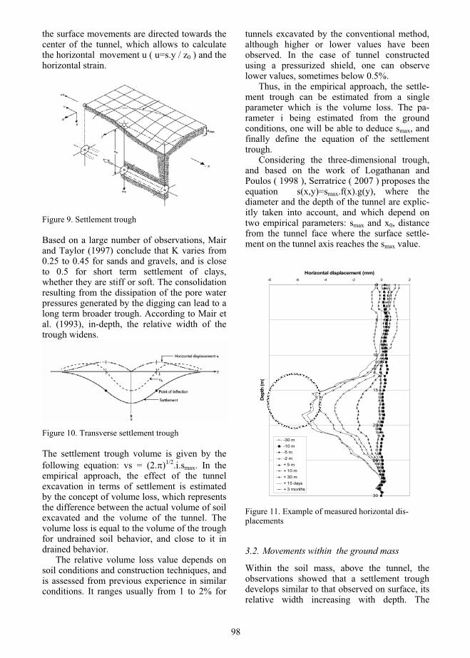
the surface movements are directed towards the center of the tunnel, which allows to calculate the horizontal movement u ( u=s.y / z0 ) and the horizontal strain.

Figure 9. Settlement trough

Based on a large number of observations, Mair and Taylor (1997) conclude that K varies from 0.25 to 0.45 for sands and gravels, and is close to 0.5 for short term settlement of clays, whether they are stiff or soft. The consolidation resulting from the dissipation of the pore water pressures generated by the digging can lead to a long term broader trough. According to Mair et al. (1993), in-depth, the relative width of the trough widens.

Figure 10. Transverse settlement trough

The settlement trough volume is given by the following equation: vs = (2. )1/2.i.smax. In the empirical approach, the effect of the tunnel excavation in terms of settlement is estimated by the concept of volume loss, which represents the difference between the actual volume of soil excavated and the volume of the tunnel. The volume loss is equal to the volume of the trough for undrained soil behavior, and close to it in drained behavior.

The relative volume loss value depends on soil conditions and construction techniques, and is assessed from previous experience in similar conditions. It ranges usually from 1 to 2% for

tunnels excavated by the conventional method, although higher or lower values have been observed. In the case of tunnel constructed using a pressurized shield, one can observe lower values, sometimes below 0.5%.

Thus, in the empirical approach, the settle-ment trough can be estimated from a single parameter which is the volume loss. The pa-rameter i being estimated from the ground conditions, one will be able to deduce smax, and finally define the equation of the settlement trough.

Considering the three-dimensional trough, and based on the work of Logathanan and Poulos ( 1998 ), Serratrice ( 2007 ) proposes the equation s(x,y)=smax.f(x).g(y), where the diameter and the depth of the tunnel are explic-itly taken into account, and which depend on two empirical parameters: smax and x0, distance from the tunnel face where the surface settle-ment on the tunnel axis reaches the smax value.

0

5

10

15

20

25

30

-8 -6 -4 -2 0 2

Horizontal displacement (mm)

Dep

th (m

)

-30 m-10 m-5 m-2 m+ 5 m+ 10 m+ 30 m+ 15 days+ 3 months

Figure 11. Example of measured horizontal dis-placements

3.2. Movements within the ground mass

Within the soil mass, above the tunnel, the observations showed that a settlement trough develops similar to that observed on surface, its relative width increasing with depth. The

98

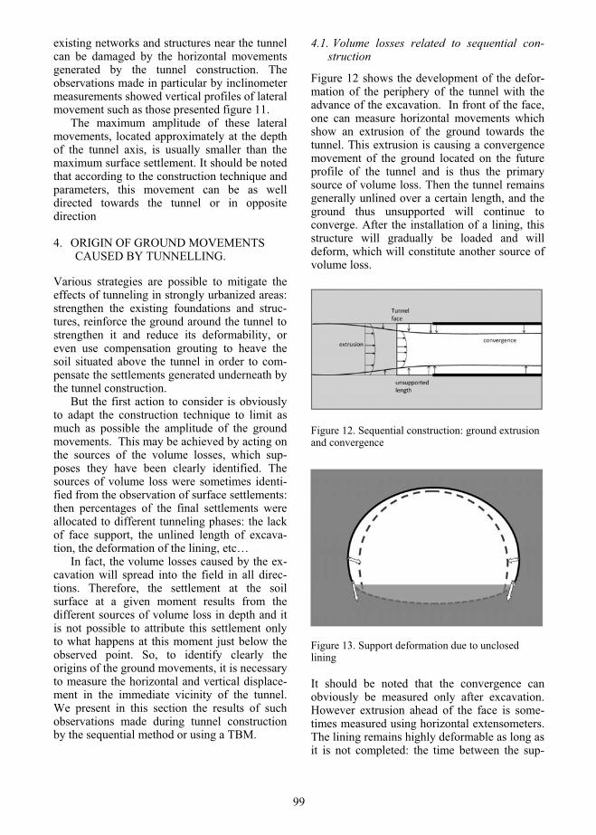
existing networks and structures near the tunnel can be damaged by the horizontal movements generated by the tunnel construction. The observations made in particular by inclinometer measurements showed vertical profiles of lateral movement such as those presented figure 11.

The maximum amplitude of these lateral movements, located approximately at the depth of the tunnel axis, is usually smaller than the maximum surface settlement. It should be noted that according to the construction technique and parameters, this movement can be as well directed towards the tunnel or in opposite direction

4. ORIGIN OF GROUND MOVEMENTS CAUSED BY TUNNELLING.

Various strategies are possible to mitigate the effects of tunneling in strongly urbanized areas: strengthen the existing foundations and struc-tures, reinforce the ground around the tunnel to strengthen it and reduce its deformability, or even use compensation grouting to heave the soil situated above the tunnel in order to com-pensate the settlements generated underneath by the tunnel construction.

But the first action to consider is obviously to adapt the construction technique to limit as much as possible the amplitude of the ground movements. This may be achieved by acting on the sources of the volume losses, which sup-poses they have been clearly identified. The sources of volume loss were sometimes identi-fied from the observation of surface settlements: then percentages of the final settlements were allocated to different tunneling phases: the lack of face support, the unlined length of excava-tion, the deformation of the lining, etc…

In fact, the volume losses caused by the ex-cavation will spread into the field in all direc-tions. Therefore, the settlement at the soil surface at a given moment results from the different sources of volume loss in depth and it is not possible to attribute this settlement only to what happens at this moment just below the observed point. So, to identify clearly the origins of the ground movements, it is necessary to measure the horizontal and vertical displace-ment in the immediate vicinity of the tunnel. We present in this section the results of such observations made during tunnel construction by the sequential method or using a TBM.

4.1. Volume losses related to sequential con-struction

Figure 12 shows the development of the defor-mation of the periphery of the tunnel with the advance of the excavation. In front of the face, one can measure horizontal movements which show an extrusion of the ground towards the tunnel. This extrusion is causing a convergence movement of the ground located on the future profile of the tunnel and is thus the primary source of volume loss. Then the tunnel remains generally unlined over a certain length, and the ground thus unsupported will continue to converge. After the installation of a lining, this structure will gradually be loaded and will deform, which will constitute another source of volume loss.

Figure 12. Sequential construction: ground extrusion and convergence

Figure 13. Support deformation due to unclosed lining

It should be noted that the convergence can obviously be measured only after excavation. However extrusion ahead of the face is some-times measured using horizontal extensometers. The lining remains highly deformable as long as it is not completed: the time between the sup-

99

porting of the tunnel and its closing by concret-ing the invert thus represents an additional source of convergence as shown on figure 13. Finally, in the case of saturated soils the tunnel can play the role of a drain and the resulting water seepage can induce settlements by con-solidation of soft soil strata.

To illustrate the ground behavior around a tunnel constructed by a conventional method, an example of the displacements observed during the construction of a tunnel using a sequential technique is presented hereafter (Janin, 2009). The monitored section is described on figure 14. This road tunnel has a section of 12 meters width and 11 meters height. In this section the invert of the tunnel is situated in a hard Permian ground (E = 500 MPa) and the crown in a Trias hard soil (E=90 MPa). In order to stabilize the face and to limit the settlements, 5 to 26 bolts 18 m long are installed through the face every 4.5 meters of excavation advance. An umbrella vault composed of 18 m long steel tubes is installed every 9 m if needed. The primary lining consists of shotcrete reinforced by steel arches and is installed immediately after each 1.5 m excavation phase.

Figure 14. Geological section and monitoring installation

An inclinometer tube situated on the tunnel axis permitted to observe the soil extrusion ahead of the tunnel face. The results presented figure 15 show a general horizontal movement towards the tunnel beginning when the face is at about 20 meters from the monitored section. In this example where the face is reinforced by fiber glass bolts, a slight extrusion at the tunnel level can be observed when the face is at 3 meters from the inclinometer, but this extrusion devel-ops clearly when the face is very close (1.5m) to

the observed section. This result indicates that the stiffness of the soil associated with the reinforcement by face bolting leads to reduce the ground extrusion, and finally limit the volume loss and the settlement ahead the excavation.

The convergence measurements inside the tunnel on this section are presented figure 16. A general settlement of the tunnel is observed, but the side walls being situated in a hard Permian ground, the lateral convergence is extremely small. This explains the negligible lateral displacement observed on the 2 lateral incli-nometers (which are not presented here).

Figure 15. Inclinometer situated on the tunnel axis: horizontal movements

Figure 16. Convergence measurements

Finally the development of the settlements measured at different depths between 2 and 6 meters is presented figure 17. As an umbrella

100

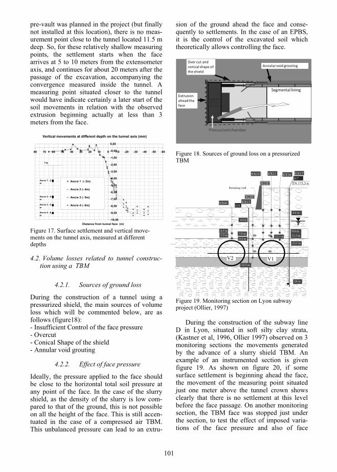
pre-vault was planned in the project (but finally not installed at this location), there is no meas-urement point close to the tunnel located 11.5 m deep. So, for these relatively shallow measuring points, the settlement starts when the face arrives at 5 to 10 meters from the extensometer axis, and continues for about 20 meters after the passage of the excavation, accompanying the convergence measured inside the tunnel. A measuring point situated closer to the tunnel would have indicate certainly a later start of the soil movements in relation with the observed extrusion beginning actually at less than 3 meters from the face.

Vertical movements at different depth on the tunnel axis (mm)

-10,50

-9,50

-8,50

-7,50

-6,50

-5,50

-4,50

-3,50

-2,50

-1,50

-0,50

0,50

-60-50-40-30-20-1001020304050607080

Distance from tunnel face (m)

Ancre 1 (- 2m)

Ancre 2 (- 4m)

Ancre 3 (- 5m)

Ancre 4 (- 6m)

Ancre 1: -2 m

Ancre 4: -6 m

Ancre 3: -5 m

Ancre 2: -4 m

T.N.

Figure 17. Surface settlement and vertical move-ments on the tunnel axis, measured at different depths

4.2. Volume losses related to tunnel construc-tion using a TBM

4.2.1. Sources of ground loss

During the construction of a tunnel using a pressurized shield, the main sources of volume loss which will be commented below, are as follows (figure18): - Insufficient Control of the face pressure - Overcut - Conical Shape of the shield - Annular void grouting

4.2.2. Effect of face pressure

Ideally, the pressure applied to the face should be close to the horizontal total soil pressure at any point of the face. In the case of the slurry shield, as the density of the slurry is low com-pared to that of the ground, this is not possible on all the height of the face. This is still accen-tuated in the case of a compressed air TBM. This unbalanced pressure can lead to an extru-

sion of the ground ahead the face and conse-quently to settlements. In the case of an EPBS, it is the control of the excavated soil which theoretically allows controlling the face.

Pressurised chamber

Segmental liningExtrusionahead theface

Over cut andconical shape ofthe shield

Annularvoid grouting

Figure 18. Sources of ground loss on a pressurized TBM

-13,1 m

-12,5 m

-24 m

-4,4 m

-9,5 m

-7,8 m-7,5 m

-6,5 m

-12,3 m -11,3 m-9,6 m

-5,6 m

TN 173,3 mRetaining wall

EX15 EX16 EX17EX11

EX41I14

EX13CPI19

CPI18

V1V2

I17

Figure 19. Monitoring section on Lyon subway project (Ollier, 1997)

During the construction of the subway line D in Lyon, situated in soft silty clay strata, (Kastner et al, 1996, Ollier 1997) observed on 3 monitoring sections the movements generated by the advance of a slurry shield TBM. An example of an instrumented section is given figure 19. As shown on figure 20, if some surface settlement is beginning ahead the face, the movement of the measuring point situated just one meter above the tunnel crown shows clearly that there is no settlement at this level before the face passage. On another monitoring section, the TBM face was stopped just under the section, to test the effect of imposed varia-tions of the face pressure and also of face

101

stabilisation by compressed air. The settlements generated during this test remain negligible.

Figure 20.Surface settlement and settlement 1 meter above the tunnel (Ollier, 1997)

During the construction of the Toulouse subway line B, comparison between the effect of a slurry shield and an EPBS showed no major difference concerning the ground movements ahead of the face. But it has to be mentioned that on 2 examples, one concerning a slurry shield and the other an EPBS, a face collapse happened near a monitoring section where the measured soil movements just above the face were very low.

4.2.3. Effect of over cut and shield conical shape

In order to allow curved alignment of the tunnel, and also to limit the steering force on the TBM, the diameter of the cutting wheel can be adjusted and is generally greater than the shield diameter. For the same reasons, the shield has a conical shape, with a diameter decreasing from the face to the tail. All the observations made in Lyon (Ollier, 1997) and Toulouse (Emeriault, 2005, Robert et al, 2007) on different types of TBMs, showed a clear increase of the settle-ment during the shield passage

4.2.4. Annular void grouting

The advancement of the shield generates an annular tail void due to the difference between the excavated diameter and the diameter of the segmental lining which is installed inside the shield. This annular void can lead to an impor-tant soil convergence towards the lining and must therefore be filled to limit this conver-gence. The nature of the grout and the process to control the grout injection are important

parameters for limiting the settlements after the shield passage.

During the Lyon subway line D construc-tion, the influence of the grouting pressure (compared to the vertical total soil stress) has been tested on two sections Ollier (1997). The grout injection was made through six pipes regularly installed around the tail of the shield. On the first section, the average grouting pressure was close to the total vertical soil stress, and the volume loss deduced from the surface settlement is about 0.7% (figure 21). On the second section, where the grouting pressure was 2 to 3 times greater than the vertical total soil stress, the final volume loss is reduced to 0.1%.

4.2.5. Effect of K0 on ground move-ments

The influence of K0 has been observed by comparing the soil behaviour during the Lyon subway construction in normally consolidated soft clays, to the observed movements during the subway line 2 construction in Toulouse, in highly over consolidated molasses, where K0 is about 1.8.

v = 250 kPa

v = 369 kPa

200 kPa < Grout < 400 kPa

300 kPa < Grout < 400 kPa

SITE 1 - Section 1

v = 250 kPa

v = 369 kPa

200 kPa < Grout < 400 kPa

300 kPa < Grout < 400 kPa

SITE 1 - Section 1

EX11EX15

-1 m

-2 m

-3 m

-4 m

-5 m

-6 m

-7 m

-8 m

-9 m

-10 m

-11 m

-12 m

-13 m

-14 m

-15 m

-16 m

-17 m

-18 m

-19 m

-20 m

-21 m

-22 m

-23 m

-24 m

-25 m

EX16 EX17

EX13

0 mm5 mm10 mm

Echelle desdéplacements

Profondeur

I14

I17 EX31EX32 EX33

0 mm5 mm10 mm

Echelle desdéplacements -1 m

-2 m

-3 m

-4 m

-5 m

-6 m

-7 m

-8 m

-9 m

-10 m

-11 m

-12 m

-13 m

-14 m

-15 m

-16 m

-17 m

-18 m

-19 m

-20 m

ProfondeurI36 EX34 I37

VOLUME LOSS: 0.7 % VOLUME LOSS: 0.1 %

EX11EX15

-1 m

-2 m

-3 m

-4 m

-5 m

-6 m

-7 m

-8 m

-9 m

-10 m

-11 m

-12 m

-13 m

-14 m

-15 m

-16 m

-17 m

-18 m

-19 m

-20 m

-21 m

-22 m

-23 m

-24 m

-25 m

EX16 EX17

EX13

0 mm5 mm10 mm

Echelle desdéplacements

Profondeur

I14

I17 EX31EX32 EX33

0 mm5 mm10 mm

Echelle desdéplacements -1 m

-2 m

-3 m

-4 m

-5 m

-6 m

-7 m

-8 m

-9 m

-10 m

-11 m

-12 m

-13 m

-14 m

-15 m

-16 m

-17 m

-18 m

-19 m

-20 m

ProfondeurI36 EX34 I37

VOLUME LOSS: 0.7 % VOLUME LOSS: 0.1 %

v = 206 kPa

v = 333 kPa

250 kPa < Grout < 550 kPa

250 kPa < Grout < 550 kPa

SITE 2

v = 206 kPa

v = 333 kPa

250 kPa < Grout < 550 kPa

250 kPa < Grout < 550 kPa

SITE 2

v = 250 kPa

v = 369 kPa

200 kPa < Grout < 400 kPa

300 kPa < Grout < 400 kPa

SITE 1 - Section 1

v = 250 kPa

v = 369 kPa

200 kPa < Grout < 400 kPa

300 kPa < Grout < 400 kPa

SITE 1 - Section 1

EX11EX15

-1 m

-2 m

-3 m

-4 m

-5 m

-6 m

-7 m

-8 m

-9 m

-10 m

-11 m

-12 m

-13 m

-14 m

-15 m

-16 m

-17 m

-18 m

-19 m

-20 m

-21 m

-22 m

-23 m

-24 m

-25 m

EX16 EX17

EX13

0 mm5 mm10 mm

Echelle desdéplacements

Profondeur

I14

I17 EX31EX32 EX33

0 mm5 mm10 mm

Echelle desdéplacements -1 m

-2 m

-3 m

-4 m

-5 m

-6 m

-7 m

-8 m

-9 m

-10 m

-11 m

-12 m

-13 m

-14 m

-15 m

-16 m

-17 m

-18 m

-19 m

-20 m

ProfondeurI36 EX34 I37

VOLUME LOSS: 0.7 % VOLUME LOSS: 0.1 %

EX11EX15

-1 m

-2 m

-3 m

-4 m

-5 m

-6 m

-7 m

-8 m

-9 m

-10 m

-11 m

-12 m

-13 m

-14 m

-15 m

-16 m

-17 m

-18 m

-19 m

-20 m

-21 m

-22 m

-23 m

-24 m

-25 m

EX16 EX17

EX13

0 mm5 mm10 mm

Echelle desdéplacements

Profondeur

I14

I17 EX31EX32 EX33

0 mm5 mm10 mm

Echelle desdéplacements -1 m

-2 m

-3 m

-4 m

-5 m

-6 m

-7 m

-8 m

-9 m

-10 m

-11 m

-12 m

-13 m

-14 m

-15 m

-16 m

-17 m

-18 m

-19 m

-20 m

ProfondeurI36 EX34 I37

VOLUME LOSS: 0.7 % VOLUME LOSS: 0.1 %

v = 206 kPa

v = 333 kPa

250 kPa < Grout < 550 kPa

250 kPa < Grout < 550 kPa

SITE 2

v = 206 kPa

v = 333 kPa

250 kPa < Grout < 550 kPa

250 kPa < Grout < 550 kPa

SITE 2

Figure 21. Lyon subway: grouting pressure and settlements

102

In the Lyon subway example, due to the very soft character of the silty clay soils, there is no overcut and the cutting wheel works inside the shield. So, there is no volume loss during the face passage. Nevertheless, one meter above the tunnel, a clear settlement was observed just at the face passage (figure 20), and at the same moment, inclinometer measurements showed a lateral outward movement at the tunnel level (figure 22). The simultaneity of this convergent vertical movement towards the tunnel and a horizontal outward movement can be explained by the cancellation of the shear stresses at the interface between the ground and the shield, as the natural water content of the clay is locally close to its liquid limit.

Figure 22. Lyon subway : horizontal movements (Ollier, 1997)

The cancellation of the shear stresses then allow the soil to slip around the shield, changing the K0 state of stress to an hydrostatic one, and leading to these simultaneous vertical soil settlement and lateral outward movement. This has been confirmed (figure 23) by a numerical simulation which shows clearly these soil movements. (Benmebarek et al, 1998, 2000).

In the case of the Toulouse subway works (Vanoudheusden 2007), the 7.8 m diameter tunnel is excavated in highly over consolidated clayey molassic sands, where K0 is about 1.8. Although the excavation is made with an overcut, which corresponds to a volume loss, the settlement monitoring shows here clearly a heaving at the soil surface just after the face passage (Figure 24).

Figure 23. Lyon subway : simulation of face passage- soil movements around the shield (Benmebarek et al, 1998))

-1

-0.8

-0.6

-0.4

-0.2

0

0.2

0.4

0.6

0.8

1

1.2

-15 -10 -5 0 5 10 15

Distance to the tunnel axis (m)

Vert

ical

dis

plac

emen

t (m

m)

-19.6 04.2 712.6 4283.8

Figure 24. Toulouse subway - surface movements

On the other hand, the inclinometer measure-ments of the horizontal movements show a convergence of the ground towards the tunnel, greater than the vertical heave. The explanation, confirmed by numerical simulations is the same that for the example of Lyon: due to over consolidation, the horizontal stresses are here greater than the vertical ones. The excavation made with an overcut has for consequence to cancel the shear stresses around the shield. Although there is here a loss of volume, the passage of a K0 state of stress (with K0 > 1) to a hydrostatic state allows the soil to slide around the tunnel, leading to the heaving of the ground above the tunnel at the same time as the soil converges laterally (figure 24 et 25).

103

0

5

10

15

20

25

30

-8 -6 -4 -2 0 2

Horizontal displacement (mm)

Dep

th (m

)

-30 m-10 m-5 m-2 m+ 5 m+ 10 m+ 30 m+ 15 days+ 3 months

Figure 25. Toulouse subway – lateral displacements

4.2.6. Correlation between TBM pa-rameters and settlements

Based on an extensive settlement survey during the Toulouse subway line B construction, (Vanoudheuseden et al 2005, 2007) examined the possible statistical correlations between the excavation parameters of an earth pressure balanced shield working in over-consolidated molasses, and the observed surface settlements. The main parameters considered in this analysis were the following:

- average advancement speed of the TBM

- face pressure - average grouting pressure - volume of injected grout - torque on the cutting head - total jacking force - Total time for installing one lining ring - variation of vertical TBM angle - variation of horizontal TBM angle

Following a large statistical analysis, Vanoud-heuseden et al (2005, 2007) found out that essentially 3 parameters could be correlated to the surface settlements:

- The average speed of the TBM, parameter that Ollier (1997) found also important in soft

silty clay. This can be certainly explained by a delayed convergence blocked by tail grouting when the advancement of the TBM is rapid

- The torque on the cutting head. In an EPBS, a low value of the torque can be corre-lated with a looser state of the earth in the excavation chamber, leading to a lower face pressure;

- The variation of the vertical angle of the TBM articulation, which is correlated to the difficulty of controlling the direction of excava-tion, and could lead to some over excavation

5. NUMERICAL SIMULATION OF GROUND MOVEMENTS GENERATED BY TUNNEL CONSTRUCTION

The estimation of the green field settlement trough by empirical approaches is generally reliable, if the volume loss is carefully assessed. But in urban areas, it is often needed to assess not only the surface settlements, but the 3D movements in the soil mass, as they can lead to damages on all existing surface and buried structures. Moreover, these structures interact-ing with the construction process can modify the field of deformations. Also, specific soil conditions can lead to atypical settlement troughs. And finally, the rapid evolution of construction techniques, leading sometimes to very complex works, can affect the behaviour of the ground around the tunnel.

Theoretically, finite element or finite differ-ence numerical approaches should allow to simulate more precisely the construction of underground structures in a complex environ-ment, and to take into account complex soil conditions, the effect of water seepage and consolidation, the interaction with existing structures, the construction phases... But using 2D or 3D simulations can lead to very poor modelling if some basic requirements such as initial conditions, appropriate soil model, simulation of construction phases are not achieved.

The construction of a tunnel being a 3D process, the numerical 3D approaches are most appropriate to simulate this process. But as such approaches are generally highly time consum-ing, 2D approaches are widely used. Based on some examples, the limits and difficulties of 2D and 3D approaches will be shortly described.

104

6. 2D NUMERICAL MODELS

Simpler and less time consuming than 3D models, and therefore often used, 2D ap-proaches nevertheless need some more or less simplifying hypotheses in order to model in 2 dimensions an actually 3D process with differ-ent phases going from the approach of the excavation to the installation of the final lining. Diverse approaches have been proposed by many authors in order to simulate this passage from 3D to 2D, and used to simulate the con-ventional tunnelling method as well as the construction using a TBM. Most often, these approaches, especially when using a linear isotropic elastic perfectly plastic soil model, lead to a settlement trough wider and shallower than the observed ones, and the various alterna-tives aim at approaching as well as possible the movements observed in reality.

Three examples of these approaches are pre-sented here (figure 26):

- Progressive softening: the excavation-phases are simulated by a progressive softening of the soil module in the corresponding zone, before installing the lining (Leca and Clough, 1992). The arbitrary parameter here is the rate of softening.

- Convergence- confinement approach (Pa-net, 1995). Before setting up the lining, a reduction of the initial stresses at the tunnel periphery is applied by a factor equal to (1- ), being the so-called “deconfinement parameter”. The successive construction phases are simu-lated by applying specific values of (1 0) which are defined empirically, with the support of simplified analytical approaches. For simu-lating the tail void grouting when using a TBM, values of greater than 1 can be used.

- Diameter reduction used for simulating the construction using a TBM. The diameter of the excavation is reduced (or increased during grouting phases) by an empirical coefficient to simulate the successive phases of interaction between the TBM and the ground: face passage, effect of the conical shape of the shield, annular void filling, grout consolidation…

A great number of alternatives are possible, based on these approaches, considering the different phases, such as a fixed centre of the tunnel, a fixed base, and changes of the me-chanical properties at the soil tunnel interface. It is also possible to use alternatively the stress reduction approach and the diameter reduction, depending on the construction phases simulated.

Diameterreduction

E

Softening convergence /confinement

Figure 26. Numerical simulation: example of 2D approaches

Most often, these approaches, especially when using a linear isotropic elastic soil model, lead to a settlement trough wider and shallower than the observed ones, and the various alternatives aim at approaching as well as possible the movements actually observed in the field.

6.1. An example of 2D approach by diameter reduction

Benmebarek and al (1998, 2000) proposed a back analysis of the experimental results on the Lyon subway line D (figure 19), improving the diameter reduction approach by separating radial and tangential displacements.

The principle is to use a ring with a diame-ter at first equal to the shield external diameter. This ring will successively represent the shield wall, then the segment lining and the grout. The computation was performed with Flac 2D, in large deformation mode. Soil-shield and soil-grout interactions were modelled using a Mohr-Coulomb yield criterion. The different stages were modelled by decreasing or increasing the ring diameter and simultaneously activating interface elements and adjusting the interface mechanical parameters, permitting more or less sliding of the ground around the ring.

This model is controlled by adjusting 2 pa-rameters: the diameter of the ring and the Mohr-Coulomb criterion at the interface. These parameters were adjusted on the settlement observed just 1 meter above the tunnel. The global field of displacement at each stage was then compared to the monitoring results. The calculated settlement troughs and the final measured settlement trough are compared in figure 27.

This simulation approach reproduced rea-sonably well not only the observed vertical settlements at different depth, but also the lateral response of the ground measured by inclinometer measurements. It confirmed for

105

example that the movements observed during the face passage without any overcut (vertical settlements and lateral outward movement), can only be explained by cancelling partly the soil-shield shear strength, without any diameter reduction, as shown by the displacement vectors on figure 22.

Figure 27. Measured and calculated settlement troughs

6.2. Influence of the constitutive model

Concerning the description of the settlement trough, the results obtained by 2D approaches depend on the constitutive model adopted for the soil. Using a simple isotropic elastic linear soil model generally leads to a settlement trough shape wider than the actual ones. For example, considering a strain softening model and an elastic orthotropic model (Potts and Zdravkovic, 2001) allow a more realistic modelling.

0

20

40

60

80

100

120

140

160

1,E-05 1,E-04 1,E-03 1,E-02 1,E-01Axial strain

E(M

Pa)

Test 1Test 2MCHSHS-Small

Figure 28. Stiffness-strain curves (comparison between model predictions and test data)

Hejazi et al (2007), using the approach of stress reduction, tested the influence of the soil model. The behaviour of the over-consolidated clay

layer was simulated using 3 different soil models: linear elastic-Mohr-Coulomb, harden-ing soil model, and HS Small implemented in Plaxis (Schanz, 98, Benz, 2006). A comparison of experimental stiffness-strain curves to those obtained by the 3 model predictions is presented on figure 28.

Figure 29: Finite element geometry and mesh.

-0,006

-0,005

-0,004

-0,003

-0,002

-0,001

0,000

0 20 40 60 80 100Offset from tunnel centreline (m)

Surf

ace

settl

emen

t (m

)

MCHSHS-Small

a)

-40

-35

-30

-25

-20

-15

-10

-5

0-0,02 -0,015 -0,01 -0,005 0

Horizontal displacement (m)

Dep

th b

elow

gro

und

surf

ace

(m)

b)Figure 30. Settlement troughs (a) and lateral dis-placements (b)

106

The Plaxis plane strain model created for comparing the 3 soil models is presented in figure 29. The water table is assumed to be 2.5 m below the ground surface. The extension of the mesh is 100 m wide and the tunnel is lo-cated at H = 53.75 m above the substratum. The tunnel is circular and its diameter is D = 7.7 m. The covering height adopted for the reference calculation is 2D.

The numerical simulation presented here corresponds to a stress reduction =35%. The surface settlements and their corresponding horizontal displacements are presented on Figure 30 a et b. The impact of the constitutive model appears by a difference in response in terms of ground movements. In spite of a satisfactory lateral mesh extension, it can be noticed that by using the MC model, surface settlements at 100 m from the axis were observed which seems unrealistic. This problem can be explained by the fact that even in the zones of small-strains, the MC model modulus is constant. The model based on a higher stiffness under small-strain is closer to the experimental observations contrary to the MC model.

A difference of about 40% between the maximum settlement estimated by the HS and the HS-Small model can be seen, which indi-cates that it is important to take into account the soil modulus variation with strain. Regarding the horizontal displacement corresponding to the tunnel centerline level, the HS model provides a displacement 60% larger than that predicted by the HS-Small model. However, the MC model shifts considerably from the two other models with a displacement 290% higher than that observed by the HS-Small model.

7. 3D NUMERICAL MODELS

The construction of a tunnel being a highly three-dimensional process, 3D approaches are theoretically the most appropriate and suitable to model the entire construction process. But the complexity of the tunnelling process, either by the conventional method or using a TBM makes these models difficult to implement, and often leads eventually to reintroduce in these 3D approaches empirical factors

7.1. 3D model –conventional tunnelling method

In the case of conventional tunnelling tech-niques, the boundary conditions related to the

construction process are generally well known, and it is now possible without major difficulty, and with an adapted 3D mesh, to model the successive phases of excavation and support. However some specific difficulties can be mentioned:

- the ground near the unsupported parts may experience a high level of plastic deformation, which can lead to a softening generally not taken into account;

- reinforcements such as face bolting, radial bolting or pre-vaults correspond to elements whose geometrical scale is much lower than that of the tunnel and of the mesh of the model: their explicit representation is difficult. Various strategies are possible for their consideration: i) to apply an equivalent pressure on the tunnel face or to assign to the bolted zone an equiva-lent cohesion ii) to replace the individual modelling of the soil and the bolts by an equiva-lent homogenised material, iii) to model the bolts individually.

The pre-vaults are generally represented by shells. In the case of umbrellas vaults made of tubes or other reinforcements installed in drillings, these tubes are not jointed longitudi-nally and do not form a continuous vault. There is then a difference in stiffness between the axial direction of the vault and the orthogonal direction which can be represented by an orthotropic elastic model (Shin et al, 2007, Eclaircy-Caudron et al 2006). In the case of pre-vaults realized by pre-cutting, the resulting local deconfinement concerning this operation must be modelled.

In the case of reinforcement by soil bolting, Dias (1999), Dias et al (2000, 2005) compared the results obtained by a full 3D model where all the bolts are individually represented with 2 simplified approaches where the bolts are not directly modelled: i) considering an equivalent face pressure and ii) considering an equivalent cohesion in the bolted zone.

The efficiency of the global face bolting sys-tem can be estimated by the reduction of the face extrusion. In the 3D model, Dias et al (2005) compared the effect of a reduced number of bolts with a high axial stiffness to a larger number of bolts with a reduced axial stiffness; The results showed that the face extrusion does not depend on the number of bolts but on the global stiffness of the bolting system, provided that the distance between the bolts does not allow excessive local extrusion between the bolts.

107

Peila (1994) and Grasso (1991, 1993) pro-posed simplified approaches to simulate the action of the bolting in stability calculations. The principle of these approaches is to take into account the bolting by means of a pressure applied to the tunnel face or by means of in-creased soil cohesion in the reinforced volume. The equivalent pressure (Pface) or cohesion (cr)are given by the following equations:

SnFaPface / [Eq. 1]

24tan. SnF

racc

Where: n Number of bolts S Surface of the tunnel face c : soil cohesion

: Friction angle of soil Fa: Axial load in the bolt

In these equations Fa is taken as the minimum of the axial resistance of the bolt and the maxi-mal shear force at the soil/bolt interface

Comparing on several examples the face ex-trusion obtained by full 3D simulations with these simplified approaches, Dias et al (2005) showed that the simplified approaches strongly over-estimate the effect of the reinforcement on the displacement reduction. As an example, for circular tunnel where 16 to 144 bolts were installed, back analyses were performed to estimate the equivalent value of the pressure at the face, taking as a reference the axial face extrusion obtained using the 3D calculation .

These results show that the face pressure calculated with the bolt axial resistance overes-timates largely the equivalent face pressure. In fact the equivalent face pressure depends on the axial force actually mobilised in the bolting system. As demonstrated by this back analysis, the axial force depends on the face extrusion which is directly linked to the total stiffness of the bolting system. In this example, the bolt resistance is equal to 700 kN and the mobilised force derived from the back analysis is equal to145 KN for 16 bolts and decreases to 60 kN for 144 bolts (figure 31).

In a second stage, Dias & Kastner (2005) compare the deformations calculated using the full 3D model and the simplified models.

The axial extrusion ahead of the face ob-tained by the three methods are almost identical

(figure 32) but the simplified approaches underestimate the convergence by 20% (figure 33).

Number of bolts

Max

. fac

e ex

trusi

on (m

)

Mobilised axial force in 1 bolt

3D ModelFa = 60 kNFa = 100 kNFa = 145 kNFa = 700 kN

Number of bolts

Max

. fac

e ex

trusi

on (m

)

Mobilised axial force in 1 bolt

3D ModelFa = 60 kNFa = 100 kNFa = 145 kNFa = 700 kN

Figure 31. Comparison of full 3D model and simplified “equivalent face pressure” model

max

. fac

e ex

trusi

on (m

)

Relative distance to the face (y/R)

3D Model , 52 bolts

Equivalent face pressure: 0.053 MPa

Equivalent cohesion: 82.8 kPamax

. fac

e ex

trusi

on (m

)

Relative distance to the face (y/R)

3D Model , 52 bolts

Equivalent face pressure: 0.053 MPa

Equivalent cohesion: 82.8 kPa

Figure 32. Axial extrusion

Relative distance to the face (y/R)

Rad

ial c

onve

rgen

ce (m

)

3D Model

Equivalent face pressure

Equivalent cohesion

Relative distance to the face (y/R)

Rad

ial c

onve

rgen

ce (m

)

3D Model

Equivalent face pressure

Equivalent cohesion

Figure 33. Radial convergence

Therefore, applying these simplified meth-ods supposes to assess the actual force mobi-lised in the bolts, especially for shallow tunnel where it is generally low compared to the axial resistance. Finally, following these results, a method to assess the equivalent face pressure, based on 2 characteristic curves (the ground characteristic curve and the reinforcement characteristic curve) is proposed and can be found in Dias et al (2003).

108

7.2. 3D model of TBM/ground interaction

TBMs are complex machines which are con-trolled by a great number of parameters. Several authors proposed 3D simulations aiming at modelling the different physical phenomena acting during their functioning. Based on a back-analysis, Dias et al (2000) modelled the face pressure, the effect of overcut and shield conical shape, the injection of the annular void. Kasper and Meschke (2004, 2006) proposed a comprehensive 3D model where the trajectory changes of the TBM are derived from the steering forces on the different jacks. Sugimoto and Sramoon (2002) proposed a model where the ground action on the TBM is modelled by springs. In order to derive the ground move-ments from their model, they apply the dis-placements calculated at the limits of the TBM to a separated 3D finite element model of the ground mass (Sugimoto et al, 2007).

Hereafter are listed and discussed the main parameters influencing the ground movements:

- the face pressure is relatively easy to model in the case of slurry shields and com-pressed air shields, provided that the face is enough impervious to avoid air or seepage flow in the soil. It is not so easy in the case of EPBS where the face pressure is difficult to assess;

- Over cut and conical shape of the shield are easy to model, but in the case of a slurry shield, the slurry seepage around the shield and the resulting pressure are difficult to model precisely;

- Only very few models take into account the shield articulation and the effects of differ-ential forces in the steering jacks

- The annular void filling is a complex proc-ess, studied recently by Bezuijen (2007), Bezui-jen & Talmon (2008). The injections are gener-ally made by strokes, generating high pressure variations. More over, the grout properties are rapidly changing from a liquid state to a solid state, due to consolidation and hardening. The grout may also flow ahead around the shield on a certain distance, applying a radial pressure to the soil. All these phenomena are difficult to model precisely, but have a real influence on the induced movements.

Demagh et al (2009a, 2009b) proposed a three-dimensional simulation procedure, using finite differences code Flac-3D, taking into account in an explicit manner the main sources of movements in the soil mass. This procedure is applied to three different case studies (differ-

ent type of face support, nature of soils or mechanical characteristics):

Case 1: Lyon subway line D (Ollier, 1997): the slurry shield passes through heterogeneous silty and clayey alluvial normally consolidated deposits

Case 2: Toulouse subway line B (Vanoud-heusden, 2006, Vanoudheusden et al, 2006): the earth pressure balance shield passes through clayey molasses highly over consolidated (Ko is about 1.8).

Case 3: Shanghai Yangtze River Tunnel (Yan, 2007): this very large slurry shield (15.4 m diameter) crosses normally consolidated deposits of soft clay.

The main geometrical and geotechnical pa-rameters concerning the 3 monitoring sections are summarized in the tables 3 to 6.

Table 3. Geometrical characteristics

Case H(m)

D(m)

C/D conicity (mm)

Annular gap (cm)

Lyon 13,6 6,3 1,66 15 27

Toulouse 16,5 7,7 1,64 25 20

Shanghai 17,5 15,4 0,64 85 23

Table 4. Geotechnical profile (Case 2- Toulouse)

Soil type Thickness(m) kN/m3

K0 cukPa

udegrees

EMPa

fill 0-4 20 0,5 0 25 25

molasses 4-10 >10

2222

1,71,7

300 300

00

165E(z)

E(z)=9,9z+66,1 (Vanoudheusden, 2006). The water table is 4m under the soil surface

Table 5. Geotechnical profile (Case 1- Lyon)

Soil type Thickness

(m) (kN/m3 )

c’ (kPa)

’ ’ EMPa

Fill 0-3 19 30 30° 17° 7,8

Brown silt 3-5 21 10 25° 15° 7,3

Beige silt 5-8 21 15 32° 20° 7,3

Ocre silt 8-12 21 15 25° 14° 7,3

Grey silt 12-15 21 5 30° 14° 4,2

Fine sand 15-18,4 21 0 34° 20° 28

gneiss 18,4-20 21 150 45° 30 140

The water table is 3m under the soil surface

109

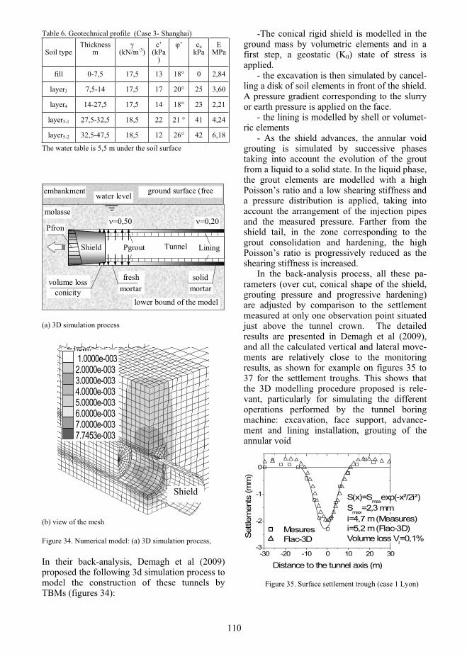
Table 6. Geotechnical profile (Case 3- Shanghai)

Soil type Thickness

m (kN/m-3)c’

(kPa)

’ cukPa

EMPa

fill 0-7,5 17,5 13 18° 0 2,84

layer3 7,5-14 17,5 17 20° 25 3,60

layer4 14-27,5 17,5 14 18° 23 2,21

layer5-1 27,5-32,5 18,5 22 21 ° 41 4,24

layer5-2 32,5-47,5 18,5 12 26° 42 6,18

The water table is 5,5 m under the soil surface

Shield

embankment ground surface (free fi ld)

volume loss conicity

molasse

water level

Pfron

Pgrout Tunnel Lining

fresh mortar

solid mortar

=0,50 =0,20

lower bound of the model

(a) 3D simulation process

(b) view of the mesh

Figure 34. Numerical model: (a) 3D simulation process,

In their back-analysis, Demagh et al (2009) proposed the following 3d simulation process to model the construction of these tunnels by TBMs (figures 34):

-The conical rigid shield is modelled in the ground mass by volumetric elements and in a first step, a geostatic (K0) state of stress is applied.

- the excavation is then simulated by cancel-ling a disk of soil elements in front of the shield. A pressure gradient corresponding to the slurry or earth pressure is applied on the face.

- the lining is modelled by shell or volumet-ric elements

- As the shield advances, the annular void grouting is simulated by successive phases taking into account the evolution of the grout from a liquid to a solid state. In the liquid phase, the grout elements are modelled with a high Poisson’s ratio and a low shearing stiffness and a pressure distribution is applied, taking into account the arrangement of the injection pipes and the measured pressure. Farther from the shield tail, in the zone corresponding to the grout consolidation and hardening, the high Poisson’s ratio is progressively reduced as the shearing stiffness is increased.

In the back-analysis process, all these pa-rameters (over cut, conical shape of the shield, grouting pressure and progressive hardening) are adjusted by comparison to the settlement measured at only one observation point situated just above the tunnel crown. The detailed results are presented in Demagh et al (2009), and all the calculated vertical and lateral move-ments are relatively close to the monitoring results, as shown for example on figures 35 to 37 for the settlement troughs. This shows that the 3D modelling procedure proposed is rele-vant, particularly for simulating the different operations performed by the tunnel boring machine: excavation, face support, advance-ment and lining installation, grouting of the annular void

-30 -20 -10 0 10 20 30-3

-2

-1

0

S(x)=Smax

exp(-x²/2i²)S

max=2,3 mm

i=4,7 m (Measures) i=5,2 m (Flac-3D) Volume loss V

l=0,1%

Mesures Flac-3DSe

ttlem

ents

(mm

)

Distance to the tunnel axis (m)

Figure 35. Surface settlement trough (case 1 Lyon)

Liv

I

hown 1.0000e-0032.0000e-0033.0000e-0034.0000e-0035.0000e-0036.0000e-0037.0000e-0037.7453e-003

Shield

110

-0,6

0

0,6

1,2

0 3 6 9 12 15

Position/tunnel axis (m)

Dis

plac

emen

ts (m

m)

front passagetail passage+12 meters+30 meters final

Simulation

-0,6

0

0,6

1,2

0 3 6 9 12 15

Position/tunnel axis (m)

Dis

plac

emen

ts (m

m)

-19,6 metersfront passage+4,2 meters+12,6 meters+42 meters

Measurements

Figure 36. Surface settlements and heave (a) Simulations (b) Measured (case 2 – Toulouse)

Nevertheless, some adjustment had to be made concerning the overcut, the amount of diameter reduction of the shield, the grouting pressure and the changes in the grout parameters in order to take into account the complex phenomena around the shield such as the flow of slurry and of grout along the external face of the shield. Therefore, predicting settlements and global movements using such a 3D model supposes to assess the adjustment of several parameters on an empirical way, or by back analysis on the very beginning of a tunnelling work.

-40 -30 -20 -10 0 10 20 30 40-50

-40

-30

-20

-10

0

S(x)=Smaxexp(-x²/2i²) Smax=42,5 mmi=7,35 m (Measures) i=10,3 m (Flac-3D) Volume loss V

l=0,42%

Mesures Flac-3D

Settl

emen

ts (m

m)

Distance to the tunnel axis (m)

Figure 37. Final settlement trough (Case 3 Shanghai)

.

8. REAL TIME UPDATING THE GROUNG RESPONSE TO TUNNELLING

Tunnel construction, either by conventional methods or TBM, involves always complex processes, and their effect on the surrounding ground frequently differs from the estimated behaviour at the design phase. Moreover, tunnelling works generally concern important volumes of ground over long distances, which lead to important uncertainties regarding the local soil characteristics. Therefore, in almost all the tunnelling projects, monitoring is an important part of the project and the design is based, at least partially, on the observational approach: different construction procedures (excavation sequences, support, soil reinforce-ment, etc..) are predetermined based on unfa-vourable, average or favourable hypothesis, and the project is adapted continuously, based on appropriate observations. The monitoring principles and techniques, and the observational approach, are described largely in a great number of publications and recommendations and will not be presented here. We will simply present some methods such as the inverse analysis or neural network which could be useful to enhance the real time process of estimating the actual characteristics or behavior of the ground in a observational type approach.

8.1. Inverse analysis

The aim of an inverse analysis process is the identification of parameters using tests results or/and experimental measurement carried out during works.The principle of the direct simula-tion and that of the inverse analysis are shown in Figure 38. In the direct approach, based on initial conditions, boundary conditions, a simulation model, a soil model and its parame-ters, the ground and support is calculated. In the inverse method, the response is measured and therefore known, and it is the value of some model parameters which is unknown. To assess these values, the difference between calculation and observed response is compared through an error function. Finally, the value of the parame-ters minimizing the error function is obtained using optimization methods.

111

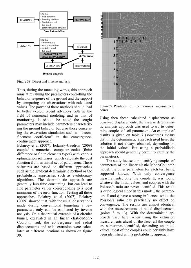
LOADING

SYSTEM- Initial conditions- Boundary conditions - Simulation model- Soil model- parameters (soil & simulation)

RESPONSE???

SYSTEM- initial conditions- Boundary conditions- simulation model- Soil model

RESPONSE

OBSERVATIONSOPTIMISATION

PARAMETERS ???(SOIL & SIMULATION)

Direct simulation

Inverse analysis

SYSTEM- Initial conditions- Boundary conditions - Simulation model- Soil model- parameters (soil & simulation)

RESPONSE???

SYSTEM- initial conditions- Boundary conditions- simulation model- Soil model

RESPONSE

OBSERVATIONSOPTIMISATION

PARAMETERS ???(SOIL & SIMULATION)

SYSTEM- initial conditions- Boundary conditions- simulation model- Soil model

RESPONSELOADING

OBSERVATIONSOPTIMISATION

PARAMETERS ???(SOIL & SIMULATION)

Direct simulation

difference

Inverse analysis Figure 38. Direct and inverse analysis Thus, during the tunneling works, this approach aims at revaluing the parameters controlling the behavior response of the ground and the support by comparing the observations with calculated values. The power of these methods should lead to better exploit recent advances both in the field of numerical modeling and in that of monitoring. It should be noted the sought parameters may include parameters characteriz-ing the ground behavior but also those concern-ing the excavation simulation such as “decon-finement coefficient” in the convergence-confinement approach. Eclaircy et al (2007), Eclaircy-Caudron (2009) coupled a numerical computer codes (finite difference or finite elements types) with various optimization softwares, which calculate the cost function from an initial set of parameters. These softwares are based on different approaches such as the gradient deterministic method or the probabilistic approaches such as evolutionary algorithms. The deterministic approach are generally less time consuming but can lead to find parameter values corresponding to a local minimum of the error function. Testing all these approaches, Eclaircy et al (2007), Eclaircy (2009) showed that, with the usual observations made during conventional tunneling a few parameters only can be estimated by inverse analysis. On a theoretical example of a circular tunnel, excavated in an linear elastic/Mohr-Coulomb soil, the convergence and radial displacements and axial extrusion were calcu-lated at different locations as shown on figure 39.

1

2

4

3

5

6

7

8 9 10 11 12 13

Figure39. Positions of the various measurement points Using then these calculated displacement as observed displacements, the inverse determinis-tic analysis approach was used to try to deter-mine couples of soil parameters. An example of results is given on table 7 (sometimes means that in the deterministic approach used here, the solution is not always obtained, depending on the initial values. But using a probabilistic approach should generally permit to identify the parameters).

The study focused on identifying couples of parameters of the linear elastic Mohr-Coulomb model, the other parameters for each test being supposed known. With only convergence measurements, only the couple E, is found whatever the initial values, and couples with the Poisson’s ratio are never identified. This result is quite logical since in this model, the parame-ters E and have a strong influence, while the Poisson’s ratio has practically no effect on convergence. The results are almost identical with the measurements of radial displacement (points 8 to 13). With the deterministic ap-proach used here, when using the extrusion measurements ahead of the face, all the couple are sometimes identified, depending on initial values: most of the couples could certainly have been identified with a probabilistic approach

LOADING

112

Table 7. Inverse analysis -Test on couples of parame-ters

Tests Parameters

Pt 1;2 orPt 1 to 7

Pt 8 to13

Pt 14to 20

1 E, No No Sometimes

2 E, Yes Yes Sometimes

3 E, C Sometimes

Sometimes

Sometimes

4 C, Sometimes

Sometimes

Sometimes

5 C, No No Sometimes

6 , Sometimes

No Yes

Finally, this study showed that couples of parameters, often difficult to evaluate at the scale of a tunnelling project, but having a noticeable influence on the tunnel and ground behaviour can be theoretically obtained from an inverse analysis approach, provided that appro-priate observations are available and that the other parameters are correctly identified.

However, this method supposes that the global modelling approach (including the soil constitutive law and the procedure to model the tunnel construction) allows effectively simulat-ing the observed behaviour.

8.2. Settlement evaluation by neural network

Artificial Neural Networks (ANN) are computa-tion models schematically inspired by the functioning of real neurones. They are generally classified in the family of statistical applications as well as that of artificial intelligence.

The function of formal neurons networks, following the example of the alive model, is to solve problems. Unlike the more usual ap-proach, this ability is not based on algorithms constructed from understanding the problem, but on a network with many "synaptic connec-tions". From the input parameters, the network will give an answer and output, without a model representing the physical problem being estab-lished (figure 40). This capability must there-fore be based on a learning phase from known situations.

In practice, illustrated by the examples pre-sented by Neaupane and Adhikari (2006), or Suwansawat and Einstein (2006), a neural network is developed in two stages:

- Learning phase: first, for a given site on

which sufficient monitoring results are already available, a "multiple correlation" model is developed between measured parameters (maximum settlement, settlement trough, ...), and input parameters influencing the ground response to tunnelling such as geology, depth of tunnel, operation parameters of the TBM (face pressure, advancement speed, grouting pressure and volume…);

- forecast phase: After the learning phase, the model can be used to assess the future settlement for the rest of the project, and to test for example the influence of changes of work-ing parameters.

Input 4

Input 1

Hidden layers

Input 3

Input 2

Output

Input 5

Figure40. Example of multilayer neural network architecture.

Boubou et al (2009) tested the neural net-work method for predicting surface settlement troughs based on Toulouse subway line B monitoring results. The vertical surface ground movements were monitored during the different tunnelling phases by precise levelling of trans-verse profiles installed every 30 m along the tunnel drive. Each profile consists of at least 5 points located on pavement or on nearby build-ings.

Due to the overconsolidated character of Toulouse underground, it appeared that the shape of the settlement trough can be classified in 3 groups:

-“Pure settlements” zones where the dis-placements profiles present the usual gaussian curve;

-“Heave in the centre” zones where settle-ments were observed at a certain distance from the tunnel axis while reduced settlements or heave were obtained for the points close to the tunnel axis.

- Zones where no clear behaviour can be de-fined.

Out of more than 150 operation parameters recorded by the TBM control system, a first a

113

priori selection was made based on previous researches and 10 main operation parameters selected to be correlated with ground move-ments.

After some adjustment, Boubou et al (2009) proposed a neural network able to describe the correlation between the selected parameters and the surface settlements, for the observed Gaus-sian troughs and for the troughs with a reduced central settlement. Although the maximum value of settlement is about 3mm with an uncertainty evaluated at 0.5mm, about 80% of the settlements are calculated by the neural network with an error of less than 0.75 mm.

Table 8. Classification of the respective parameters influence

N Parameter 1 TBM Advance rate 2 vertical guidance parameter 3 Torque on the cutting wheel 4 Total jacks thrust 5 Confining pressure

6 Time for one tunnel ring realisation

7 Volume of injected grout

8 Total work required for one ring excavation

9 horizontal guidance parameter 10 Grouting pressure

-

Inf

luen

tial

+

7,5

8

8,5

9

9,5

0 2 4 6 8 10 12

Parameters number

RM

SE %

Figure 41: Evolution of RMSE value according to the parameters number.

The influence of each parameter was studied and permits to determine their respective influence which is given in table 8. It has to be underlined that the results obtained using only the five most influent parameters are slightly better than those calculated with all the parame-

ters (Figure 41). For a practical use of the neural network ap-

proach, one has to consider two main questions: - What percentage of the available data shall be used to get an optimal training and validation of the ANN -to which extend can the ANN be used to predict the final ground movements for a given set of TBM parameters values.

In order to answer the first question, the ANN approach is used with different percentage of the settlement data in the training and valida-tion sets. Starting with 10% of the data for the ANN training, it is observed that an increase in the number of data used for the training im-proves the results by decreasing the RMSE value (which is an error indicator). This value remains stable and approximately equal to 8% for a training data set greater than 40% of the total data set (Figure 42).

7

8

9

10

11

12

0 10 20 30 40 50 60 70 80

Training data percentage (%)

RM

SE %

Figure42. Influence of the % of training data on the prediction error.

For the second question, a specific analysis has been performed by considering data in training and validation sets ordered with respect to the chainage of the levelling points (instead of a random distribution). When the training data set covers the first 1100 m of the tunnel drive (with 148 data points), the resulting RMSE is 9.9 % for the validation set corre-sponding to the next 500 m (with 103 points). And If the length of the drive corresponding to training increases (for example up to 1500 m with 245 points), then RMSE decreases to 7.20 % for a validation set covering the next 400 m. The case studied by Boubou et al (2009) was not the best example to test the ANN approach, as the measured settlements were small and sometimes near the measuring uncertainty. Nevertheless, it has been demonstrated that the

114

ANN approach can be useful to identify the main TBM parameters influencing the settle-ments and that naturally increasing the data used for training as the TBM advances will lead to improved prediction of the settlements for future zone concerned by the TBM operations.

8.3. Evaluation of final settlement based on early settlement monitoring

The use of the observational method supposes that appropriate measurements and analysis of the results allow evaluate the scenario of behav-iour compared to the different scenarii consid-ered at the design phase. Serratrice (2007) proposed a simple method to derive the final settlement from early surface measurements. Janin (2009) developed a similar approach which is used for a conventional tunnelling project in a sensitive urban area. This approach is based on the observations that, for a given tunnelling process and without major changes of the geological conditions, the shape of the longitudinal surface settlement curve (figure 43) can be described by the following equation with 3 empirical parameters only:

axKTanhSxS 15.0)( max

x: distance to the excavation face Smax : final surface settlement on the tunnel axis K et a: empirical adjustment parameters

-14

-13

-12

-11

-10

-9

-8

-7

-6

-5

-4

-3

-2

-1

0-60-55-50-45-40-35-30-25-20-15-10-505101520253035404550

Distance to face [m]

settl

emen

t [m

m]

PM 2168

Prévision

measured settlements

fitted curve

Distance to face (m)

Fitted curve

Set

tlem

ent(

mm

)

Measured settlements

-14

-13

-12

-11

-10

-9

-8

-7

-6

-5

-4

-3

-2

-1

0-60-55-50-45-40-35-30-25-20-15-10-505101520253035404550

Distance to face [m]

settl

emen

t [m

m]

PM 2168

Prévision

measured settlements

fitted curve

Distance to face (m)

Fitted curve

Set

tlem

ent(

mm

)

Measured settlements

Figure 43. Longitudinal settlement: experimental results and fitted empirical curve.

These 3 parameters can be evaluated rapidly by adjusting this curve on early settlement meas-urements on the tunnel axis. The fitted curve can then be compared to target curves such as a “vigilance curve “ or a “alert curve” defined at

the design phase, taking into account the local conditions such as the type and characteristics of existing buildings. Janin (2009) tested this method during the construction by conventional method of the tunnel presented figure 14, with full face exca-vation and soil reinforcement by face bolting and umbrella vault.

-39-37-35-33-31-29-27-25-23-21-19-17-15-13-11

-9-7-5-3-1

-120 -110 -100 -90 -80 -70 -60 -50 -40 -30 -20 -10 0 10 20 30 40 50 60 70

Distance to face [m]

settl

emen

t [m

m]

PM 879

Courbe de vigilance (37 mm)

Prévision à + 10 m

Prévision à -15 m

Measured

vigilance curve

estimated (+10 m)

estimated (-15 m)

Distance to face (m)

Set

tlem

ent(

mm

)

-39-37-35-33-31-29-27-25-23-21-19-17-15-13-11

-9-7-5-3-1

-120 -110 -100 -90 -80 -70 -60 -50 -40 -30 -20 -10 0 10 20 30 40 50 60 70

Distance to face [m]

settl

emen

t [m

m]

PM 879

Courbe de vigilance (37 mm)

Prévision à + 10 m

Prévision à -15 m

Measured

vigilance curve

estimated (+10 m)

estimated (-15 m)

Distance to face (m)

Set

tlem

ent(

mm

)Figure 44. Successive adjustments of the longitudinal settlement curve

In the example presented figure in 44, a first adjustment is made when the face is at 10 m of the considered surface target, leading to a final settlement assessment of 21 mm, which is well below the “vigilance curve”. A second adjust-ment after the face had passed under the ob-served point and is 15 m further, leading to a reduced final settlement of about 13 mm. After a first stabilisation, the measurements showed a new start of the settlement, which is explained by excavation works at the invert of the tunnel.

This example shows that these real time ad-justments of the settlement curve can be used to estimate continuously the final settlement with an improved accuracy as the excavation ad-vances, and therefore to adapt the type of support and of soil reinforcement based on the actual response of the ground to tunnelling.

9. CONCLUSION

In urban site, during tunnelling works, beyond the tunnel stability which must be necessarily insured, the presence of existing constructions imposes that soil movements and settlements are well controlled.

Regarding the risk of collapse, 3D com-puters finite elements or finite difference codes allow verifying the stability of the tunnel, but they are still much time consuming. However the current computing possibilities allowed

115

developing, within the framework of the limit analysis theory, relatively complex but easy to use models of face collapse or blow out. The most sophisticated often get close to 3d contin-uum models. However, most of these models being based on the upper bound approach, it is important to keep in mind that the solutions obtained are on the unsafe side, and that an inappropriate mechanism could lead to greatly underestimate the risk of failure.

Regarding the interaction between the tun-nelling operations and the soil, and the resulting ground movements, finite difference and finite element approaches are now becoming more widely used, either in 2D or 3D, complementing empirical approaches. However, the power of these computing resources should not hide the difficulty to model correctly and in details the complex interactions and mechanisms involved during the construction of a tunnel. Thus, considering the 2D approaches which are mostly used, the two-dimensional simulation of the physical three-dimensional problem remains problematic and can lead for instance to settle-ment troughs whose shape differs notably from what is observed. To handle this problem, the numerous methods proposed in the literature rely on parameters whose values are chosen empirically, such as for example the ratio of diameter reduction or stress reduction.

The 3-D models appear a priori more capa-ble of simulating the sequence of operations that characterize the construction of a tunnel. Never-theless, their practical implementation and comparison with site observations show that, as it is not possible to simulate all the details that characterize the construction of a tunnel, either by the conventional method or by TBM, it is necessary to introduce empirical coefficients in the simulation process. For all these reasons, an approach such as the observational method is therefore essential and most often used as soon as the context imposes severe constraints, particularly in terms of settlements: the excava-tion and support processes are then continu-ously adjusted based on the observed behaviour. With the development of automatic real time monitoring, we may consider in the near future new approaches such as inverse analysis or neural networks: they can bring valuable in-sights to the observational approach but their capabilities and scope must still be precisely identified.

.

10. REFERENCES

Augarde, C.E., Lyamin, A.V., and Sloan, S.W. 2003. Stability of an undrained plane strain heading revisited., Computers and Geotechnics, 30, 419-430.

Atkinson, J.H. and Potts, D.M. Stability of a shallow circular tunnel in cohesionless soil. Geotechnique27 2 (1977), pp. 204–215.

Benmebarek, S. Kastner, R. Charif, A. Auscultation et modélisation numérique des processus de creu-sement à l'aide d'un tunnelier. GEOTECHNIQUE, 1998. N 6,Vol.48. p.801-818.

Benmebarek, S. Kastner, R. Ollier, C. 2000. Reduc-ing settlement caused by shield tunnelling in al-luvial soil. Geotechnical aspects of underground construction in soft ground. Kusakabe, O. Fujita, K. Miyazaki, Y. (eds) Balkema, Rotterdam, pp. 203-208.

Benz, T. 2006. Small strain stiffness in soils and its numerical consequences, Ph. D. Thesis, Univer-sitât Stuttgart

Bezuijen, A. Bentonite and grout flow around a TBM. 2007. Underground Space- The 4th dimen-sion in metropolises, Bartak, Hridna, Romankov & Zlamal (eds), Taylor &Francis Group, London. pp. 755-760.

Bezuijen, A. Talmon A.M. 2008. Processes around a TBM, International Symposium (IS-Shanghai, 2008) Geotechnical Aspects of Underground Construction in Soft Ground-Ng, Huang & Liu (eds)

Boubou, R. Emeriault, F. Kastner R. 2009. Predic-tion of surface settlements induced by Tunnel Boring Machines using Artificial Neural Net-works method. EURO:TUN 2009 - 2nd Int. Conf. on Computational Methods in Tunnelling, Ruhr University Bochum, 9-11 September 2009.

Broms, B.B and Bennermark, H. 1967. Stability of clay at vertical openings., Journal of the Soil Me-chanics & Foundation Engineering, 193(SM1), 71-94.

Burland, J.B. Standing, J.R. Jardine, F.M. 2001. Building response to tunnelling – Case studies from the construction of the Jubilee Line Exten-sion. Thomas Telford, London.

Chambon, P. & Corté, J.F. 1994. Shallow tunnels in cohesionless soil: Stability of tunnel face. ASCE Journal of Geotechnical Engineering. 120: 1148-1165.

Davis, E. H., Gunn, M. J., Mair, R. J. & Seneviratne, H. N. 1980. The Stability of Shallow Tunnels and Underground Openings in Cohesive Material. Geotechnique. 30 (4): 397-416.

Demagh, R. Emeriault, F. Benmebarek, S. Kastner, R. 2006. Analyse 3D des mécanismes de rupture du front de taille des tunnels en sols meubles. ELU-ULS 2006, Symposium International sur les états limites ultimes des ouvrages géotechniques, Volume 1, pp. 311-318, Paris, août 2006

116

Demagh, R. Emeriault, F. Benmebarek, S. 2008. Analyse numérique 3D de la stabilité du front de taille d’un tunnel superficiel en milieu frottant. Revue Francaise de Géotechnique, n° 123, pp 27-35.

Demagh, R. Emeriault, F. Kastner R. 2009a. Shield tunnelling -Validation of a complete 3D numeri-cal simulation on 3 different case studies. EURO:TUN 2009 - 2nd Int. Conf. on Computa-tional Methods in Tunnelling, Ruhr University Bochum, 9-11 September 2009.

Demagh, R. Emeriault, F. Kastner R. 2009b. Modéli-sation 3D du creusement de tunnel par tunnelier à front pressurisé – Validation sur 3 cas d’études. XVIIème Congrès International de Géotechnique et Mécanique des Sols, Alexandria, Egypt, 5-9 October.

Dias D., Kastner R. 2000. Numerical simulation of bolted tunnels : comparison of a three dimen-sional approach and homogeneisation. 3rd Inter-national Conference on Ground Improvment Techniques. SINGAPOUR, 25/09/2000.

Dias D., Kastner R. 2000. Slurry shield tunneling : comparison between in situ data and three dimen-sional numerical simulations. International Con-ference on Geotechnical & Geological Engineer-ing. MELBOURNE (Australie), 01/11/2000. Tome 1,

Dias D., Kastner R. 2003. Approche de type conver-gence confinement pour le dimensionnement de front de taille des tunnels renforcés par boulon-nage. XXI rencontres Universitaires de Génie Civil AUGC 2003. La Rochelle (in French).

Dias, D. Kastner, R. 2005. Modélisation numérique de l’apport du renforcement par boulonnage du front de taille des tunnels. Can. Geotech. J. Vol. 42, 2005

Dias, D. 1999. Renforcement du front de taille des tunnels par boulonnage. Étude numérique et ap-plication à un cas réel en site urbain. Thèse de doctorat, INSA de Lyon.

Eclaircy-Caudron S., Dias D., Chantron L., Kastner R. (2006). Numerical modeling of a reinforce-ment process by umbrella arch. InternationalConference on Numerical Simulation of Con-struction Processes in Geotechnical Engineering for Urban Environment (NSC06), Bochum, Ger-many, 23-24 March 2006.

Eclaircy-Caudron, S., Dias, D. Kastner, R. Determi-nation of soil parameters from an inverse analysis of a tunnel excavation. Xth International Sympo-sium on Numerical Model in Geomechanics (NUMOG X), Rhodes, Greece, 25-27 April 2007.

Eclaircy-Caudron, S., 2009. Mise au point d’une méthodologie permettant l’adaptation du creuse-ment et du soutènement en travaux souterrains fondée sur l’auscultation et l’analyse numérique en temps réel. Thése INSA-Lyon.

Ellstein, A.R. 1986. Heading failure of lined tunnels in soft soils. Tunnels and tunnelling, 51-54

Emeriault F., Bonnet-Eymard T., Kastner R.,

Vanoudheusden E., Petit G., Robert J., Lam-ballerie J.Y., Reynaud B. 2005. Ground move-ments induced by earth-pressure balanced, slurry shield and compressed-air tunnelling techniques on the Toulouse subway line B. Underground Space Use - Proceeding of the 31st ITIA-AITES World Tunnel Congress. Erdem & Solak eds BALKEMA, Istanbul , 07-12/05/2005. p.841-848.

Emeriault, F. Kastner, Li, Y. Zhang, Z.X. Stabilité locale du front pour les tunneliers à pression de boue de grand diamètre dans les argiles molles. Tunnels et Ouvrages Souterrains, n° 206, Mars-avril 2008, pp. 87-93.

Grasso, P., Mahtab, A., Ferrero, A.M., et Pelizza, S. 1991. The role of cable bolting in ground rein-forcement. Soil and rock improvement in under-ground works. Proceedings of the Geotechnical Engineering Congress, Milano. A.A. Balkema, Rotterdam, The Netherlands. Vol. 1. p. 127–138.

Grasso, P., Mahtab, A., Pelizza, S., et Rabajoli, G. 1993. Consideration for design of shallow tun-nels. International Conference on underground transportation infrastructures, Toulon. A.A. Balkema,Rotterdam, The Netherlands

Hejazi, Y. Dias, D. Kastner, R. 2007. Impact of Impact of constitutive models on the numerical analysis of underground constructions. Euro: tun 2007, Vienne, Austria, 27-29 August 2007.

Janin, J.-P. 2009, Internal research report. INSA-Lyon. France

Kasper, T. Meschke G. 2006. On the influence of face pressure, grouting pressure and TBM design in soft ground tunnelling. Tunnelling and Under-ground Space Technology, 21, pp. 160-171.

Kasper, T. Meschke G. 2004. A 3D finite element simulation model for TBM tunnelling in soft ground. Int. J. Numer. Anal. Meth. Geomech.,28; pp. 1441-1460.

Kastner, R. Ollier, C. Guibert, G. « In situ monitoring of the Lyons métro D line extension A ». Int.Conf. on Geotechnical aspects of underground construction in soft ground. London 15-17 avril 1996.

Kimura, T. Mair, R.J. 1981. Centrifugal testing of model tunnels in clay. Proc. 10th Int. Conf. of Soil Mechanics and Foundation Engineering,

Leca, E. Clough, W.G. 1992 Preliminary Design for NATM Tunnel Support in Soil. J. Geotech. Engrg. Volume 118, Issue 4, pp. 558-575

Leca, E. & Dormieux, L. 1990. Upper and lower bound solutions for the face stability of shallow circular tunnels in frictional material. Géotech-nique 40, 4: 581-606.

Leca, E. New, B. 2007. ITA/AITES report 2006 on "Settlements induced by tunneling in Soft Ground. Tunneling and Underground Space Technology, Vol. 22, pp. 119-149.

Li, Y. Zhang, Z. Emeriault, F. Kastner R. 2008. Stability Analysis of Large Slurry Shield-driven Tunnel in Soft Clay—Local Failure, 6th Int.

117

Symp. Geotechnical aspects of Underground construction in Soft Ground, Shanghai, pp. 689-695.

Li, Y. Emeriault, F. Kastner, R. Zhang Z. 2009. Stability Analysis of Large Slurry Shield-driven Tunnel in Soft Clay. Tunneling and Underground Space Technology, Vol. 24, n° 4, July 2009, pp 472-481.

Loganathan, N. Poulos, H.G. Stewart, D.P. 2000. Centrifuge model testing of tunnelling induced ground and pile deformations. Géotechnique,50(3), pp. 283-294.

Mair, R.J. 1979. "Centrifugal modelling of tunnel construction in soft clay.", PhD thesis, University of Cambridge.

Mair, R.J. Taylor, R.N. Bracegirdle, A. (1993). Subsurface settlement profiles above tunnels in clay. Géotechnique 43; (2); pp. 315–320

Mair, R., Taylor, R.N. (1997). Bored tunnelling in the urban environment. 16th International Con-ference on Soil Mechanics and Geotechnical En-gineering, Hambourg. Millpress Rotterdm, Vol.4, pp 2353-2383

Mollon G., Dias D., Soubra A.H., 2010 Face stability analysis of circular tunnels driven by a pressur-ized shield, Journal of Geotechnical and Geoen-vironmental Engineering, ASCE, Vol. 136, N° 1, 215-229 (8010).

Muelhaus H. B. 1985. Lower bound solutions for circular tunnels in two and three dimensions.Rock Mechanics and Rock Engineering 18, , p. 35-52.

Neaupaune, K.M., Adhikari, N.R. 2006. Prediction of tunneling-induced ground movement with the multi-layer perceptron, Tunneling and Under-ground Space Technology, Vol. 21, pp.151-159.

Ollier, C. (1997) Etude expérimentale de l’interaction sol-machine lors du creusement d’un tunnel peu profound par tunnelier à pression de boue. Thèse de Doctorat . INSA Lyon, No : 97 ISAL 0096

O’Reilly, M.P. and New, B.M. (1982). Settlements above tunnels in the United Kingdom – their magnitude and prediction. Tunnelling ‘82, Lon-don, pp. 173–181.

Panet, M. 1995. Le calcul des tunnels par la méthode convergence-confinement. Presses de l'École Na-tionale des Ponts et Chaussées, Paris.

Peck, R.B. (1969). Deep excavations and tunnelling in soft ground. State of the art report, Proc 7th Int Conf SMFE, Mexico City, State of the Art Vol-ume, pp. 225–290

Peila, D. (1994). A theoretical study of reinforcement influence on the stability of a tunnel face. Geo-technical and Geological Engineering. N° 12, pp. 145-168.

Potts, D.M. Zdravkovi , L. 2001. Finite element analysis in geotechnical engineering – Applica-tion. Thomas Telford Ltd, London.

Robert, J. Vanoudheusden, E. Emeriault, F. and Kastner R. 2007. Soil déformation analysis dur-ing IBM excavation: comparing three different

TBM technologies used during the construction of the Toulouse Metro Line B. RETC Con-férence, Toronto, Canada, 10-13/06/07.

Serratrice; J.-F. 2007. Models for settlement trough above shallow tunnel during construction, Proc.14th European Conference on Soil Mechanics and Geotechnical engineering, Madrid, pp. 1019-1024

Schanz, T. 1998. Zur modellierung des mechanischen verhaltens von reibungsmaterialen, Habilitation,Stuttgart Universitât.

Shin, H. S. Bae, G.J. Kim, D.G. Lee S.W. (2007). Non-linear analysis of a grouted pipe-roofing re-inforcement applied in a tunnel portal area, Un-derground Space-The 4th dimension in metropo-lises, Bartak, Hridna, Romankov & Zlamal (eds), Taylor &Francis Group, London pp. 697 – 703

Soubra, A. H. 2000. Three-dimensional face stability analysis of shallow circular tunnels. International Conference on Geotechnical and Geological En-gineering, 19-24 November 2000. Melbourne, Australia.

Subrin, D. Wong, H. 2002. Tunnel face stability in frictional material: a new 3D failure mechanism. C. R. Mécanique, 330, pp. 513-519. (In French)

Sugimoto, M. Sramoon, A. 2002. Theoretical model of shield behavior during excavation. Journal of Geotechnical and Geoenvironmental Engineer-ing, Vol. 128, No 2, February 1, 2002, pp. 138-155.

Sugimoto, M. Sramoon, A. Konishi, S. Sato Y. (2007). Simulation of shield tunneling behavior along a curved alignment in a multilayered ground. Journal of Geotechnical and Geoenvi-ronmental Engineering, Vol. 133, No 6, June 1, 2007, pp. 684-694.

Suwansatan, S., Einstein, H.H. 2006. Artificial neural network for predicting the maximum surface set-tlement caused by EPB shield tunneling, Tunnel-ing and Underground Space Technology, Vol. 21, pp.133-150.

Vanoudheusden, E., Petit, G., Robert, J., Emeriault, F., Kastner, R., de Lamballerie, J.Y., Reynaud, B. 2005. Analysis of movements induced by tunnel-ling with an earth-pressure balance machine and correlation with excavating parameters. Geotech-nical aspects of underground construction in soft ground. AMSTERDAM (Pays-bas), 15-17 june. p.81-86.

Vanoudheusden, E. Impact de la construction de tunnels urbains sur les mouvements de sol et le bâti existant - Incidence du mode de pressurisa-tion du front. Thèse : Institut National des Scien-ces Appliquées de Lyon, 2006

Vanoudheusden, E., Petit, G., Robert, J., Emeriault, F., Kastner, R., Lamballerie, J.-Y. et Reynaud, B. 2006. Analysis of movements induced by tunnel-ling with an earth-pressure balance machine and correlation with excavating parameters. Geotech-nical Aspects of Underground Construction in soft Ground-Bakker et al (eds), London, 81-86.

118

Vanoudheusden, E. Emeriault, F. Kastner, R. Robert, J. 2007. Corrélation entre paramètres de creuse-ment de tunneliers à front pressurisé et tasse-ments de surface – Application au cas de la ligne B du métro de Toulouse. XIV European Confer-ence on Soil Mechanics and Geotechnical Engi-neering. Madrid, Espagne, Septembre 2007, pp 1039-1045.

Yan, J. 2007. Impact of Tunnelling on Soil Environ-ment. MIRA 2006 Programmes conjoints de re-cherche INSA. Opération n° 06 037672 01 –

119

State of practice for the cost-optimized foundation ofhigh-rise buildings Prof. Dr.-Ing. Rolf Katzenbach, Dipl.-Ing. Steffen Leppla Technische Universität Darmstadt, Institute and Laboratory of Geotechnics

Dr.-Ing. Matthias Vogler, Dipl.-Ing. Robert Dunaevskiy, Dipl.-Ing. Heiko Kuttig Ingenieursozietät Professor Dr.-Ing. Katzenbach GmbH, Frankfurt am Main/Moscow/Kiev

ABSTRACT: Economic and environment-friendly design focuses on a reduction of construction material used,construction time spent and energy consumed within the buildings construction and service time. One waytherefore is the execution of a Combined Pile-Raft Foundation (CPRF). The CPRF has been successfully usedfor many high-rise building projects, e.g. the Messeturm and the European Central Bank in Frankfurt am Mainand Mirax Plaza Kiev. The optimized design of deep foundation systems relies on the knowledge of the pileshaft and base resistance values. In comparison to the use of empirical values, the shaft resistance and baseresistance which are obtained from pile load tests are higher in the majority of cases, e.g. by the FederationTower in Moscow. To ensure the quality of the construction a measurement based monitoring is needed as theobservational method implies.

1. WORKING PRINCIPLES AND NORMATIVE STANDARDS OF PILE LOAD TESTS AND CPRFS

1.1. Working principles of CPRFs

Combined Pile-Raft Foundations (CPRFs) are a combined construction of the simultane-ously working load-bearing elements: piles, foundation raft and the present soil. Thereby an interaction between these load-bearing elements appears. These interactions are a pile-soil-interaction, a pile-pile-interaction, a raft-soil-interaction and pile-raft-interaction (figure 1).

Figure 1. Working principle of a CPRF.

The concept of the CPRF implies that the construction loads are carried partly by the piles in terms of base resistance and shaft resistance and partly by the foundation raft in terms of base pressure (figure 2), whereas by the conven-tional pile foundation the foundation raft is not considered for load transfer (Hanisch et al., 2002), (SNIP 2.02.01-83).

Figure 2. Load transfer from structure into soil.

The resistance of the CPRF is calculated by:

Resistance of the raft:

dA)y,x(=Rraft , (1)

Total resistance of the pile: )s(R+)s(R=)s(R sbpile , (2)

120

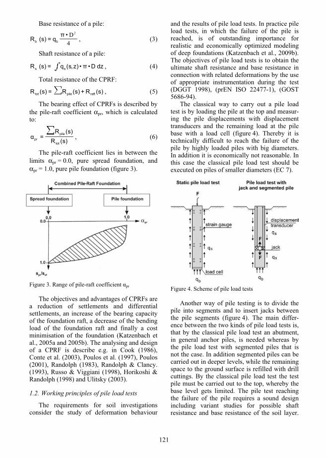
Base resistance of a pile:

4D2•

q=)s(R bb , (3)

Shaft resistance of a pile:

dzD••)z,s(q=)s(R ss , (4)

Total resistance of the CPRF:

)s(R+)s(R=)s(R raftpiletot , (5)

The bearing effect of CPRFs is described by the pile-raft coefficient αpr, which is calculated to:

)s(R)s(R

=tot

pilepr , (6)

The pile-raft coefficient lies in between the limits αpr = 0.0, pure spread foundation, and αpr = 1.0, pure pile foundation (figure 3).

Figure 3. Range of pile-raft coefficient pr

The objectives and advantages of CPRFs are a reduction of settlements and differential settlements, an increase of the bearing capacity of the foundation raft, a decrease of the bending load of the foundation raft and finally a cost minimisation of the foundation (Katzenbach et al., 2005a and 2005b). The analysing and design of a CPRF is describe e.g. in Cook (1986), Conte et al. (2003), Poulos et al. (1997), Poulos (2001), Randolph (1983), Randolph & Clancy. (1993), Russo & Viggiani (1998), Horikoshi & Randolph (1998) and Ulitsky (2003).

1.2. Working principles of pile load tests

The requirements for soil investigations consider the study of deformation behaviour

and the results of pile load tests. In practice pile load tests, in which the failure of the pile is reached, is of outstanding importance for realistic and economically optimized modeling of deep foundations (Katzenbach et al., 2009b). The objectives of pile load tests is to obtain the ultimate shaft resistance and base resistance in connection with related deformations by the use of appropriate instrumentation during the test (DGGT 1998), (prEN ISO 22477-1), (GOST 5686-94).

The classical way to carry out a pile load test is by loading the pile at the top and measur-ing the pile displacements with displacement transducers and the remaining load at the pile base with a load cell (figure 4). Thereby it is technically difficult to reach the failure of the pile by highly loaded piles with big diameters. In addition it is economically not reasonable. In this case the classical pile load test should be executed on piles of smaller diameters (EC 7).

Figure 4. Scheme of pile load tests

Another way of pile testing is to divide the pile into segments and to insert jacks between the pile segments (figure 4). The main differ-ence between the two kinds of pile load tests is, that by the classical pile load test an abutment, in general anchor piles, is needed whereas by the pile load test with segmented piles that is not the case. In addition segmented piles can be carried out in deeper levels, while the remaining space to the ground surface is refilled with drill cuttings. By the classical pile load test the test pile must be carried out to the top, whereby the base level gets limited. The pile test reaching the failure of the pile requires a sound design including variant studies for possible shaft resistance and base resistance of the soil layer.

121

Often the settlement failure criterion is defined as 0.1*D (D = diameter of the pile). The failure criterion for creep behaviour is defined by ks 2 mm. The control of creep limit ensures that the pile failure is not reached before the settlement criterion is applied. The design of pile load tests should ensure that the test does not have to be finished due to material capacity.

The limitation of the pile settlement by maximum of 4 cm in Russian Codes (SNIP 2.02.03-85) without any relation to the pile diameter, especially for big diameter piles, leads to not reaching the ultimate bearing capacity of the test pile and, as a consequence, to more conservative design of pile foundations and especially of CPRFs. It is possible to save costs in future without any negative impact on safety or serviceability.

1.3. Normative requirements for design and execution of CPRFs according to Russian and German Building Codes

The Combined Pile-Raft Foundation (CPRF) is mentioned in many normative docu-ments, which have been published in Russian Federation in the last years. Especially the Moscow Building Codes (MGSN 4.19-05, MGSN 2.07-01) and other normative docu-ments of Moscow City contain recommenda-tions regarding CPRFs. Some recommendations are given in St. Petersburg Building Code (TSN 50-302-2004).

In Germany the design of CPRFs is defined in DIN 1054, which considers the requirements of Eurocode 7 towards National Building Codes in European countries. Regarding the design of CPRFs DIN 1054 refers to CPRF Guideline (Hanisch et al., 2002).

In the following a comparison between the requirements of normative documents in Russia and the German CPRF Guideline (Hanisch et al., 2002) is carried out. Additionally some piece of advice is given from the practical experience.

In German and Russian normative docu-ments some limitations concerning the execu-tion of CPRFs in weak soils are given. In (Hanisch et al., 2002) limitations regarding the stiffness of layered soil (stiffness ratio ES,up/ES,down 1/10) and pile-raft coefficient

pr > 0.9 are stated. In practice CPRFs are mostly applied in cohesive soils, sands and weathered rocks and rarely in sound rock. CPRFs are mostly applied for predominantly

vertically loaded foundations, which is also stated in DIN 1054. However, in practice predominantly horizontally loaded CPRFs have been already successfully applied, e.g. Exhibi-tion Hall 3 in Frankfurt am Main, Germany (Katzenbach et al., 2002).

The design procedures for CPRFs differ strongly from each other in Russia and Ger-many. In Germany advanced requirements are set concerning the calculation model. In practice CPRFs are calculated with the Finite Element Method (FEM), using a 3-dimensional model that gets adjusted to pile load test (Katzenbach et al., 2009a).

The deformation behaviour of the soil is de-rivated from back analysis of former built structures (Katzenbach et al., 2008). In the CPRF Guideline the calculation procedure for the Ultimate Limit State (ULS) and the Service-ability Limit State (SLS) is given. The calcula-tion procedure of CPRFs in ULS contains calculation of external (soil-pile-raft interaction) bearing capacity and calculation of material bearing capacity. Calculations have to be carried out with characteristic values for soil and construction materials. The calculation of external (soil-pile-raft interaction) bearing capacity in ULS is applied to the entire founda-tion system with the safety factor of = 2. The calculation of external bearing capacity in ULS for each pile of the foundation is not required. The calculations in SLS have to be executed with characteristic values for soil and construc-tion materials, applying the working loads. The calculation of internal forces has to be executed for two limit cases: for ULS and SLS. So the design of raft and piles has to cover the most unfavorable case. Strict limitations for building settlements are normally not applied. Limita-tions of settlements of surrounding building and structures must be defined with regard to sensitivity of each structure. In practice the design criteria for differential settlements are chosen for high-rise buildings as 1/1000.

In Russian Codes the calculation procedure for ULS is not defined. The calculation of ULS, especially the evaluation of settlements, is described as an analytical solution for pr = 0.85 (SP 50-102-2003, Recommendations 1999, MGSN 2.07-01, Guideline 2001, Recommenda-tions 1997) and for simple examples as a settlement formula in MGSN 2.07-01 and Guideline 2001. According to Russian Building Codes the calculation of the settlement of CPRFs has to be checked by the method of deep

122

laying shallow foundation. The limitations of settlements and differential settlements are given in SP 50-102-2003 and SP-50-101-2004.

Russian Codes consider only bored and driven piles to be suitable for CPRFs MGSN 2.07-01, Guideline 2001, Recommendations 1997. A rigid connection between the piles and raft is required, due to MGSN 2.07-01.

The CPRF Guideline does not restrain the type of vertical elements; the use of bored and driven piles, barrettes and sheet piles is possible for CPRFs. However, in practice the mostly used vertical elements are bored piles of various diameters up to 2 m and barrettes. Often the retaining wall of the excavation pit is used as vertically loaded foundation element. The driven piles are rarely used due to their low bearing capacity. Piles, considered as settlement reduction measures, are situated under the area with the highest load; the pile length and diame-ters are chosen to reach similar stiffness of piles and to ensure uniform settlements of the foun-dation. Uncoupled CPRFs (without rigid con-nection between piles and raft) have been executed several times and are especially reasonable in the seismic regions. Depending on soil conditions with the modern technology and advanced approaches in design CPRFs with

pr = 0.5 have successfully completed.Moreover in CPRF Guideline the design

checking procedure for CPRFs and quality assurance measures are defined. The Russian Codes do not regulate the procedures mentioned above.

Concluding the analysis of normative re-quirements for CPRFs in Russia and Germany strong differences have been identified, espe-cially in the calculations of CPRFs in ULS and SLS. Therefore, the consolidation of the experi-ences gathered in both countries and the work-ing out of new normative documents for CPRFs seems to be reasonable in the future.

2. OBSERVATIONAL METHOD

The observational method is an instrument for quality insurance and final control of the reli-ability and correctness of the applied geotechni-cal theoretical model as basis of the design. According to Eurocode 7 the application of the observational method is recommended for constructions of geotechnical category 3, such as e.g. CPRFs. The observational method pays attention to the dominating role of the soil

during and after the construction of a building (EC 7). The observational method is a step by step method, considering the interaction and interconnection between the single steps. The first step comprehends the compiling of a computational model (prognosis) of the ex-pected results as e.g. the expected settlements of a construction respectively foundation (van Impe, 1991). Simultaneously a measurement based controlling monitoring is carried out. The second step is the comparison of the prognosti-cated values with the measured values. If the values are conform in sufficient accuracy the final step is the ongoing realisation of the project. If a sufficient accuracy is not reached the definition of contingency actions is neces-sary. That can lead to a modification of the theoretical model, whereby the step by step procedure continues newly at the start of the chain. The second possible step after the defini-tion of contingency actions is the adaptation of the construction process, which on the one hand leads to a modification of the computational model, and the new start of the chain, and on the other hand can require a revision of the contract between the contractor and the em-ployer.

Figure 5. Flow chart for the Observational Method.

Geotechnical measuring facilities are e. g. displacement transducers, strain gauges, load cells, pore-water pressure cells, inclinometers, (multi-) extensometers and geodetical levelling. More examples for the observational method can be found in Katzenbach & Moormann (2003), Peck (1969) and Schmitt et al. (2002).

123

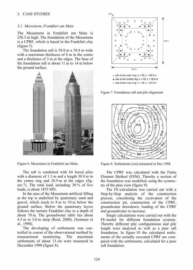
3. CASE STUDIES

3.1. Messeturm, Frankfurt am Main

The Messeturm in Frankfurt am Main is 256.5 m high. The foundation of the Messeturm is a CPRF, which is based in the Frankfurt clay (figure 5).

The foundation raft is 58.8 m x 58.8 m wide with a maximum thickness of 6 m in the centre and a thickness of 3 m at the edges. The base of the foundation raft is about 11 m to 14 m below the ground surface.

Figure 6. Messeturm in Frankfurt am Main.

The raft is combined with 64 bored piles with a diameter of 1.3 m and a length 30.9 m in the centre ring and 26.9 m at the edges (fig-ure 7). The total load, including 30 % of live loads, is about 1855 MN.

In the area of the Messeturm artificial filling at the top is underlied by quaternary sand and gravel, which reach to 8 m to 10 m below the ground surface. Below the quaternary layers follows the tertiary Frankfurt clay to a depth of about 70 m. The groundwater table lies about 4.5 m to 5.0 m deep (Reul, 2000), (Sommer et al., 1990).

The developing of settlements was con-trolled in course of the observational method by measurement monitoring. The maximum settlements of about 13 cm were measured in December 1998 (figure 8).

Figure 7. Foundation raft and pile alignment.

Figure 8. Settlements [cm] measured in Dec.1998.

The CPRF was calculated with the Finite Element Method (FEM). Thereby a section of the foundation was modelled, using the symme-try of the plan view (figure 9).

The FE-calculation was carried out with a Step-by-Step analysis of the construction process, considering the excavation of the construction pit, construction of the CPRF, groundwater drawdown, loading of the CPRF and groundwater re-increase.

Single calculations were carried out with the FE-model for different foundation systems. Thereby different pile configurations and pile length were analysed as well as a pure raft foundation. In figure 10 the calculated settle-ments of the actually executed CPRF are com-pared with the settlements, calculated for a pure raft foundation.

124

The settlements of a pure raft foundation were calculated to 32.5 cm. The calculated settlements of the CPRF are nearly equal to the in-situ measured 13 cm. The pile raft coefficient is about αpr = 0.43 (Reul, 2002).

Figure 9. FE mesh of the foundation.

Figure 10. Measured and calculated settlements.

In course of the lot of high-rising buildings, which were constructed in Frankfurt, the shaft resistance of bored piles in Frankfurt clay was

determined in serial of in-situ pile tests. As a result the ultimate shaft resistance was deter-mined to 60 kN/m² to 80 kN/m² for 20 m long piles.

At the piles of the Messeturm, whose base is about 50 m below the ground surface, an aver-age shaft resistance qS of 90 kN/m² to 105 kN/m² was measured. At the lower section of the pile a maximum of qS = 200 kN/m² was measured. The reason for such high values of shaft resistance, occurring by CPRFs, is an increase of the general state of stress of the soil between the single piles. This stress increase is inter alia influenced by the initiation of stresses by the foundation raft, which is used for load transfer.

A pure pile foundation would have required 316 piles with 30 m length. In comparison to the executed CPRF with 64 piles and an average length of about 30 m a pure pile foundation would have required more resources e.g. con-crete, energy and would have been 3.9 Million Euros more expensive.

3.2. Federation Tower

The Federation Tower is a part of the project Moscow City, which contains the construction of several high-rising buildings for business in central Moscow on an area of more than one square kilometre.

The Federation Tower is a complex of two single towers (figure 11). Tower A is about 360 m high respectively about 506 m with regard to the spire on the roof. Tower B is about 243 m high. The high-rise double-towers of the Federation Tower farly exceed all experi-ences with high-rise buildings in Russia and in Europe, gained up to now. The two towers will share an about 140 m long and about 80 m wide, 4.6 m thick foundation raft made of reinforced concrete in a depth of approx. 20 m below the surface level.

125

Figure 11. Moscow City (source: www.panoramio.com).

The total load is about 3000 MN for Tower A and 2000 MN for Tower B. With additionally about 1000 MN load for flat buildings and the basement floors and a load of the self-weight of the foundation raft of about 1300 MN the total load results to about 7300 MN.

The project area of Moscow City is located in the west of the central district of Moscow at the left bank of the River Moskwa. Underneath anthropogenic influenced artificial back-fill, at first the quaternary accumulation of the river terrace and underneath the alternating sequences of the carbon are located. Underneath the foundation level of the Federation Tower, a complex alternating sequence is found, consist-ing of variably intensively fissured, cavernous and porous limestone and variably hard, more or less watertight clay (marl). The layers have different thicknesses which range between about 3 m and 10 m. Moscow City and also the building area of the Federation Tower are located in a territory, where potentially danger-ous karst-suffusion-processes occur.

In the project area, several ground water ho-rizons, carrying perched waters, have been found. Because of the sealing effect of the clay (marl), they are not or just moderately corre-sponding with each other. The ground water mainly circulates in the fissured and karst-suffusion affected limestone. The ground water, circulating in the lower limestone-aquifer, has risen about 12 m high beyond the bottom line of the sealing clay layer. The limestone-horizons

located above, carry ground water with higher hydraulic heads.

In the area of the Federation Tower the pile load tests TP-15-1 and TP-15-2 with Osterberg-cells (O-cells) were carried out in spring 2005. The test piles were constructed with a diameter of 1.2 m and a length of 6.90 m and 13.35 m. The empty drill hole was filled with sand. The piles are completely positioned in the limestone (figure 12).

Each pile was divided into 2 segments. Be-tween the pile segments 2 O-cells were in-stalled. In each test pile displacement transduc-ers were installed to measure the displacements of the pile segments.

Pile load test TP-15-1 was carried out to a maximum load of about 33 MN. In between an unloading-phase was made at 15 MN back to zero-load followed by a reloading-phase (fig-ure 13).

Figure 12. Section of test piles TP-15-1 and TP-15-2.

-0,6

-0,4

-0,2

0

0,2

0,4

0,6

0,80 5 10 15 20 25 30 35 40

upper pile segment

lower pile segment

load [MN]

displacement [cm]

Figure 13. Load-displacement-diagram, TP-15-1.

The final displacement was about 0.6 cm at the upper pile segment and 0.4 cm at the lower pile segment. Neither a failure of one of the pile segments was seen nor the empirically defined

126

limit of 0.1*D = 12 cm was reached. The evaluation of pile-test TP-15-1 yields a shaft resistance of about 1140 kN/m² and a base resistance of about 5380 kN/m². These values are not ultimate values.

-3,0

-2,0

-1,0

0,0

1,0

2,0

3,0

4,0

5,00 5 10 15 20 25 30 35 40

displacement [cm]

load [MN]

upper pile segment

lower pile segment

Figure 14. Load-displacement-diagram, TP-15-2.

Pile load test TP-15-2 was carried out to a maximum load of about 33 MN as well. In between three unloading-phases back to zero-load were made (figure 14). The final displace-ment was about 4.3 cm at the upper pile seg-ment and 2.2 cm at the lower pile segment. Neither a failure of one of the pile segments was seen nor the empirically defined limit of 0.1*D = 12 cm was reached, too. The evalua-tion of pile-test TP-15-2 yields a shaft resistance of about 2310 kN/m² and a base resistance of about 5630 kN/m².

The shaft resistance in the variably inten-sively fissured, cavernous and porous limestone was in pile load test TP-15-1 measured with about 1100 kN/m² by pile displacements of about 0.5 cm and in pile load test TP-15-2 a shaft resistance of about 2300 kN/m² was measured by displacements of about 2 cm. In German standard DIN 1054 the empirical maximum shaft resistance for solid rock with an uniaxial compression strength of 20 MN/m² is given with 500 kN/m² and in EA-Pfähle (DGGT, 2007) with 500 kN/m² to 2000 kN/m² as ultimate values, which means for the de-scribed test piles by displacements of 12 cm. So the empirical ultimate maximum value for shaft resistance is reached by the in-situ pile load test by just about 17 % of the empirical evaluated settlements and is in practice far away from being an ultimate value. The in-situ existing ultimate shaft resistance cannot be deriated from the two pile load tests.

3.3. Mirax Plaza

In the scope of the project Mirax Plaza in Kiev 2 high-rise towers, each of them 192 m (46 storeys) high, shopping and entertainment mall and underground parking is under con-struction (figure 15). The gross area of the project is about 294000 m². The project area cuts a 30 m high natural slope.

The geotechnical investigations have been executed 70 m deep, there the quaternary, Neogene and Paleogene sediments (Kiev Marl Clays and Buchak Sands) have been encoun-tered.

Figure 15. Mirax Plaza.

For the previous project on the territory of the project Mirax Plaza 4 pile load tests (2 tension and 2 compression tests) on the piles with diameter 0.82 m have been executed. Also here no failure of pile in accordance with the criterion 0.1*D was achieved. Using the results of the test, the back analysis was executed by means of FEM-model. The soil properties in accordance with the results of the back analysis were partly 3 times higher, than indicated in the geological report.

The obtained results of the pile test and of the executed back analysis were applied in three dimensional FEM-model of the foundation for Tower A, taking advantage of the symmetry of the footprint of the building. The overall load of the Tower A is about 2200 MN and the area of the foundation about 2000 m² (figure 16).

The foundation design considers a CPRF with 64 barrettes with 33 m length and a cross section of 2.8 m x 0.8 m. The raft of 3 m thick-ness is laying in Kiev Marl Clays at about 10 m depth below the ground surface at the lower part of the slope. The barrettes are penetrating the layer of Kiev Marl Clays reaching Buchak Sands.

127

Figure 16. FEM model for CPRF of tower A an calculated settlements in cm.

The calculated loads on the barrettes were in the range of 22.1 MN to 44.5 N. The load on the outer barrettes were about 41.2 MN to 44.5 MN, which significantly exceeds the loads on the inner barrettes with the maximum value of 30.7 N. This behaviour is typical for a CPRF, that the outer barrettes of piles take more load because of their higher stiffness due to the higher volume of the activated soil. The pile-raft coefficient is αpr = 0.88. Maximum settle-ments of ca. 12 cm were resulting calculative due to the settlement-relevant load with 85 % of the total design load. The pressure under the foundation raft is calculated in the most areas not exceeding 200 kN/m², at the raft edge the pressure under the raft reaches 400 kN/m². The calculated base pressure for outer barrettes was calculated in average with 5100 kN/m² and for inner barrettes in average with 4130 kN/m². The mobilized shaft resistance increases with the depth reaching 180 kN/m² for outer barrettes and 150 kN/m² for inner barrettes. During the construction of Mirax Plaza Tower the observational method according to EC 7 is applied. Especially the distribution of the loads between the piles and the raft is monitored. For this reason 3 earth pressure devices were in-stalled under the raft and 2 barrettes (most loaded outer barrette and average loaded inner barrette) were instrumented over the length.In the scope of the project Mirax Plaza the new allowable shaft resistance and base resistance were defined for typical soil layers in Kiev. This unique experience should be used for the skyscrapers of new generation in Ukraine.

The CPRF of the high-rise building project Mirax Plaza represents the first authorized CPRF in the Ukraine. Using the advanced optimization approaches and taking advantage of the positive effect of CPRF the number of barrettes could be reduced from 120 barrettes with 40 m of length to 64 barrettes with 33 m of length. The foundation optimization leads to considerable decrease of the utilised resources

(cement, aggregates, water, energy etc.) and to cost savings of 3.3 Million US$.

4. SUMMARY

On the exemplary chosen high rise buildings projects Messeturm, Federation Tower and Mirax Plaza, it is shown, that it is possible by the use of CPRFs, and an optimization of the pile foundation design by the results of pile load tests, to save resources and so costs in million-order magnitude (Katzenbach et al., 2001). For quality assurance an international CPRF guide-line as a new normative document based on the experiences mentioned by Hanisch et al. is necessary.

5. REFERENCES

CEN European Committee of standardization (2008). Eurocode 7: Geotechnical design – Part 1:

General rules. Conte, G., Mandolini, A., Randolph, M. F., 2003.

Centrifuge modelling to investigate the perform-ance of piled rafts. Deep Foundations on Bored and Auger Piles (BAP IV), van Impe (ed.), Mill-press Rotterdam, pp.359-366.

Cooke, R. W., 1986. Piled raft foundations on stiff clays – a contribution to design philosophy. Géotechnique 36, No. 2, pp. 169-203.

Deutsche Gesellschaft für Geotechnik (DGGT), 1998. Empfehlungen für statische und dynami-sche Pfahlprüfungen. Eigenverlag Institut für Grundbau und Bodenmechanik der Technischen Universität Braunschweig.

Deutsche Gesellschaft für Geotechnik (DGGT), 2007. Empfehlungen des Arbeitskreises „Pfähle“ – EA Pfähle. Berlin: Ernst & Sohn.

DIN 1054:2005-01 Subsoil. Verification oft he safety of earthworks and foundations.

GOST 5686-94 Soils. Field test methods by piles Guideline for design and execution of pile founda-

tions for buildings and structures in the City of Moscow, 2001.

Hanisch, J., Katzenbach R., König G., 2002. CPRF Guideline, Kombinierte Pfahl-Platten-gründungen. Berlin, Ernst & Sohn.

Horikoshi, K. Randolph, M. F., 1998. A contribution to optimal design of piled rafts. Géotechnique 48, No. 3, pp. 301-317.

Katzenbach, R., Hoffmann, H., Vogler, M., Moor-mann, Ch. 2001. Costoptimized foundation sys-tems of high-rise structures, based on the results of actual geotechnical research. Proc. Internatio-nal Conference Trends in Tall Building – Ten-denzen im Hochhausbau, Frankfurt am Main, 5.-7.9.2001, pp. 421-443.

128

Katzenbach, R., Turek J., Vogler M., 2002. Entwick-lung einer horizontal belasteten KPP am Beispiel der neuen Messe in Frankfurt am Main. Bauinge-nieur Heft September 2002, pp. 393-399.

Katzenbach, R., Moormann, C., 2003. Instrumenta-tion and monitoring of combined piled rafts (CPRF): State-of-the-art report. 6th Field Meas-urements in Geomechanics, Sept. 2003, Oslo.

Katzenbach, R., Hoffmann, H., Vogler, M., Giere, J., Wachter, St., 2005a. Sichere Hochhausfundamen-tierungen. Aktuelle Erfahrungen bezüglich der Sicherheit von Hochhausgründungen in weichen Böden und weichem Fels Setzungen, Verkantun-gen, Gebrauchstauglichkeit. 2nd Int. Conference on Unique and Special Building Technologies, USTBuild 2005 Moskau, 12.-13.04.2005.

Katzenbach, R., 2005b. Optimized design of high-rise building foundations in settlement-sensitive soils. International Geotechnical Conference of Soil-Structure Interaction, St. Petersburg, 26.-28.5.2005, pp. 39-46.

Katzenbach, R., Bachmann, G., Gutberlet, C., 2008. FEM for ULS and SLS checks of complex Foun-dations. Foundations: Proceedings of the Second BGA International Conference on Foundations, ICOF2008. Brown M. J., Bransby M. F., Brennan A. J. and Knapppett J. A. (Editors). HIS BRE Press.

Katzenbach, R., Bachmann, G., Gutberlet, C., 2009a. Assessment of settlements of high-rise structures by numerical analysis. Linear and Non-linear Numerical Analysis of Foundations, pp. 390-419. New York: John W. Bull.

Katzenbach, R., Leppla, S., Vogler, M., Kuttig, H., Dunaevskiy, R., 2009b. Gründungsoptimierung von Hochhäusern in Kiew. Mitteilungen des In-stitutes und der Versuchsanstalt für Geotechnik der Technischen Universität Darmstadt, Heft 81, pp. 93-107.

MGSN 2.07-01 Soil base, foundation and under-ground structures.

MGSN 4.19-05 Multifunctional high-rise buildings and complexes.

Peck,. R. B., 1969. Advantages and limitations of the observational method in applied soil mechanics. Géotechnique 19, No. 2, pp. 171-187.

Poulos, H. G., Small, J. C., Ta, L. D., Simha, J., Chen, L., 1997. Comparison of some methods for analysing of piled rafts. Proc. XIVth ICSMFE, Hamburg, 2:1119-1124.

Poulos, H. G., 2001. Piled-raft foundation: design and applications. Géotechnique 51, No. 2, pp. 95-113.

prEN ISO 22477-1- Geotechnical investigation and testing – Testing of geotechnical structures- Part 1: Pile load test by static axially loaded compres-sion.

Randoph, M. F., 1983. Design of piled raft founda-tion. Proceedings of the international symspo-sium on recent developments in laboratory and field tests and analysis of geotechnical problems,

Bangkok, pp. 525-527. Randolph, M. F., Clancy, P., 1993. Efficient design

of piled rafts. Proceedings Deep Foundations on Bored and Auger Piles, Ghent, pp. 119-130.

Recommendations for calculations and design of pile foundations of new types in the City of Moscow, 1997.

Recommendations for design and execution of foundations during the erection of building near to existing structures in the tightly built-up area in the City of Moscow, Moskomarchitektura, 1999.

Reul, O., 2000. In-situ-Messungen und numerische Studien zum Tragverhalten der Kombinierten Pfahl-Plattengründung. Mitteilungen des Institu-tes und der Versuchsanstalt für Geotechnik der Technischen Universität Darmstadt, Heft 53, pp.136-154.

Russo, G., Vigggiani, C., 1998. Factors controlling soil-structure interaction for piled-rafts. Interna-tional Conference on Soil-Structure Interaction in Urban Civil Engineering, 8./9. October 1998, Darmstadt Geotechnics, No. 4.

Schmitt, A., Turek, J., Katzenbach, R., 2002. Appli-cation of geotechnical measurements for founda-tions of high rise structures. 2nd World Engineer-ing Congress (WEC), 22.-25. July 2002, Sara-wak, Malaysia, pp. 40-46.

SNIP 2.02.01-83, Foundations of buildings and structures.

SNIP 2.02.03-85, pile foundations, Moscow, 1995. Sommer, H., Katzenbach, R., DeBenedittis, C., 1990.

Last-Verformungsverhalten des Messeturms Frankfurt/Main. Vorträge der Baugrundtagung in Karlsruhe, pp. 371-380.

SP 50-101-2004 Design and construction of soil bases and foundations for buildings and struc-tures.

SP 50-102-2003, Design and execution of pile foundations, Moscow 2004.

TSN 50-302-2004 St. Petersburg 2004, Design of foundations of buildings and structures in St. Pe-tersburg.

Ulitsky, V. M. 2003. Geotechnical Challenges in Reconstruktion of Historical Cities. Proceedings of the International Geotechnical Conference “Reconstruction of Historical Cities and Geo-technical Engineering”, St. Petersburg, Vol-ume 1, pp. 13-29.

van Impe, W. F., 1991. Deformations of deep foundations. Proceedings European Conference on Soil Mechanics and Foundation Engineering, Vol. 3, pp. 555-560, Stockholm, Sweden.

129

Railway Old Station Building: Enlargement and Underpinning

Pedro Simão Sêco e Pinto João Barradas University of Coimbra, Portugal Arlindo SousaNational Laboratory of Civil Engineering (LNEC) National Laboratory of Civil

Engineering (LNEC),Lisboa, Portugal Lisboa, Portugal

ABSTRACT: This paper describes the enlargement and underpinning of old Rossio railway station building (1886). These works included the construction of new underground walls and mechanical stairways for the connection with a nearby underground metro station and also the construction of a new underground metro gallery for a new line, under some old huge retaining walls that sustain the embankment of the railway platforms. A careful study was performed for this station in order to avoid unacceptable damages. Some of the system and suitability tests that were performed for the anchors are presented.

The design of the retaining walls was based in Eurocode 7. The seismic design was based in Eurocode 8. The monitoring results of the anchor loads and ground displacements resulting from the excavation are presented.

1. INTRODUCTION

This paper describes the enlargement and underpinning of old Rossio railway station building (1886). These works included the construction of new underground walls and mechanical stairways for the connection with a nearby underground metro station and also the construction of a new underground metro gallery for a new line, under some old huge retaining walls that sustain the embankment of the railway platforms. A careful study was performed for this station in order to avoid unacceptable damages. Some of the system and suitability tests that were performed for the anchors are presented.

It was necessary to perform the underpinning of an east-west and the principal retaining walls, with 15m in height and a thickness around 2.5 m, and Bairro Alto wall. These walls were later reinforced in order to ensure their long-term safety against rotational failure.

The main geological conditions are described.

The field and laboratory tests are referred, as well as the geotechnical characteristics.

The methodology to design the retaining walls, based in Eurocode 7, is introduced. The seismic design is based in Eurocode 8.

The monitoring results of the anchor loads and ground displacements resulting from the excavation are presented.

Some final considerations are presented.

2. BACKGROUND

Due to the crossing of the Rossio railway station building (1886) by an underground gallery (for the Lisbon Metro), a careful study was performed for this station in order to avoid unacceptable damages. The building had originally three levels: ground floor (+11.86), 1st floor (+19.93) and 2nd floor (+25.96). For the installation of a Commercial Centre two new floors were built: intermediate first floor (+15.21) and intermediate second floor (+22.79).

For the construction of the underground

130

with 13m in height and a thickness around 3m. Both walls sustain an embankment on which the railways platforms were built.

The underground gallery was built underneath the whole extension of the north-south retaining wall and part of the east-west retaining wall.

The enlargement of the station including two new underground halls connected by mechanical and fixed stairways with each other.

A cross section of the tied back wall is shown in Fig. 1.

For the underpinning of the retaining walls, more than a dozen large reinforced concrete frames were erected, side by side, under the base of the walls (Consortium, 1996b). This simple but massive structures allowed the excavation of the space for the installation of the Metro gallery (Fig. 2), under the beam of each frame.

Other parts of the station building had also to be underpinned, by means of r.c. frames, micro-piles and jet-grout columns.

In the design phase of the underpinning of the retaining walls, it was recognized that the walls didn’t verify the safety conditions required by Eurocodes 7 and 8 and Portuguese Actions Code, specially in what concerns the rotational failure scenario for both static and seismic actions.

Therefore it was decided to reinforce both walls by means of (i) definitive anchorages and a grid of r.c. beams, in the case of the north-south wall; and (ii) micropiles going through the body of the wall and into the ground behind and under it, in the case of the east-west wall (Seco e Pinto et al., 2008).

3. MAIN GEOLOGICAL CHARACTERISTICS

In this section the main geological characteristics of each layer are presented.

Based in the results collected from borings executed at Rossio site, the following units were considered as shown in Fig. 2 (Consortium, 1996a).

Landfill

The landfill is composed by sandy clayey material with a thickness varying from 3.5 to 20 meters.

Estefânia Areolas

The unit is composed by sandy materials or silty sandy materials with thickness around 3 meters.

Clays and calcareous rocks from Prazeres

This lower unit is composed by dark grey to dark brown clay, with layers of sandy material, up to the depth which is significant to the design of the structures of the Rossio station.

4. GEOTECHNICAL CHARACTERISTICS

After an evaluation of the results of the field investigation (boreholes, trenches, vane shear tests, pressurometer tests, penetrometer tests and Lefranc tests) and the laboratory tests (chemical tests, oedometer tests, triaxial tests, the following geotechnical characteristics were adopted (Consortium, 1996a):

Landfill

Unified classification: CL, CH % passing sieve # 200 (ASTM): 28 to 100% Liquid limit: 18 to 47% Plastic index: 3.4 to 26.7% Unit weight: 17.6 kN/m3 Uniaxial compressive tests: Strength (Cu): 32.7 to 169.7 kPa Tangent elasticity modulus: 4.3 to 10.7 MPa Triaxial tests (C.U.): Cohesion c (in effective stresses): 0 kPa Friction angle φ (in effective stresses): 30o

k (permeability coefficient): 10-9 m/s Poisson ratio: 0.35 The most representative SPT values of this material are between 4 and 18. CPT results were between 0.2 and 5 MPa.

131

Figure. 1. Cross section of the tied back wall

132

Figure 2. Geological profile (adopted from Consortium, 1996a)

Estefânia Areolas

Cohesion c (in effective stresses): 0Friction angle φ ( in effective stresses): 33o

Elasticity modulus: 36 MPa k (permeability coefficient): 10-5 m/s. SPT results were between 6 and 39 blows.

Clays and calcareous rocks from Prazeres

Unified classification: CL, CH % passing sieve # 200 (ASTM): 32 to 75% Liquid limit: 28.3 to 43.4% Plastic index: 4.3 to 21% Triaxial tests (C.U.):Cohesion c (in effective stresses): 33 kPa

Friction angle φ (in effective stresses): 35o

k (permeability coefficient): 10-6 to 10-7 m/s Poisson ratio: 0.25 SPT results were between 10 and 60 blows, with the upper layer having SPT values lower than 40 blows and the lower layer having SPT values higher than 60.

Masonory retaining wall materials

Unit weight: 22 kN/m3 Triaxial tests (C.U.):Cohesion c (in effective stresses): 1 MPa Friction angle φ ( in effective stresses): 45o

Poisson ratio: 0.20

133

5. DESIGN OF RETAINING WALLS

5.1.Static Conditions

The gravity type retaining structures were designed taking into consideration limit states (Eurocode 7, 1997). The following ultimate states (with severe consequences) can occur: (i) loss of overall stability; (ii) failure of a structural element such as the retaining wall, an anchorage, a micropile, etc; (iii) foundation failure; (v) unacceptable leakage through or beneath the wall; (v) rotational failure; (vi) movements of the retaining structure which may cause collapse of other structures; (vii) unacceptable change to the flow of groundwater; and (viii) failure by sliding at the base of the wall. The following serviceability limit states (with less severe consequences) can occur: (i) movements of the retaining structure which may affect the appearance or efficient use of the building and other structures; and (ii) excessive vibrations.

The values of partial factors for permanent and variable actions given in Table 1 were used for verification of ultimate limit states situations. For accidental situations all numerical values of partial factors for actions were taken equal to [1.0] (Eurocode 7, 1997).

Cases A, B and C have been introduced in order to ensure stability and adequate strength in the structure and in the ground.

Case A is only relevant to buoyancy problems, where hydrostatic forces are included in the main unfavourable action.

Case B is often critical to the design of the strength of structural elements involved in foundations or retaining structures. Where there is no strength of structural materials involved, Case B is irrelevant.

Case C is generally critical in cases, such as slope stability problems, where there is no strength of structural elements involved. Case C is often critical to the sizing of structural elements involved in foundations or retaining structures, and sometimes to the strength of structural elements. Where there is no strength of ground involved in the verification, Case C is irrelevant.

Permanent actions include self weight of structural and non structural components and those actions caused by ground, groundwater and free water.

In calculation of design earth pressures for Case B, the partial factors given in Table 1 are applied to characteristic earth pressures. Characteristic earth pressures comprise characteristic water pressures together with stresses that are admissible in relation to the characteristic ground properties and characteristic surface loads.

All permanent characteristic earth pressures on both sides of a wall are multiplied by [1.35] if the total resulting action is unfavourable and by [1.00] if the total resulting action effect is favourable. Thus, all characteristic earth pressures are treated as being derived from a single source.

For the verification of serviceability limit states, partial safety factors are used for all permanent and variable actions except where specified otherwise.

.

Table 1. Partial factors - ultimate limit states in persistent and transient situations (Eurocode 7, 1997)

Case Actions Ground Properties Permanent Variable Unfavour-able Favourable Unfavourable tanφ’ c’ cu qu

1)

Case A [1.00] [0.95] [1.50] [1.1] [1.3] [1.2] [1.2] Case B [1.35] [1.00] [1.50] [1.0] [1.0] [1.0] [1.0] Case C [1.00] [1.00] [1.30] [1.25] [1.6] [1.4] [1.4] 1) Compressive strength of soil or rock.

134

For the anchored structures the following additional limit states are considered (Eurocode 7, 1997):

- failure of the ground anchorage by tension;

- structural failure of the ground anchorage due to shear forces, distortion at anchorage head or corrosion;

- loss of anchorage load due to excessive displacements of the anchorage head or by creep and relaxation;

- failure or excessive deformation of parts of the structure due to the applied anchorage force.

For permanent ground anchorages (those which service life is greater than two years) protective corrosion barriers must be provided.

Design values of ground properties, Xd, are derived from characteristic values, Xk, using the equation:

Xd = Xk/ Ym (1) where Ym is the safety factor for the ground property, or shall be assessed directly.

The characteristic value of a soil or rock parameter is selected as a cautious estimate of the value affecting the occurrence of the limit state.

For serviceability limit states all values of Ym are equal to [1.0].

5.2. Analysis of the Principal Retaining Wall.

For the design and behavior evaluation of the principal retaining wall with 15m high and 2.5 m thick, numerical analyses were performed using the FLAC code (Consortium, 1996b), with the following purposes:

- identification of plastic zones; - computation of displacements

distribution;- distribution of stresses and strains in

the retaining walls. The analysis of the principal wall was

performed with the following phases: - phase 1 - calculation of the ground

initial stresses; - phase 2 - introduction of the effect of

masonry retaining wall;

- phase 3 – remotion of the material near Rossio station structure;

- phase 4 - introduction of the linear elements of the building;

- phase 5 - introduction of the effect of the retaining wall.

The results obtained for the different phases are presented in Figs. 3 to 6.

5.3. Seismic Analysis

The seismic action was based on the Portuguese Code (RSA, 1983) and defined by a stochastic gaussian stationary vectorial process (two horizontal orthogonal components and one vertical component). The Portuguese territory is affected by two seismotectonic sources: (i) near source which represents a moderate magnitude earthquake at a short focal distance with a duration of 10 seconds; (ii) far source which represents a higher magnitude earthquake at a longer focal distance with a duration of 30 seconds.

In Eurocode 8(1998) the seismic hazard is described in terms of a single parameter, i.e. the value ag of the effective peak ground acceleration in rock or firm soil called “design ground acceleration” expressed in terms of: (i) the reference seismic action associated with a probability of exceeding (PNCR) of 10 % in 50 years; or (ii) a reference return period (TNCR)=475 years. These recommended values may be changed by the National Annex of each country.The earthquake motion in EC 8 is represented by the elastic response spectrum defined by 3 components.

The following factors can be listed to explain the behavior of gravity retaining structures during an earthquake: (i) increasing of dynamic earth pressures; (ii) variation of hydrodynamic pressure of the backfill; (iii) decreasing of stabilizing forces related with the weight of the structure; (iv) increasing of pore pressures and consequently reduction of effective pressures; and (v) soil liquefaction of backfill and/or foundation material.

135

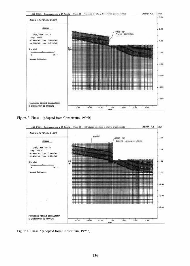
Figure. 3. Phase 1 (adopted from Consortium, 1996b)

Figure 4. Phase 2 (adopted from Consortium, 1996b)

136

Figure. 5. Phase 4 (adopted from Figueiredo Ferraz, 1996b)

Figure. 6. Phase 5 (adopted from Figueiredo Ferraz, 1996b)

137

The stability of soil foundation shall be assessed for the following conditions: (i) overall stability; and (ii) local soil failure.

For the pseudo-static analysis of rotating structures the seismic coefficients can be taken as (Eurocode 8, 1998): kh = αgrγf S/ g.r (2) kv = ± 0.5 kh when the ratio αvg/αgr is greater than 0.6 (3) kv = ± 0.33 kh otherwise (4)

Where αgr is the reference peak ground acceleration, αvg is the vertical component of acceleration, S is the soil parameter, γf is the importance factor of the structure and the factor r takes the values listed in Table 2.

Table 2. Factor affecting the horizontal seismic coefficient (Eurocode 8, 1998)

Type of retaining structure r Free gravity walls that can accept a displacementdr ≤ 300 α S(mm)

2

As above with dr ≤ 200 α S(mm) 1.5Flexural r.c. walls, anchored or braced walls,r.c. walls founded on vertical piles, Restrained basement walls and bridge abutments.

1.0

In Rossio station, the following values were adopted: for the near source, kh = 0.27 and kv = 0.135; for the far source, kh = 0.16 and kv = 0.08.

The earth pressure coefficients were computed by the Mononobe and Okabe method.

5.4. Experimental Tests

Three types of on-site anchorage tests are usually considered: (i) investigation tests; (ii) suitability tests; and (iii) acceptance tests. The lack of results of system tests to evaluate the long term behavior of anchorages of the type which was intended to be used in Rossio station also required a test of this type to be performed in one anchorage. According to standard CEN EN 1537 “Execution of special geotechnical work - Ground Anchorages”, a test of this type requires the excavation of the

anchorage after the load protocol has been carried out, and so this anchorage had to be built outside the station. Investigation tests were needed to establish for the designer, in advance of the installation of the working ground anchorages, the ultimate load resistance in relation to the ground conditions and materials used. Suitability tests were carried out to confirm the acceptable creep and load characteristics at proof and lock-off load levels, following the procedure recommended in the above mentioned CEN EN 1537.

For the determination of the anchorage characteristic load value Rak, from Ram valuesmeasured in one or more suitability tests, a reduction factor was used to take into account the variability of ground and the constructive procedure. As minimum both conditions a) and b) from Table 3 were satisfied using equation:

ζ/R=R aak (5)

The calculation of the anchorage strength Ram,obtained from suitability tests considers the two modes of failure and the creep limit load. The design value Ra, is given by equation:

a ak mR = R / γ (6) where γm = [1.25] for temporary ground anchorages and γm = [1.5] for permanent ground anchorages. The total length of the permanent anchorages is 18m with a tendon free length of 9m and a fixed tendon length bonded to the ground by grout of 9m measured in one or more suitability tests. The 6 steel cables tendon has a cross sectional area of 592.2 mm2. For each load test the anchorages were loaded in 4 incremental cycles from a datum load to a maximum test load, with measurement of displacements of the anchorage head. Displacement values due to creep were also determined. Figs. 7, 8, 9 and 10 related the anchor A02 show the applied loads versus anchorage head displacements, the applied loads versus elastic and permanent displacements, the displacement values versus time and the Ks values for the evaluation of creep, for the

138

suitability test of an anchorage of the principal wall. Measurement of electrical resistance between an anchorage and the surrounding soil or structure to determine the effectiveness of the applied corrosion protection system was also performed.

6. RETAINING WALL OF BAIRRO ALTO

The results of some of the anchorage tests are summarized in Table 4. The total length of the permanent anchorages is 18m with a tendon free length of 9m and a fixed tendon length bonded to the ground by grout of 9 m. The 6 steel cables tendon has a cross sectional area of 592.2 mm2. The results of investigation tests of anchor A16F1 are shown in Figs. 11 to 14. The results of acceptance tests of anchor A6F2 are shown in Figs. 15 to 18.

Table 3. Coefficient ξ for determination of Rak (Eurocode 7, 1997)

Number of suitability tests 1 2 > 2

a) coefficient ξ applied to the mean value Ram [1.5] [1.35] [1.3]

b) coefficient ξ applied to the minimum value Ram [1.5] [1.25] [1.1]

Figure 7. Applied loads versus displacement for Principal Wall anchor A02

139

Figure 8. Applied loads versus elastic and permanent displacements for Principal Wall anchor A02

Figure 9. Displacements versus time for Principal Wall anchor A02

140

Figure 10. Values of Ks for Principal Wall anchor A02

Figure 11. Applied loads versus displacement for Bairro Alto Wall anchor A16F1

141

Table 4. Anchorage tests

AnchorageMax.Force(kN)

MaximumDisp. (mm)

PermanentDisp. (mm)

TestMethod.

InitialFree

Length(m)

CalculatedFree

Length (m)

MaximumKs (mm)

MP02 457,5 69,60 14,54 Accep. T 15,3 15,6 0,39

MP14 453,0 89,19 14,05 Accep. T 21,3 21,2 0,60

MP21 459,0 86,27 14,97 Accep. T 21,3 20,3 0,91

MP35 456,0 77,33 16,16 Accep. T 21,3 17,9 0,70

MBA2F3 619,8 127,50 19,18 Accep. T 21,0 20,8 0,64

MBA6F2 621,6 116,05 10,19 Accep. T 21,0 20,2 0,41

MBA8V 728,1 130,33 16,87 Accep. T 21,0 17,6 0,58

MBA13F1 581,7 189,50 65,52 Accep. T 25,6 25,6 0,53

MBA16F1 673,9 149,49 32,89 Inv. T. 21,0 20,0 0,32

MBA18V 642,5 122,27 5,79 Accep. T. 21,0 20,8 1,07

MBA19F3 631,8 119,14 22,73 Accep. T 21,0 17,7 0,48

142

Figure 12. Applied loads versus elastic and permanent displacements Bairro Alto Wall anchor A16F1

Figure 13. Displacements versus time Bairro Alto Wall anchor A16F1

143

Figure 14. Values of Ks for Bairro Alto Wall anchor A16F1

Figure 15. Applied loads versus displacement for Bairro Alto Wall anchor A6F2

144

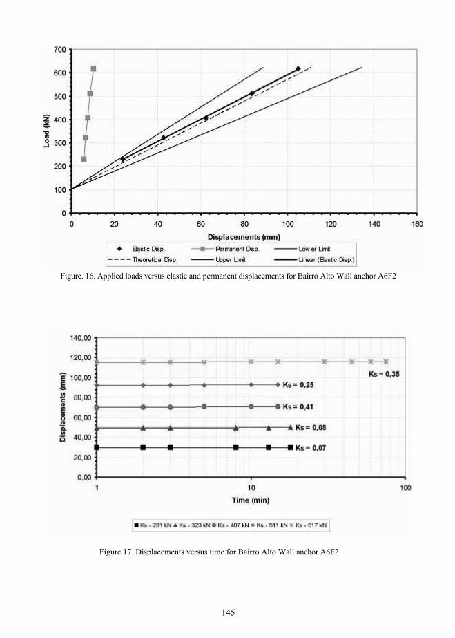
Figure. 16. Applied loads versus elastic and permanent displacements for Bairro Alto Wall anchor A6F2

Figure 17. Displacements versus time for Bairro Alto Wall anchor A6F2

145

Figure .18. Values of Ks for Bairro Alto Wall anchor A6F2

7. CORROSION PROTECTION TESTS

In permanent anchors the integrity of the pregrouted encapsulation shall be proven in order to detect:i) The existence of voidsii) The existence of longitudinal fissures; iii) The existence of transverse fissures.

Following EN 1537(1994): (i) in the encapsulation zone a minimum cover of 5mm shall be provided; (ii) exterior to corrugated duct a minimum cover of 20mm shall be provided; (iii) anti-corrosive protection of tendons shall be provided.

In addition electrical resistivity tests shall provide a minimum value of 100 k between tendon and ground.

Water samples shall be taken for the determination of pH value and concentration of ionic sodic, magnesium and potassium.

In summary the corrosion protection systems tests aim to test the corrugated duct and the internal and external protections.

A detailed suitability test shall also be preformed.

The check list includes: - thickness of the grout and behaviour of the spacers; - position of the tendon. The properties of grouts such as density,

viscosity, exsudation and setting time shall be verified.

During grouting, grouting pressure and grouting volume shall be controlled.

The results of the suitability tests are shown in Figs 19 to 22.

After the anchor load test the anchor shall be excavated and the different elements anchor namely head, tendon and grout body shall be observed.

The measurements of electrical resistivity allow the checking of the protective barrier of the steel tendon from the ground and the protection of the anchor head.

Figs 23 to 27 show photos representatives of the steel tendon protection different phases of the test.

146

The visual inspections have shown: i) a good encapsulation; ii) no direct contact between anchor head and

reinforcement steel of the anchored structure ;

iii) in some sections there was no minimum cover of 5mm between the duct and bar.

iv) No cracks were observed in the grout body exterior to the manchette tube.

The tests have shown a good overall electrical isolation of the anchor from ground and structure.

8. EVALUATION OF THE STATION BUILDING BEHAVIOUR

To study the effects of interaction of the underpinning works (including the already mentioned retaining walls) with the railway Rossio station building, a 3D linear finite element analysis, using SAP 90 code, to predict the maximum stresses and strain values, was performed (Consortium, 1996c).

For the calcareous stone of the façade the following parameters were adopted:

Unit weight: 25 kN/m3 Elasticity modulus: 30 GPaPoisson ratio: 0.26 Tension failure stress 1000 kPa Two numerical analyses were performed::i) The first analysis simulated the former situation of the building and can be considered as a reference. ii) The second analysis simulated the final phase after the reinforcement.

Fig. 28 shows the finite element mesh. Fig. 29 shows the horizontal stress distribution of principal façade.Fig. 30 shows the vertical stress distribution of principal façade.Fig. 31 shows the deformations of principal façade.

It is important to remark that: (i) The Rossio station building has a historical and patrimonial value; (ii) one important purpose was to minimize the damages, even the non structural ones; (iii) the predictable damages were extensive cracks on façades of stonework;

Figure 19. Applied loads versus displacement

147

Figure 20. Applied loads versus elastic and permanent displacements

.

Figure 21. Displacements versus time

148

Figure 22. Values of Ks

Figure 23. Anchor excavation

149

Figure 24. Close view of anchor excavation

Figure 25. Detaill of the transverse section of the anchor

150

Figure 26. Detail of the longitudinal section of the anchor

Figure 27. Detail of the anchor cross section

151

iv) the rehabilitation works in this kind of cases are delicate and have high costs; (v) the negative

impact on population due to the damages related with underground works would be relevant.

Figure 28. 3D model

Figure 29. Horizontal stress distributions of principal façade

152

Figure 30. Vertical stress distribution of principal façade

Figure 31. Deformations of principal façade

153

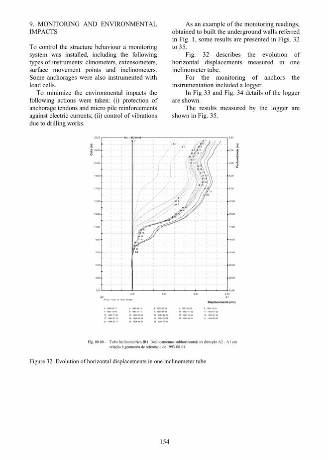
9. MONITORING AND ENVIRONMENTAL IMPACTS

To control the structure behaviour a monitoring system was installed, including the following types of instruments: clinometers, extensometers, surface movement points and inclinometers. Some anchorages were also instrumented with load cells. To minimize the environmental impacts the following actions were taken: (i) protection of anchorage tendons and micro pile reinforcements against electric currents; (ii) control of vibrations due to drilling works.

As an example of the monitoring readings, obtained to built the underground walls referred in Fig. 1, some results are presented in Figs. 32 to 35.

Fig. 32 describes the evolution of horizontal displacements measured in one inclinometer tube.

For the monitoring of anchors the instrumentation included a logger.

In Fig 33 and Fig. 34 details of the logger are shown.

The results measured by the logger are shown in Fig. 35.

4,503,001,500,00

23,00

21,00

19,00

17,00

15,00

13,00

11,00

9,00

7,00

5,00

3,00

Ref.: 1993-08-042

34

56

7

7

8

8

9

9

10

10

11

11

12

12

13

13

14

14

15

15

16

16

17

17

18

18

19

19

20

20

21

21

22

22

23

23

24

24

P.Fixo -> Leit.: 11 | Prof.: 18,46mA1A2

2 - 1993-08-11 3 - 1993-09-13 4 - 1993-09-29 5 - 1993-10-08 6 - 1993-10-217 - 1993-11-09 8 - 1993-11-11 9 - 1993-11-15 10 - 1993-11-22 11 - 1993-11-25

12 - 1993-11-29 13 - 1993-12-06 14 - 1993-12-13 15 - 1993-12-23 16 - 1994-01-0517 - 1994-01-13 18 - 1994-01-26 19 - 1994-02-04 20 - 1994-02-21 21 - 1994-03-0722 - 1994-05-17 23 - 1994-06-01 24 - 1994-06-09

2,00

4,00

6,00

8,00

10,00

12,00

14,00

16,00

18,00

20,00

22,00

1,04

25,00

Displacements (cm)

Cot

a (m

)

0,00

23,96

Prof

undi

dade

(m)

Fig. 00.00 - Tubo Inclinométrico IR1. Deslocamentos subhorizontais na direcção A2 - A1 em relação à geometria de referência de 1993-08-04.

Figure 32. Evolution of horizontal displacements in one inclinometer tube

154

Figure 33. Logger

Figure 34. General view of equipment

155

500,00

525,00

550,00

575,00

600,00

0:00 1

994-01

-04

0:00 19

94-01

-06

0:00 1

994-01

-08

0:00 19

94-01

-10

0:00 1

994-01

-12

0:00 1

994-01

-14

0:00 1

994-01

-16

0:00 1

994-01

-18

0:00 1

994-01

-20

0:00 1

994-01

-22

0:00 1

994-01

-24

0:00 1

994-01

-26

0:00 1

994-01

-28

0:00 1

994-01

-30

0:00 19

94-02

-01

0:00 1

994-02

-03

0:00 19

94-02

-05

0:00 1

994-02

-07

0:00 19

94-02

-09

0:00 1

994-02

-11

0:00 19

94-02

-13

0:00 1

994-02

-15

0:00 19

94-02

-17

0:00 1

994-02

-19

0:00 1

994-02

-21

Tempo

Trac

ção

(kN)

16 23 27 31

Figure 35. Values of anchor loads measured by the logger

10. CONCLUSIONS

The following conclusions can be drawn: a) The selected enlargement and underpinning solutions allowed the construction of the underground gallery for the Lisbon Metro and excessive damages in the station building and in other structures were avoided. This solution enabled the use of the railway platforms of the station without any major constraints.b) The numerical analyses with simulation of the construction phases allowed the calculation of the stresses and strains distributions and also the identification of the plastic zones. The analyses of the alternative solutions were of great importance to select the one which was retained in each zone.c) The need to reinforce both main retaining walls against rotational failure arose from the lack of safety conditions for this scenario which was identified during the design analyses for the underpinning of the station. d) The tests performed for the anchorages of the reinforcement works of the two main walls supported the design of these works and allowed an adequate quality control. e) The corrosion tests to assess the behaviour of permanent anchors have shown a good overall electrical isolation of the anchor from ground and structure. f) The 3D finite element linear analyses to predict the maximum stresses and strain

distributions of Rossio station building were important to analyse the damages and to guide the rehabilitation works. g) The monitoring of the structures during construction allowed the safe implementation of the solutions including the purpose of maintaining most of the station functionality.

REFERENCES

Consortium 1996a. Section 60 - Restauradores-Baixa/Chiado. Geological and Geotechnical Report. (in portuguese), Doc. RT - 02.3-0238.

Consortium 1996b. Section 60 - Restauradores-Baixa/Chiado. Crossing under CP-Rossio. Numerical Analysis of the Principal Retaining Wall. (in portuguese), Doc. RT - 02.3-0168.

Consortium 1996c. Section 60 - Restauradores-Baixa/Chiado. Crossing under CP-Rossio. 3- D Analysis of the Station Building (in portuguese), Doc. RT-02.3-0242, 31.12.96.

Eurocode 0 1990 Basis of Structural Design. Eurocode 1 1991 Actions on Structures Eurocode 7 1997. Geotechnical Design-Part 1.

ENV.Eurocode 8 1998. Design of Structures for

Earthquake Resistance of Structures. ENV. European Standard (EN 1537) 1994. Execution of Special Geotechnical Work- Ground Anchors.

156

RSA 1983. "Regulamento de Segurança e Acções para Estruturas de Edifícios e Pontes". Decreto-Lei nº 235/83 de 31 de Maio.

Seco e Pinto, P.S. Barradas, J. and Sousa, A. 2008. Lessons Learned from Two Case Histories of Retaining Structures. 5th International Conference on Case Histories in Geotechnical Engineering, Arlington.

ACKNOWLEDGEMENTS

Special thanks are due to REFER, EP, Metropolitano de Lisboa, EP, Consortium, and LNEC for the permission to publish the results of Rossio railway station.

157

Seismic design of large, long underground structures: Metro andparking stations, highway tunnels

K. Pitilakis Professor, Department of Civil Engineering, Aristotle University, Thessaloniki, Greece

G. Tsinidis Civil Engineer, MSc

ABSTRACT: Large and elongated underground structures, such as metro lines, parking stations or highwaytunnels, are usually constructed in Megacities in order to improve life quality. Several features of this type ofconstructions render their seismic behaviour distinct. Various approaches, from full dynamic time-historyanalysis to simplified analytical methods, have been introduced for the seismic analysis. In this study, thesedifferent approaches are presented and compared in terms of displacements, stresses, internal forces, and seismicearth pressures. The participation of seismic loads in the overall response of the structures is also presented.Through this presentation we also highlight certain critical issues which remain open and call for more research.

1. INTRODUCTION

Large and long underground structures such as parking stations, subways, railway lines and highway tunnels, are more and more frequent in densely populated agglomerations that can significantly improve the traffic conditions in large cities. In seismic prone regions their seismic design, combined to their importance from economic point of view, as well as for life safe, becomes a crucial design step.

Underground structures have specific geo-metrical and conceptual features, which make their seismic behavior very distinct from above-ground structures. This particular nature of these structures requires a special seismic design approach, based essentially on imposed ground deformations than inertial forces.

Moreover there are few relative guidelines and specific seismic code regulations, rendering them vague and generally lacking of a solid methodology that can adequately address their study.

Full dynamic time-history analysis, is cer-tainly the most accurate method for transversal and longitudinal seismic analysis for long underground structures, or metro and parking stations. However this is often expensive and a simpler approach is always wished. Therefore analytical closed form solutions have been proposed for transversal seismic analysis, based on imposed seismic ground deformations. In the longitudinal direction, modelling of the tunnel

as a “beam” on springs and dashpots is quite popular in engineering practice, while the input motion remains a vague parameter. Finally it is quite common in practice to use equivalent static analysis, neglecting the specific features of these structures. All these different ap-proaches have never been seriously compared between them and validated with rigorous experimental data. Consequently the selection of the design method is crucial for seismic design and safety of this type of structures.

The aim of the paper is to provide a short but comprehensive review of the different design and analysis methods of large and long underground structures, using two examples of real cases: a deep metro station, part of the new Metro system under construction in Thessalo-niki, and an immersed tunnel that is planned to be constructed also in Thessaloniki. Several issues such as the seismic shaking modeling, the way to estimate seismic input, the estimation of seismic earth pressures and seismic shear stresses along the perimeter of underground structures, the evaluation of impedance func-tions for underground structures needed in order to model kinematic and inertial soil-structure interaction effects, the estimation of some important parameters when imposed seismic ground deformations are applied to the struc-ture, the effects of ground failure on long segmented underground structures (e.g. due to liquefaction), as well as the relative importance of the seismic loads compared to the static

158

design loads are among the issues that are presented and discussed herein. Through the specific comparisons it is aimed to highlight the open critical issues, and to examine the possibil-ity to develop a simplified and yet rigorous method that could efficiently consider some of the key parameters affecting the behavior of underground structures.

2. TYPOLOGY – CONSTRUCTION METHODS – CASE STUDIES

2.1. Typology – construction methods

Large and long underground structures can be grouped in two categories:

• Multi story large dimensions structures (e.g. parking stations, subway stations)

• Long underground structures (e.g. tun-nels). In this case the length is much larger than the cross-sectional dimen-sions.

Each group has features that make its seismic behavior quite distinct.

Considering the construction method, large and extended underground structures can be grouped in three categories:

• Bored and mined underground struc-tures (e.g. tunnels).

• Cut and cover structures (e.g. tunnels or subway stations).

• Immersed structures (e.g. immersed tunnels).

cut and cover (rectangular) bored tunnel (circular)

cut and cover (vertical tubes)

cut and cover(center columns or wall)

immersed tube tunnels (single and multiple tubes)

Figure 1. Typical cross-sections of underground structures (Power et al., 1996).

Bored and mined underground structures refer usually to circular tunnels with or without lining; in alluvium and they are usually exca-vated using boring machines (TBM). Cut and cover structures, typically of rectangular cross-sections, are made with open, rather shallow excavation, associated with diaphragm walls. Immersed structures are usually dry dock constructed in segments, usually about 100m long, then moved and sink into their construc-tion place. The segments are connected through special joints (figure 2).

roof

IPEGina gasket steel strip

gasket supporting platebolts

roofbolts

grout fill

steel stripOmega seal

bolts

After installation of Omega

Before Initial Contact

Figure 2. Gina gasket (after Trelleborg -Bakker).

As mentioned before, a metro station and an immersed roadway tunnel in Thessaloniki are used as typical examples to provide a review of seismic design and analysis.

2.2. Metro station

The Thessaloniki Metro, under construction since 2006, has a single line 9.5 km long (with two independent single track tunnels), con-structed with TBM (7.7 km) and cut-and-cover method, with 13 modern center platform sta-tions. “Venizelos” station is constructed using the cover and cut method. It consists of 4 under-ground levels, reaching a depth of 25.5m. The side diaphragm walls continue under inverted

159

slab, as seen in stations cross section (figure 3), in order to reduce the internal forces caused mainly by uplift and lateral earth pressures. For the same reason the initially conceived inverted slab reaches a thickness of 2.5m. The design soil profile is depicted in figure 4. The bedrock in the area of the station is estimated at 78m.

36.5

0

P0

1 P1

P2

P3

P4

2

3 4

5 6

9 10

1.2

0.9

0.9

0.9

2.56.

984.

554.

554.

55

1

1

1

1

21.75

7 8

Figure 3. Venizelos station cross section.

2.3. Thessaloniki immersed roadway tunnel

The linear morphology and geographical loca-tion of Thessaloniki urban area would require a detour crossing the sea, in order to reduce the traffic and upgrade the life quality in the densely-populated historical center of the city. Hence an immersed tunnel has been proposed to bypass the centre from the sea. However the construction of is actually delayed due to environmental and operational constrains that are still not solved.

The overall construction comprises of a sys-tem of cut and cover segmented tunnel (2.9km length), an underwater tunnel (1.2km) and conjunction ramps to the local road system (1.2km). The immersed tunnel consists of 8, 155m long segments. They are connected to each other through specially chosen intermedi-ate rubber joints (Gina-gaskets) that secure the tunnel’s water - proof under differential dis-placements. A simplified version of the rein-forced concrete tunnel’s cross-section is de-picted in figure 5. The cross-section consists of two separate traffic branches and an escape corridor in the middle.

The simplified typical soil profile for the de-sign is given in figure 6. Next to the tunnel, there is a backfill with compacted gravel mate-rial, to improve the soil drainage conditions and confinement. The bedrock (Vs>750m/s) is estimated at about 110m.

Vs =216m/s, =18.1kN/m

Venizelou station cross section

Vs =258m/s, =18.5kN/mVs =159m/s, =18.1kN/m

Vs =269m/s, =21.1kN/mVs =187m/s, =20.3kN/m

Vs =393m/s, =20.8kN/mVs =181m/s, =20.3kN/m

Vs =474m/s, =21.0kN/m

Vs =523m/s, =21.0kN/m

Vs =571m/s, =21.5kN/m

Vs =619m/s, =21.5kN/m

Vs =668m/s, =22.0kN/m

Vs =718m/s, =22.0kN/m

0.00 m-4.30 m

-78.0 m

-69.0 m

-64.0 m

-52.0 m

-44.0 m

-32.50 m

-24.80 m-19.90 m-18.00 m-14.40 m

-9.80 m-6.15 m

Debris -CL clayey sands

CL-CI (with SC)Sandy - silty clayswith clayey sands

CI (with SC-GC)Stiff clays with

sand-clay mixtures

Figure 4. Simplified station - soil deposit cross section.

160

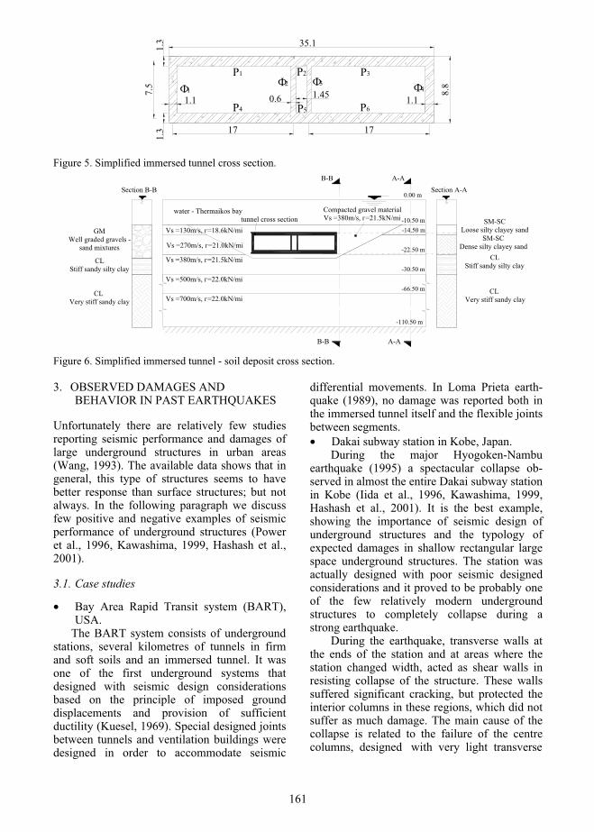
35.1

8.8

1.1

1.3

0.6 1.45

1.3

1.1

17

7.5

P1 P2

12

P3

43

P4 P5 P6

17

Figure 5. Simplified immersed tunnel cross section.

SM-SCLoose silty clayey sand

CLStiff sandy silty clay

SM-SCDense silty clayey sand

CL Very stiff sandy clay

Section A-A A-A

A-A

CLStiff sandy silty clay

CL Very stiff sandy clay

Section B-B B-B

B-B

GMWell graded gravels -

sand mixtures

water - Thermaikos bay

0.00 m

-10.50 m-14.50 m

-22.50 m

-30.50 m

-66.50 m

-110.50 m

Vs =130m/s, =18.6kN/m

Vs =270m/s, =21.0kN/m

Vs =380m/s, =21.5kN/m

Vs =500m/s, =22.0kN/m

Vs =700m/s, =22.0kN/m

Compacted gravel materialVs =380m/s, =21.5kN/mtunnel cross section

Figure 6. Simplified immersed tunnel - soil deposit cross section.

3. OBSERVED DAMAGES AND BEHAVIOR IN PAST EARTHQUAKES

Unfortunately there are relatively few studies reporting seismic performance and damages of large underground structures in urban areas (Wang, 1993). The available data shows that in general, this type of structures seems to have better response than surface structures; but not always. In the following paragraph we discuss few positive and negative examples of seismic performance of underground structures (Power et al., 1996, Kawashima, 1999, Hashash et al., 2001).

3.1. Case studies

• Bay Area Rapid Transit system (BART), USA.

The BART system consists of underground stations, several kilometres of tunnels in firm and soft soils and an immersed tunnel. It was one of the first underground systems that designed with seismic design considerations based on the principle of imposed ground displacements and provision of sufficient ductility (Kuesel, 1969). Special designed joints between tunnels and ventilation buildings were designed in order to accommodate seismic

differential movements. In Loma Prieta earth-quake (1989), no damage was reported both in the immersed tunnel itself and the flexible joints between segments.• Dakai subway station in Kobe, Japan. During the major Hyogoken-Nambu earthquake (1995) a spectacular collapse ob-served in almost the entire Dakai subway station in Kobe (Iida et al., 1996, Kawashima, 1999, Hashash et al., 2001). It is the best example, showing the importance of seismic design of underground structures and the typology of expected damages in shallow rectangular large space underground structures. The station was actually designed with poor seismic designed considerations and it proved to be probably one of the few relatively modern underground structures to completely collapse during a strong earthquake. During the earthquake, transverse walls at the ends of the station and at areas where the station changed width, acted as shear walls in resisting collapse of the structure. These walls suffered significant cracking, but protected the interior columns in these regions, which did not suffer as much damage. The main cause of the collapse is related to the failure of the centre columns, designed with very light transverse

161

Figure 7. Collapse of centre columns.

shear reinforcement compared to the main bending reinforcement (figure 7). The collapse of the columns caused also cracking of ceiling slab and severe settlements and disruption to the overlying roadway (figure 8). Center columns wit zigzag reinforcement in addition to the hoop steel, did not buckle as much as those without this reinforcement. There was also significant separation at some construction joints, and water leakage through cracks. Only few cracks, if any, were observed in the base slab.

Figure 8. Settlements of the overlaying roadway caused by the subway collapse.

The damages’ pattern is attributed to the relative displacement between the base and ceiling slabs, due to the imposed important transient differential ground movement during the ground shaking. It is further believed that the overburden soil affected the extent of damage between sections of the station by adding extra inertial force to the structure.

3.2. Seismic performance of underground structures

The observed damages in several underground structures lead to the following conclusions regarding the seismic performance of under-ground structures (after Hashash et al., 2001):

• Underground structures seem less vulner-able than surface structures.

• Deep or constructed in rock underground structures seem to be safer to earthquakes than are shallow or constructed in soils un-derground structures.

• Lined and grouted tunnels are safer than unlined tunnels in rock.

• By stabilizing the ground around a tunnel or by improving the contact between the lining and the surrounding ground, through grouting, damage from shacking can be re-duced. Improving the tunnel lining by plac-ing thicker and stiffer sections without sta-bilizing surrounding poor ground may re-sult in excess seismic forces in the lining.

• Structure vulnerability may be related to peak ground acceleration and velocity based on the magnitude and epicentral dis-tance of the affected earthquake.

• Duration of earthquake is of utmost impor-tance because it may cause fatigue failure and therefore, large deformations.

• High frequency motions, expected mainly at small distances from the causative fault, may explain the local spalling of rock or concrete along planes of weakness.

• Ground motion may be amplified if wave-lengths are between one and four times the tunnel diameter.

• Damage through slope instability, near tunnel portals may be significant.

3.3. Seismic behaviour of underground struc-tures

An underground structure is affected during an earthquake by shacking or/and permanent ground deformations (i.e. ground failure). Seismic shacking refers to ground deformation due to seismic waves propagation, while ground failure refers to induced phenomena such as liquefaction, slope instability or fault displace-ment.• Seismic shaking.

It is evident that the inertia of the surround-ing soil is much larger than the structure’s one. This means that the response of an underground structure is dominated by the surrounding ground response, which is manifested through important transient ground deformations. This feature makes the seismic behaviour of under-ground structures distinct from the behaviour of aboveground structures, where the response is

162

Figure 9. Deformation modes of tunnels due to seismic waves (after Hashash et al., 2001).

basically related to the structure’s inertia.When seismic waves are propagating along

an underground structure, its cross section is deformed in various modes, both in the longitu-dinal and transverse direction (figure 9). Seis-mic waves producing soil particle movement parallel to the underground structure (e.g. tunnel) axis, result in axial deformation of structure (compression-extension in figure 9a), whereas soil movement perpendicular to the tunnel axis causes longitudinal bending (figure 9c). Shear wave propagation normal to the underground structure axis, causes the deforma-tion mode presented in figure 9e and 9f. De-pending on the shape of the structure’s cross-section, this type of deformation produces ovaling or racking effects for circular and rectangular cross-sections respectively. For rectangular tunnels, on which the present work is concentrated, the main seismic load is racking deformation of the rectangular cross-sections.

It is quite clear that a strong interaction ef-fect is developed between the underground structure and the surrounding soil during earth-quake shaking. The soil deformation in the

proximity of the structure imposes displacement constraint on the structure’s cross-section. Yet, due to the stiffness variation between the two media, the structure responds in a different way to the imposed deformation. The overall seismic behaviour of the structure depends both on the properties of the surrounding soil and the inertial properties of the structure’s cross-section.• Ground failure

Ground failure is related to large permanent deformations, caused by liquefaction, slope failure or fault movements.

It is quite difficult, to design an underground structure to resist large ground deformations. The commonly used techniques, are related to ground strengthening, (ground stabilization, ground improvement etc), or with improving drainage conditions. In that way the liquefaction risk is reduced and the slope stability is im-proved. On the contrary when a normally stiff tunnel is crossing a well-identified and con-strained active seismic fault, normally the only realistic solution is to avoid this dangerous crossing.

163

4. DESIGN PRINCIPLES IN PRACTICE

It is common in engineering practice to evaluate underground structure’s behavior under static or seismic loads, separately. The final design output is a combination of both static and seismic loads.

The seismic analysis and design of under-ground structures consists of three major steps: • Definition of seismic background (seismic

hazard) and design criteria. • Evaluation of ground response to seismic

shacking (design transient motions-shaking, and induced phenomena i.e. liquefaction, ground failure).

• Evaluation of structure seismic behavior.

4.1. Seismic background definition and design earthquake criteria

In order to design an underground facility, under seismic ground motion, the level of expected (design) ground motion must be defined. It describes the amplitudes and charac-teristics of expected ground motions along the structure and their return period. The design ground motion is usually proposed in national seismic codes. However the importance of the large underground structures makes necessary the performance of site-specific hazard analysis, which leads to safer estimation of expected motions.

There are two methods of analysis: • A deterministic seismic hazard analysis

(DSHA) that is normally applied when the seismic sample is not very rich and there are well-identified seismic faults affecting directly the structure.

• A probabilistic seismic hazard analysis (PSHA) that quantifies the uncertainties in the analysis and develops a range of ex-pected ground motions with their probabili-ties of occurrence.

Once the level of seismicity in a region es-tablished, the design earthquake has to be defined. Two design earthquake levels are commonly defined, the Maximum Design Earthquake (MDE) and the Operational Design Earthquake (ODE). The first level refers to the maximum level of ground motion expected in the region, with small probability of occurrence and the design goal in this case, is the public safety during and after an earthquake. The second level expected to occur once during the life of the underground facility and the design

goal is to continue operating during and after an earthquake. This means that the damages must keep in minimum.

Through the procedures described before ground motion parameters for analysis, such as acceleration, velocity and displacement ampli-tudes can be estimated.

4.2. Evaluation of ground response to seismic shacking

As mentioned before the ground response to seismic shacking categorized into ground failure and ground shacking. • Ground failure.

The liquefaction potential of soils in case of swallow tunnels for example, the possibility of slope instability in case of tunnels portals and the possibility of fault displacement in case of a structure crossing an active fault, must be consider in the design.• Ground shacking.

The design in this case focuses to the tran-sient ground deformations, caused by seismic wave’s propagation. The phenomena can be more complicated, considering the soil structure interaction effects, which in case of large and extended underground structures can be ampli-fied. Spatial variability of ground motion, differential movement and loss of coherency are also very important parameters in particular for the analysis in the longitudinal direction.

4.3. Evaluation of structure seismic response

Commonly the evaluation of seismic response of underground structures is performed in transversal and longitudinal direction sepa-rately. The final design output is a combination of both directions results.• Transversal seismic analysis.

The response of underground structures in the transverse direction is crucial for the evalua-tion of the maximum inertial forces. For this, different approaches, from full dynamic analy-sis to simplified analytical closed form solutions have been proposed.

In order to fully capture both the kinematic and the inertial part of the soil-structure interac-tion, a full dynamic time-history analysis would be the most appropriate approach. Normally a 2D model of the soil and the structure repro-duces efficiently the interaction phenomena; in that way seismic loading is applied on the tunnel through the soil deformation from the

164

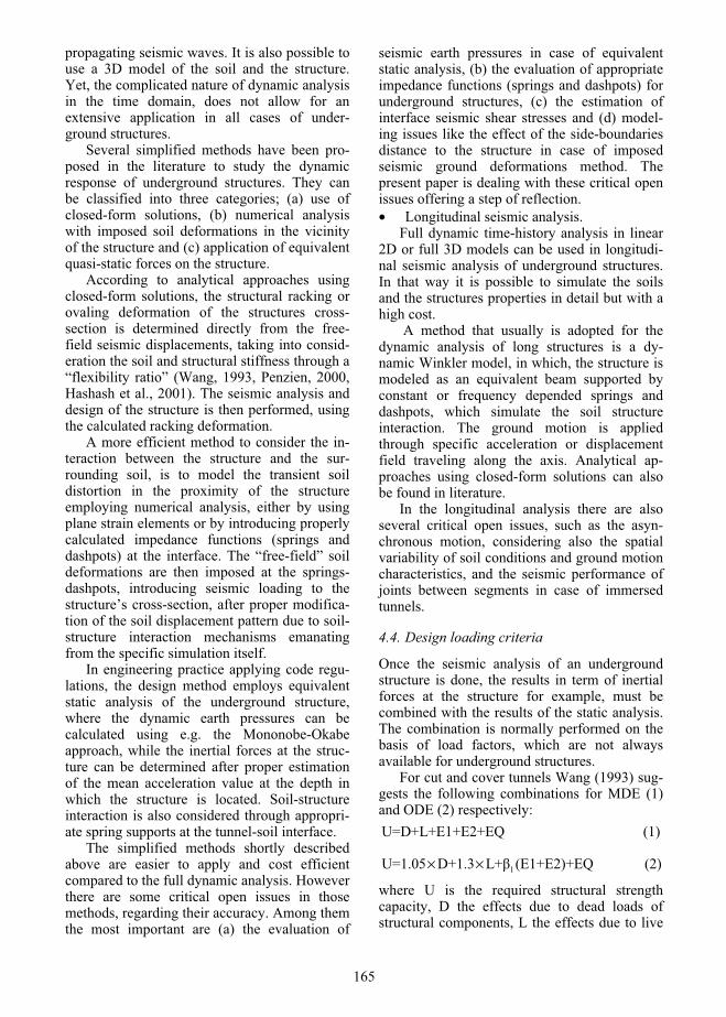
propagating seismic waves. It is also possible to use a 3D model of the soil and the structure. Yet, the complicated nature of dynamic analysis in the time domain, does not allow for an extensive application in all cases of under-ground structures.

Several simplified methods have been pro-posed in the literature to study the dynamic response of underground structures. They can be classified into three categories; (a) use of closed-form solutions, (b) numerical analysis with imposed soil deformations in the vicinity of the structure and (c) application of equivalent quasi-static forces on the structure.

According to analytical approaches using closed-form solutions, the structural racking or ovaling deformation of the structures cross-section is determined directly from the free-field seismic displacements, taking into consid-eration the soil and structural stiffness through a “flexibility ratio” (Wang, 1993, Penzien, 2000, Hashash et al., 2001). The seismic analysis and design of the structure is then performed, using the calculated racking deformation.

A more efficient method to consider the in-teraction between the structure and the sur-rounding soil, is to model the transient soil distortion in the proximity of the structure employing numerical analysis, either by using plane strain elements or by introducing properly calculated impedance functions (springs and dashpots) at the interface. The “free-field” soil deformations are then imposed at the springs-dashpots, introducing seismic loading to the structure’s cross-section, after proper modifica-tion of the soil displacement pattern due to soil-structure interaction mechanisms emanating from the specific simulation itself.

In engineering practice applying code regu-lations, the design method employs equivalent static analysis of the underground structure, where the dynamic earth pressures can be calculated using e.g. the Mononobe-Okabe approach, while the inertial forces at the struc-ture can be determined after proper estimation of the mean acceleration value at the depth in which the structure is located. Soil-structure interaction is also considered through appropri-ate spring supports at the tunnel-soil interface.

The simplified methods shortly described above are easier to apply and cost efficient compared to the full dynamic analysis. However there are some critical open issues in those methods, regarding their accuracy. Among them the most important are (a) the evaluation of

seismic earth pressures in case of equivalent static analysis, (b) the evaluation of appropriate impedance functions (springs and dashpots) for underground structures, (c) the estimation of interface seismic shear stresses and (d) model-ing issues like the effect of the side-boundaries distance to the structure in case of imposed seismic ground deformations method. The present paper is dealing with these critical open issues offering a step of reflection.• Longitudinal seismic analysis.

Full dynamic time-history analysis in linear 2D or full 3D models can be used in longitudi-nal seismic analysis of underground structures. In that way it is possible to simulate the soils and the structures properties in detail but with a high cost.

A method that usually is adopted for the dynamic analysis of long structures is a dy-namic Winkler model, in which, the structure is modeled as an equivalent beam supported by constant or frequency depended springs and dashpots, which simulate the soil structure interaction. The ground motion is applied through specific acceleration or displacement field traveling along the axis. Analytical ap-proaches using closed-form solutions can also be found in literature.

In the longitudinal analysis there are also several critical open issues, such as the asyn-chronous motion, considering also the spatial variability of soil conditions and ground motion characteristics, and the seismic performance of joints between segments in case of immersed tunnels.

4.4. Design loading criteria

Once the seismic analysis of an underground structure is done, the results in term of inertial forces at the structure for example, must be combined with the results of the static analysis. The combination is normally performed on the basis of load factors, which are not always available for underground structures.

For cut and cover tunnels Wang (1993) sug-gests the following combinations for MDE (1) and ODE (2) respectively: U=D+L+E1+E2+EQ (1)

1U=1.05 D+1.3 L+ (E1+E2)+EQ× × (2)

where U is the required structural strength capacity, D the effects due to dead loads of structural components, L the effects due to live

165

loads, E1 the effects due to vertical loads of earth and water, E2 the effects due to horizontal loads of earth and water, EQ the effects due to design earthquake motion and 1 is a factor taking values 1.05 if extreme loads are assumed for E1 and E2 with little uncertainty, otherwise 1.3.

Considering the design goals for maximum and operational design earthquake, structures must provide strength and sufficient ductility, through special structural considerations.

5. DETERMINATION OF INPUT MOTION

Regardless of the implicated analysis method, an important element in an underground struc-ture’s design process is the evaluation of the seismic shaking imposed on the structure. There are two methods to estimate the design seismic shacking: application of seismic codes and detailed site specific seismic hazard analysis.

Seismic code regulations offer some guide-lines on the selection of the input motion characteristics, yet those are aimed for above ground structures, and for different return periods and probabilities of exceedance.

As mentioned before, a site-specific seismic hazard analysis is more suitable- if not manda-tory- to determine the dynamic loading levels in the case of important constructions, such as metro lines or underground roadway tunnels, since they specifically address the local site conditions.

A typical “ground motion deconvolution” procedure is usually followed, as schematically described in figure 10. The procedure refers to

the immersed roadway tunnel of Thessaloniki and to the earthquake scenario conforming to the Thessaloniki, 1978 earthquake. The peak ground acceleration (PGA) for outcrop rock conditions is determined through a typical probabilistic seismic hazard analysis. Then a conventional equivalent linear site response analysis (SH waves) or a full non-linear analysis is employed to calculate the input motion characteristics at the soil deposit, where the underground structure is located.

In case of full dynamic time-history analy-sis, where the soil and the structure is simulated using 2D plane strain elements, the bedrock motion obtained in the first step of the afore-mentioned procedure (seismic hazard and deconvolution) can be applied directly. The soil-structure response in this case is explicitly computed by the upward propagating seismic waves, from the base of the model towards the surface.

In the case of analytical closed-form solu-tions with imposed seismic ground displace-ments, the required displacement pattern which will be applied directly upon or in the proximity of the structure, is calculated through a 1D soil-column non-linear or equivalent linear (i.e. SHAKE type) analysis, using as input the bedrock motion that was calculated through the deconvolution process.

Finally, the “equivalent static” method ap-plies “quasi-static” forces on the structure (slabs and vertical walls). These inertial forces nor-mally correspond to the average acceleration level observed at any depth defined from the 1D free-field ground response analysis.

Figure 10. Deconvolution process (Thessaloniki 1978 seismic scenario): (1) Outcrop target acceleration time history, (2) acceleration time history at the bedrock level, (3) acceleration time history along the soil column.

166

In this case, the equivalent static method ig-nores the kinematic part of soil-tunnel interac-tion that would normally alter the initial accel-eration time-histories at the proximity of the underground structure. If the detailed soil profile is not available, an acceleration value at the depth of interest could always be estimated using the ground acceleration defined by the national seismic code for the investigated site. Along with the deficiencies concerning the kinematic interaction, this simplified approach includes several uncertainties that would only lead to a crude estimation of the actual loading level.

In the longitudinal seismic analysis, spatial variability of seismic ground motion must be properly estimated and accounted (Kramer, 1996, Zerva & Zervas 2002, Zerva & Beck, 2003). Seismic shaking is continuously and spatially varying in terms of wave amplitude, phase, frequency characteristics and duration. A simple phase difference due exclusively to the incident angle of traveling waves is not always sufficient. These aspects can significantly affect the response of long structures (L>200-300m). Differential movements may be very important even in small distances. A schematic illustration of the potential sources of ground motion incoherency is presented in figure 11.

Wavefront

1 2 3

1 2 3

epicenter

heterogeneity

1 2 3

epicenter

Afault

B

1 2 3

1 2 3

Figure 11. Sources of asynchronous shaking and spatial variation of ground motion.

6. TRANSVERSAL SEISMIC ANALYSIS

Different approaches and methods for transver-sal seismic analysis of underground structures are presented in this paragraph, using as exam-ples the Venizelos Metro station and the Thes-saloniki immersed tunnel in Thessaloniki. Through the presentation and discussion of the

results from different methods, in terms of internal forces, seismic shear stresses developed around the tunnel, selection of impedence functions, and evaluation of seismic earth pressures, we illustrate several important points and needs aiming to improve the present quality of the seismic design of these structures.

6.1. Analytical approaches and closed-form solutions

A simple, straightforward method to study underground structures and especially tunnels, taking into consideration the relative stiffness of soil and structure, is described by Wang (1993) and Hashash et al. (2001). Rather than applying a predetermined free-field seismic deformation on the structure, which may be, in several cases, inaccurate, a stepped procedure is suggested, that adjusts the soil deformation profile accord-ing to a soil-structure stiffness ratio, before applying it on the structure’s cross-section.

The first step of the proposed methodology requires the determination of the free-field deformation profile, at the soil deposit near the location of the tunnel. Usually this deformation profile is obtained through simple 1D site response analyses, with selected input motions corresponding to the particular characteristics of the investigated area.

Then, the rigidity of the structure’s cross-section is defined comparatively to the stiffness of the surrounding soil, introducing the term flexibility ratio. The flexibility ratio (F) can be calculated, albeit for simple one barrel frames, using the following equation:

2 2m

R W

G HW H WF= +24 EI EI

(3)

where IR and IW are the slab and side wall moments of inertia respectively, H and W are the height and width of the structure, E is the elasticity modulus of the structural material and Gm is the soil shear modulus. In case of differ-ent inertia moment for roof and invert slabs, a procedure described by Wang (1993) can be followed, for flexibility ratio estimation.

The value of the flexibility ratio is related closely to the expected stress level on the structure:• F 0 - the structure is rigid and will not

display any type of racking deformation.• F < 1 - the structure is stiffer than the

surrounding soil, thus the structural defor-

167

mation level will be smaller than the free-field deformation level.

• F = 1 - the structure and the surrounding soil share the same level of stiffness, so the tunnel will follow the free-field deforma-tion.

• F > 1 - the racking deformation of the structure is amplified compared to the free-field deformations.

The ratio of structural to free-field deforma-tion (racking ratio R), can be estimated utilizing the flexibility ratio (F) according to the diagram of figure 13. The structural deformation is calculated using Eq. 4, and the internal stress of the underground structure is determined for the imposed deformation as demonstrated in figure 12. This pseudo-triangular pressure distribution corresponds better to swallow structures. For deep structures (e.g. deep tunnels) the pseudo-concentrated force at the top of structure seems to be a better selection. For deep metro station there no specific guidelines.

structure free-field=R× (4)

• Thessaloniki immersed roadway tunnel. For the case study of Thessaloniki immersed

tunnel, the F ratio is estimated at about 3 ~ 3.1, indicating a considerably more flexible structure than the surrounding soil. This means that according to figure 13 the racking ration R is equal to 1.5. After conducting an equivalent linear 1D analysis for two earthquake time-histories (Kozani 1995 and Thessaloniki 1978), both scaled to rock outcropping acceleration equal to 0.35g (estimate from the probabilistic hazard analysis), the maximum deformation at free field conditions is calculated equal to 4.9mm while the maximum differential dis-placement on the structure (drift) equal to 7.35 mm. This displacement is then applied to the rectangular tunnel cross section to estimate the internal forces and bending moments.

structure=R x free field

Figure 12. Seismic loads applied on shallow tunnel (Wang, 1993).

Figure 13. Normalized structure deflections, circular vs. rectangular tunnels: solid lines for circular tunnels, filled triangular symbols for rectangular tunnels (Wang, 1993).

A critical issue in seismic design of under-ground structures is the evaluation of the inter-face seismic shear stresses in the structure’s perimeter. Through this method those stresses can be estimated, as follows:

structure

structure structure

free-fieldfree-field free-field

R= = = (5)

where H is the height of the structure, and structure and free-field, are the shear strains near the

structure and at free-field respectively. Through Equation 6 the shear stresses can be estimated.

structure m structure=G × (6)

The calculated shear stresses for this case study are given in Table1. As the soil next to the tunnel, is replaced with compacted gravel material, two hypotheses for soils properties have been used. In the first one the initial soils properties have been used, while the second uses the compacted gravel material properties.Table 1. Seismic shear stress around the tunnel.

Approach Gm(kPa)

ffeff(%) F R str

(kN/m2)Gravel material-

Thessaloniki (1978) 277431 0.017 10.3 2.0 94.0

Gravel material- Kozani (1995) 280240 0.017 10.4 2.0 97.1

Initial soilsproperties-

Thessaloniki (1978) 83911 0.051 3.1 1.5 64.2

Initial soilsproperties-

Kozani (1995) 83185 0.052 3.08 1.5 64.9

168

The results of this method are compared with those came out from full dynamic analysis, in next paragraphs.

6.2. Imposed seismic ground deformations

This type of analysis, although inspired by the previous one, attempts to reproduce more accurately the soil-structure interaction effects during the quasi-static analysis procedure. The calculated “far-field” deformations are now imposed on the soil next to the structure’s cross-section, contrary to the previous analytical approach, where a “modified deformation profile” was applied directly on the structure. In this case the final imposed deformations on the structure’s side walls are determined depending on the type of constraint between the structure and the surrounding soil. The soil compliancy is simulated through a finite element code with appropriate constitutive law (i.e. Mohr - Cou-lomb), either by using 2D elements for the soil, or via proper springs that correspond to the degree of the support the soil offers to the structure’s cross-section. In the examples presented herein, the soil surrounding the structures is simulated using 2D plane strain elements to account for the elastic support of the cross-section in the lateral and vertical direction. The deformation profile is imposed at the side FE mesh boundaries of the soil models.

The determination of the free-field soil de-formation profile, which will be imposed on the model, boundaries can be calculated by 1D site response analysis, in the same way described in the previous section, supposing free-field conditions. In this case though, it is the com-plete deformation profile at a specific instance that is required rather than the maximum dis-placement value at the cross-section’s level. The selected deformation profile corresponds to the time step, where the maximum differential displacement between the base and the top of the cross-section is observed.

Being essentially a static analysis, this ap-proach is cost-effective compared to more elaborate full dynamic time-history analysis. However, it is still lacking guidelines concern-ing several modelling specifics of the soil-structure system.

Critical issues, such as the modelling of stratified heterogeneous soil, or the selection of appropriate distances of the side-boundaries to the structure’s cross-section, can significantly

affect the results. In case of ground improve-ment, for example, the method raises some modelling questions regarding the geometry of the 1D soil profile that should be used during the calculation of the free-field ground deforma-tions. Also, there are no specific guidelines for the distance of the side-boundaries to the structure’s cross section. When the deformation profile is imposed in a long distance from the underground structure, it is possible for the soil elements to absorb a great amount of induced ground strain, thus “relieving” the structure and altering the analysis results. If, on the other hand, the model is laterally reduced, bringing the side boundaries close to the structure, it is doubtful whether the soil-structure interaction mechanisms will deploy to their full extent. • Venizelos Metro station.

In order to apply the imposed seismic ground deformations method, a FE model in ADINA was created (figure 14). Plane strain elements used to model the soil deposit, whereas the station’s cross-section is modelled using frame-type elements of proper dimen-sions. The soil shear modulus and damping properly modified, in order to account for inelastic behavior of soils under seismic load-ing, according to the shear deformation level of the soil deposit at each depth. For this reason selected G- -D curves corresponding to each soil type used.

Five real earthquake time-histories were used, all scaled to bedrock acceleration equal to 0.22g, as seismic hazard analysis estimated for bedrock conditions. The results of this method are compared with those came out from full dynamic analysis, in next paragraphs. • Thessaloniki immersed roadway tunnel.

The same procedure is followed in case of Thessaloniki immersed roadway tunnel. The presence of the inclined gravel bed, in the examined case study, raises some modelling questions regarding the geometry of the 1D soil profile that should be used during the estimation of the free-field ground deformations, as men-tioned before. If the simulated soil area is extended laterally, far away from the gravel bed location, then a single soil column analysis using the in situ soil characteristics is accurate enough to provide the deformation profile for the 2D analysis (model C in figure 15 and corresponding simulated area of model C in figure 16).

169

Figure 14. Venizelos Metro station FE model and application of imposed seismic ground motions.

model A, Bmodel C model D, E

u=0.030m u=0.015m

u=0.0073mz = 0.0m

z = -100.0m

u=0.012m

u=0.0052m

soil deformation profile for initial soil layerssoil deformation profile for soil column includinggravel bed

d = 5.0md = 27.0md = 63.0m

z = -3.5m

z = -11.0m

z = -30.0m z = -20.0m

Figure 15. Soil deformation profile applied in the proximity of the tunnel (at distances d equal to 5m, 27m, 63m).

In the case though, that the modelled soil area is in the edge or inside the gravel bed region, the soil column layering that should be employed in order to obtain a realistic soil deformation profile is not obvious. If, for instance, model A or B of figure 15 are exam-ined, the soil deposit at this specific location would refer to the initial soil layering. Never-theless, it is obvious that the complex soil geometry of this location after the construction of the gravel bed, will affect the free-field response of the unmodified soil profile, altering the obtained results. Therefore, when the FE model does not extend laterally in the 2D analysis (models A, B, D and E of figure 16), both soil column profiles are employed for the determination of the soil deformations during the 1D analysis, serving as lower and upper bound for the 2D analysis that will follow.

Three different models have been proposed, in order to investigate the effect of the side-

boundaries distance to the tunnel. Moreover, in each of the reduced size models, two different imposed deformation profiles are utilized, to account for the effect of the surface gravel bed on the free-field response as previously ex-plained. Therefore, in models A and E the imposed seismic equivalent static loading is the seismic displacement profile obtained from the 1D site response analysis of the initial soil profile. In models B and D on the other hand, the imposed ground deformations have been calculated for a soil profile where the surface layer is replaced by compacted gravel material. In the case of model C there is no such di-lemma, since the mesh boundaries are far enough to imply any effect of the gravel bed on the ground response. The purpose of this para-metric analysis is to form an envelope stress condition for the tunnel, in order to compare the output with the results of the other proposed methods and the detailed full dynamic analysis.

170

Models A, B

Model C

Models D, E

Figure 16. Application of imposed free-field soil displacement profile for different soil-tunnel models.

The results of this approach are compared with those from full dynamic analysis, in next paragraphs.

6.3. Equivalent static analysis

The approach using static forces to model seismic loading is quite common in several recent seismic codes; it is employed for the study of aboveground structures that meet certain criteria concerning their morphology. It is rather questionable whether a similar method could be used in the case of underground structures, at least in its present form, where the equivalent (to the inertial) static forces obtain a distribution profile that conforms to the dy-namic characteristics of an oscillating structure free of lateral supports. Moreover, the determi-

nation of the dynamic earth pressures, using methods described in the case of retaining walls, such as the Mononobe-Okabe approach, (Okabe, 1926, Mononobe, 1929) may be often proved inadequate for underground structures. Nevertheless, several studies utilize an “equiva-lent static approach” to design underground structures, mainly because the use of static forces is more straightforward and easily controlled by an average engineer using existing commercial software.

Usually the soil-structure model consists of linear frame-type elements for the structure’s cross-section and linear springs to simulate the soil support compliancy.

Equivalent static forces on structure due to seismic loading are determined, based on the

171

average acceleration level calculated at the depth of the structure’s cross-section. The base shear force, a term borrowed from the study of aboveground structures, follows a distribution compatible to the first eigen-mode of oscillation of the structure considering the foundation soil compliancy. The calculated static forces are applied at the horizontal diaphragms and at the side walls of the underground structure, in order to correspond to the racking deformation that causes differential displacement between the upper and the lower slabs of the structure.

Seismic earth pressures at structure’s side walls are calculated according to the guidelines of seismic codes (e.g. Greek Seismic Code 2003, or EC8) for retaining wall, applying two methods; (i) the Mononobe-Okabe for walls that can move/tilt sufficiently and (ii) a procedure proposed for rigid non-deformable walls (figure 17).

Hydrodynamic pressures at the sidewalls are calculated according to the guidelines of seis-mic codes based on the Westergard theory (Westergard, 1933).

Seismic shear stresses at the perimeter of the structure can be modeled using adequate shear impedance functions (e.g. constant value springs.

A rather delicate issue is the determination of the impedance factors for the soil spring-properties and values of the sidewalls and the slabs of the cross-section. There are several plausible suggestions in the literature for the calculation of horizontal springs on the side-walls, but very few specifically for underground structures.

H

H 0.5 a H

1.5 a H

H

i

h

EAE

a.

b.Figure 17. Geostatic and seismic earth pressures for non-deformable wall (a) and Mononobe-Okabe approach (b).

Almost all are inspired from surface and deep foundations solutions. Yet, in the case of vertical and horizontal soil springs for the cross-section slabs, as well as for the determination of the vertical (shear) soil-springs on the side walls of the structure, (especially in case of a deep Metro station), few references are roughly compatible to the actual problem configuration and can be applied in this type of structures.

soils weight + inertia forces

seismic shearstresses

springs-impedancefunctions

Kx,Ky

seismic shearstresses

bedrock

dynamic pressures

ground differential displacementbetween surface and bedrock

x

structure'sweight +

inertia forces

hydro-dynamic pressures

hydro-dynamic pressures

dynamic pressures

Figure 18. Equivalent static forces utilized in equivalent static analysis.

172

Except impedance factors values estimation for static and dynamic loading, several issues, including the concept and distribution of the so called “base shear force” in underground structures and the validity of the seismic earth pressure calculation based on clauses for retain-ing walls, discredit the accuracy of this ap-proach.

We will examine several of these issues in the next paragraphs in the light of specific examples.• Venizelos Metro station.

In order to use the equivalent static analysis method, a model in SAP2000, was created (figure 20). The model consists of linear frame-type elements for the structure’s cross-section and linear springs to simulate the soil support compliancy.

The equivalent static forces are the follow-ing:• Equivalent static forces through structure’s

inertia.Those static forces, depicted in figure 21,

applied at the horizontal diaphragms and at the side walls of the underground structure. The estimated average acceleration at the depth of the structure’s cross-section is 0.42g. The base shear force is distributed to the diaphragms and side walls according to each section’s mass, using Equation 7.

i iO

j jj

m ×hF=V × , i , j = 1,2...N

m ×h (7)

where mi is the mass of a section at hi level.• Seismic earth pressures.

Seismic earth pressures distribution at struc-ture’s sidewalls is depicted in figure 21.The distribution consists of a uniform part at the deeper part and a distribution proposed for rigid non-deformable walls near the surface.

m=79t

m=79t

m=62t

m=156t

m=53t

8.7

14.1

519

.60

25.2

0

m=53t

Figure 19. Masses of each section of the station. D

=28m

H=2

7m

2B=22m

Kwx

Kwz

Kwx

Kwz

Kbz Kbz

Ksx

Ksz

d=24

m(s

oils

in fu

ll co

ntac

t with

the

stru

ctur

e)

d/2

h (to

d/2

)=15

m

2L=80m

Figure 20. Venizelos metro station. Analytical model for the for equivalent static analysis.

173

F0=42.2kN/m (a)

F1=13kN/m (a)

x

z

F2=12kN/m (a)

F3=7.4 kN/m (a)F=8.

70kN

/m (a

)

F=8.

70kN

/m (a

)

0.5a =20.90kN/m (b)

20.90kN/m (b)

1.5a =62.7kN/m (b)

Kwx

Kwz

Kwx

Kwz

Kbz Kbz

Ksx

Ksz

Figure 21. Equivalent static model: (a: Equivalent static inertial forces, b: Seismic earth pressure).

A simple triangular distribution at these depths should be erroneous as it will be proved later by the full dynamic analysis. • Hydrodynamic pressures.

Due to the soil type (stiff clays) hydrody-namic pressures did not considered, explicitly, and the seismic earth pressures were calculated for saturated conditions.

Considering that this is a single-direction loading approach, and the linear springs used in this analysis work in both directions, the left side wall should not be supported by horizontal springs, as this would relieve the structure from the applied earth pressure.

Table 2 presents the different expressions and values of the impedance factors (springs) used in the analysis. As mentioned before, due to the lack of specific functions for deep under-ground structures, most of them are inspired from surface and deep foundations solutions, and consequently they may vary a lot. • Thessaloniki immersed roadway tunnel. The numerical model is depicted in figure 23.• Equivalent static forces through structure’s

inertia.Using the same procedure as before a design

acceleration of 0.28 g has been estimated at tunnel’s depth and the static and quasi-static (seismic) forces acting on the submerged tunnel have been evaluated. Seismic quasi-static forces due to inertial loading are not applied on the side walls, since the mass of the vertical dia-phragms is negligible compared to the horizon-tal diaphragm mass.• Seismic earth pressures.

Seismic earth pressures are estimated ac-cording the rigid non-deformable walls ap-proach suggested in the Greek seismic code. • Hydrodynamic pressures.

Hydrodynamic pressures are computed ac-cording the Greek seismic code for retaining wall.

Considering that this is a single-direction loading approach, and the linear springs used in this analysis work in both directions, one side wall (the left in this case), should not be sup-ported by horizontal springs, as this would relieve the structure from the applied earth pressure. For the same reason, the tunnel should not be supported by horizontal springs in both side-walls, when hydrodynamic pressures are applied (figure 23). The roof-slab is free from

174

shear springs as it was supposed that the cover thin loose soil layers could move together with the tunnel, rather than provide any shear reac-tion.

The results of this method are compared with those from full dynamic analysis, in the next paragraphs.

9.1

1.60

m=211.6 t

m=216.6 t

m=34.2 t m=34.2 tm=18.7 t m=18.7 t

Figure 22. Masses of each section of the tunnel.

Kwx

Kwz

Ksx

x

z F1=32.95kN/m

F2=5.90kN/m

1.5 a =76.44 kN/m

0.5a =32.34 kN/m

(b)

(a)

(a)

Kzx

15.20 kN/m

26.95 kN/m

15.20 kN/m

26.95 kN/mKzx

(c) (c)

2B=34m

h=7.

5m

Kwx

Kwz

Ksx

x

z

D=1

1mFigure 23. Equivalent static models: (a: Equivalent static inertial forces, b: Seismic earth pressure, c: Hydrody-namic pressure).

Table 2. Impedance functions and computed values of soil-structure springs.

Station(E=400 MPa G=138 MPa,

v=0.45)

Immersed tunnel (E=721.3 MPa, G=277.4 MPa,

v=0.30)Reference Impedance function

Value(kN/m2/m)

Value(kN/m2/m)

Kw,x

Gazetas(1991)

0.4w

w,x x,sur 2

AD hK =K × 1+0.15 × 1+0.52 ×B B L

23590 230320

Scott (1973) w,x8G 1-K = ×

10H 1-223700 51790

Veletsos and Younan(1994)

2

w,xGK ×H=1.086× ×

4 (1- )×(2- )15600 90865

175

Table 2. Calculated impedance functions (continue).

Station(E=400 MPaG=138 MPa,

v=0.45)

Immersedtunnel

(E=721.3 MPa, G=277.4 MPa,

v=0.30)Reference Impedance function

Value(kN/m2/m)

Value(kN/m2/m)

Kw,x

AFPS/AFTES Guidelines

(2001)w,x

GK =H

5400 36990

FEMA (2003) aw,x

a

8G×r 2 dK = × 1+ × 2- 3 r

12800 42440

St. John and ahrah (1987) w,x

w

16× ×G×(1- )K = ×(3-4 ) L 10350 13560

Gerolymosand Gazetas

(2006)

-0.13

w,x sDK =2.18× ×E2B

11300 33860

Gazetas and Dorby (1984) w,x sK =1.2×E 6400 25460

Used value Kw,x: 16200 46900 Ks,z

Gazetas(1991)

23

ws,z z,sur

b

A1 DK =K × 1+ × (1+1.3× ) × 1+0.221 B A

15500 207442

Kw,z

Mylonakis(1995)

w,z sK = ×G

m

2×=2×rln( )

d

2290 2204

O'Rourke and Dobry (1978)

w,z sK = ×G-1.04-0.74 1.3

p

s

EL L=1+5.5× +0.6× ×D D E

4880 7861

Used value Kw,z: 8300 5032 Ks,x

(for sandy soils)

us,x

u u

1 2 v 2s,x

u

P n×N= =x x

n×(W +W +0.3×Q+k ×W )=x

- 4825

(for clays) u us,x

u u

P ×S= =x x 18900 -

Kb,z

Mylonakis(1995)

sb,z 2

s b

D×E DK = ×(1+0.65 )1- h 577000 -

176

6.4. Dynamic time history analysis

The full dynamic 2D analysis can better cap-ture the various aspects of the seismic response, considering at the same time the kinematic and inertial aspects of the soil-structure interaction.

Plane strain elements are used to model the soil whereas the structures cross-section is modeled using frame-type elements. The size of the plane strain elements is carefully selected depending on the soil deposit properties, in order to efficiently reproduce propagation of seismic wave frequencies up to 10~15Hz, an upper frequency bound considered adequate for civil engineering purposes. Usually dynamic time-history analysis is performed imposing the input motion at the base of the model (i.e. bedrock level).

Unlike many construction materials, soil ex-hibits nonlinear behavior even in small strain levels. An equivalent linear approximation is employed in order to simulate the behavior of the soil deposit under seismic excitation. The soil shear modulus and damping properties are modified in a multi-step procedure at every analysis cycle, according to the shear deforma-tion ( ) of the soil deposit, in the previous time step, and this at each depth. This simple ap-proach is quire efficient for describing the soil inelastic behavior under seismic loading and is incorporated in many programs specialized in soil seismic response calculations (i.e. code SHAKE (Schnabel et al., 1972). The variation (degradation) of soil shear modulus [G( )] and material damping increasing [D%( )] with increasing shear strain ( ), is described by selected G- -D curves corresponding to each soil type.

The material damping for soils is normally

of hysteretic type and frequency independent. Nevertheless, employing the frequency depend-ent Rayleigh-type damping facilitates the dynamic analysis. Indeed, since Rayleigh damping is a linear combination of mass and stiffness matrices, it is efficiently incorporated into the analysis procedure. Yet, the selection of the damping parameters and the resulting damping curve should be carefully inspected, in order to achieve constant damping properties at the frequency range of interest.

In both case studies, adequate 2D models in ADINA have created having the features presented before (figure 24 and figure 25 for the Metro station and the submerged tunnels re-spectively). The input motions in both case studies imposed at the base of the models (bedrock level), as deformation time-histories (Kozani 1995 and Thessaloniki 1978 records scaled to 0.22g in the first case and the same records scaled to 0.35g in the second). The full dynamic analysis is used as benchmark model to validate the results of the simplified methods.

6.5. Presentation and Discussion on the results

The results of the different approaches pre-sented herein, are compared to each other in order to provide some useful conclusions on some of the most important open questions for the seismic analysis and design of rage under-ground structures, related in particular to the following items: • Differential slab displacements (drift). • Seismic earth pressures. • Seismic shear stress developed on the soil-

structure interface. • Axial, shear forces and bending moments

on critical structure..

Figure 24. Numerical model for the Metro Station.

177

Figure 25. Numerical model for the submerged tunnel.

• Differential slab displacements. The maximum differential slab displace-

ments acquired by the full dynamic time-history analysis are compared to the closed-form solution results in figures 26 and 27, in case of Thessaloniki immersed tunnel. The Wang-Hashash method is well compared to the full dynamic analysis for this particular structure. For the Thessaloniki 1978 input motion the

analytical solution gives a maximum differential slab displacement of 7.4mm, whereas in the 2D dynamic analysis the maximum differential slab displacement is 6.0mm, (22.8% lower). In the case of the Kozani 1995 input motion, the results were even closer; 6.6mm for the analyti-cal solution and 6.9mm for the dynamic analy-sis (4.2% higher).

Differential slab displacements - THESS

-0.008-0.006-0.004-0.002

00.0020.0040.0060.008

0 5 10 15 20 25

t (sec)

d (m

)

Closed form solution (Wang)Full dynamic time-history analysis

Figure 26. Comparison between closed-form solutions and dynamic analysis results (Thessaloniki time-history).

Differential slab displacements - KOZ

-0.008-0.006-0.004-0.002

00.0020.0040.0060.008

0 5 10 15 20 25 30

t (sec)

d (m

)

Closed-form solution (Wang)Full dynamic time-history analysis

Figure 27. Comparison between closed-form solutions and dynamic analysis results (Kozani time-history).

178

• Dynamic earth pressures. a) Metro station.A simplified section of a station (figure 28)

used in order to validate the dynamic earth pressures, calculated according to seismic code regulations, with those came out from dynamic analysis. The station consists of 3 levels, each 7m high. The results correspond to an artificial acceleration time-history according to EC8, scaled to bedrock acceleration equal to 0.22g.

The maximum dynamic earth pressures on the side walls of the structure, calculated apply-ing the various approaches, are presented in figure 29. The values of the dynamic analysis correspond to the absolute maximum calculated dynamic earth pressure at each depth, independ-ently of the time step. The Mononobe-Okabe active earth pressures and the earth pressures calculated for non-deformable walls, according to the Greek Seismic Code (as adapted in the present study), present globally similar values with the pressures calculated through the full dynamic analysis. The earth pressures calcu-lated for non-deformable walls seem to be an upper limit of the dynamic earth pressures. However stress concentrations at the slabs level cannot be captured with the simplified M-O approaches, neither the important earth-pressures computed at the base of the structure.

b) Thessaloniki immersed roadway tunnel. The maximum dynamic earth pressures on

the side-walls of the tunnel, applying the vari-ous approaches, are presented in figure 30.

The values of the full dynamic analysis cor-respond to the absolute maximum calculated dynamic earth pressure values at each depth,

independently of the time step. Despite the minor differences due to different input motion characteristics, the pressure distribution trend with depth is similar for the two earthquakes.

The non-deformable wall approach deviates considerably from the results of the dynamic time history analysis. Actually, due to the tunnel’s complex behavior during ground shaking, the earth pressure developed along the side-walls shifts between passive and active limit state, reaching values between the two limit state earth pressures.

On the other hand, designing underground structures without considering the simultaneous but the absolute maximum earth pressure values at each depth, calculated from the numerical dynamic analysis, is a rather conservative approach. Estimating an average dynamic earth pressures (see figure 30) we observe that it cannot capture complete dynamic earth pres-sures on the sidewalls, which is clearly depend-ing on the flexibility of the tunnel cross-section. However, being in the conservative side, it could be used in a preliminary design, contrary to the conventional methods, which may give erroneous results.

Figure 28. Numerical simplified station’s FE model.

yy Earth Pressure on station wall

-21

-18

-15

-12

-9

-6

-3

0

0 50 100 150 200 250 300 350yy(kPa)

z (m

)

Dynamic analysisDynamic analysis (uniformly distributed)M.O. (uniformly distributed)M.O. triangularly distributedSolid wall E.A.K.20031 slab level (-7m)2 slab level (-14m)

Figure 29. Metro Station. Computed dynamic earth-pressure with the different approaches.

179

yy Earth Pressure on tunnel wall

-7.5

-6.5

-5.5

-4.5

-3.5

-2.5

-1.5

-0.5

0 50 100 150 200 250 300 350yy(kPa)

z(m

)

Seismic pressure THESSSeismic pressure KOZSolid Wall E.A.K. 2003 Average (time history)M.O.- uniformly distributedM.O. triangularly distributedM.O. passive

Figure 30. Submerged tunnel. Computed dynamic earth-pressure with the different approaches.

The main conclusion from both examples treated here is that further studies are deemed necessary in order to propose specific methods and guidelines. • Seismic shear stresses.

In underground structures subjected to se-vere ground shaking, shear stresses are bound to be developed along the structure lining, as friction builds up at the border of the structure and the surrounding soil. The development of these perimeter shear stresses is very important for seismic response and design of underground structures (Penzien, J. & Wu, C.L., 1998, Sedarat, H., et al., 2009).

a) Metro station.Seismic shear stresses at inverted slab calcu-

lated through 1D site response analyses for different input motions (figure 31), compared to those calculated through full dynamic analysis, for the Kozani (1995) earthquake scenario are depicted in Table 3.

1D response analysis seems to give reasona-bly accepted values. Table 3. Seismic shear stresses comparison

Shear stress (kN/m2)Method

Max value 3rd peak value 1D FF analysis

(mean) 95.0 66.5

1D FF analysis (Kozani 95) 68.0 47.6

DynamicAnalysis 65.0-70.0 48.0

Figure 31. Maximum shear stress distribution from 1D analyses (after Pitilakis et. al. (2004)).

b) Immersed roadway tunnel. The solid connection of the tunnel nodes to

the plane strain soil elements is certainly not entirely accurate; a preliminary evaluation of this hypothesis is possible by calculating the maximum shear stress that the surrounding soil can develop, according to Mohr-Coulomb:

yz zz=t=c+ ×tan (slabs) (8)

yz yy=t=c+ ×tan (side-walls) (9)

using in this case a friction angle ~320. The dynamic stresses in the above calculations are the effective values from the numerical analysis, considering the 2/3 of the respective maximum values. The results of this procedure are de-

180

picted in the following diagrams. The calculated shear stress (figure 32) does not exceed the limit stress, with the exception of a small area on the side walls. Large differences mean that there would be considerable slip between tunnel and soil, casting the so forth results unreliable. The shear stresses on the roof slab, are reaching the limit shear stresses line at several points, while in the base slab there is a convenient safety margin.

With solid connection of the tunnel nodes to the plane strain soil elements, the slip phenom-ena between tunnel and soil cannot be modeled. In this case a special simulation of the connec-tion, with contact elements must be used.

Another comparison between dynamic shear stress calculated by different models of imposed seismic ground deformation method, analytical approaches (Wang and Hashash et. al.) and full dynamic analysis is depicted in figures 33-35. In case of analytical approach a mean value is also used, utilizing the values calculated with

the initial soils properties and the compacted gravel material properties.

It is obvious that the side-boundaries dis-tance to the tunnel and the different imposed deformation profiles affects the results. Also, it seems that shear stress computed by the analyti-cal approach can estimate reasonably well the shear stress, at sidewalls or at the inverted slab, considering a constant distribution.• Cross-section internal forces.

The internal forces (i.e. axial and shear forces as well as bending moments), computed through different approaches and methods, are of prior importance, as those combined with the static internal forces, are used to design a structure. We compare in the following section seismic internal forces calculated through different methods. The comparison is made for the effective values because the adoption of maximum values is certainly a conservative conception in engineering practice (figure 36).

Effective shear stress yz at roof and inverted slabs

-150

-100

-50

0

50

100

150

200

250

0 2 4 6 8 10 12 14 16 18 20 22 24 26 28 30 32 34

L (m)

yz (k

Pa)

Thessaloniki time-history- Roof slabKozani time-history- Roof slabMohr Coulomb limit stress-Roof slabThessaloniki time-history- Inverted slabKozani time-history- Inverted slabMohr Coulomb limit stress- Inverted slab

Effective shear stress at side walls

-7,5

-6,5

-5,5

-4,5

-3,5

-2,5

-1,5

-0,5

-50 -25 0 25 50 75 100 125 150 175 200yz(kPa)

z(m

)

Thessaloniki time-history Kozani time-historyMohr-Coulomb limit stress

Figure 32. Comparison between calculated shear stress and the limit stress by Mohr-Coulomb.

181

Effective seismic shear stress yz at the side walls (Kozani95)

-7.5

-6.5

-5.5

-4.5

-3.5

-2.5

-1.5

-0.5

-60 -40 -20 0 20 40 60 80 100 120yz(kPa)

z(m

)

Dynamic analysisModel AModel BModel CModel DModel EWang (mean value)Wang (Initial soil properties)Wang (Gravel material properties)

Figure 33. Comparison between calculated shear stress from different methods at side walls.

Effective seismic shear stress yz at the inverted slab (Kozani95)

-100

-80

-60

-40

-20

0

20

40

60

80

100

120

0 2 4 6 8 10 12 14 16 18 20 22 24 26 28 30 32 34

L (m)

yz (k

Pa)

Dynamic analysis Model AModel BModel CModel DModel EWang (mean value)Wang (Initial soil properties)Wang (Gravel material properties)

Figure 34. Comparison between calculated shear stress from different methods at the inverted slab.

Effective seismic shear stress yz at the roof slab (Kozani95)

-140-120-100-80-60-40-20

020406080

100120

0 2 4 6 8 10 12 14 16 18 20 22 24 26 28 30 32 34

L (m)

yz (k

Pa)

Dynamic analysis Model Model Model CModel DModel Wang (mean value)Wang (Initial soil properties)Wang (Gravel material properties)

Figure 35. Comparison between calculated shear stress from different methods at the roof slab.

182

Bending moment time - history (Thessaloniki78)

-2000

-1600

-1200

-800

-400

0

400

800

1200

1600

0 5 10 15 20 25

t (sec)

Ben

ding

mom

ent (

kNm

)

P4 left bending moment time historyEffective value (1123.8kNm)

Figure 36. Effective value estimation for an internal moment (immersed tunnel).

a) Metro station.Computed internal forces can vary a lot,

when different seismic motions with different frequency content are used (figure 37). For this reason, the input motions must carefully se-lected and scaled (using seismic hazard analysis output), in order to correspond to the specific site properties.

In figure 38 bending moments computed with the full dynamic analysis and the equiva-lent static analysis, at several crucial cross-sections, are compared. In general the equiva-lent static analysis gives more conservative results in most cross-sections, giving bending moments as high as 100% compared to the full dynamic analysis. This conservatism could been seen as necessary to cover various uncertainties of equivalent static analysis method, such as the estimation of impedance functions, or the estimation of the equivalent static loads (seis-mic earth pressures, inertia forces), etc.

Bending moments calculated by imposed seismic ground deformation method and com-

pared with the previous methods are given in figure 39. The comparison is quite good for most segments with the exception of the roof slab, where the “imposed deformation ap-proach” gives much lower bending moments.

b) Immersed roadway tunnel.It is quite interesting to review the results of

the parametric analysis employing the method of imposed seismic ground displacements at the side boundaries, where five different models (A to E) have been used modifying the extent of the modelled area. Internal forces at the struc-ture are depicted in the diagrams of figures 40-42 for several locations of the tunnel’s cross-section. In models A and D the calculated bending moments are almost identical, confirm-ing the effect of the distance of the imposed displacements on the response of the system. Indeed, in model A the ground deformation is imposed at the distance of 27m from the cross-section, with peak calculated displacement at the surface equal to 1.5cm.

Bending moment results (left structure side)

-1500

-1000

-500

0

500

1000

1500

Slab P0 Slab P1 Slab P2 Slab P3 Slab P4 T1 up T7 down T9 up

Ben

ding

Mom

ent (

kNm

)

Koz95-TThess78SturnoMontenegro855-75s

Figure 37. Comparison between calculated bending moments by imposed seismic ground deformation method for different input motions in Venizelos station.

183

In model D on the other hand, the imposed ground displacement is equal to 0.52cm and at a very short distance from the tunnel, considering also the existence of the gravel bed. Comparing the results of all models with the results of the

full dynamic analysis, it is observed that the better results are provided when the ground deformation of the unmodified soil (far-field conditions) are applied quite close to the tunnel cross section.

Bending moments

0

400

800

1200

1600

2000

Bend

ing

mom

ent (

KN

m) Equivalent static analyis

Dynamic analysis

P1 T9 UPP0 T7 downT1upP2 P3 P4

Figure 38. Bending moments at the cross-section for various analysis cases (Venizelos station).

Kozani earthquake (1995)

0

200

400

600

800

1000

1200

Ben

ding

mom

ent (

KN

m) Static analysis (imposed

deformations)Dynamic analysis (withoutstructural inertial forces)Dynamic analysis(structural inertia included)

Foundation slab

Diaphragms (above)

Diaphragms (below)

Roof slab

Figure 39. Bending moments at the cross-section for various analysis cases (Venizelos station).

Bending Moment results

-2000

-1500

-1000

-500

0

500

1000

1500

2000

Ben

ding

Mom

ent

M (k

Nm

)

model Amodel Bmodel Cmodel Dmodel EDynamic analysisEquivalent static analysis

P1 le

ft

P1

cent

erP

1 rig

ht

P2 le

ft

P2

right

P2

cent

er

P3 le

ft

P3

right

P3

cent

er

P4 le

ft

P4

right

P4

cent

er

P5 le

ft

P5

right

P5

cent

er

P6 le

ft

P6

right

P6

cent

er

1 up

1 do

wn

2 up

2 do

wn

3 up

3 do

wn

4 up

4 do

wn

..

P1 le

ft

P1

cent

er

P2 le

ft

P2

right

P2

cent

er

P3 le

ft

P3

right

P3

cent

er

P4 le

ft

P4

right

P4

cent

er

P5 le

ft

P5

right

P5

cent

er

P6 le

ft

P6

right

P6

cent

er

1 up

1 do

wn

2 up

2 do

wn

3 up

3 do

wn

4 up

4 do

wn

..

Figure 40. Bending moments at the cross-section for various analysis cases (immersed tunnel).

184

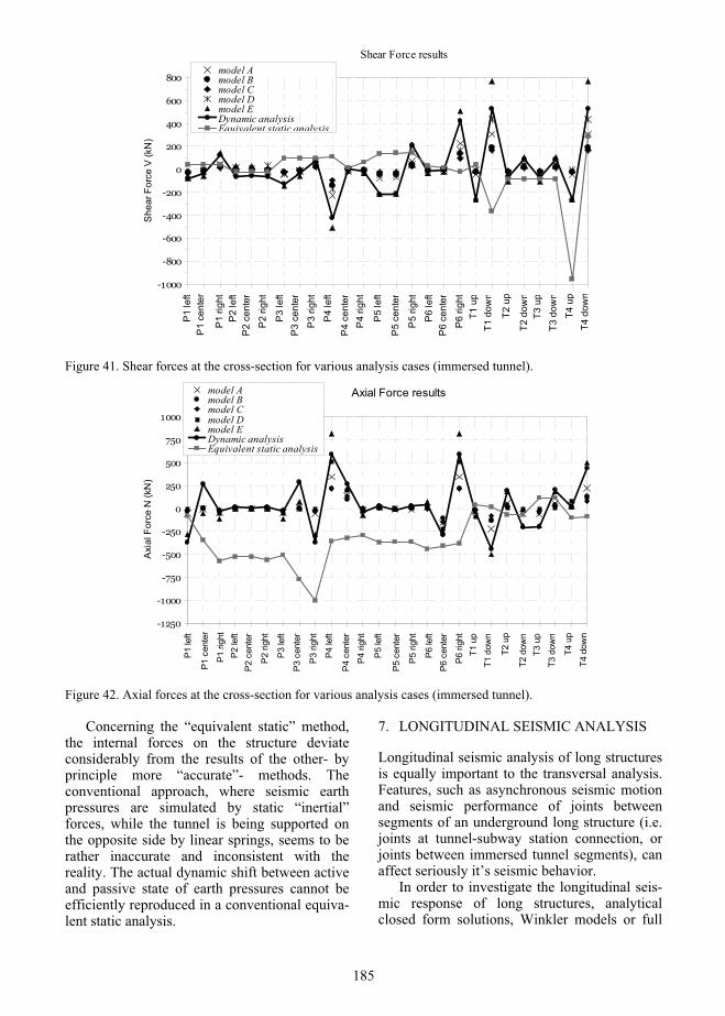
Shear Force results

-1000

-800

-600

-400

-200

0

200

400

600

800

She

ar F

orce

V (k

N)

model Amodel Bmodel Cmodel Dmodel EDynamic analysisEquivalent static analysis

P1

left

P2

left

P2

right

P2

cent

er

P3

left

P3

right

P3

cent

er

P4

left

P4

right

P4

cent

er

P5

left

P5

right

P5

cent

er

P6

left

P6

right

P6

cent

er

1 up

1 do

wn

2 up

2 do

wn

3 up

3 do

wn

4 up

4 do

wn

P1

left

P1

cent

er

P1

right

P2

left

P2

right

P2

cent

er

P3

left

P3

right

P3

cent

er

P4

left

P4

right

P4

cent

er

P5

left

P5

right

P5

cent

er

P6

left

P6

right

P6

cent

er

1 up

1 do

wn

2 up

2 do

wn

3 up

3 do

wn

4 up

4 do

wn

Figure 41. Shear forces at the cross-section for various analysis cases (immersed tunnel).

Axial Force results

-1250

-1000

-750

-500

-250

0

250

500

750

1000

Axi

al F

orce

N (k

N)

model Amodel Bmodel Cmodel Dmodel EDynamic analysisEquivalent static analysis

P1 le

ft

P1

cent

er

P2 le

ft

P2 ri

ght

P2 c

ente

r

P3 le

ft

P3 ri

ght

P3 c

ente

r

P4 le

ft

P4 ri

ght

P4 c

ente

r

P5 le

ft

P5 ri

ght

P5 c

ente

r

P6 le

ft

P6 ri

ght

P6 c

ente

r

1 up

1 do

wn

2 up

2 do

wn

3 up

3 do

wn

4 up

4 do

wn

P1 le

ft

P1

right

P2 le

ft

P2 ri

ght

P2 c

ente

r

P3 le

ft

P3 ri

ght

P3 c

ente

r

P4 le

ft

P4 ri

ght

P4 c

ente

r

P5 le

ft

P5 ri

ght

P5 c

ente

r

P6 le

ft

P6 ri

ght

P6 c

ente

r

1 up

1 do

wn

2 up

2 do

wn

3 up

3 do

wn

4 up

4 do

wn

Figure 42. Axial forces at the cross-section for various analysis cases (immersed tunnel).

Concerning the “equivalent static” method, the internal forces on the structure deviate considerably from the results of the other- by principle more “accurate”- methods. The conventional approach, where seismic earth pressures are simulated by static “inertial” forces, while the tunnel is being supported on the opposite side by linear springs, seems to be rather inaccurate and inconsistent with the reality. The actual dynamic shift between active and passive state of earth pressures cannot be efficiently reproduced in a conventional equiva-lent static analysis.

7. LONGITUDINAL SEISMIC ANALYSIS

Longitudinal seismic analysis of long structures is equally important to the transversal analysis. Features, such as asynchronous seismic motion and seismic performance of joints between segments of an underground long structure (i.e. joints at tunnel-subway station connection, or joints between immersed tunnel segments), can affect seriously it’s seismic behavior.

In order to investigate the longitudinal seis-mic response of long structures, analytical closed form solutions, Winkler models or full

185

dynamic time-history analysis utilizing contin-uum models can be used.

The first two methods are presented in this paper, as they seem to be the less demanding in terms of computational power, as the continuum model requires full 3D modelling of the tunnel and the surrounding soil, using rather elaborate 3D-solid elements, or brick elements, rendering this solution as time-consuming with no assur-ance of the output quality, due to the nature of the used finite-element type.

For the description and discussion of the dif-ferent problems encountered, we use the case of the Thessaloniki’s immersed Tunnel.

7.1. Asynchronous shaking, apparent velocity, wave-front angle.

Seismic shaking is continuously varying in terms of wave amplitude, frequency characteris-tics, time of arrival and duration. These aspects can significantly affect the response of long structures. A schematic attempt to explain the above mentioned factors is presented before in figure 11.

In order to investigate the effects of asyn-chronous motion on underground structures, shaking table experiments using a segmented utility tunnel model in laminar boxes, are under preparation, by Professor Jie LI. The results are going to be very useful for the understanding of seismic behavior of long underground structures under asynchronous motion.

The simplest source of asynchronous shak-ing lies in the angle of the wave-front to the tunnel axis. The apparent velocity of propagating waves causing different arrival times between two separate joints can be calcu-lated by the following equation.

appVV =

sin (10)

V is the wave propagation speed and the

angle, in which the seismic wave reaches the structure. Vapp is the apparent velocity later used in the analysis. Figure 43 schematically explains this effect.

tunnel

propagation direction

shear wave

Figure 43. Wave propagation angle effect on the structure’s response.

In figure 44 the time-lag effect is presented, albeit in a crude application of the asynchronous shaking theory, with no alteration to the signal. The exact time lag in the present case study is calculated by the following expression ( q. 11) and an apparent velocity ranging from 1000m/s to 2500m/s.

ii+1 i

app

Lt -t = V (11)

7.2. Immersed tunnel’s joints seismic behaviour

The intermediate rubber joints between the separate tunnel elements (figure 2) are of the utmost importance regarding the longitudinal response of the tunnel to seismic shaking. The main component of the joint is the Gina gasket, whereas the Omega seal serves only as a water-proof measure. Due to differential water-pressure inside and outside of the tunnel, the gaskets are pre-compressed to a certain extent.

ad t

ad t

ad t

ad t

t i t i+1 t i+2

Li LiLi

S1 S2 S3 S4

Figure 44. Time lag phenomenon for long structures.

186

0 20 40 60 80 100 120

Compression (mm)

2500

0

250

500

750

1000

1250

1500

1750

2000

2250

Forc

e(kN

/m)

10

0

1

2

3

4

5

6

7

8

9

Con

tact

pre

ssur

e (N

/mm

)

Force of endless seal Local contact pressure

Figure 45. Compression-deformation diagram for GINA ETS-180-220 (Daewoo 2004).

In case of seismic differential displacement they must be in position to maintain contact to the nearby concrete surface, ensuring water-tightness and usability to the tunnel. The joints display non-linear behaviour under seismic stress (figure 45), which makes their simulation difficult and crucial for the tunnel’s seismic design.

7.3. Analytical closed form solution

The basic conception is that the seismic ground deformations are not affected by the presence of the structure, being equal to the free-field ground deformations. An example of an analyti-cal solution is given by Power et al. (1996). The axial deformation can be calculated as follows:

3s saxial 2

s s

v= ×sin ×cos +r× ×cos

C C (12)

where Cs is the apparent velocity of the seismic motion, vs and as are the maximum velocity and acceleration of the seismic motion respectively,

the angle of incidence and r the half width of the structure. The joint deformation can be calculated by Equation 13.

u axial e= ×l (13)

where :le is the segment length (equal to 153m in this case).

Joints deformation estimated through this analytical method for the Thessaloniki im-mersed tunnel are presented in figures 46 and 47. It is observed that apparent velocity and the

angle are affecting significantly the joints deformations. It must be noticed that this method does not separate the deformations to tension or compression deformations.

Max joint deformation as function of Cs

0.00

0.01

0.02

0.03

0.04

0.05

0.06

0.07

0.08

500 750 1000 1250 1500 1750 2000 2250 2500Cs (m/sec)

u (m

)

Thessaloniki 78 Kozani 95

Figure 46. Variation of joint deformations with the apparent velocity Cs (analytical solution).

187

Max joint deformation as function of

0.000

0.005

0.010

0.015

0.020

0.025

0 10 20 30 40 50 60 70 80 90 (deg)

u (m

)

Thessaloniki 78Kozani 95

Figure 47. Variation of the joint deformations with the angle of incidence (analytical solution).

7.4. Winkler model

The tunnel is modeled as a linear equivalent elastic beam on dynamic Winkler foundation. The surrounding soil is modeled via linear springs calculated according to Mylonakis et. al. (2006), taking into consideration the dynamic effect of the seismic motion to the soil’s damp-ing properties (Tsinidis & Chalatis 2008). The formed model is schematically depicted in figure 49. The Winkler model constituted with the ADINA code.

The non-linear intermediate joints (Gina-gaskets) are modelled via special gap elements, functioning only in compression (compression springs). Based on figure 45, the initial joint stiffness is calculated, assuming that the joint is deformed (pre-compressed) by approximately 10 cm.

The main difficulty in modelling such a complex behaviour is the changing joint stiff-ness, with time due to the transient ground deformations imposed on the structure. The Gina gasket, however, functions only in the direction of the tunnel longitudinal axis, as the friction built between the gasket and the con-

crete surface of the tunnel is not constant, and reliable to take into consideration, when model-ling the joint’s behaviour. The control of trans-versal and vertical shear displacements is achieved through specially designed reinforced concrete shear keys (Figure 48).

shear key

shear key

Figure 48. Shear keys.

The tunnel model is loaded by displacement time-histories. They represent compression waves that mainly stress the intermediate joints; no important deformation is observed on the tunnel’s segments. Again, the Thessaloniki and Kozani time-histories, scaled to 0.35g, are being utilized.

Figure 49. Beam on dynamic Winkler foundation of the tunnel - soil system.

188

A critical parameter in this part of the study is to determine the deformations applied to the tunnel in its entire length. This is attempted by 1D site-specific response analysis, taking into consideration the spatial variability of the soil layers surrounding the tunnel. The output is displacement time-histories that are applied to each tunnel segment with a pre-determined time-lag, to incorporate the effect of the appar-ent velocity for travelling seismic waves, who may intercept the tunnel.

Another significant factor is the distance be-tween the springs used in the Winkler model, as it is a vital parameter of the problem, depending upon the frequency spectrum of interest (1-15 Hz), (figure 50).

Figure 50. Discretization of soil-springs.

Due to the complexity of the multi-parametrical problem, 6 different models have been used, for the soil, the joints and the input

motion. Model A does not include any time lag effects and it uses the steady stiffness in the joint material. Model B includes time-lag effects. Model C is similar to Model B, with the introduction of frequency-dependant damping properties. Model D is equivalent to Model B, but introducing longitudinal modifications of the soil properties along the tunnel. Model E uses a bi-linear material law for the intermediate joints, with constant soil stiffness and damping properties. Finally, Model F incorporates both changing soil properties and a bi-linear material law for the joints.

Positive values of differential joint dis-placement means “opening” of the joint, whereas negative values of differential joint displacement mean “compression” of the joint. As seen in figure 51 and Table 4, Model F gives the worst results, but the initial joint compres-sion of 10 cm is never exceeded.

In engineering practise the joints between segments are constrained through pre-stressed tendons that do not leave the joints to deform freely. Utilizing these tendons the joints and generally the tunnel’s seismic response is somehow restrained compared to the hypothesis that the joint can move freely.

8. GROUND FAILURE

Underground long structures are quite vulner-able to ground failures associated with large permanent deformations, caused by ground liquefaction, slope instability or fault move-ments.

Figure 51. Joint 6 deformations time-histories for each model variation.

189

Table 4. Maximum joint deformations for each model.

Thessaloniki 78 MODEL Joint 1 Joint 5 Joint 9

max x(m) min x(m) max x(m) min x(m) max x(m) min x(m)A 0.058 -0.056 0.011 -0.01 0.059 -0.062 B 0.07 -0.061 0.045 -0.048 0.06 -0.058 C 0.07 -0.061 0.044 -0.046 0.06 -0.058 D 0.07 -0.057 0.099 -0.088 0.088 -0.049 E 0.07 -0.052 0.043 -0.039 0.059 -0.06 F 0.07 -0.052 0.099 -0.071 0.078 -0.05

analytical solution ( =0o, Cs=1000 m/sec) 0.0095

8.1. Liquefaction

Liquefaction associated with the increase of pore water pressure and reduction of effective stresses in saturated loose cohesionless silty sands. Liquefaction phenomena can produce important longitudinal or transversal deforma-tions on underground structures, due to lateral spreading and settlements of the liquefiable soils. These deformations can act as differential quasi - static deformations on the structure. Liquefaction can also cause uplift phenomena to an immerged structure, due to important in-crease of pore water pressure.

In order to avoid the liquefaction phenom-ena, several measures can be taken. Ground improvement, increase of the dead load of the structure, drainage or soil replacement, are among the most popular countermeasures to mitigate liquefaction risk.

The mechanism of uplift of light immersed tunnels surrounding by liquefiable soils, during an earthquake, has been described by Trava-sarou & Chacko (2008). The 5.8km BART immersed metro tunnel, in the seismically active bay of San Francisco, has been extensively studied. Uplift hazard considered as the primary vulnerability reason. In order to understand better the uplift mechanism, numerical analyses and centrifuge experiments are recently per-formed (Kutter et al. (2008)). Both analyses and experiments revealed that uplift mechanism related primarily to movement of soil under the tunnel during an earthquake.

The estimated uplift seemed to be limited and so no retrofit strategy was adopted.

As mentioned before, shear displacements at joints of immersed tunnels are dealt with spe-cially designed reinforced concrete shear keys, which must resist to the differential displace-

ments between segments due to the large horizontal or vertical displacements produced by the liquefaction. Hence the capability of the shear keys, to carry out these deformations, is a crucial factor. The case of Thessaloniki im-mersed tunnel utilized here as a typical case study.

Figure 52. Centrifuge experiments to estimate uplift mechanism and numerical analysis results (Kutter et al. ,2008).

190

The tunnel segment has been modeling with a linear beam on Winkler foundation (springs). The shear keys at each tunnel extremities have been modeled taking into consideration the full shear-strength capacity of the shear keys.

Figure 53. Description of the shear key support conditions.

As the soil is supposed to be liquefied, the supporting soil-spring stiffness is reduced to 10%, compared to the initial values used in other models for longitudinal seismic analysis of the tunnel presented before. To examine their efficiency, two shear-slip scenarios are exam-ined: (a) Uniform displacement (horizontal and vertical) imposed upon the tunnel segment, while the segments next to it remain in their place, and so no displacement is permitted to the nodes of the shear key. (b) Differential displacement imposed upon the tunnel segment, due to possible movement of the opposite segment, because of lateral spreading and uplift phenomena.Table 5. Shear forces in the shear-keys due to imposed horizontal displacements d.

Horizontal displacement Case (a) Case (b)

d (m) Vsd (kN) d (m) Vsd (kN)

0.10 3630 0.10 19200 15600* 0.05 1815 0.05 9600 7800*0.01 363 0.01 1920 1560*

Table 6. Shear forces in the keys due to imposed vertical displacements d.

Vertical displacement Case (a) Case (b)

d (m) Vsd (kN) d (m) Vsd (kN)

0.10 38150 0.10 51330 13160* 0.05 19075 0.05 25665 6580*0.01 3815 0.01 5133 1316*

(* denotes the opposite key to the one with the maximum stress).

The support conditions of the shear key nodes (ux, uz, uy = 0) was selected, because the keys can be considered as “wedged” into the opposite tunnel segment as they are cast-in after the placement of the tunnel on the water basin.

It must be noted at this point, that the shear strength of the keys, not taking any reinforce-ment into consideration, is 1500 kN for the 2 horizontal keys (190x60x70 cm), and 2600 kN for the 4 vertical keys (60x165x70 cm).

These computed values of shear forces de-veloped in the keys are significantly higher than their strength. This is not being surprising due to the extreme stress considerations utilized in this analysis. Relative displacements of the order of several centimeters are a severe sce-nario. Moreover there has not been any consid-eration of the other elements of the tunnel joint, such as the Gina gasket, and the tendons, which would add to the shear strength of the joint, as a whole.

The vertical displacement scenario (uplift or settlements) appears to be the worst; hence the increased number of vertical keys compared to the horizontal shear keys. This is caused by the tunnel segment’s horizontal diaphragms, which deform less than the tunnel walls under in-plane loading, subsequently causing less stress to the shear keys.

8.2. Fault deformations-Slope instability

The general philosophy, in case of an under-ground structure crossing an active fault, is to design the structure to accommodate expected fault displacements, with probable damages, that can be repaired afterwards. In order to estimate fault displacements empirical methods, using empirical relationships for calculating the expecting displacements, can be used.

In case of an underground structure crossing above an active fault, the methodology pro-posed by Anastasopoulos et al. (2007), could be used as a guide.

In case of slope instabilities, special mitiga-tion measures to stabilize the ground should be used.

9. IMPORTANCE OF SEISMIC DESIGN COMPARED TO STATIC

After the presentation of methodologies for seismic analysis of underground structures, and the discussion of several critical points, it is interesting to reveal the importance of this

Joint restraints

Tunnel segment Shear key

191

seismic analysis, compared to static analysis. The comparison is made in terms of internal forces at the structures.

9.1. Static analysis of underground structures

Usually in static analysis of underground structures, models consist of linear frame-type elements for the structure’s cross-section and linear springs to simulate the soil support. The springs values (impedance functions) can be estimated through the expressions presented before, in equivalent static analysis method,

using properties that correspond to the soils static behaviour. Generally the static loads considered through static analysis are: • Dead loads of the structure (g1+g2).• Live loads of the structure (q). • Hydrostatic pressures and uplift force at the

structure (E1).• Geostatic pressures at the structure (E2).

The uplift force is of the utmost importance for static analysis of underground structures.

q

E1 E1E1

E2 E2

g1

Kwx

Kwz

KsxKzx

g1+g2

g1+g2+E1

g1

Figure 54. Static loads at immersed tunnel.Model A

Inverted slab (h=2.5m)

Model B

Inverted slab (h=4.0m)

Model D

Inverted slab (h=1.5m)& friction piles (d =1m)

Model C

Inverted slab (h=2.5m)& extened side walls

Figure 55. Different models for station foundation.

192

9.2. Comparison between seismic and static inertial forces at the structures

In order to reduce the calculated high stresses at the inverted slab of Venizelos metro station caused by uplift force, a parametric analysis, utilizing 4 different models for the station’s foundation, has been done (Matsoukas & Fletzouris, 2007). The different models incorpo-rated in this study are presented in figure 55. The long side diaphragms wall plays an impor-tant role for the whole stability of the station and the control of underwater flow. The friction piles beneath the foundation are proposed to reduce the uplift forces from buoyancy. Two cases have been incorporated; one using 68 friction piles and one using 36 piles for the whole station (20x100m2). Through this para-metric analysis an estimation of the participa-tion of static and seismic loads to the final response of the station, in terms of internal forces has been done.

It is observed that the static loads are actu-ally dominating the design values of the station (figures 58-59). The uplift force seems to have the biggest contribution to the final response of the station’s foundation slab, whereas the other static loads seem to dominate the station’s upper levels response. The use of friction piles has a very beneficial effect on the foundation slab internal forces, reducing considerably (almost 3 times) the bending moments.

In general in the case of the metro station studied in this paper, the contribution of the seismic forces is about 20% of the total forces. This is due to the very important contribution of the buoyancy (uplift) forces reaching almost the 50% of the total loads. In other cases the seis-mic forces are of the order of 40% of the total stresses.

In the case of the Thessaloniki immersed tunnel, again the contribution of the static loads were more crucial for the design.

B ending mo ment at inverted slab - static loads

-12000

-9000

-6000

-3000

0

3000

6000

9000

12000

0 3 6 9 12 15 18 21

L(m)

Ben

ding

mom

ent(k

Nm

)

M ode l AM ode l BM ode l CM ode l D

Figure 56. Bending moment at inverted bottom slab for static loads and different models for station foundation. Bending moment at inverted slab - seismic loads

-1500

-1000

-500

0

500

1000

1500

0 3 6 9 12 15 18 21

L( m)

Bend

ing

mom

ent (

kNm

)

Mo del AMo del BMo del CMo del D

Figure 57. Bending moment at inverted bottom slab for seismic loads and different models for station foundation

193

Loads participation to the final design results (at joints of inverted slab)

0%10%20%30%40%50%60%70%80%90%

100%

Dynamic analysis -Model C

Dynamic analysis -Model D (68 piles)

Dynamic analysis -Model D (36 piles)

Equiv. Static analysis-Model D (36 piles)

% P

artic

ipat

ion

Uplift Static loads (except uplift) Seismic loads

Loads participation to the final design results (at the middle of the inverted slab)

0%10%20%30%40%50%60%70%80%90%

100%

Dynamic analysis -Model C

Dynamic analysis -Model D (68 piles)

Dynamic analysis -Model D (36 piles)

Equiv. Static analysis-Model D (36 piles)

% P

artic

ipat

ion

Uplift Seismic loads (except uplift) Seismic loads

Loads participation to the final design results (at joints of the roof slab)

0%10%20%30%40%50%60%70%80%90%

100%

Dynamic analysis -Model C

Dynamic analysis -Model D (68 piles)

Dynamic analysis -Model D (36 piles)

Equiv. Static analysis-Model D (36 piles)

% P

artic

ipat

ion

Uplift Static loads (except uplift) Seismic loads

Figure 58. Loads participation to the final design loads: (a) at joints of inverted slab, (b) at the middle of inverted slab, (c) at joints of the roof slab (Venizelos station).

194

Loads participation to the final design results (at the middle of the roof slab)

0%10%20%30%40%50%60%70%80%90%

100%

Dynamic analysis -Model C

Dynamic analysis -Model D (68 piles)

Dynamic analysis -Model D (36 piles)

Equiv. Static analysis-Model D (36 piles)

% P

artic

ipat

ion

Uplift Static loads (except uplift) Seismic loads

Figure 59. Loads participation to the final design results at the middle of roof slab (Venizelos station).

Final bending moments (after adding static bending moments)

010002000300040005000600070008000

Ben

ding

mom

ent (

KN

m) Equivalent static analysis

Dynamic analysis

P1 T9 upP0 T7 downT1 upP2 P3 P4

Figure 60. Bending moments at the cross-section for various analysis cases, after adding and the static part of internal loads. (Venizelos station).

10. CONCLUSIONS

Considering the importance of large and ex-tended underground structures, like metro and parking stations or tunnels, their seismic design in seismically prone areas is critical parameter to their safety. The presentation of two specific cases enables the discussion of several critical points for the seismic design. - Input motions and seismic design loads must be estimated through a detailed seismic hazard analysis, considering seriously the specific site effects due to local soil conditions and geometries (stratification).

- There is no doubt that the most accurate method for seismic design of extended under-ground structures is the full dynamic time-history analysis, utilizing 2D or 3D FE models, and adequate soil and structural models. This method can successfully simulate the complex soil-structure interaction effects.

- Simplified methods on the other hand, can be used more easily, as they are less demanding in terms of computational power and can more easily be understood and controlled from engineers.

- Underground structures should be designed for imposed seismic ground deformations rather than inertial forces, as in the case of above ground structures.

- Analytical methods utilizing the racking coefficient (i.e. Wang, 1993), seems to give rather accurate results, in case of shallow underground structures like tunnels.

- Numerical FE methods based on quasi-static imposed seismic ground deformation, is an interesting approach. Soil-structure interac-tion can be directly taken into account. How-ever the main difficulty rises from the difficulty to estimate the appropriate distance of the boundaries of the model that used, as this parameter can affect seriously the results. In

195

general the distance should be kept lower that one or twice the width of the structure.

- Equivalent static analysis is proved to be conservative, for subway stations, or deep and large underground structures. In tunnels it cannot reproduce correctly the seismic phenom-ena. Issues, such as the appropriate estimation of impedance functions for underground struc-tures to model soils behaviour and SSI effects, the modelling of equivalent static forces, the estimation of seismic earth pressures or seismic shear stress at the interface of a structure, are still open and more research is deemed neces-sary.

- Longitudinal seismic analysis of long seg-mented structures is equally important to the transversal analysis, especially in case of water presence (immersed tunnels). Asynchronous motion must incorporate in the analysis proce-dure. Simple phase difference introducing a simple time lag may not be accurate enough. Special seismic design provisions must be taken in case of joints between segments, as these joints can be the most vulnerable parts of an underground structure.

- Ground failures due to liquefaction, slope instability or fault movements must be taken seriously into consideration to the seismic design of an underground structure, as they can affect the overall design of the structure.

- Finally it seems that the static loads and especially uplift, are dominating the response of an underground structure. Seismic loads are more important when uplift loads are mini-mized.

11. REFERENCES

ADINA. 2005. Automatic Dynamic Incremental Nonlinear Analysis. Theory and Modelling Guide. ADINA R&D, Inc.

AFPS/AFTES. 2001. Guidelines on Earthquake Design and Protection of Underground Struc-tures. Washington D.C.

Anastasopoulos, I., Gerolymos, N., Drosos, V., Georgarakos, T., Kourkoulis, R. & Gazetas, G. 2008. Behaviour of deep immersed tunnel under combined normal fault rupture deformation and subsequent seismic shaking. Bulletin of Earth-quake engineering, Vol.6, pp. 213–239.

Building Seismic Safety Council. 2003. FEMA 450 - NHRP Recommended Provisions for Seismic Regulations for New Buildings and Other Struc-tures. Federal Emergency Management Agency. Washington D.C.

Computers and Structures Inc. 2004. SAP 2000 -Structural Analysis Program: Linear and Nonlin-

ear Static and Dynamic Analysis and Design of Three-Dimensional Structures. Berkeley, Cali-fornia, USA.

Gazetas, G. & Dobry, R. 1984. Horizontal response of piles in layered soils. Journal of Geotechnical Engineering. ASCE, Vol. 110, No. 1.

Gazetas, G. 1991. Formulas and Charts for Imped-ances of Surface and Embedded Foundations.Journal of Geotechnical Engineering. ASCE,Vol. 117, No. 9, pp. 1363-1381.

Gerolymos, N. & Gazetas, G. 2006. Winkler Model for Lateral Response of Rigid Caisson Founda-tions in Linear Soil. Soil Dynamics and Earth-quake Engineering, Vol. 26, No. 5, pp. 347-361.

Greek Seismic Code EAK2000. 2000. Ministry of Public Works (in Greek).

Hashash, Y.M.A., Tseng, W.S., Krimotat, A. 1998. Seismic soil-structure interaction analysis for immersed tube tunnels retrofit. Geotechical Earthquake Engineering and Soil Mechanics III,ASCE Geotechnical Special publication, Vol. 75, No. 2, pp. 1380-1391.

Hashash, Y.M.A., Hook J.J., Schmidt B. & Yao J.I.-C. 2001. Seismic Design and Analysis of Under-ground Structures. Tunelling and Underground Space Technology, Vol. 16, pp. 247-293.

Hausgaard Lyngs, J. 2008. Model accuracy in aseismic design of immersed tunnel. Msc thesis, The school of civil engineering, Aalborg Univer-sity.

Iida, H., Hiroto, T., Yoshida, N.& Iwafuji, M. 1996. Damage to Daikai subway station. Soils and Foundations, Special Issue on Geotechnical As-pects of the January 17 1995 Hyogoken-Nambu Earthquake. Japanese Geotechnical Society, pp. 283-300.

Kavvadas, M. & Gazetas, G. 1993. Kinematic seismic response and bending of free-head piles in layered soil. Geotechnique, Vol. 43, No. 2, pp. 207-222.

Kawasima, K. 1999. Seismic design of underground structures in soft ground, a review. Proceedingsof the International Symposium on Tunneling in Difficult Ground Conditions. Tokyo, Japan.

Kitiyodom, P. & Matsumoto, T. 2002. A Simplified Analysis Method for Piled Raft and Pile Group Foundations with Batter Piles. InternationalJournal for Numerical and Analytical Methods in Geomechanics, Vol. 26, No. 13, pp. 1349-1369.

Kramer, S.L.1996. Geotechnical earthquake engi-neering. New Jersey: Prentice Hall Inc., Upper Saddle River.

Kuesel, T.R. 1969. Earthquake Design Criteria for Subways. J. Struct. Div., ASCE ST6, pp. 1213-1231.

Kutter, B.L., Chou, J.C. & Travasarou, T. 2008. Centrifuge testing of the seismic performance of a submerged cut and cover tunnel in liquefiable soils. 4th Geotechnical Earthquake Engineering and Soils Dynamics Conference; Proceeding of 4th GEESDC, Sacramento, May,2008.

196

Matsoukas, P. & Fletzouris V. 2007. Seismic design of metro stations - Application at the Thessalo-niki Venizelos metro station. MSc thesis, Civil Engineering Dept., Aristotle University of Thes-saloniki, Greece, (in Greek with English ab-stract).

Modaressi, H. & Foerster, E. 2000. CyberQuake: User’s manual. France: BRGM

Mononobe, N.1929. Earthquake Proof Construction of Mansonry Dams. Proceedings, World Engi-neering Conference, Vol. 9, pp. 275.

Mylonakis, G. 1995. Contribution to Static and Seismic Analysis of Piles and Pile-supported Bridge Piers. PhD Thesis. State University of New York, Buffalo, USA.

Mylonakis, G., Nikolaou, S. & Gazetas, G. 2006. Footings under seismic loading: Analysis and design issues with emphasis on bridge founda-tions. Soil Dynamics and Earthquake Engineer-ing, Vol.26, No.9, pp.824-853.

Okabe, S.1926. General Theory of Earth Pressure. Journal Japanese Society of Civil Engineers,Vol. 12, No. 1.

O'Rourke M.J & Dobry R. 1978. Spring and dashpot coefficients for machine foundations on piles. American Concrete Institute, Detroit, Publication SP-10, pp.177-198.

Penzien, J. & Wu, C. 1998. Stresses in linings of bored tunnels. Earthquake Engineering and Struc-tural Dynamics. Vol.27, pp.283-300.

Penzien, J. 2000. Seismically induced racking of tunnel linings. Earthquake Engineering and Structural Dynamics, Vol. 29,pp. 684-691.

Pitilakis, K. & Associates. 2004. Earthquake hazard assessment and determination of the design strong motion parameters along the axis of Thes-saloniki's metro line. Technical re-port.Thessaloniki.Greece.

Pitilakis, K. & Associates. 2007. Design principles of underground metro stations under earthquake loading according to the equivalent static force method. Technical report no. 2 (in Greek with English summary). Thessaloniki.Greece.

Pitilakis, K. & Associates. 2007. Seismic analysis of the underground metro station “VENIZELOS” according to (a) Imposed seismic ground defor-mations method and (b) Full dynamic analysis. Technical report no. 3 (in Greek with English summary). Thessaloniki.Greece.

Pitilakis, K., Kirtas, E., Riga, E., Matsoukas, P. & Flentzouris, V. 2008. Seismic design of under-ground structures with large dimensions. 3rd Hel-lenic National Conference of Earthquake Engi-neering and Engineering Seismology; Proceed-ings of 3rd HCEEES Conference, Athens, Greece, November 5-7, 2008 (in Greek with English ab-stract).

Pitilakis, ., Tsinidis, G., Chalatis, . & Kirtas .2009. Numerical analysis and seismic design of shallow tunnels in soft alluvial deposits. Compu-tational Methods in Structural Dynamics and

Earthquake Engineering; Proceedings of COMPDYN2009, Rhodes, Greece, June 22–24, 2009.

Power, M.S., Rosidi, D. & Kaneshiro, J. 1996. Vol.III Strawman: screening, evaluation and retrofit of tunnels. Report Draft. National Center for Earthquake Engineering Research. Buffalo, New York.

Schnabel, P.B., Lysmer, J. & Seed, H.B. 1972. SHAKE: A computer program for earthquake response analysis of horizontally layered sites. Report no. UCB/EERC-72/12, Earthquake Engi-neering Research Center, University of Califor-nia, Berkeley.

Scott, R.F. 1973. Earthquake Induced Pressures on Retaining Walls. Proceedings of the 5th World Conference on Earthquake Engineering, Vol. 2, pp. 1611-1620.

Sedarat H., Kozak A., Hashash Y.M.A., Shamsabadi A. & Krimotat A.2009. Contact interface in seismic analysis of circular tunnels. Tunnellingand Underground Space Technology, Vol. 24, No.4, pp.482-490.

St. John, C.M. & Zahrah T.F. 1987. Aseismic Design of Underground Structures. Tunneling Under-ground Space Technology, Vol. 2, No. 2, pp. 165-197.

Travasarou, T. & Chacko J. 2008. Liquefaction-induced uplift mechanism of immersed tunnel. 3rd Hellenic National Conference of Earthquake Engineering and Engineering Seismology; Pro-ceedings of 3rd HCEEES Conference, Athens, Greece, November 5-7, 2008 (in Greek with Eng-lish abstract).

Tsinidis, G. & Chalatis, A. 2008. Seismic design of immersed tunnels - Application at the Thessalo-niki immersed roadway tunnel. MSc thesis, Civil Engineering Dept., Aristotle University of Thes-saloniki, Greece, (in Greek with English ab-stract).

Veletsos, A.S. & Younan, A.H. 1994. Dynamic Soil Pressures on Rigid Vertical Walls. EarthquakeEngineering and Structural Dynamics, Vol. 23, pp. 275-301.

Wang, J.N. 1993. Seismic Design of Tunnels: A Simple State-of-the-Art Design Approach. New York: Parsons Brinckerhoff Inc.

Westergaard, H. M. 1933. Water pressures on dams during earthquakes. Transactions. A.S.C.E., Vol. 98, pp.418-433.

Zerva, A. & Zervas, V. 2002. Spatial variation of seismic ground motions: An overview. ASME,Applied Mechanics Review, Vol. 55, No.3, pp. 271-297.

Zerva, A. & Beck, J.L. 2003. Identification of parametric ground motion random fields from spatially recorded seismic data. Earthquake En-gineering Structural Dynamics, Vol. 32, pp. 771-791.

197

Geo-environmental Conditions Impact on Underground Projects

P. I. B. Queiroz Instituto Tecnologico de Aeronautica, Sao Jose dos Campos, SP, Brazil, pi@ita.br

A. Negro Bureau de Projetos e Consultoria, Sao Paulo, SP, Brazil, bureau@bureauprojetos.com.br

ABSTRACT: Megacities urban environments frequently present potential sources of soil and groundwatercontamination resulting from uncontrolled losses of contaminants to the environment, in activities such as fuelstorage, laundry services, cars maintenance and cleaning, industrial production and urban solid waste or waste-water destination.

In a continuously changing urban environment, megacities demand ever changing infrastructures and cres-cent use of underground space in an impacted subsurface. If this condition is not accounted for in due time, itmay imply in construction delays, increase in project costs and health risks to workers or users of the under-ground installation. This paper illustrates case histories of underground structures built in contaminated groundand the impact of this condition on different project stages. 1. INTRODUCTION

An underground project may be affected by environmental conditions in terms of costs, time schedule and public health of workers as well as users. Despite this, the subject is frequently neglected by owners, designers and contractors. As a result, unnecessary problems take place during construction in contaminated under-ground of megacities. A brief discussion on the subject is presented herein, to illustrate how environmental investigations prior to construc-tion can solve or can mitigate potential prob-lems, notwithstanding the additional costs of the investigations proper.

Some technical aspects of contaminants are reviewed, with emphasis on soil contamination. Next, five case histories are revisited, to illus-trate typical problems of underground projects in soils contaminated by different compounds. In an earlier review, the authors (Queiroz and Negro, 2002) focused the construction of tunnels in soils contaminated by hydrocarbons only. Finally, some conclusions are presented.

2. CHARACTERISTICS OF COMMON CONTAMINANTS

2.1. Hazardous Substances

According to LaGrega, Buckingham and Evans (2001), there are several difficulties in defining hazardous substances, as it involves distinct

areas of knowledge, like environmental, health and materials sciences. The definition proposed by Batstone, Smith Jr. & Wilson (1989) is favoured. They define hazardous wastes as wastes other than radioactive and infectious materials, which, by reason of their chemical activity or particular nature such as toxic, explosive, corrosive or any other detrimental characteristics, may cause, or may likely cause, danger to health or to the environment, either alone or when coming into contact with some other waste.

With respect to toxicity, a substance might present two dominant characteristics, being either a non-carcinogenic toxic substance or a carcinogenic substance. The essential difference between both is that, due to the insidious character of cancer, a carcinogenic substance is treated as not possessing a safe dose, while a non-carcinogenic substance may present a level of exposure to which no adverse effect is expected to take place.

Explosive substances are hazardous due to risk of related fire or explosion. As non-carcinogenic substances, they possess a limit concentration, below which no danger is ex-pected; this concentration in air is called LowerExplosive Limit or LEL.

Corrosive substances are those that may cor-rode materials used for temporary or permanent lining of underground openings such as con-crete, steel, iron, wood or plastics.

Reactive substances may become toxic, ex-

198

plosive or corrosive by reacting with other substances or by degradation in the environ-ment.

Although biological and radioactive wastes may impose hazards like those described, they are usually regulated by specific legislation in most countries and will not be dealt herein.

2.2. Classes of contaminants

For management purposes, contaminants may be classified by two approaches: either by laboratory tests or by official specific contami-nants lists. Laboratory tests verify contaminants characteristics such as corrosiveness, ignita-bility, explosiveness, reactivity and toxicity. Specific contaminants lists usually classify contaminants according to their chemical composition. The second approach is usually used to determine groundwater or soil treat-ments and to assess the most likely characteris-tics provided by the first approach. In the following, three main classes of contaminants usually found in megacities are presented, together with some of their main characteristics. For further details the reader should refer to specific literature (LaGrega et al., op. cit. and Watts, 1998).

Hydrocarbons may be regarded as the main contaminant of megacities underground. Usu-ally they derive from spills from underground storage tanks fuels of gas stations. All hydro-carbons are ignitable, although only the gaseous are usually explosive. Nevertheless, gasoline and diesel oil may have methane in concentra-tion high enough to be a matter of concern. Most petroleum hydrocarbons are not toxic to humans, nor corrosive, although aromatic hydrocarbons (BTEX – benzene, toluene, ethylene and xylene and PAH – polycyclic aromatic hydrocarbons) are usually toxic, and some of them are carcinogenic. The latter are found in small quantities in fuels, but are of great concern regarding the environmental conditions. Gaseous hydrocarbons like methane, ethane, butane and propane may also occur naturally in peat from bogs and marshes. They are always explosive, but not toxic to man: they can simply be asphyxiating, as their presence in the air may reduce oxygen concentration.

Halogenated compounds belong to another class of contaminant frequently found in mega-cities. Their origin is credited only to human activities, usually related to spills from indus-trial processes (chlorinated hydrocarbons are

largely used as degreasers and cleaners) or spills from old laundries in which PCE (tetrachloro-ethylene) was used for dry washing. PCBs (polychlorinated biphenyls) were used in capacitors and electric transformers. They are toxic for causing depression of central nervous system, and because some of them are carcino-genic.

Metallic elements are naturally found in soils, particularly in tropical soils, and have geochemical origin. However, several industrial and commercial processes use metallic com-pounds that may impact on the ground if an uncontrolled spill happens. Heavy metals like lead and mercury are largely used in batteries, but only recently they were treated as hazardous substances. Since then, they are not allowed to be disposed in municipal landfills. Heavy metals may cause damage to liver, kidney and are involved in a series of psychiatric diseases. The classification of a metallic element is difficult because its hazardous characteristics depend largely on the chemical composition and on the valence associated to the metal. As an example, iron may occur in nature as oxides, all of them chemically stable minerals; on the other hand, pyrite, an iron sulphide (FeS2), is a very unstable compound, which reacts with oxygen and water, producing an acid effluent, which is toxic, corrosive and reactive.

3. CONSTRUCTION MANAGEMENT IN CONTAMINED SITES

3.1. Importance of early detection

Ideally, managing a contaminated site requires complete identification of the contaminants, full knowledge of the spatial distribution of the contamination, as well as of the extent of the flow and transport of contaminants under-ground. This condition fulfilled allows the best choices for management decisions. Eventually, costs related to handling certain environmental conditions may turn an underground project virtually unfeasible. Although environmental investigations may also involve high costs, previous knowledge of environmental condi-tions usually lead to total cost savings due to avoidance of duplicated work and best choices for construction maintenance.

Environmental conditions usually affect all stages of an underground project, and late detection of soil contamination may lead to

199

additional works and loss of construction materials.• Detection of contamination after complete

site investigations may lead to a new tunnel line position, which involves unplanned additional geotechnical investigations.

• Detection after conceiving the lining system, may involve new conception of the lining, like adoption of a “sacrifice thick-ness” for it, ensuring the required lining lifetime or a new waterproof system.

• Detection after lining design is completed may lead to new calculations, revision of drawings and specifications.

• Detection of contamination after construc-tion is completed, especially during opera-tion of the tunnel, may require at least lin-ing maintenance if not replacement. More-over, this may lead to additional costs re-lated to possible loss of construction mate-rial apart from costs in legal disputes be-tween environmental agencies, state prose-cuting officers, owners, designers and con-tractors.

The risks involved in a delayed environ-mental assessment of an underground project are large enough to make compulsory the requirement of an earlier environmental investi-gation in geotechnical baseline reports. Despite this, good guidelines for tunnel projects avail-able (for example, ASCE, 2007 and FHWA, 2009) furnish incomplete and unsystematic coverage of soil contamination investigation and management of the consequences of con-taminations in underground projects.

3.2. Management of Contamination

The main components of the management of an underground project in a contaminated site are related to Investigation, Remediation and Monitoring of the contamination.

Investigation - Although ASTM Standards (ASTM 1997a and ASTM 1997b) were created as guidelines for real estate investigations, their working approach is totally adequate for inves-tigating a contaminated underground. ASTM (1997a) describes a “Phase I Environmental Site Assessment Process”. Putting it in simple way, it describes recommendations for records review, site reconnaissance and interviews only. This initial investigation should furnish data to encourage or not a “Phase II Site Assessment”, which may involve sampling of soil and groundwater for chemical analysis, enabling

directed investigations for specific strata, specific sampling locations and specific series of chemical analyses, answering questions or doubts raised in the Phase I assessment. While Phase I has specific scope with bounded time and costs, Phase II may be as large and as expensive as the cost-benefit of taking risk allows. It is important that, under this approach, an investigation might stop without conclusive results when it takes unreasonable time or costs.

Remediation may be considered one of the most difficult subjects of the management of a contaminated site. Several text books (for example LaGrega. Buckingham & Evans, 2001 and Sharma & Reddy, 2004) and some classic papers (for instance, Shackelford & Jefferis, 2000) are written about the subject and none of them may be considered as definitive. The manager in charge must have clear understand-ing of the main concepts of remediation, in order to assess the adequacy of one or other remediation technique, which should be chosen by an expert or by a board of consultants. It is important to emphasize that the cleanup cost of a contaminated site may be up to ten times more expensive than the cost of the land itself. Nowadays, there are several cleanup techniques, and the manager should decide between high costs of fast remediation techniques (such as in situ thermal treatment or disposal of contami-nated soil in hazardous waste landfills) and the long time of cost-effective techniques (biore-mediation and monitoring natural attenuation, for instance).

Monitoring contaminated sites is another difficult subject. The distribution of samples in space and time is a complex subject and the cost-benefit involved in the conception of a monitoring plan is related to the acceptance of the risk in neglecting a small spot of contamina-tion versus the cost of a large monitoring campaign, with conflicting results that are hard to interpret. Statistics of results are also com-plex to interpret, as multi-modal distributions and outliers are a commonplace in field moni-toring programs of the sort. Lower-cost field instruments like photo-ionization detectors (PID) and infrared detectors must be calibrated to a certain mixture of gases (measured by gas chromatography), to give some idea of the concentration of a specific hazardous substance. Corrosiveness of groundwater may be assessed by pH and pE, though knowledge of the ions in groundwater should also be granted by chroma-tographic analysis.

200

4. CASE HISTORIES

4.1. Caracas Metro

The construction of Line 1 of Caracas Metro started in 1978 (Centeno & Centeno, 1998), with a Robbins open face TBM (Tunnel Boring Machine). It was composed by twin circular tunnels with external diameter of 5.5m, lined by a six segments plus a closing wedge ring made of reinforced concrete with strength of 50 MPa. The joints were designed to be watertight with two rubber gaskets.

About 90% of Metro tunnels passed through alluvial valleys or colluvial soils, while the other 10% passed through soft fractured rocks. Few months after construction started, a consid-erable inflow of gasoline water mixture hap-pened through the tunnel face in the western part of the city. Construction was halted for more than a hundred working days to imple-ment safeguards for workers health and to ensure safety of surrounding structures in the event of an explosion.

Open face TBM lacks ability to control wa-ter inflow through the face, aggravating risks in the case contamination exists. For this reason and also for improved settlement control, a different TBM technology was adopted for Line 2. An unsophisticated Lovat closed face EPB shield, with adjustable face opening was intro-duced combined with improved ventilation system and continuous gas monitoring. These procedures reduced the risk of explosions which in fact happened in few occasions. Some of these were related to the presence of methane leaks from an old sewer in the older part of the city. Improved ventilation reduced the chronic exposure of workers to the gases and the control of soil excavation rate at the face improved controlling the contaminants concentration inflow into the tunnel.

Despite all efforts, three major inflows of gasoline were experienced during tunnelling in Caracas from 1990 to 1995. The latest took place with the Metro system in operation, with gasoline leaking into the tunnel through deterio-rated rubber gaskets between lining segments. Gasoline rich groundwater corroded gaskets, allowing major inflow into the tunnel. This caused trains stoppage for six days in a stretch of the metro line, forcing emergency program of bus services. Costs of remediation ranged at level of hundreds thousand US dollars. The

incident pointed towards the need of using gasoline resistant gasket materials for such conditions.

Local hydrogeological features led to accu-mulation of gasoline in certain parts of Caracas subsoil. Old buried river valleys, old debris flow materials and main faults are found in Caracas all representing zones of higher permeability, where gasoline leak found its way through. Tunnelling in Caracas usually takes place few metres below groundwater level. If construction procedures allow the depression of the water surface, gasoline, which is a light non-aqueous phase liquid (LNAPL) may enter the tunnel, as it happened in many locations.

During tunnels excavation, the concentration of hydrocarbons in the air had to be kept below human toxicity and explosiveness levels. When the health limit was reached, excavation stopped and ventilation system was activated. When explosiveness limit was reached, TBM advance had to stop because its operation causes sparks that may ignite vapours in the air. These inter-ruptions had significant impact on construction schedule and costs. As a consequence, the contractor claimed an additional cost of US$ 1308.00 per metre of tunnel and a final settle-ment of US$ 790.90 per metre was met (1995 dollar), which represented an increase of almost 15% to the initial budget of the project.

The main reason for the widespread pres-ence of gasoline in Caracas subsoil is related to underground storage tanks with riveted joints and rubber seals. Seal deterioration and corro-sion of tanks or connecting pipes led to gasoline leakage. It should be noted that modern recom-mendations for underground storage, enforces its installation inside a concrete box, in order to allow inspection and maintenance, avoiding the direct contact of tanks with soil, thus reducing risk of corrosion by aggressive soils or by fault currents.

4.2. Madrid Metro

Madrid Metro underground Line 8 was re-viewed by Arnaiz et al. (2000). It includes cut-and-cover stations and double track tunnels 160km long, with 9.38m of excavated diameter. Reference data available from the Madrid-Barajas International Airport Authority prior to site investigation indicated that a small area to be crossed by that line was contaminated by kerosene that had leaked from storage tanks. Due to the short time available for the under-

201

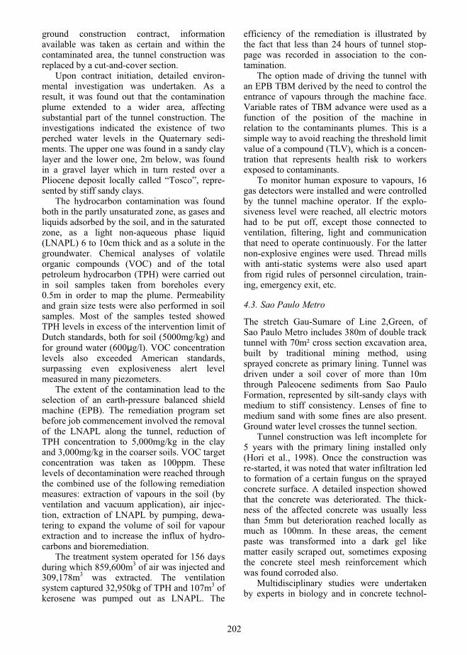
ground construction contract, information available was taken as certain and within the contaminated area, the tunnel construction was replaced by a cut-and-cover section.

Upon contract initiation, detailed environ-mental investigation was undertaken. As a result, it was found out that the contamination plume extended to a wider area, affecting substantial part of the tunnel construction. The investigations indicated the existence of two perched water levels in the Quaternary sedi-ments. The upper one was found in a sandy clay layer and the lower one, 2m below, was found in a gravel layer which in turn rested over a Pliocene deposit locally called “Tosco”, repre-sented by stiff sandy clays.

The hydrocarbon contamination was found both in the partly unsaturated zone, as gases and liquids adsorbed by the soil, and in the saturated zone, as a light non-aqueous phase liquid (LNAPL) 6 to 10cm thick and as a solute in the groundwater. Chemical analyses of volatile organic compounds (VOC) and of the total petroleum hydrocarbon (TPH) were carried out in soil samples taken from boreholes every 0.5m in order to map the plume. Permeability and grain size tests were also performed in soil samples. Most of the samples tested showed TPH levels in excess of the intervention limit of Dutch standards, both for soil (5000mg/kg) and for ground water (600μg/l). VOC concentration levels also exceeded American standards, surpassing even explosiveness alert level measured in many piezometers.

The extent of the contamination lead to the selection of an earth-pressure balanced shield machine (EPB). The remediation program set before job commencement involved the removal of the LNAPL along the tunnel, reduction of TPH concentration to 5,000mg/kg in the clay and 3,000mg/kg in the coarser soils. VOC target concentration was taken as 100ppm. These levels of decontamination were reached through the combined use of the following remediation measures: extraction of vapours in the soil (by ventilation and vacuum application), air injec-tion, extraction of LNAPL by pumping, dewa-tering to expand the volume of soil for vapour extraction and to increase the influx of hydro-carbons and bioremediation.

The treatment system operated for 156 days during which 859,600m3 of air was injected and 309,178m3 was extracted. The ventilation system captured 32,950kg of TPH and 107m3 of kerosene was pumped out as LNAPL. The

efficiency of the remediation is illustrated by the fact that less than 24 hours of tunnel stop-page was recorded in association to the con-tamination.

The option made of driving the tunnel with an EPB TBM derived by the need to control the entrance of vapours through the machine face. Variable rates of TBM advance were used as a function of the position of the machine in relation to the contaminants plumes. This is a simple way to avoid reaching the threshold limit value of a compound (TLV), which is a concen-tration that represents health risk to workers exposed to contaminants.

To monitor human exposure to vapours, 16 gas detectors were installed and were controlled by the tunnel machine operator. If the explo-siveness level were reached, all electric motors had to be put off, except those connected to ventilation, filtering, light and communication that need to operate continuously. For the latter non-explosive engines were used. Thread mills with anti-static systems were also used apart from rigid rules of personnel circulation, train-ing, emergency exit, etc.

4.3. Sao Paulo Metro

The stretch Gau-Sumare of Line 2,Green, of Sao Paulo Metro includes 380m of double track tunnel with 70m² cross section excavation area, built by traditional mining method, using sprayed concrete as primary lining. Tunnel was driven under a soil cover of more than 10m through Paleocene sediments from Sao Paulo Formation, represented by silt-sandy clays with medium to stiff consistency. Lenses of fine to medium sand with some fines are also present. Ground water level crosses the tunnel section.

Tunnel construction was left incomplete for 5 years with the primary lining installed only (Hori et al., 1998). Once the construction was re-started, it was noted that water infiltration led to formation of a certain fungus on the sprayed concrete surface. A detailed inspection showed that the concrete was deteriorated. The thick-ness of the affected concrete was usually less than 5mm but deterioration reached locally as much as 100mm. In these areas, the cement paste was transformed into a dark gel like matter easily scraped out, sometimes exposing the concrete steel mesh reinforcement which was found corroded also.

Multidisciplinary studies were undertaken by experts in biology and in concrete technol-

202

ogy (Shirakawa et al., 1997). These studies have shown that the noticed structural decay of the primary lining resulted from the formation of a specific environment, in which water, nutrients and temperature interplayed. The nutrient was identified as gasoline that leaked from a gas station tank in the vicinities. Aerobic Thioba-cilus bacteria digest gasoline and combined with bacteria that reduce sulphates, are able to transform inorganic compounds with sulphur into sulphuric acid which, on the other hand, corrodes the concrete. This is referred to as the bio-deterioration of the concrete in which bacteria have a central role. Though some of these bacteria are unable to live within the concrete mass, they are able to create polysac-charide protecting films called bio films thatallow their development on the inner surface of the tunnel lining.

Traditional remediation processes for the case (pump-and-treat or bio remediation) were understood as too expensive. A simpler ap-proach was favoured, combining the removal of the affected concrete, the reconstitution of the primary lining and the application of a water proof mortar layer, admixed with silica fume and an acrilate polymer resistant to dissolution by hydrocarbons. This was followed by the application of the secondary sprayed concrete lining. Some 150m of tunnel was subjected to this procedure, based on the extent of the contaminant plume defined. A monitoring natural attenuation approach, as defined by Bedient el al. (1999), was also implemented, with periodic measurement of VOC concentra-tion in the air within the tunnel and periodic extraction of concrete samples from the lining, to assess bio deterioration, during the entire time life of this structure. Observations made over the last 10 years have indicated the effec-tiveness of the approach chosen.

Sao Paulo Metro had also other recent cases of construction in contaminated soils. During Line 2 extension, near Vila Mariana district, it was noticed a smell of gasoline inside the extended mined tunnel (Rocha, 2010). At the same time, it was detected leakage from tanks of two gas stations. It was noted that gasoline was dissolving the asphalt coating that provided waterproofing to the existing cut-and-cover tunnel. The Metro Company decided to pump the free non-aqueous liquid phase, to stop leakage into the tunnel. A flotation chamber was used to separate free phase from groundwa-ter. This was simply a solution to the problem

of tunnel construction, which was the Metro concern, and not a remediation of the contami-nated soil and groundwater. Indeed the solution provided satisfactory result regarding tunnel construction performance. Since then, Sao Paulo Metro decided to stop using asphalt to provide tunnel waterproofing, as gasoline contamination became a commonplace in megacities.

Another case of gasoline contamination was detected before construction of Sao Paulo Metro Line 4 more recently (Rocha, 2010). In this case, both gasoline tank and the contamination plume coincided exactly at the location where a double cylinder shaft of Paulista Station was to be excavated. The tank owner and responsible for the contamination, Petrobras, requested three months to start soil and groundwater remediation. As construction was beginning, Metro Co. itself decided to provide the remedia-tion. Groundwater investigation indicated the presence of perched water table in sand layers between clayey soils. Specific field pumping tests showed that, during construction, pumping in the lower water table would not affect the upper water table, which was the one contami-nated. Hence, Metro Co. decided to keep the tunnel excavation program by lowering the lower water table and isolating the contami-nated soil with slurry diaphragm plastic walls, which, due to interfacial tension in the bentonite fraction, operates as an efficient barrier to the NAPL. The contaminated soil excavated during shaft construction was then removed and incinerated. Waterproofing for tunnel and shaft were provided by PVC membranes, which is less affected by gasoline than asphalt. Although expensive, this solution proved to be efficient, as neither smell nor stain were noticed in the secondary lining later on.

4.4. London Metro

The railway twin tunnels that are now part of the City Branch of the Northern Line were constructed between 1899 and 1901 (Bracegir-dle et al. 1996). The tunnels are located at about 25m below surface, level of the interface between the London Clay and the underlying Woolwich and Reading Beds, and passes through lenses of sand, as at Old Street Station. Between 1922 and 1924, the tunnels were expanded from 3.2 to 3.56m, by insertion of four new ordinary castings and a new tapered key, producing a non-circular section.

203

By the end of 1962, 20 segments of the tun-nel were found to be cracked and water that seeped into the tunnel was found to be highly acidic (pH 2 to 3). Seepage of water and chemi-cal deposits had been noted for some 17 years previously, but had not been considered of great significance.

Although earlier discussions on the possibil-ity of contamination took place, deeper studies concluded that the cause of the acid drainage was formation of pyrite in the sand lens, which was oxidized by the presence of oxygen and certain bacteria that occur in the soil mass. The oxygen entered to the soil mass by the tunnel joints that just could not be impermeable to gases. The acid liquor generated in soil attacked both the steel segments of the lining and the contact grout. The grout expansion, estimated to be up to the order of 30%, caused the lining to bend.

An instrumentation program was carried in the tunnel, including installation of vibrating wire strain gauges in 1970, and horizontal extensometers at axis level. The instrumentation indicated that continuous convergence of the horizontal axis of the tunnel, at a rate of 3-4mm per decade. Some segments were also removed from tunnel lining for load tests in laboratory. They were loaded to failure, which occurred with an applied bending moment of 33.2MN.mm, while instrumentation indicated that removal of the lining segment caused relief of a bending moment of 28.3MN.mm. Instru-mentation also indicated that ring segments were loaded by a hoop stress of about 1.8N/mm², equivalent to a uniform loading of 1.6m of soil.

Finite Element analyses indicated that the bending moments which caused lining damages were associated to the grout expansion near to tunnel, caused by sulphate attack to the lime of the grouting.

4.5. New York Metro

According to Munfah & Butler (2006), East Side Access Project (ESA) will connect the Long Island Rail Road (LIRR) with Grand Central Terminal (GCT), improving the daily commute to over 300,000 people. The project was budgeted to cost US$ 6.3 Billion and is to be completed by the year of 2012.

Within ESA project, the Queens segment extends about 1800m from the existing bulk-head of the 63rd Street line near to 29th Street

and 41st Avenue, across Northern Boulevard and connects to LIRR’s Main Line and the Port Washington Branch. It starts with a cut and cover section adjacent to an existing tunnel bellmouth structure and extends under a five-track subway box and a two-tracks elevated transit line. The railroad tunnels will have an excavated diameter of 6.55m. There will be both Sequential Excavation Method (NATM) and TBM excavations, depending on geotechni-cal and environmental constraints. Ground conditions vary from gneissic and schist rocks to manmade fills, passing through glacial deposits.

Both previous investigations and project re-lated investigations indicated that tunnels will pass through or nearby existing soil and groundwater contaminated sites in Sunnyside Yard, the existing Yard A and nearby areas. The New York State Department of Environmental Conservation (NYSDEC) issued a Record of Decision (RoD) with a list of contaminants in soil and groundwater at Sunnyside Yard, which included lead, PCB, polycyclic aromatic hydro-carbons and chlorinated volatile organic com-pounds. The RoD also focused on specific contaminants which should be monitored, properly managed or remediated prior or during any construction in the area.

Special measures were taken during project phase, including assessment of potential of migration of plumes during construction, prevention of migration and monitoring pro-grams and remediation measures for the case of abnormal migration of plumes.

Within these measures, project decided to construct a 760mm thick slurry wall keyed in rock, in order to prevent migration due to water draining to the excavations. Tunnel construction method near the contaminated area was speci-fied to be by a TBM with earth pressure balance (as discussed in the case of Caracas Metro), with segmented bolted and gasketed lining.

Moreover, the designer had to prove to NYSDEC and to the owner of the terrain (Amtrak, which will have to remediate con-taminated area) that construction will not hinder future remediation activities nor preclude further site improvements by the site owner. So, project avoided excessive groundwater draw-down, which could cause contaminant plumes to migrate. Groundwater drained during excava-tion will be sampled, treated and disposed properly. Water from cut and cover excavation will be collected to an oil-water separation

204

system before disposal. Ground water treatment system will be equipped with settling tanks, oil-water separation, flocculation, filtration sys-tems, together with carbon adsorption or dis-solved air flotation systems, necessary to meet environmental discharge limits.

5. CONCLUDING REMARKS

An overview on geo-environmental conditions impact on underground projects was presented. Theoretical aspects were briefly discussed, in an attempt to provide a current state-of-the-practice in management of tunnel construction in con-taminated sites. Some case histories were revisited to illustrate some actual problems and solutions adopted in certain projects. Fuel contaminations predominate in the cases studied herein. Broadly speaking, early detection of contaminations, in present time, seems to occur in more structured projects. Environmental investigations were always directed to minimize uncertainties during construction. It is believed that a geotechnical baseline report prepared before design and construction should be supplemented by an environmental baseline investigation, in parallel to the former, as a minimum requirement for future underground projects in megacities.

6. REFERENCES

Arnaiz, M., Melis, M., Mendaña, F., Oteo, C. & Sola, P. 2000. EPB tunnelling on ground contaminated by kerosene in the new line 8 of the Madrid Metro extension project, In AITES-ITA World Tunnel Congress, pp.21-28, Durban: South Afri-can Institute of Mining and Metallurgy.

ASCE. (American Society for Civil Engineers) 2007. Geotechnical Baseline Reports for Construction: Suggested Guidelines, 62 p. Reston: ASCE.

ASTM (American Society for Testing and Materials) 1997a. E1527 – Environmental Site Assess-ments: Phase I Environmental Site Assessment Process. West Conshohocken: ASTM.

ASTM (American Society for Testing and Materials) 1997b. E1903 – Environmental Site Assess-ments: Phase II Environmental Site Assessment Process. West Conshohocken: ASTM.

Batstone, R., Smith Jr., J.E. & Wilson, D. 1989. The safe disposal of hazardous wastes. World Bank Technical Paper Number 93, vols. 1-3. Washing-ton: World Bank.

Bracegirdle, A., Jefferis, S. A., Tedd, P., Crammond, N.J., Chudleigh, I. & Burgess, N. 1996. The in-vestigation of acid generation within the Wool-

rich and Reading Beds at Old Street and its effect on tunnel linings, In Mair & Taylor (eds.), Geo-technical Aspects of Underground Construction in Soft Ground, pp. 653-658, Rotterdam: Balkema.

Bedient, P. B., Rifai, H. S. and Newell, C. J. 1999. Groundwater Contamination-Transport and Remediation,Prentice-Hall, Upper Saddle River.

Centeno W., R. R. and Centeno P., F.A. 1998: Tunneling through gasoline contamination; the Caracas Metro experience, In Lambrechts, Hwang and Urzua (eds.), Big Digs Around the World – Proceed. of Sessions of Geo-Congress’98, pp.189-210. Reston: ASCE

FWHA (U.S. Federal Highway Administration) 2009. Technical Manual for Design and Con-struction of Road Tunnel, Technical Report Number FHWA-NHI-09-010, 694 p. Washington D.C.: FHWA.

Hori, K., Palermo, G. and Rocha, H. 1998. Design guidelines in case of long term interruption in NATM tunnelling, In Negro and Ferreira (eds.) Tunnels and Metropolises, World Tunnel Con-gress (Sao Paulo), Rotterdam: Balkema.

LaGrega, M.D., Buckingham, P.L. & Evans, J.C. 2001. Hazardous Waste Management. 2nd ed. 1202 p. Boston:McGraw-Hill.

Munfah, N.A. & Butler, J. 2006. Control of contami-nated groundwater during tunnel excavation, in Bakker, Bezuijen, Broere and Kwast (eds.), Geo-technical Aspects of Underground Construction in Soft Ground, pp. 265-270. London: Taylor & Francis Group.

Queiroz, P.I.B. & Negro, A. 2002. Tunnel Construc-tion in Soils Contaminated by Hydrocarbons (in Portuguese), In Hori, Knapp and Cordeiro (orgs.) Proceedings of the 4th Symp. on Urban Tunnels (TURB 2002), pp.27-39, Sao Paulo: ABGE/CBT/IBRACON.

Rocha, H. C. 2010. Personal communication.Shackelford, C.D. & Jefferis, S.A. 2000. Geoenvi-

ronmental engineering for in situ remediation, In International Conference on Geotechnical and Geoenvironmental Engineering (GeoEng2000),Melbourne, Vol. 1, 121-185.Australia, Nov. 19-24, Lancaster: Technomic Publ. Co.

Sharma, H. D. & Reddy, K. R. 2004. Geoenviron-mental engineering: site remediation, waste con-tainment, and emerging waste management tech-nologies, 968 p. Hoboken: John Wiley & Sons.

Shirakawa, M., John, V., Cincotto, M.A. & Gambale, W. 1998. The bio-deterioration of construction materials (in Portuguese), Téchne, no 33 (May/April) pp. 36–39.

Shirakawa, M., Cincotto, M.A. & Rzyski. B.M. 1997. The Bio-deterioration of concrete: a multidisci-plinary study (in Portuguese), IBRACON Journal,(July/August) pp. 16–21.

Watts, R.J. 1998. Hazardous Wastes: Sources, Path-ways, Receptors, 784 p. New York: John Wiley.

205

Numerical analysis of deep excavations and tunnels in accordancewith EC7 design approaches

H.F. Schweiger Computational Geotechnics Group, Institute for Soil Mechanics and Foundation Engineering Graz University of Technology, Austria

ABSTRACT: Numerical methods are well established in practical geotechnical engineering to assess the deformation behaviour of deep excavations and tunnels. However, it becomes more and more common to use results from numerical analysis for ultimate limit state design (ULS) and in these cases compatibility withstandards and codes of practice, valid in the respective country, has to be fulfilled. This is by no means straight-forward and in this paper design approaches defined in EC7 will be applied to deep excavation and tunnelling problems highlighting some key aspects. Secondly the importance of the appropriate choice of a constitutive model for the soil is pointed out by comparing results obtained from different soil models.

1. INTRODUCTION

Numerical analyses are widely used in practical geotechnical engineering to assess the deforma-tion behaviour of deep excavations and tunnels, in particular when the influence on existing buildings has to be assessed or the interaction between different structures has to be taken into account. In addition a tendency can be ob-served, namely to use results from numerical analysis as basis for the design which is of course only possible if compatibility with relevant standards and codes of practice, valid in the respective country, is guaranteed. In general this is a well established procedure when employing conventional design calcula-tions based e.g. on limit equilibrium methods, but there are no clear guidelines how this can be achieved in the context of numerical modelling. Therefore literature on this subject is not ex-hausting, but some discussion on the compati-bility of EC7 design approaches with numerical analyses can be found in e.g. Bauduin et al. (2000), Schweiger (2005, 2009), Simpson (2000, 2007), Walter (2006).

An important aspect in any numerical analy-sis in geotechnics, no matter whether ULS (ultimate limit state) or SLS (serviceability limit state) is considered, is the appropriate choice of the constitutive model for the soil, which has a direct consequence for the design because different constitutive models will lead to differ-ent structural forces. Both of these aspects are

addressed in this paper by means of benchmark examples, i.e. the influence of the choice of the constitiutive model on calculated displacements and structural forces is investigated first and then consequences for the design, employing different design approaches, are discussed. Finally, results form the analysis of two real case histories, a station tunnel in soil and a deep excavation in sand, is presented in order to address specific problems relevant in practice.

It follows from these examples that the choice of the constitutive model and the design approach has an influence on the results, but given the uncertainties inherent in any analysis in geotechnical engineering the differences due to the different EC7 design approaches seem acceptable provided a suitable constitutive model is employed.

2. EC7 DESIGN APPROACHES

In Eurocode7 the partial factor of safety concept replaces the global factor of safety concept employed until now. Three different design approaches DA1 to DA3 have been specified which differ in the application of the partial factors of safety on actions, soil properties and resistances. They are summarized in Tables 1 and 2 for all three approaches. It is noted that two separate analyses are required for design approach 1. The problem when using numerical methods is immediately obvious because DA1/1 and DA2 require permanent unfavourable

206

actions to be factored by a partial factor of safety, e.g. the earth pressures acting on struc-tural elements such as retaining walls and tunnel linings. This is of course not possible because in numerical analyses the earth pressure is a result of the analysis and not an input. However, EC7 allows for an alternative, namely of applying the partial factor on the effect of the action instead on the actions itself, e.g. bending mo-ments or strut forces. This is commonly referred to as DA2* and throughout this paper DA2 is understood in the form of DA2*. Now numeri-cal methods can be readily applied because the analysis is performed with characteristic loads and characteristic parameters introducing the relevant partial factors at the end of the analysis. It is beyond the scope of this contribution to elaborate on the advantages and disadvantages of each of the approaches in detail but some discussion can be found e.g. in Simpson (2000, 2007), Bauduin et al. (2003) and Schweiger (2005). However the differences in results depending on the design approach employed will be shown whereas special emphasis will be put on the choice of the constitutive model.

Table 1. EC7 partial factors for actions

DesignApproach

Permanent unfavourable Variable

DA1/1 1.35 1.50 DA1/2 1.00 1.30 DA2 1.35 1.50 DA3 1.00 1.30

Table 2. EC7 partial factors for soil strength proper-ties and resistances

DesignApproach tan ' c' Undrained

shear strengthPassive

resistanceDA1/1 1.00 1.00 1.00 1.00 DA1/2 1.25 1.25 1.40 1.00 DA2 1.00 1.00 1.00 1.40 DA3 1.25 1.25 1.40 1.00

3. DEEP EXCAVATION BENCHMARKS

First, two deep excavation benchmarks are discussed. Their general layout and the con-struction sequence are similar but ground conditions are different. A soft clay layer is assumed in the first example whereas an over-

consolidated clay is considered in the second example. Different constitutive models are employed for modelling the mechanical behav-iour of the soil, the simple Mohr-Coulomb failure criterion (MC), the so called Hardening Soil model (HS), the Hardening Soil Small model (HSS) and the Soft Soil model (SS). All models are standard models of the finite ele-ment code Plaxis (Brinkgreve et al. 2006), which has been used for all analyses presented in this paper. The Hardening Soil model is an elastic-plastic model featuring deviatoric and volumetric yield surfaces (doubel hardening model), the HSS model is the extension to account for small strain stiffness effects (Benz 2007) and the Soft Soil model is a modification of the well known Modified-Cam-Clay model incorporating a Mohr-Coulomb failure criterion and allowing for a modification of the volumet-ric yield surface in order to improve K0-predictions. Parameters are based on experi-mental data and experience and can be consid-ered representative for the type of soils investi-gated in this study. For simplicity the sheet pile wall (EA = 2.53E06 kN/m, EI = 3.02E4 kNm2/m) and the strut (EA = 1.5E06 kN/m) have been assumed the same for both ground conditions, only the length of the wall and drainage conditions vary. Wall friction was taken as 2/3 of the friction angle of the soil. First the influence of the constitutive model on lateral displacement of the wall and bending moments is presented. Secondly the influence of the design approach on design forces is shown.

3.1. Problem definition – soft clay layer

The geometry of the problem follows from Figure 1 and the construction steps modelled in the undrained analysis are as follows:

Step 0: Initial stress state ( 'v = .h, 'h = K0 'v, K0 = 1 - sin ')

Step 1: Apply surcharge load (permanent load of 10 kPa)

Step 2: Activate wall (wished-in-place) set displacements to zero

Step 3: Excavation to level -2.0 m Step 4: Activate strut at level -1.5 m Step 5: Excavation to level -4.0 m Step 6: Excavation to level -6.0 m Step 7: Apply variable load of 15 kPa

(for comparison of design approaches)

207

Figure 1. Geometry of excavation in soft clay layer.

Table 3. Parameters for the HSS and SS model for soft clay layer

Parameters HSS SS , kN/m3 15 15

sat, kN/m3 16 16

', ° 27 27 c', kPa 15 15

, ° 0 0

ur 0.2 0.2 E50

ref, kPa 4 300 - Eoed

ref, kPa 1 800 - Eur

ref, kPa 14 400 - m 0.9 -

pref, kPa 100 - K0

nc 0.546 0.546

tens, kPa 0 0 G0, kPa 25 000 -

0.7 0.0003 -

* - 0.0556

* - 0.0125

The parameters for the HSS model and the SS model are listed in Table 3. The parameters for the HS model are the same as given in Table 3, with the exception of G0 and 0.7 which do not apply for this model. Stiffness parameters in the advanced models are stress dependent (values in Table 1 are reference values) but in the MC-model a constant elasticity modulus has to be

used. The average value of loading and unload-ing stiffness which follows from the HS model at the base of the retaining wall has been as-signed as stiffness in the latter, which results in EMC = 4 650 kPa. Unit weight and strength parameters are the same in all models. The groundwater table is at a level of -2.0 m below surface.

3.2. Results – soft clay layer

Figures 2 and 3 depict lateral wall displace-ments and bending moments for the wall respectively. The difference between HS and HSS models depends to a large extent on 0.7(see Table 3) and a represenatative value based on literature date has been chosen for this study. The SS model gives the smallest displacements and the MC model shows a different shape of wall deflection, namely an almost parallel movement of the bottom half of the wall, which is in contrast to the other models. This behav-iour also leads to differences in the bending moments, which will be discussed again when looking at design approaches.

horizontal wall displacement [mm]-100102030405060

dept

h be

low

sur

face

[m]

0

1

2

3

4

5

6

7

8

9

10

11

HSHSSMCSS

Figure 2. Wall deflection - soft clay layer.

208

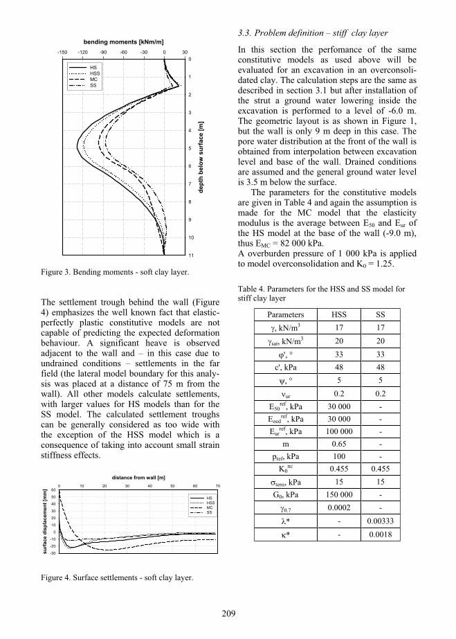
bending moments [kNm/m]-150 -120 -90 -60 -30 0 30

dept

h be

low

sur

face

[m]

0

1

2

3

4

5

6

7

8

9

10

11

HSHSSMCSS

Figure 3. Bending moments - soft clay layer.

The settlement trough behind the wall (Figure 4) emphasizes the well known fact that elastic-perfectly plastic constitutive models are not capable of predicting the expected deformation behaviour. A significant heave is observed adjacent to the wall and – in this case due to undrained conditions – settlements in the far field (the lateral model boundary for this analy-sis was placed at a distance of 75 m from the wall). All other models calculate settlements, with larger values for HS models than for the SS model. The calculated settlement troughs can be generally considered as too wide with the exception of the HSS model which is a consequence of taking into account small strain stiffness effects.

distance from wall [m]0 10 20 30 40 50 60 70

surf

ace

disp

lace

men

t [m

m]

-30

-20

-10

0

10

20

30

40

50

60

HSHSSMCSS

Figure 4. Surface settlements - soft clay layer.

3.3. Problem definition – stiff clay layer

In this section the perfomance of the same constitutive models as used above will be evaluated for an excavation in an overconsoli-dated clay. The calculation steps are the same as described in section 3.1 but after installation of the strut a ground water lowering inside the excavation is performed to a level of -6.0 m. The geometric layout is as shown in Figure 1, but the wall is only 9 m deep in this case. The pore water distribution at the front of the wall is obtained from interpolation between excavation level and base of the wall. Drained conditions are assumed and the general ground water level is 3.5 m below the surface. The parameters for the constitutive models are given in Table 4 and again the assumption is made for the MC model that the elasticity modulus is the average between E50 and Eur of the HS model at the base of the wall (-9.0 m), thus EMC = 82 000 kPa. A overburden pressure of 1 000 kPa is applied to model overconsolidation and K0 = 1.25.

Table 4. Parameters for the HSS and SS model for stiff clay layer

Parameters HSS SS , kN/m3 17 17

sat, kN/m3 20 20

', ° 33 33 c', kPa 48 48

, ° 5 5

ur 0.2 0.2 E50

ref, kPa 30 000 - Eoed

ref, kPa 30 000 - Eur

ref, kPa 100 000 - m 0.65 -

pref, kPa 100 - K0

nc 0.455 0.455

tens, kPa 15 15 G0, kPa 150 000 -

0.7 0.0002 -

* - 0.00333

* - 0.0018

209

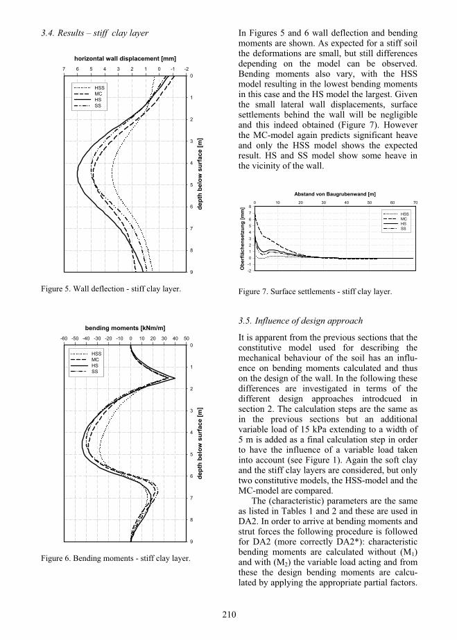
3.4. Results – stiff clay layer

horizontal wall displacement [mm]-2-101234567

dept

h be

low

sur

face

[m]

0

1

2

3

4

5

6

7

8

9

HSSMCHSSS

Figure 5. Wall deflection - stiff clay layer.

bending moments [kNm/m]-60 -50 -40 -30 -20 -10 0 10 20 30 40 50

dept

h be

low

sur

face

[m]

0

1

2

3

4

5

6

7

8

9

HSSMCHSSS

Figure 6. Bending moments - stiff clay layer.

In Figures 5 and 6 wall deflection and bending moments are shown. As expected for a stiff soil the deformations are small, but still differences depending on the model can be observed. Bending moments also vary, with the HSS model resulting in the lowest bending moments in this case and the HS model the largest. Given the small lateral wall displacements, surface settlements behind the wall will be negligible and this indeed obtained (Figure 7). However the MC-model again predicts significant heave and only the HSS model shows the expected result. HS and SS model show some heave in the vicinity of the wall.

Abstand von Baugrubenwand [m]0 10 20 30 40 50 60 70

Obe

rflä

chen

setz

ung

[mm

]

-2-1012345678

HSSMCHSSS

Figure 7. Surface settlements - stiff clay layer.

3.5. Influence of design approach

It is apparent from the previous sections that the constitutive model used for describing the mechanical behaviour of the soil has an influ-ence on bending moments calculated and thus on the design of the wall. In the following these differences are investigated in terms of the different design approaches introdcued in section 2. The calculation steps are the same as in the previous sections but an additional variable load of 15 kPa extending to a width of 5 m is added as a final calculation step in order to have the influence of a variable load taken into account (see Figure 1). Again the soft clay and the stiff clay layers are considered, but only two constitutive models, the HSS-model and the MC-model are compared. The (characteristic) parameters are the same as listed in Tables 1 and 2 and these are used in DA2. In order to arrive at bending moments and strut forces the following procedure is followed for DA2 (more correctly DA2*): characteristic bending moments are calculated without (M1)and with (M2) the variable load acting and from these the design bending moments are calcu-lated by applying the appropriate partial factors.

210

The same procedure is used for calculating design strut forces. It should be noted that this is an approximation only due to the nonlinear behaviour of the soil.

Mdesign, DA2 = M1 x 1.35 + (M2 – M1) x 1.5

For DA3 the strength parameters have to be reduced by the partial factors listed in Table 2 resulting in values for the effective friction angle and the effective cohesion as given in Table 5 for both soils. The dilatancy angle is also reduced by the partial factor which is however not explicitly mentioned in EC7. Finally a decision with respect to initial stresses has to be made. Here the value for K0 has been kept the same for DA2 and DA3, i.e. it is based on the characteristic value for the friction angle (1 - sin 'char) although an alternative would be to have it based on the design value in DA3. (It should be noted that for certain conditions K0

based on 'char may however violate the yield function).

Table 5. Reduced strength parameters for DA3

Design Parameter Soft Clay Stiff Clay', ° 22.2 27.5

c', kPa 12 38.4 , ° 0 4

tens, kPa 0 12

The differences in design strut forces and bending moments obtained from utilizing design approaches DA2 and DA3 (DA1 is basically a combination of the two) are pre-sented in the following. Figure 8 shows design bending moments (envelope over all construction stages) for the soft clay layer for both design approaches and both constitutive models. The following can be observed: for the HSS model DA2 and DA3 yield very similar results (DA2 slightly higher) but for the MC model the difference between DA2 and DA3 is higher. As expected from Figure 3, bending moments are higher for the advanced model. Figure 9 compares design bending moments for the wall in the overconsolidated clay. The following can be noted: first bending moments are higher for the MC model than for the HSS model which is in contrast to the wall in the soft soil layer.

design bending moments [kNm/m]-250 -200 -150 -100 -50 0 50

dept

h be

low

sur

face

[m]

0

1

2

3

4

5

6

7

8

9

10

11

HSS-DA2MC-DA2HSS-DA3MC-DA3

Figure 8. Comparison of design bending moments - soft clay layer.

bending moments [kNm/m]-60 -50 -40 -30 -20 -10 0 10 20 30 40 50

dept

h be

low

sur

face

[m]

0

1

2

3

4

5

6

7

8

9

HSS-DA3MC-DA3HSS-DA2MC-DA2

Figure 9. Comparison of design bending moments - stiff clay layer.

211

Secondly, the difference between the design approaches is larger, in this case also for the HSS model. The reason is the following. Be-cause of the overconsolidation stress paths are predominantly inside the yield surface and thus the behaviour is mainly (nonlinear) elastic. A reduction in soil strength has therefore a small influence on the structural forces and thus calculated bending moments from DA2 and DA3 are similar, but in DA2 they have to be multiplied by the partial factor for actions where in DA3 the results are already design values. Similar tendencies are observed for design strut forces, summarized in Table 6 for the soft clayer and in Table 7 for the stiff clay layer. Excavation in the soft layer results in higher strut forces when using the HSS model as compared to MC and it is the other way round in the stiff layer. In both cases DA2 design strut forces are higher compared to DA3 but in the soft layer this is only in the order of 10% for the HSS model.

Table 6. Comparison of design strut forces – soft clay layer [kN/m]

Design Approach HSS MC DA2 193 150 DA3 176 123

Table 7. Comparison of design strut forces – stiff clay layer [kN/m]

Design Approach HSS MC DA2 143 164 DA3 112 130

4. DEEP EXCAVATION PRACTICAL CASE

The benchmark examples presented in the sections above indicate that both design ap-proaches DA2 and DA3 and consequently also DA1 can be applied in combination with nu-merical methods. It was the purpose of these examples to show that differences in results due to the choice of the constitutive model are at least in the same order (or larger) than differ-ences coming from the different design ap-proaches. However, for real practical problems details of the design may have more severe consequences for the choice of the design

approach as compared to the simplified exam-ples presented above. This will be demonstrated by considering a diaphragm wall with three rows of prestressed ground anchors. The exca-vation is about 17 m deep in a homogeneous layer of medium dense sand (Figure 10). The details of the analysis are not of interest here because the goal of this section is only to highlight a particular aspect, namely the result-ing design anchor forces. The Hardening Soil model has been used as constitutive model for the sand. As described in the previous section, analyses were performed with characteristic soil strength parameters (DA2) and with design strength parameters (DA3). The only permanent action is the earth pressure and variable loads are not considered. Again DA2 is used in form of DA2*, i.e. the partial factor is applied to effects of actions rather than on the action itself.

Figure 10. Layout of practical example.

Table 8. Comparison of design forces - practical example

DesignApproach

Layer 1 kN/m

Layer 2 kN/m

Layer 3 kN/m

characteristic 334 756 755 DA2

(= characteristic x 1.35)

451 1 021 1 020

DA3 358 805 766

The resulting design anchor forces obtained from the two approaches are summarized in Table 8 and it can be seen that DA3 leads to significantly lower forces. The reason for this difference is the following: if anchors are highly

212

prestressed, and this was the case in this exam-ple, a reduction in soil strength has a minor influence on calculated anchor forces. Thus in DA2 the result has to be multiplied by the partial factor for actions (= 1.35) whereas in DA3 the forces obtained from the analysis are already design forces. It should be pointed out that in DA2 the effects of the water pressure are fully factored whereas they are not in DA3. This could be partly compensated for by taking into account an uncertainty in the water table as a "geometric" factor in DA3. However forces would not increase that much to reach values close to DA2.

5. TUNNEL EXCAVATION BENCHMARK

In this section results from a benchmark exam-ple for tunnel excavation are presented. In a similar way as for the excavation examples the influence of the constitutive model for the soil is addressed first followd by a discussion on EC7 design approaches. Tunnel excavation is based on the principles of the New Austrian Tunnelling Method (NATM).

5.1. Problem definition

A typical NATM cross section has been chosen, and the excavation is top heading, bench and invert (Figure 11). The overburden is 15 m.

Figure 11. Layout of benchmark tunnel excavation.

The same overconsolidated clay which has been used for the excavation example presented in the section above is considered, thus parameters are the same as given in Table 4 and the same

constitutive models have been employed. For the MC model the stiffness is the average of E50and Eur at the level of the tunnel axis, which yields EMC = 174 500 kPa. Again a "pre-overburden pressure (POP)" of 1 000 kPa is taken into account and K0 = 1.25. However, the ground water table is assumed to be well below the tunnel so that drained conditions can be postulated. Shotcrete is treated as elastic material but the stiffness is increased in two steps to account for the increase of stiffness with time, denoted as shotcrete "young" and "old" respectively (Table 9). Relaxation factors are applied in the 2D plane strain analysis in order to take 3D effects into account in an approximate manner. Thus the constrcution steps modelled are: Step 0: Initial stresses (K0 = 1.25) Step 1: Pre-relaxation top heading (55%) Step 2: Full excavation top heading with lining in place (shotcrete "young") Step 3: Pre-relaxation bench (35%, shotcrete top heading > "old")) Step 4: Full excavation bench with lining in place (shotcrete bench "young") Step 5: Pre-relaxation invert (20%, shotcrete bench > "old")) Step 6: Full excavation invert with lining in place (shotcrete invert "young")

Table 9. Parameters for the shotcrete lining

Shotcrete "Young" "Old" EA, kN/m 1.25e6 3.75e6

EI, kNm2/m 6 510 19 500

5.2. Results

Figure 12 plots surface settlements for the final excavation stage and similar arguments as put forward for the deep excavation example hold. The simple MC model gives a very wide set-tlement trough which is usually not observed in reality. The SS model is slightly better but again the small strain stiffness model can be consid-ered as the most reasonable one. This is qualita-tively in agreement with observations publishedin the literature (e.g. Addenbrooke et al. 1997, Scharinger et al. 2007). In Figures 13 and 14 maximum normal forces and maximum bending moments in the lining are compared for DA2 and DA3. For the latter the reduced soil strength parameters as

213

listed in Table 5 have been used. It should be noted at this stage that it is under discussion whether the concepts of EC7 can (could) be applied to tunnelling problems because EC7 does not explicitly make reference to tunnelling. However in order to contribute to this discus-sion some results from this priliminary study are presented here. If one looks at the influence of the constitutive model first, it is obvious that the the maximum normal force is obtained from the MC model and the HS model, the lowest for HSS and SS models, the difference being about 30% (DA2 in Figure 13). As far as bending moments are concerned the HS models give the largest moments (DA2 in Figure 14).

distance from tunnel axis [m]0 5 10 15 20 25 30 35 40 45 50 55 60 65 70 75 80 85 90 95 100

surf

ace

disp

lace

men

t [m

m]

-20

-15

-10

-5

0

HSSMCHSSS

Figure 12. Comparison of surface settlements.

design approach

DA2 DA3

desi

gn n

orm

al fo

rce

[kN

/m]

0

200

400

600

800

1000

1200

1400 HSSMC HS SS

Figure 13. Comparison of maximum normal forces.

design approach

DA2 DA3

Max

imum

ben

ding

mom

ent [

kNm

/m]

0

20

40

60

80

100HSSMCHS SS

Figure 14. Comparison of maximum bending mo-ments.

If results of DA3 are examined the following is noted. Normal forces reduce for all models and bending moments increase significantly. This can be explained that in the construction step "pre-relaxation bench" the shotcrete lining is punched into soil because of the reduced strength and thus stress redistribution in the soil takes place reducing the normal forces but increasing bending moments. This is clearly evident from comparison of Figures 15 and 16 where vertical displacements are plotted at the same scale for DA3 and DA2 respectively.

Figure 15. Vertical displacements – DA3.

Figure 16. Vertical displacements – DA2.

6. TUNNEL EXCAVATION PRACTICAL CASE

Finally a practical tunnel example is considered, which is based on a real project, but has been modified for the purpose of this study.

214

6.1. Problem definition and parameters

The geometric layout, the finite element mesh (using 15-noded triangles) and the simplified soil profile are shown in Figure 17. The water table is approximately 5.5 m below surface and drained conditions have been postulated. The excavation stages involving construction of a pilot tunnel supported by a jetgrout canopy where modelled in 10 computational steps whereas stress release factors, to account for 3D-effects in the two-dimensional analysis in an approximate manner, were based on experience from projects under similar conditions. As in the benchmark example of the previous section the increase of stiffness of the shotcrete lining with time was taken into account by increasing the Young's modulus of the shotcrete in subse-quent excavation phases. Again the simple elastic-perfectly plastic Mohr-Coulomb criterion and the advanced Hardening Soil Small model have been com-pared. The most relevant material parameters are summarized in Table 10 for all soil layers.

Figure 17. Layout and fe-mesh of station tunnel

Table 10. Parameters for the HSS model

Parameters Q1 Q5 N1 N5 ϕ', ° 20 34 25.5 27

c', kPa 16 0 21 5 E50

ref, kPa 7 000 100 000 18 300 18 200 Eoed

ref, kPa 7 000 100 000 18 300 18 200 Eur

ref, kPa 20 160 200 000 49 000 48 500 m 0.5 0.5 0.85 0.5

pref, kPa 100 100 100 100 G0, kPa 22 500 240 000 90 740 38 190

γ0.7 0.00015 0.00015 0.00015 0.00015

6.2. Results

Figures 18 and 19 plot the design values for the normal forces in the lining for DA3 and DA2 when using the Mohr-Coulomb model. It can be observed that application of DA2 leads to significantly higher design forces than DA3. The reason is that calculated forces are almost the same (a reduction in soil strength by a factor of 1.25 does not change the normal force in the lining significantly) and thus the difference is mainly the multiplication of the normal force by the partial factor for "effects of actions" in DA2* (the result of DA3 is the design value). A similar result is obtained for the HSS-model. For bending moments the influence of the constitutive model for DA3 is larger. For the Mohr-Coulomb model bending moments differ significantly for DA3 and DA2 but for the HSS-model the differences are not siginificant (Table 11). For DA2 both models give the same maximum bending moments in this case.

Figure 18. Design normal force – DA2

Figure 19. Design normal force – DA3

It should be mentioned at this stage that the results shown here, in particular for bending moments, have to be interpreted with care because the assumption of elastic material behaviour for the shotcrete lining is not very realistic and it can be expected that bending

215

moments reach the capacity of the lining at certain stages which will lead to load redistribu-tions in the lining. This can be taken into account in the finite element analysis, but at present there is no generally accepted procedure how this should be done. Some suggestions can however be found in Schweiger et al. (2010).

Finally, it is pointed out that for DA2 ground failure in all construction stages has to be checked separately whereas this is not required when applying DA3.

Table 11. Comparison of maximum values of design bending moments- station tunnel [kNm/m]

Design Approach HSS MC DA2 309 309 DA3 286 231

7. SUMMARY AND CONCLUSIONS

In this contribution the influence of the constitu-tive model on the results of finite element analyses of deep excavations and tunnels has been demonstrated. The results clearly empha-size the well known fact that elastic-perfectly plastic constitutive models such as the Mohr-Coulomb model are not well suited for analys-ing this type of problems and more advanced models are required to obtain realistic results. Although reasonable lateral wall movements may be produced with simple failure criteria with appropriate choice of parameters, vertical movements behind the wall are in general not well predicted, obtaining heave in many cases instead of settlements. The same holds for tunnelling problems where surface settlement troughs from Mohr-Coulomb models are generally considered as being too widespread. Strain hardening plasticity models including small strain stiffness behaviour are in general a better choice and produce settlement troughs being more in agreement with expected behav-iour. As the goal of the study presented here was to qualitatively highlight the differences in results with respect to the constitutive model no quantitative comparison with in situ measure-ments of real project has been provided. It is emphasized that the models used in this study should be seen as representatives for certain classes of models and conclusions can be transferred to other constitutive models of

similar type. The second aspect addressed in this paper is ULS-design of deep excavations and tunnels by means of numerical methods. This is a topic which has come into focus more recently in the context of introducing Eurocode7 into the geotechnical community. As EC7 does not make any statements on the calculation model to be used the question can be asked whether or not it can be done with numerical methods. However distinction has to be made here be-tween deep excavations and tunnels. Whereas deep excavations are clearly dealt with in EC7 tunnelling is not and therefore this part of the paper should be considered as feasibilty study contributing to the discussion whether EC7 should be applied to (shallow) tunnelling. It has been shown that the concept of partial factors of safety as established in Eurocode7 can be applied in combination with numerical methods, but differences have to be expected depending on how this is done in the respective design approaches. Although more experience is needed in performing such analyses for practical examples, a cautious conclusion from this study could be that the differences in results depending on the design approach used are less pronounced for more advanced constitutivemodels as compared to simple elastic-perfectly plastic failure criteria. Postulating that advanced constitutive models are capable to capture the stress strain behaviour of soils for stress levels ranging from working load conditions up to failure with reasonable accuracy from a practi-cal point of view it could be argued that ad-vanced models have advantages not only for predicting displacements and stresses for working load conditions but have their merits also in ULS-design. If this can be confirmed in further studies it would have strong conse-quences for numerical modelling in practical geotechnical engineering. It can be concluded that in principle all design approaches specified in EC7 can be used in combination with numerical modelling provided DA2 is employed in the form of DA2*, i.e. the partial factors are applied to the "effects of actions" rather than on the actions itself. When using DA3 large plastic strains may develop and a significant number of elements may reach the ultimate strength of the material. In that situation design forces may increase significantly and a careful judgement has to be made if these are realistic. An additional difficulty arises in tunnelling

216

because the shotcrete is a material with a strongly nonlinear mechanical behaviour and no rules are given in EC7 how to deal with nonlin-ear structural elements. This aspect has been not covered in this paper. A possible way to pursue would be the application of a partial factor of safety on the shotcrete strength in nonlinear numerical analyses in order to avoid unrealistic design forces. For DA3 in particular this ap-proach could be considered to be in accordance with the concepts of EC7. For deep excavations this issue does usually not arise because dia-phragm walls or sheet pile walls are not de-signed for plastic hinges although this would be acceptable under the new code.

8. REFERENCES

Addenbrooke, T.I., Potts, D.M. & Puzrin, A.M. 1997. The influence of pre-failure soil stiffness on the numerical analysis of tunnel construction. Geo-technique. 47(3), 693-712.

Bauduin, C., De Vos, M. & Simpson, B. 2000. Some considerations on the use of finite element meth-ods in ultimate limit state design. Proc. Int. Workshop on Limit State Design in Geotechnical Engineering, Melbourne.

Bauduin, C., De Vos, M. & Frank, R. 2003. ULS and SLS design of embedded walls according to Eurocode 7. Proc. XIII ECSMGE, Prague (Czech Republic), Vol. 2, 41-46.

Benz, T. 2007. Small-Strain Stiffness of Soils and its Numerical Consequences. Publication No. 55, Institute for Geotechnical Engineering, Univer-sity of Stuttgart.

Brinkgreve, R.B.J., Broere, W. & Waterman, D. 2006. Plaxis, Finite element code for soil and rock analyses, users manual. The Netherlands.

Scharinger, F., Schweiger, H.F., & Pande, G.N. 2007. Application of a Multilaminate Model for Soil to tunnel excavation. Proc. 10th Intern. Symp. Nu-merical Models in Geomechanics (G.N. Pande, S. Pietruszczak, eds.), Taylor & Francis, London, 381-386.

Schweiger, H.F. 2005. Application of FEM to ULS design (Eurocodes) in surface and near surface geotechnical structures. Proc. 11th Int. Confer-ence of IACMAG, Turin, Italy, 19-24 June 2005. Bologna: Patron Editore. 419-430.

Schweiger, H.F. 2009. Influence of constitutive model and EC7 design approach in FEM analysis of deep excavations. Proc. ISSMGE Int. Seminar on Deep Excavations and Retaining Structures (Mahler & Nagy, eds.), Budapest, 99-114.

Schweiger, H.F., Marcher, T. & Nasekhian, A. 2010. Nonlinear fe-analysis of tunnel excavation - comparison of EC7 design approaches. Geome-chanics and Tunnelling, Vol. 3, No.1, in print

Simpson, B. 2000. Partial factors: where to apply

them? Proc. Int. Workshop on Limit State Design in Geotechnical Engineering, Melbourne, 145-154.

Simpson, B. 2007. Approaches to ULS design – The merits of Design Approach 1 in Eurocode 7. First International Symposium on Geotechnical Safety & Risk, Oct. 18-19, 2007, Shanghai, Tongji Uni-versity, China.

Walter, H. 2006. Eurocode-based ultimate limit state design of NATM tunnels using nonlinear consti-tutive models for sprayed concrete and soil. Proc. 6th European Conference on Numerical Methods in Geotechnical Engineering (H.F. Schweiger, ed.), Taylor & Francis, London, 305-311.

217

Urban Environmental Geotechnics Construction on Brownfields

I. Vaní ekCzech Technical University in Prague, Faculty of Civil Engineering, Geotechnical Department

ABSTRACT: The position and main aims of Environmental Geotechnics are defined, above all in urban areas and the main activities are mentioned such as waste deposition on the surface, remediation of contaminated ground, utilization of different waste materials in civil engineering, protection against natural hazards andconstruction on brownfields. Construction on brownfields is specified in more detail as a very important step in urban redevelopment. Basic steps of brownfields redevelopment are specified while highlighting the role ofgeotechnical engineers for example in site investigation, remediation of subsoil and foundation of new structures. Possibility of the utilization of old foundations for new structures is discussed as well. At the end practical examples are presented.

1. INTRODUCTION

During the last 30, 40 years more attention is generally devoted to environment protection. As geotechnical engineering is connected with subsoil, geological environment, soil, rock, ground water, the interest connected with protection of subsoil has always existed, but a new form gained after the ISSMGE Interna-tional Conference in Stockholm, 1981. There-fore in the paper a brief summary of environ-mental geotechnics development is presented.

Problems of construction on brownfields create a significant part of environmental geotechnics, especially for urban environment. The basic principle is connected with the main aim to decrease the orientation of new construc-tion on greenfields, on the ground, which was not previously used for construction activities and has been used in many cases up to now for agricultural purposes. On the other hand we would prefer to construct new structures on brownfields, on the ground which was previ-ously affected by man – (Fig. 1.a.,b.).

In spite of the difficulties how to calculate the area of greenfields used per day for the new construction in individual countries, some value are alerting, e.g. in Germany the estimation is around 1, 200, 000 m2 per day. Therefore in some countries the governmental policy de-clares the aims for the future and at the same time defines legal regulations how these aims can be reached, how more brownfields have to be used for new construction. In principle it is

the reaction to the fact that especially in cities many previous activities are closed as, mining activities together with concentrator factories, heavy industry as metallurgy, light industry as textile industry, together with dwellings not ful-

Figure 1a. Greenfield on unaffected ground (agricul-tural land)

218

filling up to date demands. But on the other hand there are new de-

mands for different offices, banks, shopping centres, garages together with new demands on apartment blocks.

Figure 1b. Brownfield on previously man affected ground

Therefore all aspects connected with con-struction on brownfields are discussed, above all from the view of individual steps of the whole process as geotechnical engineering is playing a very significant role, especially from the perspective of site investigation, potential evaluation of the potential risk of underground contamination, selection of remediation tech-nology and their completion. The last aspect is connected with selection of the appropriate methods of foundation as ground is usually affected well with the possibility of utilization of old foundations for new structures.

2. POSITION OF ENVIRONMENTAL GEOTECHNICS

One of the plausible perceptions about a safe and generally optimal geotechnical structure leads to the conclusion that its success is sup-ported by four columns, Vaní ek I. and Vaní ekM. (2008). The first column relies on the understanding of natural sciences such as geology, engineering geology and hydrogeology on the one hand, and on the understanding of mechanics, theory of elasticity on the other.

This first column can be called Theoretical background. The second column relies on the application of existing findings to the behaviour of soils and rocks under different stress - strain states – speaking about support from soil and rock mechanics, generally about Geomechanics. The third column relies on the combination of the theoretical findings with practical technolo-gies during execution of geotechnical structures speaking about Geotechnics, Geo-Technology. Finally the fourth column relies on a certain feeling of geological environment which Ter-zaghi (1959) denotes as “capacity for judg-ment”, and he says that “this capacity can be gained only by years of contact with field conditions”, (Fig. 2).

Figure 2. Four columns of Geotechnical Engineering

The branch of Environmental Geotechnics is a part of the third column – Geotechnics –Geo-technology, as this column can be divided into the following four branches, which are very often treated at Universities as independent subjects:• Foundation Engineering, • Underground Structures, • Earth Structures, • Environmental Geotechnics

As previously mentioned the first important steps in the recognition of the new branch Environmental Geotechnics under the umbrella ISSMGE was State of the Art Report during the Xth International Conference in Stockholm 1981 presented by Sembenelli and Ueshita.

Those days they devoted most attention to the problems of: • Solids removal from the surface, • Solids extraction from the underground, • Solids accumulated on the surface, • Underground deposits.

Above all the last two problems are very important, especially when waste material is

219

deposited. Growing attention is now devoted to the problem of underground waste disposal. Filling of underground spaces by large volumes of waste as for example flying ash from electric power stations can on the one side limit the surface deformations but on the other this waste material is in direct contact with ground water and therefore it is necessary to prove that this interaction is not dangerous for environments, Vaní ek (1995). A very specific problem is associated with high level radioactive waste disposal in underground spaces, e.g. Pusch (2003).

Using this problem some specificity of En-vironmental Geotechnics can be shown. Firstly it is the principle of multi-barrier protection, where a natural, geological barrier is a funda-mental element; however an engineered barrier is also very important. Spent fuel from nuclear power plants is fixed in special containers, which are in underground spaces separated from the surrounding rock massif by a special sealing zone, where often bentonite is proposed.

The second specificity is connected with the time effect, as contamination spreading is a strongly time dependent process. The numerical model, describing not only radio-nuclides spreading in the sealing layer and rock massif but also taking into consideration mechanical and thermal properties of the all multi-barrier system, has to be tested and verified, so to prove its credibility. In underground rock laboratories all the above mentioned processes are simulated and compared with proposed numerical models. The credibility of the models can be performed there even just for a much shorter period, from today’s perspective roughly 20-30 years, com-pared to the life-expectancy of underground repository of the order of ten thousand years.

A special recognition of Environmental Geotechnics gained by establishing independent conferences – the International Congress on Environmental Geotechnics – first congress was arranged in Edmonton, Canada in 1994 and continuing via Osaka, Japan 1996, Lisbon, Portugal 1998, Rio de Janeiro, Brazil 2002, to Cardiff, UK in 2006. Next one will be held in New Delhi, India in 2010. TC5 of ISSMGE is also playing very significant role there.

Continuously Environmental Geotechnics is reacting to the new demands and now concen-tration on the following spheres of interest can be distinguish: • Waste deposition on the surface;

• Remediation of contaminated ground; • Utilization of different waste materials in

civil engineering; • Protection against natural hazards; • Construction on brownfields.

Subsequently the first four spheres of inter-est are briefly characterized.

Waste deposition on the surface is reaching a significant dimension. The volume of such deposited material is extremely high, only in the Czech Republic it is hundreds of million tons per year. Present-day generations are thus in such a significant way reshaping the landscape, that we can speak even about new artificial geological period, about the period of Quinter-nary. A fundamental overview of the problems associated with deposition of waste material on the surface was summarized e.g. by Vaní ek(2002), respectively by Clark and Weltman (2003).

Basically most of the material is deposited in:• Spoil heaps as a result of mining activity –

as overburden for open pit mines or waste rock for deep mines;

• Tailing dams as a result of hydraulic way deposition of fine waste material - as flying ash from electric power stations or sludge from different concentrator factories;

• Landfills where municipal waste or many other different waste materials as chemical or low radioactive waste material are stored. All these new structures on the surface can

be classified as earth structures of environ-mental engineering. During the design of these earth structures we have to count with: • Limit states as for any other earth structures,

as limit state of stability, deformation, ero-sion;

• Impact on environment - above all to limit the contaminants spreading from the depos-ited waste as much possible;

• Steps permitting future utilization of surface for new construction. Remediation of contaminated ground repre-

sents a significant activity of this generation as previous ones because they are strongly respon-sible for these “old burdens” as a result of earlier activities during which different con-taminants polluted the geological environment. Geotechnical engineers are called up to contrib-ute to in the elaboration of solutions which are realistic, compatible with environmental needs

220

and cost effective – Jessberger (1996). To deal with these tasks there are among others the following main subjects to be considered: • Site investigation including sampling and

laboratory analysis; • Estimation of potential danger – environ-

mental risk analysis; • Development and evaluation of remediation

concepts;• Performance of the clean up or provision of

containment;• After care measures – monitoring.

As some brownfields are also contaminated, more details will be presented hereafter.

Utilization of different waste material in civil engineering (in geotechnical applications) is human response to the new philosophy – to limit waste as possible, or to recycle it or reuse it. The detailed description of possibilities with the use of existing large-volume waste is given by Head et al.(2006) with reference to condi-tions in the UK. Besides the dump from coal mining, spent oil shale is mentioned, which can be useful construction material provided that due account is taken of the potentially elevated sulphate contents and a potential vulnerability to frost heave in near-surface applications. Others possibilities come e.g. from: • Excavated surplus soil; • Construction and demolition waste; • Quarrying industry – quarry by-products; • China clay waste; • Industrial by-products such as steel slag and

pulverized-fuel ash • Municipal solid waste incineration.

The potential for application, first of all for aggregates, is very high as substitution of gravel and sand due to the limited amount of natural resources in some countries is nearly a neces-sity. Next applications are earth structures in transport engineering. However two viewpoints should be considered: • Character of the leachate from the used

material, inclusive of confirmation (usually using numerical models for contaminant spreading) that potential leachate (certain concentration) when reaching the aquifer at the given time will be lower than recom-mended limits, e.g. Vaní ek, M. (2006).

• Potential of used material to volume changes as structural instability, frost heave or swelling potential. Protection against natural hazards. Problem

of natural hazards is very sensitive for cities, for places with high concentration of population and buildings. In most European countries the image of natural hazards is connected with floods and landslides, exceptionally with earthquakes, however generally also with tsunami, volcano activity, typhoons, hurricanes etc. The role of geotechnical engineers is for floods, landslides and earthquakes connected with two aspects: • Definition of the potential risk for a certain

area, e.g. flood prone area• Preventive protective measures – e.g.

construction of dykes, construction of steps for slope stability increase, construction of buildings less sensitive to earthquakes or even flooding etc.

• Recommendation of steps for remediation of affected land when natural hazards really hit the area. The problem of natural hazards has some

connection to construction on brownfields as brownfields can be also originated by these accidents.

With time special attention is devoted to the environmental problems in cities, we are speak-ing about Environmental Urban Geotechnics, e.g. Jefferson, I. and Braithwaite, P. 2009. According to the authors, environmental geo-technics has now developed into a well-defined and mature discipline that encompasses engi-neering geology, geotechnical engineering, environmental engineering, hydrogeology and soil physics. Many of the most pressing issues related to environmental geotechnics occur in the urban areas as increasing pressure for development is being driven to cope with ever more demanding societal needs and desires. This is only going to increase as population moves substantially to a more urban basis. Therefore, environmental urban geotechnics has become, in recent years, a critical aspect of the work of ground professionals from engineering geologists to geotechnical engineering. Jeffer-son and Braithwaite included into these prob-lems also naturally occurring geohazards, as for example foundation material which is unstable, as some loess and clays. Between anthropogenic geohazards not only problems with subsoil contamination are discussed but also other manmade activities. For example Koshelev et al. (2009) examined changes to thermal, mois-ture and chemical fields within subsurface of Moscow, associated with the distribution

221

system, specifically pipelines, and how these influence the geotechnical behaviour of the near-surface.

Very sensitive is the question of man made activities in urban areas on the underground water table. Summarizing we can conclude that geo engineers have to play a very important role even in the phase of city development, during the phase of definition of the municipal plan.

Hereafter the main attention will be devoted to the problem of construction on brownfields in urban areas.

3. BROWNFIELDS DELIMITATION

3.1. Brownfields definition

There are different definitions of brownfields, however hereafter the definition of CABERNET European network will be pre-sented. The EC funded “Concerted Action on Brownfields and Economic Regeneration Network (see www.CABERNET.org.uk) was established in January 2002 to enhance the regeneration of brownfield sites by developing an intellectual framework to structure ideas and stimulate new solutions, e.g. Nathanail et al. 2003. The following definition of brownfields is used there: • Have been affected by former uses of the

site and surrounding land; • Are derelict or underused; • Are mainly in fully or partly developed

urban areas; • Require intervention to bring them back to

beneficial use; and

• May have real or perceived contamination problems.According to this definition brownfields

with contamination but also without it can be recognized. Therefore one of the first steps during the phase of brownfields investigation is connected with adjustment of the risk. However the ground cannot be affected only by chemical impact, but also physical or biological impacts, when the physical impact is mostly connected with lower porosity, with the risk of higher total and differential settlement, and biological impact is very often connected with the pres-ence of methane. In all cases a special care to foundation has to be devoted.

3.2. Brownfields classification

The brownfields classification strongly depends on the stand-point from which brownfields are differentiated, Vaní ek 2006. According to different stand-points we can differentiate between:• Brownfields where the subsoil is contami-

nated or not – differences in the degree of contamination;

• Brownfields inside of cities – urban brown-fields and brownfields out of towns, above all lands connected with previous mining activity and concentrator factories – differ-ences in location;

• Small and large brownfields – differences in scaleHowever given practical implementation the

financial aspect is extremely important, there-fore from the financial perspective we can differentiate between: • Brownfields which are attractive for private

investors – above all urban brownfields in large cities as capitals;

• Brownfields where the attractiveness of land can balance the higher cost of redevelop-ment;

• Brownfields where private investors are attracted by some investment stimulus from the government or municipalities, or where some sort of public-private-partnership is established;

• Brownfields redevelopment (first of all contamination remediation) of which should be taken care and financially supported by the government or municipalities. From this perspective it is obvious that the

market cannot solve all cases. In fact there are three aspects, the financial one, the potential environmental risk and the time factor. The financial one compares the sum of money which is spent for purchase of the brownfields land plus money for preparation of brownfields for new construction with the price of greenfields. The potential environmental risk is connected with uncertainties of the remediation process, whether the recommended process of remedia-tion will reach the demanded values, whether there is the risk of supplemental increase of chemical contamination or whether the accept-able boundaries will not be decreased by addi-tional law. However the time factor is also important because some investors prefer speed, to start with construction as soon as possible,

222

e.g. with construction of different supermarkets etc. Therefore they are not trying to go with new construction on brownfields because there is always some delay. Some of these aspects will be shown in next chapter, where individual steps of the brownfields redevelopment process are discussed.

4. INDIVIDUAL STEPS OF THE BROWNFIELDS REDEVELOPMENT

Very often the whole process of the brownfields redevelopment can be divided into the follow-ing individual steps, e.g. Vaní ek and Valenta (2009):• site location identification, • First phase of investigation, • preliminary economic analysis,• Second phase of investigation – detailed

site analysis • project of site development and methods of

financing – feasibility study • project and completion of site remediation • project and completion of construction of

new development (including foundation en-gineering, reuse of old foundations).

From these basic 7 steps, it is obvious that environmental geotechnics is strongly involved

in the whole process. But typical for geotechni-cal engineers are four parts – 1st phase of investigation, 2nd phase of investigation – detailed site analysis, project and completion of site remediation and the problem of foundation engineering, respectively reuse of old founda-tions. These parts will be discussed further in more detail.

The first two steps are labelled as the first phase which can be also called the desk study, which is only supplemented by visual inspec-tion. So this first phase mostly uses existing materials, where the study of archive materials and different maps composes the most impor-tant part of this phase.

Preliminary economic analysis has a key role in defining the suitability of the site for new construction, how this site can attract a new investor, especially after the comparison of financial inputs for redevelopment and the economic return. This preliminary economic analysis is supported by architectural study (which can for example define if some of the old buildings should be protected), and social study – how the redevelopment can improve the style and quality of life in the affected area.

The 2nd phase of the investigation encom-passes site investigation, usually starting with

Figure 3. Basic steps of Brownfield redevelopment

223

borings, field tests, collection of samples and laboratory tests. Classical geotechnical data are useful from the foundation design perspective, geoenvironmental data from the view of site contamination.

Feasibility study evaluates the workability from the financial point of view and defines the financial plan for remediation and completion of construction. The project and completion of site remediation can be very expensive if the degree of contamination is a high one, and includes the whole process of remediation (starting from the evaluation of contaminant spreading as a function of time and position, comparison of the obtained data with limits defined by administrative body, the selection of the most appropriate method, phase of comple-tion and ending with monitoring, which have to prove that the proposed level of clean up was reached), the impact on the existing community and the final report for the administrative body, Vaní ek, I. (2002b).

Significant decisions can be made after individ-ual steps, see Fig. 3 as for example: • After the first phase (the first two steps), the

local authority can discuss the realistic plans for future, having relatively good informa-tion about the degree of contamination,

• After the feasibility study the potential financial risk for investors can be defined. Assessed brownfields can be divided be-tween perspective projects, projects recom-mended for transformation into greenfields or the project is recommended to postpone with monitoring of site.

• Many investors prefer to purchase the site at the end of the remediation process, after the statement (from the administrative body) that the site will not pose any potential envi-ronmental risk for the future. However the potential developer can enter in the process after the first economic study, to make all necessary steps and after that to sell the land, just prepared for new construction.

5. ROLE OF ENVIRONMENTAL GEOTECHNICS IN THE PROCESS OF BROWNFIELDS REDEVELOPMENT

5.1. First phase of investigation

Site identification is mostly connected with identification in the real estate register, where the first information about the site area, the owner, and some other conditions can be obtained. The type of owner can have some influence on different grants, which can be obtained from different agencies. Supplemented materials are – prices for parcels in a wider area, potential interest, and advertising, all of them can help to define the potential attractive-ness of the site.

Visual inspection. The main aim of the vis-ual inspection is to give the first information, above all about morphology in the wider area, surface water, ground water via observation of old wells, discussion with owners about quality of water, information about vegetation, inspec-tion of existing buildings with brief evaluation of their situation, with special aspect of unusual symptoms, as colour, odour, talks with older citizens, with old employees, whereas all visual inspection will be supported by photographs, videos, etc.

Archive and up-to-date data collection. Thisstep will help to obtain or find not only useful

information about buildings, but also about the type of production, with what materials the production was connected, what sort of waste material was produced. From the archive and other historical documents some information can be obtained about potential problems or accidents in the past and from these data the probability of soil and water contamination can be judged. And finally different hydrological data can be useful as well. Nevertheless the most valuable data are obtained from Geo-environmental maps. Further main steps are defined, while details can be found e.g. in Vaní ek and Valenta (2009). • General information about buildings; • History of the buildings utilization; • Information from the archive and other

historical documents; • Materials from hydro meteorological insti-

tutes;• Materials from aerial observation – military

and civic photographs • Set of different maps.

From different maps e.g. in the Czech Re-public the following can be used:

• Set of Geoenvironmental maps • City maps with surroundings, contour plans • Land-use plans, Ortho photo maps, GIS

system• Infrastructure and underground service plans

224

• Maps of documentation points - Materials from Geofond – state office, where all bore-holes data are collected for the whole Czech Republic as borehole geology description, geotechnical data, ground water level etc. A very important source of information can

be obtained from a set of Geoenvironmental maps in the scale 1:50 000. In the Czech Repub-lic this set is composed of up to 17 maps, the most important are geological, hydrogeological, engineering-geology, mineral deposits, rock geochemical reactivity, soil or geophysical maps, or maps of surface water geochemistry, or geofactors of environment. Only 3 of them are shown further.

The geological map is a fundamental map, which is necessary for constitution of all other layers, (Fig. 4). This map represents rock and soil types in the ground, their age, stratigraphy, tectonical position and so on.

Figure 4. Example of the Geological map (1:50 000)

The hydrogeological map describes types of hydrogeological aquifers and their quantitative characteristics, (Fig. 5). A colour in a map projects discharge of ground water (m3/s). Different symbols indicate ground water quality from the serviceability perspective, ground water flow direction and important boreholes with water yield and mineralization data.

Figure 5. Example of the Hydrogeological map (1:50 000)

The Map of surface water geochemistry (Fig. 6) shows a catchment area of water streams and their pH value. On the map the

water sampling place and he trace elements content (As, Pb, Be, Zn, Li) are marked. The map of water surface geochemistry displays the level of pollution of the water surface.

Figure 6. Example of the Map of surface water geochemistry (1:50 000)

For the largest cities in the Czech Republic, e.g. for the capital of Prague maps in a larger scale can be used – in the scale 1:5000, however only 4 such maps are there – geological and hydrogeological maps and maps of superficial deposits and documentation points (from Geofond).

Briefly speaking the main aim of this phase is to obtain maximum relevant information with minimum financial input. According to the author’s opinion all the obtained information is a very useful tool for the decision making process on the municipality level and should be recommended to all municipalities dealing with the problem of brownfields, because it gives a reliable answer to the following four questions: • Potential site contamination – on the one

hand the first phase of investigation collects all information, from which researchers can distinguish whether contamination occurs, at what level and at what extent. On the other one, from other information, engineers can estimate the possibility of spreading of con-tamination in subsoil (e.g. direction, veloc-ity) and what impact on the surrounding it can have.

• Evaluation of the potential of the site – information which makes the best account of this fact is the site size, disposition, quality of buildings, halls, technical equipment, quality and density of engineering networks, what can be used in the future, what is rec-ommended for demolition etc.

• Site attractiveness – in which the part of the city is situated, what is traffic accessibility, what is concurrency in near surroundings. What are restrictions (e.g. from the owner ´s point of view), whether there are some bur-

225

dens. Comparison with similar localities or similar projects, why they were successful or only partly successful and the reason of this fact. What is the position of citizens to the remediation process, what profit citizens and local authority can obtain (higher prices of the surrounding areas, lower unemploy-ment etc.).

• Recommendation for the second phase of investigation.

5.2. Second phase of investigation

This phase is predominantly orientated to the application of direct investigation methods with the help of which findings from the first phase can be verified and supplemented.

The classical approach is based on the drill-ing, collection of samples (water, soil, air) and geotechnical and geochemical analysis in the laboratory. This classical approach has many advantages but also disadvantages giving information only for a selected point from which samples were extracted and also that there is a direct exposition of contaminated soil with a drilling crew and the need to safely deposit unused material on landfills.

Geophysical methods are based on the changes of geophysical characteristics. Pre-dominantly these methods are cheap and opera-tive. Most commonly they are orientated to obtaining a continuous picture between bore-holes, points of sample collection, or the picture of the cross section of the observed subsoil. They are able to recognize the boundary be-tween subsoil with different physical (moisture content, temperature), mechanical (density, stiffness) properties as well with different chemical properties (pH, electrical conductivity, radioactivity etc.). However the interpretations of the measured data require good experience.

Hydrogeological investigative boreholes are very useful for non problematic subsoil, as open piezometers can be used for definition of pore pressure and sampling of water, respectively for pumping tests for permeability determination. However for laminated subsoil, where only one layer is contaminated, a borehole can constitute potential danger of contamination spreading as well as interconnection of layers with different pore pressures.

Therefore during the last period different penetration methods are preferred, specially cone penetration tests - CPT. Lunne, Robertson and Powell (1997) give an overview of these

methods where for the classical geotechnical investigation cone resistance, skin friction, and pore pressures are determined (CPTu test). Generally CPT tests are used for the following information:• Nature and sequence of subsoil layers

(geological data); • Ground water information (hydrogeological

data);• Physical and mechanical properties of

individual layers (geotechnical data) For contaminated subsoil penetrometers

with additional sensors were developed, ena-bling to measure temperature, electrical resistiv-ity or conductivity, pH, redox potential, radioac-tivity, etc. Two examples of such penetrometers are in Fig. 7.

Figure 7. Cone penetrometers with additional sensors

Testing the samples from the same points in different time, researchers can obtain the degree of contamination as a function of the position and time. So engineers can get the first informa-tion about contaminant spreading in time. These

226

results can be checked, verified and prolonged for future time by numerical modelling, after determination of input data into a numerical model of contaminant transport equation, taking into account not only advection but also diffu-sion, dispersion, and sorption.

The basic equation for a 2 D problem of contamination spreading in an earth domain may be written in the form (Eq. 1):

tcK

zcvn

xcvn

zcDn

xcDn

tcn

dz

xzx

∂∂ρ

∂∂

∂∂∂∂∂

⋅−⋅−

⋅−∂

⋅+∂

⋅=∂ 2

2

2

2

(1)

which expresses a change in the concentra-tion c of a certain substance in time t in relation to the porosity n and the groundwater flow velocity v in the direction z and x. Further on:

Dz , Dx – are coefficients of hydrodynamic dispersion in directions z, x, which is a sum of diffusion De and dispersion Dm coefficients

K – distribution coefficient This equation incorporates contaminant

spreading through the following processes: • Advection – contaminant movement with

flowing water, the decisive factor being the water velocity v

• Diffusion – expressing contaminant move-ment from a point of a higher chemical con-centration to points with a lower concentra-tion, the decisive factor being the effective diffusion coefficient De

• Dispersion – which includes “mixing“ and dispersion due to the non-homogeneity of the aquifer, the decisive factor being the co-efficient of mechanical dispersion Dm

• Sorption – i.e. mechanisms which remove contaminants from the solution, the decisive factor being the distribution coefficient K. The obtained data of contaminant concentra-

tion as a function of position and time are compared with allowable limits defined by the national ministry of environment or by the national environmental protection agency. As a result of this comparison the potential risk of the observed locality and the need of remedia-tion action are defined.

The detailed assessment of the brownfields site, based on the result of the second phase of investigation, is also connected with recom-mendation for site remediation, either from the chemical, and/or physical or biological views.

5.3. Brownfield site remediation

The properties of the brownfields ground is usually affected by previous man made activity. These changes have character of physical, chemical or biological change. Owing to bio-logical degradation some problems with gas (mostly with methane) are expected. However in most cases the subsoil remediation is con-nected with • Physical improvement of the subsoil quality,

with porosity decrease; • Chemical improvement.

5.4. Physical improvement

As the depth of the affected subsoil is usually deeper than the depth for which classical com-paction rollers can be used it is necessary to apply other methods. The dynamic consolida-tion method was for example used for the subsoil improvement of old toxic landfill in Neratovice, where on the compacted material a new landfill was constructed, e.g. Vaní ek et al (2003). The dynamic consolidation method was chosen there not only in order to improve the quality of the subsoil material to a much greater depth than using other methods, but also be-cause the so called observation method can be used for a step by step improvement by the monitored response of the subsoil. For the given case the pounder weighing 15 tonnes falling from the height of 20 m was used, see (Fig. 8). The effectiveness of this method was demonstrated not only by a considerable imme-diate compression of the surface – 0.567 m on average – but also with the consolidation reaching a considerable depth – 10 m. This deep improvement was controlled by CPT tests before and after dynamic consolidation was applied.

Figure 8. Compaction of deposited waste by dynamic consolidation

227

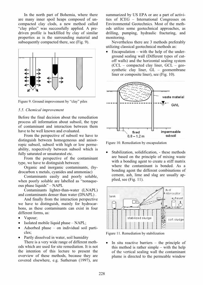
In the north part of Bohemia, where there are many inner spoil heaps composed of un-compacted clay clods, a new method called “clay piles” was successfully applied. A pre-driven profile is backfilled by clay of similar properties as is the surrounding material and subsequently compacted there, see (Fig. 9).

Figure 9. Ground improvement by “clay” piles

5.5. Chemical improvement

Before the final decision about the remediation process all information about subsoil, the type of contaminant and interaction between them have to be well known and evaluated.

From the perspective of subsoil we have to distinguish between homogeneous and anisot-ropic subsoil, subsoil with high or low perme-ability, respectively between subsoil which is fully saturated or unsaturated etc.

From the perspective of the contaminant type, we have to distinguish between:

Organic and inorganic contaminants, (hy-drocarbon x metals, cyanides and ammoniac)

Contaminants easily and poorly soluble, when poorly soluble are labelled as “nonaque-ous phase liquids” – NAPL

Contaminants lighter-than-water (LNAPL) and contaminants denser than water (DNAPL) .

And finally from the interaction perspective we have to distinguish, mainly for hydrocar-bons, as these contaminants can exist in four different forms, as:• Vapour;• Isolated mobile liquid phase – NAPL; • Adsorbed phase – on individual soil parti-

cles;• Partly dissolved in water, soil humidity

There is a very wide range of different meth-ods which are used for site remediation. It is not the intention of this lecture to present the overview of these methods, because they are covered elsewhere, e.g. Suthersan (1997), are

summarized by US EPA or are a part of activi-ties of ICEG – International Congresses on Environmental Geotechnics. Most of the meth-ods utilize some geotechnical approaches, as drilling, pumping, hydraulic fracturing, and monitoring.

Nevertheless there are 3 methods preferably utilizing classical geotechnical methods as: • Encapsulation – with the help of the under-

ground sealing wall (Different types of cut-off walls) and the horizontal sealing system (CCL – compacted clay liner, GCL – geo-synthetic clay liner, GL – geomembrane liner or composite liner), see (Fig. 10).

Figure 10. Remediation by encapsulation

• Stabilization, solidification, - these methods are based on the principle of mixing waste with a bonding agent to create a stiff matrix where the contaminant is bonded. As a bonding agent the different combinations of cement, ash, lime and slag are usually ap-plied, see (Fig. 11).

Figure 11. Remediation by stabilization

• In situ reactive barriers – the principle of this method is rather simple – with the help of the vertical sealing wall the contaminant plume is directed to the permeable window

228

– permeable reactive barrier where contami-nated water is cleaned – with the help of sorption, precipitation or degradation, see (Fig. 12).

Figure 12. Remediation by in situ reactive barriers

5.6. Foundation of new structure

After the physical and chemical subsoil im-provement there should not be great problems with the foundation of new structures, neverthe-less engineers have to be very careful about contaminants residuum because some problems with concrete degradation and steel corrosion can start.

However interesting problems are on sites where old foundations exist. This case applies to centres of major cities across the World. Throughout history mankind has been content to build new buildings on the remains of the previous ones to save the time and trouble of digging new foundations. Such examples can be found for churches, e.g. in Prague the baroque church was constructed on the gothic one. And this gothic church was constructed roughly in

the 13 century on the oldest Romanesque church from the 9 century. The discussion about utilization of old foundations is now typical of large cities as the average design life of office buildings is about fifty years. So it means that buildings constructed in the 1950´s- 1960´s are now often demolished and reconstructed. Many of these large modern buildings have been designed with wide column spacing necessitat-ing the use of deep piles or piled raft founda-tions, as was the case e.g. for London, Chow (2003). Therefore the discussion is about three options – avoid, remove, reuse. The last option is now preferred as reuse of old foundations has many positive aspects from the environmental point of view, e.g. Butcher, Powell and Skinner (2006), as this option reduces: • Use of natural resources; • Total energy used; • Potential for groundwater level changes and

groundwater pollution during construction; • Quality of waste materials produced both

during demolition and construction; • Number of vehicle and plant movements.

However before the final decision it is nec-essary in general to collect all possible informa-tion based on the available data and new inves-tigation, during technical assessment to count with ground conditions, the foundations layout and dimensions, integrity and durability and with the load capacity and performance.

The final decision therefore can recommend the old foundations reuse, reuse with repairs or augmentation, or no reuse. The decision not to use the old foundations can also be affected by the investor, asking for higher utilization of underground spaces, as for example for garages.

Especially the problem of assessment of the existing pile foundation capacity is a very complicated process and is not only based on old construction records, but has to take into account also changes in the surrounding soil with time as a result of changes of stresses induced there by loading, unloading and reload-ing.

The above discussion in principle applies also to spread foundations, which were used for old dwellings, e.g. prefab panel buildings; for farm buildings as well as for old industrial structures. Although the price for removal is not as problematic there as for pile foundations, the version of reuse is very attractive. Here the bearing capacity for subsoil composed of clays increased with time as the result of consolida-

229

tion. Also the foundation settlement induced by new loading can be rather low, as some addi-tional structural strength had chance to develop there with time for particle arrangement given by stresses from the old foundations. The possibility of foundation strengthening is easier for spread foundations. For example a combina-tion of old footings with micropiles can be a good solution.

Many practical examples for pile founda-tions are presented by Butcher, Powell and Skinner. They also discuss design of new foundations for future reuse. So it means that new foundations can have a much longer lifetime than the rest of the structure. This approach can be attractive for geological pro-file, where good subsoil is in a reasonable depth. The perimeter of the foundation pit can be constructed from a cut-off diaphragm wall and the contact with good subsoil uses the foundation slab. In this case some underground levels can be used and in future there is no problem to reinforce this slab directly or via additional piles below it.

6. PRACTICAL EXAMPLES

All over the World there is plentiful first ex-perience with construction on brownfields. However London docklands are usually men-tioned as the typical example, e.g. Berry (2003).

The London Docklands Development Cor-poration was set up by an Act of Parliament in 1981 as an urban development corporation. Its objective was to secure the regeneration of the London Docklands Urban Development Area comprising 8.5 sq miles of East London just 3 miles from one of the largest and influential financial centres of the world. This was a Government led response to a huge decline in the economy of the area brought about by the progressive closure of the docks from the 1960´s which led to the loss of 12, 000 jobs. A certain advantage there was the fact that a high proportion of the land at that time was held by public bodies.

Remediation of the site was a very difficult task as the ground was contaminated physically and chemically. Physical contamination was defined there as contamination which causes an adverse variation to the mechanical and physi-cal characteristics of the subsoil to the extent that the engineering design must take due regard of it. Chemical contamination was treated either by removal and replacement of contaminated

soil or by direct treatment in the place. By 1998 when the project ended 85, 000

permanent new jobs had been created in Dock-land, and thousands more were created during its construction. The locality completely changed its character and now can be character-ized as a part of the modern, environment friendly city, (Fig.13).

Figure 13. London Dockland – a) general view 1983 – according to Berry, b) present view – the O2 and Canary Wharf from the Royal Victoria Dock - Wikipedia

Since these days similar experience has been gained in many other countries. In the next part four examples were selected from the Czech Republic.

230

6.1. Prague – Sazka Arena

The capital of the Czech Republic Prague is not only a historical city with unique architecture in the centre but also with many heavy-machinery industries around, not so far from the centre. The brownfield site “Green island” a part of which is Sazka Arena is situated in the northeast part of Prague. For the last century this place was used by CKD company, producing there locomotives. The main activities ended there in 1994. The fundamental conception counts with redevelopment to a central multi functional complex with a congress centre, hotels, enter-tainment centre, shopping and administrative centres as sport playgrounds. The locality has very good transport accessibility by the metro system and along both sides there are tram and railway tracks.

The first part of this complex Sazka Arena was opened in 2004 with the world ice-hockey championship. The site investigation started in the phase when most of the old buildings were demolished, see (Fig. 14).

Figure 14. Prague Sazka Arena – demolition of old structures

Therefore many complications were there, especially in connection with underground structures, cables, pipelines etc. This investiga-tion proved the geological profile with the bedrock composed mainly of black clayey shale which is covered by deluvial and fluvial materi-als. The terrain is inclined in one direction to the brook passing through a small valley. Two water collectors are there, the first one in quaternary sediments and the second one in the bedrock.

Contamination of subsoil was mainly cre-ated by hydrocarbons (mostly oil), but only locally. It was approved that the bedrock was

not affected. Since the foundation slab was situated on the top of the bedrock, the recom-mended solution was rather simple. All the overlying material was excavated and treated off- site. To solve the problem of ground water, drains for gravitational dewatering was pro-posed and bentonite mattresses applied to improve the sealing capacity of the concrete slab. Great care was devoted to the cleaning of the bedrock surface to prove a very good contact with the foundation slab, (Fig. 15).

Figure 15. Prague Sazka Arena – Cleaning of the bedrock surface

Irregularities were fulfilled by concrete. Now the Sazka Arena is an integral part of the city, see (Fig. 16) and the surrounding area is under the process of reconstruction as well.

Figure 16. Prague Sazka Arena – general view

6.2. Ostrava – Karolina

Ostrava is the third larges city in the Czech Republic with 320, 000 inhabitants, situated in the northeast part of the country, close to the boundary with Poland and Slovakia. Heavy

231

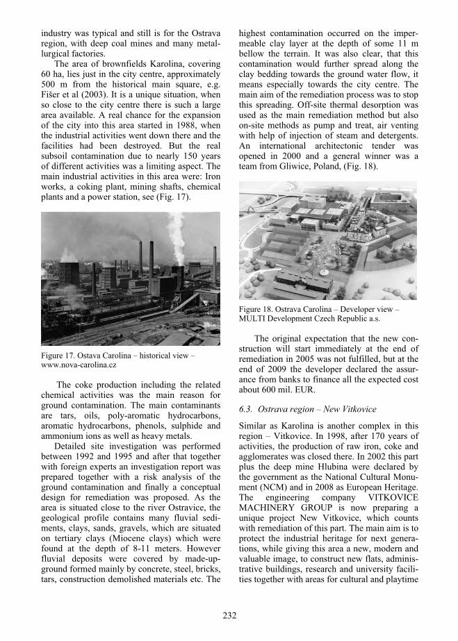
industry was typical and still is for the Ostrava region, with deep coal mines and many metal-lurgical factories.

The area of brownfields Karolina, covering 60 ha, lies just in the city centre, approximately 500 m from the historical main square, e.g. Fišer et al (2003). It is a unique situation, when so close to the city centre there is such a large area available. A real chance for the expansion of the city into this area started in 1988, when the industrial activities went down there and the facilities had been destroyed. But the real subsoil contamination due to nearly 150 years of different activities was a limiting aspect. The main industrial activities in this area were: Iron works, a coking plant, mining shafts, chemical plants and a power station, see (Fig. 17).

Figure 17. Ostava Carolina – historical view – www.nova-carolina.cz

The coke production including the related chemical activities was the main reason for ground contamination. The main contaminants are tars, oils, poly-aromatic hydrocarbons, aromatic hydrocarbons, phenols, sulphide and ammonium ions as well as heavy metals.

Detailed site investigation was performed between 1992 and 1995 and after that together with foreign experts an investigation report was prepared together with a risk analysis of the ground contamination and finally a conceptual design for remediation was proposed. As the area is situated close to the river Ostravice, the geological profile contains many fluvial sedi-ments, clays, sands, gravels, which are situated on tertiary clays (Miocene clays) which were found at the depth of 8-11 meters. However fluvial deposits were covered by made-up-ground formed mainly by concrete, steel, bricks, tars, construction demolished materials etc. The

highest contamination occurred on the imper-meable clay layer at the depth of some 11 m bellow the terrain. It was also clear, that this contamination would further spread along the clay bedding towards the ground water flow, it means especially towards the city centre. The main aim of the remediation process was to stop this spreading. Off-site thermal desorption was used as the main remediation method but also on-site methods as pump and treat, air venting with help of injection of steam and detergents. An international architectonic tender was opened in 2000 and a general winner was a team from Gliwice, Poland, (Fig. 18).

Figure 18. Ostrava Carolina – Developer view – MULTI Development Czech Republic a.s.

The original expectation that the new con-struction will start immediately at the end of remediation in 2005 was not fulfilled, but at the end of 2009 the developer declared the assur-ance from banks to finance all the expected cost about 600 mil. EUR.

6.3. Ostrava region – New Vitkovice

Similar as Karolina is another complex in this region – Vitkovice. In 1998, after 170 years of activities, the production of raw iron, coke and agglomerates was closed there. In 2002 this part plus the deep mine Hlubina were declared by the government as the National Cultural Monu-ment (NCM) and in 2008 as European Heritage. The engineering company VITKOVICE MACHINERY GROUP is now preparing a unique project New Vitkovice, which counts with remediation of this part. The main aim is to protect the industrial heritage for next genera-tions, while giving this area a new, modern and valuable image, to construct new flats, adminis-trative buildings, research and university facili-ties together with areas for cultural and playtime

232

activities (Fig. 19).In the frame of NCM activities three basic

objects will be reconstructed and protected: • Power station – central; • Blast furnace • Gas-holder

A special exposition “Universe of Technol-ogy” is proposed as a part of all the new area.

Figure 19. New Vítkovice – general view

6.4. Prague – Karlin, Rohan

The last example represents a combination of classical brownfields with a flood prone area.

During the heavy floods in 2002 this area was completely flooded. The Vltava River passing through the centre of Prague had the old river-basin in this place. About a hundred years ago this river-basin was shifted about 100 m apart. The old river-basin was refilled with gravel or permeable backfill. The bedrock is composed by shale in different phases of weathering and is overlaid by fluvial deposits of different charac-teristics and partly by man-made deposits. In this prone flood area the old structures as stocks

Small workrooms were used there in most cases.

After floods in 2002, the dike, the protection dam along river was increased to protect the area against roughly 500 year’s flood. However the protected terrain is about 3 m lower than the crest of the new dike, see the plan and cross section, Fig. 20.

When the developer started to think about future utilization two problems came forth. The first one was connected with the water level in the river Vltava higher than the surrounding terrain as a significant factor influencing the sensitivity of the dike subsoil to piping, a factor affecting the underground water table increase and a factor enabling the outlet of water from

Figure 20. Prague – Karlin, Rohan – a) Plan, b) Pumping station, c) Schematic cross section

233

the nearest brook to the river Vltava. Protection gates were constructed in the place of meeting of the brook with the river Vltava together with a pumping station to pump water when the gates are closed to the main stream.

The second problem was connected with foundation of new buildings with 3 up to 8 above-ground floorings and with proposed only 1-2 underground floorings, (Fig. 21).

Figure 21. Prague – Karlin, Rohan – Cross section through proposed buildings

In this case the ground water table under general conditions is lower than the foundation slab. When the ground water table is higher during foundation construction, a version with artificial flooding of the foundation pit was proposed. Also for the finished structure the underground floors will be flooded when the water table will be roughly 1-2 m below the terrain.

7. CONCLUSION

A brief overview of Environmental Geotechnics shows that this profession plays a very signifi-cant role in the urban development process. Environmental Geotechnics can guarantee that the plans for the urban developments will agree with the principle of sustainable development.

Construction on urban brownfields is a very sensitive process, falling fully under the term of sustainable construction. This new approach shows that an excellent technical solution is a necessary precondition, but not sufficient. Other aspects to which the modern project must apply itself to, are the environmental, sociological and architectural ones, and of course also an eco-nomic perspective because the final solution should be economically competitive.

Therefore for construction on urban brown-fields the basic technical problems were defined together with individual steps of the whole process of redevelopment. But at the same time connection to the other aspects was mentioned

as well. From the practical example it is evident that

we are on the right way to redevelop derelict or underused urban areas, to return them back as integral part of the whole city.

Acknowledgement: The work presented in this paper was carried out with funding from the MSM CR grant number 6840770005 Sustainable construction.

8. REFERENCES

Berry, R.M. 2003. The dockland experience. Vaní eket al. (eds) Proc. 13th EC SMGE, Prague, Czech Geotechnical Soc. Vol. 3, pp.293-307.

Butcher, A.P., Powell, J.J.M., Skinner, H.D. 2006. Reuse of foundations for urban sites. A best prac-tice handbook. IHS BRE Press, Bracknell, 2006. 136p.

Clark, R., Weltman, A.J. 2003. Man-made deposits - recent and ancient. State of the Art report.Vaní ek et al. (eds) Proc. 13th EC SMGE, Pra-gue,Czech Geotechnical Soc. Vol. 3, pp.77-96.

Chow, F.C. 2003. Geotechnical aspects of tunnel-ling, reuse of foundations and building on landfill in brownfield development. Vaní ek et al. (eds) Proc. 13th EC SMGE, Prague, Czech Geotechni-cal Soc. Vol. 3, pp.343-348.

Fišer et al. 2003. Remediation of the area of coking plant Karolina and its further development.Vaní ek et al. (eds) Proc. 13th EC SMGE, Pra-gue, Czech Geotechnical Soc. Vol. 4, pp.77-98.

Head ,M., Lamb, M., Reid, M., Winter, M. 2006. Theuse of waste materials in construction - progress made and challenges for the future. Feature Lec-ture. Thomas H (ed) Proc. 5 ICEG, Cardiff, Lon-don, Thomas Telford, Vol. 1,pp.70-92.

Jefferson, I. Braithwaite, P. 2009.Environmentalurban geotechnics. Culshaw,M.G., Reeves,H.J., Jefferson,I., Spink,T.W. (eds) 2009. Engineering Geology for Tomorrow's Cities. Geological Soci-ety, London, Engineering Geology Special Publi-cation, 22, 257-263.

Jessberger, H. 1996. TC5 activities -Technical Committee on Environmental Geotechnics, ISSMFE. Proc. 2nd ICEG Osaka, Jap.Geot. Soc. State of the Art Reports. Pp.1-28.

Koshelev, A., Sokolov, V., Korolev,V. 2009. As-sessment of technogenic impacts on the geologi-cal environment of big cities. Culshaw, M.G., Reeves, H.J., Jefferson, I.,

Pusch, R. 2003. Concept for disposal of radioactive waste. Lead discussion. Vaní ek et al. (eds) Proc. 13th EC SMGE, Prague, Czech Geotechnical Soc. Vol. 3, pp.239-252.

Sembenelli. P., Ueshita. K. 1981. EnvironmentalGeotechnics. State of the Art Report. Proc. 10th IC SMFE, Stockholm, Balkema, Vol. 4, pp 335-394.

234

Spink, T.W. (eds) 2009. Engineering Geology for Tomorrow's Cities. Geological Society, London, Engineering Geology Special Publication, 22, /on CD-ROM insert, Paper 164/.Vaní ek, I., Vaní ek, M. 2008. Earth Structures in Transport, Water and Environmental Engineering. Springer Science+Business Media B.V., 637 p.

Suthersan,S.S. 1997. Remediation Engineering. Design Concept. CRC. Lewis publishers, New York, 362 p.

Terzaghi, K. 1959. Soil Mechanics in Action. Civil Engineering. Vol. 69, February,pp.33-34.

Vaní ek, I. 1995, The conception and solutions of underground waste storage in excavated rock spaces. State Programme - Environmental Pro-tection. Czech Technical University, Prague, 120 p.

Vaní ek, I. 2002a. Deposition of waste material on the surface. Main Lecture, Session 4: Environmental protection. Proc. 12th Danube-European conference Geotechnical Engineering, ISSMGE, Passau, Verlag Gluckauf GmbH,Essen, pp.543-554.

Vaní ek, I. 2002b. Remediation of old landfills, old ecological burdens. Czech Technical University Press, 246 p., (In Czech).

Vaní ek, I : The role of geotechnical engineering in brownfields redevelopment. Keynote lecture.Proc. XIII. Danube European Conference on Geotechnical Engineering - Active geotechnical design in infrastructure development. Ljubljana 2006, Slovenian Geotechnical Society, editors: J. Logar, A. Gaberc, B. Majes Vol. 1, pp. 163-170. ISBN 961-90043-8-8

Vaní ek,I., Vaní ek,M. 2008. Earth Structures in Transport, Water and Environmental Engineer-ing. Springer Science + Business Media B.V., 637 p.

Vaní ek, I., Valenta, J. 2009. Examples of the use of environmental urban geotechnics for brownfield redevelopment. Culshaw, M.G., Reeves, H.J., Jefferson, I., Spink,T.W. (eds) 2009. Engineering Geology for Tomorrow's Cities. Geological Soci-ety, London, Engineering Geology Special Publi-cation, 22, /on CD-ROM insert, Paper 380/.

Vaní ek, M. 2006. Risk assessment for the case of waste utilization for embankment construction. Logar, J., Gaberc, A., Majes, B (eds) Prof. 13th Danube European Conference on geotechnical Engineering. Ljubljana, Slovenian Geot. Society, Vol. 2, pp. 799-806.

235

Excavations in the urban environment: examples from the construc-tion of Napoli underground

G.M.B., Viggiani Dipartimento di Ingegneria Civile, Università di Roma Tor Vergata, Italy

A., Mandolini Dipartimento di Ingegneria Civile, Seconda Università di Napoli, Italy

A., Flora, G., Russo Dipartimento di Ingegneria Geotecnica, Università di Napoli Federico II, Italy

ABSTRACT: This lecture presents some geotechnical aspects of excavation in the urban environment, drawingfrom recent experience gathered during construction of Lines 1 and 6 of Napoli Underground. The lecturedescribes the construction techniques that were implemented to construct the stations of Line 1, includingartificial ground freezing, and illustrates some of the analyses that were carried out to interpret the observedbehaviour of the ground and the structures during construction. In most cases, the settlements connected directlyto the main excavation were small and the largest part of the settlements derived from accessory works. Thelecture also details how the experience gathered during construction of Line 1 oriented some of the choices thatwere made in the design of Line 6.

1. INTRODUCTION

As public demand for services to improve the quality of life in the urban environment is constantly growing, almost all greater cities face the necessity of modifying the existing balance between private and public transport. With an urban population of approximately 1.2 million people, Napoli is Italy's third largest city after Roma and Milano. The population of the metropolitan area centred around the city, or Greater Napoli, is 4.4 million inhabitants according to SVIMEZ (Smarazzo, 1999) or nearly 5 million according to CENSIS (2008), for a density of population of about 1.950 ab/km², the highest in all Italian metro-politan areas and one of the most elevated in Europe.

At the end of the 1990s, Napoli public transport network still suffered from the lack of integration and poor connections, as well as from the fact that large areas of the city were not served by any underground station. As a result, Napoli had become notorious for its horrendous traffic problems with a dramatically increasing air pollution, unacceptably long travel times in rush hour, and negative effects on the city economy and public health.

In 1997, the Municipality of Napoli ap-proved a new City Transport Plan which called for a review of the network, improved controls over maintenance expenditure and general finances, a new tariff control system, and better

management of the urban rail network. The objective of the administration was that of rendering the many different functions of city life accessible through the creation of a sustain-able and extended net of public transport, such that the use of private transport may become an option rather than a necessity. These policies in the management of mobility have lead to a significant pressure for the construction of new underground train lines, stations, and car parks, together with the integration of existing lines. This implied the necessity to carry out open excavations and bored tunnels in the urban environment, often in difficult ground, such as coarse grained soils and weak rocks, and below the water table, and almost always in close vicinity of existing buildings and structures.

The ability to control displacements is cru-cial to the viability of any urban tunnelling project in soft ground as ground movements transmit to adjacent structures as settlements, rotations and distortions of their foundations, which can, in turn, induce damage affecting visual appearance and aesthetics, serviceability or function, and, in the most severe cases, stability of the structures (Burland & Wroth, 1974; Burland et al., 1977; Boscardin & Cord-ing, 1989). The need to limit ground move-ments can place significant restraints on the position in plan and level of the tunnels and the stations, resulting in more devious routing or deepening of the works to reduce near surface effects; also the methods of construction have to

236

be chosen to contain ground losses and subsi-dence. This is particularly applicable to cases where existing structures are of monumental and historical value - Napoli historic city centre is listed by UNESCO as a World Heritage Site - and thus the control of ground movements and the protection of the built environment from potential damage become the main design and construction issues.

This lecture deals with the geotechnical as-pects of excavation in the urban environment drawing from experience gathered during construction of Lines 1 and 6 of Napoli Under-ground. In both cases, the running tunnels are very deep, so that the surface effects due to their construction are negligible; the main source of potential damage on the built environment is represented by the deep open excavations required to accommodate station boxes and by shafts, passageways and accessory excavation works. This lecture describes the construction techniques that were implemented to construct the stations of Line 1, including artificial ground freezing, and illustrates some of the analyses that were carried out to interpret the observed behaviour of the ground and the structures during construction (Viggiani & de Sanctis, 2006).

The lecture also details how the experience obtained during construction of Line 1 oriented some of the choices that were made in the design of Line 6. In this case, the design was oriented at minimising ground settlements connected to accessory construction activities such as anchor installation and station tunnel enlargements, and the expected settlements due to the excavation of the stations are small. Therefore particular care was given to the measurement and control of ground movements connected to diaphragm wall installation in coarse grained soils under the water table.

2. NAPOLI UNDERGROUND

Metropolitana di Napoli, or Napoli Under-ground, is the metro system serving the city. At present, it includes six underground rapid transit railway lines, a commuter rail network, and four funicular lines, with planned upgrading and expansion work underway (see Fig. 1). With nearly 54 km of track and 69 stations currently operating and more due to open as part of the expansion plans, Napoli Underground is the second largest in Italy after Metropolitana di Milano. As of 2005, the daily ridership on

Napoli Underground was 470,000, or 29 million per year, but following the planned network expansions, this is expected to rise to over 700,000 per day by 2011.

The first railway in Naples was the Naples–Portici line, which was 7.640 km long and was inaugurated on October 3, 1839, only nine years after the opening of the world's first inter-city railway - the Liverpool and Manchester Rail-way. By the late 19th century, competing private enterprises had established various lines, primarily crossing the city east to west, with poor access to northern suburbs. In 1911, construction on the urban section of the Napoli-Roma railway was commenced and it eventu-ally opened in 1925; at present, this urban section of the Napoli-Roma train line is still part of Line 2 of Napoli Underground. At the end of World War II, the metropolitan rail network of Naples consisted of five urban and some subur-ban lines which were poorly connected with each other: Ferrovia Cumana and Circumfle-grea, Ferrovia Circumvesuviana, Ferrovia Alifana (now MetroCampania Nord-Est) and Metropolitana Trenitalia.

The idea of a fully integrated urban rail net-work for Naples was first proposed in the 1950s as part of the post-war regeneration of the city. Plans were first formulated in the 1960s, but funding, planning and development problems and crime and corruption all caused long delays. Construction began in 1976, and it was hoped that a line connecting central Napoli to Stadio San Paolo in the borough of Fuorigrotta would be completed in time for the 1990 FIFA World Cup competition in which Napoli was a host city. A 2.2 km section with two stations at the western end of the line was completed in 11 months, however the line was not able to operate during the World Cup. This part of the line is currently being integrated as part of Line 6.

Napoli first rapid transit line opened in 1993, running for 4 km between Colli Aminei and Vanvitelli station; two years later the line was extended to reach Piscinola station for an overall track length of 8 km (Briginshaw, 1999).

The 1997 City Transport Plan included three main phase of redevelopment. Phase 1 consisted of an expansion to five lines, with major rede-velopments of Line 1, to take the network up to 53 km of track (45 km of existing lines), with 68 stations (23 newly built), and 12 interchange nodes, which was completed by 2002. Phase 2 was designed to increase the network to 7 lines,

237

Figure 1. Napoli Underground network: present situation.

with 84 stations, and 16 interchange nodes, and is currently under way. Phase 3 will see the network expanded to 10 rail lines with 93 km of track, and a further 30 km of new light rail linking 114 stations, with 21 interchanges. Once the plan is completed, 70% of Neapolitans should be living within 500 meters of a trans-port access point. In the following, attention will be focused on Phase 2 construction works of Line 1, nearly completed, and Line 6, cur-rently under way.

3. LINE 1

The final route of Line 1 consists of a closed ring connecting the North outskirts of the city, the area of the hills, the historical centre, the administrative district, and the airport, for a total length of about 30 km and 25 stations (see Fig. 2). About one half of the line, the so called Tratta Alta, between Piscinola and Dante stations, has been constructed during Phase 1, with a very positive impact on the traffic at surface; an estimated 40,000 people/hour in rush hour should travel on the line once com-pleted (Cascetta, 2000).

The construction of the Tratta Bassa, about 6 km long and currently nearly completed, has proved more problematic. The five stations

included in this part of the route, namely Toledo, Municipio (Town Hall), Università, Duomo and Garibaldi (Main Railway Station), have required very deep open excavations in coarse-grained soils below the water table (up to a maximum of 30 to 35 m), in a densely built urban environment, characterized by the pres-ence of many buildings of historical and artistic value at the surface. Furthermore, significant direct interferences between the line and impor-tant buried archaeological remnants have arisen during excavation: at Dante Station the works were interrupted when they hit the city walls of the Greek Neapolis, the headworks for Mu-nicipio Station exposed part of the structures of the Roman port of the city, dating to the II century, with the recovery of at least three roman ships, and at Duomo Station a medieval fountain from the XIII century and a Roman building of Imperial age with important decora-tions and mosaic floors were uncovered by excavation. In fact, in this case, the original design had to be changed to accommodate for the outstanding archaeological findings, and the completion of this station is lagging behind the rest of the line.

For all the reasons above, construction of the line was accompanied by an intense pro-gram of monitoring designed to measure and/or

238

Figure 2. Plan view of Linea 1 of Napoli Underground.

control the effects of excavation on the adjacent structures. This included the measurement of the displacements of existing buildings, of the ground surface behind the excavations, and of the retaining structures; of any changes in the groundwater regime; of the forces in the an-chors used to support excavations.

3.1. Ground conditions

Figure 3 shows the soil profile and groundwater conditions along the route of the Tratta Bassa (Viggiani and de Sanctis, 2006). All the natural deposits within the depth of interest are geo-logically recent and were formed in a relatively short period of time. The Yellow Tuff and the Pozzolanas were deposited during the second active phase of the volcanic complex of the nearby Phlegrean fields (or II period according to De Lorenzo, 1904) about 12,000 years ago, as pyroclastic flows, or hot masses of ashes, pumices, rock fragments and gases moving rapidly along the ground surface in response to

gravity, filling the existing valleys and ditches and then growing in thickness, as different eruptions put in place more materials. The fact that the materials are deposited at high tempera-ture, induces the formation of hydrated alumi-nosilicates such as zeolites, inducing interparti-cle bonding. In this case, both deeper cemented deposits (Tuff) and granular deposits (Poz-zolanas) at shallower depths were formed. The Neapolitan Yellow Tuff is characterized by the presence of a system of randomly distributed sub-vertical fractures, locally known as scarpine, connected to the progressive cooling of the pyroclastic mass with the emission of trapped gas.

During the following rest period of about 2000 years, the pyroclastic materials were eroded, transported, and re-deposited. The remoulded Pozzolanas are very well graded and not easily recognised from the intact pyroclastic deposits. They appear layered, sometimes interbedded with in situ Pozzolanas, sometimes

239

Figure 3. Line 1: geotechnical profile along tunnel axis.

with marine sand deposits, such as in the area of Municipio Station. A deep erosion ditch exist-ing near Duomo Station is filled with remoulded Pozzolana.

A new active phase of the Phlegrean Fields (III De Lorenzo Period), this time explosive, deposited the so called Neapolitan Pyroclastic Pile, consisting of easily eroded alternating layers of pumices, ashes, pozzolanas, and lapillus. In the city the thickness of the Pyro-clastic Pile, where not eroded, is about 15 m. The eruptions of Mount Vesuvius, even major ones such as the Plinius eruption of 79 A.D., contributed little to the subsoil of Napoli.

The pyroclastic deposits are overlain by sands or silty sands of marine or fluvial-palustrine origin. The whole area between Piazza Municipio and Piazza Garibaldi was below sea level. Depending on the distance from the coast line, the conditions of deposition were either marine or palustrine; in the area of Municipio Station the deposits are of shallow sea depositional environment. In the final segment of the Tratta Bassa the thickness of the marine deposits increases gradually due to the accumulation of the pyroclastic products of the III Phlegrean Period transported and re-deposited in the water.

Most of the areas near the coast derive from reclamations carried out in historical times, between 1400 and the late 1800; quite meaning-fully, up to relatively recently, the area of the central railway station was known as Paludi, the Italian word for swamps. This is reflected in the thickness of the made ground, in some areas larger than 10 m. Because of the close vicinity to the sea, the water table is relatively close to ground level.

3.2. Design issues

The preliminary design of the part of the line

between Duomo and Garibaldi stations con-sisted of shallow tunnels constructed by cut-and-cover. At a later stage, it was decided to bore the tunnels within the Yellow Tuff forma-tion, with the main advantages of minimising direct interferences with the archaeological layer and the surface, which is restricted solely to the stations, and, due to the good mechanical properties of the tuff, reducing the settlements and the potential damage induced at surface. In this manner it was possible to cross a densely built environment without significant interfer-ences with existing structures and infrastruc-tures and very limited disruption of transport at surface during construction (Viggiani, 2000).

The main drawback associated to this design is the fact that a long part of the line is well below ground water table with hydraulic heads between 25 and 30 m. The very high pore pressures, together with the random occurrence of scarpine in the tuff, have made it necessary to bore the tunnels with closed shield earth pressure balance machines, while the station tunnels were enlarged by conventional mining with the aid of artificial ground freezing, chemical injections and cement grouting. The stations were excavated within reinforced concrete diaphragm walls supported by steel tubular props at the surface and several levels of pre-stressed anchors; protective measures were adopted to minimise the effects of anchor installation below the water table.

Further interferences of the line with ground water table may arise in exercise. Between Università and Garibaldi Stations, in fact, the tunnels are orthogonal to the direction of the ground water flow towards the sea, and may potentially restrict the water flow causing ground water surges, or backwater, with nega-tive effects on the existing structures. Pore water pressures in the potentially affected area

240

Figure 4. Plan view of Garibaldi Station.

were carefully monitored to define accurately the hydraulic boundary conditions and seepage analyses were carried out to show that the potential surges are relatively small.

In the urban area, a complex and largely unmapped network of cavities exists within the Tuff formation; these are mostly man made cisterns, aqueducts and abandoned quarries. Along the Tratta Bassa, however, the tunnels are very deep and it is unlikely that they might intersect any significant man made cavity; only in the initial part of the line, between Dante and Toledo, do the tunnels run at relatively shallow depths and above the ground water table. In this case the tunnels intersect a very well known cavity or Carceri di San Felice for which very detailed studies were carried out (Viggiani, 2000).

3.3. Deep excavations

The open excavations required to build the stations of the Tratta Bassa have a maximum depth ranging between 35 and 50 m b.g.l., and a typical plan area of about 1000 m2. They are

excavated in a very densely built environment through cohesionless granular deposits with a thickness between 20 and 30 m and then in a fissured soft rock, under water tables at 30 to 35 m above the bottom of the excavation. These are very major works requiring adequate con-struction techniques.

Support for the excavations is provided by reinforced concrete diaphragm walls excavated using a hydromill, in 2.5 m wide, 1 m thick panels, typically supported by steel tubular props at the surface and 4 to 6 levels of pre-stressed anchors. In some cases, to restrain further ground movements, the floor slabs of the station boxes were constructed top-down as excavation proceeded; this support system was adopted when the buildings at the soil surface were located very close to the excavation area, as e.g. in the case of Garibaldi Station.

Enlargement of running tunnels to accom-modate platforms and excavation of inclined access passageways, both in conventional mining, are also part of station construction. Platform tunnels are generally contained within

241

Figure 5. Cross section of the station box (at position of inclinometer S2).

the Neapolitan yellow tuff, while inclined passageways run, at least partly, in the granular soils.

This part of construction was carried out with the aid of Artificial Ground Freezing. The technique consists of driving freeze tubes into the ground parallel to the tunnel length around the future excavation section, and then circulat-ing a refrigerating fluid into the tubes until the temperature of the ground around the tubes is below the freezing point of the groundwater. The refrigerating fluid can be Nitrogen, liquid at about -196°C and then exhaust as gas in the atmosphere, or brine (calcium chloride) at about - 35°C which is generally re-circulated through a refrigeration plant. The contractor specified that construction of both platform tunnels and inclined passageways should be undertaken within 1 m thick frozen collars with external surfaces at a temperature of -10°C.

The frozen collar serve static purposes for the inclined tunnels and water proofing purposes for both platform tunnels and passageways.

4. GARIBALDI STATION

The new Piazza Garibaldi station was con-structed within a 44 × 20 m2 rectangular exca-vation, with a maximum depth of 45 m b.g.l., protected by 1 m thick concrete diaphragm walls, excavated using a hydromill, in 2.5 m wide panels, see Figures 4 and 5. Four floor slabs, constructed top-down as excavation proceeded, provided support in the upper part of the excavation, while in its lower part six levels of anchors with lengths between 12 and 31 m were installed. At the top of the retaining walls, one level of tubular steel props further restricted wall movements. The sequence of main construction phases for

242

Table 1. Construction phases of Piazza Garibaldi Station.

# Description Date 1 Install diaphragm wall 19.10.02 2 Inst. 1st level of support + exc. to 3.3 m asl 10.12.02 3 Install first floor 19.02.03 4 Excavate to -2.7 m asl 17.06.03 5 Install second floor 18.07.03 6 Excavate to -6 m asl + drill anchor level A 22.08.03 7 Pre-stress anchor level A 11.09.03 8 Excavate to -8.7 m asl 30.09.03 9 Install third floor 04.11.03

10 Exc. To -12 m asl + drill anchor level B 18.11.03 12 Pre-stress anchor level B + drill anchor level C 28.02.04 13 Pre-stress anchor level C 08.03.04 14 Excavate to -14.7 m asl 30.03.04 15 Install fourth floor 00.05.04 16 Excavate to -19.7 m asl & drill anchor level D 19.06.04 17 Pre-stress anchor level D 10.07.04 18 Excavate to -24m asl & drilling anchor level E 31.08.04 19 Pre-stress anchor level E 14.09.04 20 Excavate to -28.5 m asl + drill anchor level F 28.09.04 21 Pre-stress anchor level F

Garibaldi Station box is summarised in Table 1.The presence of adjacent structures is unavoid-able in such a dense urban environment as Napoli; in this case, two relatively big residen-tial masonry buildings, 37 × 74 m2 size in plan, of 5 and 7 storeys, are located very close to the station box, at a minimum distance of about 3.6 m (see Figs 4 and 5).

4.1. Local ground conditions

Ground conditions along the route of the Tratta Bassa are very variable, both horizontally and vertically. In this area, starting from ground level and moving downwards, the subsoil profile consists of made ground and remoulded ash underlain by remoulded ash and alluvial and/or in situ pyroclastic sand (Pozzolana) over a base layer of yellow Neapolitan tuff (Man-dolini et al., 2004).

Figure 6 details the soil profile and the main physical (voids ratio, e0, dry density, γd, and density at the natural water content, γ) and mechanical properties (SPT blow-counts, CPT profiles, and friction angles from laboratory tests) of the ground in the area of the new Garibaldi Station, as obtained from site and laboratory investigations carried out since 1997. This included tens of boreholes formed in the vicinity of the station with SPT tests about every three meters and retrieval of disturbed-

samples for testing in the laboratory and CPT tests close to the excavation. The groundwater table is hydrostatic at about 9.5 m b.g.l.

4.2. Monitoring

An intense programme of monitoring was set up to control construction and mitigate and/or prevent the effects induced by excavation on the surrounding buildings. The layout of instru-ments is represented schematically in Figure 5. Monitoring activities included the measurement of: horizontal displacements of the diaphragm walls delimiting the station box, by means of 6 inclinometers; hydraulic head, by means of 10 Casagrande piezometers installed along the perimeter of the excavation and of one stand-pipe within the excavated area; anchor forces at installation and in working conditions, by means of 15 load cells; settlements of the ground and buildings adjacent to the excavation works, by precision levelling of 18 reference points.

Figure 7 shows the deflected wall profiles measured by inclinometers S1 and S2 at differ-ent dates during excavation. As a consequence of some faulty operation, inclinometer S2 was damaged at the end of construction phase n. 16. Therefore, the total deflections of the wall at the end of the excavation (construction phase n. 22)

243

10 12 14 16 18 20γ, γd (kN/m3)

30

20

10

00 0.5 1 1.5

e0

γγd

e0

0 10 20 30 40 50qc (MPa)

0 10 20 30 40 50NSPT

30 32 34 36 38 40 42ϕ'

NSPT

ϕ' (triaxial tests)

Made groundγ=19 kN/m3

ϕ=30

Cohesionless pozzolanaγsat=17 kN/m3

e0=1.10ϕ=33k=10-5-10-3 cm/s

Sand sea bed depositsγ=18 kN/m3

e0=0.49ϕ=38k=10-2 cm/s

Lower pozzolanaγ=17 kN/m3

e0=1.06ϕ=38k=10-5-10-3 cm/s

Volcanic Tuffγ=17 kN/m3

e0=1.22ϕ=28k=10-4-10-5 cm/s

Figure 6. Soil profile, physical and mechanical properties from in-situ and laboratory investigations at Garibaldi Station.

are only available at the position of inclinometer S1.

From construction phase n. 4 onwards, the magnitude of the horizontal displacements measured by both inclinometers S1 and S2 increases substantially and the classical bulging shape characterizes the deflected wall profiles. The maximum measured wall deflection was about 35 mm at a depth of about 20 m b.g.l., and was measured at inclinometer S2 during construction stage n. 14. After reaching a depth of excavation of about 24 m b.g.l. the deflec-tions of the wall did not increase any more. Because inclinometers S1 and S2 were installed within the panels, the measured deflections only represent ground movements after wall installa-tion.

Figure 7. Inclinometer profiles S1 and S2.

The settlements of the buildings in a number of reference points installed close to the station box are plotted in Figure 8 as a function of time.

-30

-25

-20

-15

-10

-5

0

5

Nov

-02

Jan-

03

May

-03

Aug-

03

Nov

-03

Feb-

04

May

-04

Aug-

04

Nov

-04

B4

B5

B11

B12

w [

mm

]

Building A

-35

-30

-25

-20

-15

-10

-5

0

5

B7

B5

B16

B15

w [

mm

]

Building B

Figure 8. Foundation settlements measured after completion of excavation.

The base reading for surface settlements was taken after completion of wall installation, so

244

the measurements cannot shed any light on the magnitude of ground movements due to wall installation. The maximum absolute settlement connected to excavation (wmax ≅ 31 mm) was recorded at reference point B6, installed near the corner of Building B. At the early stages of construction the rate of settlement was in the range 1÷2 mm/month. During construction stage n. 10 (excavation at –12 m a.s.l.), carried out in mid November 2003, the observed rate of settlement suddenly increased to about 25 mm/month. This was connected to significant water and soil flow into the boreholes drilled to install anchor level B. As these were put in place and injected while the casing of the hole was retrieved, large amounts of water and soil were flowing out of the holes, creating localised ground loss and therefore subsidence immedi-ately beneath the foundations of the adjacent buildings. After changing the technique to install the anchors the rate of settlements de-creased back to about 2.5 mm/month. The observed settlements (w/H ~ 0.1%, H = maxi-mum excavation depth) are in good agreement with the experimental data reported by Clough and O’Rourke (1990) for similar retaining structures in coarse grained ground (w/H =0.1÷0.2%) and smaller than those corresponding to damage in the buildings (βmax=1.23×10-3).

-5

5

15

25

35

0 10 20 30 40Distance from the wall [mm]

Building B -Alignment B6-B14Building A -Alignment B5-B13

w [

mm

]

Figure 9. Ground surface profiles recorded at con-struction phase n. 18 (see Table 1).

Figure 9 illustrates the settlement profiles of alignments B6-B14 and B5-B13 (see Figure 5) at the end of August 2004, or construction phase n. 18. They did not increase significantly during subsequent construction phases, and, therefore, they can be considered well representative of the surface settlement at the back of the wall

due to the main excavation.

4.3. Numerical analyses of the main excavation

Many factors affect the numerical prediction of ground movements associated with excavations: the choice of an adequate constitutive model for the soil, the correct definition of the soil profile, the selection of representative mechanical properties for each layer, the definition of appropriate ground water conditions and initial stress states, the representation of the structural geometry and boundary conditions, and the modelling of the sequence of construction phases. Each stage of the process requires approximations and simplifications of the physical problem under examination, which will affect the results of the analyses to a greater or lesser extent.

The analyses described below (de Sanctis etal., 2006) were carried out in plane strain condition using version 6.4 of the commercial finite element code ABAQUS. The analysed section of the station box corresponds to the position of inclinometer S2.

The ground was taken to behave fully drained both during installation and subsequent excavation; for construction phases in which the bottom of the excavation was below groundwa-ter table, pore fluid pressures were calculated for steady state seepage with the following hydraulic boundary conditions: impervious wall, pervious boundary at the bottom of the excavation with zero pore water pressure, impervious boundaries at the sides and at the base of the mesh, constant hydraulic head at the back of the wall, corresponding to the hydro-static condition before excavation. Table 2. Anchor forces.

Anchor level Force, kN/m A 537 B 386 C 286 D 868 E 929 F 806

The soil was assumed to behave like a linear elastic – perfectly plastic material with Mohr-Coulomb failure criterion while the diaphragm wall was modelled as a linear elastic solid with a Young´s modulus E = 31.2 GPa and a Pois-son´s ratio ν = 0.15.

Anchors were modelled as constant nodal

245

forces, see Table 2; this is because the meas-urements of anchor forces at installation and in exercise showed that there was less than 6 % variation from the initial value as excavation proceeded below each anchor level. Floor slabs were modelled as linear springs whose stiffness was obtained by finite element analyses of the floor slabs to take into account their geometry with irregular openings for mucking, see Ta-ble 3. Table 3. Stiffness of floor slabs.

Slab EA, kN/m K, kN/m/m 1 1.68·106 1.58·105 2 1.86·106 1.75·104 3 1.68·106 1.58·105 4 1.86·106 1.75·104

The friction angles of cohesionless layers were obtained from in situ and laboratory tests. The values of cohesion and friction angle for the yellow tuff were derived from a few available results of unconfined compression tests and published data. Interface elements within the tuff were given cohesion of 20 kPa and no tractions were allowed between the wall and the tuff.

Elastic modules of the different layers were obtained by back analyses of wall deflections according to the following procedure: the relative stiffness of the different layers was evaluated first, based on the results of site cone and standard penetration tests (CPT, SPT) and then the absolute value of the stiffness of each layer was fixed by fitting the wall deflection profile measured by inclinometer S2 at stage n. 16. The above procedure was applied in analy-ses where the process of slurry trenching and concreting was modelled (WIM, or Wall Instal-lation Modelled analyses).

Recent experiences of diaphragm walls built in Singapore (Poh et al., 2001) showed that there is a significant effect of the width of the panels on the magnitude of the horizontal displacements of the ground during installation. In particular the maximum horizontal displace-ment increases as the area of the lateral surface of each excavated panel increases. Because they are carried out in plane strain conditions, WIM analyses modelled wall installation as the excavation of an infinitely long slot, and, therefore, installation effects are likely to be overestimated.Figure 10 shows the deflected wall profile

161410

T

WIM analysis

-37.5

-32.5

-27.5

-22.5

-17.5

-12.5

-7.5

-2.5

2.5

7.5

12.50 10 20 30 40 50

u [mm]

z [m

asl

]

Measureddeflections

Figure 10. Ground surface profiles recorded at construction phase n. 18 (see Table 1).

obtained from WIM analyses. In order to compare with the measured values, the com-puted horizontal displacements are increments relative to the end of the installation stage. The match between the predicted and expected deflections is satisfactory, with the exception of the upper part of the diaphragm wall (z = 0 ÷ 10 m b.g.l.), where the measured displacements are nearly constant (w ≅ 5mm) while the com-puted values increase almost linearly from a minimum value of about 4 mm at surface to about 20 mm at a depth of 10 m b.g.l.

WIM

-5

0

5

10

15

20

25

30

0 10 20 30 40Distance from the wall [mm]

Building B - B6-B14

Building A - B5-B13

w [

mm

]

Figure 11. Predicted and observed settlements at the back of the wall.

246

An estimate of the settlements of the buildings induced only by excavation can be obtained correcting the plots of Figure 8 to subtract the sudden increase of settlements observed at construction stage n. 10. Figure 11 summarizes the comparison between the surface displace-ment predicted at the back of the wall and the observed values corrected to eliminate the sudden increase recorded during installation of anchor level B. The agreement is very satisfac-tory with the exception of distances from the wall smaller than 10 m. When the loads trans-mitted by the adjacent buildings to the ground (about 60 kPa, in plane strain conditions) were included in the analyses, the pattern of com-puted surface settlements at the back of the wall did not change substantially.

Figure 12. Temperature changes recorded during construction.

A very substantial improvement of the pattern of the predicted deflections of the wall was obtained when thermal effects were explicitly considered in the analyses. Significant changes in temperature were recorded during construc-tion as shown in Figure 12. These temperature changes affect primarily the tubular steel props at ground level and floor slab 1 (see Figure 5), i.e. those support elements directly exposed to sun radiation.Table 4. Temperature changes corresponding to thermal distortions applied in the analyses.

Period ΔT, °C January-July 2003 ~ 20

September-December 2003 ~ -20 January-August 2004 ~ 20

WIM analyses were carried out in which three uniform thermal distortions corresponding to the changes of temperature summarised in

Table 4 were applied to the two up-most levels of support. The results of these analyses corre-spond to the deflection profile labelled T in Figure 10 and are in very good agreement with the experimental observations.

4.4. Platform tunnels. Effects of artificial ground freezing

The excavation of the station box began in October 2002 and was completed nearly exactly two years later, in October 2004. The working activities for the platform tunnels began, ap-proximately, after completion of the main excavation, in the mid of October 2002. At present, all four station tunnels and inclined passageways have been successfully completed.

Even if the platform tunnels crown is always below the roof of the Neapolitan Yellow tuff, artificial ground freezing was implemented as a protective measure before excavation. In this case, the intention was to create an impermeable collar around each tunnel in order to prevent water flow into the excavated area from the existing system of sub-vertical fractures known as scarpine and previously mentioned. Figure 13 shows the location of the freezing pipes around the tunnel. Ground temperatures during the freezing stages were measured using thermo-couples installed in observation holes.

Figure 13. Location of the freezing pipes around a platform tunnel.

Figure 14 illustrates the foundations settlements for building B recorded at various construction phases, including those for ground freezing, bottom sealing treatment and excavation of the platform tunnel. Some heave was ob-served at the ground surface, clearly connected to the

0

5

10

15

20

25

30

35

40

12-0

2

06-0

3

01-0

4

08-0

4

02-0

5

09-0

5

T [°

C]

247

Figure 14. Settlements of reference points by preci-sion levelling.

freezing phase (Nov 2004 - July 2005). The complete displacement history of refer-

ence point B8, belonging to the vertical section located in the mid of tunnel B1, is shown in Figure 15, as an example. During excavation and subsequent installation of permanent lining in frozen ground the settlements of the building increased and continued to increase, at a quite dramatic gradient, as thawing proceeded. This was probably due to a combination of the effects of thawing and water flow into the excavated area through the imperfections of the ice lining and particularly at the connection between the diaphragm wall and the station tunnel. Such unfavourable trend of the settle-ments at the ground surface appeared incom-patible with the safety of the existing buildings and, consequently, their foundations were underpinned by micropiles.

Ground freezing also affected wall deflec-tions and hence the loads of anchors. This phe-

Punto B8Edificio lato CDN

(2)

(7)(6)

(5)

(4)

(3)(1)

-50,0

-40,0

-30,0

-20,0

-10,0

0,0

nov-

02

mag

-03

nov-

03

mag

-04

nov-

04

mag

-05

nov-

05

mag

-06

nov-

06

cedi

men

ti [

mm

]

Nov

-02

May

-03

Nov

-03

May

-04

Nov

-04

May

-05

Nov

-05

May

-06

Nov

-06

(1) (2) (3)

(4)(5)

(6) (7)

0

-10

-20

-30

-40

-50

Punto B8Edificio lato CDN

(2)

(7)(6)

(5)

(4)

(3)(1)

-50,0

-40,0

-30,0

-20,0

-10,0

0,0

nov-

02

mag

-03

nov-

03

mag

-04

nov-

04

mag

-05

nov-

05

mag

-06

nov-

06

cedi

men

ti [

mm

]

Nov

-02

May

-03

Nov

-03

May

-04

Nov

-04

May

-05

Nov

-05

May

-06

Nov

-06

(1) (2) (3)

(4)(5)

(6) (7)

0

-10

-20

-30

-40

-50

Figure 15. Settlements of reference point n. 8 (‘Side CDN’ Building). (1) and (2): Installation of anchors; (2) and (3): Ground freezing; (4): Excavation of platform tunnel; (5): Permanent lining installation; (5) and (6): Thawing; (7): Corrective measures by underpinning.

nomenon was probably due to the formation of a continuously growing ice lens behind the diaphragm wall, due to the frozen front attract-ing water, because of the suctions developed around the frozen fringe.

5. MUNICIPIO STATION

The new station in Piazza Municipio was constructed within a 23.4 × 49.2 m2 rectangular excavation, with a maximum depth of 38 m b.g.l., protected by 1 m thick concrete dia-phragm walls, excavated using a hydromill, in 2.5-2.8 m wide panels, see Figures 16 and 17.

The excavation was supported by six levels of anchors with lengths between 11 and 18 m. To further restrict wall movements one level of tubular steel props was added at the top of the retaining wall as for the case of Piazza Gari-baldi. The anchors are temporary support systems for the excavation, permanent struc-tures of the station have been designed to sustain the whole earth pressure in exercise. The sequence of main construction phases for Municipio Station is summarised in Table 5.

5.1. Local ground conditions

The subsoil profile in the area of the new Municipio Station is similar to that found at Garibaldi Station. It consists essentially of made ground and remoulded ash underlain by re-moulded ash and alluvial and/or in-situ pyro-clastic sand (Pozzolana) over a base layer of yellow Neapolitan tuff. The groundwater table is found at a depth of 7 m from the ground surface corresponding to 2.0 m a.s.l.

The geotechnical investigations included tens of boreholes formed in the vicinity of the station with SPT tests and retrieval of disturbed samples for testing in the laboratory and CPT tests close to the excavation box. The made ground is around 9 m thick and consists essen-tially of a matrix of pyroclastic sand incorporat-ing fragments of rubbles and Neapolitan tuff. Below the made ground a layer of remoulded ash mixed with marine sand is found between 2 and -2 m a.s.l. At greater depth and down to about -11 m a.s.l. there is a low sea deposit of marine sand. The total thickness of the cohe-sionless granular materials over the yellow Neapolitan tuff amounts to about 21 m. Results from boreholes highlight that the roof depth of the Neapolitan tuff is somewhat variable,

248

Figure 16. Plan view of the Municipio Station.

Figure 17. Cross section and subsoil conditions at Piazza Municipio.

standing between -18 to –22 m a.s.l. (see Fig. 17).

5.2. Monitoring

The layout of instruments is schematically shown in Figure 16. Monitoring activities included the measurements of: hydraulic head by means of Casagrande piezometers installed along the perimeter of the excavation; anchor forces at installation and in working conditions by means of load cells; settlements of the

ground and buildings adjacent to the excavation works by precision levelling.

In the case of Piazza Municipio a very im-portant 5–storey masonry building, the seat of the Administrative Court, is situated in prox-imity of the station box at a distance of about 9 m. The settlements of this building were measured in a number of reference points. Figure 18 reports the time-displacements plots recorded during excavation. The base readings for settlements was taken after the completion

249

Figure 18. Time-displacements plots for some reference points.

of wall installation, so the measurements cannot provide any information on the ground move-ments due to the installation of the panels. As for Garibaldi Station, a sudden increase of settlement was observed during the installation of an intermediate anchor level (anchor level E). Again, such an increase was due to water and soil flow into the boreholes drilled to install the anchors.

Figure 19. Hydraulic head measurements behind the panels during construction.

Figure 19 details the measurements of the hydraulic head at the back of the wall recorded during the various construction phases. The abrupt changes in hydraulic head recorded in the mid of May 2005, i.e. during installation of anchor level E, are clearly related to the unex-pected increase of settlement that has been

already discussed.

5.3. Platform tunnels. Effects of artificial ground freezing

At present all four platform tunnels at Mu-nicipio station have been successfully com-pleted with the aid of artificial ground freezing. As an example, some data from the construction of tunnel A1 are described in the following. This is about 60 m long. Horizontal freeze–tubes were installed to protect tunnel excavation within a 1 m thick frozen collar of Neapolitan tuff, see Figure 20.

Figure 20. Freezing-tubes and observation holes arrangement for tunnel platform A1.

The thermal properties of the frozen pyroclastic deposits for numerical analysis were obtained by back analysing the behaviour observed on a trial site including several vertical freezing tubes and observation holes for the measure-ment of ground temperatures in cycles of freezing and thawing.

Transient heat propagation is a very non lin-ear problem as the thermal diffusivity of ice is about eight times that of liquid water, and the propagating ice front separates the dominium in two regions with very different thermal proper-ties; in this case the problem was tackled numerically, using the FE code ABAQUS (Viggiani and de Sanctis, 2006).

In the case of piazza Municipio freezing was activated with nitrogen and maintained with brine. This permitted to reduce the times re-quired for the formation of the frozen collar of a few weeks and to overcome the main reason for incomplete or inadequate ground freezing that is the excessive seepage of water in the vicinity of the ice barrier, while containing the mainte-nance costs. At the end of the nitrogen activa-

250

tion phase, before brine can be circulated in the freeze tubes the temperature of the ground immediately around the freeze tubes has to rise to -40° C, otherwise the brine would freeze in the tubes. In the time interval before circulating brine the frozen front continues to expand due to thermal inertia.

Figure 21. Temperature contours computed at different stages of the freezing plan: (a) predicted temperatures at end of the activation with nitrogen and (b) temperatures computed after 9 days of maintenance with brine (NT11 = nodal temperature variable).

The predicted temperature contours at the end of activation with nitrogen and after 9 days of maintenance with brine are shown in Figure 21.

Figure 22. Ice wall defined by the contour at -10°C.

Due to the misalignment of the freeze tubes, the real ice wall, whose extent is defined by the contour at –10°C, as measured by the thermo-couples in the observation holes is much less regular than that predicted by numerical analy-sis. In particular, closer to the diaphragm wall a thinner ice wall was observed as shown in Figure 22.

The settlements of the adjacent buildings did not change significantly during ground freezing around the first tunnel to be excavated. This is probably due to the fact that the lowering of the ground water table due to the water flow to-wards the tunnel did not exceed the lowering already experienced during the main excavation phase, due to the installation of anchor level E.

6. LINE 6

At present, Line 6 only connects the borough of Fuorigrotta with that of Mergellina, but exten-sions to the line are under design to reach the eastern borough of Bagnoli and under construc-tion to connect with the city centre at Municipio Station (see Fig. 23), for a total final length of about 8 km and 12 stations.

Figure 23. Overview of Line 6.

The design of the eastward part of the line, approximately 3 km long with 4 stations, should be completed within 2011 and construction should start in 2012. About 2 km of the line, between Politecnico and Mergellina Stations, have been constructed and are operating since February 2007. The line follows in part the route of the old Linea Tranviaria Rapida (Fast Tram Line), begun in 1980s and later aban-doned. In 2006 preliminary work began on the 3 km extension of the line to Municipio, where work is under way on Line 1. Figure 24 shows in more detail this part of the line and the location of its four stations, namely Arco Mirelli, San Pasquale, Chiaia and Municipio.

251

Figure 24. Detail of eastwards extension of Line 6 currently under construction.

The first three are under construction, while the works for the connection with Line 1 at Mu-nicipio have not begun yet. The estimated number of daily travellers on Line 6 will be about 154,000, for a yearly figure of about 46 million passengers.

Similarly to the stations of the Tratta Bassa of Line 1, the open excavations required to build Arco Mirelli and S. Pasquale Stations are very deep and have to be created through coarse-grained soils below the water table. In fact, in this part of the city, the roof of the tuff layer is at an even deeper level than in the area of the Tratta Bassa, at about 30-40 m b.g.l., and the water table closer to the ground surface, at about 1-2 m b.g.l., as the line runs very close to the sea coast. In both cases, the open excava-tions required to accommodate the stations are very close to buildings of historical and artistic value. Line 6 proceeds towards Piazza Mu-nicipio passing very close to one side of Palazzo Calabritto and under the Pizzofalcone hill. The deep station of Chiaia is located under Piazza S. Maria degli Angeli; this is above groundwater level and it will be excavated mostly in the tuff. The most significant design issue for this station is the high probability to meet large urban cavities in the tuff above the groundwater table.

Large ventilation shafts will also be con-structed along Line 6. The tunnel between via Piedigrotta and Municipio will be excavated with a new TBM; an old TBM which was used to excavate the first stretch of the line between Fuorigrotta and Mergellina has been carefully demolished after a challenging program of soil treatment which was used to render the provi-sional tunnel face stable and watertight.

6.1. Ground conditions

Figure 25 shows the soil profile and groundwa-ter conditions along the part of Line 6 currently under construction, together with the position of the tunnel and of the stations. The ground conditions of the eastern part of the route, between Mergellina and Pizzofalcone Hill, are completely different from those on the western part of the route, between Pizzofalcone Hill and Municipio. In the eastern part of the route a thick layer of granular soils, i.e.: made ground underlain by marine sands, remoulded ash and in-situ Pozzolana, rests on top of tuff and the roof of the tuff layer is very deep and erratic, probably due to past erosive action of superfi-cial running water coming from the hills sur-rounding the bay. In the western part, the tuff layer raises to ground level or at relatively shallow depth, posing much less design prob-lems.

The marine sands are usually dense with high values of the friction angle; the pyroclastic materials have similar properties to those previously reported. As the route runs very close to the sea coast, groundwater is only slightly above sea level.

6.2. Design issues

Because of the large and sharply variable depth of the tuff layer, on the part of the line between Mergellina and Pizzofalcone Hill the single two-track running tunnel (o.d. 8.50 m) has to be excavated in granular soils. This poses a num-ber of problems, as larger surface displacements may be expected in comparison to the Tratta

252

Figure 25. Geotechnical profile along the part of Line 6 currently under construction.

Bassa of Line 1, where the two running tunnels of a smaller o.d. (6.75 m) run mostly into the tuff layer. However, in this part of the route the tunnel runs along existing streets and gardens, the closest buildings being at least 2-3 diameters away from the tunnel axis. In the part of the route between Pizzofalcone Hill and Municipio the tunnel will be excavated under intensely urbanised areas but it will be always contained in the tuff layer; only in the final hundred meters the tunnel runs again in granular soils but without passing under any significant building.

The only critical point for tunnelling in-duced subsidence is where the tunnel turns towards Pizzofalcone Hill. In this area, many valuable historical buildings (such as e.g.:Palazzo Satriano and Palazzo Calabritto dating to the 1600 and the 1700 respectively) are close to the large diameter tunnel to be excavated in granular soils. The present route, as shown in Figures 23 and 24, results from a complex optimisation process based on different issues. Among others, geotechnical constraints sug-gested to leave the valuable buildings at least 2-3 diameters away from the tunnel axis.

The three stations of Line 6 under construc-tion will be excavated after the passage of the TBM. The diaphragm walls supporting the deep excavations of the stations will be exe-cuted first, leaving soft eyes with fibre glass reinforcement bars to be drilled by TBM. The tunnel will be excavated in the second step through the stations. The excavations of the stations will then require the demolition of the

lining of the tunnel in the station area. The main lesson learnt during construction

of the stations of Line 1, as from the examples of Garibaldi and Municipio Stations detailed above, was that ground settlements connected directly with the main excavation phase only amounted to a few millimetres and were much smaller than those corresponding to structural damage for the adjacent buildings. Both for Garibaldi and Municipio stations, the largest part of the final settlements derived from the lowering of the ground water table behind the diaphragm walls due to water flow into the station box either through the boreholes drilled to install the anchors and the freezing-tubes or into the platforms tunnels through unavoidable imperfection of the collars of artificially frozen ground.

It followed that for Arco Mirelli and S. Pasquale stations, that have to be excavated in granular soils under the water table level and relatively close to sensible buildings, the deci-sion was made to build the station fully top down with all support to the diaphragm walls provided by floor slabs constructed as excava-tion proceeds, thus avoiding the necessity for anchors. Also, the stations are oriented parallel to the running tunnel so as to contain the plat-forms for passenger access to the trains and eliminate the requirement to enlarge the tunnel section. The diaphragm walls adopted for excavation support are very substantial having a T-shaped cross section; therefore, an area of soil around the position where the diaphragm wall had to be created by slurry trenching and

253

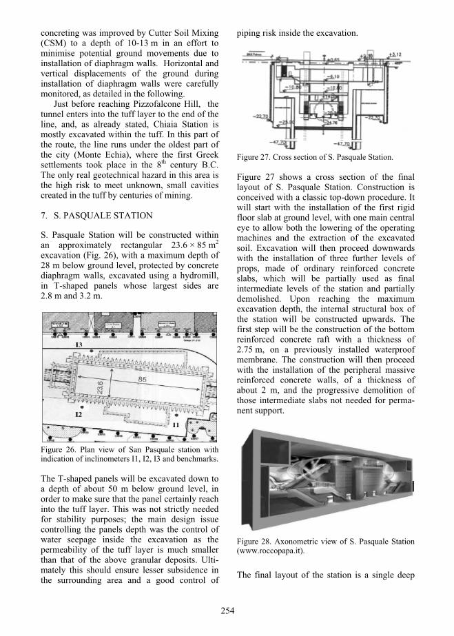
concreting was improved by Cutter Soil Mixing (CSM) to a depth of 10-13 m in an effort to minimise potential ground movements due to installation of diaphragm walls. Horizontal and vertical displacements of the ground during installation of diaphragm walls were carefully monitored, as detailed in the following.

Just before reaching Pizzofalcone Hill, the tunnel enters into the tuff layer to the end of the line, and, as already stated, Chiaia Station is mostly excavated within the tuff. In this part of the route, the line runs under the oldest part of the city (Monte Echia), where the first Greek settlements took place in the 8th century B.C. The only real geotechnical hazard in this area is the high risk to meet unknown, small cavities created in the tuff by centuries of mining.

7. S. PASQUALE STATION

S. Pasquale Station will be constructed within an approximately rectangular 23.6 × 85 m2

excavation (Fig. 26), with a maximum depth of 28 m below ground level, protected by concrete diaphragm walls, excavated using a hydromill, in T-shaped panels whose largest sides are 2.8 m and 3.2 m.

Figure 26. Plan view of San Pasquale station with indication of inclinometers I1, I2, I3 and benchmarks.

The T-shaped panels will be excavated down to a depth of about 50 m below ground level, in order to make sure that the panel certainly reach into the tuff layer. This was not strictly needed for stability purposes; the main design issue controlling the panels depth was the control of water seepage inside the excavation as the permeability of the tuff layer is much smaller than that of the above granular deposits. Ulti-mately this should ensure lesser subsidence in the surrounding area and a good control of

piping risk inside the excavation.

Figure 27. Cross section of S. Pasquale Station.

Figure 27 shows a cross section of the final layout of S. Pasquale Station. Construction is conceived with a classic top-down procedure. It will start with the installation of the first rigid floor slab at ground level, with one main central eye to allow both the lowering of the operating machines and the extraction of the excavated soil. Excavation will then proceed downwards with the installation of three further levels of props, made of ordinary reinforced concrete slabs, which will be partially used as final intermediate levels of the station and partially demolished. Upon reaching the maximum excavation depth, the internal structural box of the station will be constructed upwards. The first step will be the construction of the bottom reinforced concrete raft with a thickness of 2.75 m, on a previously installed waterproof membrane. The construction will then proceed with the installation of the peripheral massive reinforced concrete walls, of a thickness of about 2 m, and the progressive demolition of those intermediate slabs not needed for perma-nent support.

Figure 28. Axonometric view of S. Pasquale Station (www.roccopapa.it).

The final layout of the station is a single deep

254

open space (see Fig.28), in which the external natural light will be allowed to reach directly platform level at a depth of about 25 m below ground level.

7.1. Local ground conditions

The subsoil profile in the area of San Pasquale Station consists of a thin layer of made ground underlain by marine sands and silty sands, remoulded ash and in situ pyroclastic sand (Pozzolana) over a base layer of yellow Nea-politan tuff. Locally, the roof of the tuff layer is rather deep and at a variable depth ranging from 35 to 45 m b.g.l.. The groundwater table is at a depth of about 1 m from the ground surface, corresponding to about 1.2 m a.s.l..

The geotechnical investigations in the area of the station included many boreholes with SPT tests and retrieval of disturbed samples for laboratory tests, CPT tests, two seismic flat dilatometer tests (SDMT) located at the south east corner of the station (Fig. 29) and carried out to a maximum depth of 35 m b.g.l., and one cross-hole test down to a depth corresponding to the roof of the tuff layer.

Figure 29. Location of seismic flat dilatometer tests – south-east corner.

The layer of made ground is about 2 m thick. This is underlain by a thick layer of marine sand and silty sand down to about 24 m b.g.l.. Within this layer, there are lenses of remoulded ash and pumices. At greater depths and down to the roof of the tuff, there is a deposit of undisturbed Pozzolana. The total thickness of the cohe-sionless granular materials over the yellow Neapolitan tuff amounts to about 35÷45 m.

The marine deposits are dense or very dense, with values of the friction angle as high as 40°, while for the measured values of friction angle for the remoulded ash are smaller (33°<ϕ<38°).SDMT tests allowed to estimate the value of the

coefficient of earth pressure at rest K0.

Figure 30. K0 values obtained by flat dilatometer tests.

Originally, only one test had been programmed. The extremely high values of K0 obtained from this first test in the upper ten meters of subsoil (see Fig. 30) were much larger than expected, and possibly influenced by wall installation previously carried out nearby. A second SDMT test (see Figure 34) was therefore carried out far from the constructed panles to avoid any inter-ference due to installation, confirming the unexpectedly high values of K0.

7.2. Installation effects

Published surface displacements observed during construction of diaphragm walls in granular soil, soft to medium clay, and stiff to very hard clay show that the maximum settle-ment connected to slurry trenching can reach values of up to 0.15 % of the depth of the wall and extend to a distance of up to about two times the maximum depth of the wall (Clough and O’Rourke, 1990). In the case of a coarse grained deposit with a relatively low value of the initial coefficient of earth pressure at rest, as it is the case at S. Pasquale station at depths larger than about 10 m b.g.l., the variation of the state of stress induced in the ground during wall installation by slurry trenching and concreting might correspond to an actual increase of the initial horizontal stress. During this process the walls of the trench may deform outwards and some heave may be induced in the surrounding ground, before the main excavation stage. If high values of K0 are expected, as in the case of

255

San Pasquale station at shallower depths, the opposite is true and inwards displacements and surface settlements may take place.

At San Pasquale an intense programme of monitoring was planned to control construction, including installation of diaphragm wall. Benchmarks for precision levelling were set on buildings close to the station and at different locations around it (Fig. 26). Three inclinome-ters were installed into the ground to measure subsurface horizontal displacements both during wall installation and during the main excavation stage. The three inclinometers are about 55 m deep, with the final 5-10 meters cemented into the tuff layer. Daily readings were taken during the installation of single wall panels (each having a total volume of about 300 m3) to monitor the displacements induced in the adjacent ground. The effect of some of the geometrical factors affecting horizontal ground displacements caused by wall installation (such as e.g.: the distance from the panel, the eccen-tricity from the panel axis, etc.) could be as-sessed based on the observations. These data also helped in building a simple empirical formulation to predict the maximum horizontal displacement caused by wall installation (L’Amante et al., this conference).

Figure 30. Horizontal displacements and azimuth at inclinometers I3.

In all cases the displacements caused by wall installation were towards the panel, with values lower than 10 mm. In Figure 35 an example of a reading at inclinometer I3 (see Fig. 26) related to the displacements caused by the installation

of the panels of the north-west corner of the station is reported. The displacements are very small and they are likely to incorporate the beneficial effects of CSM. As the inclinometer is very long and the displacements extremely small, doubts on the reliability of the readings may exists. However, the measured azimuth consistently indicates that the direction of the horizontal displacement is towards the exca-vated panel, suggesting that the readings have a physical meaning.

A series of two and three dimensional finite element analyses modelling the installation of the diaphragm wall panels in which the soil is modelled using an incrementally non linear hypoplastic model with elastic strain range (Niemunis & Herle, 1997) is currently under way.

8. SUMMARY AND CONCLUSIONS

This lecture has dealt with some geotechnical aspects of excavation in the urban environment drawing from recent experience gathered during construction of Lines 1 and 6 of Napoli Under-ground. The attention was focused on the prediction of the behaviour and on the measured performance of deep open excavations, rather than on their design.

In the construction of deep open excavations a number of issues must be address such as: the choice of an adequate support system; the definition of the sequence of construction phases; the computation of the stresses in the ground and in the structural members; the evaluation of the magnitude and distribution of ground displacements connected to the con-struction phases; and to possible changes of groundwater pressures connected with the excavation. In the urban environment, the ability to control and predict correctly ground movements around excavations is a crucial aspect of successful design, particularly because of their potential for causing damage to adjacent structures and services. At present, the avail-able means of analysis permit only qualitatively prediction. The accuracy of the available procedures for the prediction of relevant quanti-ties (displacements, rotations, stresses, strains, bending moments, etc.), can only be assessed by comparing the predicted values against the measured performance. It is therefore vital that well documented case histories, don’t just report on a project but play a major role in assessing the validity of existing design criteria. In

256

addition they will hopefully widen and clarify their applicability, and suggest possible im-provements in the interpretation of the behav-iour of real structures, that can be both of scientific importance and of assistance to practitioners in the future (Mair, 2001; Higgins, 2001).

The examples of the new Garibaldi and Mu-nicipio Stations of Line 1 of the Napoli under-ground have shown that, in both cases, the settlement of the foundations of adjacent build-ings and structures that were directly associated to the main excavation only amounted to a few millimetres. These observations are in good agreement with the experimental values col-lected by Clough and O’Rourke (1991) for similar retaining structures in granular soil and are smaller than those corresponding to struc-tural damage.

In the case of Garibaldi Station, an attempt was made to back analyse the excavation using finite elements. The numerical predictions were undertaken using the available measurements both to assess the numerical predictions, in terms of diaphragm displacements, and to guide in the way in which some support elements, e.g.anchors, should be treated in the analyses. The analyses showed how apparently minor details, such as the thermal expansion of the tubular steel props at ground can have a major effect on the predicted pattern of wall displacements.

Both for Garibaldi and Municipio stations, the largest part of the final settlements derived from the lowering of the groundwater table behind the diaphragm walls due to water flow into the station box either through boreholes that were drilled to install the anchors, the freezing-tubes for the ground freezing opera-tions or the platform tunnels caused unavoid-able imperfection of the artificially frozen ground collars. The evaluation of ground and foundation settlements connected to these changes in pore water pressure is very compli-cated and probably beyond current predictive models. To prevent damage to the existing buildings it is therefore crucial to have an intense program of monitoring in order to be able to observe the effects at the ground surface and hence be able to adopt suitable re-medial measures if required.

The experience gathered during construction of Line 1 oriented some of the design choices on Line 6. In this case, support for the dia-phragm walls will be provided entirely by the floor slabs of the stations which will be con-

structed top- down as excavation proceeds, thus avoiding the installation of anchors in granular below the water table. Also, the stations will be oriented parallel to the running tunnels which will be excavated through "soft eyes" left in the diaphragm walls on the short side of the sta-tions. The stations will be long enough to accommodate the platforms, thus avoiding the need to carry out station tunnel enlargements in conventional mining. It is expected that all these construction procedures will result in very small settlements around the stations. It follows that the displacements associated to the installa-tion of diaphragm walls by slurry trenching and subsequent concreting may be of the same order of magnitude as those connected to the main excavation stage. These are carefully monitored during construction, as detailed in the example of S. Pasquale Station.

9. ACKNOWLEDGEMENTS

The work described in this lecture results from the efforts of a large number of people, far too many to mention them all individually. None-theless, we feel we should acknowledge the financial and logistical support of some institu-tions and organisations.

The work on Line 1 was carried out in the framework of two research agreements between Dipartimento di Ingegneria Civile of the Sec-onda Università di Napoli and Pizzarotti Spa and Sudmetro Spa. The work on artificial ground freezing at Municipio station was sponsored by the Consorzio Icotekne. The work on Line 6 was carried out a spart of a research agreement between Dipartimento di Ingegneria Idraulica, Geotecnica e Ambientale and Ansaldo Spa.

Dr. Luca de Sanctis contributed to the finite element analyses of the excavation, of artificial ground freezing and of installation effects of diaphragm walls in saturated coarse grained soils.

10. REFERENCES

Boscardin, M.D., Cording, E.J. 1989. Building response to excavation-induced settlements. J.Geotech. Eng., 115, 1, 1-21.

Briginshaw, D. 1999. Signs Of Progress In Naples And Turin - Brief Article. International Railway Journal, December 1999

Burland, J.B., Broms, B.B., DeMello, V.F.B. 1977. Behaviour of foundations and structures, IX

257

ICSMFE Tokio, 2, 495-546. Burland, J.B., Wroth, C.P., 1974. Settlements of

buildings and associated damage. State of the Art Review. Conf. Settlement of Structures, Pentech Press, London, 611-654.

Cascetta, E. 2000. La Metropolitana nel progetto per la mobilità di Napoli. La Metropolitana di Napoli – nuovi spazi per la mobilità e per la cultura.Electa Napoli, 17-29

CENSIS 2008 42° Rapporto sulla Situazione Sociale del Paese. Franco Angeli, Roma.

Clough, G.W., O’Rourke T.D. 1991. Construction induced movements of in situ wall. Design and Performance of Earth Retaining Structures,Lambe and Hansen, Ithaca (NY). ASCE GSP 25: 430-470.

De Lorenzo, G. 1904. L'Attività vulcanica dei Campi Flegrei. Rend. Accad. Sci. Fis. Mat. Naples 10:203-211

De Sanctis, L., Mandolini, A., Viggiani, G.M.B. 2006. Finite element analysis of the excavation of the new Garibaldi station of Napoli Underground. in: Numerical Modelling of Construction Proc-esses in Geotechnical Engineering for Urban En-vironment. Traintafyllidis ed., pp.57-68.

Higgins, K.G. 2001. Prediction of damage to build-ings and subsurface structures from open excava-tions. General Report, Session 5, Proc. Int. Conf. Response of Buildings to Excavation-induced Ground Movements, 97-113.

L'Amante, D., Flora, A., Russo, G., Viggiani, C. 2010. An empirical prediction of maximum hori-zontal displacements caused by the construction of diaphragm wall panels. This conference.

Mandolini, A., Viggiani C. e Viggiani G.M.B. 2004. Interazione fra Linee Metropolitane e il tessuto urbano storico e monumentale della città di Na-poli. Incontro Annuale dei Ricercatori di Geotec-nica, IARG 2004, Trento

Ng, C.W.W. 1994. Effects of modelling wall installa-tion on multi-staged excavations in stiff clays. Proc. 1st Int. Conf. Pre-failure Deformation of Geomaterials, Sapporo 1, 595-600.

Niemunis, A. & Herle, I. 1997. Hypoplastic model for cohesionless soils with elastic strain range. Mechanics of Cohesive-Frictional Materials, 2,279-299.

O’Reilly, M.P., New B.M. 1982. Settlements above tunnels in the United Kingdom – their magnitude and predic-tion. Proc. Tunneling 82: 173-181.

Poh, T.Y., Chee-Goh, A.T., Wong, I.H. 2001. Ground Movements Associated with Wall Con-struction: Case Histories. Journal of Geotechni-cal and Geoenvironmental Engineering, ASCE, 127(12): 1061-1069.

Smarazzo, D. 1999. Documenti e studi per una definizione dell'area Metropolitana di Napoli. Collana Strumenti. Edizioni Maggioli, Rimini.

Viggiani G.M.B, de Sanctis L., 2009. Geotechnical aspects of underground railway construction in the urban environment: the examples of Roma

and Napoli. Engineering Geology Special Publication, 22, 215-240

Viggiani, C. 2000. Aspetti geotecnici e scelte di progetto. La Metropolitana di Napoli – nuovi spazi per la mobilità e per la cultura. Electa Na-poli, 145-153

258

–.

. .. . . , , .

: ,.

20 . -. -

- .,

. -,

« - ». ,.

1.

-, , , -

. --

-.

10 . .

,, -

. 90- 20

- – 4,5 . 1939 9 . 1990 -

– 362,9 . 1941 994,0 . 1990 . . 1 ,

20 .

90- ,,

--

, -,

.

-

, ,, -

. - 13,3% 1992

15,4% 2000 , 2000 2004 23%.

-.

20 80 .

, -

. 1 200 -

.-

: 600 ,420 , 147 , 60 ,

.-

,, ,

-. - – , , ,

, .,

, ,

259

.

-,.

,,

.

1. : – 20 ; – 21 . 1-

, --

«» 2015 . -

. 2. 60

., -

-,

.,

, -

- 15 .

2.-

“ ”

260

-, -

, -

.

2. -

---

“ : ”( , ., 1997). . 3

.

3. .

--

. , , -, -

,, , . -

-, , -

, , .

, .

10-15 , 25 -.

- 2 .

-.

,. .

-

,

. -

( 70 2),. .

.

. 1-2 6-8 .

- ( ) -

,, .

. .. -

.

,,

,

261

. (

2,5 ), -. 4-6

, 6-8 . 10-12 , 15-16 . .

( -) . -

8-10 . -

( - ,).

12 . ( )

. -. -

-. 20-25 , -

. - 10-12 .

18-20 , ( -

). - - 12 .

( ) -. -

-.

. 30-35 . ,

,:

- ( -), -

( -). -

- - 6-

7 .--

- -,

.-

. — -. -

-, , -

. -,

, .

. 10-15 . -

-: -

, ..

-, , -

,.

-.

: - ( ).

.

.

. --

- ( -

- -).

, . -

-, -

: -- , -

- - -- - .

., -.

( -) ( -

) ..

, -, ,

, ,, , .

,

.

,,

262

, ..-

( 300 )-

.

: ,, ,

.-

.-

( -), -

-.

230-300 .

-, ,

.

, , ,- .

-

— , 0,8-1,0 ,

100 , , — 0,002 ,

1-5, 10 .-

,- . -

-. 235 . -

35 . , 14%.

90- 300.

,,

-,

.

3.

-

15 . --

,

.-

,,

( ) -, -

.-

.

–

( ). -. -

, -.

- 115-140 , ,

--

., -

, , - (“ ”).

, , -, ( -

) – .

-, , ,

. -

2 15 . XIX XX (

100 !)

( ),.

-.

XX

263

“ ” – 5-6 – .

, 1,5

.

- ., -

, -,

8,1 . -,

19 , - 7,4 .

XX .

– ., -

, -

.,

,

. ( 80 ) -

XIX . -

. 1960-1980 .

-

( 12 ,, “ ”

.)-

( , 2004 .).

:-

4 ;-

1963-1965 .;

-

“ ”;

-.

, , -,

. . 4 ,

“ ”.

1505-1508 . , . . 500 .

,, -

.

4.

50-80 20 -

,.

, , -, – -

XIX – XX , -

-, XX

.,

.

264

4. 1950-

, --

15 , -, 50-

20 .

-

., 7 -

1947 , --

,.

,

. -,

, -

, -

30-40 .-

( ), -,

,, .

-.

.

1.

,2

-

-

,

,

/ 2

,

/ 2

-

-

-

-

,

-

-

,

-

-

,

1.11725 - - - - - -

)- 13 2,6 5,0 7 5,3 7,2

) 13 2,6 4,0 5 4,7 5,6

2.3945 10 1,5 4,6 9 6,3 7,4

3. -2772 7 1,2 4,1 4 5,0 6,5

4.6830 6 0,8 3.6 13 11,2 16,0

5.1188 7 1,1 3,8 29 13,4 18,0

6. -2960 10 1,8 4,2 7 9,7 11,5

7.3030 7 1,3 3,5 - 4,8 5,5

265

--

---

.

,

.

. . 1953 .

35 183 . -

13 .

( ) - ( ., 1957),

1955 - 7,2 ( . 1). -

-

. “ ” 15 2010 .

: « -

: , -, 10 ,

.. -

, ,. ,

».--

,, -

., ,

- ,.

, -, -

1955 18,0 ( .. 5-10).

1961-1964 .

5.

( )

6.

( )

7.

( “ ”)

8.

( )

266

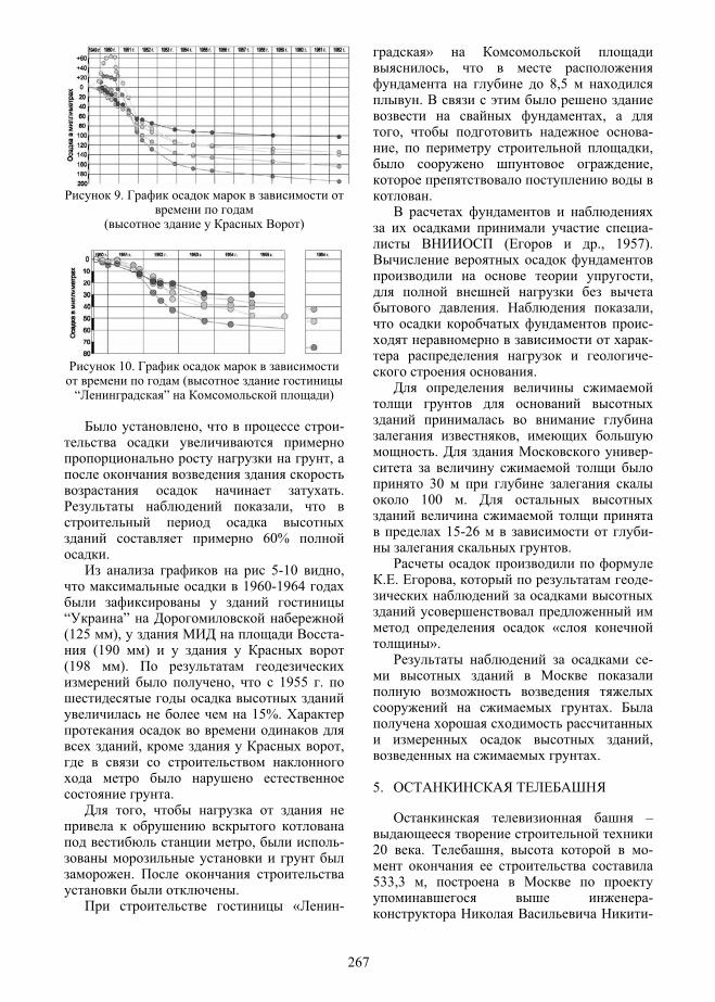
9.

( )

10. (

“ ” )

, -

,

.,

60% .

5-10 , 1960-1964

“ ”(125 ), -

(190 )(198 ).

, 1955 .

15%.

, ,

.,

, -

..

« -

»,

8,5 .

,, -

, ,,

.

- ( ., 1957).

,

. ,---

.

,. -

30 100 .

15-26 -.

. . , -

«».

-

.

,.

5.

–

20 . , -

533,3 ,--

267

. 1975

, . – 20 000 ,

– 55 000 . 11,65 .

– 540 (1999 .), 300

215 .,

..

-9,5 , 70 .

110 .

, ,. 150

70 .

.

..

11. -

-.

– 3,0 , 4,0

( . 11). 1940 2. -

– -, - « » .

, . . -,

, -- . -

, -. -

,-

. -

.

268

.--

. . .

2000 . -,

.

., -

64 .

6.

,

-

., , -

-

, ,-

.

,, -

, , -, . -

-.

( . 12), --

- -.

-

.: , ,

. 3%

. - – , 0,8-1 2

100 , - ( ) – 0,002 2

1-

5, 10 .-,

(Petrukhin, 2007).

12.

1 - ; 2 – ; 3 –

, -,

, -,

., , -

. ,

-

: ; -, , -

; -;

.

269

, 21 -

.-

-

SLIDE ( . . ,. . ).

,.

.13.

13.

2. .

- - - -

1 1,532 1,524 0,937 0,913 2,038 2,015

2 1,101 1,093 0,936 0,913 0,603 0,590

3 1,361 1,351 1,184 1,146 1,617 1,588

4 1,111 1,098 1,181 1,136 0,966 0,945

,

,

.. 2 ,

0.6,

., -

. ,

..14 , ,

-

.,

-, -

.

. -

,, " " -

.

.

270

,.

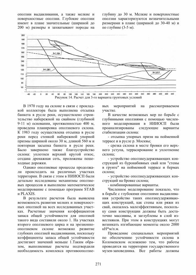
(200 )

30 .

( 30-40 ) (3-5 ).

14. 3-

1970 -

, - (

9-11 ) , 400 ,.

1983

30 , 560 .

: ,, -

.-

.-

STAB PLAXIS.

--

.

1. -

,

1. -,

-

.

-

:-

. ;- -

,;

- - "

";

- -;

- .,

--

,, , -

-, -

. 2000

* / . .

,

- .

271

, -,

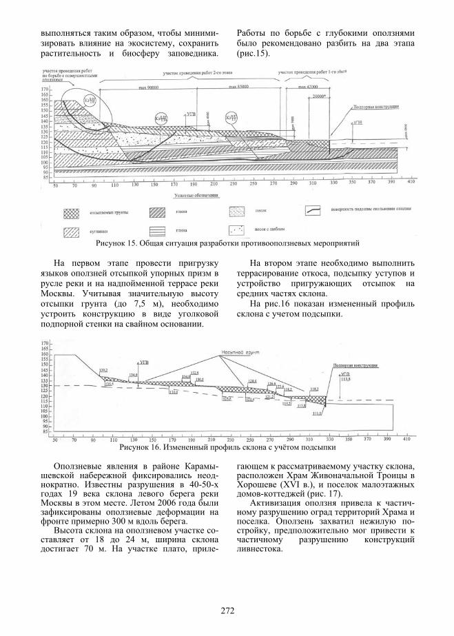
. ( .15).

15.

. ( 7,5 ),

.

,

..16

.

16.

--

. 40-50- 19

. 2006

300 .-

18 24 , 70 . , -

,

(XVI .),- ( . 17).

-

. -,

.

272

17.

, , - ( .18)

18.

273

- -

,.

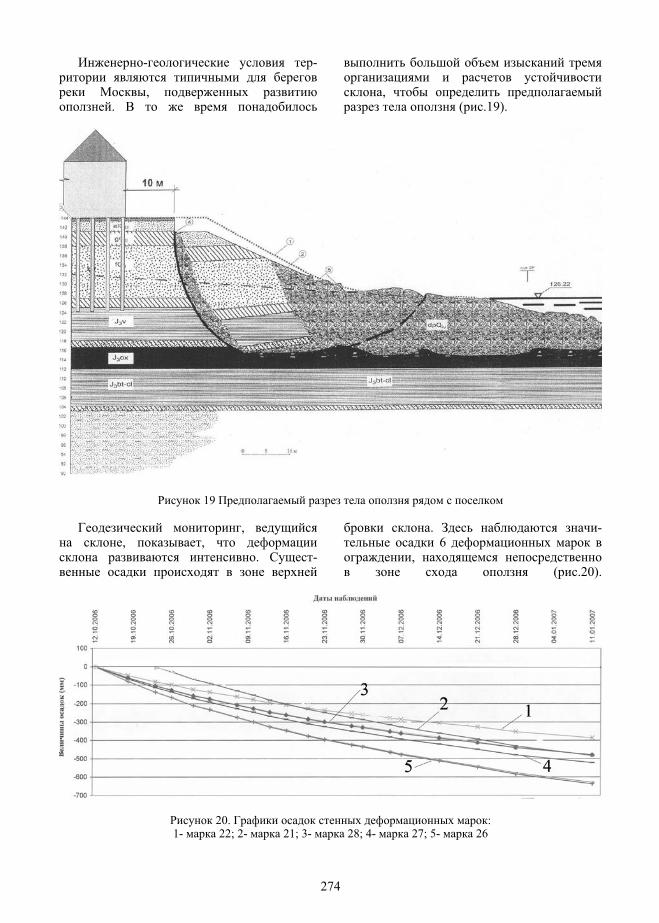
, ( .19).

19

,, ,

. -

. - 6

, ( .20).

20. :1- 22; 2- 21; 3- 28; 4- 27; 5- 26

274

---

. -

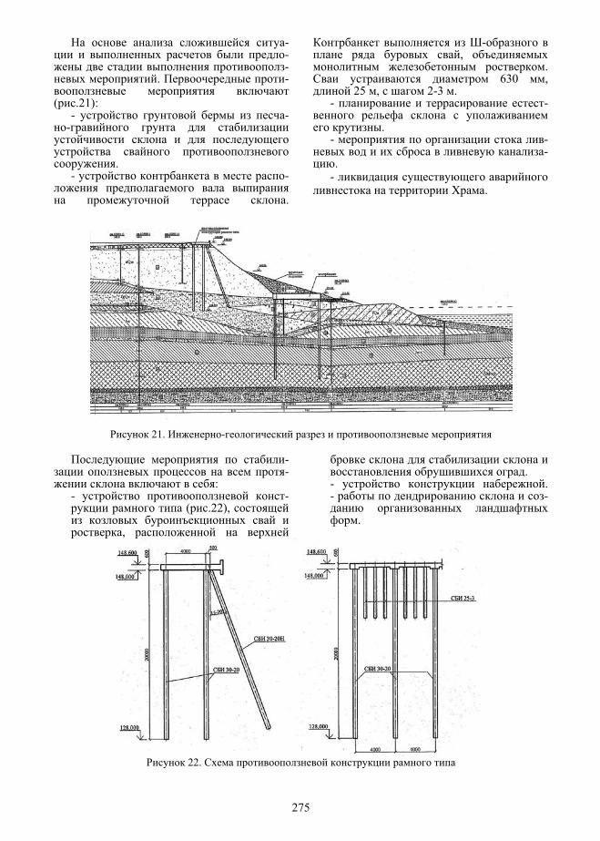
( .21):- -

-

.- -

.

-,

. 630 ,

25 , 2-3 .- -

.- -

-.

-.

21. -

--

:- -

( .22),

,

.- .- -

.

22.

275

, -

,

. -: -

, -, , -

.

-

.,

, --

,,

.-

. -

.,

.

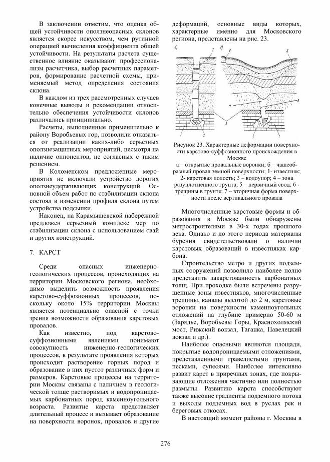
7.

-,

, -

- , - 15%

., -

-,

. ---

.

,

, ,

, . 23.

23. --

– ; – -; 1- ;

2- ; 3 – ; 4 – ; 5 – ; 6 -

; 7 – -

-

30-.

-.

-

. -,

, 2 ,

50-60 ( , ,

, , ,.).

,,,

, ., -

.

..

276

- -,

.-

( . 24, ):-

-;

-

1 ;-

( 2-3 ), -;

-,

.-

( . 24, ):-

1 ;-

( 6 ), -;

- -

3. -

.- -

, 1960

42 .

24. - , -

– ; – ; 1- ; 2- ; 3 – ; 4 – ; 5 – ; 6 – ; 7 –

277

. --

. 25.

-:

-,

;- -

-, -

,-

( ),, -

-.

,

- . , " - ", -

-

,

.--

- ., -

40% , 5-7

.-

,-

. ,, -

.-

,--

-, -

, -. .

25. -.

-

-

--

. -, -

,

,. . .

. 26.

26.

278

-,

-,

, –. -

,

, -,

-, -

. -

. , ,.

. 27

27.

, -

-,

,.

--

-

, -

, -. -

. 28.

,

.

--

.

. 28.

1- ; 2- ;3 –

279

8.

-

,, , -

-.

-, 2008

“ -

2009-2011 . .”. -

-

.-

-:

-;

- -

;-

;-

;-

.-

3. , 3 -

-.

-

. -

,.

-

.

3. 2008 .

()

2009 . 2010 . 2011.

-, .

.650 700 850 1000 2550

, % 6 10 12 15 -

-

, % - 27 33 40 100

.-

. , 100%

.

, -

.

-, ( -, ),

.-

( ). -

, -.

-. -

280

- ( , ).

-

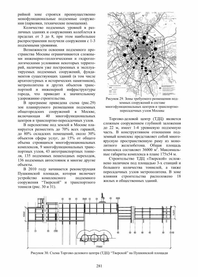
3 8, 1-3

.--

- --

, -, -

(),-

,.

( .29)

, 40

- .-

70% , 80% , 30%

, 15%

, 9 -, 43 -

, 135 ,136

. 2010

,

“ ” ( . 30 31).

29. -

-

- ( )

22 , 1-4 . -

--

. 36000 2. -

175 54 . « » -

3-,

. 18

.

30. - ( ) “ ”

281

31.

. . .

- ( . 32).

32. . .

---

.

,,

- ( . 33). – 3-4-

- , -.

– 4-5--

. – --

.

.248 161 .

136000 2, 106000 2.

282

33.

- ( . 34), - 5 -

20,7 .

– 296 , – 174 .

112000 2.

34. -

-, -

,

( . 35),

.

35.

283

4.

4.

-, 3

,-

,

« - »1 354 000 1770 26 6

« » 280 000 780 18 4

« » 155 000 534 15 4

«Ritz Carl-ton» .

100 000 280 20 5

78 000 314 13 3

« - »44 000 255 16 5

22 000 220 14 4

« », 17-18 « - »

830 000 672 30 6

620 000 1 050 15-30 3-6

490 000 1 200 15-22 3-5

- « - » 350 000 1 100 16 4

“”

240 000 620 10 3

9.“ ”

90- 20

().

8- , -. -

1978-1987 . . -, . .

-, -

.-

1994

- ( )

( , ., 2001).

1997 ., -

.

380 150 2 ( . 36). --

,

.

15-17 . « »

« » ,, -

( . 37).

284

36. -

“ ”

- -

( . 38). 14

-, (1485-1495 . .),

(1701-1736 . .), - (1492 .), -

(1874-1884 . .), (1786-1793 . .), - (1892 .) .

,

-,

,-

-

, -

. ,

, -,

-.

--

" " - 900 , -

" " 750 .

115 . " "

6 .

" ",

800 , 115 .

-.

1500-2000 .

37. - “ ”

285

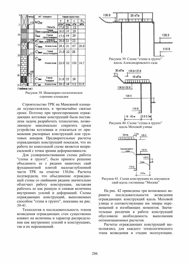
38. -

-

. --

, -

--

.,

-.

" ",

130,0 ., -

,

.,

" ", .39-41.

-,

.

39. “ ”

40. “ ”

41. “ ”

. 42 -

-. -

.-

.

286

42. (x) ( )

-.

,- -

-

.-

, -

, , -

, ,-

,-.

-: -, -

.

:- 14

287

, ,;

- -;

-

;-

;- -

;- -

.

--

. . 43 44

- “ ”

.

43.

44.

, -,

,

-.

, -, 5-10 , -

- 0,0005. ,

-.

,,

.

10.

. 45 « »

.-

« », 13 200-

2004 .-

( . 46): , --

. 1817

( 6 )

I.

(166x44,8 ),. ,

.,

-

, ., -

- 45 , 1817

. -, -

6 .

-, 1824

-, -

- .

288

45. “ ”

46.

-

, - -

.

, -.

-

,-

( . 47).

47. -

289

-

-.

, -

- (

). , -,

, .

- - 12 -

, (3/4 )

.-

,-

:,

, -.

-, -.

, -

- (199 ) “1”/“ ”.

- , - 5,27 7,4 ,

- ( )

-.

:,

-, , 1 .

.,

, .

- . -

- ., -

. , -,

, -.

-,

. ,

7,5 .-

,-

, -.

10 , – 7*104.

, -

. -, -:

- ;- ;-

(

).

(Mozgacheva et al, 2007): - -

, -

( - PLAXIS);

- « » 4 ;

-( « -

») 4- -

;-

( , -,

,1 !);

- -

290

;- -

.-

- - -

-

, .

-,

( . 48).

48.

, 16 17 2004 . -

(),

200-220 , 18-20 -

- - .

- 12-15 ,

0,9.

--

-.

.

-,

.

, ,

, --

,

-.

,-

. -,

-.

-.

-

PLAXIS.

:.

.

291

.-

., “ ”

,

, , 1.1.

-

« » -. -

- 1.3.

-

.-

“ ” 49 50. “ ” -

.

12 .-

3-4 ,-7-9 .

-

.

49.

50.

,

7,5

« » 0,6 ,12-14 .

, - « »

,

,.

« » -

« -» . -4,0

.

, - «

», .-

-7,5 ,

,.

-

. 51.

292

51.

-,

,

, ( . 52).

52.

293

(4.04.04-18.12.04 .)

“ ”, “1” “ ” “ ”, -

, “24-26” “5-10” “ ” ( . 53).

53.

8,4...12,1 . -

, ,

.. 54 -

7 30,

., -

.

54..

.

,

3...6 .

1-3 ., -

(12 ) - -

.--

(30 - 50% ),

« » (30 -40%).

, 10-20% .

– 1 . ,

- --

.

11.

- – -

294

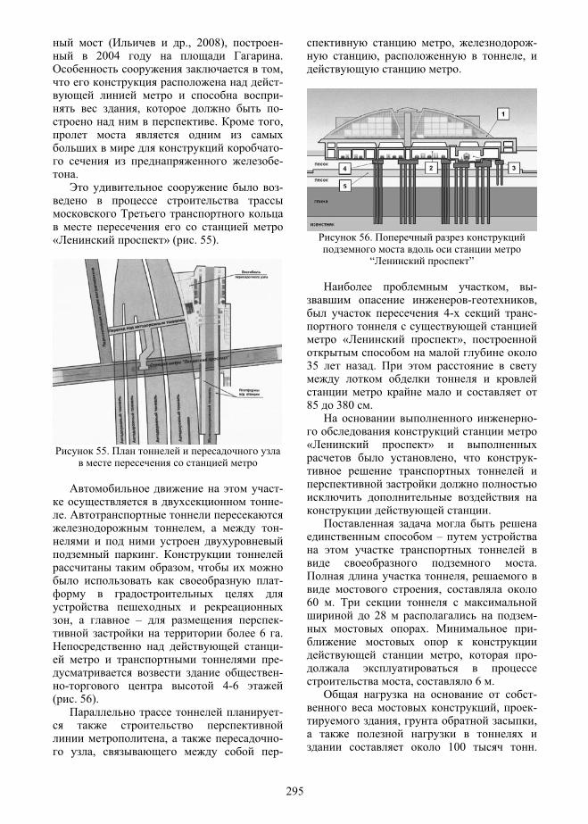
( ., 2008), - 2004 .

,--

, -. ,

--

.-

« » ( . 55).

55.

--

., -

.,

-

, – - 6 .

---

- 4-6 ( . 56).

-

, -, -

, -, ,

.

56.

“ ”

, -- ,

4- -

« »,

35 .

85 380 .-

« », -

.

–

.,

,60 .

28 -. -

, -

, 6 .-

, -, ,

100 .

295

10-12 . , -

-

,-

, -.

-- . -

( , ) 20-30 .

-,

. ,

, 60 .

-

( -, , - ,

- .).,-

- , 65

20 .-

, 6 12 , -

- 2,5 ( . 57).

57.

– 1,5 1,35 .

,-

- 25 ,

« » 10 .-

,

-, . 58.

58. ,

296

-

-.

-,

-,

-,

.,

, ,

.

12. “ - ”

1992 . --

« -- ». « - »

.,

,.

“ - ” 19 -

30 . « - »

- 60 -

, -.

( 2 -

- ), -,

. . “ -” 2010 . -

. 59. “ - ”

-. -

2005 “ ” (

“ ”), “ -

”. - " - " -

, —

.

59. “ - ” 2010 .

297

“ - ” -, -

.-

30-

– 3-6 ( . 5).

( , “ ”).

“ -”

,-

,.

,,

-.

-,

., -

“ - ”, :- (III ) -

- -;-

( ,, -

,

.);- -

;- -

;- .

, -, :

- ( -

),-

,-

.

5. “ - ”

,/

- -

2-3 204/45 3 4 234/64 3 6 * 5-6

7-85 - 5 5-6 8 * 5-6

9 « »: « »« - »

241/73234/62 3-6

10* 243/58, 119/27, 76/17 4-5 11* 167/41, 124/30, 55/15 5 12 « » 300/75 5 13 « » 354/93, 242/63 5 14 « » 322/70 5

15 307/70 6

16 - - 393/67 5

20 - 164/54 5

19 - “ - ” -

-, -

.

. -

298

-,

,,

, : - -,

60 , 1000-1500 , -

3500 .

,

- ( ).

-. ,

“ ” “ - ”, -

- , 4, 8 8

,.

- “ -

” 10 .--

, -:

- -

-. , , -

.,

.

-.

19 - 10-

15 .

,.

,

- -,

. “ -

” -. .

70-100 . ,

124,3 126,04 . . 60, -

, 11- .

60. - , “ - ”

,

, -. -

,.

- « - »

:

299

, -, ( 0,5

40 / .), -

. -

.

13. “ - ”.

- - “ - ”

( ., 2001). -

, 1725 , - 24 .

-

, -.

,

, ,, , ,

. 8-

, ( . 61).

61.

,- .

-

.-

.---

. “ -

” -

, -

, --

.

150-200 . .

: -- , -

, , -,

, ,.

-,

7 73 / .

.-

6-10 .

-:

11 . 3/ . -

300

,.

--

,

, ,-

. “ ”

0,9 20-25 . 1761,7 .

1 . 3

( . 62).

62.

, -

, -

, . .-

( ).

.“ ”

- ( )

18-24 .,

8 .,

“ ”, “ ”, -

. 0,9x2,20,9 2,6 .

“ ” -

.-

:

- --

“c ” ;- -

, .

63 .

.

3 , W12,

-01.

« » -

100x100 10 - 36 .

, - 830

880 , - “ ” “ ”.

0,6 830 0,66 - -

880 .-

12032 .

-

.

-,

,.

---

. --

.

-

,-

4( .63).

301

--.

426x8,

- .-

-

-

.

63.

-

,-

.

., -

- , ,

1.7 . -

,.

, -

,

5 .-

139 ,--

,.

14.“ - ”

-, . . , -

, , -,

,

.

12, .,

,60 .

20-25 ( , 2008).

« » 0,6-0,8 1000 .

, -.

64. 14-15

-, , .

“”, -

. . 64

302

14-15 25 . “ ”

800 , 5

60 120 .-

-,

--

.

11 ( . 65).

11

10 12. -

11 -

, -.

11 -

1000 0,9.

13,0 32,0 .-

25, W8, -

500 .

65. 11

- 3-5

50-95 .

,- 12

. 66-68.

66. 11 12

303

. 66 -

,

« ». . 67

« ».

“ ” “ ”

3- . “ ” “ ”

-.

12 ( . 68). - “ - ” -

,- .

67. 11

, -, ,

-.

, , 0,4 .

1,0-1,5 .,

, -

( -- )

3,5 .

68. 11 12

--

.-

,,

6 .

, -,

, ,

.

.--

1,5-3,5 . .. 69

4 -,

-.

3-5 .

40... 60.

304

69. 4: ,

, - ( , 2006 .)

. 70 4,5

4. -. -

1-2 2-3 . 3 .

70. 4,5

4

-,

300 ,,

( . 71). ,,

, - -.

--

11.

71.

-

. -.

.

(q > 0,4 )

∅ 1,2 , 20 , 3,5x3,5

( -) 3,5

.,

.---

, ( )

.

( )

25 .-

, -.

--

.-

305

: 75 ; - ( b = 50

); (10 )

;-

( q = 0,5 ).

- ( -

“ - -

-”)

( , ), -.

( , ,“ ” .) ,

, b. -

,

, 2...3b

1...2b (

).-

,

. --

.

( 30-40 ) -, -

, -, -

- .

“ ”

2-3. – 248 ., -

( . 72).

.

.

72.

:

( )

,.

q ≈ 0,2 ---

. -

306

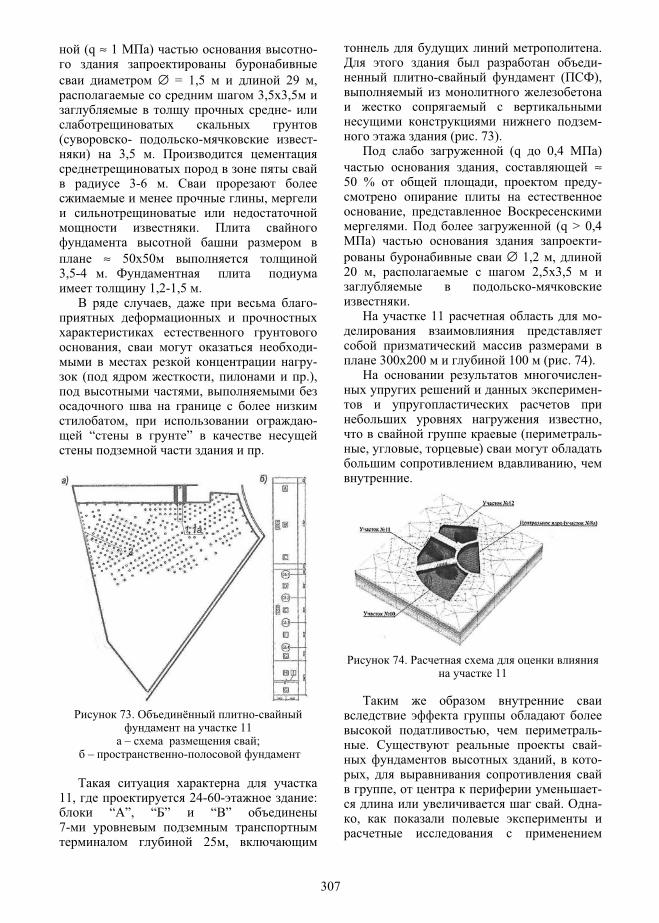
(q ≈ 1 ) -

∅ = 1,5 29 , 3,5x3,5

-

( - - -) 3,5 .

3-6 .,

.

≈ 50x503,5-4 .

1,2-1,5 ., -

, --

( , .),,

, - “ ”

.

73. - 11

– ; – -

11, 24-60- : “ ”, “ ” “ ”

7- 25 ,

.-

- ( ),

- ( . 73).

(q 0,4 ), ≈

50 % , -

,. (q > 0,4

) -∅ 1,2 ,

20 , 2,5x3,5 -

. 11 -

300x200 100 ( . 74). --

, ( -

, , ),

.

74. 11

, -. -

, -,

, -. -

,

307

( ., 2007) ,

- - -

,.

-. ,

, , --

.-

, 11,

,- .

. 73, . -

( , -, .) -

.-

, -

,

.

--

( . 75). -

5 4

. - ( , -

) ( - Kwp Kwg ) -

, -

-.

75. 11

2-3, -

,,

≈1/8 ,-

.-

.. 76 - -

, -

.-

.

-, ,

,.

308

76.

--

( . 77). --

. 77

3.

“ - ” --

(2-3 . ). (

) -,

, -. -

“ - ”-

. , --

.

, ., -

,-

.

77. 3

11.

, ,

-. -

, 20 .

- 20,1

309

16,43 . TP-1 -

1200 81,79 ( -2 - 81,76 ). -

.

O-cell. -

( ).

- (LVWDT Geokon,

4450), O-cell -

(p c. 78). -

O-cell -, -

., -

4 , 2 ( -

28, 89 92 ) 2 - ( -400, 89 92 ).

-1 ,, -

20,1 . O-cell, ,

2,3 . -, 83,43 (

1,5 ),1 ( . 79) – 1,25 , -

45% . , -

( ) 1,05 .

,, -

1 ( 1,5), 13,7 ,

68%, ( 1

)32%. -

, ,

-.

78.

1 -

- 1. -

, = 1,13 / 2., -

F2 = 12,8 Q = 7,3 .

79.

310

80.

, -,

, 19,77 (, - 0,33 ),

- O-cell - 1,73

, - 0.05 ., -

( + )1,68 .

( -400), - 89 92 ( . 80),

82% (16,2 ) 96% (19 ), -, -

. - 1,05 / 2 -

89 -

.-

.

-2,.

15.

. -,

,

. 50-60 -

-. ,

, --

.

( ) , -.-

, -. -

,

.

,. -

--

, -.

, ,,

,.

, -,

. ,

.

( ).--

( ., 2001). 30 .

( – -). -

, -, ,

, -

( ). , 10-30 10-20

311

- (5-10 ) .

. ,, ,

-,

, --

, -,

.-

.

., ,

.-

- --

.,-

-.

- ( ), , -

,,

, — ( ) -

.

---

( ).,-

, ,, -

. ( )

,

. ( ), ( ),

-

, -

.

-

-30 ( . 81). --30,

, " "

" "

.

81. -30

. 82, 83.

82. -

( ): I- ; II- -

; III- ;IV-

; 1- ; 2- ; 3- -; 4- ;

312

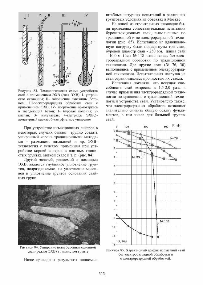
83. ( ): I- -

; II- -; III-

; IV- ; 1- ; 2-

; 3- ; 4- ;5-; 6-

- – , . -

--

, . . ( . 84). ,

, -, -

-.

84. ( )

-

.-

,-

( . 85). -,

- 250 ,– 10,0 . 118 -

. ( 76, 30) -

..

, - 1,5-2,0

--

. ,

-,

.

85.

.

313

-30 -

. 80 ,

10 ( -).

- 8 7-9

.

.. 86.

- 50 ,

≈ 0,3 3.

86. -

( – , - )

« ».

,

. - 6.

6. 1 2 3

-

( )

, 2110 2370 2690

-

,1260 1480 1300

- , 850 890 1390

--30

.

20% ( 2 -

). 60 % .

.-

,,

, , .

16.

90- -

-. 1998-2000

- (Petrukhin et al, 2001).

2245428.-

4 - 9

( . 87).

87.

314

88.

( . 88), ,

, --

32,44 ,

(20 ) . 1997

--

( . 89).

89.

-

- , -

--

. --

25-30 30

( 10 ).

( . 90), -

3,44 , -.

, 1, ,

3 , 2 -

,-

2,8 2,1 .

90.

-

-.

( )

(Petrukhin et al., 2006) --

- - 1420 2,6 3,58

.

315

-- 1,0 . , -

25,6 .

7 .

10,4 .-

( . 91). , -

,

1,5...3,5 -.

91.

- 120x60 ,

5...6 -,

10,4 ( ). - ( )

“ ” 17,5 0,6 . “ ”

260. -

. “

”, ,

1 “” ( . 92).

92.

, ---

19 ( . 93), -

(5 ),. , -

“ ”2,1 20-25 , . .

39-44 .

93. 1

316

6,9 ( . 94).

94. 1

1 - -12,7 . -

“ ” 8,3 ( . 95).

95. 71, 72 73

, -

.-

1,2 4 , .

30 ( - 31,7 ). , -

--

( . 96).

96. 1

317

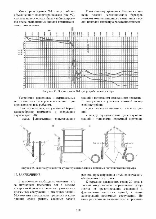
1 ( . 97),

--

.

-

.

97. 1

.,

( . 98): -

--

;- -;-

.

98.

17.

,

.-

,.

20 -

,.

-

318

-.

-

-, -

-

-.

-:

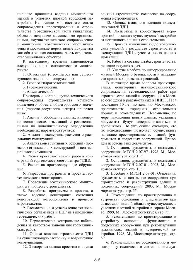
1. ( -).

2. - .3. .4. .

-

- ( - )

.1. -

- -

.2. -

.3. ( -

) -.

4. -- ( ).

5. -.6. -

.7. -

.8. ,

.9. -

.10. -

-.

11.

.12.

-.

13. -.

14. -

.15. -

.16. ,

.17.

-.

-, , -

-

10

. ,

. ,

, -. -

.1. ,

. 2.07-97. 1998, ., -, . 136.

2. ,. 2.07-01. 2003, ., -

, . 108. 3. 2.07-01. ,

. 2003, ., -, . 55.

4.

-. 1999, ., , . 55.

5.,

-. 1998, ., , .

89.6. -

-

319

,.

199, ., , . 89. ,

-,

, -.

18.

--

2009-2011 . 2008. -, ., . 39.

. ., . ., -. . 2001.

, . ., ., . 49-60.

. ., . .,. . 2002.

..

. . . , ., . 147-158. . ., . .,

. ., . ., . . 2000.

- 3- -

. . -I ,

, ., . 191-199. . ., . ., -

. ., . . 2008. -

. . -- , XII ,

. .,. 250-254.

. ., . ., -. ., . . 2001. -

. . XX . « - », ., .521-523.

. ., . .,. ., . ., . . 2001.

« -- ». . .

. . – 70 , ., . 61-69.

. ., . ., -. ., . ., . .

2001. - « ».. . . . –

70 , ., . 31-38. . . 2007. -

– . – XXI , I , ., .

114-153.. 850 . . . .

. . . 1997, II , . « -», ., . 399.

. ., . ., -. ., . . 2007.

., 11, -

, . 90-97. . ., . . -

( ) « - ». 2008. -

, 12, - , . 54-89. . . 2004.

. ,, 6, .

15-18.Mozgacheva O.A., Petrukhin V.P., Raz-

vodovsky D.E., Shulyatev O.A. 2007. Recon-struction of a Manage building and underground development. Proceedings of the 14 European Conference on SMGE, volume 2, Millpress, Madrid, pp. 919-924.

Petrukhin V.P. 2007. Geotechnical prob-lems of landslides prevention in Moscow. Proceedings of the IGS “Geotechnical Engi-neering for Disaster Prevention and Reduction”. CIR Publishers of Korean Publishing Company, Seoul, pp. 40-50.

Petrukhin V.P., Shulyatev O.A., Mozgacheva O.A. 2001. Monitoring of a building behavior during compensation grouting operations. International geotechnical conf., St. Petersburg, p. 170-181.

Petrukhin V.P., Shulyatev O.A., Mozgacheva O.A., 2006. Vertical geotechnical barrier erected by compensation grouting. Geotechnical Aspects of Underground Con-struction in Soft ground – Bakker et al. Taylor & Francis Group, London, p. 433-437.

320

. . , . . , . . “ ”, - ,

:-

.. -

. -- - , -

. -.

-

,,

.

. -

,-

. -

,-

. - –

, -

. ,

,, -

-,

, -, -

., –

.

.

-,

.

( ).

-

,-

, . . ( -

),-

.

,,

-, -

. ,, -

[10]. -

. -

: ,

321

,.

,--

. --

:

0uad

n

i

iad SS ≤

=

Siad –

, n – , Sad u – -

, - « – –

»., -

,

,, .

Siad -

, , -. ,

,,

-. :

, -, -

, -

. --

, -, -

-. , -

,-

( ,).

, , ,

.

,,

, -- .

1. --

, - --

.-

-

., 57, - -

6 .

– .

.-

. -

.,

., 57

,.

,

-. 55 59

. 20 ( . 1).

- 26 30

.,

-

( FA).,

23 ( . 2).

.

322

. 1. 55 59 .

. 2. 26 30 . 18.02.98 . 29.06.98 .

. 3. . 8 -.

8 . ---

30 1.2 , -

« ».

15 , - (

8 !) ( . 3). , -

-,

.

. «

». - 18

4,5 .« » ,

323

, .,

,.

-

,.-

, -

.

2007-2008 . --

.

,

.

,.

( . 4) ( « » «Franki»)

-

,:

3- . --

. «Franki»

-- -

1.5 / ³.

-

.

. 4. . ( ) ( )

,,

,- . -

-.

, .

50 .

. -

,-

.

324

30 , -( . 5, 6), -

.

. 5. ( ).

05

1015

2025

0 20 40 60 80 100

120

140

160

180

200

05

1015

2025

0 50 100

150

200

250

300

4 5

. 6. ( )

--

.-

, ( . 7).

325

, -

-, -

, .

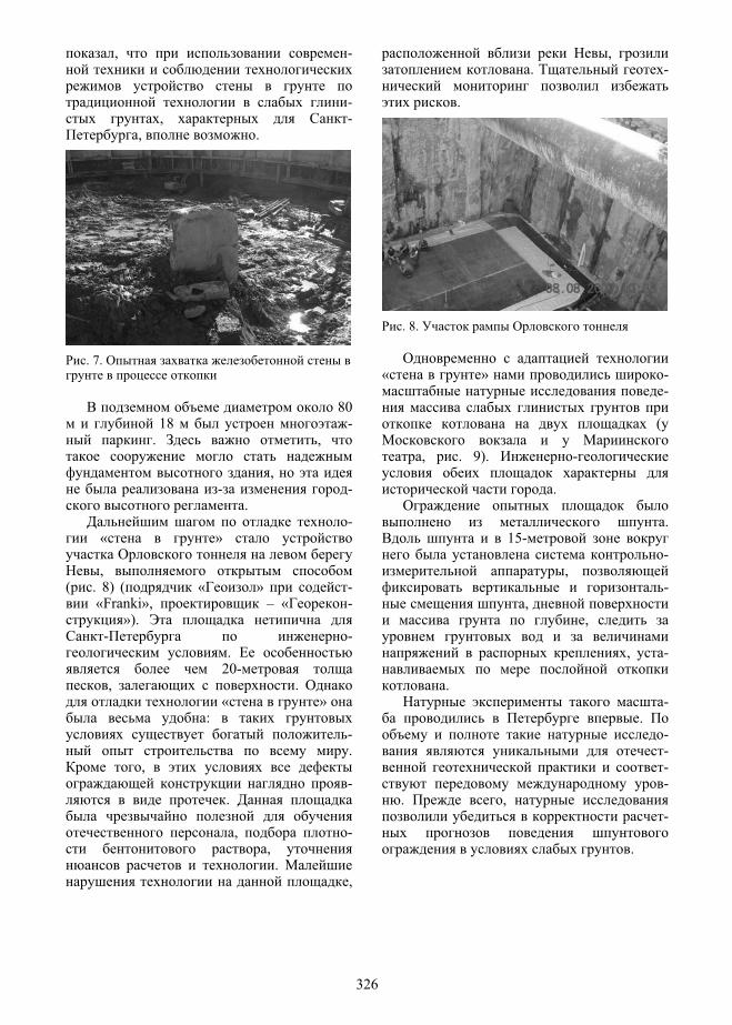
. 7.

80 18 -. ,

,- -

.-

« »

,( . 8) ( « » -

«Franki», – « -»).

- -.

20-, .

« »:

-.

,-

.

, -,

.,

,. -

.

. 8.

« » --

(

, . 9). -

.

. 15-

-,

-,

,

, -

.-

.----

. ,-

.

326

. 9. .

.--

,,

-.

, -

., -

, -. -

, « V»

40 ,

.-

, -.

.-

.-

( -)

-

.

( -. , . 10),

«» .

,

-

. -

.. -

-. « »

-. ,

, (

– « -»).

.,

, -

, .

1.8 -.

:, –

– -.

-,

, -.

,-

: --

327

. , -

:

18 ,--

. ( . . 10, ).

10,

.,

-

. ,-

-, -

-.

-. -

800 2.5 2.5 .

,

-

, -

,.

, -,

,, . 2.

- –

– I., .

« »,, –

--

.,

3000 2,.

)

0

1

2

3

4

5

6

7

8

9

10

11

12

13

14

15

16

17

18

19

20

21

22

23

24

25

26

27

28

29

30

31

32

33

34

-4 -2 0 2 4 6 8 10 12,

,

07/11/200713/11/200721/11/200727/11/200705/12/200711/12/200718/12/200711/01/2008

)

. 10. ( - ,., . 2-4) : – -

; – ( ) -

-

328

-

6 40×80 .

« itan», . ( 2008 .)

«top–down»,

: « - ».

,,

:, –

. -

.

20 , -,

( – -) -

7 ., -

,- , -

-, , -

.

. 11. .

, 2006 . -

,.

, -- ,

, -,

: -

-

( ) [12,13]. -

,

. - 15

,. -

-,

-,

.

,- .

329

. 12. .

-

jet grouting .

-

.

10

.

,-

«top-down» ( , - -

-) c

-,

jet grouting. ,

80

2,0 , 60% -

. -

( 15 ). -

,, 50 ,

– 80 . .-

, --

. 26 30

. , - 1998 .

330

. 13. 44 . .

,,

44 . – -

( ). 1999 .

30 , - 2007 70

( . 13), -

-. -

2007 ., -

8 10 .

,

«top-down». -

, --

, --

.

331

. 14. . 44 . (2007 ).

8 15 .

-,

- , -. -

., , -

( → →, )

: -, ,, -

, , -,

.,

. . 14 -

, -.

137×87 - «top-

down».,

jet grouting.

--

-

--,

.-

,-

.--

. --

, -

, , ,-

., ,

,.

-.

- jet grouting,

. ,,

2-

332

-,

.,

. ( -

).

,-

. , -

.

( 50 ), -,

.-

. 60 .

,-

.

. 15. -. .

112 -. 4 . ,

, 9 7 , 3

.-

, --

.

, -

. , -,

,-

, -, -

333

, ., , -

-. , ,

,

.

2.

-

.

-.

-,

. -

. -

. -

.

, [11].

2.1. - -,

- ( -)

,-

- .

, (

, , 5…10 ). -

. -

:

. -, -

-.

2.2.

,

« am Clay». -

, -.

« – ».

. . 1979

- [1]. -

-, -

.

, -.

( ,).

-

( -).

0-1-2-3-4 ( . 16)

, 2, 3, 4 -

, 0-1.

. 2 4

. 0-2-5 0-1-2-3-4-5,

,-

.

334

(0-1-2-5) ,

(0-2-5).

. 16. ,.

-0.1

0

0.1

0.2

0.3

0.4

0.5

0.6

0 0.02 0.04 0.06 0.08 0.1 0.12 0.14 0.16

. 17. -: 1 – 0-2-5 ( 0.3 ,

); 2 – 0-1-2-3-4-5 ( 0.6 , -0.3 , 2-5 ).

- ( . 17). -

. .-

, - « »

.

-

, -.

-.

p

q

p1p2=p4=p1/2

12=4

3

5

q,

0.3 0.6 p,

q,

12=43

5

1

2

2 4

0

0

335

0

0.002

0.004

0.006

0.008

0.01

0.012

0 0.1 0.2 0.3 0.4 0.5 0.6 0.7. 18. -

.

-, -

. 0-1-2-3 ( . 18) 2 3 -

(,

),

.,

( . . -)

( . .).

,, -

,,

.,

.,

.. . [1]

,

.--

,.

« » -. -

- .,

, Soft Soil Creep Model, Plaxis,

.

2.3. « »(Double Hardening)

,

( ). -

c --

p,

0.2 0.6 p,

q,

1

320.1

0

2 3

336

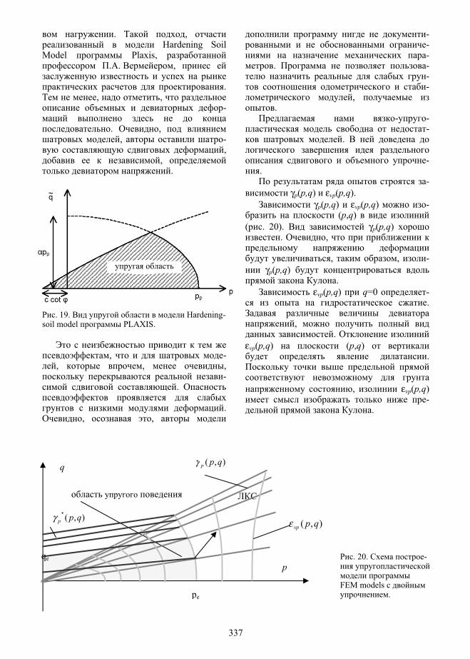
. , Hardening Soil

Model Plaxis, . . ,

., ,

-

. ,, -

,,

.

. 19. Hardening-soil model PLAXIS.

, -, , ,

-.

., ,

---

. ---

,.

- --

.

-.

-γp(p,q) εvp(p,q).

γp(p,q) εvp(p,q) - (p,q)

( . 20). γp(p,q). ,

, , -γp(p,q)

.εvp(p,q) q=0 -

.

,.

εvp(p,q) (p,q).

, εvp(p,q)-

.

p

q

pe

),( qpvpε

),( qppγ

),(* qppγ

qe . 20. -

FEM models .

337

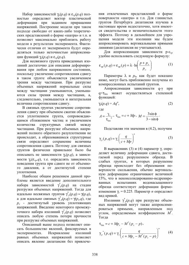
γp(p,q) εvp(p,q) -

.- - « » . .

. ---

γp(p,q) εvp(p,q).--,

.

, -, ,

,.

--

, -

. -

,

.

γp(p,q), -γp(εvp,q), . .

-,

.-

γ*p(p,q)

.γ*

p(p,q) ≈ γ(p,q),γ*

p(p,q) ≈ γ(pe,q),pe -

. -γ*

p(p,q)

.-

,.

-

« » . .

, -

. -

( ). p- vp

:

+⋅λ=ε=ε

o

o

ppppqp ln)(),( vpvp

(1)

λ p0,,

. q-

q<τlim:

γp(p,q) = Aqn, (2)

ncA

limτγ= , Mpc +=τlim ,

φ−φ=

sin3sin3M .

(4.2), n

cp Mpcqqp

+γ=γ ),( (3)

(3) (4) γc -, -

.,

-, -

15%, - -

-γc = 0.225. n.

γ*p(p,q) -

-,

, M*.

)(*lim ppMMpc ee −−+=τ ,

n

eecp ppMMpc

qqp−−+

γ=γ)(

),( ** (4)

338

M* -M:

*

**

sin3sin3

φ−φ=M ,

φ*

. (4)

, -. ,

, --

, .

2.4.

-, -

, ,

. -

. , ,

,,

,, -

,.

-.

,, -

, -.- -

-,

.-

.

( . . [2], . . - [3], .) .

. 21. , -

--

-

.

. 21.

- (lgIII).

, -

. -,

. -

(Hardening Soil Model),

.-

Creep Model. -

, Cam Clay.

,

-, -

. -, ,

., -

:-

, ,

.-

339

, .

. . . ,. . [4,5]

--

. , --

,,.

-- .

.-

.,

- ( -

) -,

1 .

-,

,15% ( , -

12248). ,

. ,

,,

( ).

.,

( , --

) -,

. -

, -.

,

-:

-

?, -

-.

. ,

-.

--

, - ( )

.,

,, -

. - [5], -

- .

,,

. -

. . , . . [4,5]. ,

. ,, -

. .,

-.

:

-:

340

lim

lim0)(

ττ−τη=τη . (5)

,

[3,6] ( . 23).

0

0.02

0.04

0.06

0.08

0.1

0.12

0.14

0.16

0.18

0.2

0 0.2 0.4 0.6 0.8 1

1/

. 23.

. 1 – - W=30%; 2 –

W=24%; 3 – W=21%; 4 – -

(5).

-

:--

.-

., -

.-

.

--

.. . ,

. . [4,5]. ,

.

. ,-

, -.

-

. - (

) , -, -

,.

:-

. ,-

, . . [4], . . [2], .

( )-

. ,-

.

. 24. 1

1 2

4

3

341

01020304050607080

0 500 1000 1500 2000 2500 3000 3500

. 25. 1:1 – ; 2 – - -

-

. - ( . 24, 25).

:η0 ≈ 100cu [ ] (6)

, , -, ,

,

, -

. (6)

-

- ,.

.-

- [7].

,

. -

. 26.

, -- -

.

( . 26, , , ).)

)

,

, 1

2

3

3

342

)

)

. 26. :

) 2.02.01-83, ) 50-101-2004,) , ) - -

. 1 – ;

2 – ;3 – .

, ,-

. -

2.02.01-83*, 30% -

. ( -

50-101-2004) (78 176% ),

-.

-- -

. - ,

« » ,,

. -, -

,-

. - , -

. -.

- - -

-, -

, , - ( . 21).

.-

. -,

.

( . 27), [8, 9].

- -

.

.,

--

( . 26). -

.

,,

,

.

3

3

343

. 27. :

, -

.

2.5. -

,

,-

. ,

,

.,

, -,

.

.

, -

.

, -

« » - ( . 28),

,,

.

. 28. « »

(Tavenas & Leroueil, 1977).

--

-- .

. 1 .,,-

().

( --

).,

.

-,

,.

-

344

- c -, -

.- ,

.

e1, %

. 29. .

. 30. ,

.

-,

. --

, (3…6%) -

- ( . 29, 30).

(35 ), 1,

( ) 1.24,

, -.

.

30 . -

. 29. ,-

, ,..-

« ».,

. -

., -

- -, -

, -

231 σ−σ

=q

345

. ,,

,- , -

, -

.

, - ( . 31).

0

0.01

0.02

0.03

0.04

0.05

0.06

-0.02 0 0.02 0.04 0.06 0.08 0.1 0.12 0.14

. 31. -: 1 – 12248; 2 –

2 .

,,

-- - .

,-

.

,.

,, -

,,

. -

.

3.

--

.,

.

,

.

. ( -. 1). . 32 -

-. -

q,

2

1

346

- (6),

-.

, (6) -

–

– . . 32

: (6)

.

0

50

100

150

200

250

300

0 20 40 60 80 100 120 140 160 180

. 32. 15 .

., -. 1.

(6), - (

12 ) ( 12…14 ) 6 .

-

,:

80% 2…3

( . 33) -.

, --

, 2 (6).

-

- . (

.)

-. , (6)

( ),

?

.. -

- (6) ( . 34). ,

, -

-.

,

,

347

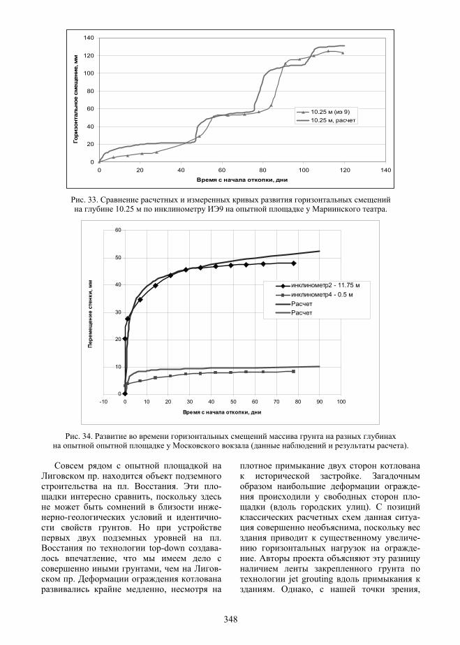
0

20

40

60

80

100

120

140

0 20 40 60 80 100 120 140

,

,

10.25 ( 9)10.25 ,

. 33. 10.25 9 .

0

10

20

30

40

50

60

-10 0 10 20 30 40 50 60 70 80 90 100

,

, 2 - 11.75 4 - 0.5

. 34. ( ).

.. . -

,-

- -.

. top-down -

,, -

.,

.--

( ).-

,--

.

jet grouting . , ,

348

., -

--

80 3 .

, - « » ( . 35).

-

.

. 35. , jet-grouting. .

-20

0

20

40

60

80

0 100 200 300 400 500 600

,

,

. 36. ( 1 ) ( 2).

2

1

349

--

( . 36). -

. ( -

-)

60 , -.

- 100 ,

5 . ,

, .,

5 , 10 .

30 ,

. .

,

, - (6). -

---

. -

, -,

- ( . 22).

--

, -. ,

., ,

-. -

8 , --.

, . . -,

15 . – . ,

(

) --

., -

.

,

.-

.

, ,.

-,

( 30 ) 15 . .

-. ,

-

, -:

.,

.-

[6]. - -

-. , -

, --

, (6) - 1 cu [ ].

, -, , ,

.

350

« -» -

..

,. -

-.

--

. , , -.

, -

-.

« -», ,

-,

. ,:-

,.

,:

?,

,

. -, « »

() « -

» () -

.

.

80×40 6.5 . -

-

( 10 ).-

, ,

.

, -

,,

.

- ---

. -

. ,,

,

. « -

– - – – »,

-, -

.

.,

,.

-,

« ». 7 .

4.

.

, -

. -, , -

,-

351

.--

.

, , ,-

. -

-,

.

.--

: -

,.

- ( ) -

, --,

.-

,--

.

,-

., -

, -.

., -

, -.

- - ,-

(6). ,

:1.

( -

, , -, -

. ., -);

2. --

;3.

-.

,

( -,

.). ,

--

,, -

. --:

.

.

-

,

.,

--

.

-

-.

,.

352

-

.- -

--

. ,-

() -

.

-, -

-, -

.

, -

.,

( -) 5 -

, -. 3

2 . ,10 (

).

, .-

,

. - (

, ,)

.

-.

-,

.

, Soletanche-Bachy

« -». – -

, ,,

. -

, -.

,

, -

,,

.-

FEM models,

-. -

-,

,.

, ( -

), -

( -), -

( ), (

).

-

.- -

--

.

353

1. . ., . . , . . -.

.// . . . .. , 2005.

2. . . -

// ,1981. 1.

3. . . - --

. . . 1975. 4. . .

. . 1977 .5. . .

. . , 1978.6. . .

. ., 1996.

7. . . , . . , . . ,. . “ -

-” // -

, 11,2007.

8. . . ---

: …. . ./ . . 1991.

9. . . -

: . … .. . . – ., 1987.

10. . . «

»// -. 12, 2008 - : -

« » 90-124 11. . .

.// -

. 12, 2008 - : - « -» 215-222.

12. Peck R.B. Advantages and limitation of the observational method in supplied soil mechanics. Geotechnique Vol. 19 #2 181-187, 1969.

13. . .-

»// -. 8, 2004 - :

- « » 5-29.

354

Geotechnical evaluation of projects and validation of design• Evaluation of sites’ investment potential• Site investigation• Geotechnical calculations, design solutions• Choice of a safe technology of works

implementation• Geotechnical calculation of construction

or reconstruction impact on the adjacent buildings, underground space and underground mains

• Preparation of geotechnical validation of design documents

Geotechnical monitoring• Development of method statements and

geotechnical schedules for special works• Adjustment of sparing technology regimes• Deformation monitoring• Condition monitoring of existing buildings• Ground water level monitoring• Vibration and acceleration monitoring

in soils and structures• Quality assessment of completed projects

Condition surveying• Construction sites and real estate• Historic buildings and structures

Works in congested urban environment• Surveying• Site investigation• Geophysical works

Civil and industrial design• Architectural design• Construction design and engineering• Complex development of investment validation,

design and working drawings• Design of engineering restoration of historic buildings• Designs for construction, reconstruction and

strengthening of underground structures in complicated geological conditions

• Design of dewatering and waterproofing• Foundations for machines with dynamic loads• Cost and technology optimization of designs• Expert assessment of designs, design solutions

Special works• Function of the General Designer• Function of the Client’s Engineer• Theoretical and practical construction supervision

G R O U P O F C O M P A N I E S

GEORECONSTRUCTION

The Group of companies «Georeconstruction» (GRF) was founded 15 years ago by the leading geotechnical engineers and designers of Saint-Petersburg. Since the earliest days of its existence the company has upheld and enriched profes-sional traditions and intellectual potential of Sankt-Peterburg school of construction design.

GRF has revived the best traditions of research design institutes on the modern cutting edge level of construction related scholarship. Consolidation of geotechnical research, calculations and design practice forms the basis for the company's competitive advantage. Participation in major international projects enables GRF to exchange experience with the leading local and foreign geotechnical companies and design bureaus.

architectural design,geotechnical engineering, complex reconstruction,

engineering restoration of buildings

190005, Russia, St. Petersburg, Izmaylovskiy prospekt 4Tel./Fax: +7 (812) 316-6118, 575-3587, 251-7098

e-mail: mail@georec.spb.ru http://www.georec.spb.ru

Обследование технического состояния• Объектов строительства и недвижимости• Исторических зданий и сооруженийГеотехническая оценка и обоснование проектов• Оценка инвестиционной привлекательности

объекта• Геотехнические исследования• Геотехнический расчет, проектные решения• Выбор безопасной технологии производства

работ• Геотехнический расчет влияния строительства

или реконструкции на прилегающую застрой-ку, подземное пространство и подземные коммуникации

• Разработка геотехнического обоснования проекта

Геотехнический мониторинг• Разработка проектов производства работ и

геотехнического регламента ведения специаль-ных работ

• Отладка щадящих технологических режимов• Контроль деформаций объектов• Контроль технического состояния застройки• Контроль уровня грунтовых вод• Контроль параметров колебаний грунта и

конструкций• Контроль качества возведенных конструкций

Изыскания в условиях городской застройки• Инженерно-геодезические• Инженерно-геологические• ГеофизическиеГражданское и промышленное проектирование• Архитектурное проектирование• Строительное проектирование и конструирова-

ние• Комплексная разработка обоснований инвести-

ций (ТЭО), проектов и рабочей документации• Проекты инженерной реставрации историче-

ских зданий• Проекты строительства, реконструкции и

усиления подземных конструкций в сложных инженерно-геологических условиях

• Проекты геотехнического водоотведения и гидроизоляции

• Фундаменты под машины с динамическими нагрузками

• Стоимостная и техническая оптимизация проектов

• Экспертиза проектов, проектных решенийСпециальные работы• Проектирование и мониторинг сейсмостойких

объектов• Научно-техническое сопровождение строитель-

ства и экспертиза безопасности объектов

Г Р У П П А К О М П А Н И Й

ГЕОРЕКОНСТРУКЦИЯ

Группа компаний «Геореконструкция» (GRF) создана 15 лет назад ведущими петербугскими геотехниками и проек-тировщиками. Со дня основания компания поддерживает и приумножает традиции и интеллектуальный потенциал петербургской школы строительного проектирования.

В GRF возрождены лучшие традиции научно-исследова- тельских проектных институтов на новом уровне развития строительной науки. Объединение научных исследований в области геотехники, расчетов и проектной практики составляют основу конкурентного преимущества фирмы. Участие в крупных международных проектах обеспечивает GRF обмен опытом с ведущими отечественными и зарубеж-ными геотехническими и проектными фирмами.

архитектурное проектирование и конструирование,геотехника, сложная реконструкция,

инженерная реставрация зданий

190005, Санкт-Петербург, Измайловский пр., 4тел./факс: (812) 316-6118, 575-3587, 251-7098

e-mail: mail@georec.spb.ru http://www.georec.spb.ru