GENETIC ANALYSIS OF NEUROPSYCHIATRIC DISORDERS ...

GENETIC ANALYSIS OF NEUROPSYCHIATRIC DISORDERS

IN A SOUTH AMERICAN POPULATION ISOLATE

BY

BARBARA KREMEYER

Submitted for the degree of Doctor of Philosophy

The Galton Laboratory

Research Department of Genetics, Evolution and Environment

University College London (UCL)

2008

1

UMI Number: U591592

All rights reserved

INFORMATION TO ALL USERS The quality of this reproduction is dependent upon the quality of the copy submitted.

In the unlikely event that the author did not send a complete manuscript and there are missing pages, these will be noted. Also, if material had to be removed,

a note will indicate the deletion.

Dissertation Publishing

UMI U591592Published by ProQuest LLC 2013. Copyright in the Dissertation held by the Author.

Microform Edition © ProQuest LLC.All rights reserved. This work is protected against

unauthorized copying under Title 17, United States Code.

ProQuest LLC 789 East Eisenhower Parkway

P.O. Box 1346 Ann Arbor, Ml 48106-1346

To my family

“In sooth, I know not why I am so sad:

It wearies me; you say it wearies you;

But how I caught it, found it, or came by it,

What stuff ‘tis made of, whereof it was born,

I am to learn. ”

Shakespeare, The Merchant o f Venice

Statement of Authorship

I, Barbara Kremeyer, confirm that the work presented in this thesis is my own.

Where information has been derived from other sources, I confirm that this has been

indicated in the thesis.

The sequencing of the CLINT 1 gene described in chapter 3 has been performed with

the help of the undergraduate student Amy Roberts, who was carrying out a research

project in our lab. Similarly, the genotyping of the SNP rsl 1955293, also described

in chapter 3, has been carried out with the help of the undergraduate student Natalia

Szypilow as part of a research project she performed in our lab. Both students

worked under my supervision.

I have genotyped all microsatellite markers typed for the linkage scan in chapter 4,

with technical assistance of Heike Muller, Emilie Boucher and Julie Pivard.

Most SNPs for the association analysis of the NOS1AP gene presented in chapter 5

were typed by our collaborators on that project at Rutgers University, U.S.A. SNP

rs 1415263 was genotyped by myself, with the help of the undergraduate student

Hanna Kymalainen who was carrying out a research project in our lab under my

supervision.

With exception of the factor analysis of schizophrenia symptoms in chapter 5, which

was done by Dr. Jenny Garcia from Universidad de Antioquia in Medellin,

Colombia, and of the haplotype analysis of the chromosome 5q region in chapter 3,

which was done by Susan Service at UCLA, I have personally performed all

statistical analyses in this thesis, and I have interpreted the results with the help of

my supervisor, Professor Andres Ruiz-Linares.

I have written this thesis myself without any help or use of materials other than that

acknowledged in this thesis. Comments were made by Professor Andres Ruiz-

Linares.

4

Acknowledgements

First and foremost, I would like to thank my supervisor, Professor Andres Ruiz Linares, to whom I am greatly indebted for his invaluable support and guidance. Thank you, Andres, for your incredible enthusiasm in discussing and encouraging my research, for teaching me so much, and for giving me so many opportunities to expand my horizon, here and overseas! Thank you for being such an inspiring supervisor! I would certainly not be where I am without your guidance. Muchas gracias por todo!

I would also like to express my gratitude to my secondary supervisor, Professor Sue Povey, who has always been available for discussion and feedback. Thank you Sue, for being so generous with your time and advice! I would also like to give you very special thanks for making it possible to concentrate wholly on my research in the last year of my PhD by granting me financial help. It was invaluable for me.

I am very grateful to Professor Steve Jones, who gave me the opportunity to work with him on his genetics course. Not only has this work helped me through most of my PhD financially; more importantly, it has provided me with a unique teaching experience, which I enjoyed very much.

It would have been impossible for me to write this thesis had it not been for the help and support of many colleagues and friends. From Andres’ group, I am especially grateful to Heike Muller, who has been wonderful both inside and outside the lab. Thank you so much for your great help with my project - I wouldn’t have been able to do it without you. And above all: thank you for being such a good friend! - I would also like to give very special thanks to Mari Wyn Burley, for being a wonderful colleague and friend, for many interesting discussions, and for always having an ear for my worries. Thank you! - Ibi, thank you so much for your friendship and all the great times we had together. I will never forget them! - Sijia, thanks for all those interesting discussions about science, politics and society. Your point of view always opened up new perspectives. - Ningning, Danny, Desmond, Kaisu, Nicolas, and Roisin - thanks a lot to all of you for your company!

To the undergraduate students who helped me with the data collection: Hanna, Amy, Natalia, Emilie and Julie - thank you for your excellent work!

From Wolfson House, I would like to thank Kevin Fowler and Jacques Gianino for their patience with all the complications inherent to my ever changing student status, and for the quick help they always provided with all administrative and financial issues. Thanks to Ian Evans for always being so friendly and helpful, and to all the Human Geneticists, especially Kate and Larissa, for all the good times we shared.

I owe great thanks to our collaborators from Universidad de Antioquia in Medellin. Not only did they contribute a lot to my PhD project, they also accepted me as a colleague and friend during my stay at the Laboratorio de Genetica Molecular. Many thanks to el profe, Professor Gabriel Bedoya, for being such a special host at Genmol, to Connie and Vicky for their friendship and the great times we had together, both in London and in Colombia, and to all the other - numerous! -

5

members of Genmol for being so friendly and open, and for making me feel at home in the lab.

From the Department of Psychiatry at U de A, I would especially like to thank Jenny Garcia: thank you for all your help and advice, both professional and personal, for sharing your enthusiasm for psychiatry and for being a good friend! - To all the members of the Group of Investigation in Psychiatry (GIPSI), especially Dr Jorge Ospina, and Patricia and Maria Cecilia: thanks for all your support and help, and for a great collaboration!

I am also very grateful to our collaborators at UCLA, especially to Professor Nelson Freimer, who kindly accepted me as a guest student in his lab and gave me the opportunity to learn a lot from him and his team.

Many thanks to my friends, for keeping me company through good and through difficult times. It is so good to know that true friendship lasts! Special thanks to Sarah, Anne, Christiane, Angelika, Sylvia, Antonia, Jana, Lucia, Yvonne, Fabio, Jan, and Nele.

To my Colombian family, thank you so much for giving me a second home in Medellin, and for making me a paisa at heart!

Last, but not least, I would like to thank my parents and my sisters. Thank you for all you have done for me and, most of all, for always, always believing in me! You truly gave me wings. I love you!

6

Abstract

Bipolar disorder (BP) and schizophrenia are severe neuropsychiatric conditions that

are among the leading causes of morbidity and chronic disability world-wide. Both

conditions are characterised by a substantial genetic heterogeneity, which has

complicated the search for susceptibility loci. One strategy to tackle this difficulty

lies in the study of population isolates that are characterised by a reduced genetic

heterogeneity. In this thesis, I have therefore conducted genetic studies of BP and

schizophrenia in the well-characterised South American population isolate of

Antioquia, Colombia.

Our group has recently reported the results of a linkage scan of six Antioquian

families segregating severe BP. Here, I performed a follow-up study of a candidate

region on chromosome 5q33. I sequenced the CLINT 1 gene, a functional candidate

that has also been implicated in schizophrenia, in affecteds from four BP pedigrees

from the original linkage study and identified three single base pair variants, all of

which had been previously described. A transmission distortion test of one of these

variants, rs 11955293, in a sample of 176 unrelated BP patients from Antioquia and

their parents found no evidence of association with BP. Although these results do not

rule out a minor effect of the CLINT 1 gene on susceptibility to the disorder in

Antioquia, other loci are likely to be of greater significance. This includes other

genes on chromosome 5q33, but also other candidate regions in the genome.

To further explore the latter possibility, I conducted a whole-genome linkage scan in

an additional nine pedigrees with severe BP from Antioquia and analysed the

obtained genotype data jointly with that of the initial linkage scan. Using parametric

and non-parametric linkage approaches, I explored three different diagnostic models:

a narrow model including only BP type I (BPI) as affected; a model including BPI

and II and major unipolar depression; and a third model including only individuals

who had experienced psychosis as affected. This second linkage scan found evidence

for a number of candidate regions, including chromosome 13q33 for BPI,

chromosomes l p l 3-31 and 1 q25-31 for mood disorders, chromosome 12ct-ql4 for

mood disorders, and chromosomes 2q24-31 and 16pl 2 for psychosis. Encouragingly,

many of these loci had previously been pinpointed as BP susceptibility loci in other

populations; on the other hand, we also identified a novel locus on chromosome 12q.

7

While the use of population isolates can help decrease the genetic heterogeneity of a

complex disease, complementary strategies can be used to reduce this heterogeneity

even further. In studying the NOS JAP gene, a functional candidate on chromosome

lq23 that is involved in glutamatergic neurotransmission, in a sample of 102

unrelated Antioquian schizophrenia patients and their parents, I have therefore used

both categorical and dimensional approaches to the disease phenotype. In the

categorical approach, I conducted an analysis for association between the NOS1AP

gene and DSM-IV schizophrenia by TDT. For the dimensional approach, two clinical

scales measuring positive and negative symptoms, SANS and SAPS, were applied to

all patients and dimensional scores were obtained from these scales by factors

analysis. I then performed quantitative TDT analysis of the dimensional scores. My

analyses found association to both DSM-IV schizophrenia and a clinical dimension

capturing negative symptoms, in line with a role of NOS1AP in glutamatergic

neurotransmission. The results of these analyses also underline the usefulness of a

dimensional approach in psychiatric genetics.

8

Table of Contents

STATEMENT OF A U TH O R SH IP................................................................................................................................................. 4

ACKNOWLEDGEMENTS............................................................................................................................................................... 5

ABSTRACT..........................................................................................................................................................................................7

LIST OF FIG URES...........................................................................................................................................................................13

LIST OF TABLES..............................................................................................................................................................................15

1. INTRODUCTION.......................................................................................................................................................... 20

1.1. W hy Study Psychiatric G enetics? ........................................................................................................................20

1.1.1. Limitations o f current diagnostic and trea tm ent stra teg ies ..................................................................................................21

1.1.2. The relevance o f genetics to psychiatry ...................................................................................................................................................................................23

1.1.2.1. Identification of disease markers...................................................................................... 24

1.1.2.2. Genetic counselling and predictive testing.....................................................................25

1.1.2.3. Drug development and individualised pharmacological treatm ent........................... 27

1.1.2.4. Impact on psychiatric research...........................................................................................31

1.1.3. The exam ple o f Alzheimer's Disease ................................................................................................................................................................................................32

1 .2 . Strategies fo r Gene Discovery.............................................................................................................................34

1.2.1. M onogenic vs. complex diseases .............................................................................................................................................................................................................34

1.2.2. Genetic M apping - a Conceptual Overview ....................................................................................................................................................................35

1.2.3. Linkage Analysis .................................................................................................................................................................................................................................................................................38

1.2.4. Linkage Disequilibrium and Association M apping ......................................................................................................................................... 43

1.2.4.1. Linkage disequilibrium as a tool for gene mapping........................................................ 43

1.2.4.2. Measures of linkage disequilibrium...................................................................................46

1.2.4.3. Patterns of linkage disequilibrium in the human genom e........................................... 47

1.2.4.4. The "common disease, common variant" and "common disease, rare variant"

hypotheses................................................................................................................................................ 51

1.2.4.5. Candidate Gene Studies...................................................................................................... 52

1.2.4.6. Population stratification and family-based association...............................................52

1.3. Population isolates and the Paisa Co m m u n ity of A ntioquia , Co l o m b ia ............................................... 55

1.3.1. Population Isola tes ....................................................................................................................................................................................................................................................................55

1.3.2. The Paisa Community o f Antioquia, Colom bia .......................................................................................................................................................58

1.4. Bipolar D isorder ...................................................................................................................................................... 60

1.4.1. Clinical Presentation and Classification ...................................................................................................................................................................................60

1.4.2. Epidemiology ............................................................................................................................................................................................................................................................................................62

1.4.3. Genetics o f Bipolar Disorder ................................................................................................................................................................................................................................63

1.5. Schizophrenia.............................................................................................................................................................66

1.5.1. Clinical Presentation and Classification ...................................................................................................................................................................................66

9

1.5.2. Epidemiology ............................................................................................................................................................. 67

1.5.3. Genetics o f Schizophrenia ..................................................................................................................................68

1 .6 . Ps y c h ia tr ic G en e tic s in A n t io q u ia a n d t h e C e n tr a l V alley o f Co s t a R ic a .....................................................7 1

1 .7 . T hesis O v e r v ie w a n d A i m s .........................................................................................................................................................7 3

2 . SUBJECTS AND M ETHO DS......................................................................................................................................75

2 .1 . Su b j e c t s ...............................................................................................................................................................................................7 5

2.1.1. Patient Ascertainment and Diagnostic Procedure ............................................................................ 7 5

2.1.2. Extended Bipolar Pedigrees..............................................................................................................................78

2.1.3. Bipolar Trio Sample................................................................................................................................................ 87

2.1.4. Schizophrenia Trio Sample................................................................................................................................88

2.1.5. Ethical Committee Approval............................................................................................................................88

2.2. L a b o ra to r y M e th o d s ...................................................................................................................................................................8 9

2.2.1. Sample Collection and DNA Extraction .................................................................................................... 89

2.2.2. DNA Concentration Measurement and Adjustm ent........................................................................89

2.2.3. The Polymerase Chain Reaction (PCR)...................................................................................................... 89

2.2.4. Agarose Gel Electrophoresis ........................................................................................................................... 92

2.2.5. G enotyping ................................................................................................................................................................. 93

2.2.5.1. Microsatellite Markers......................................................................................................... 94

2.2.5.2. Fragment Length Analysis....................................................................................................95

2.2.5.3. Single Nucleotide Polymorphisms......................................................................................98

2.2.5.4. Restriction Fragment Length Polymorphism Analysis................................................... 98

2.2.6. Sequencing................................................................................................................................................................100

2 .3 . D a t a A nalysis a n d St a t is t ic a l M e t h o d s ......................................................................................................................... 1 0 1

2.3.1. The Linkage Format, Recoding and File Conversion ..................................................................... 102

2.3.2. The SimWalk2 Programme ............................................................................................................................ 103

2.3.3. Hardy Weinberg Equilibrium .........................................................................................................................104

2.3.4. Test fo r Mendelian Inheritance ....................................................................................................................106

2.3.5. Test fo r Non-Mendelian Errors ................................................................................................................... 106

2.3.6. Estimation o f Allele Frequencies from Pedigree Data ..................................................................107

2.3.7. Parametric Linkage Analysis .........................................................................................................................108

2.3.8. Non-Parametric Linkage Analysis..............................................................................................................109

2.3.9. Haplotype Analysis ............................................................................................................................................. 109

2.3.10. Transmission Disequilibrium Analysis .............................................................................................. 109

2.3.11. Linkage Disequilibrium Analysis...........................................................................................................110

2.3.12. Quantitative TDT Analysis ........................................................................................................................ I l l

3. ANALYSIS OF THE CLINT1 GENE AS A CANDIDATE LOCUS FOR PSYCHOSIS................................ 113

3 .1 . Ba c k g r o u n d a n d P r e v io u s W o r k ........................................................................................................................................1 1 3

10

3.2. M aterials and M e th o d s ...................................................................................................................................... 116

3.2.1. Sequencing o f the CLINT1 gene in the Antioquian fa m ilie s ................................................................................................116

3.2.2. Transmission Distortion Analysis o f a SNP in Exon 12 o f the CLINT1 gene in a

Bipolar Trio sam ple from A ntioquia ................................................................................................................................................................................................................................123

3.3. Results....................................................................................................................................................................... 127

3.3.1. Sequencing o f the CLINT1 gene in the Antioquian fa m ilie s ................................................................................................127

3.3.2. TDT Analysis o f a marker r s ll9 5 5 2 9 3 ....................................................................................................................................................................................131

3.4. D iscussion.................................................................................................................................................................132

3.5. Conclusion and Future W ork ............................................................................................................................136

4 . GENOM E-W IDE LINKAGE STUDY IN 15 EXTENDED BIPOLAR PEDIGREES FROM THE PAISA

CO M M UN ITY ............................................................................................................................................................................... 1 3 8

4.1 . Background and Previous W ork.......................................................................................................................138

4.2 . Study De s ig n ........................................................................................................................................................... 140

4.3 . Power A nalysis ...................................................................................................................................................... 143

4.4 . Data Collection ..................................................................................................................................................... 150

4.4.1. Genotype Collection fo r Nine Extended Bipolar Pedigrees from the Paisa Community

150

4.4.2. Building the Joint Data Set ...................................................................................................................................................................................................................................154

4.5 . Data A nalysis.......................................................................................................................................................... 160

4.6 . Results....................................................................................................................................................................... 162

4.6.1. Data Com pleteness ................................................................................................................................................................................................................................................................162

4.6.2. Linkage Analysis: Narrow M odel .........................................................................................................................................................................................................165

4.6.2.1. Parametric Analysis............................................................................................................165

4.6.2.2. Non-Parametric Analysis.................................................................................................. 177

4.6.3. Linkage Analysis: Broad M odel .................................................................................................................................................................................................................186

4.6.4. Linkage Analysis: Psychosis M o d el .................................................................................................................................................................................................195

4.6.5. Sum m ary o f the Linkage Results ..........................................................................................................................................................................................................202

4 .7 . D iscussion.................................................................................................................................................................208

4 .8 . Conclusion and Future W ork ........................................................................................................................... 225

5 . TRANSMISSION DISTORTION ANALYSIS OF A SCHIZOPHRENIA TRIO SAMPLE FROM

ANTIOQUIA AT THE N O S1A P LOCUS............................................................................................................................... 22 9

5.1. NOS1AP as a Candidate Gene fo r Schizophrenia........................................................................................229

5.2. Clinical D imensions of Schizophrenia ............................................................................................................. 231

5.3. M aterials and M e th o d s ......................................................................................................................................235

5.3.1. M arker Selection and G enotyping ...................................................................................................................................................................................................235

5.3.2. Data Analysis ......................................................................................................................................................................................................................................................................................238

5.4. Results....................................................................................................................................................................... 239

11

239

240

241

243

245

247

251

25 3

255

2 8 6

286

288

302

12

5.4.1. Hardy- Weinberg Equilibrium ................................................................................................................................................

5.4.2. Linkage Disequilibrium Analysis ......................................................................................................................................

5.4.3. Single marker association te s ts ......................................................................................................................................

5.4.4. Haplotype association ..........................................................................................................................................................................

5.4.5. QTDT analysis on clinical dim ensions ................................................................................................................

D is c u s s io n .............................................................................................................................................................

F u t u r e W o r k ......................................................................................................................................................

SUMMARY AND CONCLUDING REMARKS...............................................................

BIBLIOGRAPHY......................................................................................................................

A PPEN D IX ................................................................................................................................

A b b r e v ia t io n s .....................................................................................................................................................

D a t a c o m p l e t e n e s s f o r a l l m a r k e r s g e n o t y p e d a s p a r t o f t h e B P l in k a g e s c a n

P u b l is h e d P a p e r s a n d M a n u s c r ip t s ..................................................................................................

List of Figures

Figure 1.1: Liability distribution for a complex disease in the population...................................................35

Figure 1.2: Stages o f gene discovery.................................................................................................................... 36

Figure 1.3: Co-segregation o f a disease phenotype and a two-locus haplotype in a three-generation

pedigree........................................................................................................................................................................39

Figure 1.4: Linkage Disequilibrium...................................................................................................................... 44

Figure 1.5: The principle o f association analysis............................................................................................... 45

Figure 1.6: Spurious association due to population stratification in case-control studies........................ 53

Figure 1.7: Principle o f trio-based association....................................................................................................54

Figure 1.8: Population growth in the Province o f Antioquia, Colombia, from 1780 to the 1990s.........58

Figure 1.9: Map o f Colombia and the Province o f Antioquia........................................................................ 59

Figure 2.1: Set o f six Antioquian pedigrees genotyped as part o f the whole-genome linkage study

performed by Herzberg et al. (2006) and re-analysed in the frame o f this thesis....................................... 82

Figure 2.2: Set o f nine paisa pedigrees genotyped and analysed for this thesis......................................... 86

Figure 2.3: Agarose gel with PCR products........................................................................................................93

Figure 2.4: Schematic representation o f a microsatellite locus.......................................................................94

Figure 2.5: Fragment length analysis with the GeneMapper® software.......................................................97

Figure 2.6: Principle o f restriction fragment length polymorphism analysis...............................................99

Figure 3.1: Results o f the fine mapping o f the candidate region on chromosome 5q31-34 in 17

pedigrees from Antioquia and the Central Valley o f Costa Rica..................................................................114

Figure 3.2: Results o f the haplotype analysis o f chromosome 5q in families ANT03, ANT04, ANT07

and ANT15................................................................................................................................................................ 120

Figure 3.3: Sequence o f the amplicon designed for rsl 1955293 genotyping.......................................... 123

Figure 3.4: Electropherogram showing a heterozygous genotype for SNP rsl 1955293...................... 124

Figure 3.5: LD structure across the CLINT1 gene region the European HapMap population............. 133

Figure 4.1: Cut-down version o f pedigree FAZU01 used for the power simulations..............................145

Figure 4.2: Results o f the power simulation for parametric linkage analysis under the narrow model.

......................................................................................................................................................................................146

Figure 4.3: Schematic representation o f the data collection procedure.......................................................153

Figure 4.4: “Mirror image” for marker D6S462............................................................................................. 157

13

Figure 4.5: Mix-up between genotypes o f panel 10 in data set 1............................................................... 159

Figure 4.6: Flow chart o f the data analysis procedure................................................................................... 161

Figure 4.7: Multipoint study-wide HLOD scores along chromosome 21 ................................................. 166

Figure 4.8: Multipoint study-wide HLOD scores and a-values along chromosome 13..................166

Figure 4.9: Multipoint study-wide HLOD scores and a-values along chromosome....... 1.................. 167

Figure 4.10: Haplotype reconstruction for chromosome 21 in family A N T 07........................................ 172

Figure 4.11: Haplotype reconstruction for a candidate region on chromosome 3 in family ANT07. 173

Figure 4.12: Haplotype reconstruction for a candidate region on chromosome 15 in family ANT18.

......................................................................................................................................................................................174

Figure 4.13: Haplotype reconstruction for a candidate region on chromosome 11 in family FAZU01.

......................................................................................................................................................................................175


Figure 4.15: Combined N P L PAirs scores for chromosomes 1-5 (narrow model).................................... 179

Figure 4.16: Combined N P L PAirs scores for chromosomes 6-12 (narrow model)................................ 180

Figure 4.17: Combined NPLPA|RS scores for chromosomes 13-22 (narrow model)................................181


......................................................................................................................................................................................184

Figure 4.19: Haplotype reconstruction for chromosome 21 in family A N T 14....................................... 185

Figure 4.20: Combined NPLpairs scores for chromosomes 1-5 (broad model).......................................189

Figure 4.21: Combined NPLpairs scores for chromosomes 6-12 (broad model).................................... 190

Figure 4.22: Combined N P L PAiRS scores for chromosomes 13-22 (broad model).................................. 191


Figure 4.24: Combined NPLpairs scores for chromosomes 1-5 (psychosis model)............................... 197

Figure 4.25: Combined N P L PAiRS scores for chromosomes 6-12 (psychosis model).............................198

Figure 4.26: Combined N P L PAirs scores for chromosomes 13-22 (psychosis model)...........................199


Figure 4.28: Haplotype reconstruction for chromosome 21 in family ANT15.........................................204

Figure 4.29: Haplotype reconstruction for a candidate region on chromosome lp in pedigrees ANT03

(top) and ANT 19 (bottom).................................................................................................................................... 206

Figure 4.30: Haplotype reconstruction for a candidate region on chromosome lp in a nuclear family

forming part o f pedigree FAZU01...................................................................................................................... 207

14

Figure 5.1: Location o f all genotyped markers along the NOS1AP gene region,.................................... 235

Figure 5.2: LD structure between 22 genotyped SNPs across the NOS1AP gene in the Antioquian trio

sample........................................................................................................................................................................ 240

Figure 5.3: LD structure across the NOS1AP gene based on data for the European HapMap population

..................................................................................................................................................................................... 241

List of Tables

Table 2.1: Pedigree characteristics........................................................................................................................ 79

Table 2.2: Characteristics o f the sample for family-based association in BPI. nf, nuclear family.......87

Table 2.3: Characteristics o f the sample for family-based association in BPI. nf, nuclear family.......88

Table 2.4: Set-up o f a standard PCR reaction (per reaction)...........................................................................91

Table 2.5: Cycling conditions for a standard PCR............................................................................................ 92

Table 2.6: Set-up o f the Tsp509I digest (per reaction).....................................................................................99

Table 2.7: Sequencing reaction set-up (per reaction)..................................................................................... 101

Table 3.1: Set-up o f the PCRs for amplification o f the CLINT1 gene.........................................................121

Table 3.2: Touch-down PCR programme used for the CLINT1 amplicons............................................... 121

Table 3.3: Sequences o f the primers used for the amplification o f the CLINT 1 gene.............................122

Table 3.4: Touch-down PCR programme used for the amplification o f the genomic sequence around

rsl 1955293.............................................................................................................................................................. 125

Table 3.5: Sequencing success for the CLINT1 gene in Antioquian BP family samples.......................128

Table 3.6: Transmission distortion analysis o f alleles at locus rsl 1955293............................................ 131

Table 4.1: Markers with heterogeneity LOD scores > 1.3 in two-point parametric linkage analysis o f

genome scan data from six Antioquian BPI pedigrees....................................................................................138

Table 4.2: Markers with the highest combined NPL scores (p < 0.05) in the genome scan o f six

Antioquian pedigrees.............................................................................................................................................. 139

Table 4.3: Study-wide results o f the power simulation for parametric linkage analysis under the

narrow model............................................................................................................................................................ 146

Table 4.4: Pedigree-wise results o f the power simulation for parametric linkage analysis under the

narrow model............................................................................................................................................................ 147

Table 4.5: Microsatellite markers for which repeats were performed using M l 3-tailed primers 151

15

Table 4.6: Set-up for PCRs using the M l 3-tailed primers (per reaction)................................................... 151

Table 4.7: Cycling conditions for the PCRs with M l 3-tailed primers...................................................... 152

Table 4.8: Pooling panel comprising four o f the M13-PCR products....................................................... 152

Table 4.9: Completeness o f the data obtained for the genome-wide linkage scan in fifteen extended

pedigrees from Antioquia (by chromosome).....................................................................................................164

Table 4.10: Regions with study-wide HLOD scores > 1 .3 .............................................................................165

Table 4.11: Maximum multipoint LOD scores for each o f the 15 extended pedigrees in the three

chromosomal regions with a study-wide HLOD score > 1 .3 .........................................................................168

Table 4.12: Chromosome regions with single-family LOD scores > 2.0..................................................169

Table 4.13: Markers with combined NPLpairs scores > 1.3 (equivalent to p < 0.05) in the genome scan

o f fifteen BPI pedigrees (narrow model)............................................................................................................178

Table 4.14: Markers with single-family NPLPAiRS scores > 2.0 (narrow model)...................................... 182

Table 4.15: Markers with combined NPLPAirS scores > 1.3 (equivalent to p < 0.05) in the genome scan

o f fifteen extended paisa pedigrees (broad model)..........................................................................................188

Table 4.16: Markers with single-family NPLpairs scores > 2.0 (broad) model)....................................... 192

Table 4.17: Markers with combined NPLpafrs scores > 1.3 (equivalent to p < 0.05) in the genome scan

o f fifteen extended paisa pedigrees (psychosis model).................................................................................. 196

Table 4.18: Markers with single-family NPLPA|RS scores > 2.0 (psychosis model).................................200

Table 4.19: Synopsis o f the chromosomal regions for which a HLOD score (in parametric analysis) or

a combined NPLpairs score (in non-parametric analysis) > 1.3 were obtained (across all diagnostic

models)...................................................................................................................................................................... 203

Table 4.20: Synopsis o f the chromosomal regions for which a LOD score (in parametric analysis) or

an individual NPLpairs score (in non-parametric analysis) > 2 .0 were obtained for in a single pedigree

(all diagnostic models)........................................................................................................................................... 203

Table 5.1: Clinical dimensions obtained from SANS and SAPS by factor analysis............................... 234

Table 5.2: Results o f the Hardy-Weinberg equilibrium test in 23 SNPs across the NOS1AP gene

region in the schizophrenia trio sample from Antioquia................................................................................ 239

Table 5.3: Single marker TDT (TRANSMIT) for 22 SNPs within the CAPON gene............................242

Table 5.4: Results o f the transmission disequilibrium test o f the haplotype containing the ten SNPs

forming LD region 1...............................................................................................................................................244

Table 5.5: Results o f the QTDT analysis for 17 SNPs in the NOS1AP gene region............................... 246

Table 8.1: Completeness o f the data obtained for chromosome 1 in the genome-wide linkage scan o f

fifteen extended pedigrees segregating severe bipolar disorder from Antioquia......................................288

16






fifteen extended pedigrees segregating severe bipolar disorder from Antioquia..................................... 291











Table 8.10: Completeness o f the data obtained for chromosome 10 in the genome-wide linkage scan

o f fifteen extended pedigrees segregating severe bipolar disorder from Antioquia.................................296

















17









18

C h a p t e r O n e

In t r o d u c t io n

1. Introduction

This thesis aims at making a contribution to the genetics of two major

neuropsychiatric disorders, bipolar disorder, also known as manic depression, and

schizophrenia. In this introduction, I shall put the present work into the context of

current efforts to understand the aetiology of psychiatric disease. First, I shall

introduce the rationale of focussing on the genetics of psychiatric disease (chapter

1.1). In chapters 1.2 and 1.3, I will introduce different aspects of the methodology

used in this thesis and elsewhere to localise and identify loci involved in the genetic

susceptibility to disease. Chapters 1.4 and 1.5 shall give an introduction to the

phenotypes studied here - bipolar disorder and schizophrenia - , and to their

epidemiology and genetics. In chapter 1.6, I will present the ongoing psychiatric

genetics project in the populations of Antioquia and Costa Rica, in the context of

which this thesis has to be viewed. Finally, the aims of this thesis will be presented in

detail in chapter 1.7.

1.1. Why Study Psychiatric Genetics?

Neuropsychiatric disorders are among the leading causes of morbidity and chronic

disability world-wide, with unipolar depression as well as the two major psychoses,

bipolar disorder and schizophrenia, ranking among the top ten causes of years lost to

disability in both the developing and the developed world1. Severe psychiatric

conditions do not only have devastating consequences for the patients’ mental, social9 r sr

and economic well-being ' and even their general health , they also represent a

major cost to health systems and national economies alike. It has been estimated that

the annual cost of bipolar disorder to society, including treatment as well as indirect

costs due to factors such as unemployment and absenteeism, amounts to about £2

billion in the UK7. The figure for schizophrenia is even higher, with an estimated

annual cost of £2.6 billion for England alone8, and the yearly costs of major unipolar

depression for adults in England are leading the list at a staggering £9 billion9. It is

evident that there is a great need to reduce the burden of mental illness on both

affected individuals and society as a whole.

20

1.1.1. Limitations of current diagnostic and treatment strategies

The successful and cost-efficient treatment of psychiatric illness (its cure not

currently being conceivable) relies crucially on a meaningful and reliable diagnosis,

as well as on an adequate choice of pharmacotherapy. In practice, however, both the

correct diagnosis of psychiatric illness and the choice of treatment can represent a

challenge. Because there are no indicators at a molecular, physiological or

behavioural level that are at the same time necessary and sufficient for the diagnosis

of any mental disorder (i.e., there are no biological or behavioural markers for mental

disease), psychiatric diagnoses rely solely on constellations of clinical signs and

symptoms as well as on the course of disease10. This is reflected by the diagnostic

procedures specified in the main clinical manuals of psychiatry, the Diagnostic and

Statistical Manual of Mental Disorders, published by the American Psychiatric

Association (currently in its 4th edition: DSM-IV)11 and the International

Classification of Diseases, published by the World Health Organization (currently in

its 10 edition: ICD-10) . The classification system on which these manuals are

based does most likely not represent true disease entities. Indeed, there is substantial

clinical heterogeneity within the current diagnostic categories for many mental

disorders. An extreme example is schizophrenia, where two patients with the same1 9diagnosis might not share a single symptom . This supports the idea that the current

diagnostic categories include distinct diseases with different, but possibly related,

pathophysiologies, resulting in a similar clinical phenotype. Conversely, disorders

which have traditionally been regarded as distinct entities, namely the two main

functional psychoses, bipolar disorder and schizophrenia14, might share at least part

of their aetiopathology15,16. As these examples show, there is still considerable

uncertainty in psychiatric nosology, and although the diagnoses based on the current

classification of mental disease are reliable and practical in many ways, they might

not be valid from an aetiological point of view17.

A valid and meaningful diagnosis should be based on the aetiology of the disease and

will ideally inform the choice of treatment, with the ultimate goal to spare patients

the tedious procedure of trial and error in order to find the right medication, as it is

currently the case in psychiatric practice. This trial and error procedure is not only

emotionally upsetting for patients and delays the onset of efficient treatment; it can

even have an adverse impact on the treatment outcome, since the success of

21

pharmacological treatment may depend on an early intervention at the onset of the

disease. This is thought to be due to neurotoxic effects of psychotic and depressive

episodes, leading to structural changes in the brain and rendering subsequent

treatment more difficult18'20. A quick start of the right course of pharmacotherapy is

therefore essential, and a meaningful diagnosis is crucial to achieve this.

An additional factor influencing and often complicating diagnosis and treatment is91comorbidity with other psychiatric disorders . Mood disorders, for example,

9 9 99frequently co-occur with anxiety disorders ’ . There is also substantial comorbidity

between bipolar disorder and panic disorder24 and, in children, attention-deficit

hyperactivity disorder25, while substance abuse disorder is very common in patients9A 9 8with schizophrenia and mood disorders among others ' . There are several possible

mechanisms leading to psychiatric comorbidity: (1) one disorder could act as a risk

factor for the development of another (e.g., cannabis abuse increases the risk of

developing psychosis29); (2) the two disorders might share common risk factors (e.g.,

it has been suggested that schizophrenia and diabetes might share common genetic

predisposition ); and (3) the two co-occurring disorders might in fact be different

facets of the same disease. It is possible that all three mechanisms are truly relevant

to psychiatric comorbidity. The distinction between them ultimately comes down to

the distinction between true comorbidity, i.e., the true co-occurrence of two distinct

disorders in the same patient, and the co-occurrence of symptoms in a single

disorder. Since the aetiology of a disorder whose phenotype, for example, comprises

both depressive and anxious symptoms might be different to the aetiology of both

depression and anxiety disorder, this distinction might entail important consequences91for the treatment and the prediction of course and outcome of mental illness .

As we have seen, there are several limitations to the current, descriptive classi

fication system of psychiatric illness concerning the aetiological relationship between

diseases, including comorbidity. Resolving these issues would lead to a better and

more complete understanding of the epidemiology of psychiatric illness, including

risk factors, course of disease, treatment outcome and patterns of true comorbidity, as

well as to an aetiologically valid diagnostic system. To achieve a shift from a

descriptive to a true taxonomic classification of disease (i.e., a classification system

based on true disease entities), better insights into the pathophysiology of mental

illness are indispensable.

22

While substantial advances have been made in the elucidation of disease mechanisms

in other areas of medicine, research into the biological causes of mental illness has

been much less successful, and our understanding of its aetiopathology remains

poor31. This is due to the aetiological complexity of psychiatric disease, resulting

from genetic heterogeneity, variable expressivity, pleiotropy and gene-environmental

interaction among others10,32, and reflecting the complexity of brain function.

However, while we still have a long way to go in order to achieve a thorough

understanding of mental illness that can be translated into better diagnosis and,

ultimately, into better and more individualised treatment options, we have certainly

started to move into the right direction. The past decades have seen important

progress in the understanding of the neurobiology underlying many neuropsychiatric'K'X T7conditions, including Alzheimer’s disease, schizophrenia, and bipolar disorder ' ,

and the field of psychiatric genetics has significantly contributed to these advances.

1.1.2. The relevance of genetics to psychiatry

From the early days of genetic research in psychiatry on, family, twin, and adoption

studies have demonstrated the importance of genetic liability to mental illness ’ .

With the advent of the first generation of psychotropic drugs, specific pathways

involved in the aetiology of psychiatric disease, such as monoaminergic

neurotransmission, could be pinpointed for the first time40,41. One of the major roles

of genetic research since then has consisted in confirming the importance of these

biochemical pathways for the pathophysiology of mental illness42, the main

methodological approach consisting in candidate gene association studies. In recent

years, advances in high-throughput genotyping techniques and statistical analysis

have made whole-genome association studies a reality43-45, a development that raises

the distinct possibility of inversing this relationship and uncovering new pathways

involved in psychiatric disease through the identification of novel susceptibility loci.

Since long before the era of genome-wide association, linkage analysis studies have

pursued the same goal, although their success in psychiatric disease has been limited

by the complex nature of mental illness46,47. The feasibility of whole-genome

association approaches has been shown for other complex traits, such as obesity,

where the discovery of a previously unknown susceptibility locus, the FTO gene, hasAO

opened up the possibility of detecting a whole new pathway . At the same time, the

23

establishment of large-scale national and international collaborations allows the

collection of samples that are large enough to detect susceptibility loci with small to

moderate effects, such as they are expected for most psychiatric diseases49. This

approach has been successful in other diseases including type l 50 and type 2

diabetes51,52 and breast cancer53.

Through the uncovering of susceptibility loci and novel pathways leading to mental

illness, progress in psychiatric genetics has the potential to catalyse advances in

many areas of psychiatry. Some of the most important areas will be discussed in the

following.

1.1.1.1. Identification of disease markers

As an essential step towards valid and meaningful diagnoses, as well as towards

early detection and prevention of illness, genetics may contribute to the development

of biological markers of disease. Because psychiatric diseases are thought to be

caused by an accumulation of common genetic variants, each of which might only

confer a small increase in disease risk, it seems unlikely that the test of a single

genetic variant will be specific and at the same time sensitive enough to serve as a

disease marker on its own10,54. However, the elucidation of disease mechanisms with

the help of genetics should facilitate the identification of physiological markers with

a higher predictive value than the genetic polymorphisms associated with disease

alone. These might include neuroendocrinological factors and proteins involved in

signal transduction, among others. Additionally, genetic polymorphisms could be

incorporated in a panel of markers that together have a higher and more specific

predictive value than any marker on its own10. A recent study on type 2 diabetes, for

example, has shown that the combined information from three known risk loci allows

the identification of population subgroups at risk for the disease55. Through

simulation studies, Janssens et al. (2006) have recently shown that genetic profiling

by typing a panel of up to 400 risk-associated polymorphisms can have high

specificity and sensitivity in predicting the risk of developing common disease56.

This is particularly true for rare diseases with a prevalence of around 1 % and a high

heritability, such as schizophrenia and bipolar disorder.

24

The development of biological markers of disease will be essential for the diagnostic

process, as well as for the early identification of individuals at risk for psychiatric

illness, thereby moving towards the ultimate goal of disease prevention. One setting

in which early identification of individuals at risk might happen, is genetic

counselling.

I.I.I.2. Genetic counselling and predictive testing

Genetic counselling is the process of educating patients and/or their relatives about

principles of human genetics applicable to inherited disease, such as patterns of

inheritance and the risk of disease attached to predisposing genes, thereby enabling

them to make informed and autonomous decisions in all areas of their lives57.

Importantly, this process should always be non-directive so that the decision making

remains entirely with the consultand. Most counselling situations explore two basic

scenarios: (1) in the case of affected individuals and their spouses, most questions

evolve around the risk of disease in offspring, and (2) in the case of unaffected

relatives of patients suffering from the disease, both the risk of disease in the

offspring and the personal risk of developing the disease later in life are of1 0 r o

concern ’ . Most genetic counselling occurs in the context of rare Mendelian

disorders where risk estimation is relatively straightforward and is either based on

the results of a genetic test or on the mode of inheritance. In psychiatry, where

inheritance patterns are much more complex, genetic counselling is still a nascent

field, but there is growing awareness of a need for such services59. This need might

become more urgent as patients’ awareness of genetic predisposition to mental

illness is raised through the mass media.

Because there are no predictive tests for the vast majority of psychiatric diseases, and

because of the complex inheritance of mental illness, recurrence risk estimates can

only be given based on empirical epidemiological data. Currently, the main goals of

genetic counselling in psychiatry are therefore to educate the patient about genetic

factors in psychiatric disease, to provide empirical recurrence risks and to help the

consultand cope with practical and psychological issues arising from this process59,60.

While the first and the last point represent very important aspects of the genetic

25

counselling process, it is on risk prediction that advances in psychiatric genetics are

most likely to have a direct impact.

Empirical recurrence risks are available for all major psychiatric conditions38. For

example, the recurrence risk in the first-degree relative of a bipolar patient lies

between 4 and 18%, while for the same relative, the risk of developing unipolar

major depression can be as high as 25%59. These estimates can vary according to the

number of affected relatives and their relationship to the consultand38. Naturally,

empirical risk figures are not available for every possible family constellation, and it

is therefore difficult to give consultands an estimate of their personal disease

liability. The development of disease markers, as discussed in chapter 1.1.1.1, holds

the - albeit still distant - promise of a more accurate disease prediction. This would

enable mental health professionals to monitor specific individuals at high risk and

intervene at the earliest stage of the disease, thereby significantly increasing the

chance of effective treatment and management of the disease. Early recognition of

individuals at risk for mental illness paired with innovative treatment approaches (see

chapter 1.1.1.3), both fuelled by advances in psychiatric genetics, could constitute an

important step on the way to disease prevention.

An aspect of special interest in the context of genetic counselling is the possibility of

defining the interaction between genetic and environmental factors in a way that

could enable counsellors in the future to give consultands personalised advice about

which environmental risk factors best to avoid in order to keep their disease risk at

bay. Given our current fragmentary level of knowledge, this scenario might seem

even further away than risk prediction based on genetics alone, but its potential for

disease prevention would make it well worth striving for. In recent years, evidence

for the modifying effect of specific genotypes on the susceptibility to environmental

risk factors for mental illness has accumulated (Ref 61; see also chapter 1.1.1.4), and

this knowledge could be used to inform life-style choices in individuals at risk for

psychiatric disease.

While predictive testing in psychiatry has the potential to be of great benefit for

psychiatric patients and their relatives, some important ethical considerations need to

be made. Although these issues can only be touched upon in this thesis, it should be

emphasised that it is crucial for every researcher in psychiatric genetics to realise and

reflect on the profound impact the possibility of predictive testing might have on the

26

lives of those suffering from or at risk for mental illness. The availability of a genetic

test for psychiatric disease introduces the possibility of prenatal or preimplantation

testing for children of couples with a family history of mental illness. Although it

might be justifiable to screen for the most severe conditions such as treatment

resistant schizophrenia, it is not clear where the limit lies between disease prevention

and screening for offspring with a certain behaviour, desirable to the parents or

society as a whole. Only recently, a genetic test that helps predict physical endurancefi'yhas become available , and while this test (which only analyses a single genetic

polymorphism) might still be a long way from allowing precise predictions of

physical performance, the possibility of tailoring one’s offspring according to

specific, non health-related ideals is conceivable. The prospect of this kind of

physical performance-based selection seems sinister; a behaviour-based selection

might seem even more so.

Furthermore, predictive testing in psychiatry can have a profound impact on the

availability of medical insurance to individuals at risk, as well as on employment

chances. These are just very few aspects of the stigmatisation resulting from being

labelled as “at risk” for psychiatric disease, and a legal and ethical framework is

needed before predictive testing in psychiatry can be put into practice.

1.1.1.3. Drug development and individualised pharmacological treatment

The first drug for the treatment of a psychiatric condition to become available was

iproniazid, an antidepressant belonging to the class of monoamine oxidase inhibitors

(MAOIs). Its discovery in the early 1950s was serendipitous - it had originally been

developed for the treatment of tuberculosis but was then found to produce euphoria

and enhanced activity in some patients - , and so were the discoveries of the first

antipsychotic, chlorpromazine, the first tricyclic antidepressant (TCA), imipramine,

and the mood stabiliser lithium . Because they had not been specifically designed

for the use in psychiatric disease, it was not surprising that this first generation of

psychotropic drugs showed a broad spectrum of side effects, including

cardiovascular and anticholinergic complications (TCAs), potentially life-threatening

hypertensive crises through interaction with tyramine contained in food (MAOIs)64,

and debilitating extra-pyramidal side effects and tardive dyskinesia (first generation

27

antipsychotics)65. The side effects of lithium, an alkali metal about whose mechanism* 'X1of action very little is known , include lack of coordination, cognitive effects,

weight gain, hypothyroidism, and, in the case of lithium intoxication, renal failure

and cardiac problems66. The most important innovation in psychiatric pharmacology

in the last fifty years has therefore been the development of substances with fewer of

these unwanted and often harmful effects, such as selective reuptake inhibitor

antidepressants (SRIs) and atypical antipsychotics41.

However, these second-generation psychotropic drugs are generally no more

efficacious than older compounds41,64,67. Only 60-70% of patients with major

depression respond to antidepressant treatment41, and a recent review of published as

well as unpublished clinical trials submitted to the U.S. American Food and Drug

Administration (FDA) concluded that new generation antidepressants only

performed significantly better than placebo in severe, but not moderate or mild/TO

depression . An additional drawback of currently available antidepressants is the

delay in the onset of therapeutic response, although, at least for selective serotonin

reuptake inhibitors (SSRIs), this view has recently been challenged69.

In schizophrenia, between 25 and 60% of all cases are classified as treatment

resistant or partial responders. The only compound that has consistently been proven

to be more efficacious than first-generation, or conventional, antipsychotics in the

treatment of positive, negative and cognitive symptoms (see chapter 1.5.1), is

clozapine. It is also characterised by the absence of extra-pyramidal side effects and

tardive dyskinesia; however, it can cause other severe and debilitating side effects

including weight gain, seizures, diabetes, and agranulocytosis, and is therefore never

the first choice for treating schizophrenia65.

Because of the severe limitations of currently available treatment options, there is a

great need for the development of new psychotropic drugs with novel mechanisms of

pharmacological action. Research in genetics and genomics holds great potential for

this process. As discussed above, through the identification of susceptibility loci for

mental illness, advances in psychiatric genetics can lead to the uncovering of novel

pathways involved in the aetiology of disease (e.g., for depression, outside the

monoaminergic pathway, which is currently targeted by all known classes of

antidepressants41). Such novel pathways could then be targeted by new, and possibly

more efficacious, therapeutic agents31. Importantly, this includes the possibility of

28

finding drugs that do not only treat the symptoms of psychiatric disease, but fix the

underlying defect (current relapse rates upon treatment discontinuation indicate that

the medications available at present do not achieve this)41,70. Genomic approaches

could also contribute to the identification of novel targets for existing drugs, which

could then pave the way to the development of new compounds aiming at the same

pathways41. Furthermore, an improved understanding of the aetiology of psychiatric

disease spawned by advances in genetics should help determine specific subgroups

within the current diagnostic categories which will then allow the development of

more specific drugs for each of these subgroups, with the ultimate goal of

individualised treatment options41.

A truly individualised treatment should take into account not only the patient’s

belonging to a specific subgroup within a diagnostic category (or, ideally, his

aetiologically valid diagnosis once a true classification of disease has been

established), but also his personal genetic makeup which might influence the efficacy

of psychotropic drug action, as well as the patient’s propensity to side effects71. The

targets of pharmacogenetic studies include the site of drug action, as well as drug-I'y

metabolising enzymes . A class belonging to the latter type, the cytochrome P450

(CYP) enzymes, has been studied extensively in the context of psychotropic drug

metabolism. Many of its members have been shown to be involved in the metabolism

of antidepressants and antipsychotics, and associations between specific alleles of the

CYP-coding genes and adverse response to drug treatment have been reported79(reviewed by Kerwin and Arranz 2004) . As a taste of the potential use of

pharmacogenetics for individualised drug response prediction, the FDA has recently

approved the AmpliChip CYP450 Test (developed by Roche), which screens

polymorphisms in the CYP2D6 and CYP2C19 genes. CYP2D6 plays a role in the

metabolism of many antidepressants and antipsychotics, while CYP2C19 is

important for the metabolism of some antidepressants, such as amytriptiline,

citalopram and imipramine, among others72,73. The AmpliChip CYP450 Test is

designed to identify ultrarapid and poor metabolisers to help choose a treatment for

individual patients, and concrete suggestions for antidepressant and antipsychotic79treatment according to metaboliser status have been made .

Finally, genetic research could help overcome an important limitation to current drug

development strategies: the lack of adequate animal models reflecting the aetiology

29

of mental illness to test newly developed compounds on70,74. The development of

such animal models is severely hampered by the paucity of our knowledge about the

neurobiology and the genetics of psychiatric disease. Currently, it is therefore

common practice to conduct tests in healthy animals, mostly rodents, in which

symptoms resembling mental illness are induced externally, either through

behavioural or pharmacological stimuli, or through neurosurgery. The forced swim-7c H f\ HH 7ft

test , the tail suspension test and the learned helplessness test ’ all induce

hypoactive behaviour similar to that seen in depressive patients and are therefore

used as behavioural models of depression in the screening of antidepressants. In

pharmacological models, drugs such as amphetamines and hallucinogens are used to

produce specific effects similar to characteristic symptoms of mental disease (e.g.

hallucinations as the hallmark of psychosis), and drug withdrawal can cause

depressive or anxious symptoms. An example of the neurological approach is

olfactory bulbectomy in rats, which causes a constellation of symptoms resembling

major depression and has a high predictive value for the effectiveness ofHA. HQ ft 1antidepressants ’ ' . However, there is considerable uncertainty about the validity

of such models of psychiatric symptoms from an aetiological point of view. Often

their validation is based on the model’s susceptibility to currently available7Q ftnpsychotropic drugs targeted at the modelled condition ’ . While this allows for a

good prediction of the efficaciousness of compounds targeted at the same pathways

as currently used drugs, it might not be a good strategy to screen drugs targeted at

different pathways. This might be more successful if true aetiological models of the

disease could be developed, and knowledge about the genetics of psychiatric disease

is indispensable to achieve this.

In this context, a further crucial advantage of genetic models in psychiatry is the

possibility to distinguish between substances that only target the symptoms of mental

illness and those that address the underlying defect of the brain. This is based on the

assumption that, while drugs that only cope with the symptoms can be tested in

healthy animals with induced mental illness-like behaviour, drugs that target the

underlying defect will only show an effect in aetiological animal models of disease70.

In summary, progress in psychiatric genetics will have an important impact on the

field of drug development and individualised treatment, and will therefore constitute

30

an essential step towards the management and, in the long term, perhaps even the

cure of mental illness.

1.1.1.4. Impact on psychiatric research

By helping to cast light onto the “black box” of psychiatric aetiopathology, advances

in genetics will be of great benefit for further research in the field of psychiatry. The

identification of susceptibility loci and the biochemical pathways that link them

should spark a new generation of neurobiological studies which should allow a much89improved understanding of the mechanisms of disease . Together, progress in

genetics and neurobiology should then enable psychiatrists to move towards

establishing a nosology of psychiatric illness that reflects true disease entities. This

will not only be of great clinical benefit, it will also allow a more precise phenotype

definition for future research into the neurology, epidemiology and genetics of

psychiatric illness, thereby further catalysing our understanding of psychiatric

aetiopathology.

Specifically, the identification of genetic risk factors will allow researchers to

explore gene-gene and gene-environmental interactions, an approach that is

increasingly being put into practice. Gene-gene interactions have been studied a

number of psychiatric phenotypes, such as attention deficit hyperactivity disorder

(ADHD), suicidal behaviour, anorexia nervosa, and autism, among others83'87. So far,

the field of gene-gene interactions in psychiatry is still a nascent one. However, as

the number of susceptibility loci identified in mental disease and our knowledge

about the pathways they are involved in grows, the number of true gene-gene

interactions being identified will increase as well. This will not least be due to the

fact that more detailed knowledge about the aetiopathology of disease will enable

researchers to formulate meaningful hypotheses which will inform research strategies

better than it is possible at present.

Research into gene-environmental interactions has shown some interesting results in

recent years. These include evidence that a functional polymorphism in the serotonin

transporter acts as a modifier on life stress as a risk factor for depression88, and that

genetic variation in the MAO A gene influences mental health outcomes in children

exposed to maltreatment89,90. Again, a lot of work remains to be done before the

31

effects of nature and nurture can be disentangled and incorporated into a

comprehensive model of the aetiology of mental illness, but as with gene-gene

interactions, this is likely to become increasingly feasible the more we learn about

genetic susceptibility factors. It is also noteworthy that gene-environmental

interactions can be studied in animal models once susceptibility loci have been

established61.

In summary, advances in psychiatric genetics will help shed light on disease

aetiopathology, thereby enabling progress in many fields of psychiatry.

Improvements in the diagnostic process through the establishment of disease markers

and a meaningful nosology of mental illness, as well as advances in drug discovery

will be of immediate clinical benefit to patients. Genetic counselling in psychiatry,

on the other hand, is still in its infancy, but will improve with increasing knowledge

about the aetiopathology of psychiatric diseases. Progress in psychiatric genetics will

also reflect back on research in other areas of psychiatry, such as neuropsychiatry

and psychiatric epidemiology, as well as on further research in genetics, and will

therefore catalyse advances in all areas of psychiatry. The ultimate goal of this

process is disease prevention.

1.1.3. The example of Alzheimer's Disease

An example of how advances in genetics can help decipher the underlying causes of

a complex disease is provided by Alzheimer’s Disease (AD), a severe

neurodegenerative disease and the leading cause of dementia9192. Although the brain

lesions characteristic for AD had been known for several decades, it was the

localisation and identification of the first AD locus, the gene encoding the Amyloid

Precursor Protein (APP), in the late 1980s/early 1990s93’96 that led to the formulation0 7of a hypothesis explaining the aetiopathology of AD , the amyloid cascade

hypothesis. This hypothesis has been further corroborated by the subsequent

identification of additional loci for AD, PSEN19S, PSEN299'100, and ApoE]0\ which1 07are all thought to act together in one pathway .

Although familial forms of AD constitute a minority of all cases91, the APP, PSEN1

and PSEN2 genes were all identified through linkage analysis in extended pedigrees,

thereby demonstrating the potential of the study of Mendelian forms of complex

32

diseases. While it is uncertain whether this approach can easily be transferred to

other neuropsychiatric diseases - simply because true Mendelian forms of these

disorders might not exist it shows that the identification of loci that have a direct

impact on a small subset of affecteds only might represent an essential step towards

the understanding of the molecular mechanisms of disease.

The identification of ApoE as an important risk factor for the common, late-onset,

sporadic form of the disease, on the other hand, is a success story of association

mapping approaches and provides hope for similar findings in other complex

diseases. Additionally, the fact that ApoE has also been shown to act as a modifier of

the age of onset in familial disease103,104 is an example of the possibilities to study

gene-gene (as in this case), but also gene-environmental interactions, which will then

further enhance our understanding of the aetiopathological process.

The advances in AD also show how an improved understanding of disease aetiology

can be translated into real therapeutic benefit for the patients. The formulation and

subsequent corroboration of the amyloid hypothesis have made it possible for drug

development strategies to move from targeting symptoms to targeting the underlying

pathway of AD aetiology105,106. Although none of the approaches have yet led to the

approval of an innovative, disease-modulating drug for AD, many compounds have

entered clinical trials, and there is considerable hope that drugs targeting the

aetiology of the disease will be available within the next five to ten years106. This

development would be a very encouraging one for the vision of a disease-modifying

therapy in other neuropsychiatric disorders.

Although there are clear differences between the elucidation of the aetiology of AD

and that of other neuropsychiatric diseases - such as the fact that biomarkers for AD

had been known for a long time before the first locus was identified, whereas the

same is not true for other phenotypes - , the recent advances in AD can serve as an

inspiring example of successes in neuropsychiatric genetics.

33

1.2. Strategies for Gene Discovery

1.2.1. Monogenic vs. complex diseases

An important distinction for the purposes of genetic mapping is that between

monogenic and complex diseases. As their name implies, monogenic diseases are

caused by a mutation at a single locus, and their inheritance often follows simple

Mendelian patterns. A mutation at the disease locus is necessary and in many cases

sufficient to cause the phenotype. The probability of developing the disease given a

certain genotype is referred to as the penetrance. At full penetrance, this probability

equals 1 for homozygotes and heterozygotes in dominant disorders, and in

homozygotes for recessive disorders. Several factors can render the inheritance

patterns of monogenic diseases more complex, such as parental genomic imprinting,

variable expressivity, and reduced penetrance, suggesting the interaction with

additional, possibly genetic, factors. However, there is always one specific gene with

a major effect. Monogenic diseases are often severe and debilitating from young age,

and affected individuals may not reproduce. Therefore, even recessive disorders tend

to be rare in the population. Examples of monogenic disorders include Huntington’s

Disease and familial Alzheimer’s Disease, both autosomal dominant conditions, and

cystic fibrosis, an autosomal recessive disease.

The relationship between genotype and phenotype is much more complicated in

common diseases with a genetic component, such as diabetes, asthma, cardiovascular

disease and psychiatric disorders. They are characterised by very complex, polygenic

patterns of inheritance, where a combination of genetic variants at different loci1 07influences the phenotype . None of these variants seem to be sufficient, and most of

them are probably not necessary to cause the disease. In contrast to monogenic

disorders, mutations and polymorphisms implicated in the aetiology of complex

diseases should therefore be thought of as risk or susceptibility factors, rather than

causative variants. Additionally, the risk for complex diseases is influenced by

environmental factors, and by the interaction of genes and environment. Complex

diseases might be thought of as representing the extreme of a distribution of normal

variation in the population, although this concept seems more intuitive for some

phenotypes, such as cardiovascular disease, than for others, such as schizophrenia

and bipolar disorder, where it is not clear of which normal variation they might

34

represent an extreme; however, the underlying concept is the same. Under this

model, every individual has a certain liability for a complex disease. This liability is

a function of the exposure to a variety of genetic and non-genetic risk factors. If the

disease liability is higher than a certain threshold, the individual will become affected

(see Figure 1.1 for illustration).

Figure 1.1: Liability distribution for a complex disease in the population.

Unaffecteds

Affecteds

Threshold

Here, it is assumed that the underlying distribution of the disease liability in the population is normal, as it is typical for polygenic traits. Individuals become affected when their liability exceeds a certain threshold.

This thesis is a contribution to the genetic mapping of two complex neuropsychiatric

diseases, bipolar disorder and schizophrenia. The discussion of mapping strategies in

this chapter will therefore focus on complex disease, although the first method

discussed, linkage analysis (chapter 1.2.3), is of great relevance for the discovery of

genes in monogenic disorders.

1.2.2. Genetic Mapping - a Conceptual Overview

In order to provide the conceptual context for the different gene mapping strategies

presented in this chapter, this section will give an overview of the process of gene

mapping and its different stages. Further details will be given in the subsequent

sections.

Genetic mapping is the process of localising and identifying genetic variants that

contribute to a phenotypic trait. In most cases, the trait of interest is a disease, and in

35

the following, I will refer to disease mapping. However, the same strategies can be

applied to normal human variation. Genetic mapping involves three main stages - (1)

establishing evidence for a genetic contribution to a disease (in practice, this is not

part of the mapping procedure, but it represents an essential condition for mapping

projects to go ahead), (2) gene localisation, and (3) gene identification. A schematic

summary of the gene mapping procedure is shown in Figure 1.2.

Figure 1.2: Stages of gene discovery.

Stage 1 - genetic contribution to disease?_____________

Family, twin and adoption studiesStage 2 - gene localisation ~J~L~

Genome-wide scanf t

Fine-mappingStage 3 - gene identification ^

Candidate gene analysis

See text for details of the gene mapping process.

Stage 1 - establishing evidence fo r the genetic contribution to a disease

Before embarking on a mapping project, there has to be convincing evidence for a->0 1 AO

genetic contribution to the phenotype ’ . A first indication is familial accumulation

of the disease; however, this might be due to a shared environment. Genetic factors

can be disentangled from environmental ones through twin and adoption studies.

These study designs shall not be explained in detail here; briefly, in twin studies, trait

concordance is compared in monozygotic twins, who share genes and environment,

and dizygotic twins, who also share their environment, but only 50% of their genes.

In adoption studies, disease recurrence is compared between adoptive and biological

families of affected adoptees, or between adopted-away offspring of affected and

unaffected biological parents. The idea behind these approaches is that, in these

settings, trait concordance patterns will vary with the relative importance of genetic

36

as opposed to environmental risk factors. The relative contribution of genetic factors

to phenotypic variability is expressed as the heritability (h2)m .

h2 = — = ----- - ----- (1)V G + B + E

Here, V denotes the total phenotypic variance, G is the genetic variance of the

phenotype, B the within-family variance of the phenotype, and E represents the

random environmental variance of the phenotype. It is important to note that

heritability estimates are specific for the population in which they have been

obtained; in a population with a very uniform exposure to environmental risk factors,

the heritability estimate will be higher than in a population with large environmental

variance although the genetic component might be the same109.

Stage 2 - localisation o f the disease gene

Once it has been established that the phenotype has a genetic component, the next

step is a genome-wide screen for causal variants using genetic markers such as

microsatellites and/or single nucleotide polymorphisms (SNPs). Traditionally, this

used to be a linkage screen with highly polymorphic markers, usually microsatellites,

an approach that proved very successful for monogenic Mendelian disorders, but less

so for complex diseases, as will be discussed later in this chapter. Whole-genome

association using SNPs has only recently become feasible but has already provided

promising results for common diseases with complex inheritance49. Whole-genome

analyses, be they based on linkage or association methods, are free of a prior

hypothesis and are carried out to pinpoint candidate regions that might be involved in

the aetiology of a disease.

The next step consists in fine-mapping the candidate regions identified in whole-

genome scans, particularly linkage scans. This is normally done by adding additional

markers in the region of interest to obtain a higher resolution image of that region.

The genotyping of additional individuals or families in this step can also be useful.

Sometimes, not all available samples can be included in the initial scan because of

limits to the budget or the availability of DNA for specific samples; adding these

samples to the study at the fine-mapping stage can help decide whether a linkage

peak represents a genuine signal.

37

Stage 3 - identification o f the disease gene

Finally, if there is good evidence for a specific candidate region, the last stage of the

mapping project consists in screening genes located within that region. Those genes

with a known biological function that fit best into the emerging picture of the

aetiopathology underlying a disease should be considered first; they are often

referred to as candidate genes. In the ideal case, candidate gene screening efforts will

identify a clear sequence variant, such as a single-base change, an insertion or

deletion, which will then have to be shown to co-segregate with the disease (in

Mendelian disorders) or to be associated with the phenotype (in the case of complex

diseases) before it can be considered as a candidate for the disease mutation, or, in

complex disease, the susceptibility variant. In complex disease, a replication of the

results obtained for a specific candidate region or gene in an independent sample is

crucial. The ultimate proof that a variant is relevant to the aetiology of a disease,

especially in diseases with complex inheritance, cannot be provided by studies at the

DNA level. Instead, functional studies have to be carried out in order to establish a

causal link between genetic and phenotypic variation.

Although genetic mapping is straightforward in theory, its practical implementation

is often less simple. The genetic mapping of complex diseases in particular is riddled

by difficulties, and successes in this field are still scarce, especially in the genetic

dissection of psychiatric disorders110. However, if used correctly, the toolbox of

genetic mapping described in detail in the remainder of this chapter should continue

to yield important results in the discovery of genetic variation leading to disease.

1.2.3. Linkage Analysis

The main gene mapping strategy in family studies is linkage analysis' 11. Linkage

analysis tests for co-segregation within a family between a disease phenotype and

genetic marker loci, such as microsatellites or SNPs. The principle of linkage

analysis is illustrated in Figure 1.3.

Under the null hypothesis of no linkage - i.e., independent assortment - , the

recombination fraction 0 between a marker and the phenotype is expected to

correspond to 0.5. This means that the inheritance of the phenotype is independent of

that of a given marker allele. A recombination fraction of < 0.5, on the other hand,

38

means that the inheritance of the phenotype and of given marker allele are not

independent events; there is genetic linkage between the marker and the locus

causing the phenotype. It is noteworthy that the observed phenotype serves as a

proxy for the underlying genotype at the susceptibility locus, which cannot be

observed; the simpler the relationship between genotype and phenotype, the easier it

is to infer the underlying genotype based on the phenotype. The complexity of this

relationship in common, complex diseases is one of the reasons why the genetic

mapping of these diseases is difficult.

Figure 1.3: Co-segregation of a disease phenotype and a two-locus haplotype in a three-generation pedigree.

Marker A Marker B

Marker A Marker B

O32 1 4

Marker A 5 3 1 3 1Marker B 2 1 3 1 3

a

o4456

Filled symbols indicate diseased individuals, blank ones unaffected individuals. The co- segregating haplotype is marked by a red box. Founders are phase-unknown, all other genotypes are phased. Note the recombination between marker B and the disease phenotype in the third generation. Based on this pedigree, it seems likely that the gene causing the disease is located on the same chromosome as the two markers, probably closer to marker A than marker B: everybody who has allele 1 at marker A, also has the disease.

The kind of linkage analysis described so far relies on the specification of a genetic

model, which describes mode of inheritance, allele frequencies at trait and marker

loci, penetrances (i.e., the probability of developing the disease given a certain

genotype at the susceptibility locus), as well as the sex-specific recombination rates

between the marker loci and the mutation rate at the marker loci (although the latter

39

119is often assumed to be zero) . It is therefore referred to as parametric linkage

analysis.

The statistic generally employed to measure statistical significance in parametric1 i ^

linkage analysis is the LOD score . It is equal to the logarithm of the likelihood

ratio of the data under linkage (0 < 0.5) compared to the data under free

recombination (0 = 0.5).

, likelihooddata\0 <0.5)LOD - log10----------------- 1------- (2)likelihood^data \ 6 = 0.5)

For a fully informative pedigree,

f)R(\ — ff\NRLOD = logl0 ° ^ , (3)

where R is the number of recombinant meioses, NR the number of non-recombinant

meioses, and TV the total number of meioses.

A LOD score of 3.0 means that the likelihood of the observed pedigree data

(including information on pedigree structure, phenotypes and marker genotypes) is

1000 times higher under linkage than under independent assortment. In genome-wide

studies (in fact, in any study that is not hypothesis-driven, even if only few markers

are tested), the prior probability of linkage at any one marker locus is low. Given this

low prior probability, Lander & Kruglyak (1995) have shown that a LOD score of

3.3 needs to be attained in order to declare genome-wide significance of linkage,

corresponding to an adjusted p-value of 0.05114. In practice, many studies use a119threshold of LOD = 3.0 to declare genome-wide significance . A LOD score < -2.0

is considered to provide evidence against linkage113.

The LOD score is a function of several parameters: the pedigree data, the genetic

model specified and the recombination fraction, 0. By maximising the LOD score

over the different parameters, it is therefore possible to get an estimate of these119parameters . This is one of the advantages of the LOD score method compared to

other mapping methods. By determining the maximum LOD for a range of

recombination fractions, for example, we can get a good estimate of the true 0

between marker and disease locus. In addition to measuring statistical significance,

the LOD score therefore also allows us to estimate how far the disease locus is from

the marker.

40

The simple LOD score statistic assumes that the disease locus is the same in all

families; however, in the analysis of complex diseases, this is an unlikely situation.

This locus heterogeneity between families can be accounted for by incorporating an

additional variable in the likelihood model. This variable is termed a (for

“admixture”) and corresponds to the proportion of families that are linked to a

potential disease locus. The calculation of this “heterogeneity LOD score” (HLOD)119provides a simultaneous test for linkage and heterogeneity :

A further extension of the LOD score method is the possibility to analyse co

segregation of the disease phenotype with a map of markers. This allows to

overcome limitations imposed by missing genotype data and uninformative markers,

where <po represents a specific genetic model and x is the location of the disease locus

on a specified marker map. The null hypothesis, no linkage, is defined by assuming

that the disease locus is not located on the marker map (x = oo).

The LOD score method is a powerful tool for the genetic mapping of monogenic

Mendelian disorders; however, in the context of complex diseases it is only of

limited use. As explained above, parametric linkage analysis relies on the

specification of a genetic model, which can be done with reasonable confidence for

Mendelian disorders. For complex traits, the underlying genetic model is far more

difficult to estimate. Since model mis-specification can produce misleading results in119parametric analysis , the use of mapping strategies that are less dependent on model

specification has become commonplace in the analysis of complex traits. Affected-

only approaches measure the amount of allele sharing between affecteds within a

pedigree115. These methods are based on the principle that, at a marker locus close to

a disease-causing gene, affected individuals should have identical alleles more often

than expected by chance. In this context, it should be distinguished between identity

by state (IBS) and identity by descent (IBD). While IBS can occur in unrelated

HLOD = log10likelihood^data\ 6 < 0.5,a > 0) likelihooc{data\ 0 = 0.5, a — 0)

119and helps localise the disease locus on the marker map . The multipoint LOD score

is defined as

likelihood^data\ x = oo,^0) ’likelihood^data | x,(f)Q)

(5)

41

individuals and simply refers to the fact that genotyping methods will produce the

same result in both cases, IBD means that the shared allele is inherited from a

common ancestor. By definition, this can only occur in related individuals. Allele

sharing methods are generally aimed at investigating IBD in affecteds (since the

disease locus is also assumed to be IBD); however, some methods use IBS status as a

surrogate for IBD, and the distribution of IBS sharing probabilities between two

affecteds approaches the IBD distribution for polymorphic markers, such as

microsatellites115.

Because they do not depend on the specification of a genetic model of disease

inheritance, allele sharing methods are frequently referred to as non-parametric

linkage approaches. However, this term can be misleading since these methods are

not parameter-free in the statistical sense; they may still depend on the specification

of certain parameters, e.g. marker allele frequencies and recombination fractions

between marker loci.

A popular statistic measuring the significance of evidence in non-parametric linkage

approaches is the NPL score116. It is calculated by first determining the amount of

allele sharing, either between pairs of affecteds (NPLPAirs), or between all affecteds

(NPLall), and then evaluating whether there is significant evidence against

independence of marker and disease loci. The NPLPAirs scoring statistic is defined

as:

(6)

where Sy is the number of alleles shared IBD by two individuals i and j . It can be 0, 1

or 2115. The significance of this statistic is evaluated by either normalising it and

comparing it to a normal distribution, or by generating an empirical p-value by

simulation.

The NPLALl scoring statistic is defined as:

s* u . = 2 - £ (7)

where a denotes the number of affecteds in the pedigree; h is the collection of alleles

generated by taking one allele from each affected individual - there are 2a possible

collections - ; 2 /is the total number of founder alleles in the pedigree; and bj(h) is the

42

total number of copies of founder allele j in collection hus. Again, the significance of

this statistic can be determined by a normal transformation or through simulation.

Both the N PL rairs and the NPLall statistics depend on the inheritance pattern of

marker alleles. For most pedigrees, this inheritance cannot be determined

unambiguously; the statistics are then calculated and weighted across inheritance

patterns. Genome-wide significance is reached for p-values that occur with a

probability of 0.05 in a whole-genome scan, or in other words, that occur by chance

once in every 20 genome scans114. For a microsatellite scan with 382 independent

markers, this is equal to a p-value of 0.05/382 = 1.3 x 10'4, or a NPL score of 3.88.

While non-parametric approaches are popular in the analysis of complex diseases,

some authors have suggested that LOD score-based methods can be more powerful,

especially when the LOD score is maximised over several inheritance models,

thereby circumnavigating the difficulties caused by model mis-specification. This117 171seems to hold even when accounting for multiple testing ‘ . However, the

reasoning of these authors is mainly based on simulations where complex diseases

are modelled as two-locus traits, and it is not certain whether these conclusions can

be extended to true polygenic inheritance, such as it is expected to underlie complex

human disease.

1.2.4. Linkage Disequilibrium and Association Mapping

1.2.4.1. Linkage disequilibrium as a tool for gene mapping

Linkage disequilibrium mapping is based on allelic association and is a powerful tool

for the genetic dissection of complex disease. Allelic association between two loci is

observed when a combination of alleles at these loci is more frequent in the

population than expected if the loci were independent. Therefore, alleles at two loci

are associated when

fAB ± /a x f B, (8)

where/} is the frequency of allele A at locus \ , / b is the frequency of allele B at locus

2, and / ab is the frequency of the joint occurrence of alleles A and B in a haploid

genome (in most cases, and in all cases relevant to linkage disequilibrium mapping,

this means the frequency of a haplotype carrying both alleles A and B). Allelic

43

association can occur in linked as well as unlinked loci; it should not be confused

with linkage which refers to a recombination fraction 0 < 0.5 between two loci (see

chapter 1.2.3). Allelic association usually arises through the occurrence of a mutation

on a particular haplotypic background (see Figure 1.4), the ancestral haplotype.

Because each mutational event only occurs once, and because the same mutation is

unlikely to occur more than once on different haplotypic backgrounds, this event

creates allelic association between the new mutant allele and SNP alleles on the

ancestral haplotype.

Recombination between the mutation-carrying haplotype and other haplotypes

present in the population gradually leads to the decay of allelic association (see

Figure 1.4). This decay is a function of the time that has passed since the original

mutational event, and the distance between loci (and the mutation rate; however,

mutation rates are so low they are unlikely to contribute significantly to the decay of

LD122). Because of this pattern of decline, allelic association naturally occurs more

commonly between alleles at linked than at unlinked loci. Allelic association

maintained by linkage is referred to as linkage disequilibrium (LD)123.

Figure 1.4: Linkage Disequilibrium.

Mutation

Historical Recombination

Linkage Disequilibrium arises through the occurrence of a mutational event on an ancestral haplotype (represented by the red horizontal bar). The boxed letters represent alleles at biallelic SNP loci; the star, the mutation, in this case a single base substitution. Historical recombination events gradually lead to the decline of linkage disequilibrium, until in a contemporary population - represented by the four haplotypes, or chromosomes, at the bottom of the figure - complete association can only be observed between the mutation and allele A at the adjacent SNP. Varying degrees of association can be observed with alleles at the other loci.

44

Allelic association and LD can be exploited to map loci predisposing for common,

complex diseases47,124,125. The principle of association mapping is that, while there is

no straightforward relationship between genotype and phenotype in these diseases,

genetic risk variants will occur more frequently in individuals with the disease than

in ones without it. By collecting a large enough sample of affected (cases) and

unaffected individuals (controls), it is possible to test whether a specific variant is

more common in either of the groups and therefore increases or decreases the

susceptibility to complex disease (see Figure 1.5). From the design of association

studies, it results that, as opposed to linkage analysis, where a locus can be mapped

using different families sharing the same disease locus, but not necessarily the same

mutant allele, mapping strategies based on association rely on affected individuals

sharing the same susceptibility allele.

Figure 1.5: The principle of association analysis.

Controls

Among both affecteds and unaffecteds, there are individuals exposed to a specific genetic risk factor, i.e., individuals possessing a specific susceptibility allele (shown in yellow). Because there is no straightforward relationship between genotype and phenotype, not all individuals carrying the risk-conferring allele will become affected, and not all affecteds will carry the risk allele. However, a significantly larger proportion of cases as opposed to controls will carry the risk allele. Picture courtesy of Andres Ruiz-Linares.

Association analysis is relatively straightforward if the risk-conferring allele is

genotyped and analysed directly. Flowever, because of the very nature of gene

mapping studies, it cannot be known whether the variants chosen for study include

the risk allele. Additionally, although a vast amount of SNPs have been reported

across the human genome (the current build of the NCBI’s dbSNP database (no. 128)

contains approximately 12 million SNPs; http://www.ncbi.nlm.nih.gov/SNP/;

45

http://www.ncbi.nlm.nih.gov/SNP/

accessed on 08/04/2008), the risk variant might not be among them, especially if it is

rare, or not a SNP. This problem can be circumvented by typing densely spaced

genetic markers across a region of interest. If there is a risk allele in that region and if

the marker density is high enough, one of the typed markers will be in LD with the

risk allele. This LD between marker and risk alleles will allow the detection of

association between the marker allele and the disease. Because the marker allele is

not the disease causing variant, this is an example of indirect association. In Figure

1.4, allele A of the SNP to the right of the disease mutation is in complete LD with

the mutant allele; allele A will therefore be found more commonly in affecteds than

in unaffecteds although it is not the risk-conferring variant. When association

between a genetic variant and a disease phenotype is found, it remains unclear

whether this variant is the risk-conferring allele until further studies (preferably of a

functional nature) have been undertaken; however, the risk-conferring variant will be

located very close-by.

LD mapping can be carried out in different contexts, either as a fine-mapping

strategy after an initial whole-genome linkage scan, as a tool for candidate gene

analysis, or, thanks to recent advances in genotyping technologies and statistical

analysis tools, in a genome-wide approach. From a conceptual point of view, the first

two strategies are hypothesis-based, while the last is free of a prior hypothesis (other

than that the disease has a genetic component).

I.2.4.2. Measures of linkage disequilibrium

Several statistics have been proposed to measure the amount of LD between markers.

One of the earliest statistics, and also the simplest, has been suggested in the 1960s126

and can easily be derived from equation 8 (see chapter 1.2.4.1).

D = /ab - / a x / b (9)

If two markers are completely independent of each other, D is expected to be 0.

Flowever, because D depends on the allele frequencies at both markers, its values for

different pairs of markers are hard to compare, and it does not provide a very useful

measure of LD. Therefore, several other measures have been introduced127. A

popular measure is D ’, which describes the observed D in relation to the maximum

possible modulus of D given the allele frequencies at both loci.

46

D '= ------- =-^-------- for D > 0 (10a)mi n ( J J hJ J B)

D '= -------------------- for D < 0 (10b)ma

D ’ can vary between 0 (no association) and 1 (complete linkage disequilibrium). A

D ’ value of 1 means that there is no evidence of recombination between the two loci

in the analysed sample. Because recombination between two bi-allelic loci always

results in the creation of all four possible haplotypes (i.e., A-B, A-b, a-B, and a-b), a

D ’ of 1 occurs when not all of these possible haplotypes are present in the sample.

The formula of the correlation coefficient r2 shows a key property of this statistic: it

is equal to 1 if, and only if, the two alleles that are in LD also have the exact same

allele frequencies; i.e., if only two out of the four possible haplotypes occur in the

population.

Like D \ r2 ranges between 0 and 1; however, these two statistics, which are the most

commonly used in the literature, measure slightly different properties of the data:

because D ’ always equals 1 for a pair of loci unless there has been at least one

recombination between them, the pattern of D ’ in a certain region can be interpreted

as an indicator of recombination in that region, whereas r2 focuses on measuring the

correlation between the alleles at two loci. Pairs of loci including a rare allele tend to

have a D ’ value of 1 because, due to the rarity of that allele, not all four haplotypes

will tend to occur. They are, however, unlikely to have an r2 value of 1, because the

second locus is unlikely to have an equally rare allele.

If D ’ = 1 for a pair of loci, this is referred to as complete LD; if r2 is = 1, this is1 99known as perfect LD .

I.2.4.3. Patterns of linkage disequilibrium in the human genome

Since Risch and Merikangas predicted the future of complex disease mapping to lie

in association-based rather than linkage-based strategies in 199647, there has been

considerable interest in the extent and patterns of LD in the human genome. As

47

discussed before, untyped susceptibility alleles for complex diseases can be mapped

through their LD with typed marker alleles. The greater the extent of LD in the

genome, the lower the number of markers that need to be typed across a candidate

region in order to capture the susceptibility variant, thereby reducing the cost of

association studies. On the other hand, in fine-mapping studies greater stretches of

LD result in a lower average resolution. In either case, the extent of LD levels in the

human genome has important implications for genetic association studies.

Results from early studies of LD patterns varied a lot, with some studies providing

evidence for high LD over hundreds of kilobases (kb), while others detected very

little LD over distances as short as 10 kb. The latter results were corroborated by

simulation studies, which predicted that levels of LD high enough to be used for1 Ofi 1 OQ

mapping purposes would occur over distances no greater than 5-10 kb ’ . These

discrepancies triggered a systematic attempt to empirically study LD in unrelated1TOindividuals across a range of independent genomic regions . That study found high

levels of LD at distances of up to 60 kb in North Americans of European ancestry,

but a much shorter range of LD of < 5kb in the Yoruban population from Nigeria,

thereby suggesting that the extent of LD in the genome might be population-specific.

Like the findings from some of the earlier studies, the observation of long stretches

of LD in European Americans found by Reich and colleagues (2001) were in marked

contrast to the results obtained in simulations. Pritchard and Przeworski (2001)

discussed several possible reasons for these discrepancies, including the fact that

local variation in recombination frequency had not been taken into account in the

simulations129. This point proved to be of great relevance when it was found that

indeed, recombination rates vary greatly throughout the genome, and that the

majority of recombination events are concentrated in very restricted areas along the

genome, the so-called recombination hotspots. Direct evidence for the existence of

such hotspots came from single-molecule analysis of the HLA locus in male spermi ' l l

cells . At the same time, it became evident that the human genome is organised in

distinct haplotype blocks of limited diversity, i.e., with few distinct haplotypes

accounting for the majority of observed chromosomes, but with high levels of1 T9recombination between adjacent blocks . These findings are complementary and

provide a simple and plausible explanation for the widely varying estimates of LD

extent obtained from previous studies: long stretches with relatively low levels of

48

recombination and therefore high levels of LD, the haplotype blocks, are interspersed

by short sequences with high recombinational activity, the hotspots, which account

for the vast majority of cross-overs in the human genome (as much as 80% of

recombination occurs in only 10-20% of the sequence)133. These hotspots are

responsible for “re-shuffling” adjacent haplotypes and cause the abrupt, but not

complete134, decay of LD. Further investigation of LD patterns in the human genome

showed the importance of hotspots in both female and male meiosis, the general

similarity of LD patterns between different ethnic groups, although with significantly

lower levels of LD in populations of African ancestry, and the genome-wide

correlation of high LD levels and haplotype blocks133,135.

The haplotype block structure of the genome has important consequences for genetic

association mapping. Because of high levels of LD within blocks, combinations of

single-marker analyses can be substituted by haplotype analysis, where each

haplotype can be treated as a distinct allele at a multi-locus marker. In addition to

reducing the complexity of analysis, this might reflect the underlying populationi ^

structure better than any single-marker analysis . It has been suggested to use a

subset of SNPs in each haplotype block that are in strong LD with the remaining

SNPs to capture the complete variation of that block. Such SNPs, which can be typed1 ̂in representation of the whole haplotype, are called haplotype tag SNPs (htSNPs) ,

or tagging SNPs.

The completion of the first haplotype map of the human genome, the HapMap

(http://www.hapmap.org). represented a major landmark on the way to understanding1 ^ 4 1 7 7 I T Spatterns of LD in the human genome ’ ’ . The aim of its first phase was to

characterise the haplotype block structure of the entire genome by typing at least one

common SNP [minor allele frequency (MAF) > 0.05] every ~5 kb in four different

populations: the Yoruba from Ibadan, Nigeria (YRI), North Americans of European

ancestry from Utah (CEU), Han Chinese from Beijing (CHB), and Japanese from

Tokyo (JPT). Phase I of the HapMap project provided genotype and allele frequency

information for these populations on -1.3 million SNPs. The second phase of the

project, completed in 2005, added information for the same populations on a further

3.1 million SNPs to this unique resource, increasing its resolution to ~1 SNP per kb,

and the HapMap data is now thought to capture all common genetic variation with an

average maximum r2 between 0.8 (for Africans) and 0.95 (for non-African

49

http://www.hapmap.org

populations). Although the project data has shown many similarities between LD

patterns in different human populations, there are also important differences, e.g. in

allele frequencies and fine-scale LD variation, due to differences in genetic

population histories. A third phase of the project, which at the time of writing is

ongoing, therefore aims at characterising an additional seven populations (Luhya and

Maasai in Kenya, Italians from Tuscany, African Americans, and Gujarati Indians,

Chinese and Mexicans from the U.S.A.). The extension of the HapMap to include a

wider range of human populations will further promote the understanding of LD

patterns in humans and facilitate the marker choice for association studies in

populations not included in the current HapMap. Because of their high coverage of

the human genome, enabling researchers to choose tagging SNPs capturing most of

the variation in any of the available populations, the data from the HapMap project

represent an invaluable and very powerful resource for the design of genetic

association studies. It is also an important tool in the analysis of association data,

where it is often useful to see how far LD extends from a site where association with

a disease phenotype is detected, facilitating a more detailed interpretation of

association signals in the context of the surrounding genes.

After LD is created by the occurrence of a new mutation on a particular ancestral

haplotype, the single most important factor leading to a decrease in LD, and thereby

shaping LD patterns in the human genome, is recombination, which, as discussed

above, is governed by the occurrence of hotspots. Additional forces contributing to

the creation of specific LD patterns are related to the genetic history of a population

and include genetic drift, population growth, admixture, migration, population

structure, and selection122. Some of these factors, such as drift, population growth

and admixture, are of particular interest for the work presented in this thesis because

of the choice of population in which this work has been carried out. This will be

discussed in more detail in chapter 1.3.

50

I.2.4.4. The "common disease, common variant" and "common disease, rare variant" hypotheses

In complex disease, the effect size of each susceptibility variant is likely to be small,

an estimate that has been supported by the recent results obtained in complex disease

association studies (e.g., reference 49). However, disease variants might be present at

high frequencies within the general population, and it has been pointed out that in

spite of their small to modest effect sizes, their population-attributable risk (i.e., the

proportion of people affected by the disease due to a specific variant) might be high

because of their common occurrence47. This hypothesis is often dubbed the

“common disease, common variant” (CD/CV) hypothesis139’141. A much-cited

example of a common allele predisposing for a common disease is the ApoE e4

allele in Alzheimer’s Disease139,142 (see chapter 1.1.3). A simulation-based approach

has been used to explore the competing hypothesis, namely whether complex disease

could instead be ascribed to the occurrence of combinations of rare variants (the

“common disease, rare variant” hypothesis; CD/RV)143. The results of these

simulations show that the allelic heterogeneity at putative disease loci depends on

several parameters, such as the mutation rate at that locus and the selective pressure

on the mutant allele. The results from that study do not contradict the CD/CV

hypothesis for loci with a low mutation rate, for which a specific variant represents a

major fraction of the disease-causing alleles at that locus; however, loci with a higher

mutation rate are shown to be likely to exhibit a more complex spectrum of disease

alleles, thereby leading to substantial allelic heterogeneity. Although to a lesser

extent than for the CD/CV hypothesis, there is also some empirical support for the

CD/RV hypothesis144,145, and it is well possible that both common and rare alleles

play a role in the aetiology of complex disease.

Whether a susceptibility variant is common or rare has important implications for the

genetic analysis of complex disease. Because of the nature of association mapping,

much larger sample sizes will be needed to detect the effect of rare variants, and

allelic heterogeneity can therefore cause a significant loss of power in association

studies143. The development of more advanced statistical methods for the analysis of

association data might overcome this problem, but the methods currently available

perform better at uncovering the effects of common alleles than rare ones.

51

Importantly, this might be one of the reasons why there seem to be more examples of

common variants influencing complex disease as opposed to rare ones.

1.2.4.5. Candidate Gene Studies

Before the recent advent of genome-wide association studies, the most common use

of LD-based strategies was for the fine mapping of candidate regions after an initial

linkage scan, and for the association analysis of candidate genes in complex diseases,

applications that remain highly relevant. Candidate genes are chosen for study

because of their location within a candidate region identified in a genome-wide

linkage scan, based on findings from previous studies, or based on prior hypotheses

about their potential function for the aetiology of a disease. They are studied in a

straightforward way by typing genetic variants, mostly SNPs, across the gene and

testing these variants for association with the disease under study. Although

candidate gene studies are very popular and have helped establish genetic risk factors

for complex disease, such as DTNBP1 in schizophrenia146, they are often criticised

for generating false-positive results147,148. This might be due to the relatively low

thresholds of statistical significance and the small or medium-sized samples often

used in these studies, which have been shown to contribute to false-positive results

and the overestimation of the effect size, especially in the first report of a candidate

gene association, where publication bias is a common issue (i.e., studies with

positive results have a better chance of being published in a scientific journal)149,150.

However, these are not inherent limitations of the candidate gene approach; they can

be overcome by careful study design and strict and consistent standards for data

analysis. Nevertheless, as with any association study, replication is crucial to lend

credibility to the results of candidate gene studies151.

1.2.4.6. Population stratification and family-based association

Association studies can be done in different settings, the simplest one consisting in a

case-control approach where genotype, haplotype or allele frequencies (at a

candidate locus, or genome-wide) are compared between a sample of unrelated cases

and a sample of unrelated controls. However, a common issue with case-control

52

studies is the occurrence of undetected population structure within the sample. This

is also referred to as population stratification; it describes a situation where samples

within the same study are - unknowingly - ascertained from different genetic

backgrounds, such as different ethnic or religious groups.

Figure 1.6: Spurious association due to population stratification in case-control studies.

From Marchini et al. (2004)152. See text for explanations.

Figure 1.6 shows how such sampling problems can lead to false positive association

results. Assume cases and controls are sampled from a population that comprises two

distinct underlying sub-populations. Assume furthermore that (1) these two sub

populations differ in their allele (and therefore, assuming Hardy-Weinberg,

genotype) frequency distribution at the marker locus of interest, and that (2) the

disease prevalence also varies between the two sub-populations, so that they will

make up different proportions of case and control groups. In this case, frequencies

between the combined case and control samples will vary, although there is no

association between the locus tested and the disease153.

One strategy to overcome this problem is the use of family-based approaches. In the

simplest case, association analysis is carried out in a sample of trios consisting of

affected individuals and their parents. Consider the trio shown in Figure 1.7.

53

Figure 1.7: Principle of trio-based association.

a/b b/d

b/b

See text for explanations.

In this example, the affected daughter has received a copy of allele b from each

parent, while alleles a and c, also present in the parents, have not been transmitted. In

a large sample of trios, it will be possible to detect if some alleles are transmitted to

the affected offspring more often than expected. If there is such preferential

transmission of one allele over the other(s), this provides evidence for association

between that allele and the disease. This is the principle of the trio design in

association studies. At first, this approach might seem somehow counterintuitive

because it seems to imply that the disease status of the child determines allele

transmission from the parents, when the causal link should be the other way round.

However, this is merely an artefact of the ascertainment strategy, which is based on

the affected offspring. Importantly, family-based association analysis is robust to

population stratification because every transmitted allele is matched to an

untransmitted allele from the same individual. Even if the study sample contains

individuals of different genetic backgrounds, “case” and “control” chromosomes will

therefore always be perfectly matched.

One of the most well-known tests implementing this approach is the Transmission

Disequilibrium Test (TDT)154, which counts the occurrences of paired observations

of transmission of alleles of one type and non-transmission of alleles of another type

and compares them to the expected values. An extended version of the original TDT,

which allows for missing data and makes it possible to analyse association with

haplotypes is implemented in the program TRANSMIT 155 156.

54

1.3. Population isolates and the Paisa Community of Antioquia,

Colombia

1.3.1. Population Isolates

The great difficulty in the genetic mapping of complex diseases lies in their

heterogeneity at both locus and allelic levels. One of the possible strategies to help

reduce this genetic heterogeneity and thereby increase the chances of mapping

susceptibility loci for complex diseases consists in the use of population isolates.

In genetics, a population is considered to be isolated if it has not had any substantial

admixture with neighbouring populations for a number of generations. This might be

due to geographical, socio-political, or religious barriers157. Additionally, isolated

populations often go back to a limited number of founding individuals, whose gene

pool represented a sub-sample of that of their parental population, therefore leading

to a reduced genetic heterogeneity in the newly founded population. This

phenomenon is known as the founder effect. In the newly established population,

genetic drift - the loss or fixation of alleles through random stochastic processes -

will further decrease genetic heterogeneity, especially if the population is small,

resulting in a noticeably less variable gene pool than that of outbred populations. A

variety of studies have successfully exploited this reduced heterogeneity to map1genes for Mendelian disorders , and as a consequence, a substantial interest has

arisen in the use of population isolates for the mapping of complex diseases159. As

outlined below, the advantages of isolates apply to both linkage-based and

association-based methods.

The success of family-based linkage analysis strongly depends on the use of

extended pedigrees with multiple affected individuals, or alternatively on the

combined analysis of several families segregating the same disease locus (see chapter

1.2.3). Due to the genetic complexity of diseases like schizophrenia and bipolar

disorder, it is highly unlikely to obtain a suitable, genetically homogeneous

collection of pedigrees from an outbred population. This problem might be dealt with

through the use of pedigrees from population isolates. The use of sub-isolates in

particular can offer advantages for family-based studies160. Sub-isolates are local,

often small, populations with restricted gene flow to and from other parts of the

55

isolate, such as the population of a village in an inaccessible mountainous region.

Because of their restricted size, founder effect and genetic drift are stronger here than

for the isolate as a whole, and there is often increased inbreeding due to a limited

choice of mates. Coupled with a founder effect and genetic drift, inbreeding can lead

to the accumulation of particular susceptibility variants in a sub-isolate, and a

collection of disease-loaded pedigrees from such a population is likely to be

genetically more homogeneous than a collection of pedigrees from an outbred

population, thereby increasing the chances of gene localisation through pedigree

analysis.

Similarly, population isolates offer advantages for LD mapping. A key prerequisite

for association mapping is that affecteds share the same predisposing variants, that is,

not only the same loci but more specifically the same allelic variants at those loci.

Hence, the reduced heterogeneity found in population isolate can be crucial to the

success of an LD study160. Additionally, it has long been suspected and recently been

shown that isolated populations have increased levels of LD, especially if they have

been founded recently (< 20 generations ago) and by a limited number of

individuals161. Longer stretches of LD make it possible to use a reduced number of

markers in mapping studies160, as well as to use the detection of shared (IBD)

haplotype signatures in affecteds as an additional strategy in disease mapping162.

Generally, it has been argued that different populations might be suitable for

different purposes160. While younger isolates, such as the Colombian province of

Antioquia (see below) and the Central Valley of Costa Rica (CVCR) 163, with their

high levels of background LD, are thought to be useful for the initial mapping of a

candidate region using genome-wide LD approaches, they might prove less useful to

narrow down candidate regions. This is because their longer LD blocks offer limited

resolution for fine-mapping studies. In this case, the use of older isolates (< 200

generations), also with an increased genetic homogeneity compared to outbred

populations, but with less background LD than younger isolates, might be of greater

advantage. Examples of such populations include Finland, which has become well-

known because of its unique disease heritage - another common characteristic of

isolated populations and where many Mendelian disease genes have successfully

been mapped158; Iceland, Sardinia and Japan160.

56

Other factors influencing the choice of population for mapping studies are the

number of founders - with smaller founder populations leading to an increased

genetic homogeneity - and the current size of the population160. The latter can be of

considerable importance for disease mapping because, if the population is too small,

it might not be possible to collect a sufficiently large sample in order to carry out an

association study. Linkage-based studies, on the other hand, are less affected by a

small population size, as long as there are large disease-loaded pedigrees available

for study.

An additional advantage of population isolates in the context of complex disease

mapping is their higher environmental homogeneity compared to outbred

populations157. Members of a population isolate are often exposed to a more uniform

environment, including dietary, socio-economical and cultural factors, than members

of an outbred population. Environmental factors influence the risk for complex

disease and can act as confounders in genetic studies; greater uniformity in the

exposure to environmental risk factors can therefore help disentangle environment

and genetics in complex disease. This increased cultural homogeneity might apply

particularly to sub-isolates.

Complex disease mapping has already yielded promising results in isolated

populations. Family-based successes include the localisation of susceptibility loci for

high-density lipoprotein cholesterol levels, a trait related to cardiovascular disease164,

and asthma165 in Finland, for non-syndromic hearing loss in Bedouins166, and for

type 2 diabetes167,168 and stroke169,170 in Iceland. The two Icelandic studies used a

two-step approach where linkage analysis was followed by population-based

association analysis, showing that isolates can offer advantages for both strategies.

Population isolates have also shown their potential for research in psychiatric

genetics. The NRG1 gene, encoding neuregulin, a neuronal signalling protein, and

the DAO A gene, encoding a protein involved in glutamatergic neurotransmission,

both associated with schizophrenia and BP, were first identified in Iceland and

French Canada, respectively171,172. A series of studies conducted in the CVCR has

identified susceptibility loci for bipolar disorder on chromosomes 5q, 8p and 18p and1 7^ 1 '7Q

q, using a combination of pedigree- and population-based approaches ' . The

studies in the CVCR are of particular interest for this thesis because of its close

57

genetic and demographic relatedness to the population of Antioquia, Colombia,

studied here180.

1.3.2. The Paisa Community of Antioquia, Colombia

The province of Antioquia is located in the Northwest of Colombia (see Figure 1.9)

and lies embedded between the Central and Western ranges of the Andean*L iL

Mountains. Its population has been founded in the 16 /17 century through] Q 1 t O'}

admixture of mostly native women and European men of Spanish ancestry ’ .

Historical and genetic evidence indicates that the admixture process was mostly

completed by the mid-17th century, and that subsequent population growth from

initially a few thousand individuals to the current size of ~4 million (see Figure 1.8)

was fuelled almost entirely from within the population, with no substantial

immigration taking place due to the rugged mountainous territory isolating the

inhabitants of Antioquia from other local populations181,182. During this period of

relative isolation, a strong sense of local identity developed in the region, reflected in

the term paisa , derived from the Spanish word for compatriot, and used in Colombia

to describe the inhabitants of Antioquia.

Figure 1.8: Population growth in the Province of Antioquia, Colombia, from 1780 to the 1990s.

Modified from Alvarez (1996)183

The original area of settlement of the paisa community is not entirely equivalent to

the political limits of today’s province of Antioquia, shown in Figure 1.9. Instead,

paisa settlement was concentrated in the coffee-growing regions of today’s

58

Antioquia and also extended to what is nowadays the province of Caldas (also shown

in Figure 1.9), whose inhabitants are also part of the paisa community. In the

following, the term “Antioquia” will be used as a synonym of the paisa community.

Figure 1.9: Map of Colombia and the Province of Antioquia

The province of Antioquia lies in the Northwest of Colombia. It consists of nine regions; the province’s capital, Medellin, lies in the “Area Metropolitana” Region, the Metropolitan Area. The outlines of the province of Caldas, south of Antioquia and part of the region of original paisa settlement, are also shown on the map of Colombia. The map of Antioquia is taken from http://www.antioquia.gov.co/generalidades/mapas.htm; accessed on 20/05/2006.

Having been founded only ~20 generations ago, Antioquia is a young population

isolate and is therefore expected to have increased LD in comparison with older

isolates and outbred populations. Because of differences in allele frequencies

between the parental populations - Spanish and Native Americans - , the admixture

process is an additional source of LD in Antioquia. Increased levels of LD in this

population have indeed recently been shown161. As discussed in chapter 1.3.1, this

increased LD, together with the limited number of founder individuals and the initial

small population size, giving rise to founder effect and genetic drift and therefore to a

decrease in genetic heterogeneity, makes Antioquia a suitable population for the

genetic mapping of complex diseases. Additional advantages of Antioquia in both

59

http://www.antioquia.gov.co/generalidades/mapas.htm

complex and Mendelian disease mapping include the relatively common occurrence

of large sibships and tight family bonds that make it feasible to localise members of

large extended pedigrees.

Within the paisa community, the region of Oriente (see Figure 1.9) has been

established as a sub-isolate showing reduced mtDNA, Y-chromosomal andi g2

autosomal diversity than Antioquia as a whole . The use of multigenerational

pedigrees segregating severe bipolar disorder from this region, as well as from a

village in Caldas, Aranzazu, whose founders had immigrated from the Oriente region

(A. Ruiz-Linares, personal communication), therefore represents a promising

approach to the identification of locally enriched susceptibility loci. This has been

implemented in a genome-wide microsatellite scan of bipolar families described in

chapter 4.

The population of the Central Valley of Costa Rica (CVCR) is demographically

related to Antioquia: it originates from related ancestral populations, has been

founded around the same time as Antioquia and has also shown a high demographic

expansion based almost only on internal growth. Autosomal, Y-chromosomal and

mtDNA analyses have confirmed this close relatedness180, giving rise to the

possibility that susceptibility loci for complex diseases might be shared between the

two populations. The joint analysis of pedigree data from both isolates has identified

a candidate susceptibility region on chromosome 5q31-34184. This promising result

from the analysis of two closely related population isolates has been followed up

within the frame of this thesis (see chapter 3).

1.4. Bipolar Disorder

1.4.1. Clinical Presentation and Classification

Bipolar disorder (BP) is a complex psychiatric condition characterised by severe

mood disturbances manifesting as alternating episodes of depression and mania185.

Depressive episodes in BP show great similarity to recurrent unipolar disorder; they

are characterised by low mood and energy levels, loss of interest in activities

otherwise enjoyed, decreased self-esteem, changes in sleep patterns (sleeping to

much or too little), changes in appetite leading to weight loss or gain, decreased

60

psychomotor activity and difficulties to concentrate. These changes lead to a marked

impairment of everyday functioning. Suicidal ideation is common, and 10-20% of

bipolar patients take their own life185. Psychotic symptoms, such as hallucinations,

paranoia, and delusions, may be present in depression, but are more characteristic of

manic episodes. Mania is in many respects the opposite of depression. Its main

symptom is extremely elevated mood, accompanied by inflated self-esteem, often

leading to risk-taking behaviour, decreased need of sleep and increased energy

levels, high activity levels and high levels of psychomotor activity. Patients may

experience racing or crowded thoughts, and their ability to concentrate is decreased.1 8ADuring severe mania, everyday functioning is also markedly impaired . While

depressive episodes are characteristic of BP, it is the occurrence of at least one

episode of mania that serves as a necessary diagnostic criterion for BP.

A commonly made distinction is that between Bipolar Disorder Type I (BP I), which

includes at least one episode of full-blown mania, and Bipolar Disorder Type II (BP

II), for which a milder form of mania, referred to as “hypomania”, is typical.

Hypomania shares many features with mania but is less severe and by definition

never requires hospitalisation. Many patients describe an increase of goal-directed1 fiAactivities and creativity during hypomanic episodes , and artists and writers are

over-represented among BP patients187. In contrast to severe mania, functioning in

hypomania might be increased compared to the euthymic state (i.e., the state of

normal mood in between affective episodes), and patients’ mood is often

characterised by irritability rather than the elatedness typical of mania. Mixed

episodes, where symptoms of depression and mania co-occur, can occur in both BPI

and BPII185.

While the differences in the severity of manic episodes, along with further

epidemiological evidence, seem to support BPI and II as different subtypes, it is still

unknown whether these subtypes are a reflection of true aetiological

differences186,188. A concept that has gained popularity in recent years views bipolar

disorders as a spectrum, or continuum, of conditions with gradual rather than1 QQ

categorical differences between subtypes . This spectrum concept can be applied to

different dimensions. One dimension incorporates the different types of mood

disorders and extends from BPI over BPII to unipolar depression, while another

spectrum-based approach can be used to capture the severity of the disease190. A

61

severe subtype of BP in this dimension is that of rapid cycling, which is defined as

the occurrence of four or more episodes of either polarity within one year is

generally reported to occur in 10-20% of patients with bipolar disorder, especially

BPII185’191, while a less severe subtype is cyclothymia, in which hypomania alternates

with depressive symptoms that do not meet the criteria for a major depressive1 09episode . A possible continuum between mood disorders and schizophrenia has

1 09also been suggested . For none of these possible spectra, it has been established

with certainty whether a dimensional or a categorical approach is a more accurate

reflection of the underlying aetiology. This underlines the nosological and

aetiological uncertainties discussed in chapter 1.1.1.

1.4.2. Epidemiology

The lifetime prevalence of bipolar disorder in the general population is often cited as

—1-1.6% [e.g., Mtiller-Oerlinghausen (2002)] ; however, these estimates are based

on a restricted definition of the disorder, taking into account only the most severe

forms of the disease194 and might therefore be interpreted as estimates of the

prevalence of BPI only. This is in agreement with a more recent review of the

prevalence of bipolar disorders across European countries, which found estimates1 O')between 0.2 and 1.8% for BPI lifetime prevalence . The prevalence of BPII is less

well studied. In the past, the administration of structured (and therefore possibly too

rigid) diagnostic interviews by lay interviewers is thought to have led to common

misdiagnosis of the disorder as unipolar depression, thereby leading to relatively low

lifetime prevalence estimates of -0.5% for BPII. Recent studies focusing on

symptoms particularly characteristic for hypomania have resulted in much higher

lifetime prevalence estimates of up to -5% in community samples, while 50% of

depressed outpatients are thought to be suffering from BPII186,194. The prevalence of

bipolar spectrum disorders (including BPI, BPII and cyclothymia) has been estimated

at up to 13.5%, although it is likely to be closer to 5%186.

The prevalence of BPI is the same in both genders, while findings on BPII are more

divergent. Some authors report a higher rate of BPII in females than males [e.g.,1 8ABenazzi (2007)] , whereas other epidemiological reviews find no differences

1 09between the two genders [e.g., Pini et al. (2005)] . While the comparison of

62

epidemiological studies is hampered by their use of different diagnostic instruments

and the inclusion of different phenotypes, no evidence for a variation in prevalence

across populations could be found in the literature [e.g., Pini et al. (2005)192 and

Wittchen & Jacobi (2005)195 for Europe].

The age at onset of BPI varies, and it has been suggested that there are several peak

ages of onset - 17, 27 and 46 years - for an early, intermediate and late age of onset

group, respectively196. Other authors do not make this distinction and cite the averagei qj 1 Qn

age of onset between 20 and 30 years ’ . While the average age at onset of BPII

does not differ from that of BPI, there has been evidence for a possible gender-effect,

with early-onset females more likely to suffer from BPII, and early-onset males more

likely to be affected with BPI197.

Bipolar disorder is often accompanied by other psychiatric conditions, such as

alcohol and substance abuse. A study of nearly 400 bipolar patients from North

Carolina, U.S.A., has found lifetime drug abuse rates as high as 60%26, and

conversely, significantly elevated rates of mood disorders, including bipolar disorder,

have been reported in a cross-European study of drug and alcohol abusers . High

rates of comorbidity also exist between BP and anxiety disorders22, BP and eating

disorders198 and BP and attention-deficit hyperactivity disorder, especially in

children25.

Relatively little research has been conducted on the role of environmental risk factors

in BP, although some evidence points towards the importance of stressful life events

in precipitating the disease199’200. The biggest risk factor for BP, however, is of a

genetic nature.

1.4.3. Genetics of Bipolar Disorder

There is a wealth of studies showing that BP runs in families, and numerous twin and

adoption studies have provided evidence that this familial aggregation is caused by901 90?shared genes rather than a shared environment ’ . Heritability estimates for BP are

very high (80-90%)203, and the greatest risk factor for developing BP remains a

strong family history of the disease (^s, the ratio of the recurrence risk in siblings of

bipolar probands to the one of the general population, is 5-10) . I n spite of the

strong evidence pointing towards the importance of a genetic predisposition to BP,

63

no locus with a major effect on disease risk has been identified to date. This is almost

certainly due to the complex nature of the disease (see chapter 1.2.1), where every

predisposing variant is thought to have only a small effect on disease risk. In spite of

these difficulties, there are now a range of interesting findings that have been

confirmed through replication or in meta-analyses. Some of these findings have

arisen from linkage-based studies, others from candidate gene analyses.

Several meta-analyses have been carried out on genome-wide linkage scans of BP.

The first meta-analysis in the literature included eleven linkage scans and found

genome-wide evidence for linkage on chromosomes 13q and 22q204, while a

subsequent analysis, based on 18 genome-wide scans and using a different

methodology, identified suggestive evidence for linkage on chromosomes 9p, lOq

and 14q205. The most recent meta-analysis for BP is based on eleven studies; the

main regions identified here are chromosomes 6q and 8q, both of which reached00 f\genome-wide significance for linkage . All three meta-analyses were based on a

range of populations; however, the most recent one excluded studies from special

populations (e.g., isolates).

While a review of candidate gene studies published as recently as 2006 still

concluded that no locus had been consistently implicated in the genetics of BP203,

this picture seems to be rapidly changing. The most recent review of the genetics of

BP has identified a number of genes that have repeatedly and consistently been found001to be associated with the disease . These include genes that are of importance in the

metabolism of the neurotransmitter serotonin, such as the serotonin transporter gene

5HTT on chromosome 1 7 q ll.l-q l2 and the gene encoding the neuronal tryptophan

hydroxylase {TPH2\ chromosome 12q21.1), an enzyme involved in serotonin

synthesis. Another pathway that might be implicated in the aetiology of BP is that of

dopaminergic neurotransmission, with evidence for association between the disease

and the DRD4 gene on chromosome 1 l p l 5.5, encoding the dopamine receptor D4,

and the dopamine transporter gene SLC6A3 on chromosome 5pl5.3. Promising

results have also been obtained for the D-amino acid oxidase activator

DAOA(G72)/G30 locus on chromosome 13q34, which encodes a protein involved in

glutamatergic neurotransmission, and the gene encoding the brain-derived

neurotrophic factor (BDNF) located on chromosome l lp l3 207. Our group has

performed a transmission distortion analysis of the BDNF gene in a sample of 224

64

BPI patients from the paisa community and their parents and has found an

association of a BDNF functional variant, and of a two-marker haplotype comprising

this variant and a nearby microsatellite, to BP208 (our article is attached to this thesis

in appendix 8.3). Further genes that have repeatedly shown association with BP

include the dystrobrevin binding protein 1 (or dysbindin) locus (DTNBP1) on

chromosome 6p22.3, the neuregulin 1 gene (NRG1) on chromosome 8p22-pll, and

the DISCI (disrupted in schizophrenia) locus on chromosome lq42.1. These last

three genes have also been implicated in schizophrenia, a finding that lends support

to a theory of common susceptibility to BP and schizophrenia16,146,193. Other

promising candidate genes comprise the gene for the monoamine oxidase A (MAOA)

on chromosome Xp 11.23 and the gene encoding the catechol-o-methyltransferase

(COMT) on chromosome 22ql 1.2, yet another gene which has also been shown to be

associated with schizophrenia.

In spite of these very promising results, there is still a great deal to be learnt about

the genetics of BP. Only those genes for which the evidence of association is

currently strongest have been included here; this list of candidate genes is not

exhaustive, and in the future, other genes might well receive further confirmation as

candidates. Furthermore, the findings that are mentioned in this chapter need to be

further replicated and confirmed, possibly in different populations, and additional

loci remain to be discovered, so that an ever more detailed picture of the pathways of

disease can be achieved.

65

1.5. Schizophrenia

1.5.1. Clinical Presentation and Classification

Schizophrenia is a severe and debilitating psychiatric condition, which often leads to

life-long disability. Its symptoms can be grouped into three main complexes: positive

symptoms, negative symptoms, and cognitive impairment209,210. Different groups of

symptoms can dominate over others in different patients, making schizophrenia an

extremely clinically heterogeneous disease and giving rise to the notion that it might

represent a group of related conditions rather than one disease entity211.

Positive, or psychotic, symptoms include delusions, hallucinations and bizarre

behaviour. Delusions are irrational but firmly held beliefs that are not rooted in the

patient’s culture, such as delusions of control, where patients believe that their

behaviour is controlled by, e.g., aliens, and paranoid delusions, where patients have a

groundless fear of being persecuted, or the target of a conspiracy. Hallucinations,

sensory perceptions that seem real to patients but cannot be perceived by others, are

most commonly of an auditory nature (“hearing voices”)210, but other types of

hallucinations, such as visual and olfactory ones, also occur209.

The domain of negative symptoms is characterised by social withdrawal, lack of

pleasure, poverty of thought, avolition (i.e., the lack of initiative and perseverance)209 212and blunted affected ’ . While the symptoms of psychosis often occur in episodes,

with significant inter-episode recovery, negative symptoms are more stable in nature

and show greater persistence between psychotic episodes209. A subtype of

schizophrenia, dominated by persistent negative symptoms and poor long-term

outcome, has been suggested (the “deficit syndrome” of schizophrenia)213, and more

recently, it has even been put forward that the deficit syndrome might represent a

distinct disease entity214. As it occurs so often in psychiatric nosology, this putative

disease entity has neither been disproved nor confirmed, and the true situation might

yet again best be approximated by a disease spectrum concept.

The third symptom complex in schizophrenia, cognitive dysfunction, includes

working memory defects, problems with verbal and visual learning, deficits in

concentration, and the impairment of problem-solving capacities and abstract

thinking209,212.

66

Taken together, these three symptom complexes affect almost every aspect of

psychosocial functioning. Although the severity and features of the course of illness,

such as age of onset, inter-episode recovery, and prominence of symptoms, may vary

between patients, schizophrenia is always a very debilitating condition, which in

most cases leads to chronic disability and the need of life-long psychiatric care212.

Schizophrenia and BP are both characterised by the occurrence of psychosis,

indicating that the two disorders might share part of their aetiology. This is further

stressed by the fact that several genes have been found to be associated to both BP

and schizophrenia16,146,193 (see chapter 1.4.3), as well as by the occurrence of both

schizophreniform and affective symptoms in a disease phenotype called

schizoaffective disorder (SAD). Although SAD is often classified as a schizophrenia

spectrum disorder, it has been suggested that it should be regarded as an affective9 1 Sdisorder with psychotic features , thereby bridging the gap between affective

disorders and schizophrenia and lending support to the idea of a spectrum of

psychiatric illness encompassing both mood disorders and schizophrenia.

1.5.2. Epidemiology

The lifetime prevalence of schizophrenia lies at around 0.45%216. There is an

ongoing debate about whether the prevalence varies between populations216’217, and

the figure cited above is the median of the prevalence estimates from nearly 200

studies conducted in 46 populations from all continents216. There are some well-

documented cases of populations with a particularly high (e.g., second-generation

Afro-Caribbean immigrants in the UK) or low (e.g., the Hutterites in North Dakota,911 9 1 7U.S.A.) prevalence ’ ; however, a lot of the inter-population variation is more

subtle and might, at least partly, be the result of methodological problems.

Schizophrenia is equally common in both sexes, but male sex is associated with

lower levels of pre-morbid functioning, a younger average age at onset, and a more9 0 0 9 1 7severe course of illness ’ . Typically, the onset of the disease occurs in late

adolescence or early adulthood, between 16 and 30 years of age, and onset after 40-

45 years is rare209.

A number of environmental factors have been found to influence the risk of

schizophrenia. A higher risk of developing the disease has been associated with

67

winter/spring births218’219, urban upbringing218220, and complications during'y-y i 'y y y

pregnancy and birth ’ , and an increased prevalence of schizophrenia is observed'y/y'i 'yyA

in immigrants ’ . As for BP, however, there is strong evidence for the importance

of genetic factors in the development of schizophrenia.

1.5.3. Genetics of Schizophrenia

Family, twin and adoption studies have provided significant evidence for a genetic

component to schizophrenia225, and as for BP, the heritability of the disorder is in the00 f\order of 80-90% . Like BP, schizophrenia is a complex disease - genetically as

well as clinically - , and a polygenic susceptibility model with many loci conferringoonlow to medium risk has been suggested as early as the 1960s .

Despite the polygenic nature of the disease, several candidate regions and genes have

now received substantial support through replication and/or meta-analyses. Most

candidate loci for schizophrenia have emerged from positional cloning - namely

through the follow-up of linkage studies - , but association studies of functional

candidates have also shown some success.

To date, there have been two meta-analyses of genome-wide linkage studies in

schizophrenia. Badner and Gershon (2002)204 included 18 linkage scans from

different populations and found significant support for loci on chromosomes 8p, 13q

and 22q. The second published meta-analysis included 20 genome-wide scans, also

from a range of different populations, and used a different methodology228. It found

significant evidence for a susceptibility locus on chromosome 2q. A range of other

regions were also strongly supported, although they did not reach genome-wide

significance. These included a second locus on chromosome 2q and regions on

chromosomes 1, 3p, 5q, 6p, 8p, 1 lq, 14, 20p, and 22. The great amount of candidate

regions supported in the latter meta-analysis underlines the amount of heterogeneity

in schizophrenia susceptibility, as does the lack of agreement between the two meta

analyses.

A number of candidate genes in schizophrenia have been found through the follow-

up o f linkage signals. The two loci for which an implication in schizophrenia is

currently most strongly supported, the neuregulin gene (NRG1) and the dysbindin

68

gene (DTNBP1), have been identified through such positional cloning approaches.

NRG1 is localised on chromosome 8p22-pll, a locus that was identified through171linkage analysis in a collection of Icelandic pedigrees . There is some evidence that

NRG1 might be involved in glutamatergic neurotransmission; however, the locus

encodes -15 different proteins with a variety of functions in the brain, so that it

might influence the aetiology of schizophrenia through a different pathway229. The

DTNBP1 locus on chromosome 6p22.3 has been identified by following up a signal

from a genome-wide linkage study of Irish schizophrenia families ’ . As for

NRG1, its function remains unclear, but it has also been suggested to be involved in7 7 0glutamatergic neurotransmission . Additional genes identified through positional

cloning include the DAO A gene on chromosome 13q33-34 (also called G72) and the

gene for the nitric oxide synthase 1 associated protein (NOS1AP or CAPON) on

chromosome lq23.3. Interestingly, the proteins encoded by both these loci also play

a role in glutamatergic neurotransmission, in agreement with several other lines of

evidence pointing towards an implication of this pathway in schizophrenia232. An

association analysis of the NOS1AP locus with schizophrenia in the paisa community

has been carried out as part of this thesis; it is described in chapter 5, and the

glutamatergic hypothesis of schizophrenia will be discussed in greater detail there.

Finally, the regulator of G protein signalling 4 (RGS4) gene, located close to

NOS1AP on chromosome lq23.3 and encoding a GTPase activator involved in G-

protein mediated neuronal signal transduction, is another interesting candidate locus

identified through positional cloning that has been found to be associated with7̂ 7schizophrenia .

Schizophrenia has been associated with a number of chromosomal abnormalities.

Individuals with Velo-cardio-facial Syndrome (VCFS), caused by a microdeletion on

chromosome 22ql 1, have an increased risk for schizophrenia, an observation that has

prompted the search for susceptibility genes in that region. Several genes located in

the region of the deletion have been implicated in the disorder, most prominently so

the catechol-o-methyltransferase (COMT) gene. It encodes a dopamine metabolising

protein, a functional variant of which has repeatedly been found to be associated with7 'XAschizophrenia . Because of its location on chromosome 22ql 1 and its involvement

in dopaminergic neurotransmission, another pathway implied in the aetiology of the

schizophrenia, COMT is an excellent candidate gene, and the evidence for its

69

importance in disease susceptibility has grown in recent years234. Further genes

identified in the 22qll microdeletion region include the PRODH locus, which

encodes a proline dehydrogenase that metabolises L-proline, and ZDHHC8, the gene

product of which interacts with postsynaptic density protein 95 (PSD-95). Both gene

products are involved in neurotransmission processes in the brain and therefore

represent plausible candidate genes for schizophrenia .

Linkage analysis of a large Scottish pedigree found co-segregation between

psychopathology including schizophrenia and a balanced translocation between

chromosomes lq and l lq (lq42 .1; 1 lql4.3)235. Sequencing of the translocation

breakpoint identified the DISCI locus (disrupted in schizophrenia 1) on chromosome

lq42.1, a locus that has subsequently been found to be associated with schizophrenia.

As for all of the loci mentioned here, there have also been negative association

studies for D ISCI; the overall evidence suggests, however, that the locus is a goodO'!'I

candidate for causing susceptibility to schizophrenia . The function of the DISCI

protein is not yet fully understood, but it is known that it is associated with a number

of cytoskeletal proteins and might influence cell architecture233 and thereby possibly

synaptic function236.

Most functional candidates have arisen from neuropharmacological studies225.

Overall, they seem to have been less well replicated than positional candidates, but

there are a few genes that have received support from meta-analyses. Among them

are the serotonin receptor gene HTR2A on chromosome 13ql4-q21 and the dopamine

receptor genes DRD2 and DRD3 on chromosomes 1 lq23 and 3ql3.3, respectively146.

As for BP, the list of candidate genes in this chapter is not exhaustive. Association

with schizophrenia has been reported (but not necessarily replicated) for many

different candidate genes and only the most convincing findings are discussed here.

As for BP, a lot of work remains to be done before we can even begin to understand

the complexity of the genetics of schizophrenia, but the progress that has been made

over the past decades is very encouraging for future work on the genetics of

schizophrenia.

70

1.6. Psychiatric Genetics in Antioquia and the Central Valley of

Costa Rica

Our group has been conducting psychiatric genetics studies in the population isolate

of Antioquia for more than ten years. During this time, we have established an

excellent collaboration with a team of clinicians at the Department of Psychiatry at

Universidad de Antioquia (U de A) in Medellin, who in the course of, and inspired

by, our joint work founded the Group of Psychiatric Investigation (GIPSI), with

whom we continue to collaborate. Under the leadership of Drs Jorge Ospina, Jenny

Garcia and Carlos Lopez, the clinical team has collected large case samples for

different psychiatric disorders, including bipolar disorder, schizophrenia, alcoholism,

and autism. All of these collections include several hundred cases and are constantly

expanded. Both extended pedigrees and sporadic cases are available for most of the

conditions studied by our groups, thereby enabling us to use both linkage and

association approaches in our studies.

An integral part of the collaboration with Universidad de Antioquia is our special

connection to the Molecular Genetics Laboratory (Genmol), which was established

by Professor Ruiz-Linares whilst still in Medellin, and which continues to be under

his leadership, in tight collaboration with Professor Gabriel Bedoya from U de A.

The population genetics research conducted by our groups in London and Medellin

has provided, and continues to provide, the basis for our research in psychiatric1 8 0 -1 8 9 9 9 7 9 9 8genetics ’ ’ . Furthermore, as part of the studies of the population of

Antioquia, our colleagues at Genmol have collected large samples of healthy

population controls, which are available for use in case control studies.

Our groups in London and Medellin also have a longstanding collaboration with

Professor Nelson Freimer and his research group at UCLA, who have established a

psychiatric genetics project in the Central Valley of Costa Rica, an isolated

population that is genetically very similar to that of Antioquia173,180,239. The parallel

study of two closely related population isolates holds the promise of maintaining the

advantages of a genetically relatively homogeneous population while at the same

time facilitating the access to a greater amount of samples for both family and

population-based association studies. Laying the foundations for our joint research in

psychiatric genetics, our groups have collaborated on a number of projects aimed at

71

investigating the genetics of the populations of Costa Rica and Antioquia180, the

patterns of linkage disequilibrium in population isolates161, and the genetics of

admixture in Latino populations240.

An important condition for the genetic study of psychiatric disorders is the

availability of a reliable diagnostic tool, such as the Diagnostic Interview for Genetic

Studies (DIGS)241, a semi-structured interview for the use in research studies, which

was originally developed in English. In order to be able to apply this valuable tool in

the Spanish-speaking populations of Antioquia and the CVCR, our group has9 4 9published a validated Spanish translation, which is now widely used .

For many years, the focus of our collaborations with U de A, UCLA and Costa Rica

has been bipolar disorder. We have performed several association studies, linking a

polymorphism in the promoter region of the 5-HTTL serotonin transporter, as well as

the BDNF gene to the disorder208,243, and our most important project so far in the

genetics of BP is a genome-wide linkage scan of six extended pedigrees from1 84Antioquia segregating severe bipolar disorder . In this study, we have identified

several candidate regions for BPI, including regions on chromosomes lp, 3q, 21q,

and chromosome 5q. This last region was also implicated in the genetic susceptibility

to the disorder in a large Costa Rican pedigree ascertained and studied by our

collaborators178,244. Follow-up studies, conducted in pedigrees and trio samples from

both Antioquia and the CVCR, continue to support the presence of a BPI

susceptibility locus on chromosome 5q184,245, although it might be of greater

importance in the CVCR than Antioquia. As part of this thesis, I have conducted a

candidate gene study of the CLINT1 gene on 5q33 in Antioquia, the results of which

are presented in chapter 3 .1 have also carried out a genome scan in an additional nine

BPI families from Antioquia and conducted joint analysis of both our previous

linkage scan and the one performed as part of this thesis. This work is presented in

chapter 4.

In an attempt to direct our studies towards a more clearly defined phenotype and

thereby further reduce trait heterogeneity, our groups have now embarked on an

ambitious project aimed at the identification and study of BP endophenotypes,

involving both study sites, Costa Rica and Antioquia. We are currently also

collaborating on a whole-genome association analysis of TS as part of the Tourette

Syndrome Association International Consortium for Genetics.

72

The work conducted for this thesis therefore represents the continuation of a long and

fruitful collaboration between researchers and clinicians from several continents and

should be viewed in this context.

1.7. Thesis Overview and Aims

The central aim of this thesis is to make a contribution to the identification of genetic

factors that confer susceptibility to two complex neuropsychiatric conditions, bipolar

disorder and schizophrenia. The approach taken here is to perform gene mapping

studies in a well-characterised population isolate, the paisa community of Antioquia,

North West Colombia, thereby reducing the heterogeneity that complicates the

genetic analysis of complex diseases.

Within this scope, the specific aims of this thesis are:

1. To follow up, by sequencing and association analysis, the most promising

signal from a whole-genome linkage scan of six families segregating severe

bipolar disorder (BPI) from Antioquia conducted in our group184. (Chapter 3)

2. To carry out a linkage scan of an additional nine BPI families from the paisa

community, and to conduct joint analyses of the combined autosomal data

sets of first and second linkage scans (i.e., the published scan184 and the one

undertaken for this thesis). (Chapter 4)

3. To carry out an association analysis of the NOS1AP gene and schizophrenia

in a trio sample from Antioquia, incorporating a categorical as well as a

dimensional approach to the phenotype. (Chapter 5)

73

C h a p t e r T w o

S u b je c t s A n d M e t h o d s

2. Subjects and Methods

This chapter provides a general description of the subjects studied and the methods

used in this thesis. Descriptions of specifically designed assays and specialised

statistical methods that were of importance for specific projects can be found in the

corresponding chapters, along with any reaction protocols deviating from the

standard ones presented in this chapter.

2.1. Subjects

All patients studied for this thesis originate from the paisa community of North Westi so i soColombia ' (see chapter 1.2.4). The gene mapping project in bipolar disorder is

based on both linkage and association approaches; therefore, a sample of extended

pedigrees as well as a collection of nuclear families (mainly trios) for family-based

association analysis were studied. The schizophrenia project is based on an

association approach only; here too, a study design based on nuclear families, mainly

trios, was used.

2.1.1. Patient Ascertainment and Diagnostic Procedure

Patients with clinical diagnoses of bipolar disorder or schizophrenia were recruited in

the municipalities of Medellin and Envigado (Antioquia, Colombia) at Hospital

Mental de Antioquia, Hospital San Vicente de Paul, Clinica Samein, Clinica Insam,

and the Mental Health Centre of Envigado.

Both BP and schizophrenia are clinically heterogeneous disorders, and schizophrenia

in particular can present with so many different symptom constellations that two

patients may not share a single symptom246,247. Because phenotypic variation might

reflect underlying genetic heterogeneity, which can mask linkage and association

signals, it is crucial for the success of a gene mapping study to limit this variation as

much as possible. One approach is to use a narrow and clear-cut definition of the

phenotype. In the case of bipolar disorder, only individuals affected with bipolar

disorder type I, the most clinically homogeneous type of the disorder, were therefore

75

recruited as probands (however, relatives of BPI patients with different psychiatric

diagnoses were studied in the context of the pedigree based linkage study, see

below). In the case of schizophrenia, no other spectrum phenotypes were included.

To further ensure minimal diagnostic variation for both diseases, we aimed at

assessing all patients following a standardised best estimate diagnostic procedure: As

a first step, patients would be assessed by a psychiatrist using the Spanish version of

the Diagnostic Interview for Genetic Studies (DIGS version 3) previously validated

in Colombia241242. During the DIGS interview, it would also be established whether

the patient had experienced psychotic episodes. The DIGS as well as all available

clinical records would then be revised by two further, experienced psychiatrists (the

best estimators) who were each required to reach an independent diagnosis based on

DSM-IV-TR criteria11. A final diagnosis would then be obtained through consensus

between the best estimators. In case no consensus diagnosis could be reached, a third

psychiatrist would be consulted; failing this, the subject would be excluded from

further study.

While most patients involved in this study were diagnosed based on the strict best

estimate procedure described above (including all sporadic samples used for

association analysis in BPI and schizophrenia), for some patients from the extended

BPI pedigrees, the diagnostic procedure has not yet been completed and a definite

best estimate diagnosis has not yet been established. However, all living, genotyped

patients studied have been seen and interviewed by an experienced psychiatrist

involved in this study. In all cases, the diagnoses for these patients are based on the

DIGS interview and follow DSM-IV-TR criteria. See Figures 2.1 and 2.2 for details

on which patients do not have a best estimate diagnosis.

Two affected individuals included in the study (both part of the BPI pedigree

collection) were deceased at the time of the analyses; however, they were

interviewed when still alive and were diagnosed according to the criteria outlined

above.

To ensure the population homogeneity of the sample, an additional inclusion

criterion required at least six out of the patients’ eight great-grandparents to be of

Antioquian origin. For this reason, a genealogical interview was conducted with all

patients. Furthermore, as part of the genealogical interview, the patients and/or their

76

family members were asked for information about possible further cases of the

disease under study, or any other psychiatric diseases occurring in the immediate or

extended family. For the bipolar study, families with at least three cases were then

chosen for pedigree extension using the Family Interview for Genetic Studies (FIGS)

241, applied by an experienced social worker (a single family included in this study,

ANT24, only has two BPI cases; it was included because it had an additional case of

major depression and one case of schizophrenia). The other, sporadic BPI cases were

included in the trio sample. For schizophrenia, only a trio sample was collected.

Following the FIGS, all potentially informative members of the extended pedigrees,

possible cases as well as their relatives, were invited to participate in the study and,

upon agreement to do so, assessed following the diagnostic procedure described

above. Again, diagnoses were ideally based on a best estimate, but in some cases

they were reached by a single experienced psychiatrist after revision of the DIGS and

all available medical records (see Figures 2.1 and 2.2). All resulting psychiatric

diagnoses were recorded, including bipolar disorder type I and II, major depression

and any other mood disorders, schizophrenia and schizophrenia spectrum disorders,

Gilles de la Tourette Syndrome, and substance abuse.

Any psychiatric diagnoses in patients with mental retardation and/or neurological

lesions, as well as for cases of substance abuse, were disregarded, and such patients

were excluded from the trio sample. For linkage analysis, even individuals with

uncertain diagnostic status can be informative as they can provide haplotype phasing

information and help infer missing parental genotypes. For this reason, patients with

mental retardation and/or neurological lesions as well as cases of substance abuse

could be included in the pedigree sample to help the reconstruction of missing data;

however, their affection status was set to unknown. All schizophrenic patients were

in remission during the entire assessment procedure.

A written informed consent was obtained from all subjects prior to enrolment in the

study.

77

2.1.2. Extended Bipolar Pedigrees

Extended pedigrees from the Antioquian population segregating BPI were identified

through probands with a clinical diagnosis of bipolar disorder as described in chapter

2.1.1. Altogether, patients from 15 families were studied for this thesis. While all

probands were initially identified in the city of Medellin, 13 of these families

originate in the Oriente region of Antioquia (family code beginning with ANT), and

the two remaining families are from Aranzazu in the province of Caldas, Colombia

(family code beginning with FAZU).

Of the 15 families studied in this thesis, six (all from the Antioquian Oriente region)

had been genotyped and analysed as part of a previous genome-wide linkage scan for

BPI184 (see Figure 2.1). The data resulting from that first linkage scan were re

analysed together with the data for the nine remaining families (see Figure 2.2),

which were obtained as part of this thesis (see chapter 4.1).

A total of 161 individuals were included in the pedigree sample. Although the

families were ascertained through the recruitment of probands with a DSM-IV-TR

diagnosis of BPI, there were a number of different psychiatric diagnoses amongst

their relatives, most notably unipolar major depression (MD). The sample comprised

90 cases of BPI (37.8% males, 62.2% females), 22 cases of MD (18.2% males,

82.8% females), and one case each of BPII (one male) and schizophrenia (one

female). Other diagnoses included alcohol and drug abuse and dysthymia; however,

these phenotypes were not analysed in the linkage study and are therefore not

discussed any further. Reliable information on age at onset was available for 62 out

of the 90 BPI cases, and for 10 out of the 22 cases of MD. The average age at onset

(± standard deviation) for BPI and MD were 22.2±7.6 years and 26.6±13.8 years,

respectively. The age at onset for the schizophrenia patient was 27 years, and there

was no reliable information about the age at onset for the BPII patient.

A summary of pedigree characteristics can be found in Table 2.1, and the pedigrees

are shown in Figure 2.1 [pedigrees genotyped by Herzberg et al. (2006)184] and

Figure 2.2 (pedigrees genotyped as part of this thesis).

78

Table 2.1: Pedigree characteristics. For each pedigree, the number of individuals typed, and the number of patients with a specific diagnosis is shown. The number in brackets indicates how many of these cases have a best estimate diagnosis. MD, major depression; SCZ, schizophrenia. It is also indicated whether genome-wide genotype data were collected as part of this thesis.

P e d ig re en o .

# in d iv id u a ls

ty p e dBPI BPII MD SCZ P sychosis

G e n o ty p e d a ta c o lle c te d a s p a r t o f

th is th e s is ?

FAZU01 16 6(3) 0 2(1) 0 1 yes

FAZU28 12 7(3) 0 0 0 2 yes

ANT03 9 6(5) 0 3(3) 0 2 no

ANT04 15 8(8) 0 4(4) 0 3 no

ANT07 26 13(12) 1(1) 5(3) 0 8 no

ANT10 8 4(2) 0 3(3) 0 1 yes

ANT14 10 7(7) 0 KD 0 7 no

ANT15 5 3(3) 0 0 0 2 yes

ANT18 14 6(6) 0 0 0 3 no

ANT19 6 4(4) 0 KD 0 1 yes

ANT21 6 5(3) 0 0 0 3 yes

ANT23 8 6(5) 0 2(2) 0 3 yes

ANT24 5 2(1) 0 1(0) 1(1) 2 yes

ANT26 4 4(1) 0 0 0 0 yes

ANT27 17 9(9) 0 0 0 5 no

Total 161 90 (72) 1(1) 22(18) 1(1) 43 -

79

Family ANT03

+ +■ — i— •35 30

P s y P s y

i+ °i+ i+ i+ d+41 238 50 38 47 46 39

P s y P a y

Family ANT04

P»y

111 30344 333 334 342Psy Psy

Family ANT14

P s y P s y

P s yP s y P s y P s y

172P s y

80

Family ANT07

O 8

□ s• - ©

O S

0 8

81

Family ANT18

P s yP s y

145 325P s y

Family ANT27

184 Psy

• D 0 -225 9285 290 224

Psy291

Psy301 298 295

Psy

284222 226 297

221Psy

Figure 2.1 (extends over the previous three pages): Set of six Antioquian pedigrees genotyped as part of the whole-genome linkage study performed by Herzberg et al. (2006) and re-analysed in the frame of this thesis. Individuals marked by a cross were available for genotyping. Filled symbols indicate BPI, symbols with a filled right half MD, symbols with a filled left half BPII. Individuals suffering from psychosis are labelled “Psy”. Individuals for whom no best estimate diagnosis is available are indicated by a circle (see chapter 2.1.1 for an explanation).

82

Family FAZU01

- o

r O

- □

83

Family FAZU28901 902

911 912 914

<yy-

231366 36S 363 362 381 292253 232 214 237

Psy

Family ANT10 901

922

18 1125P s y

84

Family ANT15 Family ANT19

+ +

131

Psy143

132 136 135

Psy Psy

903 904 902 901

251 197 911 278

196 198 252Psy

Family ANT21

+ o +

233228

227 236 234 229

Family ANT24

901 213

182 179 169 257

Psy Psy Psy P s y P s y

85

Family ANT23

902901

913 219912911

J ” ! *217 215216155

Psy921

153157 154

Psy Psy

Family ANT26

902901

913 914912 171911

178 170192

Figure 2.2 (extends over the previous four pages): Set of nine paisa pedigrees genotyped and analysed for this thesis. Individuals marked by a cross were available for genotyping. Filled symbols indicate BPI, symbols with a filled right half MD, filled symbols with the upper right quarter left blank indicate schizophrenia. Individuals suffering from psychosis are labelled “Psy”. Individuals for whom no best estimate diagnosis is available are indicated by a circle (see chapter 2.1.1 for an explanation).

86

2.1.3. Bipolar Trio Sample

A sample of 176 unrelated BPI patients (64 males, 112 females; mean age 34.9 ± 9.8

years; mean age of onset 24.1 ± 8.2 years; mean duration of illness 10.7 ± 8.5 years)

was recruited in the city of Medellin as described in chapter 2.1.1.

The sample recollection aimed at obtaining a sample of affected offspring-parent

trios to carry out transmission disequilibrium analysis and is therefore referred to as

the BPI trio sample; however, not all sporadic BPI cases had both parents available.

The inclusion of siblings paired with the use of special analysis programs facilitates

the reconstruction of missing parental genotypes; wherever parents were not

available, siblings were therefore collected.

The characteristics of the nuclear families included in the sample are summarised in

Table 2.2.

Table 2 .2 : Characteristics of the sample for family-based association in B P I. nf, nuclear family.

n f s t ru c tu r e # a f fe c te d s # p a r e n t s# u n a f f e c te dsib lings

T o ta l # in d iv id u a ls in n f

# n f w ith sp ec ifie d s t ru c tu r e

Trio 1 2 0 3 81

Trio with sib 1 2 1 4 5

Duo 1 1 0 2 14

Duo with sib 1 1 1 3 68

Duo with 2 sibs 1 1 2 4 1

Three sibs 1 0 2 3 5

Two affecteds, one parent, one sib 2 1 1 4 2

87

2.1.4. Schizophrenia Trio Sample

The sample for family-based association analysis in schizophrenia consisted of 102

patients diagnosed as described in chapter 2.1.1 (79 males, 23 females; mean age

34.3 ± 10.2 years; mean age of onset 21 ± 7.2 years; mean duration of illness 13.4 ±

8.7 years), and their nuclear families.

As for the BPI trio sample, the schizophrenia sample was collected with the aim of

performing transmission disequilibrium analysis. It was therefore attempted to

collect parent-affected offspring trios, but again, not all patients had both parents

available for study, and again, nuclear families of different structures were therefore

collected, with an emphasis on collecting siblings where parents could not be

obtained.

Table 2.3 shows an overview over the different types of nuclear families used in the

schizophrenia association study.

Table 2.3: Characteristics of the sample for family-based association in BPI. nf, nuclear family.

nf structure #affecteds #parents #unaffectedsiblings

Total # individuals in nf

# nf with specified structure

Trio 1 2 0 3 38

Duo 1 1 0 2 13

Duo with sib 1 1 1 3 45

Duo with two sibs 1 1 2 4 2

Three sibs 1 0 2 3 1

Two affecteds, one parent, one sib

2 1 1 4 1

Affected, sibling, aunt/uncle

1 0 1 3 2

2.1.5. Ethical Committee Approval

This study was approved by the Ethics Committees of all participating institutions.

88

2.2. Laboratory Methods

2.2.1. Sample Collection and DNA Extraction

Blood samples were collected from patients and their relatives by our clinical

collaborators at the Department of Psychiatry at Universidad de Antioquia, Medellin.

In some cases where blood samples could not be obtained a saliva sample was taken

instead. DNA was extracted at Laboratorio de Genetica Molecular (Genmol),

Universidad de Antioquia, following a standard phenol-chloroform protocol. The

DNA extraction was also done by our Colombian collaborators, and an aliquot of

each DNA sample was then sent to our laboratory at UCL.

2.2.2. DNA Concentration Measurement and Adjustment

The DNA concentration of the samples was determined by photospectrometric

measurement. Samples were diluted 1:100 with sterile de-ionized water (dH20) and

their concentration was measured using a spectrophotometer (Biophotometer by

Eppendorf), which records the absorption of the dilution at a wavelength (A,) of

260nm, where an absorption of 1.0 corresponds to 50pg of double stranded DNA.

Prior to every measurement, the spectrophotometer was calibrated by performing a

blank measurement using dFUO only. After recording the concentration, samples

were diluted to a working concentration of 20ng/pl. For some samples, the stock

solution had a concentration of <20ng/pl; in these cases, the stock solutions were

used for genotyping and sequencing.

2.2.3. The Polymerase Chain Reaction (PCR)

The polymerase chain reaction (PCR)248 is a standard and well-characterised tool in

molecular genetics, which allows the in vitro replication (amplification) of specific

DNA segments.

Both the genotyping assays and the sequencing performed for this thesis relied on

performing a PCR as a first step. Primers were obtained from different sources: the

whole-genome linkage scan was carried out using the ABI Linkage Mapping Set

v2.5 (Applied Biosystems); this set contained all primers ready for use. All other

89

PCRs for microsatellite markers were performed using primers published in the

Genome Database (http://www.gdb.org). The remaining primers were designed using

the Primer3 programme (available at http ://frodo.wi .mit.edu/). The following well-

established criteria were taken into account for primer design:

1. Primers should be between 18 and 24 bp long: the length of a primer is key to

the specificity of the PCR; the shorter it is, the higher are the chances of

unspecific annealing at other sites than the target of the PCR. If, on the other

hand, the primer is too long, it might not properly anneal at all, and the

efficiency of the PCR might be compromised. Deviations from the optimal

primer length were possible, but it was attempted to keep primer

oligonucleotides in the size range specified above.

2. The GC content of a primer should be around 60%. Guanidin and Cytosin are

paired via three hydrogen bonds, and therefore require a greater amount of

energy to be separated from each other than Adenine and Thymine. If the GC

content of a primer is too high, it might form more stable secondary

structures (see 3.) than primers with a higher AT content and therefore be

unavailable for the PCR reaction, thereby lowering its efficiency. If the GC

content of a primer is too low, however, it might not anneal stably to the

DNA template, thereby also decreasing PCR efficiency.

3. To avoid the formation of primer dimers, the sequences of a primer pair

should not be complementary to each other. Primer dimers capture primer

molecules and make them unavailable for PCR, again decreasing the

efficiency of the reaction. A similar problem occurs if a primer shows self

complementarity; it then forms a secondary structure, which keeps the primer

from annealing at the target DNA.

4. The melting temperatures of the two primers constituting a pair should not lie

too far apart as that might interfere with the annealing of at least one of the

primers, thereby decreasing PCR efficiency. The annealing temperature of a

PCR should be approximately 5°C below the primers’ average melting

temperature.

PCR conditions varied according to the primers used. A standard reaction set-up that

was used as the starting point for the optimisation of many PCR assays is presented

90

http://www.gdb.org

in Table 2.4. Standard cycling conditions are presented in Table 2.5. For full

information on PCR conditions for each assay refer to the corresponding chapters.

All PCRs preceding genotyping were set up in 96-well plates, while PCRs preceding

sequencing were set up in strips of 8 0.5pi tubes (both ABgene). PCR reactions were

carried out in a 96-well plate DYAD™ DNA Engine Thermal Cycler or its disciple

(MJ Research). Except for the primers that were part of the ABI linkage mapping set,

all primers were purchased from Sigma Aldrich in lyophilised form. Primer stock

solutions were prepared and kept at a concentration of lOOpM; working solutions

were IOjuM. Each PCR included a negative and a positive control (dFhO and a

CEPH sample, respectively).

Table 2.4: Set-up of a standard PCR reaction (per reaction).

PCR c o m p o n e n t v o lu m e (pi)fina l

c o n c e n tra tio nfu n c t io n in PCR

Buffer (Bioline) 2.5 lxStabilisation of reaction environmentCo-factor for

MgCI2 (Bioline) 0.75 1.5 mM oligonucleotides, primers, and enzyme

dNTPs (Bioline) 0.625 25 pMBuilding blocks of nascent DNA

Taq polymerase (BIOTAQ™, Bioline) 0.1 0.5 U* Catalyses DNA replication

forward primer 1.5 0.4 pM The primers determine the fragment to be amplified and

reverse primer 1.5 0.4 pM serve as starting point for elongation.

DNA 2 1.6 ng/pl DNA template

dH20 16.025 - Concentration adjustment

total 25 - -

*As customary for enzymes, this figure does not denote a concentration but the total amount in the reaction.

91

Table 2.5: Cycling conditions for a standard PCR.

PCR s te p te m p e r a tu r e tim e

1 - Initiation 94°C 4 min

2 - Denaturing 94°C 30 sec

3 - Primer Annealing 55°C 30 sec

4 - Elongation 72°C 45 sec

5 - Repeat steps 2-4 29 x (for a total of 30 cycles) - -

6 - Final Elongation 72°C 5 min

7 - Cool-Down 4°C 15 min

2.2.4. Agarose Gel Electrophoresis

PCR amplification success was checked by means of agarose gel electrophoresis. In

gel electrophoresis, DNA fragments are separated according to their size. This is

achieved by applying an electric field to the gel. DNA molecules are negatively

charged and will therefore migrate towards the plus pole of this field. Smaller

molecules migrate faster through the gel matrix, while larger molecules are held back

by the polymer structure of the gel. A base pair ladder, which consists of a mix of

fragments of known sizes, is included in each run, allowing to determine the size of

DNA fragments by comparison to the ladder. The resolution of an agarose gel

depends on its concentration. PCR products in this thesis were between -100 and

-500 bp long; an adequate agarose concentration to separate fragments in this size

range is 2%.

DNA visualisation was achieved by staining agarose gels with ethidium bromide

(EtBr), a reagent that intercalates between DNA base pairs. The region of inter

calation shows intense fluorescence under a UV lamp, allowing the distinction of

DNA bands.

Agarose gels were prepared as follows:

1. 2g of agarose were mixed with 100ml of lxTBE buffer (both Sigma).

2. The mix was heated in a microwave oven for approximately 2min at 800W,

or until the agarose had completely dissolved and the solution appeared clear.

92

3. 80pl EtBr (Gene Choice) were added to the gel solution to make for a final

concentration of 0.5jag/ml.

4. The mix was gently stirred to avoid the formation of bubbles and carefully

poured into a previously prepared gel chamber (Electro-fast® Stretch System

by ABgene). The combs were added, and the gel was then left to polymerise

for ~45min.

5. After polymerisation, lxTBE was poured into the chamber until the gel and

the electrodes on both sides of the chamber were completely covered.

3 pi of each PCR product were then mixed with 2pi loading buffer and loaded onto

the gel. 2pl of a lOObp size standard (500pg/ml, New England Biolabs) were loaded

into a separate well, and the gel was run for 35min at 80V. Finally, the DNA was

visualised with the help of a UV transilluminator (BioDoc-It™ System, UVP), and a

picture was taken using the built-in digital camera. An example of an agarose gel

picture is shown in Figure 2.3.

Figure 2.3: Agarose gel with PCR products.

BP pedigree samples

The gel picture shows the products of the amplification of STR marker D5S410 by PCR. A lOObp ladder is included. From comparison with this ladder, it can be seen that the PCR product is ~350bp long. A positive and negative control are also shown. Here, the positive control is the CEPH sample 1347-02.

2.2.5. Genotyping

Two basic methods of genotyping were used in this thesis: fragment length analysis

for the genotyping of microsatellite markers, and restriction fragment length analysis

for the genotyping of SNP markers.

93

2.2.5.1. Microsatellite Markers

Microsatellite markers, also called short tandem repeats (STRs), are genomic DNA

sequences consisting of a variable number of repeats of a short sequence motif249,250.

The repeat motif is most commonly two to four bp long. The alleles of a

microsatellite marker locus differ from each other in the number of repeat units (see

Figure 2.4); amplification by PCR therefore results in differently-sized fragments, a

property that can be used to separate the two fragments resulting from an individual’s

alleles by electrophoresis and to determine the genotype according to the size of the

amplified fragments (fragment length analysis, see chapter 2.2.5.2).

Figure 2.4: Schematic representation of a microsatellite locus.

Allele 1: 5 repeats

GAGAGAGAGA

GAGAGAGAGAGAGA

Allele 2; 7 repeats

The microsatellite shown here has a dinucleotide repeat motif (GA)n. The two alleles differ from each other by the number of repeat units (five vs. seven). The sequences on both sides of the microsatellite locus (shown in grey) are the same for both alleles, and PCR primers would be designed to be complementary to a section of this surrounding sequence.

Microsatellite loci occur spread throughout the whole genome. Some are located

within genes (such as the trinucleotide sequence in that, through expansion, causes

Huntington’s Disease ), but most are located in non-coding regions and seem to

evolve neutrally . Partly because of their mechanism of mutation, which involves a

process called “slippage”, during which the DNA polymerase erroneously omits, or

adds in, additional repeat units252, partly because of their neutrality in evolution,

microsatellites mutate relatively fast and are therefore highly polymorphic. Because

linkage analysis depends on the identification of recombinants, for which

94

heterozygosity at both disease and marker loci is crucial, microsatellites are ideal

markers for linkage analysis .

2.2.5.2. Fragment Length Analysis

Fragment length analysis consists in the electrophoretic separation of microsatellite

alleles and the calling of the genotype based on the fragment lengths observed.

Microsatellite alleles differ from each other by only a few base pairs, and the

resolution of agarose gels is not high enough to separate them. For genotyping,

microsatellite PCR products are therefore run through a high resolution

electrophoresis that is able to detect size differences of less than a base pair. High

resolution electrophoresis is either polyacrylamide gel- or capillary-based, but the

principle of both methods is the same. Here, capillary electrophoresis was used. In

both systems, DNA detection relies on a laser positioned near the plus pole, which

records the signals emitted by a fluorescence labelled primer incorporated into the

PCR product. Because the laser can detect a range of different fluorescence labels, an

advantage of this system is the possibility of pooling several PCR products and

running them in the same gel lane or capillary, thereby reducing genotyping costs.

The ABI linkage mapping set v2.5 is organised into 28 panels (i.e., groups of

markers that can be run simultaneously owing to different combinations of size

ranges and fluorescence labels). Panels comprised markers with three different

fluorescence labels: FAM (blue), VIC (green), and NED (yellow). The ABI linkage

mapping set (“ABI markers”) had originally been purchased for the previous linkage1 84scan carried out in our lab , and the fluorescence of the primers had diminished

somewhat over time. Therefore, the dilution of PCR products that is necessary prior

to fragment length analysis could not always be done according to the

manufacturer’s instructions. For example, ABI recommends diluting PCR products

for FAM-labelled markers 1:20 before analysing it by polyacrylamide gel or

capillary electrophoresis; however, to obtain a readable result, FAM-labelled markers

with a weak PCR product had to be diluted 1:10. After PCR and agarose gel

electrophoresis, each marker was therefore visually inspected to decide on a dilution.

All dilutions were in the range of 1:20 - 3.5:20, and FAM- and VIC-labelled markers

95

were generally diluted more than NED-labelled ones, because the yellow

fluorescence of NED is naturally weaker than that of the other fluorophores.

PCR product dilution is achieved as the different PCR products are pooled together

in a fresh 96-well plate; if markers cannot be diluted as intended by the

manufacturer, the panel structure suggested by ABI will not hold anymore. For this

reason, and because of the relatively weak fluorescence of NED, with which stronger

fluorophores can interfere, FAM- and VIC-labelled markers were pooled together,

while NED-labelled markers were pooled separately for each panel. Because panel

28 contained X-chromosomal markers, which were not analysed in the BP linkage

scan presented here, the ABI markers were run in 27x2 = 54 panels.

Non-ABI microsatellite markers were organised into panels by size ranges (as

indicated on the Genome Database), and primers were ordered with different 5’

fluorescence labels so as to make the genotyping as efficient as possible. For green

fluorescence, HEX was used instead of VIC. For blue and yellow fluorescence, FAM

and NED were used, respectively. Non-ABI microsatellite markers were used to

follow up the 5q region, a candidate region that had emerged from the linkage scan

by Herzberg et al. (2006)184 (see chapter 3), and for some repeats in the BP linkage

scan, where ABI primers had run out.

2.5pi of the pooling mix were transferred to a new 96-well plate, which was then

handed over to the in-house genotyping service at the Centre of Comparative

Genomics (CCG; http://www.ucl.ac.uk/biology/centre-for-comparative-genomics/).

where both sequencing and genotyping are performed on a 96-capillary 373Ox/ DNA

Analyzer (Applied Biosystems).

Raw genotyping data were returned by the CCG in ABI’s .fsa file format and

subsequently analysed using the GeneMapper® software v 3.7 (Applied Biosystems).

Fragment sizes were determined by calibration to the LIZ500 size standard (Applied

Biosystems), and alleles were called using the standard microsatellite analysis

procedure implemented in the GeneMapper® software. See Figure 2.5 for an example

of the GeneMapper® output for one sample. After automatic calling, peaks were

checked by eye and any mislabelled peaks were corrected. Genotypes were then

exported into a table.

96

http://www.ucl.ac.uk/biology/centre-for-comparative-genomics/

This procedure, from importing the raw data into GeneMapper* to exporting the

genotype data, was carried out by two independent researchers, including the author

of this thesis, and the resulting genotypes were compared (“double scoring”). Any

discrepancies between the results of the two double scorers were examined in detail

by both researchers together. If the double scorers could not agree on a genotype, the

allele calls were deleted and the sample repeated for the marker in question, until the

maximum number of repeat rounds for a marker was reached (usually two, unless a

new primer had been ordered or for any other reason it was sensible to perform more

repeats).

Figure 2.5: Fragment length analysis with the GeneMapper software

p«iul_3r t f 004 G02f.iL

0 7V4 IT 4?.73

r*f_004_G 02f*«

' ..... ....... U . ...... J J !|«194 5 1 |«1142 1 |ar 12177 7(55 [« 21103]

r*x_CC4_G02f»* a a3000 ----------------------- 1-------------- 1-------------- 1

2000- |

7 ............................... ..Id 97ff 1572

i _____________jJ1 Id 12:

18 5751 |ff 1<5‘n [ d imj |ff_9

1.................... ................. ........................................................33"1 5551

r«*_0C4_GC2 f

The figure shows an extract of an electropherogram for sample FAZU Ol-H-376. The different size ranges and fluorescent labels of different microsatellite marker systems allow them to be run together in one capillary. The top panel shows markers labelled with FAM (blue; from left to right: D2S286 and D2S165); the one below shows markers labelled with VIC (green; from left to right: D2S125 and D2S206). The second lowest panel shows markers labelled with NED (yellow fluorescence, however, on screen, it is represented in black; from left to right: D2S2333 and D2S126). The LIZ500 size standard is shown in the bottom panel (orange peaks; the peaks shown in this extract correspond to the 100 bp, 139 bp, 150 bp and 160 bp peak). The analysed sample is homozygous for two systems and heterozygous for the remaining four.

97

2.2.5.3. Single Nucleotide Polymorphisms

Single Nucleotide Polymorphisms, or SNPs, occur when two alleles at a locus differ

by a single base pair. In order to be called a SNP, such a single base pair substitution

must occur with a minor allele frequency (MAF) of at least 1% in the population254.

SNPs mutate at a much slower rate than microsatellites and, by definition, cannot

have more than four alleles. Most SNPs have two alleles, meaning that their

maximum possible heterozygosity is 0.5 (if both alleles occur at equal frequencies).

As mentioned in chapter 1.2.4.3, the current build of the NCBI’s dbSNP database

(no. 128; http://www.ncbi.nlm.nih.gOv/SNP/i contains approximately 12 million

SNPs, most of which are located in non-coding sequences. As opposed to

microsatellites, however, there are a great number of SNPs occurring in coding

regions, too255. This is an advantage for association analysis because it opens up the

possibility that the causative SNP might be amongst the ones typed in an association

study. There are a number of ways in which SNPs can be genotyped; in this thesis,

restriction fragment length polymorphism (RFLP) analysis was used.

2.2.5.4. Restriction Fragment Length Polymorphism Analysis

RFLP analysis relies on the activity of restriction enzymes, or endonucleases. These

enzymes recognise, and subsequently cut the DNA molecule at, specific short, often

palyndromic sequences. A base pair change, such as it occurs in SNPs, can destroy

such a recognition site, preventing the endonuclease from cutting at that position.

Alternatively, a SNP can introduce a new restriction site. As a result, endonuclease

assays can be used to distinguish two alleles of a SNP locus from each other. After

amplifying the sequence surrounding a SNP by PCR, the PCR product is left to be

cut (or digested) by an endonuclease. While one allele is cut during digestion with

the enzyme, the other is not. This principle is illustrated in see Figure 2.6. An

important limitation of this method is that the SNP has to be located at an

endonuclease recognition site. If there is no endonuclease that cuts at the location of

a SNP, another way of genotyping has to be found, e.g. single strand conformation

polymorphism (SSCP) analysis.

98

http://www.ncbi.nlm.nih.gOv/SNP/i

Figure 2.6: Principle of restriction fragment length polymorphism analysis.

From Syvanen (2001)255

The usual way of separating the different fragments resulting from an endonuclease

digestion is by agarose gel electrophoresis. However, the assay used in this thesis

(used to type a polymorphism in the CLINT 1 gene, see chapter 3) was designed in a

slightly different way: because the DNA fragments resulting from the enzymatic

digestion were too small to be distinguished by agarose electrophoresis, a

fluorescently labelled primer was used, and the digestion product was run on a

capillary sequencer instead. The design of the assay is explained in chapter 3.2. The

reaction was set up in 96-well plates as shown in Table 2.6.

Table 2.6: Set-up of the Tsp509I digest (per reaction)

Reaction component volume (pi)final

concentration

Buffer (New England Biolabs) 1.25 lx

Tsp509l Endonuclease (New England Biolabs)

0.4 4U*

PCR product 10 7

dH20 0.85 -

total 12.5 -

*As customary for enzymes, this figure does not denote aconcentration but the total amount in the reaction.

The reaction mix was incubated for 5h at 65°C in a DYAD™ DNA Engine Thermal

Cycler or its disciple (MJ Research). Subsequently, 2jal of a 1:10 dilution of the

digest were transferred into a new plate and sent to the CCG for electrophoresis in a

99

capillary sequencer. After receiving the raw data back from the CCG, the results

were analysed using the GeneMapper® software version 4.0, using the standard

analysis procedure for microsatellites, which could also be applied for this RFLP

assay.

2.2.6. Sequencing

Sanger-sequencing was performed as part of the effort to identify new variants

potentially associated with psychosis in the CLINT 1 gene (chapter 3). The

sequencing procedure consists of five steps: (1) amplification of the segment to be

sequenced by PCR, (2) clean-up of the PCR product, (3) the sequencing reaction, (4)

clean-up of the sequencing product, and (5) the sequencing run. Step (1), the PCR,

was carried out as described in chapter 2.2.3, with some adjustments to the protocol

(see chapter 3.2 for details).

After checking the amplification success on an agarose gel, the remaining 22pl of the

PCR product were cleaned up (step 2) by adding a shrimp alkaline phosphatase

(SAP), used to eliminate unincorporated dNTPs, and an exonuclease (Exo-I), used to

digest left-over primer molecules, so that neither of these PCR reagents could

interfere with the sequencing reaction. 2.5pl (2.5U) SAP and 0.1 pi (1U) Exo-I (both

USB Corporation) were added to 22pl PCR product. The mix was then left to

incubate for lh at 37°C, followed by 15min at 72°C (enzyme deactivation step). This

protocol was set up in strips of 8 0.5pi tubes.

l-1.5pl of the clean PCR product was then used in the sequencing reaction (step 3).

Sequencing was carried out using the Big Dye Terminator v3.1 kit (Applied

Biosystems). It was found that, instead of the 8pl/reaction of the Big Dye mix

recommended by the manufacturer, 1 pl/reaction was enough to give good

sequencing results, and the resulting reaction protocol is shown in Table 2.7. A

positive sequencing control was included as provided in the Big Dye kit, and

sequencing reaction was carried out following the manufacturer’s instructions.

100

Table 2.7: Sequencing reaction set-up (per reaction)

R e a c tio n c o m p o n e n t v o lu m e (pi)fina l

c o n c e n tra tio n

Big Dye v3.1 1 ?

Buffer (from Big Dye kit) 1.5 lx

sequencing primer (5[iM) 0.64 0.32pM

PCR product 1-1.5 ?

dH20 5.81-5.86 -

total 10 -

The product of the sequencing reaction was subsequently cleaned up (step 4) by first

adding 2.5pi of 125pM EDTA and 30pl of 100% ethanol to each sample and

incubating the mix for lOmin at room temperature. The samples were subsequently

centrifuged for lh at high speed (3870 rpm) in order to precipitate the product of the

sequencing reaction. The supernatant was subsequently removed by inverting the

samples and centrifuging at low speed (1000 rpm) for lmin. As a second cleaning

step, 30pl of 70% ethanol were then added to each sample, and the mix was again

centrifuged at 3870 rpm, this time for lOmin. The samples were then again inverted

and the supernatant removed by centrifuging at lOOOrpm for lmin. After this final

centrifugation step, the samples were left to dry at room temperature and

subsequently sent to the CCG for the sequencing run (step 5).

The raw data received from the CCG was analysed using the Sequencher software

v4.7 (Demo version; Gene Codes Corporation) and the ChromasPro software

(Technelysium). The freely available online version of the MAFFT v5.8 software

(http ://ali gn. bmr .kvushu-u. ac. i p/mafft/online/server/) was used for sequence

alignments.

2.3. Data Analysis and Statistical Methods

A range of methods was used for the analysis of the genetic data collected for this

thesis. The first method, presented in section 2.3.1, is not part of the actual data

analysis but describes how the data, which was stored in the so-called “linkage

101

format”, was recoded and converted into the different input file formats needed for

the different analyses. In section 2.3.2, the SimWalk2 programme, a package for

pedigree-based statistical genetics analysis, is introduced.

An important part of data analysis is concerned with the quality control of the

genotyping data. Sections 2.3.3, 2.3.4 and 2.3.5, dealing with Hardy Weinberg

equilibrium and the detection of genotyping errors, fall into this category. Section

2.3.6 describes the estimation of population allele frequencies from pedigree data, an

important step prior to linkage analysis.

Finally, the analysis methods that are at the core of this thesis, the tests for genetic

linkage or association in the clean data, are presented in sections 2.3.7 to 2.3.12.

2.3.1. The Linkage Format, Recoding and File Conversion

All genotype data were stored in the “linkage format”, a straightforward computer

readable format, which as well as assigning genotype data to each individual,

describes the pedigree structure. In the linkage format, the data for each individual

are displayed in one row: the first column contains the pedigree identifier, the second

a unique personal identifier (PID), followed by the PID of the individual’s father and

mother in the third and fourth columns, respectively. These columns take the value of

0 for founder individuals. The fifth column contains the gender (1 = male, 2 =

female) , the sixth the affection status (1 = unaffected, 2 = unaffected, 0 = unknown).

The following columns contain the genotypes. For all microsatellite loci, genotypes

were initially recorded in the form of either 2- or 3-digit alleles, according to the size

of the corresponding DNA fragment. Because SimWalk2 does not handle 3-digit

alleles, all microsatellite alleles were recoded to successive 2-digit alleles for all

further analyses using the recoding facility of the programme Mega2, a file handling

tool for linkage analysis

While many programmes for the analysis of gene mapping data use input files in the

linkage format, some do not, including both the Mendel software v8.0.1 (used to

estimate population allele frequencies from the pedigree data, see chapter 2.3.6) and

the programme SimWalk2 v2.9.1 (used for a range of different analyses, see sections

2.3.5 and 2.3.7 to 2.3.9). The linkage format input files were therefore converted into

formats readable by these programmes using Mega2.

102

2.3.2. The SimWalk2 Programme")CH

SimWalk2 is a software package that performs a range of statistical genetics

analyses on pedigree data. Available options include parametric and non-parametric

linkage analysis, haplotype inference, mistyping analysis and the calculation of

identity by descent probabilities. Several of the options available in SimWalk2 v2.9.1

have been used to analyse the data from the whole-genome linkage scan for BP for

this thesis (see sections 2.3.5 and 2.3.7 to 2.3.9). SimWalk2 operates in a maximum

likelihood framework, where the likelihood of the observed pedigree data is

represented as a function of a number of variables. These include allele frequencies,

marker map and order, and a penetrance function linking genotypes and phenotypes.

The different variables can then be varied until the point of maximum pedigree

likelihood is reached.

The most distinct feature of the SimWalk2 programme, however, is that instead of

performing an exact likelihood calculation, it relies on an approximation using a

Markov Chain Monte Carlo (MCMC) algorithm. The MCMC method is a complex

one; essentially, “Monte Carlo” refers to estimating an expectation by the sample

mean of a set of simulated random variables. In the genetic analysis of pedigree data,

the expectation represents the outcome of the pedigree likelihood function. A

Markov Chain is a random walk procedure commencing at a (random) starting point

and moving from one state to the next as determined by a matrix of transitional

probabilities. Because of the inherent linearity of the process, the first steps will

depend on the starting point, but as the Markov Chain continues, the state of the

chain will become more and more independent of this starting position and will start

to converge into a limiting probability distribution. The proportion of time the

Markov chain spends in a certain state then tends towards the probability of that

state. The first, starting position-dependent steps, referred to as “burn-in”, are

discarded. The principle of the MCMC method in the context of pedigree analysis is

that the pedigree likelihood will be estimated by a Monte Carlo process that relies on

a Markov Chain to sample from a distribution of random variables (essentially, every

pedigree/data conformation consistent with the given data).

Although exact methods should be preferred if possible, the MCMC approach is

extremely useful when dealing with a sampling space that is too big for an exact

likelihood calculation. In the context of pedigree analysis, this refers to pedigrees

103

with a large amount of founder individuals, and to the simultaneous consideration of

a large amount of marker loci. Other programmes available for linkage analysis are

restricted either in the number of marker loci they can handle (programmes based on

the Elston-Steward algorithm, e.g., Linkage258'260 and Vitesse261), or in the number of

founding individuals in a pedigree (programmes based on the Lander-Green

algorithm, e.g., GeneHunter116). Even newer programmes that have implemented

improved versions of the original algorithms, such as Allegro262 and Merlin263,

cannot handle extended pedigrees of a complexity similar to that of two of the

pedigrees analysed as part of the genome-wide linkage study of BP, ANT07 and

FAZU01 (see Figures 2.1 and 2.2). Therefore, to facilitate the joint analysis of all

pedigrees, SimWalk2 was chosen for most pedigree-based analyses. Furthermore,

although SimWalk2 does not provide exact results, its results have been found to

show excellent agreement with those of software packages that are based on an exact

algorithm264.

2.3.3. Hardy Weinberg Equilibrium

The Hardy Weinberg equilibrium (HWE) describes a situation, in which the

genotype distribution at a genetic locus can be predicted for a population if the allele

frequencies at that locus are known. For a biallelic locus with the alleles A and a and

the allele frequencies f(A) = p and f(a) = q, the genotype distribution at HWE is:

f(AA) = p x p = p2 ; f(Aa) = p x q + q x p = 2pq ; f(aa) = q x q = q2. (12)

Equivalently, the allele frequency distribution can be inferred from the genotype

distribution.

A number of theoretical conditions have to be fulfilled for the HWE to hold: (1) the

population has to be o f an infinite size, (2) there has to be random mating in the

population, (3) there must not be any gene flow to and from the population, (4) no

mutations must occur at the locus under consideration, and (5) there must be no

selective pressure on that locus.

The Hardy Weinberg model is an idealised one, and no population can fulfil its

theoretical conditions. In practice, the HWE is usually achieved in populations of

moderate size, as well as for loci with a relatively high mutation rate, such as

104

microsatellites. More significant deviations can be observed if any of the other

conditions are violated. Especially the presence of population substructure (i.e. the

absence of random mating) and the action of a selective force on the locus under

consideration can result in significant deviations from the HWE265. However, the

most common cause of deviations from the HWE in genotyping studies are

systematic genotyping errors, such as the consistent mis-scoring of certain

heterozygotes as homozygotes, or the failure to score a specific allele (e.g. because it

presents as an unusually small peak in fragment length analysis and is therefore taken

for an artefact and ignored). For this reason, an important part of the quality control

procedure in genotyping projects consists in checking for HWE. Because selection

might play a role in causing deviations from the HWE, only unaffected founder

individuals were tested (i.e., the patients’ parents in the trio sample). Within an

extended pedigree, genotypes are not independent of each other, and and the

genotype distribution within a family is therefore likely to deviate from the HWE.

One possible way to overcome this problem is to include only unrelated founders

into the HWE test; however, there were too few of these available to obtain a

meaningful result. Other means of genotyping quality control were therefore used in

the families (see chapters 2.3.4 and 2.3.5).

The test for deviations from the HWE was carried out using the online version of the

Genepop software v3.4 (http://genepop.curtin.edu.au/) . Genepop can test for either

excess or deficiency of heterozygotes (one-tailed tests), as well as for a general

deviation from HWE (two-tailed test). Since there was no a priori reason to assume a

deviation in any one direction, the two-tailed test was performed.

The test for deviations from HWE implemented in Genepop is a Fisher’s Exact Test

approximated using a Markov Chain Method, where the space of possible genotype

tables given the allele frequencies is explored by a random walk procedure. The p-

value for the test is obtained by comparing the observed genotype proportions with267the distribution of possible genotype tables . The Genepop run parameters were set

to 1000 dememorisations (equivalent to the burn-in period in MCMC), 100 batches

and 1000 iterations per batch.

Some basic parameters for the data collected in the trio samples (allele and genotype

frequencies, and expected and observed amount of heterozygotes and homozygotes)

were also calculated using the Genepop software.

105

http://genepop.curtin.edu.au/

2.3.4. Test for Mendelian Inheritance

When dealing with family data, an important part of the genotyping quality control

procedure is to test for inconsistencies with Mendelian inheritance. Patterns of

inconsistencies can help indicate whether there is a problem with the quality of the

genotyping data, and of which kind the problem is. Sporadic inconsistencies indicate

non-systematic genotyping errors; the occurrence of many inconsistencies for one

marker might indicate systematic genotyping errors; and inconsistencies across

markers between a child and one of its parents (or both) can uncover problems with

the samples, such as false paternity and sample mix-ups.

Consistency with Mendelian inheritance was tested using the programme

PedCheck . As a first and basic step, this program carries out a comparison of

genotypes within a nuclear family, checking whether the children’s genotypes are

consistent with their parents’, as well as their siblings’. In a second step of the

analysis, genotypes are then compared and tested for consistency across the extended

pedigree.

PedCheck was used to test both pedigree and trio data. Genotypes that were

inconsistent with Mendelian inheritance were removed, and the sample was re-typed

for the marker in question. If a marker showed a considerable amount of

inconsistencies, it was checked for systematic genotyping errors and, if necessary, re

typed for all samples using fresh and possibly newly designed primers. In cases of

false paternity and sample mix-ups, the problematic samples were excluded from

further analyses.

2.3.5. Test for Non-Mendelian Errors

Not all genotyping errors cause Mendelian inconsistencies. Simulation studies have

shown that the percentage of genotyping errors consistent with Mendelian

transmission can be up to -50% for multiallelic markers, and as high as 87% for

biallelic markers269, and a check for Mendelian inconsistencies only is unlikely to

identify all problematic genotypes. However, genotyping errors can mask linkage

signals and distort marker maps (this includes producing an inaccurate estimate of

the trait location on the marker map)264, and it is crucial to obtain data as free of

genotyping errors as possible before proceeding to linkage analysis. SimWalk2

106

9 ̂ 7v2.91 (see chapter 2.3.2) was therefore used to check for these “non-Mendelian

errors”.

The mistyping analysis (option 5 of the SimWalk2 programme) detects genotypes

that introduce recombination in a small region of the chromosome and are therefore

unlikely to be correct, even though they are consistent with Mendelian transmission.

While haplotype analysis, which can also be carried out using SimWalk2 (see section

2.3.9) produces just one solution which might or might not contain double

recombination around a problematic allele, there might be several equally likely

solutions to the haplotype analysis, as well as solutions that are only slightly less

likely. It is only by considering all solutions at the same time and weighting them

according to their likelihood that it can be determined whether a genotype, or even a

single allele, is likely to have been mistyped264.

After either rectifying or removing genotypes that were inconsistent with Mendelian

inheritance as described in chapter 2.3.4, the pedigree data collected for the whole

genome linkage scan (see chapter 4) was tested for “non-Mendelian errors” using

option 5 of the SimWalk2 programme v2.9.1 (“mistyping analysis”). Genotypes with

a mistyping probability > 0.5 were flagged by the programme and subsequently

removed from the data set.

2.3.6. Estimation of Aliele Frequencies from Pedigree Data

Linkage analysis relies on the availability of allele frequencies in the population

under study. Because the genotypes within a pedigree are not independent from each

other, the allele frequencies obtained from it do not provide an accurate estimate of

the population allele frequencies. One possible way to overcome this problem is to

calculate the allele frequencies from unrelated founder individuals only. The other

possibility consists in typing all markers to be analysed in a sample of unrelated

individuals from the same population. However, both approaches are unsatisfactory:

the former wastes a lot of the available information, the latter leads to a considerable

increase in genotyping costs and ultimately also wastes the information contained in

the pedigree data.

A third possibility is to estimate the population allele frequencies using the data from

the complete pedigree data, thereby neither wasting available information not

107

incurring additional genotyping costs. This can be achieved within a pedigree770likelihood framework , where the likelihood of the observed data is maximised by

varying the allele frequency estimates. An algorithm based on this approach is

implemented in the programme Mendel271, and analysis option 6 (“Allele

Frequencies”) of the Mendel software v8.0.1 was used in the genome-wide linkage

study of BP to estimate allele frequencies from the pedigree data.

2.3.7. Parametric Linkage Analysis

Multipoint parametric linkage analysis (see chapter 1.2.3) was carried out using

SimWalk2 v2.9.1 (see chapter 2.3.2). The whole-genome linkage scan data were

analysed considering individuals diagnosed with BP1 as affected and all other family

members as of an unknown phenotype. No family members were considered as

unaffected. The following parameters were used:

• frequency of the mutant allele: 0.003

• penetrance of the homozygous mutant genotype: 0.9

• penetrance of the heterozygous genotype: 0.81

• phenocopy rate: 0.01

This genetic model has been established through segregation analysis of BPI in the

population of the Central Valley of Costa Rica, which is genetically very similar to

that of Antioquia and has been used previously for the analysis of BPI pedigree data

from the paisa community173,184. Population allele frequencies were estimated from

the pedigree data using Mendel v8.0.1 as described in chapter 2.3.6. A genetic

marker map for each chromosome was obtained from the Marshfield Mammalian

Genotyping Service (http://research.marshfieldclinic.org/genetics/home/

index.asp)272, and sex-specific recombination ratios were used. The output of the

parametric linkage analysis using SimWalk2 are so-called location scores, which

correspond to multipoint LOD scores, and multipoint HLOD scores.

108

http://research.marshfieldclinic.org/genetics/home/

2.3.8. Non-Parametric Linkage Analysis

Multipoint non-parametric linkage analysis was also performed using SimWalk2

v2.9.1 (see chapter 2.3.2; analysis option 3). Evidence for linkage was measured

using the N P L pa ir s statistic, which has previously been used to analyse pedigrees• * 1 7 8 184 *from Antioquia and Costa Rica ’ . Allele frequencies and marker maps were used

as described in chapter 2.3.7. Only individuals with the phenotype under study were

considered as affected (see chapter 4.1 for the phenotype models used in the analysis

of the Antioquian pedigree data). All other individuals were considered as of an

unknown phenotype; no family members were considered as unaffected.

2.3.9. Haplotype Analysis

Haplotype analysis is the reconstruction of haplotypes based on genotype data. It is a

useful tool in linkage studies because it allows the comparison of potential risk

haplotypes within and across families. Haplotype reconstruction in family data is

relatively straightforward in theory; however, when analysing complex extended

pedigrees, it becomes too complex to carry out by hand, and a computer programme

is needed to complete the task. SimWalk2 was used for haplotype reconstruction.

Haplotypes were then imported into the Haplopainter software v024 beta for easy

visualisation.

2.3.10. Transmission Disequilibrium Analysis

The Transmission Disequilibrium Test (TDT)154 for single markers was carried out

as implemented in the TRANSMIT program, version 2.5.4155’156. TRANSMIT carries

out a generalised transmission/disequilibrium test that can be applied to situations of

uncertain allele or haplotype transmission, allowing the analysis of data from patients

with only one available parent, and to multilocus data even under uncertain phase,

thereby permitting the use of all available genotypic data, including all nuclear

family structures (data from unaffected siblings are used to infer parental genotypes).

The statistic estimated by TRANSMIT follows a x distribution and is calculated as

(0-E )2= Var(0-E), (13)

109

where O and E refer to the number of observed and expected transmissions of

alleles/haplotypes. As an alternative method of determining the p-value, the program

employs a bootstrap method which provides more accurate results than the x2

approximation. The minimal haplotype frequency for all TRANSMIT analyses was

set to 2%.

As part of the candidate gene study of the NOS1AP gene (see chapter 5), haplotype-

based TDT analysis was carried out using the WHAP programme v.2.09274. WHAP

has the advantage of offering a flexible, regression-based statistical framework,

allowing the user to perform a variety of haplotype- and SNP-conditional tests, as

well as a global test of haplotype association. As part of the NOS1AP study, two tests

were performed: an omnibus haplotype test (testing the effects across all haplotypes)

and a haplotype-specific test (testing the effect of each haplotype against all others).

For these analyses, the prevalence of the disease in the population was set to“) I f%0.55% , and the minimum frequency for a haplotype to be included in the analysis

was fixed at 1 %.

A further programme for single marker as well as haplotype-based TDT in unphased

genotype data from nuclear families is TDTPHASE, which forms part of the

UNPHASED suite o f genetic association programmes275. While in this thesis, TDT

analysis was performed using TRANSMIT and WHAP, TDTPHASE offers the

advantage of producing an estimate of the allele frequencies of transmitted and

untransmitted alleles/haplotypes in a trio sample. TDTPHASE v.2.4 was therefore

used to estimate allele frequencies of the untransmitted alleles in TDT analysis.

2.3.11. Linkage Disequilibrium Analysis

LD patterns across the NOS1AP locus (see chapter 5) were evaluated using the

programme Haploview v3.2276. This programme calculates and visualises patterns of

LD, as measured by either D’ or r2, as well as haplotype blocks, and may also be

used to choose htSNPs, making it a very useful tool for LD analysis. To evaluate LD

patterns in a population, an sample of unrelated individuals is needed; this analysis

was therefore based on parental genotypes only.

Haploview offers the two general options of loading one’s own data set and of

importing data from the HapMap project. This allows a quick and easy comparison

1 10

of LD patterns in the study population (here the population of Antioquia) and the

HapMap populations.

2.3.12. Quantitative TDT Analysis

The TDT analysis can be extended to quantitative traits (i.e., continuous traits, such

as height or weight, as opposed to dichotomous traits such as whether or not a person

suffers from a disease). Quantitative TDT (qTDT) is based on a regression approach,

where it is assumed that the dose of a certain allele will increase or decrease the trait

value. In this thesis, the programme QTDT v2.5.1277 was used to carry out a qTDT

analysis of the NOS1AP gene with clinical dimensions in schizophrenia. The QTDT

programme makes use of a variance components-framework, which distinguishes

between-family and within-family association effects. In order to evaluate true

genetic association effects without the confounder of population stratification, QTDT

tests the within-family component.

I l l

C h a p t e r T h r e e

A n a l y s is O f T h e CLINT1 G e n e A s A

C a n d id a t e L o c u s F o r P s y c h o s is

112

3. Analysis of the CLINT1 Gene as a Candidate Locus for

Psychosis

3.1. Background and Previous Work

We recently performed a genome-wide linkage scan of six extended pedigrees1 Oyl

segregating severe bipolar disorder from Antioquia . One of the most promising

regions identified in that linkage scan was on chromosome 5q31-34, with a

maximum N P L PAirs score of 1.92 for marker D5S410. The same region had

previously shown suggestive evidence for linkage in a large Costa Rican

pedigree178,244, and fine mapping of chromosome 5q involving the original six

pedigrees, eight additional pedigrees from Antioquia and three pedigrees from the

Central Valley of Costa Rica, a population which is genetically very close to that of

Antioquia (see chapter 1.3.2), resulted in a maximum N P L pairs score of 4.40 (p <

0.00004; see Figure 3.1). In a further follow-up study, two-point parametric linkage

analysis was performed in the same collection of pedigrees for 1082 SNPs saturating

the candidate region. The maximum LOD score obtained from these analyses was

4.9245 (this study is included as a manuscript in appendix 8.3). The two follow-up

studies of the original linkage scan therefore provide highly significant evidence for

linkage of a locus predisposing to severe bipolar disorder on chromosome 5q31 -33.

113

Figure 3.1: Results of the fine mapping of the candidate region on chromosome 5q31-34 in 17 pedigrees from Antioquia and the Central Valley of Costa Rica.

A, individual and study-wide NPLpairs scores across the candidate region on chromosome 5q; B, location of some of the strongest candidate genes in this region. The black boxes represent genes; they are drawn approximately to scale with respect to gene size and position. From Herzberg et al. (2006)184.

Interestingly, whole-genome linkage scans in several populations have repeatedly

implicated regions on chromosome 5q31 -35 in the genetic susceptibility to

schizophrenia278,279, including two studies from the Central Valley of Costa

Rica280,281. Under the current classification of psychiatric disease, BP and

schizophrenia are categorised as distinct disease entities, a concept that goes back to

the German psychiatrist Emil Kraepelin, who introduced the syndromes ‘dementia

praecox’ (schizophrenia) and ‘manic-depressive illness’ (bipolar disorder) in the

beginning of the 20th century. This ‘Kraepelinian dichotomy’, however, has been

much criticised, and there is an emerging picture of a shared genetic susceptibility

and hence, possibly - at least partly - shared aetiology between the two

disorders15,16,193,282. The locus on chromosome 5q identified in our bipolar families

might therefore predispose to psychosis, a symptom that is common in severe bipolar

disorder and characteristic of schizophrenia, rather than bipolar disorder as such. In

line with this interpretation, Kemer and colleagues recently reported evidence of

linkage to psychosis for chromosome 5q33-34 in a collection of bipolar pedigrees

114

from the NIMH Bipolar Genetics Initiative , and a Portuguese study including both

schizophrenia and bipolar families and using psychosis as the phenotype also

implicated the same region279. Furthermore, it is of interest that all of the

schizophrenia linkage scans mentioned above used a phenotype definition including

schizoaffective disorder, which is characterised by features of both schizophrenia and

affective disorder.

Several possible candidate genes for psychiatric illness are located within the

candidate region on chromosome 5q. The gene located directly under the linkage

peak identified in the Antioquian study encodes the ENTH domain containing

clathrin interactor protein 1, CLINT1 (see Figure 3.1; in the figure, the gene bears

one of its alternative names, ENTH). Genetic variants in the CLINT1 gene region

have recently been found to be associated with schizophrenia in a sample of 450JO A

British and Irish cases and 450 matched controls , a finding that was replicated in a

family-based sample from the Han Chinese population . Another, independent

Chinese study failed to provide significant evidence for association after a promising'yof.

signal did not survive the correction for multiple testing ; however, this might be

due to low power of the study and does not exclude an effect of the CLINT 1 gene on

genetic susceptibility to schizophrenia in that sample

CLINT 1, also known as EpsinR, Espin 4 and enthoprotin, is a member of a family of

proteins containing an epsin NH2-terminal homology domain (ENTH) and has been7 8 8 7Q0found to be enriched on clathrin coated pits and vesicles (CCPs and CCVs)

The ENTH functional domain is thought to be involved in the formation of

membrane curvature, and the Epsin proteins, after which the domain is named, play701 7Q7an essential part in the formation of CCVs and the endocytosis process ’ .

Likewise, CLINT 1 has been shown to participate in clathrin-mediated membrane

budding and vesicular transport between intra-cellular compartments including the7 8 8 7 8 0trans-Golgi network and the endosomes ’ .

In the brain, clathrin-mediated endocytosis plays an important role in the trafficking7 0 7and recycling of neurotransmitter transporters at the presynaptic membrane , and of

neurotransmitter receptors at the postsynaptic membrane294'296. The availability of

neurotransmitter transporters and receptors at the synaptic membranes influences the

concentration of neurotransmitters in the synaptic cleft on the one hand, and the

efficiency of signal transmission on the other. Alterations in the endocytic pathway,

115

potentially leading to a change in neurotransmitter transporter or receptor density,

might therefore interfere with synaptic signal transmission, a process which is

thought to be altered in psychiatric illness.

More recently, CLINT 1 has been shown to interact with the soluble N-

ethylmaleimide-sensitive factor attachment protein receptor (SNARE) V tilb297.

Through interaction with each other, SNARE proteins on vesicle and target

membranes play a crucial role in the membrane recognition and fusion process of

clathrin-mediated endocytosis, and different SNARE proteins therefore have to be

sorted with great precision onto vesicle, cell organelle and plasma membranes, a^QO ^QQ

process which is partly mediated by CLINT 1 ’ . Abnormalities in SNARE protein

interactions have been found in post-mortem brain studies of psychiatric patients,

and it has been suggested that these abnormalities could contribute to the disturbed

neural connectivity characteristic of schizophrenia and other major mental illness300.

Given the involvement of CLINT 1 in clathrin-mediated endocytosis, a process

which, if disturbed, might contribute to altered neurotransmission and neural

connectivity, as well as the recent association findings and the gene location at the

height of the linkage peak identified in the Antioquian and Costa Rican families,

CLINT 1 is a prime candidate gene for susceptibility to psychiatric disease. We

therefore sequenced the CLINT 1 gene in those families that had contributed most to

the linkage signal on chromosome 5q, and followed up a polymorphism identified in

these families by transmission distortion analysis in a collection of 176 BP trios from

Antioquia.

3.2. Materials and Methods

3.2.1. Sequencing of the CLINT1 gene in the Antioquian families

The ascertainment of the BPI families recruited for the linkage scan and followed up

here, and all diagnostic procedures are described in chapter 2.1. Figure 2.1 shows the

pedigrees of all six families. Follow-up by sequencing of the CLINT1 gene was

conducted in those families with individual N P L pa ir s scores > 1 in the 5q region.

These families were ANT03 (maximum NPL = 1.20), ANT04 (maximum NPL =

1.30), ANT07 (maximum NPL = 2.12) and ANT 15 (maximum NPL = 1.81). The

116

choice of individuals for sequencing was based on haplotype analysis of the fine-

mapped region on chromosome 5q. The haplotype analysis was carried out by Susan

Service at UCLA using SimWalk2, based on the microsatellite fine mapping data

which also formed the basis for Figure 3.1. For the results of this haplotype analysis,

see Figure 3.2. For each family, an affected individual carrying the haplotype linked

to disease was chosen for sequencing. This was judged by inspecting the haplotype

between markers D5S487 and D5S1403, which frame the CLINT 1 gene on both sides

and are highlighted by a black box in Figure 3.2. Where there were several potential

disease-carrying haplotypes, several individuals were chosen from one pedigree so

that each of these haplotypes would be represented in sequencing.

Altogether, six individuals from the Antioquian pedigrees were sequenced. In family

ANT03, both the dark blue and the dark green haplotypes (see Figure 3.2) were

present in all affected offspring; individual 03150 had most DNA available and was

therefore chosen for sequencing. In family ANT04, the majority of affected

individuals shared the light blue haplotype; one of these, individual 04149, was

therefore chosen for sequencing. In pedigree ANT07, there were several potential

disease-carrying haplotypes; three individuals were therefore sequenced from this

family: 07T166 shares the green haplotype with several other affecteds, 07R259

additionally carries part of a haplotype displayed in pink shared by his affected

cousin (individual 21 in Figure 3.2), and 0711 shares the dark green haplotype with

the majority of the remaining affecteds. From family 15, all affecteds again shared

most of both haplotypes. Individual 15H135 had most DNA available and was

therefore chosen for sequencing.

117

Fam ily ANT03

147 49149 43150 34152 52153 17 155 92 15*47

159 771«.I71*1 94 152 47154 19155 13 15* 58 159 45

14* *3150 34153 17

1 5 7 2 1 i «i i ■ i ni i ■ i in i i*i i ii162 47154 19155 1315*5*

03I50

Family ANT04

|—0

E — —<£) ® - r - E

D«4t7

3

04I49

118

Family ANT07

D5S43605S203305S2090DSS2015DSS2014D5S673D5S4K1

3 © S -r-®

150.3415 U 'I I

DSS1971 161.94D5S4C3 162.4705S422 164.19D5S2066 165.13D5S2OI0 168.68D5S415 169.45 7 07T166

©—r-5 0-r-S ©~T -311 30 10 9 13 12

i a m1 1-'

\

D5S1971 05S403 D5S422 D5S2066 D5S2040 D5S415

147.4914063150.34152.62 153.17 155.9? 8156.47

a B i m i i i n i n iD5S2049D5S1971D5S403D5S422D5S2066D5S2040D5S415

160.87161.94 6162.47164.19165.1316068n.u j-,

0 7 R 2 5 9

D5S436D5S2G33D5S2090D5S2015D5S2014D5S673D5S41Q

147.49 14063 15034 152.62 153.17 155.92 156 1 '

m iD5S2049D5S1971D5S4C3D5S422D5S2Q66D652M6D5S415

16087161.94162.47164.19165.1316068169.45

119

Family ANT15 0 — ®i s

06*43* 147 41 3 1 o 3 1*06*2033 14*63 4 I o 4 4DM1064 16*34 6 ■ * 4 2D!>S7016 162*3 * 1 1 3 7D6S2014 1*3 17 10 1 1 1 406*473 166*2 7 T o 7 «06*410 16*47 6

167 >1 16I

6

16* 12 * * 7|106*1403 16*77 4 4 I

1*0.67 4 1 } 2DM1071 1*1*4 3 T o 6 1DM401 1*247 * ■ 3 2 406*422 1*4 1* 2 1 10 • 1t'tS .'0 t6 1*6.16 I ® 6 •06*2040 16*6* 2 I 7 7 306*416 16*46 6 I ’5 1* 3

r r06*43*06*2033 MOM 06#2016 D682014pm w06*410

*m s M H

147 4* *146 63 416014 *162*3 •163 17 10 166*3 716*47 6

■ «

10 1 4 43 *I 1 •4 10I • 76 *

- w H—*

4 - i- W

06*1*7106*40306*4320 6 * 20*606*304006*416

1*1 *4 163 47 1641* 1*613 16*64 16* 46

15H135

Figure 3.2 (extends over the previous three pages): Results of the haplotype analysis of chromosome 5q in families ANT03, ANT04, ANT07 and AN TI5. The CLIJ\T1 gene lies between the highlighted markers D5S487 and D5S1403. Blackened symbols indicate BPI. The sequenced individuals are highlighted with a red rectangle. Figure produced together with Amy Roberts.

The CLINT 1 gene spans 73 kb on chromosome 5q33.3 (www.ensembl.org: last

accessed 25/06/2008). It consists of 12 exons, most of which are under 300 bp long.

The largest exon, exon 12, is 1704 bp long. In order to capture variation inside the

exons as well as any changes in the gene sequence that might affect splicing, all

exons and intron/exon boundaries were sequenced. Primers for 15 amplicons - one

covering each of exons 1-11 of the gene (amplicons 1 to 11), four covering the large

exon twelve (amplicons 12.1 to 12.4) - were provided by Hugh Gurling’s laboratory

at the Department of Psychiatry, UCL.

All primers were initially provided with a universal 5’ tail consisting of a viral (M l3)

sequence. The addition of a universal tail to the primers used in the PCR preceding

sequencing enables the use of a single, universal sequencing primer matching this

tail. PCRs for CLINT1 exons 1 and 9 could not be optimised with the original

primers although the PCR conditions provided by Hugh Gurling’s lab were used.

This might be due to differences between thermal cyclers and reactives used in both

laboratories. New primers for exons 1 and 9 were therefore designed using the

Primer3 software as described in chapter 2.2.3. These were ordered without an M13

tail.

1 2 0

http://www.ensembl.org

PCR of the CLINT 1 amplicons was carried out using a standard PCR cocktail set-up

as shown in Table 3.1. A touch-down protocol with variable annealing temperatures,

facilitating PCR specificity in early cycles and efficiency in later ones, was used for

all amplicons (see Table 3.2). Primer sequences are shown in Table 3.3.

Table 3.1: Set-up of the PCRs for amplification of the CLINT1 gene.

PCR com ponent volume (pi) finalconcentration

Buffer (Bioline) 2.5 lx

MgCI2 (Bioline) 1.0 2 mMdNTPs (Bioline) 0.625 25 pMTaq polymerase (BIOTAQ™, Bioline) 0.5 2.5 U*forward primer 1.0 0.26 pMreverse primer 1.0 0.26 pMDNA 2 1.6 ng/pldH20 16.375 -

total 25 -

Table 3.2: Touch-down PCR programme used for the CLINT1 amplicons.

PCR step tem perature time # cycles

Initiation 95°C 5 min

Denaturing 94°C 30 sec

Primer Annealing 63°C 30 sec 3 cycles

Elongation 72°C 30 sec
















Final Elongation 72°C 10 min

121

Table 3.3: Sequences of the primers used for the amplification of the CL1NT1 gene. All sequences are noted in 5’-3’ direction.

P rim e r N a m e P rim e r S e q u e n c e P ro d u c t L eng th

Epsin4_ExonlF CGGCACTCAGGGAAAACTAC380 bp

Epsin4_ExonlR CCAAG G CC AG CT CCTT CT

Epsin4_Exon2F ca cgacgttgta a a a cga c AGTGTCCTTGG GGTAG CTTG464 bp

Epsin4_Exon2R ggataacaatttcacacaggGGAATGGATTGCATAAAA

Epsin4_Exon3F ca cga cgttgta a a a cgac AACATAGG G AAAACATTTTC AAG G419 bp

Epsin4_Exon3R ggataacaatttcacacaggAATCTACTTCTTTCATGTGCTTTCG

Epsin4_Exon4F ggataacaatttcacacaggAGAAACCTCACCACCAGCAT444 bp

Epsin4_Exon4R ca cgacgttgta a a a cga cG CCAGTCTTTTCTG CAAGTTC

Epsin4_Exon5F ca cga cgttgta a a a cga cTAG CACAACTTG CCCCTTTC526 bp

Epsin4_Exon5R ggataacaatttcacacaggCTATTGCCGAACCCACAAGT

Epsin4_Exon6F cacga cgttgta a a acga cG AATCTG CATTCCTG CCACT570 bp

Epsin4_Exon6R ggataacaatttcacacaggTTTCTGTGAGCTTAAATTGCTCT

Epsin4_Exon7F ggataacaatttcacacaggCCCCAGCGCACATATATCA530 bp

Epsin4_Exon7R cacga cgttgta a a a cga cGCCCAAG CCTACTAATGCAG

Epsin4_Exon8F ca cga cgttgta a a a cga cG CTTG CTG CCTCTCCATAAG369 bp

Epsin4_Exon8R gga ta a ca a tttca ca cagg AAAAATG AACCCAATG CAAA

Epsin4_Exon9F AGCTTTTGTGAGGCATCTGG373 bp

Epsin4_Exon9R TTTGGCACATTTAAGGCATCT

Epsin4_ExonlOF ggataacaatttcacacaggAATCTGGGGGACTCAGATCA579 bp

Epsin4_ExonlOR ca cga cgttgtaa a a cga c AATG AAATGTG CAAATGCGTA

Epsin4_ExonllF ca cgacgttgta a a acga cTGTTGT GATTAAATT G CC AT CT G478 bp

Epsin4_ExonllR ggataacaatttcacacaggTCAATGTGCCAGGAGGAATA

Epsin4_Exonl2.1F ggataacaatttcacacaggTCAAGAGGAACCAGTGCAGA606 bp

Epsin4_Exonl2.1R ca cga cgttgta a a a cga cG CA M il CCAT CCCAAC AT C

Epsin4_Exonl2.2F ca cga cgttgtaaa acga cAACCCAAGCAAG ATG CCTTT722 bp

Epsin4_Exonl2.2R ggataacaatttcacacaggAAAAGTCCCATGGCAATCAC

Epsin4_Exonl2.3F ggataacaatttcacacaggTGGCTAAATCAAAGGTAACTGGA665 bp

Epsin4_Exonl2.3R cacgacgttgtaaaacgacCCAGCTTGAGGGTAAAACA

Epsin4_Exonl2.4F cacgacgttgtaaaacgacTGAAAATGI 111I G I 111ICTGC469 bp

Epsin4_Exonl2.4R ggataacaatttcacacaggAAGAATGGAGCAGGTCAGGA

PCR product clean-up and sequencing were performed as described in chapter 2.2.6.

Both forward and reverse sequencing were attempted for each exon, and for each of

the samples. The CEPH sample 1344-03 was included as a positive control in both

PCR and sequencing; in PCR only, dP^O was included as a negative control.

All sequences were visually checked for the presence of mutations or

polymorphisms, initially using the Sequencher software v4.7 (Demo version). A

122

license for the programme ChromasPro was purchased while this project was already

underway, and analyses were continued using that software. The sequences obtained

in this project were aligned with the human reference sequence using MAFFT v5.8

to identify the reference allele for any polymorphism encountered. The CEPFI

sample provided an additional healthy reference sample.

3.2.2. T ransm ission D isto rtion Analysis of a SNP in Exon 12 of the CLINT1

gene in a B ipolar Trio sam ple from A ntioquia

Sequencing of CLINT1 in BP cases from the pedigrees, we identified a SNP in intron

11 of the gene, close to the intron/exon boundary with exon 12 (see section 3.3). This

SNP had been previously described as rsl 1955293 (NCBI dbSNP;

http://www.ncbi.nlm.nih.gov/SNP/snp ref.cgi? rs=l 1955293). In order to investigate

whether this SNP showed association with BP in the Antioquian population, we

genotyped the SNP rsl 1955293 in a collection of 176 unrelated BP patients and their

parents (or, if unavailable, their siblings) and performed a transmission distortion

analysis in this sample. A detailed description of the sample can be found in chapter

2.1.3.

The SNP rsl 1955293 was genotyped using an RFLP-based assay. The T allele

introduces a recognition site for the restriction enzyme Tsp509I at the SNP; this

enzyme was therefore used in the RFLP assay. A difficulty lay in the fact that the

recognition motif for Tsp509I, AATT, recurs several times in close proximity of

rsl 1955293; the next one lies only 15 bp downstream of the SNP (see Figure 3.3).

Figure 3.3: Sequence of the amplicon designed for rsl 1955293 genotyping.

fW j-TG A G G T T C A C A G C T C C A A A A C T T T G A G T C A T C A C A T T C A T A G G C T G C T G C A T A T C T A C C A G A C G AA A A C A G A C A G A A G A A C /T T T T A C C A C A A T A A A T T T T T A G G T T C A T A G A A C A G A G A A C T A A T A A C T T C T TG A C C A T C T A T C T A T A C T T C T T T A G C C C C A A T A A A A T T C C T T T A C A G T G A T T T T A T T A G A A A T C A A T T A CTCTGCACTGGTTCCTCTTGA

The two alleles of the SNP are represented in red. Tsp509I recognition sites are highlighted in yellow. PCR primers are shown in bold type. For detection of the digestion product on a capillary sequencer, the forward primer was labelled with FAM.

123

http://www.ncbi.nlm.nih.gov/SNP/snp

Because a size difference of 15 bp cannot be reliably detected on an agarose gel, a

suitable agarose electrophoresis-based assay could not be designed. Instead, the

forward primer used to amplify the genomic DNA around the SNP was labelled with

the fluorescent dye FAM, allowing the detection of the size-variable digestion

product through electrophoresis on a capillary sequencer: while complete digestion

of the 221 bp-amplicon shown in Figure 3.3 results in five short DNA fragments,

only the fluorescently labelled fragments can be detected in capillary electrophoresis:

a 78 bp long fragment for the T allele (cut at rsl 1955293), and a 93 bp long fragment

for the C allele (uncut at rsl 1955293).

Figure 3.4: Electropherogram showing a heterozygous genotype for SNP rsl 1955293 (from the GeneMapper® software).

The fluorescent dye at the 5’ end of the forward primer allows the detection of the size-variable digestion product by capillary electrophoresis. The 15 bp-difference between both alleles is easily detectable using high-resolution electrophoresis.

As a first step, a 221 bp-fragment containing the SNP was amplified by PCR using a

standard protocol as shown in Table 2.4. Modifications made to this protocol were:

• 1.5 pi MgCh were used per sample (final concentration 3.0 mM).

• 0.13 pi (0.65 U) Taq polymerase were used per sample.

• The volume of dh^O was adjusted accordingly to maintain a total volume of

25 pi.

124

PCR primers were designed using the Primer3 programme as described in section

2.2.3. Primer sequences were as follows:

forward primer: 5 ’ FAM-TGAGGTTCACAGCTCCAAAA-3 ’

reverse primer: 5’-TCAAGAGGAACCAGTGCAGA-3’

A touch-down cycling protocol was used, as shown in Table 3.4. A negative (dPhO)

and a positive control (CEPH sample 1347-02) were included in each PCR.

Table 3.4: Touch-down PCR programme used for the amplification of the genomic sequence around rs!195S293.

PCR s te p t e m p e r a tu r e t im e # cyc le s














Denaturing 94° C 30 sec







After checking the amplification success by agarose gel electrophoresis (see chapter

2.2.4), the PCR product was digested with Tsp509I following the standard protocol

described in section 2.2.5.4. After the enzymatic digestion, the samples were sent to

the Centre of Comparative Genomics, where they were run on an ABI 3730x1®

genetic analyser (Applied Biosystems). The resulting raw data was sent back to our

125

lab, and genotype analysis was performed with the GeneMapper® v3.7 software. All

genotypes were visually checked by two independent researchers (“double scoring”).

Upon disagreement between the two scorers, a single attempt was made to re

genotype the sample in question. If re-genotyping was unsuccessful, the sample was

excluded from the study.

The methods used for the statistical analysis of the trio data have are presented in

detail in chapter 2.3. Briefly, the genotype data were checked for Mendelian

inconsistencies using PedCheck . Hardy-Weinberg equilibrium was evaluated

separately in founders and cases using the Genepop program . The Transmission

Disequilibrium Test (TDT)154 was carried out as implemented in the TRANSMIT

program, version 2.5.4.155.

126

3.3. Results

3.3.1. Sequencing of the CLINT1 gene in the Antioquian families

Amplification success

Amplification by PCR was attempted for fifteen amplicons covering the twelve

exons and the intron/exon boundaries of the CLINT1 gene. Amplicons 1-11

correspond to exons 1-11; the large exon 12 was covered by amplicons 12.1-12.4.

Despite various attempts at optimisation of the PCR, including the design of a new

primer pair, amplicon 1 could not successfully be amplified. This amplification

failure might be due to the high GC content of this amplicon, which was 70%.

Amplicon 9 could not be amplified using the original primers provided by Hugh

Gurling’s lab; after re-designing the primers, however, amplification was successful.

PCR for all other amplicons was successful in all six samples from the BP families,

as well as in the CEPH sample 1344-03.

Sequencing success

Both forward and reverse sequencing were attempted for all successfully amplified

amplicons in all samples, making for a total of 196 sequences (14 amplicons x 2 x 7

samples). For most samples, at least one readable sequence, either forward or

reverse, could be obtained for every amplicon (see Table 3.5 for details). For the

following amplicons and samples, no readable sequence could be obtained: amplicon

4 (sample 04149), amplicon 8 (07T166 and 15H135), and amplicon 12.4 (07R259).

127

Table 3.5: Sequencing success for the C LIN T1 gene in Antioquian BP family samples.

S eq u en ce 03150 04149 0711 07T166 07R 259 15H 135 CEPH*

Amplicon 2-F sequenced X sequenced sequenced sequenced sequenced sequenced

Amplicon 2-R sequenced sequenced X sequenced sequenced sequenced sequenced

Amplicon 2 3'-gap 3'-gap 3'*gap 3'-gap 3'-gap 3'-gap 3'-gap

Amplicon 3-F sequenced sequenced sequenced sequenced sequenced sequenced sequenced

Amplicon 3-R sequenced sequenced sequenced sequenced sequenced X sequenced

Amplicon 3 complete complete 3'-gap complete complete complete complete


Amplicon 4-R sequenced X X X X sequenced X

Amplicon 4 3'-gap X 3'-gap 3'-gap 3'-gap 3'-gap 3'-gap


Amplicon 5-R sequenced sequenced sequenced sequenced sequenced sequenced sequenced

Amplicon 5 complete complete complete complete complete complete complete


Amplicon 6-R X X X X X X X

Amplicon 6 GBE GBE GBE GBE GBE GBE GBE



Amplicon 7 3'-gap 3'-gap 3'-gap 3'-gap 3'-gap 3'-gap GBE

Amplicon 8-F sequenced sequenced X X sequenced X sequenced

Amplicon 8-R sequenced X sequenced X X X sequenced

Amplicon 8 complete 5'-gap 3'-gap X 5'-gap X 3'-gap



Amplicon 9 5'-gap 5'-gap 3'-gap 5'-gap 5'-gap S'-gap complete



Amplicon 10 complete complete complete complete complete complete complete



Amplicon 11 complete complete 3'-gap complete complete complete complete

Amplicon 12.1-F sequenced sequenced sequenced sequenced sequenced sequenced X

Amplicon 12.1-R sequenced sequenced sequenced sequenced sequenced sequenced sequenced

Amplicon 12.1 complete complete 3'-gap complete complete complete complete

Amplicon 12.2-F sequenced sequenced sequenced sequenced sequenced sequenced sequenced

Amplicon 12.2-R sequenced sequenced sequenced sequenced sequenced sequenced X

Amplicon 12.2 GBE GBE GBE GBE GBE GBE GBE

Amplicon 12.3-F sequenced sequenced sequenced sequenced sequenced X X

Amplicon 12.3-R sequenced X sequenced sequenced sequenced sequenced sequenced

Amplicon 12.3 complete 3'-gap 3'-gap 5'-gap complete complete 3'-gap

Amplicon 12.4-F sequenced sequenced sequenced sequenced X sequenced sequenced

Amplicon 12.4-R sequenced sequenced sequenced X X sequenced sequenced

Amplicon 12.4 3'-gap 3'-gap 3'-gap 3'-gap 3'-gap 3'-gap 3'-gap

Sequencing of amplicon 1 was not attempted because of PCR failure. For each amplicon, success of forward and reverse sequencing is indicated separately; a third row then shows the overall success for the amplicon in each sample (i.e., whether the sequence is complete, or whether there is a gap at either of the two ends; 5’ and 3’ refer to the forward sequence), x, sequence could not be obtained/sequence not readable; GBE, gap at both ends. *CEPH 1344-03

128

As shown in Table 3.5, many sequences have gaps at either or both ends, meaning

that for none of the samples, the entire sequence was obtained. However, these gaps

were typically only a few bp long. Because the PCR products were designed to

include intron/exon boundaries, in most cases, the complete exon and the sequence

immediately adjacent to it was therefore covered whenever sequencing in either

direction was successful. The only exception was the large exon 12, which was

amplified in several fragments, and where sequencing gaps therefore led to gaps in

the assembly of exonic DNA.

Among all amplicons, the most sequences were missing for amplicon 8 and for

reverse sequencing of amplicon 6. This might be explained by the fact that both

amplicons contained long repeat stretches. In amplicon 6, a long mononucleotide T-

repeat was located next to the reverse sequencing primer. Such long repeat stretches

are extremely difficult to sequence because of polymerase slippage: during

sequencing, template and product strands might denature and subsequently re-

hybridise in the wrong position, forming a loop on either strand and thereby

shortening or lengthening the repeat stretch. Because the repeat stretch was located

next to the reverse primer in amplicon 6, forward sequencing worked without

problems; reverse sequencing, however, was messed up from the beginning by the

mononucleotide T-run. Several shorter repeat runs occur throughout the sequence of

amplicon 8. The fact that the repeat runs were shorter than in amplicon 6 might

explain why part of the sequences could be obtained.

In summary, exon 1 could not be sequenced in any sample. The remaining exons of

the CLINT 1 gene were successfully sequenced in samples 03150, 0711, and in the

CEPH sample 1344-03; although not for all amplicons, both forward and reverse

sequences could be obtained. For the remaining samples, the majority of the

amplicons were successfully sequenced, leaving only small segments of the coding

region unsequenced.

Identification of sequence variants

We identified three sequence variants in the CLINT 1 gene region in the BP samples

from Antioquia. In individual 0711, a T > C change was observed in the 3’

untranslated region of the gene, which forms part of exon 12 (amplicon 12.2). This

129

SNP has been previously described as rs 12284 (NCBI dbSNP;

http://www.ncbi.nlm.nih.gov/SNP/snp ref.cgi?rs= 12284, last accessed 27/06/2008).

This change did not occur in any other individuals sequenced in this study, in line

with the low frequency of the derived C allele in Europeans (~4-10%, dbSNP; the

Antioquian population has highly predominant European ancestry, and allelei

frequencies in Europeans are a proxy for those in Antioquia ).

The second sequence variation we identified was a C > T change, which occurred in

intron 11 of the CLINT 1 gene, 27 bp away from the intron/exon boundary with exon

12 (amplicon 12.1). This change was found in individuals 03150 and 15H135. It has

been previously described as rsl 1955293, and the frequency of the rare T allele has

been reported to be ~8% in Europeans (NCBI dbSNP).

Finally, a third change was found in the same two individuals who carried the rare

allele for SNP rs 11955293, 03150 and 15H135. This SNP, which has equally been

previously described and bears the number rs6682224, is a C > T change in intron 3,

just four bp away from the intron/exon boundary with exon 4 (NCBI dbSNP,

http://www.ncbi.nlm.nih.gov/SNP/snp ref.cgi?rs=6882224). As for rsl 1955293, the

frequency of the rare T allele in Europeans is around 8%.

130



3.3.2. TDT Analysis of a marker rsll955293

Test for Hardy-Weinberg equilibrium

The Hardy-Weinberg equilibrium at SNP locus rsl 1955293 was tested for parents

and offspring separately. In none of the two groups, the genotype distribution

showed a significant deviation from that expected under Hardy-Weinberg (parents:

p-value = 0.16; affected offspring: p-value 1.0).

Transmission Distortion Analysis

The results of the TDT analysis of rsl 1955293 in a collection of 176 unrelated BPI

patients and their parents/siblings are shown in Table 3.6. The observed allele

transmissions correspond almost exactly to the expected transmission under

Mendelian inheritance; thereby indicating that there is no transmission distortion at

the SNP locus analysed here.

Table 3.6: Transmission distortion analysis of alleles at locus rsl 1955293.

A lle le 0 E V ar (O-E) X2 ( ld . f . ) p -v a lu eb o o ts t r a pp -v a lu e c

C 313 312.45 5.848 0.05 0.819 0.816

T 15 15.55 5.848 0.05 0.819 0.816

G lo b al 0 .0 5 0 .8 1 9 0 .8 1 6

O, observed allele transmission; E, expected allele transmission under Mendelian inheritance; Var(O-E), variance of O-E; d.f., degrees of freedom.

131

3.4. Discussion

Sequencing of the CLINT 1 gene in six BPI patients from four extended pedigrees

showing evidence of linkage for a region on chromosome 5q identified three

sequence variants. These changes had been previously described as rs6682224,

rsl 1955293 and rsl2284.

Rsl 2284 is located in the 3’ untranslated region of the CLINT I gene and is not

predicted to have an effect on gene expression. Furthermore, this change was only

seen in a single individual, 0711. Because the number of individuals sequenced for

this study was very small, this fact alone does not exclude a potential role for SNP

r s l2284 in bipolar disorder in the population of Antioquia; however, it was not a

prime candidate for follow-up by association analysis.

The identification of the two SNPs rs6682224 and rsl 1955293 in two apparently

unrelated individuals, 03150 and 15H135, seemed of greater interest. Both SNPs

have a minor allele frequency of around 8% in Europeans (NCBI dbSNP, last

accessed on 27/06/2008). The population of Antioquia is of predominantly EuropeanI o?

ancestry ; allele frequencies in that population are therefore a good approximation

of those in Antioquia. The shared occurrence of a rare allele in two out of four

unrelated BPI families might indicate a possible role for this variant in the genetic

susceptibility to bipolar disorder. Furthermore, individuals 03150 and 15H135 share a

rare allele not just at one, but at both SNP loci, thereby opening up the distinct

possibility of IBD sharing in families ANT03 and A N TI5. Inspection of the

reconstructed haplotypes for the region on chromosome 5q (shown in Figure 3.2)

additionally reveals that affected individuals from families ANT03 and ANT 15 also

share alleles at the microsatellite markers on both sides of the CLINT 1 gene: allele 5

at marker D5S487, and allele 4 at marker D5S1403. Although these alleles are not

uncommon, with estimated frequencies of 14 and 23%, respectively, in the

population of Antioquia (Susan Service, personal communication), this finding is in

line with possible IBD haplotype sharing between the two families.

Both rs6682224 and rsl 1955293 are located in intronic sequence - introns 3 and 11,

respectively - and are therefore not expected to influence the amino acid sequence of

the CLINT 1 protein directly. However, because they are relatively close to the

intron/exon boundary, they might affect the splicing of the CLINT 1 transcript. It was

132

therefore of interest to investigate a possible association between these SNPs and

BPI in the population of Antioquia. The TDT analysis of the SNP rsl 1955293 in the

BPI trio sample, however, revealed no transmission distortion of alleles at that locus.

Failure to detect association at a single SNP locus does not exclude the possibility of

finding association for other markers in the same gene because there may be several

LD blocks within a gene. However, HapMap data show that LD across the entire

CLINT 1 gene is extremely high, with a single haplotype block covering the whole

gene region in all HapMap populations (Figure 3.5 shows the data for Europeans

only; patterns in the Asian and Yoruba populations are the same).

Figure 3.5: LD structure across the CLINT1 gene region the European HapMap population.

11 III 111 I I I ! 111111 III II! 11111 III 1111! 1111 III 11II III 111 III 1111 III I ! 11111

Shown are pairwise D’ values for position 157145 - 157218 kb on chromosome 5q, covering the CLINT1 gene region. The vast majority of D’ values between marker pairs are 1.0; for D’ values < 1.0, values in the boxes refer to % D’ Red boxes indicate a LOD score of > 2.0 (D’ significant); blue and boxes indicate a LOD score of < 2.0 (D’ not significant).

Our analyses provided no evidence for an implication of the CLINT1 gene in genetic

susceptibility to bipolar disorder. The haplotype sharing between affected individuals

from families ANT03 and ANT 15, which prompted the association study in the trios,

might be a chance event. Alternatively, and independently from the question whether

CLINT 1 is a predisposing locus for bipolar disorder or psychosis, it might indicate

that these families are distantly related. Given that both families stem from the

133

Antioquian sub-isolate of Oriente, this is a distinct possibility. Such a connection

between the two pedigrees might prove useful for future gene mapping studies

because it increases the probability that individuals from these families will share

predisposing variants, which might be localised through the identification of shared

haplotypes in candidate regions.

The lack of even a trend towards association in our BPI trio sample seems surprising,

given the fact that CLINT 1 is located at the height of the highly significant linkage

peak detected in the Antioquian families. There are several possible interpretations

for our findings. The simplest of these is that our study did not have sufficient power

to detect an existing weak association. Given the modest size of the trio sample

examined here, this possibility cannot be disregarded. However, as noted above, we

did not even observe a trend towards overtransmission of one allele in our data, so

that, if there is indeed an association between rsl 1955293 and BPI, the effect size for

this variant is likely to be small and might not be able to explain the highly

significant linkage peak obtained in the families. Further explanations for the

discrepancy between the results in families and trios should therefore be explored.

A fundamental question emerging in this context is that of the adequacy of following

up linkage signals from extended pedigrees by means of association studies, which

are typically conducted in sporadic cases. This approach can only be successful if the

same predisposing factors are acting in familial and sporadic cases. However, this is

not necessarily true. Alzheimer’s disease and breast cancer are only two examples of

complex diseases where different genes are involved in sporadic and familial cases.

These examples are different from familial psychiatric disease in that the familial

forms are truly Mendelian, and the distinction between susceptibility to familial and

sporadic forms of psychiatric illness might not be as clear-cut as that seen in

Alzheimer’s and breast cancer. However, these examples do show that different loci

might be involved in familial and sporadic disease, and this might at least partly

explain why the follow-up of the linkage peak in a collection of unrelated sporadic

samples was unsuccessful.

CLINT 1 was chosen for candidate gene analysis because of functional evidence

linking it to psychiatric disease, because of evidence for association to schizophrenia,

and because of its location directly beneath the linkage peak on chromosome 5q in

the BPI families. However, several other interesting candidate genes for major

134

psychiatric illness are located within this linkage peak (see Figure 3.1). Amongst

them are a cluster of gamma-aminobutyric acid receptor subunit genes (GABRA1,

GABRA6, GABRB2, GABRG2), the gene encoding the glutamate receptor 1 subunit

of the ionotropic AMPA receptor (GRIA1), and the serotonin receptor gene HTR4X84.

GRIA1 has been linked to both schizophrenia and affective disorder by mRNA™ i

expression analysis in the cells of the dorsolateral prefrontal cortex , and a fine

mapping study in pedigrees from the NIMH Genetics Initiative which had produced

evidence for linkage of psychosis to chromosome 5q33-34 , found association of

that phenotype to polymorphisms in the GRIA1 gene . Findings of association of

the major psychoses to the HTR4 gene, and to the cluster of GAB A receptor subunit

genes found on chromosome 5q have also been reported ' . Therefore, it seems

possible that one of these genes, rather than CLINT7, could be at the root of the

linkage signal obtained in our genome scan for chromosome 5q, and it would be of

great interest to further explore a possible role of these genes in predisposition to

bipolar in our Antioquian sample.

It is noteworthy that a whole-genome linkage scan of bipolar disorder performed as

part of this thesis and incorporating a further nine Antioquian families in addition to

those included in our original study, did not provide evidence for linkage on

chromosome 5q. The results of this linkage scan are presented in chapter 4 of this

thesis. As noted in the discussion of that chapter, the lack of a signal for chromosome

5q in the new study does not invalidate our original report of linkage, but it might

nevertheless indicate that the locus on chromosome 5q is of greater importance in the

Costa Rican families than in those from Antioquia. This is in line with the fact that

our collaborators had previously reported linkage for that region in a very large Costa

Rican pedigree, which was also included in the finemapping efforts preceding the

present study of the CLINT1 gene178 244. One final interpretation of our failure to find

association between BPI and CLINT 1 is therefore that the 5q-locus might not be as

important in the Antioquian population as appears from the results of our first

linkage scan184, and that the exploration of other candidate regions might be of

greater interest.

135

3.5. Conclusion and Future Work

In this study, we have followed up the results of a previous linkage scan by

sequencing and association analysis of the CLINT1 gene on chromosome 5q33 as a

possible candidate gene for psychosis. We have found no evidence for a contribution

of this gene to disease susceptibility in the population of Antioquia.

In our effort to sequence the CLINT1, some portions of the genomic sequence,

including the entire exon 1 and small segments of exon 12, could not be covered. It

might be o f interest to obtain the missing parts of the CLINT1 sequence in our

samples in order to ensure that no sequence variants that might be of importance in

the families have been missed. Sequencing of the promoter region, which plays an

important part in the regulation of gene expression, is already underway. However, in

the light o f the results presented here, it might be of greater interest to focus on

follow-up studies o f other genes in the 5q region, including GRIA1, HTR4, and the

GABA receptor subunit genes. In an approach equivalent to that taken in the CLINT1

study, these genes could be sequenced in the Antioquian families first. Interesting

variants could then be further investigated in the BPI trio sample. It would also be

interesting to conduct follow-up studies in the Costa Rican pedigrees, which might

have been the main contributors to the 5q linkage signal.

136

C h a p t e r F o u r

G e n o m e -W id e L in k a g e S c a n In 15

E x t e n d e d B ip o l a r P e d ig r e e s F r o m T h e

P a is a C o m m u n it y

137

4. Genome-Wide Linkage Study in 15 Extended Bipolar

Pedigrees from the Paisa Community

4.1. Background and Previous Work

As discussed in previous chapters of this thesis (see chapters 1.6 and 3), we have

recently conducted a whole-genome linkage scan of six extended pedigrees

segregating severe bipolar disorder from the paisa community184. In that study, we

conducted both two-point parametric and multipoint non-parametric linkage analysis

using bipolar disorder type I as the phenotype definition.

Our analyses identified several candidate regions for BPI, which are presented in

Tables 4.1 (two-point parametric analysis) and 4.2 (multipoint non-parametric

analysis). The most important of these regions are located on chromosomes 6q22,

15q26, and 21q21 in parametric analysis, and on chromosomes 3q28, 5q33 and

21q21, and lp22 in non-parametric analysis.

Table 4.1: Markers with heterogeneity LOD scores > 1.3 in two-point parametric linkage analysis of genome scan data from six Antioquian BPI pedigrees.

From Herzberg et al. (2006)184. Families C 03 to C027 correspond to the families named ANT03 to ANT27 in this thesis. See Figure 2.1 for the pedigrees.

138

Table 4.2: Markers with the highest combined NPL scores (p < 0.05) in the genome scan of six Antioquian pedigrees.

From Herzberg et al. (2006)184. Families C03 to C027 correspond to the families named ANT03 to ANT27 in this thesis. See Figure 2.1 for the pedigrees.

We initially chose to follow up the signal on chromosome 5q33-34, because our

collaborators had found the same region to be implicated in susceptibility to BPI in a

very large pedigree from the genetically closely related population of the Central

Valley o f Costa Rica178,244. While follow-up studies in pedigree and trio samples

from Antioquia and Costa Rica continue to support the existence of a susceptibility

locus for severe bipolar disorder on chromosome 5q in both populations184 245, the

most important contribution to the linkage signal is made by the Costa Rican

pedigrees, indicating that that there might be other predisposing loci of greater

relevance in the Antioquian population (see also the discussion of the previous

chapter, section 3.4).

We wanted to explore this possibility further by performing a linkage scan in an

additional nine BPI families from the paisa community that had become available for

study. O f these, seven families stem from the Oriente region in Antioquia, while two

families originate in the village o f Aranzazu in the Colombian province of Caldas.

As described in chapter 1.3.2, the population of Caldas forms part o f the paisa

community through historical connections. Furthermore, a genealogical study of the

families from Aranzazu conducted by our collaborators in Medellin has shown that

the founder o f these families immigrated from the village of Marinilla in the Oriente

region of Antioquia. This places all fifteen paisa pedigrees (six families from the

original linkage scan and nine newly ascertained families) in the same circumscribed

and genetically homogeneous sub-isolate of Oriente, making them an ideal pedigree

collection for the study of a complex disease such as BP. We therefore decided to

genotype the same set o f microsatellite markers used for the original scan in the nine

139

new families and carry out a joint analysis of the two data sets with the aim of

identifying chromosomal regions harbouring potential susceptibility variants for

bipolar disorder in the population of Antioquia.

4.2. Study Design

Ascertainment and diagnostic procedures for all fifteen pedigrees are described in

detail in chapter 2.1. Genotype data were obtained for 382 evenly spaced autosomal

microsatellite markers from the ABI Linkage Mapping Set v2.5 (average distance

~10cM) were analysed. Data for nine extended pedigrees (Figure 2.2) were obtained

for this thesis and combined with data from the earlier genome-wide linkage scan of

six BPI families (Figure 2.1). All analyses were carried out on the combined data set.

Because the patterns o f disease transmission did not support an X-chromosomal

mode of inheritance in the Antioquian pedigrees, the X-chromosome was not

analysed. The present study therefore represents an autosome-wide linkage scan.

The original design o f this study was focused on the phenotype of bipolar disorder

type I, and before embarking on the data collection, a simulation analysis based on

this phenotype was carried out to assess the power of the pedigrees for linkage

analysis (see section 4.3). However, because of the uncertainties attached to the

nosological classification o f mood disorders, including bipolar disorder, and the

difficulties in choosing an adequate definition of the phenotype to study, it was

decided to analyse the data under three different models as follows:

1. “Narrow model” : As discussed previously, BP is a complex disorder, whose

considerable genetic heterogeneity is reflected in a broad range of clinical

phenotypes. One strategy to reduce the genetic heterogeneity within a linkage

study lies in focussing on a particular, well-defined subtype of the disorder.

Furthermore, severe forms of the disorder might have a greater genetic

component than milder phenotypes. In this model, only patients diagnosed

with BPI are considered as affected. All other family members were

considered of unknown phenotype.

2. “Broad model”: All pedigrees were ascertained through probands with a

diagnosis of BPI as described in chapter 2.1; however, several other

140

psychiatric diagnoses occurred in the relatives of the BPI probands, most

notably major unipolar depression (see Table 2.1). This is consistent with

epidemiological findings of an increased rate of unipolar depression in the

first-degree relatives of patients with BP307 and lends support to the notion of

a genetic relatedness between bipolar and unipolar affective disorders. To

explore the possibility of a shared genetic susceptibility between the major

mood disorders in the pedigrees from Antioquia, all family members

diagnosed with BPI, BPII and unipolar depression were considered as

affected under this broad model; the phenotype of all other family members

was considered unknown.

3. “Psychosis model” : This last model is concerned with the phenotype of

psychosis, the experience of perceptions that are not grounded in reality.

Psychosis does not occur in all BP patients and might therefore characterise a

distinct subtype o f the disorder. Selecting patients for psychosis might further

reduce the genetic heterogeneity within the sample. On the other hand, as

discussed in chapter 3, there is a growing amount of evidence for an at least

partially shared aetiology between BP and schizophrenia, and there might be

genetic variants predisposing to psychosis rather than to the phenotypes of

schizophrenia or BP as such. The “psychosis model” therefore considers

those pedigree members as affected that have experienced psychosis at some

point o f their illness. This includes many of the BPI patients, but also one

schizophrenic and two individuals with a psychotic mood disorder that did

not meet the full criteria for BP (these individuals are from family ANT24

and families ANT14 and ANTI 5, respectively; see Figures 2.1 and 2.2). A

similar approach has been taken by Kemer and colleagues in analysing a

collection o f BP pedigrees from the U.S. National Institute o f Mental

Health283. As for the other two models, all other family members were

considered as o f an unknown phenotype. Importantly, not all families

included two or more members affected by psychosis, so that the analysed

data set for this model comprised only eleven extended pedigrees (see Figures

2.1 and 2.2).

The pedigree data from Antioquia were analysed using both parametric and non-

parametric linkage approaches. Because a genetic model based on epidemiological

141

data was only available for the narrow model of disease classification (see chapter

2.3.7), parametric linkage analysis was only performed for this model. Non-

parametric linkage analysis was carried out for all three phenotype models.

The exploration o f three different models of disease classification introduces a

problem of multiple testing into the analyses carried out on the Antioquian pedigree

data (further to the one caused by the analysis of a large amount o f markers, which is

inherently corrected for by the use of the recommended significance thresholds as

discussed in chapter 1.2.3). Formally, this might be corrected for by applying a

simple Bonferroni correction, taking the form of

a ’ = a/t, (14)

where a is the nominal level of significance, a ’ is the corrected level of significance,

and t is the number o f models tested308. Likewise, the use of both parametric and

non-parametric linkage approaches in the analysis under the narrow model must

formally be seen as multiple testing and should be corrected for in order to control

the false positive rate. LOD scores should be adjusted using the following equation:

z ’ = z + logio(t), (15)

where z is the LOD score threshold for genome wide significance (i.e., 3), and z’ is

the LOD score to be achieved for significance after correction for multiple testing; t

is the number o f models tested308. Here, t = 4; the formal significance levels for this

study are therefore LOD > 3.60 and N P L p a ir s > 4.49.

However, this study is a hypothesis-generating one and, considering the genetic

heterogeneity o f the disorder under study, even linkage peaks that do not fulfil the

formal criteria for genome-wide linkage might contain susceptibility variants. In the

interpretation of results, failure to achieve a formally significant LOD score or NPL

statistic should therefore not lead to completely disregarding a chromosomal region

as potentially harbouring a predisposing variant. While any follow-up studies of the

present linkage scan should naturally be informed by the LOD score or NPL statistic

of a potential candidate region, other important factors also need to be considered.

These include consistencies between the analyses performed within this study and

with previous findings for BP, as well as the presence of strong candidate genes in

the chromosomal region.

142

4.3. Power Analysis

The power of a study is defined as the probability of rejecting a false null hypothesis

(Ho) based on the data collected. In linkage analysis, the Ho corresponds to the

absence of linkage. A straightforward way to assess whether the available pedigrees

will have sufficient power to reject this Ho, and thus provide evidence for genetic

linkage, is by using a simulation-based approach. In such power simulation,

genotype data are generated for pedigrees of a given structure, corresponding to the

real pedigrees available for study. Simulations are carried out under the assumption

of linkage and, for parametric analysis, based on a specific genetic model, which is

thought to best describe the inheritance of the disease and which will also be used in

the subsequent linkage analysis. The process of generating genotypes for the

complete set of pedigrees available for study is repeated many times, until a large

number of simulated data sets are available, each of them representing a study

equivalent to the one to be carried out. Linkage analysis is then performed on each of

these replicates, resulting in a set of pedigree and study-wide linkage statistics for

each replicate (i.e., LOD scores for parametric analysis, NPL scores for non-

parametric analysis). Because all marker data are simulated assuming linkage, if a

sufficient number o f replicates is generated, the distribution of the resulting statistics

indicates whether the pedigrees are powerful enough to allow a rejection of the null

hypothesis o f no linkage.

This approach was first implemented for parametric linkage analysis in the

programme SLINK309,310. In this study, for the majority of analyses, its faster (but

otherwise unchanged) successor FastSLINK v2.51 was employed (distributed by Dr

Daniel Weeks from the University of Pittsburgh; http://watson.hgen.pitt.edu/

register/soft doc.html). One exception, where the SLINK programme v2.60 was

used, is discussed below. The FastSLINK analysis was performed within the frame

of the easyLINKAGE Plus package v5.05, a tool for the easy execution of a variety

o f linkage programmes, which was chosen because of its comprehensive visual

output311,312.

SLINK and FastSLINK perform simulations of parametric linkage (LOD score)

analysis only. As discussed in the previous section, a genetic model of inheritance

based on epidemiological data was only available for the narrow model where BPI

143

http://watson.hgen.pitt.edu/

was considered as the phenotype. Parametric linkage analysis, and hence simulation-

based power analysis for parametric linkage analysis, were therefore only carried out

for the narrow model. It would have been of interest to assess the power of the

Antioquian pedigree collection for non-parametric linkage analysis. However, the

only programme that implements this type of analysis, Allegro262, cannot handle

pedigrees as complex as the ones used in this study. The power for non-parametric

linkage analysis could therefore not be assessed.

For the power analysis under the narrow model, pedigree data were simulated using

the parameters specified in chapter 2.3.7: frequency of the mutant allele = 0.003;

penetrance o f the homozygous mutant genotype = 0.9; penetrance of the

heterozygous genotype = 0.81; and phenocopy rate = 0.01. It was furthermore

assumed that the disease locus was 5 cM away from the nearest marker locus. Given

the average marker distance o f -10 cM, this is a reasonable assumption: the maximal

possible distance between a marker and the disease locus, reached if the disease

locus lies right in the middle between two markers, is ~5 cM. Genotype data was

generated for a marker with four equifrequent alleles, resulting in an average marker

heterozygosity o f 0.75, a typical value for microsatellites. The analysis was based on

1000 replicates.

Both SLINK and FastSLINK cannot handle inbreeding loops such as they occur in

family FAZU01 (see Figure 2.2), and a cut-down version of this pedigree, in which

all loops have been eliminated, had to be used for the simulation study (see Figure

4.1).

144

Figure 4.1: Cut-down version of pedigree FAZU01 used for the power simulations.

34 12 It

Inbreeding loops have been eliminated from the pedigree for power analysis. Double mating lines from the original pedigree have been preserved in this figure so as to indicate where the inbreeding loops are located. Filled symbols indicate a diagnosis of BPI; only those individuals were considered as affected in the power analysis. Symbols with a filled right half indicate a diagnosis of major unipolar depression; these patients were considered as of an unknown phenotype for the analyses. A cross next to a symbol indicates the availability of a DNA sample.

The results o f the simulation-based power analysis are presented in Figure 4.2 and

Tables 4.3 and 4.4. Average, minimum and maximum expected LOD scores

(ELODS) were obtained for the complete study, as well as for individual pedigrees.

145

Tabic 4.3: Study-wide results o f the power simulation for parametric linkage analysis under thenarrow model.

Theta Average ELODStandarddeviation

Minimum ELODMaximum

ELOD

0.05 5.12 1.99 -1.66 11.06

0.10 4.82 1.56 -0.38 9.67

0.15 4.21 1.24 0.20 8.19

0.20 3.48 0.93 0.24 6.67

0.25 2.70 0.74 0.19 5.16

ELOD, expected LOD score.

Figure 4.2: Results of the power simulation for parametric linkage analysis under the narrow model.

CLOD (PAR) FastSLmk v? 51 - TwoFontf Parametric Simulation Analyst*

12.00 12.00

11.00 11.0010.00 1000

900900 . -

* 0 0 ■ -

7.00 . - 7.00

6.00

5.00 . . 5.00

4.00 . - 4.00

3.003.00 . .

2.002.00 ■ -

1.00 . . 1.00

0.000.000150 0 200 0 250 0300 0350 0400 0450 05000050 0100

potM) t»<M>

Theta(Marker density) CopvTigJu C. Tom H Utufcter A Kama Hoffmann

can LINKAGE PIm vj.05. Auftal 19. 2006

Average study-wide expected parametric LOD (ELOD) scores are shown for 0 between 0.05 and 0.5 (filled grey bars). Maximum LOD scores are indicated by the black lines. The exact values are presented in Table 4.3. The box on the right side of the graph shows the first lines of the pedigree input file used in the simulation.

146

Table 4.4: Pedigree-wise results of the power simulation for parametric linkage analysis under the narrow model.

T h e ta FAZU01 FAZU28 ANT03 ANT04 ANT07 ANT10 ANT14 ANT15 ANT18 ANT19 ANT21 ANT23 ANT24 ANT26 ANT27

Av ELOD 0.08 0.20 0.03 0.15 0.25 0.70 0.63 0.46 0.59 0.76 0.49 0.14 0.13 0.19 0.31

St Dev 0.26 0.39 0.16 0.32 0.53 0.71 0.71 0.58 0.68 0.79 0.63 0.32 0.29 0.32 0.500 .0 5 Min

ELOD -0.68 -0.77 -0.56 -1.03 -0.97 -1.80 -1.52 -1.44 -1.74 -1.44 -1.42 -1.19 -0.61 -1.20 -1.08

M axELOD

0 .5 9 0 .7 8 0 .2 4 0 .5 4 1 .61 2 .07 2 .3 1 1 .29 2 .0 1 2 .6 4 1 .8 2 0 .6 7 0 .5 1 0 .4 2 0 .7 8

Av ELOD 0.08 0.19 0.03 0.14 0.24 0.66 0.59 0.44 0.55 0.71 0.46 0.13 0.12 0.19 0.30

0 .1 0St Dev 0.21 0.30 0.12 0.24 0.44 0.55 0.54 0.47 0.54 0.64 0.49 0.24 0.22 0.22 0.40

MinELOD

-0.44 -0.53 -0.37 -0.68 -0.76 -1.22 -1.01 -1.08 -1.27 -1.02 -1.00 -0.77 -0.40 -0.76 -0.73

M axELOD

0 .5 0 0 .6 7 0 .1 9 0 .4 4 1 .42 1 .81 1 .9 6 1 .14 1 .79 2 .3 4 1 .5 8 0 .5 7 0 .4 5 0 .3 4 0 .6 8

Av, average; Min, minimum; Max, maximum; ELOD, expected LOD score; St Dev, standard deviation.

147

Although none of the pedigrees on its own reaches the significance thresholds in any

instance (see Table 4.4), Table 4.3 shows that for a 0 up to 0.15, the average study-

wide expected LOD score is well above the widely accepted genome-wide LOD

score threshold of 3.00, and even above the LOD score threshold for significance

after correction for multiple models (LOD = 3.60, as discussed in chapter 4.1).

However, the standard deviation for the average expected LOD scores are relatively

large, and it is difficult to make inferences about the power of the Antioquian

pedigrees to detect linkage from these figures alone. A direct power estimate is

therefore given in the FastSLINK output by listing the percentage of simulated

studies that achieved a study-wide LOD score above a certain threshold for any 0.

When running FastSLINK within the easyLINKAGE package, these thresholds are

fixed at LOD = 1.0, LOD = 2.0 and LOD = 3.0. In the present power simulation,

99.6% of all simulated studies achieved a LOD score > 1.0; 96.7% resulted in a LOD

score > 2.0; and 87.6% gave a LOD score > 3.0. The power of the present study to

detect linkage at a genome-wide significance level of LOD = 3.0 using a parametric

approach under the narrow model as defined in chapter 4.1 is therefore estimated to

be 87.6%. Because the design o f the study entailed the analysis of multiple disease

models, increasing the formal threshold for significance of linkage to 3.60, it was of

interest to gauge the power o f the study to reach this level of significance. Changing

the thresholds for significance was not possible within the easyLINKAGE package;

this last analysis was therefore performed using SLINK v2.60. The same parameters

were used as for the FastSLINK analysis performed with the easyLINKAGE

package. 79.0% of the studies reached a LOD score > 3.60, translating into an

estimated study-wide power o f 79% to detect linkage even in the context of testing

multiple models.

It is widely accepted that the power o f a study to reject the Ho should be at least 80%.

The power of the present study to result in a LOD score > 3.0, and thus to detect

genome-wide linkage, lies above this threshold. Even in the context of testing

multiple phenotype models, the power of the Antioquian pedigree collection to reach

significance is very close to 80%. Under the given models (i.e., both the genetic and

disease classification models), the present study has therefore a high chance in

succeeding to reject the null hypothesis of no linkage.

148

The main limitation of the simulation-based power analysis presented here lies in its

being restricted to parametric analysis. On the one hand, this allowed only the

assessment of power for the narrow model of phenotype classification, because a

genetic model was not available for broad and psychosis models. On the other hand,

although based on epidemiological data, it is not certain whether the assumed model

is correct. Indeed, in view o f the fact that the model specifies a near-dominant pattern

o f inheritance, for which a gene should be straightforward to localise, yet no single

major locus has been identified for bipolar disorder, there is the distinct possibility of

it not being correct. It would therefore have been of great interest to perform a power

analysis for non-parametric linkage, which, due to computational restrictions of the

Allegro programme, could not be accomplished. However, this is part of the

difficulties inherent to the analysis of complex disorders and should not deter us from

the study of a collection of pedigrees comprising as many heavily BP-loaded

pedigrees as that from Antioquia.

149

4.4. Data Collection

This section deals with the process of obtaining the joint data set for linkage analysis

of the 15 extended BP families available. First, a description of the data collection

for the nine extended pedigrees genotyped as part of this thesis is given in section

4.4.1. Section 4.4.2 then explains how the final data set for analysis was constructed

by adding the genotype data that had previously been obtained by Herzberg and

colleagues184 to those obtained here.

4.4.1. Genotype Collection for Nine Extended Bipolar Pedigrees from the P aisa Community

PCRs for all 382 autosomal microsatellite markers from the ABI Linkage Mapping

Set v2.5 were performed for all samples from the nine Antioquian BPI families

shown in Figure 2.2. Every run included a negative and a positive control (dFLO and

the CEPH sample 1347-02, respectively). The CEPH sample 1347-02, for which ABI

provides genotype information for each of the markers that are part of the Linkage

Mapping Set, was used for genotype calibration within and between runs.

The aim was to collect at least 90% of the data for each marker, and 95% of the data

for each chromosome. A maximum of three repeat rounds were performed for

markers with a data completeness under 90%, unless it seemed sensible to perform

more, e.g. because a new pair o f primers had been ordered that was expected to yield

better results.

PCRs for all markers were initially carried out using the primers provided in the ABI

Linkage Mapping Set. However, whenever it was necessary to re-order primers for a

marker, primer sequences were obtained from the Genome Database

(http://www.gdb.org). and primers ordered from Sigma Aldrich. To reduce

genotyping costs, marker-specific primers were not fluorescently labelled; instead,

each forward primer was designed to contain a universal 5 ’ tail, whose sequence

stemmed from the M l3 virus, so as not to interfere with PCR in humans. This tail

matched a third, fluorescently labelled, primer (see also chapter 3.2). The universal

primer was available with different fluorescent labels, enabling a flexible approach to

150

http://www.gdb.org

setting up panels for fragment length analysis313. Markers for which repeats were

performed using the M 13 system are listed in Table 4.5.

Table 4.5: Microsatellite markers for which repeats were performed using M13-tailed primers.

C h ro m o s o m e # M a rk e r n a m e F ra g m e n t le n g th ra n g e (b p )

7 D7S2465 172-196

14 D14S68 160-172

15 D15S994 209-233

D20S117 170-19620 D20S195 262-280

D20S889 282-310

21 D21S263 190-220

All PCRs using ABI primers were set up according to the manufacturer’s

instructions. PCRs using M l 3-tailed primers were set up according to the protocol

shown in Table 4.6, and cycling conditions for the M13-PCRs are listed in Table 4.7.

Amplification using the M l 3-tailed primers resulted in fragment sizes that were

different from the ones obtained using the original ABI primers, and consistency

between runs was achieved by calibration to the CEPH sample 1347-02.

Table 4.6: Set-up for PCRs using the M13-tailed primers (per reaction).

PCR c o m p o n e n t V o lu m e (pi)Final

c o n c e n tra t io n

HotStar Mastermix (Qiagen) 5 ?

M13-tailed forward primer 0.25 0.25 pM

reverse primer 1 1.0 pM

M13 primer 1 1.0 pM

DNA 2 1.6 ng/pl

dH20 0.75 -

total 10 -

151

Table 4.7: Cycling conditions for the PCRs with M 13-tailed primers.

PCR s t e p T e m p e r a tu r e T im e C ycles



Primer Annealing 56°C 45 sec 30



Primer Annealing 53°C 45 sec 8



Cool-Down 4°C 15 min

In five cases, M13-based repeats had to be performed for the entire set of samples.

PCR products for four o f these markers were pooled together in a panel prior to

fragment length analysis as shown in Table 4.8. The fifth marker, D7S2465, was not

included in this panel because the repeats were performed at a later time than those

for the other markers. PCRs for the remaining M l 3-markers (D14S68 and D20S889)

were only used to perform repeats of few samples at a time. For these markers, the

data obtained from the M13-PCR repeats were integrated with the data obtained

using the ABI-primers. In these cases, genotype calibration based on the CEPH

sample was o f particular importance.

Table 4.8: Pooling panel comprising four of the M13-PCR products.

M a rk e r n a m e F ra g m e n t le n g th ra n g e (b p ) F lu o re s c e n t lab e l

D20S117 170-196 FAM (blue)

D15S994 209-233 FAM (blue)

D21S263 190-220 HEX (green)

D20S195 262-280 HEX (green)

152

Fragment length analysis, genotyping and double scoring were done as described in

chapter 2.2.5.2. When data completeness for a chromosome had reached 95%, and at

least 90% of the data for each marker on that chromosome were available, the

PedCheck programme was used to test the genotype data for consistency with

Mendelian transmission as described in chapter 2.3.4. The data were also checked for

non-Mendelian errors using SimWalk2 (see chapter 2.3.5). Any inconsistent

genotypes were removed and, if as a consequence the genotyping completeness for a

marker or the whole chromosome dropped under 90% or 95%, respectively, the

samples in question were repeated. As mentioned above, however, generally no more

than three repeat rounds were performed for any one marker. The data set resulting

from this procedure was then merged with the data collected in the earlier BPI

linkage scan performed in Antioquia184 as described in section 4.4.2.

A schematic overview of the data collection procedure is shown in Figure 4.3.

Figure 4.3: Schematic representation of the data collection procedure.

no yesyes no

yes

Repeats using M13 primers

Repeats using ABI primers

Removeinconsistentgenotypes

Enough ABI primer left for

repeats?

M endelian/non-M endelian genotyping errors?

Amplification of 382 autosomal microsatellites with ABI primers

Check data completeness:At least 90% for each marker?

At least 95% for each chromosome?

1

FINAL DATA

See text for details.

153

4.4.2. Building the Joint Data Set

The genotype data that formed the basis of the linkage study carried out by Herzberg

and colleagues184 were available as final clean data. The original samples, as well as

most of the raw data, were also available. The data from Herzberg and colleagues

will from now on be referred to as data set 1, while the data obtained as part of this

thesis will be called data set 2.

To enable a straightforward joint analysis o f both data sets, all genotypes have been

obtained using the ABI Linkage Mapping Set v2.5. In theory, because all genotypes

in a run are calibrated to the same CEPH sample - 1347-02 - , it should have been

possible to simply join both data sets, which had separately undergone strict

genotyping quality controls including double scoring and checks for genotyping

errors. However, when attempting to join the two data sets, it became evident that

although the genotypes in data set 1 had been calibrated to the CEPH sample 1347-

02, this sample had not been assigned its genotype as provided by ABI in the

analysis of data set 1. Instead, the alleles were named after the size of the PCR

product as it resulted from fragment length analysis. An example shall be given to

clarify this problem: for marker D5S410, ABI provides the genotype 331/341 for

sample 1347-02. In the analysis of data set 2, this genotype was assigned to the

CEPH sample, and all other genotypes were calibrated to this sample. The genotype

for the CEPH sample 1347-02 in data set 1, however, read 333/343, indicating that

instead of applying the nomenclature provided by ABI, the alleles were called after

the fragment length. Because ABI’s nomenclature is also based on fragment sizes,

the two calls are very close; however, the same PCR product may appear to be of a

slightly different length when run on different DNA sequencers, so that a consistent

nomenclature is difficult to achieve if allele calls are based on the apparent fragment

length in a genotyping run. It would therefore have been desirable to follow ABI’s

nomenclature, allowing an easier comparison of the obtained data with future data

sets. Note that this discrepancy in allele callings is a problem for linkage analysis

because allele frequencies are an important input parameter for both parametric and

non-parametric analyses. If the alleles are not called in a consistent manner, the allele

frequencies will be skewed, and any results obtained from joint analyses are likely to

be inaccurate, or even wrong. In haplotype analysis, a consistent nomenclature is

154

essential in order to be able to detect similarities in potential disease-carrying

haplotypes between families.

Before being able to carry out any analysis on the joint data, the genotypes from both

data sets therefore had to be adjusted to each other. In order to achieve this, the

difference between the CEPH genotype calls in both data sets was noted, and all

genotypes from data set 1 were corrected by this difference, thereby resulting in an

adjusted data set which was compatible with the genotypes provided by ABI for

sample 1347-02, and therefore with the genotypes in data set 2. In some instances,

calibration was not possible based on the original data because the CEPH genotype

had not successfully been obtained in one of the data sets. In these cases, a PCR

involving two samples from each data set and the CEPH sample 1347-02 was carried

out for calibration purposes. After this additional experiment, the great majority of

marker genotypes were successfully calibrated. There were only four markers for

which the calibration process was unsuccessful because the genotypes of the samples

from data set 1 obtained in the calibration experiment differed from the genotypes

that were originally included in data set 1. Since it was impossible to decide which

genotypes were wrong, the genotypes from data set 1 for these makers were excluded

from the joint analysis. These markers were D13S159, D17S798, D19S221, and

D21S263.

A further problem was the presence of “intermediate” alleles in the data. In contrast

to the usual microsatellite variation, where alleles differ from each other by complete

repeat motifs, “intermediate” or “odd-sized” alleles fall outside the normal allele

ladder, i.e., in between regular alleles. This phenomenon seems to be particularly

common in compound microsatellites of the form (CA)m(CG)n, possibly because of

the tendency of CG-rich repeats to form secondary hair-pin structures that might alter

the motility of the PCR product during gel electrophoresis314. Some of the markers

for which intermediate alleles were observed in this study are of this structure (e.g.

D6S434); other markers have a different complex repeat structure, such as

(TA)m(CA)n (e.g., D7S486). Alternative sources of intermediate alleles can lie in

deletions/insertions interrupting the homogeneous repeat stretch315, or variation in

the flanking non-repeat sequence .

While genotyping the ABI microsatellite markers for data set 2, intermediate alleles

were identified at 21 markers. After cross-checking with data set 1, it was found that

155

the occurrence of intermediate alleles had not been taken into account for ten of these

markers in that data set. It was therefore attempted to re-analyse available raw data

for data set 1 at these markers. These raw data were in the format of GeneMapper’s

precursor programme, the Genotyper® software v3.6 (Applied Biosystems); this

programme was therefore used for their re-analysis.

Genotypes could successfully be obtained for five markers (D6S434, D7S486,

D11S925, D15S127, and D18S70). Re-analysis of markers D1S498, D1S2836,

D6S262, and D15S994 was not possible because the correspondent raw data were

not available. For these markers, genotypes from data set 1 were therefore excluded

from the joint analyses.

Additional problems were encountered with the following markers:

P5S2115

In data set 1, the genotypes labelled as D5S2115 really belonged to marker D6S462.

This was discovered because the genotype patterns seemed exactly the same for both

markers; i.e., all heterozygotes for one marker were also heterozygous for the other,

and the distances in bp between the two alleles were always the same. In the same

manner, all homozygotes for one marker were homozygous for the other, and allele

differences between two individuals were the same for both markers. Since it is

highly improbable for such a situation to occur naturally, the raw data for both

markers were checked. It was discovered that the marker D6S462, which belongs to

the same genotyping panel as D5S2115 and occupies an adjacent size range in the

same colour lane (green), produced a “mirror image”, where there are two PCR

products for each allele, which differ by a constant number of bp (see Figure 4.4).

156

Figure 4.4: “Mirror image” for marker D6S462.

110 120 130 1403000-

2000 -

1000 -

AAA A.Mb

110 120 130 1403000-

2000-

1000-

110 120 130

4000-

2000-

Electropherograms for three samples (from GeneMapper®). What initially looks like the product of two different markers could be identified as a “mirror image” phenomenon. The group of peaks at the left lie within the predicted size range for marker D6S462 (103-120 bp). The peaks at the right lie close to, or even within, the predicted size range for marker D5S2115 (142-170 bp). In data set 1, they were therefore mislabelled as marker D5S2115. In reality, this is a mirror image o f marker D6S462, as can be seen from the equal patterns of the peaks in both groups. Although this pattern is only shown for three samples here, it could be observed throughout all samples.

The biological explanation for this phenomenon might be that the binding site for

one of the primers lies in a duplicated segment. Alternatively, this pattern might be

due to primer degeneration. Degeneration might reduce primer specificity, thereby

allowing it to anneal at a close-by site which might be similar, but not identical, to

the targeted primer binding site. Upon discovering this issue, it was also found out

that the genotypes that really belonged to marker D5S2115 were labelled as D5S418,

another marker from panel 10 (see below). These genotype data were correctly re

labelled as D5S2115 and could subsequently be analysed as part of the joint data set.

157

D5S418

As explained above, the genotypes included in data set 1 for marker D5S418 really

belonged to marker D5S2115. This is likely to be a consequence of the mix-up

between markers D6S462 and D5S2115 as described above. Because the peaks that

were interpreted as D5S2115 really belonged to marker D6S462, the peaks that really

belonged to D5S2115 were taken for marker D5S418, although they did not lie

within the size range for the latter marker (207-227 bp; see Figure 4.5 for

clarification). This suspicion was confirmed by the genotype for the CEPH sample,

which corresponded to that for marker D5S2115 (168/168) and not to that for marker

D5S418 (209/211). As already mentioned above, the data was relabelled as

D5S2115. Although some peaks could be distinguished within the expected size

range for marker D5S418, they were extremely low (see Figure 4.5). This might

indicate that the PCR for this marker had not worked very well, or there had been a

problem during marker pooling. At the time, this might not have been noticed

because o f the appearance o f the “additional marker” (the mirror image o f D6S462).

It is, however, surprising that the inconsistencies with the size ranges provided by

ABI were not taken notice of.

158

Figure 4.5: Mix-up between genotypes of panel 10 in data set 1.

> 1W cAtWtl

(40 100 it

14001000

fiw l

IAmmJ I■

ICO

Genotypes formarkerD6S462

“Mirrored" genotypes for marker D6S462; mistaken for D5S2115

Genotypes for marker D5S2115, mistaken for D5S418

True size range for marker D5S418

Electropherogrammes showing the green lane of panel 10 from the ABI Linkage Mapping Set for samples from data set 1 (from Genotyper® v3.6). To clarify the mix-up in genotype calling, the labels at the bottom of the figure describe which marker truly lies within each marked size range, and for which marker the genotypes might have been mistaken. The presence of very low PCR products within the size range of marker D5S418 indicates that the PCR for this marker might not have worked very well, or that there might have been problems with the pooling procedure.

159

L*J*W

T|w|W

D7S2465

This marker contained intermediate alleles but was very difficult to retype for data

set 1 based on the available raw data. Because a new primer had to be ordered to

carry out repeats in data set 2, this marker was retyped for all samples from families

o f data set 1. Samples were typed and genotypes analysed as described for data set 2,

and the resulting genotypes were included in the joint data analysis.

D11S905

There were no genotype data for this marker in data set 1. Since no raw data were

available for this marker, the joint analysis did not include any genotypes from data

set 1 for this marker.

In conclusion, there were ten markers for which there were no genotypes from data

set 1 to be included in the joint analysis (D1S498, D1S2836, D5S418, D6S262,

D11S905, D13S159, D15S994, D17S798, D19S221, and D21S263). For these

markers, only the data obtained as part of this thesis (data set 2) were analysed. For

the remaining 372 markers, a joint data set was obtained for linkage analysis.

4.5. Data Analysis

The aim of this section is to provide an outline of the analysis procedure. For details

o f the methods employed, please refer to chapter 2.3.

As a first step, the programme Mega2 was used to recode allele labels from the 2- or

3-digit fragment size-based nomenclature used in data collection, to a consecutive

numeric nomenclature running from 1 to n, where n is the number of alleles observed

at each locus. After allele recoding, Mega2 was used to convert the linkage format

files, in which the genotype data were stored, to the input format for Mendel v8.0.1.

Mendel was then used to estimate population allele frequencies from the pedigree

data as described in chapter 2.3.6. After completing these preparatory analyses,

Mega2 was used to create the input files for the SimWalk2 programme based on the

recoded genotypes and incorporating the population allele frequency estimates

obtained from the Mendel programme. Finally, SimWalk2 was used to carry out the

analyses that are at the core of this chapter: parametric and non-parametric linkage

analyses, as well as haplotype analysis.

160

A flow chart summing up the analysis procedure is presented in Figure 4.6.

Figure 4.6: Flow chart of the data analysis procedure.

Clean genotype data

I Mega 2

Recoded GenotypesMendel Population marker

allele frequency estimates

Mega 2

SimWalk2 input files

SimWalk2

Haplotypeanalysis

Parametric linkage analysis

Non-parametrichaplotypeanalysis

4.6. Results

In this section, I present a description of the results obtained in the genome-wide

scan of 15 extended pedigrees from the paisa community segregating severe bipolar

disorder. First, an overview on data completeness shall be given. Subsequently, the

results of the linkage scan for each phenotype model will be summarised. Haplotype

analyses have been conducted to facilitate the identification of potential common

disease-carrying haplotypes in regions selected for a high LOD or NPL score;

therefore, results from haplotype analyses will be presented together with the results

o f the linkage analyses.

4.6.1. Data Completeness

Genotyping o f 382 autosomal microsatellite markers was attempted in 75 samples

from nine pedigrees (data set 2). Genotype data for a further 91 samples from six

pedigrees that had been subject of a previous linkage study were available for the

same set of markers (data set 1).

In collecting the genotypes for data set 2, it was aimed at obtaining at least 90% of

the genotypes for any one marker, and at least 95% of all genotypes for each

chromosome. It was generally not attempted to obtain missing genotypes from data

set 1; changes that were made to data set 1 in order to prepare a merged data set for

joint analysis were described in chapter 4.4.2. The most important reasons for

excluding genotypes from data set 1 from the joint analyses were the presence of

intermediate alleles in the data which had not been accounted for in the genotype

scoring of data set 1, and problems in calibrating genotype data from both data sets

to the CEPH genotypes. Genotypes from data set 1 had to be excluded for ten

markers (D1S498, D1S2836, D5S418, D6S262, D11S905, D13S159, D15S994,

D17S798, D19S221, and D21S263).

Overall and chromosome-wise data completeness

The overall completeness of the data collected here (data set 2) was 97%, with

chromosome averages ranging from 94% (for chromosome 16) to 98% (for

chromosomes 5, 6, 9, and 11; see Table 4.9 on page 164). The overall completeness

o f data set 1 was 93%. Chromosome averages for data set 1 ranged from 72%

162

(chromosome 21) to 97% (chromosome 10; see Table 4.9). The low value for

chromosome 21 results from there only being five markers on that chromosome, of

which one (D21S263) had to be excluded because the genotypes of both data sets

could not be calibrated to each other.

Data completeness bv marker

For data set 2, data completeness for single markers ranged from 83% for marker

D6S516, to 100% for 72 out of 382 markers (average 97 ± 3%). Overall, there were

15 markers for which less than the targeted 90% of genotypes could be collected in

data set 2. In all cases, the maximum number of repeat rounds had already been

completed, and in all but one case (marker D16S516 on chromosome 16),

chromosome averages of at least 95% were achieved nonetheless. For data set 1, the

lowest percentage o f completeness of all markers for which genotypes were available

(i.e., disregarding the 10 markers for which genotypes from data set 1 could not be

used for joint analysis) was 77% (D8S1784). For 51 of the 382 markers, 100% of

genotypes were available. The average single marker data completeness for data set 1

was 93 ± 16%. This high variability is due to the markers for which genotypes could

not be used in the joint analyses; without these markers, the average data

completeness for single markers was 95 ± 4%.

For details o f marker data completeness by chromosome, see Tables 8.1 to 8.22 in

the Appendix.

Data completeness bv sample

Data completeness for individual samples lied between 57% and 97% for data set 1

(average 93 ± 6%), and between 74% and 100% for data set 2 (average 97 ± 4%)

(data not shown).

In conclusion, the genotyping success for both data sets was very high (93% and

97% for data sets 1 and 2, respectively), and variation in genotyping success was

small for both markers and samples. Also, the standard deviations of the averages of

data completeness for markers and samples are very similar, both within and between

data sets (when excluding the markers for which data set 1 genotypes were not used

in the joint analyses); thereby indicating that neither DNA quality nor PCR

efficiency represented a major source of variation in genotyping success. High

genotyping success was o f particular importance for the families from data set 2, for

163

which linkage analysis was performed here for the first time. With an overall data

completeness of 97%, it can be said that this has been achieved. Furthermore, the

genotypes included in the final data set were subject to strict quality checks, and the

resulting data therefore represent a solid basis for all analyses to be performed in the

frame of this thesis.

Table 4.9: Completeness of the data obtained for the genome-wide linkage scan in fifteen extended pedigrees from Antioquia (by chromosome).

C h ro m o s o m eD a ta C o m p le te n e s s (%)

D a ta S e t 1 D a ta S e t 2 W e ig h te d A v e ra g e 1

1 0 .8 7 0 .9 7 0 .9 2

2 0 .9 7 0 .9 7 0 .9 7

3 0 .9 4 0 .9 6 0 .9 5

4 0 .9 3 0 .9 7 0 .9 5

5 0 .9 3 0 .9 8 0 .9 5

6 0 .9 0 0 .9 8 0 .9 3

7 0 .9 6 0 .9 7 0 .9 6

8 0 .9 6 0 .9 7 0 .9 6

9 0 .9 6 0 .9 8 0 .9 7

10 0 .9 7 0 .9 7 0 .9 7

11 0 .8 9 0 .9 8 0 .9 3

12 0 .9 4 0 .9 5 0 .9 5

13 0 .8 8 0 .9 6 0 .9 2

14 0 .9 5 0 .9 6 0 .9 5

15 0 .9 0 0 .9 7 0 .9 3

16 0 .9 4 0 .9 4 0 .9 4

17 0 .8 9 0 .9 6 0 .9 2

18 0 .9 5 0 .9 6 0 .9 5

19 0 .8 7 0 .9 6 0 .9 1

2 0 0 .9 5 0 .9 6 0 .9 5

21 0 .7 2 0 .9 5 0 .8 2

2 2 0 .9 4 0 .9 7 0 .9 5

W e ig h te dA v e ra g e 2

0 .9 3 0 .9 7

- . ■ 2 n r • t-x j

0 .9 4

Weighted by the number of individuals in each sample. 2Weighted by the number of markersper chromosome.

164

4.6.2. Linkage Analysis: Narrow Model

4.6.2.I. Parametric Analysis

Parametric linkage analysis of the fifteen extended Paisa pedigrees under the narrow

model identified three genomic regions with study-wide multipoint heterogeneity

LOD scores > 1.3 (see Table 4.10). The threshold of 1.3 is arbitrary; however, the

same cut-off has been chosen by Herzberg and colleagues to indicate the most

important results of their genome scan for bipolar disorder184. The highest HLOD

score (2.14) was obtained for chromosome 21q21.1-q22.13 at marker D21S1914.

The proportion o f families linked to this locus (a) was 0.15. The two other regions

identified are located on chromosomes 13q33 and lp22-31. No LOD scores above

the previously defined thresholds for genome-wide significance were obtained (LOD

= 3.0, or LOD = 3.6 after correction for multiple models; see chapter 4.1); and for a

= 1.0, i.e., under the assumption of locus homogeneity, no LOD scores > 1 . 3

occurred anywhere in the genome (data not shown).

Plots showing multipoint HLOD scores and a-values along each of the chromosomes

for which HLOD scores > 1.3 were found, are displayed in Figures 4.7 to 4.9.

Table 4.10: Regions with study-wide HLOD scores > 1.3.

C h ro m o s o m ere g io n

C e n tro m e r icm a r k e r

T e lo m e ricm a rk e r

h ig h e s tHLOD

c lo s e s tm a rk e r1 a

21q21.1-q22.13 D21S1256 D21S1252 2.14 D21S1914 0.15

13q33.1-q33.3 D13S158 D13S173 1.46 D13S158 0.3

Ip22.1-p31.1 D1S2868 D1S2841 1.32 D1S207 0.35

b a rk er at the shortest genetic distance from the position at which the highest HLOD score has been obtained.

165

Figure 4.7: Multipoint study-wide HLOD scores along chromosome 21.

2.5

0.8

1.5 0.6

0.4

0.5 0.2Cl

20 40 60 80 100 120

- 0.5 -0.2c M

a lp h aHLOD

Multipoint study-wide HLOD scores for chromosome 21 are plotted against the genetic distance on the chromosome in cM (blue line). Also shown are the estimates of the proportion of families showing linkage to each point along the map (a; red line).

Figure 4.8: Multipoint study-wide HLOD scores and a-values along chromosome 13.

2.5

0.8CL

1.5 0.6

0.4

0.5 0.2

100

n.

15050 200

- 0.5 - 0.2c M

a lp h aHLOD


166

Figure 4.9: Multipoint study-wide HLOD scores and a-valucs along chromosome 1.

2.5

2

1.5

1

0.5

n.q.ja100

050 150 200 2 50 300 350 400

- 0.5

0.8 -r-

0.6 .£1joTJ VC

0.4

0.2

- O

0 §1oQ.2 Q.

- 0.2

c M

-H LO D a lp h a


In order to determine which were the pedigrees that most contributed to the linkage

signals, particularly in view of the generally small a-values, maximum multipoint

LOD scores for each individual family in all three candidate regions were examined

(Table 4.11). The highest LOD score (3.21) occurred in family ANT07 at marker

D21S1914 on chromosome 21, at the location of the maximum overall HLOD score.

Additional individual multipoint LOD scores > 1 . 3 were found for the candidate

region on chromosome 13q in families FAZU01 and ANT07, and for the candidate

region on chromosome lp in family ANT27.

167

Table 4.11: Maximum multipoint LOD scores for each of the 15 extended pedigrees in the three chromosomal regions with a study-wide HLOD score > 1.3.

2 1 q 2 1 .1 -q 2 2 .1 3 1 3 q 3 3 .1 -q 3 3 .3 Ip 3 1 .1 -p 2 2 .1

Fam ilyM ax LOD

c lo s e s tm a r k e r1

M ax LODc lo s e s tm a rk e r1

M ax LODc lo s e s tm a rk e r1

FAZU01 -1.15 D21S263 1.38 D13S158 -0.89 D1S207/D1S2868

FAZU28 -0.39 D21S1256 -0.54 D13S158 -0.18 D1S2841

ANT03 -0.11 D21S1914 0.27 D13S173 0.55 D1S2868

ANT04 -3.08 D21S263 1.11 D13S173 -1.47 D1S207

ANT07 3 .2 1 D21S1914 1.47 D13S158 0.19 D1S2841/D1S207

ANT10 -0.19 D21S1256/D21S1914 -0.45 D13S173 0.85 D1S2868

ANT14 0.80 D21S1914 -1.16 D13S173 -0.53 D1S207

ANT15 0.38 D21S263 0.30 D13S158 0.29 D1S2841/D1S207

ANT18 0.13 D21S1914 -1.29 D13S173 -1.35 D1S2868

ANT19 -0.01 D21S263 -0.97 D13S173 0.82 D1S207

ANT21 -0.95 D21S1252 -0.82 D13S173/D13S158

-0.04 D1S2868

ANT23 -0.59 D21S1256 0.37 D13S158 0.37 D1S207

ANT24 0.28 D21S1256 0.00wholeinterval 0.28 D1S207

ANT26 -1.26 D21S1252 -0.61 D13S158 0.86 D1S207

ANT27 -0.81 D21S263 -2.29 D13S158 1.52 D1S207

All 2 .1 4 D 21S 1914 1 .4 6 D 13S158 1 .32 D 1S207

1 Marker at the shortest genetic distance from the position at which the highest LOD score (HLOD score for “All families”) has been obtained. If the highest LOD score occurred right in between two markers, both have been named. Instances where the LOD score was constant for the whole interval have been indicated. Individual multipoint LOD scores >1.3 are underlined; LOD scores > 2.0 are printed in bold.

In addition to considering regions identified based on study-wide heterogeneity LOD

scores > 1.3, single-family results were scanned for the occurrence of individual

LOD scores > 2.0 anywhere along the genome (Table 4.12). O f the five

chromosomal regions for which individual LOD scores > 2 . 0 were obtained, one

showed a study-wide HLOD score suggestive of linkage (chromosome 21q). In

addition, a LOD score of 2.06 in family ANT27 occurs close to the candidate region

168

on chromosome lp. For the other three regions on chromosomes 3q, 15q and 1 lq, no

study-wide signal was picked up.

Table 4.12: Chromosome regions with single-family LOD scores > 2.0.

Fam ilyC h ro m o s o m ere g io n

M ax LOD1 c lo s e s t m a rk e r2

ANT07 21q21.2 3.21 D21S1914

ANT07 3q27.3 2.57 D3S1262

ANT18 15q26.3 2.46 D15S120

FAZU01 llq l2 .2 2.19 D11S4191

ANT27 lp31.3 2.06 D1S230

fFor each region with LOD scores > 2.0, the highest LOD score is given. 2Marker at the shortest genetic distance from the position at which the highest LOD score occurred.

Haplotype analysis

In determining regions of potential interest in individual families, the threshold of

LOD = 2.0 was chosen because it is commonly considered to indicate suggestive

evidence for linkage (see chapter 1.2.3). To explore the basis for the linkage signals

detected, haplotypes at each of the regions with LOD scores > 2 . 0 were visually

inspected in each family. These haplotypes are shown below (Figures 4.10 - 4.14).

Haplotypes are displayed for the candidate regions listed in Table 4.12. For

chromosome 21, on which only five markers have been typed, the whole

chromosome is shown. For all other chromosomes, haplotypes are limited by

markers with LOD scores < -2.0 (i.e. where there is significant evidence for

exclusion of linkage).

Despite the high LOD score for family ANT07 on chromosome 21q, there is no co

segregation of one haplotype with the disease phenotype. There is, however, co

segregation of a haplotype in the leftmost branch of the pedigree with BPI (light blue

haplotype; see Figure 4.10), and partial co-segregation of another haplotype in the

other branches of the pedigree: the majority of all individuals that do not share the

light blue haplotype, do share a haplotype comprising alleles at markers D21S1814

to D21S266 (dark blue haplotype in Figure 4.10; the allele at marker D21S1914 is

169

represented in red in some individuals, indicating that it is assumed to be part of a

different haplotype; however, it cannot be distinguished with certainty where the

crossovers in individuals 8 and 13 have happened, and there is a possibility of

identity by descent for all three markers).

On chromosome 3q - again for family ANT07 - , there is co-segregation of a

haplotype ranging from marker D3S1614 to marker D3S1580 (inclusive) with BPI

within the left branch of the pedigree (dark red haplotype; see Figure 4.11). As is the

case for chromosome 21, there seems to be no co-segregation within the right branch

of the pedigree.

For family AN TI8, no co-segregation of a chromosome 15q haplotype and the

disease phenotype could be identified (see Figure 4.12): although some alleles are

identical by state in affecteds, they do not seem to be identical by descent.

In family FAZU01, for the candidate region on chromosome l lq, there is a

haplotype showing near perfect co-segregation with BPI (because BP is a complex

disease, in this context, “near perfect co-segregation” only refers to affecteds sharing

a haplotype, while it is not taken into account whether family members of an

unknown phenotype status share this haplotype or not). In Figure 4.13, a haplotype

comprising markers D11S904 to D11S4191 occurs in all but one (individual 55) of

the affecteds. In most individuals, this haplotype is represented in light red; however,

in individuals 40 and 376, parts of the haplotype are shown in blue; this is probably

due to the fact that the family is inbred, which might cause the SimWalk2

programme difficulties in assigning the most probable haplotypes. However,

inspection of the alleles shows that there is co-segregation between disease and

haplotype. Similarly, for individual 34, part of the haplotype is shown in green. This

means that SimWalk2 inferred the occurrence of a crossover between markers

D11S905 and D11S935 (e.g. because it is likely that at least one crossover occurs on

this chromosome), but this inference, although based on a maximum likelihood

approach, might be wrong, and the haplotype shown in green in individual 34 might

indeed be identical by descent to the light red and the blue haplotypes in the

remaining affecteds.

Inspection of the haplotypes on chromosome lp in family ANT27 shows co

segregation o f a putative disease-causing haplotype comprising markers D1S207 and

170

D1S2868 with the phenotype (see Figure 4.14). This haplotype is represented in blue

for some individuals, and in pale green for others because the maximum likelihood

approach employed by SimWalk2 did not result in an IBD-inference for these

haplotypes. It has to be stressed that this is a statistical inference, which does not

preclude that in reality, these haplotypes might be identical by descent.

171

Figure 4.10: Haplotype reconstruction for chromosome 21 in family ANT07. Marker D21S263, for which no genotype data were available in data set 1, is not shown.

D21S1256021*1914D2111252C2*S2t€

D21S125GD2151914D21S12S2D21S2G6

D21S12S6021*1914D2131252D21I266

D21S1256D21S1914D2111252D21S266

000 3 67

2073 3015

Eh268

0 00 1 ■ ■ 1 9 67 3 ■ ■ 5

25 73 4 ■ ■ 536 15 9 1 1 4

259

aoo 13 67 5

2 373 43 615 3

0.003 6 7

23733615

Eh1

i I :246

111 ill

02

I I

Eh3

&130 166

ill illi ill! ill!i~~d) dT̂ i

<5" Eh

:IH

234 57 69 25 26 34

II ill! ill! ill! fli II Hi ill

0 S ~ r ® •

- 0

-®

I E

10s - r - 6 12

i l l illi

I^h13 243

ill II

305 14

Hi ill

■011

H i100 16 191 98 99 15

llilli ill! ill ill illi

260 89 102

- 0277

H I

dT ■ d>275 276 281

ill lilil ill H i IIBlackened symbols represent individuals diagnosed with BPI; all other individuals were considered as of an unknown phenotype for linkage analysis and are therefore labelled with a question mark. See Figure 2.1 for full affection status information of these individuals; refer to the text for further explanations.

172


D 3S1569D3S1279D 3S1614D3S1565Q 3S1262D 3S1580D3S1601D3S1311

D3S1569D3S12790351614D3S156SD3S1262D 3S1580D35160103S1311

D 3S1569D 3S1279D3S1614D3S1565D 3S1262O 3 S I5 8 003S 1 6 0 1D3S1311

D3S1569 D351279 D351614 D3S1565 D3S1262 D3S1580 D3S1601 D351311

150.07161.29169.44177.73192.83199.42206.14216.57

268

IS' 29

177.73192 83

2 '6 .5 7

i': r161.29

177.73192 83199.42206 142*6.5?

150.07161.29169.44177.73192.83199.42206.14216.57

a-1

EH —(5 EF246

il 1-6" a

i n294 57 69 25 26 34 36

1 1 1 1 E III! 1

-® 0 - r ® •

a a10

1 1 1

<5 cb -®243

98 99 15

& & £275 276 281

I IBlackened symbols represent individuals diagnosed with BPI; all other individuals were considered as of an unknown phenotype for linkage analysis and are therefore labelled with a question mark. See Figure 2.1 for full affection status information of these individuals; refer to the text for further explanations.

173


7

1

D155127 80.70 16 ■ 113D15S130 94.48 3 2D15S120 106.47 6 1 l»

D15S127D15S130D15SI20

D15S127D15S130D15S120

80.7094.48

106.47

94.48 2l 106.47 6

">3 — © M

i n ill?

<D2

ill?

• 7 ■ © 7

167 168 180 316 7

80.70 18B ■ 4 183 118 18 |18 1881B18 131

7 .

5r©

c

111 J

HI!- L 1

■©

210

329 164 310

m m i i n i i i

7

328

18■ ■26

©324

<5209

S B 6 2 | 44 1 3

208

I I1 8 | 12 16

8 34 6

D15S127D15S130D15S120

80.7094.48

106.47

145

II:

325

111:

Blackened symbols represent individuals diagnosed with BPI; all other individuals were considered as of an unknown phenotype for linkage analysis and are therefore labelled with a question mark. See Figure 2.1 for full affection status information of these individuals and refer to the text for further explanations.

174

Figure 4.13: Haplotype reconstruction for a candidate region on chromosome 11 in family FAZU01.

8!!S£

tm

3:8

» n88 57 Jt UN7US7l.1tttm

ss

Iih-HS

I i l l 1 1

0—T-® 5-r® Ill-r-®

6 0=F=d)

"&=

II

Blackened symbols represent individuals diagnosed with BP1; all other individuals were considered as of an unknown phenotype for linkage analysis and are therefore labelled with a question mark. See Figure 2.2 for full affection status information of these individuals and refer to the text for further explanations.

175

Figure 4.14: Haplotype reconstruction for a candidate region on chromosome 1 in familyANT27.

EH-®

0111M018211D1I2M018413

18848173 84 177.27

108 47 13104 120.08 14018

D182870 018188018218

188 81266.2221843

6-t- e i *-r-® S 5 & 4 4 5"7 184 206

S-r-6 &286 290 281 301 223 224 226 8 298 286

!

138 88148 16 146.06 18648 17884177.27 187 30 188.812082321643

018188018318018330018413

166 48173 84 17727 187 JO 18861 20822 21643

4 1226 1

»'S4

th267

■Si18 7 • S 8 3

1017

3 31 3 3 5

I 1 12 33 10

11

S 3 5 10 4 8 3 3 3 3 lj

61.2971448166

173.84177.7718730

Blackened symbols represent individuals diagnosed with BPI; all other individuals were considered as of an unknown phenotype for linkage analysis and are therefore labelled with a question mark. See Figure 2.1 for full affection status information of these individuals and refer to the text for further explanations.

176

4.6.2.2. Non-Parametric Analysis

Non-parametric linkage analysis of the fifteen bipolar pedigrees from Antioquia

under the narrow model identified no region showing genome-wide evidence for

linkage (i.e., regions with an N P L pairs score > 3.88, or N P L PAirs > 4.49 accounting

for the testing of multiple models; see chapters 1.2.3 and 4.1). Figures 4.15 to 4.17

(pages 179-181) show plots of the combined N P L pairs scores along the entire

genome (note that the level of significance was measured with the N P L pairs statistic

for all non-parametric analyses; in the text, it shall therefore simply be referred to as

NPL score).

Nine markers provided nominally significant evidence for linkage, with combined

NPL scores > 1.3, corresponding to a p-value of < 0.05. They are listed in Table

4.13, together with the NPL scores obtained for individual families at the same

markers. These nine markers define six separate candidate regions:

1. Chromosome 1 p 13-31 (limited by markers D1S230 and D1S2726).

While the NPL score for marker D1S2841 is only 1.26, it is

immediately adjacent to markers D1S207-D1S206, for which NPL

scores are > 1.3, with a maximum of 2.13 at D1S2868; it is therefore

considered to be part of the candidate region.

2. Chromosome 1 q25-31 (limited by markers D 1S218 and D 1S413);

3. Chromosome 5ql 1-12 (limited by markers D5S407 and D5S424);

4. Chromosome 9p 13-21 (limited by markers D9S171 and D9S1817);

5. Chromosome 12p 12-12ct (telomeric limit: marker D 12S1617);

6. Chromosome 12ct-12ql4 (telomeric limit: marker D12S83).

The highest combined NPL scores were observed on chromosomes 12q and lp (2.55

and 2.13, respectively). Several of the pedigrees show individual NPL scores >1.3

within these candidate regions (see Table 4.13). The highest individual statistic in

any of these candidate regions was obtained for family ANT27 on chromosome

lp31.1 (marker D1S207; NPL = 2.0).

177

Table 4.13: Markers with combined NPLpairs scores > 1.3 (equivalent to p < 0.05) in the genome scan of fifteen BP1 pedigrees (narrow model).

Chromosome Position on NPLpairs

region chromosome all FAZU01 FAZU28 ANT03 ANT04 ANT07 ANT10 ANT14 ANT15 ANT18 ANT19 ANT21 ANT23 ANT24 ANT26 ANT27

D12S85 12ql3.11 68.90 2.55 0.54 0.84 0.47 1.57 0.17 0.23 0.17 0.36 0.90 0.62 0.76 0.23 0.12 1.37 0.51

DIS2868 lp22.1 136.57 2.13 0.11 0.28 1.10 0.26 0.84 0.75 0.47 0.08 0.65 1.21 0.24 0.03 0.13 0.38 1.58

D12S368 12ql3.3 74.12 1.93 0.56 0.84 0.41 1.69 0.01 0.21 0.15 0.30 0.86 0.59 0.86 0.25 0.10 1.23 0.24

D1S207 lp31.1 122.43 1.90 0.14 0.02 0.07 0.31 1.01 0.26 0.57 0.35 0.08 1.33 0.32 0.24 0.52 0.73 2.00

D5S647 5ql2.3 81.62 1.85 0.26 0.85 0.24 1.35 0.32 0.59 0.16 0.15 0.60 0.14 0.00 1.14 0.08 0.06 1.77

D12S345 12pll.21 56.90 1.77 0.60 0.71 0.62 0.18 0.44 0.22 0.12 0.51 0.87 0.52 0.76 0.24 0.12 1.42 0.35

D1S238 lq31.1 221.17 1.71 0.49 1.48 0.33 0.48 0.59 0.23 0.24 0.35 0.09 0.28 0.07 1.26 0.00 0.44 1.10

D9S161 9p21.2 46.90 1.61 0.53 0.82 0.31 0.74 0.38 0.24 0.13 0.35 1.20 0.15 0.13 0.21 0.60 0.27 1.64

D1S206 lp21.2 145.27 1.37 0.13 0.44 1.05 0.33 0.68 0.65 0.10 0.08 0.42 1.15 0.25 0.07 0.13 0.23 1.06

Family-specific NPL scores > 13 are underlined (scores > 2.0 are printed in bold).

178

NP

Lpai

rs

Figure 4.15: Combined N P L pairs scores for chromosomes 1-5 (narrow model).

chr1 chr2 chr3 chr4 chr5

♦♦

♦♦

♦♦ ♦* . *

♦ ♦♦v ♦♦ ♦

♦. ♦ ♦

♦♦♦ ♦ ♦

♦ <♦ ♦ ■

____

.... -

«T * + *

♦* %* \ v .*

I* ♦

-V*

• ♦ ♦♦

0 200 400 600 800 1000 1200

CM

Dotted lines separate individual chromosomes. The X-axis represents the cumulative genetic distance from chromosome lpter.

NP

Lpai

rs

Figure 4.16: Combined NPLpairs scores for chromosomes 6-12 (narrow model).

chr6 chr7 chr8 chr9 chiiO chr11 chr12

i l i t i it i i i i ii i i i i ii i i i i i2 .5 1---------------------- ;--------------------- ;--------------------- ;-------------------- ;-------------------- ;------- - -----------

i i i i i ii i i i i ii i i i i ii i i * i ii i i i i i2 ---------------------- 1-------------------- 1----------------- 1——------------- ■--------------------•---------------- j------------------i i i • 1 ■ ♦

I I I > 1 I ▲

I I I ▼ I I |1 c ----------------------- 1_____________ i---------------- -i—---------------- *----------------- 1------------------1------------------

i i i ' i i:4 a : i ♦♦ i ♦ i :♦ i i i i . ii i ■ a 1 • • 'i 1 ^____________i---------- -— i— *-----------1----------------- 1------------------1------------------5% i i i i i ^i i i ♦ 1 4 1 1

♦ ♦ 1 ̂ «

o.s 1------------------- i * J ♦ ♦« « !--------♦ ♦ i» ♦— *-----^ a# ' * **♦♦♦ ♦ ♦ ** * ♦ 1 % ' «

♦ v v ♦ ♦ v r * ♦ :♦ n t * ♦♦ :**: v V .* : * ♦ * : ♦ r* «* * • ► ♦ -0 ~i------------------------------- i----------------^ ----------*-1--------------—* ---- !-------1--------------------------------1-------------- !----------------1-------- !---------------------- 1—

1210 1410 1610 1810 2010 2210 2410cM

♦

♦♦♦

♦ ♦ ♦ ♦ ♦♦ ♦

♦♦ ♦♦

♦♦ ♦♦

♦ ♦♦♦♦ ♦ ♦ A +♦♦♦♦

♦♦ ♦A v \ ♦ ♦ * ♦♦ ♦♦ ♦V♦♦ ♦ ^► ^♦ A ♦

♦ V♦ > 1♦♦♦♦ ♦♦ *

k* ♦* *«’ ♦

b* ♦► ♦ <


Figure 4.17: Combined NPLPAirs scores for chromosomes 13-22 (narrow model).

chr13 chr14 chr15 chr16 chr17 chr18 chr19 chr20 chr21 chr22

i i i i i i i i ii i i i i i i i i• i i i i i i i ii i i i i i i i ii i i i i i i i i2 5 ---------------1___________ 1--------------1--------------- 1----------------'---------------- 1________1-------------1------1------I I I ■ I I I I II I I I I I I I II I I I I I I I II I I I I I I I II I I I I I I I I2 ----------------------------------1_______________________ i----------------------------- i-------------------------------- 1--------------------------------- 1-----------------------------------1_________________i_________________ i _ — ,— i— —

i i i i i i i i iC/5 i i i ■ i i i i i( £ i i i i ■ i i i iIP i i i i * i i i in i i i i i i i i i

I 1 C ---------------------------------1____________________ i------------------------------1----------------------------- 1-------------------------------■---------------------------- 1---------------------------1________________i-------------1------------— 1 ' i i i i i i i i iQ. I I I I I i i i i^ I I I I 1 t i l l^ I I I I I I I I I

I I I I I I I I I

1 ____________________ i____________________ i___________________ i---------------------------m------------------------------ *---------------------------- -i________________ i________________i________ i_____▲ I I I I I ^ I I I I

I I I I 1 w ̂ I I 1A ♦ I I ▲ 1 ^ I I ▼ l A I^ I I ^ A

0 5 _______♦___ H*_________ *1___- _______________ ^ ______ 1 — 1___________ 5_________ U _______ <1 * !♦ *i i i . ♦* i* J «»

♦♦♦ * ♦ * ! ♦ * * * ♦ : ♦ ♦ ♦ ♦ ; ♦ • ♦ ♦ ♦ ♦ « ! ♦ ♦ * * : : *v ♦♦ ♦♦ ♦* V * ;* * v 1 * * *0 -I ± ------------------- :-------- ,------------ * -------- *----------------------------- 1— :-------------------------------- :-------------- ,-------------:--------------------------- :----------- r --------------

2433 2633 2833 3033 3233 3433CM


♦

♦ ♦ . ♦ ♦ ♦ ♦

♦

♦*.♦

4

♦♦

♦

___

♦♦ ♦♦ . <

♦

b V*► ♦ ♦

♦* ♦ ♦ ♦

♦ ♦► ♦ ♦ ♦

♦ ♦ 1

♦ ♦♦

* ♦ V / ♦ ♦♦ ♦

* ♦ ♦ * ♦♦ ♦

♦♦♦

" ♦ ♦ H

4<

Markers, for which single-family NPL scores > 2.0 were obtained under the narrow

model, are listed in Table 4.14. Haplotype reconstructions for these regions are

shown in Figure 4.18 (chromosome 16, family ANT07) and Figure 4.19

(chromosome 21, family ANT27). Haplotypes for chromosome 3q in family ANT07

have already been examined in the previous section, in the frame of the results from

the parametric linkage analysis (see also Figure 4.11). Haplotypes for chromosome

21 are again shown for the entire chromosome, whereas haplotypes for chromosome

16 in family ANT07 are displayed for all markers with NPL > 1.3, as well as for the

adjacent markers on both sides.

Table 4.14: Markers with single-family NPLpairs scores > 2.0 (narrow model).

Fam ilyC h ro m o s o m ereg io n

NPLpairs M a rk e r

ANT07 16pl2.2 2.49 D16S3046

ANT07 3q26 2.32 D3S1580

ANT14 21q21.2 2.32 D21S1914

ANT07 16pl2.1 2.07 D16S3068

ANT27 lp31.1 2.00 D1S207

182

Haplotype analysis

The haplotype reconstruction for chromosome 16p in family ANT07 shows the

occurrence of a particular haplotype (shown in light brown in Figure 4.18) in the

majority of the affecteds. Haplotype patterns in the remaining affecteds, however,

provide a less clear picture.

On chromosome 21, haplotype reconstruction for pedigree ANT 14 shows near

perfect co-segregation of a haplotype comprising markers D21S1256 and D21S1914

with BPI (the blue haplotype in Figure 4.19). Individual 172, the only one not to

display the “blue” haplotype, nonetheless shares the same alleles at the markers in

question. Since the mother of individual 172, individual 188, is homozygous for both

markers, the haplotype for individual 172 cannot be confidently reconstructed, and it

is indeed possible that all affecteds share a haplotype that is identical by descent.

The reconstruction o f haplotypes on chromosome lp in family ANT27 has already

been discussed in the context of parametric linkage analysis in the previous section

(chapter 4.6.2.1; see also Figure 4.14).

183


D16S3075 D16S3103 D1683046 D1653068 D16S3136

D1683075 D1653103 D16S3Q46 Q16S3068 D16S3136

016S3073 D16S3103 016S3046 D1653068 D16S3136

D16S3075 D16S3103 31653046 D1653068 D16S3136

12.32 21.71 30 29 30.17 5173

&268

12 92 4 H 8 2 1 7 1 i l l 330 29 7 1 1 130.17 3 ■ ■ 551 .75 4 | | 4

259

12.92 8 1 21.71 330.29 1 38.17 3 51.75 4

12.92 21.71 30 29 38.17 51.75

246

ill! ill! ill8 6 <S

Eh1

II-© 0 - T - ®

-©

Psy130 166

l ! il! ill il ill69 25 26

Hi ill! ill! il i I I! i'li ill! i I260

&

E H - d )

l psy i Psy i Psy 6 i ^ r - ® E h - 6 4 P:

III ill

IIsy

10

IIPsy

100 16

& til89 102

I! Ii! II1

-©

II! illL_J12 13

■ I 0 5I I1 1 0 3I I1 0 3I1 0 3I I1 1 0 I I

4 ■

! II i'll ill! ill275

— i— ©243

III—©16 277

in; |2II 1|i 1

6 ■ 6276 281

III ill! illBlackened symbols represent individuals diagnosed with BPI; individuals 57, 100, 89, 275 and 281 are diagnosed with MD, and individual 102 has a diagnosis of BPII. Individuals suffering from psychosis are labelled “Psy”. Diagnoses differing from BPI are indicated in this pedigree because the region on chromosome 16p was picked up under all three analysis models for family ANT07. All other pedigree members are of an unknown phenotype status. See text for further explanations.

184

Figure 4.19: Haplotype reconstruction for chromosome 21 in family ANT14. Marker D21S263,for which no genotype data were available in data set 1, is not shown.

D21S1256 0.00 0 1 ■ 2 0 | |D21S1914 9.67 2 I I 5 5 ■ |D21S1252 25.73 7 I I 3 5 ID21S266 36.15 4 I I s 2 1

D21S1256D21S1914D21S1252D21S266

D21S1256D21S1914D21S1252D21S266

Psy

<D

.P sy

D21S1256 0.00 2 ■ I9 2 ■ H 2 2 U U 2 ° 1 1 °D21S1914 9.67 3 I 6 5 1 1 3 5 | | 3 2II5D21S1252 25.73 8 1 1 0 3 1 1 5 3 I I 5 7 | 1 5D21S266 36.15 3 1 1 o 8 1 1 7 8 1 1 4 4 1 1 ?

^ P s y j|Psy

189 190 241

133 138 165

0.00 2 9.67 3

25.73 836.15 3 Hi i l l i i l l

? d

314 1

I 11 0 2 19 0 3 I

0 8 10 3 I

Psy

• • • 188 183 185

Hi ill! i l l

0.009.67

25.7336.15

172

H

Blackened symbols represent individuals diagnosed with BPI; individuals suffering from psychosis are labelled “Psy”. They are indicated because chromosome 21 was also picked up as a region of interest under the psychosis model. All other individuals were considered as of an unknown phenotype. See Figure 2.1 for full affection status information of these individuals, and refer to the text for further explanations.

185

4.6.3. Linkage Analysis: Broad Model

Under the broad model, where all family members diagnosed with BPI, BPII or

major depression were considered affected, only non-parametric analysis was

performed. The results of this analysis are summarised in Figures 4.20 to 4.22. No

marker showed genome-wide significance for linkage. Twelve markers had

combined NPL scores >1.3; these markers are listed in Table 4.15. Individual NPL

scores for all fifteen pedigrees at these markers are also shown. The twelve

nominally significant markers define seven candidate regions:

1. Chromosome lp l3-31 (limited by markers D1S230 to D1S2726).

Like for the non-parametric analysis under the narrow model, the NPL

score for marker D1S2841 did not quite reach 1.3; however, it is close

to this cut-off (1.28), and the marker is therefore considered to be part

o f the candidate region.

2. Chromosome 1 q25-31 (limited by markers D 1S218 and D 1S413);

3. Chromosome 6pl2-22 (limited by markers D6S422 and D6S257);

4. Chromosome 7pl 5-21 (limited by markers D7S513 and D7S493);

5. Chromosome 9 p l3-21 (limited by D9S171 and D9S1817);

6. Chromosome 12p 12-12ct (telomeric limit: marker D12S1617);

7. Chromosome 12ct-12q21 (telomeric limit: D12S351; marker

D12S326, which is directly adjacent to the markers with NPL > 1.3,

has an NPL score of 1.24 and might therefore still considered to be

part of the candidate region).

The candidate regions with the highest combined NPL scores (> 2.0) were

chromosome 12p and q, and lp and q (NPL scores between 2.07 and 2.35).

Several of the families show individual NPL scores > 1 .3 within these candidate

regions (see Table 4.15). Again, the highest individual statistic in any of these

candidate regions was obtained for family ANT27 on chromosome lp 3 1.1 (marker

D1S207; NPL = 2.0). This NPL score is the same as for the analysis under the

narrow model because all affected pedigree members in family ANT27 are

diagnosed with BPI, rendering the analyses under the two different models identical

(see Figure 2.1).

186

O f the seven candidate regions identified in non-parametric analysis under the broad

model, five overlap partly or completely with the ones identified in non-parametric

analysis under the narrow model; these are the regions on chromosome lp, lq, 9p,

12p, and 12q. The candidate region on chromosome lp was also identified in

parametric linkage analysis.

187

Table 4.15: Markers with combined NPLpairs scores > 1.3 (equivalent to p < 0.05) in the genome scan of fifteen extended paisa pedigrees (broad model).

Chromosome Position on NPL,Mrs

region chromosome all FAZU01 FAZU28 ANT03 ANT04 ANT07 ANT10 ANT14 ANT15 ANT18 ANT19 ANT21 ANT23 ANT24 ANT26 ANT27

D12S85 12ql3.11 68.90 2.35 0.38 0.84 0.36 0.73 0.51 0.71 0.31 0.36 0.90 0.62 0.76 0.28 0.35 1.37 0.51

D1S2868 lp22.1 136.57 2.22 0.19 0.28 1.06 0.10 1.39 0.57 0.77 0.08 0.65 1.21 0.24 0.09 0.00 0.38 1.57

D12S345 12pll.21 56.90 2.10 0.58 0.71 0.43 0.26 0.91 0.65 0.12 0.51 0.87 0.52 0.76 0.29 0.35 1.42 0.35

D12S368 12ql3.3 74.12 2.07 0.31 0.84 0.34 1.19 0.33 0.64 0.29 0.30 0.86 0.59 0.86 0.32 0.28 1.23 0.25

D1S207 lp31.1 122.43 1.68 0.10 0.02 0.16 0.23 0.80 0.66 0.70 0.35 0.08 1.33 0.32 0.23 0.31 0.73 2.00

D1S238 lq31.1 221.17 1.68 0.50 1.47 0.18 0.49 0.36 0.33 0.23 0.35 0.09 0.28 0.07 1.87 0.00 0.44 1.10

D7S507 7p21.1 26.00 1.67 0.40 0.01 0.94 0.15 1.13 0.62 0.54 0.35 0.01 0.59 0.07 0.78 0.78 0.87 0.68

D6S1610 6p21.2 48.86 1.54 0.21 0.04 0.13 0.49 0.19 1.29 1.73 0.00 0.47 0.78 0.84 0.27 1.21 0.22 0.54

D9S161 9p21.2 46.90 1.50 0.75 0.82 0.62 0.61 0.47 0.36 0.10 0.35 1.20 0.15 0.13 0.25 0.00 0.27 1.64

D1S206 lp21.2 145.27 1.46 0.25 0.44 1.05 0.17 1.24 0.65 0.16 0.08 0.42 1.15 0.24 0.05 0.00 0.23 1.06

D6S276 6p22.2 38.44 1.37 0.19 0.20 0.15 0.53 0.11 1.33 1.57 0.00 0.37 0.71 0.72 0.30 1.23 0.17 0.57

D12S83 12ql4.1 84.54 1.32 0.25 0.54 0.23 0.52 0.92 0.28 0.35 0.18 0.47 0.52 0.84 0.32 0.22 1.09 0.12

Individual NPL scores > 1.3 are underlined; N P L PAir s scores > 2.0 are additionally printed in bold.

188

Figure 4.20: Combined N P L PAirs scores for chromosomes 1-5 (broad model).


3

2 . 5

2

l

0 . 5

00 2 0 0 4 0 0 6 0 0 8 0 0 1 0 0 0 1 2 0 0

CM

♦

♦ ♦♦

♦ ♦ ♦ ♦♦♦♦♦♦ ♦ ♦ ♦

♦% ♦ •♦ > A.A** # ♦ ♦♦♦* « A ♦ ♦ ♦► 4 -V \

v.\♦ ^ ♦♦

V *♦ ♦♦+ * ♦ ♦ ♦ ♦

♦ ♦ ̂f A _ ♦♦ ♦


NP

Lpai

rs

Figure 4.21: Combined N P L PAirs scores for chromosomes 6-12 (broad model).

chr6 chr7 chr8 chr9 chr10 chr11 chr12

♦

♦♦

♦♦

♦ ♦♦♦

♦♦

♦♦ ♦ ♦

♦♦ ♦♦ ♦ ^

♦♦♦

* ♦

♦♦

*♦

♦♦

4 ♦

♦ ♦

♦ ♦«♦♦ *-■

♦ ♦ ♦♦ * ~ I

► ♦♦ ♦ ♦

............ .............A-.-j

♦♦

% ♦ ♦ • * - - 1♦♦ ♦♦

♦ ♦ '■------ -—

1210 1410 1610 1810 2010 2210 2410


Figure 4.22: Combined NPLPA|r$ scores for chromosomes 13-22 (broad model).


i i i i i i i i ii i i i i i i i ii i i i i i i i ii i i i i i i i iI I I I I I I I IO C ___________I__________ I__________I_________ I__________ I__________I________ l_________ I___ I___i i i i i i i i iI I I I I I I I II I I I I I I I II I I I I I I I II I I I I I I I In _______________ i______________ i______________i_____________ i______________ |__________ i________ i____________ i_____ i______t i i i i i i i i

(A i i i i i i i i ify I i i i i i i i i^ i i i i i i i i iQ- 1 5 _______________ 1__________ ■____________ i________________i______________ i__________i________ i_________ i____ i-------_J ' I I I I I I I I I

I I I I I I I I Ii i i i i i i i i i i

■ ■ ■ ■ ■ i i i ii i i i i i i i ii i i i i i i i ii ---------------- 1--------------- 1------------- 1----------------- 1--------------- 1---------------1------------- 1--------------1------ 1-----

/ : : : * , :i i i i i i i ♦ i»4 I I I I I I I 1 1 A

A ♦ 1 I A A ' 4 A 1 1 ♦ ♦ 1 * 1 Ao -s *------ ;--------------- --------------- 1— ; — * - u --------------------------------- *--------: «♦ ♦♦ : :

♦ I A ♦ ♦ !►

i * ♦ ♦ A ♦ ♦ ♦ W 4 a A 1 > ♦ ♦ a 1 % V ! ♦0 [ «.♦ ! T . ♦ ! * » ♦♦♦♦ ; + ** i V ♦ ! ,____ i_________________ I

2433 2633 2833 3033 3233 3433CM


1 I I I 1 I I I 1 I I I 1 I I I 1 I I I 1 I I I 1 I I I1 I I I 1 I I I 1 I I I 1 I I I 1 I I I 1 I I I 1 1 1 11 I I I 1 I I I 1 I I I 1 I I I 1 I I I 1 I I I1 I I I I I I I 1 I I I 1 I I I 1 I I I 1 I I I

♦♦A ♦a

4

4

1 I I I: : ♦ : ♦■ i i ♦■ i i i♦ « ♦ ̂ ^ V

____

_

♦

♦ A * 4 ♦ * ♦ ♦ ♦♦ ♦ ♦

♦ ♦

<

< ♦__

__4_

_ ♦

f c * * ♦

♦ ! ♦ . ♦ . 7 ? . ♦♦

I v % r %vi * i♦<

Single-family NPL scores > 2.0 were found in three pedigrees (see Table 4.16).

Haplotype reconstructions for these families are discussed below; as in section

4.6.2.2, haplotypes are displayed for all markers with NPL > 1.3, as well as for the

adjacent markers on both sides.

Table 4.16: Markers with single-family N P L PAir s scores > 2.0 (broad) model).

Family Chromosomeregion NPLpairs Marker

ANT23 2q33.3 2.23 D2S325

ANT23 2q32.3 2.19 D2S117

ANT07 16pl2.1 2.12 D16S3068

ANT27 lp31.1 2.00 D1S207

Visual inspection of the results o f the haplotype analysis suggests that in family

ANT23, a 3-marker haplotype comprising markers D2S117 to D2S2382 on

chromosome 2 is co-segregating with the broadly defined phenotype (see Figure

4.23). Although according to the reconstruction by SimWalk2, the haplotypes do not

seem to be identical by descent in all affecteds, it has to be remembered that

SimWalk2 uses a maximum likelihood approach, and it is possible that there is

another, equally likely haplotype configuration (or even several), which allows for

the two haplotypes that are identical by state (dark green and light blue in Figure

4.23) to be also identical by descent. Note that at first sight, the haplotype

reconstruction as shown in Figure 4.23 seems less likely than an alternative where

the potential disease-carrying haplotype is identical by descent in all affecteds;

however, this has to do with the fact that only a limited region on chromosome 2 is

shown in the figure, whereas the haplotypes were reconstructed based on information

for the whole chromosome.

The haplotypes on chromosome 16p in pedigree ANT07 have been previously

discussed in section 4.6.2.2 (see Figure 4.18); however, in the present analyses,

individuals diagnosed with BPII and MD were also considered affected. This makes

192

the co-segregation patterns between haplotypes and phenotypes less clear; however,

the light brown haplotype (as shown in Figure 4.18) still shows co-segregation with

the phenotype in part of the pedigree.

Co-segregation patterns between haplotypes in a candidate region on chromosome lp

and the phenotype in family ANT27 have equally been previously discussed (see

section 4.6.2.1 and Figure 4.14). Because there are no individuals affected with either

BPII or MD in this family, the conclusions remain the same: there is co-segregation

of a putative disease-carrying haplotype comprising markers D1S207 and D1S2868

with BPI, the only affecteds without the haplotype under consideration being

individuals 284 and 291.

193


D2S364D2S117D2S325D2S2382D2S126D2S396

D2S364D2S117D2S325D2S2382D2S126D2S396

D2S364D2S117D2S325D2S2382D2S126D2S396

D2S364D2S117D2S325D2S2382D2S126D2S396

178.61186.85196.93205.89213.53225.30

178.61186.85196.93205.89213.53225.30

178.61186.85196.93205.89213.53225.30

I

901■118

532

1 *

of911■ 0 110 80 50 30 29 0 4

&912

9 W921 155■ 1I1 1 ■ ■10 7 110 9 I

3 3 12 8 I■ I *11

157 153 154178.61 1186.85 10196.93 10205.89 3213.53 2225.30 9Hill

O902

1 I I 07 I I °9 ■ I 03 ■ I 02 I I 04 ■ I 0

913 219

II216 217 215

III II ill

Blackened symbols represent individuals considered affected in linkage analysis; all other individuals were considered as o f an unknown phenotype and are therefore labelled with a question mark. See Figure 2.2 for full affection status information of these individuals. See text for further explanations.

194

4.6.4. Linkage Analysis: Psychosis Model

Non-parametric linkage analysis of the fifteen bipolar pedigrees from Antioquia

under the psychosis model provided no genome-wide evidence for linkage. Plots of

the combined NPL scores along the genome are shown below (Figures 4.24 to 4.26).

For five markers in five different chromosomal regions, combined NPL scores > 1.3

were obtained, indicating nominally significant evidence for linkage; they are listed

in Table 4.17, along with single-family NPL scores for these markers. The candidate

regions identified through the analysis under the psychosis model are:

1. Chromosome 2q24-31 (limited by markers D2S142 and D2S335);

2. Chromosome 6q24-25 (limited by markers D6S308 and D6S1581);

3. Chromosome lOql 1-22 (limited by markers D10S196 and D10S537);

4. Chromosome 12q21 -23 (limited by markers D 12S326 and D 12S346);

5. Chromosome 16pl2-ql2 (limited by markers D16S3046 and

D16S3136).

The highest combined NPL scores were achieved for chromosomes 2q (2.09) and

16p (2.05). Within these candidate regions, several of the pedigrees show individual

NPL scores >1.3. The highest individual statistic was obtained for family ANT07 for

the candidate regions on chromosome 16p and 6q (NPL scores for both marker

D16S3068 and marker D6S441 were 1.90).

195

Table 4.17: Markers with combined NPLPAirs scores > 1.3 (equivalent to p < 0.05) in the genome scan of fifteen extended paisa pedigrees (psychosis model).

Chromoso Position on NPLpairsMaiKci me region chromosome all FAZU28 ANT03 ANT04 ANT07 ANT14 ANT15 ANT18 ANT21 ANT23 ANT24 ANT27

D2S2330 2q24.3 178.85 2.09 0.60 0.37 0.02 0.98 0.80 0.60 0.29 0.36 0.60 0.13 0.26

D16S3068 16pl2.1 41.82 2.05 0.60 0.00 0.00 1.90 0.53 0.62 0.26 1.09 0.12 0.61 0.09

D6S441 6q25.2 166.61 1.44 0.13 1.20 0.06 1.90 0.05 0.58 0.11 0.00 0.60 0.05 0.33

D12S351 12q21.33 106.94 1.39 0.12 0.01 0.62 0.13 1.44 0.13 0.17 0.33 0.61 0.41 0.33

D10S1652 10q21.2 87.87 1.36 0.23 0.00 0.00 1.68 0.42 0.37 0.17 0.36 0.13 0.13 0.57

Individual NPL scores >1.3 are underlined; N P L PAir s scores > 2.0 are additionally printed in bold.

NP

Lpai

rs

Figure 4.24: Combined N P L PAirs scores for chromosomes 1-5 (psychosis model).


♦

♦♦ ♦ # ♦«• . ♦ #

♦ ♦♦ ♦% x* ♦ * * *♦ ♦«

♦♦ ♦ ♦ ♦♦♦ ♦ ♦ <

v **'v ♦*** *♦♦♦♦*♦ ♦%♦ ♦ ♦ ♦♦♦

♦ A ♦ ♦V ♦♦♦ ♦♦ V %♦ ♦ ♦ ♦ v

♦* ♦ ♦

..... ♦0 200 400 600 800 1000 1200

cM


NP

Lpai

rs

Figure 4.25: Combined NPLPAirs scores for chromosomes 6-12 (psychosis model).

chr6 chr7 chr8 chr9 chiiO chr11 chr12

♦

♦♦

♦

♦ ♦

♦

* ♦ i

< ♦♦

♦ ♦ ♦

♦

♦

♦ * ♦ . v # *4 ♦

♦v ♦ ♦

♦

* ♦ ♦ ♦ %

. % <

V «* / *♦ •*V ♦

♦

1210 1410 1610 1810 2010 2210 2410CM


NP

Lpa

irs

Figure 4.26: Combined NPLPAirs scores for chromosomes 13-22 (psychosis model).


3

2.5

2

1.5

1

0.5

02433 2633 2833 3033 3233 3433

cM


♦

♦♦ ♦ ♦ ♦v ♦

♦ +♦ ♦ ♦

♦ V4

♦ ̂ ♦ ♦ ♦♦

♦

♦

♦ ♦ ♦ ♦

♦

♦♦ ► ♦♦ ♦♦ ♦ .

♦ / ♦ V♦

* ....# ♦♦►

♦

.<

a. _

__

r * ♦♦ * r ♦ \ ♦ ► ♦ ► 4

♦ v

Individual NPL scores >2 .0 were found in two families for three markers, as shown

in Table 4.18.

Table 4.18: Markers with single-family N P L PAir s scores > 2.0 (psychosis model).

Family Chromosomeregion NPLpAIRS Marker

ANT07 16pl2.2 2.40 D16S3046

ANT14 21q21.2 2.33 D21S1914

ANT14 4q31.21 2.30 D4S424

Haplotvne analysis

In family ANT07, chromosome 16p was picked up as a region of interest in non-

parametric analysis under all three models (see sections 4.6.2.2 and 4.6.3). The

haplotype reconstruction is shown in Figure 4.18; visual inspection of the haplotypes

suggests co-segregation of the light brown haplotype with psychosis in the left

branch of the pedigree.

Haplotype reconstructions of chromosome 21 in pedigree ANT 14 are shown in

Figure 4.19 and have been previously discussed in section 4.6.2.2. The only

individual that was not considered affected in the analysis under the narrow model,

individual 185, a woman with an affective disorder that did not meet the criteria for

BP but who is affected by psychosis, displays the same haplotype comprising

markers D2IS 1256 and D21S1914 as the other affecteds in that family, making

chromosome 21 an interesting candidate region in that family.

A haplotype reconstruction for chromosome 4q in family ANT 14 is shown in Figure

4.27. Shown are all markers with NPL scores > 1.0, as well as one adjacent marker

on each side. Co-segregation of a haplotype comprising the three bottom markers

with psychosis is nearly perfect; individual 172 alone does not share this haplotype

with the remaining affecteds.

2 0 0


D4S406D4S402D4S1S7SD4S424D4S413D4S1997

D4S406D4S402D4S1S7SD4S424D4S413D4S1597

D4S406D4S402D4S1575D4S424D4S413D4S1597

D4S406D4S402D4S1575D4S424D4S413D4S1597

112 32 119.71 127.31 139 82 183.28 164 68

EHr-#

0 - 1 r ®1 2

7 ■ ■ 9 8 | | 2

V 1? v | | i1 5

n ■ 1 ft S l l I0 111 11

^ ■ 1

112.32118.71127.31139.82183.28164.68 II

189 190

133

11232119.71127.31139.82183.28164 68

■ * 0138

■ ■

165

9 8 ■ ■ 8 2 I

314

■ 1

i iI? i | | ” l\

112.32119.71127.31139.82183.28164.68

172

II

241

II! 1 II11

188 183 185

lliiill

Blackened symbols represent individuals with psychosis; all other individuals were considered as of an unknown phenotype in linkage analysis and are therefore labelled with a question mark. See Figure 2.2 for full affection status information of these individuals, and refer to the text for further explanations.

2 0 1

4.6.5. Summary of the Linkage Results

Linkage analysis o f fifteen extended pedigrees segregating severe bipolar disorder

from the paisa community in Colombia was performed under three different

phenotype models - narrow, broad and psychosis models (see chapter 4.1) - and

using both parametric and non-parametric approaches. The use o f these different

approximations has yielded a wealth of results (presented in the previous sections,

4.6.2 - 4.6.4), and this subchapter shall provide a summary of these results.

None of the analyses performed resulted in significant evidence for linkage on a

genome-wide level, neither with nor without accounting for the testing o f multiple

models (thresholds: LOD > 3.60 / NPL > 4.49 and LOD > 3.00 / NPL > 3.88,

respectively). However, several regions showed study-wide suggestive evidence for

linkage, and a number o f regions of interest were identified in different pedigrees.

Tables 4.19 and 4.20 provide a synopsis of the results for the whole set of pedigrees

and single families, respectively.

Several regions were picked up in more than one analysis. The candidate region on

chromosome lp was identified through both parametric and non-parametric analyses

under the narrow model, as well as under the broad model, and candidate regions on

chromosome lq, chromosome 12p and q and chromosome 9p showed nominal

significance in non-parametric analysis under both narrow and broad models. The

region on chromosome lp produced consistently high LOD/NPL scores under

narrow and broad models in family ANT27. On chromosome 21q, parametric linkage

analysis produced high LOD scores both study-wide and for family ANT07, and

non-parametric analyses under both narrow and psychosis models resulted in NPL

scores > 2.0 for family ANT 14 in the same chromosomal region. Finally, for family

ANT07, the candidate region on chromosome 16p was identified through non-

parametric analysis under all three models.

2 0 2

Table 4.19: Synopsis of the chromosomal regions for which a HLOD score (in parametric analysis) or a combined NPLPAirs score (in non-parametric analysis) >1.3 were obtained (across all diagnostic models).

Narrow Model Broad Model Psychosis ModelParametric LA Non-param etric LA (Non-parametric LA) (Non-parametric LA)

chr lp22-31 (1.32) chr lp l3 -3 1 (2.13) chr lp l3-31 (2.22) chr 2q24-31 (2.09)

chr 21q21-22 (2.14) chr lq25-31 (1.71) chr lq25-31 (1.68) chr 16pl2-q l2 (2.05)

chr 13q33 (1.46) chr 12pl2-ct (1.77) chr 12pl2-ct (2.10) chr 6q24-25 (1.44)

chr 12ct-12ql4 (2.55) chr 12ct-12q21 (2.35) chr 12q21-23 (1.39)

chr 9pl3-21 (1.37) chr 9pl3-21 (1.50) chr 10q ll-22 (1.36)

chr 5 q ll-1 2 (1.85) chr 7pl5-21 (1.67)

chr 6pl2-22 (1.54)

LA, Linkage analysis. Maximum HLOD (for parametric analysis) or combined N P L PAirs (for non-parametric analyses) scores for each region are shown in brackets.

Table 4.20: Synopsis of the chromosomal regions for which a LOD score (in parametric analysis) or an individual NPLPAirs score (in non-parametric analysis) > 2.0 were obtained for in a single pedigree (all diagnostic models).

Narrow Model Broad Model Psychosis ModelParametric LA Non-param etric LA (Non-parametric LA) (Non-parametric LA)

ANT07:chr 21q21 (3.21)

ANT14:chr 21q21 (2.32)

ANT23:chr2q32-33 (2.23)

ANT14:chr 21q21 (2.33)

ANT07:chr 3q27 (2.57)

ANT07:chr 16pl2 (2.49)

ANT07:chr 16pl2 (2.12)

ANT07:chr 16pl2 (2.40)

ANT18:chr 15q26 (2.46)

ANT27:chr lp31 (2.00)

ANT27:chr lp31 (2.00)

ANT14:chr4q31 (2.30)

FAZU01: chr l l q l 2 (2.19)

ANT07:chr 3q26 (2.32)

ANT27:chr lp31 (2.06)

LA, Linkage analysis. Maximum LOD (for parametric analysis) or NPLPA|rs (for non-parametric analyses) scores for each region are shown in brackets.

Haplotype analyses showed co-segregation of specific haplotypes with the disease

phenotype in several cases. The most consistent pattern of co-segregation was seen

between BPI and a haplotype comprising markers D2IS 1252 and D21S1914 on

chromosome 21 in family ANT14 (Figure 4.19). This co-segregation is also seen

when psychosis is considered as the phenotype. A comparison between chromosome

21 haplotypes in families ANT 14 and ANT07 shows that the former pedigree and the

203

left branch of the latter share an allele at marker D21 SI 914 (allele 3, see Figure 4.10

for haplotypes in family ANT07). Whether it is identical by state or identical by

descent, however, cannot be decided based on the available information. Inspection

of haplotypes for chromosome 21 in the remaining pedigrees showed that the same

allele was present in a haplotype co-segregating with BPI and psychosis in family

ANTI5 (see Figure 4.28). The potential susceptibility haplotype additionally shows

the same allele at marker D2IS 1256 in family ANT 15 and the left branch of family

ANT07 (allele 1).

Figure 4.28: Haplotype reconstruction for chromosome 21 in family A N T I5.

n rPsy

L _131

1 ' o '143

D21S1256 0.00 7 ■ 1 1 l l 7D21S1914 9.67 4 3 7I I 5D21S263 17.68 3 7 i i | | nD21S1252 25.73 9 5 m l | i oD21S266 36.15 9 1 4 4 | | 4

1r 1r *132 136 135

D21S1256 0.00 1 | j ■ 1 1 ■ 7 1 i 7D21S1914 9.67 3 I 7 3 ■ 5 3 1 5D21S263 17.68 7 1 7 |1 1 7 111D21S1252 25.73 5 I1() 5 |1 0 9 | | 1 0D21S266 36.15 4 1 * < 1 4 9 1 1 4

Blackened symbols represent individuals diagnosed with BPI; individuals suffering from psychosis are labelled “Psy”. Individual 143 was considered as of an unknown phenotype in linkage analysis. See text for further explanations.

Haplotype comparison between pedigrees ANT07 and ANT 15 furthermore reveals

the occurrence of a shared haplotype comprising markers D21S1525 and D21S266

(different from the potential susceptibility haplotype discussed so far), possibly

indicating that members of these two pedigrees are related.

A haplotype comprising markers D1S207 to D1S206 co-segregates with the

phenotype of BPI in family ANT27 (see Figure 4.14). For two other families,

individual NPL scores > 1.0 were obtained for the same region under both narrow

and broad models: ANT03 and ANT 19 (see Table 4.14 and Table 4.16 for narrow

and broad models, respectively). Haplotype analysis of these two families showed

that, although they do not share any alleles with family ANT27, they do share a

204

common haplotype between them, which comprises markers D1S206 to D1S252 (see

Figure 4.29 on page 206). Visual inspection of the haplotypes for this region in the

remaining pedigrees revealed that BPI affecteds in one nuclear family (forming part

o f pedigree FAZU01) also shared the same haplotype (see Figure 4.30 on page 207).

The common region o f co-segregation with BPI (but not o f haplotype sharing

between families) in all three families is around marker D1S206 on chromosome

lp21.2. Co-segregation between chromosome lp and the broadly defined phenotype

is far less consistent, with two individuals diagnosed with unipolar depression in

families ANT03 and FAZU01 not sharing the haplotype.

205

Figure 4.29: Haplotype reconstruction for a candidate region on chromosome lp in pedigreesANT03 (top) and ANT19 (bottom).

D1S230D1S2841D1S207D1S2868D18206D1S2726D1S252D1S484

D1S230D1S2841D1S207D1S2868D1S206D1S2726D1S252D1S484

91.09102.23109.47121.94129.98140.16146.05165.46

35 30

41 238 50 38 47 46 39

91.09102.23 81 0 9 .4 7 8121.94129.981 4 0 .1 6146.05165.46

? [— ©903 904

D1S230 91.09 3 ■ ■ I3 3 1 ■D1S2841 102.23 3 6 3 |D1S207 109.47 2 3 2 ID1S2868 121.94 2 2 3 1D1S206 129.98 4 4 3D1S2726 140.16 4 2 4D1S252 146.05 11 6 1 l |D1S484 165.46 4 I 4 4 1

O1S230D1S2841D1S207D1S2868D1S206D1S2726D1S252D1S484

D1S230D1S2841D1S207D1S2868D1S206D1S2726D1S252D1S484

91.09102.23109.47121.94129.98140.16146.05165.46

91.09102.23109.47121.94129.98140.16146.06165.46

6261

196 198 252

Blackened symbols represent individuals diagnosed with BPI. Individuals 238, 38 and 39 in family ANT03 (top), and individual 197 in family ANT19 (bottom) have a diagnosis o f major unipolar depression. See text for further explanations.

206

Figure 4.30: Haplotype reconstruction for a candidate region on chromosome lp in a nuclearfamily forming part of pedigree FAZU01.

© — r ^ 1931 9

D1S230 91.09 6 ■ ■ 3 6 ■ ■D1S2841 102.23 6 I 2 6 1D1S207 109.47 « I 6 6ID1S2868 121.94 1 6 2 1D1S206 129.98 1 I 6 1 1D1S2726 140.16 4 | 2 4D1S262 146.06 10 I 8 11lD1S484 166.46 2 I 4 4I

36 553>

37

D1S230 91.09 3 ■ ■ 3 6 ■ ■ 6 6 ■ ■ 3 3 ■ 3 6 ■ ■ 3D1S2841 102.23 6 I 2 5 ■ 6 5 ■ ■ 2 6 I 2 5 9 6D 18207 109.47 9 1 5 6 1 I 6 6 1 | 5 9 | 6 6 I 6D1S2868 121.94 3 I 6 2 I 1 3 2 1 1 6 2 ■ 1 3 2 1 3D 18206 129.98 1 1 ‘ 6 1 | ■ 1 1 6 1 ■ ■ 1 1 | 1D182726 140.16 6 f l 2 4 1 1 2 4 1 2 5 | 4 5 4D1S262 146.06 12 | 8 11 ' 8 1 1 8 12 | 1 0 12 10D1S484 166.46 2 m * * | | 4 4 I I 4 2 1 2 2 4

The nuclear family shown here is the leftmost from pedigree FAZU01 as shown in Figure 2.2; blackened symbols indicate individuals with a diagnosis of BPI. Individual 36 has a diagnosis of major unipolar depression. See text for further explanations.

In family FAZU01, a haplotype comprising alleles at markers D11S904 to

D ll S4191 is shared between all but one affecteds, making this an interesting region

in this family (see Figure 4.13). This is all the more interesting because the affecteds

in this family are quite distantly related and a haplotype shared between all affecteds

should be a rare event in the absence of linkage.

Also of interest are the co-segregation of a haplotype on chromosome 3q with BPI in

family ANT07 (see Figure 4.11) and that of a haplotype on chromosome 2q with the

broadly defined phenotype in family ANT23 (see Figure 4.23). Finally, a haplotype

on chromosome 4q shows near-perfect co-segregation with psychosis in family

ANT14 (Figure 4.27), and a haplotype on chromosome 16p occurs in most affecteds

under any phenotype definition in family ANT07 (Figure 4.18).

207

4.7. D iscussion

I performed linkage analysis in a collection o f fifteen extended pedigrees segregating

severe bipolar disorder from the paisa community in Colombia. In view of the

uncertainties attached to the nosological classification of mood disorders in general,

and BP in particular, I explored different diagnostic models for linkage analysis: a

narrow model considering only BPI as affected, a broad model considering BPI, BPII

and major depression as affected, and a model under which only individuals affected

by psychosis were considered affected. As a first step, I shall therefore discuss how

the results obtained from the different analyses compare to each other, before putting

the findings from the present study into the context of previous reports in the

literature.

Under the narrow model, parametric and non-parametric linkage analyses have

yielded somewhat differing results. Regions on chromosome 21q and chromosome

13q have been highlighted by parametric linkage analysis only, while regions on

chromosomes 12p and q, lq , 5q and 9p have provided suggestive evidence for

linkage in non-parametric, but not in parametric analysis. The only region supported

by both analyses is that on chromosome lp. These discrepancies are most likely due

to the different characteristics o f parametric and non-parametric analyses: while

LOD score analysis is more powerful upon specification o f an (at least

approximately) correct genetic model112, non-parametric analysis is more suitable to

detecting signals when the mode o f inheritance is unknown115. In the context o f the

present study, a possible interpretation is that co-segregation of loci on chromosomes

21q and 13q with the disease phenotype, BPI, in the Antioquian families is

compatible with the specified, near-dominant genetic model, while segregation

patterns o f the loci identified in non-parametric analysis were more complex. On the

other hand, the regions on chromosome 2 1 q and 13q might not have been picked up

by the non-parametric analysis because o f lack of power.

When comparing the non-parametric analyses under the three different models, it can

be seen that the analyses under the narrow and the broad models yielded similar

results, i.e., several chromosomal regions were highlighted by both analyses, while

none o f the regions identified in the study-wide analysis under the psychosis model

overlapped with any o f the regions o f highest significance under narrow and broad

208

models. This might be due to real differences between susceptibility factors

implicated in psychosis on the one hand, and affective disorder as such on the other.

Alternatively, the differences between findings might reflect differences between the

samples on which the analyses are based: only eleven out of the fifteen families

available for analysis under the narrow and broad models could be analysed under

the psychosis model. Families FAZU01, ANT10, ANT19 and ANT26 comprised less

than two cases o f psychosis and were therefore not included in the analysis under the

psychosis model. Furthermore, most other families had less affecteds under the

psychosis model than under the other two models, most notably families FAZU28,

ANT03, ANT04 and ANT23. However, these two explanations (based on real

aetiological differences and power issues, respectively) are not mutually exclusive.

Some o f the regions highlighted under narrow and broad models could also be

implicated in the aetiology o f psychosis, but might have a weak effect on

susceptibility, thereby being more difficult to detect with a smaller sample. On the

other hand, the fact that some regions, such as those on chromosomes 2 q and 16p,

reach suggestive linkage only in the analysis under the psychosis model, might imply

that there are indeed real differences in predisposition to psychosis and to mood

disorders as such. There are very few examples in the literature of the analysis of

psychosis as a phenotype in extended bipolar pedigrees; however, the available

results are consistent with findings from the present study in that they implicate a

number o f regions in the predisposition to psychosis, which have not been found to

be linked to the phenotype o f bipolar disorder317,318, thereby strengthening the

hypothesis that there are genetic loci conferring susceptibility to psychosis rather

than affective disorders per se. This is also in line with the growing body of evidence

supporting shared genetic susceptibility between bipolar disorder and

schizophrenia16,193 (see also chapter 3).

As mentioned above, the results obtained in the analyses under narrow and broad

models show many overlaps. Most notably, both analyses provide study-wide

suggestive evidence for the involvement o f chromosomal regions l p l3-31, lq25-31,

12ct-12ql4 and 12pl2-12ct in disease susceptibility. A possible explanation is that

some o f the factors causing susceptibility to narrowly defined bipolar disorder type I,

might also predispose to affective disorders in general, including major unipolar

depression. This is consistent with reports that unipolar depression occurs more often

209

in the first-degree relatives o f BP patients than in the general population307. There

are, however, some regions that are only supported by one of the two analyses, such

as chromosome 5ql 1-12, which has only been detected under the narrow model, and

chromosomes 6 p 12-22 and 7p 15-21, for which suggestive evidence for linkage was

provided under the broad, but not under the narrow model. This might again either be

due to changes in sample composition (although the same families were analysed, the

analysis under the broad model included more affecteds and should therefore have

had more power to detect susceptibility regions), or it might reflect real differences

in genetic predisposition to the two phenotypes. Analysis of the same linkage data

under both narrow and broad models is common in the BP gene mapping literature;

the most distinctive difference between the two models is usually the addition of

recurrent unipolar depression as a phenotype under the broad model, while the

narrow phenotype definition mostly considers only BPI, or BPI and II as affected.

The results o f these studies are consistent with findings from this thesis in that they

show important overlaps between the analyses under the different models, while at1 f t ^ A A

the same time, some regions are only highlighted under one of the models ' . It

seems therefore likely that there are loci which confer susceptibility to developing a

mood disorder in general, while others predispose specifically to bipolar disorder.

This might help explain why, although unipolar depression is more common in the

relatives o f bipolar probands, the opposite is not true307: families segregating bipolar

disorder might carry susceptibility loci for both mood disorders in general and

bipolar disorder in particular, while the risk o f carrying a predisposing variant for

bipolar disorder is not elevated in relatives o f unipolar patients, in whom “only”

genetic variants predisposing to mood disorders in general are enriched.

The most important findings o f the present study will now be discussed individually.

Chromosome lp

Non-parametric analysis under both narrow and broad models provided suggestive

study-wide evidence for linkage to a region on chromosome 1 p i 3.3-31.1, a region

that was also found to be o f interest in our previous linkage scan, where markers

D1S2868 and D1S207 produced NPL scores of 1.53 and 1.33, respectively. The

evidence o f linkage has increased in the present genome scan, where we obtained a

2 1 0

maximum NPL score of 2.13 for marker D1S2868 under the narrow model. For the

broad model, the NPL score for this marker is even higher (2.22). The addition of a

further nine families has therefore strengthened the evidence for the presence of a

susceptibility locus for severe mood disorder on chromosome 1 q in Antioquia.

Chromosome lp22-31 is also the only region picked up by both parametric and non-

parametric analyses under the narrow model. One interpretation of this consistency

between parametric and non-parametric analyses might lie in the possibility that

inheritance patterns in the region are consistent with the mode of inheritance

specified for the parametric analysis, while at the same time, the signal is strong

enough across families to be detected in the non-parametric analysis o f lesser power.

This region is also supported by previously published findings. Ewald and colleagues

obtained a two-point LOD score o f 2.75 for marker D1S216 on chromosome lp31.1

in a sample o f Danish BP pedigrees, using a broad affection model similar to the one

used here . The NIMH Genetics Initiative also found significant evidence for

linkage to chromosome 1 p 3 1.1 using affection models very similar to the ones used

in the present study including BPI, BPII and unipolar depression (broad model), or

only BPI/II (narrow model)326. Interestingly, the bipolar genome scan meta-analysis

for linkage by Segurado and colleagues ranked a 30 cM-bin on chromosome lp,

delimitated by markers D1S2742 and D1S226, third (out of 120 bins covering the

entire genome) for significance under a narrow model, where only BPI and

schizoaffective disorder are considered as affected205. Under a model that

additionally included BPII, the same bin was still ranked 10th. The most significant

marker identified here, D1S2868, lies outside this bin; however, there is an important

overlap between the region identified in the meta-analysis and the candidate region

found here. The fact that the region on chromosome lp31.1 has been implicated in

bipolar disorder in a number o f other studies, as well as in a comprehensive genome

scan meta-analysis, adds to the interest o f this finding.

Haplotype analyses o f the three families that contribute most to the linkage signal in

this region - families ANT03, A N TI9 and ANT27 - revealed co-segregation of

marker D1S206 with BPI in all three pedigrees. At the same time, families ANT03

and ANT 19 share a haplotype comprising marker D1S206 and two additional makers

centromeric o f the latter. The same haplotype is additionally shared by the affecteds

o f a nuclear family belonging to pedigree FAZU01. Although the alleles forming this

2 1 1

haplotype are common, with frequency estimates between 1 1 .6 % for allele 1 1 at

marker D1S252 and 41.4% for allele 4 at marker D1S2726, the fact that these

families stem from the same population isolate allows for the possibility o f identity

by descent-sharing o f this haplotype. Co-segregation of a possible IBD-haplotype

with the disease phenotype means that the shared haplotype might carry a founder

mutation conferring susceptibility to BPI in these three pedigrees.

In conclusion, parametric and non-parametric analyses under different models, as

well as haplotype analyses, suggest the presence of a susceptibility locus for bipolar

disorder on chromosome lp 2 1-31 in the sample from Antioquia. The region

identified in this study overlaps with previously reported candidate regions, although

there is some evidence from both linkage and haplotype analyses pointing towards a

slightly more centromeric location o f the locus identified here. In any case, there is

accumulating evidence for an important susceptibility locus for BPI on chromosome

lp, which has consistently been replicated in a number of different populations.

Chromosome lq

Non-parametric analysis under both narrow and broad models has yielded suggestive

evidence of linkage to a region on chromosome lq25-31. This initially suggests a

possible involvement o f a locus in this region in genetic susceptibility to mood

disorders, rather than bipolar disorder as such. However, in the two families that

contributed the highest individual NPL scores to the combined score, ANT27 and

FAZU28, all affecteds have a diagnosis o f BPI, and it remains therefore possible that

the locus on lq is involved in susceptibility to BPI, and not so much to mood

disorders in general.

A number of studies have reported linkage o f BP to loci on chromosome lq 319’327'330,

and this region has also repeatedly been implicated in genetic susceptibility to

schizophrenia228,331'333. Most notably, the genes encoding the regulator of G

signalling protein, RGS4, and the nitric oxide synthase 1 (neuronal) adaptor protein,

NOS1AP, which have both been found to be associated to schizophrenia146,229,334,335

(see also chapter 5), are located on the long arm of chromosome 1 (lq23.3). In view

of the possible shared genetic susceptibility to schizophrenia and bipolar disorder,

there have been attempts to replicate the association results obtained for

2 1 2

schizophrenia in bipolar disorder, and a study carried out in a Brazilian population

has indeed found RGS4 to be associated to BP336. Later studies in Scottish and

Ashkenazi Jewish samples, however, failed to replicate this result337,338. There are no

published genetic association studies between NOS1AP and BP, but Xu and

colleagues reported increased expression of the NOS1AP protein in the prefrontal

cortex of bipolar subjects339.

Together, these results indicate that there might be at least one locus predisposing to

both schizophrenia and BP on the long arm of chromosome 1; however, the exact

location of that locus, and whether it is indeed the same locus that confers

susceptibility to both disorders, is not clear. Results from this thesis place the

candidate region for BPI on chromosome lq25-31, while previously published

results point at slightly different locations including chromosome lq23 and lq32.

More work remains to be done in order to establish how many susceptibility loci for

BP there are on the long arm o f chromosome 1, and what their role might be in

predisposition to affective disorders in general, to BP in particular, and to

schizophrenia.

Chromosome 2q

A candidate region on chromosome 2q24-31 provided suggestive evidence for

linkage to psychosis in the pedigree sample from Antioquia. The same region

showed suggestive linkage to bipolar disorder in a study including families of

German, Israeli and Italian origin; however, that study used a broad phenotype

definition, which included BPI and II, schizoaffective disorder and recurrent unipolar

depression340. A recent linkage study by Zandi and colleagues, found - again

suggestive - evidence for linkage to chromosome 2q24 in a collection of North

American BP pedigrees using both narrow (including BP and schizoaffective

disorder, manic type) and broad (additionally including major depression) phenotype

definitions341. There seem to be no published studies reporting linkage to

chromosome 2q24-31 using psychosis as a phenotype, making this the first study to

implicate that region in genetic susceptibility to psychosis rather than mood disorders

in general, or bipolar disorder in particular. It is, however, of interest that a meta

analysis of linkage studies in schizophrenia ranked a 30cM-bin adjacent to the locus

213

reported here 5th for significance (out of 120 bins covering the whole genome),

thereby corroborating the hypothesis that there might be a locus predisposing to

psychosis on chromosome 2q228. Further work needs to be carried out in order to

evaluate the possible role of the region identified here in BP and psychosis.

Chromosome 12q

In the present study, the most significant evidence for linkage to BP was found for a

region on chromosome 1 2 q, stretching from the centromere to 12ql4/12q21 (for

narrow/broad models, respectively). While a locus on chromosome 12q23-24 has

consistently been implicated in susceptibility to bipolar disorder in a number ofIJA i * 2 0 0 I v f O

studies ’ ’ ’ , so far, there has only been one report of linkage for a locus

centromeric of that region: a French Canadian study reported suggestive LOD scores

for chromosome 12ql3.12-ql4.1, under a recessive model of inheritance, and using a

broad affection model including BPI, BPII, schizoaffective disorder and recurrent

unipolar depression as affected343. However, the authors of that study conclude that

the main susceptibility locus in their sample coincides with the previously reported

locus on chromosome 12q23-24, where they identified two shared, possibly disease-

carrying haplotypes in two branches o f the largest pedigree analysed in their study;

thereby making this the first study to identify the region on chromosome 12ct-12ql4

as the most significant finding in a genome-wide linkage scan. Also, to the best of

my knowledge, there are no reports on candidate gene association studies for the

region reported here. It is therefore possible that we have identified a novel locus,

possibly one that might be o f major importance for BP susceptibility in the

population o f Antioquia. Because this locus was supported by both narrow and broad

analyses, it might represent a predisposing locus for mood disorders including both

BP and major unipolar depression.

Chromosome 12p

Like the candidate region on the long arm o f chromosome 12, the candidate region

on chromosome 1 2 p was supported by suggestive evidence for linkage in non-

parametric analysis under both narrow and broad models. There are no previous

reports in the literature explicitly implicating this region in the genetic susceptibility

214

to bipolar disorder, neither from linkage nor from association studies, although the

Canadian linkage study that also found linkage on chromosome 12q, reported a near-

suggestive LOD score of 1.61 for marker D12S87 on chromosome 12pl 1.22, under a

recessive model343. However, the authors of that study have not discussed their

finding any further, and it is not clear what importance they attribute to it.

Like the region on chromosome 12q, the candidate region on the short arm of

chromosome 1 2 is a novel finding, and because o f it being identified under both

narrow and broad models, it might contain a susceptibility locus for mood disorders

in general. On the other hand, however, it is noteworthy that the region on

chromosome 12p is supported by linkage o f a single marker, D12S345, to the disease

phenotype. This marker is immediately adjacent to the first marker analysed on the

long arm o f chromosome 12, D12S85, which is part o f the candidate region on

chromosome 12q. Recombination maps o f single chromosomes344, as well as of the

entire human genome345,346, show a suppression o f recombination events in

centromeres, with cross-overs concentrated towards the telomeres in males. While in

females, recombination events near the centromeres seem to be more common344,345,

it is nevertheless possible that a reduced recombination rate around the centromere

leads to the chromosome 1 2 q signal stretching into the short arm of the chromosome.

One possible interpretation of our findings is therefore that the region on

chromosome 1 2 p does not represent an independent candidate region; instead, the

“real” candidate region might be that on chromosome 12q. It remains, of course,

possible that there is an additional susceptibility locus for mood disorders on

chromosome 1 2 p l 2 -ct, and further work is needed to establish the role of

chromosome 12p in BP.

Chromosome 13q

Parametric linkage analysis under the narrow model yielded some evidence for

linkage o f chromosome 13q33 to severe BP. This region was not identified in the

non-parametric analysis, possibly because o f the reduced power of that approach.

Chromosome 13q33 has been implicated in BP through linkage analysis of a series of

North American pedigrees347, and this finding was later confirmed in an expanded

sample from the same North American population; although the linkage peak in that

215

second study occurred on chromosome 13q32.3 rather than 13q33, it is still located

very close to the region identified here348. Chromosome 13q is also the region that

obtained strongest support in a meta-analysis of BP linkage scans performed by

Badner and Gershon (2002)204. It is of interest that the DAO A gene, which encodes

the D-Amino Acid Oxydase Activator, a protein involved in glutamatergic

neurotransmission and which has been found to be associated with both BP and

schizophrenia, is located in the same region172,349'352. In fact, this gene is only one of

nine in the candidate region identified here. It would be extremely interesting to

investigate whether association to the DAOA locus can be detected in a sample of

unrelated bipolar patients from Antioquia.

Chromosome 16p

Marker D16S3068 on chromosome 16 p l2.1 provided suggestive study-wide

evidence for linkage to psychosis, and family ANT07 yielded high individual NPL

scores for markers in that region (including D16S3068) under all three phenotypic

models (see Table 4.20). When comparing the individual NPL scores for pedigree

ANT07 under the three models, an interesting observation is that, in spite o f the

lower power o f analyses under narrow and psychosis models compared to that under

the broad model (due to the reduced number of affecteds), it was under these more

stringently defined phenotypic models that higher NPL scores for chromosome 16p

in family ANT07 were reached. Together with the study-wide evidence for linkage in

the psychosis analysis, this might indicate that chromosome 16p carries a

predisposing locus for severe BPI with occurrence of psychosis.

There are numerous reports o f linkage and association of bipolar disorder to

chromosome 16pl2-13 in the literature. While some studies have identified a locusJ A A A

telomeric o f the region found to be linked to the disease here ’ ’ ’ , there have

also been reports o f linkage to chromosome 16pl2, the same region that was

highlighted by analyses in the present study. A sample of BP pedigrees from an

isolated Finnish population showed linkage to that region under a broad phenotype

definition including bipolar spectrum disorders and major unipolar depression320, and

pedigrees from the NIMH Genetics Initiative were found to be linked to 16pl2 using

a range o f diagnostic models including one that considered only cases o f BPI that

216

had also experienced psychosis as affected318. Interestingly, chromosome 16pl2 also

contains the SNP that shows the most significant association to BP in a whole-

genome association scan carried out as part of the Wellcome Trust Case Control

Consortium initiative, rs420259, located in the gene encoding the partner and

localiscr o f BRCA2, PALB249. Taken together, there is accumulating evidence for an

involvement of a candidate region on chromosome 16pl2 in susceptibility to BP, to

which the findings from the present study add.

Chromosome 21q

Parametric linkage analysis under the narrow model produced suggestive evidence

for linkage o f BPI to a candidate locus on chromosome 21q21-22. Non-parametric

analyses failed to provide study-wide evidence for this locus; as discussed above, this

might reflect the greater power to detect linkage using a parametric approach when

an approximately correct model o f genetic inheritance is specified. The genetic

model used in the parametric analysis specifies a near-dominant mode o f inheritance

(see chapter 2.3.7), and, as discussed in section 4.3, it is far from certain, even

unlikely, that this model holds for the inheritance of bipolar disorder per se.

However, it has been shown that the crucial condition for parametric linkage analysis

consists in that the specified mode of inheritance should hold at the locus under

consideration, even though it might not be true for the disease as such121. It seems

therefore possible that a locus on chromosome 2 1 q2 1 - 2 2 acts as a major

susceptibility locus in the present sample, most notably so in pedigree ANT07, for

which the LOD score at this locus was 3.21. On inspecting the reconstructed

haplotypes for this family, however, it becomes evident that there are at least two

haplotypes co-segregating with the phenotype; one in the left branch of the pedigree

(shown in light blue in Figure 4.10 on page 172), and a different one in the remaining

branches o f the pedigree (shown in dark blue/red; see also section 4.6.2.1). In view

of the complex mode o f inheritance o f bipolar disorder, it would seem likely that, if

there were one locus of major impact on the genetic susceptibility to the disease, it

should be a rare event, accounting only for a minute fraction o f affecteds, and all

affecteds in a family with a high LOD score should share one haplotype. In other

words, in the - perhaps unlikely, but possible - event of there being one major locus

responsible for the susceptibility to disease in one family, it would seem unlikely for

217

the different branches o f this family to show allelic heterogeneity. This, however, is

the case in family ANT07, thereby somewhat weakening the evidence for linkage in

that pedigree.

On the other hand, family ANT 14 produced NPL scores suggestive of linkage under

both narrow and psychosis models for marker D21S1914, thereby implicating the

same locus on chromosome 21 q in disease susceptibility in that family. Additionally,

haplotype analysis o f families ANT 14 and ANT 15 revealed that these two families

share an allele at locus D21S1914 with the left branch o f family ANT07 (allele 3).

Family ANT 14 and the left branch o f family ANT07 furthermore share an allele at

the telomeric neighbouring marker D2IS 1252 (allele 8 ), while the latter and ANT 15

share an additional allele at the centromeric adjacent marker D21S1256 (allele 1).

Although all o f these alleles are relatively common, with population allele frequency

estimates ranging from 10.3% for allele 8 at locus D21S1252 and 11.5% for allele 3

at marker D2IS 1914, to 36.5% for allele 1 at marker D21S1256, the sharing o f a

haplotype that is identical by state and that additionally co-segregates with the

disease in three different pedigrees might indicate the presence o f a common disease-

predisposing founder mutation at a locus on chromosome 2 1 q in these three families.

None o f the other families have produced evidence for linkage at markers on

chromosome 21q, and the a-value o f 0.15 corresponding to the study-wide HLOD

score o f 2.14 at this locus further corroborates the notion that the linkage signal is

mainly driven by the three families discussed here: ANT07, ANT14 and ANTI5.

This heterogeneity between pedigrees, however, is to be expected in the genetic

analysis o f a complex disease; it can indeed be seen for all other candidate regions

discussed here.

Not surprisingly, the candidate region on chromosome 21 was also implicated in our

previous linkage scan, which included both families ANT07 and ANT 14. Unlike the

present genome scan, our previous study also implicated this region in BPI through

non-parametric linkage analysis, indicating that the addition o f a further nine

pedigrees might have introduced a somewhat increased heterogeneity with regards to

this locus. This is also supported by the difference in a-values in parametric linkage

analysis between previous and present linkage scan: while in our first study, we

found an a-value o f 0.51, implying that half o f the families studied were linked to

chromosome 21q21 (see Table 4.1), as mentioned above, a is only 0.15 for the

218

highest HLOD score identified here. Nevertheless, there continues to be very

interesting evidence for the presence of a BPI susceptibility locus on chromosome

21 q21 in our Antioquian pedigrees.

Evidence for linkage o f chromosome 21q21-22 to bipolar disorder has also

repeatedly been reported in the literature. Detera-Wadleigh and colleagues found a

LOD score of 1.85 for a region on chromosome 21q22.1 l-q22.12 in a collection of

extended pedigrees o f European ancestry319, and a linkage study of two BP pedigrees

from Quebec, one o f them very large, resulted in LOD scores of > 1.0 on

chromosome 21q21.3-q22.13 (this is the same study that also provided evidence for

linkage to chromosome 12q)343. A family study from Bulgaria yielded suggestive

evidence for linkage around marker D21S1252353, and finally, a recent Irish study of

affected sib pair families detected linkage to chromosome 21q21324. Interestingly,

except for the Canadian study, the analyses yielding evidence for a locus on

chromosome 2 1 q had been performed using a narrow definition o f the disease

phenotype in all o f these studies, including only BPI, or BPI and II as well as

schizoaffective disorder, but excluding unipolar depression. Where parallel analyses

on the same data were conducted under a broader phenotype model including

recurrent unipolar depression, evidence for linkage o f chromosome 2 1 q to the-JA i A 1 A

phenotype was either not found , or it was weaker than under the narrow model

This is in line with the results from the present study, where the strongest evidence

for chromosome 21q was found under the narrow model. For family ANT 14,

suggestive evidence for linkage was also obtained under the psychosis model, but the

locus was not supported by the analysis under the broad model, neither for the

complete study, nor for any individual pedigree. It therefore seems possible that a

locus on chromosome 21q21-22 acts as a risk factor for severe bipolar disorder. This

hypothesis is further strengthened by a finding by Lin and colleagues, who reported

significant evidence for a locus on chromosome 21q22.13 as a susceptibility factor

for early-onset BP354, a sub-type o f the disorder associated with increased severity of107clinical symptoms, including higher incidence o f psychosis .

Other authors have reported evidence for the presence o f a susceptibility factor on

chromosome 21q22.3, telomeric of the region reported here and close to the gene

encoding the liver phosphofructokinase PFKL355'359, although not all results for that

region are conclusive360,361. Further work is needed to determine whether there are

219

indeed several distinct candidate regions on chromosome 2 1 q, and what their

respective role is in the aetiology o f BP.

Additional candidate regions

Linkage and haplotype analyses have identified a number of additional regions that

could be o f importance for genetic susceptibility to mood disorders in general, BP in

particular, or psychosis. These include regions on chromosomes 2q32-33, 3q26-28,

4q31, 5ql 1-12, 6pl2-22, 6q24-25, 7pl5-21, 9pl3-21, 10qll-22, l l q l2 , and 12q21-

23. Some o f these loci, such as the regions on chromosomes 2q32-33, 3q26-27, 4q31

and 1 lql2, were o f importance in individual pedigrees only. Chromosomes 4q31 and

3q28 had produced study-wide two-point heterogeneity LOD scores of 1.35 and

1.61, respectively, in our previous linkage scan o f six families. For chromosome

3q28, we had additionally found a NPL score o f 1.96 at marker D3S1580. These

signals are lost in the present genome scan. This probably reflects the fact that the

study-wide signals found on those chromosomes in the first scan were mainly driven

by individual families (ANT27 and ANT07, respectively), and that the addition of

further families might have introduced more heterogeneity with regards to these loci.

Regions that are implicated in individual families only might either contain

susceptibility variants that are unique to single families, or else susceptibility variants

that interact with other genetic factors present in these families, leading to the

clinical phenotype only on the background of the genetic makeup of a specific

family. A further possibility that always has to be accounted for, especially in the

context o f the genetic dissection of complex disease, is the occurrence of false

positive results. Where many families are involved in a linkage study, the probability

o f obtaining high individual NPL or LOD scores is substantial even in the absence of

linkage, making a comparison to findings from other studies all the more important.

The majority o f the regions reported above have previously been implicated in the

genetic susceptibility to BP through linkage, and, in some cases, association analyses

(reviewed in ref. 207). Exceptions are the regions on chromosomes 5ql 1-12, 6q24-25,

and 9 pl 3 -2 1 , for which no previous reports o f linkage are available to the best of my

knowledge. However, a case-control study from Taiwan reported an association

between BP and the gene encoding the serotonin receptor 1A (HTR1A) on

2 2 0

chromosome 5ql2.2362, and although other authors have found less conclusive

results363, it might be of interest to study this gene in the Antioquian population.

The present study has implicated several chromosomal regions in the genetic

susceptibility to bipolar disorder that were not identified in our initial linkage scan.

Most notably, regions on chromosomes 12q, 13q and lq have provided suggestive

evidence for linkage in the analysis of the joint data set under the narrow model,

which corresponds to the phenotype model used in our previous scan. These new

findings most likely reflect the increased power to detect linkage of the expanded

sample used in this thesis. Moreover, genetic heterogeneity between families remains

an issue, even within a population isolate, and the addition of new families might

indeed have introduced novel signals.

On the other hand, our first linkage scan had identified several regions which are not

supported by the analysis o f the expanded sample. This includes regions on

chromosome 2q33, 6q22, and 18q23, as well as the region on chromosome 5q33 on

whose follow-up we had concentrated because o f the agreement with linkage signals

from the Central Valley o f Costa Rica. The signals for chromosomes 2q33 and

18q23, identified in parametric and non-parametric analysis, respectively, were only

o f modest strength, with a HLOD score of 1.33 for chromosome 2q33 and an NPL

score o f 1.34 for chromosome 18q (see Tables 4.1 and 4.2). These signals could

either have been o f only minor significance in the original sample, or they might

even have represented false positive findings. It is surprising that the signal on

chromosome 6q22, which was relatively strong, with a parametric HLOD score of

2.01, disappeared in the joint analysis. One reason for this might also lie in an

increased genetic heterogeneity at this locus. However, because the signal was

previously so strong, this explanation alone seems unlikely to account for the

discrepancy between the two studies. An additional factor might have been the re

analysis o f the marker D6S434, located adjacent to the microsatellite which provided

the strongest evidence for linkage in our first study, D6S287 (see Table 4.1). In our

first study, the occurrence o f intermediate alleles had not been taken into account for

marker D6S434. Analysis o f the corrected genotypes shows evidence against linkage

at that marker in family ANT04 (LOD score -2.45), formerly the family providing

strongest support for linkage to chromosome 6q22. Because we performed multipoint

2 2 1

analysis in the present study, the low LOD score for D6S434 might have pulled

down the signal for D6S287.

An important observation is that the present study has not confirmed our previous

findings o f a locus predisposing to severe BP on chromosome 5q31-34184. A likely

explanation for this discrepancy lies in that in our previous linkage scan, the region

on chromosome 5q received only moderate support from the analysis of the six

Antioquian pedigrees alone. The maximum N P L pairs score in the region was 1.92

for marker D5S410, lower than the most interesting NPL scores reported here. It was

through the addition o f a further eight Antioquian pedigrees, and most importantly,

three pedigrees from the Central Valley o f Costa Rica, that a much higher maximum

N P L pairs score o f 4.40 was obtained for 5q31-34. Genome-wide analysis of the

largest o f the Costa Rican pedigrees, followed by fine mapping, had previously

yielded suggestive evidence for the same region on chromosome 5q178,244, and

without this pedigree, the evidence for linkage does probably not reach significance.

This does not invalidate our earlier results for chromosome 5q; however, it suggests

that it is not a major candidate locus in the population o f Antioquia, and that there are

other loci that contribute more to the genetic susceptibility to BP in our sample.

Bipolar disorder is a complex disorder, which is characterised by substantial genetic

heterogeneity. By studying pedigrees from a population isolate, we have

endeavoured to minimise this heterogeneity. Nevertheless, none of the analyses have

identified a region for which there is significant evidence of linkage on a genome-

wide level. This indicates that, even within a population isolate - and in fact, even

within sub-isolates such as the Oriente region of Antioquia and the village of

Aranzazu - , the level o f genetic heterogeneity is substantial enough to complicate the

use o f linkage approaches in the discovery o f genetic susceptibility factors to bipolar

disorder. This is consistent with findings from other population isolates such as the

Amish, the Ashkenazim, and the populations o f the Central Valley o f Costa Rica and

the Canadian province o f Quebec, where linkage approaches have apparently failed

to yield the successes promised by the increased genetic homogeneity of these

populations, either because no significant evidence o f linkage was found ’ ' , or

because follow-up analyses produced conflicting results ’ . In other cases, follow-

up studies have supported initial findings, yet any interesting signals have not led to

the identification o f a concrete susceptibility locus174,177. Although disappointing, the

2 2 2

lack o f obvious linkage signals in the study o f bipolar disorder need not be

interpreted as a failure of linkage approaches to yield interesting and important

results. As discussed in the introduction to this thesis (see chapter 1.4.3), meta

analyses o f genome-wide linkage scans have found several genomic regions to be

consistently implicated in the genetic susceptibility to bipolar disorder204'206.

Importantly, the regions highlighted in these genome scan meta-analyses did not

always coincide with those observed to be the most significant in the individual

studies included. This finding might be interpreted in several ways. First, the most

significant results o f a genome scan might be of importance in a specific family or

population only, while less prominent signals could reflect loci o f lesser impact but

possibly o f greater consistency across studies. An alternative explanation lies in that

any of the signals in a linkage scan might represent false positives, especially if they

do not reach genome-wide significance. It is very common for genome-wide linkage

scans in psychiatric disease to produce suggestive rather than significant evidence for

linkage, and it might indeed require the comparison and meta-analysis o f such

linkage scans to decide which of the original signals are real. It has to be stressed,

however, that this does not invalidate the use o f linkage approaches in the context of

complex disease; instead, it highlights the need to re-adjust how results from these

studies should be interpreted. In the light of complex inheritance patterns, most

individual linkage studies might not have sufficient power to detect susceptibility

loci for psychiatric disease on their own. Nevertheless, they can - and do, as the

recent meta-analyses have shown - contribute important information to the emerging

picture o f genetic predisposition to bipolar disorder.

The results obtained in the present study are typical of a linkage study of an

aetiologically complex and genetically heterogeneous disorder. While no significant

evidence for linkage has been found at any analysed marker, there are a number of

chromosomal regions for which suggestive evidence o f linkage has been detected

under different models, and interesting patterns o f marker genotype-disease

phenotype co-segregation have been observed in several pedigrees. The results

reported here are therefore encouraging and will certainly contribute to our growing

knowledge o f genetic susceptibility to BP. Nevertheless, a few limitations to the

present study shall also be discussed. First, it is possible that our study lacked power

to detect loci o f minor impact, or loci showing substantial heterogeneity between and

223

within families, such as they are typical of genetically complex disease. Because of

the complexity o f some o f the pedigrees included in the study, we were only able to

perform a power analysis for the parametric approach, leaving the (probably lower)

power o f the present collection of pedigrees for the non-parametric approach

unexplored. This makes it difficult to judge the false-negative rate of this study. In

the same manner, some o f the loci that we did identify might have reached genome-

wide levels o f significance, had our pedigree sample been bigger. On the other hand,

it was the aim of this study to generate hypotheses for further study in the population

of Antioquia and elsewhere, and we did identify some promising candidate regions.

Also, as has been pointed out above, it might not be possible at all to reliably identify

loci involved in complex disease in a single linkage screen. Our results add

significance to some o f the findings reported by other groups, and we might also

have identified some novel loci, especially on chromosome 1 2 , which now await

replication in additional samples.

Replication, in fact, is required for all findings from the present study: an important

implication o f the fact that none of our results reached statistical significance on a

genome-wide level is that some of our findings, or, in the worst case, all o f them,

could be false positives, which have occurred by chance in the absence o f linkage.

Although the consistency of our results with those from previous studies is very

encouraging because it indicates that our findings are not mere products o f chance, it

is still essential to seek replication of the results from the present study in additional

samples from Antioquia and other populations.

A further limitation o f the present work lies in the fact that the X-chromosome has

not been analysed. It was decided to leave this chromosome out because there was no

indication of sex-linked segregation o f the phenotype in the pedigrees under study.

Also, non-parametric analysis o f X-chromosome data is not straightforward and

cannot be performed using SimWalk2. Nevertheless, complex inheritance patterns

mean that there might be susceptibility genes of minor impact or modifier genes on

the X-chromosomes without reflecting into a clear sex-linked transmission pattern of

the disease. Linkage studies have found some evidence for the implication o f X-

linked loci in BP, and there has been support for genetic association between severalyo 7genes, such as the gene encoding the monoamine oxidase A, MAO A , and BP . It

224

might therefore be o f interest to perform linkage analysis on the X-chromosome in

the Antioquian sample studied here.

4.8. Conclusion and Future Work

Linkage analysis o f a collection of fifteen extended paisa pedigrees segregating

severe bipolar disorder has yielded suggestive evidence for the implication of a range

of loci in genetic susceptibility to bipolar disorder in particular, mood disorders in

general, and the experience of psychosis. The most interesting loci specific to bipolar

disorder are chromosomes 21q21-22 and 13q33. We have also found loci that might

predispose to mood disorders in general, including unipolar depression, rather than

BP in particular, in our sample; the most interesting results are candidate regions on

chromosomes l p l 3-31, lq25-31 and 12ct-12ql4. Linkage analysis using psychosis

as the disease phenotype identified candidate regions on chromosomes 2q24-31 and

16pl2. The fact that many o f these loci had been previously identified as

susceptibility loci for BP in other samples, often even in several independent studies,

is very encouraging and fosters the hope that a clearer picture of the genetic

aetiology o f BP will emerge. On the other hand, we have also identified a novel locus

on chromosome 1 2 q and, possibly, 1 2 p.

Most o f the candidate regions supported by the present study are several tens o f cM

long and harbour hundreds o f genes, thereby complicating a follow-up o f this linkage

study by candidate gene analysis. The only exception is the candidate region on

chromosome 13q33, which contains no more than nine genes (www.ensembl.org:

last accessed on 13/06/2008). One o f them is the DAO A gene, which has repeatedly

been found to be associated to both schizophrenia and bipolar disorder. It will be of

great interest to follow up this finding by sequencing the DAO A gene in the families

analysed here, especially in families FAZU01 and ANT07, in which the LOD scores

for this region were highest. Additionally, an association study o f that gene should be

performed in the Antioquian population using established genetic variants as well as

possible variation identified through sequencing in the families, to try and further

define the role of the DAO A gene in the genetic susceptibility to BP.

In a similar manner, further candidate genes implicated in previously published

studies and located within the candidate regions found here, such as the HTR1A gene

225


on chromosome 5ql2.2, could be sequenced in the pedigrees and/or studied by

association analysis in the Antioquian population. Association analysis of candidate

genes can be carried out immediately, using the well-characterised sample of

sporadic cases that has already been collected in Antioquia and that has also been

used in the context of this thesis (see chapter 3).

Additionally, in an effort ultimately aimed at finding new candidate genes for BP,

fine mapping should be undertaken in all o f the promising candidate regions found in

this study by typing additional markers in those regions, and even more importantly,

by typing additional individuals from the same pedigrees. For a number of samples

from the pedigrees analysed here, not enough DNA was available to carry out a

whole-genome linkage scan. However, enough DNA is left for most o f these samples

to allow including them in a follow-up study involving few markers. The addition of

further affected individuals increases the power o f follow-up fine mapping efforts,

and while some regions might not gain further support, others might show more

significant evidence for linkage, thereby guiding further attempts to identify suitable

candidate loci. Fine mapping of the regions on chromosomes lp and q and 12q is

already underway.

Because none o f our findings reached statistical significance on a genome-wide

level, it is essential to confirm the results from the present study through the analysis

o f additional pedigree, trio or case-control samples from Antioquia, as well as from

other populations. As a first step, an association analysis of genetic variants in the

candidate regions with BPI should be performed in the available BP trio sample;

however, further replication will be required. Moreover, it is of special interest to

further investigate the role o f specific loci in the causation of the different

phenotypes studied here. This might involve the collection o f a large sample of

affecteds and either their parents or matched controls, allowing enough power to

study BP with and without psychosis separately in an association approach (the latter

possibly combined with schizophrenia), in order to test the hypothesis that at least

partly different loci are responsible for the causation of these phenotypes. It would

naturally also be o f great interest to study further family samples, but it might not be

realistic to hope for the identification of an additional collection of large and equally

heavily BPI- and psychosis-loaded pedigrees in the paisa population.

226

While it could be argued that our findings should be replicated before attempting to

fine map specific regions and identify candidate genes, replication requires the

collection o f additional samples and is therefore a task for the medium to long term.

Other follow-up work, on the other hand, can be carried out immediately using the

available pedigree and trio samples: fine mapping and sequencing of previously

reported candidate genes, as well as testing previously reported genes for association

in our trio sample will therefore represent the short-term goals to aim for, while long

term goals lie in the replication o f our findings in additional samples, as well as the

identification o f susceptibility genes within the candidate regions identified here.

A further approach to be pursued in our collection o f paisa pedigrees segregating BP

is the analysis o f linkage to endophenotypes o f the disorder. The endophenotype

approach is based on the concept that, while the behavioural outcome o f psychiatric

disease is extremely complex, there are simpler phenotypes on a lower physiological

level that are associated with the disease. Such internal phenotypes, or

era/ophenotypes, are thought to be closer to the genetic basis of the disease, and

linkage analysis o f these traits holds the promise of being more straightforward

because o f a simpler genotype-(endo)phenotype relationship368,369. While

endophenotypes are only starting to be explored in BP, they have already been

studied for a long time in schizophrenia. An example is eyetracking dysfunction,

where affected individuals have difficulties in the smooth visual pursuit o f moving

objects. As is characteristic for an endophenotype, this trait is not only associated

with the disorder, it is also significantly more common in unaffected relatives of

schizophrenia patients than in the general population369.

In collaboration with UCLA and Universidad de Antioquia, we have recently started

a project aiming at establishing endophenotypes in bipolar disorder and subsequently

conducting linkage analysis to these traits in bipolar families from Antioquia and the

Central Valley o f Costa Rica. The families investigated as part o f this new project are

extended versions o f some o f the pedigrees involved in this study (including ANT04,

ANT07 and ANT 10), and it shall be of great interest to see whether the results will

be consistent with the ones obtained here.

227

C h a pt e r F iv e

T r a n sm iss io n D is t o r t io n A n a ly s is O f A

S c h iz o p h r e n ia T r io S a m p le F ro m

A n t io q u ia A t T h e NOS1AP Locus

228

5. Transmission distortion analysis of a schizophrenia trio

sample from Antioquia at the N O S1A P locus

5.1. NOS1AP as a Candidate Gene for Schizophrenia

Linkage studies o f families with schizophrenia have identified several potential

susceptibility regions throughout the ge n o m e 172’228>230«331>370-372 One of the most

promising linkage findings in schizophrenia to date was reported by Brzustowicz and

colleagues, who carried out a whole genome scan in a collection of 2 2 extended

Canadian pedigrees segregating schizophrenia and schizoaffective disorder and

found a maximum parametric multipoint LOD score o f 6.5 for a region on

chromosome lq21-23331. This finding is supported by several other studies involving

independent pedigree collections o f Caucasian origin. Shaw and colleagues reported

a heterogeneity LOD score of 2.4 for marker D1S196 on chromosome lq24 for 70

families from the U.S.A. and Europe373, and interestingly, the same marker produced

a HLOD score o f 3.2 in a sample of British and Icelandic schizophrenia pedigrees332.

Finally, a Taiwanese study o f 45 schizophrenia sib pairs found an estimated

proportion of IBD sharing o f 57% (p-value 0.03) at marker D1S1679, the same

marker which showed the most significant evidence of linkage in the Canadian

study374. The consistency o f linkage findings for chromosome lq21-23 is further

stressed by the results o f a recent comprehensive meta-analysis including 2 0

genome-wide linkage scans o f schizophrenia families, which found evidence for the

presence o f a schizophrenia susceptibility locus in this region228.

Chromosome lq23 harbours several potential susceptibility genes for schizophrenia,

including the Regulator o f G Protein Signalling 4 (RGS4), the U2AF Homology

M otif Kinase 1 (UHMK1), and the Nitric Oxide Synthase 1 (neuronal) Adaptor

Protein (NOS1AP; also called CAPON). Fine mapping o f a 15 cM interval on

chromosome lq23 in the Canadian sample confirmed the previously obtained LOD

score o f 6.5 and narrowed the candidate region down to 3 cM (~1 Mb)375. Both

UHMK1 and RGS4 lie outside this narrow region, and LD analysis o f genetic

markers across the original linkage peak in the Canadian family sample yielded

229

significant evidence o f association between SNPs within the NOS1AP gene and

schizophrenia (minimum p-value 0.0016)334.

The NOS1AP gene is not only a prime positional candidate gene for schizophrenia; it

is also an interesting functional candidate due to its role in the glutamatergic

neurotransmission system. Glutamatergic neurotransmission was first implicated in

the aetiology o f schizophrenia when it was discovered that subanaesthetic doses of

dissociative anaesthetics, such as phencyclidine and ketamine, induce negative

symptoms and cognitive deficits in healthy volunteers that are clinically

indistinguishable from schizophrenia376. Phencyclidine and ketamine were known to

act as non-competitive antagonists o f N-methyl-D-aspartate sensitive glutamate

receptors (NMDARs); the observation that this antagonistic action could lead to

schizophrenia-like symptoms laid the foundation for the NMDAR hypofunction

hypothesis o f schizophrenia. This hypothesis postulates that a reduced function of the

NMDAR on corticolimbic GABAergic neurons is at the root of negative, cognitive

and, as a downstream effect, positive symptoms, and that NMDAR hypofunction

also triggers the cortical atrophy that is characteristic of schizophrenia376. The

NMDAR hypofunction hypothesis has gained further support through

pharmacological studies, which found that administration o f NMDAR agonists, such

as glycine and D-serine, to schizophrenic patients led to a significant improvement of

negative and cognitive symptoms377.

The protein encoded by the NOS1AP gene has been shown to act within the pathway

of NMDAR mediated neurotransmission. Intracellular NMDAR induced signal

transmission relies on the interaction of the receptor molecule with the neuronal

Nitric Oxide Synthase (nNOS) through a mediator protein, PSD95. The NOS1AP

protein competes with PSD95 for interaction with nNOS and is thought to be

involved in the regulation o f nNOS activity in the neuron378. Dysregulation of

NOS1AP availability might lead to a disruption of signalling processes following

glutamatergic neurotransmission downstream o f the NMDAR, thereby possibly

eliciting a similar effect to that o f NMDAR hypofunction. In line with a possible role

for abnormal NOS1AP expression in schizophrenia, Xu and colleagues have recently

identified a short isoform o f the NOS1AP protein and shown its increased expression

in the schizophrenic brain in comparison to healthy subjects in a post-mortem brain

study339.

230

In an effort to further characterise the role o f NOS1AP in schizophrenia, several

studies have evaluated association between markers across the gene region and the

disorder. A study o f Han Chinese detected significant association between a

synonymous SNP located in exon 9 of the gene, rs348624, and the disorder (p =

0.000017)379; however, the results from Canada and China could not be replicated in

a large British sample380. It is therefore of interest to examine a possible association

in additional independent samples.

In an evaluation o f candidate genes, our group analysed D1S1679, a microsatellite

marker 23.5 kb downstream o f the NOS1AP gene, in a trio sample from Antioquia

and found a significant association o f this marker with schizophrenia (p = 0.019)381.

To further evaluate this association, I examined the same collection of 102

Antioquian schizophrenia trios with a dense set of SNPs spread throughout the

NOS1AP gene and performed single-marker as well as haplotype-based TDT

analyses. In view o f the psychopathological heterogeneity o f schizophrenia, I also

used a dimensional approach to evaluate association between clinical features and the

NOS1AP gene. This dimensional approach was developed together with Dr Jenny

Garcia from Universidad de Antioquia in Medellin and will be explained in greater

detail in the following section.

5.2. Clinical Dimensions of Schizophrenia

As discussed earlier, schizophrenia is a clinically heterogeneous disorder. Age of

onset, inter-episode recovery, and symptom constellations can vary widely between

patients, and two patients with the same diagnosis of schizophrenia might in fact not

share a single symptom13,212. It seems therefore likely that the diagnostic category of

“schizophrenia” encompasses several distinct disease entities with different, yet

probably related, aetiologies (see chapter 1 ); and the psychopathological

heterogeneity o f the disorder known to us as schizophrenia is likely to reflect the

genetic heterogeneity underlying its aetiology. One possible way o f unravelling this

heterogeneity lies in the use o f clinical dimensions. The concept of clinical

dimensions is based on the notion that there are symptomatic complexes coexisting

within the disorder, which vary across affected individuals and which can be

quantified by using clinical scales measuring the prominence o f each symptom

231

complex in affecteds382,383. The rationale for the use of clinical dimensions, rather

than the diagnosis o f schizophrenia, as a phenotype in gene mapping studies is that

there should be fewer genes contributing to each dimension than to the disorder as

such, thereby facilitating the identification of these genes.

There are a number o f examples o f studies using the dimensional approach in the

literature. The His452Tyr polymorphism in the gene encoding the serotonin receptor

HTR2A has been found to be associated to affective symptoms of schizophrenia384,

and negative symptoms o f schizophrenia have been reported to be associated with

the number o f copies o f a CAG repeat within the hKCa3 potassium channel

gene385,386, with a specific allele of a microsatellite within the gene encoding the

brain-derived neurotrophic factor (BDNF)384, and with a haplotype in the

dystrobrevin binding protein 1 gene (DTNBPl)m . While these results will need to be

replicated in independent samples, they represent encouraging examples of the

feasibility o f the dimensional approach in identifying susceptibility genes for

complex disease. We therefore decided to use this approach in addition to the

categorical one in assessing association between the NOS1AP gene and

schizophrenia in the sample from Antioquia.

The clinical dimensions used in this study were obtained from the Scales of

Assessment o f Positive and Negative Symptoms (SAPS and SANS)388'390 by factor

analysis. The SANS and SAPS were applied to all schizophrenic patients by an

experienced psychiatrist. To comply with the minimum sample size recommended

for factor analysis391,392, the scales were also applied to an additional sample of 150

schizophrenic patients diagnosed according to the same diagnostic criteria as the

patients belonging to the trio sample (see chapter 2.1.1) and with similar clinical

parameters. However, these additional individuals were not available for genotyping.

On the other hand, the SANS and SAPS could only be applied to 98 out of the 102

patients available for genotyping, making for a total sample of 248 for factor analysis

and 98 for the genetic analysis o f the clinical dimensions (see below).

Dimensional scores were obtained by principal component factor analysis performed

on the individuals items o f the SANS and SAPS. Sampling adequacy was evaluated

using the Kaiser-Meyer-Olkin measure (KMO)393. The resulting KMO of 0.89

indicated good variable factorability (i.e., the variables under study have a low partial

correlation coefficient). Factor analysis was then performed using the programme

2 3 2

SPSS 13.0 (SPSS Inc.), using the Scree criterion for factor selection394. In order to

assign items to factors, only the items with a loading of 0.40 or greater were taken

into account. The factor solution was then rotated (using the VARIMAX procedure)

and factor scores calculated using regression. All factors had eigenvalues > 1.0,

indicating that they account for more variance than any single SANS or SAPS item.

The resulting dimensions and the factor loadings are presented in Table 5.1. The

dimensions are: (1) affective flattening and alogia; (2) auditory, somatic and visual

hallucinations, and first rank and paranoid delusions; (3) formal thought disorders;

(4) avolition and social isolation; (5) bizarre behaviour; and (6) olfactory

hallucinations and other delusions.

After factor analysis, dimensional scores were calculated for each patient. These

scores represented the trait, or phenotype, input for the quantitative genetic

association analysis using the QTDT programme277,395. Trait values should follow a

normal distribution for analysis with the QTDT programme (Gonsalo Abecasis,

personal communication); therefore, the dimensional scores were normalised before

quantitative TDT analysis. To achieve this, all 98 individuals were ranked based on

their dimensional score. Ranks were converted to percentiles [rank / (N + 1), where

N is the number o f individuals], and z-scores were obtained using the inverse

standard normal cumulative distribution. The z-scores were then used as input for the

quantitative genetic association analysis (see section 5.3.2).

The factor analysis, and the normalisation of the resulting dimensional scores were

performed by Dr Jenny Garcia at Universidad de Antioquia, Medellin.

2 3 3

Table 5.1: Clinical dimensions obtained from SANS and SAPS by factor analysis.

1 2Dimension 3 4 5 6

Eigenvalue 12.5 7.3 3.7 2.04 1.9 1.5% of variance 25.1 14.7 7.3 4.1 3.7 3Items Facial expression 0.80 0.05 0.003 0.37 0.03 0.004

Spontaneous movements 0.83 0.01 -0.04 0.23 0.02 -0.09Expressive gestures 0.84 0.04 -0.05 0.34 0.01 0.01Eye contact 0.79 0.04 0.09 0.20 0.17 -0.10Affective non-responsiveness 0.79 0.04 0.001 0.34 0.09 0.005Vocal inflections 0.84 -0.009 0.02 0.27 0.07 0.11Poverty of speech 0.74 -0.09 0.13 0.19 0.35 -0.03Poverty of content 0.64 -0.10 0.31 0.27 0.24 0.10Blocking 0.49 0.09 0.33 -0.08 0.25 0.05Latency of response 0.71 -0.02 0.14 0.07 0.27 -0.13Grooming and hygiene 0.38 0.07 0.13 0.34 0.42 0.17Impersistence at work 0.23 -0.01 0.04 0.60 0.20 0.08Physical anergia 0.37 0.08 0.07 0.64 0.01 -0.04Recreational interests 0.36 0.16 0.07 0.71 0.073 -0.04Sexual interest 0.38 0.05 0.02 0.66 0.01 0.05Intimacy and closeness 0.38 0.12 0.11 0.67 0.15 0.07Relationship with friends 0.37 0.11 0.08 0.72 0.03 0.03Social inattentiveness 0.49 0.001 0.34 0.33 0.42 0.02Inattentiveness during testing 0.30 -0.05 0.26 0.29 0.46 0.03Auditory hallucinations -0.13 0.72 0.06 0.24 0.16 0.07Voices commenting -0.20 0.75 0.11 0.16 0.09 -0.03Voices conversing -0.08 0.75 0.16 0.15 0.08 0.09Somatic hallucinations 0.03 0.51 0.12 0.18 0.13 0.41Olfactory hallucinations 0.01 0.29 0.05 0.26 0.06 0.48Visual hallucinations -0.02 0.50 0.06 0.12 0.19 0.39Persecutory delusions -0.07 0.75 0.04 0.16 0.17 0.12Delusions of jealously 0.08 0.05 -0.03 -0.12 0.16 0.55Delusions of guilt -0.12 0.08 0.02 0.0001 0.12 0.46Grandiose delusions -0.05 0.08 0.06 0.03 0.05 0.61Religious delusions 0.002 0.19 0.04 -0.02 -0.09 0.68Somatic delusions 0.002 0.37 0.17 0.15 0.07 0.52Delusions of reference -0.07 0.71 -0.04 0.09 0.17 0.11Delusions of being controlled 0.06 0.77 0.19 0.01 0.06 0.16Delusions of mind reading 0.14 0.78 0.06 -0.08 -0.004 0.12Thought broadcasting 0.14 0.75 0.07 -0.13 -0.01 0.07Thought insertion 0.13 0.78 0.04 -0.03 0.004 0.13Thought withdrawal 0.15 0.77 0.06 -0.14 -0.06 0.10Clothing and appearance 0.24 0.21 0.23 -0.12 0.57 0.07Social and sexual behaviour 0.22 0.25 0.17 0.08 0.59 0.15Aggressive behaviour 0.09 0.26 0.02 0.13 0.49 0.20Stereotyped behaviour 0.19 0.11 0.05 0.21 0.54 0.29Derailment 0.26 0.21 0.74 0.08 0.01 0.22Tangentiality 0.27 0.16 0.66 0.15 0.06 0.26Incoherence 0.27 0.04 0.76 -0.01 0.08 0.11Illogicality 0.25 0.14 0.71 0.02 -0.005 0.19Circumstantiality -0.19 0.14 0.68 -0.04 0.05 -0.07Pressure of speech -0.26 0.10 0.60 0.09 0.04 0.04Distractible speech 0.16 -0.04 0.61 0.16 0.33 -0.06Clanging -0.06 0.04 0.54 0.07 0.26 -0.15Inappropriate affect 0.17 0.09 0.48 -0.05 0.51 -0.06

Item loadings after VARIMAX rotation. An item contributes to a dimension if its loading value is > 0.4 (indicated by bold type). The dimensions are: 1, affective flattening and alogia; 2, auditory, somatic and visual hallucinations, and first rank and paranoid delusions; 3, formal thought disorders; 4, a volition and social isolation; 5, bizarre behaviour; 6, olfactory hallucinations and other delusions.

2 3 4

5.3. M aterials and M ethods

The study sample, the diagnostic procedures and the statistical analyses have been

described in detail in chapter 2. It is therefore the main aim of this section to provide

details on marker selection and genotyping methods, and to give a brief overview

over the data analysis.

5.3.1. M arker Selection an d G enotyping

24 SNP markers covering 314 kb across the NOS1AP gene region were genotyped in

this study. A schematic overview of the markers chosen and their location with

respect to NOS1AP is given in Figure 5.1. The 24 markers included 9 SNPs from the

original association study of NOS1AP334 (numbers in brackets refer to SNP

numbering as in Figure 5.1): rsl572495 [#3], rsl538018 [#4], rs945713 [#5],

rs l4 15263 [#7], rs3924139 [#8], rs4145621 [#11], rs2661818 [#16], rs3751284

[#17], and rs348624 [#22], and additional SNPs selected from evolutionary

conserved regions within or close to NOS1AP396: rs 12090585 [#1], rsl 1579080 [#2],

rs6664602 [#6], rs4592244 [#9], rs4657179 [#10], rs4656362 [#12], rs6680461

[#13], rs4657181 [#14], rsl0800405 [#15], rsl504430 [#18], rsl7468951 [#19],

r s l2122048 [#20], rs905720 [#21], rsl 123005 [#23], rsl 1806859 [#24].

Figure 5.1: Location o f all genotyped markers along the NOS1AP gene region,

10 kb

910

This figure shows all markers genotyped in the present study, including markers rs6664602 (#61 and rs4656362 [#12] that were later excluded from all analyses (see text). The locations of NOS1AP exons are indicated by black boxes; exon numbers are in italics. Consecutive marker numbers from 1 to 24 are included for easier comparison with the LD plot in Figure 5.2. Markers significantly associated with schizophrenia in Brzustowicz et al. (2004)334 are labelled with an asterisk.

235

Genotyping for all but one marker (rs 1415263) was conducted by our collaborators

on this project at Rutgers University, U.S.A.; the genotyping method used by them

for this project is based on a ligation detection assay397,398. Clean genotypes were

sent to our laboratory for data analysis.

Genotyping for marker rs 1415263 was performed in our laboratory using the

SNaPshot® genotyping kit (Applied Biosystems). The SNaPshot® system is a primer

extension-based genotyping method that allows the multiplex typing of up to 10

SNPs. This system was chosen because it enabled us to genotype the SNP rs 1415263

together with four other SNPs that were used in a different project.

In SNaPshot® genotyping, the genomic DNA containing the SNP is first amplified

by PCR. In a second step, an extension primer and the four different ddNTPs, each

labelled with a different fluorescent dye, are added to the cleaned-up PCR product.

The extension primer comprises a -2 0 bp-sequence matching the sequence of the

PCR product directly adjacent to the polymorphic site, and a universal tail o f variable

length, which can be adjusted to distinguish the different products of the multiplex

assay from each other. In the primer extension reaction, the ddNTP that matches the

polymorphic site is added to the 3’ end o f the extension primer. After denaturing, the

product o f the extension reaction is run on a capillary sequencer, where the detection

of the different fluorescent labels enables genotyping (one peak is detected for

homozygotes, two peaks o f different colours are detected for heterozygotes). The

position o f the peak corresponds to the length of the extended SNaPshot® primer.

A 209 bp-fragment containing rs 1415263 was amplified from genomic DNA using a

standard PCR mix, as shown in Table 2.4. PCR primers were designed by using the

Primer3 program as described in chapter 2.2.3. Primer sequences were as follows:

forward primer: 5 ,-CAGTGCCTCAGTGCTTTGTT-3 ’

reverse primer: 5 ’ -CT A AAT GGT G AGCCCC A AT G-3 ’

PCR cycling conditions were as listed in Table 2.5, except for the annealing

temperature, which was 57°C.

After checking the amplification success by agarose gel electrophoresis as described

in chapter 2.2.4, the PCR product was cleaned in preparation for the SNaPshot®

reaction. This clean-up step is equivalent to the one used before sequencing (see

chapter 2.2.6). 2.5pl (2.5U) SAP and 0.1 pi (1U) Exo-I (both USB Corporation) were

236

added to lOjil PCR product and topped up with 6H 2O to a total volume of 20pl. The

mix was then left to incubate for lh at 37°C, followed by 15min at 72°C for enzyme

deactivation.

1.6pi o f the clean PCR product were carried forward to the SNaPshot® reaction,

which was performed following the manufacturer’s instructions. The extension

primer was designed using the Jellyfish™ vl.5 program (Labvelocity) taking into

account the following criteria:

• The extension primer must anneal adjacent to the polymorphic site.

• The optimal length o f the extension primer is between 15 and 25bp

(excluding the universal tail).

• Its GC content should be between 40 and 60%.

• The extension primer should have no more than 4bp self-complementarity.

• If mismatches are to be incorporated, the 3’ bp (adjacent to the

polymorphism) must not be a mismatch.

The extension primer used to type SNP rs l415263 had the following sequence:

5’-(GACT)i0TTCCCTATTCCTTTATC-3’

After the SNaPshot® reaction, the samples were sent to the Centre of Comparative

Genomics, where they were run on an ABI 3730x1® genetic analyser (Applied

Biosystems). The resulting raw data was sent back to our lab, and genotype analysis

was performed with the GeneMapper® v3.7 software, using its inbuilt SNaPshot®

analysis routine. All genotypes were visually checked by two independent

researchers, including the author o f this thesis (“double scoring”). Upon

disagreement between the two scorers, a single attempt was made to re-genotype the

sample in question. If re-genotyping was unsuccessful, the sample was excluded

from the study.

237

5.3.2. Data Analysis

The methods used for the statistical analysis of the data collected as part of this

project have been presented in detail in chapter 2.3. Briefly, the genotype data were

checked for Mendelian inconsistencies using PedCheck268. Hardy-Weinberg

equilibrium was evaluated separately in founders and cases using the Genepop

program266, and allele frequencies of non-transmitted alleles were estimated using

TDTPHASE v.2.4275.

The Transmission Disequilibrium Test (TDT)154 for single markers was carried out

as implemented in the TRANSMIT program, version 2.5.4.155.

Linkage disequilibrium across the NOS1AP gene was evaluated using Haploview

v3.2276 based on parental genotypes. To compare the LD structure in the Antioquian

sample to the LD structure in the European population, to which the Antioquian

population is very close with 80% autosomal European ancestry182, the CEU

HapMap data for the same region was downloaded from the HapMap project website

(http://www.hapmap.orgL and the LD plot was also displayed in Haploview. Regions

with the highest levels o f linkage disequilibrium were used for haplotype-based TDT

with WHAP v.2.09274 as described in chapter 2.3. Because WHAP only accepts data

from parent-offspring trios or duos and cannot accommodate other relatives, WHAP

analyses included only 99 index cases: 38 complete trios and 61 duos. Two tests

were performed: an omnibus haplotype test (testing the effects across all haplotypes)

and a specific haplotype test (testing the effect of each haplotype against all others).

Quantitative TDT analysis was carried out on the normalised dimensional scores (z-

scores; see section 5.2) using the QTDT v.2.5.1 programme277. As mentioned above,

four o f the index cases had no quantitative data available; thus reducing the sample

size for these analyses to 98.

238

http://www.hapmap.orgL

5.4. Results

5.4.1. Hardy-Weinberg Equilibrium

All markers tested were found to be in Hardy-Weinberg equilibrium, with exception

o f marker rs4656362 [#12] (p = 0.0197) (see Table 5.2). Marker rs6664602 [#6] was

found not to be polymorphic in the Antioquian population. These two markers were

therefore excluded from all further analyses.

Table 5.2: Results of the Hardy-Weinberg equilibrium test in 23 SNPs across the N O S1A P gene region in the schizophrenia trio sample from Antioquia.

LocusFounders (parents) Schizophrenia patients

p-value s.e. p-value s.e.

rsl2090585 0.077 0.0029 0.841 0.0019

rsll579080 0.835 0.002 0.545 0.0043

rsl572495 0.674 0.002 1.000 0

rsl538018 0.847 0.0019 1.000 0

rs945713 1.000 0 0.364 0.0054

rsl415263 0.739 0.0031 0.227 0.0045

rs3924139 1.000 0 0.207 0.0048

rs4592244 1.000 0 0.204 0.0047

rs4657179 0.589 0.003 0.373 0.0033

rs4145621 0.712 0.0036 1.000 0

rs4656362 0.020 0.0015 0.821 0.002

rs6680461 0.443 0.0051 0.546 0.0039

rs4657181 0.850 0.0018 0.223 0.0044

rsl0800405 1.000 0 0.411 0.0045

rs2661818 0.695 0.0033 0.140 0.0042

rs3751284 0.864 0.002 0.288 0.0051

rsl504430 0.334 0.0052 0.263 0.0054

rsl7468951 0.577 0.0039 1.000 0

rsl2122048 0.709 0.0033 1.000 0

rs905720 0.685 0.0031 0.137 0.0031

rs348624 1.000 0 0.367 0.0033

rsll23005 1.000 0 0.783 0.0018

rs l1806859 0.494 0.0039 0.067 0.0025

Global Test3 (44 d.f.) 0.9892 - 0.6754

"Excludes marker rs!415263, which has been tested separately.

239

5.4.2. Linkage Disequilibrium Analysis

The pattern of LD between the SNPs genotyped in the Antioquian sample, as

determined by Haploview, is represented in Figure 5.2. Two regions of strong LD are

apparent, the first one covering markers rs945713 [#5] to rs2661818 [#16], spanning

129.1 kb and comprising introns 2 and 3 of NOS1AP (region 1), the second one

covering markers r s l504430 [#18] to rs348624 [#22] and spanning 5.1 kb mostly

within intron 8 (region 2). For comparison, the LD structure of the European

HapMap population (CEU) in the same region is displayed in Figure 5.3. It shows

great similarity to the pattern seen in the Antioquian sample, with two regions of

high LD in the same location as observed in Antioquia.

Figure 5.2: LD structure between 22 genotyped SNPs across the NOS1AP gene in the Antioquian trio sample.

8 X ® AT O * c

Marker numbers (1 to 24) are as in Figure 5.1. Values in the boxes refer to % D \ Where no number is shown, D ’=1.0. Red and pink boxes indicate a LOD score of > 2.0 (D’ significant); blue and white boxes indicate a LOD score of < 2.0 (D’ not significant).

240

Figure 5.3: LD structure across the NOS1AP gene based on data for the European HapMap population (CEU; http://www.hapmap.org).

SC2522S2S32

k 21 yAj L 34

Only HapMap SNPs also genotyped in this study arc shown. Since not all SNPs included here are HapMap SNPs, the set o f SNPs displayed for the European population is smaller than the one typed in the Antioquian population. Marker numbers (1 to 24) are as in Figure 5.1. Values in the boxes refer to % D \ W here no number is shown, D’=1.0. Red and pink boxes indicate a LOD score o f > 2.0 (D ’ significant); blue and white boxes indicate a LOD score of < 2.0 (D’ not significant).

5.4.3. Single m a rk e r a sso c ia tio n te s ts

The results of the single marker TDT are summarised in Table 5.3. Of the 22 SNPs

examined, eight showed significant association to schizophrenia (overtransmitted

alleles are shown in parentheses): rs945713 [#5] (G), rs 1415263 [#7] (T), rs3924139

[#8] (T), rs4592244 [#9] (A), rs4145621 [#11] (C), rs6680461 [#13] (G), rs4657181

[#14] (A), and rs3751284 [#17] (T). For all eight markers, both the p-value based on

the chi-squared approximation and the bootstrap p-value are nominally significant.

Of these eight markers, seven are in high LD with each other and are located in LD

region 1, while the remaining marker, rs3751284 [#17], is not in strong LD with any

other marker (Figure 5.2).

241


Tabic 5.3: Single marker TDT (TRANSMIT) for 22 SNPs within the CAPON gene.

SNP #* allele allelefrequency11 O E Var(O-E) X* (ld.f.) p-value

bootstrapp-valuec

G 0.667 132 132.98rsl2090585 1 19.558 0.0487 0.825 0.820

A 0.333 68 67.024

G 0.623 110 109.87rsl 1579080 2 13.812 0.0012 0.972 0.970

T 0.377 64 64.129

G 0.907 180 182.74rsl572495 3 8.5861 0.8728 0.350 0.397

A 0.093 24 21.263

G 0.650 146 142.31rsl538018 4 18.396 0.7392 0.390 0.392

C 0.350 60 63.688

G 0.470 120 109.93rs945713 5 18.947 5.3500 0.021 0.011

A 0.530 82 92.068

C 0.478 87 97.35rsl415263 7 19.523 5.4866 0.019 0.015

T 0.522 117 106.65

C 0.426 95 105.48rs3924139 8 18.506 5.9341 0.015 0.007

T 0.574 107 96.521

G 0.426 95 105.48rs4592244 9 18.506 5.9341 0.015 0.007

A 0.574 107 96.521

G 0.802 164 165.42rs4657179 10 13.308 0.1518 0.697 0.704

T 0.198 40 38.579

C 0.570 138 126.19rs4145621 11 18.856 7.3991 0.007 0.004

T 0.430 64 75.812

T 0.740 136 144.44rs6680461 13 15.679 4.5391 0.033 0.028

G 0.260 68 59.564

A 0.567 143 131.54rs4657181 14 19.618 6.6972 0.010 0.006

T 0.433 63 74.462

C 0.724 132 139.15rsl0800405 15 15.149 3.3715 0.066 0.053

G 0.276 66 58.853

C 0.651 128 124.71rs2661818 16 16.631 0.6498 0.420 0.391

G 0.349 62 65.287

C 0.638 105 114.27rs3751284 17 20.327 4.2276 0.040 0.019

T 0.362 95 85.73

C 0.681 129 134.41rs l504430 18 19.001 1.5430 0.214 0.254

T 0.319 75 69.585

A 0.639 139 136.23rsl7468951 19 18.138 0.4228 0.516 0.538

G 0.361 65 67.769

G 0.633 138 135.1rsl2122048 20 17.474 0.4817 0.488 0.469

A 0.367 64 66.901

C 0.696 143 139.31rs905720 21 16.922 0.8057 0.369 0.389

T 0.304 59 62.692

C 0.845 171 171.12rs348624 22 11.231 0.0013 0.971 0.977

T 0.155 33 32.877

A 0.854 169 173.3rsll23005 23 11.254 1.6394 0.200 0.283

A 0.718 55 56.138

G 0.282 147 145.86r s l1806859 24 15.976 0.0810 0.776 0.801

A 0.718 55 56.138

aSNP number as in Figure 5.1. bin untransmittcd chromosomes; Cbascd on 1000 bootstrapsamples; O, observed transmissions; E, expected transmissions; d.f., degree of freedom. Nominally significant x 2- and p-values are italicised and bold. Markers belonging to LD regions 1 (above) and 2 (below) arc shaded.

242

5.4.4. Haplotype association

Haplotype analyses were carried out based on the two LD regions shown in Table 5.3

and Figure 5.2. The results of association tests for LD region 1 (markers rs945713

[#5] to rs2661818 [#16]) are shown in Table 5.4. The omnibus haplotype test

resulted in a p-value o f 0.348, indicating no significant overall association of this

region with schizophrenia. In the specific haplotype test, the p-value for the most

common haplotype was 0.04 with an odds ratio of 0.54, indicating a possible trend

towards (negative) association between this particular haplotype and schizophrenia.

For five of seven markers in LD region 1, the haplotype showing possible negative

association consisted o f alleles found to be undertransmitted in the single marker

analyses (rs945713 [#5] - A; rs3924139 [#8] - C; rs4145621 [#11] - T; rs6680461

[#13] - T; and rs4657181 [#14] - T). No significant association was detected

between LD region 2 (markers r s l504430 [#18] to rs348624 [#22]) and

schizophrenia (data not shown).

2 4 3

Table 5.4: Results of the transmission disequilibrium test of the haplotype containing the ten SNPs forming LD region 1.

0)Q.

Lf>2*rr>

rsl4

1526

3 [#

7]

CDCO

rs45

9224

4 [#

9] orH2*o>

rs41

4562

1 [#

11] rn

rH2*rHVO

rH2*H00

LOrH2*in

rs26

6181

8 [#

16]

£

Omnibus test (OT) overall p=0.348

Haplotype-specific test (HS)

£*OQ.mX

r*incr>«/»k_

rsl<T»co£

rH

inID%k_

VO</>

rH

inIDinI—

§orH£

0)3O '<uh_LL.

ORqtlowerlimit3

upperlimit3 ORhs p-value

1 A C T A G T T T C G 0.281 reference haplotype 0.54 0.042 G T C G T C G A G C 0.131 1.79 0.73 4.37 1.13 0.753 G T C G G C G A G C 0.096 2.29 0.85 6.18 1.48 0.384 G T c G G c T A C C 0.084 3.37 1.21 9.40 2.24 0.095 G T c G G c T T C G 0.059 3.40 1.07 10.82 2.22 0.146 A T c G G c G A G C 0.056 1.23 0.36 4.24 0.77 0.657 A C T A G c T A C C 0.053 1.67 0.43 6.42 0.99 0.99

8 A C T A G T T A C C 0.048 0.63 0.16 2.40 0.39 0.159 G c T A G c T A C C 0.03 1.33 0.25 6.98 0.87 0.8610 G T C G T c T A C C 0.03 1.12 0.21 5.93 0.72 0.68

11 A T c G G c T A C C 0.028 4.86 1.06 22.24 3.03 0.1412 G C T A G T T T C G 0.027 1.55 0.25 9.78 0.88 0.8813 G T T A G c T A C C 0.025 4.19 0.84 20.80 2.63 0.23

14 G T T A T c T A C C 0.015 3.30 0.40 27.33 2.00 0.5115 A C T A T c G A G C 0.014 0.95 0.06 14.07 0.56 0.66

16 G T C G T c T T C C 0.013 0.92 0.08 10.21 0.59 0.65

17 G C T A G c G A G C 0.011 0.28 0.03 2.77 0.19 0.15

'Upper and lower limit of the 95% confidence interval for the OR of the omnibus test. WHAP does not calculate the 95% confidence intervals for the ORs of the haplotype-specific test; instead, a p-value is given for each of the tested haplotypes. Nominally significant p-values are printed in bold italics. OT, omnibus test; HS, haplotype-specific test; OR, odds ratio.

2 4 4

5.4.5. QTDT analysis on clinical dimensions

The results o f the QTDT analysis on these clinical dimensions are summarised in

Table 5.5. Since the QTDT program can only test markers for which 30 or more

probands are informative, markers rsl 1579080 [#2], r s l572495 [#3], rs4657179

[#10], rs348624 [#22], and rsl 123005 [#23] could not be included in the analysis.

Nominally significant associations were obtained for the following marker-

dimension combinations (the allele associated with increased trait values is given

after the p-value): dimension 1 (affective flattening and alogia) with marker

rs3751284 [#17] (p = 0.016; C), dimension 2 (auditory, somatic and visual

hallucinations, and first rank and paranoid delusions) with marker rs 1415263 [#7] (p

= 0.034; C), dimension 4 (avolition and social isolation) with markers rs6680461

[#13] (p = 0.004; G) and rsl0800405 [#15] (p = 0.001; G), and dimension 6

(olfactory hallucinations and other delusions) with marker rs6680461 [#13] (p =

0.048; C). Three o f the markers showing nominally significant p-values in the

analysis o f clinical dimensions had also shown nominally significant p-values in the

categorical analyses (rs3751284 [#17], rsl415263 [#7], and rs6680461 [#13]). For

markers rs3751284 [#17] and rsl415263 [#7], the alleles associated with increased

trait values in the quantitative analysis are different from the ones shown to be

overtransmitted to schizophrenic patients in the categorical analysis (see Table 5.3

and Table 5.5), whereas for marker rs6680461 [#13], the allele shown to increase the

trait value corresponds to the overtransmitted allele in the categorical analysis (allele

G).

245

Table 5.5: Results o f the QTDT analysis for 17 SNPs in the NOS1AP gene region.

SNP Informativetrios Dim. 1 Dim. 2 Dim. 3 Dim. 4 Dim. 5 Dim. 6

rsl2090585 1 47 * * * * * *

rsl538018 4 40 * * ♦ * * *

rs945713 5 44 * * * * * *

rsl415263 7 43 * 0.034(C)

* * * *

rs3924139 8 38 * * * * * *

rs4592244 9 38 * * * * * *

rs4145621 11 39 * * * * * *

rs6680461 13 34 * * * 0.004(G)

* *

rs4657181 14 45 * * * * * *

rsl0800405 15 31 * • * 0.001(G)

* *

rs2661818 16 32 « * * * * *

rs3751284 17 500.016

(C)• * * * *

rsl504430 18 42 * * * * * *

rsl7468951 19 44 * * * * ★ *

rsl2122048 20 39 * * * * * *

rs905720 21 43 * * ♦ * , 0.048 (C)

r s l1806859 24 31 ♦ * * * * *

Overall Bonferroni significance level: 0.10; overall empirical significance level: 0.08

*SNP number as in Figure 5.1. Dim., dimension. For the explanation of the dimensions, see text and Table 5.1. P-values are shown for each marker/dimension combination; the allele that increases the trait (dimension) value is shown in parentheses. *p-value > 0.05

246

5.5. D iscussion

We have found association of several SNPs in the NOS1AP gene to schizophrenia

and to clinical dimensions of the disorder in the population of Antioquia, Colombia.

These findings are in line with previous studies providing compelling evidence for

the implication o f chromosome lq21-23, and in particular the NOS1AP gene, in

schizophrenia susceptibility in the Canadian ’ and Chinese Han populations.

Furthermore, an association between a microsatellite marker 23.5 kb downstream of

NOSJAP, D1S1679, and schizophrenia has been observed in the population of

Antioquia381, suggesting that the region might play a role in the aetiology of

schizophrenia in this population.

NOS JAP is an interesting candidate gene for schizophrenia susceptibility because of

its involvement in NMDA receptor mediated glutamatergic neurotransmission, which

is thought to be implicated specifically in the aetiology of schizophrenia232,376. The

observation o f association of several SNPs in the NOS1AP gene to the schizophrenia

phenotype and also to specific clinical dimensions of the disorder confirms and

extends the previous results from Antioquia and further strengthens the link between

NOS JAP and schizophrenia.

O f the SNPs found to be associated with schizophrenia in our study, two were also

found to be significant in the study by Brzustowicz and colleagues: rs 1415263 [#7]

and rs4145621 [#11]334. Moreover, the associated allele was the same in both studies:

the T allele o f rsl415263 [#7], and the C allele of rs4145621 [#11] (see Table 5.3).

Interestingly, Xu and colleagues339 found the expression levels of the short NOS JAP

isoform overexpressed in the schizophrenic brain to be associated with the T allele of

marker r s l415263 [#7].

Most o f the SNPs found to be associated to schizophrenia in the present study are

located within LD region 1. The only associated SNP outside LD region 1,

rs3751284 [#17], is a synonymous change in exon 6 of the gene and has no obvious

effect on NOS1AP. The markers in LD region 1 showing association are located in

intron 2 o f NOSJAP. It is possible that these markers are in LD with a further,

unidentified susceptibility-conferring variant, such as a regulatory element upstream

of the NOSJAP gene. This scenario could also explain the identification of a

protective, rather than a risk-conferring, haplotype - the common protective

247

haplotype 1 might be in LD with the protective allele at the susceptibility locus,

whereas the risk allele at the same locus might be in LD with not one, but several of

the remaining, rarer haplotypes, thereby diluting the susceptibility-conferring effect

in the observed haplotypes. Another possible explanation for our findings is that

intronic and synonymous exonic SNPs could affect posttranscriptional mRNA

processes399. In both scenarios, genetic variation could lead to changes in the

availability o f functional NOS1AP in the neuron and thereby to alterations in

glutamatergic neurotransmission.

The analysis o f clinical dimensions showed an association between markers

rs6680461 [#13] and r s l0800405 [#15] with features of avolition and social isolation

(dimension 4). For both markers, the allele associated with increased symptom

severity is also overtransmitted to schizophrenic patients in the single marker

categorical TDT analysis (although the results do not reach statistical significance for

rsl0800405 [#15]; see Table 5.3 and Table 5.5). These findings are consistent with

the role o f NOS1AP in the NMDA receptor pathway and the NMDA receptor

hypofunction theory o f schizophrenia. As discussed above, NMDAR mediated

neurotransmission is hypothesised to be involved in the aetiology of schizophrenia.

Interestingly, NMDAR hypofunction - or generally, hypofunction of glutamatergic

neurotransmission - might account for the negative symptoms of schizophrenia, as

suggested by the induction o f negative symptoms in healthy patients after

administration o f an NMDAR antagonist, as well as by the improvement of these

symptoms in schizophrenics during a course of treatment with an NMDAR

agonist232-376. It is noteworthy that the dimension found to be associated with

polymorphisms within the NOS1AP gene, dimension 4 (avolition and social

isolation), captures negative symptoms o f the disorder, in accordance with the role of

the NOS1AP gene in glutamatergic neurotransmission.

For dimension 1 (affective flattening and alogia), the C allele of marker rs3751284

[#17] was found to increase trait values. However, in the categorical single marker

analysis, this allele was found to be undertransmitted to schizophrenic patients. In a

similar manner, the C allele o f marker rs 1415263 [#7] is associated with increased

values for dimension 2 (auditory, somatic and visual hallucinations, and first rank

and paranoid delusions) but was found to be undertransmitted to schizophrenic

patients. The results o f the different analyses therefore seem somewhat contradictory.

248

However, the p-values from the quantitative analyses, although nominally

significant, are not very small, particularly in view of the many tests carried out in

this analysis. It is therefore possible that the associations found for dimensions 1 and

2 are false positives. For marker rs905720 [#21], the direction of association is the

same in both categorical and quantitative analyses. However, the categorical results

are not significant, and the uncorrected p-value close to 0.05 in the quantitative

analysis, suggests that this association might also be a false positive. Further studies

would be needed to shed light on a possible role of NOS1AP in dimensions 1, 2 and

6.

While there is mounting evidence for a possible link between NOS1AP and schizo

phrenia400, not all results are consistent. A large case-control study by Puri and

colleagues failed to replicate the positive findings in a British sample380. Instead,

these authors have found an association between schizophrenia and the UHMK1

gene, also located on chromosome lq23, in the British sample and suggest that the

original linkage signal, as well as the subsequent association results for NOS1AP by

Brzustowicz and colleagues might be due to UHMKlm . However, the analysis of

LD patterns in the European HapMap population in the region encompassing

NOS1AP and UHMK1 revealed no significant LD between the two genes (data not

shown).

Such discordant results between studies could be accounted for by the presence of

different susceptibility alleles or loci in the samples under study, especially in a

heterogeneous disorder such as schizophrenia. The original study by Brzustowicz

and colleagues was family-based334. Risk factors for a complex disease might vary

between familiar and sporadic cases (the genetics of breast cancer serve as an

extreme example), providing a possible explanation for the failure to replicate the

original findings in the British case-control study. Although the sample used in the

present study is also based on sporadic cases, it is taken from a well-described

population isolate (see chapter 1.3). It is an established fact that the genetic history of

population isolates can lead to the enrichment o f specific risk factors159. It is

therefore possible that NOS1AP represents a risk factor of specific importance in the

population o f Antioquia and that cases from this population are enriched for

NOS1AP susceptibility variants.

249

An additional limitation to the comparison of different genetic studies of

schizophrenia arises from the clinical variability of the disorder and the nosological

uncertainties it might lead to. We therefore want to stress the importance of the

results obtained using a dimensional approach, which should be valid independently

o f such possible nosological uncertainties.

Our results have to be viewed in the context of several limitations. From a conceptual

point o f view, it should be emphasized that the SANS and SAPS only measure

positive and negative symptoms, leaving other aspects of the disease, such as

cognitive and neuropsychological symptoms, unconsidered. However, these scales

allowed for a hypothesis-driven exploration of a possible link between NOS1AP as

part o f the NMDA receptor pathway and negative symptoms in schizophrenia, and

we therefore considered them a good starting point for our analyses.

The main limitation o f our study lies in the moderate sample size. On the one hand,

this puts a limit to the power o f our statistical analyses; on the other hand, genetic

effect sizes have been found to be overestimated in small vs. larger studies 402.

Additionally, because o f high levels of LD observed between the markers under

study, none o f the analyses presented here have been corrected for multiple testing

and the interpretation o f our results is based on nominal significance only. All results

should therefore be interpreted with caution and will need to be replicated in

independent study samples. However, there are notable consistencies between the

results o f several o f the analyses within this study, as well as with previously

published studies. These consistencies corroborate the evidence found in this study

for an association o f the NOS1AP gene to schizophrenia and to a negatively loaded

dimension (avolition and social isolation) of the disorder in the population of

Antioquia.

250

5.6. Future Work

Future work should aim to investigate whether the association found here,

particularly the association of NOS1AP with negative symptoms of the disease

described here, can be replicated in further independent samples. To shed further

light on a possible role o f NOS1AP in the aetiology of negative symptoms, it would

be of great interest to study schizophrenia deficit patients. The deficit syndrome of

schizophrenia is characterised by the enduring presence of negative symptoms, even

in phases o f clinical remission, and it has been suggested that it might represent a

separate disease entity to non-deficit schizophrenia214,403 (see also chapter 1.5). If

NOS1AP is truly relevant to the aetiology of negative symptoms, it should show a

stronger effect size if examined in a sample selected for persistence of these

symptoms. It is also o f great interest that negative symptoms do not only occur in

disorders o f the schizophreniform spectrum (although this is where they are most

common); persistent negative symptoms can also be found in mood disorders404"406.

It would therefore be interesting to focus follow-up studies on a possible the role of

NOS1AP in the deficit syndrome on deficit patients, both within and outside

schizophrenia.

While genetic linkage and association studies can provide importance evidence for

the involvement o f a gene in a certain disorder, the ultimate confirmation must come

from functional studies, which can help bridge the gap between genotype and

phenotype and provide a model for the molecular aetiology o f complex disease. It

would therefore be desirable to conduct further functional studies on NOS1AP and

schizophrenia. Due to the inherent restraints on functional studies in brain tissue,

which is only available post mortem, one possibility could be the focus on animal

studies. On the other hand, adequate animal models will always only be able to

mirror specific aspects o f human psychiatric disease, and the study of post-mortem

brain tissue from schizophrenic (or generally, deficit) patients might complement this

approach.

251

C h a p t e r Six

Su m m a r y A n d C o n c l u d in g R e m a r k s

252

6. Summary and Concluding Remarks

This thesis aimed at making a contribution to the elucidation of the genetic basis of

two severe psychiatric conditions, bipolar disorder and schizophrenia, by studying

pedigree and trio samples from the population isolate o f Antioquia. Population

isolates are characterised by a decreased genetic heterogeneity and therefore provide

an excellent opportunity for the study of genetically complex diseases, for which

sufficiently homogeneous samples are difficult to collect in an outbred population.

Although the genetic complexity o f psychiatric illness has complicated the search for

susceptibility loci, in recent years, a picture of genetic predisposition has begun to

emerge for both schizophrenia and bipolar disorder146,193,207. The results obtained in

this thesis add to this picture and thereby provide further reason for optimism for the

future o f psychiatric genetics.

While the candidate gene study o f the CLINT1 gene on chromosome 5q33 has

provided negative results (chapter 3), the whole-genome linkage scan of bipolar

disorder, performed to further explore the importance of other candidate regions in

Antioquia, has been successful in identifying a number of candidate regions for BPI

in particular, mood disorders in general, and psychosis (chapter 4). While none of the

linkage signals obtained here reached the formal threshold for genome-wide

significance, it is very encouraging that many o f the candidate regions we identified

had been previously implicated in susceptibility to BP in different populations, and

that our study has therefore provided an independent replication of such prior

findings. We have also identified a novel locus on chromosome 12q, which now

awaits replication in additional samples from other populations.

In the light o f genetically complex inheritance, most single genome-wide linkage

scan might not have sufficient power to reliably detect risk-conferring variants for

psychiatric illness. An important lesson from the past decade should therefore be that

we might need to jointly evaluate individual linkage efforts, e.g. by the means of

meta-analysis, before being able to tease out the real findings from the inevitable

false positive results. Since meta-analyses will join data sets obtained in a range of

different populations, this might at first seem contradictory to the emphasis I have

placed on the importance o f the genetic homogeneity o f population isolates.

253

However, we do not expect most loci identified in any population to be exclusive to

that population (although there might be exceptions to this). We do, however, expect

that patients from population isolates will be more similar in their genetic makeup,

thereby increasing the chances of detecting a signal in an initial genome scan, which

will then contribute to the findings of a meta-analysis. The linkage scan performed as

part o f this study is a good example of this: the region on chromosome lp, e.g.,

seems to be o f importance in several populations, but we have increased our chances

of detecting this signal in our patients by choosing them from a relatively

homogeneous population.

As we have seen, population isolates provide an excellent opportunity for the study

of complex diseases, including psychiatric disorders. However, as both the genome-

wide linkage scan and the association study between the NOS1AP gene and

schizophrenia (chapter 5) show, complementary strategies can be useful in further

reducing the genetic heterogeneity underlying the aetiology o f mental illness. In the

genome scan, I have explored different diagnostic models - BPI; BPI, BPII and

major depression; and psychosis - , all o f which produced evidence for linkage to a

different range o f candidate regions. In the candidate gene analysis of the NOS1AP

gene, we have used a dimensional approach to the phenotype of schizophrenia,

thereby allowing us to dissect the heterogeneous phenotype of DSM-IV

schizophrenia and to show that the NOS1AP gene might be of special importance in

the causation o f negative symptoms captured in the dimension of “avolition and

social isolation”. These are only two examples of phenotypic dissection; another

important example is the use o f endophenotypes, which allows the identification of

genes responsible for physiological traits associated with disease. It is of great

interest to explore such approaches to the dissection of psychiatric phenotypes

further, and the identification and linkage analysis o f bipolar disorder

endophenotypes is indeed the next step we are taking in our BP project in Antioquia

and the Central Valley o f Costa Rica. Generally, it can be anticipated that the

exploration o f alternative approaches to phenotype definitions will represent one of

the main focal points o f psychiatric genetics research in the years to come.

254

7. Bibliography

1. Murray, C. J. L. and Lopez, A. D.(1996) The global burden o f disease: a comprehensive assessment o f mortality and disability from diseases, injuries, and risk factors in 1990 and projected to 2020. Cambridge, MA: The Harvard School o f Public Health.

2. Wells KB, Stewart A, Hays RD, Bumam MA, Rogers W, Daniels M et al (1989): The functioning and well-being of depressed patients. Results from the Medical Outcomes Study [Abstract]. Jama 262: 914-919.

3. Malla A, Payne J (2005): First-episode psychosis: psychopathology, quality o f life, and functional outcome. Schizophr Bull 31: 650-671.

4. Angermeyer MC, Holzinger A, Matschinger H, Stengler-Wenzke K (2002): Depression and quality o f life: results of a follow-up study. In tJS o c Psychiatry 48: 189-199.

5. Michalak EE, Yatham LN, Kolesar S, Lam RW (2006): Bipolar disorder and quality o f life: a patient-centered perspective. Qual Life Res 15: 25-37.

6. Harris EC, Barraclough B (1998): Excess mortality of mental disorder. B r J Psychiatry 173: 11-53.

7. Das Gupta R, Guest JF (2002): Annual cost of bipolar disorder to UK society. Br J Psychiatry 180: 227-233.

8. Knapp M (1997): Costs o f schizophrenia. Br J Psychiatry 171: 509-518.

9. Thomas CM, Morris S (2003): Cost o f depression among adults in England in 2000. Br J Psychiatry 183: 514-519.

10. Avissar S, Schreiber G (2002): Toward molecular diagnostics of mood disorders in psychiatry. Trends Mol Med 8: 294-300.

11. American Psychiatric Association(2000) Diagnostic and Statistical Manual o f Mental Disorders. 4th Edition, Text Revision. Washington, DC: American Psychiatric Association.

12. The World Health Organization(2004) International Statistical Classification o f Diseases and Health Related Problems (The) ICD-10. 2nd edition.Geneva: World Health Organization.

13. Jablensky A (2006): Subtyping schizophrenia: implications for genetic research. Mol Psychiatry 11: 815-836.

14. Jablensky A (2007): Living in a Kraepelinian world: Kraepelin's impact on modem psychiatry. Hist Psychiatry 18: 381-388.

255

15. Craddock N, Owen MJ (2005): The beginning of the end for the Kraepelinian dichotomy. Br J Psychiatry 186: 364-366.

16. Craddock N, Owen MJ (2007): Rethinking psychosis: the disadvantages of a dichotomous classification now outweigh the advantages. World Psychiatry 6: 20-27.

17. Gould TD, Gottesman II (2006): Psychiatric endophenotypes and the development o f valid animal models. Genes Brain Behav 5: 113-119.

18. Post RM (1992): Transduction of psychosocial stress into the neurobiology of recurrent affective disorder. Am J Psychiatry 149: 999-1010.

19. Lieberman JA, Sheitman BB, Kinon BJ (1997): Neurochemical sensitization in the pathophysiology o f schizophrenia: deficits and dysfunction in neuronal regulation and plasticity. Neuropsychopharmacology 17: 205-229.

20. Post RM, Weiss SR (1998): Sensitization and kindling phenomena in mood, anxiety, and obsessive-compulsive disorders: the role o f serotonergic mechanisms in illness progression. Biol Psychiatry 44: 193-206.

21. Merikangas KR, Kalaydjian A (2007): Magnitude and impact o f comorbidity o f mental disorders from epidemiologic surveys. Curr Opin Psychiatry 20: 353-358.

22. McIntyre RS, Soczynska JK, Bottas A, Bordbar K, Konarski JZ, Kennedy SH(2006): Anxiety disorders and bipolar disorder: a review. Bipolar Disord 8: 665-676.

23. Belzer K, Schneier FR (2004): Comorbidity of anxiety and depressive disorders: issues in conceptualization, assessment, and treatment. JPsychiatr Pract 10: 296-306.

24. MacKinnon DF, Zamoiski R (2006): Panic comorbidity with bipolar disorder: what is the manic-panic connection? Bipolar Disord 8: 648-664.

25. Singh MK, DelBello MP, Kowatch RA, Strakowski SM (2006): Cooccurrence o f bipolar and attention-deficit hyperactivity disorders in children. Bipolar Disord 8: 710-720.

26. Cassidy F, Aheam EP, Carroll BJ (2001): Substance abuse in bipolar disorder. Bipolar Disord 3: 181-188.

27. Westermeyer J (2006): Comorbid schizophrenia and substance abuse: a review o f epidemiology and course. Am J Addict 15: 345-355.

28. Jane-Llopis E, Matytsina I (2006): Mental health and alcohol, drugs and tobacco: a review o f the comorbidity between mental disorders and the use of alcohol, tobacco and illicit drugs. Drug Alcohol Rev 25: 515-536.

256

29. Moore TH, Zammit S, Lingford-Hughes A, Barnes TR, Jones PB, Burke M et al (2007): Cannabis use and risk of psychotic or affective mental health outcomes: a systematic review. Lancet 370: 319-328.

30. Bellivier F (2005): Schizophrenia, antipsychotics and diabetes: Genetic aspects. Eur Psychiatry 20 Suppl 4: S335-S339.

31. Scolnick EM (2006): Mechanisms of action of medicines for schizophrenia and bipolar illness: status and limitations. Biol Psychiatry 59: 1039-1045.

32. Merikangas KR, Risch N (2003): Will the genomics revolution revolutionize psychiatry? Am J Psychiatry 160: 625-35.

33. Miyamoto S, LaMantia AS, Duncan GE, Sullivan P, Gilmore JH, Lieberman JA (2003): Recent advances in the neurobiology of schizophrenia. Mol Interv 3: 27-39.

34. Manji HK, Quiroz JA, Payne JL, Singh J, Lopes BP, Viegas JS et al (2003): The underlying neurobiology of bipolar disorder. World Psychiatry 2: 136- 146.

35. Ross CA, Margolis RL, Reading SA, Pletnikov M, Coyle JT (2006): Neurobiology o f schizophrenia. Neuron 52: 139-153.

36. Hardy J, Selkoe DJ (2002): The amyloid hypothesis of Alzheimer's disease: progress and problems on the road to therapeutics. Science 297: 353-356.

37. Walsh DM, Selkoe DJ (2007): A beta oligomers - a decade of discovery. J Neurochem 101: 1172-1184.

38. Faraone, S. V., Tsuang, M. T., and Tsuang, D. W.(1999) Genetics o f mental disorders. New York: The Guilford Press.

39. Shih RA, Belmonte PL, Zandi PP (2004): A review of the evidence from family, twin and adoption studies for a genetic contribution to adult psychiatric disorders. Int Rev Psychiatry 16: 260-283.

40. King LJ (1999): A brief history o f psychiatry: millennia past and present. Part IV. Ann Clin Psychiatry 11: 175-185.

41. Wong ML, Licinio J (2004): From monoamines to genomic targets: a paradigm shift for drug discovery in depression. Nat Rev Drug Discov 3: 136- 151.

42. Craddock N, Dave S, Greening J (2001): Association studies of bipolar disorder. Bipolar Disord 3: 284-298.

43. Farrall M, Morris AP (2005): Gearing up for genome-wide gene-association studies. Hum Mol Genet 14 Spec No. 2: R157-R162.

44. Hirschhom JN, Daly MJ (2005): Genome-wide association studies for common diseases and complex traits. Nat Rev Genet 6: 95-108.

257

45. Kruglyak L (2008): The road to genome-wide association studies. Nat Rev Genet

46. Risch N, Merikangas KR (1993): Linkage studies of psychiatric disorders.Eur Arch Psychiatry Clin Neurosci 243: 143-149.

47. Risch N, Merikangas K (1996): The future of genetic studies of complex human diseases. Science 273: 1516-1517.

48. Lango H, Weedon MN (2008): What will whole genome searches for susceptibility genes for common complex disease offer to clinical practice? J Intern M ed 263: 16-27.

49. The Wellcome Trust Case Control Consortium (2007): Genome-wide association study o f 14,000 cases of seven common diseases and 3,000 shared controls. Nature 447: 661-678.

50. Todd JA, Walker NM, Cooper JD, Smyth DJ, Downes K, Plagnol V et al (2007): Robust associations of four new chromosome regions from genome- wide analyses o f type 1 diabetes. Nat Genet 39: 857-864.

51. Saxena R, Voight BF, Lyssenko V, Burtt NP, de Bakker PI, Chen H et al(2007): Genome-wide association analysis identifies loci for type 2 diabetes and triglyceride levels. Science 316: 1331-1336.

52. Zeggini E, Weedon MN, Lindgren CM, Frayling TM, Elliott KS, Lango H et al (2007): Replication o f genome-wide association signals in UK samples reveals risk loci for type 2 diabetes. Science 316: 1336-1341.

53. Stacey SN, Manolescu A, Sulem P, Rafiiar T, Gudmundsson J, Gudjonsson SA et al (2007): Common variants on chromosomes 2q35 and 16ql2 confer susceptibility to estrogen receptor-positive breast cancer. Nat Genet 39: 865- 869.

54. Ware JH (2006): The limitations of risk factors as prognostic tools. N Engl J M ed 355: 2615-2617.

55. Weedon MN, McCarthy MI, Hitman G, Walker M, Groves CJ, Zeggini E et al (2006): Combining information from common type 2 diabetes risk polymorphisms improves disease prediction. PLoS M ed 3: e374-

56. Janssens AC, Aulchenko YS, Elefante S, Borsboom GJ, Steyerberg EW, van Duijn CM (2006): Predictive testing for complex diseases using multiple genes: fact or fiction? Genet M ed 8: 395-400.

57. Biesecker BB, Marteau TM (1999): The future o f genetic counselling: an international perspective. Nat Genet 22: 133-137.

58. Scourfield J, Owen MJ (2004) Genetic counselling. In Psychiatric genetics and genomics, Oxford University Press, Oxford, pp 419-427.

258

59. Finn CT, Smoller JW (2006): Genetic counseling in psychiatry. Harv Rev Psychiatry 14: 109-121.

60. Austin JC, Honer WG (2004): The potential impact of genetic counseling for mental illness. Clin Genet 67: 134-142.

61. Caspi A, Moffitt TE (2006): Gene-environment interactions in psychiatry: joining forces with neuroscience. Nat Rev Neurosci 7: 583-590.

62. Savulescu J, Foddy B (2005): Comment: genetic test available for sports performance. Br J Sports M ed 39: 472-

63. Ban TA (2006): The role o f serendipity in drug discovery. Dialogues Clin Neurosci 8: 335-344.

64. Broekkamp CL, Leysen D, Peeters BW, Pinder RM (1995): Prospects for improved antidepressants. J M ed Chem 38: 4615-4633.

65. De Oliveira IR, Juruena MF (2006): Treatment of psychosis: 30 years of progress. J Clin Pharm Ther 31: 523-534.

66. Freeman MP, Freeman SA (2006): Lithium: clinical considerations in internal medicine. Am J M ed 119: 478-481.

67. Tandon R, Belmaker RH, Gattaz WF, Lopez-Ibor JJ, Jr., Okasha A, Singh B et al (2008): World Psychiatric Association Pharmacopsychiatry Section statement on comparative effectiveness of antipsychotics in the treatment of schizophrenia. Schizophr Res

68. Kirsch I, Deacon BJ, Huedo-Medina TB, Scoboria A, Moore TJ, Johnson BT(2008): Initial Severity and Antidepressant Benefits: A Meta-Analysis of Data Submitted to the Food and Drug Administration. PLOS Medicine 5: e45-

69. Taylor MJ, Freemantle N, Geddes JR, Bhagwagar Z (2006): Early onset of selective serotonin reuptake inhibitor antidepressant action: systematic review and meta-analysis. Arch Gen Psychiatry 63: 1217-1223.

70. Agid Y, Buzsaki G, Diamond DM, Frackowiak R, Giedd J, Girault JA et al (2007): How can drug discovery for psychiatric disorders be improved? Nat Rev Drug Discov 6: 189-201.

71. Malhotra AK, Lencz T, Correll CU, Kane JM (2007): Genomics and the future o f pharmacotherapy in psychiatry. Int Rev Psychiatry 19: 523-530.

72. Kerwin RW, Arranz MJ (2004) Psychopharmacogenetics. In Psychiatric genetics and genomics, Oxford University Press, New York, pp 397-417.

73. de Leon J, Armstrong SC, Cozza KL (2006): Clinical guidelines for psychiatrists for the use of pharmacogenetic testing for CYP450 2D6 and CYP450 2C19. Psychosomatics 47: 75-85.

259

74. Pangalos MN, Schechter LE, Hurko O (2007): Drug development for CNS disorders: strategies for balancing risk and reducing attrition. Nat Rev Drug Discov 6: 521-532.

75. Porsolt RD, Le Pichon M, Jalfre M (1977): Depression: a new animal model sensitive to antidepressant treatments. Nature 266: 730-732.

76. Stem L, Chermat R, Thierry B, Simon P (1985): The tail suspension test: a new method for screening antidepressants in mice. Psychopharmacology (Berl) 85: 367-370.

77. Seligman ME, Beagley G (1975): Learned helplessness in the rat. J Comp Physiol Psychol 88: 534-541.

78. Anisman H, Irwin J, Sklar LS (1979): Deficits of escape performance following catecholamine depletion: implications for behavioral deficits induced by uncontrollable stress. Psychopharmacology (Berl) 64: 163-170.

79. Cryan JF, Mombereau C (2004): In search of a depressed mouse: utility of models for studying depression-related behavior in genetically modified mice. M ol Psychiatry 9: 326-357.

80. Cryan JF, Holmes A (2005): The ascent of mouse: advances in modelling human depression and anxiety. Nat Rev Drug Discov 4: 775-790.

81. Tordjman S, Drapier D, Bonnot O, Graignic R, Fortes S, Cohen D et al(2007): Animal models relevant to schizophrenia and autism: validity and limitations. Behav Genet 37: 61-78.

82. Owen MJ, McGuffin P, Gottesman II (2004) The future and post-genomic psychiatry. In Psychiatric genetics and genomics, Oxford University Press, New York, pp 449-467.

83. Qian Q, Wang Y, Li J, Yang L, Wang B, Zhou R et al (2007): Evaluation of potential gene-gene interactions for attention deficit hyperactivity disorder in the Han Chinese population. Am J M ed Genet B Neuropsychiatr Genet 144: 200-206.

84. De Luca V, Tharmalingam S, Sicard T, Kennedy JL (2005): Gene-gene interaction between MAOA and COMT in suicidal behavior. Neurosci Lett 383: 151-154.

85. De Luca V, Tharmalingam S, Muller DJ, Wong G, de Bartolomeis A, Kennedy JL (2006): Gene-gene interaction between MAOA and COMT in suicidal behavior: analysis in schizophrenia. Brain Res 1097: 26-30.

86. Urwin RE, Bennetts BH, Wilcken B, Lampropoulos B, Beumont PJ, Russell JD et al (2003): Gene-gene interaction between the monoamine oxidase A gene and solute carrier family 6 (neurotransmitter transporter, noradrenalin) member 2 gene in anorexia nervosa (restrictive subtype). E u rJ Hum Genet 11: 945-950.

260

87. Ma DQ, Whitehead PL, Menold MM, Martin ER, Ashley-Koch AE, Mei H et al (2005): Identification of significant association and gene-gene interaction of GAB A receptor subunit genes in autism. Am J Hum Genet 77: 377-388.

88. Caspi A, Sugden K, Moffitt TE, Taylor A, Craig IW, Harrington H et al(2003): Influence of life stress on depression: moderation by a polymorphism in the 5-HTT gene. Science 301: 386-389.

89. Caspi A, McClay J, Moffitt TE, Mill J, Martin J, Craig IW et al (2002): Role of genotype in the cycle of violence in maltreated children. Science 297: 851- 854.

90. Kim-Cohen J, Caspi A, Taylor A, Williams B, Newcombe R, Craig IW et al (2006): MAOA, maltreatment, and gene-environment interaction predicting children's mental health: new evidence and a meta-analysis. Mol Psychiatry 11:903-913.

91. Blennow K, de Leon MJ, Zetterberg H (2006): Alzheimer's disease. Lancet 368: 387-403.

92. Samanta MK, Wilson B, Santhi K, Kumar KP, Suresh B (2006): Alzheimer disease and its management: a review. Am J Ther 13: 516-526.

93. George-Hyslop PH, Tanzi RE, Polinsky RJ, Haines JL, Nee L, Watkins PC et al (1987): The genetic defect causing familial Alzheimer's disease maps on chromosome 21. Science 235: 885-890.

94. Goate A, Chartier-Harlin MC, Mullan M, Brown J, Crawford F, Fidani L et al (1991): Segregation of a missense mutation in the amyloid precursor protein gene with familial Alzheimer's disease. Nature 349: 704-706.

95. Murrell J, Farlow M, Ghetti B, Benson MD (1991): A mutation in the amyloid precursor protein associated with hereditary Alzheimer's disease. Science 254: 97-99.

96. Naruse S, Igarashi S, Kobayashi H, Aoki K, Inuzuka T, Kaneko K et al (1991): Mis-sense mutation Val— lie in exon 17 of amyloid precursor protein gene in Japanese familial Alzheimer's disease. Lancet 337: 978-979.

97. Hardy JA, Higgins GA (1992): Alzheimer's disease: the amyloid cascade hypothesis. Science 256: 184-185.

98. Sherrington R, Rogaev El, Liang Y, Rogaeva EA, Levesque G, Ikeda M et al(1995): Cloning of a gene bearing missense mutations in early-onset familial Alzheimer's disease. Nature 375: 754-760.

99. Rogaev El, Sherrington R, Rogaeva EA, Levesque G, Ikeda M, Liang Y et al(1995): Familial Alzheimer's disease in kindreds with missense mutations in a gene on chromosome 1 related to the Alzheimer's disease type 3 gene. Nature 376: 775-778.

261

100. Levy-Lahad E, Wasco W, Poorkaj P, Romano DM, Oshima J, Pettingell WH et al (1995): Candidate gene for the chromosome 1 familial Alzheimer's disease locus. Science 269: 973-977.

101. Strittmatter WJ, Saunders AM, Schmechel D, Pericak-Vance M, Enghild J, Salvesen GS et al (1993): Apolipoprotein E: high-avidity binding to beta- amyloid and increased frequency of type 4 allele in late-onset familial Alzheimer disease. Proc Natl Acad Sci U SA 90: 1977-1981.

102. Hardy J (2003): Alzheimer's disease: genetic evidence points to a single pathogenesis. Ann Neurol 54: 143-144.

103. (1993): Apolipoprotein E genotype and Alzheimer's disease. Alzheimer's Disease Collaborative Group. Lancet 342: 737-738.

104. Pastor P, Roe CM, Villegas A, Bedoya G, Chakraverty S, Garcia G et al(2003): Apolipoprotein Eepsilon4 modifies Alzheimer's disease onset in an E280APS1 kindred. Ann Neurol 54: 163-169.

105. Citron M (2004): Strategies for disease modification in Alzheimer's disease. Nat Rev Neurosci 5: 677-685.

106. Giacobini E, Becker RE (2007): One hundred years after the discovery of Alzheimer's disease. A turning point for therapy? J Alzheimers Dis 12: 37-52.

107. Aylsworth AS (2006) Defining disease phenotypes. In Genetic analysis o f complex disease. 2nd edition. Wiley-Liss, Hoboken, N.J., pp 51-89.

108. Ashley-Koch A (2006) Determining genetic component of a disease. In Genetic analysis o f complex disease. 2nd edition. Wiley-Liss, Hoboken, N.J., pp 91-115.

109. Visscher PM, Hill WG, Wray NR (2008): Heritability in the genomics era - concepts and misconceptions. Nat Rev Genet

110. Bearden CE, Reus VI, Freimer NB (2004): Why genetic investigation of psychiatric disorders is so difficult. Curr Opin Genet Dev 14: 280-6.

111. Terwilliger, J. D. and Ott, J.( 1994) Handbook o f human genetic linkage. Baltimore, London: The Johns Hopkins University Press.

112. Schmidt S (2006) Advanced parametric linkage analysis. In Genetic analysis o f complex diseases. 2nd edition. Wiley-Liss, Hoboken, N.J., pp 255-281.

113. Morton NE (1955): Sequential tests for the detection of linkage. Am J Hum Genet 1: 277-318.

114. Lander E, Kruglyak L (1995): Genetic dissection of complex traits: guidelines for interpreting and reporting linkage results. Nat Genet 11: 241-7.

262

115. Hauser ER, Haines J, Goldgar DE (2006) Nonparametric linkage analysis. In Genetic analysis o f complex disease. 2nd edition. Wiley-Liss, Hoboken, N.J., pp 283-328.

116. Kruglyak L, Daly MJ, Reeve-Daly MP, Lander ES (1996): Parametric and nonparametric linkage analysis: a unified multipoint approach. Am J Hum Genet 58: 1347-63.

117. Goldin LR, Weeks DE (1993): Two-locus models of disease: comparison of likelihood and nonparametric linkage methods. Am J Hum Genet 53: 908- 915.

118. Greenberg DA, Hodge SE, Vieland VJ, Spence MA (1996): Affecteds-only linkage methods are not a panacea. Am J Hum Genet 58: 892-895.

119. Greenberg DA, Abreu P, Hodge SE (1998): The power to detect linkage in complex disease by means of simple LOD-score analyses. Am J Hum Genet 63: 870-9.

120. Abreu PC, Greenberg DA, Hodge SE (1999): Direct power comparisons between simple LOD scores and NPL scores for linkage analysis in complex diseases. Am J Hum Genet 65: 847-57.

121. Dumer M, Vieland VJ, Greenberg DA (1999): Further evidence for the increased power of LOD scores compared with nonparametric methods. Am J Hum Genet 64: 281-289.

122. Ardlie KG, Kruglyak L, Seielstad M (2002): Patterns of linkage disequilibrium in the human genome. Nat Rev Genet 3: 299-309.

123. Martin ER (2006) Linkage disequilibrium and association analysis. In Genetic analysis o f complex disease. 2nd edition. Wiley-Liss, Hoboken, N.J., pp 329-353.

124. Risch N, Botstein D (1996): A manic depressive history. Nat Genet 12: 351-353.

125. Botstein D, Risch N (2003): Discovering genotypes underlying human phenotypes: past successes for mendelian disease, future approaches for complex disease. Nat Genet 33 Suppl: 228-37.

126. Lewontin RC (1964): The Interaction of Selection and Linkage. I. General Considerations; Heterotic Models. Genetics 49: 49-67.

127. Devlin B, Risch N (1995): A comparison of linkage disequilibrium measures for fme-scale mapping. Genomics 29: 311-22.

128. Kruglyak L (1999): Prospects for whole-genome linkage disequilibrium mapping of common disease genes. Nat Genet 22: 139-144.

129. Pritchard JK, Przeworski M (2001): Linkage disequilibrium in humans: models and data. Am J Hum Genet 69: 1-14.

263

130. Reich DE, Cargill M, Bolk S, Ireland J, Sabeti PC, Richter DJ et al (2001): Linkage disequilibrium in the human genome. Nature 411: 199-204.

131. Jeffreys AJ, Kauppi L, Neumann R (2001): Intensely punctate meiotic recombination in the class II region of the major histocompatibility complex. Nat Genet 29: 217-222.

132. Daly MJ, Rioux JD, Schaffner SF, Hudson TJ, Lander ES (2001): High- resolution haplotype structure in the human genome. Nat Genet 29: 229-232.

133. Myers S, Bottolo L, Freeman C, McVean G, Donnelly P (2005): A fme-scale map of recombination rates and hotspots across the human genome. Science 310: 321-324.

134. The International HapMap Consortium (2005): A haplotype map of the human genome. Nature 437: 1299-1320.

135. Gabriel SB, Schaffner SF, Nguyen H, Moore JM, Roy J, Blumenstiel B et al(2002): The structure of haplotype blocks in the human genome. Science 296: 2225-9.

136. Johnson GC, Esposito L, Barratt BJ, Smith AN, Heward J, Di Genova G et al(2001): Haplotype tagging for the identification of common disease genes. Nat Genet 29: 233-237.

137. The International HapMap Consortium (2003): The International HapMap Project. Nature 426: 789-96.

138. The International HapMap Consortium (2007): A second generation human haplotype map of over 3.1 million SNPs. Nature 449: 851-861.

139. Lander ES (1996): The new genomics: global views of biology. Science 274: 536-539.

140. Cargill M, Altshuler D, Ireland J, Sklar P, Ardlie K, Patil N et al (1999): Characterization of single-nucleotide polymorphisms in coding regions of human genes. Nat Genet 22: 231-8.

141. Chakravarti A (1999): Population genetics—making sense out of sequence. Nat Genet 21: 56-60.

142. Reich DE, Lander ES (2001): On the allelic spectrum of human disease. Trends Genet 17: 502-510.

143. Pritchard JK (2001): Are rare variants responsible for susceptibility to complex diseases? Am J Hum Genet 69: 124-137.

144. Cohen JC, Kiss RS, Pertsemlidis A, Marcel YL, McPherson R, Hobbs HH (2004): Multiple rare alleles contribute to low plasma levels of HDL cholesterol. Science 305: 869-872.

264

145. Feamhead NS, Wilding JL, Winney B, Tonks S, Bartlett S, Bicknell DC et al(2004): Multiple rare variants in different genes account for multifactorial inherited susceptibility to colorectal adenomas. Proc Natl Acad Sci U SA 101: 15992-15997.

146. Craddock N, O'Donovan MC, Owen MJ (2005): The genetics of schizophrenia and bipolar disorder: dissecting psychosis. J Med Genet 42: 193-204.

147. Terwilliger JD, Weiss KM (1998): Linkage disequilibrium mapping of complex disease: fantasy or reality? Curr Opin Biotechnol 9: 578-594.

148. Weiss KM, Terwilliger JD (2000): How many diseases does it take to map a gene with SNPs? Nat Genet 26: 151-7.

149. Ioannidis JP (2003): Genetic associations: false or true? Trends Mol Med 9: 135-8.

150. Easterbrook PJ, Berlin JA, Gopalan R, Matthews DR (1991): Publication bias in clinical research. Lancet 337: 867-872.

151. Cardon LR, Bell JI (2001): Association study designs for complex diseases. Nat Rev Genet 2: 91-9.

152. Marchini J, Cardon LR, Phillips MS, Donnelly P (2004): The effects of human population structure on large genetic association studies. Nat Genet 36: 512-7.

153. Cardon LR, Palmer LJ (2003): Population stratification and spurious allelic association. Lancet 361: 598-604.

154. Spielman RS, McGinnis RE, Ewens WJ (1993): Transmission test for linkage disequilibrium: the insulin gene region and insulin-dependent diabetes mellitus (IDDM). Am J Hum Genet 52: 506-16.

155. Clayton D (1999): A generalization of the transmission/disequilibrium test for uncertain-haplotype transmission. Am J Hum Genet 65: 1170-7.

156. Clayton D, Jones H (1999): Transmission/disequilibrium tests for extended marker haplotypes. Am J Hum Genet 65: 1161-9.

157. Escamilla MA (2001): Population isolates: their special value for locating genes for bipolar disorder. Bipolar Disord 3: 299-317.

158. Peltonen L, Jalanko A, Varilo T (1999): Molecular genetics of the Finnish disease heritage. Hum Mol Genet 8: 1913-1923.

159. Peltonen L, Palotie A, Lange K (2000): Use of population isolates for mapping complex traits. Nat Rev Genet 1: 182-90.

160. Wright AF, Carothers AD, Pirastu M (1999): Population choice in mapping genes for complex diseases. Nat Genet 23: 397-404.

265

161. Service S, Deyoung J, Karayiorgou M, Roos JL, Pretorious H, Bedoya G et al (2006): Magnitude and distribution of linkage disequilibrium in population isolates and implications for genome-wide association studies. Nat Genet 38: 556-560.

162. Service SK, Lang DW, Freimer NB, Sandkuijl LA (1999): Linkage- disequilibrium mapping of disease genes by reconstruction of ancestral haplotypes in founder populations. Am J Hum Genet 64: 1728-38.

163. Mathews CA, Reus VI, Bejarano J, Escamilla MA, Fournier E, Herrera LD et al (2004): Genetic studies of neuropsychiatric disorders in Costa Rica: a model for the use of isolated populations. Psychiatr Genet 14: 13-23.

164. Pajukanta P, Allayee H, Krass KL, Kuraishy A, Soro A, Lilja HE et al(2003): Combined analysis of genome scans of dutch and finnish families reveals a susceptibility locus for high-density lipoprotein cholesterol on chromosome 16q. Am J Hum Genet 72: 903-917.

165. Laitinen T, Daly MJ, Rioux JD, Kauppi P, Laprise C, Petays T et al (2001): A susceptibility locus for asthma-related traits on chromosome 7 revealed by genome-wide scan in a founder population. Nat Genet 28: 87-91.

166. Scott DA, Carmi R, Elbedour K, Duyk GM, Stone EM, Sheffield VC (1995): Nonsyndromic autosomal recessive deafness is linked to the DFNB1 locus in a large inbred Bedouin family from Israel. Am JHum Genet 57: 965-968.

167. Reynisdottir I, Thorleifsson G, Benediktsson R, Sigurdsson G, Emilsson V, Einarsdottir AS et al (2003): Localization of a susceptibility gene for type 2 diabetes to chromosome 5q34-q35.2. Am J Hum Genet 73: 323-335.

168. Grant SF, Thorleifsson G, Reynisdottir I, Benediktsson R, Manolescu A, Sainz J et al (2006): Variant of transcription factor 7-like 2 (TCF7L2) gene confers risk of type 2 diabetes. Nat Genet 38: 320-323.

169. Gretarsdottir S, Sveinbjomsdottir S, Jonsson HH, Jakobsson F, Einarsdottir E, Agnarsson U et al (2002): Localization of a susceptibility gene for common forms of stroke to 5ql2. Am J Hum Genet 70: 593-603.

170. Gretarsdottir S, Thorleifsson G, Reynisdottir ST, Manolescu A, Jonsdottir S, Jonsdottir T et al (2003): The gene encoding phosphodiesterase 4D confers risk of ischemic stroke. Nat Genet 35: 131-138.

171. Stefansson H, Sigurdsson E, Steinthorsdottir V, Bjomsdottir S, Sigmundsson T, Ghosh S et al (2002): Neuregulin 1 and susceptibility to schizophrenia. Am JHum Genet 71: 877-892.

172. Blouin JL, Dombroski BA, Nath SK, Lasseter VK, Wolyniec PS, Nestadt G et al (1998): Schizophrenia susceptibility loci on chromosomes 13q32 and 8p21. Nat Genet 20: 70-73.

266

173. Freimer NB, Reus VI, Escamilla M, Spesny M, Smith L, Service S et al (1996): An approach to investigating linkage for bipolar disorder using large Costa Rican pedigrees. Am J Med Genet 67: 254-63.

174. Mclnnes LA, Escamilla MA, Service SK, Reus VI, Leon P, Silva S et al (1996): A complete genome screen for genes predisposing to severe bipolar disorder in two Costa Rican pedigrees. Proc Natl Acad Sci U SA 93: 13060- 5.

175. Escamilla MA, Mclnnes LA, Spesny M, Reus VI, Service SK, Shimayoshi N et al (1999): Assessing the feasibility of linkage disequilibrium methods for mapping complex traits: an initial screen for bipolar disorder loci on chromosome 18. Am JH um Genet 64: 1670-8.

176. Escamilla MA, Mclnnes LA, Service SK, Spesny M, Reus VI, Molina J et al (2001): Genome screening for linkage disequilibrium in a Costa Rican sample of patients with bipolar-I disorder: a follow-up study on chromosome 18. Am J Med Genet 105: 207-213.

177. Mclnnes LA, Service SK, Reus VI, Bames G, Charlat O, Jawahar S et al(2001): Fine-scale mapping of a locus for severe bipolar mood disorder on chromosome 18pl 1.3 in the Costa Rican population. Proc Natl Acad Sci U S A 98: 11485-90.

178. Gamer C, Mclnnes LA, Service SK, Spesny M, Fournier E, Leon P et al(2001): Linkage analysis of a complex pedigree with severe bipolar disorder, using a Markov chain Monte Carlo method. Am J Hum Genet 68: 1061-4.

179. Ophoff RA, Escamilla MA, Service SK, Spesny M, Meshi DB, Poon W et al(2002): Genomewide linkage disequilibrium mapping of severe bipolar disorder in a population isolate. Am J Hum Genet 71: 565-74.

180. Carvajal-Carmona LG, Ophoff R, Service S, Hartiala J, Molina J, Leon P et al (2003): Genetic demography of Antioquia (Colombia) and the Central Valley of Costa Rica. Hum Genet 112: 534-41.

181. Carvajal-Carmona LG, Soto ID, Pineda N, Ortiz-Barrientos D, Duque C, Ospina-Duque J et al (2000): Strong Amerind/white sex bias and a possible Sephardic contribution among the founders of a population in northwest Colombia. Am J Hum Genet 67: 1287-95.

182. Bedoya G, Montoya P, Garcia J, Soto I, Bourgeois S, Carvajal L et al (2006): Admixture dynamics in Hispanics: A shift in the nuclear genetic ancestry of a South American population isolate. Proc Natl Acad Sci U SA 103: 7234- 7239.

183. Alvarez VM (1996) Poblamiento y poblacion en el valle de Aburrd y Medellin, 1541 -1591. In Historia de Medellin., Suramericana, Medellin,

184. Herzberg I, Jasinska A, Garcia J, Jawaheer D, Service S, Kremeyer B et al(2006): Convergent linkage evidence from two Latin American population

267

isolates supports the presence of a susceptibility locus for bipolar disorder in 5q31-34. Hum Mol Genet 15: 3146-3153.

185. Muller-Oerlinghausen B, Berghofer A, Bauer M (2002): Bipolar disorder. Lancet 359: 241-247.

186. Benazzi F (2007): Bipolar disorder—focus on bipolar II disorder and mixed depression. Lancet 369: 935-945.

187. Jamison, K. R.(1994) Touched with fire . Manic-depressive illness and the artistic temperament. New York: Simon & Schuster.

188. Craddock N, Jones I (1999): Genetics of bipolar disorder. J Med Genet 36: 585-94.

189. Angst J, Cassano G (2005): The mood spectrum: improving the diagnosis of bipolar disorder. Bipolar Disord 1 Suppl 4: 4-12.

190. Phelps J, Angst J, Katzow J, Sadler J (2008): Validity and utility of bipolar spectrum models. Bipolar Disord 10: 179-193.

191. Mackin P, Young AH (2004): Rapid cycling bipolar disorder: historical overview and focus on emerging treatments. Bipolar Disord 6: 523-529.

192. Pini S, de Q, V, Pagnin D, Pezawas L, Angst J, Cassano GB et al (2005): Prevalence and burden of bipolar disorders in European countries. Eur Neuropsychopharmacol 15: 425-434.

193. Craddock N, O'Donovan MC, Owen MJ (2006): Genes for schizophrenia and bipolar disorder? Implications for psychiatric nosology. Schizophr Bull 32: 9- 16.

194. Akiskal HS, Bourgeois ML, Angst J, Post R, Moller H, Hirschfeld R (2000): Re-evaluating the prevalence of and diagnostic composition within the broad clinical spectrum of bipolar disorders. J Affect Disord 59 Suppl 1: S5-S30.

195. Wittchen HU, Jacobi F (2005): Size and burden of mental disorders in Europe—a critical review and appraisal of 27 studies. Eur Neuropsychopharmacol 15: 357-376.

196. Leboyer M, Henry C, Paillere-Martinot ML, Bellivier F (2005): Age at onset in bipolar affective disorders: a review. Bipolar Disord 7: 111-118.

197. Suominen K, Mantere O, Valtonen H, Arvilommi P, Leppamaki S, Paunio T et al (2007): Early age at onset of bipolar disorder is associated with more severe clinical features but delayed treatment seeking. Bipolar Disord 9: 698- 705.

198. McElroy SL, Kotwal R, Keck PE, Jr. (2006): Comorbidity of eating disorders with bipolar disorder and treatment implications. Bipolar Disord 8: 686-695.

268

199. Ambelas A (1979): Psychologically stressful events in the precipitation of manic episodes. Br J Psychiatry 135: 15-21.

200. Mortensen PB, Pedersen CB, Melbye M, Mors O, Ewald H (2003): Individual and familial risk factors for bipolar affective disorders in Denmark. Arch Gen Psychiatry 60: 1209-1215.

201. Smoller JW, Finn CT (2003): Family, twin, and adoption studies of bipolar disorder. Am J Med Genet C Semin Med Genet 123: 48-58.

202. Jones I, Kent L, Craddock N (2004) Genetics of affective disorders. In Psychiatric genetics and genomics., Oxford University Press, New York, pp 211-245.

203. Craddock N, Forty L (2006): Genetics of affective (mood) disorders. Eur J Hum Genet 14: 660-668.

204. Badner JA, Gershon ES (2002): Meta-analysis of whole-genome linkage scans of bipolar disorder and schizophrenia. Mol Psychiatry 7: 405-411.

205. Segurado R, Detera-Wadleigh SD, Levinson DF, Lewis CM, Gill M, Numberger JI, Jr. et al (2003): Genome scan meta-analysis of schizophrenia and bipolar disorder, part III: Bipolar disorder. Am JHum Genet 73: 49-62.

206. McQueen MB, Devlin B, Faraone SV, Nimgaonkar VL, Sklar P, Smoller JW et al (2005): Combined Analysis from Eleven Linkage Studies of Bipolar Disorder Provides Strong Evidence of Susceptibility Loci on Chromosomes 6q and 8q. Am J Hum Genet 77:

207. Serretti A, Mandelli L (2008): The genetics of bipolar disorder: genome 'hot regions,' genes, new potential candidates and future directions. Mol Psychiatry

208. Kremeyer B, Herzberg I, Garcia J, Kerr E, Duque C, Parra V et al (2006): Transmission distortion of BDNF variants to bipolar disorder type I patients from a South American population isolate. Am J Med Genet B Neuropsychiatr Genet 141: 435-439.

209. Mueser KT, McGurk SR (2004): Schizophrenia. Lancet 363: 2063-72.

210. Austin J (2005): Schizophrenia: an update and review. J Genet Couns 14: 329-340.

211. Jablensky A (1997): The 100-year epidemiology of schizophrenia. Schizophr Res 28: 111-125.

212. Tamminga CA, Holcomb HH (2005): Phenotype of schizophrenia: a review and formulation. Mol Psychiatry 10: 27-39.

213. Carpenter WT, Jr., Heinrichs DW, Wagman AM (1988): Deficit and nondeficit forms of schizophrenia: the concept. Am J Psychiatry 145: 578- 583.

269

214. Kirkpatrick B, Buchanan RW, Ross DE, Carpenter WT, Jr. (2001): A separate disease within the syndrome of schizophrenia. Arch Gen Psychiatry 58: 165-171.

215. Lake CR, Hurwitz N (2007): Schizoaffective disorder merges schizophrenia and bipolar disorders as one disease—there is no schizoaffective disorder. Curr Opin Psychiatry 20: 365-379.

216. Saha S, Chant D, Welham J, McGrath J (2005): A systematic review of the prevalence of schizophrenia. PLOS Medicine 2: 413-433.

217. Jablensky A (2000): Epidemiology of schizophrenia: the global burden of disease and disability. Eur Arch Psych Clin Neurosc 250: 274-285.

218. Mortensen PB, Pedersen CB, Westergaard T, Wohlfahrt J, Ewald H, Mors O et al (1999): Effects of family history and place and season of birth on the risk of schizophrenia. N Engl J Med 340: 603-608.

219. Davies G, Welham J, Chant D, Torrey EF, McGrath J (2003): A systematic review and meta-analysis of Northern Hemisphere season of birth studies in schizophrenia. Schizophr Bull 29: 587-593.

220. Marcelis M, Navarro-Mateu F, Murray R, Selten JP, van Os J (1998): Urbanization and psychosis: a study of 1942-1978 birth cohorts in The Netherlands. Psychol Med 28: 871-879.

221. Hultman CM, Sparen P, Takei N, Murray RM, Cnattingius S (1999): Prenatal and perinatal risk factors for schizophrenia, affective psychosis, and reactive psychosis of early onset: case-control study. BMJ 318: 421-426.

222. Jones PB, Rantakallio P, Hartikainen AL, Isohanni M, Sipila P (1998): Schizophrenia as a long-term outcome of pregnancy, delivery, and perinatal complications: a 28-year follow-up of the 1966 north Finland general population birth cohort. Am J Psychiatry 155: 355-364.

223. Selten JP, Cantor-Graae E, Kahn RS (2007): Migration and schizophrenia. Curr Opin Psychiatry 20: 111-115.

224. Weiser M, Werbeloff N, Vishna T, Yoffe R, Lubin G, Shmushkevitch M et al(2007): Elaboration on immigration and risk for schizophrenia. Psychol Med 1-7.

225. Owen MJ, O'Donovan M C, Gottesman II (2004) Schizophrenia. In Psychiatric genetics and genomics.,Oxford University Press, New York, pp 247-266.

226. Cardno AG, Gottesman II (2000): Twin studies of schizophrenia: from bow- and-arrow concordances to star wars Mx and functional genomics. Am J Med Genet 97: 12-17.

227. Gottesman II, Shields J (1967): A polygenic theory of schizophrenia. Proc Natl Acad Sci U SA 58: 199-205.

270

228. Lewis CM, Levinson DF, Wise LH, DeLisi LE, Straub RE, Hovatta I et al(2003): Genome scan meta-analysis of schizophrenia and bipolar disorder, part II: Schizophrenia. Am JHum Genet 73: 34-48.

229. Owen MJ, Craddock N, O'Donovan MC (2005): Schizophrenia: genes at last? Trends Genet 21:518-525.

230. Straub RE, MacLean CJ, Ma Y, Webb BT, Myakishev MV, Harris-Kerr C et al (2002): Genome-wide scans of three independent sets of 90 Irish multiplex schizophrenia families and follow-up of selected regions in all families provides evidence for multiple susceptibility genes. Mol Psychiatry 7: 542- 559.

231. Straub RE, Jiang Y, MacLean CJ, Ma Y, Webb BT, Myakishev MV et al(2002): Genetic variation in the 6p22.3 gene DTNBP1, the human ortholog of the mouse dysbindin gene, is associated with schizophrenia. Am JHum Genet 71: 337-348.

232. Coyle JT (2006): Glutamate and schizophrenia: beyond the dopamine hypothesis. Cell Mol Neurobiol 26: 365-384.

233. Gogos JA, Gerber DJ (2006): Schizophrenia susceptibility genes: emergence of positional candidates and future directions. Trends Pharmacol Sci 27: 226- 233.

234. Lewandowski KE (2007): Relationship of catechol-O-methyltransferase to schizophrenia and its correlates: evidence for associations and complex interactions. Harv Rev Psychiatry 15: 233-244.

235. St Clair D, Blackwood D, Muir W, Carothers A, Walker M, Spowart G et al (1990): Association within a family of a balanced autosomal translocation with major mental illness. Lancet 336: 13-16.

236. Lang UE, Puls I, Muller DJ, Strutz-Seebohm N, Gallinat J (2007): Molecular mechanisms of schizophrenia. Cell Physiol Biochem 20: 687-702.

237. Mesa NR, Mondragon MC, Soto ID, Parra MV, Duque C, Ortiz-Barrientos D et al (2000): Autosomal, mtDNA, and Y-chromosome diversity in Amerinds: pre- and post-Columbian patterns of gene flow in South America. Am JHum Genet 67: 1277-86.

238. Bedoya G, Garcia J, Montoya P, Rojas W, Amezquita ME, Soto I et al(2006): Analisis de isonimia entre poblaciones del noroeste de Colombia. Biomedica 26: 538-545.

239. Escamilla MA, Spesny M, Reus VI, Gallegos A, Meza L, Molina J et al(1996): Use of linkage disequilibrium approaches to map genes for bipolar disorder in the Costa Rican population. Am J Med Genet 67: 244-53.

240. Wang S, Ray N, Rojas W, Parra MV, Bedoya G, Gallo C et al (2008): Geographic Patterns of Genome Admixture in Latin American Mestizos. PLoS Genetics 4: e 1000037-

271

241. Numberger JI, Jr., Blehar MC, Kaufmann CA, York-Cooler C, Simpson SG, Harkavy-Friedman J et al (1994): Diagnostic interview for genetic studies. Rationale, unique features, and training. NIMH Genetics Initiative. Arch Gen Psychiatry 51: 849-59.

242. Palacio CA, Garcia J, Arbel&ez MP, S&nchez R, Aguirre B, Garc6s I et al(2004): Validacidn de la entrevista diagnostica para estudios geneticos (DIGS) en Colombia. Biomedica 24: 56-62.

243. Ospina-Duque J, Duque C, Carvajal-Carmona L, Ortiz-Barrientos D, Soto I, Pineda N et al (2000): An association study of bipolar mood disorder (type I) with the 5-HTTLPR serotonin transporter polymorphism in a human population isolate from Colombia. Neurosci Lett 292: 199-202.

244. Hong KS, Mclnnes LA, Service SK, Song T, Lucas J, Silva S et al (2004): Genetic mapping using haplotype and model-free linkage analysis supports previous evidence for a locus predisposing to severe bipolar disorder at 5q31 - 33. Am J Med Genet 125B: 83-6.

245. Jasinska A, Service S, Jawahar S, Deyoung J, Levinson M, Kremeyer B et al (2008): Narrow and highly significant linkage signal for severe bipolar disorder on the chromosome 5q33 region in Latin American pedigrees, (in preparation)

246. Andreasen NC (1995): Symptoms, signs, and diagnosis of schizophrenia. Lancet 346: 477-481.

247. Alda M (2004): The phenotypic spectra of bipolar disorder. Eur Neuropsychopharmacol 14 Suppl 2: 94-9.

248. Mullis KB, Faloona FA (1987): Specific synthesis of DNA in vitro via a polymerase-catalyzed chain reaction. Methods Enzymol 155: 335-350.

249. Litt M, Luty JA (1989): A hypervariable microsatellite revealed by in vitro amplification of a dinucleotide repeat within the cardiac muscle actin gene. Am J Hum Genet 44: 397-401.

250. Weber JL, May PE (1989): Abundant class of human DNA polymorphisms which can be typed using the polymerase chain reaction. Am JHum Genet 44: 388-396.

251. The Huntington's Disease Collaborative Research Group (1993): A novel gene containing a trinucleotide repeat that is expanded and unstable on Huntington's disease chromosomes. Cell 72: 971-983.

252. Ellegren H (2004): Microsatellites: simple sequences with complex evolution. Nat Rev Genet 5: 435-445.

253. Edwards A, Civitello A, Hammond HA, Caskey CT (1991): DNA typing and genetic mapping with trimeric and tetrameric tandem repeats. Am J Hum Genet 49: 746-756.

272

254. Brookes AJ (1999): The essence of SNPs. Gene 234: 177-186.

255. Syvanen AC (2001): Accessing genetic variation: genotyping single nucleotide polymorphisms. Nat Rev Genet 2: 930-942.

256. Mukhopadhyay N, Almasy L, Schroeder M, Mulvihill WP, Weeks DE(2005): Mega2: data-handling for facilitating genetic linkage and association analyses. Bioinformatics 21: 2556-7.

257. Sobel E, Lange K (1996): Descent graphs in pedigree analysis: applications to haplotyping, location scores, and marker-sharing statistics. Am J Hum Genet 58: 1323-37.

258. Lathrop GM, Lalouel JM, White RL (1986): Construction of human linkage maps: likelihood calculations for multilocus linkage analysis. Genet Epidemiol 3: 39-52.

259. Lathrop GM, Lalouel JM (1984): Easy calculations of lod scores and genetic risks on small computers. Am JHum Genet 36: 460-465.

260. Lathrop GM, Lalouel JM, Julier C, Ott J (1984): Strategies for multilocus linkage analysis in humans. Proc Natl Acad Sci U SA 81: 3443-6.

261. O'Connell JR, Weeks DE (1995): The VITESSE algorithm for rapid exact multilocus linkage analysis via genotype set-recoding and fuzzy inheritance. Nat Genet 11: 402-408.

262. Gudbjartsson DF, Jonasson K, Frigge ML, Kong A (2000): Allegro, a new computer program for multipoint linkage analysis. Nat Genet 25: 12-3.

263. Abecasis GR, Cherny SS, Cookson WO, Cardon LR (2002): Merlin—rapid analysis of dense genetic maps using sparse gene flow trees. Nat Genet 30: 97-101.

264. Sobel E, Papp JC, Lange K (2002): Detection and integration of genotyping errors in statistical genetics. Am J Hum Genet 70: 496-508.

265. Lange, K.(2002) Mathematical and statistical methods fo r genetic analysis. 2nd edition. New York, Berlin, Heidelberg: Springer.

266. Raymond M, Rousset F (1995): GENEPOP (Version 1.2): population genetics software for exact tests and ecumenicism. JH ered 86: 248-249.

267. Guo SW, Thompson EA (1992): Performing the exact test of Hardy- Weinberg proportion for multiple alleles. Biometrics 48: 361-72.

268. O'Connell JR, Weeks DE (1998): PedCheck: a program for identification of genotype incompatibilities in linkage analysis. Am J Hum Genet 63: 259-66.

269. Douglas JA, Skol AD, Boehnke M (2002): Probability of detection of genotyping errors and mutations as inheritance inconsistencies in nuclearfamily data. Am J Hum Genet 70: 487-495.

273

270. Boehnke M (1991): Allele frequency estimation from data on relatives. Am J Hum Genet 48: 22-25.

271. Lange K, Cantor R, Horvath S, Perola M, Sabatti C, Sinsheimer J et al(2001): Mendel version 4.0: A complete package for the exact genetic analysis of discrete traits in pedigree and population data sets. Am J Hum Genet 69S: A 1886-

272. Broman KW, Murray JC, Sheffield VC, White RL, Weber JL (1998): Comprehensive human genetic maps: individual and sex-specific variation in recombination. Am J Hum Genet 63: 861-9.

273. Thiele H, Numberg P (2005): HaploPainter: a tool for drawing pedigrees with complex haplotypes. Bioinformatics 21: 1730-2.

274. Purcell S, Daly MJ, Sham PC (2006): WHAP: haplotype-based association analysis. Bioinformatics

275. Dudbridge F (2003): Pedigree disequilibrium tests for multilocus haplotypes. Genet Epidemiol 25: 115-21.

276. Barrett JC, Fry B, Mailer J, Daly MJ (2005): Haploview: analysis and visualization of LD and haplotype maps. Bioinformatics 21: 263-265.

277. Abecasis GR, Cardon LR, Cookson WO (2000): A general test of association for quantitative traits in nuclear families. Am J Hum Genet 66: 279-92.

278. Paunio T, Ekelund J, Varilo T, Parker A, Hovatta I, Turunen JA et al (2001): Genome-wide scan in a nationwide study sample of schizophrenia families in Finland reveals susceptibility loci on chromosomes 2q and 5q. Hum Mol Genet 10: 3037-3048.

279. Sklar P, Pato MT, Kirby A, Petryshen TL, Medeiros H, Carvalho C et al(2004): Genome-wide scan in Portuguese Island families identifies 5q31- 5q35 as a susceptibility locus for schizophrenia and psychosis. Mol Psychiatry 9:213-218.

280. DeLisi LE, Mesen A, Rodriguez C, Bertheau A, LaPrade B, Llach M et al(2002): Genome-wide scan for linkage to schizophrenia in a Spanish-origin cohort from Costa Rica. Am J Med Genet 114: 497-508.

281. Escamilla MA, Ontiveros A, Nicolini H, Raventos H, Mendoza R, Medina R et al (2007): A genome-wide scan for schizophrenia and psychosis susceptibility loci in families of Mexican and Central American ancestry. Am J Med Genet B Neuropsychiatr Genet 144: 193-199.

282. Angst J (1993): Today's perspective on Kraepelin's nosology of endogenous psychoses. Eur Arch Psychiatry Clin Neurosci 243: 164-170.

283. Kemer B, Brugman DL, Freimer NB (2007): Evidence of linkage to psychosis on chromosome 5q33-34 in pedigrees ascertained for bipolar disorder. Am J Med Genet B Neuropsychiatr Genet 144: 74-78.

274

284. Pimm J, McQuillin A, Thirumalai S, Lawrence J, Quested D, Bass N et al(2005): The Epsin 4 gene on chromosome 5q, which encodes the clathrin- associated protein enthoprotin, is involved in the genetic susceptibility to schizophrenia. Am J Hum Genet 76: 902-907.

285. Tang RQ, Zhao XZ, Shi YY, Tang W, Gu NF, Feng GY et al (2006): Family- based association study of Epsin 4 and Schizophrenia. Mol Psychiatry 11: 395-399.

286. Liou YJ, Lai IC, Wang YC, Bai YM, Lin CC, Lin CY et al (2006): Genetic analysis o f the human ENTH (Epsin 4) gene and schizophrenia. Schizophr Res 84: 236-243.

287. Gurling H, Pimm J, McQuillin A (2007): Replication of genetic association studies between markers at the Epsin 4 gene locus and schizophrenia in two Han Chinese samples. Schizophr Res 89: 357-359.

288. Wasiak S, Legendre-Guillemin V, Puertollano R, Blondeau F, Girard M, de Heuvel E et al (2002): Enthoprotin: a novel clathrin-associated protein identified through subcellular proteomics. J Cell Biol 158: 855-862.

289. Kalthoff C, Groos S, Kohl R, Mahrhold S, Ungewickell EJ (2002): Clint: a novel clathrin-binding ENTH-domain protein at the Golgi. Mol Biol Cell 13: 4060-4073.

290. Hirst J, Motley A, Harasaki K, Peak Chew SY, Robinson MS (2003):EpsinR: an ENTH domain-containing protein that interacts with AP-1. Mol Biol Cell 14: 625-641.

291. Legendre-Guillemin V, Wasiak S, Hussain NK, Angers A, McPherson PS(2004): ENTH/ANTH proteins and clathrin-mediated membrane budding. J Cell Sci 117: 9-18.

292. Horvath CA, Vanden Broeck D, Boulet GA, Bogers J, De Wolf MJ (2007): Epsin: inducing membrane curvature. IntJBiochem Cell Biol 39: 1765-1770.

293. Melikian HE (2004): Neurotransmitter transporter trafficking: endocytosis, recycling, and regulation. Pharmacol Ther 104: 17-27.

294. Man HY, Lin JW, Ju WH, Ahmadian G, Liu L, Becker LE et al (2000): Regulation of AMPA receptor-mediated synaptic transmission by clathrin- dependent receptor internalization. Neuron 25: 649-662.

295. Man HY, Ju W, Ahmadian G, Wang YT (2000): Intracellular trafficking of AMPA receptors in synaptic plasticity. Cell Mol Life Sci 57: 1526-1534.

296. Wang YT, Linden DJ (2000): Expression of cerebellar long-term depression requires postsynaptic clathrin-mediated endocytosis. Neuron 25: 635-647.

297. Chidambaram S, Mullers N, Wiederhold K, Haucke V, von Mollard GF(2004): Specific interaction between SNAREs and epsin N-terminal

275

homology (ENTH) domains of epsin-related proteins in trans-Golgi network to endosome transport. J Biol Chem 279: 4175-4179.

298. Miller SE, Collins BM, McCoy AJ, Robinson MS, Owen DJ (2007): A SNARE-adaptor interaction is a new mode of cargo recognition in clathrin- coated vesicles. Nature 450: 570-574.

299. Chidambaram S, Zimmermann J, von Mollard GF (2008): ENTH domain proteins are cargo adaptors for multiple SNARE proteins at the TGN endosome. J Cell Sci 121: 329-338.

300. Honer WG, Falkai P, Bayer TA, Xie J, Hu L, Li HY et al (2002): Abnormalities of SNARE mechanism proteins in anterior frontal cortex in severe mental illness. Cereb Cortex 12: 349-356.

301. O'Connor JA, Hemby SE (2007): Elevated GRIA1 mRNA expression in Layer II/III and V pyramidal cells of the DLPFC in schizophrenia. Schizophr Res 97: 277-288.

302. Kemer B, Jasinska AJ, Deyoung J, Almonte M, Choi OW, Freimer NB (2008): Polymorphisms in the GRIA1 gene region in psychotic bipolar disorder. American Journal o f Medical Genetics Part B: Neuropsychiatric Genetics

303. Ohtsuki T, Ishiguro H, Detera-Wadleigh SD, Toyota T, Shimizu H, Yamada K et al (2002): Association between serotonin 4 receptor gene polymorphisms and bipolar disorder in Japanese case-control samples and the NIMH Genetics Initiative Bipolar Pedigrees. Mol Psychiatry 7: 954-961.

304. Suzuki T, Iwata N, Kitamura Y, Kitajima T, Yamanouchi Y, Ikeda M et al (2003): Association of a haplotype in the serotonin 5-HT4 receptor gene (HTR4) with Japanese schizophrenia. Am J Med Genet B Neuropsychiatr Genet 121B: 7-13.

305. Petryshen TL, Middleton FA, Tahl AR, Rockwell GN, Purcell S, Aldinger KA et al (2005): Genetic investigation of chromosome 5q GABAA receptor subunit genes in schizophrenia. Mol Psychiatry 10: 1074-88, 1057.

306. Horiuchi Y, Nakayama J, Ishiguro H, Ohtsuki T, Detera-Wadleigh SD, Toyota T et al (2004): Possible association between a haplotype of the GABA-A receptor alpha 1 subunit gene (GABRA1) and mood disorders. Biol Psychiatry 55: 40-45.

307. McGuffln P, Katz R (1989): The genetics of depression and manic-depressive disorder. Br J Psychiatry 155: 294-304.

308. Risch N (1991): A note on multiple testing procedures in linkage analysis.Am J Hum Genet 48: 1058-64.

309. Ott J (1989): Computer-simulation methods in human linkage analysis. Proc Natl Acad Sci U S A 86: 4175-8.

276

310. Weeks DE, Ott J, Lathrop GM (1990): SLINK: a general simulation program for linkage analysis. Am J Hum Genet 47: A204 (abstr)-

311. Lindner TH, Hoffmann K (2005): easy LINKAGE: a PERL script for easy and automated two-/multi-point linkage analyses. Bioinformatics 21: 405-7.

312. Hoffmann K, Lindner TH (2005): easyLINKAGE-Plus—automated linkage analyses using large-scale SNP data. Bioinformatics 21: 3565-7.

313. Schuelke M (2000): An economic method for the fluorescent labeling of PCR fragments. Nat Biotechnol 18: 233-234.

314. Bull LN, Pabon-Pena CR, Freimer NB (1999): Compound microsatellite repeats: practical and theoretical features. Genome Res 9: 830-8.

315. Brinkmann B, Klintschar M, Neuhuber F, Huhne J, Rolf B (1998): Mutation rate in human microsatellites: influence of the structure and length of the tandem repeat. Am J Hum Genet 62: 1408-1415.

316. Grimaldi MC, Crouau-Roy B (1997): Microsatellite allelic homoplasy due to variable flanking sequences. J Mol Evol 44: 336-340.

317. Park N, Juo SH, Cheng R, Liu J, Loth JE, Lilliston B et al (2004): Linkage analysis of psychosis in bipolar pedigrees suggests novel putative loci for bipolar disorder and shared susceptibility with schizophrenia. Mol Psychiatry 9: 1091-1099.

318. Cheng R, Juo SH, Loth JE, Nee J, Iossifov I, Blumenthal R et al (2006): Genome-wide linkage scan in a large bipolar disorder sample from the National Institute o f Mental Health genetics initiative suggests putative loci for bipolar disorder, psychosis, suicide, and panic disorder. Mol Psychiatry 11: 252-260.

319. Detera-Wadleigh SD, Badner JA, Berrettini WH, Yoshikawa T, Goldin LR, Turner G et al (1999): A high-density genome scan detects evidence for a bipolar-disorder susceptibility locus on 13q32 and other potential loci on lq32 and 18pl 1.2. Proc Natl Acad Sci U SA 96: 5604-9.

320. Ekholm JM, Kieseppa T, Hiekkalinna T, Partonen T, Paunio T, Perola M et al(2003): Evidence of susceptibility loci on 4q32 and 16pl2 for bipolar disorder. Hum Mol Genet 12: 1907-15.

321. Mclnnis MG, Dick DM, Willour VL, Avramopoulos D, MacKinnon DF, Simpson SG et al (2003): Genome-wide scan and conditional analysis in bipolar disorder: evidence for genomic interaction in the National Institute of Mental Health genetics initiative bipolar pedigrees. Biol Psychiatry 54: 1265- 73.

322. Schumacher J, Kaneva R, Jamra RA, Diaz GO, Ohlraun S, Milanova V et al(2005): Genomewide scan and fine-mapping linkage studies in four European samples with bipolar affective disorder suggest a new susceptibility locus on

277

chromosome Ip35-p36 and provides further evidence of loci on chromosome 4q31 and 6q24. Am J Hum Genet 77: 1102-1111.

323. Marcheco-Teruel B, Flint TJ, Wikman FP, Torralbas M, Gonzalez L, Blanco L et al (2006): A genome-wide linkage search for bipolar disorder susceptibility loci in a large and complex pedigree from the eastern part of Cuba. Am J Med Genet B Neuropsychiatr Genet 141: 833-843.

324. Cassidy F, Zhao C, Badger J, Claffey E, Dobrin S, Roche S et al (2007): Genome-wide scan of bipolar disorder and investigation of population stratification effects on linkage: support for susceptibility loci at 4q21, 7q36, 9p21, 12q24, 14q24, and 16p 13. Am J Med Genet B Neuropsychiatr Genet 144B: 791-801.

325. Ewald H, Flint T, Kruse TA, Mors O (2002): A genome-wide scan shows significant linkage between bipolar disorder and chromosome 12q24.3 and suggestive linkage to chromosomes lp22-21,4pl6, 6q 14-22, 10q26 and 16pl3.3. Mol Psychiatry 7: 734-744.

326. Rice JP, Goate A, Williams JT, Bierut L, Dorr D, Wu W et al (1997): Initial genome scan of the NIMH genetics initiative bipolar pedigrees: chromosomes 1, 6, 8, 10, and 12. Am J Med Genet 74: 247-253.

327. Blackwood DH, Fordyce A, Walker MT, St Clair DM, Porteous DJ, Muir WJ (2001): Schizophrenia and affective disorders—cosegregation with a translocation at chromosome 1 q42 that directly disrupts brain-expressed genes: clinical and P300 findings in a family. Am J Hum Genet 69: 428-433.

328. Curtis D, Kalsi G, Brynjolfsson J, Mclnnis M, O'Neill J, Smyth C et al(2003): Genome scan of pedigrees multiply affected with bipolar disorder provides further support for the presence of a susceptibility locus on chromosome 12q23-q24, and suggests the presence of additional loci on lp and lq. Psychiatr Genet 13: 77-84.

329. Fallin MD, Lasseter VK, Wolyniec PS, McGrath JA, Nestadt G, Valle D et al(2004): Genomewide linkage scan for bipolar-disorder susceptibility loci among Ashkenazi Jewish families. Am J Hum Genet 75: 204-19.

330. Savitz J, Cupido CL, Ramesar RK (2007): Preliminary evidence for linkage to chromosome lq31-32, 10q23.3, and 16pl3.3 in a South African cohort with bipolar disorder. Am J Med Genet B Neuropsychiatr Genet 144: 383-387.

331. Brzustowicz LM, Hodgkinson KA, Chow EW, Honer WG, Bassett AS(2000): Location of a major susceptibility locus for familial schizophrenia on chromosome Iq21-q22. Science 288: 678-82.

332. Gurling HM, Kalsi G, Brynjolfson J, Sigmundsson T, Sherrington R, Mankoo BS et al (2001): Genomewide genetic linkage analysis confirms the presence of susceptibility loci for schizophrenia, on chromosomes lq32.2, 5q33.2, and 8p21-22 and provides support for linkage to schizophrenia, on chromosomes1 lq23.3-24 and 20ql2 .1-11.23. Am J Hum Genet 68: 661-673.

278

333. Bulayeva KB, Glatt SJ, Bulayev OA, Pavlova TA, Tsuang MT (2007): Genome-wide linkage scan of schizophrenia: a cross-isolate study. Genomics 89: 167-177.

334. Brzustowicz LM, Simone J, Mohseni P, Hayter JE, Hodgkinson KA, Chow EW et al (2004): Linkage disequilibrium mapping of schizophrenia susceptibility to the CAPON region of chromosome lq22. Am J Hum Genet 74: 1057-63.

335. Kremeyer B, Garcia J, Kymalainen H, Wratten N, Restrepo G, Palacio C et al(2008): Evidence for a role of the NOS1AP (CAPON) gene in schizophrenia and its clinical dimensions: an association study in a South American population isolate. Human Heredity (in press):

336. Cordeiro Q, Talkowski ME, Chowdari KV, Wood J, Nimgaonkar V, Vallada H (2005): Association and linkage analysis of RGS4 polymorphisms with schizophrenia and bipolar disorder in Brazil. Genes Brain Behav 4: 45-50.

337. Prata DP, Breen G, Munro J, Sinclair M, Osborne S, Li T et al (2006):Bipolar 1 disorder is not associated with the RGS4, PRODH, COMT and GRK3 genes. Psychiatr Genet 16: 229-230.

338. Fallin MD, Lasseter VK, Avramopoulos D, Nicodemus KK, Wolyniec PS, McGrath JA et al (2005): Bipolar I disorder and schizophrenia: a 440-singlenucleotide polymorphism screen of 64 candidate genes among Ashkenazi Jewish case-parent trios. Am J Hum Genet 77: 918-936.

339. Xu B, Wratten N, Charych El, Buyske S, Firestein BL, Brzustowicz LM(2005): Increased Expression in Dorsolateral Prefrontal Cortex of CAPON in Schizophrenia and Bipolar Disorder. PLoS Med 2: e263-

340. Cichon S, Schumacher J, Muller DJ, Hurter M, Windemuth C, Strauch K et al (2001): A genome screen for genes predisposing to bipolar affective disorder detects a new susceptibility locus on 8q. Hum Mol Genet 10: 2933-2944.

341. Zandi PP, Badner JA, Steele J, Willour VL, Miao K, MacKinnon DF et al(2007): Genome-wide linkage scan of 98 bipolar pedigrees and analysis of clinical covariates. Mol Psychiatry 12: 630-639.

342. Shink E, Harvey M, Tremblay M, Gagne B, Belleau P, Raymond C et al(2005): Analysis o f microsatellite markers and single nucleotide polymorphisms in candidate genes for susceptibility to bipolar affective disorder in the chromosome 12Q24.31 region. Am J Med Genet B Neuropsychiatr Genet 135B: 50-58.

343. Morissette J, Villeneuve A, Bordeleau L, Rochette D, Laberge C, Gagne B et al (1999): Genome-wide search for linkage of bipolar affective disorders in a very large pedigree derived from a homogeneous population in quebec points to a locus of major effect on chromosome 12q23-q24. Am J Med Genet 88: 567-587.

279

344. Tease C, Hartshome GM, Hulten MA (2002): Patterns of meiotic recombination in human fetal oocytes. Am J Hum Genet 70: 1469-1479.

345. Kong A, Gudbjartsson DF, Sainz J, Jonsdottir GM, Gudjonsson SA, Richardsson B et al (2002): A high-resolution recombination map of the human genome. Nat Genet 31: 241-7.

346. Sun F, Oliver-Bonet M, Liehr T, Starke H, Ko E, Rademaker A et al (2004): Human male recombination maps for individual chromosomes. Am J Hum Genet 74: 521-531.

347. Kelsoe JR, Spence MA, Loetscher E, Foguet M, Sadovnick AD, Remick RA et al (2001): A genome survey indicates a possible susceptibility locus for bipolar disorder on chromosome 22. Proc Natl Acad Sci U SA 98: 585-590.

348. Shaw SH, Mroczkowski-Parker Z, Shekhtman T, Alexander M, Remick RA, Sadovnick AD et al (2003): Linkage of a bipolar disorder susceptibility locus to human chromosome 13q32 in a new pedigree series. Mol Psychiatry 8: 558-564.

349. Chumakov I, Blumenfeld M, Guerassimenko O, Cavarec L, Palicio M, Abderrahim H et al (2002): Genetic and physiological data implicating the new human gene G72 and the gene for D-amino acid oxidase in schizophrenia. Proc Natl Acad Sci U SA 99: 13675-13680.

350. Hattori E, Liu C, Badner JA, Bonner TI, Christian SL, Maheshwari M et al(2003): Polymorphisms at the G72/G30 gene locus, on 13q33, are associated with bipolar disorder in two independent pedigree series. Am J Hum Genet 72: 1131-1140.

351. Schumacher J, Jamra RA, Freudenberg J, Becker T, Ohlraun S, Otte AC et al(2004): Examination of G72 and D-amino-acid oxidase as genetic risk factors for schizophrenia and bipolar affective disorder. Mol Psychiatry 9: 203-207.

352. Prata DP, Breen G, Osborne S, Munro J, St Clair D, Collier D (2007): Association of DAO and G72(DAOA)/G30 genes with bipolar affective disorder. American Journal o f Medical Genetics Part B: Neuropsychiatric Genetics

353. Kaneva RP, Chorbov VM, Milanova VK, Kostov CS, Nickolov KI, Chakarova CF et al (2004): Linkage analysis in bipolar pedigrees adds support for a susceptibility locus on 21q22. Psychiatr Genet 14: 101-106.

354. Lin PI, Mclnnis MG, Potash JB, Willour VL, MacKinnon DF, Miao K et al(2005): Assessment of the effect of age at onset on linkage to bipolar disorder: evidence on chromosomes 18p and 21q. Am J Hum Genet 77: 545- 555.

355. Straub RE, Lehner T, Luo Y, Loth JE, Shao W, Sharpe L et al (1994): A possible vulnerability locus for bipolar affective disorder on chromosome 21q22.3. Nat Genet 8: 291-296.

280

356. Aita VM, Liu J, Knowles JA, Terwilliger JD, Baltazar R, Grunn A et al (1999): A comprehensive linkage analysis of chromosome 21q22 supports prior evidence for a putative bipolar affective disorder locus. Am J Hum Genet 64: 210-217.

357. Smyth C, Kalsi G, Curtis D, Brynjolfsson J, O'Neill J, Rifkin L et al (1997): Two-locus admixture linkage analysis of bipolar and unipolar affective disorder supports the presence of susceptibility loci on chromosomes 1 lp l 5 and 21q22. Genomics 39: 271-278.

358. Kwok JB, Adams LJ, Salmon JA, Donald JA, Mitchell PB, Schofield PR (1999): Nonparametric simulation-based statistical analyses for bipolar affective disorder locus on chromosome 21q22.3. Am J Med Genet 88: 99- 102.

359. McQuillin A, Bass NJ, Kalsi G, Lawrence J, Puri V, Choudhury K et al(2006): Fine mapping of a susceptibility locus for bipolar and genetically related unipolar affective disorders, to a region containing the C210RF29 and TRPM2 genes on chromosome 21q22.3. Mol Psychiatry 11: 134-142.

360. Ewald H, Eiberg H, Mors O, Flint T, Kruse TA (1996): Linkage study between manic-depressive illness and chromosome 21. Am J Med Genet 67: 218-24.

361. Vallada H, Craddock N, Vasques L, Curtis D, Kirov G, Lauriano V et al(1996): Linkage studies in bipolar affective disorder with markers on chromosome 21. J Affect Disord 41:217-221.

362. Lin YM, Yang HC, Lai TJ, Fann CS, Sun HS (2003): Receptor mediated effect o f serotonergic transmission in patients with bipolar affective disorder. J Med Genet 40: 781-786.

363. Vincent JB, Masellis M, Lawrence J, Choi V, Gurling HM, Parikh SV et al (1999): Genetic association analysis of serotonin system genes in bipolar affective disorder. Am J Psychiatry 156: 136-138.

364. Gerhard DS, LaBuda MC, Bland SD, Allen C, Egeland JA, Pauls DL (1994): Initial report of a genome search for the affective disorder predisposition gene in the old order Amish pedigrees: chromosomes 1 and 11. Am J Med Genet 54: 398-404.

365. LaBuda MC, Maldonado M, Marshall D, Otten K, Gerhard DS (1996): A follow-up report of a genome search for affective disorder predisposition loci in the Old Order Amish. Am J Hum Genet 59: 1343-1362.

366. Avramopoulos D, Lasseter VK, Fallin MD, Wolyniec PS, McGrath JA, Nestadt G et al (2007): Stage II follow-up on a linkage scan for bipolar disorder in the Ashkenazim provides suggestive evidence for chromosome 12p and the GRIN2B gene. Genet Med 9: 745-751.

281

367. Shink E, Morissette J, Barden N (2003): Genetic heterogeneity in a very large bipolar affective disorder pedigree from Quebec. Am J Med Genet B Neuropsychiatr Genet 119B: 65-68.

368. Gottesman II, Shields J (1973): Genetic theorizing and schizophrenia. B rJ Psychiatry 122: 15-30.

369. Gottesman I, Gould TD (2003): The endophenotype concept in psychiatry: etymology and strategic intentions. Am J Psychiatry 160: 636-45.

370. Brzustowicz LM, Honer WG, Chow EW, Little D, Hogan J, Hodgkinson K et al (1999): Linkage of familial schizophrenia to chromosome 13q32. Am J Hum Genet 65: 1096-1103.

371. Cao Q, Martinez M, Zhang J, Sanders AR, Badner JA, Cravchik A et al(1997): Suggestive evidence for a schizophrenia susceptibility locus on chromosome 6q and a confirmation in an independent series of pedigrees. Genomics 43: 1-8.

372. Lindholm E, Ekholm B, Shaw S, Jalonen P, Johansson G, Pettersson U et al(2001): A schizophrenia-susceptibility locus at 6q25, in one of the world's largest reported pedigrees. Am J Hum Genet 69: 96-105.

373. Shaw SH, Kelly M, Smith AB, Shields G, Hopkins PJ, Loftus J et al (1998):A genome-wide search for schizophrenia susceptibility genes. Am J Med Genet 81: 364-376.

374. Hwu HG, Liu CM, Fann CS, Ou-Yang WC, Lee SF (2003): Linkage of schizophrenia with chromosome lq loci in Taiwanese families. Mol Psychiatry 8: 445-452.

375. Brzustowicz LM, Hayter JE, Hodgkinson KA, Chow EW, Bassett AS (2002): Fine mapping of the schizophrenia susceptibility locus on chromosome lq22. HumHered 54: 199-209.

376. Coyle JT, Tsai G, Goff D (2003): Converging evidence of NMD A receptor hypofunction in the pathophysiology of schizophrenia. Ann N Y Acad Sci 1003: 318-327.

377. Javitt DC (2004): Glutamate as a therapeutic target in psychiatric disorders. Mol Psychiatry 9: 984-97, 979.

378. Jaffrey SR, Snowman AM, Eliasson MJ, Cohen NA, Snyder SH (1998): CAPON: a protein associated with neuronal nitric oxide synthase that regulates its interactions with PSD95. Neuron 20: 115-24.

379. Zheng Y, Li H, Qin W, Chen W, Duan Y, Xiao Y et al (2005): Association of the carboxyl-terminal PDZ ligand of neuronal nitric oxide synthase gene with schizophrenia in the Chinese Han population. Biochem Biophys Res Commun 328: 809-15.

282

380. Puri V, McQuillin A, Thirumalai S, Lawrence J, Krasucki R, Choudhury K et al (2006): Failure to confirm allelic association between markers at the CAPON gene locus and schizophrenia in a British sample. Biological Psychiatry 59: 195-197.

381. Miranda A, Garcia J, Lopez C, Gordon D, Palacio C, Restrepo G et al (2006): Putative association of the carboxy-terminal PDZ ligand of neuronal nitric oxide synthase gene (CAPON) with schizophrenia in a Colombian population. Schizophr Res 82: 283-285.

382. Fanous AH, Kendler KS (2005): Genetic heterogeneity, modifier genes, and quantitative phenotypes in psychiatric illness: searching for a framework. Mol Psychiatry 10: 6-13.

383. Peralta V, Cuesta MJ (2001): How many and which are the psychopathological dimensions in schizophrenia? Issues influencing their ascertainment. Schizophr Res 49: 269-285.

384. Fanous AH, Neale MC, Straub RE, Webb BT, O'Neill AF, Walsh D et al(2004): Clinical features of psychotic disorders and polymorphisms in HT2A, DRD2, DRD4, SLC6A3 (DAT1), and BDNF: a family based association study. Am J Med Genet B Neuropsychiatr Genet 125: 69-78.

385. Cardno AG, Bowen T, Guy CA, Jones LA, McCarthy G, Williams NM (1999): CAG repeat length in the hKCa3 gene and symptom dimensions in schizophrenia. Biol Psychiatry 45: 1592-1596.

386. Ritsner M, Modai I, Ziv H, Amir S, Halperin T, Weizman A et al (2002): An Association of CAG Repeats at the KCNN3 Locus with Symptom Dimensions o f Schizophrenia. Biol Psychiatry 51: 788-794.

387. Fanous AH, van den Oord EJ, Riley BP, Aggen SH, Neale MC, O'Neill FA et al (2005): Relationship between a high-risk haplotype in the DTNBP1 (dysbindin) gene and clinical features of schizophrenia. Am J Psychiatry 162: 1824-1832.

388. Andreasen, N. C.( 1984) The Scale fo r the assessment ofpositive symptoms (SAPS). Iowa City, IA: The University of Iowa.

389. Andreasen NC (1989): The Scale for the Assessment of Negative Symtoms (SANS): conceptual and theorical foundations. Br J Psychiatry Suppl 7: 49- 58.

390. Garcia J, Palacio CA, Garces I, Arbeldez MP, Sanchez R, Lopez CA et al(2003): Inferencias fenomenoldgicas y nosoogicas en la esquizoffenia a partir de la validacion de las escalas de sintomas positivos (SAPS) y de sintomas negativos (SANS) en Colombia. Revista de Neuro-Psiquiatria 66: 195-214.

391. Dawson B, Trapp RG, Trapp R (2004) Statistical methods for multiple variables. In Basic And Clinical Biostatistics. 4th edition. Appleton & Lange, Norwalk CT, pp 245-279.

283

392. Kline, P.(1993) The Handbook o f Psychological Testing. London: Routledge.

393. Kaiser HF (1974): Index of Factorial Simplicity. Psychometrika 39: 31-36.

394. Cattell RB (1966): The scree test for the number of factors. Multivariate Behavioral Research 1: 245-276.

395. Abecasis GR, Cookson WO, Cardon LR (2000): Pedigree tests of transmission disequilibrium. EurJH um Genet 8: 545-551.

396. Wratten N, Bruse SE, Azaro MA, Simone J, Hayter JE, Brzustowicz LM Identifying schizophrenia-associated non-coding variants in the CAPON gene. (2005)[Abstract]: 55th Annual Meeting of the American Society of Human Genetics, Salt Lake City, Utah, 10/25/05-10/29/05.

397. Taylor JD, Briley D, Nguyen Q, Long K, Iannone MA, Li MS et al (2001): Flow cytometric platform for high-throughput single nucleotide polymorphism analysis. Biotechniques 30: 661-669.

398. Bruse SE, McGregor N, Azaro MA, Xu B, Brzustowicz LM An inexpensive bead-based oligonucleotide ligation assay for SNP genotyping.(2006)[Abstract]: 56th Meeting of the American Society of Human Genetics, New Orleans, Louisiana, 10/9/06-10/13/06.

399. Pagani F, Raponi M, Baralle FE (2005): Synonymous mutations in CFTR exon 12 affect splicing and are not neutral in evolution. Proc Natl Acad Sci U SA 102: 6368-6372.

400. Brzustowicz LM (2008): NOS1AP in schizophrenia. Curr Psychiatry Rep 10: 158-163.

401. Puri V, McQuillin A, Choudhury K, Datta S, Pimm J, Thirumalai S et al(2006): Fine Mapping by Genetic Association Implicates the Chromosome lq23.3 Gene UHMK1, Encoding a Serine/Threonine Protein Kinase, as a Novel Schizophrenia Susceptibility Gene. Biol Psychiatry 61: 873-879.

402. Ioannidis JP, Trikalinos TA, Ntzani EE, Contopoulos-Ioannidis DG (2003): Genetic associations in large versus small studies: an empirical assessment. Lancet 361: 567-71.

403. Carpenter WT, Jr., Arango C, Buchanan RW, Kirkpatrick B (1999): Deficit psychopathology and a paradigm shift in schizophrenia research. Biol Psychiatry 46: 352-360.

404. Gerbaldo H, Fickinger MP, Wetzel H, Helisch A, Philipp M, Benkert O (1995): Primary enduring negative symptoms in schizophrenia and major depression. JPsychiatr Res 29: 297-302.

405. Herbener ES, Harrow M (2001): Longitudinal assessment of negative symptoms in schizophrenia/schizoaffective patients, other psychotic patients, and depressed patients. Schizophr Bull 27: 527-537.

284

406. Peralta V, Cuesta MJ (2004): The deficit syndrome of the psychotic illness. A clinical and nosological study. Eur Arch Psychiatry Clin Neurosci 254: 165-171.

URLs:

The Centre of Comparative Genomics Sequencing and Genotyping Service


Ensembl http://www.ensembl.org

FastSLINK http://watson.hgen.pitt.edu/register/soft doc.html

Genepop on the web http://genepop.curtin.edu.au/

The Genome Database http://www.gdb.org

HapMap http://www.hapmap.org

The Mammalian Genotyping Service

http://research.marshfieldclinic.org/genetics/home/index.asp

NCBI http://www.ncbi.nlm.nih.gov/

NCBI dbSNP http://www.ncbi.nlm.nih.gov/proiects/SNP/

Primer3 http://frodo.wi.mit.edu/

The University of California at Santa Cruz Genome Browser

http://genome.ucsc.edu

285



http://watson.hgen.pitt.edu/register/soft

http://genepop.curtin.edu.au/

http://www.gdb.org


http://research.marshfieldclinic.org/genetics/home/index.asp

http://www.ncbi.nlm.nih.gov/

http://www.ncbi.nlm.nih.gov/proiects/SNP/

http://frodo.wi.mit.edu/

http://genome.ucsc.edu

8. Appendix

8.1. Abbreviations

% percent

°C degrees centigrade

bp base pairs

CEPH Centre d ’Etude du Polymorphisme Humain

dthO de-ionised water

ddNPT s di-deoxynucleosidetriphosphates

dNTPs deoxynucleosidetriphosphates

EDTA ethylene diamine tetraacetic acid

ELOD expected LOD score

g gram

Genmol Molecular Genetics Laboratory; Prof. Andres Ruiz-Linares’ research

laboratory at U de A, Medellin

GIPSI Group of Psychiatric Investigation, our clinical collaborators at U de

A, Medellin

h hour(s)

kb kilobases (1000 bp)

LOD logarithm of the odds

min minute(s)

ng nanogram

nm nanometer

NPL non-parametric linkage

pg microgram

pi microliter

pM micromolar

mM millimolar

BP bipolar disorder

PCR polymerase chain reaction

rpm rounds per minute

sec second(s)

286

STR short tandem repeats (microsatellite marker)

taq Thermus aquaticus

TBE tris-borate-EDT A

TS Tourette’s Syndrome

u unit(s)

UCLA University of California at Los Angeles

U de A Universidad de Antioquia

UV ultraviolet

V Volt

W Watt(s)

8.2. Data completeness for all markers genotyped as part of the BP

linkage scan

Table 8.1: Com pleteness o f the d a ta obtained for chromosome 1 in the genome-wide linkage scan of fifteen extended pedigrees segregating severe b ipolar d isorder from Antioquia.

m arker nam e data se t 1 data set 2 weighted average1D1S468 1.00 0.97 0.99D1S214 0.93 0.92 0.93D1S450 0.92 0.96 0.94D1S2667 0.95 1.00 0.97D1S2697 0.90 0.97 0.93D1S199 0.97 0.97 0.97D1S234 0.95 0.99 0.96D1S255 0.96 1.00 0.98D1S2797 0.95 0.96 0.95D1S2890 0.97 0.96 0.96D1S230 0.93 0.99 0.96D1S2841 0.93 0.97 0.95D1S207 0.88 1.00 0.93D1S2868 0.89 0.95 0.92D1S206 0.95 0.96 0.95D1S2726 0.93 1.00 0.96D1S252 0.86 1.00 0.92D1S498 0.00 0.97 0.44D1S484 0.92 0.97 0.95D1S2878 0.97 0.91 0.94D1S196 0.98 0.99 0.98D1S218 0.90 0.95 0.92D1S238 0.91 0.99 0.95D1S413 0.90 0.96 0.93D1S249 0.84 0.91 0.87D1S425 0.99 0.99 0.99D1S213 0.99 0.97 0.98D1S2800 0.95 0.97 0.96D1S2785 0.90 0.96 0.93D1S2842 0.95 0.91 0.93D1S2836 0.00 0.97 0.44Average chr 1 0.87 0.97 0.921 W eighted by the num ber o f individuals in each data set.

288

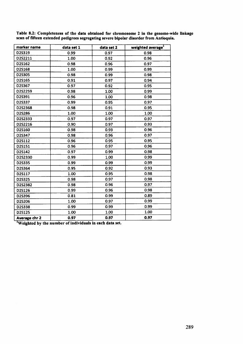
Table 8.2: Completeness of the data obtained for chromosome 2 in the genome-wide linkagescan of fifteen extended pedigrees segregating severe bipolar disorder from Antioquia.

m arker nam e data se t 1 data set 2 weighted average1D2S319 0.99 0.97 0.98D2S2211 1.00 0.92 0.96D2S162 0.98 0.96 0.97D2S168 1.00 0.99 0.99D2S305 0.98 0.99 0.98D2S165 0.91 0.97 0.94D2S367 0.97 0.92 0.95D2S2259 0.98 1.00 0.99D2S391 0.96 1.00 0.98D2S337 0.99 0.95 0.97D2S2368 0.98 0.91 0.95D2S286 1.00 1.00 1.00D2S2333 0.97 0.97 0.97D2S2216 0.90 0.97 0.93D2S160 0.98 0.93 0.96D2S347 0.98 0.96 0.97D2S112 0.96 0.95 0.95D2S151 0.96 0.97 0.96D2S142 0.97 0.99 0.98D2S2330 0.99 1.00 0.99D2S335 0.99 0.99 0.99D2S364 0.95 0.92 0.93D2S117 1.00 0.95 0.98D2S325 0.98 0.97 0.98D2S2382 0.98 0.96 0.97D2S126 0.99 0.96 0.98D2S396 0.81 0.99 0.89D2S206 1.00 0.97 0.99D2S338 0.99 0.99 0.99D2S125 1.00 1.00 1.00Average chr 2 0.97 0.97 0.971 Weighted by the number of individuals in each data set

289


m a r k e r n a m e d a ta s e t 1 d a t a s e t 2 w e ig h te d a v e r a g e 1D 3S1297 0 .9 6 0 .9 6 0 .9 6D 3S1304 0 .9 6 0 .9 9 0 .9 7

D 3S1263 0 .8 1 0 .8 9 0 .8 5

D 3S 2338 0 .9 3 0 .9 7 0 .9 5

D 3S 1266 0 .9 8 0 .9 6 0 .9 7

D 3S1277 0 .9 2 0 .9 3 0 .9 3

D 3S 1289 0 .9 8 0 .9 7 0 .9 8

D 3S1300 0 .9 7 0 .8 9 0 .9 3

D 3S1285 0 .9 7 0 .9 6 0 .9 6

D 3S1566 0 .8 4 0 .9 6 0 .8 9

D 3S3681 0 .8 4 0 .9 7 0 .9 0

D 3S1271 0 .9 9 1 .00 0 .9 9

D 3S1278 0 .9 9 0 .9 6 0 .9 8

D 3S1267 0 .9 9 0 .9 7 0 .9 8

D 3S1292 1 .0 0 0 .9 9 0 .9 9

D 3S1569 0 .9 6 1 .0 0 0 .9 8

D 3S1279 0 .9 6 0 .9 5 0 .9 5

D 3S1614 0 .8 7 1 .0 0 0 .9 3

D 3S 1565 0 .9 7 1 .0 0 0 .9 8

D 3S1262 0 .9 7 0 .9 5 0 .9 6

D 3S 1580 0 .9 3 0 .9 2 0 .9 3

D 3S1601 0 .9 8 0 .9 9 0 .9 8

D 3S1311 0 .9 8 1 .0 0 0 .9 9

A v e ra g e c h r 3 0 .9 4 0 .9 6 0 .9 5

’Weighted by the number of individuals in each data set.

290


m a r k e r n a m e d a t a s e t 1 d a ta s e t 2 w e ig h te d a v e r a g e 1D 4S412 0 .8 8 1 .0 0 0 .9 3

D 4S2935 0 .9 7 1 .0 0 0 .9 8

D 4S403 0 .9 0 0 .9 6 0 .9 3

D 4S419 0 .8 9 0 .9 7 0 .9 3

D 4S391 0 .9 9 1 .00 0 .9 9

D 4S405 0 .9 6 0 .9 9 0 .9 7

D 4S1592 0 .9 7 0 .9 5 0 .9 6

D 4S392 0 .9 8 0 .9 7 0 .9 8

D 4S2964 0 .9 0 1 .0 0 0 .9 5

D 4S1534 0 .9 3 1 .0 0 0 .9 6

D 4S414 0 .8 7 0 .9 9 0 .9 2

D 4S1572 0 .9 7 0 .9 7 0 .9 7

D 4S406 1 .0 0 0 .9 9 0 .9 9

D 4S402 0 .8 8 0 .9 6 0 .9 2

D 4S1575 1 .0 0 1 .0 0 1 .0 0

D 4S424 0 .9 3 0 .9 3 0 .9 3

D 4S413 0 .8 0 0 .8 4 0 .8 2

D 4S1597 0 .8 7 0 .9 6 0 .9 1

D 4S1539 0 .8 6 0 .9 7 0 .9 1

D 4S415 0 .9 3 0 .9 6 0 .9 5

D 4S1535 0 .9 8 0 .9 9 0 .9 8

D 4S426 1 .0 0 0 .9 9 0 .9 9

A v e ra g e c h r 4 0 .9 3 0 .9 7 0 .9 5

1 Weighted by the number of individuals in each data set

291


m a r k e r n a m e d a ta s e t 1 d a ta s e t 2 w e ig h te d a v e r a g e 1D5S1981 0.99 0.97 0.98D5S406 0.98 0.99 0.98D5S630 0.96 1.00 0.98D5S416 0.97 0.97 0.97D5S419 0.96 1.00 0.98D5S426 0.99 0.99 0.99D5S418 0.00 1.00 0.45D5S407 0.93 0.91 0.92D5S647 0.99 1.00 0.99D5S424 0.98 0.99 0.98D5S641 0.95 0.97 0.96D5S428 0.95 0.91 0.93D5S644 0.96 1.00 0.98D5S433 1.00 1.00 1.00D5S2027 0.99 1.00 0.99D5S471 0.99 0.97 0.98D5S2115 0.91 0.95 0.93D5S436 0.95 1.00 0.97D5S410 0.98 0.96 0.97D5S422 1.00 1.00 1.00D5S400 1.00 1.00 1.00D5S408 0.98 0.96 0.97A v e ra g e c h r 5 0.93 0.98 0.951 Weighted by the number of individuals in each data set.

292


m a r k e r n a m e d a ta s e t 1 d a ta s e t 2 w e ig h te d a v e ra g eD 6S 1574 0 .9 7 1 .00 0 .9 8

D 6S309 0 .9 6 0 .9 7 0 .9 6D 6S470 0 .9 9 0 .9 3 0 .9 6

D 6S289 0 .9 9 1 .0 0 0 .9 9

D 6S422 0 .9 7 0 .9 9 0 .9 8

D 6S276 0 .9 6 0 .9 6 0 .9 6

D 6S1610 0 .9 5 0 .9 6 0 .9 5

D 6S257 0 .9 9 0 .9 9 0 .9 9

D 6S460 0 .9 8 0 .9 9 0 .9 8

D 6S462 0 .9 6 0 .9 9 0 .9 7

D 6S434 0 .8 7 0 .9 5 0 .9 0

D 6S287 1 .0 0 0 .9 7 0 .9 9

D 6S262 0 .0 0 1 .0 0 0 .4 5

D 6S292 0 .9 6 0 .9 9 0 .9 7

D 6S308 0 .8 7 0 .9 7 0 .9 2

D 6S441 1 .0 0 0 .9 9 0 .9 9

D 6S1581 0 .8 5 0 .9 9 0 .9 1

D 6S264 0 .9 0 0 .9 7 0 .9 3

D 6S446 0 .9 1 0 .9 6 0 .9 3

D 6S281 0 .9 0 0 .9 9 0 .9 4

A v e ra g e c h r 6 0 .9 0 0 .9 8 0 .9 3

’Weighted by the number of individuals in each data set.

293


m a r k e r n a m e d a ta s e t 1 d a t a s e t 2 w e ig h te d a v e ra g e 1D7S531 0.91 0.92 0.92D7S517 0.99 1.00 0.99D7S513 0.92 0.97 0.95D7S507 0.98 0.97 0.98D7S493 0.95 0.97 0.96D7S516 0.98 1.00 0.99D7S484 0.98 0.97 0.98D7S510 0.95 1.00 0.97D7S519 0.92 0.97 0.95D7S502 0.98 0.95 0.96D7S669 0.95 0.99 0.96D7S630 0.97 1.00 0.98D7S657 0.98 1.00 0.99D7S515 0.98 0.93 0.96D7S486 0.95 0.88 0.92D7S530 0.89 0.99 0.93D7S640 0.91 0.99 0.95D7S684 1.00 1.00 1.00D7S661 1.00 1.00 1.00D7S636 0.92 0.95 0.93D7S798 1.00 1.00 1.00D7S2465 0.98 0.97 0.98A v e ra g e c h r 7 0 .9 6 0 .9 7 0 .9 6

'Weighted by the number of individuals in each data set.

Table 8.8: Completeness of the data obtained for chromosome 8 in the genome-wide linkage scan of fifteen extended pedigrees segregating severe bipolar disorder from Antioquia.

m a r k e r n a m e d a t a s e t 1 d a ta s e t 2 w e ig h te d a v e ra g e 1

D8S264 0.97 1.00 0.98D8S277 0.93 0.96 0.95D8S550 0.97 1.00 0.98D8S549 0.99 0.93 0.96D8S258 0.99 0.95 0.97D8S1771 0.98 0.97 0.98D8S505 0.96 0.95 0.95D8S285 0.99 0.97 0.98D8S260 0.92 1.00 0.96D8S270 1.00 0.97 0.99D8S1784 0.77 0.95 0.85D8S514 0.99 1.00 0.99D8S284 0.98 0.99 0.98D8S272 0.99 0.88 0.94A v e ra g e c h r 8 0 .9 6 0 .9 7 0 .9 6

’Weighted by the number of individuals in each data set

294


m a r k e r n a m e d a ta s e t 1 d a t a s e t 2 w e ig h te d a v e r a g e 1D 9S 288 1 .0 0 0 .9 9 0 .9 9

D 9S 286 0 .9 0 0 .9 6 0 .9 3

D 9S285 1 .0 0 0 .9 7 0 .9 9

D 9S157 0 .9 8 1 .0 0 0 .9 9

D 9S171 0 .9 0 0 .9 9 0 .9 4

D 9S161 1 .0 0 0 .9 5 0 .9 8

D 9S1817 0 .9 9 0 .9 6 0 .9 8

D 9S273 0 .9 0 1 .0 0 0 .9 5

D 9S175 0 .9 9 0 .9 9 0 .9 9

D 9S167 0 .9 6 1 .0 0 0 .9 8

D 9S283 0 .9 6 0 .9 9 0 .9 7

D 9S287 1 .0 0 0 .9 9 0 .9 9

D 9S1690 0 .9 9 0 .9 9 0 .9 9

D 9S 1677 0 .9 7 1 .0 0 0 .9 8

D 9S1776 0 .9 6 0 .9 9 0 .9 7

D 9S1682 0 .9 5 1 .0 0 0 .9 7

D 9S290 0 .9 3 0 .9 9 0 .9 6

D 9S164 0 .9 5 0 .9 9 0 .9 6

D 9S1826 0 .9 1 0 .9 2 0 .9 2

D 9S158 0 .9 0 0 .9 3 0 .9 2

A v e ra g e c h r 9 0 .9 6 0 .9 8 0 .9 7

W eighted by the number of individuals in each data set.

295

Table 8.10: Completeness o f the data obtained for chromosome 10 in the genome-wide linkagescan of fifteen extended pedigrees segregating severe bipolar disorder from Antioquia.

m a r k e r n a m e d a ta s e t 1 d a ta s e t 2 w e ig h te d a v e r a g e 1D10S249 0.99 0.97 0.98D10S591 0.97 0.99 0.98DIOS189 0.97 1.00 0.98D10S547 0.88 0.91 0.89D10S1653 0.97 1.00 0.98D10S548 0.99 0.96 0.98D10S197 0.93 1.00 0.96D10S208 0.97 1.00 0.98D10S196 0.97 0.95 0.96D10S1652 0.97 0.93 0.95D10S537 0.97 0.95 0.96D10S1686 0.98 0.97 0.98D10S185 0.98 1.00 0.99D10S192 0.97 1.00 0.98D10S597 0.99 0.95 0.97D10S1693 0.97 0.97 0.97D10S587 0.98 0.95 0.96D10S217 1.00 0.96 0.98D10S1651 1.00 0.99 0.99D10S212 1.00 1.00 1.00A v e ra g e c h r 1 0 0 .9 7 0 .9 7 0 .9 7

W eighted by the number of individuals n each data set.


m a r k e r n a m e d a ta s e t 1 d a ta s e t 2 w e ig h te d a v e r a g e 1

D11S4046 0.92 0.99 0.95D11S1338 0.85 0.97 0.90D11S902 1.00 0.99 0.99D11S904 0.93 1.00 0.96D11S935 0.93 0.95 0.94D11S905 0.00 0.97 0.44D11S4191 0.93 0.99 0.96D11S987 1.00 0.99 0.99D11S1314 1.00 1.00 1.00D11S937 0.92 0.99 0.95D11S901 1.00 1.00 1.00D11S4175 0.89 0.96 0.92D11S898 0.96 0.99 0.97D11S908 0.90 0.99 0.94D11S925 0.87 0.96 0.91D11S4151 0.99 0.97 0.98D11S1320 0.97 0.93 0.95D11S968 0.93 0.97 0.95A v e ra g e c h r 11 0 .8 9 0 .9 8 0 .9 3


296


m a r k e r n a m e d a ta s e t 1 d a ta s e t 2 w e ig h te d a v e r a g e 1D12S352 0.95 0.99 0.96D12S99 0.98 0.91 0.95D12S336 0.95 0.95 0.95D12S364 0.95 0.97 0.96D12S310 0.91 0.92 0.92D12S1617 0.98 0.97 0.98D12S345 0.91 0.91 0.91D12S85 0.90 0.96 0.93D12S368 0.90 0.96 0.93D12S83 0.90 0.93 0.92D12S326 0.93 0.96 0.95D12S351 0.99 0.92 0.96D12S346 0.99 0.99 0.99D12S78 1.00 0.92 0.96D12S79 0.84 0.99 0.90D12S86 0.93 0.99 0.96D12S324 0.92 0.92 0.92D12S1659 1.00 0.99 0.99D12S1723 1.00 0.91 0.96A v e ra g e c h r 12 0 .9 4 0 .9 5 0 .9 5W eighted by the number of individuals in each data set.


m a r k e r n a m e d a ta s e t 1 d a ta s e t 2 w e ig h te d a v e r a g e 1

D13S175 1.00 0.99 0.99D13S217 0.96 0.88 0.92D13S171 0.97 0.95 0.96D13S218 0.98 0.99 0.98D13S263 0.96 1.00 0.98D13S153 0.85 0.97 0.90D13S156 0.97 0.96 0.96D13S170 0.93 0.99 0.96D13S265 0.95 0.97 0.96D13S159 0.00 0.93 0.42D13S158 0.96 0.95 0.95D13S173 0.95 0.96 0.95D13S1265 0.91 0.89 0.90D13S285 0.97 1.00 0.98A v e ra g e c h r 13 0 .8 8 0 .9 6 0 .9 2

W eighted by the number of individuals in each data set

297


marker name data set 1 data set 2 weighted average1D14S261 0.96 0.96 0.96D14S283 1.00 0.95 0.98D14S275 0.98 0.97 0.98D14S70 0.95 0.92 0.93D14S288 0.91 1.00 0.95D14S276 0.92 1.00 0.96D14S63 0.97 0.97 0.97D14S258 1.00 0.97 0.99D14S74 0.91 1.00 0.95D14S68 0.93 0.89 0.92D14S280 0.98 0.92 0.95D14S65 0.90 0.97 0.93D14S985 0.93 0.91 0.92D14S292 1.00 0.93 0.97Average chr 14 0.95 0.96 0.95W eighted by the number of individuals In each data set.


marker name data set 1 data set 2 weighted average1D15S128 1.00 1.00 1.00D15S1002 0.97 0.89 0.93D15S165 0.97 0.93 0.95D15S1007 0.93 0.95 0.94D15S1012 0.99 1.00 0.99D15S994 0.00 0.97 0.44D15S978 1.00 1.00 1.00D15S117 0.98 0.95 0.96D15S153 0.95 0.99 0.96D15S131 0.95 0.99 0.96D15S205 0.91 0.97 0.94D15S127 0.95 0.97 0.96D15S130 0.99 0.95 0.97D15S120 1.00 0.99 0.99Average chr 15 0.90 0.97 0.93‘Weighted by the number of individuals in each data set.

298


m a r k e r n a m e d a ta s e t 1 d a ta s e t 2 w e ig h te d a v e r a g e 1D16S423 0.89 0.91 0.90D16S404 0.92 0.93 0.93D16S3075 0.96 0.92 0.94D16S3103 0.96 0.97 0.96D16S3046 1.00 1.00 1.00D16S3068 0.95 1.00 0.97D16S3136 0.97 0.96 0.96D16S415 0.95 0.97 0.96D16S503 0.97 0.92 0.95D16S515 0.89 0.92 0.90D16S516 0.96 0.83 0.90D16S3091 0.92 0.97 0.95D16S520 0.95 0.97 0.96A v e ra g e c h r 1 6 0 .9 4 0 .9 4 0 .9 4!Weighted by the number of individuals in each data set


m a r k e r n a m e d a t a s e t 1 d a ta s e t 2 w e ig h te d a v e r a g e 1

D17S849 0.82 0.92 0.87D17S831 0.96 0.97 0.96D17S938 0.98 0.99 0.98D17S1852 0.99 0.97 0.98D17S799 0.99 0.93 0.96D17S921 0.98 0.97 0.98D17S1857 1.00 0.95 0.98D17S798 0.00 0.92 0.42D17S1868 0.90 0.93 0.92D17S787 1.00 0.96 0.98D17S944 0.98 0.97 0.98D17S949 0.91 0.95 0.93D17S785 1.00 0.99 0.99D17S784 0.91 0.96 0.93D17S928 0.99 0.97 0.98A v e ra g e c h r 17 0 .8 9 0 .9 6 0 .9 2


299


m a r k e r n a m e d a t a s e t 1 d a ta s e t 2 w e ig h te d a v e r a g e 1D 18S59 0 .9 5 0 .9 6 0 .9 5D 18S63 1 .0 0 0 .9 9 0 .9 9D 18S452 0 .9 2 0 .9 5 0 .9 3D 18S 464 0 .9 6 0 .9 9 0 .9 7

D 18S53 0 .9 9 0 .9 9 0 .9 9D 18S478 0 .9 0 0 .9 7 0 .9 3D 18S 1102 0 .9 8 0 .8 8 0 .9 3D 18S474 1 .0 0 0 .9 9 0 .9 9D 18S64 0 .9 6 0 .9 7 0 .9 6D 18S68 0 .9 7 0 .8 8 0 .9 3D 18S61 0 .9 8 0 .9 5 0 .9 6

D 18S 1161 0 .9 5 0 .9 6 0 .9 5

D 18S462 0 .9 8 0 .9 5 0 .9 6

D 18S70 0 .7 8 0 .9 6 0 .8 6

A v e ra g e c h r 18 0.95 0.96 0.95Weighted by the number of individuals in each data set.



D 19S209 0 .9 6 0 .9 6 0 .9 6

D 19S216 1 .0 0 0 .9 9 0 .9 9

D 19S 884 0 .9 7 0 .9 9 0 .9 8

D 19S221 0 .0 0 0 .8 7 0 .3 9

D 19S 226 0 .9 9 0 .9 9 0 .9 9

D 19S 414 0 .9 5 0 .9 9 0 .9 6

D 19S 220 0 .9 6 1 .0 0 0 .9 8

D 19S 420 1 .0 0 0 .9 9 0 .9 9

D 19S902 0 .9 8 0 .9 3 0 .9 6

D 19S571 0 .8 0 0 .9 2 0 .8 6

D 19S 418 0 .8 7 0 .9 7 0 .9 2

D 19S 210 0 .9 9 0 .8 8 0 .9 4

A v e ra g e c h r 19 0.87 0.96 0.911 Weighted by the number of individuals in each data set.

3 0 0


m a r k e r n a m e d a t a s e t 1 d a t a s e t 2 w e ig h te d a v e r a g e 1D20S117 0.93 1.00 0.96D20S889 0.96 0.99 0.97D20S115 0.98 0.99 0.98D20S186 0.96 0.97 0.96D20S112 0.90 0.91 0.90D20S195 0.99 0.97 0.98D20S107 0.97 0.92 0.95D20S119 1.00 0.96 0.98D20S178 0.86 0.95 0.90D20S196 0.97 0.97 0.97D20S100 0.98 0.92 0.95D20S171 0.85 0.95 0.89D20S173 0.99 0.95 0.97A v e ra g e c h r 20 0.95 0.96 0.95'Weighted by the number of individuals in each data set.



D21S1256 0.84 0.89 0.86D21S1914 0.98 0.93 0.96D21S263 0.00 0.95 0.43D21S1252 0.90 0.99 0.94D21S266 0.90 0.97 0.93A v e ra g e c h r 21 0.72 0.95 0.82W eighted by the number of individuals in each data set.


m a r k e r n a m e d a t a s e t 1 d a t a s e t 2 w e ig h te d a v e r a g e 1

D22S420 1.00 0.97 0.99D22S539 0.91 0.97 0.94D22S315 0.87 0.96 0.91D22S280 0.95 0.97 0.96D22S283 0.96 0.97 0.96D22S423 0.99 0.96 0.98D22S274 0.89 0.96 0.92A v e ra g e c h r 2 2 0.94 0.97 0.95

i n each data set.

3 0 1

8.3. Published Papers and Manuscripts

In this section o f the appendix, I have attached all papers on which I have

collaborated during the time o f my Ph.D. studies in Professor Ruiz-Linares’

laboratory.

302

GENETIC ANALYSIS OF NEUROPSYCHIATRIC DISORDERS ...

Documents

Transcript of GENETIC ANALYSIS OF NEUROPSYCHIATRIC DISORDERS ...