Generation of Rainfall Intensity-Duration-Frequency curves for ...

Vol. 6 Issue

Generation of Rainfall Intensity-Duration-Frequency curves for the Barak River Basin

Violina Basumatary, Briti Sundar SilNational Institute of Technology, Silchar, Department of Civil Engineering, NIT Road, District-Cachar, Silchar, Assam 788010, India, e-mail: [email protected], [email protected]

Abstract. Analysis of a design storm, explained as the expected rainfall intensity for a given storm duration and return period is carried out to establish Rainfall Intensity-Duration-Frequency (IDF) relationships. The IDF relationships are essential for the designing of hydraulic structures for future planning and management. The intent was to deter-mine IDF relationship for the Barak River Basin in India. This region receives heavy rainfall but lacks potential in harnessing the available water resources. Rain gauge stations are not so frequent in this region. Under this condition, the engineers are bound to use IDF relationships. Using the 24-hour annual maximum rainfall and disaggregated hourly maximum rainfall as a measure of rainfall intensity for each station, IDF curves and isopluvial maps of rain-fall intensities of 30-minute to 24-hour durations were generated. Analysis was done using the best fit amongst the Gumbel, Log Pearson Type III and Lognormal probability distribution functions. The goodness-of-fit tests indicated the Log Pearson Type III distribution was a suitable distribution for the area. After developing IDF curves for each station, an average IDF curve was developed using the Thiessen Polygon method in ArcGIS. The IDF relationship developed can be used as valuable information for the planning and management of hydraulic structures in the region.

Keywords: Barak River, design storm, IDF curve, isopluvial map, probability distribution, Thiessen Polygon

Submitted 2 May 2017, revised 17 July 2017, accepted 25 October 2017

1. Introduction

Rainfall is a fundamental element in the hydrologic cycle. To design structures influenced by rainfall or con-cerned with its accumulation and conveyance, engineers are required to be able to assess rainfall. Assessment of rainfall is usually done using Intensity-Duration-Frequency curves (IDF curves) for various water resource-related schemes. An IDF curve is a graphical representation of the probability that rainfall with a particular intensity and duration will occur and the probable time interval between storms with similar characteristics. IDF curves are a potent representation of the extreme rainfall that is expected in a region of interest, which reflects the average intensity of rainfall at every return period for all durations of rainfall.

The determination of the probable frequency of extreme rainfall events of different intensities and durations is the basic step in designing a flood control structure, in order to provide an economic size of the structure. On most occasions designing a structure that can withstand the greatest rainfall ever to have occurred is not practical. Having periodic fail-ures is more economical than designing for a very intense storm. However, where life is concerned, the designed structure should be able to administer a greater runoff than has ever been recorded. To achieve this, data providing information about return periods of extreme rainfall events of various intensities and durations are vital. Although

precipitation in the form of rainfall is life-supporting, it can also cause serious problems. An abundance or shortfall of rainfall, if not controlled, has an impact in all environmental events, and extreme events have serious consequences for human society. The evaluation of extreme rainfall is critical in hydrologic studies. Interpretation of their return periods and design values are of great significance for the design and management of water resource systems and reservoirs, and planning for weather related urgencies, etc. depends on knowledge of the frequency of these extreme events. IDF curves give useful information about when there will be flooding in an area, and when a particular rainfall rate or a certain volume of flow will recur in the future. The IDF curves are usually derived by carrying out annual maximum analysis of historical precipitation data, assuming there is no change in climate. IDF curves are useful in determining the peak runoff in a catchment, using the rational method, and for designing channels and other water ways (Isikwue et al. 2012). The design rainfall intensity for a specified storm duration and frequency is generally estimated from a set of statistically derived IDF curves suitable for a given region.

IDF relationships are suitable for estimating design storms (DS) to obtain peak discharge and hydrograph shape in any hydraulic design. The DS are applied abun-dantly to design flood control structures (Ewea et al. 2016). Although many studies have been done to develop the IDF relationships in the Brahmaputra River Basin of Assam

2 V. Basumatary, B. Sundar Sil

state (Sharma et al. 2016a; Das et al. 2016), few studies have been conducted in the Barak River Basin. Generating IDF relationships requires good quality and long-term his-torical data. A common problem in developing countries is the non-availability or sparse network of rain gauge stations, whose data are the ultimate basis for establish-ing IDF relationships. Some interpolated rainfall data are available on the Global Weather Data for SWAT site and can be downloaded from the link (https://rda.ucar.edu/pub/cfsr.html). This dataset is the result of close cooperation between two organizations, the National Centers for Envi-ronmental Prediction (NCEP) and the National Center for Atmospheric Research (NCAR), who completed a global climate data reanalysis over the 36-years period from 1979 to 2014.

IDF curves are discussed in numerous hydrological books (Chow et al. 1988). A relationship for intensity of rainfall, duration and frequency was developed for Rwanda. The stations were divided into five homogeneous regions and quantile estimation was carried out using the Generalised Logistic, Gamma and Pearson Type III and Generalised Extreme Value distributions (Wagesho, Claire 2016). IDF curves were developed for shorter durations and various return periods in different regions (Logah et al. 2013; Rasel, Islam 2015; Palaka et al. 2016; Dar, Maqbool 2016). IDF curves were developed for the Sinai Peninsula with available methods of estimation of recurrence periods, such as California, Hazen, Kimbell and Gumbel. A contour map of Sherman coefficients was developed using GIS tools. Rainfall intensities obtained using the Log Pearson Type III (LPIII) and Gumbel methods showed uniformity with the results accomplished in studies carried out previ-ously on the area (Fathy et al. 2014). Isopluvial maps were developed for the Tehri-Garhwal Himalayan region, India. Isopluvial maps show the spatial variability and IDF rela-tionships developed for the Bhagirathi-Bhillangana catch-ment (Sarkar et al. 2010). Spatial and temporal variation of IDF parameters was developed in the Awash River Basin, Ethiopia (Gebreslassie 2014). IDF curves were developed using the Gumbel and LPIII distributions, with the Gumbel distribution showing higher results than the LPIII distribution (Antigha, Ogarekpe 2013). The safety factor was considered to be necessary while evaluating IDF curves for different parts of a city because rainfall inten-sity is not uniform throughout a city (Sharma et al. 2016b). A mathematical model was developed between peak flood discharge and return period to assess rainfall for different storm durations for the Bhadar catchment, Gujarat (Bhatt et al. 2014). A study was carried out to find the influence of global warming on rainfall intensity in Toronto before and after 1980 (Carlier, Khattabi 2016). A regional analysis

of DS was conducted based on topographic and rainfall characteristics to determine rainfall IDF relationships in Botswana for three homogeneous regions which were con-structed with the K-means Clustering algorithm (Alemaw, Chaoka 2016). Autorun analysis on a daily time scale was used to generate wet and dry spell durations and rainfall intensities (Subyani, Al-Amri 2015). IDF curves were pro-posed using Kothyari and Garde’s empirical equation and then IDF curves were derived by developing a modified IDF equation so as to maintain compatibility with changes in the rainfall pattern in Mumbai (Zope et al. 2016). They proposed an IDF equation for Mumbai city using a single rain gauge station. Flood frequency analysis using probability distribution functions were performed, as they are useful in urban development planning and floodplain management (Izinyon, Ajumuka 2013; Sharma et al. 2016a). Various studies have been carried out in different parts of Saudi Arabia (Elsebaie 2012; Al-anazi, El-Sebaie 2013; Subyani, Al-Amri 2015). The impact of climate change on rainfall IDF was studied in Alabama (Mirhos-seini et al. 2013).

The Barak River Basin has good hydropower poten-tial but it is rather under-developed and is lacking when it comes to harnessing the potential of available water resources. Floods, drainage congestion and bank erosion are major problems of the basin. Floods are caused by banks spilling over due to inadequate carrying capacity of the channels; this results from aggravation of the river beds, backing up effect of the main river on to its tributar-ies and also due to excessive rainfall in the region. Due to poor drainage, many depressions remain waterlogged long after monsoons. Hydrological analysis is a prereq-uisite for the better utilization of the resources (Bora, Choudhury 2015). In this study, an attempt has been made to develop an Intensity-Duration-Frequency model for the Barak River Basin using annual maximum series (AMS). The IDF model can be used to estimate DS intensities. The suggested expression allows the estimation of the expected rainfall intensities for different durations and return periods in the basin area.

2. Study area

The Barak River, one of the major rivers of south Assam, India, rises in the hill country of Manipur State, where it is the biggest and most important of the hill coun-try rivers. The Barak Basin covers the States of Assam, Manipur, Mizoram, Nagaland and Tripura. From Assam, it enters Bangladesh, where the Surma and Kushiyara rivers begin, and is a part of the Surma-Meghna River System. The Barak River is the single largest contributory

Generation of Rainfall Intensity-Duration-Frequency curves for the Barak River Basin 3

river to the northeast region of Bangladesh. The major tributaries of the Barak are all in India and are the Jiri, the Dhaleshwari, the Singla, the Longai, the Madhura, the Sonai, the Rukni and the Katakhal. The total area of the Barak River Basin is 41 723 km2 which is nearly 1,38% of the total geographical area of India. In this study, an area of nearly 25 000 km2 is considered, up to Badar-purghat, India (92,58°E, 24,87°N) where it enters Bang-ladesh. The topography of this region is characterized by hills, hillocks, plains and low lying waterlogged areas. Generally, winter lasts from December to February and the period is rather dry. The climate of the Barak Basin is sub-tropical, warm and humid. The annual rainfall ranges from 2 500 mm to 4 000 mm. The periods from March-April and October-November are defined by low erratic rainfall with occasional hailstorms. The period between May and September is defined by high rainfall with a risk of floods. The seasonal distribution of rainfall indicates that while total annual rainfall is satisfactory, the dis-tribution is uneven and most of the rainfall is confined to the period between June and August. Normally, the temperature ranges from a minimum of 12,2°C in January to 25,4°C in August and the mean maximum of 24,3°C in January to 36,0°C in August. The map of the study area is shown in Fig. 1.

3. Materials and methods3.1. Data collection

For the generation of IDF curves, daily precipitation data at 23 stations in the study area were obtained from https://globalweather.tamu.edu/ for a period of 35 years (1979-2013). The stations considered for this study in the Barak Basin were located between 92,4°E to 94,3°E longitude and 23,5°N and 25,7°N latitude. From the data-base, the annual maximum series (AMS) were extracted and disaggregated to shorter duration rainfall series using

the Indian Meteorological Department (IMD) one third reduction formula, as given in equation (1). Chowdhury et al. (2007) used the IMD one-third reduction formula to estimate short duration rainfall for Slyhet city and found the formula gave the best estimation for short duration rainfall (Rashid et al. 2012).

where: pt denotes the rainfall depth (millimetres) for t-hour duration, p24 denotes the daily rainfall (millimetres), and t denotes the duration (hours) of rainfall for which the rain-fall depth is required. The rainfall events were analysed by breaking down the AMS to shorter durations of 30-minute, 1-hour, 2-hour, 3-hour, 6-hour, 12-hour and 24-hour.

3.2. IDF quantile estimation

In the present study, the return period (T) was com-puted using the Weibull plotting position formula as given in equation (2),

where n is the total number of years of rainfall data and m is the rank of the events. The probability of exceedance of the rainfall values is the reciprocal of the return period (Kumar, Bhardwaj 2015). An extreme event (XT) is decided based on the assumed probability distribution employing the method of moments, method of L-moments or method of maximum likelihood (Stedinger, Cohn 1986; Hosking, Wallis 1993). Alternatively, with reference to frequency factors, it can be computed for the probability distribution functions (Chow et al. 1988) as given in equation (3),

where KT is the frequency factor which is a function of return period and the parameter of the distribution, and X and σX are mean and standard deviation of the variate. For LPIII, the probability of exceedance corresponding to T-year recurrence interval was assigned to each variate using the Weibull plotting position formula. The mean, standard deviation and coefficient of skewness for the log transformed series were computed using equations (4), (5), and (6), respectively.

Fig. 1. Location map of the study area

t24

pt = p24( )1/3

(1)

n + 1T =

m(2)

(3)

(4)

XT = X + KTσX

∑log Xnlog X =


The value of XT for a specified return period was com-puted by equation (7),

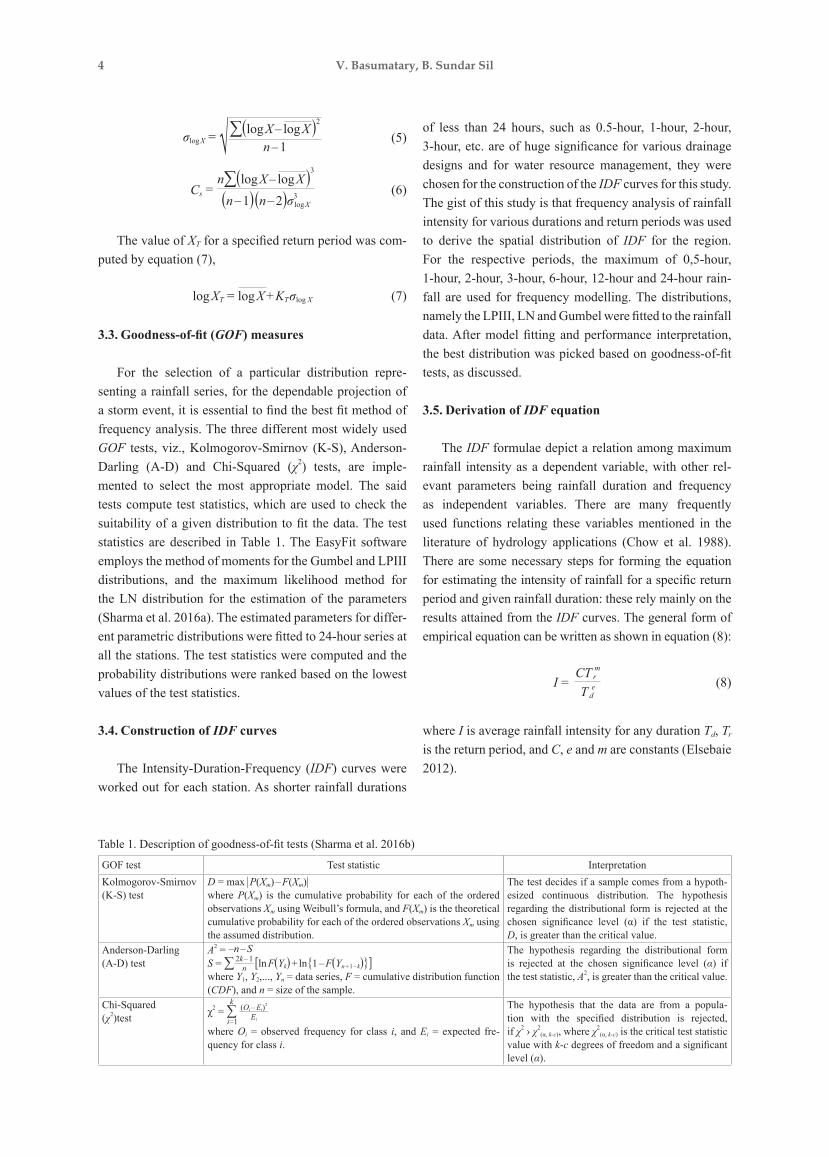
3.3.Goodness-of-fit(GOF) measures

For the selection of a particular distribution repre-senting a rainfall series, for the dependable projection of a storm event, it is essential to find the best fit method of frequency analysis. The three different most widely used GOF tests, viz., Kolmogorov-Smirnov (K-S), Anderson-Darling (A-D) and Chi-Squared (χ2) tests, are imple-mented to select the most appropriate model. The said tests compute test statistics, which are used to check the suitability of a given distribution to fit the data. The test statistics are described in Table 1. The EasyFit software employs the method of moments for the Gumbel and LPIII distributions, and the maximum likelihood method for the LN distribution for the estimation of the parameters (Sharma et al. 2016a). The estimated parameters for differ-ent parametric distributions were fitted to 24-hour series at all the stations. The test statistics were computed and the probability distributions were ranked based on the lowest values of the test statistics.

3.4. Construction of IDF curves

The Intensity-Duration-Frequency (IDF) curves were worked out for each station. As shorter rainfall durations

of less than 24 hours, such as 0.5-hour, 1-hour, 2-hour, 3-hour, etc. are of huge significance for various drainage designs and for water resource management, they were chosen for the construction of the IDF curves for this study. The gist of this study is that frequency analysis of rainfall intensity for various durations and return periods was used to derive the spatial distribution of IDF for the region. For the respective periods, the maximum of 0,5-hour, 1-hour, 2-hour, 3-hour, 6-hour, 12-hour and 24-hour rain-fall are used for frequency modelling. The distributions, namely the LPIII, LN and Gumbel were fitted to the rainfall data. After model fitting and performance interpretation, the best distribution was picked based on goodness-of-fit tests, as discussed.

3.5. Derivation of IDF equation

The IDF formulae depict a relation among maximum rainfall intensity as a dependent variable, with other rel-evant parameters being rainfall duration and frequency as independent variables. There are many frequently used functions relating these variables mentioned in the literature of hydrology applications (Chow et al. 1988). There are some necessary steps for forming the equation for estimating the intensity of rainfall for a specific return period and given rainfall duration: these rely mainly on the results attained from the IDF curves. The general form of empirical equation can be written as shown in equation (8):

where I is average rainfall intensity for any duration Td, Tr is the return period, and C, e and m are constants (Elsebaie 2012).

n – 1∑(log X – log X )2

σlog X = √ (5)

(6)

(7)

n∑(log X – log X )3

(n – 1) (n – 2)σ3log X

Cs =

log XT = log X + KT σlog X

Table 1. Description of goodness-of-fit tests (Sharma et al. 2016b)

GOF test Test statistic InterpretationKolmogorov-Smirnov (K-S) test

D = max ǀ P(Xm) – F(Xm)ǀwhere P(Xm) is the cumulative probability for each of the ordered observations Xm using Weibull’s formula, and F(Xm) is the theoretical cumulative probability for each of the ordered observations Xm using the assumed distribution.

The test decides if a sample comes from a hypoth-esized continuous distribution. The hypothesis regarding the distributional form is rejected at the chosen significance level (α) if the test statistic, D, is greater than the critical value.

Anderson-Darling (A-D) test

A2 = –n – SS = ∑ [ln F(Yk) + ln{1 – F(Yn + 1 – k)}]where Y1, Y2,..., Yn = data series, F = cumulative distribution function (CDF), and n = size of the sample.

The hypothesis regarding the distributional form is rejected at the chosen significance level (α) if the test statistic, A2, is greater than the critical value.

Chi-Squared (χ2)test χ2 = ∑

k

i=1where Oi = observed frequency for class i, and Ei = expected fre-quency for class i.

The hypothesis that the data are from a popula-tion with the specified distribution is rejected, if χ2 › χ2

(α, k-c), where χ2(α, k-c) is the critical test statistic

value with k-c degrees of freedom and a significant level (α).

2k – 1n

(Oi – Ei)2

Ei

CT rm

T deI = (8)


3.6. Thiessen Polygon method

The Thiessen Polygon method estimates average rain-fall aspects over an area. The recorded rainfall at each rain gauge station is given a weightage according to the posi-tion of the station with respect to the boundary of the area. The average intensity of rainfall over an area is expressed in equation (9):

where I1, I2,…, In are the intensities of recorded rainfall at the respective stations 1, 2,.., n and A1, A2,…, An are the areas of the Thiessen Polygons, respectively. The Thiessen Polygon method is used to produce an average IDF curve for the whole study area (Sarkar et al. 2010).

3.7. Isopluvial map

The rainfall intensity values at different sites inside the Barak River Basin were interpolated using the Geo-statistical Analyst in GIS. To show spatial variability of rainfall intensity, Isopluvial maps were generated using the Inverse Distance Weighted (IDW) method (Sarkar et al. 2010). To interpolate a value for any unmeasured site, IDW executes the assumption that each measured point has a local impact that decreases with distance.

4. Results and discussion

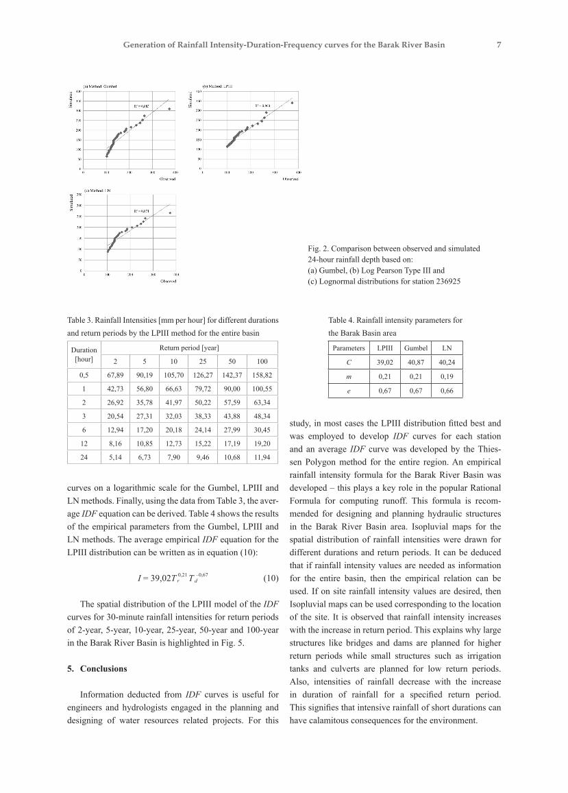
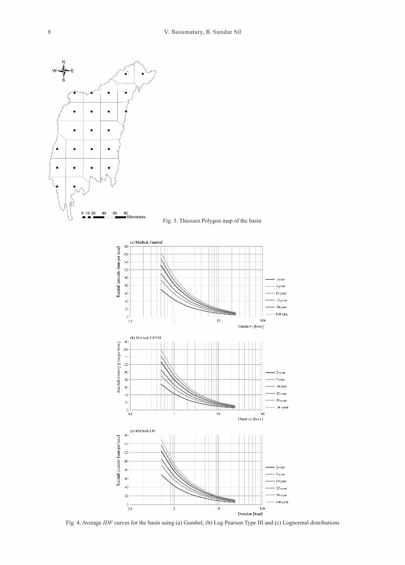
The annual maximum series was extracted from daily rainfall and disaggregated to smaller durations using the IMD reduction formula for all the 23 stations. The AMS was subjected to preliminary analysis for consistency using the Double Mass Curve method. Figure 2 shows a comparison between observed and expected 24-hour rainfall based on the Gumbel, LPIII and LN methods for station 236925. The performances of the models were decided against a model performance index, which gave very high model efficiency, a coefficient of determina-tion (R2) that is above 90%. The goodness-of-fit of the distribution was worked out using EasyFit software 5.6. It shows the model parameters and the goodness-of-fit of the Gumbel, LPIII and LN distributions. The results of goodness-of-fit tests for 24-hourseries using the K-S, A-D and χ2 tests for the stations are shown in Table 2. From the results, LPIII can be considered more reliable for the study area. After completion of the above steps, the IDF curves were generated for each station at time steps 30-minute, 1-hour, 2-hour, 3-hour, 6-hour, 12-hour and 24-hour and an average IDF curve for the whole area was deduced using the Thiessen Polygon method in ArcGIS. Figure 3 shows the Thiessen Polygon map of the basin. Thiessen Polygon area weightages were assigned to each station and the quantiles at each station were used to generate an average IDF curve for the basin. Figure 4 shows the IDF

I1 A1 + I2 A2 + ... + In An

A1 + A2 + ... + AnI = (9)

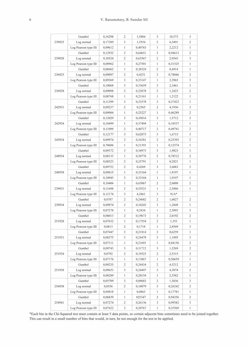
Table 2. Goodness-of-fit results for 24-hour series

Station ID DistributionKolmogorov-Smirnov Anderson-Darling Chi-Squared

Statistic Rank Statistic Rank Statistic Rank

248928

Gumbel 0,13801 3 0,65068 3 2,5056 3

Log normal 0,13005 2 0,58594 2 1,3188 1

Log Pearson type III 0,12183 1 0,52785 1 1,3437 2

248931

Gumbel 0,15941 3 0,87762 3 7,9743 3

Log normal 0,15519 2 0,77755 2 7,7261 2


245928

Gumbel 0,10941 3 0,53773 3 3,6693 3

Log normal 0,09271 1 0,40278 2 1,6901 2


245931

Gumbel 0,08388 3 0,41902 3 1,3578 1

Log normal 0,07392 2 0,29631 2 1,571 2


242925

Gumbel 0,09764 3 0,49631 3 0,5119 1

Log normal 0,07467 2 0,12534 1 0,69228 2


242928

Gumbel 0,13861 3 0,53783 3 4,702 3

Log normal 0,13222 2 0,46006 2 2,5999 2



239925

Gumbel 0,16298 2 1,5884 3 10,573 3

Log normal 0,17289 3 1,5554 2 6,5491 2


239928

Gumbel 0,12932 3 0,64651 3 0,94613 2

Log normal 0,10524 2 0,63567 2 2,9543 3


236925

Gumbel 0,08462 1 0,38324 2 0,4914 1

Log normal 0,09097 2 0,4251 3 0,78046 2


236928

Gumbel 0,10068 3 0,33659 3 2,3461 3

Log normal 0,09098 2 0,22878 2 1,2423 2


242931

Gumbel 0,11299 3 0,33578 3 0,37423 1

Log normal 0,09237 2 0,2565 2 4,1936 3


242934

Gumbel 0,12029 3 0,45016 3 1,5712 3

Log normal 0,10499 1 0,37494 1 0,18537 1


245934

Gumbel 0,12177 3 0,62073 3 1,6715 3

Log normal 0,09974 2 0,34381 2 0,25393 2


248934

Gumbel 0,09372 3 0,34973 3 1,9823 3

Log normal 0,08133 1 0,30776 2 0,78512 2


248938

Gumbel 0,09752 2 0,4269 3 3,6883 3

Log normal 0,09615 1 0,33164 1 1,9197 1


239931

Gumbel 0,10406 1 0,63067 2 2,6008 2

Log normal 0,11698 2 0,55521 1 2,5886 1

Log Pearson type III 0,12174 3 4,2461 3 N/A*

239934

Gumbel 0,0787 2 0,24682 2 1,6027 2

Log normal 0,09874 3 0,34245 3 1,2849 1


251928

Gumbel 0,08013 2 0,19673 3 2,0192 2

Log normal 0,07632 1 0,17554 2 1,353 1


251931

Gumbel 0,07447 2 0,21814 2 0,6259 1

Log normal 0,08375 3 0,24479 3 1,1995 3


251934

Gumbel 0,09743 3 0,31712 3 1,5269 2

Log normal 0,0792 2 0,19523 2 2,5315 3


251938

Gumbel 0,09235 2 0,24434 2 4,5212 3

Log normal 0,09653 3 0,24497 3 4,3074 2


254938

Gumbel 0,05709 3 0,09683 2 1,3036 3

Log normal 0,0556 2 0,10079 3 0,26242 2


254941

Gumbel 0,06839 1 025347 2 0,94356 2

Log normal 0,07274 2 0,26136 3 0,99382 3


*Each bin in the Chi-Squared test must contain at least 5 data points, so certain adjacent bins sometimes need to be joined together. This can result in a small number of bins that would, in turn, be not enough for the test to be applied.


curves on a logarithmic scale for the Gumbel, LPIII and LN methods. Finally, using the data from Table 3, the aver-age IDF equation can be derived. Table 4 shows the results of the empirical parameters from the Gumbel, LPIII and LN methods. The average empirical IDF equation for the LPIII distribution can be written as in equation (10):

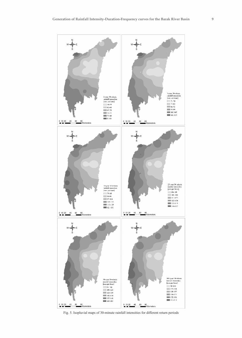
The spatial distribution of the LPIII model of the IDF curves for 30-minute rainfall intensities for return periods of 2-year, 5-year, 10-year, 25-year, 50-year and 100-year in the Barak River Basin is highlighted in Fig. 5.

5. Conclusions

Information deducted from IDF curves is useful for engineers and hydrologists engaged in the planning and designing of water resources related projects. For this

study, in most cases the LPIII distribution fitted best and was employed to develop IDF curves for each station and an average IDF curve was developed by the Thies-sen Polygon method for the entire region. An empirical rainfall intensity formula for the Barak River Basin was developed – this plays a key role in the popular Rational Formula for computing runoff. This formula is recom-mended for designing and planning hydraulic structures in the Barak River Basin area. Isopluvial maps for the spatial distribution of rainfall intensities were drawn for different durations and return periods. It can be deduced that if rainfall intensity values are needed as information for the entire basin, then the empirical relation can be used. If on site rainfall intensity values are desired, then Isopluvial maps can be used corresponding to the location of the site. It is observed that rainfall intensity increases with the increase in return period. This explains why large structures like bridges and dams are planned for higher return periods while small structures such as irrigation tanks and culverts are planned for low return periods. Also, intensities of rainfall decrease with the increase in duration of rainfall for a specified return period. This signifies that intensive rainfall of short durations can have calamitous consequences for the environment.

Fig. 2. Comparison between observed and simulated 24-hour rainfall depth based on: (a) Gumbel, (b) Log Pearson Type III and (c) Lognormal distributions for station 236925

I = 39,02T r0,21 T d–0,67 (10)

Table 3. Rainfall Intensities [mm per hour] for different durations and return periods by the LPIII method for the entire basin

Duration [hour]

Return period [year]

2 5 10 25 50 100

0,5 67,89 90,19 105,70 126,27 142,37 158,82

1 42,73 56,80 66,63 79,72 90,00 100,55

2 26,92 35,78 41,97 50,22 57,59 63,34

3 20,54 27,31 32,03 38,33 43,88 48,34

6 12,94 17,20 20,18 24,14 27,99 30,45

12 8,16 10,85 12,73 15,22 17,19 19,20

24 5,14 6,73 7,90 9,46 10,68 11,94

Table 4. Rainfall intensity parameters for the Barak Basin area

Parameters LPIII Gumbel LN

C 39,02 40,87 40,24

m 0,21 0,21 0,19

e 0,67 0,67 0,66


Fig. 3. Thiessen Polygon map of the basin

Fig. 4. Average IDF curves for the basin using (a) Gumbel, (b) Log Pearson Type III and (c) Lognormal distributions


Fig. 5. Isopluvial maps of 30-minute rainfall intensities for different return periods


AcknowledgmentWe would like to show our gratitude to Prof. U. Kumar,

HOD, Civil Engineering Department, NIT Silchar for sharing his pearls of wisdom with us during the course of this research. Also, we would like to thank to other faculty members, staffs and reviewers for their so-called insights and constant support.

Bibliography

Al-anazi K.K., El-Sebaie I.H., 2013, Development of Intensity-Duration-Frequency relationships for Abha city in Saudi Arabia, International Journal of Computational Engineering Research, 3 (10), 58-65

Alemaw B.F., Chaoka R.T., 2016, Regionalization of Rainfall Intensity-Duration-Frequency (IDF) curves in Botswana. Journal of Water Resource and Protection, 8 (12), 1128-1144, DOI: 10.4236/jwarp.2016.812088

Antigha R.E., Ogarekpe N.M., 2013, Development of Intensity Duration Frequency curves for Calabar metropolis, South-South, Nigeria, International Journal of Engineering and Science, 2 (3), 39-42

Bhatt J.P., Gandhi H.M, Gohil K.B., 2014, Generation of Inten-sity Duration Frequency curve using Daily Rainfall Data for different return period, Journal of International Academic Research for Multidisciplinary, 2(2), 717-722.

Bora K., Choudhury P., 2015, Estimation of annual maximum daily rainfall of Silchar, Assam, International Conference on Engineering Trends and Science and Humanities, Trichy, Tamil Nadu, Imayan College of Engineering, 12-16

Carlier E., Khattabi J.E., 2016, Impact of global warming on Intensity-Duration-Frequency (IDF) relationship of precipi-tation: a case study of Toronto, Canada, Open Journal of Mod-ern Hydrology, 6 (1), 1-7, DOI: 10.4236/ojmh.2016.61001

Chow V.T., Maidmen D.R., Mays L.W., 1988, Applied hydrol-ogy, McGraw-Hill, New York, 572 pp.

Chowdhury R., Alam J.B., Das P., Alam M.A., 2007, Short dura-tion rainfall estimation of Slyhet: IMD and USWB method, Journal of Indian Water Works Association, 9, 285-292

Dar A.Q., Maqbool H., 2016, Rainfall Intensity-Duration-Fre-quency relationship for different regions of Kashmir Valley (J&K) India, International Journal of Advance Research in Science and Engineering, 5 (1), 113-125

Das R., Goswami D., Sharma B., 2016, Generation of Intensity Duration Frequency curve using short duration rainfall data for different return period for Guwahati city, International Journal of Scientific and Engineering Research, 7 (7), 908-911

Elsebaie I.H., 2012, Developing rainfall Intensity-Duration-Frequency relationship for two regions in Saudi Arabia, Journal of King Saud University – Engineering Sciences, 24 (2), 131-140, DOI: 10.1016/j.jksues.2011.06.001

Ewea H.A., Elfeki A.M., Al-Amri N.S., 2016, Development of Intensity-Duration-Frequency curves for the Kingdom of Saudi Arabia, Geomatics, Natural Hazards and Risk, 1-15, DOI: 10.1080/19475705.2016.1250113

Fathy I., Negm A.M., El-Fiky M., Nassar M., Al-Sayed, E., 2014, Intensity Duration Frequency curves for Sinai Peninsula, Egypt, International Journal of Research in Engineering and Technology, 2 (6), 105-112

Gebreslassie B., 2014, Spatial and temporal rainfall Intensity-Duration-Frequency parameters variability for Awash River Basin, Ethiopia, Thesis for Master of Science, Haramaya University, Ethiopia

Hosking J.R.M., Wallis J.R., 1993, Some statistics useful in regional frequency analysis, Water Resources Research, 29 (2), 271-281, DOI: 10.1029/92WR01980

Isikwue M.O., Onoja S.B., Laudan K.J., 2012, Establishment of an empirical model that correlates Rainfall-Intensity-Duration-Frequency for Makurdi area, Nigeria, International Journal of Advances in Engineering and Technology, 5 (1), 40-46

Izinyon O.C., Ajumuka H.N., 2013, Probability distribution models for flood prediction in Upper Benue River Basin – Part II, Civil and Environmental Research, 3 (2), 62-74

Kumar R., Bhardwaj A., 2015, Probability analysis of return period of daily maximum rainfall in annual data set of Ludhi-ana, Punjab, Indian Journal of Agricultural Research, 49 (2), 160-164, DOI: 10.5958/0976-058X.2015.00023.2

Mirhosseini G., Srivastava P., Stefanova L., 2013, The impact of climate change on rainfall Intensity-Duration-Frequency (IDF) curves in Alabama, Regional Environmental Change, 13 (1), 25-33, DOI: 10.1007/s10113-012-0375-5

Logah F.Y., Kankam-Yeboah K., Bekoe E.O., 2013, Developing Short Duration Rainfall Intensity Frequency curves for Accra in Ghana, International Journal of Research in Engineering and Computing, 1 (1), 67-73.

Palaka R., Prajwala G., Navyasri K.V.S.N., Anish I.S., 2016, Development of Intensity Duration Frequency curves for Narsapur Mandal, Telangana State, India, International Journal of Research in Engineering and Technology, 5 (6), 109-113

Rasel M., Islam M., 2015, Generation of Rainfall-Duration-Frequency relationship for North-Western region in Bangla-desh, IOSR Journal of Environmental Science, Toxicology and Food Technology, 9 (9), 41-47, DOI: 10.9790/2402-09914147

Rashid M.M., Faruque S.B., Alam J.B., 2012, Modelling of Short Duration Rainfall Intensity Duration Frequency (SDR-IDF) equation for Slyhet city in Bangladesh, ARPN Journal of Sci-ence and Technology, 2 (2), 92-95

Sarkar S., Goel N.K., Mathur B.S., 2010, Development of iso-pluvial map using L-moment approach for Tehri-Garhwal Himalaya, Stochastic Environmental Research and Risk


Assessment, 24 (3), 411-423, DOI: 10.1007/s00477-009-0330-2

Sharma R., Choudhury N., Alam R., Seleyi V., Sangtam Y., 2016a, Development of Intensity-Duration-Frequency curves for precipitation in western watershed of Guwahati (Assam), International Journal of Latest Trends in Engineer-ing and Technology, 6 (4), 575-579

Sharma P.J., Patel P.L., Jothiprakash V., 2016b, At-site flood fre-quency analysis for Upper Tapi Basin, India, [in:] 21st Inter-national Conference on Hydraulics, Water Resources and Coastal Engineering (HYDRO 2016), Pune, CWPRS, 1-10

Stedinger J.R., Cohn T.A., 1986, Flood frequency analysis with historical and Paleoflood information, Water Resources

Research, 22 (5), 785-793, DOI: 10.1029/WR022i005p00785Subyani A.M., Al-Amri N.S., 2015, IDF and daily rainfall gen-

eration for Al-Madinah city, western Saudi Arabia, Arabian Journal of Geosciences, 8 (12), 11107-11119, DOI: 10.1007/s12517-015-1999-9

Wagesho N., Claire M., 2016, Analysis of rainfall Intensity-Duration-Frequency relationship for Rwanda, Journal of Water Resource and Protection, 8 (7), 706-723, DOI: 10.4236/jwarp.2016.87058

Zope P.E., Eldho T.I., Jothiprakash V., 2016, Development of rainfall Intensity Duration Frequency curves for Mumbai city, India, Journal of Water Resource and Protection, 8, 756-765, DOI: 10.4236/jwarp.2016.87061

Generation of Rainfall Intensity-Duration-Frequency curves for ...

Documents

Transcript of Generation of Rainfall Intensity-Duration-Frequency curves for ...