Generating descriptive text from functional brain images
13
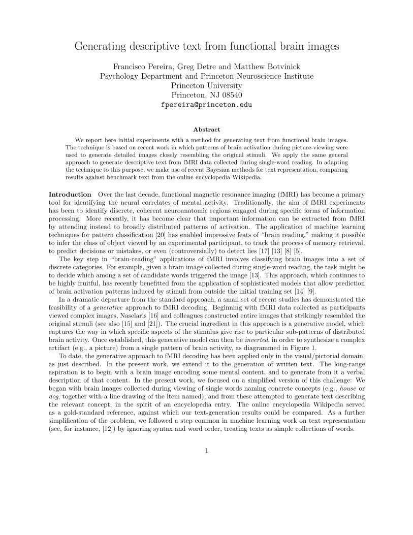
Generating descriptive text from functional brain images Francisco Pereira, Greg Detre and Matthew Botvinick Psychology Department and Princeton Neuroscience Institute Princeton University Princeton, NJ 08540 [email protected] Abstract We report here initial experiments with a method for generating text from functional brain images. The technique is based on recent work in which patterns of brain activation during picture-viewing were used to generate detailed images closely resembling the original stimuli. We apply the same general approach to generate descriptive text from fMRI data collected during single-word reading. In adapting the technique to this purpose, we make use of recent Bayesian methods for text representation, comparing results against benchmark text from the online encyclopedia Wikipedia. Introduction Over the last decade, functional magnetic resonance imaging (fMRI) has become a primary tool for identifying the neural correlates of mental activity. Traditionally, the aim of fMRI experiments has been to identify discrete, coherent neuroanatomic regions engaged during specific forms of information processing. More recently, it has become clear that important information can be extracted from fMRI by attending instead to broadly distributed patterns of activation. The application of machine learning techniques for pattern classification [20] has enabled impressive feats of “brain reading,” making it possible to infer the class of object viewed by an experimental participant, to track the process of memory retrieval, to predict decisions or mistakes, or even (controversially) to detect lies [17] [13] [8] [5]. The key step in “brain-reading” applications of fMRI involves classifying brain images into a set of discrete categories. For example, given a brain image collected during single-word reading, the task might be to decide which among a set of candidate words triggered the image [13]. This approach, which continues to be highly fruitful, has recently benefitted from the application of sophisticated models that allow prediction of brain activation patterns induced by stimuli from outside the initial training set [14] [9]. In a dramatic departure from the standard approach, a small set of recent studies has demonstrated the feasibility of a generative approach to fMRI decoding. Beginning with fMRI data collected as participants viewed complex images, Naselaris [16] and colleagues constructed entire images that strikingly resembled the original stimuli (see also [15] and [21]). The crucial ingredient in this approach is a generative model, which captures the way in which specific aspects of the stimulus give rise to particular sub-patterns of distributed brain activity. Once established, this generative model can then be inverted, in order to synthesize a complex artifact (e.g., a picture) from a single pattern of brain activity, as diagrammed in Figure 1. To date, the generative approach to fMRI decoding has been applied only in the visual/pictorial domain, as just described. In the present work, we extend it to the generation of written text. The long-range aspiration is to begin with a brain image encoding some mental content, and to generate from it a verbal description of that content. In the present work, we focused on a simplified version of this challenge: We began with brain images collected during viewing of single words naming concrete concepts (e.g., house or dog, together with a line drawing of the item named), and from these attempted to generate text describing the relevant concept, in the spirit of an encyclopedia entry. The online encyclopedia Wikipedia served as a gold-standard reference, against which our text-generation results could be compared. As a further simplification of the problem, we followed a step common in machine learning work on text representation (see, for instance, [12]) by ignoring syntax and word order, treating texts as simple collections of words. 1
-
Upload
independent -
Category
Documents
-
view
2 -
download
0
Transcript of Generating descriptive text from functional brain images
Generating descriptive text from functional brain images
Francisco Pereira, Greg Detre and Matthew Botvinick
Psychology Department and Princeton Neuroscience Institute
Princeton University
Princeton, NJ 08540
Abstract
We report here initial experiments with a method for generating text from functional brain images.The technique is based on recent work in which patterns of brain activation during picture-viewing wereused to generate detailed images closely resembling the original stimuli. We apply the same generalapproach to generate descriptive text from fMRI data collected during single-word reading. In adaptingthe technique to this purpose, we make use of recent Bayesian methods for text representation, comparingresults against benchmark text from the online encyclopedia Wikipedia.
Introduction Over the last decade, functional magnetic resonance imaging (fMRI) has become a primarytool for identifying the neural correlates of mental activity. Traditionally, the aim of fMRI experimentshas been to identify discrete, coherent neuroanatomic regions engaged during specific forms of informationprocessing. More recently, it has become clear that important information can be extracted from fMRIby attending instead to broadly distributed patterns of activation. The application of machine learningtechniques for pattern classification [20] has enabled impressive feats of “brain reading,” making it possibleto infer the class of object viewed by an experimental participant, to track the process of memory retrieval,to predict decisions or mistakes, or even (controversially) to detect lies [17] [13] [8] [5].
The key step in “brain-reading” applications of fMRI involves classifying brain images into a set ofdiscrete categories. For example, given a brain image collected during single-word reading, the task might beto decide which among a set of candidate words triggered the image [13]. This approach, which continues tobe highly fruitful, has recently benefitted from the application of sophisticated models that allow predictionof brain activation patterns induced by stimuli from outside the initial training set [14] [9].
In a dramatic departure from the standard approach, a small set of recent studies has demonstrated thefeasibility of a generative approach to fMRI decoding. Beginning with fMRI data collected as participantsviewed complex images, Naselaris [16] and colleagues constructed entire images that strikingly resembled theoriginal stimuli (see also [15] and [21]). The crucial ingredient in this approach is a generative model, whichcaptures the way in which specific aspects of the stimulus give rise to particular sub-patterns of distributedbrain activity. Once established, this generative model can then be inverted, in order to synthesize a complexartifact (e.g., a picture) from a single pattern of brain activity, as diagrammed in Figure 1.
To date, the generative approach to fMRI decoding has been applied only in the visual/pictorial domain,as just described. In the present work, we extend it to the generation of written text. The long-rangeaspiration is to begin with a brain image encoding some mental content, and to generate from it a verbaldescription of that content. In the present work, we focused on a simplified version of this challenge: Webegan with brain images collected during viewing of single words naming concrete concepts (e.g., house ordog, together with a line drawing of the item named), and from these attempted to generate text describingthe relevant concept, in the spirit of an encyclopedia entry. The online encyclopedia Wikipedia servedas a gold-standard reference, against which our text-generation results could be compared. As a furthersimplification of the problem, we followed a step common in machine learning work on text representation(see, for instance, [12]) by ignoring syntax and word order, treating texts as simple collections of words.
1
"Table"
wood
table
chair
food
furniture
Stimulus fMRI data fMRI data
topic model
Model relating stimulus
representation to fMRI data
semantic model
visual model
Output
invert model
invert model
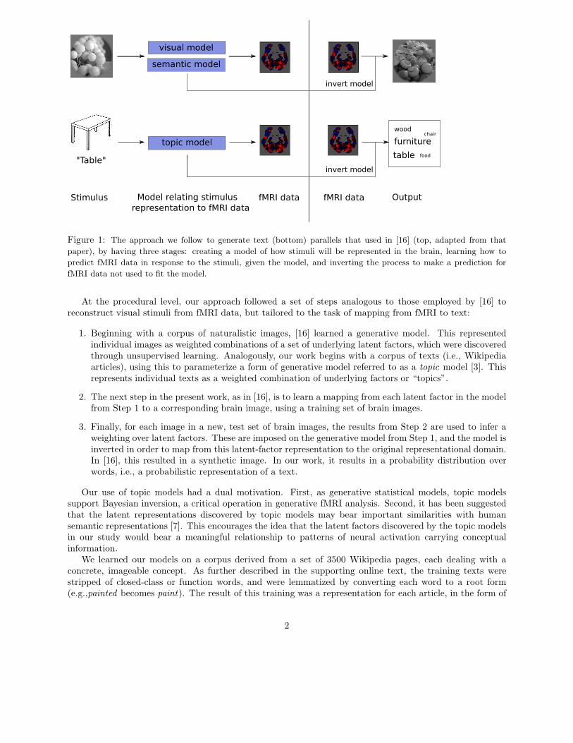
Figure 1: The approach we follow to generate text (bottom) parallels that used in [16] (top, adapted from that
paper), by having three stages: creating a model of how stimuli will be represented in the brain, learning how to
predict fMRI data in response to the stimuli, given the model, and inverting the process to make a prediction for
fMRI data not used to fit the model.
At the procedural level, our approach followed a set of steps analogous to those employed by [16] toreconstruct visual stimuli from fMRI data, but tailored to the task of mapping from fMRI to text:
1. Beginning with a corpus of naturalistic images, [16] learned a generative model. This representedindividual images as weighted combinations of a set of underlying latent factors, which were discoveredthrough unsupervised learning. Analogously, our work begins with a corpus of texts (i.e., Wikipediaarticles), using this to parameterize a form of generative model referred to as a topic model [3]. Thisrepresents individual texts as a weighted combination of underlying factors or “topics”.
2. The next step in the present work, as in [16], is to learn a mapping from each latent factor in the modelfrom Step 1 to a corresponding brain image, using a training set of brain images.
3. Finally, for each image in a new, test set of brain images, the results from Step 2 are used to infer aweighting over latent factors. These are imposed on the generative model from Step 1, and the model isinverted in order to map from this latent-factor representation to the original representational domain.In [16], this resulted in a synthetic image. In our work, it results in a probability distribution overwords, i.e., a probabilistic representation of a text.
Our use of topic models had a dual motivation. First, as generative statistical models, topic modelssupport Bayesian inversion, a critical operation in generative fMRI analysis. Second, it has been suggestedthat the latent representations discovered by topic models may bear important similarities with humansemantic representations [7]. This encourages the idea that the latent factors discovered by the topic modelsin our study would bear a meaningful relationship to patterns of neural activation carrying conceptualinformation.
We learned our models on a corpus derived from a set of 3500 Wikipedia pages, each dealing with aconcrete, imageable concept. As further described in the supporting online text, the training texts werestripped of closed-class or function words, and were lemmatized by converting each word to a root form(e.g.,painted becomes paint). The result of this training was a representation for each article, in the form of
2
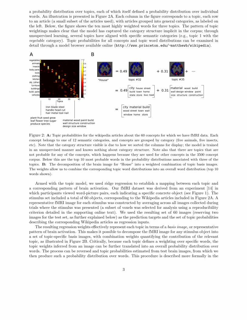
a probability distribution over topics, each of which itself defined a probability distribution over individualwords. An illustration is presented in Figure 2A. Each column in the figure corresponds to a topic, each rowto an article (a small subset of the articles used), with articles grouped into general categories, as labeled onthe left. Below, the figure shows the ten most highly weighted words for three topics. The pattern of topicweightings makes clear that the model has captured the category structure implicit in the corpus; throughunsupervised learning, several topics have aligned with specific semantic categories (e.g., topic 1 with thevegetable category). Topic probabilities for all concepts and topic word distributions can be examined indetail through a model browser available online (http://www.princeton.edu/~matthewb/wikipedia).
Topics10 20 30 40
vegetables
animals
insects
body parts
tools
clothing
kitchen
obj. (other)
furniture
buildings
build. parts
vehicles
0
0.1
0.2
0.3
0.4
0.5
0.6
0.7
0.8
0.9
1
plant fruit seed grow
leaf flower tree sugar
produce species
iron blade steel
handle head cut
hair metal tool nail
material wood paint build
wall structure construction
design size window
"House" topic #32 topic #35
+=
woodmaterialpaint
build
wall design window
structure constructionsize
0.49 0.31 + ...
city
build
house
store
town home
state bus road
street
city materialwood street
buildtown wall
storewindow home
= 0.49 0.31+
=
A B
Figure 2: A: Topic probabilities for the wikipedia articles about the 60 concepts for which we have fMRI data. Each
concept belongs to one of 12 semantic categories, and concepts are grouped by category (five animals, five insects,
etc). Note that the category structure visible is due to how we sorted the columns for display; the model is trained
in an unsupervised manner and knows nothing about category structure. Note also that there are topics that are
not probable for any of the concepts, which happens because they are used for other concepts in the 3500 concept
corpus. Below this are the top 10 most probable words in the probability distributions associated with three of the
topics. B: The decomposition of the brain image for “House” into a weighted combination of topic basis images.
The weights allow us to combine the corresponding topic word distributions into an overall word distribution (top 10
words shown).
Armed with the topic model, we used ridge regression to establish a mapping between each topic anda corresponding pattern of brain activation. Our fMRI dataset was derived from an experiment [14] inwhich participants viewed word-picture pairs, each indicating a specific concrete object (see Figure 1). Thestimulus set included a total of 60 objects, corresponding to the Wikipedia articles included in Figure 2A. Arepresentative fMRI image for each stimulus was constructed by averaging across all images collected duringtrials where the stimulus was presented (a subset of voxels was selected for analysis using a reproducibilitycriterion detailed in the supporting online text). We used the resulting set of 60 images (reserving twoimages for the test set, as further explained below) as the prediction targets and the set of topic probabilitiesdescribing the corresponding Wikipedia articles as regression inputs.
The resulting regression weights effectively represent each topic in terms of a basis image, or representativepattern of brain activation. This makes it possible to decompose the fMRI image for any stimulus object intoa set of topic-specific basis images, with combination weights quantifying the contribution of the relevanttopic, as illustrated in Figure 2B. Critically, because each topic defines a weighting over specific words, thetopic weights inferred from an image can be further translated into an overall probability distribution overwords. The process can be reversed and topic probabilities estimated from test brain images, from which wethen produce such a probability distribution over words. This procedure is described more formally in the
3
supporting online material.
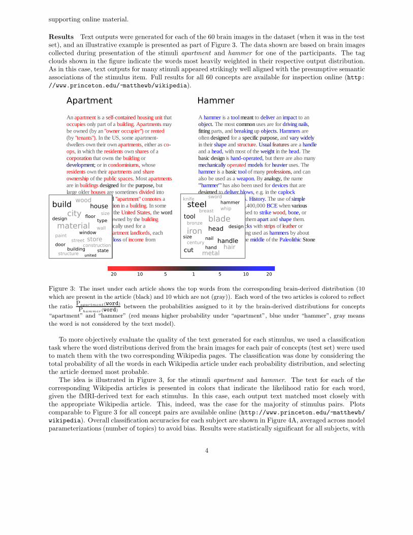
Results Text outputs were generated for each of the 60 brain images in the dataset (when it was in the testset), and an illustrative example is presented as part of Figure 3. The data shown are based on brain imagescollected during presentation of the stimuli apartment and hammer for one of the participants. The tagclouds shown in the figure indicate the words most heavily weighted in their respective output distribution.As in this case, text outputs for many stimuli appeared strikingly well aligned with the presumptive semanticassociations of the stimulus item. Full results for all 60 concepts are available for inspection online (http://www.princeton.edu/~matthewb/wikipedia).
Apartment
vacancy represents
Hammer
15 520 2010 10
An apartment is a self-contained housing unit that
occupies only part of a building. Apartments may
be owned (by an "owner occupier") or rented
(by "tenants"). In the US, some apartment-
dwellers own their own apartments, either as co-
ops, in which the residents own shares of a
corporation that owns the building or
development; or in condominiums, whose
residents own their apartments and share
ownership of the public spaces. Most apartments
are in buildings designed for the purpose, but
large older houses are sometimes divided into
apartments. The word "apartment" connotes a
residential unit or section in a building. In some
locations, particularly the United States, the word
denotes a rental unit owned by the building
owner, and is not typically used for a
condominium. For apartment landlords, each
vacancy represents a loss of income from
A hammer is a tool meant to deliver an impact to an
object. The most common uses are for driving nails,
fitting parts, and breaking up objects. Hammers are
often designed for a specific purpose, and vary widely
in their shape and structure. Usual features are a handle
and a head, with most of the weight in the head. The
basic design is hand-operated, but there are also many
mechanically operated models for heavier uses. The
hammer is a basic tool of many professions, and can
also be used as a weapon. By analogy, the name
"'hammer'" has also been used for devices that are
designed to deliver blows, e.g. in the caplock
mechanism of firearms. History. The use of simple
tools dates to about 2,400,000 BCE when various
shaped stones were used to strike wood, bone, or
other stones to break them apart and shape them.
Stones attached to sticks with strips of leather or
animal sinew were being used as hammers by about
30,000 BCE during the middle of the Paleolithic Stone
build house
building
design
window
door
floortype
stateunited
city
store
wood
streetpaint
wall
structure
construction
size
material
steel
head
cut
handle
tool
nail
design
hammer
size
hand
iron
blade
hairmetal
whipbreast
bronze
century
knifesword
Figure 3: The inset under each article shows the top words from the corresponding brain-derived distribution (10
which are present in the article (black) and 10 which are not (gray)). Each word of the two articles is colored to reflect
the ratioPapartment(word)
Phammer(word)between the probabilities assigned to it by the brain-derived distributions for concepts
“apartment” and “hammer” (red means higher probability under “apartment”, blue under “hammer”, gray means
the word is not considered by the text model).
To more objectively evaluate the quality of the text generated for each stimulus, we used a classificationtask where the word distributions derived from the brain images for each pair of concepts (test set) were usedto match them with the two corresponding Wikipedia pages. The classification was done by considering thetotal probability of all the words in each Wikipedia article under each probability distribution, and selectingthe article deemed most probable.
The idea is illustrated in Figure 3, for the stimuli apartment and hammer. The text for each of thecorresponding Wikipedia articles is presented in colors that indicate the likelihood ratio for each word,given the fMRI-derived text for each stimulus. In this case, each output text matched most closely withthe appropriate Wikipedia article. This, indeed, was the case for the majority of stimulus pairs. Plotscomparable to Figure 3 for all concept pairs are available online (http://www.princeton.edu/~matthewb/wikipedia). Overall classification accuracies for each subject are shown in Figure 4A, averaged across modelparameterizations (number of topics) to avoid bias. Results were statistically significant for all subjects, with
4
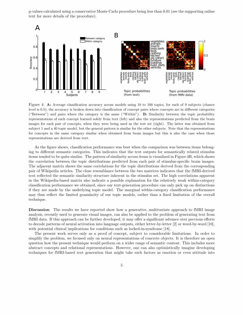
p-values calculated using a conservative Monte Carlo procedure being less than 0.01 (see the supporting onlinetext for more details of the procedure).
1 2 3 4 5 6 7 8 90
0.2
0.4
0.6
0.8
1
Accuracy
Subjects
Between category
Within category
A
Topic probabilities
(from text)
vegeta
ble
sanim
als
insects
body p
arts
tools
clo
thin
gkitchen
obj (o
ther)
furn
iture
build
ings
build
. parts
vehic
les
vegetablesanimalsinsectsbody partstoolsclothingkitchenobj (other)furniturebuildingsbuild. partsvehicles
Topic probabilities
(from fMRI data)
vegeta
ble
sanim
als
insects
body p
arts
tools
clo
thin
gkitchen
obj (o
ther)
furn
iture
build
ings
build
. parts
vehic
les
0
0.5
1
B
Figure 4: A: Average classification accuracy across models using 10 to 100 topics, for each of 9 subjects (chance
level is 0.5); the accuracy is broken down into classification of concept pairs where concepts are in different categories
(“Between”) and pairs where the category is the same (“Within”). B: Similarity between the topic probability
representations of each concept learned solely from text (left) and also the representations predicted from the brain
images for each pair of concepts, when they were being used as the test set (right). The latter was obtained from
subject 1 and a 40 topic model, but the general pattern is similar for the other subjects. Note that the representations
for concepts in the same category similar when obtained from brain images but this is also the case when those
representations are derived from text.
As the figure shows, classification performance was best when the comparison was between items belong-ing to different semantic categories. This indicates that the text outputs for semantically related stimulusitems tended to be quite similar. The pattern of similarity across items is visualized in Figure 4B, which showsthe correlation between the topic distributions predicted from each pair of stimulus-specific brain images.The adjacent matrix shows the same correlations for the topic distributions derived from the correspondingpair of Wikipedia articles. The close resemblance between the two matrices indicates that the fMRI-derivedtext reflected the semantic similarity structure inherent in the stimulus set. The high correlations apparentin the Wikipedia-based matrix also indicate a possible explanation for the relatively weak within-categoryclassification performance we obtained, since our text-generation procedure can only pick up on distinctionsif they are made by the underlying topic model. The marginal within-category classification performancemay thus reflect the limited granularity of our topic models, rather than a fixed limitation of the overalltechnique.
Discussion The results we have reported show how a generative, multivariate approach to fMRI imageanalysis, recently used to generate visual images, can also be applied to the problem of generating text fromfMRI data. If this approach can be further developed, it may offer a significant advance over previous effortsto decode patterns of neural activation into language outputs, either letter-by-letter [2] or word-by-word [10],with potential clinical implications for conditions such as locked-in-syndrome [18].
The present work serves only as a proof of concept, subject to considerable limitations. In order tosimplify the problem, we focused only on neural representations of concrete objects. It is therefore an openquestion how the present technique would perform on a wider range of semantic content. This includes moreabstract concepts and relational representations. However, one can also optimistically imagine developingtechniques for fMRI-based text generation that might take such factors as emotion or even attitude into
5
account. A second important simplification was to ignore word order and grammatical structure. Althoughthis is a conventional step in text-analysis research, a practical method for text generation would clearlyrequire grammatical structure to be taken into account. In this regard, it is interesting to note that [7]proposed an approach to enriching topic model representations using a generative model of word order.Integrating such a modeling approach into the present generative approach to fMRI analysis might supportmore transparently meaningful text outputs.
Acknowledgments
We would like to thank Tom Mitchell and Marcel Just for generously agreeing to share their dataset, Dave Blei
for help with building and interpreting topic models and Ken Norman and Sam Gershman for several discussions
regarding presentation of the material.
References
[1] W. F. Battig and W. E. Montague. Category Norms for Verbal Items in 56 Categories. Journal ofExperimental Psychology, 80(3), 1969.
[2] N. Birbaumer. Breaking the silence: brain-computer interfaces (BCI) for communication and motorcontrol. Psychophysiology, 43(6):517–32, November 2006.
[3] D. Blei, M. Jordan, and A. Y. Ng. Latent Dirichlet allocation. Journal of Machine Learning Research,3:993–1022, 2003.
[4] J. M. Clark and A. Paivio. Extensions of the Paivio, Yuille, and Madigan (1968) norms. Behaviorresearch methods, instruments, & computers : a journal of the Psychonomic Society, Inc, 36(3):371–83,August 2004.
[5] C. Davatzikos, K. Ruparel, Y. Fan, D. G. Shen, M. Acharyya, J. W. Loughead, R. C. Gur, and D. D.Langleben. Classifying spatial patterns of brain activity with machine learning methods: application tolie detection. NeuroImage, 28(3):663–8, 2005.
[6] M. Grant and S. Boyd. CVX users guide, 2009.
[7] T. L. Griffiths, M. Steyvers, and J. B. Tenenbaum. Topics in semantic representation. Psychologicalreview, 114(2):211–44, April 2007.
[8] J. Haynes and G. Rees. Decoding mental states from brain activity in humans. Nature reviews. Neuro-science, 7(7):523–34, 2006.
[9] K. N. Kay, T. Naselaris, R. J. Prenger, and J. L. Gallant. Identifying natural images from human brainactivity. Nature, 452(7185):352–5, 2008.
[10] S. Kellis, K. Miller, K. Thomson, R. Brown, P. House, and B. Greger. Decoding spoken words usinglocal field potentials recorded from the cortical surface. Journal of neural engineering, 7(5):056007,September 2010.
[11] G. Minnen, J. Carroll, and D. Pearce. Applied morphological processing of English. Natural LanguageEngineering, 7(03):207–223, 2001.
[12] T. M. Mitchell. Machine Learning. 1997.
[13] T. M. Mitchell, R. Hutchinson, R. S. Niculescu, F. Pereira, X. Wang, M. Just, and S. Newman. Learningto Decode Cognitive States from Brain Images. Machine Learning, 57(1/2):145–175, October 2004.
6

[14] T. M. Mitchell, S. V. Shinkareva, A. Carlson, K. Chang, V. L. Malave, R. A. Mason, and M. A. Just.Predicting human brain activity associated with the meanings of nouns. Science (New York, N.Y.),320(5880):1191–5, 2008.
[15] Y. Miyawaki, H. Uchida, O. Yamashita, M. Sato, Y. Morito, H. Tanabe, N. Sadato, and Y. Kamitani.Visual image reconstruction from human brain activity using a combination of multiscale local imagedecoders. Neuron, 60(5):915–29, 2008.
[16] T. Naselaris, R. J. Prenger, K. N. Kay, M. Oliver, and J. L. Gallant. Bayesian reconstruction of naturalimages from human brain activity. Neuron, 63(6):902–15, 2009.
[17] K. A. Norman, S. M. Polyn, G. J. Detre, and J. V. Haxby. Beyond mind-reading: multi-voxel patternanalysis of fMRI data. Trends in cognitive sciences, 10(9):424–30, 2006.
[18] A. M. Owen, M. R. Coleman, M. Boly, M. H. Davis, S. Laureys, and J. Pickard. Detecting awarenessin the vegetative state. Science, 313(5792):1402, September 2006.
[19] A. Paivio, J. C. Yuille, and S. A. Madigan. Concreteness, Imagery, and Meaningfulness Values for 925Nouns. Journal of Experimental Psychology, 76(1), 1968.
[20] F. Pereira, T. M. Mitchell, and M. Botvinick. Machine learning classifiers and fMRI: a tutorial overview.NeuroImage, 45(1 Suppl):S199–209, March 2009.
[21] B. Thirion, E. Duchesnay, E. Hubbard, J. Dubois, J. B. Poline, Denis Lebihan, and Stanislas Dehaene.Inverse retinotopy: inferring the visual content of images from brain activation patterns. NeuroImage,33:1104–1116, 2006.
[22] J. Van Overschelde. Category norms: An updated and expanded version of the Battig and Montague(1969) norms. Journal of Memory and Language, 50(3):289–335, 2004.
7
A Supporting Online Material
A.1 Web resources
The web resources mentioned in the text can be accessed through the website for the Botvinick lab (http://www.princeton.edu/~matthewb/wikipedia). We focus on a topic model with 40 topics and α = 25
#topics,
the model with the fewest topics where we can achieve asymptotic performance across subjects. For thatmodel we provide
• Text output from concept brain images when used as test set, for every concept, as shown in Figure 3
• Interactive browser showing the word probabilities predicted from brain images, for every concept pair,when those two concepts were in the test set, as shown for “apartment” and “hammer” in Figure 3
• Visualizations of a topic model learned on approximately 3500 Wikipedia articles, namely how conceptsrelate to topics and topics to concepts, as well as the topic-specific probability distributions over words
• Basis images for the topics in the 60 concept fMRI dataset
A.2 Data (fMRI Data collection and preprocessing from [14])
Nine right-handed adults (5 female, age between 18 and 32) from the Carnegie Mellon University communityparticipated in the fMRI study, and gave informed consent approved by the University of Pittsburgh andCarnegie Mellon Institutional Review Boards. Data from two additional participants exhibiting head motionof 2.2 mm and 3.0 mm were excluded. The stimuli were line drawings and noun labels of 60 concrete objectsfrom 12 semantic categories with 5 exemplars per category, as shown in Figure S1. Most of the line drawingswere taken or adapted from the Snodgrass and Vanderwart set (S1) and others were added using a similardrawing style. The entire set of 60 stimulus items was presented six times, randomly permuting the sequenceof the 60 items on each presentation. Each stimulus item was presented for 3s, followed by a 7s rest period,during which the participants were instructed to fixate on an X displayed in the center of the screen. Therewere twelve additional presentations of a fixation X, 31s each, distributed across the session to provide abaseline measure. When an exemplar was presented, the participant’s task was to think about the propertiesof the object. To promote their consideration of a consistent set of properties across the 6 presentations,they were asked to generate a set of properties for each item prior to the scanning session (for example, forthe item castle, the properties might be cold, knights, and stone). Each participant was free to choose anyproperties they wished, and there was no attempt to obtain consistency across participants in the choiceof properties. Functional images were acquired on a Siemens (Erlangen, Germany) Allegra 3.0T scanner atthe Brain Imaging Research Center of Carnegie Mellon University and the University of Pittsburgh using agradient echo EPI pulse sequence with TR = 1000 ms, TE = 30 ms and a 60 degree flip angle. Seventeen5-mm thick oblique-axial slices were imaged with a gap of 1 mm between slices. The acquisition matrix was64 x 64 with 3.125-mm x 3.125-mm x 5-mm voxels. Initial data processing was performed using StatisticalParametric Mapping software (SPM2, Wellcome Department of Cognitive Neurology, London, UK). The datawere corrected for slice timing, motion, and linear trend, and were temporally filtered using a 190s cutoff.The data were spatially normalized into MNI space and resampled to 3x3x6 mm3 voxels. The percent signalchange (PSC) relative to the fixation condition was computed at each voxel for each stimulus presentation. Asingle fMRI mean image was created for each of the 360 item presentations by taking the mean of the imagescollected 4s, 5s, 6s, and 7s after stimulus onset (to account for the delay in the hemodynamic response).Each of these images was normalized by subtracting its mean and dividing by its standard deviation, bothacross all voxels.
A.3 Wikipedia corpus and topic models
To derive a corpus from Wikipedia we started with the classical lists of words in [19] and [1], as well asmodern revisions/extensions [4] and [22], and compiled words corresponding to concepts that were deemed
8
concrete or imageable, be it because of their score in one of the lists or through editorial decision. Wethen identified the corresponding Wikipedia article titles (e.g. “airplane” is “Fixed-wing aircraft”) and alsocompiled related articles which were linked to from these (e.g. “Aircraft cabin”). If there were words in theoriginal lists with multiple meanings we included the articles for at least a few of those meanings. Giventime constraints, we stopped the process with a list of 3500 concepts and their corresponding articles. Weused Wikipedia Extractor 1 to remove HTML, wiki formatting and annotations and processed the resultingtext through the morphological analysis tool Morpha [11] 2 to lemmatize all the words to their basic stems(e.g. “taste”,”tasted”,”taster” and “tastes” all become the same word).
The resulting text corpus was processed with the topic modelling software from [3] to build several LDA 3
models. The articles were converted to the required format, keeping only words that appeared in at least twoarticles, and words were also excluded resorting to a custom stopword list. We run the software varying thenumber of topics allowed from 10 to 100, in increments of 10, setting the α parameter to 25
#topics(following
[7], though a range of multiples of the inverse of the number of topics yielded comparable experiment results).LDA models each document w (a collection of words) as coming from a process where the number of
words N and the probabilities of each topic being present θ are drawn. Each word w is produced by selectinga topic z (according to probabilities θ), and drawing from the topic-specific probability distribution p(w|z)over words. In the process of learning a model of our corpus, a vector of topic probabilities is produced foreach article/concept, and the topic-specific distributions are learned. The topic probabilities are what weuse as the low-dimensional representation of each concept.
Given the probabilities θ for a concept, we can combine the topic-specific distributions over words into asingle distribution, e.g.
p(w|θ) = p(w|topic 1)θ1 + . . . + p(w|topic K)θk
i.e. the more probable a topic is the more bearing it has in determining what the probability of a wordis. In the paper this is used to convert the topic probabilities estimated from a test set brain image into aword distribution corresponding to that image.
Note also that, since the topic probabilities add up to 1, the presence of one topic trades off with thepresence of the others, something that is desirable if expressing one brain image as a combination of basisimages weighted by the topic probabilities
A.4 Basis image decomposition
The procedure depicted in Figure 6 has two steps that require solving optimization problems. The first islearning a set of basis images, given example images for 58 concepts and their respective topic probabilities.The second is predicting the topic probabilities present in an example image, given a set of basis images.The following sections provide notation and a formal description of these two problems.
A.4.1 Notation
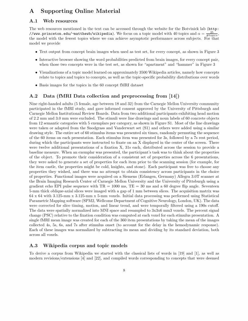
As each example is a 3D image divided into a grid of voxels, it can be unfolded into a vector x with as manyentries as voxels containing cortex. A dataset is a n×m matrix X where row i is the example vector xi. Eachexample x will be expressed as a linear combination of basis images b1, . . . ,bK of the same dimensionality,with the weights given by the topic probability vector z = [z1, . . . , zK ], as depicted on the top of Figure 5.The low-dimensional representation of dataset X is a n × K matrix Z where row i is a vector zi and thecorresponding basis images are a K ×m matrix B, where row k corresponds to basis image bk, as shown onthe bottom of Figure 5.
1http://medialab.di.unipi.it/wiki/Wikipedia_extractor2http://www.informatics.susx.ac.uk/research/groups/nlp/carroll/morph.html3http://www.cs.princeton.edu/~blei/topicmodeling.html
9
~x z1 z2 z3
b1
b2
b3
(...) (...)
dataset X low-dim Z image basis B
b1
b2
b3
Figure 5: Top: Each brain image can be written as a row vector, and the combination as a linear combinationof three row vectors. Bottom: A dataset contains many such patterns, forming a matrix X where rows areexamples and whose low-dimensional representation is a matrix Z.
A.4.2 Learn basis images given example images and topic probabilities
Learning the basis images given X and Z can be decomposed into a set of independent regression problems,one per voxel j, i.e. the values of voxel j across all examples, X(:, j), are predicted from Z using regressioncoefficients β = B(:, j), which are the values of voxel j across basis images. Any situation where linearregression was infeasible because the square matrix in the normal equations was not invertible was addressedby using a ridge term with the trade-off parameter set to 1. Hence, for voxel j, we solve:
maxβ
‖X:,j − Zβ‖2(+λ‖z}2)
A.4.3 Predict topic probabilities given example images and basis images
Predicting the topic probability vector z = Zi,: for an example x = Xi,: is a regression problem where x′
is predicted from B′ using regression coefficients z′. The prediction of the topic probability vector is doneunder the additional constraint that the values need to be greater than or equal to 0 and add up to 1, asthey are probabilities. We used CVX [6] to solve for topic vector z:
maxβ
‖Xi,: − zB‖2
subject to :
∀jzj >= 0∑
j zj = 1
A.5 Experiment
A.5.1 Classification procedure
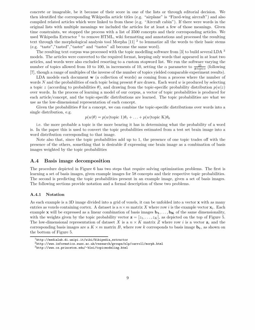
Classification accuracy was measured on the task of matching two example images with the two correspondingwikipedia articles, by considering the probability assigned to the words in each article by the distributionsderived from the example images, as illustrated in Figure 6 and described in the following steps:
• leave out one pair of concepts (e.g. “apartment” and “hammer”) as test set
• use the example images for the remaining 58 concepts, together with their respective topic probabilitiesunder the model, as the training set to obtain a set of basis images (over 1000 stable voxels, selected inthis training set)
• for each of the test concepts (for instance, “apartment”):
• predict the probability of each topic being present from the “apartment” example image
• obtain an “apartment”-brain probability distribution for that combination of topic probabilities
10
• compute the probability of “apartment” article and “hammer” article under that distribution, re-spectively papartment(“apartment
′′) and papartment(“hammer′′)
• assign the article with highest probability to the corresponding test concept, and the other article to theother concept (this will be correct or incorrect)
The steps are repeated for every possible pair of concepts, and the accuracy is the fraction of the pairswhere the assignment of articles to example images was correct.
house
building
door
...
wikipedia
topic model
apartment
hammer
predicted
topic
probabilities
predicted
word
distributions
A hammer is a tool
meant to deliver an
impact to an object ...
An apartment or flat isa self-contained housingunit that occupies onlypart of a building ...
"apartment" wikipedia article
"hammer" wikipedia articleimage basis
concept 1
concept 58
...
steel
hammer
tool
...
prob("apartment" article)
prob("hammer" article)
prob("apartment" article)
prob("hammer" article)
apartment
hammer
hammer
apartment
test
train
Figure 6: Classification procedure for the “apartment” and “hammer” example images.
A.5.2 Classification results
0 10 20 30 40 50 60 70 80 90 1000.5
0.55
0.6
0.65
0.7
0.75
0.8
0.85
0.9
0.95
1
clas
sific
atio
n ac
cura
cy
number of topics
subject P1
vege
tabl
es
anim
als
inse
cts
body
part
s
tool
s
clot
hing
kitc
hen
man
mad
e
furn
iture
build
ings
build
part
s
vehi
cles
vegetables
animals
insects
bodyparts
tools
clothing
kitchen
manmade
furniture
buildings
buildparts
vehicles
subject P4
vege
tabl
es
anim
als
inse
cts
body
part
s
tool
s
clot
hing
kitc
hen
man
mad
e
furn
iture
build
ings
build
part
s
vehi
cles
vegetables
animals
insects
bodyparts
tools
clothing
kitchen
manmade
furniture
buildings
buildparts
vehicles
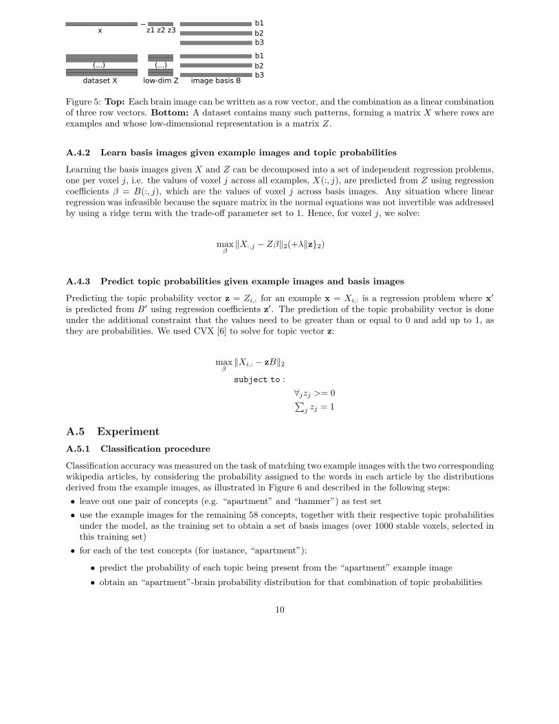
Figure 7: Left: Average classification accuracy across 9 subjects, using models with 10-100 topics. Right:
Plot of correct (blue) or incorrect (red) predictions for all possible concept pairs, for subjects P1 and P4,using a model with 40 topics.
We reported results in Figure 4 of the main paper, averaging across models using various numbers oftopics. We could also have averaged across subjects, and the classification results using topic models with 10to 100 topics are shown in Figure 7. The curve is the average classification accuracy across 9 subjects. Forthe best scoring model (40 topics), the individual subject results were 0.89, 0.77, 0.74, 0.85, 0.77, 0.79, 0.72,
11
0.62 and 0.79. Again one can ask is whether some concepts pairs are more easily classifiable than others. Inorder to answer this we can plot a 60 × 60 binary matrix, shown on the right of Figure 4 for the two bestsubjects, P1 and P4. The most salient aspect of these plots is that the predominantly confused pairs liealong the diagonal of the matrix, i.e. they correspond to pairs of concepts that belong to the same category.
A.5.3 Selection of stable voxels
The reproducibility criterion we used identifies voxels whose activation levels across the training set examplesof each concept bear the same relationship to each other over epochs (mathematically, the vector of activationlevels across the sorted concepts is highly correlated between epochs). As [14] points out, we do not expectall – or even most – of the activation to be differentially task related, rather than uniformly present acrossconditions, or consistent between the various presentations of the same noun stimulus. We chose to use1000 rather than 500 reproducible voxels, as the results were somewhat better (and still comparable with2000 voxels, say), but it’s legitimate to consider how sensitive the results are to this choice. Given that thereproducibility criterion for selecting voxels is essentially a correlation computation, one can find a thresholdat which the null hypothesis of there being no correlation has a given p-value, using the Fisher transformation.For instance, given that 59 voxel values are compared across 6×5/ pairs of runs, observed correlation r = 0.1has a p-value of 0.01 if the true correlation ρ = 0. Using this threshold gives us a different number of voxelsin each subject, ranging from approximately 200 to well over 2000, but the results are still very similar tothose obtained with 1000 voxels.
A.5.4 Normal testing of classification results
In the common situation where there are n independent test examples, a statistically significant classificationresult is one where we can reject the null hypothesis that there is no information about the variable of interest(the variable being predicted by the classifier) in the fMRI data from which it is being predicted. Establishingstatistical significance is generally done by determining how improbable the observed classification accuracywould be were the null hypothesis to be true (this probability is called a p-value).
In this situation the probability of obtaining a given classification result under this null hypothesis is theprobability of achieving k successes out of n independent trials, which is given by a binomial distribution.Ifwe define k to be the number of correctly labeled test set examples out of n, the p-value under the nullhypothesis is simply P (X ≥ k), where X is a random variable with a binomial distribution with n trials andprobability of success 0.5 (two class). If the p-value is below a certain threshold the result will be declaredsignificant.
A.5.5 Testing dependent classification results in our situation
In the experiment described in the paper we have one classification decision for each possible pair of concepts(1770 in total). Those decisions are not independent, as each concept appears in 59 pairs. The expectedaccuracy under the null hypothesis that the classification was being made at random is still 50%, but thevariance is not what the same as in the binomial case described above. So how could get this distribution?
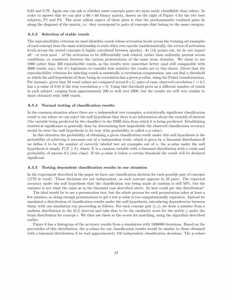
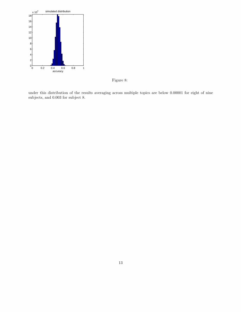
The ideal would be to use a permutation test, but the whole process for each permutation takes at least afew minutes, so doing enough permutations to get a low p-value is too computationally expensive. Instead wesimulated a distribution of classification results under the null hypothesis, introducing dependencies betweenthem, with one simulation run proceeding as follows. For each concept pair (i, j), we draw a number from auniform distribution in the [0,1] interval and take that to be the similarity score for the article j under thebrain distribution for concept i. We then use these as the scores for matching, using the algorithm describedearlier.
Figure 8 has a histogram of the accuracy results from a simulation with 1000000 iterations. Based on thepercentiles of this distribution, the p-values for our classification results would be similar to those obtainedwith a binomial distribution if we had approximately 150 independent classification decisions. The p-values
12
0 0.2 0.4 0.6 0.8 10
2
4
6
8
10
12
14
16
18x 10
4
accuracy
simulated distribution
Figure 8:
under this distribution of the results averaging across multiple topics are below 0.00001 for eight of ninesubjects, and 0.003 for subject 8.
13