Generating and Auto-Tuning Parallel Stencil Codes - CORE
297
Generating and Auto-Tuning Parallel Stencil Codes Inauguraldissertation zur Erlangung der W¨ urde eines Doktors der Philosophie vorgelegt der Philosophisch-Naturwissenschaftlichen Fakult¨ at der Universit¨ at Basel von Matthias-Michael Christen aus Affoltern BE, Schweiz Basel, 2011 Originaldokument gespeichert auf dem Dokumentenserver der Universit ¨ at Basel: edoc.unibas.ch. Dieses Werk ist unter dem Vertrag “Creative Commons Namensnennung–Keine kommerzielle Nutzung–Keine Bearbeitung 2.5 Schweiz” lizenziert. Die vollst ¨ andige Lizenz kann unter http://creativecommons.org/licences/by-nc-nd/2.5/ch eingesehen werden.
-
Upload
khangminh22 -
Category
Documents
-
view
0 -
download
0
Transcript of Generating and Auto-Tuning Parallel Stencil Codes - CORE

Generating and Auto-Tuning
Parallel Stencil Codes
Inauguraldissertation
zur Erlangung der Wurde eines Doktors der Philosophie
vorgelegt der Philosophisch-Naturwissenschaftlichen Fakultat
der Universitat Basel
von
Matthias-Michael Christen
aus Affoltern BE, Schweiz
Basel, 2011
Originaldokument gespeichert auf demDokumentenserver der Universitat Basel: edoc.unibas.ch.
Dieses Werk ist unter dem Vertrag “Creative CommonsNamensnennung–Keine kommerzielle Nutzung–KeineBearbeitung 2.5 Schweiz” lizenziert. Die vollstandigeLizenz kann unterhttp://creativecommons.org/licences/by-nc-nd/2.5/ch
eingesehen werden.

Attribution – NonCommercial – NoDerivs 2.5 Switzerland
You are free:
to Share — to copy, distribute and transmit the work
Under the following conditions:
Attribution — You must attribute the work in the manner specified bythe author or licensor (but not in any way that suggests that they endorseyou or your use of the work).Noncommercial — You may not use this work for commercial pur-poses.No Derivative Works —You may not alter, transform, or build uponthis work.
With the understanding that:
Waiver — Any of the above conditions can be waived if you get permission from thecopyright holder.
Public Domain — Where the work or any of its elements is in the public domain underapplicable law, that status is in no way affected by the license.
Other Rights — In no way are any of the following rights affected by the license:
• Your fair dealing or fair use rights, or other applicable copyright exceptions and limi-tations;
• The author’s moral rights;
• Rights other persons may have either in the work itself or in how the work is used,such as publicity or privacy rights.
Notice — For any reuse or distribution, you must make clear to others the licenseterms of this work. The best way to do this is with a link to the web page http:
//creativecommons.org/licenses/by-nc-nd/2.5/ch.
Disclaimer — The Commons Deed is not a license. It is simply a handy reference for un-derstanding the Legal Code (the full license) – it is a human-readable expression of someof its key terms. Think of it as the user-friendly interface to the Legal Code beneath.This Deed itself has no legal value, and its contents do not appear in the actual license.Creative Commons is not a law firm and does not provide legal services. Distributingof, displaying of, or linking to this Commons Deed does not create an attorney-clientrelationship.

Genehmigt von der Philosophisch-Naturwissenschaftlichen Fakultat aufAntrag von
Prof. Dr. Helmar BurkhartProf. Dr. Rudolf Eigenmann
Basel, den 20. September 2011
Prof. Dr. Martin Spiess,Dekan


Abstract
In this thesis, we present a software framework, PATUS, which generateshigh performance stencil codes for different types of hardware platforms,including current multicore CPU and graphics processing unit architec-tures. The ultimate goals of the framework are productivity, portability(of both the code and performance), and achieving a high performanceon the target platform.
A stencil computation updates every grid point in a structured gridbased on the values of its neighboring points. This class of computationsoccurs frequently in scientific and general purpose computing (e.g., inpartial differential equation solvers or in image processing), justifyingthe focus on this kind of computation.
The proposed key ingredients to achieve the goals of productivity, porta-bility, and performance are domain specific languages (DSLs) and the auto-tuning methodology.
The PATUS stencil specification DSL allows the programmer to ex-press a stencil computation in a concise way independently of hardwarearchitecture-specific details. Thus, it increases the programmer produc-tivity by disburdening her or him of low level programming model is-sues and of manually applying hardware platform-specific code opti-mization techniques. The use of domain specific languages also impliescode reusability: once implemented, the same stencil specification canbe reused on different hardware platforms, i.e., the specification code isportable across hardware architectures. Constructing the language to begeared towards a special purpose makes it amenable to more aggressiveoptimizations and therefore to potentially higher performance.
Auto-tuning provides performance and performance portability by au-tomated adaptation of implementation-specific parameters to the char-acteristics of the hardware on which the code will run. By automating

the process of parameter tuning — which essentially amounts to solvingan integer programming problem in which the objective function is thenumber representing the code’s performance as a function of the param-eter configuration, — the system can also be used more productively thanif the programmer had to fine-tune the code manually.
We show performance results for a variety of stencils, for which PA-TUS was used to generate the corresponding implementations. The se-lection includes stencils taken from two real-world applications: a sim-ulation of the temperature within the human body during hyperthermiacancer treatment and a seismic application. These examples demonstratethe framework’s flexibility and ability to produce high performance code.

Contents
Contents i
1 Introduction 3
I High-Performance Computing Challenges 7
2 Hardware Challenges 9
3 Software Challenges 173.1 The Laws of Amdahl and Gustafson . . . . . . . . . . . . . 183.2 Current De-Facto Standards . . . . . . . . . . . . . . . . . . 243.3 Beyond MPI and OpenMP . . . . . . . . . . . . . . . . . . . 283.4 Optimizing Compilers . . . . . . . . . . . . . . . . . . . . . 323.5 Domain Specific Languages . . . . . . . . . . . . . . . . . . 423.6 Motifs . . . . . . . . . . . . . . . . . . . . . . . . . . . . . . . 45
4 Algorithmic Challenges 53
II The PATUS Approach 59
5 Introduction To PATUS 615.1 Stencils and the Structured Grid Motif . . . . . . . . . . . . 63
5.1.1 Stencil Structure Examples . . . . . . . . . . . . . . . 645.1.2 Stencil Sweeps . . . . . . . . . . . . . . . . . . . . . . 685.1.3 Boundary Conditions . . . . . . . . . . . . . . . . . . 695.1.4 Stencil Code Examples . . . . . . . . . . . . . . . . . 705.1.5 Arithmetic Intensity . . . . . . . . . . . . . . . . . . 71

ii CONTENTS
5.2 A PATUS Walkthrough Example . . . . . . . . . . . . . . . . 745.2.1 From a Model to a Stencil . . . . . . . . . . . . . . . 755.2.2 Generating The Code . . . . . . . . . . . . . . . . . . 765.2.3 Running and Tuning . . . . . . . . . . . . . . . . . . 78
5.3 Integrating into User Code . . . . . . . . . . . . . . . . . . . 815.4 Alternate Entry Points to PATUS . . . . . . . . . . . . . . . . 835.5 Current Limitations . . . . . . . . . . . . . . . . . . . . . . . 835.6 Related Work . . . . . . . . . . . . . . . . . . . . . . . . . . . 84
6 Saving Bandwidth And Synchronization 896.1 Spatial Blocking . . . . . . . . . . . . . . . . . . . . . . . . . 896.2 Temporal Blocking . . . . . . . . . . . . . . . . . . . . . . . 91
6.2.1 Time Skewing . . . . . . . . . . . . . . . . . . . . . . 926.2.2 Circular Queue Time Blocking . . . . . . . . . . . . 976.2.3 Wave Front Time Blocking . . . . . . . . . . . . . . . 99
6.3 Cache-Oblivious Blocking Algorithms . . . . . . . . . . . . 1016.3.1 Cutting Trapezoids . . . . . . . . . . . . . . . . . . . 1016.3.2 Cache-Oblivious Parallelograms . . . . . . . . . . . 102
6.4 Hardware-Aware Programming . . . . . . . . . . . . . . . . 1056.4.1 Overlapping Computation and Communication . . 1056.4.2 NUMA-Awareness and Thread Affinity . . . . . . . 1066.4.3 Bypassing the Cache . . . . . . . . . . . . . . . . . . 1086.4.4 Software Prefetching . . . . . . . . . . . . . . . . . . 109
7 Stencils, Strategies, and Architectures 1117.1 More Details on PATUS Stencil Specifications . . . . . . . . 1117.2 Strategies and Hardware Architectures . . . . . . . . . . . . 115
7.2.1 A Cache Blocking Strategy . . . . . . . . . . . . . . . 1157.2.2 Independence of the Stencil . . . . . . . . . . . . . . 1177.2.3 Circular Queue Time Blocking . . . . . . . . . . . . 1197.2.4 Independence of the Hardware Architecture . . . . 1227.2.5 Examples of Generated Code . . . . . . . . . . . . . 124
8 Auto-Tuning 1278.1 Why Auto-Tuning? . . . . . . . . . . . . . . . . . . . . . . . 1278.2 Search Methods . . . . . . . . . . . . . . . . . . . . . . . . . 131
8.2.1 Exhaustive Search . . . . . . . . . . . . . . . . . . . . 1318.2.2 A Greedy Heuristic . . . . . . . . . . . . . . . . . . . 1328.2.3 General Combined Elimination . . . . . . . . . . . . 132

CONTENTS iii
8.2.4 The Hooke-Jeeves Algorithm . . . . . . . . . . . . . 1338.2.5 Powell’s Method . . . . . . . . . . . . . . . . . . . . 1358.2.6 The Nelder-Mead Method . . . . . . . . . . . . . . . 1368.2.7 The DIRECT Method . . . . . . . . . . . . . . . . . . 1378.2.8 Genetic Algorithms . . . . . . . . . . . . . . . . . . . 137
8.3 Search Method Evaluation . . . . . . . . . . . . . . . . . . . 138
III Applications & Results 147
9 Experimental Testbeds 1499.1 AMD Opteron Magny Cours . . . . . . . . . . . . . . . . . . 1519.2 Intel Nehalem . . . . . . . . . . . . . . . . . . . . . . . . . . 1529.3 NVIDIA GPUs . . . . . . . . . . . . . . . . . . . . . . . . . . 153
10 Performance Benchmark Experiments 15710.1 Performance Benchmarks . . . . . . . . . . . . . . . . . . . 157
10.1.1 AMD Opteron Magny Cours . . . . . . . . . . . . . 15810.1.2 Intel Xeon Nehalem Beckton . . . . . . . . . . . . . . 16410.1.3 NVIDIA Fermi GPU (Tesla C2050) . . . . . . . . . . 165
10.2 Impact of Internal Optimizations . . . . . . . . . . . . . . . 16810.2.1 Loop Unrolling . . . . . . . . . . . . . . . . . . . . . 168
10.3 Impact of Foreign Configurations . . . . . . . . . . . . . . . 17010.3.1 Problem Size Dependence . . . . . . . . . . . . . . . 17010.3.2 Dependence on Number of Threads . . . . . . . . . 17110.3.3 Hardware Architecture Dependence . . . . . . . . . 172
11 Applications 17511.1 Hyperthermia Cancer Treatment Planning . . . . . . . . . . 175
11.1.1 Benchmark Results . . . . . . . . . . . . . . . . . . . 17811.2 Anelastic Wave Propagation . . . . . . . . . . . . . . . . . . 180
11.2.1 Benchmark Results . . . . . . . . . . . . . . . . . . . 182
IV Implementation Aspects 187
12 PATUS Architecture Overview 18912.1 Parsing and Internal Representation . . . . . . . . . . . . . 191
12.1.1 Data Structures: The Stencil Representation . . . . . 19112.1.2 Strategies . . . . . . . . . . . . . . . . . . . . . . . . . 194

iv CONTENTS
12.2 The Code Generator . . . . . . . . . . . . . . . . . . . . . . . 19612.3 Code Generation Back-Ends . . . . . . . . . . . . . . . . . . 19912.4 Benchmarking Harness . . . . . . . . . . . . . . . . . . . . . 20212.5 The Auto-Tuner . . . . . . . . . . . . . . . . . . . . . . . . . 205
13 Generating Code: Instantiating Strategies 20713.1 Grids and Iterators . . . . . . . . . . . . . . . . . . . . . . . 20713.2 Index Calculations . . . . . . . . . . . . . . . . . . . . . . . 211
14 Internal Code Optimizations 21714.1 Loop Unrolling . . . . . . . . . . . . . . . . . . . . . . . . . 21814.2 Dealing With Multiple Code Variants . . . . . . . . . . . . . 22114.3 Vectorization . . . . . . . . . . . . . . . . . . . . . . . . . . . 22214.4 NUMA-Awareness . . . . . . . . . . . . . . . . . . . . . . . 228
V Conclusions & Outlook 229
15 Conclusion and Outlook 231
Bibliography 239
Appendices 257
A PATUS Usage 259A.1 Code Generation . . . . . . . . . . . . . . . . . . . . . . . . 259A.2 Auto-Tuning . . . . . . . . . . . . . . . . . . . . . . . . . . . 261
B PATUS Grammars 265B.1 Stencil DSL Grammar . . . . . . . . . . . . . . . . . . . . . . 265B.2 Strategy DSL Grammar . . . . . . . . . . . . . . . . . . . . . 266
C Stencil Specifications 269C.1 Basic Differential Operators . . . . . . . . . . . . . . . . . . 269
C.1.1 Laplacian . . . . . . . . . . . . . . . . . . . . . . . . . 269C.1.2 Divergence . . . . . . . . . . . . . . . . . . . . . . . . 269C.1.3 Gradient . . . . . . . . . . . . . . . . . . . . . . . . . 270
C.2 Wave Equation . . . . . . . . . . . . . . . . . . . . . . . . . . 270C.3 COSMO . . . . . . . . . . . . . . . . . . . . . . . . . . . . . . 271
C.3.1 Upstream . . . . . . . . . . . . . . . . . . . . . . . . . 271C.3.2 Tricubic Interpolation . . . . . . . . . . . . . . . . . . 271

CONTENTS v
C.4 Hyperthermia . . . . . . . . . . . . . . . . . . . . . . . . . . 272C.5 Image Processing . . . . . . . . . . . . . . . . . . . . . . . . 273
C.5.1 Blur Kernel . . . . . . . . . . . . . . . . . . . . . . . . 273C.5.2 Edge Detection . . . . . . . . . . . . . . . . . . . . . 273
C.6 Cellular Automata . . . . . . . . . . . . . . . . . . . . . . . . 274C.6.1 Conway’s Game of Life . . . . . . . . . . . . . . . . 274
C.7 Anelastic Wave Propagation . . . . . . . . . . . . . . . . . . 274C.7.1 uxx1 . . . . . . . . . . . . . . . . . . . . . . . . . . . . 274C.7.2 xy1 . . . . . . . . . . . . . . . . . . . . . . . . . . . . 275C.7.3 xyz1 . . . . . . . . . . . . . . . . . . . . . . . . . . . . 276C.7.4 xyzq . . . . . . . . . . . . . . . . . . . . . . . . . . . . 278
Index 281


Acknowledgments
I would like to thank Prof. Dr. Helmar Burkhart and PD Dr. Olaf Schenkfor having been given the opportunity to start this project and for theirresearch guidance, their support, advice, and confidence.
I would also like to thank Prof. Dr. Rudolf Eigenmann for kindly agree-ing to act as co-referee in the thesis committee and for reading the thesis.
I am grateful to the other members of research group, Robert Frank, Mar-tin Guggisberg, Florian Muller, Phuong Nguyen, Max Rietmann, SvenRizzotti, Madan Sathe, and Jurg Senn for contributing to the enjoyableworking environment and for stimulating discussions.
I wish to thank the people at the Lawrence Berkeley National Laboratoryfor welcoming me – twice – as an intern in their research group and forthe good cooperation; specifically my thanks go to Lenny Oliker, KaushikDatta, Noel Keen, Terry Ligocki, John Shalf, Sam Williams, Brian VanStraalen, Erich Strohmaier, and Horst Simon.
Finally, I would like to express my gratitude towards my parents for theirsupport.
This project was funded by the Swiss National Science Foundation (grantNo. 20021-117745) and the Swiss National Supercomputing Centre (CSCS)within the Petaquake project of the Swiss Platform for High-Performanceand High-Productivity Computing (HP2C).


Chapter 1
Introduction
The advent of the multi- and manycore era has led to a software cri-sis. In the preceding era of frequency scaling, performance improve-ment of software came for free with newer processor generations. Thecurrent paradigm shift in hardware architectures towards more and sim-pler “throughput optimized” cores, which essentially is motivated by thepower concern, implies that, if software performance is to go along withthe advances in hardware architectures, parallelism has to be embracedin software. Traditionally, this has been done for a couple of decades inhigh performance computing. The new trend, however, is towards multi-level parallelism with gradated granularities, which has led to mixingprogramming models and thereby increasing code complexity, exacer-bating code maintenance, and reducing programmer productivity.
Hardware architectures have also grown immensely complex, andconsequently high performance codes, which aim at eliciting the ma-chine’s full compute power, require meticulous architecture-specific tun-ing. Not only does this obviously require deeper understanding of thearchitecture, but also is both a time consuming and error-prone process.
The main contribution of this thesis is a software framework, PATUS,for a specific class of computations — namely nearest neighbor, or stencilcomputations — which emphasizes productivity, portability, and perfor-mance. PATUS stands for Parallel Auto-Tuned Stencils.
A stencil computation updates every grid point in a structured gridbased on the values of its neighboring points. This class of computationsis an important class occurring frequently in scientific and general pur-pose computing (e.g., in PDE solvers or in image processing), justifying

4 CHAPTER 1. INTRODUCTION
the focus on this kind of computation. It was classified as the core compu-tation of one of the currently 13 computing patterns — or motifs — in theoften-cited Landscape of Parallel Computing Research: A View from Berkeley[9].
The proposed key ingredients to achieve the goals of productivity,portability, and performance are domain specific languages and the auto-tuning methodology. The domain specific language approach enablesthe programmer to express a stencil computation in a concise way inde-pendently of hardware architecture-specific details such as a low levelprogramming model and hardware platform-specific code optimizationtechniques, thus increasing productivity. In our framework, we further-more raise productivity by separating the specification of the stencil fromthe algorithmic implementation, which is orthogonal to the definition ofthe stencil.
The use of domain specific languages also implies code reusability:the same stencil specifications can be reused on different hardware plat-forms, making them portable across hardware architectures. Thus, thecombined use of domain specific languages and auto-tuning make theapproach performance-portable, meaning that no performance is sacri-ficed for generality. This requires, of course, that an architecture-awareback-end exists, which provides the domain-specific and architecture-specific optimizations. Creating such a back-end, however, has to bedone only once.
We show that our framework is applicable to a broad variety of sten-cils and that it provides its user with a valuable performance-orientedtool.
This thesis is organized in five parts. The first part is a survey of thecurrent challenges and trends in high performance computing, from boththe hardware and the software perspective. In the second part, our codegeneration and auto-tuning framework PATUS for stencil computationsis introduced. It covers the specification of stencil kernels and providessome background on algorithms for saving bandwidth and synchroniza-tion overhead in stencil computations, and presents ideas how to imple-ment them within the PATUS framework. The part is concluded with adeliberation on auto-tuners and search methods. In the third part, perfor-mance experiments with PATUS-generated codes are conducted, both forsynthetic stencil benchmarks and for stencils taken from real-world ap-plications. Implementation details on PATUS are discussed in part four,

5
and part five contains concluding remarks and ideas how to proceed inthe future.
PATUS is licensed under the GNU Lesser General Public License. Acopy of the software can be obtained at http://code.google.com/p/patus/.


Part I
High-Performance ComputingChallenges


Chapter 2
Hardware Challenges
To return to the executive faculties of thisengine: the question must arise in everymind, are they really even able to followanalysis in its whole extent? No reply,entirely satisfactory to all minds, can begiven to this query, excepting the actualexistence of the engine, and actualexperience of its practical results.
— Ada Lovelace (1815–1852)
In advancing supercomputing technology towards the exa-scale range,which is projected to be implemented by the end of the decade, power isboth the greatest challenge and the driving force. Today, the establishedworldwide standard in supercomputer performance is in the PFlop/srange, i.e., in the range of 1015 floating point operations per second. Real-izing that imminent scientific questions can be answered by models andsimulations, the scientific world also has come to realize that accuratesimulations have a demand for still higher performance, hence the exi-gence for ever increasing performance. Hence, the next major milestonein supercomputing is reaching one EFlop/s — 1018 operations per second— subject to a serious constraint: a tight energy budget.
A number of studies [21, 94, 168] have addressed the question how afuture exa-scale system may look like. There are three main design areas

10 CHAPTER 2. HARDWARE CHALLENGES
that have to be addressed: the compute units themselves, memory, andinterconnects.
Until 2004, performance scaling of microprocessors came at no effortfor programmers: each advance in the semiconductor fabrication pro-cess reduces the gate length of a transistor on an integrated circuit. Thetransistors in Intel’s first microprocessor in 1971, the Intel 4004 4-bit mi-croprocessor, had a gate length of 10μm [103]. Currently, transistor gatelengths have shrunken to 32 nm (e.g., in Intel’s Sandy Bridge architec-ture). The development of technology nodes, as a fabrication process in acertain gate length is referred to, is visualized in Fig. 2.1. The blue line vi-sualizes the steady exponential decrease of gate lengths since 1971 (notethe logarithmic scale of the vertical axis).
Overly simplified, a reduction by a factor of 2 in transistor gate lengthsused to have the following consequences: To keep the electric field con-stant, the voltage V was cut in half along with the gate length. By re-ducing the length of the gates, the capacitance C was cut in half. En-ergy therefore, obeying the law E � CV2, was divided by 8. Because ofthe reduced traveling distances of the electrons, the processor’s clock fre-quency could be doubled. Thus, the power consumption of a transistor inthe new fabrication process is Pnew � fnewEnew � 2 fold � Eold�8 � Pold�4.As integrated circuits are produced on 2D silicon wafers, 4 times moretransistors could be packaged on the same area, and consequently the(dynamic) power consumption of a chip with constant area remainedconstant. In particular, doubling the clock frequency led to twice thecompute performance at the same power consumption.
The empirical observation that the transistor count on a cost-effectiveintegrated circuit doubles every 18–24 month (for instance, as a conse-quence of the reduction of transistor gate lengths) is called Moore’s Law[115]. Although stated in 1965, today, almost half a century later, the ob-servation still holds. The red line in Fig. 2.1, interpolating the transistorcounts of processors symbolized by red dots, visualizes the exponentialtrend. The number of transistors is shown on the right vertical logarith-mic axis.
A widespread misconception about Moore’s Law is that compute per-formance doubles every 18–24 months. The justification for this is that, in-deed, as a result of transistor gate length reduction, both clock frequencyand packaging density could be increased — and compute performanceis proportional to clock frequency.
However, reducing the voltage has a serious undesired consequence.

11
The leakage power in semiconductors is increased dramatically relativeto the dynamic power, which is the power used to actually switch thegates. Also, semiconductors require a certain threshold voltage to func-tion. Hence, eventually, the voltage could not be decreased any further.Keeping the voltage constant in the above reasoning about the conse-quences of gate length scaling has the effect that, since the energy is pro-portional to the square of the voltage, the power is now increased by afactor of 4. The power that can be reasonably handled in consumer chips(e.g., due to cooling constraints), is around 80 W to 120 W, which is thereason for choosing not to scale processor frequencies any further. Thegreen line in Fig. 2.1 visualizes the exponential increase in clock fre-quency until 2004, after which the curve visibly flattens out. Current pro-cessor clock rates stagnate at clock frequencies of around 2–3 GHz. Theprocessor with the highest clock frequency ever sold commercially, IBM’sz196 found in the zEnterprise System, runs at 5.2 GHz. Intel’s cancella-tion of the Tejas and Jayhawk architectures [61] in 2004 is often quoted asthe end of the frequency scaling era.
After clock frequencies stopped scaling, in a couple of years transistorgate length scaling in silicon-based semiconductors will necessarily cometo a halt as well. Silicon has a lattice constant of 0.543 nm, and it willnot be possible to go much further beyond the 11 nm technology nodedepicted in Fig. 2.1 — which is predicted for 2022 by the InternationalRoadmap for Semiconductors [63] and even as early as for 2015 by Intel[88] — since transistors must be at least a few atoms wide.
Yet, Moore’s Law is still alive thanks to technological advances. Fab-rication process shrinks have benefited from advances in semiconduc-tor engineering such as Intel’s Hafnium-based high-κ metal gate silicontechnology applied in Intel’s 45 nm and 32 nm fabrication processes [84].Technological advances, such as Intel’s three-dimensional Tri-Gate tran-sistors [35], which will be used in the 22 nm technology node, are a wayto secure the continuation of the tradition of Moore’s Law. Other ideasin semiconductor research include graphene-based transistors [102, 146],which have a cut-off frequency around 3� higher than the cut-off fre-quency of silicon-based transistors; or replacing transistors by novel com-ponents such as memristors [151]; or eventually moving away from usingelectrons towards using photons.
The era of the frequency scaling has allowed sequential processorsto become increasingly faster, and the additionally available transistorswere used to implement sophisticated hardware logic such as out-of-

12 CHAPTER 2. HARDWARE CHALLENGES
10μm
, In
tel 4
004,
Inte
l 800
8
3μm
, In
tel 8
085,
Inte
l 808
8
1.5μ
m,
Inte
l 286
1μ
m,
Inte
l 386
80
0nm
, In
tel 4
86,
Pent
ium
P5
600n
m,
Inte
l Pen
tium
, IB
M P
ower
PC 6
01
350n
m,
Inte
l Pen
tium
Pro
/Pen
tium
II,
AM
D K
5, N
VID
IA R
IVA
250n
m,
Inte
l Pen
tium
III,
AM
D K
6-2,
Pla
ySta
tion
2, N
VID
IA V
anta
220n
m, N
VID
IA G
eFor
ce 2
56
180n
m,
Inte
l Cel
eron
, Mot
orol
a Po
wer
PC 7
445,
N
VID
IA G
eFor
ce 2
130n
m,
Inte
l Xeo
n, A
MD
A
thlo
n/D
uron
/Sem
pron
/Opt
eron
, N
VID
IA G
eFor
ce F
X 56
00
90nm
, In
tel X
eon/
Pent
ium
D, A
MD
A
thlo
n/Se
mpr
on/T
urio
n/O
pter
on, I
BM
Pow
erPC
G5,
N
VID
IA G
eFor
ce 7
000
65nm
, In
tel C
ore,
A
MD
Ath
olon
/Dur
on/P
heno
m,
Sony
/Tos
hiba
/IBM
Cel
l, N
VID
IA G
eFor
ce 8
300/
GeF
orce
880
0/G
TX
280
45nm
, In
tel C
ore
2/C
ore
i7,
AM
D P
heno
m/O
pter
on,
IBM
PO
WER
7,
NV
IDIA
GeF
orce
3XX
/4XX
/5XX
32nm
, In
tel C
ore
i3/C
ore
i5/
Sand
y Br
idge
28
nm
22nm
16nm
11nm
1E+0
2
1E+0
3
1E+0
4
1E+0
5
1E+0
6
1E+0
7
1E+0
8
1E+0
9
1E+1
0
110100
1000
1000
0 1970
1975
1980
1985
1990
1995
2000
2005
2010
2015
Number of Transistors / Clock Frequency
Gate Length in nm
Sem
icon
duct
or F
abri
catio
n Pr
oces
ses,
Tra
nsis
tor C
ount
s, a
nd C
lock
Fre
quen
cies
Tech
nolo
gy N
odes
Num
ber o
f Tra
nsis
tors
Clo
ck F
requ
ency
[Hz]
Figu
re2.
1:D
evel
opm
ento
ftec
hnol
ogy
node
s,tr
ansi
stor
coun
ts,a
ndcl
ock
freq
uenc
ies.
Not
ethe
loga
rith
mic
scal
es.D
ata
sour
ces:
[87,
174,
175]
.

13
order execution, Hyper Threading, and branch prediction. Hardwareoptimizations for a sequential programming interface were exploited to amaximum. To sustain the exponential performance growth today and inthe future, the development has to be away from these complex designs,in which overhead of control hardware outweighs the actual computeengines. Instead, the available transistors have to be used for computecores working in parallel. Indeed, the end of frequency scaling simulta-neously was the beginning of the multicore era. Parallelism is no longeronly hidden by the hardware, such as in instruction level parallelism,but is now exposing explicitly to the software interface. Current industrytrends strive towards the manycore paradigm, i.e., towards integratingmany relatively simple and small cores on one die.
The end of frequency scaling has also brought back co-processors oraccelerators. Graphics processing units (GPUs), which are massively par-allel compute engines and, in fact, manycore processors, have becomepopular for general-purpose computing. Intel’s recent Many IntegratedCore (MIC) architecture [35] follows this trend, as do the designs of manymicroprocessor vendors such as adapteva, Clearspeed, Convey, tilera,Tensilica, etc.
There are a number of reasons why many smaller cores are favoredover less and bigger ones [9]. Obviously, a parallel program is requiredto take advantage of the increased explicit parallelism, but assuming thata parallel code already exists, the performance-per-chip area ratio is in-creased. Addressing the power consumption concern, many small coresallow more flexibility in dynamic voltage scaling due to the finer granu-larity. The finer granularity also makes it easier to add redundant coreswhich can either take over when others fail, or redundant cores can beutilized as a means to maximize silicon waver yield: if two cores out ofeight are not functional due to fabrication failures, the die still can be soldas a six-core chip: e.g., the Cell processor in Sony’s PlayStation3 is in facta nine-core chip, but one (possibly not functional) core is disabled to re-duce production costs. Lastly, smaller cores are also easier to design andverify.
Today, throughput-optimized manycore processors are implementedas external accelerators (GPUs, Intel’s MIC), but eventually the designswill be merged together into a single heterogeneous chip including tradi-tional “heavy” latency-optimized cores and many light-weight throughput-optimized cores. A recent example for such a design was the Cell Broad-band Engine Architecture [76] jointly developed by Sony, Toshiba, and

14 CHAPTER 2. HARDWARE CHALLENGES
IBM. The main motivation for these heterogeneous designs are their en-ergy efficiency. Going further toward energy efficient designs, special-purpose cores might be included, which are tailored to specific class of al-gorithms (signal processing, cryptography, etc.) or which can be reconfig-ured at runtime, much like Convey’s hybrid-core computers, into whichalgorithm classes (“Personalities”) are loaded at runtime and emerge inhardware.
Memory remains the major concern in moving towards an exa-scalesystem. While microprocessor compute performance used to double ev-ery 18–24 months, memory technology evolved, too, but could not keepup at this pace. The consequence is what is often called the memorygap: the latency between a main memory request and the request beingserved has grown into an order of hundreds of processor cycles. Equally,memory bandwidth has not increased proportionally to compute perfor-mance. For a balanced computation, several tens of operations on onedatum are required. The consequence is that many important scientificcompute kernels (including stencil computations, sparse equation systemsolvers and algorithms on sparse graphs) have become severely band-width limited. A hierarchy of caches, i.e., a hierarchy of successivelysmaller, but faster memories, mitigate this problem to some extent, as-suming that data can be reused after bringing them to the processingelements. The memory gap also has a new interpretation in the light ofenergy efficiency. Data movement is expensive in terms of energy, andmore so the farther away the data has to be transferred from. Data trans-fers have become more expensive than floating point operations. There-fore, data locality not only has to be taken seriously because of the impacton performance, but also as an energy concern.
Improvements in the near future include DDR4 modules, which of-fer higher bandwidth, yet have lower power consumption, higher mem-ory density and a resilient interface to prevent errors. More interest-ingly, Hybrid Memory Cubes are a major advance in memory technology,i.e., stacked 3D memory cubes with yet higher bandwidth, lower powerconsumption, and higher memory density. Other ideas are in the areaof bridging the gap between DRAM and hard disk drives by means offlash-type non-volatile memories, thereby addressing application faulttolerance; check-pointing to non-volatile semiconductor-based memorywill be a lot faster than check-pointing to hard disks, and therefore couldsubstantially speed up scientific applications, which depend on fault tol-erance.

15
The third pillar in high performance computing hardware are inter-connects. The increasing demand for bandwidth has led to increasingdata rates. Electrical transmission suffers from frequency-dependent at-tenuation (the attenuation increases as the frequency is raised), limitingboth the frequency and the cable length. Thus, electrical cables are grad-ually being replaced by optical interconnects (e.g., active optical cables,which convert electrical signals to optical ones for transmission and backto electrical ones so that they can be used as a seamless replacements forcopper cables [178]). Not only can optical interconnects tolerate higherdata rates, but they are also around one order of magnitude more powerefficient [24].
As thousands of nodes need to be connected, it is not practical to usecentral switches. Instead, hierarchical structures can be used. On theother hand, finding good network topologies is a concern, as a substruc-ture of the network is used for a parallel application running on a partof a supercomputer, and thus a good mapping between the application’scommunication requirements and the actual hardware interconnect hasto be set up so as to avert performance deterioration. The current top 1supercomputer (as of June 2011), the K computer installed at the RIKENAdvanced Institute for Computational Science in Japan [161], employsthe “Tofu” interconnect, a 6D mesh topology with 10 links per node, intowhich 3D tori can be embedded. In fact, whenever a job is allocated onthe machine, it is offered a 3D torus topology [4].
The consequence of substantially increasing explicit on-chip paral-lelism is profound. Inevitably, it needs to be embraced in order for appli-cations to benefit from the increased total performance the hardware hasto offer. Simultaneously, both network and memory bandwidth per Flopwill drop and the memory capacity per compute unit will drop. Thismeans that data can no longer be scaled up exponentially in size, andthe work per compute unit decreases as the explicit parallelism increasesexponentially. An exa-scale machine is expected to have a total numberof cores in the order of 108 to 109, and, therefore, likely a thousand-wayon-chip parallelism.
These issues must be somehow addressed in software. Most urgently,the question must be answered how this amount of parallelism can behandled efficiently. This is the challenge of programmability; other chal-lenges are minimizing communication and increasing data locality —which in the long run means that a way must be found of expressing

16 CHAPTER 2. HARDWARE CHALLENGES
data locality in a parallel programming language, either implicitly or ex-plicitly — and, lastly, fault tolerance and resilience.

Chapter 3
Software Challenges
It must be evident how multifarious andhow mutually complicated are theconsiderations which the working of such anengine involve. There are frequently severaldistinct sets of effects going onsimultaneously; all in a manner independentof each other, and yet to a greater or lessdegree exercising a mutual influence.
— Ada Lovelace (1815–1852)
As described in the previous chapter, there are currently two trendsin the evolution of hardware architectures: The hardware industry hasembraced the manycore paradigm, which means that explicit parallelismis increasing constantly. On the other hand, systems will become moreheterogeneous: processing elements specialized for a specific task are farmore power efficient than general purpose processors with the same per-formance.
These trends necessarily need to be reflected in software. High per-formance computing has been dealing with parallelism almost from thestart. Yet, in a way, parallelism was simpler when it “only” had to dealwith homogeneous unicore processors. Having entered the multi- andmanycore era, not only do we have to address parallelism in desktopcomputing, but this new kind of on-chip parallelism also needs to be re-

18 CHAPTER 3. SOFTWARE CHALLENGES
flected in how we program supercomputers: now not only inter-nodeparallelism has to be taken care of, but also the many-way explicit finer-grained intra-node parallelism has to be exploited. Also, the specializa-tion of processor components obviously entails specialization at the soft-ware level.
With the massive parallelism promised in the near future, several is-sues become critical, which must be addressed in software. They willeventually also influence programming models. Synchronization needsto be controllable in a fine-grained manner; frequent global synchroniza-tions become inhibitingly expensive. Data locality becomes increasinglyimportant, calling for control over the memory hierarchy and for com-munication-reducing and communication-avoiding algorithms. In largeparallel systems, statistically a larger absolute number of failures will oc-cur, which must be addressed by fault-tolerant and resilient algorithms.
3.1 The Laws of Amdahl and Gustafson
In the following we give a theoretical example of the impact on a fixedproblem when the amount of explicit parallelism is increased. Assumewe are given two hypothetical processors, A and B. Let A be a processorwith medium-sized cores and B a processor with small cores. We assumethat both processors consume the same amount of power; let A have Ncores running at a clock frequency of f , and let B have 4N cores run-ning at half the frequency, f �2, and assume that the reduction in controllogic reduces the power consumption of each small core by a factor of 2compared to the medium-sized cores of processor A.
As the industry trend moves towards processors of type B rather thanA as outlined in Chapter 2, now we can ask: what are the implicationsfor software when replacing processor A by processor B? How muchparallelism does a program need so that it runs equally fast on both pro-cessors? Given an amount of parallelism in the program, do we needto increase it so that we can take advantage of the increased parallelismoffered by processor B running at a slower speed?
Let P denote the percentage of parallelism in the program under con-sideration, 0 � P � 1. In view of Amdahl’s law [6], which states that, fora fixed problem, the speedup on a parallel machine with N equal com-

3.1. THE LAWS OF AMDAHL AND GUSTAFSON 19
60%
65%
70%
75%
80%
85%
90%
95%
100%
0 10 20 30 40 50
Req
uire
d A
mou
nt o
f Par
alle
lism
N (Number of cores)
Required Amount of Parallelism for Equal Performance on A and B
-30%
-20%
-10%
0%
10%
20%
30%
40%
50%
0 5 10 15 20
Rel
ativ
e A
dditi
onal
Par
alle
lism
N (Number of cores)
Required Additional Parallelism
0.5 0.6 0.7 0.8 0.9 0.95P
(a) (b)
Figure 3.1: Required amount of parallelism and additionally required paral-lelism when switching from faster, heavier cores to more cores, which are morelight weight and slower.
pute entities is limited by
Sstrong�P, N� �1
PN � �1� P�
,
in order to achieve identical speedups SA and SB for both processors Aand B in our hypothetical setup, we have
SA �2
PN � �1� P�
�1
P4N � �1� P�
� SB,
or, after solving for P,
P�N� �2N
2N � 1.
The graph of this function is shown in Fig. 3.1 (a). If, for some fixed N,the amount of parallelism P is smaller than indicated by the curve in Fig.3.1 (a), the program will run slower on processor B than on processor A.Note that in our setup already for N as small as 5, 90% of the programneeds to be parallelized. Fig. 3.1 (b) shows the amount of parallelism thathas to be added relative to the already existing amount, which is givenby
q�P, N� �2N�P� 1� � P�1� 4N�P
.
In general, if the clock frequency of A is ρ times faster than the oneof B, but B has c times more cores than A, The amount of parallelism

20 CHAPTER 3. SOFTWARE CHALLENGES
0
50
100
150
200
250
1 2 4 8 16 32 64 128 256
Spee
dup
r
Speedups for different multi-core chip designs for N=256
0.5 0.9 0.990.5 0.9 0.990.5 0.9 0.99
symmetric asymmetric dynamic
Parallel program portion (P)
Figure 3.2: Amdahl’s law for symmetric (solid lines), asymmetric (dashedlines), and dynamic (dashed-dotted lines) multicore chips with 256 base coreequivalents due to Hill and Marty [81] for three different quantities of programparallelism.
required of a program so that it runs equally fast on both A and B isgiven by
P�N, c, ρ� �1
1� c�ρ�ρ�1�cN
,
and the relative amount of parallelism by which a program has to beincreased to run equally fast is given by
q�P, N, c, ρ� ��ρ� 1�cN�P� 1� � �c� ρ�P
ρ�1� cN�P.
Assuming that more powerful cores can be built given the necessaryresources, we can ask how the ideal multi- or manycore chip should looklike, given the parallel portion of a program. Hill and Marty take thisviewing angle [81], again assuming the simple model of Amdahl’s law.The chip designer is given N base core equivalents, each with the normal-ized performance 1. We also assume that r base core equivalents can befused into a Φ�r�-times more powerful core, i.e., a core which speeds asequential workload up by a factor of Φ�r�. Φ is assumed to be a sub-linear function; if it were linear or super-linear, combining would alwaysbe beneficial.

3.1. THE LAWS OF AMDAHL AND GUSTAFSON 21
In the simplest symmetric setting, all of the N base core equivalentsare combined into equally large cores of r base core equivalents each, thusresulting in a device of N
r cores. Then, as all cores are Φ�r�-times moreefficient than a base core equivalent, the speedup is given by
Ssymmetric�P, N, r� � 1P
Φ�r�Nr� 1�P
Φ�r�
.
In an asymmetric — or heterogeneous — setting, Hill and Marty as-sume that there are small cores, one base core equivalent each, and onelarger Φ�r�-times more powerful core of r base core equivalents. Then,assuming the sequential part is executed by the larger core and the par-allel portion by both the larger and all the N� r small cores, the speedupbecomes
Sasymmetric�P, N, r� � 1P
1��r���N�r��1 � 1�P�r�
.
Furthermore, if the cores could be dynamically reconfigured to be-come one larger core of r base core equivalents for sequential executionor N small cores for parallel execution, the speedup in this dynamic set-ting is
Sdynamic�P, N, r� � 1PN � 1�P
Φ�r�
.
Fig. 3.2 shows speedup curves for both the symmetric, asymmetric,and dynamic designs for N � 256 base core equivalents. As in [81], thegraphs show the behavior for Φ�r� :� �
r, which is sub-linear for r � 1.The colors in the figure encode the parallelism quantity: blue for P � 0.5,dark green for P � 0.9, and light green for P � 0.99. The speedup isplotted on the vertical axis; on the horizontal axis the number of base coreequivalents r is varied. Thus, in the symmetric case, to the left (for r � 1)all cores are small, and to the right (for r � 256) the number for one largecore consisting of 256 base core equivalents is given. Similarly, in theasymmetric and dynamic cases, the size of the one larger core increasesfrom left to right.
The most striking results, which can be inferred from the graphs,apart from the fact that in any case the amount of parallelism is crucial,is that too many small cores are sub-optimal; that the asymmetric con-figuration leads to greater speedups than the symmetric configuration inany case; and that the dynamic configuration is most beneficial. The sub-optimality of many small cores is also highlighted by Fig. 3.3. It shows

22 CHAPTER 3. SOFTWARE CHALLENGES
0
50
100
150
200
250
0.1 0.2 0.3 0.4 0.5 0.6 0.7 0.8 0.9 1
r
P
Multi-core chips: optimal r for given P
dynamic symmetric assymetric
Figure 3.3: Optimal choices for the number of base core equivalents (r) for pro-gram parallelism percentages P in Hill’s and Marty’s model.
the optimal number of base core equivalents r to be coalesced into thelarger cores in the symmetric, asymmetric, and dynamic scenarios fora given parallelism percentage P. In the symmetric setting (the orangecurve in Fig. 3.3), if less than 50% of the program is (perfectly) paral-lelized, the model favors one large core (r � 256). The dashed orangeline shows the number of base core equivalents per core that partitionthe resources without reminder. According to this line, up to P � 65% 2cores, up to P � 80% 4 cores, etc. are required. In the asymmetric set-ting, the required size of the one large core decreases only slowly as Pincreases, and only drops sharply, favoring small cores, if P is close to 1.The dynamic configuration is designed to adapt to sequential and paral-lel regions; thus, clearly, the maximum speedup is reached in a parallelregion when there are many small cores and in a sequential region whenthere is one core which is as powerful as possible, i.e., for maximal r, asconveyed by Figs. 3.2 and 3.3.
Gustafson put the pessimistic prospects of Amdahl’s law into per-spective [78]. He argued that rather than fixing the problem instance,the time to solve the problem should be fixed: in practice, when scalinga parallel program up on a large parallel machine with many nodes, theproblem size is scaled up simultaneously. This scenario is commonly re-ferred to as weak scaling, whereas scaling out a fixed problem on a parallelmachine is referred to as strong scaling. In the weak scaling setting, let the

3.1. THE LAWS OF AMDAHL AND GUSTAFSON 23
time required to solve a problem with a percentage P of parallelism be1 on a parallel machine with N compute entities. Then if the same pro-gram is executed sequentially, the time required is N � P � �1� P�, as theparallel part takes N times longer to execute. Thus, the speedup is
Sweak�P, N� �NP � �1� P�
1� N � �1� N��1� P�,
which is commonly called the law of Gustafson-Barsis.Traditionally, weak scaling was indeed what was applied in practice:
larger machines enabled solving larger problems. However, with thedramatic increase of explicit on-chip parallelism and the consequentialdecrease of per-core memory we are facing today and in the near future,we are inevitably forced to leave the area of weak scaling and graduallyforced into the realm of strong scaling governed by Amdahl’s law.
With his law, Amdahl made a case against massive parallelism; Gustaf-son could relativize it by assuming that the problem size grew along withthe available parallelism. Today we are challenged by having to embracemassive parallelism, but we are no longer in the position in which we canmake use of Gustafson’s loophole.
Amdahl’s law is a model in which simplifying assumptions are made.It may give a speedup estimate for an upper bound of the speedup, yetthe relative amount of parallelism is hardly quantifiable precisely in prac-tice, so Amdahl’s law gives rather a qualitative than a quantitative assess-ment. Furthermore, it might have to be applied to code section ratherto a whole program, as parallelism can change dynamically. Platformsbecome more and more heterogeneous, which implies that there can bemany types of explicit parallelism. For instance, a trend today is to hy-bridize MPI codes by inserting OpenMP pragmas so that the softwaretakes advantage of the hardware’s architectural features. Thus, thereis a level of coarse-grained parallelism from the MPI parallelization, aswell as the more fine-grained OpenMP concurrency layer, which is used,e.g., to explicitly extract loop-level parallelism — a typical application ofOpenMP. Another trend is to deliberately enter the regime of heterogene-ity by using hardware accelerators: for instance, general purpose GPUcomputing enjoys a constantly gaining popularity. In fact, 3 of the cur-rent world’s fastest computers are equipped with GPU accelerators [161].In this case there are even more levels of explicit parallelism.
Thus, the question remains how the additionally required parallelismcan be extracted from a program. It can be accepted for a fact that compil-ers have failed at auto-parallelization. Certainly, compilers can vectorize

24 CHAPTER 3. SOFTWARE CHALLENGES
or automatically parallelize certain types of loops. In fact, automatic loopparallelizers such are Cetus [157] or PLuTo [23] are able to automaticallyinsert an OpenMP pragma at the right place into the loop nest of a stencilcomputation. But a compiler typically is not able to extract additionalparallelism or reduce the bandwidth usage or the synchronization over-head, e.g., by automatically applying one of the algorithms, which willbe discussed in Chapter 6, given a naıve implementation of a stencil cal-culation.
Mostly, the inhibiting factor for parallelization lies in fact within thealgorithmic design. Coming from a long tradition of sequential comput-ing, algorithms still have sequential semantics, and therefore intuitivelyare implemented inherently sequentially. Obviously, a compiler can typi-cally not, or only to a very limited extent, make such an algorithm “moreparallel” by applying loop transformations. Undoubtedly, most of thecompute time is spent in loops, which is a reason why a lot of research hasfocused on understanding loops. Unfortunately, loop-level parallelism isnot sufficient: not enough parallelism might be exposed or it might havethe wrong granularity, thus, e.g., incurring a high synchronization over-head and ultimately result in a slow-down instead of a speedup. Typ-ically, a parallel version of an algorithm is in fact a radically differentalgorithm; we will give a concrete example in Chapter 4.
History teaches us that we must embrace parallelism rather than fightit, even more so as, having forcibly left the frequency scaling era, par-allelism has started to permeate “consumer computing”: not seldom to-day, desktop and laptop computers have CPUs with four or even morecores, and general purpose-programmable GPUs are omnipresent. Thisinevitably leads to the question how to program these devices.
3.2 Current De-Facto Standards for Parallel Pro-
gramming Models
Historically, high performance computing has been concerned with par-allel processing since the 1960s. In contrast, desktop computing was tra-ditionally typically sequential (in the sense that algorithms were imple-mented sequentially), at least until the beginning of the multicore com-modity CPU era in 2004, the year of Intel’s cancellation of their Tejas andJayhawk architectures, which is often quoted as the end of the frequencyscaling era and therefore the rise of the multicores.

3.2. CURRENT DE-FACTO STANDARDS 25
Surprisingly, despite the long history of parallel computing in highperformance computing, the programming languages used in both ar-eas are not much different in style. Notably, C/C++ as examples forlanguages used in both areas, they are inherently sequential languages:there are no language constructs for parallel execution�. Parallelism isonly offered through external libraries, typically the Message Passing In-terface (MPI) and threading libraries such as pthreads (POSIX threads) orthe Microsoft Windows threading API. In fact, the notion of parallelismhas been known in desktop computing for a while; multi-threading isused to carry out (sequential) compute-intensive operations in the back-ground, which is the natural application of the task parallel model of-fered by these threading libraries. The tight interaction of threads re-quired when decomposing an algorithm into parallel parts as required intypical high performance computing tasks, however, can only be doneat a high programming effort. For instance, data-level parallelism orloop-level parallelism is cumbersome to implement with pthreads, Javathreads, or even Java’s concurrency library, since the programmer has totake care of subdividing the data or the iteration space manually. Un-less additional libraries, such as Intel’s Threading Building Blocks, areused on top of the threading libraries, the programmer is responsible forassigning the work to threads and for doing the load balancing. Decom-posing data volumes, for instance, involves easy-to-miss translations ofthread IDs to index spaces. Furthermore, parallel programming requiresconstructs for communication and synchronization, which are often notself-explanatory to the parallel programming novice (such as a future inJava). This leads to a steep learning curve and is a reason why paral-lel programming is said to be difficult and why parallel programminghas not been taught in programming classes. In view of today’s hard-ware, sequential programming should really be considered a special caseof parallel programming instead of the other way around.
Both message passing libraries and threading libraries are typicallyprogrammed in a way that make many instances of the same programexecute the same instructions, but on different sets of data. This pro-gramming model is called the single program multiple data (SPMD) model.It is currently the most common programming model; almost all MPI
�Fortran offers a data-level parallel notation in the form of vectors, which is oneform of parallelism. In Java, threads are part of the runtime system, and Java offers thesynchronized keyword. These concepts target another form of parallelism: task-levelparallelism.

26 CHAPTER 3. SOFTWARE CHALLENGES
codes are written in this fashion, and it extends to more modern parallellanguages, such as the ones in the PGAS family (cf. Chapter 3.3). Thegreatest shortcoming of the SPMD model is that it obfuscates the struc-ture of an algorithm by splitting it into program fragments and forcingthe programmer to add the required management overhead. The modelalso makes it hard to express nested parallelism, which might occur nat-urally, e.g., in divide-and-conquer algorithms.
SPMD is a simple model in the sense that there are few primitives forcommunication and synchronization and it offers high execution modeltransparency. Although MPI offers an abundance of communication stylesand functions, they could be emulated using sends and receives. As for theexecution model transparency, the programmer knows exactly by designhow the data is distributed and where code is executed. The simplic-ity also extends to the compilation and deployment process: a standardsequential compiler is sufficient. However, the simplicity of the modelcomes at a high overhead for the programmer, placing the burdens offragmented style programming and the error-prone bookkeeping over-head that is associated with it on her or him.
So far, MPI [111] is most prevalent programming paradigm for pro-gramming distributed memory architectures. It has become the de-factostandard for these types of architectures. MPI was conceived in the early1990s by a consortium from academia and industry. The first MPI stan-dard was released in 1994; currently the MPI forum is working on thethird version of the standard. The fact that many reliable and freely avail-able implementations for a multitude of platforms and many languagebindings (C/C++, Fortran, Java, Python, Perl, R) exist and the fact that itis a well specified standard have significantly contributed to the successof MPI.
A typical MPI code runs as many program instances simultaneouslyas there are hardware resources (in concordance with the SPMD model);thus parallelism is expressed at program granularity. Communicationand synchronization are done by calls to the MPI library. Communica-tion is typically two-sided, i.e., one process issues a send to the receiverprocess, which must call the recv function, lest the program hangs up ina dead lock.
Today, OpenMP is a popular choice to utilize thread-level parallelism.For shared memory computer systems and for intra-node concurrency,the OpenMP API [127] has become the de-facto standard. OpenMP isa set of compiler directives rather than providing language level con-

3.2. CURRENT DE-FACTO STANDARDS 27
structs, or providing support for concurrency by means of a library. Assuch, while not being tied to a programming language, it depends onthe compiler supporting it. The programming paradigm is quite suc-cessful, and it has been adapted in many C/C++ and Fortran compil-ers. Because OpenMP instructions are directives or pragmas, an OpenMP-instrumented program can still be compiled to a correct sequential pro-gram, even if a compiler does not support OpenMP. It therefore also al-lows the programmer to parallelize a code incrementally. The beauty ofOpenMP is that, in contrast to the fragmenting SPMD style, it gives theprogrammer a global view of a parallel algorithm. OpenMP can be usedto express both loop-level and task-level parallelism. Its major shortcom-ing is that it is designed for a shared memory environment; as commonlyknown, shared memory platforms do not scale above a certain numberof processors. It does not offer as fine-grained (and therefore, low-level)control over threads as could be done with pthreads or operating system-specific functions, such as setting thread priorities, and it offers no so-phisticated synchronization constructs such as semaphores or barriers in-volving subgroups of threads. Instead, the thread-level details are takencare of by the compiler and the OpenMP runtime system, and thereforealso relieve the programmer of tedious bookkeeping tasks.
OpenMP has been developed since 1997 by a broad architecture re-view board with members from industry (hardware and compiler ven-dors) and academia. Its shortcomings of being restricted to the sharedmemory domain have been addressed in research as source-to-sourcetranslation from OpenMP to distributed memory and accelerator pro-gramming paradigms, specifically to SHMEM [96], MPI [16], and CUDA[97]. (CUDA C [123] is the model for programming NVIDIA GPUs; alsoa programming model in the SMPD style.)
In high performance computing programming, the heterogeneity ofthe hardware platforms is reflected in the current trend to mix program-ming models. The different levels of explicit parallelism (inter-node, intra-node, or even accelerators) are addressed by using hybrid programmingparadigms, most commonly in the form of MPI+OpenMP or, with accel-erators such as GPUs becoming more popular, e.g., MPI+CUDA or evenMPI+OpenMP+CUDA. The different programming models are used toaddress the different levels or types of parallelism. Typically, MPI is usedfor the coarse-grained inter-node parallelism and OpenMP for the fine-grained intra-node and on-chip parallelism, such as to express loop-levelparallelism.

28 CHAPTER 3. SOFTWARE CHALLENGES
3.3 Beyond MPI and OpenMP
One way to make parallel programming accessible to a broader publicis by promoting new languages explicitly targeted at parallel program-ming. The holy grail of parallel programming is no longer to find agood parallel implementation for a given good sequential implementa-tion of a program automatically, but to provide a language and a compilerthat bridges the unavoidable tensions between generality, programma-bility, productivity, and performance. Obviously, a language targetedat parallel programming has to allow a natural expression of variousflavors of parallelism, preferably in a non-obscuring global view sortof way, thus allowing concise formulations of algorithms. Parallel pro-grammability means to provide useful abstractions of parallel concepts,i.e., the way concurrency is expressed, data is distributed, and synchro-nization and communication are programmed. Furthermore, abstractionshould not come at the cost of an opaque execution model, giving theprogrammer no fine-grained control of the mapping between the soft-ware and the hardware, and thus ultimately limiting the performanceby potentially ignoring native architectural features a hardware platformhas to offer. Ideally, a language should also be portable across multi-ple flavors of hardware architectures. For instance, OpenCL [95] tries tobridge the chasm between latency-optimized multicore designs (CPUs)and throughput-optimized manycore architectures (GPU-like devices).While it works in principle, in practice, a programmer striving for goodperformance (i.e., efficient use of the hardware), still has to carry outhardware-specific optimizations manually.
A number of approaches towards productivity in parallel computinghas been proposed. One idea is to reuse sequential program componentsand to orchestrate data movement between them on a high abstractionlevel using a coordination language such as ALWAN [28, 79], which wasdeveloped at the University of Basel.
A recent trend aiming at productivity are languages in the partitionedglobal address space (PGAS) family. The latest attempt at creating newparallel productivity languages are the projects developed and fundedwithin DARPA’s� High Productivity Computing Systems (HPCS) pro-gram. The parallel languages which have emerged from there are Chapel
�DARPA is the Defense Advanced Research Projects Agency, an agency of theUnited States Department of Defense responsible for the development of new technol-ogy for military use.

3.3. BEYOND MPI AND OPENMP 29
(by Cray), X10 (by IBM), and Fortress (by Sun/Oracle). However, timewill tell whether these new languages are adopted by the community andcould even eventually replace traditional and established languages suchas C/C++, Fortran, and Java, which have matured over the years; manyparallel languages have come and silently vanished again.
The underlying idea of PGAS languages, including Unified ParallelC (UPC), Co-Array Fortran, and Titanium is to model the memory asone global address space, which is physically subdivided into portionslocal to one process. Any portion of the data can be accessed by anyprocess, but an access time penalty is incurred if non-local data is reador written. This concept obviously increases productivity, relieving theprogrammer of the need of explicit communication calls; yet, both UPC,Co-Array Fortran, and Titanium are still languages in the SPMD model,thus providing no global view. The data is (more or less, depending onthe language) partitioned implicitly, while the algorithm still has to bedecomposed by the programmer in an explicit way.
Co-Array Fortran [122] is an extension to Fortran which introducesa new, special array dimension for referencing an array across multipleinstances of an SPMD program. Such an array is called a co-array. Thearray size in the local dimensions typically depends on the number ofSPMD instances, hence obstructing the global view.
UPC [45] is a C-like language, which supports the PGAS idea by theshared keyword, which causes arrays to be distributed automatically ina cyclic or block-cyclic way over the SPMD instances. The programmer isgiven some control over the data distribution by the possibility to specifyblock sizes. UPC provides a more global view via a for-all construct withaffinity control, i.e., a mechanism to distribute iterations among programinstances. The idea of the affinity control is to minimize the (implicit)communication by matching the distributed iteration space to the datasubdivision. Data locality is managed by distinct pointer specifiers iden-tifying global or local memory portions as a part of UPC’s type system,which enables the compiler to reason about locality statically. Except forthe for-all construct, UPC is a language in the SPMD model, which makesit a mix between SPMD and a global view approach.
Finally, Titanium [187] is a Java-like language developed at Berkeleywith extensions for the SPMD model (affinity control, and keywords forsynchronization and communication). Its main goals are performance,safety, and expressiveness. There is no Java Virtual Machine; instead,Titanium compiles to C code and therefore only a subset of Java’s runtime

30 CHAPTER 3. SOFTWARE CHALLENGES
and utility classes, and also only a subset of Java’s language constructsare supported.
The two languages developed within the DARPA HPCS program,Chapel [32] and X10 [83], are explicitly targeted at productivity. (Fortresswas dropped from the HPCS project in November 2006.) Productivityis not quantifiable (certainly the number of lines of a program is not aproductivity measure), but it encompasses the notions of performance,programmability, portability, and robustness. The grand challenge forthese undertakings was “deliver[ing] 10� improvement in HPC applica-tion development productivity over today’s systems by 2010, while de-livering acceptable performance on large-scale systems” [145].
Chapel’s two main design goals were to address productivity througha global view model by supporting general parallelism. Traditionally,there have been languages and libraries geared towards data parallelism(High Performance Fortran, ZPL [33], Intel’s Ct, which is now Intel’s Ar-ray Building Blocks, etc.) and others geared towards task parallelism(Charm++, Cilk, Intel Threading Building Blocks, etc.). One of the goalsof Chapel is to support both types of parallelism naturally.
Chapel’s data parallel features were most influenced by High Perfor-mance Fortran, the Cray MTA™ and XMT™ language extensions, and byZPL, an array-based parallel language, supporting global view computa-tion on distributed arrays, and therefore limited to data parallel compu-tations.
In Chapel, data parallelism uses domains, which define the size andshape of the data arrays upon which a computation operates, and sup-ports the parallel iteration by a for-all construct iterating over a domain.Task parallelism is introduced as anonymous threads by the cobegin lan-guage construct rather than an explicit fork-join.
Parallelism is understood as may parallelism rather than must paral-lelism. In this way arbitrary nesting is supported without swamping thesystem with too many threads, and sophisticated mechanisms for loadbalancing such as work stealing can be applied.
The global view model allows algorithms and data structures to beexpressed in their entirety and thereby allows them to be expressed in ashorter and conciser form. Thus, they become them less error-prone toprogram more maintainable, as overhead cluttering the actual computa-tion is rendered unnecessary. The program starts as one logical thread ofexecution and concurrency is spawned on demand by means of data ortask parallel language constructs, i.e., for-all loops or cobegin constructs.

3.3. BEYOND MPI AND OPENMP 31
As a modern programming language, Chapel supports object orien-tation, generic programming, and managed memory. Its syntax is de-liberately distinct from programming languages which have previouslyexisted, but it is inspired by C, Java, Fortran, Modula, and Ada.
X10 is a purely object oriented language (also primitive data typesare treated as classes, but X10 distinguishes reference and value classes)and follows the PGAS paradigm, extending it to a globally asynchronous,locally synchronous model. The syntax is reminiscent of C++, Java, andScala, also allowing constructs known from functional programming lan-guages. As in Chapel, threads are spawned anonymously — in X10by the async keyword, — which runs a lightweight activity at a certainplace. Places are an abstraction for a shared-memory computational con-text [34]. They can be therefore thought of as abstractions of shared-memory multi-processors. The global view for data parallelism is sup-ported via distributions: mappings from regions, i.e., index sets, to subsetsof places. Arrays are mappings from distributions to a base type, therebyimplementing a general multi-dimensional array concept, inspired byZPL [33]. Fine-grained synchronization constructs are provided by clocksand atomic sections. Also, reading from remote locations has to be doneasynchronously within an activity; such an activity is left a future, whichwill receive the result. X10 forces the programmer to manage data distri-bution explicitly in the belief that data locality and distribution cannot behidden in favor of a transparent execution model and good performance.
The “traditional” PGAS languages as well as Chapel and X10 addresshorizontal data locality. As mentioned in Chapter 2, vertical data locality,i.e., the data locality of a datum within the memory hierarchy will be-come more and more important as the memory gap continues to diverge.Currently, there is a lot of active research in communication minimiz-ing and avoiding algorithms, particularly for linear algebra algorithms[12, 13, 56, 75, 114]. Data transfers are expensive both in time and in en-ergy. High memory latencies and relatively low bandwidths impact per-formance, and transferring data over long stretches impact performanceper Watt.
However, none of the languages presented above addresses this issue.Eventually there will be a need for explicit data placement in both thehorizontal and the vertical dimension. A priori, this puts yet anotherburden on the programmer, unless a model can be found that is bothexpressive enough to facilitate the implementation of (at least a certainclass of) algorithms and provide a data transfer-minimizing mapping to

32 CHAPTER 3. SOFTWARE CHALLENGES
the memory hierarchy. Sequoia [60, 140] takes steps in this direction: itprovides language mechanisms to describe data movement through thememory hierarchy and to localize computation.
3.4 Optimizing Compilers
Traditionally, compilers were the magic instrument to achieve both goodcode performance and code portability. An optimizing compiler was sup-posed to take care of architecture-specific details and carry out the corre-sponding code optimizations, and possibly also automatically parallelizethe code at the same time.
General purpose languages, such as C/C++ or Fortran, which stillare the most popular languages in the high performance computing area,have an abstraction level which is high enough so that programs can becompiled to and ported across various ISAs of diverse microprocessorarchitectures. Code portability is provided by leaving the decision to thecompiler which optimizations to perform that work well for the targetarchitecture. (Of course, portability is broken if architecture-specific orcompiler-specific optimizations are carried out by the programmer.)
However, as hardware architectures or architecture subsystems be-come more specialized, traditional languages (C/C++, Fortran) becomeinsufficient or inadequate for expressing mappings of algorithms to thehardware, lest the compiler is able to perform aggressive algorithmictransformations. A recent example are GPUs, which are designed to bemassively (data-) parallel architectures. Despite NVIDIA, as an exam-ple, proposes C/C++ as base language, a C for CUDA program translatedfrom a C program, differs significantly from the original. Also, Fortranfor CUDA requires architecture-specific modification of the original code.
Although we came to recognize that more than an optimizing com-piler is needed to be successful in parallel computing, the value of anoptimizing compiler and the advances in compiler technology must notbe underestimated.
In this chapter we discuss some types of compiler optimizations andconcentrate on loop transformations, which are in fact the basis for thestencil code generation framework PATUS proposed in part II.
Depending on the requirements of the environment, there are a num-ber of possible objectives to optimize for. In the area of high performancecomputing, a popular requirement is to minimize the time to solution,

3.4. OPTIMIZING COMPILERS 33
so the goal of the optimization is to maximize program performance.This means: maximizing the use of computational resources, minimiz-ing number of operations (or clock cycles spent doing the operations),and minimizing data movement, i.e., making the most efficient use of thememory bandwidth between parts of the memory hierarchy. A variantwhich becomes more and more relevant in high performance computing,and has always been highly relevant in embedded and mobile systems,is to optimize for performance per Watt. Embedded systems with tightmemory constraints might also ask for minimizing memory usage (min-imizing program size, avoid duplicating data, etc.).
An optimizing compiler has three tasks: It needs to decide which partof the program is subject to optimization and which transformations areapplicable and contribute toward the optimization objective; it needs toverify that the transformation is legal, i.e., conserves the semantics of theoriginal program; and it finally has to actually transform the code portion[10]. Furthermore, the scope of the optimization can be a single statement(“peephole optimization”), a code block, a loop, a perfect loop nest (i.e., aloop nest in which each loop contains only the nested loop, except for theinner-most loop), an imperfect loop nest, a function, or the compiler canapply interprocedural analysis and optimization, which is most expen-sive, but yields the most gain. Current state-of-the-art compilers (e.g.,Intel’s C/C++ compiler as of version 8 [86], GNU gcc since version 4.1[173], the PGI compilers [112], Microsoft’s C compiler [70]) support inter-procedural optimization and can deliver substantial performance gainsif this option is turned on.
A typical compiler optimization does not just have a benefit associ-ated with it, but it is rather a tradeoff between two ends. An optimizationmight reduce computation or increase instruction level parallelism at thecost of register usage, or remove subroutine call or control overhead atthe risk of incurring instruction level cache capacity misses, or increasedata locality at the price of increased control overhead, or remove accessconflicts by allowing increased memory usage. Also, compiler optimiza-tions are typically dependent on each other or optimize towards oppo-site ends. Thus, applying optimizations independently does not guaran-tee that the global optimum is reached. While applying an optimizationmight increase the performance of a program part, applying it globallymight be harmful. Pan and Eigenmann have proposed a framework,PEAK [129], to break a program into parts for which the best compiler op-timization flags are determined individually by using an auto-tuning ap-

34 CHAPTER 3. SOFTWARE CHALLENGES
proach: the performance is measured based on a benchmark executablecreated from a code section and the best combination of compiler opti-mization flags is determined iteratively with a search method. Indeed,we believe that the auto-tuning methodology will play an increasinglyimportant role in compiler technology.
In the following, we give a survey over common compiler optimiza-tions. For a more detailed overview, the reader is referred to [10] or [93].
Types of Compiler Optimizations
There is range of basic optimizations which are always beneficial, orat least do not de-optimize the code. Such optimizations include deadand useless code removal and dead variable elimination. Partial evalu-ation type of optimizations (constant propagation, constant folding, al-gebraic simplification, and strength reduction) are also beneficial in anycase. They can also act as enablers for other types of optimizations.
Many algorithms in practice tend to be limited in performance by thebandwidth to the memory subsystem. An optimizing compiler can ap-ply a certain number of memory access transformations, which try tomitigate the problem. One of the most essential tasks in this category isregister allocation, i.e., assigning variables to (the limited set of) regis-ters such that loads and stores are minimized. Register allocation can bemodeled as a graph coloring problem. Graph coloring is NP-complete,but good heuristics exist. Another aspect of memory access transforma-tions is removing cache set conflicts, bank conflicts, or false sharing ofcache lines. In current hardware architectures, e.g., shared memory ofGPUs is organized in banks, and when threads try to write to the samememory bank concurrently, the accesses are serialized, resulting in a se-vere performance penalty. Array padding, i.e., adding “holes” to an arrayat the end in unit stride direction, can eliminate or at least mitigate suchproblems.
As most of the execution time is typically spent in loops, loop trans-formations are a more valuable type of optimizations, which can resultin considerable performance gains. This is certainly true for stencil com-putations. In fact, our stencil code generation framework, which willbe presented in Part II, is concerned with applying kinds of loop trans-formation techniques, which a current state-of-the-art compiler does notperform, as they are specific to stencil computations.
There are a number of goals in terms of performance improvements

3.4. OPTIMIZING COMPILERS 35
that one tries to achieve by transforming loops involving computationsof or access to array elements. General goals of loop transformations are:
• Increasing data locality. One transformation doing this is loop tiling.The idea is to decompose the iteration space of a loop nest into smalltiles. The goal is then to choose the tile size such that the data in-volved in iterating over a tile fits into cache memory and thus avoidnon-compulsory transfers to and from memory further down in thememory hierarchy, thus optimizing cache usage.Another transformation increasing data locality is loop interchange:sometimes loops could be interchanged so that the innermost loopbecomes the loop iterating over the unit stride dimension of an ar-ray. This maximizes cache line reuse and reduces potential TLBmisses.
• Increasing instruction level parallelism. By replicating the loopbody, loop unrolling potentially increases instruction level parallelismand decreases loop control overhead, but, on the downside, it in-creases register pressure. Loop unrolling introduces a new param-eter, the number of loop body replications, which has to be chosen(in an optimizing compiler at code generation time) such that in-struction level parallelism is maximized under the constraint thatnot too many variables are spilled into slower memory and therebydegrade the performance.Software pipelining helps removing pipeline stalls. The operations inone loop iteration are broken into stages S1�i�, . . . , Sk�k�, where i isthe index in the original loop. In the pipelined loop, one iterationperforms the stages S1�j�, S2�j � 1�, . . . , Sk�j � k�. Software pipelin-ing comes with some overhead; it requires prologue and epilogueloops (filling and draining pipeline), each of which requires k � 1iterations.
• Decreasing loop control overhead. Loop fusion, i.e., combining mul-tiple loops into one, reduces loop control overhead (and potentialpipeline stalls due to branch misprediction), but increases registerpressure.Loop unrolling, as mentioned before, also decreases loop control over-head.
• Decreasing computation overhead. Loop invariant code motion movessubexpressions which are invariant with respect to the loops’ index

36 CHAPTER 3. SOFTWARE CHALLENGES
variables out of the loop so that they are computed only once. Espe-cially array address calculations (created by either the programmeror the compiler) benefit from this optimization. However, the opti-mization increases register pressure.
• Decreasing register pressure. Loop fission, i.e., splitting a loop intotwo or more loops, decreases register pressure and can thereby avoidspilling of variables into slower memory, but the loop control over-head is increased.
• Parallelization. Loop parallelization comes in two flavors: vector-ization, exploiting data level parallelism; and a task parallelism-based idea of parallelization, actually assigning different iterates todifferent units of execution.
• Exposing parallelism. The original loop nest might not be paral-lelizable. For instance, vectorization may only become applicableafter a loop interchange transformation.Loop skewing is a technique that reshapes the iteration space (by in-troducing new loop indices depending on the original ones) so thatloop carried data dependences are removed.
• Enabling other types of loop transformations. Given a loop nest,some loop transformation may not be legal a priori, i.e., if applied, itwould change the semantics due to loop carried data dependences.Such techniques include the ones mentioned in the bullet above, aswell as loop splitting and loop peeling (which is a special case ofloop splitting), which break a loop into many to avoid a special firstiteration.
Dependences
The basic tool for loop analysis are data dependences. Determining thelegality of a loop transformation, i.e., under which circumstances, withrespect to dependences, a loop transformation does not change the mean-ing of a program, and, as a consequence, developing tests that could rec-ognize dependences or prove independence was an active research areafrom the 1970s to the 1990s [5, 14, 26, 71, 100, 101, 105, 138, 182].
Two statements S1, S2 are data dependent if they contain a variable suchthat they cannot be executed simultaneously due to a conflicting use of

3.4. OPTIMIZING COMPILERS 37
the variable�. In particular, if variable written by S1 is read by S2 there isa flow dependence, if a variable in S1 is read and written in S2 there is ananti-dependence, and if both S1 and S2 write the same variable there is anoutput dependence.
Note that anti-dependences and output dependences are not as re-strictive as flow dependences. The variable in S2 could be replaced byanother variable, which would remove the dependence.
For loop analysis, both inter- and intra-iteration dependences haveto be captured. Dependences between iterations are called loop-carrieddependences. Consider a general perfect loop nest which reads from andwrites to a multi-dimensional array a:
Listing 3.1: Dependences in a perfect loop nest.
1: for i1 = l1 . . u12: . . .3: for ik = lk . . uk4: S1 : a [ f1�i1, . . . , ik�, . . . , f��i1, . . . , ik� ] = . . .5: S2 : . . . = a [ g1�i1, . . . , ik�, . . . , g��i1, . . . , ik� ]
Obviously, if S2 of the iteration �i1, . . . , ik� � �J1, . . . , Jk� depends on S1
in another iteration �i1, . . . , ik� � �I1, . . . , Ik�, it must hold that
f j�I1, . . . , Ik� � gj�J1, . . . , Jk� �j � 1, . . . , �. (3.1)
If it can be proven that Eqn. 3.1 has an integer solution �i1, . . . , ik� suchthat lj � ij � uj for j � 1, . . . , k, then there is a loop carried depen-dence. Conversely, if no integer solution exists, the loop carries no de-pendences. Hence, deciding whether there are loop carried dependencesamounts to solving a system of Diophantine equations, which is an NP-complete problem. Optimizing compilers resort to restricting f and gto affine functions; if they are not, compilers err on the conservativeside, and all possible dependences are assumed. Numerous number-theoretical results have been applied to prove or disprove the existenceof a solution, including simple observations as: “If f j and gj are differentconstant functions for some j, then Eqn. 3.1 cannot have a solution” (inthe literature this is referred to as the “ZIV test,” ZIV being the acronym
�There is also the notion of control dependence: two statements S1, S2 are control de-pendent if S1 determines whether S2 is executed. This type of dependence will not bediscussed in this overview.

38 CHAPTER 3. SOFTWARE CHALLENGES
for “zero index variable”), or more sophisticated GCD, Banerjee, λ, andOmega tests [93]. The problem can also be formulated as a linear inte-ger programming problem, or Fourier-Motzkin elimination can be used(the complexity of which is double exponential in the number of inequal-ities). If simple tests handling special cases fail, the optimizing compilercan gradually proceed to more complex and more general tests.
A solution to Eqn. 3.1 — should there be one — gives rise to thenotions of distance vectors and direction vectors. For a solution J � J�I� �Zk, the distance vector is defined as d :� J � I. A direction vector is asymbolic representation of the signs of d.
Example 3.1: Calculating distance vectors.
Consider the loop nestfor i1 = 2 .. n
for i2 = 1 .. n-1
S1 : a[i1,i2] = a[i1-1,i2] + a[i1-1,i2+1]
The statement S1 has a loop carried dependence on itself: We have thefollowing index function for the right and left hand side, respectively:
f �i1, i2� � �i1, i2�
g1�i1, i2� � �i1 � 1, i2�, g2�i1, i2� � �i1 � 1, i2 � 1�
Solving f �I1, I2� � g1�J1, J2� gives I1 � J1 � 1, I2 � J2, i.e.,
J�I� � �I1 � 1, I2�,
and hence the first distance vector is
d1 � ��I1 � 1� � I1, I2 � I2� � �1, 0�.
Similarly, solving f �I1, I2� � g2�J1, J2� yields the second distance vec-tor
d2 � �1,�1�.
The distance vectors of the transformed loop nest give informationabout whether the transformation is legal: a legal distance vector d mustbe lexicographically positive, denoted d � 0, meaning that the first non-zeroentry in d must be positive. (A negative component in d correspondsto a dependence on an iteration of the corresponding loop with higher

3.4. OPTIMIZING COMPILERS 39
iteration count. If the first non-zero component was negative, this wouldmean that there is a dependence on a statement in a future iteration.)
There are two general models for loop transformations. The polyhedralmodel [74], applicable to loops with affine index functions and affine loopbounds, interprets the iteration space as a polyhedron, and loop trans-formations correspond to operations on or affine transformations of thatpolyhedron. For instance, loop tiling decomposes the polyhedron intosmaller sub-polyhedra. The unimodular model associates unimodular ma-trices, i.e., matrices in GLn�Z�, with loop transformations. For instance,interchanging the two loops in a doubly nested loop would be describedby the matrix
�0 11 0
�.
The beauty of the latter framework is that chaining loop transforma-tions corresponds to simple multiplication of the matrices. The matricesalso describe how distance vectors are altered under the transformation,namely simply by multiplying the distance vector by the matrix describ-ing the transformation. Thus, legality of a transformation can be easilychecked by testing the corresponding resulting vector for lexicographi-cal positivity. However, it is less general than the polyhedral model. Forinstance, loop tiling cannot be described by a unimodular matrix.
Example 3.2: Determining interchangeability of loops.
Interchanging the loops of the loop nest in Example 3.1 is not legal,because the second distance vector d2 would not be lexicographicallypositive: �
0 11 0
��1�1
��
��11
�� 0
Parallelization
The following theorem answers the question under which conditions aloop within a loop nest can be parallelized. The theorem is equivalent toTheorem 3.1 in [180] and [179], and a proof can be found there.
Theorem 3.1. The j-th loop in a loop nest is parallelizable if and only if for everydistance vector d � �d1, . . . , dk� either dj � 0 or there exists � � j such thatd� � 0.

40 CHAPTER 3. SOFTWARE CHALLENGES
Example 3.3: Determining which loops can be parallelized.
In the loop nest in example 3.1, the outer cannot be parallelizedbecause the first entry of both distance vectors is 1. The inner loop,however, can be parallelized because the second entry of d1 is 0, andthe second condition holds for d2 setting � � 1.
Loop Skewing
Wolfe and Lam propose skewing as a powerful enabling transformationfor parallelization [180, 179]. In fact, Wolf shows in [179] that any loopnest can be made parallelizable after applying a skewing transforma-tion. Different hardware architectures have different requirements forthe granularity of parallelism. For instance, multicore CPU systems favorcoarse grained parallelism (parallel loops should be as far out as possiblein a loop nest), while GPUs prefer finer grained parallelism. Skewing cantransform a loop nest such that the desired granularity of parallelism isexposed. Skewing is an affine transformation of the iteration space, in theunimodular framework for a doubly nested loop described by the matrix
�1 0f 1
�.
f is the skewing factor which has to be chosen such that the distance vec-tors of the loops to parallelize fulfill the parallelization condition in Thm.3.1. Skewing is always legal, but the disadvantage is that the loop boundsbecome more complicated, as, e.g., originally rectangular iteration spacesare mapped to trapezoidal iteration spaces.
Vectorization
Current CPU architectures support a Single Instruction Multiple Data (SIMD)mode, which carries out an arithmetic instruction on a vector of datarather than only on a single scalar value. In contrast to vector machines,examples for which include the Cray-1 (1976) and the Japanese “EarthSimulator” supercomputer, which was number one on the TOP500 listfrom June 2002 until June 2004 [161], current SIMD implementations inmicroprocessors feature short and fixed vector lengths: current Intel andAMD architectures implement the Streaming SIMD Extensions (SSE) in-struction set; SSE registers are 128 bytes wide, so that 2 double precision

3.4. OPTIMIZING COMPILERS 41
or 4 single precision fixed-length floating point vector operands can beoperated on simultaneously. Similarly, AltiVec [113] implemented in thePowerPC processor family, has 128 byte wide SIMD registers. The newerAVX [85] instruction set, which has 256 byte wide SIMD vectors, is sup-ported as of Intel’s Sandy Bridge and Ivy Bridge processor microarchitec-tures released in 2011 and 2012, and in AMD’s Bulldozer released in 2011.Manycore architectures, such as GPUs or Intel’s new MIC (“Many Inte-grated Core”) architecture tend to have wider SIMD vectors.
Vectorization is a special form of parallelization. It modifies a fixedsequence of operations which are previously performed sequentially ona set of individual data elements into a mode in which the sequence ofoperations is performed simultaneously on multiple data elements. Anoptimizing compiler tries to extract data level parallelism from a loop toleverage SIMD processing.
Loop Tiling
Loop tiling is a loop transformation that breaks the original iterationspace into small tiles. The transformation converts a loop or a loop nestinto a loop nest with doubly as many nested loops so that the iterationspace is subdivided into smaller iteration subspaces (tiles) over whichthe the inner loop nest iterates, while the outer loop nest controls the it-eration over the tiles. Tiling is done to improve spatial data locality forone level of the memory hierarchy, or for multiple levels if applied recur-sively. Tiling of a pair of loops in a loop nest is legal whenever they canbe interchanged legally.
Example 3.4: Rectangular Loop Tiling
This example shows the result of a tiling transformation of therectangular iteration space � min i, max i �� � min j, max j �� � min k,max k �.
for i=min_i . . max_ifor j=min_j . . max_j
for k=min_k . . max_k. . .
for ti=min_i . . max_i by tile_ifor tj=min_j . . max_j by tile_j
for tk=min_k . . max_k by tile_kfor i=ti . . min ( max_i , ti + tile_i�1)
for j=tj . . min ( max_j , tj + tile_j�1)for k=tk . . min ( max_k , tk + tile_k�1)
. . .
Compilers try to find the best optimizations based on static reasoning.

42 CHAPTER 3. SOFTWARE CHALLENGES
Their real challenge is to do so without actually executing the code. Thereis a current research trend away from statical optimization towards auto-matically evaluating the effect of optimizations based on actual programexecution, thus determining ideal parameterizations based on benchmarks.This automatic tuning or auto-tuning methodology will be discussed fur-ther in Chapter 8.
3.5 Domain Specific Languages
Another approach aiming at code and performance portability across ar-chitectures are domain specific languages (DSLs). As opposed to generalpurpose languages such as C/C++, Fortran, Java, or the new parallel lan-guages such as Chapel and X10, domain specific languages are designedto express solutions in a very specific problem domain. Well-known ex-amples for DSLs are the database query language SQL; Matlab, a lan-guage used for rapid prototyping of numerical algorithms; HTML to cre-ate websites. Akin to the current trend of specialization at the hardwarelevel, DSLs propose specialization at the software/language level.
The effectiveness of a programming language is measured in terms ofgenerality, productivity, and performance [108]. Generality means pro-viding constructs rich enough so that the language can ideally be usedto solve an arbitrary type of problem. Productivity means supportingidioms that are easy to use and understand and provide a high level ofabstraction, e.g., through rich data types. Performance means that thelanguage can be compiled to machine code that matches the hardwarearchitecture and makes good use of the hardware resources.
Obviously, it is desirable to have a language that is highly effective,meeting all of these three criteria. However, such a language does notexist, as the three criteria are conflicting. Programming languages sacri-fice one goal to some extent for the two others. C/C++, Fortran, Java, oreven more platform-specific languages such as OpenCL are general pur-pose languages which let the programmer achieve good performance,but require a verbose programming style. The languages allow to expressplatform-specific optimizations at the cost of maintainability, reusability,portability, error-proneness, and time spent to implement the optimiza-tions. On the other hand, scripting languages such as Python or Rubyallow the programmer to be productive by providing expressive syntaxand good library support, but in general, scripts written in such lan-

3.5. DOMAIN SPECIFIC LANGUAGES 43
guages cannot optimized for high performance. DSLs can take the role oflanguages sacrificing generality for productivity and performance [31].
Restricting a language to a narrow, well defined domain has severaladvantages [165]:
• DSLs are designed to be expressive and concise. They enable the do-main specialist to express an algorithm or a problem in an idiomthat is natural to the domain, typically on a high level of abstrac-tion. This facilitates the maintainability of the code. It also conveyssafety: it is easier to produce correct code. Sources of error might beprevented by the design of the language or by an automated analy-sis of the code.
• Running DSL programs on a new platform requires that the back-end infrastructure is ported once. Porting programs to a new plat-form therefore does not require re-writing of the entire application,emphasizing portability and reusability of the code. By relying onexpert knowledge of the new platform, platform-specific optimiza-tions have to be done once, resulting also in performance portabilityof the application.As an example in particular, switching from a CPU-based systemto GPUs, requires re-engineering the entire application or even re-engineering algorithms for a better match of the new hardware plat-form, which can be prevented by using a DSL.
• Due to the fact that the expressiveness of a DSL is restricted to aprecisely defined problem domain, domain-specific knowledge en-ables aggressive optimizations, which can lead to a substantial in-crease in performance.
On the downside, the user is required to learn a new language, andthe developer pays the cost of implementing and maintaining the sys-tem, which might include creating a compiler and a programming envi-ronment (IDE, debugging facilities, profilers, etc.).
There are different approaches to mitigate these disadvantages. If theDSL is compiled to a lower-level, possibly hardware-specific program-ming language there is no need for a dedicated compiler, and the generalpurpose compiler can be relied on to perform additional general opti-mizations. Instead of doing a source-to-source translation, another ap-proach is to embed a DSL into a host language. Then, the constructs of

44 CHAPTER 3. SOFTWARE CHALLENGES
the host language, the optimization features, and the programming en-vironment of the host language can be reused. Also, the programmerdoes not need to learn an entirely new syntax. Furthermore, in the em-bedded DSL approach, multiple DSLs can interoperate through the hostlanguage, which enables seamless combinability of DSLs embedded intothe same host language. However, the host language might not providea direct mapping to specialized hardware. For instance, if a DSL wasembedded in Java or a language that compiled to Java Bytecode, the pro-gram could not be run on a GPU.
Chafi et al. counter this problem by a concept they call language vir-tualization [31]. They call a language virtualizable if, among other criteria,performance on the target architecture can be guaranteed, which, as oneapproach, entails that the embedded program is liftable to an internalrepresentation within the host language, i.e., the embedded program canbe represented using an abstract syntax tree within the host language.From this internal representation, a performance layer code in a languagesupported by the target architecture can be synthesized. The languageof their choice, which allows to do this, is Scala [125]. The proposedframework, Delite [31, 126], aims at simplifying DSL development tar-geting parallel execution. Delite compilation stages comprise virtualiza-tion, which lifts the user program into an internal representation in whichdomain-specific optimizations (written by DSL developer) are performedand represents operations as Delite nodes, thereby mapping them to par-allel patterns such as map, reduce, zip, and scan; the Delite compilationhandles Delite-specific implementation details and performs generic op-timizations; and finally the domain-specific operations are mapped to thetarget hardware.
Liszt [31] is a DSL approach for finite element-based simulations —and therefore loosely related to the framework presented in Part II —built on top of Delite with the goal to express simulation code at a highlevel of abstraction, independently of the parallel target machine. Theframework generates code for lower level programming models (MPIand C for CUDA).
Other approaches to bridge the gap between productivity and perfor-mance have been proposed. SEJITS [30] is an approach, which does ajust-in-time compilation of an algorithm or a part of an algorithm spec-ified in a high productivity language (such as a scripting language likePython) to an efficiency-level language, which maps more directly to theunderlying hardware. PetaBricks [7] is a framework that tries to com-

3.6. MOTIFS 45
pose an algorithm from sub-algorithms selected by an auto-tuner andthereby guaranteeing that the final implementation is hardware-efficientand maps well to the selected hardware architecture.
3.6 Motifs
So far, we have discussed separate efforts in hardware and software/lan-guage design. Motifs provide a basis for bringing the research areas to-gether.
Motifs were conceived in a joint effort by interdisciplinary scientistsfrom the Lawrence Berkeley Lab and UC Berkeley [9]. They originatedfrom an idea presented in 2004 by Phillip Colella [43], who identifiedseven dwarves, methods he believed would be important in the numer-ics related to physical sciences for at least the next decade. The sevendwarves are perceived as “well-defined targets from [the] algorithmic,software, and architecture standpoint” [43]. They were subsequentlycomplemented by more dwarves in discussions with experts from var-ious fields of computer and computational sciences. The resulting 13motifs try to capture and categorize any type of algorithm or numericalmethod in computer science and computational sciences.
The main motivation for motifs is to provide a fundament for innova-tion in parallel computing. They can be viewed as a high-level abstrac-tion unified framework, spanning algorithms and methods applied inthe entire range from embedded computing to high performance com-puting, which are relevant now and in the long term. Realizing thatmethods may change over time, more motifs may be added as needed.The high level of abstraction allows reasoning about requirements of par-allel applications without fixing and thereby limiting oneself to specificcode instances solving a certain problem. Rather, freedom to explore newparallel methods and algorithms is encouraged, while knowledge fromlessons learned in the past can be incorporated, e.g., which methods workwell on large-scale parallel systems and which do not. Ongoing effortsaim at formalizing and systematizing the motif approach [91].
Traditionally, selecting or designing a hardware infrastructure for asoftware application was guided by benchmarks such as SPEC [48]. Oneof the hopes in the development of motifs is to facilitate the decompo-sition of an application into basic modules describing computation andcommunication aspects of the application, which is somewhat obscured

46 CHAPTER 3. SOFTWARE CHALLENGES
in traditional benchmark suites. Conversely, the original paper [9] alsomaps benchmarks from embedded and general purpose computing andapplication domain-specific problems to motifs.
Motifs are classes of algorithms and methods characterized by theircompute and data movement patterns. Often, similar parallelization tech-niques apply to any algorithm or method within a motif. Motif bound-aries are highlighted by the fact that in some cases there are libraries en-capsulating subsets of algorithms within a motif, e.g., dense linear alge-bra operations or fast Fourier transforms. However, a motif may alsocontain significantly different algorithmic approaches to a method. Forinstance, there are multiple algorithmic approaches to particle simula-tions.
Since motifs are designed to capture the algorithmic essence of anapplication and since they are not implementation-specific, they can beused as a measure of success for both hardware architects and (paral-lel) programming language or programming model designers. By iden-tifying the motifs within an application and by evaluating motif-basedbenchmarks on some hardware architecture, it can be judged whetherthat hardware architecture is a good match for that application. In fact,in this way they can be viewed as a tool for the hardware-software co-design methodology. We also view them as basic building blocks. Thework proposed in this thesis tries to provide a software infrastructurecapturing a subset of the structured grid motif: the class of stencil com-putations.
In the following, we briefly describe the 13 motifs. The first 7 are theoriginal seven dwarves. We try to describe the quintessential operationswithin a motif, characterize computation, data movement, and paralleliz-ability.
• Dense Linear Algebra. This motif covers linear algebra operations(products of vectors and matrices and basic vector and matrix op-erations such as transposition or calculating norms as encapsulatedby BLAS (“Basic Linear Algebra Subroutines”) packages and moresophisticated LAPACK routines such as matrix decompositions (LU,QR, Cholesky, SVD, etc.), and solvers (triangular solves, eigenvaluesolvers, etc.). “Dense” refers to the storage format of vectors andmatrices: the entire mathematical objects are stored in memory ina contiguous data layout. This implies that dense linear algebramotif instances have very regular data access patterns and further-

3.6. MOTIFS 47
more lend themselves well to vectorization and usually also wellto parallelization (e.g., a matrix-matrix multiply consists of manyindependent scalar products).
This motif encapsulates a mathematical domain (linear algebra) andworks on objects stored in one specific format.
• Sparse Linear Algebra. The operations are the same as in the denselinear algebra motif. However, objects are stored in a sparse formatin which zero elements are omitted. This means that indices refer-encing non-zero elements must be stored as well. There are a num-ber of established sparse matrix storage formats. The richness ofthe motif comes from the ways sparse matrices are stored, whichleads to fundamentally different algorithmic instances of linear al-gebra operations depending on the storage format. Due to the ir-regularity and unpredictability of the sparsity pattern it is difficultto exploit the memory hierarchy, and finding a good representationof the matrix data is essential for finding a good mapping to thearchitecture [188, 17]. The irregularity is also a major challenge forparallelization (most notably for finding a good load balance).
Again, this motif deals with one mathematical domain, but, as op-posed to the dense linear algebra motif, is generalized to arbitrarydata storage formats.
• Spectral Methods. The archetype of the spectral method motif isthe discrete Fourier transform. The most popular algorithm forcomputing discrete Fourier transforms is the The Cooley-Tukey al-gorithm [47], which reduces the time complexity of a transform oflength n from O�n2� to O�n log n� by using properties of the n-throots of unity e�
2πin � in a recursive scheme. Due to the natural re-
cursive structure of the algorithm, it can be decomposed into sub-problems that can be solved independently, hence, the algorithm’sstructure can be exploited for parallelism. Furthermore, multidi-mensional transforms can be viewed as many independent one-dimensional transforms. One of the challenges of the Cooley-Tukeyalgorithm is the array holding the input data is accessed with vary-ing (yet pre-determinable) strides, reducing spatial data locality.There are ways around this, e.g., by reordering data elements bywhat corresponds to a transpose.
Generally, this motif encapsulates mathematical integral transforms.

48 CHAPTER 3. SOFTWARE CHALLENGES
• N-Body Methods. N-Body methods summarize particle simula-tions in which any two particles within the system interact. GivenN particles, the naıve approach therefore has O�N2� operations,rendering the computation processor bound as N becomes large.This approach exhibits natural parallelism, since all particle-particleinteractions occur simultaneously and can be computed indepen-dently. More sophisticated approaches (e.g., the Barnes-Hut algo-rithm [15] or the Fast Multipole Method [73]) reduce the computecomplexity to O�N log N� or even to linear complexity. In theseapproaches, tree structures are needed to manage the computation,since the space is broken recursively into boxes, and thus the overallstructure of the computation becomes related to the graph traversalmotif. Load balancing becomes an issue in parallelization, whichhas to be done dynamically at runtime.
This motif is specific to one particular technique of physical simu-lations.
• Structured Grids. The structured grid motif comprises computa-tions updating each grid point of the structured grid with valuesfrom neighboring grid points. Typically the neighborhood struc-ture is fixed, in which case it is called a stencil. Hence, this motifis often identified with stencil computations, which, from the pointof view of the computation and data movement structure, are themain interest in this thesis.
The structured grid motif naturally exposes a high degree of par-allelism. (At least natural parallelism is exposed if distinct gridsare read and written; this approach is called Jacobi iteration. Theother approach is to update the grid in place (Gauss-Seidel itera-tion), which initially is an inherently sequential approach, but reme-dies exist, e.g., by skewing the iteration space (cf. section 3.4) or ap-plying a colored iteration scheme.) The parallelism exposed is alsodata level parallelism, thus there is also opportunity for vectoriza-tion. However, instances of the structured grid motif are memorybound as typically only a very limited amount of computation isperformed per grid point. Yet, the data access patterns are regularand statically determinable.
Motif instances are relatively easy to implement in software (whenperformance is not an issue) and map well to the hardware architec-
3.6. MOTIFS 49
tures of the current trend (GPUs, Intel’s MIC architectures). A morecomplex version of the motif is found in adaptive mesh refinement[19].
This motif is related to the sparse linear algebra motif as stenciloperators are mostly considered to be linear and therefore the up-dates can be expressed as a multiplication of a highly regular ma-trix encoding the neighborhood structure (which obviously con-tains many redundancies due to its regularities) by a vector con-taining all the grid point values.
This motif encapsulates a specific class of computations defined byits regular and localized structure on data stored also in a regularfashion.
• Unstructured Grids. Similarly to the structured grid motif, in theunstructured grid motif grid points are updated with values on theneighboring grid points. In contrast to the structured grid motif,the grids operated on are not given, e.g., as Cartesian grids, but,e.g., as a list of triangles from some triangulation of the model ge-ometry. This obviously destroys the regularity and determinabilityof the data access pattern. The double indirection used to accessgrid nodes also destroys data locality. But still the amount of par-allelism is the same as in the structured grid motif except that itdoes not lend itself for immediate vectorization. Depending on thedesired granularity of parallelization, often graph partitioning tech-niques are applied for load balancing.
This motif is used whenever the model geometry is representedirregularly, such as by a triangulation. It occurs in finite elementsolvers, for instance. It is related to the sparse linear algebra motifas the updates — provided that they are linear — can be expressedas a multiplication of a vector containing all the grid point valuesby a matrix encoding the neighborhood structure.
As the sparse linear algebra motif is a generalization of the denselinear algebra motif in terms of data storage, this motif is a general-ization of the structured grid motif.
• MapReduce. The MapReduce motif summarizes parallel patterns,most notably the embarrassingly parallel map, i.e., the applicationof some function to every data element — a name borrowed from

50 CHAPTER 3. SOFTWARE CHALLENGES
functional-style programming languages, — and reduce, i.e., com-bining a set of data elements by some reduction operator. Map andreduce can be generalized to subsets and are arbitrarily compos-able. The name was coined by Google, proposing the homonymousalgorithm [54].
• Combinational Logic. The archetype of this motif is bitwise logicapplied to a huge amount of data, used, e.g., when calculating CRCsums, or for encryption. It can exploit bit-level parallelism. Thismotif encapsulates operations on bit streams.
• Graph Traversal. Irregular memory accesses and typically onlya low amount of computation characterize this motif. Its perfor-mance is limited by memory latency.
• Dynamic Programming. The idea of dynamic programming is todecompose a problem recursively into smaller (and therefore moreeasily solvable) subproblems. Instances of this motif include theViterbi algorithm, methods for solving the Traveling SalespersonProblem, or the Knapsack Problem. The motif encapsulates a spe-cific algorithmic technique typically related to optimization.
• Backtrack and Branch-and-Bound. Branch-and-bound algorithmsare used to find global optima in certain types of combinatorialoptimization problems such as Integer Linear Programming prob-lems, Boolean Satisfiability, or the Traveling Salesperson Problemby using a divide-and-conquer strategy, which dynamically gener-ates parallelism in a natural way. Again, this motif encapsulates aspecific algorithmic technique related to optimization.
• Graphical Models. This motif is related and very similar to graphtraversal, although the intention of this motif is to highlight prob-abilistic aspects found in Bayesian networks, hidden Markov mod-els, or neural networks. Applications include speech and imagerecognition. So, in contrast to the more general graph traversal mo-tif, this motif highlights the intended application domain.
• Finite State Machines. Finite state machines can model a systemwith a finite set of states and a set of rules of under which cir-cumstances to transition between these states. It has been conjec-tured that finite state machines might be embarrassingly sequen-tial [9]. Finite state machines have applications in electronic design

3.6. MOTIFS 51
automation, design of communication protocols, and parsing (andrepresenting languages in general). This motif encapsulates a gen-eral discrete modeling technique.
From the previous presentation we can see that motifs are a melangeof mathematical domains, of (physical) simulation, modeling, and algo-rithmic techniques and are differentiated by data storage patterns.
In certain cases (for specific algorithms or applications) it might notbe entirely clear how to categorize the candidate in question. For in-stance, sorting, one of the fundamental algorithmic problems in com-puter science, is mentioned in [9], but it is not explicitly classified. Maybesurprisingly, Quicksort is mentioned as an example of graph traversal.Clearly, Quicksort (and other sort algorithms) are divide-and-conquer al-gorithms, for which no explicit motif was defined. They could be sub-sumed under the quite general motif of graph traversal, mapping therecursive nature of the algorithms to trees, or they could be captured bythe dynamic programming motif. In the traditional sense, an algorithmis said to be a dynamic programming algorithm if subproblems overlap,and a divide-and-conquer algorithm if the subproblems are independent,which then could be interpreted as a special case of dynamic program-ming.
It is noteworthy that, while established parallelization styles exist forspecific motifs, the concept of parallel patterns (including the high-levelstructural parallel pattern, the parallelism type (task parallelism, dataparallelism), parallel data structures, and implementation of parallel prim-itives (barriers, locks, collectives)) is orthogonal to motifs [176].
Software libraries exist for several of the motifs, at least for the initialseven dwarves, the computational science motifs. Also, the auto-tuningmethodology has been applied successfully to some of the motifs. Themost prominent auto-tuning frameworks within motif boundaries are:
• ATLAS [171, 172] for a subset of the dense linear algebra motif(BLAS) — one of the first frameworks to embrace the auto-tuningmethodology for a scientific computing library;
• MAGMA [3, 160], bringing LAPACK and auto-tuning to multicorearchitectures and GPUs;
• OSKI [166] for sparse linear algebra kernels;

52 CHAPTER 3. SOFTWARE CHALLENGES
• FFTW [65], which is an auto-tuned framework for Fast Fourier Trans-forms;
• SPIRAL [139], which does auto-tuning in a more generalized settingthan FFTW for many types of signal processing transforms.
Besides supporting software infrastructures for computations in thestructured grid motif such as POOMA [2] and FreePOOMA [77] — whichprovide mechanisms to partition and parallelize over regular grids andautomatically takes care of ghost zones, — or supporting software foractual stencil kernels, such as a set of C++ classes to guide efficient im-plementations of stencil-based computations using one particular paral-lelization scheme [154], and besides toolkits for sophisticated finite dif-ference solvers such as the adaptive mesh refinement package CHOMBO[44], there are ongoing projects dedicated to stencil computations, whichalso support some level of tuning [92, 99, 163, 155]. Most notably, theauto-tuning methodology is pursued by Berkeley scientists in [92]; theother projects are compiler infrastructures, further discussed in the re-lated work section in Chapter 5.6. In this thesis, we propose a softwareframework for the core computations of the structured grid motif em-bracing the auto-tuning methodology with the idea of bringing DSLsinto play for user productivity and performance. The auto-tuning pro-cess is done on the basis of Strategies, hardware-architecture- and stencil-independent descriptions of parallelization and optimization methods tobe applied.

Chapter 4
Algorithmic Challenges
The Analytical Engine has no pretensionswhatever to originate anything. It can dowhatever we know how to order it to perform.It can follow analysis; but it has no power ofanticipating any analytical relations or truths.
— Ada Lovelace (1815–1852)
Besides the hardware and software pillars, algorithmics is the thirdpillar of computer science. The increasing complexity and diversity ofhardware platforms and the explicit parallelism in particular have se-vere implications for algorithm design. Traditionally, the field of algo-rithmics concerns itself with theoretical development of algorithms, forwhich provable worst-case or average-case performance guarantees arededucted. These predictions are typically based on overly simplified,thus non-realistic machine models such as (P)RAM� and on an abstractdescription of the algorithm, which does not require an actual implemen-tation of the algorithm.
The ultimate goal of the relatively new discipline of algorithm engi-neering — the community even speaks of the new paradigm — consistsin bridging the gap between the algorithmic theory and practice. This
�(P)RAM, which stands for (parallel) random access machine, is a model of a registermachine with an unbound memory, which is also shared addressable and uniformlyaccessible in the parallel model [72].

54 CHAPTER 4. ALGORITHMIC CHALLENGES
Figure 4.1: The process of algorithm engineering
gap was caused by separating design and analysis from implementationand experimentation [117]. Algorithm engineering promotes tighter inte-gration of algorithm design and analysis with the practical aspects of im-plementation and experimentation as well as inductive reasoning, and isoften driven by an application. In the algorithm engineering cycle illus-trated in Fig. 4.1, design and analysis, implementation, experimentationand modeling of realistic hardware architectures are equally importantconcepts, and the feedback loop suggests that findings from experimen-tation potentially give rise to alterations and improvements of the modeland the algorithm design for the next iteration. Thus, algorithm engi-neering, like software engineering, is not a linear process.
Emphasizing practical concerns in algorithm engineering has severalconsequences:
• Algorithms have to be designed based on a model capturing theactual hardware characteristics including deep memory hierarchiesand, more importantly, parallelism. Creating the hardware modelitself is one of the challenges of algorithm engineering as it has toreflect and adapt to the technological advances in hardware design.
• Simpler algorithms and simpler data structures are favored overmore complex ones. Immensely complex algorithms and data struc-tures have emerged from classical algorithmics as one of its goalsis to improve asymptotic run time complexity of algorithms. As a

55
matter of fact, algorithm were designed which are so complex thatthey have never been implemented.
• The actual running time matters. Oftentimes, worst case complex-ities are too pessimistic for input data from a realistic application.Also, the big O notation can hide huge constant factors — notablyin the case of many complex algorithms developed for a “good”asymptotic running time complexity, — thus rendering an algo-rithm inefficient for practical purposes.
• Space efficiency can often be traded for time efficiency. Preprocess-ing can help to make a more time efficient algorithm applicablegiven that auxiliary data can be stored. Of course, preprocessing isonly viable if the time used for preprocessing can be compensated.
• The movement towards data-driven computation entails the ne-cessity to process exponentially increasing volumes of data. A re-sponse to the problem is the active research in one-pass space-effi-cient, (sub-) linear time, and approximation algorithms.
• Implementations of algorithms have to be engineered to be robust,efficient, as generally applicable as possible, and therefore reusable.
• Raising experimentation to a first class citizen implies that the ex-periments be reproducible. As in the natural sciences, experimentsshould be conducted in a rigorous manner, including the applica-tion of sound statistical methods for result evaluation.
Addressing the first point of the above list, which is probably the mostimportant in the light of this thesis, we state that a parallel version of analgorithm typically is in fact a radically different algorithm, which al-though shares the same preconditions and postconditions as the sequen-tial one. We exemplify this on the basis of the single source shortest pathproblem. Let G � �V, E, w� be a weighted undirected graph with vertexset V, edge set E � V �V, and a weight function w : E �� R�. The se-quential textbook algorithm to find the shortest path from a given sourcevertex s � V to all other vertices in V is Dijkstra’s algorithm [58] shownin Algorithm 4.1.

56 CHAPTER 4. ALGORITHMIC CHALLENGES
Algorithm 4.1: Dijkstra’s Single Source Shortest Path Algorithm.
Input: Graph G � �V, E � V �V, w : E �� R��, source vertex s � VOutput: Path lengths ��v : v � V
1: �s 02: �v � for v � V��s3: Priority queue Q ��v, �v� : v � V4: while Q � do5: u Q.pop6: for all v � Adj�u� do7: if v � Q and �u �w�u, v� � �v then8: �v �u �w�u, v� � update length9: end if
10: end for11: end while
The algorithm requires an efficient implementation of a priority queueQ; the time complexity depends on how “fast” the minimum elementcan be extracted from the queue. For instance, when choosing a binarymin heap for Q, elements can be extracted in O�log �Q�� time. Then, thealgorithm’s time complexity is O��E� � log��V���.
The for-all loop in Algorithm 4.1 suggests that the algorithm can beeasily parallelized. Note, however, that the parallelism is limited to thenumber of vertices adjacent to u — on average �E���V�. Also, an efficientconcurrent implementation of a priority queue is required. By observ-ing that the priority queue does not distinguish nodes with equal ��, theparallelism can be increased by extracting and processing all the verticeswith equal �� at once. However, as the adjacency sets might overlap inthis case, the queries and updates then have to be done atomically. Theseand some further ideas on parallelization are discussed in [72], yet fromthese brief observations it can be recognized that, in spite of the sugges-tive for all loop, this algorithm cannot be parallelized effectively.
Finding efficient algorithms for the shortest path problem is still an ac-tive area of research: The ninth DIMACS challenge [62] held in 2006 wasdedicated to this problem; one of the recent algorithms, PHAST [55] waspublished in 2011. However, only two [59, 104] of the twelve DIMACSchallenge papers deal with parallel algorithms.
Shortest path algorithms are not only of academic interest: they arekey ingredients in routing (typical examples including web-based map

57
services and navigation systems) as well as in (social) network analysis(e.g., the betweenness centrality measure, which indicates how well a ver-tex is connected to the network, is based on shortest paths).
The ideas and implementations presented in one of the parallel DI-MACS papers [59] are based on Dijkstra’s algorithm, while in the other[104] the Δ-stepping algorithm is used, which offers more opportunityfor parallelization and uses a simpler and more efficient data structurethan a priority queue. Vertices are filled into buckets, which group ver-tices with tentative path lengths in a certain range. The path lengths —and therefore the buckets — are updated as the algorithm progresses.
PHAST on the other hand leverages preprocessing (which has to bedone only once per graph) to introduce a hierarchy of shortcut paths,which are utilized in the actual algorithm. Not only has the sequentialversion of the algorithm been reported to be an order of magnitude fasterthan Dijkstra’s (for a particular graph), but it is also amenable to paral-lelization and offers better data locality [55]. However, it only works asefficiently for a certain type of graphs such as road networks.


Part II
The PATUS Approach


Chapter 5
Introduction To Patus
We may say most aptly, that the AnalyticalEngine weaves algebraical patterns just asthe Jacquard-loom weaves flowers andleaves.
— Ada Lovelace (1815–1852)
PATUS is a code generation and auto-tuning framework for the corecomputations of the structured grid motif: the class of stencil computa-tions [38, 37, 39]. PATUS stands for Parallel Auto-Tuned Stencils.
Its ultimate goals are to provide a means towards productivity andperformance on current and future multi- and manycore platforms. Theconceptional tool to reach these goals are separation and composability:PATUS separates the point-wise stencil evaluation from the implementa-tion of stencil sweeps, i.e., the way the grid is traversed and the com-putation is parallelized. The goal is to be able to use any of the (non-recursive) stencil-specific bandwidth- and synchronization-saving algo-rithms, which will be described in Chapter 6, for any concrete stencilinstance. The actual point-wise stencil computation is described by thestencil specification, and the grid traversal algorithm and parallelizationscheme is described by what we call a Strategy. Also, both stencil specifi-cation and Strategy are (ideally) independent of a hardware architecture de-scription, which, together with back-end code generators, forms the basisfor the support of various hardware platforms and programming models.

62 CHAPTER 5. INTRODUCTION TO PATUS
These three concepts are orthogonal and (ideally) composable. The actualstencil computation is typically dictated by the application and thereforehas to be implemented as a stencil specification by the PATUS user. Asmall domain specific language was designed for this purpose. Choos-ing a Strategy is independent of the specification, and also selecting thehardware platform is naturally independent of the stencil and also of theStrategy.
Thus, PATUS is an attempt at leveraging DSLs as a method for high-level abstraction specifications, implemented exemplarily for the corecomputations of one of the motifs, and thereby, sacrificing generality,aiming at productivity and performance.
The idea of leveraging the auto-tuning methodology is to find thebest Strategy, i.e., the Strategy that yields the best performance (GFlop/s,GFlop/s per Watt, or any other performance metric which can be mea-sured in the benchmarking code), for a fixed, application-specific stenciland a fixed hardware platform — the one the code will run on�. WhileStrategies are designed to be independent of the hardware architecture,they obviously have an impact on the performance as they, by their na-ture, define the mapping to the hardware architecture, and they containsome architecture-related optimizations. Yet, by leveraging DSLs onceagain, Strategies are independent of the programming model used toprogram the platform, and thus they also provide a basis for experimen-tation with parallelization schemes and optimization techniques. For theuser who only wants to generate and auto-tune a code for an application-specific stencil, PATUS comes with a selection of Strategies, which haveproven successful in practice.
Unlike in a co-design approach, we take the hardware platform asgiven and try to maximize the performance under these constraints. Cur-rently traditional CPU architectures (using OpenMP for parallelization)and NVIDIA CUDA-programmable GPUs are supported as target plat-forms. However, separating the stencil from the grid traversal algorithmand from platform-specific optimizations, can make the tool also valu-able in a hardware-software co-tuning environment.
�In the current state, the auto-tuner does not yet search over Strategies. Instead,Strategies are typically parametrized, and the auto-tuner tries to find the parameter con-figuration which yields the best performance for a given stencil and a given hardwareplatform.

5.1. STENCILS AND THE STRUCTURED GRID MOTIF 63
5.1 Stencils and the Structured Grid Motif
Stencil computations are the core operation of the structured grid mo-tif. A stencil computation is characterized by updating each point in astructured grid by an expression depending on the values on a fixed ge-ometrical structure of neighboring grid points.
Applications of stencil computations range from simple finite differ-ence-type partial differential equation (PDE) solvers to complex adaptivemesh refinement methods and multigrid methods. As in simple PDEsolvers, finite difference adaptive mesh refinement methods use stencilsto discretize differential operators. In multigrid methods, the interpola-tion operators (restriction, smoothing, and prolongation) are stencil op-erations. Stencil computations also occur in multimedia applications, forinstance as filters in image processing such as edge detection, blurring orsharpening.
A structured grid can be viewed as a graph, but unlike the graphs con-sidered in the unstructured grid motif or the two graph motifs, the onlyadmissible type of graphs in the structured grid motif is such that eachinterior vertex has the same neighborhood structure, and, in particular,the same number of edges.
Although, in theory, the node valence, i.e., the number of a vertex’sof outgoing edges, can be arbitrary, the most common case are rectilin-ear grids with 2d edges per interior node, where d is the dimensionalityof the grid. The reason for this choice is the resulting simplicity of theunderlying mathematics (e.g., the discretization of differential operators)and that the method then can be easily mapped to a programming modeland programming language, and, ultimately, to the hardware. However,it is instructive to note that, while certain topological structures — planarsurfaces, cubes, or cylinders and tori by gluing appropriate boundaries— can be readily discretized with rectilinear grids, others cannot. For in-stance, a rectilinear discretization of the surface of a sphere would leadto problems at the poles; an iteratively refined icosahedral mesh wouldbe more suitable in that it would provide a uniform discretization of thesphere. A nice overview is given in [176]. In this work, we restrict our-selves to rectilinear grids.

64 CHAPTER 5. INTRODUCTION TO PATUS
5.1.1 Stencil Structure Examples
The geometrical structure of the actual stencil is interrelated to the gridtopology. Although, once the grid topology is fixed, thereby dictatingthe neighborhood structure, there is still freedom to chose the neighborscontributing to the stencil. Table 5.1 shows some examples of typicalstencil structures defined on rectilinear grids. These stencil structuresall occur in practice when discretizing basic differential operators (upperrow) or have been taken from operators found within applications.
The images show other aspects in which stencil computations can dif-fer: although all the stencils shown are defined on a rectilinear grid, thevalues defined over the grid nodes can have different data structures. Insimple finite difference-type PDE solvers, stencils represent discretizedversions of differential operators, i.e., a stencil is a representation of adifferencing operator. Table 5.1 (a) – (c) show representations of finitedifference discretizations of three basic differential operators, the Lapla-cian, the divergence and the gradient operators. Typical finite differenceapproximations of these operators in Cartesian coordinates on a uniformgrid with mesh size h are shown in table 5.2. Obviously, the structureof these operators differ: the Laplacian maps functions to functions, thedivergence operator maps a vector field to a function and, vice versa, thegradient operator maps a function to a vector field. Therefore, the stencilrepresentations of these operators have structurally different inputs andoutputs: The discrete Laplacian operates on a scalar-valued grid, andthe result is written back to a scalar-valued grid (the same or a differentgrid, depending on the grid traversal strategy). The divergence opera-tor takes a vector-valued input grid and writes to a scalar-valued outputgrid. Conversely, the gradient has a scalar-valued grid as input and avector-valued grid as output.
Table 5.1 (d) visualizes the stencil of the hyperthermia application(cf. Chapter 11.1), which requires many additional coefficients; (e) and(f) are higher-order stencils, which depend on more than the immediateneighboring grid points. The stencils are inspired by stencils occurringin COSMO [64], a weather prediction code. The Wave stencil in (g) vi-sualizes the stencil of an explicit finite difference solver for the classicalwave equation, which will be used in Chapter 5.2 as an illustrative ex-ample for the usage of PATUS. Unlike the other stencils in Table 5.1 itdepends on two previous time steps instead of just one. Sub-figure (h)finally visualizes the 2D stencil from the edge detection and the Game of

5.1. STENCILS AND THE STRUCTURED GRID MOTIF 65
(a) Laplacian (b) Divergence (c) Gradient3D 7-point stencil, 3D 6-point stencil, 3D 6-point stencil,scalar� scalar vector� scalar scalar� vector
(d) Hyperthermia (e) 6th order Laplacian (f) Tricubic interpolation3D 7-point stencil, 3D 19-point stencil, 3D 64-point stencil,scalar + 9 coefficients scalar� scalar scalar� scalar� scalar
(g) Wave (h) Edge detection /3D 13-point stencil, Game of Lifescalar� scalar 2D 9-point stencil,depending on 2 time steps scalar� scalar
Table 5.1: Some examples of typical stencil structures.

66 CHAPTER 5. INTRODUCTION TO PATUS
Notation & Cart.Operator representation A finite difference approximation
Gradient ∇ �
�. . . , �
�xi, . . .
�ᵀ1
2h
�. . . , u�x�hei� � u�x�hei�, . . .
�ᵀ
Divergence ∇� ��
. . . , �
�xi, . . .
�1
2h
�i
�ui�x� hei� � ui�x� hei�
�
Laplacian Δ :� ∇ �∇ ��
i
�2
�x2i
1h2
�i
�u�x�hei��2u�x��u�x�hei�
�
Table 5.2: Basic differential operators, their Cartesian representation, and afinite difference approximation evaluated on a function u, which is scalar-valuedfor the gradient and the Laplacian, and vector-valued for the divergence operator.
Life kernels.
Image Processing
In image processing applications, stencil computations occur in kernelsbased on convolution matrices, which assign each pixel in the result im-age the weighted sum of the surrounding pixels of the correspondingpixel in the input image. The matrix contains the weights, which stayconstant within a sweep. Fig. 5.1 shows two examples of image process-ing kernels and the corresponding convolution matrices; a blur kernelbased on the Gaussian blur
G�x, y� � 1�2πσ2
exp��x2 � y2
2σ2
�
with σ � 5 (but cut off to fit into a 5 � 5 matrix) and an edge detectionkernel [25].
Cellular Automata
Another application of stencil operations are cellular automata. Concep-tually, a cellular automaton is an infinite discrete grid of cells, each ofwhich takes one of finitely many states at any given time within a dis-crete time line. In each time step, a set of rules is applied to each cell, de-pending on its state and the state of its neighbors. Thus, the global stateof the cellular automaton is evolved over time from an initial configura-tion. The term was coined in the 1960s by von Neumann [144] who was

5.1. STENCILS AND THE STRUCTURED GRID MOTIF 67
�1� 1
1000
��
36 39 40 39 3639 42 43 42 3940 43 44 43 4039 42 43 42 3936 39 40 39 36
��
�1 2 12 �12 21 2 1
�
Original image Blur filter Edge detection
Figure 5.1: Two examples of image processing filters and the correspondingconvolution matrices.
working on models for self-replicating biological systems. Cellular au-tomata have been applied by physicists and biologists as a discrete mod-eling technique. Cellular automata were broadly popularized by Gard-ner who described Conway’s Game of Life, a cellular automaton devisedin the 1970s [69].
In the Game of Life, each cell — also called an organism in this context— can be either live or dead. Starting from an initial configuration thefollowing “genetic” rules are applied:
• Survival. A live cell with two or three neighbors remains live.
• Death. A live cell dies from overpopulation if there are more thanthree live neighbors or from isolation if there are fewer than two liveneighbors.
• Birth. A dead cell becomes live if it has exactly three live neighbors.
Obviously, the rules are nearest neighbor operations, and, in 2D, theycan be formulated as a 9-point stencil. Currently, PATUS does not sup-port conditionals, but for the Game of Life they can be converted to anarithmetic expression, which lets PATUS emulate the cellular automaton,albeit inefficiently: If live cells are represented by the value 1 and deadcells by a value close to 0, then the number of live neighboring cells at

68 CHAPTER 5. INTRODUCTION TO PATUS
Figure 5.2: Four iterations of the Game of Life.
time step t is
L : u x 1, y 1; t u x, y 1; t u x 1, y 1; t
u x 1, y; t u x 1, y; t
u x 1, y 1; t u x, y 1; t u x 1, y 1; t
by making use of the fact that on a computer 1 α 1 for a sufficientlysmall α.
The rules could then be encoded as the arithmetic stencil expression
u x, y; t 1 :1
1 u x, y; t L 3 L 3 C,
where C 1 is some large number. The observation is that the poly-nomial u x, y; t L 3 L 3 has zeros for L 3 (i.e., if the num-ber of live neighbors is 3) and, since u x, y; t 0, 1 , for u x, y; t , L
0, 3 , 1, 2 . The function ξ 11 Cξ maps ξ 0 to 1 and any other
ξ Z to a number close to 0. Hence, in summary, if the number of liveneighbors is 3 (i.e., L 3), u x, y; t 1 will become 1, regardless of thevalue of u x, y; t , in accordance with the second part of the survival ruleand the birth rule. If u x, y; t 1 and the number of live neighbors is 2,L 2, u x, y; t 1 will also become 1 in accordance with the first part ofthe survival rule. In all other cases the organism dies (u x, y; t 1 0).
5.1.2 Stencil Sweeps
We call the application of a stencil computation to all the interior pointsin a grid a stencil sweep, or simply, a sweep.
Oftentimes, when conducting scientific simulations modeled by PDEs,it is of interest how the observables evolve over time. Such time-de-pendent problems are discretized in time, and advancing the states byone time step corresponds to carrying out one stencil sweep. Examplesfor such simulations are the applications discussed in Chapter 11. The

5.1. STENCILS AND THE STRUCTURED GRID MOTIF 69
Hyperthermia cancer treatment planning application is a simulation thattries to predict the temperature distribution within the human body dur-ing the treatment, which involves applying heat to the body at the tumorlocation. The second application is an explicit finite difference solver toconduct earthquake simulations.
Another characteristic of the stencil motif is the way the grid is tra-versed. If there are distinct input and output sets — sets of nodes onwhich data is only read from and other sets of nodes to which data isonly written to within one sweep — the order in which the nodes areprocessed is irrelevant. This type of procedure is called the Jacobi iter-ation. This is the problem structure which we limit ourselves to in thiswork.
However, if, while sweeping through the grid, the same node set isused for both read and write accesses, the order in which the nodes arevisited becomes relevant, as the method then prescribes which part ofthe stencil uses the new, updated values for the evaluation and whichpart still operates on the old values. Such a method is called a Gauss-Seidel iteration. Such a method is hard to parallelize. One common vari-ant which lends itself to parallelization is a red-black Gauss-Seidel: everyother node is colored in the same color and in the first sweep all the rednodes are updated while the black nodes are only read, and in the secondsweep the roles of the nodes are exchanged. This is akin to the homony-mous methods in numerical linear algebra [143] to solve sparse systemsof linear equations.
5.1.3 Boundary Conditions
Another concern are handling nodes at boundaries (i.e., nodes with aneighborhood structure differing from the “standard” structure). Be-cause of the different structure, the stencil might not be applicable toboundary nodes; neighboring nodes might be missing. Also, the contin-uous mathematical model for the computation might require to handleboundary nodes differently and apply problem-specific boundary condi-tions. For instance, the simplest case (Dirichlet boundary conditions) isto keep the value on the boundary constant. Other applications might re-quire that the flux through the boundary is conserved (Neumann bound-ary conditions), or, when modeling waves, a common requirement is thatwaves are absorbed instead of reflected at the domain boundary (absorb-ing boundary conditions, e.g., perfectly matched layers [18], since typi-

70 CHAPTER 5. INTRODUCTION TO PATUS
cally only a small subdomain of the otherwise infinite domain is mod-eled). In this work we choose not to treat boundaries specially for thetime being. Instead, since the boundary can be viewed as a sub-manifold,we suggests that a special, separate stencil is defined, implementing theboundary handling.
5.1.4 Stencil Code Examples
In code, a simple, basic stencil computation is shown in Algorithm 5.1.The stencil, a 3D 7-point Laplacian, which depends on all the nearestneighbors parallel to the axes, is evaluated for all the interior grid pointsindexed by integer coordinates �1, X� � �1, Y� � �1, Z� � Z3. The centerpoint is denoted by u�x, y, z; t�. x, y, z are the spatial coordinates, t is thetemporal coordinate.
Algorithm 5.1: A Laplacian stencil sweeping over �1, X� � �1, Y� � �1, Z�.
1: procedure STENCIL-LAPLACIAN
2: initialize u�x, y, z; 0� and boundaries u��0, X � 1�, �0, Y �
1�, �0, Z � 1�; t�3: for t � 0..T 1 do iterate over time domain4: for z � 1..Z do iterate over spatial domain5: for y � 1..Y do6: for x � 1..X do7: u�x, y, z; t� 1� � α � u�x, y, z; t� � β � evaluate8: u�x 1, y, z; t� � u�x � 1, y, z; t�� stencil9: u�x, y 1, z; t� � u�x, y� 1, z; t��
10: u�x, y, z 1; t� � u�x, y, z� 1; t��11: end for12: end for13: end for14: end for15: end procedure
In practice, however, it is hardly necessary to save every time step.Hence, we can use only two grids in the computation, old and new, asshown in Algorithm 5.2. After each sweep, the roles of old and new areexchanged (line 14), and the values computed in the previous sweep areagain accessed from the old grid in the current sweep.

5.1. STENCILS AND THE STRUCTURED GRID MOTIF 71
Algorithm 5.2: Modified Laplacian stencil.
1: procedure STENCIL-LAPLACIAN
2: initialize old�x, y, z� (including boundary points)3: for t � 0..T � 1 do � iterate over time domain4: for z � 1..Z do � iterate over spatial domain5: for y � 1..Y do6: for x � 1..X do7: new�x, y, z� � α � old�x, y, z� � β � � evaluate8: old�x � 1, y, z� � old�x � 1, y, z�� � stencil9: old�x, y� 1, z� � old�x, y� 1, z��
10: old�x, y, z� 1� � old�x, y, z� 1�11: end for12: end for13: end for14: swap (new, old) � swap pointers to new and old15: end for16: end procedure
5.1.5 Arithmetic Intensity
The arithmetic intensity [131] is a metric which is often used for analyzingand predicting the performance of algorithms and compute kernels.
Definition 5.1. The arithmetic intensity of an algorithm or a compute kernel isdefined as the number of floating point operations used for that algorithm dividedby the number of data elements that have to be transferred to the compute unit(s)in order to carry out the computation.
Example 5.1: Arithmetic intensity of a matrix-matrix multiplication.
Multiplying two n � n matrices equates to evaluating n2 scalarproducts, each of which has On floating point operations. The datathat need to be brought into memory are the two matrix factors: adata volume of On2 data elements. Thus, the arithmetic intensity isO�n3�O�n2�
� On.
From a hardware architecture point of view, stencil computations areattractive because of the regularity of the data access pattern. This allows

72 CHAPTER 5. INTRODUCTION TO PATUS
streaming in the data from the main memory to the compute elements,unlike in the unstructured grid motif where logically related data canbe far apart in memory. Yet, due to their typical low arithmetic inten-sity, the performance of typical structured grid motif kernels is limitedby the available memory bandwidth: The number of floating point op-erations per grid point is constant and is typically low compared to the— also constant — number of memory references. Thus, stencil compu-tations have a constant arithmetic intensity with respect to the problemsize, unlike, e.g., a matrix-matrix multiplication, whose arithmetic inten-sity scales with the problem size as shown in Example 5.1.
The upper bounds for the arithmetic intensities of the stencils shownin Table 5.1 are summarized in Table 5.3. The numbers given in Table5.3 are actually upper bounds on the ideal arithmetic intensities, whichare calculated only from compulsory data transfers. Viewed globally, weneed to bring the data entire d-dimensional domain required for the com-putation to the compute elements, and write the result back. In additionto the computed data, the data volume that is read has to include the halolayer. Thus, for instance, for the Laplacian, on a domain in which N gridpoints are computed, we need to bring N � O
�dN�d�1��d
�points� (in-
cluding the halo points) to the compute elements (or into fast memory)and write back N points. Equivalently, 1
N
��N �O
�dN�d�1��d
��� N
��
2�O�
dN�d�2��d�
data elements per computed element need to be trans-ferred. In Table 5.3 we neglect the extra term, thus ignoring the extraboundary data that has to be brought in. Therefore the values shown asarithmetic intensities are really upper bounds which cannot be reachedin practice. To compute the divergence operator, we have to read 3 gridsinstead of just one, and write back one grid, hence the “4” in the “num-ber of data elements” column in Table 5.3. Conversely, to compute thegradient, one grid has to be read and 3 grids written back, etc.
There is also a hardware-related local-view justification for the as-
�A face of a hypercube-shaped (rectilinear) discrete d-dimensional domain contain-ing N points has approximately N�d�1��d points, and a d-dimensional hypercube has2d faces, which accounts for the factor d. The latter can be seen inductively from theconstruction of a �d � 1�-dimensional hypercube from two d-dimensional ones: eachof the two d-dimensional hypercubes are one face of the new �d � 1�-dimensional one,and each of the 2d faces (by induction hypothesis) gives rise to a face in the �d � 1�-dimensional hypercube by connecting the �d�1�-dimensional faces of each of the copiesof the d-dimensional hypercubes to d-dimensional sub-hypercubes: the faces in the new�d� 1�-dimensional hypercube.

5.1. STENCILS AND THE STRUCTURED GRID MOTIF 73
Kernel Flops # Data Elements Arithmetic IntensityLaplacian 8 2 4.0Divergence 8 4 2.0Gradient 6 4 1.5Hyperthermia 16 11 1.46th order Laplacian 22 2 11.0Tricubic 318 5 63.6Wave 19 2 9.5Blur 31 2 15.5Edge Detection 10 2 5.0Game of Life 13 2 6.5
Table 5.3: Flop counts, compulsory numbers of data elements to transfer, andarithmetic intensities (Flops per transferred data element) for the stencils shownas examples in Table 5.1.
sumption that by loading the center point of a stencil the neighboringpoints are made available automatically: In hardware, data is loaded byblocks rather than by individual elements. For instance, by reading oneelement on a cache-based CPU architecture, in fact an entire cache line ofdata is read. Also the typical shared memory loading pattern on CUDA-programmed GPUs follows this pattern.
The arithmetic intensity is a kernel-specific metric. Its analogue for ahardware platform is sometimes called the compute balance. The computebalance is defined as the number of (floating point) operations the ma-chine can do per transferred data element. To measure realistic computebalances, we could measure the sustained performance of a machine, e.g.,by running the LINPACK benchmark or benchmarking a matrix-matrixmultiply with two large matrices (or some other compute bound kernel),and divide the number by the available bandwidth, measured, e.g., usingthe STREAM benchmark [106]. The compute balances for the machinesused for our benchmarks in Part III are shown in Table 5.4�.
� The performance numbers were measured by benchmarking a single precisionmatrix-matrix multiply (SGEMM) of two large square matrices (8192� 8192) using theMKL on the Intel platform, the ACML on the AMD and CUBLAS on the GPU, respec-tively, on all available cores. The performance of a double precision matrix-matrix mul-tiply (DGEMM) is half of that of SGEMM. Note that the compute balance in Flops perdata element does not change when the data type is altered, as the bandwidth in numberof data elements per second is halved when switching from single to double precision.(A single precision number has a length of 4 Bytes, a double precision requires 8 Bytes.)The bandwidths of the Intel and AMD CPU systems were measured with the STREAMbenchmark [106], and the bandwidth of the NVIDIA Fermi C2050 GPU was measured

74 CHAPTER 5. INTRODUCTION TO PATUS
Architecture Sust. Performance Sust. Bandwidth Compute BalanceIntel 155 GFlop/s 35.0 GB/s 17.7 Flop/datum
Xeon E7540 (Nehalem)AMD 309 GFlop/s 53.1 GB/s 23.3 Flop/datum
Opteron 6172 (Magny Cours)NVIDIA 618 GFlop/s 84.4 GB/s 29.3 Flop/datum
Tesla C2050 (Fermi)
Table 5.4: Sustained single precision peak performances, sustained DRAMbandwidths, and compute balances for the hardware platforms used in the bench-marks in Part III.
Intuitively, one might argue that if the arithmetic intensity of a ker-nel is less than the compute balance of a machine, the kernel is memorybound, and if the arithmetic intensity is greater than the compute bal-ance, the kernel is compute bound. Asymptotically, the statement is true,but today’s complex architectures introduce subtleties which call for so-phistication of the model. In [176], Williams develops the roofline model,which, based on the arithmetic intensity, provides a means to reflect theimpact of certain hardware-specific code optimizations. The models al-low to determine which memory-specific or compute-specific optimiza-tions (NUMA awareness, software prefetching, vectorization, balancingmultiply and add instructions, etc.) have to be carried out so that the ker-nel, given its arithmetic intensity, runs most efficiently on a given hard-ware platform. Note that the notion of the compute balance should evenbe differentiated with respect to the memory hierarchy since the band-widths to the different levels in the memory hierarchy differ — by ordersof magnitude. Hence, in reality, there are DRAM, L3, L2, L1, and regis-ter compute balances. In Table 5.4 only the DRAM compute balance isshown.
5.2 A Patus Walkthrough Example
In this section, we give an example, how a PATUS stencil specification canbe derived from a mathematical problem description. From this stencilspecification, the PATUS code generator generates a C code which imple-ments the compute kernel along with a benchmarking harness that can be
using NVIDIA’s bandwidth benchmark with ECC turned on.

5.2. A PATUS WALKTHROUGH EXAMPLE 75
used to measure the performance of the generated code and also showshow the kernel is called from within a user code.
5.2.1 From a Model to a Stencil
Consider the classical wave equation on ٠� ��1, 1�3 with Dirichlet bound-ary conditions and some initial condition:
�2u�t2 � c2Δu � 0 in Ω,
u � g on �Ω, (5.1)
u�t�0 � f .
We use an explicit finite difference method to discretize the equationboth in space and time. For the discretization in time we use a second-order scheme with time step δt. For the discretization in space we choosea fourth-order discretization of the Laplacian Δ on the structured uni-formly discretized grid Ωh with step size h. This discretization gives us
u�t�δt� � 2u�t� � u�t�δt�
δt� c2Δhu�t� � 0, (5.2)
where Δh is the discretized version of the Laplacian:
Δhu�t��x, y, z � �152h2 u�t��x, y, z� (5.3)
�112h2
�u�t��x � 2h, y, z � u�t��x, y � 2h, z � u�t��x, y, z � 2h
��
43h2
�u�t��x � h, y, z � u�t��x, y � h, z � u�t��x, y, z � h
��
43h2
�u�t��x � h, y, z � u�t��x, y � h, z � u�t��x, y, z � h
��
�112h2
�u�t��x � 2h, y, z � u�t��x, y � 2h, z � u�t��x, y, z � 2h
�.
Substituting Eqn. 5.3 into Eqn. 5.2, solving Eqn. 5.2 for u�t�δt�, and inter-preting u as a grid in space and time with mesh size h and time step δt,we arrive at the stencil expression
u�x, y, z; t � 1� � 2u�x, y, z; t� � u�x, y, z; t � 1� � c2 δth2
��15
2 u�x, y, z; t���112 �u�x � 2, y, z; t� � u�x, y � 2, z; t� � u�x, y, z � 2; t��
43 �u�x � 1, y, z; t� � u�x, y � 1, z; t� � u�x, y, z � 1; t��43 �u�x � 1, y, z; t� � u�x, y � 1, z; t� � u�x, y, z � 1; t��
�112 �u�x � 2, y, z; t� � u�x, y � 2, z; t� � u�x, y, z � 2; t�
�,

76 CHAPTER 5. INTRODUCTION TO PATUS
which is visualized in Fig. 5.1 (g).To actually solve the discretized equation, we need to specify the
mesh size h and the time step δt or, equivalently, the number of gridpoints N and the number of time steps tmax. Choosing a concrete num-ber for the number of time steps, we can transform the above equationalmost trivially into a PATUS stencil specification:
Example 5.2: A PATUS stencil specification.
The listing below shows the PATUS stencil specification for theclassical wave equation discretized by 4th order finite differences inspace and by 2nd order finite differences in time. Note that the maxi-mum N in the domain size specification is inclusive.
1: stencil wave
2: {3: domainsize = (1 . . N , 1 . . N , 1 . . N ) ;4: t_max = 1 0 0 ;5:6: operation ( float grid u , float param c2dt_h2 )7: {8: u [ x , y , z ; t+1] = 2 * u [ x , y , z ; t ] � u [ x , y , z ; t�1]+9: c2dt_h2 * (
10: �15/2 * u [ x , y , z ; t ] +11: 4/3 * (12: u [ x+1 , y , z ; t ] + u [ x�1, y , z ; t ] +13: u [ x , y+1 , z ; t ] + u [ x , y�1, z ; t ] +14: u [ x , y , z+1; t ] + u [ x , y , z�1; t ]15: )16: �1/12 * (17: u [ x+2 , y , z ; t ] + u [ x�2, y , z ; t ] +18: u [ x , y+2 , z ; t ] + u [ x , y�2, z ; t ] +19: u [ x , y , z+2; t ] + u [ x , y , z�2; t ]20: )21: ) ;22: }23: }
5.2.2 Generating The Code
We feed this stencil specification as an input to PATUS, which will turnit to C code. PATUS expects two other input files: a template defininghow the code will be parallelized and how code optimizations will beapplied, e.g., how loop tiling/cache blocking is applied. In PATUS lingo,

5.2. A PATUS WALKTHROUGH EXAMPLE 77
this is called a Strategy. The other input is a description of the hard-ware architecture. It defines which code generation back-end to use (e.g.,the OpenMP paradigm for shared memory CPU system, or NVIDIA Cfor CUDA for NVIDIA GPUs), and how arithmetic operations and datatypes are mapped to the corresponding vector intrinsics and vector datatypes, for instance.
Example 5.3: Generating the C code from a stencil specification.
java -jar patus.jar codegen --stencil=wave.stc
--strategy=cacheblocking.stg
--architecture="arch/architectures.xml,Intel x86 64 SSE"
--outdir=output
The command in Example 5.3 will create an implementation for thestencil kernel specified in the file wave.stc and a benchmarking harnessfor that kernel and file it in the directory output. The Strategy chosen isa cache blocking strategy defined in the file cacheblocking.stg, whichcomes with the PATUS software. The hardware architecture for which thecode will be generated is specified by the identifier Intel x86 64 SSE,the definition of which can be found in the architecture definition file,arch/architectures.xml.
After running the PATUS code generation, the directory output willcontain the following files:
• kernel.c — The implementation of the stencil kernel defined inwave.stc.
• driver.c — The benchmarking harness invoking the stencil kerneland measuring the time for the stencil call. It allocates and initial-izes data with arbitrary values and (by default) validates the resultreturned by the stencil kernel by comparing it to a naıve sequentialimplementation.
• timer.c — Functions related to timing and calculating the perfor-mance.
• patusrt.h — Header file for the timing functions.
• cycle.h — Functions for counting clock cycles to do the timing.(This code was borrowed from FFTW [65].)

78 CHAPTER 5. INTRODUCTION TO PATUS
• Makefile — A GNUmake Makefile to build the benchmarking har-ness.
The benchmarking harness then can be built by typing make on thecommand line. This will compile and link the generated code and pro-duce the benchmarking executable, by default called bench.
5.2.3 Running and Tuning
The benchmark executable requires a number of parameters to run:
Example 5.4: Starting the benchmark executable.
chrmat@palu1:wave> ./bench
Wrong number of parameters. Syntax:
./bench <N> <cb x> <cb y> <cb z> <chunk> < unroll p3>
N corresponds to the N used in the stencil specification for the defini-tion of the domain size. If additional identifiers would have been usedto define the domain size, they would appear as parameters to the ex-ecutable as well. The cb x, cb y, cb z, and chunk arguments come fromthe Strategy. They specify the sizes of the cache blocks in x, y, and z direc-tions and the number of consecutive cache blocks assigned to one thread.PATUS unrolls the inner-most loop nest containing the stencil evaluation.unroll p3 selects one of the unroll configuration code variants: by de-
fault, PATUS creates code variants with the loop nest unrolled once (i.e.,no unrolling is done) or twice in each direction. Since the example wavestencil is defined in 3 dimensions, there are 23
� 8 code variants withdifferent unrolling configurations.
In Example 5.5, the benchmark executable was run with a domainsize of 2003 grid points and an arbitrary cache block size of 16� 16� 16grid points per block, one block in a packet per thread, and the 0th loopunrolling configuration.
Example 5.5: Running the benchmark executable with arbitrary parameters.
chrmat@palu1:wave> ./bench 200 16 16 16 1 0
Flops / stencil call: 19
Stencil computations: 40000000
Bytes transferred: 509379840
Total Flops: 760000000
Seconds elapsed: 0.230204

5.2. A PATUS WALKTHROUGH EXAMPLE 79
Example 5.5: Running the benchmark executable with arbitrary parameters. (cont.)
Performance: 3.301418 GFlop/s
Bandwidth utilization: 2.212731 GB/s
506450156.000000
Validation OK.
The benchmark executable prints the number of floating point oper-ations per stencil evaluation, the total number of stencil evaluations thatwere performed for the time measurement, the number of transferredbytes and the total number of floating point operations, the time it tookto complete the sweeps and the calculated performance in GFlop/s andthe bandwidth utilization. The number below that is a representation ofthe time spent in the compute kernel, on which the auto-tuner bases thesearch. (It tries to minimize that number.) The string “Validation OK”says that the validation test (against the naıve, sequential implementa-tion) was passed, i.e., the relative errors did not exceed certain bounds.
The idea is that the user chooses the problem size, N, but all the otherparameters, which do not change the problem definition, but rather im-plementation details which potentially affect the performance, are to bechosen by the auto-tuner. In the current state of the software, the userstill needs some knowledge how to find the performance-specific param-eters (in this case cb x, cb y, cb z, chunk, unroll p3). An idea for futurework is to encapsulate this knowledge in the Strategy, which defines theparameters, so that an auto-tuner configuration script can be generatedin order to fully automate the auto-tuning process.
We choose N � 200. Experience tells us that in cases with relativelysmall domain size (such as N � 200), a good choice for cb x is N. Thereare several reasons why it is a bad idea to cut the domain in the x di-rection — which is the unit stride direction, — i.e., choosing cb x � N.Reading data in a streaming fashion from DRAM is faster than jump-ing between addresses. Utilizing full cache lines maximizes data locality.And the hardware prefetcher is most effective when the constant-stridedata streams are as long as possible. In Example 5.6 we let the auto-tunerchoose cb y, cb z, chunk, and unroll p3 by letting cb y and cb z from4 to N � 200 in increments of 4 (4:4:200), and we want the auto-tuner totry all the powers of 2 between 1 and 16 (1:*2:16!) for the fifth commandline argument, chunk, and try all the values between 0 and 7 (0:7!) forunroll p3, by which all the generated loop unrolling variants are refer-
enced. The exclamation mark specifies that the corresponding parameter

80 CHAPTER 5. INTRODUCTION TO PATUS
is searched exhaustively, i.e., the auto-tuner is instructed to visit all of thevalues in the range specified.
Example 5.6: Running the PATUS auto-tuner.
java -jar patus.jar autotune ./bench 200 200 4:4:200 4:4:200
1:*2:16! 0:7!
"C((\$1+\$3-1)/\$3)*((\$1+\$4-1)/\$4)>=$OMP NUM THREADS"
The auto-tuner also allows the user to add constraints, such as theexpression in the last argument in the call in Example 5.6. Constraintsare preceded by a C and can be followed by any comparison expressioninvolving arithmetic. Parameter values are referenced by a number pre-ceded by a dollar sign $; the numbering starts with 1. In Example 5.6,the condition reads �$1 � $3 � 1��$3 � �$1 � $4 � 1��$4 � T. The sub-expression �$1 � $3 � 1��$3 is the number of blocks in the y-direction,using the integer division (which rounds towards zero) to express themissing ceiling function§). Similarly, �$1 � $4 � 1��$4 is the number ofblocks in z-direction. Thus, the condition demands that the total numberof blocks must be greater or equal than the number of threads executingthe program (assuming the environment variable $OMP NUM THREADS isset and controls how many OpenMP threads the program uses). Addingconstraints is optional, but they can reduce the number of searches asthey restrict the search space. In this case, we exclude the configurationsin the search space of which we know they result in bad performance,but constraints can be a helpful tool to suppress invalid configurations.For instance, the numbers of threads per block on a GPU must not exceeda particular number lest the program fails. (The numbers are 512 threadsper block on older graphics cards, and 1024 threads per block on FermiGPUs).
Example 5.7 shows an excerpt of the auto-tuner output. The programis run for many parameter configurations, and at the end of the search,the auto-tuner displays the parameter configuration and output of therun for which the best performance was achieved.
§For positive integers a, b and the integer division � (defined by a � b :�� a
b�), it
holds� a
b�� �a� b� 1� � b.

5.3. INTEGRATING INTO USER CODE 81
Example 5.7: Output of the auto-tuner.
./bench 200 200 4:4:200 4:4:200 1:*2:16! 0:7!
Parameter set { 200 }Parameter set { 200 }Parameter set { 4, 8, ...}Parameter set { 4, 8, ...}Parameter set , Exhaustive { 1, 2, 4, 8, 16 }Parameter set , Exhaustive { 0, 1, 2, 3, 4, 5, 6, 7 }Using optimizer: Powell search method
Executing [./bench, 200, 200, 4, 4, 1, 0]...
...
200 200 36 160 1 3
1.5052755E8
Program output of the optimal run:
Flops / stencil call: 19
Stencil computations: 40000000
Bytes transferred: 509379840
Total Flops: 760000000
Seconds elapsed: 0.068421
Performance: 11.107680 GFlop/s
Bandwidth utilization: 7.444774 GB/s
150527550.000000
Validation OK.
5.3 Integrating into User Code
By default, PATUS creates a C source file named kernel.c (The defaultsetting can be overridden with the --kernel-file command line option,cf. Appendix A.) This kernel file contains all the generated code variantsof the stencil kernel, a function selecting one of the code variants, and aninitialization function, initialize, which does the NUMA-aware datainitialization and should preferably be called directly after allocating thedata (cf. Chapter 6.4.2).
Example 5.8: The generated stencil kernel code for the example wave stencil.
The generated stencil kernel and the data initialization functionhave the following signatures:
1: void wave ( float * * u_0_1_out ,2: float * u_0_m1 , float * u_0_0 , float * u_0_1 ,

82 CHAPTER 5. INTRODUCTION TO PATUS
Example 5.8: The generated stencil kernel code for the example wave stencil. (cont.)
3: float c2dt_h2 ,4: int N ,5: int cb_x , int cb_y , int cb_z , int chunk ,6: int _unroll_p3 ) ;7:8: void initialize (9: float * u_0_m1 , float * u_0_0 , float * u_0_1 ,
10: float dt_dx_sq ,11: int N ,12: int cb_x , int cb_y , int cb_z , int chunk ) ;
The selector function, which is named exactly as the stencil in the sten-cil specification (wave in Example 5.8), is the function, which should becalled in the user code. Its parameters are:
• pointers to the grid arrays, which will contain the results on exit;these are double pointers and marked with the out suffix;
• input grid arrays, one for each time index required to carry out thestencil computation; e.g., in the wave equation example, three timeindices are required: the result time step t � 1, which depends onthe input time steps t and t� 1; the time index is appended to thegrid identifier as last suffix; the m stands for “minus”;
• any parameters defined in the stencil specification, e.g., c2dt h2 inthe wave equation example;
• all the variables used to specify the size of the problem domain;only N in our example;
• Strategy- and optimization-related parameters, the best values ofwhich were determined by the auto-tuner and can be substitutedinto the stencil kernel function call in the user code; the strategyused in the example has one cache block size parameter, (cb x, cb y,cb z) and a chunk size chunk; furthermore, unroll p3 determinesthe loop unrolling configuration.
The output pointers are required because PATUS rotates the time stepgrids internally, i.e., the input grids change roles after each spatial sweep.Thus, the user does typically not know which of the grid arrays contains

5.4. ALTERNATE ENTRY POINTS TO PATUS 83
the solution. A pointer to the solution grid is therefore assigned to theoutput pointer upon exit of the kernel function.
The initialization function can be modified to reflect the initial con-dition required by the problem. However, the generated loop structureshould not be altered. Alternatively, a custom initialization can be doneafter calling the initialization function generated by PATUS.
5.4 Alternate Entry Points to Patus
As the auto-tuner module is decoupled from the code generating system,it can be used as a stand-alone auto-tuner for other codes besides the onescreated by PATUS. If the user has a hand-crafted existing parametrizedcode for which the best configurations need to be determined, the PATUS
auto-tuner is a perfectly valid option to find the best set of parameters.The only requirements are that the tunable parameters must be exposedas command line parameters and that the program must print the timinginformation to stdout as last line of the program output in an arbitrarytime measurement unit. Note that the auto-tuner tries to minimize thisnumber, i.e., it must be a time measurement rather than a performancenumber.
5.5 Current Limitations
In the current state, there are several limitations to the PATUS framework:
• Only shared memory architectures are supported (specifically: sharedmemory CPU systems and single-GPU setups).
• It is assumed that the evaluation order of the stencils within onespatial sweep is irrelevant. Also, always all points within the do-main are traversed per sweep. One grid array is read and anotherarray is written to. Such a grid traversal is called a Jacobi iteration.In particular, this rules out schemes with special traversal rules suchas red-black Gauss-Seidel iterations.
• No extra boundary handling is applied. The stencil is applied to ev-ery interior grid point, but not to boundary points. I.e., the bound-ary values are kept constant. This corresponds to Dirichlet bound-ary conditions. To implement boundary conditions, they could be

84 CHAPTER 5. INTRODUCTION TO PATUS
factored into the stencil operation by means of extra coefficient grids.In the same way, non-rectilinear domain shapes and non-uniformgrids can be emulated by providing the shape and/or geometry in-formation encoded as coefficients in additional grids. Alternatively,special �d � 1�-dimensional stencil kernels could be specified forthe boundary treatment, which are invoked after the d-dimensionalstencil kernel operating on the interior. This approach, however,will not allow to use temporal blocking schemes.
• The index calculation assumes that the stencil computation is car-ried out on a flat grid (or a grid which is homotopic to a flat grid).In particular, currently no cylindrical or torical geometries are im-plemented, which require modulo index calculations.
• There is no support for temporally blocked schemes yet.
5.6 Related Work
There are a number of research projects related to PATUS.The Berkeley stencil auto-tuner [92] aims at converting Fortran 95
stencil code automatically into a tuned parallel implementation. It gen-eralizes prior work by Williams [176] and Datta [53] who identified po-tential optimizations for stencil computations and implemented theseoptimizations manually or with simple code generation scripts specificfor a selected stencil. Auto-tuning is applied to select the best blocking,loop unrolling, and software prefetching method configuration. The em-phasis of the work of Kamil et al. in [92] is on fully automated transla-tion and tuning process, including the replacement of the original codeby the tuned version. In the user program, stencil loops are annotated,and thereby marked as such. The stencil expressions are then parsedand transformed into an abstract syntax tree (AST) on which the opti-mizations are performed as manipulations of the abstract syntax tree.From the abstract syntax tree, C, Fortran, and CUDA code can be gen-erated. Currently, similarly to PATUS, the Berkeley auto-tuner supportscompiler-type optimizations: loop unrolling, cache blocking, arithmeticsimplification and constant propagation. In the future, better utiliza-tion of SIMD, common subexpression elimination, cache bypass, soft-ware prefetching will be integrated. The parallelization is based on do-

5.6. RELATED WORK 85
main decomposition (blocking), and optimizations relevant on parallelmachines (in particular, NUMA-awareness) are addressed.
Auto-tuning involves building of a hardware-specific benchmarkingharness for the extracted loops. In [92] only exhaustive search is men-tioned as search method, which is applied after the search space is prunedbased on hardware-specific heuristics. For instance, only block sizes arechosen such that the maximum number of threads is used. Speedupsof around 2� over naıve implementations on traditional CPU systemsfor selected stencil kernels (gradient, divergence, and Laplacian) are re-ported.
Pochoir [155] is a stencil compiler developed at the MIT. The theoreticfoundation is derived from a generalization of Frigo’s and Strumpen’scache oblivious stencil algorithm [66, 67], cf. Chapter 6. This impliesthat Pochoir is designed for iterative stencil computations which executemany sweeps atomically. The aforementioned generalization consists inallowing hyperspace cuts, i.e., cutting multiple spatial dimensions at oncewhile the original papers [66, 67] only did one space cut. This increasesparallelism, yet does not impair the cache efficiency of the original algo-rithm.
The stencils are specified in a DSL embedded into C++, which offersthe advantages that existing tool chains and IDEs can be used. Addition-ally, it allows Pochoir also to offer a non-optimized template-based im-plementation of the stencil which can be compiled without the Pochoircompiler. This feature simultaneously provides the mechanism for er-ror checking and debugging. Similarly to PATUS, the stencil operation isspecified in a per-point Pochoir kernel function. Since the Pochoir DSLis embedded into C++, the kernel function can contain arbitrary C++code. Pochoir also provides a clean mechanism for handling boundaryconditions. However, the stencil shape needs to be specified explicitly.The Pochoir compiler is a source-to-source translator, which applies thecache oblivious algorithm and parallelization (threading) using Cilk++to the stencil specified in the Pochoir EDSL. Optionally, auto-tuning canbe used to find the best trapezoid base size, i.e., the size of the trapezoidsfor which the recursion stops. Currently only one specific algorithm issupported (which requires multiple time steps so that it becomes benefi-cial), but the Pochoir EDSL was designed in a way flexible enough that itcould be exchanged with other back-ends.
The authors report large speedups (� 10�) compared to naıvely im-

86 CHAPTER 5. INTRODUCTION TO PATUS
plemented code for a 2D 5-point stencil on large data sets (5000� 5000grid points) and an appropriately large number of time steps (5000).
Other frameworks for dynamically time-blocked stencil computationsinclude CORALS [153] by Strzodka et al., and newer work by the team[152], and the stencil C++ class framework described in [154]. CORALSand other temporal blocking algorithms such as wave front paralleliza-tion [170] are described in more detail in Chapter 6.
Mint [163] targets NVIDIA GPUs as hardware platforms and trans-lates traditional, but annotated, C code to CUDA C. The goal is to in-crease programmer productivity by introducing pragmas similar to thoseof OpenMP, but keeping them to a limited set of intuitive annotations(parallel for data parallel execution of the annotated code section, for forparallelizing a loop nest and doing the data decomposition, barrier for aglobal synchronization point, single if only one thread of execution (ei-ther the host or one GPU thread) is to execute the annotated section,and copy for copying data into and out of the GPU memory). The pro-grammer is not required to have CUDA C knowledge, and knowledge ofCUDA-specific optimizations in particular. The advantage of the pragmaapproach is that the code can be compiled and run on conventional hard-ware since a standard compiler ignores any Mint-specific pragmas. Mintestablishes a simple data parallel model, which a priori is not limitedto stencil computations, but if the pragmas are inserted into C stencilcode programmed in a straight-forward fashion, the Mint stencil opti-mizer carries out domain-specific optimizations when stencil computa-tions are recognized. The optimizations include finding a good data de-composition and thread block layout, usage of shared memory inferringmemory requirements by analyzing the stencil structure, and the use ofGPU registers. The authors report that Mint reaches around 80% of theperformance of that of aggressively hand-optimized CUDA code.
Other CUDA code generators use the circular queue time blockingmethod to increase the arithmetic intensity, and elaborate register reuseschemes for data locality optimizations [110].
The STARGATES project [135] is somewhat different in that it is a codegenerator not only for stencil computations, but for entire simulations us-ing finite difference discretizations of PDEs both in space and time. Thefinite difference solvers are built from a DSL, a mathematical descrip-tion of a PDE. Modular back-ends generate code for the Intel ThreadingBuilding Blocks, MPI, and CUDA.

5.6. RELATED WORK 87
Panorama [99, 149] was a research compiler for tiling iterative stencilcomputations in order to minimize cache misses; the authors establisheda relation between the skewing vector and cache misses and a model pre-dicting performance and cache misses, respectively.
More general approaches, not only limited to stencil computations,consider tiling of perfectly and imperfectly nested loops in the polyhedralmodel [141]. Loop transformation and (automatic parallelizing) compilerinfrastructures in the polyhedral model include CHiLL [80] and PLuTo[23].
Automatic parallelization, code optimizations and auto-tuning are alsobeing factored into existing solver packages. For instance, CHOMBO[8, 44] is an adaptive mesh refinement finite difference solver framework,which has been used, e.g., for hydrodynamics simulations. Currently,some auto-parallelization and auto-tuning efforts are undertaken withinthe software [36].


Chapter 6
Intermezzo: Saving Bandwidth
And Synchronization
There are many ways in which it may bedesired in special cases to distribute andkeep separate the numerical values ofdifferent parts of an algebraical formula; andthe power of effecting such distributions toany extent is essential to the algebraicalcharacter of the Analytical Engine.
— Ada Lovelace (1815–1852)
6.1 Spatial Blocking
As we showed previously, the performance of stencil computations (i.e.,the number of stencil computations per time unit) is typically limited bythe available bandwidth to the memory subsystem. Hence we are inter-ested in maximizing the use of the available bandwidth or in enhancingthe arithmetic intensity to increase performance.
The key idea in reducing memory transfers from and to slower mem-ory in the memory hierarchy is to reuse the data that have already beentransferred to the faster and closer memory — e.g., the cache memorieson a CPU system, or the shared memory on NVIDIA GPUs.

90 CHAPTER 6. SAVING BANDWIDTH AND SYNCHRONIZATION
Assume we are given a 3D 7-point stencil dependent only on its im-mediate neighbors along the axes. Then, if the values for a fixed z � z0
have been loaded into the fast memory and they still reside in fast mem-ory when moving to the next plane z � z0 � 1, all of these data can bereused for the computation of the stencil on the points �x, y, z0� 1�, whichdepend on the data points �x, y, z0�. However, if domain sizes are large,it is likely that the points �x, y, z0 � 1� or even �x, y, z0� have been evictedfrom the fast memory before they can be reused in iteration z � z0 � 1,and they have to be transferred once more.
This can be prevented by working only on small blocks of the domainat a time, with the block sizes chosen such that a sub-plane of data canbe kept in fast memory until it is reused, i.e., by tiling or blocking the spa-tial loop nest. Indeed, tiling has been a well-known method to improvetemporal data locality [142, 181].
Usually it is beneficial to apply this idea recursively with decreasingblock sizes to account for the multiple layers in the memory hierarchy (L2cache, which is possibly shared among multiple cores, per core L1 cache,and registers).
The idea also lends itself to parallelization. In a shared memory en-vironment which introduces a layer of spatial blocking in which eachthread is assigned a distinct subset of blocks, the stencil sweep can be ex-ecuted in parallel without any synchronization points within the sweep,since the stencil computation on one point is completely independent ofthe calculation of other points.
Fig. 6.1 shows a possible hierarchical decomposition of a cube-shapeddomain into blocks. In level 1, each thread is assigned a thread block.Thread blocks are executed in parallel. Each thread block is decomposedinto cache blocks to optimize for highest level cache data locality. Whenchoosing the cache block sizes, there are a number of facts that have to bekept in mind. Typically, the highest level cache is shared among multiplethreads (e.g., on an AMD Opteron Magny Cours the six cores on a socketshare a 6 MB L3 cache, and each core has its own unified 512 KB L2 cacheand its own 64 KB L1 data cache). It is not necessary that the cache holdsall of the data in the cache block. It is sufficient if the neighboring planesof the plane being calculated fit into the cache. To avoid loading a planetwice, thread blocks should not be cut in z direction if it can be avoided.

6.2. TEMPORAL BLOCKING 91
Figure 6.1: Levels of blocking: decomposition of the domain into thread andcache blocks for parallelization and data locality optimization.
6.2 Temporal Blocking
In iterative or time-dependent schemes, the stencil kernel does multiplesweeps over the entire grid. If intermediate results are of no interest, wecan think of not only blocking the stencil computation in space, but alsoin the time dimension, i.e., blocking the outermost loop and thereby sav-ing intermediate write-backs and loads — thus increasing temporal datalocality, — as well as reducing the synchronization overhead. Instead ofloading, writing, and synchronizing in every time step, these costly op-erations are only performed every tlocal time steps. In this section severalways of parallelizing and handling the data dependences are discussedbased on the idea of blocking in the temporal dimension. As temporalblocking methods reduce the number of data transfers, they increase thearithmetic intensity — by a factor of O �tlocal�.
Although temporal blocking schemes have a high potential to increaseperformance — both data transfer operations in a bandwidth limited set-ting and synchronization are expensive operations — there are disad-vantages to it. Firstly, the application must not request the state of thesolution after every time step. Secondly, in order to integrate a tempo-rally blocked compute kernel into an existing code, it typically has tobe re-engineered since the outermost loop has to be altered. Also, sinceboundary conditions have to be applied after every time step, temporalblocking schemes require adaption to incorporate the boundary condi-

92 CHAPTER 6. SAVING BANDWIDTH AND SYNCHRONIZATION
tions dictated by the application and therefore they cannot be used in aplug-and-play fashion.
The PATUS software framework proposed in this thesis was designedto support temporal blocking schemes conceptually. However, the focusof the work is on generating stencil kernels that can easily be integratedinto existing applications, and at the time of writing the PATUS code gen-erator is still missing some essential parts to support temporal blockingschemes, which are planned to be completed in the future.
6.2.1 Time Skewing
Time skewing is a loop transformation which essentially modifies the it-eration order such that temporal data locality is increased: by interchang-ing the temporal loop to an inner position, values computed in previoustime steps can be reused through the entire iteration in time. The methodrequires that the number of time steps is known at runtime; alternativelythe temporal iteration space can be blocked such that a constant numberof time steps are performed per time block.
To keep the illustration of the method simple, consider a 1D 3-pointstencil ϕ. We assume that the values u�x; 0� at time 0 as well as the bound-ary values u�0; t�, u�X � 1; t� are given and set.
Listing 6.1: A 1D example stencil.
1: for t = 0 . . T� 12: for x = 1 . . X3: u�x; t � 1� = ϕ�u�x � 1; t�, u�x; t�, u�x � 1; t��
The t and the x loops cannot be interchanged due to data depen-dences: solving the equations �x1, t1 � 1� � f �x1, t1� � gj�x2, t2� withgj�x, t� � �x � j, t� for j � �1, 0, 1 as detailed in 3.4, we find the distancevectors
D �
��11
�,�
10
�,�
1�1
��.
In the unimodular framework, loop interchange is represented by thematrix
�0 11 0
�. Multiplying the third distance vector by this matrix gives
a new distance vector ��1, 1�ᵀ, which is not lexicographically positive,which in turn means that interchanging the loops is not legal.

6.2. TEMPORAL BLOCKING 93
However, we can skew the inner loop first and find a skewing factorsuch that interchanging becomes legal. The problem is to find f � Z suchthat �
0 11 0
����������
interchange
�1 0f 1
����������skewing
D �
��f � 1
1
�,�
f1
�,�
f � 11
��!� 0.
Clearly, the condition is fulfilled for f � 1. Hence, after skewing, the loopindex x is replaced by x� :� t� x, as�
t�
x�
��
�1 01 1
��tx
��
�t
t� x
�,
and the loop nest takes the following shape:
Listing 6.2: Skewing the spatio-temporal loop nest.
1: for t� = 0 . . T� 12: for x� = t� � 1 . . t� � X3: u�x� � t�; t� � 1� = ϕ�u�x� � t� � 1; t��, u�x� � t�; t��, u�x� � t� � 1; t���
Interchanging the t� and x� is now legal, and we arrive at the loopnest shown in the next listing. Care has to be taken in adjusting the loopbounds, however. Since x� � t� x, for x� we now have 0� 1 � x� � �T �
1� �X. The more complicated bounds for the inner t� loop are derived byintersecting the original loop ranges.
Listing 6.3: Exchanging temporal and spatial loops.
1: for x� = 1 . . X � T � 12: for t� = max�0, x� � X� . . min�x� � 1, T � 1�3: u�x� � t�; t� � 1� = ϕ�u�x� � t� � 1; t��, u�x� � t�; t��, u�x� � t� � 1; t���
Fig. 6.2 shows the order of the iterates before skewing (a) and afterskewing (b) for X � 4 and T � 3. Without skewing, one spatial sweepis completed before the proceeding to the next time step. After skewing,the spatio-temporal iteration space is traversed in diagonal lines shownin red. Note that the traversal order shown in (b) is indeed legal since thedependences, which are indicated by arrows, are respected.
The impact on data locality of time skewing is shown in Fig. 6.3. As-suming that only the values in the last time step are of interest, the inter-mediate values, shaded in gray, can be discarded as soon as they cannot

94 CHAPTER 6. SAVING BANDWIDTH AND SYNCHRONIZATION
(a) (b)
Figure 6.2: Traversal order before (a) and after (b) skewing. The numbers showthe orders in which the data points are evaluated, the arrows symbolize the datadependences.
be reused any longer. The outer iteration proceeds along the horizontalaxis. One value, marked in blue and labeled “load”, is loaded from mainmemory. Having all the values in the area colored in blue in cache (in[107], McCalpin and Wonnacott propose a temporary array to hold thesevalues), the values across all time steps symbolized with red dots and la-beled “compute” can be computed in sequence, walking diagonally frombottom to top. Note that only the values in the blue sliding window areneeded to satisfy the dependences doing one sweep along the skewed t -axis. As soon as the inner sweep is completed, the oldest, left most valuesare not needed any longer and can be overwritten in the next iteration.The dark red “computed values” are written back to main memory.
The method also works in higher dimensions by interpreting the dotsin Figs. 6.2 and 6.3 as lines (for 2D stencils) or planes (for 3D stencils) ofdata, which are loaded and computed atomically. This approach woulddo skewing in just one direction, which is the approach taken in [107, 184,185]. Skewing can also be done in all directions [89].
Time skewing can be parallelized [107, 152]. The idea is illustrated inFig. 6.4. Note that the parallelization cannot be straightforward, i.e., theouter loop cannot be do-all loop since no matrix T GL2 Z exists suchthat the first components of all the transformed distance vectors are zero,
T21
,11
,01
! 0,
which, by Theorem 3.1, would mean that the outer loop were paralleliz-able. (The first component of the products is only zero if the first row of T

6.2. TEMPORAL BLOCKING 95
Figure 6.3: Temporal data locality in time skewing: many stencil computationsare done when only one point is loaded from main memory. The only values thatneed to be kept in fast local memory are symbolized by the points within the bluearea.
is zero, but then, clearly, T GL2 Z .) This example shows that finding agood parallelization automatically is far from trivial. Note that the innerloop is parallelizable by Theorem 3.1, so an auto-parallelizing compilerwould pick this loop for parallelization. However, because of the highsynchronization overhead the performance will likely be inferior to theperformance of the method described below.
The entire spatio-temporal iteration space is subdivided into blocksin the time dimension. In Fig. 6.4 only one time block is shown. A timeblock of the iteration space is then divided among the processes alongthe black diagonal lines. Due to this particular decomposition of the iter-ation space, each process can start computing without any dependenceson values held by other processes. Per processor the same strategy ap-plies as described above, with only keeping the data within the blue slid-ing window area in fast memory. The computation of the values withinthe red trapezoidal area on process p depend on values calculate by pro-cess p 1. Therefore process p has to wait until the values within thedark blue area on process p 1 have been computed, or, in a distributedmemory setting, have been communicated to and received by process p.Note that if the processes work in a sufficiently synchronous manner andthe data blocks in the spatial dimension (along the horizontal axis) aresufficiently large, the values on process p 1 required be process p, be-ing the first values that are computed, are already available when processp reaches the dependence area.

96 CHAPTER 6. SAVING BANDWIDTH AND SYNCHRONIZATION
Figu
re6.
4:Pa
ralle
ltim
eske
win
g.A
timeb
lock
isdi
vide
dal
ong
theb
lack
diag
onal
lines
amon
gth
epro
cess
es.A
sin
thes
eque
ntia
lca
se,e
ach
proc
esso
ron
lyne
eds
toca
che
the
valu
esw
ithin
the
blue
slid
ing
win
dow
area
.Be
fore
com
putin
gth
eva
lues
inth
ere
dar
ea,p
roce
ssp
mus
twai
tfor
proc
ess
p1
toco
mpl
ete
the
com
puta
tion
ofth
eva
lues
inth
eda
rkbl
uear
ea.

6.2. TEMPORAL BLOCKING 97
Figure 6.5: The parallel circular queue method. Each process computes a num-ber of time steps independently and without synchronizing at the cost of redun-dant computation at the artificial boundaries.
6.2.2 Circular Queue Time Blocking
The idea behind the circular queue method is to use a more regular sub-division for parallelization compared to the one used in the parallel timeskewing described above. Instead of skewing the spatial iteration space,overlapping “pyramids” of data are computed: Starting from a base tileat local time step 0, the tiles computable values shrink with each timestep due to the data dependences as shown in Fig. 6.5. The upper mosttiles computed in the last local time step have to be aligned such thatthe spatial domain is seamlessly tiled, which means that there are re-dundant computations at the inner artificial boundaries [177, 51]. This isthe cost for a simpler code structure: no checking for data availability isneeded during the computation of a block; the blocks can be worked oncompletely independently. The 3.5D blocking method described in [121]is proposes to stream z-planes (planes orthogonal to the z-axis, the axiswith the slowest varying indices) through the local memory. But if circu-lar queue time blocking is implemented reasonably, this is done anyway[40, 41, 42], so the methods are equivalent.
We want to maximize the number of local time steps as the arithmeticintensity increases about proportionally to the number of local time stepssince we need to load only one input plane and store one output planeper set of local time steps. However, with each additional local time stepthe amount of redundant computation increases. Additionally, the size ofthe planes directly limits the number of time steps that can be performedsimultaneously on the data, since the size of the intermediate planes de-creases with each time step. Therefore, planes should be as large as pos-

98 CHAPTER 6. SAVING BANDWIDTH AND SYNCHRONIZATION
Figure 6.6: Memory layout of planes in the time-blocking scheme.
sible. On the other hand, with each additional local time step the numberof intermediate planes that need to be kept in fast memory increases. Thememory size limits the size of the planes. Hence a trade-off between theincreased arithmetic intensity and the redundant computations must befound by determining the best number of local time steps.
In the shared memory environment, no explicit treatment of the arti-ficial block boundary has to be carried out. We simply have to make surethat the overlaps of the input data of adjacent blocks are large enough sothat the result planes are laid out seamlessly when written back to mainmemory. Distributed memory environments require the artificial bound-aries to be exchanged, the width of which is multiplied by the number oftime steps that are performed on the data between two synchronizationpoints.
Boundary conditions have to be applied after each time step on theblocks that contain boundaries. Dirichlet boundary conditions (bound-aries whose values do not change in time) can be easily implementedby simply copying the boundary values on the input plane forward tothe planes belonging to the intermediate time levels. Note that, e.g., dis-cretized Neumann or convective boundary conditions can be rewrittenas Dirichlet boundary conditions, a process that involves only modifica-tions of the stencil coefficients on the boundary [120].
Fig. 6.6 shows the layout of the planes u in memory for time block

6.2. TEMPORAL BLOCKING 99
size 2. It shows the most compact memory layout that can be explicitlyprogrammed on architectures with a software-managed cache (e.g., theshared memory of GPUs). The lower indices of u denote the spatial in-dices and the upper indices are the indices in time. The figure illustratesthat the spaces in memory are filled as time advances (from top to bot-tom in the diagram): u0
0, u01, u0
2, u03 are loaded in succession (the white
items symbolize loading of data into fast memory). In the fourth row, u00,
u01, and u0
2 are available, and the first time step u11 can be computed. The
memory locations that receive calculated data are drawn in black. In thenext step, u0
0 is no longer needed and can be overwritten to contain dataof u0
4, while simultaneously u12 is calculated from u0
1, u02, and u0
3. In thesixth row, after calculating u1
3, the input planes to compute the first planeof the next second step, u2
2, are available. As we want to overlap compu-tation and communication, u2
2 is written back from fast to slower memoryonly a step later (this can, of course, only be controlled in architectureswhich support explicit memory transfers). Note that for a given time incomputation (i.e., on a specific row in the diagram), the spatial indices ofthe planes being calculated are skewed. For example, in the last row ofthe diagram, plane 4 of time step 1 (u1
4) and plane 3 of time step 2 (u23) are
calculated.This time blocking scheme was implemented on the Cell Broadband
Engine Architecture [76] for the hyperthermia cancer treatment planningapplication (cf. Chapter 11.1), and the speedup when applying the cir-cular queue time blocking method to the stencil kernel on that particulararchitecture has been found to be a factor of 2 [40, 41, 42]. In this appli-cation, numerous coefficient fields put a heavy pressure on the relativelysmall local stores, which was the main reason for the speedup limit.
The circular queue method has also been successfully adapted to GPUs[110]by using the shared memory or even devising a scheme how to ex-plicitly reuse data through the register file, which is comparatively largeon GPUs.
6.2.3 Wave Front Time Blocking
The idea of the wavefront parallelization [170, 162] is to have a team ofthreads cooperate on a set of planes of data and each thread computingone time step. Fig. 6.7 illustrates how the algorithm works. Thread 1reads planes from the input array (depicted in blue) and after the com-putation writes its result plane (drawn in red) into a temporary array. The

100 CHAPTER 6. SAVING BANDWIDTH AND SYNCHRONIZATION
Figure 6.7: Wavefront parallelization of a 7-point stencil in 3D. A team of 4threads compute 4 time steps by having thread i perform a sweep on the datapreviously computed by thread i 1.
results produced previously by thread 1 are consumed by thread 2, whichsimultaneously computes the next time step. The last thread (thread 4 inFig. 6.7) write the result to the output array, which can be identical to theinput array, since the output lags behind and does not overwrite planesthat are still needed as inputs for thread 1. To save temporary array space,intermediate threads can also write to the input array as long as the datathat is still needed is not overwritten. The algorithm requires that all thethreads within a team are synchronized after computing one plane.
If the threads work on planes that are cross-sections of the entire do-main, each thread can apply boundary conditions before the result is con-sumed by the next thread. If the domain is too large to be handled by onethread team, the planes can be decomposed into smaller panels. Then,multiple thread teams can work on a stack of panels each, and there aretwo levels of parallelism. Handling the interior boundaries makes thealgorithm more intricate, and the threads computing the lower local timesteps have to load and compute redundantly, similarly as in the circularqueue method, or they can avoid redundant computation by setting upa separate data structure holding the values on the artificial boundary.If redundant computation approach is chosen, a global synchronizationpoint is required after each sweep.

6.3. CACHE-OBLIVIOUS BLOCKING ALGORITHMS 101
6.3 Cache-Oblivious Blocking Algorithms
An algorithm is cache-oblivious if it is agnostic to concrete cache specifi-cations such as the number of cache levels, the cache and cache line sizes,and yet makes optimal or near-optimal use of the cache hierarchy. Themagic behind the concept is often a recursive divide-and-conquer-likerecipe.
6.3.1 Cutting Trapezoids
Frigo and Strumpen present a cache-oblivious grid traversal algorithmfor stencil computations [66] for a uniprocessor mapping which worksby recursively dividing the trapezoid spanned by the spatio-temporal it-eration space into two new trapezoids, which are obtained from cuttingthe old trapezoid through its center point either in space if the width islarge enough so that both parts are again trapezoids, or from cutting theold trapezoid through its center point in the time dimension.
Again for the 1D case, let a trapezoid T be given by
T � �t0, t1, x0, �x0, x1, �x1�,
where t0 is the lower and t1 the higher coordinate in time dimension (i.e.,t0 � t1), x0 the lower and x1 higher spatial coordinate vectors (x0
i � x1i
for all i), and �x0 and �x1 are the slopes at x0i and x1
i , respectively. Let σ
be the maximum slope between two consecutive time steps, e.g., σ � 1for a 3D seven point stencil, or σ � 2 for a stencil depending on twoneighbor points, etc. The exact process of cutting the trapezoids is givenin Algorithm 6.1.
Algorithm 6.1: A cache-oblivious blocking algorithm for stencil computations.
1: procedure WALK(trapezoid T � �t0, t1, x0, �x0, x1, �x1�)2: Δt � t1 � t0
3: if Δt � 1 then4: evaluate stencil for all points in T5: else6: find the minimum i such that wi � 2σΔt,7: where wi :�
�x1
i � x0i�� 1
2
��x1
i � �x0i�
Δt is the width8: in dimension i9: if i exists then cut in space along dimension i

102 CHAPTER 6. SAVING BANDWIDTH AND SYNCHRONIZATION
Figure 6.8: Spatial (left) and temporal (right) cuts of a trapezoid in one spatialdimension.
Algorithm 6.1: A cache-oblivious blocking algorithm for stencil computations. (cont.)
10: xnew � 12
�x1
i � x0i�� 1
4
��x1
i � �x0i�� 1
2 σΔt � new base pt11: walk (T�x1
i � xnew, �x1i � �σ�) � walk “left” T first
12: walk (T�x0i � xnew, �x0
i � �σ�)13: else � cut in the temporal dimension14: walk (T�t1 � t0 �
12 Δt�) � walk the T with lower time
15: walk (T�t0 � t0 �12 Δt�) � coordinates first
16: end if17: end if18: end procedure
For 1D, cutting a trapezoid is illustrated in Fig. 6.8. The trapezoidon the left is wide enough so that a cut in the spatial cut is possible (here,σ � 1), whereas the width of the trapezoid on the right is too small, hencea cut in the spatial dimension (vertical axis) is performed as prescribedby the method.
In [66], Frigo and Strumpen generalize the method to arbitrary dimen-sions and prove that this method incurs O
�Vol�TZ�
1d
�cache misses for
an ideal cache of size Z. In [67, 155] a parallelization of the method ispresented. The idea is to extend the spatial cuts such that multiple in-dependent trapezoids and connecting dependent triangular shapes areobtained. The independent trapezoids can then be processed in parallel.
6.3.2 Cache-Oblivious Parallelograms
In [153], Strzodka et al. propose a cache-oblivious algorithm, CORALS,for temporal blocking of iterative stencil computations by consideringthe entire space-time iteration space and embedding it within a �d � 1-

6.3. CACHE-OBLIVIOUS BLOCKING ALGORITHMS 103
dimensional parallelotope, which the algorithm subdivides recursivelyinto 2d�1 smaller parallelotopes by halving each side. The observationsare that parallelism can be extracted from the subdivision, which con-verges to the ideal speedup number as the number of subdivisions tendsto infinity, and that assigning threads in a certain way guarantees goodspatial and temporal data locality. Both a static and a dynamic assign-ment of threads are presented.
For illustration purposes, we show the algorithm for a 1D stencil withthe static thread assignment. First, a parallelogram is chosen with width2w and height 2h for some w and h such that the entire spatio-temporaliterations space of the stencil computation is covered by the parallelo-gram as shown in Fig. 6.9 (a). The powers of 2 are enforced to enablemaximally many subdivisions.
The sub-figures (b) and (c) in Fig. 6.9 show the recipes proposed in[153] assigning numbers of threads to sub-parallelograms and steps ofthe recursive subdivision. After subdividing a parallelogram, the bottomleft and the top right parts are assigned n threads, and the bottom rightand top left parts n�2 threads. A parallelogram assigned one thread isnot subdivided any further.
The main observation is that the top left and the bottom right sub-parallelograms in Fig. 6.9 (a) can be processed in parallel: The bottomright parallelogram obviously does not have any dependences, and cantherefore be processed anytime, in particular after the bottom left par-allelogram was processed. The top left parallelogram only depends onvalues from the bottom left parallelogram. Only one of the threads as-signed to a parallelogram does the computation. Fig. 6.10 (a) showsthe order in which the parallelograms are processed. Sub-parallelogramslabeled with the same numbers are processed in parallel. In the exam-ple, 4 threads are used; Each of the 4 threads processes one of the sub-parallelograms with labels 5, 11, 13, 15, and 21. The remaining sub-parallelograms are not processed with maximum parallelism. However,as the number of subdivision steps tends to infinity, the parallelism be-comes optimal. Fig. 6.10 (b) shows a possible assignment of threads tothe sub-parallelograms; the labels are thread IDs. However, to processthe original rectangular iteration space optimally, a more effective dy-namic load balancing strategy is required, as shown in [153].

104 CHAPTER 6. SAVING BANDWIDTH AND SYNCHRONIZATION
(a)
(b)
(c)
Figure 6.9: (a) shows the spatio-temporal iteration space covered by a parallelo-gram. The spatial coordinate varies along the horizontal axis, the time along thevertical axis. (b) shows the recursive subdivision and the assignment of numberof threads when using 2 threads. Similarly, (c) shows the recursive subdivisionand assignment for 4 threads.
(a) (b)
Figure 6.10: In (a), the sequence of the iteration over the parallelograms isshown when using 4 threads. Note that parallelograms with the same numberare executed in parallel. (b) shows an assignment of parallelograms to threads(the numbers are thread IDs).

6.4. HARDWARE-AWARE PROGRAMMING 105
6.4 Hardware-Aware Programming
In this section, techniques are presented which hardly qualify as algo-rithms, but rather are hardware-specific code optimizations which cansignificantly reduce memory bandwidth usage or bandwidth pollution.
6.4.1 Overlapping Computation and Communication
If cores share a common cache it can be beneficial — especially if fewthreads already exhaust the available memory bandwidth — to have twoclasses of threads: one class of threads doing the computation while theother class is responsible for bringing data from main memory into thecache shared with the compute thread(s). This approach guarantees aconstant flow of data from the memory to the compute cores and thusmaximizes memory throughput. Such a mechanism is built into the C++framework detailed in [154].
In a distributed memory environment, usually a ghost layer is addedat the block borders that replicates the nodes of the adjacent blocks inorder to account for the data dependences. If multiple sweeps have to berun on the data, the ghost nodes need to be updated after each sweep.The simplest parallelization scheme simply synchronizes the executionafter the sweep and exchanges the values on the artificial boundaries. Amore elaborate scheme that allows overlapping the computation and thecommunication of the boundary values (and thus scales if the block sizesare large enough) is described in Algorithm 6.2.
Algorithm 6.2: Scalable distributed memory parallelization.
1: for each process do2: for t � 0..tmax do3: copy boundary data to send buffers4: initiate asynchronous transfers of the send buffers5: into the neighbors’ receive buffers6: compute7: wait for the data transfers from the neighbors to complete8: update the boundary nodes with the data in the recv bufs9: apply boundary conditions
10: end for11: end for

106 CHAPTER 6. SAVING BANDWIDTH AND SYNCHRONIZATION
The algorithm works with extra send and receive buffers. It is as-sumed that each process is assigned exactly one block. Before the actualcomputation, the data which have to be sent to the neighboring processesare copied to the send buffers and an asynchronous transfer is initiated,which copies the data from the send buffers into the neighbors’ receivebuffers while simultaneously the main computation is done. As soonas both the computation and the data transfers are complete, the nodesat the artificial boundaries are updated with the values from the receivebuffers. Note that the update step in line 7 requires that the stencil ex-pression can be separated into single components depending only onneighboring nodes in one direction and that the ghost zones are initial-ized with zero so that the nodes at the boundaries are not affected bythe ghost zones when applying the regular stencil. Splitting can be donewhenever the stencil computation is linear in the node values, e.g., if thestencil expression is a weighted sum over the values of the neighboringnodes. Note that there might be stencils for which the separation is notpossible, and hence the algorithm is not applicable.
6.4.2 NUMA-Awareness and Thread Affinity
Currently, the majority of CPU clusters are, on the node level, multi-socket designs with cache coherent non-uniform memory architectures(cc-NUMA). This means that each socket or even a sub-entity of a sockethas its own memory controller and DRAM, which can be accessed byother sockets, although doing so incurs a latency penalty since the datahas to be transferred over the socket interconnect (Intel’s Quick Path In-terconnect or AMD’s HyperTransport), and a bandwidth penalty, sincethe bandwidth to the DRAM module or the interconnect bandwidth hasto be shared.
Ideally, if a NUMA architecture is used, each thread should not be al-lowed to migrate between sockets, i.e., threads should be pinned to thesocket on which they were created or even to a single core to preventcache thrashing and access of foreign DRAM modules (since the DRAMpages do not migrate along with the threads), and ideally they shouldonly access the DRAM belonging to the socket they are running on. Also,going forward to exa-scale HPC systems, energy and power consump-tion are concerns that have to be addressed. On a small scale, placingdata in memories as close as possible to the compute element, requiresless energy than fetching data across the node and therefore is a contri-

6.4. HARDWARE-AWARE PROGRAMMING 107
0
5
10
15
20
1 2 4 6 12 24 1 2 4 6 12 24
No NUMA NUMA-Aware
Sing
le P
reci
sion
GFl
op/s
Performance of no-NUMA vs. NUMA-aware code
3D 7-point Laplacian on AMD Magny Cours
Figure 6.11: NUMA-aware data initialization.
bution to energy-aware programming.Thread affinity can be set programmatically using the operating sys-
tem API, and also most OpenMP implementations provide options tospecify the thread affinity by means of setting environment variables .Cray’s aprun launcher pins threads automatically, by default to cores.
Memory affinity is harder to set programmatically. Typically, operat-ing systems implement the first touch policy. I.e., the data will be placed ina page of the DRAM module belonging to the socket on which the threadis running which touches the data first. Hence it is important to to thinkcarefully about the initialization of the data. Ideally, the data on whicha thread computes should also be initialized by that thread. In that way,memory affinity is ensured implicitly on systems implementing the firsttouch policy.
Fig. 6.11 compares the performances of two versions of an exam-ple codes, once without and once with NUMA-aware data initialization.NUMA-aware initialization is not really a code optimization technique,but if it is possible to employ NUMA-awareness, there is a huge perfor-mance benefit on NUMA architectures.
The GNU OpenMP implementation recognizes the GOMP CPU AFFINITY environ-ment variable, which can be assigned a comma-separated core ID list; Intel’s OpenMPimplementation reads the KMP AFFINITY environment variable, which can also be as-signed a core ID list, or, more conveniently, a list of keywords describing the affinitypattern. In addition, the GOMP CPU AFFINITY variable is also recognized.

108 CHAPTER 6. SAVING BANDWIDTH AND SYNCHRONIZATION
The left part of the figure shows the version of the code in which noNUMA-aware initialization of the data was done; the right part showsthe scaling behavior with NUMA-awareness. The minor horizontal axisshows the number of threads used, and the vertical axis the performancein GFlop/s for the single precision 3D 7-point Laplacian stencil compu-tation.
In the No NUMA version of the code, the grid arrays were set to zerousing the stdlib C function memset after allocating (equivalently, calloccould have been used to allocate and initialize the data to zero). In con-trast, in the NUMA-aware version, relying on the first-touch policy, theinitialization was done in a loop nest parallelized identically to the com-pute loop nest.
The machine on which the benchmark was run is a dual-socket AMDOpteron Magny Cours system, cf. Chapter 9. Since one socket consists oftwo hexa core dies, each of which has its own memory interface, there are4 NUMA domains. One to six threads ran on the same NUMA domain,so both parts of the figure with 1 to 6 threads show the same (linear)scaling behavior. In the result for 12 threads, the threads ran on the twodies of a single socket. Since all the data is initialized by one thread inthe No NUMA case, all the data is owned by one NUMA domain, and thesecond die has to send data requests to the first die, which has to satisfyboth memory requests of its own cores as well as of the other die’s cores,and the data sent to the foreign cores additionally have to travel over theHyperTransport interconnect. As the bandwidth is exhausted, the resultis the slowdown shown in the left part of Fig. 6.11. The situation becomeseven worse when 4 dies send their data requests to the single die whichhas initialized and therefore owns the data. In the right part of the figurethis problem does not occur since all the dies operate on data served bytheir own memory modules.
6.4.3 Bypassing the Cache
Another viable optimization is bypassing the cache entirely when datacannot be reused. While data read from main memory can be reused,data written back to main memory (at least in the last sweep) cannot.So-called streaming or non-temporal stores prevent that data being writ-ten back to main memory is first updated in the cache by transferringthem from DRAM, and transferred back to the main memory again. Thisoptimization is potentially valuable as without it, the so-called write allo-

6.4. HARDWARE-AWARE PROGRAMMING 109
cation traffic (bringing data from DRAM into cache before writing back)doubles the amount of transferred data. Bypassing the cache is especiallyvaluable in cc-NUMA systems because no additional bandwidth is con-sumed by the cache coherency protocol [176].
6.4.4 Software Prefetching
The idea of software prefetching is to give the processor hints about thedata that will be used in a future computation. The processor mightchoose to act on these hints and bring the data into cache in advance. Forstencil computations, the data pattern is known and static, so the datamovement can be choreographed easily. However, in current processorarchitectures the hardware prefetchers have become so sophisticated thatexplicit software prefetching hints are hardly noticeable in terms of per-formance benefits [53, 176]. Yet, certain architectures require that data isbrought into the local memories explicitly (e.g., into the shared memoryof CUDA-based GPUs or into the local store of the Cell Broadband EngineArchitecture’s processing elements). In this context, software prefetchingis also referred to as double buffering, since an additional data buffer isallocated into which the data are streamed before being consumed fromthe computation buffer by the computation.

Chapter 7
Stencils, Strategies, and
Architectures
We might even invent laws for series orformulæ in an arbitrary manner, and set theengine to work upon them, and thus deducenumerical results which we might nototherwise have thought of obtaining; but thiswould hardly perhaps in any instance beproductive of any great practical utility, orcalculated to rank higher than as aphilosophical amusement.
— Ada Lovelace (1815–1852)
7.1 More Details on Patus Stencil Specifica-
tions
In the current version, PATUS stencil specifications consist of 3 parts: thesize of the domain, a d-dimensional grid, to the points of which the sten-cil is applied; a specification of the number of time steps (sweeps) that isperformed within one stencil kernel call; and, most importantly, the op-eration: the definition of the actual stencil expression(s), which is applied

112 CHAPTER 7. STENCILS, STRATEGIES, AND ARCHITECTURES
to each point of the grid(s) over which the computation sweeps.The following listing shows a skeleton of a stencil specification:
stencil name{
domainsize = ( xmin . . xmax , ymin . . ymax , . . . ) ;t_max = number of sweeps ;
operation ( grid argument and parameter declarations ){
stencil expressions}
}Sweeps are not programmed explicitly in the stencil specification; the
operation only contains a localized, point-wise stencil expression. Cur-rently, PATUS supports Jacobi iterations, which means that the grids whichare written to are distinct in memory from the grids that are read. In thefuture, other types of grid traversals, e.g., red-black Gauss-Seidel sweeps,may be supported. Given the Jacobi iteration as structural principle, thereare no loop carried dependences within the spatial iteration over the grid.Hence, the order in which the grid points are visited and the stencil ex-pressions evaluated does not matter. This fact is actually exploited by theStrategies.
Both the domain size and the number of sweeps can contain symbolicidentifiers, in which case these identifiers are added as arguments to thestencil kernel function in the generated code. The dimensionality of thestencil is implicitly defined by the dimensionality of the domain size andthe subscripts in the stencil expressions. Currently, it is not possible tomix grids of different dimensionalities. xmin, xmax, . . . can be integer lit-erals, identifiers, or arithmetic expressions. Number of sweeps can be ei-ther an integer literal or an identifier if the number of time steps has to becontrolled from outside the stencil kernel. Both minimum and maximumexpressions in domain size specifications are inclusive, i.e., the domainsize �xmin..xmax, . . . � has xmax � xmin � 1 points in x-direction.
There can be arbitrarily many grid arguments to the stencil operation,depending on the application. For instance, discretizing the divergenceoperator, which maps vector fields to a scalar function, might be imple-mented in the 3D case with three grids, which are read, and one grid towhich the result is written. Grid arguments (in first line in the follow-

7.1. MORE DETAILS ON PATUS STENCIL SPECIFICATIONS 113
ing listing) and parameter declarations (second line) have the followingform:
Listing 7.1: Operation arguments in the stencil specification.
1: �const� �float �double� grid grid name �2: � ( x�
min . . x�
max , y�
min . . y�
max , . . . ) � � [ number of grids ] �3: �float �double� param parameter name � [ array size ] �
Both grids and parameters can either be based on single or doubleprecision floating point data types. If a grid is declared to be const, it isassumed that the values do not change in time, i.e., the grid is read-only.The optional grid size specification after the grid name defines the sizeof the array as it is allocated in memory. This is useful if the kernel isto be built into an existing code. If no explicit size of the grid is speci-fied, the size is calculated automatically by PATUS by taking the size ofthe iteration space domainsize, the inner domain, and adding the bor-der layers required so that the stencil can be evaluated on each point ofthe inner domain. Again, x�
min, x�
max, . . . can be integer literals, identi-fiers, which can be distinct from the identifiers used for the domainsize
specification, or arithmetic expressions. Any additional identifiers usedto specify the grid size will be added as arguments to the stencil kernelfunction. Multiple grids can be subsumed in one grid identifier. Insteadof using 3 distinct grid identifiers in the above example of the divergenceoperator, the inputs can be declared as float grid X[3] rather than, e.g.,float grid Xx, float grid Xy, float grid Xz. In the generated code,an array of grids will be split into distinct grid identifiers, however. Thenumber of grids has to be an integer literal. Also, parameters can be bothscalar identifiers or arrays.
The body of the operation consists of one or more assignment expres-sion statements. The left hand side of the assignments can be a grid accessto which the right hand side is assigned or a temporary scalar variable,which can be used later in the computation. The arithmetic expressionson the right hand side involve previously calculated scalar variables orreferences to a grid point.
In Table 7.1 some flavors of assigning and referencing points in a gridare shown.

114 CHAPTER 7. STENCILS, STRATEGIES, AND ARCHITECTURES
Assignment to a grid u[x,y,z ; t+1] = ...
Assignment to temporary variables float tmp1 = ...double tmp2 = ...
Referencing a float grid u
// center point... = u[x,y ,z; t] + ...// right neighbor... = u[x+1,y,z ; t] + ...// center pt of prev time step... = u[x,y ,z; t�1] + ...
Referencing an array // center point of component 0float grid X[3] ... = X[x,y ,z; t; 0] + ...
Referencing a const float grid c// center point of a const grid... = c[x,y,z] + ...
Referencing an array // center point of component 0const float grid c[3] ... = c[x,y,z; 0] + ...
Table 7.1: Assigning and referencing points in a grid in the stencil specificationlanguage.
The center point of a stencil� is always denoted by u[x,y,z; �], neigh-boring points by u[x�δx, y�δy, z�δz; �] if u is the identifier of thegrid we wish to access and the stencil is defined in 3 dimensions. 2-dimensional grids would only use x and y as spatial references, for ar-bitrary-dimensional stencils spatial reference identifiers x0, x1, . . . are de-fined. The δ� must be integer literals, i.e., the neighborhood relationshipto the center point must be constant and known at compile time.
Non-constant grids, i.e., grids which change their values in the timedimension and are read from and written to, require an additional indexdenoting the time step, which is interpreted relatively to the time step ofthe corresponding left hand side grid. The temporal reference identifieris always t. Note that no references to future time steps can occur onthe right hand side, i.e., the temporal indices of the grid references inexpressions on the right hand side must be strictly less than the temporal
�Here, “center” always refers to the current point within a sweep. Sweeps are notexplicitly programmed in the stencil specification as detailed above.

7.2. STRATEGIES AND HARDWARE ARCHITECTURES 115
index on the left hand side. (If this was not the case, the method wouldbe implicit, and a linear solver would be required to solve the problem.)
If an identifier has been declared to be an array of grids, an addi-tional index has to be appended after the temporal one, which determineswhich array element to use. The index has to be an integer literal.
The complete grammar of the stencil specification DSL is given in Ap-pendix B. Also, more examples of stencil specifications — the ones forwhich benchmarking results are given in Chapter 10 and the stencils oc-curring in the applications discussed in Chapter 11 — can be found inAppendix C.
7.2 Strategy Examples and Hardware Architec-
ture Considerations
A PATUS Strategy is the means by which we aspire to implement paral-lelization and bandwidth-optimizing methods such as the ones discussedin Chapter 6. In practice it mostly is at least cumbersome to adapt animplementation for a toy stencil (e.g., a 3D 7-point constant coefficientLaplacian) to a stencil occurring in an application, since the implemen-tation of the algorithm most likely depends on the shape of the stenciland the grid arrays used, and very probably on the dimensionality of thestencil. Extending a coded template to incorporate a stencil computationfor which it was not designed initially is tedious and error prone.
The idea of Strategies is to provide a clean mechanism which sep-arates the implementation of parallelization and bandwidth-optimizingmethods from the actual stencil computation. In this way, the implemen-tation of the algorithm can be reused for arbitrary stencils.
7.2.1 A Cache Blocking Strategy
We start by looking at the implementations of a cache blocking method.The Strategy in Listing 7.2 iterates over all the time steps in the t loop,and within one time step in blocks v of size cb over the root domain u,i.e., the entire domain to which to apply the stencil. Both the root do-main and the size of the subdomain v are given as Strategy parameters.The blocks v are executed in parallel by virtue of the parallel keyword,which means that the subdomains v are dealt out in a cyclic fashion to theworker threads. The parameter chunk to the schedule keyword defines

116 CHAPTER 7. STENCILS, STRATEGIES, AND ARCHITECTURES
how many consecutive blocks one thread is given. Then, the stencil isapplied for each point in the subdomain v.
The Strategy argument cb has a specifier, auto, which means that thisparameter will be interfaced with the auto-tuner: it is exposed on thecommand line of the benchmarking harness so that the auto-tuner canprovide values for cb� �c1, c2, . . . , cd�, where d is the dimensionality ofthe stencil, and pick the one for which the best performance is measured.
Listing 7.2: A cache blocking Strategy implementation.
1: strategy cacheblocked ( domain u , auto dim cb ,2: auto int chunk )3: {4: // iterate over time steps
5: for t = 1 . . stencil . t_max6: {7: // iterate over subdomain
8: for subdomain v ( cb ) in u ( : ; t ) parallel schedule chunk
9: {10: // calculate the stencil for each point
11: // in the subdomain
12: for point p in v ( : ; t )13: v [ p ; t+1] = stencil ( v [ p ; t ] ) ;14: }15: }16: }
In the Strategy of Listing 7.2, the parameter cb controls both the gran-ularity of the parallelization and consequently the load balancing, andthe size of the cache blocks. The size of the blocks ultimately limits thenumber of threads participating in the computation. If the blocks be-come too large the entire domain will be divided into less subdomainsthan there are threads available, and the performance will drop. In prac-tice, the auto-tuner will prevent such cases. But the consequence is thata configuration for cb, which runs well for a specific number of threadsmight not perform well for another number of threads.
The Strategy in Listing 7.3 this one block v was split into smallerblocks w. Here, the idea is that v is responsible for the parallelizationand load balancing, while the inner subdomain w is reserved for cacheblocking.

7.2. STRATEGIES AND HARDWARE ARCHITECTURES 117
Listing 7.3: Another way of subdividing for cache blocking.
1: strategy cacheblocked2 ( domain u ,2: auto dim tb , auto dim cb , auto int chunk )3: {4: // iterate over time steps
5: for t = 1 . . stencil . t_max6: {7: // parallelization
8: for subdomain v ( tb ) in u ( : ; t ) parallel schedule chunk
9: {10: // cache blocking
11: for subdomain w ( cb ) in v ( : ; t )12: {13: for point pt in w ( : ; t )14: w [ pt ; t+1] = stencil ( w [ pt ; t ] ) ;15: }16: }17: }18: }
Although this is currently not done yet, restrictions could be inferredfor w, limiting the search space the auto-tuner has to explore: Since w is aniterator within the subdomain v, we could restrict cb by cb
�� tb
�(where
tb is the size of v).Also, we could infer a restriction preventing that threads are sitting
idle by calculating the number of blocks v: Let �s1, . . . , sd� be the size ofthe root domain u. Then we could require that the following inequalityholds:
d�i�1
�si
tbi
�� T,
where T is the number of threads.
7.2.2 Independence of the Stencil
By concept, Strategies are designed to be independent of both the sten-cil and the concrete hardware platform. The obvious means to achieveindependence of the stencil is to not specify the actual calculation in theStrategy, but have a reference to it instead. This is done by the formalstencil call, which expects a grid reference as argument (actually, a point

118 CHAPTER 7. STENCILS, STRATEGIES, AND ARCHITECTURES
within a domain) and assigns the result to another grid reference. Strate-gies therefore also must have the notion of grids, but interpreted as indexspaces rather than actual mappings to values. Each Strategy has one re-quired argument of type domain, the root domain, which represents theentire index space over which the Strategy is supposed to iterate. In theStrategy, this domain can be subdivided, defining the way in which theactual stencil grids are traversed. This is done using subdomain iterators,which are constructs that advance a smaller box, the iterator, within alarger one, its parent domain. The size of a Strategy domain is always thesize of the computed output, i.e., not including the border layers requiredfor a stencil computation.
Being independent of the stencil means in particular being indepen-dent of the stencil’s dimensionality. The root domain inherits the di-mensionality of the stencil. Subdomains, however, need a notion of thedimensionality in order to specify their size. Strategies provide datatypes dim and codim(n), which can be used in Strategy arguments. Ifthe stencil dimensionality is d, a dim variable is a d-dimensional vector,and a codim(n) variable is a �d � n�-dimensional vector (a vector of co-dimension n).
Again consider the cache blocking Strategy in Listing 7.2. The size ofthe subdomain v being iterated over the root domain u is specified by cb,an argument to the strategy of type dim. This means that the subdomainv will have the same dimensionality as the stencil and the root domain.
The instruments provided by Strategies to deal with the unknowndimensionalities are the following:
• subdomain iterators rather than simple for loops,
• dim and codim(n) typed variables,
• subdomain and stencil properties: when a Strategy is parsed, bothw.dim and stencil.dim are replaced by the dimensionality of thestencil and of the subdomain w, respectively,
• a subdomain’s size property, which is a dim-typed variable contain-ing the size of a subdomain (i.e., w.size is a d-dimensional vectorwith its components set to the size of w),
• subscripting dim or codim(n) type variables by an index vector. Anindex vector can be either

7.2. STRATEGIES AND HARDWARE ARCHITECTURES 119
– a single integer (e.g., the value of w.size(1) is the first compo-nent of the size vector of w);
– a vector of integers (e.g., w.size(1,2,4) returns a 3-dimen-sional vector containing the first, second, and fourth compo-nent of the size of w);
– a range (e.g., w.size(2 .. 4) returns a 3-dimensional vectorcontaining the second, third, and fourth component of the sizeof w, or w.size(1 .. w.dim-1) returns a vector containing allthe components of the size of w except the last one);
– ellipses, which fill a vector in a non-greedy fashion so that thevector is of dimension stencil.dim:
* (a ...) is a d-dimensional vector with each componentset to a (a must be a compile-time constant);
* (a, b ...) is a d-dimensional vector with the first com-ponent set to a, and all the others to b;
* (a, b ... c) is a vector with the first component set to aand the last set to c, and all the components in the middleset to b;
– any combinations of the above.
The size of a subdomain might also depend on the structure or thebounding box of a stencil. This can be achieved by the stencil.box prop-erty, which can be used to enlarge a subdomain.
7.2.3 Circular Queue Time Blocking
In the following, a circular queue time blocking method is shown howit is envisioned as a Strategy implementation. In the current state atthe time of writing, the code generator still lacks certain mechanisms re-quired for generation of the final C code.
The algorithm is in the spirit of [40, 41, 121]. For the sake of simplicityof presentation, no pre-loading scheme is implemented. The parametersto tune for is the number of local time steps timeblocksize in the innertime blocked iteration, and the cache block size cb. The implementationassumes that the stencil only requires the data of time step t in order tocompute the result at time step t� 1.

120 CHAPTER 7. STENCILS, STRATEGIES, AND ARCHITECTURES
Listing 7.4: A circular queue time blocking Strategy implementation.
1: strategy circularqueue ( domain u , auto int timeblocksize ,2: auto dim cb )3: {4: int lower = �stencil . min ( stencil . dim ) ;5: int upper = stencil . max ( stencil . dim ) ;6:7: // number of regular planes
8: int numplanes = lower + upper + 1 ;9:
10: for t = 1 . . stencil . t_max by timeblocksize
11: {12: for subdomain v ( cb ) in u parallel
13: {14: // local timesteps 0 .. last -1
15: domain pln (16: v . size (1 . . stencil . dim�1) +17: timeblocksize * stencil . box ( 1 . . stencil . dim�1) , 1 ;18: timeblocksize �1;19: lower+upper + 1 ) ;20: // last timestep
21: domain pnlL ( v . size (1 . . stencil . dim�1) , 1 ) ;22:23: // preloading phase and filling phase omitted ...
24:25: // working phase
26: for z = ( timeblocksize �1)* upper + 1 . . v . max ( v . dim )�227: {28: // load
29: memcpy (30: pnl [ : ; 0 ; ( z + upper + 1) % numplanes0 ] ,31: v ( : + timeblocksize * stencil . box ( 1 . . stencil . dim�1) ,32: z + upper + 1)33: ) ;34:35: // compute
36: for t0 = 0 . . timeblocksize � 237: {38: int idx = ( z � t0 * upper ) % numplanes ;39: for point pt in v (40: : + ( timeblocksize�t0�1) *41: stencil . box ( 1 . . stencil . dim�1) , 1 ;42: t+t0 )43: {44: pnl [ pt ; t0 ; idx ] = stencil ( pnl [ pt ; t0�1;idx ] ) ;

7.2. STRATEGIES AND HARDWARE ARCHITECTURES 121
Listing 7.4: A circular queue time blocking Strategy implementation. (cont.)
45: }46: }47: for point pt in v ( : , 1 ; t+t0 )48: {49: pnlL [ pt ] = stencil ( pnl [50: pt ;51: timeblocksize � 2 ;52: ( z � ( timeblocksize �1)* upper ) % numplanes ] ) ;53: }54:55: // write back
56: memcpy ( v ( : , z�(timeblocksize �1)* upper �1) , pnlL ) ;57: }58:59: // draining phase omitted ...
60: }61: // implicit synchronization point from parallel v loop
62: }63: }
The d-dimensional root domain is cut into �d � 1�-dimensional slicesorthogonal to the last axis, called planes in the following and in Listing7.4. The number of planes required is given by the shape of the stencil.For a calculation of one output plane, lower+upper+1 planes are required,where lower is the number of stencil nodes below the center node, andupper the number of nodes above the center.
The outer temporal t loop iterates over all the time steps, increasingthe global time step by the timeblocksize, the number of inner temporaliterations. The actual algorithm applies to the subdomain v. The algo-rithm is a sort of software pipelining; the pipelined operations are load-compute-store blocks. For brevity, Listing 7.4 only shows the steady-statephase of the pipeline. pnl and pnlL are sets of temporary data buffers.pnlL is the plane into which the last local time step is written, and whichis copied back to the main memory. Within the z loop, which processesall the planes in the subdomain v, data is loaded from v into the tempo-rary buffer pnl and consumed in the compute loops. Data at the borderis loaded and computed redundantly and in an overlapping fashion withrespect to other subdomains v. To express this, the subdomain on whichthe stencil is evaluated is enlarged by the expression

122 CHAPTER 7. STENCILS, STRATEGIES, AND ARCHITECTURES
v ( : + ( timeblocksize � t0 � 1) *stencil . box (1 . . stencil . dim�1) , 1 ;t+t0 )
which means that the first d� 1 coordinates of bounding box of the stencilis added (timeblocksize-t0-1)-times to the size of v, while the size in thelast dimension remains 1. There is an implicit synchronization point afterthe parallel v loop.
7.2.4 Independence of the Hardware Architecture
A Strategy’s independence of the hardware architecture is given by thenotions of general iterators over subdomains and generic data copy op-erations, and, more importantly, by the liberty of interpreting the paral-lelism defined in a strategy as a may parallelism rather than a must paral-lelism.
The underlying model of the hardware is a simple hierarchical model,to some extent inspired by the OpenCL execution model [95]. The execu-tion units are indexed by multi-dimensional indices, similar to OpenCL’sNDRange index spaces. This guarantees that there is an optimal map-ping to architectures that have hardware support for multi-dimensionalindexing or have multidimensional indices built into the programmingmodel such as CUDA or OpenCL. We call a level in the hierarchy a par-allelism level. The dimension of the indices may differ in each parallelismlevel.
Each parallelism level entity can have its own local memory, whichis only visible within and below that parallelism level. We allow thedata transfers to the local memories to be either implicit or explicit, i.e.,managed by hardware or software. Furthermore, we permit both syn-chronous and asynchronous data transfers.
According to this model, a shared-memory CPU architecture has oneparallelism level with local memory (cache) with implicit data transfer,and a CUDA-capable GPU has two parallelism levels, streaming multi-processors and streaming processors – or thread blocks and threads, re-spectively. The thread block level has an explicit transfer local memory,namely the per-multiprocessor shared on-chip memory.
An architecture description together with the PATUS back-end codegenerators specific for a hardware platform are responsible for the cor-rect mapping to the programming model. In particular, nested paral-lelism within a Strategy is mapped to subsequent parallelism levels in

7.2. STRATEGIES AND HARDWARE ARCHITECTURES 123
the model. If a hardware platform has less parallelism levels than givenin a Strategy, the parallel Strategy entities will be just mapped onto thelast parallelism level of the architecture and executed sequentially.
Domain decomposition and mapping to the hardware is implicitlygiven by a Strategy. Every subdomain iterator, e.g.,
for subdomain v ( size_v ) in u ( : ; t ). . .
decomposes the domain u into subdomains of smaller size size v. When,in addition, the parallel keyword is used on a subdomain iterator, theloop is assigned to the next parallelism level (if there is one available),and each of the iterator boxes is assigned to an execution unit on that par-allelism level. All the loops within the iterator also belong to the sameparallelism level (i.e., are executed by the units on that level), until an-other parallel loop is encountered in the loop nest.
If a parallelism level requests explicit data copies, memory objects areallocated for an iterator box as “late” as possible: since local memoriestend to be small, the iterator within the parallelism level with the smallestboxes, i.e., as deep down in the loop nest as possible (such that the loopstill belongs to the parallelism level), is selected to be associated with thememory objects. The sizes of the memory objects are derived from thebox size of that iterator, and data from the memory objects associatedwith the parallelism level above are transferred. In the case that the iter-ator contains a stencil call within a nested loop on the same parallelismlevel, the iterator immediately above a point iterator
for point p in v ( : ; t ). . .
is selected, if there is one, or if there is no such iterator, the iterator con-taining the stencil call is selected.
The Strategy excerpt
for subdomain v ( size_v ) in u ( : ; t ) parallel
for subdomain w ( size_w ) in v ( : ; t ) parallel
for point p in w ( : ; t ). . .
and the resulting data decomposition and the ideal hardware mappingare visualized in Fig. 7.1. The upper layer shows the hierarchic domaindecomposition of u into v and w. The bottom layer shows an abstractionof the hardware architecture with 2 parallelism levels, work groups and

124 CHAPTER 7. STENCILS, STRATEGIES, AND ARCHITECTURES
Figure 7.1: Mapping between data and hardware. Both hardware architecture(bottom layer) and data (top layer) are viewed hierarchically: the domain u issubdivided into v and w, the hardware architecture groups parallel executionunits on multiple levels together.
work items, which both can have a local memory. By making the v loop inthe Strategy parallel, it is assigned to the first parallelism level, labeledwork groups in the figure (following the OpenCL nomenclature). And bymaking the nested w loop parallel, this, in turn, is assigned to the secondparallelism level, the work items within a work group. The points p in w
are all assigned to the same work item that “owns” w.
7.2.5 Examples of Generated Code
To conclude this chapter, we show two examples how a simple strategyiterator is mapped to code, once for a OpenMP-parallelized shared mem-ory CPU system, and once for a CUDA-programmed NVIDIA GPU.
Listing 7.5 shows an example of a generated C code using OpenMPfor parallelization. It was generated for a 3D stencil from the parallelStrategy subdomain iterator
for subdomain v ( cb ) in u ( : ; t ) parallel
. . .
OpenMP provides one level of one-dimensional indexing (by the threadnumber, omp get thread num ()), but the domain to decomposed is 3-

7.2. STRATEGIES AND HARDWARE ARCHITECTURES 125
dimensional. Thus, the 3-dimensional index range
�vidxx, vidxxmax� � �vidxy, vidxymax� � �vidxz, vidxzmax�
is calculated based on the thread ID. By incrementing the loop indexv idx by the number of threads, the v blocks are dealt out cyclically.
Listing 7.5: C/OpenMP code generated for a 3D stencil.
1: int dimidx0 = omp_get_thread_num ( ) ;2: int dimsize0 = omp_get_num_threads ( ) ;3: int v_numblocks =4: ( ( x_max+cb_x�1)/cb_x ) * ( ( y_max+cb_y�1)/cb_y ) *5: ( ( z_max+cb_z�1)/cb_z ) ;6: for ( v_idx=dimidx0 ; v_idx <= v_numblocks �1;7: v_idx += dimsize0 )8: {9: tmp_stride_0z = ( ( x_max+cb_x�1)/cb_x ) *
10: ( ( y_max+cb_y�1)/cb_y ) ;11: v_idx_z = v_idx/tmp_stride_0z ;12: tmpidxc0 = v_idx�(v_idx_z * tmp_stride_0z ) ;13: v_idx_y = tmpidxc0 / ( ( x_max+cb_x�1)/cb_x ) ;14: tmpidxc0 �= v_idx_y * ( ( x_max+cb_x�1)/cb_x ) ;15: v_idx_x = tmpidxc0 ;16: v_idx_x = v_idx_x * cb_x +1;17: v_idx_x_max = min ( v_idx_x+cb_x , x_max + 1 ) ;18: v_idx_y = v_idx_y * cb_y +1;19: v_idx_y_max = min ( v_idx_y+cb_y , y_max + 1 ) ;20: v_idx_z = v_idx_z * cb_z +1;21: v_idx_z_max = min ( v_idx_z+cb_z , z_max + 1 ) ;22:23: // inner loops/computation within
24: // [v_idx_x , v_idx_x_max] x ...
25: }
In contrast, CUDA provides 2 levels of indexing, the thread blockand the thread level. Moreover, the indices on the thread block levelcan be 1 or 2-dimensional (prior to CUDA 4.0) or 1, 2, or 3-dimensionalin CUDA 4.0 on a Fermi GPU, and thread indices can be 1, 2, or 3-di-mensional. Also, a GPU being a manycore architecture, we assume thatthere are enough threads to compute the iterates in v completely in par-allel. Hence, there is no loop iterating over the domain, but a conditionalguarding the “iteration” space instead as shown in Listing 7.6.

126 CHAPTER 7. STENCILS, STRATEGIES, AND ARCHITECTURES
Listing 7.6: C for CUDA code generated for a 3D stencil.
1: stride_1 = ( blockDim . y+y_max�1)/blockDim . y ;2: tmp = blockIdx . y ;3: idx_1_2 = tmp/stride_1 ;4: tmp �= idx_1_2 * stride_1 ;5: idx_1_1 = tmp ;6: v_idx_x = 1+( blockDim . x * blockIdx . x+threadIdx . x ) * cbx ;7: v_idx_x_max = v_idx_x+cbx ;8: v_idx_y = threadIdx . y+idx_1_1 * blockDim . y+1;9: v_idx_y_max = v_idx_y +1;
10: v_idx_z = threadIdx . z+idx_1_2 * blockDim . z+1;11: v_idx_z_max = v_idx_z +1;12:13: if ( ( ( ( v_idx_x<=x_max )&&(v_idx_y<=y_max ))&&14: ( v_idx_z<=z_max ) ) )15: {16: // inner loops/computation within
17: // [v_idx_x , v_idx_x_max] x ...
18: }
Again, the 3-dimensional index range
�vidxx, vidxxmax� � �vidxy, vidxymax� � �vidxz, vidxzmax�
is calculated before the actual calculation, but now based on the 2-dimen-sional thread block indices (blockIdx.x, blockIdx.y) and the 3-dimen-sional thread indices (threadIdx.x, threadIdx.y, threadIdx.z).blockIdx and threadIdx are built-in variables in C for CUDA.

Chapter 8
Auto-Tuning
In almost every computation a great varietyof arrangements for the succession of theprocesses is possible, and variousconsiderations must influence the selectionsamongst them for the purposes of acalculating engine. One essential object is tochoose that arrangement which shall tend toreduce to a minimum the time necessary forcompleting the calculation.
— Ada Lovelace (1815–1852)
8.1 Why Auto-Tuning?
Automated tuning or auto-tuning is the use of search to select the bestperforming code variant and parameter configuration from a set of pos-sible versions. This means that a benchmarking executable is built andactually run on the target machine. The code versions can range fromvalid re-parameterizations that have an impact on cache behavior, — inthe context of PATUS finding the best combination of Strategy parame-ters — to code transformations as described in Chapter 3.4, which can bedone using dedicated source-to-source transformation frameworks suchas CHiLL [80], or also by determining the best configuration for an opti-

128 CHAPTER 8. AUTO-TUNING
mizing compiler [129], to data structure transformations, or even to dif-ferent algorithmic design, i.e., substituting the original algorithm with a“smarter” variant, which performs better under the given circumstances.In PATUS this would mean exchanging a Strategy by another one andfinding the one with the best overall performance behavior.
Another — famous — example for the latter would be to replace thenaıve O�N2� N-body algorithm by a tree code such as the O�N log N�
Barnes-Hut algorithm or the O�N� Fast Multipole Method (FMM). Allthree are approaches to solve the same problem, so the results, given thesame input set, will be equivalent. The performance, however, is de-pendent on the size of the input set: for small problem sizes the O�N2�
method will win because in this case Barnes-Hut and FMM have non-negligible overheads associated with them (in other words, albeit beingO�N log N� and O�N� algorithms, respectively, the constants are quitelarge). On the other hand, if N is large, the Fast Multipole Method willwin.
However, although auto-tuning has become a widely accepted tech-nique, at least in the research community, and has been applied success-fully in a number of scientific computing libraries including the pioneersof auto-tuned libraries for scientific computing: ATLAS [172] for denselinear algebra, FFTW [65] and SPIRAL [139] for spectral algorithms, andOSKI [166] for sparse linear algebra, the optimization scope of today’sauto-tuners encompasses only code transformations and maybe data struc-ture transformations. As these projects demonstrate, auto-tuning is stilla valuable approach for creating high performance codes. Rather thanhand-tuning and specifically tailoring code to a specific hardware archi-tecture, which is done, e.g., in vendor libraries such as Intel’s Math Ker-nel Library (MKL), auto-tuning is an attempt at transferring performanceacross hardware platforms and letting the code adapt to the architecture’speculiarities. Of course, this comes at a cost. While Intel’s MKL can justbe copied to a new machine and is ready to be used, the installation ofATLAS requires going through a one-time procedure of adapting the ker-nels in an offline time intensive auto-tuning phase. But the benefit is thata single code base can be reused across many different architectures with-out needing to re-engineer and re-optimize compute kernels for everynew emerging architecture in an error prone and time intensive process.
The same holds true for the PATUS approach: migrating to anotherplatform requires a one-time offline re-tuning and possibly a precedingcode generation phase, but none of the existing code has to be changed.

8.1. WHY AUTO-TUNING? 129
The three major concepts of auto-tuning are the optimization scope,code generation for the specific optimizations enumerated, and explo-ration of the code variant and parameter space [176]. In our approachwe aim at an integration of all three concepts. The optimization scope isdefined by the Strategy set and ultimately the Strategy design, code gen-eration is handled by the PATUS code generator which depends on boththe problem description in the form of the stencil specification and the ona Strategy, and Strategies also form the bridge to the PATUS auto-tuningmodule, which is dedicated to the search space exploration. Other ap-proaches prefer a more composable structure, such as Active Harmony[159], which essentially provides a means to navigate the search space,while code generation is delegated to a decoupled transformation frame-work (currently, the loop transformation framework CHiLL [80] is used).Both FFTW and SPIRAL are appealing in that the search space essentiallyis constituted by code variants emerging from transformations within arigorous mathematical framework, which enables enumerating valid al-gorithms.
The difficult task of an optimizing compiler is to decide on the po-tentially best combination of transformations without knowledge of theproblem domain and completely obliviously of the data. The output isa single executable, based on a heuristically chosen path in the decisiontree. In contrast, the auto-tuning approach encourages a choice of codevariants for the tuning phase. Auto-tuners mostly are domain specific: Inthe code generation phase, variants can be generated which an optimiz-ing compiler has to reject because it has to err on the conservative sidefor safety’s sake. Also, the resultant optimization configuration returnedby an auto-tuner is necessarily data-aware since an input data set (whichideally is real data or a training data set reflecting the properties of thereal data) is required to run the benchmarks. Thus, optimizing compilersaim at best performance while being agnostic of the problem, the exe-cution platform (to some extent), and the data, while auto-tuners aim atbest performance for a specific problem domain, a specific hardware plat-form, and a specific input data set. By performance we do not necessarilymean maximum number of Flops per time unit, but a more general term,which can indeed include GFlop/s, but can also mean energy efficiencyor maximum GFlop/s subject to constraints such as memory usage ortotal power consumption.
On the other hand, it can be too restrictive to optimize for a singleinput data set since the performance behavior can depend sensitively on

130 CHAPTER 8. AUTO-TUNING
the input data. Approaches to mitigate this include online auto-tuning,i.e., adapting the code while the program is running. This is an approachtaken by Tiwari et al. in [159]. Another way would be to tune for multipleprobable input data sets simultaneously, and choose the best code variantbased on a probability distribution of the input data sets.
Another question is how to deal with and navigate the typically enor-mous search space, which is exponential in the number of parameters,and therefore how to deal with the time required to execute the bench-marks while traversing the search space. A purely theoretical approach isto find a performance model predicting the performance for each param-eter configuration. This would not solve the problem of navigating thesearch space, but it could give insights which areas of the search space are“bad” and can be avoided. It might be the case that model-based pruningof the search space is sufficient so that the remaining configurations areso low in number so they can be examined exhaustively. In the context ofour work, it is not clear whether and how this approach is applicable. Itwould require that a performance model is created (preferably automat-ically) for each PATUS Strategy.
Navigating the search space is a combinatorial optimization [22, 130]or integer programming [183] problem. Lacking a performance model,the cost function is not given as a mathematical model. Instead, eval-uating the cost function for a certain input means executing the bench-marking executable under a specific parameter configuration and mea-suring the time spent in the kernel. Clearly, gradient-based optimizationtechniques are not applicable. In the next chapter, a choice of gradient-free search methods are discussed that could be used to traverse thesearch space. Gradient-free search methods include direct search meth-ods, which were popularized in the 1960s and 1970s as well as meta-heuristics such as genetic algorithms, which have enjoyed some popular-ity since the 1990s and can be counted to the state-of-the-art algorithmsin integer programming today.
Finally, an essential requirement for the actual auto-tuning bench-marking process is a “clean” environment. When running the bench-marks, it is assumed that no other (significantly compute intensive) pro-cess is running besides the application being tuned so that measurementsare not perturbed. Also, it is assumed that background noise (e.g., pro-duced by the operating system) is negligible. Typically multiple runs aredone and the performance is averaged or the median is taken.

8.2. SEARCH METHODS 131
8.2 Search Methods
Direct search methods have been characterized as optimization methodsthat are derivative-free methods (and therefore sometimes are referred toas zero-order methods), which only require the range of the objective func-tion to be equipped with a partial order [98]. Some of the algorithms de-veloped in the 1960’s and 1970’s, the golden era of direct search methods,are still in use in practice today since they have proven to be robust in thatthey are able to deliver at least a local optimum and they are simple andtherefore easy to implement. The probably most famous of these algo-rithms is the Nelder-Mead method [118], also called simplex search (butnot to be confused with the simplex algorithm for linear programming).In [98], Lewis et al. partition classical direct search methods into three cat-egories: pattern search methods, simplex methods, and adaptive searchdirection methods. Originally, direct search methods were designed forcontinuously differentiable objective functions f : Ω � Rn
�� R, and inthat case convergence proofs can be given. Because they do not requirethe calculation of derivatives they can be applied to our discrete settingand actually work well enough for our purpose.
All the algorithms in pseudo code presented in this section try to finda local minimum of the objective function f , but they can be re-writteneasily to find a local maximum instead. In the text we use the genericterm, optimum.
8.2.1 Exhaustive Search
Exhaustive search, i.e., enumeration of the entire search space, is the mostbasic approach as a search method and is guaranteed to find the globaloptimum. Obviously, due to tight time constraints this method has onlylimited use in practice since the search space grows exponentially withthe number of parameters. However, it might be valuable to search a verylimited number of parameters exhaustively, for which only a small rangeof values needs to be covered. An example within PATUS could be loopunrolling configurations. On the other hand, if heuristics can be foundwhich can be used to prune the search space so that a manageable setof combination is left, these combinations can be searched exhaustively.Obviously, exhaustive search is trivially parallelizable. Thus, if a clusterof n equal machines is available, the time required for the exhaustivesearch can be cut by a factor of n.

132 CHAPTER 8. AUTO-TUNING
8.2.2 A Greedy Heuristic
A simple greedy search method, which is only additive in the numberof parameter values instead of multiplicative as the exhaustive search,varies one parameter at a time while the others remain fixed. Specifically,starting from an initial point, all the points parallel to the first axis areenumerated (potentially in parallel). From these points, the best one ispicked and fixed, and from this new point, the method proceeds to enu-merating all the points parallel to the second axis, and so forth. In Algo-rithm 8.1 we assume that the entire search space is given by the integersin �xmin
1 , xmax1 � � � � � � �xmin
d , xmaxd �.
Algorithm 8.1: A greedy search method.
Input: Objective function f , starting point x0
Output: Local minimizer x for f1: x � x0
2: for i � 1, . . . , d do3: for all ζ � xmin
i , . . . , xmaxi do
4: ξ � �x1, . . . , xi�1, ζ, xi�1, . . . , xd� write: x �: �x1, . . . , xd�
5: if f �ξ� f �x� then if ξ is better than x6: x � ξ [atomically] accept ξ as new point7: end if8: end for9: end for
8.2.3 General Combined Elimination
This greedy algorithm was proposed by Pan and Eigenmann in [129]. Thebasic idea is to fix the parameters that have the most beneficial effect onperformance one by one and iterate as long as parameters can be foundwhich have not been fixed and improve the performance.
As for the greedy heuristic above, we assume that the d-dimensionalsearch space is given by the integers in �xmin
1 , xmax1 � � � � � � �xmin
d , xmaxd �. In
Algorithm 8.2 we write x � �x1, . . . , xd�, and we use the notation
x�xi�ξ :� �x1, . . . , xi�1, ξ, xi�1, . . . , xd�
to replace the ith coordinate by ξ.

8.2. SEARCH METHODS 133
Algorithm 8.2: General combined elimination.
Input: Objective function f , starting point x0
Output: Local minimizer x for f1: x � x0
2: I � �1, . . . , d�3: repeat
4: ρiξ �f �x�xi�ξ�� f �x�
f �x� for all i � I, ξ � xmini , . . . , xmax
i
5: X �
��i, ξ� : ρiξ � 0 and ξ � arg min
ζ
ρiζ
�
6: for all �i, ξ� � X ordered ascendingly by ρiξ do7: if f �xxi�ξ� � f �x� then8: I � I�i� � remove processed index from index set9: x � xxi�ξ � replace the old configuration
10: end if11: end for12: until X � ��
Algorithm 8.2 iteratively reduces the parameter index set I. In line 4,the relative improvement percentage ρ is calculated for each parameter stillreferenced by the index set I and for each admissible value in �xmin
� , xmax�
(in an embarrassingly parallel fashion). ρ is the relative improvementover the currently best parameter configuration x. In line 5, the set Xof index-value pairs is formed, consisting of parameter configurationswhich improve the objective function over the old configuration x, i.e.,ρ� � 0, and for each index only the value which results in the most im-provement of the objective function. Then, in the for loop (lines 6 to 11),iteratively all the parameters are fixed to their best values ξ replacing theold configuration x, and the parameter reference is removed from the in-dex set, provided that the objective function is still improved over thenew configuration x. The process is repeated as long as there are param-eters which improve the objective function, i.e., as long as X is not empty.
8.2.4 The Hooke-Jeeves Algorithm
The idea of the Hooke-Jeeves algorithm [82, 137], shown in Algorithm 8.3is to make exploratory moves from the current best point by taking dis-crete steps in each positive and negative directions parallel to the coordi-nate axes. If an improvement could be found, the new point is accepted

134 CHAPTER 8. AUTO-TUNING
and the process is repeated. If no improvement was found, the step sizeis halved, and the process is repeated. If no improvement can be foundand the step size has reached the tolerance, the algorithm stops and thecurrent best point is returned as local optimum.
Hence this algorithm does a local search trying to improve a startingpoint by searching in its neighborhood. The algorithm also qualifies as apattern search: Pattern search methods explore the search space by visit-ing a pattern of points in the search space, which lie on a rational lattice.For integer search, the algorithm terminates as soon as the step size be-comes � 1.
Algorithm 8.3: The Hooke-Jeeves algorithm.
Input: Objective function f , starting point x0, initial step width hOutput: Local minimizer x for f
1: x � x0
2: while not converged do3: repeat4: xc � x5: for i � 1, . . . , d do � Try to find improvements at6: if f �xc � hei� � f �x� then � x� h
�di�1��ei�
7: xc � xc � hei � Accept improvement8: else9: if f �xc hei� � f �x� then
10: xc � xc hei � Accept improvement11: end if12: end if13: end for14: if x xc then � Value of f was improved15: d � xc x16: x � xc � d17: end if18: until x � xc � No improvement possible19: h � h�2 � Tighten mesh if no improvement can be found20: end while21: x � x

8.2. SEARCH METHODS 135
8.2.5 Powell’s Method
Powell’s Method [136] is an extension of the greedy search method de-scribed above. It starts in the same way as the greedy method, searchinga local optimum along the coordinate axes. However, in contrast to thegreedy method, in Powell’s method after completing the run through theaxes, a new search direction, ξd in Algorithm 8.4 is constructed, whichis based on the local optimum found during the iteration and is linearlyindependent of the other search directions ξ1, . . . , ξd�1. The process is re-peated with the new set of search directions until no improvement can bemade.
In [136], Powell proves that for a convex quadratic the set of searchdirections always forms a set of conjugate directions (i.e., assuming thatthe objective function can be written as f �x� � xᵀQx for a symmetric pos-itive definite matrix Q � Rd�d, ξ jQξk � 0 holds for any distinct searchdirections ξ j, ξk), and that the method finds the optimum of the quadraticin finitely many steps. Note that, as in the greedy search, line 4 in Algo-rithm 8.4 can be done by parallel function evaluations.
Algorithm 8.4: Powell’s method.
Input: Objective function f , starting point x0
Output: Local minimizer x for f1: ξi � ei �i � 1, . . . , d� � Initialize search directions parallel to
axes2: while f �x0� � f
�xold
0�
do3: for i � 1, . . . , d do4: Find λi such that f �xi�1 � λiξi� is a minimum5: xi � xi�1 � λiξi6: end for7: ξi � ξi�1 �i � 1, . . . , d 1� � Construct new search
directions8: ξd � xd x0
9: Find λd such that f �xd � λdξd� is a minimum10: xold
0 � x0
11: x0 � x0 � λdξi�112: end while13: x � x0

136 CHAPTER 8. AUTO-TUNING
8.2.6 The Nelder-Mead Method
The Nelder-Mead method [118], also called simplex search or downhillsimplex method, is probably the best known direct search method. Onevariant of the simplex search is given in Algorithm 8.5. The search workslike so: After choosing d� 1 points spanning a non-degenerate simplex inthe d-dimensional search space and sorting them according to the func-tion values such that x1 has the “best” value for the objective functionrelative to the other points, and xd�1 the “worst”, four types of transfor-mations are applied to the simplex by reflecting, expanding, or contractingthe point with the worst function value at the centroid of the simplex. Ifone of these new transformed points happens to be superior to the worstpoint, the worst point is replaced by a transformed point (lines 5–18, andthe process is repeated. If no better point is found, the simplex is shrunkaround the best point (line 20). Nelder and Mead give a set of rules whenthe worst point is replaced by which transformed point. This is encodedin conditionals in lines 6–18 in Algorithm 8.5. Standard values for theparameters occurring in the algorithm (which were also used in PATUS’sNelder-Mead implementation, are α � 1., γ � 2, ρ � 1
2 , and σ � 12 .
The search method used in the ActiveHarmony auto-tuning frame-work [159], for instance, is based on the Nelder-Mead method, extendedby a parallel evaluation of the objective function on the vertices after thetransformation of the simplex (multiple transformations are done simul-taneously).
Algorithm 8.5: One variant of the Nelder-Mead method.
Input: Objective function fOutput: Local minimizer x for f
1: Choose d � 1 points x1, . . . , xd�1 in the search space spanning anon-degenerate d-dimensional simplex
2: Sort the points such that f �x1� � � � � � f �xd�1�
3: while not converged do4: x � 1
d�d
i�1 xi � compute the centroid of all points exceptworst
5: xr � x� α �x xd�1� � compute reflected point6: if f �x1� � f �xr� f �xd� then7: xd�1 � xr � accept reflected point8: else if f �xr� f �x1� then9: xe � x� γ �x xd�1� � compute expansion

8.2. SEARCH METHODS 137
Algorithm 8.5: One variant of the Nelder-Mead method. (cont.)
10: if f �xe� � f �xr� then11: xd�1 � xe � accept expansion12: else13: xd�1 � xr � accept reflected point14: end if15: else16: xc � xd�1 � ρ �x� xd�1� � compute contraction17: if f �xc� � f �xd�1� then18: xd�1 � xr � accept reflection19: else20: xi � x1 � σ �xi � x1� , i � 2, . . . , d� 1 � reduce simplex21: end if22: end if23: end while24: x � x1
8.2.7 The DIRECT Method
The DIRECT method [68, 90] is another pattern search, which, in con-trast to the Hooke-Jeeves algorithm, was devised for global optimization.The basic idea is simple: The search space is covered with a rectilinear,initially coarse lattice, and the objective function is evaluated at the cen-ters of the lattice cells. The cells with the best function values are sub-divided recursively (each cell is cut into 3 sub-cells along one axis), andthe objective function is evaluated at the cell centers of the sub-cells. Thissubdivide-and-evaluate process is repeated until a potential global opti-mum is found.
For the implementation in PATUS, the original idea has been modifiedslightly to match the problem structure better. The objective functionevaluations are done at the cell corners instead of the cell centers, andcells are recursively bi-sected instead of tri-sected.
8.2.8 Genetic Algorithms
An approach to combinatorial optimization radically different from thedirect search methods presented above are nature-inspired evolution-ary algorithms [22]. The main conceptual difference between the direct

138 CHAPTER 8. AUTO-TUNING
search methods and evolutionary algorithms is that the former are deter-ministic methods, whereas the basic principle for the latter is randomiza-tion.
Genetic algorithms, ant colony optimization, and particle swarm op-timization are popular types of evolutionary algorithms. A genetic algo-rithm is included in PATUS, which is based on the JGAP [109] package.The idea behind genetic algorithms is natural selection. Roughly speak-ing, a population — a set of potential solutions — is evolved iterativelytowards a “better” population, a set of solutions more optimal than theone before the evolution. Trivially, as the individuals in the populationare independent, the population can be evolved in an embarrassinglyparallel fashion. The actions driving an evolution are crossover, i.e., in-terbreeding two potential solutions, and mutation, i.e., modifying one ormultiple genes of a potential solution, and selection, i.e., selecting the in-dividuals of the population, which survive the evolution step. The latteris done by means of the fitness function — the objective function in evolu-tionary algorithm lingo, — which measures the quality of a solution.
In the genetic algorithm used currently in PATUS, the crossover oper-ator mixes some of the genes of two individuals, i.e., swaps the valuesof certain parameters. Mutation is applied on a randomly selected, smallset of individuals in the population: mutating means altering the valueof a parameter by a random percentage between �100% and �100%.
8.3 Experiments with the Patus Auto-Tuner —
Search Method Evaluation
Fig. 8.1 summarizes the need for auto-tuning and the need for a goodsearch method. It shows the performance distribution of the search spacefor a specific stencil — the Wave stencil from the example in Chapter 5.2for a 2003 problem size — and for a specific Strategy. The Strategy chosenis the chunked cache blocking strategy presented in Listing 7.2, with loopunrolling enabled. The Strategy has 4 parameters for 3D stencils, the firstthree ranging from 2 to 200 in increments of 2, the fourth accepting valuesin �1, 2, 4, 8, 16, 32�. There were 8 loop unrolling configurations. Thus, thetotal search space contained 1003 � 6 � 8 � 4.8 � 107 points.
The data for Fig. 8.1 was obtained by conducting a partial exhaustivesearch, fixing the first parameter to 200 (a reasonable choice, since thefirst parameter corresponds to the block size in unit stride direction, and

8.3. SEARCH METHOD EVALUATION 139
0%
10%
20%
30%
40%
50%
60%
70%
80%
90%
100%
0%
6%
12%
18%
24%
30%
0 10 20 30 40 50GFlop/s
Performance Distribution over all Configurations Single Precision Wave Stencil on AMD Opteron, 24 Threads
CumulativeDistribution Function
Percentage ofConfigurations
(a)
0%
10%
20%
30%
40%
50%
60%
70%
80%
90%
100%
0%
1%
2%
3%
4%
5%
6%
7%
8%
9%
10%
0 10 20 30 40 50GFlop/s
Performance Distribution over Load Balanced Configurations
CumulativeDistribution Function
Percentage ofConfigurations
(b)
Figure 8.1: Performance distribution over the full search space (a) and restrictedto load balanced configurations (b).

140 CHAPTER 8. AUTO-TUNING
by deciding not to cut along the unit stride dimension, the use of thehardware prefetcher is maximized, and also data is loaded in as largecontiguous chunks as possible), and letting parameters 2 and 3 acceptvalues between 4 and 200 in increments of 4. Thus, the exhaustive searchcould be constrained to a tractable number of 120, 000 benchmark runs,for which 150 one-hour jobs were allocated on a cluster.
Fig. 8.1 (a) shows the distribution over the this entire search space;Fig. 8.1 (b) restricts the benchmark runs to load balanced ones, i.e., runsin which all of the 24 threads of the AMD Opteron Mangy Cours (cf.Chapter 9), the hardware platform on which the experiment was con-ducted, participated in the computation.�
The orange lines show how many configurations, in percent, causedthe benchmark executable to run at the performance given on the hori-zontal axis, i.e., it visualizes the probability distribution of the randomvariable mapping parameter configurations to the corresponding perfor-mance. The number percentages are labeled to the left of the figures. Inthe total search space, in sub-figure (a), almost one fourth of the configu-ration ran at around 5 GFlop/s, whereas the maximum attainable perfor-mance for this stencil and this strategy is around 50 GFlop/s. Restrictingthe block sizes to load balanced configurations effectuates a more uni-form distribution of the configurations across the performance range, al-though the spike at 5 GFlop/s remains, if less pronounced. The blueareas are cumulative distribution functions with percentages labeled tothe right of the figures: Given a specific performance number, the upperboundary of the blue area gives the percentage of configurations whichachieved at least that performance. Thus, e.g., the probability to pick aload balanced configuration which achieves at least 40 GFlop/s is around5% for this particular stencil and Strategy on this particular hardwareplatform.
For the evaluation of the search methods for auto-tuning, two stencilkernels were picked for which tuning had different benefits: the singleprecision Wave stencil and a double precision 6th order Laplacian, calledUpstream in the following charts. On the AMD Opteron Magny Cours, onwhich the auto-tuning was performed, the Wave stencil benefited mostlyfrom explicit vectorization, and the Upstream stencil, in contrast, fromblocking (cf. Chapter 10). Vectorization obviously is not a tunable opti-mization (it can be either turned on or off), whereas blocking is. Thus, for
�In the Strategy, the size of the blocks determines how many threads can participate;if the block sizes are too large, some threads remain idle.

8.3. SEARCH METHOD EVALUATION 141
the Wave stencil we want to verify that the performance does not deteri-orate with respect to the base line when using the auto-tuner with a spe-cific search method, and for Upstream, for which blocking about doublesthe performance, we want to test whether the various search methods areable to find blocking configurations which improve the performance.
For the search method evaluation, we added a method that was notdiscussed in the previous section: random search. This method just takesrandomly a number (here: 500) of samples from the search space andevaluates them. For the Wave stencil, we also included the partial ex-haustive search described above, labeled “Exhaustive*” in the charts.
We did 25 auto-tuning runs with each search method. We only didone run using the DIRECT algorithm since it is deterministic. All otheralgorithms have some stochastic elements, at least for picking a startingpoint. The performance numbers shown for the DIRECT algorithm mightbe suboptimal, since it exceeded the 3 hour time budget, causing an earlytermination of the algorithm.
The purple and blue bars in Figs. 8.2 and 8.3 visualize ranges; thelower end of a bar is the minimum and the upper end the maximumvalue. The more strongly colored middle part of the bar shows the stan-dard deviation around the mean, which is marked by a yellow or greendiamond.
Fig. 8.2 (a) shows the performance ranges, the standard deviations,and the average performance numbers achieved by the search methodsfor both the Wave (left) and the Upstream stencils (right). In both cases,the genetic algorithm (except from the exhaustive search), reached thehighest average performance. In the Wave example, general combinedelimination (GCE) and simplex search reached higher maximum abso-lute performances, but both methods have a large variance in the perfor-mance outcome; so does Hooke-Jeeves. Judging by the standard devi-ation, the genetic algorithm was still able to outperform both GCE andsimplex search. The large variance implies that the methods are sensitiveto the choice of the starting point. Apparently, a poor choice for a startingpoint cannot improve performance very far; the result being that the out-come can even be worse than when applying random search. Conversely,if a good starting point is given, both GCE and simplex search yield verygood results. Greedy search and the genetic algorithm, both having amore “global view,” have a significantly smaller variance. Greedy search,however, is likely to get stuck in a local optimum; thus the genetic al-gorithm overall delivers higher average and maximum performances —

142 CHAPTER 8. AUTO-TUNING
15
20
25
30
35
40
45
50
55
Exha
ustiv
e*D
IREC
TG
CE
Gen
etic
Gre
edy
Hoo
ke-Je
eves
Ran
dom
Sea
rch
Sim
plex
Sea
rch
DIR
ECT
GC
EG
enet
icG
reed
yH
ooke
-Jeev
esRa
ndom
Sea
rch
Sim
plex
Sea
rch
Single Precision Wave Double Precision Upstream
GFl
op/s
Attained Performance Numbers
Performance Range Average Performance
(a)
0%
5%
10%
15%
20%
25%
30%
35%
Exha
ustiv
e*D
IREC
TG
CE
Gen
etic
Gre
edy
Hoo
ke-Je
eves
Ran
dom
Sea
rch
Sim
plex
Sea
rch
DIR
ECT
GC
EG
enet
icG
reed
yH
ooke
-Jeev
esR
ando
m S
earc
hSi
mpl
ex S
earc
h
Wave Upstream
Perc
enta
ge o
f Run
s
Percentage of Runs within 10% of Max. Performance
Percentage Range Average Percentage
(b)
Figure 8.2: Ranges, standard deviations, and averages of (a) attained perfor-mance and (b) percentage of runs with at least 90% of the maximum performanceof the respective search method.

8.3. SEARCH METHOD EVALUATION 143
which, however, can be less than the best achieved with GCE and simplexsearch as shown in the Wave example. For the Upstream stencil, GCE, ge-netic, and greedy search are about on par; here simplex search performsslightly worse.
15%–30% of all benchmark runs in the genetic algorithm search have aperformance, which is at least 90% of the maximum of that auto-tuningrun. This is shown in Fig. 8.2 (b). The fact is quite surprising, but it meansthat the chosen mutation and crossover operators are well suited to theproblem (at least for the chosen Strategy). Naturally by construction, ex-haustive search and the DIRECT method, which evaluates many pointsspread over the entire search space, perform many benchmark runs in“bad regions,” therefore only a very low percentage of the runs fall intothe high performing category. Equally, random search, agnostic of therun history during the tuning process, does many low performing bench-mark runs. For greedy search, the percentage of “good runs” obviouslydepends on the search space structure.
Fig. 8.3 shows the price that was paid for the good performance out-come in the genetic algorithm. The blue bars represent the results forthe Wave stencil, the purple bars for the Upstream stencil. Where Hooke-Jeeves, simplex search, and GCE stayed under 500 benchmark runs onaverage, more than 1000 (up to 1700) runs were done when applying thegenetic algorithm. As a local search method, Hooke-Jeeves terminatesquickly�; each auto-tuning run took well under 10 minutes as shown inFig. 8.3 (b), one benchmark run taking 2.3 seconds on average. Witharound 10 and around 20 minutes tuning time, simplex search� and GCE,respectively, are the methods of choice if fast tuning is desired, keepingin mind that performance might deteriorate for poor choices for startingpoints. The running time of greedy search again depends on the struc-ture of the search space; Upstream, with a higher potential of performanceincrease due to tuning, requires more adjusting than Wave.
Fig. 8.4 shows the convergence of the search methods under study.The lines show the maximum attained performance after 2, 4, 8, . . . , 1024benchmark runs — for Wave in (a) and Upstream in (b). Note the log-arithmic scale of the horizontal axis. Also note that the performancesshown in the figures are averages over the conducted experiments. Thefigures show that the genetic algorithm — on average — beats Hooke-
�In fact, 5 Hooke-Jeeves runs were carried out, each starting from another randomlychosen starting point.
�Again, 5 runs were done starting from different randomly chosen simplices.

144 CHAPTER 8. AUTO-TUNING
0
200
400
600
800
1000
1200
1400
1600
1800
Num
ber o
f Ben
chm
ark
Run
s
Number of Benchmark Runs Wave | Upstream
(a)
0
10
20
30
40
50
60
Opt
imiz
atio
n D
urat
ion
[min
utes
]
Auto-Tuning Process Duration Wave | Upstream
(b)
Figure 8.3: Number of benchmark runs in the auto-tuning process (a) and totalduration of the auto-tuning process (b).

8.3. SEARCH METHOD EVALUATION 145
0
5
10
15
20
25
30
35
40
45
50
2 4 8 16 32 64 128 256 512 1024
Sing
le P
reci
sion
GFl
op/s
Number of Benchmark Runs
Search Method Convergence Single Precision Wave Stencil
DIRECTGCEGeneticGreedyHooke-JeevesRandom SearchSimplex Search
(a)
0
5
10
15
20
25
30
35
2 4 8 16 32 64 128 256 512 1024
Dou
ble
Prec
isio
n G
Flop
/s
Number of Benchmark Runs
Search Method Convergence Double Precision Upstream Stencil
DIRECTGCEGeneticGreedyHooke-JeevesRandom SearchSimplex Search
(b)
Figure 8.4: Performance convergence of the search methods for (a) the Waveand (b) the Upstream stencils. The performance numbers are averages over allruns. Note the logarithmic scale of the horizontal axis.

146 CHAPTER 8. AUTO-TUNING
Jeeves, GCE, and simplex search, even if not as many as� 1000 iterationsare carried out. As the figures show, in fact it can be stopped earlier, asthe performance increase from 512 to 1024 runs is not as pronounced.On average, the performance during a GCE run seems to increase ratherslowly, the convergence rates of Hooke-Jeeves and simplex search areabout equal. Maybe surprisingly, random search shows a steady con-vergence and rather good performance numbers, but remember that thenumbers are statistically expected values; thus, in a specific instance theperformance outcome might not be as desired.
For the performance benchmark results in Chapter 10, we used thegenetic algorithm as search method.

Part III
Applications & Results


Chapter 9
Experimental Testbeds
It is desirable to guard against the possibilityof exaggerated ideas that might arise as tothe powers of the Analytical Engine.
— Ada Lovelace (1815–1852)
In this chapter, we give an overview over the hardware architecturethat were used to conduct the performance benchmark experiments whichwill be discussed in the next chapter. Table 9.1 shows a summary of thearchitectural features.
The bandwidth was measured using the STREAM triad benchmark[106], and the performance is for a single precision matrix-matrix mul-tiplication of two large (8192� 8192) square matrices. The compute bal-ance measures how many floating point operations have to be carried outper data element D transferred from main memory to the compute unitsso that there is no pipeline stall. Table 9.1 shows that the numbers arein the range of 20–30 Flops per datum on these current architectures —a high number which is not reached for typical stencils. This once againhighlights the importance of algorithms making efficient use of the cachehierarchy.

150 CHAPTER 9. EXPERIMENTAL TESTBEDS
AMD Intel NVIDIAOpteron 6172 Xeon E7540 Tesla C2050Magny Cours Nehalem Fermi
Cores 2� 2� 6 2� 6 14Concurrency 24 HW threads 24 HW threads 448 ALUsClock 2.1 GHz 2 GHz 1.15 GHzL1 Data Cache 64 KB 32 KB 48� 16 KBL2 Cache 512 KB 256 KB —Sh’d Last Level Cache 6 MB 18 MB 768 KBAvg. Sh’d L3/HW Thd 1 MB 1.5 MB —Measured Bandwidth 53.1 GB/s 35.0 GB/s 84.4 GB/sMeasured SP Perf. 209 GFlop/s 155 GFlops/s 618 GFlop/sCompute Balance 23.3 Flop/D 17.7 Flop/D 29.3 Flop/D
Table 9.1: Hardware architecture characteristics summary.
Figure 9.1: Block diagram of one die of the 12 core AMD Opteron Magny Coursarchitecture.

9.1. AMD OPTERON MAGNY COURS 151
9.1 AMD Opteron Magny Cours
AMD’s Magny Cours processor integrates two dies of six x86-64 cores,each manufactured in 45 nm silicon on insulator (SOI) process technol-ogy, in one package, which total around 2.3 billion transistors.
The cores are out-of-order, three-way superscalar processors, i.e., theycan fetch and decode up to three x86-64 instructions per cycle to dispatchthem to independent functional units. Specifically, variable length x86-64instructions are converted to fixed-length macro-operations, which aredispatched to two independent schedulers for integer and to a floatingpoint/multimedia operations, respectively. There are three integer pipe-lines for integer operations and address generation, and three pipelinesfor floating point and multimedia operations.
Each core has its own two-way associative 64 KB L1 caches (two, onefor instructions and one for data) and its own on-chip 16-way associativeunified 512 KB L2 cache, and all the cores on a die share a 16-way asso-ciative 6 MB L3 cache. The load-to-use latencies for the L1 cache are 3cycles, and 12 cycles for the L2 cache. The L2 cache is a victim cache forthe L1 caches, i.e., DRAM fetches are moved directly into L1, and cachelines evicted from the L1 cache are caught by the L2 cache. Similarly, theL3 cache is a victim cache for the L2 caches of the individual cores. Asophisticated algorithm prevents L3 cache thrashing based on the cores’cache efficiency.
AMD’s solution to the cache coherence problem in multiprocessor set-tings in the Magny Cours architecture is HT Assist, also known as theProbe Filter: a cache directory that keeps track of all the cache lines thatare in the caches of other processors in the system and therefore elimi-nates the need of broadcasting probes. If activated, the cache directoryreserves 1 MB of the L3 cache for its use [46].
Each of the two dies has two DDR3 memory channels and four Hy-perTransport 3.0 links, cf. Fig. 9.1. This implies that the package itselfis a NUMA architecture: each die is a NUMA node, each having its ownmemory controller. Two of the per-die HyperTransport links are usedto connect the dies internally. Hence, the package exposes four mem-ory channels and four HyperTransport links. The maximum theoreticalmemory bandwidth per socket is 25.6 GB/s. We measured an aggregatebandwidth of 53.1 GB/s using all 24 threads on all 4 dies on the dual-socket node using the STREAM triad benchmark [106].
The benchmarks were run on one node of a Cray XE6. On the ma-

152 CHAPTER 9. EXPERIMENTAL TESTBEDS
Figure 9.2: Block diagram of one die of the 6 core Intel Xeon Nehalem architec-ture.
chine, the Cray Linux Environment 3.1 was run as operating system. TheGNU gcc 4.5.2 C compiler was used.
9.2 Intel Nehalem
The Intel Xeon E7540 Beckton belongs to the family of the recently re-leased Nehalem architectures, which differs drastically from the previousgenerations in that the frontside bus, which used to connect processorsvia a north-bridge chip to memory, has been forgone in favor of QuickPath Interconnect (QPI) links, which is Intel’s point-to-point coherenceinterface, and in favor of on-chip memory controllers. This feature ef-fectuates a considerably higher bandwidth compared to older generationsystems. Coherency is managed through distributed or directed snoopmessages.
The chip is also manufactured in 45 nm technology and contains alsoaround 2.3 billion transistors. The system we used is a dual-socket hexa-core architecture running at 2 GHz clock frequency. We used the CPUsin Hyper Threading mode, thus there are 24 hardware threads available.The cores are 4-wide out-of-order cores. Each of the cores is equippedwith a 32 KB L1 data and a 32 KB L1 instruction cache and a shared 256KB L2 cache. The six cores on one socket share an 18 MB L3 cache. Thereare four Scalable Memory Interconnect channels. We measured 35 GB/s

9.3. NVIDIA GPUS 153
Figure 9.3: Block diagram of one die of the NVIDIA Fermi GPU Tesla C2050architecture.
of sustained bandwidth from the memory to the sockets. The bandwidthmeasurement have been done using the STREAM Triad benchmark [106].
The Caching Agents connect the cores to the un-core interconnect andthe L3 cache. The 8-port router manages the QPI layer and is directlyconnected to the Caching and Home Agents. The remaining four portsare connected to the external QPI ports. The Home Agents handle readand write requests to the memory controllers, as well as data write-backsfrom L3 cache replacement victims.
For the benchmarks, we used one node of an IBM x3850 M2 systemrunning SUSE SLES 11.1. The benchmarks were compiled with Intel’s Ccompiler, icc 11.1.
9.3 NVIDIA GPUs
CUDA, the Compute Unified Device Architecture, is NVIDIA’s graphics pro-cessing unit (GPU) architecture introduced with the G80 series of theirGeForce GPUs in the fall of 2006. The GeForce 8800 was the first CUDA-programmable GPU. In CUDA GPUs, the traditional graphics pipelineconsisting of stages of special-purpose compute units was replaced byunified cores, which could carry out any of the graphics-specific opera-tions previously reserved to dedicated geometry, vertex, and pixel shaders.Advantages of the unified architecture are better balanced workloads,with the added benefit that the by nature massively parallel device could

154 CHAPTER 9. EXPERIMENTAL TESTBEDS
be used much more easily for general purpose computations�. Aroundthe same time, AMD-ATI released their version of unified architectureGPUs, initially with their Stream Processor based on the Radeon R580GPU.
Since then, GPU computing has become increasingly popular — un-derstandably, since GPUs, as inexpensive commodity devices are ubiq-uitous and deliver a high floating point performance. They have beenso successful that they have been readily adapted in high performancecomputing; in fact, 3 of the top five supercomputers at the time of writing(TOP500 [161], June 2011) use NVIDIA GPUs as hardware accelerators.
The high-end version of NVIDIA’s first CUDA GPU had 128 unifiedshaders — so-called streaming processors. The device used for the bench-marks in this thesis, a Tesla C2050, which is explicitly dedicated to com-putation, has 448. The C2050 is one of the first GPUs in NVIDIA’s Fermi[124] architecture. It is fabricated in a 40 nm process and has around 3 bil-lion transistors. The core clock is 1.15 GHz, which is lower than the clockrate of graphics-dedicated GPUs, in favor of increased reliability. The the-oretical single precision peak performance therefore is around 1 TFlop/s,and the double precision peak performance is about 500 GFlop/s. In theFermi architecture, the double precision performance has been greatlyimproved over the previous GPU generations.
For computation, the GPU is understood as a co-processor connectedto the CPU host system over the PCIexpress bus. A block diagram of theinternals of the GPU is shown in Fig. 9.3. The diagram reveals that the448 light-weight cores are organized in 14 streaming multiprocessors, con-taining 32 cores each. From another viewpoint, the C2050 is a 14 core ar-chitecture with each core being a 32-way SIMD unit, since all the stream-ing processors within a scheduling unit carry out the same instruction.The streaming multiprocessors are again organized into graphics process-ing clusters, grouping 3 or 4 streaming multiprocessors and containingone raster engine.
Each streaming multiprocessor contains 64 KB of shared memory (here“shared” means that the memory is shared among all the streaming pro-cessors within a streaming multiprocessor), which can be configured as
�GPGPU, i.e., general purpose computing on GPUs, has been done prior to thelaunch of unified device architectures. However, graphics knowledge was required,and computation had to be translated to the graphics metaphor; e.g., running an algo-rithm would correspond to rendering an image, or to transfer data, the image had to beprojected onto a surface. Also, non-IEEE compliant floating point arithmetic could leadto occasional surprises.

9.3. NVIDIA GPUS 155
a 16 KB cache and 48 KB of explicit, software-controlled local memory or48 KB of cache and 16 KB of local memory. Each streaming multiproces-sor has a rather large register file: there are 32768 32-bit wide registers.Access latencies to the register file is one clock cycle, and a couple of clockcycles to the shared memory. The entire device comes with a modest 768KB last level cache.
The GPU is equipped with 3 GB of on-board ECC-protected GDDR5memory, for which we measured 84.4 GB/s of sustained bandwidth withECC turned on using NVIDIA’s bandwidth measurement utility. DRAMlatency is in the range of several hundred clock cycles.
Parallel to the hardware, NVIDIA developed C for CUDA [123], thegeneral-purpose language used to program their CUDA GPUs. CUDAC is a slight extension of C/C++. In particular, there are new specifiersidentifying a kernel, the program portion which is executed on the GPU.The CUDA programming model follows the SPMD model; each logi-cal thread executes the same kernel, and a kernel therefore is a thread-specific program, in which special built-in variables have to be used toidentify a thread and the portion of the data the thread is supposed tooperate on.
In correspondence to the hierarchical structure of the hardware, thethreads — which are logically executed by streaming processors — aregrouped into thread blocks, which are mapped onto streaming multipro-cessors. Thread blocks, in turn, are grouped into the grid, which, inthe execution model, corresponds to the entire GPU. In the Fermi ar-chitecture, both thread blocks and the grid can be one, two, or three-dimensional (i.e., indexed by one, two, or three-dimensional thread andthread block IDs), which eases index translations for three-dimensionalphysical simulations, for instance.
For the benchmarks, version 4.0 of the CUDA SDK and runtime wasused, compiled with nvcc release 4.0, V0.2.1221 wrapping GNU gcc 4.4.3.


Chapter 10
Performance Benchmark
Experiments
In studying the action of the AnalyticalEngine, we find that the peculiar andindependent nature of the considerationswhich in all mathematical analysis belong tooperations, as distinguished from the objectsoperated upon and from the results of theoperations performed upon those objects, isvery strikingly defined and separated.
— Ada Lovelace (1815–1852)
10.1 Performance Benchmarks
In this chapter, we conduct performance benchmark experiments for sixselected stencil kernels. For presentation reasons they were divided intotwo sets: Set 1 contains the low-arithmetic intensity stencils of the basiclow-order discretization differential operators Gradient, Divergence, andLaplacian as described in Chapter 5.1. Set 2 contains the higher-arithmeticintensity kernels Wave, Upstream, and Tricubic. Wave is the 3D 13-pointstencil of a fourth-order discretization of the classical wave equation usedin the example in Chapter 5.2. Upstream is the 3D 19-point stencil of

158 CHAPTER 10. PERFORMANCE BENCHMARK EXPERIMENTS
a sixth-order discretization of the Laplacian shown in Chapter 5.1, andTricubic is the tricubic interpolation, also shown in Chapter 5.1: a 3D 64-point stencil. Both Upstream and Tricubic stencils are inspired by a real-world application, the weather code COSMO [64].
All the stencils were auto-tuned and benchmarked both in single anddouble precision, as some striking optimization impact phenomena canbe observed when switching the precision modes. As search method forthe auto-tuner the genetic algorithm was used. The benchmarks wereall done on a grid with 2003 interior grid points. To obtain the perfor-mance numbers, the run time of 5 one-sweep runs was measured afterone warm-up run.
Table 10.1 summarizes the arithmetic intensities and the performancebounds for both sets of stencils used in the benchmarks. In contrast to theasymptotic numbers given earlier in Table 5.3, the numbers in Table 10.1account for the boundary data. Furthermore, for each stencil, two arith-metic intensities in Flops per data element are given: The one in the up-per row is the ideal arithmetic intensity, counting the number of compul-sory data transfers for the actual problem size. The arithmetic intensitiesprinted in italics in the lower row, are the numbers corresponding to theactual transfer done by the hardware, including the write-allocate traf-fic: On a CPU system, before every write-back, the data is brought fromDRAM into the cache before the actual write-back to DRAM occurs. Thiscauses the write-back transfer volume to be doubled, resulting in a signif-icantly lower arithmetic intensity for most of the stencils, and thereforein a lower effective performance. The Tricubic stencil is compute-boundon all of the three selected architectures.
10.1.1 AMD Opteron Magny Cours
On the AMD Opteron Magny Cours, we auto-tuned and benchmarkedstencil codes from three cache blocking Strategy variations.
Strategy 1, shown in Listing 10.1, decomposes the total domain intosmaller domains for parallelization, assigning one or multiple consec-utive subdomains to one thread, and doing cache blocking within thethread’s local domain. Both the thread block and the cache block sizesare parameters to be tuned. For a 3D stencil, this Strategy requires tuningof 7 parameters.

10.1. PERFORMANCE BENCHMARKS 159
Stencil Arith. Int. Max. SP Perf. [GFlop/s] Max. DP Perf. [GFlop/s]
[Flop/data elt.] AMD Intel NVIDIA AMD Intel NVIDIA
Gradient 1.50 19.9 13.1 31.7 10.0 6.6 15.80.86 11.4 7.5 — 5.7 3.8 —
Divergence 2.00 26.6 17.5 42.2 13.3 8.8 21.11.60 21.1 14.0 — 10.6 7.0 —
Laplacian 3.94 52.3 34.5 83.1 26.2 17.2 41.62.64 35.0 23.1 — 17.5 11.6 —
Wave 9.22 122.4 80.7 194.5 61.2 40.3 97.26.21 82.4 54.3 — 41.2 27.2 —
Upstream 10.51 139.6 92.0 221.8 69.8 46.0 110.97.11 94.4 62.2 — 47.2 31.1 —
Tricubic 63.02 (CB) (CB) (CB) (CB) (CB) (CB)52.60 — —
Table 10.1: Arithmetic intensities of the stencils in Flops per data element ne-glecting (upper row) and accounting for (lower row in italics) write allocatetransfers. The Performance bounds for single (SP and double precision (DP)stencils are inferred from the bandwidth measurements in Table 9.1. (CB) meanscompute bound.
Listing 10.1: Strategy 1: Thread block parallelization and cache blocking.
1: strategy thdblk ( domain u , auto dim tb , auto dim cb ,2: auto int chunk )3: {4: // iterate over time steps
5: for t = 1 . . stencil . t_max {6: // iterate over subdomain , parallelization
7: for subdomain v ( tb ) in u ( : ; t ) parallel schedule chunk
8: {9: // cache blocking
10: for subdomain w ( cb ) in v ( : ; t )11: for point pt in w ( : ; t )12: w [ pt ; t+1] = stencil ( w [ pt ; t ] ) ;13: }14: }15: }
Strategy 2 collapses the parallelization and cache blocking subdivision ofStrategy 1 into one level of decomposition. The size of the blocks is to betuned. In 3D, this Strategy has 3 tuning parameters.

160 CHAPTER 10. PERFORMANCE BENCHMARK EXPERIMENTS
Listing 10.2: Strategy 2: Simple cache blocking.
1: strategy compact ( domain u , auto dim cb ) {2: // iterate over time steps
3: for t = 1 . . stencil . t_max {4: // iterate over subdomain
5: for subdomain v ( cb ) in u ( : ; t ) parallel {6: // calculate the stencil for each point
7: // in the subdomain
8: for point p in v ( : ; t )9: v [ p ; t+1] = stencil ( v [ p ; t ] ) ;
10: }11: }12: }
Strategy 3 is a variation of Strategy 2, allowing multiple subsequent blocksto be assigned to one thread (“chunking”). For a 3D stencil, there are 4parameters to be tuned.
Listing 10.3: Strategy 3: Cache blocking with chunking.
1: strategy chunked ( domain u , auto dim cb , auto int chunk )2: {3: // iterate over time steps
4: for t = 1 . . stencil . t_max {5: // iterate over subdomain
6: for subdomain v ( cb ) in u ( : ; t ) parallel schedule chunk
7: {8: // calculate the stencil for each point
9: // in the subdomain
10: for point p in v ( : ; t )11: v [ p ; t+1] = stencil ( v [ p ; t ] ) ;12: }13: }14: }
The benchmarks executables were compiled with the GNU C compilergcc 4.5.2 using the -O3 optimization flag.
All the following charts are done in the following way: The bluebars visualize the performance numbers for the basic, NUMA-aware par-allelization scheme, slicing the domain into equally sized subdomains

10.1. PERFORMANCE BENCHMARKS 161
0
5
10
15
20
25
30
35
1 2 4 6 12 24 1 2 4 6 12 24 1 2 4 6 12 24
Gradient Divergence Laplacian
Sing
le P
reci
sion
GFl
op/s
Set 1, SP, Strategy 3 on AMD Opteron
Basic +Blocking +SSE +Loop Unrolling Peak
0
2
4
6
8
10
12
14
16
18
1 2 4 6 12 24 1 2 4 6 12 24 1 2 4 6 12 24
Gradient Divergence Laplacian
Dou
ble
Prec
isio
n G
Flop
/s
Set 1, DP, Strategy 3 on AMD Opteron
Basic +Blocking +SSE +Loop Unrolling Peak
(a) (b)
Figure 10.1: Set 1 benchmarks on AMD Opteron Magny Cours in single (SP)and double precision (DP) for Strategy 3.
along the z-axis, the direction in which the indices vary slowest. The pur-ple bars on top show the performance increase due to blocking, applyingthe best blocking size found by the auto-tuner. The red bars visualize theadded benefit of explicit vectorization, additionally to blocking, and theyellow bars show the performance gain from loop unrolling, on top ofthe other optimizations. When shown, the orange plus signs denote themaximum achievable performance, limited by bandwidth or compute ca-pability.
For Set 1, we only show the performance results of Strategy 3. Theother strategies gave almost identical figures. Single precision results (SP)are shown in Fig. 10.1 (a), and double precision results (DP) in Fig. 10.1(b). The scaling is almost linear in both cases, except when moving from4 to 6 threads. As the figures show by the orange plus signs, the avail-able bandwidth is already exhausted when using 4 threads, so increasingthe on-die concurrency further has no added benefit. As the basic par-allelization scheme already almost reaches the maximum performance,blocking does not increase performance significantly.
On one die, around 95% of the maximum attainable performance isreached in double precision. In single precision, both Gradient and Di-vergence stencils reach also 95%; the “Laplacian” reaches 90%. Using all24 threads, in both single and double precision around 85% of the peakperformance is reached, except for the single precision Laplacian, whichattains 80%.
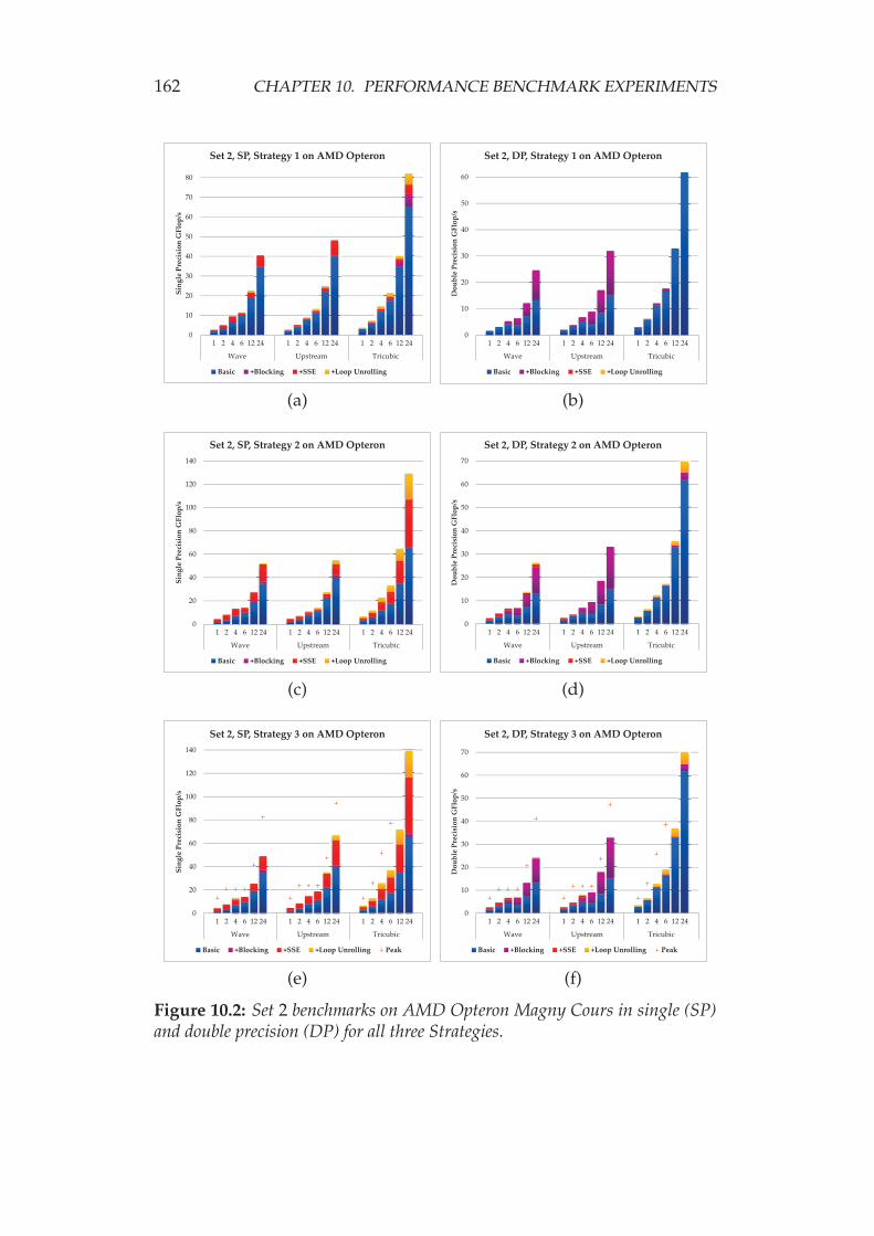
162 CHAPTER 10. PERFORMANCE BENCHMARK EXPERIMENTS
0
10
20
30
40
50
60
70
80
1 2 4 6 12 24 1 2 4 6 12 24 1 2 4 6 12 24
Wave Upstream Tricubic
Sing
le P
reci
sion
GFl
op/s
Set 2, SP, Strategy 1 on AMD Opteron
Basic +Blocking +SSE +Loop Unrolling
0
10
20
30
40
50
60
1 2 4 6 12 24 1 2 4 6 12 24 1 2 4 6 12 24
Wave Upstream Tricubic
Dou
ble
Prec
isio
n G
Flop
/s
Set 2, DP, Strategy 1 on AMD Opteron
Basic +Blocking +SSE +Loop Unrolling
(a) (b)
0
20
40
60
80
100
120
140
1 2 4 6 12 24 1 2 4 6 12 24 1 2 4 6 12 24
Wave Upstream Tricubic
Sing
le P
reci
sion
GFl
op/s
Set 2, SP, Strategy 2 on AMD Opteron
Basic +Blocking +SSE +Loop Unrolling
0
10
20
30
40
50
60
70
1 2 4 6 12 24 1 2 4 6 12 24 1 2 4 6 12 24
Wave Upstream Tricubic
Dou
ble
Prec
isio
n G
Flop
/s
Set 2, DP, Strategy 2 on AMD Opteron
Basic +Blocking +SSE +Loop Unrolling
(c) (d)
0
20
40
60
80
100
120
140
1 2 4 6 12 24 1 2 4 6 12 24 1 2 4 6 12 24
Wave Upstream Tricubic
Sing
le P
reci
sion
GFl
op/s
Set 2, SP, Strategy 3 on AMD Opteron
Basic +Blocking +SSE +Loop Unrolling Peak
0
10
20
30
40
50
60
70
1 2 4 6 12 24 1 2 4 6 12 24 1 2 4 6 12 24
Wave Upstream Tricubic
Dou
ble
Prec
isio
n G
Flop
/s
Set 2, DP, Strategy 3 on AMD Opteron
Basic +Blocking +SSE +Loop Unrolling Peak
(e) (f)
Figure 10.2: Set 2 benchmarks on AMD Opteron Magny Cours in single (SP)and double precision (DP) for all three Strategies.

10.1. PERFORMANCE BENCHMARKS 163
For Set 2, the performance numbers for all of the three Strategies aregiven in Fig. 10.2. The Strategies are varied from top to bottom in thefigure; the sub-figures to the left show single precision results (SP), thesub-figures to the right show double precision results (DP).
Although the basic parallelization delivers the same performance inall Strategies, vectorization and loop unrolling do not have as large aneffect in Strategy 1 as in the other Strategies, resulting in poorer over allperformance of Strategy 1. This is due to the added control overhead; em-ulating Strategy 2 with Strategy 1 using the best parameter configurationshows that the poorer performance is not an artifact of the auto-tuner.
The additional parameter in Strategy 3 gives the stencils in single pre-cision some additional performance boost over the performance achievedwith Strategy 2, while the double precision results are not affected. Thefigures show that the gains in performance in single precision come mostlyfrom explicit vectorization and from loop unrolling (especially in thecompute-bound Tricubic stencil), whereas in the double precision case theexplicit SSE code cannot improve the performance gained by optimallyblocking the Wave and Upstream stencil codes. In the compute-boundcase, only loop unrolling is able to give a performance gain, the effect ofblocking is negligible.
In the best case, the Wave stencil reaches 65% of the peak on one dieand 60% with all 24 threads in both single and double precision. Forthe Upstream stencil, PATUS achieves 65% of the peak in single precisionmode. In double precision the numbers are 80% using one die and 70%when all threads are used. The bandwidth bound Tricubic stencil runs at50% of the peak on one die and at 45% using all 24 threads, both in singleand double precision modes.
Analyzing the cache performance (cf. Table 10.2) shows that for thedouble precision Wave stencil blocking significantly reduces the numberof L2 misses by around 60%, whereas in single precision mode the L2misses are not decreased by much. Indeed, for the 2003 problem used inthe benchmarks one plane of data as used in the basic parallelization, has40, 000 grid points. In single precision, three such planes, each havinga data volume of 160 KB, fit into the Opteron’s 512 KB L2 cache, but indouble precision only one plane (320 KB) fits.
The GNU C compiler auto-vectorizes the code, but using explicit SSEintrinsics and forcing aligned loads removes slow non-aligned moves. InSSE, single precision vectors contain 4 data elements, and double preci-sion vectors contain 2. Thus, higher order stencils with more than the

164 CHAPTER 10. PERFORMANCE BENCHMARK EXPERIMENTS
Wave, 2003 L1 Cache L2 CacheAccesses�106 Misses�106 Accesses�106 Misses�106
SPBasic 615 0.74 18.7 0.74Blocked 624 1.95 21.1 0.51Vectorized 191 1.52 19.1 0.51
DPBasic 758 5.13 36.6 5.08Blocked 627 6.99 38.1 1.94Vectorized 365 4.78 38.5 1.82
Table 10.2: Numbers (in millions) of L1 and L2 cache accesses and misses forthe single (SP) and double precision (DP) 2003 Wave problem.
immediate neighbors in the unit stride direction (such as the stencils inSet 2) have higher data reuse in the single precision case (less loads are re-quired, as neighboring values are brought into the registers automaticallywhen loading a SIMD vector). Indeed, the cache analysis shows, that thenumber of L1 accesses is halved in the double precision case when turn-ing on explicit vectorization, and divided by 4 in single precision.
10.1.2 Intel Xeon Nehalem Beckton
For the experiments on the Intel Xeon platform, the benchmark executa-bles were compiled with Intel C compiler icc 11.1, again using the -O3
optimization flag. Thus, we could take advantage of Intel’s OpenMP im-plementation, which allegedly has less overhead than GNU’s. Also, itallows us to control thread affinity by setting the KMP AFFINITY environ-ment variable. We chose the compact scheme, which fills up cores first(the CPU is uses the Hyper-Threading Technology, thus each core accom-modates 2 hardware threads), and then sockets. The reverse case, i.e., fill-ing up sockets first, and then cores, which is implemented by the scatter
scheme, might be the obvious choice for bandwidth-limited compute ker-nels; however, as we want to run the benchmarks with up to 24 threads,using all available hardware resources. The choice does not really mat-ter as long as we are aware of the fact that at some point (which is whenmoving from 1 to 2 threads in the compact scheme (cf. Fig. 10.3) and whenmoving from 12 to 24 threads in the scatter scheme) the bandwidth doesnot scale, thus limiting the performance.
Again, both sets of stencils were auto-tuned and benchmarked in bothprecision modes, but we omitted the Strategies 1 and 2, which performedmore poorly. The results are shown in Fig. 10.3.

10.1. PERFORMANCE BENCHMARKS 165
On the Intel platform, explicit vectorization (and also loop unrolling)is much more pronounced than on AMD, whereas blocking has an al-most negligible effect. The reason why vectorization has such a largeeffect on the Intel platform is that the Intel C compiler does not vectorizethis particular code using the -O3 optimization option. It does, however,vectorize when compiling with -fast, but in our tests the performancegain were not substantial. Therefore, explicit SSE intrinsics and forcingdata alignment leverage the full power of the Streaming SIMD Exten-sions. The effect can be seen in all the benchmarks except for the doubleprecision Gradient and Divergence stencil, for which already the basic par-allelization gives the maximum yield.
10.1.3 NVIDIA Fermi GPU (Tesla C2050)
As a proof of concept, GPU results are also included here. While CUDAprogramming can be learned relatively easily, experience shows that op-timizing CUDA C code is non-trivial and a hardware-specific codingstyle (e.g., making use of shared memory and registers, adhering to dataalignment rules, etc.) is absolutely essential for well performing GPUcodes. Thus, these results are to be treated as a first step towards GPUsupport in PATUS.
The results shown in Fig. 10.4 are again the stencils from Sets 1 (upperrow) and 2 (lower row) in single (to the left) and double precision (to theright). We used only one Strategy: the one shown in Listing 10.4.
Listing 10.4: Strategy used on the GPU.
1: strategy gpu ( domain u , auto int cbx ) {2: // iterate over time steps
3: for t = 1 . . stencil . t_max {4: // iterate over subdomain
5: for subdomain v ( cbx , 1 . . . ) in u ( : ; t ) parallel
6: for point pt in v ( : ; t )7: v [ pt ; t+1] = stencil ( v [ pt ; t ] ) ;8: }9: }
It has only one parallelism level, which then is assigned to the lowestlevel in the hierarchy, i.e., to threads. Each thread receives a small subdo-main of size �cbx, 1, 1� to process, cbx being a parameter to be determined

166 CHAPTER 10. PERFORMANCE BENCHMARK EXPERIMENTS
0
5
10
15
20
25
30
1 2 4 6 12 24 1 2 4 6 12 24 1 2 4 6 12 24
Gradient Divergence Laplacian
Sing
le P
reci
sion
GFl
op/s
Set 1, SP, Streategy 3 on Intel Xeon
Basic +Blocking +SSE +Loop Unrolling
0
2
4
6
8
10
12
14
16
1 2 4 6 12 24 1 2 4 6 12 24 1 2 4 6 12 24
Gradient Divergence Laplacian
Dou
ble
Prec
isio
n G
Flop
/s
Set 1, DP, Streategy 3 on Intel Xeon
Basic +Blocking +SSE +Loop Unrolling
(a) (b)
0
20
40
60
80
100
120
1 2 4 6 12 24 1 2 4 6 12 24 1 2 4 6 12 24
Wave Upstream Tricubic
Sing
le P
reci
sion
GFl
op/s
Set 2, SP, Strategy 3 on Intel Xeon
Basic +Blocking +SSE +Loop Unrolling
0
10
20
30
40
50
60
1 2 4 6 12 24 1 2 4 6 12 24 1 2 4 6 12 24
Wave Upstream Tricubic
Dou
ble
Prec
isio
n G
Flop
/s
Set 2, DP, Streategy 3 on Intel Xeon
Basic +Blocking +SSE +Loop Unrolling
(c) (d)
Figure 10.3: Set 1 and 2 benchmarks on Intel Xeon Nehalem in single (SP) anddouble precision (DP) for Strategy 3.
by the auto-tuner, in addition to the thread block size, which is implicitin this Strategy.
We use the Strategy in three different indexing modes, though, to de-termine which of the three yields the best performance result. The index-ing modes are plotted as juxtaposed bars in Fig. 10.4. The 1, 1 indexingmode maps the 3D domain onto a one-dimensional thread block and one-dimensional thread index, thus ignoring the fact that thread and threadblock indices can have a higher dimensionality. The 2, 3 indexing modeuses a 2D grid and 3D thread blocks, which were the highest supportedindexing dimensionalities in pre-Fermi cards and CUDA SDKs beforeversion 4.0. 2, 3 -indexing means that the third problem dimension is

10.1. PERFORMANCE BENCHMARKS 167
0
5
10
15
20
25
30
35
(1,1) (2,3) (3,3) (1,1) (2,3) (3,3) (1,1) (2,3) (3,3)
Gradient Divergence Laplacian
Sing
le P
reci
sion
GFl
op/s
Set 1, SP on NVIDIA Fermi GPU
Default +Blocking +Loop Unrolling
0
5
10
15
20
(1,1) (2,3) (3,3) (1,1) (2,3) (3,3) (1,1) (2,3) (3,3)
Gradient Divergence Laplacian
Dou
ble
Prec
isio
n G
Flop
/s
Set 1, DP on NVIDIA Fermi GPU
Default +Blocking +Loop Unrolling
(a) (b)
0
20
40
60
80
100
120
140
160
180
200
(1,1)(2,3)(3,3) (1,1)(2,3)(3,3) (1,1)(2,3)(3,3)
Wave Upstream Tricubic
Sing
le P
reci
sion
GFl
op/s
Set 2, SP on NVIDIA Fermi GPU
Default +Blocking +Loop Unrolling
0
20
40
60
80
100
120
(1,1)(2,3)(3,3) (1,1)(2,3)(3,3) (1,1)(2,3)(3,3)
Wave Upstream Tricubic
Dou
ble
Prec
isio
n G
Flop
/s
Set 2, DP on NVIDIA Fermi GPU
Default +Blocking +Loop Unrolling
(c) (d)
Figure 10.4: Set 1 and 2 benchmarks on NVIDIA Fermi in single (SP) anddouble precision (DP) for one GPU strategy in different indexing modes.
emulated by the second grid dimension, cf. Chapter 13.2. Therefore theindex calculations are more complicated than in 3, 3 -indexing mode.
The blue bars show the performance of an arbitrarily chosen defaultthread block sizes of 16 4 4 and 200 1 1 for 1, 1 -indexing, re-spectively — sizes which exhibited reasonable performance, — settingcbx to 1. On top of that, the purple bars show the performance afterselecting the best thread block size, and the red bars after choosing thebest loop unrolling factor. Loop unrolling included both picking the bestvalue for cbx and picking the best configuration of unrolling the loop inthe unit stride dimension (which obviously is only possible if cbx 1).Generally speaking, the charts show that the performance are about on

168 CHAPTER 10. PERFORMANCE BENCHMARK EXPERIMENTS
par for all indexing modes, in most cases, native �3, 3�-indexing performsslightly better than the other modes, as the index calculations are doneby the hardware to the largest extent. An exception is the double pre-cision Tricubic stencil, for which two-fold unrolling in �2, 3�-indexing infact triples the performance.
There is still room for optimization of the generated code; PATUS cur-rently reaches between 40% and 60% of the peak for the stencils in Set 1 insingle precision and between 50% and 70% in double precision. The rel-ative performance of higher-arithmetic intensity kernels in Set 2 is moredisappointing, as only 23%–30% of the maximum is reached.
10.2 Impact of Internal Optimizations
10.2.1 Loop Unrolling
We examine various loop unrolling configurations for the basic paral-lelization scheme and the blocking configuration that was found to givethe best performance. The benchmarks for this experiment were run onthe AMD Opteron platform using 24 threads. We chose two stencils, thedouble precision Laplacian and the single precision Tricubic; the first didnot seem to profit from loop unrolling (cf. Fig. 10.1) whereas the seconddid (cf. Fig. 10.2). We want to evaluate by what amount the performancedegrades or improves, and how the performances are distributed.
Figs. 10.5 and 10.6 show heat map plots for the Laplacian and the Tricu-bic, respectively. The loop unrolling factors are varied among the x-, y-,and z-axes as powers of 2. The 4 plots in the upper row show the perfor-mance numbers in the basic parallelization scheme, the lower rows thenumbers after the best block sizes were picked.
As expected, small loop unrolling numbers yield the best performancefor the Laplacian, in both basic and blocked cases. More precisely, anyloop unrolling factor in unit stride direction (along the x-axis) between 1and 8 gives an acceptable performance as long as in y- and z-directionsthe unrolling factors are 1 or 2. This coincides with the deliberation onspatial data locality along the unit stride direction, which is disruptedwhen the stride within the inner loop becomes too large (which is thecase for larger unrolling factors in non-unit stride directions). In bothparallelization schemes, the performance degradation is only to around67% of the maximum for the examined unrolling factors. For the Tricubicstencil, in contrast, the performance degrades down to 20% of the maxi-

10.2. IMPACT OF INTERNAL OPTIMIZATIONS 169
8 8.44 8.94 8.26 8.92 8.13 8.75 8.48 8.73 8.90 9.35 8.95 9.16 9.24 9.57 9.41 9.41
4 11.65 11.61 11.16 10.59 9.61 9.69 9.16 9.18 9.29 9.70 9.46 9.53 10.12 10.00 10.06 9.99
2 12.36 12.39 12.39 12.34 11.86 11.80 11.73 11.49 9.67 10.36 10.07 9.92 9.86 10.62 10.48 10.46
1 12.33 12.27 12.32 12.36 11.80 11.78 11.80 11.85 12.04 11.73 11.61 10.39 10.54 9.55 9.97 10.24y x 1 2 4 8 1 2 4 8 1 2 4 8 1 2 4 8
z � 1 z � 2 z � 4 z � 8
8 11.54 11.79 11.37 12.44 11.09 11.68 11.17 12.05 10.77 11.00 10.65 10.66 10.26 10.29 10.19 10.94
4 14.28 14.12 13.74 12.48 11.58 11.07 10.50 10.54 10.06 10.36 10.12 10.43 11.19 11.20 11.07 11.12
2 14.91 14.83 14.83 14.79 14.65 14.59 14.46 14.16 10.55 11.03 11.01 10.88 11.29 12.07 11.96 12.52
1 14.78 14.77 14.73 14.75 14.63 14.62 14.70 14.63 13.83 13.28 13.19 11.72 12.11 11.10 11.58 12.30y x 1 2 4 8 1 2 4 8 1 2 4 8 1 2 4 8
z � 1 z � 2 z � 4 z � 8
Figure 10.5: Impact of varying loop unrolling factors on a fixed blocking size.Double precision Laplacian stencil. Basic parallelization in the upper row, andbest block sizes in the lower row.
8 107.5298.47 61.57 61.50 107.5068.04 64.56 46.12 68.72 62.06 55.85 31.97 64.07 51.68 32.19 32.02
4 104.33106.1294.97 59.50 108.53103.8166.05 63.80 112.4569.21 67.92 62.60 69.61 63.78 54.98 32.20
2 117.02114.54107.6194.09 114.94109.4199.63 64.22 116.52106.0567.68 67.03 114.9168.88 68.64 66.46
1 113.59107.16105.2699.68 133.96127.38120.71104.96 109.76109.7199.61 63.61 109.40106.4765.12 65.21y x 1 2 4 8 1 2 4 8 1 2 4 8 1 2 4 8
z � 1 z � 2 z � 4 z � 8
8 108.5994.98 62.16 58.84 109.2866.93 65.94 51.09 66.28 56.83 43.72 26.71 60.53 49.48 30.57 26.92
4 109.95106.7286.63 58.23 112.80102.0264.60 61.60 110.9367.23 65.58 57.00 67.93 60.06 44.87 27.94
2 116.87113.01101.7477.43 122.26111.7190.58 59.45 114.79100.0764.06 61.28 109.7166.62 66.00 58.97
1 106.7198.83 96.65 86.47 128.16119.63109.5882.18 111.42108.1687.56 58.42 104.3197.48 62.33 59.52y x 1 2 4 8 1 2 4 8 1 2 4 8 1 2 4 8
z � 1 z � 2 z � 4 z � 8
Figure 10.6: Impact of varying loop unrolling factors on a fixed blocking size.Single precision Tricubic stencil. Basic parallelization in the upper row, andbest block sizes in the lower row.

170 CHAPTER 10. PERFORMANCE BENCHMARK EXPERIMENTS
0%
20%
40%
60%
80%
100%
120%
0
10
20
30
40
50
60
50 100 150 200 256 400 50 100 150 200 256 400
Laplaican (DP) Wave (SP)
GFl
op/s
Problem Size Dependence of Configurations
AMD Opteron Magny Cours
Optimal configuration Foreign configuration (of size=200) % of perf. with opt. config.
Figure 10.7: Performance impact of using the optimal configuration for oneproblem size for other problem sizes.
mum performance, i.e., loop unrolling has an a lot larger impact on per-formance. The best performance numbers are achieved for an unrollingfactor of 2 in z-direction. As the unrolling factor in z-direction becomeslarger, the performance decreases rapidly due to the increased registerpressure.
10.3 Impact of Foreign Configurations
After tuning Strategy and code generation characteristics (e.g., block sizes,loop unrolling factors), the resulting configuration works best if in theproduction run the settings are exactly replicated, in particular, if theproblem size is not modified, the number of threads used remains un-changed, and the program is run on the same hardware platform. In thissection, we evaluate the consequences when one of the characteristics ischanged.
10.3.1 Problem Size Dependence
Fig. 10.7 shows the impact on performance when the problem size is var-ied for an unchanged parameter configuration obtained for a 2003 prob-lem. We call this the default configuration. We study two stencils, the dou-ble precision Laplacian and the single precision Wave kernel. The bench-

10.3. IMPACT OF FOREIGN CONFIGURATIONS 171
marks are run on the AMD Opteron with 24 threads. The blue bars showthe maximum performance obtained by applying the appropriate param-eter configuration; the overlaid red bars show the performance numbersobtained when using the default configuration. The yellow line showsthe percentage of the performance that was achieved with the defaultconfiguration; the percentages are given on the right vertical axis. Bothstencils exhibit a significantly above-average maximum performance forthe 1003 problem: evidently a sweet spot on the given architecture; theline lengths in unit stride direction are long enough to engage the hard-ware prefetcher, and the problem is still small enough so that the requiredplanes — after subdividing among the 24 threads — fit into cache so thattemporal data locality could be fully exploited.
Due to the nature of the chosen Strategy, the performance is abysmalfor problem sizes smaller than nominal size: block sizes that are wellsuited to the original problem size most likely are too large for the smallerproblem sizes, and a set of threads is underutilized. The performance isacceptable for problem sizes larger than the nominal one, in particular ifthe larger problem size is divisible by the original one.
To deal with multiple problem sizes successfully, all the problem sizescould be benchmarked for each of the configurations picked by the searchmethod in the auto-tuning process — provided that the set of admissibleproblem sizes is limited and the probability distribution over the problemsizes is known — and the objective function to maximize would be mod-ified to be the weighted sum of the performance numbers, with weightscorresponding to the probability distribution.
10.3.2 Dependence on Number of Threads
On a fixed architecture, we could alter the number of threads used forthe computation. The performance behavior for constant block sizes andvarying numbers of threads is shown in Fig. 10.8 for the double precisionLaplacian (a) and the single precision Wave (b) for a 2003 problem run onthe AMD Opteron.
On the horizontal axis in the sub-figures in Fig. 10.8, the configura-tions are varied (i.e., the caption “1” identifies the configuration obtainedfor one thread, etc.), and on the vertical axis the number of threads usedto execute the benchmark program is varied. Thus, the original and high-est numbers occur on the diagonals. (Interestingly, there is one deviation:according to Fig. 10.8 (b), the Wave stencil ran faster with two threads us-

172 CHAPTER 10. PERFORMANCE BENCHMARK EXPERIMENTS
Thread configuration1 2 4 6 12 24
#T
hrea
dsus
ed 1 1.80 1.75 1.71 1.54 1.56 1.69
2 2.79 2.80 2.75 2.45 2.54 2.70
4 3.63 2.80 3.87 3.37 3.72 3.81
6 3.72 2.85 3.97 4.14 3.97 3.90
12 4.81 3.02 7.66 6.55 7.69 7.63
24 4.81 3.09 14.71 12.74 13.03 14.72
Thread configuration1 2 4 6 12 24
#T
hrea
dsus
ed 1 4.37 4.16 4.27 4.32 4.24 4.26
2 4.37 7.56 8.04 7.87 7.41 7.06
4 4.23 11.09 13.00 11.12 11.84 11.21
6 4.23 12.80 12.54 13.94 13.22 12.35
12 4.23 21.31 14.16 17.67 25.11 24.67
24 4.21 31.08 13.96 17.37 46.47 48.55
(a) (b)
Figure 10.8: Varying the number of threads for a fixed configuration. Doubleprecision Laplacian stencil (a) and single precision Wave stencil (b).
ing the 4-thread configuration than with the native configuration. This isan auto-tuner artifact.) Ideally, the numbers in a horizontal row wouldremain constant. We can observe the tendency that the configurations tothe right of a diagonal element are larger than the ones to the left. Thisis again due to the nature of the Strategy, which guides the auto-tunerto pick larger block sizes for lower concurrencies. The lacking granular-ity, when switching to a number of threads larger than the nominal onemight cause additional threads to remain idle. In the Laplacian stencil theeffect is particularly pronounced when more than two threads run thetwo-thread configuration, and in the Wave stencil when more than onethread run the one-thread configuration.
On average, 91% (one thread) down to 66% (24 threads) of the perfor-mance of the best configuration is reached in the double precision Lapla-cian, and 97% (one thread) down to 47% (24 threads) in case of the singleprecision Wave stencil.
10.3.3 Hardware Architecture Dependence
Finally, also the hardware platform can be exchanged. We ran all thebenchmarks with exchanged configuration sets, i.e., the Intel configura-tions were applied to benchmarks run on the AMD platform and viceversa. The architectures are quite similar. The major difference is the sizeof the L2 cache, which is 512 KB on the Opteron cores, and only 256 KBon the Nehalem cores, which, in addition, accommodate two hardwarethreads each. Thus, we expect that the Intel configurations run reason-ably well on the AMD processor, but Magny Cours configurations mightdegrade the performance on the Intel CPU.

10.3. IMPACT OF FOREIGN CONFIGURATIONS 173
40%50%60%70%80%90%100%
051015202530
1 2 4 6 12 24 1 2 4 6 12 24 1 2 4 6 12 24
Gradient Divergence Laplacian
SP G
Flop
/s
Set 1, SP, Intel-conf on AMD Opteron
Native (AMD) Foreign (Intel) % of perf. w/ opt. config.
30%
50%
70%
90%
110%
0
5
10
15
20
1 2 4 6 12 24 1 2 4 6 12 24 1 2 4 6 12 24
Gradient Divergence Laplacian
DP
GFl
op/s
Set 1, DP, Intel-conf on AMD Opteron
Native (AMD) Foreign (Intel) % of perf. w/ opt. config.
(a) (b)
30%40%50%60%70%80%90%100%
020406080100120140
1 2 4 6 12 24 1 2 4 6 12 24 1 2 4 6 12 24
Wave Upstream Tricubic
SP G
Flop
/s
Set 2, SP, Intel-conf on AMD Opteron
Native (AMD) Foreign (Intel) % of perf. w/ opt. config.
30%40%50%60%70%80%90%100%
010203040506070
1 2 4 6 12 24 1 2 4 6 12 24 1 2 4 6 12 24
Wave Upstream Tricubic
DP
GFl
op/s
Set 2, DP, Intel-conf on AMD Opteron
Native (AMD) Foreign (Intel) % of perf. w/ opt. config.
(c) (d)
-20%0%20%40%60%80%100%120%
05101520253035
1 2 4 6 12 24 1 2 4 6 12 24 1 2 4 6 12 24
Gradient Divergence Laplacian
SP G
Flop
/s
Set 1, SP, AMD-conf on Intel Xeon
Native (Intel) Foreign (AMD) % of perf. w/ opt. config.
20%
40%
60%
80%
100%
0
5
10
15
20
1 2 4 6 12 24 1 2 4 6 12 24 1 2 4 6 12 24
Gradient Divergence Laplacian
DP
GFl
op/s
Set 1, DP, AMD-conf on Intel Xeon
Native (Intel) Foreign (AMD) % of perf. w/ opt. config.
(e) (f)
0%20%40%60%80%100%120%
020406080100120
1 2 4 6 12 24 1 2 4 6 12 24 1 2 4 6 12 24
Wave Upstream Tricubic
SP G
Flop
/s
Set 2, SP, AMD-conf on Intel Xeon
Native (Intel) Foreign (AMD) % of perf. w/ opt. config.
0%20%40%60%80%100%120%
010203040506070
1 2 4 6 12 24 1 2 4 6 12 24 1 2 4 6 12 24
Wave Upstream Tricubic
DP
GFl
op/s
Set 2, DP, AMD-conf on Intel Xeon
Native (Intel) Foreign (AMD) % of perf. w/ opt. config.
(g) (h)
Figure 10.9: Using optimal configurations on foreign hardware platforms.

174 CHAPTER 10. PERFORMANCE BENCHMARK EXPERIMENTS
Indeed, Fig. 10.9 shows acceptable performance matches of Intel con-figurations on the AMD Opteron in sub-figures (a)–(d). The matches ofthe AMD configurations on the Intel CPU in sub-figures (e)–(h) exhibitlarger deviations.
The blue bars are the native performances in GFlop/s, the overlaidred bars the foreign ones. The yellow lines visualize the relative perfor-mance with respect to the native one; the percentages are shown on theright vertical axis.
Generally, the performance numbers on the Magny Cours are no lessthan 60% of the maximum numbers when using the foreign configura-tions, 80% on average, in both double and single precision modes and forboth sets of stencils. In contrast, on the Intel platform the performancedrops down to almost 20% of the original performance in certain cases;on average 75% of the original performance is reached. Again, the av-erage does not change when switching precision modes or stencil sets.However, we can also observe that the AMD configurations give almostperfect results on Intel in certain cases, e.g., in case of single precision Gra-dient or Upstream stencils, or the double precision Tricubic stencil, wherealmost 100% of the original performance is brought back for 6, 12, and 24threads.

Chapter 11
Applications
Without, however, stepping into the regionof conjecture, we will mention a particularproblem which occurs to us at this momentas being an apt illustration of the use towhich such an engine may be turned fordetermining that which human brains find itdifficult or impossible to work outunerringly.
— Ada Lovelace (1815–1852)
11.1 Hyperthermia Cancer Treatment Planning
Hyperthermia cancer treatment, i.e., application of moderate heat to thebody, is a promising modality in oncology that is used for a wide varietyof cancer types (including pelvic, breast, cervical, uterine, bladder, andrectal cancers, as well as melanoma and lymphoma). Both animal andclinical studies have proven that hyperthermia intensifies both radio- andchemo-therapies by factors of 1.2 up to 10, depending on heating qual-ity, treatment modality combination, and type of cancer [57, 164, 186].Hyperthermia is therefore applied in conjunction with both radio- andchemo-therapies.

176 CHAPTER 11. APPLICATIONS
An effect of hyperthermia treatment is apoptosis of tumor cells, whichhave a chaotic vascular structure resulting in poorly perfused regions inwhich cells are very sensitive to heat. Hyperthermia further makes thetumor cells more susceptible to both radiation and certain cancer drugs.There are a variety of reasons for this. Among others, heat naturally in-creases blood flow and therefore increases drug delivery to the tumorcells, and also increases the toxicity of some drugs. The effect of radia-tion is amplified as a result of improved oxygenation due to increases inblood flow. In our setting, we are dealing with local hyperthermia wherethe aim is to focus the energy noninvasively only at the tumor location.This is done by creating a constructive interference at the tumor locationusing nonionizing electromagnetic radiation (microwaves) and therebyaiming at heating the tumor to 42� 43�C, but even lower temperaturescan be beneficial.
Figure 11.1: Head and neck hyperthermia applicator HYPERcollar developedat the Hyperthermia Group of Erasmus MC (Daniel den Hoed Cancer Center),Rotterdam, the Netherlands.
Cylindrical applicators, such as one shown in Fig. 11.1, which showsthe HYPERcollar applicator developed for head and neck hyperthermiatreatment at the Hyperthermia Group of Erasmus MC (Daniel den HoedCancer Center) in Rotterdam, the Netherlands [132, 133], feature a num-

11.1. HYPERTHERMIA CANCER TREATMENT PLANNING 177
ber of dipole antennae arranged on the circumference of the applicator,whose amplitudes and phase shifts can be controlled to create the de-sired electric field inducing heat. Here the aim is to avoiding cold spotswithin the tumor and hotspots in healthy tissue to maximize tumor heat-ing and limit pain and tissue damage. The water bolus between the pa-tient’s skin and the applicator prevents heating of the skin and more im-portantly, from an engineering point of view, it is an efficient transfermedium for the electromagnetic waves into the tissue: it reduced reflec-tions and allows for smaller antenna sizes. In treatment planning, it istherefore highly relevant to determine the therapeutically optimal an-tenna settings, given the patient geometry. This leads to a large-scalenonlinear, nonconvex PDE-constrained optimization problem, the PDEbeing the thermal model shown in Eqn. 11.1, which is known as Pennes’sbioheat equation [134], or a variant thereof. Another important aspect oftreatment planning is simulating the temperature distribution within thehuman body given the antenna parameters, which has been successfullydemonstrated to accurately predict phenomena occurring during treat-ment [150, 119]. Simulations are helpful in order to determine the cor-rect doses and help to overcome the difficulty of temperature monitoringduring treatment. Other benefits include assistance in developing newapplicators and training staff.
In this chapter, we focus on the simulation only. The thermal modelis given by the parabolic partial differential equation
ρCp�u�t
� ∇ � �k ∇u� � ρbW�u�Cb�u � Tb� � ρQ � σ2‖E‖2, (11.1)
which is the simplest thermal model. On the boundary we impose Dirich-let boundary conditions to model constant skin temperature, Neumannboundary conditions, which account for constant heat flux through theskin surface, or convective boundary conditions [120]. In Eqn. 11.1, uis the temperature field, for which the equation is solved, ρ is density,Cp is the specific heat capacity, k is thermal conductivity, W�u� is thetemperature-dependent blood perfusion rate, Tb is the arterial blood tem-perature (the subscript “b” indicates blood properties), Q is a metabolicheat source, σ is electric conductivity, and E is the electric field gener-ated by the antenna. The electric field has to be calculated (by solvingMaxwell’s equations) before computing the thermal distribution. Moreelaborate models include, e.g., temperature-dependent material parame-

178 CHAPTER 11. APPLICATIONS
Figure 11.2: Model of a boy and the HYPERcollar applicator. The left imageshows the model and FD discretization, the right images show simulation re-sults. Lighter colors correspond to higher temperatures.
ters or tensorial heat conductivity to account for the directivity of bloodflow [169].
We use a finite volume method for discretizing Eqn. 11.1. The bloodperfusion is modeled as a piecewise linear function of the temperature.As a discretized version of Eqn. 11.1 we obtain the stencil expression
u n 1i,j,k u n
i,j,k ai,j,ku ni,j,k bi,j,k ci,j,k (11.2)
di,j,ku ni 1,j,k ei,j,ku n
i 1,j,k
fi,j,ku ni,j 1,k gi,j,ku n
i,j 1,k
hi,j,ku ni,j,k 1 li,j,ku n
i,j,k 1.
Note that the coefficients a, . . . , l depend on their location in space. ThePDE in Eqn. 11.1 is solved with a simple explicit Euler time integrationscheme. Each evaluation of the stencil expression amounts to 16 floatingpoint operations.
11.1.1 Benchmark Results
Performance results for the hyperthermia stencil from Eqn. 11.2 on theAMD Opteron Magny Cours and on the NVIDIA C2050 Fermi GPU areshown in Fig. 11.3. The performance numbers and scalings are given

11.1. HYPERTHERMIA CANCER TREATMENT PLANNING 179
0
5
10
15
20
1 2 4 6 12 24 1 2 4 6 12 24
Double precision Single precision
GFl
op/s
Hyperthermia Stencil AMD Opteron “Magny Cours”
Naive +Blocking +SSE +Loop Unrolling Peak
0
5
10
15
20
25
30
(1,1) (2,3) (3,3) (1,1) (2,3) (3,3)
Double precision Single precision
GFl
op/s
Hyperthermia Stencil NVIDIA Tesla C2050
Default +Blocking +Loop Unrolling Peak
Figure 11.3: Performance results for the Hyperthermia stencil on the AMDOpteron Magny Cours and on the NVIDIA Fermi GPU.
for both double (left half of the graphs) and single (right half) precisiondata types, as the data type can be changed in the solver’s user interface.Usually, single precision is sufficient in practice. The performance resultswere obtained for a problem domain of 2003 grid points.
The orange bars mark the maximum reachable performance for thestencil’s arithmetic performance (0.16 Flop/Byte for double precision and0.33 Flop/Byte for single precision — or 1.33 Flops per transferred dataelement, accounting for write allocate traffic). The graphs show that inboth cases (single and double precision) on the AMD Opteron around85% of the optimal performance was reached when using all availableNUMA domains. Using only one NUMA domain (one to six threads inthe figure), around 90% of the maximum performance is reached. Notethat using more than 4 threads on one NUMA domain does not increaseperformance. The two remaining threads could be used to stream datainto the caches and thereby to potentially increase the performance byperfectly overlapping computation and communication.
For double precision, blocking gives a moderate performance increaseof 16% over the base line with 24 threads. In the single precision case,vectorization and blocking help to increase the performance by around40%. This suggests that padding the grids correctly so that no unalignedvector loads have to be carried out yields a major performance gain.
Similarly, on the GPU around 80% of the attainable performance wasreached. Interestingly, switching indexing modes did not change the per-formance. The default thread block sizes (200 in the 1D indexing case

180 CHAPTER 11. APPLICATIONS
and 16� 4� 4 in the other cases) gave no relevant performance increase,meaning that the default choice was already a good choice for the threadblock size. Indeed, for both indexing modes, the auto-tuner changedthe default configuration only slightly to 16� 2� 6 (and alternatively to72� 2� 2, which performed equally well). In the single precision case,however, the thread block size was increased to 40–50 for both indexingmodes, so that in both single and double precision modes about the equalamount of contiguous memory was accessed. Making explicit use of theGPU’s shared memory might increase the performance further.
11.2 Anelastic Wave Propagation
The Anelastic Wave Propagation code AWP-ODC of the Southern Cali-fornia Earthquake Center (SCEC), which was developed by Olsen, Day,Cui, and Dalguer [49] is a scientific modeling code for simulating bothdynamic rupture and earthquake wave propagation. It has been used toconduct numerous significant simulations at the SCEC. It provides thecapability of simulating the largest earthquakes expected around the SanAndreas Fault in southern California at high shaking frequencies (up to2 Hz in the simulation described below), which allow scientists to under-stand seismic risks, and thereby help mitigate life and property losses,and let scientists gain new insight about ground motion levels to be ex-pected for a great earthquake along the fault.
The largest simulations done was a simulation of a magnitude-8 earth-quake rupturing the entire San Andreas Fault from central California tothe Mexican border, a fault length of 545 km. The result is shown in Fig.11.4. A full description and discussion of the simulation can be foundin [49]. The simulation required a discretization of a 810� 405� 85 km3
volume with a 40 m-resolution mesh, resulting in 4.4 � 1011 voxels. Thesimulation was executed in a 24 hour production run — correspondingto 6 minutes of wave propagation — on around 223, 000 nodes of Jaguar,a Cray XT5 supercomputer, operated at the Oak Ridge National Labo-ratory in Oak Ridge, Tennessee, USA. On Jaguar, the code achieved asustained performance of 220 TFlop/s. Simultaneously with this simu-lation, the code (Fortran, parallelized with MPI) was shown to be highlyscalable.
The model’s governing elastodynamic equations is the following sys-

11.2. ANELASTIC WAVE PROPAGATION 181
Figure 11.4: Peak ground velocities derived from a magnitude-8 earthquakesimulation along the southern California San Andreas Fault with seismogramsand peak velocities for selected locations.Image courtesy: Southern California Earthquake Center, Y. Cui, K. B. Olsen,T. H. Jordan, K. Lee, J. Zhou, P. Small, D. Roten, G. Ely, D. K. Panda, A.Chourasia, J. Levensque, S. M. Day, and P. Maechling [49].

182 CHAPTER 11. APPLICATIONS
tem of PDEs [49, 50]:
� �u�t
� ρ�1∇ � σ (11.3)
�σ
�t� λ�∇ � �u�I � μ�∇ �u �∇ �uᵀ�.
The dependent variables are the velocity vector field �u ��
�ux, �uy, �uz�
and
the stress tensor σ �
�σxx σxy σxzσyx σyy σyzσzx σzy σzz
�. λ and μ are the Lame coefficients, ρ is
the density, and I is the identity tensor.The equations are discretized in the finite difference method — ac-
cording to [49] the best trade-off between accuracy (fourth-order dis-cretizations of differential operators in space and second-order discretiza-tions in time are used throughout the code), computational efficiency(stencil codes map well to parallel architectures without large overheadsuch as graph partitioning required for finite element codes), and easeof implementation. The velocity-stress wave equations are solved withan explicit scheme on a staggered grid with equidistant mesh points. Asplit-node approach is used to model dynamic fault ruptures [50]. As ab-sorbing boundary conditions, the code uses perfectly matched layers ordampening within a sponge layer.
11.2.1 Benchmark Results
We selected 4 kernels (corresponding to 4 Fortran routines in the origi-nal code) for the benchmarks, which are the 3D stencil routines in whichmost of the compute time is spent. Table 11.1 shows an overview of thekernels. The corresponding stencil specifications can be found in Ap-pendix C, which are translations to the PATUS stencil specification DSLfrom the original Fortran code. The discretization of Eqns. 11.3 can befound in [50] and [49].
The stencils are all fourth-order discretizations of the spatial differen-tial operators. The kernels listed in Table 11.1 are to be understood asprototypes; e.g., the actual code contains three variants of uxx1 — whichcalculates the velocity field �ux in x-dimension, — namely two more forthe y and z-dimensions, which are almost identical to uxx1. We thereforeexpect a similar performance and scaling behavior for these related ker-nels. Similarly, there are two other variants of xy1. xy1 computes the σxy
component of the stress tensor, the other variants compute σxz and σyz.Note that the stress tensor σ is symmetric. Both xyz1 and xyzq compute

11.2. ANELASTIC WAVE PROPAGATION 183
Name Description Flops/Stencil Arith. Int.uxx1 Velocity in x-dimension 20 0.70 Flop/Bxy1 Stress tensor component σxy 16 0.65 Flop/Bxyz1 Stress tensor components σxx, σyy, σzz 90 1.58 Flop/Bxyzq Stress tensor components σxx, σyy, σzz 129 1.22 Flop/B
in viscous mode
Table 11.1: Summary of the AWP kernels which were used in the performancebenchmarks.
0
5
10
15
20
25
30
35
40
45
1 2 4 6 12 24 1 2 4 6 12 24 1 2 4 6 12 24 1 2 4 6 12 24
uxx1 xy1 xyz1 xyzq
Sing
le P
reci
sion
GFl
op/s
Performance and Scaling of AWP-ODC Kernels AMD Opteron “Magny Cours”
Patus, Basic Cache Blocking +SSE +Loop Unrolling Peak Reference (Fortran)
Figure 11.5: AWP kernel benchmarks on the AMD Opteron Magny Cours.
the remaining components of the stress tensor, σxx, σyy, σzz, all in onekernel.
The performance benchmarks were done only in single precision, sincethe original application only uses that precision mode. Again, the or-ange markers show the maximum attainable performance for the lowerarithmetic intensity kernels. On one die (6 threads) the uxx1 and xy1 ker-nels reach around 80% of the peak and around 70% if all 24 threads areused. The theoretical maximum is quite high for the xyz* kernels, andthe reason why only a fraction (around 40%–50%) of the maximum wasachieved lies in the arithmetic operations: the kernels contain many divi-sions (18 in both cases), which are notorious for incurring pipeline stalls.In this case, many of the divisions could be removed by pre-computingand storing the inverses of the Lame parameters. This manual optimiza-

184 CHAPTER 11. APPLICATIONS
0
10
20
30
40
50
60
70
80
(1,1) (2,3) (3,3) (1,1) (2,3) (3,3) (1,1) (2,3) (3,3) (1,1) (2,3) (3,3)
uxx1 xy1 xyz1 xyzq
Sing
le P
reci
sion
GFl
op/s
Performance of AWP-ODC Kernels
NVIDIA Tesla C2050
Default +Blocking +Loop Unrolling
Figure 11.6: AWP kernel benchmarks on the NVIDIA Tesla C2050 Fermi GPU.
tion was indeed carried out in an optimized version of the AWP-ODCcode.
A possible way for PATUS to remove divisions automatically is to re-write arithmetic expressions by virtue of the equality α
aβb
αb βaab .
This transformation removes one division, but introduces three multi-plications. For similar transformation of larger sums i
αiai
there is alsoa tuning opportunity: finding the right trade-off between the number ofdivisions removed and the number of multiplications added.
The green line shows the performance of the reference Fortran code,which was parallelized by inserting an OpenMP sentinel above the outermost spatial loop. No NUMA optimization was done, which is evidentfrom the scaling behavior of the reference uxx1 and xy1 kernels. Thearithmetic intensities of the xyz* kernels are higher; hence the NUMA ef-fect is mitigated to some extent by the relatively high number of floatingpoint operations, and the performance can increase further when goingto 2 and 4 NUMA domains (12 and 24 threads, respectively).
The blue bars show the performances of auto-tuned blocked codes,including the NUMA optimization, and relying on the compiler (GNUgfortran/gcc 4.5.2 with the -O3 optimization flag, for both the referencecodes and the generated PATUS codes) to do the vectorization. With theNUMA optimization enabled, the performance scales almost linearly upto 24 threads. Fig. 11.5 shows that explicit use of SSE intrinsics and

11.2. ANELASTIC WAVE PROPAGATION 185
padding for optimal vector alignment results in a significant performanceboost, in particular for the xyz1 kernel, where explicit vectorization gavea performance increase of 150%. Activating and tuning for loop unrollinggave another slight gain in performance.
Overall, PATUS achieved speedups between 2.8� and 6.6� when 24threads were used on the AMD Opteron Magny Cours with the NUMAoptimization and a cache blocking Strategy.
The GPU performance results are shown in Fig. 11.6. Again, theresults are for single precision stencils, and the three indexing modeswere used: one-dimensional thread blocks and grids, three-dimensionalthread blocks and a two-dimensional grid, and both three-dimensionalthread blocks and grids, supported as of CUDA 4.0 on Fermi GPUs. Forboth the uxx1 and xy1 kernels, the default thread block size of 16� 4� 4threads was an adequate choice, and tuning the thread block sizes in-creased the performance only slightly. In both cases, the fully 3D index-ing mode outperformed the �2, 3�-dimensional indexing by a tight mar-gin due to the simplified index calculation code. Surprisingly, the fully3D indexing delivered worse performance in the xyz* kernels. Loop un-rolling could compensate for the loss in performance for the “xyz1” ker-nel — the only case in which loop unrolling really showed a significantbenefit. Also in this case we hope to be able to increase the performancein the future by making use of the GPU’s shared memory.


Part IV
Implementation Aspects


Chapter 12
Patus Architecture Overview
The distinctive characteristic of theAnalytical Engine, and that which hasrendered it possible to endow mechanismwith such extensive faculties as bid fair tomake this engine the executive right-hand ofabstract algebra, is the introduction into it ofthe principle which Jacquard devised forregulating, by means of punched cards, themost complicated patterns in the fabricationof brocaded stuffs.
— Ada Lovelace (1815–1852)
PATUS is built from four core components as shown in the high-leveloverview in Fig. 12.1: the parsers for the two input files, the stencil def-inition and the Strategy, the actual code generator, and the auto-tuner.PATUS is written in Java and can be therefore run on any major currentoperating system including Linux, MacOS, and Microsoft Windows. PA-TUS uses Coco/R [116] as generator for the stencil specification and Strat-egy parsers, and also for the parser used to interface with the computeralgebra system Maxima [20], which is used as a powerful expression sim-plifier. The Cetus framework ([157, 11]), a compiler infrastructure forsource-to-source transformations, provides Java classes for the internalrepresentations for both the Strategies and the generated code, i.e., the

190 CHAPTER 12. PATUS ARCHITECTURE OVERVIEW
Figure 12.1: A high-level overview over architecture of the PATUS framework.
Strategy parse tree and the abstract syntax tree of the generated code,and Cetus also provides the mechanism for unparsing the internal repre-sentation of the generated code.
The internal representation of the stencil specification consists of thedomain size and number-of-iterations attributes and a graph represen-tation of the actual stencil parts described in the stencil operation. Thiswill be discussed in detail in section 12.1. The Strategy is transformed toan abstract syntax tree that is used as a template by the code generator.These structures are passed as input to the code generator, along with anadditional configuration describing the characteristics of the hardwareand the programming model used to program the architecture and spec-ifies the code generation back-end to use. The code generator producesC code for variants of the stencil kernel and also creates an initializationroutine that implements a NUMA-aware data initialization based on theparallelization scheme used in the kernel routine.
Along with an implementation for the stencil kernel, the code gen-erator also creates a benchmarking harness from an architecture- andprogramming model-specific template into which the dynamic memoryallocations, the grid initializations, and the kernel invocation are substi-tuted. The benchmarking harness expects the problem-specific parame-ters related to the domain size (specified in the stencil specification), theStrategy-specific auto parameters, as well as internal code generation pa-rameters (currently loop unrolling factors) to be provided to the bench-

12.1. PARSING AND INTERNAL REPRESENTATION 191
marking executable as command line arguments.Currently, the post-code generation compilation and auto-tuning pro-
cesses have yet to be initiated manually; as of yet, the auto-tuner is stilla decoupled part of the system. In consequence, also the feedback loop,returning the set of parameters for which the generated stencil kernelperforms well to the code generator in order to substitute them into theparametrized code, has not been implemented yet. Note that it might noteven be desirable to do so in a fully automated fashion, since the codegenerator and the auto-tuning system (and consequently the benchmark-ing executable) might run on different systems. Also, the auto-tuningsubsystem can be used independently for tuning existing parametrizedcodes not generated by PATUS.
12.1 Parsing and Internal Representation
12.1.1 Data Structures: The Stencil Representation
The stencil specification parser turns a stencil specification into an ob-ject structure for which the class diagram is shown in Fig. 12.2. TheStencilCalculation encapsulates the entire specification including thedomain size and the number of iterations, a list of arguments, which willbe reflected in the function signature of the generated stencil kernel func-tion, and the actual stencil structure represented by the StencilBundle.As an operation in the stencil specification can have not only one, butmultiple stencil expressions that are computed within a single stencil ker-nel, the StencilBundle contains a list of Stencil objects, which are both agraph representation of the geometrical structure of stencil and an arith-metic expression (a Cetus Expression object). The graph structure is rep-resented by sets of StencilNodes, one set of input nodes, i.e., the nodeswhose values are read, and one set of output nodes, the nodes to whichvalues are written in the computation.
Stencil nodes represent a position in the grid relative to the centerpoint, both in space and time. Additionally, they capture which grid isaccessed by accessing a stencil node’s value. In a mathematical notation,let
N :� Zd�Z�N
be the index space consisting of a d-dimensional spatial component, atemporal component and a natural-numbered counting component. Then,

192 CHAPTER 12. PATUS ARCHITECTURE OVERVIEW
Stencil
#m
_edS
tenc
ilCal
cula
tion:
Exp
ress
ionD
ata
#m
_set
AllIn
putN
odes
: Se
t<St
enci
lNod
e>#
m_s
etO
utpu
tNod
es:
Set<
Sten
cilN
ode>
+ad
dInp
utN
ode(
node
: St
enci
lNod
e) :
voi
d+
addO
utpu
tNod
e(no
de:
Sten
cilN
ode)
: v
oid
+ite
rato
r()
: It
erat
or<
Sten
cilN
ode>
+ge
tDim
ensi
onal
ity()
: b
yte
+of
fset
InTi
me(
nTim
eOff
set:
int)
: v
oid
+of
fset
InSp
ace(
rgSp
aceO
ffse
t: in
t[])
: v
oid
+ge
tMin
Spac
eInd
ex()
: in
t[]
+ge
tMax
Spac
eInd
ex()
: in
t[]
+ge
tMin
Spac
eInd
exBy
Tim
eInd
ex(n
Tim
eInd
ex:
int)
: in
t[]
+ge
tMax
Spac
eInd
exBy
Tim
eInd
ex(n
Tim
eInd
ex:
int)
: in
t[]
+is
Tim
eblo
ckin
gApp
licab
le()
: b
oole
an
StencilBundle
-m
_ste
ncilF
used
: St
enci
l-
m_l
istS
tenc
ils:
List
<St
enci
l>
+ad
dSte
ncil(
sten
cil:
Sten
cil) :
voi
d
«int
erfa
ce»
IStencilOperations
+of
fset
InTi
me(
nTim
eOff
set:
int)
: v
oid
+of
fset
InSp
ace(
rgSp
aceO
ffse
t: in
t[])
: v
oid
+ge
tDim
ensi
onal
ity()
: b
yte
+ge
tMin
Spac
eInd
ex()
: in
t[]
+ge
tMax
Spac
eInd
ex()
: in
t[]
+ge
tMin
Spac
eInd
exBy
Tim
eInd
ex(n
Tim
eInd
ex:
int)
: in
t[]
+ge
tMax
Spac
eInd
exBy
Tim
eInd
ex(n
Tim
eInd
ex:
int)
: in
t[]
+is
Tim
eblo
ckin
gApp
licab
le()
: b
oole
an
«int
erfa
ce»
IStencilStructure
+ad
dInp
utN
ode(
node
: St
enci
lNod
e) :
voi
d+
addO
utpu
tNod
e(no
de:
Sten
cilN
ode)
: v
oid
+ite
rato
r()
: It
erat
or<
Sten
cilN
ode>
+ge
tDim
ensi
onal
ity()
: b
yte
StencilNode
-m
_spe
cTyp
e: S
peci
fier
-m
_ind
ex:
Inde
x
+is
Scal
ar()
: b
oole
an Index
-m
_nTi
meI
ndex
: in
t-
m_r
gSpa
ceIn
dex:
int[
]-
m_n
Vect
orIn
dex:
int
+of
fset
InTi
me(
nTim
eOff
set:
int)
: v
oid
+of
fset
InSp
ace(
rgSp
aceO
ffse
t: in
t[])
: v
oid
IdentifierCe
tus
IR c
lass
StencilCalculation
-m
_str
Nam
e: S
trin
g-
m_b
oxD
omai
n: B
ox-
m_e
xprM
axIt
er:
Expr
essi
on-
m_l
istA
rgum
ents
: Li
st<
Strin
g>
+lo
ad(s
trFi
lena
me:
Str
ing,
opt
ions
: Co
deG
ener
atio
nOpt
ions
) :
Sten
cilC
alcu
latio
n
10.
.*
1..*
1
Figu
re12
.2:U
ML
clas
sdi
agra
mof
the
inte
rnal
repr
esen
tatio
nof
the
sten
cils
peci
ficat
ion.

12.1. PARSING AND INTERNAL REPRESENTATION 193
a stencil node is an element of N . Furthermore, let
α : N � Zd,
τ : N � Z,
ι : N � N
be the canonical projections onto the spatial, temporal, and counting com-ponent, respectively. The spatial component defines the spatial locationof the stencil node relative to the center node, the temporal componentspecifies to which temporal instance of the grid, relative to the currenttime step, the stencil node belongs, and the counting component distin-guishes between different grids. For instance, a stencil for the divergenceoperator, which maps a vector field to a function, in a d-dimensional set-ting requires a vector-valued input grid with d components, or, equiva-lently, d input grids, which are numbered by the counting component.
Definition 12.1. A stencil is denoted by a triple �Σi, Σo, Φ�, where Σi, Σo � Nare finite subsets of N ; Σi is the set of input stencil nodes and Σo is the set ofoutput stencil nodes. The mapping
Φ : 2Σi��
�f : R
���2Σi
���� R
�� 2Σo
assigns a real-valued function in the input stencil nodes (the actual stencil ex-pression), and a set of output stencil nodes (the nodes to which the value isassigned after evaluation of the function) to a subset of input stencil nodes.
In the UML class diagram in Fig. 12.2, Φ corresponds to the stencilexpression m edStencilExpression in the Stencil class.
Each Stencil instance in the list of stencils in the StencilBundle repre-sents an object
�Σi�, Σo
�, Φ�
�, � � 1, . . . , k. The fused stencil, m stencilFused,
contained in the StencilBundle is a stencil structure synthesized from allthe stencils within the specification, Σ�
fused :��k
��1 �
� . Reasoning aboutwhich grids are used or transferred is done based on the fused stencil.
The stencil node n with spatial component 0 � Zd, i.e., α�n� � 0 iscalled the center node; it corresponds to a grid access at [x,y,z] in thestencil specification of a 3-dimensional stencil. For each output stencilnode no � Σo we require that the temporal index is larger than max
ni�Σiτ�ni�.
(Note that if this requirement is not fulfilled, the method would not be anexplicit method and would require solving a system of equations.)

194 CHAPTER 12. PATUS ARCHITECTURE OVERVIEW
Internally, the stencil node components are normalized by shifting thespatial and temporal components in Σi and Σo such that the spatial in-dices of the output stencil nodes are 0 � Zd, and the largest temporalcomponent is 0, i.e.,
α�n� � 0 �n � Σo,
maxn�Σo
τ�n� � 0.
The notion of stencil nodes, in conjunction with a Strategy, enablesus to map grids, or parts of grids, to arrays which are stored physicallyin main memory or temporarily in some local memory. In section 13.1we will discuss in detail how this is done. Also, stencil nodes providea mechanism to determine the size of an input subdomain required tocalculate a result subdomain of a certain size. The fused stencil holds theinformation for all the subdomain that need to be kept in (local) memoryat a given point in time.
12.1.2 Strategies
The Coco/R-based Strategy parser creates a traditional parse tree com-posed of Cetus IR objects. To encapsulate the special, PATUS Strategy-specific loop structures, additional IR classes have been added. Specif-ically, RangeIterators represent traditional for loops, and SubdomainIt-
erators represent loops that iterate a smaller subdomain over a parentdomain.
Both RangeIterators and SubdomainIterators extend the class Loop
which encapsulates the common attributes as shown in Fig. 12.3: thenumber of threads, chunk size (i.e., the number of consecutive iteratesassigned to one thread), and the level of parallelism on which the loopwas defined. RangeIterators extend the list of attributes to the loop in-dex variable, start and end expressions and the step by which the indexvariable is incremented in each iteration. A SubdomainIterator has twospecial identifier objects representing the parent domain and the subdo-main being iterated within the parent domain. A SubdomainIdentifier
inherits from the Cetus IR class Identifier and adds specific attributes:spatial and temporal offsets as defined in the Strategy and a list of in-dices through which an array of subdomain identifiers in the Strategy isaccessed. This is not to be confused with a stencil node’s counting index;a Strategy subdomain is a placeholder for all the stencil grids (defined inthe stencil specification) simultaneously.

12.1. PARSING AND INTERNAL REPRESENTATION 195
Loop
# m_exprNumThreads: Expression# m_exprChunkSize: Expression# m_nParallelismLevel: int
CompoundStatement
RangeIterator
# m_idLoopIndex: Identifier# m_exprStart: Expression# m_exprEnd: Expression# m_exprStep: Expression
IdentifierCetus IRClasses
SubdomainIterator
# m_sdidDomain: SubdomainIdentifier# m_sdidIterator: SubdomainIdentifier# m_sdTotalDomain: Subdomain# m_borderDomain: Border
SubdomainIdentifier
- m_subdomain: Subdomain- m_rgSpatialOffset: Expression[]- m_exprTemporalIndex: Expression- m_listVectorIndices: List<Expression>
Subdomain
- m_sdParent: Subdomain- m_size: Size- m_ptRefParent: Point- m_ptRefGlobal: Point- m_bIsBaseGrid: boolean
Parent
Child
Figure 12.3: UML class diagram for Strategy loop IR classes.
For representing the stencil calls and arithmetic expressions, stan-dard Cetus IR class instances are used. The internal representation ofthe Strategy is used as a template by the code generator into which theconcrete stencil computation and the concrete grids are substituted: spe-cial Strategy-specific IR objects are gradually replaced by Cetus IR ob-jects that have a C representation. For instance, Strategy-type loops areconverted to C for loops, and grid-stencil node pairs are converted tolinearly indexed grid arrays.
The Strategy parser exploits the fact that the stencil representation isalready constructed when the Strategy is being parsed. Hence, stencilproperties (e.g., dimensionality, minimum and maximum spatial sten-cil node coordinates) and aspects of the Strategy that depend on sten-cil properties, such as vectors of length d specifying Strategy subdomainsizes, where d is the dimensionality of the stencil, or vector subscriptsdepending on d, are instantiated concretely. For instance, if d is knownto be 3, the Strategy subscript expression (1 ...) becomes (1, 1, 1) atthe time of parsing, or a variable b of type dim becomes (b x, b y, b z).Thus, Strategy subscript expressions are resolved at parse time, and theinternal representation only holds the concrete instantiations.

196 CHAPTER 12. PATUS ARCHITECTURE OVERVIEW
12.2 The Code Generator
The objective of the code generator is to translate the Strategy into whichthe stencil has been substituted, into the final C code. In particular, ittransform Strategy loops into C loops and parallelizes them according tothe specification in the Strategy, and it unrolls and vectorizes the inner-most loop containing the stencil calculation if desired; it determines whicharrays to use based on the Strategy structure and the grids defined in thestencil specification and calculates the indices for the array accesses. Thecode generator classes are contained in the package ch.unibas.cs.hpwc.
patus.codegen.Fig. 12.4 shows the UML class diagram of the code generation pack-
age. CodeGeneratorMain is the main entry point of the PATUS code gen-eration module. The method generateCode parses both the stencil andStrategy files and invokes the actual code generator CodeGenerator. Thegenerate method of the latter first “resolves” the Strategy parallel key-word: by means of the ThreadCodeGenerator an internal representationfor the per-thread code of the kernel function is created based on theinternal representation of the Strategy. The ThreadCodeGenerator classprovides methods for parallelizing range iterators and subdomain itera-tors. The resulting AST is processed by the SingleThreadCodeGenerator,which invokes the specialized sub-code generators:
• The class SubdomainIteratorCodeGenerator translates Strategy sub-domain iterators to C loop constructs. For an iterator over a d-dimensional subdomain, it creates a loop nest with d loops, infer-ring the loop bounds from the surrounding subdomain iterator orfrom the problem domain. The inner-most loop is both unrolledand vectorized if these transformations are enabled in the code gen-eration configuration. More details on unrolling and vectorizationare given in Chapters 14.1 and 14.3. The actual code generation isdone recursively in the inner CodeGenerator class.
• The LoopCodeGenerator is the counterpart for range iterators, whichare simply expanded to C for loops. No unrolling or vectorizationis done.
• The StencilCalculationCodeGenerator substitutes stencil nodes con-stituting the stencils by accesses to the arrays that contain the gridvalues. The actual code generation is done within the inner Code-

12.2. THE CODE GENERATOR 197
CodeGenerator
-m
_cgT
hrea
dCod
e: T
hrea
dCod
eGen
erat
or-
m_d
ata:
Cod
eGen
erat
orSh
ared
Obj
ects
+ge
nera
te(u
nit:
Tra
nsla
tionU
nit,
bIn
clud
eAut
otun
ePar
amet
ers:
boo
lean
) :
void
#cr
eate
Func
tionP
aram
eter
List
() :
voi
d#
optim
izeC
ode(
slbI
nput
: St
atem
entL
istB
undl
e) :
voi
d
IndexCalculatorCodeGenerator
-m
_dat
a: C
odeG
ener
ator
Shar
edO
bjec
ts
+ca
lcul
ateI
ndic
es(s
izeD
omai
n: S
ize)
: E
xpre
ssio
n[]
+ca
lcul
ateS
izes
(siz
eDom
ain:
Siz
e) :
Exp
ress
ion[
]+
calc
ulat
eOne
ToM
ulti(
expr
Inde
x: E
xpre
ssio
n, r
gSiz
es:
Expr
essi
on[]
, rg
Strid
es:
Expr
essi
on[]
) :
Expr
essi
on[]
+ca
lcul
ateM
ultiT
oOne
(rgI
ndex
: Ex
pres
sion
[], rg
Size
s: E
xpre
ssio
n[])
: E
xpre
ssio
n
SingleThreadCodeGenerator
-m
_dat
a: C
odeG
ener
ator
Shar
edO
bjec
ts
+ge
nera
te()
: S
tate
men
tLis
tBun
dle
#ge
nera
teRan
geIt
erat
or()
: S
tate
men
tLis
tBun
dle
#ge
nera
teSu
bgrid
Iter
ator
() :
Sta
tem
entL
istB
undl
e#
gene
rate
Expr
essi
on()
: S
tate
men
tLis
tBun
dle
ThreadCodeGenerator
-m
_dat
a: C
odeG
ener
ator
Shar
edO
bjec
ts
+ge
nera
te()
: C
ompo
undS
tate
men
t#
gene
rate
Ran
geIt
erat
or()
: v
oid
#ge
nera
teSu
bgrid
Iter
ator
() :
voi
d
CodeGeneratorMain
-m
_ste
ncil:
Ste
ncilC
alcu
latio
n-
m_s
trat
egy:
Str
ateg
y-
m_h
ardw
areD
escr
iptio
n: I
Arch
itect
ureD
escr
iptio
n-
m_d
ata:
Cod
eGen
erat
orSh
ared
Obj
ects
-m
_opt
ions
: Co
deG
ener
atio
nOpt
ions
+m
ain(
args
: St
ring[
]) :
voi
d-
gene
rate
Code
() :
voi
d
DatatransferCodeGenerator
-m
_dat
a: C
odeG
ener
ator
Shar
e...
+al
loca
teLo
calM
emor
yObj
ects
() ...
+lo
adD
ata(
) :
void
+st
oreD
ata(
) :
void
+w
aitF
or()
: v
oid
FuseMultiplyAddCodeGenerator
-m
_dat
a: C
odeG
ener
ator
Shar
edO
bjec
ts
+ap
plyF
MAs
(exp
ress
ion:
Exp
ress
ion,
spe
cDat
atyp
e: S
peci
fier)
: E
xpre
ssio
n
CodeGenerators
-m
_bac
kend
Code
Gen
erat
or:
IBac
kend
-m
_loo
pCod
eGen
erat
or:
Loop
Code
Gen
erat
or-
m_i
ndex
Calc
ulat
or:
Inde
xCal
cula
torC
odeG
ener
ator
-m
_ste
ncilC
odeG
ener
ator
: St
enci
lCal
cula
tionC
odeG
ener
ator
-m
_fm
aCod
eGen
erat
or:
Fuse
Mul
tiply
AddC
odeG
ener
ator
-m
_dat
atra
nsfe
rCod
eGen
erat
or:
Dat
atra
nsfe
rCod
eGen
erat
or-
m_c
onst
Code
Gen
erat
or:
Cons
tant
Gen
erat
edId
entif
iers
-m
_SIM
DSc
alar
Code
Gen
erat
or:
SIM
DSc
alar
Gen
erat
edId
entif
iers
-m
_unr
olle
dIds
Code
Gen
erat
or:
Unr
ollG
ener
ated
Iden
tifie
rs
CodeGenerator
#m
_exp
r: E
xpre
ssio
n#
m_s
gidS
tenc
ilArg
: Su
bgrid
Iden
tifie
r
+ge
nera
te()
: v
oid
#ge
nera
teSi
ngle
Calc
ulat
ion(
) :
void
#re
plac
eSte
ncilN
odes
() :
Exp
ress
ion
#cr
eate
SIM
DSt
enci
lNod
e()
: Ex
pres
sion
StencilCodeGenerator
InitializeCodeGenerator
«int
erfa
ce»
IBackend
CodeGeneratorSharedObjects
-m
_ste
ncil:
Ste
ncilC
alcu
latio
n-
m_s
trat
egy:
Str
ateg
y-
m_h
ardw
areD
escr
iptio
n: I
Arch
itect
ureD
escr
iptio
n-
m_o
ptio
ns:
Code
Gen
erat
ionO
ptio
ns-
m_g
ener
ator
s: C
odeG
ener
ator
s-
m_d
ata:
Cod
eGen
erat
orD
ata
CodeGeneratorRuntimeOptions
CodeGeneratorData
-m
_gen
erat
edG
loba
lIden
tifie
rs:
Glo
balG
ener
ated
Iden
tifie
rs-
m_g
ener
ated
Iden
tifie
rs:
Subg
ridG
ener
ated
Iden
tifie
rs-
m_m
oMan
ager
: M
emor
yObj
ectM
anag
er
CodeGenerationOptions
SubdomainIteratorCodeGenerator
-m
_cgP
aren
t: I
Code
Gen
erat
or-
m_d
ata:
Cod
eGen
erat
orSh
ared
Obj
ects
+ge
nera
te()
: S
tate
men
tLis
tBun
dle
CodeGenerator
-m
_sgI
tera
tor:
Sub
grid
Iter
ator
+ge
nera
te()
: S
tate
men
tLis
tBun
dle
-ge
nera
teIn
ner(
) :
Stat
emen
tLis
tBun
dle
-ge
nera
teIt
erat
orFo
rDim
ensi
on()
: S
tat.
..
LoopCodeGenerator
-m
_dat
a: C
odeG
ener
ator
Shar
edO
bjec
ts
+ge
nera
te()
: S
tate
men
tLis
tBun
dle
StencilCalculationCodeGenerator
-m
_dat
a: C
odeG
ener
ator
Shar
edO
bjec
ts
+ge
nera
te()
: S
tate
men
tLis
tBun
dle
Figu
re12
.4:U
ML
clas
sdi
agra
mof
the
code
gene
rato
rcl
asse
s.

198 CHAPTER 12. PATUS ARCHITECTURE OVERVIEW
Generator class, which has two specializations, StencilCodeGen-
erator, which creates the code used in the stencil kernel function,and InitializeCodeGenerator, which is responsible for the initial-ization of the grid arrays in the initialization function thus provid-ing the NUMA-aware initialization. The code generator takes careof stencil node offsets due to loop unrolling and vectorization.
• The actual array indices are calculated by the IndexCalculatorCode-Generator. In the generated code, the index calculations are placedjust before the stencil evaluation, i.e., within the inner-most loop.We count on the compiler to perform loop-invariant code motionand pull the bulk of the index calculation out of the loop. All thecompilers which have been tested (GNU 4.4, Intel icc 11.1, Microsoftcl 16) were able to perform this transformation. The details how theindices are calculated are given in Chapter 13.2.
• The FuseMultiplyAddCodeGenerator creates fused multiply adds forarchitectures which have a corresponding intrinsic by replacing mul-tiply-add combinations in the internal representation, and
• The DatatransferCodeGenerator creates the code responsible forcopying data to and from memory on other levels of the memoryhierarchy, e.g., from global to shared memory on a GPU. The ac-tual implementation depends on the architecture and is thereforeprovided by an instance of a back-end code generator IBackend.
The code generation options are controlled by the settings in CodeGen-
erationOptions and CodeGeneratorRuntimeOptions. The former containsthe settings for the global options (e.g., whether or not to vectorize andin which way, how to unroll the inner-most loops, whether to create afunction interface that is compatible with Fortran, etc.). The latter spec-ifies the local options for the current code generation pass. For instance,if the user wants the code generator to unroll loops, there are most likelymultiple unrolling configurations, and the local options specify the un-rolling configuration which is currently generated. An instance of theCodeGeneratorRuntimeOptions class is passed to the generate methodsof the code generators; due to space limits the arguments to the codegenerator methods were omitted in the UML class diagram in Fig. 12.4.
All the code generator objects receive an instance of CodeGenerator-SharedObjects when they are constructed. Such an object encapsulatesthe “common knowledge” of the code generators, in particular the stencil

12.3. CODE GENERATION BACK-ENDS 199
representation, the internal representation of the Strategy, and the hard-ware architecture description. Identifiers created during code generationare stored in CodeGeneratorData.
12.3 Code Generation Back-Ends
The code generation back-ends are responsible for providing the detailsto effect the parallelization in the respective programming model, for im-plementing data movement functions if needed or desired, for convert-ing arithmetic operations and standard function calls into intrinsics andfor mapping the standard floating point data types to native data typesif necessary. For instance, if explicit vectorization is turned on and thevectorization is done using SSE, an addition is no longer written usingthe “+” operator, but using the mm addpd intrinsic function instead, andas arguments this function expects two m128ds, so a double — or rathera SIMD vector of 2 doubles — has to be converted to the SSE data type
m128d.Also, the code generation back-ends provide implementations of func-
tions not specific to the compute kernel: the benchmarking harness needsto allocate memory for the grids and free it again, or it needs to createmetrics expressions for the stencil, such as the number of Flops per sten-cil evaluation or the expression computing the performance number.
The code generation back-ends consist of multiple interwoven parts.The Java back-end code generator is chosen by the architecture descrip-tion. The backend attribute of the codegenerator tag (cf. Listing 12.1)defines the back-end ID for which the BackendFactory will return an in-stance of the corresponding back-end implementation.
Listing 12.1: An excerpt of a PATUS architecture description.
1: <?xml version ="1.0"?>2: <architectureTypes >3: <!-- Intel x86_64 architecture with SSE ,4: OpenMP parallelization -->5: <architectureType name="Intel x86_64 SSE">6: <codegenerator backend="OpenMP" src -suffix="c" .../>7: ...8: <intrinsics >9: <!-- intrinsics for double precision arithmetic
10: operations -->11: <intrinsic baseName="plus" name="_mm_add_pd"12: datatype="__m128d"/>

200 CHAPTER 12. PATUS ARCHITECTURE OVERVIEW
Listing 12.1: An excerpt of a PATUS architecture description. (cont.)
13: ...14: </intrinsics >15: <includes >16: <include file="omp.h"/>17: <include file="xmmintrin.h"/>18: <include file="emmintrin.h"/>19: </includes >20: <build harness -template -dir="arch/CPU_OpenMP" .../>21: </architectureType >22: </architectureTypes >
Conversely, the Java back-end implementation (in the package ch.
unibas.cs.hpwc.patus.codegen.backend; a UML class diagram is shownin Fig. 12.5) is backed by the architecture description, which providesback-end details such as a mapping between arithmetic operators andtheir replacing intrinsic functions, and a mapping between primitive datatypes and their native representation as shown in Listing 12.1. The base-
Names in the intrinsic tags correspond to the methods of IArithmetic.The default implementation in the class AbstractArithmeticImpl con-verts unary and binary arithmetic operators to function calls with func-tions named as specified in the architecture description. If certain oper-ators require special treatment (e.g., there is no SSE intrinsic to negatethe SSE vector entries), the corresponding IArithmetic method can beoverwritten in the concrete back-end implementation, which will then beused instead of the default.
Apart from providing architecture-specific bindings for use within thestencil kernel function, the back-end generator also provides mechanismsused to create the benchmarking harness. Details are described in Chap-ter 12.4.
The IBackend interface is composed of logically separated sub-inter-faces:
• IParallel defines code generation methods related to paralleliza-tion, such as synchronization constructs.
• IDataTransfer provides code generation related to data movementbetween memories in the memory hierarchy.
• IIndexing defines how subdomain indices are calculated. In theCPU multicore realm, each thread has a one-dimensional ID. InCUDA, on the other hand, there are two levels of indices: thread

12.3. CODE GENERATION BACK-ENDS 201
«int
erfa
ce»
INonKernelFunctions
+fo
rwar
dDec
ls()
: S
tate
men
tLis
t+
decl
areG
rids(
) :
Stat
emen
tLis
t+
allo
cate
Grid
s()
: St
atem
entL
ist
+in
itial
izeG
rids(
) :
Stat
emen
tLis
t+
send
Dat
a()
: St
atem
entL
ist
+re
ceiv
eDat
a()
: St
atem
entL
ist
+co
mpu
teSt
enci
l() :
Sta
tem
entL
ist
+va
lidat
eCom
puta
tion(
) :
Stat
emen
tLis
t+
deal
loca
teG
rids(
) :
Stat
emen
tLis
t+
getF
lops
PerS
tenc
il()
: Ex
pres
sion
+ge
tGrid
Poin
tsCo
unt(
) :
Expr
essi
on+
getB
ytes
Tran
sfer
red(
) :
Expr
essi
on+
getD
oVal
idat
ion(
) :
Expr
essi
on+
getV
alid
ates
() :
Exp
ress
ion
AbstractNonKernelFunctionsImpl
AbstractArithmeticImpl
«int
erfa
ce»
IBackend
AbstractBackend
OpenMPCodeGenerator
CUDACodeGenerator
BackendFactory
+cr
eate
(str
Back
end:
Str
ing)
: I
Back
end
«int
erfa
ce»
IAdditionalKernelSpecific
+ge
tAdd
ition
alKe
rnel
Spec
ificC
ode(
) :
Strin
g
«int
erfa
ce»
IParallel
+ge
tBar
rier(
) :
Stat
emen
t
«int
erfa
ce»
IDataTransfer
+al
loca
teD
ata(
) :
void
+lo
adD
ata(
) :
void
+st
oreD
ata(
) :
void
+w
aitF
or()
: v
oid
«int
erfa
ce»
IArithmetic
+cr
eate
Expr
essi
on(e
xprI
n: E
xpre
ssio
n, s
pecD
atat
ype:
Spe
cifie
r, b
Vect
oriz
e: b
oole
an)
: Ex
pres
sion
+pl
us(e
xpr:
Exp
ress
ion,
spe
cDat
atyp
e: S
peci
fier,
bVe
ctor
ize:
boo
lean
) :
Expr
essi
on+
min
us(e
xpr:
Exp
ress
ion,
spe
cDat
atyp
e: S
peci
fier,
bVe
ctor
ize:
boo
lean
) :
Expr
essi
on+
add(
expr
1: E
xpre
ssio
n, e
xpr2
: Ex
pres
sion
, spe
cDat
atyp
e: S
peci
fier,
bVe
ctor
ize:
boo
lean
) :
Expr
essi
on+
subt
ract
(exp
r1:
Expr
essi
on, e
xpr2
: Ex
pres
sion
, spe
cDat
atyp
e: S
peci
fier,
bVe
ctor
ize:
boo
lean
) :
Expr
essi
on+
mul
tiply
(exp
r1:
Expr
essi
on, e
xpr2
: Ex
pres
sion
, spe
cDat
atyp
e: S
peci
fier,
bVe
ctor
ize:
boo
lean
) :
Expr
essi
on+
divi
de(e
xpr1
: Ex
pres
sion
, exp
r2:
Expr
essi
on, s
pecD
atat
ype:
Spe
cifie
r, b
Vect
oriz
e: b
oole
an)
: Ex
pres
sion
+fm
a(ex
pr1:
Exp
ress
ion,
exp
r2:
Expr
essi
on, e
xpr3
: Ex
pres
sion
, spe
cDat
atyp
e: S
peci
fier,
bVe
ctor
ize:
boo
lean
) :
Expr
essi
on+
sqrt
(exp
r: E
xpre
ssio
n, s
pecD
atat
ype:
Spe
cifie
r, b
Vect
oriz
e: b
oole
an)
: Ex
pres
sion
+sh
uffle
(exp
r1:
Expr
essi
on, e
xpr2
: Ex
pres
sion
, spe
cDat
atyp
e: S
peci
fier,
nO
ffse
t: in
t) :
Exp
ress
ion
+sp
lat(
expr
: Ex
pres
sion
, spe
cDat
atyp
e: S
peci
fier)
: T
rave
rsab
le
«int
erfa
ce»
IIndexing
+ge
tInd
exin
gLev
elsC
ount
() :
int
+ge
tInd
exin
gLev
el(n
Inde
Leve
l: in
t) :
IIn
dexi
ngLe
vel
+ge
tInd
exin
gLev
elFr
omPa
ralle
lism
Leve
l(nPa
ralle
lism
Leve
l: in
t) :
IIn
dexi
ngLe
vel
+ge
tThr
eadi
ng()
: E
Thre
adin
g
mix
in
mix
in
Figu
re12
.5:U
ML
clas
sdi
agra
mof
the
code
gene
rato
rba
ck-e
nds.

202 CHAPTER 12. PATUS ARCHITECTURE OVERVIEW
and thread block indices, which can be one-, two-, or three-dimen-sional. IIndexing takes care of how to map these programmingmodel-specific peculiarities.
• IArithmetic provides the mapping between arithmetic operatorsand their architecture-specific native nature as intrinsic as discussedabove.
• INonKernelFunctions deals with the architecture-specific function-alities related to the benchmarking harness rather than the actualstencil kernel.
AbstractBackend provides a base for concrete back-end implementa-tions and mixes in the methods of AbstractArithmeticImpl and Abstract-
NonKernelFunctionsImpl. Currently, an OpenMP back-end for sharedmemory CPU systems and a C for CUDA back-end for NVIDIA graphicsprocessing units are implemented as concrete back-end classes.
12.4 Benchmarking Harness
The benchmarking harness is generated from an architecture-specific tem-plate consisting of a set of C (or C for CUDA) files and a Makefile withina directory. The architecture description file specifies the directory inwhich the code generator will look for the template files to process in theharness-template-dir attribute of the build tag in Listing 12.1. The codegenerator (ch.unibas.cs.hpwc.patus.codegen.benchmark.BenchmarkHar-ness) looks for patus pragmas and identifiers starting with PATUS in theC files and replaces them with actual code, depending on the stencil spec-ification.
A simple benchmarking harness template for OpenMP is shown inListing 12.2.
Listing 12.2: Sample OpenMP benchmarking harness template.
1: #pragma patus forward_decls
2: int main ( int argc , char * * argv )3: {4: // prepare grids
5: #pragma patus declare_grids
6: #pragma patus allocate_grids
7:

12.4. BENCHMARKING HARNESS 203
Listing 12.2: Sample OpenMP benchmarking harness template. (cont.)
8: // initialize
9: #pragma omp parallel
10: {11: #pragma patus initialize_grids
12: }13:14: long nFlopsPerStencil = PATUS_FLOPS_PER_STENCIL ;15: long nGridPointsCount = 5 * PATUS_GRID_POINTS_COUNT ;16: long nBytesTransferred = 5 * PATUS_BYTES_TRANSFERRED ;17:18: // run the benchmark
19: tic ( ) ;20: #pragma omp parallel private ( i )21: for ( i = 0 ; i < 5 ; i++) {22: #pragma patus compute_stencil
23: #pragma omp barrier
24: }25: toc ( nFlopsPerStencil , nGridPointsCount , nBytesTransferred ) ;26:27: // free memory
28: #pragma patus deallocate_grids
29: return 0 ;30: }
The pragmas create forward declarations for the functions containedin the kernel file, declare the grid arrays, allocate, initialize, and freethem. The pragma compute stencil is replaced by the call to the kernelfunction.
In the code generator, both the patus pragmas and the PATUS * identi-fiers are mapped to INonKernelFunctions methods in the Java part, whichare invoked while scanning the template files. The INonKernelFunctions
interface defines the functions corresponding to the pragmas and iden-tifiers shown in Listing 12.2, but should additional stencil- or Strategy-dependent code substitutions for the benchmarking harness be neces-sary for an architecture, methods named as the pragmas or identifierscan simply be added to the corresponding implementation of the back-end code generator (the implementation of INonKernelFunctions), whichare called by reflection by the framework�.
�The underscores in the pragmas and identifiers are removed and the names areconverted to camel-case to meet Java conventions. Thus, e.g., the method in the

204 CHAPTER 12. PATUS ARCHITECTURE OVERVIEW
«interface»
IOptimizer
+ optimize(run: IRunExecutable) : void+ getResultParameters() : int[]+ getResultTiming() : double
«interface»
IRunExecutable
+ execute(rgParams: int[], sbResult: StringBuilder, bCheckBounds: boolean) : double+ getParameterValueLowerBounds() : int[]+ getParameterValueUpperBounds() : int[]+ getParameterLowerBounds() : int[]+ getParameterUpperBounds() : int[]+ setParameterSets(listParamSets: List<int[]>) : void
StandaloneAutotuner
+ main(args: String[]) : void+ run() : void- parseCommandLine(args: String[]) : void- optimize() : void
MetaHeuristicOptimizer
+ optimize(run: IRunExecutable) : void
OptimizerFactory
+ getOptimizer(strOptimizerKey: String) : IOptimizer
RunExecutable
+ execute(rgParams: int[], sbResult: StringBuilder, bCheckBounds: boolean) : double
... and other searchmethodimplementations ...
Figure 12.6: UML class diagram of the auto-tuner subsystem.
Optionally, the code generator can generate code validating the re-sult of the generated kernel function against a naıve sequential versionof the stencil. If validation is turned on, the grid declarations and ini-tializations are duplicated to accommodate both the result computed bythe optimized kernel and the reference solution. The validation code,which is inserted directly into the benchmarking harness source, com-putes the reference solution based on a naıve sequential Strategy, whichis constructed internally. Then, it compares the values of the inner gridpoints of the result returned by the kernel function to the values of thereference grids. More precisely, the relative error is computed, and if itexceeds a certain predefined threshold, the computation implemented inthe kernel function is assumed to be faulty, and the validation fails.

12.5. THE AUTO-TUNER 205
12.5 The Auto-Tuner
The implementation of the PATUS auto-tuner module is contained in theJava package ch.unibas.cs.hpwc.patus.autotuner. Architecturally, themain parts of the auto-tuner are two Java interfaces, IOptimizer andIRunExecutable, and the OptimizerFactory. The latter instantiates anobject implementing the IOptimizer interface, i.e., the class implement-ing a search method. The optimizer is started by invoking IOptimizer’sonly method, optimize, and passing it an instance of a class implement-ing IRunExecutable. The interface does the evaluation of the objectivefunction, i.e., in the context of auto-tuning, runs the benchmarking ex-ecutable. The default implementation simply starts the executable andreads its output, which must include the time measurement. The timemeasurement is taken as the value of the objective function for the givenset of parameters (objective function arguments). Additional programoutput is saved (at least for the current best evaluation), which in caseof the default benchmarking harness includes some metrics of the com-putation (number of grid points, Flops per stencil, total Flops), and theperformance in GFlop/s.
The RunExecutable class, which is the default implementation for I-
RunExecutable, separates the parameter space for the actual program ex-ecution from the space of decision variables, which the optimizer classessee. The actual parameter space for the program execution might be anarbitrary list of integers per parameter. The StandaloneAutotuner, whichis instantiated when the PATUS auto-tuner is invoked from the commandline, accepts parameter ranges that are parts of arithmetic or geometricsequences, or a list of arbitrary integers (cf. Appendix A.2). Each of theseranges is mapped onto a set of consecutive integers, which is what thesearch methods see.
RunExecutable caches execution times (assuming that the variationin execution time is negligible) and returns the cached value if the ex-ecutable has been started with the same parameters in a previous runto save time. Also, before executing, constraints are checked, and if aconstraint is violated a penalty value is returned. Constraints are com-parison expressions containing references to the benchmark executableparameters (cf. Appendix A.2). At runtime, the concrete parameter val-ues are substituted for the references, and Cetus’s simplifier is used to
IBackend implementation corresponding to the compute stencil pragma should becomputeStencil.

206 CHAPTER 12. PATUS ARCHITECTURE OVERVIEW
check whether the comparison expression is satisfied.

Chapter 13
Generating Code: Instantiating
Strategies
Those who may have the patience to study amoderate quantity of rather dry details willfind ample compensation. . .
— Ada Lovelace (1815–1852)
13.1 Grids and Iterators
In Chapters 12.1.2 and 12.2 we discussed how strategies are representedinternally in PATUS and how C code is generated using a Strategy as atemplate. In this Chapter, we want to give some more details how thestencil specification and the Strategy play together. In particular, themechanism is presented, how a subdomain iterator together with a sten-cil node induces the notion of a memory object: a (possibly local) arraywhich holds the data for computation or the result of the computation.
The notion of stencil nodes enables us to map grids, or parts of grids,to arrays which are stored physically in main memory or some localmemory. In Chapter 6 we discussed how portions of the grids can be laidout in memory, e.g., in cache. It has been argued that it is not necessaryto bring an entire cube-shaped subdomain into memory, but rather, e.g.,

208 CHAPTER 13. GENERATING CODE: INSTANTIATING STRATEGIES
for a 7-point stencil in 3D with stencil nodes �0, 0,�1;�1; ��, �0, 0, 0;�1; ��,��1, 0, 0;�1; ��, �0,�1, 0;�1; ��, �0, 0, 1;�1; ��, 3 input planes or data pointsare required to produce one output plane. Assume that the planes are or-thogonal to the z-axis. Then, these 3 planes, P
�1, P0, P1, contain the stencilnodes
P�1 � ��0, 0,�1;�1; ���,
P0 � ��0, 0, 0;�1; ��, ��1, 0, 0;�1; ��, �0,�1, 0;�1; ���,
P1 � ��0, 0, 1;�1; ���.
Conversely, if we know that we want to cut the domain into planes, wecan infer the planes required from the set of stencil nodes, and thereforethe space in memory required and also the memory layout. We call aportion of a grid stored in an array in some memory a memory object. Ingeneral, we define a memory object as follows:
Definition 13.1. Let n Σ� be a stencil node and let A : Zd � Zd be aprojection. The memory object for n under A is the equivalence class Σ��A : �A�α�n�� : n Σ��.
Formally, we denote the d-dimensional subdomain iterator
for subdomain v ( s ) in u ( : ; t ) . . .
by a d-dimensional vector s defining the size of the subdomain v beingiterated within its parent subdomain u, as v �s1, . . . , sd� Nd withs1, . . . , sd � 1.
Definition 13.2. Let v �s1, . . . , sd� be a subdomain iterator. The projectionmask π Zd�d associated with v is the diagonal d � d matrix over Z definedby
πii :
�1 if si 1,
0 otherwise.
In this way, every subdomain iterator gives rise to a projection, which,as per Definition 13.1, can be applied to a stencil node, and we obtain amemory object; in fact we obtain the memory object containing that sten-cil node when iterating over the parent domain. The idea behind Defini-tion 13.2 is the following. In 3D, we assume that a subdomain iterator iseither a plane (a slice of width 1, no matter how it is oriented, but orthog-onal to some coordinate axis — if exactly one coordinate si is set to 1), a

13.1. GRIDS AND ITERATORS 209
Figure 13.1: Memory objects (MOs) and memory object classes obtained by pro-jecting stencil nodes using the projections π and I ρ induced by the subdomainiterator.
line (a stick with exactly two coordinates set to 1), or a point (if all 3 co-ordinates are set to 1). All other configurations are assumed to be boxeswhich contain as least as many points such that a stencil can be evaluatedusing the points within the box.
Thus, if, e.g., v s1, s2, 1 is a plane subdomain iterator (with planeorthogonal to the z-axis), the associated projection mask is the projection
00
1. Applying the projection to the stencil nodes of the 3D 7-point
stencil mentioned above, we retrieve three memory objects, correspond-ing to the P 1, P0, P1 from above. The four stencil nodes 1, 0, 0; 1; ,0, 1, 0; 1; , being projected to 0, 0, 0; 1; , are “masked out,” hence
the name of the projection.Fig. 13.1 shows an example of a subdomain iterator v s1, 1, 1 .
The projection mask is π0
11
, hence there are five memory ob-jects (MOs) , 1, 0 , , 0, 0 , , 0, 1 as shown in the figure. The sten-cil nodes 0, 0, 0; 1; and 1, 0, 0; 1; are collapsed into the singlememory object , 0, 0 . (Although the memory object space Σ π is 2-dimensional, we keep the coordinate which was projected to zero in thenotation for clarity and mark it by an asterisk.)
The way subdomain iterators are constructed, we can identify thereuse direction, the direction in which data from memory objects into whichdata was loaded previously, can be reused. The reuse direction is the firstdirection with a unit step progression. In Fig. 13.1, the x-direction isfully spanned by the subdomain iterator, and the first unit step directionis along the y-axis. Hence, in this example, the reuse direction is the y-direction. This motivates the definition of the reuse mask:
Definition 13.3. The reuse mask ρ Zd d for the subdomain iterator v is the

210 CHAPTER 13. GENERATING CODE: INSTANTIATING STRATEGIES
diagonal d� d matrix over Z defined by
ρii :�
�1 if πii � 1 and πjj � 0 for j � i,
0 otherwise,
i.e., ρ has exactly one non-zero entry at the first non-zero position in π.
Applying the projection �I � ρ� � π to the set of stencil nodes Σ� givesrise to memory object equivalence classes
Σ�� ��I � ρ� � π�
within which memory objects can be reused cyclically. I is the identitymatrix.
The structure labeled “MO classes” in Fig. 13.1 show the three classesinto which memory objects are divided, ��, �,1� and ��, �, 0� after apply-
ing the projection I � ρ ��
11
1
��� 0
10
��
�1
01
�to the memory
objects ��,1, 0�, ��, 0, 0�, ��, 0,1�. The lower and upper classes ��, �,1�symbolized with a purple bullet contain one memory object each, whichmeans that there is no data reuse from the respective memory objectswhen the subdomain iterator is advanced by one step (which is in y-direction). The middle class symbolized by the pink bullet, however,contains three memory objects ��, 0, 0�, ��,1, 0�. When the iterator pro-gresses one step, two of the memory objects within the class can be reused,namely ��, 0, 0� and ��, 1, 0�, and only one, the one with the oldest data,has to be loaded newly. Of course, the same theory also applies to othersubdomain iterator shapes.
For overlapping computation and data transfers, the reuse directiongives rise to preload memory objects, memory objects which are pre-loadedwith data before they are consumed in the next iteration step. In Fig. 13.1they are drawn in dotted lines and labeled accordingly. The set of pre-load memory objects can be found by advancing the spatial coordinatesof the stencil nodes by 1 in the reuse direction and subtracting the originalset from the union:
Preload ���n � �ρ1; 0; 0� : n � Σ� � Σ�
�� �
��π.
Here, 1 is the vector �1, . . . , 1�ᵀ � Zd.

13.2. INDEX CALCULATIONS 211
13.2 Index Calculations
Another concern in the code generator is calculating indices into subdo-mains and into memory objects. We declare all the arrays used for thecomputation as one-dimensional arrays, thus a the d-dimensional index-ing in the stencil specification and the Strategy has to be converted toone linear index. Internally, subdomains keep their d-dimensional in-dexing, but when assigning subdomains to parallel entities (threads orthread blocks), the hardware- or programming model-specific indexinghas to be converted to the d-dimensional indexing of the subdomains. InOpenMP we have one level of one-dimensional indexing: each thread isassigned a linear index. In CUDA, however, there are two levels of index-ing, one for the thread blocks and one for the threads. Moreover, threadblock indices are natively two-dimensional prior to version 4 of CUDA(but the programmer could discard the second dimension), and threadsare indexed by 1, 2, or 3-dimensional indices. Hence, a two-level �2, 3�-dimensional index has ultimately to be converted to a d-dimensional in-dex. In CUDA 4.0 the grid dimensionality was extended to 3 dimen-sions for Fermi GPUs, so the source is a �3, 3�-dimensional index. In thischapter, a general framework for converting between multi-level multi-dimensional indices is established.
A linearized index i is calculated from a d-dimensional index �i1, . . . , id�
in a domain sized �N1, . . . , Nd� by means of the formula
i � i1 � n1�i2 � n2�� � � �id�1 � nd�1id� � � � ��. (13.1)
We do not need multi-level indices to calculate the linear memory objectindex, since we always know the global coordinates.
However, we do need multi-level indices to compute a subdomaintarget index from a hardware index, such as a thread ID. Let D be thedimensionality of the target index (e.g., 3 for 3-dimensional stencil com-putations). Assume there are L indexing levels. Let d��� be the minimumof the index dimensionality of the indexing level �, � � 1, 2, . . . , L, andthe target dimensionality D. By taking the minimum, excess hardwareindices are simply ignored.
Example 13.1: NVIDIA GPUs
On a pre-Fermi NVIDIA GPU with two indexing levels, threadblocks and the grid of blocks, threads within a block can be addressed

212 CHAPTER 13. GENERATING CODE: INSTANTIATING STRATEGIES
Example 13.1: NVIDIA GPUs (cont.)
with 3-dimensional indices, and the blocks in a grid can be addressedwith 2-dimensional indices. So for this example, L � 2 and d�1� �3, d�2� � 2.
By�
i���1 , i���2 , . . . , i���d���
�� Nd���
we denote an actual index for indexing
level �, and by�
n���1 , n���2 , . . . , n���d���
�the block size, i.e., the bounds for the
indices, 0 � i���j � n���j , for j � 1, 2, . . . , d���. Also, denote the full domainsize by �N1, N2, . . . , ND�.
We create the D-dimensional target index from the hierarchical sourceindices, whose dimensions are dictated by the hardware, in two steps.First, we expand the source indices
�i���1 , i���2 , . . . , i�j�
d���
�, � � 1, . . . , L, to in-
dices of dimension D. For the source indices where � � L, we appendzeros so that the index has the desired dimensionality. For the last in-dexing level (� � L), we emulate the possibly missing dimensions byextrapolating the last dimension. The block sizes are expanded similarly.Secondly, we calculate the total global index from the expanded indices.
In detail, for all indexing levels � � 1, . . . , L � 1, but the last, we ex-tend the dimensionalities to the target dimensionality D of the indices bydefining
i�j :�
�i���j if 1 � j � d���,
0 if d��� � 1 � j � D,
n���j :�
�n���j if 1 � j � d���,
1 if d��� � 1 � j � D.
We assume that the block sizes�
n���1 , n���2 , . . . , n���d���
�are given (dic-
tated by the hardware) for � � 1, . . . , L� 1. For the block sizes in the lastindexing level L, we calculate how many level L� 1 blocks are needed ineach dimension by
n�L�j �
�Nj
�L�1���1
n���j
�for j � 1, . . . , d�L� � 1
n�L�d�L� �
D�k�d�L�
�Nk
�L�1���1
n���k
�. (13.2)

13.2. INDEX CALCULATIONS 213
Up to the dimensionality minus 1 of the last indexing level, the numberof �L � 1�-level blocks is just the domain size divided by the size of the�L � 1�-level block. The size of an �L � 1�-level block is the product overall levels of the number of blocks. In the last dimension we emulate thedimensions that are possibly missing in the last indexing level, hence theproduct over the last (d�L�) and possibly missing dimensions (d�L�, . . . , D).
The index�
i�L�1 , i�L�2 , . . . , i�L�D
�on the last indexing level is calculated
for j � D, D � 1, . . . , d�L� � 1, d�L� in decrementing order, by the recursion
i�L�j �
������i�L�
d�L� �D�
k�j�1
i�L�k σk�1
�σj�1
���� , (13.3)
with strides (i.e., the total number of level L blocks in the grid in theemulated directions � j)
σj :�
������
1 for 0 � j � d�L� � 1,
σj�1 �
�Nj
L�1���1
n���j
�for d�L� � j � D
(13.4)
For 1 � j � d�L� � 1, we set i�L�j � i�L�j .Note that the factor in the definition of σj corresponds to the number
of blocks being multiplied together in Eqn. 13.2. Also note that Eqn. 13.3solves the equation
i�L�d�L� �
D�k�d�L�
i�L�k σk�1
iteratively for the unknowns i�L�d�L� , i�L�
d�L��1, . . . i�L�D�1, i�L�D . This equation cor-
responds to the calculation of a linearized index (Eqn. 13.1), with theblock sizes n� written as strides σ�. (Indeed, set nj �
�Nj
��L�1��1 n���j
�and cf. Eqn. 13.4.) In this case, however, the linearized index (the lefthand side) is given, and the coordinates of the multi-dimensional indexare sought.
Now, the total global index�i1, i2, . . . , iD
�is calculated using the ex-
panded indices and block sizes by
ij :� i�1�j � n�1�j
�i�2�j � n�2�j
�� � ��
i�L�1�j � n�L�1�
j � i�L�j
�� � ���
�j � 1, . . . , D�.

214 CHAPTER 13. GENERATING CODE: INSTANTIATING STRATEGIES
Example 13.2: Calculating a 3D index from a 1D OpenMP thread ID.
The target dimensionality is D � 3, and we have one indexinglevel, hence L � 1. Also, d�1� � min�1, 3� � 1. i�1�1 � thdid andn�1�
1 � numthds.
n�1�1 �
3�k�1
�Nk�1� � N1N2N3
σ0 � 1, σ1 � σ0 �N1�1� � N1, σ2 � σ1 �N2�1� � N1N2
z � i�1�3 ���
i�1�1 � 0��
σ2
�� �thdid�σ2�
y � i�1�2 ���
i�1�1 � i�1�3 σ2
��σ1
���thdid� i�1�3 σ2
�N1
�
x � i�1�1 ���
i�1�1 � i�1�2 σ1 � i�1�3 σ2
��σ0
�� thdid� i�1�2 σ1 i�1�3 σ2.
Example 13.3: Some concrete numbers...
In Example 13.2, set N1 � 4, N2 � 3, N3 � 2. Then, σ0 � 1,σ1 � N1 � 4, σ2 � N1N2 � 12. In the figure we can see that the threadwith ID 23 is mapped to the coordinates �3, 2, 1�. Indeed, from theformulae in Example 13.2 we have
z � �23�12� � 1y � ��23 � 1 � 12��4� � 2x � 23 � 1 � 12 � 2 � 4 � 3.
Example 13.4: 1D indexing on a CUDA GPU for blocks and grids. 3D target.
Here, again D � 3 and L � 2, but we set d�1� � d�2� � 1.Level 1: i�1�1 � threadIdx.x, n�1�
1 � blockDim.x.Level 2: i�2�1 � blockIdx.x, n�2�
1 � gridDim.x.

13.2. INDEX CALCULATIONS 215
Example 13.4: 1D indexing on a CUDA GPU for blocks and grids. 3D target. (cont.)
To compute the global index �x, y, z�, we calculate
σ0 � 1,
σ1 � σ0 � �N1�blockDim.x� ,
σ2 � σ1 � �N2�1� � σ1N2
i�2�3 ��i�2�1
�σ2
�� �blockIdx.x�σ2�
i�2�2 ���
i�2�2 � i�2�3 � σ2
��σ1
�
i�2�1 � i�2�2 � i�2�2 � σ1 � i�2�3 � σ2
x � threadIdx.x� blockDim.x � i�2�1
y � 0� 1 � i�2�2 � i�2�2
z � 0� 1 � i�2�3 � i�2�3
Example 13.5: CUDA GPU with 3D thread blocks and 2D grids. 3D target.
The target dimensionality is specified to be 3, so D � 3. We havetwo levels of indices, threads and blocks, hence L � 2. Furthermore,we have d�1� � min�3, 3� � 2 and d�2� � min�2, 3� � 2.
Level 1:�i�1�1 , i�1�2 , i�1�3
�� �threadIdx.x, threadIdx.y, threadIdx.z�,�
n�1�1 , n�1�
2 , n�1�3
�� �blockDim.x, blockDim.y, blockDim.z�.
Level 2:�i�2�1 , i�2�2
�� �blockIdx.x, blockIdx.y�,�
n�2�1 , n�2�
2
�� �gridDim.x, gridDim.y�.
The global index �x, y, z� is calculated as follows:
σ1 � 1
σ2 � σ1 � �N2�blockDim.y�

216 CHAPTER 13. GENERATING CODE: INSTANTIATING STRATEGIES
Example 13.5: CUDA GPU with 3D thread blocks and 2D grids. 3D target. (cont.)
i�2�3 �
�i�2�2
�σ2
�� �blockIdx.y�σ2�
i�2�2 ���
i�2�2 � i�2�3 � σ2
��σ1
�� i�2�2 � i�2�3 � σ2
x � threadIdx.x� blockDim.x � blockIdx.x
y � threadIdx.y� blockDim.y � i�2�2
z � threadIdx.z� blockDim.z � i�2�3

Chapter 14
Internal Code Optimizations
Still it is a very important case as regards theengine, and suggests ideas peculiar to itself,which we should regret to pass whollywithout allusion. Nothing could be moreinteresting than to follow out, in every detail,the solution by the engine of such a case asthe above; but the time, space and labour thiswould necessitate, could only suit a veryextensive work.
— Ada Lovelace (1815–1852)
In this chapter, code transformations are described which are not con-trolled by Strategies. They are complementary optimizations, which theuser can control on the PATUS command line when the code is gener-ated. Currently, these code optimizations comprise loop unrolling and(explicit) vectorization.
In contrast to the optimization concepts provided by Strategies, in-ternal code optimizations are not parameterizable in the same way as,e.g., cache block sizes. Parameters defined in a Strategy can be incorpo-rated symbolically into the generated code and do not need to be knownat code generation time, whereas the internal code optimizations alterthe structure of the generated code. Hence parameters to internal codeoptimizations need to be known at code generation time. The optimiza-

218 CHAPTER 14. INTERNAL CODE OPTIMIZATIONS
tions described here generate multiple code variants, from which one isselected when the program is run. In the file containing the generatedkernels there will indeed by one function for each loop unrolling variant,provided that different loop unrolling configurations are to be generated,along with one master function selecting one of the variants based on a pa-rameter.
14.1 Loop Unrolling
Assuming that the stencil on the grid points can be evaluated in any or-der (e.g., using the Jacobi iteration, the loops sweeping over the spatialdomain are fully permutable), we can do loop unrolling not only in one,the inner-most, loop, but also unroll the enclosing loops, while collaps-ing the inner loops and pull the loop bodies, the actual computation, intothe inner-most loop in an unroll-and-jam [29] kind of way. Hence, all dloops sweeping over a d-dimensional block of data are unrolled simulta-neously, thus providing another level of blocking. This transformation isalso referred to as register blocking [52]. The idea is illustrated in Listing14.1 for d � 2 and unrolling factors of 2 for each of the loops in the nest.
Listing 14.1: Unrolling a loop nest.
1: // original loop nest
2: for i = imin . . imax
3: for j = jmin . . jmax
4: S ( i , j )5:6: // unrolled loop nest
7: for i = imin . . imax by 28: for j = jmin . . jmax by 29: S ( i , j )
10: S ( i , j+1)11: S ( i+1 ,j )12: S ( i+1 ,j+1)
Special treatment is required when the number of iterations is not di-visible by the unrolling factor. In that case, cleanup loops have to beadded which handle the remaining iterations. Algorithm 14.1 shows themethod PATUS uses to unroll loop nests. Creating the unrolled and the

14.1. LOOP UNROLLING 219
cleanup loops is done recursively. Unrolling is only applied to the inner-most subdomain iterator of a Strategy containing a stencil call.
Algorithm 14.1: Creating an unrolled loop nest in PATUS.
1: function UNROLL(it, config, dim, unroll)2: AST � ��
3: if dim � 0 then � create unrolled loop4: loopunrolled � createLoopHead (it, dim, unrolldim)5: loopunrolled.setBody (unroll (it, config��unrolldim�, dim �1))6: AST.add (loopunrolled)7: if unrolldim � 1 then � create cleanup loop8: loopcleanup � createLoopHead (it, dim, 1)9: loopcleanup.setBody (unroll (it, config��1�, dim �1))
10: AST.add (loopcleanup)11: end if12: else13: AST.add (generateUnrolledLoopBody (it, config))14: end if15: return AST16: end function
The function UNROLL expects three parameters, the subdomain iter-ator it, which we want to unroll, a configuration config, which encodeswhich loops being unrolled in the current state of the recursion, and forwhich loops cleanup loops are being generated. The parameter dim spec-ifies which dimension of the subdomain iterator it is to be processed, andunroll is the desired unrolling configuration for the loop nest. For in-stance, if it is a 3-dimensional subdomain iterator and we want to unrolltwice in the first dimension and four times in the second and third, unrollwould be the vector �2, 4, 4. The initial call to the function is
UNROLL�it, ��, d, desired unrolling configuration,
where d is the dimensionality of the block the subdomain iterator it it-erates through, and an empty set is passed as configuration. An emptylocal AST is created, to which the loop head of the unrolled loop and thecleanup loop are added, and which is returned by the function. The bod-ies of the unrolled and cleanup loops are the recursively generated ASTsby UNROLL with dim decremented, or the actual computation if dim hasreached 0 at the leafs of the recursion tree.

220 CHAPTER 14. INTERNAL CODE OPTIMIZATIONS
The listing in Example 14.1 shows the code generated by UNROLL fora 3-dimensional subdomain iterator v with unroll � �4, 4, 4�. Every for
loop in which the loop index is incremented by 4 is therefore an unrolledloop, all the loops with one increments are cleanup loops. Note that in theunrolled loops the original upper loop bounds were reduced by 3 (whichis unrolldim � 1) so that the upper bounds are not overshot, and that theinitialization of the loop index in the cleanup loops is omitted so that thecleanup loops pick up where the unrolled loops left off.
Example 14.1: Loop nests produced by unrolling.
This listing shows an inner-most loop nest over points p �
�p idx x, p idx y, p idx z� in a 3D subdomain v � �v idx x,v idx y, v idx z�:
1: for ( p_idx_z = v_idx_z ; p_idx_z < v_idx_z_max � 3 ;2: p_idx_z += 4)3: {4: for ( p_idx_y = v_idx_y ; p_idx_y < v_idx_y_max � 3 ;5: p_idx_y += 4)6: {7: for ( p_idx_x = v_idx_x ; p_idx_x < v_idx_x_max � 3 ;8: p_idx_x += 4)9: {
10: // (4, 4, 4)-unrolled stencil code
11: }12: for ( ; p_idx_x < v_idx_x_max ; p_idx_x += 1)13: // (1, 4, 4)-unrolled stencil code
14: }15: for ( ; p_idx_y < v_idx_y_max ; p_idx_y += 1) {16: for ( p_idx_x = v_idx_x ; p_idx_x < v_idx_x_max � 3 ;17: p_idx_x += 4)18: {19: // (4, 1, 4)-unrolled stencil code
20: }21: for ( ; p_idx_x < v_idx_x_max ; p_idx_x += 1)22: // (1, 1, 4)-unrolled stencil code
23: }24: }25: for ( ; p_idx_z < v_idx_z_max ; p_idx_z += 1) {26: for ( p_idx_y=v_idx_y ; p_idx_y < v_idx_y_max � 3 ;27: p_idx_y += 4)28: {29: for ( p_idx_x = v_idx_x ; p_idx_x < v_idx_x_max � 3 ;30: p_idx_x += 4)

14.2. DEALING WITH MULTIPLE CODE VARIANTS 221
Example 14.1: Loop nests produced by unrolling. (cont.)
31: {32: // (4, 4, 1)-unrolled stencil code
33: }34: for ( ; p_idx_x < v_idx_x_max ; p_idx_x += 1)35: // (1, 4, 1)-unrolled stencil code
36: }37: for ( ; p_idx_y<v_idx_y_max ; p_idx_y += 1) {38: for ( p_idx_x = v_idx_x ; p_idx_x < v_idx_x_max � 3 ;39: p_idx_x += 4)40: {41: // (4, 1, 1)-unrolled stencil code
42: }43: for ( ; p_idx_x < v_idx_x_max ; p_idx_x += 1)44: // (1, 1, 1)-unrolled stencil code
45: }46: }
14.2 Dealing With Multiple Code Variants
Having code generation options which create a multitude of code vari-ants is managed in the internal representation through statement list bun-dles: each element of the bundle corresponds to one configuration in theproduct space of the code generation options. This allows us to do onlyone code generation pass through the Strategy tree instead of as many asthere are code variants. Adding a statement to a bundle means addingthe statement to all the statement lists within the bundle. Adding a state-ment specific to one configuration of a code generation option meansadding that statement to only the elements in the bundle with the match-ing configuration of that code generation option.
Suppose there are two code generation options generating multiplecode variants, loop unrolling and software prefetching, for which a num-ber of different implementations are provided�. Then, the stencil callwithin the inner-most spatial loop affects loop unrolling, but not soft-ware prefetching. For each loop unrolling configuration, the same un-rolled statements are added to each of the statement lists within the bun-dle, which are tagged with the respective loop unrolling configuration,
�This example is just for illustration; currently no software prefetching has beenimplemented in PATUS.

222 CHAPTER 14. INTERNAL CODE OPTIMIZATIONS
but regardless of the configuration of the lists software prefetching op-tion tag, i.e., it is added to as many statement lists as there are softwareprefetching configurations.
14.3 Vectorization
Stencil computations naturally exhibit a large amount of data parallelism:the same arithmetic operations are performed on each point of the inputgrids (again assuming that the spatial loops are fully permutable). Inparticular, if we are free to traverse the grid in any order, we may chooseto group consecutive elements in unit stride direction, and the compu-tation becomes highly vectorizable. (In a red-black Gauss-Seidel schemewhich computes only every other element within a sweep, vectorizationobviously becomes less straightforward, though.)
For instance, when vectorized, the scalar assignment statement of a1D 3-point stencil
u�x; t� 1� � u�x� 1; t� � u�x; t� � u�x� 1; t�
becomes
u�x : x� 3; t� 1� � u�x� 1 : x� 2; t� � u�x : x� 3; t� � u�x� 1 : x� 4; t�
if the length of a SIMD vector is 4 as is the case for the SSE single preci-sion floating point data type. Unlike the general Fortran vector notation,when making use of low-level optimizations such as explicitly generat-ing SSE code, the length of the vectors is dictated by the hardware andfixed.
In practice, there are at least two issues which make vectorizationmore complicated than illustrated above. Firstly, the number of gridpoints to compute may not be a multiple of the SIMD vector length. Thus,the excess grid points need to be treated specially in an epilogue loop,which does the computation in a scalar fashion. Secondly, the hardwaremay impose alignment restrictions. In SSE, if a vector read or writtenis not aligned at 16 Byte boundaries, which is the width of SSE vectors,there is a performance penalty. In fact, there are two specialized SSE in-structions, movaps, which loads only aligned single precision data into anSSE register, and movups, which can also load unaligned data. movaps isfast, but the processor throws an exception if the alignment restriction isviolated. movups has several cycles more latency, but it works in any case.

14.3. VECTORIZATION 223
On other hardware, such as the Cell Broadband Engine Architecture, un-aligned moves are not possible, i.e., if not correctly aligned data is triedto be brought into a register, always an exception will be thrown.
In the above example, if x � 0 mod 4, u�x : x � 3; t� is a SIMD vectoraligned at vector boundaries, but both u�x � 1 : x � 2; t� and u�x � 1 :x � 4; t� are not. These vectors could be loaded with a slower unalignedmove instruction. Shuffle or select instructions, respectively, are anotherway around this: using such instructions, a new vector can be createdfrom two input operands and a mask that specifies which bits of the twoinputs are copied to which bits of the output. PATUS uses this approachand expects a recipe for using shuffle intrinsics in the code generationback-end for the respective architecture. For mixed-type computationsfor data types with SIMD vector lengths λ1, . . . , λk, we require that thealignment restriction requirements be replaced by Λ :� lcm�λ1, . . . , λk�.
In multiple dimensions, as the data is stored linearly in memory, itmakes sense to do the vectorization only in the unit stride dimension.Alignment considerations, however, apply to any dimension: in 3D, as-suming that x is the unit stride dimension and that z is the dimensionvarying slowest in memory, whether or not u�x, y � δ, z; t� is aligned atSIMD vector boundaries, does not depend on δ alone, but on the numberof in-memory grid points in the x direction, X. In particular, if X is di-visible by the SIMD vector length, then u�x, y � δ, z; t� is aligned for anyδ Z. Note that in that case u�x, y, z � δ; t� is aligned as well. There-fore, PATUS assumes that X is a multiple of the SIMD vector length, thusshuffle instructions or unaligned moves are not necessary in the y and zdimensions. This requirement is not as restrictive as it may seem; it doesnot require that the number of computed grid points in the unit stridedimension is a multiple of the SIMD vector length, only that the num-ber of elements in memory meets the condition. This can be achievedby padding the grid array in the unit stride direction�. Yet, compilershave to err on the conservative side and cannot make such assumptions.Even when a simple stencil code is automatically vectorized by a com-piler, the performance benefit is not drastic. In fact, Intel’s C compiler,icc v11.1, refuses to vectorize the code when compiled with the -O3 op-timizing option. It does vectorize when optimization is set to -fast, butthe performance gain is negligible.
�The benchmarking harness does not do the padding automatically. If SIMD code isgenerated and the condition is not met, a warning is displayed, and the benchmarkingexecutable terminates.

224 CHAPTER 14. INTERNAL CODE OPTIMIZATIONS
Figure 14.1: Alignments in native SIMD data type vectorization mode.
PATUS supports two modes of vectorization. Either native SIMD datatypes are used throughout the kernel, which also implies that the stencilkernel function expects grid arrays typed as native SIMD vectors (e.g.,
m128 in case of SSE). The other mode allows grids to be declared asarrays of “regular” data types, which are then re-interpreted as SIMDvectors for the calculation.
Native SIMD Data Types
In this mode, a SIMD vector is treated as an entity, and the inner mostloop in the generated code containing the stencil expression iterates overvectors of grid points. Using native SIMD data types automatically en-sures that data is aligned at SIMD vector boundaries. However, the PA-TUS code generator expects that certain alignment properties are met inunit stride direction (which have to be fulfilled by the code calling thegenerated stencil kernel): as shown in Fig. 14.1, the start of the interiorarea must be aligned at a SIMD vector boundary, and the size of the in-terior of the domain has to be divisible by the SIMD vector width. Thedomain boundaries and ghost zones have to be padded to full multiplesof SIMD vector lengths. If parallelization along the unit stride directionis done, PATUS will automatically take care of dividing the domain alongSIMD vector boundaries and of adding the appropriate ghost zones.
This version of vectorization carries less overhead; there are no cleanuploops which are required to deal with non-native SIMD data types. How-ever, code vectorized in this fashion is not trivial to integrate into existingcodes. On the command line, native SIMD data type vectorization can be

14.3. VECTORIZATION 225
turned on by setting the option --use-native-simd-datatypes=yes. It isturned off by default. Also, the benchmark results presented in Chapter10 were not done in this mode.
Non-Native SIMD Data Types
In non-native SIMD data type mode, grids are declared as arrays of regu-lar floating point data types (float, double) and passed as as such to thestencil kernel function. In this mode we do not make any assumptionson the alignment of inner nodes as restrictive as in native SIMD mode.However, we make the assumption that the number of grid points in thefull grid in unit stride direction is divisible by the SIMD vector length.This requirement allows to forgo shuffle or unaligned move instructionswhen accessing neighboring points in non-unit stride directions as dis-cussed above.
Non-native SIMD data type vectorization is associated and tightly in-tegrated with loop unrolling. It only affects the inner-most loop directlycontaining the stencil call, though. This loop is split into three loops:
• The prologue loop does scalar stencil computations for as many iter-ations until the output grid node is aligned at a vector boundary.The number of iterations in the prologue loop is determined by theaddress of the first output grid node to which data is written toand the SIMD vector width. We assume that all the grids passed tothe stencil kernel are aligned at vector boundaries. An example isshown in Example 14.2. Assuming a SIMD vector is 16 Bytes longand idx0 points to the first computed grid point in u, prologendcalculates the end index for the prologue loop.
• The main loop is the loop which does the bulk of the computation ina vectorized fashion, and which also is unrolled if the loop unrollingconfiguration asks to unroll the inner-most loop. In the listing inExample 14.2, the loop is unrolled twice, and hence the index of themain loop is incremented by twice the SSE single precision vectorlength after each iteration.
• The epilogue loop is what corresponds to the cleanup loop for loopunrolling. It processes the remaining iterates in a scalar manner. Ifthe main loop was unrolled, the first iterates of the epilogue loopcould be vectorized, but this was omitted in favor of less loop con-trol overhead.

226 CHAPTER 14. INTERNAL CODE OPTIMIZATIONS
Example 14.2: Non-native SIMD data type vectorization.
This listing shows the prologue, main, and epilogue loops in non-native SIMD data type vectorization.
1: prologend = min (2: v_idx_x + (16 � ( ( ( uintptr_t ) &u [ idx0 ] ) + 15) & 15) /3: sizeof ( float ) ,4: v_idx_x_max ) ;5:6: // prolog loop
7: for ( p_idx_x = v_idx_x ; p_idx_x < prologend ; p_idx_x++) {8: // scalar stencil code
9: }10:11: // main loop
12: for ( ; p_idx_x < v_idx_x_max � 7 ; p_idx_x += 8) {13: // vectorized and unrolled stencil code
14: }15:16: // epilog loop
17: for ( ; p_idx_x < v_idx_x_max ; p_idx_x++) {18: // scalar stencil code
19: }
The length of data vectors per data type is specified by the architecturedescription. It also provides a mapping from arithmetic operation-datatype pairs to vector intrinsics replacing the arithmetic operation. Addi-tionally, if there is no intrinsic available for a certain type of operation,the code generator back-end can also be modified so as to provide anarchitecture-specific implementation for that operation. In this way, flex-ibility is guaranteed that the vectorization can be mapped to any archi-tecture supporting a SIMD mode and to any implementation of the SIMDmode, such as SSE or AVX.
Listing 14.2 is an extract from an architecture description and showshow scalar data types, float and double, are mapped to their respec-tive SSE data types, m128 and m128d, of SIMD vector length 4 and2, respectively; and it shows how arithmetic operations (addition, sub-traction, multiplication, division, and a function — exemplified by thesquare root extraction) are mapped onto the double precision SSE intrin-sics mm add pd, mm sub pd, mm mul pd, mm div pd, mm sqrt pd.

14.3. VECTORIZATION 227
Listing 14.2: Mapping primitive types and operators to SSE equivalents.
1: <?xml version ="1.0"?>2: <architectureTypes >3: <!-- Intel x86_64 architecture with SSE ,4: OpenMP parallelization -->5: <architectureType name="Intel x86_64 SSE">6: <datatypes >7: <datatype basetype="float" name="__m128"8: simdVectorLength="4"/>9: <datatype basetype="double" name="__m128d"
10: simdVectorLength="2"/>11: </datatypes >12: <intrinsics >13: <intrinsic baseName="plus" name="_mm_add_pd"14: datatype="__m128d"/>15: <intrinsic baseName="minus" name="_mm_sub_pd" .../>16: <intrinsic baseName="multiply" name="_mm_mul_pd" .../>17: <intrinsic baseName="divide" name="_mm_div_pd" .../>18: <intrinsic baseName="sqrt" name="_mm_sqrt_pd" .../>19: ...20: </intrinsics >21: ...22: </architectureType >23: </architectureTypes >
As with any form of parallel execution involving floating point arith-metic, it cannot be guaranteed that the result of the computation is thesame as if the computation had been carried out sequentially. This isdue to the fact that floating point arithmetic breaks the associativity law,i.e., the sequence of operations has an influence on the result. In particu-lar, PATUS’s stencil specification parser interprets non-bracketed expres-sions (e.g., a1 � a2 � a3 � . . . ) in such a way that a balanced expressiontree is created, i.e., has as minimum depth. For instance, the expressiona1 � a2 � a3 � a4 would be interpreted as ��a1 � a2� � �a3 � a4��. This isdone in the hope that as many temporary subexpressions as possible canbe calculated independently and therefore that instruction level paral-lelism is maximized. As binary expressions are translated from this rep-resentation to vector intrinsics, the shape of the expression tree dictatesthe sequence in which the vector intrinsics are executed, which mightdiffer from the sequence which a vectorizing compiler would generate orfrom the sequence the expression is executed using scalar values.

228 CHAPTER 14. INTERNAL CODE OPTIMIZATIONS
14.4 NUMA-Awareness
NUMA-Awareness of the stencil code is achieved by providing a datainitialization function along with the actual stencil compute kernel func-tion, which is also parallelized in the same way as the compute kerneland initializes all the grids used by the stencil kernel. Using the same par-allelization as the stencil function ensures that the data used for compu-tation later on is made local to the CPU cores as detailed in Chapter 6.4.2— as long as the system implements a first touch policy. The user shouldinvoke this initialization function directly after allocating the data. If pos-sible, the initialization routine can also be modified to reflect the actualapplication-specific initial conditions. This can have a beneficial impacton the cache performance. If the data is initialized with the real initialconditions separately and later, the cache data locality established in theinitialization function provided by PATUS might be destroyed (in partic-ular, if the real initialization is done sequentially).

Part V
Conclusions & Outlook


Chapter 15
Conclusion and Outlook
While parallel machines of yesteryear mayhave been constructed of enchanted metalsand powered by unicorn tears, today’sparallel machines are as common — andnearly as inexpensive — as hamburgers.
Steve Teixeira, April 19, 2010
In this thesis, we presented PATUS, a software framework for gener-ating stencil codes from a high-level, portable specification in a domainspecific language (DSL). By using this approach, we expressed our be-lief that domain specific languages are an effective means to bridge pro-grammer productivity, reusability, and the ability to deliver performance,albeit sacrificing generality of the language.
Developments in hardware have driven us to a point at which it be-comes troublesome to write programs which can fully exploit a machine’scompute power. Parallelization, sophisticated program transformations,and hardware-specific optimizations are required, which, however, areerror-prone and at odds with the need for productivity: carrying outthese transformations manually not only render the code unmaintain-able, but also tie it to the particular platform for which it has been crafted,i.e., the code becomes non-portable. Recently, the comeback of hardwareaccelerators, which show a tremendous performance potential for certaintypes of code structures and therefore can be highly attractive, has added

232 CHAPTER 15. CONCLUSION AND OUTLOOK
to complicate the picture. Typically they require their own programmingmodel; thus heterogeneous hardware has to be addressed in a heteroge-neous coding style.
Traditionally, the burden of transforming a portable code (e.g., writ-ten in ANSI C or Fortran, which are still the prevalent languages in sci-entific computing) into a code adapted to the target hardware platformwas laid on the compiler. Yet, we have come to accept that sophisticatedtransformations, in particular parallelization, which might require new,specifically tailored algorithms, are beyond the compiler’s reach. Hence,we believe that concentrating on a specific domain for which we possessthe knowledge of applicable, aggressive transformation and optimizationtechniques, which might not be generally applicable, and encapsulatingthese domains in concise domain specific languages, is a way to go for-ward in maintaining both productivity and performance.
While complementary ongoing research focuses on the developmentof new parallel languages, experience with these new languages — suchas Chapel — has shown that embracing productivity and generality comes,at least to some extent, at the expense of performance. For instance, in anexperiment conducted with the students of the high performance com-puting course at the University of Basel, we could observe that Chapel,although it was given good productivity grades by the students, still lagsbehind other programming models — in particular the DSL approach —in terms of performance [27].
Domain specific languages are robust enough to support portabilityacross hardware platforms, therefore enabling code reusability: once aport of the back-end to the target platform exists, any implementation inthe respective domain specific language automatically runs on the newhardware. Thus, when the underlying hardware changes, or when a newarchitecture emerges, domain specific languages are a way to support itwithout having to rewrite the entire application.
We implemented this DSL idea exemplarily for the class of stencilcomputations, the core computation of the structured grid motif in theBerkeley terminology. Especially in scientific computing, but also in con-sumer codes, stencil computations are an important class of computa-tions. Indeed, the two applications presented in this thesis, which arebased on stencil computations, are targeted at medically, scientifically,and socially relevant questions. Stencil computations arise in finite dif-ference-type PDE solvers, and despite the finite element method being envogue, finite differences still enjoy considerable popularity for the sim-

233
plicity of the mathematical method and the simplicity of transferring itto computer code.
We deliberately separated the algorithmic implementation from thecomputation from the pointwise specification of the stencil structure, asthey are orthogonal concepts. In PATUS, an algorithmic implementationis called a Strategy. Strategies are independent of both the stencil speci-fication and of the hardware platform; to guarantee performance porta-bility, auto-tuning is the methodology of choice: given a benchmark ex-ecutable created from the stencil specification and the Strategy, we em-ploy a search method to find the Strategy parameter combination (andeven possibly a Strategy from a predefined set) which delivers the bestperformance on the hardware platform under consideration. The auto-tuning methodology has been adopted successfully in a number of sci-entific libraries, and we believe that auto-tuners will play an increasinglyimportant role, complementing and supporting compilers, or in the fu-ture of increasingly complex and diverse hardware architectures. Usingthis combined DSL and auto-tuning approach, we were able to presentsome promising results in terms of performance for a broad range of sten-cils on three different hardware platforms.
Looking Forward
The work described in this thesis is but a beginning, and a lot remainsto be done. In the near future, technicalities, such as CUDA-specific opti-mizations (taking care of hardware particularities, e.g., alignment of data,making use of shared memory and registers) or a distributed memoryback-end need to be addressed, and extending the code generator to fullysupport temporally blocked methods.
Boundary conditions are a concern as they are one of the defining as-pects of stencil codes. So far, PATUS can handle boundaries only by defin-ing specific boundary stencils, which then are applied to the the bound-ary data after doing the inner sweep, or by incorporating the boundarycalculation into coefficient data. The two real-world application codesincidentally met this assumption. However, multi-time step methodsclearly cannot be applied in the former approach. Hence, when goingforward to supporting such methods through strategies, boundary han-dling within the stencil kernel becomes essential, albeit non-trivial.
The auto-tuner should support tuning multiple stencils or multiple

234 CHAPTER 15. CONCLUSION AND OUTLOOK
problem sizes at once by tuning over distributions rather than a singlestencil and problem size. Also, we need to make advances in automatingparts of the tool that have to be done manually for the time being, such asdevising a method to generate an auto-tuner configuration script basedon the Strategy.
Programming more complex Strategies could prove to error-prone,and errors might be hard to detect. Sketching, i.e., leaving hard-to-get-right expressions unspecified and rely on a SAT solver for finding thecorrect completions based on a reference implementation is an appealingoption to be explored, as it was successfully applied to stencil computa-tions in [148], although without the idea of separating the actual stencilexpression from the algorithm.
For production use of the tool, tighter integration of PATUS into ex-isting tool chains might be desirable. We chose to define our own do-main specific language for stencil specifications. This more light weightapproach has the advantage that we have the guarantee that the inputis indeed as stencil, rendering the need for additional code analysis de-tecting stencil expressions unnecessary. It also guarantees that we aregiven exact control over the supported computation structures. This fa-cilitates code generator features such as vectorization. However, the in-ternal representation of a stencil is not tied to the stencil specification lan-guage. Therefore, PATUS can be extended modularly to support otherstencil specification syntaxes by providing the corresponding parser; theactual code generator, the Strategy machinery, and the back-ends do nothave to be touched. For instance, a parser could be added which acceptsannotated Fortran as input format. This, of course, changes nothing inthe philosophy of the approach: the stencil is still specified in a domainspecific language, now embedded into a host language (Fortran).
Thinking further in this direction, we also may want to consider com-posability of DSLs, realizing that real applications have a variety of com-ponents which could be captured by (a variety of) DSLs. Language vir-tualization is an appealing concept which could provide this. However,the performance aspect currently ties the target language to a selectionof low-level, close-to-the-metal languages. Language virtualization doesallow a code generation approach by lifting the program to an internalAST-like representation, but an effective mechanism must be found forthe interoperability between the host language and the generated code.
In a broader context, as parallel computing becomes the norm rather

235
than the exception, the disciplines of software engineering and high per-formance computing will have to inspire each other. For instance, today,high performance computing applications are typically monolithic piecesof software; the typical established reuse and composability principlesin scientific computing are through library calls, and even when usingparallel libraries technical difficulties need to be overcome: threaded li-braries are parallelized with OpenMP, Intel’s Threading Building Blocks,Cilk++, or some other threading library, and contain their own resourcemanagement. Thus, when an application utilizes multiple threaded li-braries, the performance can suffer from destructive interference of thelibraries caused by over-subscription of the hardware resources. Theproblem really lies in the way how operating systems virtualize hard-ware resources. Two or more software threads sharing a single hardwarethread force frequent context switches and abet cache trashing, thus de-grading performance. Therefore it is desirable that libraries rely on acommon resource management infrastructure such as Lithe [128], whichadvocates that the caller allocates resources for the callee and providesa mechanism precluding over-subscription of the hardware resources. Itproposes the use of actual hardware threads (“harts”) rather than virtualsoftware threads.
Altering scientific questions to be answered by a simulation might en-tail non-trivial modifications of the simulation software. If a simulationcould be pieced together from black box components which are accessi-ble through a well-defined interface, they would become faster to buildand more maintainable. Efforts in the direction of composable scientificsoftware are addressed by the Common Component Architecture Forum[1]. In consumer and business informatics, such component systems areknown in the form of the service-oriented architecture (SOA) architec-tural pattern. For instance, web services are a concrete instantiation ofSOA. The interface of a web service is exposed through a clearly defineddescription in an interface definition language: the web service descrip-tion language (WDSL), which eases the composability of web serviceswithout the need of knowing their internals.
Other inter-disciplinary cooperations must include tight integrationof the hardware- and software design processes. One of the problems en-countered when microprocessor manufacturers and software developerseach go their own way in optimizing their designs is that processors areoptimized based on fixed benchmark codes, or even fixed benchmark bi-

236 CHAPTER 15. CONCLUSION AND OUTLOOK
naries, and software is optimized for a given, existing hardware platform.A path is taken in the hardware/software design space that successivelybuilds on results of the complementary domain, and is prone to steer to-wards a local optimum.
With this difficulty in mind, one of the ideas for implementing an exa-scale system by the end of the decade is an approach which brings bothareas together: hardware/software co-design. The hope is that, basedon design interaction, a path can be taken towards a global rather thanmerely a local optimum and that the development cycle can be substan-tially accelerated.
In the past, such approaches have been taken. A prominent exam-ple is the Gravity Pipe — short: GRAPE — computer, a hardware specif-ically designed for computing stellar dynamics calculations. The projectwas started in 1989 and won the Gordon Bell Prize in the special-purposemachines category in 1995 and in the price performance category in 1999[147]. However, GRAPE was overtaken by the brute-force improvementsof clock frequency scaling in the commodity market.
Now that frequency scaling has come to a halt, the idea for special-purpose machines has become attractive again. Rather than limiting prob-lems that can be solved on current machines, the relevant question toanswer relevant scientific issues — such as climate change — is whatmachine is needed to address that scientific problem. Many of today’soutstanding scientific questions call for substantially increased computerequirements so that they can be answered. Greenflash [168] is a projectthat works in the direction of a special-purpose hardware platform forclimate simulations. A study has been conducted for an application-targeted exa-scale machine implemented by using mainstream embed-ded design processes. The study concluded that in this particular case acustom system consisting of Tensilica XTensa processors with small cores,tailored to the computational requirements following an embedded de-sign philosophy, has both a considerably lower cost and is significantlymore power efficient than AMD Opteron-based or a Blue Gene/P systemwith comparable application-specific performance characteristics.
Processor performance emulation based on the target application priorto manufacturing the actual hardware allows efficient design process iter-ations. However, emulating a system, especially a large parallel system,in software is too slow to be practical. As a remedy, in [167] a researchaccelerator for multi-processors (“RAMP”) is proposed. RAMP is a sys-tem which emulates microprocessors based on FPGAs. This reduces the

237
slowdown compared to the actual system to a feasible range of 1–2 ordersof magnitude. It therefore permits performance assessment of the entireapplication rather than of simplified kernels. It also allows an effectiveco-tuning approach: decisions about the hardware design can be madebased on performance data from (auto-) tuned code instead of fixed codeinstances.
For a broader context than one specific target application, motifs canbe helpful in the co-design process. The intention behind TORCH [91]is to create a kernel reference testbed to drive hardware/software co-design. To this end, it provides a high-level description of algorithmic in-stances within motifs, reference implementations, generators for scalableinput data sets, and verification mechanisms. As a basis for hardwareand software optimization research, it aims at being agnostic of hard-ware and software instances and of algorithms developed and tuned forthese ecosystems.
Whether scientific simulations, which are to run on large supercom-puter systems, or personal computing is targeted, the current hardwaretrends dictate that parallel computing permeate all disciplines in com-puter science. Parallelism has grown from the niche reserved to scien-tific computing and supercomputing specialists to a crosscutting concern;parallelism has become a mainstream matter. Gradually, parallel con-structs have begun to seep into standard APIs, e.g., in the form of Java’sconcurrency package or as new features of Microsoft’s Visual Studio inthe form of the parallel .NET extensions or parallel libraries, and tak-ing advantage of new language constructs to ease parallel programming,such as lambda expressions defined in the upcoming C++0x standard[158]. Simultaneously, new languages with inherent support for concur-rency are being developed.
The ubiquity of parallelism obviously has consequences for educa-tion as well. Instead of being taught in advanced classes in the com-puter science curriculum, parallel programming needs to be integratedas one of the pillars in computer science and treated as self-evidently inthe undergraduate program, which is for instance proposed by the NSF-TCPP [156]. It is encouraging to see that these ideas are gradually beingadopted worldwide.
Thus, there is hope that advances in other fields of computer science,especially in software and algorithm engineering, can stimulate parallelcomputing and vice versa, and that the general computer science com-

238 CHAPTER 15. CONCLUSION AND OUTLOOK
munity can ingest the lessons learned by the community of parallel com-puting.

Bibliography
[1] The Common Component Architecture Forum. http://www.cca-forum.
org/. Accessed August 2011. [cited at p. 235]
[2] LANL Advanced Computing Laboratory. POOMA. http://acts.nersc.gov/pooma/. Accessed July 2011. [cited at p. 52]
[3] E. Agullo, J. Demmel, J. Dongarra, B. Hadri, J. Kurzak, J. Langou,H. Ltaief, P. Luszczek, and S. Tomov. Numerical Linear Algebra on Emerg-ing Architectures: The PLASMA and MAGMA Projects. J. Phys. Conf. Ser.,180(1):1–5, July 2009. [cited at p. 51]
[4] Y. Ajima, S. Sumimoto, and T. Shimizu. Tofu: A 6D Mesh/Torus Inter-connect for Exascale Computers. Computer, 42:36–40, November 2009.[cited at p. 15]
[5] J. Allen. Dependence analysis for subscripted variables and its application toprogram transformations. PhD thesis, Rice University, Houston, TX, USA,1983. [cited at p. 36]
[6] G. Amdahl. Validity of the Single Processor Approach to Achieving LargeScale Computing Capabilities. In Proc. AFIPS Spring Joint Computer Con-ference 1967, pages 483–485, New York, NY, USA, 1967. ACM. [cited at p. 18]
[7] J. Ansel, Y. Won, C. Chan, M. Olszewski, A. Edelman, and S. Amarasinghe.Language and Compiler Support for Auto-Tuning Variable-Accuracy Al-gorithms. Technical Report MIT-CSAIL-TR-2010-032, Massachusetts In-stitute of Technology, Cambridge, MA, July 2010. [cited at p. 44]
[8] Applied Numerical Algorithms Group (ANAG), Lawrence Berkeley Na-tional Laboratory, Berkeley, CA. Chombo Website. http://seesar.lbl.
gov/anag/chombo. Accessed July 2011. [cited at p. 87]

240 BIBLIOGRAPHY
[9] K. Asanovic, R. Bodik, B. Catanzaro, J. Gebis, P. Husbands, K. Keutzer,D. Patterson, W. Plishker, J. Shalf, S. Williams, and K. Yelick. The Land-scape of Parallel Computing Research: a View from Berkeley. TechnicalReport UCB/EECS-2006-183, Electrical Engineering and Computer Sci-ences, University of California at Berkeley, December 2006. [cited at p. 4,
13, 45, 46, 50, 51]
[10] D. Bacon, S. Graham, and O. Sharp. Compiler Transformations for High-Performance Computing. ACM Comput. Surv., 26:345–420, December1994. [cited at p. 33, 34]
[11] H. Bae, L. Bachega, C. Dave, S. Lee, S. Lee, S. Min, R. Eigenmann, andS. Midkiff. Cetus: A Source-to-Source Compiler Infrastructure for Multi-cores. In Proc. Int’l Workshop on Compilers for Parallel Computing (CPC 2009),2009. [cited at p. 189]
[12] G. Ballard, J. Demmel, and I. Dumitriu. Minimizing Communica-tion for Eigenproblems and the Singular Value Decomposition. CoRR,abs/1011.3077:1–44, 2010. [cited at p. 31]
[13] G. Ballard, J. Demmel, O. Holtz, and O. Schwartz. Communication-optimal Parallel and Sequential Cholesky Decomposition. SIAM J. Sci.Comp., 32(6):3495–3523, 2010. [cited at p. 31]
[14] U. Banerjee. Dependence Analysis for Supercomputing. Kluwer AcademicPublishers, Norwell, MA, USA, 1988. [cited at p. 36]
[15] J. Barnes and P. Hut. A hierarchical O�N log N� force-calculation algo-rithm. Nature, 324(6096):446–449, December 1986. [cited at p. 48]
[16] A. Basumallik, S. Min, and R. Eigenmann. Programming DistributedMemory Sytems Using OpenMP. In Proc. IEEE Int’l Parallel & DistributedProcessing Symposium (IPDPS 2007), pages 1–8. IEEE Computer Society,2007. [cited at p. 27]
[17] N. Bell and M. Garland. Efficient Sparse Matrix-Vector Multiplication onCUDA. Technical report, NVIDIA Corporation, Santa Clara, CA, USA,December 2008. [cited at p. 47]
[18] J. Berenger. A Perfectly Matched Layer for the Absorption of Electromag-netic Waves. J. Comput. Phys., 114:185–200, October 1994. [cited at p. 69]
[19] M. Berger and J. Oliger. Adaptive Mesh Refinement for Hyperbolic PartialDifferential Equations. J. of Comput. Phys., 53:484–512, 1984. [cited at p. 49]

BIBLIOGRAPHY 241
[20] L. Beshenov. Maxima, a Computer Algebra System. http://maxima.
sourceforge.net/. Accessed July 2011. [cited at p. 189]
[21] A. Bhatele, P. Jetley, H. Gahvari, L. Wesolowski, W.D. Gropp, and L.V.Kale. Architectural Constraints to Attain 1 Exaflop/s for Three ScientificApplication Classes. In Proc. IEEE Int’l Parallel & Distributed ProcessingSymposium (IPDPS 2011), May 2011. [cited at p. 9]
[22] C. Blum and A. Roli. Metaheuristics in combinatorial optimization:Overview and conceptual comparison. ACM Comput. Surv., 35:268–308,September 2003. [cited at p. 130, 137]
[23] U. Bondhugula, A. Hartono, J. Ramanujam, and P. Sadayappan. A Prac-tical Automatic Polyhedral Parallelizer and Locality Optimizer. In Proc.ACM SIGPLAN Conference on Programming Language Design and Implemen-tation (PLDI 2008), 2008. [cited at p. 24, 87]
[24] U. Bruning. Exascale Computing - What is required for HW? Presentation,Int’l Supercomputing Conference (ISC 2011), 2011. [cited at p. 15]
[25] W. Burger and M. Burge. Digital image processing: an algorithmic introduc-tion using Java. Springer, 2008. [cited at p. 66]
[26] M. Burke and R. Cytron. Interprocedural dependence analysis and par-allelization. In Proc. SIGPLAN Symposium on Compiler Construction (SIG-PLAN 1986), pages 162–175. ACM, 1986. [cited at p. 36]
[27] H. Burkhart, M. Christen, M. Rietmann, M. Sathe, and O. Schenk. Run,Stencil, Run! A Comparison of Modern Parallel Programming Paradigms.In PARS-Mitteilungen 2011, 2011. [cited at p. 232]
[28] H. Burkhart, R. Frank, and G. Hachler. ALWAN: A Skeleton ProgrammingLanguage. In P. Ciancarini and C. Hankin, editors, Coordination Languagesand Models, volume 1061 of Lecture Notes in Computer Science, pages 407–410. Springer Berlin / Heidelberg, 1996. [cited at p. 28]
[29] S. Carr and Y. Guan. Unroll-and-jam using uniformly generated sets. InProc. ACM/IEEE Int’l Symposium on Microarchitecture (MICRO 30), pages349–357. IEEE Computer Society, 1997. [cited at p. 218]
[30] B. Catanzaro, S. Kamil, Y. Lee, K. Asanovic, J. Demmel, K. Keutzer, J. Shalf,K. Yelick, and A. Fox. SEJITS: Getting Productivity and Performance withSelective Embedded JIT Specialization. In Proc. First Workshop on Pro-grammable Models for Emerging Architecture (PMEA) at the ACM Int’l Confer-ence on Parallel Architectures and Compilation Techniques (PACT 2009), 2009.[cited at p. 44]

242 BIBLIOGRAPHY
[31] H. Chafi, Z. DeVito, A. Moors, T. Rompf, A. Sujeeth, P. Hanrahan,M. Odersky, and K. Olukotun. Language Virtualization for Heteroge-neous Parallel Computing. In Proc. ACM Int’l Conference on Object OrientedProgramming Systems Languages and Applications (OOPSLA 2010), pages835–847, 2010. [cited at p. 43, 44]
[32] B. Chamberlain, D. Callahan, and H. Zima. Parallel Programmability andthe Chapel Language. Int. J. High Perform. Comput. Appl., 21:291–312, Au-gust 2007. [cited at p. 30]
[33] B. Chamberlain, S. Choi, E. Lewis, L. Snyder, W. Weathersby, and C. Lin.The Case for High-Level Parallel Programming in ZPL. IEEE Comput. Sci.Eng., 5:76–86, July 1998. [cited at p. 30, 31]
[34] P. Charles, P. Cheng, C. Donawa, J. Dolby, P. Gallop, C. Grothoff, A. Kiel-stra, and F. Pizlo. Report on the Experimental Language X10. Technicalreport, IBM, 2006. [cited at p. 31]
[35] R. Chau. Integrated CMOS Tri-Gate Transistors. http://www.intel.
com/technology/silicon/integrated_cmos.htm. Accessed August 2011.[cited at p. 11, 13]
[36] M. Christen, N. Keen, T. Ligocki, L. Oliker, J. Shalf, B. Van Straalen, andS. Williams. Automatic Thread-Level Parallelization in the Chombo AMRLibrary. Technical report, Lawrence Berkeley National Laboratory, Berke-ley CA, USA / University of Basel, Switzerland, 2011. [cited at p. 87]
[37] M. Christen, O. Schenk, and H. Burkhart. Automatic Code Generationand Tuning for Stencil Kernels on Modern Microarchitectures. In Proc.Int’l Supercomputing Conference (ISC 2011), volume 26, pages 205–210, 2011.[cited at p. 61]
[38] M. Christen, O. Schenk, and H. Burkhart. PATUS: A Code Generationand Autotuning Framework For Parallel Iterative Stencil Computationson Modern Microarchitectures. In Proc. IEEE Int’l Parallel & DistributedProcessing Symposium (IPDPS 2011), pages 1–12, 2011. [cited at p. 61]
[39] M. Christen, O. Schenk, and H. Burkhart. PATUS: A Code Generation andAuto-Tuning Framework For Parallel Stencil Computations. In Proc. CetusUsers and Compiler Infastructure Workshop, pages 1–5, 2011. [cited at p. 61]
[40] M. Christen, O. Schenk, P. Messmer, E. Neufeld, and H. Burkhart. Ac-celerating Stencil-Based Computations by Increased Temporal Localityon Modern Multi- and Many-Core Architectures. In High performance

BIBLIOGRAPHY 243
and hardware aware computing: Proceedings of the First International Work-shop on New Frontiers in High-performance and Hardware-aware Computing(HipHaC’08), pages 47–54. Universitatsverlag Karlsruhe, 2008. [cited at p. 97,
99, 119]
[41] M. Christen, O. Schenk, E. Neufeld, P. Messmer, and H. Burkhart.Parallel Data-Locality Aware Stencil Computations on Modern Micro-Architectures. In Proc. IEEE Int’l Parallel & Distributed Processing Sympo-sium (IPDPS 2009), pages 1–10, May 2009. [cited at p. 97, 99, 119]
[42] M. Christen, O. Schenk, E. Neufeld, M. Paulides, and H. Burkhart. Many-core Stencil Computations in Hyperthermia Applications. In J. Dongarra,D. Bader, and J. Kurzak, editors, Scientific Computing with Multicore andAccelerators, pages 255–277. CRC Press, 2010. [cited at p. 97, 99]
[43] P. Colella. Defining Software Requirements for Scientific Computing. Pre-sentation, 2004. [cited at p. 45]
[44] P. Colella, D. Graves, T. Ligocki, D. Martin, D. Modiano, D. Serafini,and B. Van Straalen. Chombo Software Package for AMR Applications:Design Document. http://davis.lbl.gov/apdec/designdocuments/
chombodesign.pdf. Accessed July 2011. [cited at p. 52, 87]
[45] UPC Consortium. UPC Specifications, v1.2. Technical Report LBNL-59208, Lawrence Berkeley National Laboratory, 2005. [cited at p. 29]
[46] P. Conway, N. Kalyanasundharam, G. Donley, K. Lepak, and B. Hughes.Cache Hierarchy and Memory Subsystem of the AMD Opteron Processor.IEEE Micro, 30:16–29, 2010. [cited at p. 151]
[47] J. Cooley and J. Tukey. An Algorithm for the Machine Calculation of Com-plex Fourier Series. Math. Comput., 19(90):297–301, April 1965. [cited at p. 47]
[48] Standard Performance Evaluation Corporation. Standard performanceevaluation corporation. http://www.spec.org. Accessed July 2011.[cited at p. 45]
[49] Y. Cui, K. Olsen, T. Jordan, K. Lee, J. Zhou, P. Small, D. Roten, G. Ely,D. Panda, A. Chourasia, J. Levesque, S. Day, and P. Maechling. ScalableEarthquake Simulation on Petascale Supercomputers. In Proc. ACM/IEEEInt’l Conference for High Performance Computing, Networking, Storage andAnalysis (SC 2010), pages 1–20, Washington, DC, USA, 2010. IEEE Com-puter Society. [cited at p. 180, 181, 182]
[50] L. Dalguer. Staggered-Grid Split-Node Method for Spontaneous RuptureSimulation. J. Geophys. Res., 112(B02302):1–15, 2007. [cited at p. 182]

244 BIBLIOGRAPHY
[51] K. Datta, S. Kamil, S. Williams, L. Oliker, J. Shalf, and K. Yelick. Opti-mization and Performance Modeling of Stencil Computations on ModernMicroprocessors. SIAM Review, 51(1):129–159, 2009. [cited at p. 97]
[52] K. Datta, S. Williams, V. Volkov, J. Carter, L. Oliker, J. Shalf, andK. Yelick. Auto-tuning Stencil Computations on Diverse Multicore Archi-tectures. In Parallel and Distributed Computing. IN-TECH Publishers, 2009.[cited at p. 218]
[53] K. Datta, S. Williams, V. Volkov, J. Carter, L. Oliker, J. Shalf, and K. Yelick.Auto-tuning Stencil Computations on Multicore and Accelerators. InJ. Dongarra, D. Bader, and J. Kurzak, editors, Scientific Computing withMulticore and Accelerators, pages 219–253. CRC Press, 2010. [cited at p. 84,
109]
[54] J. Dean and S. Ghemawat. MapReduce: Simplified Data Processing onLarge Clusters. Commun. ACM, 51:107–113, January 2008. [cited at p. 50]
[55] D. Delling, A. Goldberg, A. Nowatzyk, , and R. Werneck. PHAST:Hardware-Accelerated Shortest Path Trees. In Proc. IEEE Int’l Paral-lel & Distributed Processing Symposium (IPDPS 2011), pages 1–11, 2011.[cited at p. 56, 57]
[56] J. Demmel, L. Grigori, M. Hoemmen, and J. Langou. Communication-Optimal Parallel and Sequential QR and LU Factorizations. Technical Re-port EECS-2008-89, Electrical Engineering and Computer Sciences, Uni-versity of California at Berkeley, 2008. [cited at p. 31]
[57] M. Dewhirst, Z. Vujaskovic, E. Jones, and D. Thrall. Re-setting the Biolog-ical Rationale for Thermal Therapy. Int. J. Hyperthermia, 21:779–790, 2005.[cited at p. 175]
[58] E. Dijkstra. A note on two problems in connexion with Graphs. Numer.Math., 1(1):269–271, December 1959. [cited at p. 55]
[59] N. Edmonds, A. Breuer, D. Gregor, and A. Lumsdaine. Single-SourceShortest Paths with the Parallel Boost Graph Library. In The Ninth DI-MACS Implementation Challenge: The Shortest Path Problem, Piscataway, NJ,November 2006. [cited at p. 56, 57]
[60] K. Fatahalian, D. Horn, T. Knight, L. Leem, M. Houston, J. Park, M. Erez,M. Ren, A. Aiken, W. Dally, and P. Hanrahan. Sequoia: Programmingthe Memory Hierarchy. In Proc. ACM/IEEE Int’l Conference for High Perfor-mance Computing, Networking, Storage and Analysis (SC 2006), pages 1–13.ACM, 2006. [cited at p. 32]

BIBLIOGRAPHY 245
[61] L. Flynn. Intel Halts Development of 2 New Microprocessors. The NewYork Times, May, 8 2004. http://www.nytimes.com/2004/05/08/business/08chip.html. [cited at p. 11]
[62] Center for Discrete Mathematics & Theoretical Computer Science. 9th DI-MACS Implementation Challenge — Shortest Paths. http://www.dis.
uniroma1.it/˜challenge9/index.shtml, 2006. Accessed August 2011.[cited at p. 56]
[63] International Technology Roadmap for Semiconductors. 2010 Ta-bles, Lithography. http://www.itrs.net/Links/2010ITRS/2010Update/
ToPost/2010Tables_LITHO_FOCUS_D_ITRS.xls, 2011. [cited at p. 11]
[64] Consortium for small-scale modelling. Core Documentation ofthe COSMO-Model. http://cosmo-model.cscs.ch/content/model/
documentation/core/default.htm. Accessed July 2011. [cited at p. 64, 158]
[65] M. Frigo and S. Johnson. The Design and Implementation of FFTW3.P. IEEE — Special issue on Program Generation, Optimization, and PlatformAdaptation, 93(2):216–231, 2005. [cited at p. 52, 77, 128]
[66] M. Frigo and V. Strumpen. Cache oblivious stencil computations. In Proc.ACM Int’l Conference on Supercomputing (ICS 2005), pages 361–366, 2005.[cited at p. 85, 101, 102]
[67] M. Frigo and V. Strumpen. The Cache Complexity of MultithreadedCache Oblivious Algorithms. In Proc. ACM Symposium on Parallelismin Algorithms and Architectures (SPAA 2006), pages 271–280. ACM, 2006.[cited at p. 85, 102]
[68] J. Gablonsky. Modifications of the DIRECT Algorithm. PhD thesis, NorthCarolina State University, 2001. [cited at p. 137]
[69] M. Gardner. The Fantastic Combinations of John Conway’s New SolitaireGame “Life”. Scientific American, 223:120–123, October 1970. [cited at p. 67]
[70] K. Gatlin. Power Your App with the Programming Model and Com-piler Optimizations of Visual C++. http://msdn.microsoft.com/en-us/
magazine/cc163855.aspx#S4, 2005. [cited at p. 33]
[71] G. Goff, K. Kennedy, and C. Tseng. Practical Dependence Testing. In Proc.ACM SIGPLAN Conference on Programming Language Design and Implemen-tation (PLDI 1991), pages 15–29. ACM, 1991. [cited at p. 36]
[72] A. Grama, A. Gupta, G. Karypis, and V. Kumar. Introduction to ParallelComputing. Addison-Wesley Longman Publishing Co., Inc., Boston, MA,USA, 2nd edition, 2003. [cited at p. 53, 56]

246 BIBLIOGRAPHY
[73] L. Greengard and V. Rokhlin. A Fast Algorithm for Particle Simulations.J. Comput. Phys., 73:325–348, December 1987. [cited at p. 48]
[74] M. Griebl, C. Lengauer, and S. Wetzel. Code Generation in the PolytopeModel. In Proc. ACM Int’l Conference on Parallel Architectures and Compila-tion Techniques (PACT 1998), pages 106–111. IEEE Computer Society, 1998.[cited at p. 39]
[75] L. Grigori, J. Demmel, and H. Xiang. Communication avoiding Gaus-sian elimination. In Proc. ACM/IEEE Int’l Conference for High PerformanceComputing, Networking, Storage and Analysis (SC 2008), pages 1–12, 2008.[cited at p. 31]
[76] M. Gschwind. Chip multiprocessing and the cell broadband engine. InProc. ACM Conference on Computing Frontiers (CF 2006), pages 1–8. ACM,2006. [cited at p. 13, 99]
[77] Richard Gunther. FreePOOMA — Parallel Object Oriented Methods andApplications. http://www.nongnu.org/freepooma/. Accessed July 2011.[cited at p. 52]
[78] John L. Gustafson. Reevaluating Amdahl’s Law. Commun. ACM, 31:532–533, May 1988. [cited at p. 22]
[79] G. Hachler and H. Burkhart. Implementing the ALWAN Communica-tion and Data Distribution Library Using PVM. In A. Bode, J. Dongarra,T. Ludwig, and V. Sunderam, editors, Parallel Virtual Machine – EuroPVM’96, volume 1156 of Lecture Notes in Computer Science, pages 243–250.Springer Berlin / Heidelberg, 1996. [cited at p. 28]
[80] M. Hall, J. Chame, C. Chen, J. Shin, Gabe Rudy, and Malik Khan. LoopTransformation Recipes for Code Generation and Auto-Tuning. In GuangGao, Lori Pollock, John Cavazos, and Xiaoming Li, editors, Languages andCompilers for Parallel Computing, volume 5898 of Lecture Notes in ComputerScience, pages 50–64. Springer Berlin / Heidelberg, 2010. [cited at p. 87, 127,
129]
[81] Mark D. Hill and Michael R. Marty. Amdahl’s Law in the Multicore Era.Computer, 41:33–38, July 2008. [cited at p. 20, 21]
[82] R. Hooke and T. A. Jeeves. Direct Search Solution of Numerical and Sta-tistical Problems. J. ACM, 8(2):212–229, April 1961. [cited at p. 133]
[83] IBM. X10: Performance and Productivity at Scale. http://www.x10-lang.org/. Accessed July 2011. [cited at p. 30]

BIBLIOGRAPHY 247
[84] Intel. High-κ and Metal Gate Research. http://www.intel.com/
technology/silicon/high-k.htm. Accessed August 2011. [cited at p. 11]
[85] Intel. Intel® Advanced Vector Extensions Programming Reference. http://software.intel.com/file/35247/. Accessed June 2011. [cited at p. 41]
[86] Intel. Interprocedural Optimization (IPO) Overview. http:
//software.intel.com/sites/products/documentation/studio/
composer/en-us/2009/compiler_c/optaps/common/optaps_ipo_mult.htm.Accessed August 2011. [cited at p. 33]
[87] Intel. Moore’s law — 40th anniversary. http://www.intel.com/
pressroom/kits/events/moores_law_40th/, 2005. Accessed August 2011.[cited at p. 12]
[88] Intel. Petascale to Exascale — Extending Intel’s Commitment.http://download.intel.com/pressroom/archive/reference/ISC_2010_
Skaugen_keynote.pdf, 2010. Presentation, Accessed August 2011.[cited at p. 11]
[89] G. Jin, J. Mellor-Crummey, and R. Fowler. Increasing Temporal Localitywith Skewing and Recursive Blocking. In Proc. ACM/IEEE Int’l Conferencefor High Performance Computing, Networking, Storage and Analysis (SC 2001),pages 43–43. ACM, 2001. [cited at p. 94]
[90] D. Jones, C. Perttunen, and B. Stuckman. Lipschitzian Optimization With-out the Lipschitz Constant. J. Optim. Theory Appl., 79:157–181, October1993. [cited at p. 137]
[91] A. Kaiser, S. Williams, K. Madduri, K. Ibrahim, D. Bailey, J. Demmel,and E. Strohmaier. TORCH Computational Reference Kernels: A Testbedfor Computer Science Research. Technical Report UCB/EECS-2010-144,EECS Department, University of California, Berkeley, December 2010.[cited at p. 45, 237]
[92] S. Kamil, C. Chan, L. Oliker, J. Shalf, and S. Williams. An Auto-tuningFramework For Parallel Multicore Stencil Computations. In Proc. IEEEInt’l Parallel & Distributed Processing Symposium (IPDPS 2010), pages 1–12,April 2010. [cited at p. 52, 84, 85]
[93] K. Kennedy and J. R. Allen. Optimizing Compilers for Modern Architec-tures: A Dependence-Based Approach. Morgan Kaufmann Publishers Inc.,San Francisco, CA, USA, 2002. [cited at p. 34, 38]
[94] D. Keyes. Exaflop/s: The Why and the How. C. R. Mec., 339:70–77, 2011.[cited at p. 9]

248 BIBLIOGRAPHY
[95] Khronos OpenCL Working Group. The OpenCL Specification, December, 82008. [cited at p. 28, 122]
[96] K. Kusano, M. Sato, T. Hosomi, and Y. Seo. The Omni OpenMP Com-piler on the Distributed Shared Memory of Cenju-4. In R. Eigenmann andM. Voss, editors, OpenMP Shared Memory Parallel Programming, volume2104 of Lecture Notes in Computer Science, pages 20–30. Springer Berlin /Heidelberg, 2001. [cited at p. 27]
[97] S. Lee and R. Eigenmann. OpenMPC: Extended OpenMP Programmingand Tuning for GPUs. In Proc. ACM/IEEE Int’l Conference for High Perfor-mance Computing, Networking, Storage and Analysis (SC 2010), pages 1–11,Washington, DC, USA, 2010. IEEE Computer Society. [cited at p. 27]
[98] R. Lewis, V. Torczon, and M. Trosset. Direct search methods: then andnow. J. Comput. Appl. Math., 124(1-2):191–207, 2000. [cited at p. 131]
[99] Z. Li and Y. Song. Automatic Tiling of Iterative Stencil Loops. ACM Trans.Program. Lang. Syst., 26(6):975–1028, November 2004. [cited at p. 52, 87]
[100] Z. Li and P. Yew. Some results on exact data dependence analysis. InProc.: Selected Papers of the Second Workshop on Languages and Compilers forParallel Computing, pages 374–401, London, UK, 1990. Pitman Publishing.[cited at p. 36]
[101] Z. Li, P. Yew, and C. Zhu. Data dependence analysis on multi-dimensionalarray references. In Proc. ACM Int’l Conference on Supercomputing (ICS1989), pages 215–224. ACM, 1989. [cited at p. 36]
[102] Y. Lin, C. Dimitrakopoulos, K. Jenkins, D. Farmer, H. Chiu, A. Grill, andP. Avouris. 100-GHz Transistors from Wafer-Scale Epitaxial Graphene. Sci-ence, 327(5966):662, 2010. [cited at p. 11]
[103] C. Mack. Seeing Double. IEEE Spectrum, 45:47–51, November 2008.[cited at p. 10]
[104] K. Madduri, D. Bader, J. Berry, and J. Crobak. Parallel Shortest Path Al-gorithms for Solving Large-Scale Instances. In The Ninth DIMACS Imple-mentation Challenge: The Shortest Path Problem, Piscataway, NJ, November2006. [cited at p. 56, 57]
[105] D. Maydan, J. Hennessy, and M. Lam. Efficient and exact data dependenceanalysis. In Proc. ACM SIGPLAN Conference on Programming Language De-sign and Implementation (PLDI 1991), pages 1–14. ACM, 1991. [cited at p. 36]

BIBLIOGRAPHY 249
[106] J. McCalpin. STREAM: Sustainable Memory Bandwidth in High-Performance Computers. http://www.cs.virginia.edu/stream/. Ac-cessed July 2011. [cited at p. 73, 149, 151, 153]
[107] J. McCalpin and D. Wonnacott. Time skewing: A value-based approachto optimizing for memory locality. Technical Report DCS-TR-379, Depart-ment of Computer Science, Rutgers University, 1998. [cited at p. 94]
[108] P. McKenney and M. Michael. Is Parallel Programming Hard, And If So,Why? http://www.cs.pdx.edu/pdfs/tr0902.pdf. Accessed July 2011.[cited at p. 42]
[109] K. Meffert. JGAP — Java Genetic Algorithm Package. http://jgap.
sourceforge.net/. Accessed July 2011. [cited at p. 138]
[110] J. Meng and K. Skadron. A Performance Study for Iterative Stencil Loopson GPUs with Ghost Zone Optimizations. Int. J. Parallel Prog., 39:115–142,February 2011. 10.1007/s10766-010-0142-5. [cited at p. 86, 99]
[111] Message Passing Interface Forum. The Message Passing Interface (MPI)standard. http://www.mcs.anl.gov/research/projects/mpi/. AccessedJuly 2011. [cited at p. 26]
[112] D. Miles, B. Leback, and D. Norton. Optimizing Application Performanceon x64 Processor-based Systems with PGI Compilers and Tools. Technicalreport, The Portland Group, 2008. [cited at p. 33]
[113] F. Miller, A. Vandome, and J. McBrewster. AltiVec. Alpha Press, 2010.[cited at p. 41]
[114] M. Mohiyuddin, M. Hoemmen, J. Demmel, and K. Yelick. MinimizingCommunication in Sparse Matrix Solvers. In Proc. ACM/IEEE Int’l Confer-ence for High Performance Computing, Networking, Storage and Analysis (SC2009), pages 1–12, 2009. [cited at p. 31]
[115] G. Moore. Cramming more components onto integrated circuits. Electron-ics, 38(8):114–117, April 1965. [cited at p. 10]
[116] H. Mossenbock, M. Loberbauer, and A. Woß. The Compiler Genera-tor Coco/R. http://www.ssw.uni-linz.ac.at/coco. Accessed July 2011.[cited at p. 189]
[117] M. Muller-Hannemann and S. Schirra, editors. Algorithm Engineering:Bridging the Gap between Algorithm Theory and Practice. Springer-Verlag,Berlin, Heidelberg, 2010. [cited at p. 54]
250 BIBLIOGRAPHY
[118] J. A. Nelder and R. Mead. A simplex method for function minimization.Comput. J., 7:308–313, 1965. [cited at p. 131, 136]
[119] E. Neufeld. High Resolution Hyperthermia Treatment Planning. PhD thesis,ETH Zurich, August 2008. [cited at p. 177]
[120] E. Neufeld, N. Chavannes, T. Samaras, and N. Kuster. Novel conformaltechnique to reduce staircasing artifacts at material boundaries for FDTDmodeling of the bioheat equation. Phys. Med. Biol., 52(15):4371, 2007.[cited at p. 98, 177]
[121] A. Nguyen, N. Satish, J. Chhugani, C. Kim, and P. Dubey. 3.5-D BlockingOptimization for Stencil Computations on Modern CPUs and GPUs. InProc. ACM/IEEE Int’l Conference for High Performance Computing, Network-ing, Storage and Analysis (SC 2010), pages 1–13, Washington, DC, USA,2010. IEEE Computer Society. [cited at p. 97, 119]
[122] R. Numrich and J. Reid. Co-array Fortran for Parallel Programming. SIG-PLAN Fortran Forum, 17:1–31, August 1998. [cited at p. 29]
[123] NVIDIA. NVIDIA CUDA™ — NVIDIA CUDA C Programming Guide.http://developer.download.nvidia.com/compute/DevZone/docs/html/
C/doc/CUDA_C_Programming_Guide.pdf. Accessed July 2011. [cited at p. 27,
155]
[124] NVIDIA. NVIDIA’s Next Generation CUDA Compute Architec-ture: Fermi. http://www.nvidia.com/content/PDF/fermi_white_papers/
NVIDIA_Fermi_Compute_Architecture_Whitepaper.pdf. Accessed July2011. [cited at p. 154]
[125] M. Odersky. Scala. http://www.scala-lang.org. Accessed July 2011.[cited at p. 44]
[126] K. Olukotun, P. Hanrahan, Hassan Chafi, N. Bronson, A. Sujeeth, andD. Makarov. Delite. http://ppl.stanford.edu/wiki/index.php/Delite.Accessed July 2011. [cited at p. 44]
[127] OpenMP Architecture Review Board. The OpenMP® API Specificationfor Parallel Programming. http://www.openmp.org. Accessed July 2011.[cited at p. 26]
[128] H. Pan, B. Hindman, and K. Asanovic. Lithe: Enabling Efficient Compo-sition of Parallel Libraries. In Proc. USENIX Workshop on Hot Topics in Par-allelism (HotPar’09), pages 1–11. USENIX Association, 2009. [cited at p. 235]

BIBLIOGRAPHY 251
[129] Z. Pan and R. Eigenmann. PEAK – A Fast and Effective Performance Tun-ing System via Compiler Optimization Orchestration. ACM Trans. Pro-gram. Lang. Syst., 30:1–43, May 2008. [cited at p. 33, 128, 132]
[130] C. Papadimitriou and K. Steiglitz. Combinatorial Optimization. Dover Pub-lications, Inc., 1998. [cited at p. 130]
[131] D. Patterson and J. Hennessy. Computer Organization and Design: TheHardware/Software Interface, chapter 7.1: Roofline: A Simple PerformanceModel, pages 667 – 675. Morgan Kaufmann, 4 edition, November 2008.[cited at p. 71]
[132] M. Paulides, J. Bakker, E. Neufeld, J. van der Zee, P. Jansen, P. Levendag,and G. van Rhoon. The HYPERcollar: A novel applicator for hyperther-mia in the head and neck. Int. J. Hyperther., 23:567 – 576, 2007. [cited at p. 176]
[133] M. Paulides, J. Bakker, A. Zwamborn, and G. van Rhoon. A head and neckhyperthermia applicator: Theoretical antenna array design. InternationalJournal of Hyperthermia, 23(1):59–67, 2007. [cited at p. 176]
[134] H. H. Pennes. Analysis of Tissue and Arterial Blood Temperatures in theResting Human Forearm. J. Appl. Physiol., 1(2):93–122, 1948. [cited at p. 177]
[135] D. Playner and K. Hawick. Auto-Generation of Parallel Finite-Differencing Code for MPI, TBB and CUDA. In Proc. Int’l Workshop onHigh-Level Parallel Programming Models and Supportive Environments (HIPS2011), pages 1–8, 2011. [cited at p. 86]
[136] M. Powell. An efficient method for finding the minimum of a function ofseveral variables without calculating derivatives. Comput. J., 7(2):155–162,January 1964. [cited at p. 135]
[137] C. Price, B. Robertson, and M. Reale. A hybrid Hooke and Jeeves — Di-rect Method for Non-Smooth Optimization. Adv. Model. Optim., 11, 2009.[cited at p. 133]
[138] W. Pugh. The Omega Test: a Fast and Practical Integer ProgrammingAlgorithm for Dependence Analysis. In Proc. ACM/IEEE Int’l Conferencefor High Performance Computing, Networking, Storage and Analysis (SC 1991),pages 4–13. ACM, 1991. [cited at p. 36]
[139] M. Puschel, J. Moura, J. Johnson, D. Padua, M. Veloso, B. Singer, J. Xiong,F. Franchetti, A. Gacic, Y. Voronenko, K. Chen, R. Johnson, and N. Rizzolo.SPIRAL: Code generation for DSP transforms. P. IEEE — Special issue onProgram Generation, Optimization, and Platform Adaptation, 93(2):232–275,2005. [cited at p. 52, 128]

252 BIBLIOGRAPHY
[140] M. Ren, J. Y. Park, M. Houston, A. Aiken, and W. Dally. A Tuning Frame-work for Software-Managed Memory Hierarchies. In Proc. ACM Int’lConference on Parallel Architectures and Compilation Techniques (PACT 2008),pages 280–291, 2008. [cited at p. 32]
[141] L. Renganarayanan, D. Kim, S. Rajopadhye, and M. Strout. Parameter-ized Tiled Loops for Free. In Proc. ACM SIGPLAN Conference on Program-ming Language Design and Implementation (PLDI 2007), pages 405–414, NewYork, NY, USA, 2007. ACM. [cited at p. 87]
[142] G. Rivera and C. Tseng. Tiling optimizations for 3D scientific computa-tions. In Proc. ACM/IEEE Conference on Supercomputing (SC 2000), 2000.[cited at p. 90]
[143] Y. Saad. Iterative Methods for Sparse Linear Systems. PWS Pub. Co., 1996.[cited at p. 69]
[144] Palash Sarkar. A brief history of cellular automata. ACM Comput. Surv.,32:80–107, March 2000. [cited at p. 66]
[145] V. Sarkar. Language and Virtual Machine Challenges for Large-scaleParallel Systems. Presentation, http://www.research.ibm.com/vee04/
Sarkar.pdf. Accessed July 2011. [cited at p. 30]
[146] N. Savage. First Graphene Integrated Circuit. IEEE Spectrum, 48, June2011. [cited at p. 11]
[147] Supercomputing Conference Series. Gordon Bell Prize Winners. http:
//www.sc2000.org/bell/pastawrd.htm. Accessed July 2011. [cited at p. 236]
[148] A. Solar-Lezama, G. Arnold, L. Tancau, R. Bodik, V. Saraswat, and S. Se-shia. Sketching stencils. In Proc. ACM SIGPLAN Conference on Pro-gramming Language Design and Implementation (PLDI 2007), pages 167–178.ACM, 2007. [cited at p. 234]
[149] Y. Song and Z. Li. New Tiling Techniques to Improve Cache Temporal Lo-cality. In Proc. ACM SIGPLAN Conference on Programming Language Designand Implementation (PLDI 1999), 1999. [cited at p. 87]
[150] G. Sreenivasa, J. Gellermann, B. Rau, J. Nadobny, P. Schlag, P. Deuflhard,R. Felix, and P. Wust. Clinical use of the hyperthermia treatment plan-ning system HyperPlan to predict effectiveness and toxicity. Int. J. Radiat.Oncol. Biol. Phys., 55:407–419, February 2003. [cited at p. 177]
[151] J. Strachan, D. Strukov, J. Borghetti, J. Yang, G. Medeiros-Ribeiro, andR. Williams. The Switching Location of a Bipolar Memristor: Chemical,

BIBLIOGRAPHY 253
Thermal and Structural Mapping. Nanotechnology, 22(25):254015, 2011.[cited at p. 11]
[152] R. Strzodka, M. Shaheen, and D. Pajak. Time skewing made simple. InProc. ACM SIGPLAN Symposium on Principles and Practice of Parallel Pro-gramming (PPoPP 2011), pages 295–296, New York, NY, USA, 2011. ACM.[cited at p. 86, 94]
[153] R. Strzodka, M. Shaheen, D. Pajak, and H. Seidel. Cache oblivious parallel-ograms in iterative stencil computations. In Proc. ACM Int’l Conference onSupercomputing (ICS 2010), pages 49–59, New York, NY, USA, 2010. ACM.[cited at p. 86, 102, 103]
[154] M. Sturmer. A framework that supports in writing performance-optimized stencil-based codes. Technical report, Universitat Erlangen, In-stitut fur Informatik, 2010. [cited at p. 52, 86, 105]
[155] Y. Tang, R. Chowdhury, B. Kuszmaul, C. Luk, and C. Leiserson. ThePochoir Stencil Compiler. In Proc. ACM Symposium on Parallelism inAlgorithms and Architectures (SPAA 2011), pages 117–128. ACM, 2011.[cited at p. 52, 85, 102]
[156] TCPP. NSF/IEEE-TCPP Curriculum Initiative on Parallel and DistributedComputing Core Topics for Undergraduates. http://www.cs.gsu.edu/
˜tcpp/curriculum/index.php. Accessed August 2011. [cited at p. 237]
[157] The Cetus Team. Cetus – A Source-to-Source Compiler Infrastructurefor C Programs. http://cetus.ecn.purdue.edu/. Accessed July 2011.[cited at p. 24, 189]
[158] S. Teixeira. Visual Studio 2010 Brings Parallelism Mainstream. Dr. Dobb’s,April 19 2010. [cited at p. 237]
[159] A. Tiwari and J. Hollingsworth. Online Adaptive Code Generation andTuning. In Proc. IEEE Int’l Parallel & Distributed Processing Symposium(IPDPS 2011), May 2011. [cited at p. 129, 130, 136]
[160] S. Tomov, J. Dongarra, and M. Baboulin. Towards Dense Linear Alge-bra for Hybrid GPU Accelerated Manycore Systems. Parallel Computing,36:232–240, June 2010. [cited at p. 51]
[161] TOP500.org. TOP500 Supercomputer Sites. http://www.top500.org. Ac-cessed July 2011. [cited at p. 15, 23, 40, 154]
[162] J. Treibig, G. Wellein, and G. Hager. Efficient Multicore-Aware Paralleliza-tion Strategies for Iterative Stencil Computations. Journal of Computational

254 BIBLIOGRAPHY
Science, 2(2):130 – 137, 2011. Simulation Software for Supercomputers.[cited at p. 99]
[163] D. Unat, X. Cai, and S. Baden. Mint: Realizing CUDA Performance in 3DStencil Methods with Annotated C. In Proc. ACM Int’l Conference on Su-percomputing (ICS 2011), pages 214–224, New York, NY, USA, 2011. ACM.[cited at p. 52, 86]
[164] J. van der Zee. Heating the Patient: a Promising Approach? Ann. Oncol.,13(8):1173–1184, 2002. [cited at p. 175]
[165] A. van Deursen, P. Klint, and J. Visser. Domain-Specific Languages: AnAnnotated Bibliography. SIGPLAN Notices, 35(6):26–36, 2000. [cited at p. 43]
[166] R. Vuduc, J. Demmel, and K. Yelick. OSKI: A Library of Automati-cally Tuned Sparse Matrix Kernels. J. Phys. Conf. Ser., 16(1):521, 2005.[cited at p. 51, 128]
[167] J. Wawrzynek, D. Patterson, M. Oskin, S. Lu, C. Kozyrakis, J. Hoe,D. Chiou, and K. Asanovic. RAMP: Research Accelerator for MultipleProcessors. IEEE Micro, 27:46–57, March 2007. [cited at p. 236]
[168] M. Wehner, L. Oliker, and J. Shalf. Towards Ultra-High Resolution Mod-els of Climate and Weather. Int. J. High Perform. C., 22(2):149–165, 2008.[cited at p. 9, 236]
[169] S. Weinbaum and L. M. Jiji. A New Simplified Bioheat Equation for theEffect of Blood Flow on Local Average Tissue Temperature. J. Biomech.Eng.-T. ASME, 107(2):131–139, 1985. [cited at p. 178]
[170] G. Wellein, G. Hager, T. Zeiser, M. Wittmann, and H. Fehske. Efficienttemporal blocking for stencil computations by multicore-aware wavefrontparallelization. In Proc. IEEE Int’l Computer Software and Applications Con-ference (COMPSAC 2009), pages 579–586, 2009. [cited at p. 86, 99]
[171] C. Whaley and J. Dongarra. Automatically tuned linear algebra software.In Proc. ACM/IEEE Int’l Conference for High Performance Computing, Net-working, Storage and Analysis (SC 2009), pages 1–27, Washington, DC, USA,1998. IEEE Computer Society. [cited at p. 51]
[172] R. C. Whaley and A. Petitet. Minimizing Development and MaintenanceCosts in Supporting Persistently Optimized BLAS. Softw. Pract. Exper.,35:101–121, February 2005. [cited at p. 51, 128]
[173] GCC Wiki. Interprocedural optimizations. http://gcc.gnu.org/
wiki/Interprocedural_optimizations, 2008. Accessed August 2011.[cited at p. 33]

BIBLIOGRAPHY 255
[174] Wikipedia. Microprocessor chronology. http://en.wikipedia.org/wiki/Microprocessor_chronology, August 17, 2011. Accessed August 2011.[cited at p. 12]
[175] Wikipedia. Transistor count. http://en.wikipedia.org/wiki/
Transistor_count, June 19, 2011. Accessed August 2011. [cited at p. 12]
[176] S. Williams. Auto-tuning Performance on Multicore Computers. PhD the-sis, EECS Department, University of California, Berkeley, December 2008.[cited at p. 51, 63, 74, 84, 109, 129]
[177] S. Williams, J. Shalf, L. Oliker, S. Kamil, P. Husbands, and K. Yelick. Sci-entific computing kernels on the Cell processor. Int. J. Parallel Program.,35(3):263–298, 2007. [cited at p. 97]
[178] D. Wohlfeld, F. Lemke, S. Schenk, H. Froening, and U. Bruening. HighDensity Active Optical Cable — From a New Concept to a Prototype. InProc. SPIE Conference on Optoelectronic Interconnects and Component Integra-tion, volume 7944, pages 1–7, 2011. [cited at p. 15]
[179] M. Wolf. Improving Locality and Parallelism in Nested Loops. PhD thesis,Stanford University, Stanford, CA, USA, 1992. [cited at p. 39, 40]
[180] M. Wolf and M. Lam. A Loop Transformation Theory and an Algorithmto Maximize Parallelism. IEEE Trans. Parallel Distrib. Syst., 2:452–471, Oc-tober 1991. [cited at p. 39, 40]
[181] M. Wolf and M. Lam. A data locality optimizing algorithm. SIGPLANNot., 26:30–44, May 1991. [cited at p. 90]
[182] M. Wolfe. Optimizing Supercompilers for Supercomputers. MIT Press, Cam-bridge, MA, USA, 1990. [cited at p. 36]
[183] L. Wolsey. Integer Programming. John Wiley & Sons, Inc., 1998.[cited at p. 130]
[184] D. Wonnacott. Time skewing for parallel computers. In Proc. Int’l Workshopon Compilers for Parallel Computing (CPC 1999), pages 477–480. Springer-Verlag, 1999. [cited at p. 94]
[185] D. Wonnacott. Using time skewing to eliminate idle time due to mem-ory bandwidth and network limitations. In Proc. IEEE Int’l Parallel &Distributed Processing Symposium (IPDPS 2000), Cancun, Mexico, 2000.[cited at p. 94]

256 BIBLIOGRAPHY
[186] P. Wust, B. Hildebrandt, G. Sreenivasa, B. Rau, J. Gellermann, H. Riess,R. Felix, and P. Schlag. Hyperthermia in Combined Treatment of Cancer.Lancet Oncol., 3:487–497, 2002. [cited at p. 175]
[187] K. Yelick, L. Semenzato, G. Pike, C. Miyamoto, B. Liblit, A. Krishna-murthy, P. Hilfinger, S. Graham, D. Gay, P. Colella, and A. Aiken. Tita-nium: A High-Performance Java Dialect. Concurrency–Pract. Ex., 10(11-13):825–836, 1999. [cited at p. 29]
[188] A. Yzelman and R. Bisseling. Cache-Oblivious Sparse Matrix–Vector Mul-tiplication by Using Sparse Matrix Partitioning Methods. SIAM J. ScientificComputing, 31(4):3128–3154, 2009. [cited at p. 47]

Appendices


Appendix A
Patus Usage
A.1 Code Generation
The PATUS code generator is invoked by the following command:
java -jar patus . jar codegen
--stencil=�Stencil File� --strategy=�Strategy File�--architecture=�Architecture Description File� ,�Hardware Name�[ --outdir=�Output Directory� ] [--generate=�Target� ][ --kernel�file=�Kernel Output File Name� ][ --compatibility={ C � Fortran } ][ --unroll=�UnrollFactor1� ,�UnrollFactor2� , . . . ][ --use�native�simd�datatypes={ yes � no } ][ --create�validation={ yes � no } ][ --validation�tolerance=�Tolerance� ][ --debug=�DebugOption1� , [�DebugOption2� , [ . . . ,
[�DebugOptionN� ] . . . ]]
--stencil=�Stencil File�
Specifies the stencil specification file for which to generatecode.
--strategy=�Strategy File�
The Strategy file describing the parallelization/optimizationstrategy.
--architecture=�Architecture Description File�,�Hardware Name�

260 APPENDIX A. PATUS USAGE
The architecture description file and the name of the selectedarchitecture (as specified in the name attribute of the architectureTypeelement).
--outdir=�Output Directory�
The output directory into which the generated files will bewritten. Optional; if not specified the generated files will becreated in the current directory.
--generate=�Target�
The target that will be generated. �Target� can be one of:
• benchmark
This will generate a full benchmark harness. This is thedefault setting.
• kernel
This will only generate the kernel file.
--kernel-file=�Kernel Output File Name�
Specifies the name of the C source file to which the generatedkernel is written. The suffix is appended or replaced from thedefinition in the hardware architecture description.Defaults to kernel.c.
--compatibility={C � Fortran}
Selects whether the generated code has to be compatible withFortran (Omits the double pointer output type in the kerneldeclaration; therefore multiple time steps are not supported.)Defaults to C.
--unroll=�UnrollFactor1�,�UnrollFactor2�,...
A list of unrolling factors applied to the inner most loop nestcontaining the stencil computation. The unrolling factors areapplied to all the dimensions.
--use-native-simd-datatypes={yes � no}

A.2. AUTO-TUNING 261
Specifies whether the native SSE data type is to be used in thekernel signature. If set to yes, this also requires that the fieldsare padded correctly in unit stride direction.Defaults to no.
--create-validation={yes � no}
Specifies whether to create code that will validate the result.If �Target� is not benchmark, this option will be ignored.Defaults to yes.
--validation-tolerance=�Tolerance�
Sets the tolerance for the relative error in the validation. Thisoption is only relevant if validation code is generated(--create-validation=yes).Defaults to yes.
--debug=�DebugOption1�,[�DebugOption2�,[...,[�DebugOptionN�]...]]
Specifies debug options (as a comma-separated list) that willinfluence the code generator. Valid debug options (for�DebugOptionI�,I � 1, . . . , N) are:
• print-stencil-indices
This will insert a printf statement for every stencil cal-culation with the index into the grid array at which theresult is written.
• print-validation-errors
Prints all values if the validation fails. The option is ig-nored if no validation code is generated.
A.2 Auto-Tuning
The PATUS auto-tuner is invoked on the command line like so:
java -jar patus . jar autotune
�Executable Filename��Param1 � �Param2 � . . . �ParamN �[ �Constraint1� �Constraint2� . . . �ConstraintM� ][ -m�Method� ]

262 APPENDIX A. PATUS USAGE
�Executable Filename� is the path to the file name of the benchmarkexecutable. The benchmark executable must expose the tunable param-eters as command line parameters. The PATUS auto-tuner only gener-ates numerical parameter values. If the benchmark executable requiresstrings, these must be mapped from numerical values internally in thebenchmarking program.
The parameters ParamI, I � 1, . . . , N, define integer parameter rangesand have the following syntax:
�StartValue�:[[*]�Step�:]�EndValue�[!]
or
�Value1�[,�Value2�[,�Value3�...]][!]
The first version, when no asterisk * in the �Step� is specified, enumer-ates all values in
�a :� �StartValue�� k � �Step� : k � N0 and a � �EndValue�.
If no �Step� is given, it defaults to 1. If there is an asterisk * in front ofthe �Step�, the values enumerated are
�a :� �StartValue� � �Step�k : k � N0 and a � �EndValue�.
In the second version, all the comma-separated values�Value1�,�Value2�,. . . are enumerated.
If the optional ! is appended to the value range specification, each ofthe specified values is guaranteed to be used, i.e., an exhaustive search isused for the corresponding parameter.
Example A.1: Specifying parameter ranges.
1:10 enumerates all the integer numbers between and in-cluding 1 and 10.
2:2:41 enumerates the integers 2, 4, 6, . . . , 38, 40.
1:*2:128 enumerates some powers of 2, namely 1, 2, 4, 8, 16, 32,64, 128.

A.2. AUTO-TUNING 263
Optional constraints can be specified to restrict the parameter values.The syntax for the constraints is
C�ComparisonExpression�
where �ComparisonExpression� is an expression which can contain arith-metic operators +, -, *, and /, as well as comparison operators <, <=, ==,>=, >, !=, and variables $1, . . . , $N, which correspond to the parameters�Param1 �, . . .�ParamN �.
Example A.2: Constraints examples.
C$2<=$1 forces the second parameter to be less orequal to the first.
C($2+$1-1)/$1>=24 forces $2�$1�1$1 �
�$2$1
�� 24.
The PATUS auto-tuner supports a range of search methods. The methodcan be selected by -m�Method� where �Method� is one of
• ch.unibas.cs.hpwc.patus.autotuner.DiRectOptimizer
DIRECT method
• ch.unibas.cs.hpwc.patus.autotuner.ExhaustiveSearchOptimizer
exhaustive search
• ch.unibas.cs.hpwc.patus.autotuner.GeneralCombinedElimination-
Optimizer
general combined elimination
• ch.unibas.cs.hpwc.patus.autotuner.GreedyOptimizer
greedy search
• ch.unibas.cs.hpwc.patus.autotuner.HookeJeevesOptimizer
Hooke-Jeeves algorithm
• ch.unibas.cs.hpwc.patus.autotuner.MetaHeuristicOptimizer
genetic algorithm
• ch.unibas.cs.hpwc.patus.autotuner.RandomSearchOptimizer
draws 500 random samples

264 APPENDIX A. PATUS USAGE
• ch.unibas.cs.hpwc.patus.autotuner.SimplexSearchOptimizer
simplex search (aka Nelder-Mead method)
These are Java class paths to IOptimizer implementations; this allows toextend range of methods easily. Please refer to Chapter 8 for a discussionand comparison of the methods. If no method is specified, the greedyalgorithm is used by default.

Appendix B
Patus Grammars
B.1 Stencil DSL Grammar
In the following, the EBNF grammar for the PATUS stencil specificationssyntax is given. The grayed out identifiers have not yet been specified orimplemented and will be added eventually in the future.
�Stencil� ::= ‘stencil’ �Identifier� ‘{’ [ �Options� ] �DomainSize��NumIterations� �Operation� �Boundary� [ �Filter� ] [�StoppingCriterion� ] ‘}’
�DomainSize� ::= ‘domainsize’ ‘=’ �Box� ‘;’�NumIterations� ::= ‘t max’ ‘=’ �IntegerExpr� ‘;’�Operation� ::= ‘operation’ �Identifier� ‘(’ �ParamList� ‘)’ ‘{’ {
�Statement� } ‘}’
�ParamList� ::= { �GridDecl� � �ParamDecl� }�Statement� ::= �LHS� ‘=’ �StencilExpr� ‘;’�LHS� ::= �StencilNode� � �VarDecl��StencilExpr� ::= �StencilNode� � �Identifier� � �NumberLiteral� �
�FunctionCall� � ( �UnaryOperator� �StencilExpr� ) � ( �StencilExpr��BinaryOperator� �StencilExpr� ) � ‘(’ �StencilExpr� ‘)’
�StencilNode� ::= �Identifier� ‘[’ �SpatialCoords� [ ‘;’ �TemporalCoord� ] [‘;’ �ArrayIndices� ] ‘]’
�SpatialCoords� ::= (‘x’ � ‘y’ � ‘z’ � ‘u’ � ‘v’ � ‘w’ � ‘x’ �IntegerLiteral� ) [�Offset� ]
�TemporalCoord� ::= ‘t’ [ �Offset�

266 APPENDIX B. PATUS GRAMMARS
�ArrayIndices� ::= �IntegerLiteral� { ‘,’ �IntegerLiteral� }�Offset� ::= �UnaryOperator� �IntegerLiteral�
�FunctionCall� ::= �Identifier� ‘(’ [ �StencilExpr� { ‘,’ �StencilExpr� } ] ‘)’
�IntegerExpr� ::= �Identifier� � �IntegerLiteral� � �FunctionCall� � (�UnaryOperator� �IntegerExpr� ) � ( �IntegerExpr� �BinaryOperator��IntegerExpr� ) � ‘(’ �IntegerExpr� ‘)’
�VarDecl� ::= �Type� �Identifier�
�Box� ::= ‘(’ �Range� { ‘,’ �Range� ‘)’
�Range� ::= �IntegerExpr� ‘..’ �IntegerExpr�
�GridDecl� ::= [ �Specifier� ] �Type� ‘grid’ �Identifier� [ ‘(’ �Box� ‘)’ ] [�ArrayDecl� ]
�ParamDecl� ::= �Type� ‘param’ �Identifier� [ �ArrayDecl� ]
�ArrayDecl� ::= ‘[’ �IntegerLiteral� { ‘,’ �IntegerLiteral� } ‘]’
�Specifier� ::= ‘const’
�Type� ::= ‘float’ � ‘double’
�UnaryOperator� ::= ‘+’ � ‘-’
�BinaryOperator� ::= ‘+’ � ‘-’ � ‘*’ � ‘/’ � ‘ˆ’
B.2 Strategy DSL Grammar
The following EBNF grammar specifies the PATUS Strategy syntax. Again,as the project matures, the specification might change so that yet missingaspects of parallelization and optimization methods can be specified asPATUS Strategies.
�Strategy� ::= ‘strategy’ �Identifier� ‘(’ �ParamList� ‘)’�CompoundStatement�
�ParamList� ::= �SubdomainParam� { ‘,’ �AutoTunerParam� }�SubdomainParam� ::= ‘domain’ �Identifier�
�AutoTunerParam� ::= ‘auto’ �AutoTunerDeclSpec� �Identifier�
�AutoTunerDeclSpec� ::= ‘int’ � ‘dim’ � ( ‘codim’ ‘(’ �IntegerLiteral� ‘)’ )
�Statement� ::= �DeclarationStatement� � �AssignmentStatement� �
�CompoundStatement� � �IfStatement� � �Loop�
�DeclarationStatement� ::= �DeclSpec� �Identifier� ‘;’
�AssignmentStatement� ::= �LValue� ‘=’ �Expr� ‘;’

B.2. STRATEGY DSL GRAMMAR 267
�CompoundStatement� ::= ‘{’ { �Statement� } ‘}’
�IfStatement� ::= ‘if’ ‘(’ �ConditionExpr� ‘)’ �Statement� [ ‘else’�Statement� ]
�Loop� ::= ( �RangeIterator� � �SubdomainIterator� ) [ ‘parallel’ [�IntegerLiteral� ] [ ‘schedule’ �IntegerLiteral� ] ] �Statement�
�RangeIterator� ::= ‘for’ �Identifier� ‘=’ �Expr� ‘..’ �Expr� [ ‘by’ �Expr� ]
�SubdomainIterator� ::= ‘for’ �SubdomainIteratorDecl� ‘in’ �Identifier� ‘(’�Range� ‘;’ �Expr� ‘)’
�SubdomainIteratorDecl� ::= �PointDecl� � �PlaneDecl� �
�SubdomainDecl�
�PointDecl� ::= ‘point’ �Identifier�
�PlaneDecl� ::= ‘plane’ �Identifier�
�SubdomainDecl� ::= ‘subdomain’ �Identifier� ‘(’ �Range� ‘)’
�Range� ::= �Vector� { �UnaryOperator� �ScaledBorder� }�Vector� ::= �Subvector� [ ‘...’ [ ‘,’ �Subvector� ] ]
�Subvector� ::= ( ‘:’ { ‘,’ �ScalarList� } ) � �DimensionIdentifier� �
�DomainSizeExpr� � �BracketedVector� � �ScalarList�
�ScalarList� ::= �ScalarRange� { ‘,’ �ScalarRange� }�DimensionIdentifier� ::= �Expr� [ ‘(’ �Vector� ‘)’ ]
�DomainSizeExpr� ::= �SizeProperty� [ ‘(’ �Vector� ‘)’ ]
�BracketedVector� ::= ‘(’ �Vector� { ‘,’ �Vector� } ‘)’
�ScalarRange� ::= �Expr� [ ‘..’ �Expr� ]
�SizeProperty� ::= ( ‘stencil’ � �Identifier� ) ‘.’ ( ‘size’ � ‘min’ � ‘max’ )
�ScaledBorder� ::= [ �Expr� �MultiplicativeOperator� ] �Border� [�MultiplicativeOperator� �Expr� ]
�Border� ::= �StencilBoxBorder� � �LiteralBorder�
�StencilBoxBorder� ::= ‘stencil’ ‘.’ ‘box’ [ ‘(’ �Vector� ‘)’ ]
�LiteralBorder� ::= ‘(’ �Vector� ‘)’ ‘,’ ‘(’ �Vector� ‘)’
�LValue� ::= �GridAccess� � �Identifier�
�GridAccess� ::= �Identifier� ‘[’ �SpatialIndex� ‘;’ �Expr� { ‘;’ �Expr� } ‘]’
�SpatialIndex� ::= �Identifier� � �Range�
�Expr� ::= �Identifier� � �NumberLiteral� � �FunctionCall� � (�UnaryOperator� �Expr� ) � ( �Expr� �BinaryOperator� �Expr� ) � ‘(’�Expr� ‘)’

268 APPENDIX B. PATUS GRAMMARS
�FunctionCall� ::= �Identifier� ‘(’ [ �Expr� { ‘,’ �Expr� } ] ‘)’
�ConditionExpr� ::= �ComparisonExpr� � ( �ConditionExpr��LogicalOperator� �ConditionExpr� )
�ComparisonExpr� ::= �Expr� �ComparisonOperator� �Expr�
�UnaryOperator� ::= ‘+’ � ‘-’
�MultiplicativeOperator� ::= ‘*’
�BinaryOperator� ::= ‘+’ � ‘-’ � ‘*’ � ‘/’ � ‘%’
�LogicalOperator� ::= ‘��’ � ‘&&’
�ComparisonOperator� ::= ‘�’ � ‘�=’ � ‘==’ � ‘�=’ � ‘�’ � ‘!=’

Appendix C
Stencil Specifications
C.1 Basic Differential Operators
C.1.1 Laplacian
1: stencil laplacian
2: {3: domainsize = (1 . . N , 1 . . N , 1 . . N ) ;4: t_max = 1 ;5:6: operation ( float grid u , float param alpha , float param beta )7: {8: u [ x , y , z ; t+1] =9: alpha * u [ x , y , z ; t ] +
10: beta * (11: u [ x+1 , y , z ; t ] + u [ x�1, y , z ; t ] +12: u [ x , y+1 , z ; t ] + u [ x , y�1, z ; t ] +13: u [ x , y , z+1; t ] + u [ x , y , z�1; t ] ) ;14: }15: }
C.1.2 Divergence
1: stencil divergence
2: {3: domainsize = (1 . . x_max , 1 . . y_max , 1 . . z_max ) ;4: t_max = 1 ;5:6: operation (7: float grid u (0 . . x_max+1 , 0 . . y_max+1 , 0 . . z_max +1) ,

270 APPENDIX C. STENCIL SPECIFICATIONS
8: const float grid ux (0 . . x_max+1 , 0 . . y_max+1 , 0 . . z_max +1) ,9: const float grid uy (0 . . x_max+1 , 0 . . y_max+1 , 0 . . z_max +1) ,
10: const float grid uz (0 . . x_max+1 , 0 . . y_max+1 , 0 . . z_max +1) ,11: float param alpha , float param beta , float param gamma )12: {13: u [ x , y , z ; t ] =14: alpha * ( ux [ x+1 , y , z ] � ux [ x�1, y , z ] ) +15: beta * ( uy [ x , y+1 , z ] � uy [ x , y�1, z ] ) +16: gamma * ( uz [ x , y , z+1] � uz [ x , y , z�1 ] ) ;17: }18: }
C.1.3 Gradient
1: stencil gradient
2: {3: domainsize = (1 . . x_max , 1 . . y_max , 1 . . z_max ) ;4: t_max = 1 ;5:6: operation (7: const float grid u (0 . . x_max+1 , 0 . . y_max+1 , 0 . . z_max +1) ,8: float grid ux (0 . . x_max+1 , 0 . . y_max+1 , 0 . . z_max +1) ,9: float grid uy (0 . . x_max+1 , 0 . . y_max+1 , 0 . . z_max +1) ,
10: float grid uz (0 . . x_max+1 , 0 . . y_max+1 , 0 . . z_max +1) ,11: float param alpha , float param beta , float param gamma )12: {13: ux [ x , y , z ; t ] = alpha * ( u [ x+1 , y , z ] + u [ x�1, y , z ] ) ;14: uy [ x , y , z ; t ] = beta * ( u [ x , y+1 , z ] + u [ x , y�1, z ] ) ;15: uz [ x , y , z ; t ] = gamma * ( u [ x , y , z+1] + u [ x , y , z�1 ] ) ;16: }17: }
C.2 Wave Equation
1: stencil wave
2: {3: domainsize = (1 . . N , 1 . . N , 1 . . N ) ;4: t_max = 1 0 0 ;5:6: operation ( float grid u , float param c2dt_h2 )7: {8: u [ x , y , z ; t+1] = 2 * u [ x , y , z ; t ] � u [ x , y , z ; t�1] +9: c2dt_h2 * (
10: �15/2 * u [ x , y , z ; t ] +11: 4/3 * (12: u [ x+1 , y , z ; t ] + u [ x�1, y , z ; t ] +

C.3. COSMO 271
13: u [ x , y+1 , z ; t ] + u [ x , y�1, z ; t ] +14: u [ x , y , z+1; t ] + u [ x , y , z�1; t ]15: )16: �1/12 * (17: u [ x+2 , y , z ; t ] + u [ x�2, y , z ; t ] +18: u [ x , y+2 , z ; t ] + u [ x , y�2, z ; t ] +19: u [ x , y , z+2; t ] + u [ x , y , z�2; t ]20: )21: ) ;22: }23: }
C.3 COSMO
C.3.1 Upstream
1: stencil upstream_5_3d
2: {3: domainsize = (1 . . x_max , 1 . . y_max , 1 . . z_max ) ;4: t_max = 1 ;5:6: operation ( double grid u , double param a )7: {8: u [ x , y , z ; t+1] = a * (9: �2 * ( u [ x�3, y , z ; t ] + u [ x , y�3, z ; t ] + u [ x , y , z�3; t ] ) +
10: 15 * ( u [ x�2, y , z ; t ] + u [ x , y�2, z ; t ] + u [ x , y , z�2; t ] ) +11: �60 * ( u [ x�1, y , z ; t ] + u [ x , y�1, z ; t ] + u [ x , y , z�1; t ] ) +12: 20 * u [ x , y , z ; t ] +13: 30 * ( u [ x+1 , y , z ; t ] + u [ x , y+1 , z ; t ] + u [ x , y , z+1; t ] ) +14: �3 * ( u [ x+2 , y , z ; t ] + u [ x , y+2 , z ; t ] + u [ x , y , z+2; t ] ) ;15: }16: }
C.3.2 Tricubic Interpolation
1: stencil tricubic_interpolation
2: {3: domainsize = (1 . . x_max , 1 . . y_max , 1 . . z_max ) ;4: t_max = 1 ;5:6: operation ( double grid u ,7: const double grid a , const double grid b , const double grid c )8: {9: double w1_a = 1 . 0 / 6 . 0 * a [ x , y , z ] * ( a [ x , y , z ] + 1 . 0 ) * ( a [ x , y , z ] + 2 . 0 ) ;
10: double w2_a = �0.5*( a [ x , y , z ] �1 . 0 ) * ( a [ x , y , z ] + 1 . 0 ) * ( a [ x , y , z ] + 2 . 0 ) ;11: double w3_a = 0 . 5 * ( a [ x , y , z ] �1 .0 ) * a [ x , y , z ] * ( a [ x , y , z ] + 2 . 0 ) ;

272 APPENDIX C. STENCIL SPECIFICATIONS
12: double w4_a = �1 .0/6 .0* ( a [ x , y , z ] �1 .0 ) * a [ x , y , z ] * ( a [ x , y , z ] + 1 . 0 ) ;13:14: double w1_b = 1 . 0 / 6 . 0 * b [ x , y , z ] * ( b [ x , y , z ] + 1 . 0 ) * ( b [ x , y , z ] + 2 . 0 ) ;15: double w2_b = �0.5*( b [ x , y , z ] �1 . 0 ) * ( b [ x , y , z ] + 1 . 0 ) * ( b [ x , y , z ] + 2 . 0 ) ;16: double w3_b = 0 . 5 * ( b [ x , y , z ] �1 .0 ) * b [ x , y , z ] * ( b [ x , y , z ] + 2 . 0 ) ;17: double w4_b = �1 .0/6 .0* ( b [ x , y , z ] �1 .0 ) * b [ x , y , z ] * ( b [ x , y , z ] + 1 . 0 ) ;18:19: double w1_c = 1 . 0 / 6 . 0 * c [ x , y , z ] * ( c [ x , y , z ] + 1 . 0 ) * ( c [ x , y , z ] + 2 . 0 ) ;20: double w2_c = �0.5*( c [ x , y , z ] �1 . 0 ) * ( c [ x , y , z ] + 1 . 0 ) * ( c [ x , y , z ] + 2 . 0 ) ;21: double w3_c = 0 . 5 * ( c [ x , y , z ] �1 .0 ) * c [ x , y , z ] * ( c [ x , y , z ] + 2 . 0 ) ;22: double w4_c = �1 .0/6 .0* ( c [ x , y , z ] �1 .0 ) * c [ x , y , z ] * ( c [ x , y , z ] + 1 . 0 ) ;23:24: u [ x , y , z ; t+1] =25: w1_a * w1_b * w1_c * u [ x�1, y�1, z�1; t ] +26: w2_a * w1_b * w1_c * u [ x , y�1, z�1; t ] +27: w3_a * w1_b * w1_c * u [ x+1 , y�1, z�1; t ] +28: w4_a * w1_b * w1_c * u [ x+2 , y�1, z�1; t ] +29: . . . // etc. for all 64 combinations of w?_a * w?_b * w?_c
30: // and u[x+d1 , y+d2 , z+d3; t], d1 ,d2 ,d3=-1,0,1,2
31: }32: }
C.4 Hyperthermia
1: stencil hyperthermia
2: {3: domainsize = (1 . . x_max , 1 . . y_max , 1 . . z_max ) ;4: t_max = 1 ;5:6: operation (7: float grid T (0 . . x_max+1 , 0 . . y_max+1 , 0 . . z_max +1) ,8: const float grid c (0 . . x_max+1 , 0 . . y_max+1 , 0 . . z_max + 1 ) [ 9 ] )9: {
10: T [ x , y , z ; t+1] =11:12: // center point
13: T [ x , y , z ; t ] * ( c [ x , y , z ; 0 ] * T [ x , y , z ; t ] + c [ x , y , z ; 1 ] ) +14: c [ x , y , z ; 2 ] +15:16: // faces
17: c [ x , y , z ; 3 ] * T [ x�1, y , z ; t ] +18: c [ x , y , z ; 4 ] * T [ x+1 , y , z ; t ] +19: c [ x , y , z ; 5 ] * T [ x , y�1, z ; t ] +20: c [ x , y , z ; 6 ] * T [ x , y+1 , z ; t ] +21: c [ x , y , z ; 7 ] * T [ x , y , z�1; t ] +22: c [ x , y , z ; 8 ] * T [ x , y , z+1; t ] ;

C.5. IMAGE PROCESSING 273
23: }24: }
C.5 Image Processing
C.5.1 Blur Kernel
1: stencil blur
2: {3: domainsize = (1 . . width , 1 . . height ) ;4: t_max = 1 ;5:6: operation ( float grid u , float param sigma )7: {8: float f0 = 1 / (2 * sigma ˆ 2 ) ;9: float s0 = exp ( 0 * f0 ) ;
10: float s1 = exp (�1 * f0 ) ;11: float s2 = exp (�2 * f0 ) ;12: float s4 = exp (�4 * f0 ) ;13: float s5 = exp (�5 * f0 ) ;14: float s8 = exp (�8 * f0 ) ;15: float f = 1 / ( s0 + 4 * ( s1 + s2 + s4 + s8 ) + 8 * s5 ) ;16:17: u [ x , y ; t+1] = f * (18: s0 * u [ x , y ; t ] +19: s1 * ( u [ x � 1 , y ; t ] + u [ x + 1 , y ; t ] +20: u [ x , y � 1 ; t ] + u [ x , y + 1 ; t ] ) +21: s2 * ( u [ x � 1 , y � 1 ; t ] + u [ x + 1 , y � 1 ; t ] +22: u [ x � 1 , y + 1 ; t ] + u [ x + 1 , y + 1 ; t ] ) +23: s4 * ( u [ x � 2 , y ; t ] + u [ x + 2 , y ; t ] +24: u [ x , y � 2 ; t ] + u [ x , y + 2 ; t ] ) +25: s5 * (26: u [ x � 2 , y � 1 ; t ] + u [ x � 1 , y � 2 ; t ] +27: u [ x + 1 , y � 2 ; t ] + u [ x + 2 , y � 1 ; t ] +28: u [ x � 2 , y + 1 ; t ] + u [ x � 1 , y + 2 ; t ] +29: u [ x + 1 , y + 2 ; t ] + u [ x + 2 , y + 1 ; t ]30: ) +31: s8 * ( u [ x � 2 , y � 2 ; t ] + u [ x + 2 , y � 2 ; t ] +32: u [ x � 2 , y + 2 ; t ] + u [ x + 2 , y + 2 ; t ] )33: ) ;34: }35: }
C.5.2 Edge Detection
1: stencil edge

274 APPENDIX C. STENCIL SPECIFICATIONS
2: {3: domainsize = (1 . . width , 1 . . height ) ;4: t_max = 1 ;5:6: operation ( float grid u )7: {8: u [ x , y ; t+1] =9: �12 * u [ x , y ; t ] +
10: 2 * ( u [ x � 1 , y ; t ] + u [ x + 1 , y ; t ] +11: u [ x , y � 1 ; t ] + u [ x , y + 1 ; t ] ) +12: u [ x � 1 , y � 1 ; t ] + u [ x + 1 , y � 1 ; t ] +13: u [ x � 1 , y + 1 ; t ] + u [ x + 1 , y + 1 ; t ] ;14: }15: }
C.6 Cellular Automata
C.6.1 Conway’s Game of Life
1: stencil game_of_life
2: {3: domainsize = (1 . . width , 1 . . height ) ;4: t_max = 1 ;5:6: operation ( float grid u )7: {8: // some large number
9: float C = 100000000000000000000;10:11: // count the number of live neighbors
12: float L =13: u [ x � 1 , y � 1 ; t ] + u [ x , y � 1 ; t ] + u [ x + 1 , y � 1 ; t ] +14: u [ x � 1 , y ; t ] + u [ x + 1 , y ; t ] +15: u [ x � 1 , y + 1 ; t ] + u [ x , y + 1 ; t ] + u [ x + 1 , y + 1 ; t ] ;16:17: // apply the rules
18: u [ x , y ; t+1] = 1 / (1 + ( u [ x , y ; t ] + L � 3) * ( L � 3) * C ) ;19: }20: }
C.7 Anelastic Wave Propagation
C.7.1 uxx1
1: stencil pmcl3d_uxx1
2: {

C.7. ANELASTIC WAVE PROPAGATION 275
3: domainsize = ( nxb . . nxe , nyb . . nye , nzb . . nze ) ;4: t_max = 1 ;5:6: operation (7: const float grid d1 (�1 . . nxt+2 , �1 . . nyt+2 , �1 . . nzt +2) ,8: float grid u1 (�1 . . nxt+2 , �1 . . nyt+2 , �1 . . nzt +2) ,9: const float grid xx (�1 . . nxt+2 , �1 . . nyt+2 , �1 . . nzt +2) ,
10: const float grid xy (�1 . . nxt+2 , �1 . . nyt+2 , �1 . . nzt +2) ,11: const float grid xz (�1 . . nxt+2 , �1 . . nyt+2 , �1 . . nzt +2) ,12: float param dth )13: {14: float c1 = 9 . / 8 . ;15: float c2 = �1 ./24 . ;16:17: float d = 0 . 2 5 *18: ( d1 [ x , y , z ] + d1 [ x , y�1,z ] + d1 [ x , y , z�1] + d1 [ x , y�1,z�1 ] ) ;19: u1 [ x , y , z ; t+1] = u1 [ x , y , z ; t ] + ( dth / d ) * (20: c1 * (21: xx [ x , y , z ] � xx [ x�1,y , z ] +22: xy [ x , y , z ] � xy [ x , y�1,z ] +23: xz [ x , y , z ] � xz [ x , y , z�1]) +24: c2 * (25: xx [ x+1 ,y , z ] � xx [ x�2,y , z ] +26: xy [ x , y+1 ,z ] � xy [ x , y�2,z ] +27: xz [ x , y , z+1] � xz [ x , y , z�2])28: ) ;29: }30: }
C.7.2 xy1
1: stencil pmcl3d_xy1
2: {3: domainsize = ( nxb . . nxe , nyb . . nye , nzb . . nze ) ;4: t_max = 1 ;5:6: operation (7: const float grid mu (�1 . . nxt+2 , �1 . . nyt+2 , �1 . . nzt +2) ,8: float grid xy (�1 . . nxt+2 , �1 . . nyt+2 , �1 . . nzt +2) ,9: const float grid u1 (�1 . . nxt+2 , �1 . . nyt+2 , �1 . . nzt +2) ,
10: const float grid v1 (�1 . . nxt+2 , �1 . . nyt+2 , �1 . . nzt +2) ,11: float param dth )12: {13: float c1 = 9 . / 8 . ;14: float c2 = �1. / 2 4 . ;15:16: float xmu = 2 . / ( 1 . / mu [ x , y , z ] + 1 . / mu [ x , y , z�1 ] ) ;

276 APPENDIX C. STENCIL SPECIFICATIONS
17:18: xy [ x , y , z ; t+1] = xy [ x , y , z ; t ] + dth * xmu * (19: c1 * (20: u1 [ x , y+1 , z ] � u1 [ x , y , z ] +21: v1 [ x , y , z ] � v1 [ x�1, y , z ]22: ) +23: c2 * (24: u1 [ x , y+2 , z ] � u1 [ x , y�1, z ] +25: v1 [ x+1 , y , z ] � v1 [ x�2, y , z ]26: )27: ) ;28: }29: }
C.7.3 xyz1
1: stencil pmcl3d_xyz1
2: {3: domainsize = ( nxb . . nxe , nyb . . nye , nzb . . nze ) ;4: t_max = 1 ;5:6: operation (7: const float grid mu (�1 . . nxt+2 , �1 . . nyt+2 , �1 . . nzt +2) ,8: const float grid lam (�1 . . nxt+2 , �1 . . nyt+2 , �1 . . nzt +2) ,9: const float grid u1 (�1 . . nxt+2 , �1 . . nyt+2 , �1 . . nzt +2) ,
10: const float grid v1 (�1 . . nxt+2 , �1 . . nyt+2 , �1 . . nzt +2) ,11: const float grid w1 (�1 . . nxt+2 , �1 . . nyt+2 , �1 . . nzt +2) ,12: float grid xx (�1 . . nxt+2 , �1 . . nyt+2 , �1 . . nzt +2) ,13: float grid yy (�1 . . nxt+2 , �1 . . nyt+2 , �1 . . nzt +2) ,14: float grid zz (�1 . . nxt+2 , �1 . . nyt+2 , �1 . . nzt +2) ,15: float param dth )16: {17: float c1 = 9 . / 8 . ;18: float c2 = �1 ./24 . ;19:20: float b = 8 . / (21: 1 . / lam [ x , y , z ] + 1 . / lam [ x+1 , y , z ] +22: 1 . / lam [ x , y�1, z ] + 1 . / lam [ x+1 , y�1, z ] +23: 1 . / lam [ x , y , z�1] + 1 . / lam [ x+1 , y , z�1] +24: 1 . / lam [ x , y�1, z�1] + 1 . / lam [ x+1 , y�1, z�1]25: ) ;26:27: float a = b + 2 . * 8 . / (28: 1 . / mu [ x , y , z ] + 1 . / mu [ x+1 , y , z ] +29: 1 . / mu [ x , y�1, z ] + 1 . / mu [ x+1 , y�1, z ] +30: 1 . / mu [ x , y , z�1] + 1 . / mu [ x+1 , y , z�1] +31: 1 . / mu [ x , y�1, z�1] + 1 . / mu [ x+1 , y�1, z�1]

C.7. ANELASTIC WAVE PROPAGATION 277
32: ) ;33:34: // find xx stress
35: xx [ x , y , z ; t+1] = xx [ x , y , z ; t ] + dth * (36: a * (37: c1 * ( u1 [ x+1 , y , z ] � u1 [ x , y , z ] ) +38: c2 * ( u1 [ x+2 , y , z ] � u1 [ x�1, y , z ] )39: ) +40: b * (41: c1 * (42: v1 [ x , y , z ] � v1 [ x , y�1, z ] +43: w1 [ x , y , z ] � w1 [ x , y , z�1]44: ) +45: c2 * (46: v1 [ x , y+1 , z ] � v1 [ x , y�2, z ] +47: w1 [ x , y , z+1] � w1 [ x , y , z�2]48: )49: )50: ) ;51:52: // find yy stress
53: yy [ x , y , z ; t+1] = yy [ x , y , z ; t ] + dth * (54: a * (55: c1 * ( v1 [ x , y , z ] � v1 [ x , y�1, z ] ) +56: c2 * ( v1 [ x , y+1 , z ] � v1 [ x , y�2, z ] )57: ) +58: b * (59: c1 * (60: u1 [ x+1 , y , z ] � u1 [ x , y , z ] +61: w1 [ x , y , z ] � w1 [ x , y , z�1]62: ) +63: c2 * (64: u1 [ x+2 , y , z ] � u1 [ x�1, y , z ] +65: w1 [ x , y , z+1] � w1 [ x , y , z�2]66: )67: )68: ) ;69:70: // find zz stress
71: zz [ x , y , z ; t+1] = zz [ x , y , z ; t ] + dth * (72: a * (73: c1 * ( w1 [ x , y , z ] � w1 [ x , y , z�1]) +74: c2 * ( w1 [ x , y , z+1] � w1 [ x , y , z�2])75: ) +76: b * (77: c1 * (78: u1 [ x+1 , y , z ] � u1 [ x , y , z ] +

278 APPENDIX C. STENCIL SPECIFICATIONS
79: v1 [ x , y , z ] � v1 [ x , y�1, z ]80: ) +81: c2 * (82: u1 [ x+2 , y , z ] � u1 [ x�1, y , z ] +83: v1 [ x , y+1 , z ] � v1 [ x , y�2, z ]84: )85: )86: ) ;87: }88: }
C.7.4 xyzq
1: stencil pmcl3d_xyzq
2: {3: domainsize = ( nxb . . nxe , nyb . . nye , nzb . . nze ) ;4: t_max = 1 ;5:6: operation (7: const float grid mu (�1 . . nxt+2 , �1 . . nyt+2 , �1 . . nzt +2) ,8: const float grid lam (�1 . . nxt+2 , �1 . . nyt+2 , �1 . . nzt +2) ,9: float grid r1 (�1 . . nxt+2 , �1 . . nyt+2 , �1 . . nzt +2) ,
10: float grid r2 (�1 . . nxt+2 , �1 . . nyt+2 , �1 . . nzt +2) ,11: float grid r3 (�1 . . nxt+2 , �1 . . nyt+2 , �1 . . nzt +2) ,12: float grid xx (�1 . . nxt+2 , �1 . . nyt+2 , �1 . . nzt +2) ,13: float grid yy (�1 . . nxt+2 , �1 . . nyt+2 , �1 . . nzt +2) ,14: float grid zz (�1 . . nxt+2 , �1 . . nyt+2 , �1 . . nzt +2) ,15: const float grid u1 (�1 . . nxt+2 , �1 . . nyt+2 , �1 . . nzt +2) ,16: const float grid v1 (�1 . . nxt+2 , �1 . . nyt+2 , �1 . . nzt +2) ,17: const float grid w1 (�1 . . nxt+2 , �1 . . nyt+2 , �1 . . nzt +2) ,18: const float grid qp (�1 . . nxt+2 , �1 . . nyt+2 , �1 . . nzt +2) ,19: const float grid qs (�1 . . nxt+2 , �1 . . nyt+2 , �1 . . nzt +2) ,20: const float grid tau (�1 . . nxt+2 , �1 . . nyt+2 , �1 . . nzt +2) ,21: float param dh , float param dt , float param dth ,22: float param nz )23: {24: float c1 = 9 . / 8 . ;25: float c2 = �1 ./24 . ;26:27: float d = 8 . / (28: 1 . / mu [ x , y , z ] + 1 . / mu [ x+1 , y , z ] +29: 1 . / mu [ x , y�1, z ] + 1 . / mu [ x+1 , y�1, z ] +30: 1 . / mu [ x , y , z�1] + 1 . / mu [ x+1 , y , z�1] +31: 1 . / mu [ x , y�1, z�1] + 1 . / mu [ x+1 , y�1, z�1]32: ) ;33:34: float a2 = 2 * d ;

C.7. ANELASTIC WAVE PROPAGATION 279
35: float c = a2 + 8 . / (36: 1 . / lam [ x , y , z ] + 1 . / lam [ x+1 , y , z ] +37: 1 . / lam [ x , y�1, z ] + 1 . / lam [ x+1 , y�1, z ] +38: 1 . / lam [ x , y , z�1] + 1 . / lam [ x+1 , y , z�1] +39: 1 . / lam [ x , y�1, z�1] + 1 . / lam [ x+1 , y�1, z�1]40: ) ;41:42: float qpa = 0 .125 * (43: qp [ x , y , z ] + qp [ x+1 , y , z ] +44: qp [ x , y�1, z ] + qp [ x+1 , y�1, z ] +45: qp [ x , y , z�1] + qp [ x+1 , y , z�1] +46: qp [ x , y�1, z�1] + qp [ x+1 , y�1, z�1]47: ) ;48:49: float qsa = 0 .125 * (50: qs [ x , y , z ] + qs [ x+1 , y , z ] +51: qs [ x , y�1, z ] + qs [ x+1 , y�1, z ] +52: qs [ x , y , z�1] + qs [ x+1 , y , z�1] +53: qs [ x , y�1, z�1] + qs [ x+1 , y�1, z�1]54: ) ;55:56: // (we can ’t handle indirect grid accesses for the time being)
57: // float tauu = tau[(( coords1 * nxt + this.x) % 2) +
58: // 2 * (( coords2 * nyt + this.y) % 2) +
59: // 4 * ((nz + 1 - (coords3 * nzt + this.z)) % 2)];
60:61: float vxx = c1 * ( u1 [ x+1 , y , z ] � u1 [ x , y , z ] ) +62: c2 * ( u1 [ x+2 , y , z ] � u1 [ x�1, y , z ] ) ;63: float vyy = c1 * ( v1 [ x , y , z ] � v1 [ x , y�1, z ] ) +64: c2 * ( v1 [ x , y+1 , z ] � v1 [ x , y�2, z ] ) ;65: float vzz = c1 * ( w1 [ x , y , z ] � w1 [ x , y , z�1]) +66: c2 * ( w1 [ x , y , z+1] � w1 [ x , y , z�2 ] ) ;67:68: float a1 = �qpa * c * ( vxx + vyy + vzz ) / ( 2 . * dh ) ;69:70: // float x1 = tauu / dt + 0.5;
71: float x1 = tau [ x , y , z ] / dt + 0 . 5 ;72: float x2 = x1 � 1 ; // (tauu/dt) -(1./2.)
73:74: // normal stress xx, yy and zz
75: xx [ x , y , z ; t+1] = xx [ x , y , z ; t ] + dth * ( c * vxx + ( c � a2 ) *76: ( vyy + vzz ) ) + dt * r1 [ x , y , z ; t ] ;77: yy [ x , y , z ; t+1] = yy [ x , y , z ; t ] + dth * ( c * vyy + ( c � a2 ) *78: ( vxx + vzz ) ) + dt * r2 [ x , y , z ; t ] ;79: zz [ x , y , z ; t+1] = zz [ x , y , z ; t ] + dth * ( c * vzz + ( c � a2 ) *80: ( vxx + vyy ) ) + dt * r3 [ x , y , z ; t ] ;81:

280 APPENDIX C. STENCIL SPECIFICATIONS
82: float hdh = �d * qsa / dh ;83: r1 [ x , y , z ; t+1] = ( x2 * r1 [ x , y , z ; t ] � hdh * ( vyy + vzz ) + a1 )/ x1 ;84: r2 [ x , y , z ; t+1] = ( x2 * r2 [ x , y , z ; t ] � hdh * ( vxx + vzz ) + a1 )/ x1 ;85: r3 [ x , y , z ; t+1] = ( x2 * r3 [ x , y , z ; t ] � hdh * ( vxx + vyy ) + a1 )/ x1 ;86:87: xx [ x , y , z ; t+1] = xx [ x , y , z ; t+1] + dt * r1 [ x , y , z ; t + 1 ] ;88: yy [ x , y , z ; t+1] = yy [ x , y , z ; t+1] + dt * r2 [ x , y , z ; t + 1 ] ;89: zz [ x , y , z ; t+1] = zz [ x , y , z ; t+1] + dt * r3 [ x , y , z ; t + 1 ] ;90: }91: }

Index
codim, 116dim, 116domainsize, 111domain, 116operation, 111parallel, 121stencil, 115subdomain, 116
accelerator, 13affinity, 104algorithm engineering, 53AltiVec, 41ALWAN, 28AMD Opteron, 149, 156Amdahl’s law, 18anelastic wave propagation, 178architecture description, 120arithmetic intensity, 71ATLAS, 126auto-tuning, 77, 125, 203automatic parallelization, 23, 36, 39AVX, 41
back-end, 120, 197backtracking, 50benchmark, 155, 162, 163, 176, 180benchmarking harness, 77, 200bioheat equation, 175BLAS, 46blocking
spatial, 87temporal, 89, 97
blocking, temporal, 95boundary condition, 69
branch-and-bound, 50
C/C++, 32cache blocking, 88, 113cache bypass, 106cache-oblivious, 99cancer treatment, 173Cell broadband engine, 13cellular automaton, 66Cetus, 24, 187Chapel, 30CHiLL, 125CHOMBO, 86circular queue, 95, 117clock frequency, 10Co-Array Fortran, 29Coco/R, 187code generator, 194code variants, 219combinational logic, 50combinatorial optimization, 128compiler, 32compute balance, 72constraints, 79CORALS, 85, 100CUDA, 27, 32, 85, 122, 151
data locality, 35dense linear algebra, 46dependence, 36Dijkstra’s algorithm, 55DIMACS challenge, 56DIRECT, 135direct search, 129Dirichlet boundary condition, 69

282 INDEX
distance vector, 38divergence, 64, 66domain decomposition, 121DRAM, 14dwarf, 45dynamic programming, 50
earthquake simulation, 178edge detection, 66evolutionary algorithm, 135exa-scale, 9exhaustive search, 129
fabrication process, 10fault tolerance, 14FEM, 49Fermi, 152, 163FFT, 47FFTW, 126finite difference, 64, 74finite state machines, 50Fortran, 32frequency scaling, 10fused multiply-add, 196
Game of Life, 66gate length, 10Gauss-Seidel iteration, 68Gaussian blur, 66general combined elimination, 130genetic algorithm, 135global view, 27, 30GPU, 13, 41, 80, 122, 151, 163gradient, 64, 66gradient-free, 128graph traversal, 50graphical models, 50graphics processing cluster, 152greedy heuristic, 130Gustafson-Barsis’s law, 23
hardware mapping, 121hardware model, 120Hooke-Jeeves algorithm, 131HPCS, 28HT Assist, 149Hyper Threading, 150HYPERcollar, 174
hyperthermia, 173HyperTransport, 149
image processing, 64index calculation, 123, 209instruction level parallelism, 35integer programming, 128Intel Nehalem, 150, 162interconnect, 15internal representation, 189
Jacobi iteration, 68Java Concurrency, 25
Laplacian, 64, 66, 69leakage power, 11legality, 36lexicographically positive, 38LINPACK, 72loop
fission, 36fusion, 35invariant code motion, 35peeling, 36reordering, 35skewing, 36, 40splitting, 36tiling, 35, 41, 88transformation, 34, 90unrolling, 35, 216
Magny Cours, 149, 156MapReduce, 49Maxima, 187memory, 14memory access transformation, 34memory gap, 14memory object, 205, 206MIC, 13, 41Mint, 85MKL, 126Moore’s law, 10motif, 45MPI, 25, 26multicore era, 24
N-body simulation, 48, 126Nehalem, 150, 162

INDEX 283
Nelder-Mead method, 134NUMA, 81, 104, 149, 188, 226NVIDIA, 151
online tuning, 128OpenCL, 28OpenMP, 26, 122optimization, 129, 215optimizing compiler, 33OSKI, 126
PATUS, 61, 74, 109, 187PATUS code generator, 76, 194Panorama, 86parallelism level, 120parallelization, 39PDE, 63, 64, 74PGAS, 29PLuTo, 24Pochoir, 84polyhedral model, 39Powell method, 133PRAM, 53preload memory object, 208Probe Filter, 149projection mask, 206pthreads, 25
Quick Path Interconnect, 150
RAM, 53range iterator, 192register blocking, 216reuse direction, 207reuse mask, 207root domain, 116
scalingstrong, 22weak, 22
search method, 128, 129semiconductor, 10shared memory, 153shortest path problem, 55SIMD, 40, 152, 220simplex search, 134skewing, 40software prefetching, 107
sparse linear algebra, 47spatial blocking, 87spectral method, 47SPIRAL, 126SPMD model, 25SSE, 40STARGATES, 86stencil, 63, 189stencil computation, 63stencil node, 191, 206stencil specification, 75, 109Strategy, 76, 113, 115strategy, 113, 192STREAM, 72, 147, 151Stream Processor, 152streaming multiprocessor, 152strong scaling, 22structured grid, 48, 63subdomain iterator, 116, 121, 192, 205–
207sweep, 68, 110
technology node, 10temporal blocking, 89, 95, 97Tesla, 151, 163thread affinity, 104tiling, 41time blocking, 117time skewing, 90Titanium, 29Tofu, 15transformation
legality, 36loop, 34memory access, 34
transistor, 10trapezoid, 99
unimodular model, 39unstructured grid, 49UPC, 29
vectorization, 40, 220
wave equation, 74wavefront parallelization, 97weak scaling, 22

284 INDEX
X10, 31Xeon, 150, 162

Curriculum Vitae
Personal Data
Name Matthias-Michael Christen
Date of birth April 17, 1980, Zurich, Switzerland
Parents Sophie and Walter Christen-Tchung
Nationality Swiss
Citizenship Affoltern BE, Switzerland
Family Status unmarried
Education
1987 – 1999 Waldorf School in Adliswil ZH and Basel (Switzer-land)
1999 – 2000 Gymnasium am Kirschgarten, Basel (Switzerland)
2000 – 2006 Diploma in Mathematics, minors in Computer Sci-ence and Musicology at the University of Basel(Switzerland)
2007 – 2011 Ph.D. candidate in Computer Science at the Univer-sity of Basel (Switzerland)
Summer 2009 andFall 2010
Internships at the Lawrence Berkeley National Lab-oratory, Berkeley CA (USA)
22 Sept. 2011 Ph.D. examination, University of Basel (Switzer-land)
I enjoyed attending the lectures of the following professors and lecturers:
W. Arlt, H. Burkhart, N. A’Campo, D. Cohen, F.-J. Elmer, M. Grote, M. Guggisberg,M. Haas, L. Halbeisen, H.-C. Im Hof, A. Iozzi, J. Konigsmann, H. Kraft, E. Lederer,Y. Lengwiler, D. Masser, D. Muller, O. Schenk, M. Schmidt, A. C. Shreffler, J. Stenzl,C. Tschudin, J. Willimann, C. Wattinger.