Generalized Frequency Modulation Wade P. Torres - DSpace ...

Generalized Frequency Modulation

by

Wade P. Torres

B.S., Electrical Engineering and Mathematics (1995)Southern Illinois University

M.S. Electrical Engineering (1997)Massachusetts Institute of Technology

Submitted to the Department of Electrical Engineering and ComputerScience

in partial fulfillment of the requirements for the degr t

Doctor of PhilosophyNOV 0 1 2001

at theLIBRARIES

MASSACHUSETTS INSTITUTE OF TECHNOLOG

September 2001 BARKER

© Massachusetts Institute of Technology 2001. All rights reserved.

A/

Author ...........................Department of Electrical Engineering and Computer Science

/ .ugust 24, 2001

Certified by .. ...............ea V. Uppenheim

Ford Professor of Engineering,--T1hesjs Supfrvisor

Accepted by...............Arthur C. Smith

Chairman, Department Committee on Graduate Students

Generalized Frequency Modulation

by

Wade P. Torres

Submitted to the Department of Electrical Engineering and Computer Scienceon August 24, 2001, in partial fulfillment of the

requirements for the degree ofDoctor of Philosophy

Abstract

In frequency modulation (FM) systems, a continuous-time information signal is mod-ulated onto a sinusoidal carrier wave by using the information signal to modulate thefrequency of the carrier wave. In this thesis, a more general type of modulation isdeveloped, of which FM is a special case, that we refer to as rate modulation. A ratemodulation system consists of a dynamical system whose rate of evolution is variedin proportion to an information signal. The rate-modulated carrier wave is a scalarfunction of the state variables of the modulator.

The thesis is focused on three aspects of rate modulation and demodulation sys-tems. First, explicit expressions are derived for the power density spectrum of therate modulated carrier wave for sinusoidal modulation. Second, a systematic pro-cedure is derived for constructing demodulators. This procedure requires that thedynamical system used in the modulator has a known exponentially convergent ob-server. Assuming such an observer is known, a systematic procedure for constructingdemodulators is given that depends on the underlying dynamical system in a simplemanner. Finally, the quasi-moment neglect closure technique is used to approximatethe signal-to-noise ratio when the carrier wave is corrupted by additive white-noise.

Thesis Supervisor: Alan V. OppenheimTitle: Ford Professor of Engineering

Acknowledgments

I would like to first thank Professor Alan Oppenheim for taking me under his wing,

then shoving me out of the nest, guiding me while I flailed and flapped about franti-

cally, and then helping me land gracefully. The Ph.D. experience involves much more

than just research, and I was very fortunate that I could turn to him as a friend.

I would also like to thank Professor R. Ruben Rosales. He has had a tremendous

impact on how I think about research and engineering. Working closely with him has

made my graduate studies extremely rewarding.

Many people have helped me along the way. Professor Anantha Chandrakasan

served on my thesis committee and as a thesis reader. Professor George Verghese and

Professor John Wyatt helped me formulate and think about aspects of this thesis, as

did members of the Digital Signal Processing Group - Nick Laneman, Andrew Rus-

sell, Stark Draper, Kathleen Wage, and Chris Hadjicostis. Of course, as all graduate

students eventually realize, the non-technical benefits of being in a research group

outweigh the technical benefits. For those other things, I would like to thank, in

addition to those already mentioned, Matt Secor, Yonina Eldar, Maya Said, Charles

Sestok, Emin Martinian, Everest Huang, Micheal Lopez, Li Lee, Albert Chan, Petros

Boufounos, Huan Yao, Brian Chen, Richard Barron, and, of course, Giovanni Alib-

erti. Thanks also to Darla Secor and Dianne Wheeler for administrative support and

mediating the informal DSPG chat forums held in 36-615.

I would like to thank the National Science Foundation and AT&T Laboratories

for supporting me throughout my graduate studies. I would like also like to thank

Dr. Rick Rose for being my mentor in the AT&T Laboratories program.

None of this would have been possible without my mother, father, grandmother,

and great-grandmother keeping me pointed in more or less the right direction as I

was growing up. I owe all my success to them.

Finally, I would like to thank my family, Donna and Xavier, for supporting me

through all of this. I am truly lucky to have both of you in my life, and I love you

more than anything.

5

In loving memory of my great-grandmother, Ethel Porter.

Contents

1 Introduction

1.1 Outline of the Thesis . . . . . . . . . . . . . . . . . . . . . . . . . . .

2 Modulation

2.1 Rate M odulation . . . . . . . . . . . . . . . . . . . . . . . . . . . . .

2.2 Power Density Spectrum of Rate-Modulated Carrier Waves . . . . . .

2.3 Bandwidth Expansion of Modulated Systems . . . . . . . . . . . . . .

3 Demodulation

3.1 Observers and Self-Synchronizing Systems . . . . . . . .

3.1.1 O bservers . . . . . . . . . . . . . . . . . . . . . .

3.1.2 Self-Synchronizing Systems . . . . . . . . . . . . .

3.1.3 Observers as Self-Synchronizing Replica Systems .

3.2 Demodulator Structure . . . . . . . . . . . . . . . . . . .

3.3 Demodulator Design . . . . . . . . . . . . . . . . . . . .

3.4 Examples of the Basic Demodulator . . . . . . . . . . . .

3.4.1 The van der Pol Oscillator . . . . . . . . . . . . .

3.4.2 The Lorenz System . . . . . . . . . . . . . . . . .

3.5 Demodulator Enhancements . . . . . . . . . . . . . . . .

3.5.1 Filtering . . . . . . . . . . . . . . . . . . . . . . .

3.5.2 Increasing the Convergence Rate . . . . . . . . .

3.5.3 Reduction of the Number of Nonlinearities . . . .

3.6 Gradient Descent Demodulators . . . . . . . . . . . . . .

9

15

16

19

19

25

35

39

. . . . . . 40

. . . . . . 40

. . . . . . 40

. . . . . . 41

. . . . . . 42

. . . . . . 43

. . . . . . 46

. . . . . . 46

. . . . . . 47

. . . . . . 49

. . . . . . 50

. . . . . . 51

. . . . . . 53

. . . . . . 56

4 Demodulation in the Presence of Additive Noise

4.1 Dynamical Systems and Stochastic Processes . . . . . . .

4.2 Moment Evolution . . . . . . . . . . . . . . . . . . . . .

4.3 Quasi-Moment Neglect Closure . . . . . . . . . . . . . .

4.4 The Channel and Demodulator as Stochastic Differential

4.5 Exam ples . . . . . . . . . . . . . . . . . . . . . . . . . .

4.5.1 The Stiff Harmonic Oscillator . . . . . . . . . . .

4.5.2 The van der Pol Oscillator . . . . . . . . . . . . .

4.5.3 The Lorenz System . . . . . . . . . . . . . . . . .

Equations

59

60

61

63

70

71

72

80

85

5 Design and Construction of Lorenz Based Modulator and Demodu-

lator Circuits 91

5.1 Modulator and Demodulator Circuits . . . . . . . . . . . . . . . . . . 91

5.1.1 Rescaled Lorenz Equations . . . . . . . . . . . . . . . . . . . . 91

5.1.2 Modulator Circuit . . . . . . . . . . . . . . . . . . . . . . . . 93

5.1.3 Demodulator Circuit . . . . . . . . . . . . . . . . . . . . . . . 94

5.2 Design Considerations . . . . . . . . . . . . . . . . . . . . . . . . . . 99

5.2.1 Fabrication . . . . . . . . . . . . . . . . . . . . . . . . . . . . 99

5.2.2 Circuit Layout . . . . . . . . . . . . . . . . . . . . . . . . . . 99

5.3 Demodulation Examples . . . . . . . . . . . . . . . . . . . . . . . . . 102

6 Summary and Conclusions

6.1 Suggestions for Further Research . . . . . . . . . . . . . . . . .

A Parameter Tracking by a Backwards Perturbation Expansion

B Quasi-moment Neglect Applied to the PLL

105

107

109

115

10

List of Figures

2-1 A state-space perspective of frequency modulation. . . . . . . . . . . 21

2-2 The effect of sinusoidal modulation on the Lorenz system. . . . . . . 24

2-3 Unmodulated carrier wave and its power density spectrum for the van

der Pol oscillator. . . . . . . . . . . . . . . . . . . . . . . . . . . . . . 31

2-4 Estimated power density spectrum of the modulated van der Pol carrier

w ave. . . . . . . . . . . . . . . . . . . . . . . . . . . . . . . . . . . . . 32

2-5 Estimated power density spectrum of the unmodulated Lorenz carrier

w ave. . . . . . . . . . . . . . . . . . . . . . . . . . . . . . . . . . . . . 33

2-6 Predicted power density spectrum of the modulated Lorenz carrier wave. 35

3-1 A block diagram of the basic demodulator structure. . . . . . . . . . 43

3-2 Convergence of the rate estimate for the van der Pol based system. 48

3-3 Convergence of the state estimate for the van der Pol based system. 48

3-4 Convergence of the rate estimate for the Lorenz based system. . . . . 50

3-5 Convergence of the state estimates for the Lorenz based system. . . . 51

3-6 Demodulator with a filter in feedback path. . . . . . . . . . . . . . . 52

3-7 A comparison of the convergence of rn for increasing values of param-

eter K .. . . . . .... ....... ....... . ........ .. . .. .. 53

3-8 An example of demodulation. . . . . . . . . . . . . . . . . . . . . . . 54

4-1 Demodulator noise model. . . . . . . . . . . . . . . . . . . . . . . . . 70

4-2 The effect of Ks on the rate of convergence of the stiff harmonic oscil-

lator. ........ ................................... 73

4-3 SNROt vs. SNRb for the stiff harmonic oscillator. . . . . . . . . . . . 77

11

4-4 A comparison of the pdfs of the stiff harmonic oscillator obtained from

the QMNC technique and a direct simulation. . . . . . . . . . . . . .

4-5 The effect of the stiffness parameter on the output SNR. . . . . . . .

4-6 SNROt vs. SNRb for the van der Pol oscillator .. . . . . . . . . . . . .

4-7 A comparison of the pdfs of the van der Pol system obtained from the

QMNC technique and a direct simulation. . . . . . . . . . . . . . . .

4-8 SNRut vs. SNRin for the Lorenz based system . . . . . . . . . . . . .

4-9 A comparison of the pdfs for the Lorenz system. . . . . . . . . . . . .

5-1

5-2

5-3

Rescaled Lorenz variables. . . . . . . . . . . . . . . . . . . . . . . . .

Circuit diagram for the Lorenz-based modulator. . . . . . . . . . . .

Circuit diagram for the Lorenz-based demodulator - observer component

5-4 Circuit diagram for the Lorenz-based demodulator

com ponent. . . . . . . . . . . . . . . . . . . . . . .

5-5 Etch patterns for the modulator circuit . . . . . . .

5-6 Etch patterns for the demodulator circuit. . . . . .

5-7 An example of a demodulated 1kHz sine wave .. .

5-8 An example of a demodulated speech waveform. . .

B-1

B-2

B-3

B-4

The phase-locked loop. . . . . . . . . . . . . . . .

A model of the phase-locked loop. . . . . . . . . .

SNROUt vs. SNRb for the PLL. . . . . . . . . . . . .

A comparison of the pdfs for the PLL obtained from

nique and a direct simulation. . . . . . . . . . . . .

- rate-estimator

. . . . . . . . . .

the QMNC tech-

12

78

79

83

84

88

89

92

95

96

97

100

101

102

103

115

117

123

124

List of Tables

2.1 Bandwidth of the modulated van der Pol carrier wave for A = 0.5. . . 36

2.2 Bandwidth of the modulated van der Pol carrier wave for A = 3. . 36

2.3 Bandwidth of the modulated Lorenz carrier wave. . . . . . . . . . . . 37

4.1 Moments as functions of cumulants up to seventh order. . . . . . . . 65

4.2 Cumulants as functions of moments up to seventh order. . . . . . . . 66

4.3 Cumulants as functions of quasi-moments for up to seventh order. 67

4.4 Quasi-moments as functions of cumulants for up to seventh order. 68

4.5 Moments as functions of quasi-moments up to seventh order. . . . . . 68

4.6 Quasi-moments as functions of moments for up to seventh order. . . . 69

4.7 A performance comparison between the stiff harmonic oscillator and

the PLL........ ................................... 77

5.1 Passive component values. . . . . . . . . . . . . . . . . . . . . . . . . 98

B.1 Moment equations for the PLL. . . . . . . . . . . . . . . . . . . . . . 119

B.2 Moments expressed in terms of quasi-moments. . . . . . . . . . . . . 120

B.3 Moments expressed in terms of quasi-moments after applying third

order quasi-moment neglect. . . . . . . . . . . . . . . . . . . . . . . 120

B.4 Quasi-moments expressed in terms of moments. . . . . . . . . . . . . 120

B.5 Closed moment equations for the PLL. . . . . . . . . . . . . . . . . . 121

B.6 A comparison of the PLL output SNR predicted by QMNC and that

predicted by a linearized model of the PLL. . . . . . . . . . . . . . . 125

13

Chapter 1

Introduction

Frequency modulation (FM) systems modulate a continuous-time information signal

onto a sinusoidal carrier wave by varying the frequency of the carrier wave in a man-

ner proportional to the information signal. FM is a special case of a more general

type of modulation developed in this thesis that is referred to as rate modulation.

A rate modulated system is a dynamical system whose rate of evolution is modu-

lated proportional to an information signal. The carrier wave is a scalar function,

possibly nonlinear, of the state of the modulated dynamical system. Our approach

to demodulation requires that the dynamical system used in the modulator have a

known exponentially convergent observer. From such an observer, a demodulator is

systematically constructed. The focus of this thesis is on the fundamental aspects of

rate modulation and demodulation. In particular, the effect that modulation has on

the bandwidth of the carrier wave is analyzed, a systematic procedure for the con-

struction of demodulators is developed, and the robustness of the demodulator with

respect to additive noise is analyzed.

The potential advantages of our rate modulation scheme result from the ability to

use nonlinear systems and to choose the carrier wave from a large class of signals. For

example, chaotic systems are nonlinear systems that are among the class of systems

to which our approach to rate modulation and demodulation can be applied. Chaotic

systems are potentially advantageous for communications because they produce nat-

urally spread-spectrum signals. Also, chaotic signals are difficult to predict, which

15

suggests that they are less susceptible to eavesdropping. Also among the class of

potential rate modulation systems are simple nonlinear oscillators, such as the Duff-

ing oscillator and the van der Pol oscillator. Many of these nonlinear oscillators are

appealing because they have very simple circuit implementations.

1.1 Outline of the Thesis

In Chapter 2, rate modulation of dynamical systems is described along with its rela-

tion to FM. The power density spectrum of the modulated carrier wave is shown to

be related to the power density spectrum of the unmodulated carrier wave through a

linear integral transform. For certain types of modulation, it is possible to determine

the kernel of the integral transform and determine the power density spectrum of the

modulated carrier wave from the power density spectrum of the unmodulated carrier

wave.

In Chapter 3, a general procedure for constructing demodulators is described. The

dynamical system used in the modulator is assumed to have a known exponentially

convergent observer. Based on a new perturbation technique developed in this thesis,

the observer is systematically modified so that it recovers the information signal from

the modulated carrier waveform. Examples of demodulators are presented based on

the van der Pol oscillator and the chaotic Lorenz system. The remainder of the

chapter covers three ways in which the demodulator can be enhanced. First, the

demodulator is modified to track signals that vary at a higher rate. Second, a filter

is added to smooth the rate estimate and potentially improve performance of the

demodulator in the presence of noise. Finally, the demodulator is approximated in a

manner that reduces the number of nonlinearities. This approximation is shown to

be equivalent to a least squares solution for tracking the modulating signal.

Chapter 4 presents a technique for approximately analyzing the effects of additive

noise on the demodulator for the high signal-to-noise ratio (SNR) case. The technique

is called the quasi-moment neglect closure (QMNC) technique and is a method for

approximating the probability distributions of the state variables of dynamical sys-

16

tems that are driven by white noise [8]. From these distributions, the signal-to-noise

ratio at the output of the demodulator is computed. Three systems are analyzed

with the QMNC technique. The first system is based on a nonlinear oscillator that

can be used to demodulate FM signals. The next system is based on the Van der Pol

oscillator and the last is based on the chaotic Lorenz system.

In Chapter 5, a hardware implementation of the Lorenz based modulator and

demodulator is described. The circuit is built using operational amplifiers, analog

multipliers, capacitors, and resistors. The chapter contains discussion on some of the

design issues that were encountered in building the system, such as the circuit board

layout, building materials, shielding of sensitive traces, and component selection. The

chapter concludes with examples of the modulation and demodulation of a pure sine

wave and a speech signal.

Chapter 6 summarizes the contributions of the thesis an suggests directions for

further study.

17

Chapter 2

Modulation

Traditional FM signals are sinusoids whose frequency varies proportional to an in-

formation signal. An FM signal can be generated by using an information signal to

modulate the rate at which a harmonic oscillator evolves. The FM signal is then

obtained by taking a linear combination of the state variables of the modulated har-

monic oscillator. Interpreting FM in this manner leads to the more general concept,

which is referred to as rate modulation, that is developed in this thesis. A rate mod-

ulated signal is a scalar function of the state variables of a dynamical system whose

rate of evolution is modulated by an information signal.

In the first half of this chapter, rate modulation is described in detail. In the second

half of this chapter, the effect that modulation has on the power density spectrum of

the carrier wave is explored, and the conditions are described under which the power

density spectrum of the modulated signal can be determined explicitly in terms of

the power density spectrum of the unmodulated carrier wave.

2.1 Rate Modulation

An FM signal has the form

ym(t) = A cos(wt + #!m(T)dT) t > 0, (2.1)0

19

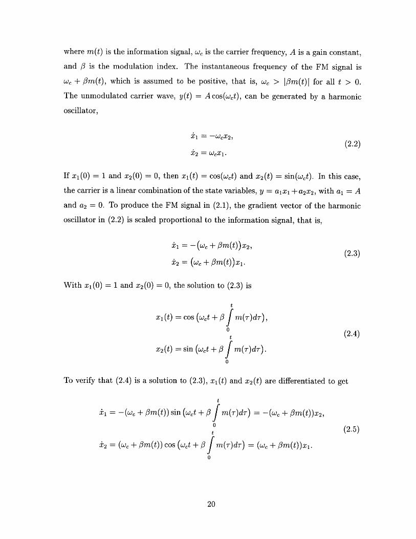
where m(t) is the information signal, w, is the carrier frequency, A is a gain constant,

and 3 is the modulation index. The instantaneous frequency of the FM signal is

Wc + 3m(t), which is assumed to be positive, that is, w, > L3m(t)I for all t > 0.

The unmodulated carrier wave, y(t) = A cos(wet), can be generated by a harmonic

oscillator,

±1 = -WcX 2 ,(2.2)

2 WcX 1 -

If x1 (0) = 1 and x 2 (0) = 0, then xi(t) = cos(wct) and x 2 (t) = sin(wct). In this case,

the carrier is a linear combination of the state variables, y = a 1 x1 +a 2x 2 , with a, = A

and a2 = 0. To produce the FM signal in (2.1), the gradient vector of the harmonic

oscillator in (2.2) is scaled proportional to the information signal, that is,

1= -(Wc + m(t))x 2 , (2.3)

2= (we + m(t))x1.

With xi(0) = 1 and x2 (0) = 0, the solution to (2.3) is

x1(t) = cos (wct + m()dT),

(2.4)

x 2 (t) = sin (wct + # m(T)dT).

0

To verify that (2.4) is a solution to (2.3), x,(t) and x2 (t) are differentiated to get

= -(we + fm(t)) sin (wet + 1 m(T)dT) = -( O + (t))X2,

(2.5)

'2= (w, + /3m(t)) cos (Wct + / m(T)dT) = (w, + 3m(t))x 1 .

0

20

Assuming m(t) is continuous, the solution to (2.3) is unique [6], and since (2.2) and

(2.3) have the same initial conditions, (2.4) is the unique solution to (2.3).

In Figure 2-1, the state-space trajectory of the harmonic oscillator is shown. The

gradient vector points in the direction of the trajectory that the states of the dynami-

cal system follow. The length of the gradient vector determines the rate at which the

system travels along its trajectory. Since an FM signal can be generated by scaling

the gradient vector of a harmonic oscillator as in (2.3), FM can be interpreted as rate

modulation of a harmonic oscillator.

GradientVector

x1

x2

Figure 2-1: A state-space perspective of frequency modulation.

The rate modulation interpretation of FM can be extended to any dynamical

system1 . For example, consider an arbitrary dynamical system given by

xnom = f(Xnom), (2.6)

where Xnom and f(xnom) are both N-dimensional vectors. Modulation is introduced

'However, for the class of demodulators discussed in Chapter 3, the dynamical system must havea known exponentially convergent observer.

21

by scaling the gradient vector,

Xmod = (PC + 3m(t)) f (Xmod), (2-7)

where w, > Jm(t) I for all t. Similar to FM, the carrier wave is a scalar function of

the state variables. Specifically, the transmitted signal is

y = h(x), (2.8)

where h(.) is a possibly nonlinear function that maps the N-dimensional state-space

vector to a scalar function. The demodulators discussed in Chapter 3 require that

h(x) be chosen so that Vh(x) = 0 only at isolated points along the orbit of the

dynamical system2 .

The state variables of the modulated system can be expressed in terms of the

nominal system in (2.6) in a manner similar to that of FM. Let Xmod(t) be the solution

of the modulated system in (2.7) with Xmod = c0, and let Xnom(t) be the solution of the

nominal system in (2.6) with Xnom(0) = Xmod(0). Then Xmod(t) is related to Xnom(t)

byt

Xmod(t) = Xnom (Pct + 43 m(r)dT). (2.9)0

This relationship is verified by showing that Xnom( Wt + 3 fJ m(T)dT) satisfies (2.7).

Taking the derivative of Xnom(Wct +#0 fo m(T)dr) with respect to time gives

t t

y {Xnom (wct fm(T)dr)= ( +#Om(t))f(xnom (eCt + m(T)dr)). (2.10)0 0

Substituting (2.9) into (2.10) gives the relationship in (2.7). Therefore, Xmod(t) -

2Vh(x) is the gradient of h(x), that is,

Vh(x) = [h(x) . 9 h(x)1[Ox 1 jx

22

Xnom(Wct + 3 fJ m(-r)dr) is a solution to (2.7). If the solution to (2.6) is unique and

m(t) is continuous and bounded, then the solution to (2.7) is also unique [6]. Since

Xmod(0) = Xnom(0), Xmod(t) = Xnom(Wct+# fo m(r)dT) is the unique solution to (2.7).

Returning to FM, any dynamical system that has a sinusoidal solution for at least

one state variable can be used to generate an FM signal. Suppose that state variable

xi(t) of (2.6) is a sinusoid, for example x1(t) = sin(t). Applying the result given in

(2.9), the modulated system produces a signal

t

x1 (t) = sin (wet + /3 m(T)dT), (2.11)

0

which is an FM signal.

As an example of using a different dynamical system for carrier wave generation,

the rate modulation procedure is applied to the Lorenz system. The Lorenz system

is a simplified model of fluid convection [7] and is given by

i1 = U(x 2 - X1),

i2 = rx 1 - x 1x 3 - X2 , (2.12)

= X1 X 2 - bX3 ,

For appropriate choices of the constants c-, r, and b, the Lorenz system is chaotic.

Chaotic systems are generally defined as those with bounded solutions that exhibit

long-term aperiodic behavior and have a sensitive dependence on initial conditions.

Applying the modulation procedure to these equations results in

i1= (W, + 3m(t))O(x 2 - x1)

L2 = (w, + 3m(t))(rxi - x1x3 - X2) (2.13)

Y3 = (W, + Om(t))(x1x 2 - bX 3 )

Figure 2-2 shows a comparison between the trajectories of the Lorenz system with-

out modulation, as given in (2.12), and the trajectories of the Lorenz system with

modulation, as given in (2.13), when the modulating signal is m(t) = sin(O.2t). Just

23

C

10

5

(A) 0

-5

-10

10

5

(B) 0

-5

-10

1

0.5

(C) 0

-0.5

5

10

10

10

15Time (sec)

15Time (sec)

15Time (sec)

20 25

20

30

25

20

30

25 30

The effect of sinusoidal modulation on the Lorenz system: (A) xl(t)without modulation, (B) x1 (t) with w, = 1, m(t) = sin(0.2t), and# = 0.8, and (C) m(t).

24

I I I I I

I I I

5

5I I

I I

I I-10

Figure 2-2:

-I

-

-

-

-

as with FM, the carrier wave is dilated and compressed in time proportional to m(t),

while the amplitude remains unaltered.

2.2 Power Density Spectrum of Rate-Modulated

Carrier Waves

Although the bandwidth of an FM signal is infinite, most of its power lies within a

finite frequency range and, for practical purposes, any signal power outside of this

range is negligible. For example, Carson's rule states that ninety-eight percent of

the power of an FM signal lies within a spectral range of 2(3 + 1)wm when m(t) =

wm sin(wmt). In this section, the power density spectrums of rate modulated signals

are analyzed.

In this section, the usual definitions of the autocorrelation function and the power

density spectrum are used. Specifically, the time-average autocorrelation function of

a finite power deterministic signal, y(t), is defined as

T

Ry(r) = lim y(t)y(t + T)dt. (2.14)T-+oo 2T

-T

The ensemble-average autocorrelation function of a stochastic process, ym (t), is de-

fined as

Rym,, (t, 7) = E [ym (t) ym (t + T)] (2.15)

and the time-average autocorrelation function is

T1 (

Rym(T)= lim - Rym(tT)dt. (2.16)T-+oo 2T

-T

If ym(t) is a wide-sense stationary stochastic process, then (2.15) and (2.16) are equiv-

alent. The power density spectrum is defined as the Fourier transform of the time-

25

average autocorrelation function, that is,

Sym(W) = JRym (T)e jWrdT.

-00

From the Wiener-Khintchine Theorem [3], if

I-00

TrRym(T)ldT < 00,

then

Sym(W) = limT-+oo

where

(E [|YmT(W) 122T

T

Ym(t)e-3jWdt.

In terms of the unmodulated carrier wave, the modulated carrier wave is

t

ym(t) = Y(Wt + ± / m(T)dT))

0

= y (wt + /M(t)).

When M(t) is a stochastic process, the autocorrelation of ym(t) is, from (2.15),

Rym(t, T) = E[y(wc(t + r) + /M(t + r))y(wct + ,3M(t))]. (

Assuming M(t) is a stationary process, (2.22) becomes

RYm (t, T) = E[y (wc(t + T) + /M(T))y (wet + 3M(0))].

26

(2.17)

(2.18)

)(2.19)

Ym,T(W) =

-T

(2.20)

2.21)

2.22)

2.23)

From (2.16), the time-average autocorrelation of ym(t) is

T11

RYM(r) = Tim E[y(wc(t+T) +/M(T))y(wct+OM(0))]dtT -400 2T-T

T (2.24)= E [ lim f (Lic(t + T) + 3M(T))y(wet + #M(0))dt (

LT -+oo 2TT-T

= E [Ry(wcT +/3M(T) - OM(0))

where y(t) is assumed to be well-behaved so that the interchange of the expectation

with the limit is allowed. From (2.17),

Sym (w) = E [Ry (OCT + /3M(7) - /M(0))] e-w"dT. (2.25)-00

In the context of rate modulation, (2.25) can be interpreted in a meaningful way.

The time-average autocorrelation function given in (2.24) can alternatively be arrived

at by assuming that the modulating signal, M(t), is independent of the position of x

along its orbit. In this case, let 0 be a random variable that is uniformly distributed

on [-T, T] and is independent of M(t). First assume that y(t) is periodic with period

T. If Ym(t) h(x(t + 0)) = ym(t + 0), then

T

Rym(r) = E[y(wc(t++)+M(t+T+))y(wc(t+)+M(t+ ))]dO. (2.26)2T

For the general case in which y(t) may not be periodic, the limit as the period of y(t)

goes to infinity is taken, in which case

T

Rym (r) = lim - J E[y(wc(T + 0) + /M(T))y(wc(0) + #M(O))]d0, (2.27)T ->oo 2T

-T

which is the same as the time-average autocorrelation function given in (2.24). In

other words, the power density spectrum of ym(t) given in (2.25) can be interpreted as

27

the expected power in ym (t) assuming that the position of x is randomly distributed

along its orbit, independently of M(t).

From (2.25), the relationship between the power density spectrum of ym (t) and

the power density spectrum of y(t) can be established.

power density spectrum given in (2.17),

From the definition of the

00

Sy(A)e jAdA. (2.28)R(T) = - 0

Substituting (2.28) into (2.25) results in

SY. w E [fS,(A)ei-'(WC7±/M(7>/-3M(O))dA] 6)-w7dT

-00 -00

C

-00

1

2Kww0

S,(A) J E [eiA[(M(T)-M(O))] e-j(wW-cA)dTdA

-00

WC E eW(C )-() -j(w--X)rdrdA.

-00

(2.29)

(2.30)

(2.31)

-00

Defining the random variable a, to be a, = M(T) - M(0), a, has a characteristic

function given by

q(w, T) = E[ejWar].

Substituting the characteristic equation of a, given in (2.32) into (2.31) gives

00

SY.(W) = -I I- 00

00

-0-A(Wc

T) e-(w-A)'drdA.

Denoting the Fourier transform of q(A, T) as

00

41(A, w)=f O(A , -jw-rdT,

-00

28

(2.32)

(2.33)

(2.34)

the expression in (2.33) becomes

00

Sym(W) = SY -( -,o - A) dA. (2.35)27rw, WC WC

-00

From (2.35), Sym (w) and SY(w) are related through a linear integral transform where

< (A, c - A) is the transform kernel. Since the integral transform is linear, if the

relationship between Sym (w) and Sy(w) is known for all Sy(w) E A, where A is some

set of functions, then the relationship is known for all Sy(w) E B, where B is the

set of all linear combinations of functions in A. For many modulating signals, the

power density spectrum corresponding to Rym (r) = E[cos (wor + OM(T) - #M(0)) ] is

known. For example, when M(T) = sin(wmr + 0), where 0 is a random variable with

a probability density function that is uniform on [0,27r], the power density spectrum

of ym(t) is [11]

Sym(W) = 2 --- w, - kwm) + 6(w + W - kwm)], (2.36)k=-oo

where Jk (-) is the kth order Bessel function of the first kind. Comparing (2.36) with

(2.35), the kernel of the integral transform is given by

S , w) = J2 o(w - kwm). (2.37)wc k=-o~o we

From the linearity of the integral operator, Sym (w) can be determined for any carrier

wave, y(t), that can be expressed as a linear combination of sinusoids.

Another example of a type of modulation for which Sym (w) is known when Ry (r) =

cos(WoT) is the case in which M(t) is a Gaussian random process with a power density

spectrum given by

SM P) = 27ror 2 ( (2.38)SWM W-33

29

where

II(w)={ W<21

In this case, the power density spectrum of ym(t) is [13]

S2 >(w) =- [6(w - 0) + J(w + )],k=0

where the notation (k), denotes self-convolution k times, that is,

G(w)(O)*= 6(w)

G(w)(k)* - G(w)(k- 1 )* * G(w).

In this case,00 / (k)*

=Z (A /3k=O Wcom

An explicit formula for each term in the right hand side of (2.42) is [12]

) (k) *W

cWWCW

k+1

= E

n=0

(-! k + 1) (/OwWcWm

k+1 \kl3W+ -n) u2 IWcom

where

0 W< 0,

1 w>0.

Power Density Spectrum of a Modulated van der Pol Carrier

Pol oscillator is given by

The van der

x1 =22

z2= A(1 - x2)x 2 - x1,

(2.45)

where A is a positive constant. An unmodulated carrier wave, such as y(t) = xi(t),

is obtained by numerically integrating the van der Pol equations given in (2.45). A

30

(2.39)

(2.40)

(2.41)

(2.42)

k+1+ 2 -n) ,

(2.43)

(2.44)

Ab,')Wc

plot of the unmodulated carrier wave and an estimate of its power density spectrum

for A = 3 is shown in Figure 2-3.

(A)

2

1

0

-1

0 5 10 15 20 25Time (sec)

0.2 0.4 0.6 0.8Frequency (Hz)

30 35 40 45 50

1

Figure 2-3: Unmodulated carrier wave (A) and its power densityfor the van der Pol oscillator (A = 3).

[.2 1.4

spectrum (B)

The modulated van der Pol equations are

si = (PC + Om(t))x 2 ,

= (Wc + Om(t))(A(1 - xi)x2 - xi), (2.46)

y = xi,

When m(t) = sin(wmt + 0), where 0 is a random variable that is distributed uniformly

on [0, 27r], M(t) = - cos(Wmt+ 0). The power density spectrum is, from (2.35) and

(2.37),

00

Sym(W) = 127rwc k=-oo

0 0

SY( A ) ( AO )6 ( - A - kwm)dA.Wc MC

31

I I I I I I 7

40

20

(B) 0

0-20

-40

I I I I I I I

-60C

(2.47)

I

Each term of the series in (2.47) can be generated by multiplying Sy ( L) by J2 ( ),

and shifting the result by kwm. An example of the estimated power density spectrum

is shown in Figure 2-4.

40

20

(A)0

-20

-40

40

20

(B)0

-20

-40C

Figure 2-4:

) 0.1 0.2 0.3 0.4 0.5 0.6 0.7 0.8 0.9 1Frequency (Hz)

0.05 0.1 0.15 0.2 0.25Frequency (Hz)

(A) Estimated power density spectrum of y, for the van der Poloscillator (we = 1, 1 = 0.1, wm = 0.2), (B) Power density spectrumon an expanded scale - direct estimation (solid), estimation using(2.47) (dashed).

The advantage of using (2.47) over a direct simulation of (2.46) is that using

(2.47) only requires the nominal system given in (2.45) to be numerically integrated

once. Given the nominal carrier wave, computing the power density spectrum of the

modulated carrier only involves scalar multiplications, shifts, and additions of the

nominal power density spectrum.

Power Density Spectrum of a Modulated Lorenz Carrier The power density

spectrum of a carrier wave generated from the Lorenz system, given in (2.12), can

also be approached in the same manner. However, the power density spectrum of

32

\.~...

the Lorenz system is closely approximated by a decaying exponential, as shown in

Figure 2-5, and this can be exploited to derive a more direct representation for the

power density spectrum when the modulation is sinusoidal. Returning to (2.29),

40

20-0

0-40 --

-60 -

-80 -0 2 4 6 8 10 12

Frequency (Hz)

Figure 2-5: Estimated power density spectrum of the unmodulated Lorenz carrierwave (solid) and a decaying exponential approximation (dotted).

which is repeated in (2.48),

Sym(W) = E Sy (A)ejA(wc±r+/M(-r)-M(O))dA e-wrdT, (2.48)- 00 "-00

and substituting the approximation Sy(w) ~ 3569e-0. 33 6 IwI gives

Sy. (w) = - f E 3569e 336AeA(wc+#M()-M(o)) wdT. (2.49)

- 00 -- 00

If the modulating signal is m(t) = sin(wmt + 0), where 0 is a random variable that is

distributed uniformly on [0, 27r], then M(t) -- cos(wmt + 6) and (2.49) becomes

0c 0c 27r

Sy )= M f f 3569e W33 ejA J e M (W) cos()ddAe rdr.

-(-2 0(2.50)

33

The innermost integral in (2.50) is [1]

27rI j2-~ (W0' sinO)d _ , / 2A/3Om \

e W2W2 (_2 cos 1(W)) dm = sin (" )),27r f cWm 2(2.51)

where Jo(.) is the zero-order Bessel function of the first kind. Substituting (2.51) into

(2.50) results in

Sym(W) = 2w 0 fJ3569e--0 3 l e--(w-A)T7o( 2 A# sin-00 -0017

2'rW0J

00

e-j- f 3569e- L |j'\'r J (2A3 sin

(m)) dAdT

( " ))dAdr2

(2.52)

(2.53)

-00 -00

The innermost integral in (2.53) is [1]

( 2A/# sink com

1 e 700

-1 {=re0

(WM )dA=2

3569-0.336() eTjA ( 2 sin

3569

213 sin( ) 2

} (5dA2

(2.5

+ ( . +33 r

where the fact that JO(-) is an even function has been used. Substituting (2.55) into

(2.53) results in

SJ

SY. (W) = WC/003569

(2 sin (fjmT)\ + (0.336 +WCWm ~2) \W

eJW dr. (2.56)

jT)

In other words, the power density spectrum of the modulated Lorenz carrier wave is

the Fourier transform of the function given in (2.55). To approximate Sym (w), the

function in (2.55) is sampled and its discrete-time Fourier transform is computed.

An example of the predicted power density spectrum using this technique is shown

34

21r0J3569e W3jpjAT J27rwc-

-00

(2.54)

5)

in Figure 2-6 along with the estimated power density spectrum obtained from the

periodogram of a numerical simulation of the modulated Lorenz equations given in

(2.13).

(A) )

0

1 2 3 4 5Frequency (Hz)

6 7 8 9

40

20

0

-20

-40

-60

-80

Figure 2- 6:

2 4 6 8 10 12Frequency (Hz)

Predicted power density spectrum of the modulated Lorenz carrierwave - predicted from (2.56) (dotted) and estimated from peri-odogram (solid) for (A) # = 0.1, wm = 0.2, and w, = 1 and (B)

# = 0.5, wm = 0.5, and w, = 1.

2.3 Bandwidth Expansion of Modulated Systems

As with FM signals, rate modulated signals are generally not band-limited. However,

for many signals, most of the signal power is contained in a finite spectral range.

The working definition that is adopted for bandwidth is the smallest spectral range

that contains ninety-eight percent of the signal power. In this section, results from

Section 2.2 are used to determine the bandwidth of the carrier waves generated by

two rate-modulation systems that are used as examples throughout this thesis.

35

0

(B

I I I I

4(

2(

-2(

-4(

-6(

-8(

Bandwidth of a Modulated van der Pol Carrier The effective bandwidth of

the modulated van der Pol Carrier is approximated by estimating the power density

spectrum as described in Section 2.2 and then finding W98 such that the spectral range

[0, w9 8] contains ninety-eight percent of the average power. The results for A = 0.5

and A = 3 are shown in Table 2.1 and Table 2.2, respectively.

Wm

# 0.1 0.2 0.3 0.4 0.50.1 1.4765 1.389 1.389 1.389 1.3950.2 1.577 1.577 1.395 1.395 1.4890.3 1.678 1.590 1.678 1.772 1.4950.4 1.778 1.778 1.690 1.791 1.8790.5 1.879 1.791 1.879 1.791 1.891

Table 2.1: Bandwidth (in rad/sec) of the modulated van der Pol carrier wave forA = 0.5 (w, = 1, unmodulated bandwidth = 1.389 (rad/sec)).

Wm

# 0.1 0.2 0.3 0.4 0.50.1 2.331 2.331 2.425 2.143 2.1360.2 2.526 2.532 2.438 2.532 2.6260.3 2.639 2.727 2.727 2.538 2.6330.4 2.827 2.740 2.733 2.752 2.6330.5 2.928 2.934 3.022 2.934 2.645

Table 2.2: Bandwidth (in rad/sec) of the modulated van der Pol carrier wave forA = 3 (w, = 1, unmodulated bandwidth = 2.136 (rad/sec)).

Bandwidth of a Modulated Lorenz Carrier The width of the frequency range

that contains ninety-eight percent of the signal power is summarized in Table 2.3.

For the range of values in Table 2.3, the bandwidth of the modulated carrier is

independent of win.

36

Wm# 0.1 0.2 0.3 0.4 0.5

0.1 11.676 11.676 11.676 11.676 11.6760.2 11.844 11.844 11.844 11.844 11.8440.3 12.125 12.125 12.125 12.125 12.1250.4 12.516 12.516 12.516 12.516 12.5160.5 13.000 13.000 13.000 13.000 13.000

Table 2.3: Bandwidth (in rad/sec) of the modulated Lorenz carrier wave

(w = 1, unmodulated bandwidth = 11.649 (rad/sec)).

37

Chapter 3

Demodulation

The previous chapter describes how an information signal can be modulated onto

a carrier wave generated by a dynamical system. This chapter describes how the

information signal can be recovered. The dynamical system used in the modulator

is assumed to have a known exponentially convergent observer, which is described

below. Using a novel perturbation technique, the observer is systematically modified

so that it is capable of extracting the information signal from the modulated carrier

wave. The end result is a systematic procedure for constructing demodulators when

the observer assumption holds. These demodulators can be modified to enhance

aspects of their performance. Three examples of such enhancements are presented

which result in improved tracking capability, increased noise immunity, and a reduced

number of nonlinearities present in the demodulator. The system that results from

reducing the number of nonlinearities is shown to be equivalent to an alternative

least-squares solution for demodulation.

39

3.1 Observers and Self-Synchronizing Systems

3.1.1 Observers

An observer is a system that reconstructs the full state of a dynamical system from

the output of the dynamical system. For example, consider a dynamical system

x = f(x), (3.1)

y = h(x),

where x and f(-) are N-dimensional vectors and y is a scalar. An observer of this

system is any system, f(-), such that if

z = f(z,y), (3.2)

then z converges to x. It is a local observer if it converges only when x remains in

a subset of the phase space, i.e. x E D C RN. Since the dynamical systems used for

modulation remain on their periodic, aperiodic, or chaotic orbits, it is only necessary

for the observers to be local observers, converging when x lies on the orbit. An

exponentially convergent observer is an observer with the property that ||z--x| < e-At

for some A > 0.

3.1.2 Self-Synchronizing Systems

Self-synchronizing systems have the property that when a state variable from one

system drives a replica system, the replica state variables converge to the drive state

variables. In other words, the replica system is an observer. An example of a self-

synchronizing system is the chaotic Lorenz system described at the end of Section 2.2.

40

The equations for the Lorenz system are

- l U2 ~ X1),

'2= rxi - x1x3 - x2, (3.3)

3 X1X2 ~ bX3,

where -, r, and b are constant parameters. If a replica system is driven by x1 in the

following way,

i = -(z2 - Z),

Z 2 = rz1 - X1z 3 - z2, (3.4)

3 =X 1z2 - bZ3 ,

then z converges to x exponentially. In general, self-synchronizing systems have the

form

Drive System:

Replica System:

y = h(x)

z = f(z, y)

3.1.3 Observers as Self-Synchronizing Replica Systems

Because the modulator remains on its orbit, the modulator dynamical system and

the observer can be formulated as a drive/replica pair. Suppose the drive system is

given by

S= f(x), (36)

y = h(x),

where x E D C RN, and a local observer system given by

z = f(z,y). (3.7)

41

(3.5)

From the assumption that the observer is convergent for x E D, if the systems are

perfectly synchronized at some time, i.e. z(to) = x(to) E D, then they remained

synchronized for t > to. For this to hold, it must be the case that

f(x) = f(x, y), for x E D. (3.8)

This means that the system in (3.6) can be replaced with

x = f(x, y)

y = h(x).

Note that (3.9) and (3.7) are a drive/replica pair.

3.2 Demodulator Structure

The basic structure of a demodulator is shown in Figure 3-1. The rate-modulated

observer is given by

= (w + #f^n)f(z, y), (3.10)

where fn is the rate estimate. The observer, f(-,-) is assumed to be a known exponen-

tially convergent local observer of the dynamical system used in the modulator. The

rate estimator takes as its input the reconstructed state from the observer and the

transmitted signal and tracks m(t). The low-pass filter removes any spectral energy

known not to be present in the original modulating signal, m(t). This system can be

42

y(t)Rate t) Low-Pass _ft)

Estimator Filter

z(t)

Rate-Modulated,-Observer

Figure 3-1: A block diagram of the basic demodulator structure. The signal y(t)is the transmitted signal, rin(t) is the estimate of the modulatingsignal, and z(t) is the estimate of state-variables of the transmittersystem.

represented mathematically as

Modulator:

y = h(x),

z = (w, + 3)f(z, y), (3.11)

Demodulator: f = 9(z, y),

S= A,4;+ Bf,,

fi = Cp 4 + Dp f,

where g is an operator that represents the rate estimator and Ap, Bp, Cp, and D,

represent the low-pass filter.

3.3 Demodulator Design

Assuming that the dynamical system used in the modulator has a known exponen-

tially convergent local observer, the observer can be modified so that it is an expo-

nentially convergent observer of the modulator when m(t) = m, where mo is an

unknown constant. If the rate estimator converges to m, then the augmented ob-

server is assumed to be able to track a time-varying in(t) provided that m(t) varies

sufficiently slow.

43

The design of the rate estimator is based on a technique developed in Appendix A

that is referred to as a backwards perturbation expansion. The essential step in

this perturbation expansion is to express the modulator state, x, as a perturbation

expansion about the demodulator state, z, in terms of the rate estimate error, em =

n - mo. By expanding the modulator as a perturbation about the demodulator,

the resulting expansion terms depend only on variables local to the demodulator.

The perturbation variables can then be combined in such a way that they force

the demodulator rate estimate error to zero. Summarizing the results obtained in

Appendix A, if the dynamical system used in the modulator is of the form

x = F(x; 0),(3.12)

y = h(x),

where 0 is an unknown parameter and x E D C RN, and the known exponentially

convergent observer is of the form

i = F(z, y; 0), (3.13)

for x E D, then the system given by

z = F(z, y; ),

9 = K(h(z) - y)C1, (3.14)

S (z,y; 0) + Kr(z, ()) y; 0),

is an exponentially convergent observer of the system given in (3.12), where

r(z,1) = (Oh (z) - g((z) -( ), (3.15)

sgn(g(a)) = sgn(a), and assuming that h(x) is persistently exciting (see Appendix A).

44

For rate modulated systems,

F(z, y; rM) = (wc + /3)f(z, y). (3.16)

Substituting the form given in (3.16) into (3.14), the demodulator system, including

the low-pass filter shown in Figure 3-1, is given by

z = (w, + /^n)f(z, y)

= h(z)

M~ = K(Q - y)g ( 0z (Z)-(3.17)

Ofai= (wc + #7^n) (Oz (Z, Iy) + Kr (z, J) c1 - Of (Z, y),

= A4; + Bp7;h,

f~t = Cp; + Dpf^n,

where

r(z, i) = ( i (z) - g (" (z).- , (3.18)

0 < K < K. for some K, sgn(g(a)) = sgn(a), and AP, Bp, C, and Dp correspond to

the low-pass filter.

The determination of K, requires, in general, the use of numerical techniques. The

difficulty lies in the fact that the explicit determination of K" requires knowledge of

a Lyapunov function for the linear, time-varying system given by

afC = -(Xy)Ci. (3.19)

Lyapunov functions are usually difficult to determine. However, K' can be estimated

by numerically computing the Floquet exponents [9] or the Lyapunov exponents [14].

45

3.4 Examples of the Basic Demodulator

In this section, demodulation is demonstrated for two dynamical systems. The first

is based on the van der Pol oscillator, which is a two-dimensional nonlinear system

with a periodic attractor. The second system is the Lorenz system, which is a chaotic

system with a strange attractor.

3.4.1 The van der Pol Oscillator

The differential equations corresponding to the van der Pol oscillator are

:li =X2(3.20)

2 = A(1 - X1)X2 - X1,

where A > 0. An exponentially convergent observer of the van der Pol oscillator is

z1 = z 2 + y - zi,

i2 = A(1 - Y2)Z2 - y-

46

Introducing modulation to (3.20) and following the formulation specified in (3.17),

the complete modulation/demodulation system is given by

Modulator

J1 = (w, + /3m)x 2,

= (+m)(A(1 - X-1),

y = x1,

(3.22)

Demodulator

[2

i = (Wc + 3fn)(2 + Y - Zi),

2= (w, + Ifin)(A(I - -Y),

m = K(zi - y)sgn(o 1 ),

+- +

0 A(1 - y2)

+ KIII" 1 01] z 2 + y - zi

).2 A( - y2)Z2 - yI

s= AP4, + Bpin,

~n = Cps + Drnii,

where I is the 2 x 2 identity matrix. The convergence of rn when K = 1, A = 1, and

# = 1 is shown in Figure 3-2. The convergence of the state variable z2 to x 2 is shown

in Figure 3-3.

3.4.2 The Lorenz System

Repeating (3.3), the Lorenz equations are

'1 = o-(x 2 - X1),

z2 = rx 1 - X 1X 3 - X2, (3.23)

= X1 x 2 - bx3 ,

47

0

I,-2

-- 4

'0 5 10 15 20 25 30 35 40 45 5

Time (sec)

Figure 3-2: Convergence of the rate estimate for the van der Pol based systemwith K= land 3=1.

0 ' I I I I I I I I I

Nq

-5

-10

0

10 15 20 25 30 35 40 45 50I I I I I I I I

0 5 10 15 20 25 30 35 40 45 50Time (sec)

Figure 3-3: Convergence of the state estimate for the van der Pol based systemwith K= land /3=1.

where, for example, - = 10, r = 25, and b = 8/3.

observer of this system is

An exponentially convergent

1 = -(Z2 - Z1),

i2 = ry - yz3 - Z2, (3.24)

3 = yz2 - bz3,

48

I I I I I I I I I

7

I I I I I I I 2

Adding the modulation to (3.3) and following the formulation specified in (3.17), the

modulator and demodulator are given by

Modulator (3.25)

31 = (w +

2= (Wc +

£3 = (Wc +

y =1,

3m)O-(x 2 - X1),

Om) (rxi - X1X3 - X2),

Om)(Xx 2 - bX3),

Demodulator

1= (w, + /r h)U(z 2 - Z1),

,i'= (Wc + /3^n)(ry - yz3 - z 2),

Z3 = (wc+/#?^)(yz 2 -bz 3 ),

= K(zi - y)sgn(o 1 ),

o- a- 0

0- -y +KI1iI <L 0 y -b i

s= AP4; + Bpfn,

7~n = Cp4; + Dp1^n,

2

L03

2

3-3 F-(Z2 - z1)

ry - yz 3 - Z2

yz 2 - bz 3

where I is the 3 x 3 identity matrix. The convergence of fan when K = 0.02 and # = 1

is shown in Figure 3-4. The convergence of the state variable z2 to x2 and z3 to X3 is

shown in Figure 3-5.

3.5 Demodulator Enhancements

In this section, modifications are made to the demodulator to improve its perfor-

mance in various ways. First, a low-pass filter is added between the rate estimator

49

(3.26)

= (w, + Of^n)

0 I I I I I I I I I

-10 --

-15'0 5 10 15 20 25 30 35 40 45 50

Time (sec)

Figure 3-4: Convergence of the rate estimate for the Lorenz based system withK = 0.02 and # = 1.

and the observer to remove spectral energy in ?h(t) that is outside the bandwidth of

m(t). Second, K is increased beyond the value for which the perturbation expansion

analysis guarantees stability. Although stability is no longer guaranteed, numerical

simulations suggest that the demodulator remains stable over a range of K > K". A

larger value for K allows ri(t) to track faster signals. Finally, many of the nonlin-

earities in the demodulator are removed by approximating the rate estimator with

a linear system. The system that results from the approximation is equivalent to a

least-squares approach to designing a demodulator.

3.5.1 Filtering

To remove spectral energy in fin(t) that is outside the bandwidth of m(t), a filter is

added to the feedback loop as shown in Figure 3-6. The filtering operation, denoted

as (-), is given byt

(fn (t)) = J4 (t, T)fin(T)dT, (3.27)0

where 0(t, T) is the kernel. If the support of this kernel is sufficiently small compared

to the rate at which m and fn vary, then

iiOh Oh(fn) =K -(z) - - (z) -(fn( - m))(0z OZ (3.28)

ah ah~-K( (-(z) - g - (z) -(fn -Tm).

50

5

N --

o-10

-150 5 10 15 20 25 30 35 40 45 50

Time (sec)

5

-5 -

0

-150 5 10 15 20 25 30 35 40 45 50

Time (sec)

Figure 3-5: Convergence of z2 to x 2 and z3 to x 3 for the Lorenz based systemwith K = 0.02 and 0 = 1.

Effectively, the filter smooths the time-varying coefficient (2(z) g( (z) .

3.5.2 Increasing the Convergence Rate

In Section 3.3, the gain parameter K had to be smaller than some K, to guarantee that

the perturbation expansion was bounded. For K < K,, the rate estimate converged

exponentially and monotonically. Choosing K slightly larger than K" affects the

system in two ways. First, since K scales the derivative of fn, increasing K increases

the rate at which rn can vary, allowing fn to track signals that vary more rapidly.

Second, the perturbation term may not remain bounded. Returning to the equation

for the perturbation variable,

afdi=(w, + &7n) -z (z, y) + Kr(z, J) c1 - Of (Z, y), (3.29)

where( (g (h (z) .(330)

51

' Rate n(t) , Low-Pass m~ nt)Estimator Filter

X(t) Filter

Observer .4

Figure 3-6: Demodulator with a filter in feedback path.

If K is set to zero in (3.29), then, from the analysis in Appendix A, C1 is bounded.

Of course, the dynamics of the system are now changed and convergence is no longer

guaranteed. Numerical experimentation suggests, however, that the system remains

stable for a range of K > K,.

As an example, consider the Lorenz based modulation/demodulation system given

in (3.25) and (3.26) with K > K,. The term KIr(z, ip) is dropped from (3.29) and

the demodulator equations become

i = (w, + 0^n)o-(z 2 - Z1),

Z2 = (wc + &4^)(ry - yz3 - z 2),

= (w, + f3n) (yz 2 - bZ3),

m = K(zi - y)sgn(0 1), (3.31)

a o~ro 0 01 o-(z2 - Z1)

[2 = (w + #3^n) 0 -1 -Y [2 - ry - yz3 - Z2

03J 0 y -b _03J Lyz2 - bZ3

The convergence of fn for K = 0.1 and for K = 0.02 is compared in Figure 3-7.

An example of demodulation is shown in Figure 3-8. The parameters in this

example are w, = 5, K = 0.6, 0 = 3, and the modulating signal is a zero-mean

Gaussian noise process band-limited to 0.4 Hz with a standard deviation of 0.5.

52

0-- K=0.1

--- - - -K=0.i2

-5 - -

10 -- -0

-15-

-200 5 10 15 20 25 30 35 40 45 50

Time (sec)

Figure 3-7: A comparison of the convergence of rfn when K = 0.1 and K = 0.02.

3.5.3 Reduction of the Number of Nonlinearities

The demodulators discussed so far have significant additional nonlinearities added be-

yond those already present in the dynamical system. These additional nonlinearities

appear in the equation for 1, since as given in (3.17),

Of= (we + r~n) (-(z, y) + Kr(z, C1)) 1 - /f(z, y), (3.32)

where

r(zi) = (a(z) - g1 g (O(z) ) (3.33)Oz 19z

0 < K < K. for some K., and sgn(g(a)) = sgn(a). Even when K > K, and Kr(z, 1)

is removed, a nonlinear equation remains.

The last term, f(z, y), also appears in the observer portion of the demodulator.

Since f(z, y) is required by the observer, removing it from the rate estimator does not

reduce the total number of nonlinearities present in the demodulator. This term is

left as it is. The first term, (w, + /rn) 1, is generally nonlinear and does not appear

elsewhere in the system. Approximating this term with a linear, time-invariant (LTI)

system simplifies the hardware implementation of the demodulator.

53

20

(A)0

-20'0 5 10 15 20 25 30 35 40 45 5

1

0

-1

-2

-2

Figure 3-

Time (sec)

5 10 15 20 25 30 35 40 45Time (sec)

3: An example of demodulation. (A) The transmitted signal, y(t). (B)The recovered signal (dashed), the actual modulating signal (solid).

)

50

First, if w, > 07h then1

1 ~Wc (z, y) C - f(z, y). (3.34)

The time-varying gain matrix, .(z, y), is generally nonlinear. However, the differen-

tial equation in (3.34) is linear with respect to Cj and is a time-varying linear filter

with -f(z, y) as its input. Using the notation (.) to denote the filtering operation,

Ci = -W(f(z,y)). (3.35)

Replacing this linear time-varying filter with a linear time-invariant filter makes the

equation for j consists of only linear components and f(x, y), the latter of which is

already present in the demodulator.

The difference between the derivatives of and y can be approximated in a manner

'Typically, w, is orders of magnitude greater than max(r3n?). For example, in FM radio broad-casts, w, is on the order of 10 7 times greater.

54

(B)

- - Recovered

2

similar to y - y,

- = (PC + #fin)z ((z)f(z, y)-

Oh- (w+ #(n - em)) A (z + iem + -- -)f(z + jem + - -- ,y) (3.36)

OzOh

Sem# n (Z) f(Z, y).-

Filtering j - y with the same filter that appears in (3.35) results in

((Z -y)' ~ ( ), y) em, (3.37)

assuming that em varies slowly with respect to the time constant of the filter so that

em can be moved outside of the filtering operation. Combining (3.35) and (3.37), the

rate estimator equation becomes

= - y)(f(z, y)) (3.38)

~ -KO(f (z, y)) 2 (7n - m), (3.39)

where h(z) is assumed to be a linear function of z. Without this assumption, (3.35)

should be changed to

A= - (z)(z, y), (3.40)

in which case the rate estimator equation becomes

i = K#e - y (Z)f, y))mW z 2 (3.41)

~-K# (zz)k(z, y)) (fn -Tm).

In both cases, the rate estimator equation has the form

n ~ -a(t)(fn - m), (3.42)

where a(t) is positive semi-definite, which suggests fn converges to m.

55

An example of a system using this type of linearized demodulator is given in

Chapter 5, where the system is constructed in hardware.

3.6 Gradient Descent Demodulators

In Section 3.5.3, the number of nonlinearities that appear in the demodulator are

reduced by replacing the time-varying filter that appears in the rate estimator with

an LTI filter. The resulting rate estimator is a special case of the type of rate estimator

obtained from a gradient descent approach to designing the demodulator.

Starting with the structure shown in Figure 3-1, the rate estimator component of

the demodulator is designed so that the rate estimate, rh, descends along the gradient

of some distance measure between (b) and (y). Specifically,

m = -K'- , (3.43)

where d(.,-) is a distance function and (-) is an averaging operation given by

t

= J (t, T)y(T)dT (3.44)0

y(t)/(t, t) - y(T))(t, 0) - y(r)dr, (3.45)

0

where 4(t, r) is the averaging kernel.

When the distance function is chosen to be the square of the distance between ()and (y), that is,

d((je), (2)) = ((7) - (3.46)

56

the corresponding least-squares rate estimator equation becomes

m = - (y)) (-K) -(y))-

SK(-) (h(z)z)) (3.47)Orn 19Z at

= -K#(e - ) (f(z, y)).

The rate estimator equation given in (3.47) is the same as that given in (3.41) for the

linearized rate estimator.

57

Chapter 4

Demodulation in the Presence of

Additive Noise

FM systems trade-off between noise immunity and bandwidth. The rate modulated

systems developed in this thesis behave in a similar manner, that is, increasing #

increases the bandwidth of the transmitted signal and increases the signal-to-noise

ratio (SNR) at the output of the demodulator. In this chapter, a general approach is

described and demonstrated to approximate the effects that additive white noise has

on the performance of the demodulator in the high input SNR case.

In the previous chapters, the modulators and demodulators have been expressed

as ordinary differential equations. When noise is added to these systems, they must

be expressed as stochastic differential equations. This chapter begins with a brief

introduction to stochastic differential equations and the relevant results from the

It6 calculus, which describes how to manipulate and analyze stochastic differential

equations. Using the rules of the 1t6 calculus, a set of ordinary differential equations

are derived that govern the time evolution of the moments. When the system is

nonlinear, low order moment equations depend on higher order moments, leading to

an infinite hierarchy of equations. A technique called quasi-moment neglect closure

(QMNC) is used to truncate these equations. The end result is a finite set of ordinary

differential equations that approximate the behavior of the low order moments. From

the moments, the time-varying probability distributions of the demodulator state

59

variables are approximated along with the SNR at the output of the demodulator.

Three different demodulators are analyzed in this chapter. The first system is

based on a stiff harmonic oscillator, which is a system that has a circular orbit and

is compatible with FM signals. It performs similar to the phase-locked loop (PLL)1

with respect to the SNR at the output of the demodulator. The last two examples

are based on the van der Pol oscillator and the Lorenz system. All three systems

exhibit a bandwidth/noise-immunity trade-off.

4.1 Dynamical Systems and Stochastic Processes

A stochastic differential equation (SDE) [2, 4, 5] has the form

dx = f(x, t)dt + g(x, t)dW(t), (4.1)

where dW(t) is defined as the derivative of a white noise process. That is, dW(t) =

rq(t)dt, where 7j(t) is a white noise process. The notation for an SDE is different

than the notation for an ordinary differential equation to emphasize the fact that the

white noise process is not Riemann-Lebesgue integrable. Because white noise is not

Riemann-Lebesgue integrable, the integral equation corresponding to (4.1) must be

interpreted carefully. The most common interpretation results in the It6 calculus [4].

The It6 calculus is a special set of rules for manipulating SDEs. Two rules from the

It6 calculus are used in this chapter.

Change of Variables Formula: Given an arbitrary SDE,

dx = f(x, t)dt + g(x, t)dW(t), (4.2)

'The phase-locked loop is analyzed in Appendix B.

60

let h(x) be a scalar function of x. Then h(x) satisfies the stochastic differential

equation given by

dz = Vh(x) (f(x, t)dt + g(x, t)dW(t)) + tr (g(x, t)Q(t)gT (x, t) Jh(x))dt, (4.3)

where Vh(x) is the gradient of h(x), Jh(x) is the Jacobian matrix of h(x), and

Q(t) = E[dW(t)dW(t)T].

Mean Value Formula: Given a continuous, non-anticipatory function, g(-, -),

E[f g (x(7), r)dW(r)] = 0. (4.4)

to

4.2 Moment Evolution

When a dynamical system is driven by additive white noise, the states become random

variables, each with its own probability density function (pdf). These pdfs can be

obtained exactly by solving what is known as the Fokker-Planck equation [4]. The

Fokker-Planck equation is a parabolic partial differential equation with non-constant

coefficients. It can be solved explicitly in only a few special cases. However, the

closeness of the rate estimate, M, and the true rate, m, is of interest and can often

be determined by approximating the first few moments of M'. Also, from these first

few moments, the pdfs of the state-variables can be approximated.

An ordinary differential equation that governs the evolution of the moments is

obtained from It6's change of variables formula. Given an arbitrary SDE,

dx = f(x, t)dt + g(x, t)dW(t), (4.5)

let h(x) be a polynomial function of the state-variables, for example, h(x) = x' or

h(x) = x 1x 2. Applying It6's change of variables formula given in (4.3), and taking

61

the expectation of (4.5) gives

E[dh(x)] = E[Vh(x)f(x, t)dt] + E[Vh(x)g(x, t)dW(t)]+

+ E[ tr (g(x, t)Q(t)g' (x, t) Jh(x))dt]. (4.6)

Since expectation and differentiation are both linear operators, they commute, giving

dE[h(x)] = E[Vh(x)f(x, t)]dt + E[Vh(x)g(x, t)d(t)]+

1+ E[tr (g(x, t)Q(t)g T (x, t) J(x)) ]dt. (4.7)

From the mean value formula given in (4.4), the second term is zero, which leaves

dE[h(x)] = E[Vh(x)f(x, t)]dt + 1E[tr (g(x, t)Q(t)gT (x, t) Jh(x))]dt. (4.8)

Since dW(t) does not appear in (4.8), it is an ordinary differential equation and can

be expressed in the usual deterministic form as

dE[h(x)] = E[Vh(x)f(x,dt

1) + 1E2[tr (g(x, t)Q(t)g T (x, t) J(x))].

By choosing h(x) appropriately, the equation of motion for any moment from (4.9)

can be derived. For example, substituting h(x) = x3 into (4.9) gives the equation of

motion for the third moment of the state variable x1 .

Two difficulties arise when f(x, t) is nonlinear. First, a nonlinear f(x, t) makes

E[h(x)f(x, t)] a function of higher order moments. For example, consider the scalar

SDE,

dx = -x 3 dt + dW(t). (4.10)

From (4.9), the equation of motion for the first moment is

dE[x] E [ 3

dt =(4.11)

62

(4.9)

which contains the third order moment, E[x3 ]. Similarly, the differential equation for

the third order moment contains the fifth order moment, and so on. In general, if the

system is nonlinear, the differential equation for any moment depends on at least one

higher order moment. If this hierarchy of moment equations is truncated, then there

are more unknowns than equations and no solution. The second difficulty caused

by a nonlinear f(x, y) has to do with computing the expectations. The differential

equations for the moments are are exact when the expectations are taken with respect

to the true pdfs of the state variables. However, the true distributions are not known

when the system is nonlinear2 . To work around these two difficulties, a technique

known as quasi-moment neglect closure is used.

4.3 Quasi-Moment Neglect Closure

As described in the preceding section, a nonlinear SDE results in a hierarchy of

moment equations in which the lower order equations depend on the higher order

equations. This hierarchy of equations can be closed by a technique called the quasi-

moment neglect closure (QMNC) technique [8]. QMNC truncates the hierarchy by

approximating the pdfs of the state variables as an Edgeworth series truncated to

order N. This series is given by

N ak1 aknp(x; t) = (1 + b(ki, k2 , ... , kn; t) - PG (X; t), (4.12)

\ O x k l &X'kns=3 1 n

where p(x; t) is the non-stationary, multivariate pdf of the state variables, pG(X; t)

is a multivariate non-stationary Gaussian pdf, and the coefficients b(ki, k2 ,... , kn; t)

are called the quasi-moments. To show how approximating the pdfs of the state vari-

ables as an Edgeworth series truncated to order N closes the moment equations, the

relationship between the moments and quasi-moments is derived. This relationship is

derived by using the cumulants as an intermediate relationship between the moments

2When the equations are linear and the white noise is Gaussian, it can be shown that the resultingpdfs are all Gaussian.

63

and quasi-moments.

The relationship between the moments and the cumulants is established using the

characteristic function, which is defined as

0C00 0C

e(w; t) = - ] - e W" p(x; t)dx, (4.13)-M -00 -00

where p(x; t) is the time-varying pdf of the state-space solution. The moments can

be computed from (4.13), and they are given by

ki k ... k, 8 ( 9 E) (w ; t) ( .4Ex(t)[xl1xf2 -X ; t] = ( Os k (4.4)W

1W2 wn w=0

where s = E_> ki is the order of the moment and ki > 0 is an integer. To simplify

subsequent expressions, the moments are denoted as

mkik 2 ...k(t) = Ex(t)[4Xk 2 ... -k;. (4.15)

Using (4.14), the Taylor series expansion of 0(w; t) is

00

o(w; t) = 1+ L mkik 2.- k.(t)wk1 - Wk", (4.16)s=1 {kl+---+kN=s}

where the notation E{k1 +---+kn=s} means the summation over all ki > 0 such that

i= ki = s, where each ki is an integer.

The cumulants are defined as the partial derivatives of the natural logarithm of

the characteristic function evaluated at w = 0. Specifically,

ik1 k2 .__Ast= a'In(E((w;t) (4.17)

1 2 n W=0

where s = En 1 ki. Using the cumulants, the Taylor series of In e(w; t) is

8(w; t) = exp Skik2 -- k (t)Wi'- .- .- f). (4.18)s=1 {k+---+kn=s}

64

Substituting (4.18) into (4.14) gives the moments as functions of the cumulants. For

example, the first moment in terms of the cumulants for a one dimensional system is

mi(t) = (-j) aE(w; t)W1=0

=(-j) a(jer" ) (4.19)aw1

=a =

Higher order moments are derived in a similar manner and expressions for the first

seven are given in Table 4.1. In Table 4.1, all the moments and cumulants are func-

tions of time. The first N moments are in terms of the first N cumulants and this

Ml = ki2

M2= kl + k2

M3 = k3 + 3 k1 k2 + k3

M4= k +6 k k2 +4k 1k 3 k2+ k4

M5 = k5 + 10k3k 2 + 10k2k3 + 15 k1k2 + 5 kk4 + 10k 2k3 + k5

M 6 = k6 + 15 k4k 2 + 20 k3k 3 +45 k2k2 + 15 k2k 4 + 60 k1 k2k3

+ 15k3 + 6k1k5 +15 k2 k4 + 10k2 + k6

M7= k7 + 21 k5k 2 + 35 k k3 + 105 k3k2 + 35 k3k4

+ 210 k 2k2 k3 + 105 k1k3 + 21 k k5 + 105 k1 k2k4 + 70 k1k2

+105 k k3 + 7k1k6 + 21k 2k5 + 35 k3 k4 + k7

Table 4.1: Moments as functions of cumulants up to seventh order for a one-dimensional system.

relationship can be inverted to get the first N cumulants as functions of the first N

moments. The resulting relationships are shown in Table 4.2.

The cumulants have been expressed as functions of the moments and the moments

have been expressed as functions of the cumulants. Once similar relationships between

65

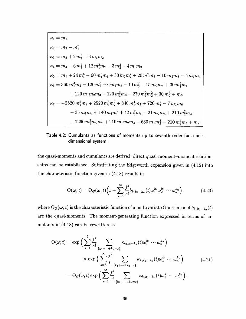
Ki =M

- 2K 2 = M2 - Mi

K3 = m 3 + 2 mi - 3 m 1 m 2

K 4 =M4 - 6 m4 + 12 m m2 - 3 m2 - 4 m 1m 3

K5 = m + 24m5 - 60 mm 2 +3Omim2 + 20 m m3 - 10 m 2m 3 - 5mm 4

K6 =360 m m 2 120 6 2 - Mm5 2-1Om-15m2 m 4 +3Omim4

+ 120 mm 2m 3 - 120 m m3 - 270 m2m2 + 30mi + mM

r 7 = -2520 mim2 + 2520 m3m2 + 840 m4m3 + 720 m - 7 m 1 m6

- 35 m 3m 4 + 140 m1m2 + 42 mim2 - 21 m 2 m5 + 210 m2m 3

- 1260 mim2 m 3 + 210 mim 2m 4 - 630 mim3 - 210 mim4 + m

Table 4.2: Cumulants as functions of moments up to seventh order for a one-dimensional system.

the quasi-moments and cumulants are derived, direct quasi-moment-moment relation-

ships can be established. Substituting the Edgeworth expansion given in (4.12) into

the characteristic function given in (4.13) results in

00

e(w; t) = eG(W; t) ( +E1 bkk2-k (t)wik 1k2 ...

s=3

(4.20)

where EG(W t) is the characteristic function of a multivariate Gaussian and bklk 2 ... k (t)

are the quasi-moments. The moment-generating function expressed in terms of cu-

mulants in (4.18) can be rewritten as

2 .s

6(w; t) = exp (Z E E kik 2 -k... (t)W's=1 {k 1+---+kn=s}

ooWk ... Wk

= eG(w;t)exp Kkk 2... k (t)W n -

s=3 {kl+---+k.=s}

(4.21)

66

From (4.21) and (4.20), the quasi-moments and the cumulants are related through

0000exp K(Xi k2 ... XN 1 .. WN

s=3 k1+---+kN=s

W1 + b ( X l , . . . , X N ; t 1 .i ...W N

s=3 9(4.22)

Comparing the above expression to (4.16) and (4.18), the relationship between the

quasi-moments and the cumulants is similar to that of the moments and the cu-

mulants. In fact, the cumulant-quasi-moment relationships can be obtained directly

from the moment-cumulant relationships. Combining (4.16) and (4.18) gives the rela-

tionship between the moments and cumulants used to derive Table 4.1 and Table 4.2.

Specifically,

s=1 {k1+---+kN=s}

m k 2.k(t)Wi .Mkjk ...k. 1 n

00

exS5=1 {kl+...+kn=S}

(4.23)

Comparing (4.22) with (4.23), the relationship between the quasi-moments and the

cumulants is identical to the relationship between the moments and cumulants if the

first and second order moments and cumulants in (4.23) are set to zero. Therefore,

the quasi-moment-cumulant relationships can be obtained directly from Table 4.1

and Table 4.2 and are given in Table 4.3 and Table 4.4.

K3 =b3 K4 =b4

K5 =b 5 K6 =-10 b2 + b6

K7 = -35 b3b4+ b7

Table 4.3: Cumulants as functions of quasi-moments for up to seventh order.

Substituting the cumulant-quasi-moment relationships in Table 4.3 into the moment-

67

(t)Wki ... knNki k2 ... kn 1 n )-

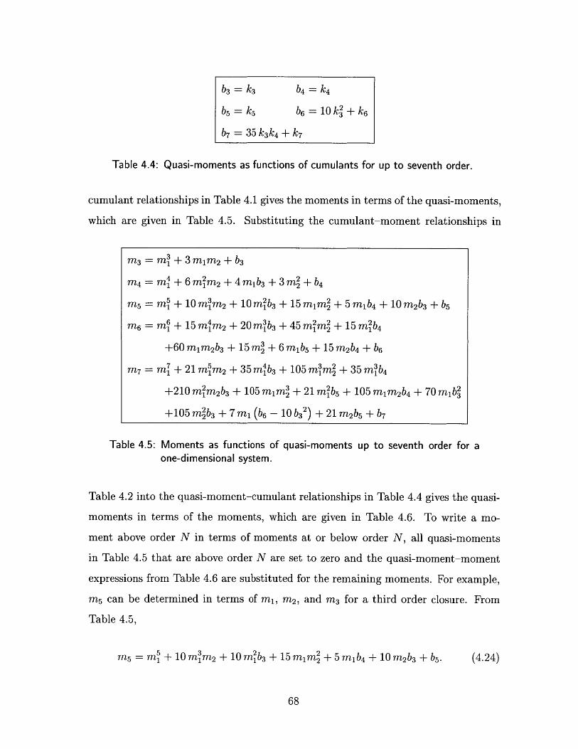
Table 4.4: Quasi-moments as functions of cumulants for up to seventh order.

cumulant relationships in Table 4.1 gives the moments in terms of the quasi-moments,

which are given in Table 4.5. Substituting the cumulant-moment relationships in

M3 = m3 + 3 m 1m 2 + b3

M4 = m4 + 6 mm 2 + 4m 1b3 + 3m2 + b4

m 5 = mi + 10mim 2 + 10 mb 3 + 15mimi + 5m 1 b4 + 10m 2 b3 + b5

M6 = 6i + 15 mn4m2 + 20 mnib + 45 M2M2 + 15 M2 b4

+60mlm2b3 + 15m2 + 6m1 b5 + 15m 2 b4 + b6

m 7 = mj + 21mJm 2 + 35mlb3 + 105 mm1 + 35 mb 4

+210 mim2 b3 + 105 mimi + 21 m2b5 + 105 mim2 b4 + 70 m 1b2

+105 m2b3 + 7m (b6 - lob32 ) +21m 2b5 + b7

Table 4.5: Moments as functions of quasi-moments up to seventhone-dimensional system.

order for a

Table 4.2 into the quasi-moment-cumulant relationships in Table 4.4 gives the quasi-

moments in terms of the moments, which are given in Table 4.6. To write a mo-

ment above order N in terms of moments at or below order N, all quasi-moments

in Table 4.5 that are above order N are set to zero and the quasi-moment-moment

expressions from Table 4.6 are substituted for the remaining moments. For example,

m5 can be determined in terms of in, mn2 , and m 3 for a third order closure. From

Table 4.5,

M5 = m + 10'mi 2 + 10Mi2b3 +15mimnu +5im 1b4 + 10m 2b3 +±b. (4.24)

68

b3 = k3 b4 =k4

b5 = k5 b6 =10k 2 + k6b7= 35k 3k4 + k7

b3 - m 3 + 2 mi - 3 m1m 2

b4= M4- 6 m4 + 12 mrm 2 - 3 m2 - 4 m 1m 3

b5 = m 5 + 24 m5 - 60 m3m 2 + 30 mim2 + 20 m2m 3 - 10 m 2 m 3 - 5 mim4

b6 = m6 + 240 m4m 2 -180 m2m2 - 80 mim3 + 30 m2m 4

-15m 2m 4 + 30m3 - 6mm 5 - 80 m6 + 60m 1 m 2m 3

b7 = m7 + 300m7 - 1050 m5m 2 + 1050 m3m2 + 350 4 m3

-315 miml - 140 mim4 + 105 m2m 3

+42 m m - 21m 2 m 5 - 7 mim6 - 420 mim2m 3 + 105 mm 2 m4

Table 4.6: Quasi-moments as functions of moments for up to seventh order fora one-dimensional system.

Setting b4 and b5 to zero in (4.24) gives

m5 = m5 + 10mim2 + 10mib3 + 15 mmi + 10m 2 b3 . (4.25)

From Table 4.6,

b3 = m 3 + 2 m 3 -3 m 1 m 2, (4.26)

and substituting (4.26) into (4.25) gives

m 5 = m5 + 10m3m 2 + 10m(m 3 +2 m3 -3mim 2)+15 mim2 + 10 m 2 (m 31 1 1 2(4.27)

+ 2 mi - 3 mim2 ).

In summary, the assumption that the pdfs of the state variables can be approxi-

mated as an Edgeworth series truncated to the Nth order makes the moments above

order N functions of the moments at or below order N and closes the differential

moment equations at order N. A detailed example of applying this technique to the

second-order phase-locked loop, a two-dimensional system, is given in Appendix B.

69

4.4 The Channel and Demodulator as Stochastic

Differential Equations

When the modulated signal, ym (t), is corrupted with additive white noise, the de-

modulator is preceded with a filter that filters out any spectral energy that is outside

the bandwidth of ym(t). Assuming that the pre-filter passes the modulated signal,

ym(t), without significantly altering it, the noise model shown in Figure 4-1 is used.

The pre-filter written as an SDE is

di = AOdt + BdW(t) (4.28)

v =CV,

where A, B, and C are the matrices and vectors associated with the state-space

representation of the filter. In general, the state-space form of a filter has an additional

parameter, D, and the output of the filter is v = CO + DdW(t). However, a filter

that has D = 0 must always be chosen. Otherwise, the demodulator equation for z

becomes

z = (wc + frin)f(z, y + C9 + DdW(t)). (4.29)

If f(-,-) is nonlinear with respect to its second argument, the noise process appears

nonlinearly in the demodulator, and the demodulator does not have the form of an

dW(t)

Pre-Filter

IV(t)y(t) t(t) )(t)

± Demodulator Post-Filter

Figure 4-1: Demodulator noise model.

70

SDE as described in Section 4.1.

The SDE for the complete demodulator, including the pre- and post-filters, is

dz = (w + #n)i(z, y + v)dt,

d&h = -K (h(z) - y +v) - g (A (z) dt,oOZ

d(j = ((Wc + &) a(z, y + v) + IKr(z, i)) idt - #f(z, y + v)dt,

dV = AOdt + BdW (t), (4.30)

dq = Apsdt + Bprfhdt,

m = Cpq + DT,,

where A, B, and C correspond to the pre-filter filter and A., Bv, Cp, and Dp corre-

spond to the post-filter.

4.5 Examples

In this section, the QMNC technique is applied to three examples3 . The first example

is based on a system referred to as the stiff harmonic oscillator. The stiff harmonic

oscillator has sinusoidal solutions, and therefore can be used to generate FM signals.

The associated demodulator can therefore be used to demodulate FM signals. This

is an example of how different demodulators can be used for the same carrier wave as

described in Section 3.1.3. The second example is based on the van der Pol oscillator

and the last example is based on the chaotic Lorenz system, both of which have

already been used as examples in Chapter 3.

3In addition to the examples in this section, a detailed example of applying the QMNC techniqueto the phase-locked loop is given Appendix B.

71

4.5.1 The Stiff Harmonic Oscillator

The stiff harmonic oscillator has a circular limit cycle like a harmonic oscillator, but it

has an added nonlinearity to make the limit cycle globally attracting. The differential

equations describing the oscillator are

z1=Ks I1 - I! + X2 X1 -4 31,' 2 = KS I - X2+ ) X2 + X1,

where Ks is the "stiffness" constant that determines how quickly the system converges

to its stable limit cycle. Figure 4-2 shows the effect that Ks has on the rate at which

the system approaches its limit cycle4 .

The Modulator: Introducing the modulation as described in Chapter 2, the mod-

ulator is given by

bi = (w, + #m(t)) Ks(1 .- 3I + X X22) X 1(4 .3 2 )

22 = (wc + m(t)) (Ks (1 - 1 +X2

Since the modulator operates on the unit circle, x2 + x = 1 and (4.32) can be

simplified to

= - (PC + 3m(t))x 2, (4.33)

2= (Wc + #m(t))x1.

The system in (4.33) is a rate modulated harmonic oscillator.

'The term "stiff" comes from the fact that for large values of Ks, the convergence to the limitcycle is much faster than the oscillatory rate. Dynamical systems that evolve on two different timescales are called "stiff".

72

2

1.5

1

0.5 F

0

-0.5 F

-1

-1.5 --1.5 -1

Figure 4-2: The effectoscillator.

-0.5 0 0.5

of Ks on the rate of convergence

1

of

1.5

the stiff harmonic

The Channel and Pre-Filter: The transmitted signal is y = x 2. The channel is

an additive white Gaussian noise channel and the pre-filter is given by

dO = AOdt + BdW(t) (4.34)

V = C29,

where A, B, and C correspond to a bandpass filter with a bandwidth of Bw centered

at w,. The noise process, dW(t), is a Gaussian white noise process. Bw is chosen to

be equal to the bandwidth of the transmitted signal as obtained from Carson's rule,

which is Bw = 2Wm(± + 1) when m(t) = sin(wmt).

73

K =1K= K =3 /

The Demodulator: An exponentially convergent observer for the stiff harmonic

oscillator is

1 =Ks (1- + 2)zi-z 2 ,

i2= Ks (1 - ±z z + KI(y -Z2),(4.35)

where y = x2 . Choosing g(02) = 02 and following the demodulator design procedure

of Section 3.5.2, the demodulator equations are

z1 = (w +/#r) Ks (1 - z 2 z)zi -

i2 (C + n) (Ks (1 - 4z +z) z2 +zi + K(y + v

f = KKs (z 2 - (y + v))+ 2 ,

2z +Z2

(wc + Ofn)Ks 1 +Z2ziz2 +

2L VZ1 + 2

WC

Z1 Z2 _1ir i_+ z2 KS

1 ,2+2z2 _ K 1

z K+ z2 KS 2

Ks(1 - z+) zi-z 2

z ± 2 )z 2 + z 1 + K 1 (y + v -Z2)]

(4.36)

where the equations for I. and fn have been rescaled so that

of the rate estimator is approximately independent of we, #,3n(t), is subsequently filtered with a low-pass filter that has

m(t),

S=AP4; + Bpih

in =Cpi; + dpin.

the rate of convergence

and Ks. The estimate,

the same bandwidth as

(4.37)

Error Dynamics: The performance of the demodulator is quantified through the

statistics of the error between the modulator state variables and the demodulator state

variables. To write the error equations, two states that correspond to the demodulator

74

- Z2) ,

states $ and 02 are added

between the modulator and

states are

to the modulator to obtain a one to one correspondence

demodulator state variables.. The additional modulator

= (w, + /m)Ks2 2

K-s2x+x

X1 +X

WC

X1X2 -i

1- __ ~ 1X2 KS (1

fx+X2 KS .2

II-1+ -X2 2x + )X1 - X2

x +Xx2 + X1

Since the demodulator operates on the unit

simplified to

[. , = +,m)Ks[(2

- 2

-x1x2 + 1

circle, x2 + x2 = 1 and (4.38) can be

- -s1 - - wKs . (4.39)x 2 ( IX2 J L 2i L j

Defining e. = z - x, ep = 0 - C, and em = fn - m, the error equations are

= (we + 0(m + em)) (f(x + e., y) - f(x, y)) + #,emf(x, y),

m = KKs we 1 ((I + ep 1),

Ofeg = (wC + /(m + em)) -(x + ez, y)eO - wcf(x + ez, y).

(4.40)

Applying Quasi-moment Neglect Closure: The quasi-moment neglect closure

technique allows only polynomial nonlinearities. Any nonlinearities that are not poly-

nomials are approximated through a multivariate Taylor series expansion. Two subex-

pressions appear in (4.36) that are not polynomials in the error variables, specifically

s 1 (z)-= z + z2 = /(x1 + ezi)2 +(x2 ez 2 )2,

1 1

z1 + z / + + eZ2)2 + (x 2 + eZ2 )2

(4-41)

The subexpressions in (4.41) are approximated with a second order Taylor series

expansion with respect to ez1 and ez2-

75

(4.38)

The Moment Equations: The equations for e7, em, and ep consist of five equa-

tions. The pre-filter is a tenth order band-pass filter and the post-filter is fifth order

low-pass filter. Including the filters, the system has a total of twenty states. Closing

the moment equations at second order requires all the first and second order moments.

The second order moments correspond to a symmetric twenty by twenty covariance

matrix, making a total of N(N + 1)/2 = 210 second order moments. The first-order

moments must also be computed, bringing the total up to 230. Finally, the modula-

tor states x and ( add another four states, making a total of 234 differential moment

equations. The moment equations were derived using Maple, a symbolic math pro-

cessing software package. The resulting differential equations for the moments were

numerically integrated in Matlab.

Results: The output SNR of the demodulator is defined to be

SNROt = 10 logo ((i =) (dB), (4.42)((f - mn)2

where m 2 is the average power in m. Figure 4-3 shows the demodulator output SNR

versus the baseband output SNR for # = 2, 5, and 10. The baseband output SNR is

SNRb = 10 log1 0 ( M) (dB), (4.43)

where Wm is the bandwidth of the information signal, m(t), and No is the level of the

power density spectrum of the white noise. SNRb corresponds to the output SNR

achieved if the information signal, m(t), is sent directly through the additive white

noise channel and subsequently filtered with a low-pass filter with a cut-off frequency

of Wm. Therefore, plotting SNROt as a function of SNRb shows how rate modulation

compares to using no modulation. From the plot, increasing 3 increases the noise

immunity. In Table 4.7, the SNR at the output of the stiff harmonic demodulator is

compared to the SNR at the output of the second-order PLL analyzed in Appendix B.

A comparison between the time-averaged pdfs obtained from the QMNC tech-

76

60

55

50

45

440

35

30

25

20

15A15

Figure 4-3:

20 25SNRb (dB)

SNROUt vs. SNRb for # = 2, 5, and 10 for theThe pdfs associated with the point markedFigure 4-4.

Table 4.7: A performance comparison between thethe PLL.

30 35

stiff harmonic oscillator.with a '*' are shown in

stiff harmonic oscillator and

77

=10

=2

-Baseband-.. .. .. ... .. .. -.. .. ... .. - -.. . .. .. .. .. .... .

- -. . .... ... ... ... .. .. ... ..-. ... - -. .. .. . -.

2 5 10SNRb SHO PLL SHO PLL SHO PLL

35 41.80 43.92 49.58 51.60 55.66 57.9032 38.80 40.92 46.57 48.88 52.59 54.9029 35.82 37.91 43.46 45.87 49.58 51.8926 32.84 34.89 40.12 42.84 44.98 48.8723 29.91 31.84 37.33 39.80 - 45.8220 27.12 28.75 - 36.71 - 42.73

-0.4

10

(A) 8

6

4

2

0

10

(B) 8

6

4

2

0

20

-0.1

-0.2

-0.2

0

0

0.2

0.2

0

0.4

0.4

0.1

A comparison of the pdfs of the stiff harmonic oscillator obtainedfrom the QMNC technique (solid line) and a direct simulation (dots),(A) p(ezi), (B) p(ez2 ), and (C), p(ri~).

78

I

-0.4

(C) 15

10

5

0

0.6I I

- ~-

.6 0.6

.1

I

Figure 4-4:

--

nique and the time-averaged pdfs obtained from a direct simulation of the stochastic

differential equations is shown in Figure 4-4 for 0 = 2 and SNRb = 23 (dB), which

corresponds to the data point marked with an asterisk in Figure 4-3. The mean of

em predicted by the QMNC technique is 6.77 x 10-4 and the mean of em estimated

from the direct simulation is 6.76 x 10--4. The average SNR at the output of the de-

modulator predicted by the QMNC technique is 29.91 dB and the estimated average

SNR at the output of the demodulator is 29.66 dB.

The stiffness parameter, Katiff, also affects the SNR at the output of the demodu-

lator. In Figure 4-5, SNRut is shown as a function of Ktiff for Kstiff = 0.2, 0.5, 1, 2,

and 5, # = 2, and SNRb = 35 (dB).

42 .5 I I I I I I I I I

42-

; 41.5-0

41-

40.50 0.5 1 1.5 2 2.5 3 3.5 4 4.5 5

Kstiff

Figure 4-5: The effect of the stiffness parameter on the output SNR, 3 = 2, andSNRb = 35 (dB).

Threshold: Just as with the PLL analyzed in Appendix B, the moment equations

have been closed at second order, which means that the demodulator state variables

are assumed to be Gaussian. The match between the pdfs predicted by the QMNC

technique and the pdfs estimated from a direct simulation of the nonlinear system

shown in Figure 4-4 indicates that for sufficiently high input SNRs, this assumption

is valid. However, as with the PLL, the stiff harmonic oscillator system exhibits a

threshold effect as SNRb decreases and the second order QMNC fails to capture this

phenomenon. Instead, the QMNC moment equations become unstable.

79

4.5.2 The van der Pol Oscillator

The differential equations describing the behavior of the van der Pol oscillator are

' l -X2,

2= A(1 - -x2 -4.4,

where A is a positive constant.

The Modulator: Introducing modulation as described in Chapter 2, the modulator

is given by

i1 = (we + #m)x 2 ,(4.45)

i = (we + /m) (A(1 - X2- x 1 ).

The Channel and Pre-Filter: The transmitted signal is y = x1 . the channel is

an additive white noise channel and the pre-filter is given by

d = AVdt + BdW (t) (4.46)



be equal to the bandwidth of the transmitted signal as described in Section 2.3.

The Demodulator: An exponentially convergent observer for the van der Pol os-

cillator is

i = z2 + Ki(y - zi),

2= A(1 - z, Z2 - Z1,

80

where K1 is a positive constant. Choosing g(,O1) = 01 and following the demodulator

design procedure of Section 3.5.2, the demodulator equations are, after rescaling',

1 = (w + fn)(z 2 + KI(y + v - zi)),

i2= (w, + /3h)(A(I - Z )Z2 - z)

h= K1 (z - (y + v))0i,

1 (wc + #?6n_ 2 -

The estimate, fn, is

bandwidth as m(t),

)-K, 1 1 Wz2 + K1(y + v - zi)

-2Azz2 - 1 A(1 -z) 02 A( -z(42 - Z )

(4.48)

subsequently filtered with a low-pass filter that has the same

= Ap + Bh,(

Error Dynamics: To get a one to one correspondence between the state variables of

the modulator and the state variables of the demodulator, the modulator is augmented

so that it has state variables corresponding to the demodulator state variables VP, and

'02. The additional modulator state variables are

1

A(1 - X2

K](w-Km. P (C + #M)

(2 1-2AxiX2 - 1

(1 [ C X2

_ (2_ A(l - X2 )X2 - X1

Defining e. = z - x, ep = iP - C, and em = m - m, the error equations are

z= (w, + 0(m + em)) (i(x + ez, y) - f(x, y)) + Oemf(x, y),

m= KW (( 1 + ep), (4.51)/3

C= (c + /(m + em)) (x + ez, y)ep - wjc(x + ez, y).

5The equations for fn and 0/ are rescaled so that the rate of convergence of the rate estimator isindependent of wc and 0.

81

(4.50)

Applying Quasi-Moment Neglect Closure: All nonlinearities that appear in

the error equations are polynomials and the quasi-moment neglect closure technique

can be applied directly to the error equations.

The Moment Equations: The equations for e,, em, and egp consist of a total

of five equations. The pre-filter is a fifth order low-pass filter and the post-filter is

a third-order low-pass filter. Including the filters, the system has a total of thirteen

states. Closing the moment equations at second order requires all the first and second

order moments. The second order moments correspond to a symmetric thirteen by

thirteen covariance matrix, making a total of N(N+1)/2 = 91 second order moments.

Including the first-order moments brings the total to 104 moment equations. Finally,

the modulator states x and C must be included, bringing the total number of equations

to 108. The moment equations were derived using Maple and the resulting differential

equations were numerically integrated in Matlab.

Results: The output SNR of the demodulator is defined to be

SNROot = 10 logo (( 2 ) (dB), (4.52)(fm -Tm)2

where m 2 is the average power in m. Figure 4-6 shows the demodulator output SNR

versus the baseband output SNR for 3 = 0.2, 0.5, and 0.7. The baseband output

SNR is

SNRb = 10 log 10 ( (dB), (4.53)( rNo

where Wm is the bandwidth of the information signal, m(t), and No is the level of the

power density spectrum of the white noise. SNRb corresponds to the output SNR

achieved if the information signal, m(t), is sent directly through the additive white

noise channel and subsequently filtered with a low-pass filter with a cut-off frequency

of Wm. Therefore, plotting SNRot as a function of SNRb shows how rate modulation

compares to using no modulation. From the plot, increasing 3 increases the noise

immunity.

82

50

=0.7

4 0 - --. ............- -- .... - ......... -.-.-.- - 0 .5 - - -. .......... -

SNR =S

2 5 - ......- - -. .- - --. .- --. .- ---. .- - --.- -. .- -.-. .-

20'20 25 SNb() 30 35

Figure 4-6: SNROut vs. SNRb for /= 0.2, 0.5, and 0.7 for the van der Poloscillator. The pdfs associated with the point marked with a '*' areshown in Figure 4-7.

83

3

(A) 2.52

1.5

1

0.5

2.5

(B) 2

1.5

1

0.5

-0

Figi

-0.06 -0.04 -0.02 0

A comparison of the pdfs of the vanthe QMNC technique (solid line) andp(ezi), (B) p(ez2 ), and (C), p(fin).

0.02

der Pola direct

5.5 -1 -0.5 0 0.5

1.5 -1 -0.5 0 0.5 1 1.

0.04 0.06 0.08

system obtained fromsimulation (dots), (A)

84

5

.08

ure 4-7

A comparison between the time-averaged pdfs obtained from the QMNC tech-

nique and the time-averaged pdfs obtained from a direct simulation of the stochastic

differential equations is shown in Figure 4-7 for # = 0.2 and SNRb = 29 (dB), which

corresponds to the data point marked with an asterisk in Figure 4-6. The mean of

em predicted by the QMNC technique is 3.25 x 10-3 and the mean of em estimated

from the direct simulation is 1.30 x 10-3. The average SNR at the output of the de-

modulator predicted by the QMNC technique is 32.00 dB and the estimated average

SNR at the output of the demodulator is 31.79 dB.

4.5.3 The Lorenz System

The Lorenz system, which is given by

'1 = c-(x 2 - X1),

z2 = rx1 - x1x3 - x2 , (4.54)

i6 = xlX2 - bx3,

is a chaotic system for appropriate choices of the constants a, r, and b.

The Modulator: Introducing modulation as described in Chapter 2, the modulator

is given by

:1 = (W, + /m)o-(x 2 - X1),

= (W, + Om) (rx1 - x1x3 - x 2 ), (4.55)

= (W + Om) (x1x2 - bx3)

The Channel and Pre-Filter: The transmitted signal is y = x1 . The channel is

an additive white noise channel and the pre-filter is given by

0 = Andt + BdW (t), (456)

V = C9,



be equal to the bandwidth of the transmitted signal as described in Section 2.3.

The Demodulator: An exponentially convergent observer for the Lorenz system

is

i = U(z 2 - Zi),

i2 = ry - yz 3 - z 2 , (4.57)

i3= yz 2 - bz 3.

Choosing g(O1) = / 1 and following the demodulator design procedure of Section 3.5.2,

the demodulator equations are, after rescaling ,

-i = (Pc + /3in)a(z2 - zi),

i2= (w, + O^h) (r(y + v) - (y + v)z 3 - Z2),

i3 = (w, + /3^h)((y+ v)z 2 - bZ)

Mn= K -- (z1 - (y + v))N1,

[2 =( +#^n) 0

3 0

-1

y + v

0( ]1

-(Y + 1/) 02 -We r(y

-b 03

The estimate, fn, is subsequently filtered with a low-pass

bandwidth as m(t),

U-(z 2 - zI)

+ v) - (y + v)z3

(y + v)z 2 - bz 3

Z2

(4.58)

filter that has the same

s = Apq + Bum,(4.59)

'The equations for i and 40 are rescaled so that the rate of convergence of fn is independent ofwe and #.

86

Error Dynamics: The probability density functions are computed for the error

between the state variables of the modulator and the state variables of the demodula-

tor. To get a one to one correspondence between the state variables of the modulator

and the state variables of the demodulator, the modulator is augmented so that it

has state variables corresponding the demodulator state variables 01 and '0 2 . The

additional modulator state variables are

[--a 0 [U(x2 - X1)[2 (W + #fr) 0 -1 -xj (2 - c rx1 - X1X3 - X2 . (4.60)

6 3 0 x1 -b (3 XiX2 - bx 3

Applying Quasi-Moment Neglect Closure: The equations for the demodulator

are in polynomial form, so the quasi-moment neglect technique can be applied directly

to the error equations.

The Moment Equations: The equations for e., em, and e, consist of seven equa-

tions. The pre-filter is a fifth-order low-pass filter and the post-filter is a third-order

low-pass filter. Including the filters, the system has a total of fifteen states. Clos-

ing the moment equations at second order requires all of the first and second order

moments. The second order moments correspond to a symmetric fifteen by fifteen

matrix, making a total of N(N + 1)/2 = 120 second order moments. The first-order

moments must also be computed, bring the total to 135. Finally, the modulator states

x, and C add another six equations, bringing the total to 141. The moment equations

were generated using Maple and were numerically integrated using Matlab.

Results: The SNR at the input to the demodulator is defined as

SNRio = 10 logo -- (4.61)(2)/2

87

The SNR at the output of the demodulator is defined as

SNROUt = 10 log 0 (( rn) 2 ). (4.62)

Figure 4-8 shows a plot of the output SNR as a function of the input SNR for #3 =

0.2, 0.5, and 0.7. Similar to the previous modulation/demodulation systems, there is

a trade-off between noise-immunity and bandwidth

30

=0.7

-10 - -.-.-.-. p- 0.2 -

0

SNSNR (dB)R

Figure 4-9 compares the probability density functions approximated using the

QMNC technique and the probability density function estimated by a direct simula-

tion of the SDE.

88

0.25

0.2 -

0.15-

0.1 -

0.05 -

0-1

0.25

0.2

0.15

0.1

0.05

A-1

0.25 r

0.2 -

0.15 F

0.1 -

0.05 F

o - . . I I I L- -

-10 -8 -6 -4 -2 0 2 4 6 810-

8-

6 -

4-

2-

-0.2 -0.15 -0.1 -0.05

Figure 4-9:

0 0.05 0.1 0.15 0.2 0.25 0.3

A comparison of the pdfs (QMNC - solid, SDE - dotted) for theLorenz system for SNRin = 15 dB, wm = 0.2 (rad/sec), / = 0.5,We = 1 (rad/sec), (A) p(zi - xi), (B) p(z 2 - X2 ), (C) p(z3 - X3 ),and (D) p(Fn).

89

(A)

(B)

-8 -6 -4 -2 0 2 4 6 8 10

-8 -6 -4 -2 0 2 4 6 8 10

(C)

(D)

10

0'

0

Chapter 5

Design and Construction of Lorenz

Based Modulator and

Demodulator Circuits

In this chapter, the design and construction of a prototype of a complete modula-

tion/demodulation system based on the chaotic Lorenz system is described. The

circuits are constructed with analog components, the nonlinear terms being imple-

mented with analog multipliers. The other components used to build the circuits are

operational amplifiers, resistors, and capacitors.

Section 5.1 describes the Lorenz-based modulator and demodulator circuits. Sec-

tion 5.2 summarizes some basic issues that were considered regarding the layout of

the components. Section 5.3 provides examples of the performance of the system.

5.1 Modulator and Demodulator Circuits

5.1.1 Rescaled Lorenz Equations

The operational amplifiers and the analog multipliers used have an input/output

range of ±12 volts. The circuit is designed such that the state variables correspond

to voltage levels in the circuit and the Lorenz equations must be rescaled so that all

91

voltage levels remain within the operating range of the components. The resealed

variables are X, = jX 1 , X 2 = IX2 , and X 3 = X3 . The resealed Lorenz equations

implemented in the circuit are

= -(X2

9k2 = rX 1 - X1X3 - X2,

8 2)6= X1X2- bX 3 ,

9

(5.1)

where -, r, and b are 10, 25, and , respectively.

and X 3 remain within +12.

-5

-10

0 5 10 15 20 25Time (sec)

As shown in Figure 5-1, X 1, X 2,

30 35 40 45 50

Figure 5-1: Rescaled Lorenz variables from simulation, X1 (solid), X 2 (dash),and X 3 (dash-dot).

92

10

5

0

I I I -

- -~

'.11 A,~I

- -

I I I I I I I

5.1.2 Modulator Circuit

Introducing modulation into the rescaled Lorenz equations, as described in Chapter 2,

the modulator equations become

ki= (We)Pi=(C + &m(t))(Cr(X2-X),

i2 = (Wc + /m(t)) rXi - XX3- X 2),

A3 = (wc + /m(t)) (8X 1 X 2 - bX3(

y = Xi,

The analog circuit implementation of (5.2) is shown in Figure 5-2 The operational

amplifiers perform the operations of addition, subtraction, multiplication by a con-

stant, and integration. The nonlinear terms, such as X1X 3 , are implemented with

analog multipliers1 . The set of equations that describe the behavior of the modulator

circuit are

I m(t) R1o2V( t 4 R1022_= +I -+ R12)

C101 R1 1 4 10R115 (Rio, R10 3 + R 104 Rio11 __ ___) R1 21 fti 09 Ri__ + i

#2= + m(t) R1 R106 + R 16C10 2 R1 10R117 R120 I 08+ Rio R105 R107)

f 1 0 6 Rio61ORt107 Rt105 J

1(1 m(t) Ru3 Ri3= + l 1 + f -

C103 Ri118 10R119 R112+ R113 R0 V

- Rl1 V1V2 ?.

1The multiplier circuits have as their output the product of the inputs divided by ten, which isthe reason some terms in the circuit equations are divided by ten.

93

5.1.3 Demodulator Circuit

The Lorenz system has the following observer when y(t) = Xi (t),

1 = o-2 - y)

9X2 = ry - yX 3 - X22

8X3 = -yX 2 - bZ 3 ,9

(5.3)

where X, is not generated, since only F = U(± 2 - y) is needed.

Following the linearization procedure described in Section 3.5.3 and using a first-

order low-pass filter that has cut-off frequency of WL, the rate estimation equations

are

m = -K((we + 3rin)ri - (y - r2))ri,

1= -wL(rl - F1 ),

r2 = -WL(r2 - y)-

Analog circuit implementations of (5.3) and (5.4) are shown in Figure 5-3 and Fig-

ure 5-4, respectively.

circuit are

The equations that describe the behavior of the demodulator

R204 (1

R 203 + R 2 04

r+n(t)10R 2151

+R202)yR201

R 2 06

1OR 2 07

+ ( R 2 09(R 208 + R 209 ( 1

R206 2- 2 +R205

+ R 2 06

R 2 05+ R 206

R2o7

C202 R216r+n(t)

10R 217 1 R 2 13 )\(1 ±R212 + R213

R 21 1

IOR 2 10

where y = V

94

P1 = R202 _-R 20 1

( 1

(R214V12

C201

(5.5)

(5.4)

R219

R218

R211V

R210)

V2 ,

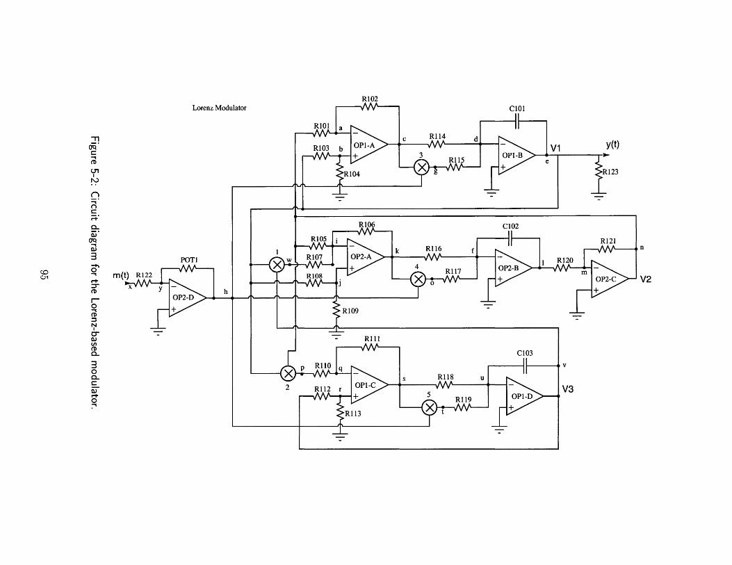
Lorenz Modulator

POTI

m(t) R122xmy

h- -D

n

V2

AAk X RI6 R f7

R109

-miOr.

-9

;W

01

-30)

0r1

C- 1

Iv

V3

x

1 '.

R102OAA- C101

RIO1R I O a O P - Ac R 1 1 4 d

y tR103 b + 3- -B v1 it

IRt4 x9 RI1 123

RIII

C103

RHO -q

Rl 10 Eqx s RI 18 U2 R112 r OPI-C

+ 5 R1 19 OPI-D

1:a l 13

x t

>

-n

Ln

01

(3

-

0~

-

0

3D

1

R202

R201a

R203 b OP1-A g

R204

R206 C201

k R214 R2fw R207 OP2-A -V/1 R218

x P2-B m

R209

R211

-0

y(t) e

A^ hm(t) -

V2

v

.V3

p ~~ R216 q C2 10

2 R212 r P-

+ ~ 4 tR217 OPI-D

R213

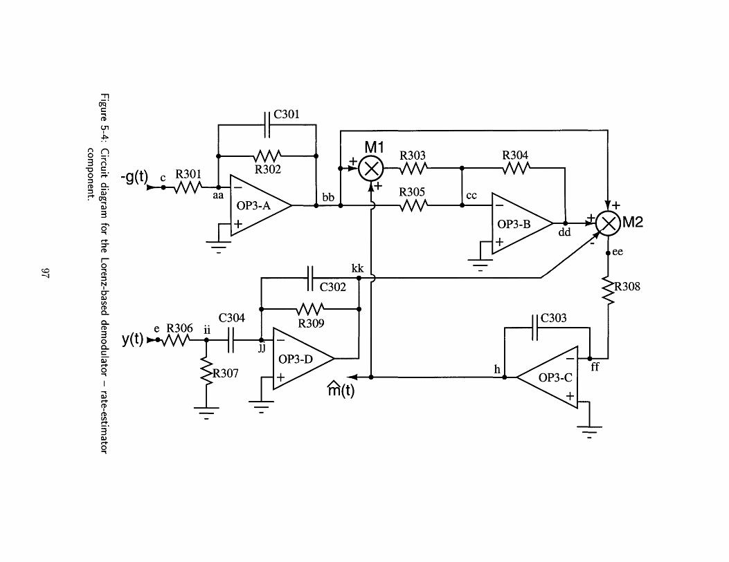
-g(t) c R301 R302

aa

JOP3-.A

(yq

0,

11)

CL

0

-9

(D

IDLA

0.)C+

0

e R306 ii

R307

n-0 M1 R303 R304

bb R305 c

C302 R308

3C30

Ah AfrrA At)

The equations describing the rate estimator behavior are

f = 1 1100C303 R309

R 3 04

R 305

+ R304 2 11OR303 ) R308'

C302R309(ri -I)

r2= 03 oR 302 (r ) -)

(5.6)

Component values are listed in Table 5.1. The resistors are the surface mount type

and have a 1% tolerance. The capacitors are axial lead polypropylene capacitors with

a 2.5% tolerance. The operational amplifier used is the OP467 by Analog Devices.

The analog multiplier used is the AD734 by Analog Devices. The choice of component

values makes w, ~ 196, 000, a 36, 700, and WL a 1, 960, 000.

Component I Value Component Value Component ValueR101 2kQ R102 2kQ R103 2kQR104 2kQ R105 68.1kQ R106 4.75kQR107 1.54kQ R108 4.75kQ R109 3.32kQR110 1.21kQ Rill 1.54kQ R112 10kQR113 2kQ R114 2.32kQ R115 1.24kQR116 1.74kQ R117 887Q R118 3.57kQR119 1.78kQ R120 lkQ R121 2k2R201 2kQ R202 2kQ R203 2kQR204 2kQ R205 68.lkQ R206 4.75kQR207 1.54kQ R208 4.75kQ R209 2.49kQR210 1.21kQ R211 1.54kQ R212 lOkQR213 2kQ R214 1.74kQ R215 887QR216 3.57kQ R217 1.78kQ R218 1kQR219 2kQR301 2.32kQ R302 2.32kQ R303 4.99kQR304 lOkQ R305 1OkQ R306 2kQR307 2kQ R308 1kQ R309 2.32kQC101 220pF C102 220pF C103 220pFC201 220pF C202 220pFC301 220pF C302 220pF C303 1OnF

Table 5.1: Passive component values.

98

5.2 Design Considerations

Analog circuits, especially those that have power in the radio frequency (RF) range,

must be designed carefully to avoid electro-magnetic interference, both internally and

externally generated. In this section, some of the design issues encountered in building

the prototype are discussed.

5.2.1 Fabrication

The circuit boards used were double-sided boards made by chemically etching the

circuit trace pattern. The circuit layouts for both sides of the modulator board and

the demodulator board are shown in Figure 5-5 and Figure 5-6, respectively. Two-

sided boards pose some problems because ground planes, power planes, and several

traces have to be broken to route the connections. Many traces had to be jumped

by breaking the trace on the board and reconnecting it using wire. Also, the ground

planes, which are the large black spaces in Figure 5-5 and Figure 5-6, had to be broken

up so that traces could be routed. These ground planes were then reconnected with

wire.

5.2.2 Circuit Layout

In laying out the circuit, the following considerations were important:

High frequency signals: Signal traces that are carrying the derivative signals 1,

2, 1V3, V2, and 13 were routed first. They were made as short as possible and

shielded by ground traces if possible. Also, if possible, two derivative traces

were not routed next to each other or next any IC pins that are sensitive to

these signals.

Ground returns: All signals have a return path to ground that terminates near the

signal source. This is particularly important for high frequency signals. If there

is no direct signal return, high frequency signals will couple electro-magnetically.

99

0 0Last Cap *. Ca.

a 00 0000000000 0

0 00000000 0 0

0 0 0000000

0 ~ ~ 0 000a00 ~ 00000000 I00 000'

0 0 00000000 0000000M 0 0

0 0 0

00000 0

(A)

0 0

00

(B)

0 0

Figure 5-5: Etch patterns for the component-side (A) and solder-side (B) of themodulator circuit (actual size).

100

00

0 00~ ~ 0 00OOOO0 0 0OO

0 0 0O

0 0 0(A)

0

0

0

0

(B)

0 0

Figure 5-6: Etch patterns for the component-side (A) and solder-side (B) of thedemodulator circuit (actual size).

101

00

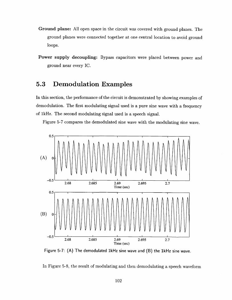
Ground plane: All open space in the circuit was covered with ground planes. The

ground planes were connected together at one central location to avoid ground

loops.

Power supply decoupling: Bypass capacitors were placed between power and

ground near every IC.

5.3 Demodulation Examples

In this section, the performance of the circuit is demonstrated by showing examples of

demodulation. The first modulating signal used is a pure sine wave with a frequency

of 1kHz. The second modulating signal used is a speech signal.

Figure 5-7 compares the demodulated sine wave with the modulating sine wave.

0.5

(A) 0

2.68 2.685 2.69 2.695 2.7Time (sec)

2.68 2.685 2.69Time (sec)

2.695 2.7

Figure 5-7: (A) The demodulated 1kHz sine wave and (B) the 1kHz sine wave.

In Figure 5-8, the result of modulating and then demodulating a speech waveform

102

-0.5

0.5

(B) 0

-0.5

I I

I I

I

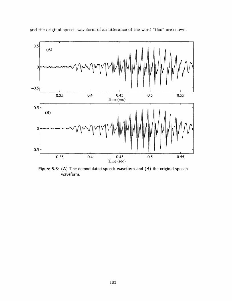
and the original speech waveform of an utterance of the word "this" are shown.

0.5-(A)

0

-0.5

0.35 0.4 0.45 0.5 0.55Time (sec)

0.5-

0(B)

-0.5--

0.35 0.4 0.45Time (sec)

0.5 0.55

Figure 5-8: (A) The demodulated speech waveform and (B) the original speechwaveform.

103

Chapter 6

Summary and Conclusions

In this thesis, a generalization of frequency modulation (FM) was developed that

was referred to as rate modulation. A rate modulator consists of a dynamical sys-

tem whose rate of evolution is modulated by a continuous-time information signal.

The carrier wave is a linear or nonlinear scalar function of the state variables of the

modulated dynamical system. Our approach to designing a corresponding rate de-

modulator assumed that the dynamical system used in the modulator has a known

exponentially convergent observer. The demodulator was constructed by systemat-

ically modifying the observer in a manner based on a new perturbation technique

developed in this thesis.

Chapter 2 began with a reinterpretation of FM from a dynamical systems per-

spective, which led to the more general notion of rate modulation. The remainder

of the chapter focused on the effect that modulation has on the bandwidth of the

modulated carrier wave. In particular, the power density spectrum of the modulated

carrier wave was related to the unmodulated carrier wave through a linear integral

transform. Because the relationship is linear and the effect of certain types of mod-

ulation is known when the carrier wave is sinusoidal, explicit representations were

found for the kernel of the integral transform. Knowledge of the kernel allowed the

power density spectrum of the modulated carrier to be determined from the power

density spectrum of the unmodulated carrier wave. The special case of the Lorenz

system was also examined. The power density spectrum of the first state variable of

105

the Lorenz system can be approximated with a decaying exponential. Because of this

special structure of the power density spectrum, an explicit formula was obtained for

the autocorrelation function of the modulated carrier wave, from which the power

density spectrum was determined.

In Chapter 3, the design of demodulators was described. To design the demodu-

lators, a new perturbation technique that was developed in this thesis was used that

is referred to as a backwards perturbation expansion. In the perturbation technique,

the modulator state variables are expanded about the demodulator state variables in

terms of the rate estimate error. This produces expansion terms that depend only on

signals that are local to the demodulator. These expansion variables can then be com-

bined in such a way that the demodulator converges exponentially to the state and

rate of the modulator. The demodulators obtained from the perturbation technique

were then modified to enhance aspects of their performance. First, a filter was added

in the feedback path of the rate estimate to smooth the rate estimate. Second, it was

empirically shown that the rate estimator could be modified so that the demodulator

can track signals that vary more rapidly. Finally, the rate estimator was simplified

by approximating the nonlinear, time-varying components with linear, time-invariant

components. The chapter concluded by showing how the resulting demodulator is

equivalent to a least-squares approach to demodulation.

In Chapter 4, the probability density functions of the state variables of the de-

modulator were approximated when the carrier wave was corrupted with additive

white Gaussian noise. When a dynamical system is driven by white noise, it be-

comes a stochastic differential equation and cannot be analyzed with the usual rules

of calculus. In the beginning of the chapter, results from the theory of stochastic

differential equations were briefly overviewed along with the related It6 calculus that

is drawn upon throughout the remainder of the chapter. It6's change of variables

formula was then used to generate the differential equations that describe the evo-

lution of the time-varying moments of the state-variables. For nonlinear systems,

low-order moment equations depend on higher-order moments, leading to an infinite

hierarchy of equations. This set of equations was closed by the quasi-moment neglect

106

closure technique. Essentially, this technique is based on approximating the probabil-

ity distribution of the state variables as a truncated Edgeworth series. Truncating the

Edgeworth series at order N closes the moment equations at order N, and the moment

equations can then be solved. In the examples, the Edgeworth series was truncated at

second order, which means that the distribution of the state variables was assumed to

be Gaussian. As the input SNR is increased, the effects of the nonlinearities becomes

more significant and the Gaussian approximation is no longer valid. In this case, the

moment equations became unstable. Therefore, the QMNC technique can only be

used when the input SNR is sufficiently high.

Finally, in Chapter 5, a circuit implementation of a Lorenz based modulator and

demodulator systems was presented. The prototype circuit was described and an

example of demodulation of a sine wave speech waveform was included.

6.1 Suggestions for Further Research

In this thesis, the foundation for rate modulation and demodulation has been laid.

Several unanswered questions remain and many new directions remain to be explored.

For example, the perturbation expansion presented in Appendix A is more general

than the manner in which it was used in this thesis. In particular, the perturbation

expansion technique resulted in a systematic technique for tracking multiple unknown

parameters that appear nonlinearly in a dynamical system that has a known exponen-

tially convergent observer when the parameters are fixed and known. This presents

two immediate avenues to explore. First, instead of modulating the rate of evolu-

tion, a parameter could be modulated proportional to an information signal and a

demodulator could be constructed using the perturbation technique. Second, the per-

turbation technique allows for more than one parameter to be tracked, which suggests

that some type of multiplexing scheme is possible for rate modulation systems.

Another new area to explore is the use of time-varying dynamical systems. In this

thesis, only autonomous dynamical systems were used. Many of the ideas and results

that were presented can be carried over to time-varying systems provided that the

107

modulator and demodulator are synchronized in time. Using time-varying systems

could lead to a type of generalized frequency-hopping.

Yet another direction that could be pursued is one of analog channel coding. Rate

modulation allows the carrier wave to be choosen from a large class of waveforms.

Perhaps it is possible to search over the class waveforms to find a carrier wave that

is in some sense optimal. For example, it may be possible to find an optimal carrier

wave for a channel with a particular type of distortion.

In addition to these new directions, there are fundamental aspects of rate mod-

ulation that have yet to be analyzed. For example, in designing the demodulator,

convergence was forced when the modulating signal was an unknown constant. It was

then assumed that the demodulator would be able to track slowly varying signals,

The ability to track non-constant signals was demonstrated, but this was not verified

analytically. Also, the constraints on the rate at which the modulating signal can

vary were not determined. Currently, these constraints are determined by trial and

error.

As mentioned in the beginning of this chapter, this thesis constitutes the foun-

dations for rate modulation and demodulation and there remain many unanswered

questions regarding the practicality and potential benefits of rate modulation in com-

parison to standard modulation schemes.

108

Appendix A

Parameter Tracking by a

Backwards Perturbation Expansion

Many systems have parameters that vary as a function of time. In this appendix, it

is shown how parameter variations can be tracked when the dynamical system has a

known exponentially convergent local observer for the case in which the parameters

are fixed and known, and the observed output of the dynamical system satisfies an

observability condition.

Perturbation Expansion The case in which there is only one unknown parameter

is considered first. The system that is derived to track the unknown parameter

is an augmentation of the known observer. The augmented observer is derived by

expressing the state of the dynamical system as a perturbation expansion about the

observer state in terms of the parameter estimate error. Specifically, the dynamical

system is

x=F(x; 0), (A.1)

where 0 is the unknown parameter and x is assumed to be confined to a region of RN,

that is, x E D C RN. The observed output is a scalar function of the state variables,

y = h(x). (A.2)

109

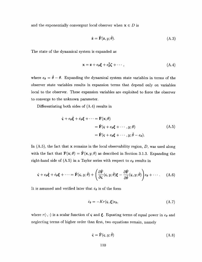
and the exponentially convergent local observer when x E D is

z = F(z, y; 0). (A.3)

The state of the dynamical system is expanded as

x=z0+ eo+ e C --- , (A.4)

where eo = 6 - 6. Expanding the dynamical system state variables in terms of the

observer state variables results in expansion terms that depend only on variables

local to the observer. These expansion variables are exploited to force the observer

to converge to the unknown parameter.

Differentiating both sides of (A.4) results in

+ eoC + e0(+ --- = F(x;6)

= F(4 + eot+- ,y;0) (A.5)

=F(+eo±+- ,y;O-eo).

In (A.5), the fact that x remains in the local observability region, D, was used along

with the fact that F(x; 0) = P(x, y; 0) as described in Section 3.1.3. Expanding the

right-hand side of (A.5) in a Taylor series with respect to eo results in

S+ eo + do + - F(q, y; 0) + -(q, y; 0) - - (4;, y; 0) eo + ---. (A.6)

It is assumed and verified later that 6o is of the form

o = -Kr(4, )eo, (A.7)

where r(., -) is a scalar function of ; and . Equating terms of equal power in eo and

neglecting terms of higher order than first, two equations remain, namely

= F(Cy; 0) (A.8)

110

and

-(a(4, y; ) + Kr~g O) F (4;, y, ).(A.9)

From (A.8), ; = z. The equation in (A.9) generates the first-order term of the

perturbation expansion. For the perturbation expansion to be valid, this expansion

term must be bounded.

Boundedness of the Expansion The exponential stability of the observer is used

to show that the perturbation term, , remains bounded. When there is no parameter

mismatch, the error between the dynamical system and the observer evolves according

to

F& (z, y; 9) - F(z - ez, y; 9). (A.10)

The assumption that the observer is exponentially stable is equivalent to (A.10) hav-

ing an exponentially stable equilibrium point at e. = 0. A nonlinear system has an

exponentially stable equilibrium point at ez = 0 if and only if the corresponding lin-

earized system has an exponentially stable equilibrium point at e7 = 0 [6]. Therefore,

the system given byOFez = (z, y; 6)ez (A.11)

has an exponentially stable equilibrium point at ez = 0. The perturbed system given

by

S= (F(z, y; ) + Kr(z, ez) ez (A.12)az

is also exponentially stable for 0 < K < K, for some sufficiently small K, [6]. An ex-

ponentially stable linear system is bounded input-bounded output (BIBO) stable [9].

Since T(z, y; b) is bounded,

6Z = Z, ; + Kr(z, ez) ez - 9 (Z, y; 0) (.3

results in a bounded ez. But (A.13) is identical to (A.9), which means that is

bounded and the perturbation expansion is valid. Moreover, is determined by z,

111

y, and 0, all of which are local to the observer, which means that each can be

generated at the observer.

Forcing the Parameter Error to Zero Because is local to the observer, it can

be generated in the observer and used to force convergence.

A signal is said to be persistently exciting if, for any 6 > 0,

t+j

f(y(t))2dt > 0 (A.14)t

for all t. In other words, a signal that is persistently exciting can cross zero, but

cannot remain at zero for any length of time.

The difference between y = h(x) and 9 = h(z) can be approximated as

S-y =h(z) - h(x)

=h(z) - h(z + eo +---) (A.15)ch

= z(z) eo +---.

Since each can be generated at the observer, 0 can be chosen to be

= K(9 - y)g -z(z) -(A.16)

where g(.) is a real-valued function that has the property sgn(g(a)) = sgn(a), that is,

g(.) has the same sign as its argument. This gives, to first-order,

(Oh \ Oh0=-K( (z) g(-(z) eo

ah ah (A.17)0=-K z(Z). -g(&z-( o -0).

To clarify the behavior of 9, its equation of motion can be written as

0 = a(t)(O - 0), (A.18)

112

where the time-varying coefficient, a(t), is

a(t) = -K (z) ( - g ( z) - < 0. (A.19)az az

Rewriting (A.18) in terms of the error between 6 and 6 results in

d0 = a(t)eo. (A.20)

The solution to (A.20) is

eo = cefo a(r)d-, (A.21)

where c = 6(0) - 0. Assuming that 2(z) - is persistently exciting, efa(ar)d-r is

a monotonically decreasing and goes to zero as t -+ oo. From (A.21), eo = 0 is a

uniformly asymptotically stable equilibrium point. A linear system that is uniformly

asymptotically stable is also uniformly exponentially stable [9]. It follows that z

converges to x exponentially as well [6]. This means that the augmented observer is

an exponentially stable local observer of the dynamical system when 6 is unknown.

The assumption made during the derivation of the perturbation expansion that

dO = -Kr(z, )eo (A.22)

is valid with

r, (z,) = hB (Z) - -g (,h (z) -(.(A.23)

Since the augmented observer for one unknown is an exponentially convergent

local observer, it can be used as the basis for a further augmented observers when

there are additional unknown parameters.

113

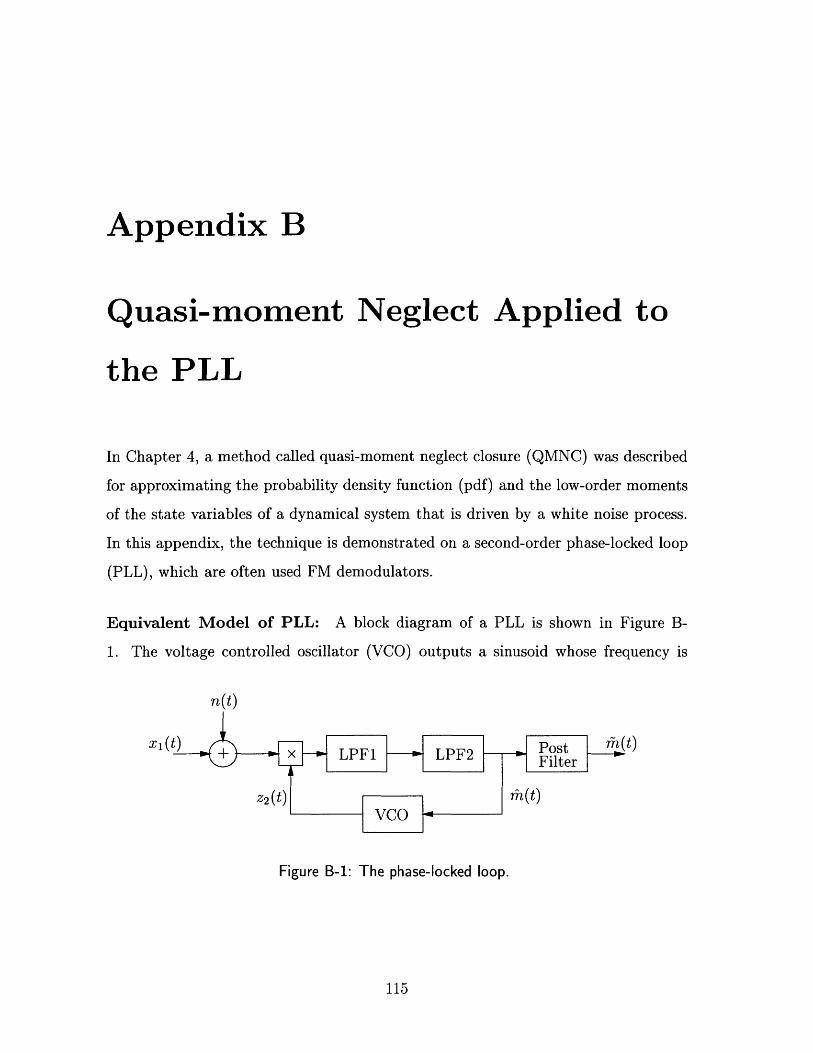
Appendix B

Quasi-moment Neglect Applied to

the PLL

In Chapter 4, a method called quasi-moment neglect closure (QMNC) was described

for approximating the probability density function (pdf) and the low-order moments

of the state variables of a dynamical system that is driven by a white noise process.

In this appendix, the technique is demonstrated on a second-order phase-locked loop

(PLL), which are often used FM demodulators.

Equivalent Model of PLL: A block diagram of a PLL is shown in Figure B-

1. The voltage controlled oscillator (VCO) outputs a sinusoid whose frequency is

n(t)

X1 (t) + x LPF1 LPF2 - oster W

Z2 (t) - r07n(t)

Figure B-1: The phase-locked loop.

115

proportional to the input. That is,

z2 (t) = sin (wet + frn(-)dr), (B.1)

where w, is the zero-input frequency of the VCO. The input to the first low-pass filter,

labeled LPF1 in Figure B-1, is

(x1(t)+n(t))z2 (t) = K sin (J (Om(T) - rn(r))dT)

+ K sin (2wet + f(3m(r) + rnh(T))dT)

(B.2)- Kn,(t) sin(] rn(T)dT) + Knrc(t) cos(] 11(T)dT)

± Kn,(t) sin(2w, + J ^n(-r)dT) + Knc(t) cos(2wet + J n(Tr)dr).

The derivation of (B.2) uses the fact that a zero-mean Gaussian process that has a

power density spectrum equal to N0/2 for Iwj < B (rad/sec) and zero elsewhere can

be represented as

n(t) = v2 (n,(t) sin(wct) + n,(t) cos(wet)), (B.3)

where n8 (t) and nc(t) are independent, zero-mean Gaussian processes that also have

a PSD that is equal to N0 /2 for jwj < B (rad/sec) and negligible elsewhere [13].

The first low-pass filter, LPF1, has a cut-off frequency of w, and is assumed

remove all components in (B.2) centered at w = 2w,. Representing the noise terms

that remain after filtering as

h (t) = -ns (t) sin(J ?n(T)dT) + nc(t) cos(J rn(T)dT), (B.4)

the output of the first low-pass filter is

r(t) = K( sin (f (m(T) - fn(r))d-) + h(t))L, (B.5)

where ()L represents the operation of the low-pass filter. It can be shown that

116

the power density spectrum of h(t) is equal to N0 /2 over the bandwidth of the PLL.

Therefore, (O(t))L can be treated as a Gaussian process with a power density spectrum

level equal to N0/2 [13]. The second low-pass filter, LPF2, smooths r(t) before it is

input into the VCO and has a transfer function of the form

H(s) = 1 + . (B.6)S

Using filter transfer function given in (B.6), the second order PLL is given by

do = aK(sin($)dt + dW(t)),

d$ = /mdt - (4dt + K sin($)dt + KdW (t)),

d = APsdt + Bp (4dt + K sin(q)dt + KdW(t)), (B.7)

fn = Cps,

where dW(t) is a Gaussian white noise process with a power density spectrum level of

nr2and A, Bp, and Cp correspond to the space-space implementation of the post-filter.

The block diagram of the system given in (B.7) is shown in Figure B-2.

dW(t)

+ sin(-

#rfn(t) +K

Pst- fn(t)

Figure B-2: A model of the phase-locked loop.

117

Quasi-moment Neglect Applied to the Two Dimensional PLL: To demon-

strate the QMNC technique on the PLL, LPF1 and the post-filter are excluded. This

makes the system equations

do = aK(sin(#)dt + dW(t)),

do = Omdt - (odt + K sin(#)dt + KdW(t)).

The quasi-moment neglect technique allows only nonlinearities that are polyno-

mials. Taking a fourth-order Taylor series expansion of the sin(.) terms gives

1do = aK(pdt - #3dt + dW(t)),

(B.9)d# = /mdt - (odt + K(qdt - #q3 dt) + KdW(t)).

To generate the moment equations, (4.9) is used. E[4] is obtained by setting

h(4, q) = 4 and substituting this into (4.9), giving

dE[4'] _13

dt = aK(E[#] - 1E[3]). (B.10)

Similarly, E[] is obtained by setting h(o, #) = 0, which gives

dE[o] = #E[m] - E[O] - K(E[] - I E[03]). (B.11)

The rest of the moments up to third order are obtained in a similar manner and they

are listed in Table B.1. In the table, the notation used is

mk1 = E [Ok#l]. (B.12)

For example, m, = E[00] and M20 = E[0 2 ]. The modulating signal, m(t), was taken

to be zero and r72 is the level of the power density spectrum of the white noise process,

dW(t).

To close the moment equations in Table B.1, moments above third order must

be expressed as moments at or below third order. The moments that are above

118

h(V), #) Moment Equation

OaK(moi - 1mo3 )

dmpi -nidt -i - K(moi - ymo3)

i2 n2 = aK(2mn - }m 13) + 2K 2 72

dmi 1 aK(mo2 - -mo 4 ) - M 20 + K( mi3 - mn)

#2 di 2 = -2mnl + K(}mo4 - 2mO2 ) + K 2r12

dt3

3 d aK(3M21 - }M 2 3 ) + 3aK m2,2mo

24 d =2 1 aK(2ml2 - 1M14) + K(1 m23 - m21) - M 30 + a2K2772o

2 =12 aK(M - iM0 5 ) + K(iM14 - 2m 12 ) - 2m 2 1 + K 2 772 m 10

3 =ng3 K(}m05 - 3mO3) - 3m 12 + 3K 2r 2mo1

Table B.1: Moment equations for the PLL.

third order that appear in the set of equations in Table B.1 are M 1 3 , M0 4, M 2 3, M 14 ,

and M0 5 . The moment equations are closed by setting the quasi-moments above

the third order to zero. Following the same procedure used in Section 4.3 to find

the quasi-moment-moment relationships for a one dimensional system, the quasi-

moment-moment relationships for a two dimensional system are shown in Table B.2

for Mi13 , M0 4 , M 23 , M 14 , and m0 5 . Setting all of the quasi-moments above order three

to zero results in moment-quasi-moment relationships shown in Table B.3.

Just as with the one-dimensional case, the quasi-moments are expressed in terms

of the moments by inverting the relationship established by (4.14) and (4.18). The

relationships for up to third order are shown in Table B.4. The equations in Table B.4

are symmetric, meaning that b03 can be obtained from b3o be interchanging the first

and second indices in every term, e.g.,

b03 = n 03 - 3moimO2 + 2mi (B.13)

Substituting the quasi-moment-moment relationships shown in Table B.4 into the

119

Table B.2: Moments expressed in terms of quasi-moments.

M04= 4b03b01 + 3bO2 + 6bO2bl 1 + bo1

M13= 3b12b01 + 3bllbO2 + 3bn bo, + bo1b03 + 3biobO2boi + biobo1

M05 = 10bO3bO2 + 1ObO3b21 + 15bo2b01 + 10bO2b 1 + bo1

M14= 6b1 2bO2 + 6b1 2b21 + 4bnjbO3 + 12bjjbO2bo1

+ 4bnlbo1 + 4b10b03b01 + 3b10bO2 + 6b10 bO2bo1 + b10bo1

n 2 3 = 3b20b02bo1 + 3b21 bo1 + bio bg1 + 3biob02 boj + 6biob01 b12

+ 6b10bO2bnl + b20bo1 + 3b21bO2 + b20bO + 6bjjb 12

+ 6biiboi + bIObO + 6biobolbn1

Table B.3: Moments expressed in terms of quasi-moments after applying thirdorder quasi-moment neglect.

b30 = in 3 0 - 3inOm20 + 2i3

b21 = M 2 1 - 2ioml + 2moimi - Mim1 n 2 O

Table B.4: Quasi-moments expressed in terms of moments.

120

M= b04 + 4bO3bo1 + 3b 2 + 6b0 2bi 1 + b41

m 13 =b 13 + 3b1 2b01 + 3bllbO2 + 3b11 boi + bo1b03 + 3biobO2bol + biob21

Tn5= b05 + 5bO4bO1 + 10bO3bO2 + 1ObO3b$1 + 15b 2bo1 + 10bO2b01 + b01

m14= b1 4 + 4b1 3b01 + 6b1 2bO2 + 6b1 2bo1 + 4b11 bO + 12bjjbO2bo1

+ 4bnlbg1 + b10 b04 + 4b10 bO3bo1 + 3b10 b$2 + 6b10b02 bl 1 + b10b41

m23= 3b20bo2bi + 3b21 bo1 + blobo1 + 3bob02boi + 6biob01 b12

+ 6b10 bO2bnl + b2ob1 + b2 3 + 3b22bo1 + 3b21 bO2 + b20bO + 6bjjb 12

+ 6b(1b01 + 2b10b13 + bjObO + 6biobolb11

dmi 1di - aK(moi - IM0 3 )dt 6

din1 - -nio - K(moi - M03)

dM = 2aKmll - 1aK(3moim 12 - 6m21m 1 + 6miom 1

- 6momOm0 2 + 3m11 mO2 + mIOmO3 ) + Q2K 2 ) 2

dt = cKm02 - aK(4moimo3 - 12m 1m 02 + 6m + 3m02 ) - M 20

- Km 11 + 1K(3moim1 2 - 6m21mi, + 6mom 16 00

- 6m0oiM1OmO2 + 3m11 mO2 + MiOm03 )

di 02 = -2n 1 1 - 2KmO2 + IK(4moMo 3 - 12m21m 0 2 + 6m41 + 3m22 ) + K 2 q 2

din 3 3 1

dt = 3aKm21 - 1caK(-6minomm1ino 2 - 3inoM 20 2 + 3m 21iM0 2

2 32

+ 6m1 0 m0 1 + m 20 mOs - 6moinm2 1 + 6m 1 m1 2) + 3a 2K 2 2m 10

din 2 1 __12

dt = 2aKm1 2 - 1ocK(6m12mo 2 + 6mom4i1 + 4m1 m0O - 3miom 231

- 12moimumo2) - n 30 - Km 21 + 1K(-6miomumo 2

- 3m 1Om 20mO2 + 3m 21m 2 + 6mio0m 1 + m 20mO3 - 6mo 1m( 1+

6m1 1 m 12 ) + a 2 K 2 2mOI

din12 _1

dt = cKm03 - -aK(10n 3 m 2 - 15mim02 + 6m81 ) - 2m 2 1 + -2Km 1 2

1+ IK(6m1 2mO2 + 6miomn4 1 + 4mIiM0 3 - 3miom 2

3 00

12m0om 1 1 m 0 2 ) + K 2 77 2m 1 0

di 03 - -3m 12 - 3KmO3 + IK(1Omo3 mo2 - 15mim22 + 6m21) + 3K 2 2m01

(B.14)

Table B.5: Closed moment equations for the PLL.

121

moments equations shown in Table B.3, the moments up to fifth order are expressed in

terms of moments at or below third order. The differential equations for the moments

are now closed and are shown in Table B.5.

Quasi-moment Neglect Applied to the PLL with the Post-filter: Adding

the post-filter filter to the PLL results in the system given in (B.7). Using a third

order Taylor series to approximate the sin(.) function gives

13dO = aK($dt - 1q3 dt + dW(t)) (B.15)

6

do = /mdt - (V$dt + Kdt - K 103dt + KdW(t)) (B.16)6

A = Apdt + Bp41 (Vbdt + Kdt - K 1#3dt + KdW(t)) (B.17)

i = C,,s, (B.18)

where dW(t) is a Gaussian white noise processand A,, B,, and C correspond to

the space-space implementation of the post-filter. The post-filter has a dimension of

five, making the entire PLL system have a dimension of seven. Second order QMNC

requires the first and second order moments. The second order moments correspond

to a symmetric seven by seven covariance matrix, which has twenty-eight unique

entries. There are seven first order moments, bringing the total dimension of the

differential moment equations to thirty-five.

Bandwidth of Modulated Signal: The bandwidth of the FM signal is, from

Carson's rule described in Chapter 2, approximately 2(03+ 1)wm when y(t) = cos(PC +

1 sin(wmt)). The input signal is m(t) = wm cos(wmt), which makes Pm = m 2 (t) =

wM/2. The baseband SNR is

SNRb == 10 log 0 7r) dB. (B.19)

SNRb corresponds to the output SNR when the information signal, m(t), is sent

directly through the additive white noise channel and then filtered with a low-pass

122

filter with a cut-off frequency of win. Therefore, plotting SNRout as a function of

SNRb shows how rate modulation compares to using no modulation. The SNR at the

output of the post filter is

(B.20)SNROut = 10 log 0 2= dB.((fn - M)2

Results: In presenting the results, the noise output of the demodulator is assumed

to be independent of the modulating signal, m(t), which was shown by Sakrison [10].

This assumption allows the modulating signal to be set to zero to simplify the numer-

ical simulations. Figure B-3 shows the demodulator output SNR versus the baseband

output SNR for # = 2, 5, and 10. From the plot, increasing # increases the noise

60

50 -

401-F

0

30 -

20 H

10k_

05 10 15 20

SNRb

25 30 35

Figure B-3: SNRut vs. SNRb for ,3 = 2, 5, and 10 for the PLL.

immunity.

123

p=10

P=2

SNR =SN

....... ;-:............. . .. . . ..... ........................

The results of the QMNC technique are compared with a direct simulation of

the SDE. The direct simulation corresponds to # = 2 and SNRb = 14 dB, which

corresponds to the data point marked with a star in Figure B-3. From the direct

simulation, the estimated output SNR is 23.24 dB and the QMNC technique estimates

the output SNR to be 23.35 dB. The pdf of the output noise process estimated from

the direct simulation and the pdf estimated from the QMNC technique are compared

in Figure B-4.

10

8- .

6-

4-

2-

0-0.2 0 0.2

Figure B-4: A comparison of the pdfs for the PLL obtained from the QMNCtechnique (solid line) and a direct simulation (dots).

Threshold: The PLL exhibits a threshold [11]. At the threshold, the SNR output

of the PLL drops of dramatically as SNRb is decreased. Second order QMNC is

not capable of capturing this phenomenon. Instead the moment equation become

unstable. In Figure B-3, the points where the SNR curves terminate are the points

at which the equations became unstable. However, these points do not necessarily

correspond to the threshold points.

Comparison of QMNC and Analytical Results: For the high input SNR case,

the relationship between SNRout and SNRb for a linearization of the PLL model shown

in Figure B-2 is [11]

SNROUt = 3 2SNRb. (B.21)2

124

Table B.6 compares the output SNR predicted by the QMNC technique to the output

SNR predicted by the linearized PLL.

2 5 10SNRb QMNC Linear QMNC Linear QMNC Linear

35 43.92 42.78 51.60 50.74 57.90 56.7632 40.92 39.78 48.88 47.74 54.90 53.7629 37.91 36.78 45.87 44.74 51.89 50.7626 34.89 33.78 42.84 41.74 48.87 47.7623 31.84 30.78 39.80 38.74 45.82 44.7620 28.75 27.78 36.71 35.74 42.73 41.76

Table B.6: A comparison of the PLL output SNR predicted by QMNC and thatpredicted by a linearized model of the PLL.

125

Bibliography

[1] F. Bowman. Introduction to Bessel Functions. Dover Publications, New York,

1958.

[2] R. W. Brockett. Notes on stochastic control. Course notes., 2000.

[3] Leon W. Couch. Digital and Analog Communication Systems. Prentice-Hall,

Upper Saddle River, NJ, sixth edition, 2000.

[4] C. W. Gardiner. Handbook of Stochastic Methods for Physics, Chemistry and

the Natural Sciences. Springer Series in Synergetics. Springer-Verlag, Berlin,

Germany, second edition, 1985.

[5] A. H. Jazwinski. Stochastic Processes and Filtering Theory. Mathematics in

Science and Engineering. Academic Press, New York, New York, 1970.

[6] H. K. Khalil. Nonlinear Systems. Prentice-Hall, Upper Saddle River, NJ, second

edition, 1996.

[7] E. N. Lorenz. Deterministic nonperiodic flow. Journal of the Atmospheric Sci-

ences, 20:130-141, March 1963.

[8] J. B. Roberts and P. D. Spanos. Random Vibration and Statistical Linearization.

John Wiley & Sons, New York, New York, 1990.

[9] W. J. Rugh. Linear System Theory. Prentice-Hall, Upper Saddle River, NJ,

second edition, 1996.

127

[10] D. Sakrison. Communication Theory. John Wiley & Sons, Inc., New York, New

York, 1968.

[11] H. Taub and D. Schulling. Principles of Communication Systems. McGraw Hill,

New York, New York, second edition, 1986.

[12] M. Unser, A. Aldroubi, and M. Eden. B-spline signal processing: Part i - theory.

IEEE Trans. on Sig. Proc., 41(2):821-833, February 1993.

[13] Andrew J. Viterbi. Principles of Coherent Communication. McGraw-Hill Series

in Systems Science. McGraw-Hill, New York, New York, 1966.

[14] A. Wolf, J. B. Swift, H. L. Swinney, and J. A. Vastano. Determining lyapunov

exponents from a time series. Physica D, 16D(3):285-317, July 1985.

128

Generalized Frequency Modulation Wade P. Torres - DSpace ...

Documents

Transcript of Generalized Frequency Modulation Wade P. Torres - DSpace ...