Gas-kinetic schemes for direct numerical simulations of compressible homogeneous turbulence

Gas-kinetic schemes for direct numerical simulations of compressible homogeneous turbulence

Wei Liao,* Yan Peng,† and Li-Shi Luo‡

Department of Mathematics and Statistics and Center for Computational Sciences, Old Dominion University,Norfolk, Virginia 23529, USA

�Received 12 June 2009; published 14 October 2009�

We apply the gas-kinetic scheme �GKS� for the direct numerical simulations �DNSs� of compressibledecaying homogeneous isotropic turbulence �DHIT�. We intend to study the accuracy, stability, and efficiencyof the gas-kinetic scheme for DNS of compressible homogeneous turbulence depending on both flow condi-tions and numerics. In particular, we study the GKS with multidimensional, quasi-one-dimensional,dimensional-splitting, and smooth-flow approximations. We simulate the compressible DHIT with the Taylormicroscale Reynolds number Re�=72.0 and the turbulence Mach number Mat between 0.1 and 0.6. Wecompute the low-order statistical quantities including the total kinetic energy K�t�, the dissipation rate ��t�, theskewness Su�t�, and the flatness Fu�t� of the velocity field u�x , t�. We assess the effects on the turbulencestatistics due to the approximations made in the treatment of fluxes, the flux limiter, the accuracy of theinterpolation, and the bulk viscosity. Our results show that the GKS is adequate for DNS of compressiblehomogeneous turbulence as far as the low-order turbulence statistics are concerned.

DOI: 10.1103/PhysRevE.80.046702 PACS number�s�: 47.11.�j, 47.40.�x, 94.05.Lk, 47.45.Ab

I. INTRODUCTION

Compressible turbulence has been a subject of interest fora long time �1–14�. In compressible turbulence, the Kolmog-orov paradigm, which forms the basis of most equilibriumturbulence models, is questionable. This is due to the factthat there can be baroclinic-type production of energy at allscales of turbulence, including the inertial range, invalidatingthe Kolmogorov hypotheses. Consequently, the premises ofmost existing closure models for turbulence may not be validany more, thus the turbulent mass, energy and momentumtransport in compressible turbulence may not be amenable tostandard treatment. Hence, physics-based modeling of com-pressible turbulence must start from fundamental first prin-ciples.

Recently, there has been an intense effort to use directnumerical simulation �DNS� for shock/turbulent boundarylayer interactions �STBLI� �cf., e.g., �15–19� and a recentsurvey �20��, which are critically important for high-speedflows. The hope is that by vigorously interrogating data gen-erated by high-fidelity DNS, one can gain insights into flowphysics, which can in turn provide guidelines for turbulencemodeling. To ensure high fidelity of DNS for compressibleturbulent flows, the numerical methods are required to haveminimal numerical dissipation and high bandwidth effi-ciency. These requirements naturally favor high-order meth-ods. However, when shocks are considered, these require-ments are more difficult to satisfy because they conflict withthe stability requirement for shock capturing. The generalsolution to this conflict is a judicious addition of numericaldissipation in the neighborhood of shocks, which are treatedas discontinuities �Godunov type of approaches �21–23��,while maintaining the desired �high� order of accuracy insmooth flow regions.

For compressible homogeneous isotropic turbulence inthree dimensions, high-order methods which have been usedfor the purpose of DNS include the pseudospectral �PS�method �2,3,6,7�, the high-order compact finite-differencescheme �4,10,13,24�, and the fourth-order weighted essentialnonoscillatory �WENO� scheme �25–27�. For homogeneousturbulence with high turbulence Mach number, shocklets areubiquitous, and the Godunov-type methods become nomi-nally first-order accurate across discontinuities, regardless ofthe order of accuracy of the interpolation used in reconstruc-tion. Whether high-order schemes are more accurate and ef-ficient than second-order schemes for flows with discontinui-ties is a subject of ongoing debate �20,28,29�.

In this study we will use the gas-kinetic scheme �GKS��30,31� for direct numerical simulations of the compressibledecaying homogeneous isotropic turbulence �DHIT�. TheGKS is a second-order finite-volume kinetic scheme derivedfrom the Boltzmann equation as opposed to conventionalmethods of computational fluid dynamics �CFD� based ondiscretizations of the Navier-Stokes equations. In contrast toconventional CFD methods, kinetic methods have two dis-tinctive features. First, kinetic methods have the potential toinclude extended hydrodynamics beyond the validity of theNavier-Stokes equations because kinetic methods are basedon kinetic theory and the Boltzmann equation, which providethe theoretical connection between hydrodynamics and theunderlying microscopic physics. And, second, the Boltzmannequation is a first-order integro-partial-differential equationwith a linear advection term, while the Navier-Stokes equa-tion is a second-order partial differential equation with anonlinear advection term. The nonlinearity in the Boltzmannequation resides in its collision term, which is local. Thisfeature may lead to some computational advantages �32�.

Compared to most conventional CFD methods, the GKSis relatively new and is still a topic of active research �e.g.,�31,33–40��. Despite the fact that the GKS has been appliedto simulate a wide variety of flow problems, such as non-equilibrium hypersonic flows with STBLIs �35,39,41�, shockstructures in gases �40,42–45�, scalar transport and mixing incompressible flows �46–49�, chemically reacting multicom-

*[email protected]†[email protected]‡[email protected]

PHYSICAL REVIEW E 80, 046702 �2009�

1539-3755/2009/80�4�/046702�26� ©2009 The American Physical Society046702-1

http://dx.doi.org/10.1103/PhysRevE.80.046702

ponent compressible flows �50–52�, nonequilibrium microf-lows �53,54�, magnetohydrodynamics �55,56�, and solutionsof the shallow water equation �57–60�, little has been done inthe application of the GKS for DNS of compressible homo-geneous turbulence �61�. It is well known that DNS of ho-mogeneous turbulence are particularly sensitive to, amongother things, numerical dissipations and thus are challengingfor a second-order method.

The main objective of this work is to investigate the nu-merical accuracy, stability, and efficiency of the GKS forDNS of compressible DHIT in three dimensions. We willinvestigate the effects due to the approximations in the fluxcalculations, the flux limiters, the accuracy of the interpola-tion in reconstruction, and the bulk viscosity on the low-order statistical turbulence quantities, which include the ki-netic energy K�t�, the dissipation rate ��t�, and the skewnessSu�t� and the flatness Fu�t� of the velocity field u�x , t�. Wewill simulate compressible DHIT with the initial turbulenceMach number Mat ranging from 0.1 to 0.6, corresponding tonear incompressible to fully compressible flow regions.

The remaining part of this paper is organized as follows.In Sec. II we discuss in detail �a� the construction of the fullmultidimensional �MD� GKS; �b� the quasi-one-dimensional�Q1D� and the dimensional-splitting �DS� gas-kineticschemes, which are simpler thus more efficient than the fullGKS; �c� the simplified GKS for smooth �incompressible�flows which is considerably simpler and efficient than thefull GKS; and �d� the limiter, the interpolations used in thereconstruction, and the bulk viscosity in the GKS. In Sec. IIIwe discuss the governing equations and flow conditions forthe compressible DHIT, as well as the low-order statisticalturbulence quantities to be computed. We also show sometesting results to validate our code. In Sec. IV we present ourmain results. We first evaluate the necessity of using the fullmultidimensional GKS by comparing the results obtainedwith the Q1D-GKS, DS-GKS, and full MD-GKS. We test theMach-number limit in the simplified GKS for smooth flows.We next investigate the effects due to the flux limiter, theinterpolation, and the bulk viscosity on the low-order turbu-lence statistics. Finally, we conclude the paper in Sec. V.

II. GAS-KINETIC SCHEME

In this section we provide the details in the constructionof the full MD GKS and several simplified versions of it,including the Q1D, DS, and the simplified GKS for smoothflows. We also discuss artificial dissipation, flux limiter, in-terpolations at cell boundaries, and the bulk viscosity in theGKS. We intend to provide sufficient details here so the GKScan be easily implemented and the results can be easily re-produced by our readers.

A. Construction of gas-kinetic scheme

To construct the full multidimensional gas-kinetic schemefor compressible flows �30,31,39,40�, we begin with the lin-earized Boltzmann equation �cf., e.g., �62��:

�t f + � · �f = L�f , f� , �1�

where fª f�x ,� ,� , t� is the single particle distribution func-tion of space x, the particle velocity �ª x, the particle inter-

nal degrees of freedom � of Z dimensions, and the time t; Lis the linearized collision operator. For the sake of simplicityand without losing generality in the context of the linearizedBoltzmann equation, we will use the Bhatnagar-Gross-Krook�BGK� single relaxation-time model for L �63�:

�t f + � · �f = −1

��f − f �0�� , �2�

where � is the relaxation time related to the mean free timebetween successive collisions and f �0� is the Maxwellianequilibrium distribution function of D dimensions,

f �0� = ��

2��D+Z�/2

exp�−1

2��c · c + � · �� , �3�

where cª ��−u� is the peculiar velocity, �= �RT�−1, R is thegas constant, and �, u and T are the density, flow velocity,and temperature, respectively.

By integrating along the characteristics �64�, one can ob-tain the following solution of the BGK equation �2�:

f�x + �t,t� = e−t/�f0 +1

�

0

t

f �0��x�,�,�,t��e�t�−t�/�dt�, �4�

where x�ªx+�t�, and the initial state f0ª f�x ,� ,� , t=0�.The GKS is formulated based on the above equation. With f0and f0

�0�ª f �0��x ,� ,� , t=0� given, one can construct an ap-

proximate solution for f at any time t�0. The gas-kineticscheme is a finite-volume method for compressible flows.Thus, the values of the conserved variables are given at cellcenters, while the values of fluxes are needed at cell bound-aries. Unlike conventional CFD methods which evaluatefluxes from the hydrodynamic variables, the gas-kineticscheme computes the numerical fluxes from the distributionfunction f .

For the sake of convenience, we shall use the followingnotation for the vectors of �D+Z� dimensions:

� ª „1,�,��2 + 2�/2…†, �5a�

W ª ��,�u,�E�† = f�d� = f �0��d� , �5b�

F ª f��d�, � x,y,z� ª 1,2,3� , �5c�

h ª ��,u,T�†, �5d�

h� ª ��−1,�u,1

2��c2 + 2� − �D + Z��T−1�†

, �5e�

where † denotes the transpose operation; �, W, F, and hhave the collisional invariants, the conserved quantities, thefluxes along the axis, and the primitive variables as theircomponents, respectively; E is the specific total energy, �E=��+ 1

2�u2, where �ª 12 �D+Z�RT is the specific internal en-

ergy and R is the gas constant; and �ª �� ,�� denotes thesingle particle velocity space and the internal degrees of free-dom. According to Eq. �5b�, the conserved variables are the

LIAO, PENG, AND LUO PHYSICAL REVIEW E 80, 046702 �2009�

046702-2

conserved moments of the collision operator. In this work wewill study three-dimensional �3D� flows in which the totalnumber of internal degrees of freedom is Z= �5−3�� / ��−1� and �=cp /cv is the ratio of specific heats.

For a finite-volume scheme to be truly multidimensional,the gradients of flow variables in both normal and two tan-gential directions at a cell interface must be considered im-partially. This can be easily achieved in the GKS methodbecause the advection term � ·�fª� · ��f� in the Boltzmannequation is linear, thus operator splitting among D coordi-nates can be easily implemented. To simplify the ensuingdiscussion, we will show the construction of fluxes in theGKS method along one direction, say x, for construction offluxes along the other two directions can be done similarly.We denote a cell center by xi,j,k, and its left and right cellboundaries along x coordinate by xi−1/2,j,k and xi+1/2,j,k, re-spectively. For simplicity, we set the initial time t0=0, thensolution �4� at position xi+1/2,j,k and time t is

f�xi+1/2,j,k,t� = e−t/�f0�xi+1/2,j,k − �t�

+1

�

0

t

f �0��x�,t��e−�t−t��/�dt�, �6�

where x�ªxi+1/2,j,k−��t− t�� is the coordinate of the particletrajectory. In the above equation, we omit the variables � and� in f whenever they remain constant. Initially, only the val-ues of the conserved variables �, �u, and �E are given at thecell center xi,j,k, but the fluxes are to be evaluated at the cellboundaries xi 1/2,j,k=0. Therefore, both f0 and f �0��x� , t�� inthe above equation are to be constructed from the hydrody-namic variables through the Boltzmann equation and Taylorexpansions of f .

We can formally write the BGK equation �2� as the fol-lowing:

f = f �0� − �dtf , dt ª �t + � · � . �7�

Thus, f can be solved iteratively, starting with f = f �0� on theright-hand side of the above equation. For the purpose ofsimulating the Navier-Stokes equation, f = f �0�−�dtf

�0� is suf-ficient. The initial value can be approximated as

f0�x,0� � �1 − ��t + � · ��f �0��x,0� = �1 − �h� · ��t

+ � · ��h�f �0��x,0� . �8�

In addition, the equilibrium can be expanded in a Taylorseries about x=0,

f �0��x,0� � �1 + x · ��f �0��0,0� = �1 + h� · �x · ��h�f �0��0,0� ,

�9�

where xª �x ,y ,z�. By substituting Eq. �9� into Eq. �8�, wehave

f0�x,0� � �1 + h� · �x · ��h��1 − �h� · ��t + � · ��h�f �0��0,0�

= �1 + a · �x − �� − A��f �0��0,0� , �10�

where aª �a1 ,a2 ,a3�ª �h� ·�xh ,h� ·�yh ,h� ·�zh�ªh� · ��xh ,�yh ,�zh� and A=h� ·�th are functions of � and �,and the hydrodynamic variables �, u, and T, and their first-

order derivatives. The coefficients a and A are related by thecompatibility condition for f

f �n��d� = 0, ∀ n � 0,

where f �n� is the nth-order Chapman-Enskog expansion of fand f �0� is the Maxwellian given by Eq. �9�. Therefore, thefirst-order compatibility condition

f �1��d� = − � dtf�0��d� = − � �A + a · ��f �0��d�

= 0 �11�

leads to the relation between A and aª �a1 ,a2 ,a3�,

Af �0��d� = − a · �f �0��d� . �12�

We can concisely write the end results of a=� ln f �0� andA=�t ln f �0� as following �65�:

a = � ln � + � �c2 + 2�2RT

−3 + Z

2� � ln T +

1

RT =1

3

c � u,

�13a�

A = − a · � + � �c2 + 2�2RT

−5 + Z

2�c · � ln T

+1

RT�cc −

1

5�c2 + 2�I�:�u , �13b�

where cª ��−u� is the peculiar velocity, c2ªc ·c, and I is

the 3�3 identity matrix. For fully compressible flows, theconserved variables �� ,�u ,�E� are used as opposed to theprimitive ones �� ,u ,T�. The Jacobians between the primitiveand conserved variables are readily available to transfer oneset of variables to the other. It should also be noted that incomputing the gradients �h for the coefficients aª �a1 ,a2 ,a3� in Eq. �10�, we should allow the hydrodynamicvariables to be discontinuous at the cell boundary xi 1/2,j,k ingeneral for compressible flows.

As for f �0��x , t� in the integrand of Eq. �6�, it can be evalu-ated by its Taylor expansion,

f �0��x,t� � �1 + t�t + x · ��f �0��0,0� = f �0��0,0��1 + h� · �t�t

+ x · ��h� = �1 + a · x + At�f �0��0,0� , �14�

where aª �a1 , a2 , a3� and A are similar to aª �a1 ,a2 ,a3� andA, respectively. The difference is that in aª �a1 , a2 , a3�, thehydrodynamic variables themselves are assumed to be con-tinuous, but not their gradients in the directions normal tocell interfaces, while in aª �a1 ,a2 ,a3�, both the hydrody-namic variables and their gradients are allowed to be discon-tinuous. That means that, for example, in a1 the gradients ofhydrodynamic variables are allowed to be discontinuouswhen computing �xh. The details about how to evaluate aª �a1 ,a2 ,a3�, A, aª �a1 , a2 , a3�, and A will be further dis-cussed next.

GAS-KINETIC SCHEMES FOR DIRECT NUMERICAL… PHYSICAL REVIEW E 80, 046702 �2009�

046702-3

Assuming the hydrodynamic variables are discontinuousat the cell boundary of xi+1/2,j,k=0, then the values of theequilibrium f �0� on both sides of the cell boundary have to beevaluated differently. For the value fL

�0� on the left side, thehydrodynamic variables h are interpolated to the left cellboundary xi+1/2,j,k

− with two points left of and one point rightof xi+1/2,j,k, i.e., xi−1,j,k, xi,j,k and xi+1,j,k. Then the left equi-librium value fL

�0� is computed from the hydrodynamic vari-ables at xi+1/2,j,k

− . Similarly, the right equilibrium value fR�0� is

evaluated from the hydrodynamic variables interpolated toxi+1/2,j,k

+ with two points right of and one point left ofxi+1/2,j,k, i.e., xi,j,k, xi+1,j,k, and xi+2,j,k. The van Leer limiter isused in the interpolations to suppress the spurious oscilla-tions �31,66�:

�Wi

�x= �sign�W+� + sign�W−��

�W+��W−��W+� + �W−�

, �15a�

Wi+1/2R = Wi+1 −

�Wi+1

�x�xi+1 − xi+1/2� , �15b�

Wi+1/2L = Wi +

�Wi

�x�xi+1/2 − xi� , �15c�

where �Wi /�x denotes the approximated gradient in x direc-tion of the conserved variable W at the ith cell center,W+

ª �Wi+1−Wi� /�x and W−ª �Wi−Wi−1� /�x.

Specifically, the gradients of the hydrodynamic variablesat the left cell boundary are computed as the following:

�xhL�xi+1/2,j,k− � =

h�xi+1/2,j,k− � − h�xi,j,k�xi+1/2,j,k − xi,j,k

, �16a�

�yhL�xi+1/2,j,k− � =

h�xi+1/2,j+1,k− � − h�xi+1/2,j−1,k

− �yi+1/2,j+1,k − yi+1/2,j−1,k

, �16b�

�zhL�xi+1/2,j,k− � =

h�xi+1/2,j,k+1− � − h�xi+1/2,j,k−1

− �zi+1/2,j,k+1 − zi+1/2,j,k−1

. �16c�

Then the coefficients aLª �a1L ,a2L ,a3L� at the left cellboundary xi+1/2,j,k

− are given by

a1L�xi+1/2,j,k− � = hL��xi+1/2,j,k

− � · �xhL�xi+1/2,j,k− � , �17a�

a2L�xi+1/2,j,k− � = hL��xi+1/2,j,k

− � · �yhL�xi+1/2,j,k− � , �17b�

a3L�xi+1/2,j,k− � = hL��xi+1/2,j,k

− � · �zhL�xi+1/2,j,k− � . �17c�

Similarly, at the right cell boundary xi+1/2,j,k+ , the hydrody-

namic variables are interpolated from the following threepoints: xi,j,k, xi+1,j,k, and xi+2,j,k, and we have

�xhL�xi+1/2,j,k+ � =

h�xi+1/2,j,k+ � − h�xi+1,j,k�xi+1/2,j,k − xi+1,j,k

, �18a�

�yhL�xi+1/2,j,k+ � =

h�xi+1/2,j+1,k+ � − h�xi+1/2,j−1,k

+ �yi+1/2,j+1,k − yi+1/2,j−1,k

, �18b�

�zhL�xi+1/2,j,k+ � =

h�xi+1/2,j,k+1+ � − h�xi+1/2,j,k−1

+ �zi+1/2,j,k+1 − zi+1/2,j,k−1

, �18c�

and coefficients aRª �a1R ,a2R ,a3R� can be calculated simi-larly to aLª �a1L ,a2L ,a3L�, except that they are computed atxi+1/2,j+1,k

+ , instead of xi+1/2,j+1,k− , in Eq. �17�. With aL

ª �a1L ,a2L ,a3L� and aRª �a1R ,a2R ,a3R� given, AL and ARcan be obtained immediately by using the compatibility con-dition �12�.

The equilibria at the both sides of the cell boundaryxi+1/2,j,k are fL

�0�ª f �0�� ,hL� and fR

�0�ª f �0�� ,hR�, which are

available now because hL and hR are given. At the equilib-rium f �0�, the hydrodynamic variables are assumed to be con-tinuous. Therefore, the conservative variables W at the cellboundary xi+1/2,j,k are obtained by integrating the equilibriumat both sides of the cell boundary xi+1/2,j,k:

W�xi+1/2,j,k� = �x�0

d��fL�0� +

�x�0d��fR

�0�, �19�

the hydrodynamic variables hª �� ,u ,T�† can be easily ob-tained from the conservative variables Wª �� ,�u ,�E�†, andthen the coefficients a1L and a1R are computed as the follow-ing:

a1L�xi+1/2,j,k� = h��xi+1/2,j,k� ·h�xi+1/2,j,k� − h�xi,j,k�

xi+1/2,j,k − xi,j,k,

a1R�xi+1/2,,j,k� = h��xi+1/2,j,k� ·h�xi+1/2,j,k� − h�xi+1,j,k�

xi+1/2,j,k − xi+1,j,k.

Consequently, we have

f0�x,0� = f0L�x,0� + f0R�x,0�

= H�− x��1 + aL · �x − �� − �AL�fL�0��0,0�

+ H�x��1 + aR · �x − �� − �AR�fR�0��0,0� ,

�20a�

f �0��x,t� = �1 + H�− x�a1Lx + H�x�a1Rx + a2y

+ a3z + At�f �0��0,0� , �20b�

where H�x� is the Heaviside function. Finally, the value of fat a cell boundary can be obtained by substituting the aboveequations of f0�x , t� and f �0��x , t� into Eq. �6�,

f�xi+1/2,j,k,t� = ��1 − A��1 − e−t/�� + At�

+ ��t + ��e−t/� − ��a1LH��1�

+ a1RH�− �1��1 + a2�2 + a3�3��f0�0�

+ e−t/��1 − �t + ��aL · � − �AL�H��1�f0L�0�

+ �1 − �t + ��aR · � − �AR�H�− �1�f0R�0�� , �21�

where f0�0�, f0L

�0�, and f0R�0� are initial values of f �0�, fL

�0�, and fR�0�

evaluated at the cell boundary xi+1/2,j,k. The only unknown in

f�xi+1/2,j,k , t� of Eq. �21� is the coefficient A. By usingf �0��xi+1/2,j,k , t� of Eq. �20� and f�xi+1/2,j,k , t� of Eq. �21�, theconservation laws lead to the following equation:


046702-4

0

�t

dt d��f �0��xi+1/2,j,k,t� = 0

�t

dt d��f�xi+1/2,j,k,t� ,

�22�

which determines A in terms of spatial gradients of hydrody-namic variables: aLª �a1L ,a2L ,a3L�, aRª �a1R ,a2R ,a3R�,a1L, a1R, a2, and a3. Therefore, f �0��xi+1/2,j,k , t� is determinedfrom the hydrodynamic variables at the cell centers aroundthe cell boundary xi+1/2,j,k. Figure 1 provides an 1D illustra-tion of construction of the distribution function f with a lim-iter.

A succinct comment concerning the multidimensionalityof the GKS is in order at this point. Clearly, the flux in xdirection given by Eq. �21� includes the gradients of hydro-dynamic variables in all directions, regardless of the meshorientation. The only effect of mesh here is the accuracy withwhich the gradients are computed with a given mesh. Thismultidimensional feature saliently distinguishes the GKSfrom any Riemann solver based on the picture of one-dimensional wave.

In the gas-kinetic scheme, the relaxation time � in Eq.�21� is determined by the local hydrodynamic variablesthrough

� = �/p , �23�

where � is the dynamic viscosity and p is the pressure. Theabove relation between �, �, and p is valid when hydrody-namic variables are continuous. When discontinuity is al-lowed as in compressible flows with shocks, artificial dissi-pation must be introduced to capture shocks �31�. Theartificial dissipation is introduced in the GKS method bymodifying the relaxation time � as the following:

� =��xi+1/2�p�xi+1/2�

+ ��t�pL − pR��pL + pR�

= �� + ��, �24�

where �� and �� represent the physical and artificial relax-ation times, respectively. A detailed discussion about com-puting �� and �� is referred to Sec. II D.

With f given at the cell boundaries, the time-dependentfluxes can be evaluated,

Fxi+1/2,j,k = �x�f�xi+1/2,j,k,t�d� , �25a�

Fyi,j+1/2,k = �y�f�xi,j+1/2,k,t�d� , �25b�

Fzi,j,k+1/2 = �z�f�xi,j,k+1/2,t�d� . �25c�

Thus the fluxes F are fully determined through the distribu-tion function f at the cell interfaces xi+1/2,j,k, xi,j+1/2,k, andxi,j,k+1/2. By integrating the above equation over each timestep �t, we obtain the total fluxes as

Fxi 1/2,j,k =

0

�t

Fxi 1/2,j,kdt ,

Fyi,j 1/2,k =

0

�t

Fyi,j 1/2,kdt , �26�

Fzi,j,k 1/2 =

0

�t

Fzi,j,k 1/2dt .

The GKS is an explicit numerical scheme and therefore itstime step �t in Eq. �27� is dictated by local flow character-istics. For the viscous flows governed by Navier-Stokesequations, the time step is determined by the followingCourant-Friedrichs-Lewy �CFL� condition:

�t ��x�CFL

��u� + cs��1 + 2/Re��, �27�

where �CFL is the CFL number, cs=��RT is the speed ofsound, and Re�

ª �u��x /� is the grid Reynolds number. Thegoverning equations in the finite-volume formulation canthen be written as

FIG. 1. �Color online� A 1D illustration of construction of f . Dashed and solid vertical lines indicate cell centers and boundaries,respectively. Discs and circles indicate the values of the equilibrium f �0� at cell centers and boundaries, which are given initially at t= t0 andby Eq. �19�, respectively. The continuous piecewise linear dash-dot line represents f �0�, which is assumed to be linear between two cell-centervalues. The continuous piecewise linear dash line connecting the discs and circles and the discontinuous solid lines represent f �0� and f0

obtained with a limiter, respectively.


046702-5

Wijkn+1 = Wijk

n −1

�x�Fx

i+1/2,j,k − Fxi−1/2,j,k� −

1

�y�Fy

i,j+1/2,k

− Fyi,j−1/2,k� −

1

�z�Fz

i,j,k+1/2 − Fzi,j,k−1/2� , �28�

which are used to update the conserved flow variables.

B. Multidimensional, quasi-one-dimensional, and directionalsplitting GKS

The particle velocity distribution function f�xi+1/2,j,k , t� ata cell interface is computed according to Eq. �21�, which inturn determines the fluxes at a cell interface. To make thegas-kinetic scheme multidimensional, the fluxes must con-sider, in principle, the gradients of flow variables in bothnormal and tangential directions at a cell interface. The fluxcalculation in the GKS method is more costly than mostconventional CFD methods, thus one often invokes variousapproximations to enhance computational efficiency withoutthorough understanding and assessment of the effects ofthese approximations on physical fidelity of the GKSmethod. Specifically, we will discuss the approximationsleading to the quasi-one-dimensional �Q1D� and thedirectional-splitting �DS� GKS schemes �31,39,48,57,67� andevaluate the effects of these approximations in comparisonwith the full multidimensional GKS scheme.

In both the Q1D-GKS and the DS-GKS, the fluxes com-puted at cell interfaces ignore gradients of flow variablestangential to cell interfaces, that is, in Eq. �21� off�xi+1/2,j,k , t� for the flux along x direction, all the terms re-lated with a2L, a3L, a2R, a3R, a1, and a3, which are related togradients in y and z directions, are ignored. Consequently,Eq. �21� becomes

f�xi+1/2,j,k,t� = ��1 − A��1 − e−t/�� + At� + ��t + ��e−t/� − ��

��a1LH��1� + a1RH�− �1��1�f0�0� + e−t/��1

− �t + ��1a1L� − �AL�H��1�f0L�0� + �1 − �t

+ ��1a1R� − �AR�H�− �1�f0R�0�� . �29�

Clearly, both the Q1D-GKS and the DS-GKS only considerthe normal slopes in computing the fluxes. In the Q1D-GKS,the fluxes along all directions at t= tn are computed indepen-dently and simultaneously according to Eq. �29�, and thenthey are used to update flow variables simultaneously ac-cording to Eq. �28�. In the DS-GKS, an operator splittingprocedure is used. The fluxes are updated in an asymmetricand sequential manner, say, in the order of x, y, and z. Whenthe fluxes along x direction are obtained, it is immediatelyused to update all flow variables and the updated flow vari-ables are then used to compute the fluxes along y direction,which are used to update flow variables again; the twice-updated flow variables are used to compute the fluxes alongz direction. Thus, the fluxes computed first depend only onthe flow variables at time t= tn; the fluxes computed next inline depend on the flow variables updated by the fluxes com-puted first; and the fluxes computed last depend on the flowvariables updated by all the fluxes computed previously.Clearly the DS-GKS intends to utilize the fluxes as soon as

they are available. This leads to an asymmetry in the fluxupdating, depending to the order of calculations. There is noprevailing guide to determine the order of updating in thisapproach.

In the compressible Navier-Stokes equations, the heatfluxes depend only on the gradients normal to cell interfaces,while the viscous fluxes depend on gradients both normaland tangential to cell interfaces. The components of the rate-of-strain tensor in the x direction, for instance, can be de-rived from the non equilibrium part in Eq. �21�:

�xx = 2��xu + �� −2

3��xu + �yv + �zw� , �30a�

�xy = ��xv + �yu� , �30b�

�xz = ��xw + �zu� , �30c�

where � is the bulk viscosity. However, in the Q1D-GKS andthe DS-GKS, all the tangential derivatives are omitted asindicated by Eq. �29�, which leads to

�xx = 2��xu + �� −2

3��xu , �31a�

�xy = ��xv , �31b�

�xz = ��xw . �31c�

Clearly, all tangential velocity gradients have been omitted inboth the Q1D-GKS and the DS-GKS. The approximationwould inevitably induce modeling errors in simulations.

We note that the existing comparative studies of the Q1D,DS, and full GKS were mostly restricted to steady laminarflows in two dimensions �37,38�. Li et al. assess the Q1D,DS, and full GKS for several laminar flows and the rarefiednonequilibrium gas flows in 2D and concluded that the fullGKS is needed for rarefied nonequilibrium flows, and theDS-GKS is adequate for low-Reynolds-number laminarflows, while the Q1D-GKS is less so. May et al. �37� ob-served that the difference between the Q1D-GKS and the fullGKS is small for steady subsonic laminar flows in 2D. Theseprevious studies are inconclusive and for the most part havelittle bearings to the three-dimensional turbulent flows. Inthis work we will compare the Q1D-GKS, the DS-GKS, andthe full multidimensional GKS for the DNS of fully com-pressible turbulent flows with shocklets in three dimensions.

C. Simplified GKS for smooth flows

In Eq. �21�, flows are assumed to be discontinuous, andthe flow variables and their gradients on both sides of a cellboundary are computed differently. The GKS is essentially ashock-capturing method, which is only first-order accurateacross a shock, regardless of the order of accuracy of themethod. The discontinuous treatment of hydrodynamic vari-ables at cell boundaries will introduce numerical errors, es-pecially for smooth flows. These errors are the consequencesof inequalities of hydrodynamic variables and their gradientsevaluated from both sides of a cell boundary with finite grid


046702-6

spacings. For smooth �incompressible� flows, however, hy-drodynamic variables and their gradients must be continuousacross a cell boundary, thus their values on both sides of acell boundary must be equal. This simply means that a1L=a1R= a1L= a1R, a2L=a2R, and a3L=a3R. And as a conse-

quence, AL=AR= A. Therefore, for smooth flows, Eq. �21�reduces to

f�xi+1/2,j,k,t� = f0�0��1 − �a · � + A�� + At� , �32�

where aª �a1 ,a2 ,a3� is given by Eq. �13a�, and flow vari-ables and their gradients at cell boundaries can be computedby using linear interpolations or other high-order reconstruc-tions depending on accuracy requirement. This will be fur-ther discussed in Sec. II E.

Clearly, the distribution function given by Eq. �32� ismuch simpler than that given by Eq. �21� and hence canreduce computational time considerably. This approximationhas been used to simulate low-Mach-number viscous flowsor incompressible flows �61,65,68�. It has been observedthat, for compressible decaying homogeneous turbulence,numerical schemes for smooth flows would work well, ingeneral, if the initial turbulent Mach number Mat�0.5 �10�.Our results concur with the previous observations. This is,the approximation given by Eq. �32� works well for com-pressible decaying homogeneous turbulence with Mat�0.6.

In theory, the full GKS with Eq. �21� should automaticallyreduce to the simplified GKS with Eq. �32� in smooth flowregions when the grid spacing is infinitesimal, and the twoapproaches should be equivalent if the linear interpolationsare used to compute both the hydrodynamic variables andtheir gradients at cell boundaries for both of them. However,it is not so in reality because of the difference in the numer-ics of these two approaches and finite grid spacings. We willcompare the simplified GKS and the full GKS schemes forcompressible homogeneous turbulence simulations.

D. Viscosity, flux limiter, and artificial dissipation

As shown in Eqs. �23� and �24�, the relaxation time � inthe GKS is related to the dynamic viscosity � and pressure pby �=� / p. In this work, the value of the dynamic viscosity��xi+1/2,j,k� in Eq. �23� and �24� is determined by

� = �0� T

T0�0.76

, �33�

where �0 and T0 are material-dependent constants. In Eq.�24�, we use ��=� / p=�� /� to calculate ��, and the value of��xi+1/2,j,k� at t= tn is determined by the values of T�xi+1/2,j,k�and ��xi+1/2,j,k� at the previous time step t= tn−1, given by thehydrodynamic variables h�xi+1/2,j,k , tn−1� through the con-served variables W�xi+1/2,j,k� of Eq. �19�.

The term �� in Eq. �24� gives rise to artificial dissipa-tion, where �� is the relaxation time corresponding to theartificial dissipation. The parameter �� 0,1� is used to ad-just the intensity of artificial dissipation. We should empha-size that the artificial dissipation is necessary only when theMach number is sufficiently high. When the turbulenceMach number is greater than 0.65 or so, we must use a lim-

iter to stabilize the code. However, when the turbulenceMach number is further increased beyond a certain point, wemust use artificial dissipation in addition to a limiter. We willassess the effect of the artificial dissipation on turbulence.

The values of pressure evaluated at the left and the rightof the cell boundary xi+1/2,j,k, pL and pR, are obtained fromh�xi+1/2,j,k

− � and h�xi+1/2,j,k+ �, respectively. Therefore, the arti-

ficial dissipation is effective only when shocks are treated asdiscontinuities. Obviously, when flow fields are continuous,pL= pR, hence the artificial dissipation vanishes. We use thevan Leer limiter �31,66� in the interpolations of hydrody-namic variables at cell interfaces, which also introduces nu-merical dissipations. These dissipations due to the limiterand the artificial relaxation time �� are the so-called dynamicartificial dissipations �31�. On the other hand, the GKS alsoassumes discontinuity at cell interfaces in the reconstructionstep. The averaging process in the initial reconstruction alsointroduces numerical dissipations, which are the so-calledkinematic artificial dissipations �31�. All artificial dissipa-tions, whether dynamic or kinematic, can severely affect theaccuracy of the GKS scheme although they can enhance nu-merical stability. We will assess the effects of the artificialdissipations due to the flux limiter and initial reconstructionin this work.

E. Interpolations at cell boundaries for smooth flows

For smooth flows, the flow variables and their gradients atcell boundaries are obtained by interpolations. To achieve asecond-order accuracy, it is sufficient to the following linearinterpolations, for instance, in the x direction,

Wi+1/2,j,k =1

2�Wi,j,k + Wi+1,j,k� , �34a�

�xWi+1/2,j,k =1

�x�Wi+1,j,k − Wi,j,k� , �34b�

�yWi+1/2,j,k =1

2�y�Wi+1/2,j+1,k − Wi+1/2,j−1,k� , �34c�

�zWi+1/2,j,k =1

2�z�Wi+1/2,j,k+1 − Wi+1/2,j,k−1� . �34d�

Unless otherwise stated, the above linear interpolations willbe used in the simplified GKS. It should also be noted that,when the linear interpolation of Eq. �34a� is also used in thereconstruction for the full GKS, the gradients given aboveare fully equivalent to those given by Eqs. �16� and �18� forsmooth flows. To understand the effect due to the interpola-tions, we will also test the following third-order interpola-tions in our simulations,

Wi+1/2,j,k =9

16�Wi,j,k + Wi+1,j,k� −

1

16�Wi−1,j,k + Wi+2,j,k� ,

�35a�


046702-7

�xWi+1/2,j,k =5

4�x�Wi+1,j,k − Wi,j,k� −

1

12�x�Wi+2,j,k

− Wi−1,j,k� , �35b�

�yWi+1/2,j,k =8

12�y�Wi+1/2,j+1,k − Wi+1/2,j−1,k�

−1

12�y�Wi+1/2,j+2,k − Wi+1/2,j−2,k� , �35c�

�zWi+1/2,j,k =8

12�z�Wi+1/2,j,k+1 − Wi+1/2,j,k−1�

−1

12�z�Wi+1/2,j,k+2 − Wi+1/2,j,k−2� . �35d�

Note that, in calculating the gradients at the cell interfacexi+1/2 using above interpolations given by Eqs. �34c� and�34d� or Eqs. �35c� and �35d�, all the values of the flowvariables at xi+1/2 must be interpolated from the cell centervalues using Eq. �34a� or Eq. �35a�, respectively. Obviously,interpolations for y and z directions can be easily done, in asimilar manner as Eq. �34� or Eq. �35�.

For smooth flows, the linear interpolations given by Eq.�34� make the GKS scheme a second-order accurate one�34,38,40�. For DNS of turbulence, however, quantities re-lated to high-order gradients of flow variables may be sensi-tive to the accuracy of interpolations used at cell interfaces,thus higher-order interpolations may be required. We willinvestigate the effects due to different interpolations at cellinterfaces for DNS of compressible homogeneous turbu-lence.

F. Bulk viscosity �

For thermochemical nonequilibrium hypersonic flows, theinternal degrees of freedom of gas molecules must be con-sidered. In the framework of continuum theory and theNavier-Stokes equations, the internal degrees of freedom isaccounted for through the bulk �second� viscosity

� =2Z

3�Z + 3�� , �36�

where � is the dynamic �first� viscosity and Z is the numberof the internal degrees of freedom, which is equal to 2 fordiatomic gases with rotational degrees of freedom in three-dimensional space. Thus �=4� /15 with Z=2. In the GKS,the bulk viscosity � can be easily adjusted by tuning theparameter Z. We will study the effects of the bulk viscosity�, and in turn the compressibility � ·u, in DNS of compress-ible homogeneous turbulence.

III. COMPRESSIBLE DECAYING HOMOGENEOUSISOTROPIC TURBULENCE

A. Governing equations and flow conditions

We use the GKS method to solve the fully compressibleNavier-Stokes equations in 3D,

�t� + � · �u = 0, �37a�

�t�u + � · �uu + �p = � · � , �37b�

�tE + � · Eu + � · pu =1

� · �� T� + � · �� · u� , �37c�

�ij ª ��iuj + � jui� + �� −2

3��ij � · u , �37d�

where � is the stress tensor and � is the heat conductivity.The dimensionless parameters for the compressible Navier-Stokes equations are

(b)(a)

FIG. 2. �Color online� The kinetic energy K�t�� /K0 and dissipation rate ��t�� /�0 in DHIT. Mat=0.1, Re�=24.0, and N3=2563. The GKSmethod �thick lines� vs pseudospectral method �thin lines with symbols�.


046702-8

Re =�0cs0L

�0, Ma =

U

cs0, cs0 = ��RT0, Pr =

�0cp

�0= 0.7.

�38�

For decaying homogeneous isotropic turbulence �DHIT�, theflow domain is a three-dimensional cube of size L3= �2��3

with periodic boundary conditions in all three directions. Thecube is discretized with a uniform Cartesian mesh size N3. Adivergence-free random initial velocity field u0�x� is gener-ated for a given spectrum by using the method of Rogallo�69� with a specified root mean square �rms�:

u� ª1�3

��u · u� . �39�

The initial energy spectrum E0�k� in the Fourier space k isgiven by

E0�k� = A0k4 exp�− 2k2/k02� , �40�

where A0=1.3�10−4 and k0=8. At t=0,

K0 =3A0

64�2�k0

5,

�0 =15A0

256�2�k0

7,

�0 = 2�0

�0�0,

Re� ª��u��

��=

�2��1/4

4

�0

�0

�2A0k03/2,

Mat ª�3u�

�cs�=

�3u��RT0

,

where K0, �0, and �0 are the initial kinetic energy, enthalpy,and dissipation rate, respectively; and Re� and Mat are theinitial Taylor microscale Reynolds number and turbulenceMach number, respectively. With u�, Re�, and Mat given att=0, we set �0=1, and determine �0 and T0 from Re� andMat, respectively.

The following quantities of turbulence will be computedin our simulations �5,7,8,10,70�:

K�t� ª1

2��u · u� , �41a�

��t� ª 2��

�u · �2u� , �41b�

Su�t� =1

3 i

Sui, �41c�

Sui=

��iui�3��iui�2�3/2 , �41d�

Fu�t� =1

3 i

Fui, �41e�

Fui�t� =

��iui�4��iui�2�2 , �41f�

where K�t� and ��t� are the kinetic energy and dissipationrate, respectively; Sui

and Fuiare the skewness and flatness of

the velocity derivative �iui, with i� x ,y ,z�, and Su and Fuare the skewness and flatness averaged over three directions,

(b)(a)

FIG. 3. �Color online� The skewness Sui�t�� left� and flatness Fui

�t�� right� in DHIT. Mat=0.1, Re�=24.0, and N3=2563. The GKSmethod �lines� vs pseudospectral method �symbols�.


046702-9

respectively. We will investigate effects on these quantitiesdue to numerics.

B. Code validation

To validate our code, we first test the code for the incom-pressible DHIT by using a low turbulent Mach numberMat=0.1 and compare the results with a pseudospectral �PS�method. For the pseudospectral method we use here, thesecond-order Adam-Bashforth scheme is used to numericallyintegrate the nonlinear term, while the viscous term is treatedexactly. In the GKS method, no artificial dissipation is usedin this work unless otherwise stated, that is, we set �=0 inEq. �24�. The mesh size used for the validation is N3=2563

and the Taylor Reynolds number is set to Re�=24.0. With the

resolution given, the flow is well resolved. In this test, theDHIT is simulated by using the simplified GKS with thethird-order interpolations given by Eq. �35� and the bulk vis-cosity �=4� /15 �Z=2 in Eq. �36��.

We first compare the kinetic energy K�t� and the dissipa-tion rate ��t� computed by using the GKS method and thepseudospectral method in Fig. 2. The time is normalized bythe turbulence turnover time �0=K0 /�0, i.e., t�= t /�0, and thesimulations are carried out to t��3.5. We observe excellentagreement between the results obtained by both methods.

We next show in Fig. 3 the comparison of the skewnessSui

and the flatness Fui, i� x ,y ,z�, obtained by using the two

methods. The skewness and flatness are related to the fourth-order and the first-order velocity gradients, respectively, andare sensitive to numerical accuracy and dissipations. It can

(a)

(c)

(b)

(d)

FIG. 4. �Color online� The comparison of the GKS and the dealiased spectral computation �13� on the kinetic energy and thermodynamicfluctuations at Mat=0.3, Re�=30.0 and N3=643: �a� kinetic energy K��t��, �b� the rms of the specific volume V��t��, �c� the rms of thepressure p��t��, and �d� the rms of the temperature T��t��.


046702-10

be a challenging task for a second-order method, such as theGKS method, to accurately compute these quantities. Theresults of Fig. 3 show that the skewness and flatness com-puted from the GKS method agree very well with those fromthe pseudospectral method, and they are close to the theoret-ical values for isotropic turbulence, Su�−0.5 and Fu�3.5.

To further validate the GKS code, we use the same GKSstrategy for a compressible DHIT with Mat=0.3 and Re�

=30 and compare our results with the data obtained with adealiased spectral method �13�. The mesh size is N3=643, thesame as what has been used previously �13,14�. In this case,a divergence-free random initial velocity field u0 is generatedwith A0=3.74�10−4 and k0=4 for the initial energy spec-trum given by Eq. �40�.

We compute the evolution of the normalized kinetic en-ergy K��t��, the normalized root mean squares of the pressurefluctuation, p��t��, the temperature fluctuation, T��t��, and thespecific volume fluctuation, V��t��,

K� ª3u�2

cs02 Mat

2 ,

p� ª��p − p�2�1/2

�p0Mat2 ,

T� ª��T − T�2�1/2

�� − 1�T0Mat2 ,

V� ª��V − V�2�1/2

V0Mat2 ,

where V=1 /�, V0=1 /�0, and V=1 / �; p0, T0, and �0 are the

initial mean values of p, T, and �, respectively; p, T, and �are the instantaneous mean values of p, T, and �, respec-tively; and cs0=��RT0. The results of K��t��, V��t��, p��t��,

and T��t�� are shown in Fig. 4, and our results agree wellwith the existing data obtained by using spectral and high-order finite difference methods �13�. We should also notethat, with a small mesh size of N3=643, the initial conditionshave observable effects on the results of K��t��, V��t��,p��t��, and T��t��. This is responsible in part for the differ-ences between our results and the existing data shown in Fig.4.

IV. NUMERICAL RESULTS AND DISCUSSIONS

The main focus in this study is to investigate the efficacyand fidelity of the GKS schemes for direct numerical simu-lations �DNSs� of compressible homogeneous turbulence.Thus turbulence physics is not main focus of this study. Inwhat follows, we will investigate the effects on interestedturbulence quantities due to approximations in the flux con-struction, flux limiters, interpolations at cell boundaries, andthe bulk viscosity under different flow conditions. We do notuse any artificial dissipation in the results presented in thissection unless otherwise stated; that is, we set �=0 in Eq.�24�. Unless otherwise stated, we will use the linear interpo-lations of Eqs. �16� and �18� at cell boundaries, and considerthe bulk viscosity �=4� /15.

For the cases present in this section, we will use the res-olution of N3=1283 and the Taylor microscale Reynoldsnumber Re�=72.0, which has been used previously �10�. Theinitial turbulence Mach number Mat will be between 0.1 and0.6.

A. Effect of multidimensional fluxes

We will first assess the necessity to use the full multidi-mensional �MD GKS� fluxes based on Eq. �21�, as oppose tothe Q1D and DS fluxes based on Eq. �29� for DNS of com-pressible DHIT. The mesh size we use is N3=1283, and theflow conditions are Mat=0.5 and Re�=72.0. We also use

(b)(a)

FIG. 5. �Color online� The evolution of the kinetic energy K�t�� /K0 �left� and dissipation rate ��t� /�0 �right� with Mat=0.5, Re�=72.0,N3=1283, and �CFL=0.1. The results are computed by using the full MD GKS, the Q1D GKS, and the DS-GKS.


046702-11

different values of the CFL number �CFL to test the numeri-cal stability of these GKS schemes.

We first show in Fig. 5 the kinetic energy K�t�� /K0 andthe dissipation rate ��t�� /�0 computed from three GKSschemes, denoted as MD, Q1D, and DS GKS schemes. TheCFL number is �CFL=0.1. While the results of K�t�� /K0computed from three GKS schemes are rather close to eachother on the log-log scales, a close look reveals that duringthe initial stage t��1.0 the kinetic energy K�t�� /K0 com-puted from the full MD GKS is greater than that from the DSGKS scheme, which is greater than that from the Q1D GKSscheme. This suggests that both the DS and Q1D-GKSschemes are more dissipative then the full multidimensionalGKS scheme and especially so is the Q1D-GKS scheme al-though all these schemes are all second-order accurate. Thisfact is further confirmed by the results for the dissipation rate

��t�� /�0. As clearly shown in the figure, the maximum of��t�� /�0 computed from the full MD GKS is greater than thatfrom the DS and Q1D-GKS schemes and in that order. Thisis because the numerical dissipations in DS and Q1D-GKSschemes weaken the nonlinearity in the Navier-Stokes equa-tion and, in turn, the peak of the dissipation rate. This alsosuggests that numerical dissipations can effectively decreasethe Reynolds number of the flow.

We next show in Fig. 6 the skewness Su�t�� and the flat-ness Fu�t�� computed from three GKS schemes. Because theskewness and flatness are related to fourth- and first-ordervelocity derivatives, respectively, both these quantities candistinguish the three schemes more prominently. For Su�t��,during a short initial period of time t��0.8, the results com-puted from GKS schemes agree well with each other. Afterthis short initial period of time, the result of the Q1D-GKS

(b)(a)

(c) (d)

FIG. 6. �Color online� The evolution of the skewness Su�t�� left� and flatness Fu�t�� right� with Mat=0.5, Re�=72.0, N3=1283, and�CFL=0.1. The results are computed by using the full MD GKS, the Q1D-GKS, and the DS-GKS. In the bottom row, the results aresmoothed.


046702-12

quickly and significantly deviates from the results of the fullMD GKS and the DS-GKS, which agree with each otherclosely for the entire period of the simulation t��16.0 andremain close to the theoretical value of Su�−0.5. Similarobservations can be made for the flatness Fu�t�� as well. Theresults obtained by all three GKS schemes agree with eachother for a very short period of time initially. After this shortinitial period of time, the result of Fu�t�� computed from theQ1D-GKS quickly deviates from that computed by using thefull MD GKS and the DS-GKS, while the result computedby using the DS-GKS starts to deviate significantly from theMD-GKS result only after t��8.0. The MD-GKS resultmaintains close to the theoretical value of Fu�3.5.

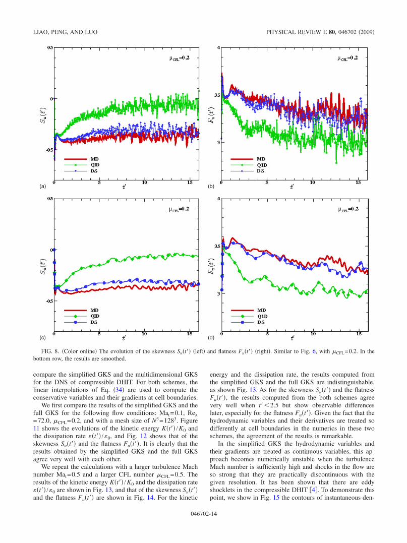
To investigate the effect of the CFL number �CFL, werepeat the simulations with �CFL=0.2 and 0.5. The evolu-tions of the kinetic energy, K�t�� /K0, and the dissipation rate,��t� /�0 for �CFL=0.2 are shown in Fig. 7. The differencesbetween the Q1D-GKS results for both K�t�� /K0 and ��t� /�0and those computed by using the DS-GKS and the full MDGKS are obviously larger than the case of �CFL=0.1 of Fig.5. Similar observations can be made for the skewness Su�t��and flatness Fu�t�� shown in Fig. 8. We also observe that thedifferences between results computed by using the DS-GKSand the full MD GKS appear to be affected very little by theCFL number �CFL.

As the CFL number is increased to �CFL=0.5, the Q1D-GKS becomes unstable, as shown in Fig. 9 for K�t�� /K0 and��t� /�0. In addition, the differences for the results of theskewness Su�t�� and flatness Fu�t�� Fig. 10� computed byusing the DS-GKS and the full MD GKS are further ampli-fied, and the values of Su�t�� and Fu�t�� computed by usingthe full MD GKS remain close to their theoretical values.The high-frequency oscillations in both Su�t�� and Fu�t��weaken as the CFL number �CFL increases. This is under-standable because as the CFL number �CFL increases so dothe time step size and the corresponding truncation errors.The former reduces the resolution in time, and the latter in-

creases numerical dissipations; both effects suppress thehigh-frequency oscillations.

Our results show that among three schemes, the Q1D-GKS is the most dissipative, least accurate, and most un-stable. The full MD GKS is the best one in terms of numeri-cal dissipation, accuracy, and stability, while the DS-GKSranks second. Obviously, the Q1D-GKS is not adequate forDNS of homogeneous turbulence flows, while the DS-GKSis adequate for the purpose provided that the CFL number issmall enough. We also observe that an increase in numericaldissipations leads to an increase in the skewness Su�t�� aswell as a decrease in the flatness Fu�t�� after a very shortinitial period in time.

We also assess the computational efficiencies of the threeapproaches. For the part related to the calculation of fluxes,the computational effort of the DS-GKS is only slightly morethan that of the Q1D-GKS �less than 5%�, while the compu-tational effort of the full GKS is about twice of that of theDS-GKS. In light of the results above and the considerationof the computational efficiency, the DS-GKS appears to beadequate to compute low-order turbulence statistics withinthe parameter ranges tested for the DNS for decaying turbu-lence.

B. Simplified GKS vs full multidimensional GKS

The simplified GKS with the fluxes determined by Eq.�32� is much simpler, thus much computationally efficientthan the full multidimensional GKS with the fluxes deter-mined by Eq. �21�. Another benefit of using the simplifiedGKS for smooth flows is numerical consistency of the valuesof hydrodynamic variables and their gradients at cell bound-aries because the simplified GKS assumes these quantities tobe continuous, while the multidimensional GKS assumesthem to be discontinuous. It is important to note that thesimplified GKS is a multidimensional scheme, it does notneglect the derivatives tangential to cell interfaces. We will

(b)(a)

FIG. 7. �Color online� The evolution of the kinetic energy K�t�� /K0 �left� and dissipation rate ��t� /�0 �right�. Similar to Fig. 5, with�CFL=0.2.


046702-13

compare the simplified GKS and the multidimensional GKSfor the DNS of compressible DHIT. For both schemes, thelinear interpolations of Eq. �34� are used to compute theconservative variables and their gradients at cell boundaries.

We first compare the results of the simplified GKS and thefull GKS for the following flow conditions: Mat=0.1, Re�

=72.0, �CFL=0.2, and with a mesh size of N3=1283. Figure11 shows the evolutions of the kinetic energy K�t�� /K0 andthe dissipation rate ��t�� /�0, and Fig. 12 shows that of theskewness Su�t�� and the flatness Fu�t��. It is clearly that theresults obtained by the simplified GKS and the full GKSagree very well with each other.

We repeat the calculations with a larger turbulence Machnumber Mat=0.5 and a larger CFL number �CFL=0.5. Theresults of the kinetic energy K�t�� /K0 and the dissipation rate��t�� /�0 are shown in Fig. 13, and that of the skewness Su�t��and the flatness Fu�t�� are shown in Fig. 14. For the kinetic

energy and the dissipation rate, the results computed fromthe simplified GKS and the full GKS are indistinguishable,as shown Fig. 13. As for the skewness Su�t�� and the flatnessFu�t��, the results computed from the both schemes agreevery well when t��2.5 but show observable differenceslater, especially for the flatness Fu�t��. Given the fact that thehydrodynamic variables and their derivatives are treated sodifferently at cell boundaries in the numerics in these twoschemes, the agreement of the results is remarkable.

In the simplified GKS the hydrodynamic variables andtheir gradients are treated as continuous variables, this ap-proach becomes numerically unstable when the turbulenceMach number is sufficiently high and shocks in the flow areso strong that they are practically discontinuous with thegiven resolution. It has been shown that there are eddyshocklets in the compressible DHIT �4�. To demonstrate thispoint, we show in Fig. 15 the contours of instantaneous den-

(b)(a)

(c) (d)

FIG. 8. �Color online� The evolution of the skewness Su�t�� left� and flatness Fu�t�� right�. Similar to Fig. 6, with �CFL=0.2. In thebottom row, the results are smoothed.


046702-14

sity � and local Mach number Ma for a simulation of com-pressible DHIT with Re�=72.0 and Mat=0.5 by using thesimplified GKS scheme. The figure clearly shows areaswhere the gradients of � and Ma have very high intensities,indicating the presence of shocklets.

To test the limit of the turbulence Mach number Mat forthe simplified GKS, we perform simulations with a fixedCFL number �CFL=0.5 and a fixed Reynolds number Re�

=72.0 and various values of the initial turbulence Machnumber Mat. Figure 16 shows the results for the kinetic en-ergy K�t�� /K0 and the dissipation rate ��t� /�0 obtained byusing the simplified GKS with Mat=0.1, 0.5, and 0.6. Thecorresponding results for the skewness Su�t�� and the flatnessFu�t�� are shown in Fig. 17. Clearly, as the turbulence Machnumber Mat increases, so also do the strengths of shocklets

in the flow. Consequently, the gradients of flow fields be-come larger and larger as Mat increases. This phenomenon isclearly reflected in both the skewness Su�t�� and the flatnessFu�t�� shown in Fig. 17: as Mat increases, the amplitudes ofoscillations in both Su�t�� and Fu�t�� increase significantly.The oscillation amplitudes also grow in time. If the initialturbulence Mach number Mat is increased to 0.65, the simu-lation becomes unstable quickly regardless of how small theCFL number �CFL is. Our results indicate that the upper limitof the initial turbulence Mach number Mat, below which thesimplified GKS can yield acceptable results, is about 0.6.Below this limit of Mat, the simplified GKS works effec-tively for the compressible DHIT.

We note that the simplified GKS is much more efficientcomputationally—it is about five times faster than the full

(b)(a)

FIG. 9. �Color online� The evolution of the kinetic energy K�t�� /K0 �left� and dissipation rate ��t� /�0 �right�. Similar to Fig. 5, with�CFL=0.5.

(b)(a)

FIG. 10. �Color online� The evolution of the skewness Su�t�� left� and flatness Fu�t�� right�. Similar to Fig. 6, with �CFL=0.5.


046702-15

multidimensional GKS. Thus it is highly recommended forflows for which the simplified GKS is suitable.

C. Effects of flux limiter and artificial dissipation

In the previous section we show that, for compressibleflows with a high enough turbulent Mach number, the sim-plified GKS with the continuous treatment of hydrodynamicvariables and their gradients is inadequate. When dealingwith high Mach number turbulence, some sort of discontinu-ous treatment of shocks must be used. In addition to treatinghydrodynamic variables and their gradients as discontinuitiesat cell boundaries, a flux limiter has to be used when theMach number is sufficient high. Inevitably flux limiters do

introduce numerical dissipations. In this section we will as-sess the effects of a flux limiter, as well as artificial dissipa-tion on the DNS of compressible turbulence.

We use the full MD GKS with the van Leer limiter�31,66� for the following tests. With the limiter, we can usethe GKS to simulate compressible DHIT with a turbulenceMach number up to Mat=2.0. Figure 18 compares the resultsof the kinetic energy K�t�� /K0 and the dissipation rate��t�� /�0 computed by using the full MD-GKS with and with-out the limiter. The flow conditions are Re�=72.0 and Mat=0.5, and the mesh size is N3=1283 and the CFL number is�CFL=0.5. This is the case for which the limiter is not nec-essary. The evolutions of the kinetic energy and the dissipa-tion rate clearly show that the limiter introduces a significant

(b)(a)

FIG. 11. �Color online� Evolutions of the kinetic energy K�t�� /K0 �left� and the dissipation rate ��t�� /�0 �right� obtained by the simplifiedGKS and the full GKS. N3=1283, Re�=72.0, Mat=0.1, and �CFL=0.2.

(b)(a)

FIG. 12. �Color online� Evolutions of the skewness Su�t�� left� and the flatness Fu�t�� right� obtained by the simplified GKS and the fullGKS. N3=1283, Re�=72.0, Mat=0.1, and �CFL=0.2.


046702-16

amount of numerical dissipation: the kinetic energy K�t�� /K0and the dissipation rate computed with the limiter are muchlower than their counterparts computed without the limiter.The results of the skewness Su�t�� and the flatness Fu�t��shown in Fig. 19 corroborate the above observation. Beforethe viscous decay completely dominates the decaying pro-cess �71�, when t��5.0, the flatness Fu�t�� computed withoutthe limiter is closer to its theoretical value of 3.5 than thatwith the limiter. Our results clearly demonstrate that fluxlimiters can introduce significant amount of numerical dissi-pation, which can adversely affect the quality of DNS resultsfor compressible turbulence.

To assess the effect of the artificial dissipation, we use thevan Leer limiter, plus the artificial dissipation with �=1.0 inEq. �24�. Note that, without a limiter, the values of hydrody-

namic variables in both sides of a cell boundary are equalbecause of the linear interpolations used to compute thesevalues �cf. Eqs. �16� and �18� and Fig. 1�. Therefore theartificial dissipation will not take effect unless a limiter isused in the GKS used in this work. In Figs. 18 and 19 wealso show the effects of the artificial dissipation on K�t�� /K0,��t�� /�0, Su�t��, and Fu�t�� obtained by using the MD-GKSwith the van Leer limiter and with �=1.0 in Eq. �24�.Clearly, the artificial dissipation has no visible effect on thesequantities. This indicates that when a limiter is working, thedissipation due to the limiter is overwhelmingly dominant,and the effect of artificial dissipation is negligible for thelow-Mach-number cases tested here.

(b)(a)

FIG. 13. �Color online� Evolutions of the kinetic energy K�t�� /K0 �left� and the dissipation rate ��t�� /�0 �right� obtained by the simplifiedGKS and the full GKS. Similar to Fig. 11, with Mat=0.5 and �CFL=0.5.

(b)(a)

FIG. 14. �Color online� Evolutions of the skewness Su�t�� left� and the flatness Fu�t�� right� obtained by the simplified GKS and the fullGKS. Similar to Fig. 12, Mat=0.5 and �CFL=0.5.


046702-17

D. Effect of the interpolation accuracy at cell boundaries

In the GKS, one must interpolate hydrodynamic variablesand their gradients from cell centers to cell boundaries. Theaccuracy of interpolations determines the accuracy of thescheme. Since the GKS is constructed as a second-orderscheme, the linear interpolations of Eq. �34� are sufficient toachieve the required second-order accuracy. Because turbu-lence DNS have a very stringent requirement on the accuracyof numerical schemes, we would like to investigate the nu-merical fidelity of the linear interpolations used in the GKSfor DNS of compressible DHIT. In what follow, we will usethe simplified GKS to test the linear interpolation of Eq. �34�against the third-order interpolations of Eq. �35�. We main-tain the Reynolds number Re�=72.0 and the mesh size N3

=1283.In Fig. 20, we show the kinetic energy and the dissipa-

tions rate with two sets of conditions: Mat=0.1 and �CFL=0.2 and Mat=0.5 and �CFL=0.4. For the case of Mat=0.1,the kinetic energy K�t�� /K0 shows no visible difference dueto the difference of interpolations used, while the dissipation

rate clear indicates that the linear interpolations are moredissipative than the third-order ones—the peak of ��t�� /�computed with the linear interpolations is lower than whatcomputed with the third-order interpolations. For the case ofMat=0.5, the discrepancy in the ��t�� /� due to interpolationsdisappears. However, the kinetic energy K�t�� /K0 computedwith the linear interpolations decays slower after t��8.0,indicating that a larger numerical dissipation due to linearinterpolations. The reason behind this phenomenon can beexplained as follows. Stronger numerical dissipations due tolinear interpolations reduce the dissipation rate � in the initialstage, as clearly shown in Fig. 20 for the case of Mat=0.1,which in turn slow down the decay of the kinetic energy K inlater times. Thus, a larger numerical dissipation leads to aslower decay of the kinetic energy in this case.

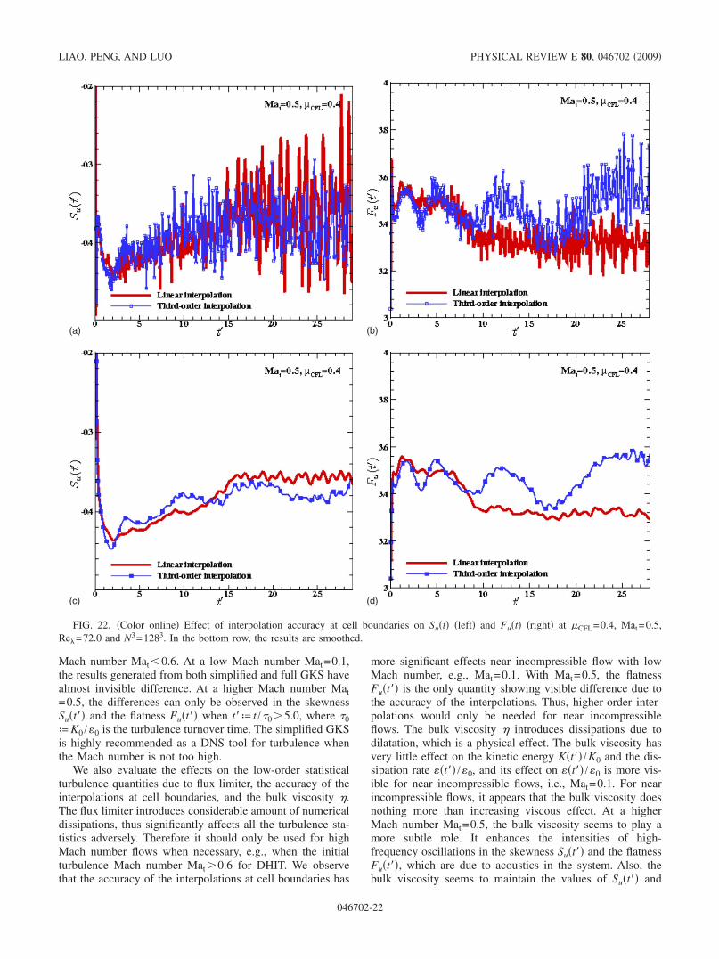
Figures 21 and 22 show the evolution of Su�t�� and Fu�t��for Mat=0.1 and Mat=0.5, respectively, corresponding to theresults shown in Fig. 20. For the case of Mat=0.1, the resultsin Fig. 21 show that the results computed with linear andthird-order interpolations display large discrepancies. Whileone cannot argue that the results computed with the third-order interpolations are better than that computed with thelinear interpolations, there are some indications—the flatnessSu�t�� computed with the third-order interpolations isbounded between −0.5 and −0.4, which is more reasonablethan that computed with the linear interpolations, which goesbeyond the bound of �−0.5,−0.4� after t��15.0. For the caseof Mat=0.5, oscillations in the Su�t�� and Fu�t�� computedwith the linear interpolations have larger amplitudes. How-ever, the smoothed Su�t�� and Fu�t�� computed with the linearand third-order interpolations agree with each other ratherwell, as shown in Fig. 22.

Our results here clear show that the accuracy of interpo-lations does have observable effects on various quantities inDNS of compressible DHIT. Clearly, the linear interpolationsintroduce stronger numerical dissipations. These effects seemto be stronger at lower Mach numbers. Overall, the linear

(b)(a)

FIG. 15. �Color online� Contours of the density �left� and theMach number �right� on the xy plane k=2 at t�=1.03 for �CFL

=0.5, Mat=0.5, Re�=72.0, and N3=1283.

(b)(a)

FIG. 16. �Color online� The evolution of K�t�� /K0 �left� and ��t�� /�0 �right� obtained by using the simplified GKS with N3=1283,�CFL=0.5, Re�=72.0, and Mat=0.1, 0.5, and 0.6.


046702-18

interpolations are acceptable for DNS of compressible turbu-lence flows. Overall, the linear interpolations save about15% computational time when compared with the third-orderinterpolations.

E. Effect of bulk viscosity

Finally, we assess the effect of the bulk viscosity �. Weuse the simplified GKS with linear interpolations at cellboundaries. In GKS, the bulk viscosity is tuned with theparameter Z and it does not change the complexity of thecode because one does not need to explicitly compute thedivergence of the velocity field � ·u. We perform the simu-lations for the compressible DHIT at Mat=0.1 and 0.5 with�K=2� or without �K=0� the bulk viscosity �. Figure 23shows the effect of the bulk viscosity at Mat=0.1 on thekinetic energy K�t�� /K0 and the dissipation rate ��t�� /�0. We

can see that the bulk viscosity has no observable effect onthe kinetic energy K�t�� /K0; however, it does increase thedissipation rate ��t�� /�0 slightly in the initial stage. Clearly,the dissipation due to the bulk viscosity � produces observ-able effects in both the skewness Su�t�� and the flatnessFu�t��, as shown in Fig. 24.

When the initial turbulent Mach number Mat=0.5, thebulk viscosity � does not seem to have any observable ef-fects on both the kinetic energy K�t�� /K0 and the dissipationrate ��t�� /�0, as shown in Fig. 25. However, the bulk viscos-ity do have prominent effects on both the skewness Su�t��and the flatness Fu�t��, as shown in Fig. 26. Several obser-vations can be made here. First, for a low initial turbulenceMach number Mat=0.1, the bulk viscosity � simply addsmore dissipation to the flow; it enhances the value of theskewness Su�t�� and depresses that of the flatness Fu�t�� afteran initial period of time. It seems to be difficult to distinguisha priori between the dissipative effects due to the bulk vis-

(b)(a)

(c) (d)

FIG. 17. �Color online� The evolution of Su�t� �left� and Fu�t� �right� obtained by using the simplified GKS with N3=1283, �CFL=0.5,Re�=72.0, and Mat=0.1, 0.5, and 0.6. In the bottom row, the results are smoothed.


046702-19

cosity � and that due to numerical viscosities. Secondly, fora higher initial turbulence Mach number Mat=0.5, the skew-ness Su�t�� and the flatness Fu�t�� computed with a nonzerobulk viscosity have high-frequency oscillations stronger thanthat with zero bulk viscosity. In addition, it is interesting tonote that the skewness Su�t�� and the flatness Fu�t�� com-puted with a nonzero bulk viscosity remain much closer totheir theoretical values of −0.5 and 3.5 at late stage of DHIT,respectively, than their counterparts with a zero bulk viscos-ity.

V. CONCLUSIONS

In this paper we apply the gas-kinetic scheme �GKS� forDNSs for compressible decaying homogeneous isotropic tur-

bulence in a three-dimensional cube with periodic boundaryconditions. We measure the statistical quantities includingthe total kinetic energy K�t��, the dissipation rate ��t��, theskewness Su�t��, and the flatness Fu�t��. The simulations arecarried out with the Taylor microscale Reynolds numberRe�=72.0, a fixed mesh size of N3=1283, and various valuesof initial turbulence Mach number Mat, up to the dimension-less time t��30 in terms of the turbulence turnover time�0=K0 /�0.

We first validate our GKS code against pseudospectralsimulations in both near incompressible and fully compress-ible regions for the DHIT, corresponding to the initial turbu-lence Mat=0.1 and 0.5, respectively. We find that the GKScan yield satisfactory results for K�t��, ��t��, Su�t��, and

(b)(a)

FIG. 18. �Color online� Effects of flux limiter and artificial dissipation �AD� on the kinetic energy K�t�� /K0 �left� and ��t�� /�0 �right�. Weset �=1.0 in Eq. �24� when AD is used. Re�=72.0, Mat=0.5, �CFL=0.5, and N3=1283.

(b)(a)

FIG. 19. �Color online� Effect of flux limiter and AD on the skewness Su�t� �left� and the flatness Fu�t� �right�. We set �=1.0 in Eq. �24�when AD is used. Re�=72.0, Mat=0.5, �CFL=0.5, and N3=1283.


046702-20

Fu�t��, and the results are in good agreement with pseu-dospectral results.

We investigate effects due to approximations made incomputing the fluxes, that is, we compare the quasi-one-dimensional �Q1D� GKS and dimensional-splitting �DS�GKS, versus the full MD GKS. We find that the Q1D-GKS isthe most dissipative and the least stable and accurate schemeamong the three, while the full GKS is the best. The accu-racy and numerical stability of the Q1D-GKS deteriorate asthe initial turbulence Mach number Mat increases, while theDS-GKS is only slightly more dissipative than the full MDGKS, which is only observable in the skewness and the flat-ness. For most part, the DS-GKS results agree well with thefull MD-GKS ones in the parameter ranges we have tested.

The ratio of the computational speeds of the DS-GKS andthe full GKS is about 1.8. The tests performed in this workshow that the DS-GKS is an adequate DNS tool to computethe low-order turbulence statistical quantities in compress-ible decaying turbulence, while the Q1D-GKS is not recom-mended for the purpose of turbulence DNS.

We test the simplified GKS for smooth flows. The simpli-fied GKS treats the hydrodynamic variables and their deriva-tives as continuous variables at cell boundaries, leading toconsiderably simplifications in the calculations of fluxes,thus significantly reducing the computational cost. The com-putational cost of the simplified GKS is only about 1/5 ofthat of the full GKS. The simplified GKS works very well forthe DNS of decaying turbulence when the initial turbulence

(b)(a)

FIG. 20. �Color online� Effect of the accuracy of interpolations on the kinetic energy K�t�� /K0 and the dissipation rate ��t�� /�0.N3=1283, Re�=72.0, Mat=0.1, and �CFL=0.2 �left�; and Mat=0.5 and �CFL=0.4 �right�.

(b)(a)

FIG. 21. �Color online� Effect of interpolation accuracy at cell boundaries on Su�t� �left� and Fu�t� �right� at �CFL=0.2, Mat=0.1,Re�=72.0, and N3=1283.


046702-21

Mach number Mat�0.6. At a low Mach number Mat=0.1,the results generated from both simplified and full GKS havealmost invisible difference. At a higher Mach number Mat=0.5, the differences can only be observed in the skewnessSu�t�� and the flatness Fu�t�� when t�ª t /�0�5.0, where �0ªK0 /�0 is the turbulence turnover time. The simplified GKSis highly recommended as a DNS tool for turbulence whenthe Mach number is not too high.

We also evaluate the effects on the low-order statisticalturbulence quantities due to flux limiter, the accuracy of theinterpolations at cell boundaries, and the bulk viscosity �.The flux limiter introduces considerable amount of numericaldissipations, thus significantly affects all the turbulence sta-tistics adversely. Therefore it should only be used for highMach number flows when necessary, e.g., when the initialturbulence Mach number Mat�0.6 for DHIT. We observethat the accuracy of the interpolations at cell boundaries has

more significant effects near incompressible flow with lowMach number, e.g., Mat=0.1. With Mat=0.5, the flatnessFu�t�� is the only quantity showing visible difference due tothe accuracy of the interpolations. Thus, higher-order inter-polations would only be needed for near incompressibleflows. The bulk viscosity � introduces dissipations due todilatation, which is a physical effect. The bulk viscosity hasvery little effect on the kinetic energy K�t�� /K0 and the dis-sipation rate ��t�� /�0, and its effect on ��t�� /�0 is more vis-ible for near incompressible flows, i.e., Mat=0.1. For nearincompressible flows, it appears that the bulk viscosity doesnothing more than increasing viscous effect. At a higherMach number Mat=0.5, the bulk viscosity seems to play amore subtle role. It enhances the intensities of high-frequency oscillations in the skewness Su�t�� and the flatnessFu�t��, which are due to acoustics in the system. Also, thebulk viscosity seems to maintain the values of Su�t�� and

(b)(a)

(c) (d)

FIG. 22. �Color online� Effect of interpolation accuracy at cell boundaries on Su�t� �left� and Fu�t� �right� at �CFL=0.4, Mat=0.5,Re�=72.0 and N3=1283. In the bottom row, the results are smoothed.


046702-22

Fu�t�� closer to their theoretical ones, −0.5 and 3.5, respec-tively, than the simulations without the bulk viscosity.

Overall, our results demonstrate that the gas-kineticscheme is adequate to simulate decaying homogeneous iso-tropic turbulence as far as the low-order statistics are con-cerned. The GKS is not the most effective and efficientmethod for near incompressible flows with low Mach num-bers �65�. For near incompressible flows, our experience in-dicates that the lattice Boltzmann equation �LBE� is a muchbetter method in terms of effectiveness and efficiency�61,72�. Since the GKS is only a second-order scheme, thestrength of the GKS may be in high-Mach-number flows inwhich a flux limiter must be used. When a flux limiter mustbe used, the benefit of using more accurate high-order meth-ods may not be so obvious because the numerical dissipation

introduced by the flux limiter becomes the dominating factoraffecting the accuracy of the scheme.

Kinetic schemes have two notable advantages in general,which motivate this work in part. The first one is the numer-ics. In contrast to the Navier-Stokes equation with a nonlin-ear advection term u ·�u, the Boltzmann equation has a lin-ear advection term � ·�f =� · ��f� and its nonlinearity residesin the collision term which is local. This feature of the ki-netic equation has important ramifications including �32�: �a�its nonlinearity is in local collision term, stiffness of whichcan be overcome by local techniques; and �b� it is mucheasier to formulate multidimensional schemes for fluxes. Thesecond advantage of the GKS is physics. Kinetic schemesbased on the Boltzmann equation have the potential to modelextended hydrodynamics which is beyond the validity of the

(b)(a)

FIG. 23. �Color online� Effect of the bulk viscosity � on the kinetic energy K�t�� /K0 and the dissipation rate ��t�� /�0. N3=1283,Re�=72.0, Mat=0.1, and �CFL=0.2.

(b)(a)

FIG. 24. �Color online� Effect of the bulk viscosity on the skewness Su�t� �left� and the flatness Fu�t� �right�. N3=1283, Re�=72.0,Mat=0.1, and �CFL=0.2.


046702-23

(b)(a)

FIG. 25. �Color online� Effect of the bulk viscosity � on the kinetic energy K�t�� /K0 and the dissipation rate ��t�� /�0. N3=1283,Re�=72.0, Mat=0.5, and �CFL=0.5.

(b)(a)

(c) (d)

FIG. 26. �Color online� Effect of the bulk viscosity on the skewness Su�t� �left� and the flatness Fu�t� �right�. N3=1283, Re�=72.0,Mat=0.5, and �CFL=0.5. The bottom figures are the smoothed ones of the top ones.


046702-24

macroscopic continuum theory. This feature is particularlyrelevant to thermochemically nonequilibrium flows forwhich the Navier-Stokes equations are no longer valid�39,40,73,74�. We also note that the full MD-GKS is compu-tationally more intensive for the benefit of better fidelity offlow physics. To fully exploit the advantages and to fullyrealize the potential of gas-kinetic schemes will remain thesubjects of our future research.

ACKNOWLEDGMENTS

The authors are grateful to an anonymous reviewer whose

comments have helped us improve the paper considerably.The authors would like to thank Dr. A. Honein for providingthe data of Ref. �13� shown in Fig. 4, and Dr. P. K. Sub-bareddy and Professor G. V. Candler for providing Ref.�14� to us before its publication. We would also like to ac-knowledge the funding support from U.S. Department of De-fense and Air Force Office of Scientific Research underAFOSR-MURI Project 19 “Hypersonic Transition and Tur-bulence with Nonequilibrium Thermochemistry” �Dr. J.Schmisseur�.

�1� T. Passot and A. Pouquet, J. Fluid Mech. 181, 441 �1987�.�2� S. Kida and S. A. Orszag, J. Sci. Comput. 5, 1 �1990�.�3� S. Kida and S. A. Orszag, J. Sci. Comput. 5, 85 �1990�.�4� S. Lee, S. K. Lele, and P. Moin, Phys. Fluids A 3, 657 �1991�.�5� S. Sarkar, G. Erlebacher, M. Y. Hussaini, and H. O. Kreiss, J.

Fluid Mech. 227, 473 �1991�.�6� G. Erlebacher, M. Y. Hussaini, C. G. Speziale, and T. A. Zang,

J. Fluid Mech. 238, 155 �1992�.�7� G. A. Blaisdell, N. N. Mansour, and W. C. Reynolds, J. Fluid

Mech. 256, 443 �1993�.�8� S. K. Lele, Annu. Rev. Fluid Mech. 26, 211 �1994�.�9� F. A. Jaberi, D. Livescu, and C. K. Madnia, Phys. Fluids 12,

1189 �2000�.�10� R. Samtaney, D. I. Pullin, and B. Kosović, Phys. Fluids 13,

1415 �2001�.�11� H. Foysi, S. Sarkar, and R. Friedrich, J. Fluid Mech. 509, 207

�2004�.�12� D. Livescu and C. K. Madnia, Phys. Fluids 16, 2864 �2004�.�13� A. E. Honein and P. Moin, J. Comput. Phys. 201, 531 �2004�.�14� P. K. Subbareddy and G. V. Candler, J. Comput. Phys. 228,

1347 �2009�.�15� M. Wu and M. P. Martín, AIAA Paper. 2005-4895, 2005.�16� M. P. Martín, A. J. Smits, M. Wu, and M. Ringuette, AIAA

Paper. 2006-0497, 2006.�17� M. P. Martín, J. Fluid Mech. 570, 347 �2007�.�18� M. Wu and M. P. Martín, AIAA J. 45, 879 �2007�.�19� M. W. Wu and M. P. Martín, J. Fluid Mech. 594, 71 �2008�.�20� J. R. Edwards, Prog. Aerosp. Sci. 44, 447 �2008�.�21� S. K. Godunov, Math. USSR. Sb. 47, 271 �1959�.�22� B. van Leer, J. Comput. Phys. 32, 101 �1979�.�23� D. Drikakis and W. Rider, High-resolution Methods for Incom-

pressible and Low-speed Flows �Springer, Berlin, 2005�.�24� S. K. Lele, J. Comput. Phys. 103, 16 �1992�.�25� M. P. Martín, E. M. Taylor, M. Wu, and V. G. Weirs, J. Com-

put. Phys. 220, 270 �2006�.�26� E. M. Taylor and M. P. Martín, J. Sci. Comput. 30, 533 �2007�.�27� E. M. Taylor, M. W. Wu, and P. Martín, J. Comput. Phys. 223,

384 �2007�.�28� M. Delanaye and J. A. Essers, AIAA J. 35, 631 �1997�.�29� C. Ollivier-Gooch, A. Nejat, and K. Michalak, AIAA Paper,

2007-4464, 2007.�30� K. Xu, in The 29th Computational Fluid Dynamics, VKI Lec-

ture Series �The von Karman Institute for Fluid Dynamics,Rhode-St-Genèse, Belgium, 1998�, Vol. 1998-03, pp. 1–202.

�31� K. Xu, J. Comput. Phys. 171, 289 �2001�.�32� B. Van Leer, AIAA Paper, 2001-2520, 2001.�33� K. Xu, J. Comput. Phys. 178, 252 �2002�.�34� T. Ohwada, J. Comput. Phys. 177, 156 �2002�.�35� K. Xu, M. L. Mao, and L. Tang, J. Comput. Phys. 203, 405

�2005�.�36� T. Ohwada and S. Fukata, J. Comput. Phys. 211, 424 �2006�.�37� G. May, B. Srinivasan, and A. Jameson, J. Comput. Phys. 220,

856 �2007�.�38� Q. B. Li and S. Fu, J. Comput. Phys. 220, 532 �2006�.�39� W. Liao, L.-S. Luo, and K. Xu, J. Rocket and Spacecraft 44,

1232 �2007�.�40� W. Liao, Y. Peng, L.-S. Luo, and K. Xu, Prog. Comput. Fluid

Dym. 8, 97 �2008�.�41� K. Xu, X. He, and C. P. Cai, J. Comput. Phys. 227, 6779

�2008�.�42� K. Xu and L. Tang, Phys. Fluids 16, 3824 �2004�.�43� K. Xu and E. Josyula, Phys. Rev. E 71, 056308 �2005�.�44� K. Xu and E. Josyula, Comm. Comp. Phys. 1, 425 �2006�.�45� C. P. Cai, D. D. Liu, and K. Xu, AIAA J. 46, 1054 �2008�.�46� Q. B. Li, H. X. Chen, and S. Fu, Phys. Fluids 15, 3240 �2003�.�47� Q. B. Li and S. Fu, Comput. Fluids 32, 1357 �2003�.�48� Q. B. Li, S. Fu, and K. Xu, J. Comput. Phys. 204, 692 �2005�.�49� S. Fu and Q. B. Li, Int. J. Heat Fluid Flow 27, 895 �2006�.�50� K. Xu, J. Comput. Phys. 134, 122 �1997�.�51� Y. S. Lian and K. Xu, J. Comput. Phys. 163, 349 �2000�.�52� Y. S. Lian and K. Xu, Comput. Fluids 29, 725 �2000�.�53� T. Ohwada and K. Xu, J. Comput. Phys. 201, 315 �2004�.�54� K. Xu and Z. H. Li, J. Fluid Mech. 513, 87 �2004�.�55� K. Xu, J. Comput. Phys. 153, 334 �1999�.�56� H. Z. Tang and K. Xu, J. Comput. Phys. 165, 69 �2000�.�57� K. Xu, J. Comput. Phys. 178, 533 �2002�.�58� H. Z. Tang, T. Tang, and K. Xu, Z. Angew. Math. Phys. 55,

365 �2004�.�59� M. S. Ghidaoui, A. A. Kolyshkin, J. H. Liang, F. C. Chan, Q.

Li, and K. Xu, J. Fluid Mech. 548, 309 �2006�.�60� Y. T. Que and K. Xu, Int. J. Numer. Methods Fluids 50, 1003

�2006�.�61� W. Liao, Y. Peng, and L.-S. Luo, AIAA Paper, 2008-0548,

2008.�62� S. Harris, An Introduction to the Theory of Boltzmann Equa-

tion �Holt, Rinehart and Winston, New York, 1971; reprintedby Dover, New York, 2004�.

�63� P. Bhatnagar, E. Gross, and M. Krook, Phys. Rev. 94, 511


046702-25

�1954�.�64� M. N. Kogan, Rarefield Gas Dynamics �Plenum Press, New

York, 1969�.�65� Z. L. Guo, H. W. Liu, L.-S. Luo, and K. Xu, J. Comput. Phys.

227, 4955 �2008�.�66� B. van Leer, J. Comput. Phys. 14, 361 �1974�.�67� Q. B. Li, S. Fu, and K. Xu, AIAA J. 43, 2170 �2005�.�68� K. Xu and X. Y. He, J. Comput. Phys. 190, 100 �2003�.�69� R. S. Rogallo, NASA, Technical Report No. TM-8135, 1981

�unpublished�.

�70� S. B. Pope, Turbulent Flows �Cambridge University Press,Cambridge, England, 2000�.

�71� T. T. Clark and C. Zemarch, Phys. Fluids 10, 2846 �1998�.�72� Y. Peng, W. Liao, L.-S. Luo, and L.-P. Wang, Comput. Fluids

�unpublished�.�73� J. D. Anderson, Hypersonic and High Temperature Gas Dy-

namics �McGraw-Hill, New York, 1989; reprinted by AIAA,Reston, VA, 2000�.

�74� W. Vincenti and C. Krueger, Introduction to Physical Gas Dy-namics �Krieger Wiley, New York, 1965�.


046702-26

Gas-kinetic schemes for direct numerical simulations of compressible homogeneous turbulence

Documents

Transcript of Gas-kinetic schemes for direct numerical simulations of compressible homogeneous turbulence