Gap-filling measurements of carbon dioxide storage in tropical rainforest canopy airspace

Gap-filling measurements of carbon dioxide storage in

tropical rainforest canopy airspace

Hiroki Iwata a,*, Yadvinder Malhi b,c, Celso von Randow d

a Terrestrial Environment Research Center, University of Tsukuba, Tsukuba 305-8577, Japanb Oxford University Centre for Environment, University of Oxford, Oxford OX1 3QY, UK

c School of GeoSciences, University of Edinburgh, Edinburgh EH9 3JU, UKd Alterra, Wageningen University and Research Center, P.O. Box 47, 6700 AA, Wageningen, The Netherlands

Received 26 October 2004; received in revised form 12 August 2005; accepted 16 August 2005

Abstract

For the determination of biotic fluxes of carbon dioxide (CO2) or other trace gases to or from a forest canopy, it is important to

measure the storage of the trace gas within the forest canopy in addition to the net vertical flux above the forest canopy. However, the

data continuity of within-canopy storage measurements can be poor because these measurements are subject to frequent equipment

breakdowns. We here explore methods for gap-filling within-canopy CO2 storage, using the data derived from an Amazonian

rainforest (Caxiuana). Our first approach was to estimate hourly storage from hourly CO2 concentration measured above the canopy

at the tower top. This proved unreliable, since at this hourly time scale the variations in above-canopy CO2 are often decoupled from

local changes in within-canopy storage. We then explored a second approach based on determination of the total CO2 accumulation

over a night. This was found to be adequately correlated with a time-weighted friction velocity (u*w) averaged over a night

(R2 = 0.42). The total night-time storage was then used to model daytime depletion of CO2 within the canopy. The gap-filling model

was validated against independent data from the same site, and also applied to another tropical forest (Jaru) with similar results.

The modelled storage is in good agreement with the measured storage, and by reducing susceptibility to advection error it is in some

ways superior to the direct storage measurements. This suggests at the possibility of a general method for estimating storage in

forest canopies, with re-calibration for each site.

# 2005 Elsevier B.V. All rights reserved.

Keywords: Within-canopy CO2 storage; Gap-filling method; Tropical rainforest; Friction velocity; Eddy covariance method

www.elsevier.com/locate/agrformet

Agricultural and Forest Meteorology 132 (2005) 305–314

1. Introduction

Over the past decade, there has been a proliferation

of studies utilising micrometeorological methods to

quantify the flux of carbon dioxide (CO2) and other

trace gases between vegetation canopies and the

atmosphere (Baldocchi et al., 2001). Whilst the focus

of these studies has been on above-canopy fluxes, there

* Corresponding author. Tel.: +81 29 853 2531;

fax: +81 29 853 2530.

E-mail address: [email protected] (H. Iwata).

0168-1923/$ – see front matter # 2005 Elsevier B.V. All rights reserved.

doi:10.1016/j.agrformet.2005.08.005

was an early realisation that there can be significant

storage of trace gases within the canopy airspace. The

degree of storage varies with the intensity of boundary-

layer turbulence and thus over the diurnal cycle. For

CO2 and other trace gases with nocturnal, sub-canopy

emissions, there is a tendency of accumulation of the

trace gases within the canopy airspace at night, and a

depletion of this store in the early morning as thermal

convection sets in.

Whilst the net effect of the storage of CO2 over a

full diurnal cycle is approximately zero (night-time

accumulation = daytime loss), it can be important to

measure this storage if our interest is to estimate the

H. Iwata et al. / Agricultural and Forest Meteorology 132 (2005) 305–314306

Nomenclature

C CO2 concentration (mmol m�3)

Ctop CO2 concentration measured by the

eddy covariance instrumentation at

the top of the tower (mmol m�3)

d zero-plane displacement (m)

h the height of eddy covariance instru-

mentation (m)

LW above-canopy downward long-wave

radiation (W m�2)

R2 coefficient of determination

RMSE root mean square error

Sc accumulated storage during night

(g (C) m�2 night�1)

Sc/Fbiotic ratio of night-time storage to night-time

biotic flux

Sc/Fc ratio of night-time storage to night-time

above-canopy flux

Ta air temperature at tower-top (8C)Ts soil temperature (8C)u* friction velocity at tower-top (m s�1)

u*w time-weighted friction velocity aver-

aged over a night (ms�1)

z height above the ground surface (m)

(z � d)/L Monin–Obukhov stability parameter

(dimensionless)

‘‘biotic’’ flux of the trace gas, and understand its

physiological controls. The biotic flux (or net ecosystem

exchange, NEE) is defined as biotic flux = above-

canopy flux + storage flux. Measurement of within-

canopy storage is now standard in many canopy flux

measurement studies, with the most common approach

using a gas analyser to measure gas concentrations from

a sampling system that automatically cycles between

intakes at various heights within the forest canopy. The

mechanical nature of these measurements, however,

means that there can often be problems of equipment

breakdown (e.g. pump failure and solenoid switch

failure), especially in challenging environments such as

remote tropical forests (with problems with insects and

humidity) or boreal forests (with problems with insects

and icing). Therefore, the data continuity of storage

measurements may often not match those of the above-

canopy measurements. A reliable method of ‘‘gap-

filling’’ measurements for within-canopy storage would

clearly be desirable.

In this paper we explore the potential of various

approaches to gap-filling measurements of storage in

tropical forest canopies, utilising either data from the

above-canopy flux measurements or from meteorolo-

gical observations. In addition to describing a technical

procedure, this paper is also of more general value in

its exploration of the determinants of within-canopy

CO2 storage. We first explore the potential of utilising

hourly or 30-min observations of above-canopy

turbulence and CO2 concentration. This approach is

demonstrated to be unreliable, because at this time

scale the variations in above-canopy CO2 are often

decoupled from local changes in within-canopy

storage, and more influenced by advection from nearby

regions.

In homogeneous canopies, advection problems are

often related to limited sampling times, and we then

explore an approach of utilising the mean meteorolo-

gical or turbulence conditions over the entire night to

estimate the total storage over the night. Total night-

time storage is found to be more consistently

predictable, and we then develop empirical relation-

ships between total storage and the daytime evacuation

of CO2 from the canopy. Our aim here is to present an

approach to site-specific gap-filling of CO2 storage, but

we also present evidence that there may be generalities

in the storage phenomenon that are consistent across

forest sites.

In summary, the questions that we address in this

paper are:

(1) c
an the accumulation of CO2 in a forest canopy be
predicted from standard turbulence or meteorolo-

gical variables?

(2) w
hich variable is the best predictor of CO2 storage?
(3) is
the relationship between storage and turbulence
invariant between forest sites?

2. Methods

2.1. Sites and measurements

The data used in our main analysis were collected in

the Caxiuana National Forest (18430S, 518270W, 20 m

above mean sea level), approximately 350 km to the

west of the city of Belem, Para, Brazil. This is an

extensive, undisturbed, dense lowland tropical forest

with a mean annual rainfall of 2400 mm, a mean

canopy height of 35 m, an above-ground dry biomass of

330–430 t ha�1 (Wood et al., submitted for publica-

tion) and a leaf area index of 5–6 (P. Meir, unpublished

data). Further site details are given in Carswell et al.

(2002). The Edisol eddy covariance system (Moncrieff

et al., 1997)wasmounted above a 51.5 m tall aluminum

tower. Eddy covariance sensors were mounted 4 m

H. Iwata et al. / Agricultural and Forest Meteorology 132 (2005) 305–314 307

above the tower (i.e. at a total height of 55.5 m

above-ground level) on the easterly side so as to

minimize flow distortion for the prevailing wind

direction (which was easterly both day and night).

Within- and above-canopy measurements of CO2 were

made at six heights (0.2, 2.0, 8.0, 16.0, 32.0 and

55.5 m),with the topmost intake being the outflow from

the eddy covariance system to provide cross-calibra-

tion between the twomeasurement systems. The profile

system sampled each height for 5 min, cycling through

the entire profile every half hour. At each height, 2 min

were allowed for flushing residual air from the tube

before measurement using an infrared gas analyser

(PP Systems, Hitchin, UK). Vertical profiles of CO2

concentration were collected in batches as follows:

between 16/04/1999 and 11/06/1999, between 24/06/

1999 and 08/08/1999, between 06/09/1999 and 09/09/

1999 and between 07/10/1999 and 19/10/1999 (most of

the time corresponding to dry season), before final

mechanical breakdown of the system. The data

acquisition percentage during the storagemeasurement

period was approximately 47% and the mean daily

storage was 0.32 mmol m�2 s�1 with skewness of

�0.32.

Another site used for comparison was Jaru (10850S,618560W, 145 m above mean sea level) which is located

about 100 km north of Ji-Parana, Rondonia, Brazil. This

undisturbed tropical forest has the same mean canopy

height (35 m) as the Caxiuana forest and the storage

measurement was performed at six heights (0.05, 2.7,

25.0, 35.0, 45.0 and 62.7 m) at the same sampling

interval as Caxiuana (i.e. 5 min intervals). A mean

annual rainfall of 1900 mm (Culf et al., 1996), an

above-ground dry biomass of 220 t ha�1 and a leaf area

index of 4.0 (Meir, 1996) indicate that Jaru forest is

drier and less dense than Caxiuana forest. The storage

data used in this paper is between 19/04/1999 and 24/

05/1999 (34 days in total), which corresponding to the

early dry season. Further details are given in Von

Randow et al. (2004).

2.2. Calculation of storage from

concentration profiles

For Caxiuana, within-canopy CO2 concentrations

calculated from the non-synchronous measurements at

different heights were interpolated in time to provide

instantaneous profiles at half-hour intervals, and these

profiles were then interpolated vertically to estimate the

total CO2 stored. A cubic spline scheme was used for

both interpolations, but comparison with a linear

interpolation demonstrated that the calculated storage

was insensitive to the details of the interpolation

method. A similar calculation procedure was applied for

Jaru. However, interpolation in time was not performed,

and only linear interpolation was performed vertically

(Von Randow et al., 2004).

2.3. Estimation of storage from above-canopy

concentration measurements

We first tried to estimate within-canopy storage from

measurements of the change of CO2 concentration at the

top of the tower, as measured by the eddy covariance

instrumentation. Our hypothesis was that the top-of-

canopy change in concentration was related to the total

storage by an unknown function f(u*), i.e.

dCtop

dth ¼ f ðu�Þ

Zh

0

dC

dtdz (1)

where Ctop is CO2 concentration measured on the top of

the tower, h the height of eddy covariance instrument, f

an unknown function of the friction velocity (u*), C CO2

concentration at each height of profile measurement and

z is above-ground height. The function f would be

expected to range between 0 and 1, and become close

to 1 when u* is high.

2.4. Relation of total night-time storage

to environmental conditions

We next tried to evaluate whether the total night-time

CO2 storage was more predictable than 30-min or

hourly storage, through a number of linear and

logarithmic regressions using night-time averaged

variables.

Sc ¼ a f ðxÞ þ b (2)

where Sc is accumulated storage during night, func-

tion f can be linear or logarithmic, and a, b are fitting

parameters. Night-time was defined as 1 8:00–

06:00 h, and showed little seasonal variation in timing

at this equatorial location. For variable x several

night-time averaged variables were tested as listed

in Table 1. To reflect the fact that turbulent conditions

immediately prior to dawn are more relevant in

determining dawn concentrations, a time-weighted

friction velocity (u*w), which applied a linear weight-

ing that increased with hour of the night, was also

tested for variable x, i.e.

u�w ¼P12

n¼1 u�nnP12n¼1 n

(3)


Table 1

Values of the coefficient of determination, R2, derived in the regres-

sions: Sc = af(x) + b

u* u*w Ta Ts (z � d)/L LW

Linear 0.29** 0.35** 0.035 0.0006 0.14* 0.23**

Log 0.36** 0.42** 0.035 0.0005 0.18* 0.23**

Linear and logarithmic functions are used for function f(x). Variables

in the header row were substituted as the variable x.* P < 0.01.** P < 0.001.

where n is the number of hours since the beginning of

night (weighting factor) and u*n represents u* at nth

hour. From the definition of night-time above, n = 1

corresponds to the 18:00–19:00 h. The total night-time

storage was then used to model the cycle of daytime

depletion of the forest canopy by convective motion

using a linear equation below,

Sci ¼ ai Sc for i ¼ 1; 2; 3; . . . ; 12 (4)

where Sci is hourly daytime storage at ith hour and ai is

the fitted parameter for the ith hour. The subscript i

begins at 6:00 h. We assumed that there was no storage

change during daytime if no accumulation occurred

during the previous night. To model hourly night-time

storages we assumed that hourly biotic fluxes did not

vary significantly over the course of any one night, and

allocated the total storage so that the night-time total

fluxes were constant. This could be improved by mod-

elling total fluxes as a function of temperature and

moisture—such variations are generally minor at this

wet tropical forest site, but would clearly be more

important at seasonally dry forests or temperate or

boreal forests. Eight days of data were excluded to

act as a validation dataset, and the robustness of this

model was validated against those data.

3. Results and discussion

3.1. Hourly storage and above-canopy

CO2 measurements

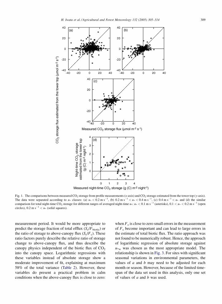
The relationship between CO2 storage estimated

from CO2 concentration at the top of the tower and

measured CO2 storage is shown in Fig. 1. The data

were divided into three ranges of u*, with the

expectation that agreement would be better when u*is high. The ratio function f(u*), as defined in Eq. (1),

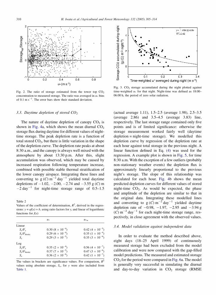
is plotted in Fig. 2. There is no tendency of increasing

f(u*) with increasing u*, and the scatter in individual

data points is so large that this function is of little

descriptive value. Clearly, variations in above-canopy

CO2 concentration do not reflect variations in storage

immediately below, i.e. the above-canopy airspace is

decoupled from the within-canopy airspace immedi-

ately below, and both terms could be strongly

influenced by advection. This decoupling could be

enhanced by the fact that the measurement height is

20 m above the 35 m forest canopy. Hence, at tropical

forest sites at least, the prospect of directly deriving

storage from above-canopy concentrations is poor.

The estimated CO2 storage from the top of the tower

were aggregated to derive total night-time storage

and compared with corresponding measured storage

(Fig. 1d). However, the scatter is large when averaged

night-time u* is low, thus making the use of CO2

concentration at the top of the tower for gap-filling

inappropriate.

3.2. Total night-time storage and mean

meteorological and turbulence conditions

Problems with advection in and above homogeneous

vegetated canopies are often indicative of inadequate

sampling times, and the storage flux over longer periods

(e.g. the entire night) may be more predictable than

hourly storage flux using some mean meteorological or

turbulent parameter. The R2 values of linear and

logarithmic fits between total night-time storage (Sc)

and a number of parameters (air temperature Ta, soil

temperature Ts, Monin–Obukhov stability parameter

(z � d)/L, downward longwave radiation (LW, an

indicator of nocturnal cloudiness), friction velocity u*and time-weighted friction velocity u*w) are shown in

Table 1. Time-weighted friction velocity u*w is defined

in Eq. (3). A logarithmic regression against u*w was the

best predictor of total night-time storage, explaining

46% of the total variance. Logarithmic regressions

performed better than linear regressions. Ta, Ts, (z � d)/

L and LW were of little predictive value with either

linear or logarithmic and did not show any improvement

when logarithmic regression was used. Therefore, only

u* and u*w were considered further. This result seems to

be reasonable since the exchange processes at the

atmosphere-canopy interface during night-time (when

there is no thermal convection generated by solar

heating) are strongly dominated by sweep-ejection

cycles (e.g. Baldocchi and Meyers, 1988), and thereby

effect of turbulence (i.e. u*) on night-time accumulation

is more important than that of Ta, Ts, (z � d)/L and LW.

The disadvantage of using direct regressions to predict

change in total storage was that this did not allow

for any variation in total respiratory efflux over the


Fig. 1. The comparisons between measured CO2 storage from profile measurements (x-axis) and CO2 storage estimated from the tower top (y-axis).

The data were separated according to u* classes: (a) u* < 0.2 m s�1, (b) 0.2 m s�1 < u* < 0.4 m s�1, (c) 0.4 m s�1 < u* and (d) the similar

comparison for total night-time CO2 storage for different ranges of averaged night-time u*: u* < 0.1 m s�1 (asterisks), 0.1 < u* < 0.2 m s�1 (open

circles), 0.2 m s�1 < u* (solid squares).

measurement period. It would be more appropriate to

predict the storage fraction of total efflux (Sc/Fbiotic) or

the ratio of storage to above-canopy flux (Sc/Fc). These

ratio factors purely describe the relative ratio of storage

change to above-canopy flux, and thus describe the

canopy physics independent of the biotic flux of CO2

into the canopy space. Logarithmic regressions with

these variables instead of absolute storage show a

moderate improvement of fit, explaining at maximum

58% of the total variance (Table 2). However, these

variables do present a practical problem in calm

conditions when the above-canopy flux is close to zero:

when Fc is close to zero small errors in the measurement

of Fc become important and can lead to large errors in

the estimate of total biotic flux. The ratio approach was

not found to be numerically robust. Hence, the approach

of logarithmic regression of absolute storage against

u*w was chosen as the most appropriate model. The

relationship is shown in Fig. 3. For sites with significant

seasonal variations in environmental parameters, the

values of a and b may need to be adjusted for each

month or season. However, because of the limited time-

span of the data set used in this analysis, only one set

of values of a and b was used.


Fig. 2. The ratio of storage estimated from the tower top CO2

concentration to measured storage. The ratio was averaged in u* bins

of 0.1 m s�1. The error bars show their standard deviation.

Fig. 3. CO2 storage accumulated during the night plotted against

time-weighted u* for that night. Night-time was defined as 18:00–

06:00 h, the period of zero solar radiation.

3.3. Daytime depletion of stored CO2

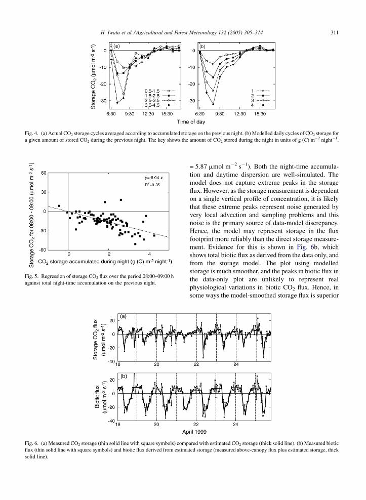
The nature of daytime depletion of canopy CO2 is

shown in Fig. 4a, which shows the mean diurnal CO2

storage flux during daytime for different values of night-

time storage. The peak depletion rate is a function of

total stored CO2, but there is little variation in the shape

of the depletion curve. The depletion rate peaks at about

8:30 a.m., and the canopy is always well mixed with the

atmosphere by about 13:30 p.m. After this, slight

accumulation was observed, which may be caused by

increased respiration following temperature increase,

combined with possible stable thermal stratification of

the lower canopy airspace. Integrating these lines and

converting to g (C) m�2 day�1 yielded total daytime

depletions of �1.02, �2.00, �2.74 and �3.55 g (C) m

�2 day�1 for night-time storage range of 0.5–1.5

Table 2

Values of the coefficient of determination, R2, derived in the regres-

sions: y = af(x) + b, using ratio factors for y, and linear of logarithmic

functions for f(x)

u* u*w

Linear

Sc/Fc 0.30 (8 � 10�4) 0.42 (4 � 10�5)

Sc/Fbiotic 0.29 (6 � 10�4) 0.35 (1 � 10�4)

Sc 0.29 (3 � 10�5) 0.35 (3 � 10�6)

Log

Sc/Fc 0.35 (2 � 10�4) 0.56 (4 � 10�7)

Sc/Fbiotic 0.37 (7 � 10�5) 0.47 (3 � 10�6)

Sc 0.36 (2 � 10�6) 0.42 (1 � 10�7)

The values in brackets are significance values. For comparison, R2

values using absolute storage, Sc, for y were also included from

Table 1.

(actual average 1.11), 1.5–2.5 (average 1.98), 2.5–3.5

(average 2.86) and 3.5–4.5 (average 3.83) line,

respectively. The last storage range contained only five

points and is of limited significance: otherwise the

storage measurement worked fairly well (daytime

depletion = night-time storage). We modelled this

depletion curve by regression of the depletion rate at

each hour against total storage in the previous night. A

linear function defined in Eq. (4) was used for the

regression. A example plot is shown in Fig. 5, for time

8:30 a.m. With the exception of a few outliers (probably

non-stationary weather events) the depletion flux is

approximately linearly proportional to the previous

night’s storage. The slope of this relationship was

calculated for each hour. Fig. 4b shows the mean

predicted depletion curves for different values of stored

night-time CO2. As would be expected, the phase

and amplitude of the depletion are similar to that in

the original data. Integrating these modelled lines

and converting to g (C) m�2 day�1 yielded daytime

depletion rate of �0.98, �1.97, �2.95 and �3.94 g

(C) m�2 day�1 for each night-time storage range, res-

pectively, in close agreement with the observed values.

3.4. Model validation against independent data

In order to evaluate the method described above,

eight days (18–25 April 1999) of continuously

measured storage had been excluded from the model

calibration and were now compared with the gap-filled

model predictions. The measured and estimated storage

CO2 for the period were compared in Fig. 6a. The model

is generally very successful in simulating the diurnal

and day-to-day variation in CO2 storage (RMSE


Fig. 4. (a) Actual CO2 storage cycles averaged according to accumulated storage on the previous night. (b) Modelled daily cycles of CO2 storage for

a given amount of stored CO2 during the previous night. The key shows the amount of CO2 stored during the night in units of g (C) m�2 night�1.

Fig. 5. Regression of storage CO2 flux over the period 08:00–09:00 h

against total night-time accumulation on the previous night.

Fig. 6. (a) Measured CO2 storage (thin solid line with square symbols) comp

flux (thin solid line with square symbols) and biotic flux derived from estima

solid line).

= 5.87 mmol m�2 s�1). Both the night-time accumula-

tion and daytime dispersion are well-simulated. The

model does not capture extreme peaks in the storage

flux. However, as the storage measurement is dependent

on a single vertical profile of concentration, it is likely

that these extreme peaks represent noise generated by

very local advection and sampling problems and this

noise is the primary source of data-model discrepancy.

Hence, the model may represent storage in the flux

footprint more reliably than the direct storage measure-

ment. Evidence for this is shown in Fig. 6b, which

shows total biotic flux as derived from the data only, and

from the storage model. The plot using modelled

storage is much smoother, and the peaks in biotic flux in

the data-only plot are unlikely to represent real

physiological variations in biotic CO2 flux. Hence, in

some ways the model-smoothed storage flux is superior

ared with estimated CO2 storage (thick solid line). (b) Measured biotic

ted storage (measured above-canopy flux plus estimated storage, thick


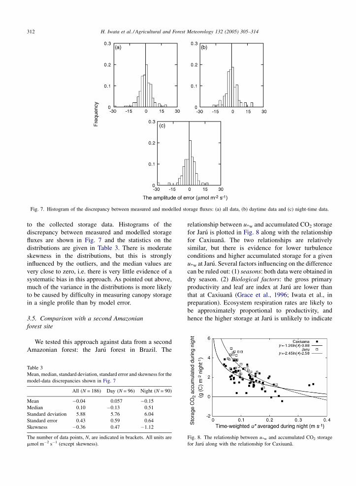
Fig. 7. Histogram of the discrepancy between measured and modelled storage fluxes: (a) all data, (b) daytime data and (c) night-time data.

to the collected storage data. Histograms of the

discrepancy between measured and modelled storage

fluxes are shown in Fig. 7 and the statistics on the

distributions are given in Table 3. There is moderate

skewness in the distributions, but this is strongly

influenced by the outliers, and the median values are

very close to zero, i.e. there is very little evidence of a

systematic bias in this approach. As pointed out above,

much of the variance in the distributions is more likely

to be caused by difficulty in measuring canopy storage

in a single profile than by model error.

3.5. Comparison with a second Amazonian

forest site

We tested this approach against data from a second

Amazonian forest: the Jaru forest in Brazil. The

Table 3

Mean, median, standard deviation, standard error and skewness for the

model-data discrepancies shown in Fig. 7

All (N = 186) Day (N = 96) Night (N = 90)

Mean �0.04 0.057 �0.15

Median 0.10 �0.13 0.51

Standard deviation 5.88 5.76 6.04

Standard error 0.43 0.59 0.64

Skewness �0.36 0.47 �1.12

The number of data points, N, are indicated in brackets. All units are

mmol m�2 s�1 (except skewness).

relationship between u*w and accumulated CO2 storage

for Jaru is plotted in Fig. 8 along with the relationship

for Caxiuana. The two relationships are relatively

similar, but there is evidence for lower turbulence

conditions and higher accumulated storage for a given

u*w at Jaru. Several factors influencing on the difference

can be ruled out: (1) seasons: both data were obtained in

dry season. (2) Biological factors: the gross primary

productivity and leaf are index at Jaru are lower than

that at Caxiuana (Grace et al., 1996; Iwata et al., in

preparation). Ecosystem respiration rates are likely to

be approximately proportional to productivity, and

hence the higher storage at Jaru is unlikely to indicate

Fig. 8. The relationship between u*w and accumulated CO2 storage

for Jaru along with the relationship for Caxiuana.


higher ecosystem respiration rates. Factors that are

likely to contribute to the difference include: (1)

measurement heights of CO2 profile: especially, the

lowest profilemeasurement in Jaru forest was at 0.05 m

above the ground, whichmay induce the value of higher

accumulation in stable nights. The importance of

measuring the first couple of meters is also addressed in

Gu et al. (2005). (2) Topography: the Caxiuana tower is

located close to the watershed in a weakly undulating

landscape, the Jaru tower is closer to the centre of a

river valley. Hence, the Jaru tower is less exposed to

winds (mean night-time u* at Jaru is 0.11 m s�1,

compared to 0.15 m s�1 at Caxiuana) and more likely

to accumulate CO2 associated with drainage in

katabatic flows.

4. Conclusions

To evaluate biotic CO2 exchange between the

vegetation and the atmosphere above, it is crucial to

include within-canopy CO2 storage, particularly in tall

forests, in calculating biotic flux. We developed a

simple method to estimate the within-canopy storage of

CO2. We found that estimating hourly storage from

hourly CO2 concentration at the tower top is unreliable,

since at this time scale the variations in above-canopy

CO2 are often decoupled from local changes in within-

canopy storage. We then estimated total night-time CO2

accumulation from meteorological or turbulence data

averaged overnight. The time-weighted friction velo-

city, u*w, was found to be the most reliable to estimate

CO2 accumulation. This enabled development of an

empirical storage accumulation and depletion model

that worked successfully when compared to indepen-

dent data from the same site. Application of the

model to independent data showed that, in spite of the

simplicity of this approach, the modelled storage was in

good agreement with the measured storage. Little bias

was found in the error histograms.

The approach presented in this paper is primarily

intended as a practical method of gap-filling of storage

data. However, the general similarity between two

forests in topographically distinct sites hints at the

possibility of applying a general correction model.

Topographic factors are most likely to explain the

difference between the two sites. At present, with only

two sites analysed, we suggest that site-specific

calibration would be necessary.

In this study, night-time accumulation was estimated

from one equation, since the lack of data limited the

examination of seasonal variations of accumulation

model curve. However, applying different equations for

each month or season may be more appropriate. For

sites with stronger temporal variations in temperature, a

temperature-dependent model for night-time respiration

would be required when allocating estimated night-time

storage, rather than constant respiration as used here.

Acknowledgements

We would like to thank Antonio Carlos Lola da

Costa, Fiona Carswell, Marcia Palheta, Rafael da Costa,

Joao Athaydes and Alan Braga for their roles in the

collection of long term data from Caxiuana, and Patrick

Meir and John Grace for their significant contributions

to this project. Research at Caxiuana was funded by

the EU Fifth Framework EUSTACH project as part

of the Large-Scale Biosphere Atmosphere Programme

in Amazonia (LBA). H.I. would like to take this

opportunity to thank Eiji Ohtaki and John Moncrieff

for giving him a chance to work on this project. Y.M.

gratefully acknowledges the support of a Royal Society

University Research Fellowship.

References

Baldocchi, D.D., Meyers, T.P., 1988. Turbulence structure in a decid-

uous forest. Boundary-Layer Meteorol. 43, 345–364.

Baldocchi, D., Falge, E., Gu, L.H., Olson, R., Hollinger, D., Running,

S., Anthoni, P., Bernhofer, C., Davis, K., Evans, R., Fuentes, J.,

Goldstein, A., Katul, G., Law, B., Lee, X.H., Malhi, Y., Meyers, T.,

Munger,W., Oechel, W., PawU, K.T., Pilegaard, K., Schmid, H.P.,

Valentini, R., Verma, S., Vesala, T., Wilson, K., Wofsy, S., 2001.

FLUXNET: a new tool to study the temporal and spatial variability

of ecosystem-scale carbon dioxide, water vapor, and energy flux

densities. Bull. Am. Meteorol. Soc. 82, 2415–2434.

Carswell, F.E., Costa, A.L., Palheta, M., Malhi, Y., Meir, P., Costa, J.

de P.R., Ruivo,M. de L., Leal, L. do S.M., Costa, J.M.N., Clement,

R.J., Grace, J., 2002. Seasonality in CO2 and H2O flux at an eastern

Amazonian rain forest. J. Geophysical Res. 107, 43,1–43,16.

Culf, A.D., Esteves, J.L., Marques Filho, A.O., da Rocha, H.R., 1996.

Radiation, temperature and humidity over forest and pasture in

Amazonia. In: Gash, J.H.C., Nobre, C.A., Roberts, J.M., Victoria,

R.L. (Eds.), Amazonian Deforestation and Climate. John Wiley

and Sons, Chichester, pp. 175–192.

Grace, J., Malhi, Y., Lloyd, J., McIntyre, J., Miranda, A.C., Meir, P.,

Miranda, H.S., 1996. The use of eddy covariance to infer the net

carbon dioxide uptake of Brazilian rain forest. Global Change

Biol. 2, 209–218.

Gu, L., Falge, E.M., Borden, T., Baldocchi, D.D., Black, T.A., Saleska,

S.R., Suni, T., Verma, S.B., Vesala, T., Wofsy, S.C., Xu, L., 2005.

Objective threshold determination for nighttime eddy flux filter-

ing. Agric. For. Meteorol. 128, 179–197.

Meir, P., 1996. The exchange of carbon dioxide in tropical forest. PhD

Thesis. University of Edinburgh.

Moncrieff, J.B., Massheder, J.M., de Bruin, H., Elbers, J., Friborg, T.,

Heusinkveld, B., Kabat, P., Scott, S., Soegaard, H., Verhoef, A.,

1997. A system to measure surface fluxes of momentum, sensible


heat, water vapour and carbon dioxide. J. Hydrol. 188–189, 589–

611.

Von Randow, C., Manzi, A.O., Kruijt, B., de Oliveira, P.J., Zanchi,

F.B., Silva, R.L., Hodnett, M.G., Gash, J.H.C., Elbers, J.A.,

Waterloo, M.J., Cardoso, F.L., Kabat, P., 2004. Comparative

measurements and seasonal variations in energy and carbon

exchange over forest and pasture in South West Amazonia. Theor.

Appl. Climatol. 78, 5–26.

Wood, D., Malhi, Y., Baker, T.R., Write, J., Phillips, O.L., Cochrane,

T., Meir, P., Lloyd, J., Almeida, S., Arroyo, L., Chave, J., Higuchi,

N., Killeen, T.J., Laurance, S.G., Laurance, W.F., Lewis, S.L.,

Monteagudo, A., Neill, D.A., Vargas, P.N., Pitman, N.C.A., Ques-

ada, C.A., Salomao, R., Silva, J.N.M., Lezama, A.T., Terborgh, J.,

Martinez, R.V., Vinceti, B. The regional variation of above-ground

live biomass in old-growth Amazonian forest, Global Change

Biol., submitted for publication.

Gap-filling measurements of carbon dioxide storage in tropical rainforest canopy airspace

Documents

Transcript of Gap-filling measurements of carbon dioxide storage in tropical rainforest canopy airspace