14 Packing R-trees with Space-filling Curves
47
14 Packing R-trees with Space-filling Curves: Theoretical Optimality, Empirical Efficiency, and Bulk-loading Parallelizability JIANZHONG QI, The University of Melbourne, Australia YUFEI TAO, Chinese University of Hong Kong, Hong Kong, China YANCHUAN CHANG and RUI ZHANG, The University of Melbourne, Australia The massive amount of data and large variety of data distributions in the big data era call for access methods that are efficient in both query processing and index management, and over both practical and worst-case workloads. To address this need, we revisit two classic multidimensional access methods—the R-tree and the space-filling curve. We propose a novel R-tree packing strategy based on space-filling curves. This strategy produces R-trees with an asymptotically optimal I/O complexity for window queries in the worst case. Ex- periments show that our R-trees are highly efficient in querying both real and synthetic data of different distributions. The proposed strategy is also simple to parallelize, since it relies only on sorting. We propose a parallel algorithm for R-tree bulk-loading based on the proposed packing strategy and analyze its per- formance under the massively parallel communication model. To handle dynamic data updates, we further propose index update algorithms that process data insertions and deletions without compromising the op- timal query I/O complexity. Experimental results confirm the effectiveness and efficiency of the proposed R-tree bulk-loading and updating algorithms over large data sets. CCS Concepts: • Theory of computation → Data structures and algorithms for data management;• Information systems → Multidimensional range search; Spatial-temporal systems; Additional Key Words and Phrases: R-trees, window queries, rank space, logarithmic method ACM Reference format: Jianzhong Qi, Yufei Tao, Yanchuan Chang, and Rui Zhang. 2020. Packing R-trees with Space-filling Curves: Theoretical Optimality, Empirical Efficiency, and Bulk-loading Parallelizability. ACM Trans. Database Syst. 45, 3, Article 14 (August 2020), 47 pages. https://doi.org/10.1145/3397506 This work is supported in part by Australian Research Council (ARC) Discovery Project DP180103332, a direct grant (Project Number: 4055079) from the Chinese University of Hong Kong, and a Faculty Research Award from Google. Authors’ addresses: J. Qi, Y. Chang, and R. Zhang, School of Computing and Information Systems, The University of Melbourne, Parkville, Victoria, Australia 3010; emails: [email protected], [email protected], [email protected]; Y. Tao, Department of Computer Science and Engineering, Chinese University of Hong Kong, Shatin, Hong Kong, China; email: [email protected]. Permission to make digital or hard copies of all or part of this work for personal or classroom use is granted without fee provided that copies are not made or distributed for profit or commercial advantage and that copies bear this notice and the full citation on the first page. Copyrights for components of this work owned by others than the author(s) must be honored. Abstracting with credit is permitted. To copy otherwise, or republish, to post on servers or to redistribute to lists, requires prior specific permission and/or a fee. Request permissions from [email protected]. © 2020 Copyright held by the owner/author(s). Publication rights licensed to ACM. 0362-5915/2020/08-ART14 $15.00 https://doi.org/10.1145/3397506 ACM Transactions on Database Systems, Vol. 45, No. 3, Article 14. Publication date: August 2020.
-
Upload
khangminh22 -
Category
Documents
-
view
5 -
download
0
Transcript of 14 Packing R-trees with Space-filling Curves
14
Packing R-trees with Space-filling Curves: Theoretical
Optimality, Empirical Efficiency, and Bulk-loading
Parallelizability
JIANZHONG QI, The University of Melbourne, Australia
YUFEI TAO, Chinese University of Hong Kong, Hong Kong, China
YANCHUAN CHANG and RUI ZHANG, The University of Melbourne, Australia
The massive amount of data and large variety of data distributions in the big data era call for access methods
that are efficient in both query processing and index management, and over both practical and worst-case
workloads. To address this need, we revisit two classic multidimensional access methods—the R-tree and the
space-filling curve. We propose a novel R-tree packing strategy based on space-filling curves. This strategy
produces R-trees with an asymptotically optimal I/O complexity for window queries in the worst case. Ex-
periments show that our R-trees are highly efficient in querying both real and synthetic data of different
distributions. The proposed strategy is also simple to parallelize, since it relies only on sorting. We propose
a parallel algorithm for R-tree bulk-loading based on the proposed packing strategy and analyze its per-
formance under the massively parallel communication model. To handle dynamic data updates, we further
propose index update algorithms that process data insertions and deletions without compromising the op-
timal query I/O complexity. Experimental results confirm the effectiveness and efficiency of the proposed
R-tree bulk-loading and updating algorithms over large data sets.
CCS Concepts: • Theory of computation → Data structures and algorithms for data management; •
Information systems → Multidimensional range search; Spatial-temporal systems;
Additional Key Words and Phrases: R-trees, window queries, rank space, logarithmic method
ACM Reference format:
Jianzhong Qi, Yufei Tao, Yanchuan Chang, and Rui Zhang. 2020. Packing R-trees with Space-filling Curves:
Theoretical Optimality, Empirical Efficiency, and Bulk-loading Parallelizability. ACM Trans. Database Syst. 45,
3, Article 14 (August 2020), 47 pages.
https://doi.org/10.1145/3397506
This work is supported in part by Australian Research Council (ARC) Discovery Project DP180103332, a direct grant (Project
Number: 4055079) from the Chinese University of Hong Kong, and a Faculty Research Award from Google.
Authors’ addresses: J. Qi, Y. Chang, and R. Zhang, School of Computing and Information Systems, The University of
Melbourne, Parkville, Victoria, Australia 3010; emails: [email protected], [email protected],
[email protected]; Y. Tao, Department of Computer Science and Engineering, Chinese University of Hong Kong,
Shatin, Hong Kong, China; email: [email protected].
Permission to make digital or hard copies of all or part of this work for personal or classroom use is granted without fee
provided that copies are not made or distributed for profit or commercial advantage and that copies bear this notice and
the full citation on the first page. Copyrights for components of this work owned by others than the author(s) must be
honored. Abstracting with credit is permitted. To copy otherwise, or republish, to post on servers or to redistribute to lists,
requires prior specific permission and/or a fee. Request permissions from [email protected].
© 2020 Copyright held by the owner/author(s). Publication rights licensed to ACM.
0362-5915/2020/08-ART14 $15.00
https://doi.org/10.1145/3397506
ACM Transactions on Database Systems, Vol. 45, No. 3, Article 14. Publication date: August 2020.

14:2 J. Qi et al.
1 INTRODUCTION
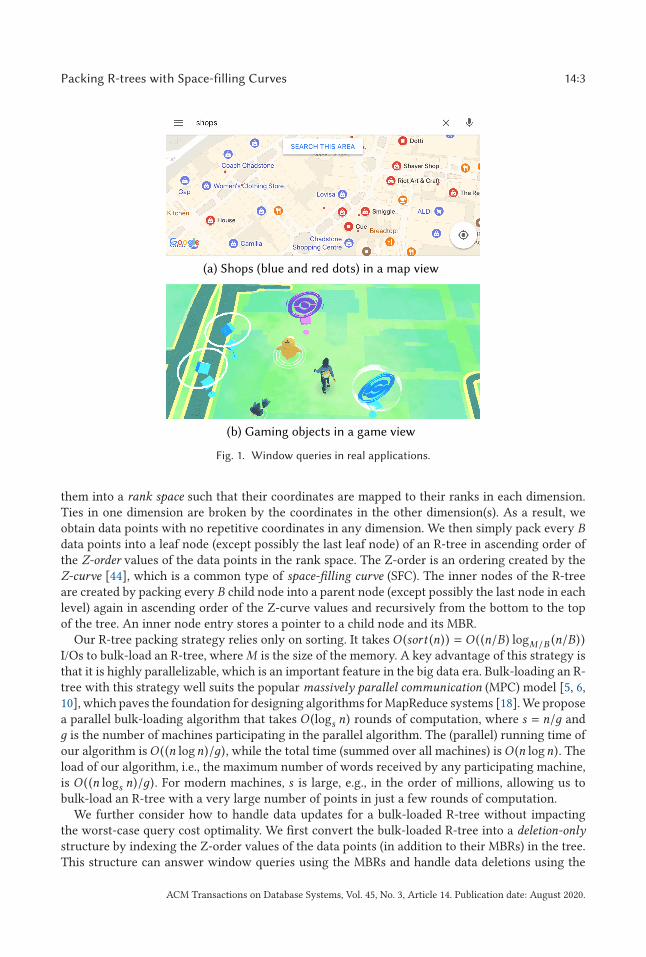
Spatial databases have been traditionally used in geographic information systems, computer-aideddesign, multimedia data management, and medical studies. They are becoming ubiquitous with theproliferation of location-based services such as digital mapping, augmented reality gaming, geoso-cial networking, and targeted advertising. For example, in digital mapping services such as GoogleMaps, the “search this area” functionality supports querying places of interest (POIs) such as shopswithin a given view area (cf. Figure 1(a)). In a popular augmented reality game, Pokémon GO [58],every player has an avatar placed in the game map based on the player’s geographical location.The players can interact with gaming objects (e.g., “Pokémon”) in the game view through theiravatars (cf. Figure 1(b)). Managing POIs or gaming objects in a view that usually has a rectangularwindow shape is a typical application of spatial databases.
In these applications, there may be hundreds of millions of spatial objects (e.g., shops, restau-rants, Pokémon) with a variety of distributions to be managed. Meanwhile, there may be hugenumbers of service requests from users, e.g., Google Maps has reached 1B users [49], and Poké-mon GO is attracting over 20M daily active users [20]. Reporting POIs or Pokémon in a given areain real time under such settings poses significant challenges.
Spatial indices are important techniques to address such challenges. They offer fast retrievalof spatial objects. We revisit a classic spatial index—the R-tree [27]. We aim to achieve an R-treestructure that is efficient in both window query processing and tree bulk-loading, and over bothpractical and worst-case workloads. R-trees have attracted extensive research interest [4, 7, 11,28, 33, 51, 55] and have been implemented in industrial database systems [42, 43]. An R-tree is abalanced tree structure for external memory-based spatial object indexing. Every node in an R-tree may contain multiple entries. In the leaf nodes, the entries are minimum bounding rectangles
(MBR) of the data objects (and pointers to them); in the inner nodes, the entries are MBRs of andpointers to the child nodes. An R-tree node usually corresponds to a disk block, the size of whichconstrains the node capacity, i.e., the maximum number of entries per node, denoted by B. Givenan R-tree, a window query returns all the data objects (e.g., POIs or Pokémon) indexed in the treethat are within or intersect a given query window, which is usually a rectangular region of interest.
R-trees have good query efficiency in practice when they are constructed with carefully craftedheuristics [11, 33, 36, 55]. However, all these heuristics cannot produce an R-tree with attrac-tive performance guarantees in the worst case. The Priority R-tree (PR-tree) [7] is an R-treewith a non-trivial theoretical query performance guarantee. It answers a window query withO ((n/B)1−1/d + k/B) I/Os in the worst case, which is known to be asymptotically optimal [4].Here, n, d , and k denote the data set size, the dimensionality, and the output size, i.e., the numberof objects satisfying the query, respectively. The PR-tree is designed for rectangles. As a follow-upstudy shows [28], the PR-tree may not have satisfactory empirical performance on data objects ofa small size (e.g., point data) or queries with small query windows; and the tree construction isdifficult to parallelize.
We re-examine the construction of R-trees and aim for high window query efficiency over pointdata, which is a common way for representing locations on digital maps. Spatial objects withextents can also be efficiently transformed into points for query processing [65]. We target appli-cation scenarios such as digital mapping where queries are much more frequent than updates overthe data. We construct R-trees that are query cost optimal. Our R-trees can also handle dynamicdata updates efficiently and without compromising the query cost optimality.
We propose an R-tree packing strategy that creates R-trees with the worst-case optimal windowquery I/O cost O ((n/B)1−1/d + k/B). This strategy has a simple procedure and yields R-trees thathave high practical query efficiency. A key step we take before packing the data points is to map
ACM Transactions on Database Systems, Vol. 45, No. 3, Article 14. Publication date: August 2020.
Packing R-trees with Space-filling Curves 14:3
Fig. 1. Window queries in real applications.
them into a rank space such that their coordinates are mapped to their ranks in each dimension.Ties in one dimension are broken by the coordinates in the other dimension(s). As a result, weobtain data points with no repetitive coordinates in any dimension. We then simply pack every Bdata points into a leaf node (except possibly the last leaf node) of an R-tree in ascending order ofthe Z-order values of the data points in the rank space. The Z-order is an ordering created by theZ-curve [44], which is a common type of space-filling curve (SFC). The inner nodes of the R-treeare created by packing every B child node into a parent node (except possibly the last node in eachlevel) again in ascending order of the Z-curve values and recursively from the bottom to the topof the tree. An inner node entry stores a pointer to a child node and its MBR.
Our R-tree packing strategy relies only on sorting. It takes O (sort (n)) = O ((n/B) logM/B (n/B))I/Os to bulk-load an R-tree, where M is the size of the memory. A key advantage of this strategy isthat it is highly parallelizable, which is an important feature in the big data era. Bulk-loading an R-tree with this strategy well suits the popular massively parallel communication (MPC) model [5, 6,10], which paves the foundation for designing algorithms for MapReduce systems [18]. We proposea parallel bulk-loading algorithm that takes O (logs n) rounds of computation, where s = n/д andд is the number of machines participating in the parallel algorithm. The (parallel) running time ofour algorithm isO ((n logn)/д), while the total time (summed over all machines) isO (n logn). Theload of our algorithm, i.e., the maximum number of words received by any participating machine,is O ((n logs n)/д). For modern machines, s is large, e.g., in the order of millions, allowing us tobulk-load an R-tree with a very large number of points in just a few rounds of computation.
We further consider how to handle data updates for a bulk-loaded R-tree without impactingthe worst-case query cost optimality. We first convert the bulk-loaded R-tree into a deletion-only
structure by indexing the Z-order values of the data points (in addition to their MBRs) in the tree.This structure can answer window queries using the MBRs and handle data deletions using the
ACM Transactions on Database Systems, Vol. 45, No. 3, Article 14. Publication date: August 2020.

14:4 J. Qi et al.
Z-order values (just like a B-tree). It retains the O (n/B) space cost and the O ((n/B)1−1/d + k/B)window query I/O cost, while it can also handle a deletion in O (logB n) amortized I/Os.
We then extend this structure to support insertions via the logarithmic method [13, 45]. Thelogarithmic method replaces dynamic data insertions with bulk-loading a series of up to �logB n�R-trees, where the ith R-tree holds at most Bi new data points. When a window query is issued, thequery is run on every bulk-loaded R-tree. The worst-case query cost optimality of any individualR-tree is retained, since there are no dynamic insertions on these trees. The overall window queryI/O cost does not exceedO ((n/B)1−1/d + k/B) either. This is because the tree sizes form a geometricseries, the maximum of which is n. The overall query cost is dominated by that of the largest tree,which is O ((n/B)1−1/d + k/B).
When applying the logarithmic method, we use a B-tree to record theID of the tree in which adata point is indexed. This B-tree helps identify the tree from which a data point is to be deleted.The treeIDs in this B-tree may need to be updated when there are data insertions, which adds addi-tional insertion costs. To reduce the insertion costs, we further modify our deletion-only structureby adding pointers that point from data points to the B-tree nodes. Such pointers enable efficientlylocating the B-tree nodes to be updated for data insertions. As a result, compared with an earlierstudy on dynamization of bulk-loaded structures [8], we reduce the amortized insertion I/O costfrom O (log2
B n) to O (logB n) when O (logM/B (n/B)) = O (1), i.e., the memory size M is at the scaleof the data set size n, which is typically satisfied by modern machines.
While the rank space has been used by the computational geometry community to develop the-oretical bounds [17, 21], we observe for the first time that rank-space conversion can be leveragedto build a worst-case optimal structure for window queries. Furthermore, it is perhaps surprisingthat we are able to achieve the purpose by combining the rank space with an SFC, because SFC-based indices were previously thought to have poor worst-case query costs. Indeed, as shown byArge et al. [7], if an SFC is used directly (i.e., in the original data space) for indexing, there ex-ist window queries that retrieve few points, but have I/O costs linear to the data set size. In fact,even analyzing the query cost of an SFC-based index is non-trivial. The limited literature on thistopic [31, 39, 60] has focused on the average query cost, which is analyzed indirectly by studyingthe clustering behavior of SFCs.
In summary, this article makes the following contributions:
(1) We propose the first SFC-based packing strategy that creates R-trees with a worst-caseoptimal window query I/O cost.
(2) The proposed packing strategy suggests a simple R-tree bulk-loading algorithm relyingonly on sorting. We propose such an algorithm under the massively parallel communi-cation model (and thus, it works on MapReduce systems) with attractive performanceguarantees.
(3) We propose R-tree-based dynamic index structures to handle data updates. We show thatsuch dynamic structures retain the optimal window query I/O cost in the worst case.Further, compared with an earlier study on dynamization of bulk-loaded structures [8],we reduce the amortized data insertion cost from O (log2
B n) to O (logB n).(4) We perform extensive experiments on both real and synthetic data. The results confirm
the superiority of the proposed R-tree packing strategy: on real data, the query I/O cost ofthe R-trees that we construct is up to 31% lower than that of PR-trees [7] and similar to thatof STR-trees [36], which are a classic type of sorting-based bulk-loaded R-trees; on highlyskewed synthetic data, the query I/O cost of the R-trees that we construct is 54% lowerthan that of PR-trees and 64% lower than that of STR-trees. The proposed bulk-loadingalgorithm also outperforms the PR-tree bulk-loading algorithm in running time by 85%
ACM Transactions on Database Systems, Vol. 45, No. 3, Article 14. Publication date: August 2020.
Packing R-trees with Space-filling Curves 14:5
over large data sets with 20M data points. When processing updates with the proposeddynamic index structures, we achieve up to 98% lower query I/O costs comparing with theLR-tree [16]—a Hilbert R-tree [33] variant with update supports. The advantage is mostsignificant when the data distribution is highly skewed.
This article is an extension of our previous conference paper [50]. In the previous work, wepresented the R-tree packing strategy based on SFCs in the rank space. We showed the worst-casequery I/O cost optimality and the parallel implementation of the strategy. In this article, we presentnew techniques to handle data updates to the R-trees constructed by our packing strategy whileretaining the worst-case query I/O cost optimality (Section 5). As a result, we obtain a fully dynamicindex structure that is worst-case optimal and empirically efficient for window query processing.Further, we show that our techniques can reduce the amortized data insertion cost fromO (log2
B n)to O (logB n), comparing with an earlier study on dynamization of bulk-loaded structures [8]. Ouradditional experiments on the index update techniques show (i) the effectiveness of the techniquesfor retaining the high query efficiency of our index structure and (ii) the efficiency of the techniquesin handling updates to our index structure (Section 6.2.3). We have also added a literature reviewon R-tree update techniques (Section 2).
The rest of the article is organized as follows: Section 2 reviews related work. Section 3 details theproposed R-tree packing strategy and the worst-case window query I/O costs. Section 4 describesthe proposed parallel R-tree bulk-loading algorithm. Section 5 discusses data update handling.Section 6 presents experimental results, and Section 7 concludes the article.
2 RELATED WORK
We review studies on spatial queries and access methods with a focus on R-trees.Spatial queries and access methods. We focus on the window query (rectangular range
query), which is a basic type of spatial query [26]. A window query returns all data objects thatsatisfy a certain predicate with a given query window, i.e., a (hyper)rectangular region of interest.Common query predicates include containment and intersection, which require the data objectsto be fully contained in or intersect the query window, respectively.
A straightforward window query algorithm sequentially checks every data object and returnsan object if it satisfies the query predicate. This algorithm takes O (n/B) I/Os regardless of datadistribution and output size. Spatial indices have been used to obtain higher query efficiency. Wefocus on the R-tree index [27]. For a comprehensive review on spatial indices and spatial queryprocessing, interested readers are referred to Reference [22].
R-trees. As discussed earlier, the R-tree is a balanced tree structure. The maximum number ofentries per tree node (node capacity) B is constrained by the disk block size, while the minimum
number of entries per tree node (except the root node) is Ω(B). The root node needs to contain atleast two entries unless it is also a leaf node. Thus, the height of an R-tree indexing n objects isbounded by O (logB n).
A window query is processed by a top-down traversal over the nodes of an R-tree whose MBRssatisfy the query. When the leaf nodes are reached, data objects in them satisfying the query arereturned. A series of studies [11, 14, 30, 41, 55] propose heuristics to optimize the node MBRsduring dynamic data insertion. The R*-tree [11], for example, considers the MBR overlaps andregion perimeters to decide the node into which a new object should be inserted.
R-tree packing and bulk-loading. A different stream of research considers how to con-struct an R-tree by packing data objects into the leaf nodes directly rather than inserting themindividually. The entire R-tree is bulk-loaded in a bottom-up fashion. Most R-tree packing algo-rithms [1, 19, 28, 33, 36, 52] rely on some ordering of the data objects and hence have an I/O cost
ACM Transactions on Database Systems, Vol. 45, No. 3, Article 14. Publication date: August 2020.
14:6 J. Qi et al.
of O ((n/B) logM/B (n/B)), which is the cost for sorting n objects (recall that M is the number ofobjects allowed in the main memory). Specifically, Roussopoulos and Leifker [52] sort the data ob-jects by their x-coordinates and pack every B objects into a leaf node. Leutenegger et al. [36] firstsort the data objects by their x-coordinates and then partition the data into
√n/B subsets. Objects
in each subset are sorted by their y-coordinates and packed into the leaf nodes. Other studies usethe Hilbert ordering [19, 28, 33]. Their resultant R-trees have shown good window query perfor-mance on nicely distributed data [28]. Achakeev et al. [1] also use an SFC (e.g., a Hilbert curve)for object ordering. Instead of packing every B objects into a leaf node, they compute a series ofsplit points to split the list of sorted objects and pack the objects into leaf nodes accordingly. Theiraim is to minimize the sum of the MBR areas of the resultant tree nodes. These R-trees are notworst-case optimal for window queries.
There are also top-down bulk-loading algorithms. The Top-down Greedy Split (TGS) algo-rithm [23] is a typical example. TGS partitions the data set into two subsets repeatedly until Bapproximately equisized subsets have been obtained. The MBRs of these B subsets form entriesof the root. Each partition uses a cut orthogonal to an axis that yields two subsets with the min-imum sum of costs, where the cost is based on a user-defined function, e.g., the area of the MBRof a subset. There are O (B) candidate cuts, where the hidden constant lies in the different cuts indifferent dimensions and on different orderings (e.g., lower x corner, center). In each dimensionand with a particular ordering, the ith cut puts i · (n/B) objects in one subset and the rest in theother subset. TGS has been shown to produce R-trees with good query efficiency, but it has a highworst-case I/O cost, O (n logB n), for R-tree construction. This is because it needs to scan the dataset B times to create the B partitions of a node (assuming that the orderings used for partitioninghave been precomputed). If viewed from a recursive binary partition perspective, the I/O cost ofTGS is effectively O ((n/B) log2 n) [7].
Agarwal et al. [4] propose an algorithm to bulk-load a Box-tree, which can be converted to an R-tree with a worst-case query I/O cost ofO ((n/B)1−1/d + k logB n). This work is more of theoreticalinterest. No implementation or experimental results have been given for the algorithm.
The PR-tree [7] is an R-tree that offers a worst-case window query I/O cost of O ((n/B)1−1/d +
k/B), which is asymptotically optimal [4]. A PR-tree is created from a pseudo-PR-tree, which is anunbalanced tree built in a top-down fashion. To create a pseudo-PR-tree, the data set is partitionedinto six partitions to form the child nodes of the root. Four of the partitions contain B objectseach, which are objects with the smallest lower x-coordinates, the smallest lower y-coordinates,the largest upper x-coordinates, and the largest upper y-coordinates, respectively. The remainingtwo partitions are two equisized partitions of the remaining objects, which are then recursivelypartitioned to form subtrees of the root. When a pseudo-PR-tree is created, its leaf nodes are usedas the leaf nodes of a PR-tree. The MBRs of the leaf nodes are used to create another pseudo-PR-tree, the leaf nodes of which are used as the parent nodes of the leaf nodes of the PR-tree. APR-tree is then built with O ((n/B) logn) I/Os bottom-up. Arge et al. [7] further propose a bulk-loading strategy that lowers the I/O cost to O ((n/B) logM/B (n/B)). The main issue of the PR-treeis that it lacks practical efficiency in answering queries with small query windows or over dataobjects of a small size (e.g., point data) [28].
We also note that other spatial indices such as kd-trees [12], O-trees [34], and cross-trees [25] canoffer a worst-case optimal query I/O performance. Compared with R-trees created by our packingstrategy, kd-trees are more difficult to bulk-load in parallel. In the MPC model, Agarwal et al. [5]propose a randomized algorithm that can bulk-load a kd-tree with O (polylogs n) rounds of com-putation. In contrast, we can bulk-load an R-tree with O (logs n) rounds of computation, which islower, and our bulk-loading algorithm is deterministic. As for O-trees, they do not belong to the
ACM Transactions on Database Systems, Vol. 45, No. 3, Article 14. Publication date: August 2020.

Packing R-trees with Space-filling Curves 14:7
R-tree family. They combine multiple auxiliary structures to ensure their theoretical guarantees.This approach is mainly of theoretical interest, but in practice is expensive in both space con-sumption and query cost (even being asymptotically optimal in the worst case). Cross-trees sharea similar issue in its practical query performance [3]. These indices are not discussed further.
R-tree update handling. The dynamic R-tree construction heuristics [11, 14, 30, 41, 55] men-tioned above (e.g., the R*-tree insertion heuristics [11]) can also handle R-tree updates. Such heuris-tics, however, do not guarantee optimal query performance for the updated R-trees.
Studies on R-tree packing and bulk-loading focus on static data settings. Most of them either donot consider updates at all [4, 23, 36] or simply use the above dynamic R-tree construction heuris-tics for updates [52]. The Hilbert R-tree [28] takes a slightly different update handling strategy.This R-tree can be seen as a B-tree that indexes the Hilbert-order values of the data points, and itsupdates are handled by B-tree update algorithms. None of these studies guarantee optimal queryperformance, with or without updates.
Arge et al. [7] extend the PR-tree to an LPR-tree using the logarithmic method [13, 45] forhandling updates while retaining the worst-case optimal window query performance. The LPR-tree consists of a series of annotated pseudo-PR-trees (APR-trees) with increasing sizes. An APR-treeis a pseudo-PR-tree with additional aggregate information stored in the inner nodes of the tree.Data insertions on the LPR-tree are handled by bulk-loading new (and larger) APR-trees over thedata points to be inserted together with the data points in the existing (and smaller) APR-trees.Data deletions, however, are handled by deleting the data points directly from the APR-trees thatcontain them. To help locate a data point to be deleted, a time index is used to keep track of theAPR-tree in which a data point is contained. To further improve the update efficiency, an O (M )sized component of the LPR-tree is kept in main memory, which includes the first log2 (M/B) APR-trees and the top levels of the rest of the APR-trees. By doing so, the LPR-tree obtains an amortizedinsertion I/O cost ofO (logB (n/M ) + (1/B) logM/B (n/B) · log2 (n/M )) and an amortized deletion I/Ocost of O (logB (n/M )). The LPR-tree is more of theoretical interest. No implementation or exper-imental results have been given for it. Our proposed dynamic structure also uses the logarithmicmethod, but it differs from the LPR-tree in that it is built on R-trees directly, which are much easierto construct and update than the APR-trees. This enables us to implement our dynamic structureand evaluate its empirical performance. Also, our dynamic structure does not need to reside inmain memory, which is more flexible. To the best of our knowledge, our dynamic structure is thefirst dynamic structure that is built on the R-trees directly while retaining the worst-case optimalwindow query performance.
Bozanis et al. [16] apply the logarithmic method over the Hilbert R-tree and propose the LR-tree.The LR-tree bulk-loads new Hilbert R-trees to handle data insertions. It uses a simplified R∗-treedeletion algorithm without node merging to handle data deletions. Since the underlying R-treesin the LR-tree are not window query optimal, the LR-tree does not guarantee worst-case optimalwindow query performance either. Regardless of this, the LR-tree is the closest structure to ourproposed dynamic structure. Thus, it is used as a baseline in our experiments.
Parallel R-tree management. Parallelism has been exploited to scale R-trees to large data setsand user groups. An early study [32] considers storing an R-tree on a multi-disk system. It stores anewly created tree node in the disk that contains the most dissimilar nodes to optimize the systemthroughput. A few studies [35, 38, 54] assume a shared-nothing (client-server) architecture fordistributed R-tree storing and query processing. Koudas et al. [35] store the inner nodes on a serverwhile the leaf nodes are stored on clients. They study how to decide the number of data objectsto be stored on a client and which objects to be stored together. Schnitzer and Leutenegger [54]further create local R-trees on clients for higher query efficiency. Mondal et al. [38] study loadbalancing for R-trees in shared-nothing systems.
ACM Transactions on Database Systems, Vol. 45, No. 3, Article 14. Publication date: August 2020.

14:8 J. Qi et al.
Table 1. Frequently Used Symbols
Symbol Description
P A data setp A data pointn The cardinality of Pd The dimensionality of Pq A window queryk The answer set size of a window queryT An R-treeB The node capacity of an R-treeh The height of an R-treeM The memory size of a standalone machineд The number of machines in a clusters The number of data points allowed in a machineΓ An R-tree (B-tree) indexing both MBRs and Z-order values of data points
Λid A B-tree mapping data pointIDs to Z-order values and treeIDsH The number of sub-trees in a LogR∗-treeμ The number of data point updates processedη The number of global rebuildsnj The number of data points at the jth global rebuild
The studies above do not focus on parallel R-tree bulk-loading. Papadopoulos and Manolopou-los [48] propose a generic procedure for parallel spatial index bulk-loading. They use sampling toestimate the data distribution, which helps partition the data space into regions. Data objects indifferent regions are assigned to different clients for local index building. A global index is built onthe server to serve as a coordinator for query processing. A more recent study [2] bulk-loads anR-tree with the MapReduce framework level-by-level, where each level takes a MapReduce round.It uses the bulk-loading strategy mentioned above that aims to minimize the sum of the MBR areasof the tree nodes [1]. Similar ideas have been used on GPUs [61] without a cost analysis.
3 R-TREE PACKING
We consider a set P of n data points in a d-dimensional Euclidean space. For ease of presentation,we use d = 2 in our examples, although our approach applies to an arbitrary fixed dimensionalityd ≥ 2. We focus on window queries. Given a rectangle q, a window query reports all the points inP ∩ q. We list the frequently used symbols in Table 1.
3.1 Mapping to Rank Space
Before creating an index structure over P , we first map the data points into a d-dimensional rank
space as follows: In each dimension of the original data space, we sort the data points by theircoordinates and use the ranks as the coordinates in the corresponding dimension of the rank space.If two data points have the same rank in a dimension, we break the tie by further comparing theircoordinates in the other dimensions (of the original space) in the order of dimension 1, dimension2, . . ., dimension d . We assume no data points with the same coordinates in all d dimensions.
Define by [n] the integer domain [0,n − 1]. After the mapping, P becomes a set ofn d-dimensional
points in [n]d such that no two points share the same coordinate in any dimension.
ACM Transactions on Database Systems, Vol. 45, No. 3, Article 14. Publication date: August 2020.
Packing R-trees with Space-filling Curves 14:9
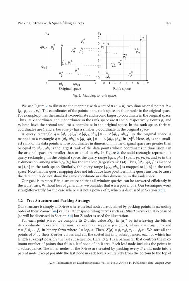
Fig. 2. Mapping to rank space.
We use Figure 2 to illustrate the mapping with a set of 8 (n = 8) two-dimensional points P ={p1,p2, . . . ,p8}. The coordinates of the points in the rank space are their ranks in the original space.For example,p1 has the smallest x-coordinate and second largesty-coordinate in the original space.Thus, its x-coordinate and y-coordinate in the rank space are 0 and 6, respectively. Points p2 andp3 both have the second smallest x-coordinate in the original space. In the rank space, their x-coordinates are 1 and 2, because p2 has a smaller y-coordinate in the original space.
A query rectangle q = [qle1,qhe1] × [qle2,qhe2] × · · · × [qled ,qhed ] in the original space ismapped to a rectangle q = [ql1,qh1] × [ql2,qh2] × · · · × [qld ,qhd ] in [n]d . Here, qli is the small-est rank of the data points whose coordinates in dimension i in the original space are greater thanor equal to qle1; qhi is the largest rank of the data points whose coordinates in dimension i inthe original space are smaller than or equal to qhi . In Figure 2, the solid rectangle represents aquery rectangle q. In the original space, the query range [qle1,qhe1] spans p2,p3,p4, and p6 in thex-dimension, among which p2 (p6) has the smallest (largest) rank 1 (4). Thus, [qle1,qhe1] is mappedto [1, 4] in the rank space. Similarly, the query range [qle2,qhe2] is mapped to [2, 5] in the rankspace. Note that the query mapping does not introduce false positives in the query answer, becausethe data points do not share the same coordinate in either dimension in the rank space.
Our goal is to store P in a structure so that all window queries can be answered efficiently inthe worst case. Without loss of generality, we consider that n is a power of 2. Our techniques workstraightforwardly for the case where n is not a power of 2, which is discussed in Section 3.3.1.
3.2 Tree Structure and Packing Strategy
Our structure is simply an R-tree where the leaf nodes are obtained by packing points in ascendingorder of their Z-order [44] values. Other space-filling curves such as Hilbert curves can also be used(as will be discussed in Section 3.4) but Z-order is used for illustration.
For each point p ∈ P , we compute its Z-order value Z (p) in [n]d by interleaving the bits ofits coordinate in every dimension. For example, suppose p = (x ,y), where x = α1α2 . . . αl andy = β1β2 . . . βl in binary form where l = log2 n. Then, Z (p) = β1α1β2α2 . . . βlαl . We sort all thepoints of P by their Z-order values and cut the sorted list into subsequences, each of which haslength B, except possibly the last subsequence. Here, B ≥ 1 is a parameter that controls the max-imum number of points that fit in a leaf node of an R-tree. Each leaf node includes the points ina subsequence. The inner nodes of the R-tree are created by packing every B child node into aparent node (except possibly the last node in each level) recursively from the bottom to the top of
ACM Transactions on Database Systems, Vol. 45, No. 3, Article 14. Publication date: August 2020.
14:10 J. Qi et al.
Fig. 3. R-tree packing.
the tree. This process resembles how a B-tree is created, except that an inner node entry stores apointer to a child node and its MBR instead of a key value. This creates our target R-tree.
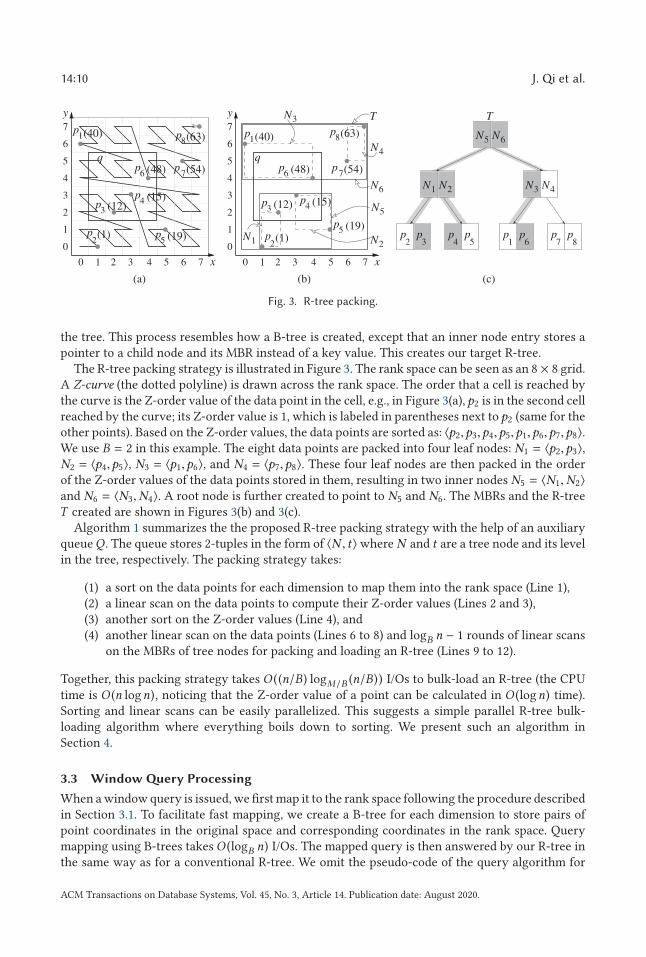
The R-tree packing strategy is illustrated in Figure 3. The rank space can be seen as an 8 × 8 grid.A Z-curve (the dotted polyline) is drawn across the rank space. The order that a cell is reached bythe curve is the Z-order value of the data point in the cell, e.g., in Figure 3(a), p2 is in the second cellreached by the curve; its Z-order value is 1, which is labeled in parentheses next to p2 (same for theother points). Based on the Z-order values, the data points are sorted as: 〈p2,p3,p4,p5,p1,p6,p7,p8〉.We use B = 2 in this example. The eight data points are packed into four leaf nodes: N1 = 〈p2,p3〉,N2 = 〈p4,p5〉, N3 = 〈p1,p6〉, and N4 = 〈p7,p8〉. These four leaf nodes are then packed in the orderof the Z-order values of the data points stored in them, resulting in two inner nodes N5 = 〈N1,N2〉and N6 = 〈N3,N4〉. A root node is further created to point to N5 and N6. The MBRs and the R-treeT created are shown in Figures 3(b) and 3(c).
Algorithm 1 summarizes the the proposed R-tree packing strategy with the help of an auxiliaryqueueQ . The queue stores 2-tuples in the form of 〈N , t〉where N and t are a tree node and its levelin the tree, respectively. The packing strategy takes:
(1) a sort on the data points for each dimension to map them into the rank space (Line 1),(2) a linear scan on the data points to compute their Z-order values (Lines 2 and 3),(3) another sort on the Z-order values (Line 4), and(4) another linear scan on the data points (Lines 6 to 8) and logB n − 1 rounds of linear scans
on the MBRs of tree nodes for packing and loading an R-tree (Lines 9 to 12).
Together, this packing strategy takes O ((n/B) logM/B (n/B)) I/Os to bulk-load an R-tree (the CPUtime is O (n logn), noticing that the Z-order value of a point can be calculated in O (logn) time).Sorting and linear scans can be easily parallelized. This suggests a simple parallel R-tree bulk-loading algorithm where everything boils down to sorting. We present such an algorithm inSection 4.
3.3 Window Query Processing
When a window query is issued, we first map it to the rank space following the procedure describedin Section 3.1. To facilitate fast mapping, we create a B-tree for each dimension to store pairs ofpoint coordinates in the original space and corresponding coordinates in the rank space. Querymapping using B-trees takes O (logB n) I/Os. The mapped query is then answered by our R-tree inthe same way as for a conventional R-tree. We omit the pseudo-code of the query algorithm for
ACM Transactions on Database Systems, Vol. 45, No. 3, Article 14. Publication date: August 2020.

Packing R-trees with Space-filling Curves 14:11
ALGORITHM 1: Build-R-tree
Input: P = {p1,p2, . . . ,pn }: a d-dimensional database; B: the capacity of a tree node.
Output: T : an R-tree over P .
1 Map P into the rank space;
2 for each pi ∈ P in the rank space do
3 Compute Z-order value of pi ;
4 Sort P in ascending order of the Z-order values;
5 Let Q ← ∅;6 for every B data points in the sorted P do
7 Create a leaf node N to store the B data points;
8 Q .enqueue (〈N , 1〉);9 while Q .size () > 1 do
10 Dequeue the first B nodes of the same level t from Q ;
11 Create a node N to store MBRs (pointers) of the nodes;
12 Q .enqueue (〈N , t + 1〉);13 Let T point to the last node in Q ;
14 return T ;
conciseness. As an example, in Figure 3(c), we show the search paths for processing query q ingray.
3.3.1 Query Cost. We prove that our R-tree answers a window query withO ((n/B)1−1/d + k/B)I/Os in the worst case, where k is the number of points reported. This query complexity is knownto be asymptotically optimal [4, 15]. We start with the case where d = 2 and prove the worst-casequery cost to be O (
√n/B + k/B)) in this subsection. We will generalize the proof to an arbitrary
fixed dimensionality d ≥ 2 in the next subsection.Let h ≤ logB n be the height of the tree. Label the levels of the tree as 1, 2, . . . ,h bottom up.
Consider any level t ∈ [1,h]. Let � be any vertical line in [n]2. We prove the following lemma,which is sufficient for establishing our claim:
Lemma 3.1. The line � intersects the MBRs of O (√n/Bt ) nodes at level t .
Proof. Intuitively, the MBR of a node intersects a line � when it covers data points on bothsides of � (e.g., in Figure 4, node N3 contains p1 and p6 on both sides of the dashed line �) or datapoints on � (e.g., p2 in N1). Such a node corresponds to a Z-curve segment that crosses or ends at�. Since different nodes correspond to non-overlapping curve segments (because the data pointsare packed by ascending Z-order values), we derive the number of nodes intersecting � via thenumber of times that the Z-curve crosses �.
Letm be the smallest power of 2 larger than or equal to√nBt . Divide [n]2 into an (n/m) × (n/m)
grid denoted byG, where each cell hasm2 locations in [n]2. Note that the Z-curve traverses all thelocations in a cell before moving to another, i.e., it never comes back to the same cell.
We use Figure 4 to illustrate the proof for the case where t = 1, i.e., at the leaf node level. It showsthe four leaf nodes N1,N2,N3, and N4 (the dashed rectangles) of an R-tree constructed. We have√nBt =
√8 × 21 = 4, which means m = 4. The rank space is divided into an (8/4) × (8/4) = 2 × 2
grid, as denoted by the black solid line grid. The Z-curve enters and leaves each cell once, e.g., forthe top-left cell, the Z-curve enters at its bottom-left corner and leaves from its top-right corner.
Let C = [a,b] × [n] be the column of G that contains line �. In Figure 4, the vertical dashedline represents �, which is in column C = [0, 3] × [8] highlighted in gray. Define the line x = a
ACM Transactions on Database Systems, Vol. 45, No. 3, Article 14. Publication date: August 2020.
14:12 J. Qi et al.
Fig. 4. Window query I/O cost.
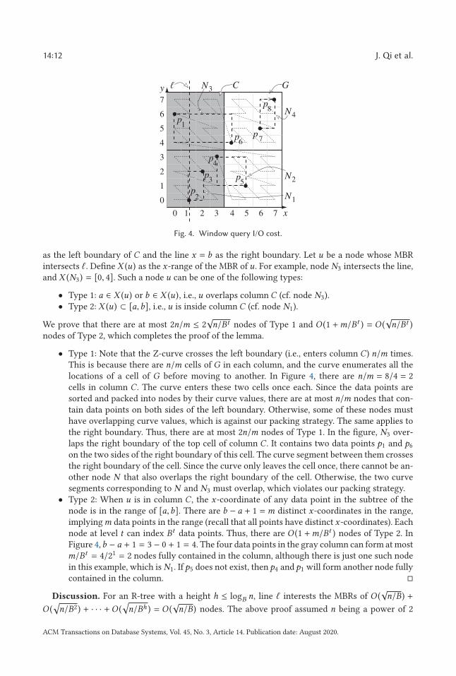
as the left boundary of C and the line x = b as the right boundary. Let u be a node whose MBRintersects �. Define X (u) as the x-range of the MBR of u. For example, node N3 intersects the line,and X (N3) = [0, 4]. Such a node u can be one of the following types:
• Type 1: a ∈ X (u) or b ∈ X (u), i.e., u overlaps column C (cf. node N3).• Type 2: X (u) ⊂ [a,b], i.e., u is inside column C (cf. node N1).
We prove that there are at most 2n/m ≤ 2√n/Bt nodes of Type 1 and O (1 +m/Bt ) = O (
√n/Bt )
nodes of Type 2, which completes the proof of the lemma.
• Type 1: Note that the Z-curve crosses the left boundary (i.e., enters column C) n/m times.This is because there are n/m cells of G in each column, and the curve enumerates all thelocations of a cell of G before moving to another. In Figure 4, there are n/m = 8/4 = 2cells in column C . The curve enters these two cells once each. Since the data points aresorted and packed into nodes by their curve values, there are at most n/m nodes that con-tain data points on both sides of the left boundary. Otherwise, some of these nodes musthave overlapping curve values, which is against our packing strategy. The same applies tothe right boundary. Thus, there are at most 2n/m nodes of Type 1. In the figure, N3 over-laps the right boundary of the top cell of column C . It contains two data points p1 and p6
on the two sides of the right boundary of this cell. The curve segment between them crossesthe right boundary of the cell. Since the curve only leaves the cell once, there cannot be an-other node N that also overlaps the right boundary of the cell. Otherwise, the two curvesegments corresponding to N and N3 must overlap, which violates our packing strategy.
• Type 2: When u is in column C , the x-coordinate of any data point in the subtree of thenode is in the range of [a,b]. There are b − a + 1 =m distinct x-coordinates in the range,implyingm data points in the range (recall that all points have distinct x-coordinates). Eachnode at level t can index Bt data points. Thus, there are O (1 +m/Bt ) nodes of Type 2. InFigure 4,b − a + 1 = 3 − 0 + 1 = 4. The four data points in the gray column can form at mostm/Bt = 4/21 = 2 nodes fully contained in the column, although there is just one such nodein this example, which is N1. If p5 does not exist, then p4 and p1 will form another node fullycontained in the column. �
Discussion. For an R-tree with a height h ≤ logB n, line � interests the MBRs of O (√n/B) +
O (√n/B2) + · · · +O (
√n/Bh ) = O (
√n/B) nodes. The above proof assumed n being a power of 2
ACM Transactions on Database Systems, Vol. 45, No. 3, Article 14. Publication date: August 2020.

Packing R-trees with Space-filling Curves 14:13
and d = 2. When n is not a power of 2, let ρ = �log2 n�. We enlarge the rank space to [2ρ ]2. Line
� intersects O (√
2ρ/B) nodes in the enlarged rank space. We have O (√
2ρ/B) = O (√n/B) because
2ρ ≤ 2n. The above argument can also be generalized to an arbitrary fixed dimensionality d ≥ 2to prove that our query cost is bounded by O ((n/B)1−1/d + k/B) in the worst case. This will beproven in the following Section 3.3.2, which proves an even stronger result that subsumes theaforementioned bound as a special case.
3.3.2 Query-sensitive Bound in Arbitrary Dimensionality. Consider a query rectangle q =[ql1,qh1] × [ql2,qh2] × · · · × [qld ,qhd ] in [n]d , where d ≥ 2 is an arbitrary fixed dimensionality.For each i ∈ [1,d], set δi = qhi − qli + 1, and let Zi = {1, 2, . . . ,d } \ {i}, namely, Zi includes all theintegers from 1 to d except i . We prove a stronger version of our previous lemma: our structureanswers the query in
O (logB n + Δ1/d/B1−1/d + k/B) (1)
I/Os where Δ =∑d
i=1
∏j ∈Zi
δ j . In this bound, the three components logB n, Δ1/d/B1−1/d , and k/Bdenote the costs to map the query to rank space (query q here is already mapped), to find the nodesintersecting the query boundary, and to output the points within the query, respectively.
The bound looks a bit unusual such that it would help to look at some special cases: ford = 2, the
query cost isO (logB n +√
(δ1 + δ2)/B + k/B), while ford = 3, the cost becomesO (logB n + (δ1δ2 +
δ1δ3 + δ2δ3)1/3/B2/3 + k/B). Since δi ≤ n for all i ∈ [1,n], it always holds that∏
j ∈Ziδ j ≤ nd−1 and
Δ ≤ d · nd−1. Thus, Equation (1) is bounded by O ((d · nd−1)1/d/B1−1/d + k/B) = O ((n/B)1−1/d +
k/B). In other words, Equation (1) is never worse than the (query insensitive) bound established inSection 3.3.1, but could be substantially better when q is small.
We say that the MBR of a node partially intersects q if it has a non-empty intersection with q,but is not contained by q. We prove the following lemma, which is sufficient for establishing ourclaim.
Lemma 3.2. The query rectangle q partially intersects the MBRs ofO (1 + Δ1/d/(Bt )1−1/d ) nodes at
level t .
Proof. Letm be the smallest power of 2 at least (Δ · Bt )1/d . Divide [n]d into a grid G of size:
(n/m) × (n/m) × · · · × (n/m)︸��������������������������������︷︷��������������������������������︸d
.
Each cell ofG hasmd locations in [n]d (the cell’s projection on each dimension coversm values).For each i ∈ [1,d], define a dimension-i column of G as the maximal set of cells in G that havethe same projection on dimension i . Grid G has n/m dimension-i columns, each of which is ad-dimensional rectangle in [n]d that covers the entire range [n] on every dimension j � i .
We use Figure 5 to illustrate the proof, where d = 2 and t = 1, i.e., we consider the leaf nodelevel. We have q = [1, 4] × [2, 5] (the solid line rectangle) and hence δ1 = 4 − 1 + 1 = 4 and δ2 =
5 − 2 + 1 = 4. Thus,m = (Δ · Bt )1/d =√
(δ1 + δ2)Bt =√
(4 + 4) × 21 = 4. The rank space is dividedinto an (8/4) × (8/4) = 2 × 2 grid, which is represented by the black solid line grid. Grid G has8/4 = 2 dimension-1 (the x-dimension) columns, i.e., the two vertical columns.
A node whose MBR partially intersects q must intersect one of the 2d boundary faces of q (e.g.,edges of q in Figure 5). We will prove that there can be at most O (1 +m/Bt +
∏j ∈Zi
δ j/md−1)
nodes intersecting each of the two faces of q perpendicular to dimension i . Summing this upon all d dimensions gives the desired upper bound on the total number of nodes that partially
ACM Transactions on Database Systems, Vol. 45, No. 3, Article 14. Publication date: August 2020.

14:14 J. Qi et al.
Fig. 5. Query-sensitive I/O cost.
intersect q: ∑di=1 O (1 +m/Bt +
∏j ∈Zi
δ j/md−1)
= O (d + dm/Bt + Δ/md−1)= O (1 + Δ1/d/(Bt )1−1/d ).
Due to symmetry, it suffices to consider the face of q that corresponds to ql1 (i.e., perpendicularto dimension 1)—we refer to it as the dimension-1 left face of q. LetC be the dimension-1 column ofG that covers this face;C is a rectangle that can be written as [a,b] × [n] × [n] × · · · × [n]︸��������������������︷︷��������������������︸
d−1
for some
a,b satisfying b − a + 1 =m and b is a multiple of 2. In Figure 5, dimension 1 is the x-dimension,and C is the gray column [0, 3] × [8]. Define the left boundary (or right boundary) of C to be theset of points in [n]d with coordinate a (or b, respectively) on dimension 1.
Let u be a level-t node with an MBR intersecting the dimension-1 left face of q, and X (u) bethe projection of the MBR of u on dimension 1, e.g., node N3 intersects the left edge of q, andX (N3) = [0, 4]. Such a node u can be one of the following types:
• Type 1: a ∈ X (u) or b ∈ X (u).• Type 2: X (u) ⊂ [a,b].
Next, we analyze the number of nodes for each type.
• Type 1: The Z-curve crosses the left boundary of C at most O (∏d
j=2�δi/m�) = O (1 +
δ2δ3 . . . δd /md−1) times within the dimension-1 left face of q. This is because there are
O (∏d
j=2�δi/m�) cells ofC within the range of q in dimensions 2 to d (e.g., in Figure 5, there
are 1 + δ2/m = 1 + 4/4 = 2 cells ofC within the dimension 2 range [2, 5] of q), and the curveenumerates all the locations of a cell before moving to another cell. By the reasoning ex-
plained in the proof of Lemma 3.1, there are at most O (∏d
j=2�δi/m�) nodes containing data
points on both sides of the left boundary. The same applies to the right boundary. Therefore,the number of Type-1 nodes is O (1 + δ2δ3 . . . δd/m
d−1).• Type 2: All the Bt points in the subtree of node u must have x-coordinates between a and b.
There can be only b − a + 1 =m such points (recall that all points have distinct coordinatesin each dimension), implying at most O (1 +m/Bt ) such nodes.
It thus follows that the dimension-1 left face of q intersects the MBRs of O (1 +m/Bt +∏j ∈Zi
δ j/md−1) nodes at level t . This completes the proof. �
ACM Transactions on Database Systems, Vol. 45, No. 3, Article 14. Publication date: August 2020.
Packing R-trees with Space-filling Curves 14:15
3.4 Extending to Other Space-filling Curves
Although we have used the Z-curve as the representative SFC, the only property that we requirefrom the Z-curve is the following quad-tree recursive pattern. Divide the data space [n]d (where nis a power of 2) into 2d rectangles of the same size, i.e., each rectangle is a “d-dimensional square”with a projection length of n/2 on each dimension (recall how the root of a d-dimensional quad-tree would partition the space). For example, in Figure 5, gridG is divided into 22 = 4 squares (cells)each with an edge length of 4. The quad-tree recursive pattern says that the SFC must first enumer-ate all the points within a rectangle before starting to enumerate the points of another. In Figure 5,the Z-curve enumerates the points of the bottom-left cell before moving to the bottom-right cell.The pattern must be followed recursively within each rectangle by treating it as a smaller dataspace [n/2]d . All our proofs hold verbatim on any SFCs (e.g., the Hilbert curve) that obey thispattern.
4 PARALLEL R-TREE BULK-LOADING
Next, we present a parallel R-tree bulk-loading algorithm based on our packing strategy. A straight-forward parallel algorithm that bulk-loads an R-tree level by level requires O (logB n) rounds ofparallel computation. We show how to reduce the number of rounds toO (logs n) without sacrific-ing the computation time. Here, s denotes the number of data points that a machine participatingin the parallel algorithm can handle. Modern machines can easily handle millions of data points,where logs n is typically bounded by a constant.
The key idea of the proposed algorithm is to distribute the data points (or MBRs of treenodes) in a way that the machines can bulk-load O (logB s ) levels of the final R-tree in eachround of parallel computation. Then, O (logs n) such rounds suffice to build the entire R-tree oflogB s · logs n = logB n levels. To bulk-load logB s levels in each round, a machine is assigned asubset of the data points (MBRs) that forms a few R-tree branches of logB s levels independentlyfrom the data assigned to the other machines. This is feasible, because we can assign data pointsto the machines in their sorted order for packing independently.
4.1 Parallel Computation Model
Without relying on a particular parallel platform such as Apache Hadoop, we design the parallelbulk-loading algorithm based on a generalized parallel model named the massively parallel
communication (MPC) model [5, 6, 10]. Popular parallel frameworks such as MapReduce [18]and Spark [62] are typical examples of this model. Our implementation differs slightly from thatof Agarwal et al. [5] who also use the MPC model to build an index. We copy the built index backto a single machine, while Agarwal et al. leave the index distributed among the machines. This isbecause our query algorithm runs on a single machine. We leave distributed query processing forfuture work.
The MPC model makes the following assumptions: Letn be the input size,д be the number of ma-chines, and s = n/д. In each round of parallel computation, every machine receives some data fromother machines, performs computation, and sends some data to other machines. The computationis done in the memory and hence there is no disk I/O cost, except for the initial data reading and thefinal data writing. We consider only algorithms that require a machine to receive/sendO (s ) wordsof information in each round, i.e., the communication I/O cost for a machine in each round isO (s )(with the terminology of Beame et al. [10], these algorithms must have load O (s ) in each round).
MPC algorithms are measured by:
(1) the number of computation rounds R;(2) the (parallel) running time T , which sums up the maximum computation cost of a single
machine in each round; and
ACM Transactions on Database Systems, Vol. 45, No. 3, Article 14. Publication date: August 2020.

14:16 J. Qi et al.
(3) the total amount of computationW , which sums up the computation costs of all machines
in all rounds.
Let tMi,rbe the time complexity of machineMi in round r . Then:
T =R∑
r=1
maxi ∈1..д
tMi,r, (2)
W =
R∑r=1
д∑i=1
tMi,r. (3)
For the purpose of building an R-tree,W should not exceed the time complexity O (n logn) fora single-machine implementation of the proposed packing strategy; T should beO ((n logn)/д) toachieve a speedup of д with д machines.
A primitive operation we need is sorting. In the MPC model, sorting n elements (initially evenlydistributed on the д machines) can be done in O (logs n) rounds, O ((n logn)/д) running time,O (n logn) total amount of computation, and O ((n logs n)/д) load (communication I/Os) [24] (seeTao et al. [57] for a simple algorithm when s ≥ д ln(д · n) holds).
Mapping n data points to the rank space and sorting them by their Z-order values thus canbe done in O (logs n) rounds. This process takes O ((n logn)/д) running time and O (n logn) totalamount of computation. We focus on packing the sorted data points to form an R-tree next.
4.2 Distributed Packing
Every round bulk-loads Θ(logB s ) levels of the target R-tree. In the first round, O (s ) consecutivedata points are assigned to a machine by the ascending order of their Z-order values, where anR-tree of Θ(logB s ) levels is bulk-loaded locally. This createsO (n/s ) R-trees. A second round bulk-loads the next Θ(logB s ) levels of the target R-tree over the root MBRs of those O (n/s ) R-trees.For this purpose, O (1 + д/s ) machines are used, each assigned O (s ) root MBRs; this results inO (n/s2) tree roots. The above process repeats until the MBRs can all be bulk-loaded in a singlemachine (the number of participating machines decreases by a factor of Θ(s ) each time, while eachsuch machine is always assigned O (s ) MBRs). A total of O (logB n/ logB s ) = O (logs n) rounds areincurred, whereO (s logs n) = O ((n logs n)/д) running time andO (n) total amount of computationare taken to compute the MBRs. Over theO (logs n) rounds, the maximum load of any participatingmachine, i.e., the load (communication I/O cost) of our packing algorithm, is also O (s logs n) =O ((n logs n)/д).
The rounds are illustrated in Figure 6, where n = 16, B = 2, д = 4, and s = 4. A total of logs n = 2rounds are needed. Each round bulk-loads logB s = 2 levels. In the first round R1, every machineis assigned s = 4 data points. The 4 machines bulk-load 4 R-trees of 2 levels locally. The 4 MBRs ofthe roots of these local R-trees are bulk-loaded by a single machineM1 in the second round R2.
We omit the pseudo-code of the parallel bulk-loading algorithm, as it is similar to Algorithm 1,except that now a machine handles O (s ) data points instead of n, and the loop to bulk-load anR-tree (Lines 9 to 12) is broken into rounds.
5 UPDATE HANDLING
In previous sections, we focused on bulk-loading a static R-tree structure to guarantee a worst-caseoptimal window query performance. In this section, we discuss how to handle data updates forthe bulk-loaded tree without impacting the worst-case optimal query performance. We will firstconvert the static R-tree structure into a deletion-only R-tree structure in Section 5.1. This structureretains theO (n/B) space cost and theO ((n/B)1−1/d + k/B) window query I/O cost, while it can also
ACM Transactions on Database Systems, Vol. 45, No. 3, Article 14. Publication date: August 2020.

Packing R-trees with Space-filling Curves 14:17
Fig. 6. Parallel R-tree bulk-loading.
handle a deletion inO (logB n) amortized I/Os. The structure does not support insertions. We thenextend this structure to support insertions in Section 5.2, which leads to a fully dynamic structurenamed the LogR-tree that still answers a window query in O ((n/B)1−1/d + k/B) I/Os. We studyhow to further reduce the insertion cost, resulting in an insertion improved structure named theLogR∗-tree in Section 5.3.
5.1 Deletion
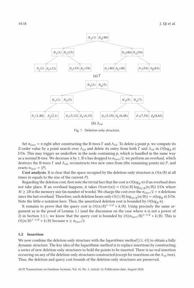
Recall that our static R-tree structure stores all the points of P sorted by their Z-order values. Inthis tree, an inner node entry stores a pointer to a child node and its MBR. We modify this treeslightly such that an inner node entry also stores the minimum Z-order value of the correspondingchild node. This increases the size of an inner node entry and reduces the node capacity B by asmall constant factor, but it does not impact either the space cost or the window query cost in big-O notation. The modified R-tree structure can be seen as a B-tree Γ over P with the Z-order valuesas the key values. This structure is illustrated in Figure 7(a), where the numbers in parenthesesrepresent Z-order values, e.g., p2 has a Z-order value of 1, and N1 has a minimum Z-order valueof 1.
We support deletion by object identifiers. Every point p ∈ P is associated with a unique integer
identifier denoted by id , and a user supplies the id of p to trigger the deletion of p. Since the B-treeΓ is constructed using Z-order values as the keys, we need to further construct a structure to mapid’s to Z-order values and enable deletion by id . This is done by an additional B-tree over the pointsin P , where the id’s are the keys, and the points in P are stored in the leaf nodes with their Z-ordervalues. We call this additional B-tree the ID B-tree and denote it by Λid . As Figure 7(b) shows, theID B-tree stores the data points in its leaf nodes. Each point is associated with a pair (id, z_value )representing the id and the Z-order value of the point, e.g., p2 has an id of 2 and a Z-order valueof 1. The minimum data point id in a leaf node is stored in its corresponding entry in the parentnode, e.g., the minimum data point id of the leftmost leaf node, node N1, is 1, which is stored inthe parent node as N1 (1).
ACM Transactions on Database Systems, Vol. 45, No. 3, Article 14. Publication date: August 2020.
14:18 J. Qi et al.
Fig. 7. Deletion-only structure.
Set nlast = n right after constructing the B-trees Γ and Λid . To delete a point p, we compute itsZ-order value by a point search over Λid and delete its entry from both Γ and Λid in O (logB n)I/Os. This may trigger an underflow in the node containing p, which is handled in the same wayas a normal B-tree. We decrease n by 1. If n has dropped to nlast/2, we perform an overhaul, whichdestroys the B-trees Γ and Λid , reconstructs two new ones from (the remaining points in) P , andresets nlast = |P |.
Cost analysis. It is clear that the space occupied by the deletion-only structure is O (n/B) at alltimes (n equals to the size of the current P ).
Regarding the deletion cost, first note the trivial fact that the cost isO (logB n) if an overhaul doesnot take place. If an overhaul happens, it takes O (sort (n)) = O ((n/B) logM/B (n/B)) I/Os whereM ≥ 2B is the memory size (in number of words). We charge the cost over thenlast/2 = n deletionssince the last overhaul. Therefore, each deletion bears onlyO ((1/B) logM/B (n/B)) = o(logB n) I/Os.Note the little-o notation here. Thus, the amortized deletion cost is bounded by O (logB n).
It remains to prove that the query cost is O ((n/B)1−1/d + k/B). Using precisely the same ar-gument as in the proof of Lemma 3.1 (and the discussion on the case where n is not a power of2) in Section 3.3.1, we know that the query cost is bounded by O ((nlast/B)1−1/d + k/B). This isO ((n/B)1−1/d + k/B) because n ≥ nlast/2.
5.2 Insertion
We now combine the deletion-only structure with the logarithmic method [13, 45] to obtain a fullydynamic structure. The key idea of the logarithmic method is to replace insertions by constructinga series of new deletion-only structures to hold the points to be inserted. There is no real insertionoccurring on any of the deletion-only structures constructed (except for insertions on the Λid tree).Thus, the deletion and query cost bounds of the deletion-only structures are preserved.
ACM Transactions on Database Systems, Vol. 45, No. 3, Article 14. Publication date: August 2020.

Packing R-trees with Space-filling Curves 14:19
Fig. 8. LogR-tree.
Specifically, as shown in Figure 8, we create a series of �logB n� deletion-only structures denotedby Γ1, Γ2, . . . , Γ�logB n � , where Γi can index up to Bi data points. The initial data set P is indexed inΓ�logB n � , while the rest of the deletion-only structures are empty.
To insert a new point pnew , we find the smallest j such that 1 +∑j
i=1 |Γi | ≤ B j , where |Γi | repre-sents the number of points indexed in Γi . We use pnew and the points in Γ1, Γ2, . . . , Γj to bulk-loada new Γj , and empty Γ1, Γ2, . . . , Γj−1. To delete a point pdel , we locate the deletion-only structurethat indexes pdel and delete pdel following the procedure described in Section 5.1. To help locatepdel , we modify the ID B-tree Λid such that it also stores theID of the deletion-only structurein which a point is indexed, denoted by tree_id . Thus, in Λid , a leaf node entry now stores atriple (id, tree_id, z_value ) instead of (id, z_value ). A window query is processed over each ofΓ1, Γ2, . . . , Γ�logB n � , and the results are combined together as the final query answer.
We use LogR-tree to denote the above structure resulted from applying the logarithmic methodover our deletion-only structure. The following result holds for the LogR-tree, which is due toArge and Vahrenhold [8]:
Lemma 5.1. Suppose that we have anO (n/B)-space structure that supports a deletion inO (logB n)amortized I/Os, answers a reporting query inO (Q (n) + k/B)) I/Os (k is the number of points reported),
and can be constructed in O (sort (n)) I/Os. Then, we can apply the logarithmic method to obtain a
structure with the following guarantees:
• Space cost: O (n/B);
• Query cost: O( ∑ �logB n �
i=1 Q (min{Bi ,n}))+O (k/B);
• Deletion cost: O (logB n) amortized;
• Insertion cost: O (log2B n + logB n · logM/B (n/B)) amortized.
Applying the lemma to our deletion-only structure described in Section 5.1, we have Q (n) =(n/B)1−1/d . The lemma yields a fully dynamic structure that consumesO (n/B) space and supportsa deletion inO (logB n) amortized I/Os and an insertion inO (log2
B n + logB n · logM/B (n/B)) amor-tized I/Os. The query cost is bounded by:
O��
�logB n �∑i=1
Q (min{Bi ,n})��+O (k/B)
= O��
�logB n �∑i=1
min{(Bi/B)1−1/d , (n/B)1−1/d }��+O (k/B)
= O ((n/B)1−1/d + k/B).
(4)
Note that the summation term in the equation above is asymptotically dominated by the last term(i.e., i = �logB n�).
ACM Transactions on Database Systems, Vol. 45, No. 3, Article 14. Publication date: August 2020.

14:20 J. Qi et al.
Nowadays, the memory size M typically satisfies logM/B (n/B) = O (1)—recall thatO (logM/B (n/B)) is the number of passes performed by an external sort on n points. The
insertion cost is then O (log2B n) amortized.
5.3 Improving the Insertion Cost
Next, we will hack into the logarithmic method and present an improved version of Lemma 5.1specific to our structures. The improvement lowers the amortized insertion cost fromO (log2
B n) toO (logB n) when logM/B (n/B) = O (1).
The description below essentially follows the ideas of Arge and Vahrenhold [8], but introducesnew pointers to lower the insertion cost. The focus will be placed on explaining the algorithmsteps involving these pointers and the corresponding analysis.
B-tree. Regarding the B-trees used in our structure, we require that:
• All the data points are at the leaf level.• If a leaf node overflows, Ω(B) points must have been inserted into the node since the node
was created.• If a leaf node underflows, Ω(B) points must have been deleted from the node since the node
was created.
These requirements can be easily fulfilled by slightly modifying the standard B-tree algorithms(see, e.g., Arge and Vitter [9] and Huddleston and Mehlhorn [29]).
The LogR∗-tree structure. We use LogR∗-tree to denote the proposed structure with improvedinsertion costs. The LogR∗-tree resembles the LogR-tree, as shown in Figure 8, but with additionalpointers in the leaf nodes of the deletion-only structures Γi . For conciseness, we do not drawanother figure to illustrate the LogR∗-tree.
In a LogR∗-tree, at all times, the input set P is stored in a sequence of H ≤ 1 + �logB n� deletion-only structures Γ1, Γ2, . . . , ΓH that satisfy the following conditions:
• Each point in P is in one and only one deletion-only structure;• The number of points in Γi , denoted by |Γi |, can be anywhere from 0 to Bi .
Each point p ∈ P is said to have the structure index i if p is stored in Γi .Same as that in the LogR-tree, the ID B-tree Λid in LogR*-tree also stores the structure index of
the points. For each point p ∈ P , its entry in Λid stores its id , structure index tree_id , and Z-ordervalue in the structure z_value . Now Λid serves as a “dictionary” that maps the id of a point to itsstructure index in O (logB n) I/Os.
Based on the structural design above, each point p ∈ P with structure index i is stored: (i) at a
leaf node u of Γi and (ii) at a leaf node v of Λid .We refer to the address of v as the dictionary address of p. Along with the entry of p in u, we
store a pointer tov , which we call the dictionary pointer of p. As an example, consider the structureΓ and its corresponding ID B-tree Λid in Figure 7. The dictionary pointer of p2 should point to N1
of Λid , since p2 is in N1 of Λid . This pointer allows us to fetch v in a single I/O once u has beenfound, which is essential for reducing the insertion cost from O (log2
B n) to O (logB n).Finally, we also store an integer nдlobal to be defined in the global rebuilding operation below.Global rebuilding. This operation constructs a “clean” structure from the current P with n
points. It takes the following steps:
• Destroy all structures.• Build (i.e., bulk-load) a deletion-only structure Γ�logB n � on all the points in P .• Build Λid and update the dictionary pointers in Γ�logB n � .• Set nдlobal to n.
ACM Transactions on Database Systems, Vol. 45, No. 3, Article 14. Publication date: August 2020.

Packing R-trees with Space-filling Curves 14:21
It is rudimentary to implement the above operation inO (sort (n)) = O ((n/B) logM/B (n/B)) I/Os.We use the above operation to build the first structure from the initial P (before all updates). Ingeneral, after a global rebuild, we perform the next global rebuild after �nдlobal/2� updates. Theglobal rebuild takes O (sort (nдlobal )) = O ((nдlobal/B) logM/B (nдlobal/B)) I/Os. Therefore, each ofthose updates is amortized only o(logB n) I/Os.
Query. To answer a query, we simply search all theH deletion-only structures in the LogR∗-tree.The query cost is:
O ���
1+ �logB n �∑i=1
Q (min{Bi ,n})��+O (k/B) = O ((n/B)1−1/d + k/B). (5)
ALGORITHM 2: LogR∗-tree-Deletion
Input: 〈Γ1, Γ2, . . . , ΓH ; Λid 〉: a LogR∗-tree; pdel : a point to be deleted.
Output: 〈Γ1, Γ2, . . . , ΓH ; Λid 〉: the updated LogR∗-tree.
1 i, z ← Point query on Λid to find pdel , return treeID i and Z-order value z of pdel ;
2 Delete pdel from Γi using standard B-tree deletion procedures by key value z;
3 Delete pdel from Λid using standard B-tree deletion procedures;
4 if underflow and node merging occur in Λid then
5 for each p ∈ Λid that has been moved to a new node v do
6 i ′, z′ ← treeID i ′ and Z-order value z′ of p;
7 Point query on Γi′ by key value z′ to find p;
8 Dictionary address of p ← v ;
9 return 〈Γ1, Γ2, . . . , ΓH ; Λid 〉;
Deletion. We delete a point pdel in two steps, as summarized in Algorithm 2:
(1) Find the structure index i of pdel using Λid and perform the deletion in Γi (Lines 1 and 2).This takes O (logB n) I/Os.
(2) Delete pdel from Λid (Line 3). If this triggers an underflow, treating the underflow maychange the dictionary addresses of O (B) points in the deletion-only structures. For everysuch point p, we perform a point query on its corresponding deletion-only structure tolocate it and update its dictionary pointer (Lines 4 to 8), which takes O (logB n) I/Os. Atotal of O (B logB n) I/Os are incurred by these dictionary pointer updates. However, anunderflow can happen only after Ω(B) points have been deleted from the node. We cancharge theO (B logB n) cost over those deletions, each of which is amortized onlyO (logB n)I/Os.
Insertion. We insert a point pnew as follows, which is summarized in Algorithm 3:
(1) Find the smallest j satisfying 1 +∑j
i=1 |Γi | ≤ B j (recall that |Γi | is the number of pointsstored in Γi , Lines 1 to 5). Denote by S1 the set of points stored in Γ1, Γ2, . . . , Γj−1 anddenote by S2 the set of points in Γj . Destroy Γ1, Γ2, . . . , Γj , and construct a new Γj onS1 ∪ S2 ∪ {pnew } (Lines 6 to 11). This process takes O (sort (B j )) = O (B j−1 logM/B B j−1) =
O (B j−1 logM/B (n/B)) I/Os.For every point p ∈ S1, update its structure index in Λid (Lines 7 and 8). This takes only
O (1) I/Os using the dictionary pointer of p, which results in O ( |S1 |) I/Os in total. Everysuch p has moved up to a deletion-only structure with a higher index—we say that p hasbeen promoted.
ACM Transactions on Database Systems, Vol. 45, No. 3, Article 14. Publication date: August 2020.

14:22 J. Qi et al.
By definition of j, we have |S1 | ≥ B j−1. Hence, the total cost of this step isO ( |S1 | logM/B (n/B)) I/Os. We charge this cost over the points in S1 such that every pro-moted point is amortized O (logM/B (n/B)) I/Os.
(2) Insert pnew into Λid (Line 12). If this triggers an overflow, treating the overflow maychange the dictionary addresses of O (B) points in the deletion-only structures. For everysuch point, updating its dictionary pointer takesO (logB n) I/Os (Lines 13 to 17). A total ofO (B logB n) I/Os are incurred by these dictionary pointer updates. However, an overflowcan happen only after Ω(B) points have been inserted into the node. We can charge theO (B logB n) cost over those insertions, each of which is amortized only O (logB n) I/Os.
ALGORITHM 3: LogR∗-tree-Insertion
Input: 〈Γ1, Γ2, . . . , ΓH ; Λid 〉: a LogR∗-tree; pnew : a point to be inserted.
Output: 〈Γ1, Γ2, . . . , ΓH ; Λid 〉: the updated LogR∗-tree.
1 i ← 1, sum ← |Γi |;2 while 1 + sum > Bi do
3 i ← i + 1;
4 sum ← sum + |Γi |;5 j ← i;
6 S1 ← the set of points in Γ1, Γ2, . . . , Γj−1;
7 for each p ∈ S1 do
8 Find p in Λid via its dictionary pointer and update its treeID to j;
9 S2 ← the set of points in Γj ;
10 Destroy Γ1, Γ2, . . . , Γj ;
11 Bulk-load Γj with S1 ∪ S2 ∪ {pnew };12 Insert pnew into Λid using standard B-tree insertion procedures;
13 if overflow and node split occur in Λid then
14 for each p ∈ Λid that has been moved to a new node v do
15 i ′, z′ ← treeID i ′ and Z-order value z′ of p;
16 Point query on Γi′ by key value z′ to find p;
17 Dictionary address of p ← v ;
18 return 〈Γ1, Γ2, . . . , ΓH ; Λid 〉;
Finishing the update cost analysis. Suppose that we perform μ updates in total. Let ni bethe value of n before the ith (1 ≤ i ≤ μ) update. We prove that our algorithms handle these up-dates inO (
∑μi=1 (1 + logB ni · logM/B (ni/B))) I/Os. This proves that our amortized cost isO (logB n ·
logM/B (n/B)) per insertion and deletion.We will focus on bounding the cost that arises at Step (1) of the insertion procedure. By the
earlier discussion, it is clear that the other steps in the insertion and deletion procedures performO (logB n) amortized I/Os per insertion and deletion.
The cost of Step (1) of insertion can be computed via the number of point promotions, since everypoint promotion bears an amortized I/O cost ofO (logM/B (n/B)). The number of point promotionsis in turn determined by the number of points promoted and the number of times that these pointsare promoted. We analyze these two factors by separating the μ updates into epochs.
Suppose that there were η global rebuilds in total. They divide the time line into η epochs, wherethe jth epoch starts from the moment when the jth global rebuild happened and ends right beforethe next global rebuild (the last epoch is “open” by this definition). Define nj as the value of n atthe jth global rebuild (n1 is the size of the initial P before all updates).
ACM Transactions on Database Systems, Vol. 45, No. 3, Article 14. Publication date: August 2020.

Packing R-trees with Space-filling Curves 14:23
Since there are at most �nj/2� updates in the jth epoch, the number of points that were promotedat least once in this epoch is obviously O (nj ). A point can only be promoted to a deletion-onlystructure with a higher index. Thus, the number of deletion-only structures H in the LogR∗-tree inthe jth epoch bounds the number of times that a point can be promoted. The value ofH is boundedby the following lemma:
Lemma 5.2. The number of deletion-only structures in the LogR∗-tree (i.e., the value of H ) remains
between �logB nj � and 1 + �logB nj � throughout the jth epoch.
Proof. The value of H equals �logB nj � right after the jth global rebuild and never decreases(recall that Γ�logB nj � has nj points at the beginning of the jth epoch, while the epoch has at most
nj/2 deletions). Meanwhile, at any moment, it must hold that BH ≤ n ≤ 3nj/2, since we performglobal rebuilding after �nj/2� updates. Hence,H ≤ logB (3nj/2) ≤ 1 + �logB nj � because B ≥ 2. �
Based on Lemma 5.2, in the jth epoch, a point can be promoted O (logB nj ) times. As discussedabove, there are O (nj ) points promoted where each promotion bears an amortized I/O cost ofO (logM/B (n/B)). Thus, Step (1) of insertion incurs in totalO (nj · logB nj · logM/B (n/B)) I/Os. Thismeans O (logB nj · logM/B (n/B)) I/Os per update.
Therefore, we obtain a fully dynamic structure that hasO (n/B) space cost,O ((n/B)1−1/d + k/B)query I/O cost, O (logB n) deletion I/O cost, and O (logB n · logM/B (n/B)) insertion I/O cost. Asmentioned earlier, the insertion I/O cost becomes O (logB n) when logM/B (n/B) = O (1).
5.4 Practical Considerations
In this section, we constructed a dynamic structure named LogR∗-tree that retains the worst-caseoptimal query performance while also having attractive update performance. Due to the complexdesign of this structure, there are factors to be considered when applying this structure.
In terms of the application scenarios, as mentioned in Section 1, we target applications suchas digital mapping where queries are much more frequent than updates over the data, e.g., theremay be millions of users querying Google Maps while the map data may not require constantupdates. Our index design is thus prioritized for the query performance. Our static structure offersan empirically efficient and worst-case optimal query performance. It may be used for applicationssuch as data warehousing that allow periodic rebuilds (e.g., overnight). Our dynamic structure (i.e.,the LogR∗-tree) further allows online data updates for applications such as digital mapping withoutimpacting the worst-case optimal query performance, which is the core contribution of Section 5.However, we do acknowledge that our LogR∗-tree is not designed for applications with a highdata update frequency, e.g., moving object databases. How to retain the worst-case optimal queryperformance in such applications is challenging and an interesting future study. Also, we focus onrelatively low dimensional space and mention that there are studies for high-dimensional windowqueries (e.g., Reference [64]), but those are not our target applications.
In terms of the implementation complexity, while our LogR∗-tree may look complex at a firstglance, it only consists of slightly adapted versions of B-trees and can be implemented based on theB-tree. Index management over our LogR∗-tree such as concurrency control and caching can bedone using standard B-tree concurrency control and caching algorithms. Our use of the ID B-treeto keep track of the tree IDs of the data points does bring extra update workloads, and it breaks thenice property of being cache-oblivious for the trees constructed by the logarithmic method. Thesemay impact the update efficiency and the throughput of the database system. As our experimentsin Section 6.2.3 show, our LogR∗-tree does have a higher update cost than a baseline tree structurethat uses the logarithmic method without the ID B-tree. This would limit the applicability of ourindex structure to applications with highly frequent updates, as discussed above.
ACM Transactions on Database Systems, Vol. 45, No. 3, Article 14. Publication date: August 2020.
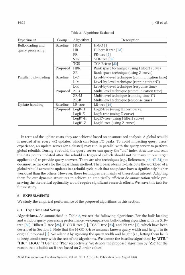
14:24 J. Qi et al.
Table 2. Algorithms Evaluated
Experiment Group Algorithm Description
Bulk-loading and
query processing
Baseline HGO H-GO [1]HR Hilbert R-tree [28]PR PR-tree [7]STR STR-tree [36]TGS TGS R-tree [23]
Proposed HRR Rank space technique (using Hilbert curve)ZR Rank space technique (using Z-curve)
Parallel bulk-loading Baseline L-C Level-by-level technique (communication time)L-M Level-by-level technique (running time T )L-R Level-by-level technique (response time)
Proposed ZR-C Multi-level technique (communication time)ZR-M Multi-level technique (running time T )ZR-R Multi-level technique (response time)
Update handling Baseline LR-tree LR-tree [16]Proposed LogR-H LogR-tree (using Hilbert curve)
LogR-Z LogR-tree (using Z-curve)LogR*-H LogR*-tree (using Hilbert curve)LogR*-Z LogR*-tree (using Z-curve)
In terms of the update costs, they are achieved based on an amortized analysis. A global rebuildis needed after every n/2 updates, which can bring I/O peaks. To avoid impacting query users’experience, an update server (or a cluster) may run in parallel with the query server to performglobal rebuilds. During a rebuild, the query server can query the “old” index structure and scanthe data points updated after the rebuild is triggered (which should not be many in our targetapplications) to provide query answers. There are also techniques (e.g., References [46, 47, 53]) tode-amortize the costs for the logarithmic method. Their basic idea is to distribute the workload of aglobal rebuild across the updates in a rebuild cycle, such that no updates have a significantly higherworkload than the others. However, these techniques are mainly of theoretical interest. Adaptingthem for our dynamic structures to achieve an empirically efficient de-amortization while pre-serving the theoretical optimality would require significant research efforts. We leave this task forfuture study.
6 EXPERIMENTS
We study the empirical performance of the proposed algorithms in this section.
6.1 Experimental Setup
Algorithms. As summarized in Table 2, we test the following algorithms: For the bulk-loadingand window query processing performance, we compare our bulk-loading algorithm with the STR-tree [36], Hilbert R-tree [28], H-GO R-tree [1], TGS R-tree [23], and PR-tree [7], which have beendescribed in Section 2. Note that the H-GO R-tree assumes known query width and height in itsoriginal proposal [1]. We adapt it by ignoring the query width and height (i.e., letting them be 0)to keep consistency with the rest of the algorithms. We denote the baseline algorithms by “STR,”“HR,” “HGO,” “TGS,” and “PR,” respectively. We denote the proposed algorithm by “ZR” for thereason that it builds an R-tree based on Z-order values.
ACM Transactions on Database Systems, Vol. 45, No. 3, Article 14. Publication date: August 2020.
Packing R-trees with Space-filling Curves 14:25
As discussed in Section 3.4, the proposed packing strategy is also applicable to other space-filling curves such as the Hilbert curve. To demonstrate this applicability, we further implementan R-tree based on the proposed packing strategy where the data points are sorted and packed bytheir Hilbert-order values in the rank space. We denote this R-tree by “HRR.” This R-tree shares asimilar structure with the Hilbert R-tree, except that the data points are mapped to the rank spacebefore they are packed. Note that the query cost bounds derived in Section 3.3.1 hold for this tree.
For the update handling performance, we compare our LogR-tree and LogR*-tree with the LR-tree [16] that applies the logarithmic method over the Hilbert R-tree, as discussed in Section 2.We denote this baseline algorithm by “LR-tree.” We implement the LogR-tree and the LogR*-treeover both Z-curves and Hilbert-curves. We denote the resultant trees by “LogR-Z,” “LogR*-Z,”“LogR-H,” and “LogR*-H,” where the suffixes “-Z” and “-H” denote Z-curve- and Hilbert-curve-based implementations, respectively. We do not compare with the other baseline bulk-loadingalgorithms (HGO, PR, STR, and TGS), because their bulk-loaded R-trees are uncompetitive in queryprocessing, as shown in the experimental results in Section 6.2.1. Combining such R-trees with thelogarithmic method to handle updates will not be competitive either. We also note that the PR-treehas an update algorithm [7] based on the logarithmic method. However, this algorithm is more oftheoretical interest. No implementation or empirical result has been presented for it.
Following previous studies [7, 23, 28, 36], we focus on the I/O cost of the algorithms above.For the parallel bulk-loading performance, we compare our proposed multi-level algorithm with
a level-by-level parallel bulk-loading algorithm that also uses the proposed packing strategy. Weimplement these algorithms over both Z-curves and Hilbert curves. We observe that the SFC usedhas very small impact on the parallel bulk-loading performance, since it only affects the curvevalues of the data points. To keep the figures concise, we only report the results over Z-curvesand denote the two corresponding algorithms by “ZR” and “L,” respectively. For these parallelalgorithms, we measure (i) the response time (denoted by “ZR-R” and “L-R,” respectively), whichis the duration for which an algorithm runs; (ii) the running time T (denoted by “ZR-M” and“L-M,” respectively), which is the sum of the maximum single machine response time over allMapReduce rounds of an algorithm; and (iii) the communication time (denoted by “ZR-C” and“L-C,” respectively), which is the part of the response time spent on communication. We do notmeasure the I/O cost of the parallel algorithms, because they are based on Spark, which has adifferent I/O mechanism from those of the standalone algorithms based on the TPIE library [37].
System environment. The window query and index update experiments are run on a 64-bitmachine running Ubuntu 14.04 with a 2.60 GHz Intel i5 CPU, 4 GB memory, a 1 TB TOSHIBAMQ01ABD075 (5400 RPM) hard disk drive, and a 240 GB SanDisk SSD Plus solid-state drive. Weuse Ke Yi’s single-machine implementation1 of the Hilbert R-tree, TGS R-tree, and PR-tree, whichuses the TPIE library [37]—a C++ library that provides APIs for implementation of external mem-ory algorithms and data structures. For ease of comparison, we also implement a single-machineversion of the H-GO R-tree (based on Ke Yi’s Hilbert R-tree implementation), the STR-tree, theLR-tree, and the proposed HRR, ZR, LogR-tree, and LogR*-tree using TPIE. In all the R-tree struc-tures except for those used in the LogR-tree and the LogR*-tree, we use 40 bytes for each entry in anode. For an inner node entry, these 40 bytes include 32 bytes for the 4 coordinates (8 bytes each)of an MBR and 8 bytes for a pointer pointing to the disk block storing the corresponding childnode. For a leaf node entry, these 40 bytes include 8 bytes for anID of a data point and 32 bytes forthe coordinates also in the form of an MBR for ease of implementation. For the LogR-tree, eachentry in an R-tree node has 48 bytes instead of 40, where the 8 extra bytes store a space-fillingcurve value. For the LogR*-tree, a leaf node entry needs to additionally store a space-filling curve
1https://www.cse.ust.hk/∼yike/prtree/.
ACM Transactions on Database Systems, Vol. 45, No. 3, Article 14. Publication date: August 2020.
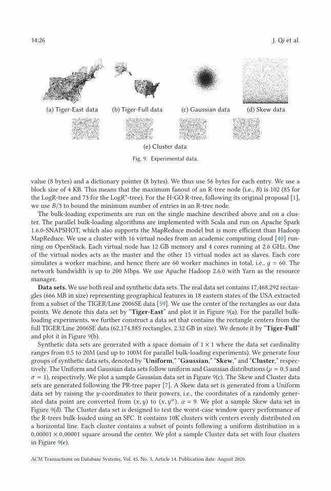
14:26 J. Qi et al.
Fig. 9. Experimental data.
value (8 bytes) and a dictionary pointer (8 bytes). We thus use 56 bytes for each entry. We use ablock size of 4 KB. This means that the maximum fanout of an R-tree node (i.e., B) is 102 (85 forthe LogR-tree and 73 for the LogR*-tree). For the H-GO R-tree, following its original proposal [1],we use B/3 to bound the minimum number of entries in an R-tree node.
The bulk-loading experiments are run on the single machine described above and on a clus-ter. The parallel bulk-loading algorithms are implemented with Scala and run on Apache Spark1.6.0-SNAPSHOT, which also supports the MapReduce model but is more efficient than HadoopMapReduce. We use a cluster with 16 virtual nodes from an academic computing cloud [40] run-ning on OpenStack. Each virtual node has 12 GB memory and 4 cores running at 2.6 GHz. Oneof the virtual nodes acts as the master and the other 15 virtual nodes act as slaves. Each coresimulates a worker machine, and hence there are 60 worker machines in total, i.e., д = 60. Thenetwork bandwidth is up to 200 Mbps. We use Apache Hadoop 2.6.0 with Yarn as the resourcemanager.
Data sets. We use both real and synthetic data sets. The real data set contains 17,468,292 rectan-gles (666 MB in size) representing geographical features in 18 eastern states of the USA extractedfrom a subset of the TIGER/Line 2006SE data [59]. We use the center of the rectangles as our datapoints. We denote this data set by “Tiger-East” and plot it in Figure 9(a). For the parallel bulk-loading experiments, we further construct a data set that contains the rectangle centers from thefull TIGER/Line 2006SE data (62,174,885 rectangles, 2.32 GB in size). We denote it by “Tiger-Full”and plot it in Figure 9(b).
Synthetic data sets are generated with a space domain of 1 × 1 where the data set cardinalityranges from 0.5 to 20M (and up to 100M for parallel bulk-loading experiments). We generate fourgroups of synthetic data sets, denoted by “Uniform,” “Gaussian,” “Skew,” and “Cluster,” respec-tively. The Uniform and Gaussian data sets follow uniform and Gaussian distributions (μ = 0.5 andσ = 1), respectively. We plot a sample Gaussian data set in Figure 9(c). The Skew and Cluster datasets are generated following the PR-tree paper [7]. A Skew data set is generated from a Uniformdata set by raising the y-coordinates to their powers, i.e., the coordinates of a randomly gener-ated data point are converted from (x ,y) to (x ,yα ), α = 9. We plot a sample Skew data set inFigure 9(d). The Cluster data set is designed to test the worst-case window query performance ofthe R-trees bulk-loaded using an SFC. It contains 10K clusters with centers evenly distributed ona horizontal line. Each cluster contains a subset of points following a uniform distribution in a0.00001 × 0.00001 square around the center. We plot a sample Cluster data set with four clustersin Figure 9(e).
ACM Transactions on Database Systems, Vol. 45, No. 3, Article 14. Publication date: August 2020.
Packing R-trees with Space-filling Curves 14:27
Table 3. Parameters and Their Settings
Parameter Setting
Data sets Tiger-East, Tiger-Full, Uniform, Gaussian, Skew, Clusterd 2, 3, 4, 5n (million) 0.5, 1, 5, 10, 20, 40, 60, 80, 100Cache size (blocks) 0, 1, 4, 16, 64, 256Percentage of data updates (%) 20, 40, 60, 80, 100, 120Query window area (%) 0.0001, 0.001, 0.01, 0.1, 1, 2Storage hardware hard disk drive, solid-state drive
We vary the query window size, the data set size, the data dimensionality, the cache size, thehardware for index storage, and the percentage of data updates. The experimental parameters aresummarized in Table 3, where default values are in bold.
6.2 Results
We present results on window query processing, bulk-loading, and update handling, respectively.
6.2.1 Window Query Processing. We start with the window query performance of the bulk-loaded R-trees (without data updates). We generate 100 square-shaped queries at locations follow-ing the data distribution in each experiment except for the experiments on the Cluster data set. TheCluster data set is designed to test the worst-case performance of the R-trees. Following the PR-tree paper [7], we generate long and thin window queries to query this data set. The bottom-left(bottom-right) corner of each query is randomly placed to the left (right) of the leftmost (right-most) cluster, such that the query spans all 10K clusters. The height of the query is generated asthe intended query window size divided by the query width.
For ease of comparison, we follow previous studies [7, 23, 28, 36] and report the average I/O costper query relative to the output size. Let the number of blocks read for a query be I and the outputsize be k/B. We report I/(k/B). Note that I/(k/B) ≥ 1, i.e., we need to at least read all the blockscontaining the data points in the query answer. A smaller value of I/(k/B) is more preferable.
Varying the query window size. We first vary the area of the query window from 0.0001%to 2% of the data space. We show the query I/O cost relative to the output size k/B over 10M datapoints (17M for Tiger-East) in Figure 10. A general observation is that the relative query costs ofthe R-trees decrease as the query window area increases. This is because a larger query windowoverlapping a tree node is more likely to overlap the data points in this node, i.e., there are lowerpercentages of extra query I/Os that do not contribute to the output.
The R-trees HRR and ZR created by the proposed packing strategy have the smallest query I/Ocosts on Uniform, Gaussian, and Cluster data (Figures 10(a), 10(b), and 10(c)). On Skew and Tiger-East data, the query I/O costs of HRR and ZR are close to those of TGS, which are the smallest(Figures 10(d) and 10(e)). This demonstrates that HRR and ZR not only have an asymptoticallyoptimal cost in the worst case but also perform well in other cases. Our advantage attributes tothe rank space mapping before packing the data points. Such a packing strategy effectively incor-porates the designs of both HR and STR, which both perform well on non-extreme data.
We also notice that HRR outperforms ZR. This suggests that when packing data points in thesame rank space, the Hilbert curve yields a better packed R-tree than the Z-curve does. This resultis consistent with an earlier study [33] that compares the query performance of R-trees packedwith the Hilbert curve and the Z-curve in the same Euclidean space.
ACM Transactions on Database Systems, Vol. 45, No. 3, Article 14. Publication date: August 2020.
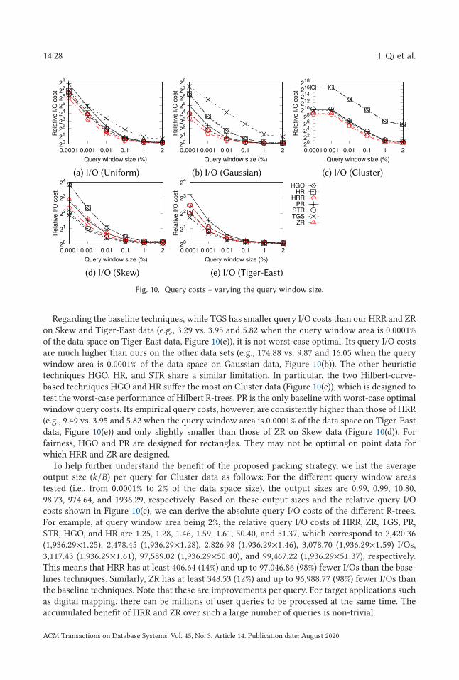
14:28 J. Qi et al.
Fig. 10. Query costs – varying the query window size.
Regarding the baseline techniques, while TGS has smaller query I/O costs than our HRR and ZRon Skew and Tiger-East data (e.g., 3.29 vs. 3.95 and 5.82 when the query window area is 0.0001%of the data space on Tiger-East data, Figure 10(e)), it is not worst-case optimal. Its query I/O costsare much higher than ours on the other data sets (e.g., 174.88 vs. 9.87 and 16.05 when the querywindow area is 0.0001% of the data space on Gaussian data, Figure 10(b)). The other heuristictechniques HGO, HR, and STR share a similar limitation. In particular, the two Hilbert-curve-based techniques HGO and HR suffer the most on Cluster data (Figure 10(c)), which is designed totest the worst-case performance of Hilbert R-trees. PR is the only baseline with worst-case optimalwindow query costs. Its empirical query costs, however, are consistently higher than those of HRR(e.g., 9.49 vs. 3.95 and 5.82 when the query window area is 0.0001% of the data space on Tiger-Eastdata, Figure 10(e)) and only slightly smaller than those of ZR on Skew data (Figure 10(d)). Forfairness, HGO and PR are designed for rectangles. They may not be optimal on point data forwhich HRR and ZR are designed.
To help further understand the benefit of the proposed packing strategy, we list the averageoutput size (k/B) per query for Cluster data as follows: For the different query window areastested (i.e., from 0.0001% to 2% of the data space size), the output sizes are 0.99, 0.99, 10.80,98.73, 974.64, and 1936.29, respectively. Based on these output sizes and the relative query I/Ocosts shown in Figure 10(c), we can derive the absolute query I/O costs of the different R-trees.For example, at query window area being 2%, the relative query I/O costs of HRR, ZR, TGS, PR,STR, HGO, and HR are 1.25, 1.28, 1.46, 1.59, 1.61, 50.40, and 51.37, which correspond to 2,420.36(1,936.29×1.25), 2,478.45 (1,936.29×1.28), 2,826.98 (1,936.29×1.46), 3,078.70 (1,936.29×1.59) I/Os,3,117.43 (1,936.29×1.61), 97,589.02 (1,936.29×50.40), and 99,467.22 (1,936.29×51.37), respectively.This means that HRR has at least 406.64 (14%) and up to 97,046.86 (98%) fewer I/Os than the base-lines techniques. Similarly, ZR has at least 348.53 (12%) and up to 96,988.77 (98%) fewer I/Os thanthe baseline techniques. Note that these are improvements per query. For target applications suchas digital mapping, there can be millions of user queries to be processed at the same time. Theaccumulated benefit of HRR and ZR over such a large number of queries is non-trivial.
ACM Transactions on Database Systems, Vol. 45, No. 3, Article 14. Publication date: August 2020.
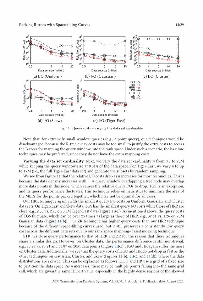
Packing R-trees with Space-filling Curves 14:29
Fig. 11. Query costs – varying the data set cardinality.
Note that, for extremely small window queries (e.g., a point query), our techniques would bedisadvantaged, because the R-tree query costs may be too small to justify the extra costs to accessthe B-trees for mapping the query window into the rank space. Under such a scenario, the baselinetechniques may be preferred, since they do not have the extra mapping costs.
Varying the data set cardinality. Next, we vary the data set cardinality n from 0.5 to 20Mwhile keeping the query window size at 0.01% of the data space. For Tiger-East, we vary n to upto 17M (i.e., the full Tiger-East data set) and generate the subsets by random sampling.
We see from Figure 11 that the relative I/O costs drop as n increases for most techniques. This isbecause the data density increases with n. A query window overlapping a tree node may overlapmore data points in this node, which causes the relative query I/Os to drop. TGS is an exception,and its query performance fluctuates. This technique relies on heuristics to minimize the area ofthe MBRs for the points packed together, which may not be optimal for all cases.
Our HRR technique again yields the smallest query I/O costs on Uniform, Gaussian, and Clusterdata sets. On Tiger-East and Skew data, TGS has the smallest query I/O costs while those of HRR areclose, e.g., 2.50 vs. 2.78 on 0.5M Tiger-East data (Figure 11(e)). As mentioned above, the query costsof TGS fluctuate, which can be over 25 times as large as those of HRR, e.g., 32.61 vs. 1.26 on 20MGaussian data (Figure 11(b)). Our ZR technique has higher query costs than our HRR techniquebecause of the different space-filling curves used, but it still preserves a consistently low querycost across the different data sets due to our rank space mapping–based indexing technique.
STR has close query performance to that of HRR and ZR for the reason that these techniquesshare a similar design. However, on Cluster data, the performance difference is still non-trivial,e.g., 78.28 vs. 28.21 and 33.87 on 20M data points (Figure 11(c)). HGO and HR again suffer the moston Cluster data. Additionally, we see that the query costs of HGO and HR do not drop as fast as theother techniques on Gaussian, Cluster, and Skew (Figures 11(b), 11(c), and 11(d)), where the datadistributions are skewed. This can be explained as follows: HGO and HR use a grid of a fixed sizeto partition the data space. As n increases, there may be multiple points falling into the same gridcell, which are given the same Hilbert value, especially in the highly dense regions of the skewed
ACM Transactions on Database Systems, Vol. 45, No. 3, Article 14. Publication date: August 2020.
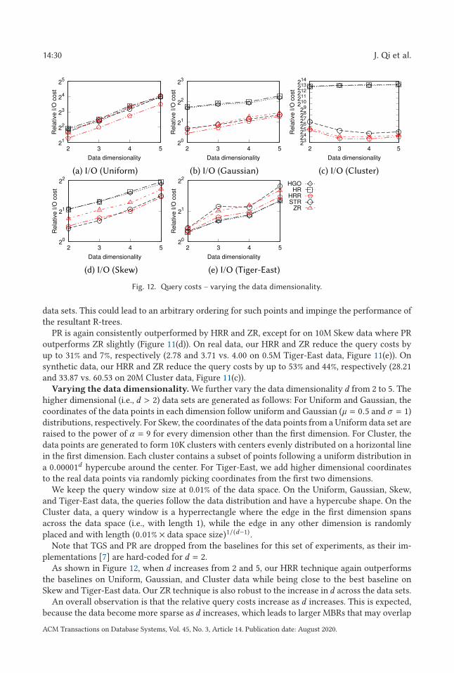
14:30 J. Qi et al.
Fig. 12. Query costs – varying the data dimensionality.
data sets. This could lead to an arbitrary ordering for such points and impinge the performance ofthe resultant R-trees.
PR is again consistently outperformed by HRR and ZR, except for on 10M Skew data where PRoutperforms ZR slightly (Figure 11(d)). On real data, our HRR and ZR reduce the query costs byup to 31% and 7%, respectively (2.78 and 3.71 vs. 4.00 on 0.5M Tiger-East data, Figure 11(e)). Onsynthetic data, our HRR and ZR reduce the query costs by up to 53% and 44%, respectively (28.21and 33.87 vs. 60.53 on 20M Cluster data, Figure 11(c)).
Varying the data dimensionality. We further vary the data dimensionality d from 2 to 5. Thehigher dimensional (i.e., d > 2) data sets are generated as follows: For Uniform and Gaussian, thecoordinates of the data points in each dimension follow uniform and Gaussian (μ = 0.5 and σ = 1)distributions, respectively. For Skew, the coordinates of the data points from a Uniform data set areraised to the power of α = 9 for every dimension other than the first dimension. For Cluster, thedata points are generated to form 10K clusters with centers evenly distributed on a horizontal linein the first dimension. Each cluster contains a subset of points following a uniform distribution ina 0.00001d hypercube around the center. For Tiger-East, we add higher dimensional coordinatesto the real data points via randomly picking coordinates from the first two dimensions.
We keep the query window size at 0.01% of the data space. On the Uniform, Gaussian, Skew,and Tiger-East data, the queries follow the data distribution and have a hypercube shape. On theCluster data, a query window is a hyperrectangle where the edge in the first dimension spansacross the data space (i.e., with length 1), while the edge in any other dimension is randomly
placed and with length (0.01% × data space size)1/(d−1) .Note that TGS and PR are dropped from the baselines for this set of experiments, as their im-
plementations [7] are hard-coded for d = 2.As shown in Figure 12, when d increases from 2 and 5, our HRR technique again outperforms
the baselines on Uniform, Gaussian, and Cluster data while being close to the best baseline onSkew and Tiger-East data. Our ZR technique is also robust to the increase in d across the data sets.
An overall observation is that the relative query costs increase as d increases. This is expected,because the data become more sparse as d increases, which leads to larger MBRs that may overlap
ACM Transactions on Database Systems, Vol. 45, No. 3, Article 14. Publication date: August 2020.
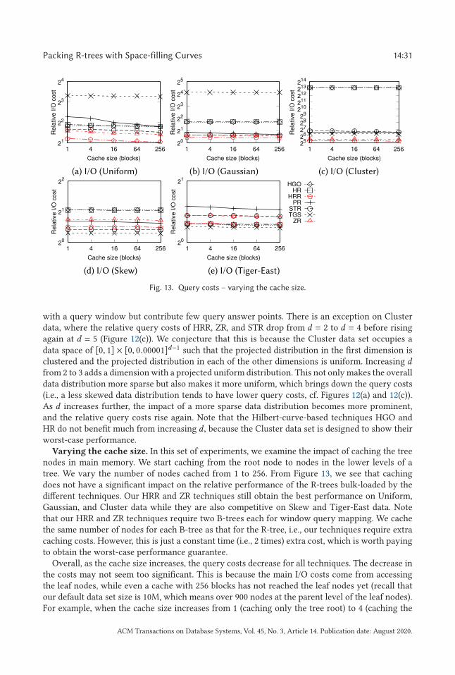
Packing R-trees with Space-filling Curves 14:31
Fig. 13. Query costs – varying the cache size.
with a query window but contribute few query answer points. There is an exception on Clusterdata, where the relative query costs of HRR, ZR, and STR drop from d = 2 to d = 4 before risingagain at d = 5 (Figure 12(c)). We conjecture that this is because the Cluster data set occupies adata space of [0, 1] × [0, 0.00001]d−1 such that the projected distribution in the first dimension isclustered and the projected distribution in each of the other dimensions is uniform. Increasing dfrom 2 to 3 adds a dimension with a projected uniform distribution. This not only makes the overalldata distribution more sparse but also makes it more uniform, which brings down the query costs(i.e., a less skewed data distribution tends to have lower query costs, cf. Figures 12(a) and 12(c)).As d increases further, the impact of a more sparse data distribution becomes more prominent,and the relative query costs rise again. Note that the Hilbert-curve-based techniques HGO andHR do not benefit much from increasing d, because the Cluster data set is designed to show theirworst-case performance.
Varying the cache size. In this set of experiments, we examine the impact of caching the treenodes in main memory. We start caching from the root node to nodes in the lower levels of atree. We vary the number of nodes cached from 1 to 256. From Figure 13, we see that cachingdoes not have a significant impact on the relative performance of the R-trees bulk-loaded by thedifferent techniques. Our HRR and ZR techniques still obtain the best performance on Uniform,Gaussian, and Cluster data while they are also competitive on Skew and Tiger-East data. Notethat our HRR and ZR techniques require two B-trees each for window query mapping. We cachethe same number of nodes for each B-tree as that for the R-tree, i.e., our techniques require extracaching costs. However, this is just a constant time (i.e., 2 times) extra cost, which is worth payingto obtain the worst-case performance guarantee.
Overall, as the cache size increases, the query costs decrease for all techniques. The decrease inthe costs may not seem too significant. This is because the main I/O costs come from accessingthe leaf nodes, while even a cache with 256 blocks has not reached the leaf nodes yet (recall thatour default data set size is 10M, which means over 900 nodes at the parent level of the leaf nodes).For example, when the cache size increases from 1 (caching only the tree root) to 4 (caching the
ACM Transactions on Database Systems, Vol. 45, No. 3, Article 14. Publication date: August 2020.
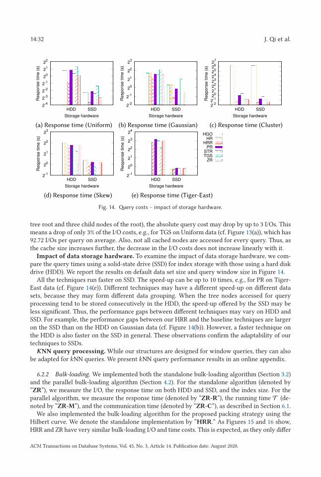
14:32 J. Qi et al.
Fig. 14. Query costs – impact of storage hardware.
tree root and three child nodes of the root), the absolute query cost may drop by up to 3 I/Os. Thismeans a drop of only 3% of the I/O costs, e.g., for TGS on Uniform data (cf. Figure 13(a)), which has92.72 I/Os per query on average. Also, not all cached nodes are accessed for every query. Thus, asthe cache size increases further, the decrease in the I/O costs does not increase linearly with it.
Impact of data storage hardware. To examine the impact of data storage hardware, we com-pare the query times using a solid-state drive (SSD) for index storage with those using a hard diskdrive (HDD). We report the results on default data set size and query window size in Figure 14.
All the techniques run faster on SSD. The speed-up can be up to 10 times, e.g., for PR on Tiger-East data (cf. Figure 14(e)). Different techniques may have a different speed-up on different datasets, because they may form different data grouping. When the tree nodes accessed for queryprocessing tend to be stored consecutively in the HDD, the speed-up offered by the SSD may beless significant. Thus, the performance gaps between different techniques may vary on HDD andSSD. For example, the performance gaps between our HRR and the baseline techniques are largeron the SSD than on the HDD on Gaussian data (cf. Figure 14(b)). However, a faster technique onthe HDD is also faster on the SSD in general. These observations confirm the adaptability of ourtechniques to SSDs.KNN query processing. While our structures are designed for window queries, they can also
be adapted for kNN queries. We present kNN query performance results in an online appendix.
6.2.2 Bulk-loading. We implemented both the standalone bulk-loading algorithm (Section 3.2)and the parallel bulk-loading algorithm (Section 4.2). For the standalone algorithm (denoted by“ZR”), we measure the I/O, the response time on both HDD and SSD, and the index size. For theparallel algorithm, we measure the response time (denoted by “ZR-R”), the running time T (de-noted by “ZR-M”), and the communication time (denoted by “ZR-C”), as described in Section 6.1.
We also implemented the bulk-loading algorithm for the proposed packing strategy using theHilbert curve. We denote the standalone implementation by “HRR.” As Figures 15 and 16 show,HRR and ZR have very similar bulk-loading I/O and time costs. This is expected, as they only differ
ACM Transactions on Database Systems, Vol. 45, No. 3, Article 14. Publication date: August 2020.
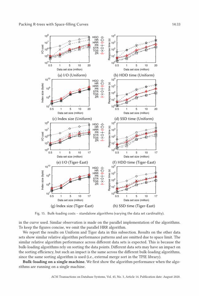
Packing R-trees with Space-filling Curves 14:33
Fig. 15. Bulk-loading costs – standalone algorithms (varying the data set cardinality).
in the curve used. Similar observation is made on the parallel implementation of the algorithms.To keep the figures concise, we omit the parallel HRR algorithm.
We report the results on Uniform and Tiger data in this subsection. Results on the other datasets show similar relative algorithm performance patterns and are omitted due to space limit. Thesimilar relative algorithm performance across different data sets is expected. This is because thebulk-loading algorithms rely on sorting the data points. Different data sets may have an impact onthe sorting efficiency, but such an impact is the same across the different bulk-loading algorithms,since the same sorting algorithm is used (i.e., external merge sort in the TPIE library).
Bulk-loading on a single machine. We first show the algorithm performance when the algo-rithms are running on a single machine.
ACM Transactions on Database Systems, Vol. 45, No. 3, Article 14. Publication date: August 2020.
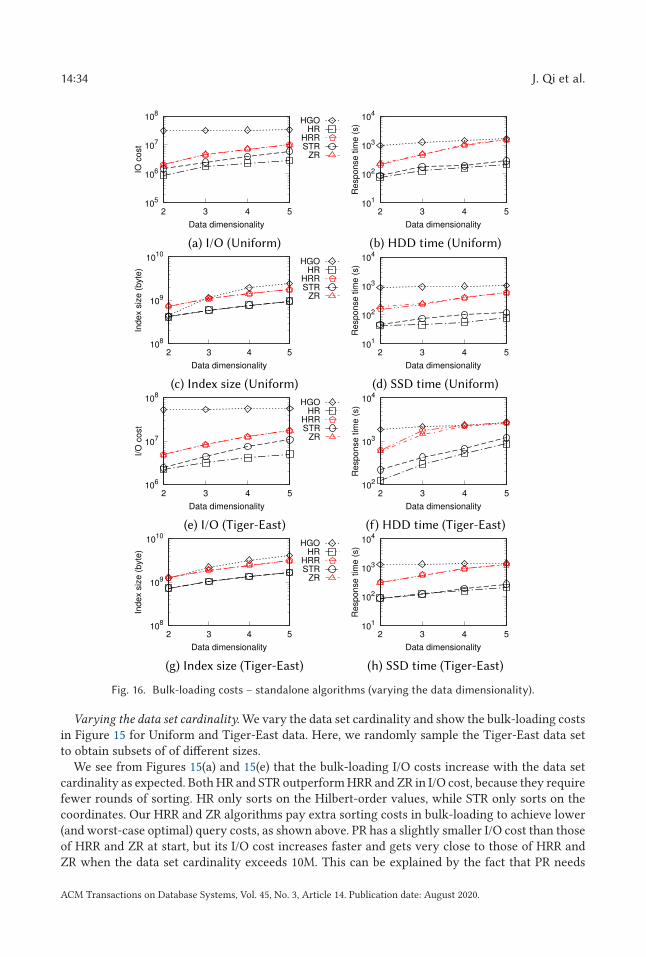
14:34 J. Qi et al.
Fig. 16. Bulk-loading costs – standalone algorithms (varying the data dimensionality).
Varying the data set cardinality. We vary the data set cardinality and show the bulk-loading costsin Figure 15 for Uniform and Tiger-East data. Here, we randomly sample the Tiger-East data setto obtain subsets of of different sizes.
We see from Figures 15(a) and 15(e) that the bulk-loading I/O costs increase with the data setcardinality as expected. Both HR and STR outperform HRR and ZR in I/O cost, because they requirefewer rounds of sorting. HR only sorts on the Hilbert-order values, while STR only sorts on thecoordinates. Our HRR and ZR algorithms pay extra sorting costs in bulk-loading to achieve lower(and worst-case optimal) query costs, as shown above. PR has a slightly smaller I/O cost than thoseof HRR and ZR at start, but its I/O cost increases faster and gets very close to those of HRR andZR when the data set cardinality exceeds 10M. This can be explained by the fact that PR needs
ACM Transactions on Database Systems, Vol. 45, No. 3, Article 14. Publication date: August 2020.
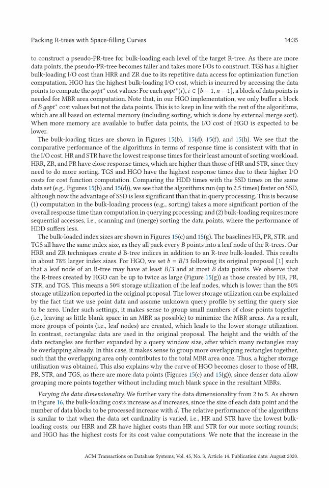
Packing R-trees with Space-filling Curves 14:35
to construct a pseudo-PR-tree for bulk-loading each level of the target R-tree. As there are moredata points, the pseudo-PR-tree becomes taller and takes more I/Os to construct. TGS has a higherbulk-loading I/O cost than HRR and ZR due to its repetitive data access for optimization functioncomputation. HGO has the highest bulk-loading I/O cost, which is incurred by accessing the datapoints to compute theдopt∗ cost values: For eachдopt∗ (i ), i ∈ [b − 1,n − 1], a block of data points isneeded for MBR area computation. Note that, in our HGO implementation, we only buffer a blockof B дopt∗ cost values but not the data points. This is to keep in line with the rest of the algorithms,which are all based on external memory (including sorting, which is done by external merge sort).When more memory are available to buffer data points, the I/O cost of HGO is expected to belower.
The bulk-loading times are shown in Figures 15(b), 15(d), 15(f), and 15(h). We see that thecomparative performance of the algorithms in terms of response time is consistent with that inthe I/O cost. HR and STR have the lowest response times for their least amount of sorting workload.HRR, ZR, and PR have close response times, which are higher than those of HR and STR, since theyneed to do more sorting. TGS and HGO have the highest response times due to their higher I/Ocosts for cost function computation. Comparing the HDD times with the SSD times on the samedata set (e.g., Figures 15(b) and 15(d)), we see that the algorithms run (up to 2.5 times) faster on SSD,although now the advantage of SSD is less significant than that in query processing. This is because(1) computation in the bulk-loading process (e.g., sorting) takes a more significant portion of theoverall response time than computation in querying processing; and (2) bulk-loading requires moresequential accesses, i.e., scanning and (merge) sorting the data points, where the performance ofHDD suffers less.
The bulk-loaded index sizes are shown in Figures 15(c) and 15(g). The baselines HR, PR, STR, andTGS all have the same index size, as they all pack every B points into a leaf node of the R-trees. OurHRR and ZR techniques create d B-tree indices in addition to an R-tree bulk-loaded. This resultsin about 78% larger index sizes. For HGO, we set b = B/3 following its original proposal [1] suchthat a leaf node of an R-tree may have at least B/3 and at most B data points. We observe thatthe R-trees created by HGO can be up to twice as large (Figure 15(g)) as those created by HR, PR,STR, and TGS. This means a 50% storage utilization of the leaf nodes, which is lower than the 80%storage utilization reported in the original proposal. The lower storage utilization can be explainedby the fact that we use point data and assume unknown query profile by setting the query sizeto be zero. Under such settings, it makes sense to group small numbers of close points together(i.e., leaving as little blank space in an MBR as possible) to minimize the MBR areas. As a result,more groups of points (i.e., leaf nodes) are created, which leads to the lower storage utilization.In contrast, rectangular data are used in the original proposal. The height and the width of thedata rectangles are further expanded by a query window size, after which many rectangles maybe overlapping already. In this case, it makes sense to group more overlapping rectangles together,such that the overlapping area only contributes to the total MBR area once. Thus, a higher storageutilization was obtained. This also explains why the curve of HGO becomes closer to those of HR,PR, STR, and TGS, as there are more data points (Figures 15(c) and 15(g)), since denser data allowgrouping more points together without including much blank space in the resultant MBRs.
Varying the data dimensionality. We further vary the data dimensionality from 2 to 5. As shownin Figure 16, the bulk-loading costs increase as d increases, since the size of each data point and thenumber of data blocks to be processed increase with d . The relative performance of the algorithmsis similar to that when the data set cardinality is varied, i.e., HR and STR have the lowest bulk-loading costs; our HRR and ZR have higher costs than HR and STR for our more sorting rounds;and HGO has the highest costs for its cost value computations. We note that the increase in the
ACM Transactions on Database Systems, Vol. 45, No. 3, Article 14. Publication date: August 2020.
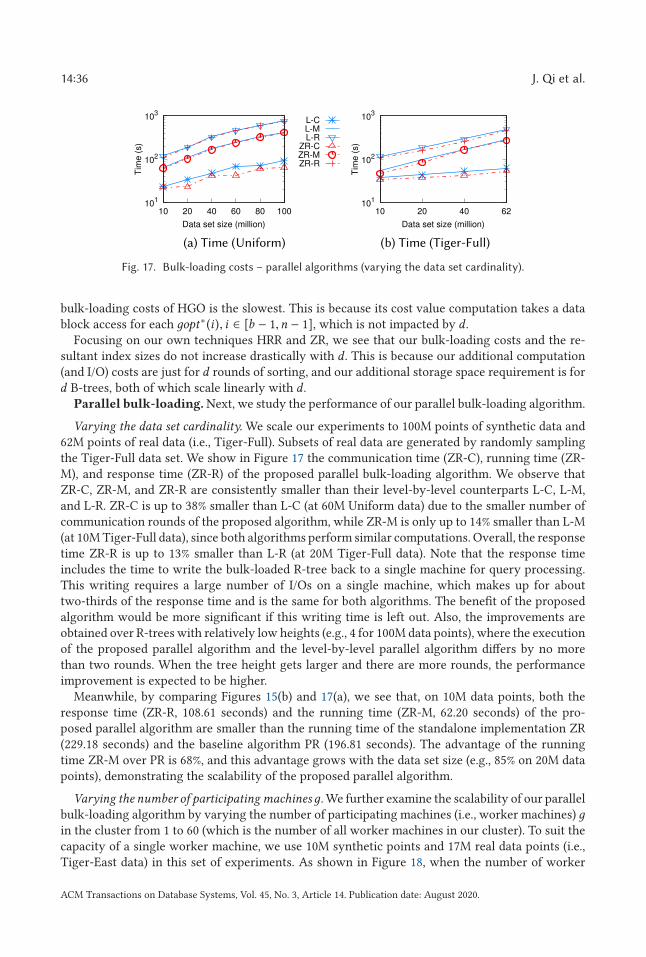
14:36 J. Qi et al.
Fig. 17. Bulk-loading costs – parallel algorithms (varying the data set cardinality).
bulk-loading costs of HGO is the slowest. This is because its cost value computation takes a datablock access for each дopt∗ (i ), i ∈ [b − 1,n − 1], which is not impacted by d .
Focusing on our own techniques HRR and ZR, we see that our bulk-loading costs and the re-sultant index sizes do not increase drastically with d . This is because our additional computation(and I/O) costs are just for d rounds of sorting, and our additional storage space requirement is ford B-trees, both of which scale linearly with d .
Parallel bulk-loading. Next, we study the performance of our parallel bulk-loading algorithm.
Varying the data set cardinality. We scale our experiments to 100M points of synthetic data and62M points of real data (i.e., Tiger-Full). Subsets of real data are generated by randomly samplingthe Tiger-Full data set. We show in Figure 17 the communication time (ZR-C), running time (ZR-M), and response time (ZR-R) of the proposed parallel bulk-loading algorithm. We observe thatZR-C, ZR-M, and ZR-R are consistently smaller than their level-by-level counterparts L-C, L-M,and L-R. ZR-C is up to 38% smaller than L-C (at 60M Uniform data) due to the smaller number ofcommunication rounds of the proposed algorithm, while ZR-M is only up to 14% smaller than L-M(at 10M Tiger-Full data), since both algorithms perform similar computations. Overall, the responsetime ZR-R is up to 13% smaller than L-R (at 20M Tiger-Full data). Note that the response timeincludes the time to write the bulk-loaded R-tree back to a single machine for query processing.This writing requires a large number of I/Os on a single machine, which makes up for abouttwo-thirds of the response time and is the same for both algorithms. The benefit of the proposedalgorithm would be more significant if this writing time is left out. Also, the improvements areobtained over R-trees with relatively low heights (e.g., 4 for 100M data points), where the executionof the proposed parallel algorithm and the level-by-level parallel algorithm differs by no morethan two rounds. When the tree height gets larger and there are more rounds, the performanceimprovement is expected to be higher.
Meanwhile, by comparing Figures 15(b) and 17(a), we see that, on 10M data points, both theresponse time (ZR-R, 108.61 seconds) and the running time (ZR-M, 62.20 seconds) of the pro-posed parallel algorithm are smaller than the running time of the standalone implementation ZR(229.18 seconds) and the baseline algorithm PR (196.81 seconds). The advantage of the runningtime ZR-M over PR is 68%, and this advantage grows with the data set size (e.g., 85% on 20M datapoints), demonstrating the scalability of the proposed parallel algorithm.
Varying the number of participating machinesд. We further examine the scalability of our parallelbulk-loading algorithm by varying the number of participating machines (i.e., worker machines) дin the cluster from 1 to 60 (which is the number of all worker machines in our cluster). To suit thecapacity of a single worker machine, we use 10M synthetic points and 17M real data points (i.e.,Tiger-East data) in this set of experiments. As shown in Figure 18, when the number of worker
ACM Transactions on Database Systems, Vol. 45, No. 3, Article 14. Publication date: August 2020.
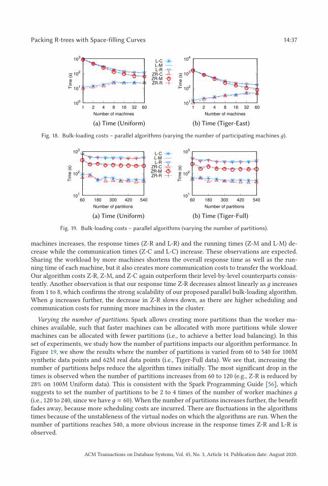
Packing R-trees with Space-filling Curves 14:37
Fig. 18. Bulk-loading costs – parallel algorithms (varying the number of participating machines д).
Fig. 19. Bulk-loading costs – parallel algorithms (varying the number of partitions).
machines increases, the response times (Z-R and L-R) and the running times (Z-M and L-M) de-crease while the communication times (Z-C and L-C) increase. These observations are expected.Sharing the workload by more machines shortens the overall response time as well as the run-ning time of each machine, but it also creates more communication costs to transfer the workload.Our algorithm costs Z-R, Z-M, and Z-C again outperform their level-by-level counterparts consis-tently. Another observation is that our response time Z-R decreases almost linearly as д increasesfrom 1 to 8, which confirms the strong scalability of our proposed parallel bulk-loading algorithm.When д increases further, the decrease in Z-R slows down, as there are higher scheduling andcommunication costs for running more machines in the cluster.
Varying the number of partitions. Spark allows creating more partitions than the worker ma-chines available, such that faster machines can be allocated with more partitions while slowermachines can be allocated with fewer partitions (i.e., to achieve a better load balancing). In thisset of experiments, we study how the number of partitions impacts our algorithm performance. InFigure 19, we show the results where the number of partitions is varied from 60 to 540 for 100Msynthetic data points and 62M real data points (i.e., Tiger-Full data). We see that, increasing thenumber of partitions helps reduce the algorithm times initially. The most significant drop in thetimes is observed when the number of partitions increases from 60 to 120 (e.g., Z-R is reduced by28% on 100M Uniform data). This is consistent with the Spark Programming Guide [56], whichsuggests to set the number of partitions to be 2 to 4 times of the number of worker machines д(i.e., 120 to 240, since we haveд = 60). When the number of partitions increases further, the benefitfades away, because more scheduling costs are incurred. There are fluctuations in the algorithmstimes because of the unstableness of the virtual nodes on which the algorithms are run. When thenumber of partitions reaches 540, a more obvious increase in the response times Z-R and L-R isobserved.
ACM Transactions on Database Systems, Vol. 45, No. 3, Article 14. Publication date: August 2020.
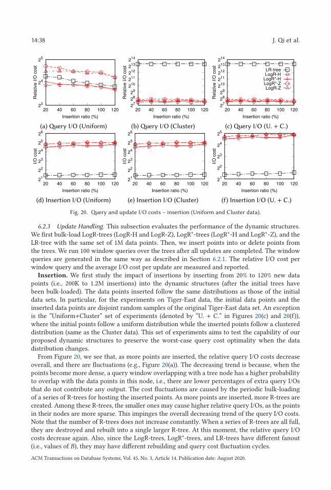
14:38 J. Qi et al.
Fig. 20. Query and update I/O costs – insertion (Uniform and Cluster data).
6.2.3 Update Handling. This subsection evaluates the performance of the dynamic structures.We first bulk-load LogR-trees (LogR-H and LogR-Z), LogR∗-trees (LogR∗-H and LogR∗-Z), and theLR-tree with the same set of 1M data points. Then, we insert points into or delete points fromthe trees. We run 100 window queries over the trees after all updates are completed. The windowqueries are generated in the same way as described in Section 6.2.1. The relative I/O cost perwindow query and the average I/O cost per update are measured and reported.
Insertion. We first study the impact of insertions by inserting from 20% to 120% new datapoints (i.e., 200K to 1.2M insertions) into the dynamic structures (after the initial trees havebeen bulk-loaded). The data points inserted follow the same distributions as those of the initialdata sets. In particular, for the experiments on Tiger-East data, the initial data points and theinserted data points are disjoint random samples of the original Tiger-East data set. An exceptionis the “Uniform+Cluster” set of experiments (denoted by “U. + C.” in Figures 20(c) and 20(f)),where the initial points follow a uniform distribution while the inserted points follow a clustereddistribution (same as the Cluster data). This set of experiments aims to test the capability of ourproposed dynamic structures to preserve the worst-case query cost optimality when the datadistribution changes.
From Figure 20, we see that, as more points are inserted, the relative query I/O costs decreaseoverall, and there are fluctuations (e.g., Figure 20(a)). The decreasing trend is because, when thepoints become more dense, a query window overlapping with a tree node has a higher probabilityto overlap with the data points in this node, i.e., there are lower percentages of extra query I/Osthat do not contribute any output. The cost fluctuations are caused by the periodic bulk-loadingof a series of R-trees for hosting the inserted points. As more points are inserted, more R-trees arecreated. Among these R-trees, the smaller ones may cause higher relative query I/Os, as the pointsin their nodes are more sparse. This impinges the overall decreasing trend of the query I/O costs.Note that the number of R-trees does not increase constantly. When a series of R-trees are all full,they are destroyed and rebuilt into a single larger R-tree. At this moment, the relative query I/Ocosts decrease again. Also, since the LogR-trees, LogR∗-trees, and LR-trees have different fanout(i.e., values of B), they may have different rebuilding and query cost fluctuation cycles.
ACM Transactions on Database Systems, Vol. 45, No. 3, Article 14. Publication date: August 2020.

Packing R-trees with Space-filling Curves 14:39
The insertion I/O costs increase slowly as there are more points inserted, and there are alsofluctuations (e.g., Figure 20(d)). The slow increasing trend is expected, as the amortized insertionI/O cost is in the scale of logB n where B is quite large (i.e., B ≥ 73). Even for the smallest B value73, when n grows from the initial value 1,000,000 by 120% to 2,200,000, the cost difference is onlylog73 2,200,000 − log73 1,000,000 ≈ 3.40 − 3.22 = 0.18. The fluctuations in the insertion I/O costscan also be explained by the periodic bulk-loading of the R-trees. When a large R-tree is bulk-loaded, there will be a peak in the insertion I/O costs. Then, the insertion I/O costs may dropslightly until the next bulk-loading of another large R-tree.
Focusing on the comparison among the different structures, we see that, in terms of the queryI/O costs, both proposed structures LogR-H and LogR∗-H outperform the baseline structure LR-treeconsistently across Uniform, Cluster, and Uniform+Cluster data (Figures 20(a), 20(b), and 20(c)). Inparticular, on Cluster data, LogR-H and LogR∗-H reduce the relative query I/O cost by up to 98%,e.g., 172.40 (LogR-H) vs. 10,227.56 (LR-tree) for query processing after 120% insertions. Similarquery I/O cost reduction is observed on Uniform+Cluster data, which confirms the capability ofour LogR-trees and LogR∗-trees to preserve the worst-case query I/O cost optimality. Between ourstructures LogR-H and LogR∗-H, LogR∗-H yields slightly higher query I/O costs. This is becauseLogR∗-H stores extra dictionary pointers in its R-trees to improve insertion performance, whichleads to a smaller fanout and hence more I/Os to fetch the query answer. LogR-Z and LogR∗-Zhave higher query I/O costs than LogR-H and LogR∗-H (and LR-tree on Uniform data) do. Theyuse the Z-curve, which is known to be outperformed by the Hilbert curve used by the other trees.
The lower query I/O costs of our structures come with higher insertion costs (Figures 20(d), 20(e),and 20(f)). The extra insertion costs are incurred by the rank space mapping and the ID B-treemaintenance, which are not required by LR-tree. We argue that the extra insertion costs (e.g.,32.45 vs. 2.82 for 120% insertions of LogR-H and LR-tree on Cluster data) are worth spending,considering the significant gains in the query performance. Also, using our proposed parallel bulk-loading strategy, we can further bring down the bulk-loading times of the R-trees in our structures.Another observation is that LogR∗-H and LogR∗-Z have very similar insertion I/O costs, which isexpected, as they only differ in the curve value computation. They both have lower insertion I/Ocosts than those of LogR-H and LogR-Z, and the improvement is up to 23%, e.g., 25.24 vs. 32.59after 80% insertions on Uniform data (Figure 20(d)). On the same data set, the extra query I/Ocosts paid by LogR∗-H comparing with LogR-H are just up to 12%, e.g., 16.45 vs. 14.73 after 20%insertions (Figure 20(a)). This verifies the effectiveness of our insertion improvement techniquefor the LogR∗-trees.
The experimental results on Gaussian, Skew, and Tiger-East data are shown in Figure 21. Theoverall performance patterns of the different structures resemble those in Figure 20. We noticethat LR-tree has slightly lower query I/O costs than those of the proposed structures on Skewdata, e.g., 2.58 vs. 3.28 for LR-tree and LogR-H after 100% insertions (Figure 21(b)). This is becauseLogR∗-trees and LogR-trees may have slightly more tree nodes than LR-trees due to their smallerB values, which cost more query I/Os. On Skew data, such extra costs dominate the query costreduction achieved by our rank space based R-trees in LogR∗-trees and LogR-trees over HilbertR-trees in LR-tree.
Deletion. Next, we study the impact of deletions by deleting from 20% to 100% of the ini-tial data points (i.e., 200K to 1M deletions). The points are randomly deleted, except for the“Uniform→Cluster” data (denoted by “U.→ C.” in Figures 22(c) and 22(f)). For this set of experi-ments, the initial data points follow a uniform distribution, and 10% to 50% of the points are laterdeleted to form a clustered distribution, i.e., only points outside the clusters are deleted to forma data set similar to the Cluster data. The aim is to test the capability of our proposed dynamicstructures to preserve the worst-case query cost optimality when the data distribution changes.
ACM Transactions on Database Systems, Vol. 45, No. 3, Article 14. Publication date: August 2020.
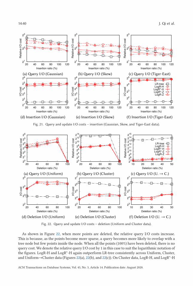
14:40 J. Qi et al.
Fig. 21. Query and update I/O costs – insertion (Gaussian, Skew, and Tiger-East data).
Fig. 22. Query and update I/O costs – deletion (Uniform and Cluster data).
As shown in Figure 22, when more points are deleted, the relative query I/O costs increase.This is because, as the points become more sparse, a query becomes more likely to overlap with atree node but few points inside the node. When all the points (100%) have been deleted, there is noquery cost. We denote the relative query I/O cost by 1 in this case to suit the logarithmic notation ofthe figures. LogR-H and LogR∗-H again outperform LR-tree consistently across Uniform, Cluster,and Uniform→Cluster data (Figures 22(a), 22(b), and 22(c)). On Cluster data, LogR-H, and LogR∗-H
ACM Transactions on Database Systems, Vol. 45, No. 3, Article 14. Publication date: August 2020.
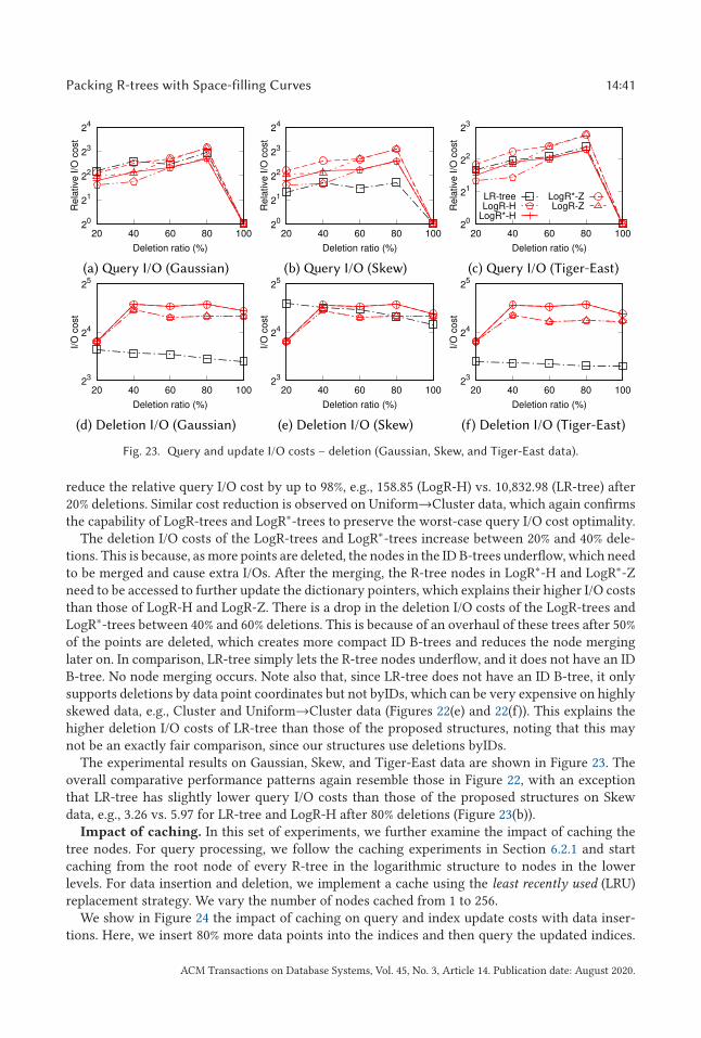
Packing R-trees with Space-filling Curves 14:41
Fig. 23. Query and update I/O costs – deletion (Gaussian, Skew, and Tiger-East data).
reduce the relative query I/O cost by up to 98%, e.g., 158.85 (LogR-H) vs. 10,832.98 (LR-tree) after20% deletions. Similar cost reduction is observed on Uniform→Cluster data, which again confirmsthe capability of LogR-trees and LogR∗-trees to preserve the worst-case query I/O cost optimality.
The deletion I/O costs of the LogR-trees and LogR∗-trees increase between 20% and 40% dele-tions. This is because, as more points are deleted, the nodes in the ID B-trees underflow, which needto be merged and cause extra I/Os. After the merging, the R-tree nodes in LogR∗-H and LogR∗-Zneed to be accessed to further update the dictionary pointers, which explains their higher I/O coststhan those of LogR-H and LogR-Z. There is a drop in the deletion I/O costs of the LogR-trees andLogR∗-trees between 40% and 60% deletions. This is because of an overhaul of these trees after 50%of the points are deleted, which creates more compact ID B-trees and reduces the node merginglater on. In comparison, LR-tree simply lets the R-tree nodes underflow, and it does not have an IDB-tree. No node merging occurs. Note also that, since LR-tree does not have an ID B-tree, it onlysupports deletions by data point coordinates but not byIDs, which can be very expensive on highlyskewed data, e.g., Cluster and Uniform→Cluster data (Figures 22(e) and 22(f)). This explains thehigher deletion I/O costs of LR-tree than those of the proposed structures, noting that this maynot be an exactly fair comparison, since our structures use deletions byIDs.
The experimental results on Gaussian, Skew, and Tiger-East data are shown in Figure 23. Theoverall comparative performance patterns again resemble those in Figure 22, with an exceptionthat LR-tree has slightly lower query I/O costs than those of the proposed structures on Skewdata, e.g., 3.26 vs. 5.97 for LR-tree and LogR-H after 80% deletions (Figure 23(b)).
Impact of caching. In this set of experiments, we further examine the impact of caching thetree nodes. For query processing, we follow the caching experiments in Section 6.2.1 and startcaching from the root node of every R-tree in the logarithmic structure to nodes in the lowerlevels. For data insertion and deletion, we implement a cache using the least recently used (LRU)replacement strategy. We vary the number of nodes cached from 1 to 256.
We show in Figure 24 the impact of caching on query and index update costs with data inser-tions. Here, we insert 80% more data points into the indices and then query the updated indices.
ACM Transactions on Database Systems, Vol. 45, No. 3, Article 14. Publication date: August 2020.
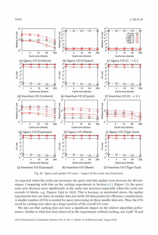
14:42 J. Qi et al.
Fig. 24. Query and update I/O costs – impact of the cache size (insertion).
As expected, when the cache size increases, the query and data update costs decrease for all tech-niques. Comparing with that on the caching experiments in Section 6.2.1 (Figure 13), the querycosts now decrease more significantly as the cache size increases (especially when the cache sizeexceeds 16 blocks, e.g., Figures 24(a) to 24(c)). This is because, as mentioned above, the updateexperiments here are done on smaller data sets (with 1M data points) for efficiency consideration.A smaller number of I/Os is needed for query processing on these smaller data sets. Thus, the I/Ossaved by caching now takes up a larger portion of the overall I/O costs.
We also see that caching does not have a significant impact on the relative algorithm perfor-mance. Similar to what has been observed in the experiments without caching, our LogR∗-H and
ACM Transactions on Database Systems, Vol. 45, No. 3, Article 14. Publication date: August 2020.
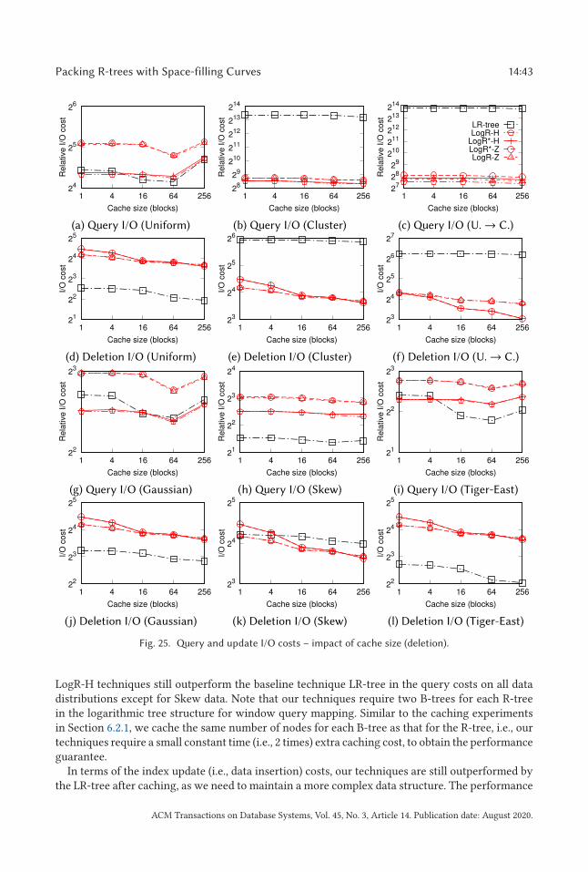
Packing R-trees with Space-filling Curves 14:43
Fig. 25. Query and update I/O costs – impact of cache size (deletion).
LogR-H techniques still outperform the baseline technique LR-tree in the query costs on all datadistributions except for Skew data. Note that our techniques require two B-trees for each R-treein the logarithmic tree structure for window query mapping. Similar to the caching experimentsin Section 6.2.1, we cache the same number of nodes for each B-tree as that for the R-tree, i.e., ourtechniques require a small constant time (i.e., 2 times) extra caching cost, to obtain the performanceguarantee.
In terms of the index update (i.e., data insertion) costs, our techniques are still outperformed bythe LR-tree after caching, as we need to maintain a more complex data structure. The performance
ACM Transactions on Database Systems, Vol. 45, No. 3, Article 14. Publication date: August 2020.
14:44 J. Qi et al.
gap does not increase with the cache size (note the logarithmic scale in the y-axis of the figures).This shows that our techniques can take advantage of the cache as well as the LR-tree does.
For data deletions, we show the impact of caching in Figure 25, where we delete 80% (40% forthe “Uniform→Cluster” data) of the data points and then query the updated indices. The overallobservations are similar to that in Figure 24. The query and index update costs drop when thecache size increases, while the cache does not significantly impact the relative performance ofthe different techniques. There are two exceptions: First, the query costs rise back on the Uniform,Gaussian, and Tiger-East data when the cache size reaches 256 blocks (Figures 25(a) and 25(g)). Thisis because we counted the cost of pre-loading the tree nodes into the cache as part of the queryI/O costs. When 256 tree nodes are cached, the pre-loading I/O costs outweigh the reduction inthe query costs (on Uniform, Gaussian, and Tiger-East data, which are less skewed and have lowerquery costs), which causes the rise in the overall query costs. Second, on Uniform and Tiger-Eastdata, LR-tree now yields slightly lower query I/O costs when the cache size reaches 16 blocks,e.g., 3.44 vs. 4.50 for LR-tree and LogR-H when caching 64 blocks on Tiger-East data (Figure 25(i)).However, LR-tree is still much worse than our techniques on worst-case workloads, e.g., on Clusterdata (cf. Figure 25(b)).
Insertion and deletion. Experiments where there are both insertions and deletions show con-sistent results to the above. We omit the results due to space limit.
7 CONCLUSIONS
We revisited a classic spatial index, the R-tree, and proposed an R-tree packing strategy to con-struct R-trees that are worst-case optimal and empirically efficient for query processing. Thispacking strategy maps data points into a rank space where the points are packed by their Z-order values. Mapping into a rank space avoids data points with the same coordinates. This over-comes the difficulty of space-filling curve-based indices in offering optimal query performance inworst-case scenarios [7, 65]. It results in an R-tree structure that can answer a window query withO ((n/B)1−1/d + k/B) I/Os in the worst case, which is asymptotically optimal. Experiments on bothreal and synthetic data confirmed the query efficiency of such an R-tree: on real data, the query I/Ocost of the R-tree is up to 31% lower than that of PR-trees and similar to that of STR-trees; on highlyskewed synthetic data, the query I/O cost of the R-tree is 54% lower than that of PR-trees and 64%lower than that of STR-trees. Another advantage of this packing strategy is that it only relies onsorting, which well suits parallel bulk-loading of R-trees over large data sets. We proposed a paral-lel R-tree bulk-loading algorithm based on this packing strategy using the MapReduce model. Thealgorithm takes only O (logs n) rounds of computation to bulk-load an R-tree. It outperforms thePR-tree bulk-loading algorithm in running time by 85% on large data sets with 20M data points. Wealso considered data update handling. Our R-tree-based dynamic index structures can process datainsertions and deletions without compromising the worst-case query I/O cost optimality. Theseproposed dynamic index structures achieve up to 98% lower query I/O costs comparing with theLR-tree—a Hilbert R-tree variant with update supports. The advantage is most significant whenthe data distribution is highly skewed.
For future work, we are interested in applying the rank space technique over other indices suchas quad-trees and GiMP [63] to optimize window query processing. De-amortizing the update costto avoid workload peaks for global rebuilds would be another interesting direction to explore.
ELECTRONIC APPENDIX
The electronic appendix for this article can be accessed in the ACM Digital Library.
ACM Transactions on Database Systems, Vol. 45, No. 3, Article 14. Publication date: August 2020.

Packing R-trees with Space-filling Curves 14:45
REFERENCES
[1] Daniar Achakeev, Bernhard Seeger, and Peter Widmayer. 2012. Sort-based query-adaptive loading of R-trees. In
Proceedings of the Conference on Information and Knowledge Management. 2080–2084.
[2] Daniar Achakeev, Marc Seidemann, Markus Schmidt, and Bernhard Seeger. 2012. Sort-based parallel loading of R-
trees. In Proceedings of the 1st ACM SIGSPATIAL International Workshop on Analytics for Big Geospatial Data. 62–70.
[3] Pankaj K. Agarwal, Lars Arge, Octavian Procopiuc, and Jeffrey Scott Vitter. 2001. A framework for index bulk loading
and dynamization. In Proceedings of the 28th International Colloquium on Automata, Languages and Programming.
115–127.
[4] Pankaj K. Agarwal, Mark de Berg, Joachim Gudmundsson, Mikael Hammar, and Herman J. Haverkort. 2001. Box-trees
and R-trees with near-optimal query time. In Proceedings of the 17th Annual Symposium on Computational Geometry
(SoCG’01). 124–133.
[5] Pankaj K. Agarwal, Kyle Fox, Kamesh Munagala, and Abhinandan Nath. 2016. Parallel algorithms for constructing
range and nearest-neighbor searching data structures. In Proceedings of the Symposium on Principles of Database
Systems. 429–440.
[6] Alexandr Andoni, Aleksandar Nikolov, Krzysztof Onak, and Grigory Yaroslavtsev. 2014. Parallel algorithms for geo-
metric graph problems. In Proceedings of the ACM Symposium on Theory of Computing. 574–583.
[7] Lars Arge, Mark De Berg, Herman Haverkort, and Ke Yi. 2008. The priority R-tree: A practically efficient and worst-
case optimal R-tree. ACM Trans. Algor. 4, 1 (2008), 9:1–9:30.
[8] Lars Arge and Jan Vahrenhold. 2004. I/O-efficient dynamic planar point location. Comput. Geom. 29, 2 (2004), 147–162.
[9] Lars Arge and Jeffrey Scott Vitter. 2003. Optimal external memory interval management. SIAM J. Comput. 32, 6 (2003),
1488–1508.
[10] Paul Beame, Paraschos Koutris, and Dan Suciu. 2013. Communication steps for parallel query processing. In Proceed-
ings of the Symposium on Principles of Database Systems. 273–284.
[11] Norbert Beckmann, Hans-Peter Kriegel, Ralf Schneider, and Bernhard Seeger. 1990. The R*-tree: An efficient and
robust access method for points and rectangles. In Proceedings of the ACM Conference on Management of Data. 322–
331.
[12] Jon Louis Bentley. 1975. Multidimensional binary search trees used for associative searching. Commun. ACM 18, 9
(1975), 509–517.
[13] Jon Louis Bentley. 1979. Decomposable searching problems. Inf. Proc. Lett. 8, 5 (1979), 244–251.
[14] Stefan Berchtold, Daniel A. Keim, and Hans-Peter Kriegel. 1996. The X-tree: An index structure for high-dimensional
data. In Proceedings of the International Conference on Very Large Data Bases. 28–39.
[15] Mark Berg, Marc Kreveld, Mark Overmars, and Otfried Cheong Schwarzkopf. 2000. Computational Geometry. Springer
Berlin.
[16] Panayiotis Bozanis, Alexandros Nanopoulos, and Yannis Manolopoulos. 2003. LR-tree: A logarithmic decomposable
spatial index method. Comput. J. 46, 3 (2003), 319–331.
[17] Bernard Chazelle. 1988. Functional approach to data structures and its use in multidimensional searching. SIAM J.
Comput. 17, 3 (1988), 427–462.
[18] Jeffrey Dean and Sanjay Ghemawat. 2008. MapReduce: Simplified data processing on large clusters. Commun. ACM
51, 1 (2008), 107–113.
[19] David J. DeWitt, Navin Kabra, Jun Luo, Jignesh M. Patel, and Jie-Bing Yu. 1994. Client-server paradise. In Proceedings
of the International Conference on Very Large Data Bases. 558–569.
[20] Artyom Dogtiev. 2018. Pokémon GO Revenue and Usage Statistics (2017). Retrieved from http://www.businessofapps.
com/data/pokemon-go-statistics/.
[21] Harold N. Gabow, Jon Louis Bentley, and Robert E. Tarjan. 1984. Scaling and related techniques for geometry prob-
lems. In Proceedings of the ACM Symposium on Theory of Computing. 135–143.
[22] Volker Gaede and Oliver Günther. 1998. Multidimensional access methods. Comput. Surv. 30, 2 (1998), 170–231.
[23] Yván J. García R, Mario A. López, and Scott T. Leutenegger. 1998. A greedy algorithm for bulk loading R-trees. In
Proceedings of the ACM SIGSPATIAL International Conference on Advances in Geographic Information Systems. 163–164.
[24] Michael T. Goodrich. 1999. Communication-efficient parallel sorting. SIAM J. Comput. 29, 2 (1999), 416–432.
[25] Roberto Grossi and Giuseppe F. Italiano. 1999. Efficient cross-trees for external memory. In Proceedings of a DIMACS
Workshop: External Memory Algorithms. American Mathematical Society, 87–106.
[26] Ralf Hartmut Güting. 1994. An introduction to spatial database systems. VLDB J. 3, 4 (1994), 357–399.
[27] Antonin Guttman. 1984. R-trees: A dynamic index structure for spatial searching. In Proceedings of the ACM Confer-
ence on Management of Data. 47–57.
[28] Herman Haverkort and Freek V. Walderveen. 2008. Four-dimensional Hilbert curves for R-trees. J. Experim. Algor. 16
(2008).
ACM Transactions on Database Systems, Vol. 45, No. 3, Article 14. Publication date: August 2020.

14:46 J. Qi et al.
[29] Scott Huddleston and Kurt Mehlhorn. 1982. A new data structure for representing sorted lists. Acta Inf. 17, 2 (1982),
157–184.
[30] H. V. Jagadish. 1990. Spatial search with polyhedra. In Proceedings of the IEEE International Conference on Data Engi-
neering. 311–319.
[31] H. V. Jagadish. 1997. Analysis of the Hilbert curve for representing two-dimensional space. Inf. Proc. Lett. 62, 1 (1997),
17–22.
[32] Ibrahim Kamel and Christos Faloutsos. 1992. Parallel R-trees. In Proceedings of the ACM Conference on Management
of Data. 195–204.
[33] Ibrahim Kamel and Christos Faloutsos. 1994. Hilbert R-tree: An improved R-tree using fractals. In Proceedings of the
International Conference on Very Large Data Bases. 500–509.
[34] Kothuri Venkata Ravi Kanth and Ambuj K. Singh. 1999. Optimal dynamic range searching in non-replicating index
structures. In Proceedings of the International Conference on Database Theory. 257–276.
[35] Nick Koudas, Christos Faloutsos, and Ibrahim Kamel. 1996. Declustering spatial databases on a multi-computer ar-
chitecture. In Proceedings of the International Conference on Extending Database Technology. 592–614.
[36] Scott T. Leutenegger, J. M. Edgington, and Mario A. López. 1997. STR: A simple and efficient algorithm for R-tree
packing. In Proceedings of the IEEE International Conference on Data Engineering. 497–506.
[37] Thomas Mølhave. 2012. Using TPIE for processing massive data sets in C++. SIGSPATIAL Special 4, 2 (2012), 24–27.
[38] Anirban Mondal, Masaru Kitsuregawa, Beng Chin Ooi, and Kian Lee Tan. 2001. R-tree-based data migration and self-
tuning strategies in shared-nothing spatial databases. In Proceedings of the ACM SIGSPATIAL International Conference
on Advances in Geographic Information Systems. 28–33.
[39] Bongki Moon, H. V. Jagadish, Christos Faloutsos, and Joel H. Saltz. 2001. Analysis of the clustering properties of the
hilbert space-filling curve. IEEE Trans. Knowl. Data Eng. 13, 1 (2001), 124–141.
[40] Nectar. 2018. The National eResearch Collaboration Tools and Resources Project. Retrieved from https://nectar.org.
au/.
[41] Yutaka Ohsawa and Masao Sakauchi. 1990. A new tree type data structure with homogeneous nodes suitable for a
very large spatial database. In Proceedings of the IEEE International Conference on Data Engineering. 296–303.
[42] Oracle Corporation. 2001. Oracle Spatial User’s Guide and Reference Release 9.0.1. Retrieved from https://docs.oracle.
com/cd/A91202_01/901_doc/appdev.901/a88805/toc.htm.
[43] Oracle Corporation. 2019. MySQL 8.0 Reference Manual. Retrieved from https://dev.mysql.com/doc/refman/8.0/en/
creating-spatial-indexes.html.
[44] Jack A. Orenstein and T. H. Merrett. 1984. A class of data structures for associative searching. In Proceedings of the
Symposium on Principles of Database Systems. 181–190.
[45] Mark H. Overmars. 1987. Design of Dynamic Data Structures. Springer-Verlag.
[46] Mark H. Overmars and Jan van Leeuwen. 1981. Dynamization of decomposable searching problems yielding good
worst-case bounds. In Proceedings of the 5th GI-Conference on Theoretical Computer Science. 224–233.
[47] Mark H. Overmars and Jan van Leeuwen. 1981. Worst-case optimal insertion and deletion methods for decomposable
searching problems. Inf. Proc. Lett. 12, 4 (1981), 168–173.
[48] Apostolos Papadopoulos and Yannis Manolopoulos. 2003. Parallel bulk-loading of spatial data. Parallel Comput. 29,
10 (2003), 1419–1444.
[49] Ben Popper. 2017. Google Announces over 2 Billion Monthly Active Devices on Android. Retrieved from https://
www.theverge.com/2017/5/17/15654454/android-reaches-2-billion-monthly-active-users.
[50] Jianzhong Qi, Yufei Tao, Yanchuan Chang, and Rui Zhang. 2018. Theoretically optimal and empirically efficient R-
trees with strong parallelizability. Proc. VLDB Endow. 11, 5 (2018), 621–634.
[51] Jianzhong Qi, Rui Zhang, Lars Kulik, Dan Lin, and Yuan Xue. 2012. The min-dist location selection query. In Proceed-
ings of the IEEE International Conference on Data Engineering. 366–377.
[52] Nick Roussopoulos and Daniel Leifker. 1985. Direct spatial search on pictorial databases using packed R-trees. In
Proceedings of the ACM Conference on Management of Data. 17–31.
[53] James B. Saxe and Jon L. Bentley. 1979. Transforming static data structures to dynamic structures. In Proceedings of
the IEEE Symposium on Foundations of Computer Science. 148–168.
[54] Bernd Schnitzer and Scott T. Leutenegger. 1999. Master-client R-trees: A new parallel R-tree architecture. In Proceed-
ings of the Scientific and Statistical Database Management Conference. 68–77.
[55] Timos K. Sellis, Nick Roussopoulos, and Christos Faloutsos. 1987. The R+-tree: A dynamic index for multi-dimensional
objects. In Proceedings of the International Conference on Very Large Data Bases. 507–518.
[56] Apache Spark. 2016. Spark Programming Guide. Retrieved from https://spark.apache.org/docs/1.6.0/programming-
guide.html.
[57] Yufei Tao, Wenqing Lin, and Xiaokui Xiao. 2013. Minimal MapReduce algorithms. In Proceedings of the ACM Confer-
ence on Management of Data. 529–540.
ACM Transactions on Database Systems, Vol. 45, No. 3, Article 14. Publication date: August 2020.

Packing R-trees with Space-filling Curves 14:47
[58] The Pokémon Company. 2018. Pokémon Go. Retrieved from http://www.pokemongo.com.
[59] United States Census Bureau. 2006. TIGER/Line Shapefiles and TIGER/Line Files. Retrieved from https://www.census.
gov/geo/maps-data/data/tiger-line.html.
[60] Pan Xu and Srikanta Tirthapura. 2014. Optimality of clustering properties of space-filling curves. ACM Trans. Datab.
Syst. 39, 2 (2014), 10:1–10:27.
[61] Simin You, Jianting Zhang, and Le Gruenwald. 2013. Parallel spatial query processing on GPUs using R-trees. In
Proceedings of the 2nd ACM SIGSPATIAL International Workshop on Analytics for Big Geospatial Data. 23–31.
[62] Matei Zaharia, Mosharaf Chowdhury, Michael J. Franklin, Scott Shenker, and Ion Stoica. 2010. Spark: Cluster com-
puting with working sets. In Proceedings of the 2nd USENIX Conference on Hot Topics in Cloud Computing. 10–10.
[63] Rui Zhang, Panos Kalnis, Beng Chin Ooi, and Kian-Lee Tan. 2005. Generalized multidimensional data mapping and
query processing. ACM Trans. Datab. Syst. 30, 3 (2005), 661–697.
[64] Rui Zhang, Beng Chin Ooi, and Kian-Lee Tan. 2004. Making the pyramid technique robust to query types and work-
loads. In Proceedings of the IEEE International Conference on Data Engineering. 313–324.
[65] Rui Zhang, Jianzhong Qi, Martin Stradling, and Jin Huang. 2014. Towards a painless index for spatial objects. ACM
Trans. Datab. Syst. 39, 3 (2014), 19:1–19:42.
Received February 2019; revised January 2020; accepted April 2020
ACM Transactions on Database Systems, Vol. 45, No. 3, Article 14. Publication date: August 2020.