Abstract— Game companies avoid sharing their game data

with external researchers. Only a few research groups have

been granted limited access to game data so far. The reluctance

of these companies to make data publicly available limits the

wide use and development of data mining techniques and

artificial intelligence research specific to the game industry. In

this work, we developed and implemented an international

competition on game data mining using commercial game log

data from one of the major game companies in South Korea:

NCSOFT. Our approach enabled researchers to develop and

apply state-of-the-art data mining techniques to game log data

by making the data open. For the competition, data were

collected from Blade & Soul, an action role-playing game, from

NCSOFT. The data comprised approximately 100 GB of game

logs from 10,000 players. The main aim of the competition was

to predict whether a player would churn and when the player

would churn during two periods between which the business

model was changed to a free-to-play model from a monthly

subscription. The results of the competition revealed that

highly ranked competitors used deep learning, tree boosting,

and linear regression.

Index Terms— Churn prediction, Competition, Data mining,

Game log, Machine learning, Survival analysis

I. INTRODUCTION

Game artificial intelligence (AI) competition platforms

help researchers access well-defined benchmarking

problems to evaluate different algorithms, test new

approaches, and educate students [1]. Since the early 2000s,

considerable effort has focused on designing and running

new game AI competitions using mathematical, board, video,

and physical games [2]. Despite a few exceptions, most of

K.-J. Kim, D.-M. Yoon, and J-H. Jeon are with the Computer Science

and Engineering Department, Sejong University, Korea (e-mail: kimkj@sejong.ac.kr, corresponding author)

S.-I. Yang, S.-K. Lee and D.-W. Kim are with ETRI (Electronics and

Telecommunications Research Institute) Korea (e-mail: siyang@etri.re.kr) E.-J. Lee and Y.-J. Jang are with NCSOFT, Korea (e-mail:

gimmesilver@ncsoft.com)

P.P. Chen, A. Guitart, P. Bertens, and Á . Periáñez are with Game Data Science Department, Yokozuna Data, Silicon Studio, 1-21-3 Ebisu

the research has concentrated on building AI players to play

challenging games such as StarCraft and simulated car

racing and fighting games; these competitions commonly

rank AI players based on the results of numerous game plays,

using, for example, final scores and win ratios. Recently,

there have been special competitions that target human-

likeness [3], general game playing [4], and the learning

ability of AI players. However, there have been few

competitions on content creation [5], game player modeling,

or game data mining.

There have been many attempts to analyze game players.

Bartle proposed analyzing multi-user dungeon game players

(MUDs) into four types in 1996 [13] and expanded the

model to eight types [14]. Quantic Foundry proposed six

gamer motivation models based on 12 motivation factors

from 5-min surveys with 250,000 gamers [15]. Others have

attempted to model game players based on data analysis

[16][17][18][19][20]. In recent years, game data mining has

become increasingly popular. Data mining techniques

extract useful information from large databases and are

widely adopted in practical data analysis [21][22].

Game companies generate a large amount of game player

data based on their actions, progress, and purchases. From

such data, it is possible to model the users’ patterns [6] and

attain useful information, including in-game dynamics, a

user’s likelihood of churning, lifetime, and user clusters. For

example, Kim et al. discovered a “real money trading (RMT)”

pattern from the MMORPG Lineage game [8] and detected

Bots and socio-economy patterns from the MMORPG Aion

game [7][9]. Despite its potential benefits to the game

industry, collaboration between academics and game

companies to develop and apply advanced techniques to

game log data has not flourished to the extent of AI game

player development or content generation. Figure 1 shows

Shibuya-ku, Tokyo, Japan (e-mail: {peipei.chen, anna.guitart, paul.bertens,

africa.perianez} @siliconstudio.co.jp) Fabian Hadiji and Marc Müller are with goedle.io GmbH (e-mail:

{fabian, marc}@goedle.io)

Youngjun Joo, Jiyeon Lee, and Inchon Hwang are with Dept. of Computer Engineering, Yonsei University, Korea (e-mail: {chrisjoo12,

jitamin21, ich0103}@gmail.com)

Game Data Mining Competition on Churn

Prediction and Survival Analysis using

Commercial Game Log Data

EunJo Lee, Yoonjae Jang, DuMim Yoon, JiHoon Jeon, Seong-il Yang, Sang-Kwang Lee, Dae-Wook

Kim, Pei Pei Chen, Anna Guitart, Paul Bertens, Á frica Periáñez, Fabian Hadiji, Marc Müller,

Youngjun Joo, Jiyeon Lee, Inchon Hwang and Kyung-Joong Kim

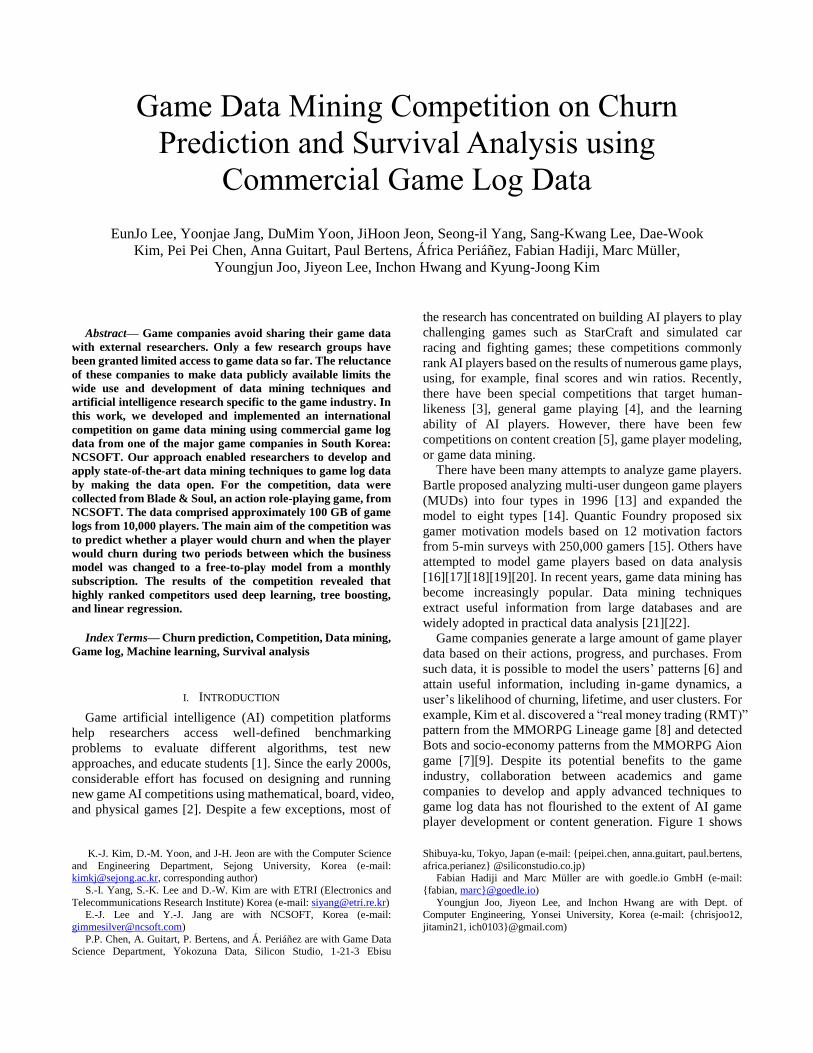
that the number of studies on game data mining plateaued

after a sudden increase in 2013.

Figure 1. Number of papers on game data mining in 2010–2017

(from Google Scholar using “Game Data Mining” keywords)

The purpose of our game data mining competition was to

promote the research of game data mining by providing

commercial game logs to the public. In coordination with

NCSOFT, one of the largest game companies in South Korea,

approximately 100 GB of game log data from Blade & Soul

were made available.

We hosted the competition for five months from March

28, 2017, to August 25, 2017. During this period, we had 300

registrations on the competition’s Google Groups that were

given access to the log data. Finally, we received 13

submissions for Track 1 (churn prediction) and 5

submissions for Track 2 (survival analysis). The participants

predicted the future behavior of users by applying different

sets of state-of-the-art techniques such as deep learning,

ensemble tree classifiers, and logistic regression.

The contributions of the game data mining competition

are listed below.

The competition opened commercial game log data from

an active game to the public for benchmarking purposes.

After the competition, NCSOFT allowed users to copy

and retain data for educational, scholarly, and research

applications. In addition, labels for the test dataset were

made publicly available.

Similar to the ImageNet competition, the competition

provided a test server for participants to submit their

intermediate performance and benchmark predictions

using 10% of the test data.

The competition problems applied practical

containments. For example, a much longer time span

(e.g., three weeks) was given between the training data

and prediction window, reflecting the minimum time

required to develop and execute churn prevention

strategies to retain potential churners. This enhanced the

1 http://www.bladeandsoul.com/en/

difficulty of the competition problem compared with the

conventional time span of one to two weeks.

The competition was designed to incorporate concept

drift, specifically, a change in the business model, to

measure the robustness of the participants’ models when

applied to constantly evolving conditions. Consequently,

the competition comprised two test datasets, each from

different periods. Between the two periods, the

aforementioned business model change took place. The

final standings of entries were determined based on the

harmonic average of final scores from both test datasets.

II. COMPETITION PROBLEMS: CHALLENGES IN GAME DATA

MINING COMPETITION

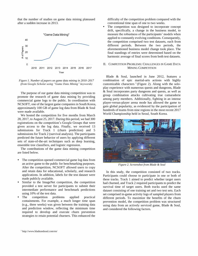
Blade & Soul, launched in June 2012, features a

combination of epic martial-arts actions with highly

customizable characters 1 (Figure 2). Along with the solo-

play experience with numerous quests and dungeons, Blade

& Soul incorporates party dungeons and quests, as well as

group combination attacks cultivating true camaraderie

among party members. Additionally, fighting in an intense

player-versus-player arena mode has allowed the game to

gain global popularity, as evidenced by the participation of

hundreds of teams from nine regions in the most recent 2017

World Championship held in Seoul, South Korea.

Figure 2. Screenshot from Blade & Soul

In this study, the competition consisted of two tracks.

Participants could choose to participate in one or both of

these tracks. Track 1 aimed to predict whether target users

had churned, and Track 2 required participants to predict the

survival time of target users. Both tracks used the same

dataset consisting of one training set and two test sets. Each

set comprised in-game activity logs of sampled players from

different periods. To maximize the benefits of the churn

prevention model, the competition problem was structured

using data from an actively serviced game, Blade & Soul,

and considered the following factors.

A. Prediction targets

To benefit the most from churn prediction and prevention,

prediction targets should be those that provide the most

profit if retained. Naturally, not all users provide game

companies with the same profit; in fact, most users are casual

game players accounting for a small proportion of sales, and

there are even users who undermine the game services [23].

These light, casual, and malicious players were excluded

from the scope of this competition, as our focus was on

predicting the churn of loyal users only, namely, highly loyal

users with a cumulative purchase above a certain threshold

and many in-game activities. Given that highly loyal users

seldom churn or churn on occasion due to external factors,

we expected that the participants’ churn prediction

performance would not be comparable to prior churn

prediction work. Table 1 shows that several previous works

included all or most game player types in their churn

prediction.

B. Definition of player churn

Unlike telecommunication services in which user churn

can be easily defined and identified by the user

unsubscribing [24], such is not the case for online game

services. Online game players seldom delete their accounts

or unsubscribe, although they have no intention of resuming

game play. In fact, according to our analysis, only 1% of the

players inactive for over one year explicitly leave the service

by deleting their accounts.

Consequently, we decided player churn using consecutive

periods of inactivity. However, what length of inactivity

should be considered as churn? This is a difficult question to

answer, given that there are various reasons behind a

player’s inactivity. For example, some players may be

inactive for several days because they only play on the

weekends. Some may appear inactive for a few weeks

because they went on a trip or because they had an important

exam that month. If the period to decide player churn is too

short, the misclassification rate will be high. If the period is

too long, on the other hand, the misclassification rate would

be lower but it would take longer to determine whether a

player had churned or not; consequently, by the time a player

is identified as a churner, there would not be sufficient time

to persuade him or her to return.

To resolve this dilemma, we defined a churner as a user

who does not play the game for more than five weeks. Figure

3 shows the weekly and daily play patterns of players in

concordance with their life patterns and weekly server

maintenance every Wednesday morning. Thus, in our

analysis, a week is defined from one Wednesday to the next

Wednesday. Table 1 shows that previous works used ten

days or two weeks for the decision of churn. However, in a

recent work for the AAA title, Destiny used four weeks for

the churn decision, similar to our definition.

Figure 3. Time series of concurrent users for one week. Daily and

weekly cyclic patterns are shown

C. Prediction point

It is likely that user behaviors leading up to the point of

churn (e.g., deleting the game character) would play a vital

role in churn prediction. However, predicting churn just

before the point of leaving would be pointless, as at that

point not much can be done to persuade users to stay loyal.

Predictions should be made in a timely manner before the

churning point so that a churn prevention strategy, namely,

a new promotion campaign, content update, and so on, can

Table 1. Summary of churn prediction study

Year References Games (Publisher) Genre

(Platform)

Payment

System Target Customers

Churn

Definition

(Inactivity Period)

Prediction Point

2017 GDMC 2017

Competition

Blade & Soul

(NCSOFT)

MMORPG

(PC)

Monthly

Charge,

Free-to-Play

Highly Loyal Users

(cumulative purchase

above the certain threshold)

five weeks

Churn after

three weeks

Survival

Analysis

2017 Kim et al.,[12] Dodge the Mud,

Undisclosed, TagPro Causal Game

(Online/Mobile) Free-to-

Play All gamers ten days

Churn within 10 days

2016 Tamassia et al.,

[26] Destiny (Bungie)

MMOG (Online)

Package Price

Randomly sampled

players

(play time > 2 hours)

four weeks Churn after four

weeks

2016 Perianez et al.

[11]

Age of Ishtaria

(Silicon Studio)

Social RPG

(Mobile)

Free-to-

Play

High value players

(whales) ten days

Survival

Analysis

2014 J. Runge et al.,

[10]

Diamond Dash and

Monster World Flash (Wooga)

Social Game

(Mobile)

Free-to-

Play

High Value Player

(top 10% of all paying players)

two weeks Churn within

the Week

be implemented to retain potential churners. If the prediction

is made too early, the result will not be sufficiently accurate,

whereas if the prediction is made too late, not much can be

done to retain the user even if the prediction is correct. For

our competition, making predictions three weeks ahead of

the point of actual churn was deemed effective.

Consequently, as shown in Figure 4, we examined user data

accounts up to three weeks before the initiation of the five-

week churning window.

Figure 4. User data and churning window were used to predict

and determine churn, respectively

D. Survival analysis

While churn prediction itself is well worthwhile,

predicting the specific churn point would increase the value

of the model, so this is the second focus of the competition.

In addition to churn prediction, we asked participants to

perform a survival analysis to predict the survival time. The

survival time was then added to the labeled data for the

training set. Survival time is defined as the period between

the date of last activity from the provided data and the date

of most recent activity, which was not provided but instead

calculated when all predictions were submitted. Because we

can only check for observable periods, this survival analysis

is regarded as a censoring problem. We added a ‘+’ sign after

survival periods for right-censoring data to distinguish

censoring data from churning data.

E. Concept drift

Various operational issues arise when applying the

prediction model to actively serviced and continuously

evolving games; concept drift epitomizes how such change

can affect a prediction model [25]. Compared to a model that

had high performance during the modeling period but

showed declining performance over time, a robust model

that maintains performance, despite externalities, often

proves to be more valuable considering update and

maintenance costs, even if the prediction performance of the

robust model during the modeling period was not as accurate.

To encourage the participants to generate a model that is

robust enough to withstand changing conditions over time,

we created two test sets each with data from different periods

to evaluate model performance. The first test set consisted of

data from the period two months after the training data

period, and the second consisted of data 7 months after the

training data period.

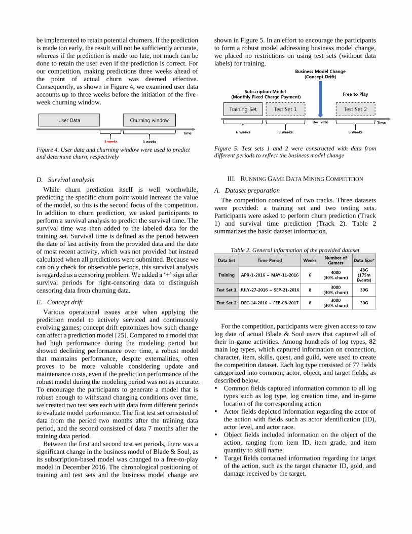
Between the first and second test set periods, there was a

significant change in the business model of Blade & Soul, as

its subscription-based model was changed to a free-to-play

model in December 2016. The chronological positioning of

training and test sets and the business model change are

shown in Figure 5. In an effort to encourage the participants

to form a robust model addressing business model change,

we placed no restrictions on using test sets (without data

labels) for training.

Figure 5. Test sets 1 and 2 were constructed with data from

different periods to reflect the business model change

III. RUNNING GAME DATA MINING COMPETITION

A. Dataset preparation

The competition consisted of two tracks. Three datasets

were provided: a training set and two testing sets.

Participants were asked to perform churn prediction (Track

1) and survival time prediction (Track 2). Table 2

summarizes the basic dataset information.

Table 2. General information of the provided dataset

For the competition, participants were given access to raw

log data of actual Blade & Soul users that captured all of

their in-game activities. Among hundreds of log types, 82

main log types, which captured information on connection,

character, item, skills, quest, and guild, were used to create

the competition dataset. Each log type consisted of 77 fields

categorized into common, actor, object, and target fields, as

described below.

Common fields captured information common to all log

types such as log type, log creation time, and in-game

location of the corresponding action

Actor fields depicted information regarding the actor of

the action with fields such as actor identification (ID),

actor level, and actor race.

Object fields included information on the object of the

action, ranging from item ID, item grade, and item

quantity to skill name.

Target fields contained information regarding the target

of the action, such as the target character ID, gold, and

damage received by the target.

Each field held different information depending on the log

type; detailed log schema and descriptions were provided to

the participants, along with the data, through the competition

website2.

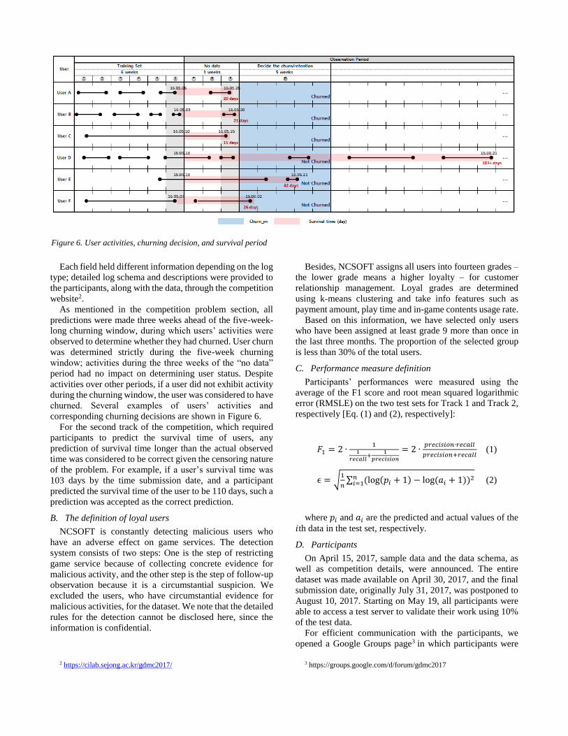
As mentioned in the competition problem section, all

predictions were made three weeks ahead of the five-week-

long churning window, during which users’ activities were

observed to determine whether they had churned. User churn

was determined strictly during the five-week churning

window; activities during the three weeks of the “no data”

period had no impact on determining user status. Despite

activities over other periods, if a user did not exhibit activity

during the churning window, the user was considered to have

churned. Several examples of users’ activities and

corresponding churning decisions are shown in Figure 6.

For the second track of the competition, which required

participants to predict the survival time of users, any

prediction of survival time longer than the actual observed

time was considered to be correct given the censoring nature

of the problem. For example, if a user’s survival time was

103 days by the time submission date, and a participant

predicted the survival time of the user to be 110 days, such a

prediction was accepted as the correct prediction.

B. The definition of loyal users

NCSOFT is constantly detecting malicious users who

have an adverse effect on game services. The detection

system consists of two steps: One is the step of restricting

game service because of collecting concrete evidence for

malicious activity, and the other step is the step of follow-up

observation because it is a circumstantial suspicion. We

excluded the users, who have circumstantial evidence for

malicious activities, for the dataset. We note that the detailed

rules for the detection cannot be disclosed here, since the

information is confidential.

2 https://cilab.sejong.ac.kr/gdmc2017/

Besides, NCSOFT assigns all users into fourteen grades –

the lower grade means a higher loyalty – for customer

relationship management. Loyal grades are determined

using k-means clustering and take info features such as

payment amount, play time and in-game contents usage rate.

Based on this information, we have selected only users

who have been assigned at least grade 9 more than once in

the last three months. The proportion of the selected group

is less than 30% of the total users.

C. Performance measure definition

Participants’ performances were measured using the

average of the F1 score and root mean squared logarithmic

error (RMSLE) on the two test sets for Track 1 and Track 2,

respectively [Eq. (1) and (2), respectively]:

𝐹1 = 2 ∙1

1

𝑟𝑒𝑐𝑎𝑙𝑙+

1

𝑝𝑟𝑒𝑐𝑖𝑠𝑖𝑜𝑛

= 2 ∙𝑝𝑟𝑒𝑐𝑖𝑠𝑖𝑜𝑛∙𝑟𝑒𝑐𝑎𝑙𝑙

𝑝𝑟𝑒𝑐𝑖𝑠𝑖𝑜𝑛+𝑟𝑒𝑐𝑎𝑙𝑙 (1)

ϵ = √1

𝑛∑ (log(𝑝𝑖 + 1) − log(𝑎𝑖 + 1))2𝑛

𝑖=1 (2)

where 𝑝𝑖 and 𝑎𝑖 are the predicted and actual values of the

𝑖th data in the test set, respectively.

D. Participants

On April 15, 2017, sample data and the data schema, as

well as competition details, were announced. The entire

dataset was made available on April 30, 2017, and the final

submission date, originally July 31, 2017, was postponed to

August 10, 2017. Starting on May 19, all participants were

able to access a test server to validate their work using 10%

of the test data.

For efficient communication with the participants, we

opened a Google Groups page3 in which participants were

3 https://groups.google.com/d/forum/gdmc2017

Figure 6. User activities, churning decision, and survival period

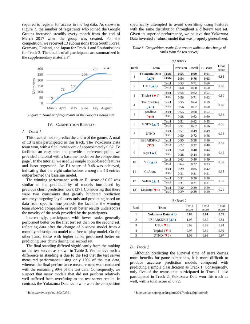
required to register for access to the log data. As shown in

Figure 7, the number of registrants who joined the Google

Groups increased steadily every month from the end of

March 2017 when the group was created. For the

competition, we received 13 submissions from South Korea,

Germany, Finland, and Japan for Track 1 and 5 submissions

for Track 2. The details of all participants are summarized in

the supplementary materials4.

Figure 7. Number of registrants in the Google Groups site

IV. COMPETITION RESULTS

A. Track 1

This track aimed to predict the churn of the gamer. A total

of 13 teams participated in this track. The Yokozuna Data

team won, with a final total score of approximately 0.62. To

facilitate an easy start and provide a reference point, we

provided a tutorial with a baseline model on the competition

page5. In the tutorial, we used 22 simple count-based features

and lasso regression. An F1 score of 0.48 was achieved,

indicating that the eight submissions among the 13 entries

outperformed the baseline model.

The winning performance with an F1 score of 0.62 was

similar to the predictability of models introduced by

previous churn prediction work [27]. Considering that there

were two constraints that greatly hindered prediction

accuracy: targeting loyal users only and predicting based on

data from specific time periods, the fact that the winning

team showed comparable or even better results underscores

the novelty of the work provided by the participants.

Interestingly, participants with lower ranks generally

performed better on the first test set than on the second set,

reflecting data after the change of business model from a

monthly subscription model to a free-to-play model. On the

other hand, those with higher ranks performed better on

predicting user churn during the second set.

The final standing differed significantly from the ranking

on the test server, as shown in Table 3. We believe such a

difference in standing is due to the fact that the test server

measured performance using only 10% of the test data,

whereas the final performance measurement was conducted

with the remaining 90% of the test data. Consequently, we

suspect that many models that did not perform relatively

well suffered from overfitting to the test-server results. In

contrast, the Yokozuna Data team who won the competition

4 https://arxiv.org/abs/1802.02301

specifically attempted to avoid overfitting using features

with the same distribution throughout a different test set.

Given its superior performance, we believe that Yokozuna

Data invented a robust model that was properly generalized.

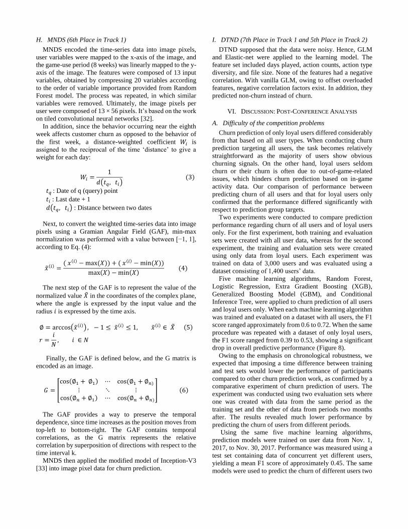
Table 3. Competition results (the arrows indicate the change of

ranks from the test server)

(a) Track 1

Rank Team Precision Recall F1 score Final

score

1 Yokozuna Data

(▲3)

Test1 0.55 0.69 0.61 0.62 Test2 0.54 0.76 0.63

2 UTU (▲1) Test1 0.53 0.71 0.60

0.60 Test2 0.60 0.60 0.60

3 TripleS (▼1) Test1 0.54 0.62 0.57

0.60 Test2 0.56 0.71 0.62

4 TheCowKing

(▲1)

Test1 0.55 0.64 0.59 0.60 Test2 0.56 0.67 0.60

5 goedleio

(▼4)

Test1 0.55 0.60 0.57 0.58 Test2 0.58 0.62 0.60

6 MNDS (▲2) Test1 0.51 0.62 0.55

0.56 Test2 0.51 0.62 0.56

7 DTND Test1 0.51 0.49 0.49

0.53 Test2 0.50 0.72 0.58

8 IISLABSKKU

(▼2)

Test1 0.55 0.58 0.56 0.52 Test2 0.72 0.37 0.48

9 suya (▲1) Test1 0.50 0.40 0.44

0.42 Test2 0.38 0.44 0.40

10 YK (▲2) Test1 0.63 0.40 0.49

0.39 Test2 0.64 0.22 0.33

11 GoAlone Test1 0.29 0.85 0.42

0.35 Test2 0.31 0.31 0.31

12 NoJam (▲1) Test1 0.31 0.30 0.30

0.30 Test2 0.31 0.31 0.31

13 Lessang (▼4) Test1 0.30 0.29 0.29

0.29 Test2 0.29 0.29 0.29

(b) Track 2

Rank Team Test1 score

Test2 score

Total score

1 Yokozuna Data ▲3) 0.88 0.61 0.72

2 IISLABSKKU (▲3) 1.03 0.67 0.81

3 UTU (▼2) 0.92 0.89 0.91

4 TripleS (▼1) 0.95 0.89 0.92

5 DTND (▼3) 1.03 0.93 0.97

B. Track 2

Although predicting the survival time of users carries

more benefits for game companies, it is more difficult to

produce accurate prediction models compared with

predicting a simple classification as Track 1. Consequently,

only five of the teams that participated in Track 1 also

participated in Track 2. Yokozuna Data won this track as

well, with a total score of 0.72.

5 https://cilab.sejong.ac.kr/gdmc2017/index.php/tutorial/

0

76106

206

255 264

0

50

100

150

200

250

300

March April May June July August

Mem

ber

s

Unlike Track 1, performance was measured using

RMSLE, in which a lower score is better. As with the results

for Track 1, the test server results differed from those at the

final outcome. The highest score from the test server was

0.41, whereas that of the final performance measure was

around 0.72.

V. METHODS USED BY PARTICIPANTS

A. Overview

Throughout the competition, various methods were

applied and tested on the game log data of Blade & Soul of

NCSOFT. For Track 1, there was no overriding technique.

All groups were evenly distributed in the rankings. This

means that the combination of features, learning models, and

feature selection is more important than what learning model

is used to improve churn prediction accuracy.

Proper data pre-processing was highly important with

regard to achieving high performance in the prediction. The

winner, Yokozuna Data used the most various features

among participants. They used daily features, entire period

features, time-weighted features and statistical features. It is

also interesting that Yokozuna Data used different

algorithms for each of the test sets. In addition, deep learning

appeared to be less popular than computer vision, speech

analysis, and other engineering domains in the field of game

data mining, as there were many participants who

implemented tree-based ensemble classifiers (e.g., extra-tree

classifiers and Random Forest) and logistic regression.

These prediction techniques were classified into three major

groups: neural network, tree-based, and linear model.

For Track 2, no entries with deep learning techniques were

submitted; all of the submissions used either tree regression

or linear models. The winner, Yokozuna Data, combined

900 trees for the regression task.

Those who performed well for Track 1 also excelled in

Track 2, as the rankings among Track 2 participants were the

same as those of Track 1, except for team IISLABSKKU.

Although the rankings for Track 2 were somewhat similar to

those for Track 1, the same was not the case for the usage of

techniques, as no one implemented a neural network model

to solve the problem for Track 2. Even team Yokozuna Data,

which showed impressive performance for Track 1 using a

neural network, chose not to apply neural network

techniques to Track 2.

Now, we describe each method submitted to the

competition, beginning with Yokozuna Data, the winner of

the competition.

B. Yokozuna Data (Winner of Track 1 and Track 2)

Here are summarized methods of the Yokozuna Data

feature engineering process, which is based on previous

works [27][28].

Yokozuna Data used two types of features: daily features

and overall features. Daily features are the features which

are aggregated the user’s in-game activities by day, while

overall features are calculated over the whole data period.

There were more than 3000 extracted features after the

data preparation. Besides adopting all features, the following

three feature selection methods were also tested: LSTM,

auto encoder, feature value distribution and feature

importance.

Multiple models were evaluated for both tracks.

Additionally, different models were used for the two test

datasets. The models that produced the best results – and

that led us to win both tracks – were LSTM, extremely

randomized trees and conditional inference trees. Parameters

were adjusted through cross-validation.

1) Binary Churn Prediction (Track 1)

1-1) LSTM

A model combining an LSTM network with a deep neural

network (DNN) was used for test set 1. First, a multilayer

LSTM network was employed to process the time-series data

and learn a single vector representation describing the time-

series behavior. Then, this vector was merged with the

output of a multilayer DNN that was trained on the static

features. After merging, an additional layer was trained on

top of the combined representation to get the final output

layer predicting the binary result. In order to prevent

overfitting, dropout [29] was used at every layer.

Additionally, dropout was also applied to the input to

perform random feature selection and further reduce

overfitting. As there were many correlated features,

selecting only a subset of the time-series and static features

of the input prevents the model from depending too much on

a single feature and improves generalization.

1-2) Extremely Randomized Trees

This technique provided better prediction results for the

test set 2. After parameter tuning, 50 sample trees were

selected and the minimum number of samples required to

split an internal node was set to 50. Yokozuna Data used a

splitting criterion based on the Gini impurity.

2) Survival Time Analysis (Track 2)

2-1) Conditional Inference Survival Ensembles

For both tests of the survival track, the best results were

obtained with a censoring approach, using conditional

inference survival ensembles. The final parameter selection

was performed using 900 selected unbiased trees and

subsampling without replacement. At each node of the trees,

30 input features were randomly selected from the total input

sample. The stopping criteria employed was based on

univariate p-values. For more details please check [27].

C. UTU (2nd Place in Track 1 and 3rd Place in Track 2)

UTU used various features that represented activities such

as availability, playing probability, message rate, session

lengths, and entry time. These features were split into three

features of overall, last week, and change measure. In

addition, these activity features were extended by smart

features of essentially previous activity (total experience,

maximum experience, current experience, rating, money,

etc.), whereby “smart” means that they reverse-engineered

how the experience accumulation worked with regard to

'previous activity' measurement.

For classification, UTU used simple logistic regression,

with some regularization. They did not attempt to use the

cross-validated 'optimal settings' for parameters because

they were unable to find any differences. Moreover, because

of a covariate shift, they concluded that it would not

necessarily be an optimal setting. Feature selection based on

the basic L1-norm seemed useful in Test Set 2.

For regression, UTU used ridge regression. To linearize

the features for both submissions, they used a feature

transformation based on quantiles.

D. TripleS (3rd place in Track 1 and 4th Place in Track 2)

TripleS used play time (referring to how long the user was

connected to the game), level and mastery level, the sum of

mastery experience, log count, and specific log ID count as

features. All features were extracted on a weekly basis. In

addition, they calculated the coefficient of variance and first-

order and quadratic functions of the abovementioned

features and added them as features only for active players.

After preprocessing the features (normalizing and scaling),

TripleS used an ensemble method, such as Random Forest,

for Tracks 1 and 2. Moreover, to obtain the best result, the

parameters for Random Forest were optimized. All of the

results of Tracks 1 and 2 were validated by five-fold cross-

validation with a training dataset.

E. IISLABSKKU (8th Place in Track 1 and 2nd place in

Track 2)

IISLABSKKU created 1639 features through feature

engineering. They calculated the feature's importance

through Random Forest and used xgboost to calculate the

final results for the 100 critical features.

F. TheCowKing (4th Place in Track 1)

TheCowKing used log counts on a weekly basis. Log ID

and actor level were used as features. The main learning

model of TheCowKing was LightGBM6.

G. goedle.io (5th Place in Track 1)

1) Feature engineering

Goedle.io transformed the events for each player into an

event-based format. Additional information, such as an

event identifier (e.g., to differentiate a kill of a PC vs. NPC)

or an event value (e.g., to track the amount of money spent),

can be added to each event. While not all events provide

meaningful identifiers or values, they added to roughly a

third of the events an identifier, value, or both. Sometimes,

more than one identifier or value is possible. In such cases,

they duplicated the event and set the fields accordingly.

6 https://github.com/Microsoft/LightGBM

Many of the features used were initially inspired by

[30][31]. Over the past years, they have added numerous

additional features to their toolbox. The features can be

categorized into different buckets:

Basic activity: measuring basic activity such as the

current absence time of a player, the average playtime of

player, the number of days a player has been active, or

the number of sessions.

Counts: counting the number of times an event or an

event-identifier combination occurs.

Values: different mathematical operations applied to the

event values, e.g., sum, mean, max, min, etc. (i.e., to the

statistic features).

Timings: timing between events to detect recurring

patterns, e.g., a slowly decreasing retention.

Frequencies: a player’s activity can be transformed from

a time-series into the frequency domain. Now the

strongest recurring frequency of a player can be

estimated and used as a feature. Curve Fitting: as described in [30], curve fitting can be

applied to time series data. Parameters such as a positive

slope of the fit suggest that the interest in the game is

increasing.

Based on these features, datasets for training and testing

sets generated. This resulted in almost 600 features for each

player. But with only 4,000 players in the training dataset,

one has to be careful with too many dimensions. Depending

on the algorithm, feature selection and regularization are not

only helpful but necessary. Additionally, they applied the

outlier detection to the training dataset. Outlier detection

helps to remove noise from the raw data and to exclude

misleading data introduced by malicious players or bots. The

outlier detection removed 0.5% of players in the training

dataset.

2) Modeling

Goedle.io evaluated a variety of algorithms for each

prediction problem. Some algorithms handle raw datasets

quite well, e.g., tree-based algorithms, but other algorithms

strongly benefit from a scaling the data. For that reason, they

apply a simple scaler to the datasets.

To find the best performing algorithm including features,

preprocessing steps, and parameters, they iteratively test

different combinations. To evaluate algorithms and to

measure the improvements due to the optimization, they

used a 5-fold cross validation based on the F1-score.

Geodle.io selected the best algorithm among different ones

including: Logistic Regression (LR), Voted Perceptron (VP),

Decision Trees (DT), Random Forests (RF), Gradient Tree

Boosting (GTB), Support Vector Machines (SVM), and

Artificial Neural Networks (ANN).

H. MNDS (6th Place in Track 1)

MNDS encoded the time-series data into image pixels,

user variables were mapped to the x-axis of the image, and

the game-use period (8 weeks) was linearly mapped to the y-

axis of the image. The features were composed of 13 input

variables, obtained by compressing 20 variables according

to the order of variable importance provided from Random

Forest model. The process was repeated, in which similar

variables were removed. Ultimately, the image pixels per

user were composed of 13 × 56 pixels. It’s based on the work

on tiled convolutional neural networks [32].

In addition, since the behavior occurring near the eighth

week affects customer churn as opposed to the behavior of

the first week, a distance-weighted coefficient 𝑊𝑖 is

assigned to the reciprocal of the time ‘distance’ to give a

weight for each day:

𝑊𝑖 =1

𝑑(𝑡𝑞 , 𝑡𝑖) (3)

𝑡𝑞 : Date of q (query) point

𝑡𝑖 : Last date + 1

𝑑(𝑡𝑞 , 𝑡𝑖) : Distance between two dates

Next, to convert the weighted time-series data into image

pixels using a Gramian Angular Field (GAF), min-max

normalization was performed with a value between [−1, 1],

according to Eq. (4):

�̃�(𝑖) =( 𝑥(𝑖) − max (𝑋)) + ( 𝑥(𝑖) − min (𝑋))

max(𝑋) − min(𝑋) (4)

The next step of the GAF is to represent the value of the

normalized value �̃� in the coordinates of the complex plane,

where the angle is expressed by the input value and the

radius 𝑖 is expressed by the time axis.

∅ = arccos(�̃�(𝑖)) , − 1 ≤ �̃�(𝑖) ≤ 1, �̃�(𝑖) ∈ �̃� (5)

𝑟 =𝑖

𝑁, 𝑖 ∈ 𝑁

Finally, the GAF is defined below, and the G matrix is

encoded as an image.

𝐺 = [

cos(∅1 + ∅1) ⋯ cos (∅1 + ∅𝑛)

⋮ ⋱ ⋮cos(∅𝑛 + ∅1) ⋯ cos (∅𝑛 + ∅𝑛)

] (6)

The GAF provides a way to preserve the temporal

dependence, since time increases as the position moves from

top-left to bottom-right. The GAF contains temporal

correlations, as the G matrix represents the relative

correlation by superposition of directions with respect to the

time interval k.

MNDS then applied the modified model of Inception-V3

[33] into image pixel data for churn prediction.

I. DTND (7th Place in Track 1 and 5th Place in Track 2)

DTND supposed that the data were noisy. Hence, GLM

and Elastic-net were applied to the learning model. The

feature set included days played, action counts, action type

diversity, and file size. None of the features had a negative

correlation. With vanilla GLM, owing to offset overloaded

features, negative correlation factors exist. In addition, they

predicted non-churn instead of churn.

VI. DISCUSSION: POST-CONFERENCE ANALYSIS

A. Difficulty of the competition problems

Churn prediction of only loyal users differed considerably

from that based on all user types. When conducting churn

prediction targeting all users, the task becomes relatively

straightforward as the majority of users show obvious

churning signals. On the other hand, loyal users seldom

churn or their churn is often due to out-of-game-related

issues, which hinders churn prediction based on in-game

activity data. Our comparison of performance between

predicting churn of all users and that for loyal users only

confirmed that the performance differed significantly with

respect to prediction group targets.

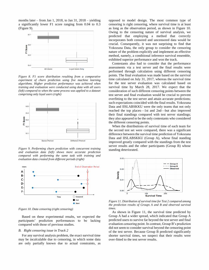
Two experiments were conducted to compare prediction

performance regarding churn of all users and of loyal users

only. For the first experiment, both training and evaluation

sets were created with all user data, whereas for the second

experiment, the training and evaluation sets were created

using only data from loyal users. Each experiment was

trained on data of 3,000 users and was evaluated using a

dataset consisting of 1,400 users’ data.

Five machine learning algorithms, Random Forest,

Logistic Regression, Extra Gradient Boosting (XGB),

Generalized Boosting Model (GBM), and Conditional

Inference Tree, were applied to churn prediction of all users

and loyal users only. When each machine learning algorithm

was trained and evaluated on a dataset with all users, the F1

score ranged approximately from 0.6 to 0.72. When the same

procedure was repeated with a dataset of only loyal users,

the F1 score ranged from 0.39 to 0.53, showing a significant

drop in overall predictive performance (Figure 8).

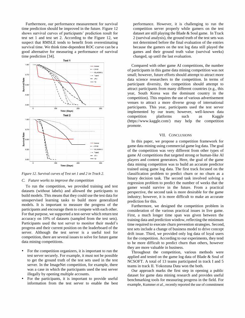
Owing to the emphasis on chronological robustness, we

expected that imposing a time difference between training

and test sets would lower the performance of participants

compared to other churn prediction work, as confirmed by a

comparative experiment of churn prediction of users. The

experiment was conducted using two evaluation sets where

one was created with data from the same period as the

training set and the other of data from periods two months

after. The results revealed much lower performance by

predicting the churn of users from different periods.

Using the same five machine learning algorithms,

prediction models were trained on user data from Nov. 1,

2017, to Nov. 30, 2017. Performance was measured using a

test set containing data of concurrent yet different users,

yielding a mean F1 score of approximately 0.45. The same

models were used to predict the churn of different users two

months later – from Jan 1, 2018, to Jan 31, 2018 – yielding

a significantly lower F1 score ranging from 0.04 to 0.3

(Figure 9).

Figure 8. F1 score distribution resulting from a comparative

experiment of churn prediction using five machine learning

algorithms. Higher predictive performance was achieved when

training and evaluation were conducted using data with all users

(left) compared to when the same process was applied to a dataset

comprising only loyal users (right)

Figure 9. Performing churn prediction with concurrent training

and evaluation data (left) shows more accurate prediction

compared with performing the same task with training and

evaluation data created from different periods (right)

Figure 10. Data censoring (right censoring)

Based on these experimental results, we expected the

participants’ prediction performances to be lacking

compared with those of previous studies.

B. Right censoring issue in Track 2

For any survival analysis problem, the exact survival time

may be incalculable due to censoring, in which some data

are only partially known due to actual constraints, as

opposed to model design. The most common type of

censoring is right censoring, where survival time is at least

as long as the observation period, as shown in Figure 10.

Owing to the censoring nature of survival analysis, we

predicted that employing a method that correctly

incorporates both censored and uncensored data would be

crucial. Consequently, it was not surprising to find that

Yokozuna Data, the only group to consider the censoring

nature of the problem explicitly and implement an effective

method, namely, a conditional inference survival ensemble,

exhibited superior performance and won the track.

Contestants also had to consider that the performance

assessments via a test server and the final results were

performed through calculation using different censoring

points. The final evaluation was made based on the survival

time calculated on July 31, 2017, whereas the survival time

for the test server evaluation was calculated based on

survival time by March 28, 2017. We expect that the

consideration of such different censoring points between the

test server and final evaluation would be crucial to prevent

overfitting to the test server and attain accurate predictions;

such expectations coincided with the final results. Yokozuna

Data and IISLABSKKU were the only teams that not only

reached the top places—1st and 2nd—but also improved

their final standings compared with test server standings;

they also appeared to be the only contestants who considered

the different censoring points.

When the distributions of survival time of each team for

the second test set were compared, there was a significant

difference between the survival time prediction of Yokozuna

Data and IISLABSKKU (Group A), whose final standing

improved greatly compared with the standings from the test

server results and the other participants (Group B) whose

standing deteriorated.

Figure 11. Distribution of survival time for Test 2 compared among

the prediction results of Groups A and B and observed survival

times.

As shown in Figure 11, the survival time predicted by

Group A had a wider spread, which indicated that Group A

predicted users to survive far beyond the test server and final

evaluation censoring point. In contrast, Group B’s prediction

did not seem to consider survival beyond the censoring point

of the test server. Because Group B predicted significantly

shorter survival times, we suspect that their results were

over-fitted to the test server results.

Furthermore, our performance measurement for survival

time prediction should be improved in the future. Figure 12

shows survival curves of participants’ prediction result for

test set 1 and test set 2. According to the Figure 12, we

suspect that RMSLE tends to benefit from overestimating

survival time. We think time-dependent ROC curve can be a

good alternative for measuring a performance of survival

time prediction [34].

Figure 12. Survival curves of Test set 1 and 2 in Track 2.

C. Future works to improve the competition

To run the competition, we provided training and test

datasets (without labels) and allowed the participants to

build models. This means that they could use the test data for

unsupervised learning tasks to build more generalized

models. It is important to measure the progress of the

participants and encourage them to compete with each other.

For that purpose, we supported a test-server which return test

accuracy on 10% of datasets (sampled from the test sets).

Participants used the test server to monitor their model’s

progress and their current position on the leaderboard of the

server. Although the test server is a useful tool for

competition, there are several issues to solve for future game

data mining competitions.

For the competition organizers, it is important to run the

test server securely. For example, it must not be possible

to get the ground truth of the test sets used in the test

server. In the ImageNet competition, for example, there

was a case in which the participants used the test server

illegally by opening multiple accounts.

For the participants, it is important to provide useful

information from the test server to enable the best

performance. However, it is challenging to run the

competition server properly while gamers on the test

dataset are still playing the Blade & Soul game. In Track

2 (survival analysis), the ground truth of the test sets was

not determined before the final evaluation of the entries

because the gamers on the test log data still played the

games and their ground truth value (survival weeks)

changed, up until the last evaluation.

Compared with other game AI competitions, the number

of participants in this game data mining competition was not

small; however, future efforts should attempt to attract more

data science researchers to the competition. In terms of

participant diversity, the competition should attempt to

attract participants from many different countries (e.g., this

year, South Korea was the dominant country in the

competition). This requires the use of various advertisement

venues to attract a more diverse group of international

participants. This year, participants used the test server

implemented by our team; however, well-known data

competition platforms such as Kaggle

(https://www.kaggle.com/) may help the competition

promote.

VII. CONCLUSIONS

In this paper, we propose a competition framework for

game data mining using commercial game log data. The goal

of the competition was very different from other types of

game AI competitions that targeted strong or human-like AI

players and content generators. Here, the goal of the game

data mining competition was to build an accurate predictor

trained using game log data. The first track focused on the

classification problem to predict churn or no churn as a

binary decision task. The second task involved solving a

regression problem to predict the number of weeks that the

gamer would survive in the future. From a practical

perspective, the second task is more desirable for the game

industry; however, it is more difficult to make an accurate

prediction for this.

Furthermore, we designed the competition problem in

consideration of the various practical issues in live game.

First, a much longer time span was given between the

training data and prediction window, reflecting the minimum

time required to execute churn prevention strategies. Second,

test sets include a change of business model to drive concept

drift issue. Third, we provided only log data of loyal users

for the competition. According to our experiments, they tend

to be more difficult to predict churn than others, however

they are more valuable in business.

Throughout the competition, various methods were

applied and tested on the game log data of Blade & Soul of

NCSOFT. A total of 13 teams participated in track I and 5

teams in track II. Yokozuna Data won the both.

Our approach marks the first step in opening a public

dataset for game data mining research and provides useful

benchmarking tools for measuring progress in the field. For

example, Kummer et al., recently reported the use of commitment

features using the benchmarking dataset [35]. Although we

limited the competition’s goal to predict players’ churning

behavior and number of surviving weeks, another purpose of

our game data mining competition is to promote the research

of game data mining by providing commercial game logs to

the public.

ACKNOWLEDGEMENTS

We’d like to express great thanks to the all contributors. All the data used

in this competition is freely available through GDMC 2017 homepage (https://cilab.sejong.ac.kr/gdmc2017/) and google groups (https://groups.

google.com/d/forum/gdmc2017). This research is partially supported by

Basic Science Research Program through the National Research Foundation of Korea(NRF) funded by the Ministry of Science, ICT & Future Planning

(2017R1A2B4002164). This research is partially supported by Ministry of

Culture, Sports and Tourism (MCST) and Korea Creative Content

Agency(KOCCA) in the Culture Technology(CT) Research & Development Program 2017. This work is partially supported by the

European Commission under grant agreement number 731900 -

ENVISAGE. Supplementary material file is available from https:// arxiv.org/abs/1802.02301

REFERENCES

[1] K.-J. Kim, and S.-B. Cho, “Game AI competitions: An open platform

for computational intelligence education,” IEEE Computational Intelligence Magazine, August 2013.

[2] J. Togelius, “How to run a successful game-based AI competition,”

IEEE Transactions on Computational Intelligence and AI in Games, vol. 8, no. 1, pp. 95-100, 2016.

[3] P. Hingston, “A Turing test for computer game bots,” IEEE

Transactions on Computational Intelligence and AI in Games, Sep 2009.

[4] D. Perez et al., “The general game playing competition,” IEEE

Transactions on Computational Intelligence and Games, 2015. [5] N. Shaker et al., “The 2010 Mario AI championship: Level generation

track,” IEEE Transactions on Computational Intelligence and Games,

vol. 3, no. 4, pp. 332-347, 2011.

[6] M. S. El-Nasr, A. Drachen, and A. Canossa, Game Analytics:

Maximizing the Value of Player Data, Springer, 2013.

[7] J.-Lee, S.-W. Kang, and H.-K. Kim, “Hard-core user and bot user classification using game character’s growth types,” 2015

International Workshop on Network and Systems for Games

(NetGames), 2015. [8] E.-J. Lee, J.-Y. Woo, H.-S. Kim, and H.-K. Kim, “No silk road for

online gamers!: Using social network analysis to unveil black markets

in online gamers,” Proceedings of the 2018 World Wide Web Conference, pp. 1825-1834, 2018.

[9] S. Chun, D. Choi, J. Han, H. K. Kim, and T.K. Kwon, “Unveiling a

socio-economic system in a virtual world: A case study of an MMORPG,” Proceedings of the 2018 World Wide Web Conference,

pp. 1929-1938, 2018.

[10] J. Runge, P. Gao, F. Garcin, and B. Faltings, “Churn prediction for high-value players in casual social games,” IEEE Conference on

Computational Intelligence and Games, 2014.

[11] A. Perianez, A. Saas, A. Guitart, and C. Magne, “Churn prediction in mobile social games: Towards a complete assessment using survival

ensembles,” IEEE International Conference on Data Science and

Advanced Analytics (DSAA), 2016. [12] S. Kim, D. Choi, E. Lee, and W. Rhee, “Churn prediction of mobile

and online casual games using play log data,” PLOS One, vol. 12, no.

7, 2017. [13] R. Bartle, “Hearts, clubs, diamonds, spades: Players who suit MUDs,”

Journal of MUD research, vol. 1, no. 1, p. 19, 1996.

[14] R. Bartle, “A self of sense,” Available on April, vol. 9, p. 2005, 2003. [15] N. Yee, “The Gamer Motivation Profile: What We Learned From

250,000 Gamers,” in Proceedings of the 2016 Annual Symposium on

Computer-Human Interaction in Play, New York, NY, USA, 2016, pp. 2-2.

[16] Artificial and Computational Intelligence in Games, Artificial and

Computational Intelligence in Games: a follow-up to Dagsthul Seminar 12191. Red Hook, NY: Curran Associates, Inc, 2015.

[17] S. S. Farooq and K.-J. Kim, “Game Player Modeling,” in Encyclopedia

of Computer Graphics and Games, N. Lee, Ed. Springer International Publishing, 2015, pp. 1-5.

[18] A. Drachen, A. Canossa, and G. N. Yannakakis, “Player modeling

using self-organization in Tomb Raider: Underworld,” in 2009 IEEE Symposium on Computational Intelligence and Games, 2009, pp. 1-8.

[19] J. M. Bindewald, G. L. Peterson, and M. E. Miller, “Clustering-Based

Online Player Modeling,” in Computer Games, Springer, Cham, 2016, pp. 86-100.

[20] M. S. El-Nasr, A. Drachen, and A. Canossa, Game Analytics:

Maximizing the Value of Player Data. Springer Publishing Company, Incorporated, 2013.

[21] J. Han, J. Pei, and M. Kamber, Data Mining: Concepts and Techniques.

Elsevier, 2011. [22] U. M. Fayyad, G. Piatetsky-Shapiro, P. Smyth, and R. Uthurusamy,

Advances in knowledge discovery and data mining, vol. 21. AAAI

press Menlo Park, 1996. [23] Lee, Eunjo, et al. “You are a game bot!: uncovering game bots in

MMORPGs via self-similarity in the wild.” Proc. Netw. Distrib. Syst.

Secur. Symp.(NDSS). 2016. [24] Mozer, Michael C., et al. “Predicting subscriber dissatisfaction and

improving retention in the wireless

telecommunications industry.” IEEE Transactions on neural networks, vol. 11, no. 3, pp. 690-696, 2000.

[25] Tsymbal, Alexey. “The problem of concept drift: definitions and related work.” Computer Science Department, Trinity College Dublin

106.2, 2004.

[26] Tamassia, Marco & Raffe, William & Sifa, Rafet & Drachen, Anders & Zambetta, Fabio & Hitchens, Michael. (2016). Predicting Player

Churn in Destiny: A Hidden Markov Models Approach to Predicting

Player Departure in a Major Online Game. 10.1109/CIG.2016.7860431.

[27] Á . Periáñez, A. Saas, A. Guitart and C. Magne, "Churn Prediction in

Mobile Social Games: Towards a Complete Assessment Using Survival Ensembles," 2016 IEEE International Conference on Data

Science and Advanced Analytics (DSAA), Montreal, QC, 2016, pp.

564-573. doi: 10.1109/DSAA.2016.84

[28] P. Bertens, A. Guitart and Á . Periáñez, "Games and big data: A

scalable multi-dimensional churn prediction model," 2017 IEEE

Conference on Computational Intelligence and Games (CIG), New York, NY, 2017, pp. 33-36. doi: 10.1109/CIG.2017.8080412

[29] G. E. Hinton, N. Srivastava, A. Krizhevsky, I. Sutskever, and R. R.

Salakhutdinov, “Improving neural networks by preventing co-adaptation of feature detectors,” arXiv preprint arXiv:1207.0580,

2012.

[30] Hadiji, F., Sifa, R., Drachen, A., Thurau, C., Kersting, K., and Bauckhage, C., “Predicting player churn in the wild,” In 2014 IEEE

Conference on Computational Intelligence and Games, pp. 1–8, 2014.

[31] Sifa, R., Hadiji, F., Runge, J., Drachen, A., Kersting, K., and Bauckhage, C., “Predicting purchase decisions in mobile freeto-play

games,” In AIIDE, 2015.

[32] Z. Wang, and T. Oates, “Encoding time series as images for visual inspection and classification using tiled convolutional neural

networks,” Workshops at the Twenty-Ninth AAAI Conference on

Artificial Intelligence, 2015. [33] Szegedy, C., Vanhoucke, V., Ioffe, S., Shlens, J., and Wojna, Z.,

“Rethinking the inception architecture for computer vision,”

In Proceedings of the IEEE conference on computer vision and pattern recognition, pp. 2818-2826, 2016.

[34] Heagerty, P.J., Lumley, T., and Pepe, M. S., “Time-dependent ROC

curves for censored survival data and a diagnostic marker,” Biometrics, vol. 56, no. 2, pp. 337-344, 2000.

[35] Luiz Bernardo Martins Kummer, Júlio César Nievola and Emerson

Paraiso. “Applying Commitment to Churn and Remaining Players Lifetime Prediction,” IEEE Conference on Computational

Intelligence and Games, 2018.

Supplementary Material

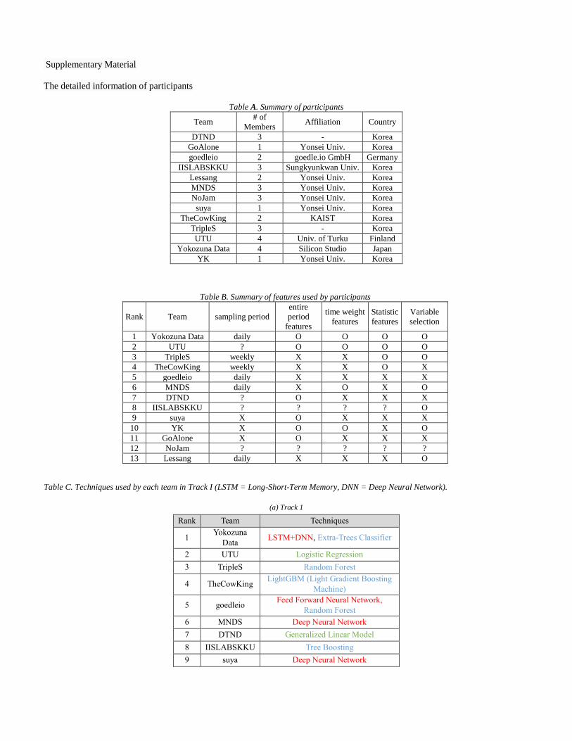
The detailed information of participants

Table A. Summary of participants

Team # of

Members Affiliation Country

DTND 3 - Korea

GoAlone 1 Yonsei Univ. Korea

goedleio 2 goedle.io GmbH Germany

IISLABSKKU 3 Sungkyunkwan Univ. Korea

Lessang 2 Yonsei Univ. Korea

MNDS 3 Yonsei Univ. Korea

NoJam 3 Yonsei Univ. Korea

suya 1 Yonsei Univ. Korea

TheCowKing 2 KAIST Korea

TripleS 3 - Korea

UTU 4 Univ. of Turku Finland

Yokozuna Data 4 Silicon Studio Japan

YK 1 Yonsei Univ. Korea

Table C. Techniques used by each team in Track I (LSTM = Long-Short-Term Memory, DNN = Deep Neural Network).

(a) Track 1

Rank Team Techniques

1 Yokozuna

Data LSTM+DNN, Extra-Trees Classifier

2 UTU Logistic Regression

3 TripleS Random Forest

4 TheCowKing LightGBM (Light Gradient Boosting

Machine)

5 goedleio Feed Forward Neural Network,

Random Forest

6 MNDS Deep Neural Network

7 DTND Generalized Linear Model

8 IISLABSKKU Tree Boosting

9 suya Deep Neural Network

Table B. Summary of features used by participants

Rank Team sampling period

entire

period

features

time weight

features

Statistic

features

Variable

selection

1 Yokozuna Data daily O O O O

2 UTU ? O O O O

3 TripleS weekly X X O O

4 TheCowKing weekly X X O X

5 goedleio daily X X X X

6 MNDS daily X O X O

7 DTND ? O X X X

8 IISLABSKKU ? ? ? ? O

9 suya X O X X X

10 YK X O O X O

11 GoAlone X O X X X

12 NoJam ? ? ? ? ?

13 Lessang daily X X X O

> REPLACE THIS LINE WITH YOUR PAPER IDENTIFICATION NUMBER (DOUBLE-CLICK HERE TO EDIT) <

14

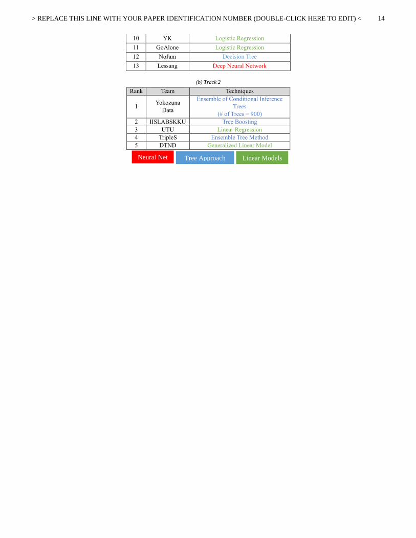
10 YK Logistic Regression

11 GoAlone Logistic Regression

12 NoJam Decision Tree

13 Lessang Deep Neural Network

(b) Track 2

Rank Team Techniques

1 Yokozuna

Data

Ensemble of Conditional Inference

Trees

(# of Trees = 900)

2 IISLABSKKU Tree Boosting

3 UTU Linear Regression

4 TripleS Ensemble Tree Method

5 DTND Generalized Linear Model

Linear Models Neural Net Tree Approach

> REPLACE THIS LINE WITH YOUR PAPER IDENTIFICATION NUMBER (DOUBLE-CLICK HERE TO EDIT) <

15

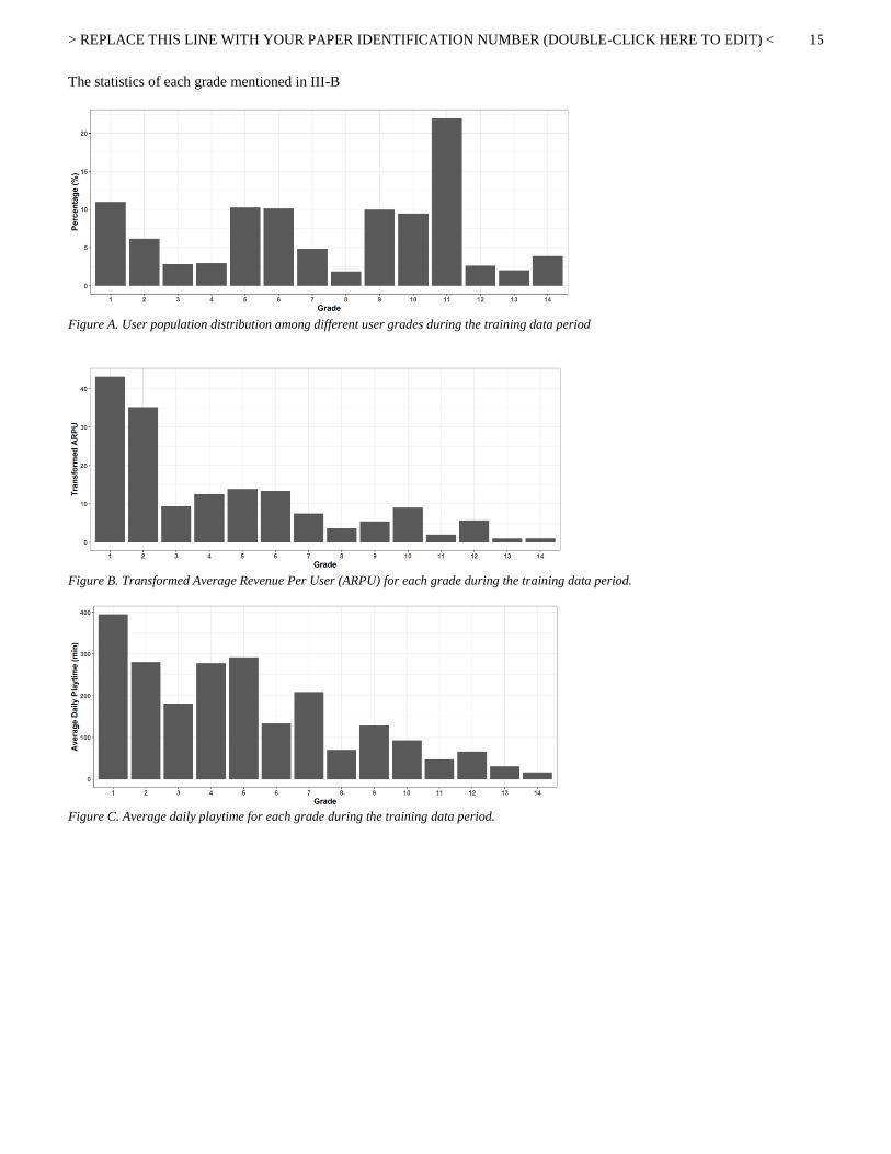
The statistics of each grade mentioned in III-B

Figure A. User population distribution among different user grades during the training data period

Figure B. Transformed Average Revenue Per User (ARPU) for each grade during the training data period.

Figure C. Average daily playtime for each grade during the training data period.

> REPLACE THIS LINE WITH YOUR PAPER IDENTIFICATION NUMBER (DOUBLE-CLICK HERE TO EDIT) <

16

The detailed materials of Yokozuna Data

Table D. The summary of features which are used by Yokozuna Data

Type Feature Description

Daily Action Number of times each action was performed per day. Some actions

were grouped, and then their counts were summed up. For example,

every time a player created, joined, or invited other players to a guild

was counted as a “Guild” feature.

Session Number of sessions per day. The session was considered to be over

once the player had been inactive for more than 15 minutes.

Playtime Total playtime (summing all sessions) per day.

Level Daily last level and number of level-ups per day.

Target level Daily highest battle-target level. If the player did not engage in any

battle on a certain day, the target level of that day was set to the value

of the previous day.

Number of actors Number of actors played per day.

In-game money Total amount of money earned and spent per day.

Equipment Daily equipment score. The higher this score, the better the

equipment owned by the player. If there was no equipment score

logged on a certain day, the equipment score of that day was set to

the value of the previous day.

Overall Statistics Statistics, such as the mean, standard deviation, and sum of all the

time-series features. For example, the total amount of money the

player got during the data period or the standard deviation of the daily

highest battle-target level.

Relation beween the first and last days Differences in the behavior of a player between the first and last days

in the data period were calculated to measure changes over time. For

example, the difference between the total number of level-ups in the

first three days and the last three days.

Actors information Number of actors usually played.

Loyalty index Percentage of days in which the player was connected between their

first and last connection.

Guilds Total number of guilds joined.

Information of days of weeks Distribution of actions over different days of weeks.

> REPLACE THIS LINE WITH YOUR PAPER IDENTIFICATION NUMBER (DOUBLE-CLICK HERE TO EDIT) <

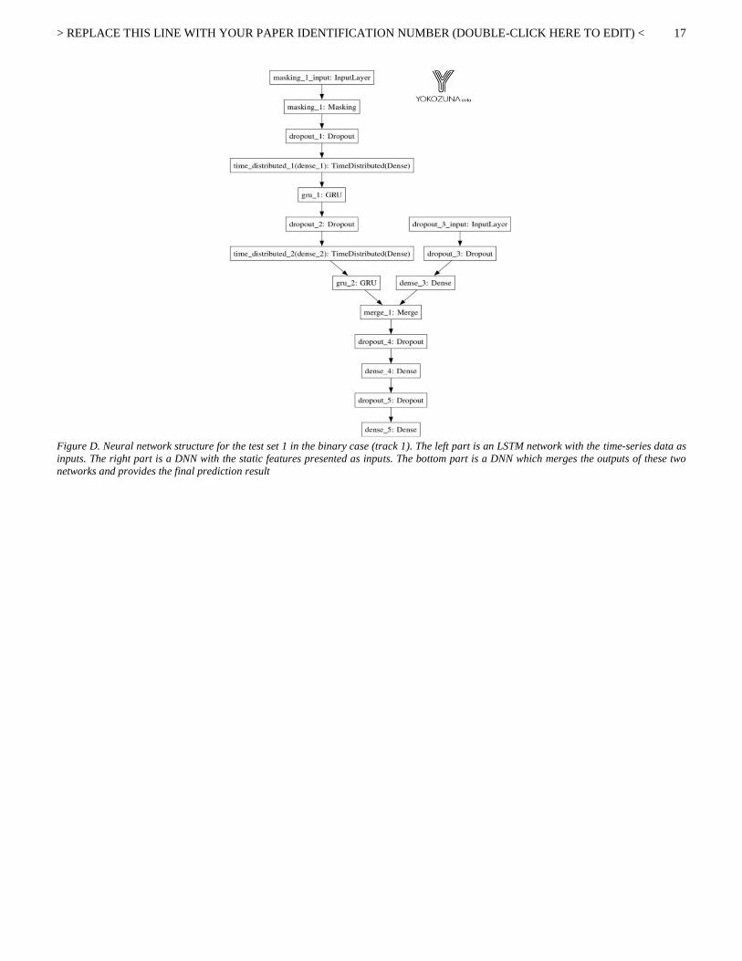
17

Figure D. Neural network structure for the test set 1 in the binary case (track 1). The left part is an LSTM network with the time-series data as

inputs. The right part is a DNN with the static features presented as inputs. The bottom part is a DNN which merges the outputs of these two

networks and provides the final prediction result

> REPLACE THIS LINE WITH YOUR PAPER IDENTIFICATION NUMBER (DOUBLE-CLICK HERE TO EDIT) <

18

The detailed materials of geodle.io

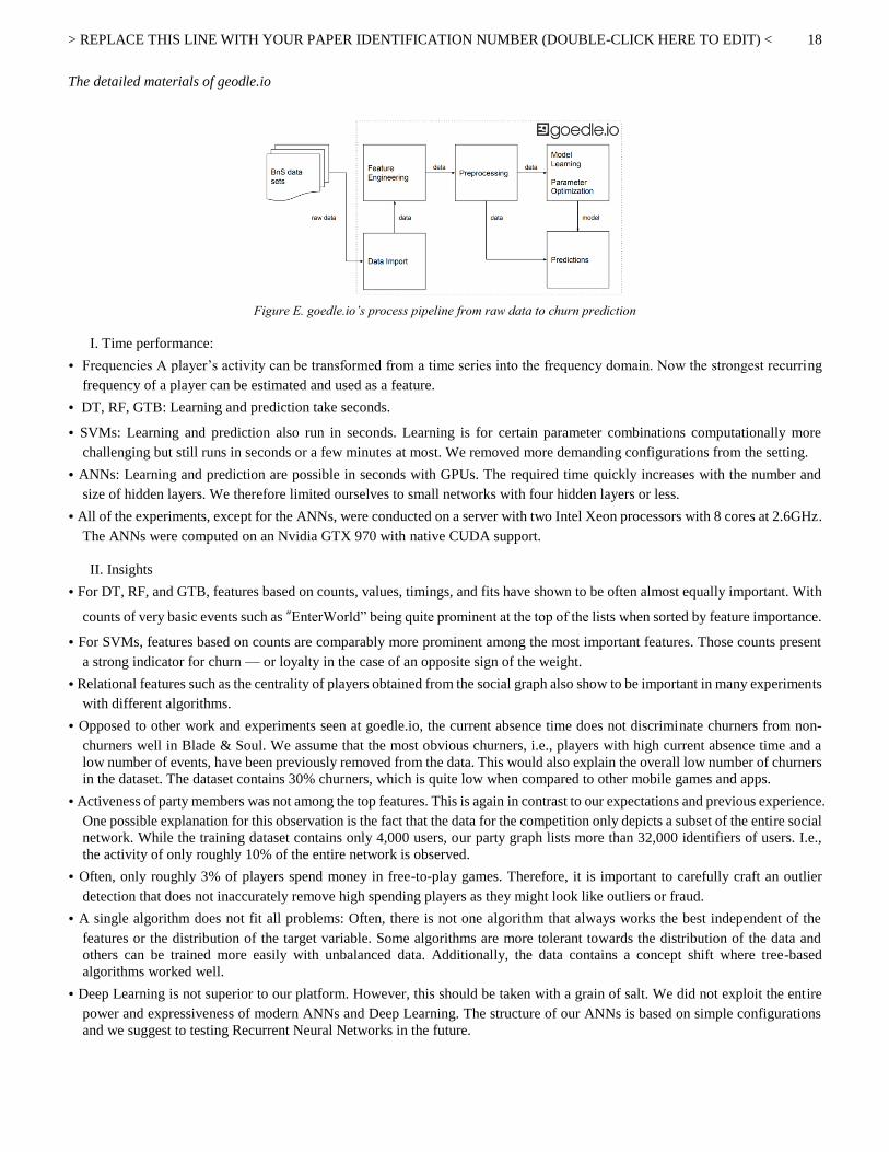
Figure E. goedle.io’s process pipeline from raw data to churn prediction

I. Time performance:

• Frequencies A player’s activity can be transformed from a time series into the frequency domain. Now the strongest recurring

frequency of a player can be estimated and used as a feature.

• DT, RF, GTB: Learning and prediction take seconds.

• SVMs: Learning and prediction also run in seconds. Learning is for certain parameter combinations computationally more

challenging but still runs in seconds or a few minutes at most. We removed more demanding configurations from the setting.

• ANNs: Learning and prediction are possible in seconds with GPUs. The required time quickly increases with the number and

size of hidden layers. We therefore limited ourselves to small networks with four hidden layers or less.

• All of the experiments, except for the ANNs, were conducted on a server with two Intel Xeon processors with 8 cores at 2.6GHz.

The ANNs were computed on an Nvidia GTX 970 with native CUDA support.

II. Insights

• For DT, RF, and GTB, features based on counts, values, timings, and fits have shown to be often almost equally important. With

counts of very basic events such as “EnterWorld” being quite prominent at the top of the lists when sorted by feature importance.

• For SVMs, features based on counts are comparably more prominent among the most important features. Those counts present

a strong indicator for churn — or loyalty in the case of an opposite sign of the weight.

• Relational features such as the centrality of players obtained from the social graph also show to be important in many experiments

with different algorithms.

• Opposed to other work and experiments seen at goedle.io, the current absence time does not discriminate churners from non-

churners well in Blade & Soul. We assume that the most obvious churners, i.e., players with high current absence time and a

low number of events, have been previously removed from the data. This would also explain the overall low number of churners

in the dataset. The dataset contains 30% churners, which is quite low when compared to other mobile games and apps.

• Activeness of party members was not among the top features. This is again in contrast to our expectations and previous experience.

One possible explanation for this observation is the fact that the data for the competition only depicts a subset of the entire social

network. While the training dataset contains only 4,000 users, our party graph lists more than 32,000 identifiers of users. I.e.,

the activity of only roughly 10% of the entire network is observed.

• Often, only roughly 3% of players spend money in free-to-play games. Therefore, it is important to carefully craft an outlier

detection that does not inaccurately remove high spending players as they might look like outliers or fraud.

• A single algorithm does not fit all problems: Often, there is not one algorithm that always works the best independent of the

features or the distribution of the target variable. Some algorithms are more tolerant towards the distribution of the data and

others can be trained more easily with unbalanced data. Additionally, the data contains a concept shift where tree-based

algorithms worked well.

• Deep Learning is not superior to our platform. However, this should be taken with a grain of salt. We did not exploit the entire

power and expressiveness of modern ANNs and Deep Learning. The structure of our ANNs is based on simple configurations

and we suggest to testing Recurrent Neural Networks in the future.

> REPLACE THIS LINE WITH YOUR PAPER IDENTIFICATION NUMBER (DOUBLE-CLICK HERE TO EDIT) <

19

The detailed materials of MNDS

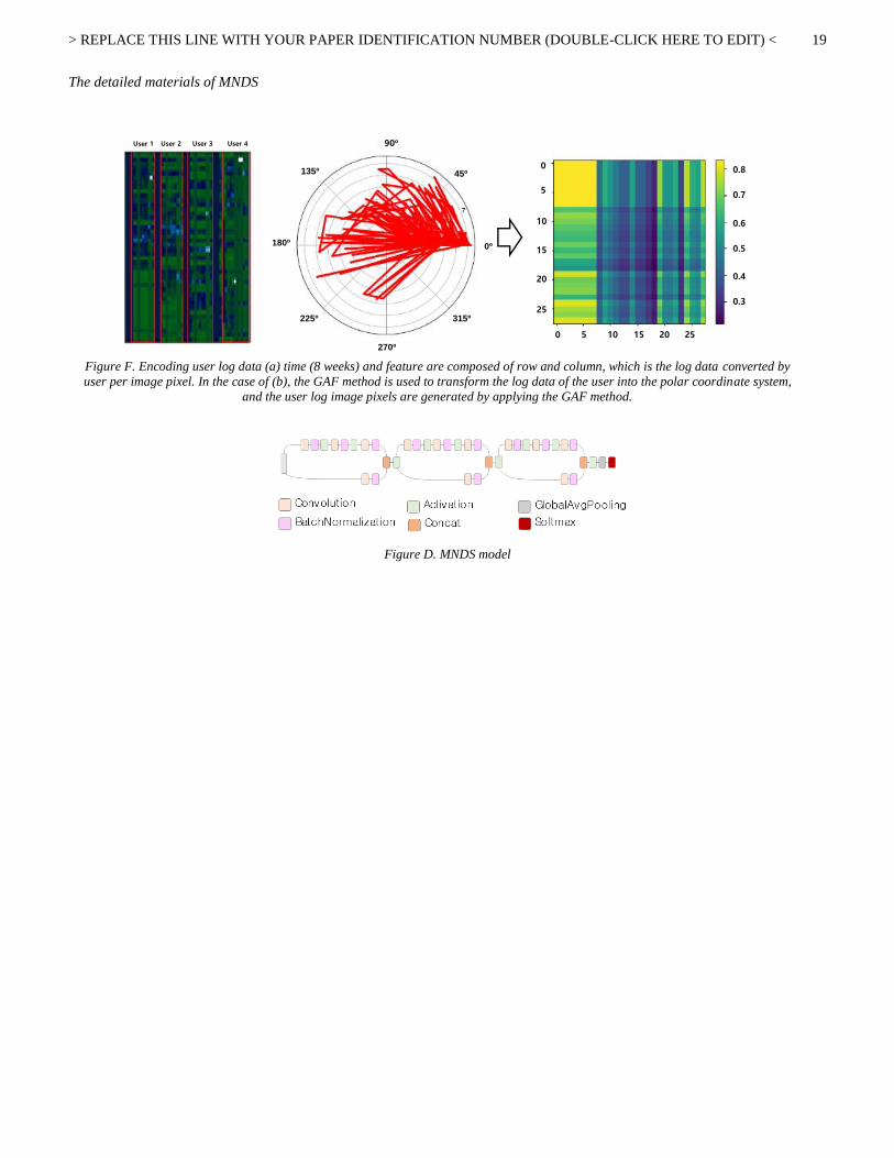
Figure D. MNDS model

Figure F. Encoding user log data (a) time (8 weeks) and feature are composed of row and column, which is the log data converted by

user per image pixel. In the case of (b), the GAF method is used to transform the log data of the user into the polar coordinate system,

and the user log image pixels are generated by applying the GAF method.

0

5

10

15

20

25

0 5 10 15 20 25

0.8

0.7

0.6

0.5

0.4

0.3

90º

45º

0º

315º

270º

225º

180º

135º

User 1 User 2 User 3 User 4