Egyptian Informatics Journal (2012) 13, 9–17

Cairo University

Egyptian Informatics Journal

www.elsevier.com/locate/eijwww.sciencedirect.com

ORIGINAL ARTICLE

GA for straight-line grid drawings of maximal

planar graphs

Mohamed A. El-Sayed *

Mathematics department, Faculty of Science, Fayoum University, Fayoum, EgyptCollege of Computers and Information Technology, Taif University, Taif, Saudi Arabia

Received 13 August 2011; revised 24 November 2011; accepted 8 January 2012Available online 15 February 2012

*

Sc

In

E-

11

U

re

Pe

In

do

KEYWORDS

Genetic algorithms;

Graph drawing;

Maximal planar graphs

Corresponding author at: M

ience, Fayoum University,

formation Technology, Taif

mail addresses: mas06@fayo

10-8665 � 2012 Faculty o

niversity. Production and

served.

er review under responsib

formation, Cairo University.

i:10.1016/j.eij.2012.01.003

Production and h

athema

Egypt;

Universit

um.edu.e

f Compu

hosting

ility of

osting by E

Abstract A straight-line grid drawing of a planar graph G of n vertices is a drawing of G on an

integer grid such that each vertex is drawn as a grid point and each edge is drawn as a straight-line

segment without edge crossings. Finding algorithms for straight-line grid drawings of maximal pla-

nar graphs (MPGs) in the minimum area is still an elusive goal. In this paper we explore the poten-

tial use of genetic algorithms to this problem and various implementation aspects related to it. Here

we introduce a genetic algorithm, which nicely draws MPG of moderate size. This new algorithm

draws these graphs in a rectangular grid with area b2ðn� 1Þ=3c � b2ðn� 1Þ=3c at least, and that this

is optimal area (proved mathematically). Also, the novel issue in the proposed method is the fitness

evaluation method, which is less costly than a standard fitness evaluation procedure. It is described,

tested on several MPG.� 2012 Faculty of Computers and Information, Cairo University.

Production and hosting by Elsevier B.V. All rights reserved.

tical Department, Faculty of

College of Computers and

y, Taif, Saudi Arabia.

g, m.sayed@tu.edu.sa

ters and Information, Cairo

by Elsevier B.V. All rights

Faculty of Computers and

lsevier

1. Introduction

Graph drawing problem can be found in many areas of com-puter sciences, such as in the computer networks, data net-works, information visualization, maps [1–5], class inter-

relationship diagrams in object oriented databases and objectoriented programs, visual programming interfaces, databasedesign systems, project management, visual languages and

web sites [6–8]. Graph drawing addresses the problem of find-ing a layout of a graph that satisfies given esthetic and under-standability objectives. The most important objective in graph

drawing is minimization of the number of crossings in thedrawing, as the esthetics and readability of graph drawings de-pend on the number of edge crossings. VLSI layouts with few-er crossings are more easily realizable and consequently

cheaper [9–11].

10 M.A. El-Sayed

Graph drawing – also known as network visualization –

deals with all aspects of representing relational structures.The automatic generation of graph drawings is of relevancenot only in computer science, but in virtually every area con-cerned with graphical data analysis or visual communication

of information. Research field of graph drawing encompassesdesign and analysis of algorithms and algorithm engineering,as well as modeling aspects, topics from graph theory and

combinatorics, and the development of software tools [12].In what follows we assume that the reader is familiar withthe basics of graph drawing as given e.g. in [13]. It is suitable

for use in advanced undergraduate and graduate level courseson algorithms, graph theory, graph drawing, information visu-alization and computational geometry.

Esthetics plays a fundamental role, their optimization aimsat facilitating both readability and memorization of the infor-mation contained in the graphs. Frequently adopted estheticcriteria include: minimization of the drawing area, minimiza-

tion of the edge crossing number, minimization of the sumof the arc lengths, etc. However, recent experiments have con-firmed that the minimization of edge crossing is by far the most

important criterion [14,15].Many algorithms for graph visualization have been pro-

posed, and an extensive survey was done by Di Battista, Eades

and Tamassia. Heuristic approaches were introduced to gra-phic drawing in earlier researches [16,17], and of which, geneticalgorithm (GA) show its excellent flexibility to complex con-strains. GA can be a viable alternative to more traditional ap-

proaches for graph drawing, but at the same time encountersserious performance issues, which made it hard to be appliedto large scale applications [18,19].

GA in [20–22] has been described for solving many prob-lems of graph, for example, graph partitioning problem, andthe page number problem. Evolutionary computation tech-

niques especially GAs based on planar graph have been suc-cessfully applied to multiple sequence alignment problem[23–26].

A maximal plane graph is one, which cannot have any addi-tional edges without destroying its planarity. Such a graph isalso called triangulated since all the faces are triangles. Sinceevery planar graph can be triangulated by adding additional

(dummy) edges. A straight-line embedding of a plane graphG is a plane embedding of G in which edges are representedby straight-line segments joining their vertices without any

edge-intersection [27]. An example of a planar straight-linedrawing is illustrated in Fig. 1.

1

5

2

3

4

Figure 1 A planar straight-line drawing.

This problem was solved by Chrobak and Payne [28] who

proved that, for n P 3, each n-vertex planar graph could bedrawn on the (2n � 4) · (n � 2) grid. They also presented anlinear time algorithm for constructing such embedding. Then,it is shown that every plane graph with n P 3 vertices has a

planar straight-line drawing in a rectangular grid with area(n � 2) · (n � 2) by two methods. Schnyder’s realizer [29,30],‘‘realizer concept’’, for plane triangulation was invented for

compact straight-line drawing of plane graph. Researchers[28,31–36] also obtained similar and other graph drawing re-sults using ‘‘the canonical ordering concept’’. Each method is

a constructive proof and yields a simple linear-time algorithmto find such a drawing. Nakano [37] attempted to explain thehidden relation between these two concepts.

The following question ‘‘what is an algorithm for the min-imum area of the rectangular grid for planar straight-linedrawings’’ remains open up to now. Thus there still exists agap between upper and lower bounds for the area of the rect-

angular grid.This paper introduces a GA which nicely draws planar

graphs in a rectangular grid with area at least

b2ðn� 1Þ=3c � b2ðn� 1Þ=3c. Our algorithm has been inspiredby the ideas from Refs. [8,38–40].

The remainder of the paper is organized as follows. In Sec-

tion 2, presents the principles of GA, then it is introduce theproblem representation and the genetic operators we used. InSection 3, the representations of chromosomes are explained.The selection and the evaluation function are investigated,

the genetic operations are explained in Section 4. The param-eters of our algorithm, the results are given in Section 5. Final-ly, conclusions are in Section 6.

2. Genetic algorithms

GAs are a class of randomized optimization heuristics basedloosely on the biological paradigm of natural selection. Whilethe exact mechanisms behind natural evolution are not very

well known, some aspects have been studied in considerabledepth. The general principle underlying GAs is that of main-taining a population of possible solutions, which are often

called chromosomes. It is believed that chromosomes are theinformation carriers and that the evolution process works atthe chromosome level through reproduction. The reproductioncan be made by either combining chromosomes from the par-

ents to produce offspring, a process called crossover, or by arandom change occurring in the chromosome pattern, termedmutation.

Population size is the number of chromosomes used to rep-resent a set of solutions to the problem. In our problem a pop-ulation is a set of graph layouts. The population undergoes an

evolutionary process that imitates the natural biological evolu-tion. In each generation better chromosomes have greater pos-sibilities to reproduce, while worse chromosomes have greater

possibilities to die and to be replaced by new individuals.A GA first creates an initial population of solutions. The

solutions are then evaluated, using an application-specific cri-teria of fitness, to characterize them from most fit to least fit. A

subset of the population is selected, using criteria that tend tofavor the most fit solutions. This subset is then used to producea new generation of offspring solutions. Finally, a number of

solutions in this new generation are subjected to random muta-

GA for straight-line grid drawings of maximal planar graphs

tions. The processes of selection, crossover and mutation are

then repeated. A drawback of GAs is that the optima of theseproblems are generally unknown and it is therefore difficult toassess their performance. Another drawback is that GAs needa simple fitness function with a reasonably fast evaluation to

distinguish between ‘‘good’’ and ‘‘bad’’ chromosomes, but thisis often not possible. GAs are usually slow, especially becausethe fitness function evaluation takes a long time.

In graph drawing the evaluation function depends on theesthetic criteria used, our evaluation function is discussed ingreater detail in the next section.

A genetic algorithm must have the following five basiccomponents:

1. A genetic representation of solutions to the problem.2. A way to create an initial population of solutions.3. An evaluation function rating solutions in terms of their

fitness.

4. Genetic operators that alter the genetic composition of chil-dren fitness.

5. Values for the parameters of genetic algorithms.

The general structure of a GA [see Fig. 2] is as follows:

procedure GA{t: = 0;create the initial population P0;evaluate the initial population;while not Termination-condition do{t: = t+ 1;select individuals to be reproduced;perform crossover and mutation operations to create the

new population Pt;

evaluate (Pt)}

}

Data

Best solution

found so far Initialization

Evaluate chromosomes

Select chromosomes

Crossover chromosomes

Mutate chromosomes

Initial population

Evaluated population

Candidate next generation

Candidate next generation

next

generation

Figure 2 procedure GA and it architecture.

There are several parameters to be fixed. First, we have to

decide how to represent the set of possible solutions. In ‘‘pure’’genetic algorithms only bit string representations were al-lowed, but we allow any representation that makes efficient

computation possible. Second, we have to choose an initialpopulation. We use initial populations created by randomselection. Third, we have to design the genetic operations,

which alter the composition of children during reproduction.The two basic genetic operations are the mutation operationand the crossover operation. Mutation is an unary operation,

which increases the variability of the population by makingpoint wise changes in the representation of the individuals.Crossover combines the features of two parents to form twonew individuals by swapping corresponding segments of par-

ent’s representations. It turns out that the main problem in ge-netic graph drawing algorithms is to find efficient crossoveroperations.

3. Representations of chromosomes

Our algorithm draws planar graphs in a rectangular grid witharea L · L. Each node is located in a Cartesian point of thegrid and all edges are drawn as straight lines. Chrobak and

Nakano [41] obtained mathematically L ¼ b2ðn� 1Þ=3c inthe following theorem:

Theorem 1. For each n P 3 there is an n-vertex plane graph Gn

such that the width and height of each grid drawing of Gn is at

least b2ðn� 1Þ=3c.

Proof [41]. It is sufficient to consider the width only. We con-struct Hn recursively. H3 is the triangle (m1, m2, m3) and forn P 4, Hn is obtained by adding vertex mn to the outer face

of Hn�1, and connecting it to mn�3, mn�2, mn�1, in such a waythat the outer face of Hn is (mn, mn�1, mn�2).

First, notice that for n= 3, 4, and 5,Hn requires width 1, 2,2 respectively, which equals b2ðn� 1Þ=3c. The theorem followsby induction, since adding mn+1, mn+2 and, mn+3 to Hn forces

us to use at least two more x-coordinates, see Fig. 3. h

11

vnvn+1

vn+2

vn-2 vn-3

vn-1

Hn-1

Hn+2

Figure 3 The construction of graph Hn from Theorem 1.

Nodes matrix, n=5 Edges matrix, m=9 v1 v2 v3 v4 v5 e1 e2 e3 e4 e5 e6 e7 e8 e9

x 0 5 3 3 4 1 1 1 1 2 2 2 3 4

y 2 0 2 3 5 2 3 4 5 3 4 5 4 5

Figure 4 The representation of a sample maximal planar graph

in Fig. 1.

2-tneraP1-tneraP

2-dlihC1-dlihC

Figure 6 A sample of Crossover1 operation.

12 M.A. El-Sayed

To represent a graph with n nodes and m= 3(n � 2) edges,

we use a 2 · n matrix to indicate the positions of the nodes anda 2 · m matrix to indicate the edges by storing pairs of nodes.The corresponding end points are then found from the nodematrix. Fig. 4, shows the representation used of a sample

example, Fig. 1. Groves et al. [42] have used similar represen-tation for nodes.

Representing a solution of planar graph drawing problem

into a chromosome is a key issue when using genetic algo-rithms. Chromosomes are the strings or arrays of genes (a geneis the smallest building block of the solution). A chromosome

can be represented by a string of integers with length n, where nis the number of nodes in planar graph, a gene, gi is representthe position (x,y) of mi in grid, and the genes have different val-

ues in the chromosome. See Fig. 5.We select optional face in G, say (m1–m2–mn) to represent the

outer face of output layout graph in the grid. Hence, m1, m2 andmn be the nodes to form a largest triangulated face. See Fig. 5.

Take P(m1) = (0,0), P(m2) = (L, 0) and P(mn) = (|L/2|,L). Agene, gi of the chromosome, 3 6 i 6 n � 1, is represent a gridpoint P(mi) e D, where D is a set of Cartesian points, p1,

p2, . . .,pk, are lies inside the triangle (0,0)-(L, 0)-(|L/2|, L).The domain D can be generated using the following simple

code:

k = 0;

for y= 1 to L � 1

{ if L even then c= |y/2| + 1

else c= |(y – 1)/2| + 1;

for x = c to L � |y/2| � 1

{ k= k+ 1; pk = (x,y);};

};

D= {(1,1), (2,1), (3,1),. . . (L �3,1), (L �2,1), (L �1,1),(2,2), (3,2), (4,2), . . . (L �2,3)(2,3), (3,3), (4,3), . . . (L �2,3)(3,4), . . . (L �3,4)(3,5), . . . (L �3,4). . .

(|L/2|, L �2)(|L/2|, L �1)}.

4. Genetic operations

Here we describe the following operations: selection process,fitness function, crossover and mutation operations in ouralgorithm. The selection process directs the genetic algorithm

v1 v2 v3 . . . vn-1 vn

g1 g2 g3 . . . gn-1 gn

Figure 5 The representation of chrom

towards promising regions in the search space. One of the

selection method is used the linear normalization suggestedby Davis [32] together with elitism. The linear normalizationworks as follows. The chromosomes are sorted in decreasing

order by their evaluation function values. The best chromo-some gets a certain constant value (e.g. 100) and the otherchromosomes get stepwise decreasing constant values (e.g.

98, 96, 94, etc.). Chromosomes are then selected to the geneticoperations proportionally to the values so obtained. In ourproblem instead of using stepwise decreasing constant ourselection depends on the number of crossing and coincide

edges, i.e. the chromosome which has a small number will bein the top. This method can be parameterized to give a desiredemphasis to the best chromosomes. It uses elitist selection, i.e.

the best chromosome is always chosen as such to the nextgeneration.

The esthetic criteria used are imported to genetic graph

drawing algorithms in the form of the evaluation function(also called the fitness function). The algorithm tries to mini-mize the number of edge crossings, to distribute the nodes

1 2

n

g1=(0,0) g2=(L,0)

gn=(|L/2|,L)

gi ∈D3 ≤ i ≤ n-1

osome, and domain of the genes.

2-tneraP1-tneraP

2-dlihC1-dlihC

Figure 7 A sample of Crossover2 operation.

Figure 8 Chart of vertices n with m, NCCE and average

performance over time t.

Table 1 Test problems.

Graph No. n m NCCE GN t Area

1 6 12 4 1 0.04 3 · 3

2 7 15 11 9 0.064 4 · 4

3 9 21 23 78 0.357 5 · 5

4 10 24 29 301 0.987 6 · 6

5 12 30 56 547 2.402 7 · 7

6 13 33 69 620 3.381 8 · 8

7 14 36 92 1034 7.524 8 · 8

8 15 39 108 1133 9.142 9 · 9

9 19 51 198 1684 28.706 12 · 12

10 20 54 223 1890 32.231 12 · 12

Figure 9 Graph No. 1, a random chromosome and a solution

chromosome, respectively.

Figure 10 Graph No. 2, a random chromosome and a solution

chromosome, respectively

Figure 11 Graph No. 3, a random chromosome and a solution

chromosome, respectively.

GA for straight-line grid drawings of maximal planar graphs 13

evenly over the drawing area. Fitness function based on twowell-known measurable esthetic criteria for graphs:

1. Minimize graph area. This is a calculation of area of the

bounding rectangle of the nodes in the graph on grid.

Figure 12 Graph No. 4, a random chromosome and a solution

chromosome, respectively.

14 M.A. El-Sayed

2. Minimize edge crossings. The number of edge crossings isminimized to zero in the drawing grid.

Input MPG with the edges:

E = { (1,2),(1,3),(1,4),(1,5),(1,8),(1,12),(2,3),(2,9),

(2,12), (3,4),(3,7),(3,9),(3,10),(4,5),(4,6),(4,7),(5,6),

(5,7), (5,8),(6,7),(7,8),(7,10),(7,12),(8,12),(9,10),

(9,11), (9,12),(10,11), (10,12),(11,12) }

(a) a random chromosome.

Figure 13 Graph No. 5, a random chromosome wit

Input MPG with the edges:E= { (1,2),(1,3),(1,4),(1,5),(1,8),(1,13),(2,3),(2,9),(2,13),(3,4),(3,7),(3,9),(3,10),(4,5),(4,6),(4,7),(5,6),(5,7),(5,8),(6,7),(7,8),(7,10),(7,12),(7,13),(8,13),(9,10),(9,11),(9,13),(10,11),(10,12),(11,12),(11,13),(12,13) }

(a) a random chromosome.

Figure 14 Graph No. 6, a random chromosome wit

GAs are usually slow, especially because the fitness function

evaluation takes a long time. The algorithm spends most of itscomputation time in evaluating the chromosomes. One of theproblematic issues is the counting of the number of edge cross-

ings. There is a well-known method based on cross produc-tions to check whether two line segments intersect [[43], pp.889–90]. More advanced methods are introduced by Bentleyand Ottmann [44] and Chazelle and Edelsbrunner [45]. In or-

der to reduce the run time of the execution our GA, we haveused a method of our own for counting the number of edgecrossing. We keep track of the movements of the nodes, and

update the number of edge crossings only when a node ismoved. This method outperforms the Bentley and Ottman’salgorithm in the present situation.

The crossover operation transforms two chromosomes intotwo new chromosomes. The algorithm has two types of cross-over operations. Crossover1 works as follows. First it ran-

domly chooses an integer number or more, 3 6 i 6 n � 1and, say gi is gene of the parent chromosome Parent-1, anda gene g�i of the parent chromosome Parent-2. The parent

(b) a solution chromosome of G

h 12 vertices and the esthetically optimized result.

(b) a solution chromosome of G

h 13 vertices and the esthetically optimized result.

Input MPG with the edges:E= { (1,2),(1,3), (1,4),(1,5),(1,8),(1,14), (2,3), (2,9),(2,13),(2,14),(3,4),(3,7),(3,9),(3,10),(4,5),(4,6),(4,7),(5,6),(5,7),(5,8),(6,7),(7,8),(7,10),(7,12),(7,13),(8,13),(8,14),(9,10),(9,11),(9,13),(10,11),(10,12),(11,12),(11,13),(12,13), (13,14) }

(a) a random chromosome. (b) a solution chromosome of G

Figure 15 An initial MPG of Graph No. 7, with 14 vertices and the esthetically optimized result.

Input MPG with the edges:E= { (1,2),(1,3),(1,4),(1,6),(1,9),(1,10),(1,11),(1,15),(2,5),(2,4),(2,7),(2,8),(2,9),(2,10),(2,12),(2,15),(3,4),(3,6),(4,5),(4,6),(4,7),(5,7),(6,7),(6,8),(6,9),(7,8),(8,9),(9,10),(10,12),(10,14),(10,13),(10,11),(11,13),(11,15),(12,14),(12,15),(13,14),(13,15),(14,15) }

(a) a random chromosome. (b) a solution chromosome of G

Figure 16 An initial MPG of Graph No. 8, with 15 vertices and the esthetically optimized result.

GA for straight-line grid drawings of maximal planar graphs 15

chromosomes exchange the genes gi and g�i to produce new off-spring, Child-1 and Child-2. The rest of the genes are kept un-changed, if possible. i.e. In Crossover1, an exchange happensin each gene position with a certain probability. For example

if Parent-1: g1, g2, . . .,gi, . . .,gj, . . .,gn and Parent-2: g�i ,g�2, . . .,g�i , . . .,g�j , . . .,g�n, then the new offspring after Crossover1at positions i and j are Child-1: g1, g2, . . .,g�i , . . .,g�j , . . .,gn andChild-2: g�1, g

�2, . . .,gi, . . .,gj, . . .,g�n.

The sample Crossover1 operation of Fig. 6 uses rectanglesof size 6 · 6, with n= 10. Since genes g5 = (2,2), and

g9 = (1,1) of Parent-1, g5 = (4,1), and g9 = (3,5) of Parent-2. The parents change the genes 5 and 9 (from Parent-1) andgenes 5 and 9 (from Parent-2). then genes g5 = (2,2), andg9 = (1,1) of Child-2. Similarly, the genes g5 = (4,1), and

g9 = (3,5), of Child-1. Clear that, the Child-1 is represent asolution of our case problem and good chromosome.

The other crossover operation in the algorithm is called

Crossover2. It works as follows. First it randomly chooses atwo integers i, j e {3,4, . . .,n � 1} and, say gi and gj are genesof the parent chromosome Parent-1. Similarly of two genes g�iand g�j of the parent chromosome Parent-2. Genes gi and gj inParent-1 are exchange with g�j and g�i in Parent-2, respectively,

to produce new offspring, Child-1: g1, g2, . . .,g�j , . . .,g�i , . . .,gnand Child-2: g�1, g

�2, . . .,gj, . . .,gi, . . .,g�n. The rest of the genes

are kept unchanged, if possible.The sample Crossover2 operation of Fig. 7 uses rectangles

of size 6 · 6, with n = 10. Since genes g5 = (3,2), andg7 = (3,1) of Parent-1, g5 = (3,2), and g7 = (4,2) of Parent-2. The parents change the genes 5 and 7 (from Parent-1) and

genes 5 and 7 (from Parent-2). Then genes g5 = (4,2), andg7 = (3,2) of Child-1. Similarly, the genes g5 = (3,1), andg7 = (3,2), of Child-2. Here, the Child-2 is represent a solution

of our case problem and good chromosome.Groves et al. [42] introduced about a dozen different muta-

tion operations. We have used two different mutations per-formed best in our tests. First, single mutation, choose a

random node and move it to a random empty position. Sec-ond, inversion mutation, the order of the genes is inverted be-tween two random nodes.

5. Parameters and results

Thesizeof thegrid:what is theoptimal sizeof thedrawingareaforourtest graphs? The optimum size was b2ðn� 1Þ=3c � b2ðn� 1Þ=3c of

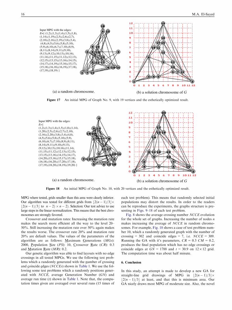
Input MPG with the edges:E={ (1,2),(1,3),(1,4),(1,5),(1,8),(1,14), (1,20),(2,5),(2,6),(2,7),(2,10),(2,16),(2,20),(3,8),(3,4),(4,8),(4,5),(5,6),(5,8),(5,10),(5,9),(6,10),(6,7),(7,10),(8,9),(8,11),(8,14),(9,11),(9,10),(9,13),(9,12),(10,13),(10,16),(11,14),(11,15),(11,12),(12,13),(12,15),(13,15),(13,16),(14,15),(14,17),(14,20),(15,16),(15,17),(15,18),(16,18),(16,20),(17,20),(17,18),(17,19),(18,20),(18,19),(19,20) }

(b) a solution chromosome of G(a) a random chromosome.

Figure 18 An initial MPG of Graph No. 10, with 20 vertices and the esthetically optimized result.

Input MPG with the edges:E={ (1,2),(1,3),(1,4),(1,5),(1,8),(1,14),(1,19),(2,5),(2,6),(2,7),(2,10),(2,16),(2,19),(3,8),(3,4),(4,8),(4,5),(5,6),(5,8),(5,10),(5,9),(6,10),(6,7),(7,10),(8,9),(8,11),(8,14),(9,11),(9,10), (9,13),(9,12),(10,13),(10,16),(11,14),(11,15),(11,12),(12,13),(12,15),(13,15),(13,16),(14,15),(14,17),(14,19),(15,16),(15,17),(15,18),(16,18),(16,19),(17,18),(17,19),(18,19) }

(b) a solution chromosome of G(a) a random chromosome.

Figure 17 An initial MPG of Graph No. 9, with 19 vertices and the esthetically optimized result.

16 M.A. El-Sayed

MPGwhere tested, grids smaller than this area were clearly inferior.Our algorithm was tested for different grids from b2ðn� 1Þ=3c�b2ðn� 1Þ=3c to n� 2Þ � n� 2Þ. Selection: Our test advice to uselarge steps in the linear normalization. Thismeans that the best chro-mosomes are strongly favored.

Crossover and mutation rates: Increasing the mutation rate

makes the search more efficient all the way to the level 20–50%. Still increasing the mutation rate over 50% again makesthe results worse. The crossover rate 20% and mutation rate

20% are default values. The values of the parameters of thealgorithm are as follows: Maximum Generations (MGs):2000, Population Size (PS): 10, Crossover Rate (CR): 0.3

and Mutation Rate (MR): 0.2.Our genetic algorithm was able to find layouts with no edge

crossings in all tested MPGs. We use the following test prob-lems which a randomly generated with the number of crossing

and coincide edges (NCCEs) shown in Table 1. We use the fol-lowing some test problems which a randomly positions gener-ated with NCCE, average Generation Number (GN) and

average run time (t) shown in Table 1. Note that, the compu-tation times given are averaged over several runs (15 times of

each test problem). This means that randomly selected initialpopulations may distort the results. In order to the readers

can be reproduce the experiments, the graphs structure is pre-senting in Figs. 9–18 of each test problem.

Fig. 8 shows the average crossing number NCCE evolutionfor the whole set of graphs. Increasing the number of nodes n

makes increasing the average of NCCE in random chromo-somes. For example, Fig. 18 shows a case of test problem num-ber 10, which a randomly generated graph with the number of

crossing = 302 and coincide edges = 7, i.e. NCCE = 309.Running the GA with it’s parameters, CR = 0.3 CM= 0.2,produces the final population which has no edge crossings or

coincide edges at GN = 1788 and t= 30.9 on 12 · 12 grid.The computation time was about half minute.

6. Conclusion

In this study, an attempt is made to develop a new GA forstraight-line grid drawings of MPG in b2ðn� 1Þ=3c�b2ðn� 1Þ=3c at least, and that this is minimum area. OurGA nicely draws most MPG of moderate size. Also, the novel

GA for straight-line grid drawings of maximal planar graphs 17

issue in the proposed method is the fitness evaluation method,

which is less costly than a standard fitness evaluation proce-dure. We make experiments with simple MPG and results al-low us to think that GA technology is a strong candidate tosolve this kind of problems.

References

[1] Eades Peter, Cohen Robert F, Huang Mao Lin. Online animated

graph drawing for web navigation. In: Di Battista G, editor.

Graph drawing ’97. Lecture notes in computer science, vol. 1653.

Rome, Italy: Springer-Verlag; 1998.

[2] Farrugiaa M, Quigley A. Effective temporal graph layout: a

comparative study of animation versus static display methods.

Inform Visual 2011;10(1):47–64.

[3] Gansner E, Hu Y, Kobourov SG. Visualizing graphs and clusters

as maps. IEEE Comput Graphics Appl 2010;30(6):44–66.

[4] Six Janet, Tollis Ioannis. A framework for circular drawings of

networks. In: Proc symp graph drawing GD’99. Lecture notes in

computer science, 1731. Springer-Verlag; 2000. p. 107–16.

[5] Tubaishat M, Madria S. Sensor networks: an overview. IEEE

Potentials 2003;22:20–3.

[6] Didimo W, Liotta G, Romeo Salvatore A. A graph drawing

application to web site traffic analysis. J Graph Algorithms Appl

2011;15(2):229–51.

[7] Williams C, Rasure J, Hansen C. The state of the art of visual

languages for visualization. In: Visualization ‘92, proc., IEEE

computer society press; 1992. p. 202–9.

[8] Radwan Ahmed A, El-Sayed Mohamed A, Omran Nahla F.

Hybrid GA for straight-line drawings of level clustered planar

graphs. Int J Comput Sci Issues (IJCSI) 2011;8(4):229–35, No. 2.

[9] Dornheim Christoph. Planar graphs with topological constraints.

J Graph Algorithms Appl (JGAA) 2002;6(1):27–66.

[10] Fowler J, Juenger M, Kobourov SG, Schulz M. Characterizations

of restricted pairs of planar graphs allowing simultaneous

embedding with fixed edges. Comput Geom: Theory Appl

2011;44(8):385–98.

[11] Harel D. On visual formalisms. CommunACM1988;31(5):514–30.

[12] Kaufmann Michael, Wagner Dorothea. Drawing graphs: methods and

models. Lecture notes in computer science, 2025. Springer-Verlag; 2001.

[13] Nishizeki Takao, Rahman Md Saidur. Planar graph drawing,

world scientific books. Lect Notes Ser Comput 2004;12.

[14] Bridgeman S, Tamassia R. A user study in similarity measures for

graph drawing. J Graph Algorithms Appl 2002;6(3):225–54.

[15] Purchase H. Effective information visualization: a study of graph

drawing aesthetics and algorithms. Interact Comput 2000;13(2).

[16] Di Battista G, Eades P, Tamassia R, Tollis IG. Annotated

bibliography on graph drawing algorithms. Comput Geom

Theory Appl 1994;4:235–82.

[17] Eades P. A heuristic for graph drawing. Congressus Numerantium

1984;42:149.

[18] Vrajitoru D, DeBoni J. Hybrid real-coded mutation for genetic

algorithms applied to graph layouts. In: Proceeding of the genetic

and evolutionary computation conference (GECCO’05 and SIG-

EVO 1), Washington, DC; June 25–29 2005. p. 1563–4.

[19] Vrajitoru D. Hybrid multi-objective optimization genetic algo-

rithms for graph drawing. In: Proc genetic and evolutionary

computation conference (GECCO’07); 2007.

[20] Bui TN, Moon BR. Genetic algorithm and graph partitioning.

IEEE Trans Comput 1996;45(7):841–55.

[21] Kapoor N, Russell M, Stojmenovic I, Zomaya AY. A genetic

algorithm for finding the page number of interconnection

networks. J Parallel Distrib Comput 2002;62:267–83.

[22] Pinaud B, Kuntz P, Lehn R. Dynamic graph drawing with a

hybridized genetic algorithm. Automat Comput Des Manuf

2004;VI:365–75.

[23] Chen WBL, Zhu W, Xiang X. Multiple sequence alignment

algorithm based on a dispersion graph and ant colony algorithm.

J Comput Chem 2009;30:2031–8.

[24] Lee ZJ, Su SF, Chuang CC, Liu KH. Genetic algorithm with ant

colony optimization (GA–ACO) for multiple sequence alignment.

Appl Soft Comput J 2008;8:55–78.

[25] Wallace PM, Blackshields G, Higgins DG. Multiple sequence

alignments. Curr Opin Struct Biol 2005;15:261–6.

[26] Xiang X, Zhang D, Qia J, Fu y. Ant colony with genetic algorithm

based on planar graph for multiple sequence alignment. Inform

Technol J 2010;9(2):274–81.

[27] de Fraysseix H, Pach J, Pollack R. Small sets supporting straight-

line embeddings of planar graphs. In: Twentieth annual ACM

symposium on theory of computing; 1988. p. 426–33.

[28] Chrobak M, Payne T. A liner-time algorithm for drawing a planar

graphs on a grid. Inform Process Lett 1995;54:241–6.

[29] Schynder W. Planar graphs and poset dimension. Order

1989;5:323–43.

[30] Schynder W. Embedding planar graphs on the grid. In: Proceed-

ings of the first annual ACM-SIAM symposium on discrete

algorithms, San Franciso; 1990. p. 138–47.

[31] Chiba N, Yamanouchi T, Nichireki T. Linear algorithms for

convex drawings of planar graphs. In: Bondy JA, R Murty US,

editors. Progress in graph theory. New York: Academic Press;

1984. p. 153–73.

[32] Davis L. A genetic algorithms tutorial. In: Davis L, editor.

Handbook of genetic algorithms. Van Nostrand Reinhold; 1991.

p. 1–101.

[33] He X. A simple linear time algorithm for proper box rectangular

drawings of plane graphs. J Algorithms 2001;40(1):82–101.

[34] Kant G. Drawing planar graphs using the canonical ordering.

Algorithmica 1996;16(1):4–32.

[35] Kant G, He X. Regular edge labeling od 4-connected plane graphs

and its applications in graph drawing problems. Theor Comput

Sci 1997;172(1–2):175–93.

[36] Radwan AAA, El-Sayed MA. New algorithm for drawing planar

straight-line graphs. Int J Appl Math 2003;11(3):265–82.

[37] Nakano S. Planer drawings of plane graphs. IEICE Trans

Fundam 2000;E00-A(3).

[38] Eloranta T, Makinen E. TimGA – a genetic algorithm for drawing

undirected graphs. Report series A-1996-10. University of

Tampere, Department of Computer Science; 1996. <citeseer.nj.

nec.com/eloranta96timga.html>.

[39] Radwan AAA, El-Sayed MA. Using Genetic Algorithm for

Drawing Triangulated Planar Graphs. J Inst Math Comput Sci

(Comp Sci Ser) 2004;15(1):137–47.

[40] Rosete A, Ochoa A. Genetic graph drawing. In: Proceeding of the

13th international conference of applications of artificial intelli-

gence in engineering, Galway; 1998. p. 37–41.

[41] Chrobak M, Nakano S. Minimum-width grid drawings of plane

graphs. Comput Geometry: Theory Appl 1998;10:29–54.

[42] Groves L, Michalewicz Z, Elia P, Janikow C. Genetic algorithms

for drawing directed graphs. In: Proceedings of the fifth interna-

tional symposium on methodologies for intelligent systems.

Elsevier North-Holland; 1990. p. 268–76.

[43] Cormen TH, Leiserson CE, Rivest RL. Introduction to algo-

rithms. The MIT Press; 1990.

[44] Bentley JL, Ottmann TA. Algorithms for reporting and counting

geometric intersections. IEEE Trans Comput 1979;C-28:643–7.

[45] Chazelle B, Edelsbrunner H. An optimal algorithm for intersect-

ing line segments in the plane. J ACM 1992;39(1):1–54.