fx(P) > 0 2 + 2y 2 − 5x − 8y + 4 qy = 3x + 4y
18
◦ • f ◦ f x (P ) > 0 x f x f ◦ f x (P ) < 0 x f x f ◦ f P f x (P )=0 y x f y (P )=0 • f (x, y) (x 0 ,y 0 ) f x (x 0 ,y 0 )=0= f y (x 0 ,y 0 ) f x (x 0 ,y 0 ) f y (x 0 ,y 0 ) ◦ • g(x, y)= x 2 + y 2 +3 ◦ g x =2x g y =2y g x = g y =0 ◦ g x =0 x =0 g y =0 y =0 ◦ (x, y)= (0, 0) • h(x, y)= x 2 − 4x + y 2 +2y ◦ h x =2x − 4 h y =2y +2 h x = h y =0 ◦ h x =0 x =2 h y =0 y = −1 ◦ (x, y)= (2, −1) • q(x, y)= x 2 +3xy +2y 2 − 5x − 8y +4 ◦ q x =2x +3y − 5 q y =3x +4y − 8 q x = q y =0 ◦ 2x +3y − 5=0 3x +4y − 8=0 ◦ 2x +3y − 5=0 y y = (5 − 2x)/3 x/3 − 4/3=0 x =4 y = −1 ◦ (x, y)= (4, −1) • p(x, y)= x 3 + y 3 − 3xy ◦ p x =3x 2 − 3y p y =3y 2 − 3x p x = p y =0
-
Upload
khangminh22 -
Category
Documents
-
view
0 -
download
0
Transcript of fx(P) > 0 2 + 2y 2 − 5x − 8y + 4 qy = 3x + 4y

◦ ���� ��� ����� �� ��� ����� ���������
• �� ����� ���� ���� �� ��������� ����� � �������� f ��� ���� � ������� �� ������� ������
◦ �� fx(P ) > 0� ���� �� ������ �������� �� ��� �������� x���������� ��� ����� �� f ���� ��������� ��� �������� �������� �� ��� �������� x���������� ��� ����� �� f ���� ���������
◦ ���������� �� fx(P ) < 0� ���� �� ������ �������� �� ��� �������� x���������� ��� ����� �� f ���� ������������ �� ������ �������� �� ��� �������� x���������� ��� ����� �� f ���� ���������
◦ ����� f ��� ���� ���� � ����� ������� �� ������� �� P �� fx(P ) = 0� �� ��� ���� ��������� ���� y�� ����� �� x� �� ���� ���� ���� fy(P ) = 0 �� � ����� ������� �� ��������
• ���������� � �������� ����� �� ��� �������� f(x, y) �� � ����� (x0, y0) ���� ���� fx(x0, y0) = 0 = fy(x0, y0)� �������� fx(x0, y0) �� fy(x0, y0) �� ���������
◦ �� ��� ������������ ������ � ����� ������� �� ������� �� � �������� ��� ���� ����� �� � �������� ������
• �������� ���� ��� �������� ������ �� ��� �������� g(x, y) = x2 + y2 + 3�
◦ �� ���� gx = 2x ��� gy = 2y� ����� ���� ������� ����������� ��� ������ ����������� ��� ���� �������������� ���� ����� ���� gx = gy = 0�
◦ �� ��� gx = 0 ��������� ���� x = 0 ��� gy = 0 ��������� ���� y = 0�
◦ ����� ����� �� � ������ �������� ����� (x, y) = (0, 0) �
• �������� ���� ��� �������� ������ �� ��� �������� h(x, y) = x2 − 4x+ y2 + 2y�
◦ �� ���� hx = 2x − 4 ��� hy = 2y + 2� ����� ���� ������� ����������� ��� ������ ����������� ��� ������������ ������ ���� ����� ���� hx = hy = 0�
◦ �� ��� hx = 0 ��������� ���� x = 2 ��� hy = 0 ��������� ���� y = −1�
◦ ����� ����� �� � ������ �������� ����� (x, y) = (2,−1) �
• �������� ���� ��� �������� ������ �� ��� �������� q(x, y) = x2 + 3xy + 2y2 − 5x− 8y + 4�
◦ �� ���� qx = 2x+ 3y − 5 ��� qy = 3x+ 4y − 8� ����� ���� ������� ����������� ��� ������ �������������� ���� �������� ������ ���� ����� ���� qx = qy = 0�
◦ ���� ������ ��� ��������� 2x+ 3y − 5 = 0 ��� 3x+ 4y − 8 = 0�
◦ ������� 2x+ 3y − 5 = 0 ��� ������� ��� y ������ y = (5− 2x)/3� �������� ���� ��� ������ �������� �������������� ���������� ����� x/3− 4/3 = 0� �� ���� x = 4 ��� ���� y = −1�
◦ ���������� ����� �� � ������ �������� ����� (x, y) = (4,−1) �
• �������� ���� ��� �������� ������ �� ��� �������� p(x, y) = x3 + y3 − 3xy�
◦ �� ���� px = 3x2 − 3y ��� py = 3y2 − 3x� ����� ���� ������� ����������� ��� ������ ����������� ������� �������� ������ ���� ����� ���� px = py = 0�
�

EM2 Solved problems 3 c° pHabala 2010
MA2: Solved problems—Functions of more variables: Extrema
1. Find and identify local extrema of f(x, y) = 2x3 + 9xy2 + 15x2 + 27y2.
2. Find and identify local extrema of f(x, y, z) = x3 − 2x2 + y2 + z2 − 2xy + xz − yz + 3z.
3. Find the global extrema of f(x, y) = x2 + 2y2 given the condition
x2 − 2x + 2y2 + 4y = 0.
4. Find the point on the plane given by x + y − z = 1 that is closest to the point P = (0,−3, 2)and calculate their distance. Use Lagrange multipliers.
5. A certain line in 3D is given by the equations
x + y + z = 1, 2x − y + z = 3.
Find the distance between this line and the point P = (1, 2,−1).
6. Find the global extrema of f(x, y) = x2 + 4y2 on the finite region M bounded by the curvesx2 + (y + 1)2 = 4, y = −1 and y = x + 1.
7. Find the global extrema of f(x, y) = x2 + y2 − 6x + 6y on the disk of radius 2, centred atthe origin.
8. The equation y2 + 2xy = 2x − 4x2 defines an implicit function y(x). Find and classify itslocal extrema.
Solutions:
1. First we find stationary points. Partial derivatives:∂f∂x
= 6x2 + 9y2 + 30x, ∂f∂y
= 18xy + 54y.
We have to make them equal to zero. We get the system
2x2 + 3y2 + 10x = 0 xy + 3y = 0.
The second equation looks promising, since we can write it as y(x + 3) = 0. Thus there are twopossibilities:1) y = 0. Then the first equation reads x2 + 5x = 0, which yields x = 0 and x = −5. Thispossibility therefore leads to points (0, 0) and (−5, 0)2) x = −3. Then the first equation reads y2 = 4, which yields y = ±2 and points (−3,±2).Thus we obtain four stationary points: (0, 0), (−5, 0), (−3, 2), and (−3,−2).To classify them we need to find second order partial derivatives and form the Hess matrix:
∂2f∂x2 = 12x + 30, ∂2f
∂x∂y= 18y, ∂2f
∂y2 = 18x + 54
H =
µ
12x + 30 18y
18y 18x + 54
Now the classification.
For (0, 0) we get H =
µ
30 00 54
. Determinants of principal minors (subdeterminants) are
Δ1 = a11 = 30 and Δ2 = det(H) = 30 · 54 = 1620. Their signs are Δ1 > 0, Δ2 > 0, whichshows that the point f(0, 0) = 0 is a local minimum.
For (−5, 0) we get H =
µ
−30 00 −26
. Subdeterminants are Δ1 = −30 and Δ2 = 780. Their
signs are Δ1 < 0, Δ2 > 0, which shows that the point f(−5, 0) = 125 is a local maximum.
For (−3,−2) we get H =
µ
−6 −36−36 0
. Subdeterminants are Δ1 = −6 and Δ2 = −(−36)2.
Their signs are Δ1 < 0, Δ2 < 0, this does not follow pattern for any local extreme. But fromΔ2 < 0 we conclude that the point f(−3, 2) = 81 is a saddle point.
1

◦ ���� ��� ����� �� ��� ����� ���������
• �� ����� ���� ���� �� ��������� ����� � �������� f ��� ���� � ������� �� ������� ������
◦ �� fx(P ) > 0� ���� �� ������ �������� �� ��� �������� x���������� ��� ����� �� f ���� ��������� ��� �������� �������� �� ��� �������� x���������� ��� ����� �� f ���� ���������
◦ ���������� �� fx(P ) < 0� ���� �� ������ �������� �� ��� �������� x���������� ��� ����� �� f ���� ������������ �� ������ �������� �� ��� �������� x���������� ��� ����� �� f ���� ���������
◦ ����� f ��� ���� ���� � ����� ������� �� ������� �� P �� fx(P ) = 0� �� ��� ���� ��������� ���� y�� ����� �� x� �� ���� ���� ���� fy(P ) = 0 �� � ����� ������� �� ��������
• ���������� � �������� ����� �� ��� �������� f(x, y) �� � ����� (x0, y0) ���� ���� fx(x0, y0) = 0 = fy(x0, y0)� �������� fx(x0, y0) �� fy(x0, y0) �� ���������
◦ �� ��� ������������ ������ � ����� ������� �� ������� �� � �������� ��� ���� ����� �� � �������� ������
• �������� ���� ��� �������� ������ �� ��� �������� g(x, y) = x2 + y2 + 3�
◦ �� ���� gx = 2x ��� gy = 2y� ����� ���� ������� ����������� ��� ������ ����������� ��� ���� �������������� ���� ����� ���� gx = gy = 0�
◦ �� ��� gx = 0 ��������� ���� x = 0 ��� gy = 0 ��������� ���� y = 0�
◦ ����� ����� �� � ������ �������� ����� (x, y) = (0, 0) �
• �������� ���� ��� �������� ������ �� ��� �������� h(x, y) = x2 − 4x+ y2 + 2y�
◦ �� ���� hx = 2x − 4 ��� hy = 2y + 2� ����� ���� ������� ����������� ��� ������ ����������� ��� ������������ ������ ���� ����� ���� hx = hy = 0�
◦ �� ��� hx = 0 ��������� ���� x = 2 ��� hy = 0 ��������� ���� y = −1�
◦ ����� ����� �� � ������ �������� ����� (x, y) = (2,−1) �
• �������� ���� ��� �������� ������ �� ��� �������� q(x, y) = x2 + 3xy + 2y2 − 5x− 8y + 4�
◦ �� ���� qx = 2x+ 3y − 5 ��� qy = 3x+ 4y − 8� ����� ���� ������� ����������� ��� ������ �������������� ���� �������� ������ ���� ����� ���� qx = qy = 0�
◦ ���� ������ ��� ��������� 2x+ 3y − 5 = 0 ��� 3x+ 4y − 8 = 0�
◦ ������� 2x+ 3y − 5 = 0 ��� ������� ��� y ������ y = (5− 2x)/3� �������� ���� ��� ������ �������� �������������� ���������� ����� x/3− 4/3 = 0� �� ���� x = 4 ��� ���� y = −1�
◦ ���������� ����� �� � ������ �������� ����� (x, y) = (4,−1) �
• �������� ���� ��� �������� ������ �� ��� �������� p(x, y) = x3 + y3 − 3xy�
◦ �� ���� px = 3x2 − 3y ��� py = 3y2 − 3x� ����� ���� ������� ����������� ��� ������ ����������� ������� �������� ������ ���� ����� ���� px = py = 0�
�

◦ ���� ����� ��� ��� ��������� 3x2 − 3y = 0 ��� 3y2 − 3x = 0� ��� ������������� x2 = y ��� y2 = x�
◦ �������� ��� ���� �������� ���� ��� ������ ������ x4 = x� ����� x4 − x = 0� ��� ��������� ������x(x− 1)(x2 + x+ 1) = 0�
◦ ��� ���� ���� ��������� ��� x = 0 ������ ���� ����� y = x2 = 0� ��� x = 1 ������ ���� ����� y = x2 = 1��
◦ ���������� ����� ��� ��� �������� ������� (0, 0) ��� (1, 1) �
• �������� ���� ��� �������� ������ �� ��� �������� f(x, y) = x ey2−2x2
�
◦ �� ���� fx = ey2−2x2
+xey2−2x2 ·(−4x) = (1−4x2)ey
2−2x2
��� fy = x ey2−2x2 ·(2y) = 2xy ey
2−2x2
� ��������� ������� ����������� ��� ������ ����������� ��� ���� �������� ������ ���� ����� ���� fx = fy = 0�
◦ ����� ������������ ��� ����� ����� �� ��� ���� fx = 0 ���� 1 − 4x2 = 0 �� ���� x = ±1
2� ����� fy = 0
���� 2xy = 0 �� ���� x = 0 �� y = 0� ����� x ������ �� ���� �� ��� ���� �������� ������ x = ±1
2� ��
���� ���� y = 0�
◦ ���������� ����� ��� ��� �������� ������� (1
2, 0) ��� (−1
2, 0) �
����� ����������� �������� ������
• ��� ���� �� ���� � ���� �� �������� ������ �������� ��� ������ ���� � �������� ����� ����������� ���� � ��������� ������� ������ �� ����� ���� �� ���� ������� ����� ������ �������� ��� ������ �� ������ �� f �
• ���������� ��� ������������ ����� ������ ��� �������� �� � �������� ����� �� ��� ����� D = fxx · fyy − (fxy)2�
����� ���� �� ��� ������������ �������� �� ��������� �� ��� �������� ������
◦ ��� ��� �� �������� ��� ��������� �� ��� ������������ �� �� ��� ����������� �� ��� ������ �� ��� ���������������� ��������� D =
����fxx fxyfyx fyy
����� ��� ��� ���������� ����� ��� ���� ���� fxy = fyx��
◦ �������� ��� g(x, y) = x2 + y2 �� ���� gxx = gyy = 2 ��� gxy = 0 �� D = 4 �� ��� �������
◦ �������� ��� h(x, y) = x2 − y2 �� ���� hxx = 2� hyy = −2� ��� hxy = 0 �� D = −4 �� ��� �������
◦ ������� ��� ������ ���� ����� �� ����� �������������� ��� �� ���� �� ��������� D ��� ��� ��������p(x, y) = ax2+ bxy+ cy2� ��� ������ �� D = 4ac− b2� ����� �� −1 ����� ��� �������� b2−4ac� ��� ������������������ ��� ��� ��������� ���������� ax2 + bx + c� ������� ���� ��� ������������ �� ax2 + bx + c���������� ��� ���� ���� ����� ��� ���������� �����
• ������� ������� ����������� ������ ������� P �� � �������� ����� �� f(x, y)� ��� ��� D �� ��� ����� �� ��������������� fxxfyy − f2
xy �� P � �� D > 0 ��� fxx > 0� ���� ��� �������� ����� �� � �������� �� D > 0 ���fxx < 0� ���� ��� �������� ����� �� � �������� �� D < 0� ���� ��� �������� ����� �� � ������ ������ ��� D = 0����� ��� ���� �� ��������������
◦ ����� ���������� ������ ��� ���������� ���� P �� �� ��� ������� ���� ��� ��� ���� ���� ��� ��������
f(x, y) − f(P ) �� ������� ������������ �� ��� ���������� ax2 + bxy + cy2� ����� a =1
2fxx� b = fxy�
��� c =1
2fyy� �� D �= 0� ���� ��� �������� �� f(x, y) ���� ��� �������� ����� P ���� �� ��� ���� �� ����
��������� ����������� ���������� ��� ������ ��� ��������� ������� ��� ��������� ��������� ������������� ��� ���� ����� ��� ������� �� ����� �� ��������� ������ ��� �����
• �� ��� ������� ��� ����� ������� �� ����� � ��������� ��� ������ ��� ����������� ��� �������� ������ �� ��������� f(x, y)�
◦ ���� �� ������� ���� ������� ����������� fx ��� fy�
◦ ���� �� ���� ��� ������ (x, y) ����� ���� ������� ����������� ��� ����� �� ����� ��� ������ ��� �� ��� ������������������ �� ���������
�

Example 4 (f(x, y) = x2 − 2xy + 2y2 + 2x− 6y + 12)
Find all critical points of f(x, y) = x2 − 2xy + 2y2 + 2x− 6y + 12.
Solution. As a preliminary calculation, we find the two first order partial derivatives of
f(x, y).
fx(x, y) = 2x− 2y + 2
fy(x, y) = −2x+ 4y − 6
So the critical points are the solutions of the pair of equations 2x−2y+2 = 0, −2x+4y− 6,
or equivalently (dividing by two and moving the constants to the right hand side)
x− y = −1 (1a)
−x+ 2y = 3 (1b)
One strategy for solving a system of two equations in two unknowns (x and y) like this is to
• First use one of the equations to solve for one of the unkowns in terms of the other
unknown. For example (1a) tells us that y = x+1. This expresses y in terms of x. We
say that we have solved for y in terms of x.
• Then substitute the result, y = x+ 1 in our case, into the other equation, (1b). In our
case, this gives
−x+ 2(x+ 1) = 3 ⇐⇒ x+ 2 = 3 ⇐⇒ x = 1
• We have now found that x = 1, y = x+ 1 = 2 is the only solution. So the only critical
point is (1, 2).
An alternative strategy for solving a system of two equations in two unknowns like (1) is to
• add equations (1a) and (1b) together. This gives
(1a) + (1b) : (1− 1)x+ (−1 + 2)y = −1 + 3 ⇐⇒ y = 2
The point here is that adding equations (1a) and (1b) together eliminates the unknown
x, leaving us with one equation in the unknown y, which is easily solved. For other
systems of equations you might have multiply the equations by some numbers before
adding them together.
• We now know that y = 2. Substituting it into (1a) gives us
x− 2 = −1 =⇒ x = 1
• Once again we have found that the only critical point is (1, 2).
Example 4
c� Joel Feldman. 2014. All rights reserved. 3 January 29, 2014

Example 5 (f(x, y) = 2x3 − 6xy + y2 + 4y)
Find all critical points of f(x, y) = 2x3 − 6xy + y2 + 4y.
Solution. The first order partial derivatives are
fx = 6x2 − 6y fy = −6x+ 2y + 4
So the critical points are the solutions of
6x2 − 6y = 0 − 6x+ 2y + 4 = 0
We can rewrite the first equation as y = x2, which expresses y as a function of x. We can
then substitute y = x2 into the second equation, giving
−6x+ 2y + 4 = 0 ⇐⇒ −6x+ 2x2 + 4 = 0 ⇐⇒ x2 − 3x+ 2 = 0 ⇐⇒ (x− 1)(x− 2) = 0
⇐⇒ x = 1 or 2
When x = 1, y = 12 = 1 and when x = 2, y = 22 = 4. So, there are two critical points:
(1, 1), (2, 4).
Example 5
Example 6 (f(x, y) = xy(5x+ y − 15))
Find all critical points of f(x, y) = xy(5x+ y − 15).
Solution. The first order partial derivatives of f(x, y) = xy(5x+ y − 15) are
fx(x, y) = y(5x+ y − 15) + xy(5) = y(5x+ y − 15) + y(5x) = y(10x+ y − 15)
fy(x, y) = x(5x+ y − 15) + xy(1) = x(5x+ y − 15) + x(y) = x(5x+ 2y − 15)
The critical points are the solutions of fx(x, y) = fy(x, y) = 0 or
y(10x+ y − 15) = 0 and x(5x+ 2y − 15) = 0 (2)
The first equation, y(10x+y−15) = 0, is satisfied if either of the two factors y, (10x+y−15)
is zero. So the first equation is satisfied if either of the two equations
y = 0 (3a)
10x+ y = 15 (3b)
is satisfied. The second equation, x(5x+ 2y− 15) = 0, is satisfied if either of the two factors
x, (5x+ 2y − 15) is zero. So the first equation is satisfied if either of the two equations
x = 0 (4a)
5x+ 2y = 15 (4b)
is satisfied. So both critical point equations (2) are satisfied if one of (3a), (3b) is satisfied
and in addition one of (4a), (4b) is satisfied. There are four possibilities:
c� Joel Feldman. 2014. All rights reserved. 4 January 29, 2014

• (3a) and (4a) are satisfied if and only if x = y = 0
• (3a) and (4b) are satisfied if and only if y = 0, 5x+ 2y = 15 ⇐⇒ y = 0, 3x = 15
• (3b) and (4a) are satisfied if and only if 10x+ y = 15, x = 0 ⇐⇒ y = 15, x = 0
• (3b) and (4b) are satisfied if and only if 10x+ y = 15, 5x+ 2y = 15. We can use, for
example, the second of these equations to solve for x in terms of y: x = 15(15 − 2y).
When we substitute this into the first equation we get 2(15− 2y) + y = 15, which we
can solve for y. This gives −3y = 15− 30 or y = 5 and then x = 15(15− 2× 5) = 1.
In conclusion, the critical points are (0, 0), (3, 0), (0, 15) and (1, 5).
A more compact way to write what we have just done is
fx(x, y) = 0 and fy(x, y) = 0
⇐⇒ y(10x+ y − 15) = 0 and x(5x+ 2y − 15) = 0
⇐⇒�
y = 0 or 10x+ y = 15�
and�
x = 0 or 5x+ 2y = 15�
⇐⇒�
x = y = 0�
or�
y = 0, x = 3�
or�
x = 0, y = 15�
or�
x = 1, y = 5�
Example 6
Example 7
In a certain community, there are two breweries in competition, so that sales of each nega-
tively affect the profits of the other. If brewery A produces x litres of beer per month and
brewery B produces y litres per month, then the profits of the two breweries are given by
P = 2x− 2x2 + y2
106Q = 2y − 4y2 + x2
2× 10⁶
respectively. Find the sum of the two profits if each brewery independently sets its own
production level to maximize its own profit and assumes that its competitor does likewise.
Find the sum of the two profits if the two breweries cooperate so as to maximize that sum.
Solution. If A adjusts x to maximize P (for y held fixed) and B adjusts y to maximize Q
(for x held fixed) then x and y are determined by
Px = 2− 4x106
= 0 =⇒ x = 12106
Qy = 2− 8y2×106
= 0 =⇒ y = 12106
=⇒ P +Q = 2(x+ y)− 1106
�
52x2 + 3y2
�
=⇒ = 106�
1 + 1− 58− 3
4
�
= 58106
On the other hand if (A,B) adjust (x, y) to maximize P + Q = 2(x + y)− 1106
�
52x2 + 3y2
�
,
then x and y are determined by
c� Joel Feldman. 2014. All rights reserved. 5 January 29, 2014

◦ ���� ����� ��� ��� ��������� 3x2 − 3y = 0 ��� 3y2 − 3x = 0� ��� ������������� x2 = y ��� y2 = x�
◦ �������� ��� ���� �������� ���� ��� ������ ������ x4 = x� ����� x4 − x = 0� ��� ��������� ������x(x− 1)(x2 + x+ 1) = 0�
◦ ��� ���� ���� ��������� ��� x = 0 ������ ���� ����� y = x2 = 0� ��� x = 1 ������ ���� ����� y = x2 = 1��
◦ ���������� ����� ��� ��� �������� ������� (0, 0) ��� (1, 1) �
• �������� ���� ��� �������� ������ �� ��� �������� f(x, y) = x ey2−2x2
�
◦ �� ���� fx = ey2−2x2
+xey2−2x2 ·(−4x) = (1−4x2)ey
2−2x2
��� fy = x ey2−2x2 ·(2y) = 2xy ey
2−2x2
� ��������� ������� ����������� ��� ������ ����������� ��� ���� �������� ������ ���� ����� ���� fx = fy = 0�
◦ ����� ������������ ��� ����� ����� �� ��� ���� fx = 0 ���� 1 − 4x2 = 0 �� ���� x = ±1
2� ����� fy = 0
���� 2xy = 0 �� ���� x = 0 �� y = 0� ����� x ������ �� ���� �� ��� ���� �������� ������ x = ±1
2� ��
���� ���� y = 0�
◦ ���������� ����� ��� ��� �������� ������� (1
2, 0) ��� (−1
2, 0) �
����� ����������� �������� ������
• ��� ���� �� ���� � ���� �� �������� ������ �������� ��� ������ ���� � �������� ����� ����������� ���� � ��������� ������� ������ �� ����� ���� �� ���� ������� ����� ������ �������� ��� ������ �� ������ �� f �
• ���������� ��� ������������ ����� ������ ��� �������� �� � �������� ����� �� ��� ����� D = fxx · fyy − (fxy)2�
����� ���� �� ��� ������������ �������� �� ��������� �� ��� �������� ������
◦ ��� ��� �� �������� ��� ��������� �� ��� ������������ �� �� ��� ����������� �� ��� ������ �� ��� ���������������� ��������� D =
����fxx fxyfyx fyy
����� ��� ��� ���������� ����� ��� ���� ���� fxy = fyx��
◦ �������� ��� g(x, y) = x2 + y2 �� ���� gxx = gyy = 2 ��� gxy = 0 �� D = 4 �� ��� �������
◦ �������� ��� h(x, y) = x2 − y2 �� ���� hxx = 2� hyy = −2� ��� hxy = 0 �� D = −4 �� ��� �������
◦ ������� ��� ������ ���� ����� �� ����� �������������� ��� �� ���� �� ��������� D ��� ��� ��������p(x, y) = ax2+ bxy+ cy2� ��� ������ �� D = 4ac− b2� ����� �� −1 ����� ��� �������� b2−4ac� ��� ������������������ ��� ��� ��������� ���������� ax2 + bx + c� ������� ���� ��� ������������ �� ax2 + bx + c���������� ��� ���� ���� ����� ��� ���������� �����
• ������� ������� ����������� ������ ������� P �� � �������� ����� �� f(x, y)� ��� ��� D �� ��� ����� �� ��������������� fxxfyy − f2
xy �� P � �� D > 0 ��� fxx > 0� ���� ��� �������� ����� �� � �������� �� D > 0 ���fxx < 0� ���� ��� �������� ����� �� � �������� �� D < 0� ���� ��� �������� ����� �� � ������ ������ ��� D = 0����� ��� ���� �� ��������������
◦ ����� ���������� ������ ��� ���������� ���� P �� �� ��� ������� ���� ��� ��� ���� ���� ��� ��������
f(x, y) − f(P ) �� ������� ������������ �� ��� ���������� ax2 + bxy + cy2� ����� a =1
2fxx� b = fxy�
��� c =1
2fyy� �� D �= 0� ���� ��� �������� �� f(x, y) ���� ��� �������� ����� P ���� �� ��� ���� �� ����
��������� ����������� ���������� ��� ������ ��� ��������� ������� ��� ��������� ��������� ������������� ��� ���� ����� ��� ������� �� ����� �� ��������� ������ ��� �����
• �� ��� ������� ��� ����� ������� �� ����� � ��������� ��� ������ ��� ����������� ��� �������� ������ �� ��������� f(x, y)�
◦ ���� �� ������� ���� ������� ����������� fx ��� fy�
◦ ���� �� ���� ��� ������ (x, y) ����� ���� ������� ����������� ��� ����� �� ����� ��� ������ ��� �� ��� ������������������ �� ���������
�
EM2 Solved problems 3 c° pHabala 2010
For (−3, 2) we get H =
µ
−6 −36−36 0
. Subdeterminants are Δ1 = −6 and Δ2 = −362. As
above, from Δ2 < 0 we conclude that the point f(−3,−2) = 81 is a saddle point.
Some people prefer a different approach that might be simpler if the derivatives are not too bad,it is also somewhat more organized.First we evaluate those subdeterminants in general, we obtain Δ1 = 12x + 30 andΔ2 = (12x+30)(18x+54)−(18y)2 = 36(6x2+23x+45−9y2). Then we substitute the stationarypoints and reach conclusions:
point: (0, 0) (−5, 0) (−3, 2) (−3,−2)
Δ1: + − − −Δ2: + + − −conclusion: loc. min. loc. max. saddle saddle
Then one has to write the answer: f(0, 0) = 0 is a local minimum, f(−5, 0) = 125 is a localmaximum, f(−3, 2) = f(−3,−2) = 81 are saddle points.
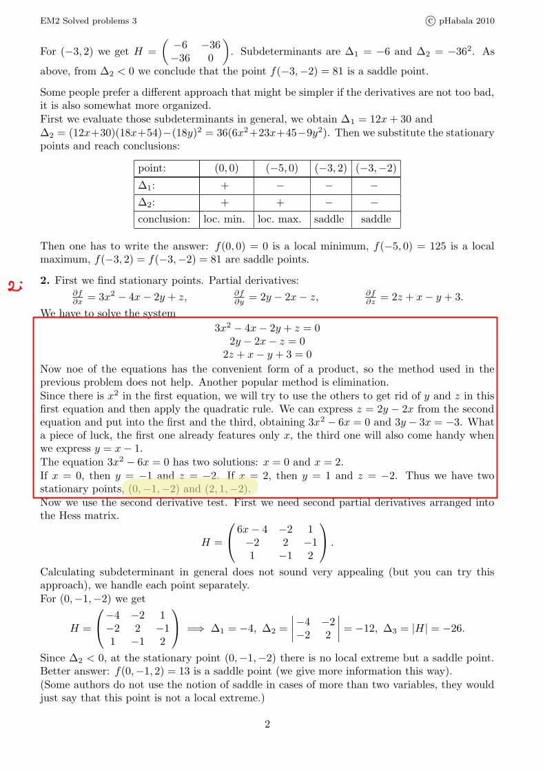
2. First we find stationary points. Partial derivatives:∂f∂x
= 3x2 − 4x − 2y + z, ∂f∂y
= 2y − 2x − z, ∂f∂z
= 2z + x − y + 3.
We have to solve the system
3x2 − 4x − 2y + z = 02y − 2x − z = 0
2z + x − y + 3 = 0
Now noe of the equations has the convenient form of a product, so the method used in theprevious problem does not help. Another popular method is elimination.Since there is x2 in the first equation, we will try to use the others to get rid of y and z in thisfirst equation and then apply the quadratic rule. We can express z = 2y − 2x from the secondequation and put into the first and the third, obtaining 3x2 − 6x = 0 and 3y − 3x = −3. Whata piece of luck, the first one already features only x, the third one will also come handy whenwe express y = x − 1.The equation 3x2 − 6x = 0 has two solutions: x = 0 and x = 2.If x = 0, then y = −1 and z = −2. If x = 2, then y = 1 and z = −2. Thus we have twostationary points, (0,−1,−2) and (2, 1,−2).Now we use the second derivative test. First we need second partial derivatives arranged intothe Hess matrix.
H =
6x − 4 −2 1−2 2 −11 −1 2
.
Calculating subdeterminant in general does not sound very appealing (but you can try thisapproach), we handle each point separately.For (0,−1,−2) we get
H =
−4 −2 1−2 2 −11 −1 2
=⇒ Δ1 = −4, Δ2 =
¯
¯
¯
¯
−4 −2−2 2
¯
¯
¯
¯
= −12, Δ3 = |H| = −26.
Since Δ2 < 0, at the stationary point (0,−1,−2) there is no local extreme but a saddle point.Better answer: f(0,−1, 2) = 13 is a saddle point (we give more information this way).(Some authors do not use the notion of saddle in cases of more than two variables, they wouldjust say that this point is not a local extreme.)
2
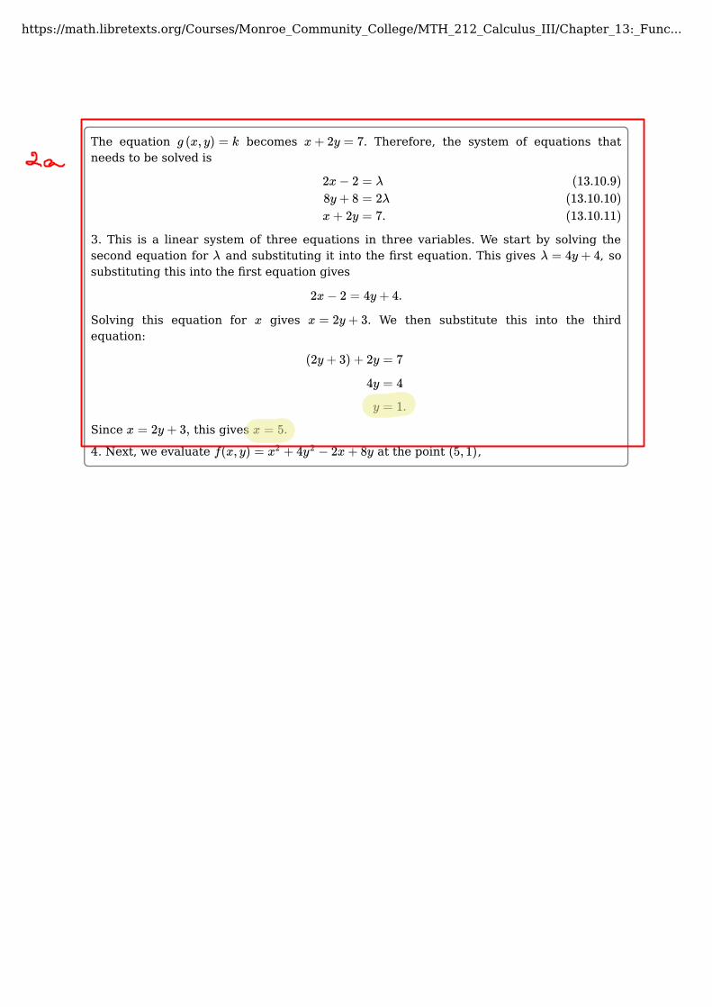
The equation becomes . Therefore, the system of equations thatneeds to be solved is
3. This is a linear system of three equations in three variables. We start by solving thesecond equation for and substituting it into the first equation. This gives , sosubstituting this into the first equation gives
Solving this equation for gives . We then substitute this into the thirdequation:
Since this gives
4. Next, we evaluate at the point ,
g (x, y) = k x + 2y = 7
2x − 28y + 8x + 2y
= λ
= 2λ
= 7.
(13.10.9)(13.10.10)(13.10.11)
λ λ = 4y + 4
2x − 2 = 4y + 4.
x x = 2y + 3
(2y + 3) + 2y
4y
y
= 7
= 4
= 1.
x = 2y + 3, x = 5.
f(x, y) = + 4 − 2x + 8yx2 y2 (5, 1)
https://math.libretexts.org/Courses/Monroe_Community_College/MTH_212_Calculus_III/Chapter_13:_Func...

for the maximum value of , subject to this constraint.2. So, we calculate the gradients of both and :
The equation becomes
which can be rewritten as
We then set the coefficients of and equal to each other:
The equation becomes . Therefore, the system of equations thatneeds to be solved is
3. We use the left-hand side of the second equation to replace in the first equation:
Then we substitute this into the third equation:
Since this gives
f
f g
f(x, y)∇⇀
g(x, y)∇⇀
= (48 − 2x − 2y) + (96 − 2x − 18y)i j
= 5 + .i j
f(x, y) = λ g(x, y)∇⇀
∇⇀
(48 − 2x − 2y) + (96 − 2x − 18y) = λ(5 + ),i j i j
(48 − 2x − 2y) + (96 − 2x − 18y) = λ5 + λ .i j i j
i j
48 − 2x − 2y
96 − 2x − 18y
= 5λ
= λ.
g(x, y) = k 5x + y = 54
48 − 2x − 2y
96 − 2x − 18y
5x + y
= 5λ
= λ
= 54.
λ
48 − 2x − 2y
48 − 2x − 2y
8x
x
= 5(96 − 2x − 18y)
= 480 − 10x − 90y
= 432 − 88y
= 54 − 11y.
5(54 − 11y) + y
270 − 55y + y
216
y
= 54
= 54
= 54y
= 4.
x = 54 − 11y, x = 10.
https://math.libretexts.org/Courses/Monroe_Community_College/MTH_212_Calculus_III/Chapter_13:_Func...

Calculus III 37
© 2018 Paul Dawkins http://tutorial.math.lamar.edu
Let’s choose 1x y= = . No reason for these values other than they are “easy” to work with. Plugging
these into the constraint gives,
31
1 32 2 312
z z z z+ + = → = → =
So, this is a set of dimensions that satisfy the constraint and the volume for this set of dimensions is,
31 31
1,1, 15.5 34.83762 2
V f = = = <
So, the new dimensions give a smaller volume and so our solution above is, in fact, the dimensions that will give a maximum volume of the box are 3.266x y z= = =
Notice that we never actually found values for λ in the above example. This is fairly standard for these
kinds of problems. The value of λ isn’t really important to determining if the point is a maximum or a minimum so often we will not bother with finding a value for it. On occasion we will need its value to help solve the system, but even in those cases we won’t use it past finding the point.
Example 2 Find the maximum and minimum of ( ), 5 3f x y x y= − subject to the constraint
2 2 136x y+ = .
Solution This one is going to be a little easier than the previous one since it only has two variables. Also, note
that it’s clear from the constraint that region of possible solutions lies on a disk of radius 136 which
is a closed and bounded region, 136 , 136x y− ≤ ≤ , and hence by the Extreme Value Theorem
we know that a minimum and maximum value must exist. Here is the system that we need to solve.
2 2
5 2
3 2
136
x
y
x y
λλ
=− =
+ =
Notice that, as with the last example, we can’t have 0λ = since that would not satisfy the first two
equations. So, since we know that 0λ ≠ we can solve the first two equations for x and y respectively. This gives,
5 3
2 2x y
λ λ= = −
Plugging these into the constraint gives,

Calculus III 38
© 2018 Paul Dawkins http://tutorial.math.lamar.edu
2 2 2
25 9 17136
4 4 2λ λ λ+ = =
We can solve this for λ .
2 1 1
16 4λ λ= ⇒ = ±
Now, that we know λ we can find the points that will be potential maximums and/or minimums.
If 1
4λ = − we get,
10 6x y= − =
and if 1
4λ = we get,
10 6x y= = − To determine if we have maximums or minimums we just need to plug these into the function. Also recall from the discussion at the start of this solution that we know these will be the minimum and maximums because the Extreme Value Theorem tells us that minimums and maximums will exist for this problem. Here are the minimum and maximum values of the function.
( ) ( )( ) ( )
10,6 68 Minimum at 10,6
10, 6 68 Maximum at 10, 6
f
f
− = − −
− = −
In the first two examples we’ve excluded 0λ = either for physical reasons or because it wouldn’t solve one or more of the equations. Do not always expect this to happen. Sometimes we will be able to
automatically exclude a value of λ and sometimes we won’t. Let’s take a look at another example.
Example 3 Find the maximum and minimum values of ( ), ,f x y z xyz= subject to the constraint
1x y z+ + = . Assume that , , 0x y z ≥ .
Solution First note that our constraint is a sum of three positive or zero number and it must be 1. Therefore, it is clear that our solution will fall in the range 0 , , 1x y z≤ ≤ and so the solution must lie in a closed
and bounded region and so by the Extreme Value Theorem we know that a minimum and maximum value must exist. Here is the system of equation that we need to solve.
yz λ= (10) xz λ= (11) xy λ= (12)

EM2 Solved problems 3 c° pHabala 2010
By the way, comparing values at the three points we can guess that f¡
23
√5, 1
3
¢
= 83 is a local
minimum of f with respect to the arc we investigate here.2b) The next part to explore is the oblique segment given by y = x + 1, −2 ≤ x ≤ 0. It hastwo endpoints, (0, 1) we already listed and the other is f(−2,−1) = 8, another candidate forextrema on M .To see what happens in the middle of this curve we can again use Lagrange multipliers, thistime applied to g(x, y) = y − x = 1:
2x = −λ
8y = λ
y − x = 1
=⇒ 4y = −x
y − x = 1
¾
=⇒ 5y = 1 =⇒ y = 15 ,
then x = − 45 . We have another candidate, f
¡
− 45 , 1
5
¢
= 45 (which seems to be a local minimum
of f with respect to that oblique line).Since the condition is so simple, one might be tempted to simply substitute the expressiony = x + 1 into f , obtaining
ϕ(x) = f(x, x + 1) = x2 + 4(x + 1)2 = 5x2 + 8x + 4.
The one can use the usual tools of one-variable calculus to find candidates for extrema of thisfunction over the interval [−2, 0], arriving at the same results as above.2c) Finally we check on the horizontal segment, which is given by y = −1, −2 ≤ x ≤ 2. Again,candidates come as endpoints, but we already included them above, and local extrema fromthe middle. Here the simplest way is to substitute, we are interested in extrema of ϕ(x) =f(x,−1) = x2 + 4 over −2 ≤ x ≤ 2. Endpoints are already done, local extrema are given by thecondition ϕ′(x) = 0, which gives x = 0. We have another candidate to consider, f(0,−1) = 4.
Now we put it all together. Candidates are f(0, 0) = 0, f(2,−1) = 8, f(0, 1) = 4, f(−2,−1) = 8,f¡
23
√5, 1
3
¢
= 83 , f
¡
− 45 , 1
5
¢
= 45 , and f(0,−1) = 4. Comparing values we arrive at the answer:
Global maximum of f over M is f(−2,−1) = f(2,−1) = 8, global minimum is f(0, 0) = 0.Just out of curiosity, global minimum with respect to the whole border is f
¡
− 45 , 1
5
¢
= 45 .
Remark: If we wanted to express M using set notation, we could start with the disc given bythe first condition and intersect it with two half-planes given by the lines:
M = {(x, y) ∈ IR2; x2 + (y + 1)2 ≤ 4 and y ≥ −1 and y ≤ x + 1}.
7. The set M can be described as M = {(x, y) ∈ IR2; x2 + y2 ≤ 4}. To find the global extremawe first look at what is happening inside, that is, we check on stationary points of f :
∂f∂x
= 0∂f∂y
= 0
)
=⇒ 2x − 6 = 0
2y + 6 = 0
¾
=⇒ x = 3, y = −3.
However, the point (3,−3) is not in M and therefore we disregard it.Next we have to check on the boundary, that is, we have to find extrema of f given the conditionx2 + y2 = 4. This calls for Lagrange multipliers:
∂f∂x
= λ ∂g∂x
∂f∂y
= λ ∂g∂y
g = 4
=⇒2x − 6 = λ · 2x
2y + 6 = λ · 2y
x2 + y2 = 4
=⇒x − 3 = λx
y + 3 = λy
x2 + y2 = 4
Now we would like to eliminate λ from the first two equations. Could it happen that x = 0? Thenthe first equation would read −3 = 0, not possible; similarly we have y 6= 0. Thus we can expressλ from the first equation, substitute into the second and eventually obtain y = −x. Puttingthis into the constraint equation we get x = ±
√2. Thus there are two candidates, (
√2,−
√2)
and (−√
2,√
2). We put them into f : f(√
2,−√
2) = 4 − 12√
2, f(−√
2,√
2) = 4 + 12√
2, so itseems that the first is the minimum, the second is the maximum.
6

Calculus III 38
© 2018 Paul Dawkins http://tutorial.math.lamar.edu
2 2 2
25 9 17136
4 4 2λ λ λ+ = =
We can solve this for λ .
2 1 1
16 4λ λ= ⇒ = ±
Now, that we know λ we can find the points that will be potential maximums and/or minimums.
If 1
4λ = − we get,
10 6x y= − =
and if 1
4λ = we get,
10 6x y= = − To determine if we have maximums or minimums we just need to plug these into the function. Also recall from the discussion at the start of this solution that we know these will be the minimum and maximums because the Extreme Value Theorem tells us that minimums and maximums will exist for this problem. Here are the minimum and maximum values of the function.
( ) ( )( ) ( )
10,6 68 Minimum at 10,6
10, 6 68 Maximum at 10, 6
f
f
− = − −
− = −
In the first two examples we’ve excluded 0λ = either for physical reasons or because it wouldn’t solve one or more of the equations. Do not always expect this to happen. Sometimes we will be able to
automatically exclude a value of λ and sometimes we won’t. Let’s take a look at another example.
Example 3 Find the maximum and minimum values of ( ), ,f x y z xyz= subject to the constraint
1x y z+ + = . Assume that , , 0x y z ≥ .
Solution First note that our constraint is a sum of three positive or zero number and it must be 1. Therefore, it is clear that our solution will fall in the range 0 , , 1x y z≤ ≤ and so the solution must lie in a closed
and bounded region and so by the Extreme Value Theorem we know that a minimum and maximum value must exist. Here is the system of equation that we need to solve.
yz λ= (10) xz λ= (11) xy λ= (12)

Calculus III 39
© 2018 Paul Dawkins http://tutorial.math.lamar.edu
1x y z+ + = (13) Let’s start this solution process off by noticing that since the first three equations all have λ they are all equal. So, let’s start off by setting equations (10) and (11) equal.
( ) 0 0 oryz xz z y x z y x= ⇒ − = ⇒ = =
So, we’ve got two possibilities here. Let’s start off with by assuming that 0z = . In this case we can
see from either equation (10) or (11) that we must then have 0λ = . From equation (12) we see that
this means that 0xy = . This in turn means that either 0x = or 0y = .
So, we’ve got two possible cases to deal with there. In each case two of the variables must be zero. Once we know this we can plug into the constraint, equation (13), to find the remaining value.
0, 0 : 1
0, 0 : 1
z x y
z y x
= = ⇒ == = ⇒ =
So, we’ve got two possible solutions ( )0,1,0 and ( )1,0,0 .
Now let’s go back and take a look at the other possibility, y x= . We also have two possible cases to
look at here as well. This first case is 0x y= = . In this case we can see from the constraint that we must have 1z = and
so we now have a third solution ( )0,0,1 .
The second case is 0x y= ≠ . Let’s set equations (11) and (12) equal.
( ) 0 0 orxz xy x z y x z y= ⇒ − = ⇒ = =
Now, we’ve already assumed that 0x ≠ and so the only possibility is that z y= . However, this also
means that, x y z= = Using this in the constraint gives,
13 1
3x x= ⇒ =
So, the next solution is 1 1 1
, ,3 3 3
.
We got four solutions by setting the first two equations equal. To completely finish this problem out we should probably set equations (10) and (12) equal as well as setting equations (11) and (12) equal to see what we get. Doing this gives,
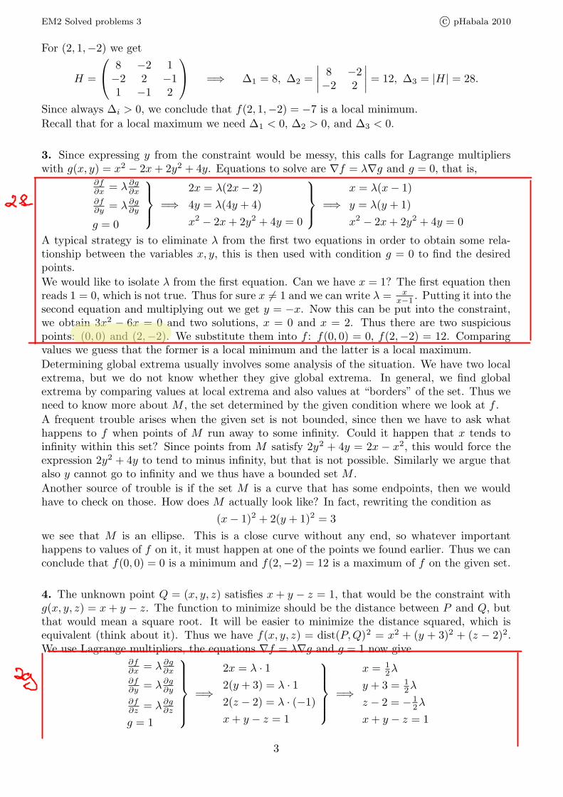
EM2 Solved problems 3 c° pHabala 2010
For (2, 1,−2) we get
H =
8 −2 1−2 2 −11 −1 2
=⇒ Δ1 = 8, Δ2 =
¯
¯
¯
¯
8 −2−2 2
¯
¯
¯
¯
= 12, Δ3 = |H| = 28.
Since always Δi > 0, we conclude that f(2, 1,−2) = −7 is a local minimum.
Recall that for a local maximum we need Δ1 < 0, Δ2 > 0, and Δ3 < 0.
3. Since expressing y from the constraint would be messy, this calls for Lagrange multiplierswith g(x, y) = x2 − 2x + 2y2 + 4y. Equations to solve are ∇f = λ∇g and g = 0, that is,
∂f∂x
= λ ∂g∂x
∂f∂y
= λ ∂g∂y
g = 0
=⇒2x = λ(2x − 2)
4y = λ(4y + 4)
x2 − 2x + 2y2 + 4y = 0
=⇒x = λ(x − 1)
y = λ(y + 1)
x2 − 2x + 2y2 + 4y = 0
A typical strategy is to eliminate λ from the first two equations in order to obtain some rela-tionship between the variables x, y, this is then used with condition g = 0 to find the desiredpoints.
We would like to isolate λ from the first equation. Can we have x = 1? The first equation thenreads 1 = 0, which is not true. Thus for sure x 6= 1 and we can write λ = x
x−1 . Putting it into thesecond equation and multiplying out we get y = −x. Now this can be put into the constraint,we obtain 3x2 − 6x = 0 and two solutions, x = 0 and x = 2. Thus there are two suspiciouspoints: (0, 0) and (2,−2). We substitute them into f : f(0, 0) = 0, f(2,−2) = 12. Comparingvalues we guess that the former is a local minimum and the latter is a local maximum.
Determining global extrema usually involves some analysis of the situation. We have two localextrema, but we do not know whether they give global extrema. In general, we find globalextrema by comparing values at local extrema and also values at “borders” of the set. Thus weneed to know more about M , the set determined by the given condition where we look at f .
A frequent trouble arises when the given set is not bounded, since then we have to ask whathappens to f when points of M run away to some infinity. Could it happen that x tends toinfinity within this set? Since points from M satisfy 2y2 + 4y = 2x − x2, this would force theexpression 2y2 + 4y to tend to minus infinity, but that is not possible. Similarly we argue thatalso y cannot go to infinity and we thus have a bounded set M .
Another source of trouble is if the set M is a curve that has some endpoints, then we wouldhave to check on those. How does M actually look like? In fact, rewriting the condition as
(x − 1)2 + 2(y + 1)2 = 3
we see that M is an ellipse. This is a close curve without any end, so whatever importanthappens to values of f on it, it must happen at one of the points we found earlier. Thus we canconclude that f(0, 0) = 0 is a minimum and f(2,−2) = 12 is a maximum of f on the given set.
4. The unknown point Q = (x, y, z) satisfies x + y − z = 1, that would be the constraint withg(x, y, z) = x + y − z. The function to minimize should be the distance between P and Q, butthat would mean a square root. It will be easier to minimize the distance squared, which isequivalent (think about it). Thus we have f(x, y, z) = dist(P, Q)2 = x2 + (y + 3)2 + (z − 2)2.We use Lagrange multipliers, the equations ∇f = λ∇g and g = 1 now give
∂f∂x
= λ ∂g∂x
∂f∂y
= λ ∂g∂y
∂f∂z
= λ∂g∂z
g = 1
=⇒
2x = λ · 12(y + 3) = λ · 12(z − 2) = λ · (−1)
x + y − z = 1
=⇒
x = 12λ
y + 3 = 12λ
z − 2 = − 12λ
x + y − z = 1
3

EM2 Solved problems 3 c° pHabala 2010
Again, we start by eliminating λ from the first three equations, for instance by substituting for12λ from the first equation into the next two. Then
y + 3 = x
2 − z = x
x + y − z = 1
=⇒y = x − 3
z = 2 − x
x + y − z = 1
=⇒ x + (x − 3) + (2 − x) = 1 =⇒ x = 2.
We easily find the other unknowns and obtain a suspicious point Q = (2,−1, 0). Is the functionf and hence the distance really minimal, not for instance maximal at Q? We try another pointfrom the plane. Say, the point R = (0, 1, 0) has dist(R,P ) =
√42 + 22 =
√20. On the other
hand, the distance from Q to P is dist(Q,P ) =√
22 + 22 + 22 =√
12, so it looks like the desiredminimum.
We can also argue that it is possible to go to infinity within the given plane, we can easily letx → ∞ and the other coordinates adjust, then also the distance goes to infinity (this is obviouswhen we imagine the situation) and thus the value we found cannot be the maximum.
Alternative: The first three equations offer the possibility of easily expressing all variables usingλ (say, z = 2 − 1
2λ). When we do it and substitute into the constrain, we get an equation withone unknown λ, namely 3
2λ = 6. For this we have λ = 4 and we now have exactly the samex = 2 etc. as before.
Note: Instead of Lagrange multipliers one could use the constraint to get x = 1 − y + z andsubstitute into f , obtaining F (y, z) = (1−y+z)2 +(y+3)2 +(z−2)2. We find its local extrema:
∂F∂y
= 0
∂F∂z
= 0
)
=⇒ −2(1 − y + z) + 2(y + 3) = 0
2(1 − y + z) + 2(z − 2) = 0
¾
=⇒ y = −1, z = 0.
5. The distance between a point and a line is given as the distance between the given point andthe closest point of the line, so we have to find that point.
We have two constraints, one given by g(x, y, z) = x + y + z = 1, the other by h(x, y, z) =2x− y + z = 3. We want a point Q = (x, y, z) satisfying these constraints such that its distancefrom P is minimal, we will minimize the distance squared f(x, y, z) = (x−1)2+(y−2)2+(z+1)2.Now there will be two Lagrange multipliers, we call them λ and µ (it is easier to write g, h andλ, µ rather then g1, g2 and λ1,λ2 as in the theorem). The equations are ∇f = λ∇g + µ∇h,g = 1 and h = 3, that is,
∂f∂x
= λ ∂g∂x
+ µ∂h∂x
∂f∂y
= λ ∂g∂y
+ µ∂h∂y
∂f∂z
= λ∂g∂z
+ µ∂h∂z
g = 1
h = 3
=⇒
2(x − 1) = λ · 1 + µ · 22(y − 2) = λ · 1 + µ · (−1)
2(z + 1) = λ · 1 + µ · 1x + y + z = 1
2x − y + z = 3
=⇒
2(x − 1) = λ + 2µ
2(y − 2) = λ − µ
2(z + 1) = λ + µ
x + y + z = 1
2x − y + z = 3
We will again try to eliminate the multipliers from the first three equations. For instance, weadd the second and the third equation, get λ = y +z−1, putting it back into the third equationwe get µ = z − y + 3. Substituting λ, µ into the first equation we get 2x + y − 3z = 6. This istypical, we had 3 equations with 5 unknowns, so after using up two equations we end up withone and only three unknowns.
Now we also take into account the two constraints, so we get
2x + y − 3z = 6
x + y + z = 1
2x − y + z = 3
=⇒ x = 2, y = 0, z = −1.
We then calculate the distance from Q = (2, 0,−1) to P : dist(P,Q) =√
5. Just to make sure
4