FUTURE OF WLAN AND THE INFLUENCES TO THE ARCHITECTURAL

FORMS AND DESIGN

by

SERHAN HAKGÜDENER

Submitted to the Institute of Graduate Studies in

Science and Engineering in partial fulfillment of

the requirements for the degree of

Master of Architecture

in

Architecture

Yeditepe University

2007

ii

FUTURE OF WLAN AND THE INFLUENCES TO THE ARCHITECTURAL

FORMS AND DESIGN

APPROVED BY:

Prof.Dr. Fatih Pakdil ……………………

(Thesis Supervisor)

Dr. Cahit Canbay ……………………

(Co-Advisor)

Prof.Dr. Yavuz Ko�aner …………………

Assoc. Prof.Dr. Ahmet Kızılay …………………

DATE OF APPROVAL: ...../...../2007

iii

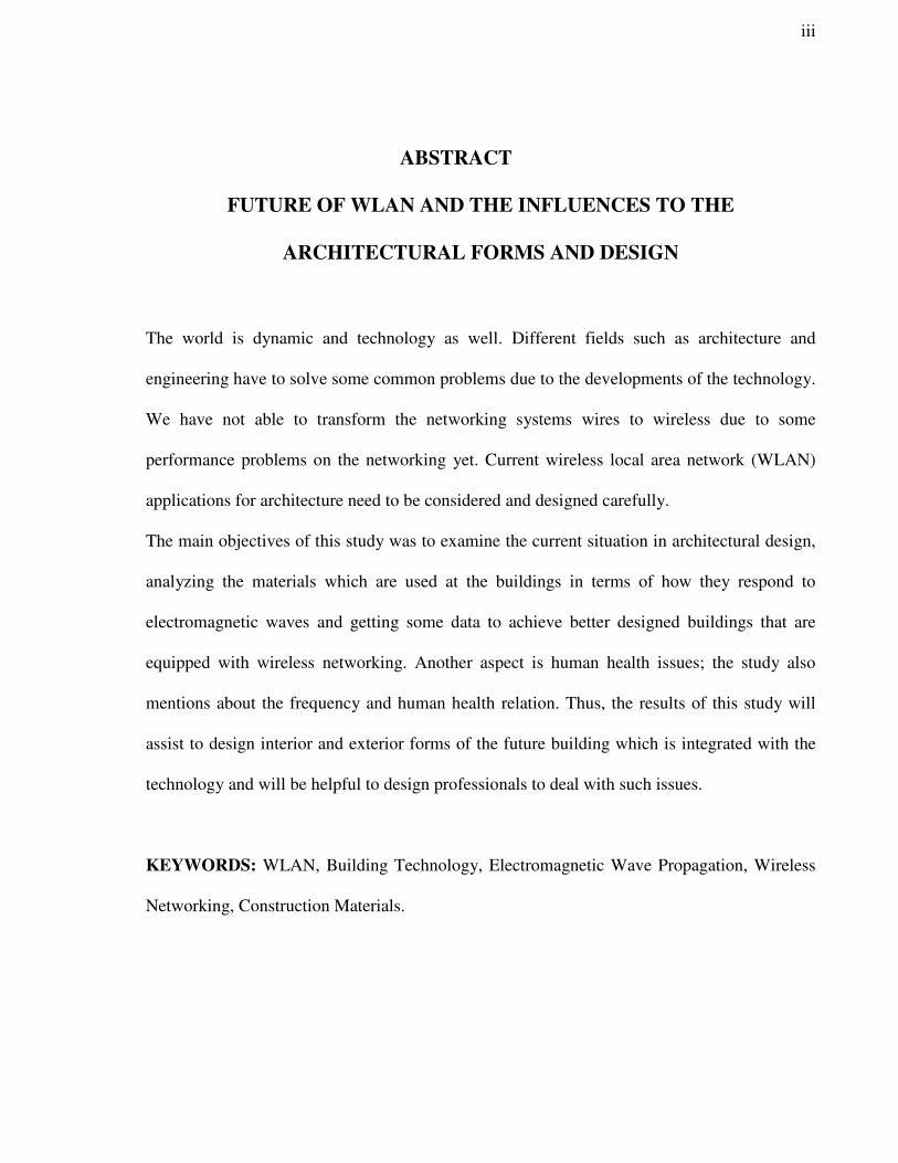
ABSTRACT

FUTURE OF WLAN AND THE INFLUENCES TO THE

ARCHITECTURAL FORMS AND DESIGN

The world is dynamic and technology as well. Different fields such as architecture and

engineering have to solve some common problems due to the developments of the technology.

We have not able to transform the networking systems wires to wireless due to some

performance problems on the networking yet. Current wireless local area network (WLAN)

applications for architecture need to be considered and designed carefully.

The main objectives of this study was to examine the current situation in architectural design,

analyzing the materials which are used at the buildings in terms of how they respond to

electromagnetic waves and getting some data to achieve better designed buildings that are

equipped with wireless networking. Another aspect is human health issues; the study also

mentions about the frequency and human health relation. Thus, the results of this study will

assist to design interior and exterior forms of the future building which is integrated with the

technology and will be helpful to design professionals to deal with such issues.

KEYWORDS: WLAN, Building Technology, Electromagnetic Wave Propagation, Wireless

Networking, Construction Materials.

iv

ÖZET

KABLOSUZ �LET���M S�STEMLER�N�N (WLAN) GELECE��, BUNUN

TASARIM VE M�MAR� FORMLAR ÜZER�NDEK� ETK�LER�

Dünya gibi teknolojide her gün dinamik bir �ekilde ilerler. Günümüzde Mimarlık ve

Mühendislik gibi farklı alanlar bu geli�melere ba�lı olarak ortak sorunlar ya�amaktadır.

Performans problemleri yüzünden, ileti�im sistemleri kabloludan kablosuza henüz tam olarak

adapte edilememi�tir. Güncel olan kablosuz ileti�im sistemleri (WLAN) mimari

uygulamalarda iyi incelenmeli ve bu durum göz önünde bulundurularak binalar dikkatlice

tasarlanmalıdır.

Bu çalı�manın amacı kablosuz ileti�im sistemlerindeki bu güncel problemleri mimari tasarım

çerçevesinde de�erlendirebilmek, yapı malzemelerinin analizini, elektromanyetik alanlar

kar�ısındaki tepkilerini ara�tırmak ve bunun sonucunda bina tasarımlarında izlenecek

metodların belirlenmesini kolayla�tırabilmektir. Üzerinde durulması gereken diger konu ise

insan sa�lı�ıdır. Bu çalı�ma aynı zamanda frekans ve insan sa�lı�ı ili�kisinide

de�erlendirmi�tir. Sonuç olarak bu çalı�ma, gelecekte kablosuz ileti�im sistemleri ile iç içe

olan yapılardaki iç ve dı� formların tasarlanmasında mimarlara, kar�ıla�acakları sorunları

çözebilmelerinde yardımcı olacaktır.

ANAHTAR KEL�MELER: WLAN, Yapı Teknolojisi, Elektromanyetik Dalga Yayılımı,

Kablosuz �leti�im Sistemleri, Yapı Malzemeleri.

v

To my Parents

With all my Love

vi

TABLE OF CONTENTS

ABSTRACT........................................................................................................................... iii

ÖZET ..................................................................................................................................... iv

LIST OF FIGURES ............................................................................................................... viii

LIST OF TABLES................................................................................................................. x

LIST OF SYMBOLS / ABBREVIATIONS.......................................................................... xi

PREFACE.............................................................................................................................. xiv

CHAPTER 1. INTRODUCTION. ......................................................................................... 1

1.1. Electromagnetic Radiation........................................................................................ 4

1.2. Concept of WLAN.................................................................................................... 8

1.3. EMW propagation and the function of buildings..............................................….... 9

1.4. Frequency and Human Health................................................................................. 10

1.5. WLAN Technologies................................................................................................. 12

1.6. Summary.................................................................................................................... 13

CHAPTER 2. EMW (Electromagnetic Wave) Issues ........................................................... 14

2.1. EMC (Electromagnetic Compability)....................................................................... 14

2.2. EMI (Electromagnetic Interference).......................................................................... 15

2.3. Building Materials and EMW (Electromagnetic Wave) bond.................................. 16

2.4. Summary...................................................................................................................... 20

CHAPTER 3. MEGACELLS TO PICOCELLS.................................................................... 21

3.1. Brief introduction about Megacells .......................................................................... 21

3.2. Picocells .................................................................................................................... 22

3.2.1. Introduction ................................................................................................... 22

3.2.2. Sample Office Room Layout ........................................................................ 24

3.2.2.1. Scenario I .......................................................................................... 26

3.2.2.2. Scenario II…………………….......................................................... 28

3.2.2.3. Scenario III…..................................................................................... 29

3.2.2.4. Location Triangle............................................................................... 30

3.2.3. Yeditepe University’s Campus Layout (Site Computation) ......................... 31

3.2.3.1. Yeditepe University’s Architecture / Engineering Building............. 33

vii

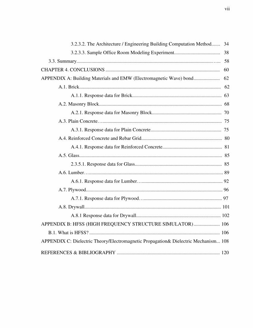
3.2.3.2. The Architecture / Engineering Building Computation Method....... 34

3.2.3.3. Sample Office Room Modeling Experiment..................................... 38

3.3. Summary.............................................................................................................…... 58

CHAPTER 4. CONCLUSIONS ............................................................................................ 60

APPENDIX A: Building Materials and EMW (Electromagnetic Wave) bond..................... 62

A.1. Brick.................................................................................................................. 62

A.1.1. Response data for Brick........................................................................ 63

A.2. Masonry Block................................................................................................... 68

A.2.1. Response data for Masonry Block........................................................ 70

A.3. Plain Concrete…................................................................................................ 75

A.3.1. Response data for Plain Concrete......................................................... 75

A.4. Reinforced Concrete and Rebar Grid................................................................. 80

A.4.1. Response data for Reinforced Concrete................................................ 81

A.5. Glass................................................................................................................... 85

2.3.5.1. Response data for Glass...................................................................... 85

A.6. Lumber…............................................................................................................ 89

A.6.1. Response data for Lumber…................................................................. 92

A.7. Plywood.............................................................................................................. 96

A.7.1. Response data for Plywood…............................................................... 97

A.8. Drywall.............................................................................................................. 101

A.8.1 Response data for Drywall.................................................................... 102

APPENDIX B: HFSS (HIGH FREQUENCY STRUCTURE SIMULATOR) ..................... 106

B.1. What is HFSS? ......................................................................................................... 106

APPENDIX C: Dielectric Theory/Electromagnetic Propagation& Dielectric Mechanism... 108

REFERENCES & BIBLIOGRAPHY ................................................................................... 120

viii

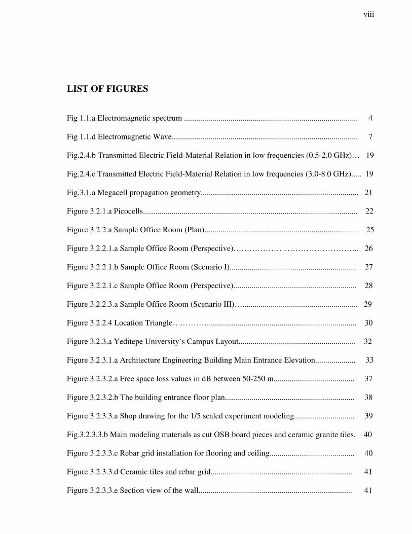
LIST OF FIGURES

Fig 1.1.a Electromagnetic spectrum ...................................................................................... 4

Fig 1.1.d Electromagnetic Wave............................................................................................ 7

Fig.2.4.b Transmitted Electric Field-Material Relation in low frequencies (0.5-2.0 GHz)… 19

Fig.2.4.c Transmitted Electric Field-Material Relation in low frequencies (3.0-8.0 GHz)..... 19

Fig.3.1.a Megacell propagation geometry.............................................................................. 21

Figure 3.2.1.a Picocells.......................................................................................................... 22

Figure 3.2.2.a Sample Office Room (Plan)............................................................................ 25

Figure 3.2.2.1.a Sample Office Room (Perspective)……………………………………….. 26

Figure 3.2.2.1.b Sample Office Room (Scenario I)............................................................... 27

Figure 3.2.2.1.c Sample Office Room (Perspective)............................................................. 28

Figure 3.2.2.3.a Sample Office Room (Scenario III)…......................................................... 29

Figure 3.2.2.4 Location Triangle….……….......................................................................... 30

Figure 3.2.3.a Yeditepe University’s Campus Layout.......................................................... 32

Figure 3.2.3.1.a Architecture Engineering Building Main Entrance Elevation.................... 33

Figure 3.2.3.2.a Free space loss values in dB between 50-250 m........................................ 37

Figure 3.2.3.2.b The building entrance floor plan................................................................ 38

Figure 3.2.3.3.a Shop drawing for the 1/5 scaled experiment modeling.............................. 39

Fig.3.2.3.3.b Main modeling materials as cut OSB board pieces and ceramic granite tiles. 40

Figure 3.2.3.3.c Rebar grid installation for flooring and ceiling.......................................... 40

Figure 3.2.3.3.d Ceramic tiles and rebar grid...................................................................... 41

Figure 3.2.3.3.e Section view of the wall............................................................................ 41

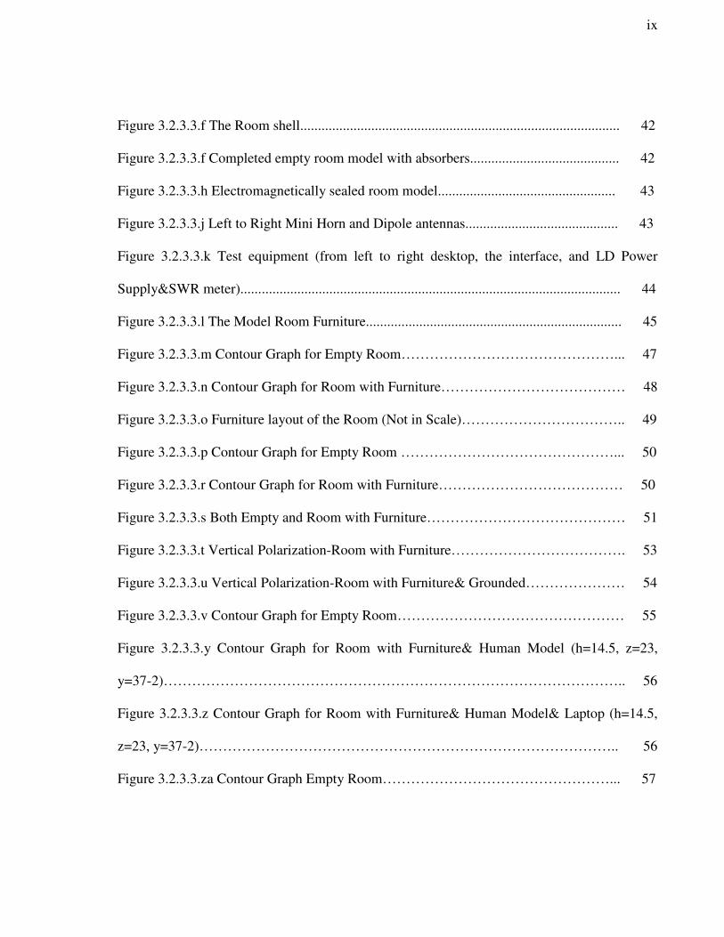
ix

Figure 3.2.3.3.f The Room shell.......................................................................................... 42

Figure 3.2.3.3.f Completed empty room model with absorbers.......................................... 42

Figure 3.2.3.3.h Electromagnetically sealed room model.................................................. 43

Figure 3.2.3.3.j Left to Right Mini Horn and Dipole antennas........................................... 43

Figure 3.2.3.3.k Test equipment (from left to right desktop, the interface, and LD Power

Supply&SWR meter)........................................................................................................... 44

Figure 3.2.3.3.l The Model Room Furniture........................................................................ 45

Figure 3.2.3.3.m Contour Graph for Empty Room………………………………………... 47

Figure 3.2.3.3.n Contour Graph for Room with Furniture………………………………… 48

Figure 3.2.3.3.o Furniture layout of the Room (Not in Scale)…………………………….. 49

Figure 3.2.3.3.p Contour Graph for Empty Room ………………………………………... 50

Figure 3.2.3.3.r Contour Graph for Room with Furniture………………………………… 50

Figure 3.2.3.3.s Both Empty and Room with Furniture…………………………………… 51

Figure 3.2.3.3.t Vertical Polarization-Room with Furniture………………………………. 53

Figure 3.2.3.3.u Vertical Polarization-Room with Furniture& Grounded………………… 54

Figure 3.2.3.3.v Contour Graph for Empty Room………………………………………… 55

Figure 3.2.3.3.y Contour Graph for Room with Furniture& Human Model (h=14.5, z=23,

y=37-2)…………………………………………………………………………………….. 56

Figure 3.2.3.3.z Contour Graph for Room with Furniture& Human Model& Laptop (h=14.5,

z=23, y=37-2)…………………………………………………………………………….. 56

Figure 3.2.3.3.za Contour Graph Empty Room…………………………………………... 57

x

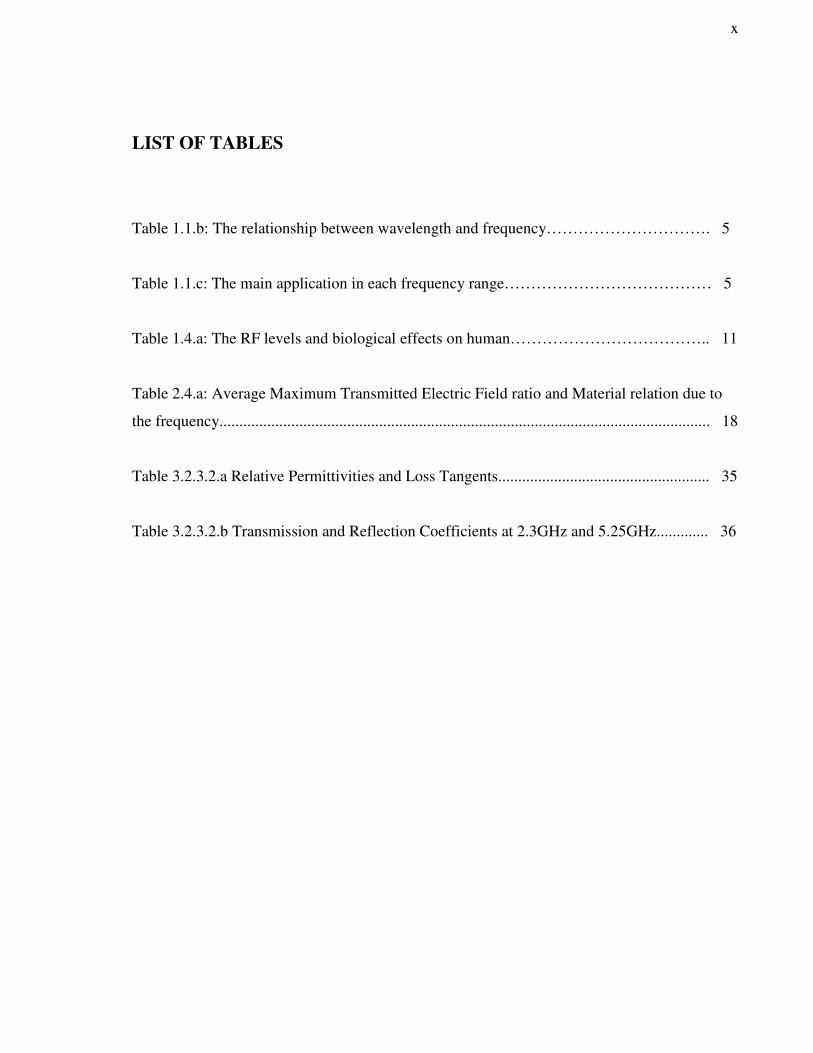
LIST OF TABLES

Table 1.1.b: The relationship between wavelength and frequency…………………………. 5

Table 1.1.c: The main application in each frequency range………………………………… 5

Table 1.4.a: The RF levels and biological effects on human……………………………….. 11

Table 2.4.a: Average Maximum Transmitted Electric Field ratio and Material relation due to

the frequency........................................................................................................................... 18

Table 3.2.3.2.a Relative Permittivities and Loss Tangents..................................................... 35

Table 3.2.3.2.b Transmission and Reflection Coefficients at 2.3GHz and 5.25GHz............. 36

xi

LIST OF SYMBOLS / ABBREVIATIONS

WLAN Wireless Local Area Network

mi Miles

km Kilometers

RF Radio Frequency

IrDA Infrared Data Association

LAN Local Area Network

EMW Electromagnetic Wave

WiMAX Worldwide Interoperability for Microwave Access

UBW Ultra Bandwidth

EMC Electromagnetic Compability

EMI Electromagnetic Interference

NIST The United States National Institute of Standards and Technology

Hz Hertz (formerly cycles per second)

KHz Kilohertz

MHz Megahertz (million Hertz)

GHz Gigahertz (thousands of MHz)

cm Centimeter

m Meter (SI unit of length)

MM Million

E Electric field

H Magnetic field

λ Wavelength

xii

MMAC Multimedia Mobile Access Communication System

HiperLAN High Performance Local Area Network (European)

IEEE Institute of Electrical and Electronic Engineers

FHSS Frequency Hopping Spread Spectrum

DSSS Direct Sequence Spread Spectrum

RFR Radio Frequency Radiation

ANSI American National Standards Institute

ICNIRP International Commission on Non-Ionizing Radiation Protection

NCRP National Council on Radiation protection and Measurements

mW Milliwatt

MAN Metropolitan Area Network

Mbps Megabits per Second

FCC Federal Communications Commission for the United States

CEN European Committee for Standardization

CENELEC European Committee for Standardization

ETSI European Telecommunications Standards Institute for Europe

BSI British Standards for Britain

TSE Turkish Standards Institute

IEC International Electro technical Commission

RFI Radio Frequency Interference

� Electrical conductivity

J Current density

E Electric field strength

xiii

µ Magnetic permeability

B Magnetic field

H Magnetic field strength

D Electric displacement field

E Electric field

� Permittivity

transE Transmitted field

incE Incident electric field

τ Transmission coefficient

α Attenuation constant

L Length of the material

rP Received Power

tP Transmitted Power

aG Maximum Gain of the antenna A

bG Maximum gain for B

Wrec Received Power in dB

Wtr Transmitted Power in dB

GRec(max) Received Gain in dB

GTr(max) Transmitter Gain in dB

S/m Siemens/meter

xiv

PREFACE

I here would like to thank the people who made this thesis possible. I have the pleasure to

thank Prof. Dr. Fatih Pakdil, my thesis supervisor who witnessed to my growth during these

MArch years and for his trust prior to begin working on this subject.

I am honored for being given the chance of working with Dr. Cahit Canbay, my thesis co-

advisor who showed me how to breaking the walls between different disciplines. He always

encouraged me and provided me support. He taught me how to deal with the issues during this

study. This thesis would not have been possible without his remarkable patience and prompt

guidance in this complex EMW propagation issues.

I thank to Associate Prof. Dr. Ahmet Kızılay for helping me with his comments and many

thanks to my friend Research Assistant �lhami Ünal for his help especially during the sample

office room modeling experiment process.

I would like to thank my committee members for careful reading and for suggestions in

improving the manuscript and many thanks to Prof. Dr. Yavuz Ko�aner who is my chairman at

interior architecture department for going through the thesis and correcting the format.

Hopefully, this research will help to highlight the importance of this issue and accelerate the

developments in Turkey and also establish a well-built reference for my future studies about

this topic. All in all, the future is bright waiting for us to solve more technology related issues,

we just need to understand and show a bit effort.

Serhan Hakgüdener

November, 2007

1

CHAPTER 1

1. INTRODUCTION

There are two types’ problems as seen and unforeseen. People generally tend to ignore the

unforeseen ones. Electromagnetic waves (EMW) are metaphysic for the most because not

seen like light. They are basically “oscillating electric and magnetic fields traveling

together through space at a speed of nearly 186,000 mi/300,000 km per second. The

(limitless) range of possible wavelengths or frequencies or electromagnetic waves, which

can be thought of as making up the electromagnetic spectrum, includes radio waves,

infrared radiation, visible light, ultraviolet radiation, X-rays and gamma rays.” [1]

When you deal with electromagnetic waves, this design issue is not considered by the most

professionals in architecture till users encounter technical difficulties on their wireless

networking or any electronic devices they use. Thus, Wireless Local Area Networks

(WLAN) uses Radio Frequency (RF) or infrared waves. They do not demand optical or

copper wires to transfer the data. They are user friendly in terms of installing, full scope to

act and broadband capability. [2] WLAN systems also uses small amount of infrared

(IrDA) technologies besides RF. Infrared systems use waves that are below of visible light

spectrum. This is how they transfer the data between antennas. However, Infrared radiation

is sensitive to dust, moisture and light as physical affects. This technology also requires

line of sight between equipments. Moreover, the coverage area is just 10 meters. [3]

Because of those reasons above mentioned, Infrared technology is not appropriate for

interior spaces. In contrast, hybrid combination of Local Area Network (LAN) and WLAN

brings flexible design solutions in architecture. For instance, main line is brought by local

telephone company to the building and distribution is made by WLAN.

2

The future of WLAN is wide open because of industrial organizations support and demand

from the market. Those studies focus on non-licensed frequencies and pushes for new

regulations for countries. [4]

The objective of this study is to determine both electromagnetic waves (EMW)

propagation versus building materials and assisting to architecture society when they deal

with WLAN related issues during their design process. To be able to approach the subject

matter, this thesis is organized as follows:

• First Chapter has the brief introduction of electromagnetic waves (EMW) including

electromagnetic radiation, the concept of WLAN, EMW propagation and the

function of the buildings, frequency and human health relations plus detailed

research about WLAN technologies such as; WiMAX, 802.11n and UBW so that it

helps to understand in applications for architecture and interior design. [5]

• Second chapter deals with EMC (Electromagnetic Compability), EMI

(Electromagnetic Interference) and case study for RF signals and material relations

give us deeper understanding of both building materials and electromagnetic wave

response such as; glass, brick, concrete, wood, etc. The results of the

experimentations are analyzed and the best design approach is experimented using

the basic construction materials.

• Third chapter is Megacells to Picocells applications. A sample office room plan

layout is chosen to make the site survey. Moreover, HFSS (High Frequency

Structure Simulation) is used to be able to understand electromagnetic propagation

predictions for the room using the software. Finally, sample office room modeling

experiment is done to spot electromagnetic propagation in 1/5 scaled model. As a

result of this, For WLAN applications, different variables are analyzed in a real

3

environment so that the professionals might be using those as reference during the

design process of buildings.

• Fourth chapter concludes and discusses future prospects of WLAN integrated

design.

The results of this study would provide understanding electromagnetic propagation for

building materials in WLAN frequencies and help to the designers such as; which

materials they need to choose depends on the function of the buildings prior to start

construction. Using these results also will shape new design code both buildings and future

forms of the structures in case of they are considered carefully.

4

1.1 Electromagnetic Radiation

Electromagnetic radiation (also known as radiant energy) is the biggest of wave-like

transfer way of the energy through deep space. It also includes visible light that have the

same propagation features of the other wave types such as; Microwaves, Infrared,

Ultraviolet, X-Rays, Gamma Rays, Radio Waves.[6]

Fig 1.1.a: Electromagnetic spectrum [42]

Figure 1.1.a shows the entire spectrum of electromagnetic radiation including frequency

wavelength relation as higher frequency means lower wavelength. In addition to that both

the relation between wavelength and frequency (See Table1.1.b) and the main application

in each frequency (See Table 1.1.c) are needed to be showed.

5

Band Frequency Wavelength

ELF 30-300 Hz 10-1 Mm

VLF 3-30 KHz 100-1 Km

LF 30-300 MHz 1 Km-100M

HF 3-30 MHz 100-10m

VHF 30-300 MHz 10-1m

UHF 300-3000 MHz 1m-10 cm

SHF 3-30 GHz 10-1 cm

EHF 30-300 GHz 1 cm-1 mm

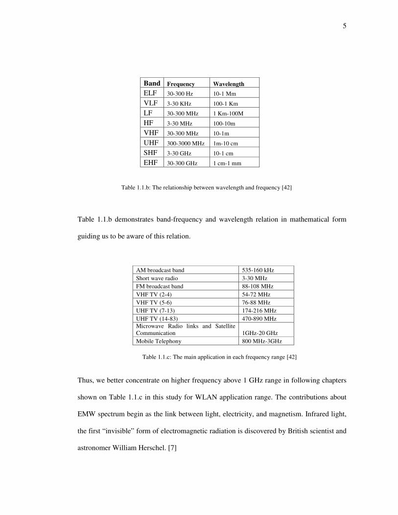
Table 1.1.b: The relationship between wavelength and frequency [42]

Table 1.1.b demonstrates band-frequency and wavelength relation in mathematical form

guiding us to be aware of this relation.

AM broadcast band 535-160 kHz

Short wave radio 3-30 MHz

FM broadcast band 88-108 MHz

VHF TV (2-4) 54-72 MHz

VHF TV (5-6) 76-88 MHz

UHF TV (7-13) 174-216 MHz

UHF TV (14-83) 470-890 MHz Microwave Radio links and Satellite Communication 1GHz-20 GHz

Mobile Telephony 800 MHz-3GHz

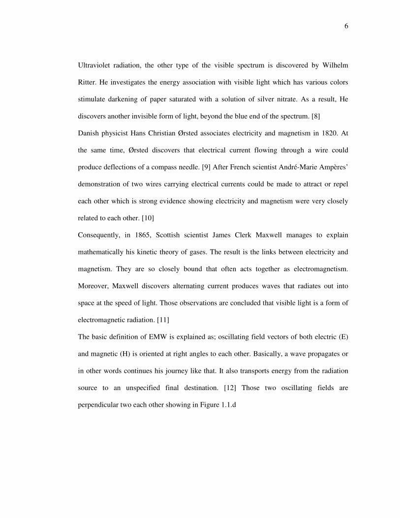
Table 1.1.c: The main application in each frequency range [42]

Thus, we better concentrate on higher frequency above 1 GHz range in following chapters

shown on Table 1.1.c in this study for WLAN application range. The contributions about

EMW spectrum begin as the link between light, electricity, and magnetism. Infrared light,

the first “invisible” form of electromagnetic radiation is discovered by British scientist and

astronomer William Herschel. [7]

6

Ultraviolet radiation, the other type of the visible spectrum is discovered by Wilhelm

Ritter. He investigates the energy association with visible light which has various colors

stimulate darkening of paper saturated with a solution of silver nitrate. As a result, He

discovers another invisible form of light, beyond the blue end of the spectrum. [8]

Danish physicist Hans Christian Ørsted associates electricity and magnetism in 1820. At

the same time, Ørsted discovers that electrical current flowing through a wire could

produce deflections of a compass needle. [9] After French scientist André-Marie Ampères’

demonstration of two wires carrying electrical currents could be made to attract or repel

each other which is strong evidence showing electricity and magnetism were very closely

related to each other. [10]

Consequently, in 1865, Scottish scientist James Clerk Maxwell manages to explain

mathematically his kinetic theory of gases. The result is the links between electricity and

magnetism. They are so closely bound that often acts together as electromagnetism.

Moreover, Maxwell discovers alternating current produces waves that radiates out into

space at the speed of light. Those observations are concluded that visible light is a form of

electromagnetic radiation. [11]

The basic definition of EMW is explained as; oscillating field vectors of both electric (E)

and magnetic (H) is oriented at right angles to each other. Basically, a wave propagates or

in other words continues his journey like that. It also transports energy from the radiation

source to an unspecified final destination. [12] Those two oscillating fields are

perpendicular two each other showing in Figure 1.1.d

7

Fig 1.1.d Electromagnetic Wave [43]

And the vibration is sine wave in mathematical form. As shown in Fig 1.1.d

In addition to that “Electric and magnetic field vectors are not only perpendicular to each

other, but are also perpendicular to the direction of wave propagation.” [43] To simplify

to understand illustrations magnetic oscillating fields of electromagnetic waves are often

omitted though they are known as exist.

Another feature is defined that various type of electromagnetic radiation has identical

wave-like properties. Every category which includes visible light oscillates in a periodic

way and shows some characteristic as; amplitude, wavelength, frequency and intensity of

the radiation. [13]

Thus, measurement of all electromagnetic waves is the magnitude of wavelength (in a

vacuum). The unit is nanometers (one-thousandth of a micrometer) for the visible light

portion of the spectrum.

Last definition is about the number of sinusoidal cycles called frequency (see Figure 1.1.d)

which is usually expresses in quantities of hertz (Hz) or cycles per second (cps). [13]

8

Consequently, from visible light to the others as; Microwaves, Infrared, Ultraviolet, X-

Rays, Gamma Rays, Radio Waves which have electric (E) and magnetic fields (H)

perpendicular to each other are the parts of entire electromagnetic wave spectrum.

Furthermore, the relationship between wavelength and the frequency is mentioned above

as higher frequency means lower wavelength. After this brief introduction, the concept of

WLAN can be introduced as follows.

1.2 Concept of WLAN

Early 90s is the period of wireless networking developments. Comparing both wireless and

wired networking systems show the benefits of using the first one. The capability of fast

data transferring makes the wireless systems become widespread. The data transfer of two

or more digital devices as computers set up the structure of WLAN. This type of

networking system might be used by the purpose of education, private, national, or public.

In addition, WLAN has the all features of LAN (Local Area Networking) which uses cable

for connection between devices. It also provides broadband internet access which means

gateway to the e mails or shared folder options to the user. Moreover, WLAN is very

efficient in open spaces as parks and streets. There are two standard technologies which are

US based IEE 802.11x and European based HiperLAN. [14]

Beside of these Japanese based MMAC (Multimedia Mobile Access Communication

System) is another alternative to use WLAN. Unfortunately, MMAC system uses 3-60

GHz frequency band and not suitable for European standards. [15]

IEEE (Institute of Electrical and Electronic Engineers) defines the most common standards

worldwide. IEEE 802.11 works with 2.4 GHz frequency. The max capable limit is 2 Mbps

by using FHSS (Frequency Hopping Spread Spectrum) and DSSS (Direct Sequence Spread

Spectrum). The purpose of this protocol is that keeping the current LAN systems in one

9

roof and make adaptation to WLAN. After successful achievements of those studies, IEEE

published new WLAN protocols as 802.11 xs. The studies still continues to provide better

service. IEEE 802.11b work with 2.4 GHz frequency. It is commonly used in Turkey and

worldwide. It can transfer the data up to 11 Mbps. Nowadays, 802.11g protocol works with

the same frequency mentioned above. Their limits are up to 54 Mbps and very popular in

the market. [16]

Another protocol is HiperLAN (High Performance Radio LAN) that is developed in

Europe and it is a different standard of WLAN. There are two types which are HiperLAN1

and HiperLAN2 work with 5 GHz frequency. They have some similarities with 802.11 in

terms of speed and capacity. Moreover, HiperLAN uses ATM technology that provides

better service quality. [17] Unfortunately, it is not very common like WLAN. As a result,

HiperLAN might be considered as better alternative to WLAN.

All in all, early 90s is the period of acceleration for WLAN. IEE 802.11x and European

based HiperLAN are introduced to the market and spread worldwide. Researches still

continue and push the limits of WLAN in terms of standards, performance and technology.

Next section shows us the function of buildings and EMW propagation that helps better

understanding of WLAN.

1.3 EMW propagation and the function of buildings

Another aspect needs to be considered is electromagnetic wave and frequency relation.

EMW penetrates variously to buildings due to the frequency. The function of the building

becomes significant in terms of propagation such as; hospitals, apartments, schools, and

military buildings. They require different needs for propagation. For instance, military

orders total security that means full exterior sealing of the buildings using some materials

as “An electromagnetic wave absorption panel for use in building construction includes a

10

protective tile layer, an absorber layer, a metal reflective layer, and a building support

layer, such as concrete. The absorber layer utilizes novel materials including high

dielectric constant materials, such as ABO.sub.3 type perovskites, layered superlattice

materials, conducting oxides, and signet magnetics, ferroelectrics, such as ABO.sub.3 type

perovskites and layered superlattice materials, garnets, a nickel-zinc ferrite, Ni.sub.0.4

Zn.sub.0.6 Fe.sub.2 O.sub.4, and polymer-ceramic composites of the above materials.”[18]

Nowadays technology is capable to see the heart beat of a man from the satellites. Thus,

hospitals, residential buildings and schools need variety of design solutions to reach EMW

and health friendly environments. However, we do not have chance to see good design

solution samples around because EMW is not being aware of thread or necessity for most

professionals and it is considered unforeseen factor for design. Next section covers this

unforeseen factor.

1.4 Frequency and Human Health

The range of radio frequency (RF) spectrum spans 3 kHz to several hundred GHz. The

microwave range starts from 1 GHz to 40 GHz is being used in contemporary point to

point, wireless, and satellite communications. The public concern is that how radio

frequency and microwave radiations affect on human health of exposure close to radio and

television transmitters, mobile base stations, wireless networks and so on.

Several investigations of non-ionizing radiation as RFR (Radio Frequency Radiation)

levels are done all over the world to resolve the safety levels of exposure on humans.

Specific guidelines and standards have been issued by ANSI (American National

Standards Institute) /IEEE (Institute of Electrical and Electronics Engineers), ICNIRP

(International Commission on Non-Ionizing Radiation Protection), NCRP (National

11

Council on Radiation protection and Measurements) and other organizations. These

standards are expressed in power density in (mW/cm2). For instance,

The 1992 ANSI/IEEE exposure standard for the general public is 1.2 mW/cm2 with the

antennas operating in the 1800-2000 MHz range. The RF levels produced by mobile base

stations that can produce known biological effects are showed below. [19]

100 mW/cm2 Clear Hazard 40 mW/cm2 Reproducible effects 4 mW/cm2 Unconfirmed reports of effects 1 mW/cm2 FCC public exposure standard (2000 MHz) 0.5 mW/cm2 FCC public exposure standard (00 MHz) 0.01 mW/cm2 Maximum near a cell phone tower 0.0002 mW/cm2 Typical near a modern phase tower

Table 1.4.a The RF levels and biological effects on human [19]

As a result, high frequency radiation exists both inside of the buildings and free space

around us. They are variety of RF sources and cover a wide range of the electromagnetic

spectrum. Mostly, rapidly expanding source is the mobile phone base stations.

The priority is that taking care of the design codes of new base stations. Moreover, meeting

the guidelines set for the antennas and their mounting so that the minimum required

distance can be observed for the public access. To reduce the radiation power levels next

generation antennas might be developed. Thus, WLAN technologies reflect the

developments about the field on the next part.

12

1.5 WLAN Technologies

WLAN technologies are evolving to allow for faster transmission speeds and greater

bandwidth. To be able to transfer data WLAN has some options as RF (Radio Frequency)

and infrared. They both have advantages and disadvantages. Making right choice affect

efficiency of the system. Some criteria’s as coverage and speed are main factors for a

network. In application, RF is common because of high speed data transfer and passing

through physical barriers. [20]

Another new approach is WiMAX (Worldwide Interoperability for Microwave Access).

This is the recently approved IEEE 802.16 wireless metropolitan area network (MAN)

standard for broadband wireless access. WiMAX is real wireless fidelity with connectivity

up to several kilometers as opposed to a couple hundred meters for 802.11a/b/g.

Nowadays, 802.11g standard is approved and IEEE looks at even faster standards like

802.11n. As mentioned above, 802.11g runs at rates up to 54Mbps which is more than

adequate for most WiFi users. Even if they do not notice the difference between 50Mbps

and 320Mbps, many applications runs better at a higher speed. [21]

UWB is similar to Bluetooth technology but 100 times faster. It refers to Ultra-wideband

(UWB) is used to transmit data at high speeds over short distances. As a result, UWB is

perfect choice for home market. UWB is that the standard works across a wide range of

frequencies as opposed to most other.

However, main concern is interference problems with other networking and consumer

electronic technologies which are assigned a narrow band of spectrum. Despite these

concerns, UWB product development is moving forward in the home networking market

due to its fast transmission rates. [22]

13

As mentioned above, it is seen that WiMAX (Worldwide Interoperability for Microwave

Access and Ultra-wideband (UWB) compete with each other in near future to be able to

get the WLAN market.

1.6 Summary

Chapter one starts with the definition of Electromagnetic Radiation including the full

spectrum, frequency-wavelength relation to be able to understand the behaviors of EMW

propagation easily. Then, The Concept of WLAN expresses how EMW is used by the

technology for human beings. Furthermore, EMW propagation and the function of

buildings is the other step to achieve deeper understanding for design professionals. Thus,

Frequency and Human Health is the most crucial point for the designers to think. To be

able to understand this, necessary information and peak values is showed in the Table

1.4.a. Consequently, the last section answer this question which is what is the future of

WLAN? In addition to the topics above mentioned next chapter covers electromagnetic

wave related issues to be able to highlight the bond between EMW propagation and

building materials in architectural spaces. Those relations guide to architects informing

current issues and what should be done as next step.

14

CHAPTER 2

2. EMW (Electromagnetic Wave) Issues

After giving brief introduction about electromagnetic waves in the first chapter, some

topics as; electromagnetic compability, interference and building material relations needs

to be revealed to improve design professionals’ knowledge about electromagnetic

propagation in a space. This chapter covers those as follows.

2.1 EMC (Electromagnetic Compability)

The brief definition of the term is “Electromagnetic Compability (EMC) is the ability of a

device to operate faultlessly in a prescribed electromagnetic environment without at the

same time affecting its surroundings in an inadmissible way.”[23]

The explanation above mentioned tends to explain unintentional generation, propagation

and reception of electromagnetically energy. Thinking about an environment might be an

office or a school laboratory having full of electronic devices such as computers, cell

phones, TVs, lighting fixtures, and wireless gadgets that causes electromagnetic

phenomena in their operation. The goal of EMC (Electromagnetic Compability) is to

harmonize the conflicts between devices.

To be able to fix this problem, EMC deals with emission issues which are related to the

reduction of unintentional generation of electromagnetic energy. For the buildings,

countermeasures should be taken in order to avoid the external environment propagation

towards to the space as EMW isolation. This design solution is the major step to avoid

electromagnetic disturbances due to the incorrect operation of electrical equipments.

In order to achieve such an objective in architecture, during the design process

susceptibility issues needs to be considered. The importance of EMC has taken account in

many countries and standardization has been made by The FCC (Federal Communications

Commission) for the United States, CEN (European Committee for Standardization),

15

CENELEC (European Committee for Standardization) and ETSI (European

Telecommunications Standards Institute) for Europe, BSI (British Standards) for Britain

and TSE (Turkish Standards Institute) for Turkey. Moreover, the most important

international organization is the International Electrotechnical Commission (IEC), which

has several committees working full time on EMC issues. [24]

To sum up, electromagnetic compability solution purpose is getting the harmonious

environment for electronic devices for them to operate functionally. Now, it is time to

address electromagnetic interference issue as next step.

2.2 EMI (Electromagnetic Interference)

Electrical circuits emit electromagnetic radiation knows as Radio Frequency Interference

(RFI). The devices carry rapidly changing signals which is the result of unwanted signals

called interference or noise in other circuits. EMI (Electromagnetic Interference) interrupts

or limits the effective performance of those other circuits. Sometimes it is intended action

as some forms of electronic warfare.

In this case, the EMI issue is urgent to be able to protect military buildings which include

some electronic defense system devices from this type of hustle actions. For instance, EMI

is a vital problem for hospital buildings. According to extensive study carried out in 2004,

at Massachusetts General Hospital, "Cellular phones placed in close proximity to some

commercially available intensive care ventilators can cause malfunctions, including

irrecoverable cessation of ventilation. This is most likely to occur if the cellular phone is

<30 cm from the device and ringing. Based on our data and the available literature, we

believe it is reasonably safe to permit the use of cellular phones in the intensive care unit,

as long as they are kept > or =3 feet from all medical devices. The current electromagnetic

16

compatibility standards for mechanical ventilators are inadequate to prevent malfunction."

[25]

There are generally two techniques to be able to seal EMI at higher frequencies like 500

MHz. Wave shaping with series resistors and inserting the traces between the two planes.

As we know most of digital equipment is made of metal, coated plastic and cases. In the

case of too much EMI, shielding such as RF gaskets and copper tape can be used.

Most of countries have legal codes to prevent EMI on electrical hardware and still work on

to be able to fix this issue. [26]

Electromagnetic Interference is a vital disturbance for WLAN environment. Thus, the

codes are the key to prevent this issue. Next section gives detailed information about this

bond between building materials and EMW.

2.3 Building Materials and EMW (Electromagnetic Wave) bond

Building materials are the core of architecture. Sometimes they are like skin or skeleton of

the structures. In the building environment, EMW propagates differently due to the

material inside. To be able to understand this issue, the relation between conductivity,

magnetic permeability and electric permittivity are handy. First of all, “Electrical

conductivity is a measure of a material's ability to conduct an electric current. When an

electrical potential difference is placed across a conductor, its movable charges flow and

gives rise to an electric current. The conductivity � is defined as the ratio of the current

density J to the electric field strength E.” [27] The equation is J= �.E

Secondly, The definition of magnetic permeability is “Relative increase or decrease in the

resultant magnetic field inside a material compared with the magnetizing field in which the

given material is located; or the property of a material that is equal to the magnetic flux

density B established within the material by a magnetizing field divided by the magnetic

17

field strength H of the magnetizing field. Magnetic permeability µ is thus defined as

µ = B/H. Magnetic flux density B is a measure of the actual magnetic field within a

material considered as a concentration of magnetic field lines, or flux, per unit cross-

sectional area. Magnetic field strength H is a measure of the magnetizing field produced

by electric current flow in a coil of wire.” [28]

Finally, “in electromagnetism, electric displacement field D represents how an electric

field E influences the organization of electrical charges in a given medium, including

charge migration and electric dipole reorientation. Its relation to permittivity is D= �E”

[29]. Adding the issues above mentioned such as EMI (Electromagnetic Interference) and

EMC (Electromagnetic Compability), it becomes more complicated problem to be able to

solve in the space. Thus, next paragraphs emphasize building material versus EMW

propagation interaction as follows.

Based on the material/EMW bond data on NIST (See Appendix A for detailed

information) experimentation, [30] both a table and figure is created so that the

professionals can compare the transmitted field and frequency relations of the materials.

(See Table 2.4.a, Fig. 2.4.b and Fig.2.4.c)

Prior to looking at figures and the table some equations needs to be understood as;

t r a n s

in c

E

Eτ =

�

�

In this equation, τ is transmission constant, transE�

is transmitted field

and incE�

is the incident electric field also the amplitude of incident electric field

represents. The transmitted electric field can be written in terms of incident electric field

amplitude and the transmission coefficient as.. . L

trans incE E eατ −= . For this equation τ

18

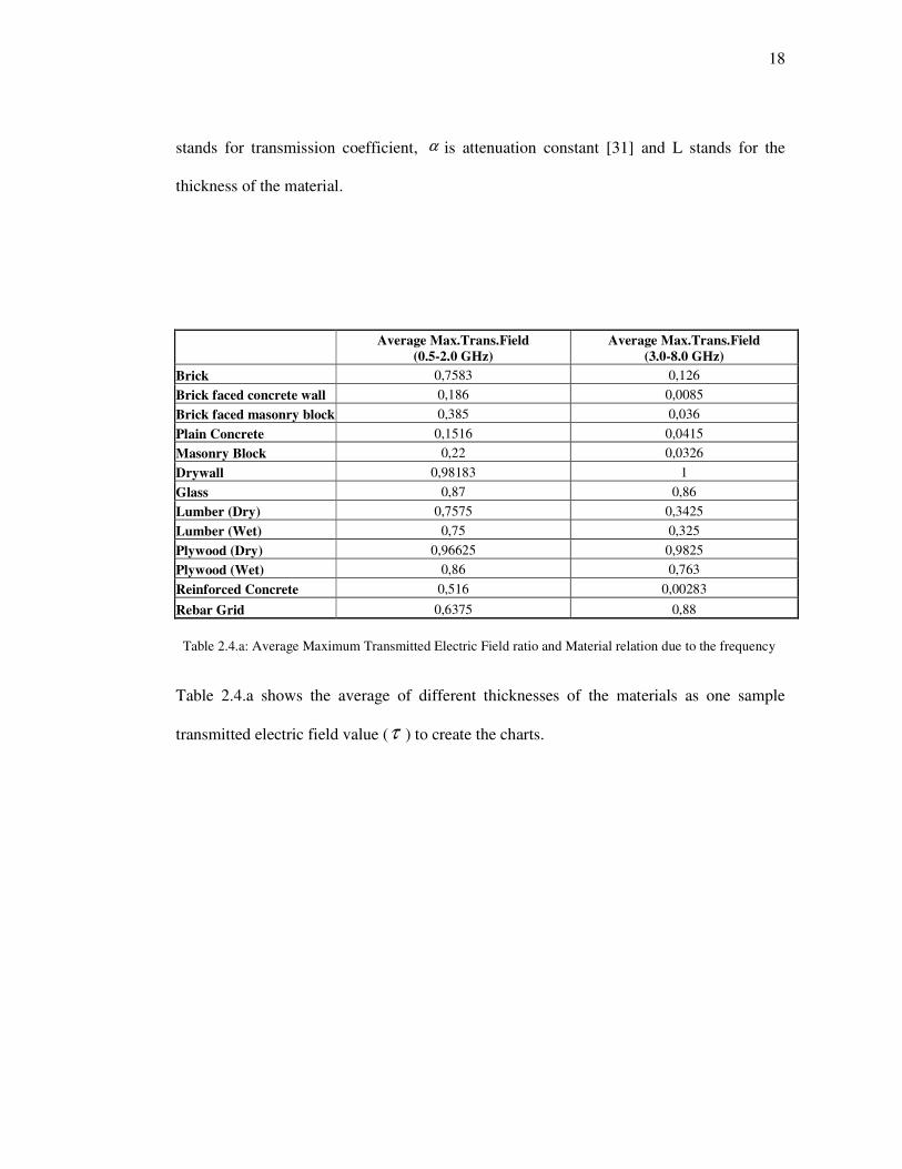
stands for transmission coefficient, α is attenuation constant [31] and L stands for the

thickness of the material.

Average Max.Trans.Field

(0.5-2.0 GHz) Average Max.Trans.Field

(3.0-8.0 GHz)

Brick 0,7583 0,126

Brick faced concrete wall 0,186 0,0085

Brick faced masonry block 0,385 0,036

Plain Concrete 0,1516 0,0415

Masonry Block 0,22 0,0326

Drywall 0,98183 1

Glass 0,87 0,86

Lumber (Dry) 0,7575 0,3425

Lumber (Wet) 0,75 0,325

Plywood (Dry) 0,96625 0,9825

Plywood (Wet) 0,86 0,763

Reinforced Concrete 0,516 0,00283

Rebar Grid 0,6375 0,88

Table 2.4.a: Average Maximum Transmitted Electric Field ratio and Material relation due to the frequency

Table 2.4.a shows the average of different thicknesses of the materials as one sample

transmitted electric field value (τ ) to create the charts.

19

0

0,2

0,4

0,6

0,8 1

1,2

Brick

Brick faced

concrete wall

Brick faced

masonry block

Plain Concrete

Masonry Block

Drywall

Glass

Lumber (Dry)

Lumber (Wet)

Plywood (Dry)

Plywood (Wet)

Reinforced

Concrete

Rebar Grid

Materials

Transmitted Electric Field Ratio

F

ig.2.4.b: Transm

itted Electric F

ield-Material R

elation in low frequencies (0.5-2.0 G

Hz)

0

0,2

0,4

0,6

0,8 1

1,2

Brick

Brick faced concretewall

Brick faced masonryblock

Plain Concrete

Masonry Block

Drywall

Glass

Lumber (Dry)

Lumber (Wet)

Plywood (Dry)

Plywood (Wet)

Reinforced Concrete

Rebar Grid

Materials

Transmitted Electric Field Ratio

F

ig.2.4.c: Transm

itted Electric F

ield-Material R

elation in high frequencies (3.0-8.0 GH

z)

20

Most of the materials such as; brick, brick faced masonry block, plain concrete, reinforced

concrete lose their transmission due to the frequency increase. Fig.2.4.c. needs to be

underlined to design wireless networking by the design professionals.

2.4 Summary

Two important definitions as EMC (Electromagnetic Compability) which is to harmonize

the conflicts between devices and EMI (Electromagnetic Interference) are explained in this

chapter to be able to define the other variables effecting EMW propagation in an

environment. Moreover, the data above mentioned is a fairly comprehensive set of

information for the penetration to the most common used construction materials which are

exposed by electromagnetic (EM) radiation in the 0.5 to 8.0 GHz (60 cm to 4 cm

wavelength) range.

As it is appeared on the figures, as an example, in the 0.5 to 2.0 GHz, 3-wythe thick (267

mm) brick wall is get 40% of the transmitted signal power. And, similar characteristics

apply to masonry block walls, a staple of commercial construction practice. Thus, the most

common residential construction materials such as; plywood, lumber studs, glass, and

drywall penetrate even more easily. On the other hand, the strongest signal absorption

occurs for concrete specimens.

Next chapter analyzes some computation methods as computer aided and manually solving

process to find the best suitable design approach for structures. In addition to that, sample

office room model experiment shows us how EMW propagates in a space depends on

different variables.

21

CHAPTER 3

3. Megacells to Picocells

Understanding the issues such as; EMC, EMI, and the EMW relation between basic

building materials are given in previous chapter that guide designers to the type of

networking coverage as megacell and picocell applications so that architects can reach the

problem solution methods in a space. This chapter emphasizes those terminologies and

gives information about solutions to be found in the next paragraphs.

3.1 Brief introduction about Megacells

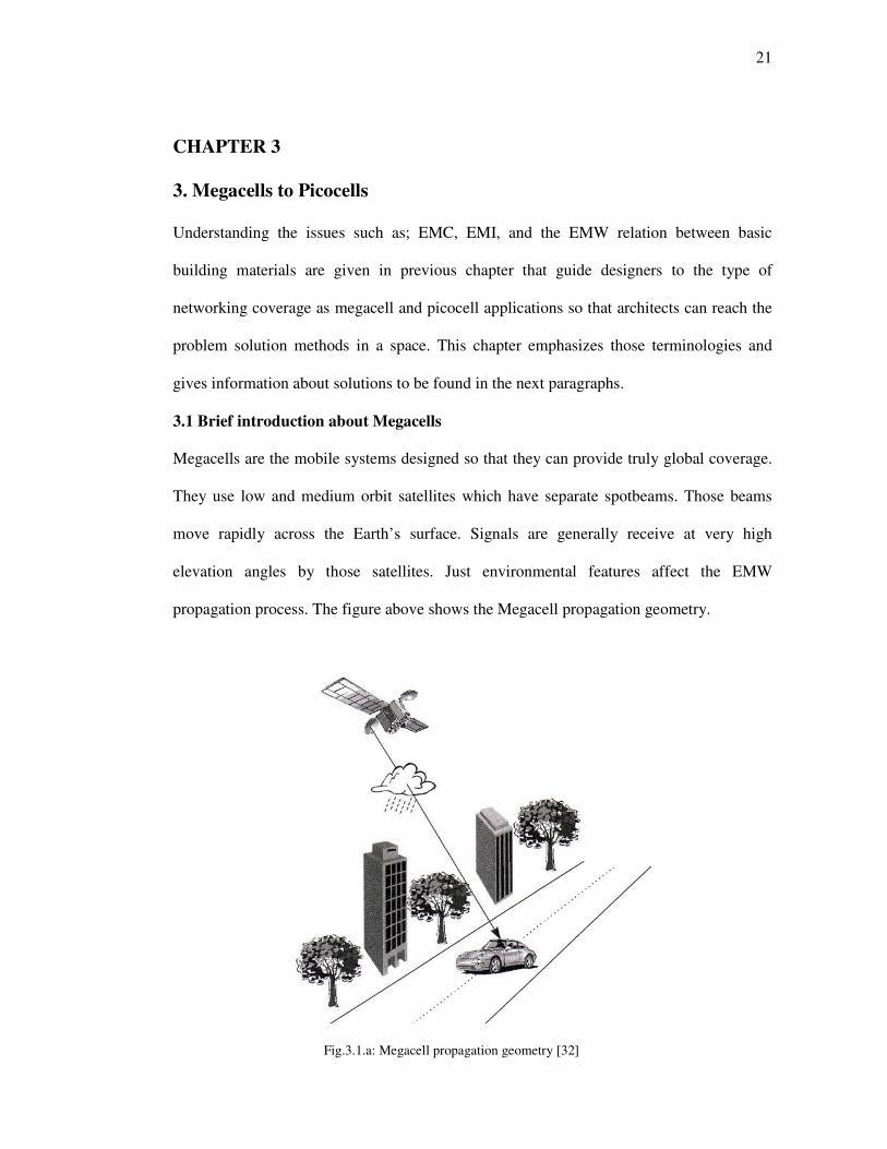
Megacells are the mobile systems designed so that they can provide truly global coverage.

They use low and medium orbit satellites which have separate spotbeams. Those beams

move rapidly across the Earth’s surface. Signals are generally receive at very high

elevation angles by those satellites. Just environmental features affect the EMW

propagation process. The figure above shows the Megacell propagation geometry.

Fig.3.1.a: Megacell propagation geometry [32]

22

3.2 Picocells

3.2.1. Introduction

Basically, Picocells is formed by a base station which is located inside a building. Picocells

are generally used in high traffic areas such as; airports, railway stations, office buildings

and university campuses. As mentioned in chapter one, wireless local area networks

require high data rates. Both macrocellular and microcellular systems might cause

interference in the buildings. Thus, spectrum analysis needs to be done prior to design

WLAN for structures. The nature of Picocells is demonstrated below in figure 3.2.1.a

Figure 3.2.1.a: Picocells [32]

When professionals deal with simulations to design wireless local area networks for

buildings, Empirical Models of propagation come out as handy tools to solve the problems.

Some models as The Friis Formula that is a good starting point to analyze buildings.

Basically, the formula helps to calculate propagation loss in free space. The equation

is2

.4

ra b

t

PG G

P r

λ

π

� �= � �

� �. In this equation, rP refers to received and tP refers to transmitted

power. aG stands for the maximum gain of the antenna A, bG refers to maximum gain for

23

B and λ is the wavelength. Therefore, it is useful for us to state the equation in decibels

as;

Wrec (dBm) ≅ Wtr (dBm) + GRec(max) (dB) + GTr(max) (dB) – 20 log R (km) – 20 log f (MHz) -32.44

In this formula, Wrec is for received power in dB, Wtr (dBm) for transmitted power in dB,

GRec(max) (dB) for received gain in dB and GTr(max) (dB) for transmitter gain in dB. [33]

The others as Wall and Floor Factor, COST231 Multi-wall, Ericsson Models are handy to

create simulations. There is multiplicative noise arises between transmitter antenna and the

receiver antenna. It also needs to be clarified before starting the calculations of the

buildings. Here are some of them such as;

• The directional characteristics of both the transmitter and receiver antennas ( In

this case, direct polarization is considered for the building)

• Reflection from the smooth surfaces of walls and hills around the building

(especially in corridors )

• Absorption by walls, trees, interior space elements and by the atmosphere ( See

Table 2.4.a for the percentage of transmitted ratio due to building material and the

frequency)

• Scattering from the rough surfaces as rough ground, leaves, branches of tress

around the buildings

• Diffraction from edges of the building interior and exterior corners, rooftops even

hilltops around it.

• Refraction due to both layered or other materials like insulation of the building.

On the other hand, manually solving process using the models takes so much time to be

able to get the accurate results. Nowadays, Computer simulation methods are used widely

24

in the world. HFSS (High Frequency Structure Simulation) is one of the solution software

for engineers. (See Appendix A for detailed information)

All in all, Sample Office Layout is created and analyzed to predict the EMW propagation

in buildings as follows.

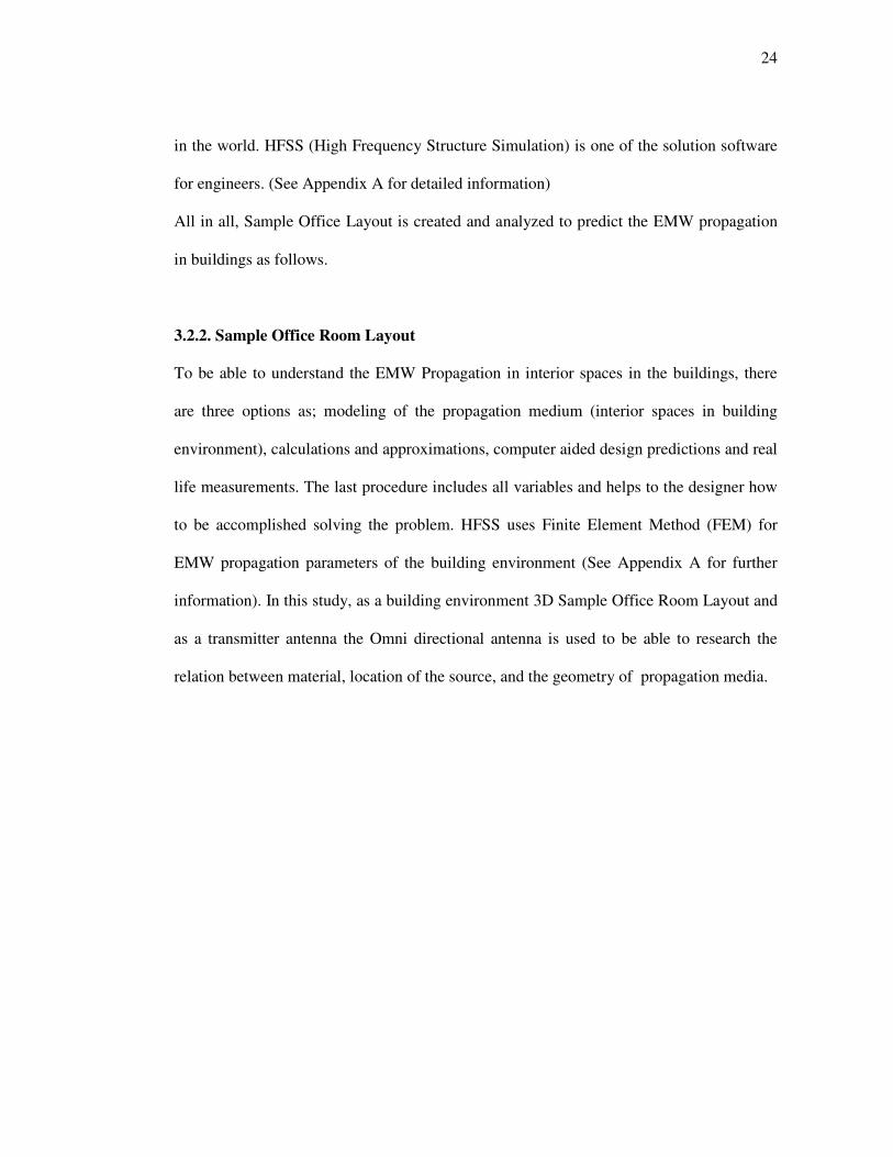
3.2.2. Sample Office Room Layout

To be able to understand the EMW Propagation in interior spaces in the buildings, there

are three options as; modeling of the propagation medium (interior spaces in building

environment), calculations and approximations, computer aided design predictions and real

life measurements. The last procedure includes all variables and helps to the designer how

to be accomplished solving the problem. HFSS uses Finite Element Method (FEM) for

EMW propagation parameters of the building environment (See Appendix A for further

information). In this study, as a building environment 3D Sample Office Room Layout and

as a transmitter antenna the Omni directional antenna is used to be able to research the

relation between material, location of the source, and the geometry of propagation media.

25

Figure 3.2.2.a: Sample Office Room (Plan)

The dimension of the office room is considered as 10 m X 5 m X 3.5m. Basic office

equipments such as; task chairs, tables, desk computers, file cabinets and seating in the

space are located in different places and conditions in the room. (See Fig. 3.2.2.a) The

source which is the antenna of WLAN is located in different places around the space and

propagation simulations has been developed and accomplished.

26

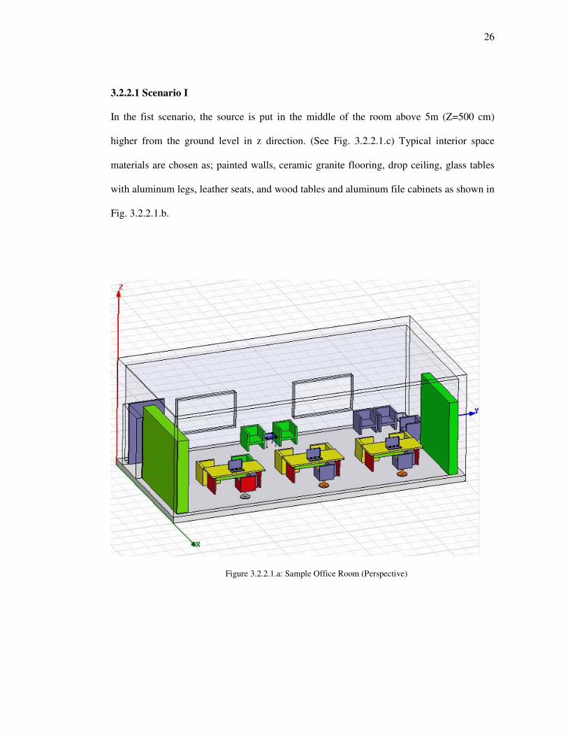
3.2.2.1 Scenario I

In the fist scenario, the source is put in the middle of the room above 5m (Z=500 cm)

higher from the ground level in z direction. (See Fig. 3.2.2.1.c) Typical interior space

materials are chosen as; painted walls, ceramic granite flooring, drop ceiling, glass tables

with aluminum legs, leather seats, and wood tables and aluminum file cabinets as shown in

Fig. 3.2.2.1.b.

Figure 3.2.2.1.a: Sample Office Room (Perspective)

27

Figure 3.2.2.1.b: Sample Office Room (Scenario I)

HFFS is designed to solve electromagnetic propagation design problems. Due to

dimensions and complexity of the structure in architectural area are extremely hard to

solve this problem in HFFS. The model can be created in real dimension but in this case,

problem can not be solved.

28

Figure 3.2.2.1.c: Sample Office Room (Perspective)

3.2.2.2 Scenario II

In the second scenario, the source is placed in the middle of the room above Z=3.5m higher

from the ground level. All conditions stays still just 1.5 m height difference bring different

results as reflection from the interior walls and diffraction from the corners. Aluminum file

cabinets and table legs act like sources in the room. In this scenario, this is very beneficial

for WLAN application in the space.

29

3.2.2.3 Scenario III

In the third scenario, the source is located X=250 cm Y=50 cm and Z=350cm coordinates.

Figure 3.2.2.3.a: Sample Office Room (Scenario III)

Looking at the plan and the location of the source display how close the antenna to the

aluminum files cabinet. Diffraction is the reason for this result and sometimes it is

necessary to increase the value of the electromagnetic wave propagation as mentioned in

previous section.

Third Scenario is the last step of completing the location triangle which is very handy tool

for the designer to compare the value changes of the field.

30

3.2.2.4 Location Triangle

Figure 3.2.2.4.: Location Triangle

The first recognized feature is diffraction from edges of the room interior corners, furniture

including aluminum file cabinets. Comparing the minimum values starting from Scenario I

to III proves the file cabinet acts like source. Thus, the min and max values increase (See

Figure 3.2.2.4). The location triangle is practical for the design professionals to be able to

judge different propagation principles in the environment.

The purpose of those simulations is to predict EMW propagation before the structure is

being built and help to resolve problems mentioned before in the previous chapters. Next

sections underline site computations to be able to predict EMW propagation in existing

environments.

31

3.2.3. Yeditepe University’s Campus Layout (Site Computation)

26 August Campus is located at Kayisdagi region in Istanbul/TURKEY. The campus has

236 thousand square meters closed area with 125 thousand square meters open area which

include “319 classrooms, 22 lecture halls, 32 computer and 74 professional labs belonging

to Fine Arts, Architecture, Communication, Engineering and Sciences Faculties. Also, 2

professional photographic studios, 34 academic administration units, 287 Faculty Offices,

28 student club rooms, a 3000 square meters Central Library, Residence Halls,

multipurpose Conference Hall, cinema complex, a theatre Hall. Moreover, a 524 square

meters and 384 square meters two television studios, 200 square meters educational TV

studio lab, 150 square meters educational radio facilities, 550 square meters indoor

basketball court, 620 square meters outdoor basketball courts, outdoor volleyball, tennis

courts, Indoor and outdoor half Olympic sized swimming pools, 300 square meters fitness

and aerobics center, 783 square meters modern shopping complex, 79000 square meters of

open grassy area, and 400 vehicle capacity indoor parking lots.” [34]

32

Fig. 3.2.3.a: Yeditepe University’s Campus Layout [36]

From number 1 to 8;

1. Rectorate,

2. Architecture and Engineering,

3. Social Facilities,

4. Law Faculty,

5. Fine Arts Faculty,

6. Dormitories and North Preparation School,

7. Hotel,

8. Dormitories and Merchandising Academy buildings are illustrated on Fig. 3.2.3.a.

33

3.2.3.1 Yeditepe University’s Architecture / Engineering Building

The Building has constructed in sloped surface close to Rectorate structure. (See Fig.

3.2.3.a. number 2). It has six floors above the ground and tree floors below the entrance

floor. The Seljuk post modern style building has different basic construction materials such

as; concrete, stone, steel, drywall, glass, and aluminum. The building form has both

curvilinear and linear which makes it hard site survey in terms of electromagnetic wave

predictions. The shell of the building is assembled by façade, insulation and masonry

block. The partitions are mostly made of drywall. Granite and PVC combination is used for

flooring. Interior doors are made of aluminum frame and glass interior. And all the

windows are made by PVC (vinyl) based material. That gives a general building material

analysis of the building to start the simulation calculations. (See Fig.3.2.3.1.a)

Fig.3.2.3.1.a: Architecture Engineering Building Main Entrance Elevation [36]

34

3.2.3.2 The Architecture / Engineering Building Computation Method

Prior to start the computation, Dielectric theory needs to be revised. Appendix B gives

detailed information about Dielectric theory, electromagnetic propagation and dielectric

mechanism. The Computation method based on free space lost and transmission losses

through the building. As mentioned in previous sections (See 3.2.1.), free space lost is

being showed as;

Wrec (dBm) ≅ Wtr (dBm) + GRec(max) (dB) + GTr(max) (dB) – 20 log R (km) – 20 log f (MHz) -32.44

And for the transmission losses the formula below mentioned is being used as;

0( / )incE E V m= (See 2.4)

.0. . L

transE E e ατ −=

tanrπ εα δ

λ= In this formula, rε is Relative Permittivity, ( λ = c/f ) λ wavelength,

c=3x108 m/sn, f=2.4 GHz in this situation and the losses in the dielectric depend on the

loss tangent (tan�) of the material, which depends inversely on the wavelength of the signal

and is directly proportional to the frequency. (See Appendix C)

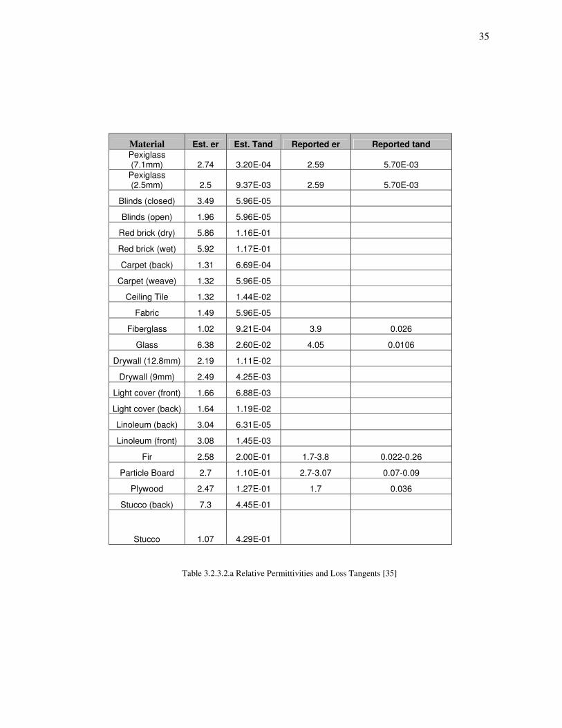
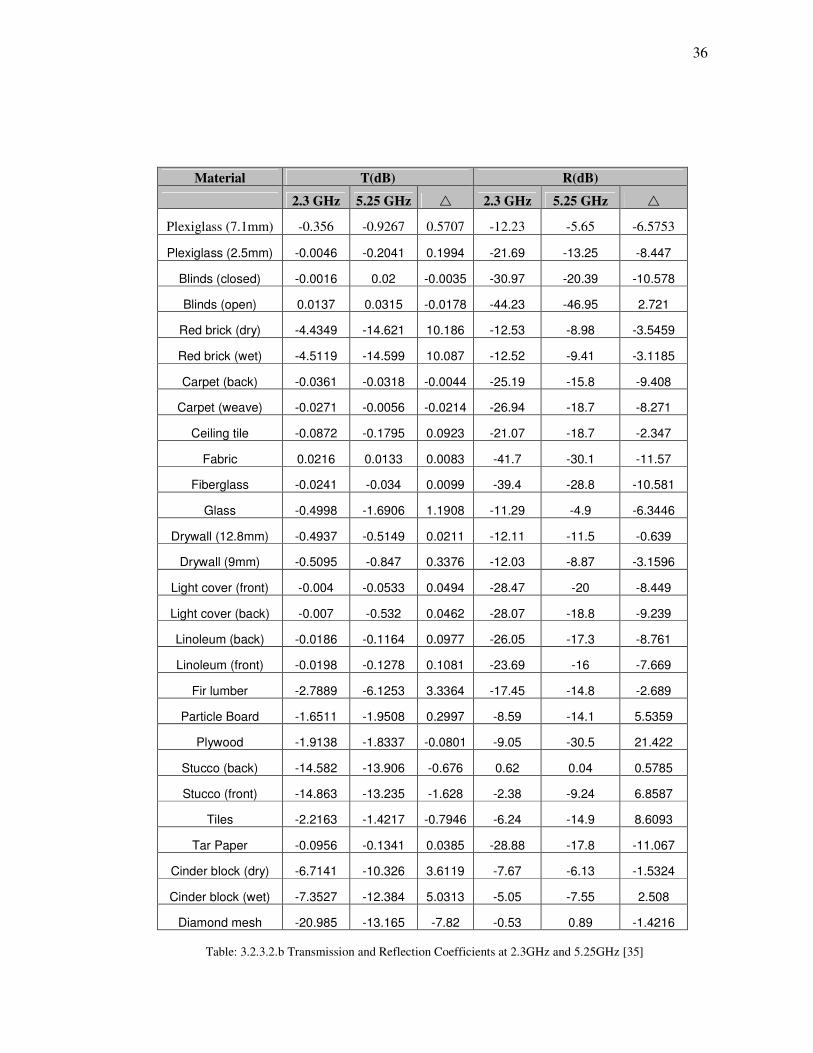
To be able to make the calculation we need to know Transmission coefficient, the relative

permittivity and tan delta values for specific frequency. Table 3.2.3.2.a and 3.2.3.b gives

necessary information below.

35

Material Est. er Est. Tand Reported er Reported tand

Pexiglass (7.1mm) 2.74 3.20E-04 2.59 5.70E-03

Pexiglass (2.5mm) 2.5 9.37E-03 2.59 5.70E-03

Blinds (closed) 3.49 5.96E-05

Blinds (open) 1.96 5.96E-05

Red brick (dry) 5.86 1.16E-01

Red brick (wet) 5.92 1.17E-01

Carpet (back) 1.31 6.69E-04

Carpet (weave) 1.32 5.96E-05

Ceiling Tile 1.32 1.44E-02

Fabric 1.49 5.96E-05

Fiberglass 1.02 9.21E-04 3.9 0.026

Glass 6.38 2.60E-02 4.05 0.0106

Drywall (12.8mm) 2.19 1.11E-02

Drywall (9mm) 2.49 4.25E-03

Light cover (front) 1.66 6.88E-03

Light cover (back) 1.64 1.19E-02

Linoleum (back) 3.04 6.31E-05

Linoleum (front) 3.08 1.45E-03

Fir 2.58 2.00E-01 1.7-3.8 0.022-0.26

Particle Board 2.7 1.10E-01 2.7-3.07 0.07-0.09

Plywood 2.47 1.27E-01 1.7 0.036

Stucco (back) 7.3 4.45E-01

Stucco 1.07 4.29E-01

Table 3.2.3.2.a Relative Permittivities and Loss Tangents [35]

36

Material T(dB) R(dB)

2.3 GHz 5.25 GHz �� 2.3 GHz 5.25 GHz ��

Plexiglass (7.1mm) -0.356 -0.9267 0.5707 -12.23 -5.65 -6.5753

Plexiglass (2.5mm) -0.0046 -0.2041 0.1994 -21.69 -13.25 -8.447

Blinds (closed) -0.0016 0.02 -0.0035 -30.97 -20.39 -10.578

Blinds (open) 0.0137 0.0315 -0.0178 -44.23 -46.95 2.721

Red brick (dry) -4.4349 -14.621 10.186 -12.53 -8.98 -3.5459

Red brick (wet) -4.5119 -14.599 10.087 -12.52 -9.41 -3.1185

Carpet (back) -0.0361 -0.0318 -0.0044 -25.19 -15.8 -9.408

Carpet (weave) -0.0271 -0.0056 -0.0214 -26.94 -18.7 -8.271

Ceiling tile -0.0872 -0.1795 0.0923 -21.07 -18.7 -2.347

Fabric 0.0216 0.0133 0.0083 -41.7 -30.1 -11.57

Fiberglass -0.0241 -0.034 0.0099 -39.4 -28.8 -10.581

Glass -0.4998 -1.6906 1.1908 -11.29 -4.9 -6.3446

Drywall (12.8mm) -0.4937 -0.5149 0.0211 -12.11 -11.5 -0.639

Drywall (9mm) -0.5095 -0.847 0.3376 -12.03 -8.87 -3.1596

Light cover (front) -0.004 -0.0533 0.0494 -28.47 -20 -8.449

Light cover (back) -0.007 -0.532 0.0462 -28.07 -18.8 -9.239

Linoleum (back) -0.0186 -0.1164 0.0977 -26.05 -17.3 -8.761

Linoleum (front) -0.0198 -0.1278 0.1081 -23.69 -16 -7.669

Fir lumber -2.7889 -6.1253 3.3364 -17.45 -14.8 -2.689

Particle Board -1.6511 -1.9508 0.2997 -8.59 -14.1 5.5359

Plywood -1.9138 -1.8337 -0.0801 -9.05 -30.5 21.422

Stucco (back) -14.582 -13.906 -0.676 0.62 0.04 0.5785

Stucco (front) -14.863 -13.235 -1.628 -2.38 -9.24 6.8587

Tiles -2.2163 -1.4217 -0.7946 -6.24 -14.9 8.6093

Tar Paper -0.0956 -0.1341 0.0385 -28.88 -17.8 -11.067

Cinder block (dry) -6.7141 -10.326 3.6119 -7.67 -6.13 -1.5324

Cinder block (wet) -7.3527 -12.384 5.0313 -5.05 -7.55 2.508

Diamond mesh -20.985 -13.165 -7.82 -0.53 0.89 -1.4216 Table: 3.2.3.2.b Transmission and Reflection Coefficients at 2.3GHz and 5.25GHz [35]

37

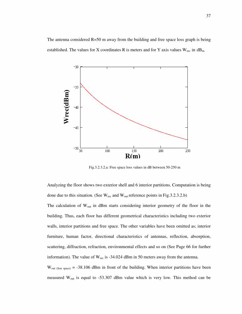
The antenna considered R=50 m away from the building and free space loss graph is being

established. The values for X coordinates R is meters and for Y axis values Wrec in dBm.

Fig.3.2.3.2.a: Free space loss values in dB between 50-250 m

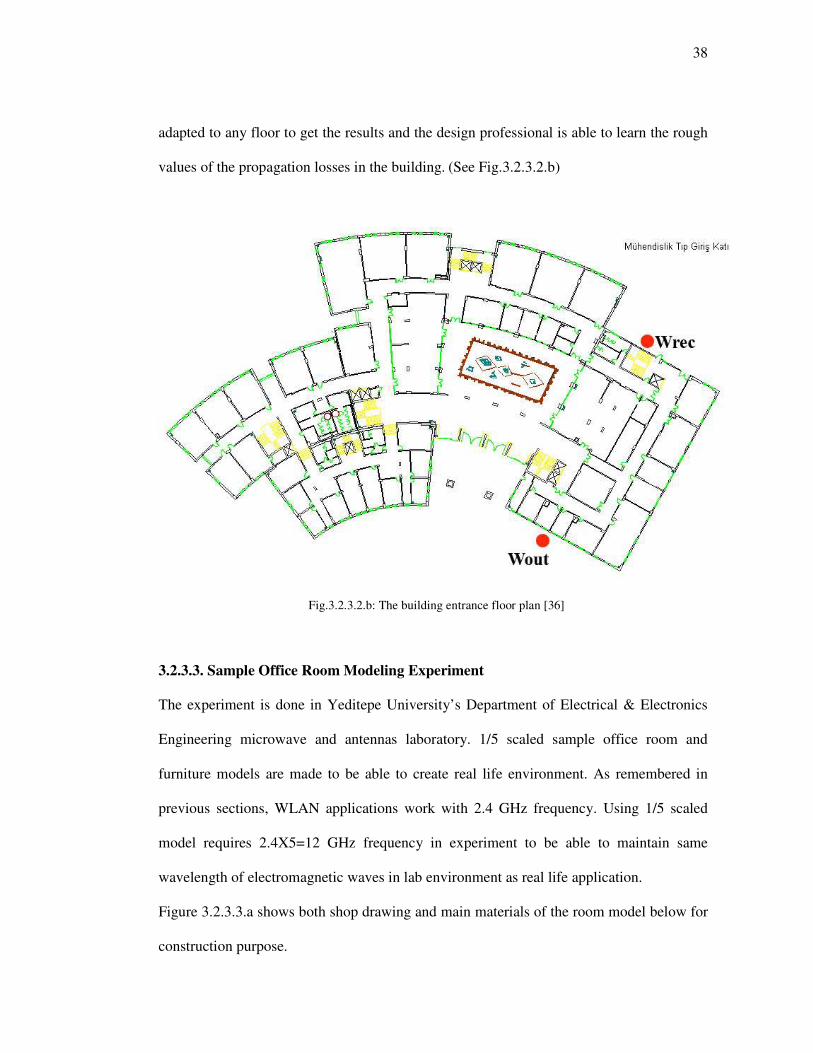
Analyzing the floor shows two exterior shell and 6 interior partitions. Computation is being

done due to this situation. (See Wrec and Wout reference points in Fig.3.2.3.2.b)

The calculation of Wout in dBm starts considering interior geometry of the floor in the

building. Thus, each floor has different geometrical characteristics including two exterior

walls, interior partitions and free space. The other variables have been omitted as; interior

furniture, human factor, directional characteristics of antennas, reflection, absorption,

scattering, diffraction, refraction, environmental effects and so on (See Page 66 for further

information). The value of Wrec is -34.024 dBm in 50 meters away from the antenna.

Wout (free space) = -38.106 dBm in front of the building. When interior partitions have been

measured Wout is equal to -53.307 dBm value which is very low. This method can be

38

adapted to any floor to get the results and the design professional is able to learn the rough

values of the propagation losses in the building. (See Fig.3.2.3.2.b)

Fig.3.2.3.2.b: The building entrance floor plan [36]

3.2.3.3. Sample Office Room Modeling Experiment

The experiment is done in Yeditepe University’s Department of Electrical & Electronics

Engineering microwave and antennas laboratory. 1/5 scaled sample office room and

furniture models are made to be able to create real life environment. As remembered in

previous sections, WLAN applications work with 2.4 GHz frequency. Using 1/5 scaled

model requires 2.4X5=12 GHz frequency in experiment to be able to maintain same

wavelength of electromagnetic waves in lab environment as real life application.

Figure 3.2.3.3.a shows both shop drawing and main materials of the room model below for

construction purpose.

39

Fig.3.2.3.3.a: Shop drawing for the 1/5 scaled experiment modeling

In addition to the main materials as seen above, silicone to connect the parts and aluminum

foil for window frame are being used. Fig.3.2.3.3.b shows main modeling materials as cut

OSB board (15 mm thickness) pieces and 30X30 cm ceramic granite tiles. This model is

designed as self standing object. (See Table 3.2.3.2.a for Relative Permittivities and Loss

Tangents and Table: 3.2.3.2.b Transmission and Reflection Coefficients of the materials)

When the parts assembled, the room stands still that makes it very modular and makes the

work practical in terms of measurement process. For two slabs, peeled copper wires are

modified as rebar grid. The distance between grids are 30 mm in 1/5 scale. Fig.3.2.3.3.c

shows creating rebar grids and connections for floor and ceiling of the room. Above this

level, ceramic granite tiles are oriented. (See Fig.3.2.3.3.d and Fig.3.2.3.3.e for completed

one unit)

40

Fig.3.2.3.3.b: Main modeling materials as cut OSB board pieces and ceramic granite tiles

Fig.3.2.3.3.c: Rebar grid installation for flooring and ceiling

41

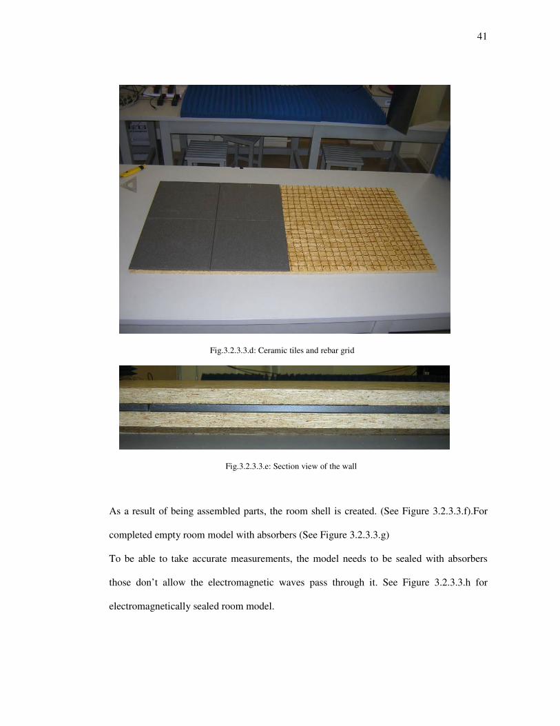
Fig.3.2.3.3.d: Ceramic tiles and rebar grid

Fig.3.2.3.3.e: Section view of the wall

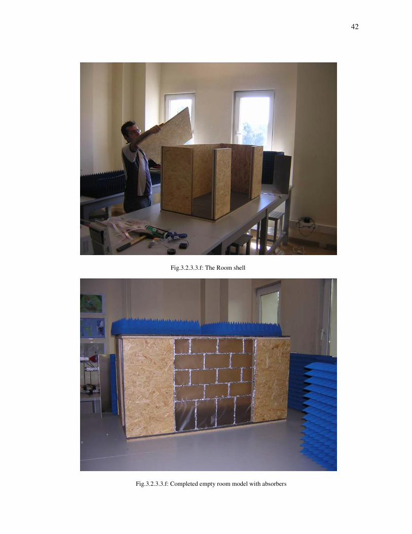
As a result of being assembled parts, the room shell is created. (See Figure 3.2.3.3.f).For

completed empty room model with absorbers (See Figure 3.2.3.3.g)

To be able to take accurate measurements, the model needs to be sealed with absorbers

those don’t allow the electromagnetic waves pass through it. See Figure 3.2.3.3.h for

electromagnetically sealed room model.

42

Fig.3.2.3.3.f: The Room shell

Fig.3.2.3.3.f: Completed empty room model with absorbers

43

Fig.3.2.3.3.h: Electromagnetically sealed room model

The other step is measurement for the experiment. Two antennas which are mini horn

(transmitter) and dipole (receiver) used to get the data of indoor electromagnetic

environment. (See Figure 3.2.3.3.j)

Figure 3.2.3.3.j: Left to Right Mini Horn and Dipole antennas

44

In addition to that, LD Gunn Power Supply with SWR Meter transfers the data which is

taken from receiver to the computer with an interface. This gadget works as a combo that

provides both power supply and measurement. The crucial point is how to transfer this

accurate data to the computer in this case. Cassy Lab software integrated with an interface

is connected to the LD test gadget using by USB port of the computer. This method is very

handy to take the very accurate measurement instead of writing the results from the scale

of the LD test equipment. See Figure 3.2.3.3.k for measurement process.

Fig. 3.2.3.3.k: Test equipment (from left to right desktop, the interface, and LD Power Supply&SWR meter)

45

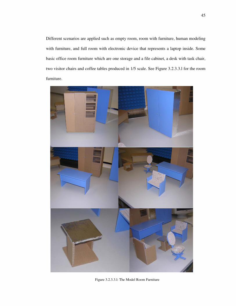
Different scenarios are applied such as empty room, room with furniture, human modeling

with furniture, and full room with electronic device that represents a laptop inside. Some

basic office room furniture which are one storage and a file cabinet, a desk with task chair,

two visitor chairs and coffee tables produced in 1/5 scale. See Figure 3.2.3.3.l for the room

furniture.

Figure 3.2.3.3.l: The Model Room Furniture

46

Human existence is also a variable for electromagnetic propagation in an environment. It is

known that conductivity of human body is in the range of 0.1-0.5 S/m for 2.4 GHz. [37]

Moreover, using sea water in proper percentage as 1/7 gives the fraction of human model.

Electrical conductivity of sea water starts from 1.7 to 6 S/m due to the temperature and

salinity of the sea. [38] Our percentage allows to produce the 32 cm height in 1/5 scale

human model.

The last piece of the model is laptop modeling for the experiment. A working digital clock

is put inside to the room to observe the changes of the EMW propagation. There are also

some letters such as; h = the height of transmitter antenna, z = the height of receiver

antenna, x and y refer to the coordinate system of the receiver.

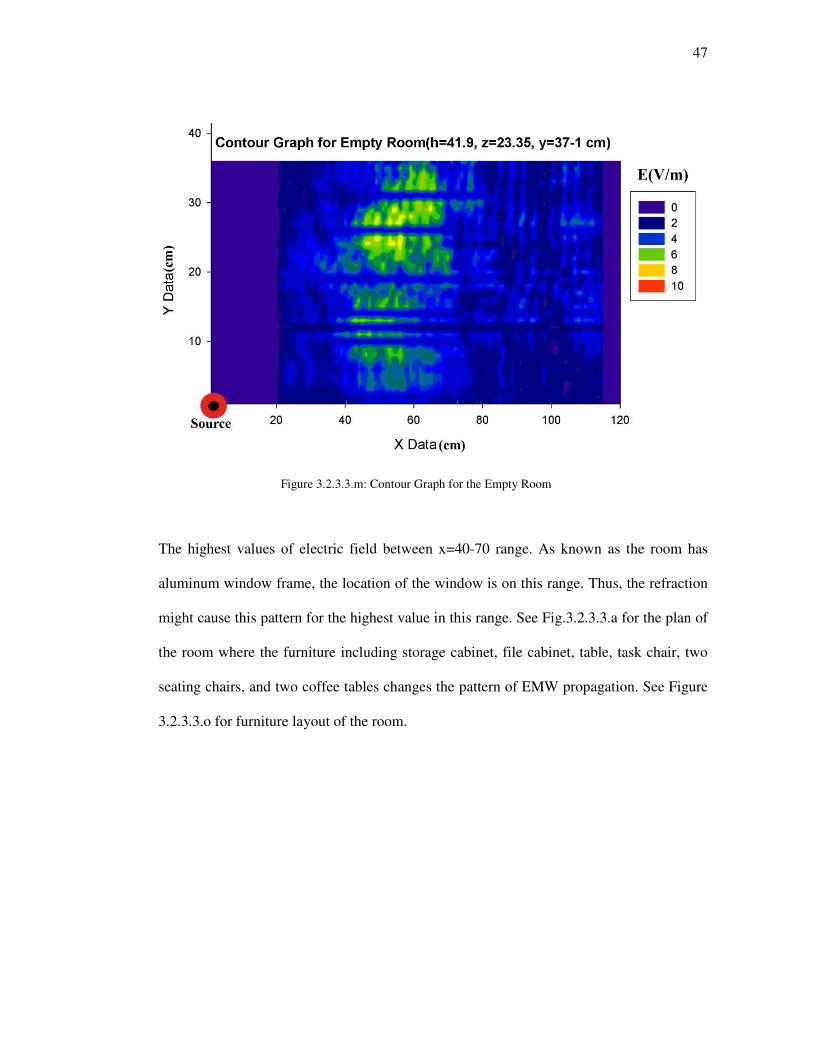
The first measurement is done for empty room by the h=41.9, z=23.35, x=21-115, y=37-1

coordinates. The polarization of the horn antenna is horizontal. Contour Graph for the

empty room clearly shows us the propagation of EMW. The scale (E) between 0-10 V/m.

(See Figure 3.2.3.3.m below)

47

Figure 3.2.3.3.m: Contour Graph for the Empty Room

The highest values of electric field between x=40-70 range. As known as the room has

aluminum window frame, the location of the window is on this range. Thus, the refraction

might cause this pattern for the highest value in this range. See Fig.3.2.3.3.a for the plan of

the room where the furniture including storage cabinet, file cabinet, table, task chair, two

seating chairs, and two coffee tables changes the pattern of EMW propagation. See Figure

3.2.3.3.o for furniture layout of the room.

48

Figure 3.2.3.3.n: Contour Graph for Room with Furniture

It is obviously seen that putting the furniture change the propagation pattern. In Figure

3.2.3.3.n, wider and stronger electric field is seen on the graph. Especially above seating

group and table areas has the level of 6-10 V/m values as seen on the graph. The nature of

the table made of dielectric material as laminated wood and seating group has the same

specialty. The coffee table has an aluminum top. Thus, this must boost the value. In this

study, just electric field has been considered, the other issues which are mentioned in

previous chapters as Electromagnetic Compability or Interference need to work on

separately.

49

Figure 3.2.3.3.o: Furniture layout of the room (Not in Scale)

Changing the height of transmitter antenna as h=29 cm comes out very accurate

measurement due to the closeness of the receiver. Moreover, highest peak values are also

seen in that session. Figure 3.2.3.3.p Empty Room Contour Graph explains the

electromagnetic propagation pattern in visual form. The pattern is wider and stronger in

this case. In the graph, the direction of the horn antenna reflection is seen and makes the

propagation area so wide and strong.

50

Figure 3.2.3.3.p: Contour Graph for Empty Room

Figure 3.2.3.3.r: Contour Graph for Room with Furniture

51

In all cases up to now prove for the Room EMW propagations with Furniture that have

higher values than empty room configurations. The pattern in Figure 3.2.3.3.r is wider and

stronger comparing with the previous one.

Another configuration for the transmitter (horn) antenna is vertical polarization. The

receiver antenna (dipole) is mismatched and data has been measured. See Figure 3.2.3.3.s

for both empty and room with furniture layout.

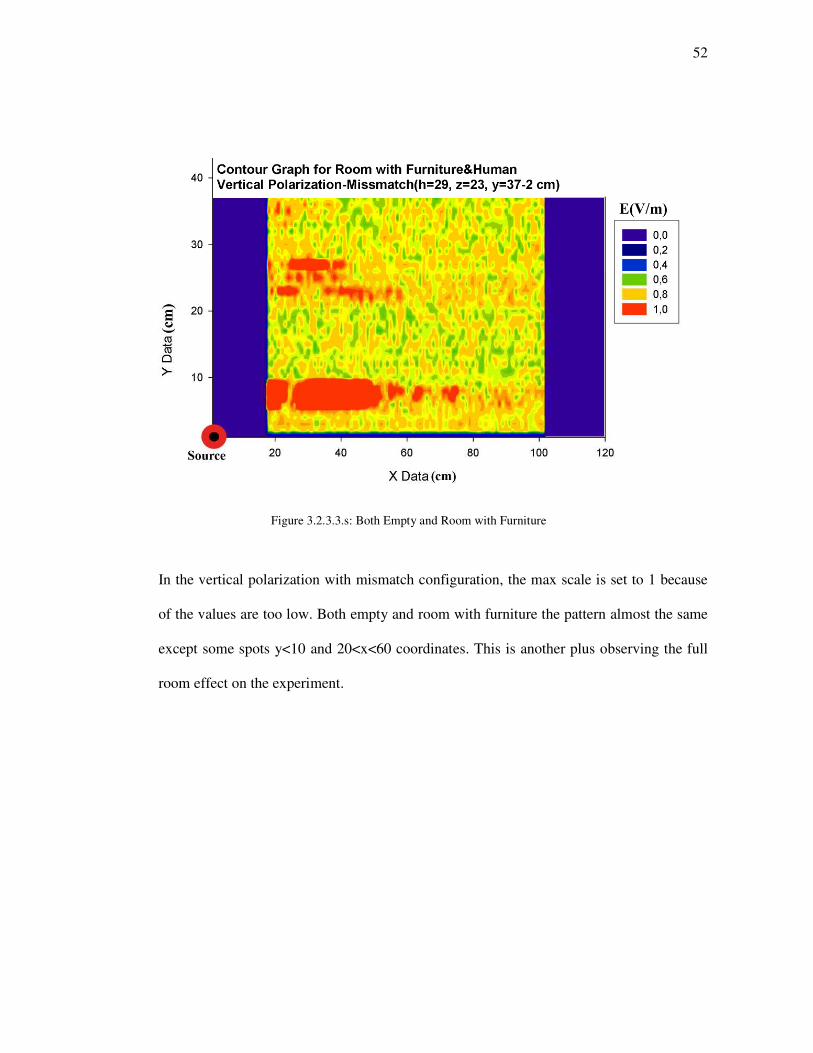
Figure 3.2.3.3.s: Both Empty and Room with Furniture (See page 51)

52

Figure 3.2.3.3.s: Both Empty and Room with Furniture

In the vertical polarization with mismatch configuration, the max scale is set to 1 because

of the values are too low. Both empty and room with furniture the pattern almost the same

except some spots y<10 and 20<x<60 coordinates. This is another plus observing the full

room effect on the experiment.

53

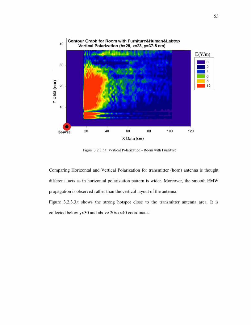
Figure 3.2.3.3.t: Vertical Polarization - Room with Furniture

Comparing Horizontal and Vertical Polarization for transmitter (horn) antenna is thought

different facts as in horizontal polarization pattern is wider. Moreover, the smooth EMW

propagation is observed rather than the vertical layout of the antenna.

Figure 3.2.3.3.t shows the strong hotspot close to the transmitter antenna area. It is

collected below y<30 and above 20<x<40 coordinates.

54

Figure 3.2.3.3.u: Vertical Polarization - Room with Furniture & Grounded

Grounded room brings the result of one hot spot which reduces its value till the end of the

room. Between 20<x<40, it has its maximum range over 10 V/m. All surfaces of are

grounded. Thus, the room responses as Faraday cage which is an ideal hollow conductor.

Instead of refraction of excess charges on the outer face, they go to the ground. That makes

the room remain neutral. Besides the hotspot, the rest of the areas values around 2 V/m.

And comparing with the Figure 3.2.3.3.t proves totally different pattern on the grounded

room.

Application of this feature in architecture helps to use cordless phones and wireless

networks inside buildings and houses in different cases. On the other hand, this feature is

very vital for some buildings which require total security mitigation against

electromagnetic pulse.

55

Figure 3.2.3.3.v: Contour Graph for Empty Room

Locating of the transmitter (mini horn) to below level of the receiver (dipole) antenna

carries different patterns seen in Figure 3.2.3.3.v, Figure 3.2.3.3.y and Figure 3.2.3.3.z.

The hot spot in Figure 3.2.3.3.v close to the transmitter antenna as expected. Adding the

furniture and human model distribute the hot spot till x<80 cm.

56

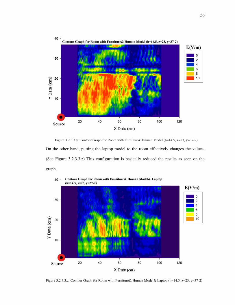
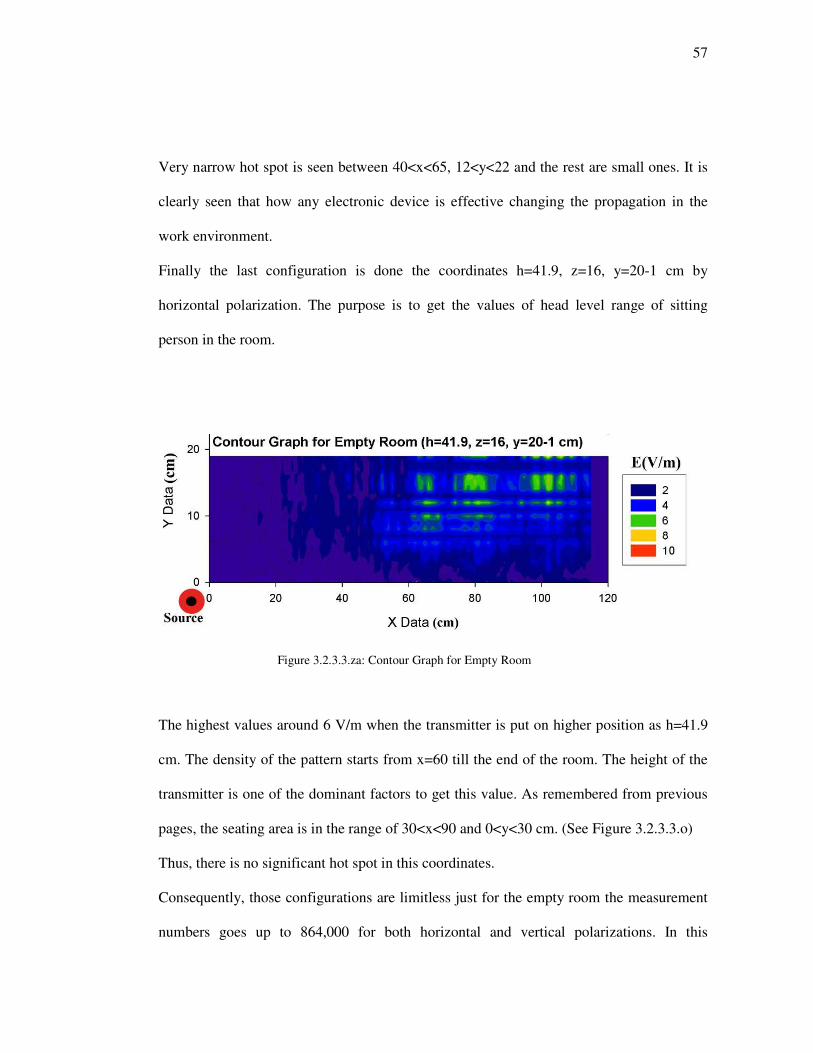
Figure 3.2.3.3.y: Contour Graph for Room with Furniture& Human Model (h=14.5, z=23, y=37-2)

On the other hand, putting the laptop model to the room effectively changes the values.

(See Figure 3.2.3.3.z) This configuration is basically reduced the results as seen on the

graph.

Figure 3.2.3.3.z: Contour Graph for Room with Furniture& Human Model& Laptop (h=14.5, z=23, y=37-2)

57

Very narrow hot spot is seen between 40<x<65, 12<y<22 and the rest are small ones. It is

clearly seen that how any electronic device is effective changing the propagation in the

work environment.

Finally the last configuration is done the coordinates h=41.9, z=16, y=20-1 cm by

horizontal polarization. The purpose is to get the values of head level range of sitting

person in the room.

Figure 3.2.3.3.za: Contour Graph for Empty Room

The highest values around 6 V/m when the transmitter is put on higher position as h=41.9

cm. The density of the pattern starts from x=60 till the end of the room. The height of the

transmitter is one of the dominant factors to get this value. As remembered from previous

pages, the seating area is in the range of 30<x<90 and 0<y<30 cm. (See Figure 3.2.3.3.o)

Thus, there is no significant hot spot in this coordinates.

Consequently, those configurations are limitless just for the empty room the measurement

numbers goes up to 864,000 for both horizontal and vertical polarizations. In this

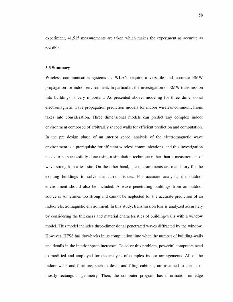
58

experiment, 41,515 measurements are taken which makes the experiment as accurate as

possible.

3.3 Summary

Wireless communication systems as WLAN require a versatile and accurate EMW

propagation for indoor environment. In particular, the investigation of EMW transmission

into buildings is very important. As presented above, modeling for three dimensional

electromagnetic wave propagation prediction models for indoor wireless communications

takes into consideration. Three dimensional models can predict any complex indoor

environment composed of arbitrarily shaped walls for efficient prediction and computation.

In the pre design phase of an interior space, analysis of the electromagnetic wave

environment is a prerequisite for efficient wireless communications, and this investigation

needs to be successfully done using a simulation technique rather than a measurement of

wave strength in a test site. On the other hand, site measurements are mandatory for the

existing buildings to solve the current issues. For accurate analysis, the outdoor

environment should also be included. A wave penetrating buildings from an outdoor

source is sometimes too strong and cannot be neglected for the accurate prediction of an

indoor electromagnetic environment. In this study, transmission loss is analyzed accurately

by considering the thickness and material characteristics of building-walls with a window

model. This model includes three-dimensional penetrated waves diffracted by the window.

However, HFSS has drawbacks in its computation time when the number of building-walls

and details in the interior space increases. To solve this problem, powerful computers need

to modified and employed for the analysis of complex indoor arrangements. All of the

indoor walls and furniture, such as desks and filing cabinets, are assumed to consist of

mostly rectangular geometry. Then, the computer program has information on edge

59

coordinates and material composition. The material characteristics of walls are usually

represented by permittivity and conductivity, and reflection and diffraction coefficients are

computed using those parameters. These coefficients are stored for each wall with its

coordinate as input variables for the computer program. Figure 3.2.2.4 shows the indoor

model used for the computer program, which consists of walls, doors, and windows for a

sample office environment. Walls in the Figure have thickness, and the characteristics of

penetrated waves through the walls are analyzed using the simulation program. Figure

3.2.2.4 also shows the way to compare the results. The material of the inside wall to face

the passage is a concrete wall containing a door made with aluminum. The outside wall

contains windows. This model considers building transmission loss for an accurate

prediction in the case where the antenna is located in three different locations. As a result,

computer aided design software is expected to be used for the design of wireless networks

in pico-cells more effectively in near future.

The other achievement is the prediction of propagation losses. With this method, the

design professional can predict rough propagation losses for either pre design status or

existing building in case of the need.

The last step is the experiment process before making spectrum analysis on the site for

total survey of any environment. Following the steps are vital to be able to go deep in

issues mentioned in previous chapters and finding to solve the problems. The experiment

results give very accurate values to be able to understand EMW propagation in the closed

spaces such as, how the furniture, polarization, location of the transmitter and receiver

antennas and human being affect it.

60

CHAPTER 4

4. Conclusions

Technology is evolving. Thus, what should be done? Adapting the buildings to the

technology or adapting the technology to the buildings. Actually, for the performance

improvements, the designer needs to know and consider the bond of electromagnetic

waves and building materials well. Unfortunately, this interdisciplinary topic has not been

able to underline by the architecture society yet. To solve EMW related design problems,

the first step is trying to reach theoretical solutions by using propagation models for

prediction. Thus, there is an ongoing need for the solution of basic electromagnetic

problems. There are lots of variables such as; type of building materials, frequency,

environmental effects, design geometry and more. For the different scenarios and multiple

conditions, new prediction models might need to permit rapid evaluation compared to

brute-force numerical techniques and allow predictions to be able to get the accurate

results. Moreover, experimentations also need to be done in laboratories as second step.

Real-time channel predictions support both theoretical predictions and measurements.

Another crucial aspect is anechoic chambers which are basically constructed as shielded

rooms. All over the walls and the ceiling, absorbing materials and/or ferrite tiles are

attached for EMW free environment. Moreover, anechoic chambers show superb shielding

performance and are mainly applied in EM emission testing according to commercial and

military standards. [44] Thus, for the real time experiments, it is a must to have one. As if,

surgeon cannot do his surgery in the street, this type of research cannot be done without the

chamber. Thus, the following results need to be underlined for future studies about EMW

propagation related issues in architecture field:

1. WLAN require a versatile and accurate EMW propagation for indoor environment.

61

2. The investigation of EMW transmission into buildings is very important for design

professionals so that they can understand propagation needs of the structures.

3. Three dimensional models can predict any complex indoor environment composed

of arbitrarily shaped walls for efficient prediction and computation.

4. HFSS has drawbacks in its computation time when the number of building-walls

and details in the interior space increases. To solve this problem, powerful

computers need to modified and employed for the analysis of complex indoor

arrangements.

5. The experiment results give very accurate values to be able to understand EMW

propagation in the closed spaces such as, how the furniture, polarization, location

of the transmitter and receiver antennas and human being affect it.

Lastly, this research is focused on 2.4 GHz which is used in most of country’s WLAN

frequency because of today’s standard but it can be adapted to any frequency range to

analyze the building materials and set the codes for the buildings of future. In addition, this

research covers all both gives the idea of the future of wireless local area networking and

the effect of architectural forms and design.

62

APPENDIX A:

Building Materials and EMW (Electromagnetic Wave) bond

Due to the NIST (The United States Department of Commerce Technology Administration

National Institute of Standards and Technology) research which is called Electromagnetic

Signal Attenuation in Construction Materials Report October 1997 Number 3 , The main

building materials and combinations are analyzed below as; Brick, Masonry Block, Plain

Concrete, Reinforced Concrete and Rebar Grid, Glass, Lumber ( dry and wet), Plywood

(dry and wet), Drywall, Brick-Faced Concrete Wall, Brick-Faced Masonry Block, various

Plain Concrete Mixtures and Rebar Grid.

A.1 Brick

The red clay brick is widely used material in both residential and commercial building

construction. Figure A.1.a shows three different brick wall thickness configuration used in

NIST experiment. Moreover, 1x1 meter single Wythe brick walls were fabricated for

convenience.

63

Figure A.1.a: Brick wall geometries. Top to Bottom: single Wythe, double Wythe, triple Wythe construction. (C. Stone, William, October 1997 p. 32)

A.1.1 Response data for Brick

In this study, both low and high frequency ranges (0.5-2.0 GHz / 3.0-8.0 GHz) response of

the building materials` spectra results are being analyzed. Moreover, figures are showed

below for each material. Thus, transmission coefficient (decimal) ranges 1 to 0 that means

full transmission of the electromagnetic wave or full attenuation includes absorption or

reflection of the waves.

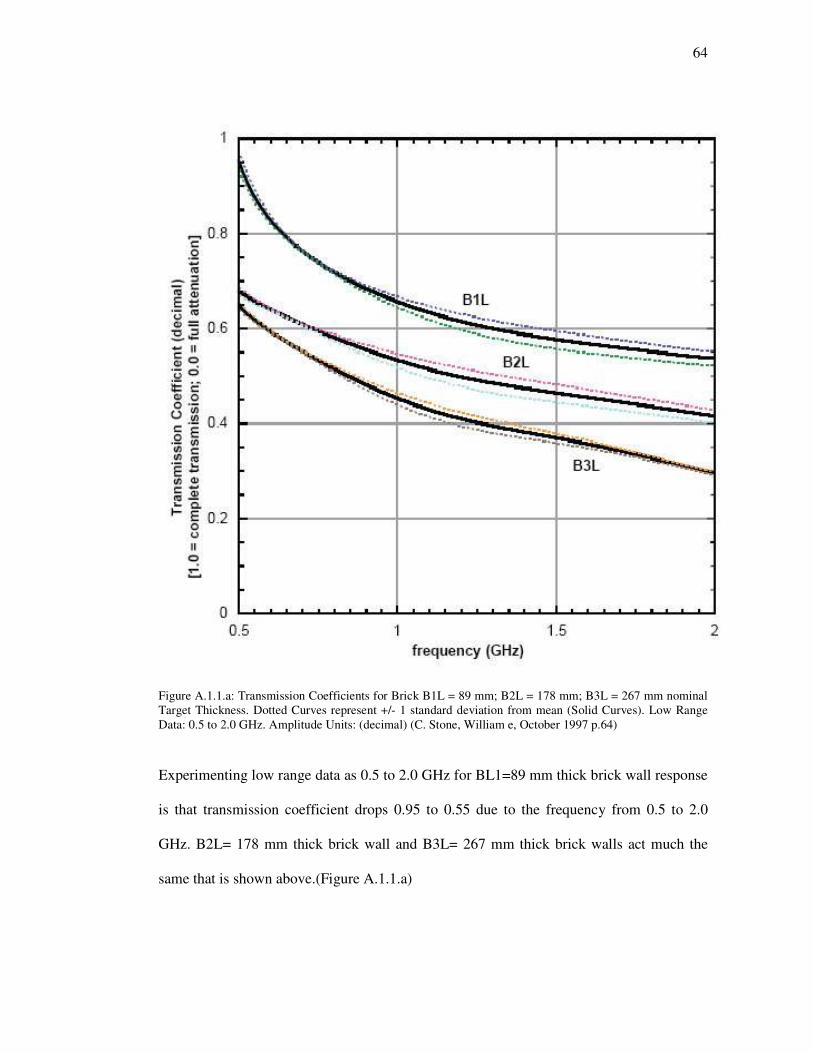
64

Figure A.1.1.a: Transmission Coefficients for Brick B1L = 89 mm; B2L = 178 mm; B3L = 267 mm nominal Target Thickness. Dotted Curves represent +/- 1 standard deviation from mean (Solid Curves). Low Range Data: 0.5 to 2.0 GHz. Amplitude Units: (decimal) (C. Stone, William e, October 1997 p.64)

Experimenting low range data as 0.5 to 2.0 GHz for BL1=89 mm thick brick wall response

is that transmission coefficient drops 0.95 to 0.55 due to the frequency from 0.5 to 2.0

GHz. B2L= 178 mm thick brick wall and B3L= 267 mm thick brick walls act much the

same that is shown above.(Figure A.1.1.a)

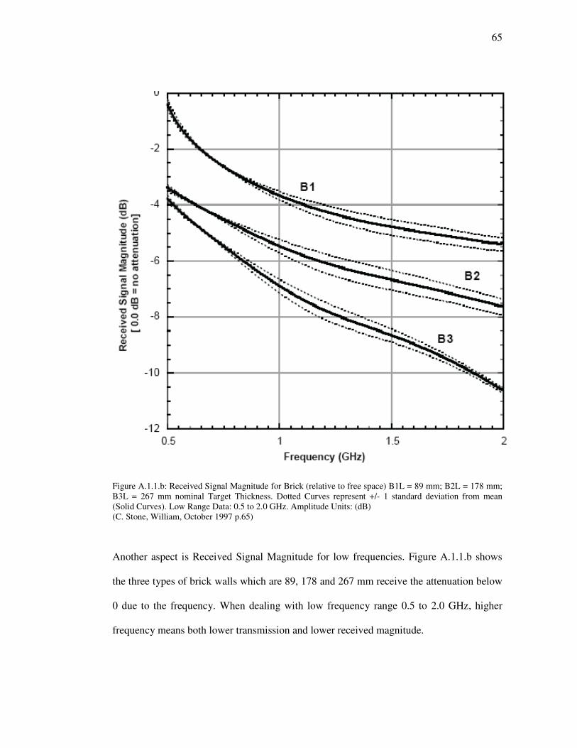
65

Figure A.1.1.b: Received Signal Magnitude for Brick (relative to free space) B1L = 89 mm; B2L = 178 mm; B3L = 267 mm nominal Target Thickness. Dotted Curves represent +/- 1 standard deviation from mean (Solid Curves). Low Range Data: 0.5 to 2.0 GHz. Amplitude Units: (dB) (C. Stone, William, October 1997 p.65)

Another aspect is Received Signal Magnitude for low frequencies. Figure A.1.1.b shows

the three types of brick walls which are 89, 178 and 267 mm receive the attenuation below

0 due to the frequency. When dealing with low frequency range 0.5 to 2.0 GHz, higher

frequency means both lower transmission and lower received magnitude.

66

Figure A.1.1.c: Transmission Coefficients for Brick B1L = 89 mm; B2L = 178 mm; B3L = 267 mm nominal Target Thickness. Dotted Curves represent +/- 1 standard deviation from mean (Solid Curves). High Range Data: 3.0-8.0 GHz. Amplitude Units: (decimal) (C. Stone, William, October 1997 p.66)

Comparing with the lower frequency range, higher frequency from 3.GHz to 8 GHz has

lower transmission of electromagnetic waves. The all types of brick walls have the

transmission below 0.2 that means loosing more than 80 percentage of the signal power.

B1L=89 mm thick brick wall acts almost stable to the frequency changes but the other

brick walls respond in very unsettled to the frequency changes. (Figure A.1.1.c)

67

Figure A.1.1.d: Received Signal Magnitude for Brick (relative to free space) B1L = 89 mm; B2L = 178 mm; B3L = 267 mm nominal Target Thickness. Dotted Curves represent +/- 1 standard deviation from mean (Solid Curves). High Range Data: 3.0-8.0 GHz. Amplitude Units: (dB) (C. Stone, William, October 1997 p.67)

The reflection of the transmission behaviors are the same in received signal magnitude as

89 mm brick wall and the others above mentioned. All of the walls have below -10 (db) in

high frequencies. (Figure A.1.1.d)

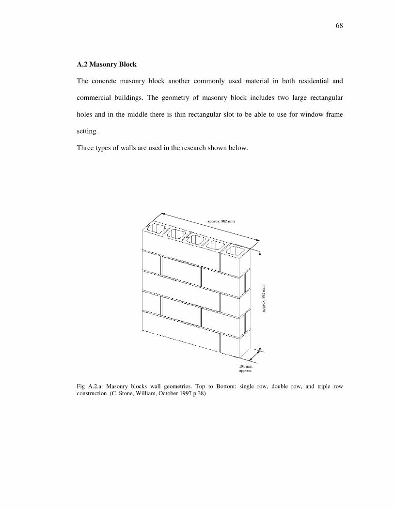
68

A.2 Masonry Block

The concrete masonry block another commonly used material in both residential and

commercial buildings. The geometry of masonry block includes two large rectangular

holes and in the middle there is thin rectangular slot to be able to use for window frame

setting.

Three types of walls are used in the research shown below.

Fig A.2.a: Masonry blocks wall geometries. Top to Bottom: single row, double row, and triple row construction. (C. Stone, William, October 1997 p.38)

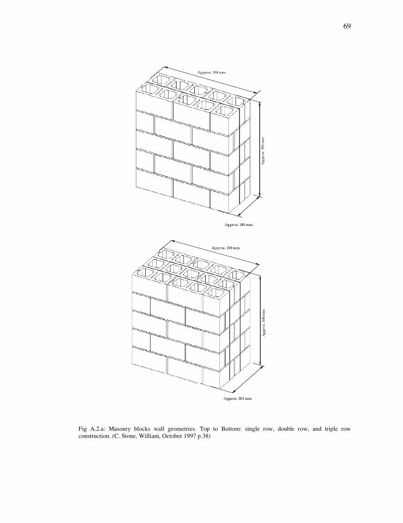
69

Fig A.2.a: Masonry blocks wall geometries. Top to Bottom: single row, double row, and triple row construction. (C. Stone, William, October 1997 p.38)

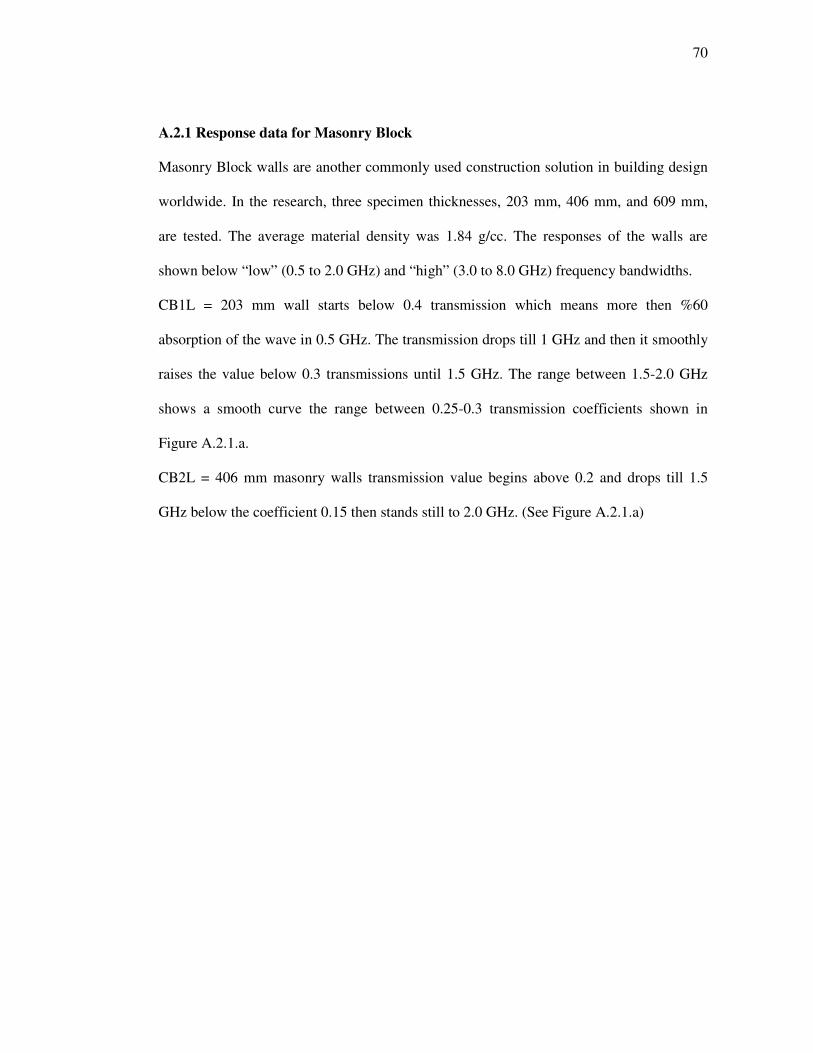
70

A.2.1 Response data for Masonry Block

Masonry Block walls are another commonly used construction solution in building design

worldwide. In the research, three specimen thicknesses, 203 mm, 406 mm, and 609 mm,

are tested. The average material density was 1.84 g/cc. The responses of the walls are

shown below “low” (0.5 to 2.0 GHz) and “high” (3.0 to 8.0 GHz) frequency bandwidths.

CB1L = 203 mm wall starts below 0.4 transmission which means more then %60

absorption of the wave in 0.5 GHz. The transmission drops till 1 GHz and then it smoothly

raises the value below 0.3 transmissions until 1.5 GHz. The range between 1.5-2.0 GHz

shows a smooth curve the range between 0.25-0.3 transmission coefficients shown in

Figure A.2.1.a.

CB2L = 406 mm masonry walls transmission value begins above 0.2 and drops till 1.5

GHz below the coefficient 0.15 then stands still to 2.0 GHz. (See Figure A.2.1.a)

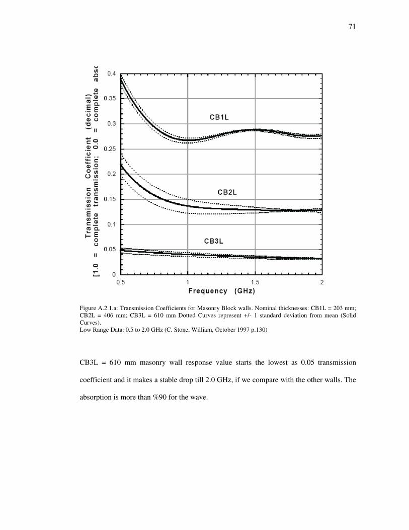
71

Figure A.2.1.a: Transmission Coefficients for Masonry Block walls. Nominal thicknesses: CB1L = 203 mm; CB2L = 406 mm; CB3L = 610 mm Dotted Curves represent +/- 1 standard deviation from mean (Solid Curves). Low Range Data: 0.5 to 2.0 GHz (C. Stone, William, October 1997 p.130)

CB3L = 610 mm masonry wall response value starts the lowest as 0.05 transmission

coefficient and it makes a stable drop till 2.0 GHz, if we compare with the other walls. The

absorption is more than %90 for the wave.

72

Figure A.2.1.b: Received Signal Magnitude (dB) for Masonry Block Walls. Nominal thicknesses: CB1L = 203 mm; CB2L = 406 mm; CB3L = 610 mm Dotted Curves represent +/- 1 standard deviation from mean (Solid Curves). Low Range Data: 0.5 to 2.0 GHz (C. Stone, William, October 1997 p.131)

The responses of Received Signal Magnitude for the walls (CB1L = 203 mm; CB2L = 406

mm; CB3L = 610 mm) are like the reflection of transmission coefficients geometry shown

in Figure A.2.1.b.

73

Figure A.2.1.c: Transmission Coefficients for Masonry Block walls. Nominal thicknesses: CB1H = 203 mm; CB2H = 406 mm; CB3H = 610 mm Dotted Curves represent +/- 1 standard deviation from mean (Solid Curves). High Range Data: 3.0 to 8.0 GHz (C. Stone, William, October 1997 p.132)

Higher frequencies (3.0 to 8.0 GHz) are unstable responses for CB2H = 406 mm; CB3H =

610 mm masonry walls. On the other hand, CB1H = 203 mm wall value begins between

0.15- 0.2 transmission coefficient in 3.0 GHz frequency and decreases smoothly below

0.15 in 8.0 GHz shown in Figure A.2.1.c.

74

Figure A.2.1.d: Received Signal Magnitude (dB) for Masonry Block Walls. Nominal thicknesses: CB1H = 203 mm; CB2H = 406 mm; CB3H = 610 mm Dotted Curves represent +/- 1 standard deviation from mean (Solid Curves). High Range Data: 3.0 to 8.0 GHz (C. Stone, William, October 1997 p.133)

Similar type of behavior of the waves on high range data (3.0 to 8.0 GHz) is seen in Figure

2.3.2.1d. CB1H = 203 mm masonry block is stable then the others (CB2H = 406 mm;

CB3H = 610 mm).

75

A.3 Plain Concrete

Plain concrete has different variables such as; geometry, thickness, aggregate size,

water/cement ratio, and slump. Three main form is beings used to experiment the material

in NIST research.

Figure: A.3.a: Plain concrete specimen geometry. (C. Stone, William, October 1997 p.42)

A.3.1 Response data for Plain Concrete

Different batch concrete specimens are used for the research. The first one have an

approximate water cement ratio of 0.4, a slump of 57 mm, a nominal maximum crushed

aggregate size of 12.7 mm, a cement content by weight of 22% and an average density of

2.31 g/cc.

76

Fig. A.3.1.a: Transmission Coefficients for Concrete Type 1 walls. Nominal thicknesses: C14L = 102 mm; C18L = 203 mm; C112L = 305 mm Dotted Curves represent +/- 1 standard deviation from mean (Solid Curves). Low Range Data: 0.5 to 2.0 GHz (C. Stone, William, October 1997 p.82)

Transmission for C14L = 102 mm type concrete wall value initiates above 0.3 then it

decreases to below 0.2 in 2.0 GHz. Secondly, C18L = 203 mm concrete wall

approximately establish the response 0.1 in 0.5 GHz frequency almost absorbing %90 of

the waves and drops below 0.05 in 2.0 GHz. Finally, C112L = 305 mm wall responses

more stable starting like 0.025 transmission coefficient and ends above 0.020 in 2.0 GHz

frequency. (See Fig. A.3.1.a)

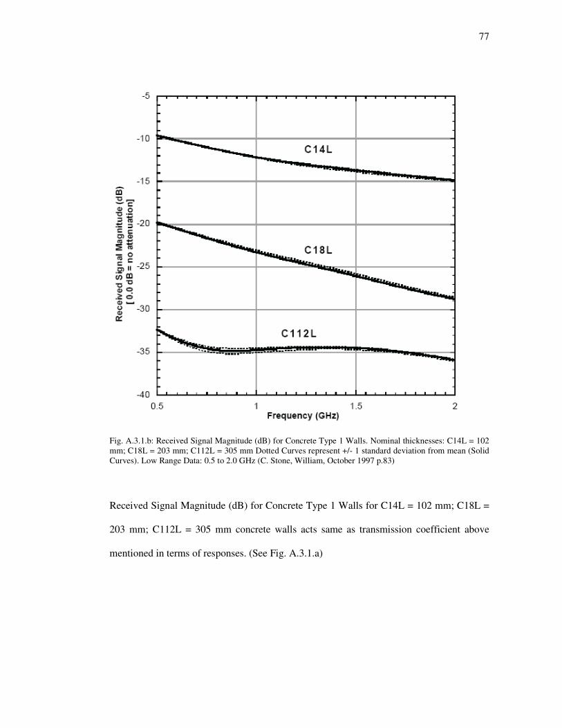
77

Fig. A.3.1.b: Received Signal Magnitude (dB) for Concrete Type 1 Walls. Nominal thicknesses: C14L = 102 mm; C18L = 203 mm; C112L = 305 mm Dotted Curves represent +/- 1 standard deviation from mean (Solid Curves). Low Range Data: 0.5 to 2.0 GHz (C. Stone, William, October 1997 p.83)

Received Signal Magnitude (dB) for Concrete Type 1 Walls for C14L = 102 mm; C18L =

203 mm; C112L = 305 mm concrete walls acts same as transmission coefficient above

mentioned in terms of responses. (See Fig. A.3.1.a)

78

Fig. A.3.1.c: Transmission Coefficients for Concrete Type 1 walls. Nominal thicknesses: C14H = 102 mm; C18H = 203 mm; C112H = 305 mm Dotted Curves represent +/- 1 standard deviation from mean (Solid Curves). High Range Data: 3.0 to 8.0 GHz (C. Stone, William, October 1997 p.84)

Higher frequency response for C14H = 102 mm is different than lower frequencies of the

same wall as increasing transmission between 3.0- 4.8 GHz frequencies. The other type

concrete walls (C18H = 203 mm; C112H = 305 mm) have dramatic transmission loss

below 0.01 till almost complete absorption in 8.0 GHz frequency. (See Fig. A.3.1.c)

79

Fig. A.3.1.d: Received Signal Magnitude (dB) for Concrete Type 1 Walls. Nominal thicknesses: C14H = 102 mm; C18H = 203 mm; C112H = 305 mm Dotted Curves represent +/- 1 standard deviation from mean (Solid Curves). High Range Data: 3.0 to 8.0 GHz (C. Stone, William, October 1997 p.85)

Received Signal Magnitude range for C14H = 102 mm, C18H = 203 mm and C112H =

305 mm concrete walls are -30 to -20 db, -58 to -46 and -90 to -74 db between high range

frequencies shown in Fig. 3.1.d.

80

A.4 Reinforced Concrete and Rebar Grid

Two type of concrete and rebar grid combination is used in the research shown above. The

first one has 140 mm square grid and the second has 70 mm square grid with 203 mm

concrete thickness.

Fig. A.4.a: Reinforced concrete, nominally 203 mm thick with 140 mm square grid rebar. (C. Stone, William, October 1997 p.47-48)

Fig. A.4.b: Reinforced concrete, nominally 203 mm thick with 70 mm square grid rebar. (C. Stone, William, October 1997 p.47-48)

81

A.4.1 Response data for Reinforced Concrete

Fig. A.4.1.a: Transmission Coefficients for Reinforced Concrete Walls (relative to free space). Nominal thicknesses: All Specimens are 203 mm Thick. Low Range Data: 0.5 to 2.0 GHz C88L = Unreinforced Reference; RC881L = 1% Steel; RC882L = 2% Steel Dotted Curves represent +/- 1 standard deviation from mean (Solid Curves). (C. Stone, William, October 1997 p.172)

Same thickness for all specimens is used with different percentage of steel as unreinforced

1%, 2%. The three curves from unreinforced concrete to 2% steel included shows a smooth

drop. RC881L = 1% Steel concrete value stops approximately 0.018 in 2 GHz and

RC882L = 2% Steel concrete value keeps close to 0.015 value in 2 GHz frequency.

82

Surprisingly, C88L = Unreinforced concrete value is between two reinforced concrete

sample but close to the RC882L in value at the same frequency. (See Fig. A.4.1.a)

Fig. A.4.1.b: Received Signal Magnitude (dB) for Reinforced Concrete Walls (relative to free space). All Specimens are 203 mm Thick. Low Range Data: 0.5 to 2.0 GHz C88L = Unreinforced Reference; RC881L = 1% Steel; RC882L = 2% Steel Dotted Curves represent +/- 1 standard deviation from mean (Solid Curves). (C. Stone, William, October 1997 p.173)

Received Signal Magnitude (dB) figure for Reinforced Concrete Walls has the similar type

of response in terms of geometrical form. (See Fig. A.4.1.b)

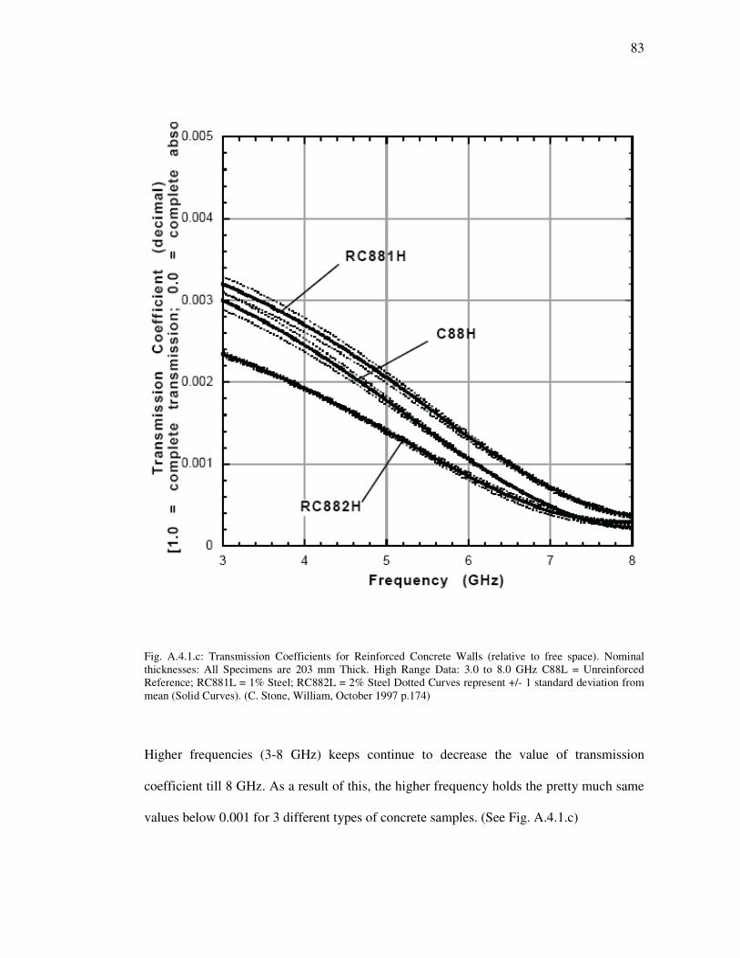
83

Fig. A.4.1.c: Transmission Coefficients for Reinforced Concrete Walls (relative to free space). Nominal thicknesses: All Specimens are 203 mm Thick. High Range Data: 3.0 to 8.0 GHz C88L = Unreinforced Reference; RC881L = 1% Steel; RC882L = 2% Steel Dotted Curves represent +/- 1 standard deviation from mean (Solid Curves). (C. Stone, William, October 1997 p.174)

Higher frequencies (3-8 GHz) keeps continue to decrease the value of transmission

coefficient till 8 GHz. As a result of this, the higher frequency holds the pretty much same

values below 0.001 for 3 different types of concrete samples. (See Fig. A.4.1.c)

84

Fig. A.4.1.d: Received Signal Magnitude (dB) for Reinforced Concrete Walls (relative to free space). All Specimens are 203 mm Thick. High Range Data: 3.0 to 8.0 GHz. C88L = Unreinforced Reference; RC881L = 1% Steel; RC882L = 2% Steel Dotted Curves represent +/- 1 standard deviation from mean (Solid Curves). (C. Stone, William, October 1997 p.175)

Received Signal Magnitude (dB) for Reinforced Concrete Walls in higher frequencies

starts with similar response as transmission coefficient but ends a bit different not very

close value in 8 GHz frequency. (Fig. A.4.1.d)

85

A.5 Glass

NIST study uses ordinary architectural window glass that made of soda-lime silica float

glass with the dimension shown above.

Fig. A.5.a: Glass panel specimens used in the NIST study. (C. Stone, William, October 1997 p.49)

A.5.1 Response data for Glass

Fig. 2.3.5.1 a shows one of the best transmission coefficiency value comparing with the

other building materials. G25L = 6 mm thick glass starts almost complete transmission and

ends to close to 0.85 value in 2 GHz. G50L = 13 mm and G75L = 19 mm thick glasses also

begins higher transmission end ends satisfactory responses in lower frequencies.

86

Fig. A.5.1.a: Transmission Coefficients for Glass Panels (relative to free space). Nominal thicknesses: G25L = 6 mm; G50L = 13 mm; G75L = 19 mm Dotted Curves represent +/- 1 standard deviation from mean (Solid Curves). Low Range Data: 0.5 to 2.0 GHz (C. Stone, William, October 1997 p.142)

The curves of the three glass panels are almost similar. They all smoothly drop till 2 GHz

frequency. (See Fig. A.5.1.a)

Received Signal Magnitude (dB) for Glass Panels in lower frequencies illustrate parallel

responses in geometrical form as it is expected. (Fig. A.5.1.b)

87

Fig. A.5.1.b: Received Signal Magnitude (dB) for Glass Panels (relative to free space). G25L = 6 mm; G50L = 13 mm; G75L = 19 mm Dotted Curves represent +/- 1 standard deviation from mean (Solid Curves). Low Range Data: 0.5 to 2.0 GHz (C. Stone, William, October 1997 p.143)

In contrast, G25H= 6 mm, G50H = 13 mm and G75H = 19 mm thickness glass panels

response totally different if we compare with the lower responses in higher frequencies (3-

8 GHz). G50H = 13 mm glass panel commence below 0.95 transmission in 3 GHz

frequency and continue to increase it value approximately 4.5 GHz frequency close to

complete transmission rate.

88

Fig. A.5.1.c: Transmission Coefficients for Glass Panels (relative to free space). Nominal thicknesses: G25H = 6 mm; G50H = 13 mm; G75H = 19 mm Dotted Curves represent +/- 1 standard deviation from mean (Solid Curves). High Range Data: 3.0 to 8.0 GHz (C. Stone, William, October 1997 p.144)

Above 5 GHz, the transmission value decreases till 8 GHz for G25H = 6 mm glass panel.

The other two acts like related response to the electromagnetic waves but in term of

frequency range changes. They both G75H = 19 mm and G25H = 6 glass panels get their

peak transmission value between 5-6 GHz frequencies. Above these frequencies till 8 GHz,

they all continue to decrease their charges. (See Fig. A.5.1.c)

89

Fig. A.5.1.d: Received Signal Magnitude (dB) for Glass Panels (relative to free space). G25H = 6 mm; G50H = 13 mm; G75H = 19 mm Dotted Curves represent +/- 1 standard deviation from mean (Solid Curves). High Range Data: 3.0 to 8.0 GHz (C. Stone, William, October 1997 p.145)

Received Signal Magnitude (dB) for Glass Panels is the likeness of the transmission

coefficient form in higher frequencies. (Fig. A.5.1.d)

A.6 Lumber

In terms of commercial lumber species, Spruce-Pine-Fir; Douglas Fir-Larch; Hemlock-Fir,

and Southern Pine are used in the research. Those species grow up in North America but

the experimentation results help us to understand Lumber-EMW relation and show a path

in design process in architecture. Both dry and wet specimens tested. Combinations and

dimensions of frames are shown below.

90

Fig. A.6.a: A single layer built-up lumber specimen consisting of three planks mounted on exterior frame. (C. Stone, William, October 1997 p.53)

Fig. A.6.b: A double layer built-up lumber specimen consisting of six planks. (C. Stone, William, October 1997 p.53)

91

Fig. A.6.c: A triple layer built-up lumber specimen consisting of nine studs. (C. Stone, William, October 1997 p.54)

Fig. A.6.d: A quadruple layer built-up lumber specimen consisting of twelve studs. (C. Stone, William, October 1997 p.54)

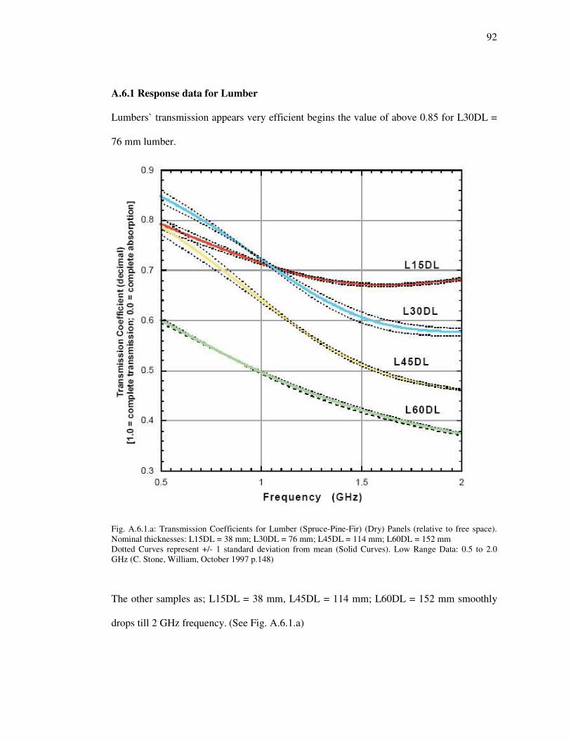
92

A.6.1 Response data for Lumber

Lumbers` transmission appears very efficient begins the value of above 0.85 for L30DL =

76 mm lumber.

Fig. A.6.1.a: Transmission Coefficients for Lumber (Spruce-Pine-Fir) (Dry) Panels (relative to free space). Nominal thicknesses: L15DL = 38 mm; L30DL = 76 mm; L45DL = 114 mm; L60DL = 152 mm Dotted Curves represent +/- 1 standard deviation from mean (Solid Curves). Low Range Data: 0.5 to 2.0 GHz (C. Stone, William, October 1997 p.148)

The other samples as; L15DL = 38 mm, L45DL = 114 mm; L60DL = 152 mm smoothly

drops till 2 GHz frequency. (See Fig. A.6.1.a)

93

Fig. A.6.1.b: Received Signal Magnitude (dB) for Lumber (Spruce-Pine-Fir) (Dry) Panels (relative to free space). L15DL = 38 mm; L30DL = 76 mm; L45DL = 114 mm; L60DL = 152 mm Dotted Curves represent +/- 1 standard deviation from mean (Solid Curves). Low Range Data: 0.5 to 2.0 GHz (C. Stone, William, October 1997 p.149)

As expected, Received Signal Magnitude (dB) for Lumber Spruce-Pine-Fir Dry Panels is

the image of Transmission coefficient Figure above seen.

94

Fig. A.6.1.c: Transmission Coefficients for Lumber (Spruce-Pine-Fir) (Dry) Panels (relative to free space). Nominal thicknesses: L15DH = 38 mm; L30DH = 76 mm; L45DH = 114 mm; L60DH = 152 mm Dotted Curves represent +/- 1 standard deviation from mean (Solid Curves). High Range Data: 3.0 to 8.0 GHz (C. Stone, William, October 1997 p.150)

Higher frequency range (3 GHz-8 GHz) is more stable when comparing the lower ones. As

see in the Fig. A.6.1.c a bit loss has been identified.

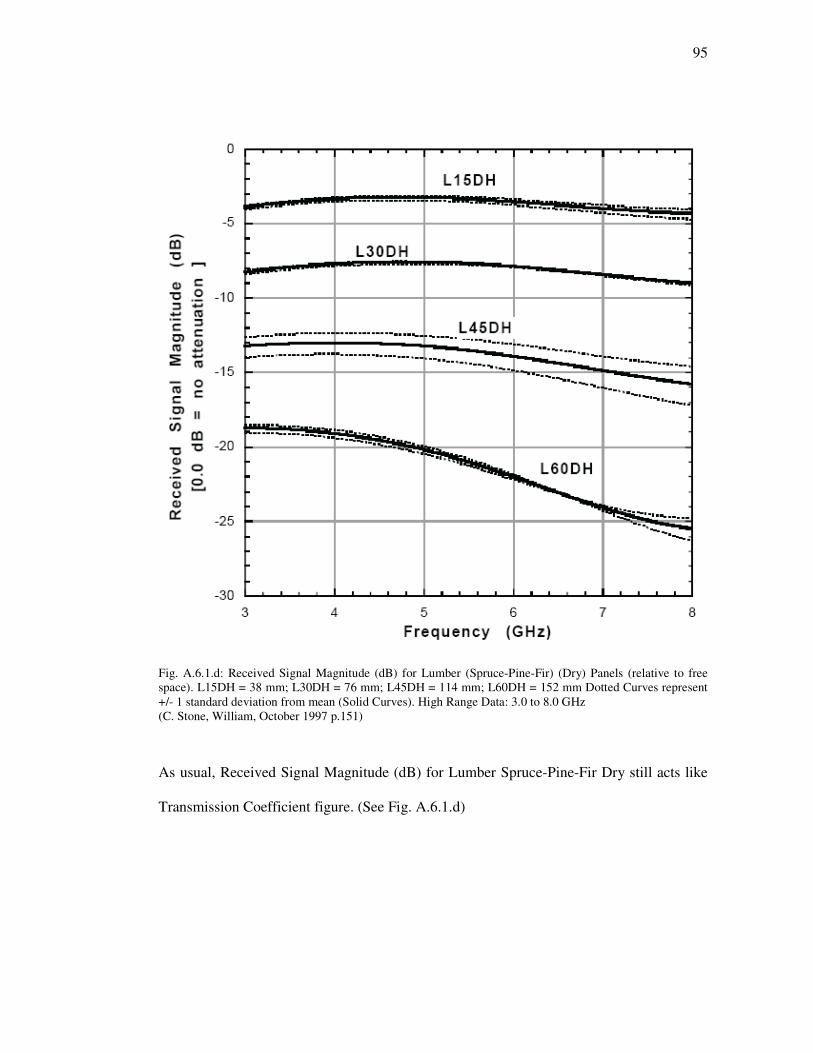
95

Fig. A.6.1.d: Received Signal Magnitude (dB) for Lumber (Spruce-Pine-Fir) (Dry) Panels (relative to free space). L15DH = 38 mm; L30DH = 76 mm; L45DH = 114 mm; L60DH = 152 mm Dotted Curves represent +/- 1 standard deviation from mean (Solid Curves). High Range Data: 3.0 to 8.0 GHz (C. Stone, William, October 1997 p.151)

As usual, Received Signal Magnitude (dB) for Lumber Spruce-Pine-Fir Dry still acts like

Transmission Coefficient figure. (See Fig. A.6.1.d)

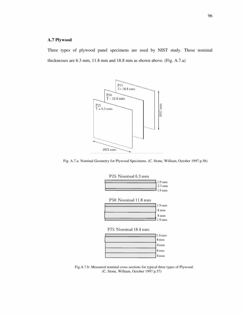
96

A.7 Plywood

Three types of plywood panel specimens are used by NIST study. Those nominal

thicknesses are 6.3 mm, 11.8 mm and 18.8 mm as shown above. (Fig. A.7.a)

Fig. A.7.a: Nominal Geometry for Plywood Specimens. (C. Stone, William, October 1997 p.56)

Fig.A.7.b: Measured nominal cross sections for typical three types of Plywood. (C. Stone, William, October 1997 p.57)

97

A.7.1 Response data for Plywood

Fig. A.7.1.a: Transmission Coefficients for Plywood (Dry) Panels (relative to free space). Nominal thicknesses: P25DL = 6 mm; P50DL = 13 mm; P75DL = 19 mm; P125DL = 32 mm Dotted Curves represent +/- 1 standard deviation from mean (Solid Curves). Low Range Data: 0.5 to 2.0 GHz (C. Stone, William, October 1997 p.160)

Another friendly material for electromagnetic waves is Plywood. As seen in Fig. A.7.1.a,

P25DL = 6 mm panels` transmission co efficiency starts almost the value 1.0 that means

complete transmission and ends below 0.9 in 2 GHz frequency. For the others, smooth

drops are seen in the figure.

98

Fig. A.7.1.b: Received Signal Magnitude (dB) for Plywood (Dry) Panels. P25DL = 6 mm; P50DL = 13 mm; P75DL = 19 mm; P125DL = 32 mm Dotted Curves represent +/- 1 standard deviation from mean (Solid Curves). Low Range Data: 0.5 to 2.0 GHz (C. Stone, William, October 1997 p.161)

Received Signal Magnitude (dB) for Plywood Dry Panels for P25DL = 6 mm, P50DL = 13

mm, P75DL = 19 mm and P125DL = 32 mm respond similarly as the transmission.

(See Fig. A.7.1.b)

99

Fig. A.7.1.c: Transmission Coefficients for Plywood (Dry) Panels (relative to free space). Nominal thicknesses: P25DH = 6 mm; P50DH = 13 mm; P75DH = 19 mm; P125DH = 32 mm Dotted Curves represent +/- 1 standard deviation from mean (Solid Curves). High Range Data: 3.0 to 8.0 GHz (C. Stone, William, October 1997 p.162)

Higher frequencies` (3 GHz-8 GHz) responses are different than the lower ones for P25DH

= 6 mm, P50DH = 13 mm, P75DH = 19 mm, P125DH = 32 mm plywood panels. Between

3GHz -5 GHz frequency shows increase of the transmission value. Over 5 GHz, The

curves decreases and increase a small amount again. (See Fig. A.7.1.c)

100

Fig. A.7.1.d: Received Signal Magnitude (dB) for Plywood (Dry) Panels (relative to free space). P25DH = 6 mm; P50DH = 13 mm; P75DH = 19 mm; P125DH = 32 mm Dotted Curves represent +/- 1 standard deviation from mean (Solid Curves). High Range Data: 3.0 to 8.0 GHz (C. Stone, William, October 1997 p.163)

Received Signal Magnitude (dB) for Plywood Dry Panels is the mirror image of

transmission coefficient as usual.

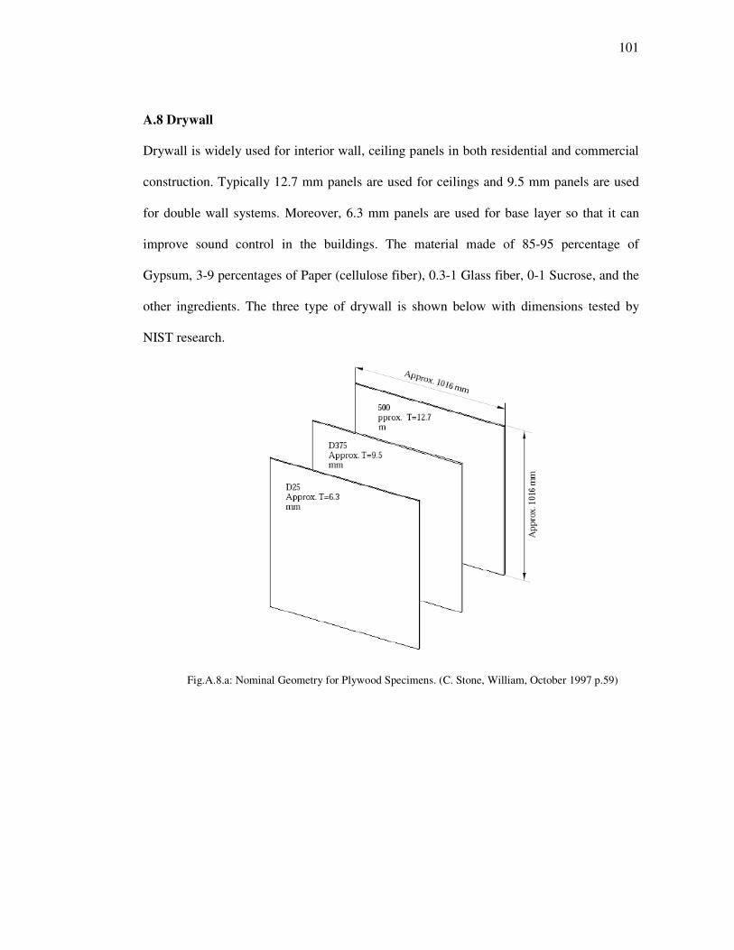
101

A.8 Drywall

Drywall is widely used for interior wall, ceiling panels in both residential and commercial

construction. Typically 12.7 mm panels are used for ceilings and 9.5 mm panels are used

for double wall systems. Moreover, 6.3 mm panels are used for base layer so that it can

improve sound control in the buildings. The material made of 85-95 percentage of

Gypsum, 3-9 percentages of Paper (cellulose fiber), 0.3-1 Glass fiber, 0-1 Sucrose, and the

other ingredients. The three type of drywall is shown below with dimensions tested by

NIST research.

Fig.A.8.a: Nominal Geometry for Plywood Specimens. (C. Stone, William, October 1997 p.59)

102

A.8.1 Response data for Drywall

Fig. A.8.1.a: Transmission Coefficients for Drywall Panels. Nominal thicknesses: D25L = 6 mm; D50L = 13 mm; D625L = 16 mm Dotted Curves represent +/- 1 standard deviation from mean (Solid Curves). Low Range Data: 0.5 to 2.0 GHz (C. Stone, William, October 1997 p.136)

The other EMW friendly building material is Drywall Panels. For Low Range Data (0.5 to

2.0 GHz), D25L = 6 mm, D50L = 13 mm and D625L = 16 mm panels response very

efficient data shown in Fig. A.8.1.a

103

Fig. A.8.1.b: Received Signal Magnitude (dB) for Drywall Panels.D25L = 6 mm; D50L = 13 mm; D625L = 16 mm Dotted Curves represent +/- 1 standard deviation from mean. Low Range Data: 0.5 to 2.0 GHz (C. Stone, William, October 1997 p.137)

The percentage is 90% efficiency for all type of panels between 0.5 GHz- 2 GHz. Received

Signal Magnitude (dB) for Drywall Panels proves that image. (See Fig. A.8.1.b)

104

Fig. A.8.1.c: Transmission Coefficients for Drywall Panels. Nominal thicknesses: D25H = 6 mm; D50H = 13 mm; D625H = 16 mm Dotted Curves represent +/- 1 standard deviation from mean (Solid Curves). High Range Data: 3.0 to 8.0 GHz (C. Stone, William, October 1997 p.138)

In higher frequencies (3.0 GHz – 8.0 GHz), D50H = 13 mm and D625H = 16 mm drywall

panels have the value above full transmission. Even if they loose their value, they all have

90% efficiency. (See Fig. A.8.1.c)

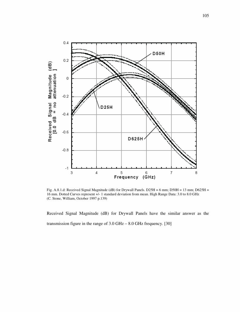
105

Fig. A.8.1.d: Received Signal Magnitude (dB) for Drywall Panels. D25H = 6 mm; D50H = 13 mm; D625H = 16 mm. Dotted Curves represent +/- 1 standard deviation from mean. High Range Data: 3.0 to 8.0 GHz (C. Stone, William, October 1997 p.139)

Received Signal Magnitude (dB) for Drywall Panels have the similar answer as the

transmission figure in the range of 3.0 GHz – 8.0 GHz frequency. [30]

106

APPENDIX B:

HFSS (HIGH FREQUENCY STRUCTURE SIMULATOR)

B.1. What is HFSS?

HFSS is a high-performance full-wave electromagnetic (EM) field simulator for arbitrary

3D volumetric passive device modeling that takes advantage of the familiar Microsoft

Windows graphical user interface. It integrates simulation, visualization, solid modeling,

and automation in an easy-to-learn environment where solutions to your 3D EM problems

are quickly and accurately obtained. Ansoft HFSS employs the Finite Element Method

(FEM), adaptive meshing and brilliant graphics to give you unparalleled performance and

insight to all of your 3D EM problems. Ansoft HFSS can be used to calculate parameters

such as S-Parameters, Resonant Frequency and Fields. Typical uses include:

• Package Modeling – BGA, QFP, Flip-Chip

• PCB Board Modeling – Power/Ground planes, Mesh Grid Grounds, Backplanes

• Silicon/GaAs – Spiral Inductors, Transformers

• EMC/EMI – Shield Enclosures, Coupling, Near-or Far-Field Radiation

• Antennas/Mobile Communications – Patches, Dipoles, Horns, Conformal Cell

Phone Antennas, Quadrafilar Helix, Specific Absorption Rate (SAR), Infinite

Arrays, Radar Cross Section (RCS), Frequency Selective Surfaces (FSS)

• Connectors – Coax, SFP/XFP, Backplane, Transitions

• Waveguide – Filters, Resonators, Transitions, Couplers

• Filters – Cavity Filters, Microstrip, Dielectric

HFSS is an interactive simulation system whose basic mesh element is a tetrahedron. This

allows you to solve any arbitrary 3D geometry, especially those with complex curves and

shapes, in a fraction of the time it would take using other techniques.

107

The name HFSS stands for High Frequency Structure Simulator. Ansoft pioneered the use

of the Finite Element Method (FEM) for EM simulation by developing/implementing

technologies such as tangential vector finite elements, adaptive meshing and Adaptive

Lanczos-Pade Sweep (ALPS). Today, HFSS continues to lead the industry with

innovations such as Modes-to-Nodes and Full Wave Spice™.

Ansoft HFSS has evolved over a period of years with input from many users and

industries. In industry, Ansoft HFSS is the tool of choice for high-productivity research,

development and virtual prototyping. [39]

108

APPENDIX C:

Dielectric Theory/Electromagnetic Propagation & Dielectric Mechanism

Dielectric Theory

The dielectric properties that will be discussed here are permittivity and permeability.

Resistivity is another material property which will not be discussed here. Information

about resistivity and its measurement can be found in the Agilent Application Note 1369-

11. It is important to note that permittivity and permeability are not constant. They can

change with frequency, temperature, orientation, mixture, pressure, and molecular structure

of the material.

Dielectric constant

A material is classified as “dielectric” if it has the ability to store energy when an external

electric field is applied. If a DC voltage source is placed across a parallel plate capacitor,

more charge is stored when a dielectric material is between the plates than if no material (a

vacuum) is between the plates. The dielectric material increases the storage capacity of the

capacitor by neutralizing charges at the electrodes, which ordinarily would contribute to

the external field. The capacitance with the dielectric material is related to dielectric

constant. If a DC voltage source V is placed across a parallel plate capacitor (Figure 1),

more charge is stored when a dielectric material is between the plates than if no material (a

vacuum) is between the plates.

109

Where C and Co are capacitance with and without dielectric, ' 'rκ ε= r is the real dielectric

constant or permittivity, and A and t are the area of the capacitor plates and the distance

between them (Figure 1). The dielectric material increases the storage capacity of the

capacitor by neutralizing charges at the electrodes, which ordinarily would contribute to

the external field. The capacitance of the dielectric material is related to the dielectric

constant as indicated in the above equations. If an AC sinusoidal voltage source V is

placed across the same capacitor (Figure 2), the resulting current will be made up of a

charging current Ic and a loss current Il that is related to the dielectric constant. The losses

in the material can be represented as a conductance (G) in parallel with a capacitor (C).

110

The complex dielectric constant k consists of a real part k' which represents the storage and

an imaginary part k'' which represents the loss. The following notations are used for the

complex dielectric constant interchangeably * *r rκ κ ε ε= = = . From the point of view of

electromagnetic theory, the definition of electric displacement (electric flux density) Df is:

Df = �E where *0 rε ε ε ε= = is the absolute permittivity (or permittivity),

rε is the

relative permittivity, 90

110

36Xε

π−≈ F/m is the free space permittivity and E is the electric

field. Permittivity describes the interaction of a material with an electric field E and is a

complex quantity. 0

"r r rjε

κ ε ε εε

= = = −

Dielectric constant (κ ) is equivalent to relative permittivity ( rε ) or the absolute

permittivity (ε ) relative to the permittivity of free space ( 0ε ). The real part of permittivity

( 'rε ) is a measure of how much energy from an external electric field is stored in a

material. The imaginary part of permittivity ( "rε ) is called the loss factor and is a measure

of how dissipative or lossy a material is to an external electric field. The imaginary part of

permittivity ( "rε ) is always greater than zero and is usually much smaller than ( 'rε ). The

loss factor includes the effects of both dielectric loss and conductivity.

When complex permittivity is drawn as a simple vector diagram (Figure 3), the real and

imaginary components are 90° out of phase. The vector sum forms an angle d with the real

111

axis ( 'rε ). The relative “lossiness” of a material is the ratio of the energy lost to the energy

stored.

The loss tangent or tanδ is defined as the ratio of the imaginary part of the dielectric

constant to the real part. D denotes dissipation factor and Q is quality factor. The loss

tangent tan δ is called tan delta, tangent loss or dissipation factor. Sometimes the term

“quality factor or Q-factor” is used with respect to an electronic microwave material,

which is the reciprocal of the loss tangent. For very low loss materials, since tan δ �δ ,

the loss tangent can be expressed in angle units, milliradians or microradians.

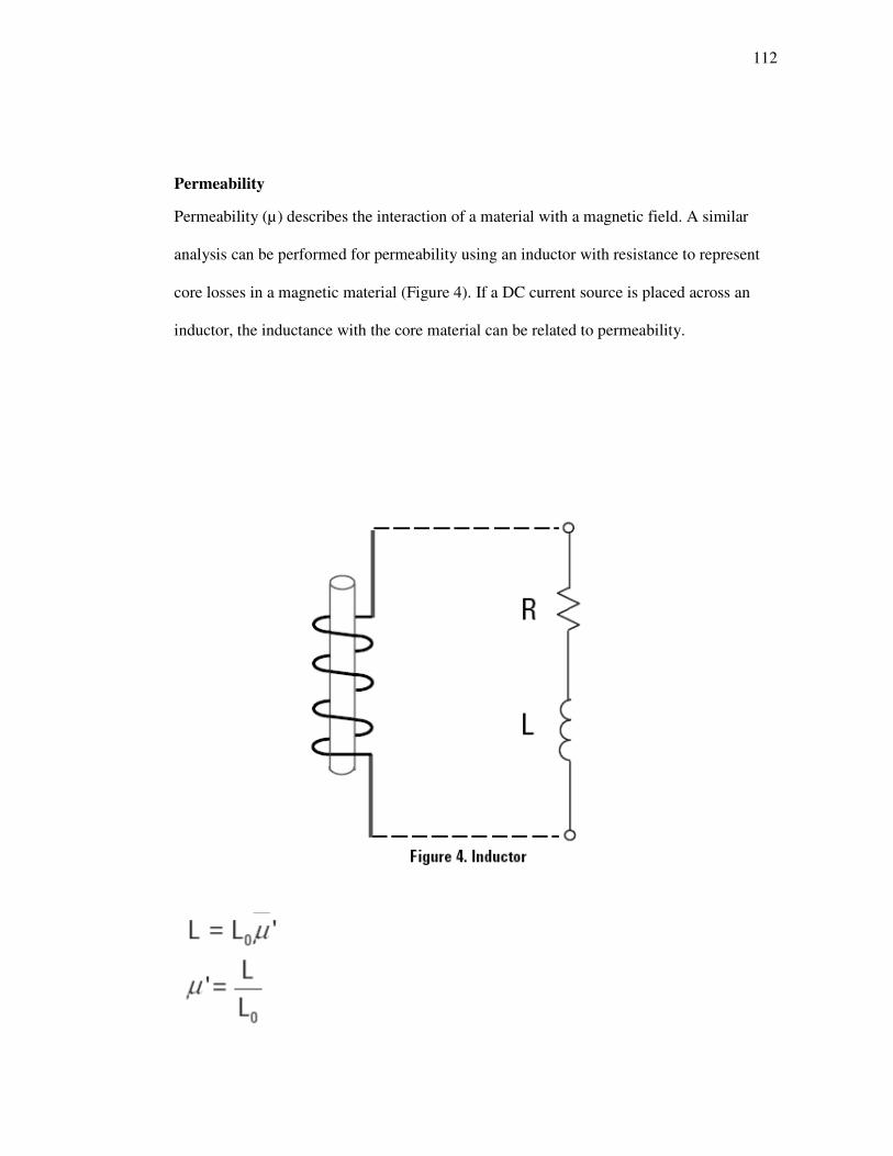
112

Permeability

Permeability (µ) describes the interaction of a material with a magnetic field. A similar

analysis can be performed for permeability using an inductor with resistance to represent

core losses in a magnetic material (Figure 4). If a DC current source is placed across an

inductor, the inductance with the core material can be related to permeability.

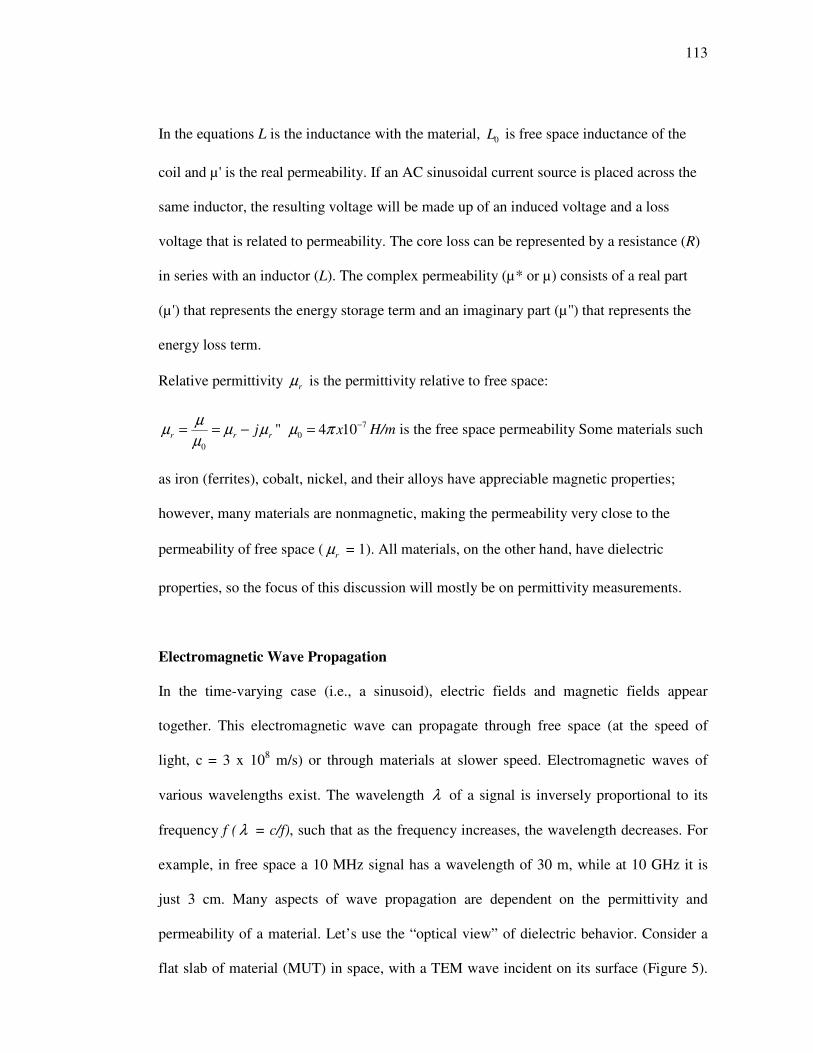
113

In the equations L is the inductance with the material, 0L is free space inductance of the

coil and µ' is the real permeability. If an AC sinusoidal current source is placed across the

same inductor, the resulting voltage will be made up of an induced voltage and a loss

voltage that is related to permeability. The core loss can be represented by a resistance (R)

in series with an inductor (L). The complex permeability (µ* or µ) consists of a real part

(µ') that represents the energy storage term and an imaginary part (µ '') that represents the

energy loss term.

Relative permittivity rµ is the permittivity relative to free space:

0

"r r rjµ

µ µ µµ

= = − 70 4 10xµ π −= H/m is the free space permeability Some materials such

as iron (ferrites), cobalt, nickel, and their alloys have appreciable magnetic properties;

however, many materials are nonmagnetic, making the permeability very close to the

permeability of free space (rµ = 1). All materials, on the other hand, have dielectric

properties, so the focus of this discussion will mostly be on permittivity measurements.

Electromagnetic Wave Propagation

In the time-varying case (i.e., a sinusoid), electric fields and magnetic fields appear

together. This electromagnetic wave can propagate through free space (at the speed of

light, c = 3 x 108 m/s) or through materials at slower speed. Electromagnetic waves of

various wavelengths exist. The wavelength λ of a signal is inversely proportional to its

frequency f ( λ = c/f), such that as the frequency increases, the wavelength decreases. For

example, in free space a 10 MHz signal has a wavelength of 30 m, while at 10 GHz it is

just 3 cm. Many aspects of wave propagation are dependent on the permittivity and

permeability of a material. Let’s use the “optical view” of dielectric behavior. Consider a

flat slab of material (MUT) in space, with a TEM wave incident on its surface (Figure 5).

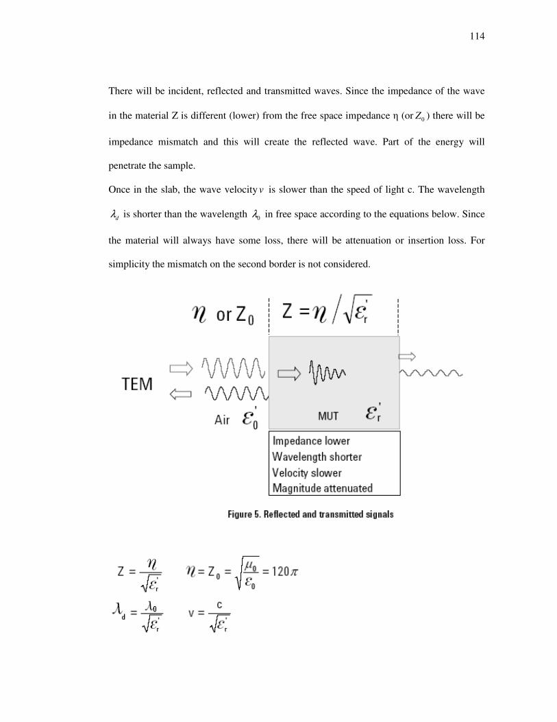
114

There will be incident, reflected and transmitted waves. Since the impedance of the wave

in the material Z is different (lower) from the free space impedance � (or 0Z ) there will be

impedance mismatch and this will create the reflected wave. Part of the energy will

penetrate the sample.

Once in the slab, the wave velocity v is slower than the speed of light c. The wavelength

dλ is shorter than the wavelength 0λ in free space according to the equations below. Since

the material will always have some loss, there will be attenuation or insertion loss. For

simplicity the mismatch on the second border is not considered.

115

Figure 6 depicts the relation between the dielectric constant of the Material Under Test

(MUT) and the reflection coefficient | Γ | for an infinitely long sample (no reflection from

the back of the sample is considered).

For small values of the dielectric constant (approximately less than 20), there is a lot of

change of the reflection coefficient for a small change of the dielectric constant. In this

range dielectric constant measurement using the reflection coefficient will be more

sensitive and hence precise. Conversely, for high dielectric constants (for example between

70 and 90) there will be little change of the reflection coefficient and the measurement will

have more uncertainty.

116

Dielectric Mechanisms

A material may have several dielectric mechanisms or polarization effects that contribute

to its overall permittivity (Figure 7). A dielectric material has an arrangement of electric

charge carriers that can be displaced by an electric field. The charges become polarized to

compensate for the electric field such that the positive and negative charges move in

opposite directions.

At the microscopic level, several dielectric mechanisms can contribute to dielectric

behavior. Dipole orientation and ionic conduction interact strongly at microwave

frequencies. Water molecules, for example, are permanent dipoles, which rotate to follow

an alternating electric field. These mechanisms are quite lossy – which explains why food

heats in a microwave oven. Atomic and electronic mechanisms are relatively weak and

usually constant over the microwave region. Each dielectric mechanism has a characteristic

“cutoff frequency.” As frequency increases, the slow mechanisms drop out in turn, leaving

the faster ones to contribute to 'ε . The loss factor ( "rε ) will correspondingly peak at each

critical frequency. The magnitude and “cutoff frequency” of each mechanism is unique for

different materials. Water has a strong dipolar effect at low frequencies – but its dielectric

constant rolls off dramatically around 22 GHz. Teflon, on the other hand, has no dipolar

mechanisms and its permittivity is remarkably constant well into the millimeter-wave

region.

117

A resonant effect is usually associated with electronic or atomic polarization. A relaxation

effect is usually associated with orientation polarization.

Orientation (dipolar) polarization

A molecule is formed when atoms combine to share one or more of theirs electrons. This

rearrangement of electrons may cause an imbalance in charge distribution creating a

permanent dipole moment. These moments are oriented in a random manner in the absence

of an electric field so that no polarization exists. The electric field E will exercise torque T

on the electric dipole, and the dipole will rotate to align with the electric field causing

orientation polarization to occur (Figure 8). If the field changes the direction, the torque

will also change.

118

The friction accompanying the orientation of the dipole will contribute to the dielectric

losses. The dipole rotation causes a variation in both 'rε and "rε at the relaxation frequency

which usually occurs in the microwave region. As mentioned, water is an example of a

substance that exhibits a strong orientation polarization.

Electronic and atomic polarization

Electronic polarization occurs in neutral atoms when an electric field displaces the nucleus

with respect to the electrons that surround it. Atomic polarization occurs when adjacent

positive and negative ions “stretch” under an applied electric field. For many dry solids,

these are the dominant polarization mechanisms at microwave frequencies, although the

actual resonance occurs at a much higher frequency.

119

In the infrared and visible light regions the inertia of the orbiting electrons must be taken

into account. Atoms can be modeled as oscillators with a damping effect similar to a

mechanical spring and mass system (Figure 7). The amplitude of the oscillations will be

small for any frequency other than the resonant frequency. Far below resonance, the

electronic and atomic mechanisms contribute only a small constant amount to 'rε and are

almost lossless. The resonant frequency is identified by a resonant response in 'rε and a

peak of maximum absorption in "rε . Above the resonance, the contribution from these

mechanisms disappears. [40]

120

REFERENCES: 1. Electromagnetic Waves www.johnbarrie.com/glossary.htm 2. Wlana Org, Education, What is a Wireless LAN? http://www.wlana.org/learn/educate1.htm 3. Val T.; Peyrard F.; Misson M., Study and simulation of the infrared WLAN IrDA: an alternative to the radio, Computer Communications, Volume 26, Number 11, Publisher: Elsevier, 1 July (2003). pp. 1210-1218(9) 4. Telecoms Regulatory Resources http://nes.aueb.gr/regResources.html 5. Which WLAN Technology is Best? http://www.zdnet.com.au/whitepaper/0,2000063328,22096255p-16001307q,00.htm 6. Electromagnetic Spectrum http://imagine.gsfc.nasa.gov/docs/science/know_l1/emspectrum.html 7. Discovery of Infrared http://coolcosmos.ipac.caltech.edu/cosmic_classroom/ir_tutorial/discovery.html 8. Johann Wilhelm Ritter http://www.corrosion-doctors.org/Biographies/RitterBio.htm 9. Hans Christian Ørsted http://en.wikipedia.org/wiki/Hans_Christian_Ørsted 10. Ampère, André (1775-1836) http://scienceworld.wolfram.com/biography/Ampere.html 11. Maxwell’s Legacy http://ieee.li/pdf/essay_maxwells_legacy.pdf 12. Asimov Isaac, Isaac Asimov's Book of Facts. Hastingshouse/Daytrips Publ., (1992). Page 389. 13. Electromagnetic Radiation http://micro.magnet.fsu.edu/primer/java/electromagnetic/index.html 14. HiperLAN http://www.webopedia.com/TERM/H/HiperLAN.html 15. What is MMAC? http://www.arib.or.jp/mmac/e/outline/index.htm

121

16. IEEE http://www.ieee.org/portal/site/mainsite/menuitem.e0007c26eb2a454de38570e85bac26c8/index.jsp?&pName=home 17. HIPERLAN Resource Center http://www.palowireless.com/hiperlan2/ 18. United States Patent 5853889 http://www.freepatentsonline.com/5853889.html 19. High Frequency Radiation and Human Exposure by Mahmoud M. Dawoud http://www.who.int/peh-emf/meetings/archive/en/keynote5dawoud.pdf 20. WiMAX Technology, LOS and NLOS Environments http://www.srtelecom.com/imports/pdf/en/white-paper/WiMAX-LOS-and-NLOS-technology-Dec2004.pdf#search=%22wimax%20coverage%22 21. WiMAX Technology http://www.wimaxforum.org/technology/ 22. Ultra-Wideband (UWB) Technology http://www.usb.org/developers/wusb/docs/Ultra-Wideband.pdf 23. EMC (Electromagnetic Compability) http://www.transpower.co.nz/?id=5326 24. Telecoms Regulatory Resources http://nes.aueb.gr/regResources.html 25. Cheryl I. Shaw; Robert M. Kacmarek; Rickey L. Hampton; Vincent Riggi; Ashraf El Masry; Jeffrey B. Cooper; William E. Hurford, Cellular Phone Interference With the Operation of Mechanical Ventilators, Posted 05/14/2004 http://www.medscape.com/viewarticle/475203 26. EMI (Electromagnetic Interference) http://www.reference.com/browse/wiki/Electromagnetic_interference 27. Electrical conductivity http://en.wikipedia.org/wiki/Electrical_conductivity 28. Magnetic Permeability http://www.britannica.com/eb/article-9050027/magnetic-permeability

29. Permittivity http://en.wikipedia.org/wiki/Electric_permittivity 30. C. Stone William, Electromagnetic Signal Attenuation in Construction Materials, NIST Construction Automation Program Report No. 3, October (1997)

122

31. Attenuation constant http://en.wikipedia.org/wiki/Attenuation_constant 32. Saunders Simon R., Antennas and Propagation for Wireless Communication Systems, John Wiley & Sons Ltd, (1999) p.271, 290 ISBN 0-471-98609-7 33. Canbay Cahit, Antennas And Propagation I, Second Edition, Department of Electrical and Electronics Engineering, Yeditepe University Istanbul, (1996), p.92 34. Some Statistics about Yeditepe University 26 August Campus http://www.yeditepe.edu.tr/yeditepe/Yeditepe%20UniverSiteSi/English/yeditepe%20university/general.aspx?cacheid=/Yeditepe%20UniverSiteSi/English/yeditepe%20university/general 35. Wilson Robert, Propagation Losses through Common Building Materials 2.4 GHz vs. 5 GHz Reflection and Transmission Losses through Common Building Materials, For: James A. Crawford, CTO Magis Networks, Inc. August (2002) p.8-9 36. Yeditepe University Layout and Architecture Engineering Building Floor Plans http://www.maestro.yeditepe.edu.tr 37. Springer Berlin Heidelberg, 4th International Workshop on Wearable and Implantable Body Sensor Networks), Volume 13, (2007), Pages 5-20 ISBN 978-3-540-70994-7 38. National Physical Laboratory /Kaye&Laby/Tables of Physical and Chemical Constants http://www.kayelaby.npl.co.uk/general_physics/2_7/2_7_9.html 39. HFSS (High Frequency Structure Simulator) V 9.2 Electronic Design Automation Software-User’s Guide p.2 / Training Seminar 40. Basics of Measuring the Dielectric Properties of Materials Application Note P.4-11

http://cp.literature.agilent.com/litweb/pdf/5989-2589EN.pdf

41. Electromagnetic spectrum http://www.mic-d.com/curriculum/lightandcolor/electromagnetic.html 42. High Frequency Radiation and Human Exposure http://www.who.int/peh-emf/meetings/archive/en/keynote5dawoud.pdf

43. Electromagnetic Wave http://www.mic-d.com/curriculum/lightandcolor/electromagnetic.html 44. Anechoic chamber http://en.wikipedia.org/wiki/Anechoic_chamber

123

BIBLIOGRAPHY: 1. Santamaria A., F.J. Lopez Hernandez, Wireless LAN Systems, Boston: Architect

House, (1994) ISBN: 0-89006-609-4 2. Feverstein Martin J., Rapport Theodore S., Wireless Personal Communications

Boston: Kluwer Academic Publishers, (1993) ISBN: 0-7923-9280-9

3. Holtzman J.M., Wireless Communications: future directions David J. Goodman Boston: Kluwer Academic Publishers, (1993) ISBN: 0-7973-9316-3

4. Nanda Sanjiu, Third Generation Wireless Information Networks, David J.Goodman ISBN: 0-7923-9218-3

5. RF / Wireless Communications USA : Philips, c (1994) 6. Sayre Cotter W., Complete Wireless Design McGraw- Hill (2001)

ISBN: 0-07-137016-1

7. Micel Andrew, Wireless Technician’s Handbook: (2000) Artech House, INC. ISBN: 1-58053-005-2

8. Makarov Sergey N., Antenna and EM Modeling with MATLAB® ,(2002) by John

Wiley and Sons, Inc. ISBN: 0-471-21876-6 9. Canbay Cahit, Antennas And Propagation I, Second Edition, Department of Electrical

and Electronics Engineering, Yeditepe University Istanbul, (1996) 10. Cátedra Manuel F., Pérez-Arriaga Jesús, Cell Planning for Wireless Communications, ISBN 0-89006-601-9 11. Stallings William, Wireless Communications and Networks, ISBN 0-13-040864-6 12. The Nature of Electromagnetic Radiation, http://www.olympusmicro.com/primer/lightandcolor/electromagintro.html 13. WiMAX Technology, LOS and NLOS Environments http://www.srtelecom.com/imports/pdf/en/white-paper/WiMAX-LOS-and-NLOS-Technology-Dec2004.pdf#search=%22wimax%20coverage%22 14. An EMC Engineer's Guide to Electromagnetic Modeling Software http://ieee.ca/diglib/library/9712hubing/hubing.pdf 15. Survey of Numerical Electromagnetic Modeling Techniques http://www.emclab.umr.edu/pdf/TR91-1-001.pdf 16. Commercial Electromagnetic Modeling Codes http://www.emclab.umr.edu/csoft.html

124

17. Computational Electromagnetic Modeling Codes Available on the Internet http://www.eee.metu.edu.tr/~ngencer/codes.htm 18. Muhiddin Can, Akın, B. Etemoglu, Atakan Avci, Deniz Suyundan Tatli Su Eldesinin Teknik ve Ekonomik Analizi, Uluda� Üniversitesi Mühendislik-Mimarlık Fakültesi Dergisi, Cilt 7, Sayı 1, (2002) 19. Tamyis Najihah M., Ghodgaonkar Deepak K., Taib Mohd. Nasir, Wui Wong Tin, Dielectric Properties of Human Skin In Vivo in Frequency Range 20-38 GHz for 42 Healthy volunteers, Microwave Technology Center Faculty of Electrical Engineering/Faculty of Pharmacy Universiti Teknologi MARA Selangor/MALAYSIA 20. Calla O.P.N., Bohra Dinesh, Vyas Rajesh, Measurement of Dielectric Constant of Saline Water and Estimation Ofemissivity and Scattering Coefficient Different Physical Temperaturesat Microwave Frequencies, International Centre for Radio Science ‘OM NIVAS’ A-23 Shastri Nagar Jodhpur – 342003 21. Geier, J., Wireless LANs, Wireless System Integration, Second edition, Chapter 6, Indiana, USA, (2002), p.1, 5, 7-10, 13 22. Intel Com, Exploring WLAN Solutions, What is Wireless LAN Networking? http://www.intel.com/business/bss/infrastructure/wireless/solutions/index.htm 23. Palowireless Com, About HiperLAN2 http://www.palowireless.com/hiperlan2/about.asp 24. Dunne, D., 10 May (2001), What is wireless LAN? http://www.cnn.com/2001/TECH/ptech/05/10/what.is.WLAN.idg/index.html 25. Wifinder Com, Wifinder Worldwide hotspots directory, Find public Access Wi-Fi hotspots around the world http://www.wifinder.com/ 26. Jiwire Com, Browse hotspots by country, hotspot directory http://www.jiwire.com/hotspot-hot-spot-directory-browse-bycountry.htm 27. Frost & Sullivan, 17 October (2003), Growth forecast for European WLAN hotspots market - Frost & Sullivan Brief Article http://www.findarticles.com/p/articles/mi_m0ECZ/is_2003_Oct_17/ai_108989399 28. Wi-Fi Alliance, 2 February (2004), Enablig the future of Wi-Fi Public Access http://www.weca.net/OpenSection/pdf/Wi-Fi_Public_Access.pdf

125

29. The Federal Communications Commission (FCC), Wireless Telecommunications Bureau, Rules & Regulations, Code of Federal Regulations, - Title 47, Radio frequency devices, p.,751-753, http://a257.g.akamaitech.net/7/257/2422/05dec20031700/edocket.access.gpo.gov/cfr_2003/octqtr/47cfr15.247.htm 30. Kurth M., 09 July (2002), Regulatory Authority for Telecommunications and Posts (Reg TP), UMTS and WLANs are complementary, New frequencies released for WLAN in the 5 GHz band, Bonn, http://www.regtp.de/en/aktuelles/pm/02605/index.html128 31. Ofcom, Office of communications, Deregulated FWA, mobile data and WLAN licensing, http://www.ofcom.org.uk/licensing_numbering/radiocomms/deregulated_fwa/?a=87101 32. Autorite de regulation des telecommunications, 24 July (2003), WIRELESS LAN, WIFI- A new and decisive change for wireless local area Networks, Paris http://www.art-telecom.fr/eng/index.htm 33. OFCOM, Federal office of communications, RIR1010, Radio local area networks (SRD), Appliances,Technical requirements, Requirements http://www.bakom.ch/en/geraete/technik/anforderungen/ 34. European Conference of Postal and Telecommunications Administrations (CEPT), Electronic Communications Committee (ECC), 15 April (2004), DRAFT ECC Report on (O)RLANs in the frequency band 2,400 – 2,4835 GHz, p.21 http://www.ero.dk/70B08505-FE3E-4FBF-B829-B3DE5CAE110F?frames=0 35. Özdemir, M., Wireless LAN Technology & Security Update, Cisco Systems Inc., April 2003,p.3 36. Ramadin, D., K., Overview of Wireless Broadband Technologies, Intel Corporation 37. Minoli, D., Telecommunications Technology Handbook, Chapter 8, Wireless Technologies: WPAN, WLAN, and WWAN, Second Edition, Artech House, Boston London, (2003) p.245-335 38. Prasad R., Muñoz L., , WLANs and WPANs towards 4G Wireless, Fundamentals of WLAN, Artech House Boston, London, 2003, p. 133,134 39. Lansford, J., Convergence of Wireless PANs, LANs, and WANs,p. 1-7 40. JOSE S., 21 January (2004), Intel Press Release, Intel Outlines Broadband Wireless Vision http://www.intel.com/pressroom/archive/releases/20040121corp.htm 41. Micro Warehouse, Search, WLAN, http://www.microwarehouse.co.uk/searchresult.aspx?Action=Search&Keywords=wlan

126

42. DealTime.co.uk, Shopping.com, Matches for "wlan", http://www.espotting.dealtime.co.uk/xKW-wlan/NS-1/linkin_id-3025539/GS.html 43. Intel, Built for wireless, http://www.intel.com/products/mobiletechnology/wireless.htm?iid=ipp_note+mobiletech_wireless& 44. Dulaney, K., Mobile and Wireless, Gartner, Inc., (2003) 45. MMAC, Multimedia Mobile Access Communication Systems Promotion Council, What is MMAC ?, System outline of MMAC, Target specification of MMAC, MMAC image http://www.arib.or.jp/mmac/e/index.htm 46. DEMIR Tamer, Member of Computer Networks Research Laboratory, IEEE 802.11 Tutorial (short and revised version on IEEE 802.11 standarts), http://www.tamerdemir.com/ 47. IEEE standards association, Welcome to IEEE standards development online, http://standards.ieee.org/resources/development/index.html 48. IEEE Board of Directors, 16 November (2003), IEEE Strategies for (2004), Issues, Desired Outcomes, and Actions http://www.ieee.org/portal/cms_docs/about/IEEE_Strategies_for_2004.pdf 49. Webopedia com, Home, Quick reference, Wireless LAN Standards http://www.webopedia.com/quick_ref/WLANStandards.asp 50. Bayılmı�, C., Ertürk, C., Çeken, C., Kablosuz Yerel Alan A�ı Uygulaması, Kocaeli Üniversitesi, International XII. Turkish Symposium on Artificial Intelligence and Neural Networks, (2003) 51. WLANA, 04/17/ (2002), The Wireless LAN Association, Wireless Networking Standards and Organizations, Wireless Networking Standards http://www.wlana.org/pdf/wlan_standards_orgs.pdf 52. ETSI, 28.07. (2004), ETSI portal, BRAN, Hiperlan2, hiperaccess http://portal.etsi.org/bran/Summary.asp 53. ETSI, 28.07. (2004), ETSI portal, BRAN, ETSI HIPERLAN/2 Standard, Overview http://portal.etsi.org/bran/kta/Hiperlan/hiperlan2.asp 54. Wikipedia, the free encyclopedia, HIPERLAN, HIPERLAN1, HIPERLAN2, http://en.wikipedia.org/wiki/HIPERLAN 55. ETSI, 28.07.(2004), HIPERLAN/2 Technical Overview, p.1-3, http://portal.etsi.org/bran/kta/Hiperlan/hiperlan2tech.asp

127

56. Johnsson, M., HiperLAN/2 Global Forum, HiperLAN2 – The Broadband Radio Transmission Technology Operating in the 5 GHz Frequency Band, (1999) 57. ETSI, 28.02. (2004), ETSI HIPERLAN/1 Standard, Future Developments http://portal.etsi.org/bran/kta/Hiperlan/hiperlan1.asp 58. Palowireless, palowireless com, Bluetooth Resource Center, Bluetooth Tutorial – Specifications, What is Bluetooth? http://www.palowireless.com/infotooth/tutorial.asp 59. Karygiannis T., Owens L., DRAFT Wireless Network Security 802.11, Bluetooth™ and Handheld Devices, NIST Special Publication 800-48, Wireless Network Security, Gaithersburg, USA. http://fpzwireless.fpz.hr/dokumentacija/Wireless_Network_Security.pdf 60. Bluetoothturkey, bluetoothturkey com, Özel, Bluetooth http://www.bluetoothturkey.com/bluetooth%20nedir.htm 61. Palowireless, palowireless com, HomeRF Overview and Market Positioning, Introduction, HomeRF Working Group, http://www.palowireless.com/homerf/homerf1.asp 62. SearchNetworking com, 10 Apr 2001, Definitions, HomeRF, http://searchnetworking.techtarget.com/sDefinition/0,,sid7_gci535092,00.html 63. Kaminski C., 15-May-(2001), Technology overview of HomeRF 2.0, http://www.homenethelp.com/web/explain/about-homerf-2b.asp 64. Baykal, N., Bilgisayar A�larının Temelleri, EMO Yayın No:EG/2003/3, Ankara, (2003), p.21, 27, 65. Raylink, WLANA The Wireless LAN Aliance, frequency hopping vs direct sequence wlana. Org p.1-4 http://www.raylink.com/whitepaper/fhss_dsss.pdf 66. YILMAZ, M., S., Temmuz (2002), CISN (computing & information services newsletter), METU computer center, Kablosuz Bilgisayar A�ları Üzerine / IEEE 802.11a Protokolü http://cisn.odtu.edu.tr/2002-6/ieee.php 67. Wepopedia com, OFDM, http://www.webopedia.com/TERM/O/OFDM.html 68. Linnartz J., P., JPL Home, Wireless, Effect of Doppler on OFDM and MC-CDMA http://www.eecs.berkeley.edu/Research/Projects/ofdm/wireless/ofdm/doppler/index.html 69. Patil B., IP in Wireless Networks, Chapter Eleven, IP in 802.11 Networks, Pearson Education Ltd. London, January 31, (2003)

128

70. INTERMEC Technologies Corporation, Guide to Wireless LAN Technologies, USA, (1998) p., 2-17 71. KLING A., CORANTE Com, 23 January (2003), Tech News Filtered daily,The bottom line: the economics of IT, When Will Wireless be Ready? , More on Local Telephone "Competition", http://www.corante.com/bottomline/20030101.shtml 72. Netsis Com, Kablosuz Teknoloji (Wireless Technology), Fonksiyonellik, Detay bilgi http://www.netsis.com.tr/goksel/Wireless/Wt.HTM 73. CWT Center for Wireless Telecommunications, Wireless Frequently Asked Questions, What are the ISM bands? http://www.cwt.vt.edu/faq/default.htm 74. ITU, International Telecommunication Union, Edition of (2001), Radio Regulations, CHAPTER II – Frequencies, ARTICLE 5, Frequency allocations, p.72, 80 75. Intel, Wireless LAN Benefits, http://www.intel.com/business/bss/infrastructure/wireless/solutions/benefits.htm 76. Intel, Intel Com, IEEE 802.11b High Rate Wireless Local Area Networks, Wireless Technology Today, What is Wireless Networking ?,p., 2-7 http://www.intel.com/network/connectivity/resources/doc_library/documents/pdf/wireless_lan.pdf 77. Long M., 2 September (2003), Network security, Wireless Security, Is WPA Good Enough? http://www.newsfactor.com/perl/story/22207.html 78. Cox C., 09/01/ (2003), Network World, WLAN security: A big problem for small nets http://www.nwfusion.com/cgi-bin/mailto/x.cgi 79. T-Mobile Hotspots, 03/04/ (2004), T-Mobile Hotspot International Locations, http://locations.hotspot.t-mobile.com/viewInternationalLocations.asp 80. Lawson S., 08/01/ (2002), WLAN use growing fast, researchers say, http://www.nwfusion.com/news/2002/0801wlan.html 81. Ziakas, D., May (2003), Hotspot in a Box – Creating publicly available WLANs, What is a Hotspot?, Hotspot Architectures, 82. Singer M., 9 july (2002), Cisco Mobile Office Takes Off Overseas, http://siliconvalley.internet.com/news/article.php/1382751 83. Delloro Group, News, Worldwide 802.11 Market Grew 21% in 4Q01 http://www.delloro.com/news/2002/021402.shtml

129

84. Delloro Group, News, Worldwide 802.11 Market Grew 8% in 2Q02 http://www.delloro.com/news/2002/081502a.shtml 85. Delloro Group, News, Worldwide 802.11 Market Exceeds $500 Million in 4Q03 http://www.delloro.com/news/2004/WL021104.shtml 86. Griffith E., 23 May (2002), Synergy Sees WLAN Growth, http://www.wi-fiplanet.com/news/article.php/1143771 87. Web Japan, 10 September (2002), Trends in Japan, ONLINE ON THE GO: Wireless LANs Becoming Commonplace in Japan http://web-japan.org/trends01/article/020910bus_r.html 88. KOÇBA A. Ç., Temmuz (2003), Uluslararası Kurulu�ların Telekomünikasyon Alanındaki Faaliyetleri, Kurumumuzun Bu Kurulu�ların Faaliyetlerine Katkısı Hususunda Kurumsalla�ması Amacıyla Yapılması Gerekenler Ve Ülke Örneklemeleri, Uzmanlık Tezi, Telekomünikasyon Kurumu, Ankara, p.23, 67, 89 http://www.tk.gov.tr/Yayin/Uzmanlik_Tezleri/tktezler/A_Cetin_Tez.pdf 89. IEEE, About the IEEE, What is the IEEE? http://www.ieee.org/portal/index.jsp?pageID=corp_level1&path=about&file=index.xml&xsl=generic.xsl 90. Sorin M. Schwartz, 19 February (2001), Frequency Hopping Spread pectrum (FHSS) vs. Direct Sequence Spread Spectrum (DSSS) in the Broadband Wireless Access and WLAN Arenas, http://www.alvarionusa.com/RunTime/Materials/KnowledgePoolFiles/C3_freq_hop_vs_direct_seq.pdf 91. Donran A., 02/06/ (2002), Network Magazine, Emerging Technology:Wireless Lan Standards, http://www.networkmagazine.com/article/NMG20020206S0006 92. Nurflus P., Envara Com, Silicon Solutions for 5 GHz Wireless Networking, Wireless Networking In The 5 GHz Band - The Real Benefits A Technology White Paper 93. IEEE P802.11 - TASK GROUP G - MEETING UPDATE, Status of Project IEEE 802.11g, Standard for Higher Rate (20+ Mbps) Extensions in the 2.4GHz Band, http://grouper.ieee.org/groups/802/11/Reports/tgg_update.htm 94. Lui B., 13 July 2001, 802.11g Faces its Final Hurdle , Internetnews com, http://www.internetnews.com/bus-news/print.php/9_801211 95. Convergedigest Com, News and Resources on the Convergence of Broadband Networking Technologies, Daily report, Weekly Report, Wi-Fi Interoperability Certification Begins For IEEE 802.11a http://www.convergedigest.com/WiFi/wlanarticle.asp?ID=4262

130

96. xilinx, Wireless LANs, Customer Tutorial http://www.xilinx.com/esp/consumer/home_networking/pdf_files/wireless_lans/wlan-complete.pdf 97. The Wireless LAN Association (WLANA), Sponsor Members, Affiliate Members, http://www.wlana.org/memb/index.htm 98. The Wireless LAN Association (WLANA), About WLANA, http://www.wlana.org/about/index.htm 99. HiperLAN2 Global Forum, FAQ’s, What is the HiperLAN2 Global Forum (H2GF)?, What is the purpose of the H2GF?, Who are the founding members?, http://www.hiperlan2.com/faq.asp 100. ERC Recommendation 70-03, February 2004, RELATING TO THE USE OF SHORT RANGE DEVICES (SRD), http://www.ero.dk/documentation/docs/doc98/official/pdf/REC7003E.PDF 101. Federal Communications Commission FCC 99-149, 24 June 1999, NOTICE OF PROPOSED RULE MAKING, http://www.fcc.gov/Bureaus/Engineering_Technology/Notices/1999/fcc99149.txt 102. Federal Communications Commission FCC 00-312, 31 August 2000, FIRST REPORT AND ORDER, http://www.fcc.gov/Bureaus/Engineering_Technology/Orders/2000/fcc00312.pdf 103. Federal Communications Commission FCC 01-158, 11 May 2001, FURTHER NOTICE OF PROPOSED RULE MAKING AND ORDER, http://ftp.fcc.gov/Bureaus/Engineering_Technology/Notices/2001/fcc01158.pdf 104. Charny B., 20 May 2002, CNET Networks, NEWS.com, Wi-Fi in the Steel City, http://news.com.com/Wi-Fi+in+the+Steel+City/2100-1033_3-918439.html 105. Legard, D., 16 july 2002, Itworld com, Report: IBM, Intel consider U.S.-wide 802.11 network, http://wireless.itworld.com/4276/020716us80211/pfindex.html http://www.mobiletechnews.com/info/2002/07/16/184535.html 106. nycwireless net, nycwireless,mission, promote open wireless hotspots in public spaces, http://nycwireless.net/nycw_mission.html 107. T- Mobile USA home, 18.08. (2004), Press room, AT&T Wireless and TMobile USA Sign Airport Wi-Fi Roaming Agreement, http://www.t-mobile.com/company/pressroom/pressrelease88.asp 108. T- Mobile USA home, 18.08. (2004) , T Mobile Hotspot, International Locations, T-Mobile HotSpot International Location Map http://selfcare.hotspot.tmobile.com/locations/viewGlobalLocationsForLocationDomain.do

131

109. Ofcom, July (2003) , Mobile data and WLANs, A Consultation Document, License Exemption For Non-Operational Use Of Wireless Telegraphy Equipment Under Suppressed Radiation Conditions http://www.ofcom.org.uk/static/archive/ra/topics/mobiledata/mobiledata-index.htm 110. BT Openzone, (2004), What is BT Openzone?, How do I use BT Openzone?, Step Three - sign up http://www.bt.com/openzone/ 111. BT Openzone, (2004), News & Events, SIMPLER, BETTER VALUE WI-FI FROM BT OPENZONE http://www.btopenzone.com/news/prices.jsp 112. Kurth M., 13 November (2002), Regulatory Authority for Telecommunications and Posts (Reg TP), WLAN frequencies in the 5 GHz band available for general use, Additional frequencies will boost innovation in the mobile data sector, Bonn, http://www.regtp.de/en/aktuelles/pm/02679/index.html 113. Swiss, 3 June (2002), monzoon networks, media release, Simple and wireless Internet access for SWISS passengers, http://www-5.ibm.com/ch/mediaflash/archiv/pdf/swiss_monzoon_ibm_0702.pdf 114. Swiss hotspots ch, search, http://www.swiss-hotspots.ch 115. Swisscom, Swisscom Mobile launches Public Wireless LAN, http://www.swisscom.com/GHQ/content/Media/Medienmitteilungen/2002/tplMediaInfo+78.htm?lang=en 116. Jiwire com, your guide to Wi-Fi, Hotspot Directory, Select Country,Turkey, http://www.jiwire.com/browse-hotspot-turkey-tr.htm