
Fundamentals of Telecommunications - ACCORD UNIVERSITY
705
-
Upload
khangminh22 -
Category
Documents
-
view
0 -
download
0
Transcript of Fundamentals of Telecommunications - ACCORD UNIVERSITY


Fundamentals ofTelecommunications
Second Edition
Roger L. Freeman
A JOHN WILEY & SONS, INC., PUBLICATION


Fundamentals ofTelecommunications


Fundamentals ofTelecommunications
Second Edition
Roger L. Freeman
A JOHN WILEY & SONS, INC., PUBLICATION

Copyright 2005 by Roger L. Freeman. All rights reserved.
Published by John Wiley & Sons, Inc., Hoboken, New Jersey.Published simultaneously in Canada.
No part of this publication may be reproduced, stored in a retrieval system, or transmitted in any form or byany means, electronic, mechanical, photocopying, recording, scanning, or otherwise, except as permittedunder Section 107 or 108 of the 1976 United States Copyright Act, without either the prior written permissionof the Publisher, or authorization through payment of the appropriate per-copy fee to the Copyright ClearanceCenter, Inc., 222 Rosewood Drive, Danvers, MA 01923, 978-750-8400, fax 978-646-8600, or on the web atwww.copyright.com. Requests to the Publisher for permission should be addressed to the PermissionsDepartment, John Wiley & Sons, Inc., 111 River Street, Hoboken, NJ 07030, (201) 748-6011, fax (201)748-6008.
Limit of Liability/Disclaimer of Warranty: While the publisher and author have used their best efforts inpreparing this book, they make no representations or warranties with respect to the accuracy or completenessof the contents of this book and specifically disclaim any implied warranties of merchantability or fitness for aparticular purpose. No warranty may be created or extended by sales representatives or written sales materials.The advice and strategies contained herein may not be suitable for your situation. You should consult with aprofessional where appropriate. Neither the publisher nor author shall be liable for any loss of profit or anyother commercial damages, including but not limited to special, incidental, consequential, or other damages.
For general information on our other products and services please contact our Customer Care Departmentwithin the U.S. at 877-762-2974, outside the U.S. at 317-572-3993 or fax 317-572-4002.
Wiley also publishes its books in a variety of electronic formats. Some content that appears in print, however,may not be available in electronic format.
Library of Congress Cataloging-in-Publication Data:
Freeman, Roger L.Fundamentals of telecommunications / by Roger L. Freeman.–2nd ed.
p. cm.Includes bibliographical references and index.ISBN 0-471-71045-8 (cloth)1. Telecommunication. I. Title.
TK5101.F6595 2005621.382—dc22
2004053001
Printed in the United States of America.
10 9 8 7 6 5 4 3 2 1
Администратор
librus

To Paquita


CONTENTS
Preface xxiii
Chapter 1 Introductory Concepts 11.1 What Is Telecommunication? 11.2 Telecommunication Will Touch Everybody 11.3 Introductory Topics in Telecommunications 2
1.3.1 End-Users, Nodes, and Connectivities 21.3.2 Telephone Numbering and Routing 51.3.3 The Use of Tandem Switches in a Local Area
Connectivity 71.3.4 Introduction to the Busy Hour and Grade of
Service 71.3.5 Simplex, Half-Duplex, and Full Duplex 91.3.6 One-Way and Two-Way Circuits 91.3.7 Network Topologies 101.3.8 Variations in Traffic Flow 13
1.4 Quality of Service 141.5 Standardization in Telecommunications 151.6 The Organization of the PSTN in the United States 16
1.6.1 Points of Presence 16Review Exercises 17References 18
Chapter 2 Signals Convey Intelligence 192.1 Chapter Objective 192.2 Signals in Everyday Life 192.3 Basic Concepts of Electricity for Communications 20
2.3.1 Early Sources of Electrical Current 202.3.2 The Electrical Telegraph: An Early Form of
Long-Distance Communications 212.3.3 What Is Frequency? 23
2.4 Electrical Signals 282.4.1 Introduction to Transmission 28
vii

viii CONTENTS
2.4.2 Modulation 282.4.3 Binary Digital Signals 29
2.5 Introduction to Transporting Electrical Signals 31
2.5.1 Wire Pair 312.5.2 Coaxial Cable Transmission 342.5.3 Fiber-Optic Cable 352.5.4 Radio Transmission 36
Review Exercises 38References 38
Chapter 3 Quality of Service and Telecommunication Impairments 413.1 Objective 413.2 Quality of Service: Voice, Data, and Image 41
3.2.1 Signal-to-Noise Ratio 413.2.2 Voice Transmission 423.2.3 Data Circuits 443.2.4 Video (Television) 45
3.3 The Three Basic Impairments and How They Affect theEnd-User 45
3.3.1 Amplitude Distortion 463.3.2 Phase Distortion 463.3.3 Noise 48
3.4 Level 51
3.4.1 Typical Levels 51
3.5 Echo and Singing 52Review Exercises 52References 53
Chapter 4 Transmission and Switching: Cornerstones of a Network 554.1 Transmission and Switching Defined 554.2 Traffic Intensity Defines the Size of Switches and the
Capacity of Transmission Links 55
4.2.1 Traffic Studies 554.2.2 Discussion of the Erlang and Poisson Traffic
Formulas 614.2.3 Waiting Systems (Queueing) 634.2.4 Dimensioning and Efficiency 634.2.5 Quantifying Data Traffic 66
4.3 Introduction to Switching 67
4.3.1 Basic Switching Requirements 674.3.2 Concentration and Expansion 684.3.3 The Essential Functions of a Local Switch 684.3.4 Introductory Switching Concepts 704.3.5 Early Automatic Switching Systems 714.3.6 Common Control (Hard-Wired) 734.3.7 Stored Program Control 734.3.8 Concentrators and Remote Switching 74

CONTENTS ix
4.4 Essential Concepts in Transmission 754.4.1 Introduction 754.4.2 Two-Wire and Four-Wire Transmission 75
4.5 Introduction to Multiplexing 784.5.1 Definition 784.5.2 Frequency Division Multiplex 794.5.3 Pilot Tones 844.5.4 Comments on the Employment and
Disadvantages of FDM Systems 85Review Exercises 85References 87
Chapter 5 Transmission Aspects of Voice Telephony 895.1 Chapter Objective 895.2 Definition of the Voice Channel 90
5.2.1 The Human Voice 905.3 Operation of the Telephone Subset 91
5.3.1 The Subset Mouthpiece or Transmitter 935.3.2 The Subset Earpiece or Receiver 93
5.4 Subscriber Loop Design 935.4.1 Basic Design Considerations 935.4.2 Subscriber Loop Length Limits 945.4.3 Designing a Subscriber Loop 955.4.4 Extending the Subscriber Loop 975.4.5 “Cookbook” Design Methods for Subscriber
Loops 985.4.6 Present North American Loop Design Rules 101
5.5 Design of Local Area Wire-Pair Trunks (Junctions) 1025.5.1 Introduction 1025.5.2 Inductive Loading of Wire-Pair Trunks
(Junctions) 1025.5.3 Local Trunk (Junction) Design Considerations 103
5.6 VF Repeaters (Amplifiers) 103Review Exercises 104References 105
Chapter 6 Digital Networks 1076.1 Introduction to Digital Transmission 107
6.1.1 Two Different PCM Standards 1086.2 Basis of Pulse Code Modulation 108
6.2.1 Sampling 1086.2.2 Quantization 1096.2.3 Coding 113
6.3 PCM System Operation 1186.4 Line Code 1196.5 Signal-to-Gaussian-Noise Ratio on PCM Repeatered
Lines 120

x CONTENTS
6.6 Regenerative Repeaters 1216.7 PCM System Enhancements 122
6.7.1 Enhancements to DS1 1226.7.2 Enhancements to E1 122
6.8 Higher-Order PCM Multiplex Systems 1226.8.1 Introduction 1226.8.2 Stuffing and Justification 1226.8.3 North American Higher-Level Multiplex 1236.8.4 European E1 Digital Hierarchy 124
6.9 Long-Distance PCM Transmission 1266.9.1 Transmission Limitations 1266.9.2 Jitter and Wander 1276.9.3 Distortion 1276.9.4 Thermal Noise 1276.9.5 Crosstalk 128
6.10 Digital Loop Carrier 1286.10.1 New Versions of DSL 128
6.11 Digital Switching 1286.11.1 Advantages and Issues of Digital Switching 1286.11.2 Approaches to PCM Switching 1296.11.3 Review of Some Digital Switching Concepts 135
6.12 Digital Network 1376.12.1 Introduction 1376.12.2 Technical Requirements of the Digital Network 1376.12.3 Digital Network Performance Requirements 142Review Exercises 145References 146
Chapter 7 Signaling 1497.1 What Is the Purpose of Signaling? 1497.2 Defining the Functional Areas 149
7.2.1 Supervisory Signaling 1497.2.2 Address Signaling 1507.2.3 Call Progress: Audible-Visual 150
7.3 Signaling Techniques 1507.3.1 Conveying Signaling Information 1507.3.2 Evolution of Signaling 1517.3.3 Subscriber Call Progress Tones and Push-Button
Codes (North America) 1587.4 Compelled Signaling 1587.5 Concepts of Link-by-Link Versus End-to-End Signaling 1607.6 Effects of Numbering on Signaling 1617.7 Associated and Disassociated Channel Signaling 1627.8 Signaling in the Subscriber Loop 164
7.8.1 Background and Purpose 1647.9 Metallic Trunk Signaling 165
7.9.1 Basic Loop Signaling 165

CONTENTS xi
7.9.2 Reverse-Battery Signaling 165Review Exercises 166References 167
Chapter 8 Local and Long-Distance Networks 1698.1 Chapter Objective 1698.2 Makeup of the PSTN 169
8.2.1 The Evolving Local Network 1698.2.2 What Affects Local Network Design? 170
8.3 Design of Long-Distance Networks 1738.3.1 Introduction 1738.3.2 Three Design Steps 1738.3.3 Link Limitation 1748.3.4 Numbering Plan Areas 1758.3.5 Exchange Location 1758.3.6 Hierarchy 1758.3.7 Network Design Procedures 176
8.4 Traffic Routing in a National Network 1808.4.1 New Routing Techniques 1808.4.2 Logic of Routing 1818.4.3 Call-Control Procedures 1838.4.4 Applications 183
8.5 Transmission Factors in Long-Distance Telephony 1878.5.1 Introduction 1878.5.2 Echo 1878.5.3 Singing 1888.5.4 Causes of Echo and Singing 1888.5.5 Transmission Design to Control Echo and
Singing 1908.5.6 Introduction to Transmission-Loss Engineering 1918.5.7 Loss Plan for Digital Networks (United States) 193Review Exercises 193References 194
Chapter 9 Concepts in Transmission Transport 1959.1 Objective 1959.2 Radio Systems 196
9.2.1 Scope 1969.2.2 Introduction to Radio Transmission 1969.2.3 Line-of-Sight Microwave 1979.2.4 Fades, Fading, and Fade Margins 2129.2.5 Diversity and Hot-Standby 2159.2.6 Frequency Planning and Frequency Assignment 216
9.3 Satellite Communications 2179.3.1 Introduction 2179.3.2 The Satellite 2179.3.3 Three Basic Technical Problems 2179.3.4 Frequency Bands: Desirable and Available 219
xii CONTENTS
9.3.5 Multiple Access to a Communication Satellite 2209.3.6 Earth Station Link Engineering 2239.3.7 Digital Communication by Satellite 2289.3.8 Very-Small-Aperture Terminal (VSAT) Networks 229
9.4 Fiber-Optic Communication Links 2319.4.1 Applications 2319.4.2 Introduction to Optical Fiber as a Transmission
Medium 2329.4.3 Types of Optical Fiber 2349.4.4 Splices and Connectors 2349.4.5 Light Sources 2369.4.6 Light Detectors 2379.4.7 Optical Fiber Amplifiers 2399.4.8 Wavelength Division Multiplexing 2409.4.9 Fiber-Optic Link Design 241
9.5 Coaxial Cable Transmission Systems 2449.5.1 Introduction 2449.5.2 Description 2449.5.3 Cable Characteristics 245
9.6 Transmission Media Summary 246Review Exercises 247References 248
Chapter 10 Data Communications 25110.1 Chapter Objective 25110.2 The Bit—A Review 25110.3 Removing Ambiguity: Binary Convention 25210.4 Coding 25210.5 Errors in Data Transmission 254
10.5.1 Introduction 25410.5.2 Nature of Errors 25510.5.3 Error Detection and Error Correction 255
10.6 dc Nature of Data Transmission 25810.6.1 dc Loops 25810.6.2 Neutral and Polar dc Transmission Systems 258
10.7 Binary Transmission and the Concept of Time 25910.7.1 Introduction 25910.7.2 Asynchronous and Synchronous Transmission 26010.7.3 Timing 26210.7.4 Bits, Bauds, and Symbols 26310.7.5 Digital Data Waveforms 264
10.8 Data Interface: The Physical Layer 26510.9 Digital Transmission on an Analog Channel 267
10.9.1 Introduction 26710.9.2 Modulation–Demodulation Schemes 26710.9.3 Critical Impairments to the Transmission of
Data 26810.9.4 Channel Capacity 272

CONTENTS xiii
10.9.5 Modem Selection Considerations 27210.9.6 Equalization 27610.9.7 Data Transmission on the Digital Network 277
10.10 What Are Data Protocols? 27810.10.1 Basic Protocol Functions 27910.10.2 Open Systems Interconnection (OSI) 28010.10.3 High-Level Data-Link Control: A Typical
Link-Layer Protocol 284Review Exercises 287References 289
Chapter 11 Enterprise Networks I: Local Area Networks 29111.1 What Do Enterprise Networks Do? 29111.2 Local Area Networks (LANs) 29111.3 LAN Topologies 29211.4 Baseband LAN Transmission Considerations 29411.5 Overview of ANSI/IEEE LAN Protocols 295
11.5.1 Introduction 29511.5.2 How LAN Protocols Relate to OSI 29511.5.3 Logical Link Control (LLC) 297
11.6 LAN Access Protocols 29811.6.1 Introduction 29811.6.2 CSMA and CSMA/CD Access Techniques 30011.6.3 Token Ring and FDDI 306
11.7 LAN Interworking via Spanning Devices 30811.7.1 Repeaters 30811.7.2 LAN Bridges 30911.7.3 Routers 31011.7.4 Hubs and Switching Hubs 311Review Exercises 312References 312
Chapter 12 Enterprise Networks II: Wide Area Networks 31512.1 Wide Area Network Deployment 315
12.1.1 Introductory Comments 31512.2 The Concept of Packet Data Communications 31812.3 TCP/IP and Related Protocols 319
12.3.1 Background and Scope 31912.3.2 TCP/IP and Data-Link Layers 32012.3.3 IP Routing Algorithm 32212.3.4 The Transmission Control Protocol (TCP) 324
12.4 Integrated Services Digital Networks (ISDN) 32712.4.1 Background and Objectives 32712.4.2 The Future of ISDN 327
12.5 Speeding Up the Network: Frame Relay 32812.5.1 Rationale and Background 32812.5.2 The Genesis of Frame Relay 329

xiv CONTENTS
12.5.3 Introduction to Frame Relay Operation 33012.5.4 Frame Structure 33112.5.5 Traffic and Billing on a Frame Relay Network 33312.5.6 Congestion Control: A Discussion 33412.5.7 Quality of Service Parameters 336Review Exercises 337References 338
Chapter 13 Metropolitan Area Networks 34113.1 Definition of a Metropolitan Area Network 34113.2 Design Approaches 34113.3 Fiber-Optic Ring Network 34113.4 IEEE 802.11 System 34213.5 IEEE 802.15 Standard 344
13.5.1 Differences Between 802.11 and 802.15 34413.6 IEEE 802.16 Standard 348
13.6.1 IEEE 802.16 MAC Requirements 348Review Exercises 359References 360
Chapter 14 CCITT Signaling System No. 7 36114.1 Introduction 36114.2 Overview of SS No. 7 Architecture 36214.3 SS No. 7 Relationship to OSI 36314.4 Signaling System Structure 364
14.4.1 Signaling Network Management 36614.5 The Signaling Data Link Layer (Layer 1) 36714.6 The Signaling Link Layer (Layer 2) 368
14.6.1 Signal Unit Delimitation and Alignment 36814.6.2 Error Detection 36914.6.3 Error Correction 36914.6.4 Flow Control 37014.6.5 Basic Signal Unit Format 370
14.7 Signaling Network Functions and Messages (Layer 3) 37214.7.1 Introduction 37214.7.2 Signaling Message-Handling Functions 372
14.8 Signaling Network Structure 37414.8.1 Introduction 37414.8.2 International and National Signaling Networks 374
14.9 Signaling Performance—Message Transfer Part 37514.9.1 Basic Performance Parameters 37514.9.2 Traffic Characteristics 37614.9.3 Transmission Parameters 37614.9.4 Signaling Link Delays over Terrestrial and
Satellite Links 37614.10 Numbering Plan for International Signaling Point Codes 37714.11 Signaling Connection Control Part (SCCP) 378

CONTENTS xv
14.11.1 Introduction 37814.11.2 Services Provided by the SCCP 37814.11.3 Peer-to-Peer Communication 37914.11.4 Connection-Oriented Functions: Temporary
Signaling Connections 37914.11.5 Structure of the SCCP 380
14.12 User Parts 381
14.12.1 Introduction 38114.12.2 Telephone User Part (TUP) 382
Review Exercises 384References 385
Chapter 15 Voice-Over Packets in a Packet Network 38715.1 An Overview of the Concept 38715.2 Data Transmission Versus Conventional Digital
Telephony 38715.3 Drawbacks and Challenges for Transmitting Voice on
Data Packets 38815.4 VoIP, Introductory Technical Description 389
15.4.1 VoIP Gateway 39015.4.2 An IP Packet as Used for VoIP 39215.4.3 The Delay Tradeoff 39215.4.4 Lost Packet Rate 39415.4.5 Echo and Echo Control 395
15.5 Media Gateway Controller and Its Protocols 395
15.5.1 Overview of the ITU-T Rec. H.323 Standard 39615.5.2 Session Initiation Protocol (SIP) 39715.5.3 Media Gateway Control Protocol (MGCP) 39715.5.4 Megaco or ITU-T Rec. H.248 (Ref. 13) 398
Review Exercises 400References 401
Chapter 16 Television Transmission 40316.1 Background and Objectives 40316.2 An Appreciation of Video Transmission 404
16.2.1 Additional Definitions 406
16.3 The Composite Signal 40716.4 Critical Video Parameters 409
16.4.1 General 40916.4.2 Transmission Standard—Level 40916.4.3 Other Parameters 409
16.5 Video Transmission Standards (Criteria for Broadcasters) 411
16.5.1 Color Transmission 41116.5.2 Standardized Transmission Parameters
(Point-to-Point TV) 41316.6 Methods of Program Channel Transmission 41316.7 The Transmission of Video Over LOS Microwave 414

xvi CONTENTS
16.7.1 Bandwidth of the Baseband and BasebandResponse 414
16.7.2 Preemphasis 41416.7.3 Differential Gain 41416.7.4 Differential Phase 41516.7.5 Signal-to-Noise Ratio (10 kHz to 5 MHz) 41516.7.6 Continuity Pilot 416
16.8 TV Transmission by Satellite Relay 41616.9 Digital Television 417
16.9.1 Introduction 41716.9.2 Basic Digital Television 41716.9.3 Bit Rate Reduction—Compression Techniques 41816.9.4 An Overview of the MPEG-2 Compression
Technique 420
16.10 Conference Television 423
16.10.1 Introduction 42316.10.2 The pX64 kbps Codec 423
16.11 Brief Overview of Frame Transport for VideoConferencing 427
16.11.1 Basic Principle 427
Review Exercises 428References 429
Chapter 17 Community Antenna Television (Cable Television) 431
17.1 Objective and Scope 43117.2 The Evolution of CATV 432
17.2.1 The Beginnings 43217.2.2 Early System Layouts 433
17.3 System Impairments and Performance Measures 434
17.3.1 Overview 43417.3.2 dBmV and Its Applications 43417.3.3 Thermal Noise in CATV Systems 43517.3.4 Signal-to-Noise Ratio (S/N) Versus
Carrier-to-Noise Ratio (C/N) in CATV Systems 43617.3.5 The Problem of Cross-Modulation (Xm) 43817.3.6 Gains and Levels for CATV Amplifiers 43917.3.7 The Underlying Coaxial Cable System 43917.3.8 Taps 440
17.4 Hybrid Fiber-Coax (HFC) Systems 441
17.4.1 Design of the Fiber-Optic Portion of an HFCSystem 441
17.5 Digital Transmission of CATV Signals 447
17.5.1 Approaches 44717.5.2 Transmission of Uncompressed Video on CATV
Trunks 44717.5.3 Compressed Video 448

CONTENTS xvii
17.6 Two-Way CATV Systems 44817.6.1 Introduction 44817.6.2 Impairments Peculiar to Upstream Service 451
17.7 Two-Way Voice and Data over CATV Systems Based onthe DOCSIS 2.0 Specification 45117.7.1 General 45117.7.2 Layer 1—Physical Layer 45217.7.3 Layer 2—Data-Link Layer 45317.7.4 Layer 3 and Above 454
17.8 Subsplit/Extended Subsplit Frequency Plan 45417.9 Other General Information 454
17.9.1 Frequency Reuse 45417.9.2 Cable Distance Limitations 454Review Exercises 454References 455
Chapter 18 Cellular and PCS Radio Systems 45718.1 Introduction 457
18.1.1 Background 45718.1.2 Scope and Objective 458
18.2 Basic Concepts of Cellular Radio 45818.3 Radio Propagation in the Mobile Environment 462
18.3.1 The Propagation Problem 46218.3.2 Propagation Models 463
18.4 Impairments: Fading in the Mobile Environment 46418.4.1 Introduction 46418.4.2 Diversity: A Technique to Mitigate the Effects
of Fading and Dispersion 46518.4.3 Cellular Radio Path Calculations 467
18.5 The Cellular Radio Bandwidth Dilemma 46818.5.1 Background and Objectives 46818.5.2 Bit Rate Reduction of the Digital Voice Channel 468
18.6 Network Access Techniques 46818.6.1 Introduction 46818.6.2 Frequency Division Multiple Access (FDMA) 46918.6.3 Time Division Multiple Access (TDMA) 46918.6.4 Code Division Multiple Access (CDMA) 472
18.7 Frequency Reuse 47618.8 Personal Communications Services (PCS) 478
18.8.1 Defining Personal Communications 47818.8.2 Narrowband Microcell Propagation at PCS
Distances 47818.9 Cordless Telephone Technology 481
18.9.1 Background 48118.9.2 North American Cordless Telephones 48118.9.3 European Cordless Telephones 481
18.10 Wireless LANs 483

xviii CONTENTS
18.11 Mobile Satellite Communications 48418.11.1 Background and Scope 48418.11.2 Advantages and Disadvantages of LEO
Systems 484Review Exercises 485References 486
Chapter 19 Advanced Broadband Digital Transport Formats 48919.1 Objective and Scope 48919.2 SONET 490
19.2.1 Introduction and Background 49019.2.2 Synchronous Signal Structure 49019.2.3 Add–Drop Multiplexer 499
19.3 Synchronous Digital Hierarchy 50119.3.1 Introduction 50119.3.2 SDH Standard Bit Rates 50119.3.3 Interface and Frame Structure of SDH 502Review Exercises 508References 509
Chapter 20 Asynchronous Transfer Mode 51120.1 Evolving Toward ATM 51120.2 Introduction to ATM 51220.3 User–Network Interface (UNI) and Architecture 51420.4 The ATM Cell: Key to Operation 516
20.4.1 ATM Cell Structure 51620.4.2 Idle Cells 520
20.5 Cell Delineation and Scrambling 52020.6 ATM Layering and B-ISDN 521
20.6.1 Physical Layer 52120.6.2 The ATM Layer 52220.6.3 The ATM Adaptation Layer (AAL) 523
20.7 Services: Connection-Oriented and Connectionless 52620.7.1 Functional Architecture 527
20.8 B-ISDN/ATM Routing and Switching 52820.8.1 The Virtual Channel Level 52820.8.2 The Virtual Path Level 528
20.9 Signaling Requirements 53020.9.1 Setup and Release of VCCs 53020.9.2 Signaling Virtual Channels 530
20.10 Quality of Service (QoS) 53120.10.1 ATM Quality of Service Review 53120.10.2 Selected QoS Parameter Descriptions 531
20.11 Traffic Control and Congestion Control 53220.12 Transporting ATM Cells 533
20.12.1 In the DS3 Frame 533

CONTENTS xix
20.12.2 DS1 Mapping 53420.12.3 E1 Mapping 53420.12.4 Mapping ATM Cells into SDH 53620.12.5 Mapping ATM Cells into SONET 537Review Exercises 537References 538
Chapter 21 Network Management 53921.1 What Is Network Management? 53921.2 The Bigger Picture 53921.3 Traditional Breakout by Tasks 540
21.3.1 Fault Management 54021.3.2 Configuration Management 54021.3.3 Performance Management 54021.3.4 Security Management 54121.3.5 Accounting Management 541
21.4 Survivability—Where Network Management ReallyPays 54121.4.1 Survivability Enhancement—Rapid
Troubleshooting 54221.5 System Depth—A Network Management Problem 544
21.5.1 Aids in Network Management Provisioning 54421.5.2 Communication Channels for the Network
Management System 54721.6 Network Management from a PSTN Perspective 548
21.6.1 Objectives and Functions 54821.6.2 Network Traffic Management Center 54821.6.3 Network Traffic Management Principles 54921.6.4 Network Traffic Management Functions 55021.6.5 Network Traffic Management Controls 551
21.7 Network Management Systems in Enterprise Networks 55321.7.1 What Are Network Management Systems? 55321.7.2 An Introduction to Network Management
Protocols 55421.7.3 Remote Monitoring (RMON) 55821.7.4 SNMP Version 2 55921.7.5 SNMP Version 3 (SNMPv.3) 56021.7.6 Common Management Information Protocol
(CMIP) 56221.8 Telecommunication Management Network (TMN) 56421.9 TMN Functional Architecture 565
21.9.1 Function Blocks 56521.9.2 TMN Functionality 56721.9.3 TMN Reference Points 567
21.10 Network Management in ATM 56821.10.1 Interim Local Management Interface (ILMI)
Functions 56921.10.2 ILMI Service Interface 570

xx CONTENTS
Review Exercises 571References 573
Appendix A Review of Fundamentals of Electricity withTelecommunication Applications 575A.1 Objective 575A.2 What Is Electricity? 575
A.2.1 Electromotive Force (EMF) and Voltage 576A.2.2 Resistance 577
A.3 Ohm’s Law 577A.3.1 Voltages and Resistances in a Closed Electric
Circuit 578A.3.2 Resistance of Conductors 579
A.4 Resistances in Series and in Parallel, and Kirchhoff’sLaws 580A.4.1 Kirchhoff’s First Law 580A.4.2 Kirchhoff’s Second Law 582A.4.3 Hints on Solving dc Network Problems 583
A.5 Electric Power in dc Circuits 584A.6 Introduction to Alternating Current Circuits 585
A.6.1 Magnetism and Magnetic Fields 585A.6.2 Electromagnetism 586
A.7 Inductance and Capacitance 587A.7.1 What Happens When We Close a Switch on an
Inductive Circuit? 587A.7.2 RC Circuits and the Time Constant 592
A.8 Alternating Currents 593A.8.1 Calculating Power in ac Circuits 596A.8.2 Ohm’s Law Applied to ac Circuits 597A.8.3 Calculating Impedance 600
A.9 Resistance in ac Circuits 601A.10 Resonance [Refs. 1 and 4] 601
References 602
Appendix B A Review of Mathematics for TelecommunicationApplications 603B.1 Objective and Scope 603B.2 Introduction 603
B.2.1 Symbols and Notation 603B.2.2 The Function Concept 604B.2.3 Using the Sigma Notation 604
B.3 Introductory Algebra 605B.3.1 Review of the Laws of Signs 605B.3.2 Conventions with Factors and Parentheses 605B.3.3 Simple Linear Algebraic Equations 607B.3.4 Quadratic Equations 609B.3.5 Solving Two Simultaneous Linear Equations
with Two Unknowns 610

CONTENTS xxi
B.4 Logarithms to the Base 10 612B.4.1 Definition of Logarithm 612B.4.2 Laws of Logarithms 612
Appendix C Learning Decibels and Their Applications 615C.1 Learning Decibel Basics 615C.2 dBm and dBW 619C.3 Volume Unit (VU) 621C.4 Using Decibels with Signal Currents and Voltages 621C.5 Calculating a Numeric Value Given a dB Value 623
C.5.1 Calculating Watt and Milliwatt Values WhenGiven dBW and dBm Values 624
C.6 Addition of dBs and Derived Units 625C.7 dB Applied to the Voice Channel 625C.8 Insertion Loss and Insertion Gain 630C.9 Return Loss 631
C.10 Relative Power Level: dBm0, pWp0, etc. 632C.10.1 Definition of Relative Power Level 632C.10.2 Definition of Transmission Reference Point 632
C.11 dBi 635C.11.1 dBd 635
C.12 EIRP 635References 636
Appendix D Acronyms and Abbreviations 637
Index 649


PREFACE
This book is an entry-level text on the technology of telecommunications. It has beencrafted with the newcomer in mind. The twenty-one chapters of text have been preparedfor high-school graduates who understand algebra, logarithms, and the basic principles ofelectricity such as Ohm’s law. However, it is appreciated that many readers require supportin these areas. Appendices A and B review the essentials of electricity and mathematicsup through logarithms. This material was placed in the appendices so as not to distractfrom the main theme, the technology of telecommunication systems. Another topic thatmany in the industry find difficult is the use of decibels and derived units. Appendix Cprovides the reader a basic understanding of decibels and their applications. The onlymathematics necessary is an understanding of the powers of ten.
To meet my stated objective where this text acts as a tutor for those with no experi-ence in telecommunications, every term and concept are carefully explained. Nearly allterminology can be traced to the latest edition of the IEEE Standard Dictionary and/orto the several ITU (International Telecommunication Union) glossaries. Other tools I useare analogies and real-life experiences. Examples are the train analogy for ATM (asyn-chronous transfer mode) and the short division experience with my younger daughter forquantization.
We hear the expression “going back to basics.” This book is back at the basics. It iswritten in such a way as to bring along the novice. Thus, the structure of the book ispurposeful; later chapters build on earlier material. The book starts with some generalconcepts in telecommunications: What is connectivity? What do nodes do? From therewe move onwards to the voice network embodied in the public switched telecommuni-cations network (PSTN), digital transmission and networks, and an introduction to datacommunications, followed by enterprise networks. It continues with switching and sig-naling, the transmission transport, cable television, cellular/PCS, ATM, and then networkmanagement. CCITT Signaling System No. 7 is a data network used exclusively for sig-naling. It was located after our generic discussion of data and enterprise networks. Thenovice would be lost in the explanation of System 7 without a basic understanding ofdata communications.
I have borrowed heavily from my many years of giving seminars, both at NortheasternUniversity and at the University of Wisconsin–Madison. The advantage of the classroomis that the instructor can stop and reiterate or explain a sticky point. Not so with a book.As a result, I have made every effort to spot those difficult issues and then give clearexplanations.
Brevity has been a challenge for me. Telecommunications is explosively developing.My goal has been to hit the high points and leave the details to other texts.
xxiii

xxiv PREFACE
A major source of reference material has been the International TelecommunicationUnion (ITU). The ITU had a major reorganization on January 1, 1993. Its two principalsubsidiary organizations, CCITT and CCIR, changed their names to ITU Telecommu-nication Standardization Sector and ITU Radio Communications Sector, respectively.Reference publications issued prior to January 1993 carry the older title: CCITT andCCIR. Standards issued after that date carry ITU-T for Telecommunication Sector publi-cations and ITU-R for the Radio Communications Sector documents.
A new edition to a publication is prepared and issued to reflect changes in the industrysince the issuance of the prior edition, to correct errors both in substance and format, andto add new material and delete obsolete items. It is truly a challenge to the author to keepup with the modernization and changes taking place in telecommunications.
ROGER L. FREEMAN
Scottsdale, Arizona
1
INTRODUCTORY CONCEPTS
1.1 WHAT IS TELECOMMUNICATION?
Many people call telecommunication the world’s must lucrative industry. In the UnitedStates, 110 million households have telephones and 50% of total households in the U.S.have Internet access and there are some 170 million mobile subscribers. Long-distanceservice annual revenues as of 2004 exceeded 100 × 109 dollars.1
Prior to divestiture (1983), the Bell System was the largest commercial company in theUnited States. It had the biggest fleet of vehicles, the most employees, and the greatestincome. Every retiree with any sense held the safe and dependable Bell stock. Bell Systemcould not be found on the “Fortune 500” listing of the largest companies. In 1982, WesternElectric Co., the Bell System manufacturing arm, was number seven on the “Fortune 500.”However, if one checked the “Fortune 100 Utilities,” the Bell System was up on the top.Transferring this information to the “Fortune 500” put Bell System as the leader on the list.
We know it is big business; but what is telecommunications? Webster’s (Ref. 1) callsit communications at a distance. The IEEE Standard Dictionary (Ref. 2) defines telecom-munications as the transmission of signals over long distance, such as by telegraph, radio,or television. Another term we often hear is electrical communication. This is a descriptiveterm, but of somewhat broader scope.
Some take the view that telecommunication deals only with voice telephony, andthe typical provider of this service is the local telephone company. We hold a widerinterpretation. Telecommunication encompasses the electrical communication at a distanceof voice, data, and image information (e.g., TV and facsimile). These media, therefore, willbe major topics of this book. The word media (medium, singular) also is used to describewhat is transporting telecommunication signals. This is termed transmission media. Thereare four basic types of medium: wire pair, coaxial cable, fiber optics, and radio.
1.2 TELECOMMUNICATION WILL TOUCH EVERYBODY
In industrialized nations, the telephone is accepted as a way of life. The telephone isconnected to the public switched telecommunications network (PSTN) for local, national,and international voice communications. These same telephone connections may also
1The source for the data in this paragraph is the (US) FCC Study on Telephone Trends 2004.
Fundamentals of Telecommunications, Second Edition, by Roger L. FreemanISBN 0-471-71045-8 Copyright 2005 by Roger L. Freeman
1

2 INTRODUCTORY CONCEPTS
carry data and image information (e.g., television). In the United States the connection tothe PSTN may be via a local exchange carrier (LEC) or by a competitive local exchangecarrier (CLEC).
The personal computer (PC) is beginning to take on a role similar to that of thetelephone—namely, being ubiquitous. Of course, as we know, the two are becomingmarried. In many situations, the PC uses telephone connectivity to obtain Internet ande-mail services. Cable television (CATV) offers another form of connectivity providingboth telephone and Internet service. In the case of Internet access, CATV can be shownto be more efficient than a telephone line for data rate capacity. Then there are the radioadjuncts to the telephone, typically cellular and PCS, which are beginning to offer similarservices such as data communications (including Internet) and facsimile (fax) as wellas voice. The popular press calls these adjuncts wireless. Can we consider wireless inopposition to being wired?
Count the number of devices one has at home that carry out some kind of control-ling or alerting function. They also carry out a personal communication service. Amongthese devices are television remote controls, garage-door openers, VCR and remote radioand CD player controllers, certain types of home security systems, pagers, and cordlesstelephones. We even take cellular radios for granted.
In some countries, a potential subscriber has to wait months or years for a telephone.Cellular radio, in many cases, provides a way around the problem, where equivalenttelephone service can be established in an hour—that is, the amount of time it takes tobuy a cellular radio in the local store and sign a contract for service.
The PSTN has ever-increasing data communications traffic where the network is usedas a conduit for data. PSTN circuits may be leased or used in a dial-up mode for dataconnections. Of course the Internet has given added stimulus to data circuit usage of thePSTN. The PSTN sees facsimile as just another data circuit, usually in the dial-up mode.Conference television traffic adds still another flavor to PSTN traffic and is also a majorgrowth segment. The trend for data is upwards where today data connectivity greatlyexceeds telephone usage on the network.
There is a growing trend for users to bypass the PSTN partially or completely. Theuse of satellite links in certain situations is one method for PSTN bypass. Another is tolease capacity from some other provider. Other provider could be a power company withexcess capacity on its microwave or fiber-optic system. There are other examples such asa railroad with extensive rights-of-way which may be used for a fiber-optic network.
Another possibility is to build a private network using any one or a combinationof fiber optics, copper wire line, line-of-sight microwave, and satellite communications.Some private networks take on the appearance of a mini-PSTN.
1.3 INTRODUCTORY TOPICS IN TELECOMMUNICATIONS
An overall telecommunications network (i.e., the PSTN) consists of local networks inter-connected by one or more long-distance networks. The concept is illustrated in Figure 1.1.This is the PSTN, which is open to public correspondence. It is usually regulated by a gov-ernment authority or may be a government monopoly, although there is a notable trendtoward privatization. In the United States the PSTN has been a commercial enterprisesince its inception.
1.3.1 End-Users, Nodes, and Connectivities
End-users, as the term tells us, provide the inputs to the network and are recipients ofnetwork outputs. The end-user employs what is called an I/O, standing for input/output

1.3 INTRODUCTORY TOPICS IN TELECOMMUNICATIONS 3
Figure 1.1 The PSTN consists of local networks interconnected by a long-distance network.
(device). An I/O may be a PC, computer, telephone instrument, cellular/PCS telephoneor combined device, facsimile, or conference TV equipment. It may also be some type ofmachine that provides a stimulus to a coder or receives stimulus from a decoder in saysome sort of SCADA2 system.
End-users usually connect to nodes. We will call a node a point or junction in atransmission system where lines and trunks meet. A node usually carries out a switchingfunction. In the case of the local area network (LAN), we are stretching the definition.In this case, a network interface unit is used, through which one or more end-users maybe connected.
A connectivity links an end-user to a node, and from there possibly through othernodes to some final end-user destination with which the initiating end-user wants tocommunicate. Figure 1.2 illustrates this concept.
The IEEE (Ref. 2) defines a connection as “an association of channels, switchingsystems, and other functional units set up to provide means for a transfer of information
Figure 1.2 Illustrating the functions of end-users, nodes, and connectivity.
2SCADA stands for supervisory control and data acquisition.

4 INTRODUCTORY CONCEPTS
between two or more points in a telecommunications network.” There would seem to betwo interpretations of this definition. First, the equipment, both switching and transmissionfacilities, are available to set up a path from, say, Point A to Point B. Assume A and B to beuser end-points. The second interpretation would be that not only are the circuits available,but also they are connected and ready to pass information or are in the information-passing mode.
At this juncture, the end-users are assumed to be telephone users, and the path thatis set up is a speech path (it could, of course, be a data or video path). There are threesequential stages to a telephone call.
1. Call setup2. Information exchange3. Call takedown
Call setup is the stage where a circuit is established and activated. The setup is facilitatedby signaling,3 which is discussed in Chapter 7. It is initiated by the calling subscriber(user) going off-hook. This is a term that derives from the telephony of the early 1900s. Itmeans “the action of taking the telephone instrument out of its cradle.” Two little knobsin the cradle pop up, pushed by a spring action causing an electrical closure. If we turn alight on, we have an electrical closure allowing electrical current to pass. The same thinghappens with our telephone set; it now passes current. The current source is a “battery”that resides at the local serving switch. It is connected by the subscriber loop. This is justa pair of copper wires connecting the battery and switch out to the subscriber premises andthen to the subscriber instrument. The action of current flow alerts the serving exchangethat subscriber requests service. When the current starts to flow, the exchange returnsa dial tone, which is audible in the headset (of the subscriber instrument). The callingsubscriber (user) now knows that she/he may start dialing digits or pushing buttons onthe subscriber instrument. Each button is associated with a digit. There are 10 digits, 0through 9. Figure 1.3 shows a telephone end instrument connected through a subscriberloop to a local serving exchange. It also shows that all-important battery (battery feedbridge), which provides a source of current for the subscriber loop.
If the called subscriber and the calling subscriber are in the same local area, onlyseven digits need be dialed. These seven digits represent the telephone number of thecalled subscriber (user). This type of signaling, the dialing of the digits, is called addresssignaling. The digits actuate control circuits in the local switch, allowing a connectivityto be set up. If the calling and called subscribers reside in the serving area of that localswitch, no further action need be taken. A connection is made to the called subscriberline, and the switch sends a special ringing signal down that loop to the called subscriber,
Figure 1.3 A subscriber set is connected to a telephone exchange by a subscriber loop. Note thebattery feed in the telephone serving switch. Distance D is the loop length discussed in Section 5.4.
3Signaling may be defined as the exchange of information specifically concerned with the establishment andcontrol of connections, along with the transfer of user-to-user and management information in a circuit-switched(e.g., the PSTN) network.

1.3 INTRODUCTORY TOPICS IN TELECOMMUNICATIONS 5
Figure 1.4 Subscriber loops connect telephone subscribers to their local serving exchange; trunksinterconnect exchanges (switches).
and her/his telephone rings, telling her/him that someone wishes to talk to her/him onthe telephone. This audible ringing is called alerting, another form of signaling. Oncethe called subscriber goes off-hook (i.e., takes the telephone out of its cradle), there isactivated connectivity, and the call enters the information-passing phase or phase 2 of thetelephone call.
When the call is completed, the telephones at each end are returned to their cradle,breaking the circuit of each subscriber loop. This, of course, is analogous to turning off alight; the current stops flowing. Phase 3 of the telephone call begins. It terminates the call,and the connecting circuit in the switch is taken down and is then freed-up for anotheruser. Both subscriber loops are now idle. If a third user tries to call either subscriberduring stages 2 and 3, she/he is returned a busy-back by the exchange (serving switch).This is the familiar “busy signal,” a tone with a particular cadence. The return of thebusy-back is a form of signaling called call-progress signaling.
Suppose now that a subscriber wishes to call another telephone subscriber outside thelocal serving area of her/his switch. The call setup will be similar as before, except thatat the calling subscriber serving switch the call will be connected to an outgoing trunk.As shown in Figure 1.4, trunks are transmission pathways that interconnect switches. Werepeat: Subscriber loops connect end-users (subscriber) to a local serving switch; trunksinterconnect exchanges or switches.
The IEEE (Ref. 2) defines a trunk as “a transmission path between exchanges or centraloffices.” The word transmission in the IEEE definition refers to one (or several) trans-mission media. The medium might be wire-pair cable, fiber-optic cable, microwave radio,and, stretching the imagination, satellite communications. In the conventional telephoneplant, coaxial cable has fallen out of favor as a transmission medium for this application.Of course, in the long-distance plant, satellite communication is fairly widely employed,particularly for international service. Our reference above was for local service.
1.3.2 Telephone Numbering and Routing
Every subscriber in the world is identified by a number, which is geographically tied toa physical location.4 This is the telephone number. The telephone number, as we used it
4This will change. At least in North America, we expect to have telephone number portability. Thus, wheneverone moves to a new location, she/he takes their telephone number with them. Will we see a day when telephonenumbers are issued at birth, much like social security numbers?

6 INTRODUCTORY CONCEPTS
above, is seven digits long. For example:
234–5678
The last four digits identify the subscriber line; the first three digits (i.e., 234) identifythe serving switch (or exchange).
For a moment, let’s consider theoretical numbering capacity. The subscriber number,consisting of the last four digits, has a theoretical numbering capacity of 10,000. Thefirst telephone number issued could be 0000; the second number, if it were assigned insequence, would be 0001, the third would be 0002, and so on. At the point where thenumbers ran out, the last number issued would be 9999.
The first three digits of the example above contain the exchange code (or centraloffice code). These three digits identify the exchange or switch. The theoretical maximumcapacity is 1000. If again we assign numbers in sequence, the first exchange would have001, the next 002, then 003, and finally 999. However, particularly in the case of theexchange code, there are blocked numbers. Numbers starting with 0 may not be desirablebecause in North America 0 is used to dial the operator.
The numbering system for North America (United States, Canada, and Caribbeanislands) is governed by the North American Numbering Plan (NANP). It states thatcentral office codes (exchange codes) are in the form NXX, where N can be any numberfrom 2 through 9 and X can be any number from 0 through 9. Numbers starting with 0or 1 are blocked numbers in the case of the first digit N . This cuts the total exchangecode capacity to 800 numbers. Inside these 800 numbers there are five blocked numberssuch as 555 for directory assistance and 958/959 for local plant test.
When long-distance service becomes involved, we must turn to using still an addi-tional three digits. Colloquially we call these area codes. In the official North Americanterminology used in the NANP is “NPA” for numbering plan area, and we call these areacodes NPA codes. We try to assure that both exchange codes and NPA codes do not crosspolitical/administrative boundaries. What is meant here are state, city, and county bound-aries. We have seen exceptions to the county/city rule, but not to the state. For example,the exchange code 443 (in the 508 area code, middle Massachusetts) is exclusively for theuse of the town of Sudbury, Massachusetts. Bordering towns, such as Framingham, shallnot use that number. Of course, the 443 exchange code number is meant for Sudbury’ssingular central office (local serving switch).
There is similar thinking for NPAs (area codes). In this case, these area codes maynot cross state boundaries. For instance, 212 is for Manhattan and may not be used fornorthern New Jersey.
Return now to our example telephone call. Here the calling party wishes to speakto a called party that is served by a different exchange (central office5). We will assignthe digits 234 for the calling party’s serving exchange; for the called party’s servingexchange we assign the digits 447. This connectivity is shown graphically in Figure 1.5.We described the functions required for the calling party to reach her/his exchange. Thisis the 234 exchange. It examines the dialed digits of the called subscriber, 447–8765.To route the call, the exchange will only work upon the first three digits. It accessesits local look-up table for the routing to the 447 exchange and takes action upon thatinformation. An appropriate vacant trunk is selected for this route, and the signaling forthe call advances to the 447 exchange. Here this exchange identifies the dialed number asits own and connects it to the correct subscriber loop, namely the one matching the 8765
5The term office or central office is commonly used in North America for a switch or exchange. The termsswitch, office, and exchange are synonymous.

1.3 INTRODUCTORY TOPICS IN TELECOMMUNICATIONS 7
Figure 1.5 Example connectivity subscriber-to-subscriber through two adjacent exchanges.
number. Ringing current is applied to the loop to alert the called subscriber. The calledsubscriber takes her/his telephone off hook, and conversation can begin. Phases 2 and 3of this telephone call are similar to our previous description.
1.3.3 The Use of Tandem Switches in a Local Area Connectivity
Routing through a tandem switch is an important economic expedient for a telephonecompany or administration. We could call a tandem switch a traffic concentrator. Up tonow we have discussed direct trunk circuits. To employ a direct trunk circuit, there mustbe sufficient traffic to justify such a circuit. One reference (Ref. 3) suggests a break pointof 20 erlangs.6 For a connectivity with traffic intensity under 20 erlangs for the busy hour(BH), the traffic should be routed through a tandem (exchange). For traffic intensities overthat value, establish a direct route. Direct route and tandem connectivities are illustratedin Figure 1.6.
1.3.4 Introduction to the Busy Hour and Grade of Service
The PSTN is very inefficient. This inefficiency stems from the number of circuits andthe revenue received per circuit. The PSTN would approach 100% efficiency if all thecircuits were used all the time. The facts are that the PSTN approaches total capacityutilization for only several hours during the working day. After 10 P.M. and before 7 A.M.,capacity utilization may be 2% or 3%. The network is dimensioned (sized) to meet theperiod of maximum usage demand. This period is called the busy hour (BH). There are
Figure 1.6 Direct route and tandem connectivities.
6The erlang is a unit of traffic intensity. One erlang represents one hour of line (circuit) occupancy.

8 INTRODUCTORY CONCEPTS
Figure 1.7 The busy hour.
two periods where traffic demand on the PSTN is maximum: one in the morning and onein the afternoon. This is illustrated in Figure 1.7.
Note the two traffic peaks in Figure 1.7. These are caused by business subscribers. Ifthe residential and business curves were combined, the peaks would be much sharper.Also note that the morning peak is somewhat more intense than the afternoon busy hour.In North America (i.e., north of the Rio Grande), the busy hour (BH) is between 9:30A.M. and 10:30 A.M. Because it is more intense than the afternoon high-traffic period, itis called the busy hour. There are at least four distinct definitions of the busy hour. TheIEEE (Ref. 2) gives several definitions. We quote only one: “That uninterrupted period of60 minutes during the day when the traffic offered is maximum.” Other definitions maybe found in Ref. 4.
BH traffic intensities are used to dimension the number of trunks required on a connec-tivity as well as the size of (a) switch(es) involved. Now a PSTN company (administration)can improve its revenue versus expenditures by cutting back on the number of trunksrequired and making switches “smaller.” Of course, network users will do a lot of com-plaining about poor service. Let’s just suppose the PSTN does just that, cuts back on thenumber of circuits. Now, during the BH period, a user may dial a number and receiveeither a voice announcement or a rapid-cadence tone telling the user that all trunks arebusy (ATB) and to try again later. From a technical standpoint, the user has encounteredblockage. This would be due to one of two reasons, or may be due to both causes. Theseare: insufficient switch capacity and not enough trunks to assign during the BH. There isa more in-depth discussion of the busy hour in Section 4.2.1.
Networks are sized/dimensioned for a traffic load expected during the busy hour. Thesizing is based on probability, usually expressed as a decimal or percentage. That prob-ability percentage or decimal is called the grade of service. The IEEE (Ref. 2) definesgrade of service as “the proportion of total calls, usually during the busy hour, that cannotbe completed immediately or served within a prescribed time.”
Grade of service and blocking probability are synonymous. Blocking probability objec-tives are usually stated as B = 0.01% or 1%. This means that during the busy hour, 1 in100 calls can be expected to meet blockage.

1.3 INTRODUCTORY TOPICS IN TELECOMMUNICATIONS 9
1.3.5 Simplex, Half-Duplex, and Full Duplex
These are operational terms, and they will be used throughout this text. Simplex is one-way operation; there is no reply channel provided. Radio and television broadcasting aresimplex. Certain types of data circuits might be based on simplex operation.
Half-duplex is a two-way service. It is defined as transmission over a circuit capableof transmitting in either direction, but only in one direction at a time.
Full duplex or just duplex defines simultaneous two-way independent transmission ona circuit in both directions. All PSTN-type circuits discussed in this text are consideredusing full-duplex operation unless otherwise specified.
1.3.6 One-Way and Two-Way Circuits
Trunks can be configured for either one-way or two-way7 operation. A third option is ahybrid where one-way circuits predominate and a number of two-way circuits are providedfor overflow situations. Figure 1.8a shows two-way trunk operation. In this case, any trunkcan be selected for operation in either direction. The incisive reader will observe that thereis some fair probability that the same trunk can be selected from either side of the circuit.This is called double seizure. It is highly undesirable. One way to reduce this probabilityis to use normal trunk numbering (from top down) on one side of the circuit (at exchangeA in the figure) and to reverse trunk numbering, from the bottom up at the opposite sideof the circuit (exchange B).
Figure 1.8 Two-way and one-way circuits: two-way operation (a), one-way operation (b), and a hybridscheme, a combination of one-way and two-way operation (c).
7Called both-way in the United States and in ITU-T documentation.

10 INTRODUCTORY CONCEPTS
Figure 1.8b shows one-way trunk operation. The upper trunk group is assigned for thedirection from A to B; the lower trunk group is assigned for the opposite direction, fromexchange B to exchange A. Here there is no possibility of double seizure.
Figure 1.8c illustrates a typical hybrid arrangement. The upper trunk group carries traf-fic from exchange A to exchange B exclusively. The lowest trunk group carries traffic inthe opposite direction. The small, middle trunk group contains two-way circuits. Switchesare programmed to select from the one-way circuits first, until all these circuits becomebusy; then they may assign from the two-way circuit pool.
Let us clear up some possible confusion here. Consider the one-way circuit from Ato B, for example. In this case, calls originating at exchange A bound for exchange Bin Figure 1.8b are assigned to the upper trunk group. Calls originating at exchange Bdestined for exchange A are assigned from the pool of the lower trunk group. Do notconfuse these concepts with two-wire and four-wire operation discussed in Chapter 4,Section 4.4.
1.3.7 Network Topologies
The IEEE (Ref. 2) defines topology as “the interconnection pattern of nodes on a net-work.” We can say that a telecommunications network consists of a group of inter-connected nodes or switching centers. There are a number of different ways we caninterconnect switches in a telecommunication network.
If every switch in a network is connected to all other switches (or nodes) in the network,we call this “pattern” a full-mesh network. Such a network is shown in Figure 1.9a. Thefigure has eight nodes.8
In the 1970s, Madrid (Spain) had 82 switching centers connected in a full-meshnetwork! A full-mesh network is very survivable because of a plethora of possible alter-native routes.
Figure 1.9b shows a star network. It is probably the least survivable. However, it isone of the most economic nodal patterns both to install and to administer. Figure 1.9cshows a multiple star network. Of course we are free to modify such networks by addingdirect routes. Usually we can apply the 20-erlang rule in such situations. If a certain trafficrelation has 20 erlangs or more of BH traffic, a direct route is usually justified. The termtraffic relation simply means the traffic intensity (usually the BH traffic intensity) we canexpect between two known points. For instance, between Albany, NY,9 and New York
Figure 1.9a A full-mesh network connecting eight nodes.
8The reader is challenged to redraw the figure, adding just one node for a total of nine nodes. Then add a tenth,and so on. The increasing complexity becomes very obvious.9Albany is the capital of the state of New York.

1.3 INTRODUCTORY TOPICS IN TELECOMMUNICATIONS 11
Figure 1.9b A star network.
Figure 1.9c A higher-order or multiple-star network. Note the direct route between 2B1 and 2B2, andnote another direct route between 3A5 and 3A6.
City there is a traffic relation. On that relation we’d probably expect thousands of erlangsduring the busy hour.
Figure 1.9d shows a hierarchical network. It is a natural outgrowth of the multiple starnetwork shown in Figure 1.9c. The PSTNs of the world universally used a hierarchicalnetwork; CCITT recommended such a network for international application. Today thereis a trend away from this structure, or, at least, there will be a reduction of the numberof levels. In Figure 1.9d there are five levels. The highest rank or order in the hierarchyis the class 1 center (shown as 1 in the figure), and the lowest rank is the class 5 office(shown as 5 in the figure). The class 5 office (switch), often called an end office, is thelocal serving switch, which was discussed above. Remember that the term office is aNorth American term meaning switching center, node, or switch.
In a typical hierarchical network, high-usage (HU) routes may be established, regard-less of rank in the hierarchy, if the traffic intensity justifies. A high-usage route orconnectivity is the same as a direct route. We tend to use direct route when discussing thelocal area, and we use high-usage routes when discussing a long-distance or toll network.
1.3.7.1 Rules of Conventional Hierarchical Networks. One will note the back-bone structure of Figure 1.9d. If we remove the high-usage routes (dashed lines in thefigure), the backbone structure remains. This backbone is illustrated in Figure 1.10. In theterminology of hierarchical networks, the backbone represents the final route from whichno overflow is permitted.
Let us digress and explain what we mean by overflow. It is defined as that part of theoffered traffic that cannot be carried by a switch over a selected trunk group. It is thattype of traffic that met congestion, which we called blockage above. We also can haveoverflow of a buffer (a digital memory), where overflow just spills, and is lost.

12 INTRODUCTORY CONCEPTS
Figure 1.9d A typical hierarchical network. This was the AT&T network around 1988. The CCITTrecommended network was very similar.
In the case of a hierarchical network, the overflow can be routed over a differentroute. It may overflow on to another HU route or to the final route on the backbone. SeeFigure 1.10.
A hierarchical system of routing leads to simplified switch design. A common expres-sion used when discussing hierarchical routing and multiple-star configurations is thatlower-rank exchanges home on higher-rank exchanges. If a call is destined for an exchangeof lower rank in its chain, the call proceeds down the chain. In a similar manner, if a callis destined for another exchange outside the chain (the opposite side of Figure 1.9d), itproceeds up the chain and across. When high-usage routes exist, a call may be routed ona route additional or supplementary to the pure hierarchy, proceeding to the distant transitcenter10 and then descending to the destination. Of course, at the highest level in a purehierarchy the call crosses from one chain over to the other. In hierarchical networks, onlythe order of each switch in the hierarchy and those additional links (high-usage routes)that provide access need be known. In such networks, administration is simplified, andstorage or routing information is reduced when compared to the full-mesh type of network,for example.
10A transit center or transit exchange is a term used in the long-distance network for a tandem exchange. Theterm tandem exchange is reserved for the local network.

1.3 INTRODUCTORY TOPICS IN TELECOMMUNICATIONS 13
Figure 1.10 The backbone of a hierarchical network. The backbone traces the final route.
1.3.7.2 The Trend Away from the Hierarchical Structure. There has been adecided trend away from hierarchical routing and network structure. However, there willalways be some form of hierarchical structure into the foreseeable future.
The change is brought about due to two factors: transmission and switching. Since 1965,transmission techniques have taken leaps forward. Satellite communications allowed directroutes some one-third the way around the world. This was followed by the introductionof fiber-optics transmission providing nearly infinite bandwidth, low loss, and excellentperformance properties. These transmission techniques are discussed in Chapter 9.
In the switching domain, the stored program control (SPC)11 switch had the computerbrains to make nearly real-time decisions for routing. This brought about dynamic routingsuch as AT&T DNHR (dynamic nonhierarchical routing). The advent of CCITT Signal-ing System No. 7 (Chapter 7) working with high-speed computers made it possible foroptimum routing based on real-time information on the availability of route capacity andshortest routes. Thus the complex network hierarchy started to become obsolete.
Nearly all reference to routing hierarchy disappeared from CCITT in the 1988 PlenarySession (Melbourne) documents. International connectivity is by means of direct/high-usage routes. In fact, CCITT Rec. E. 172 (Geneva 10/92) states that “In the ISDN12 era,it is suggested that the network structure be non-hierarchical,. . . .” Of course, reference isbeing made here to the international network.
1.3.8 Variations in Traffic Flow
In networks covering large geographic expanses and even in cases of certain local net-works, there may be a variation of the time of day of the BH or in a certain direction oftraffic flow. It should be pointed out that the busy hour is tied up with a country’s culture.Countries have different working habits and standard business hours vary. In Mexico, for
11SPC stands for stored program control. This simply means a switch that is computer-controlled. SPC switchesstarted appearing in 1975.12ISDN stands for Integrated Services Digital Network(s). This is discussed in Section 12.4.

14 INTRODUCTORY CONCEPTS
instance, the BH is more skewed toward noon because Mexicans eat lunch later than dopeople in the United States.
In the United States, business traffic peaks during several hours before and severalhours after the noon lunch period on weekdays, and social calls peak in early evening.Traffic flow tends to be from suburban living areas to an urban center in the morning,and the reverse occurs in the evening.
In national networks covering several time zones where the difference in local timemay be appreciable, long-distance traffic tends to be concentrated in a few hours commonto BH peaks at both ends. In such cases it is possible to direct traffic so that peaks oftraffic in one area (time zone) fall into valleys of traffic of another area. This is calledtaking advantage of the noncoincident busy hour. The network design can be made moreoptimal if configured to take advantage of these phenomena, particularly in the design ofdirect routes and overflow routes.
1.4 QUALITY OF SERVICE
Quality of service (QoS) appears at the outset to be an intangible concept. However, it isvery tangible for a telephone subscriber unhappy with his or her service. The concept ofservice quality must be covered early in an all-encompassing text on telecommunications.System designers should never once lose sight of the concept, no matter what segment ofthe system they may be responsible for. Quality of service means how happy the telephonecompany (or other common carrier) is keeping the customer. For instance, we might findthat about half the time a customer dials, the call goes awry or the caller cannot get a dialtone or cannot hear what is being said by the party at the other end. All these have animpact on quality of service. So we begin to find that QoS is an important factor in manyareas of the telecommunications business and means different things to different people.In the old days of telegraphy, a rough measure of how well the system was working wasthe number of service messages received at the switching center. In modern telephonywe now talk about service observation.
The transmission engineer calls QoS customer satisfaction, which is commonly mea-sured by how well the customer can hear the calling party. The unit for measuring howwell we can hear a distant party on the telephone is loudness rating, measured in decibels(dB). From the network and switching viewpoints, the percentage of lost calls (due toblockage or congestion) during the busy hour certainly constitutes another measure ofservice quality. Remember, this item is denominated grade of service. One target figurefor grade of service is 1 in 100 calls lost during the busy hour. Other elements to be listedunder QoS are:
ž Can connectivity be achieved?ž Delay before receiving dial tone (dial tone delay).ž Post dial(ing) delay (time from the completion of dialing the last digit of a number
to the first ring-back13 of the called telephone). This is the primary measure ofsignaling quality.
ž Availability of service tones [e.g., busy tone, telephone out of order, time out, andall trunks busy (ATB)].
ž Correctness of billing.ž Reasonable cost of service to the customer.
13Ring-back is a call-progress signal telling the calling subscriber that a ringing signal is being applied to thecalled subscriber’s telephone.

1.5 STANDARDIZATION IN TELECOMMUNICATIONS 15
ž Responsiveness to servicing requests.ž Responsiveness and courtesy of operators.ž Time to installation of a new telephone, and, by some, the additional services offered
by the telephone company.
One way or another, each item, depending on the service quality goal, will have an impacton the design of a telecommunication system.
1.5 STANDARDIZATION IN TELECOMMUNICATIONS
Standardization is vital in telecommunications. A rough analogy is that it allows world-wide communication because we all “speak a standard language.” As the reader progressesthrough this book, he/she will find that this is not strictly true. However, a good-faithattempt is made in nearly every case.
There are international, regional, and national standardization agencies. There are atleast two international agencies that impact telecommunications. The most encompassingis the ITU (International Telecommunication Union) based in Geneva, Switzerland, whichhas produced literally over 2000 standards. Another is the International StandardizationOrganization (ISO) that has issued a number of important data communication standards.
Unlike other standardization entities, the ITU is a treaty organization with more treatysignatories than the United Nations. Its General Secretariat produces the Radio Regula-tions. This document set is the only one that is legally binding on the nations that havesigned the treaty. In addition, two of the ITU’s subsidiary organizations prepare and dis-seminate documents that are recommendations, reports, or opinions and are not legallybinding on treaty signatories. However, they serve as worldwide standards.
The ITU went through a reorganization on January 1, 1993. Prior to that, the twoimportant branches to us were the CCITT, standing for International Consultative Com-mittee for Telephone and Telegraph; the second was the CCIR, standing for InternationalConsultative Committee for Radio. After the reorganization, the CCITT became theTelecommunication Standardization Sector of the ITU, and the CCIR became the ITURadiocommunication Sector. The former produces ITU-T Recommendations and the lat-ter produces ITU-R Recommendations. The ITU Radiocommunications Sector essentiallyprepares the Radio Regulations for the General Secretariat.
We note one important regional organization, ETSI, the European Telecommunica-tion Standardization Institute. For example, it is responsible for a principal cellular radiospecification, GSM or Ground System Mobile (in the French). Prior to the 1990s, ETSIwas the Conference European Post and Telegraph or CEPT. CEPT produced the Euro-pean version of digital network PCM, previously called CEPT30+2 and now calledE-1.
There are numerous national standardization organizations. There is the AmericanNational Standards Institute based in New York City that produces a wide range ofstandards. The Electronics Industries Association (EIA) and the TelecommunicationIndustry Association (TIA), both based in Washington, DC, are associated with oneanother. Both are responsible for the preparation and dissemination of telecommunicationstandards. The Institute of Electrical and Electronic Engineers (IEEE) produces the 802series specifications, which are of particular interest to enterprise networks. The AdvancedTelevision Systems Committee (ATSC) standards for video compression produce CATV(cable television) standards, as does the Society of Cable Telecommunication Engineers.Another important group is the Alliance for Telecommunication Industry Solutions. This

16 INTRODUCTORY CONCEPTS
group prepares standards dealing with the North American digital network. Bellcore (BellCommunications Research, now called Telcordia) is an excellent source for standards witha North American flavor. These standards were especially developed for the Regional BellOperating Companies (RBOCs). There are also a number of Forums. A forum, in thiscontext, is a group of manufacturers and users that band together to formulate standards.For example, there is the Frame Relay Forum, the ATM Forum, and so on. Often thesead hoc industrial standards are adopted by CCITT, ANSI, and the ISO, among others.
1.6 THE ORGANIZATION OF THE PSTN IN THE UNITED STATES
Prior to 1984, the PSTN in the United States consisted of the Bell System (a part ofAT&T) and a number of independent telephone companies such as GTE. A U.S. federalcourt considered the Bell System/AT&T a monopoly and forced it to divest its inter-ests.
As part of the divestiture, the Modification of Final Judgment (MFJ) called for the sep-aration of exchange and interexchange telecommunications functions. Exchange servicesare provided by RBOCs (Regional Bell Operating Companies); interexchange services areprovided by other than RBOC entities. What this means is that local telephone servicemay be provided by the RBOCs and long-distance (interexchange) services by non-RBOCentities such as AT&T, Sprint, MCI, and WorldCom.
New service territories called Local Access and Transport Areas (LATAs), also referredto as service areas by some RBOCs, were created in response to the MFJ exchange-arearequirements. LATAs serve the following two basic purposes:
ž They provide a method for delineating the area within which the RBOCs mayoffer services.
ž They provided a basis for determining how the assets of the former Bell Systemwere to be divided between the RBOCs and AT&T at divestiture.
Appendix B of the MFJ requires each RBOC must offer equal access through RBOCend offices (local exchanges) in a LATA to all interexchange carriers (IXCs, such asSprint, MCI, and many others). All carriers must be provided services that are equal intype, quality, and price to those provided by AT&T.
We define a LEC (local exchange carrier) as a company that provides intraLATAtelecommunication within a franchised territory. A LATA defines those areas within whicha LEC may offer telecommunication services. Many independent LECs are associated withRBOCs in LATAs and provide exchange access individually or jointly with a RBOC.
1.6.1 Points of Presence
A point of presence (POP) is a location within a LATA that has been designated by anaccess customer for the connection of its facilities with those of a LEC. Typically, a POPis a location that houses an access customer’s switching system or facility node. Consideran “access customer” as an interexchange carrier, such as Sprint or AT&T.
At each POP, the access customer is required to designate a physical point of termina-tion (POT) consistent with technical and operational characteristics specified by the LEC.The POT provides a clear demarcation between the LEC’s exchange access functionsand the access customer’s interexchange functions. The POT generally is a distributionframe or other item of equipment (a cross-connect) at which the LEC’s access facilities

REVIEW EXERCISES 17
terminate and where cross-connection, testing, and service verification can occur. A laterfederal court judgment (1992) required a LEC to provide space for equipment for CAPs(competitive access providers).
REVIEW EXERCISES
1. Define telecommunications.
2. Identify end-users.
3. What is/are the function(s) of a node?
4. Define a connectivity.
5. What are the three phases of a telephone call?
6. Describe on-hook and off-hook.
7. What is the function of the subscriber loop?
8. What is the function of the battery?
9. Describe address signaling and its purpose.
10. Differentiate trunks from subscriber loops (subscriber lines).
11. What is the theoretical capacity of a four-digit telephone number? Of a three-digitexchange number?
12. What is the common colloquial name for an NPA code?
13. What is the rationale for having a tandem switch?
14. Define grade of service. What value would we have for an objective grade of service?
15. How can we improve grade of service? Give the downside of this.
16. Give the basic definition of the busy hour.
17. Differentiate simplex, half-duplex, and full duplex.
18. What is double seizure?
19. On what kind of trunk would double seizure occur?
20. What is a full-mesh network? What is a major attribute of a mesh network?
21. What are two major attributes of a star network?
22. Define a traffic relation.
23. On a hierarchical network, what is final route?
24. Give at least three reasons for the trend away from hierarchical routing.
25. List at least six QoS items.
26. List at least one international standardization body, one regional standardizationgroup, and three U.S. standardization organizations.
27. Define a POP and POT.

18 INTRODUCTORY CONCEPTS
REFERENCES
1. Webster’s Third International Dictionary, G&C Merriam Co., Springfield, MA, 1981.
2. IEEE Standard Dictionary of Electrical and Electronic Terms, 6th ed., IEEE Std 100-1996, IEEE,New York, 1996.
3. Telecommunication Planning, ITT Laboratories of Spain, Madrid 1973.
4. R. L. Freeman, Telecommunication System Engineering, 4th ed., Wiley, New York, 2004.

2
SIGNALS CONVEY INTELLIGENCE
2.1 CHAPTER OBJECTIVE
Telecommunication deals with conveying information with electrical signals. This chapterprepares the telecommunication novice with some very basic elements of telecommuni-cations. We are concerned about the transport and delivery of information. The first stepintroduces the reader to early signaling techniques prior to the middle of the nineteenthcentury when Samuel Morse opened the first electrical communication circuit in 1843.
The next step is to present some of the basic concepts of electricity ; this is mandatoryfor an understanding of how telecommunications works from a technical perspective. Foran introduction to electricity, the user should consult Appendix A. After completion ofthis chapter, the reader of this text should have a grasp of electrical communications andits units of measure. Specifically, we will introduce an electrical signal and how it cancarry intelligence. We will differentiate analog and digital transmission with a very firstapproximation.
Binary digital transmission will then be introduced starting with binary numbers andhow they can be represented electrically in a simple fashion. We then delve into conductedtransmission. That is the transport of an electrical signal on a copper-wire pair, on coaxialcable, and then by light in a fiber-optic strand of glass. Radio transmission and the conceptof modulation will then be introduced.
2.2 SIGNALS IN EVERYDAY LIFE
Prior to the advent of practical electrical communication, human beings had been signalingover a distance in all kinds of ways. The bell in the church tower called people to religiousservices or “for whom the bell tolls”—the announcement of a death. We knew a prioriseveral things about church bells. We knew approximately when services were to begin,and we knew that a long, slow tolling of the bells announced death. Thus we coulddistinguish one from the other, namely a call to religious services or the announcementof death. Let’s call lesson 1 a priori knowledge.
The Greeks used a relay of signal fires to announce the fall of Troy. They knew apriori that, a signal fire in the distance announced victory at Troy. We can assume that“no fire” meant defeat. The fires were built in a form of relay, where a distant fire was
Fundamentals of Telecommunications, Second Edition, by Roger L. FreemanISBN 0-471-71045-8 Copyright 2005 by Roger L. Freeman
19

20 SIGNALS CONVEY INTELLIGENCE
just visible with the naked eye, the sight of which caused the lighting of a second fire,and then a third, fourth, and so on, in a line of fires on nine hills terminating in QueenClytemnestra’s palace in Argos, Greece. It also announced the return of her husband fromthe battle of Troy.
Human beings communicated with speech, which developed and evolved over thou-sands of years. This was our principal form of communication. However, it wasn’t exactly“communication at a distance.” Speech distance might be measured in feet or meters.
At the same time there was visual communication with body language and facialexpressions. This form of communication had even more limited distance. Then there wassemaphore, which was very specialized and required considerable training. Semaphore wasslow but could achieve some miles of distance using the manual version.
Semaphore consisted of two flags, one in each hand. A flag could assume any one ofsix positions 45 degrees apart. The two flags then could have six times six, or 36, uniquepositions. This accommodated the 25-letter alphabet and 10 numbers. The letters i and jbecame one letter for the 26-letter alphabet.
A similar system used in fixed locations, often called signal hills or telegraph hills,was made up of a tower with a movable beam mounted on a post. Each end of a beam hada movable indicator or arm that could assume seven distinct positions, 45 degrees apart.With two beams, there were 49 possibilities, easily accommodating the alphabet, ten digits,and punctuation. The origin of this “telegraph” is credited to the French in the very lateeighteenth century. It was used for defense purposes linking Toulon to Paris. There were120 towers some three to six miles apart. It took 40 minutes to transmit signals across thesystem, with about three signals per minute. It was called the Chappe semaphore, namedafter its inventor. Weather and darkness, of course, were major influences. One form ofrailroad signals using the signal arm is still in use in some areas today.
The American Indian used smoke signals by day and fires at night. The use of a drumor drums for distance communication was common in Africa.
Electrical telegraph revolutionized distance communications. We accept the date of1843 for its practical inception. It actually has roots well prior to this date. Many of thefamous names in the lore of electricity became involved. For example, Hans ChristianOersted of Denmark proposed the needle telegraph in 1819. Gauss and Weber built a2.3-km (1.4-mile), two-wire telegraph line using a technique known as the galvanometer-mirror device in 1833 in Germany. Then there was the Cooke and Wheatstone five-needletelegraph, which was placed into operation in 1839 in the United Kingdom. All thesenames are very familiar to those of us who are well-read in the history of the developmentand application of electricity. The five-needle telegraph was meant for railroad applicationand used a code of 20 letters and 10 numerals to meet railway requirements.
It was while the United States Congress in 1837 was considering a petition to authorizea New York to New Orleans Chappe semaphore line that Samuel F. B. Morse argued forthe U.S. government to support his electrical telegraph. The government appropriated themoney in early 1843. The first operational line was between New York and Baltimore.Within 20 years the telegraph covered the United States from coast to coast. The firstphase of electrical communications was completed. It revolutionized our lives (Ref. 1).
2.3 BASIC CONCEPTS OF ELECTRICITY FOR COMMUNICATIONS
2.3.1 Early Sources of Electrical Current
Rather crude dry cell batteries were employed in the earlier periods of telegraph asan electrical current source. Their development coincided with the Morse telegraph

2.3 BASIC CONCEPTS OF ELECTRICITY FOR COMMUNICATIONS 21
Figure 2.1a Graphic notation of a single dry cell.
Figure 2.1b Graphic notation of a ‘‘battery’’ of dry cells.
Figure 2.1c How dry cells can be connected in series to increase voltage.
(ca. 1835–1840). They produced about 1.5 volts (direct current) per cell. To achievea higher voltage, cells were placed in series. Figure 2.1a shows the standard graphicnotation for a cell; Figure 2.1b shows the graphic symbol for a battery made up ofseveral cells. A drawing of a battery made up of four cells is illustrated in Figure 2.1c.A dry cell stores chemical energy from which, when its positive electrode is connectedthrough some resistive device to the negative electrode, a current will flow. A battery ofcells was the simple power source for a telegraph circuit.
2.3.2 The Electrical Telegraph: An Early Form of Long-DistanceCommunications
Let’s connect a battery terminal (or electrode) with a length of copper wire looping itback to the other electrode. A buzzer or other sound-generating device is inserted into thatloop at the farthest end of the wire before looping back; we now have the essentials of atelegraph circuit. This concept is shown in Figure 2.2. The loop has a certain resistance,which is a function of its length and the diameter of the wire. The longer we make the loop,the greater the resistance. As the length increases (the resistance increases), the current inthe loop decreases. There will be some point where the current (in amperes) is so low thatthe buzzer will not work. The maximum loop length can be increased by using wire witha greater diameter. It can be increased still further by using electrical repeaters placednear the maximum length point. Another relay technique involved a human operator. Atthe far end of the loop an operator copied the message and retransmitted it down the nextleg of the circuit.
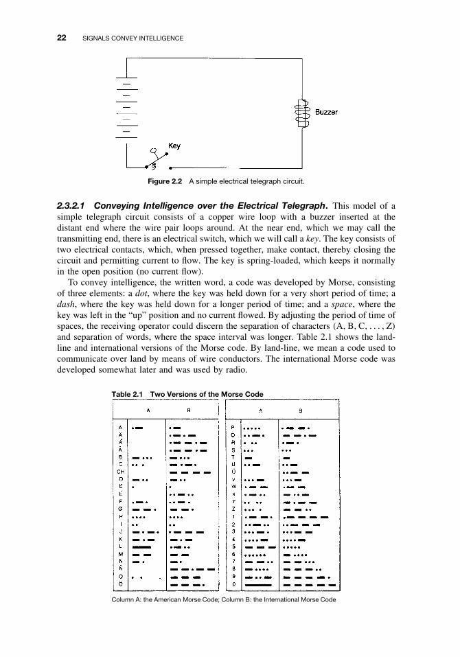
22 SIGNALS CONVEY INTELLIGENCE
Figure 2.2 A simple electrical telegraph circuit.
2.3.2.1 Conveying Intelligence over the Electrical Telegraph. This model of asimple telegraph circuit consists of a copper wire loop with a buzzer inserted at thedistant end where the wire pair loops around. At the near end, which we may call thetransmitting end, there is an electrical switch, which we will call a key. The key consists oftwo electrical contacts, which, when pressed together, make contact, thereby closing thecircuit and permitting current to flow. The key is spring-loaded, which keeps it normallyin the open position (no current flow).
To convey intelligence, the written word, a code was developed by Morse, consistingof three elements: a dot, where the key was held down for a very short period of time; adash, where the key was held down for a longer period of time; and a space, where thekey was left in the “up” position and no current flowed. By adjusting the period of time ofspaces, the receiving operator could discern the separation of characters (A, B, C, . . . , Z)
and separation of words, where the space interval was longer. Table 2.1 shows the land-line and international versions of the Morse code. By land-line, we mean a code used tocommunicate over land by means of wire conductors. The international Morse code wasdeveloped somewhat later and was used by radio.
Table 2.1 Two Versions of the Morse Code
Column A: the American Morse Code; Column B: the International Morse Code

2.3 BASIC CONCEPTS OF ELECTRICITY FOR COMMUNICATIONS 23
A more practical telegraph system is illustrated in Figure 2.3. Note that the figure hasjust one metallic wire connecting the west station to the east station. The second wire isreplaced with ground. The earth is a good conductor, and so we use earth, called ground,as the second conductor (or wire). Such a telegraph system is called single-wire groundreturn. Such a system was widely in use when my wife and I did a stint for the ITU(International Telecommunication Union) in Ecuador in 1967–1969.
This is a similar circuit as shown in Figure 2.2. In this case, when both keys are closed,a DC (direct current) circuit is traced from a battery in the west station through the keyand relay at that point to the line wire, and from there it is traced through the relay andkey at the east station and back through the earth (ground) to the battery. The relays ateach end, in turn, control the local circuits, which include a separate battery and a sounder(e.g., buzzer or other electric sounding device). Opening and closing the key at one end,while the key at the other end is closed, causes both sounders to operate accordingly.
A relay is a switch that is controlled electrically. It consists of (a) wire wrapped aroundan iron core and (b) a hinged metal strip, which is normally open. When current flowsthrough the windings (i.e., the wire wrapped around the core), a magnetic field is set up,thereby drawing the hinged metal strip into a closed position and causing current to flowin the secondary circuit. It is a simple open-and-closed device such that when currentflows there is a contact closure (the metal strip) and when there is no current through thewindings, the circuit is open. Of course there is a spring on the metal strip, holding itopen except when current flows.
Twenty years after Morse first demonstrated his telegraph on a Baltimore–Washingtonroute, telegraph covered the country from coast to coast. It caused a revolution in com-munications. Its use is still prevalent in many parts of the world, as I discussed above.
2.3.3 What Is Frequency?
To understand more advanced telecommunication concepts, we need a firm knowledge offrequency and related parameters such as band and bandwidth, wavelength, period, andphase. Let us first define frequency and relate it to everyday life.
The IEEE defines frequency as “the number of complete cycles of sinusoidal varia-tion per unit time.” The time unit we will use is the second. For those readers with amathematical bent, if we plot y = sin x, where x is expressed in radians, a “sine wave”is developed as shown in Figure 2.4.
Figure 2.5 shows two sine waves; the left side illustrates a lower frequency, and theright side shows a higher frequency. The amplitude, measured in this case as voltage,is the excursion, up or down, at any singular point. Amplitude expresses the intensity atthat point. If we spoke of amplitude without qualifying it at some point, it would be the
Figure 2.3 A practical elementary telegraph circuit with ground return.

24 SIGNALS CONVEY INTELLIGENCE
Figure 2.4 A sine wave. Here frequency is the number of times per second that a wave cycle (one peakand one trough) repeats at a given amplitude. A is the amplitude and λ is the wavelength. π is π radiansor 180◦ and 2π is the radian value at 360◦.
Figure 2.5 A simple sine wave. (a) Lower frequency, (b) higher frequency. Note that the wavelength isshown traditionally as λ (the Greek letter lambda) and that part a has a longer wavelength than part b.
maximum excursion in the negative or positive direction (up or down). In this case it is6 volts. If it is in the “down” direction, it would be −6 volts, based on Figure 2.5; andin the “up” direction it would be +6 volts.
Frequency is an important aspect of music. For example, the key of A is 440 Hz andmiddle C is 263 Hz. Note that the unit of measurement of frequency used to be cyclesper second (prior to 1963) and now the unit of measure is Hz named for Heinrich Hertz,a German physicist credited with the discovery of radio waves. Simple sine waves can beproduced in the laboratory with a signal generator, which is an electronic oscillator thatcan be tuned to different frequencies. An audio signal generator can be tuned to 263 Hz,middle C, and we can hear it if the generator output is connected to a loudspeaker. Theseare sound frequencies.
When we listen to the radio on the AM broadcast band, we may listen to a talk showon WOR, at a frequency of 710 kHz (kilohertz, meaning 710,000 Hz). On the FM bandin the Phoenix, AZ, area, we may tune to a classical music station, KBAQ, at 89.5 MHz(89,500,000 Hz). These are radio frequencies.

2.3 BASIC CONCEPTS OF ELECTRICITY FOR COMMUNICATIONS 25
Metric prefixes are often used, when appropriate, to express frequency as illustratedin the above paragraph. For example, kilohertz (kHz), megahertz (MHz), and giga-hertz (GHz) are used for Hz × 1000, Hz × 1,000,000, and Hz × 1,000,000,000. Thus38.71 GHz is 38.710,000,000 Hz.
Wavelength is conventionally measured in meters and is represented by the symbol λ.It is defined as the distance between successive peaks or troughs of a sinusoidal wave(i.e., D in Figure 2.5). Both sound and radio waves each travel with a certain velocityof propagation. Radio waves travel at 186,000 mi/sec in a vacuum, or 3 × 10⁸ m/sec.1 Ifwe multiply frequency in hertz times the wavelength in meters, we get a constant, thevelocity of propagation. In a vacuum (or in free space),
Fλ = 3 × 10⁸ m/sec, (2.1)
where F is measured in hertz, and λ is measured in meters (m). This is an importantconcept that will be freely used in the remainder of this text.
Example 1. The international calling and distress frequency is 500 kHz. What is theequivalent wavelength in meters?
500,000λ = 3 × 10⁸ m/sec
λ = 3 × 10⁸/5 × 105
= 600 m.
Example 2. A line-of-sight millimeter-wave radio2 link operates at 38.71 GHz. What isthe equivalent wavelength at this frequency?
38.71 × 10⁹λ = 3 × 10⁸ m/sec
λ = 3 × 10⁸/38.71 × 109
λ = 0.00775 m or 7.75 mm.
Figure 2.6 is an outline drawing of the radio frequency spectrum from nearly zero Hzto 100 GHz. The drawing shows several frequency bands assigned to specific services.
2.3.3.1 Introduction to Phase. The IEEE defines phase as “a relative measurementthat describes the temporal relationship between two signals that have the same fre-quency.” We can plot a sine wave (representing a certain frequency) by the methodshown in Figure 2.7, where the horizontal lines are continuation of points a, b, c, and soon, and the vertical lines a′, b′, c′, and so on, are equally spaced and indicate angulardegrees of rotation. The intersection of lines a and a′, b and b′, and so on, indicates pointson the sine wave curve.
To illustrate what is meant by phase relation, we turn to the construction of a sinewave using a circle as shown in Figure 2.7. In the figure the horizontal scale (the abscissa)represents time and the vertical scale (the ordinate) represents instantaneous values of
1Sound waves travel at 1076 ft/sec (331 m/sec) in air at 0◦C and with 1 atmosphere of atmospheric pressure.However, our interest here is in radio waves, not sound waves.2This is termed millimeter radio because wavelengths in this region are measured in millimeters (i.e., forfrequencies above 30 GHz) rather than in centimeters or meters.

26 SIGNALS CONVEY INTELLIGENCE
Figure 2.6 The radio-frequency spectrum showing some frequency band assignments.

2.3 BASIC CONCEPTS OF ELECTRICITY FOR COMMUNICATIONS 27
Figure 2.7 Graphical construction of a sine wave.
Figure 2.8 Two signals of the same frequency: (a) with different amplitudes and in-phase and (b) withthe same amplitudes but 180 degrees out of phase.
current or voltage. The complete curve shows values of current (or voltage) for all instantsduring one complete cycle. It is convenient and customary to divide the time scale intounits of degrees rather than seconds, considering one complete cycle as being completedalways in 360 degrees or units of time (regardless of the actual time taken in seconds).The reason for this convention becomes obvious from the method of constructing the sine
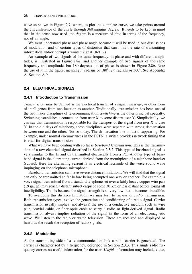
28 SIGNALS CONVEY INTELLIGENCE
wave as shown in Figure 2.7, where, to plot the complete curve, we take points aroundthe circumference of the circle through 360 angular degrees. It needs to be kept in mindthat in the sense now used, the degree is a measure of time in terms of the frequency,not of an angle.
We must understand phase and phase angle because it will be used in our discussionsof modulation and of certain types of distortion that can limit the rate of transmittinginformation and/or corrupt a wanted signal (Ref. 2).
An example of two signals of the same frequency, in phase and with different ampli-tudes, is illustrated in Figure 2.8a, and another example of two signals of the samefrequency and amplitude, but 180 degrees out of phase, is shown in Figure 2.8b. Notethe use of π in the figure, meaning π radians or 180◦, 2π radians or 360◦. See AppendixA, Section A.9.
2.4 ELECTRICAL SIGNALS
2.4.1 Introduction to Transmission
Transmission may be defined as the electrical transfer of a signal, message, or other formof intelligence from one location to another. Traditionally, transmission has been one ofthe two major disciplines of telecommunication. Switching is the other principal specialty.Switching establishes a connection from user X to some distant user Y. Simplistically, wecan say that transmission is responsible for the transport of the signal from user X to userY. In the old days of telephony, these disciplines were separate with strong demarcationbetween one and the other. Not so today. The demarcation line is fast disappearing. Forexample, under normal circumstances in the PSTN, a switch provides network timing thatis vital for digital transmission.
What we have been dealing with so far is baseband transmission. This is the transmis-sion of a raw electrical signal described in Section 2.3.2. This type of baseband signal isvery similar to the 1s and 0s transmitted electrically from a PC. Another type of base-band signal is the alternating current derived from the mouthpiece of a telephone handset(subset). Here the alternating current is an electrical facsimile of the voice sound waveimpinging on the telephone microphone.
Baseband transmission can have severe distance limitations. We will find that the signalcan only be transmitted so far before being corrupted one way or another. For example, avoice signal transmitted from a standard telephone set over a fairly heavy copper wire pair(19 gauge) may reach a distant subset earpiece some 30 km or less distant before losing allintelligibility. This is because the signal strength is so very low that it becomes inaudible.
To overcome this distance limitation, we may turn to carrier or radio transmission.Both transmission types involve the generation and conditioning of a radio signal. Carriertransmission usually implies (not always) the use of a conductive medium such as wirepair, coaxial cable, or fiber-optic cable to carry a radio or light-derived signal. Radiotransmission always implies radiation of the signal in the form of an electromagneticwave. We listen to the radio or watch television. These are received and displayed orheard as the result the reception of radio signals.
2.4.2 Modulation
At the transmitting side of a telecommunication link a radio carrier is generated. Thecarrier is characterized by a frequency, described in Section 2.3.3. This single radio fre-quency carries no useful information for the user. Useful information may include voice,

2.4 ELECTRICAL SIGNALS 29
data, or image (typically facsimile or television). Modulation is the process of impingingthat useful information on the carrier, and demodulation is the recovery of that informationfrom the carrier at the distant end near the destination user.
The IEEE defines modulation as “a process whereby certain characteristics of a wave,often called the carrier, are varied or selected in accordance with a modulating function.”The modulating function is the information baseband described above.
There are three generic forms of modulation:
1. Amplitude modulation (AM)2. Frequency modulation (FM)3. Phase modulation (PM).
Item 1 (amplitude modulation) is where a carrier is varied in amplitude in accordance withinformation baseband signal. In the case of item 2 (frequency modulation), a carrier isvaried in frequency in accordance with the baseband signal. For item 3 (phase modulation)a carrier is varied in its phase in accordance with the information baseband signal.
Figure 2.9 graphically illustrates amplitude, frequency, and phase modulation. Themodulating signal is a baseband stream of bits: 1s and 0s. We deal with digital transmission(e.g., 1s and 0s) extensively in Chapters 6 and 10.
Prior to 1960, all transmission systems were analog. Today, in the PSTN, all telecom-munication systems are digital, except for the preponderance of subscriber access lines.These are the subscriber loops described in Chapter 1. Let us now distinguish and defineanalog and digital transmission
2.4.2.1 Analog Transmission. Analog transmission implies continuity as contrastedwith digital transmission that is concerned with discrete states. Many signals can be usedin either the analog or digital sense, the means of carrying the information being thedistinguishing feature. The information content of an analog signal is conveyed by thevalue or magnitude of some characteristic(s) of the signal such as amplitude, frequency,or phase of a voltage, the amplitude or duration of a pulse, the angular position of a shaft,or the pressure of a fluid. Typical analog transmission are the signals we hear on AM andFM radio and what we see (and hear) on television. In fact, television is rather unique. Thevideo itself uses amplitude modulation; the sound subcarrier uses frequency modulation,and the color subcarrier employs phase modulation. All are in analog formats.
2.4.2.2 Digital Transmission. The information content of a digital signal is concernedwith discrete states of the signal, such as the presence or absence of a voltage (seeSection 2.3.2); a contact is the open or closed position, or a hole or no hole in certainpositions on a card or paper tape. The signal is given meaning by assigning numericalvalues or other information to the various combinations of the discrete states of thesignal. We will be dealing extensively with digital transmission as the argument in thistext proceeds.
2.4.3 Binary Digital Signals
In Section 2.4.1, we defined a digital waveform as one that displayed discreteness. Sup-pose we consider the numbers 0 through 9. In one case, only integer values are permittedin this range, no in-between values such as 3.761 or 8.07. This is digital where we can only

30 SIGNALS CONVEY INTELLIGENCE
Figure 2.9 Illustration of amplitude, frequency, and phase modulation, where the modulating signal isthe binary digital sequence 00110100010, an electrical baseband signal.
assign integer values between 0 and 9. These are discrete values. On the other hand, if wecan assign any number value between 0 and 9, there could be an infinite number of valuessuch as 7.01648754372100. This, then, is analog. We have continuity, no discreteness.
Consider now how neat it would be if we had only two values in our digital system.Arbitrarily, we’ll call them a 1 and a 0. This is indeed a binary system, just two possiblevalues. It makes the work of a decision circuit really easy. Such a circuit has to decide onjust one of two possibilities. Look at real life: A light is on or it is off; two values, on andoff. A car engine is running or not running, and so on. In our case of interest, we denominateone value a 1 and denominate the other a 0. We could have a condition where current flows,and we’ll call that condition a 1; no current flowing we’ll call a 0 (Ref. 3).3
3The reader with insight will note an ambiguity here. We could reverse the conditions, making the 1 state a 0and the 0 state a 1. We address this issue in Chapter 10.

2.5 INTRODUCTION TO TRANSPORTING ELECTRICAL SIGNALS 31
Of course we are defining a binary system with a number base of 2. Our day-to-daynumbers are based on a decimal number system where the number base is 10. There is areview of binary arithmetic in Appendix B.
The basic key in binary digital transmission is the bit, which is the smallest unit ofinformation in the binary system of notation. It is the abbreviation of the term binarydigit. It is a unit of information represented by either a “1” or a “0.”
A 1 and a 0 do not carry much information, yet we do use just one binary digit in manyapplications. One of the four types of telephone signaling is called supervisory signaling.The only information necessary in this case is that the line is busy or it is idle. We mayassign the idle state a 0 and the busy state a 1. Another application where only a singlebinary digit is required is in built-in test equipment (BITE). In this case, we accept oneof two conditions: A circuit, module, or printed circuit board (PCB) is operational or itis not. BITE automates the troubleshooting of electronic equipment.
To increase the information capacity of a binary system is to place several bits (binarydigits) contiguously together. For instance, if we have a 2-bit code, there are four possi-bilities: 00, 01, 10, and 11. A 3-bit code provides eight different binary sequences, each3 bits long. In this case we have 000, 001, 010, 011, 101, 110, and 111. We could assignletters of the alphabet to each sequence. There are only eight distinct possibilities, so onlyeight letters can be accommodated. If we turn to a 4-bit code, 16 distinct binary sequencescan be developed, each 4 bits long. A 5-bit code will develop 32 distinct sequences, andso on.
As a result, we can state that for a binary code of length n, we will have 2n differentpossibilities. The American Standard Code for Information Interchange (ASCII) is a 7-bitcode (see Section 10.4); it will then have 27, or 128, binary sequence possibilities. Whenwe deal with pulse code modulation (PCM) (Chapter 6) as typically employed on thePSTN, a time slot contains 8 bits. We know that an 8-bit binary code has 256 distinct8-bit sequences (i.e., 28 = 256).
Consider the following important definitions when dealing with the bit and binarytransmission. Bit rate is defined as the number of bits (those 1s and 0s) that are transmittedper second. Bit error rate (BER) is the number of bit errors measured or expected per unitof time. Commonly, the time unit is the second. An error, of course, is where a decisioncircuit declares a 1 when it was supposed to be a 0, or declares a 0 when it was supposedto be a 1 (Ref. 4).
2.5 INTRODUCTION TO TRANSPORTING ELECTRICAL SIGNALS
To transport electrical signals, a transmission medium is required. There are four typesof transmission media:
1. Wire pair2. Coaxial cable3. Fiber-optic cable4. Radio
2.5.1 Wire Pair
As one might imagine, a wire pair consists of two wires. The wires commonly use acopper conductor, although aluminum conductors have been employed. A basic impair-ment of wire pair is loss. Loss is synonymous with attenuation. Loss can be defined

32 SIGNALS CONVEY INTELLIGENCE
as the dissipation of signal strength as a signal travels along a wire pair, or any othertransmission medium for that matter. Loss or attenuation is usually expressed in decibels(dB). In Appendix C the reader will find a tutorial on decibels and their applications intelecommunications.
Loss causes the signal power to be dissipated as a signal passes along a wire pair.Power is expressed in watts. For this application, the use of milliwatts may be morepractical. If we denominate loss with the notation LdB, then
LdB = 10 log(P1/P2), (2.2)
where P1 is the power of the signal where it enters the wire pair, and P2 is the power levelof the signal at the distant end of the wire pair. This is the traditional formula definingthe decibel in the power domain. See Appendix C.
Example 1. Suppose a 10-mW (milliwatt), 1000-Hz signal is launched into a wire pair.At the distant end of the wire pair the signal is measured at 0.2 mW. What is the loss indecibels on the line for this signal?
LdB = 10 log(10/0.2)
= 10 log(50)
≈ 17 dB
All logarithms used in this text are to the base 10. Appendix B provides a review oflogarithms and their applications.
The opposite of loss is gain. An attenuator is a device placed in a circuit to purposelycause loss. An amplifier does just the reverse; that is, it gives a signal gain. An amplifierincreases a signal’s intensity. We will use the following graphic symbol for an attenuator:
We will also use the following symbol for an amplifier:
Wire-pair transmission suffers other impairments besides loss. One of these impair-ments is crosstalk. Most of us have heard crosstalk on our telephone line. It appears asanother, “foreign” conversation having nothing to do with our telephone call. One basiccause of crosstalk is from other wire pairs sharing the same cable as our line. These otherconversations are electrically induced into our line. To mitigate this impairment, physicaltwists are placed on each wire pair in the cable. Generally there are 2 to 12 twists perfoot of wire pair. From this we get the term twisted pair. The following figure shows a

2.5 INTRODUCTION TO TRANSPORTING ELECTRICAL SIGNALS 33
section of twisted pair:
Another impairment causes a form of delay distortion on the line, which is cumulativeand varies directly with the length of the line as well as with the construction of the wireitself. It has little effect on voice transmission, but can place definition restrictions on datarate for digital/data transmission on the pair. The impairment is due to the capacitancebetween one wire and the other of the pair, between each wire and ground, and betweeneach wire and the shield, if a shield is employed. Delay distortion is covered in greaterdepth in Chapters 6 and 10.
2.5.1.1 Capacitance. Direct-current (DC) circuits are affected by resistance, whereasalternating-current (AC) circuits, besides resistance, are affected by the properties ofinductance and capacitance. In this subsection, we provide a brief description of capaci-tance. Also see Appendix A, Section A.8.
Capacitance is somewhat analogous to elasticity. While a storage battery stores elec-tricity as another form of energy (i.e., chemical energy), a capacitor stores electricity inits natural state. An analogy of capacitance is a closed tank filled with compressed air.The quantity of air, since air is elastic, depends upon the pressure as well as the size orcapacity of the tank. If a capacitor4 is connected to a direct source of voltage through aswitch, as shown in Figure 2.10, and the switch is suddenly closed, there will be a rushof current in the circuit. This current will charge the capacitor to the same voltage valueas the battery, but the current will decrease rapidly and become zero when the capacitoris fully charged.
Let us define a capacitor as two conductors separated by an insulator. A conductorconducts electricity. Certain conductors conduct electricity better than others. Platinumand gold are very excellent conductors, but very expensive. Copper does not conductelectricity as well as gold and platinum, but is much more cost-effective. An insulatorcarries out the opposite function of a conductor. It tends to prevent the flow of electricitythrough it. Some insulators are better than others regarding the conduction of electricity.Air is an excellent insulator. However, we well know that air can pass electricity if thevoltage is very high. Consider lightning, for example. Other examples of insulators arebakelite, celluloid, fiber, formica, glass, lucite, mica, paper, rubber, and wood.
Figure 2.10 A simple capacitive circuit.
4A capacitor is a device whose primary purpose is to introduce capacitance into a circuit.

34 SIGNALS CONVEY INTELLIGENCE
The insulated conductors of every circuit, such as our wire pair, have to a greater orlesser degree this property of capacitance. The capacitance of two parallel open wires ora pair of cable conductors of any considerable length is appreciable in practice.
2.5.1.2 Bandwidth (Hz) of a Twisted Pair. The usable bandwidth of twisted wirepair varies with the type of wire pair used and its length. Ordinary wire pair used inthe PSTN subscriber access plant can support 2 MHz over about 1 mile of length.Special Category 5 twisted pair displays a 67-dB loss at 100 MHz over a length of1000 ft.
2.5.1.3 Bandwidth Defined. The IEEE defines bandwidth as “the range of frequencieswithin which performance, with respect to some characteristic, falls within specific limits.”One such limit is the amplitude of a signal within the band. Here it is commonly definedat the points where the response is 3 dB below the reference value. This 3-dB powerbandwidth definition is illustrated graphically in Figure 2.11.
2.5.2 Coaxial Cable Transmission
Up to this point we have been discussing two parallel conductors, namely, wire pair. Anentirely different configuration of two conductors may be used to advantage where highand very high radio frequencies are involved. This is a coaxial configuration. Here theconducting pair consists of a cylindrical tube with a single wire conductor going down itscenter as shown in Figure 2.12. In practice the center conductor is held in place accuratelyby a surrounding insulating material that may take the form of a solid core, discs, or beadsstrung along the axis of the wire or a spirally wrapped string. The nominal impedance is75 ohms, and special cable is available with a 50-ohm impedance.
Figure 2.11 The concept of the 3-dB power bandwidth.
Figure 2.12 A pictorial representation of a coaxial cable section.

2.5 INTRODUCTION TO TRANSPORTING ELECTRICAL SIGNALS 35
Impedance can be defined as the combined effect of a circuit’s resistance, inductance,and capacitance taken as a single property and is expressed in ohms for any given sinewave frequency. Further explanation of impedance will be found in Appendix A.
From about 1953 to 1986, coaxial cable was widely deployed for long-distance, mul-tichannel transmission. Its frequency response was exponential. In other words, its lossincreased drastically as frequency was increased. For example, for 0.375-inch coaxialcable, the loss at 100 kHz was about 1 dB and the loss at 10 MHz was about 12 dB.Thus, equalization was required. Equalization tends to level out the frequency response.With the advent of fiber-optic cable with its much greater bandwidth and comparativelyflat frequency response, the use of coaxial cable on long-distance circuits fell out of favor.It is still widely used as a (radio-frequency) (RF) transmission line connecting a radioto its antenna. It is also extensively employed in cable television plant, especially in the“last mile” or “last 100 ft” of connectivity to a subscriber’s television set.
2.5.3 Fiber-Optic Cable
Fiber-optic cable is the favored transmission medium for very wideband terrestrial links,including undersea applications. It is also used for cable television “super trunks.” Thebandwidth of fiber-optic strand can be measured in terahertz (THz). In fact, the wholeusable RF spectrum can be accommodated on just one such strand. Such a strand is aboutthe diameter of a human hair. It can carry one serial bit stream at 10 Gbps (gigabitsper second) transmission rate, or by wave division multiplexing methods (WDM), anaggregate of 100 Gbps or more. Fiber-optic transmission will be discussed further inChapter 9.
Fiber-optic systems can be loss-limited or dispersion-limited. If a fiber-optic link islimited by loss, it means that as the link is extended in distance, the signal has dissipatedso much that it becomes unusable. The maximum loss that a link can withstand and stilloperate satisfactorily is a function of the type of fiber, wavelength5 of the light signal,the bit rate and error rate, signal type (e.g., TV video), power output of the light source(transmitter), and the sensitivity of the light detector (receiver).
Dispersion-limited means that a link’s length is limited by signal corruption. As alink is lengthened, there may be some point where the bit error rate (BER) becomesunacceptable. This is caused by signal energy of a particular pulse that arrives later thanother signal energy of the same pulse. There are several reasons why energy elementsof a single light pulse may become delayed compared to other elements. One may bethat certain launched modes arrive at the distant end before other modes. Another maybe that certain frequencies contained in a light pulse arrive before other frequencies. Ineither case, delayed power spills into the subsequent bit position, which can confuse thedecision circuit. The decision circuit determines whether the pulse represented a 1 or a0. The higher the bit rate, the worse the situation becomes. Also, the delay increases asa link is extended.
The maximum length of fiber-optic links range from 20 miles (32 km) to severalhundred miles (km) before requiring a repeater. This length can be extended by the useof amplifiers and/or repeaters, where each amplifier can impart a 20- to 40-dB gain. Afiber-optic repeater detects, demodulates, and then remodulates a light transmitter. In theprocess of doing this, the digital signal is regenerated. A regenerator takes a corruptedand distorted digital signal and forms a brand new, nearly perfect digital signal.
5In the world of fiber optics, wavelength is used rather than frequency. We can convert wavelength to fre-quency using Eq. (2.1). One theory is that fiber-optic transmission was developed by physicists who are moreaccustomed to wavelength than to frequency.
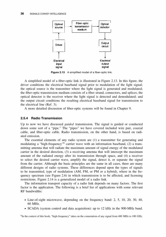
36 SIGNALS CONVEY INTELLIGENCE
Figure 2.13 A simplified model of a fiber-optic link.
A simplified model of a fiber-optic link is illustrated in Figure 2.13. In this figure, thedriver conditions the electrical baseband signal prior to modulation of the light signal;the optical source is the transmitter where the light signal is generated and modulated;the fiber-optic transmission medium consists of a fiber strand, connectors, and splices; theoptical detector is the receiver where the light signal is detected and demodulated; andthe output circuit conditions the resulting electrical baseband signal for transmission tothe electrical line (Ref. 3).
A more detailed discussion of fiber-optic systems will be found in Chapter 9.
2.5.4 Radio Transmission
Up to now we have discussed guided transmission. The signal is guided or conducteddown some sort of a “pipe.” The “pipes” we have covered included wire pair, coaxialcable, and fiber-optic cable. Radio transmission, on the other hand, is based on radi-ated emission.
The essential elements of any radio system are (1) a transmitter for generating andmodulating a “high-frequency”6 carrier wave with an information baseband, (2) a trans-mitting antenna that will radiate the maximum amount of signal energy of the modulatedcarrier in the desired direction, (3) a receiving antenna that will intercept the maximumamount of the radiated energy after its transmission through space, and (4) a receiverto select the desired carrier wave, amplify the signal, detect it, or separate the signalfrom the carrier. Although the basic principles are the same in all cases, there are manydifferent designs of radio systems. These differences depend upon the types of signalsto be transmitted, type of modulation (AM, FM, or PM or a hybrid), where in the fre-quency spectrum (see Figure 2.6) in which transmission is to be affected, and licensingrestrictions. Figure 2.14 is a generalized model of a radio link.
The information transport capacity of a radio link depends on many factors. The firstfactor is the application. The following is a brief list of applications with some relevantRF bandwidths:
ž Line-of-sight microwave, depending on the frequency band: 2, 5, 10, 20, 30, 40,60 MHz.
ž SCADA (system control and data acquisition): up to 12 kHz in the 900-MHz band.
6In the context of this book, “high-frequency” takes on the connotation of any signal from 400 MHz to 100 GHz.

2.5 INTRODUCTION TO TRANSPORTING ELECTRICAL SIGNALS 37
Figure 2.14 A generic model of a typical radio link.
ž Satellite communications, geostationary satellites: 500 MHz or 2.5-GHz bandwidthsbroken down into 36- and 72-MHz segments.
ž Cellular radio: 25-MHz bandwidth in the 800/900-MHz band. The 25-MHz band issplit into two 12.5-MHz segments for two competitive providers.
ž Personal communication services (PCS): 200-MHz band just below 2.0 GHz, brokendown into various segments such as licensed and unlicensed users.
ž Cellular/PCS by satellite (e.g., Iridium, Globalstar), 10.5-MHz bandwidth in the1600-MHz band.
ž Local multipoint distribution system (LMDS) in 28/38-GHz bands, 1.2-GHz band-width for CATV, Internet, data, and telephony services (Ref. 5).
Bandwidth is also determined by the regulating authority (e.g., the FCC in the UnitedStates) for a particular service/application. Through bit packing techniques, described inChapter 9, the information carrying capacity of a unit of bandwidth is considerably greaterthan 1 bit per Hz of bandwidth. On line-of-sight microwave systems, 5, 6, 7, and 8 bitsper hertz of bandwidth are fairly common.

38 SIGNALS CONVEY INTELLIGENCE
Chapter 9 provides a more detailed discussion of radio systems.
REVIEW EXERCISES
1. Name at least four different ways of communicating at a distance prior to the adventof electrical communication.
2. What kind of energy is stored in a battery?
3. How did the old electric telegraph communicate intelligence?
4. What limited the distance we could transmit with electrical telegraph before usinga repeater? Give at least two ways we could extend the distance.
5. How could that old-time electrical telegraph operate with just one wire?
6. Name at least four ways we might characterize a “sine wave” either partiallyor wholly.
7. What is the equivalent wavelength (λ) of 850 MHz; of 7 GHz?
8. What angle (in degrees) is equivalent to 3π/2? to π/4?
9. Give two examples of baseband transmission.
10. Define modulation.
11. What are the three generic forms of modulation? What popular device we find inthe home utilizes all three types of modulation simultaneously. The answer needs amodifier in front of the word.
12. Differentiate an analog signal from a digital signal.
13. Give at least four applications of a 1-bit code. We suggest using imagination.
14. What is the total capacity of a 9-bit binary code? The Hollerith code was a 12-bitcode. What was its total capacity?
15. Name four different transmission media.
16. What is the opposite of loss? What is the most common unit of measurement toexpress the amount of loss?
17. What is the reason of twists in twisted pair?
18. What is the principal cause of data rate limitation on wire pair.
19. What is the principal drawback of using coaxial cable for long-distance transmission?
20. What is the principal, unbeatable advantage of fiber-optic cable?
21. Regarding limitation of bit rate and length, a fiber-optic cable may be eitheror ?
22. Explain dispersion (with fiber-optic cable).
23. What are some typical services of LMDS?
REFERENCES
1. From Semaphore to Satellite, The International Telecommunication Union, Geneva, 1965.

REFERENCES 39
2. Principles of Electricity Applied to Telephone and Telegraph Work, American Telephone andTelegraph Co., New York, 1961.
3. R. L. Freeman, Telecommunication Transmission Handbook, 4th ed., Wiley, New York, 1998.
4. “Time and Frequency: Theory and Fundamentals,” NBS Monograph 140, U.S. Dept. of Com-merce, Washington, DC, May 1974.
5. Clint Smith, LMDS, McGraw-Hill, New York, 2000.


3
QUALITY OF SERVICE ANDTELECOMMUNICATION
IMPAIRMENTS
3.1 OBJECTIVE
Quality of service (QoS) was introduced in Section 1.4. In this chapter we will be moredefinitive in several key areas. There are a number of generic impairments that willdirectly or indirectly affect quality of service. An understanding of these impairments andtheir underlying causes are extremely important if one wants to grasp the entire pictureof a telecommunication system.
3.2 QUALITY OF SERVICE: VOICE, DATA, AND IMAGE
3.2.1 Signal-to-Noise Ratio
Signal-to-noise ratio (S/N or SNR) is the most widely used parameter for measurementof signal quality in the field of transmission. Signal-to-noise ratio expresses in decibelsthe amount that signal level exceeds the noise level in a specified bandwidth.
As we review the several types of material to be transmitted on a network, each willrequire a minimum S/N to satisfy the user or to make a receiving instrument functionwithin certain specified criteria. The following are S/N guidelines at the correspondingreceiving devices:
Voice: 40 dB
Video (TV): 45 dB
Data: ∼15 dB, based upon the modulation type and specified error performance
To illustrate the concept of S/N, consider Figure 3.1. This oscilloscope presentation showsa nominal analog voice channel (300–3400 Hz) with a 1000-Hz test signal. The verticalscale is signal power measured in dBm (see Appendix C for a tutorial on dBs), and thehorizontal scale is frequency, 0–3400 Hz. The S/N as illustrated is 10 dB. We can derive
Fundamentals of Telecommunications, Second Edition, by Roger L. FreemanISBN 0-471-71045-8 Copyright 2005 by Roger L. Freeman
41

42 QUALITY OF SERVICE AND TELECOMMUNICATION IMPAIRMENTS
Figure 3.1 Signal-to-noise ratio.
this by inspection or by reading the levels on the oscilloscope presentation. The signallevel is +15 dBm; the noise is +5 dBm, then
(S/N)dB = level(signal in dBm) − level(noise in dBm). (3.1)
Inserting the values from the “oscilloscope example” above, we have
S/N = +15 dBm − (+5 dBm),
S/N = 10 dB.
This expression is set up as shown because we are dealing with logarithms (see AppendixB). When multiplying in the domain of logarithms, we add. When dividing, we subtract.We are dividing because on the left side of the equation we have S/N or S divided by N.
Signal-to-noise ratio really has limited use in the PSTN for characterizing speechtransmission because of the “spurtiness” of the human voice. We can appreciate thatindividual talker signal power can fluctuate widely so that S/N is far from constant duringa telephone call and from one telephone call to the next. In lieu of actual voice, we use atest tone to measure level and S/N. A test tone is a single frequency, usually around 800or 1000 Hz, generated by an audio signal generator and inserted in the voice channel. Thelevel of the tone (often measured in dBm) can be easily measured with the appropriate testequipment. Such a tone has constant amplitude and no silent intervals, which is typicalof voice transmission.
3.2.2 Voice Transmission
3.2.2.1 Loudness Rating and Its Predecessors. Historically, on telephone con-nections, the complaint has been that at the receiving telephone the distant talker’svoice was not loud enough. “Hearing sufficiently well” on a telephone connection isa subjective matter. This is a major element of quality of service (QoS). Various meth-ods have been derived over the years to rate telephone connections regarding customersatisfaction.
The underlying cause of low signal level is loss across the network. Any method tomeasure “hearing sufficiently well” should incorporate intervening losses on a telephoneconnection. As we discussed in Chapter 2, losses are conventionally measured in decibels.Thus the unit of measure of “hearing sufficiently well” is the decibel. From the present

3.2 QUALITY OF SERVICE: VOICE, DATA, AND IMAGE 43
method of measurement we derive the loudness rating, abbreviated LR. It had severalpredecessors: reference equivalent and corrected reference equivalent.
3.2.2.2 Reference Equivalent. The reference equivalent value, called the overallreference equivalent (ORE), was indicative of how loud a telephone signal is. How loudis a subjective matter. Given a particular voice level, for some listeners it would besatisfactory; for others, unsatisfactory. The ITU in Geneva brought together a group oftelephone users to judge telephone loudness. A test installation was set up made upof two standard telephone subsets, namely, a talker’s simulated subscriber loop and alistener’s simulated loop. An adjustable attenuating network was placed between the twosimulated loops. The test group, on an individual basis, judged level at the receivingtelephone earpiece. At a 6-dB setting of the attenuator or less, calls were judged tooloud. Better than 99% of the test population judged calls to be satisfactory with anattenuator setting of 16 dB; 80% rated a call satisfactory with an ORE 36 dB or better,and 33.6% of the test population rated calls with an ORE of 40 dB as unsatisfactory,and so on.
Using a similar test set up, standard telephone sets of different telephone adminis-trations (countries) could be rated. The mouthpiece (transmitter) and earpiece (receiver)were rated separately and given a decibel value. The decibel value was indicative if theyworked better or worse than the telephones used in the ITU laboratory. The attenuatorsetting represented the loss in a particular network connection. To calculate overall refer-ence equivalent (ORE), we summed the three decibel values (i.e., the transmit referenceequivalent of the telephone set, the intervening network losses, and the receive referenceequivalent of the same type subset).
In one CCITT recommendation, 97% of all international calls were recommended tohave an ORE of 33 dB or better. It was found that with this 33-dB value, less than 10%of users were unsatisfied with the level of the received speech signal.
3.2.2.3 Corrected Reference Equivalent. Because difficulties were encountered inthe use of reference equivalents, the ORE was replaced by the corrected reference equiv-alent (CRE) around 1980. The concept and measurement technique of the CRE wasessentially the same as RE (reference equivalent), and the decibel remained the measure-ment unit.
CRE test scores varied somewhat from its RE counterparts. Less than 5 dB (CRE) wastoo loud; an optimum connection had an RE value of 9 dB and a range from 7 to 11 dBfor CRE. For a 30-dB value of CRE, 40% of a test population rated the call excellent,whereas 15% rated it poor or bad.
3.2.2.4 Loudness Rating. Around 1990 the CCITT replaced corrected referenceequivalent with loudness rating. The method recommended to determine loudness ratingeliminates the need for subjective determinations of loudness loss in terms of correctedreference equivalent. The concept of overall loudness rating (OLR) is very similar to theORE concept used with reference equivalent.
Table 3.1 gives opinion results for various values of overall loudness rating (OLR) indecibels. These values are based upon representative laboratory conversation test resultsfor telephone connections in which other characteristics such as circuit noise have littlecontribution to impairment.

44 QUALITY OF SERVICE AND TELECOMMUNICATION IMPAIRMENTS
Table 3.1 Overall Loudness Rating Opinion Results
Representative Opinion Resultsa
OverallLoudnessRating (dB)
Percent‘‘Good plus Excellent’’
Percent‘‘Poor plus Bad’’
5–15 <90 <120 80 425 65 1030 45 20
aBased on opinion relationship derived from the transmission qualityindex (see Annex A, ITU-T Rec. P.11).
Source: ITU-T Rec. P.11, Table 1/P.11, p. 2, Helsinki, 3/93.
Figure 3.2 Designation of LRs in an international connection.
3.2.2.4.1 Determination of Loudness Rating. The designation with notations of loud-ness rating concept for an international connection is given in Figure 3.2. It is assumedthat telephone sensitivity, both for the earpiece and microphone, have been measured.Overall loudness rating (OLR) is calculated using the following formula:
OLR = SLR + CLR + RLR. (3.2)
The measurement units in Eq. (3.2) are decibels.The overall loudness rating (OLR) is defined as the loudness loss between the speaking
subscriber’s mouth and the listening subscriber’s ear via a telephone connection. The sendloudness rating (SLR) is defined as the loudness loss between the speaking subscriber’smouth and an electrical interface in the network. The receive loudness rating (RLR) is theloudness loss between an electrical interface in the network and the listening subscriber’sear. The circuit loudness rating (CLR) is the loudness loss between two electrical inter-faces in a connection or circuit, with each interface terminated by its nominal impedance(Refs. 1, 2).
3.2.3 Data Circuits
Bit error rate (BER) is the underlying QoS parameter for data circuits. BER is not sub-jective; it is readily measurable. Data users are very demanding of network operatorsregarding BER. If a network did not ever carry data, BER requirements could be muchless stringent. CCITT/ITU-T recommends a BER of 1 × 10⁻⁶ for at least 80% of amonth.1 Let us assume that these data will be transported on the digital network, typ-ical of a PSTN. Let us further assume that conventional analog moderns are not used,
1See CCITT Rec. G.821.

3.3 THE THREE BASIC IMPAIRMENTS AND HOW THEY AFFECT THE END-USER 45
and the data are exchanged bit for bit with “channels” on the digital network. Thus, theBER of the data reflects the BER of the underlying digital channel which is acting as itstransport. BERs encountered on digital networks in the industrialized/postindustrializednations are far improved, some attaining an end-to-end BER of 5 × 10⁻¹⁰. Thus, the databeing transported can expect a similar BER.
The genesis of frame relay, discussed in Chapter 10, is based on the premise that theseexcellent BERs can be expected.
3.2.4 Video (Television)
Television picture quality is subjective to the viewer. It is based on S/N of the picturechannel. The S/N values derived from two agencies are provided below. The first arecalled “TASO ratings.” TASO stands for Television Allocations Study Organization. TheTASO ratings follow:
TASO PICTURE RATING
Quality S/N
1. Excellent (no perceptible snow) 45 dB2. Fine (snow just perceptible) 35 dB3. Passable (snow definitely perceptible but not objectionable) 29 dB4. Marginal (snow somewhat objectionable) 25 dBSnow is the visual perception of high levels of thermal noise typical with poorer S/N values.
CCIR developed a 5-point scale for picture quality versus impairment. This scale isshown in the following table:
CCIR FIVE-GRADE SCALE
Quality Impairment
5. Excellent 5. Imperceptible4. Good 4. Perceptible, but not annoying3. Fair 3. Slightly annoying2. Poor 2. Annoying1. Bad 1. Very annoying
Later CCIR/ITU-R documents steer clear of assigning S/N to such quality scales. In fact,when digital compression of TV is employed, the use of S/N to indicate picture qualityis deprecated.
3.3 THE THREE BASIC IMPAIRMENTS AND HOW THEY AFFECTTHE END-USER
There are three basic impairments found in all telecommunication transmission systems.These are:
ž Amplitude (or attenuation) distortionž Phase distortionž Noise

46 QUALITY OF SERVICE AND TELECOMMUNICATION IMPAIRMENTS
3.3.1 Amplitude Distortion
The IEEE defines attenuation distortion (amplitude distortion) as the change in attenuationat any frequency with respect to that of a reference frequency. For the discussion in thissection, we’ll narrow the subject to the (analog) voice channel. In most cases a user isconnected, through his/her metallic subscriber loop to the local serving exchange. Thiscircuit is analog. Based upon the CCITT definition, the voice channel occupies the bandfrom 300 to 3400 Hz. We call this the passband.
Attenuation distortion can be avoided if all frequencies within the passband are sub-jected to the same loss (or gain). Whatever the transmission medium, however, somefrequencies are attenuated more than others. Filters are employed in most active circuits(and in some passive circuits) and are major causes of attenuation distortion. Figure 3.3is a response curve of a typical bandpass filter with voice channel application.
As stated in our definition, amplitude distortion across the voice channel is measuredagainst a reference frequency. CCITT recommends 800 Hz as the reference; in NorthAmerica the reference is 1000 Hz.2 Let us look at some ways that attenuation distortionmay be stated. For example, one European requirement may state that between 600 and2800 Hz the level will vary no more than −1 to +2 dB, where the plus sign means moreloss and the minus sign means less loss. Thus if an 800-Hz signal at −10 dBm is placedat the input of the channel, we would expect −10 dBm at the output (if there were nooverall loss or gain), but at other frequencies we can expect a variation at the outputof −1 to +2 dB. For instance, we might measure the level at the output at 2500 Hz at−11.9 dBm and at 1100 Hz at −9 dBm.
When filters or filter-like devices3 are placed in tandem, attenuation distortion tends tosum. Two identical filters degrade attenuation distortion twice as much as just one filter.
3.3.2 Phase Distortion
We can look at a voice channel as a bandpass filter. A signal takes a finite time topass through the telecommunication network. This time is a function of the velocity of
Figure 3.3 Typical attenuation distortion across a voice channel bandpass filter. Crosshatched areasare response specifications, whereas the wavy line is the measured response.
2Test frequencies of 800 and 1000 Hz are not recommended if the analog voice channel terminates into thedigital network. In this case, CCITT and Bellcore (now Telcordia) recommend 1020 Hz. The reason for this isexplained in Chapter 6.3Any signal-passing device, active or passive, can display filter-like properties. A good example is a subscriberloop, particularly if it has load coils and bridged taps. Load coils and bridged taps are discussed in Chapter 5.
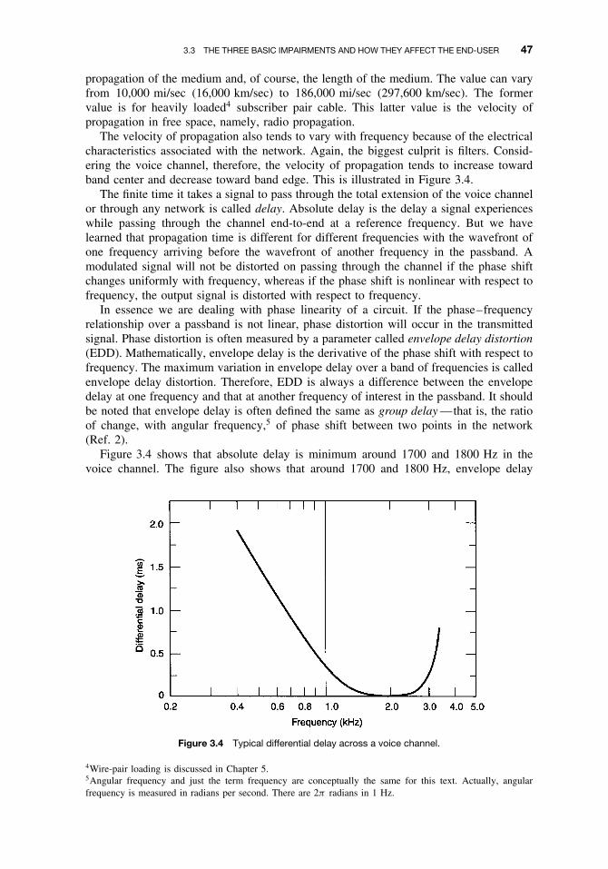
3.3 THE THREE BASIC IMPAIRMENTS AND HOW THEY AFFECT THE END-USER 47
propagation of the medium and, of course, the length of the medium. The value can varyfrom 10,000 mi/sec (16,000 km/sec) to 186,000 mi/sec (297,600 km/sec). The formervalue is for heavily loaded4 subscriber pair cable. This latter value is the velocity ofpropagation in free space, namely, radio propagation.
The velocity of propagation also tends to vary with frequency because of the electricalcharacteristics associated with the network. Again, the biggest culprit is filters. Consid-ering the voice channel, therefore, the velocity of propagation tends to increase towardband center and decrease toward band edge. This is illustrated in Figure 3.4.
The finite time it takes a signal to pass through the total extension of the voice channelor through any network is called delay. Absolute delay is the delay a signal experienceswhile passing through the channel end-to-end at a reference frequency. But we havelearned that propagation time is different for different frequencies with the wavefront ofone frequency arriving before the wavefront of another frequency in the passband. Amodulated signal will not be distorted on passing through the channel if the phase shiftchanges uniformly with frequency, whereas if the phase shift is nonlinear with respect tofrequency, the output signal is distorted with respect to frequency.
In essence we are dealing with phase linearity of a circuit. If the phase–frequencyrelationship over a passband is not linear, phase distortion will occur in the transmittedsignal. Phase distortion is often measured by a parameter called envelope delay distortion(EDD). Mathematically, envelope delay is the derivative of the phase shift with respect tofrequency. The maximum variation in envelope delay over a band of frequencies is calledenvelope delay distortion. Therefore, EDD is always a difference between the envelopedelay at one frequency and that at another frequency of interest in the passband. It shouldbe noted that envelope delay is often defined the same as group delay —that is, the ratioof change, with angular frequency,5 of phase shift between two points in the network(Ref. 2).
Figure 3.4 shows that absolute delay is minimum around 1700 and 1800 Hz in thevoice channel. The figure also shows that around 1700 and 1800 Hz, envelope delay
Figure 3.4 Typical differential delay across a voice channel.
4Wire-pair loading is discussed in Chapter 5.5Angular frequency and just the term frequency are conceptually the same for this text. Actually, angularfrequency is measured in radians per second. There are 2π radians in 1 Hz.

48 QUALITY OF SERVICE AND TELECOMMUNICATION IMPAIRMENTS
distortion is flattest.6 It is for this reason that so many data modems use 1700 or 1800 Hzfor the characteristic tone frequency, which is modulated by the data. A data modem isa device that takes the raw electrical baseband data signal and makes it compatible fortransmission over the voice channel.
This brings up an important point. Phase distortion (or EDD) has little effect on speechcommunications over the telecommunications network. However, regarding data transmis-sion, phase distortion is the greatest bottleneck for data rate (i.e., the number of bits persecond that a channel can support). It has probably more effect on limiting data rate thanany other parameter (Refs. 3 and 4).
3.3.3 Noise
3.3.3.1 General. Noise, in its broadest definition, consists of any undesired signal ina communication circuit. The subject of noise and noise reduction is probably the mostimportant single consideration in transmission engineering. It is the major limiting factorin overall system performance. For our discussion in this text, noise is broken down intofour categories:
1. Thermal noise2. Intermodulation noise3. Impulse noise4. Crosstalk
3.3.3.2 Thermal Noise. Thermal noise occurs in all transmission media and all com-munication equipment, including passive devices such as waveguide. It arises from randomelectron motion and is characterized by a uniform distribution of energy over the frequencyspectrum with a Gaussian distribution of levels.
Gaussian distribution tells us that there is statistical randomness. For those of youwho have studied statistics, this means that there is a “normal” distribution with standarddeviations. Because of this, we can develop a mathematical relationship to calculate noiselevels given certain key parameters.
Every equipment element and the transmission medium itself contribute thermal noiseto a communication system if the temperature of that element or medium is above absolutezero on the Kelvin temperature scale. Thermal noise is the factor that sets the lower limitof sensitivity of a receiving system and is often expressed as a temperature, usually givenin units referred to absolute zero. These units are called kelvins (not degrees).
Thermal noise is a general term referring to noise based on thermal agitations ofelectrons. The term “white noise” refers to the average uniform spectral distribution ofnoise energy with respect to frequency. Thermal noise is directly proportional to bandwidthand noise temperature.
We turn to the work of the Austrian scientist, Ludwig Boltzmann, who did landmarkresearch on the random motion of electrons. From Boltzmann’s constant, named forLudwig Boltzmann, we can write a relationship for the thermal noise level (Pn) in 1 Hzof bandwidth at absolute zero (kelvin scale) or
Pn = −228.6 dBW per Hz of bandwidth for a perfect receiver at absolute zero. (3.3)
6“Flattest” means that there is little change in value. The line is flat, not sloping.
3.3 THE THREE BASIC IMPAIRMENTS AND HOW THEY AFFECT THE END-USER 49
At room temperature (290 K or 17◦C) we have
Pn = −204 dBW per Hz of bandwidth for a perfect receiver (3.4)
or= −174 dBm/Hz of bandwidth for a perfect receiver.
A perfect receiver is a receiving device that contributes no thermal noise to the commu-nication channel. Of course, this is an idealistic situation that cannot occur in real life. Itdoes provide us a handy reference, though. The following relationship converts Eq. (3.4)for a real receiver in a real-life setting.
Pn = −204 dBW/Hz + NFdB + 10 log B, (3.5)
where B is the bandwidth of the receiver in question. The bandwidth must always be inhertz or converted to hertz.
NF is the noise figure of the receiver. It is an artifice that we use to quantify the amountof thermal noise a receiver (or any other device) injects into a communication channel.The noise figure unit is the decibel.
An example of application of Eq. (3.5) might be a receiver with a 3-dB noise figureand a 10-MHz bandwidth. What would be the thermal noise power (level) in dBW of thereceiver? Use Eq. (3.5).
Pn = −204 dBW/Hz + 3 dB + 10 log(10 × 106)
= −204 dBW/Hz + 3 dB + 70 dB
= −131 dBW
3.3.3.3 Intermodulation Noise. Intermodulation (IM) noise is the result of the pres-ence of intermodulation products. If two signals with frequencies F1 and F2 are passedthrough a nonlinear device or medium, the result will contain IM products that are spuriousfrequency energy components. These components may be present inside and/or outsidethe frequency band of interest for a particular device or system. IM products may beproduced from harmonics7 of the desired signal in question, either as products betweenharmonics or as one of the basic signals and the harmonic of the other basic signal orbetween both signals themselves. The products result when two (or more) signals beattogether or “mix.” These products can be sums and/or differences. Look at the mixingpossibilities when passing F1 and F2 through a nonlinear device. The coefficients indicatethe first, second, or third harmonics.
Devices passing multiple signals simultaneously, such as multichannel radio equipment,develop IM products that are so varied that they resemble white noise.
Intermodulation noise may result from a number of causes:
ž Improper level setting. If the level of an input to a device is too high, the device isdriven into its nonlinear operating region (overdrive).
ž Improper alignment causing a device to function nonlinearly.
7A harmonic of a certain frequency F can be 2F (twice the value of F ), 3F , 4F , 5F , and so on. It is aninteger multiple of the basic frequency.

50 QUALITY OF SERVICE AND TELECOMMUNICATION IMPAIRMENTS
ž Nonlinear envelope delay.ž Device malfunction.
To summarize, IM noise results from either a nonlinearity or a malfunction that has theeffect of nonlinearity. The causes(s) of intermodulation noise is(are) different from thatof thermal noise. However, its detrimental effects and physical nature can be identical tothose of thermal noise, particularly in multichannel systems carrying complex signals.
3.3.3.4 Impulse Noise. Impulse noise is noncontinuous, consisting of irregular pulsesor noise spikes of short duration and of relatively high amplitude. These spikes are oftencalled hits, and each spike has a broad spectral content (i.e., impulse noise smears a broadfrequency bandwidth.) Impulse noise degrades voice telephony usually only marginally,if at all. However, it may seriously degrade error performance on data or other digitalcircuits. The causes of impulse noise are lightning, car ignitions, mechanical switches(even light switches), fluorescent lights, and so on. Impulse noise will be discussed inmore detail in Chapter 10, Data Communications.
3.3.3.5 Crosstalk. Crosstalk is the unwanted coupling between signal paths. There areessentially three causes of crosstalk:
1. Electrical coupling between transmission media, such as between wire pairs on avoice-frequency (VF) cable system and on digital (PCM) cable systems.
2. Poor control of frequency response (i.e., defective filters or poor filter design).3. Nonlinear performance in analog (FDM) multiplex systems.
Excessive level may exacerbate crosstalk. By “excessive level” we mean that the level orsignal intensity has been adjusted to a point higher than it should be. In telephony anddata systems, levels are commonly measured in dBm. In cable television systems, levelsare measured as voltages over a common impedance (75 ohms). See the discussion oflevel in Section 3.4.
There are two types of crosstalk:
1. Intelligible, where at least four words are intelligible to the listener from extraneousconversation(s) in a 7-second period.
2. Unintelligible, with crosstalk resulting from any other form of disturbing effects ofone channel on another.
Intelligible crosstalk presents the greatest impairment because of its distraction to thelistener. Distraction is considered to be caused either by fear of loss of privacy or primarilyby the user of the primary line consciously or unconsciously trying to understand what isbeing said on the secondary or interfering circuits; this would be true for any interferencethat is syllabic in nature.
Received crosstalk varies with the volume of the disturbing talker, the loss from thedisturbing talker to the point of crosstalk, the coupling loss between the two circuits underconsideration, and the loss from the point of crosstalk to the listener. The most importantof these factors for this discussion is the coupling loss between the two circuits underconsideration. Also, we must not lose sight of the fact that the effects of crosstalk aresubjective, and other factors have to be considered when crosstalk impairments are to be

3.4 LEVEL 51
measured. Among these factors are the type of people who use the channel, the acuity oflisteners, traffic patterns, and operating practices.
3.4 LEVEL
Level is an important parameter in the telecommunications network, particularly in theanalog network or in the analog portion of a network. In the context of this book when weuse the word level, we mean signal magnitude or intensity. Level could be comparative.The output of an amplifier is 30 dB higher than the input. But more commonly, wemean absolute level, and in telephony it is measured in dBm (decibels referenced to 1milliwatt) and in radio systems we are more apt to use dBW (decibels referenced to1 watt). Television systems measure levels in voltage, commonly the dBmV (decibelsreferenced to 1 millivolt).
In the telecommunication network, if levels are too high, amplifiers become overloaded,resulting in increases in intermodulation noise and crosstalk. If levels are too low, customersatisfaction suffers (i.e., loudness rating). In the analog network, level was a major issue;in the digital network, it is somewhat less so.
System levels are used for engineering a communication system. These are usuallytaken from a level chart or reference system drawing made by a planning group or asa part of an engineered job. On the chart a 0 TLP (zero test level point) is established.A test level point is a location in a circuit or system at which a specified test-tone levelis expected during alignment. A 0 TLP is a point at which the test-tone level should be0 dBm. A test tone is a tone produced by an audio signal generator, usually 1020 Hz.Note that these frequencies are inside the standard voice channel, which covers the rangeof 300–3400 Hz. In the digital network, test tones must be applied on the analog side.This will be covered in Chapter 6.
From the 0 TLP other points may be shown using the unit dBr (decibel reference).A minus sign shows that the level is so many decibels below reference and a plus sign,above. The unit dBm0 is an absolute unit of power in dBm referred to the 0 TLP. ThedBm can be related to the dBr and dBm0 by the following formula:
dBm = dBm0 + dBr. (3.6)
For instance, a value of −32 dBm at a −22-dBr point corresponds to a reference level of−10 dBm0. A −10-dBm0 signal introduced at the 0-dBr point (0 TLP) has an absolutesignal level of −10 dBm.
3.4.1 Typical Levels
Earlier measurements of speech level used the unit of measure VU, standing for volumeunit. For a 1000-Hz sinusoid signal (simple sine wave signal), 0 VU = 0 dBm. Whena VU meter is used to measure the level of a voice signal, it is difficult to exactlyequate VU and dBm. One of the problems, of course, is that speech transmission ischaracterized by spurts of signal. However, a good approximation relating VU to dBm isthe following formula:
Average power of a telephone talker ≈ VU − 1.4 (dBm). (3.7)
In the telecommunication network, telephone channels are often multiplexed at the firstserving exchange. When the network was analog, the multiplexers operated in the fre-quency domain and were called frequency division multiplexers (FDM). Voice channel

52 QUALITY OF SERVICE AND TELECOMMUNICATION IMPAIRMENTS
inputs were standardized with a level of either −15 dBm or −16 dBm, and the out-puts of demultiplexers were +7 dBm. These levels, of course, were test-tone levels.In industrialized and postindustrialized nations, in nearly every case, multiplexers aredigital. These multiplexers have an overload point at about +3.17 dBm0. The digitalreference signal is 0 dBm on the analog side using a standard test tone between 1013and 1022 Hz.
3.5 ECHO AND SINGING
Echo and singing are two important impairments that impact QoS. Echo is when a talkerhears her/his own voice delayed. The annoyance is a function of the delay time (i.e., thetime between the launching of a syllable by a talker and when the echo of that syllableis heard by the same talker). It is also a function of the intensity (level) of the echo, butto some lesser extent. Singing is audio feedback. It is an “ear-splitting” howl, much likethe howl one gets by placing a public address microphone in front of a loudspeaker. Wewill discuss causes and cures of echo and singing in the next chapter.
REVIEW EXERCISES
1. Define signal-to-noise ratio.
2. Give signal-to-noise ratio guidelines at a receiving device for the following threemedia: voice, video-TV, and data. Base the answer on where a typical customersays the signal is very good or excellent.
3. Why do we use a sinusoidal test tone when we measure S/N on a speech channelrather than just the speech signal itself?
4. The noise level of a certain voice channel is measured at −39 dBm, and the test-tonesignal level is measured at +3 dBm. What is the channel S/N?
5. If we know the loudness rating of a telephone subset earpiece and of the subsetmouthpiece, what additional data do we need to determine the overall loudnessrating (OLR) of a telephone connection?
6. The BER of an underlying digital circuit is 1 × 10⁻⁸, for data riding on this circuit.What is the best BER we can expect on the data?
7. What are the three basic impairments on a telecommunication transmission channel?
8. Of the three impairments, which one affects data error rate the most and thus limitsbit rate?
9. Explain the cause of phase distortion.
10. Name the four types of noise we are likely to encounter in a telecommunica-tion system.
11. What will be the thermal noise level of a receiver with a noise figure of 3 dB anda bandwidth of 1 MHz?
12. Define third-order products based on the mixing of two frequencies F1 and F2.
13. Give four causes of impulse noise.

REFERENCES 53
14. Relate VU to dBm for a simple sinusoidal signal. Relate VU to dBm for a complexsignal such as human voice.
15. Echo as an annoyance to a telephone listener varies with two typical causes. Whatare they? What is the most important (most annoying)?
REFERENCES
1. Effect of Transmission Impairments , ITU-T Rec. P.11, ITU Helsinki, Mar. 1993.
2. Loudness Ratings on National Systems , ITU-T Rec. G.121, ITU Helsinki, Mar, 1993.
3. R. L. Freeman, Telecommunication System Engineering, 4th ed., Wiley, New York, 2004.
4. R. L. Freeman, Telecommunication Transmission Handbook, 4th ed., Wiley, New York, 1998.


4
TRANSMISSION AND SWITCHING:CORNERSTONES OF A NETWORK
4.1 TRANSMISSION AND SWITCHING DEFINED
The IEEE defines transmission as the propagation of a signal, message, or other formof intelligence by any means such as optical fiber, wire, or visual means. Our defini-tion is not so broad. Transmission provides the transport of a signal from an end-usersource to the destination such that the signal quality at the destination meets certainperformance criteria.
Switching selects the route to the desired destination that the transmitted signal trav-els by the closing of switches in either the space domain or the time domain or somecombination(s) of the two.
Prior to about 1985, transmission and switching were separate disciplines in telecom-munication with a firm dividing line between the two. Switching engineers knew littleabout transmission, and transmission engineers knew little about switching. As we men-tioned in Chapter 1, that dividing line today is hazy at best. Signaling develops andcarries the control information for switches. If a transmission path becomes impaired,signaling becomes ineffectual and the distant-end switch either will not operate or willnot function correctly, misrouting the connectivity. Timing, which is so vital for the digitaltransmission path, derives from the connected switches.
4.2 TRAFFIC INTENSITY DEFINES THE SIZE OF SWITCHESAND THE CAPACITY OF TRANSMISSION LINKS
4.2.1 Traffic Studies
As we have already mentioned, telephone exchanges (switches) are connected by trunks orjunctions.1 The number of trunks connecting exchange X with exchange Y is the numberof voice pairs or their equivalent used in the connection. One of the most important stepsin telecommunication system design is to determine the number of trunks required on a
1The term junction means a trunk in the local area. It is a British term. Trunk is used universally in thelong-distance plant.
Fundamentals of Telecommunications, Second Edition, by Roger L. FreemanISBN 0-471-71045-8 Copyright 2005 by Roger L. Freeman
55

56 TRANSMISSION AND SWITCHING: CORNERSTONES OF A NETWORK
route or connection between exchanges. We could say we are dimensioning the route. Todimension the route correctly we must have some idea of its usage—that is, how manypeople will wish to talk at once over the route. The usage of a transmission route orswitch brings us into the realm of traffic engineering; and usage may be defined by twoparameters: (1) calling rate, or the number of times a route or traffic path is used per unittime period; or more properly defined, “the call intensity per traffic path during the busyhour (BH)”; and (2) holding time, or “the average duration of occupancy of one or morepaths by calls.” A traffic path is a “channel, time slot, frequency band, line, trunk switch,or circuit over which individual communications pass in sequence.” Carried traffic is thevolume of traffic actually carried by a switch, and offered traffic is the volume of trafficoffered to a switch. Offered traffic minus carried traffic equals lost calls. A lost call isone that does not make it through a switch. A call is “lost” usually because it meetscongestion or blockage at that switch.
To dimension a traffic path or size a telephone exchange, we must know the trafficintensity representative of the normal busy season. There are weekly and daily variationsin traffic within the busy season. Traffic is random in nature. However, there is a certainconsistency we can look for. For one thing, there is usually more traffic on Mondaysand Fridays, and there is a lower volume on Wednesdays. A certain consistency can alsobe found in the normal workday variation. Across a typical day the variation is suchthat a one-hour period shows greater usage than any other one-hour period. From thehour of the day with least traffic intensity to the hour of greatest traffic, the variationcan exceed 100:1. Figure 4.1 shows a typical hour-to-hour traffic variation for a servingswitch in the United States. It can be seen that the busiest period, the busy hour (BH), isbetween 10 A.M. and 11 A.M. (The busy hour from the viewpoint of grade of service wasintroduced in Section 1.3.4). From one workday to the next, originating BH calls can varyas much as 25%. To these fairly “regular” variations, there are also unpredictable peakscaused by stock market or money market activity, weather, natural disaster, internationalevents, sporting events, and so on. Normal traffic growth must also be taken into account.
Figure 4.1 Bar chart of traffic intensity over a typical working day. (US, mixed business and residential).
4.2 TRAFFIC INTENSITY DEFINES THE SIZE OF SWITCHES AND THE CAPACITY OF TRANSMISSION LINKS 57
Nevertheless, suitable forecasts of BH traffic can be made. However, before proceedingfurther in this discussion, consider the following definitions of the busy hour.
1. Busy Hour. The busy hour refers to the traffic volume or number of call attempts,and is that continuous one-hour period being wholly in the time interval concernedfor which this quantity (i.e., traffic volume or call attempts) is greatest.
2. The Average Busy Season Busy Hour (ABSBH). This is used for trunk groups andalways has a grade of service2 criterion applied. For example, for the ABSBH load,a call requiring a circuit in a trunk group should encounter all trunks busy (ATB)no more than 1% of the time.
Other definitions of the busy hour may be found in Ref. 1.When dimensioning telephone exchanges and transmission routes, we shall be working
with BH traffic levels and care must be used in the definition of the busy hour.Peak traffic loads are of greater concern than average loads for the system planner
when dimensioning switching equipment.Another concern in modern digital switching systems is call attempts. We could say
that call attempts is synonymous with offered traffic. Even though a call is not carried andis turned away, the switch’s processor or computer is still exercised. In many instancesa switch’s capability to route traffic is limited by the peak number of call attempts itsprocessor can handle.
4.2.1.1 Measurement of Telephone Traffic. If we define telephone traffic as theaggregate of telephone calls over a group of circuits or trunks with regard to the durationof calls as well as their number, we can say that traffic flow (A) is expressed as
A = C × T , (4.1)
where C designates the number of calls originated during the period of one hour, and T
is the average holding time, usually given in hours. A is a dimensionless unit because weare multiplying calls/hour by hour/call.
Suppose that the average holding time is 2.5 minutes and the calling rate in the BH for aparticular day is 237. The traffic flow (A) would then be 237 × 2.5, or 592.5 call-minutes(Cm) or 593.5/60, or about 9.87 call-hours (Ch).
The preferred unit of traffic intensity is the erlang, named after the Danish mathemati-cian A.K. Erlang (Copenhagen Telephone Company, 1928). The erlang is a dimensionlessunit. One erlang represents a circuit occupied for one hour. Considering a group of cir-cuits, traffic intensity in erlangs is the number of call-seconds per second or the numberof call-hours per hour. If we knew that a group of 10 circuits had a call intensity of 5erlangs, we would expect half of the circuits to be busy at the time of measurement.
In the United States the term unit call (UC), or its synonymous term, hundred call-second, abbreviated ccs,3 generally is used. These terms express the sum of the numberof busy circuits, provided that the busy trunks were observed once every 100 seconds(36 observations in 1 hour) (Ref. 2). The following simple relationship should be kept inmind: 1 erlang = 36 ccs, assuming a 1-hour time-unit interval.
2Grade of service refers to the planned value criterion of probability of blockage of an exchange. This isthe point where an exchange just reaches its full capacity to carry traffic. This usually happens during thebusy hour.3The first letter c in ccs stands for the Roman number 100.

58 TRANSMISSION AND SWITCHING: CORNERSTONES OF A NETWORK
Extensive traffic measurements are made on switching systems because of their numer-ous traffic-sensitive components. Usual measurements for a component such as a servicecircuit include call attempts, calls carried, and usage. The typical holding time for acommon-control element in a switch is considerably shorter than that for a trunk, andshort sampling intervals (e.g., 10 seconds) or continuous monitoring are used to mea-sure usage.
4.2.1.2 Blockage, Lost Calls, and Grade of Service. Let’s assume that an iso-lated telephone exchange serves 5000 subscribers and that no more than 10% of thesubscribers wish service simultaneously. Therefore, the exchange is dimensioned withsufficient equipment to complete 500 simultaneous connections. Each connection wouldbe, of course, between any two of the 5000 subscribers. Now let subscriber 501 attempt tooriginate a call. She/he cannot complete the call because all the connecting equipment isbusy, even though the line she/he wishes to reach may be idle. This call from subscriber501 is termed a lost call or blocked call. She/he has met blockage. The probabilityof encountering blockage is an important parameter in traffic engineering of telecom-munication systems. If congestion conditions are to be met in a telephone system, wecan expect that those conditions will usually be encountered during the BH. A switchis dimensioned (sized) to handle the BH load. But how well? We could, indeed, faroverdimension the switch such that it could handle any sort of traffic peaks. However,that is uneconomical. So with a well-designed switch, during the busiest of BHs wecan expect moments of congestion such that additional call attempts will meet blockage.Grade of service4 expresses the probability of meeting blockage during the BH and iscommonly expressed by the letter p. A typical grade of service is p = 0.01. This meansthat an average of one call in 100 will be blocked or “lost” during the BH. Grade ofservice, a term in the Erlang formula, is more accurately defined as the probability ofblockage. It is important to remember that lost calls (blocked calls) refer to calls thatfail at first trial. We discuss attempts (at dialing) later—that is, the way blocked callsare handled.
We exemplify grade of service by the following problem. If we know that there are345 seizures (i.e., lines connected for service) and 6 blocked calls (i.e., lost calls) duringthe BH, what is the grade of service?
Grade of service = Number of lost calls/Number of offered calls
= 6/(354 + 6) = 6/360
p ≈ 0.017. (4.2)
The average grade of service for a network may be obtained by adding the grade ofservice provided by a particular group of trunks or circuits of specified size and carryinga specified traffic intensity. It is the probability that a call offered to the group will findavailable trunks already occupied on first attempt. This probability depends on a number offactors, the most important of which are (1) the distribution in time and duration of offeredtraffic (e.g., random or periodic arrival and constant or exponentially distributed holdingtime), (2) the number of traffic sources [limited or high (infinite)], (3) the availability oftrunks in a group to traffic sources (full or restricted availability), and (4) the manner inwhich lost calls are “handled.” Several new concepts are suggested in these four factors.These must be explained before continuing.
4Grade of service was introduced in Section 1.3.4.

4.2 TRAFFIC INTENSITY DEFINES THE SIZE OF SWITCHES AND THE CAPACITY OF TRANSMISSION LINKS 59
4.2.1.2.1 Availability. Switches were previously discussed as devices with lines andtrunks, but better terms for describing a switch are inlets and outlets. When a switch hasfull availability, each inlet has access to any outlet. When not all the free outlets in aswitching system can be reached by inlets, the switching system is referred to as one withlimited availability. Examples of switches with limited and full availability are shown inFigures 4.2a and 4.2b
Of course, full availability switching is more desirable than limited availability, butis more expensive for larger switches. Thus full availability switching is generally foundonly in small switching configurations and in many new digital switches (see Chapter 6).Grading is one method of improving the traffic-handling capabilities of switching con-figurations with limited availability. Grading is a scheme for interconnecting switchingsubgroups to make the switching load more uniform.
Figure 4.2a An example of a switch with limited availability.
Figure 4.2b An example of a switch with full availability.

60 TRANSMISSION AND SWITCHING: CORNERSTONES OF A NETWORK
4.2.1.2.2 ‘‘Handling’’ of Lost Calls. In conventional telephone traffic theory, threemethods are considered for the handling or dispensing of lost calls:
1. Lost calls held (LCH)2. Lost calls cleared (LCC)3. Lost calls delayed (LCD)
The LCH concept assumes that the telephone user will immediately reattempt the callon receipt of a congestion signal and will continue to redial. The user hopes to seizeconnection equipment or a trunk as soon as switching equipment becomes available forthe call to be handled. It is the assumption in the LCH concept that lost calls are held orwaiting at the user’s telephone. This concept further assumes that such lost calls extendthe average holding time theoretically, and in this case the average holding time is zero,and all the time is waiting time. The principal traffic formula (for conventional analogspace division switching) in North America is based on the LCH concept.
The LCC concept, which is primarily used in Europe or those countries that haveadopted European practice, assumes that the user will hang up and wait some time intervalbefore reattempting if the user hears the congestion signal on the first attempt. Such calls,it is assumed, disappear from the system. A reattempt (after the delay) is considered asinitiating a new call. The Erlang B formula is based on this criterion.
The LCD concept assumes that the user is automatically put in queue (a waiting line orpool). For example, this is done, of course, when an operator is dialed. It is also done onall modern digital switching systems. Such switches are computer-based for the “brains”of the control functions and are called switches with stored program control (SPC). TheLCD category may be broken down into three subcategories, depending on how the queueor pool of waiting calls is handled. The waiting calls may be handled last in first out, firstin first out, or at random.
4.2.1.2.3 Infinite and Finite Traffic Sources. We can assume that traffic sources areeither infinite or finite. For the infinite-traffic-sources case the probability of call arrival isconstant and does not depend on the occupancy of the system. It also implies an infinitenumber of call arrivals, each with an infinitely small holding time. An example of finitetraffic sources is when the number of sources offering traffic to a group of trunks iscomparatively small in comparison to the number of circuits. We can also say that witha finite number of sources the arrival rate is proportional to the number of sources thatare not already engaged in sending a call
4.2.1.2.4 Probability-Distribution Curves. Telephone-call originations in any particu-lar area are random in nature. We find that originating calls or call arrivals at an exchangeclosely fit a family of probability-distribution curves following a Poisson5 distribution.The Poisson distribution is fundamental in traffic theory
Most probability-distribution curves are two-parameter curves; that is, they may bedescribed by two parameters: mean and variance. The mean is a point on the probability-distribution curve where an equal number of events occur to the right of the point as tothe left of the point. Mean is synonymous with average. Consult Figure 4.3.
The second parameter used to describe a distribution curve is the dispersion, whichtells us how the values or population are dispersed about the center or mean of thecurve. There are several measures of dispersion. One is the familiar standard deviation.
5S. D. Poisson was a nineteenth-century French mathematician/physicist specializing in “randomness.”

4.2 TRAFFIC INTENSITY DEFINES THE SIZE OF SWITCHES AND THE CAPACITY OF TRANSMISSION LINKS 61
Figure 4.3 A normal distribution curve showing the mean and standard deviation, σ .
The standard deviation is usually expressed by the Greek letter sigma (σ ). For example,1 σ either side of the mean in Figure 4.3 will contain about 68% of the population ormeasurements, 2 σ will contain about 95% of the measurements, and 3 σ will containaround 99% of the subject, population, or whatever is being measured. The curve shownin Figure 4.3 is a normal distribution curve.
4.2.2 Discussion of the Erlang and Poisson Traffic Formulas
When dimensioning a route, we want to find the optimum number of circuits to servethe route. There are several formulas at our disposal to determine that number of circuitsbased on the BH traffic load. In Section 4.2.1.2, four factors were discussed that will helpus to determine which traffic formula to use given a particular set of circumstances. Thesefactors primarily dealt with (1) call arrivals and holding-time distributions, (2) number oftraffic sources, (3) availability (full or limited), and (4) handling of lost calls.
The Erlang B loss formula was/is very widely used outside of the United States.Loss in this context means the probability of encountering blockage at the switch due tocongestion or to “all trunks busy” (ATB). The formula expresses grade of service or theprobability of finding x channels busy. The other two factors in the Erlang B formula arethe mean of the offered traffic and the number of trunks or servicing channels available.The formula assumes the following:
ž Traffic originates from an infinite number of sources.ž Lost calls are cleared assuming a zero holding time.ž The number of trunks or servicing channels is limited.ž Full availability exists.
The actual Erlang B formula is out of the scope of this text. For more detailed information,it is recommended that the reader consult Ref. 3, Section 1. It is far less involved to usetraffic tables as found in Table 4.1, which gives trunk-dimensioning information for somespecific grades of service, from 0.001 to 0.05 and from 1 to 49 trunks. The table usestraffic-intensity units UC (unit call) and TU (traffic unit), where TU is in erlangs assumingBH conditions and UC is in ccs (cent-call-seconds). Remember that 1 erlang = 36 ccs(based on a 1-hour time interval).
To exemplify the use of Table 4.1, suppose a route carried 16.68 erlangs of traffic witha desired grade of service of 0.001; then 30 trunks would be required. If the grade ofservice were reduced to 0.05, the 30 trunks could carry 24.80 erlangs of traffic. Whensizing a route for trunks or an exchange, we often come up with a fractional number

62 TRANSMISSION AND SWITCHING: CORNERSTONES OF A NETWORK
Table 4.1 Trunk-Loading Capacity, Based on Erlang B Formula, Full Availability
Grade ofService
1 in 1000
Grade ofService1 in 500
Grade ofService1 in 200
Grade ofService1 in 100
Grade ofService1 in 50
Grade ofService1 in 20
Trunks UC TU UC TU UC TU UC TU UC TU UC TU
1 0.04 0.001 0.07 0.002 0.2 0.005 0.4 0.01 0.7 0.02 1.8 0.052 1.8 0.05 2.5 0.07 4 0.11 5.4 0.15 7.9 0.22 14 0.383 6.8 0.19 9 0.25 13 0.35 17 0.46 22 0.60 32 0.904 16 0.44 19 0.53 25 0.70 31 0.87 39 1.09 55 1.525 27 0.76 32 0.90 41 1.13 49 1.36 60 1.66 80 2.226 41 1.15 48 1.33 58 1.62 69 1.91 82 2.28 107 2.967 57 1.58 65 1.80 78 2.16 90 2.50 106 2.94 135 3.748 74 2.05 83 2.31 98 2.73 113 3.13 131 3.63 163 4.549 92 2.56 103 2.85 120 3.33 136 3.78 156 4.34 193 5.37
10 111 3.09 123 3.43 143 3.96 161 4.46 183 5.08 224 6.2211 131 3.65 145 4.02 166 4.61 186 5.16 210 5.84 255 7.0812 152 4.23 167 4.64 190 5.28 212 5.88 238 6.62 286 7.9513 174 4.83 190 5.27 215 5.96 238 6.61 267 7.41 318 8.8314 196 5.45 213 5.92 240 6.66 265 7.35 295 8.20 350 9.7315 219 6.08 237 6.58 266 7.38 292 8.11 324 9.01 383 10.6316 242 6.72 261 7.26 292 8.10 319 8.87 354 9.83 415 11.5417 266 7.38 286 7.95 318 8.83 347 9.65 384 10.66 449 12.4618 290 8.05 311 8.64 345 9.58 376 10.44 414 11.49 482 13.3819 314 8.72 337 9.35 372 10.33 404 11.23 444 12.33 515 14.3120 339 9.41 363 10.07 399 11.09 433 12.03 474 13.18 549 15.2521 364 10.11 388 10.79 427 11.86 462 12.84 505 14.04 583 16.1922 389 10.81 415 11.53 455 12.63 491 13.65 536 14.90 617 17.1323 415 11.52 442 12.27 483 13.42 521 14.47 567 15.76 651 18.0824 441 12.24 468 13.01 511 14.20 550 15.29 599 16.63 685 19.0325 467 12.97 495 13.76 540 15.00 580 16.12 630 17.50 720 19.9926 493 13.70 523 14.52 569 15.80 611 16.96 662 18.38 754 20.9427 520 14.44 550 15.28 598 16.60 641 17.80 693 19.26 788 21.9028 546 15.18 578 16.05 627 17.41 671 18.64 725 20.15 823 22.8729 573 15.93 606 16.83 656 18.22 702 19.49 757 21.04 858 23.8330 600 16.68 634 17.61 685 19.03 732 20.34 789 21.93 893 24.8031 628 17.44 662 18.39 715 19.85 763 21.19 822 22.83 928 25.7732 655 18.20 690 19.18 744 20.68 794 22.05 854 23.73 963 26.7533 683 18.97 719 19.97 774 21.51 825 22.91 887 24.63 998 27.7234 711 19.74 747 20.76 804 22.34 856 23.77 919 25.53 1033 28.7035 739 20.52 776 21.56 834 23.17 887 24.64 951 26.43 1068 29.6836 767 21.30 805 22.36 864 24.01 918 25.51 984 27.34 1104 30.6637 795 22.03 834 23.17 895 24.85 950 26.38 1017 28.25 1139 31.6438 823 22.86 863 23.97 925 25.69 981 27.25 1050 29.17 1175 32.6339 851 23.65 892 24.78 955 26.53 1013 28.13 1083 30.08 1210 33.6140 880 24.44 922 25.60 986 27.38 1044 29.01 1116 31.00 1246 34.6041 909 25.24 951 26.42 1016 28.23 1076 29.89 1149 31.92 1281 35.5942 937 26.04 981 27.24 1047 29.08 1108 30.77 1182 32.84 1317 36.5843 966 26.84 1010 28.06 1078 29.94 1140 31.66 1215 33.76 1353 37.5744 995 27.64 1040 28.88 1109 30.80 1171 32.54 1248 34.68 1388 38.5645 1024 28.45 1070 29.71 1140 31.66 1203 33.43 1282 35.61 1424 39.5546 1053 29.26 1099 30.54 1171 32.52 1236 34.32 1315 36.53 1459 40.5447 1083 30.07 1129 31.37 1202 33.38 1268 35.21 1349 37.46 1495 41.5448 1111 30.88 1159 32.20 1233 34.25 1300 36.11 1382 38.39 1531 42.5449 1141 31.69 1189 33.04 1264 35.11 1332 37.00 1415 39.32 1567 43.54
of servicing channels or trunks. In this case we would opt for the next highest integerbecause we cannot install a fraction of a trunk. For instance, if calculations show that atrunk route should have 31.4 trunks, it would be designed for 32 trunks.
The Erlang B formula, based on lost calls cleared, has been standardized by the CCITT(CCITT Rec. Q.87) and has been generally accepted outside the United States. In theUnited States the Poisson formula is favored. This formula is often called the Molina

4.2 TRAFFIC INTENSITY DEFINES THE SIZE OF SWITCHES AND THE CAPACITY OF TRANSMISSION LINKS 63
formula. It is based on the LCH concept. Table 4.2 provides trunking sizes for variousgrades of service deriving from the P formula; such tables are sometimes called “P ” tables(Poisson) and assume full availability. We must remember that the Poisson equation alsoassumes that traffic originates from a large (infinite) number of independent subscribersor sources (random traffic input), with a limited number of trunks or servicing channelsand LCH (Ref. 3).
4.2.3 Waiting Systems (Queueing)
The North American PSTN became entirely digital by the year 2000. Nearly all digitalswitches operate under some form of queueing discipline, which many call waiting systemsbecause an incoming call is placed in queue and waits its turn for service. These systemsare based on our third assumption, namely, lost calls delayed (LCD). Of course, a queue inthis case is a pool of callers waiting to be served by a switch. The term serving time is thetime a call takes to be served from the moment of arrival in the queue to the moment ofbeing served by the switch. For traffic calculations in most telecommunication queueingsystems, the mathematics is based on the assumption that call arrivals are random andPossonian. The traffic engineer is given the parameters of offered traffic, the size of thequeue, and a specified grade of service and will determine the number of serving circuitsor trunks that are required.
The method by which a waiting call is selected to be served from the pool of waitingcalls is called queue discipline. The most common discipline is the first-come, first-serveddiscipline, where the call waiting longest in the queue is served first. This can turn outto be costly because of the equipment required to keep order in the queue. Another typeis random selection, where the time a call has waited is disregarded and those waitingare selected in random order. There is also the last-come, first-served discipline and bulkservice discipline, where batches of waiting calls are admitted, and there are also priorityservice disciplines, which can be preemptive and nonpreemptive. In queueing systems thegrade of service may be defined as the probability of delay. This is expressed as P(t),the probability that a call is not being immediately served and has to wait a period oftime greater than t . The average delay on all calls is another parameter that can be usedto express grade of service, and the length of queue is yet another.
The probability of delay, the most common index of grade of service for waitingsystems when dealing with full availability and a Poissonian call arrival process (i.e.,random arrivals), is calculated using the Erlang C formula, which assumes an infinitelylong queue length. A more in-depth coverage of the Erlang C formula along with ErlangC traffic tables may be found in Ref. 3, Section 1.
4.2.4 Dimensioning and Efficiency
By definition, if we were to dimension a route or estimate the required number of servicingchannel, where the number of trunks (or servicing channels) just equaled the erlang load,we would attain 100% efficiency. All trunks would be busy with calls all the time orat least for the entire BH. This would not even allow time for call setup (i.e., makingthe connection) or for switch processing time. In practice, if we sized our trunks, trunkroutes, or switches this way, there would be many unhappy customers.
On the other hand, we do, indeed, want to dimension our routes (and switches) tohave a high efficiency and still keep our customers relatively happy. The goal of ourprevious exercises in traffic engineering was just that. The grade of service is one measureof subscriber satisfaction. As an example, let us assume that between cities X and Y

64 TRANSMISSION AND SWITCHING: CORNERSTONES OF A NETWORK
Table 4.2 Trunk-Loading Capacity, Based on Poisson Formula, Full Availability
Grade ofService
1 in 1000
Grade ofService1 in 100
Grade ofService1 in 50
Grade ofService1 in 20
Grade ofService1 in 10
Trunks UC TU UC TU UC TU UC TU UC TU
1 0.1 0.003 0.4 0.01 0.7 0.02 1.9 0.05 3.8 0.102 1.6 0.05 5.4 0.15 7.9 0.20 12.9 0.35 19.1 0.553 6.9 0.20 16 0.45 20 0.55 29.4 0.80 39.6 1.104 15 0.40 30 0.85 37 1.05 49 1.35 63 1.755 27 0.75 46 1.30 56 1.55 71 1.95 88 2.456 40 1.10 64 1.80 76 2.10 94 2.60 113 3.157 55 1.55 84 2.35 97 2.70 118 3.25 140 3.908 71 1.95 105 2.90 119 3.30 143 3.95 168 4.659 88 2.45 126 3.50 142 3.95 169 4.70 195 5.40
10 107 2.95 149 4.15 166 4.60 195 5.40 224 6.2011 126 3.50 172 4.80 191 5.30 222 6.15 253 7.0512 145 4.05 195 5.40 216 6.00 249 6.90 282 7.8513 166 4.60 220 6.10 241 6.70 277 7.70 311 8.6514 187 5.20 244 6.80 267 7.40 305 8.45 341 9.4515 208 5.80 269 7.45 293 8.15 333 9.25 370 10.3016 231 6.40 294 8.15 320 8.90 362 10.05 401 11.1517 253 7.05 320 8.90 347 9.65 390 10.85 431 11.9518 276 7.65 346 9.60 374 10.40 419 11.65 462 12.8519 299 8.30 373 10.35 401 11.15 448 12.45 492 13.6520 323 8.95 399 11.10 429 11.90 477 13.25 523 14.5521 346 9.60 426 11.85 458 12.70 507 14.10 554 15.4022 370 10.30 453 12.60 486 13.50 536 14.90 585 16.2523 395 10.95 480 13.35 514 14.30 566 15.70 616 17.1024 419 11.65 507 14.10 542 15.05 596 16.55 647 17.9525 444 12.35 535 14.85 572 15.90 626 17.40 678 18.8526 469 13.05 562 15.60 599 16.65 656 18.20 710 19.7027 495 13.75 590 16.40 627 17.40 686 19.05 741 20.6028 520 14.45 618 17.15 656 18.20 717 19.90 773 21.4529 545 15.15 647 17.95 685 19.05 747 20.75 805 22.3530 571 15.85 675 18.75 715 19.85 778 21.60 836 23.2031 597 16.60 703 19.55 744 20.65 809 22.45 868 24.1032 624 17.35 732 20.35 773 21.45 840 23.35 900 25.0033 650 18.05 760 21.10 803 22.30 871 24.20 932 25.9034 676 18.80 789 21.90 832 23.10 902 25.05 964 26.8035 703 19.55 818 22.70 862 23.95 933 25.90 996 27.6536 729 20.25 847 23.55 892 24.80 964 26.80 1028 28.5537 756 21.00 876 24.35 922 25.60 995 27.65 1060 29.4538 783 21.75 905 25.15 951 26.40 1026 28.50 1092 30.3539 810 22.50 935 25.95 982 27.30 1057 29.35 1125 31.2540 837 23.25 964 26.80 1012 28.10 1088 30.20 1157 32.1441 865 24.05 993 27.60 1042 28.95 1120 31.10 1190 33.0542 892 24.80 1023 28.40 1072 29.80 1151 31.95 1222 33.9543 919 25.55 1052 29.20 1103 30.65 1183 32.85 1255 34.8544 947 26.30 1082 30.05 1133 31.45 1214 33.70 1287 35.7545 975 27.10 1112 30.90 1164 32.35 1246 34.60 1320 36.6546 1003 27.85 1142 31.70 1194 33.15 1277 35.45 1352 37.5547 1030 28.60 1171 32.55 1225 34.05 1309 36.35 1385 38.4548 1058 29.40 1201 33.35 1255 34.85 1340 37.20 1417 39.3549 1086 30.15 1231 34.20 1286 35.70 1372 38.10 1450 40.3050 1115 30.95 1261 35.05 1317 36.60 1403 38.95 1482 41.15

4.2 TRAFFIC INTENSITY DEFINES THE SIZE OF SWITCHES AND THE CAPACITY OF TRANSMISSION LINKS 65
there were 47 trunks on the interconnecting telephone route. The tariffs, from whichthe telephone company derives revenue, are a function of the erlangs of carried traffic.Suppose we allow $1.00 per erlang-hour. The very upper limit of service on the route is 47erlangs, and the telephone company would earn $47 for the busy hour (much less for allother hours) for that trunk route and the portion of the switches and local plant involvedwith these calls. As we well know, many of the telephone company’s subscribers wouldbe unhappy because they would have to wait excessively to get calls through from X toY. How, then, do we optimize a trunk route (or serving circuits) and keep the customersas satisfied with service as possible?
Remember from Table 4.1, with an excellent grade of service of 0.001, that we relategrade of service to subscriber satisfaction (one element of quality of service) and that47 trunks could carry 30.07 erlangs during the busy hour. Assuming the route did carry30.07 erlangs, let’s say at $1.00 per erlang, it would earn $30.07 for that hour. From arevenue viewpoint, that would be the best hour of the day. If the grade of service werereduced to 0.01, 47 trunks would bring in $35.21 (i.e., 35.21 erlangs) for the busy hour.Note the improvement in revenue at the cost of reducing grade of service.
Here we are relating efficiency on trunk utilization. Trunks not carrying traffic do notbring in revenue. If we are only using some trunks during the busy hour only minutes aday to cover BH traffic peaks, the remainder of the day they are not used. That is highlyinefficient. As we reduce the grade of service, the trunk utilization factor improves. Forinstance, 47 trunks will only carry 30.07 erlangs with a grade of service of 1 in 1000(0.001), whereas if we reduce the grade of service to 1 in 20 (0.05), we carry 41.54erlangs (see Table 4.1). Efficiency has improved notably. Quality of service, as a result,has decreased markedly.
4.2.4.1 Alternative Routing. One method to improve efficiency is to use alternativerouting (called alternate routing in North America). Suppose we have three serving areas,X, Y, and Z, served by three switches (exchanges), X, Y, and Z, as illustrated in Figure 4.4.Let the grade of service be 0.005 (1 in 200 in Table 4.1). We find that it would require 48trunks to carry 34.25 erlangs of traffic during the BH to meet that grade of service betweenX and Y. Suppose we reduce the number of trunks between X and Y, still keeping theBH traffic intensity at 34.25 erlangs. We would thereby increase efficiency on the X–Yroute at the cost of reducing grade of service. With a modification of the switch at X, wecould route traffic bound for Y that met congestion on the X–Y route via switch Z. ThenZ would route that traffic on the Z–Y link. Essentially this is alternative routing in itssimplest form. Congestion would probably only occur during very short peaking periodsin the BH, and chances are that these peaks would not occur simultaneously with peaks
Figure 4.4 Simplified diagram of the alternative (alternate) routing concept. (Solid line represents thedirect route, dashed lines represent the alternative route carrying the overflow traffic from X to Y).

66 TRANSMISSION AND SWITCHING: CORNERSTONES OF A NETWORK
Figure 4.5 Traffic peakedness, the peaks are carried on alternative routes.
of traffic intensity on the Z–Y route. Furthermore, the incremental load on the X–Z–Yroute would be very small. The concept of traffic peakedness that would overflow ontothe secondary (X–Z–Y) is shown in Figure 4.5.
4.2.4.2 Efficiency Versus Circuit Group Size. In the present context a circuit grouprefers to a group of circuits performing a specific function. For instance, all the trunks(circuits) routed from X to Y in Figure 4.4 make up a circuit group irrespective ofsize. This circuit group should not be confused with the “group” used in transmissionengineering of carrier systems.6
If we assume full loading, we find that efficiency improves with circuit group size.From Table 4.1, given a grade of service of 1 in 100, 5 erlangs of traffic require a groupwith 11 trunks, more than 2:1 ratio of trunks to erlangs, and 20 erlangs requires 30 trunks,a 3:2 ratio. If we extend this to 100 erlangs, 120 trunks are required, a 6:5 ratio. Figure 4.6shows how efficiency improves with group size.
4.2.5 Quantifying Data Traffic
Data traffic usually consists of short, bursty transactions from a few milliseconds durationto several seconds, depending on the data transmission rate (i.e., the number of bits persecond). This is particularly true on local area networks (LANs). As the data rate slowsdown, such as we might find on a wide area network (WAN), transaction time increases,
Figure 4.6 Group efficiency increases with size.
6Carrier systems are frequency-division multiplex systems introduced in Section 4.5.

4.3 INTRODUCTION TO SWITCHING 67
possibly to a minute or so. For these reasons, it is dangerous to apply speech telephonytraffic theory and practice to the data environment.
There is an exception here—that is, when a data protocol specifies a permanent virtualcircuit (PVC). This is a circuit that is set up in advance for one or several data trans-actions. One group of traffic engineers has proposed the milli-erlang for LAN and PVCapplications. We think this idea bears merit.
4.3 INTRODUCTION TO SWITCHING
In this section our concern is telephone switching, the switching of voice channels. Wewill deal with some switching concepts and with several specifics. Switching was definedin Section 4.1 in contraposition with transmission.
Actual connectivity is carried out by the switching function. A connectivity may involvemore than one switch. As we pointed out in Chapter 1, there are local switches, tandemswitches, and transit switches. A transit switch is just a tandem switch that operates inthe long distance or “toll” service.
A local switch has an area of responsibility. We call this its serving area. All subscriberloops in a serving area connect to that switch responsible for the area. Many calls in alocal area traverse no more than one switch. These are calls to neighbors. Other calls,destined for subscribers outside of that serving area, may traverse a tandem switch fromthere to another local serving switch if there is no direct route available. If there is adirect route, the tandem is eliminated for that traffic relation. It is unnecessary.
Let us define a traffic relation as a connectivity between exchange A and B. Therouting on calls for that traffic relation is undetermined. Another connotation for the termtraffic relation implies that there would be not only a connectivity capability, but also theBH traffic expected on that connectivity.
To carry out these functions, a switch had to have some sort of intelligence. In a manu-ally operated exchange, the intelligence was human, namely, the telephone operator. Theoperator was replaced by an automatic switch. Prior to the computer age, a switch’s intel-ligence was “hard-wired” and its capabilities were somewhat limited. Today, all modernswitches are computer-based and have a wide selection of capabilities and services. Ourinterest here is in the routing of a call. A switch knows how to route a call through thedialed telephone number as we described in Section 1.3.2. There we showed that a basictelephone number consists of seven digits. The last four digits identify the subscriber; thefirst three digits identify the local serving exchange responsible for that subscriber. Thethree-digit exchange code is unique inside of an area code. In North America, an areacode is a three-digit number identifying a specific geographical area. In many countries,if one wishes to dial a number that is in another area code, an access code is required. Inthe United States that access code is a 1.
4.3.1 Basic Switching Requirements
Conceptually, consider that a switch has inlets and outlets. Inlets serve incoming calls;outlets serve outgoing calls. A call from a calling subscriber enters an exchange through aninlet. It connects to a called subscriber through an outlet. There are three basic switchingrequirements:
1. An exchange (a switch) must be able to connect any incoming call to one of amultitude of outgoing circuits.
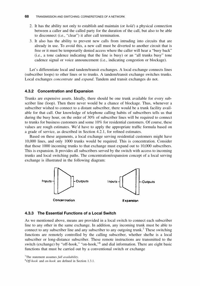
68 TRANSMISSION AND SWITCHING: CORNERSTONES OF A NETWORK
2. It has the ability not only to establish and maintain (or hold ) a physical connectionbetween a caller and the called party for the duration of the call, but also to be ableto disconnect (i.e., “clear”) it after call termination.
3. It also has the ability to prevent new calls from intruding into circuits that arealready in use. To avoid this, a new call must be diverted to another circuit that isfree or it must be temporarily denied access where the caller will hear a “busy back”(i.e., a tone cadence indicating that the line is busy) or an “all trunks busy” tonecadence signal or voice announcement (i.e., indicating congestion or blockage).
Let’s differentiate local and tandem/transit exchanges. A local exchange connects lines(subscriber loops) to other lines or to trunks. A tandem/transit exchange switches trunks.Local exchanges concentrate and expand. Tandem and transit exchanges do not.
4.3.2 Concentration and Expansion
Trunks are expensive assets. Ideally, there should be one trunk available for every sub-scriber line (loop). Then there never would be a chance of blockage. Thus, whenever asubscriber wished to connect to a distant subscriber, there would be a trunk facility avail-able for that call. Our knowledge of telephone calling habits of subscribers tells us thatduring the busy hour, on the order of 30% of subscriber lines will be required to connectto trunks for business customers and some 10% for residential customers. Of course, thesevalues are rough estimates. We’d have to apply the appropriate traffic formula based ona grade of service, as described in Section 4.2.1, for refined estimates.
Based on these arguments, a local exchange serving residential customers might have10,000 lines, and only 1000 trunks would be required. This is concentration. Considerthat those 1000 incoming trunks to that exchange must expand out to 10,000 subscribers.This is expansion. It provides all subscribers served by the switch with access to incomingtrunks and local switching paths. The concentration/expansion concept of a local servingexchange is illustrated in the following diagram:
4.3.3 The Essential Functions of a Local Switch
As we mentioned above, means are provided in a local switch to connect each subscriberline to any other in the same exchange. In addition, any incoming trunk must be able toconnect to any subscriber line and any subscriber to any outgoing trunk.7 These switchingfunctions are remotely controlled by the calling subscriber, whether she/he is a localsubscriber or long-distance subscriber. These remote instructions are transmitted to theswitch (exchange) by “off-hook,” “on-hook,”8 and dial information. There are eight basicfunctions that must be carried out by a conventional switch or exchange
7The statement assumes full availability.8Off-hook and on-hook are defined in Section 1.3.1.

4.3 INTRODUCTION TO SWITCHING 69
1. Interconnection2. Control3. Alerting4. Attending5. Information receiving6. Information transmitting7. Busy testing8. Supervisory
Consider a typical manual switching center illustrated in Figure 4.7. Here the eight basicfunctions are carried on for each call. The important interconnection function is illustratedby the jacks appearing in front of the operator. There are subscriber-line jacks9 and jacks
Figure 4.7 A manual exchange illustrating switching functions.
9A jack is an electric receptacle. It is a connecting device, ordinarily employed in a fixed location, to which awire or wires may be attached, and it is arranged for the insertion of a plug.

70 TRANSMISSION AND SWITCHING: CORNERSTONES OF A NETWORK
for incoming and outgoing trunks. The connection is made by double-ended connectingcords, which can connect subscriber to subscriber or subscriber to trunk. The cords avail-able are always less than half the number of jacks appearing on the board, because oneinterconnecting cord occupies two jacks, one on either end. Concentration takes place atthis point on a manual exchange. Distribution is also carried out because any cord maybe used to complete a connection to any of the terminating jacks. The operator is alertedby a lamp becoming lit when there is an incoming call requiring connection. This is theattending–alerting function. The operator then assumes the control function, determiningan idle connecting cord and plugging it into the incoming jack. She/he then determinescall destination, continuing her/his control function by plugging the cord into the termi-nating jack of the called subscriber or proper trunk to terminate her/his portion of controlof the incoming call. Of course, before plugging into the terminating jack, she/he carriesout a busy test function to determine that the called line or trunk is not busy. To alert thecalled subscriber that there is an incoming call, she/he uses the manual ring-down10 byconnecting the called line to a ringing current source as illustrated in Figure 4.7.
Other signaling means are used for trunk signaling if the incoming call is destined foranother exchange. On such a call the operator performs the information function orallyor by dialing the call information to the next exchange in the routing.
The supervision function is performed by lamps to show when a call is completedand the call is taken down (i.e., the patch cord can be removed). The operator conductsnumerous control functions to set up a call, such as selecting a cord, plugging it intothe originating jack of the calling line, connecting her/his headset to determine callinginformation, selecting (and busy testing) the called subscriber jack, and then plugging theother end of the cord into the proper terminating jack and alerting the called subscriberby ring-down. Concentration is the ratio of the field of incoming jacks to cord positions.Expansion is the number of cord positions to outgoing (terminating) jacks. The terminatingand originating jacks can be interchangeable. The called subscriber at one moment in timecan become the calling subscriber at another moment in time. On the other hand, incomingand outgoing trunks may be separated. In this case they would be one-way circuits. Ifnot separated, they would be both-way circuits, accepting both incoming and outgoingtraffic.
4.3.4 Introductory Switching Concepts
All local telephone switches have, as a minimum, three functional elements: concentration,distribution, and expansion. Concentration and expansion were discussed in Section 4.3.3.Viewing a switch another way, we can say that it has originating line appearances andterminating line appearances. These are illustrated in a simplified conceptual drawing inFigure 4.8, which shows three different call possibilities of a typical local exchange:
1. A call originated by a subscriber who is served by the exchange and bound for asubscriber who is served by the same exchange (route A-B-C-D-E).
2. A call originated by a subscriber who is served by the exchange and bound for asubscriber who is served by another exchange (route A-B-F).
3. A call originated by a subscriber who is served by another exchange and bound fora subscriber served by the exchange in question (route G-D-E).
10Ring-down is a method of signaling to alert an operator or a distant subscriber. In old-time telephone systems,a magneto was manually turned, thereby generating an alternating current that would ring a bell at the otherend. Today, special ringing generators are used.
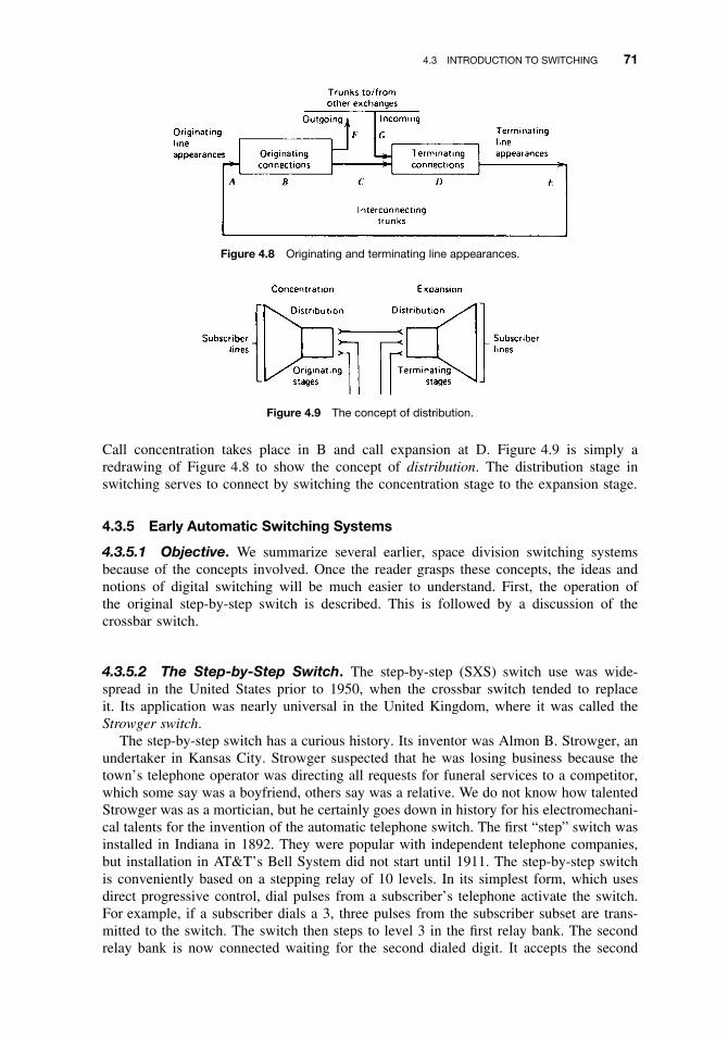
4.3 INTRODUCTION TO SWITCHING 71
Figure 4.8 Originating and terminating line appearances.
Figure 4.9 The concept of distribution.
Call concentration takes place in B and call expansion at D. Figure 4.9 is simply aredrawing of Figure 4.8 to show the concept of distribution. The distribution stage inswitching serves to connect by switching the concentration stage to the expansion stage.
4.3.5 Early Automatic Switching Systems
4.3.5.1 Objective. We summarize several earlier, space division switching systemsbecause of the concepts involved. Once the reader grasps these concepts, the ideas andnotions of digital switching will be much easier to understand. First, the operation ofthe original step-by-step switch is described. This is followed by a discussion of thecrossbar switch.
4.3.5.2 The Step-by-Step Switch. The step-by-step (SXS) switch use was wide-spread in the United States prior to 1950, when the crossbar switch tended to replaceit. Its application was nearly universal in the United Kingdom, where it was called theStrowger switch.
The step-by-step switch has a curious history. Its inventor was Almon B. Strowger, anundertaker in Kansas City. Strowger suspected that he was losing business because thetown’s telephone operator was directing all requests for funeral services to a competitor,which some say was a boyfriend, others say was a relative. We do not know how talentedStrowger was as a mortician, but he certainly goes down in history for his electromechani-cal talents for the invention of the automatic telephone switch. The first “step” switch wasinstalled in Indiana in 1892. They were popular with independent telephone companies,but installation in AT&T’s Bell System did not start until 1911. The step-by-step switchis conveniently based on a stepping relay of 10 levels. In its simplest form, which usesdirect progressive control, dial pulses from a subscriber’s telephone activate the switch.For example, if a subscriber dials a 3, three pulses from the subscriber subset are trans-mitted to the switch. The switch then steps to level 3 in the first relay bank. The secondrelay bank is now connected waiting for the second dialed digit. It accepts the second

72 TRANSMISSION AND SWITCHING: CORNERSTONES OF A NETWORK
Figure 4.10 Conceptual operation of a step-by-step switch (exchange).
digit from the subscriber and steps to its equivalent position and connects to the third relaybank and so on for four or seven dialed digits. Assume that a certain exchange only servesthree-digit numbers. A dialed number happens to be 375 and will be stepped through threesets of banks of 10 steps each. This is conceptually illustrated in Figure 4.10.
4.3.5.3 The Crossbar Switch. Crossbar switching dates back to 1938 and reached apeak of installed lines in 1983. Its life had been extended by using stored program control(SPC)11 rather than hard-wire control in the more conventional crossbar configuration. Thecrossbar is actually a matrix switch used to establish the speech path. An electrical contactis made by actuating a horizontal and vertical relay. Consider the switching mechanismillustrated in Figure 4.11. To make contact at point B4 on the matrix, horizontal relayB and vertical relay 4 must close to establish the connection. Such closing is usuallymomentary, but sufficient to cause latching. Two forms of latching are found in crossbarpractice: mechanical and electrical. The latch keeps the speech path connection until an“on-hook” condition occurs. Once the latching occurs, connection B4 is “busied out,”12 andthe horizontal and vertical relays are freed-up to make other connections for other calls.
Figure 4.11 The crossbar concept.
11SPC, stored program control, simply means that the switch or exchange is computer-controlled. Of course,all modern digital switches are computer-controlled.12“Busy-out” means that a line or connection is taken out of the pool because it is busy, it is being used, andis not available for others to utilize.

4.3 INTRODUCTION TO SWITCHING 73
4.3.6 Common Control (Hard-Wired)
First, we must distinguish common control from direct progressive control described inSection 4.3.5.2. With direct progressive control a subscriber dialed a digit, and the firstrelay bank stepped to the dialed digit; the subscriber dialed a second digit, and the secondstepping relay bank actuated, stepping to that digit level, and so on, through the entiredialed number. With common control, on the other hand, the dialed number is first storedin a register.13 These digits are then analyzed and acted upon by a marker, which is ahard-wired processor. Once the call setup is complete, the register and marker are free tohandle other call setups. The marker was specifically developed for the crossbar switch.Such marker systems are most applicable to specialized crossbar switching matrices ofcrossbar switches. Stored program control (SPC) is a direct descendent of the crossbarcommon control system. SPC is described below.
4.3.7 Stored Program Control
4.3.7.1 Introduction. Stored program control (SPC) is a broad term designatingswitches where common control is carried out entirely by computer. In some exchanges,this involves a large, powerful computer. In others, two or more minicomputers may carryout the SPC function. Still with other switches, the basic switch functions are controlled bydistributed microprocessors. Software may be hard-wired on one hand or programmableon the other. There is a natural marriage between a binary digital computer and the switchcontrol functions. In most cases these also work in the binary digital domain. The crossbarmarkers and registers are typical examples.
The conventional crossbar marker requires about half a second to service a call. Up to40 expensive markers are required on a large exchange. Strapping points on the marker areavailable to laboriously reconfigure the exchange for subscriber change, new subscribers,changes in traffic patterns, reconfiguration of existing trunks or their interface, and so on.
Replacing register markers with programmable logic—a computer, if you will—permitsone device to carry out the work of 40. A simple input sequence on the keyboard of thecomputer workstation replaces strapping procedures. System faults are displayed as theyoccur, and circuit status may be indicated on the screen periodically. Due to the high speedof the computer, postdial delay is reduced. SPC exchanges permit numerous new serviceofferings, such as conference calls, abbreviated dialing, “camp-on-busy,” call forwarding,voice mail, and call waiting.
4.3.7.2 Basic SPC Functions. There are four basic functional elements of an SPCswitching system:
1. Switching matrix2. Call store (memory)3. Program store (memory)4. Central processor (computer)
The earlier switching matrices consisted of electromechanical cross-points, such as acrossbar matrix, reed, correed, or ferreed cross-points. Later switching matrices employedsolid-state cross-points.
13A register is a device that receives and stores signals; in this particular case, it receives and stores dialed digits.

74 TRANSMISSION AND SWITCHING: CORNERSTONES OF A NETWORK
Figure 4.12 A simplified functional diagram of an SPC exchange.
The call store is often referred to as the “scratch-pad” memory. This is temporarystorage of incoming call information ready for use, on command from the central proces-sor. It also contains availability and status information of lines, trunks, and service circuitsunder internal switch-circuit conditions. Circuit status information is brought to the mem-ory by a method of scanning. All speech circuits are scanned for a busy/idle condition.
The program store provides basic instructions to the controller (central processor). Inmany installations, translation information is held in this store (memory), such as DN toEN translation and trunk signaling information.
A simplified functional diagram of a basic SPC system is shown in Figure 4.12.
4.3.8 Concentrators and Remote Switching
In Chapter 5 we discuss the design of a subscriber loop. There we will find that there arevery definite length limitations on subscriber loops. As we delve further into subscriberloop design, methods of extending loops still further are described. One way to extendsuch loops is with a remote concentrator or switch.
The simplest form of extending a switch is to use a concentrator some distance from theswitch (exchange). Concentrators or line concentrators consolidate subscriber loops, areremotely operated, and are a part of the concentration and expansion portion of a switchplaced at a remote location. The concentrator may be based on electromechanical facilitiesor solid-state cross-points for the concentration matrix. For instance, a 10:1 concentratormight serve 100 subscriber loops and deliver 10 trunks to the “mother” exchange. Aconcentrator does no switching whatsoever. All switching is carried out at the controllingor “mother” exchange. A typical line concentrator is illustrated in Figure 4.13, where 100subscriber loops are consolidated to 20 trunks plus 2 trunks for control from the nearby“mother” exchange. Of course, the ratio of loops to trunks is a key issue, and it is basedon calling habits and whether the subscribers are predominantly business or residential.
A remote switch, sometimes called a satellite, or satellite exchange, originates andterminates calls from the parent exchange. It differs from a concentrator in that local calls(i.e., calls originating and terminating inside the same satellite serving area) are served bythe remote switch and do not have to traverse the parent exchange as remote concentratorcalls do. A block of telephone numbers is assigned to the satellite serving area and isusually part of the basic number block assigned to the parent exchange. Because of thenumbering arrangement, a satellite exchange can discriminate between local calls andcalls to be handled by the parent exchange. A satellite exchange can be regarded as acomponent of the parent exchange that has been dislocated and moved to a distant site.The use of remote switching is very common in rural areas, and the distance a remoteswitch is from the parent exchange can be as much as 100 miles (160 km). Satelliteexchanges range in size from 300 to 2000 lines. Concentrators are cost effective for 300or less subscribers. However, AT&T’s SLC-96 can serve 1000 subscribers or more.

4.4 ESSENTIAL CONCEPTS IN TRANSMISSION 75
Figure 4.13 A typical concentrator.
4.4 ESSENTIAL CONCEPTS IN TRANSMISSION
4.4.1 Introduction
In this section we discuss two-wire and four-wire transmission and two impairments thatare commonly caused by two-wire-to-four-wire conversion equipment. These impairmentsare echo and singing. The second part of this section is an introduction to multiplexing.Multiplexing allows two or more communication channels to share the same transmissionbearer facility.
4.4.2 Two-Wire and Four-Wire Transmission
4.4.2.1 Two-Wire Transmission. A telephone conversation inherently requires trans-mission in both directions. When both directions are carried on the same pair of wires, itis called two-wire transmission. The telephones in our homes and offices are connectedto a local switching center (exchange) by means of two-wire circuits. A more proper def-inition for transmitting and switching purposes is that when oppositely directed portionsof a single telephone conversation occur over the same electrical transmission channel orpath, we call this two-wire operation.
4.4.2.2 Four-Wire Transmission. Carrier and radio systems require that oppositelydirected portions of a single conversation occur over separate transmission channels orpaths (or use mutually exclusive time periods). Thus we have two wires for the transmitpath and two wires for the receive path, or a total of four wires, for a full-duplex (two-way)telephone conversation. For almost all operational telephone systems, the end instrument(i.e., the telephone subset) is connected to its intervening network on a two-wire basis.
Nearly all long-distance (toll) telephone connections traverse four-wire links. Fromthe near-end user the connection to the long-distance network is two-wire or via a two-wire link. Likewise, the far-end user is also connected to the long-distance (toll) networkvia a two-wire link. Such a long-distance connection is shown in Figure 4.14. Schemat-ically, the four-wire interconnection is shown as if it were a single-channel wire-line

76 TRANSMISSION AND SWITCHING: CORNERSTONES OF A NETWORK
Figure 4.14 A typical long distance (toll) connection model.
with amplifiers. However, it would more likely be a multichannel multiplexed configu-ration on wire/fiber-optic cable or over radio. Nevertheless, the amplifiers in Figure 4.14serve to convey the ideas this section considers. As illustrated in Figure 4.14, conversionfrom two-wire to four-wire operation is carried out by a hybrid, which is a four-port,four-winding transformer.
4.4.2.3 Operation of a Hybrid. A hybrid, in terms of telephony (at voice frequency), isa transformer with four separate windings. Based on a simplified description, a hybrid maybe viewed as a power splitter with four sets of wire-pair connections. A functional blockdiagram of a hybrid device is shown in Figure 4.15. Two of the wire-pair connectionsbelong to the four-wire path, which consists of a transmit pair and a receive pair. Thethird pair is a connection to the two-wire link, which is eventually connected to thesubscriber subset via one or more switches. The last pair of the four connects the hybridto a resistance–capacitance balancing network, which electrically balances the hybridwith the two-wire connection to the subscriber subset over the frequency range of thebalancing network. Balancing, in this context, means matching impedances—that is, theimpedance of the two-wire side to the hybrid two-wire port.
Signal energy entering from the two-wire subset connection divides equally. Half ofit dissipates (as heat) in the impedance of the four-wire side receive path and the otherhalf goes to the four-wire side transmit path, as illustrated in Figure 4.15. Here the idealsituation is that no energy is to be dissipated by the balancing network (i.e., there is
Figure 4.15 Operation of a hybrid transformer.

4.4 ESSENTIAL CONCEPTS IN TRANSMISSION 77
a perfect balance or impedance match). The balancing network is supposed to displaythe characteristic impedance of the two-wire line (subscriber connection) to the hybrid.14
Signal energy entering from the four-wire side receive path is also split in half in the idealsituation where there is a perfect balance (i.e., a perfect match). Half of the energy is dis-sipated by the balancing network (N) and half at the two-wire port (L) (see Figure 4.15.)
The reader should note that in the description of a hybrid, in every case, ideally halfof the signal energy entering the hybrid is used to advantage and half is dissipated orwasted. Also keep in mind that any passive device inserted in a circuit, such as a hybrid,has an insertion loss. As a rule of thumb, we say that the insertion loss of a hybrid is0.5 dB. Thus there are two losses here that the reader must not lose sight of:
Hybrid insertion loss 0.5 dBHybrid dissipation loss 3.0 dB (half of the power)
3.5 dB (total)
As far as this section is concerned, any signal passing through a hybrid suffers a3.5-dB loss. This is a good design number for gross engineering practice. However, somehybrids used on short subscriber connections purposely have higher losses, as do specialresistance-type hybrids.
In Figure 4.15, consider the balancing network (N) and the two-wire side of the hybrid(L). In all probability (L), the two-wire side will connect to a subscriber through atleast one switch. Thus the two-wire port on the hybrid could look into at least 10,000possible subscriber connections: some short loops, some long loops, and some loops inpoor condition. Because of the fixed conditions on the four-wire side, we can generallydepend on holding a good impedance match. Our concern under these conditions isthe impedance match on the two-wire side—that is, the impedance match between thecompromise network (N) and the two-wire side (L). Here the impedance can have highvariability from one subscriber loop to another.
We measure the capability of impedance match by return loss. In this particular casewe call it balance return loss:
Balance return lossdB = 20 log10ZL + ZN
ZL − ZN
.
Let us say, for argument’s sake, that we have a perfect match. In other words, theimpedance of the two-wire subscriber loop side (L) on this particular call was exactly900 � and the balancing network (N) was 900 �. Substitute these numbers in thepreceding formula above and we get
Balance return lossdB = 20 log900 + 900
900 − 900.
Examine the denominator. It is zero. Any number divided by zero is infinity. Thus wehave an infinitely high return loss. And this happens when we have a perfect match, anideal condition. Of course it is seldom realized in real life. In real life we find that thebalance return loss for a large population of hybrids connected in service and servinga large population of two-wire users has a median more on the order of 11 dB with a
14Characteristic impedance is the impedance that the line or port on a device is supposed to display. For mostsubscriber loops it is 900 � with a 2.16-µF capacitor in series at 1000 Hz for 26-gauge wire pair or 600-�resistive. The notation for characteristic impedance is Z0.

78 TRANSMISSION AND SWITCHING: CORNERSTONES OF A NETWORK
Figure 4.16 Schematic diagram of two-wire to four-wire conversion using a hybrid. (From Figure 5-9,p. 104, Ref. 5. Reprinted with permission of the IEEE Press.)
standard deviation of 3 dB (Ref. 4). This is valid for North America. For some other areasof the world, balance return loss median may be lower with a larger standard deviation.
When the return loss becomes low (i.e., there is a poor impedance match), thereis a reflection of the speech signal. That is, speech energy from the talker at her/hisdistant hybrid leaks across from the four-wire receive to the four-wire transmit side (seeFigure 4.15). This signal energy is heard by the talker. It is delayed due to the propagationtime. This is echo, which can be a major impairment depending on its intensity and amountof time it is delayed. It can also be very disruptive on a data circuit.
We define the cause of echo as any impedance mismatch in the circuit. It is mostcommonly caused by this mismatch that occurs at the hybrid. Echo that is excessivebecomes singing. Singing is caused by high positive feedback on the intervening amplifiers(Figure 4.14). Singing on the analog network could take the network down by overloadingmultiplex equipment. The possibility of singing on the digital network is very low. Thecontrol of echo and singing is discussed in Chapter 8. Figure 4.16 is a schematic digramof a hybrid circuit.
4.5 INTRODUCTION TO MULTIPLEXING
4.5.1 Definition
Multiplexing is used for the transmission of a plurality of information channels over asingle transmission medium. An information channel may be a telephone voice chan-nel, data channel, or a channel carrying image information. Our discussion below willconcentrate on a telephone channel. A telephone channel is a channel optimized for car-rying voice traffic, in this case the voice of a single telephone user. We will define itas an analog channel with occupying the band of frequencies between 300 and 3400 Hz(CCITT/ITU-T definition).
Before launching into our discussion, keep in mind that all multiplex equipment isfour-wire equipment. If we look at one side of a circuit, there will be a multiplexer usedfor transmission and a demultiplexer used for reception.
The number of channels that can be multiplexed on a particular circuit depends onthe bandwidth of the transmission medium involved. We might transmit 24 or 48 or

4.5 INTRODUCTION TO MULTIPLEXING 79
96 channels on a wire pair, depending on the characteristics of that wire pair. Coaxialcable can support many thousands of voice channels; line-of-sight microwave radio iscapable of carrying from several hundred to several thousand voice channels. A singlefiber-optic thread can support literally tens of thousand of channels. A communicationsatellite transponder can carry between 700 and 2000 such voice channels, depending onthe transponder’s bandwidth.
There are essentially two generic methods of multiplexing information channels:
1. In the frequency domain; we call this frequency division multiplex (FDM).
2. In the time domain, which we call time division multiplex (TDM).
The concepts of frequency division multiplexing are discussed in this chapter. Time divi-sion multiplexing (pulse code modulation) is covered in Chapter 6.
4.5.2 Frequency Division Multiplex
4.5.2.1 Introduction. With FDM the available channel bandwidth is divided into anumber of nonoverlapping frequency slots. Each frequency slot or bandwidth segmentcarries a single information-bearing signal such as a voice channel. We can consideran FDM multiplexer as a frequency translator. At the opposite end of the circuit, ademultiplexer filters and translates the frequency slots back into the original informationbearing channels. In the case of a telephone channel, a frequency slot is conveniently4 kHz wide, sufficient to accommodate the standard 300- to 3400-kHz voice channel.Figure 4.17 illustrates the basic concept of frequency division multiplex.
Figure 4.17 The frequency division multiplex concept illustrated.

80 TRANSMISSION AND SWITCHING: CORNERSTONES OF A NETWORK
In practice, the frequency translator (multiplexer) uses single sideband modulation ofradio-frequency (RF) carriers. A different RF carrier is used for each channel to be mul-tiplexed. This technique is based on mixing or heterodyning the signal to be multiplexed,typically a voice channel, with an RF carrier.
An RF carrier is an unmodulated RF signal of some specified frequency. In theory,because it is not modulated, it has an indefinitely small bandwidth. In practice, of course,it does have some measurable bandwidth, although very narrow. Such a carrier derivesfrom a simple frequency source such as an oscillator or a more complex source such asa synthesizer, which can generate a stable output in a range of frequencies.
A simplified block diagram of an FDM link is shown in Figure 4.18.
4.5.2.2 Mixing. The heterodyning or mixing of signals of frequencies A and B isshown as follows. What frequencies may be found at the output of the mixer? Both theoriginal signals will be present, as well as the signals representing their sum and theirdifference in the frequency domain. Thus at the output of the illustrated mixer we willhave present the signals of frequency A, B, A + B, and A − B. Such a mixing processis repeated many times in FDM equipment.
Let us now look at the boundaries of the nominal 4-kHz voice channel. These are300 Hz and 3400 Hz. Let us further consider these frequencies as simple tones of 300 Hzand 3400 Hz. Now consider the following mixer and examine the possibilities at its output:
First, the output may be the sum or
20,000 Hz 20,000 Hz+ 300 Hz + 3,400 Hz
20,300 Hz 23,400 Hz
A simple low-pass filter could filter out all frequencies below 20,300 Hz.
Figure 4.18 Simplified block diagram of an FDM link.

4.5 INTRODUCTION TO MULTIPLEXING 81
Now imagine that instead of two frequencies, we have a continuous spectrum of fre-quencies between 300 Hz and 3400 Hz (i.e., we have the voice channel). We representthe spectrum as a triangle:
As a result of the mixing process (translation) we have another triangle, as follows:
When we take the sum, as we did previously, and filter out all other frequencies, wesay we have selected the upper sideband. Therefore we have a triangle facing to the right,and we call this an upright or erect sideband. We can also take the difference, such that
20,000 Hz 20,000 Hz− 300 Hz − 3,400 Hz
19,700 Hz 16,600 Hz
and we see that in the translation (mixing process) we have had an inversion of fre-quencies. The higher frequencies of the voice channel become the lower frequenciesof the translated spectrum, and the lower frequencies of the voice channel become thehigher when the difference is taken. We represent this by a right triangle facing theother direction:
This is called an inverted sideband. To review, when we take the sum, we get an erect side-band. When we take the difference, frequencies invert and we have an inverted sidebandrepresented by a triangle facing left.
Again, this modulation technique is called single-sideband suppressed carrier (SSBSC).It is a type of amplitude modulation (AM). With conventional AM, the modulation pro-duces two sidebands, an upper sideband and a lower sideband, symmetrical on either sideof the carrier. Each sideband carries the information signal. If we tune to 870 kHz on theAM dial, 870 kHz is the frequency of the RF carrier, and its sidebands fall on either side,where each sideband is about 7.5 kHz wide. Thus a radio station on the AM dial requiresabout 15 kHz of spectrum bandwidth.
In our case, there are also two sidebands extending about 3.4 kHz either side of thecarrier frequency. Of course, the carrier frequency is the local oscillator frequency, whichis suppressed at the output, as is the upper sideband. All that remains is the lower sideband,which contains the voice channel information.
4.5.2.3 CCITT Modulation Plan4.5.2.3.1 Introduction. A modulation plan sets forth the development of a band of fre-quencies called the line frequency (i.e., ready for transmission on the line or transmission

82 TRANSMISSION AND SWITCHING: CORNERSTONES OF A NETWORK
medium). The modulation plan usually is a diagram showing the necessary mixing,local oscillator mixing frequencies, and the sidebands selected by means of the trianglesdescribed previously in a step-by-step process from voice channel input to line frequencyoutput. The CCITT has recommended a standardized modulation plan with a commonterminology. This allows large telephone networks, on both national and multinationalsystems, to interconnect. In the following paragraphs the reader is advised to be carefulwith terminology.
4.5.2.3.2 Formation of the Standard CCITT Group. The standard group, as definedby the CCITT, occupies the frequency band of 60 kHz to 108 kHz and contains 12 voicechannels. Each voice channel is the nominal 4-kHz channel occupying the 300-Hz to
Figure 4.19 Formation of the standard CCITT group.

4.5 INTRODUCTION TO MULTIPLEXING 83
3400-Hz spectrum. The group is formed by mixing each of the 12 voice channels witha particular carrier frequency associated with each channel. Lower sidebands are thenselected, and the carrier frequencies and the upper sidebands are suppressed. Figure 4.19shows the preferred approach to the formation of the standard CCITT group. It shouldbe noted that in the 60-kHz to 108-kHz band, voice channel 1 occupies the highestfrequency segment by convention, between 104 kHz and 108 kHz. The layout of thestandard group is illustrated in Figure 4.19. Single sideband suppressed carrier (SSBSC)modulation techniques are utilized universally.
4.5.2.3.3 Formation of the Standard CCITT Supergroup. A supergroup contains fivestandard CCITT groups, equivalent to 60 voice channels. The standard supergroup, beforefurther translation, occupies the frequency band of 312 kHz to 552 kHz. Each of the fivegroups making up the supergroup is translated in frequency to the supergroup frequencyband by mixing with the appropriate carrier frequencies. The carrier frequencies are420 kHz for group 1, 468 kHz for group 2, 516 kHz for group 3, 564 kHz for group 4,and 612 kHz for group 5. In the mixing process, in each case, the difference is taken (i.e.,the lower is selected). This frequency translation process is illustrated in Figure 4.20.
4.5.2.4 Line Frequency. The band of frequencies that the multiplexer applies to theline, whether the line is a radiolink, wire pair, or fiber-optic cable, is called the linefrequency. Some texts use the term high frequency (HF) for the line frequency. This isnot to be confused with HF radio, which is a radio system that operates in the band of3 MHz to 30 MHz.
The line frequency in this case may be the direct application of a group or supergroup tothe line. However, more commonly a final frequency translation stage occurs, particularlyon high-density systems.15 An example of line frequency formation is illustrated in
Figure 4.20 Formation of the standard CCITT supergroup. The vertical arrows show the frequencies ofthe group level regulating pilot tones. (From CCITT Rec. G.233, courtesy of ITU-T Organization, Ref. 6.)
15“High-density” meaning, in this context, a system carrying a very large number of voice channels.

84 TRANSMISSION AND SWITCHING: CORNERSTONES OF A NETWORK
Figure 4.21 Makeup of the basic CCITT 15-supergroup line frequency assembly. (From CCITT Rec.G.233, courtesy of the ITU-T Organization, Geneva, Ref. 6.)
Figure 4.21. This figure shows the makeup of the basic 15-supergroup assembly. Itscapacity is (15 × 60) 900 voice channels (Ref. 7).
4.5.3 Pilot Tones
Pilot tones are used to control level in FDM systems. They may also be used to actuatemaintenance alarms. In Figures 4.20 and 4.21, the pilot tones are indicated by the verticallines with little triangles on top. For example in the 15-supergroup assembly shown inFigure 4.21, the pilot tone is at 1552 kHz.
A pilot tone provides a comparatively constant amplitude reference for an automaticgain control (AGC) circuit. Frequency division multiplex equipment was designed tocarry speech telephony. The nature of speech, particularly its varying amplitude, makesit a poor prospect as a reference for level control. Ideally, simple single-sinusoid (a sine

REVIEW EXERCISES 85
wave signal), constant-amplitude signals with 100% duty cycles provide simple controlinformation for level regulating equipment (i.e., the AGC circuit).16
Modern FDM equipments initiate a level-regulating pilot tone on each group on thetransmitting side of the circuit. Individual level-regulating pilots are inserted on eachsupergroup and other frequency configurations. The intent is to maintain the system levelwithin ±0.5 dB.
Pilots are assigned frequencies that are part of the transmitted FDM spectrum yetdo not interfer with the voice channel operation. They are standardized by CCITT andare usually inserted on a frequency in the guard between voice channels or are residualcarriers (i.e., partially suppressed carriers).
4.5.4 Comments on the Employment and Disadvantages of FDM Systems
FDM systems began to be implemented in the 1950s, reaching a peak employmentin the 1970s. All long-haul (long-distance) broadband systems, typically line-of-sightmicrowave, satellite communication, and coaxial cable systems, almost universally usedFDM configurations. One transcontinental system in North America, called the L-5 sys-tem, carried 10,800 voice channels on each cable pair. (Remember the system is four-wire,requiring two coaxial cables per system.) There were 10 working cable pairs and one pairas spare. The total system had 108,000 voice channel capacity.
Few, if any, new FDM systems are being installed in North America today. FDM isbeing completely displaced by TDM systems (i.e., digital PCM systems, see Chapter 6).The principal drawback of FDM systems is noise accumulation. At every modulation–demodulation point along a circuit, noise is inserted. Unless the system designer was verycareful, there would be so much noise accumulated at the terminal end of the system thatthe signal was unacceptable and the signal-to-noise ratio was very poor. Noise does notaccumulate on digital systems.
We incorporated this section on frequency division multiplex so that the reader wouldunderstand the important concepts of FDM. Many will find that frequency division tech-niques are employed elsewhere such as on satellite communications, cellular, and PCSsystems. Also keep in mind that FDM as described herein is still widely used in emergingnations. However, these networks are also starting to phase out FDM in favor of a digitalnetwork based on TDM (PCM). TDM techniques are covered in Chapter 6.
REVIEW EXERCISES
1. Define switching in light of transmission.
2. Define signaling.
3. Define calling rate and holding time.
4. Define lost calls using the terms offered traffic and carried traffic.
5. Why are call attempts so important in the design of modern SPC switches?
6. Suppose the average holding time of a call is 3.1 minutes and the calling rate in thebusy hour is 465 on a particular work day. What is the traffic flow?
7. Under normal operating conditions, when can we expect blockage (of calls)?
16Duty cycle refers to how long (in this case) a signal is “on.” A 100% duty cycle means the signal is on allthe time.

86 TRANSMISSION AND SWITCHING: CORNERSTONES OF A NETWORK
8. The statistics during the BH for a particular exchange is 5 lost calls in 841 offeredcalls. What is the grade of service?
9. When dealing with traffic formulas and resulting traffic tables, we have to know howlost calls are “handled.” What are the three ways that lost calls may be handled?
10. On a probability-distribution curve, define the mean.
11. What percentage of events are encompassed in one standard deviation?
12. What traffic formula (and resulting traffic tables) would be used for modern digitalexchanges (we assume such exchanges are SPC based)?
13. Consider one traffic relation that has been designed to meet grade of service objec-tives. We vary one characteristic—the number of traffic channels. Argue the casefor efficiency for 10 circuits versus 49 circuits during the BH. Assume grade ofservice as 0.01 and $1.00 per erlang.
14. Define serving time when dealing with waiting systems (Erlang C).
15. Leaving aside issues of survivability, describe how alternative routing can improvegrade of service or allow us to reduce the number of trunks on a traffic relation andstill meet grade of service objectives.
16. Why is data traffic so different from telephone traffic?
17. Distinguish between a tandem/transit switch and a local serving switch.
18. Why use a tandem switch in the first place?
19. What are the three basic requirements of a telephone switch?
20. For a local serving switch with 10,000-line capacity, exemplify concentration ratios(lines/trunks) for a residential area, for an industrial/office area.
21. List six of the eight basic functions of a local switch.
22. Give the three basic functions of a local serving switch.
23. In a very small town, its local serving exchange has only three-digit subscribernumbers. Theoretically, what is the maximum number of subscribers it can serve?
24. How many switch banks will a step-by-step (SXS) switch have if it is to serve upto 10,000 subscribers?
25. What happens to a line that is “busied out?”
26. Give at least three advantages of an SPC exchange when compared with a register-marker crossbar exchange.
27. What are the three basic functional blocks of an SPC exchange (SPC portion only)?
28. Differentiate remote concentrators from remote switches. Give one big advantageeach provides.
29. Describe two-wire operation and four-wire operation.
30. What is the function of a hybrid (transformer)?
31. Describe the function of the balancing network as used with a hybrid.

REFERENCES 87
32. There are two new telephone network impairments we usually can blame on thehybrid. What are they?
33. What is the balance return loss on a particular hybrid connectivity when the bal-ancing network is set for a 900-� loop, and this particular loop has only a 300-�impedance?
34. What are the two generic methods of multiplexing?
35. A mixer used in an FDM configuration has a local oscillator frequency of 64 kHzand is based on the CCITT modulation plan. After mixing (and filtering), what isthe resulting extension of the desired frequency band (actual frequency) limits at3 dB points)?
36. The standard CCITT supergroup consists of groups and occupies the frequencyband kHz to kHz? How many standard voice channels does it contain?
37. What are pilot tones and what are their purpose in an FDM link?
REFERENCES
1. R. L. Freeman, Telecommunication System Engineering, 4th ed., Wiley, New York, 2004.
2. R. A. Mina, “The Theory and Reality of Teletraffic Engineering,” Telephony article series, Tele-phony, Chicago, 1971.
3. R. L. Freeman, Reference Manual for Telecommunication Engineering, 3rd ed., Section 1, Wiley,New York, 1994.
4. Transmission Systems for Communications, 5th ed., Bell Telephone Laboratories, Holmdel, NJ,2002.
5. W. D. Reeve, Subscriber Loop Signaling and Transmission Handbook—Analog, IEEE Press,New York, 1992.
6. Recommendations Concerning Translating Equipments, CCITT Rec. G.233, Geneva, 1982.
7. R. L. Freeman, Telecommunication Transmission Handbook, 4th ed., Wiley, New York, 1998.


5
TRANSMISSION ASPECTS OF VOICETELEPHONY
5.1 CHAPTER OBJECTIVE
The goal of this chapter is to provide the reader with a firm foundation of the analogvoice channel. Obviously, from the term, we are dealing with the transmission of thehuman voice. Voice is a sound signal. That sound is converted to an electrical signal bythe mouthpiece of the subscriber subset. The electrical signal traverses down a subscriberloop to a local serving switch or to a PABX.1 The local serving switch is the point ofconnectivity with the PSTN.
With the exception of the subscriber plant, the PSTN has evolved to an all-digitalnetwork. In most cases the local serving switch is the point of analog-to-digital interface.Digital transmission and switching are discussed in Chapter 6. However, there are stilllocations in less-developed parts of the world where digital conversion takes place deeperin the PSTN, perhaps at a tandem exchange. Local service inside the local serving areain these cases remains analog, and local trunks (junctions) may consist of wire pairscarrying the analog signals. Analog wire pair trunks are even more prevalent outside ofNorth America.
In this chapter we will define the analog voice channel and describe its more commonimpairments. The subscriber subset’s functions are reviewed as well as the sound toelectrical signal conversion which takes place in that subset. We then discuss subscriberloop and analog trunk design.
Since the publication of the first edition of this text, the traffic intensity of voice versusdata have changed places. Whereas voice traffic was predominant in the PSTN, data trafficintensity currently is far greater. Some sources state that only some 5% of the networktraffic is voice and the remaining 95% is now data in one form or another. Much ofthe remainder being data traffic in one form or another. One such form is voice over IPwhich has the potential for astronomic jumps in traffic intensity. Do we count that asvoice or data? It should also be kept in mind that the connectivity to the PSTN—that is,the portion from the user’s subset to the local serving exchange—will remain analog for
1PABX stands for private automatic branch exchange. It is found in the office or factory environment, and it isused to switch local telephone calls and to connect calls to a nearby local serving exchange. In North Americaand in many other places a PABX is privately owned.
Fundamentals of Telecommunications, Second Edition, by Roger L. FreemanISBN 0-471-71045-8 Copyright 2005 by Roger L. Freeman
89

90 TRANSMISSION ASPECTS OF VOICE TELEPHONY
some time into the future. Here again we may have problems with definitions. The digitalsubscriber line (DSL) continues increased presence. One can argue whether it is digitalor analog. ISDN, of course, is another notable exception.
5.2 DEFINITION OF THE VOICE CHANNEL
The IEEE (Ref. 1) defines a voice-band channel as “a channel that is suitable for trans-mission of speech or analog data and has the maximum usable frequency range of 300to 3400 Hz.” CCITT/ITU-T also defines it in the range of 300–3400 Hz. Bell Tele-phone Laboratories (Ref. 2) defines it in the range of 200–3300 Hz. We remain with theCCITT/IEEE definition.
5.2.1 The Human Voice
Human voice communication depends on the voice-generating mechanism of mouth andthroat being the initial transmitter, with the acuity of the ear being the receiver. Frequencycomponents of the human voice extend down to some 20 Hz and as high as 32,000 Hz.The lower frequency components carry the voice energy and the higher frequency compo-nents carry emotion. Figure 5.1 shows a distribution of energy and emotion of the typicalhuman voice.
The human ear and many devices and components of the telecommunication net-work tend to constrain this frequency range. Young people can hear sound out to about18,000 Hz, and as we get older this range diminishes. People in their sixties may not beable to hear sounds above 7000 Hz.
It is not the intent of the PSTN operator to provide high fidelity communicationsbetween telephone users, only intelligible connections. Not only is there the frequency con-straint of voice communications brought about by the human ear, there are also constraintsbrought about by the subset transmitter (mouthpiece) and receiver (earpiece) and the sub-scriber loop (depending on its length, condition, and make up), but then purposely theelectrical voice signal will enter a low-pass filter limiting its high-frequency excursion to3400 Hz. The filter is in the input circuit of the multiplex equipment. Thus we say that thevoice channel or VF (voice-frequency) channel occupies the band from 300 to 3400 Hz.
Figure 5.1 Energy and emotion distribution of human speech. (From BSTJ, July 1931.)

5.3 OPERATION OF THE TELEPHONE SUBSET 91
Figure 5.2 Comparison of overall response of the North American 302 and 500/2500 telephone sets.(From W. F. Tuffnell, 500-Type Telephone S, Bell Labs Record, September 1951, copyright 1951 BellTelephone Laboratories.) Note: The 302 type subset is now obsolete.
Figure 5.2 shows the overall frequency response of a simulated telephone networkusing the standard 500/2500 North American telephone subset.
5.3 OPERATION OF THE TELEPHONE SUBSET
A telephone subset consists of an earpiece, which we may call the receiver; the mouth-piece, which we may call the transmitter; and some control circuitry in the telephonecradle-stand. Figure 5.3 illustrates a telephone subset connected all the way through itssubscriber loop to the local serving exchange. The control circuits are aptly shown.
The hook-switch in Figure 5.3 (there are two) are the two little “knobs” that pop up outof the cradle when the subset is lifted from its cradle. When the subset is replaced in itscradle, these knobs are depressed. This illustrates the “on-hook” and “off-hook” functionsdescribed earlier. The “dial-switch” represents the function of the telephone dial. It simplycloses and opens (i.e., makes contact, breaks contact). If a 1 is dialed, there is a singlebreak and make (the loop is opened and the loop is closed). When the “loop is closed,”

Fig
ure
5.3
The
conv
entio
nalt
elep
hone
sub
set.
Not
eth
eho
ok-s
witc
han
dd
ial-
switc
h‘‘c
ontr
ols.
’’
92

5.4 SUBSCRIBER LOOP DESIGN 93
current flows; when open, current stops flowing. If, for instance, a 5 is dialed, there willbe five break-and-make operations which represent the digit 5.
5.3.1 The Subset Mouthpiece or Transmitter
The mouthpiece converts acoustic energy (i.e., sound) into equivalent electric energyby means of a carbon granule transmitter. The transmitter requires a direct-current (dc)voltage, a minimum of 3 to 5 volts, across its electrodes. We call this talk battery. Inmodern systems it is supplied over the subscriber loop and derives from a battery sourceat the local serving switch as illustrated in Figure 5.3.
Current deriving from the local switch supply flows through the carbon grains orgranules that are contained just below a diaphragm that holds the carbon granules in place.This current flow occurs when the telephone is taken off-hook (i.e., out of its cradle). Whensound impinges on the diaphragm of the transmitter, resulting variations of air pressure aretransferred from the diaphragm to the carbon granules, and the resistance of the electricalpath through the carbon changes in proportion to the pressure. A pulsating direct currentin the subscriber loop results. The frequency response of the carbon transmitter peaksbetween 800 and 1000 Hz. This is illustrated in Figure 5.2.
5.3.2 The Subset Earpiece or Receiver
A typical receiver consists of a diaphragm of magnetic material, often soft iron alloy,placed in a steady magnetic field supplied by a permanent magnet, and a varying magneticfield, caused by the voice currents flowing through the voice coils. Such voice currents arealternating (ac) in nature and originate at the far-end telephone transmitter. These currentscause the magnetic field of the receiver to alternately increase and decrease, making thediaphragm move and respond to the variations. As a result, an acoustic pressure wave is setup, reproducing, more or less exactly, the original sound wave from the distant telephonetransmitter. The telephone receiver, as a converter of electrical energy to acoustic energy,has a comparatively low efficiency, on the order of 2% to 3%.
Sidetone is the sound of the talker’s voice heard in his own receiver. The sidetone levelmust be controlled. When the level is high, the natural human reaction is for the talkerto lower his voice. Thus by regulating the sidetone, talker levels can be regulated. If toomuch sidetone is fed back to the receiver, the output level of the transmitter is reduced,owing to the talker lowering his/her voice, thereby reducing the level (voice volume) atthe distant receiver, deteriorating performance.
5.4 SUBSCRIBER LOOP DESIGN
5.4.1 Basic Design Considerations
We speak of the telephone subscriber as the user of the subset. As we mention inSection 1.3, telephone subscribers are connected via a subscriber loop to a local serv-ing switch that can connect a call to another subscriber served by that same switch orvia other switches through the PSTN to a distant called subscriber. The conventionalsubscriber loop is a wire pair. Present commercial telephone service provides for bothtransmission and reception on the same pair of wires that connect the subscriber to her/hislocal serving switch. In other words, it is two-wire operation.
The subscriber loop is a dc loop in that it is a wire pair supplying a metallic path2 forthe following:
2Metallic path is a path that is “metal,” usually copper or aluminum. It may be composed of a wire pair orcoaxial cable. We could have a radio path or a fiber-optic path.

94 TRANSMISSION ASPECTS OF VOICE TELEPHONY
1. Talk battery.2. An ac ringing voltage for the bell or other alerting device on the telephone instru-
ment supplied from a special ringing voltage source.3. Current to flow through the loop when the telephone subset is taken out of its cradle
(off-hook), which tells the switch that it requires “access” and causing line seizureat the local serving switch.
4. The telephone dial3 that, when operated, makes and breaks the dc current on theclosed loop, which indicates to the switching equipment the telephone number ofthe distant telephone with which communication is desired.
The typical subscriber loop is supplied its battery voltage by means of a battery feedcircuit illustrated in Figure 5.3. Battery voltages have been standardized at −48 V dc. Itis a negative voltage to minimize cathodic reaction. This is a form of corrosion that canbe a thermal noise source.
5.4.2 Subscriber Loop Length Limits
It is desirable from an economic standpoint to permit subscriber loop lengths to be as longas possible. Thus the subscriber serving area could become very large. This, in turn, wouldreduce the number of serving switches required per unit area affording greater centraliza-tion, less land to buy, fewer buildings, simpler maintenance, and so forth. Unfortunately,there are other tradeoffs forcing the urban/suburban telecommunication system designerto smaller serving areas and more switches.
The subscriber loop plant, sometimes called outside plant, is the largest single invest-ment that a telecommunication company has. Physically, we can extend a subscriberloop very long distances: 5, 10, 20, 50, or even 100 miles. Such loops require expen-sive conditioning, which we will delve into later in this chapter. It is incumbent ona telecommunication company to optimize costs to have the fewest possible speciallyconditioned loops.
The two basic criteria, which limit loop length, must be considered when designing asubscriber loop:
1. Attenuation (loss) limits2. Resistance limits
Attenuation (loss) must be limited to keep within loudness rating requirements. Loudnessrating was discussed in Section 3.2. If a subscriber loop has too much loss, the telephoneuser signal level suffers and she/he cannot hear the signal well enough; the user mayconsider the connection unsatisfactory. In North America the maximum loss objective is8 dB for a subscriber loop. In some other countries, that value is 7 dB. Remember thatit takes two subscriber loops to make a connection: the subscriber loop of the callingsubscriber and the loop of the called subscriber.
The attenuation is referenced to 1000 Hz in North America and 800 Hz elsewhere inthe world. In other words, when we measure loss, unless otherwise stated, it is measuredat the reference frequency. Loss (attenuation) is a function of the diameter of the copperwire making up the pair and the length of the pair.
Consider this example. We take a reel of 19-gauge4 (American Wire Gauge, or AWG)copper wire and connect a telephone transmitter at one end. Now extend the reel laying out
3Modern telephone subsets almost universally use a touch-tone pad, which transmits a unique two-tone signalfor each digit actuated. This type of subscriber address signaling is described in Chapter 7.4A 19-gauge copper wire has a diameter of 0.91 mm.

5.4 SUBSCRIBER LOOP DESIGN 95
the wire along a track or road. At intervals somebody is assigned to talk on the transmitter,and we test the speech level, say, every 5 km. At about 30 km the level of the voice heardon the test receiver is so low that intelligible conversation is impossible. What drops thelevel of the voice as the wire is extended is the loss, which is a function of length.
Let us digress a moment and discuss American Wire Gauge or AWG. It is a standardizedmethod of measuring wire diameter. Just like the gauge on shotguns, as the AWG numberincreases, the wire diameter decreases. The following equivalents will give us a basic ideaof AWG versus diameter.
American WireGauge
Diameter(mm)
Diameter(inches)
19 0.91 0.03622 0.644 0.02524 0.511 0.02026 0.405 0.01628 0.032 0.012
Signaling limits of a subscriber loop are based on dc resistance. When we go “off-hook”with a telephone, a certain minimum amount of current must flow in the loop to actuatethe local serving switch. The generally accepted minimum loop current value in NorthAmerica is 20 mA. If subscriber loop current is below this value, we have exceeded thesignaling limits. Applying Ohm’s law, the loop resistance should not exceed 2400 �.Budget 400 � for the battery feed bridge and we are left with 2000 � for the loop itself.We must account for the resistance of the subset wiring. Budget 300 � for this. Thus theresistance of the wire itself in the loop must not exceed 1700 �.
Once we exceed the signaling limit (the loop resistance, wire only, exceeds 1700 �),when the telephone goes off-hook, no dial tone is returned. This just means that there isinsufficient loop current to actuate the switch, telling the switch we wish to make a call.When there is sufficient current, the switch, in turn, returns the dial tone. When there isinsufficient loop current, we hear nothing. If we cannot effect signaling, the telephonejust will not operate. So between the two limiting factors, loss and resistance, resistanceis certainly the most important of the criteria.
5.4.3 Designing a Subscriber Loop
Figure 5.4 is a simplified model of a subscriber loop. Distance D in the figure is the lengthof the loop. As we mentioned above, D must be limited in length owing to (1) attenuationof the voice signal on the loop and (2) dc resistance of the loop for signaling.
The maximum loop loss is taken from the national transmission plan.5 In NorthAmerica, it is 8 dB measured at 1000 Hz. We will use the maximum resistance valuecalculated above, namely 1700 � (wire only).
Figure 5.4 Subscriber loop model.
5National transmission plan for North America, see Bellcore, BOC Notes on the LEC Networks, latest edition(Ref. 5).

96 TRANSMISSION ASPECTS OF VOICE TELEPHONY
5.4.3.1 Calculating the Resistance Limit. To calculate the dc loop resistance forcopper conductors, the following formula is applicable:
Rdc = 0.1095
d2, (5.1)
where Rdc = loop resistance (�/mi) and d = diameter of the conductor (inches).If we want a 17-mile loop, allowing 100 � per mile of loop (for the 1700-� limit),
what diameter of copper wire would we need? Apply Eq. (5.1).
100 = 0.1095/d2
d2 = 0.1095/100 = 0.001095
d = 0.0331 inches or 0.84 mm or about 19 gauge
By applying resistance values from Table 5.1, we can calculate the maximum loop lengthfor 1700-� maximum signaling resistance. As an example, for a 26-gauge loop,
1700/83.5 = 20.359 kft or 20,359 feet.
This, then, is the signaling limit for 26-gauge (copper) subscriber loop. It is not the loss(attenuation) limit, or what some call the transmission limit.
Another guideline in the design of subscriber loops is the minimum loop current off-hook for effective subset operation. For example, the North American 500-type subsetrequires at least 20 mA for efficient operation.
5.4.3.2 Calculating the Loss Limit. For our discussion here, the loss at 1000 Hz of asubscriber loop varies with diameter of the wire and the length of the loop. Table 5.2 givesvalues of loss (attenuation) per unit length for typical subscriber low-capacitance wire pair.
Table 5.1 Loop Resistance for VariousConductor Gauges
AWGOhms/1000 ft
of LoopOhms/Mile
of LoopOhms/kmof Loop
28 132 697 43326 83.5 440 26824 51.9 274 168.522 32.4 171 10619 16.1 85 53
Table 5.2 Loss per Unit Length of Subscriber Wire Pairs
AWGLoss/1000 ft
(dB) dB/km dB/mi
28 0.615 2.03 3.2526 0.51 1.61 2.6924 0.41 1.27 2.1622 0.32 1.01 1.6919 0.21 0.71 1.1116 0.14 0.46 0.74

5.4 SUBSCRIBER LOOP DESIGN 97
Work the following examples based on a maximum loss of 8 dB. Here we are tocalculate the maximum loop length for that 8-dB loss. Use simple division with thevalues in column 2 of Table 5.2. The answers, of course, will be in kilofeet.
28 gauge: 8/0.615 = 13.0 kft
26 gauge: 8/0.51 = 15.68 kft
24 gauge: 8/0.41 = 19.51 kft
22 gauge: 8/0.32 = 25.0 kft
19 gauge: 8/0.21 = 38.1 kft
16 gauge: 8/0.14 = 57.14 kft
Copper is costly. Thus, many telecommunication companies employ gauges with diam-eters no greater than 22 gauge in the local trunk plant and 26 gauge in the subscriberloop plant.
5.4.4 Extending the Subscriber Loop
In many situations, subscribers will reside outside of the maximum subscriber loop lengthsdescribed above. There are five generally accepted methods that can be used to extendthese maximums. They are:
1. Increase conductor diameter (covered above).2. Use amplifiers and/or range extenders.6
3. Employ inductive loading.4. Use digital subscriber line (DSL) techniques (covered in Chapter 6).5. Employ remote concentrators or switches (see Section 4.3).
Amplifiers in the subscriber loop extend the transmission range. Perhaps better said, theycompensate for loop loss. Commonly such amplifiers are set for about 7-dB gain. Caremust be used to assure that dc signaling is not lost.
5.4.4.1 Inductive Loading. Inductive loading of a subscriber loop (or metallic VFtrunk) tends to reduce the transmission loss at the expense of amplitude–frequencyresponse beyond 3000–3400 Hz, depending on the loading technique employed. Loadinga particular subscriber loop (or metallic pair trunk) consists of inserting series inductances(loading coils) into the loop at fixed distance intervals. Adding load coils tends to:
ž Decrease the velocity of propagation7
ž Increase the impedance
Loaded cables are coded according to the spacing of the load coils. The standard codefor the spacing of load coils is shown in Table 5.3. Loaded cables typically are designated
6A range extender increases the battery voltage to either −84 or −96 V dc. In some texts the term loop extenderis used rather than range extender.7Velocity of propagation is the speed (velocity) that an electrical signal travels down a particular transmis-sion medium.

98 TRANSMISSION ASPECTS OF VOICE TELEPHONY
Table 5.3 Code for Load Coil Spacing
CodeLetter
Spacing(ft)
Spacing(m)
A 700 213.5B 3000 915C 929 283.3D 4500 1372.5E 5575 1700.4F 2787 850H 6000 1830X 680 207.4Y 2130 649.6
19H44, 24B88, and so forth. The first number indicates the wire gauge, the letter is takenfrom Table 5.3 and is indicative of the spacing, and the third number is the inductanceof the load coil in millihenries (mH). For example, 19H66 cable has been widely usedin Europe for long-distance operation. Thus this cable has 19-gauge wire pairs with loadcoils inserted at 1830-m (6000 ft) intervals with coils of 66-mH inductance. The mostcommonly used spacings are B, D, and H.
Table 5.4 will be useful in calculating the attenuation (loss) of loaded loops for a givenlength. For example, in 19H88, the last entry in the table, the attenuation per kilometeris 0.26 dB (0.42 dB per statute mile). Thus for our 8-dB loop loss limit, we have 8/02.6,limiting the loop to 30.77 km (19.23 mi).
When determining signaling limits in loop design, add about 15 � per load coil asa series resistor. In other words, the resistance values of the series load coils must beincluded in the total loop resistance.
5.4.5 ‘‘Cookbook’’ Design Methods for Subscriber Loops
5.4.5.1 Resistance Design Concept. Resistance design (RD) dates back to the 1960sand has since been revised. It was basic North American practice. Our inclusion of resis-tance design helps understand the “cookbook” design concept. At the time of its inception,nearly all local serving area switches could handle loops up to 1300 � resistance. In vir-tually every case, if the RD rules were followed, the attenuation limit of 8 dB would becomplied with. The maximum resistance limit defines a perimeter around a local switchwhich is called the resistance design boundary. For subscribers outside of this boundaryserved by the switch, long route design (LRD) rules were imposed. LRD is briefly coveredin Section 5.4.5.2.
The following additional terms dealing with RD are based on Ref. 5.
1. Resistance design limit is the maximum value of loop resistance to which the RDmethod is applicable. The value was set at 1300 � primarily to control transmissionloss. In the revised resistance design (RRD) plan, this value is increased to 1500 �.
2. Switch supervisory limit is the conductor loop resistance beyond which the operationof the switch supervisory equipment (loop signaling equipment) is uncertain.
3. Switch design limit. With RD procedures, this limit was set at 1300 � (in RRD itis increased to 1500 �).
4. The design loop is the subscriber loop under study for a given distribution area towhich the switch design limit is applied to determine conductor sizes (i.e., gaugesor diameters). It is normally the longest loop in the cable of interest.

5.4 SUBSCRIBER LOOP DESIGN 99
Table 5.4 Some Properties of Cable Conductors
Diameter(mm)
AWGNo.
MutualCapacitance
(nF/km)
Typeof
Loading
LoopResistance
(�/km)
Attenuationat 1000 Hz
(dB/km)
0.32 28 40 None 433 2.0350 None 2.27
0.40 40 None 277 1.6250 H66 1.4250 H88 1.24
0.405 26 40 None 270 1.6150 None 1.7940 H66 273 1.2550 H66 1.3940 H88 274 1.0950 H88 1.21
0.50 40 None 177 1.3050 H66 180 0.9250 H88 181 0.80
0.511 24 40 None 170 1.2750 None 1.4240 H66 173 0.7950 H66 0.8840 H88 174 0.6950 H88 0.77
0.60 40 None 123 1.0850 None 1.2140 H66 126 0.5850 H88 127 0.56
0.644 22 40 None 107 1.0150 None 1.1240 H66 110 0.5050 H66 0.5640 H88 111 0.44
0.70 40 None 90 0.9250 H66 0.4840 H88 94 0.37
0.80 40 None 69 0.8150 H66 72 0.3840 H88 73 0.29
0.90 40 None 55 0.720.91 19 40 None 53 0.71
50 None 0.7940 H44 55 0.3150 H66 56 0.2950 H88 57 0.26
Source: ITT, Outside Plant, Telecommunication Planning Documents. (Courtesy of Alcatel.) (Ref. 4)
5. The theoretical design is the subscriber cable makeup consisting of the two finest(smallest in diameter) standard consecutive gauges necessary in the design loop tomeet the switch design limit.
There are three steps or procedures that are carried out before proceeding with resis-tance design: (1) determination of the resistance design boundary, (2) determination ofthe design loop, and (3) selection of the cable gauge(s) to meet design objectives.
The resistance design boundary is applied in medium- and high-subscriber-densityareas. LRD procedures are applied in areas of sparser density (e.g., rural areas).

100 TRANSMISSION ASPECTS OF VOICE TELEPHONY
The design loop length is based on local and forecast service requirements. The plannedultimate longest loop length for the project under consideration is the design loop, andthe theoretical design and gauge(s) selection are based on it.
The theoretical design is used to determine the wire gauge or combinations of gaugesfor any loop. If more than one gauge is required, Ref. 6 states that the most economicalapproach, neglecting existing plant, is the use of the two finest consecutive standard gaugesthat meet a particular switch design limit. The smaller of the two gauges is usually placedoutward from the serving switch because it usually has a larger cross section of pairs.Since the design loop length has been determined, the resistance per kft (or km) for eachgauge may be determined from Tables 5.1, 5.2, and 5.4. The theoretical design can nowbe calculated from the solution of two simultaneous equations.
The following example was taken from Ref. 6. Suppose we wished to design a 32-kftloop with a maximum loop resistance of 1300 �. If we were to use 24-gauge copper pair,Table 5.1 shows that we exceed the 1300-� limit; if we use 22 gauge, we are under thelimit by some amount. Therefore, what combination of the two gauges in series wouldjust give us 1300 �? The loop requires five H66 load coils, each of which has a 9-�resistance. It should be noted that the 1300-� limit value does not include the resistanceof the telephone subset.
Let X be the kilofeet value of the length of the 24-gauge pair and let Y be the kilofeetvalue of the length of the 22-gauge pair. Now we can write the first equation:
X + Y = 32 kft.
Table 5.1 shows the resistance of a 24-gauge wire pair and of a 22-gauge wire pairas 51.9 �/kft, and 32.4 �/kft, respectively. We can now write a second simultaneousequation:
51.9X + 32.4Y + 5(9) = 1300 �
X = 11.2 kft of 24-gauge cable
Y = 32 − X = 20.8 kft of 22-gauge cable.
(See Appendix B for the solution of simultaneous equations.)We stated earlier that if the resistance design rules are followed, the North American
8-dB objective loss requirement will be met for all loops. However, to ensure that this isthe case, these additional rules should be followed:
ž Inductive load all loops over 18 kft long.ž Limit the cumulative length of all bridged taps on nonloaded loops to 6 kft or less.
Reference 6 recommends H88 loading where we know the spacing between load coilsis 6000 ft with a spacing tolerance of ±120 ft. Wherever possible, it is desirable to takedeviations greater than ±120 ft on the short side so that correction may later be appliedby normal build-out procedures.
The first load section out from the serving switch is 3000 ft for H66/H88 loading. Inthe measurement of this length, due consideration should be given to switch wiring sothat the combination is equivalent to 3000 ft. It should be remembered that the spacingof this first coil is most critical to achieve acceptable return loss and must be placed asclose to the recommended location as physically and economically possible.

5.4 SUBSCRIBER LOOP DESIGN 101
5.4.5.2 Long Route Design (LRD). The long route design procedure uses severalzones corresponding to the resistance of the loop in excess of 1300 �. Of course, eachsubscriber loop must be able to carry out the supervisory signaling function and meetthe 8-dB maximum loop attenuation rule (North America). LRD provides for a specificcombination of fixed-gain devices (VF repeaters/amplifiers) to meet the supervision andloss criteria.
On most long loops a range extender with gain is employed at the switch. A rangeextender (loop extender) boosts the standard −48 V by an additional 36–48 V, and anamplifier provides a gain of 3–6 dB. Inductive loading is H88. Any combination of cablegauges may be used between 19 and 26 gauge.
5.4.6 Present North American Loop Design Rules
There are three subscriber loop design methods in this category: RRD (revised resistancedesign), MLRD (modified long route design), and CREG (concentration range extenderwith gain).
5.4.6.1 Revised Resistance Design (RRD). RRD covers subscriber loop as long as24 kft. Loop length is broken down into two ranges: From 0 to 18,000 ft the maximumloop resistance is 1300 �, and from 18,000 to 24,000 ft the maximum loop resistance is1500 �. H88 loading is used on loops longer than 18,000 ft. Two gauge combinationsmay be employed selected from the following three wire gauges: 22, 24, 26 gauge.
5.4.6.2 Modified Long Route Design (MLRD). Loop resistances up to 1500 � areserved by RRD procedures. The range beyond 1500 � is served by MLRD, CREG (seebelow), or DLC (digital loop carrier; see Chapter 6).
Under MLRD, loop resistances from 1500 to 2000 � are placed in the RZ18 categoryand require 3-dB gain. The loop resistance range from 2000 to 2800 � is designated RZ28,and loops in this range require 6-dB gain. New switches have range extenders with gainthat automatically switch their gain setting to provide the 3- or 6-dB net gain as required.This automatic switching removes the need to maintain and administer transmission zones.From this standpoint, MLRD is a single range-extended zone.
5.4.6.3 Concentration with Range Extension and Gain (CREG). The CREGplan is designed for use with finer-gauge copper pair cable. It can accomplish this byproviding VF amplifier gain behind a stage of switching concentration. It employs H88loading beyond 1500 �. Any two gauges in the combination of 22, 24, or 26 gaugemay be employed. Gain and range extension applies only to loops beyond the 1500-�demarcation.
5.4.6.4 Digital Loop Carrier (DLC). Of the three long route design techniques, digitalloop carrier is the most attractive, especially for facilities greater than 28,000 ft. Manyof these DLC systems are based on T1 digital techniques (described in Chapter 6) withspecially designed terminals. One such T1 system can serve up to 40 subscriber loops overa single repeated line consisting of two wire pairs, one for transmission in one direction

102 TRANSMISSION ASPECTS OF VOICE TELEPHONY
and one for transmission in the other direction. Such a system is typically used on longroutes when relatively high subscriber density is forecast for the planning period7 andwhen such feeder routes would require expansion.
Another advantage of DLC is that it can provide improved transmission loss distribu-tions. One such system displays a 1000-Hz transmission loss of 2 dB between a servingswitch and a remote terminal regardless of the length of the digital section. The lowinsertion loss of the digital portion of such systems allows up to 6 dB to be apportionedto the analog subscriber loop distribution plant.
5.5 DESIGN OF LOCAL AREA WIRE-PAIR TRUNKS (JUNCTIONS)
5.5.1 Introduction
Exchanges in a common local area are often connected in a full-mesh topology (seeSection 1.3.7 for a definition of full mesh). Historically, depending on distance and certainother economic factors, these trunks used VF (analog wire-pair) transmission over cable.In North America, this type of transmission is phasing out in favor of a digital connectivity.However, analog wire-pair transmission still persists in a number of parts of the world,especially outside of North America. In the United Kingdom the term junction is usedfor trunks serving the local area, whether analog or digital.
There are notably less trunks than subscriber lines for which they serve. This is dueto the concentration at a local serving switch. The ratio of trunks to subscriber linesvaries from 3 to 25. Because there are less trunks, more investment can be made on thisportion of the plant. Losses are generally kept around 2 dB and return losses are well over24 dB because of excellent impedance matches. These low trunk insertion losses can beaccomplished by several means such as using larger-diameter wire pairs, employing VFamplifiers and inductive loading.
5.5.2 Inductive Loading of Wire-Pair Trunks (Junctions)
The approach to inductive loading of wire-pair trunks is similar to that for loading sub-scriber loops. The distance (D) between load coils is all important. The spacing (D)should not vary more than ±2 from the specified spacing.
The first load coil is spaced D/2 from an exchange main frame,8 where D is thespecified distance between load coils (see Table 5.3). Take the case of H loading, forinstance. The distance between load coil points is 6000 ft (1830 m), but the first load coilis placed at D/2 or 3000 ft (915 m) from the exchange. Then if the exchange is bypassedby some of the pairs, a full-load section exists. This concept is illustrated in Figure 5.5.
Now consider this example. A loaded 500-pair VF trunk cable extends across town. Anew switching center is to be installed along the route where 50 pairs are to be dropped and50 inserted. It would be desirable to establish the new switch midway between load points.At the switch, 450 circuits will bypass the office (switch). Using this D/2 technique, thesecircuits need no conditioning; they are full-load sections (i.e., D/2 + D/2 = 1D, a full-load section). Meanwhile, the 50 circuits entering from each direction are terminated for
7Planning period refers to telecommunication planning. Here we mean advanced planning for growth. Planningperiods may be 5, 10, or 15 years in advance of an installation date.8Main frame. This is a facility, often a frame at a switching center, where all circuits terminate and where theymay be cross-connected. In other words, this is a location where we can get physical or virtual access to acircuit and where we may reconfigure assets. Main frames in local serving switches often are extremely large,where 10,000 or more subscriber lines terminate.

5.6 VF REPEATERS (AMPLIFIERS) 103
Figure 5.5 Loading of VF trunks (junctions).
switching and need conditioning so that each looks electrically like a full-load section.However, the physical distance from the switch out to the first load point is D/2 or, in thecase of H loading, 3000 ft or 915 m. To make the load coil distance electrically equivalentto 6000 ft or 1830 m, line build-out (LBO) is used. LBO is described in Section 5.5.2.1.
Suppose that the location of a new switching center was such that it was not halfway,but at some other fractional distance. For the section comprising the shorter distance,LBO is used. For the other, longer run, often a half-load coil is installed at the switchingcenter and LBO is added to trim up the remaining electrical distance.
5.5.2.1 Line Build-Out (LBO). In many instances the first (and last) load coil cannotbe placed at a D/2 distance from a switch or the separation between load coils cannotbe D within tolerance. The reasons for the inability of an installation crew to meet thesiting requirements are varied. Buildings could be in the way; the right-of-way requireda detour; hostile cable ground conditions exist; and so forth. In these cases, we install theload coil at a distance less than D/2 and use LBO (line build-out).
Line build-out networks are used to increase the electrical length of a wire-pair cablesection. These networks range in complexity from a simple capacitor that simulates thecapacitance of the missing cable length to artificial cable sections. Network complexityincreases as the frequency range over which the network has to operate increases. Thereis no comparable simple means to shorten the electrical length of a cable section. LBOcan also be used for impedance matching.
5.5.3 Local Trunk (Junction) Design Considerations
The basic considerations in the design of local trunks (junctions) are loss, stability, sig-naling, noise, and cost. Each are interrelated such that a change in value of one may affectthe others. This forces considerable reiteration in the design process, and such designsare often a compromise.
One major goal is to optimize return loss on trunk facilities. This turns out to bea more manageable task than that required in the subscriber distribution plant. In NorthAmerica the characteristic impedance of local wire trunks in most cases is 900 � in serieswith a 2.16-µF capacitor to match the impedance of the local (end-offices) exchanges.It should be pointed out that some tandem and intertandem trunks connect to 600-�tandem switches.
5.6 VF REPEATERS (AMPLIFIERS)
Voice frequency (VF)9 repeaters (amplifiers) in telephone terminology imply the use ofunidirectional amplifiers on VF trunks. With one approach on a two-wire trunk, two
9VF or voice frequency refers to the nominal 4-kHz analog voice channel defined at the beginning of thischapter.

104 TRANSMISSION ASPECTS OF VOICE TELEPHONY
Figure 5.6 Simplified block diagram of a VF repeater.
amplifiers are used on each pair connected by a hybrid at the input and a hybrid at theoutput. A simplified block diagram is shown in Figure 5.6.
The gain of a VF repeater can be run up as high as 20 dB or 25 dB, and originally theywere used at 50-mi intervals on 19-gauge loaded cable in the long-distance (toll) plant.Today they are seldom found on long-distance circuits, but they do have application onlocal trunk circuits where the gain requirements are considerably less. Trunks using VFrepeaters have the repeater’s gain adjusted to the equivalent loss of the circuit minus the4-dB loss to provide the necessary singing margin. In practice, a repeater is installed ateach end of the trunk circuit to simplify maintenance and power feeding. Gains may beas high as 6–8 dB.
Another repeater commonly used on two-wire trunks is the negative-impedance repeater.This repeater can provide a gain as high as 12 dB, but 7 or 8 dB is more common in practice.The negative-impedance repeater requires an LBO at each port and is a true, two-way, two-wire repeater. The repeater action is based on regenerative feedback of two amplifiers. Theadvantage of negative-impedance repeaters is that they are transparent to dc signaling. Onthe other hand, VF repeaters require a composite arrangement to pass dc signaling. Thisconsists of a transformer by-pass (Ref. 7).
REVIEW EXERCISES
1. Define the voice channel using the band of frequencies it occupies from the CCITTperspective. What is its bandwidth?
2. Where does the sensitivity of a telephone set peak (i.e., at about what frequency)from a North American perspective, from a CCITT perspective?
3. A local serving switch provides a battery emf source for the subscriber loop. Whatis the nominal voltage of this battery? Name at least three functions that this emfsource provides.
4. A subscriber loop is designed based on two limiting conditions (impairments). Whatare they?
5. What is the North American maximum loss objective for the subscriber loop?
6. What happens when we exceed the “signaling” limit on a subscriber loop?
7. What are the two effects that a load coil has on a subscriber loop or a metallicVF trunk?
8. Using resistance design or revised resistance design, our only concern is resistance.What about loss?

REFERENCES 105
9. What is the switch design limit of RD, of RRD?
10. Where will we apply long route design (LRD)?
11. Define a range extender.
12. With RRD, on loops greater than 1500 �, what expedients do we have using stan-dardized design rules?
13. What kind of inductive loading is used with RRD?
14. Beyond what limit on a subscriber loop is it advisable to employ DLC?
15. For VF trunks, if D is the distance between load coils, why is the first load coilplaced at D/2 from the exchange?
16. Define a main frame.
17. What does line build-out do?
18. What are the two types of VF repeaters that may be used on VF trunks or subscriberloops? What are practical gain values used on these amplifiers?
REFERENCES
1. The IEEE Standard Dictionary of Electrical and Electronics Terms, 6th ed., IEEE Std-100-1996,IEEE, New York, 1996.
2. Transmission Systems for Communications, 5th ed., Bell Telephone Laboratories, Holmdel, NJ,1982.
3. W. F. Tuffnell, 500-Type Telephone Sets, Bell Labs Record, Bell Telephone Laboratories,Holmdel, NJ, September 1951.
4. Outside Plant , Telecommunication Planning Documents, ITT Laboratories Spain, Madrid, 1973.
5. BOC Notes on the LEC Networks—1994, Bellcore, Livingston, NJ, 1994.
6. Telecommunication Transmission Engineering, 2nd ed., Vols. 1–3, American Telephone andTelegraph Co., New York, 1977.
7. R. L. Freeman, Telecommunication Transmission Handbook, 4th ed., Wiley, New York, 1998.


6
DIGITAL NETWORKS
6.1 INTRODUCTION TO DIGITAL TRANSMISSION
The concept of digital transmission is entirely different than its analog counterpart. With ananalog signal there is continuity—as contrasted with a digital signal, which is concernedwith discrete states. The information content of an analog signal is conveyed by the valueor magnitude of some characteristic(s) of the signal such as amplitude, frequency, orphase of a voltage, the amplitude or duration of a pulse, the angular position of a shaft,or the pressure of a fluid. To extract the information, it is necessary to compare the valueor magnitude of the signal to a standard. The information content of a digital signal isconcerned with discrete states of the signal, such as the presence or absence of a voltage,a contact is in an open or closed position, a voltage is either positive- or negative-going,or a light is on or off. The signal is given meaning by assigning numerical values orother information to the various possible combinations of the discrete states of the signal(Ref. 1).
The examples of digital signals given above are all binary. Of course, with a binarysignal (a bit), the signal can only take on one of two states. This is very provident forseveral reasons. First, of course, with a binary system, we can utilize the number base 2and apply binary arithmetic, if need be. The other good reason is that we can use a decisioncircuit where there can be only two possible conditions. We’ll call those conditions a 1and a 0.
Key to the principal advantage of digital transmission is the employment of such simpledecision circuits. We call them regenerators. A corrupted digital signal enters on one side,and a good, clean, nearly perfect square-wave digital signal comes out the other side.Accumulated noise on the corrupted signal stops at the regenerator. This is the principaldisadvantage of analog transmission: noise accumulates. Not so with digital transmission.
Let’s list some other advantages of binary digital transmission. It is compatible with theintegrated circuits (ICs) such as LSI, VLSI, and VHSIC. PCs are digital. A digital signal ismore tolerant of noise than its analog counterpart. It remains intelligible under very poorerror performance, with bit error rates typically as low as 1 × 10⁻² for voice operation.
The PSTN in the industrialized world is 100% digital. Most of the world’s evolv-ing economies are also entirely digital. However, there are segments of a few thatremain analog.
Fundamentals of Telecommunications, Second Edition, by Roger L. FreemanISBN 0-471-71045-8 Copyright 2005 by Roger L. Freeman
107

108 DIGITAL NETWORKS
The digital network is based on pulse code modulation (PCM). The general design ofa PCM system was invented by Reeve in 1937, an ITT engineer from Standard TelephoneLaboratories (STL), while visiting a French ITT subsidiary. It did not become a realityuntil Shockley’s (Bell Telephone Laboratories) invention of the transistor. Field trials ofPCM systems were evident as early as 1952 in North America.
PCM is a form of time division multiplex. It has revolutionized telecommunications.Even our super-high-fidelity compact disc (CD) is based on PCM.
6.1.1 Two Different PCM Standards
As we progress through this chapter, we must keep in mind that there are two quitedifferent PCM standards. On one hand there is a North American standard which some callT1, and we prefer the term DS1 PCM hierarchy. The other standard is the E1 hierarchy,which we sometimes refer to as the “European” system. Prior to about 1988, E1 was calledCEPT30+2, where CEPT stood for Conference European Post and Telegraph (from theFrench). Japan has sort of a hybrid system. We do not have to travel far from the UnitedStates to encounter the E1 hierarchy, just south of the Rio Grande (Mexico).
6.2 BASIS OF PULSE CODE MODULATION
Let’s see how we can develop an equivalent PCM signal from an analog signal, typifiedby human speech. Our analog system model will be a simple tone, say 1200 Hz, whichwe represent by a sine wave.
There are three steps in the development of a PCM signal from that analog model:
1. Sampling2. Quantization3. Coding
6.2.1 Sampling
The cornerstone of an explanation of how PCM works is the Nyquist sampling theorem(Ref. 1), which states:
If a band-limited signal is sampled at regular intervals of time and at a rate equal to orhigher than twice the highest significant signal frequency, then the sample contains all theinformation of the original signal. The original signal may then be reconstructed by use of alow-pass filter.
Consider some examples of the Nyquist sampling theorem from which we derive thesampling rate.
1. The nominal 4-kHz voice channel: sampling rate is 8000 times per second (i.e.,2 × 4000).
2. A 15-kHz program channel:1 Sampling rate is 30,000 times per second (i.e.,2 × 15,000).
1A program channel is a communication channel that carries radio broadcast material such as music andcommentary. It is a facility offered by the PSTN to radio and television broadcasters.

6.2 BASIS OF PULSE CODE MODULATION 109
3. An analog radar product channel 56 kHz wide: Sampling rate is 112,000 times persecond (i.e., 2 × 56,000).
Our interest here, of course, is the nominal 4-kHz voice channel sampled 8000 times persecond. By simple division, a sample is taken every 125 µsec, or 1 sec/8000.
6.2.1.1 The Pulse Amplitude Modulation (PAM) Wave. With several exceptions,practical PCM systems involve time-division multiplexing. Sampling in these cases doesnot just involve one voice channel but several. In practice, one system (T1) samples24 voice channels in sequence and another (E1) samples 30 voice channels. The resultof the multiple sampling is a pulse amplitude modulation (PAM) wave. A simplifiedPAM wave is shown in Figure 6.1. In this case, it is a single sinusoid (sine wave). Asimplified diagram of the processing involved to derive a multiplex PAM wave is shownin Figure 6.2. For simplicity, only three voice channels are sampled sequentially.
The sampling is done by gating, which is just what the term means: A “gate” is openedfor a very short period of time, just enough time to obtain a voltage sample. With theNorth American DS1 (T1) system, 24 voice channels are sampled sequentially and areinterleaved to form a PAM multiplexed wave. The gate is open about 5.2 µsec (125/24)for each voice channel. The full sequence of 24 channels is sampled successively fromchannel 1 through channel 24 in a 125-µsec period. We call this 125-µsec period a frame,and inside the frame all 24 channels are successively sampled just once.
Another system widely used outside of the United States and Canada is E1, whichis a 30-voice channel system plus an additional two service channels, for a total of 32channels. By definition, this system must sample 8000 times per second because it is alsooptimized for voice operation; thus its frame period is 125 µsec. To accommodate the 32channels, the gate is open 125/32 µsec, or 3.906 µsec.
6.2.2 Quantization
A PCM system simply transmits to the distant end the value of a voltage sample ata certain moment in time. Our goal is to assign a binary sequence to each of thosevoltage samples. For argument’s sake we will contain the maximum excursion of thePAM wave to within +1 V to −1 V. In the PAM waveform there could be an infinitenumber of different values of voltage between +1 V and −1 V. For instance, one valuecould be −0.3875631 V. To assign a binary sequence to each voltage value, we wouldhave to construct a code of infinite length. So we must limit the number of voltagevalues between +1 V and −1 V, and the values must be discrete. For example, we couldset 20 discrete values between +1 V and −1 V, with each value at a discrete 0.1-Vincrement.
Figure 6.1 A PAM wave as a result of sampling a single sinusoid.

110 DIGITAL NETWORKS
Figure 6.2 A simplified analogy of the formation of a PAM wave. (Courtesy of GTE Lenkurt Demodulator,San Carlos, CA.)
Because we are working in the binary domain, we select the total number of discretevalues to be a binary number multiple (i.e., 2, 4, 8, 16, 32, 64, 128, 256, etc.). Thisfacilitates binary coding. For instance, if there were four values, they would be as follows:00, 01, 10, 11. This is a 2-bit code. A 3-bit code would yield eight different binarynumbers. We find, then, that the number of total possible different binary combinationsgiven a code of n binary symbols (bits) is 2n. Thus a 7-bit code would have 128 differentbinary combinations (i.e., 27 = 128).
For the quantization process, we want to present to the coder a discrete voltage value.Suppose our quantization steps were in 0.1-V increments and our voltage measure forone sample was 0.37 V. That would have to be rounded off to 0.4 V, the nearest discretevalue. Note here that there is a 0.03-V error, the difference between 0.37 V and 0.40 V.
Figure 6.3 shows one cycle of the PAM wave appearing in Figure 6.1, where we usea 4-bit code. In the figure a 4-bit code is used that allows 16 different binary-codedpossibilities or levels between +1 V and −1 V. Thus we can assign eight possibilities
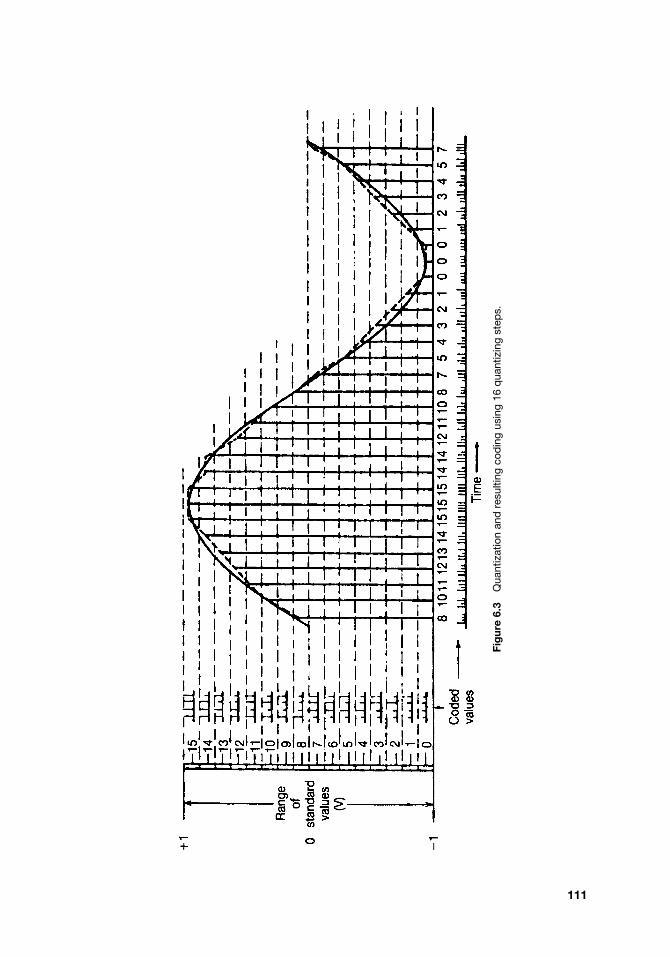
Fig
ure
6.3
Qua
ntiz
atio
nan
dre
sulti
ngco
din
gus
ing
16q
uant
izin
gst
eps.
111

112 DIGITAL NETWORKS
above the origin and eight possibilities below the origin. These 16 quantum steps arecoded as follows:
StepNumber Code
StepNumber Code
0 0000 8 10001 0001 9 10012 0010 10 10103 0011 11 10114 0100 12 11005 0101 13 11016 0110 14 11107 0111 15 1111
Examining Figure 6.3 shows that step 12 is used twice. Neither time it is used is it thetrue value of the impinging sinusoid voltage. It is a rounded-off value. These rounded-offvalues are shown with the dashed lines in Figure 6.3, which follows the general outlineof the sinusoid. The horizontal dashed lines show the point where the quantum changesto the next higher or lower level if the sinusoid curve is above or below that value. Takestep 14 in the curve, for example. The curve, dropping from its maximum, is given twovalues of 14 consecutively. For the first, the curve resides above 14, and for the second,below. That error, in the case of 14, from the quantum value to the true value is calledquantizing distortion. This distortion is a major source of imperfection in PCM systems.
Let’s set this discussion aside for a moment and consider a historical analogy. One ofmy daughters was having trouble with short division in school. Of course, her Dad wasthere to help. Divide 4 into 13. The answer is 3 with a remainder. Divide 5 into 22 andthe answer is 4 with a remainder. Of course, she would tell what the remainders were.But for you, the reader, I say let’s just throw away the remainders. That which we throwaway is the error between the quantized value and the real value. That which we throwaway gives rise to quantization distortion.
In Figure 6.3, maintaining the −1, 0, +1 V relationship, let us double the numberof quantum steps from 16 to 32. What improvement would we achieve in quantizationdistortion? First determine the step increment in millivolts in each case. In the first casethe total range of 2000 mV would be divided into 16 steps, or 125 mV/step. The secondcase would have 2000/32 or 62.5 mV/step. For the 16-step case, the worst quantizingerror (distortion) would occur when an input to be quantized was at the half-step levelor, in this case, 125/2 or 62.5 mV above or below the nearest quantizing step. For the32-step case, the worst quantizing error (distortion) would again be at the half-step level,or 62.5/2 or 31.25 mV. Thus the improvement in decibels for doubling the number ofquantizing steps is
20 log62.5
31.25= 20 log 2 or 6 dB (approximately).
This is valid for linear quantization only. Thus increasing the number of quantizingsteps for a fixed range of input values reduces quantizing distortion accordingly.
Voice transmission presents a problem. It has a wide dynamic range, on the order of50 dB. That is the level range from the loudest syllable of the loudest talker to lowest-level syllable of the quietest talker. Using linear quantization, we find it would require2048 discrete steps to provide any fidelity at all. Since 2048 is 211, this means we wouldneed an 11-bit code. Such a code sampled 8000 times per second leads to 88,000-bps

6.2 BASIS OF PULSE CODE MODULATION 113
equivalent voice channel and an 88-kHz bandwidth, assuming 1 bit per Hz. Designers feltthis was too great a bit rate/bandwidth.
They turned to an old analog technique of companding. Companding derives from twowords: compression and expansion. Compression takes place on the transmit side of thecircuit, while expansion occurs on the receive side. Compression reduces the dynamicrange with little loss of fidelity, and expansion returns the signal to its normal condition.This is done by favoring low-level speech over higher-level speech. In other words, morecode segments are assigned to speech bursts at low levels than at the higher levels,progressively more as the level reduces. This is shown graphically in Figure 6.4, whereeight coded sequences are assigned to each level grouping. The smallest range rises only0.0666 V from the origin (assigned to 0-V level). The largest extends over 0.5 V, and itis assigned only eight coded sequences.
6.2.3 Coding
Older PCM systems used a 7-bit code, and modern systems use an 8-bit code with itsimproved quantizing distortion performance. The companding and coding are carried outtogether, simultaneously. The compression and later expansion functions are logarithmic.A pseudologarithmic curve made up of linear segments imparts finer granularity to low-level signals and less granularity to the higher-level signals. The logarithmic curve followsone of two laws, the A-law and the µ-law (pronounced mu-law). The curve for the A-lawmay be plotted from the formula
FA(x) =(
A|x|1 + ln(A)
), 0 ≤ |x| ≤ 1
A,
FA(x) =(
1 + ln |Ax|1 + ln(A)
),
1
A≤ |x|≤1,
where A = 87.6. (Note: The notation ln indicates a logarithm to the natural base callede. Its value is 2.7182818340.) The A-law is used with the E1 system. The curve for the
Figure 6.4 Simple graphic representation of compression. Six-bit coding, eight six-bit sequencesper segment.

114 DIGITAL NETWORKS
µ-law is plotted from the formula
Fµ(x) = ln(1 + µ|x|)ln(1 + µ)
,
where x is the signal input amplitude and µ = 100 for the original North American T1system (now outdated), and 255 for later North American (DS1) systems and the CCITT24-channel system (CCITT Rec. G.733) (see Ref. 3).
A common expression used in dealing with the “quality” of a PCM signal is signal-to-distortion ratio (S/D, expressed in dB). Parameters A and µ, for the respective com-panding laws, determine the range over which the signal-to-distortion ratio is compara-tively constant, about 26 dB. For A-law companding, an S/D = 37.5 dB can be expected(A = 87.6). And for µ-law companding, we can expect S/D = 37 dB(µ = 255) (Ref. 4).
Turn now to Figure 6.5, which shows the companding curve and resulting coding forthe European E1 system. Note that the curve consists of linear piecewise segments, sevenabove and seven below the origin. The segment just above and the segment just belowthe origin consist of two linear elements. Counting the collinear elements by the origin,there are 16 segments. Each segment has 16 8-bit PCM codewords assigned. These arethe codewords that identify the voltage level of a sample at some moment in time. Eachcodeword, often called a PCM “word,” consists of 8 bits. The first bit (most significant
Figure 6.5 The 13-segment approximation of the A-law curve used with E1 PCM equipment.

6.2 BASIS OF PULSE CODE MODULATION 115
bit) tells the distant-end receiver if the sample is a positive or negative voltage. Observethat all PCM words above the origin start with a binary 1, and those below the originstart with a binary 0. The next 3 bits in sequence identify the segment. There are eightsegments (or collinear equivalents) above the origin and eight below (23 = 8). The last4 bits, shown in the figure as XXXX, indicate exactly where in a particular segment thatvoltage line is located.
Suppose the distant end received the binary sequence 11010100 in an E1 system. Thefirst bit indicates that the voltage is positive (i.e., above the origin in Figure 6.5). Thenext three bits, 101, indicate that the sample is in segment 4 (positive). The last 4 bits,0100, tell the distant end where it is in that segment as illustrated in Figure 6.6. Note thatthe 16 steps inside the segment are linear. Figure 6.7 shows an equivalent logarithmiccurve for the North American DS1 system.2 It uses a 15-segment approximation of thelogarithmic µ-law curve (µ = 255). The segments cutting the origin are collinear and arecounted as one. So, again, we have a total of 16 segments.
The coding process in PCM utilizes straightforward binary codes. Examples of suchcodes are illustrated in Figure 6.5 and are expanded in Figure 6.6 and Figure 6.7.
The North American DS1 (T1) PCM system uses a 15-segment approximation of thelogarithmic µ-law (µ = 255), shown in Figure 6.7. The segments cutting the origin arecollinear and are counted as one. As can be seen in Figure 6.7, similar to Figure 6.5,the first code element (bit), whether a 1 or a 0, indicates to the distant end whether thesample voltage is positive or negative, above or below the horizontal axis. The next threeelements (bits) identify the segment, and the last four elements (bits) identify the actualquantum level inside the segment.
6.2.3.1 Concept of Frame. As is illustrated in Figure 6.2, PCM multiplexing is car-ried out with the sampling process, sampling the analog sources sequentially. Thesesources may be the nominal 4-kHz voice channels or other information sources that havea 4-kHz bandwidth, such as data or freeze-frame video. The final result of the samplingand subsequent quantization and coding is a series of electrical pulses, a serial bit streamof 1s and 0s that requires some identification or indication of the beginning of a sampling
Figure 6.6 The European E1 system, coding of segment 4 (positive).
2More popularly referred to as T1.

116 DIGITAL NETWORKS
Figure 6.7 Piecewise linear approximation of the µ-law logarithmic curve used with the DS1 format.
sequence. This identification is necessary so that the far-end receiver knows exactly whenthe sampling sequence starts. Once the receiver receives the “indication,” it knows a pri-ori (in the case of DS1) that 24 eight-bit slots follow. It synchronizes the receiver. Suchidentification is carried out by a framing bit, and one full sequence or cycle of samplesis called a frame in PCM terminology.
Consider the framing structure of the two widely implemented PCM systems: the NorthAmerican DS1 and the European E1. The North American DS1 system is a 24-channelPCM system using 8-level coding (e.g., 28 = 256 quantizing steps or distinct PCM codewords). Supervisory signaling is “in-band” where bit 8 of every sixth frame is “robbed”for supervisory signaling.3 – 5 The DS1 format shown in Figure 6.8 has one bit added as aframing bit. (This is that indication to tell the distant end receiver where the frame starts.)It is called the “S” bit. The DS1 frame then consists of
(8 × 24) + 1 = 193 bits,
making up a full sequence or frame. By definition, 8000 frames are transmitted per second(i.e., 4000 × 2, the Nyquist sampling rate), so the bit rate of DS1 is
193 × 8000 = 1,544,000 bps, or 1.544 Mbps.
3“In-band,” an unfortunate expression harking back to the analog world.4In the DS1 system it should be noted that in each frame that has bit 8 “robbed,” 7-bit coding is used versus8-bit coding employed on the other five frames.5Supervisory signaling is discussed in Chapter 7. All supervisory signaling does is tell us if the channel is busyor idle.

6.2 BASIS OF PULSE CODE MODULATION 117
Figure 6.8 DS1 signal format.
The E1 European PCM system is a 32-channel system. Of the 32 channels, 30 transmitspeech (or data) derived from incoming telephone trunks and the remaining 2 channelstransmit synchronization-alignment and signaling information. Each channel is allotted an8-bit time slot (TS), and we tabulate TS 0 through 31 as follows:
TS Type of Information
0 Synchronizing (framing)1–15 Speech16 Signaling17–31 Speech
In TS 0 a synchronizing code or word is transmitted every second frame, occupying digits2 through 8 as follows:
0011011
In those frames without the synchronizing word, the second bit of TS 0 is frozen at a1 so that in these frames the synchronizing word cannot be imitated. The remaining bitsof TS 0 can be used for the transmission of supervisory information signals (Ref. 16).
Again, E1 in its primary rate format transmits 32 channels of 8-bit time slots. An E1frame therefore has 8 × 32 = 256 bits. There is no framing bit. Framing alignment iscarried out in TS 0. The E1 bit rate to the line is
256 × 8000 = 2,048,000 bps, or 2.048 Mbps
Framing and basic timing should be distinguished. “Framing” ensures that the PCMreceiver is aligned regarding the beginning (and end) of a bit sequence or frame; “timing”refers to the synchronization of the receiver clock, specifically, that it is in step with itscompanion far-end transmit clock. Timing at the receiver is corrected via the incoming“1”-to-“0” and “0”-to-“1” transitions.6 It is mandatory that long periods of no transitions
6A transition in this context is a change of electrical state. We often use the term “mark” for a binary 1 and“space” for a binary 0. The terms mark and space come from old-time automatic telegraphy and have beenpassed on through the data world to the parlance of digital communications technology.

118 DIGITAL NETWORKS
do not occur. This important point is discussed later in reference to line codes anddigit inversion.
6.3 PCM SYSTEM OPERATION
PCM channel banks operate on a four-wire basis. Voice channel inputs and outputs toand from a PCM multiplex channel bank are four-wire, or must be converted to four-wire in the channel bank equipment. Another term commonly used for channel bank iscodec, which is a contraction for coder–decoder even though the equipment carries outmore functions than just coding and decoding. A block diagram of a typical codec (PCMchannel bank) is shown in Figure 6.9.
A codec accepts 24 or 30 voice channels, depending on the system used; digitizes andmultiplexes the information; and delivers a serial bit stream to the line of 1.544 Mbps or2.048 Mbps. It accepts a serial bit stream at one or the other modulation rate, demul-tiplexes the digital information, and performs digital-to-analog conversion. Output tothe analog telecommunications network is the 24 or 30 nominal 4-kHz voice channels.Figure 6.9 illustrates the processing of a single analog voice channel through a codec.The voice channel to be transmitted is first passed through a 3.4-kHz low-pass filter. Theoutput of the filter is fed to a sampling circuit. The sample of each channel of a set of n
channels (n usually equals 24 or 30) is released in turn to the pulse amplitude modulation(PAM) highway. The release of samples is under control of a channel gating pulse derivedfrom the transmit clock. The input to the coder is the PAM highway. The coder acceptsa sample of each channel in sequence and then generates the appropriate 8-bit signalcharacter corresponding to each sample presented. The coder output is the basic PCMsignal that is fed to the digit combiner where framing-alignment signals are inserted in the
Voicechannel
input
3.4 kHz
Sampleandhold
Channelgate
Timingrecovery
Receiverclock
Channelgate
Signalingprocessing
Framealign
Digitseparator
Digitcombiner
Transmitclock
Framealignment
Coder
Decoder
Channel 1
Channel n
PAM stream(transmit)
PCMoutput
Channel 1
PCMinput
Channel n
Channel 1
Channel n
Channel 1
Channel n
PAM stream(receive)
Voicechannel
output
3.4 kHz
Signalinginterface
From transmit clock
Transmit signal digits
Figure 6.9 Simplified functional block diagram of a PCM codec or channel bank.
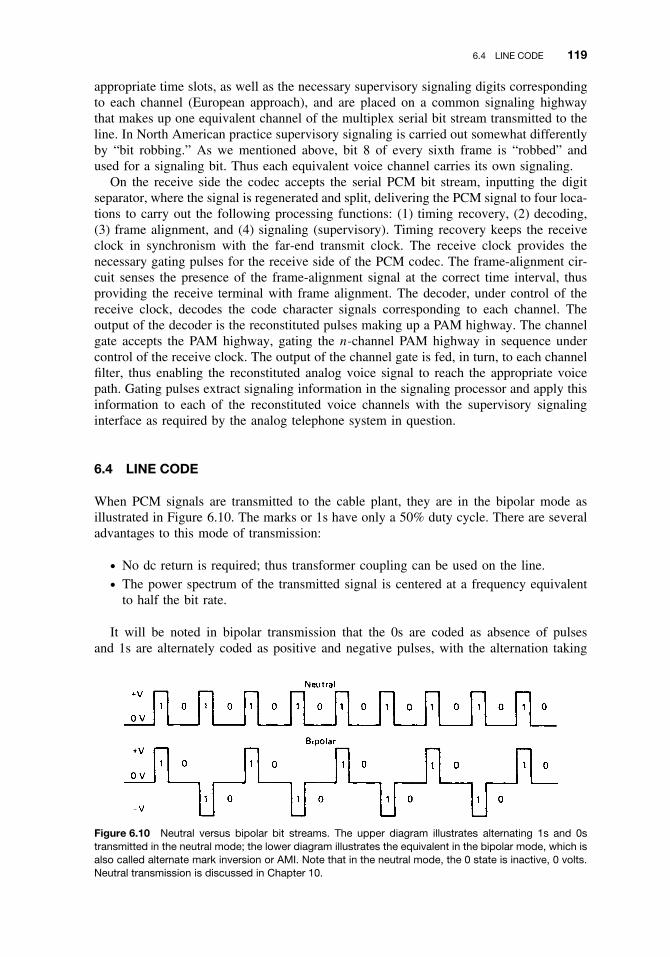
6.4 LINE CODE 119
appropriate time slots, as well as the necessary supervisory signaling digits correspondingto each channel (European approach), and are placed on a common signaling highwaythat makes up one equivalent channel of the multiplex serial bit stream transmitted to theline. In North American practice supervisory signaling is carried out somewhat differentlyby “bit robbing.” As we mentioned above, bit 8 of every sixth frame is “robbed” andused for a signaling bit. Thus each equivalent voice channel carries its own signaling.
On the receive side the codec accepts the serial PCM bit stream, inputting the digitseparator, where the signal is regenerated and split, delivering the PCM signal to four loca-tions to carry out the following processing functions: (1) timing recovery, (2) decoding,(3) frame alignment, and (4) signaling (supervisory). Timing recovery keeps the receiveclock in synchronism with the far-end transmit clock. The receive clock provides thenecessary gating pulses for the receive side of the PCM codec. The frame-alignment cir-cuit senses the presence of the frame-alignment signal at the correct time interval, thusproviding the receive terminal with frame alignment. The decoder, under control of thereceive clock, decodes the code character signals corresponding to each channel. Theoutput of the decoder is the reconstituted pulses making up a PAM highway. The channelgate accepts the PAM highway, gating the n-channel PAM highway in sequence undercontrol of the receive clock. The output of the channel gate is fed, in turn, to each channelfilter, thus enabling the reconstituted analog voice signal to reach the appropriate voicepath. Gating pulses extract signaling information in the signaling processor and apply thisinformation to each of the reconstituted voice channels with the supervisory signalinginterface as required by the analog telephone system in question.
6.4 LINE CODE
When PCM signals are transmitted to the cable plant, they are in the bipolar mode asillustrated in Figure 6.10. The marks or 1s have only a 50% duty cycle. There are severaladvantages to this mode of transmission:
ž No dc return is required; thus transformer coupling can be used on the line.ž The power spectrum of the transmitted signal is centered at a frequency equivalent
to half the bit rate.
It will be noted in bipolar transmission that the 0s are coded as absence of pulsesand 1s are alternately coded as positive and negative pulses, with the alternation taking
Figure 6.10 Neutral versus bipolar bit streams. The upper diagram illustrates alternating 1s and 0stransmitted in the neutral mode; the lower diagram illustrates the equivalent in the bipolar mode, which isalso called alternate mark inversion or AMI. Note that in the neutral mode, the 0 state is inactive, 0 volts.Neutral transmission is discussed in Chapter 10.

120 DIGITAL NETWORKS
place at every occurrence of a 1. This mode of transmission is also called alternate markinversion (AMI).
One drawback to straightforward AMI transmission is that when a long string of0s is transmitted (e.g., no transitions), a timing problem may arise because repeatersand decoders have no way of extracting timing without transitions. The problem can bealleviated by forbidding long strings of 0s. Codes have been developed that are bipolarbut with N 0s substitution; they are called “BNZS” codes. For instance, a B6ZS codesubstitutes a particular signal for a string of six 0s. B8ZS is used on subscriber loopcarrier and inserts a violation after a string of 8 zeros.
Another such code is the HDB3 code (high-density binary 3), where the 3 indicatessubstitution for binary sequences with more than three consecutive 0s. With HDB3, thesecond and third 0s of the string are transmitted unchanged. The fourth 0 is transmittedto the line with the same polarity as the previous mark sent, which is a “violation” of theAMI concept. The first 0 may or may not be modified to a 1, to ensure that the successiveviolations are of opposite polarity. HDB3 is used with European E series PCM systemsand is similar to B3ZS.
6.5 SIGNAL-TO-GAUSSIAN-NOISE RATIO ON PCM REPEATERED LINES
As mentioned earlier, noise accumulation on PCM systems is not a crucial issue. However,this does not mean that Gaussian noise (or crosstalk or impulse noise) is unimportant.7
Indeed, it will affect error performance expressed as error rate. Errors are cumulative, andas we go down a PCM-repeatered line, the error performance degrades. A decision inerror, whether a 1 or a 0, made anywhere in the digital system, is not recoverable. Thussuch an incorrect decision made by one regenerative repeater adds to the existing errorrate on the line, and errors taking place in subsequent repeaters further down the line addin a cumulative manner, thus deteriorating the received signal.
In a purely binary transmission system, if a 22-dB signal-to-noise ratio is maintained,the system operates nearly error free.8 In this respect, consider Table 6.1.
Table 6.1 Error Rate of a Binary Transmission SystemVersus Signal-to-rms-Noise Ratio
Error Rate S/N (dB) Error Rate S/N (dB)
10−2 13.5 10−7 20.310−3 16.0 10−8 21.010−4 17.5 10−9 21.610−5 18.7 10−10 22.010−6 19.6 10−11 22.2
As discussed in Section 6.4, PCM, in practice, is transmitted on-line with alternatemark inversion (in the bipolar mode). The marks (1s) have a 50% duty cycle, permittingsignal energy concentration at a frequency equivalent to half the transmitted bit rate. Thusit is advisable to add 1 dB or 2 dB to the values shown in Table 6.1 to achieve the desirederror performance in a practical system.
7Gaussian noise is the same as thermal noise.8It is against the laws of physics to have a completely error-free systems.

6.6 REGENERATIVE REPEATERS 121
6.6 REGENERATIVE REPEATERS
As we are probably aware, pulses passing down a digital transmission line suffer atten-uation and are badly distorted by the frequency characteristic of the line. A regenerativerepeater amplifies and reconstructs such a badly distorted digital signal and develops anearly perfect replica of the original at its output. Regenerative repeaters are an essentialkey to digital transmission in that we could say that the “noise stops at the repeater.”
Figure 6.11 is a simplified block diagram of a regenerative repeater and shows typicalwaveforms corresponding to each functional stage of signal processing. As illustrated inthe figure, at the first stage of signal processing is amplification and equalization. Withmany regenerative repeaters, equalization is a two-step process. The first is a fixed equal-izer that compensates for the attenuation–frequency characteristic (attenuation distortion),which is caused by the standard length of transmission line between repeaters (often6000 ft or 1830 m). The second equalizer is variable and compensates for departuresbetween nominal repeater section length and the actual length as well as loss variationsdue to temperature. The adjustable equalizer uses automatic line build-out (ALBO) net-works that are automatically adjusted according to characteristics of the received signal.9
The signal output of the repeater must be precisely timed to maintain accurate pulsewidth and space between the pulses. The timing is derived from the incoming bit stream.The incoming signal is rectified and clipped, producing square waves that are applied tothe timing extractor, which is a circuit tuned to the timing frequency. The output of thecircuit controls a clock-pulse generator that produces an output of narrow pulses that arealternately positive and negative at the zero crossings of the square-wave input.
The narrow positive clock pulses gate the incoming pulses of the regenerator, andthe negative pulses are used to run off the regenerator. Thus the combination is used tocontrol the width of the regenerated pulses.
Regenerative repeaters are the major source of timing jitter in a digital transmissionsystem. Jitter is one of the principal impairments in a digital network, giving rise to pulsedistortion and intersymbol interference. Jitter is discussed in more detail in Section 6.9.2.
Figure 6.11 Simplified functional block diagram of a regenerative repeater for use with PCM cablesystems.
9Line build-out is the adding of capacitance and/or resistance to a transmission line to look “electrically” longeror shorter than it actually is physically.

122 DIGITAL NETWORKS
Most regenerative repeaters transmit a bipolar (AMI) waveform (see Figure 6.10). Suchsignals can have one of three possible states in any instant in time—positive, zero, ornegative (volts)—and are often designated +, 0, −. The threshold circuits are gates toadmit the signal at the middle of the pulse interval. For instance, if the signal is positiveand exceeds a positive threshold, it is recognized as a positive pulse. If it is negative andexceeds a negative threshold, it is recognized as a negative pulse. If it has a (voltage) valuebetween the positive and negative voltage thresholds, it is recognized as a 0 (no pulse).
When either threshold is exceeded, the regenerator is triggered to produce a pulseof the appropriate duration, polarity, and amplitude. In this manner the distorted inputsignal is reconstructed as a new output signal for transmission to the next repeater orterminal facility.
6.7 PCM SYSTEM ENHANCEMENTS
6.7.1 Enhancements to DS1
The PCM frame rate is 8000 frames a second. With DS1, each frame has one framing bit.Thus 8000 framing bits are transmitted per second. With modern processor technology,all of the 8000 framing bits are not needed to keep the system frame-aligned. Only one-quarter of the 8000 framing bits per second are actually necessary for framing and theremainder of the bits, 6000 bits per second, can be used for other purposes such as on-linegross error detection and for a maintenance data link. To make good use of these overheadbits, DS1 frames are taken either 12 or 24 at a time. These groupings are called superframeand extended superframe, respectively. The extended superframe, in particular, providesexcellent facilities for on-line error monitoring and troubleshooting.
6.7.2 Enhancements to E1
Remember that time slot 0 in the E1 format is the synchronization channel, with a channelbit rate of 64 kbps. Only half of these bits are required for synchronization; the remainder,32 kbps, is available for on-line error monitoring, for a data channel for remote alarms.These remote alarms tell the system operator about the status of the distant PCM terminal.
6.8 HIGHER-ORDER PCM MULTIPLEX SYSTEMS
6.8.1 Introduction
Higher-order PCM multiplex is developed out of several primary multiplex sources. Pri-mary multiplex is typically DS1 in North America and E1 in Europe; some countrieshave standardized on E1, such as most of Hispanic America. Not only are E1 and DS1incompatible, the higher-order multiplexes, as one might imagine, are also incompatible.First we introduce stuffing, describe some North American higher-level multiplex, andthen discuss European multiplexes based on the E1 system.
6.8.2 Stuffing and Justification
Stuffing (justification) is common to all higher-level multiplexers that we describe in thefollowing. Consider the DS2 higher-level multiplex. It derives from an M12 multiplexer,taking inputs from four 24-channel channel banks. The clocks in these channel banks are

6.8 HIGHER-ORDER PCM MULTIPLEX SYSTEMS 123
free running. The transmission rate output of each channel bank is nominally 1,544,000bps. However, there is a tolerance of ±50 ppm (±77 bps). Suppose all four DS1 inputswere operating on the high side of the tolerance or at 1,544,077 bps. The input to the M12multiplexer is a buffer. It has a finite capacity. Unless bits are read out of the buffer fasterthan they are coming in, at some time the buffer will overflow. This is highly undesirable.Thus we have bit stuffing.
Stuffing in the output aggregate bit stream means adding extra bits. It allows us to readout of a buffer faster than we write into it.
In Ref. 1 the IEEE defines stuffing bits as “bits inserted into a frame to compensate fortiming differences in constituent lower rate signals.” CCITT uses the term justification.Figure 6.12 illustrates the stuffing concept.
6.8.3 North American Higher-Level Multiplex
The North American digital hierarchy is illustrated in Figure 6.13. The higher-level mul-tiplexers are type-coded in such a way that we know the DS levels (e.g., DS1, DS1C,DS2, DS3, DS4) that are being combined. For instance, the M34 multiplexer takes fourDS3 bit streams at its input to form the DS4 bit stream at its output. We describe theoperation of the M12 multiplexer because it typifies the series.
The formation of the second-level North American multiplex, DS2, from four DS1inputs is shown in Figure 6.14. There are four inputs to the M12 multiplexer, each oper-ating at the nominal 1.544-Mbps rate. The output bit rate is 6.312 Mbps. Now multiply1.544 Mbps by 4 and get 6.176 Mbps. In other words, the output of the M12 multiplexeris operating 136 kbps faster than the aggregate of the four inputs. Some of these extrabits are overhead bits and the remainder are stuff bits. Figure 6.15 shows the makeup ofthe DS2 frame.
The M12 multiplex frame consists of 1176 bits. The frame is divided into four 294-bitsubframes, as illustrated in Figure 6.15. There is a control bit word that is distributedthroughout the frame and that begins with an M bit. Thus each subframe begins with anM bit. There are four M bits forming the series 011X, where the fourth bit (X), whichmay be a 1 or a 0, may be used as an alarm indicator bit. When transmitted as a 1,no alarm condition exists. When it is transmitted as a 0, an alarm is present. The 011sequence for the first three M bits is used in the receiving circuits to identify the frame.
It is noted in Figure 6.15 that each subframe is made up of six 49-bit blocks. Eachblock starts with a control bit, which is followed by a 48-bit block of information. Of these48 bits, 12 bits are taken from each of the four input DS1 signals. These are interleavedsequentially in the 48-bit block. The first bit in the third and sixth block is designated an
Figure 6.12 Pulse stuffing synchronization. (From Ref. 5, Figure 29-2.)

124 DIGITAL NETWORKS
Figure 6.13 The North American Digital Hierarchy.
Figure 6.14 The formation of the DS2 signal from four DS1 signals in an M12 multiplexer.
F bit. The F bits are a 0101 . . . sequence used to identify the location of the control bitsequence and the start of each block of information bits.
6.8.4 European E1 Digital Hierarchy
The E1 hierarchy is identified in a similar manner as the DS1 hierarchy. E1 (30 voicechannels) is the primary multiplex; E2 is the second level and is derived from four E1s.

6.8 HIGHER-ORDER PCM MULTIPLEX SYSTEMS 125
Figure 6.15 Makeup of a DS2 frame.
Thus E2 contains 120 equivalent digital voice channels. E3 is the third level and it isderived from four E2 inputs and contains 480 equivalent voice channels. E4 derives fromfour E3 formations and contains the equivalent of 1920 voice channels. Internationaldigital hierarchies are compared in Table 6.2. Table 6.3 provides the basic parameters forthe formation of the E2 level in the European digital hierarchy.
CCITT Rec. G.745 (Ref. 6) recommends cyclic bit interleaving in the tributary (i.e.,E1 inputs) numbering order and positive/zero/negative justification with two-commandcontrol.10 The justification control signal is distributed and the Cjin bits (n = 1, 2, 3; seeTable 6.3) are used for justification control bits.
Positive justification is indicated by the signal 111, transmitted in each of two con-secutive frames. Negative justification is indicated by the signal 000, also transmitted ineach of two consecutive frames. No-justification is indicated by the signal 111 in oneframe and 000 in the next frame. Bits 5, 6, 7, and 8 in Set IV (Table 6.3) are used fornegative justification of tributaries 1, 2, 3, and 4, respectively, and bits 9 to 12 for positivejustification of the same tributaries.
Table 6.2 Higher-Level PCM Multiplex Comparison
Level
System Type 1 2 3 4 5
North American T/D type 1 2 3 4Number of voice channels 24 96 672 4032Line bit rate (Mbps) 1.544 6.312 44.736 274.176
JapanNumber of voice channels 24 96 480 1440 5760Line bit rate (Mbps) 1.544 6.312 32.064 97.728 400.362
EuropeNumber of voice channels 30 120 480 1920Line bit rate (Mbps) 2.048 8.448 34.368 139.264
Source: Ref. 11.
10Positive/zero/negative justification. This refers to stuffing to compensate for input channel bit rates that areeither too slow, none necessary, or too fast.

126 DIGITAL NETWORKS
Table 6.3 8448-kbps Digital Multiplexing Frame Structure Using Positive/Zero/NegativeJustification
Tributary bit rate (kbit/s) 2048Number of tributaries 4
Frame Structure Bit Number
Set IFrame-alignment signal (11100110) 1 to 8Bits from tributaries 9 to 264
Set IIJustification control bits Cj1 (see Note) 1 to 4Bits for service functions 5 to 8Bits from tributaries 9 to 264
Set IIIJustification control bits Cj2 (see Note) 1 to 4Spare bits 5 to 8Bits from tributaries 9 to 264
Set IVJustification control bits Cj3 (see Note) 1 to 4Bits from tributaries available for negative justification 5 to 8Bits from tributaries available for positive justification 9 to 12Bits from tributaries 12 to 264
Frame length 1056 bitsFrame duration 125 µsBits per tributary 256 bitsMaximum justification rate per tributary 8 kbps
Note: Cjn indicates nth justification control bit of the jth tributary.
Source: Table 1/G.745, CCITT Rec. G.745, p. 437, Fascicle III.4, IXth Plenary Assembly, Melbourne, 1988 (Ref. 6).
Besides, when information from tributaries 1, 2, 3, and 4 is not transmitted, bits 5, 6,7, and 8 in Set IV are available for transmitting information concerning the type of justifi-cation (positive or negative) in frames containing commands of positive justification andintermediate amount of jitter in frames containing commands of negative justification.11
The maximum amount of justification rate per tributary is shown in Table 6.3.
6.9 LONG-DISTANCE PCM TRANSMISSION
6.9.1 Transmission Limitations
Digital waveforms lend themselves to transmission by wire pair, coaxial cable, fiber-opticcable, and wideband radio media. The PCM multiplex format using an AMI signal wasfirst applied to wire-pair cable (see Section 5.5). Its use on coaxial cable is now deprecatedin favor of fiber-optic cable. Each transmission medium has limitations brought about byimpairments. In one way or another each limitation is a function of the length of a linkemploying the medium and the transmission rate (i.e., bit rate). We have discussed loss,for example. As loss increases (i.e., between regenerative repeaters), signal-to-noise ratiosuffers, directly impacting bit error performance. The following transmission impairmentsto PCM transmission are covered: jitter, distortion, noise, and crosstalk. The design oflong-distance digital links is covered in Chapter 9.
11Jitter, see Section 6.9.2.

6.9 LONG-DISTANCE PCM TRANSMISSION 127
6.9.2 Jitter and Wander
In the context of digital transmission, jitter is defined as short-term variation of thesampling instant from its intended position in time or phase. Longer-term variation of thesampling instant is called wander. Jitter can cause transmission impairments such as:
ž Displacement of the ideal sampling instant. This leads to a degradation in systemerror performance.
ž Slips in timing recovery circuits, manifesting in degraded error performance.ž Distortion of the resulting analog signal after decoding at the receive end of
the circuit.
Think of jitter as minute random motion of a timing gate. Timing gates are shown in thelower-right-hand corner of Figure 6.11. An analogy is a person with shaky hands tryingto adjust a screw with a screwdriver.
The random phase modulation, or phase jitter, introduced at each regenerative repeateraccumulates in a repeater chain and may lead to crosstalk and distortion on the recon-structed analog signal. In digital switching systems, jitter on the incoming lines is apotential source of slips.12 Jitter accumulation is a function of the number of regenerativerepeaters in tandem. Keep in mind that switches, fiber-optic receivers, and digital radiosare also regenerative repeaters.
Certainly by reducing the number of regenerative repeaters in tandem, we reduce jitteraccordingly. Wire-pair systems transporting PCM at the DS1 rate have repeaters every6000 ft (1830 m). If we are to reduce jitter, wire pair is not a good candidate for longcircuits. On the other hand, fiber-optic systems, depending on design and bit rate, haverepeaters every 40 miles to 200 miles (64 km to 320 km). This is another reason whyfiber-optic systems are favored for long-haul application. Line-of-sight microwave radio,strictly for budgeting purposes, may have repeaters every 30 miles (48 km), so it, too, isa candidate for long-haul systems. Satellite radio systems have the potential for the leastnumber of repeaters per unit length.
6.9.3 Distortion
On metallic transmission links, such as coaxial cable and wire-pair cable, line character-istics distort and attenuate the digital signal as it traverses the medium. There are threecable characteristics that create this distortion: (1) loss, (2) amplitude distortion (ampli-tude–frequency response), and (3) delay distortion. Thus the regenerative repeater mustprovide amplification and equalization of the incoming digital signal before regenera-tion. There are also tradeoffs between loss and distortion on the one hand and repeatercharacteristics and repeater section length on the other.
6.9.4 Thermal Noise
As in any electrical communication system, thermal noise, impulse noise, and crosstalkaffect system design. Because of the nature of a binary digital system, these impairmentsneed only be considered on a per-repeater-section basis because noise does not accumulatedue to the regenerative process carried out at repeaters and nodes. Bit errors do accumulate,and these noise impairments are one of the several causes of errors. One way to limit erroraccumulation is to specify a stringent bit error rate (BER) requirement for each repeater
12Slips are a major impairment in digital networks. Slips and slip rate are discussed in Section 12.7.

128 DIGITAL NETWORKS
section. Up to several years ago, repeater sections were specified with a BER of 1 × 10⁻⁹.Today a BER of 1 × 10⁻¹⁰ to 1 × 10⁻¹² is prevalent in the North American network.
It is interesting to note that PCM provides intelligible voice performance for an errorrate as low as 1 in 100 (1 × 10⁻²). However, the bottom threshold (worst tolerable) BER isone error in one thousand (1 × 10⁻³) at system end-points. This value is required to ensurecorrect operation of supervisory signaling. The reader should appreciate that such degradedBER values are completely unsuitable for data transmission over the digital network.
6.9.5 Crosstalk
Crosstalk is a major impairment in PCM wire-pair system, particularly when “go” and“return” channels are carried in the same cable sheath. The major offender of single-cable operation is near-end crosstalk (NEXT). When the two directions of transmissionare carried in separate cables or use shielded pairs in a common cable, far-end crosstalk(FEXT) becomes dominant.
One characteristic has been found to be a major contributor to poor crosstalk couplingloss. This is the capacitance imbalance between wire pairs. Stringent quality control duringcable manufacture is one measure to ensure that minimum balance values are met.
6.10 DIGITAL LOOP CARRIER
Digital subscriber loop carrier is a method of extending the metallic subscriber plantby using one or more DS1 configurations. As an example, the SLC-96 uses four DS1configurations to derive an equivalent of 96 voice channels.
The digital transmission facility used by a DLC system may be repeatered wire-paircable, optical fibers, either or both combined with digital multiplexers, or other appropriatemedia. In Bellcore (now Telcordia) terminology, the central office termination (COT) isthe digital terminal colocated with the local serving switch. The RT is the remote terminal.The RT must provide all of the features to a subscriber loop that the local serving switchnormally does, such as supervision, ringing, address signaling, both dial pulse and touchtone, and so on (Ref. 7).
6.10.1 New Versions of DSL
ADSL, or asymmetric digital subscriber line, as described by Bellcore (Telcordia), pro-vides 1.544 Mbps service “downstream,” meaning from the local serving switch to thesubscriber, out to 18,000 ft (5500 m). In the upstream direction 16-kbps service is fur-nished. Such service has taken on new life in providing a higher bit rate for Inter-net customers.
There is an ANSI version of ADSL that can provide 6-Mbps downstream service usinga complex digital waveform and devices called automatic equalizers to improve bandwidthcharacteristics, particularly amplitude and phase distortion. The upstream bit rate can beas high as 640 kbps. Some manufacturers purport to be able to extend this service out to12,000 kft (3700 m).
6.11 DIGITAL SWITCHING
6.11.1 Advantages and Issues of Digital Switching
There are both economic and technical advantages to digital switching; in this contextwe refer to PCM switching. The economic advantages of time-division PCM switchinginclude the following:

6.11 DIGITAL SWITCHING 129
ž There are notably fewer equivalent cross-points for a given number of lines andtrunks than in a space-division switch.
ž A PCM switch is of considerably smaller size.ž It has more common circuitry (i.e., common modules).ž It is easier to achieve full availability within economic constraints.
The technical advantages include the following:
ž It is regenerative (i.e., the switch does not distort the signal; in fact, the output signalis “cleaner” than the input).
ž It is noise-resistant.ž It is computer-based and thus incorporates all the advantages of SPC.ž The binary message format is compatible with digital computers. It is also compatible
with signaling.ž A digital exchange is lossless. There is no insertion loss as a result of a switch
inserted in the network.ž It exploits the continuing cost erosion of digital logic and memory; LSI, VLSI, and
VHSIC insertion.13
Two technical issues may be listed as disadvantages:
1. A digital switch deteriorates error performance of the system. A well-designedswitch may only impact network error performance minimally, but it still does it.
2. Switch and network synchronization, and the reduction of wander and jitter, can begating issues in system design.
6.11.2 Approaches to PCM Switching
6.11.2.1 General. A digital switch’s architecture is made up of two elements, called Tand S, for time-division switching (T) and space-division switching (S), and can be madeup of sequences of T and S. For example, the AT&T No. 4 ESS is a TSSSST switch;No. 3 EAX is an SSTSS; and the classic Northern Telecom DMS-100 is TSTS-folded.Many of these switches (e.g., DMS-100) are still available.
One thing these switches have in common is that they had multiple space (S) stages.This has now changed. Many of the new switches, or enhanced versions of the switchesjust mentioned, have very large capacities (e.g., 100,000 lines) and are simply TST orSTS switches.
We will describe a simple time switch, a space switch, and methods of making up anarchitecture combining T and S stages. We will show that designing a switch with fairlyhigh line and trunk capacity requires multiple stages. Then we will discuss the “new look”at the time stage.
6.11.2.2 Time Switch. On a conceptual basis, Figure 6.16 shows a time-switch ortime-slot interchanger (TSI). A time slot is the 8-bit PCM word. Remember, it expressesthe voltage value of a sample taken at a certain moment in time. Of course, a time slotconsists of 8 bits. A time-slot represents one voice channel, and the time slot is repeated
13VHSIC stands for very high speed integrated circuit.
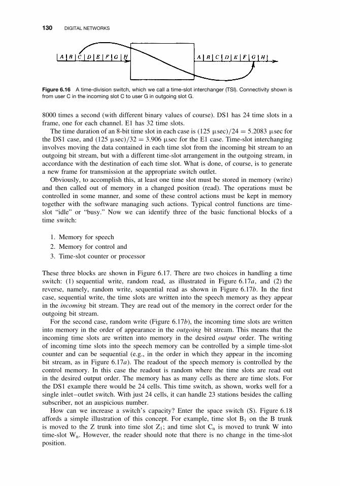
130 DIGITAL NETWORKS
Figure 6.16 A time-division switch, which we call a time-slot interchanger (TSI). Connectivity shown isfrom user C in the incoming slot C to user G in outgoing slot G.
8000 times a second (with different binary values of course). DS1 has 24 time slots in aframe, one for each channel. E1 has 32 time slots.
The time duration of an 8-bit time slot in each case is (125 µsec)/24 = 5.2083 µsec forthe DS1 case, and (125 µsec)/32 = 3.906 µsec for the E1 case. Time-slot interchanginginvolves moving the data contained in each time slot from the incoming bit stream to anoutgoing bit stream, but with a different time-slot arrangement in the outgoing stream, inaccordance with the destination of each time slot. What is done, of course, is to generatea new frame for transmission at the appropriate switch outlet.
Obviously, to accomplish this, at least one time slot must be stored in memory (write)and then called out of memory in a changed position (read). The operations must becontrolled in some manner, and some of these control actions must be kept in memorytogether with the software managing such actions. Typical control functions are time-slot “idle” or “busy.” Now we can identify three of the basic functional blocks of atime switch:
1. Memory for speech2. Memory for control and3. Time-slot counter or processor
These three blocks are shown in Figure 6.17. There are two choices in handling a timeswitch: (1) sequential write, random read, as illustrated in Figure 6.17a, and (2) thereverse, namely, random write, sequential read as shown in Figure 6.17b. In the firstcase, sequential write, the time slots are written into the speech memory as they appearin the incoming bit stream. They are read out of the memory in the correct order for theoutgoing bit stream.
For the second case, random write (Figure 6.17b), the incoming time slots are writteninto memory in the order of appearance in the outgoing bit stream. This means that theincoming time slots are written into memory in the desired output order. The writingof incoming time slots into the speech memory can be controlled by a simple time-slotcounter and can be sequential (e.g., in the order in which they appear in the incomingbit stream, as in Figure 6.17a). The readout of the speech memory is controlled by thecontrol memory. In this case the readout is random where the time slots are read outin the desired output order. The memory has as many cells as there are time slots. Forthe DS1 example there would be 24 cells. This time switch, as shown, works well for asingle inlet–outlet switch. With just 24 cells, it can handle 23 stations besides the callingsubscriber, not an auspicious number.
How can we increase a switch’s capacity? Enter the space switch (S). Figure 6.18affords a simple illustration of this concept. For example, time slot B1 on the B trunkis moved to the Z trunk into time slot Z1; and time slot Cn is moved to trunk W intotime-slot Wn. However, the reader should note that there is no change in the time-slotposition.

6.11 DIGITAL SWITCHING 131
Figure 6.17a Time-slot interchange: time switch (T). Sequential write, random read.
Figure 6.17b Time-switch, time-slot interchange (T). Random write, sequential read.
6.11.2.3 Space Switch. A typical time-division space switch (S) is shown inFigure 6.19. It consists of a cross-point matrix made up of logic gates that allow theswitching of time slots in a spatial domain. These PCM time slot bit streams are organizedby the switch into a pattern determined by the required network connectivity. The matrixconsists of a number of input horizontals and output verticals with a logic gate at eachcross point. The array, as shown in the figure, has M horizontals and N verticals, and

132 DIGITAL NETWORKS
Figure 6.18 Space switch connects time slots in a spatial configuration.
Figure 6.19 Time-division space switch cross-point array showing enabling gates.
we call it an M × N array. If M = N, the switch is nonblocking; If M > N, the switchconcentrates, and if M < N, the switch expands.
Return to Figure 6.19. The array consists of a number of (M) input horizontals and(N) output verticals. For a given time slot, the appropriate logic gate is enabled andthe time slot passes from the input horizontal to the desired output vertical. The otherhorizontals, each serving a different serial stream of time slots, can have the same timeslot (e.g., a time slot from time slots number 1–24, 1–30, or 1–n; e.g., time slot 7 on each
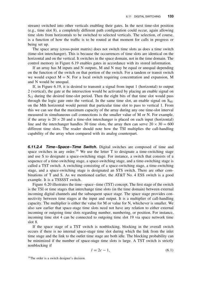
6.11 DIGITAL SWITCHING 133
stream) switched into other verticals enabling their gates. In the next time-slot position(e.g., time slot 8), a completely different path configuration could occur, again allowingtime slots from horizontals to be switched to selected verticals. The selection, of course,is a function of how the traffic is to be routed at that moment for calls in progress orbeing set up.
The space array (cross-point matrix) does not switch time slots as does a time switch(time-slot interchanger). This is because the occurrences of time slots are identical on thehorizontal and on the vertical. It switches in the space domain, not in the time domain. Thecontrol memory in Figure 6.19 enables gates in accordance with its stored information.
If an array has M inputs and N outputs, M and N may be equal or unequal dependingon the function of the switch on that portion of the switch. For a tandem or transit switchwe would expect M = N. For a local switch requiring concentration and expansion, Mand N would be unequal.
If, in Figure 6.19, it is desired to transmit a signal from input 1 (horizontal) to output2 (vertical), the gate at the intersection would be activated by placing an enable signal onS12 during the desired time-slot period. Then the eight bits of that time slot would passthrough the logic gate onto the vertical. In the same time slot, an enable signal on SM1
on the Mth horizontal would permit that particular time slot to pass to vertical 1. Fromthis we can see that the maximum capacity of the array during any one time-slot intervalmeasured in simultaneous call connections is the smaller value of M or N. For example,if the array is 20 × 20 and a time-slot interchanger is placed on each input (horizontal)line and the interchanger handles 30 time slots, the array then can serve 20 × 30 = 600different time slots. The reader should note how the TSI multiplies the call-handlingcapability of the array when compared with its analog counterpart.
6.11.2.4 Time–Space–Time Switch. Digital switches are composed of time andspace switches in any order.14 We use the letter T to designate a time-switching stageand use S to designate a space-switching stage. For instance, a switch that consists of asequence of a time-switching stage, a space-switching stage, and a time-switching stage iscalled a TST switch. A switching consisting of a space-switching stage, a time-switchingstage, and a space-switching stage is designated an STS switch. There are other com-binations of T and S. As we mentioned earlier, the AT&T No. 4 ESS switch is a goodexample. It is a TSSSST switch.
Figure 6.20 illustrates the time–space–time (TST) concept. The first stage of the switchis the TSI or time stages that interchange time slots (in the time domain) between externalincoming digital channels and the subsequent space stage. The space stage provides con-nectivity between time stages at the input and output. It is a multiplier of call-handlingcapacity. The multiplier is either the value for M or value for N, whichever is smaller. Wealso saw earlier that space-stage time slots need not have any relation to either externalincoming or outgoing time slots regarding number, numbering, or position. For instance,incoming time slot 4 can be connected to outgoing time slot 19 via space network timeslot 8.
If the space stage of a TST switch is nonblocking, blocking in the overall switchoccurs if there is no internal space-stage time slot during which the link from the inlettime stage and the link to the outlet time stage are both idle. The blocking probability canbe minimized if the number of space-stage time slots is large. A TST switch is strictlynonblocking if
l = 2c − 1, (6.1)
14The order is a switch designer’s decision.

134 DIGITAL NETWORKS
Figure 6.20 A time–space–time (TST) switch. TSI = time-slot interchanger.
where l is the number of space-stage time slots and c is the number of external TDMtime slots (Ref. 3).
6.11.2.5 Space–Time–Space Switch. A space–time–space switch reverses theorder architecture of a TST switch. The STS switch consists of a space cross–pointmatrix at the input followed by an array of time-slot interchangers whose ports feedanother cross-point matrix at the output. Such a switch is shown in Figure 6.21. Considerthis operational example with an STS. Suppose that an incoming time slot 5 on port No. 1must be connected to an output slot 12 at outgoing port 4. This can be accomplished bytime-slot interchanger No. 1, which would switch it to time slot 12; then the outgoingspace stage would place that on outgoing trunk No. 4. Alternatively, time slot 5 couldbe placed at the input of TSI No. 4 by the incoming space switch, where it would beswitched to time slot 12, and then out port No. 4.
Spaceswitcharray
(m × n)
TSI
Space stage Time stage Space stage
Spaceswitcharray
(n × p)
TSI
TSI
TSI
Figure 6.21 A space–time–space switch.

6.11 DIGITAL SWITCHING 135
6.11.2.6 TST Compared with STS. Both TST and STS switches can be designed withidentical call-carrying capacities and blocking probabilities. It can be shown that a directone-to-one mapping exists between time-division and space-division networks (Ref. 3).
The architecture of TST switching is more complex than STS switching with spaceconcentration. The TST switch becomes more cost-effective because time expansion canbe achieved at less cost than space expansion. Such expansion is required as link utilizationincreases because less concentration is acceptable as utilization increases.
It would follow, then, that TST switches have a distinct implementation advantage overSTS switches when a large amount of traffic must be handled. Bellamy (Ref. 3) statesthat for small switches STS is favored due to reduced implementation complexities. Thechoice of a particular switch architecture may be more dependent on such factors asmodularity, testability, and expandability.
One consideration that generally favors an STS implementation is the relatively simplercontrol requirements. However, for large switches with heavy traffic loads, the implemen-tation advantage of the TST switch and its derivatives is dominant. A typical large switchis the ATT No. 4 ESS, which has a TSSSST architecture and has the capability of termi-nating 107,520 trunks with a blocking probability of 0.5% and channel occupancy of 0.7.
6.11.3 Review of Some Digital Switching Concepts
6.11.3.1 Early Notions and New Ideas. In Section 6.11.2 the reader was probably ledto believe that the elemental time-switching stage, the TSI, would have 24 or 30 time-slotcapacity to match the North American DS1 rate of the “European” E1 rate, respectively.That means that a manufacturer would have to develop and produce two distinct switches,one to satisfy the North American market and one for the European market. Most switchmanufacturers made just one switch with a common internal switching network, the timeand space arrays we just discussed. For one thing, they could map five DS1 groups intofour E1 groups, the common denominator being 120 DS0/E0 (64-kbps channels). Periph-eral modules cleaned up any differences remaining, such as signaling. The “120” is a num-ber used in AT&T’s 4ESS. It maps 120 eight-bit time slots into 128 time slots. The eighttime slots of the remainder are used for diagnostic and maintenance purposes (Ref. 8).
Another early concept was a common internal bit rate, to be carried on those “high-ways” we spoke about or on junctors.15 At the points of interface that a switch has withthe outside world, it must have 8-bit time slots in DS1 (or high-level multiplex) or E1 (orhigher: E2, E3) frames each 125 µsec in duration. Inside the switch was another matter.For instance, with Nortel’s DMS-100 the incoming 8-bit time slot was mapped into a10-bit time slot, as shown in Figure 6.22.16 The example used in the figure is DS1.
Note in Figure 6.22 that one bit is a parity bit (bit 0) and the other appended bit (bit 1)carries the supervisory signaling information, telling the switch whether the time slot isidle or busy.17 Bits 2 through 9 are the bits of the original 8-bit time slot. Because Nortel intheir DMS-100 wanted a switch that was simple to convert from E1 to DS1, they built uptheir internal bit rate to 2.560 Mbps as follows: 10 bits per time slot, 32 time slots × 8000(the frame rate) or 2.560 Mbps.18 This now can accommodate E1, all 32 channels. Asmentioned, 5 DS1s are easily mapped into 4 E1s and vice versa (Ref. 17).
15Junctor is a path connecting switching networks internal to a switch.16Nortel was previously called Northern Telecom.17Parity bit is used for error detection. It is a redundant bit appended to an array of bits to make the sum ofall the 1 bits (marks) (in the array) always odd or always even.18The 8000 frames per second or frame rate is common on all conventional PCM systems. As the reader willrecall from Section 6.2.1, this is the Nyquist sampling rate for the 4-kHz analog voice channel on convertingit to a PCM equivalent.
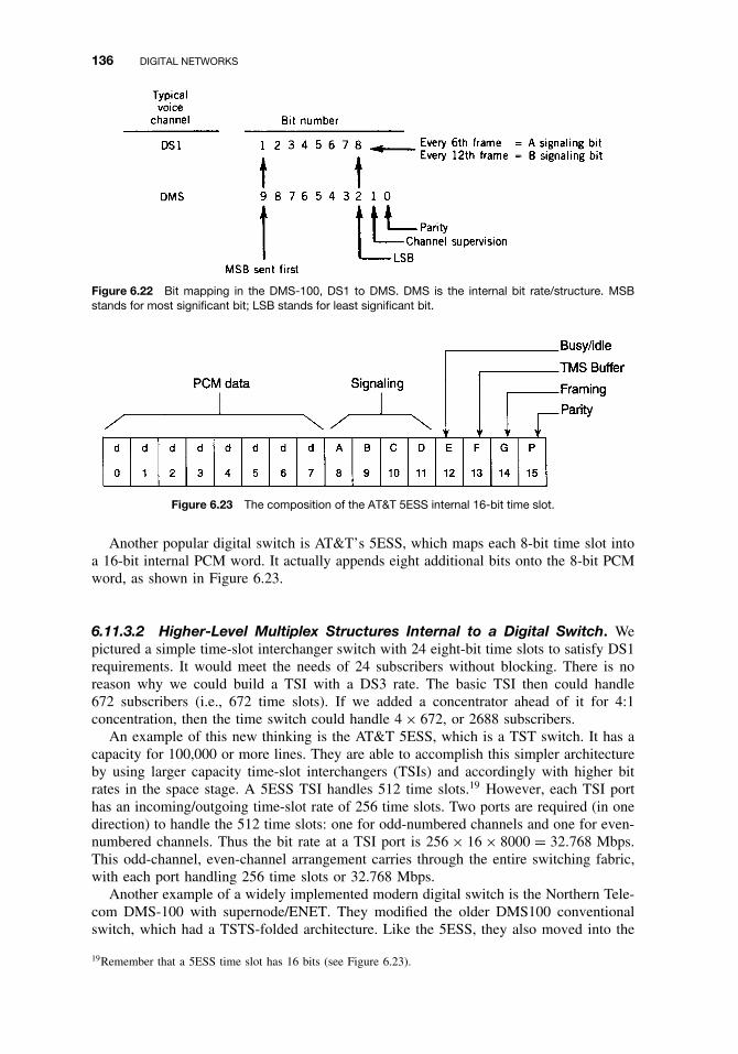
136 DIGITAL NETWORKS
Figure 6.22 Bit mapping in the DMS-100, DS1 to DMS. DMS is the internal bit rate/structure. MSBstands for most significant bit; LSB stands for least significant bit.
Figure 6.23 The composition of the AT&T 5ESS internal 16-bit time slot.
Another popular digital switch is AT&T’s 5ESS, which maps each 8-bit time slot intoa 16-bit internal PCM word. It actually appends eight additional bits onto the 8-bit PCMword, as shown in Figure 6.23.
6.11.3.2 Higher-Level Multiplex Structures Internal to a Digital Switch. Wepictured a simple time-slot interchanger switch with 24 eight-bit time slots to satisfy DS1requirements. It would meet the needs of 24 subscribers without blocking. There is noreason why we could build a TSI with a DS3 rate. The basic TSI then could handle672 subscribers (i.e., 672 time slots). If we added a concentrator ahead of it for 4:1concentration, then the time switch could handle 4 × 672, or 2688 subscribers.
An example of this new thinking is the AT&T 5ESS, which is a TST switch. It has acapacity for 100,000 or more lines. They are able to accomplish this simpler architectureby using larger capacity time-slot interchangers (TSIs) and accordingly with higher bitrates in the space stage. A 5ESS TSI handles 512 time slots.19 However, each TSI porthas an incoming/outgoing time-slot rate of 256 time slots. Two ports are required (in onedirection) to handle the 512 time slots: one for odd-numbered channels and one for even-numbered channels. Thus the bit rate at a TSI port is 256 × 16 × 8000 = 32.768 Mbps.This odd-channel, even-channel arrangement carries through the entire switching fabric,with each port handling 256 time slots or 32.768 Mbps.
Another example of a widely implemented modern digital switch is the Northern Tele-com DMS-100 with supernode/ENET. They modified the older DMS100 conventionalswitch, which had a TSTS-folded architecture. Like the 5ESS, they also moved into the
19Remember that a 5ESS time slot has 16 bits (see Figure 6.23).

6.12 DIGITAL NETWORK 137
2048-time-slot domain in the ENET (extended network). But their time slot is 10 bits,and the ENET uses a 10-bit parallel format, so each line (i.e., there are 10 lines) has2048 × 8000 or 16.384 Mbps.
6.12 DIGITAL NETWORK
6.12.1 Introduction
The North American public switched telecommunications network (PSTN) is 100% dig-ital. The interexchange carrier (IXC) portion has been 100% digital for many years. Theworld network is expected to be all-digital by the first decade of the twenty-first century.That network is still basically hierarchical, and the structure changes slowly. There arepossibly only two factors that change network structure:
1. Political2. Technological
In the United States, certainly divestiture of the Bell System/AT&T affected networkstructure with the formation of LECs (local exchange carriers) and IXCs. Outside NorthAmerica, the movement toward privatization of government telecommunication monopo-lies in one way or another will affect network structure. As mentioned in Section 1.3, andto be discussed further in Chapter 8, there is a decided trend away from strict hierarchicalstructures, particularly in routing schemes; less so in topology.
Technology and its advances certainly may be equally or even more important thanpolitical causes. Satellite communications, we believe, brought about the move by CCITTaway from any sort of international network hierarchy. International high-usage and directroutes became practical. We should not lose sight of the fact that every digital exchangehas powerful computer power, permitting millisecond routing decisions for each call. Thiswas greatly aided by the implementation of CCITT Signaling System No. 7 (Chapter 13).Another evident factor certainly is fiber-optic cable for a majority of trunk routes. It hasalso forced the use of geographic route diversity to improve survivability and availability.What will be the impact of the asynchronous transfer mode (ATM) (Chapter 18) on theevolving changes in network structure (albeit slowly)? The Internet certainly is forcingchanges in data route capacity, right up to the subscriber. Privatization schemes now beingimplemented in many countries around the world will indeed have impact, as well, onnetwork structure.
In the following section we discuss the digital network from the perspective of theoverall PSTN. Certainly the information is valid for private networks as well, particularlyif private networks are backed up by the local PSTN.
6.12.2 Technical Requirements of the Digital Network
6.12.2.1 Network Synchronization Rationale and Essentials. When a PCM bitstream is transmitted over a telecommunication link, there must be synchronization atthree different levels: (1) bit, (2) time slot, and (3) frame. Bit synchronization refers tothe need for the transmitter (coder) and receiver (decoder) to operate at the same bit rate.It also refers to the requirement that the receiver decision point be exactly at the mid-position of the incoming bit. Bit synchronization assures that the bits will not be misreadby the receiver.
138 DIGITAL NETWORKS
Obviously a digital receiver must also know where a time slot begins and ends. If wecan synchronize a frame, time-slot synchronization can be assured. Frame synchronizationassumes that bit synchronization has been achieved. We know where a frame begins (andends) by some kind of marking device. With DS1 it is the framing bit. In some framesit appears as a 1 and in others it appears as a 0. If the 12-frame super-frame is adopted,it has 12 framing bits, one in each of the 12 frames. This provides the 000111 framingpattern (Ref. 3). In the case of the 24-frame extended superframe, the repeating patternis 001011, and the framing bit occurs only once in four frames.
E1, as we remember from Section 6.2, has a separate framing and synchronizationchannel, namely, channel 0. In this case the receiver looks in channel 0 for the framingsequence in bits 2 through 8 (bit 1 is reserved) of every other frame. The framing sequenceis 0011011. Once the framing sequence is acquired, the receiver knows exactly whereframe boundaries are. It is also time-slot aligned.
All digital switches have a master clock. Outgoing bit streams from a switch are slavedto the switch’s master clock. Incoming bit streams to a switch derive timing from bit tran-sitions of that incoming bit stream. It is mandatory that each and every switch in a digitalnetwork generate outgoing bit streams whose bit rate is extremely close to the nominalbit rate. To achieve this, network synchronization is necessary. Network synchronizationcan be accomplished by synchronizing all switch (node) master clocks so that transmis-sions from these nodes have the same average line bit rate. Buffer storage devices arejudiciously placed at various transmission interfaces to absorb differences between theactual line bit rate and the average rate. Without this network-side synchronization, slipswill occur. Slips are a major impairment in digital networks. Slip performance require-ments are discussed in Section 6.12.3.5. A properly synchronized network will not haveslips (assuming negligible phase wander and jitter). In the next paragraph we explain thefundamental cause of slips.
As mentioned, timing of an outgoing bit stream is governed by the switch clock.Suppose a switch is receiving a bit stream from a distant source and expects this bitstream to have a transmission rate of F(0) in Mbps. Of course, this switch has a bufferof finite storage capacity into which it is streaming these incoming bits. Let’s furthersuppose that this incoming bit stream is arriving at a rate slightly greater than F(0), yetthe switch is draining the buffer at exactly F(0). Obviously, at some time, sooner or later,that buffer must overflow. That overflow is a slip. Now consider the contrary condition:The incoming bit stream has a bit rate slightly less than F(0). Now we will have anunderflow condition. The buffer has been emptied and for a moment in time there areno further bits to be streamed out. This must be compensated for by the insertion of idlebits, false bits, or frame. However, it is more common just to repeat the previous frame.This is also a slip. We may remember the discussion of stuffing in Section 6.8.1 in thedescription higher-order multiplexers. Stuffing allows some variance of incoming bit rateswithout causing slips.
When a slip occurs at a switch port buffer, it can be controlled to occur at frameboundaries. This is much more desirable than to have an uncontrolled slip that can occuranywhere. Slips occur for two basic reasons:
1. Lack of frequency synchronization among clocks at various network nodes2. Phase wander and jitter on the digital bit streams
Thus, even if all the network nodes are operating in the synchronous mode and synchro-nized to the network master clock, slips can still occur due to transmission impairments.An example of environmental effects that can produce phase wander of bit streams is the

6.12 DIGITAL NETWORK 139
daily ambient temperature variation affecting the electrical length of a digital transmis-sion line.
Consider this example: A 1000-km coaxial cable carrying 300 Mbps (3 × 10⁸ bps)will have about 1 million bits in transit at any given time, each bit occupying about onemeter of the cable. A 0.01% increase in propagation velocity, as would be producedby a 1◦F decrease in temperature, will result in 100 fewer bits in the cable; these bitsmust be absorbed to the switch’s incoming elastic store buffer. This may end up causingan underflow problem forcing a controlled slip. Because it is underflow, the slip will bemanifested by a frame repeat; usually the last frame just before the slip occurs is repeated.
In speech telephony, a slip only causes a click in the received speech. For the datauser, the problem is far more serious. At least one data frame or packet will be corrupted.
Slips due to wander and jitter can be prevented by adequate buffering. Thereforeadequate buffer size at the digital line interfaces and synchronization of the network nodeclocks are the basic means by which to achieve the network slip rate objective (Ref. 9).
6.12.2.2 Methods of Network Synchronization. There are a number of methodsthat can be employed to synchronize a digital network. Six such methods are showngraphically in Figure 6.24.
Figure 6.24a illustrates plesiochronous operation. In this case each switch clock isfree-running (i.e., it is not synchronized to the network master clock.) Each networknodal switch has identical, high-stability clocks operating at the same nominal rate. Whenwe say high stability, we mean a clock stability range from 1 × 10¹¹ to 5 × 10⁻¹³ permonth. Such stabilities can only be achieved with atomic clocks, rubidium, or cesium. Theaccuracy and stability of each clock are such that there is almost complete coincidence intime-keeping. And the phase drift among many clocks is, in theory, avoided or the slip rateis acceptably low. This requires that all switching nodes, no matter how small, have suchhigh-precision clocks. For commercial telecommunication networks, this is somewhat ofa high cost burden.
Figure 6.24 Digital network synchronization methods.

140 DIGITAL NETWORKS
Another synchronization scheme is mutual synchronization, which is illustrated inFigure 6.24e and 6.24f . Here all nodes in the network exchange frequency references,thereby establishing a common network clock frequency. Each node averages the incom-ing references and uses the result to correct its local transmitted clock. After an initial-ization period, the network aggregate clock converges to a single stable frequency.
It is important here to understand how we can “exchange frequency references.” Onemethod would be to have a separate synchronization channel connected to all nodes in thenetwork. This is wasteful of facility assets. We can do just as well by synchronizing theswitch clock from incoming bit streams carrying traffic, such as a DS1 or E1 bit stream.However, this (these) incoming bit stream(s) must derive from a source (a switch) thathas an equal or higher-level clock. One method of assigning clock levels based on clockstability is described later in this section. The synchronization information is carried inthe transitions of the bit stream of interest. A phase-lock loop slaves the local clock tothese transitions. Remember that a transition is a change of state in the bit stream, achange from a binary 1 to a binary 0, and vice versa.
A number of military systems as well as a growing number of civilian systems (e.g.,Bell South in the United States; TelCel in Venezuela) use external synchronization, asillustrated in Figure 6.24d . Switch clocks use disciplined oscillators slaved to an exter-nal radio source. One of the most popular today is GPS (global positioning system),which disseminates universal coordinated time called UTC, an acronym deriving fromthe French. GPS is a multiple-satellite system such that there are always three or foursatellites in view at once anywhere on the earth’s surface. Its time-transfer capability is inthe 10- to 100-nsec range from UTC. In North American synchronization parlance, it pro-vides timing at the stratum-1 level. The stratum levels are described in Section 6.12.2.2.1.We expect more and more digital networks to adopt the GPS external synchronizationscheme. It adds notably to a network’s survivability.
Other time-dissemination methods by radio are also available, such as satellite-basedTransit and GOES, or terrestrially based Omega and Loran C, which has spotty worldwidecoverage. HF radio time transfer is deprecated.
6.12.2.2.1 North American Synchronization Plan Stratum Levels. The North Amer-ican network uses a hierarchical timing distribution system, as shown in Figure 6.24c.It is based on a four-level hierarchy and these levels are called strata (stratum in thesingular). This hierarchical timing distribution system is illustrated in Figure 6.25. Thetiming requirements of each strata level are shown in Table 6.4. The parameters given inthe table are defined as follows:
1. Free-Run Accuracy. This is the maximum fractional frequency offset that a clockmay have when it has never had a reference or has been in holdover for an extendedperiod, greater than several days or weeks.
Table 6.4 Stratum-Level Specifications
Stratum Level Free-Run Accuracy Holdover Stability Pull-in/Hold-in
1 ±10−11 N/A N/A2 ±1.6 × 10⁻⁸ ±1 × 10⁻¹⁰ per day ±1.6 × 10⁻⁸
3E ±4.6 × 10⁻⁶ ±1 × 10⁻⁸ day 1 4.6 × 10⁻⁶
3 ±4.6 × 10⁻⁶ <255 slips during first day of holdover 4.6 × 10⁻⁶
4 ±32 × 10−6 No holdover 32 × 10−6
Source: Ref. 9, Table 3-1, p. 3-3.

6.12 DIGITAL NETWORK 141
Figure 6.25 North American hierarchical network synchronization. (From Ref. 9, Figure 11-2.)
2. Holdover Stability. This is the amount of frequency offset that a clock experiencesafter it has lost its synchronization reference. Holdover is specified for stratum 2.The stratum-3 holdover extends beyond one day and it breaks up the requirementinto components for initial offset, drift, and temperature.
3. Pull-in/Hold-in. This is a clock’s ability to achieve or maintain synchronization witha reference that may be off-frequency. A clock is required to have a pull-in/hold-inrange at least as wide as its free-run accuracy. This ensures that a clock of a givenstratum level can achieve and maintain synchronization with the clock of the sameor higher stratum level.
6.12.2.2.2 North American Holdover and Slip Performance. When a network clockloses its references, it enters holdover and drifts off frequency. The magnitude of thisfrequency drift determines the average slip rate experienced by equipment that dependson that clock timing source. Table 6.5 shows the number of slips expected after one dayand one week of holdover given limited ambient temperature variations of ±1◦F in theswitching center. The table shows the difference between stratum levels for performanceduring holdover. If maintenance actions are prompt when the unusual holdover occursand we base a network on stratum-2 or -3E clocks, a virtually slip-free network can beexpected (Ref. 9).
6.12.2.3 CCITT Synchronization Plans. CCITT Rec. G.811 (Ref. 10) deals withsynchronization of international links. Plesiochronous operation is preferred (seeSection 6.12.2). The recommendation states the problem at the outset:
Table 6.5 Expected Slip Performance in Holdover
Stratum Level Slips in Day 1 Slips in Week 1
2 1 or less 23E 1 or less 133 17 266
Source: Ref. 9, Table 5-1, p. 5-2.

142 DIGITAL NETWORKS
International digital links will be required to interconnect a variety of national and interna-tional networks. These networks may be of the following form:
(a) A wholly synchronized network in which the timing is controlled by a single refer-ence clock.
(b) A set of synchronized subnetworks in which the timing of each is controlled by areference clock but with plesiochronous operation between the subnetworks.
(c) A wholly plesiochronous network (i.e., a network where the timing of each node iscontrolled by a separate reference clock).
Plesiochronous operation is the only type of synchronization that can be compatiblewith all three types listed. Such operation requires high-stability clocks. Thus Rec. G.811states that all clocks at network nodes that terminate international links will have along-term frequency departure of not greater than 1 × 10⁻¹¹. This is further describedin what follows.
The theoretical long-term mean rate of occurrence of controlled frame or octet (timeslot) slips under ideal conditions in any 64-kbps channel is consequently not greater than1 in 70 days per international digital link.
Any phase discontinuity due to the network clock or within the network node shouldresult only in the lengthening or shortening of a time signal interval and should not causea phase discontinuity in excess of one-eighth of a unit interval on the outgoing digitalsignal from the network node.
Rec. G.811 states that when plesiochronous and synchronous operation coexist withinthe international network, the nodes will be required to provide both types of operation. Itis therefore important that the synchronization controls do not cause short-term frequencydeparture of clocks, which is unacceptable for plesiochronous operation.
6.12.3 Digital Network Performance Requirements
6.12.3.1 Blocking Probability. A blocking probability of B = 0.01 is the quality ofservice (QoS) objective. With judicious use of alternative routing, a blocking probabilityof 0.005 might be expected.
6.12.3.2 Error Performance from a Telcordia PerspectiveDefinitions
BER The BER is the ratio of the number of bits in error to the total number of bitstransmitted during a measurement period.
Errored Seconds (ES) An errored second is any 1-sec interval containing at leastone error.
Burst Errored Seconds A burst errored second is any errored second containing at least100 errors.
1. The BER at the interface levels DSX-1, DSX-1C, DSX-2, and DSX-3 shall be lessthan 2 × 10⁻¹⁰, excluding all burst errored seconds in the measurement period.20
During a burst errored second, neither the number of bit errors nor number of bitsis counted. This requirement applies in a normal operating environment, and it shallbe met by every channel in each protection switching section.
20DSX means digital system cross-connect.
6.12 DIGITAL NETWORK 143
2. The frequency of burst errored seconds, other than those caused by protectionswitching induced by hard equipment failures, shall average no more than fourper day at each of the interface levels DSX-1, DSX-1C, DSX-2, and DSX-3.21 Thisrequirement applies in a normal operating environment and must be met by everychannel in each protection switching system.
3. For systems interfacing at the DS1 level, the long-term percentage of errored sec-onds (measured at the DS1 rate) shall not exceed 0.04%. This is equivalent to99.96% error-free seconds (EFS). This requirement applies in a normal operatingenvironment and is also an acceptance criterion. It is equivalent to no more than 10errored seconds during a 7-hr, one-way (loopback) test.
4. For systems interfacing at the DS3 level, the long-term percentage of errored seconds(measured at the DS3 rate) shall not exceed 0.4%. This is equivalent to 99.6% error-free seconds. This requirement applies in a normal operating environment and isalso an acceptance criterion. It is equivalent to no more than 29 errored secondsduring a 2-hr, one-way (loopback) test (Ref. 11).
6.12.3.3 Error Performance from a CCITT Perspective. The CCITT cornerstonefor error performance is Rec. G.821 (Ref. 12). Here error performance objectives arebased on a 64-kbps circuit-switched connection used for voice traffic or as a “bearercircuit” for data traffic.
The CCITT error performance parameters are defined as follows (CCITT Rec. G.821):“The percentage of averaging periods each of time interval T (0) during which the biterror rate (BER) exceeds a threshold value. The percentage is assessed over a muchlonger time interval T (L).” A suggested interval for T (L) is 1 month.
It should be noted that total time T (L) is broken down into two parts:
1. Time that the connection is available2. Time that the connection is unavailable
The following BERs and intervals are used in CCITT Rec. G.821 in the statement ofobjectives (Ref. 12):
ž A BER of less than 1 × 10⁻⁶ for T (0) = 1 minž A BER of less than 1 × 10⁻³ for T (0) = 1 secž Zero errors for T (0) = 1 sec
Table 6.6 provides CCITT error performance objectives.
6.12.3.4 Jitter. Jitter was discussed in Section 6.9.2, where we stated that it was amajor digital transmission impairment. We also stated that jitter magnitude is a functionof the number of regenerative repeaters there are in tandem. Guidelines on jitter objectivesmay be found in Ref. 15.
6.12.3.5 Slips6.12.3.5.1 From a Bellcore Perspective. Slips, as a major digital network impairment,are explained in Section 6.12.2.1. When stratum-3 slip conditions are trouble-free, the
21This is a long-term average over many days. Due to day-to-day variation, the number of burst errored secondsoccurring on a particular day may be greater than the average.

144 DIGITAL NETWORKS
Table 6.6 CCITT Error Performance Objectives for International ISDN Connections
Performance Classification Objectivec
a Degraded minutesa,b Fewer than 10% of 1-min intervals to have a bit error ratio worse than1 × 10−6 d
b Severely errored secondsa Fewer than 0.2% of 1-s intervals to have a bit error ratio worse than1 × 10−3
c Errored secondsa Fewer than 8% of 1-s intervals to have any errors (equivalent to 92%error-free seconds)
aThe terms degraded minutes, severely errored seconds, and errored seconds are used as a convenient and conciseperformance objective ‘‘identifier.’’ Their usage is not intended to imply the acceptability, or otherwise, of this level ofperformance.bThe 1-min intervals mentioned in the table and in the notes are derived by removing unavailable time and severelyerrored seconds from the total time and then consecutively grouping the remaining seconds into blocks of 60. The basic1-sec intervals are derived from a fixed time pattern.cThe time interval T(L), over which the percentages are to be assessed, has not been specified since the period maydepend on the application. A period of the order of any one month is suggested as a reference.dFor practical reasons, at 64 kbps, a minute containing four errors (equivalent to an error ratio of 1.04 × 10⁻⁶) is notconsidered degraded. However, this does not imply relaxation of the error ratio objective of 1 × 10⁻⁶.
Source: CCITT Rec. G.821 (Ref. 12).
nominal clock slip rate is 0. If there is trouble with the primary reference, a maximum ofone slip on any trunk will result from a switched reference or any other rearrangement.If there is a loss of all references, the maximum slip rate is 255 slips the first day for anytrunk. This occurs when the stratum-3 clocks drift a maximum of 0.37 parts per millionfrom their reference frequency (Ref. 13).
6.12.3.5.2 From a CCITT Perspective. With plesiochronous operation, the number ofslips on international links will be governed by the sizes of buffer stores and the accuraciesand stabilities of the interconnecting national clocks.22 The end-to-end slip performanceshould satisfy the service requirements for telephone and nontelephone services on a64-kbps digital connection in an ISDN.
The slip rate objectives for an international end-to-end connection are specified withreference to the standard hypothetical reference connection (HRX), which is 27,500 kmin length.
The theoretical slip rate is one slip in 70 days per plesiochronous interexchangelink assuming clocks with specified accuracies (see Section 6.12.2.2) and provided thatthe performance of the transmission and switching requirements remain within theirdesign limits.
In the case where the international connection includes all of the 13 nodes identifiedin the HRX and those nodes are all operating together in a plesiochronous mode, thenominal slip performance of a connection could be 1 in 70/12 days (12 links in tandem)or 1 in 5.8 days. In practice, however, some nodes in such a connection would be partof the same synchronized network. Therefore, a better nominal slip performance can beexpected (e.g., where the national networks at each end are synchronized). The nominalslip performance of the connection would be 1 in 70/4 or 1 in 17.5 days. Note that thesecalculations assume a maximum of four international links.
The performance objectives for the rate of octet slips on an international connectionof 27,500 km in length of a corresponding bearer channel are given in Table 6.7. CCITT(Ref. 14) adds that further study is required to confirm that these values are compatiblewith other objectives such as error performance given in Section 6.12.3.3.
22CCITT is looking at the problem from an international switching center gateway. It will connect via digitaltrunks to many national networks, each with their own primary reference source (PRS).

REVIEW EXERCISES 145
Table 6.7 Controlled Slip Performance on a 64-kbpsInternational Connection Bearer Channel
PerformanceCategory Mean Slip Rate
Proportionof Timea
(a)b ≤5 slips in 24 h >98.9%(b) >5 slips in 24 h and <1.0%
≤30 slips in 1 h(c) >30 slips in 1 h <0.1%
aTotal time ≥1 year.bThe nominal slip performance due to plesiochronous operation aloneis not expected to exceed 1 slip in 5.8 days.
Source: CCITT Rec. G.822 (Ref. 14).
REVIEW EXERCISES
1. What is the major overriding advantage of binary digital transmission? Give at leasttwo secondary advantages.
2. Name the three steps to develop a PCM signal from an analog signal.
3. Based on the Nyquist sampling theorem, what is the sampling rate for a nominal4-kHz voice channel? for a 56-kHz radar product signal?
4. If I’m transmitting 8000 frames per second, what is the duration of one frame?
5. Give a simple definition of quantization distortion.
6. Our system uses linear quantization. How can we reduce quantization distortion(noise)?
7. What is the negative downside to increasing quantization steps?
8. Companding used in PCM systems follows one of two laws. Identify each law—itsname and where is it applied.
9. How many bits are there in a PCM word? How many different binary possibilitiescan be derived from a PCM word or codeword?
10. If a PCM code received starts with a 0, what do we know about the derived volt-age sample?
11. Bits 2, 3, and 4 of the PCM codeword identify the segment. How many total seg-ments are there?
12. In DS1, of what use is the framing bit?
13. How is the identification of frame beginning carried out in E1?
14. How is signaling carried out in DS1? in E1?
15. How do we arrive at 1.544 Mbps for DS1?
16. With the AMI line code, how is the zero coded?
17. If, with bipolar transmission, under “normal” circumstances, the first 1 is a −1.0 V,what would the second “1” be?
18. Where does a wire-pair cable or light-wave regenerative repeater derive its tim-ing from?

146 DIGITAL NETWORKS
19. What is the purpose of stuffing on a higher-order PCM multiplex?
20. In the North American digital hierarchy, just from its nomenclature, what does anM34 multiplex do?
21. On a digital link, how would excessive loss affect signal quality?
22. Define jitter from the perspective of a PCM link.
23. The principal cause of systematic phase jitter is a function of .
24. What value BER can we expect as a mean for the North American digital network?
25. What is the threshold BER for the digital network? Why is it set at that point?
26. Give at least three “economic” advantages of digital switching.
27. Define the function of a time-slot interchanger.
28. If we have a switch that is only a single time-slot interchanger for an E1 system,how many different subscribers could I be connected to?
29. What are the three functional blocks of a conventional time-slot interchanger (i.e.,a time switch)?
30. How can the capacity of a time-slot interchanger be increased? Give two methods.
31. How can a switch manufacturer sell just one switch to cover both E1 and DS1regimes?
32. What is the function of a junctor in a digital switch?
33. What are the two primary factors that can change a national digital network structure?
34. What causes a slip on a digital network?
35. What is the difference between controlled slips and uncontrolled slips?
36. Argue the efficacy of using an external timing source to synchronize networkelements.
37. What is a disciplined oscillator?
38. What is holdover stability?
39. According to CCITT, if we can maintain long-term frequency departure to betterthan 1 × 10⁻¹¹, what kind of slip performance can we expect?
40. Define a burst errored second.
41. What kind of slip rate could we expect if all network timing references were lost?
REFERENCES
1. IEEE Standard Dictionary of Electrical and Electronic Terms , 6th ed., IEEE Std. 100-1996,IEEE, New York, 1996.
2. Reference Data for Radio Engineering , 5th ed., ITT, Howard W. Sams, Indianapolis, IN, 1968.
3. J. Bellamy, Digital Telephony, Wiley, New York, 1991.
4. D. R. Smith, Digital Transmission Systems, 2nd ed., Van Nostrand Reinhold, New York, 1993.
5. Transmission Systems for Communications , 5th ed., Bell Telephone Laboratories, Holmdel, NJ,1982.

REFERENCES 147
6. Second Order Digital Multiplex Equipment Operating at 8448 kbps Using Positive/Zero/NegativeJustification , CCITT Rec. G.745, Fascicle II.4, IXth Plenary Assembly, Melbourne, 1988.
7. Functional Criteria for Digital Loop Carrier Systems, Bellcore Technical Reference TR-NWT-000057, Issue 2, Bellcore, Piscataway, NJ, 1993.
8. J. C. McDonald, ed., Fundamentals of Digital Switching, 2nd ed., Plenum Press, New York,1990.
9. Digital Network Synchronization Plan, Bellcore Generic Requirements, GR-435-CORE, Bell-core, Piscataway, NJ, 1994.
10. Timing Requirements at the Outputs of Reference Clocks and Network Nodes Suitable for Ple-siochronous Operation of International Digital Links, CCITT Rec. G.811, Fascicle III.5, IXthPlenary Assembly, Melbourne, 1988.
11. Transport Systems Generic Requirements (TSGR): Common Requirements , Bellcore GR-499-CORE, Issue 1, Bellcore, Piscataway, NJ, Dec. 1995.
12. Error Performance of an International Digital Connection Forming Part of an ISDN , CCITTRec. G.821, Fascicle III.5, IXth Plenary Assembly, Melbourne, 1988.
13. BOC Notes on the LEC Networks—1994 , Special Report SR-TSV-002275, Issue 2, Bellcore,Piscataway, NJ, 1994.
14. Controlled Slip Rate Objectives on an International Digital Connection , CCITT Rec. G.822,Fascicle III.5, IXth Plenary Assembly, Melbourne, 1988.
15. R. L. Freeman, Telecommunication Transmission Handbook, 4th ed., Wiley, New York, 1988.
16. Physical/Electrical Characteristics of Hierarchical Digital Interfaces , CCITT Rec. G.703, ITUGeneva, 1991.
17. J. C. McDonald, ed., Fundamentals of Digital Switching, 2nd ed., Plenum Press, New York,1990.


7
SIGNALING
7.1 WHAT IS THE PURPOSE OF SIGNALING?
The IEEE (Ref. 1) defines signaling as the exchange of information specifically concernedwith the establishment and control of connections and the transfer of user-to-user andmanagement information in a telecommunication network.
Conventional signaling has evolved with the telephone network. Many of the tech-niques we deal with in this chapter are applicable to a telecommunication network thatis principally involved with telephone calls. With telephony, signaling is broken down inthree functional areas:
1. Supervisory2. Address3. Call progress audible-visual
Another signaling breakdown is
A. Subscriber signalingB. Interswitch (interregister) signaling
7.2 DEFINING THE FUNCTIONAL AREAS
7.2.1 Supervisory Signaling
Supervisory signaling provides information on line or circuit condition. It informs a switchwhether a circuit (internal to the switch) or a trunk (external to the switch) is busy oridle, when a called party is off-hook or on-hook, and when a calling party is on-hook oroff-hook.
Supervisory information (status) must be maintained end-to-end on a telephone call,whether voice data or facsimile is being transported. It is necessary to know when acalling subscriber lifts her/his telephone off-hook, thereby requesting service. It is equallyimportant that we know when the called subscriber answers (i.e., lifts her telephone off-hook) because that is when we may start metering the call to establish charges. It is also
Fundamentals of Telecommunications, Second Edition, by Roger L. FreemanISBN 0-471-71045-8 Copyright 2005 by Roger L. Freeman
149

150 SIGNALING
important to know when the calling and called subscribers return their telephones to theon-hook condition. Now is when charges stop, and the intervening trunks comprising thetalk path as well as the switching points are then rendered idle for use by another pair ofsubscribers. During the period of occupancy of a speech path end-to-end, we must knowthat this particular path is busy (i.e., it is occupied) so no other call attempt can seize it.
7.2.2 Address Signaling
Address signaling directs and routes a telephone call to the called subscriber. It originatesas dialed digits or activated push-buttons from a calling subscriber. The local switchaccepts these digits and, by using the information contained in the digits, directs the callto the called subscriber. If more than one switch is involved in the call setup, signalingis required between switches (both address and supervisory). Address signaling betweenswitches is called interregister signaling.
7.2.3 Call Progress: Audible-Visual
This type of signaling we categorize in the forward direction and in the backward direc-tion. In the forward direction there is alerting. This provides some sort of audible-visualmeans of informing the called subscriber that there is a telephone call waiting. This isoften done by ringing a telephone’s bell. A buzzer, chime, or light may also be usedfor alerting.
The remainder of the techniques we will discuss are used in the backward direc-tion. Among these are audible tones or voice announcements that will inform the callingsubscriber the following:
1. Ringback. This tells the calling subscriber that the distant telephone is ringing.2. Busyback. This tells the calling subscriber that the called line is busy.3. ATB—All Trunks Busy. There is congestion on the routing. Sometimes a recorded
voice announcement is used here.4. Loud Warble on Telephone Instrument—Timeout. This occurs when a telephone
instrument has been left off-hook unintentionally.
7.3 SIGNALING TECHNIQUES
7.3.1 Conveying Signaling Information
Signaling information can be conveyed by a number of means from a subscriber to theserving switch and between (among) switches. Signaling information can be transmittedby means such as
ž Duration of pulses (pulse duration bears a specific meaning)ž Combination of pulsesž Frequency of signalž Combination of frequenciesž Presence or absence of a signalž Binary codež For dc systems, the direction and/or level of transmitted current

7.3 SIGNALING TECHNIQUES 151
7.3.2 Evolution of Signaling
Signaling and switching are inextricably tied together. Switching automated the network.But without signaling, switching systems could not function. Thus it would be better saidthat switching with signaling automated the network.
Conventional subscriber line signaling has not changed much over the years, with theexception of the push-button tones that replaced the dial for address signaling. ISDN,being a full digital service to the subscriber, uses a unique digital signaling system calledDSS-1 (Digital Subscriber Signaling No. 1). In the ATM world there is digital subscribersignaling system No. 2, Q.2931 and RFC3033.
In the 1930s and 1940s, interregister and line signaling1 evolved into many typesof signaling systems, which made international automatic working a virtual nightmare.Nearly every international circuit required special signaling interfaces. The same was true,to a lesser extent, on the national level.
In this section we will cover several of the more utilized signaling techniques usedon the analog network which operated with frequency division multiplex equipment(Section 4.5.2). Although these signaling systems are obsolete in light of the digitalnetwork, the concepts covered here will help in understanding how signaling works.
7.3.2.1 Supervisory/Line Signaling7.3.2.1.1 Introduction. Line signaling on wire trunks was based essentially on thepresence or absence of dc current. Such dc signals are incompatible with FDM equipmentwhere the voice channel does not extend to 0 Hz. Remember the analog voice channeloccupies the band from 300 to 3400 Hz. So the presence or absence of a dc current wasconverted to an ac tone for one of the states and no tone for the other state. There weretwo ways to approach the problem. One was called in-band signaling and the other wascalled out-of-band signaling.2
7.3.2.1.2 In-Band Signaling. In-band signaling refers to signaling systems using anaudio tone, or tones, inside the conventional voice channel to convey signaling informa-tion. There are two such systems we will discuss here: (1) one frequency (SF or singlefrequency) and (2) two frequency (2VF). These signaling systems used one or two tonesin the 2000- to 3000-Hz portion of the band, where less speech energy is concentrated.
Single-frequency (SF) signaling is used exclusively for supervision, often with itsadjunct called E&M signaling, which we cover in Section 7.3.2.1.4. It is used with FDMequipment, and most commonly the tone frequency was 2600 Hz. Of course, this wouldbe in four-wire operation. Thus we would have a 2600-Hz tone in either/both directions.The direction of the tone is important, especially when working with its E&M signalingadjunct. A diagram showing the application of SF signaling on a four-wire trunk is shownin Figure 7.1.
Two-frequency (2VF) signaling can be used for both supervision (line signaling) andaddress signaling. Its application is with FDM equipment. Of course when discussingsuch types of line signaling (supervision), we know that the term idle refers to the on-hook condition, while busy refers to the off-hook condition. Thus, for such types ofline signaling that are governed by audio tones of which SF and 2VF are typical, wehave the conditions of “tone on when idle” and “tone on when busy.” The discussionholds equally well for in-band and out-of-band signaling methods. However, for in-band
1Line signaling is the supervisory signaling used among switches.2Called out-band by CCITT and in nations outside of North America.

152 SIGNALING
Figure 7.1 Functional block diagram of an SF signaling circuit. Note: Wire pairs ‘‘receive’’ and ‘‘transmit’’derive from the FDM multiplex equipment. Note also the E-lead and M-lead.
signaling, supervision is by necessity tone-on idle; otherwise subscribers would have anannoying 2600-Hz tone on throughout the call.
A major problem with in-band signaling is the possibility of “talk-down,” which refersto the premature activation or deactivation of supervisory equipment by an inadvertentsequence of voice tones through the normal use of the channel. Such tones could simulatethe SF tone, forcing a channel dropout (i.e., the supervisory equipment would return thechannel to the idle state). Chances of simulating a 2VF tone set are much less likely.To avoid the possibility of talk-down on SF circuits, a time-delay circuit or slot filters toby-pass signaling tones may be used. Such filters do offer some degradation to speechunless they are switched out during conversation. They must be switched out if the circuitis going to be used for data transmission (Ref. 2).
It becomes apparent why some administrations and telephone companies have turnedto the use of 2VF supervision, or out-of-band signaling, for that matter. For example, atypical 2VF line signaling arrangement is the CCITT No. 5 code, where f1 (one of thetwo VF frequencies) is 2400 Hz and f2 is 2600 Hz. 2VF signaling is also used widelyfor address signaling (see Section 7.3.2.2 of this chapter; Ref. 3).
7.3.2.1.3 Out-of-Band Signaling. With out-of-band signaling, supervisory informationis transmitted out of band (i.e., above 3400 Hz). In all cases it is a single-frequency system.Some out-of-band systems use “tone on when idle,” indicating the on-hook condition,whereas others use “tone off.” The advantage of out-of-band signaling is that eithersystem, tone on or tone off, may be used when idle. Talk-down cannot occur because allsupervisory information is passed out of band, away from the speech-information portionof the channel.
The preferred CCITT out-of-band frequency is 3825 Hz, whereas 3700 Hz is com-monly used in the United States. It also must be kept in mind that out-of-band signalingis used exclusively on carrier systems, not on wire trunks. On the wire side, inside an

7.3 SIGNALING TECHNIQUES 153
exchange, its application is E&M signaling. In other words, out-of-band signaling is onemethod of extending E&M signaling over a carrier system.
In the short run, out-of-band signaling is attractive in terms of both economy anddesign. One drawback is that when channel patching is required, signaling leads haveto be patched as well. In the long run, the signaling equipment required may indeedmake out-of-band signaling even more costly because of the extra supervisory signal-ing equipment and signaling lead extensions required at each end, and at each time thatthe carrier (FDM) equipment demodulates to voice. The major advantage of out-of-bandsignaling is that continuous supervision is provided, whether tone on or tone off, dur-ing the entire telephone conversation. In-band SF signaling and out-of-band signalingare illustrated in Figure 7.2. An example of out-of-band signaling is the regional sig-naling system R-2, prevalent in Europe and nations under European hegeonomy (seeTable 7.1).
Figure 7.2 SF signaling (a) in-band and (b) out-of-band.

154 SIGNALING
Table 7.1 R-2 Line Signaling (3825 Hz)
Direction
Circuit State Forward (Go) Backward (Return)
Idle Tone on Tone onSeized Tone off Tone onAnswered Tone off Tone offClear back Tone off Tone onRelease Tone on Tone on or offBlocked Tone on Tone off
7.3.2.1.4 E&M Signaling. The most common form of trunk supervision in the analognetwork was E&M signaling. It derived from the SF or 2VF equipment as shown inFigure 7.1. It only becomes true E&M signaling where the trunk interfaces with theswitch (see Figure 7.3). E-lead and M-lead signaling systems are semantically derivedfrom the historical designation of signaling leads on circuit drawings covering thesesystems. Historically, the E and M interface provides two leads between the switch andwhat we call the trunk signaling equipment (signaling interface). One lead is called the E-lead which carries signals to the switching equipment. Such signal directions are shown inFigure 7.3, where we see that signals from switch A and switch B leave A on the M-leadand are delivered to B on the E-lead. Likewise, from B to A, supervisory informationleaves B on the M-lead and is delivered to A on the E-lead.
For conventional E&M signaling (referring to electromechanical exchanges), the fol-lowing supervisory conditions are valid:
Direction Condition at A Condition at B
SignalA to B
SignalB to A M-Lead E-Lead M-Lead E-Lead
On-hook On-hook Ground Open Ground OpenOff-hook On-hook Battery Open Ground GroundOn-hook Off-hook Ground Ground Battery OpenOff-hook Off-hook Battery Ground Battery GroundSource: Ref. 8.
7.3.2.2 Address Signaling. Address signaling originates as dialed digits (or activatedpush-buttons) from a calling subscriber, whose local switch accepts these digits and, usingthat information, directs the telephone call to the desired distant subscriber. If more thanone switch is involved in the call setup, signaling is required between switches (bothaddress and supervisory). Address signaling between switches in conventional systems iscalled interregister signaling.
The paragraphs that follow discuss various more popular standard ac signaling tech-niques such as 2VF and MF tone. Although interregister signaling is stressed where
Figure 7.3 E&M signaling.
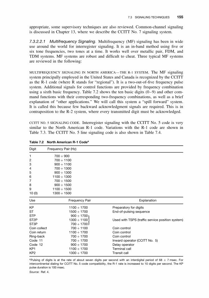
7.3 SIGNALING TECHNIQUES 155
appropriate, some supervisory techniques are also reviewed. Common-channel signalingis discussed in Chapter 13, where we describe the CCITT No. 7 signaling system.
7.3.2.2.1 Multifrequency Signaling. Multifrequency (MF) signaling has been in wideuse around the world for interregister signaling. It is an in-band method using five orsix tone frequencies, two tones at a time. It works well over metallic pair, FDM, andTDM systems. MF systems are robust and difficult to cheat. Three typical MF systemsare reviewed in the following:
MULTIFREQUENCY SIGNALING IN NORTH AMERICA—THE R-1 SYSTEM. The MF signalingsystem principally employed in the United States and Canada is recognized by the CCITTas the R-1 code (where R stands for “regional”). It is a two-out-of-five frequency pulsesystem. Additional signals for control functions are provided by frequency combinationusing a sixth basic frequency. Table 7.2 shows the ten basic digits (0–9) and other com-mand functions with their corresponding two-frequency combinations, as well as a briefexplanation of “other applications.” We will call this system a “spill forward” system.It is called this because few backward acknowledgment signals are required. This is incontraposition to the R-2 system, where every transmitted digit must be acknowledged.
CCITT NO. 5 SIGNALING CODE. Interregister signaling with the CCITT No. 5 code is verysimilar to the North American R-1 code. Variations with the R-1 code are shown inTable 7.3. The CCITT No. 5 line signaling code is also shown in Table 7.4.
Table 7.2 North American R-1 Codea
Digit Frequency Pair (Hz)
1 700 + 9002 700 + 11003 900 + 11004 700 + 13005 900 + 13006 1100 + 13007 700 + 15008 900 + 15009 1100 + 150010 (0) 1300 + 1500
Use Frequency Pair Explanation
KP 1100 + 1700 Preparatory for digitsST 1500 + 1700 End-of-pulsing sequenceSTP 900 + 1700ST2P 1300 + 1100
}Used with TSPS (traffic service position system)
ST3P 700 + 1700Coin collect 700 + 1100 Coin controlCoin return 1100 + 1700 Coin controlRing-back 700 + 1700 Coin controlCode 11 700 + 1700 Inward operator (CCITT No. 5)Code 12 900 + 1700 Delay operatorKP1 1100 + 1700 Terminal callKP2 1300 + 1700 Transit call
aPulsing of digits is at the rate of about seven digits per second with an interdigital period of 68 ± 7 msec. Forintercontinental dialing for CCITT No. 5 code compatibility, the R-1 rate is increased to 10 digits per second. The KPpulse duration is 100 msec.
Source: Ref. 4.

156 SIGNALING
Table 7.3 CCITT No. 5 Code Showing Variations withthe R-1 Codea
Signal Frequencies (Hz) Remarks
KP1 1100 + 1700 Terminal trafficKP2 1300 + 1700 Transit traffic1 700 + 9002 700 + 11003–0 Same as Table 7.2ST 1500 + 1700Code 11 700 + 1700 Code 11 operatorCode 12 900 + 1700 Code 12 operator
aLine signaling for CCITT No. 5 code is 2VF, with f1 2400 Hz and f22600 Hz. Line-signaling conditions are shown in Table 7.4.
Source: Ref. 5.
Table 7.4 CCITT No. 5 Line Signaling Code
Signal Direction Frequency Sending DurationRecognition Time
(msec)
Seizing → f1 Continuous 40 ± 10Proceed to send ← f2 Continuous 40 ± 10Busy flash ← f2 Continuous 125 ± 25Acknowledgment → f1 Continuous 125 ± 25Answer ← f1 Continuous 125 ± 25Acknowledgment → f1 Continuous 125 ± 25Clear back ← f2 Continuous 125 ± 25Acknowledgment → f1 Continuous 125 ± 25Forward transfer → f2 850 ± 200 msec 125 ± 25Clear forward → f1 + f2 Continuous 125 ± 25Release guard ← f1 + f2 Continuous 125 ± 25
Source: Ref. 4.
R-2 CODE. The R-2 code has been denominated by CCITT (CCITT Rec. Q.361) as aEuropean regional signaling code. Taking full advantage of combinations of two-out-of-six tone frequencies, 15 frequency pair possibilities are available. This number is doubledin each direction by having meaning in groups I and II in the forward direction (i.e.,toward the called subscriber) and groups A and B in the backward direction, as shown inTable 7.5.
Groups I and A are said to be of primary meaning, and groups II and B are said to beof secondary meaning. The change from primary to secondary meaning is commandedby the backward signal A-3 or A-5. Secondary meanings can be changed back to primarymeanings only when the original change from primary to secondary was made by the useof the A-5 signal. Turning to Table 7.5, the 10 digits to be sent in the forward directionin the R-2 system are in group I and are index numbers 1 through 10 in the table. Theindex 15 signal (group A) indicates “congestion in an international exchange or at itsoutput.” This is a typical backward information signal giving circuit status information.Group B consists of nearly all “backward information” and, in particular, deals withsubscriber status.
The R-2 line-signaling system has two versions: the one used on analog networks isdiscussed here; the other, used on E-1 PCM networks, was briefly covered in Chapter 6.The analog version is an out-of-band tone-on-when-idle system. Table 7.6 shows the lineconditions in each direction, forward and backward. Note that the code takes advantage of

7.3 SIGNALING TECHNIQUES 157
Table 7.5 European R-2 Signaling System
Frequencies (Hz)
1380 1500 1620 1740 1860 1980Forward
Direction I/II
Index No. forGroups I/II and A/B 1140 1020 900 780 660 540
BackwardDirection A/B
1 × ×2 × ×3 × ×4 × ×5 × ×6 × ×7 × ×8 × ×9 × ×
10 × ×11 × ×12 × ×13 × ×14 × ×15 × ×
Source: Ref. 6.
Table 7.6 Line Conditions for the R-2 Code
Operating ConditionSignaling Conditions
of the Circuit Forward Backward
1. Idle Tone on Tone on2. Seized Tone off Tone on3. Answered Tone off Tone off4. Clear back Tone off Tone on5. Release Tone on Tone on or off6. Blocked Tone on Tone off
Source: Ref. 6.
a signal sequence that has six characteristic operating conditions. Let us consider severalof these conditions.
Seized The outgoing exchange (call-originating exchange) removes the tone in theforward direction. If seizure is immediately followed by release, removal of thetone must be maintained for at least 100 msec to ensure that it is recognized at theincoming end.
Answered The incoming end removes the tone in the backward direction. When anotherlink of the connection using tone-on-when-idle continuous signaling precedes theoutgoing exchange, the “tone-off” condition must be established on the link as soonas it is recognized in this exchange.
Clear Back The incoming end restores the tone in the backward direction. Whenanother link of the connection using tone-on-when-idle continuous signaling pre-cedes the outgoing exchange, the “tone-off” condition must be established on thislink as soon as it is recognized in this exchange.
Clear Forward The outgoing end restores the tone in the forward direction.

158 SIGNALING
Table 7.7 Audible Call Progress Tones Commonly Usedin North America
ToneFrequencies
(Hz) Cadence
Dial 350 + 440 ContinuousBusy (station) 480 + 620 0.5 sec on, 0.5 sec offBusy (network 480 + 620 0.2 sec on, 0.3 sec off
congestion)Ring return 440 + 480 2 sec on, 4 sec offOff-hook alert Multifrequency 1 sec on, 1 sec off
howlRecording warning 1400 0.5 sec on, 15 sec offCall waiting 440 0.3 sec on, 9.7 sec off
Source: Ref. 7.
Table 7.8 North American Push-Button Codes
DigitDial Pulse(Breaks)
MultifrequencyPush-Button Tones
0 10 941,1336 Hz1 1 697,1209 Hz2 2 697,1336 Hz3 3 697,1474 Hz4 4 770,1209 Hz5 5 770,1336 Hz6 6 770,1477 Hz7 7 852,1209 Hz8 8 852,1336 Hz9 9 852,1477 Hz
Source: Ref. 7
Blocked At the outgoing exchange the circuit stays blocked as long as the tone remainsoff in the backward direction.
7.3.3 Subscriber Call Progress Tones and Push-Button Codes (NorthAmerica)
Table 7.7 shows the audible call progress tones commonly used in North America aspresented to a subscriber. Subscriber subsets are either dial or push-button, and theywill probably be all push-button in the next 10 years. A push-button actuates two audiotones simultaneously, similar to the multifrequency systems described previously withinterregister signaling. However, the tone library used by the subscriber is different thanthe tone library used with interregister signaling. Table 7.8 compares digital dialed, dialpulses (breaks), and multifrequency (MF) push-button tones.
7.4 COMPELLED SIGNALING
In many of the signaling systems discussed thus far, signal element duration is an impor-tant parameter. For instance, in a call setup an initiating exchange sends a 100-msecseizure signal. Once this signal is received at the distant end, the distant exchange sends a“proceed to send” signal back to the originating exchange; in the case of the R-1 system,
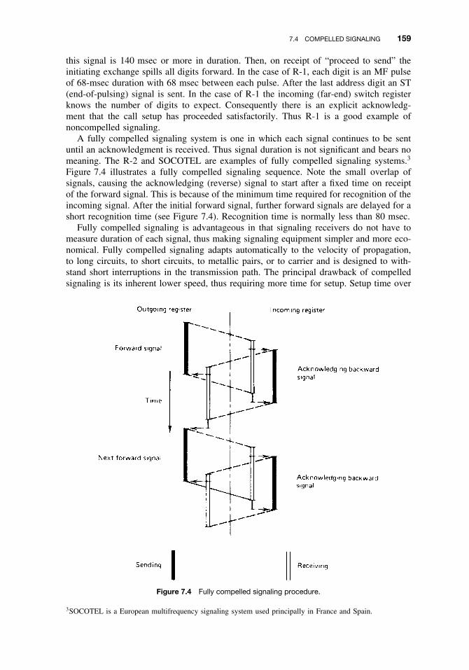
7.4 COMPELLED SIGNALING 159
this signal is 140 msec or more in duration. Then, on receipt of “proceed to send” theinitiating exchange spills all digits forward. In the case of R-1, each digit is an MF pulseof 68-msec duration with 68 msec between each pulse. After the last address digit an ST(end-of-pulsing) signal is sent. In the case of R-1 the incoming (far-end) switch registerknows the number of digits to expect. Consequently there is an explicit acknowledg-ment that the call setup has proceeded satisfactorily. Thus R-1 is a good example ofnoncompelled signaling.
A fully compelled signaling system is one in which each signal continues to be sentuntil an acknowledgment is received. Thus signal duration is not significant and bears nomeaning. The R-2 and SOCOTEL are examples of fully compelled signaling systems.3
Figure 7.4 illustrates a fully compelled signaling sequence. Note the small overlap ofsignals, causing the acknowledging (reverse) signal to start after a fixed time on receiptof the forward signal. This is because of the minimum time required for recognition of theincoming signal. After the initial forward signal, further forward signals are delayed for ashort recognition time (see Figure 7.4). Recognition time is normally less than 80 msec.
Fully compelled signaling is advantageous in that signaling receivers do not have tomeasure duration of each signal, thus making signaling equipment simpler and more eco-nomical. Fully compelled signaling adapts automatically to the velocity of propagation,to long circuits, to short circuits, to metallic pairs, or to carrier and is designed to with-stand short interruptions in the transmission path. The principal drawback of compelledsignaling is its inherent lower speed, thus requiring more time for setup. Setup time over
Figure 7.4 Fully compelled signaling procedure.
3SOCOTEL is a European multifrequency signaling system used principally in France and Spain.

160 SIGNALING
space-satellite circuits with compelled signaling is appreciable and may force the systemengineer to seek a compromise signaling system.
There is also a partially compelled type of signaling, where signal duration is fixed inboth forward and backward directions according to system specifications; or the forwardsignal is of indefinite duration and the backward signal is of fixed duration. The forwardsignal ceases once the backward signal has been received correctly. CCITT SignalingSystem No. 4 (not discussed in this text; see CCITT Recs. Q.120 to 130) is an exampleof a partially compelled signaling system.
7.5 CONCEPTS OF LINK-BY-LINK VERSUS END-TO-END SIGNALING
An important factor to be considered in switching system design that directly affects bothsignaling and customer satisfaction is postdialing delay. This is the amount of time ittakes after the calling subscriber completes dialing until ring-back is received. Ring-backis a backward signal to the calling subscriber indicating that the dialed number is ringing.Postdialing delay must be made as short as possible.
Another important consideration is register occupancy time for call setup as the setupproceeds from originating exchange to terminating exchange. Call-setup equipment, thatequipment used to establish a speech path through a switch and to select the properoutgoing trunk, is expensive. By reducing register occupancy per call, we may be able toreduce the number of registers (and markers) per switch, thus saving money.
Link-by-link and end-to-end signaling each affect register occupancy and postdialingdelay, each differently. Of course, we are considering calls involving one or more tandemexchanges in a call setup, because this situation usually occurs on long-distance or tollcalls. Link-by-link signaling may be defined as a signaling system where all interregisteraddress information must be transferred to the subsequent exchange in the call-setuprouting. Once this information is received at this exchange, the preceding exchange controlunit (register) releases. This same operation is carried on from the originating exchangethrough each tandem (transit) exchange to the terminating exchange of the call. The R-1system is an example of link-by-link signaling.
End-to-end signaling abbreviates the process such that tandem (transit) exchangesreceive only the minimum information necessary to route the call. For instance, the lastfour digits of a seven-digit telephone number need be exchanged only between the orig-inating exchange (e.g., the calling subscriber’s local exchange or the first toll exchangein the call setup) and the terminating exchange in the call setup. With this type of sig-naling, fewer digits are required to be sent (and acknowledged) for the overall call-setupsequence. Thus the signaling process may be carried out much more rapidly, decreasingpostdialing delay. Intervening exchanges on the call route work much less, handling onlythe digits necessary to pass the call to the next exchange in the sequence.
The key to end-to-end signaling is the concept of “leading register.” This is the register(control unit) in the originating exchange that controls the call routing until a speech pathis setup to the terminating exchange before releasing to prepare for another call setup.For example, consider a call from subscriber X to subscriber Y :

7.6 EFFECTS OF NUMBERING ON SIGNALING 161
The telephone number of subscriber Y is 345–6789. The sequence of events is as followsusing end-to-end signaling:
ž A register at exchange OE receives and stores the dialed number 345–6789 fromsubscriber X.
ž Exchange OE analyzes the number and then seizes a trunk (junction) to exchange B.It then receives a “proceed-to-send” signal indicating that the register at B is readyto receive routing information (digits).
ž Exchange OE then sends digits 34, which are the minimum necessary to effectcorrect transit.
ž Exchange B analyzes the digits 34 and then seizes a trunk to exchange C. ExchangesOE and C are now in direct contact and exchange B’s register releases.
ž Exchange OE receives the “proceed-to-send” signal from exchange C and then sendsdigits 45, those required to effect proper transit at C.
ž Exchange C analyzes digits 45 and then seizes a trunk to exchange TE. Directcommunication is then established between the leading register for this call at OEand the register at TE being used on this call setup. The register at C then releases.
ž Exchange OE receives the “proceed-to-send” signal from exchange TE, to which itsends digits 5678, the subscriber number.
ž Exchange TE selects the correct subscriber line and returns to A ring-back, line busy,out of order, or other information after which all registers are released.
Thus we see that a signaling path is opened between the leading register and theterminating exchange. To accomplish this, each exchange in the route must “know” itslocal routing arrangements and request from the leading register those digits it needs toroute the call further along its proper course.
Again, the need for backward information becomes evident, and backward signalingcapabilities must be nearly as rich as forward signaling capabilities when such a systemis implemented.
R-1 is a system inherently requiring little backward information (interregister). Thelittle information that is needed, such as “proceed to send,” is sent via line signaling. TheR-2 system has major backward information requirements, and backward information andeven congestion and busy signals sent back by interregister signals (Ref. 5).
7.6 EFFECTS OF NUMBERING ON SIGNALING
Numbering, the assignment and use of telephone numbers, affects signaling as well asswitching. It is the number or the translated number, as we found out in Section 1.3.2,that routes the call. There is “uniform” numbering and “nonuniform” numbering. Howdoes each affect signaling? Uniform numbering can simplify a signaling system. Mostuniform systems in the nontoll or local-area case are based on seven digits, although someare based on six. The last four digits identify the subscriber. The first three digits (or thefirst two in the case of a six-digit system) identify the exchange. Thus the local exchangeor transit exchanges know when all digits are received. There are two advantages to thissort of scheme:
1. The switch can proceed with the call once all digits are received because it “knows”when the last digit (either the sixth or seventh) has been received.

162 SIGNALING
2. “Knowing” the number of digits to expect provides inherent error control and makes“timeout” simpler.4
For nonuniform numbering, particularly on direct distance dialing in the internationalservice, switches require considerably more intelligence built in. It is the initial digit ordigits that will tell how many digits are to follow, at least in theory.
However, in local or national systems with nonuniform numbering, the originatingregister has no way of knowing whether it has received the last digit, with the exceptionof receiving the maximum total used in the national system. With nonuniform numbering,an incompletely dialed call can cause a useless call setup across a network up to theterminating exchange, and the call setup is released only after time out has run its course. Itis evident that with nonuniform numbering systems, national (and international) networksare better suited to signaling systems operating end to end with good features of backwardinformation, such as the R-2 system (Ref. 5).
7.7 ASSOCIATED AND DISASSOCIATED CHANNEL SIGNALING
Here we introduce a new concept: disassociated channel signaling. Up to now we haveonly considered associated channel signaling. In other words, the signaling is carried right
Figure 7.5 Conventional analog associated channel signaling (upper) versus separate channel signaling(which we call quasi-associated channel signaling) (lower). Note: Signaling on upper drawing accompaniesvoice paths; signaling on the lower drawing is conveyed on a separate circuit (or time slot). CCS standsfor common channel signaling such as CCITT Signaling System No. 7.
4“Timeout” is the resetting of call-setup equipment and return of dial tone to subscriber as a result of incompletesignaling procedure, subset left off hook, and so forth.
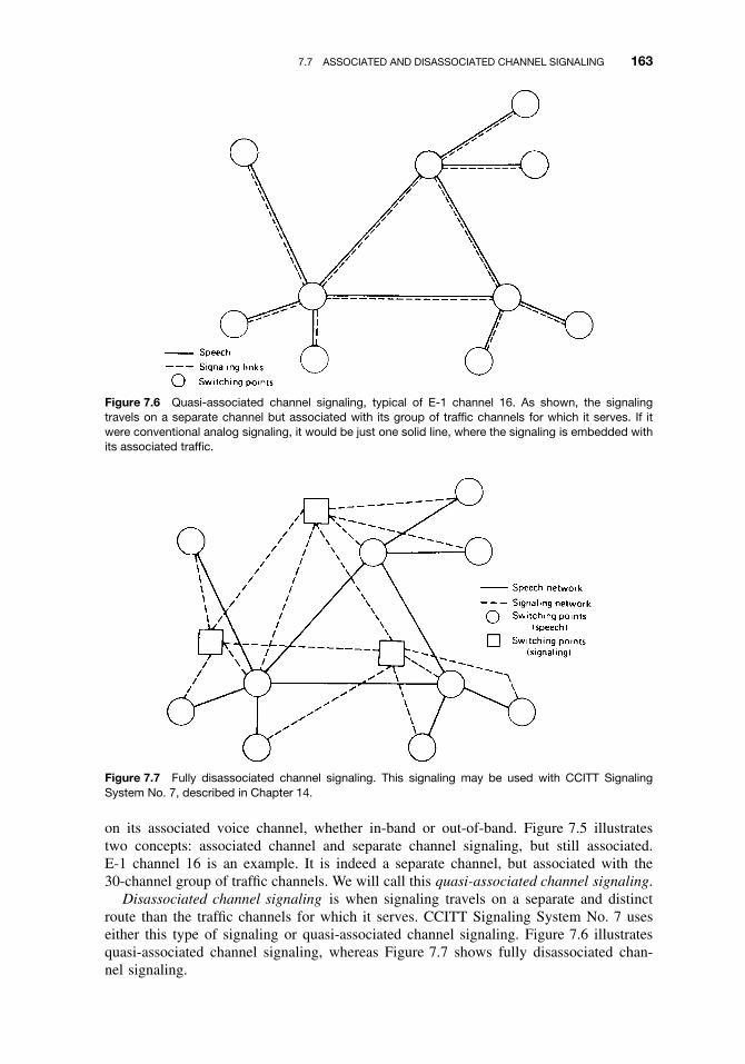
7.7 ASSOCIATED AND DISASSOCIATED CHANNEL SIGNALING 163
Figure 7.6 Quasi-associated channel signaling, typical of E-1 channel 16. As shown, the signalingtravels on a separate channel but associated with its group of traffic channels for which it serves. If itwere conventional analog signaling, it would be just one solid line, where the signaling is embedded withits associated traffic.
Figure 7.7 Fully disassociated channel signaling. This signaling may be used with CCITT SignalingSystem No. 7, described in Chapter 14.
on its associated voice channel, whether in-band or out-of-band. Figure 7.5 illustratestwo concepts: associated channel and separate channel signaling, but still associated.E-1 channel 16 is an example. It is indeed a separate channel, but associated with the30-channel group of traffic channels. We will call this quasi-associated channel signaling.
Disassociated channel signaling is when signaling travels on a separate and distinctroute than the traffic channels for which it serves. CCITT Signaling System No. 7 useseither this type of signaling or quasi-associated channel signaling. Figure 7.6 illustratesquasi-associated channel signaling, whereas Figure 7.7 shows fully disassociated chan-nel signaling.

164 SIGNALING
7.8 SIGNALING IN THE SUBSCRIBER LOOP
7.8.1 Background and Purpose
In Section 5.4 we described loop-start signaling, although we did not call it that. When asubscriber takes a telephone off-hook (out of its cradle), there is a switch closure at thesubset (see the hook-switch in Figure 5.3), current flows in the loop alerting the servingexchange that service is desired on that telephone. As a result, dial tone is returned to thesubscriber. This is basic supervisory signaling on the subscriber loop.
A problem can arise from this form of signaling. It is called glare. Glare is the result ofattempting to seize a particular subscriber loop from each direction. In this case it wouldbe an outgoing call and an incoming call nearly simultaneously. There is a much greaterprobability of glare with a PABX than with an individual subscriber.
Ground-start signaling is the preferred signaling system when lines terminate in aswitching system such as a PABX. It operates as follows: When a call is from the localserving switch to the PABX, the local switch immediately grounds the conductor tip toseize the line. With some several seconds delay, ringing voltage is applied to the line(where required). The PABX immediately detects the grounded tip conductor and will notallow an outgoing call from the PABX to use this circuit, thus avoiding glare.
In a similar fashion, if a call originates at the PABX and is outgoing to the localserving exchange, the PABX grounds the ring conductor to seize the line. The servingswitch recognizes this condition and prevents other calls from attempting to terminate thecircuit. The switch now grounds the tip conductor and returns dial tone after it connectsa digit receiver. There can be a rare situation when double seizure occurs, causing glare.Usually one or the other end of the circuit is programmed to back down and allow theother call to proceed. A ground start interface is shown in Figure 7.8.
Terminology in signaling often refers back to manual switchboards or, specifically, tothe plug used with these boards and its corresponding jack as illustrated in Figure 7.9.Thus we have tip (T), ring (R), and sleeve (S). Often only the tip and ring are used, andthe sleeve is grounded and has no real electrical function.
Figure 7.8 Ground-start interface block diagram. (From Figure 2-7 of Ref. 8, reprinted with permission.)

7.9 METALLIC TRUNK SIGNALING 165
Figure 7.9 Switchboard plug with corresponding jack (R, S, and T are ring, sleeve, and tip, respectively).
7.9 METALLIC TRUNK SIGNALING
7.9.1 Basic Loop Signaling
As mentioned earlier, many trunks serving the local area are metallic-pair trunks. Theyare actually loops much like the subscriber loop. Some still use dial pulses for addresssignaling along with some form of supervisory signaling.
Loop signaling is commonly used for supervision. As we would expect, it providestwo signaling states: one when the circuit is opened and one when the circuit is closed.A third signaling state is obtained by reversing the direction or changing the magnitudeof the current in the circuit. Combinations of (1) open/close, (2) polarity reversal, and(3) high/low current are used for distinguishing signals intended for one direction ofsignaling (e.g., dial-pulse signals) from those intended for the opposite direction (e.g.,answer signals). We describe the most popular method of supervision on metallic pairtrunks below, namely, reverse-battery signaling.
7.9.2 Reverse-Battery Signaling
Reverse-battery signaling employs basic methods (1) and (2) just mentioned, and takesits name from the fact that battery and ground are reversed on the tip and ring to changethe signal toward the calling end from on-hook to off-hook. Figure 7.10 shows a typicalapplication of reverse-battery signaling in a common-control path.
In the idle or on-hook condition, all relays are unoperated and the switch (SW) contactsare open. Upon seizure of the outgoing trunk by the calling switch (exchange) (trunkgroup selection based on the switch or exchange code dialed by the calling subscriber),the following occur:
ž SW1 and SW2 contacts close, thereby closing loop to called office (exchange) andcausing the A relay to operate.
ž Operation of the A relay signals off-hook (connect) indication to the called switch(exchange).
Figure 7.10 Reverse-battery signaling. (From Figure 6-27 of Ref. 7, reprinted with permission.)

166 SIGNALING
ž Upon completion of pulsing between switches, SW3 contacts close and the calledsubscriber is alerted. When the called subscriber answers, the S2 relay is operated.
ž Operation of the S2 relay operates the T relay, which reverses the voltage polarityon the loop to the calling end.
ž The voltage polarity causes the CS relay to operate, transmitting an off-hook (answer)signal to the calling end.
When the calling subscriber hangs up, disconnect timing starts (between 150 msecand 400 msec). After the timing is completed, SW1 and SW2 contacts are released inthe calling switch. This opens the loop to the A relay in the called switch and releasesthe calling subscriber. The disconnect timing (150–400 msec) is started in the calledswitch as soon as the A relay releases. When the disconnect timing is completed, thefollowing occur:
ž If the called subscriber has returned to on-hook, SW3 contacts release. The calledsubscriber is now free to place another call.
ž If the called subscriber is still off-hook, disconnect timing is started in the calledswitch. On the completion of the timing interval, SW3 contacts open. The calledsubscriber is then returned to dial tone. If the circuit is seized again from the callingswitch during the disconnect timing, the disconnect timing is terminated and thecalled subscriber is returned to dial tone. The new call will be completed withoutinterference from the previous call.
When the called subscriber hangs up, the CS relay in the calling switch releases. Thenthe following occur:
ž If the calling subscriber has also hung up, disconnection takes place as previ-ously described.
ž If the calling subscriber is still off-hook, disconnect timing is started. On the com-pletion of the disconnect timing, SW1 and SW2 contacts are opened. This returnsthe calling subscriber to dial tone and releases the A relay in the called switch. Thecalling subscriber is free to place a new call at this time. After the disconnect tim-ing, the SW3 contacts are released, which releases the called subscriber. The calledsubscriber can place a new call at this time.
REVIEW EXERCISES
1. Give the three generic signaling functions, and explain the purpose of each.
2. Differentiate between line signaling and interregister signaling.
3. There are seven ways to transmit signaling information, one is frequency. Namefive others.
4. How does a switch know whether a particular talk path is busy or idle?
5. A most common form of line signaling is E&M signaling. Describe how it worksin three sentences or less.
6. Compare in-band and out-of-band supervisory signaling regarding tone-on idle/busy,advantages, disadvantages.

REFERENCES 167
7. What is the most common form of in-band signaling in North America?
8. What is the standard out-of-band signaling frequency in the United States?
9. Give the principal advantage of 2VF supervisory signaling over SF.
10. Compare CCITT No. 5/R1 signaling with R2 signaling.
11. Describe and compare end-to-end signaling with link-by-link signaling.
12. Describe at least four types of backward information.
13. Distinguish between associated channel signaling and separate channel signaling.
14. What is disassociated-channel signaling?
15. What is glare?
REFERENCES
1. IEEE Standard Dictionary of Electrical and Electronic Terms, 6th ed., IEEE Std 100-1996, IEEE,New York, 1996.
2. R. L. Freeman, Telecommunication Transmission Handbook, 4th ed., Wiley, New York, 1998.
3. National Networks for the Automatic Service, CCITT-ITU Geneva, 1968.
4. Specifications of Signaling Systems 4 and 5, CCITT Recommendations, Fascicle VI.4, IXthPlenary Assembly, Melbourne, 1988.
5. “Signaling” from Telecommunications Planning Documents, ITT Laboratories, Madrid, Novem-ber, 1974.
6. Specifications for Signaling Systems R1 and R2, CCITT Recommendations, Fascicle VI.4, IXthPlenary Assembly, Melbourne, 1988.
7. BOC Notes on the LEC Networks—1994, Special Report SR-TSV-002275 Issue 2, Bellcore,Piscataway, NJ, 1994.
8. W. D. Reeve, Subscriber Loop Signaling and Transmission Handbook—Analog, IEEE Press,New York, 1992.


8
LOCAL AND LONG-DISTANCENETWORKS
8.1 CHAPTER OBJECTIVE
This chapter concentrates on the network design of the PSTN, how it is structured andwhy. Routing techniques have a strong influence on how a network is structured. Thuswe also discuss routing and, in particular, dynamic routing. The third topic deals withtransmission, namely, assigning losses in the network to eliminate any possibility ofsinging and to keep echo inside some tolerable limits.
8.2 MAKEUP OF THE PSTN
As we discussed in Section 1.3, the PSTN consists of a group of local networks connectedby a long-distance network. In countries where competition is permitted, there may betwo or many long-distance networks. Some of these may cover the nation, whereas othersare regional long-distance networks.
The heart of a local network is the subscriber plant. This consists of customer premiseequipment (CPE), a copper wire distribution network made up of subscriber loops that con-nect to a local serving switch via the main distribution frame (MDF). The concept of thesubscriber plant feeding the local network, which, in turn, feeds the long-distance networkto a distant local network and associated subscriber plant, is illustrated in Figure 8.1.
8.2.1 The Evolving Local Network
Over 65% of the investment in a PSTN is in the local network. More cost-effective andefficient means are now being implemented to connect a subscriber to the local servingexchange. In Section 4.3.8, concentrators and remote switching were introduced. Thedigital subscriber line (DSL) concept was covered in Section 6.10.
With ISDN/BRI we bring digital service directly to the subscriber premise. If the twoB-channels are combined (see Section 12.4.6.2), 128-kbps service can be provided. Usersof the Internet desire downstream1 bit rates in excess of this value, up to 1.544 Mbps
1Downstream in the direction local serving switch to the subscriber.
Fundamentals of Telecommunications, Second Edition, by Roger L. FreemanISBN 0-471-71045-8 Copyright 2005 by Roger L. Freeman
169

170 LOCAL AND LONG-DISTANCE NETWORKS
Local network Local network
Long-distance network
Figure 8.1 The general structure of a PSTN.
or better. The shorter we make a conventional subscriber loop, the greater the bit rate itcan support.
We will incorporate a new, generic device in the subscriber plant. It is called a remotesubscriber unit (RSU). It distributes service to the subscriber plant customer. The basicservice it provides is POTS using a typical subscriber line interface card (SLIC). TheRSU has a large group of optional capabilities listed below:
ž It may or may not have a local switching capability.ž In most cases the RSU will carry out a concentrator function.ž It may be a fiber-to-wire interface point for a hybrid fiber–wire-pair system.ž It may be a node for wireless local loop employing point-to-multipoint radio.ž It may provide an add–drop multiplex (ADM) capability on a SONET or SDH
self-healing ring (SHR).
Several of these RSU concepts are illustrated in Figure 8.2. Figure 8.2a shows theconventional subscriber distribution plant and identifies its various functional parts.Figure 8.2b illustrates a digital subscriber line feeding (DSL) an RSU. The DSL mightconsist of one or several DS1 or E-1 bit streams. In this case the DSL would be on twotwo-wire pairs, one for downstream and one for upstream. Figure 8.2c is the same asFigure 8.2b, but in this case the DSL is carried on two fibers plus a spare in a fiber-opticcable configuration. Figure 8.2d illustrates the use of a fiber-optic or wire-pair bus to feedseveral RSUs. Figure 8.2e shows a simple self-healing ring architecture employing eitherSONET or SDH (see Section 9.4).
In sparsely populated rural areas, point-to-multipoint full-duplex radio systems areparticularly applicable. Such systems would operate in the 2- or 4-GHz band with 10-,20-, or 30-mile links. Access to the system would probably be time division multipleaccess. However, in densely populated urban areas, the 23-, 25-, or 38-GHz frequencybands should be considered, keeping link length well under 3.5 miles (5.5 km). Becauseof expected high interference levels from nearby users, code division multiple accessshould be considered for this application. The TDMA and CDMA access schemes aredescribed in Chapter 18.
8.2.2 What Affects Local Network Design?
There are a number of important factors that will influence the design of a local network.Among these factors are:
ž Subscriber density and density distribution.ž Breakdown between residential and business subscribers.

8.2 MAKEUP OF THE PSTN 171
Figure 8.2a Conventional subscriber distribution plant.
Figure 8.2b A digital subscriber line (DSL) carrying a DS1 or E-1 configuration feeds an RSU. The RSUprovides the necessary functions for subscriber loop interface.
Figure 8.2c A fiber-optic pair feeds an RSU. This configuration is particularly useful for nests ofsubscribers beyond 12,000 ft (3700 m) from the local exchange.

172 LOCAL AND LONG-DISTANCE NETWORKS
Figure 8.2d A fiber-optic or wire-pair cable bus feeds several RSUs.
Figure 8.2e A fiber-optic cable self-healing ring feeds RSUs.
ž Further breakdown among types of business subscribers as a function of white-collarand blue-collar workers. For example, a large insurance company will have muchgreater calling activity than a steel mill with the same number of workers.
ž Cultural factors.
It follows that in regions of high subscriber density typical of urban areas, there would bemany exchanges, each with comparatively short subscriber loops. Such a network wouldtrend toward mesh connectivities. The opposite would be in rural regions where wewould expect few exchanges, and a trend toward a greater use of tandem working. Long

8.3 DESIGN OF LONG-DISTANCE NETWORKS 173
route design would be the rule rather than the exception. Suburban bedroom communitiespresent still a different problem, where we would expect calling trends toward urban,industrial centers. Many calls in this case will be served by just one exchange. Judicioususe of tandem working would be advisable.
Cultural factors can give the network designer insight into expected calling habits. Theaffluence of a region may well be a factor. However, consider countries where affluencegoes hand-in-hand with volunteerism, an organizational spirit, and a socialization factor.Certain cultures encourage strong family ties, where one can expect high intrafamilycalling activity.
8.3 DESIGN OF LONG-DISTANCE NETWORKS
8.3.1 Introduction
A long-distance network connects an aggregate of local networks. Any subscriber in thenation should be able to reach any other subscriber. Likewise, any subscriber in the nationshould be able to connect with any other subscriber in the world. So we have need notonly of local and long-distance (toll) exchanges, but international exchanges as well.
8.3.2 Three Design Steps
The design of a long-distance network involves basically three considerations:
1. Routing scheme given inlet and outlet points and their traffic intensities2. Switching scheme and associated signaling and3. Transmission plan
In the design each design step will interact with the other two. In addition, the systemdesigner must specify the type of traffic, lost-call criterion or grade of service, a sur-vivability criterion, forecast growth, and quality of service (QoS). The tradeoff of thesefactors with economy is probably the most vital part of initial planning and downstreamsystem design.
Consider transcontinental communications in the United States. Service is now avail-able for people in New York to talk to people in San Francisco. From the history of thisservice, we have some idea of how many people wish to talk, how often, and for howlong. These factors are embodied in traffic intensity and calling rate. There are also othercities on the West Coast to be served and other cities on the East Coast. In addition,there are existing traffic nodes at intermediate points such as Chicago and St. Louis. Anobvious approach would be to concentrate all traffic into one transcontinental route withdrops and inserts at intermediate points.
Again, we must point out that switching enhances the transmission facilities. From aneconomic point of view, it would be desirable to make transmission facilities (carrier,radio, and cable systems) adaptive to traffic load. These facilities taken alone are inflex-ible. The property of adaptivity, even when the transmission potential for it has beenpredesigned through redundancy, cannot be exercised, except through the mechanism ofswitching in some form. It is switching that makes transmission adaptive.
The following requirements for switching ameliorate the weaknesses of transmissionsystems: concentrate light, discretely offered traffic from a multiplicity of sources andthus enhance the utilization factor of transmission trunks; select and make connections
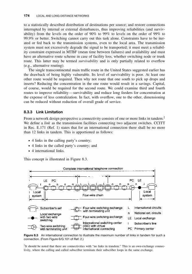
174 LOCAL AND LONG-DISTANCE NETWORKS
to a statistically described distribution of destinations per source; and restore connectionsinterrupted by internal or external disturbances, thus improving reliabilities (and surviv-ability) from the levels on the order of 90% to 99% to levels on the order of 99% to99.9% or better. Switching cannot carry out this task alone. Constraints have to be iter-ated or fed back to the transmission systems, even to the local area. The transmissionsystem must not excessively degrade the signal to be transported; it must meet a reliabil-ity constraint expressed in MTBF (mean time between failures) and availability and musthave an alternative route scheme in case of facility loss, whether switching node or trunkroute. This latter may be termed survivability and is only partially related to overflow(e.g., alternative routing).
The single transcontinental main traffic route in the United States suggested earlier hasthe drawback of being highly vulnerable. Its level of survivability is poor. At least oneother route would be required. Then why not route that one south to pick up drops andinserts? Reducing the concentration in the one route would result in a savings. Capital,of course, would be required for the second route. We could examine third and fourthroutes to improve reliability—survivability and reduce long feeders for concentration atthe expense of less centralization. In fact, with overflow, one to the other, dimensioningcan be reduced without reduction of overall grade of service.
8.3.3 Link Limitation
From a network design perspective a connectivity consists of one or more links in tandem.2
We define a link as the transmission facilities connecting two adjacent switches. CCITTin Rec. E.171 (Ref. 1) states that for an international connection there shall be no morethan 12 links in tandem. This is apportioned as follows:
ž 4 links in the calling party’s country;ž 4 links in the called party’s country; andž 4 international links.
This concept is illustrated in Figure 8.3.
Figure 8.3 An international connection to illustrate the maximum number of links in tandem for such aconnection. (From Figure 6/G.101 of Ref. 2.)
2It should be noted that there are connectivities with “no links in trandem.” This is an own-exchange connec-tivity, where the calling and called subscriber terminate their subscriber loops in the same exchange.

8.3 DESIGN OF LONG-DISTANCE NETWORKS 175
The PSTN network designer should comply with this CCITT criterion, in that fora national connection, there should be no more than four links in tandem. The reasonCCITT/ITU-T set this limit was to ensure transmission QoS. As we add links in tandem,transmission quality deteriorates. Delay increases and we include here processing delaybecause of the processing involved with a call passing through each switch. End-to-end biterror rate deteriorates and jitter and wander accumulate. Transcontinental calls in NorthAmerica generally need no more than three links in tandem, except during periods ofheavy congestion when a fourth link may be required for an alternate route.
8.3.4 Numbering Plan Areas
The geographical territory covered by the long-distance network will be broken up intonumbering plan areas (NPAs). In North America, each NPA is assigned a three-digit areacode. In other parts of the world, two- and even one-digit area codes are used. NPA sizeand shape are driven more by numbering capacity and future numbering requirements.Numbering plan administrators are encouraged to design an NPA such that it coincideswith political and/or administrative boundaries. For example, in the United States, an NPAshould not cross a state boundary; in Canada, it should not cross a provincial boundary.NPAs are also important for establishing a rates and tariffs scheme.3
We know a priori that each NPA will have at least one long-distance exchange. It maybe assigned more. This long-distance exchange may or may not colocate with the POP(point of presence).4 We now have made the first steps in determining exchange location.In other countries this exchange may be known as a toll-connecting exchange.
8.3.5 Exchange Location
We have shown that the design of the long-distance network is closely related to the layoutof numbering plan areas or simply numbering areas. These exchanges are ordinarily placednear a large city. The number of long-distance exchanges in a numbering area is dependenton exchange size and certain aspects of survivability. This is the idea of “not having allone’s eggs in one basket.” There may be other reasons to have a second or even a thirdexchange in a numbering area (NPA in the United States). Not only does it improvesurvivability aspects of the network, but it also may lead the designer to place a secondexchange near another distant large city.
Depending on long-distance calling rates and holding times, and if we assume 0.004erlangs per line during the busy hour, a 4000-line long-distance exchange could servesome 900,000 subscribers. The exchange capacity should be dimensioned to the forecastlong-distance traffic load 10 years after installation. If the system goes through a 15%expansion in long-distance traffic volume per year, it will grow to over four times itspresent size in 10 years. Exchange location in the long-distance network is not verysensitive to traffic.
8.3.6 Hierarchy
Hierarchy is another essential aspect in long-distance (toll) network design. One impor-tant criterion is establishing the number of hierarchical levels in a national network.
3This deals with how much a telephone company charges for a telephone call.4POP, remember, is where the local exchange carrier interfaces with long-distance carriers. This whole conceptof the POP is peculiar to the United States and occurred when the Bell System was divested.

176 LOCAL AND LONG-DISTANCE NETWORKS
The United States has a two-level hierarchy: the local exchange carrier (or LATA [localaccess and transport area]) and the interexchange carrier network. Our concern here is theinterexchange carrier network, which is synonymous with the long-distance network. Sothe question remains: how many hierarchical levels in the long-distance or toll network?
There will be “trandem” exchanges in the network, which we will call transit exchanges.These switches may or may not be assigned a higher hierarchical level. Let us assumethat we will have at least a two-level hierarchy.
Factors that may lead to more than two levels are:
ž Geographical sizež Telephone density, usually per 100 inhabitants5
ž Long-distance traffic trendsž Political factors (such as Bell System divestiture in the United States, privatization
in other countries)
The trend toward greater use of direct HU (high-usage) routes tends to keep the numberof hierarchical levels low (e.g., at two levels). The employment of dynamic routing canhave a similar effect.
We now deal with fan-out. A higher-level exchange, in the hierarchical sense, fans outto the next lower level. This level, in turn, fans out to still lower levels in the hierarchy.It can be shown that fan-outs of six and eight are economic and efficient.
Look at this example. The highest level, one exchange, fans out to six exchanges in thenext level. This level, in turn fans out to eight exchanges. Thus there is connectivity to 48exchanges (8 × 6), and if the six exchanges in the higher level also serve as third-levelexchanges, then we have the capability of 48 + 6, or 54 toll exchanges.
Suppose that instead of one exchange in the highest level, there were four intercon-nected in mesh for survivability and improved service. This would multiply the numberof long-distance exchanges served to 48 × 4 = 192, and if we use the 56 value it wouldbe 56 × 4 = 224 total exchanges. In large countries we deal with numbers like this. Ifwe assign a long-distance exchange in each NPA, and assume all spare NPA capacity isused, there would be 792 NPAs in the United States, each with a toll exchange. Allowfor a three- or four-level hierarchy and the importance of fan-out becomes evident.
Figure 8.4 shows one-quarter of a three-level hierarchy network, where the top levelis mesh connected with four transit exchanges.
The fan-out concept assumes a pure hierarchy without high-usage routes. HU routestend to defeat the fan-out concept and are really mandatory to reduce the number of linksin tandem to a minimum.
8.3.7 Network Design Procedures
A national territory consists of a large group of contiguous local areas, each with a toll/toll-connecting exchange. There will also be at least one international switching center (ISC).In larger, more populous countries there may be two or more such ISCs. Some may callthese switching centers gateways. They need not necessarily be near a coastline. Chicagois an example in North America. So we now have established three bases to work from:
1. There are existing local areas, each with a long-distance exchange.
5The term telephone density should not mislead the reader. Realize that some “telephone lines” terminate in amodem in a computer or server, in a facsimile machine, and so on.
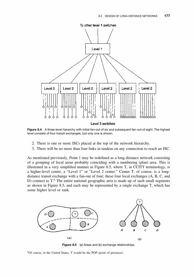
8.3 DESIGN OF LONG-DISTANCE NETWORKS 177
Figure 8.4 A three-level hierarchy with initial fan-out of six and subsequent fan-out of eight. The highestlevel consists of four transit exchanges, but only one is shown.
2. There is one or more ISCs placed at the top of the network hierarchy.3. There will be no more than four links in tandem on any connection to reach an ISC.
As mentioned previously, Point 1 may be redefined as a long-distance network consistingof a grouping of local areas probably coinciding with a numbering (plan) area. This isillustrated in a very simplified manner in Figure 8.5, where T, in CCITT terminology, isa higher-level center, a “Level 1” or “Level 2 center.” Center T, of course, is a long-distance transit exchange with a fan-out of four; these four local exchanges (A, B, C, andD) connect to T.6 The entire national geographic area is made up of such small segmentsas shown in Figure 8.5, and each may be represented by a single exchange T, which hassome higher level or rank.
Figure 8.5 (a) Areas and (b) exchange relationships.
6Of course, in the United States, T would be the POP (point of presence).

178 LOCAL AND LONG-DISTANCE NETWORKS
The next step is to examine traffic flows to and from (originating and terminating) eachT. This information is organized and tabulated on a traffic matrix. A simplified exampleis illustrated in Table 8.1. Care must be taken in the preparation and subsequent use ofsuch a table. The convention used here is that values (in erlangs or ccs) are read fromthe exchange in the left-hand column to the exchange in the top row. For example, trafficfrom exchange 1 to exchange 5 is 23 erlangs, and traffic from exchange 5 to exchange 1 is25 erlangs. It is often useful to set up a companion matrix of distances between exchangepairs. The matrix (Table 8.1) immediately offers candidates for HU routes. Nonetheless,this step is carried out after a basic hierarchical structure is established.
We recommend that a hierarchical structure be established at the outset, being fullyaware that the structure may be modified or even done away with entirely in the future asdynamic routing disciplines are incorporated (see Section 8.4). At the top of a country’shierarchy is (are) the international switching center(s). The next level down, as a minimum,would be the long-distance network, then down to a local network consisting of localserving exchanges and tandem exchanges. The long-distance network itself, as a minimum,might be divided into a two-layer hierarchy.
Suppose, for example, that a country had four major population centers and could bedivided into four areas around each center. Each of the four major population centerswould have a Level 1 switching center assigned. One of these four would be the ISC.Each Level 1 center would have one or several Level 2 or secondary centers homing onit.7 Level 3 or tertiary centers home on a Level 2 switching center. This procedure isillustrated in Figure 8.6. Its hierarchical representation is illustrated in Figure 8.7 settingout the final route. One of the Level 1 switching centers is assigned as the ISC. We definea final route as a route from which no traffic can overflow to an alternative route. It is aroute that connects an exchange immediately above or below it in the network hierarchyand there is also a connection of the two exchanges at the top hierarchical level of thenetwork. Final routes are said to make up the “backbone” of a network. Calls that areoffered to the backbone but cannot be completed are lost calls.8
A high-usage (HU) route is defined as any route that is not a final route; it mayconnect exchanges at a level of the network hierarchy other than the top level, such asbetween, 11 and 12 in Figure 8.7. It may also be a route between exchanges on differenthierarchical levels when the lower-level exchange (higher level number) does home ona higher level. A direct route is a special type of HU route connecting exchanges in the
Table 8.1 Traffic Matrix Example—Long-Distance Service (in erlangs)
To Exchange
From Exchange 1 2 3 4 5 6 7 8 9 10
1 57 39 73 23 60 17 21 23 52 62 19 30 18 26 25 2 9 63 42 18 28 17 31 19 8 10 124 70 31 23 6 7 5 8 4 35 25 19 32 5 22 19 31 13 506 62 23 19 8 20 30 27 19 277 21 30 17 40 16 32 15 16 178 21 5 12 3 25 19 17 18 299 25 10 9 1 16 22 18 19 19
10 7 8 7 2 47 25 13 30 17
7Homing on meaning subsidiary to in a hierarchical sense. It “reports to.”8Completed calls are those where a full connectivity is carried out indicated by both calling and called subscriberin the off-hook condition.

8.3 DESIGN OF LONG-DISTANCE NETWORKS 179
Figure 8.6 A sample network design.
Figure 8.7 Hierarchical representation showing final routes.
local area. Figure 8.8 shows a hierarchical network with alternative routing. Note that itemploys CCITT (ITU-T) nomenclature.
Before final dimensioning can be carried out of network switches and trunks, a gradeof service criterion must be established.9 If we were to establish a grade of service asp = 0.01 per link on a final route, and there were four links in tandem, then the grade ofservice end-to-end would be 4 × 0.01 or 0.04. In other words, for calls traversing this finalroute, one in 25 would meet congestion during the busy hour. The use of HU connectionsreduces tandem operation and tends to improve overall grade of service.
9Grade of service is the probability of meeting congestion (blockage) during the busy hour (BH).

180 LOCAL AND LONG-DISTANCE NETWORKS
Figure 8.8 A hierarchical network showing alternative (alternate) routing. Note the CCITT nomenclature.
The next step in the network design is to lay out HU routes. This is done with theaid of a traffic matrix. A typical traffic matrix is shown in Table 8.1. Some guidelinesmay be found in Section 4.2.4. Remember that larger trunk groups are more efficient.As a starting point (Section 4.2.4) for those traffic relations where the busy hour trafficintensity was >20 erlangs, establish a HU route; for those relations <20 erlangs, thenormal hierarchical routing should remain in place.
National network design as described herein lends itself well to computer-based designtechniques. The traffic intensity values used in traffic matrices, such as Table 8.1, shouldbe taken from a 10-year forecast.
8.4 TRAFFIC ROUTING IN A NATIONAL NETWORK
8.4.1 New Routing Techniques
8.4.1.1 Objective of Routing. The objective of routing is to establish a successfulconnection between any two exchanges in the network. The function of traffic routing isthe selection of a particular circuit group, for a given call attempt or traffic stream, at an

8.4 TRAFFIC ROUTING IN A NATIONAL NETWORK 181
exchange in the network. The choice of a circuit group may be affected by informationon the availability of downstream elements of the network on a quasi-real-time basis.
8.4.1.2 Network Topology. A network comprises a number of nodes (i.e., switchingcenters) interconnected by circuit groups. There may be several direct circuit groupsbetween a pair of nodes and these may be one-way or both-way (two-way). A simplifiedillustration of this idea is shown in Figure 8.9.
Remember that a direct route consists of one or more circuit groups connecting adjacentnodes. We define an indirect route as a series of circuit groups connecting two nodesproviding end-to-end connection via other nodes.
An ISC is a node in a national network, which in all probability will have some sort ofhierarchial structure as previously discussed. An ISC is also a node on the internationalnetwork that has no hierarchical structure. It consists entirely of HU direct routes.
8.4.2 Logic of Routing
8.4.2.1 Routing Structure. Conceptually, hierarchical routing need not be directlyrelated to a concept of a hierarchy of switching centers, as just described. A routingstructure is hierarchical if, for all traffic streams, all calls offered to a given route, at aspecific node, overflow to the same set of routes irrespective of the routes already tested.10
The routes in the set will always be tested in the same sequence, although some routes
Figure 8.9 A simplified network with circuit groups connecting pairs of nodes with one-way andboth-way working.
10Tested means that at least one free circuit is available to make a connectivity. This “testing” is part and parcelof CCITT Signaling System No. 7, which is discussed in Chapter 14.
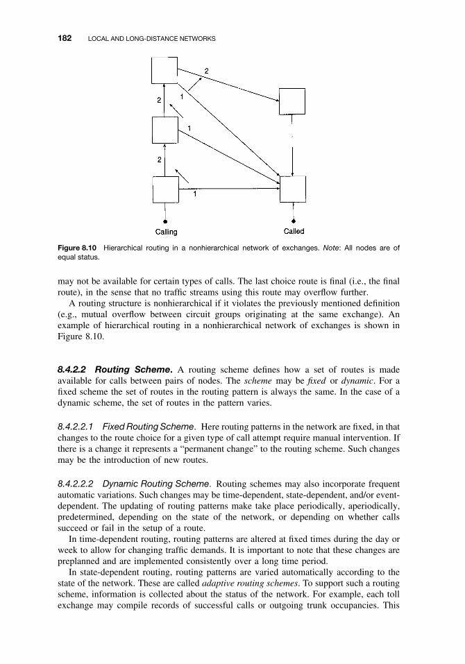
182 LOCAL AND LONG-DISTANCE NETWORKS
Figure 8.10 Hierarchical routing in a nonhierarchical network of exchanges. Note: All nodes are ofequal status.
may not be available for certain types of calls. The last choice route is final (i.e., the finalroute), in the sense that no traffic streams using this route may overflow further.
A routing structure is nonhierarchical if it violates the previously mentioned definition(e.g., mutual overflow between circuit groups originating at the same exchange). Anexample of hierarchical routing in a nonhierarchical network of exchanges is shown inFigure 8.10.
8.4.2.2 Routing Scheme. A routing scheme defines how a set of routes is madeavailable for calls between pairs of nodes. The scheme may be fixed or dynamic. For afixed scheme the set of routes in the routing pattern is always the same. In the case of adynamic scheme, the set of routes in the pattern varies.
8.4.2.2.1 Fixed Routing Scheme. Here routing patterns in the network are fixed, in thatchanges to the route choice for a given type of call attempt require manual intervention. Ifthere is a change it represents a “permanent change” to the routing scheme. Such changesmay be the introduction of new routes.
8.4.2.2.2 Dynamic Routing Scheme. Routing schemes may also incorporate frequentautomatic variations. Such changes may be time-dependent, state-dependent, and/or event-dependent. The updating of routing patterns make take place periodically, aperiodically,predetermined, depending on the state of the network, or depending on whether callssucceed or fail in the setup of a route.
In time-dependent routing, routing patterns are altered at fixed times during the day orweek to allow for changing traffic demands. It is important to note that these changes arepreplanned and are implemented consistently over a long time period.
In state-dependent routing, routing patterns are varied automatically according to thestate of the network. These are called adaptive routing schemes. To support such a routingscheme, information is collected about the status of the network. For example, each tollexchange may compile records of successful calls or outgoing trunk occupancies. This

8.4 TRAFFIC ROUTING IN A NATIONAL NETWORK 183
Figure 8.11 Adaptive or state-dependent routing, network information (status) versus routing decisions.
information may then be distributed through the network to other exchanges or passedto a centralized database. Based on this network status information, routing decisions aremade either in each exchange or at a central processor serving all exchanges. The conceptis shown in Figure 8.11.
In event-dependent routing, patterns are updated locally on the basis of whether callssucceed or fail on a given route choice. Each exchange has a list of choices, and theupdating favors those choices that succeed and discourages those that suffer congestion.
8.4.2.3 Route Selection. Route selection is the action taken to actually select a defi-nite route for a specific call. The selection may be sequential or nonsequential. In the caseof sequential selection, routes in a set are always tested in sequence and the first availableroute is selected. For the nonsequential case, the routes are tested in no specific order.
The decision to select a route can be based on the state of the outgoing circuit groupor the states of series of circuit groups in the route. In either case, it can also be basedon the incoming path of entry, class of service, or type of call to be routed.
8.4.3 Call-Control Procedures
Call-control procedures define the entire set of interactive signals necessary to establish,maintain, and release a connection between exchanges. Two such call-control proceduresare progressive call control and originating call control.
8.4.3.1 Progressive Call Control. This type of call control uses link-by-link signaling(see Chapter 7) to pass supervisory controls sequentially from one exchange to the next.Progressive call control can be either irreversible or reversible. In the irreversible case,call control is always passed downstream toward the destination exchange. Call controlis reversible when it can be passed backwards (maximum of one node) using automaticrerouting or crankback actions.
8.4.3.2 Originating Call Control. In this case the originating exchange maintains con-trol of the call setup until a connection between the originating and terminating exchangeshas been completed.
8.4.4 Applications
8.4.4.1 Automatic Alternative Routing. One type of progressive (irreversible) rout-ing is automatic alternative routing (AAR). When an exchange has the option of using

184 LOCAL AND LONG-DISTANCE NETWORKS
more than one route to the next exchange, an alternative routing scheme can be employed.The two principal types of AAR that are available are:
1. When there is a choice of direct-circuit groups between two exchanges2. When there is a choice of direct and indirect routes between the two exchanges
Alternative routing takes place when all appropriate circuits in a group are busy. Sev-eral circuit groups then may be tested sequentially. The test order is fixed or time-dependent.
8.4.4.2 Automatic Rerouting (Crankback). Automatic rerouting (ARR) is a routingfacility enabling connection of call attempts encountering congestion during the initialcall setup phase. Thus, if a signal indicating congestion is received from Exchange B,subsequent to the seizure of an outgoing trunk from Exchange A, the call may be reroutedat A. This concept is shown in Figure 8.12. ARR performance can be improved throughthe use of different signals to indicate congestion—S1 and S2 (see Figure 8.12).
ž S1 indicates that congestion has occurred on outgoing trunks from exchange B.ž S2 indicates that congestion has occurred further downstream—for example, on
outgoing trunks from D.
The action to be taken at exchange A upon receiving S1 or S2 may be either to blockthe call or to reroute it.
In the example illustrated in Figure 8.12, a call from A to D is routed via C becausethe circuit group B-D is congested (S1 indicator) and a call from A to F is routed via Ebecause circuit group D-F is congested (S2 indicator).
One positive consequence of this alternative is to increase the signaling load andnumber of call set-up operations resulting from the use of these signals. If such anincrease is unacceptable, it may be advisable to restrict the number of reroutings orlimit the signaling capability to fewer exchanges. Of course, care must be taken to avoidcircular routings (“ring-around-the-rosy”), which return the call to the point at whichblocking previously occurred during call setup.
Figure 8.12 The automatic rerouting (ARR) or crankback concept. Note: Blocking from B to D activatessignal S1 to A. Blocking from D to F activates signal S2 to A. (From Figure 4/E.170 of Ref. 3.)

8.4 TRAFFIC ROUTING IN A NATIONAL NETWORK 185
Figure 8.13 An example of preplanned distribution of load sharing. Note: Each outgoing routing pattern(A, B, C, D) may include alternative routing options.
8.4.4.3 Load Sharing. All routing schemes should result in the sharing of trafficload between network elements. Routing schemes can, however, be developed to ensurethat call attempts are offered to route choices according to a preplanned distribution.Figure 8.13 illustrates this application to load sharing, which can be made available as asoftware function of SPC exchanges. The system works by distributing the call attemptsto a particular destination in a fixed ratio between the specified routing patterns.
8.4.4.4 Dynamic Routing. Let us look at an example of state-dependent routing. Acentralized routing processor is employed to select optimum routing patterns on the basisof actual occupancy level of circuit groups and exchanges in the network which aremonitored on a periodic basis (e.g., every 10 sec). Figure 8.14 illustrates this concept.In addition, qualitative traffic parameters may also be taken into consideration in thedetermination of the optimal routing pattern.
This routing technique inherently incorporates fundamental principles of network man-agement in determining routing patterns. These principles include:
ž Avoiding occupied circuit groups.ž Not using overloaded exchanges for transit.ž In overload circumstances, restriction of routing direct connections.
Now let’s examine an example of time-dependent routing. For each originating andterminating exchange pair, a particular route pattern is planned depending on the time ofday and day of the week. This is illustrated in Figure 8.15. A weekday, for example, canbe divided into different time periods, with each time period resulting in different routepatterns being defined to route traffic streams between the same pair of exchanges.
This type of routing takes advantage of idle circuit capacity in other possible routesbetween originating and terminating exchanges which may exist due to noncoincidentbusy hours.11 Crankback may be utilized to identify downstream blocking on the secondlink of each two-link alternative path.
Figure 8.14 State-dependent routing example with centralized processor.
11Noncoincident busy hours: in large countries with two or more time zones.

186 LOCAL AND LONG-DISTANCE NETWORKS
Figure 8.15 Example of time-dependent routing. (From Figure 7/E.170 of Ref. 3.)
The following is an example of event-dependent routing. In a fully connected (mesh)network, calls between each originating and terminating exchange pair try the direct routewith a two-link alternative path selected dynamically. While calls are successfully routedon a two-link path, that alternative is retained. Otherwise, a new two-link alternative pathis selected. This updating, for example, could be random or weighted by the successof previous calls. This type of routing scheme routes traffic away from congested linksby retaining routing choices where calls are successful. It is simple, adapts quickly tochanging traffic patterns, and requires only local information. Such a scheme is illustratedin Figure 8.16 (Refs. 3, 4).
Figure 8.16 Event-dependent routing in a mesh network.
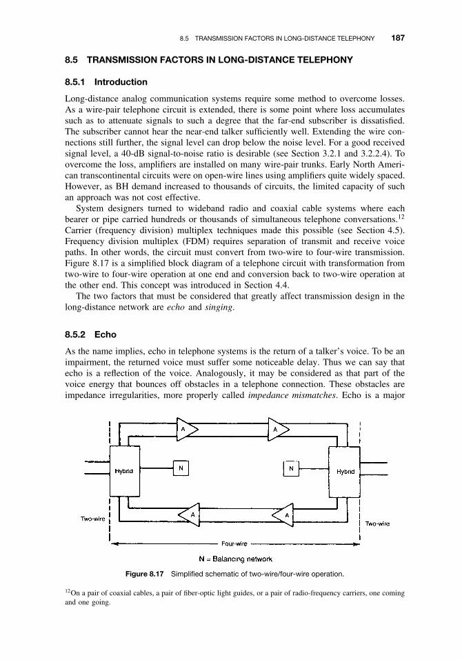
8.5 TRANSMISSION FACTORS IN LONG-DISTANCE TELEPHONY 187
8.5 TRANSMISSION FACTORS IN LONG-DISTANCE TELEPHONY
8.5.1 Introduction
Long-distance analog communication systems require some method to overcome losses.As a wire-pair telephone circuit is extended, there is some point where loss accumulatessuch as to attenuate signals to such a degree that the far-end subscriber is dissatisfied.The subscriber cannot hear the near-end talker sufficiently well. Extending the wire con-nections still further, the signal level can drop below the noise level. For a good receivedsignal level, a 40-dB signal-to-noise ratio is desirable (see Section 3.2.1 and 3.2.2.4). Toovercome the loss, amplifiers are installed on many wire-pair trunks. Early North Ameri-can transcontinental circuits were on open-wire lines using amplifiers quite widely spaced.However, as BH demand increased to thousands of circuits, the limited capacity of suchan approach was not cost effective.
System designers turned to wideband radio and coaxial cable systems where eachbearer or pipe carried hundreds or thousands of simultaneous telephone conversations.12
Carrier (frequency division) multiplex techniques made this possible (see Section 4.5).Frequency division multiplex (FDM) requires separation of transmit and receive voicepaths. In other words, the circuit must convert from two-wire to four-wire transmission.Figure 8.17 is a simplified block diagram of a telephone circuit with transformation fromtwo-wire to four-wire operation at one end and conversion back to two-wire operation atthe other end. This concept was introduced in Section 4.4.
The two factors that must be considered that greatly affect transmission design in thelong-distance network are echo and singing.
8.5.2 Echo
As the name implies, echo in telephone systems is the return of a talker’s voice. To be animpairment, the returned voice must suffer some noticeable delay. Thus we can say thatecho is a reflection of the voice. Analogously, it may be considered as that part of thevoice energy that bounces off obstacles in a telephone connection. These obstacles areimpedance irregularities, more properly called impedance mismatches. Echo is a major
Figure 8.17 Simplified schematic of two-wire/four-wire operation.
12On a pair of coaxial cables, a pair of fiber-optic light guides, or a pair of radio-frequency carriers, one comingand one going.

188 LOCAL AND LONG-DISTANCE NETWORKS
annoyance to the telephone user. It affects the talker more than the listener. Two factorsdetermine the degree of annoyance of echo: its loudness and the length of its delay.
8.5.3 Singing
Singing is the result of sustained oscillation due to positive feedback in telephone ampli-fiers or amplifying circuits. The feedback is the result of excessive receive signal feed-ing back through the hybrid to the transmit side, which is then amplified setting uposcillations. Circuits that sing are unusable and promptly overload multichannel carrier(FDM) equipment.
Singing may be regarded as echo that is completely out of control. This can occur atthe frequency at which the circuit is resonant. Under such conditions the circuit losses atthe singing frequency are so low that oscillation will continue, even after cessation of itsoriginal impulse.
8.5.4 Causes of Echo and Singing
Echo and singing can generally be attributed to the impedance mismatch between thebalancing network of a hybrid and its two-wire connection associated with the subscriberloop. It is at this point that we can expect the most likelihood of impedance mismatchwhich may set up an echo path. To understand the cause of echo, one of two possibleconditions may be expected in the local network:
1. There is a two-wire (analog) switch between the two-wire/four-wire conversionpoint and the subscriber plant. Thus, a hybrid may look into any of (say) 10,000different subscriber loops. Some of these loops are short, other are of mediumlength, and still others are long. Some are in excellent condition, and some are indreadful condition. Thus the possibility of mismatch at a hybrid can be quite highunder these circumstances.
2. In the more modern network configuration, subscriber loops may terminate in ananalog concentrator before two-wire/four-wire conversion in a PCM channel bank.The concentration ratio may be anywhere from 2:1 to 10:1. For example, in the10:1 case a hybrid may connect to any one of a group of ten subscriber loops. Ofcourse, this is much better than selecting any one of a population of thousands ofsubscriber loops as in condition 1, above.
Turning back to the hybrid, we can keep excellent impedance matches on the four-wireside; it is the two-wire side that is troublesome. So our concern is the match (balance)between the two-wire subscriber loop and the balancing network (N in Figure 8.17). If wehave a hybrid term set assigned to each subscriber loop, the telephone company (adminis-tration) could individually balance each loop, greatly improving impedance match. Suchactivity has high labor content. Secondly, in most situations there is a concentrator withfrom 4:1 to 10:1 concentration ratios (e.g., AT&T 5ESS).
With either condition 1 or condition 2 we can expect a fairly wide range of impedancesof two-wire subscriber loops. Thus, a compromise balancing network is employed to coverthis fairly wide range of two-wire impedances.
Impedance match can be quantified by return loss. The higher the return loss, the betterthe impedance match. Of course we are referring to the match between the balancingnetwork (N) and the two-wire line (L) (see Figure 8.17).
Return LossdB = 20 log10(ZN + ZL)/(ZN − ZL). (8.1)

8.5 TRANSMISSION FACTORS IN LONG-DISTANCE TELEPHONY 189
If the balancing network (N) perfectly matches the impedance of the two-wire line (L),then ZN = ZL, and the return loss would be infinite.13
We use the term balance return loss (Ref. 5) and classify it as two types:
1. Balance return loss from the point of view of echo.14 This is the return loss acrossthe band of frequencies from 300 to 3400 Hz.15
2. Balance return loss from the point of view of stability.16 This is the return lossbetween 0 and 4000 Hz.
“Stability” refers to the fact that loss in a four-wire circuit may depart from its nominalvalue for a number of reasons:
ž Variation of line losses and amplifier gains with time and temperature.ž Gain at other frequencies being different from that measured at the test frequency.
(This test frequency may be 800, 1000, or 1020 Hz.)ž Errors in making measurements and lining up circuits.
The band of frequencies most important in terms of echo for the voice channel isthat from 300 Hz to 3400 Hz. A good value for echo return loss for toll telephone plantis 11 dB, with values on some connections dropping to as low as 6 dB. For furtherinformation, the reader should consult CCITT Recs. G.122 and G.131 (Refs. 5, 6).
Echo and singing may be controlled by:
ž Improved return loss at the term set (hybrid).ž Adding loss on the four-wire side (or on the two-wire side).ž Reducing the gain of the individual four-wire amplifiers.
The annoyance of echo to a subscriber is also a function of its delay. Delay is a func-tion of the velocity of propagation of the intervening transmission facility. A telephonesignal requires considerably more time to traverse 100 km of a voice-pair cable facil-ity, particularly if it has inductive loading, than it requires to traverse 100 km of radiofacility (as low as 22,000 km/sec for a loaded cable facility and 240,000 km/sec for acarrier facility). Delay is measured in one-way or round-trip propagation time measuredin milliseconds. The CCITT recommends that if the mean round-trip propagation timeexceeds 50 msec for a particular circuit, an echo suppressor or echo canceler should beused. Practice in North America uses 45 msec as a dividing line. In other words, whereecho delay is less than that stated previously here, echo can be controlled by adding loss.
An echo suppressor is an electronic device inserted in a four-wire circuit that effec-tively blocks passage of reflected signal energy. The device is voice operated with asufficiently fast reaction time to “reverse” the direction of transmission, depending onwhich subscriber is talking at the moment. The block of reflected energy is carried outby simply inserting a high loss in the return four-wire path. Figure 8.18 shows the echopath on a four-wire circuit. An echo canceler generates an echo-canceling signal.17
13Remember, for any number divided by zero, the result is infinity.14Called echo return loss (ERL) in North America, but with a slightly different definition.15Recognize this as the CCITT definition of the standard analog voice channel.16From the point of view of stability—for this discussion, it may be called from the point of view of singing.17Echo canceler, as defined by CCITT, is a voice-operated device placed in the four-wire portion of a circuitand used for reducing near-end echo present on the send path by subtracting an estimation of that echo fromthe near-end echo (Ref. 7).

190 LOCAL AND LONG-DISTANCE NETWORKS
Figure 8.18 Echo paths in a four-wire circuit.
8.5.5 Transmission Design to Control Echo and Singing
As stated previously, echo is an annoyance to the subscriber. Figure 8.19 relates echopath delay to echo path loss. The curve in Figure 8.19 traces a group of points at whichthe average subscriber will tolerate echo as a function of its delay. Remember that thelonger the return signal is delayed, the more annoying it is to the telephone talker (i.e.,the more the signal has to be attenuated). For example, if the echo delay on a particularcircuit is 20 msec, an 11-dB loss must be inserted to make the echo tolerable to the talker.Be careful here. The reader should note that the 11 dB designed into the circuit to controlecho will increase the end-to-end loudness loss (see Section 3.2.2.4) an equal amount,which is quite undesirable. The effect of loss design on loudness ratings and the tradeoffsavailable are discussed in the paragraphs that follow.
If singing is to be controlled, all four-wire paths must have some amount of loss. Oncethey go into a gain condition, and we refer here to overall circuit gain, positive feedbackwill result and the amplifiers will begin to oscillate or “sing.” For an analog network,
Figure 8.19 Talker echo tolerance for average telephone users.

8.5 TRANSMISSION FACTORS IN LONG-DISTANCE TELEPHONY 191
North American practice called for a minimum of 4-dB loss on all four-wire circuitsto ensure against singing. CCITT recommends 10 dB for minimum loss on the nationalnetwork (Ref. 5, p. 3).
The modern digital network with its A/D (analog-to-digital) circuits in PCM channelbanks provides signal isolation, analog-to-digital, and digital-to-analog. As a result, theentire loss scenario has changed. This new loss plan for digital networks is described inSection 8.5.7.
8.5.6 Introduction to Transmission-Loss Engineering
One major aspect of transmission system design for a telephone network is to establisha transmission-loss plan. Such a plan, when implemented, is formulated to accomplishthree goals:
1. Control singing (stability).2. Keep echo levels within limits tolerable to the subscriber.3. Provide an acceptable overall loudness rating to the subscriber.
From preceding discussions we have much of the basic background necessary to developa transmission-loss plan. We know the following:
ž A certain minimum loss must be maintained in four-wire circuits to ensure againstsinging.
ž Up to a certain limit of round-trip delay, echo may be controlled by adding loss (i.e.,inserting attenuators, sometimes called pads).
ž It is desirable to limit these losses as much as possible, to improve the loudnessrating of a connection.
National transmission plans vary considerably. Obviously the length of a circuit is impor-tant, as well as the velocity of propagation of the transmission media involved.
Velocity of Propagation. A signal takes a finite amount of time to traverse frompoint A to point B over a specific transmission medium. In free space, radio signalstravel at 3 × 10⁸ m/sec or 186,000 mi/sec; fiber-optic light guide, about 2 × 10⁸ m/secor about 125,000 mi/sec; on heavily loaded wire-pair cable, about 0.22 × 10⁸ m/secor 14,000 mi/sec; and 19-gauge nonloaded wire-pair cable, about 0.8 × 10⁸ m/sec or50,000 mi/sec. So we see that the velocity of propagation is very dependent on the typesof transmission media being employed to carry a signal.
Distances covered by network connectivities are in hundreds or thousands of miles(or kilometers). It is thus of interest to convert velocities of propagation to miles orkilometers per millisecond. Let’s use a typical value for carrier (multiplex) systems of105,000 mi/sec or 105 mi/msec (169 km/msec).
First let’s consider a country of small geographic area such as Belgium, which couldhave a very simple transmission-loss plan. Assume that the 4-dB minimum loss for singingis inserted in all four-wire circuits. Based on Figure 8.19, a 4-dB loss will allow up to4 msec of round-trip delay. By simple arithmetic, we see that a 4-dB loss on all four-wire circuits will make echo tolerable for all circuits extending 210 mi (338 km) (i.e.,2 × 105). This could be an application of a fixed-loss type transmission plan. In the caseof small countries or telephone companies covering a rather small geographic expanse,the minimum loss to control singing controls echo as well for the entire system.

192 LOCAL AND LONG-DISTANCE NETWORKS
Let us try another example. Assume that all four-wire connections have a 7-dB loss.Figure 8.20 indicates that 7 dB permits an 11-msec round-trip delay. Again assume thatthe velocity of propagation is 105,000 mi/sec. Remember that we are dealing with round-trip delay. The talker’s voice reaches the far-end hybrid and some of the signal is reflectedback to the talker. This means that the signal traverses the system twice, as shown inFigure 8.20. Thus 7 dB of loss for the given velocity of propagation allows about 578 mi(925 km) of extension or, for all intents and purposes, the distance between subscribers,and will satisfy the loss requirements with a country of maximum extension of 578 mi(925 km).
It is interesting to note that the talker’s signal is attenuated only 7 dB toward thedistant-end listener; but the reflected signal is not only attenuated the initial 7 dB, butattenuated by 7 dB still again, on its return trip.
It has become evident by now that we cannot continue increasing losses indefinitelyto compensate for echo on longer circuits. Most telephone companies and administrationshave set a 45- or 50-msec round-trip delay criterion, which sets a top figure above whichecho suppressors are to be used. One major goal of the transmission-loss plan is toimprove overall loudness rating or to apportion more loss to the subscriber plant so thatsubscriber loops can be longer or to allow the use of less copper (i.e., smaller-diameterconductors). The question arises as to what measures can be taken to reduce losses andstill keep echo within tolerable limits. One obvious target is to improve return losses atthe hybrids. If all hybrid return losses are improved, the echo tolerance curve shifts; thisis because improved return losses reduce the intensity of the echo returned to the talker.Thus the talker is less annoyed by the echo effect.
One way of improving return loss is to make all two-wire lines out of the hybridlook alike—that is, have the same impedance. The switch at the other end of the hybrid(i.e., on the two-wire side) connects two-wire loops of varying length, thus causing theresulting impedances to vary greatly. One approach is to extend four-wire transmissionto the local office such that each hybrid can be better balanced. This is being carriedout with success in Japan. The U.S. Department of Defense has its Autovon (auto-matic voice network), in which every subscriber line is operated on a four-wire basis.Two-wire subscribers connect through the system via PABXs (private automatic branchexchanges).
As networks evolve to all-digital, four-wire transmission is carried directly through thelocal serving switch such that subscriber loops terminate through a hybrid directly to aPCM channel bank. Hybrid return losses could now be notably improved by adjustingthe balancing network for its dedicated subscriber loop.
Figure 8.20 Example of echo round-trip delay (5.5 + 5.5 = 11-msec round-trip delay).

REVIEW EXERCISES 193
8.5.7 Loss Plan for Digital Networks (United States)
For digital connections terminated in analog access lines, the required loss values aredependent on the connection architecture:
ž For interLATA or interconnecting network connections, the requirement is 6 dB.ž For intraLATA connections involving different LECs (local exchange carriers), 6 dB
is the preferred value, although 3 dB may apply to connections not involving atandem switch.
ž For intraLATA connections involving the same LEC, the guidelines are 0–6 dB(typically 0 dB, 3 dB, or 6 dB).
The choice of network loss value depends on performance considerations, administrativesimplicity, and current network design (Ref. 4).
Loss can be inserted in a digital bit stream by using a digital signal processor involvinga lookup table. By doing this, the bit sequence integrity is broken for each digital 8-bittime slot. Some of these time slots may be carrying data bit sequences. For this reasonwe cannot break up this bit integrity. To avoid this intermediate digital processing (whichdestroys bit integrity), loss is inserted on all-digital connections on the receiving end only,where the digital-to-analog conversion occurs (i.e., after the signal has been returned to itsanalog equivalent). Devices such as echo cancelers, which utilize digital signal processing,need to have the capability of being disabled when necessary, to preserve bit integrity.
In Section 8.5.6 round-trip delay was brought about solely by propagation delay. Indigital networks there is a small incremental delay due to digital switching and digitalmultiplexing. This is due to buffer storage delay, more than anything else.
REVIEW EXERCISES
1. Name at least three factors that affect local network design.
2. What are the three basic underlying considerations in the design of a long-distance(toll) network?
3. What is the fallacy of providing just one high-capacity trunk group across theUnited States to serve all major population centers by means of tributaries off themain trunk?
4. How can the utilization factor on trunks be improved?
5. For long-distance (toll) switching centers, what is the principal factor in the place-ment of such exchanges (differing from local exchange placement substantially)?
6. How are the highest levels of a national hierarchical network connected, and whyis this approach used?
7. On a long-distance toll connection, why must the number of links in tandem belimited?
8. What type of routing is used on the majority of international connections?
9. Name two principal factors used in deciding how many and where long-distance(toll) exchanges will be located in a given geographic area.
10. Discuss the impacts of fan-outs on the number of hierarchical levels.

194 LOCAL AND LONG-DISTANCE NETWORKS
11. Name the three principal bases required at the outset for the design of a long-distance network.
12. Once the hierarchical levels have been established and all node locations identified,what is assembled next?
13. Define a final route.
14. A grade of service no greater than % per link is recommended on a final route.
15. There are two generic types of routing schemes. What are they?
16. Name three different types of dynamic routing and explain each in one sentence.
17. What is crankback?
18. Give an example of state-dependent routing.
19. What is the principal cause of echo in the telephone network?
20. What causes singing in the telephone network?
21. Differentiate balance return loss from the point of view of stability (singing) fromecho return loss.
22. How can we control echo? (Two answers required).
23. The stability of a telephone connection depends on three factors. Give two ofthese factors.
24. Based on the new loss plan for North America for the digital network, how muchloss is inserted for interLATA connections?
REFERENCES
1. International Telephone Routing Plan , CCITT Rec. E.171, Vol. II, Fascicle II.2, IXth PlenaryAssembly, Melbourne, 1988.
2. The Transmission Plan , ITU-T Rec. G.101, ITU Geneva, 1994.
3. Traffic Routing , CCITT Rec. E.170, ITU Geneva, 1992.
4. BOC Notes on the LEC Networks—1994 , Special Report SR-TSV-002275, Issue 2, Bellcore,Piscataway, NJ, 1994.
5. Influence of National Systems on Stability and Talker Echo in International Connections , ITU-TRec. G.122, ITU Geneva, 1993.
6. Control of Talker Echo, ITU-T Rec. G.131, ITU Geneva, 1996.
7. Terms and Definitions , CCITT Rec. B.13, Fascicle I.3, IXth Plenary Assembly, Melbourne, 1988.

9
CONCEPTS IN TRANSMISSIONTRANSPORT
9.1 OBJECTIVE
A telecommunication network consists of customer premise equipment (CPE), switch-ing nodes, and transmission links as illustrated in Figure 9.1. Chapter 5 dealt with oneimportant type of CPE, namely the telephone subset. The chapter also covered wire-pair connectivity from the telephone subset to the local serving switch over a subscriberloop. Basic concepts of switching were reviewed in Chapter 4, and Chapter 6 covereddigital switching. In this chapter we introduce the essential aspects for the design oflong-distance links.
There are four different ways by which we can convey signals from one switchingnode to another:
1. Radio2. Fiber optics3. Coaxial cable4. Wire pair
Emphasis will be on radio and fiber optics. The use of coaxial cable for this application isdeprecated. However, it was widely employed from about 1960 to 1985 including somevery-high-capacity systems. One such system (L5) crossed the United States from coastto coast with a capacity in excess of 100,000 simultaneous full-duplex voice channels
Node
CPE CPE
Node NodeLink Link
Figure 9.1 A telecommunication network consists of customer premise equipment (CPE), switchingnodes, and interconnecting transmission links.
Fundamentals of Telecommunications, Second Edition, by Roger L. FreemanISBN 0-471-71045-8 Copyright 2005 by Roger L. Freeman
195

196 CONCEPTS IN TRANSMISSION TRANSPORT
in FDM configurations (see Section 4.5.2). Fiber-optic cable has replaced the greaterportion of these coaxial cable systems. There is one exception. Coaxial cable is stillwidely employed in cable television configurations (see Chapter 17). Wire pair remainsthe workhorse in the subscriber plant.
At the outset, we assume that these transmission links are digital and will be basedon the PCM configurations covered in Chapter 6, namely, either of the DS1 (T1) or E1families of formats. However, the more advanced, higher-capacity digital formats suchas synchronous optical network (SONET) or synchronous digital hierarchy (SDH) (seeChapter 19) are now being widely deployed on many, if not most, new fiber-optic systems,and with lower-capacity configurations on certain radio systems.
9.2 RADIO SYSTEMS
9.2.1 Scope
The sizes, capacities, ranges, and operational frequency bands for radio systems varygreatly. Our discussion will be limited to comparatively high-capacity systems. Onlytwo system types meet the necessary broadband requirements of the long-distance net-work. These are line-of-sight (LOS) microwave and satellite communications. Satellitecommunications is really nothing more than an extension of LOS microwave.
9.2.2 Introduction to Radio Transmission
Wire, cable, and fiber are well-behaved transmission media, and they display little vari-ability in performance. The radio medium, on the other hand, displays notable variabilityin performance. The radio-frequency spectrum is shared with others and requires licens-ing. Metallic and fiber media need not be shared and do not require licensing (but oftenrequire right-of-way).
A major factor in the selection process is information bandwidth. Fiber optics seemsto have nearly an infinite bandwidth. Radio systems have very limited information band-widths. It is for this reason that radio-frequency bands 2 GHz and above are used forPSTN and private network applications. In fact, the U.S. Federal Communications Com-mission (FCC) requires that users in the 2-GHz band must have systems supporting 96digital voice channels where bandwidths are still modest. In the 4- and 6-GHz bands,available bandwidths are 500 MHz, allocated in 20- and 30-MHz segments for eachradio-frequency carrier.
One might ask, Why use radio in the first place if it has so many drawbacks? Often, itturns out to be less expensive compared with fiber-optic cable. But there are other factorssuch as
ž No requirement for right-of-wayž Less vulnerable to vandalismž Not susceptible to “accidental” cutting of the linkž Often more suited to crossing rough terrainž Often more practical in heavily urbanized areasž As a backup to fiber-optic cable links
Fiber-optic cable systems provide strong competition with LOS microwave, but LOSmicrowave does have a place and a good market.

9.2 RADIO SYSTEMS 197
Satellite communications is an extension of LOS microwave. It is also feeling the“pinch” of competition from fiber-optic systems. It has two drawbacks. First, of course, islimited information bandwidth. The second is excessive delay when the popular geosta-tionary satellite systems are utilized. It also shares frequency bands with LOS microwave.
One application showing explosive growth is very small aperture terminal (VSAT)systems. It is very specialized and has great promise for certain enterprise networks, andthere are literally thousands of these networks now in operation.
Another application that has promise of wide deployment is large families of lowearth orbit (LEO) satellites. Motorola developed and fielded Iridium that could provideworldwide cellular/PCS coverage. Because of LEO’s low-altitude orbit (about 785 kmabove the earth’s surface), the notorious delay problem typical of GEO (geostationarysatellite) is nearly eliminated. Iridium worked perfectly. It was the marketing effort thatfailed. The system was sold at a fire sale at pennies on the dollar. Our opinion is thatIridium was too early for its time.
9.2.3 Line-of-Sight Microwave
9.2.3.1 Introduction. Line-of-sight (LOS) microwave provides a comparative broad-band connectivity over a single link or a series of links in tandem. We must be careful onthe use of language here. First a link, in the sense we use it, connects one radio terminal toanother or to a repeater site. The term link was used in Figure 9.1 in the “network” sense.Figure 9.2 illustrates the meaning of a “link” in line-of-sight microwave. Care must alsobe taken with the use of the expression line-of-sight. Because we can “see” a distant LOSmicrowave antenna does not mean that line-of-sight clearance has been complied with.
We can take advantage of this “line-of-sight” phenomenon at frequencies from about150 MHz well into the millimeter-wave region.1 Links can be up to 30 miles long, depend-ing on terrain topology. I have engineered some links well over 100 miles long. In fact,links with geostationary satellites can be over 23,000 miles long.
On conventional LOS microwave links, the length of a link is a function of antennaheight. The higher the antenna, the further the reach. Let us suppose smooth earth. Thismeans an earth surface with no mountains, ridges, buildings, or sloping ground what-so-ever. We could consider an overwater path as a smooth earth path. Some paths on theNorth American prairie approach smooth earth. In the case of smooth earth, the LOSdistance from an antenna is limited by the horizon. Given an LOS microwave antennaof hft or h′
m above ground surface, the distance dmi or dkm to the horizon just where the
Figure 9.2 A sketch of an LOS microwave radio relay system.
1Millimeter-wave region is where the wavelength of an equivalent frequency is less than 1 cm (i.e., >30 GHz).

198 CONCEPTS IN TRANSMISSION TRANSPORT
ray beam from the transmitting antenna will graze the rounded surface of the horizon canbe calculated using one of the formulas given below:
To the optical horizon (k = 1):
d =√
3h
2(9.1a)
and to the radio horizon (k = 4/3):
d = √2h, (9.1b)
d ′ = 2.9(2h′)1/2, (9.1c)
where k expresses the bending characteristic of the path.These formulas should only be used for rough estimates of distance to the horizon
under smooth earth conditions. As we will find out later, the horizon clearance must besomething greater (n feet or meters) of grazing. The difference between formulas (9.1a)and (9.1b) and (9.1c) is that formula (9.1a) is “true” line-of-sight and expresses the opticaldistance. Here the radio ray beam follows a straight line. Under most circumstances themicrowave ray beam is bent toward the earth because of characteristics of the atmosphere.This is expressed in formulas (9.1b) and (9.1c), and it assumes the most common bendingcharacteristic. Figure 9.3 is a model that may be used for formulas (9.1). It also showsthe difference between the optical distance to the horizon and the radio distance tothe horizon.
The design of an LOS microwave link involves five basic steps:
1. Setting performance requirements.2. Site selection and the preparation of a path profile to determine antenna tower
heights.3. Carrying out a path analysis, often called a link budget. Here is where we dimension
equipment to meet the performance requirements set in step 1.4. Physically running a path/site survey.5. Installation of equipment and test of the system prior to cutting it over to carry traffic.
In the following paragraphs we review the first four steps.
9.2.3.2 Setting Performance Requirements. As we remember from Chapter 6, theperformance of a digital system is expressed in a bit error rate (bit error ratio) (BER).In our case here, it will be expressed as a BER with a given time distribution. A time
d
h
Figure 9.3 Radio and optical horizon (smooth earth).

9.2 RADIO SYSTEMS 199
distribution tells us that a certain BER value is valid for a certain percentage of time,percentage of a year, or percentage of a month.
Often a microwave link is part of an extensive system of multiple links in tandem.Thus we must first set system requirements based on the output of the far-end receiverof the several or many links in tandem. If the system was transmitting in an analogformat, typically FDM using frequency modulation (FM), the requirement would be givenfor noise in the derived voice channel; if it were analog video, a signal-to-noise ratiospecification would be provided. In the case we emphasize here, of course it will be BERor a derivative unit such as errored second (ES) on the far-end receiver digital bit stream.
The requirements should be based on existing standards. If the link (or system) wereto be designed as part of the North American PSTN, we would use a Bellcore2 standard(Ref. 1). In this case the BER at the digital interface level shall be less than 2 × 10⁻¹⁰,excluding burst error seconds. Another source is CCIR/ITU-R. For example CCIR Rec.594-4 (Ref. 2) states that the errored second ratio (ESR) should not exceed 0.0032 of anymonth. The ESR is defined in this reference as the ratio of errored seconds (ES) to totalseconds in available time during a fixed measurement interval. These specifications areconsiderably more stringent than in previous editions of the reference, the more stringentvalue being driven by demands of data users. Available time in this context is defined inthe context of “unavailable time” as follows:
A period of unavailable time begins when the bit error ratio (BER) in each second is worsethan 1 × 10⁻³ for a period of 10 consecutive seconds. These 10 seconds are considered tobe unavailable time. A new period of available time begins with the first second of a periodof 10 consecutive seconds, each of which has a BER better than 10−3 (Ref. 2).
A common time distribution is 99.99% of a month to be in conformance with ITU-R/CCIR recommendations (ESR should not exceed 0.0032 of any month). This timedistribution translates directly into time availability, which is the percentage of time alink meets its performance criteria regarding propagation.
9.2.3.3 Site Selection and Preparation of a Path Profile9.2.3.3.1 Site Selection. In this step we will select operational site where we willinstall and operate radio equipment. After site selection, we will prepare a path profileof each link to determine the heights of radio towers to achieve “line of sight.” Sites areselected using large topographical maps. If we are dealing with a long system crossinga distance of hundreds of miles or kilometers, we should minimize the number of sitesinvolved. There will be two terminal sites, where the system begins and ends. Along theway, repeater sites will be required. At some repeater sites, we may have need to drop andinsert traffic. Other sites will just be repeaters. This concept is illustrated in Figure 9.4.The figure shows the drops and inserts (also called add–drops) of traffic at telephoneexchanges. These drop and insert points may just as well be buildings or other facilitiesin a private/corporate network. There must be considerable iteration between site selectionand path profile preparation to optimize the route.
In essence, the sites selected for drops and inserts will be points of traffic concentration.There are several tradeoffs to be considered:
1. Bringing traffic in by wire or cable rather than adding additional drop and insert(add–drop) capabilities at relay point. This provides additional traffic concentration.
2Bellcore, Bell Communications Research, Piscataway, NJ. Now called Telcordia.

200 CONCEPTS IN TRANSMISSION TRANSPORT
Figure 9.4 Simplified functional block diagram of the LOS microwave system shown in Figure 9.2.
2. Siting based on propagation advantages (or constraints) only versus colocation withexchange (or corporate facility) (saving money for land and buildings).
3. Choosing a method of feeding (feeders3): by light-route radio, fiber-optic cable, andwire-pair cable.
9.2.3.3.2 Calculation of Tower Heights. LOS microwave antennas are mounted ontowers. Formulas (9.1) allowed us to calculate a rough estimate of tower height. Towersand their installation are one of the largest cost factors in the provision and installationof an LOS microwave system. We recommend that actual tower heights do not exceed300 ft (∼90 m); otherwise, additional expense will be required so that the tower meetstwist and sway requirements. Of course, the objective is to keep the tower height as low aspossible and still maintain effective communication. The towers must be just high enoughto surmount obstacles in the path. High enough must be carefully defined. What sort ofobstacles might we encounter in the path? To name some: terrain such as mountains,ridges, hills, and earth curvature—which is highest at midpath—and buildings, towers,grain elevators, and so on. The path designer should consider using natural terrain suchas hill tops for terminal/relay sites. She/he should also consider leasing space on the topof tall buildings or on TV broadcast towers. In the following paragraphs we review amanual method of plotting a path profile.
From a path profile we can derive tower heights. Path profiles may be prepared by aPC with a suitable program and the requisite topological data for the region stored ona disk.
3Here the word feeders refers to feeding a mainline trunk radio systems. Feeders may also be called spurs.

9.2 RADIO SYSTEMS 201
Our recommendation is to use ordinary rectangular graph paper such as “millimeter”paper or with gradations down to one-sixteenth of an inch or better. “B-size” is suggested.There are seven steps required to prepare a path profile:
1. Obtain good topo(logical) maps of the region, at least 1:62,500 and identify thetwo sites involved, which arbitrarily we call one a “transmit” site and the other a“receive” site.
2. Draw a straight line with a long straight edge connecting the two sites identified.3. Follow along down the line identifying obstacles and their height. Put this informa-
tion on a table, labeling the obstacles “A,” “B,” and so on.4. Calculate earth curvature (or earth bulge) (EC). This is maximum at midpath. On
the same table in the next column write the earth curvature value for each obstacle.5. Calculate the Fresnel zone clearance for each obstacle. The actual value here will
be 0.6 of the first Fresnel zone.6. Add a value of additional height for vegetation such as trees; add a growth factor
as well (10 feet or 3 meters if actual values are unavailable).7. Draw a straight line from left to right connecting the two highest obstacle locations
on the profile. Do the same from right to left. Where this line intersects the verticalextension of the transmit site and the vertical extension of the receive site definestower heights.
In step 4, the calculation of EC, remember that the earth is a “sphere.” Our path is a tinyarc on that sphere’s surface. Also, in this calculation, we must account for the radio raypath bending. To do this we use a tool called K-factor. When the K-factor is greater than1, the ray beam bends toward the earth, as illustrated in Figure 9.3. When the K-factoris less than 1, the ray beam bends away from the earth.
The EC value (h) is the amount we will add to the obstacle height in feet or meters toaccount for that curvature or bulge. The following two formulas apply:
hft = 0.667d1d2/K (d in miles) (9.2a)
hm = 0.078d1d2/K (d in km) (9.2b)
where d1 is the distance from the “transmit” site to the obstacle in question and d2 is thedistance from that obstacle to the receive site.
Table 9.1 is a guide for selecting the K-factor value. For a more accurate calculationof the K-factor, consult Ref. 3. Remember that the value obtained from Eq. (9.2) is to beadded to the obstacle height.
In step 5, calculation of the Fresnel zone clearance, 0.6 of the value calculated isadded to the obstacle height in addition to earth curvature. It accounts for the expandingproperties of a ray beam as it passes over an obstacle. Use the following formulas tocalculate Fresnel zone (radius) clearance
Rft = 72.1
√d1d2
FD, (9.3a)
where F is the frequency in gigahertz, d1 is the distance from transmit antenna to obstacle(statute miles), d2 is the distance from path obstacle to receive antenna (statute miles),and D = d1 + d2. For metric units:
Rm = 17.3
√d1d2
FD, (9.3b)

202 CONCEPTS IN TRANSMISSION TRANSPORT
Table 9.1 K-Factor Guidea
Propagation Conditions
Perfect Ideal Average Difficult Bad
Weather Standardatmosphere
No surfacelayers or fog
Substandard,light log
Surface layers,ground fog
Fog moistureover water
Typical Temperate zone,no fog, noducting, goodatmosphericmix day andnight
Dry,mountainous,no fog
Flat, temperate,some fog
Coastal Coastal, water,tropical
K factor 1.33 1–1.33 0.66–1.0 0.66–0.5 0.5–0.4
aFor 99.9 to 99.99% time availability.
where F is the frequency (the microwave transmitter operating frequency) in gigahertz,and d1, d2, and D are now in kilometers with R in meters.
The three basic increment factors that must be added to obstacle heights are nowavailable: earth curvature (earth bulge), Fresnel zone clearance, and trees and growth(T&G). These are marked on the path profile chart. On the chart a straight line is drawnfrom right to left just clearing the obstacle points as corrected for the three factors.Another, similar line is drawn from left to right. A sample profile is shown in Figure 9.5.
Figure 9.5 Practice path profile. (The x-axis is in miles, the y-axis is in feet; assume that K = 0.9; EC isthe earth curvature and F is the dimension of the first Fresnel zone.)
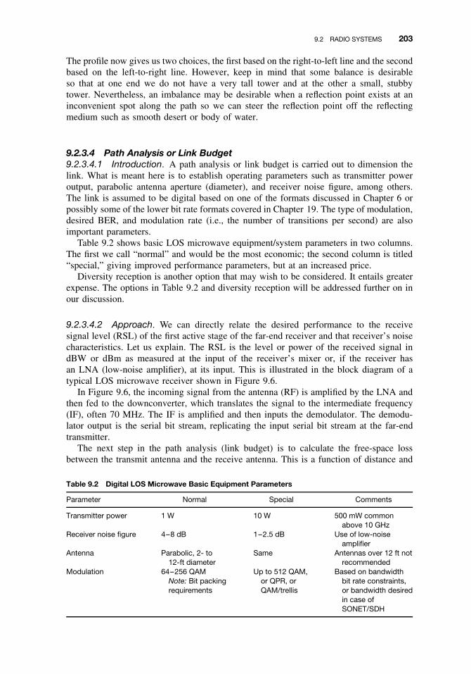
9.2 RADIO SYSTEMS 203
The profile now gives us two choices, the first based on the right-to-left line and the secondbased on the left-to-right line. However, keep in mind that some balance is desirableso that at one end we do not have a very tall tower and at the other a small, stubbytower. Nevertheless, an imbalance may be desirable when a reflection point exists at aninconvenient spot along the path so we can steer the reflection point off the reflectingmedium such as smooth desert or body of water.
9.2.3.4 Path Analysis or Link Budget9.2.3.4.1 Introduction. A path analysis or link budget is carried out to dimension thelink. What is meant here is to establish operating parameters such as transmitter poweroutput, parabolic antenna aperture (diameter), and receiver noise figure, among others.The link is assumed to be digital based on one of the formats discussed in Chapter 6 orpossibly some of the lower bit rate formats covered in Chapter 19. The type of modulation,desired BER, and modulation rate (i.e., the number of transitions per second) are alsoimportant parameters.
Table 9.2 shows basic LOS microwave equipment/system parameters in two columns.The first we call “normal” and would be the most economic; the second column is titled“special,” giving improved performance parameters, but at an increased price.
Diversity reception is another option that may wish to be considered. It entails greaterexpense. The options in Table 9.2 and diversity reception will be addressed further on inour discussion.
9.2.3.4.2 Approach. We can directly relate the desired performance to the receivesignal level (RSL) of the first active stage of the far-end receiver and that receiver’s noisecharacteristics. Let us explain. The RSL is the level or power of the received signal indBW or dBm as measured at the input of the receiver’s mixer or, if the receiver hasan LNA (low-noise amplifier), at its input. This is illustrated in the block diagram of atypical LOS microwave receiver shown in Figure 9.6.
In Figure 9.6, the incoming signal from the antenna (RF) is amplified by the LNA andthen fed to the downconverter, which translates the signal to the intermediate frequency(IF), often 70 MHz. The IF is amplified and then inputs the demodulator. The demodu-lator output is the serial bit stream, replicating the input serial bit stream at the far-endtransmitter.
The next step in the path analysis (link budget) is to calculate the free-space lossbetween the transmit antenna and the receive antenna. This is a function of distance and
Table 9.2 Digital LOS Microwave Basic Equipment Parameters
Parameter Normal Special Comments
Transmitter power 1 W 10 W 500 mW commonabove 10 GHz
Receiver noise figure 4–8 dB 1–2.5 dB Use of low-noiseamplifier
Antenna Parabolic, 2- to12-ft diameter
Same Antennas over 12 ft notrecommended
Modulation 64–256 QAMNote: Bit packingrequirements
Up to 512 QAM,or QPR, orQAM/trellis
Based on bandwidthbit rate constraints,or bandwidth desiredin case ofSONET/SDH

204 CONCEPTS IN TRANSMISSION TRANSPORT
Figure 9.6 Simplified block diagram of an LOS microwave receiver. RF is radio frequency; IF isintermediate frequency; LNA is low-noise amplifier. Point A is used to measure RSL when and LNAis employed, which is optional. Otherwise, the measurement point is point B, at the input of thedownconverter.
frequency (i.e., the microwave transmitter operational frequency). We then calculate theEIRP (effective isotropically radiated power) at the transmit antenna. The EIRP (in dBm ordBW, Appendix C) is the sum of the transmitter power output, minus the transmission linelosses plus the antenna gain, all in decibel units. The units of power must be consistent,either in dBm or dBW. If the transmitter power is in dBW, the EIRP will be in dBW andthe distant-end RSL must also be in dBW.
We then algebraically add the EIRP to the free-space loss in dB (often called pathloss), the result is the isotropic4 receive level (IRL). When we add the receive antennagain to the IRL and subtract the receive transmission line losses, we get the receive signallevel (RSL). This relationship of path losses and gains is illustrated in Figure 9.7.
Figure 9.7 LOS microwave link gains and losses (simplified). Transmitter power output is 1 W or 0 dBW.
4An isotropic antenna is an antenna that is uniformly omnidirectional and thus, by definition, it has a 0-dB gain.It is a hypothetical reference antenna. The isotropic receive level (IRL) is the power level we would expect toachieve at that point using an isotropic antenna.

9.2 RADIO SYSTEMS 205
Path Loss. For operating frequencies up to about 10 GHz, path loss is synonymouswith free-space loss. This represents the steady decrease of power flow as the waveexpands out in space in three dimensions. The formula for free-space loss is
LdB = 96.6 + 20 log10 F + 20 log10 D, (9.4a)
where L is the free-space loss between isotropic antennas, F is measured in GHz, and D
is in statute miles. In the metric system
LdB = 92.4 + 20 log FGHz + 20 log Dkm, (9.4b)
where D is in kilometers.Calculation of EIRP. Effective isotropically radiated power is calculated by adding
decibel units: transmitter power (in dBm or dBW), the transmission line losses in dB (anegative value because it is a loss), and the antenna gain in dBi.5
EIRPdBW = trans. output powerdBW − trans. line lossesdB + ant.gaindB. (9.5)
Figure 9.8 shows this concept graphically.
Example. If a microwave transmitter has 1 W (0 dBW) of power output, the waveguideloss is 3 dB and the antenna gain is 34 dBi, what is the EIRP in dBW?
EIRP = 0 dBW − 3 dB + 34 dBi
= +31 dBW.
Calculation of Isotropic Receive Level (IRL). The IRL is the RF power level impingingon the receive antenna. It would be the power we would measure at the base of an isotropicreceive antenna.
IRLdBW = EIRPdBW − Path lossdB. (9.6)
This calculation is shown graphically in Figure 9.9.Calculation of Receive Signal Level (RSL). The receive signal level (RSL) is the power
level at the input port of the first active stage in the receiver. The power level is conven-tionally measured in dBm or dBW.
RSLdBW = IRLdBW + rec. ant. gain (dB) − rec. trans. line losses (dB). (9.7)
(Note: Power levels can be in dBm as well, but we must be consistent.)
Figure 9.8 Elements in the calculation of EIRP.
5dBi stands for decibels referenced to an isotropic (antenna).

206 CONCEPTS IN TRANSMISSION TRANSPORT
Figure 9.9 Calculation of isotropic receive level (IRL).
Example. Suppose the IRL was −121 dBW, the receive antenna gain was 31 dB, andthe line losses were 5.6 dB. What would the RSL be?
RSL = −121 dBW + 31 dB − 5.6 dB
= −95.6 dBW.
Calculation of Receiver Noise Level. The thermal noise level of a receiver is a functionof the receiver noise figure and its bandwidth. For analog radio systems, receiver thermalnoise level is calculated using the bandwidth of the intermediate frequency (IF). Fordigital systems, the noise level of interest is in only 1 Hz of bandwidth using the notationN0, the noise level in a 1-Hz bandwidth.
The noise that a device self-generates is given by its noise figure (dB) or a noise tem-perature value. Any device, even passive devices, above absolute zero generates thermalnoise. We know the thermal noise power level in a 1-Hz bandwidth of a perfect receiveroperating at absolute zero. It is
Pn = −228.6 dBW/Hz, (9.8)
where Pn is the noise power level. Many will recognize this as Boltzmann’s constantexpressed in dBW.
We can calculate the thermal noise level of a perfect receiver operating at room tem-perature using the following formula:
Pn = −228.6 dBW/Hz + 10 log 290 (K)
= −204 dBW/Hz. (9.9)
The value, 290 K (kelvins), is room temperature, or about 17◦C or 68◦F.Noise figure simply tells us how much noise has been added to a signal while passing
through a device in question. Noise figure (dB) is the difference in signal-to-noise ratiobetween the input to the device and the output of that same device.
We can convert noise figure to noise temperature in kelvins with the following formula:
NFdB = 10 log(1 + Te/290), (9.10)
where Te is the effective noise temperature of a device. Suppose the noise figure of adevice is 3 dB. What is the noise temperature?
3 dB = 10 log(1 + Tc/290),
0.3 = log(1 + Tc/290),
1.995 = 1 + Te/290.

9.2 RADIO SYSTEMS 207
We round 1.995 to 2; thus
2 − 1 = Te/290,
Te = 290 K.
The thermal noise power level of a device operating at room temperature is
Pn = −204 dBW/Hz + NFdB + 10 log BWHz, (9.11)
where BW is the bandwidth of the device in Hz.
Example. A microwave receiver has a noise figure of 8 dB and its bandwidth is 10 MHz.What is the thermal noise level (sometimes called the thermal noise threshold)?
Pn = −204 dBW/Hz + 8 dB + 10 log(10 × 106)
= −204 dBW/Hz + 8 dB + 70 dB
= −126 dBW.
Calculation of Eb/N0 in Digital Radio Systems. In Section 3.2.1 signal-to-noise ratio(S/N) was introduced. S/N is widely used in analog transmission systems as one measureof signal quality. In digital systems the basic measure of transmission quality is BER.With digital radio links, we will introduce and employ the ratio Eb/N0 as a measure ofsignal quality. Given a certain modulation type, we can derive BER from an Eb/N0 curve.
In words, Eb/N0 means energy per bit per noise spectral density ratio. N0 is simplythe thermal noise in 1 Hz of bandwidth or
N0 = −204 dBW/Hz + NFdB. (9.12)
NF, as defined above, is the noise figure of the receiver in question. The noise figure tellsus the amount of thermal noise a device injects into a radio system.
Example. Suppose a receiver has a noise figure of 2.1 dB, what is its thermal noise levelin 1 Hz of bandwidth. In other words, what is N0?
N0 = −204 dBW + 2.1 dB
= −201.9 dBW/Hz.
Eb is the signal energy per bit. We apply this to the receive signal level (RSL). The RSLrepresents the total power (in dBm or dBW) entering the receiver front end, during, let’ssay, 1-sec duration. (energy). We want the power carried by just 1 bit. For example, ifthe RSL were 1 W and the signal were at 1000 bps, the energy per bit would be 1/1000or 1 mW per bit. However, it will be more convenient here to use logarithms and decibelvalues (which are logarithmic). Then we define Eb as
Eb = RSLdBm or dBW − 10 log(bit rate) (9.13)
Here is an example using typical values. The RSL into a certain receiver was −89 dBWand bit rate was 2.048 Mbps. What is the value of Eb?

208 CONCEPTS IN TRANSMISSION TRANSPORT
Eb = −89 dBW − 10 log(2.048 × 10⁶)
= −89 dBW − 63.11 dB
= −152.11 dBW
We can now develop a formula for Eb/N0:
Eb/N0 = RSLdBW − 10 log(bit rate) − (−204 dBW + NFdB). (9.14)
Simplifying, we obtain
Eb/N0 = RSLdBW − 10 log(bit rate) + 204 dBW − NFdB. (9.15)
Some Notes on Eb/N0 and Its Use. Eb/N0, for a given BER, will be different fordifferent types of modulation (e.g., FSK, PSK, QAM, etc.). When working with Eb, wedivide RSL by the bit rate, not the symbol rate nor the baud rate. There is a theoreticalEb/N0 and a practical Eb/N0. The practical is always a greater value than the theoretical,greater by the modulation implementation loss in decibels, which compensates for systemimperfections.
Figure 9.10 is an example of where BER is related to Eb/N0. There are two curves inthe figure. The first from the left is for BPSK/QPSK (binary phase shift keying/quadraturephase shift keying), and the second is for 8-ary PSK (an eight-level PSK modulationscheme). The values are for coherent detection. Coherent detection means that the receiverhas a built-in phase reference as a basis to make its binary or higher level decisions.
9.2.3.5 Digital Modulation of LOS Microwave Radios. Digital systems, typicallystandard PCM as discussed in Chapter 6, are notoriously wasteful of bandwidth comparedto their analog counterparts.6 For example, the analog voice channel is nominally of 4-kHz bandwidth, whereas the digital voice channel requires a 64-kHz bandwidth, assuming1-bit/Hz occupancy. This is a 16-to-1 difference in required bandwidth. Thus nationalregulatory authorities, such as the U.S. FCC, require that digital systems be bandwidthconservative. One means that is used to achieve bandwidth conservation is bit packing.This means packing more bits into 1 Hz of bandwidth. Another driving factor for bitpacking is the need to transmit such higher bit rate formats such as SONET and SDH(Chapter 19). Some radio systems can transmit as much as 622 Mbps using advancedbit-packing techniques.
How Does Bit Packing Work? In the binary domain we can estimate bandwidth toapproximately equate to 1 bit/Hz. For example, if we were transmitting at 1.544 Mbps,following this premise, we’d need 1.544 MHz of bandwidth. Suppose now that we turnto higher levels of modulation. Quadrature phase shift keying is one example. In this casewe achieve a theoretical packing of 2 bits/Hz. Again, if we are transmitting 1.544 Mbps,with QPSK we would need 1.544 MHz/2 or 0.772 MHz. QPSK is one of a family ofmodulation schemes that are based on phase-shift keying (PSK). With binary PSK, wemight assign a binary 1 to the 0◦ position (i.e., no phase retardation) and a binary 0 to the180◦ phase retardation point. For QPSK, the phase circle is broken up into 90◦ segments,rather than 180◦ segments as we did with binary PSK. In this case, for every transition wetransmit 2 bits at a time. Figure 9.11 is a functional block diagram of a QPSK modulator.It really only consists of two BPSK modulators where one is out of phase with the otherby 90◦.
6A cogent example is FDM using frequency modulation; another is single sideband modulation.

9.2 RADIO SYSTEMS 209
Figure 9.10 Bit error probability (BER) versus Eb/N0 performance for BPSK/QPSK and 8-ary PSK(octal PSK).
Eight-ary PSK modulation is not uncommon. In this case the phase circle is broken upinto 45◦ phase segments. Now for every transition, 3 bits at a time are transmitted. Thebit packing in this case is 3 bits/Hz theoretical.
Now add two amplitude levels to this, making a hybrid waveform covering bothamplitude modulation as well as phase modulation. This family of waveforms is calledquadrature-amplitude modulation (QAM). For example, 16-QAM has 16 different statepossibilities; eight are derived for 8-ary PSK and two are derived from the two amplitudelevels. We’d call this 16-QAM, where for each state transition 4 bits are transmitted atonce. The bit packing in this case is theoretically 4 bits/Hz. Certain digital LOS microwavesystem use 256-QAM and 512-QAM, theoretically achieving 8 and 9 bits/Hz of bit pack-ing. The difference between theoretical bit packing and the practical deals with filterdesign. For QAM-type waveforms, depending on design, practical bit packing may vary

210 CONCEPTS IN TRANSMISSION TRANSPORT
Figure 9.11 Conceptual block diagram of a QPSK modulator. Note that these are two BPSK modulatorsworking jointly, and one modulator is 90◦ out of phase with the other. The first bit in the bit stream isdirected to the upper modulator, the second to the lower, the third to the upper, and so on.
Figure 9.12 A 16-QAM state diagram. I stands for in-phase, Q stands for quadrature.
the baud-rate bandwidth from 1.25 to 1.5. The extra bandwidth required provides a filterwith spectral space to roll-off. In other words, a filter’s skirts are not perfectly vertical.Figure 9.12 is a space diagram for 16-QAM. The binary values for each of the 16 statesare illustrated.
Suppose we are using a 48-Mbps bit stream to input to our transmitter, which was using16-QAM modulation. Its baud rate, which measures transitions per second, would be 48/4megabauds/sec. If we allowed 1 baud/Hz, then a 12-MHz bandwidth would be required. Ifwe used a roll-off factor of 1.5, then the practical bandwidth required would be 18 MHz.Carry this one step further to 64-QAM. Here the theoretical bit packing is 6 bits/Hz, andfor the 48-Mbps bit stream a 12-MHz bandwidth would be required (practical).
There are no free lunches. As M increases (e.g., M = 64), for a given error rate,Eb/N0 increases. Figure 9.13 illustrates a family of Eb/N0 curves for various M-QAMmodulation schemes plotted against BER.
In summary, to meet these bit rate/bandwidth requirements, digital LOS microwavecommonly uses some form of QAM; as a minimum, it uses 64-QAM, 128-QAM, 256-QAM, or 512-QAM. The theoretical bit packing capabilities of these QAM waveforms

9.2 RADIO SYSTEMS 211
−1
−2
−3
−4
−5
−6
−7
−8
−9
−106 8 10 12 14
Energy-per-bit/Noise-density in dB (Eb/No)
BE
R w
here
BE
R is
10
xx e
xp
16 18 20
A
BC
D
E
CodeABCDE
ModulationBPSK, QPSK8-phase16-QAM32-QAM64-QAM
Figure 9.13 BER performance for several modulation types.
are 6 bits/Hz, 7 bits/Hz, 8 bits/Hz, and 9 bits/Hz, respectively. Figure 9.13 compares BERperformance versus Eb/N0 for various QAM schemes.
9.2.3.6 Parabolic Dish Antenna Gain. At a given frequency the gain of a parabolicantenna is a function of its effective area and may be expressed by the formula
G = 10 log10(4πAη/λ2), (9.16)
where G is the gain in decibels relative to an isotropic antenna, A is the area of antennaaperture, η is the aperture efficiency, and λ is the wavelength at the operating frequency.Commercially available parabolic antennas with a conventional horn feed at their focus

212 CONCEPTS IN TRANSMISSION TRANSPORT
usually display a 55% efficiency or somewhat better. With such an efficiency, gain (G,in decibels) is then
GdB = 20 log10 D + 20 log10 F + 7.5 (9.17a)
where F is the frequency in gigahertz and D is the diameter of the parabolic reflectorin feet. In metric units we have
GdB = 20 log10 D + 20 log10 F + 17.8 (9.17b)
where D is in meters and F is in gigahertz.
9.2.3.7 Running a Path/Site Survey. This exercise can turn out to be the mostimportant step in the design of an LOS microwave link (or hop). We have found throughexperience that mountains move (i.e., map error), buildings grow, grain elevators appearwhere none were before, east of Madrid a whole high-rise community goes up, andso forth.
Another point from experience: If someone says “line-of-sight” conditions exist on acertain path, don’t believe it! Line of sight must be precisely defined. We reiterate thatfor each obstacle in the LOS microwave path, earth curvature with proper K-factor mustbe added to obstacle height, 0.6 of the first Fresnel zone must be added on top of that,and then 50 ft for trees and 10 ft more for growth must be added if in a vegetated area(to avoid foliage-loss penalties).7
Much of the survey is to verify findings and conclusions of the path profile. Of course,each site must be visited to determine the location of the radio equipment shelter, thelocation of the tower, whether site improvement is required, the nearest prime powerlines, and site access, among other items to be investigated.
Site/path survey personnel must personally inspect the sites in question, walking/drivingthe path or flying the path in a helicopter, or a combination thereof. The use of GPSreceivers are helpful to verify geographical positions along the path, including altitudes.8
9.2.4 Fades, Fading, and Fade Margins
In Section 9.2.3.4.2 we showed how path loss can be calculated. This was a fixed loss thatcan be simulated in the laboratory with an attenuator. On very short radio paths belowabout 10 GHz, the signal level impinging on the distant-end receiving antenna, assumingfull LOS conditions, can be calculated to less than 1 dB. If the transmitter continues togive the same output, the RSL will remain uniformly the same over long periods of time,for years. As the path is extended, the measured RSL will vary around a median. Thesignal level may remain at that median for minutes or hours, and then suddenly dropand then return to the median again. In other periods and/or on other links, this levelvariation can be continuous for periods of time. Drops in level can be as much as 30 dBor more. This phenomenon is called fading. The system and link design must take fadinginto account when sizing or dimensioning the system/link.
As the RSL drops in level, so does the Eb/N0. As the Eb/N0 decreases, there is adeterioration in error performance; the BER degrades. Fades vary in depth, duration, andfrequency (i.e., number of fade events per unit of time). We cannot eliminate the fades,
7Often it is advisable to add 10 ft (or 3 m) of safety factor on top of the 0.6 first Fresnel zone clearance toavoid any diffraction-loss penalties.8GPS stands for global positioning system.

9.2 RADIO SYSTEMS 213
but we can mitigate their effects. The primary tool we have is to overbuild each link byincreasing the margin.
Link margin is the number of dB we have as surplus in the link design. We coulddesign and LOS microwave link so we just achieve the RSL at the distant receiver tosatisfy the Eb/N0 (and BER) requirements using free-space loss as the only factor inlink attenuation (besides transmission line loss). Unfortunately we will only meet ourspecified requirements about 50% of the time. So we must add margin to compensate forthe fading.
We have to determine what percentage of the time the link meets BER performancerequirements. We call this time availability.9 If a link meets its performance requirements99% of the time, then it does not meet performance requirements 1% of the time. We callthis latter factor unavailability.
To improve time availability, we must increase the link margin, often called the fademargin. How many additional dB are necessary? There are several approaches to thecalculation of a required fade margin. One of the simplest and most straightforwardapproaches is to assume that the fading follows a Rayleigh distribution, often consideredworst-case fading. If we base our premise on a Rayleigh distribution, then the followingfade margins can be used:
Time Availability (%) Required Fade Margin (dB)
90 899 1899.9 2899.99 3899.999 48
More often than not, LOS microwave systems consist of multiple hops. Here ourprimary interest is the time availability at the far-end receiver in the system after thesignal has progressed across all of the hops. From this time availability value we willwant to assign an availability value for each hop or link.
Suppose a system has nine hops and the system time availability specified is 99.95%,and we want to calculate the time availability per hop or link. The first step is to calculatethe system time unavailability. This is simply 1.0000 − 0.9995 = 0.0005. We now dividethis value by 9 (i.e., there are nine hops or links):
0.0005/9 = 0.0000555.
Now we convert this value to time availability:
Per-hop time availability = 1.0000000 − 0.0000555
= 0.9999445 or 99.99445%.
We recommend that for digital links, an additional 2 dB of fade margin be added tothe Rayleigh values to compensate for path anomalies which could not be handled byautomatic equalizers.
The most common cause of fading is called multipath. Refer to Figure 9.14. As theterm implies, signal energy follows multiple paths from the transmit antenna to the receive
9Other texts call this “reliability.” The use of this term should be deprecated because it is ambiguous andconfusing. In our opinion, reliability should relate to equipment failure rate, not propagation performance.

214 CONCEPTS IN TRANSMISSION TRANSPORT
Figure 9.14 Multipath is the most common cause of fading.
antenna. Two additional paths, besides the main ray beam, are shown in Figure 9.14.Most of the time the delayed signal energy (from the reflected/refracted paths) will beout of phase with the principal ray beam. These out-of-phase conditions are what causefading. On digital links we also have to concern ourselves about dispersion. This isdelayed signal energy caused by the multipath conditions. Of course, the delayed energyarrives after the main ray beam pulse energy, spilling into the subsequent bit position,greatly increasing the probability that the bit position two will be in error. This is calledintersymbol interference (ISI).
To achieve the fade margin, we must overbuild the link which will increase the RSLabove that of the RSL if we just designed the link to meet the objectives of the unfadedconditions. We must add to the link margin that number of decibels indicated by theRaleigh fading table above, plus the recommended additional 2 dB.
Probably the most economic way to overbuild a link is to increase the antenna aperture.Every time we double the aperture (i.e., in this case, doubling the diameter of the parabolicdish), we increase the antenna gain 6 dB [see Eqs. (9.17a) and (9.17b)]. We recommendthat the apertures for LOS microwave antennas not exceed 12 ft (3.7 m). Not only doesthe cost of the antenna get notably greater as aperture increases over the 12-ft (3.7-m)limit we have set, but the equivalent sail area of the dish starts to have an impact onsystem design. Wind pressure on large dishes increases tower twist and sway, resultingin movement out of the capture area of the ray beam at the receive antenna. This requiresus to stiffen the antenna tower, which can dramatically increases system cost. Also, asaperture increases, gain increases and beamwidth decreases possibly to unmanageablesmall angles.
Other measures we can take to overbuild a link are as follows:
ž Insert a low-noise amplifier (LNA) in front of the receiver-mixer. Improvement:6–12 dB.
ž Use an HPA (high-power amplifier). Usually a traveling-wave tube (TWT) amplifier;10-W output. Improvement: 10 dB.
ž Implement FEC (forward error correction). Improvement: 1–5 dB. Involves addinga printed circuit board at each end. It will affect link bandwidth. (See Ref. 3 fordescription of FEC.)
ž Implement some form of diversity. Space diversity is preferable in many countries.Can be a fairly expensive measure. Improvement: 5–20 dB or more. Diversity isdescribed in Section 9.2.5.

9.2 RADIO SYSTEMS 215
It should be appreciated that fading varies with path length, frequency, climate, andterrain. The rougher the terrain, the more reflections are broken up. Flat terrain, andespecially paths over water, tends to increase the incidence of fading. For example, indry, windy, mountainous areas the multipath fading phenomenon may be nonexistent. Inhot, humid coastal regions a very high incidence of fading may be expected.
9.2.5 Diversity and Hot-Standby
Diversity reception means the simultaneous reception of the same radio signal over twoor more paths. Each “path” is handled by a separate receiver chain and then combined bypredetection or postdetection combiners in the radio equipment so that effects of fadingare mitigated. The separate diversity paths can be based on space, frequency, and/ortime diversity. The simplest and preferred form of diversity for LOS microwave is spacediversity. Such a configuration is illustrated in Figure 9.15.
The two diversity paths in space diversity are derived at the receiver end from twoseparate receivers with a combined output. Each receiver is connected to its own antenna,separated vertically on the same tower. The separation distance should be at least 70wavelengths and preferably 100 wavelengths. In theory, fading will not occur on bothpaths simultaneously.
Frequency diversity is more complex and more costly than space diversity. It hasadvantages as well as disadvantages. Frequency diversity requires two transmitters at thenear end of the link. The transmitters are modulated simultaneously by the same signalbut transmit on different frequencies. Frequency separation must be at least 2%, but 5%is preferable. Figure 9.16 is an example of a frequency-diversity configuration. The twodiversity paths are derived in the frequency domain. When a fade occurs on one frequency,it will probably not occur on the other frequency. The more one frequency is separatedfrom the other, the less chance there is that fades occur simultaneously on each path.
Frequency diversity is more expensive, but there is greater assurance of path reliability.It provides full and simple equipment redundancy and has the great operational advantage
Figure 9.15 A space diversity configuration with LOS microwave application. The vertical distancebetween the upper and lower antennas is of key importance.
Figure 9.16 A frequency diversity configuration.

216 CONCEPTS IN TRANSMISSION TRANSPORT
of two complete end-to-end electrical paths. In this case, failure of one transmitter or onereceiver will not interrupt service, and a transmitter and/or a receiver can be taken outof service for maintenance. The primary disadvantage of frequency diversity is that itdoubles the amount of frequency spectrum required in this day and age when spectrumis at a premium. In many cases it is prohibited by national licensing authorities. Forexample, the FCC does not permit frequency diversity for industrial users. It also shouldbe appreciated that it will be difficult to get the desired frequency spacing.
The full equipment redundancy aspect is very attractive to the system designer. Anotherapproach to achieve diversity improvement in propagation plus reliability improvementby fully redundant equipment is to resort to the “hot-standby” technique. On the receiveend of the path, a space-diversity configuration is used. On the transmit end a secondtransmitter is installed, as in Figure 9.16, but the second transmitter is on hot standby.This means that the second transmitter is on but its signal is not radiated by the antenna.On a one-for-one basis, the second transmitter is on the same frequency as the firsttransmitter. On the failure of transmitter 1, transmitter 2 is switched in automatically,usually with no dropout of service at all.
9.2.6 Frequency Planning and Frequency Assignment
9.2.6.1 Introduction. To derive optimum performance from an LOS microwave sys-tem, the design engineer must set out a frequency-usage plan that may or may not have tobe approved by the national regulatory organization. The problem has many aspects. First,the useful RF spectrum is limited from above dc (0 Hz) to about 150 GHz. The upper limitis technology-restricted. To some extent it is also propagation-restricted. The frequencyranges of interest for this discussion cover the bands listed in Table 9.3. The frequenciesabove 10 GHz could also be called rainfall-restricted, because at about 10 GHz is whereexcess attenuation due to rainfall can become an important design factor.
Then there is the problem of frequency congestion. Around urban and built-up areas,frequency assignments below 10 GHz are difficult to obtain from national regulatoryauthorities. If we plan properly for excess rainfall attenuation, nearly equal performanceis available at those higher frequencies.
9.2.6.2 Radio-Frequency Interference (RFI). There are three facets to RFI in thiscontext: (1) own microwave can interfere with other LOS microwave and satellite com-munication earth stations nearby, (2) nearby LOS microwave and satellite communicationfacilities can interfere with own microwave, and (3) own microwave can interfere withitself. To avoid self-interference (3), it is advisable to use frequency plans of CCIR (ITU-R organization) as set forth in the RF Series (Fixed Service). Advantage is taken ofproper frequency separation, transmit and receive, and polarization isolation. CCIR alsoprovides methods for interference analysis (coordination contour), also in the RF series.Another alternative is specialist companies, which provide a service of electromagneticcompatibility analysis.
Table 9.3 LOS Microwave Frequency Bands
2110–2130 MHz 18,920–19,160 MHz3700–4200 MHz 19,260–19,700 MHz5925–6425 MHz 21,200–23,600 MHz6525–6875 MHz 27,500–29,500 MHz
10,700–11,700 MHz 31,000–31,300 MHz17,700–18,820 MHz 38,600–40,000 MHz
9.3 SATELLITE COMMUNICATIONS 217
The IEEE defines electromagnetic compatibility (EMC) as “The requirements forelectromagnetic emission and susceptibility dictated by the physical environment andregulatory governing bodies in whose jurisdiction a piece of equipment is operated.”
We’ll call electromagnetic emission (EMI) RFI. It just means the level of RF interfer-ence caused by a certain piece of equipment such as a microwave terminal. Susceptibilitydeals with how well a piece of equipment can operate in an RFI environment. EMC canbe a real headache for a microwave engineer.
9.3 SATELLITE COMMUNICATIONS
9.3.1 Introduction
Satellite communications is an extension of LOS microwave technology covered inSection 9.2. The satellite must be within line-of-sight of each participating earth ter-minal. We are more concerned about noise in satellite communication links than we werewith LOS microwave. In most cases, received signals will be of a much lower level.On satellite systems operating below 10 GHz, very little link margin is required; thereis essentially no fading, as experienced with LOS microwave. The discussion here onlydeals with geostationary orbit (GEO) communication satellites.
Satellite communications presents another method of extending the digital network(Chapter 6). These digital trunks may be used as any other digital trunks for telephony,data, the Internet, facsimile, and video. However, fiber optics has become a strong com-petitor of satellite communications. Only very small aperture terminal (VSAT) systemsare showing any real growth in the GEO arena. A new type of communication satelliteis being fielded. This is the LEO class of satellites, which we discuss in Chapter 15.
Three-fourths of the satellite transponders over North America are used to provideentertainment services such as direct broadcast television and cable system head-endfeeds, as well as for private broadcaster connectivity.
9.3.2 The Satellite
Most of the commercial communication satellites that are presently employed are RFrepeaters. A typical RF repeater used in a communication satellite is illustrated inFigure 9.17. The tendency is to call these types of satellite bent pipe as opposed toprocessing satellites. A processing satellite, as a minimum, demodulates and regeneratesthe received digital signal. It may also decode and recode (FEC)10 a digital bit stream.It also may have some bulk switching capability, switching to crosslinks connecting toother satellites. Theoretically, three GEO satellites placed correctly in equatorial orbitcould provide connectivity from one earth station to any other located anywhere on thesurface of the earth (see Figure 9.18). However, high latitude service is marginal and itis nil north of 80◦N and south of 80◦S.
9.3.3 Three Basic Technical Problems
As the reader can appreciate, satellite communication is nothing more than LOS micro-wave using one (or two)11 located at great distances from the terminal earth stations,
10FEC, forward error correction. (See Reference 3, Chapter 4.)11For voice communications, connectivity is limited to only one GEO satellite link because of the delayinvolved.

218 CONCEPTS IN TRANSMISSION TRANSPORT
Figure 9.17 Simplified functional block diagram of one transponder of a typical communication satellite.
Figure 9.18 Distances involved in satellite communications. One is looking down at or up at the equator(i.e., the circle).
as illustrated in Figure 9.18. Because of the distance involved, consider the slant rangefrom the earth station to the satellite to be the same as the satellite altitude above theequator. This would be true if the antenna were pointing at zenith (0-degree elevationangle) to the satellite. Distance increases as the pointing angle to the satellite decreases(elevation angle).
We thus are dealing with very long distances. The time required to traverse thesedistances—namely, earth station to satellite to another earth station—is on the order of250 ms. Round-trip delay will be 2 × 250 or 500 msec. These propagation times are muchgreater than those encountered on conventional terrestrial systems. So one major problemis propagation time and resulting echo on telephone circuits. It influences certain datacircuits in delay to reply for block or packet transmission systems and requires carefulselection of telephone signaling systems, or call-setup time may become excessive.
Naturally, there are far greater losses. For LOS microwave we encounter free-spacelosses possibly as high as 145 dB. In the case of a satellite with a range of 22,300 mi oper-ating on 4.2 GHz, the free-space loss is 196 dB and at 6 GHz, 199 dB. At 14 GHz the lossis about 207 dB. This presents no insurmountable problem from earth to satellite, where

9.3 SATELLITE COMMUNICATIONS 219
comparatively high-power transmitters and very-high-gain antennas may be used. On thecontrary, from satellite to earth the link is power-limited for two reasons: (1) in bandsshared with terrestrial services such as the popular 4-GHz band to ensure noninterferencewith those services, and (2) in the satellite itself, which can derive power only from solarcells. It takes a great number of solar cells to produce the RF power necessary; thusthe downlink, from satellite to earth, is critical, and received signal levels will be muchlower than on comparative radiolinks, as low as −150 dBW. A third problem is crowding.The equatorial orbit is filling with geostationary satellites. Radio-frequency interferencefrom one satellite system to another is increasing. This is particularly true for systemsemploying smaller antennas at earth stations with their inherent wider beamwidths. It allboils down to a frequency congestion of emitters.
It should be noted that by the year 2000, we can expect to see several low earth-orbit(LEO) satellite systems in operation. These satellites typically orbit some 500 km abovethe earth.
9.3.4 Frequency Bands: Desirable and Available
The most desirable frequency bands for commercial satellite communication are in thespectrum 1000–10,000 MHz. These bands are:
3700–4200 MHz (satellite-to-earth or downlink)
5925–6425 MHz (earth-to-satellite or uplink)
7250–7750 MHz (downlink)12
7900–8400 MHz (uplink)12
These bands are preferred by design engineers for the following primary reasons:
ž Less atmospheric absorption than higher frequenciesž Rainfall loss not a concernž Less noise, both galactic and man-madež Well-developed technologyž Less free-space loss compared with the higher frequencies
There are two factors contraindicating application of these bands and pushing for the useof higher frequencies:
1. The bands are shared with terrestrial services.2. There is orbital crowding (discussed earlier).
Higher-frequency bands for commercial satellite service are:
10.95–11.2 GHz (downlink)
11.45–12.2 GHz (downlink)
14.0–14.5 GHz (uplink)
17.7–20.2 GHz (downlink)
27.5–30.0 GHz (uplink)
12These two bands are intended mainly for military application.

220 CONCEPTS IN TRANSMISSION TRANSPORT
Above 10 GHz rainfall attenuation and scattering and other moisture and gaseousabsorption must be taken into account. The satellite link must meet a BER of 1 × 10⁻⁶ atleast 99.9% of the time. One solution is a space-diversity scheme where we can be fairlywell assured that one of the two antenna installations will not be seriously affected by theheavy rainfall cell affecting the other installation. Antenna separations of 4–10 km arebeing employed. Another advantage with the higher frequencies is that requirements fordownlink interference are less; thus satellites may radiate more power. This is often carriedout on the satellite using spot-beam antennas rather than general-coverage antennas.
9.3.5 Multiple Access to a Communication Satellite
Multiple access is defined as the ability of a number of earth stations to interconnect theirrespective communication links through a common satellite. Satellite access is classified(1) by assignment, whether quasi-permanent or temporary, namely, (a) preassigned multi-ple access or (b) demand-assigned multiple access (DAMA); and (2) according to whetherthe assignment is in the frequency domain or the time domain, namely, (a) frequency-division multiple access (FDMA) or (b) time-division multiple access (TDMA). On com-paratively heavy routes (≥10 erlangs), preassigned multiple access may become econom-ical. Other factors, of course, must be considered, such as whether the earth station is“INTELSAT” standard as well as the space-segment charge that is levied for use of thesatellite. In telephone terminology, “preassigned” means dedicated circuits. DAMA isuseful for low-traffic multipoint routes where it becomes interesting from an economicstandpoint. Also, an earth station may resort to DAMA as a remedy to overflow for itsFDMA circuits.
9.3.5.1 Frequency Division Multiple Access (FDMA). Historically, FDMA has thehighest usage and application of the various access techniques considered here. The severalRF bands available (from Section 9.3.4) each have a 500-MHz bandwidth. A satellite con-tains a number of transponders, each which covers a frequency segment of the 500 MHzbandwidth. One method of segmenting the 500 MHz is by utilizing 12 transponders, eachwith a 36-MHz bandwidth. Sophisticated satellites, such as INTELSAT VIII, segmentthe 500-MHz bandwidth available with transponders with 36, 72, and 77 MHz in the6/4-GHz13 frequency band pair and 72, 77, and 112 MHz in the 14/12-GHz frequencyband pair.
With FDMA operation, each earth station is assigned a segment or a portion of afrequency segment. For a nominal 36-MHz transponder, 14 earth stations may access ina FDMA format, each with 24 voice channels (2 groups) in a standard CCITT modula-tion plan (analog) (see Section 4.5.2.3). The INTELSAT VIII assignments for a 36-MHztransponder are shown in Table 9.4, where it can be seen that when larger channel groupsare used, fewer earth stations can access the same transponder.
9.3.5.2 Time Division Multiple Access (TDMA). Time-division multiple access oper-ates in the time domain and may only be used for digital network connectivity. Use ofthe satellite transponder is on a time-sharing basis. Individual time slots are assigned toearth stations in a sequential order. Each earth station has full and exclusive use of thetransponder bandwidth during its time-assigned segment. Depending on the bandwidth ofthe transponder, bit rates of 10–100 Mbps (megabits per second) are used.
136/4-GHz frequency band pair, meaning 5925- to 6425-MHz uplink and 3700- to 4200-MHz downlink.

9.3 SATELLITE COMMUNICATIONS 221
Table 9.4 INTELSAT VI, VII, and VII Regular FDM/FM Carriers, FDMA Voice-Channel CapacityVersus Bandwidth Assignments (Partial Listing)
Carrier capacity (number ofvoice channels)
24.0 60.0 96.0 132.0 252.0 432.0 792.0
Top baseband frequency(kHz)
108.0 252.0 408.0 552.0 1052.0 1796.0 3284.0
Allocated satellite bandwidth(MHz)
2.5 2.5 5.0 10.0 10.0 15.0 36.0
Occupied bandwidth (MHz) 2.00 2.25 4.5 7.5 8.5 12.4 32.4
Source: Ref. 4.
With TDMA operation, earth stations use digital modulation and transmit with burstsof information. The duration of a burst lasts for the time period of the slot assigned.Timing synchronization is a major problem.
A frame, in digital format, may be defined as a repeating cycle of events. It occurs ina time period containing a single digital burst from each accessing earth station and theguard periods or guard times between each burst. A sample frame is shown in Figure 9.19for earth stations 1, 2, and 3 to earth station N. Typical frame periods are 750 µsec forINTELSAT and 250 µsec for the Canadian Telesat.
The reader should appreciate that timing is crucial to effective TDMA operation. Thegreater N becomes (i.e., the more stations operating in the frame period), the more clocktiming affects the system. The secret lies in the carrier and clock timing recovery pattern,as shown in Figure 9.19. One way to ensure that all stations synchronize to a master clockis to place a synchronization burst as the first element in the frame format. INTELSAT’sTDMA does just this. The burst carries 44 bits, starting with 30 bits carrier and bit timingrecovery, 10 bits for the unique word, and 4 bits for the station identification code inits header.
Figure 9.19 Example of TDMA burst frame format.

222 CONCEPTS IN TRANSMISSION TRANSPORT
Why use TDMA in the first place? It lies in a major detraction of FDMA. Satellitesuse traveling-wave tubes (TWTs) in their transmitter final amplifiers. A TWT has theundesirable property of nonlinearity in its input–output characteristics. When there is morethan one carrier accessing the transponder simultaneously, high levels of intermodulation(IM) products are produced, thus increasing noise and crosstalk. When a transponder isoperated at full power output, such noise can be excessive and intolerable. Thus inputmust be backed off (i.e., level reduced) by ≥3 dB. This, of course, reduces the EIRPand results in reduced efficiency and reduced information capacity. Consequently, eachearth station’s uplink power must be carefully coordinated to ensure proper loading of thesatellite. The complexity of the problem increases when a large number of earth stationsaccess a transponder, each with varying traffic loads.
On the other hand, TDMA allows the transponder’s TWT to operate at full powerbecause only one earth-station carrier is providing input to the satellite transponder at anyone instant.
To summarize, consider the following advantages and disadvantages of FDMA andTDMA. The major advantages of FDMA are as follows:
ž No network timing is required.ž Channel assignment is simple and straightforward.
The major disadvantages of FDMA are as follows:
ž Uplink power levels must be closely coordinated to obtain efficient use of transponderRF output power.
ž Intermodulation difficulties require power back-off as the number of RF carriersincreases with inherent loss of efficiency.
The major advantages of TDMA are as follows:
ž There is no power sharing and IM product problems do not occur.ž The system is flexible with respect to user differences in uplink EIRP and data rates.ž Accesses can be reconfigured for traffic load in almost real time.
The major disadvantages of TDMA are as follows:
ž Accurate network timing is required.ž There is some loss of throughput due to guard times and preambles.ž Large buffer storage may be required if frame lengths are long.
9.3.5.3 Demand-Assignment Multiple Access (DAMA). The DAMA access methodhas a pool of single voice channels available for assignment to an earth station on demand.When a call has been completed on the channel, the channel is returned to the idle pool forreassignment.
The DAMA system is a subset of FDMA, where each voice channel is assigned itsown frequency slot, from 30 to 45 kHz wide.
The DAMA access method is useful at earth stations that have traffic relations ofonly several erlangs. DAMA may also be used for overflow traffic. It operates somethinglike a telephone switch with its pool of available circuits. Calls are directed to an earth

9.3 SATELLITE COMMUNICATIONS 223
station, where through telephone number analysis, that call will be routed on a DAMAcircuit. With centralized DAMA control, the earth station requests a DAMA channelfrom the master station. The channel is assigned and connectivity is effected. When thecall terminates (i.e., there is an on-hook condition), the circuit is taken down and theDAMA channel is returned to the pool of available channels. Typical DAMA systemshave something under 500 voice channels available in the pool. They will occupy one36-MHz satellite transponder.
9.3.6 Earth Station Link Engineering
9.3.6.1 Introduction. Up to this point we have discussed basic satellite communicationtopics such as access and coverage. This section covers satellite link engineering withemphasis on the earth station. The approach is used to introduce the reader to essentialpath engineering. It expands on the basic principles introduced in Section 9.2 dealing withLOS microwave. As we saw in Section 9.3.4, an earth station is a distant RF repeater.By international agreement the satellite transponder’s EIRP is limited because nearly allbands are shared by terrestrial services, principally LOS microwave. This is one reasonwe call satellite communication downlink-limited.
9.3.6.2 Satellite Communications Receiving System Figure of Merit, G/T. Thefigure of merit of a satellite communications receiving system, G/T, has been introducedinto the technology to describe the capability of an earth station or a satellite to receive asignal. It is also a convenient tool in the link budget analysis.14 A link budget is used bythe system engineer to size components of earth stations and satellites, such as RF outputpower, antenna gain and directivity, and receiver front-end characteristics.
G/T can be written as a mathematical identity:
G/T = GdB − 10 log Tsys, (9.18)
where G is the net antenna gain up to an arbitrary reference point or reference plane inthe downlink receive chain (for an earth station). Conventionally, in commercial practicethe reference plane is taken at the input of the low-noise amplifier (LNA). Thus G issimply the gross gain of the antenna minus all losses up to the LNA. These losses includefeed loss, waveguide loss, bandpass filter loss, and, where applicable, directional couplerloss, waveguide switch insertion loss, radome loss, and transition losses.
Tsys is the effective noise temperature of the receiving system and
Tsys = Tant + Trecvr. (9.19)
Tant or the antenna noise temperature includes all noise-generating components up to thereference plane. The reference plane is a dividing line between the antenna noise compo-nent and the actual receiver noise component (Trecvr). The antenna noise sources includesky noise (Tsky) plus the thermal noise generated by ohmic losses created by all devicesinserted into the system such as waveguide, bandpass filter, and radome. Trecvr is theactual receiver noise temperature, which has equivalence to the receiver noise figure. Atypical earth station receiving system is illustrated in Figure 9.20 for a 12-GHz down-link. Earth stations generally have minimum elevation angles. At 4 GHz the minimum
14We called this path analysis in LOS microwave.

224 CONCEPTS IN TRANSMISSION TRANSPORT
Figure 9.20 Model for an earth station receiving system.
elevation angle is 5◦; at 12 GHz, 10◦. The elevation angle is that angle measured fromthe horizon (0◦) to the antenna main beam when pointed at the satellite.
Take note that we are working with noise temperatures here. Noise temperature isanother way of expressing thermal noise levels of a radio system subsystem or component.In Section 9.2 we used noise figure for this function. Noise figure can be related to noisetemperature by the following formula:
NFdB = 10 log(1 + Te/290) (9.20)
where Te is the effective noise temperature measured in kelvins. Note that the kelvintemperature scale is based on absolute zero.
Example. If the noise figure of a device is 1.2 dB, what is its equivalent noise tempera-ture?
1.2 dB = 10 log(1 + Te/290)
0.12 = log(1 + Te/290)
1.318 = (1 + Te/290)
0.318 = Te/290
Te = 0.318 × 290
Te = 92.22 K
Antenna noise (Tant) is calculated by the following formula:
Tant = (la − 1)290 + Tsky
la, (9.21)

9.3 SATELLITE COMMUNICATIONS 225
where la is the numeric equivalent of the sum of the ohmic losses up to the referenceplane and is calculated by
la = log−110
La
10, (9.22)
where La is the sum of the losses in decibels.Sky noise varies directly with frequency and inversely with elevation angle. Some
typical sky noise values are given in Table 9.5.
Example. An earth station operating at 12 GHz with a 10◦ elevation angle has a 47-dBgain and a 2.5-dB loss from the antenna feed to the input of the LNA. The sky noise is25 K developing an antenna noise temperature of 240 K. The noise figure of the LNA is1.5 dB. Calculate the G/T.
Convert the 1.5-dB LNA noise figure value to its equivalent noise temperature. Useformula (9.20). For this sample problem Te = Trecvr.
1.5 dB = 10 log(1 + Te/290)
= 119.6 K = Trecvr
Tsys = Tant + Trecvr
= 240 + 119.6 = 359.6 K.
Now we can calculate the G/T. Derive the net antenna gain (up to the reference plane—atthe input of the LNA).
Gnet = 47 − 2.5
= 44.5 dB
G/T = 44.5 dB − 10 log Tsys
= 44.5 − 10 log 359.6
= +18.94 dB/K or just + 18.94 dB/K.
For earth stations operating below 10 GHz, it is advisable to have a link margin of 4 dBto compensate for propagation anomalies and deterioration of components due to aging.Such a margin gives a comfortable safety factor, but every decibel above and beyond
Table 9.5 Sky Noise Values for Several Frequenciesand Elevation Angles
Frequency(GHz)
Elevation Angle(◦)
Sky Noise(K)
4.0 5 284.0 10 167.5 5 337.5 10 18
11.7 10 2311.7 15 1820.0 10 11820.0 15 10020.0 20 80

226 CONCEPTS IN TRANSMISSION TRANSPORT
what actually needed to close the link costs money. Here is where good system designjudgment is required.
9.3.6.3 Typical Down-Link Power Budget. A link budget is a tabular method ofcalculating space communication system parameters. The approach is very similar to thatused for LOS microwave links (see Section 9.2.3.4). We start with the EIRP of the satellitefor the downlink or the EIRP of the earth station for the uplink. The bottom line is C/N0
and the link margin, all calculated with decibel notation. C/N0 is the carrier-to-noise ratioin 1 Hz of bandwidth at the input of the LNA. (Note: RSL or receive signal level and C
are synonymous).Expressed as an equation:
C
N0= EIRP − FSLdB − (other losses) + G/TdB/K − k, (9.23)
where FSL is the free-space loss to the satellite for the frequency of interest and k isBoltzmann’s constant expressed in dBW. Remember in Eq. (9.9) we used Boltzmann’sconstant, which gives the thermal noise level at the output of a “perfect” receiver operatingat absolute zero in 1 Hz of bandwidth (or N0).15 Its value is −228.6 dBW/Hz. “Otherlosses” may include:
ž Polarization loss (0.5 dB)ž Pointing losses, terminal and satellite (0.5 dB each)ž Off-contour loss (depends on satellite antenna characteristics)ž Gaseous absorption loss (varies with frequency, altitude, and elevation angle)ž Excess attenuation due to rainfall (for systems operating above 10 GHz)
The loss values in parentheses are conservative estimates and should be used only if nodefinitive information is available.
The off-contour loss refers to spacecraft antennas that provide a spot or zone beamwith a footprint on a specific geographical coverage area. There are usually two contours,one for G/T (uplink) and the other for EIRP (downlink). Remember that these contoursare looking from the satellite down to the earth’s surface. Naturally, an off-contour losswould be invoked only for earth stations located outside of the contour line. This must bedistinguished from satellite pointing loss, which is a loss value to take into account thatsatellite pointing is not perfect. The contour lines are drawn as if the satellite pointingwere “perfect.”
Gaseous absorption loss (or atmospheric absorption) varies with frequency, elevationangle, and altitude of the earth station. As one would expect, the higher the altitude, theless dense the air and thus the less loss. Gaseous absorption losses vary with frequencyand inversely with elevation angle. Often, for systems operating below 10 GHz, suchlosses are neglected. Reference 3 suggests a 1-dB loss at 7.25 GHz for elevation anglesunder 10◦ and for 4 GHz, 0.5 dB below 8◦ elevation angle.
Example of a Link Budget. Assume the following: a 4-GHz downlink, 5◦ elevationangle, EIRP is +30 dBW; satellite range is 25,573 statute miles (sm), and the terminalG/T is +20.0 dB/K. Calculate the downlink C/N0.
15Remember that geostationary satellite range varies with elevation angle and is minimum at zenith.

9.3 SATELLITE COMMUNICATIONS 227
First calculate the free-space loss. Use Eq. (9.4):
LdB = 96.6 + 20 log FGHz + 20 log Dsm
= 96.6 + 20 log 4.0 + 20 log 25, 573
= 96.6 + 12.04 + 88.16
= 196.8 dB.
Example Link Budget: Downlink
EIRP of satellite +30 dBWFree-space loss −196.8 dBSatellite pointing loss −0.5 dBOff-contour loss 0.0 dBExcess attenuation rainfall 0.0 dBGaseous absorption loss −0.5 dBPolarization loss −0.5 dBTerminal pointing loss −0.5 dBIsotropic receive level −168.8 dBWTerminal G/T +20.0 dB/KSum −148.8 dBWBoltzmann’s constant (dBW) −(−228.6 dBW)C/N0 79.8 dB
On repeatered satellite systems, sometimes called “bent-pipe satellite systems” (thosethat we are dealing with here), the link budget is carried out only as far as C/N0, aswe did above. It is calculated for the uplink and for the downlink separately. We thencalculate an equivalent C/N0 for the system (i.e., uplink and downlink combined). Usethe following formula to carry out this calculation:
(C
N0
)(s)
= 1
1/(C/N0)(u) + 1/(C/N0)(d)
(9.24)
Example. Suppose that an uplink has a C/N0 of 82.2 dB and its companion downlinkhas a C/N0 of 79.8 dB. Calculate the C/N0 for the system, (C/N0)s. First calculate theequivalent numeric value (NV) for each C/N0 value:
NV(1) = log−1(79.8/10) = 95.5 × 10⁶,
NV(2) = log−1(82.2/10) = 166 × 106,
C/N0 = 1/[(10−6/95.5) + (10−6/166)]
= 1/(0.016 × 10−6) = 62.5 × 106 = 77.96 dB.
This is the carrier-to-noise ratio in 1 Hz of bandwidth. To derive C/N for a particular RFbandwidth, use the following formula:
C/N = C/N0 − 10 log BWHz.

228 CONCEPTS IN TRANSMISSION TRANSPORT
Suppose the example system had a 1.2-MHz bandwidth with the C/N0 of 77.96 dB. Whatis the C/N ?
C/N = 77.96 dB − 10 log(1.2 × 10⁶)
= 77.96 − 60.79
= 17.17 dB.
9.3.6.4 Uplink Considerations. A typical specification for INTELSAT states that theEIRP per voice channel must be +61 dBW (example); thus, to determine the EIRP fora specific number of voice channels to be transmitted on a carrier, we take the requiredoutput per voice channel in dBW (the +61 dBW in this case) and add logarithmically10 log N , where N is the number of voice channels to be transmitted.
For example, consider the case for an uplink transmitting 60 voice channels:
+61 dBW + 10 log 60 = 61 + 17.78 = +78.78 dBW.
If the nominal 50-ft (15-m) antenna has a gain of 57 dB (at 6 GHz) and losses typicallyof 3 dB, the transmitter output power, Pt, required is
EIRPdBW = Pt + Gant − line lossesdB,
where Pt is the output power of the transmitter (in dB/W) and Gant is the antenna gain(in dB) (uplink). Then in the example we have
+78.78 dB W = Pt + 53 − 3,
Pt = +24.78 dB W
= 300.1 W.
9.3.7 Digital Communication by Satellite
There are three methods to handle digital communication by satellite: TDMA, FDMA,and over a VSAT network. TDMA was covered in Section 9.3.5.2 and VSATs will bediscussed in Section 9.3.8. Digital access by FDMA is handled in a similar fashion as withan analog FDM/FM configuration (Section 9.3.5.1). Several users may share a commontransponder and the same backoff rules hold; in fact they are even more important whenusing a digital format because the IM products generated in the satellite TWT high-poweramplifier (HPA) can notably degrade error performance. In the link budget, once wecalculate C/N0 [Eq. (9.24)], we convert to Eb/N0 with the following formula:
Eb/N0 = C/N0 − 10 log(bit rate) (9.25)
The Eb/N0 value can now be applied to the typical curves found in Figure 9.10 to derivethe BER.
As we have mentioned previously, satellite communication is downlink-limited becausedownlink EIRP is strictly restricted. Still we want to receive sufficient power to meet errorperformance objectives. One way to achieve this goal is use forward error correction onthe links where the lower Eb/N0 ratios will still meet error objectives. Thus INTELSATrequires coding on their digital accesses. Some typical INTELSAT digital link parameters
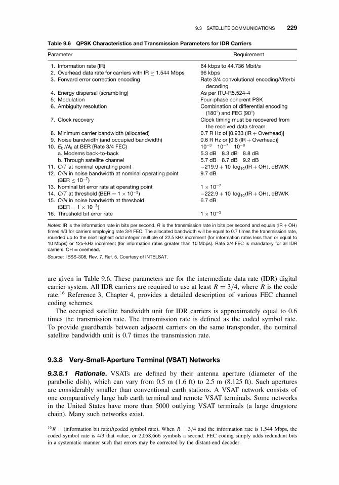
9.3 SATELLITE COMMUNICATIONS 229
Table 9.6 QPSK Characteristics and Transmission Parameters for IDR Carriers
Parameter Requirement
1. Information rate (IR) 64 kbps to 44.736 Mbit/s2. Overhead data rate for carriers with IR ≥ 1.544 Mbps 96 kbps3. Forward error correction encoding Rate 3/4 convolutional encoding/Viterbi
decoding4. Energy dispersal (scrambling) As per ITU-R5.524-45. Modulation Four-phase coherent PSK6. Ambiguity resolution Combination of differential encoding
(180◦) and FEC (90◦)7. Clock recovery Clock timing must be recovered from
the received data stream8. Minimum carrier bandwidth (allocated) 0.7 R Hz of [0.933 (IR + Overhead)]9. Noise bandwidth (and occupied bandwidth) 0.6 R Hz or [0.8 (IR + Overhead)]
10. Eb/N0 at BER (Rate 3/4 FEC) 10−3 10−7 10−8
a. Modems back-to-back 5.3 dB 8.3 dB 8.8 dBb. Through satellite channel 5.7 dB 8.7 dB 9.2 dB
11. C/T at nominal operating point −219.9 + 10 log10(IR + OH), dBW/K12. C/N in noise bandwidth at nominal operating point
(BER ≤ 10−7)9.7 dB
13. Nominal bit error rate at operating point 1 × 10⁻⁷
14. C/T at threshold (BER = 1 × 10⁻³) −222.9 + 10 log10(IR + OH), dBW/K15. C/N in noise bandwidth at threshold
(BER = 1 × 10⁻³)6.7 dB
16. Threshold bit error rate 1 × 10⁻³
Notes: IR is the information rate in bits per second. R is the transmission rate in bits per second and equals (IR + OH)
times 4/3 for carriers employing rate 3/4 FEC. The allocated bandwidth will be equal to 0.7 times the transmission rate,rounded up to the next highest odd integer multiple of 22.5 kHz increment (for information rates less than or equal to10 Mbps) or 125-kHz increment (for information rates greater than 10 Mbps). Rate 3/4 FEC is mandatory for all IDRcarriers. OH = overhead.
Source: IESS-308, Rev. 7, Ref. 5. Courtesy of INTELSAT.
are given in Table 9.6. These parameters are for the intermediate data rate (IDR) digitalcarrier system. All IDR carriers are required to use at least R = 3/4, where R is the coderate.16 Reference 3, Chapter 4, provides a detailed description of various FEC channelcoding schemes.
The occupied satellite bandwidth unit for IDR carriers is approximately equal to 0.6times the transmission rate. The transmission rate is defined as the coded symbol rate.To provide guardbands between adjacent carriers on the same transponder, the nominalsatellite bandwidth unit is 0.7 times the transmission rate.
9.3.8 Very-Small-Aperture Terminal (VSAT) Networks
9.3.8.1 Rationale. VSATs are defined by their antenna aperture (diameter of theparabolic dish), which can vary from 0.5 m (1.6 ft) to 2.5 m (8.125 ft). Such aperturesare considerably smaller than conventional earth stations. A VSAT network consists ofone comparatively large hub earth terminal and remote VSAT terminals. Some networksin the United States have more than 5000 outlying VSAT terminals (a large drugstorechain). Many such networks exist.
16R = (information bit rate)/(coded symbol rate). When R = 3/4 and the information rate is 1.544 Mbps, thecoded symbol rate is 4/3 that value, or 2,058,666 symbols a second. FEC coding simply adds redundant bitsin a systematic manner such that errors may be corrected by the distant-end decoder.

230 CONCEPTS IN TRANSMISSION TRANSPORT
There are three underlying reasons for the use of VSAT networks:
1. An economic alternative to establish a data network, particularly if traffic flow isto/from a central facility, usually a corporate headquarters to/from outlying remotes.
2. To bypass telephone companies with a completely private network.3. To provide quality telecommunication connectivity where other means are substan-
dard or nonexistent.
Regarding reason 3, the author is aware of one emerging nation where 124 bankbranches had no electrical communication whatsoever with the headquarters institution inthe capital city.
9.3.8.2 Characteristics of Typical VSAT Networks. On conventional VSAT net-works, the hub is designed to compensate for the VSAT handicap (i.e., its small size). Forexample, a hub antenna aperture is 5 m to 11 m (16 ft to 50 ft) (Ref. 12). High-poweramplifiers (HPAs) run from 100 W to 600 W of output power. Low-noise amplifiers(LNAs), typically at 12 GHz, display (a) noise figures from 0.5 dB to 1.0 dB and (b) low-noise downconverters in the range of 1.5-dB noise figure. Hub G/T values range from+29 dB/K to +34 dB/K.
VSAT terminals have transmitter output powers ranging from 1 W to 50 W, dependingon service characteristics. Receiver noise performance using a low-noise downconverteris about 1.5 dB; otherwise 1 dB with an LNA. G/T values for 12.5-GHz downlinks arebetween +14 dB/K and +22 dB/K, depending greatly on antenna aperture. The idea is tomake a VSAT terminal as inexpensive as possible. Figure 9.21 illustrates the conventionalhub/VSAT concept of a star network. The hub is at the center.
VSAT
VSAT
VSAT
VSAT
VSAT VSAT
VSAT
VSAT
Hub
Figure 9.21 Typical VSAT network topology. Note the star network configuration. The outlying VSATterminals can number in the thousands.
9.4 FIBER-OPTIC COMMUNICATION LINKS 231
9.3.8.3 Access Techniques. Inbound refers to traffic from VSAT(s) to hub, andoutbound refers to traffic from hub to VSAT(s). The outbound link is commonly a time-division multiplex (TDM) serial bit stream, often 56 kbps, and some high-capacity systemsreach 1.544 Mbps or 2.048 Mbps. The inbound links can take on any one of a numberof flavors, typically 9600 bps.
More frequently, VSAT systems support interactive data transactions, which are veryshort in duration. Thus, we can expect bursty operation from a remote VSAT terminal. Oneapplication is to deliver, in near real time, point-of-sale (POS) information, forwardingit to headquarters where the VSAT hub is located. Efficiency of bandwidth use is not aprimary motivating factor in system design. Thus for the interactive VSAT data networkenvironment, low delay, simplicity of implementation, and robust operation are generallyof importance than the bandwidth efficiency achieved.
Message access on any shared system can be of three types: (1) fixed assigned,(2) contention (random access), or (3) reservation (controlled access). There are hybridschemes between contention and reservation.
In the fixed assigned multiple access, VSAT protocols are SCPC/FDMA, CDMA (aspread spectrum technique), and TDMA.17 All three are comparatively inefficient in thebursty environment with hundreds of thousands of potential users.
9.4 FIBER-OPTIC COMMUNICATION LINKS
9.4.1 Applications
Fiber optics as a transmission medium has a comparatively unlimited bandwidth. It hasexcellent attenuation properties, as low as 0.25 dB/km. A major advantage fiber has whencompared with coaxial cable is that no equalization is necessary. Also, repeater separationis on the order of 10–100 times that of coaxial cable for equal transmission bandwidths.Other advantages are:
ž Electromagnetic immunityž Ground loop eliminationž Securityž Small size and lightweightž Expansion capabilities requiring change out of electronics only, in most casesž No licensing required
Fiber has analog transmission application, particularly for video/TV. However, for thisdiscussion we will be considering only digital applications, principally as a PCM highwayor “bearer.”
Fiber-optic transmission is used for links under 1 ft in length all the way up to andincluding transoceanic undersea cable. In fact, all transoceanic cables currently beinginstalled and planned for the future are based on fiber optics.
Fiber-optic technology was developed by physicists and, following the convention ofoptics, wavelength rather than frequency is used to denote the position of light emissionin the electromagnetic spectrum. The fiber optics of today uses three wavelength bands:(1) around 800 nm (nanometers), (2) 1300 nm, and (3) 1600 nm or near-visible infrared.This is illustrated in Figure 9.22.
17SCPC stands for single channel per carrier.

232 CONCEPTS IN TRANSMISSION TRANSPORT
Figure 9.22 Frequency spectrum above 300 MHz. The usable wavelengths are just above and below1 µm (1 × 10⁻⁶ m).
This section includes an overview of how fiber-optic links work, including the morecommon types of fiber employed, a discussion of light sources (transmitters), light detec-tors (receivers), optical amplifiers, and how lengths of fiber-optic cable are joined. Thereis also a brief discussion of wavelength-division multiplexing (WDM).
9.4.2 Introduction to Optical Fiber as a Transmission Medium
Optical fiber consists of a core and a cladding, as illustrated in Figure 9.23. At presentthe most efficient core material is silica (SiO2). The cladding is a dielectric material thatsurrounds the core of an optical fiber.
The practical propagation of light through an optical fiber may best be explained usingray theory and Snell’s law. Simply stated, we can say that when light passes from amedium of higher refractive index (n1) into a medium of lower refractive index (n2), therefractive ray is bent away from the normal. For instance, a ray traveling in water andpassing into an air region is bent away from the normal to the interface between the tworegions. As the angle of incidence becomes more oblique, the refracted ray is bent moreuntil finally the refracted energy emerges at an angle of 90◦ with respect to the normaland just grazes the surface. Figure 9.24 shows various incident angles of light enteringa fiber. Figure 9.24b illustrates what is called the critical angle, where the refracted ray
Figure 9.23 Structure of optical fiber consisting of a central core and a peripheral transparent claddingsurrounded by protective packaging.

9.4 FIBER-OPTIC COMMUNICATION LINKS 233
Figure 9.24 Ray paths for several angles of incidence (n1 > n2).
just grazes the surface. Figure 9.24c is an example of total internal reflection. This occurswhen the angle of incidence exceeds the critical angle. A glass fiber, for the effectivetransmission of light, requires total internal reflection.
Figure 9.25 illustrates a model of a fiber-optic link. Besides the supporting electricalcircuitry, it shows the three basic elements in an optical fiber transmission system: (1) theoptical source, (2) the fiber link, and (3) optical detector. Regarding the fiber-optic linkitself, there are two basic impairments that limit the length of such a link without resortingto repeaters or that can limit the distance between repeaters. These impairments areloss (attenuation), usually expressed in decibels per kilometer, and dispersion, usuallyexpressed as bandwidth per unit length, such as megahertz per kilometer. A particularfiber-optic link may be power-limited or dispersion-limited.
Dispersion, manifesting itself in intersymbol interference at the receive end, can bebrought about by several factors. There is material dispersion, modal dispersion, andchromatic dispersion. Material dispersion can manifest itself when the emission spectralline is very broad, such as with a light-emitting diode (LED) optical source. Certainfrequencies inside the emission line travel faster than others, causing some transmittedenergy from a pulse to arrive later than other energy. This causes intersymbol interference.Modal dispersion occurs when several different modes are launched. Some have morereflections inside the fiber than other modes, thus, again, causing some energy from thehigher-order modes to be delayed, compared with lower-order modes.
Let us examine the effect of dispersion on a train of pulses arriving at a light detector.Essentially, the light is “on” for a binary 1 and “off” for a binary 0. As shown inFigure 9.26, the delayed energy from bit position 1 falls into bit position 2 (and possibly
Figure 9.25 A model of a typical fiber-optic communication link.

234 CONCEPTS IN TRANSMISSION TRANSPORT
Figure 9.26 A simplified sketch of delayed symbol (bit) energy of bit 1 spilling into bit position 2.Alternating 1s and 0s are shown. It should be noted that as the bit rate increases, the bit duration (period)decreases, exacerbating the situation.
3, 4, etc.) confusing the decision circuit. Likewise, delayed energy from bit position 2falls into bit position 3 (possibly 4, 5, etc.), and so on. This is aptly called intersymbolinterference (ISI), which was previously introduced.
One way we can limit the number of modes propagated down a fiber is to make thefiber diameter very small. This is called monomode fiber, whereas the larger fibers arecalled multimode fibers. For higher bit rate (e.g., >622 Mbps), long-distance fiber-opticlinks, the use of monomode fiber is mandatory. This, coupled with the employment ofthe longer wavelengths (e.g., 1330 nm and 1550 nm), allows us to successfully transmitbit rates greater than 622 Mbps, and with certain care the new 10-Gbps rate can beaccommodated.
9.4.3 Types of Optical Fiber
There are three categories of optical fiber, as distinguished by their modal and physi-cal properties:
1. Step index (multimode)2. Graded index (multimode)3. Single mode (also called monomode)
Step-index fiber is characterized by an abrupt change in refractive index, and gradedindex is characterized by a continuous and smooth change in refractive index (i.e., fromn1 to n2). Figure 9.27 shows the fiber construction and refractive index profile for step-index fiber (Figure 9.27a) and graded-index fiber (Figure 9.27b). Both step-index andgraded-index light transmission are characterized as multimode because more than onemode propagates. (Two modes are shown in the figure.) Graded-index fiber has a superiorbandwidth–distance product compared to that of step-index fiber. In other words, it cantransport a higher bit rate further than step index. It is also more expensive. We caneliminate this cause of dispersion if we use single–mode fiber. Figure 9.28 shows atypical five-fiber cable for direct burial.
9.4.4 Splices and Connectors
Optical fiber cable is commonly available in 1-km sections; it is also available in longersections, in some types up to 10 km or more. In any case there must be some way of

9.4 FIBER-OPTIC COMMUNICATION LINKS 235
Figure 9.27 Construction and refractive index properties for (a) step-index fiber and (b) graded-index fiber.
Figure 9.28 Direct burial optical fiber cable.
connecting the fiber to the source and to the detector as well as connecting the reels ofcable together, whether in 1 km or more lengths, as required. There are two methodsof connection, namely, splicing or using connectors. The objective in either case is totransfer as much light as possible through the coupling. A good splice couples more lightthan the best connectors. A good splice can have an insertion loss as low as 0.09 dB,whereas the best connector loss can be as low as 0.3 dB. An optical fiber splice requires

236 CONCEPTS IN TRANSMISSION TRANSPORT
highly accurate alignment and an excellent end finish to the fibers. There are three causesof loss at a splice:
1. Lateral displacement of fiber axes2. Fiber end separation3. Angular misalignment
There are two types of splice now available: the mechanical splice and the fusionsplice. With a mechanical splice an optical matching substance is used to reduce splicinglosses. The matching substance must have a refractive index close to the index of the fibercore. A cement with similar properties is also used, serving the dual purpose of refractiveindex matching and fiber bonding. The fusion splice, also called a hot splice, is wherethe fibers are fused together. The fibers to be spliced are butted together and heated witha flame or electric arc until softening and fusion occur.
Splices require special splicing equipment and trained technicians. Thus it can be seenthat splices are generally hard to handle in a field environment such as a cable manhole.Connectors are much more amenable to field connecting. However, connectors are lossierand can be expensive. Repeated mating of a connector may also be a problem, particularlyif dirt or dust deposits occur in the area where the fiber mating takes place.
However, it should be pointed out that splicing equipment is becoming more economic,more foolproof, and more user-friendly. Technician training is also becoming less ofa burden.
Connectors are nearly universally used at the source and at the detector to connect themain fiber to these units. This makes easier change-out of the detector and source whenthey fail or have degraded operation.
9.4.5 Light Sources
A light source, perhaps more properly called a photon source, has the fundamental functionin a fiber-optic communication system to efficiently convert electrical energy (current) intooptical energy (light) in a manner that permits the light output to be effectively launchedinto the optical fiber. The light signal so generated must also accurately track the inputelectrical signal so that noise and distortion are minimized.
The two most widely used light sources for fiber-optic communication systems are thelight-emitting diode (LED) and the semiconductor laser, sometimes called a laser diode(LD). LEDs and LDs are fabricated from the same basic semiconductor compounds andhave similar heterojunction structures. They do differ in the way they emit light and intheir performance characteristics.
An LED is a forward-biased p–n junction that emits light through spontaneousemission, a phenomenon referred to as electroluminescence. LDs emit light throughstimulated emission. LEDs are less efficient than LDs but are considerably moreeconomical. They also have a longer operational life. The emitted light of an LEDis incoherent with a relatively wide spectral line width (from 30 nm to 60 nm) and arelatively large angular spread, about 100◦. On the other hand, a semiconductor laseremits a comparatively narrow line width (from <2 nm to 4 nm). Figure 9.29a shows thespectral line for an LED, and Figure 9.29b shows the spectral line for a semiconductorlaser (i.e., a laser diode or LD).
What is a spectral line? Many of us imagine that if we were to view a radio carrier(without modulation) on an oscilloscope, it would be a vertical line that appeared to beof infinitely narrow width. This thinking tends to be carried into the world of light in

9.4 FIBER-OPTIC COMMUNICATION LINKS 237
Figure 9.29 Spectral distribution (line width) of the emission from (a) an LED and (b) a semiconductorlaser (LD), where λ is the optical wavelength and �λ is the spectral or line width.
a fiber-optic light-guide. In neither case is this exactly true. The emission line or lightcarrier has a finite width, as does a radio carrier. The IEEE (Ref. 6) defines spectral width,full-width half-maximum as “The absolute difference between the wavelengths at whichthe spectral radiant intensity is 50% of the maximum.”
With present technology the LED is capable of launching about 100 µW (−10 dBm)or less of optical power into the core of a fiber with a numerical aperture of 0.2 or better.A semiconductor laser with the same input power can couple up to 7 mW (+8.5 dBm)into the same cable. The coupling efficiency of an LED is on the order of 2%, whereasthe coupling efficiency of an LD (semiconductor laser) is better than 50%.
Methods of coupling a source into an optical fiber vary, as do coupling efficiencies. Toavoid ambiguous specifications on source output powers, such powers should be stated atthe pigtail. A pigtail is a short piece of optical fiber coupled to the source at the factoryand, as such, is an integral part of the source. Of course, the pigtail should be the sametype of fiber as that specified for the link.
LED lifetimes are in the order of 100,000 hr mean time between failures (MTBF) withup to a million hours reported in the literature. Many manufacturers guarantee a semicon-ductor laser for 20,000 hr or more. About 150,000 hr can be expected from semiconductorlasers after stressing and culling of unstable units. Such semiconductors are used in thelatest TAT and PTAT series of undersea cables connecting North America and Europe.
Current fiber-optic communication systems operate in the nominal wavelength regionsof 820 nm, 1330 nm, and 1550 nm. Figure 9.30 is a plot of attenuation per unit length ver-sus wavelength. Based on this curve, we can expect about 3 dB/km at 820 nm, 0.50 dB/kmat 1330 nm, and at 1550 nm some 0.25 dB/km of attenuation. Also take note that at about1300 nm is a region of zero dispersion. For added expense, fiber is available with thedispersion minimum shifted to the 1550-nm band, where attenuation per unit length isminimum. There is mature technology at all three wavelengths.
9.4.6 Light Detectors
The most commonly used detectors (receivers) for fiber-optic communication systems arephotodiodes, either PIN or APD. The terminology PIN derives from the semiconductorconstruction of the device where an intrinsic (I) material is used between the p–n junctionof the diode.

238 CONCEPTS IN TRANSMISSION TRANSPORT
Figure 9.30 Attenuation per unit length versus wavelength of glass fiber (Ref. 7).
Table 9.7 Summary of Receiver Diode Sensitivities, Average Received Optical Power in dBm,BER = 1 × 10⁻⁹
Bit RateInGaAs PIN
InGaAs SAM/SAGMa
APD Ge APDInGaAs
Photoconductor
(Mbps) 1.3 µm 1.55 µm 1.3 µm 1.55 µ 1.3 µm 1.55 µm 1.3 µm 1.55 µm
34 −52.5 −46 −55.845 −49.9 −51.7 −51.9
100 −40.5140 −46 −45.2 −49.3274 −43 −45 −38.7 −36320 −43.5420 −43 −41.5450 −42.5 −39.5 −40.5565 −33650 −36
1000 −38 −37.5 −28 −34.41200 −33.2 −36.51800 −31.3 −30.12000 −36.6 −31 −28.84000 −32.6
aSAGM stands for separated absorption, grating, and multiplication regions. SAM stands for separated absorption andmultiplication regions.
Source: Ref. 8.
Another type of detector is avalanche photodiode (APD), which is a gain device dis-playing gains on the order of 15–20 dB. The PIN diode is not a gain device. Table 9.7summarizes various detector sensitivities with a “standard” BER of 1 × 10⁻⁹ for somecommon bit rates.18
18Some entities such as SPRINT (US) specify 1 × 10⁻¹².

9.4 FIBER-OPTIC COMMUNICATION LINKS 239
Of the two types of photodiodes discussed here, the PIN detector is more economicaland requires less complex circuitry that does its APD counterpart. The PIN diode haspeak sensitivity from about 800 nm to 900 nm for silicon devices.
The overall response time for the PIN diode is good for about 90% of the transient butsluggish for the remaining 10%, which is a “tail.” The power response of the tail portionof a pulse may limit the net bit rate on digital systems.
The PIN detector does not display gain, whereas the APD does. The response time ofthe APD is far better than that of the PIN diode, but the APD displays certain temperatureinstabilities where responsivity can change significantly with temperature. Compensationfor temperature is usually required in APD detectors and is often accomplished by afeedback control of bias voltage. It should be noted that bias voltages for APDs are muchhigher than for PIN diodes, and some APDs require bias voltages as high as 200 V. Boththe temperature problem and the high-voltage bias supply complicate repeater design.
9.4.7 Optical Fiber Amplifiers
Optical amplifiers amplify incident light through stimulated emission, the same mechanismas used with lasers. These amplifiers are the same as lasers without feedback. Opticalgain is achieved when the amplifier is pumped either electrically or optically to realizepopulation inversion.
There are semiconductor laser amplifiers, Raman amplifiers, Brillouin amplifiers, anderbium-doped fiber amplifiers (EDFAs). Certainly the EDFAs show the widest acceptance.One reason is that they operate near the 1.55-µm wavelength region, where fiber loss isat a minimum. Reference 11 states that it is possible to achieve high amplifier gains inthe range of 30 dB to 40 dB with only a few milliwatts of pump power when EDFAs arepumped by using 0.980-µm or 1.480-µm semiconductor lasers. Figure 9.31 is a blockdiagram of a low-noise EDFA.
In Figure 9.31, optical pumping is provided by fiber pigtailed19 semiconductor laserswith typically 100 mW of power. Low-loss wavelength division multiplexers efficientlycombine pump and signal powers and can also be used to provide a pump bypass aroundthe internal isolator. The EDFA has an input stage that is codirectionally pumped andan output stage that is counterdirectionally pumped. Such multistage EDFA designshave simultaneously achieved a low-noise figure of 3.1 dB and a high gain of 54 dB(Refs. 10, 11).
Figure 9.31 An EDFA block diagram. (From Ref. 9. Courtesy of Hewlett-Packard.)
19A pigtail is a length of fiber factory connected to an active component.

240 CONCEPTS IN TRANSMISSION TRANSPORT
Tx RxFiber
In-line amplifiers
FiberA • • • A
Figure 9.32 Applications of EDFAs.
The loops of fiber should be noted in Figure 9.32. These are lengths of fiber with adopant. The length of erbium-doped fiber required for a particular amplifier applicationdepends on the available pump power, the doping concentration, the design topology, andgain and noise requirements.
EDFAs are often installed directly after a semiconductor laser source (transmitter)and/or directly before the PIN or APD receiver at the distant end. Figure 9.32 illustratesthis concept. With the implementation of EDFAs, the length of a fiber-optic link canbe extended without repeaters an additional 100–250 km, or it can extend the distancebetween repeaters a similar amount.
9.4.8 Wavelength Division Multiplexing
Wavelength division multiplexing (WDM) is just another name for frequency divisionmultiplexing (FDM). In this section we will hold with the conventional term, WDM.The WDM concept is illustrated in Figure 9.33. WDM can multiply the transmissioncapacity of an optical fiber many-fold. For example, if we have a single fiber carrying10.0 Gbps, and it is converted for WDM operation with 20 WDM channels, where eachof these channels carry 10.0 Gbps, the total capacity of this single fiber is now 10.0 × 20or 200 Gbps.
The 1550-nm band is the most attractive for WDM applications because the aggregatewavelengths of a WDM signal can be amplified with its total assemblage together by asingle EDFA. This is a great advantage. On the other hand, if we wish to regenerate thedigital derivate of a WDM signal in a repeater, the aggregate must be broken down intoits components as shown in Figure 9.34.
The cogent question is, How many individual wavelength signals can we multiplexon a single fiber? It depends on the multiplexing/demultiplexing approach employed, thenumber of EDFAs that are in tandem, the available bandwidth, channel separation (innm), and the impairments peculiar to light systems operating at higher powers and theWDM techniques used.
As we mentioned above, the number of WDM channels that can be accommodateddepends on the bandwidth available and the channel spacing among other parameters and
Figure 9.33 The WDM concept.

9.4 FIBER-OPTIC COMMUNICATION LINKS 241
Figure 9.34 The use of regenerative repeaters on a WDM link.
characteristics. For example, in the 1330-nm band about 80 nm of bandwidth is availableand in the 1550-nm band, about 100 nm of bandwidth is available, which includes theoperational bandwidth and guardbands.20 Currently, only EDFA amplifiers provide suffi-cient gain to support WDM. These amplifiers operate only in the 1550-nm band. Allowingabout 50 GHz of separation between optical carriers, an optical fiber can support some100 DWDM channels where each optical carrier would carry on the order of 40 Gbpsusing the ITU frequency (wavelength) matrix. Thus, the aggregate bit rate capacity perfiber would be 40 × 100 Gbps or 4000 Gbps using only the 1550-nm band with currenttechnology (2004, 2005).
9.4.9 Fiber-Optic Link Design
The design of a fiber-optic communication link involves several steps. Certainly the firstconsideration is to determine the feasibility of such a transmission system for a desiredapplication. There are two aspects of this decision: (1) economic and (2) technical. Canwe get equal or better performance for less money using some other transmission mediumsuch as wire-pair cable, coaxial cable, LOS microwave, and so on?
Fiber-optic communication links have wide application. Analog applications for cabletelevision (CATV) trunks are showing particularly rapid growth. Fiber is also used forlow-level signal transmission in radio systems, such as for long runs of IF and even forRF. However, in this text we stress digital applications, some of which are listed below:
ž On-premises data busž LANs (e.g., fiber distributed data interface)ž High-level PCM or CVSD configurations21; SONET and SDHž Radar data linksž Conventional data links where bit/symbol rates exceed 19.2 kbpsž Digital video including cable television
It seems that the present trend of cost erosion will continue for fiber cable andcomponents. Fiber-optic repeaters are considerably more expensive than their PCM metal-lic counterparts. The powering of the repeaters can be more involved, particularly if poweris to be taken from the cable itself. This means that the cable must have a metallic elementto supply power to downstream repeaters, thereby losing a fiber-optic advantage. Metal
20Guardbands are empty spaces to provide isolation between adjacent channels. This helps minimize interferencefrom one channel to the next. Of course, that bandwidth allocated to guardbands is non-revenue-bearing andthus must be minimized.21CVSD stands for continuous variable slope delta (modulation), a form of digital modulation where the codingis 1 bit at a time. It is very popular with the armed forces.

242 CONCEPTS IN TRANSMISSION TRANSPORT
in the cable, particularly for supplying power, can be a conductive path for ground loops.Another approach is to supply power locally to repeaters with a floating battery backup.
A key advantage to fiber over metallic cable is fewer repeaters per unit length. InChapter 6 we showed that repeaters in tandem are the principal cause of jitter, a majorimpairment to a digital system such as PCM. Reducing the number of repeaters reducesjitter accordingly. In fact, fiber-optic systems require a small fraction of the number ofrepeaters, compared with PCM for the same unit length, on either wire-pair or coax-ial cable.
9.4.9.1 Design Approach. The first step in the design of a fiber-optic communicationsystem is to establish the basic system parameters. Among these we would wish to knowthe following:
ž Signal to be transmitted: digital or analog, video/CATV; bit rate and formatž System length, fiber portion end-to-endž Growth requirements (additional circuits, increase of bit rates)ž Availability/survivability requirementsž Tolerable signal impairment level, stated as signal-to-noise ratio on BER at the output
of the terminal-end detector
The link BER should be established based on the end-to-end BER. In the past we hadused 1 × 10⁻⁹ as a link BER. Telcordia now requires 2 × 10⁻¹⁰ end-to-end. One linkvalue might be 1 × 10⁻¹².
However, there is still another saving factor or two. If we have operation at the zero-dispersion wavelength, about 1300 nm, dispersion may really not be a concern until aboutthe 1-Gbps rate. Of course, at 1300 nm we have lost the use of the really low loss bandat around 1550 nm. There is an answer to that, too. Use a fiber where the minimumdispersion window has been shifted to the 1550-nm region. Such fiber, of course, is morecostly, but the cost may be worth it. It is another tradeoff.
The designer must select the most economic alternatives among the following factors:
ž Fiber parameters: single mode or multimode; if multimode, step index or gradedindex; number of fibers, cable makeup, strength
ž Transmission wavelength: 820 nm, 1330 nm, or 1550 nmž Source type: LED or semiconductor laser; there are subsets to each source typež Detector type: PIN or APDž Use of EDFA (amplifiers)ž Repeaters, if required, and how they will be poweredž Modulation: probably intensity modulation (IM), but the electrical waveform entering
the source is important; possibly consider Manchester coding
9.4.9.2 Loss Design. As a first step, assume that the system is power-limited. Thismeans that our principal concern is loss. Probably a large number of systems beinginstalled today can stay in the power-limited regime if monomode fiber is used withsemiconductor lasers (i.e., LDs or laser diodes). When designing systems for bit ratesin excess of 600 to 1000 Mbps, consider using semiconductor lasers with very narrowline widths (see Figure 9.33) and dispersion-shifted monomode fiber. Remember that“dispersion shifting” shifts the zero dispersion window from 1300 to 1550 nm.

9.4 FIBER-OPTIC COMMUNICATION LINKS 243
For a system operating at these high bit rates, even with the attribute of monomodefiber, chromatic dispersion can become a problem, particularly at the desirable 1550-nmband. Chromatic dispersion is really a form of material dispersion described earlier. It isthe sum of two effects: “material dispersion” and waveguide dispersion. As one wouldexpect, with material dispersion, different wavelengths travel at different velocities ofpropagation. This is true even with the narrow line width of semiconductor lasers. Wave-guide dispersion is a result of light waves traveling through single-mode fibers that extendinto the cladding. Its effect is more pronounced at the longer wavelengths because thereis more penetration of the cladding and the “effective” refractive index is reduced. Thiscauses another wavelength dependence on the velocity of light through the fiber, andtherefore another form of dispersion. Thus the use of semiconductor lasers with verynarrow line widths (e.g., <0.5 nm) helps mitigate chromatic dispersion (Ref. 11).
Link margin is another factor for tradeoff. We set this decibel value as a line item inthe link budget for the following contingencies:
ž Cable reel loss variabilityž Future added splices (due to cable repair or modification) and their insertion lossž Component degradation over the life of the system. This is particularly pronounced
for LED output. ITU-T sets aside 2–4 dB for this sector (Ref. 13).
ITU-T recommends a 3-dB link margin (inconsistent with Ref. 13). Reference 9 uses6 dB. Ideally, for system reliability, a large margin is desirable. However, to optimizesystem first cost, the designer would want as low a value as possible. (Comment: Thoseextra dBs cost money.)
The system designer develops a power budget, similar in many respects to the path anal-ysis or link budget of LOS microwave and satellite communication link design. However,there is little variability in a fiber-optic link budget; for example, there is no fading.
For a first-cut design, there are two source types, LED and semiconductor laser. Expecta power output of an LED in the range of −10 dBm; and for the semiconductor laserbudget 0 dBm, although up to nearly +10 dBm is possible. There are two types of detec-tors, PIN and APD. For long links with high bit rates, the APD may become the choice.We would expect that the longer wavelengths would be used, but 820/850-nm links arestill being installed. We must not forget reliability in our equation for choices. For lowerbit rates and shorter links, we would give LEDs a hard look. They are cheaper and aremuch more reliable (MTBF).
Example Link Budget Exercise. The desired bit rate is 140 Mbps. What will be themaximum distance achievable without the use of repeaters? The detector is a PIN type.Turn to Table 9.7 and determine that the threshold (dBm) for a BER of 1 × 10⁻⁹ is−46 dBm at 1.3 µm. One EDFA is used with a gain of 40 dB. This now becomes thestarting point for the link budget.
The light source is a laser diode with a −0.3-dBm output. The receiver threshold is−46 dBm, leaving 45.7 dB in the power budget. Add to this value the EDFA gain of40 dB, bringing the power budget up to 85.7 dB. We allocate this value as follows:
ž Fiber at 0.25 dB/kmž Two connectors22 at 0.5 dB each or a total of 1.0 dB
22These connectors are used at the output pigtail of the source and at the input pigtail to the detector. Connectorsare used for rapid and easy disconnect/connect because, at times during the life of these active devices, theymust be changed out for new ones having either failed or reached the end of their useful life.

244 CONCEPTS IN TRANSMISSION TRANSPORT
ž Fusion splices every kilometer; allows 0.25 dB per splicež A margin of 4 dB
If we subtract the 1 dB for the connectors and the 4-dB margin from the 85.7 dB, weare left with 80.7 dB. Add the splice loss and the kilometer fiber loss for 1-km reels,the result is 0.5 dB. Divide this value into 80.7 dB, and the maximum length is 160 kmbetween a terminal and first repeater or between repeaters. Of course, there is one lesssplice than 1-km lengths, plus the 0.45 dB left over from the 80.7 dB. This will beadditional margin. Setting these calculations up in tabular form as follows:
Item Loss
Connector loss @ 0.5 dB/conn, 2 connectors 1.0 dBMargin 4.0 dBSplice losses @ 0.25 dB/splice, 160 splices 40.0 dBFiber loss, 161-km fiber @ 0.25 dB/km 40.25 dBTotal 85.25 dBAdditional margin 0.45 dB
For an analysis of dispersion and system bandwidth, consult Ref. 12.
9.5 COAXIAL CABLE TRANSMISSION SYSTEMS
9.5.1 Introduction
The employment of coaxial cable in the telecommunication plant is now practically obso-lete with the following exceptions:
ž The last mile or last 100 feet in the cable television (CATV) plantž As an RF transmission line for short distances
It is being replaced in the enterprise network with high-quality twisted-pair and fiber-opticcable connectivities. Certainly in the long-distance network, the fiber-optic solution is farsuperior in nearly every respect.
In the section we provide a brief review of coaxial cable systems.
9.5.2 Description
A coaxial cable is simply a transmission line consisting of an unbalanced pair made upof an inner conductor surrounded by a grounded outer conductor, which is held in aconcentric configuration by a dielectric.23 The dielectric can be of many different typessuch as solid “poly” (polyethylene or polyvinyl chloride), foam, Spiralfil, air, or gas. Inthe case of an air/gas dielectric, the center conductor is kept in place by spacers or disks.
Historically, coaxial cable systems carried large FDM configurations, over 10,000 voicechannels per “tube.” CATV (community antenna television or cable television) systemsuse single cables for transmitted bandwidths in excess of 750 MHz. Coaxial cable systemscompeted with analog LOS microwave and often were favored because of reduced noiseaccumulation.
23Dielectric means an insulator.

9.5 COAXIAL CABLE TRANSMISSION SYSTEMS 245
9.5.3 Cable Characteristics
When employed in the long-distance telecommunication plant, standard coaxial cablesizes are as follows:
Dimension (in.) Dimension (mm)
0.047/0.174 1.2/4.4 (small diameter)0.104/0.375 2.6/9.5
The fractions express the outside diameter of the inner conductor over the insidediameter of the outer conductor. For instance, for the large bore cable, the outside diameterof the inner conductor is 0.104 in. and the inside diameter of the outer conductor is 0.375in. This is illustrated in Figure 9.35. As can be seen from Eq. (9.27) in Figure 9.35, theratio of the diameters of the inner and outer conductors has an important bearing onattenuation (loss). If we can achieve a ratio of b/a = 3.6, a minimum attenuation per unitlength results.
The characteristic impedance of coaxial cable is Z0 = 138 log(b/a) for an air dielectric.If b/a = 3.6, then Z0 = 77 �. Using dielectric other than air reduces the characteristicimpedance. If we use the disks previously mentioned to support the center conductor, theimpedance lowers to 75 �.
Figure 9.36 illustrates the attenuation–frequency characteristics of the coaxial cablediscussed in the text. Attenuation increases rapidly as frequency is increased. It is a func-tion of the square root of frequency, as shown in Figure 9.35. The telecommunicationsystem designer is basically interested in how much bandwidth there is available to trans-mit a signal. For instance, the 0.375-in. cable has an attenuation of about 5.8 dB/mi at2.5 MHz, and the 0.174-in. cable has an attenuation of about 12.8 dB/mi. At 5 MHz the0.174-in. cable has about 19 dB/mi, and the 0.375-in. cable has an attenuation of about10 dB/mi. Attenuation is specified for the highest frequency of interest.
Equalization (i.e., the use of equalizers) will tend to flatten the response curves in thefigure at the expense of some added loss per unit length. Equalization is defined by theIEEE (Ref. 6) as “a technique used to modify the frequency response of an amplifieror network to compensate for variations in the frequency response across the networkbandwidth.” The ideal result is a flat overall response. The CATV plant makes wide useof such equalizers.
Figure 9.35 The basic electrical characteristics of coaxial cable.

246 CONCEPTS IN TRANSMISSION TRANSPORT
Figure 9.36 Attenuation–frequency response per kilometer of coaxial cable.
9.6 TRANSMISSION MEDIA SUMMARY
Table 9.8 presents a summary of the performance characteristics of the five basic trans-mission media.
Table 9.8 Characteristics of Transmission Media
Item Wire-Pair Cable LOS MicrowaveSatellite
Communication Fiber Optics Coaxial Cable
Bandwidth 2 MHz to 400 MHz 500/2500 MHz 500/2500 MHz 120 GHz per band up to 1 GHzCommon bit
rates1.544/2.048 Mbps 155 Mbps 2.048 Mbps 2.4/10/40 Gbps 100 Mbps
Achievable bitrates
100 Mbps 622 Mbps 155 Mbps 4000 Gbps perfiber
1 Gbps
Limitations Length-limited By statute By statute; delay Severing cable Severing cableApplications LANs, TelCo
outside plantLong-distance/
short-distancelinks, TelCo andCATV, privatenetworks
VSAT networks,long-distancelinks, videotransport
For everybroadbandterrestrialapplication
CATV last mile/last100 feet; RFtransport shortdistances;otherwiselimited.
Notes: Wire-pair cable is distance-limited. The shorter the pair length, the higher the bit rate. Also balance andaccumulating capacitance with length affect bit rate.LOS microwave is limited by statute, meaning by the ITU Radio Regulations and the national regulatory authority. EMCmust be considered both for radiation and susceptibility.Satellite communication faces the same legal limitations. Geostationary orbit (GEO) satellites have long delays that couldaffect interactive data systems. Only one GEO satellite relay allowed for a voice connectivity. As in LOS microwave,EMC can be an issue.The limits of fiber optics are still being explored. All terrestrial buried and aerial cable systems are vulnerable to severingby natural disaster or by man.Coaxial cable is limited by amplitude-frequency response characteristics. In nearly every instance, fiber-optic cableconnectivity is preferred. Severing may also be a problem.
REVIEW EXERCISES 247
REVIEW EXERCISES
1. For very-high-capacity transmission systems (e.g., >20,000 equivalent voicechannel), what transmission medium should be selected?
2. What are the advantages of using the RF bands from 2 GHz to 10 GHz for trunktelephony/data? Name at least two.
3. Discuss the problem of delay in speech telephone circuits traversing a geostationarysatellite. Will there be any problem with data and signaling circuits?
4. Give four of the five basic procedure steps in designing an LOS microwave link.
5. Where is earth curvature maximum on an LOS microwave path?
6. In a path profile, what are the three basic increment factors that are added toobstacle height?
7. When a K factor is 4/3, does the radio ray beam bend away or toward the earth?
8. Name at least four parameters that we will derive from a path analysis to design anLOS microwave link.
9. Calculate the free space loss of a radio link operating at 4100 MHz and 21 statuemiles long.
10. What is the EIRP in dBW out of an LOS microwave antenna if the transmit poweris 2 W, the transmission line losses are 3.5 dB, and the antenna gain is 36 dB?
11. A receiving system operating at room temperature has a 5-dB noise figure, and itsbandwidth is 2000 kHz. What is its thermal noise threshold?
12. A receiver operating at room temperature in a digital LOS microwave link displaysa noise figure of 2 dB. What is its N0?
13. What theoretical bit packing can we achieve with QPSK? With 8-ary PSK?
14. What efficiency can we expect from an LOS microwave parabolic antenna boughtoff-the-shelf?
15. What is the cause of the most common form of fading encountered on an LOSmicrowave link?
16. What theoretical bit packing can be achieved from 64-QAM?
17. Why is line-of-sight something more than line-of-sight? Explain.
18. Based on the Rayleigh fade margin criterion, what fade margin will we need for a99.975% time availability? For 99.9%?
19. There are two kinds of diversity that can be used with conventional LOS microwave.What are they? It is nearly impossible for one type to be licensed in the United States.Which one and why?
20. An LOS microwave link cannot meet performance requirements. What measurescan we take to remedy this situation? List in ascending order of cost.
21. Satellite communications is just an extension of LOS microwave. Thus a satelliteearth station must be within of the satellite.

248 CONCEPTS IN TRANSMISSION TRANSPORT
22. There are two basic generic methods of satellite access. What are they? List a thirdmethod which is a subset of one of them.
23. What are two major advantages of satellite TDMA?
24. Define G/T mathematically.
25. Why is the geostationary satellite downlink-limited? Give two reasons.
26. Receiving system noise temperature has two components. What are they?
27. Name three applications for VSAT networks.
28. What sets a VSAT aside from conventional geostationary (fixed) satelliteearth stations?
29. What sort of digital format might we expect on an outbound link forVSAT operation?
30. What is the great, overriding advantage of fiber-optic communication links?
31. What are the two basic impairments that limit the length of a fiber-optic link?
32. How does dispersion manifest itself on a digital bit stream?
33. Name the three basic components of a fiber-optic link (in the light domain).
34. There are three wavelength bands currently in use on optical fiber networks. Identifythe bands and give data on loss per unit distance.
35. What does a glass fiber consist of (as used for telecommunications)?
36. What are the two generic types of optical fiber?
37. Identify the two basic light sources. Compare.
38. What is a pigtail?
39. What are the two generic types of optical detectors? Give some idea of gain thatcan be achieved by each.
40. Where do we place fiber amplifiers (in most situations)?
REFERENCES
1. Transport Systems Generic Requirements (TSGR): Common Requirements, Bellcore GR-499-CORE, Issue 1, Bellcore, Piscataway, NJ, Dec. 1995.
2. Allowable Bit Error Ratios at the Output of a Hypothetical Reference Digital Path for Radio-Relay Systems Which May Form Part of an Integrated Services Digital Network, CCIR Rec.594-3, 1994 F Series Volume, Part 1, ITU Geneva, 1994.
3. R. L. Freeman, Radio System Design for Telecommunications, 2nd ed., Wiley, New York, 1997.
4. Performance Characteristics for Frequency Division Multiplex/Frequency Modulation(FDM/FM) Telephony Carriers, INTELSAT IESS 301 (Rev. 3), INTELSAT, Washington, DC,May 1994.
5. Performance Characteristics for Intermediate Data Rate (IDR) Digital Carriers, INTELSATIESS 308 with Rev. 7 and 7A, INTELSAT, Washington, DC, Aug. 1994.
6. IEEE Standard Dictionary of Electrical and Electronic Terms, 6th ed., IEEE Std. 100-1996,IEEE, New York, 1996.
7. R. L. Freeman, Telecommunication Transmission Handbook, 4th ed., Wiley, New York, 1998.

REFERENCES 249
8. Telecommunication Transmission Engineering, 3rd ed., Vol. 2, Bellcore, Piscataway, NJ, 1991.
9. 1993 Lightwave Symposium, Hewlett-Packard, Burlington, MA, Mar. 23, 1993.
10. S. Shimada and H. Ishio, Optical Amplifiers and Their Applications, Wiley, Chichester, UK,1992.
11. G. P. Agrawal, Fiber-Optic Communication Systems, Wiley, New York, 1992.
12. J. Everett, VSATs: Very Small Aperture Terminals, IEE/Peter Peregrinus, Stevenage, Herts, UK,1992.
13. Optical Interfaces for Multichannel Systems with Optical Amplifiers, ITU-T Rec. 692, ITUGeneva, 1998.


10
DATA COMMUNICATIONS
10.1 CHAPTER OBJECTIVE
Data communications is the fastest growing technology in the telecommunications arena.In the PSTN, data and voice have traded places where data connectivities run about 95%or more of the total traffic load and conventional voice is less than 5%. The widespreadavailability of the PC not only spurred data communications forward, it added a completelynew direction: distributed processing. No longer are we tied to the main frame computer;it has taken on a secondary role in the major scheme of things. Another major impetusin this direction is of course the INTERNET.
The IEEE (Ref. 1) defines data communications (data transmission) as “The movementof encoded information by means of communication techniques.” The objective of thischapter is to introduce the reader to the technology of the movement of encoded infor-mation. Encoded information includes alphanumeric data that may broadly encompassmessages that have direct meaning to the human user. It also includes the movement ofstrictly binary sequences that have meaning to a machine, but no direct meaning to ahuman being.
Data communications evolved from automatic telegraphy, which was prevalent fromthe 1920s through the 1960s. We start the chapter with information coding or how we canexpress our alphabet and numeric symbols electrically without ambiguity. Data networkperformance is then covered with a review of the familiar BER. We next move on tothe organization of data for transmission and introduce protocols including electrical andlogical interfaces. Enterprise networks covering LAN and WAN technology, frame relay,and ISDN1 are treated in Chapters 11, 12, and 13. The asynchronous transfer mode (ATM)is discussed in Chapter 20. The principal objective of this chapter is to stress conceptsand to leave specific details to other texts.
10.2 THE BIT—A REVIEW
The bit is often called the most elemental unit of information. The IEEE (Ref. 1) defines itas a contraction of binary digit, a unit of information represented by either a 1 or a 0. These
1ISDN stands for Integrated Services Digital Networks.
Fundamentals of Telecommunications, Second Edition, by Roger L. FreemanISBN 0-471-71045-8 Copyright 2005 by Roger L. Freeman
251

252 DATA COMMUNICATIONS
are the same bits that were introduced in Section 2.4.3 and later applied in Chapter 6,and to a lesser extent in Chapter 7. In Chapter 6, Digital Networks, the primary purposeof those bits was to signal the distant end value of the voltage level of an analog channelat some moment in time. Here we will be assembling bit groupings that will representletters of the alphabet, numerical digits 0 through 9, punctuation, graphic symbols, or justoperational bit sequences that are necessary to make the data network operate with littleor no ostensible outward meaning to us.
From old-time telegraphy the terminology has migrated to data communications. Amark is a binary 1 and a space is a binary 0. A space or 0 is represented by a positive-going voltage, and a mark or 1 is represented by a negative-going voltage. (Now I amgetting confused. When I was growing up in the industry, a 1 or mark was a positive-goingvoltage, and so forth.)
10.3 REMOVING AMBIGUITY: BINARY CONVENTION
To remove ambiguity of the various ways we can express a 1 and a 0, CCITT in Rec. V.1(Ref. 2) states clearly how to represent a 1 and a 0. This is summarized in Table 10.1,with several additions from other sources. Table 10.1 defines the sense of transmissionso that the mark and space, the 1 and 0, respectively, will not be inverted. Inversion cantake place by just changing the voltage polarity. We call it reversing the sense. Some dataengineers often refer to such a table as a “table of mark-space convention.”
10.4 CODING
Written information must be coded before it can be transmitted over a data network. Onebit carries very little information. There are only those two possibilities: the 1 and the 0.It serves good use for supervisory signaling where a telephone line could only be in oneof two states. It is either idle or busy. As a minimum we would like to transmit everyletter of the alphabet and the 10 basic decimal digits plus some control characters, suchas a space and hard/soft return, and some punctuation.
Suppose we join two bits together for transmission. This generates four possible bitsequences2:
00 01 10 11,
Table 10.1 Equivalent Binary Designations: Summary of Equivalence
Symbol 1 Symbol 0
Mark or marking Space or spacingCurrent on Current offNegative voltage Positive voltageHole (in paper tape) No hole (in paper tape)Condition Z Condition ATone on (amplitude modulation) Tone offLow frequency (frequency shift keying) High frequencyInversion of phase No phase inversion (differential phase shift keying)Reference phase Opposite to reference phase
Source: Ref.2.
2To a certain extent, this is a review of the argument presented in Section 6.2.3.
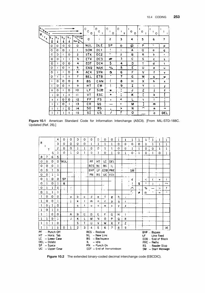
10.4 CODING 253
Figure 10.1 American Standard Code for Information Interchange (ASCII). [From MiL-STD-188C.Updated (Ref. 26).]
Figure 10.2 The extended binary-coded decimal interchange code (EBCDIC).

254 DATA COMMUNICATIONS
or four pieces of information, and each can be assigned a meaning such as 1, 2, 3, 4 or A,B, C, D. Suppose three bits are transmitted in sequence. Now there are eight possibilities:
000 001 010 011
100 101 110 111.
We could continue this argument to sequences of four bits, and it will turn out that thereare now 16 different possibilities. It becomes evident that for a binary code, the numberof distinct characters available is equal to two raised to a power equal to the number ofelements (bits) per character. For instance, the last example was based on a four-elementcode giving 16 possibilities or information characters (i.e., 24 = 16).
The classic example is the ASCII code, which has seven information bits per char-acter. Therefore the number of different characters available is 27 = 128. The AmericanStandard Code for Information Interchange (ASCII) is nearly universally used worldwide.Figure 10.1 illustrates ASCII. It will be noted in the figure that there are more than 30special bit sequences such as SOH, NAK, EOT, and so on. These are/were used for datacircuit control. For a full explanation of these symbols, refer to Ref. 3.
Another, yet richer code was developed by IBM. It is the EBCDIC (extended binarycoded decimal interchange code) code that uses eight information bits per character.Therefore it has 28 = 256 character possibilities. This code is illustrated in Figure 10.2.It should be noted that a number of the character positions are unassigned.
10.5 ERRORS IN DATA TRANSMISSION
10.5.1 Introduction
In data transmission, one of the most important design goals is to minimize error rate.Error rate may be defined as the ratio of the number of bits incorrectly received to thetotal number of bits transmitted or to a familiar number such as 1000, 1,000,000, andso on. CCITT holds with a design objective of better than one error in one million (bitstransmitted). This is expressed as 1 × 10⁻⁶. Many circuits in industrialized nations provideerror performance two or more orders of magnitude better than this.
ITU-T has revised their G.821 recommendation (Ref. 28) to reflect considerably betterperformance. Error performance is stated in terms of ESR (errored second ratio) andSESR (severely errored second ratio) with a recommended measurement period of onemonth. We should expect an ESR of <0.08 and an SESR of <0.002.
One method for minimizing the error rate would be to provide a “perfect” transmissionchannel, one that will introduce no errors in the transmitted information at the output ofthe receiver. However, that perfect channel can never be achieved. Besides improvementof the channel transmission parameters themselves, error rate can be reduced by forms ofa systematic redundancy. In old-time Morse code, words on a bad circuit were often senttwice; this is redundancy in its simplest form. Of course, it took twice as long to send amessage; this is not very economical if the number of useful words per minute receivedis compared to channel occupancy.
This illustrates the tradeoff between redundancy and channel efficiency. Redundancycan be increased such that the error rate could approach zero. Meanwhile, the informationtransfer across the channel would also approach zero. Thus unsystematic redundancyis wasteful and merely lowers the rate of useful communication. On the other hand,maximum efficiency could be obtained in a digital transmission system if all redundancy

10.5 ERRORS IN DATA TRANSMISSION 255
and other code elements, such as “start” and “stop” elements, parity bits, and other“overhead” bits, were removed from the transmitted bit stream. In other words, the channelwould be 100% efficient if all bits transmitted were information bits. Obviously, there isa tradeoff of cost and benefits somewhere between maximum efficiency on a data circuitand systematically added redundancy.
There is an important concept here that should not be missed. An entirely error-freechannel does not exist. It is against the laws of nature. We may have a channel with anexcellent error performance, but some few errors will persist. A performance parameterin these circumstances would be residual error rate.
10.5.2 Nature of Errors
In binary transmission, an error is a bit that is incorrectly received. For instance, supposea 1 is transmitted in a particular bit location and at the receiver the bit in that samelocation is interpreted as a 0. Bit errors occur either as single random errors or as burstsof errors.
Random errors occur when the signal-to-noise ratio deteriorates. This assumes, ofcourse, that the noise is thermal noise. In this case noise peaks, at certain moments oftime, are of sufficient level as to confuse the receiver’s decision, whether a 1 or a 0.
Burst errors are commonly caused by fading on radio circuits. Impulse noise canalso cause error bursts. Impulse noise can derive from lightning, car ignitions, electricalmachinery, and certain electronic power supplies, to name a few sources.
10.5.3 Error Detection and Error Correction
Error detection just identifies that a bit (or bits) has been received in error. Error correctioncorrects errors at a far-end receiver. Both require a certain amount of redundancy tocarry out the respective function. Redundancy, in this context, means those added bitsor symbols that carry out no other function than as an aid in the error-detection orerror-correction process.
One of the earliest methods of error detection was the parity check. With the 7-bitASCII code, a bit was added for parity, making it an 8-bit code. This is character parity.It is also referred to as vertical redundancy checking (VRC).
We speak of even parity and odd parity. One system or the other may be used. Eithersystem is based on the number of marks or 1s in a 7-bit character, and the eighth bit isappended accordingly, either a 0 or a 1. Let us assume even parity and we transmit theASCII bit sequence 1010010. There are three 1s, an odd number. Thus a 1 is appendedas the eighth bit to make it an even number.
Suppose we use odd parity and transmit the same character. There is an odd numberof 1s (marks), so we append a 0 to leave the total number of 1s an odd number. Withodd parity, try 1000111. If you added a 1 as the eighth bit, you’d be correct.
Character parity has the weakness that a lot of errors can go undetected. Suppose twobits are changed in various combinations and locations. Suppose a 10 became a 01; a0 became a 1, and a 1 became a 0; and two 1s became two 0s. All would get by thesystem undetected.
To strengthen this type of parity checking, the longitudinal redundancy check (LRC)was included as well as the VRC. This is a summing of the 1s in a vertical column of allcharacters, including the 1s or 0s in each eighth bit location. The sum is now appended atthe end of a message frame or packet. Earlier this bit sequence representing the sum wascalled the block check count (BCC). Today it may consist of two or four 8-bit sequences
256 DATA COMMUNICATIONS
and we call it the FCS (frame check sequence), or sometimes the CRC (cyclic redundancycheck). At the distant-end receiver, the same addition is carried out and if the sum agreeswith the value received, the block is accepted as error-free. If not, it then contains at leastone bit error, and a request is sent to the transmit end to retransmit the block (or frame).
Even with the addition of LRC, errors can slip through. In fact, no error-detectionsystem is completely foolproof. There is another method, though, that has superior errordetection properties. This is the CRC. It comes in a number of varieties.
10.5.3.1 Cyclic Redundancy Check (CRC). In very simple terms the CRC errordetection technique works as follows: A data block or frame is placed in memory. Wecan call the frame a k-bit sequence and it can be represented by a polynomial whichis called G(x). Various modulo-2 arithmetic operations are carried out on G(x) and theresult is divided by a known generator polynomial called P(x).3 This results in a quotientQ(x) and a remainder R(x). The remainder is appended to the frame as an FCS, andthe total frame with FCS is transmitted to the distant-end receiver where the frame isstored, then divided by the same generating polynomial P(x). The calculated remainderis compared to the received remainder (i.e., the FCS). If the values are the same, theframe is error-free. If they are not, there is at least one bit in error in the frame.
For many WAN applications the FCS is 16 bits long; on LANs it is often 32 bits long.Generally speaking, the greater the number of bits, the more powerful the CRC is forcatching errors.
The following are two common generating polynomials:
1. ANSI CRC-16: X16 + X15 + X2 + 12. CRC-CCITT: X16 + X12 + X5 + 1
producing a 16-bit FCS.CRC-16 provides error detection of error bursts up to 16 bits in length. Additionally,
99.955% of error bursts greater than 16 bits can be detected (Ref.4).
10.5.3.2 Forward-Acting Error Correction (FEC). Forward-acting error correction(FEC) uses certain binary codes that are designed to be self-correcting for errors introducedby the intervening transmission media. In this form of error correction the receiving stationhas the ability to reconstitute messages containing errors.
The codes used in FEC can be divided into two broad classes: (1) block codes and(2) convolutional codes. In block codes information bits are taken k at a time, and c
parity bits are added, checking combinations of the k information bits. A block consists ofn = k + c digits. When used for the transmission of data, block codes may be systematic.A systematic code is one in which the information bits occupy the first k positions in ablock and are followed by the (n − k) check digits.
A convolution(al) code is another form of coding used for error correction. As theword “convolution” implies, this is one code wrapped around or convoluted on another.It is the convolution of an input-data stream and the response function of an encoder. Theencoder is usually made up of shift registers. Modulo-2 adders3 are used to form check
3Note that modulo-2 addition is the same as binary addition but without the “carry,” or 1 + 1 = 0 and we donot carry the 1. Summing 10011 and 11001 in modulo-2, we get 01010.

10.5 ERRORS IN DATA TRANSMISSION 257
digits, each of which is a binary function of a particular subset of the information digitsin the shift register.
10.5.3.3 Error Correction with a Feedback Channel. Two-way or feedback errorcorrection is used widely today on data circuits. Such a form of error correction is calledARQ. The letter sequence ARQ derives from the old Morse and telegraph signal, “auto-matic repeat request.” There are three varieties of ARQ:
1. Stop-and-wait ARQ2. Selective or continuous ARQ3. Go-back-n ARQ
Stop-and-wait ARQ is simple to implement and may be the most economic in the shortrun. It works on a frame-by-frame basis. A frame is generated; it goes through CRCprocessing and an FCS is appended. It is transmitted to the distant end, where the frameruns through CRC processing. If no errors are found, an acknowledgment signal (ACK)is sent to the transmitter, which now proceeds to send the next frame—and so forth. If abit error is found, a negative acknowledgment (NACK) is sent to the transmitter, whichthen proceeds to repeat that frame. It is the waiting time of the transmitter as it waits foreither acknowledgment or negative acknowledgment signals. Many point to this wait timeas wasted time. It could be costly on high-speed circuits. However, the control softwareis simple and the storage requirements are minimal (i.e., only one frame).
Selective ARQ, sometimes called continuous ARQ, eliminates the waiting. The transmitside pours out a continuous stream of contiguous frames. The receive side stores and CRCprocesses as before, but it is processing a continuous stream of frames. When a frameis found in error, it informs the transmit side on the return channel. The transmit sidethen picks that frame out of storage and places it in the transmission queue. Severalpoints become obvious to the reader. First, there must be some way to identify frames.Second, there must be a better way to acknowledge or “negative-acknowledge.” The twoproblems are combined and solved by the use of send sequence numbers and receivesequence numbers. The header of a frame has bit positions for a send sequence numberand a receive sequence number. The send sequence number is inserted by the transmitside, whereas the receive sequence number is inserted by the receive side. The receivesequence numbers forwarded back to the transmit side are the send sequence numbersof frames acknowledged by the receive side. When the receive side detects an erroredframe, it repeats the send sequence number of the frame in error. Of course, the receiverside has to put the corrected frame back in its proper sequence before the frame can goonwards to the end user.
Continuous or selective ARQ is more costly in the short run, compared with stop-and-wait ARQ. It requires more complex software and notably more storage on both sides ofthe link. However, there are no gaps in transmission and no time is wasted waiting forthe ACK or NACK.
Go-back-n ARQ is a compromise. In this case, the receiver does not have to insert thecorrected frame in its proper sequence, thus less storage is required. It works this way:When a frame is received in error, the receiver informs the transmitter to “go-back-n,” n
being the number of frames back to where the errored frame was. The transmitter thenrepeats all n frames, from the errored frame forward. Meanwhile, the receiver has thrown

258 DATA COMMUNICATIONS
out all frames from the errored frame forward. It replaces this group with the new set ofn frames it received, all in proper order.
10.6 DC NATURE OF DATA TRANSMISSION
10.6.1 dc Loops
Binary data are transmitted on a dc loop. More correctly, the binary data end instrumentdelivers to the line and receives from the line one or several dc loops. In its most basicform a dc loop consists of a switch, a dc voltage, and a termination. A pair of wiresinterconnects the switch and termination. The voltage source in data work is called thebattery, although the device is usually electronic, deriving the dc voltage from an ac powerline source. The battery is placed in the line to provide voltage(s) consistent with the typeof transmission desired. A simplified drawing of a dc loop is shown in Figure 10.3a.
10.6.2 Neutral and Polar dc Transmission Systems
Older telegraph and data systems operated in the neutral mode. Nearly all present datatransmission systems operate in some form of polar mode. The words “neutral” and“polar” describe the manner in which battery is applied to the dc loop. On a “neutral” loop,following the convention of Table 10.1, battery is applied during spacing (0) conditionsand is switched off during marking (1). Current therefore flows in the loop when a spaceis sent and the loop is closed. Marking is indicated on the loop by a condition of nocurrent. Thus we have two conditions for binary transmission, an open loop (no currentflowing) and a closed loop (current flowing). Keep in mind that we could reverse this,namely, change the convention and assign marking to a condition of current flowing orclosed loop, and spacing to a condition of no current or an open loop.4 As mentioned,
Figure 10.3 Simplified diagram illustrating a dc loop with (a) neutral keying and (b) polar keying.
4In fact, this was the older convention, prior to about 1960.

10.7 BINARY TRANSMISSION AND THE CONCEPT OF TIME 259
Figure 10.4 Neutral and polar waveforms.
this is called “changing the sense.” Either way, a neutral loop is a dc loop circuit whereone binary condition is represented by the presence of voltage and the flow of current,and the other condition is represented by the absence of voltage and current. Figure 10.3aillustrates a neutral loop.
Polar transmission approaches the problem differently. Two battery sources are pro-vided, one “negative” and the other “positive.” Following the convention in Table 10.1,during a condition of spacing (binary 0), a positive battery (i.e., a positive voltage) isapplied to the loop, and a negative battery is applied during the marking (binary 1) con-dition. In a polar loop current is always flowing. For a mark or binary “1” it flows in onedirection, and for a space or binary “0” it flows in the opposite direction. Figure 10.3bshows a simplified polar loop. Notice that the switch used to selected the voltage is calleda keying device. Figure 10.4 illustrates the two electrical waveforms.
10.7 BINARY TRANSMISSION AND THE CONCEPT OF TIME
10.7.1 Introduction
As emphasized in Chapter 6, time and timing are most important factors in digital trans-mission. For this discussion consider a binary end instrument (e.g., a PC) sending out inseries a continuous run of marks and spaces. Those readers who have some familiaritywith the Morse code will recall that the spaces between dots and dashes told the operatorwhere letters ended and where words ended. The sending device or transmitter deliversa continuous series of characters to the line, each consisting of five, six, seven, eight,or nine elements (bits) per character. A receiving device starts its print cycle when thetransmitter starts sending and, if perfectly in step with the transmitter, can be expected toprovide good printed copy and few, if any, errors at the receiving end.
It is obvious that when signals are generated by one machine and received by another,the speed of the receiving machine must be the same or very close to that of the transmit-ting machine. When the receiver is a motor-driven device, timing stability and accuracyare dependent on the accuracy and stability of the speed of rotation of the motors used.Most simple data-telegraph receivers sample at the presumed center of the signal element.It follows, therefore, that whenever a receiving device accumulates timing error of morethan 50% of the period of one bit, it will print in error.

260 DATA COMMUNICATIONS
Figure 10.5 Five-unit synchronous bit stream with timing error.
The need for some sort of synchronization is illustrated in Figure 10.5. A five-unitcode is employed, and it shows three characters transmitted sequentially.5 The verticalarrows are receiver sampling points, which are points in time. Receiving timing beginswhen the first pulse is received. If there is a 5% timing difference between the transmitterand receiver, the first sampling at the receiver will be 5% away from the center of thetransmitted pulse. At the end of the tenth pulse or signal element, the receiver maysample in error. Here we mean that timing error accumulates at 5% per received signalelement and when there is a 50% accumulated error, the sampling will now be done at anincorrect bit position. The eleventh signal element will indeed be sampled in error, andall subsequent elements will be errors. If the timing error between transmitting machineand receiving machine is 2%, the cumulative error in timing would cause the receivingdevice to receive all characters in error after the 25th element (bit).
10.7.2 Asynchronous and Synchronous Transmission
In the earlier days of printing telegraphy, “start–stop” transmission, or asynchronousoperation, was developed to overcome the problem of synchronism. Here timing starts atthe beginning of a character and stops at the end. Two signal elements are added to eachcharacter to signal the receiving device that a character has begun and ended.
For example, consider the seven-element ASCII code (see Figure 10.1) configured forstart–stop operation with a stop element which is of 2 bits duration. This is illustrated inFigure 10.6. In front of a character an element called a start space is inserted, and a stopmark is inserted at the end of a character. In the figure the first character is the ASCIIletter upper case U (1010101). Here the receiving device knows (a priori) that it starts itstiming 1 element (in this case a bit) after the mark-to-space transition—it counts out 8unit intervals (bits) and looks for the stop-mark to end its counting. This is a transitionfrom space-to-mark. The stop-mark, in this case, is two unit intervals long. It is followedby the mark-to-space transition of the next start space, whence it starts counting unitintervals up to 8. So as not to get confused, the first seven information bits are the ASCIIbits, and the eighth bit is a parity bit. Even parity is the convention here.
Figure 10.6 An 8-unit start-stop bit stream with a 2-unit stop element.
5A 5-bit code. The unit and bit are synonymous in this text. A code element carries out a function. It may beone or more bits in duration.

10.7 BINARY TRANSMISSION AND THE CONCEPT OF TIME 261
In such an operation timing error only accumulates inside a character. Suppose thereceiving device is 5% slower or faster than the transmitting device. Only 40% (5 × 8)
timing error accumulates, well inside of the 50% maximum. Remember that the samplingtakes place at mid-bit position of 50% of its timing interval.
Minimum lengths of stop elements vary, depending on the convention used on a partic-ular network. In the commercial world, the stop element can be one or two unit intervals(bits) duration. With some older systems, the stop element was 1.42 unit intervals dura-tion. In military operation the stop element is 1.5 unit intervals long. The start space isalways 1 unit interval duration.
As we are aware, a primary objective in the design of data systems is to minimize errorsin a received bit stream or to minimize the error rate. Two of the prime causes of errorsare noise and improper timing relationships. With start–stop systems a character beginswith a mark-to-space transition at the beginning of the start-space. Then 1.5 unit intervalslater, the timing causes the receiving device to sample the first information element, whichis simply a 1 or 0 decision. The receiver continues to sample at one-bit intervals untilthe stop mark is received. It knows a priori where (when) it should occur. In start–stopsystems the last information bit is the most susceptible to cumulative timing errors.
Synchronous data transmission is another story altogether. It is much more efficientbecause it does not have start and stop elements, which are really overhead. Synchronousdata transmission consists of a continuous serial stream of information elements or bits,as illustrated in Figure 10.5. With start–stop systems, timing error could only accumulateinside a character, the eight bits of the example given previously. This is not so forsynchronous systems. Timing error can accumulate for the entire length of a frame orover many frames.
With start–stop systems, the receiving device knows when a character starts by themark-to-space transition at the start-space. In a synchronous transmission system, somemarker must be provided to tell the receiver when a frame starts. This “marker” is theunique field. Every data frame starts with a unique field. A generic data frame is shownin Figure 10.7. View the frame from left to right. The first field is the unique field orflag, and it generally consists of the binary sequence 01111110. A frame always startswith this field and ends with the same field. If one frame follows another contiguously,the unique field ending frame No. 1 is the unique field starting frame No. 2, and so forth.Once a frame knows where it starts, it will know a priori where the following fieldsbegin and end by simple bit/octet counting. However, with some data-link protocols, theinformation field is of variable length. In this case, the information field length will appearas a subfield in the control field.
frame checks sequence
Figure 10.7 A generic data frame. Flag pattern = unique field. Text is often called ‘‘info’’ field orinformation field.

262 DATA COMMUNICATIONS
Synchronous data transmission systems not only require frame alignment, but also mustbe bit-aligned. This was an easy matter on start–stop systems because we could let thereceive clock run freely inside the 5 bits or 8 bits of a character. There is no such freedomwith synchronous systems. Suppose we assume a free-running receive clock. However, ifthere was a timing error of 1% between the transmit and receive clocks, not more than 100bits could be transmitted until the synchronous receiving device would be off in timingby the duration of 1 bit from the transmitter, and all bits received thereafter would be inerror. Even if the timing accuracy of one relative to the other were improved to 0.05%,the correct timing relationship between transmitter and receiver would exist for onlythe first 2000 bits transmitted. It follows, therefore, that no timing error whatsoever canbe permitted to accumulate since anything but absolute accuracy in timing would causeeventual malfunctioning. In practice, the receiver is provided with an accurate clock thatis corrected by small adjustments based on the transitions of the received bit stream, asexplained in Section 10.7.3.
10.7.3 Timing
All currently used data-transmission systems are synchronized in phase and symbol ratein some manner. Start–stop synchronization has already been discussed. All fully syn-chronous transmission systems have timing generators or clocks to maintain stability. Thetransmitting device and its companion receiver at the far end of the circuit must maintaina timing system. In normal practice, the transmitter is the master clock of the system. Thereceiver also has a clock that in every case is corrected by some means to its transmitter’smaster clock equivalent at the far end.
Another important timing factor is the time it takes a signal to travel from the transmitterto the receiver. This is called propagation time. With velocities of propagation as low as20,000 mi/sec, consider a circuit 200 mi in length. The propagation time would then be200/20,000 sec or 10 msec. Ten milliseconds is the time duration of 1 bit at a data rateof 100 bps; thus the receiver in this case must delay its clock by 10 msec to be in stepwith its incoming signal. Temperature and other variations in the medium may also affectthis delay, as well as variations in the transmitter master clock.
There are basically three methods of overcoming these problems. One is to providea separate synchronizing circuit to slave the receiver to the transmitter’s master clock.However, this wastes bandwidth by expending a voice channel or subcarrier just fortiming. A second method, which was quite widely used until twenty years ago, was toadd a special synchronizing pulse for groupings of information pulses, usually for eachcharacter. This method was similar to start–stop synchronization, and lost its appeallargely because of the wasted information capacity for synchronizing. The most prevalentsystem in use today is one that uses transition timing, where the receiving device isautomatically adjusted to the signaling rate of the transmitter by sampling the transitionsof the incoming pulses. This type of timing offers may advantages, particularly automaticcompensation for variations in propagation time. With this type of synchronization thereceiver determines the average repetition rate and phase of the incoming signal transitionand adjusts its own clock accordingly by means of a phase-locked loop.
In digital transmission the concept of a transition is very important. The transitionis what really carries the information. In binary systems the space-to-mark and mark-to-space transitions (or lack of transitions) placed in a time reference contain the information.In sophisticated systems, decision circuits regenerate and retime the pulses on the occur-rence of a transition. Unlike decision circuits, timing circuits that reshape a pulse whena transition takes place must have a memory in case a long series of marks or spaces is

10.7 BINARY TRANSMISSION AND THE CONCEPT OF TIME 263
received. Although such periods have no transitions, they carry meaningful information.Likewise, the memory must maintain timing for reasonable periods in case of circuit out-age. Note that synchronism pertains to both frequency and phase and that the usual errorin high-stability systems is a phase error (i.e., the leading edges of the received pulses areslightly advanced or retarded from the equivalent clock pulses of the receiving device).Once synchronized, high-stability systems need only a small amount of correction in tim-ing (phase). Modem internal timing systems may have a long-term stability of 1 × 10⁻⁸
or better at both the transmitter and receiver. At 2400 bps, before a significant timingerror can build up, the accumulated time difference between transmitter and receiver mustexceed approximately 2 × 10⁻⁴ sec. Whenever the circuit of a synchronized transmitterand receiver is shut down, their clocks must differ by at least 2 × 10⁻⁴ sec before signif-icant errors take place once the clocks start back up again. This means that the leadingedge of the receiver–clock equivalent timing pulse is 2 × 10⁻⁴ in advance or retardedfrom the leading edge of the pulse received from the distant end. Often an idling signalis sent on synchronous data circuits during periods of no traffic to maintain the timing.Some high-stability systems need resynchronization only once a day.
Note that thus far in our discussion we have considered dedicated data circuits only.With switched (dial-up) synchronous circuits, the following problems exist:
ž No two master clocks are in perfect phase synchronization.ž The propagation time on any two paths may not be the same.
Thus such circuits will need a time interval for synchronization for each call setup beforetraffic can be passed.
To summarize, synchronous data systems use high-stability clocks, and the clock at thereceiving device is undergoing constant but minuscule corrections to maintain an in-stepcondition with the received pulse train from the distant transmitter, which is accom-plished by responding to mark-to-space and space-to-mark transitions. The importantconsiderations of digital network timing were also discussed in Chapter 6.
10.7.4 Bits, Bauds, and Symbols
There is much confusion among professionals in the telecommunication industry overterminology, especially in differentiating, bits, bauds, and symbols. The bit, a binarydigit, has been defined previously.
The baud is a unit of transmission rate or modulation rate. It is a measure of transitionsper second. A transition is a change of state. In binary systems, bauds and bits per second(bps) are synonymous. In higher-level systems, typically m-ary systems, bits and baudshave different meanings. For example, we will be talking about a type of modulationcalled QPSK. In this case, every transition carries two bits. Thus the modulation rate inbauds is half the bit rate.
The industry often uses symbols per second and bauds interchangeably. It would bepreferable, in our opinion, to use “symbols” for the output of a coder or other conditioningdevice. For the case of a channel coder (or encoder), bits go in and symbols come out.There are more symbols per second in the output than bits per second in the input. Theydiffer by the coding rate. For example, a 1/2 rate coder (used in FEC) may have 4800bps at the input and then would have 9600 symbols per second at the output.
10.7.4.1 Period of a Bit, Symbol, or Baud. The period of a bit is the time duration ofa bit pulse. When we use NRZ (nonreturn-to-zero) coding (discussed in Section 10.7.5),

264 DATA COMMUNICATIONS
the period of a bit, baud, or symbol is simply 1/(bit rate), 1/(baud rate) or 1/(symbol rate).For example, if we were transmitting 9600 bits per second, what is the period of a bit?It is 1/9600 = 104.16 µsec. For 2400 baud = 1/2400 = 416.6 µsec; for 33.6 kbps =1/33,600 = 0.0297 µsec, or 29.7 nsec.
10.7.5 Digital Data Waveforms
Digital symbols may be represented in many different ways by electrical signals to facil-itate data transmission. All these methods for representing (or coding) digital symbolsassign electrical parameter values to the digital symbols. In binary coding, of course,these digital symbols are restricted to two states, space (0) and mark (1). The electricalparameters used to code digital signals are levels (or amplitudes), transitions betweendifferent levels, phases (normally 0◦ and 180◦ for binary coding), pulse duration, and fre-quencies or a combination of these parameters. There is a variety of coding techniques fordifferent areas of application, and no particular technique has been found to be optimumfor all applications, considering such factors as implementing the coding technique inhardware, type of transmission technique employed, decoding methods at the data sinkor receiver, and timing and synchronization requirements.
In this section we discuss several basic concepts of electrical coding of binary signals.In the discussion reference is made to Figure 10.8, which graphically illustrates several
Figure 10.8 Digital data transmission waveforms.

10.8 DATA INTERFACE: THE PHYSICAL LAYER 265
line coding techniques. Figure 10.8a shows what is still called by many today neutraltransmission (also see Figure 10.4). This was the principal method of transmitting tele-graph signals until about 1960. In many parts of the world, neutral transmission is stillwidely employed. First, the waveform is a nonreturn-to-zero (NRZ) format in its mostelementary form. Nonreturn-to-zero simply means that if a string of 1s (marks) is trans-mitted, the signal remains in the mark state with no transitions. Likewise, if a string of0s is transmitted, there is no transition and the signal remains in the 0 state until a 1 istransmitted. A “0” (zero) infers the 0 voltage line as shown in the figure. Figure 10.8c isthe conventional NRZ waveform most encountered in the data industry.
Figures 10.8b and 10.8d show the typical return-to-zero (RZ) waveform, where, whena continuous string of marks (1s) or spaces (0s) is transmitted, the signal level (amplitude)returns to the zero voltage condition at each element or bit. Obviously RZ transmissionis much richer in transitions that NRZ.
In Section 10.6.2 we discussed neutral and polar transmission systems. Figure 10.8ashows a typical neutral waveform where the two state conditions are 0 V for the markor binary 1 condition and some positive voltage for the space or binary 0 condition.On the other hand, in polar transmission, as illustrated in Figures 10.8c and 10.8d, apositive voltage represents a space and a negative voltage a mark. With NRZ trans-mission, the pulse width is the same as the duration of a unit interval or bit. Not sowith RZ transmission, where the pulse width is less than the duration of a unit inter-val. This is because we have to allow time for the pulse to return to the zero (voltage)condition.
Bi-phase-L or Manchester coding (Figure 10.8e) is a code format that is being usedever more widely on digital systems such as on certain local area networks (LANs) (seeChapter 11). Here binary information is carried in the transition. By convention, a logic0 is defined as a positive-going transition and a logic 1 as a negative-going transition.Note that Manchester coding has a signal transition in the middle of each unit interval(bit). Manchester coding is a form of phase coding.
10.8 DATA INTERFACE: THE PHYSICAL LAYER
When we wish to transmit data over a conventional analog network, the electrical rep-resentation of the data signal is essentially direct current (i.e., has a frequency of 0 Hz).As such it is incompatible with that network that accepts information channels in theband 300–3400 Hz.6 A data modem is a device that brings about this compatibility.It translates the electrical data signal into a modulated frequency tone in the range of300–3400 Hz. In most cases with modern modems that tone is 1800 Hz. Also, moreoften than not, the digital network (as described in Chapter 6) has extensions that areanalog and require the same type(s) of modem. If the digital network is extended toa user’s premise, a digital conditioning device (CSU/DSU) is required for bit rate andwaveform compatibility.
For this discussion of data interface, we will call the modem or digital conditioningdevice data communication equipment (DCE). This equipment has two interfaces, one oneach side as shown in Figure 10.9. The first, which is discussed in this section, is on theuser side, which is called data terminating equipment (DTE), and the applicable interfaceis the DTE–DCE interface. The second interface is on the line side, which is covered inSection 10.9. It should be noted that the DTE–DCE interface is well-defined.
6This is the conventional CCITT voice channel.

266 DATA COMMUNICATIONS
Figure 10.9 Data circuit interfaces, physical layer.
The most well-known DTE–DCE standard was developed by EIA/TIA (ElectronicIndustries Association/Telecommunication Industry Association) and identified by thefamiliar EIA-232 (Ref. 5). At this writing the F version is current. We suggest drop-ping the letter after 232 and just add latest version. EIA-232 is essentially equivalent toITU-T Recs. V.24 and V.28 and ISO IS2110.
EIA-232 is applicable to the DTE–DCE interface employing serial binary data inter-change. It defines signal characteristics, the mechanical interface and gives functionaldescriptions of the interchange circuits. This standard is the old workhorse of data commu-nications and is applicable to data rates up to 20 kbps and for synchronous/asynchronousserial binary data systems. EIA/TIA has subsequently published many other standards forthe DTE/DCE interface. Unlike EIA-232, these standards only provide the mechanicaland functional interfaces. The electrical interface is left to still other documents, typicallyEIA-422 and EIA-423.
We think the following concept is crucial for the reader’s appreciation of data-linkphysical layer. It is from Section 2.1.3 of EIA-232 (Ref. 5).
For data interchange circuits, the signal shall be considered in the marking condition when thevoltage (V1) on the interchange circuit, measured at the interface point, is more negative thanminus three volts with respect to circuit AB (signal ground). The signal shall be considered inthe spacing condition when the voltage V1 is more positive than plus three volts with respectto circuit AB. . . . The region between plus three volts and minus three volts is defined asthe transition region. The signal state is not uniquely defined when the voltage (V1) is in thistransition region.
During the transmission of data, the marking condition is used to denote the binarystate ONE and the spacing condition is used to denote the binary state ZERO.
Besides EIA-232 there are many other interface standards issued by EIA, CCITT, U.S.federal standards, U.S. military standards, and ISO. Each defines the DTE–DCE interface.Several of the more current standards are briefly described in the following.
EIA-530 (Ref. 7) is a comparatively recent standard developed by the EIA. It providesfor all data rates below 2.1 Mbps and it is intended for all applications requiring a balancedelectrical interface.7 It can also be used for unbalanced operation.
Let us digress for a moment. An unbalanced electrical interface is where one of thesignal leads is grounded; for a balanced electrical interface, no ground is used.
EIA-530 applies for both synchronous and nonsynchronous (i.e., start–stop) operation.It uses a standard 25-pin connector; alternatively it can use a 26-pin connector. A list ofinterchange circuits showing circuit mnemonic, circuit name, circuit direction (meaningtoward DCE or toward DTE), and circuit type is presented in Table 10.2.
7EIA-530 is more properly called ANSI/EIA/TIA-530-A.

10.9 DIGITAL TRANSMISSION ON AN ANALOG CHANNEL 267
Table 10.2 EIA-530 Interchange Circuits
CircuitMnemonic CCITT Number Circuit Name Circuit Direction Circuit Type
AB 102 Signal common CommonAC 102B Signal commonBA 103 Transmitted data To DCE DataBB 104 Received data From DCECA 105 Request to send To DCECB 106 Clear to send From DCECF 109 Received line signal detector From DCECJ 133 Ready for receiving To DCECE 125 Ring indicator From DCE ControlCC 107 DTE ready From DCECD 108/1, /2 DTE ready To DCEDA 113 Transmit signal element timing
(DTE source)To DCE
DB 114 Transmit signal element timing(DCE source)
From DCE Timing
DD 115 Receiver signal element timing(DCE source)
From DCE
LL 141 Local loopback To DCERL 140 Remote loopback To DCETM 142 Test mode From DCE
Source: Ref.7.
10.9 DIGITAL TRANSMISSION ON AN ANALOG CHANNEL
10.9.1 Introduction
Two fundamental approaches to the practical problem of data transmission are (1) todesign and construct a complete, new network expressly for the purpose of data trans-mission, and (2) to adapt the many existing telephone facilities for data transmission. Thefollowing paragraphs deal with the latter approach.
Analog transmission facilities designed to handle voice traffic have characteristics thathinder the transmission of dc binary digits or bit streams. To permit the transmissionof data over voice facilities (i.e., the telephone network), it is necessary to convert thedc data into a signal within the voice-frequency range. The equipment that performsthe necessary conversion to the signal is generally called a modem, an acronym formodulator–demodulator.
10.9.2 Modulation–Demodulation Schemes
A modem modulates and demodulates a carrier signal with digital data signals. In Section2.4.3 the three basic types of modulation were introduced. These are listed as follows,along with their corresponding digital terminology:
Modulation Type Corresponding Digital Terminology
Amplitude modulation (AM) Amplitude shift keying (ASK)Frequency modulation (FM) Frequency shift keying (FSK)Phase modulation (PM) Phase shift keying (PSK)

268 DATA COMMUNICATIONS
In amplitude shift keying, the two binary conditions are represented by a tone on anda tone off. ASK used alone is not really a viable alternative in today’s digital network. Itis employed in many advanced hybrid modulation schemes.
Frequency shift keying is still used for lower data rate circuits ≤1200 bps. The twobinary states are each represented by a different frequency. At the demodulator the fre-quency is detected by a tuned circuit. So, of course, there are two tuned circuits, onefor each frequency. Binary 0 is represented by the higher frequency and binary 1 by thelower frequency.
Phase shift keying is widely used with data modems, both alone and with hybridmodulation schemes. The most elementary form is binary PSK. In this case there arejust two phases which are separated one from the other by 180◦ phase difference. Thedemodulator is based on a synchronous detector using a reference signal of known phase.This known signal operates at the same frequency of the incoming signal carrier and isarranged to be in phase with one of the binary signals. In the relative-phase system abinary 1 is represented by sending a signal burst of the same phase as that of the previoussignal burst sent. A binary 0 is represented by a signal burst of a phase opposite tothat of the previous signal transmitted. The signals are demodulated at the receiver byintegrating and storing each signal burst of 1-bit period for comparison in phase with thenext signal burst.
10.9.3 Critical Impairments to the Transmission of Data
The effect of various telephone circuit parameters on the capability of a circuit to transmitdata is a most important consideration. The following discussion is intended to familiarizethe reader with problems most likely to be encountered in the transmission of data overanalog or mixed analog–digital circuits. We make certain generalizations in some cases,which can be used to facilitate planning the implementation of data systems.
10.9.3.1 Phase Distortion. Phase distortion “constitutes the most limiting impairmentto data transmission, particularly over telephone voice channels” (Ref. 8). When specify-ing phase distortion, the terms envelope delay distortion (EDD) and group delay are oftenused. The IEEE (Ref. 1) states that envelope delay is often defined the same as groupdelay—that is, the rate of change, with angular frequency,8 of the phase shift betweentwo points in a network.
Let’s try to put this another way that will be easier to understand. We are dealingwith the voice channel, which will be transported in an analog network or in a mixedanalog/digital network. It is a band-limited system. Phase distortion arises from the factthat not all frequency components of the input signal will propagate to the receivingend in exactly the same elapsed time. This is true when the signal passes through filtersor their equivalent. Particularly troublesome are loaded cable circuits and FDM carriercircuits. Even PCM channel banks have filters.
Figure 10.10 shows a typical frequency-delay response curve in milliseconds of avoice channel due to FDM equipment only. For the voice channel (or any symmetricalpassband, for that matter), delay increases toward band edge and is minimum about bandcenter (around 1800 Hz). As the bit rate is increased on the channel, there is more andmore opportunity for the delayed energy from bit 1 to spill into the principal energycomponent of bit 2. When it does, we call it ISI (intersymbol interference).
8Angular frequency is 2π × frequency in hertz. It is sometimes called the radian frequency.

10.9 DIGITAL TRANSMISSION ON AN ANALOG CHANNEL 269
Figure 10.10 Typical differential delay across a voice channel, with FDM equipment back-to-back.‘‘Back-to-back’’ means that the transmit and receive portions of the equipment are placed on a testbench and appropriately interconnected.
Phase or delay distortion is the major limitation of modulation rate on the voice channel.The shorter the pulse width (the width or period of 1 bit in binary systems), the morecritical will be the EDD parameters. As we discuss in Section 10.9.5, it is desirable tokeep delay distortion in the band of interest below the period of 1 baud.
10.9.3.2 Attenuation Distortion (Frequency Response). Another parameter thatseriously affects the transmission of data and can place definite limits on the modulationrate is attenuation distortion. Ideally, all frequencies across the passband of a channel ofinterest should undergo the same loss or attenuation. For example, let a −10-dBm signalenter a channel at any given frequency between 300 and 3400 Hz. If the channel has13 dB of flat attenuation, we would expect an output at the distant end of −23 dBm atany and all frequencies in the band. This type of channel is ideal but unrealistic in a realworking system.
In Rec. G.132 (Ref. 9), the CCITT recommends no more than 9 dB of attenuationdistortion relative to 800 Hz between 400 Hz and 3000 Hz. This figure, 9 dB, describesthe maximum variation that may be expected from the reference level at 800 Hz. Thisvariation of amplitude response is often called attenuation distortion. A conditioned chan-nel, such as a Bell System C-4 channel, will maintain a response of −2 dB to +3 dBfrom 500 Hz to 3000 Hz and −2 dB to +6 dB from 300 Hz to 3200 Hz.
Considering tandem operation, the deterioration of amplitude response is arithmeti-cally cumulative when sections are added. This is particularly true at band edge in viewof channel unit transformers and filters that account for the upper and lower cutoff char-acteristics. Figure 10.11 illustrates a typical example of attenuation distortion (amplituderesponse) across carrier equipment back-to-back. Attenuation distortion, phase distortion,and noise were introduced in Section 3.3.
10.9.3.3 Noise. Another important consideration in the transmission of data is noise.All extraneous elements appearing at the voice channel output that were not due to theinput signal are considered to be noise. For convenience, noise is broken down intofour categories: (1) thermal, (2) crosstalk, (3) intermodulation, and (4) impulse. Thermal

270 DATA COMMUNICATIONS
Figure 10.11 Typical attenuation distortion across a voice channel, with carrier equipment back-to-back.
noise, often called “white noise,” Johnson noise, or “resistance noise,” is of a Gaussiannature meaning completely random. Any system or circuit operating above absolute zerowill display thermal noise. The noise is caused by the random noise of discrete electronsin the conduction path.
Crosstalk is a form of noise caused by unwanted coupling of one signal path intoanother. It may be caused by direct inductive or capacitive coupling between conductor orbetween radio antennas. Intermodulation noise is another form of unwanted coupling, usu-ally caused by signals mixing in nonlinear elements of a system. Carrier and radio systemsare highly susceptible to intermodulation noise, particularly when overloaded. Impulsenoise can be a primary source of error in the transmission of data over PSTN and similarnetworks. It is sporadic and may occur in bursts or discrete impulses, which are called“hits.” Some types of impulse noise are natural, such as from lightning. However, man-made impulse noise is ever-increasing, such as that from automobile ignitions and powerlines. Electromechanical space division switches were acute sources. In most countries,this type of exchange is obsolete and that source of impulse noise has disappeared.
For our discussion of data transmission, two types of noise are considered: (1) random(or Gaussian) noise and (2) impulse noise. Random noise measured with a typical trans-mission measuring set appears to have a relatively constant value. However, the instan-taneous value of the noise fluctuates over a wide range of amplitude levels. If theinstantaneous noise voltage is of the same magnitude as the received signal, the receivingdetection equipment may yield an improper interpretation of the received signal and anerror or errors will occur. Thus we need some way of predicting the behavior of datatransmission in the presence of noise. Random noise or white noise has a Gaussian dis-tribution and is considered representative of the noise encountered on a communicationschannel, which, for this discussion is the voice channel.9 From the probability distributioncurve of Gaussian noise shown in Figure 10.12, we can make some statistical predictions.It may be noted from this curve that the probability of occurrence of noise peaks that
9The definition of the term Gaussian distribution is beyond the scope of this book. It essentially means to usthat this type of noise is well-characterized, and we will use the results of this characterization such as foundin Figure 10.12.

10.9 DIGITAL TRANSMISSION ON AN ANALOG CHANNEL 271
Figure 10.12 Probability of bit error in Gaussian (random) noise, Nyquist bandwidth, and binary polartransmission. The reader should note that this is for a baseband signal. Reference 1 (IEEE) definesGaussian noise as ‘‘noise characterized by a wide frequency range with regard to the desired signal of(the) communication channel, statistical randomness, and other stochastic properties.’’
have amplitudes 12.5 dB above the rms level is 1 in 105 or about 14 dB for 1 in 106.10,11
Hence, if we wish to ensure an error rate of 10−5 in a particular system using binarypolar modulation, the rms noise should be at least 12.5 dB below the signal level (Ref. 8,p. 114). This simple analysis is only valid for the type of modulation used (i.e., binarypolar baseband modulation), assuming that no other factors are degrading the operationof the system and that a cosine-shaped receiving filter is used. If we were to interjectdistortion such as EDD into the system, we could translate the degradation into an equiv-alent signal-to-noise ratio improvement necessary to restore the desired error rate. Forexample, if the delay distortion were the equivalent of one pulse width, the signal-to-noise ratio improvement required for the same error rate would be about 5 dB, or therequired signal-to-noise ratio would now be 17.5 dB.
Unlike random noise, which is measured by its rms value when we measure level,impulse noise is measured by the number of “hits” or “spikes” per interval of timeabove a certain threshold. In other words, it is a measurement of the recurrence rate ofnoise peaks over a specified level. The word “rate” should not mislead the reader. Therecurrence is not uniform per unit time, as the word “rate” may indicate, but we canconsider a sampling and convert it to an average.
Remember that random noise has a Gaussian distribution and will produce noise peaksat 12.5 dB above the rms value 0.001% of the time on a data bit stream for an equivalenterror rate of 1 × 10⁻⁵. The 12.5 dB above rms random noise floor should establish theimpulse noise threshold for measurement purposes. We should assume that a well-designeddata-transmission system traversing the telephone network, the signal-to-noise ratio of thedata signal will be well in excess of 12.5 dB. Thus impulse noise may well be the majorcontributor to the degradation of the error rate.
10The abbreviation rms stands for root-mean square, the square root of the average (mean) of the square(s) ofthe values (of level in this case).11These dB values are for a “Nyquist bandwidth” accommodating 2 bits per Hz; for a bit-rate bandwidth, 1bit/Hz, the values would be 9.5 dB and 12.5 dB, respectively.

272 DATA COMMUNICATIONS
10.9.4 Channel Capacity
A leased or switched voice channel represents a financial investment. Therefore one goalof the system engineer is to derive as much benefit as possible from the money invested.For the case of digital transmission, this is done by maximizing the information transferacross the system. This section discusses how much information in bits can be transmitted,relating information to bandwidth, signal-to-noise ratio, and error rate. These matters arediscussed empirically in Section 10.9.5.
First, looking at very basic information theory, Shannon stated in his classic paper(Ref. 10) that if input information rate to a band-limited channel is less than C (bps),a code exists for which the error rate approaches zero as the message length becomesinfinite. Conversely, if the input rate exceeds C, the error rate cannot be reduced belowsome finite positive number.
The usual voice channel is approximated by a Gaussian band-limited channel (GBLC)with additive Gaussian noise.12 For such a channel, consider a signal wave of mean powerof S watts applied at the input of an ideal low-pass filter that has a bandwidth of W (Hz)and contains an internal source of mean Gaussian noise with a mean power of N wattsuniformly distributed over the passband. The capacity in bits per second is given by
C = W log2
(1 + S
N
).
Applying Shannon’s “capacity” formula to an ordinary voice channel (GBLC) of band-width (W ) 3000 Hz and a signal-to-noise S/N ratio of 1023 (about 30 dB), the capacity ofthe channel is 30,000 bps. (Remember that bits per second and bauds are interchangeablein binary systems.) Neither S/N nor W is an unreasonable value. Seldom, however, canwe achieve a modulation rate greater than 3000 bauds. The big question in advanceddesign is how to increase the data rate and keep the error rate reasonable.
One important item not accounted for in Shannon’s formula is intersymbol interference.A major problem of a pulse in a band-limited channel is that the pulse tends not to dieout immediately, and a subsequent pulse is interfered with by “tails” from the precedingpulse, as illustrated in Figure 10.13.
10.9.5 Modem Selection Considerations
The critical parameters that affect data transmission have been discussed; these areamplitude–frequency response (sometimes called “amplitude distortion”), envelope delaydistortion, and noise. Now we relate these parameters to the design of data modems to
Figure 10.13 Pulse response through a Gaussian band-limited channel (GBLC). ‘‘Gaussian’’ refers to achannel limited by thermal noise that has a Gaussian distribution. See Ref. 1.
12Thermal noise.

10.9 DIGITAL TRANSMISSION ON AN ANALOG CHANNEL 273
establish some general limits or “boundaries” for equipment of this type. The discussionthat follows purposely avoids HF radio considerations.
As stated earlier in the discussion of envelope delay distortion, it is desirable to keepthe transmitted pulse (bit) length equal to or greater than the residual differential EDD.Since about 1.0 msec is assumed to be reasonable residual delay after equalization (condi-tioning), the pulse length should be no less than approximately 1 msec. This correspondsto a modulation rate of 1000 pulses per second (binary). In the interest of standardization[CCITT Rec. V.22 (Ref. 11)], this figure is modified to 1200 bps.
The next consideration is the usable bandwidth required for the transmission of 1200bps. The figure is approximately 1800 Hz using modulation such as FSK (frequency shiftkeying) or PSK (phase shift keying). Since delay distortion of a typical voice channel isat its minimum between 1700 Hz and 1900 Hz, the required band, when centered aroundthese points, extends from 800 Hz to 2600 Hz or 1000 Hz to 2800 Hz. Remember, thedelay should not exceed duration of a bit (baud). At 1200 bps, the duration of a bit is0.833 msec. Turning to Figure 10.10, the delay distortion requirement is met over therange of 800–2800 Hz.
Bandwidth (Hz) limits modulation rate. However, the modulation rate in bauds andthe data rate in bits per second need not necessarily be the same. This is a very impor-tant concept. The “baud rate” is the measure of transitions per second. We then mustturn to bit packing much as we did in Section 9.3 (Digital LOS Microwave). Therewe briefly discussed PSK and especially quadrature phase shift keying (QPSK). Let’sreview it here.
The tone frequency for this example is 1800 Hz. The phase of that tone can be retarded.For binary phase shift keying, we assign binary 0 to 0◦ (no phase retardation) and binary1 to 180◦ retardation as illustrated in Figure 10.14.
Suppose we divide the circle in Figure 10.14 into quadrants with the unretarded phaseat 0◦ as before (unretarded), then with 90◦, 180◦, and 270◦ of retardation. Let us assigntwo binary digits (bits) to each of the four phase possibilities. These could be as follows:
Phase Change(Degrees)
EquivalentBinary Number
0 0090 01
180 10270 11
We could call it a 4-ary scheme. More commonly it is called quadrature phase shift keying(QPSK). This scheme is illustrated in Figure 10.15.
Figure 10.14 A spatial representation of a data tone with BPSK modulation. Commonly a circle is usedwhen we discuss phase modulation representing the phase retardation relationship up to 360◦.

274 DATA COMMUNICATIONS
Figure 10.15 A spatial representation of a data tone with QPSK modulation.
Nearly all data modems operating at 2400 bps use QPSK modulation. The phases donot have to start at 0◦. The only requirement is that each contiguous phase be separatedfrom its neighbor by 90◦ in the case of QPSK.
Of course we can carry the idea still further by breaking the circle up into 45◦ phasesegments. There are now eight phase segments, each segment represent a distinct groupingof 3 bits. This is shown in Figure 10.16. It is called 8-ary PSK (i.e., M = 8).
Several important points arise here which must be made clear. First, this is how wecan achieve a data-transmission system where the data rate exceeds the bandwidth. Westated that the data rate on a voice channel could not exceed 3100 bps, assigning 1 bit perhertz of bandwidth. We mentioned in passing that this held for the binary condition only.Theoretically, for QPSK, we can achieve 2 bits per hertz of bandwidth, but practicallyit is more like 1.2 bits per hertz. With 8-ary PSK the theoretical bit packing is 3 bitsper hertz.
Bandwidth is a function of transitions per second. Transitions per second are com-monly referred to as bauds. Only in the binary domain are bauds and bits per secondsynonymous. With QPSK operation, the baud rate is half the bit rate. For example, witha 2400-bps modem, the baud rate is 1200 bauds. The bandwidth required for a certaindata transmission system is dependent on the baud rate or the number of transitions persecond. For example, for BPSK a transition carries just one bit of information; for QPSKa transition carries 2 bits of information, and for 8-ary PSK a transition carries 3 bits ofinformation. The CCITT 4800-bps modem uses 8-ary PSK and its modulation rate is then1600 baud.
Higher-rate data modems utilize a hybrid modulation scheme, combining phase modu-lation and amplitude modulation. One typical modem in this category is based on CCITTRec. V.29 (Ref. 12) and operates at 9600 bps and its baud rate is 2400 baud. Its the-oretical bit packing capability is 4 bits per Hz of bandwidth. Each transition carries 4
Figure 10.16 A spatial representation of 8-ary PSK.

10.9 DIGITAL TRANSMISSION ON AN ANALOG CHANNEL 275
Table 10.3 Phase Encoding for the CCITT Rec.V.29 Modem
Q2 Q3 Q4 Phase Change (◦)
0 0 1 00 0 0 450 1 0 900 1 1 1351 1 1 1801 1 0 2251 0 0 2701 0 1 315
bits of information. The first three bits derive from 8-ary PSK and the fourth bit derivesfrom using two equivalent amplitude levels. Table 10.3 gives the phase encoding for theV.29 modem and Table 10.4 shows its amplitude–phase relationships. The four bits aredenominated Q1, Q2, Q3, and Q4. Figure 10.17 shows the signal space diagram of theV.29 modem. There are 16 points in the diagram representing the 16 quadbit possibilities.
Other modems of the CCITT V series are designed to operate at 14,400 bps, 28,800bps, 33.6 kbps, and up to 56 kbps over the standard voice channel. The actual transmissionrates that are achievable also have a lot to do with how far out (e.g., distance) from thelocal switch the modem is attached on the subscriber loop and the condition of the loop.Their waveforms become extremely complex.
Table 10.4 Amplitude–Phase Relationships for theCCITT Rec. V.29 Modem
Absolute Phase (◦) Q1
Relative SignalElement Amplitude
0, 90, 180, 270 0 31 5
45, 135, 225, 315 0√
21 3
√2
Figure 10.17 Signal space diagram for the CCITT Rec. V.29 modem when operating at 9600 bps(Ref. 12).
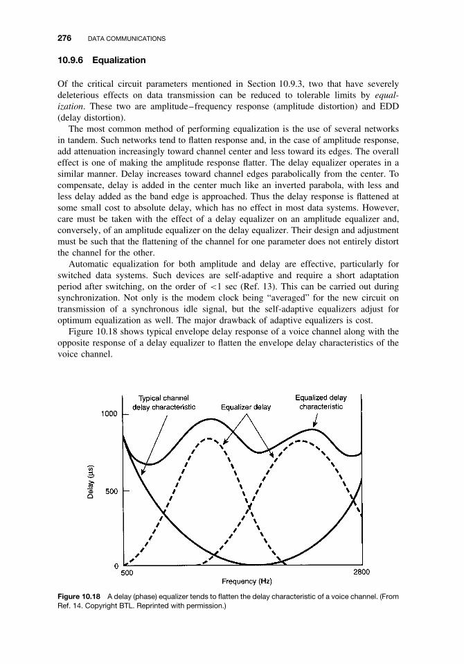
276 DATA COMMUNICATIONS
10.9.6 Equalization
Of the critical circuit parameters mentioned in Section 10.9.3, two that have severelydeleterious effects on data transmission can be reduced to tolerable limits by equal-ization. These two are amplitude–frequency response (amplitude distortion) and EDD(delay distortion).
The most common method of performing equalization is the use of several networksin tandem. Such networks tend to flatten response and, in the case of amplitude response,add attenuation increasingly toward channel center and less toward its edges. The overalleffect is one of making the amplitude response flatter. The delay equalizer operates in asimilar manner. Delay increases toward channel edges parabolically from the center. Tocompensate, delay is added in the center much like an inverted parabola, with less andless delay added as the band edge is approached. Thus the delay response is flattened atsome small cost to absolute delay, which has no effect in most data systems. However,care must be taken with the effect of a delay equalizer on an amplitude equalizer and,conversely, of an amplitude equalizer on the delay equalizer. Their design and adjustmentmust be such that the flattening of the channel for one parameter does not entirely distortthe channel for the other.
Automatic equalization for both amplitude and delay are effective, particularly forswitched data systems. Such devices are self-adaptive and require a short adaptationperiod after switching, on the order of <1 sec (Ref. 13). This can be carried out duringsynchronization. Not only is the modem clock being “averaged” for the new circuit ontransmission of a synchronous idle signal, but the self-adaptive equalizers adjust foroptimum equalization as well. The major drawback of adaptive equalizers is cost.
Figure 10.18 shows typical envelope delay response of a voice channel along with theopposite response of a delay equalizer to flatten the envelope delay characteristics of thevoice channel.
Figure 10.18 A delay (phase) equalizer tends to flatten the delay characteristic of a voice channel. (FromRef. 14. Copyright BTL. Reprinted with permission.)
10.9 DIGITAL TRANSMISSION ON AN ANALOG CHANNEL 277
10.9.7 Data Transmission on the Digital Network
Many data users only have analog access to the digital network. In other words, theirconnectivity to the network is via a subscriber loop to the local serving exchange. It iscommonly at this point where the analog channel enters a PCM channel bank and thesignal is converted to the standard digital signal. This class of data users will utilizeconventional data modems, as described in Section 10.9.5.
Other data users will be within some reasonable distance (some hundreds of feet) froma digital network terminal. This may be a PABX so equipped, providing access to a DS0or E0 line (Chapter 6), where the line rate is 64 kbps, the standard digital voice channel.In some instances in North America the digital line will only provide 56 kbps.
The digital network transmission rates are incompatible with standard transmissionrates in the data environment. Standard data rates are based on CCITT Recs. V.5 and V.6(Refs. 15, 16) as well as EIA-269 (Ref. 17). These data rates are 600, 1200, 2400, 4800,9600, 14,400, 19,200, 28,800, and 33,600 bps. They are not evenly divisible into 64,000bps, the standard digital voice channel. Two methods are described in the following tointerface these standard data rates with the 56/64 small kbps digital channel. The firstis AT&T’s Digital Data System (DDS) and the second is based on CCITT Rec. V.110(Ref. 18).
10.9.7.1 AT&T Digital Data System (DDS). The AT&T digital data system (DDS)provides duplex point-to-point and multipoint private line digital data transmission at anumber of synchronous data rates. This system is based on the standard 1.544-Mbps DS1PCM line rate, where individual bit streams have data rates that are submultiples of thatline rate (i.e., based on 64 kbps). However, pulse slots are reversed for identification inthe demultiplexing of individual user bit streams as well as for certain status and controlsignals and to ensure that sufficient line pulses are transmitted for receive clock recoveryand pulse regeneration. The maximum data rate available to a subscriber to the system is56 kbps, some 87.5% of the 64-kbps theoretical maximum.
The 1.544-Mbps line signal as applied to DDS service consists of 24 sequential 8-bitwords (i.e., channel time slots) plus one additional framing bit. This entire sequence isrepeated 8000 times per second. Note that again we have (192 + 1)8000 = 1.544 Mbps,where the value 192 is 8 × 24 (see Chapter 6). Thus the line rate of a DDS facility iscompatible with the DS1 (T1) PCM line rate and offers the advantage of allowing a mixof voice (PCM) and data where the full dedication of a DS1 facility to data transmissionwould be inefficient in most cases.
AT&T calls the basic 8-bit word a byte. One bit of each 8-bit word is reserved fornetwork control and for stuffing to meet nominal line bit rate requirements. This controlbit is called a C-bit. With the C-bit removed we see where the standard channel bitrate is derived, namely, 56 kbps or 8000 × 7. Four subrate or submultiple data rates arealso available: 2.4, 4.8, 9.6, and 19.2 kbps. However, when these rates are implemented,an additional bit must be robbed from the basic byte to establish flag patterns to routeeach substrate channel to its proper demultiplexer port. This allows only 48 kbps outof the original 64 kbps for the transmission of user data. The 48 kbps composite totalmay be divided into five 9.6-kbps channels, ten 4.8-kbps, or twenty 2.4-kbps channels,or two 19.2-kbps channels plus a 9.6-kbps channel. The subhierarchy of DDS signals isillustrated in Figure 10.19.
10.9.7.2 Transmitting Data on the Digital Network Based on CCITT Rec.V.110. This CCITT recommendation covers data rate adaption for standard rates up

278 DATA COMMUNICATIONS
Figure 10.19 Subhierarchy of DDS signals. Note: Inverse processing must be provided for the oppositedirection of transmission. Four-wire transmission is used throughout. (From Ref. 19. Copyright AmericanTelephone and Telegraph Company.)
through 19.2 kbps by means of a two-stage process. It also includes adaptation for 48 kbpsand 56 kbps to the 64 kbps E0 or clear DS0 channel.13
In the two-step case, the first conversion is to take the incoming data rate and convertit to an appropriate intermediate rate expressed by 2k × 8 kbps, where k = 0, 1, or 2. Thesecond conversion takes the intermediate rate and converts it to 64 kbps.
Simple division of 64,000 bps by standard data rates shows that as a minimum, a lot ofbit stuffing would be required. These would essentially be wasted bits. CCITT makes useof these bits to provide framing overhead, status information, and control information. Aframe (step 1 conversion) consists of 10 octets (10 × 8 = 80 bits). Six octets carry userdata, the first octet is all 0s for frame alignment, and bit 1 of the remaining 9 octets isset to 1. There are 15 overhead bits. Nine different frames accommodate the various datarates, and each frame has 80 bits (10 octets). The recommendation also covers conversionof start–stop data rates including 50, 75, 110, 150, and 300 bps and the standard rates upthrough 19.2 kbps (Ref. 18).
10.10 WHAT ARE DATA PROTOCOLS?
To get the most out of a network, certain operational rules, procedures, and interfaceshave to be established. A data network is a big investment, and our desire is to getthe best return on that investment. One way to optimize return on a data network is bythe selection of operational protocols. We must argue that there are multiple tradeoffsinvolved, all interacting one with another. Among these are data needs to be satisfied,network topology and architecture, selection of transmission media, switching and networkmanagement hardware and software, and operational protocols. In this section we willfocus on the protocols.
In the IEEE Standard Dictionary (Ref. 1), one definition of a protocol is the following:“a set of rules that govern functional units to achieve communication.” We would addinterfaces to the definition to make it more all-encompassing. In this section we will tracesome of the evolution of protocols up through the International Standards Organization
13Clear DS0 channel is a DS0 channel with the signaling bits disabled.

10.10 WHAT ARE DATA PROTOCOLS? 279
(ISO), OSI and its seven layers. Emphasis will be placed on the first three layers becausethey are more directly involved in communication.
Protocols should not be confused with formats. Formats typically show a standardorganization of bits and octets and describe the function of each to achieve a certainobjective. DS1 is a format as are SDH and SONET.
In this section we will familiarize the reader with basic protocol functions. This isfollowed by a discussion of the Open System Interconnection (OSI), which has facilitateda large family of protocols. A brief discussion of HDLC (high-level data-link control) isprovided. This particular protocol was selected because it spawned so many other linklayer protocols. Some specific higher layer protocols are described in Chapter 11.
10.10.1 Basic Protocol Functions
There are a number of basic protocol functions. Typical among these are:
ž Segmentation and reassembly (SAR)ž Encapsulationž Connection controlž Ordered deliveryž Flow controlž Error control
A short description of each follows.Segmentation and reassembly. Segmentation refers to breaking up the data message or
file into blocks, packets, or frames with some bounded size. Which term we use dependson the semantics of the system. There is a new data segment called a cell, used inasynchronous transfer mode (ATM) and other digital systems. Reassembly is the reverseof segmentation, because it involves putting the blocks, frames, or packets back intotheir original order. The device that carries out segmentation and reassembly in a packetnetwork is called a PAD (packet assembler–disassembler).
Encapsulation. Encapsulation is the adding of header and control information in frontof the text or info field and parity information, which is generally carried behind the textor info fields.
Connection control. There are three stages of connection control:
1. Connection establishment2. Data transfer3. Connection termination
Some of the more sophisticated protocols also provide connection interrupt and recoverycapabilities to cope with errors and other sorts of interruptions.
Ordered delivery. Packets, frames, or blocks are often assigned sequence numbers toensure ordered delivery of the data at the destination. In a large network with manynodes and possible routes to a destination, especially when operated in a packet mode,the packets can arrive at the destination out of order. With a unique segment (packet)numbering plan using a simple numbering sequence, it is a rather simple task for a longdata file to be reassembled at the destination it its original order.
Flow control. Flow control refers to the management of the data flow from source todestination such that buffer memories do not overflow, but maintain full capacity of all

280 DATA COMMUNICATIONS
facility components involved in the data transfer. Flow control must operate at severalpeer layers of protocols, as will be discussed later.
Error control. Error control is a technique that permits recovery of lost or erroredpackets (frames, blocks). There are four possible functions involved in error control:
1. Numbering of packets (frames, blocks) (e.g., missing packet).2. Incomplete octets (a bit sequence does not carry the proper number of bits, in this
case 8 bits).3. Error detection. Usually includes error correction (see Section 10.5.3).4. Acknowledgment of one, several, or a predetermined string of packets (blocks,
frames). Acknowledgment may be carried out by returning to the source (or node)the send sequence number as a receive sequence number.
10.10.2 Open Systems Interconnection (OSI)
10.10.2.1 Rationale and Overview of OSI. Data communication systems can bevery diverse and complex. These systems involve elaborate software that must run onequipment having ever-increasing processing requirements. Under these conditions, it isdesirable to ensure maximum independence among the various software and hardwareelements of a system for two reasons:
ž To facilitate intercommunication among disparate elements.ž To eliminate the “ripple effect” when there is a modification to one software element
that may affect all elements.
The ISO set about to make this data intercommunication problem more manageable. Itdeveloped its famous OSI reference model (Ref. 20). Instead of trying to solve the globaldilemma, it decomposed the problem into more manageable parts. This provided standard-setting agencies with an architecture that defines communication tasks. The OSI modelprovides the basis for connecting open systems for distributed applications processing.The term open denotes the ability of any two systems conforming to the reference modeland associated standards to interconnect. OSI thus provides a common groundwork forthe development of families of standards permitting data assets to communicate.
ISO broke data communications down into seven areas or layers, arranged verticallystarting at the bottom with layer 1, the input/output ports of a data device. The OSIreference model is shown in Figure 10.20. It takes at least two to communicate. Thus weconsider the model in twos, one entity to the left in the figure and one peer entity to theright. ISO and the ITU-T organization use the term peers. Peers are corresponding entitieson either side of Figure 10.20. A peer on one side of the system (system A) communicateswith its peer on the other side (system B) by means of a common protocol. For example,the transport layer of system A communicates with its peer transport layer at system B. Itis important to note that there is no direct communication between peer layers except atthe physical layer (layer 1). That is, above the physical layer, each protocol entity sendsdata down to the next lower layer, and so on to the physical layer, then across and up toits peer on the other side. Even the physical layer may not be directly connected to itspeer on the other side of the “connection” such as in packet communications. This wecall connectionless service when no physical connection is set up.14 However, peer layersmust share a common protocol in order to communicate.14Connectionless service is a type of delivery service that treats each packet, datagram, or frame as a separateentity containing the source and destination address. An analogy in everyday life is the postal service. We puta letter in the mail and we have no idea how it is routed to its destination. The address on the letter serves toroute the letter.

10.10 WHAT ARE DATA PROTOCOLS? 281
Figure 10.20 The OSI reference model.
There are seven OSI layers, as shown in Figure 10.20. Any layer may be referred toas an N -layer. Within a particular system there are one or more active entities in eachlayer. An example of an entity is a process in a multiprocessing system. It could simplybe a subroutine. Each entity communicates with entities above it and below it across aninterface. The interface is at a service access point (SAP).
The data that pass between entities are a bit grouping called a protocol data unit(PDU). Data units are passed downward from a peer entity to the next OSI layer, calledthe (N − 1) layer. The lower layer calls the PDU a service data unit (SDU). The (N − 1)
layer adds control information, transforming the SDU into one or more PDUs. However,the identity of the SDU is preserved to the corresponding layer at the other end of theconnection. This concept is illustrated in Figure 10.21.
OSI has considerable overhead. By overhead, we mean bit sequences that are usedfor logical interfaces or just simply to make the system work. Overhead does not carryrevenue-bearing traffic. Overhead has a direct bearing on system efficiency: As overheadincreases, system efficiency decreases.
OSI layering is widely accepted in the world of data communications even with itsconsiderable overhead. Encapsulation is a good example. Encapsulation is used on allOSI layers above layer 1, as shown in Figure 10.22.
Figure 10.21 An illustration of mapping between data units on adjacent layers.

282 DATA COMMUNICATIONS
Figure 10.22 Buildup and breakdown of a data message based on the OSI model. OSI encapsulates atevery layer except layer 1.
10.10.2.2 Functions of the First Four OSI Layers. Only the first four OSI layersare described in the following paragraphs. Layers 5, 6, and 7 are more in the realm ofsoftware design.
Physical layer. The physical layer is layer 1, the lowest OSI layer. It provides thephysical connectivity between two data terminals who wish to communicate. The servicesit provides to the data link layer (layer 2) are those required to connect, maintain theconnection, and disconnect the physical circuits that form the physical connectivity. Thephysical layer represents the traditional interface between the DCE and DTE, describedin Section 10.8.
The physical layer has four important characteristics:
1. Mechanical2. Electrical3. Functional4. Procedural
The mechanical aspects include the actual cabling and connectors necessary to connectthe communications equipment to the media. Electrical characteristics cover voltage andimpedance, balanced and unbalanced. Functional characteristics include connector pinassignments at the interface and the precise meaning and interpretation of the variousinterface signals and data set controls. Procedures cover sequencing rules that governthe control functions necessary to provide higher-layer services such as establishing aconnectivity across a switched network.
Data-link layer. The data-link layer provides services for reliable interchange of dataacross a data link established by the physical layer. Link-layer protocols manage the

10.10 WHAT ARE DATA PROTOCOLS? 283
establishment, maintenance, and release of data-link connections. These protocols controlthe flow of data and supervise error recovery. A most important function of this layeris recovery from abnormal conditions. The data-link layer services the network layer orlogical link control (LLC; in the case of LANs) and inserts a data unit into the INFOportion of the data frame or block. A generic data frame generated by the link layer isillustrated in Figure 10.7.
Several of the more common data-link layer protocols are: CCITT LAPB, LAPD; IBMSDLC; and ANSI ADCCP (also the U.S. government standard).
Network layer. The network layer moves data through the network. At relay andswitching nodes along the traffic route, layering concatenates. In other words, the higherlayers (above layer 3) are not required and are utilized only at user end-points.
The concept of relay open system is shown in Figure 10.23. At the relay switchingpoint, only the first three layers of OSI are required.
The network layer carries out the functions of switching and routing, sequencing,logical channel control, flow control, and error-recovery functions. We note the duplicationof error recovery in the data-link layer. However, in the network layer error recovery isnetwork-wide, whereas on the data-link layer error recovery is concerned only with thedata link involved.
The network layer also provides and manages logical channel connections betweenpoints in a network such as virtual circuits across the public switched network (PSN). Itwill be appreciated that the network layer concerns itself with the network switching androuting function. On simpler data connectivities, where a large network is not involved,the network layer is not required and can be eliminated. Typical of such connectivitiesare point-to-point circuits, multipoint circuits, and LANs. A packet-switched network isa typical example where the network layer is required.
The best-known layer 3 standard is CCITT Rec. X.25 (Ref. 22).Transport layer. The transport layer (layer 4) is the highest layer of the services asso-
ciated with the provider of communication services. One can say that layers 1–4 are theresponsibility of the communication system engineer. Layers 5, 6, and 7 are the respon-sibility of the data end-user. However, we believe that the telecommunication systemengineer should have a working knowledge of all seven layers.
Figure 10.23 Only the first three OSI layers are required at an intermediate relay (switching) point.

284 DATA COMMUNICATIONS
The transport layer has the ultimate responsibility for providing a reliable end-to-end data-delivery service for higher-layer users. It is defined as an end-system function,located in the equipment using network service or services. In this way its operations areindependent of the characteristics of all the networks that are involved. Services that atransport layer provides are as follows:
ž Connection Management. This includes establishing and terminating connectionsbetween transport users. It identifies each connection and negotiates values of allneeded parameters.
ž Data Transfer. This involves the reliable delivery of transparent data between theusers. All data are delivered in sequence with no duplication or missing parts.
ž Flow Control. This is provided on a connection basis to ensure that data are notdelivered at a rate faster than the user’s resources can accommodate.
The TCP (transmission control protocol) was the first working version of a transportprotocol and was created by DARPA for DARPANET.15 All the features in TCP havebeen adopted in the ISO version. TCP is often combined with the Internet protocol (IP)and is referred to as TCP/IP.
10.10.3 High-Level Data-Link Control: A Typical Link-Layer Protocol
High-level data-link control (HDLC) was developed by the ISO. It has spawned manyrelated or nearly identical protocols. Among these are ANSI ADCCP, CCITT LAPB andLAPD, IEEE Logical Link Control (LLC), and IBM SDLC (Refs. 20–25).
The following HDLC definitions include stations, configurations, and three modesof operation.
Primary Station A logical primary station is an entity that has primary link controlresponsibility. It assumes responsibility for organization of data flow and for linklevel error recovery. Frames issued by the primary station are called commands.
Secondary Station A logical secondary station operates under control of a primarystation. It has no direct responsibility for control of the link, but instead responds toprimary station control. Frames issued by a secondary station are called responses.
Combined Station A combined station combines the features of primary and secondarystations. It may issue both commands and responses.
Unbalanced Configuration An unbalanced configuration consists of a primary sta-tion and one or more secondary stations. It supports full-duplex and half-duplexoperation, point-to-point, and multipoint circuits. An unbalanced configuration isillustrated in Figure 10.24a.
Balanced Configuration A balanced configuration consists of two combined stations inwhich each station has equal and complementary responsibility of the data link. Abalanced configuration, shown in Figure 10.24b, operates only in the point-to-pointmode and supports full-duplex operation.
Modes of Operation With normal response mode (NRM) a primary station initiates datatransfer to a secondary station. A secondary station transmits data only in responseto a poll from the primary station. This mode of operation applies to an unbalancedconfiguration. With asynchronous response mode (ARM) a secondary station may
15DARPA stands for Defense Advanced Research Projects Agency, under the U.S. Department of Defense.

10.10 WHAT ARE DATA PROTOCOLS? 285
Figure 10.24 HDLC link configurations. (a) Unbalanced configuration; (b) balanced configuration.
initiate transmission without receiving a poll from a primary station. It is useful on acircuit where there is only one active secondary station. The overhead of continuouspolling is thus eliminated. Asynchronous balanced mode (ABM) is a balanced modethat provides symmetric data transfer capability between combined stations. Eachstation operates as if it were a primary station, can initiate data transfer, and isresponsible for error recovery. One application of this mode is hub polling, wherea secondary station needs to initiate transmission.
10.10.3.1 HDLC Frame. Figure 10.25 shows the HDLC frame format. Note the sim-ilarity to the generic data-link frame illustrated in Figure 10.8. Moving from left to rightin the figure, we have the flag field (F), which delimits the frame at both ends with theunique pattern 01111110. This unique field or flag was described in Section 10.7.2.
The address field (A) immediately follows the opening flag of a frame and precedesthe control field (C). Each station in the network normally has an individual addressand a group address. A group address identifies a family of stations. It is used whendata messages must be accepted from or destined to more than one user. Normally theaddress is 8 bits long, providing 256 bit combinations or addresses (28 = 256). In HDLC(and ADCCP) the address field can be extended in increments of 8 bits. When this isimplemented, the least significant bit is used as an extension indicator. When that bit is
Figure 10.25 The HDLC frame format (Ref. 25).

286 DATA COMMUNICATIONS
0, the following octet is an extension of the address field. The address field is terminatedwhen the least significant bit of an octet is 1. Thus we can see that the address field canbe extended indefinitely.
The control field (C) immediately follows the address field (A) and precedes the infor-mation field (I). The control field conveys commands, responses, and sequence numbersto control the data link. The basic control field is 8 bits long and uses modulo 8 sequencenumbering. There are three types of control field: (1) I frame (information frame), (2) Sframe (supervisory frame), and (3) U frame (unnumbered frame). The three control fieldformats are illustrated in Figure 10.26.
Consider the basic 8-bit format shown in Figure 10.26. The information flows fromleft to right. If the frame shown in Figure 10.25 has a 0 as the first bit in the control field,the frame is an I frame (see Figure 10.26a). If the bit is a 1, the frame is an S or a Uframe, as illustrated in Figure 10.26b and 10.26c. If the first bit is followed by a 0, it isan S frame, and if the bit again is a 1 followed by a 1, it is a U frame. These bits arecalled format identifiers.
Turning now to the information (I) frame (Figure 10.26a), its purpose is to carry userdata. Bits 2, 3, and 4 of the control field in this case carry the send sequence numberN(S) of the transmitted messages (i.e., I frames). N(S) is the frame sequence numberof the next frame to be transmitted and N(R) is the sequence number of the frame tobe received.
Each frame carries a poll/final (P/F) bit. It is bit 5 in each of the three different typesof control fields shown in Figure 10.26. This bit serves a function in both command andresponse frames. In a command frame it is referred to as a poll (P) bit; in a responseframe as a final (F) bit. In both cases the bit is sent as a 1.
The P bit is used to solicit a response or sequence of responses from a secondary orbalanced station. On a data link only one frame with a P bit set to 1 can be outstanding atany given time. Before a primary or balanced station can issue another frame with a P bitset to 1, it must receive a response frame from a secondary or balanced station with the Fbit set to 1. In the NRM mode, the P bit is set to 1 in command frames to solicit responseframes from the secondary station. In this mode of operation the secondary station maynot transmit until it receives a command frame with the P bit set to 1.
Of course, the F bit is used to acknowledge an incoming P bit. A station may notsend a final frame without prior receipt of a poll frame. As can be seen, P and F bits
Figure 10.26 The three control field formats of HDLC.

REVIEW EXERCISES 287
are exchanged on a one-for-one basis. Thus only one P bit can be outstanding at a time.As a result the N(R) count of a frame containing a P or F bit set to 1 can be used todetect sequence errors. This capability is called check pointing. It can be used not only todetect sequence errors but to indicate the frame sequence number to begin retransmissionwhen required.
Supervisory frames, shown in Figure 10.26b, are used for flow and error control. Bothgo-back-n and continuous (selective) ARQ can be accommodated. There are four typesof supervisory frames:
1. Receive ready (RR): 1000 P/F N(R);2. Receive not ready (RNR): 1001 P/F N(R);3. Reject (Rej): 1010 P/F N(R); and4. Selective reject (SRej): 1011 P/F N(R).
The RR frame is used by a station to indicate that it is ready to receive information andacknowledge frames up to and including N(R) − 1. Also, a primary station may use theRR frame as a command with the poll (P) bit set to 1.
The RNR frame tells a transmitting station that it is not ready to receive additionalincoming I frames. It does acknowledge receipt of frames up to and including sequencenumber N(R) − 1. I frames with sequence number N(R) and subsequent frames, if any, arenot acknowledged. The Rej frame is used with go-back-n ARQ to request retransmissionof I frames with frame sequence number N(R), and N(R) − 1 frames and below areacknowledged.
Unnumbered frames are used for a variety of control functions. They do not carrysequence numbers, as the name indicates, and do not alter the flow or sequencing of Iframes. Unnumbered frames can be grouped into the following four categories:
1. Mode-setting commands and responses2. Information transfer commands and responses3. Recovery commands and responses4. Miscellaneous commands and responses.
The information field follows the control field (Figure 10.25) and precedes the framecheck sequence (FCS) field. The I field is present only in information (I) frames and insome unnumbered (U) frames. The I field may contain any number of bits in any code,related to character structure or not. Its length is not specified in the standard (ISO 3309,Ref. 25). Specific system implementations, however, usually place an upper limit on Ifield size. Some versions require that the I field contain an integral number of octets.
Frame check sequence (FCS). Each frame includes an FCS field. This field immedi-ately follows the I field, or the C field if there is no I field, and precedes the closingflag (F). The FCS field detects errors due to transmission. The FCS field contains 16 bits,which are the result of a mathematical computation on the digital value of all bits exclud-ing the inserted zeros (zero insertion) in the frame and including the address, control, andinformation fields.
REVIEW EXERCISES
1. What is the basic element of information in a binary system? How much informationdoes it contain?

288 DATA COMMUNICATIONS
2. In reference to question 1 above, how does one extend the information content ofthat basic information element, a bit? For example, how would we develop a binarycode that represents our alphabet?
3. There are many ways we can express the binary 1 and binary 0. Give at least four.How do we remove the ambiguity about meaning of a bit (reversing sense)?
4. How many distinct characters and/or symbols can be represented in a 4-bit binarycode? a 7-bit binary code? an 8-bit binary code?
5. How many information elements are in an ASCII character?
6. Give two causes of burst errors.
7. Give the two generic methods of correcting errors on a datalink.
8. Name the three different types of ARQ and define each.
9. Describe the difference between neutral and polar transmission.
10. On a start–stop circuit, where does a receiver start counting information bits (insidea character or symbol)?
11. There are three major causes of error on a data link. Name two of them.
12. On start–stop transmission, the mark-to-space transition on the start element tellsthe receiver when to start counting bits. How does a synchronous data stream knowwhen to start counting bits in a frame of packet?
13. How does a synchronous data receiver keep in synchronization with an incomingbit stream?
14. A serial synchronous NRZ bit stream has a data rate of 19.2 kbps. What is theperiod of one bit?
15. What is notably richer in transitions per unit time: RZ or NRZ coding?
16. The CCITT V.29 modem operates on the standard analog voice channel at 9600bps. How can it do this on a channel with a 3100-Hz bandwidth?
17. Name the three basic impairments for data transmission.
18. Name the four types of noise. Indicate the two that a data circuit is sensitive toand explain.
19. Phase distortion, in general, has little effect on speech transmission. What can wesay about it for data transmission?
20. Shannon’s formula for capacity (bps) for a particular bandwidth was based only onone parameter. What was/is it?
21. We usually equalize two voice channel impairments. What are they and how doesthe equalization work?
22. Why do higher-speed modems use a center frequency around 1800 Hz?
23. Why is the PSTN digital network not compatible with data bit streams?

REFERENCES 289
REFERENCES
1. The IEEE Standard Dictionary of Electrical and Electronic Terms, 6th ed., IEEE Std. 100-1996,IEEE, New York, 1996.
2. Equivalence Between Binary Notation Symbols and the Significant Conditions of a Two-Condi-tion Code, CCITT Rec. V.1
3. R. L. Freeman, Practical Data Communications, 2nd ed., Wiley, New York, 2002.
4. R. L. Freeman, Telecommunication Transmission Handbook, 4th ed., Wiley, 1998.
5. Interface Between Data Terminal Equipment and Data Circuit-Terminating Equipment Employ-ing Serial Binary Data Interchange, EIA/TIA-232F, Electronics Industries Association, Wash-ington, DC, July 1999.
6. Error Performance on an International Digital Connection Forming Part of an Integrated Ser-vices Digital Network, CCITT Rec. G.821, Fascicle III.5, IXth Plenary Assembly, Melbourne,1988 (revised ITU Geneva, 1996).
7. High-Speed 25-Position Interface for Data Terminal Equipment and Data Circuit TerminatingEquipment Including Alternative 26-Position Connector, EIA/TIA-530-A, Electronic IndustriesAssociation, Washington, DC, June 1992.
8. W. R. Bennett and J. R. Davey, Data Transmission, McGraw-Hill, New York, 1965.
9. Transmission Characteristics of National Networks, ITU-T Rec. G.120, ITU Geneva, 1998.
10. C. E. Shannon, A Mathematical Theory of Communications, BSTJ 27, Bell Telephone Labora-tories, Holmdel, NJ, 1948.
11. 1200 bps Duplex Modem Standardized for Use in the General-Switched Telephone Network andon Point-to-Point 2-Wire Leased Telephone Type Circuits, CCITT Rec. V.22, Fascicle VIII.1,IXth Plenary Assembly, Melbourne, 1988.
12. 9600 bps Modem Standardized for Use on Point-to-Point 4-Wire Leased Telephone Type Circuits,CCITT Rec. V.29, Fascicle VIII.1, IXth Plenary Assembly, Melbourne, 1988.
13. K. Pahlavan and J. L. Holsinger, “Voice Band Communication Modems: An Historical Review,1919–1988,” IEEE Communications Magazine, 261(1), 1988.
14. Transmission Systems for Communications, 5th ed., Bell Telephone Laboratories, Holmdel, NJ,1982.
15. Electrical Characteristics for Unbalanced Double-Current Interchange Circuits Operating atSignaling Rates Nominally up to 100 kbps, ITU Rec, V.10, ITU Geneva, March 1993.
16. Electrical Characteristics for Balanced Double-Current Interchange Circuits Operating at DataSignaling Rates up to 10 Mbps, ITU-T Rec. V.11, ITU Geneva, 1996.
17. Synchronous Signaling Rates for Data Transmission, EIA-269A, Electronic Industries Associ-ation, Washington, DC, May 1968.
18. Support of Data Terminal Equipments with V-Series Type Interfaces by an Integrated ServicesDigital Network, CCITT Rec. V.110, ITU Geneva, 2000.
19. Digital Data System Data Service Unit Interface Specification, Bell System Reference 41450,AT&T, New York, 1981.
20. Information Processing Systems Open Systems Interconnection—Basic Reference Model, ISO7498, Geneva, 1984.
21. Advanced Data Communications Control Procedures, X.3.66, ANSI, New York, 1979.
22. Interface Between Data Terminal Equipment (DTE) and Data Circuit-Terminating Equipment(DCE) for Terminals Operating in the Packet Mode and Connected to Public Data Networks bya Dedicated Circuit, ITU-T Rec. X.25, ITU Geneva, 1996.
23. ISDN User Network Interface—Data Link Layer, ITU-T Rec. Q.921, ITU Geneva, 1997.
24. Information Processing Systems—Local Area Networks, Part 2, Logical Link Control, IEEEStd. 802.3, 1994 edition, IEEE, New York, 1994.

290 DATA COMMUNICATIONS
25. High-Level Data Link Control Procedures—Frame Structure, ISO 3309, International StandardsOrganization, Geneva, 1979.
26. Military Communication System Technical Standard, MIL-STD-188C, US Department ofDefense, Washington, DC, 1966.
27. Reference Data for Engineers: Radio, Computers and Communications, 8th edition, SAM Pub-lishing, Carmel, IN, 1993.
28. A Digital Modem and Analog Modem Pair for Use on the Public Switched Telephone Network(PSTN) at Data Signaling Rates of up to 56,000 bits/s downstream and up to 33,600 bits/sUpstream, ITU-T Rec. V.90, ITU Geneva, 1998.
29. A Digital Modem Operating at Data Signaling Rates up to 64,000 bits/s for Use on a 4-wireCircuit Switched Connection and on Leased Point-to-point 4-wire Digital Circuit, ITU-T Rec.V.91, ITU-Geneva, May 1999.
30. List of Definitions for Interchange Circuits Between Data Terminal Equipment (DTE) and DataCircuit-Terminating Equipment (DCE), ITU-T Rec. V.24, ITU Geneva, 2000.
11
ENTERPRISE NETWORKS I: LOCALAREA NETWORKS
11.1 WHAT DO ENTERPRISE NETWORKS DO?
An enterprise network consists of an interconnected group of telecommunication facilitiesthat are confined to a singular entity. There can be broad, midrange, and narrow inter-pretations of the definition. The “singular entity” may be government or an industrialenterprise. FTS2000, the large GSA (General Services Administration) that was charteredto serve all U.S. government organizations, is an example of a broad interpretation. Thisnetwork provides multiple services: voice data and image. It is the U.S. government’sown PSTN. A narrow interpretation might be Corrugated Box Works local area network.Or Walgreens’ large VSAT network. This latter example is included because the networkserves a singular purpose, for logistics and cash flow, and is owned by one entity.
This chapter will be based on the narrower interpretation and will be confined to thevarious data networks that may be employed in government and industry. We first presentan overview of local area networks (LANs) followed by a discussion in the next chapterof wide area networks (WANs).
11.2 LOCAL AREA NETWORKS (LANS)
The IEEE (Ref. 1) defines a local area network as “a communication network to inter-connect a variety of devices (e.g., personal computers, workstations, printers, file storagedevices) that can transmit data over a limited area, typically within a facility.”
The geographical extension or “local area” may extend from less than 100 ft (< 30 m)
to over 6 miles (> 10 km). More commonly we can expect a LAN to extend over a floorin a building, and in some cases over a portion of a floor. Other LANs may cover multiplefloors, groups of building in the same general area, or a college or industrial campus.
The transmission media encompass wire pair, coaxial cable, fiber-optic cable, and radio.The implementation of coaxial cable systems is slowing in favor of high-quality twistedwire pair. Wireless LANs, particular in the IEEE 802.11 series standards, are reachingmaturity. Data rates vary from 1 Mbps to 1000 Mbps. LAN data rates, the number ofdevices connected to a LAN, the spacing of those devices, and the network extensiondepend on:
Fundamentals of Telecommunications, Second Edition, by Roger L. FreemanISBN 0-471-71045-8 Copyright 2005 by Roger L. Freeman
291
292 ENTERPRISE NETWORKS I: LOCAL AREA NETWORKS
ž The transmission medium employedž The transmission technique (i.e., baseband or broadband)ž Network access protocolž The incorporation of such devices as repeaters, bridges, routers, and switching hubsž The access standard used, where there may be some upper limit on the number of
accesses per segment
The preponderance of LANs operate without error correction with BERs specified in therange of 1 × 10⁻⁸ to 1 × 10⁻¹² or better.
The most common application of a LAN is to interconnect data terminals and otherprocessing resources, where all the devices reside in a single building or complex ofbuildings, and usually these resources have a common owner. A LAN permits effectivecost sharing of high-value data processing equipment, such as mass storage media, main-frame computers or minicomputers, and high-speed printers. Resource sharing is probablyequally as important where a LAN serves as the access vehicle for an intranet. Resourcesharing in this context means that each LAN user has access to all other users’ file andother data resources.
The interconnection of LANs in the local area (e.g., the floor of a building) with ahigh-speed backbone (e.g., between building floors) is very prevalent. LANs may connectthrough wide area networks (WANs) to other distant LANs. This is frame relay’s principalapplication. The interface to the WAN may be via a smart bridge or a router.
There are two generic transmission techniques utilized by LANs: baseband and broad-band. Baseband transmission can be defined as the direct application of the basebandsignal to the transmission medium. Broadband transmission, in this context, is where thebaseband signal from the data device is translated in frequency to a particular frequencyslot in the RF spectrum. Broadband transmission requires a modem to carry out the trans-lation. Baseband transmission may require some sort of signal-conditioning device. Withbroadband LAN transmission we usually think of simultaneous multiple RF carriers thatare separated in the frequency domain. Present broadband technology comes from thecable television (CATV) industry.
The discussion in this section will essentially cover baseband LANs. An importantaspect is that only one user at a time may access a LAN segment at a time. We expectsegments to be isolated one from another by smart bridges or switched hubs.
11.3 LAN TOPOLOGIES
There are three types of basic LAN topology1: bus, ring, and star. These are illustrated inFigure 11.1 along with the tree network, which is a simple derivative of the conventionalbus topology.
A bus is a length of transmission medium from which users tap into, as shown inFigure 11.1a. Originally the medium was coaxial cable. Today coaxial cable is beingphased out in favor of unshielded twisted pair (UTP) or fiber-optic cable.
A ring is simply a bus that is folded back onto itself. A ring topology is illustrated inFigure 11.1b. User traffic flows in one direction around the ring. In some other approachesa second transmission medium is added for flow in the opposite direction. Such a dualcounterrotating ring concept improves reliability in case of a failed station or a cut inthe ring.
1Topology means the logical and/or physical arrangement of stations on a network. In other words, topologytells how these assets are connected together.

11.3 LAN TOPOLOGIES 293
Figure 11.1a A typical bus network.
Figure 11.1b A typical ring network.
A star network is illustrated in Figure 11.1c. At the center of the star is a switchingdevice. This could be a switching hub. Users can be paired, two at a time, three ata time, or all at a time, segmented into temporary families of users depending on theconfiguration of the switch at that moment in time. Such a concept lends itself particularly

294 ENTERPRISE NETWORKS I: LOCAL AREA NETWORKS
Figure 11.1c A star network.
Figure 11.1d A typical tree configuration.
well to ATM (asynchronous transfer mode). Each user is connected to the switch on apoint-to-point basis.
A tree network is illustrated in Figure 11.1d.
11.4 BASEBAND LAN TRANSMISSION CONSIDERATIONS
A baseband LAN is a point-to-point or point-to-multipoint network. Two transmissionproblems arise as a result. The first deals with signal level and signal-to-noise (S/N)ratio, and the second deals with standing waves. Each access on a common mediummust have sufficient signal level and S/N such that copied signals have a BER in the
11.5 OVERVIEW OF ANSI/IEEE LAN PROTOCOLS 295
range of 1 × 10⁻⁸ to 1 × 10⁻¹². If the medium is fairly long in extension and there aremany accesses, the signal level must be high for a transmitting access to reach its mostdistant destination. The medium is lossy, particularly at the higher bit rates, and eachaccess tap has an insertion loss. This leads to very high signal levels. These may be richin harmonics and spurious emissions, degrading bit error rate. On the other hand, withinsufficient level, the S/N ratio degrades, which will also degrade error performance. Agood level balance must be achieved for all users. Every multipoint connectivity must beexamined. The number of multipoint connectivities can be expressed by n(n − 1), wheren is the number of accesses. If, on a particular LAN, 100 accesses are planned, there are9900 possible connectivities to be analyzed to carry out signal level balance. One way tosimplify the job is to segment the network, placing a regenerative repeater (or bridge) ateach boundary. This reduces the signal balance job to realizable proportions and ensuresthat a clean signal of proper level is available at each access tap. For baseband LANs,50-� coaxial cable is favored over the more common 75-� cable. The lower-impedancecable is less prone to signal reflections from access taps and provides better protectionagainst low-frequency interference.
11.5 OVERVIEW OF ANSI/IEEE LAN PROTOCOLS
11.5.1 Introduction
Many of the widely used LAN protocols have been developed in North America throughthe offices of the Institute of Electrical and Electronic Engineers (IEEE). The AmericanNational Standards Institute (ANSI) has subsequently accepted and incorporated thesestandards, and they now bear the ANSI imprimatur.
The IEEE develops LAN standards in the IEEE 802 family of committees. Of interestin this chapter are the following IEEE committees, each with published standards, whichcontinue to evolve:
802.1 High-Level LAN Interface
802.2 Logical Link Control (LCC)
802.3 CSMA/CD Networks Ethernet working group
802.4 Token Bus Networks (inactive)
802.5 Token Ring Networks (inactive)
802.11 Wireless LAN (many subset such as 802.11b, 802.11d, others)
802.15 Wireless Personal Area Network
802.16 Broadband Wireless Access
802.17 Resilient Packet Ring
802.18 Radio Regulatory
802.19 Coexistence
802.20 Mobile Broadband Wireless Access (MBWA)
802.21 Media Independent Handoff list as of 3/22/04
11.5.2 How LAN Protocols Relate to OSI
LAN protocols utilize only OSI layers 1 and 2, the physical and data-link layers, respec-tively. The data-link layer is split into two sublayers: logical link control (LLC) and

296 ENTERPRISE NETWORKS I: LOCAL AREA NETWORKS
Figure 11.2 LAN 802 architecture related to OSI.
medium access control (MAC). These relationships are shown in Figure 11.2. The princi-pal functions of OSI layer 3, namely switching, relaying, and network end-to-end control,are not necessary in this simple, closed network. The remaining layer 3 functions that arenecessary are incorporated in layer 2. The two layer 2 sublayers (LLC and MAC) carryout four functions:
1. They provide one or more service access points (SAPs). A SAP is a logical interfacebetween two adjacent layers.
2. Before transmission, they assemble data into a frame with address and error-detection fields.
3. On reception, they disassemble the frame and perform address recognition anderror detection.
4. They manage communications over the link.
The first function and those related to it are performed by the LLC sublayer. The lastthree functions are handled by the MAC sublayer.
In the following subsections we will describe four common IEEE and ANSI stan-dardized protocols. Logical link control (LLC) is common to all four. They differ in themedium access control (MAC) protocol.
A station on a LAN may have multiple users; oftentimes these are just processes, suchas processes on a host computer. These processes may wish to pass traffic to another LANstation that may have more than one “user” in residence. We will find that LLC produces aprotocol data unit (PDU) with its own source and destination address. The source address,in this case, is the address of the originating user. The destination address is the addressof a user in residence at a LAN station. Such a user is connected through a service accesspoint (SAP) at the upper boundary of the LLC layer. The resulting LLC PDU is thenembedded in the information field of a MAC frame. This is shown in Figure 11.3. TheMAC frame also has source and destination addresses. These direct traffic to a particularLAN station or stations.

11.5 OVERVIEW OF ANSI/IEEE LAN PROTOCOLS 297
Figure 11.3 A user passes traffic to an LLC where encapsulation takes place forming an LLC PDU. TheLLC PDU is embedded in a MAC frame info(rmation) field. The resulting MAC frame is passed to thephysical layer, which transmits the traffic on the LAN.
11.5.3 Logical Link Control (LLC)
The LLC provides services to the upper layers at a LAN station. It provides two formsof services for its users:
1. Unacknowledged connectionless service2. Connection mode services.
Some brief comments are required to clarify the functions and limitations of each ser-vice. With unacknowledged connectionless service a single service access initiates thetransmission of a data unit to the LLC, the service provider. From the viewpoint of theLLC, previous and subsequent data units are unrelated to the present unit. There is noguarantee by the service provider of the delivery of the data unit to its intended user, noris the sender informed if the delivery attempt fails. Furthermore, there is no guarantee ofordered delivery. This type of service supports point-to-point, multipoint, and broadcastmodes of operation.
As we might imagine with connection mode service, a logical connection is establishedbetween two LLC users. During the data-transfer phase of the connection, the serviceprovider at each end of the connection keeps track of the data units transmitted andreceived. The LLC guarantees that all data will be delivered and that the delivery to theintended user will be ordered (e.g., in the sequence as presented to the source LLC fortransmission). When there is a failure to deliver, it is reported to the sender.
IEEE (Ref. 2) defines the LLC as that part of a data station that supports the LLCfunctions of one or more logical links. The LLC generates command PDUs and responsePDUs for transmission and interprets received command PDUs and response PDUs. Spe-cific responsibilities assigned to the LLC include:
ž Initiation of control signal interchangež Interpretation of received command PDUs and generation of appropriate response
PDUsž Organization of data flowž Actions regarding error-control and error-recovery functions in the LLC sublayer
As shown in Figure 11.3, the LLC accepts higher level user data and encapsulates it,forming an LLC PDU. The resulting LLC frame is embedded into the MAC user fieldfor transmission.

298 ENTERPRISE NETWORKS I: LOCAL AREA NETWORKS
The LLC is another derivative of HDLC, which was discussed in Section 10.10.3. It isbased on the balanced mode of that link-layer protocol with similar formats and functions.This is particularly true when operating in the connection mode.
11.5.3.1 LLC PDU Structure. As shown in Figure 11.3, the LLC appends a headerforming the LLC PDU. The PDU frame format is illustrated in Figure 11.4. The headerconsists of address and control information; the information field contains the user data.The control field is identical with HDLC control field, illustrated in Figure 10.29 anddescribed in Section 10.10.3.1. However, the LLC control field is two octets long andthere is no provision to extend it to 3 or 4 octets in length as there is in HDLC.
As mentioned previously, the LLC destination address is the user address at an SAPinside the destination LAN station. It is called the destination service access point (DSAP).The SSAP is the source service address point and it indicates the message originator insidea particular LAN station. Each has fields of 8 bits, as shown in Figure 11.5. However,only the last seven of these bits are used for the actual address. The first bit in the DSAPindicates whether the address is an individual address or a group address (i.e., addressedto more than one SAP). The first bit in the SSAP is the C/R bit, which indicates whethera frame is a command frame or a response frame. The control field is briefly describedin Section 11.5.3.2.
11.5.3.2 LLC Control Field and Its Operation. The LLC control field is illustratedin Figure 11.6. It is 16 bits long for formats that include sequence numbering and 8 bitslong for formats that do not. The three formats described for the control field are usedto perform numbered information transfer (I-frame), unnumbered control (S-frames), andunnumbered information transfer (U-frames) functions. These functions are described inSection 10.10.3.
11.6 LAN ACCESS PROTOCOLS
11.6.1 Introduction
In our context here an access protocol is a means of permitting all users to access a LANfairly and equitably. Access can be random or controlled. For the random access schemes
Figure 11.4 LLC PDU frame format.

11.6 LAN ACCESS PROTOCOLS 299
Figure 11.5 DSAP and SSAP address field formats (Ref. 2).
Figure 11.6 LLC PDU control field formats (Ref. 2).
we will review CSMA (carrier sense multiple access) and CSMA/CD, where CD standsfor collision detection. These schemes have given way to forms of controlled access.Economy and efficiency had more to do with this changeover than anything else. We willdescribe token ring, which is one of the protocols that uses a token to control access.Most new LANs and older CSMA/CD LANs have been upgraded using the electricalinterface of CSMA and CSMA/CD and now incorporate hubs, switching hubs, switches,and/or routers. This eliminated any possibility of collisions and mitigated the very limitedtraffic capacity typical of Ethernet (CSMA/CD).

300 ENTERPRISE NETWORKS I: LOCAL AREA NETWORKS
11.6.2 CSMA and CSMA/CD Access Techniques
Carrier sense multiple access (CSMA) is an early LAN access technical, which somesimplistically call “listen before transmit.” This “listen before transmit” idea gives insightinto the control mechanism. Essentially, if user No. 2 is transmitting, user No. 1 and allothers hear that the medium is occupied and refrain from using it. The technique wasprone to collisions due to propagation and processing delays to detect that the “line isbusy.” In that open period before carrier detection, user No. 1, for example, could starttransmitting where that transmission would then be corrupted. User No. 2’s transmissionwould also be corrupted. Every station must wait until the two corrupting transmissionfinish before starting a transmission of its own.
CSMA/CD (collision detection) reduced the time to detect another user on the mediumand thus did not transmit. They would backoff based on a special algorithm and wait aspecified time before trying again. Both systems were inefficient and only permitted atraffic load up to some 35% of capacity.
More and more LAN operators have turned to some sort of switching technique whereeach required connectivity was on a point-to-point basis. Just two stations would beinvolved, the sender and the receiver, or the sender and a switch or router port. Collisionsand backoff time were completely eliminated and loading could be up to nearly 100%with this approach. It became more viable because the cost of active components wasnotably reduced.
11.6.2.1 CSMA/CD Description—Conventional Operation. Carrier sense multi-ple access with collision detection is defined by ISO/IEC 8802-3 and by ANSI/IEEE802.3. This type of operation is often called Ethernet, which was initiated by the XeroxCorporation, Digital Equipment Corporation, and Intel. The version discussed in thisparagraph is based on IEEE 802.3. Figure 11.7 relates CSMA/CD protocol layers to theconventional OSI reference model described in the previous chapter. The figure also iden-tifies acronyms that we use in this description. The bit rates generally encompassed are10 Mbps and 20 Mbps. We will also briefly cover an IEEE 802.3 subset standard for100-Mbps operation. The model used in this present discussion covers the 10-Mbps datarate. There is also a 100-Mbps CSMA/CD option, which is described in Section 11.6.2.2.There will also be a 1000-Mbps variance of this popular MAC protocol.
The medium described here is coaxial cable. However, there is a trend to use twistedwire pair. The LAN station connects to the cable by means of a medium access unit(MAU). This connects through an attachment unit interface (AUI) to the data termi-nal equipment (DTE). As illustrated in Figure 11.7, the DTE consists of the physicalsignaling sublayer (PLS), the medium access control (MAC), and the logical link con-trol (LLC). The PLS is responsible for transferring bits between the MAC and thecable. It uses differential Manchester coding for the data transfer. With such codingthe binary 0 has a transition from high to low at midcell, while the binary 1 has theopposite transition.
CSMA/CD LAN systems (or Ethernet) are probably the most widely used type ofLANs worldwide. We would say that this is due to their relatively low cost to implementand maintain and to their simplicity. The down side is that their efficiency starts to dropoff radically as the number of users increases, as well as increased user activity. Thusthe frequency of collisions and backoffs increases to a point that throughput can drop tozero. Some users argue that efficiency starts to drop off at around 30% capacity, whileothers argue that that point is nearer 50%. We will discuss ways to mitigate this problemin our coverage of bridges.

11.6 LAN ACCESS PROTOCOLS 301
OSIREFERENCE MODEL
LAYERS IEEE-STD-802 LAN
HIGHER LAYERS
LLC(LOGICAL LINK CONTROL)
MAC(MEDIA ACCESS CONTROL)
PLS(PHYSICAL SIGNALING)
DTE
AUI
PMA
MEDIUM
MAU
MDI
APPLICATION
PRESENTATION
SESSION
TRANSPORT
NETWORK
DATA LINK
PHYSICAL
AUI - ATTACHMENT UNIT INTERFACEMAU - MEDIUM ATTACHMENT UNITMDI - MEDIUM DEPENDENT INTERFACEPMA - PHYSICAL MEDIUM ATTACHMENT
Figure 11.7 CSMA/CD LAN relationship to the OSI model as well as the functional blocks required.[From IEEE 802.3 (Ref. 3); Courtesy of the IEEE, New York.]
Figure 11.8 MAC frame format (Ref. 3).
11.6.2.2 System Operation—The MAC Frame. The MAC frame is shown inFigure 11.8. There are eight fields in the frame: preamble, SFD, the addresses of theframe’s destination(s) and source, a length field to indicate the length of the followingfield containing the LLC data, a field that contains padding (PAD) if required,2 and theFCS for error detection. All eight fields are of fixed size except the LLC data and PADfields, which may contain any integer number of octets (bytes) between the minimum andmaximum values determined by a specific implementation.
2Padding means the adding of dummy octets (bytes) to meet minimum frame length requirements.

302 ENTERPRISE NETWORKS I: LOCAL AREA NETWORKS
The minimum and maximum frame size limits refer to that portion of the frame fromthe destination address field through the frame check sequence field, inclusive. The defaultmaximum frame size is 1518 octets; the minimum size is 64 octets.
The preamble field is 7 octets in length and is used so that the receive PLS cansynchronize to the transmitted symbol stream. The SFD is the binary sequence 10101011.It follows the preamble and delimits the start of frame.
There are two address fields: the source address and the destination address. The addressfield length is an implementation decision. It may be 16 or 48 bits long. In either fieldlength, the first bit specifies whether the address is an individual address (bit set to 0) orgroup address (bit set to 1). In the 48-bit address field, the second bit specifies whetherthe address is globally administered (bit set to 0) or locally administered (bit set to 1).For broadcast address, the bit is set to 1.
The length field is 2 octets long and indicates the number of LLC data octets in thedata field. If the value is less than the minimum required for proper operation of theprotocol, a PAD field (sequence of octets) is appended at the end of the data field andprior to the FCS field.3 The length field is transmitted and received with the high-orderoctet first.
The data (LLC data) field contains a sequence of octets that is fully transparent in thatany arbitrary sequence of octet values may appear in the data field up to the maximumnumber specified by the implementation of the standard that is used. The maximum sizeof the data field supplied by the LLC is determined by the maximum frame size andaddress size parameters of a particular implementation.
The FCS field contains four octets (32 bits) CRC value. This value is computed as afunction of the contents of the source address, destination address, length, LLC data, andpad—that is, all fields except the preamble, SFD, and FCS. The encoding is defined bythe following generating polynomial:
G(x) = x32 + x26 + x23 + x22 + x16 + x12 + x11 + x10 + x8+x7+x5+x4+x2 + x + 1.
An invalid MAC frame meets at least one of the following conditions:
1. The frame length is inconsistent with the length field.2. It is not an integral number of octets in length.3. The bits of the received frame (exclusive of the FCS itself) do not generate a CRC
value identical to the one received. An invalid MAC frame is not passed to the LLC.
The minimum frame size is 512 bits for the 10-Mbps data rate (Ref. 3). This requiresa data field of either 46 or 54 octets, depending on the size of the address field used. Theminimum frame size is based on the slot time, which for the 10-Mbps data rate is 512bit times. Slot time is the major parameter controlling the dynamics of collision handlingand it is:
ž An upper bound on the acquisition time of the mediumž An upper bound on the length of a frame fragment generated by a collisionž The scheduling quantum for retransmission
To fulfill all three functions, the slot time must be larger than the sum of the physicalround-trip propagation time and the MAC sublayer jam time. The propagation time for
3Minimum frame length is 64 octets.

11.6 LAN ACCESS PROTOCOLS 303
a 500-m segment of 50-� coaxial cable is 2165 nsec, assuming that the velocity ofpropagation of this medium is 0.77 × 300 × 106 m/sec (Ref. 3).
11.6.2.1.1 Transmission Requirements. System model. Propagation time is critical forthe CSMA/CD access method. The major contributor to propagation time is the coaxialcable and its length. The characteristic impedance of the coaxial cable is 50 � ± 2 �.The attenuation of a 500-m (1640-ft) segment of the cable should not exceed 8.5 dB(17 db/km) measured with a 10-MHz sine wave. The velocity of propagation is 0.77c.4
The referenced maximum propagation times were derived from the physical configurationmodel described here. The maximum configuration is as follows:
1. A trunk coaxial cable, terminated in its characteristic impedance at each end, consti-tutes a coax segment. A coax segment may contain a maximum of 500 m of coaxialcable and a maximum of 100 MAUs. The propagation velocity of the coaxial cableis assumed to be 0.77c minimum (c = 300,000 km/sec). The maximum end-to-endpropagation delay for a coax segment is 2165 nsec.
2. A point-to-point link constitutes a link segment. A link segment may contain a max-imum end-to-end propagation delay of 2570 nsec and shall terminate in a repeaterset at each end. It is not permitted to connect stations to a link segment.
3. Repeater sets are required for segment interconnection. Repeater sets occupy MAUpositions on coax segments and count toward the maximum number of MAUs ona coax segment. Repeater sets may be located in any MAU position on a coaxsegment but shall only be located at the ends of a link segment.
4. The maximum length, between driver and receivers, of an AUI cable is 50 m.The propagation velocity of the AUI cable is assumed to be 0.65c minimum. Themaximum allowable end-to-end delay for the AUI cable is 257 nsec.
5. The maximum transmission path permitted between any two stations is five seg-ments, four repeater sets (including optional AUIs), two MAUs, and two AUIs. Ofthe five segments, a maximum of three may be coax segments; the remainder arelink segments.
The maximum transmission path consists of 5 segments, 4 repeater sets (with AUIs),2 MAUs, and 2 AUIs, as shown in Figure 11.9. If there are two link segments on thetransmission path, there may be a maximum of three coaxial cable segments on that path.If there are no link segments on a transmission path, there may be a maximum of threecoaxial cable segments on that path given current repeater technology. Figure 11.10 showsa large system with maximum length transmission paths. It also shows the application oflink segments versus coaxial cable segments. The bitter ends of coaxial cable segments are
Figure 11.9 Maximum transmission path.
4Where c = velocity of light in a vacuum.

304 ENTERPRISE NETWORKS I: LOCAL AREA NETWORKS
Figure 11.10 Architectural positioning of 100BASE-T. (From Ref. 4, Figure 21-1, reprinted with permis-sion of the IEEE.)
terminated with the coaxial cable characteristic impedance. The coaxial cable segmentsare marked at 2.5-m intervals. MAUs should only be attached at these 2.5-m intervalpoints. This assures nonalignment at fractional wavelength boundaries.
11.6.2.3 Later Versions of Ethernet or CSMA/CD. The later versions of Ethernetcame about when users demanded higher and higher data rates. We started at 10 Mbps,thence to 100 Mbps, 1000 Mbps, and finally 10,000 Mbps (10 Gbps). As these transmis-sion rates speeded up, there was less and less time to detect carrier presence or a collisionoccurrence. The velocity of propagation is essentially constant for all the transmissionrates using the same transmission medium type. The frame lengths remained the same(1518 octets), but at 100 Mbps the time to transmit a frame is one-tenth that of 10 Mbps.It would follow that 1 Gbps would be 100 times shorter than the 10-Mbps case.
One way to improve the situation to permit the faster data rates is to reduce themaximum length of the medium. This shortens the roundtrip propagation time to detectcarrier/collision. We remember that the maximum length of Ethernet at 10 Mbps was 2500m with repeaters. This length dropped by an order of 10 to about 200 m for 100 Mbpsusing two repeaters instead of five. These maximum lengths can be increased to 412 mif a fiber-optic medium is employed and to 316 m for 1 Gbps.
At 1000 Mbps the developers turned to frame bursting. In this burst mode the MACis allowed to send a short burst of frames equal to approximately 5.4 maximum-lengthframes without having to relinquish control of the medium. The transmitting MAC stationfills each interframe interval with extension bits so that other stations on the network willsee that the network is busy and will not attempt transmission until the burst is complete.

11.6 LAN ACCESS PROTOCOLS 305
If the length of the first frame is less than the minimum of 520 octets, an extension fieldis added to maintain the frame at minimum length. Subsequent frames in a frame-burstsequence do not need extension fields, and a burst may continue as long as the burstlimit has not been reached. The burst mode is not used in the 10-Mbps and 100-Mbpstransmission rates.
Another improvement measure that was optional was to adopt a full-duplex transmis-sion capability over point-to-point links. In Ref. 12, it has been pointed out that full-duplexoperation is much simpler than half-duplex because it involved no media contention, nocollisions, no need to schedule retransmissions, and no need for extension bits on the endof short frames. It effectively doubles the bit rate capacity of the link allowing full-rate,simultaneous, two-way transmission.
Flow control must also be incorporated on an Ethernet full-duplex link. On a point-to-point link we might typically find on one end of the link perhaps a file server and onthe other side a network switch port. Suppose the receiving node encounters congestion.It will request the sending node to stop transmitting frames by sending a “pause frame”which is valid for a short time period.
VLAN2 tagging is another important option available to the IT/system engineer.5 AVLAN tagged frame is a basic data frame that has had a 4-octet VLAN header insertedbetween the SA and length/type fields. It consists of two adjacent fields and indicatesthat the frame is a VLAN frame. The first field is a 2-octet type value indicating thatthe frame is a VLAN frame. The second field, also 2 octets long, contains a priorityvalue from 0 to 7, with 7 being the highest priority. It also has a VLAN ID to identifythe particular VLAN over which the frame is to be sent. Three advantages accrue notpreviously available to Ethernet users.
1. It provides a means to expedite time-critical network traffic by setting priorities foroutgoing frames.
2. It simplifies network management by making adds, moves, and changes easierto administer.
3. It allows stations to be assigned to logical groups, to communicate across multipleLANs as though they were a single LAN. Here we find bridges and switches thatfilter destination addresses and forward VLAN frames only to ports of the VLANto which the traffic is destined.
There are three versions of the 100-Mbps Ethernet and all use UTP (unshieldedtwisted pair) cable: 100Base-TX, 100Base-T4, and 100Base-T2. These designations (e.g.,100Base-TX) are made up of three parts:
ž 100 indicates the transmission rate or 100 Mbps.ž “Base” means the transmission is baseband, where the raw electrical signal is applied
directly to the medium. In fact, all Ethernet transmission today is baseband. Broad-band RF transmission is now obsolete in this application.
ž TX, T2, T4 indicates twisted pair or fiber-optic cable. T2, two twisted pair, T4, fourtwisted pair.
Each of the three types of Ethernet uses different encoding and a different set of media-dependent sublayers. Table 11.1 gives an overview of the physical layer interface for thethree versions compared to their 10-Mbps counterpart.
5VLAN stands for virtual LAN.

306 ENTERPRISE NETWORKS I: LOCAL AREA NETWORKS
Table 11.1 Summary of 100BASE-T Physical Layer Characteristics
EthernetVersion
TransmitSymbol Rate Encoding Cabling
Full-DuplexOperation
10Base-T 10 MBd Manchester Two pairs of UTP Category 3 orbetter
Supported
100Base-TX 125 MBd 4B/5B Two pairs of UTP Category 5 orType 1 STP
Supported
100Base-T4 33 MBd 8B/6T Four pairs of UTP Category 3 orbetter
Not supported
100Base-T2 25 MBd PAM5 × 5 Two pairs of UTP Category 3 orbetter
Supported
Source: Table 7-2 in Cisco, WWW.cisco.com/univercd/cc/td/doc (Ref. 12).
1000-Mbps Ethernet. There are two primary specifications for 1000-Mbps Ethernet:1000Base-T for UTP (unshielded twisted pair) copper cable and 1000Bbase-X for STP(shielded twisted pair) copper cable, as well as single-mode and multimode optical fiber.
1000Base-T Ethernet provides full-duplex transmission over four-pair Category 5 orbetter UTP cable. It scrambles each octet in the MAC frame to randomize the bit sequencebefore it is encoded using a 4-D, 8-state trellis forward error correction (FEC) coding inwhich four PAM5 symbols are sent at the same time over four wire pairs. Four of the fivelevels of each PAM5 symbols represent two bits in the data octet. The fifth level is usedfor FEC coding, which enables symbol recovery in the presence of noise and crosstalk.Separate scramblers for the master and slave PHYs create essentially uncorrelated datastreams between the two opposite-traveling symbol streams on each wire pair.
Clock recovery and master/slave loop timing procedures are essentially the same asthose used in 100Base-T2. Which NIC (network interface card) will be master (typicallythe NIC in a multiport intermediate network node) and which will be slave is determinedduring autonegotiation. Each transmitted frame is encapsulated with start-of-stream andend-of-stream delimiters, and loop timing is maintained by continuous streams of IDLEsymbols sent on each wire pair during interframe gaps. 1000Base-T supports both half-duplex and full-duplex operation.
There are three versions of 1000Base-X all of which support full-duplex binary trans-mission at 1250 Mbps over two strands of optical fiber or two STP copper wire pairs.Transmission coding is based on ANSI Fibre Channel 8B/10B encoding scheme. Each8-bit data octet is mapped into a 10-bit code group for serial bit transmission. Similarto earlier Ethernet versions, each data frame is encapsulated at the physical layer beforetransmission and link synchronization is maintained by sending a continuous stream ofIDLE code groups during interframe gaps. All 1000Base-X physical layers support bothhalf-duplex and full-duplex operation. The principal differences among the 1000Base-Xversions are the link media and the connectors that the particular versions will support,and, in the case of the optical media, the wavelength of the optical signal.
11.6.3 Token Ring and FDDI
Token ring and FDDI (fiber distributed data interface) are examples of controlled accessprotocols. Both protocols are now obsolete. We briefly review the concept so the readercan gain some knowledge of controlled or disciplined access. A typical token-passing ringis illustrated in Figure 11.11. A ring is formed by physically folding the medium backon itself. Each LAN station regenerates and repeats each bit and serves as a means ofattaching one or more data terminals (e.g., workstations, PCs, servers) to the ring for the

11.6 LAN ACCESS PROTOCOLS 307
Figure 11.11 A token-passing ring network.
purpose of communicating with other devices on the network. As a traffic frame passesaround the ring, all stations, in turn, copy the traffic. Only those stations included in thedestination address field pass that traffic on to the appropriate users that are attached tothe station. The traffic frame continues onward back to the originator, who then strips thetraffic from the ring. The pass-back to the originator acts as a form of acknowledgmentthat the traffic at least passed by the destination(s).
With token ring (and FDDI) a reservation scheme is used to accommodate prioritytraffic. Also, one station acts as a ring monitor to ensure correct network operation. Amonitor devolvement scheme to other stations is provided in case a monitor fails or dropsoff the ring (i.e., shuts down). Any station on the ring can become inactive (i.e., closedown), and a physical bypass is provided for this purpose.
A station gains the right to transmit frames onto the medium when it detects a tokenpassing on the medium. Any station with traffic to transmit, on detection of the appropriatetoken, may capture the token by modifying it to a start-of-frame sequence and append theproper fields to transmit the first frame. After completion of it, information will transfer;and after appropriate checking for proper operation, the station initiates a new token,which provides other stations with the opportunity to gain access to the ring.
MAC Frame Structure. As shown in Figure 11.12, there are eight fields in the MACframe: preamble, start frame delimiter (SFD), the addresses of the frame’s source anddestination(s), a length field to indicate the length of the following field containing the
Figure 11.12 Frame format for token ring.

308 ENTERPRISE NETWORKS I: LOCAL AREA NETWORKS
Figure 11.13 Token format for a token-passing ring network.
LLC data, a field that contains padding6 if required, and the frame check sequence (FCS)for error detection. All eight fields are of fixed size except the LLC data and PADfields, which may contain any integer number of octets (bytes) between the minimum andmaximum values determined by a specific implementation. The format of the token fortoken ring operation is illustrated in Figure 11.13.
11.7 LAN INTERWORKING VIA SPANNING DEVICES
11.7.1 Repeaters
A repeater is nothing more than a regenerative repeater (see Section 6.6). It extends aLAN. It does not provide any kind of segmentation of a LAN, except the physical regen-eration of the signal. Multiple LANs with common protocols can be interconnected withrepeaters, in effect making just one large segment. A network using repeaters must avoidmultiple paths, as any kind of loop would cause data to circulate indefinitely and couldultimately make the network crash. The multiple path concept is shown in Figure 11.14.
The following example shows how a loop can be formed. Suppose two repeatersconnect CSMA/CD LAN segments as shown in Figure 11.14. Station #1 initiates aninterchange with station #3, both on the same segment (upper in the figure). As datapackets or frames are transmitted on the upper segment, each repeater will transmit themunnecessarily to the lower segment. Each repeater will receive the repeated packet on thelower segment and retransmit it once again on the upper segment. As one can see, any
Figure 11.14 Repeaters in multiple paths. (Courtesy of Hewlett-Packard Co., Ref. 9.)
6The adding of dummy octets (bytes) to meet minimum frame length requirements.
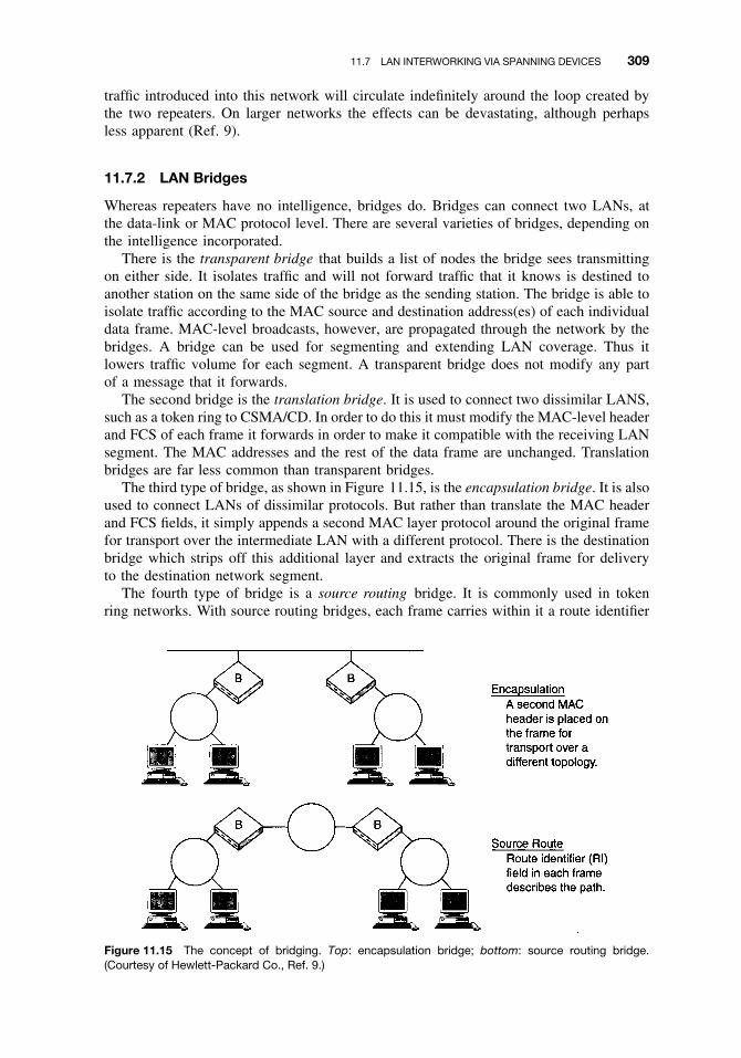
11.7 LAN INTERWORKING VIA SPANNING DEVICES 309
traffic introduced into this network will circulate indefinitely around the loop created bythe two repeaters. On larger networks the effects can be devastating, although perhapsless apparent (Ref. 9).
11.7.2 LAN Bridges
Whereas repeaters have no intelligence, bridges do. Bridges can connect two LANs, atthe data-link or MAC protocol level. There are several varieties of bridges, depending onthe intelligence incorporated.
There is the transparent bridge that builds a list of nodes the bridge sees transmittingon either side. It isolates traffic and will not forward traffic that it knows is destined toanother station on the same side of the bridge as the sending station. The bridge is able toisolate traffic according to the MAC source and destination address(es) of each individualdata frame. MAC-level broadcasts, however, are propagated through the network by thebridges. A bridge can be used for segmenting and extending LAN coverage. Thus itlowers traffic volume for each segment. A transparent bridge does not modify any partof a message that it forwards.
The second bridge is the translation bridge. It is used to connect two dissimilar LANS,such as a token ring to CSMA/CD. In order to do this it must modify the MAC-level headerand FCS of each frame it forwards in order to make it compatible with the receiving LANsegment. The MAC addresses and the rest of the data frame are unchanged. Translationbridges are far less common than transparent bridges.
The third type of bridge, as shown in Figure 11.15, is the encapsulation bridge. It is alsoused to connect LANs of dissimilar protocols. But rather than translate the MAC headerand FCS fields, it simply appends a second MAC layer protocol around the original framefor transport over the intermediate LAN with a different protocol. There is the destinationbridge which strips off this additional layer and extracts the original frame for deliveryto the destination network segment.
The fourth type of bridge is a source routing bridge. It is commonly used in tokenring networks. With source routing bridges, each frame carries within it a route identifier
Figure 11.15 The concept of bridging. Top: encapsulation bridge; bottom: source routing bridge.(Courtesy of Hewlett-Packard Co., Ref. 9.)
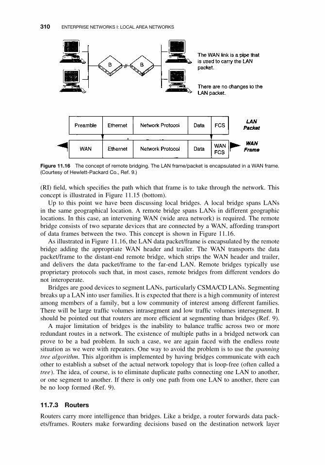
310 ENTERPRISE NETWORKS I: LOCAL AREA NETWORKS
Figure 11.16 The concept of remote bridging. The LAN frame/packet is encapsulated in a WAN frame.(Courtesy of Hewlett-Packard Co., Ref. 9.)
(RI) field, which specifies the path which that frame is to take through the network. Thisconcept is illustrated in Figure 11.15 (bottom).
Up to this point we have been discussing local bridges. A local bridge spans LANsin the same geographical location. A remote bridge spans LANs in different geographiclocations. In this case, an intervening WAN (wide area network) is required. The remotebridge consists of two separate devices that are connected by a WAN, affording transportof data frames between the two. This concept is shown in Figure 11.16.
As illustrated in Figure 11.16, the LAN data packet/frame is encapsulated by the remotebridge adding the appropriate WAN header and trailer. The WAN transports the datapacket/frame to the distant-end remote bridge, which strips the WAN header and trailer,and delivers the data packet/frame to the far-end LAN. Remote bridges typically useproprietary protocols such that, in most cases, remote bridges from different vendors donot interoperate.
Bridges are good devices to segment LANs, particularly CSMA/CD LANs. Segmentingbreaks up a LAN into user families. It is expected that there is a high community of interestamong members of a family, but a low community of interest among different families.There will be large traffic volumes intrasegment and low traffic volumes intersegment. Itshould be pointed out that routers are more efficient at segmenting than bridges (Ref. 9).
A major limitation of bridges is the inability to balance traffic across two or moreredundant routes in a network. The existence of multiple paths in a bridged network canprove to be a bad problem. In such a case, we are again faced with the endless routesituation as we were with repeaters. One way to avoid the problem is to use the spanningtree algorithm. This algorithm is implemented by having bridges communicate with eachother to establish a subset of the actual network topology that is loop-free (often called atree). The idea, of course, is to eliminate duplicate paths connecting one LAN to another,or one segment to another. If there is only one path from one LAN to another, there canbe no loop formed (Ref. 9).
11.7.3 Routers
Routers carry more intelligence than bridges. Like a bridge, a router forwards data pack-ets/frames. Routers make forwarding decisions based on the destination network layer

11.7 LAN INTERWORKING VIA SPANNING DEVICES 311
address. Whereas a bridge worked on the data-link layer, a router operates at the network-layer level. Routers commonly connect disparate LANs such as CSMA/CD to token ringand FDDI to CSMA/CD.
Routers are addressable nodes in a network. They carry their own MAC address(es)as well as a network address for each protocol handled. Because routers are addressable,a station desiring the facility of a router must direct its packets/frames to the router inquestion so that the traffic can be forwarded to the appropriate network. As one wouldexpect, networking software at each station is more complex with a network using routersthan one using bridges.
Routers handle only traffic addressed to them. They make decisions about forwardingdata packets/frames based on one or several criteria. The decisions may be based on thecost of the link, the number of hops on each path, and the time-to-live.
Routers change packets/frames that pass through them such as MAC source and desti-nation address; they may also modify the network protocol header of each frame (typicallydecrementing the time-to-live in the case of IP and other protocol fields).
Because routers have more intelligence than bridges, routers will typically have betternetwork management agents installed. This enables them to be remotely configured, tobe programmed to pass or not to pass data for security purposes, and to be monitored forperformance, particularly error performance. Due to the additional processing performedat routers, they tend to be slower than bridges. Reference 9 suggests that some protocolsdo not lend themselves to routing, such as IBM’s SNA and NetBios, among others.
11.7.4 Hubs and Switching Hubs
A hub is a multiport device that allows centralization. A hub is usually mounted in awiring closet or other central location. Signal leads are brought in from workstations/PCsand other data devices, one for each hub port. Physical rings or buses are formed byinternally configuring the hub ports. A typical hub may have 8 or 16 ports. Suppose wewished to incorporate 24 devices on our LAN using the hub. We can stack two hubs,one on top of the other (stackables), using one of the hub ports on each interconnection.In this case we would have a hub with a 30-port capacity (2 × 16 − 2).7 Hubs may alsohave a certain amount of intelligence, such as the incorporation of a network managementcapability. Also, each hub can include a repeater.
There are also hubs with higher levels of intelligence. These are typically modular,multiprotocol, multimedia, multichannel, fault-tolerant, manageable devices where onecan concentrate all the LAN connections into a wiring closet or data center. Since thesetypes of hubs are modular (i.e., they have various numbers of slots to install LAN interfaceboards), they can support CSMA/CD, token ring, FDDI, or ATM simultaneously as wellas various transmission media such as twisted pair, fiber cable, and others.8
Switching hubs are high-speed interconnecting devices with still more intelligencethan the garden-variety hub or the intelligent hub. They typically interconnect entire LANsegments and nodes. Full LAN data rate is provided at each port of a switching hub. Theyare commonly used on CSMA/CD LANs, providing a node with the entire 10-Mbps datarate. Because of a hub’s low latency, high data rates and throughputs are achieved.
With a switching hub, nodes are interconnected within the hub itself using its high-speed backplane. As a result, the only place the entire aggregate LAN traffic appears is
7Two 16-port hubs are used for a total of 32 ports. However, two ports are required to connect one hub to theother. This leaves just 30 ports for equipment connections.8ATM is covered in Chapter 18.

312 ENTERPRISE NETWORKS I: LOCAL AREA NETWORKS
on that backplane. Traffic between ports on a single card does not even appear on thebackplane (Refs. 9–11).
REVIEW EXERCISES
1. Contrast a LAN with a WAN.
2. What are the two basic underlying transmission techniques for a LAN?
3. Name the three basic LAN topologies. Identify a fourth that is a subset of one ofthe three.
4. What range of BER can we expect on LANs? How are such good BERs achieved?
5. If a LAN has 50 accesses, how many connectivities must be theoretically analyzedfor sufficient S/N?
6. What two basic transmission problems must a designer face with a baseband LAN?
7. LLC derives from what familiar link-layer protocol?
8. Relate the IEEE 802 LAN standard model with the ISO seven-layer OSI model.
9. What is a LAN access protocol?
10. Name at least three responsibilities of the LLC.
11. What are the two services the LLC provides its users?
12. How are collisions detected with CSMA/CD?
13. What is the purpose of the jam signal on CSMA/CD?
14. What is the function of a frame check sequence (FCS)?
15. Give three reasons why a MAC frame may be invalid?
16. How does a LAN know that a traffic frame is destined to it?
17. What is frame stripping?
18. How are collisions avoided using a token-passing scheme?
19. What is the function of a LAN repeater?
20. What are the four types of bridges covered in the text?
21. On what OSI layer do routers operate?
REFERENCES
1. IEEE Standard Dictionary of Electrical and Electronic Terms, 6th ed., IEEE Std. 100-1996,IEEE, New York, 1996.
2. Information Technology—Part 2, Logical Link Control, ANSI/IEEE 802.2, 1994 ed., with Amd.3, IEEE, New York, 1994.
3. Information Technology—Part 3: Carrier Sense Multiple Access with Collision Detection(CSMA/CD) Access Method, ANSI/IEEE Std. 802.3, 1996 ed., IEEE, New York, 1996.
4. Supplement to Carrier Sense Multiple Access with Collision Detection (CSMA/CD) AccessMethod—100 Mbps Operation, Type 100BaseT, IEEE Std. 802.3u-1995, IEEE, New York,1995.

REFERENCES 313
5. Information Technology—Part 5: Token Ring Access Method and Physical Layer Specification,ANSI/IEEE 802.5, 1995 ed., IEEE, New York, 1995.
6. Fiber Distributed Data Interface (FDDI)—Token Ring Physical Layer Medium Dependent,ANSI X3.166-1990, ANSI, New York, 1990.
7. Fiber Distributed Data Interface (FDDI) Physical Layer Protocol (PHY-2), ANSI X3.231-1994,ANSI, New York, 1994.
8. Fiber Distributed Data Interface (FDDI): Token Ring Media Access Control—2, MAC-3, ANSIX.239-1994, ANSI, New York, 1994.
9. Internetworking Troubleshooting Seminar Presentation, Hewlett-Packard Co., Tempe, AZ, Jan.1995.
10. ChipCom promotional material, ChipCom, Southboro, MA, 1995.
11. High-Speed Networking—Options and Implications, ChipCom, Southboro, MA, 1995.
12. Cisco, www.cisco.com/univercd/cc/td/doc.


12
ENTERPRISE NETWORKS II: WIDEAREA NETWORKS
12.1 WIDE AREA NETWORK DEPLOYMENT
Wide area networks (WANs) provide data connectivity over much greater expanses thantheir local area network counterparts. Data rates on WANs are lower. One reason is thatin many cases WANs are transported over the PSTN voice channels, either analog ordigital. In either case there is a limited bit rate capacity.
In this chapter we will cover two types of WANs. These are:
1. TCP/IP protocol family2. Frame relay and some of its variants
Two other WAN families of protocols that I am sure that many readers are familiar withhave become obsolete. These are ITU-T(CCITT) Rec.X.25 and the Integrated ServicesDigital Networks (ISDN). Each of these, however, has left its mark for posterity. HereI mean that some element or part of these protocols has been lifted or purloined foruse on new, more modern protocols. LAPB (link access protocol, B-channel) has beentaken from X.25 covering OSI layer 2. Another example is LAPD (link access protocol,D-channel) taken from ISDN and has become the basic protocol structure (layer 2) forframe relay.
12.1.1 Introductory Comments
Whereas the conventional LAN discussed in Chapter 11 provides data communicationcapabilities among a comparatively small and closed user group covering a very limitedgeographical area, a WAN not only has the potential of covering the entire world and outerspace, but also has the capability of reaching an extremely large and diverse user group(e.g., the INTERNET). With these facts in mind, what are the really key essentials thatwe must understand that will make such a system provide us the capabilities we wouldexpect? Let’s brainstorm and prepare a short list of requirements for a data network tocommunicate data messages: We must first assume that a data message is made up of oneor more data frames or packets. See Section 10.10.1 and Figure 10.25.
Fundamentals of Telecommunications, Second Edition, by Roger L. FreemanISBN 0-471-71045-8 Copyright 2005 by Roger L. Freeman
315

316 ENTERPRISE NETWORKS II: WIDE AREA NETWORKS
1. Data messages should have a high probability of reaching (a) recipient(s) intact andcomparatively error-free.
2. There may be an issue of urgency. Here we mean how soon after transmission willa data message reach its recipient.
3. The recipient(s) must be prepared to receive the message and “understand” itscontents.
12.1.1.1 A Data Message Must Reach the Recipient(s). How is a data messagerouted such that the indicated recipient(s) receive the message? With conventional tele-phony, signaling carries out this function. It sets up a circuit (Chapter 7), maintains theconnectivity throughout the call, and then takes the circuit down when one or both sub-scribers go on-hook. With data communications these same functions must be carried out.One form of data connectivity is called connection-oriented, where indeed a circuit is setup, traffic is passed, and then the circuit is taken down. There is another form of datacommunications where a frame is launched by the originator, and that frame must findits own way to the destination. Isn’t this what happens using the postal service? A letteris dropped in an outgoing box, and it finds its way (with the help of the postal service)to the destination. We, the originator, are completely unaware of the letter’s routing; wedon’t really care. In the data world, this is called connectionless service. In the case ofthe postal service, the address on the envelope routed the letter.
For the data message case, it is the header that carries the routing information. In manysituations, a data message may be made up of a number of frames. Each frame carries afield set aside for the recipient address. More often than not it is called the destinationaddress. In many cases, a frame also carries the originator’s address. In either case, theseare 8-bit fields, often extendable in increments of 8 bits.
Three key questions come to mind. (1) What part of a frame’s header can be eas-ily identified as the originator and destination address fields? (2) What is the addressingcapacity of an address field? Rephrased: How many distinct addresses can be accommo-dated in an 8-bit field? (3) Once a router, smart bridge, or data switch recognizes theboundaries of (a) destination address(es), how does it know how to route the frame?
1. A family of protocols governs the operation of a particular data network. Our interesthere is in the network layer and data-link layer protocols. These protocols carefully layout the data-link frame and the network layer frame (see Section 10.10). For example,in Section 10.7.2 we introduced synchronous transmission and the generic data-link layerframe (Figure 10.7). One thing a digital processor can do and do very well is count bits,and groups of 8 bits, which we call an octet (others call it a byte). A specific networkutilizes a particular data-link layer protocol. Thus a processor knows a priori where fieldboundaries are, because it is designed to meet the requirements of a particular protocol.With some data-link protocols, however, there may be a variable length info field. It isobvious that if this is the case, that the processor must be informed of the length of aparticular info field. When this is so, info field length information is often found in asubfield inside the control field (see Figures 10.7 and 10.25). So to answer question 1,the digital processor knows a priori exactly which 8 (or 16) bits consist the destinationaddress field by simply counting down from the unique start-of-frame octet. It knows apriori because the router processor conforms to a particular protocol.
2. What is the addressing capacity of an address field? We will let each address consistsof a distinct 8- or 16-bit binary sequence. For an 8-bit binary group, how many distinct

12.1 WIDE AREA NETWORK DEPLOYMENT 317
8-bit sequences are there? Remember, on developing code capacity (Section 10.4), thatwe can have 2n sequences where n is the number of bits in a particular sequence. In oursample case it is 8 bits. Thus, its addressing capacity is 28 or 256 distinct addresses. Theaddressing capacity can be increased by using extended addressing, namely where weuse two octets for a destination address. Often the least significant bit of the first octetis reserved to tell the receiver processor to expect the next octet also to be dedicated todestination address. Now we have only 7 bits in the first octet left for addressing and all8 bits in the second octet. Adding these two together, we get 15 bits for addressing. Thus,there is 215 or 32,768 distinct addresses, quite a respectable number.
3. How does a router or data switch know how to route to a particular address? Simplyby consulting a look-up table. Now this look-up table may have fixed routing entries, orentries that can be updated manually or routing entries that are updated dynamically. Herewe must recognize three possible conditions:
1. A node/router is added or dropped from the network.2. New routing patterns may be established; other routing patterns may be discontinued.3. There may be congestion, route/node degradation, and/or failure.
Read subsection 12.3 which describes the TCP/IP protocol family because IP has somevery interesting means and methods to update routing/look-up tables as well as findingroutes to “unknown” destination addresses.
Error detection and correction were discussed in Section 10.5.
12.1.1.2 There May Be an Issue of Urgency. There are several “families” ofdata messages that have limited or no real issue regarding urgency. For example, longaccounting files, including payroll, may only require 24- or 48-hour delivery times. Inthis case why not use the postal service, Federal Express, or UPS? On the other hand,credit card verification has high urgency requirements. A customer is waiting (probablyimpatiently) to have her/his credit verified during the process of buying some item. Mosttransaction data messages are highly urgent.
Certain data protocols involve more latency than others. One reason for implementingframe relay is its low latency. Let’s call latency the time it takes to complete a datamessage transaction. There are four causes for an increase in transaction time:
1. Propagation delay.2. The number of message exchanges required to complete a transaction (e.g., hand-
shakes, circuit setup, ARQ exchanges, and so on).3. Processing time and processing requirements. For example, every effort has been
made to reduce processing requirements in frame relay. There are virtually nomessage exchanges, such as ACK and NACK, with frame relay.
4. Secondarily, we must consider the quality of a circuit. If the circuit is noisy, manyARQ exchanges will occur increasing latency dramatically.
12.1.1.3 The Recipient Must Be Prepared to Receive and ‘‘Understand’’ a DataMessage. This is simply a question of compatibility. The data message receiver mustbe compatible with the far-end transmitter and intermediate nodes. We cannot have one

318 ENTERPRISE NETWORKS II: WIDE AREA NETWORKS
transmitting the ASCII code and the companion receiver only able to receive EBCDIC.Such compatibility MAY extend through all seven OSI layers. For example, frame relayis based ONLY on OSI layers 1 and 2. It is the responsibility of the frame relay user toprovide the necessary compatibility of the upper OSI layers.
12.2 THE CONCEPT OF PACKET DATA COMMUNICATIONS
The concept of a packet-switched network is based on the idea that the network switchingnodes will have multiple choices for routing of data packets. If a particular route becomescongested or has degraded operation, a node can send a packet on another route, and ifthat route becomes congested, possibly a third route will be available to forward thepacket to its destination.
At a data source, a file is segmented into comparatively short data packets, each of thesame length and each with its own header and trailer. As we mentioned, these packetsmay take diverse routes through various nodes to their destination. The destination nodeis responsible for data message reassembly in its proper order.
This is a short description of an idealized packet-switched network. We will run intosome terminology typical of packet handling and switching of data. For example:
A. There is connection-oriented and connectionless service.
B. Packets may be acknowledged or unacknowledged.
C. We can have PVCs or SVCs (permanent virtual circuits or switched virtual circuits).
Our POTS is a typical connection-oriented service. In other words a fixed or virtualconnection is set up at the beginning of a telephone call, is maintained in that conditionthroughout the call, and is taken down (terminated) at the end of the call. The circuit is thenreturned to the pool of idle circuits awaiting the next call assignment. Connection-orientedis sometimes called circuit-switched service.
In ideal packet-switched data service the service is connectionless. The packet isreleased by the originator and placed on an idle or “free” outgoing data link to thenext node. Each node ideally maintains a dynamically updated routing table. The rout-ing table will provide information on the appropriate outgoing port to direct the packettoward its destination and will reflect information regarding congestion and/or degrada-tion or outage on all possible outgoing routes. In the real world this dynamic updating isseldom achievable because we will tend to load circuits up with service messages ratherthan revenue-bearing traffic.
A more common method is the virtual connection where a logical connection is set upin advance before any packets are sent. The packet originator sends a call request to itsserving node, which sets up a route in advance to the desired destination. All packets of aparticular message traverse this route, and each packet of the message contains a virtualcircuit identifier (logical channel number) along with the packet data. At any given timeeach station can have more than one virtual circuit to any other station in the network.With virtual circuits, routing decisions are made in advance.
Another routing method is called the datagram. Datagram service used optimal routingon a packet-by-packet basis, usually over diverse routes. It is that ideal packet switchingservice described above. With the datagram approach ad hoc decisions are made foreach packet at each node. There is no call-setup phase with datagrams as there is withvirtual connections. Virtual connections are advantageous for high community-of-interest

12.3 TCP/IP AND RELATED PROTOCOLS 319
connectivities, whereas datagram service is advantageous for low community-of-interesttraffic relations.
Datagram service is more reliable because traffic can be alternately routed aroundnetwork congestion points. Virtual circuits are fixed-routed for a particular call. Call-setup time at each node is eliminated on a packet basis as with the virtual connectiontechnique. One packet switching protocol allows the possibility of setting up permanentvirtual connections (PVCs) and is network-assigned. This latter alternative is economicallyviable for very high traffic intensity relations; otherwise these permanently assigned logicalchannels will have long dormant periods.
12.3 TCP/IP AND RELATED PROTOCOLS
12.3.1 Background and Scope
The transmission control protocol/Internet protocol (TCP/IP) family was developed for theARPANET (Advanced Research Projects Agency Network). ARPANET was one of thefirst large advanced packet-switched networks. It was initially designed and operated tointerconnect the very large university and industrial defense communities to share researchresources. It dates back to 1998 and was well into existence before ISO and CCITT tookinterest in layered protocols.
The TCP/IP suite of protocols (Refs. 2, 3) has wide acceptance today, especially inthe commercial and industrial community worldwide. These protocols are used on bothLANs and WANs. They are particularly attractive for their Internet-working capabilities.The Internet protocol (IP) (Ref. 2) competes with CCITT Rec. X.75 protocol (Ref. 4),but is notably more versatile and has much wider application.
The architectural model of the IP (Ref. 2) uses terminology that differs from the OSIreference model.1 Figure 12.1 shows the relationship between TCP/IP and related DoD(Department of Defense) protocols and the OSI reference model. Tracing data traffic
Figure 12.1 How TCP/IP and associated protocols relate to OSI.
1IP predates OSI.

320 ENTERPRISE NETWORKS II: WIDE AREA NETWORKS
Figure 12.2 Connecting one LAN to another LAN via a WAN with routers equipped with IP.
from an originating host, which runs an applications program, to another host in anothernetwork as shown in Figure 12.2. This may be a LAN-to-WAN-to-LAN connectivity asshown in the figure. It may also be just a LAN-to-WAN or it may be a WAN-to-WANconnectivity. The host would enter its own network by means of a network access protocolsuch as HDLC or an IEEE 802 series protocol (Chapter 11).
A LAN connects via a router (or gateway) to another network. Typically a router (orgateway) is loaded with three protocols. Two of these protocols connect to each of theattached networks (e.g., LAN and WAN), and the third protocol is the IP, which providesthe network-to-network interface.
Hosts typically are equipped with four protocols. To communicate with routers orgateways, a network access protocol and Internet protocol are required. A transport layerprotocol assures reliable communication between hosts because end-to-end capability isnot provided in either the network access or Internet protocols. Hosts also must haveapplication protocols such as e-mail or file transfer protocols (FTPs).
12.3.2 TCP/IP and Data-Link Layers
TCP/IP is transparent to the type of data-link layer involved, and it is also transparentwhether it is operating in a LAN or WAN domain or among them. However, there isdocument support for Ethernet, IEEE 802 series, ARCNET LANs, and frame relay forWANS (Refs. 2, 5).
Figure 12.3 shows how upper OSI layers are encapsulated with TCP and IP headerinformation and then incorporated into a data-link layer frame.
For the case of IEEE 802 series LAN protocols, advantage is taken of the LLC commonto all 802 protocols. The LLC extended header contains the SNAP (sub-network accessprotocol) such that we have three octets of the LLC header and five octets in the SNAP.The LLC header has its fields fixed as follows (LLC is discussed in Chapter 11):
DSAP = 10101010
SSAP = 10101010
Control = 00000011
The five octets in the SNAP have three assigned for protocol ID or organizational code andtwo octets for “EtherType.” EtherType assignments are shown in Table 12.1. EtherType

12.3 TCP/IP AND RELATED PROTOCOLS 321
Figure 12.3 The incorporation of upper-layer PDUs into a data-link layer frame showing the relationshipwith TCP and IP.
Table 12.1 Ether-Type Assignments
EthernetDecimal Hex Description
512 0200 XEROX PUP513 0201 PUP address translation
1536 0600 XEROX NS IDP2048 0800 DOD Internet protocol (IP)2049 0801 X.75 Internet2050 0802 NBS Internet2051 0803 ECMA Internet2052 0804 Chaosnet2053 0805 X.25 level 32054 0806 Address resolution protocol (ARP)2055 0807 XNS compatibility4096 1000 Berkeley trailer
21000 5208 BBN Simnet24577 6001 DEC MOP dump/load24578 6002 DEC MOP remote control24579 6003 DEC DECnet phase IV24580 6004 DEC LAT24582 6005 DEC24583 6006 DEC32773 8005 HP probe32784 8010 Excelan32821 8035 Reverse ARP32824 8038 DEC LANBridge32823 8098 Appletalk
Source: Ref.6.
refers to the general class of LANs based on CSMA/CD (see Chapter 11 for a discussionof CSMA/CD).
Figure 12.4 shows the OSI relationships with TCP/IP working with the IEEE 802LAN protocol group. Figure 12.5 illustrates an IEEE 802 frame incorporating TCP, IP,and LLC.
Often addressing formats are incompatible from one protocol in one network to anotherprotocol in another network. A good example is the mapping of the 32-bit Internet addressinto a 48-bit IEEE 802 address. This problem is resolved with ARP (address resolution

322 ENTERPRISE NETWORKS II: WIDE AREA NETWORKS
Figure 12.4 How TCP/IP working with IEEE 802 series of LAN protocols relates to OSI.
Figure 12.5 A typical IEEE 802 frame showing LLC and TCP/IP functions.
protocol). Another interface problem is limited IP datagram length of 576 octets, wherewith the 802 series, frames have considerably longer length limits (Ref. 7).
12.3.3 IP Routing Algorithm
In OSI the network layer functions include routing and switching of a datagram through thetelecommunications subnetwork. The IP provides this essential function. It forwards thedatagram based upon the network address contained within the IP header. Each datagramis independent and has no relationship with other datagrams. There is no guaranteeddelivery of the datagrams from the standpoint of the Internet protocol. However, the nexthigher layer, the TCP layer, provides for the reliability that the IP lacks. It also carriesout segmentation and reassembly function of a datagram to match frame sizes of data-linklayer protocols.
Addresses determine routing, and at the far end, equipment (hardware). Actual routingderives from the IP address, and equipment addresses derive from the data-link layerheader (typically the 48-bit Ethernet address) (Ref. 5).

12.3 TCP/IP AND RELATED PROTOCOLS 323
User data from upper-layer protocols is passed to the IP layer. The IP layer examinesthe network address (IP address) for a particular datagram and determines if the destinationnode is on its own local area network or some other network. If it is on the same network,the datagram is forwarded directly to the destination host. If it is on some other network,it is forwarded to the local IP router (gateway). The router, in turn, examines the IPaddress and forwards the datagram as appropriate. Routing is based on a look-up tableresiding in each router or gateway.
12.3.3.1 IP Routing Details. A gateway (router) needs only the network ID portionof the address to perform its routing function. Each router or gateway has a routing tablewhich consists of: destination network addresses and specified next-hop gateway.
Three types of routing are performed by the routing table:
1. Direct routing to locally attached devices2. Routing to networks that are reached via one or more gateways3. Default routing to destination network in case the first types of routing are
unsuccessful
Suppose a datagram (or datagrams) is (are) directed to a host which is not in the routingtable resident in a particular gateway. Likewise, there is a possibility that the networkaddress for that host is also unknown. These problems may be resolved with the addressresolution protocol (ARP) (Ref. 7).
First the ARP searches a mapping table which relates IP addresses with correspondingphysical addresses. If the address is found, it returns the correct address to the requester.If it cannot be found, the ARP broadcasts a request containing the IP target address inquestion. If a device recognizes the address, it will reply to the request where it willupdate its ARP cache with that information. The ARP cache contains the mapping tablesmaintained by the ARP module.
There is also a reverse address resolution protocol (RARP) (Ref. 8). It works in afashion similar to that of the ARP, but in reverse order. RARP provides an IP addressto a device when the device returns its own hardware address. This is particularly usefulwhen certain devices are booted and only know their own hardware address.
Routing with IP involves a term called hop. A hop is defined as a link connectingadjacent nodes (gateways) in a connectivity involving IP. A hop count indicates howmany gateways (nodes) must be traversed between source and destination.
One part of an IP routing algorithm can be source routing. Here an upper-layer protocol(ULP) determines how an IP datagram is to be routed. One option is that the ULP passesa listing of Internet addresses to the IP layer. In this case information is provided on theintermediate nodes required for transit of a datagram in question to its final destination.
Each gateway makes its routing decision based on a resident routing list or routingtable. If a destination resides in another network, a routing decision is required by theIP gateway to implement a route to that other network. In many cases, multiple hops areinvolved and each gateway must carry out routing decisions based on its own routing table.
A routing table can be static or dynamic. The table contains IP addressing informationfor each reachable network and closest gateway for the network, and it is based on theconcept of shortest routing, thus routing through the closest gateway.
Involved in IP shortest routing is the distance metric, which is a value expressingminimum number of hops between a gateway and a datagram’s destination. An IP gatewaytries to match the destination network address contained in the header of a datagram with

324 ENTERPRISE NETWORKS II: WIDE AREA NETWORKS
a network address entry contained in its routing table. If no match is found, the gatewaydiscards the datagram and sends an ICMP (see next subsection) message back to thedatagram source.
12.3.3.2 Internet Control Message Protocol (ICMP). ICMP is used as an adjunctto IP when there is an error in datagram processing. ICMP uses the basic support of IPas if it were a higher-level protocol.; however, ICMP is actually an integral part of IPand is implemented by every IP module.
ICMP messages are sent in several situations: for example, when a datagram cannotreach its destination, when a gateway (router) does not have the buffering capacity toforward a datagram, and when the gateway (router) can direct the host to send traffic ona shorter route.
ICMP messages typically report errors in the processing of datagrams. To avoid thepossibility of infinite regress of messages about messages, and so on, no ICMP messagesare sent about ICMP messages. There are eight distinct ICMP messages:
1. Destination unreachable message2. Time exceeded message3. Parameter problem message4. Source quench message5. Redirect message6. Echo or echo reply message7. Timestamp or timestamp reply message8. Information request or information reply message
12.3.3.3 IP Summary. The IP provides connectionless service, meaning that there is nocall setup phase prior to the exchange of traffic. There are no flow control or error controlcapabilities incorporated in IP. These are left to the next higher layer, the transmissioncontrol protocol (TCP). The IP is transparent to subnetworks connecting at lower layers;thus different types of networks can attach to an IP gateway or router. To compensatefor these deficiencies in IP, the TCP (transmission control protocol) was developed asan upper layer to IP. It should be noted that TCP/IP can be found in both the LAN andWAN environments.
12.3.4 The Transmission Control Protocol (TCP)
12.3.4.1 TCP Defined. TCP (Refs. 3, 9) was designed to provide reliable commu-nication between pairs of processes in logically distinct hosts2 on networks and sets ofinterconnected networks. TCP operates successfully in an environment where the loss,damage, duplication or misorder of data, and network congestion can occur. This robust-ness in spite of unreliable communications media makes TCP well-suited to supportcommercial, military, and government applications. TCP appears at the transport layerof the protocol hierarchy. Here, TCP provides connection-oriented data transfer that is
2The IEEE (Ref. 10) defines a host as “a device to which other devices (peripherals) are connected andthat generally controls those devices” and defines a host computer (IEEE) as “a computer, attached to anetwork, providing primary services such as computation, data base access or special programs or programminglanguages.”

12.3 TCP/IP AND RELATED PROTOCOLS 325
Figure 12.6 Protocol layers showing the relationship of TCP with other layered protocols.
reliable, ordered, full duplex, and flow controlled. TCP is designed to support a widerange of upper-layer protocols (ULPs). The ULP can channel continuous streams of datathrough TCP for delivery to peer ULPs. The TCP breaks the streams into portions thatare encapsulated together with appropriate addressing and control information to form asegment—the unit of exchange between TCPs. In turn, the TCP passes the segments tothe network layer for transmission through the communication system to the peer TCP.
As shown in Figure 12.6, the layer below the TCP in the protocol hierarchy is com-monly the IP layer. The IP layer provides a way for the TCP to send and receivevariable-length segments of information enclosed in Internet datagram “envelopes.” TheInternet datagram provides a means for addressing source and destination TCPs in dif-ferent networks. The IP also deals with fragmentation or reassembly of TCP segmentsrequired to achieve transport and delivery through the multiple networks and intercon-necting gateways (routers). The IP also carries information on the precedence, securityclassification, and compartmentation of the TCP segments, so this information can becommunicated end-to-end across multiple networks.
12.3.4.2 TCP Mechanisms. TCP builds its services on top of the network layer’spotentially unreliable services with mechanisms such as error detection, positive acknowl-edgments, sequence numbers, and flow control. These mechanisms require certain address-ing and control information to be initialized and maintained during data transfer. Thiscollection of information is called a TCP connection. The following paragraphs describethe purpose and operation of the major TCP mechanisms.
Par Mechanism. TCP uses a positive acknowledgment with retransmission (PAR)mechanism to recover from the loss of a segment by the lower layers. The strategywith PAR is for sending a TCP to retransmit a segment at timed intervals until a posi-tive acknowledgment is returned. The choice of retransmission interval affects efficiency.An interval that is too long reduces data throughput while one that is too short floods

326 ENTERPRISE NETWORKS II: WIDE AREA NETWORKS
the transmission media with superfluous segments. In TCP, the timeout is expected tobe dynamically adjusted to approximate the segment round-trip time plus a factor forinternal processing; otherwise performance degradation may occur. TCP uses a simplechecksum to detect segments damaged in transit. Such segments are discarded withoutbeing acknowledged. Hence, damaged segments are treated identically to lost segmentsand are compensated for by the PAR mechanism. TCP assigns sequence numbers to iden-tify each octet of the data stream. These enable a receiving TCP to detect duplicate andout-of-order segments. Sequence numbers are also used to extend the PAR mechanismby allowing a single acknowledgment to cover many segments worth of data. Thus, asending TCP can still send new data, although previous data have not been acknowledged.
Flow Control Mechanism. TCP’s flow control mechanism enables a receiving TCP togovern the amount of data dispatched by a sending TCP. The mechanism is based on awindow, which defines a contiguous interval of acceptable sequence-numbered data. Asdata are accepted, TCP slides the window upward in the sequence number space. Thiswindow is carried in every segment, enabling peer TCPs to maintain up-to-date windowinformation.
Multiplexing Mechanism. TCP employs a multiplexing mechanism to allow multipleULPs within a single host and multiple processes in a ULP to use TCP simultaneously.This mechanism associates identifiers, called ports, to ULP processes accessing TCPservices. A ULP connection is uniquely identified with a socket, the concatenation ofa port and an Internet address. Each connection is uniquely named with a socket pair.This naming scheme allows a single ULP to support connections to multiple remoteULPs. ULPs which provide popular resources are assigned permanent sockets, calledwell-known sockets.
12.3.4.3 ULP Synchronization. When two ULPs (upper-layer protocols) wish tocommunicate (see Figure 12.4), they instruct their TCPs to initialize and synchronize themechanism information on each to open the connection. However, the potentially unre-liable network layer (i.e., the IP layer) can complicate the process of synchronization.Delayed or duplicate segments from previous connection attempts might be mistaken fornew ones. A handshake procedure with clock-based sequence numbers is used in connec-tion opening to reduce the possibility of such false connections. In the simplest handshake,the TCP pair synchronizes sequence numbers by exchanging three segments, the namethree-way handshake.
12.3.4.4 ULP Modes. A ULP can open a connection in one of two modes: passiveor active. With a passive open, a ULP instructs its TCP to be receptive to connectionswith other ULPs. With an active open, a ULP instructs its TCP to actually initiate athree-way handshake to connect to another ULP. Usually an active open is targeted toa passive open. This active/passive model supports server-oriented applications where apermanent resource, such as a database management process, can always be accessedby remote users. However, the three-way handshake also coordinates two simultaneousactive opens to open a connection. Over an open connection, the ULP pair can exchangea continuous stream of data in both directions. Normally, TCP groups the data into TCPsegments for transmission at its own convenience. However, a ULP can exercise a pushservice to force TCP to package and send data passed up to that point without waitingfor additional data. This mechanism is intended to prevent possible deadlock situations

12.4 INTEGRATED SERVICES DIGITAL NETWORKS (ISDN) 327
where a ULP waits for data internally buffered by TCP. For example, an interactive editormight wait forever for a single input line from a terminal. A push will force data throughthe TCPs to the awaiting process. A TCP also provides the means for a sending ULP toindicate to a receiving ULP that “urgent” data appear in the upcoming data stream. Thisurgent mechanism can support, for example, interrupts or breaks. When a data exchangeis complete, the connection can be closed by either ULP to free TCP resources for otherconnections. Connection closing can happen in two ways. The first, called a graceful close,is based on the three-way handshake procedure to complete data exchange and coordinateclosure between the TCPs. The second, called an abort, does not allow coordination andmay result in the loss of unacknowledged data.
NOTE: There is a certain military flavor in TCP/IP protocol family. There is good rea-son; their development (around 1975) was supported by the U.S. Department of Defensefor ARPANET. Since then, this protocol family has become extremely popular in thecommercial world (e.g., internet), both for LAN and WAN operations.
12.4 INTEGRATED SERVICES DIGITAL NETWORKS (ISDN)
12.4.1 Background and Objectives
The original concept of ISDN dates back to the early 1970s. Its design, in the contextof the period, was built around the copper distribution plant (subscriber loop and localtrunk plant). The designers saw and understood that by the early 1980s there would bea digital network in place controlled by CCITT Signaling System No. 7 (Chapter 13). Itwas revolutionary for its time by bringing 64-kbps digital channels right into the homeand office. With the ISDN design, the 64-kbps digital channel handles:
ž Voice telephony (digital)ž Digital data, both packet switched and circuit switchedž Telex/teletextž Facsimile (e.g., CCITT Group 4)ž Conference television (56, 64, or 128 kbps)
The goal of ISDN is to provide an integrated facility to incorporate each of the serviceslisted above on a common 64-kbps channel.
In North America, one gets the distinct feeling that the certain technologies [e.g., ATM(Chapter 18), frame relay (Section 12.5) and gigbit enterprise networks (Chapter 11), andEHF wireless local loops)] have leap-frogged ISDN.
12.4.2 The Future of ISDN
ISDN as an entity has become obsolete in many parts of the world. It has specificchannel configurations such as B and H channels, with fixed bit rates. Customers aredemanding much higher data rates. ISDN is inflexible and cannot provide these ratessuch as 45 Mbps and higher. Frame relay has greater flexibility and can provide suchdata rates. A customer may also choose to use DS3 or E3 or even higher specific datarates where the only interface considered is intra-network. This may well be a proprietarynetwork scheme.

328 ENTERPRISE NETWORKS II: WIDE AREA NETWORKS
ISDN does leave two of its subsidiary protocols, LAPB and LAPD. LAPD and itsvariants are used with frame relay.
12.5 SPEEDING UP THE NETWORK: FRAME RELAY
12.5.1 Rationale and Background
It would seem from the terminology and the popular press that somehow we were makingbits travel faster down the pipe. By some means we’d broken the velocity barrier bydramatically increasing the velocity of propagation. Of course, this is patently not true.
If bandwidth permits,3 bit rate can be increased. That certainly will speed things up.One way to get around the bandwidth crunch is to employ some other, less constrainingtransmission medium such as optical fiber or very-wide-bandwidth EHF radio.
Probably the greatest impetus to speed up the network came from LAN users thatwished to extend LAN connectivity to distant destinations. Ostensibly this traffic, asdescribed in Chapter 11, has local transmission rates from 4 Mbps to >1 Gbps.
A packet-switched network base on ITU-T Rec. X.25 was an intermediate expedient.On one hand, it was robust with excellent error correction capabilities. On the other hand,it was slow and tedious. It was designed for circuits where error performance was mediocreby today’s standards, as poor as 1 × 10⁻⁴. Since X.25’s inception, error performance hasimproved greatly. Today, for example, Telcordia requires 5 × 10⁻¹⁰ (Ref. 21) and Sprintrequires 1 × 10⁻¹². Such excellent error performance begs the question of removing theresponsibility of error recovery from the service provider. If statistically errors occurin about 1 in 100 million bit and better, there is a strong argument for removing errorrecovery, at least in the data-link layer. As a result, frame relay was conceived. Its salientpoints are:
ž There is no process for error recovery by the frame relay service provider.ž The service provider does not guarantee delivery nor are there any sort of acknowl-
edgments provided.ž It only uses the first two OSI layers (physical and data-link layer), thus removing
layer 3 and its intensive processing requirements.ž Frame overhead is kept to a minimum, to minimize processing time and to increase
useful throughput.ž There is no control field, and no sequence numbering.ž Frames are discarded without notifying originator for such reasons as congestion and
having encountered an error.ž It operates on a statmultiplex concept.
In sum, the service that the network provides can be speeded up by increasing datarate, eliminating error-recovery procedures, and reducing processing time. One sourcestates that a frame relay frame takes some 20 msec to reach the distant end (statistically),where an X.25 packet of similar size takes in excess of 200 msec on terrestrial circuitsinside CONUS (CONUS stands for contiguous United States).
Another advantage of frame relay over a conventional static TDM connection is thatit uses virtual connections. Data traffic is often bursty and normally would require much
3If bandwidth permits. We cannot increase bandwidth as the popular press insinuates. We can make better useof bandwidth. With data transmission, particularly as the bit rate increases, other bandwidth constraints, besidesamplitude response, may become the limiting factor on bit rate. Typically this may be group delay (envelopedelay distortion), bandwidth coherence.

12.5 SPEEDING UP THE NETWORK: FRAME RELAY 329
Figure 12.7 A typical frame relay network.
larger bandwidths to support the short data messages and much of the time that bandwidthwould remain idle. Virtual connections of frame relay only use the required bandwidth forthe period of the burst or usage. This is one reason why frame relay is used so widely tointerconnect LANs over a wide area network (WAN). Figure 12.7 shows a typical framerelay network.
12.5.2 The Genesis of Frame Relay
Frame relay extends only through the data link layer (i.e., OSI layer 2). It has derivedits data-link layer protocol from the ISDN D-channel LAPD.4 We discussed LAPD inSection 12.4.8. Frame relay’s importance has taken on such a magnitude (it was developedin North America) that the ITU-T organization formulated Rec. I.122, Framework forFrame Mode Bearer Services (Ref. 13) and I.233, Frame Mode Bearer Services (Ref. 14).Even the term LAPD, although modified in many cases for frame relay application,continues to be used.
Frame relay has become an ANSI initiative. There is also the Frame Relay Forum,consisting of manufacturers of frame relay equipment, that many feel is leading this imag-inative initiative. So when we discuss frame relay, we must consider what specificationsa certain system is designed around:
ž ANSI, based on ANSI specifications and their publication datesž Frame Relay Forum with publication datesž ITU-T organization and its most current recommendations
There are also equivalent ANSI specifications directly derived from ITU-T recommen-dations such as ANSI T1.617-1991 (Ref. 15). We will see the term core aspects of ISDN
4LAPD stands for link access protocol D-channel.

330 ENTERPRISE NETWORKS II: WIDE AREA NETWORKS
LAPD or DL-CORE. This refers to a reduced subset of LAPD found in Annex A of ITU-T Rec. Q.922 (Ref. 16). The basic body of Q.922 presents CCITT/ITU-T specificationfor frame relay. This derivative is called LAPF rather than LAPD. The material foundin ANSI T1.618-1991 (Ref. 17) is identical for all intents and purposes with Annex Aof Q.922.
To properly describe frame relay from our perspective, we will briefly give an overviewof the ANSI T1.618-1991 (Ref. 17) and T1.606-1990 (Ref. 18). This will be followed bysome fairly well identified variants.
12.5.3 Introduction to Frame Relay Operation
Frame relay may be considered a cost-effective outgrowth of ISDN, meeting high data rate(e.g., 2 Mbps) and low delay data communications requirements. Frame relay encapsulatesdata files. These may be considered “packets,” although they are called frames. Thusframe relay is compared to CCITT Rec. X.25 packet service. Frame relay was designedfor current transmission capabilities of the network with its relatively wider bandwidths5
and excellent error performance (e.g., BER better than 1 × 10⁻⁷).The incisive reader will note the use of the term bandwidth. It is used synonymously
with bit rate. If we were to admit at first approximation 1 bit per hertz of bandwidth, suchuse is acceptable. We are mapping frame relay bits into bearer channel bits probably ona one-for-one basis. The bearer channel may be a DS0/E0 64-kbps channel, a 56-kbpschannel of a DS1 configuration, or multiple DS0/E0 channels in increments of 64 kbpsup to 1.544/2.048 Mbps. We may also map the frame relay bits into a SONET or SDHconfiguration (Chapter 17). The final bearer channel may require more or less bandwidththan that indicated by the bit rate. This is particularly true for such bearer channels ridingon radio systems and, to a lesser extent, on a fiber-optic medium or other transmissionmedia. The reader should be aware of certain carelessness of language used in industrypublications.
Frame relay works well in the data rate range from 56 kbps up to 1.544/2.048 Mbps.It is being considered for the 45-Mbps DS3 rate for still additional speed.
ITU-T’s use of the ISDN D-channel for frame relay favors X.25-like switched virtualcircuits (SVCs). However, ANSI recognized that the principal application of frame relaywas interconnection of LANs, and not to replace X.25. Because of the high data rateof LANs (megabit range), dedicated connections are favored. ANSI thus focused onpermanent virtual connections (PVCs). With PVCs, routes are provisioned at the time offrame relay contract. This notably simplified the signaling protocol. Also, ANSI framerelay does not support voice or video.
As mentioned, the ANSI frame relay derives from ISDN LAPD core functions. Thecore functions of the LAPD protocol that are used in frame relay (as defined here) areas follows:
ž Frame delimiting, alignment, and transparency provided by the use of HDLC flagsand zero bit insertion/extraction.6
ž Frame multiplexing/demultiplexing using the address field.7
ž Inspection of the frame to ensure that it consists of an integer number of octets priorto zero bit insertion or following zero bit extraction.
5We would rather use the term greater bit rate capacity.6Zero bit insertion is a technique used to assure that the unique beginning flag of a frame is not imitated insidethe frame that allows full transparency.7Where the DLCI indicates a particular channel or channel group in the multiplex aggregate for PVC operation.

12.5 SPEEDING UP THE NETWORK: FRAME RELAY 331
ž Inspection of the frame to ensure that it is not too long or too short.ž Detection of (but not recovery from) transmission errors.ž Congestion control functions.
In other words, ANSI has selected certain features from the LAPD structure/protocol,rejected others, and added some new features. For instance, the control field was removed,but certain control functions have been incorporated as single bits in the address field.These are the C/R bit (command/response), DE (discard eligibility), FECN bit (forwardexplicit congestion notification), and BECN bit (backward explicit congestionnotification).
12.5.4 Frame Structure
User traffic passed to a FRAD (frame relay access device) is segmented into frames witha maximum length information field or with a default length of 262 octets. The minimuminformation field length is one octet.
Figure 12.8 illustrates the frame relay frame structure. LAPD (see Section 10.10.3)uses HDLC flags (01111110) as opening and closing flags. A closing flag may also serveas the opening flag of the next frame.
Address field. This consists of two octets, but may be extended to three or four octets.However, there is no control field as there is in HDLC, LAPB, and ISDN LAPD.
In its most reduced version, there are just 10 bits allocated to the address field in twooctets (the remainder of the bits serve as control functions) supporting up to 1024 logicalconnections.
It should be noted that the number of addressable logical connections is multipliedbecause they can be reused at each nodal (switch) interface. That is, an address in theform of a data-link connection identifier (DLCI) has meaning only on one trunk betweenadjacent nodes. The switch (node) that receives a frame is free to change the DLCI beforesending the frame onwards over the next link. Thus, the limit of 1024 DLCIs applies tothe link, not the network.
Information field. This follows the address field and precedes the frame check sequence(FCS). The maximum size of the information field is an implementation parameter, andthe default maximum is 262 octets. ANSI chose this default maximum to be compatiblewith LAPD on the ISDN D-channel, which has a two-octet control field and a 260-octetmaximum information field. All other maximum values are negotiated between users andnetworks and between networks. The minimum information field size is one octet. The
Figure 12.8 Frame relay ANSI frame format with two-octet address. DLCI—data-link connection iden-tifier. C/R—command response indicator. EA—address field extension bit. FECN/BECN—see text.DE—discard eligibility.
332 ENTERPRISE NETWORKS II: WIDE AREA NETWORKS
field must contain an integer number of octets; partial octets are not allowed. A maximumof 1600 octets is encouraged for applications such as LAN interconnects to minimize theneed for segmentation and reassembly by user equipment.
Transparency. As with HDLC, X.25 (LAPB), and LAPD, the transmitting data-linklayer must examine the frame content between opening and closing flags and inserts a 0bit after all sequences of five contiguous 1s (including the last five bits of the FCS) toensure a flag or an abort sequence is not simulated within the frame. At the other side ofthe link, a receiving data-link layer must examine the frame contents between the openingand closing flags and must discard any 0 bit that directly follows five contiguous 1s.
Frame check sequence (FCS). This is based on the generator polynomial X16 + X12 +X5 + 1. The CRC processing includes the content of the frame existing between, butnot including, the final bit of the opening flag and the first bit of the FCS, excludingthe bits inserted for transparency. The FCS, of course, is a 16-bit sequence. If thereare no transmission errors (detected), the FCS at the receiver will have the sequence00011101 00001111.
Invalid frames. An invalid frame is a frame that:
ž Is not properly bounded by two flags (e.g., a frame abort).ž Has fewer than three octets between the address field and the closing flag.ž Does not consist of an integral number of octets prior to zero bit insertion or following
zero bit extraction.ž Contains a frame check sequence error.ž Contains a single octet address field.ž Contains a data-link connection identifier (DLCI) that is not supported by the receiver.
Invalid frames are discarded without notification to the sender, with no further action.
12.5.4.1 Address Field Variables12.5.4.1.1 Address Field Extension Bit (EA). The address field range is extended byreserving the first transmitted bit of the address field octets to indicate the final octet ofthe address field. If there is a 0 in this bit position, it indicates that another octet of theaddress field follows this one. If there is a 1 in the first bit position, it indicates that thisoctet is the final octet of the address field. As an example, for a two-octet address field,bit one of the first octet is set to 0 and bit one of the second octet is set to 1.
It should be understood that a two-octet address field is specified by ANSI. It is auser’s option whether a three- or four-octet field is desired.
12.5.4.1.2 Command/Response Bit (C/R). The C/R bit is not used by the ANSIprotocol, and the bit is conveyed transparently.
12.5.4.1.3 Forward Explicit Congestion Notification (FECN) Bit. This bit may be setby a congested network to notify the user that congestion avoidance procedures shouldbe initiated, where applicable, for traffic in the direction of the frame carrying the FECNindication. This bit is set to 1 to indicate to the receiving end-system that the frames itreceives have encountered congested resources. The bit may be used to adjust the rateof destination-controlled transmitters. While setting this bit by the network or user isoptional, no network shall ever clear this bit (i.e., set to 0). Networks that do not provideFECN shall pass this bit unchanged.

12.5 SPEEDING UP THE NETWORK: FRAME RELAY 333
12.5.4.1.4 Backward Explicit Congestion Notification (BECN). This bit may be setby a congested network to notify the user that congestion avoidance procedures shouldbe initiated, where applicable, for traffic in the opposite direction of the frame carryingthe BECN indicator. This bit is set to 1 to indicate to the receiving end-system that theframes it transmits may encounter congested resources. The bit may be used to adjustthe rate of source-controlled transmitters. While setting this bit by the network or user isoptional according to the ANSI specification, no network shall ever clear (i.e., set to 0)this bit. Networks that do not provide BECN shall pass this bit unchanged.
12.5.4.1.5 Discard Eligibility Indicator (DE) Bit. This bit, if used, is set to 1 to indicatea request that a frame should be discarded in preference to other frames in a congestionsituation. Setting this bit by the network or user is optional. No network shall ever clear(i.e., set to 0) this bit. Networks that do not provide DE capability shall pass this bitunchanged. Networks are not constrained to only discard frames with DE equal to 1 inthe presence of congestion.
12.5.4.1.6 Data-Link Connection Identifier (DLCI). This is used to identify the logicalconnection, multiplexed within the physical channel, with which a frame is associated.All frames carried within a particular physical channel and having the same DLCI valueare associated with the same logical connection. The DLCI is an unstructured field. Fortwo-octet addresses, bit 5 of the second octet is the least significant bit. For three- andfour-octet addresses, bit 3 of the last octet is the least significant bit. In all cases, bit8 of the first octet is the most significant bit. The structure of the DLCI field may beestablished by the network at the user–network interface subject to bilateral agreements.
12.5.5 Traffic and Billing on a Frame Relay Network
Figure 12.9a shows a typical traffic profile on a conventional PSTN, whereas Figure 12.9billustrates a typical traffic profile of bursty traffic over a frame relay network. Such a trafficprofile is also typical of a LAN. Of course the primary employment of frame relay is tointerconnect LANs at a distance.
With conventional leased data circuits we have to pay for the bit rate capacity whetherit is used or not. On the other hand, with frame relay we only pay for the “time” used.Billing can be handled in one of three ways:
Figure 12.9a A typical traffic profile of a public switched telephone network (PSTN).

334 ENTERPRISE NETWORKS II: WIDE AREA NETWORKS
Figure 12.9b Typical bursty traffic of a frame relay circuit. Note the traffic levels indicated.
1. CIR (committed information rate) is the data rate subscribed to by the user. Thisrate may be exceed for short bursts during peak period(s) as shown in Figure 12.9b.
2. We can just pay a flat rate.3. We can pay per packet (i.e., frame).
Now turn to Figure 12.9b. Note that on the right-hand side of the figure there is theguaranteed transmission bit rate equivalent to the CIR. Depending on the traffic loadand congestion, during short periods the user may exceed the CIR. However, there is apoint where the network cannot sustain further increases in traffic without severe conges-tion resulting. Traffic above such levels is arbitrarily discarded by the network withoutinforming the originator.
12.5.6 Congestion Control: A Discussion
Congestion in the user plane occurs when traffic arriving at a resource exceeds the net-work’s capacity. It can also occur for other reasons such as equipment failure. Networkcongestion affects the throughput, delay, and frame loss experienced by the end-user.
End-users should reduce their offered load in the face of network congestion. Reductionof offered load by an end-user may well result in an increase in the effective throughputavailable to the end-user during congestion.
Congestion avoidance procedures, including optional explicit congestion notification,are used at the onset of congestion to minimize its negative effects on the network and itsusers. Explicit notification is a procedure used for congestion avoidance and is part of thedata-transfer phase. Users should react to explicit congestion notification (i.e., optional buthighly desirable). Users who are not able to act on explicit congestion notification shallhave the capability to receive and ignore explicit notification generated by the networks.
Congestion recovery and the associated implicit congestion indication due to framediscard are used to prevent network collapse in the face of severe congestion. Implicitcongestion detection involves certain events available to the protocols operating abovethe core function to detect frame loss (e.g., receipt of a REJECT frame, timer recovery).Upon detection of congestion, the user reduces the offered load to the network. Use ofsuch reduction by users is optional.
12.5.6.1 Network Response to Congestion. Explicit congestion signals are sent inboth the forward direction (toward the frame destination) and in the backwards direction
12.5 SPEEDING UP THE NETWORK: FRAME RELAY 335
(toward the frame source or originator). Forward explicit congestion notification (FECN)is provided by using the FECN bit (see Figure 12.8) in the address field. Backward explicitcongestion notification (BECN) is provided by one of two methods. When timely reversetraffic is available, the BECN bit in the appropriate address field may be used. Otherwise,a consolidated link layer management message may be generated by the network. Theconsolidated link layer management (CLLM) message travels on the network as thoughit were a conventional frame relay frame. The generation and transport of CLLM by thenetwork are optional. All networks transport the FECN and BECN bits without resetting.
12.5.6.2 User Response to Congestion. Reaction by the end-user to the receipt ofexplicit congestion notification is rate-based. Annex A to ANSI T1.618-1991 (Ref. 17)describes user reaction to FECN and BECN.
12.5.6.2.1 End-User Equipment Employing Destination-Controlled Transmitters.End-user reaction to implicit congestion detection or explicit congestion notification(FECN indications), when supported, is based on the values of FECN indications that arereceived over a period of time. The method is consistent with commonly used destination-controlled protocol suites, such as OSI class 4 transport protocol operated over the OSIconnectionless service.
12.5.6.2.2 End-User Equipment Employing Source-Controlled Transmitters. End-user reaction to implicit congestion notification (BECN indication), when supported, isimmediate when a BECN indication or a CLLM is received. This method is consistentwith implementation as a function of data-link layer elements of procedure commonlyused in source-controlled protocols such as CCITT Rec. Q.922 elements of procedure.
12.5.6.3 Consolidated Link Layer Management (CLLM) Message. The CLLMutilizes a special type of frame which has been appropriated from the HDLC protocol.This is the XID frame, commonly called an exchange identification frame. In HDLC itwas used just as the name implied, for exchange identification. In frame relay, however,it may be used for network management as an alternative to congestion control. CLLMmessages originate at network nodes, near the frame relay interface, usually housed in arouter or otherwise incorporated with operational equipment.
As mentioned, BECN/FECN bits in frames must pass congested nodes in the forward orbackward direction. Suppose that, for a given user, no frames pass in either direction, andthat the user therefore has no knowledge of network congestion because at that momentthe user is not transmitting or receiving frames. Frame relay standards do not permit anetwork to generate frames with the DLCI of the congested circuit. CLLM covers thiscontingency. It has DLCI = 1023 reserved.
The use of CLLM is optional. If it is used, it may or may not operate in conjunctionwith BECN/FECN. The CLLM frame format has one octet for the cause of congestionsuch as excessive traffic, equipment or facility failure, preemption, or maintenance action.
This same octet indicates whether the cause is expected to be short or long term. Shortterm is on the order of seconds or minutes, and anything greater is long term. There isalso a bit sequence in this octet indicating an unknown cause of congestion and whethershort or long term.
CLLM octets 19 and above give the DLCI values that identify logical links that haveencountered congestion. This field must accommodate DLCI length such as two-octet,three-octet, and four-octet DLCI fields.

336 ENTERPRISE NETWORKS II: WIDE AREA NETWORKS
12.5.6.4 Action at a Congested Node. When a node is congested, it has severalalternatives it may use to mitigate or eliminate the problem. It may set the FECN andBECN bits to a binary 1 in the address field and/or use the CLLM message. Of course,the purpose of explicit congestion notification is:
ž To inform the “edge” node at the network ingress of congestion so that edge nodecan take the appropriate action to reduce the congestion; or
ž To notify the source that the negotiated throughput has been exceeded; orž To do both.
One of the strengths of the CLLM is that it contains a list of DLCIs that correspond tothe congested frame relay bearer connections. These DLCIs indicate not only the sourcescurrently active causing the congestion, but also those sources that are not active. Thereason for the latter is to prevent those sources that are not active from becoming activeand thus causing still further congestion. It may be necessary to send more than oneCLLM message if all the affected DLCIs cannot fit into a single frame.
12.5.7 Quality of Service Parameters
The quality that frame-relaying service provides is characterized by the values of thefollowing parameters. ANSI adds in Ref. 18 that the specific list of negotiable parametersis for further study.
1. Throughput2. Transit delay3. Information integrity4. Residual error rate5. Delivered error(ed) frames6. Delivered duplicated frames7. Delivered out-of-sequence frames8. Lost frames9. Misdelivered frames
10. Switched virtual call establishment delay11. Switched virtual call clearing delay12. Switched virtual call establishment failure13. Premature disconnect14. Switched virtual call clearing failure
12.5.7.1 Network Responsibilities. Frame relay frames are routed through the net-work on the basis of an attached label (i.e., the DLCI value of the frame). This label is alogical identifier with local significance. In the virtual call case, the value of the logicalidentifier and other associated parameters such as layer 1 channel delay, and so on, maybe requested and negotiated during call setup. Depending on the value of the parameters,the network may accept or reject the call. In the case of the permanent virtual circuit, thelogical identifier and other associated parameters are defined by means of administrativeprocedures (e.g., at the time of subscription).
The user–network interface structure allows for the establishment of multiple virtualcalls or permanent virtual circuits, or both, to many destinations over a single accesschannel. Specifically, for each connection, the bearer service:

REVIEW EXERCISES 337
1. Provides bidirectional transfer of frames.2. Preserves their order as given at one user–network interface if and when they are
delivered at the other end. (Note: No sequence numbers are kept by the network.Networks are implemented in such a way that frame order is preserved).
3. Detects transmission, format, and operational errors such as frames with anunknown label.
4. Transports the user data contents of a frame transparently; only the frame’s addressand FCS fields may be modified by network nodes.
5. Does not acknowledge frames.
At the user–network interface, the FRAD (frame relay access device), as a minimum,has the following responsibilities:
1. Frame delimiting, alignment, and transparency provided by the use of HDLC flagsand zero bit insertion.
2. Virtual circuit multiplexing/demultiplexing using the address field of the frame.3. Inspection of the frame to ensure that it consists of an integer number of octets
prior to zero bit insertion or following zero bit extraction.4. Inspection of the frame to ensure it is not too short or too long.5. Detection of transmission, format, and operational errors.
A frame received by a frame handler may be discarded if the frame:
1. Does not consist of an integer number of octets prior to zero bit insertion or fol-lowing zero bit extraction.
2. Is too long or too short.3. Has an FCS that is in error.
The network will discard a frame if it:
1. Has a DLCI value that is unknown; or2. Cannot be routed further due to internal network conditions. A frame can be
discarded for other reasons, such as exceeding negotiated throughput.
Section 12.5 is based on ANSI standards T1.618-1991, T1.606-1990, and T1.606a-1992(Refs. 17, 18, 20).
REVIEW EXERCISES
1. How does a processor know where a frame’s field boundaries are?
2. Even though TCP/IP predates OSI, in what OSI layers would we expect to find TCPand IP?
3. What is the purpose of ARP (address resolution protocol)?
4. What is the primary function of IP?
5. What is the function of a router in an IP network?
6. What are the three types of routing carried out by an IP routing table?
338 ENTERPRISE NETWORKS II: WIDE AREA NETWORKS
7. How is ICMP used as an adjunct to IP?
8. What is the term used in TCP//IP parlance for segmentation?
9. What important mechanisms does TCP offer IP with its potentially unreliableservices?
10. What is the purpose of the three-way handshake?
11. What does a frame relay network do with errored frames.
12. Frame relay operation derives from which predecessor?
13. There are six possible causes for declaring a frame’s relay frame invalid. Name fourof them.
14. Discuss the use of CLLM as an alternative for congestion control?
15. Give at least two advantages of CLLM over FECN/BECN over congestion control?
16. Name some actions a congested node can take to alleviate the problems.
17. If no sequence numbers are used with frame relay, how are frames kept insequential order?
18. How does an end-user know that a frame or frames have been lost or discarded?
REFERENCES
1. Interface between Data Terminal Equipment (DTE) and Data Circuit-Terminating Equipment(DCE) for Terminals Operating in the Packet Mode and Connected to the Public Data Networksby Dedicated Circuit, ITU-T Rec. X.25, Helsinki, 1993.
2. Internet Protocol, RFC 791, DDN Network Information Center, SRI International, Menlo Park,CA, 1981.
3. Transmission Control Protocol, RFC 793, DDN Network Information Center, SRI International,Menlo Park, CA, 1981.
4. Packet-Switched Signaling System between Public Networks Providing Data Transmission Ser-vices, ITU-T Rec. X.75, Helsinki, 1993.
5. Internet Protocol Transition Workbook, SRI International, Menlo Park, CA, 1982.
6. Assigned Numbers, RFC 1060, DDN Network Information Center, SRI International, MenloPark, CA, 1990.
7. An Ethernet Address Resolution Protocol, RFC 826, DDN Network Information Center, SRIInternational, Menlo Park, CA, 1984.
8. A Reverse Address Resolution Protocol, RFC 903, DDN Network Information Center, SRIInternational, Menlo Park, CA, 1984.
9. Military Standard, Transmission Control Protocol, MIL-STD-1778, U.S. Dept. of Defense,Washington, DC, 1983.
10. IEEE Standard Dictionary of Electrical and Electronic Terms, 6th ed., IEEE Std. 100-1996,IEEE, New York, 1996.
11. ISDN User–Network Interfaces—Interface Structure and Access Capabilities, CCITT Rec.I.412, Fascicle III.8, IXth Plenary Assembly, Melbourne, 1988.
12. ISDN Network Architecture, CCITT Rec. I.324, ITU Geneva, 1991.
13. Framework of Frame Mode Bearer Services, ITU-T Rec. I.122, ITU Geneva, 1993.
14. Frame Mode Bearer Services, CCITT Rec. I.233, ITU Geneva, 1992.
15. ISDN Signaling Specification for Frame Relay Bearer Service for Digital Subscriber SignalingSystem No. 1 (DDS1), ANSI T1.617-1991, ANSI, New York, 1991.

REFERENCES 339
16. ISDN Data Link Layer Service for Frame Relay Mode Bearer Services, CCITT Rec. Q.922,ITU Geneva, 1992.
17. Integrated Services Digital Network (ISDN)—Core Aspects of Frame Protocol for Use withFrame Relay Bearer Service, ANSI T1.618-1991, ANSI, New York, 1991.
18. ISDN—Architectural Framework and Service Description for Frame Relay Bearer Service,ANSI T1.606-1990, ANSI, New York, 1990.
19. Frame Relay and SMDS Seminar, Hewlett-Packard Co., Burlington, MA, Oct. 1993.
20. Integrated Services Digital Network (ISDN)—Architectural Framework and Service Descriptionfor Frame Relay Bearer Service (Congestion Management and Frame Size), ANSI T1.606a-1992, ANSI, New York, 1992.
21. Transport SYS Terms Generic Requirements (TSGR)—Common Requirements, GR499,CORE, Issue 2, Telcordia, Piscataway, N.J., Dec. 1995.


13
METROPOLITAN AREA NETWORKS
13.1 DEFINITION OF A METROPOLITAN AREA NETWORK
The IEEE (Ref. 1) defines a Metropolitan Area Network (MAN) as “a network for con-necting a group of individual stations and networks (for example, local area networks(LANs)) located in the same urban area.” The following note was added: A MANgenerally operates at a higher speed than the networks interconnected, crosses networkadministrative boundaries, may be subject to some form of regulation, and supports severalaccess methods.
13.2 DESIGN APPROACHES
There are two basic but very different approaches to building a metropolitan area network.The most straightforward, probably the most expensive, is to build an optical fiber networkaround the urban area in question. The second is to use a radio or wireless network. Afiber-optic network has excellent expansion capabilities assuming some dark fiber is placedin the cable alongside of the operational strands. Even the operational strands’ capacitycan be notably increased by adding WDM devices and possibly amplifiers. On the otherhand, a radio (or wireless)-based network can be re-sited fairly easily. This is much moredifficult to do with the optical fiber alternative.
If the metro area is large, say >100-km circumference, LOS microwave may be aconsideration. Once installed, it would be costly to resite. If the circumference is small(e.g., <100 km), one of the IEEE 802 wireless LAN standards may want to be considered.
In this discussion three IEEE 802 Committee standards will be briefly outlined:
ž IEEE 802.11ž IEEE 802.15ž IEEE 802.16
13.3 FIBER-OPTIC RING NETWORK
Typically, a fiber-optic ring network is created when a fiber-optic cable connects theseveral nodes around the ring. We assume at the outset that each node connected to the
Fundamentals of Telecommunications, Second Edition, by Roger L. FreemanISBN 0-471-71045-8 Copyright 2005 by Roger L. Freeman
341

342 METROPOLITAN AREA NETWORKS
MAN serves an add–drop function placing traffic into the MAN and taking traffic fromthe node in its “drop” function. For added protection against vandalism, the fiber-opticcable in question is buried. Several dark fibers are placed along with the active fibers toserve an expansion capability for future growth.
The ring formation of the fiber-optic MAN is based on one of several possibleANSI/Telcordia standards under the umbrella term “automatic protection switching”(Refs. 3, 4). These techniques can improve availability by a factor of 100 or better. Fiberoffers two approaches for future growth: (1) Add spare dark fibers to handle growthand/or (2) use WDM techniques particularly in the 1550-nm band when the user needsadditional capacity. A fiber-optic MAN is much less versatile if assets have to be movedor topology changed when compared to its IEEE 802.11 radio-wireless counterpart. Oncethe maximum bit rate of a single thread is reached for an IEEE 802.11 system, we canexpand no further unless a new access point is added.
13.4 IEEE 802.11 SYSTEM
The IEEE 802.11a system operates in the 5-GHz band employing orthogonal frequencydivision multiplex modulation (OFDM) offering data rates from 6 to 54 Mbps. IEEE802.11b specifies operation in the 2.4-GHz band providing data rates of 1 or 2 Mbps ofthe initial 802.11b specification and an added capability for 6.6 Mbps and 11 Mbps withCCK (complementary code keying) modulation which makes more efficient use of theradio-frequency spectrum.
The 802.11 series are commonly referred to as wireless LANs (WLANs). TheseWLANs can be used either to replace wired LANs or as an extension of the wiredLAN infrastructure. In the WLAN arena we can have a basic service set (BSS) consistingof two or more wireless nodes or stations (STAs) which have recognized each other andhave established communications. In the most basic form, stations communicate directlywith each other on a peer-to-peer level sharing a given call coverage area. This type ofnetwork is often formed on a temporary basis and is commonly referred to as an ad hocnetwork, or independent basic service set (IBSS).
In most instances, the BSS contains an access point (AP). The main function of anAP is to form a bridge between wireless and wired LANs. The AP is analogous to abase station used in cellular phone networks. When an AP is present, stations do notcommunicate on a peer-to-peer basis. All communication between stations or between astation and the wired network client go through the AP. APs are not mobile, and theyform part of the wired network infrastructure. A BSS in this configuration is said to beoperating in the infrastructure mode.
The extended service set (ESS) illustrated in Figure 13.1 consists of a series of over-lapping BSSs, each containing an AP and are connected together by means of a DS(distributed system). Although the DS could be any kind of network, it is almost invari-ably an Ethernet LAN. Mobile nodes can roam between APs, and seamless campus-widecoverage is possible.
The MAC layer in the IEEE 802.11 standard is a set of protocols that is responsiblefor maintaining order in the use of a shared medium. The 802.11 standard specifiesa carrier sense multiple access with collision avoidance (CSMA/CA) protocol. In thisprotocol, when a node receives a packet to be transmitted, it first listens to ensure noother node is transmitting. If the channel is clear, it then transmits the packet. Otherwise,it chooses a random “backoff factor” that determines the amount of time the node mustwait until it is allowed to transmit its packet. During periods in which the channel is

13.4 IEEE 802.11 SYSTEM 343
BSS-A
DISTRIBUTION SYSTEM
BSS-B
Server
APA
APB
StationA1
StationB1
StationB2
StationA2
Figure 13.1 An ESS can provide campus-wide coverage. [From IEEE 802.11 tutorial (Ref. 5).]
clear, the transmitting node decrements its backoff counter. (When the channel is busy,it does not decrement its backoff counter.) When the backoff counter reaches zero, thenode transmits the packet. Since the probability that two nodes will choose the samebackoff factor is small, collisions between packets are minimized. Collision detection, asis employed in Ethernet, cannot be used for the radio-frequency transmissions of IEEE802.11. The reason for this is that when a node is transmitting, it cannot hear any othernode in the system that may be transmitting, since its own signal interferes with anyothers arriving at the node.
Whenever a packet is to be transmitted, the transmitting node first sends out a shortready-to-send (RTS) packet containing information on the length of the packet. If thereceiving node hears the RTS, it responds with a short clear-to-send (CTS) packet. Afterthis exchange, the transmitting node sends its packet. When the packet is received success-fully, as determined by a cyclic redundancy check (CRC), the receiving node transmits anacknowledgment (ACK) packet. This back-and-forth exchange is necessary to avoid the“hidden node” problem. This may be described by considering three nodes of a network:A, B, and C. As is often the case in these situations, node A can communicate with nodeB, and node B can communicate with node C. However, node A cannot communicatenode C. Thus, for instance, although node A may sense the channel to be clear, node Cmay in fact be transmitting to node B. The 802.11 protocol alerts node A that node B isbusy, and hence it must wait before transmitting its packet.
There are seven IEEE 802.11 subset standards (802.11a through 802.11g) as follows:
802.11a—Uses orthogonal frequency division multiplex (OFDM) modulation in the5-GHz band supporting data rates from 6 to 54 Mbps.
802.11b—Provides high-rate direct-sequence spread-spectrum (DSSS) service in the2.4-GHz band supporting 5.5 and 11 Mbps in addition to the 1- and 2-Mbps oper-ation. It uses complementary code keying (CCK) for more efficient use of theradio-frequency spectrum.
802.11c—Bridge operation procedure.
802.11d—Global harmonization to support widespread adoption in many countries.
802.11e—MAC enhancements for QoS.

344 METROPOLITAN AREA NETWORKS
802.11f—Inter-access point protocol, users roaming from one access point to another.
802.11g—Higher rate extensions in the 2.4-GHz band.
13.5 IEEE 802.15 STANDARD
IEEE 802.15 is commonly called wireless personal area network or WPAN. BluetoothWPAN and IEEE 802.15.1 refer to the specific, single example of a WPAN presented inthe reference IEEE 802.15 standard. The WPAN technology can encompass the controlof personal electronic devices such as notebooks, computers, cellular phones, personaldigital assistants (PDAs), personal solid-state music players, and digital cameras, amongmany others. They currently all have increased data capabilities.
Interconnecting personal devices is different from connecting computing devices. Typ-ically, connectivity solutions for computing devices (e.g., a WLAN connectivity solutionfor a notebook computer) associate the user of the device with the data services avail-able on, for instance, a corporate Ethernet-based intranet. This situation contrasts withthe intimate, personal nature of a wireless connectivity solution for the personal devicesassociated with a particular user. The user is concerned with electronic devices in his orher possession, or within his or her vicinity, rather than with any particular geographic ornetwork location. The term personal area network was coined to describe this differentkind of network connection. The untethered version of this concept is the WPAN (wirelesspersonal area network). A WPAN can be viewed as a personal communications bubblearound a person. Within this bubble, which moves as a person moves around, personaldevices can connect with one another. These devices may be under the control of a singleindividual or several people’s devices may interact with each other.
Communicating devices may not be within line-of-sight of each other. For this reason,WPANs may employ radio-frequency (RF) technologies to provide added flexibility tocommunicate with hidden devices. The IEEE 802.15 standard presents a WPAN usingRF techniques based on Bluetooth wireless technology. The 802.15 WPAN technologywill serve as an adjunct to a metropolitan area network and is not meant to serve as abackbone protocol as IEEE 802.16.
13.5.1 Differences Between 802.11 and 802.15
At first blush, 802.11 and 802.15 seem very similar. Their objectives of operation andmethod of operation seem very similar. However, we point up three major differences:
1. Power levels and coverage2. Control of the media3. Lifespan of the network
13.5.1.1 Power Levels and Coverage. RF power levels of 802.15 devices run from1 mW to 2.5 mW and up to “high power” of 100 mW. Coverage is roughly in the rangeof 10 m. Modulation is Gaussian FSK.
13.5.1.2 Control of the Media. Control of a medium usually refers to the allocationof bit rate capacity. The medium can remain contention-free by means of a “master-slave”relationship with a master polling incumbent slaves.

13.5 IEEE 802.15 STANDARD 345
13.5.1.3 Lifespan of the Network. WLAN and WPAN networks must be distin-guished. WLANs do not have an inherent or implied lifespan. They have “existence”independent of their constituent devices. If all the devices migrated out of a WLAN’scoverage area and replacement units arrived, the WLAN would be said to have uninter-rupted existence. This concept is not true for IEEE 802 WPANs. If the master (station)does not participate, the network no longer exists.
In a WPAN a device creates a connection that lasts only for as long as needed andhas a finite lifespan. For example, a file transfer application may cause a connection tobe created only long enough to accomplish its goal. When the application terminates, theconnection between the two devices may also be severed. The connections that a mobileclient device creates in a WPAN are ad hoc and temporary in nature. The devices to whicha personal device is connected in a WPAN at one moment may bear no resemblance tothe devices it was previously connected with, or will connect with, in the future. Forexample, a notebook computer may connect with a PDA at one moment, a digital cameraat another moment, and a cellular phone at yet another moment. At times, the notebookcomputer may be connected with any or all of these other devices. The WPAN technologymust be able to support fast (i.e., in a few seconds) ad hoc connectivity with no need ofpredeployment of any type.
The IEEE 802.15.1 utilizes Bluetooth wireless technology. In this section and in IEEE802.15, the term Bluetooth WPAN refers to a WPAN that utilizes the Bluetooth wirelesstechnology (Ref. 6).
13.5.1.4 OSI Relationship. Figure 13.2 illustrates the relationship of the IEEE802.15.1 standard and open systems interconnection (OSI). The figure shows theseparation of the system into two parts: the PHY and the MAC sublayer of the DLL(data-link layer) so that it corresponds to the lowest layers of ITU-T Rec. X.200.
13.5.1.5 Overview of the Bluetooth WPAN. The Bluetooth wireless technology usesa short-range radio link that has been optimized for power-conscious, battery-operated,small-size, lightweight personal devices. A Bluetooth WPAN supports both synchronous
Application Applications/Profiles
OTHERTCS SDP
ControlAudio
Logical Link ControlAdaptation Protocol(L2CAP)
Link Manager
Baseband
Physical Radio
IEEE 802.15.1Bluetooth WPAN
IEEE 802Standards
ISO OSILayers
RFCOMM
Presentation
Session
Transport
Network
DataLink
Logical LinkControl (LLC)
Medium AccessControl (MAC)
Physical(PNY)Physical
7
6
5
4
3
2
1
LLC
Figure 13.2 Mapping OSI into the IEEE 802.15.1 Bluetooth WPAN five layers. (From IEEE 802.15.1-2002,Fig. 2, page 23, Ref. 6.)

346 METROPOLITAN AREA NETWORKS
communication channels for telephony-grade voice communication and asynchronouscommunication channels for data communications. These facilities enable a rich set ofdevices and applications to participate in the Bluetooth WPAN. For example, a cellularphone may use the circuit-switched channels to carry audio to and from headset whileconcurrently using a packet-switched channel to exchange data with a notebook computer.
The Bluetooth WPAN operates in the unlicensed 2.4-GHz ISM band. A fast frequency-hop (1600 hops/sec) transceiver is used to combat interference and fading in this band(i.e., reduce the probability that all transmission is destroyed by interference). A Gaussian-shaped binary frequency shift keying (FSK) with a symbol rate of 1 Msymbols/secminimizes transceiver complexity. A slotted channel is used, which has a slot durationof 625 µsec. A fast time division duplex (TDD) scheme is used that enables full duplexcommunications at higher layers. On the channel, information is exchanged through pack-ets. Each packet is transmitted on a different frequency in the hopping sequence. A packetnominally covers a single slot, but can be extended up to either three or five slots. Fordata traffic, a unidirectional (i.e., symmetric) maximum of 723.2 kbps is possible betweentwo devices. A bidirectional 64-kbps channel supports voice traffic between two devices.
Figure 13.3 shows the general format for a single-slot, payload-bearing packet trans-mitted over the air in a Bluetooth WPAN. The packet comprises a fixed-size access code,which is used, among other things, to distinguish one Bluetooth WPAN from another;a fixed-size packet header, which is used for managing transmission of the packet in aBluetooth WPAN; and a variable-size payload, which carries upper layer data. Due tothe small size of these packets, large upper-layer packets need to be segmented prior totransmission over the air.
13.5.1.6 Bluetooth WPAN Connectivity TopologiesThe Bluetooth WPAN Piconet. A piconet is a WPAN formed by a Bluetooth deviceserving as a master in the piconet and one or more Bluetooth devices serving as slaves.A frequency-hopping channel based on the address of the master defines each piconet.All devices participating in communications in a given piconet are synchronized to the
Slot Slot Slot
1/1600second
The payload can be fragmented to fit into one, three, or five 625 microsecond slots.
625microseconds
68 - 72 bits 0 - 2745 bits
Payload
MSBLSB
HeaderAccess Code
Preamble
4
1 0 1 0
0 1 0 1
1 0 1 0
0 1 0 1
or
Trailer
AM_ADOR TYPE FLOW ARQN SEQN HEC
The 18 bit heater is encoded with a rate1/3 FEC resulting in a 54 bit header.
SyncWord
4
3 4 118 bits
1 1 8or
64
The 64-bitSync Word isderived from a24-bit address
(LAP)
54 bits
625microseconds
625microseconds
Figure 13.3 Format for an over-the-air payload bearing Bluetooth WPAN packet. (From Figure 3, page24, IEEE 802.15.1. Reprinted with permission, Ref. 6.)

13.5 IEEE 802.15 STANDARD 347
frequency-hopping channel for the piconet, using the clock of the master of the piconet.Slaves communicate only with their master in a point-to-point fashion under control of themaster. The master’s transmissions may be either point-to-point or point-to-multipoint.Usage scenarios may dictate that certain devices act always as masters or slaves. However,this standard does not distinguish between devices with permanent master and slavedesignations. A slave device during one communications session could be a master inanother and vice versa.
The Bluetooth WPAN Scatternet. A scatternet is a collection of operational Bluetoothpiconets overlapping in time and space. A Blue device may participate in several piconetsat the same time, thus allowing the possibility that information could flow beyond thecoverage area of a single piconet. A device in a scatternet would be a slave in severalpiconets, but master in only one of them. Figure 13.4 shows various ways that Bluetoothdevices interconnect to form communicating systems.
Figure 13.5 shows the Bluetooth protocol stack.
Single Slave(Point-to-point)
Multi-Slave(Point-to-multipoint)
Multi-Masters(Scatternet)
CBA
Master
Slave
Master/Slave
Figure 13.4 Various piconet formations: (A) single-slave operation, (B) multislave operation, and (C)scatternet operation. [From Figure 4, page 25, IEEE 802.15 (Ref. 6).]
Applications/Profiles
OTHERTCS SDP
ControlAudio
L2CAP
Link Manager
Baseband
Physical Radio
RFCOMMLLC
Figure 13.5 Bluetooth protocol stack. L2CAP stands for logical link control adaptation protocol. SDP isa service discovery layer. TCS is the telephony control and signaling layer.

348 METROPOLITAN AREA NETWORKS
13.6 IEEE 802.16 STANDARD
This is a broad-scoped standard for systems that operate between 10 and 66 GHz for afixed point-to-multipoint service. The air interface involves both PHY and MAC sublayers.There is a base station (BS) connected to the PSTN. The BS serves a number of subscriberstations (SS). BS and SSs are stationary. Figure 13.6 is the IEEE 802.16 reference model.
The system provides for broadband channels, 20, 25, or 28 MHz for both downlinkand uplink, full-duplex or half-duplex, multiple access TDM/TDMA. The IEEE 802.16system can tradeoff capacity with robustness in real-time.
On the downlink, the SS (subscriber station) is associated with a specific burst. Onthe uplink, the SS is allotted a variable length time slot for their transmissions. Whenusing time-division duplex (TDD), the downlink and uplink share the same RF channel.However, for economic design the downlink and uplink do not transmit simultaneously.A typical TDD frame is illustrated in Figure 13.7.
Figure 13.8 shows the IEEE 802.16 TDD downlink subframe. When using the fre-quency division duplex option, the downlink and uplink are on separate RF channels. Forthe half-duplex option, the SS does not transmit and receive simultaneously. Figure 13.9shows FDD burst framing and how it allows scheduling flexibility. Figure 13.10 showsFDD downlink subframe. Table 13.1 gives an overview of IEEE 802.16 modulation ratesand channel sizes. It shows a flexible plan allowing manufacturers to choose accordingto spectrum requirements.
13.6.1 IEEE 802.16 MAC Requirements
The 802.16 MAC design addresses network access in the wireless environment affordingvery efficient use of the spectrum. Its broadband services support high bit rates and a
Scope of standard
Service SpecificConvergence Sublayer
(CS)
Management Entity
Management Entity
Management Entity
Management Plane
Security Sublayer
Net
wor
k M
anag
emen
t Sys
tem
PHY Layer
MAC Common Part Sublayer
Service SpecificConvergence Sublayers
MAC Common Part Sublayer(MAC CPS)
Privacy Sublayer
Data/Control Plane
Physical Layer
(PHY)PH
YM
AC
CS SAP
MAC SAP
PHY SAP
Figure 13.6 IEEE 802.16 reference model.

13.6 IEEE 802.16 STANDARD 349
AdaptivePS n-1PS 0
Downlink Subframe Uplink Subframe
n PS = (Symbol Rate × Frame Length) / 4
Frame j-2 Frame j-1 Frame j Frame j+1 Frame j+2
Figure 13.7 A typical IEEE 802.16 TDD frame, 10–66 GHz.
TDMDIUC c
TDMDIUC b
TDM Portion
UL-MAPDL-MAP
TDMDIUC a
BroadcastControl
DIUC = 0
Pre
ambl
e
Pre
ambl
e
Tx/Rx Transition Gap
Figure 13.8 TDD downlink subframe. DIUC, downlink interval usage code.
broad range of QoS requirements. Its broadband services include IPV4, IPV6, ATM, andEthernet. It has an independent protocol engine. The MAC is connection-oriented and canoperate in difficult user environments with hundreds of users per channel.
The core MAC protocol engine is a new design for the wireless MAN. We will findthe familiar SDUs (service data units), which are data units exchanged between adjacentlayers, and PDUs (protocol data units), which are data units exchanged between peerentities. There is a unidirectional flow of MAC PDUs on a connection that provides aparticular QoS. It is uniquely identified by an SFID (service flow ID).

350 METROPOLITAN AREA NETWORKS
frame
Broadcast
DOWNLINK
UPLINK
Full Duplex Capable User
Half Duplex Terminal #1
Half Duplex Terminal #2
Figure 13.9 Burst FDD framing with IEEE 802.16.
TDMDIUC c
TDMDIUC b
TDM Portion
TDMA Portion
Burst Start Points
UL-MAPDL-MAP
TDMDIUC a
TDMDIUC d
BroadcastControl
DIUC = 0
Pre
ambl
e
TDMDIUC e
TDMDIUC f
TDMDIUC g
Pre
ambl
e
Pre
ambl
e
Pre
ambl
e
Pre
ambl
e
Pre
ambl
e
Figure 13.10 IEEE 802.16 FDD downlink subframe.
Table 13.1 IEEE 802.16 Modulation Rates and Channel Sizes
Channel Width(MHz)
Symbol Rate(Msymbols/sec)
QPSK Bit Rate(Mbps)
16-QAM Bit Rate(Mbps)
64-QAM Bit Rate(Mbps)
20 16 32 64 9625 20 40 80 12028 22.4 44.8 89.6 134.4
The ATM convergence sublayer provides support for VP (virtual path) switched con-nections and VC (virtual channel) switched connections. This sublayer also supportsend-to-end signaling of dynamically created connections such as SVCs (switched vir-tual connections) and soft PVCs (permanent virtual connections). There is ATM headersuppression as well as full QoS support.
The packet convergence sublayer provides initial support for Ethernet, IPV4 and IPV6.Here there is payload header suppression that is generic plus IP-specific with full QoS

13.6 IEEE 802.16 STANDARD 351
SDU 1 SDU 2
PDU 5PDU 4PDU 3PDU 2PDU 1
MAC PDUs Preamble FEC block
Burst P
MAC PDUs
MAC Message
FEC 1 FEC 2 FEC 3
P
Figure 13.11 A typical MAC PDU transmission.
Generic MAC Header Payload (optional) CRC (optional)
msb
lsb
Figure 13.12 MAC PDU format.
support. We can expect possible future support in this sublayer for PPP (point-to-pointprotocol; see RFC 1661), MPLS (multi-protocol label switching), and others.
MAC addressing specifies a 48-bit address capability for the subscriber station (SS)and 48-bit base station (BS) ID that is not a MAC address. There is a 24-bit operatorindicator. There is also a 16-bit connection ID (CID) that is used in MAC PDUs.
MAC PDUs are transmitted in PHY bursts. A single PHY burst can contain multipleconcatenated MAC PDUs. The PHY burst can also contain multiple FEC (forward errorcorrection) blocks. The MAC PDUs can span FEC block boundaries. The transmissionconvergence layer between the MAC and the PHY allows for capturing the start of thenext MAC PDU in case of erroneous FEC blocks. A typical MAC PDU transmissionis shown in Figure 13.11, the MAC PDU format is illustrated in Figure 13.12, and thegeneric MAC header is shown in Figure 13.13.
Fragmentation involves partitioning a MAC SDU into fragments to be transported inmultiple MAC PDUs. Each connection can only be a single fragmentation state at anytime. The fragmentation subheader contains a 2-bit fragmentation control (FC) This tellsus that it is unfragmented, the last fragment, first fragment, or continuing fragment. Thereis also a 3-bit fragmentation sequence number (FSN), which is a continuous counter acrossSDUs. It is required to detect missing continuing fragments.
Figure 13.13 illustrates the generic MAC header. It has a fixed format, and one or moreMAC subheaders may be part of the payload. The presence of subheaders is indicated bya type field in the generic MAC header.
“Packing” is the process of combining multiple MAC SDUs (or fragments thereof) intoa single MAC PDU. On connections with variable-length MAC SDUs, the packed PDUcontains a subheader for each packed SDU (or fragment thereof). On connections withfixed-length MAC SDUs, no packing subheader is necessary. Packing and fragmentationcan be combined. This process can, under certain situations, save up to 10% of the systembit rate capacity. Figure 13.14 shows packing fixed-length SDUs, and Figure 13.15 shows

352 METROPOLITAN AREA NETWORKS
CID msb (8)LEN Isb (8)
Type (6)
CID Isb (8) HCS (8)
HT
= 0
(1)
EC
(1)
msb
Isb
EKS(2)
LENmsb (3)
Rsv
(1)
Rsv
(1)
CI (
1)
Figure 13.13 Generic MAC header.
fixed lengthMAC SDUlength = n
fixed lengthMAC SDUlength = n
fixed lengthMAC SDUlength = n
fixed lengthMAC SDUlength = n
MA
C H
eade
rLE
N=
n*k
+ j
k MAC SDUs
Figure 13.14 Packing fixed-length SDUs.
variable lengthMAC SDUlength = b
variable lenghtMAC SDUlength = cP
SH
Leng
th=
b+
2
PS
HLe
ngth
= c
+ 2
PS
HLe
ngth
= a
+ 2
variable lengthMAC SDUlength = a
MA
C H
eade
rLE
N=
jT
ype
= 00
001
× b
k MAC SDUs
Figure 13.15 Packing variable-length SDUs.
packing variable-length SDUs. In Figure 13.15 it should be noted that there is a 2-bytepacking sub-header before each SDU. The length of an SDU (service data unit) is 11 bits;fragmentation control (FC) is 2 bits long; and the fragmentation sequence number (FS)is 3 bits long.

13.6 IEEE 802.16 STANDARD 353
PS
HF
C=
10, F
SN
=x
+r-
1Le
ngth
= d
+ 2
first fragmentof MAC SDU
length = d
last fragmentof MAC SDU
length = a
unfragmentedMAC SDUlength = bP
SH
FC
= 01
, FS
N =
xLe
ngth
= a
+ 2
PS
HF
C=
00, F
SN
=x
+ 1
Leng
th=
b+
2
PS
HF
C=
00, F
SN
=x
+ 2
Leng
th=
c+
2
MA
C H
eade
rLE
N=
y 1T
ype
= 00
001
× b
unfrag-mented
MAC SDUlength = c
last fragmentof MAC SDU
length = h
unfragmentedMAC SDUlength = jP
SH
FC=
01, F
SN
=x
+s
+ 1
Leng
th=
h+
2
PS
HFC
= 00
, FS
N =
x+
s+
2Le
ngth
= j+
2
PS
HFC
= 0
0, F
SN
=x
+s
+ 3
Leng
th=
j+ 2
MA
C H
eade
rLE
N=
y 5T
ype
= 00
001
× b
unfrag-mented
MAC SDUlength = j
PS
HFC
= 00
, FS
N =
x +
s+
tLe
ngth
=k
+ 2
unfragmentedMAC SDUlength = k
continuingfragment of MAC SDUlength = e
FS
HF
C=
11, F
SN
=x
+r
Leng
th=
e+
1
MA
C H
eade
rLE
N=
y 2T
ype
= 00
010
× b
continuingfragment ofMAC SDUlength = f
FS
HF
C=
11, F
SN
=x
+r
Leng
th=
f+ 1
MA
C H
eade
rLE
N=
y 3T
ype
= 00
010
× b
continuingfragment of MAC SDUlength = g
FS
HF
C=
11, F
SN
=x
+s
Leng
th=
g +
1
MA
C H
eade
rLE
N=
y 4T
ype
= 00
010
× b
s − r + 1 MAC PDUs
r MAC SDUs
t MAC PDUs
Figure 13.16 Packing with fragmentation.
Figure 13.16 illustrates packing with fragmentation.Downlink transmissions consist of two kinds of bursts: TDM and TDMA. All bursts
are identified by a DIUC (downlink interval usage code). The TDMA bursts have aresync preamble allowing more flexible scheduling. Each terminal listens to all burstsat its operational IUC (interval usage code), or at a more robust one, except when toldto transmit. Each burst may contain data for several terminals. A subscriber station (SS)must recognize the PDUs with known CIDs (connection identifiers). A DL-MAP messagesignals downlink usage.
The “downlink channel descriptor” is used for advertising downlink burst profiles.The burst profile of a DL broadcast channel is well known; all others are acquired.Burst profiles can be changed on the fly without interrupting service. It is not intendedas a super-adaptive modulation. The downlink channel descriptor establishes associationbetween DIUC and actual PHY parameters. Figure 13.17 illustrates burst profiles.
The following should be noted in Figure 13.17:
ž Each burst profile has mandatory exit threshold and minimum entry threshold.ž A subscriber station may request a less robust DIUC once above the minimum
entry level.ž A subscriber station must request fall back to more robust DIUC once at mandatory
exit threshold.ž Requests to change DIUC are done with DBPC-REQ or RNG-REQ messages.

354 METROPOLITAN AREA NETWORKS
0
C/(
N+
I) (
dB)
Burst Profile
Burst Profile Z
Overlap
Overlap
Burst Profile Y
Figure 13.17 Burst profiles.
DBPC stands for downlink burst profile change
RNG stands for ranging
REQ stands for request
The DL-MAP message defines usage of downlink and contains carrier-specific data.The DL-MAP message is the first message in every frame and its decoding is time-critical,typically done in hardware. Entries denote instants when the burst profile changes.
Uplink transmissions are invited transmissions and are in contention slots, whichinclude bandwidth requests. Transmissions are in initial ranging slots and are rangingrequests (RNG-REQs). The contention is resolved using truncated exponential back-off. The bursts are defined by UIUCs (uplink interval usage codes). Transmissions areallocated by the uplink-MAP message. All transmissions have synchronization pream-ble. Ideally, all data from a single SS (subscriber station) is concatenated into a singlePHY burst.
The uplink channel descriptor is sent regularly. It defines uplink profiles. All uplinkburst profiles are acquired. Burst profiles can be changed on the fly. The uplink channeldescriptor establishes association between UIUC and actual PHY parameters.
The uplink MAP message defines usage of the uplink and contains the “grants.” Grantsare addressed to the subscriber station. The time is given in mini-slots, the unit of uplinkbandwidth allocation. There are 2m physical slots. In the 10- to 66-GHz band PHY, thephysical slot is 4 symbols long. The time is expressed as the arrival time at the BS(base station).
There are four classes of uplink service, which is a characteristic of the service flow.
1. Unsolicited grant services (UGS). This class is for constant bit-rate (CBR) andCBR-like service flows (SFs) such as T1/E1.
2. Real-time polling services (rtPS)ž For rt-VBR-like SFs such as MPEG video
3. Non-real-time polling services (nrtPS)

13.6 IEEE 802.16 STANDARD 355
ž For nrt SFs with better than best effort service such as bandwidth-intensivefile transfer.
4. Best effort (BE) for best-effort traffic.
For uplink services such as UGS (unsolicited grant service), there are no explicitbandwidth requests issued by subscriber station. The use of any contention services isprohibited and there is no unicast request opportunity provided. The UGS may include agrant management (GM) subheader containing:
ž Slip indicator telling us that there is a backlog in the buffer due to clock skew orloss of MAPs.
ž Poll-me bit: indicates that the terminal needs to be polled (allows for not pollingterminals with UGS-only services).
Uplink services–rtPS is intended for rt-VBR-like service flows such as MPEG video.It is prohibited from using any contention request, and the terminals are polled frequentlyenough to meet the delay requirements of the SFs (service flows). Bandwidth (bit ratecapacity) is requested with BW request messages (a special MAC PDU header). It mayuse a grant management subheader. A new message request may be piggybacked witheach transmitted PDU.
The uplink service–nrtPS is intended for non-real-time service flows with better thanbest effort service, typically bit rate capacity intensive file transfer. It works like rt-pollingexcept that polls are issued less frequently. The use of contention requests are allowedin this case, and it may use the Grant Management subheader. A new request may bepiggy-backed with each transmitted PDU.
The uplink service–best effort (BE) serves generic data such as HTTP, SMTP, and soon. Here there are no QoS guarantees and contention requests are allowed. It may alsouse grant management subheader and, as above, a new request may be piggybacked witheach transmitted PDU.
The IEEE 802.16 protocol has a request/grant scheme that is self-correcting. There isno acknowledgment, and all errors are handled in the same way with periodical aggregaterequests. Bandwidth (bit rate capacity) requests are always per connection. Grants areeither per connection or per subscriber station (GPSS).
ž Grants, given as durations, are carried in the UL-MAP messages.ž The subscriber station (SS) needs to convert the time to amount of data using the
UIUC (Uplink Interval Usage Code).
Bandwidth grant (bit rate capacity) is per subscriber station (GPSS). A base stationgrants bandwidth to a subscriber station. A subscriber station (SS) may redistribute band-width among its connections, maintaining QoS and service level agreements. Such anarrangement is suitable for many connections per terminal, off-loading the base station’swork. This allows more sophisticated reaction to QoS needs. There is low overheadinvolved, but an intelligent subscriber station is required. There is also bandwidth grantper connection (GPC) where a base station grants bandwidth to a connection. This ismostly suitable when there are few users per subscriber station. This situation involves ahigher overhead but allows for a simpler subscriber station.
Bandwidth requests (bit rate capacity) requests come from the connection. There areseveral kinds of requests:
ž Implicit requests (UGS—unsolicited grant service). In this case there are no actualmessages, and they are negotiated at connection setup.

356 METROPOLITAN AREA NETWORKS
ž BW (bandwidth) request messages. Here the BW special request header is used.These requests can be up to 32 kb long with a single message. They may be incre-mental or aggregate, as indicated by the MAC header. For non-UGS services only,the request may be piggybacked. They are placed in the GM (grant management)and are always incremental and may be up to 32 kb long per request in the CID(channel identifier).
ž Poll-me bit is for UGS services only and is used by the subscriber station (SS) torequest a bandwidth poll for non-UGS services.
Figure 13.18 is a typical BW (bandwidth) request message.To maintain QoS in the Grant per Subscriber Station operation, the following measures
are taken:
ž Use of a semidistributed approach.ž A base station sees the requests for each connection. Based on this, it grants bit
rate capacity to the subscriber station (SS) while maintaining QoS and fairness. TheSS scheduler maintains QoS among its connections and is responsible to share thebandwidth among the connection, again while maintaining QoS and fairness. Thealgorithms in the BS and SS can be very different; while the subscriber station mayuse the bandwidth in a way unforeseen by the base station.
During SS initialization, there is a scan for a downlink channel and synchronization isestablished with the BS. The SS must then obtain the transmit parameters from the uplinkchannel descriptor (UCD) message. Ranging is then performed followed by negotiationof basic capabilities. The subscriber station (SS) is then authorized and there is a keyexchange carried out. Registrations are then performed and IP connectivity is established;time of day is exchanged. Operational parameters are then transferred and connectionsare set up.
Ranging is an important element in uplink and downlink communication. For uplinktransmissions, times are measured at the base station. At startup, the SS sends a RNG-REQ (ranging-request) in a ranging window. The BS now measures arrival time andsignal power, then calculates required (time) advance and power adjustment. The BSsends adjustment in RNG-RSP (range response). The SS adjusts its advance and its powerand then sends a new RNG-REQ message. This loop continues until power and timingare acceptable.
Registration is a form of capability negotiation. The Subscriber Station (SS) sendsa list of capabilities and parts of the configuration file to the Base Station (BS) in the
BR msb (8)
CID msb (8)
HCS (8)
Type (6)
BR Isb (8)
CID Isb (8)
lsb
msb
HT
= 1
(1)
EC
= 0
(1)
Figure 13.18 Typical bandwidth request message.

13.6 IEEE 802.16 STANDARD 357
REG-REQ (registration request) message. The Base Station replies with a REG-RSP(registration respond) message telling which capabilities are supported/allowed. The SSacknowledges the REG-RSP with a REG-ACK message.
The IP connectivity and configuration file downloads as followed. The IP connectiv-ity is established by means of the DHCP (Dynamic Host Configuration Protocol). Theconfiguration file is downloaded by means of TFTP (Trivial File Transfer Protocol) thatcontains provisioned information and operational parameters.
With the initial connection setup the BS passes Service Flow Encodings to the SS inmultiple DSA-REQ (Dynamic Service Addition Request). The SS replies with DSA-RSPmessages. The Service Flow Encodings contain either:
ž Full definition of service attribute, omitting defaultable items if desired.ž Service class name. This is an ASCII string which is known at the BS and which
indirectly specifies a set of QoS parameters.
Privacy and encryption secures over-the-air transmissions. It involves authentication usingX.509 certificates with RSA PKCS. The strong authentication of an SS prevents theft ofservice. It also prevents cloning. The data encryption used is currently the 56-bit DESin CBC mode. The IV is based on the frame number and is easily exportable. Messageauthentication uses key MACX management messages authenticated with one-way hash-ing (HMAC with SHA-1). It is designed to allow new/multiple encryption algorithms.The protocol descends from BPI+ (from DOCSIS).
The security associations consist of a set of privacy information shared by a BS and oneor more of its client SSs share in order to support secured communications. It includes traf-fic encryption keys and CBC IVs (Cyber Block Chaining). Primary Security Association(SA) is established during initial registration. Other SAs may be provisioned or dynami-cally created within the BS.
A listing of key management messages is given in Table 13.2.Subscriber station authorization involves authentication and then authorization. The
SS manufacturer’s X.509 certificate binding the SS’s public key to its other identifyinginformation. A trust relation is assumed between equipment manufacturer and network
Table 13.2 Key Management Messages
PKM Message Description
Authentication Information Contains the manufacturers X.509 Certificate, issued by an externalauthority.
Authorization Request Sent from an SS to its BS to request an AK and list of authorized SAIDs.Authorization Reply Sent from a BS to an SS to reply an AK and a list of authorized SAIDsAuthorization Reject Send from a BS to an SS in rejection of an Authorization Request
message sent by the SS.Authorization Invalid Send from a BS to an SS as an unsolicited indication or a response to a
message received from that SS.Key Request Sent from an SS to its BS requesting a TEK for the privacy of one of its
authorized SAIDs.Key Reply Sent from a BS to an SS carrying the two active sets of traffic keying
material for the SAID.Key Reject Sent from a BS to an SS indicating that the SAID is no longer valid and no
key will be sent.TEK Invalid Sent from a BS to an SS if it determines that the SS encrypted uplink
traffic with an invalid TEK.SA Add Sent from a BS to an SS to establish one or more additional SAs.
Legend: PKM, privacy key management; TEK, traffic encryption key; AK, authorization key; SA, security association;SAID, security association identifier.

358 METROPOLITAN AREA NETWORKS
(1)Stop
(A)Start
(B)Op Wait
(C)Op Reauth
Wait
Op ReauthWait
RekeyReauth
Wait
(D)Operational
(E)Rekey Wait
Rekey Wait
Rekey Wait
Rekey Wait
OperationalOperational
(F)Rekey
Reaut Wait
(2)Authorized
(3)Auth Pend
(6)Timeout
(4)Auth Comp
(8)Key Reply
(9)Key Reject
(5)TEK
Invalid
(7)TEK
RefreshTimeout
StateEvent or
Rcvd msg
Op Wait
Op Wait
Op Wait
Op Wait Op Wait
Op ReauthWait
StartStart
StartStart
StartStartStart
Figure 13.19 Traffic encryption key(s)—Finite State Machine Transition Matrix.
StateEvent or
Rcvd msg
(A)Start
Auth Wait
(B)Auth Wait
Auth RejectWait
Silent
Authorized
Auth Wait Start
Auth RejectWait
Silent
Authorized
ReauthWait
ReauthWait
(C)Authorized
ReauthWait
ReauthWait
ReauthWait
(F)Silent
(D)Reauth
Wait
(E)Auth
Reject Wait
(1)Provisioned
(2)Auth Reject(non-perm)
(3)Auth Reject
(perm)
(4)Auth Reply
(5)Timeout
(6)Auth Grace
Timeout
(7)Auth Invalid
(8)Reauth
Figure 13.20 Auth. (security) FSM (finite state machine) transition matrix.
operator. There is the possibility to accommodate “root authority” if required. The Autho-rization Key (AK) Update Protocol is used. The SS is responsible for maintaining validkeys. There are two active AKs with overlapping lifetimes at all times. A reauthoriza-tion process is done periodically. The AK lifetime is 7 days and the grace time timer is1 hour. Figure 13.19 is the Traffic Encryption Key (TEK)–Finite State Machine (FSM)Transition Matrix. And Figure 13.20 is the Auth(orization) finite state machine (FSM)transition matrix.
Data encryption is based on DES ion CBC mode with IV derived from the framenumber. Hooks are defined for other, stronger algorithms such as AES. Two simultaneouskeys with overlapping and offset lifetimes allow for uninterrupted service. The rules

REVIEW EXERCISES 359
for key usage are as follows: AP: encryption (older key), decryption (both keys); AT:encryption (newer key) decryption (both keys). The key sequence number is carried inthe MAC header. Only the MAC PDU payload (including subheaders) is encrypted. Themanagement messages are unencrypted.
REVIEW EXERCISES
1. Names three ways one might consider for configuring a metropolitan area net-work (MAN).
2. Which of the three ways of configuration would you use if re-siting nodes was notan option or requirement and the data rate on the backbone was > 54 Mbps.
3. Give two ways we can augment the capacity of a fiber-optic cable lay. Can youthink of a third one?
4. Why would we want a ring network for the fiber option with automatic protectionswitching?
5. Give 3 unique differences in the WLAN arena between IEEE 802.11a and 802.11b.
6. What is the main function of AP in an 802.11 configuration.
7. How would one define an “ad hoc” network?
8. What access protocol is used on IEEE 802.11.
9. Suppose a node with traffic to send heard someone else on the medium. What actionis taken?
10. What are the steps taken, in sequence, when a node has a packet to transmit?
11. The IEEE 802.15 standard goes by two common names. What are they?
12. Roughly, what kind of maximum operational range can I expect from a WPANtransmitter?
13. Distinguish between WLAnad WWPAN networks as far as lifespan is concerned.
14. What range of RF output power can we expect with an IEEE 802.15 device?
15. What frequency band does a Bluetooth device operate in? Give a number in hertzand give the name of the band.
16. What sort of RF modulation is used on IEEE 802.15 and why that particular typeof modulation.
17. What sort of duplex scheme is used with 802.15?
18. Bluetooth/802.15 layer 2 has three functional boxes. Give the basic function of eachbox left-to-right.
19. How is synchronization maintained in an 802.15 piconet?
20. What broad frequency band do devices in the IEEE 802.16 band operate?
21. Give two of the three broad bandwidths permitted in 802.16.
22. In the design of 802.16 why don’t we let the uplink and downlink transmitsimultaneous?

360 METROPOLITAN AREA NETWORKS
23. In 802.16 operation why is the preamble required before proceeding onwards witha transmission?
24. Name three types of RF modulation we might expect to find in IEEE 802.16installations.
25. For the 802.16 MAC protocol engine, what four broadband services are supported?
26. In 802.16 the ATM convergence sublayer provides support for two types of switchedvirtual connections. Name them.
27. What does fragmentation do to a MAC SDU?
28. There is a 2-bit fragmentation control field in the fragmentation subheader. Whatdoes it do. Hint : 2 bits, how many possibilities?
29. On 802.16, downlink transmissions can be one of two kinds of burst. What arethe two?
30. All these downlink bursts are identified by a DIUC. What is that?
31. Uplink transmissions are invited transmissions and are in what kind of slots?
32. See question 31. If there is contention, how is it resolved?
33. A base station grants what important unit to a subscriber station?
34. For 802.16 uplink and downlink communications (TDM/TDMA), timing isextremely important. What procedure provides timing and time corrections?
35. In your own words: what does “authentication” mean?
REFERENCES
1. The Authoritative Dictionary of IEEE Standards Terms , IEEE-100, 7th ed., IEEE New York,2004.
2. Automatic Protection Switching for SONET , Telcordia Special Report SR-NWT-001756, Issue 1,Piscataway, NJ, Oct. 1990.
3. SONET Dual-Feed Unidirectional Path Switched Ring (UPSR) Equipment Generic Criteria, Tel-cordia GR-1400, Issue 2, Piscataway, NJ, Jan. 1999.
4. SONET Bidirectional Line-Switched Ring Equipment Generic Criteria , Telcordia GR-1230-CORE, Issue 4, Piscataway, NJ, Dec. 1998.
5. Part 11: Wireless LAN Medium Access Control (MAC) and Physical Layer (PHY) Specifications ,ANSI/IEEE Std 802.11, 1999 edition, IEEE, New York, 1999.
6. Specific Requirements Part 15.1: Wireless Medium Access Control (MAC) and Physical Layer(PHY) Specifications for Wireless Personal Area Networks (WPANs(TM)), IEEE 802.15, IEEENew York, 2002.
7. Part 16: Air Interface for Fixed Broadband Wireless Access Systems , IEEE 802.16, IEEE NewYork, 2001.

14
CCITT SIGNALING SYSTEM NO. 7
14.1 INTRODUCTION
CCITT Signaling System No. 7 (SS No. 7) was developed to meet the stringent signalingrequirements of the all-digital network based on the 64-kbps channel. It operates in quite adifferent manner than the signaling discussed in Chapter 7. Nevertheless, it must providesupervision of circuits and address signaling and must also carry call progress signals andalerting notification to be eventually passed to the called subscriber. These requirementscertainly look familiar and are no different from the ones discussed in Chapter 7. Thedifference is in how it is done. CCITT No. 7 is a data network entirely dedicated tointerswitch signaling.1
Simply put, CCITT SS No. 7 is described as an international standardized general-purpose common-channel signaling system that:
ž Is optimized for operation with digital networks where switches used stored-programcontrol (SPC), such as the DMS-100 series switches and the 5ESS, among others,which were discussed in Section 6.11.
ž Can meet present and future requirements of information transfer for interprocessortransactions with digital communications networks for call control, remote control,network database access and management, and maintenance signaling.
ž Provides a reliable means of information transfer in correct sequence without lossor duplication (Ref. 1).
CCITT SS No. 7, in the years since 1980, has become known as the signaling systemfor ISDN. This it is. Without the infrastructure of SS No. 7 embedded in the digitalnetwork, there will be no ISDN with ubiquitous access. One important point is to bemade. CCITT SS No. 7, in itself, is the choice for signaling in the digital PSTN withoutISDN. It can and does stand on its own in this capacity.
As mentioned, SS No. 7 is a data communication system designed for only one purpose:signaling. It is not a general-purpose system. We then must look at CCITT SS No. 7 as(1) a specialized data network and (2) a signaling system (Ref. 2).
1This would be called interoffice signaling in North America.
Fundamentals of Telecommunications, Second Edition, by Roger L. FreemanISBN 0-471-71045-8 Copyright 2005 by Roger L. Freeman
361

362 CCITT SIGNALING SYSTEM NO. 7
14.2 OVERVIEW OF SS NO. 7 ARCHITECTURE
The SS No. 7 network model consists of network nodes, termed signaling points (SPs),interconnected by point-to-point signaling links, with all the links between two SPs calleda link set. When the model is applied to a physical network, most commonly there is aone-to-one correspondence between physical nodes and logical entities. But when there isa need (e.g., a physical gateway node needs to be a member of more than one network),a physical network node may be logically divided into more than one SP, or a logicalSP may be distributed over more than one physical node. These artifices require carefuladministration to ensure that management procedures within the protocol work correctly.
Messages between two SPs may be routed over a link set directly connecting the twopoints. This is referred to as the associated mode of signaling. Messages may also berouted via one or more intermediate SPs that relay messages at the network layer. Thisis called nonassociated mode of signaling. SS No. 7 supports only a special case of thisrouting, called quasiassociated mode, in which routing is static except for relatively infre-quent changes in response to events such as link failures or addition of new SPs. SS No. 7does not include sufficient procedures to maintain in-sequence delivery of information ifrouting were to change completely on a packet-by-packet basis.
The function of relaying messages at the network layer is called the signaling transferpoint (STP) function.2 Although this practice results in some confusion, the logical andphysical network nodes at which this function is performed are frequently called STPs,even though they may provide other functions as well. An important part in designingan SS No. 7 network is including sufficient equipment redundancy and physical-routediversity so that the stringent availability objectives of the system are met. The designis largely a matter of locating signaling links and SPs with the STP function, so thatperformance objectives can be met for the projected traffic loads at minimum cost.
Figure 14.1 is an SS No. 7 network structure model. The STP function is concentratedin a relatively small number of nodes that are essentially dedicated to that function. The
Figure 14.1 Signaling system No. 7 network structure model.
2Bellcore (Ref. 6) reports that “purists restrict this further to MTP relaying.” (MTP stands for message trans-fer part.)

14.3 SS NO. 7 RELATIONSHIP TO OSI 363
STPs are paired or mated, and pairs of STPs are interconnected with a quad configurationas shown in the figure. We could also say that the four STPs are connected in mesh. Thishas proved to be an extremely reliable and survivable backbone network. Other nodes,such as switching centers and service control points (SCPs), are typically homed on oneof the mated pairs of STPs, with one or more links to each of the mates, depending ontraffic volumes (Ref. 3).
14.3 SS NO. 7 RELATIONSHIP TO OSI
SS No. 7 relates to OSI (Section 10.10.2) up to a certain point. During the developmentof SS No. 7, one group believed that there should be complete compatibility with allseven OSI layers. However, the majority of the CCITT working group responsible forthe concept and design of SS No. 7 was concerned with delay, whether for the data,telephone, or ISDN user of the digital PSTN. Recall from Chapter 7 that postdial delay isprobably the most important measure of performance of a signaling system. To minimizedelay, the seven layers of OSI were truncated at layer 4. In fact, CCITT Rec. Q.709specifies no more than 2.2 seconds of postdial delay for 95% of calls. To accomplishthis, a limit is placed on the number of relay points, called STPs, that can be traversedby a signaling message and by the inherent design of SS No. 7 as a four-layer system.Figure 14.2 relates SS No. 7 protocol layers to the OSI reference model. Remember thatreducing the number of OSI layers reduces processing, and thus processing time. As aresult, postdial delay is also reduced.
We should note that SS No. 7 layer 3 signaling network functions include signalingmessage-handling functions and network management functions. Figure 14.3 shows thegeneral structure of the SS No. 7 signaling system.
There seem to have been various efforts to force-fit SS No. 7 into OSI layer 4 upwards.These efforts have resulted in the sublayering of layer 4 into user parts and the SCCP(signaling connection control part).
In Section 14.4 we briefly describe the basic functions of the four SS No. 7 layers,which are covered in more detail in Section 14.5 through 14.7.
Figure 14.2 How SS No. 7 relates to OSI.

364 CCITT SIGNALING SYSTEM NO. 7
Figure 14.3 General structure of signaling functions. [From ITU-T Rec. Q.701, Figure 6/Q.701, page 8,(Ref. 4).]
14.4 SIGNALING SYSTEM STRUCTURE
Figure 14.3, which illustrates the basic structure of SS No. 7, shows two parts to thesystem: the message transfer part (MTP) and the user parts. These are three user parts: tele-phone user part (TUP), data user part (DUP), and the ISDN user part (ISUP). Figures 14.2and 14.3 shows OSI layers 1, 2, and 3, which make up the MTP. The paragraphs belowdescribe the functions of each of these layers from a system viewpoint.
Layer 1 defines the physical, electrical, and functional characteristics of the signalingdata link and the means to access it. In the digital network environment the 64-kbpsdigital path is the normal basic connectivity. The signaling link may be accessed bymeans of a switching function that provides the capability of automatic reconfigurationof signaling links.
Layer 2 carries out the signaling link function. It defines the functions and proceduresfor the transfer of signaling messages over one individual signaling data link. A signalingmessage is transferred over the signaling link in variable-length signal units. A signalunit consists of transfer control information in addition to the information content of thesignaling message. The signaling link functions include:
ž Delimitation of a signal unit by means of flags.ž Flag imitation prevention by bit stuffing.ž Error detection by means of check bits included in each signal unit.ž Error control by retransmission and signal unit sequence control by means of explicit
sequence numbers in each signal unit and explicit continuous acknowledgments.ž Signaling link failure detection by means of signal unit error monitoring, and sig-
naling link recovery by means of special procedures.

14.4 SIGNALING SYSTEM STRUCTURE 365
Layer 3, signaling network functions, in principle, defines such transport functions andprocedures that are common to and independent of individual signaling links. There aretwo categories of functions in layer 3:
1. Signaling Message-Handling Functions. During message transfer, these functionsdirect the message to the proper signaling link or user part.
2. Signaling Network Management Functions. These control real-time routing, control,and network reconfiguration, if required.
Layer 4 is the user part. Each user part defines the functions and procedures peculiarto the particular user, whether telephone, data, or ISDN user part.
The signal message is defined by CCITT Rec. Q.701 as an assembly of information,defined at layer 3 or 4, pertaining to a call, management transaction, and so on, whichis then transferred as an entity by the message transfer function. Each message con-tains “service information,” including a service indicator identifying the source user partand possibly whether the message relates to international or national application of theuser part.
The signaling information portion of the message contains user information, such asdata or call control signals, management and maintenance information, and type andformat of message. It also includes a “label.” The label enables the message to be routedby layer 3 through the signaling network to its destination and directs the message to thedesired user part or circuit.
On the signaling link such signaling information is contained in the message signalunits (MSUs), which also include transfer control functions related to layer 2 functionson the link.
There are a number of terms used in SS No. 7 literature that should be understoodbefore we proceed further:
Signaling Points Nodes in the network that utilize common-channel signaling;
Signaling Relation (similar to traffic relation). Any two signaling points for which thepossibility of communication between their corresponding user parts exist are saidto have a signaling relation;
Signaling Links Signaling links convey signaling messages between two signalingpoints;
Originating and Destination Points The originating and destination points are the loca-tions of the source user part function and location of the receiving user part function,respectively;
Signaling Transfer Point (STP) An STP is a point where a message received on onesignaling link is transferred to another link;
Message Label Each message contains a label. In the standard label, the portion thatis used for routing is called the routing label. The routing label includes:
ž Destination and originating points of the message.ž A code used for load sharing, which may be the least significant part of a label
component that identifies a user transaction at layer 4.
The standard label assumes that each signaling point in a signaling network is assignedan identification code, according to a code plan established for the purpose of labeling.

366 CCITT SIGNALING SYSTEM NO. 7
Message Routing Message routing is the process of selecting the signaling link tobe used for each signaling message. Message routing is based on analysis of the rout-ing label of the message in combination with predetermined routing data at a particularsignaling point.
Message Distribution Message distribution is the process that determines to which userpart a message is to be delivered. The choice is made by analysis of the service indicator.
Message Discrimination Message discrimination is the process that determines, onreceipt of a message at a signaling point, whether or not the point is the destination pointof that message. This decision is based on analysis of the destination code of the routinglabel in the message. If the signaling point is the destination, the message is delivered tothe message destination function. If not, the message is delivered to the routing functionfor further transfer on a signaling link.
14.4.1 Signaling Network Management
Three signaling network management functional blocks are shown in Figure 14.3.These are signaling traffic management, signaling link management, and signaling routemanagement.
14.4.1.1 Signaling Traffic Management. The signaling traffic management func-tions are:
1. To control message routing. This includes modification of message routing to pre-serve, when required, accessibility of all destination points concerned or to restorenormal routing.
2. In conjunction with modifications of message routing, to control the resulting trans-fer of signaling traffic in a manner that avoids irregularities in message flow.
3. Flow control.
Control of message routing is based on analysis of predetermined information about allallowed potential routing possibilities in combination with information, supplied by thesignaling link management and signaling route management functions, about the statusof the signaling network (i.e., current availability of signaling links and routes).
Changes in the status of the signaling network typically result in modification of cur-rent message routing and thus in the transfer of certain portions of the signaling trafficfrom one link to another. The transfer of signaling traffic is performed in accordancewith specific procedures. These procedures are changeover, changeback, forced rerouting,and controlled rerouting. The procedures are designed to avoid, as far as circumstancespermit, such irregularities in message transfer as loss, missequencing, or multiple deliveryof messages.
The changeover and changeback procedures involve communication with other signal-ing point(s). For example, in the case of changeover from a failing signaling link, thetwo ends of the failing link exchange information (via an alternative path) that normallyenables retrieval of messages that otherwise would have been lost on the failing link.
A signaling network has to have a signaling traffic capacity that is higher than thenormal traffic offered. However, in overload conditions (e.g., due to network failuresor extremely high traffic peaks) the signaling traffic management function takes flowcontrol actions to minimize the problem. An example is the provision of an indication

14.5 THE SIGNALING DATA LINK LAYER (LAYER 1) 367
to the local user functions concerned that the MTP is unable to transport messages toa particular destination in the case of total breakdown of all signaling routes to thatdestination point. If such a situation occurs at an STP, a corresponding indication is givento the signaling route management function for further dissemination to other signalingpoints in the network.
14.4.1.2 Signaling Link Management. Signaling link management controls thelocally connected signaling link sets. In the event of changes in the availability of alocal link set, it initiates and controls actions with the objective of restoring the normalavailability of that link set.
The signaling link management interacts with the signaling link function at level 2 byreceipt of indications of the status of signaling links. It also initiates actions, also at level2, such as initial alignment of an out-of-service link.
The signaling system can be applied in the method of provision of signaling links.Consider that a signaling link probably will consist of a terminal device and data link.It is also possible to employ an arrangement in which any switched connection to thefar end may be used in combination with any local signaling terminal device. Here thesignaling link management initiates and controls reconfigurations of terminal devices andsignaling data links to the extent such reconfigurations are automatic. This implies somesort of switching function at layer 1.
14.4.1.3 Signaling Route Management. Signaling route management only relatesto the quasi-associated mode of signaling (see Section 7.7). It transfers information aboutchanges in availability of signaling routes in the signaling network to enable remotesignaling points to take appropriate signaling traffic actions. For example, a signalingtransfer point may send message indicating inaccessibility of a particular signaling pointvia that signal transfer point, thus enabling other signaling points to stop routing messagesto an inoperative route.
14.5 THE SIGNALING DATA LINK LAYER (LAYER 1)
A signaling data link is a bidirectional transmission path for signaling, comprising twodata channels operating together in opposite directions at the same data rate. It constitutesthe lowest layer (layer 1) in the SS No. 7 functionality hierarchy.
A digital signaling data link is made up of digital transmission channels and digitalswitches or their terminating equipment, providing an interface to SS No. 7 signalingterminals. The digital transmission channels may be derived from a digital multiplexsignal at 1.544, 2.048, or 8.448 Mbps having a frame structure as defined in CCITTRec. G.704 (see Chapter 6) or from digital multiplex bit streams having a frame structurespecified for data circuits in CCITT Recs. X.50, X.51, X.50 bits, and X.51 bit.
The operational signaling data link is exclusively dedicated to the use of SS No. 7signaling between two signaling points. No other information may be carried by the samechannels together with the signaling information.
Equipment such as echo suppressors, digital pads, or A/µ-law converters attached tothe transmission link must be disabled in order to ensure full-duplex operation and bitcount integrity of the transmitted data stream. In this situation, 64-kbps digital signalingchannels are used which are switchable as semipermanent channels in the exchange.

368 CCITT SIGNALING SYSTEM NO. 7
The standard bit rate on a digital bearer is 64 kbps. The minimum signaling bit ratefor telephone call control applications is 4.8 kbps. For other applications such as networkmanagement, bit rates lower than 4.8 kbps may also be used.
The following is applicable for a digital signaling data link derived from a 2.048-Mbpsdigital path (i.e., E1). At the input/output interface, the digital multiplex equipment ordigital switch block will comply with CCITT Recs. G.703 for electrical characteristics andG.704 for the functional characteristics—in particular, the frame structure. The signalingbit rate is 64 kbps. The standard time slot for signaling is time slot 16. When time slot 16is not available, any time slot available for 64-kbps user transmission rate may be used.No bit inversion is performed.
For a signaling data link derived from an 8.448-Mbps (E2) digital link, the followingapplies: At the multiplex input/output interface, there should be compliance with CCITTRecs. G.703 for electrical characteristics and G.704 for functional characteristics—inparticular, the frame structure. The signaling bit rate is 64 kbps. The standard time slotsfor use of a signaling data link are time slots 67–70 in descending order of priority.When these time slots are not available, any channel time slot available for 64-kbps usertransmission rate may be used. No bit inversion is performed (Ref. 5).
For North American applications of SS No. 7, Telcordia Notes on SS No. 7 and CCSNetwork Evolution (Ref. 6) states that data rates from 4.8 to 64 kbps may be used.
14.6 THE SIGNALING LINK LAYER (LAYER 2)
This section deals with the transfer of signaling messages over one signaling link directlyconnecting two signaling points. Signaling messages delivered by upper hierarchical layersare transferred over the signaling link in variable-length signal units. The signal unitsinclude transfer control information for proper operation of the signaling link in additionto the signaling information. The signaling link (layer 2) functions include:
ž Signaling unit delimitationž Signal unit alignmentž Error detectionž Error correctionž Initial alignmentž Signal link error monitoringž Flow control
All of these functions are coordinated by the link state control as shown in Figure 14.4.
14.6.1 Signal Unit Delimitation and Alignment
The beginning and end of a signal unit are indicated by a unique 8-bit pattern called theflag. Measures are taken to ensure that the pattern cannot be imitated elsewhere in the unit.Loss of alignment occurs when a bit pattern disallowed by the delimitation procedure (i.e.,more than six consecutive ls) is received, or when a certain maximum length of signalunit is exceeded. Loss of alignment will cause a change in the mode of operation of thesignal unit error rate monitor.

14.6 THE SIGNALING LINK LAYER (LAYER 2) 369
Figure 14.4 Interactions of functional specification blocks for signaling link control. Note: The MSUs,LSSUs, and SUs do not include error-control information. [From ITU-T Rec. Q.703, Figure 1/Q.703,page 2 (Ref. 7).]
14.6.2 Error Detection
The error detection function is performed by means of the 16 check bits provided atthe end of each signal unit. The check bits are generated by the transmitting signalinglink terminal by operating on the preceding bits of the signal unit following a specifiedalgorithm. At the receiving signaling link terminal, the received check bits are operatedby using specified rules which correspond to that algorithm. If consistency is not foundbetween the received check bits and the preceding bits of the signal unit according to thealgorithm, then the presence of errors is indicated and the signal unit is discarded.
14.6.3 Error Correction
Two forms of error correction are provided: the basic method and the preventive cyclicretransmission method. The basic method applies to (a) signaling links using noninter-continental terrestrial transmission means and (b) intercontinental signaling links whereone-way propagation is less than 15 msec.
The preventive cycle retransmission method applies to (a) intercontinental signalinglinks where the one-way delay is equal to or greater than 15 msec and (b) signaling linksestablished via satellite.
In cases where one signaling link with an intercontinental link set is established viasatellite, the preventive cycle retransmission method is used for all signaling links ofthat set.
The basic method is a noncompelled, positive/negative acknowledgment, retransmis-sion error correction system. A signal unit that has been transmitted is retained at thetransmitting signaling link terminal until a positive acknowledgment for that signal unitis received. If a negative acknowledgment is received, then the transmission of new sig-nal units is interrupted and those signal units which have been transmitted but not yet

370 CCITT SIGNALING SYSTEM NO. 7
positively acknowledged (starting with that indicated by the negative acknowledgment)will be transmitted once, in the order in which they were first transmitted.
The preventive cyclic retransmission method is a noncompelled, positive acknowl-edgment, cyclic retransmission forward error correction system. A signal unit that hasbeen transmitted is retained at the transmitting signaling unit terminal until a positiveacknowledgment for that signaling unit is received. During the period when there areno new signal units to be transmitted, all signal units which have not been positivelyacknowledged are retransmitted cyclically.
The forced retransmission procedure is defined to ensure that forward error correctionoccurs in adverse conditions (e.g., degraded BER and/or high-traffic loading). When apredetermined number of retained, unacknowledged signal units exist, the transmissionof new signal units is retransmitted cyclically until the number of acknowledged signalunits is reduced.
14.6.4 Flow Control
Flow control is initiated when congestion is detected at the receiving end of the signalinglink. The congested receiving end of the link notifies the remote transmitting end of thecondition by means of an appropriate link status signal and it withholds acknowledgmentsof all incoming message signal units. When congestion abates, acknowledgments of allincoming signal units are resumed. When congestion exists, the remote transmitting endis periodically notified of this condition. The remote transmitting end will indicate thatthe link has failed if the congestion continues too long.
14.6.5 Basic Signal Unit Format
Signaling and other information originating from a user part is transferred over the sig-naling link by means of signal units. There are three types of signal units used in SSNo. 7:
1. Message signal unit (MSU)2. Link status signal unit (LSSU)3. Fill-in signal unit (FISU)
These units are differentiated by means of the length indicator. MSUs are retransmittedin case of error; LSSUs and FISUs are not. The MSU carries signaling information; theLSSU provides link status information; and the FISU is used during the link idle state—itfills in.
The signaling information field is variable in length and carries the signaling informa-tion generated by the user part. All other fields are fixed in length. Figure 14.5 illustratesthe basic formats of the three types of signal units. As shown in the figure, the mes-sage transfer control information encompasses eight fixed-length fields in the signal unitthat contains information for error control and message alignment. These eight fields aredescribed in the following. In Figure 14.5 we start from right to left, which is the directionof transmission.
The opening flag indicates the start of a signal unit. The opening flag of one signal unitis normally the closing flag of the previous signal unit. The flag bit pattern is 01111110.The forward sequence number (FSN) is the sequence number of the signal unit in which itis carried. The backward sequence number (BSN) is the sequence number of a signal unitbeing acknowledged. The value of the FSN is obtained by incrementing (modulo 128) the

14.6 THE SIGNALING LINK LAYER (LAYER 2) 371
Figure 14.5 Signal unit formats. [From ITU-T Rec. Q.703, Figure 3/Q.703, page 5 (Ref. 7).]
last assigned value by 1. The FSN value uniquely identifies a message signal unit untilits delivery is accepted without errors and in correct sequence by the receiving terminal.The FSN of a signal unit other than an MSU assumes the value of the FSN of the lasttransmitted MSU. The maximum capacity of sequence numbers is 127 message unitsbefore reset (modulo 128) (i.e., a 7-bit binary sequence, 27 = 128 − 1).
Positive acknowledgment is accomplished when a receiving terminal acknowledges theacceptance of one or more MSUs by assigning an FSN value of the latest accepted MSUto the BSN of the next signal unit sent in the opposite direction. The BSNs of subsequentsignal units retain this value until a further MSU is acknowledged, which will cause achange in the BSN sent. The acknowledgment to an accepted MSU also represents anacknowledgment to all, if any, previously accepted, though not yet acknowledged, MSUs.
Negative acknowledgment is accomplished by inverting the backward indicator bit(BIB) value of the signal unit transmitted. The BIB value is maintained in subsequentlysent signal units until a new negative acknowledgment is to be sent. The BSN assumesthe value of the FSN of the last accepted signal unit.
As we can now discern, the forward indicator bit (FIB) and the backward-indicator bittogether with the FSN and BSN are used in the basic error-control method to performsignal unit sequence control and acknowledgment functions.
The length indicator (LI) is used to indicate the number of octets following the lengthindicator octet and preceding the check bits and is a binary number in the range of 0–63.The length indicator differentiates between three types of signal units as follows:
Length indicator = 0 Fill-in signal unitLength indicator = 1 or 2 Link status signal unitLength indicator ≥ 2 Message signal unit

372 CCITT SIGNALING SYSTEM NO. 7
Table 14.1 Three-Bit Link Status Indications
BitsStatus
C B A Indication Meaning
0 0 0 0 Out of alignment0 0 1 N Normal alignment0 1 0 E Emergency alignment0 1 1 OS Out of service1 0 0 PO Processor outage1 0 1 B Busy
Source: From para. 11.1:3, ITU-T Rec.Q.703 (Ref. 7).
The service information octet (SIO) is divided into a service indicator and a subservicefield. The service indicator is used to associate signaling information for a particular userpart and is present only in MSUs. Each is 4 bits long. For example, a service indicatorwith a value 0100 relates to the telephone user part, and 0101 relates to the ISDN userpart. The subservice field portion of the SIO contains two network indicator bits andtwo spare bits. The network indicator discriminates between international and nationalsignaling messages. It can also be used to discriminate between two national signalingnetworks, each having a different routing label structure. This is accomplished when thenetwork indicator is set to 10 or 11.
The signaling information field (SIF) consists of an integral number of octets greaterthan or equal to 2 and less than or equal to 62. In national signaling networks it mayconsist of up to 272 octets. Of these 272 octets, information blocks of up to 256 octetsin length may be accommodated, accompanied by a label and other possible house-keeping information that may, for example, be used by layer 4 to link such informationblocks together.
The link status signal unit (LSSU) provides link status information between signalingpoints. The status field can be made up of one or two octets. CCITT Rec. Q.703 indicatesapplication of the one-octet field in which the first three bits (from right to left) are used(bits A, B, and C) and the remaining five bits are spare. The values of the first three bitsare given in Table 14.1.
14.7 SIGNALING NETWORK FUNCTIONS AND MESSAGES (LAYER 3)
14.7.1 Introduction
In this section we describe the functions and procedures relating to the transfer of messagesbetween signaling points (i.e., signaling network nodes). These nodes are connected bysignaling links involving layers 1 and 2 described in Sections 14.5 and 14.6. Anotherimportant function of layer 3 is to inform the appropriate entities of a fault and, as aconsequence, carry out rerouting through the network. The signaling network functionsare broken down into two basic categories:
ž Signaling message handlingž Signaling network management (see Section 14.4.1 for description)
14.7.2 Signaling Message-Handling Functions
The signaling message-handling function ensures that a signaling message originated bya particular user part at an originating signaling point is delivered to the same user part

14.7 SIGNALING NETWORK FUNCTIONS AND MESSAGES (LAYER 3) 373
at the destination point as indicated by the sending user part. Depending on the particularcircumstances, the delivery may be made through a signaling link directly interconnectingthe originating and destination points or via one or more intermediate signaling transferpoints (STPs).
The signaling message-handling functions are based on the label contained in themessages which explicitly identifies the destination and origination points. The label partused for signaling message handling by the MTP is called the routing label. As shownin Figure 14.3 (upper left portion), the signaling message-handling is divided up intothe following:
ž The message routing function, used at each signaling point to determine the outgoingsignaling link on which a message is to be sent toward its destination point.
ž The message discrimination function, used at a signaling point to determine whetheror not a received message is destined to that point itself. When the signaling pointhas the transfer capability, and a message is not destined for it, that message istransferred to the message routing function.
ž The message distribution function, used at each signaling point to deliver the receivedmessages (destined to the point itself) to the appropriate user part.
14.7.2.1 Routing Label. The label contained in a signaling message and used by therelevant user part to identify a particular task to which the message refers (e.g., a telephonecircuit) is also used by the message transfer part to route the message toward its destinationpoint. The part of the message that is used for routing is called the routing label, and it con-tains the information necessary to deliver the message to its destination point. Normallythe routing label is common to all services and applications in a given signaling network,national and international. [However, if this is not the case, the particular routing labelof a message is determined by means of the service indicator (SI).] The standard routinglabel should be used in the international signaling network and is applicable in nationalapplications. The standard routing label is 32 bits long and is placed at the beginning ofthe signaling information field (SIO). Its structure is illustrated in Figure 14.6.
The destination point code (DPC) indicates the destination of the message. The orig-inating point code (OPC) indicates the originating point of the message. The coding ofthese codes is pure binary. Within each fold, the least significant bit occupies the firstposition and is transmitted first.
A unique numbering scheme for the coding of the fields is used for the signaling pointsof the international network irrespective of the user parts connected to each signaling
Figure 14.6 Routing label structure. [Based on Figure 3/Q.704, page 5, CCITT Rec. Q.704 (Ref. 8).]

374 CCITT SIGNALING SYSTEM NO. 7
point. The signaling link selection (SLS) field is used, where appropriate, in performingload sharing. This field exists in all types of messages and always in the same position.The only exception to this rule is some message transfer part layer 3 messages (e.g.,changeover order) for which the message routing function in the signaling point of originof the message is not dependent on the field. In this particular case the field does not existas such, but is replaced by other information (e.g., in the case of the changeover order,the identity of the faulty link).
In the case of circuit-related messages of the TUP, the field contains the least significantbits of the circuit identification code [or the bearer identification code in the case of thedata user part (DUP)], and these bits are not repeated elsewhere. In the case of all otheruser parts, the SLS is an independent field. In these cases it follows that the signalinglink selection of messages generated by any user part will be used in the load-sharingmechanism. As a consequence, in the case of the user parts which are not specified (e.g.,transfer of charging information) but for which there is a requirement to maintain orderof transmission of messages, the field is coded with the same value for all messagesbelonging to the same transaction, sent in a given direction.
In the case of message transfer part layer 3 messages, the signaling link selection fieldexactly corresponds to the signaling link code (SLC) which indicates the signaling linkbetween destination point and originating point to which the message refers.
14.8 SIGNALING NETWORK STRUCTURE
14.8.1 Introduction
In this section several aspects in the design of signaling networks are treated. Thesenetworks may be national or international. The national and international networks areconsidered to be structurally independent and, although a particular signaling point (SP)may belong to both networks, SPs are allocated signaling point codes according to therules of each network.
Signaling links are basic components in a signaling network connecting signalingpoints. The signaling links encompass layer 2 functions that provide for message errorcontrol. In addition, provision for maintaining the correct message sequence is provided.
Signaling links connect signaling points at which signaling network functions such asmessage routing are provided at layer 3 and at which the user functions may be providedat layer 4 if it is also an originating or destination point. An SP that only transfersmessages from one signaling link to another at level 3 serves as a signaling transfer point(STP). The signaling links, STPs, and signaling (originating or destination) points maybe combined in many different ways to form a signaling network.
14.8.2 International and National Signaling Networks
The worldwide signaling network is structured into two functionally independent levels:international and national as shown in Figure 14.7. Such a structure allows a clear divi-sion of responsibility for signaling network management and permits numbering plansof signaling points of the international network and the different national networks to beindependent of one another.
An SP including an STP may be assigned to one of three categories:
1. National signaling point (NSP) (an STP), which belongs to the national signalingnetwork (e.g., NSP1) and is identified by a signaling point code (OPC or DPC)according to the national numbering plan for signaling points.

14.9 SIGNALING PERFORMANCE—MESSAGE TRANSFER PART 375
Figure 14.7 International and national signaling networks. [From ITU-T Rec. Q.705, Figure 1/Q.705,page 2 (Ref. 9).]
2. International signaling point (ISP) (an STP), which belongs to the internationalsignaling network (e.g., ISP3) and is identified by a signaling point code (OPC orDPC) according to the international numbering plan for signaling points.
3. A node that functions both as an international signaling point (STP) and a nationalsignaling point (STP), and therefore belongs to both the international signalingnetwork and a national signaling network and accordingly is identified by a specificsignaling point code (OPC or DPC) in each of the signaling networks.3
If discrimination between international and nation signaling point codes is necessary at asignaling point, the network indicator is used.
14.9 SIGNALING PERFORMANCE—MESSAGE TRANSFER PART
14.9.1 Basic Performance Parameters
ITU-T Rec. Q.706 (Ref. 10) breaks down SS No. 7 performance into three parame-ter groups:
1. Message delay2. Signaling traffic load3. Error rate
3OPC and DPC are discussed in Section 14.7.

376 CCITT SIGNALING SYSTEM NO. 7
Consider the following parameters and values:
Availability The unavailability of a signaling route set should not exceed 10 minper year.
Undetected Errors Not more than 1 in 1010 of all signal unit errors will go undetectedin the message transfer part.
Lost Messages Not more than 1 in 107 messages will be lost due to failure of themessage transfer part.
Messages Out of Sequence Not more than 1 in 1010 messages will be delivered out ofsequence to the user part due to failure in the message transfer part. This includesmessage duplication.
14.9.2 Traffic Characteristics
Labeling Potential There are 16,384 identifiable signaling points.
Loading Potential Loading potential is restricted by the following four factors:
1. Queuing delay2. Security requirements (redundancy with changeover)3. Capacity of sequence numbering (127 unacknowledged signal units)4. Signaling channels using bit rates under 64 kbps
14.9.3 Transmission Parameters
The message transfer part operates satisfactorily with the following error performance:
ž Long-term error rate on the signaling data links of less than 1 × 10⁻⁶
ž Medium-term error rate of less than 1 × 10⁻⁴
14.9.4 Signaling Link Delays over Terrestrial and Satellite Links
Data channel propagation time depends on data rate (i.e., this reduces transmission time,thus transmitting a data message at 64 kbps requires half the time compared to 32 kbps),the distance between nodes, repeater spacing and the delays in the repeaters, and inswitches. Data rate (in bps) and repeater delays depend on the type of medium4 used
Table 14.2 Calculated Terrestrial Transmission Delaysfor Various Call Distances
Delay Terrestrial (ms)
Arc Length (km) Wire Fiber Radio
500 2.4 2.50 1.71,000 4.8 5.0 3.32,000 9.6 10.0 16.65,000 24.0 25.0 16.5
10,000 48.0 50.0 33.015,000 72.0 75.0 49.517,737 85.1 88.7 58.520,000 96.0 100.0 66.025,000 120.0 125.0 82.5
4Remember that the velocity of propagation is a function of the type of transmission medium involved.

14.10 NUMBERING PLAN FOR INTERNATIONAL SIGNALING POINT CODES 377
Table 14.3 Maximum Overall Signaling Delays
Delay (msec)a; Message Type
Country SizePercent of
ConnectionsSimple
(e.g., Answer)
ProcessingIntensive(e.g., IAM)
Large-size to 50% 1170 1800Large-size 95% 1450 2220Large-size to 50% 1170 1800Average-size 95% 1450 2220Average-size to 50% 1170 1800Average-size 95% 1470 2240
aThe values given in the table are mean values.
Source: ITU-T Rec. Q.709, Table 5/Q.709, p. 5 (Ref. 11).
to transmit messages. The velocity of propagation of the medium is a most importantparameter. Table 14.2 provides information of delays for three types of transmission mediaand for various call distances.
Although propagation delay in most circumstances is the greatest contributor to overalldelay, processing delays must also be considered. These are a function of the storagerequirements and processing times in SPs, STPs, number of SPs/STPs, signaling linkloading, and message length mix (Ref. 11).
Table 14.3 provides data on maximum overall signaling delays.
14.10 NUMBERING PLAN FOR INTERNATIONAL SIGNALING POINT CODES
The number plan described in ITU-T Rec. Q.708 (Ref. 12) has no direct relationship withtelephone, data, or ISDN numbering. A 14-bit binary code is used for identification ofsignaling points. An international signaling point code (ISPC) is assigned to each signalingpoint in the international signaling network. The breakdown of these 14 bits into fields isshown in Figure 14.8. The assignment of signaling network codes is administered by theITU Telecommunication Standardization Sector (previously CCITT).
All international signaling point codes (ISPCs) consist of three identical subfields asshown in Figure 14.8. The world geographical zone is identified by the NML field con-sisting of 3 bits. A geographical area or network in a specific zone is identified by the8-bit field K through D.5 The 3-bit subfield C-B-A identifies a signaling point in a specific
Figure 14.8 Format for international signaling point code (ISPC). [From ITU-T Rec. Q.708,Figure 1/Q.708, page 1 (Ref. 12).]
5Note here that the alphabet is running backwards, thus K, J, I, H, G . . . D.

378 CCITT SIGNALING SYSTEM NO. 7
geographical area or network. The combination of the first and second subfields is calleda signaling area/network code (SANC).
Each country (or geographical area) is assigned at least one SANC. Two of the zoneidentifications, namely, 1 and 0 codes, are reserved for future allocation.
The ISPC system provides for 6 × 256 × 8 (12,288) ISPCs. If a country or geographicalarea should require more than 8 international signaling points, one or more additionalsignaling area/network code(s) would be assigned to it by the ITU-T organization.
A list of SANCs and their corresponding countries can be found in Annex A to ITU-TRec. Q.708 (Ref. 12). The first number of the code identifies the zone. For example, zone2 is Europe and zone 3 is North America and its environs.
14.11 SIGNALING CONNECTION CONTROL PART (SCCP)
14.11.1 Introduction
The signaling connection control part (SCCP) provides additional functions to the messagetransfer part (MTP) for both connectionless and connection-oriented network servicesto transfer circuit-related and noncircuit-related signaling information between switchesand specialized centers in telecommunication networks (such as for management andmaintenance purposes) via a Signaling System No. 7 network.
Turn now to Figure 14.3 to see where the SCCP appears in a functional block diagramof an SS No. 7 terminal. It is situated above the MTP in level 4 with the user parts. TheMTP is transparent and remains unchanged when SCCP services are incorporated in anSS No. 7 terminal. However, from an OSI perspective, the SCCP carries out the networklayer function.
The overall objectives of the SCCP are to provide the means for:
ž Logical signaling connections within the Signal System No. 7 networkž A transfer capability for network service signaling data units (NSDUs) with or with-
out the use of logical signaling connections
Functions of the SCCP are also used for the transfer of circuit-related and call-relatedsignaling information of the ISDN user part (ISUP) with or without setup of end-to-endlogical signaling connections.
14.11.2 Services Provided by the SCCP
The overall set of services is grouped into:
ž Connection-oriented servicesž Connectionless services
Four classes of service are provided by the SCCP protocol, two for connectionlessservices and two for connection-oriented services. The four classes are:
0 Basic connectionless class1 Sequenced connectionless class2 Basic connection-oriented class3 Flow control connection-oriented class

14.11 SIGNALING CONNECTION CONTROL PART (SCCP) 379
For connection-oriented services, a distinction has to be made between temporarysignaling connections and permanent signaling connections.
Temporary signaling connection establishment is initiated and controlled by the SCCPuser. Temporary signaling connections are comparable with dialed telephone connections.
Permanent signaling connections are established and controlled by the local or remoteO&M function or by the management function of the node and they are provided for theSCCP user on a semipermanent basis.6 They can be compared with leased telephone lines.
14.11.3 Peer-to-Peer Communication
The SCCP protocol facilitates the exchange of information between two peers of theSCCP. The protocol provides the means for
ž Setup of logical signaling connectionž Release of logical signaling connectionsž Transfer of data with or without logical signaling connections
14.11.4 Connection-Oriented Functions: Temporary Signaling Connections
14.11.4.1 Connection Establishment. The following are the principal functionsused in the connection establishment phase by the SCCP to set up a signaling connection.
ž Setup of a signaling connectionž Establishment of the optimum size of NPDUs (network protocol data units)ž Mapping network address onto signaling relationsž Selecting operational functions during data-transfer phase (e.g., layer service selec-
tion)ž Providing means to distinguish network connectionsž Transporting user data (within the request)
14.11.4.2 Data Transfer Phase. The data transfer phase functions provide the meansof a two-way simultaneous transport of messages between two endpoints of a signalingconnection. The principal data transport phase functions are listed below. These are usedor not used in accordance with the result of the selection function performed in theconnection establishment phase.
ž Segmenting/reassemblingž Flow controlž Connection identificationž NSDU delimiting (M-bit)ž Expedited dataž Missequence detectionž Resetž Receipt confirmationž Others
6O&M stands for operations and maintenance.
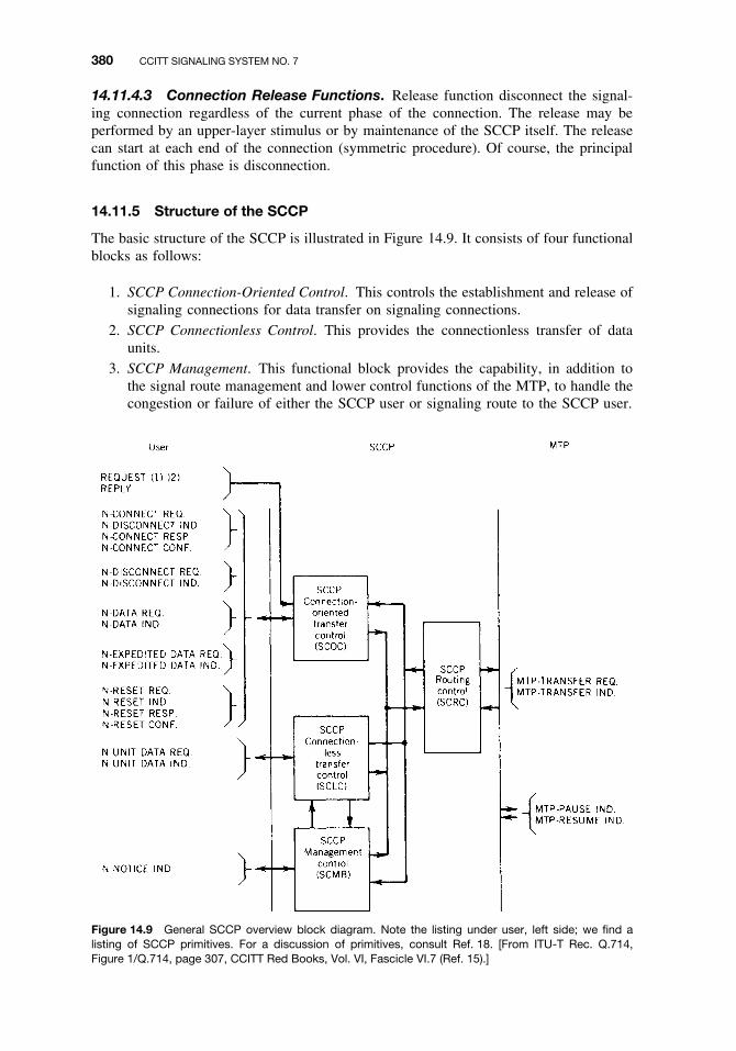
380 CCITT SIGNALING SYSTEM NO. 7
14.11.4.3 Connection Release Functions. Release function disconnect the signal-ing connection regardless of the current phase of the connection. The release may beperformed by an upper-layer stimulus or by maintenance of the SCCP itself. The releasecan start at each end of the connection (symmetric procedure). Of course, the principalfunction of this phase is disconnection.
14.11.5 Structure of the SCCP
The basic structure of the SCCP is illustrated in Figure 14.9. It consists of four functionalblocks as follows:
1. SCCP Connection-Oriented Control. This controls the establishment and release ofsignaling connections for data transfer on signaling connections.
2. SCCP Connectionless Control. This provides the connectionless transfer of dataunits.
3. SCCP Management. This functional block provides the capability, in addition tothe signal route management and lower control functions of the MTP, to handle thecongestion or failure of either the SCCP user or signaling route to the SCCP user.
Figure 14.9 General SCCP overview block diagram. Note the listing under user, left side; we find alisting of SCCP primitives. For a discussion of primitives, consult Ref. 18. [From ITU-T Rec. Q.714,Figure 1/Q.714, page 307, CCITT Red Books, Vol. VI, Fascicle VI.7 (Ref. 15).]

14.12 USER PARTS 381
4. SCCP Routing. On receipt of the message from the MTP or from the functions listedpreviously, SCCP routing either forwards the message to the MTP for transfer orpasses the message to the functions listed. A message whose called party addressis a local user is passed to functions 1, 2, or 3, whereas one destined for a remoteuser is forwarded to the MTP for transfer to the distant SCCP (Ref. 13).
14.12 USER PARTS
14.12.1 Introduction
SS No. 7 user parts, along with the routing label, carry out the basic signaling functions.Turn again to Figure 14.5. There are two fields in the figure we will now discuss: the SIO(service information octet) and the SIF (signaling information field). In the paragraphs thatfollow, we briefly cover one of the user parts, the TUP (telephone user part). As shown inFigure 14.10, the user part, OSI layer 4, is contained in the signaling information field tothe left of the routing label. ITU-T Rec. Q.723 (Ref. 14) deals with the sequence of threesectors (fields and subfields of the standard basic message signal unit shown in Figure 14.5).
Turning now to Figure 14.10, we have from right to left the service information octet(SIO), the routing label, and the user information subfields (after the routing label in theSIF). The SIO is an octet in length made up of two subfields: the service indicator (4bits) and the subservice field (4 bits). The service indicator, being 4 bits long, has 16 bitcombinations with the following meaning (read from right to left):
Bits DCBA Meaning
0000 Signaling network management message0001 Signaling network testing and maintenance0010 Spare0011 SCCP0100 Telephone user part0101 ISDN user part0110 Data user part (call- and circuit-related message)0111 Data user part (facility registration and cancellation)
Remainder (8 sequences) Spare
Figure 14.10 Signaling information field (SIF) preceded by the service information octet (SIO). Thesequence runs from right to left with the least significant bit transmitted first. DPC, destination point code;OPC, originating point code; CIC, circuit identification code.

382 CCITT SIGNALING SYSTEM NO. 7
The SIO directs the signaling message to the proper layer 4 entity, whether SCCP oruser part. This is called message distribution.
The subservice indicator contains the network bits C and D and two spare bits, A andB. The network indicator is used by signaling message-handling functions determiningthe relevant version of the user part. If the network indicator is set at 00 or 01, the twospare bits, coded 00, are available for possible future needs. If these two bits are coded10 or 11, the two spare bits are for national use, such as message priority as an optionalflow procedure. The network indicator provides discrimination between international andnational usage (bits D and C).
The routing label forms part of every signaling message:
ž To select the proper signaling routež To identify the particular transaction by the user part (the call) to which the mes-
sage pertains
The label format is shown in Figure 14.10. The DPC is the destination point code (14 bits)which indicates the signaling point for which the message is intended. The originatingpoint code (OPC) indicates the source signaling point. The circuit identification code(CIC) indicates the one circuit (speech circuit in the TUP case) among those directlyinterconnecting the destination and originating points.
For the OPC and DPC, unambiguous identification of signaling points is carriedout by means of an allocated code. Separate code plans are used for the internationaland national networks. The CIC, as shown in Figure 14.10, is applicable only to theTUP. ITU-T (CCITT) Rec. Q.704 shows a signaling link selection (SLS) field fol-lowing (to the left) the OPC. The SLS is 4 bits long and is used for load sharing.The ISDN user part address structure is capable of handling E.164 addresses in thecalling and in the called number and is also capable of redirecting address informa-tion elements.
14.12.2 Telephone User Part (TUP)
The core of the signaling information is carried in the SIF (see Figure 14.10). The TUPlabel was described briefly in Section 14.7.2.1. Several signal message formats and codesare described in the paragraphs below. These follow the TUP label.
One typical message of the TUP is the initial address message (IAM). Its format isshown in Figure 14.11. A brief description is given of each subfield, providing furtherinsight on how SS No. 7 operates.
Common to all signaling messages are the subfields H0 and H1. These are the headingcodes, each consisting of 4 bits, giving 16 code possibilities in pure binary coding. H0identifies the specific message group to follow. “Message group” means the type ofmessage. Some samples of message groups are as follows:
Message Group Type H0 Code
Forward address messages 0001Forward setup messages 0010Backward setup messages 0100Unsuccessful backward setup messages 0101Call supervision messages 0110Node-to-node messages 1001

14.12 USER PARTS 383
Figure 14.11 Initial address message format. [From CCITT Rec. Q.723, Figure 3/Q.723, page 23(Ref. 14).]
H1 contains a signal code or identifies the format of more complex messages. For instance,there are four types of address message identified by H0 = 0001, and H1 identifies thetype of message, such as the following:
Address Message Type H0 H1
Initial address message 0001 0001IAM with additional information 0001 0010Subsequent address message 0001 0011Subsequent address message with signal unit 0001 0100
Moving from right to left in Figure 14.11, after H1 we have the call party subfieldconsisting of 6 bits. It identifies the language of the operator (Spanish, English, Russian,etc.). For example, an English-speaking operator is coded 000010. It also differentiatesthe calling subscriber from one with priority, a data call, or a test call. A data call is coded001100 and a test call is coded 001101. Fifty of the 64 possible code groups are spare.
Continuing to the left in Figure 14.11, two bits are spare for international allocation.Then there is the message indicator, where the first two bits, B and A, give the natureof the address. This is information given in the forward direction indicating whether theassociated address or line identity is an international, national (significant), or subscribernumber. A subscriber number is coded 00, an international is coded 11, and a national(significant) number is coded 10.
Bits D and C are the circuit indicator. The code 00 in this location indicates that thereis no satellite circuit in the connection. Remember that the number of space satellite relaysin a speech telephone connection is limited to one relay link through a satellite becauseof propagation delay.
Bits F and E are significant for common-channel signaling systems such as CCIS, CCSNo. 6, and SS No. 7. The associated voice channel operates on a separate circuit. Doesthis selected circuit for the call have continuity? The bit sequence FE is coded:
Bits F and E Meaning
00 Continuity check not required01 Continuity check required on this circuit10 Continuity check performed on previous circuit11 Spare

384 CCITT SIGNALING SYSTEM NO. 7
Bit G gives echo suppressor information. When coded 0 it indicates that the outgoinghalf-echo suppressor is not included, and when coded 1 it indicates that the outgoing half-echo suppressor is included. Bit I is the redirected call indicator. Bit J is the all-digitalpath required indicator. Bit K tells whether any path may be used or whether only SSNo. 7-controlled paths may be used. Bit L is spare.
The next subfield has 4 bits and gives the number of address signals contained in theinitial address message. The last subfield contains address signals where each digit iscoded by a 4-bit group as follows:
Code Digit Code Digit
0000 0 1000 80001 1 1001 90010 2 1010 Spare0011 3 1011 Code 110100 4 1100 Code 120101 5 1101 Spare0110 6 1110 Spare0111 7 1111 ST
The most significant address signal is sent first. Subsequent address signals are sent insuccessive 4-bit fields. As shown in Figure 14.11, the subfield contains n octets. A fillercode of 0000 is sent to fill out the last octet, if needed. Recall in Chapter 7 that the STsignal is the “end of pulsing” signal and is often used on semiautomatic circuits.
Besides the initial address message, there is the subsequent address message usedwhen all address digits are not contained in the IAM. The subsequent address messageis an abbreviated version of the IAM. There is a third type of address message, theinitial address message with additional information. This is an extended IAM providingsuch additional information as network capability, user facility data, additional routinginformation, called and calling address, and closed user group (CUG). There is also theforward setup message, which is sent after the address messages and contains furtherinformation for call setup.
CCITT SS No. 7 is rich with backward information messages. In this group are back-ward setup request; successful backward setup information message group, which includescharging information; unsuccessful backward setup information message group, whichcontains information on unsuccessful call setup; call supervision message group; circuitsupervision message group; and the node-to-node message group (CCITT Recs. Q.722and Q.723 (Refs. 14, 16).
Label capacity for the telephone user part is given in CCITT Rec. Q.725 (Ref. 17) as16,384 signaling points and up to 4096 speech circuits for each signaling point.
REVIEW EXERCISES
1. What is the principal rationale for developing and implementing Signaling SystemNo. 7?
2. Describe SS No. 7 and its relationship with OSI. Why does it truncate at OSI layer 4?
3. Give the two primary “parts” of SS No. 7. Briefly describe each part.

REFERENCES 385
4. OSI layer 4 is subdivided into two sublayers. What are they?
5. Layer 2 carries out the functions of the signaling link. Name four of the five functionsof layer 2.
6. What are the two basic categories of functions of layer 3?
7. What is a signaling relation?
8. How are signaling points defined? (Identified).
9. What does a routing label do?
10. What are the two methods of error correction in SS No. 7?
11. What are the three types of signal units used in SS No. 7?
12. Discuss forward and backward sequence numbers.
13. The routing label is analogous to what in our present telephone system? Name thethree basic pieces of information that the routing label provides.
14. Define labeling potential.
15. What is the function of an STP? Differentiate STP with signaling point.
16. Why do we wish to limit the number of STPs in a specific relation?
17. What are the three measures of performance of SS No. 7?
18. Regarding user parts, what is the function of the SIO? Of the network indicator?
19. What is the purpose of circuit continuity?
20. With the TUP address signals are sent digit-by-digit embedded in the last subfieldof the SIF.
21. What are the two overall set of services of the SCCP?
22. What is the purpose of the SCCP?
REFERENCES
1. Specifications of Signaling System No. 7 (Q.700 Series), Fascicle VI.6, CCITT Yellow Books,VIIth Plenary Assembly, Geneva, 1980.
2. W. C. Roehr, Jr., “Signaling System No. 7,” in Tutorial: Integrated Services Digital Network(ISDN), W. Stallings, ed., IEEE Computer Society, Washington, DC, 1985.
3. Introduction to CCITT Signaling System No. 7, ITU-T Rec. Q.700, ITU Helsinki, 1993.
4. Functional Description of the Message Transfer Part (MTP) of Signaling System No. 7, ITU-TRec. Q.701, ITU Helsinki, 1993.
5. R. L. Freeman, Reference Manual for Telecommunication Engineering, 3rd ed., Wiley, NewYork, 2001.
6. BOC Notes on the LEC Networks—1994, Bellcore Special Report SR-TSV-002275, Issue 2,Piscataway, NJ, Apr. 1994.
7. Signaling System No. 7—Signaling Link, ITU-T Rec. Q.703, ITU Geneva. 1996.
8. Signaling System No. 7—Signaling Network Functions and Messages, ITU-T Rec. Q.704, ITUGeneva, 1996.
9. Signaling System No. 7—Signaling Network Structure, ITU-T Rec. Q.705, ITU Geneva, 1993.

386 CCITT SIGNALING SYSTEM NO. 7
10. Signaling System No. 7—Message Transfer Part Signaling Performance, ITU-T Rec. Q.706,ITU Geneva 1993.
11. Signaling System No. 7—Hypothetical Signaling Reference Connection, ITU-T Rec. Q.709,Helsinki, 1993.
12. Assigned Procedures for International Signaling Point Codes, ITU-T Rec. Q.708, ITU Geneva,1999.
13. Signaling System No. 7—Functional Description of the Signaling System Control Part (SCCP),ITU-T Rec. Q.711, ITU Geneva, 2001.
14. Formats and Codes, (Telephone User Part), CCITT Rec. Q.723, Fascicle VI.8, IXth PlenaryAssembly, Melbourne, 1988.
15. Signaling System No. 7—Signaling Connection Control Part User Guide, ITU-T Rec. Q.714,ITU Geneva, May 2001.
16. Signaling System No. 7—General Function of Telephone Messages and Signals, CCITT Rec.Q.722, Fascicle VI.8, IXth Plenary Assembly, Melbourne, 1988.
17. Signaling System No. 7—Signaling Performance in the Telephone Application, ITU-T Rec.Q.725, ITU Geneva 1992.
18. R. L. Freeman, Telecommunication System Engineering, 4th ed., Wiley, Hoboken, NJ, 2004.

15
VOICE-OVER PACKETS IN A PACKETNETWORK
15.1 AN OVERVIEW OF THE CONCEPT
On the surface the concept seems fairly simple. We digitize the voice and break up theresulting serial bit stream into packets of some length. A header is added to each packet,and the packet can now be sent over the data packet network. This type of operationis most commonly called voice over IP (VoIP). “IP” is the Internet protocol, which wediscuss in Chapter 12. Others prefer the broader term voice over packet. This would alsoencompass “voice over ATM (asynchronous transfer mode” (Chapter 20). Still anotherapproach is to place voice (in packets) over frame relay (Chapter 12). The concept ofVoIP is illustrated in Figure 15.1.
15.2 DATA TRANSMISSION VERSUS CONVENTIONAL DIGITAL TELEPHONY
Conventional voice telephony is transported in a full duplex mode on PSTN circuitsoptimized for voice. By the full-duplex mode we mean that there are actually two circuits,one for “send” and one for “receive” to support a normal telephone conversation betweentwo parties. With a few exceptions in the local area, all these circuits are digital. Thedescriptive word digital may seem ambiguous to some.
When we say digital in this context, we mean that all circuits would carry 8-bit “words”(timeslots), where each “word” represents an 8-bit voltage sample ostensibly of an analogvoice conversation in a PCM format. This is often characterized in the literature as G.711service (i.e., ITU-T Rec. G.711). Data are also commonly transported in 8-bit sets calledbytes, but more properly called octets from our vantage point. It is comparatively easy toreplace 8-bit voltage samples of voice with 8-bit octets of data.
However, there remained essential philosophical differences between voice in 8-bitoctets and data transmission. A voice circuit is established when a subscriber desires toconverse by telephone with some other telephone subscriber. The circuit between the two
VoiceA/D conv.
VoiceV/A conv.
Packetizer(IP)
NETDepacketizer
(IP)
Figure 15.1 Rough conceptualization of VoIP.
Fundamentals of Telecommunications, Second Edition, by Roger L. FreemanISBN 0-471-71045-8 Copyright 2005 by Roger L. Freeman
387

388 VOICE-OVER PACKETS IN A PACKET NETWORK
Direction of transmission
Flag Flag
16 bits k bits
n bitsM (x)
G (x)
Information Control AddressFrame check
sequence
Figure 15.2 A typical data frame.
is set up by a signaling routine. The distant subscriber has a telephone address representedby a distinct telephone number consisting of 7 to 12 digits. The digit sequence of thenumber sets up a circuit route and connectivity for conversation. The circuit is maintainedin place for the duration of the conversation, and it is terminated and taken down whenone or the other party hangs up (“goes on hook”). The address sequence of dialed digitsis sent just once, at the initiation of the connectivity. This whole process of setting upa circuit, holding the connectivity in place, and then taking down the circuit is calledsignaling.
Signaling on data circuits is approached quite differently. There is the permanent virtualcircuit (PVC), which has all the trappings similar to a voice circuit. The similarities stophere. Data transmission consists of frames or packets of data. A frame (or data packet)is made up of a header and payload. In some cases a portion of the “header” may beappended at the end or on the tail of the data frame (or packet). But every data frame (orpacket) has a header consisting of a destination address (or addresses) and the originator’saddress. It nearly always will also contain some control information. This may be a word(or byte/octet) count of the payload, a CRC sequence for error detection and/or correction,message priority, or some other type of control sequence or sequences.
Digital circuits on the PSTN have either 24-octet frames in the case of T1 (DS1) or32-octet frames in the case of E1. Each 8-bit octet represents a voice circuit. Such acircuit may be set up using an Initial Address Message of CCITT Signaling System No.7 or a sequence of DTMF tones where each frequency pair represents a digit in the rangeof 0 through 9. Once a circuit is set up, no more address messages or DTMF tones arerequired until the circuit is taken down.
This is not the case on a data circuit. Such a circuit also uses frames, but each andevery frame has a standard header. A typical data frame is illustrated in Figure 15.2. Theframe structure and how various octets of the header (and tail) are utilized are governedby a protocol. Various data protocols were discussed in Chapters 11–13.
We can clearly see that there are two differing philosophies here, one for data commu-nication and the other for digital voice. Digital voice is sometimes called “circuit-switchedvoice.” A majority in the telecommunication community saw how advantageous it wouldbe if we could marry the two and make them one. That is one singular approach forboth voice and data. Meanwhile, data hobbyists were trying to transmit voice using datapackets. The Internet protocol (IP) became the data protocol of choice, but there weremany drawbacks.
15.3 DRAWBACKS AND CHALLENGES FOR TRANSMITTING VOICEON DATA PACKETS
We have come to measure “quality” of packetized voice service by the equivalent serviceoffered by the switched digital network (i.e., the PSTN), sometimes called G.711 (1)

15.4 VOIP, INTRODUCTORY TECHNICAL DESCRIPTION 389
service. The user expects a quality of service (QoS) as good as he or she would get on aPSTN dial-up connection.
To achieve this goal, voice-over IP (VoIP) designers were faced with the followingdegradations:
ž Mouth-to-ear delayž Impact of errored frames (packets)ž Lost frames (packets)ž Variation of packet arrival time, jitter bufferingž Prioritizing VoIP traffic over regular Internet and data servicesž Talker echož Distortionž Sufficient bit rate capacity on interconnecting transmission mediaž Voice coding algorithm standardizationž Optimized standard packet payload sizež Packet overheadž Silence suppression
15.4 VOIP, INTRODUCTORY TECHNICAL DESCRIPTION
Figure 15.3 shows a simplified block diagram of VoIP operation from an analog signalderiving from a standard telephone, which is digitized and transmitted over the Internetvia a conversion device. Then, at the distant end, it is converted back to analog telephonyusing a similar device suitable for input to a standard telephone. The gateway is placedbetween the voice codec and the digital data transport circuit. An identical device willalso be found at the far end of the link. This equipment carries out the signaling role ona telephone call among other functions.
Moving from left to right in Figure 15.3, we have the spurty analog signal derivingfrom a standard telephone set. The signal is then converted to a digital counterpart usingone of seven or so codecs [coder-decoder(s)] that the VoIP system designer has to selectfrom. Some of the more popular codecs for this application are listed in Table 15.1. Thebinary output of the codec is then applied to a conversion device (i.e., a “packetizer”)that loads these binary 1s and 0s into an IP payload of from 20 to 40 octets in length.
The output of the converter consists of IP packets1 that are transmitted on the web orother data circuit for delivery to the distant end.
At the far end the IP packets or frames are input to a converter (i.e., depacketizer) thatstrips off the IP header, stores the payload, and then releases it in a constant bit streamto a codec (i.e., a D–A converter). Of course this codec must be compatible with its
A/Dconversionpacketizer
DepacketizerD/A
conversionrouter router
Figure 15.3 Elements of basic operation of VoIP where the input signal derives from a conventionalanalog telephone. This figure follows Figure 15.1 in sequence of complexity.
1The output may be ATM cells (see Chapter 20) if the intervening network is an ATM network.

390 VOICE-OVER PACKETS IN A PACKET NETWORK
Table 15.1 Characteristics of Speech Codecs Used in Packet Networks
Coding AlgorithmVoice Bit
Rate (kbits/sec)Voice FrameSize (bytes)
Header(bytes)
Packets perSecond
Packet BitRate (kbits/sec)
G.711 8-bit PCM [1] 64 80 40 100 96G.723.1 MPMLQa [4] 6.3 30 40 26 14.6G.723.1 ACELPb [5] 5.3 30 40 22 12.3G.726 ADPCMc [6] 32 40 40 100 64G.728 LD-CELPd [7] 16 20 40 100 48G.729a CS-ACELPe [8] 8 10 40 100 40
aMPMLQ, multipulse maximum likelihood quantization.bACELP, algebraic code-excited linear prediction.cADPCM, adaptive differential PCM.dLD-CELP, low delay code-excited linear prediction.eCS-ACELP, conjugate structure algebraic code-excited linear prediction.
near-end counterpart. The codec converts the digital bit stream back to an analog signalthat is then input to a standard telephone subset.
The insightful reader will comment that many steps of translation and interface havebeen left out. Most of these considerations will be covered below in Section 15.4.1 in ourdiscussion of the gateway.
15.4.1 VoIP Gateway
Gateways are defined in different ways by different people. In our context here a gatewayis a server; it may also be called a media gateway. Figure 15.4 illustrates a typical gateway.It sits on the edge of the network and carries out a switching function of a local, tandem,or toll-connecting PSTN switch described in Chapters 3 and 6. Media gateways are part
VoicePrompts
CallControl
Authorization&
Identification
MNSPMIB Maintenance
Administration
QoSRecords
Billing Records
H.323 API
H.323Protocol Stack
HardwareAPI
Gateway HardwareT1/E1, DSPs, etc.
Gateway Server
Figure 15.4 A media gateway from one perspective. API, application programs interface. From IECon-line: www.iec.org/online/tutorials/int tele/topic03.html (Jan. 2003).

15.4 VOIP, INTRODUCTORY TECHNICAL DESCRIPTION 391
of the physical transport layer. They are controlled by a call control function housed in amedia gateway controller. A media gateway with its associated gateway controller is atthe heart of the network transformation to packetized voice. Several of the media gatewayfunctions are listed here:
ž Carries out A/D conversion of the analog voice channel (called compression inmany texts).
ž Converts a DS0 or E0 to a binary signal compatible with IP or ATM.ž Supports several types of access networks including media such as copper (including
various DSL regimes), fiber, radio (wireless), and CATV cable. It is also able tosupport various formats found in PDH and SDH hierarchies.
ž Competitive availability (99.999%).ž Capable of handling several voice and data interface protocols.ž Multivendor interoperability.ž It must provide interface between media gateway control device and the media
gateway. This involves one of four protocols: SIP [2], H.323 [3], MGCP, andMegaco (H.248).
ž Can handle switching and media processing based on standard network PCM, ATM,and traditional IP.
ž Transport of voice. There are four transmission categories involved:1. Standard PCM (E0/E1 or DS0/DS1)2. ATM over AAL1/AAL23. IP-based RTP/RTCP4. Frame relay
The most powerful gateway supports the public network or PSTN requiring a highreliability device to meet the PSTN availability requirements. It will be required to processmany thousands of digital circuits. As shown in Figure 15.4, it has a network managementcapability most often based on SNMP (see Chapter 21).
A somewhat less formidable gateway is employed to provide VoIP for small andmedium-sized business. Some texts call this type of gateway an integrated access device(IAD) if it can handle data and video products as well. An IAD will probably be remotelyconfigurable.
The least powerful and most economic gateways are residential. They can be deployedin at least five settings:
ž POTS (telephony)ž Set-top box (CATV), which provides telephony as wellž PC/modemž XDSL terminationž Broadband last mile connectivity (to the digital network)
Figure 15.5 shows gateway interface functions via a block diagram. On the left aretime slots of a PCM bit stream (T1, in this case). The various signal functions are shownto develop a stream of data packets carrying voice or data. The output on the right consistsof IP packets.
The first functional block of the gateway analyzes the content on a time-slot basis.The time slot may contain an 8-bit data sequence where we must be hands-off regarding

392 VOICE-OVER PACKETS IN A PACKET NETWORK
Time slots
Outputs to Internet
(1) data packets(2) signaling packets(3) voice packets
1 2 3 4 5 - - 24
Time slottype decision
circuit
2100 Hzmodemsignal(data)
Demodulateor
compress
Convertto dataformat
Transmitdialed digit
packetCompressdecision
DTMFsignaling
tones
Speechactivity
detection
Speechcompression Echo
canceler
either/or
(1)
(2)
(3)
Figure 15.5 A simplified functional block diagram of a gateway providing and interface between a PCMbit stream deriving from the PSTN on the left and an IP network.
the content. A gateway senses the presence of data by the presence of a 2100-Hz tonein the time slot. The next signal type in the time slot looks for its DTMF signalingtones (see Chapter 4). If there is no modem tone nor DTMF tones in the time slot,then the gateway assumes the time slot contains human speech. Three actions now haveto be accomplished. “Silence” is removed; the standard PCM compression algorithmis applied; an echo canceler is switched in. There are three digital formats used forvoice-over packet:
1. Internet Protocol (IP) (Chapter 12, Section 12.3).2. Frame Relay (Chapter 12, Section 12.5).3. ATM—Asynchronous Transfer Mode (Chapter 20).
15.4.2 An IP Packet as Used for VoIP
Assume for argument that we use either a G.711 or G.726 packet (Table 15.1) IP packet.The packet consists of a header and a payload. Figure 15.6 shows a typical IP packet. Ofinterest, as one may imagine, is its payload.
In the case of G.711 (standard PSTN PCM), there may be a transmission rate of 100packets per second with 80 bytes in the payload of each packet. Of course our arithmeticcomes out just right and we get 8000 samples per second, the Nyquist sampling rate fora 4-kHz analog voice channel. Another transmission rate for G.711 is 50 packets persecond where each packet will have 160 bytes, again achieving 8000 samples per secondper voice channel.
The total raw bytes (octets) per channel come out as follows: 40 bytes for layers 3 and4 overhead (IP), plus 8 bytes for layer 2 (link layer) overhead. So we add 48 to 80 or160 bytes (from the previous paragraph) and we get 128 or 208 bytes for a raw packet.The efficiency is nothing to write home about. Keep in mind that the primary concern ofthe VoIP designer is delay.
15.4.3 The Delay Tradeoff
Human beings are intolerant of delay on a full-duplex circuit, typical of standard PSTNtelephony. ITU-T Rec. G.114 [10] recommends the total delay (one-way) in a voiceconnectivity as follows:

15.4 VOIP, INTRODUCTORY TECHNICAL DESCRIPTION 393
0 4 8 16 19 24
Total LengthType of ServiceLENVERS
TTL Protocol
Identification Flags Fragment Offset
Header Checksum
Source IP Address
Destination IP Address
PaddingOptions
Information(payload)
Figure 15.6 A typical IP packet (datagram). Based on RFC 791. Also see Figure 11.28.
ž 0–150 msec acceptable.ž 150–400 msec acceptable but not desirable. Connectivity through a geostationary
satellite falls into this category.ž Above 400 msec, unacceptable.
The delay objective (one-way) for a VoIP voice connectivity is <100 msec. Withbridging for conference calls, that value doubles due to the very nature of bridging.
One-way components of delay are as follows:
ž Packetization or encapsulation delay based on G.711 or other compression algorithm.In the case of G.711, we must build from 80 PCM samples at 125 µsec per sample,so we have consumed 80 × 125 µsec or 10,000 µsec or 10 msec plus time for theheader or 48 × 125 µsec or 6 msec, for a total of 16 msec. If we use 160 PCMsamples in the payload, then allow 20 msec plus 6 msec for the header or 26 msec.This is a fixed delay.
ž Buffer delay is variable. As a minimum, there must be buffering of one frameor packet period. Routers have buffers, by definition. Buffer delay varies with thenumber of routers in tandem. For G.711 the packet buffer size is 16 or 26 msec.
ž Look-ahead delay. This is used by the coder to help in compression. “Look-ahead”is a period of time where the coder looks at packet N + 1 for patterns on which itcan compress while coding packet N. With G.711 the look-ahead is 0.
ž Dejitterizer is a buffer installed at the destination. It injects at least 1 frame (packet)duration (1–20 msec) in the total delay to smooth out the apparent arrival times ofpackets (frames).

394 VOICE-OVER PACKETS IN A PACKET NETWORK
ž Queueing delay. Time spent in queue because it is a shared network. One method toreduce this delay is to prioritize voice packets (vis a vis data). Objective <50 msec.
ž Propagation delay. Variable. Major contributor to total delay. Geostationary satelliterelay of circuits is a special problem. The trip to the satellite and back is budgetedat 250 msec.
One way to speed things up is to increase the bit rate per voice data stream. To dothis, the aggregate bit rate may have to be increased. Or the number of voice streamsmay be reduced on the aggregate bit rate so that each stream can be transmitted at afaster rate.
15.4.4 Lost Packet Rate
A second concern of the VoIP designer is lost packet rate. There are several ways a packetcan be “lost.” For example, Section 15.3.3 described a dejitterizing buffer. It has a finitesize. Once the time is exceeded by a late packet, the packet in question is lost. In thecase of G.711, this would be the time equivalent of 16 or 26 msec (duration of a packetincluding its header). Another reason for a packet to be lost may be excessive error rateon a packet whereby it is deleted. When the lost (discarded) packet rate begins to exceed10%, quality of voice starts to deteriorate. If high-compression algorithms are employedsuch as G.723 or G.729, it is desirable to maintain the packet loss rate below 1%. Routerbuffer overflow is another source of packet loss.
IP through TCP has excellent retransmission capabilities for errored frames or packets.However, they are not practical for voice-over IP because of the additional delay involved.When there is a packet or frame in error, the receive end of the link transmits a request(RQ) to the transmit end for a packet retransmission and its incumbent propagation delay.This must be added to the transmission delay (and some processing delay) to send theoffending packet back to the receiver again.
15.4.4.1 Concealment of Lost Packets. A lost packet causes a gap in the receptionstream. For a single packet we are looking at a 20- to 40-msec gap. The simplest measureto take for lost packets and the resulting gaps is to disregard. The absolute silence of agap may disturb a listener. In this case, often artificial noise is inserted.
There are packet loss concealment (PLC) procedures which can camouflage gapsin the output voice signal. The simplest techniques require a little extra processingpower, and the most sophisticated techniques can restore speech to a level approx-imating the quality of the original signal. Concealment techniques are most effectivefor about 40 to 60 msec of missing speech. Gaps longer than 80 msec usually have tobe muted.
One of the most elementary PLCs simply smoothes the edges of gaps to eliminateaudible clicks. A more advanced algorithm replays the previous packet in place of thelost one, but this can cause harmonic artifacts such as tones or beeps. Good concealmentmethods use variation in the synthesized replacement speech to make the output more likenatural speech. There are better PLCs to preserve the spectral characteristics of the talker’svoice and to maintain a smooth transition between estimated signal and surroundingoriginal. The most sophisticated PLCs use CELP (codebook-excited linear predictive)or similar technique to determine the content of the missing packet by examining theprevious one [11].
Lost packets can be detected by packet sequence numbering.

15.5 MEDIA GATEWAY CONTROLLER AND ITS PROTOCOLS 395
15.4.5 Echo and Echo Control
Echo is commonly removed by the use of echo cancelers and are incorporated on the sameDSP chips that perform the voice coding. A good source of information and design ofecho cancelers is ITU-T Rec. G.168 [12]. However, most vendors of VoIP equipment havetheir own proprietary designs. A common design approach is to have the echo cancelerstore the outgoing speech in a buffer. It then monitors the stored speech after a delay tosee whether it contains a component that matches up against the stored speech after adelay. If it does, that component of the incoming speech is canceled out instead of beingpassed back to the user since it is an echo of what the user originally said. Echo cancelerscan be tuned or can tune themselves to the echo delay on any particular connection. Eachecho canceler design has a limit as to the maximum delay of echo that it can identify.Echo cancelers are bypassed if a fax signal or modem data is on the line.
15.5 MEDIA GATEWAY CONTROLLER AND ITS PROTOCOLS
The gateway controller or media gateway controller (MGC) carries out the signalingfunction on VoIP circuits. Some texts call an MGC a soft switch even though they arenot truly switches but are servers that control gateways. This function is illustrated inFigure 15.7.
An MGC can control numerous gateways. However, to improve reliability and avail-ability several MGCs may be employed in separate locations with function duplication onthe gateways they control. Thus if one MGC fails others can take over its functions. Wemust keep in mind that the basic topic of Section 15.4 is signaling. That is the establishing(setting up) of telephone connectivities, maintaining that connectivity and the taking downof the circuit when the users are finished with conversation. There is a basic discussionof signaling in Chapter 4 of this text.
There are four possible signaling protocol options between an MGC and gateways.These are:
ž ITU-T Rec. H.323. This is employed where all network elements (NEs) have softwareintelligence.
ž SIP (session initiation protocol [2]) is used when the end devices have softwareintelligence and the network itself is without such intelligence.
IP Network
Signaling
Signaling
MG
MGCMGC
MG
MG
MG
MG
Figure 15.7 A media gateway controller (MGC) provides a signaling interface for media gateways (MG)and thence to the IP network.
396 VOICE-OVER PACKETS IN A PACKET NETWORK
ž MGCP (media gateway control protocol) is another gateway control protocol.ž Megaco (ITU-T Rec. H.248 [13]) is a gateway control protocol applicable when end
devices are without software intelligence and the network has software intelligence.
15.5.1 Overview of the ITU-T Rec. H.323 Standard
In May 1996 the ITU ratified the H.323 specification, which defines how voice, video,and data traffic should be transported over IP-based LANs. It also incorporates the ITU-T Rec. T.120 [21] data-conferencing standard. The H.323 recommendation is basedon RTP/RTCP (real-time protocol/real-time control protocol) for managing audio andvideo signals.
What sets H.323 apart is that it addresses core Internet applications by defining howdelay-sensitive traffic such as voice and video get priority transport to ensure real-timecommunication service over the Internet. A related protocol is ITU-T Rec. H.324 [14]specification, which defines the transport of voice, data, and video over regular telephonenetworks. Another related protocol is ITU-T Rec. H.320 [15], which covers the transportof voice, video, and data over the integrated services digital network (ISDN).
H.323 deals with three basic functional elements of VoIP. These are:
ž Media gatewayž Media gateway controller (MGC) (in some settings this is called the gatekeeper)ž Signaling gateway
H.323 is an umbrella protocol covering the following:
ž H.225 [16], which covers the setup of multimedia channelsž H.245 [17], which deals with the setup of single-channel medium
The standard H.323 [3] prefers the use of the term gatekeeper (versus media gatewaycontroller). Some of the more important responsibilities of a gatekeeper are:
ž Security. It authenticates users of the H.323 network.ž It performs address translation between Internet addresses and ITU-T Rec. E.164
[18] addresses.ž It polices the capacity of the network in question, whether that network can accept
another call.ž H.323 determines call routing, to route through a gateway or be sent directly to the
destination.ž It keeps track of the network’s bit rate capacity.
H.323 assumes that the transmission medium is a LAN that does not provide guaranteeddelivery of packets. In the ITU H.323 standard we will find the term entity. An entitycarries out a function. For example, a terminal is an endpoint on a LAN that can supportreal-time communications with another entity on that LAN. It has a capability provided bya voice or audio codec such as a G.711 or G.728 codec. It will also provide a signalingfunction for VoIP circuit setup, maintain, and take-down. A VoIP terminal optionallycan support video and data streams including compression and decompression of thesestreams. Media streams are carried on RTP (real-time protocol) or RTCP (real-time controlprotocol). RTP deals with media content while RTCP works with the signaling functions

15.5 MEDIA GATEWAY CONTROLLER AND ITS PROTOCOLS 397
of status and control. This protocol information is embedded in UDP, which is reliablytransported by TCP.
Other VoIP entities are gateways and there is a gatekeeper that is optional.The leading issue in VoIP implementation is guaranteed quality of service (QoS).
H.323 is based on RTP (real-time protocol) which is comparatively new. RTP-compliantequipment includes control mechanisms for synchronizing different traffic streams. Onthe other side of the coin, RTP has no mechanisms for ensuring on-time delivery oftraffic signals or for recovering lost packets. It does not address the QoS issue related toguaranteed bit rate availability for specific applications. The IEC [19] reports that thereis a draft signaling proposal to strengthen the Internet’s ability to handle real-time trafficreliably. This would dedicate end-to-end transport paths for specific sessions much likethe circuit-switched PSTN does. This is the resource reservation protocol (RSVP). It willbe implemented in routers to establish and maintain requested transmission paths andQoS levels.
15.5.2 Session Initiation Protocol (SIP)
SIP is based on RFC 2543 [2] and is an application layer signaling protocol. It deals withinteractive multimedia communication sessions between end-users, called user agents.It defines their initiation, modification, and termination. SIP calls may be terminal-to-terminal, or they may require a server to intercede. If a server is to be involved, it is onlyrequired to locate the called party. For interworking with non-IP networks, Megaco andH.323 are required. Often vendors of VoIP equipment integrate all three protocols on asingle platform.
SIP is closely related to IP. SIP borrows most of its syntax and semantics from thefamiliar HTTP (hypertext transfer protocol). An SIP message looks very much like anHTTP message, especially with message formatting, header, and multipurpose Internetmail extension support. It uses addresses that are very similar to URLs (uniform resourcelocators) and to email. For example, a call may be made to so-in-so@such-and-such. SIPmessages are text-based rather than binary. This makes writing easier and the debuggingof software more straightforward.
There are two modes with which a caller can set up a call with SIP. These are calledredirect and proxy, and servers are designed to handle these modes. Both modes issuean “invite” message for another user to participate in a call. The redirect server is usedto supply the address (URL) of an unknown called addressee. In this case the “invite”message is sent to the redirect server, which consults the location server for addressinformation. Once this address information is sent to the calling user, a second “invite”message is issued, now with the correct address.
One specific type of SIP is called SIP-T (T for telephone). This is a function that allowscalls from CCITT Signaling System 7 (SS7) to interface with a telephone in an IP-basednetwork. The particular user part of SS7 for this application is ISUP (see Chapter 14, SSNo. 7).
15.5.3 Media Gateway Control Protocol (MGCP)
This protocol was the predecessor to Megaco (see Section 15.4.4) and still holds sway witha number of carriers and other VoIP users. MGCP [20] assumes a call control architecturewhere the call control “intelligence” is outside the gateways (i.e., at the network edge) andhandled by external call control elements. Thus, the MGCP assumes that these call controlelements, or “call agents,” will synchronize with each other to send coherent commands

398 VOICE-OVER PACKETS IN A PACKET NETWORK
to the gateways under their command. There is no mechanism defined in MGCP forsynchronizing “call agents.” It is, in essence, a master/slave protocol where the gatewaysare expected to execute commands sent by the “call agents.”
In the MGCP protocol an assumption is made that the connection model consists ofconstructs that are basic end-points and connections. End-points are sources or sinks ofdata and could be physical or virtual. The following are two examples of end-points:
1. An interface on a gateway that terminates a trunk connected to a PSTN switch(e.g., local or toll-connecting, etc.). A gateway that terminates trunks is called atrunk gateway.
2. An interface on a gateway that terminates an analog POTS (plain old telephoneservice) connection to a telephone, a key system, PABX, and so on. A gateway thatterminates residential POTS lines (to telephones) is called a residential gateway.
An example of a virtual end-point is an audio source in an audio-content server.Creation of physical end-points requires a hardware installation, while creation of virtualend-points can be done in software [20].
15.5.4 Megaco or ITU-T Rec. H.248 (Ref. 13)
Megaco is a call-control protocol that communicates between a gateway controller anda gateway. It evolved from and replaces SGCP (simple gateway control protocol) andMGCP (media gateway control protocol). Megaco addresses the relationship between amedia gateway (MG) and a media gateway controller (MGC). An MGC is sometimescalled a softswitch or call agent.
Both Megaco and MGCP are relatively low-level devices that instruct MGs to connectstreams coming from outside the cell or packet data network onto a packet or cell streamgoverned by RTP (real-time transport protocol). A Megaco (H.248) connection modelis illustrated in Figure 15.8. There are two principal abstractions relating to the model:terminations and contexts. A termination acts as sources and/or sinks for one or moredata streams. In a multimedia conference a termination can be multimedia, and it sourcesand sinks multiple media streams. The media stream parameters, as well as modem, andbearer parameters are encapsulated within the termination.
A context is an association between a collection of terminations. There is a special typeof context called the null context, which contain all terminations that are not associatedwith any other termination. For example, in a decomposed access gateway, all idle linesare represented by terminations in the null context.
Let’s look at three context possibilities. (1) A context with just one termination is callwaiting. The caller does not hear anyone else. (2) A context with two terminations is aregular phone call. Of course each person is expected to hear the other. (3) An exampleof more than two terminations is a conference call. Each party hears each and everyother one.
The maximum number of terminations in a context is a media gateway (MG) property.MGs that offer only point-to-point connectivity might allow at most two terminations percontext. MGs that support multipoint conferences might allow three or more terminationsper context.
The attributes of contexts are:
ž Context ID.ž The topology (who hears/sees whom).
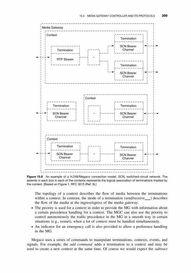
15.5 MEDIA GATEWAY CONTROLLER AND ITS PROTOCOLS 399
Media Gateway
Context
Context
Context
Termination
Termination
Termination
RTP Stream
SCN BearerChannel
SCN BearerChannel
Termination
SCN BearerChannel
Termination
SCN BearerChannel
Termination
SCN BearerChannel
Termination
SCN BearerChannel
*
*
*
Figure 15.8 An example of a H.248/Megaco connection model. SCN, switched-circuit network. Theasterisk in each box in each of the contexts represents the logical association of terminations implied bythe context. [Based on Figure 1, RFC 3015 (Ref. 9).]
The topology of a context describes the flow of media between the terminationswithin a context. In contrast, the mode of a termination (send/receive ) describesthe flow of the media at the ingress/egress of the media gateway.
ž The priority is used for a context in order to provide the MG with information abouta certain precedence handling for a context. The MGC can also use the priority tocontrol autonomously the traffic precedence in the MG in a smooth way in certainsituations (e.g., restart), when a lot of context must be handled simultaneously.
ž An indicator for an emergency call is also provided to allow a preference handlingin the MG.
Megaco uses a series of commands to manipulate terminations, contexts, events, andsignals. For example, the add command adds a termination to a context and may beused to create a new context at the same time. Of course we would expect the subtract

400 VOICE-OVER PACKETS IN A PACKET NETWORK
command to remove a termination from a context and may result in the context beingreleased if no terminations remain.
There is also the modify command used to modify the description of a termination (e.g.,the type of voice compression in use). Notify is used to inform the gateway controller ifan event occurs on a termination such as a telephone in an off-hook condition, or digitsbeing dialed. There is also a service change command.
Terminations are referenced by a TerminationID, which is an arbitrary schema selectedby the MG. TerminationIDs of physical terminations are provisioned by the media gate-way. The TerminationIDs may be chosen to have structure. For example, a TerminationIDmay consist of a trunk group and a trunk within the group (Ref. 9).
REVIEW EXERCISES
1. How many bits are in a conventional PCM voice sample?
2. How is a telephone call on the PSTN usually terminated?
3. Give the two basic components of a data message?
4. Every data frame or packet carries two components (at least) in the header. Whatare they?
5. In exercise 4, how does this differ from a PCM frame?
6. What is a CRC sequence used for?
7. Give at least two different ways the PSTN may set up a voice circuit.
8. List at list five drawbacks or challenges designers faced in making VoIP a reality.
9. List at least four tasks the gateway may do.
10. List at least four transmission media and formats that a media gateway should beable to support.
11. A media gateway interfaces a PSTN PCM bit stream. Name three types of trafficthat may be transported in that bit stream, each requiring some sort of specialhandling.
12. Given an IP packet used for voice transport. Assume G.711 or G.726 coders. Howmany bytes (octets) can we expect in the payload?
13. Give some data you have learned about one-way delay. What is the one-way delay(in ms) that should not be exceeded as a design goal?
14. What one-way delay (in milliseconds) should never be exceeded?
15. What would you say is the biggest contributor to one-way delay?
16. What is “look-ahead” used for?
17. There is buffer delay. What is its cause and it varies with the number of xxxxxin tandem?
18. What is one very obvious way to reduce delay?
19. On G.711 circuits, the lost packet rate objective is?
20. Name at least two ways to handle the presence of a lost packet.

REFERENCES 401
21. What is the basic function of a media gateway controller?
22. Name at least three of the four signaling protocol options between an MGC and amedia gateway.
23. Give a primary function of an MGC regarding delay using the H.323 protocol on aVoIP circuit.
24. Differentiate RTP and RTCP.
25. In the SIP protocol, what are end-users called.
26. What are the two modes with which a caller can set up a call with SIP.
27. In MGCP gateways are expected to execute commands sent by .
28. Megaco (H.248) is a call-control protocol that communicates between a anda ?
29. What are the two basic abstractions relating to the Megaco model?
30. A point-to-point connectivity must have at least terminations.
31. How are terminations referenced in Megaco?
REFERENCES
1. Pulse Code Modulation of Voice Frequencies, ITU-T Rec. G.711, ITU Geneva, 1988.
2. G. Malkin, Routing Information Protocol, RIP Version 2, RFC 2543.
3. Packet-Based Multimedia Communication System, ITU-T Rec. H.323, ITU Geneva, 2000.
4. Speech Coders, Dual Rate for Speech, 5.3 and 6.3 kbps, ITU-G.723.1, Multipulse MaximumLikelihood Quantization (MPMLQ), ITU Geneva, 1996.
5. Speech Coders, Algebraic Code-Excited Linear Prediction Coder, ITU-G.723.1, ITU Geneva,1996.
6. 40, 32, 24 and 16 kbps Adaptive Differential Pulse Code Modulation, ITU-T G.726, ITUGeneva, 1990.
7. Coding of Speech at 16 kbps Low-Delay Code-Excited Linear Prediction (LD-CELP), ITU-TG.728, ITU Geneva, 1992.
8. Reduced Complexity 8 kbps CS-ACELP Speech Coder, ITU-T Rec. G.729A, ITU Geneva, 1996.
9. Megaco Protocol, Version 1.0, RFC 3015, IETF Nov. 2000, www.RFC.editor.org.
10. One-Way Transmission Time, ITU-T Rec. G.114, ITU Geneva, 2000.
11. Nortel Paper on VoIP Performance, Nortel, Ottawa, Ontario, Canada, 2000.
12. Digital Network Echo Cancellers, ITU-T Rec. G.168, ITU Geneva, 2002.
13. Gateway Control Protocol, ITU-T Rec. H.248, ITU Geneva, 2000.
14. Terminal for Low Bit-Rate Multimedia Communications, ITU-T Rec. H.324, ITU Geneva, 2002.
15. Narrowband Audio/Visual Communication Systems and Terminal, ITU-T Rec. H.320, ITUGeneva, 1999.
16. Call Signaling Protocols and Media Stream Packetization for Packet-Based CommunicationSystems, ITU-T Rec. H.225, ITU Geneva, 2001.
17. Control Protocol for Multimedia Communication, ITU-T Rec. H.245, ITU Geneva, 2001.
18. The International Public Telecommunication Numbering Plan, ITU-T Rec. E.164, ITU Geneva,1997.
19. IEC Reports on-line. www.iec.org/online/tutorials, VoIP, Jan. 2003.
20. Media Gateway Control Protocol (MGCP), Version 1.0, RFC 3445, Jan. 2003.

402 VOICE-OVER PACKETS IN A PACKET NETWORK
21. Data Protocols for Multimedia Conferencing, ITU-T Rec. T.120, ITU Geneva, 1996.
22. Internet Protocol, RFC 791, DDDN Network Information Center, SRI International, MenloPark, CA, 1981.
23. R. L. Freeman, Telecommunication System Engineering, 4th ed., Wiley, Hoboken, NJ, 2004.

16
TELEVISION TRANSMISSION
16.1 BACKGROUND AND OBJECTIVES
Television was developed prior to World War II. However, it did not have any notablemarket penetration until some years after World War II. This was monochrome television.Color television began to come on the market about 1960. The next step in televisionevolvement was high-definition television (HDTV), and 1998 is considered to be the yearwhen HDTV was launched.
Interfacing standards for television have had a rather unfortunate background. NorthAmerica, Japan, and much of Latin America follow one standard called NTSC (NationalTelevision Systems Committee). The remainder of the world follows a wide variation instandards. For example, there are three different color television standards: NTSC, PAL,and SECAM. These are discussed later in the chapter.
The television signal, no matter what standard it follows, is a complex analog signal. Itis a bandwidth hog, requiring anywhere from 4 to 8 MHz for the video, color subcarrier,and the aural (audio) channel(s).
The objectives of this chapter are severalfold. The first is to provide the reader with aclear understanding of how TV works. The second goal is to describe how television istransmitted and distributed over long distances. However, the radio-broadcast of televisionis not included and is left to other texts. Cable television is covered in Chapter 17. Thethird goal of the chapter is to provide an overview of digital television, and we coverseveral generic methods of digitizing original analog television signals.
Our interest in television transmission derives from its impact on the larger telecom-munications environment. For example, the PSTN and other carriers are called upon totransport broadcast-quality TV, or to develop and transport a sub-broadcast quality TVsignal called conference television. Conference television is used in the industrial andoffice environment to facilitate “meetings at a distance.” One or more people at locationX can meet with one or more people at location Y where attendees at each site cansee and hear those at the other site. It can save money on business meetings, travel,and lodging.
Current television signals are composed of three parts: the video signal, whichis monochrome, and audio subcarrier and a color subcarrier. We first describe thevideo signal.
Fundamentals of Telecommunications, Second Edition, by Roger L. FreemanISBN 0-471-71045-8 Copyright 2005 by Roger L. Freeman
403

404 TELEVISION TRANSMISSION
16.2 AN APPRECIATION OF VIDEO TRANSMISSION
A video transmission system must deal with four factors when transmitting images ofmoving objects:
1. Perception of the distribution of luminance or simply the distribution of lightand shade
2. Perception of depth or a three-dimensional perspective3. Perception of motion relating to the first two factors above4. Perception of color (hues and tints)
Monochrome TV deals with the first three factors. Color TV includes all four factors.A video transmission system must convert these three (or four) factors into electrical
equivalents. The first three factors are integrated to an equivalent electric current orvoltage whose amplitude is varied with time. Essentially, at any one moment it mustintegrate luminance from a scene in the three dimensions (i.e., width, height, and depth)as a function of time. And time itself is still another variable, for the scene is changingin time.
The process of integration of visual intelligence is carried out by scanning. The hori-zontal detail of a scene is transmitted continuously and the vertical detail discontinuously.The vertical dimension is assigned discrete values that become the fundamental limitingfactor in a video transmission system.
The scanning process consists of taking a horizontal strip across the image on whichdiscrete square elements called pels or pixels (picture elements) are scanned from left toright. When the right-hand end is reached, another, lower, horizontal strip is explored,and so on, until the whole image has been scanned. Luminance values are translated oneach scanning interval into voltage and current variations and are transmitted over thesystem. The concept of scanning by this means is illustrated in Figure 16.1.
The National Television Systems Committee (US) (NTSC) practice divides an imageinto 525 horizontal scanning lines.1 It is the number of scanning lines that determines thevertical detail or resolution of a picture.
When discussing picture resolution, the aspect ratio is the width-to-height ratio of thevideo image (see Section 16.2.1).2 The aspect ratio used almost universally is 4:3.3 Inother words, a TV image 12 in. wide would necessarily be 9 in. high. Thus an imagedivided into 525 (491) vertical elements would then have 700 (652) horizontal elementsto maintain an aspect ratio of 4:3. The numbers in parentheses represent the practicalmaximum active lines and elements. Therefore the total number of elements approachessomething on the order of 250,000. We reach this number because, in practice, the verticaldetail reproduced is 64–87% of the active scanning lines. A good halftone engravingmay have as many as 14,400 elements per square inch, compared to approximately 3000elements per square inch for a 9 by 12-inch TV image.
Motion is another variable factor that must be transmitted. The sensation of continuousmotion, standard TV video practice, is transmitted to the viewer by a successive display ofstill pictures at a regular rate similar to the method used in motion pictures. The regulaterate of display is called the frame rate. A frame rate of 25 frames per second will give the
1With most European TV systems this value is 625 lines.2Resolution deals with the degree to which closely spaced objects in an image can be distinguished one fromanother.3High-definition television (HDTV) is a notable exception.

16.2 AN APPRECIATION OF VIDEO TRANSMISSION 405
Figure 16.1 Scanning process from TV camera to receiver display.
viewer a sense of motion, but on the other hand he/she will be disturbed by luminanceflicker (bloom and decay), or the sensation that still pictures are “flicking” on screen oneafter the other. To avoid any sort of luminance flicker sensation, the image is divided intotwo closely interwoven (interleaving) parts, and each part is presented in succession ata rate of 60 frames per second, even though complete pictures are still built up at a 30frame-per-second rate. It should be noted that interleaving improves resolution as well asapparent persistence of the cathode ray tube (CRT) by tending to reinforce the scanningspots. It has been found convenient to equate flicker frequency to power line frequency.Hence in North American practice, where power line frequency is 60 Hz, the flicker is60 frames per second. In Europe it is 50 frames per second to correspond to the 50-Hzline frequency used there.
Following North American practice, some other important parameters derive from theprevious paragraphs:
1. A field period is 160 sec. This is the time required to scan a full picture on every
horizontal line.
2. The second scan covers the lines not scanned on the first period, offset one-halfhorizontal line.
3. Thus 130 sec is required to scan all lines on a complete picture.
4. The transmit time of exploring and reproducing scanning elements or spots alongeach scanning line is 1
15,750 sec (525 lines in 130 sec) = 63.5 µsec.

406 TELEVISION TRANSMISSION
Figure 16.2 Development of a sinusoid wave from the scan of adjacent squares.
5. Consider that about 16% of the 63.5 µsec is consumed in flyback and synchro-nization. Accordingly, only about 53.3 µsec are left per line of picture to transmitinformation.
What will be the bandwidth necessary to transmit images so described? Consider theworst case, where each scanning line is made up of alternate black-and-white squares, eachthe size of the scanning element. There would be 652 such elements. Scan the picture, anda square wave will result, with a positive-going square for white and a negative for black.If we let a pair of adjacent square waves be equivalent to a sinusoid (see Figure 16.2),then the baseband required to transmit the image will have an upper cutoff frequency ofabout 6.36 MHz, provided that there is no degradation in the intervening transmissionsystem. The lower limit will be dc or zero frequency.
16.2.1 Additional Definitions
16.2.1.1 Picture Element (pixel or pel). By definition, this is the smallest area of atelevision picture capable of being delineated by an electrical signal passed through thesystem or part thereof” (Ref. 1), a picture element has four important properties:
1. Pv, the vertical height of the picture element2. Ph, the horizontal length of the picture element3. Pa, the aspect ratio of the picture element4. Np, the total number of picture elements in an entire picture
The value of Np is often used to compare TV systems.In digital TV, a picture consists of a series of digital values that represent the points
along the scanning path of an image. The digital values represent discrete points and wecall these pixels (pels).
The resolution of a digital image is determined by its pixel counts, horizontal andvertical. A typical computer picture image might have 640 × 480 pixels.
16.2.1.2 Aspect Ratio. This is the ratio of frame width to frame height. This ratio isdefined by the active picture. For standard NTSC television, PAL television, and computerdisplays, the aspect ratio is 4:3 (1.33:1). Widescreen movies and HDTV have a 16:9aspect ratio.

16.3 THE COMPOSITE SIGNAL 407
16.3 THE COMPOSITE SIGNAL
The word composite is confusing in the TV industry. On one hand, composite may meanthe combination of the full video signal plus the audio subcarrier; the meaning here isnarrower. Composite in this case deals with the transmission of video information as wellas the necessary synchronizing information.
Consider Figure 16.3. An image that is made up of two black squares is scanned.The total time for the scan line is 63.5 µsec, of which 53.3 µsec is available for thetransmission of actual video information and 10.2 µsec is required for synchronizationand flyback.4
During the retrace time or flyback it is essential that no video information be trans-mitted. To accomplish this, a blanking pulse carries the signal voltage into the reference
Figure 16.3 Breakdown in time of a scan line.
4Flyback is defined by the IEEE (Ref. 1) as “the rapid return of a beam in a cathode-ray tube in the directionopposite to that of scanning.” Flyback is shown in Figure 16.1 where the beam moves left returning to the leftside of the screen.

408 TELEVISION TRANSMISSION
black region. Beyond this region in amplitude is the blacker than black region, which isallocated to the synchronizing pulses. The blanking level (pulse) is shown in Figure 16.3.
The maximum signal excursion of a composite video signal is 1.0 V. This 1.0 V isa video/TV reference and is always taken as a peak-to-peak measurement. The 1.0 Vmay be reached at maximum synchronizing voltage and is measured between synchro-nizing “tips.”
Of the 1.0-V peak, 0.25 V is allotted for the synchronizing pulses and 0.05 V forthe setup, leaving 0.7 V to transmit video information. Therefore the video signal variesfrom 0.7 V for the white-through-gray tonal region to 0 V for black. The best way todescribe the actual video portion of a composite signal is to call it a succession of rapidnonrepeated transients.
The synchronizing portion of a composite signal is exact and well defined. A TV/videoreceiver has two separate scanning generators to control the position of the reproducingspot. These generators are called the horizontal and vertical scanning generators. Thehorizontal one moves the spot in the X or horizontal direction, and the vertical in theY direction. Both generators control the position of the spot on the receiver and must,in turn, be controlled from the camera (transmitter) synchronizing generator to keep thereceiver in step (synchronization).
The horizontal scanning generator in the video receiver is synchronized with the cam-era synchronizing generator at the end of each scanning line by means of horizontalsynchronizing pulses. These are the synchronizing pulses shown in Figure 16.3, and theyhave the same polarity as the blanking pulses.
When discussing synchronization and blanking, we often refer to certain time intervals.These are described as follows:
ž The time at the horizontal blanking pulse, 2–5 in Figure 16.3, is called the horizontalsynchronizing interval.
ž The interval 2–3 in Figure 16.3 is called the front porch.ž The interval 4–5 is the back porch.
The intervals are important because they provide isolation for overshoots of video atthe end of scanning lines. Figure 16.4 illustrates the horizontal synchronizing pulses andcorresponding porches.
The vertical scanning generator in the video/TV receiver is synchronized with the cam-era (transmitter) synchronizing generator at the end of each field by means of verticalsynchronizing pulses. The time interval between successive fields is called the vertical
Figure 16.4 Sync pulses and porches.

16.4 CRITICAL VIDEO PARAMETERS 409
interval. The vertical synchronizing pulse is built up during this interval. The scanninggenerators are fed by differentiation circuits. Differentiation for the horizontal scan hasa relatively short time constant (RC ) and that for the vertical a comparatively long timeconstant. Thus the long-duration vertical synchronization may be separated from thecomparatively short-duration horizontal synchronization. This method of separation ofsynchronization, known as waveform separation, is standard in North America.
In the composite video signal (North American standards) the horizontal synchroniza-tion has a repetition rate of 15,750 frames per second, and the vertical synchronizationhas a repetition rate of 60 frames per second (Refs. 2, 3).
16.4 CRITICAL VIDEO PARAMETERS
16.4.1 General
Raw video baseband transmission requires excellent frequency response—in particular,from dc to 15 kHz and extending to 4.2 MHz for North American systems and to 5 MHzfor European systems. Equalization is extremely important. Few point-to-point circuits aretransmitted at baseband because transformers are used for line coupling, which deterioratelow-frequency response and make phase equalization very difficult.
To avoid low-frequency deterioration, cable circuits transmitting video have resorted tothe use of carrier techniques and frequency inversion using vestigial sideband (VSB) mod-ulation. However, if raw video baseband is transmitted, care must be taken in preservingits dc component (Ref. 4).
16.4.2 Transmission Standard—Level
Standard power levels have developed from what is roughly considered to be the inputlevel to an ordinary TV receiver for a noise-free image. This is 1 mV across 75 �. Withthis as a reference, TV levels are given in dBmV. For RF and carrier systems carryingvideo, the measurement refers to rms voltage. For raw video it is 0.707 of instantaneouspeak voltage, usually taken on synchronizing tips.
The signal-to-noise ratio is normally expressed for video transmission as
S
N= peak signal (dBmV)
rms noise (dBmV). (14.1)
The Television Allocation Systems Organization (TASO) picture ratings (4-MHz band-width) are related to the signal-to-noise ratio (RF) as follows (Ref. 5):
1. Excellent (no perceptible snow) 45 dB2. Fine (snow just perceptible) 35 dB3. Passable (snow definitively perceptible but not objectionable) 29 dB4. Marginal (snow somewhat objectionable) 25 dB
16.4.3 Other Parameters
For black and white video systems there are four critical transmission parameters:
1. Amplitude-frequency response (see Figure 16.5)2. Group delay (EDD, envelope delay distortion)3. Transient response4. Noise (thermal, intermodulation (IM), crosstalk and impulse)

410 TELEVISION TRANSMISSION
1.0
0.5
0.30.20.1
−0.1−0.2−0.3
−0.5
−1.0
.01 0.1 1.0 2 3 4
0
FREQUENCY IN MHZ
RE
LAT
IVE
RE
SP
ON
SE
IN D
B
VIDEO AMPLITUDE VS.FREQUENCY RESPONSE
REFERENCEFREQUENCY
200 KHZ
Figure 16.5 Video amplitude-frequency response. (From Ref. 6, EIA/TIA-250C, Courtesy of ElectronicIndustries Association/Telecommunication Industry Association, reprinted with permission.)
Color transmission requires the consideration of two additional parameters:
5. Differential gain
6. Differential phase
A description of amplitude–frequency response (attenuation distortion) may be foundin Section 3.3.1. Because video transmission involves such wide bandwidths compared tothe voice channel and because of the very nature of video itself, both phase and amplituderequirements are much more stringent.
Transient response is the ability of a system to “follow” sudden, impulsive changesin signal waveform. It usually can be said that if the amplitude–frequency and phasecharacteristics are kept within design limits, the transient response will be sufficientlygood.
Noise and signal-to-noise ratio are primary parameters for video transmission. Ofcourse, noise is an impairment and is described in Section 3.3.3. Signal-to-noise ratio is theprincipal measure of video signal quality. Signal-to-noise ratio is defined in Section 3.2.1.
Differential gain is a parameter especially critical for the transmission of color tele-vision. It describes how system gain varies as the video signal level varies (i.e., asit traverses the extremes from black to white). Differential phase is another parameterwhich is also critical for the transmission of color television. It is any variation in phaseof the color subcarrier5 as a result of changes in luminance level. Ideally, variation inthe luminance level should produce no changes in either amplitude or phase of the colorsubcarrier.
5Note that the color subcarrier carries its color information by phase modulation.

16.5 VIDEO TRANSMISSION STANDARDS (CRITERIA FOR BROADCASTERS) 411
16.5 VIDEO TRANSMISSION STANDARDS (CRITERIA FOR BROADCASTERS)
The following outlines video transmission standards from the point of view of broadcasters(i.e., as emitted from TV transmitters). Figure 16.6 illustrates the components of theemitted wave (North American practice).
Tables 16.1a and 16.1b give a capsule summary of some national standards as takenfrom ITU-R BT.470-3 (Ref. 7).
16.5.1 Color Transmission
Three color transmission standards exist:
ž NTSC National Television System Committee (North America, Japan, and manyLatin American countries)
ž SECAM Sequential color and memory (Europe)ž PAL Phase alternation line (Europe)
The systems are similar in that they separate the luminance and chrominance inform-ation and transmit the chrominance information in the form of two color difference signals,which modulate a color subcarrier transmitted within the video band of the luminancesignal. The systems vary in the processing of chrominance information.
In the NTSC system, the color difference signals I and Q amplitude-modulate sub-carriers that are displaced in phase by π/2, giving a suppressed carrier output. A burst ofthe subcarrier frequency is transmitted during the horizontal back porch to synchronizethe color demodulator.
Figure 16.6 RF amplitude characteristics of TV picture transmission, NTSC/US practice. Field strengthat points A do not exceed 20 dB below the picture carrier. Drawing not to scale.

412 TELEVISION TRANSMISSION
Table 16.1a Television Standards, NTSC/US
Channel width (seeFigure 16.6) (Transmission)
6 MHz
Video 4.2 MHzAural ±25 kHz
Picture carrier location 1.25 MHz above lower boundary of channelModulation AM composite picture and synchronizing signal on visual carrier
together with FM audio signal on audio carrierScanning lines 525 per frame, interlaced 2:1Scanning sequence Horizontally from left to right, vertically from top to bottomHorizontal scanning
frequency15,750 Hz for monochrome, or 2/455 × chrominance subcarrier =
15,734.264 ± 0.044 Hz for NTSC color transmissionVertical scanning frequency 60 Hz for monochrome, or 2/525 × horizontal scanning frequency for
color = 59.95 HzBlanking level Transmitted at 75 ± 25% of peak carrier levelReference black level Black level is separated from blanking level by 7.5 ± 2.5% of video
range from blanking level to reference white levelReference white level Luminance signal of reference white is 12.5 ± 2.5% of peak carrierPeak-to-peak variation Total permissible peak-to-peak variation in one frame due to all
causes is less than 5%Polarity of transmission Negative; a decrease in initial light intensity causes an increase in
radiated powerTransmitter brightness
responseFor monochrome TV, RF output varies in an inverse logarithmic
relation to brightness of sceneAural transmitter power Maximum radiated power is 20% (minimum 10%) of peak visual
transmitter power
Source: Refs. 7, 8.
Table 16.1b Basic European TV Standard
Channel width (Transmission) 7 ot 8 MHzVideo 5, 5.5, and 6 MHzAural FM, ±50 kHz
Picture carrier location 1.25 MHz above lower boundary of channel
Note: VSB transmission is used, similar to North American practice.
Modulation AM composite picture and synchronizing signal on visual carriertogether with FM audio signal on audio carrier
Scanning lines 625 per frame, interlaced 2:1Scanning sequence Horizontally from left to right, vertically from top to bottomHorizontal scanning frequency 15,625 Hz ± 0.1%Vertical scanning frequency 50 HzBlanking level Transmitted at 75 ± 2.5% of peak carrier levelReference black level Black level is separated from blanking by 3–6.5% of peak
carrierPeak white level as a percentage
of peak carrier10–12.5%
Polarity of transmission Negative; a decrease in initial light intensity causes an increasein radiated power
Aural transmitter power Maximum radiated power is 20% of peak visual power
Source: Refs. 7, 8.
In the PAL system, the phase of the subcarrier is changed from line to line, whichrequires the transmission of a switching signal as well as a color burst.

16.6 METHODS OF PROGRAM CHANNEL TRANSMISSION 413
Table 16.2a Interconnection at Video Frequencies (Baseband)
Impedance 75 � unbalanced or 124 �
(resistive)Return loss No less than 30 dBNominal signal amplitude 1 V peak-to-peak (monochrome)Nominal signal amplitude 1.25 V peak-to-peak, maximum
(composite color)Polarity Black-to-white transitions,
positive going
Table 16.2b Interconnection at Intermediate Frequency (IF)
Impedance 75 � unbalancedInput level 0.3 V rmsOutput level 0.5 V rmsIF up to 1 GHz (transmitter frequency) 35 MHzIF above 1 GHz 70 MHz
Signal-to-weighted noise ratio at output of final receiver: 53 dB.
In the SECAM system, the color subcarrier is frequency modulated alternately by thecolor difference signals. This is accomplished by an electronic line-to-line switch. Theswitching information is transmitted as a line-switching signal.
16.5.2 Standardized Transmission Parameters (Point-to-Point TV)
These parameters are provided in Tables 16.2a for the basic electrical interface at videofrequencies (baseband) and Table 16.2b for the interface at IF for radio systems.
16.6 METHODS OF PROGRAM CHANNEL TRANSMISSION
Definition: A program channel carries the accompanying audio. If feeding a stereosystem, there will, of course, be two audio channels. It may also imply what are called cueand coordination channels. A cue channel is used by a program director or producer tomanage her/his people at the distant end. It is just one more audio channel. A coordinationchannel is a service channel among TV technicians.
Composite transmission normally is used on TV broadcast and community antennatelevision (CATV or cable TV) systems. Video and audio carriers are “combined” beforebeing fed to the radiating antenna for broadcast. The audio subcarrier is illustrated inFigure 16.6 in the composite mode.
For point-to-point transmission on coaxial cable, radiolink, and earth station systems,the audio program channel is generally transmitted separately from its companion videoproviding the following advantages:
ž It allows for individual channel level control.ž It provides greater control over crosstalk.ž It increases guardband between video and audio.ž It saves separation at broadcast transmitter.

414 TELEVISION TRANSMISSION
ž It leaves TV studio at separate channel.ž It permits individual program channel preemphasis.
16.7 THE TRANSMISSION OF VIDEO OVER LOS MICROWAVE
Video/TV transmission over line-of-sight microwave has two basic applications:
ž For studio-to-transmitter link. This connects a TV studio to its broadcast transmitter.ž To extend CATV systems to increase local programming content.
As covered earlier in the chapter, video transmission requires special consideration.The following paragraphs summarize the special considerations a planner must take
into account for video transmission over radiolinks.Raw video baseband modulates the radiolink transmitter. The aural channel is transmit-
ted on a subcarrier well above the video portion. The overall subcarriers are themselvesfrequency-modulated. Recommended subcarrier frequencies may be found in CCIR Rec.402-2 (Ref. 9) and Rep. 289-4 (Ref. 10).
16.7.1 Bandwidth of the Baseband and Baseband Response
One of the most important specifications in any radiolink system transmitting video isfrequency response. A system with cascaded hops should have essentially a flat bandpassin each hop. For example, if a single hop is 3 dB down at 6 MHz in the resulting baseband,a system of five such hops would be 15 dB down. A good single hop should be ±0.25 dBor less out to 8 MHz. The most critical area in the baseband for video frequency responseis in the low-frequency area of 15 kHz and below. Cascaded radiolink systems used intransmitting video must consider response down to 10 Hz.
Modern radiolink equipment used to transport video operates in the 2-GHz band andabove. The 525-line video requires a baseband in excess of 4.2 MHz plus available base-band above the video for the aural channel. Desirable characteristics for 525-line videothen would be a baseband at least 6 MHz wide. For 625-line TV, 8 MHz would berequired, assuming that the aural channel would follow the channelization recommendedby CCIR Rec. 402-2 (Ref. 9).
16.7.2 Preemphasis
Preemphasis is commonly used on wideband radio systems that employ FM modulation.After demodulation in an FM receiver, thermal noise has a ramp-like characteristic withincreasing noise per unit bandwidth toward band edges and decreasing noise toward bandcenter. Preemphasis, along with its companion deemphasis, makes thermal noise moreuniform across the demodulated baseband. Preemphasis–deemphasis characteristics fortelevision are described in CCIR Rec. 405-1 (Ref. 11).
16.7.3 Differential Gain
Differential gain is the difference in gain of the radio relay system as measured by alow-amplitude, high-frequency (chrominance) signal at any two levels of a low-frequency(luminance) signal on which it is superimposed. It is expressed in percentage of maximum

16.7 THE TRANSMISSION OF VIDEO OVER LOS MICROWAVE 415
gain. Differential gain shall not exceed the amounts indicated below at any value of APL(average picture level) between 10% and 90%:
ž Short haul 2%ž Medium haul 5%ž Satellite 4%ž Long haul 8%ž End-to-end 10%
Based on ANSI/EIA/TIA-250C (Ref. 6). Also see CCIR Rec. 567-3 (Ref. 12).
16.7.4 Differential Phase
Differential phase is the difference in phase shift through the radio relay system exhibitedby a low-amplitude, high-frequency (chrominance) signal at any two levels of a low-frequency (luminance) signal on which it is superimposed. Differential phase is expressedas the maximum phase change between any two levels. Differential phase, expressed indegrees of the high-frequency sine wave, shall not exceed the amounts indicated belowat any value of APL (average picture level) between 10% and 90%:
ž Short haul 0.5◦ž Medium haul 1.3◦ž Satellite 1.5◦ž Long haul 2.5◦ž End-to-end 3.0◦
Based on ANSI/EIA/TIA-250C (Ref. 6).
16.7.5 Signal-to-Noise Ratio (10 kHz to 5 MHz)
The video signal-to-noise ratio is the ratio of the total luminance signal level (100 IREunits) to the weighted rms noise level. The noise referred to is predominantly thermalnoise in the 10-kHz to 5.0-MHz range. Synchronizing signals are not included in themeasurement. The EIA states that there is a difference of less than 1 dB between 525-linesystems and 625-line systems.
As stated in the ANSI/EIA/TIA 250C standard (Ref. 6), the signal-to-noise ratio shallnot be less than the following:
ž Short haul 67 dBž Medium haul 60 dBž Satellite 56 dBž Long haul 54 dBž End-to-end 54 dB
and, for the low-frequency range (0–10 kHz), the signal-to-noise ratio shall not be lessthan the following:
ž Short haul 53 dBž Medium haul 48 dBž Satellite 50 dBž Long haul 44 dBž End-to-end 43 dB

416 TELEVISION TRANSMISSION
16.7.6 Continuity Pilot
A continuity pilot tone is inserted above the TV baseband at 8.5 MHz. This is a constantamplitude signal used to actuate an automatic gain control circuit in the far-end FMreceiver to maintain signal level fairly uniform. It may also be used to actuate an alarmwhen the pilot is lost. The normal TV baseband signal cannot be used for this purposebecause of its widely varying amplitude.
16.8 TV TRANSMISSION BY SATELLITE RELAY
TV satellite relay is widely used throughout the world. In fact, it is estimated that betterthan three-quarters of the transponder bandwidth over North America is dedicated to TVrelay. These satellite facilities serve CATV headends,6 hotel/motel TV service, for TVbroadcasters providing country, continental, and worldwide coverage for networks, TVnews coverage, and so on.
As we discussed in Section 16.9.3, a satellite transponder is nothing more than anRF repeater. This means that the TV signal degrades but little due to the transmissionmedium. Whereas with LOS microwave, the signal will pass through many repeaters,each degrading the signal somewhat. With the satellite there is one repeater, possibly two
Table 16.3 Satellite Relay TV Performance
ParametersSpace
SegmentTerrestrial
LinkaEnd-to-End
Values
Nominal impedance 75 �
Return loss 30 dBNonuseful dc component 0.5 VNominal signal amplitude 1 VInsertion gain 0 ± 0.25 dB 0 ± 0.3 dB 0 ± 0.5 dBInsertion gain variation (1 sec) ±0.1 dB ±0.2 dB ±0.3 dBInsertion gain variation (1 hr) ±0.25 dB ±0.3 dB ±0.5 dBSignal-to-continuous random noise 53 dBb 58 dB 51 dBSignal-to-periodic noise (0–1 kHz) 50 dB 45 dB 39 dBSignal-to-periodic noise (1 kHz–6 MHz) 55 dB 60 dB 53 dBSignal-to-impulse noise 25 dB 25 dB 25 DBc
Crosstalk between channels (undistorted) 58 dB 64 dB 56 dBCrosstalk between channels (undifferentiated) 50 dB 56 dB 48 dBLuminance nonlinear distortion 10% 2% 12%Chrominance nonlinear distortion (amplitude) 3.5% 2% 5%Chrominance nonlinear distortion (phase) 4◦ 2◦ 6◦
Differential gain (x or y) 10% 5% 13%Differential phase (x or y) 3◦ 2◦ 5◦
Chrominance–luminance intermodulation ±4.5% ±2% ±5%Gain–frequency characteristic (0.15–6 MHz) ±0.5 dB ±0.5 dBd ±1.0 dBd
Delay–frequency characteristic (0.15–6 MHz) ±50 nsec ±50 nsecd ±105 nsecd
aConnecting earth station to national technical control center.bIn cases where the receive earth station is colocated with the broadcaster’s premises, a relaxation of up to 3 dB invideo signal-to-weighted-noise ratio may be permissible. In this context, the term colocated is intended to represent thesituation where the noise contribution of the local connection is negligible.cLaw of addition not specified in CCIR. Rec. 567.dHighest frequency: 5 MHz.
Source: CCIR Rep. 965-1, Ref. 13.
6Headend is where CATV programming derives its point of origin. See Section 17.2.

16.9 DIGITAL TELEVISION 417
for world-wide coverage. However, care must be taken with the satellite delay problemif programming is interactive when two satellites in tandem relay a TV signal.
Table 16.3 summarizes TV performance through satellite relay.
16.9 DIGITAL TELEVISION
16.9.1 Introduction
Up to this point in the chapter we have covered the baseband TV signal and radiorelaying of that signal via LOS microwave and satellite, where both are analog systemsusing frequency modulation. A “raw” TV video signal is naturally analog.
Now convert a TV signal to a digital format. Let’s assume it is PCM (Chapter 6) withthose three steps required to develop a digital PCM signal from an analog counterpart.We will remember that those steps are sampling, quantization, and coding. The bit rate ofsuch a digital signal will be on the order of 80–160 Mbps. If we were to assume one bitper hertz of bandwidth, the signal would require in the range of 80 to 160 MHz for justone TV channel! This is a viable alternative on extremely wideband fiber-optic systems.However, for narrower bandwidth systems, such as radio and coaxial cable, compressiontechniques are necessary.
Television, by its very nature, is highly redundant. What we mean here is that weare repeating much of the same information over and over again. Thus a TV signal is anatural candidate for digital signal processing to remove much of the redundancy, withthe potential to greatly reduce the required bit rate after compression.
In this section we will discuss several digitizing techniques for TV video and pro-vide an overview of some bit rate reduction methods including a brief introduction to aderivative of MPEG-2.7 Section 16.10 reviews several approaches to the development ofa conference television signal.
16.9.2 Basic Digital Television
16.9.2.1 Two Coding Schemes. There are two distinct digital coding methods forcolor television: component and composite coding. For our discussion here, there are fourcomponents that make up a color video signal. These are R for red, G for green, B forblue, and Y for luminance. The output signals of a TV camera are converted by a linearmatrix into luminance (Y) and two color difference signals R-Y and B-Y.
With the component method of transmission, these signals are individually digitized byan analog-to-digital (A/D) converter. The resulting digital bit streams are then combinedwith overhead and timing by means of a multiplexer for transmission over a single mediumsuch as specially conditioned wire-pair or coaxial cable.
Composite coding, as the term implies, directly codes the entire video baseband. Thederived bit stream has a notably lower bit rate than that for component coding.
CCIR Rep. 646-4 (Ref. 14) compares the two coding techniques. The advantages ofseparate-component coding are the following:
ž The input to the circuit is provided in separate component form by the signal sources(in the studio).
ž The component coding is adopted generally for studios, and the inherent advantagesof component signals for studios must be preserved over the transmission link inorder to allow downstream processing at a receiving studio.
7MPEG stands for Motion Picture Experts Group.

418 TELEVISION TRANSMISSION
ž The country receiving the signals via an international circuit uses a color systemdifferent from that used in the source country.
ž The transmission path is entirely digital, which fits in with the trend toward all-digitalsystems that is expected to continue.
The advantages of transmitting in the composite form are the following:
ž The input to the circuit is provided in the composite form by the signal sources (atthe studio).
ž The color system used by the receiving country, in the case of an international circuit,is the same as that used by the source country.
ž The transmission path consists of mixed analog and digital sections.
16.9.2.2 Development of a PCM Signal from an Analog TV Signal. As wediscussed in Chapter 6, there are three stages in the development of a PCM signal formatfrom its analog counterpart. These are sampling, quantization, and coding. These samethree stages are used in the development of a PCM signal from its equivalent analog videosignal. There is one difference, though: No companding is used; quantization is linear.
The calculation of the sampling rate is based on the color subcarrier frequency calledfsc. For NTSC television the color subcarrier is at 3.58 MHz. In some cases the samplingrate is three times this frequency (3fsc), in other cases four times the color subcarrier fre-quency (4fsc). For PAL television, the color subcarrier is 4.43 MHz. Based on 8-bit PCMwords, the bit rates are 3 × 3.58 × 106 × 8 = 85.92 Mbps and 4 × 3.58 × 106 × 8 =114.56 Mbps. In the case of PAL transmission system using 4fsc, the uncompressedbit rate for the video is 4 × 4.43 × 106 × 8 = 141.76 Mbps. These values are for com-posite coding.
In the case of component coding there are two separate digital channels. The luminancechannel is 108 Mbps and the color-difference channel is 54 Mbps (for both NTSC andPAL systems).
In any case, linear quantization is employed, and an S/D (signal-to-distortion ratio) ofbetter than 48 dB can be achieved with 8-bit coding. The coding is pure binary or two’scomplement encoding.
16.9.3 Bit Rate Reduction—Compression Techniques
In Section 16.9.2 raw video transmitted in a digital format required from 82 to 162 Mbpsper video channel (no audio). Leaving aside studio-to-transmitter links (STL) and CATVsupertrunks, it is incumbent on the transmission engineer to reduce these bit rates withoutsacrificing picture quality if there is any long-distance requirements involved.
CCIR Rep. 646-4 (Ref. 14) covers three basic bit rate reduction methods:
ž Removal of horizontal and vertical blanking intervalsž Reduction of sampling frequencyž Reduction of the number of bits per sample.
We will only cover this last method.

16.9 DIGITAL TELEVISION 419
16.9.3.1 Reduction of the Number of Bits per Sample. There are three methodsthat may be employed for bit rate deduction of digital television by reducing the numberof bits per sample. These may be used singly or in combination:
ž Predictive coding, sometimes called differential PCMž Entropy codingž Transform coding
Differential PCM, according to CCIR, has so far emerged as the most popular method.The prediction process required can be classified into two groups. The first one is calledintraframe or intrafield, and is based only on the reduction of spatial redundancy. Thesecond group is called interframe or interfield, and is based on the reduction of temporalredundancy as well as spatial redundancy.
16.9.3.2 Specific Bit Rate Reduction Techniques. The following specific bit ratereduction techniques are based on Refs. 14 and 15.
Intraframe Coding. Intraframe coding techniques provide compression by removingredundant information within each video frame. These techniques rely on the fact thatimages typically contain a great deal of similar information; for example, a one-colorbackground wall may occupy a large part of each frame. By taking advantage of this redun-dancy, the amount of data necessary to accurately reproduce each frame may be reduced.
Interframe Coding. Interframe coding is a technique that adds the dimension of timeto compression by taking advantage of the similarity between adjacent frames. Only thoseportions of the picture that have changed since the previous picture frame are communi-cated. Interframe coding systems do not transmit detailed information if it has not changedfrom one frame to the next. The result is a significant increase in transmission efficiency.
Intraframe and Interframe Coding Used in Combination. Intraframe and interframecoding used together provide a powerful compression technique. This is achieved byapplying intraframe coding techniques to the image changes that occur from frame toframe. That is, by subtracting image elements between adjacent frames, a new imageremains that contains only the differences between the frames. Intraframe coding, whichremoves similar information within a frame, is applied to this image to provide furtherreduction in redundancy.
Motion Compensation Coding. To improve image quality at low transmission rates,a specific type of interframe coding motion compensation is commonly used. Motioncompensation applies the fact that most changes between frames of a video sequenceoccur because objects move. By focusing on the motion that has occurred betweenframes, motion compensation coding significantly reduces the amount of data that mustbe transmitted.
Motion compensation coding compares each frame with the preceding frame to deter-mine the motion that has occurred between the two frames. It compensates for this motionby describing the magnitude and direction of an object’s movement (e.g., a head movingright). Rather than completely regenerating any object that moves, motion compensationcoding simply commands that the existing object be moved to a new location.
Once the motion compensation techniques estimate and compensate for the motionthat takes place from frame to frame, the differences between frames are smaller. As a

420 TELEVISION TRANSMISSION
result, there is less image information to be transmitted. Intraframe coding techniques areapplied to this remaining image information.
16.9.4 An Overview of the MPEG-2 Compression Technique
This section is based on the ATSC (Advanced Television System Committee) version ofMPEG-2, which is used primarily for terrestrial broadcasting and cable TV.
The objective of the ATSC standard (Refs. 16, 17) is to specify a system for thetransmission of high-quality video, audio, and ancillary services over a single 6-MHzchannel.8 The ATSC system delivers 19 Mbps of throughput on a 6-MHz broadcastingchannel and 38 Mbps on a 6-MHz CATV channel. The video source, which is encoded,can have a resolution as much as five times better than conventional NTSC television.This means that a bit rate reduction factor of 50 or higher is required. To do this thesystem must be efficient in utilizing the channel capacity by exploiting complex videoand audio reduction technology. The objective is to represent the video, audio, and datasources with as few bits as possible while preserving the level of quality required for agiven application.
A block diagram of the ATSC system is shown in Figure 16.7. This system modelconsists of three subsystems:
1. Source coding and compression2. Service multiplex and transport3. RF/transmission subsystem
Of course, source coding and compression refers to bit rate reduction methods (datacompression), which are appropriate for the video, audio, and ancillary digital data bit
Figure 16.7 Block diagram of the digital terrestrial television broadcasting model. (Based on the ITU-RTask Group 11.3 model. From Ref. 18, Figure 4.1. Reprinted with permission.)
8The reader will recall that the conventional 525-line NTSC television signal, when radiated, is assigned a6-MHz channel. See Figure 16.6.
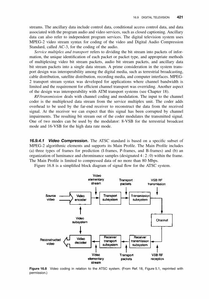
16.9 DIGITAL TELEVISION 421
streams. The ancillary data include control data, conditional access control data, and dataassociated with the program audio and video services, such as closed captioning. Ancillarydata can also refer to independent program services. The digital television system usesMPEG-2 video stream syntax for coding of the video and Digital Audio CompressionStandard, called AC-3, for the coding of the audio.
Service multiplex and transport refers to dividing the bit stream into packets of infor-mation, the unique identification of each packet or packet type, and appropriate methodsof multiplexing video bit stream packets, audio bit stream packets, and ancillary databit stream packets into a single data stream. A prime consideration in the system trans-port design was interoperability among the digital media, such as terrestrial broadcasting,cable distribution, satellite distribution, recording media, and computer interfaces. MPEG-2 transport stream syntax was developed for applications where channel bandwidth islimited and the requirement for efficient channel transport was overriding. Another aspectof the design was interoperability with ATM transport systems (see Chapter 18).
RF/transmission deals with channel coding and modulation. The input to the channelcoder is the multiplexed data stream from the service multiplex unit. The coder addsoverhead to be used by the far-end receiver to reconstruct the data from the receivedsignal. At the receiver we can expect that this signal has been corrupted by channelimpairments. The resulting bit stream out of the coder modulates the transmitted signal.One of two modes can be used by the modulator: 8-VSB for the terrestrial broadcastmode and 16-VSB for the high data rate mode.
16.9.4.1 Video Compression. The ATSC standard is based on a specific subset ofMPEG-2 algorithmic elements and supports its Main Profile. The Main Profile includes(a) three types of frames for prediction (I-frames, P-frames, and B-frames) and (b) anorganization of luminance and chrominance samples (designated 4 : 2 : 0) within the frame.The Main Profile is limited to compressed data of no more than 80 Mbps.
Figure 16.8 is a simplified block diagram of signal flow for the ATSC system.
Figure 16.8 Video coding in relation to the ATSC system. (From Ref. 18, Figure 5.1, reprinted withpermission.)

422 TELEVISION TRANSMISSION
Table 16.4 ATSC Compression Formats
Vertical Lines Pixels Aspect Ratio Picture Rate
1080 1920 16:9 60I, 30P, 24P720 1280 16:9 60P, 30P, 24P480 704 16:9 and 4:3 60P, 60I, 30P, 24P480 640 4:3 60P, 60I, 30P, 24P
Source: Ref. 18, Table 5.1. (Reprinted with permission.)
Video preprocessing converts the analog input signals to digital samples in such aform needed for later compression. The analog input signals are red (R), green (G), andblue (B).
Table 16.4 lists the compression formats covered by the ATSC standard. The followingexplains some of the items in the table. Vertical lines refers to the number of active linesin the picture. Pixels are the number of pixels during the active line. Aspect ratio, ofcourse, refers to the picture aspect ratio. Picture rate gives the number of frames orfields per second. Regarding picture rate values, P refers to progressive scanning and Irefers to interlaced scanning. It should be noted that both the 60.00-Hz and 59.95 (i.e.,60 × 1000/1001)-Hz picture rates are allowed. Dual rates are permitted at 30 Hz and24 Hz.
Sampling Rates. Three active line formats are considered: 1080, 720, and 483. Table 16.5summarizes the sampling rates.
For the 480-line format, there may be 704 or 640 pixels in an active line. If the inputis based on ITU-R Rec. BT 601-4 (Ref. 19), it will have 483 active lines with 720 pixelsin each active line. Only 480 of the 483 active lines are used for encoding. Only 704of the 720 pixels are used for encoding: the first eight and the last eight are dropped.The 480-line, 640-pixel format corresponds only to the IBM VGA graphics format andmay be used with ITU-R Rec. BT 601-4 (Ref. 19) sources by employing appropriateresampling techniques.
Sampling precision is based on the 8-bit sample.Colorimetry means the combination of color primaries, transfer characteristics, and
matrix coefficients. The standard accepts colorimetry that conforms to SMPTE.9 Videoinputs corresponding to ITU-R Rec. BT 601-4 may have SMPTE 274 M or 170 M col-orimetry.
The input video consists of the RGB components that are matrixed into luminance(Y) and chrominance (Cb and Cr) components using a linear transformation by meansof a 3 × 3 matrix. Of course, the luminance carries picture intensity information (black-and-white) and the chrominance components contain the color. There is a high degree ofcorrelation of the original RGB components, whereas the resulting Y, Cb, and Cr haveless correlation and can be coded efficiently.
Table 16.5 Sampling Rate Summary
Line FormatTotal Linesper Frame
Total Samplesper Line
SamplingFrequency Frame Rate
1080 line 1125 2200 74.25 MHz 30.00 fpsa
720 line 750 1650 74.25 MHz 60.00 fps480 line (704 pixels) 525 858 13.5 MHz 59.94-Hz field rate
afps stands for frames per second.
9SMPTE stands for Society of Motion Picture and Television Engineers.

16.10 CONFERENCE TELEVISION 423
In the coding process, advantage is taken of the differences in the ways humans perceiveluminance and chrominance. The human visual system is less sensitive to the high fre-quencies in the chrominance components than to the high frequencies in the luminancecomponent. To exploit these characteristics the chrominance components are low-pass fil-tered and subsampled by a factor of 2 along with the horizontal and vertical dimensions,thus producing chrominance components that are one-fourth the spatial resolution of theluminance components.
16.10 CONFERENCE TELEVISION
16.10.1 Introduction
Video conferencing (conference television) systems have seen phenomenal growth since1990. Many of the world’s corporations have branches and subsidiaries that are widelydispersed. Rather than pay travel expenses to send executives to periodic meetings at onecentral location, video conferencing is used, saving money on the travel budget.
The video and telecommunications technology has matured in the intervening periodto make video conferencing cost effective. Among these developments we include:
ž Video compression techniquesž Eroding cost of digital processingž Arrival of the all-digital network
Proprietary video conferencing systems normally use lower line rates than conventionalbroadcast TV. Whereas conventional broadcast TV systems have line rates at 525/480 lines(NTSC countries) or 625/580 for PAL/SECAM countries, proprietary video conferencingsystems use either 256/240 or 352/288 lines. For the common applications of confer-ence television (e.g., meetings and demonstrations), the reduced resolution is basicallyunnoticeable.
One of the compression schemes widely used for video conference systems is basedon ITU-T Rec. H.261 (Ref. 20), entitled Video Codec for Audiovisual Services at pX64kbps, which is described in the following.
16.10.2 The pX64 kbps Codec
The pX64 codec has been designed for use with some of the common ISDN data rates,specifically the B channel (64 kbps), H0 channel (384 kbps), and H11/H12 channels(1.536/1.920 Mbps) for the equivalent DS1/E1 data rates. A functional block diagramof the codec (coder/decoder) is shown in Figure 16.9. However, the pX64 system uses astandard line rate (i.e., 525/625 lines) rather than the reduced line rate structure mentionedearlier. The reduced line rate techniques are employed in proprietary systems producedby such firms as Compression Labs Inc and Picture Tel.
One of the most popular data rates for conference television is 384 kbps, which is sixDS0 or E0 channels. However, it is not unusual to find numerous systems operating at64/56 kbps.
16.10.2.1 pX64 Compression OverviewSampling Frequency. Pictures are sampled at an integer multiple of the video line rate.
A sampling clock and network clock are asynchronous.

424 TELEVISION TRANSMISSION
Figure 16.9 Functional block diagram of the px64 video codec. [From Figure 1/H.261, ITU-T Rec. H.261(Ref. 20).]
Source Coding Algorithm. Compression is based on interpicture prediction to utilizetemporal redundancy, and transform coding of the remaining signal to reduce spatialredundancy. The decoder has motion compensation capability, allowing optional incorpo-ration of this technique in the coder. There is optional forward error correction10 availablebased on the BCH (511,493) code. The codec can support multipoint operation.
16.10.2.2 Source Coder. The coder operates on non-interleaved pictures occurring30,000/1001 (approximately 29.97) times per second. The tolerance on the picture fre-quency is ±50 ppm.
As in Section 16.9.4, pictures are coded as one luminance and two color differencecomponents (Y, Cb, and Cr). Reference should be made to CCIR Rec. 601 (Ref. 23) fortheir components and codes representing their sampled values. For example:
Black = 16
White = 235
Zero color difference = 128
Peak color difference = 16 and 240
The values given are nominal values and the coding algorithm functions with inputvalues of 1 through 254. Two picture scanning formats have been specified.
For the first format (CIF), the luminance structure is 352 pels per line, 288 linesper picture in an orthogonal arrangement. The color-difference components are sampledat 176 pels per line, 144 lines per picture, orthogonal. Figure 16.10 shows the color-difference samples being sited such that the block boundaries coincide with luminanceblock boundaries. The picture area covered by these numbers of pels and lines has anaspect ratio of 4:3 and corresponds to the active portion of the local standard video input.
It should be noted that the number of pels per line is compatible with sampling theactive portions of the luminance and color-difference signals from 525- or 625-line sources
10FEC coding. Consult Ref. 21 for a discussion of FEC.
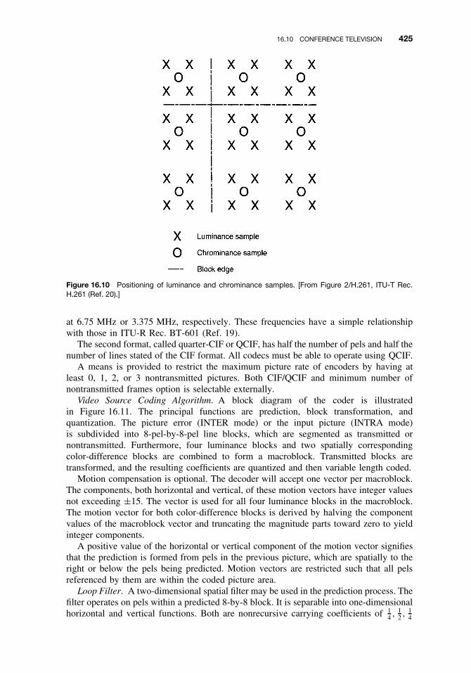
16.10 CONFERENCE TELEVISION 425
Figure 16.10 Positioning of luminance and chrominance samples. [From Figure 2/H.261, ITU-T Rec.H.261 (Ref. 20).]
at 6.75 MHz or 3.375 MHz, respectively. These frequencies have a simple relationshipwith those in ITU-R Rec. BT-601 (Ref. 19).
The second format, called quarter-CIF or QCIF, has half the number of pels and half thenumber of lines stated of the CIF format. All codecs must be able to operate using QCIF.
A means is provided to restrict the maximum picture rate of encoders by having atleast 0, 1, 2, or 3 nontransmitted pictures. Both CIF/QCIF and minimum number ofnontransmitted frames option is selectable externally.
Video Source Coding Algorithm. A block diagram of the coder is illustratedin Figure 16.11. The principal functions are prediction, block transformation, andquantization. The picture error (INTER mode) or the input picture (INTRA mode)is subdivided into 8-pel-by-8-pel line blocks, which are segmented as transmitted ornontransmitted. Furthermore, four luminance blocks and two spatially correspondingcolor-difference blocks are combined to form a macroblock. Transmitted blocks aretransformed, and the resulting coefficients are quantized and then variable length coded.
Motion compensation is optional. The decoder will accept one vector per macroblock.The components, both horizontal and vertical, of these motion vectors have integer valuesnot exceeding ±15. The vector is used for all four luminance blocks in the macroblock.The motion vector for both color-difference blocks is derived by halving the componentvalues of the macroblock vector and truncating the magnitude parts toward zero to yieldinteger components.
A positive value of the horizontal or vertical component of the motion vector signifiesthat the prediction is formed from pels in the previous picture, which are spatially to theright or below the pels being predicted. Motion vectors are restricted such that all pelsreferenced by them are within the coded picture area.
Loop Filter. A two-dimensional spatial filter may be used in the prediction process. Thefilter operates on pels within a predicted 8-by-8 block. It is separable into one-dimensionalhorizontal and vertical functions. Both are nonrecursive carrying coefficients of 1
4 , 12 , 1
4
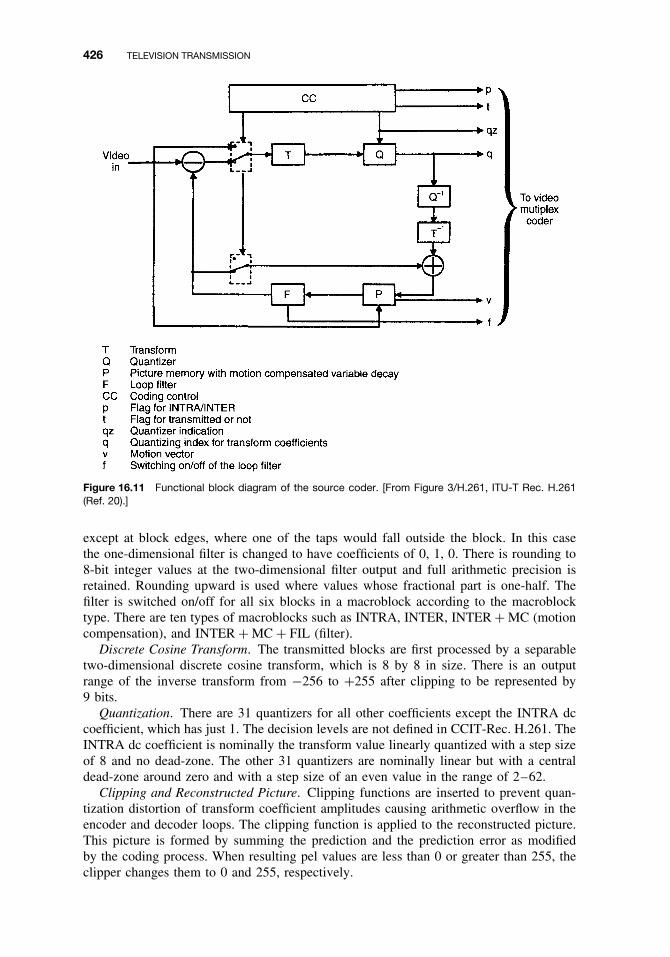
426 TELEVISION TRANSMISSION
Figure 16.11 Functional block diagram of the source coder. [From Figure 3/H.261, ITU-T Rec. H.261(Ref. 20).]
except at block edges, where one of the taps would fall outside the block. In this casethe one-dimensional filter is changed to have coefficients of 0, 1, 0. There is rounding to8-bit integer values at the two-dimensional filter output and full arithmetic precision isretained. Rounding upward is used where values whose fractional part is one-half. Thefilter is switched on/off for all six blocks in a macroblock according to the macroblocktype. There are ten types of macroblocks such as INTRA, INTER, INTER + MC (motioncompensation), and INTER + MC + FIL (filter).
Discrete Cosine Transform. The transmitted blocks are first processed by a separabletwo-dimensional discrete cosine transform, which is 8 by 8 in size. There is an outputrange of the inverse transform from −256 to +255 after clipping to be represented by9 bits.
Quantization. There are 31 quantizers for all other coefficients except the INTRA dccoefficient, which has just 1. The decision levels are not defined in CCIT-Rec. H.261. TheINTRA dc coefficient is nominally the transform value linearly quantized with a step sizeof 8 and no dead-zone. The other 31 quantizers are nominally linear but with a centraldead-zone around zero and with a step size of an even value in the range of 2–62.
Clipping and Reconstructed Picture. Clipping functions are inserted to prevent quan-tization distortion of transform coefficient amplitudes causing arithmetic overflow in theencoder and decoder loops. The clipping function is applied to the reconstructed picture.This picture is formed by summing the prediction and the prediction error as modifiedby the coding process. When resulting pel values are less than 0 or greater than 255, theclipper changes them to 0 and 255, respectively.

16.11 BRIEF OVERVIEW OF FRAME TRANSPORT FOR VIDEO CONFERENCING 427
Coding Control. To control the rate of generation of coded video data, several para-meters may be varied. These parameters include processing prior to source coder, thequantizer, block significance criterion, and temporal subsampling. When invoked, tempo-ral subsampling is performed by discarding complete pictures.
Forced Updating. Forced updating is achieved by forcing the use of the INTRA modeof the coding algorithm. Recommendation H.261 does not define the update pattern. Forthe control of accumulation of inverse transform mismatch error, a macroblock should beupdated forcibly at least once per every 132 times it is transmitted.
16.10.2.3 Video Multiplex Coder. The video multiplex is arranged in a hierarchicalstructure with four layers. From top to bottom these layers are:
ž Picturež Group of blocks (GOB)ž Macroblockž Block
For further description of these layers, consult CCITT Rec. H.261 (Ref. 20).
16.11 BRIEF OVERVIEW OF FRAME TRANSPORT FOR VIDEOCONFERENCING
This section briefly reviews one method of transporting on the PSTN digital network thevideo conferencing signals developed in Section 16.10. It is based on ITU-T Rec. H.221(Ref. 22).
16.11.1 Basic Principle
An overall transmission channel of 64–1920 kbps is dynamically subdivided into lowerrates suitable for transport of audio, video, and data for telematic purposes. The trans-mission channel is derived by synchronizing and ordering transmission over from oneto six B-channels,11 from one to five H0 channels or an H11 or H12 channel. The initialconnection is the first connection established, and it carries the initial channel in eachdirection. The additional connections carry the necessary additional channels. The totalrate of transmitted information is called the transfer rate. The transfer rate can be lessthan the capacity of the overall transmission channel.
A single 64-kbps channel is structured into octets transmitted at an 8-kHz rate.12 Eachbit position of the octets may be regarded as a subchannel of 8 kbps. A frame reflectingthis concept is illustrated in Figure 16.12. The service channel (SC) resides in the eighthsubchannel. It carries the frame alignment signal (FAS), a bit-rate allocation signal (BAS),and an encryption control signal (ECS).
We can regard an H0, H11, H12 channel as consisting of a number of 64-kbps timeslots (TS). The lowest numbered time slot is structured exactly as described above for a64-kbps channel, whereas the other time slots have no such structure. All channels havea frame structure in the case of multiple B and H0 channels; the initial channel controls
11Note the use of ISDN terminology for channel types (e.g., B-channels). Turn back to Section 12.4.2.1 for adescription of ISDN user channels.12This is the standard Nyquist sampling rate discussed in Chapter 6.

428 TELEVISION TRANSMISSION
Figure 16.12 Frame structure for a 64-kbps channel (i.e., a B-channel). [From Figure 1/H.221, ITU-TRec. H.221 (Ref. 22).]
most functions across the overall transmission, while the frame structure in the additionalchannels is used for synchronization, channel numbering, and related controls. The termI-channel is applied to the initial or only B-channel, to time slot one of the initial or onlyH0 channels, and to TS1 on H11 and H12 channels.
REVIEW EXERCISES
1. What four factors must be dealt with by a color video transmission system trans-mitting images of moving objects?
2. Describe scanning, horizontally and vertically.
3. Define a pel or pixel (besides the translation of the acronym).
4. If the aspect ratio of a television system is 4:3 and the width of a television screenis 12 inches, what is its height?
5. NTSC divides a television image into how many horizontal lines? European systems?
6. How do we achieve a sensation of motion in TV? Relate this to frame rate and flicker.
7. In North American practice, the time to scan a line is 63.5 µsec. This time intervalconsists of two segments: what are they?
8. What is the standard maximum voltage excursion of a video signal? Just what arewe measuring here?
9. Give two definitions of a composite signal.
10. At a TV receiver, about what S/N is required for an excellent picture?

REFERENCES 429
11. If we were to measure S/N, we would measure S and we would measure N. Incommon TV practice, what measurement units are used?
12. What type of modulation is used to transmit the video; the audio, the color subcarrier?
13. On a TV transport system, end-to-end S/N is often specified at 54 dB. Then why isthe TV receiver specified at 45 dB? Explain the difference.
14. Regarding TV transport, what is a program channel?
15. To digitize a TV signal, what type of generic coding is nearly always used?
16. To digitize a TV signal by PCM, calculate the sampling rate for at least two systems.
17. Give the three basic bit rate reduction techniques suggested by CCIR.
18. Give three ways of reducing the number of bits per sample.
19. Discuss intraframe coding regarding redundancy.
20. What is the voltage value of 0 dBmV? When using dBmV, we should state anotherparameter as well, which we do not have to do when using dBs in the power domain.
21. How does differential PCM bring about bit rate reduction?
22. What are the two broadcast-quality bit rates that can be derived from the ATSC(MPEG-2) coding system?
23. What is one popular bit rate for conference television? Another?
REFERENCES
1. IEEE 100 The Authorative Dictionary of IEEE Standards Terms, 7th ed., IEEE, New York,2004.
2. Fundamentals of Television Transmission, Bell System Practices, Section AB 96.100, AmericanTelephone & Telegraph Co., New York, 1954.
3. Television Systems Descriptive Information—General Television Signal Analysis, Bell SystemPractices, Section 318-015-100, No. 3, American Telephone & Telegraph Co., New York, 1963.
4. A. F. Inglis and A. C. Luther, Video Engineering, 2nd ed., McGraw-Hill, New York, 1996.
5. K. Simons, Technical Handbook for CATV Systems, 3rd ed., General Instrument–Jerrold Elec-tronics Corp., Hatboro, PA, 1980.
6. Electrical Performance for Television Transmission Systems , ANSI/EIA/TIA-250C, EIA/TIA,Washington, DC, 1990.
7. Television Systems , ITU-R Rec. BT.470-3, 1994 BT Series, ITU Geneva, 1994.
8. Reference Data for Engineers: Radio, Electronics, Computer & Communications, 8th ed,Sams–Prentice-Hall, Carmel, IN, 1993.
9. The Preferred Characteristics of a Single Sound Channel Transmitted with a Television Signalon an Analogue Radio-Relay System , CCIR Rec. 402-2, Part 1, Vol. IX, ITU Geneva, 1990.
10. The Preferred Characteristics of Simultaneous Transmission of Television and a Maximum ofFour Sound Channels on Analogue Radio-Relay Systems , CCIR Rep. 289-4, Part 1, Vol. IX,CCIR Dubrovnik, 1986.
11. Pre-emphasis Characteristics for Frequency Modulation Radio-Relay Systems for Television ,CCIR Rec. 405-1, Vol. IX, Part 1, ITU Geneva, 1990.
12. Transmission Performance of Television Circuits Designed for Use in International Connections ,CCIR Rec. 567-3, Vol. XII, ITU Geneva, 1990.
430 TELEVISION TRANSMISSION
13. Transmission Performance of Television Circuits over Systems in the Fixed Satellite Service,CCIR Rep. 965-1, Annex to Vol. XII, ITU Geneva, 1990.
14. Digital or Mixed Analogue-and-Digital Transmission of Television Signals , CCIR Rep. 646-4,Annex to Vol. XII, ITU Geneva, 1990.
15. Digital Transmission of Component-Coded Television Signals at 30–34 Mbps and 45 Mbps ,CCIR Rep. 1235, Annex to Vol. XII, ITU Geneva, 1990.
16. A Compilation of Advanced Television Systems Committee Standards, Advanced Television Sys-tems Committee (ATSC), Washington, DC, 1996.
17. ATSC Digital Television Standard, Doc. A/53, ATSC, Washington, DC, 1995.
18. Guide to the Use of the ATSC Digital Transmission Standard, Doc. A/54, ATSC, Washington,DC, 1995.
19. Encoding Parameters of Digital Television for Studios, ITU-R Rec. BT.601-4, 1994 BT SeriesVolume, ITU Geneva, 1994.
20. Video Codec for Audiovisual Services at px64 kbps, CCITT Rec. H.261, ITU Geneva, 1990.
21. R. L. Freeman, Radio System Design for Telecommunications, 2nd ed., Wiley, New York, 1997.
22. Frame Structure of a 64 to 1920 kbps Channel in Audiovisual Teleservices, ITU-T Rec. H.221,ITU Geneva, 1993.
23. R. L. Freeman, Telecommunication Transmission Handbook, 4th ed, Wiley, New York, 1998.

17
COMMUNITY ANTENNA TELEVISION(CABLE TELEVISION)
17.1 OBJECTIVE AND SCOPE
The principal thrust of community antenna television (CATV) is entertainment. However,since the early 1990s CATV has taken on some new dimensions. It is a broadband medium,providing up to nearly 1 GHz of bandwidth at customer premises. It was originally aunidirectional system, from the point of origin, which we will call the headend, towardcustomer premises, providing from 20 to some 100 television channels.
A CATV headend inserts signals into its transmission system for delivery to residencesand offices (see Figure 17.1) from off-the-air local stations, satellite, LOS microwave,and locally generated programs. In older configurations, transmission systems consisted ofcoaxial cable with wideband amplifiers spaced at uniform distances. Current configurationsconsist of a headend feeding fiber-optic trunks up to hubs which convert the signal formatto traditional coaxial cable for the last mile or last 100 feet.
Figure 17.1 An early CATV system. The transmission line from the headend to subscribers is coaxialcable. The microwave extended the ‘‘reach’’ of the system to distant TV emitters.
Fundamentals of Telecommunications, Second Edition, by Roger L. FreemanISBN 0-471-71045-8 Copyright 2005 by Roger L. Freeman
431

432 COMMUNITY ANTENNA TELEVISION (CABLE TELEVISION)
CATV does have the capability of being a two-way system and many CATV opera-tors are implementing such capability. The CATV band is actually the radio frequencyband topping off at about 1000 MHz (see Figure 2.6, Chapter 2, from about 1,000,000downwards in the figure). In this case the radio signals (e.g., the TV channels) are trans-ported in a coaxial cable medium. What a CATV operator might do is to use the bandfrom 50 MHz to 1 GHz for transmission outwards from the headend for TV channelsand “other services” and the band from about 5 MHz to 50 MHz to be employed fromthe user back to the headend. This band will transport the other services in a full duplexmode. These other services include POTS (plain old telephone service) and data.
In this chapter, we will describe conventional CATV, and the concept of supertrunksincluding HFC (hybrid fiber-coax) systems. We will involve the reader with widebandamplifiers in tandem, and the special impairments that we would expect to encounterin a CATV system. System layout, hubs, and last-mile or last 100-ft considerations willalso be covered. There will also be a brief discussion of the conversion to a digitalsystem using some of the compression concepts covered in Chapter 16. Employing thesecompression techniques, we can expect to see cable television systems delivering up to500 TV channels to customers.
17.2 THE EVOLUTION OF CATV
17.2.1 The Beginnings
Broadcast television, as we know it, was in its infancy around 1948. Fringe area problemswere much more acute in that period. By fringe area, we mean areas with poor or scantysignal coverage. A few TV users in fringe areas found that if they raised their antennashigh enough and improved antenna gain characteristics, an excellent picture could bereceived. These users were the envy of the neighborhood. Several of these people whowere familiar with RF signal transmission employed signal splitters so that their neighborscould share the excellent picture service. This concept is illustrated in Figure 17.2.
Soon it was found that there is a limit to how much signal splitting could be donebefore signal levels got so low that they became snowy or unusable. Remember that eachtime a signal splitter is added (i.e., a 50% split), neglecting insertion losses, the TV signal
Figure 17.2 CATV initial concept.

17.2 THE EVOLUTION OF CATV 433
drops 3 dB. Then someone got the bright idea of amplifying the signal before splitting.Now some real problems arose. One-channel amplifiers worked fine, but two channelsfrom two antennas with signal combining became difficult. We have begun to enter theworld of broadband amplifiers. Among the impairments we can expect from broadbandamplifiers and their connected transmission lines (coaxial cable) are the following:
ž Poor frequency response. Some part of the received band had notably lower levelsthan other parts. This is particularly true as the frequency increases. In other words,there was fairly severe amplitude distortion. Thus equalization became necessary.
ž The mixing of two or more RF signals in the system caused intermodulation productsand “beats” (harmonics), which degraded reception.
ž When these TV signals carried modulation, cross-modulation (Xm) productsdegraded or impaired reception.
Several small companies were formed to sell these “improved” television receptionservices. Some of the technicians working for these companies undertook ways of curingthe ills of broadband amplifiers.
These were coaxial cable systems, where a headend with a high tower received signalsfrom several local television broadcasting stations, amplified the broadband signals, anddistributed the results to CATV subscribers. A subscriber’s TV set was connected to thedistribution system, and the signal received looked just the same as if it were taken offthe air with its own antenna. In fringe areas, signal quality, however, was much betterthan own-antenna quality. The key to everything was that no changes were required inthe user’s TV set. It was just an extension of her/his TV set antenna. This simple conceptis illustrated in Figure 17.2.
Note in Figure 17.2 that home A is in the shadow of a mountain ridge and receivesa weakened diffracted signal off the ridge and a reflected signal off the lake. Here is thetypical multipath scenario resulting in ghosts in A’s TV screen. The picture is also snowy,meaning noisy, as a result of poor carrier-to-noise ratio. Home B extended the antennaheight to be in line-of-sight of the TV transmitting antenna. Its antenna is of higher gain;thus it is more discriminating against unwanted reflected and diffracted signals. Home Bhas an excellent picture without ghosts. Home B shares its fine signal with home A byuse of a 3-dB power split (P) and a length of coaxial cable.
17.2.2 Early System Layouts
In Figure 17.1 we showed an early CATV distribution system (ca. 1968). Taps and cou-plers (power splits) are not shown.1 These systems provided from 5 to 12 TV channels. AnLOS microwave system might bring in channels from distant cities. We had direct expe-rience with an Atlantic City, NJ, system where channels were brought in by microwavefrom Philadelphia and New York City. A 12-channel system was derived and occupiedthe entire assigned VHF band (i.e., channels 2–13).
As UHF TV stations began to appear, a new problem arose for the CATV operator. Itwas incumbent on that operator to keep the bandwidth as narrow as possible. One approachwas to convert UHF channels to vacant VHF channel allocations at the headend.1Definitions:Tap. A device for extracting a portion of the CATV signal from the cable.Coupler. A device used to combine signals or divide signals.Power Split or Power Splitter. A device used to divide a signal between or among paths and not necessarilyequally.

434 COMMUNITY ANTENNA TELEVISION (CABLE TELEVISION)
Satellite reception at the headend doubled or tripled the number of channels that couldbe available to the CATV subscriber. Each satellite has the potential of adding 24 channelsto the system. Note how the usable cable bandwidth is “broadened” as channels are added.We assume contiguous channels across the band, starting at 55 MHz. For 30 channels, wehave 55–270 MHz; for 35 channels, 55–300 MHz; for 40 channels, 55–330 MHz; for 62channels, 55–450 MHz; and for 78 channels, 55–550 MHz. These numbers of channelswere beyond the capability of many TV sets of the day. Set-top converters were providedthat converted all channels to a common channel, an unoccupied channel, usually channel2, 3, or 4, to which the home TV set is tuned. This approach is still very prevalent today.
In the next section we discuss CATV transmission impairments and measures of systemperformance. In Section 17.4, hybrid-coaxial cable/fiber-optic systems are addressed. Thefiber replaced coaxial cable trunks, which made a major stride toward better performance,greater system extension, and improved reliability/availability.
17.3 SYSTEM IMPAIRMENTS AND PERFORMANCE MEASURES
17.3.1 Overview
A CATV headend places multiple TV and FM (from 30 to 125) carriers on a broadbandcoaxial cable trunk and distribution system. The objective is to deliver a signal-to-noiseratio (S/N) of 42–45 dB at a subscriber’s TV set. From previous chapters we wouldexpect such impairments as the accumulation of thermal and intermodulation noise. Wefind that CATV technicians use the term beat to mean intermodulation (IM) products.For example, there is triple beat distortion, defined by Grant (Ref. 1) as “spurious signalsgenerated when three or more carriers are passed through a nonlinear circuit (such asa wideband amplifier).” The spurious signals are sum and difference products of anythree carriers, sometimes referred to as “beats.” Triple-beat distortion is calculated as avoltage addition.
The wider the system bandwidth is and the more RF carriers transported on that system,the more intermodulation distortion, “triple beats,” and cross-modulation we can expect.We can also assume combinations of all of the above, such as composite triple beat (CTB),which represents the pile up of beats at or near a single frequency.
Grant (Ref. 1) draws a dividing line at 21 TV channels. On a system with 21 chan-nels or fewer, one must expect Xm to predominate. Above 21 channels, CTB willpredominate.
17.3.2 dBmV and Its Applications
We define 0 dBmV as 1 mV across 75 � impedance. Note that 75 � is the standardimpedance of CATV, coaxial cable, and TV sets. From Appendix A, the electrical powerlaw, we have
Pw = E2/R, (17.1)
where Pw is the power in watts, E the voltage in volts, and R the impedance, 75 �.Substituting the values from above, we obtain
Pw = (0.001)2/75
0 dBmV = 0.0133 × 10⁻⁶ W or 0.0133 µW
By definition, then, 0.0133 W = +60 dBmVIf 0 dBmV = 0.0133 × 10⁻⁶ W and0 dBm = 0.001 W, andgain indB = 10 log(P1/P2),
or, in this case, 10 log[0.001/(0.0133 × 10−6)], then 0 dBm = +48.76 dBmV.

17.3 SYSTEM IMPAIRMENTS AND PERFORMANCE MEASURES 435
Remember that, when working with dB in the voltage domain, we are working withthe E2/R relationship, where R = 75 �. With this in mind the definition of dBmV is
dBmV = 20 log
(voltage in mV
1 mV
). (17.2)
If a signal level is 1 V at a certain point in a circuit, what is the level in dBmV?
dBmV = 20 log(1000/1) = +60 dBmV.
If we are given a signal level of +6 dBmV, to what voltage level does this correspond?
+6 dBmV = 20 log(XmV/1 mV).
Divide through by 20:
6/20 = log(XmV/1 mV)
antilog(6/20) = XmV
XmV = 1.995 mV, or 2 mV, or 0.002 V
These signal voltages are rms (root mean square) volts. For peak voltage, divide by 0.707.If you are given peak signal voltage and wish the rms value, multiply by 0.707.
17.3.3 Thermal Noise in CATV Systems
We remember from Section 3.3.3 that thermal noise is the most common type of noiseencountered in telecommunication systems. In most cases, it is thermal noise that sets thesensitivity of a system, its lowest operating threshold. In the case of a CATV system, thelowest noise levels permissible are set by the thermal noise level—at the antenna outputterminals, at repeater (amplifier) inputs, or at a subscriber’s TV set—without producingsnowy pictures.
Consider the following, remembering we are in the voltage domain. Any resistor orsource that looks resistive over the band of interest, including antennas, amplifiers, andlong runs of coaxial cable, generates thermal noise. In the case of a resistor, the thermalnoise level can be calculated based on Figure 17.3.
To calculate the noise voltage, en, use the following formula:
en = (4RBk)1/2, (17.3)
where en = rms noise voltage,R = resistance in ohms (�),B = bandwidth (Hz) of the measuring device (electronic voltmeter, V), andk = a constant equal to 40 × 10−16 at standard room temperature.2
Figure 17.3 Resistor model for thermal noise voltage, en.
2This value can be derived from Boltzmann’s constant (Chapter 3) at room temperature (68◦F or 290 K) isassumed.

436 COMMUNITY ANTENNA TELEVISION (CABLE TELEVISION)
Figure 17.4 Minimum noise model.
Let the bandwidth, B, of an NTSC TV signal be rounded to 4 MHz. The open circuitnoise voltage for a 75-� resistor is
en = (4 × 75 × 4 × 10−16)1/2
= 2.2 µV rms.
Figure 17.4 shows a 2.2-µV noise generating source (resistor) connected to a 75-�(noiseless) load. Only half of the voltage (1.1 µV) is delivered to the load. Thus thenoise input to 75 � is 1.1 µV or −59 dBmV. This is the basic noise level, the minimumthat will exist in any part of a 75-� CATV system. The value −59 dBmV will be usedrepeatedly below (Ref. 3).
The noise figure of a typical CATV amplifier ranges between 7 and 9 dB (Ref. 3).
17.3.4 Signal-to-Noise Ratio (S/N) Versus Carrier-to-Noise Ratio (C/N)in CATV Systems
We have been using S/N and C/N many times in previous chapters. In CATV systemsS/N has a slightly different definition as follows (Ref. 2):
This relationship is expressed by the “signal-to-noise ratio,” which is the difference betweenthe signal level measured in dBmV, and the noise level, also measured in dBmV, both levelsbeing measured at the same point in the system.
S/N can be related to C/N on CATV systems as
C/N = S/N + 4.1 dB (17.4)
This is based on Carson (Ref. 4), where the premise is “noise just perceptible” by apopulation of TV viewers, with an NTSC 4.2-MHz TV signal. Adding noise weighting3
improvement (6.8 dB), we find
S/N = C/N + 2.7 dB. (17.5)
It should be noted that S/N is measured where the signal level is peak-to-peak4 and thenoise level is rms. For C/N measurement, both the carrier and the noise levels are rms.
3Weighting (IEEE). The artificial adjustment of measurements in order to account for factors that in normaluse of the device would otherwise be different from the conditions during measurement. In the case of TV,the lower baseband frequencies (i.e., from 20 Hz to 15 kHz) are much more sensitive to noise than the higherfrequencies (i.e., >15 kHz).4Peak-to-peak voltage refers, in this case, to the measurement of voltage over its maximum excursion, whichis the voltage of the “sync tips.” See Figures 16.3 and 16.4.
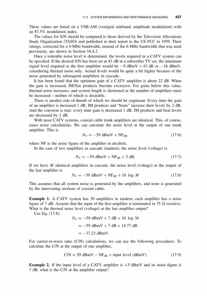
17.3 SYSTEM IMPAIRMENTS AND PERFORMANCE MEASURES 437
These values are based on a VSB-AM (vestigial sideband, amplitude modulation) withan 87.5% modulation index.
The values for S/N should be compared to those derived by the Television AllocationsStudy Organization (TASO) and published in their report to the US FCC in 1959. Theirratings, corrected for a 4-MHz bandwidth, instead of the 6-MHz bandwidth that was usedpreviously, are shown in Section 16.4.2.
Once a tolerable noise level is determined, the levels required in a CATV system canbe specified. If the desired S/N has been set at 43 dB at a subscriber TV set, the minimumsignal level required at the first amplifier would be −9 dBmV + 43 dB or −16 dBmV,considering thermal noise only. Actual levels would be quite a bit higher because of thenoise generated by subsequent amplifiers in cascade.
It has been found that the optimum gain of a CATV amplifier is about 22 dB. Whenthe gain is increased, IM/Xm products become excessive. For gains below this value,thermal noise increases, and system length is shortened or the number of amplifiers mustbe increased—neither of which is desirable.
There is another rule-of-thumb of which we should be cognizant. Every time the gainof an amplifier is increased 1 dB, IM products and “beats” increase their levels by 2 dB.And the converse is true: every time gain is decreased 1 dB, IM products and beat levelsare decreased by 2 dB.
With most CATV systems, coaxial cable trunk amplifiers are identical. This, of course,eases noise calculations. We can calculate the noise level at the output of one trunkamplifier. This is
NV = −59 dBmV + NFdB, (17.6)
where NF is the noise figure of the amplifier in decibels.In the case of two amplifiers in cascade (tandem), the noise level (voltage) is
NV = −59 dBmV + NFdB + 3 dB. (17.7)
If we have M identical amplifiers in cascade, the noise level (voltage) at the output ofthe last amplifier is
NV = −59 dBmV + NFdB + 10 log M (17.8)
This assumes that all system noise is generated by the amplifiers, and none is generatedby the intervening sections of coaxial cable.
Example 1. A CATV system has 30 amplifiers in tandem; each amplifier has a noisefigure of 7 dB. Assume that the input of the first amplifier is terminated in 75 � resistive.What is the thermal noise level (voltage) at the last amplifier output?
Use Eq. (17.8):NV = −59 dBmV + 7 dB + 10 log 30
= −59 dBmV + 7 dB + 14.77 dB
= −37.23 dBmV.
For carrier-to-noise ratio (C/N) calculations, we can use the following procedures. Tocalculate the C/N at the output of one amplifier,
C/N = 59 dBmV − NFdB + input level (dBmV) (17.9)
Example 2. If the input level of a CATV amplifier is +5 dBmV and its noise figure is7 dB, what is the C/N at the amplifier output?

438 COMMUNITY ANTENNA TELEVISION (CABLE TELEVISION)
Use Eq. (17.9):C/N = 59 dBmV − 7 dB + 5 dBmV
= 57 dB.
With N cascaded amplifiers, we can calculate the C/N at the output of the last amplifier,assuming all the amplifiers are identical, by the following equation:
C/NL = C/N (single amplifier) − 10 log N. (17.10)
Example 3. Determine the C/N at the output of the last amplifier with a cascade (intandem) of 20 amplifiers, where the C/N of a single amplifier is 62 dB.
Use Eq. (17.10):C/NL = 62 dB − 10 log 20
= 62 dB − 13.0 dB
= 49 dB.
17.3.5 The Problem of Cross-Modulation (Xm)
Many specifications for TV picture quality are based on the judgment of a populationof viewers. One example was the TASO ratings for picture quality given earlier. In thecase of cross-modulation (cross-mod or Xm) and CTB (composite triple beat), acceptablelevels are −51 dB for Xm and −52 dB for CTB. These are good guideline values (Ref. 1).
Xm is a form of third-order distortion so typical of a broadband, multicarrier system.It varies with the operating level of an amplifier in question and the number of TVchannels being transported. Xm is derived from the amplifier manufacturer specifications.The manufacturer will specify a value for Xm (in dB) for several numbers of channelsand for a particular level. The level in the specification may not be the operating level ofa particular system. To calculate Xm for an amplifier to be used in a given system, usingmanufacturer’s specifications, the following formula applies:
Xma = Xmspec + 2(OLoper − OLspec), (17.11)
where Xma = Xm for the amplifier in question,Xmspec = Xm specified by the manufacturer of the amplifier,OLoper = desired operating output signal level (dBmV), andOLspec = manufacturer’s specified output signal level.
We spot the “2” multiplying factor and relate it to our earlier comments, namely, whenwe increase the operating level 1 dB, third-order products increase 2 dB, and the contraryapplies for reducing signal level. As we said, Xm is a form of third-order product.
Example 1. Suppose a manufacturer tells us that for an Xm of −57 dB for a 35-channelsystem, the operating level should be +50.5 dBmV. We want a longer system and use anoperating level of +45 dBmV. What Xm can we expect under these conditions?
Use Eq. (17.11):
Xma = −57 dB + 2(+45 dBmV − 50.5 dBmV)
= −68 dB.

17.3 SYSTEM IMPAIRMENTS AND PERFORMANCE MEASURES 439
CATV trunk systems have numerous identical amplifiers. To calculate Xm for N ampli-fiers in cascade (tandem), our approach is similar to that of thermal noise, namely,
Xmsys = Xma + 20 log N, (17.12)
where N = number of identical amplifiers in cascade,Xma = Xm for one amplifier, and
Xmsys = Xm value at the end of the cascade.
Example 2. A certain CATV trunk system has 23 amplifiers in cascade where Xma is−88 dB. What is Xmsys?
Use Eq. (17.12):Xmsys = −88 dB + 20 log 23
= −88 + 27
= −61 dB.
17.3.6 Gains and Levels for CATV Amplifiers
Setting both gain and level settings for CATV broadband amplifiers is like walking atightrope. If levels are set too low, thermal noise will limit system length (i.e., numberof amplifiers in cascade). If levels are set too high, system length will be limited byexcessive CTB and Xm. On trunk amplifiers available gain is between 22 dB and 26 dB(Ref. 1). Feeder amplifiers will usually operate at higher gains, trunk systems at lowergains. Feeder amplifiers usually operate in the gain range of 26–32 dB with output levelsin the range of +47 dBmV. Trunk amplifiers have gains of 21–23 dB, with output levelsin the range of +32 dBmV. If we wish to extend the length of the trunk plant, we shouldturn to using lower loss cable. Using fiber optics in the trunk plant is even a betteralternative (see Section 17.4).
The gains and levels of feeder systems are purposefully higher. This is the part of thesystem serving customers through taps. These taps are passive and draw power. Runningthe feeder system at higher levels improves tap efficiency. Because feeder amplifiers runat higher gain and with higher levels, the number of these amplifiers in cascade must beseverely limited to meet CTB and cross-modulation requirements at the end-user.
17.3.7 The Underlying Coaxial Cable System
The coaxial cable employed in the CATV plant has a nominal characteristic impedance(Zo) of 75 �. A typical response curve for such cable (7/8-in., air dielectric) is illustratedin Figure 17.5. The frequency response of coaxial cable is called tilt in the CATV industry.This, of course, refers to its exponential increase in loss as frequency increases.
For 0.5-in. cable, the loss per 100 ft at 50 MHz is 0.52 dB; for 550 MHz, 1.85 dB.Such cable systems require equalization. The objective is to have a comparatively “flat”frequency response across the entire system. An equalizer is a network that presentsa mirror image of the frequency response curve, introducing more loss at the lowerfrequencies and less loss at the higher frequencies. These equalizers are often incorporatedwith an amplifier.
Equalizers are usually specified for a certain length of coaxial cable, where length ismeasured in dB at the highest frequency of interest. Grant (Ref. 1) describes a 13-dBequalizer for a 300-MHz system, which is a corrective unit for a length of coaxial cablehaving 13-dB loss at 300 MHz. This would be equivalent to approximately 1000 ft of

440 COMMUNITY ANTENNA TELEVISION (CABLE TELEVISION)
Figure 17.5 Attenuation-frequency response for 7/8-in. coaxial cable, Zo = 75 �, Andrew HJ serieshelix. (Courtesy of Andrew Corp.)
12 -in. coaxial cable. Such a length of cable would have 5.45-dB loss at 54 MHz and 13-dBloss at 300 MHz. The equalizer would probably present a loss of 0.5 dB at 300 MHz and8.1 dB at 54 MHz.
17.3.8 Taps
A tap is similar to a directional coupler. It is a device inserted into a coaxial cable, whichdiverts a predetermined amount of its RF energy to one or more tap outputs for the purposeof feeding a TV signal into subscriber drop cables. The remaining balance of the signalenergy is passed on down the distribution system to the next tap or distribution amplifier.The concept of the tap and its related distribution system is shown in Figure 17.6.
Figure 17.6 A simplified layout of a CATV system showing its basic elements. The objective is to providea +10.5-dBmV signal level at the drops (tap outputs). LEA, line extender amplifier.

17.4 HYBRID FIBER-COAX (HFC) SYSTEMS 441
Taps are available to feed 2, 4, or 8 service drops from any one unit. Many differenttypes of taps are available to serve different signal levels that appear along a CATVcable system. Commonly, taps are available in 3-dB increments. For two-port taps, thefollowing tap losses may be encountered: 4, 8, 11, 14, 17, 20, and 23 dB. The insertionloss for the lower value tap loss may be on the order of 2.8 dB and, once the tap lossexceeds 26 dB, the insertion is 0.4 dB and remains so as tap values increase. Anotherimportant tap parameter is isolation. Generally, the higher the tap loss, the better theisolation. With an 8-dB tap loss, the isolation may only be 23 dB, but with 29-dB taploss (two-port taps), the isolation can be as high as 44 dB. Isolation in this context is theisolation between the two tap ports to minimize undesired interference from a TV set onone tap to the TV set on the other tap.
For example, a line voltage signal level is +34.8 dBmV entering a tap. The tap insertionloss is 0.4 dB so the level of the signal leaving the tap to the next tap or extenderamplifier is +34.4 dBmV. The tap is two-port. We know we want at least a +10.5 dBmVat the port output. Calculate +34.8 dBmV − X dB = +10.5 dBmV. Then X = 24.3 dB,which would be the ideal tap loss value. Taps are not available off-the-shelf at thatloss value, the nearest value being 23 dB. Thus the output at each tap port will be+34.8 dBmV − 23 dB = 11.8 dBmV.
17.4 HYBRID FIBER-COAX (HFC) SYSTEMS
The following advantages accrue by replacing the coaxial cable trunk system with opticalfiber:
ž Reduces the number of amplifiers required per unit distance to reach the furthestsubscriber
ž Results in improved C/N and reduced CTB and Xm levelsž Also results in improved reliability (i.e., by reducing the number of active
components)ž Has the potential to greatly extend a particular CATV serving area
One disadvantage is that a second fiber link has to be installed for the reverse direction,or a form of WDM is required, when two-way operation is required and/or for the CATVmanagement system (used for monitoring the health of the system, amplifier degradation,or failure).
The concept is illustrated in Figure 17.7. Figure 17.8 shows an HFC system wherethere are no more than three amplifiers in tandem to reach any subscriber tap. Also notethat with this system layout there cannot be a catastrophic failure. For the loss of anamplifier, only one-sixteenth of the system is affected in the worst-case scenario; with theloss of a fiber link, the worst case would be one-sixth of the system.
17.4.1 Design of the Fiber-Optic Portion of an HFC System
Before proceeding with this section, it is recommended that the reader turn back toChapter 9 for a review of the principles of fiber-optic transmission.
There are two approaches to fiber-optic transmission of analog CATV signals. Bothapproaches take advantage of the intensity modulation characteristics of the fiber-opticsource. Instead of digital modulation of the source, amplitude modulation (analog) isemployed. The most common method takes the entire CATV spectrum as it would appear

442 COMMUNITY ANTENNA TELEVISION (CABLE TELEVISION)
Figure 17.7 A model showing the concept of hybrid fiber-coaxial cable CATV system. TX, fiber-optictransmitter; RC, fiber-optic receiver.
Figure 17.8 HFC system layout for optimal performance (one-way).
on a coaxial cable and uses that as the modulating signal. The second method also usesanalog amplitude modulation, but the modulating signal is a grouping of subcarriers thatare each frequency modulated. One off-the-shelf system multiplexes in a broad FDMconfiguration, eight television channels, each on a separate subcarrier. Thus a 48-channelCATV system would require six fibers, each with eight subcarriers (plus 8 or 16 audiosubcarriers).
17.4.1.1 Link Budget for an AM System. We will assume a model using a distributedfeedback laser (DFB) with an output of +5 dBm coupled to a pigtail. The receiver is aPINFET with a threshold of −5 dBm. This threshold will derive approximately 52-dBS/N in a video channel. The C/N required is about 49.3 dB [see formulas (17.4) and(17.5)]. This is a very large C/N value and leaves only 10 dB to be allocated to fiber loss,splices, and link margin. If we assign 2 dB for the link margin, only 8 dB is left for thefiber/splices loss. At 1550-nm operation, assuming a conservative 0.4-dB/km fiber/spliceloss, the maximum distance from the headend to the coax hub or first fiber-optic repeateris only 8/0.4 or 20 km. Of course, if we employ an EDFA (erbium-doped fiber amplifier)with, say, 20 dB gain, the distance can be extended by 20/0.4 or 50 km.

17.4 HYBRID FIBER-COAX (HFC) SYSTEMS 443
Typical design goals for the video/TV output of the fiber-optic trunk are
C/N (carrier-to-noise ratio) = 58 dB,
Composite second-order (CSO) products = −62 dBc (dB down from the carrier level),
CTB = −65 dBc.
One technique used on an HFC system is to employ optical couplers (a form of powersplitter), where one fiber trunk feeds several hubs. A hub is a location where the opticalsignal is converted back to an electrical signal for transmission on coaxial cable. Twoapplications of optical couplers are illustrated in Figure 17.9. Keep in mind that a signalsplit not only includes splitting the power but also the insertion loss5 of the coupler. Thevalues shown in parentheses in the figure give the loss in the split branches (e.g., 5.7 dB,2 dB).
17.4.1.2 FM Systems. FM systems are much more expensive than their AM counter-parts but provide improved performance. EIA/TIA-250C (Ref. 5), discussed in Chapter 16,specifies a signal-to-noise ratio of 67 dB for short-haul systems. With an AM fiber-opticsystem it is impossible to achieve this S/N, whereas a well-designed FM system canconform to EIA/TIA-250C. AM systems are degraded by dispersion on the fiber link;FM systems much less so. FM systems can be extended further than AM systems. FMsystems are available with 8, 16, or 24 channels, depending on the vendor. Of course,channel capacity can be increased by increasing the number of fibers.
Figure 17.10 shows an eight-channel-per-fiber frequency plan, and Figure 17.11 is atransmit block diagram for the video portion of the system. Figure 17.12 illustrates a
Figure 17.9 Two-way and three-way splits of a light signal transporting CATV.
5Insertion loss (IEEE, Ref. 10) is the total optical power loss caused by the insertion of an optical componentsuch as a connector, splice, or coupler.
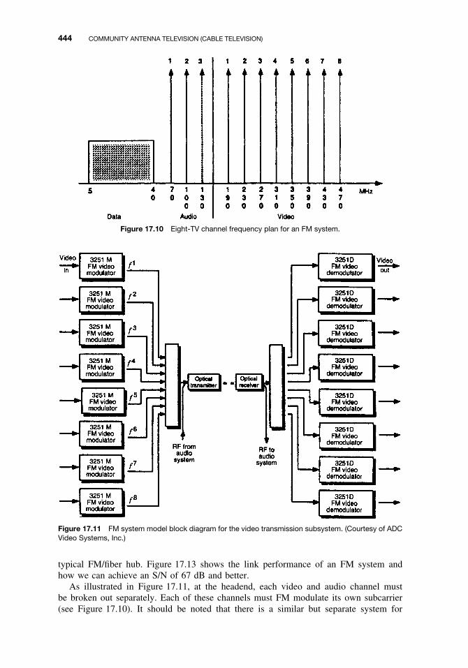
444 COMMUNITY ANTENNA TELEVISION (CABLE TELEVISION)
Figure 17.10 Eight-TV channel frequency plan for an FM system.
Figure 17.11 FM system model block diagram for the video transmission subsystem. (Courtesy of ADCVideo Systems, Inc.)
typical FM/fiber hub. Figure 17.13 shows the link performance of an FM system andhow we can achieve an S/N of 67 dB and better.
As illustrated in Figure 17.11, at the headend, each video and audio channel mustbe broken out separately. Each of these channels must FM modulate its own subcarrier(see Figure 17.10). It should be noted that there is a similar but separate system for

17.4 HYBRID FIBER-COAX (HFC) SYSTEMS 445
Figure 17.12 A typical FM/fiber hub serving both upstream and downstream directions.
the associated aural (audio) channels with 30-MHz spacing starting at 70 MHz. Theseaudio channels may be multiplexed before transmission. Each video carrier occupies a40-MHz slot. These RF carriers, audio and video, are combined in a passive network.The composite RF signal intensity-modulates a laser diode source. Figure 17.12 shows atypical fiber/FM hub where this technique is utilized.
Figure 17.13 illustrates the link performance of an FM fiber-optic system for videochannels. Table 17.1 shows typical link budgets for an HFC AM system.
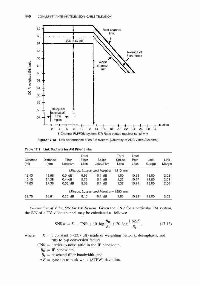
446 COMMUNITY ANTENNA TELEVISION (CABLE TELEVISION)
−2 −4 −6 −8 −10 −12 −14 −16 −18 −20 −22 −24 −26 −28 −30dBm
8-Channel FM/FDM system S/N Ratio versus receiver sensitivity
CC
IR w
eigh
ted
S/N
rat
io Worstchannel
limit
Best channellimit
Average of8 channels
S/N = 67 dB
Use opticalattenuator
in thisregion
69
68
67
66
65
64
63
62
61
60
59
58
57
Figure 17.13 Link performance of an FM system. (Courtesy of ADC Video Systems.).
Table 17.1 Link Budgets for AM Fiber Links
Distance(mi)
Distance(km)
FiberLoss/km
TotalFiberLoss
SpliceLoss/2 km
TotalSpliceLoss
TotalPathLoss
LinkBudget
LinkMargin
Mileage, Losses, and Margins—1310 nm
12.40 19.96 0.5 dB 9.98 0.1 dB 1.00 10.98 13.00 2.0215.15 24.38 0.4 dB 9.75 0.1 dB 1.22 10.97 13.00 2.0317.00 27.36 0.35 dB 9.58 0.1 dB 1.37 10.94 13.00 2.06
Mileage, Losses, and Margins—1550 nm
22.75 36.61 0.25 dB 9.15 0.1 dB 1.83 10.98 13.00 2.02
Calculation of Video S/N for FM System. Given the CNR for a particular FM system,the S/N of a TV video channel may be calculated as follows:
SNRw = K + CNR + 10 logBIF
BF+ 20 log
1.6�F
BF, (17.13)
where K = a constant (∼23.7 dB) made of weighting network, deemphasis, andrms to p-p conversion factors,
CNR = carrier-to-noise ratio in the IF bandwidth,BIF = IF bandwidth,BF = baseband filter bandwidth, and
�F = sync tip-to-peak white (STPW) deviation.

17.5 DIGITAL TRANSMISSION OF CATV SIGNALS 447
With �F = 4 MHz, BIF = 30 MHz, and BF = 5 MHz, the SNRw is improved byapproximately 34 dB above CNR.
Example. If the C/N on an FM fiber link is 32 dB, what is the S/N for a TV videochannel using the given values. Use Eq. (17.14):
S/N = 23.7 dB + 32 dB + 10 log(30/5) + 20 log(1.6 × 4/5)
= 23.7 + 32 + 7.78 + 2.14
= 65.62 dB.
17.5 DIGITAL TRANSMISSION OF CATV SIGNALS
17.5.1 Approaches
There are two approaches to digitally transmitting both audio and video TV signals: trans-port either raw, uncompressed video or compressed video. Each method has advantagesand disadvantages of which some are application-driven. For example, if the objective isdigital to the residence/office, compressed TV may be the most advantageous.
17.5.2 Transmission of Uncompressed Video on CATV Trunks
Video, as we discuss in Chapter 16, is an analog signal. It is converted to a digital formatusing techniques that are similar to the 8-bit PCM covered in Chapter 6, Section 6.2. Amajor difference is in the sampling rate. Broadcast quality TV is generally oversampled.Here we mean that the sampling rate is greater than the Nyquist rate. The Nyquist rate,as we will remember, requires that the sampling rate be two times the highest frequencyof interest. In this case, for the video, the highest frequency of interest is 4.2 MHz, thevideo bandwidth. Using the Nyquist rate, the sampling rate would be 4.2 × 106 × 2 or8.4 million samples per second.
One example is the ADC Video Systems scheme, which uses a sampling rate of13.524 × 106 samples per second. One alternative is an 8-bit system; another is a 10-bitsystem. The resulting equivalent bit rates are 108.195 Mbps and 135.24 Mbps, respec-tively. The 20-kHz audio channel is sampled at 41,880 samples per second using 16-bitPCM. The resulting bit rate is 2.68 Mbps for four audio channels (quadraphonic).
ADC Video Systems, Meriden, Connecticut, multiplexes and frames a 16-channel TVconfiguration for transmission over a fiber-optic trunk in an HFC system. The bit rateon each system is 2.38 Gbps. The frame structure is illustrated in Figure 17.14, andFigure 17.15 is an equipment block diagram for a 16-channel link.
A major advantage of digital transmission is the regeneration capability just as it is inPSTN 8-bit PCM. As a result, there is no noise accumulation on the digital portion of thenetwork. These digital trunks can be extended hundreds of miles or more. The complexity
Figure 17.14 Typical frame structure on a single fiber in a CATV trunk. (Courtesy of ADC Video Systems.)

448 COMMUNITY ANTENNA TELEVISION (CABLE TELEVISION)
Baseband
Baseband
video
Channel1
Channel1Video
encoder
Audioencoderaudio
Ch 2Ch 2
Ch 3Ch 3
Ch 4
Ch 9 Ch 9
Ch 12Ch 12
Channel16
Channel16
Baseband
Baseband
video Videoencoder
Audioencoderaudio
Baseband
Baseband
video Videoencoder
Audioencoderaudio
Baseband
Baseband
video
Videodecoder
Audiodecoder
audio
Baseband
Baseband
videoVideo
decoder
Audiodecoder audio
Baseband
Baseband
videoVideo
decoder
Audiodecoder audio
High-speed
multiplexer(LSM)
#1
High-speed
demulti-plexer(LSD)
#1
High-speed
transmitter
High-speed
receiverFiberspan
(−90 km)
(−2.4 Gpbs)
Figure 17.15 Functional block diagram of a 16-channel digital TV system. (Courtesy of ADC VideoSystems.)
is only marginally greater than an FM system. The 10-bit system can easily provide anS/N ratio at the conversion hub of 67 dB in a video channel and an S/N value of 63 dBwith an 8-bit system. With uncompressed video, BER requirements are not very stringentbecause video contains highly redundant information.
17.5.3 Compressed Video
MPEG compression is widely used today. A common line bit rate for MPEG is1.544 Mbps. Allowing 1 bit per hertz of bandwidth, BPSK modulation, and a cosineroll-off of 1.4, the 1.544-Mbps TV signal can be effectively transported in a 2-MHzbandwidth. Certainly 1000-MHz coaxial cable systems are within the state of the art.With simple division we can see that 500-channel CATV systems are technically viable.If the modulation scheme utilizes 16-QAM (4 bits/Hz theoretical), three 1.544-Mbpscompressed channels can be accommodated in a 6-MHz slot. We select 6 MHz becauseit is the current RF bandwidth assigned for one NTSC TV channel.
17.6 TWO-WAY CATV SYSTEMS
17.6.1 Introduction
Figures 17.16a and 17.16b are two views of a CATV system as they might appear oncoaxial cable. Of course, with conventional CATV systems, each NTSC television channelis assigned 6 MHz of bandwidth as shown in Chapter 16, Figure 16.6.
In Figure 17.17a, only 25 MHz is assigned to upstream6 services. Not all the bandwidthmay be used for voice and data. A small portion should be set aside for upstream telemetryfrom active CATV equipment in the system (e.g., broadband amplifiers). On the other
6Remember, upstream is the direction from the CATV subscriber to the headend, and downstream is in thedirection from the headend to the CATV subscriber.

17.6 TWO-WAY CATV SYSTEMS 449
Figure 17.16a CATV spectrum based on Ref. 1, showing additional upstream and downstream services.Note the imbalance between upstream and downstream. (Adapted from Ref. 1.)
Figure 17.16b CATV spectrum with equal upstream and downstream bandwidth for other services.
Figure 17.17 Trunk/feeder system layout for two-way operation. (From Ref.1, reprinted with permission.)
hand, downstream has 60 MHz set aside for these services. In this day of the Internet,this would be providential, because the majority of the traffic would be downstream.
17.6.1.1 Comments on Figures 17.16a and 17.16b. Large guardbands isolate up-stream from downstream TV and other services: 24 MHz in Figure 17.16a and 25 MHz in

450 COMMUNITY ANTENNA TELEVISION (CABLE TELEVISION)
Figure 17.16b. A small guardband was placed in the frequency slot from 170 to 174 MHzto isolate downstream voice and data signals from conventional CATV television signals.
We assume that the voice service will be POTS (plain old telephone service) and thatboth the data and voice will be digital.
In another approach, downstream voice, data, and special video are assigned the band550 MHz to 750 MHz, which is the highest frequency segment portion of this system(Ref. 6). In this case we are dealing with a 750-MHz aggregate system.
The optical fiber trunk terminates in a node or hub (see Figure 17.12). This is wherethe conversion from an optical signal to the standard CATV coaxial cable format occurs.Let a node serve four groupings of cable subscribers, each with a coaxial cable with thenecessary wideband amplifiers, line extenders, and taps. Typically, such subscriber groupswould consist of 200–500 terminations (TV sets) each. Assume that each termination hasupstream service using the band 5–30 MHz (see Figure 17.16a). In our example, thenode has four incoming 5- to 30-MHz bands, one for each coaxial cable termination. Itthen converts each of these bands to a higher-frequency slot 25 MHz wide in a frequencydivision configuration for backhaul on a return fiber.
In one scheme, at the headend, each 25-MHz slot is demultiplexed and the data andvoice traffic is segregated for switching and processing.
Access by data, voice, and special video users of the upstream and downstream assetsis another question. There are many ways this can be accomplished. One unique methodsuggested by a consultant is to steal a page from the AMPS cellular radio specifications(see Chapter 18 for a discussion of AMPS). Because we have twice the bandwidth ofan AMPS cellular operator, and because there are no handovers required, there are noshadowing effects and multipath (typical of the cellular environment); thus a much simplersystem can be developed. For data communications, CDPD7 can be applied directly. Keepin mind that each system only serves 500 users as a maximum. Those 500 users areallocated 25 MHz of bandwidth (one-way).
An interesting exercise is to divide 25 MHz by 500. This tells us that we can alloteach user a 50-kHz full period. By taking advantage of the statistics of calling (usage), wecould achieve a bandwidth multiplier of from 4× to 10× by using forms of concentration.However, upstream video, depending on the type of compression, might consume a largeportion of this spare bandwidth.
There are many other ways a subscriber can gain access. DAMA techniques, whereAMPS cellular is one, are favored. Suppose we were to turn to a digital format usingstandard 8-bit PCM. Allowing 1 bit/Hz and dividing 25 MHz by 64 kHz, we find onlysome 390 channels available. Keep in mind that these simple calculations are not accurateif we dig a little further. For instance, how will we distinguish one channel from anotherunless we somehow keep them in the frequency domain, where each channel is assigneda 64-kHz slot? This could be done by using QPSK modulation, which will leave somespare bandwidth for filter roll-off and guardbands.
One approach that is widely used currently is to employ the format DOCSIS (Dataover Cable Service Interface Specification). This is covered in Section 17.7.
Why not bring the fiber directly into the home or to the desktop at the office? Themost convincing argument against this approach is economic. A CATV system interfaceswith the home/office TV set by means of a set-top box. As we discussed earlier, the basicfunction of this box is to convert incoming TV channels to a common channel on the TVset, usually either channel 2, 3, or 4. Now we will ask much more of this “box.” It is toterminate the fiber in the AM system as well as to carry out channel conversion. The cost
7CDPD stands for cellular digital packet data. A brief description of CDPD is given in Chapter 18.

17.7 TWO-WAY VOICE AND DATA OVER CATV SYSTEMS BASED ON THE DOCSIS 2.0 SPECIFICATION 451
of the set-top box in 2005 dollars should not exceed $350. With AM fiber to the home,the cost target will probably be exceeded.
The reason that the driving factor is the set-top box is the multiplier effect. In this casewe would be working with multipliers of, say, 500 (subscribers) by >$350. For a totalCATV network, we would be working with 100,000 or more customers. Given the two-way and digital options, both highly desirable, the set-top box may exceed $1200 (2004dollars), even with mass production. The amount is excessive to justify the business case.
17.6.2 Impairments Peculiar to Upstream Service
17.6.2.1 More Thermal Noise Upstream than Downstream. Figure 17.17 showsa hypothetical layout of amplifiers in a CATV distribution system for two-way opera-tion. In the downstream direction, broadband amplifiers point outward, down trunks, andout distribution cables. In the upstream direction, the broadband amplifiers point inwardtoward the headend and all their thermal noise accumulates and concentrates at the head-end. This can account for 3- to 20-dB additional noise upstream at the headend where theupstream demodulation of voice and data signals takes place. Fortunately, the signal-to-noise ratio requirements for good performance of data and voice are much less stringentthan for video, which compensates to a certain extent for this additional noise.
17.6.2.2 Ingress Noise. This noise source is peculiar to a CATV system. It basicallyderives from the residence/office YV sets that terminate the system. Parts 15.31 and 15.35of the FCC Rules and Regulations govern such unintentional radiators. These rules havenot been rigidly enforced.
One problem is that the 75-� impedance match between the coaxial cable and theTV set is poor. Thus not only all radiating devices in the TV set, but other radiatingdevices nearby in residences and office buildings couple back through the TV set into theCATV system in the upstream direction. This type of noise is predominant in the lowerfrequencies, that band from 5 to 30 MHz that carries the upstream signals. As frequencyincreases, ingress noise intensity decreases. Fiber-optic links in HFC configurations canprovide considerable isolation.
17.6.2.3 Other Upstream Noise Contributors. The following are additional noisecontributors for the upstream path:
ž Relative intensity noise (RIN) contributed by the optical node return path laser(s)ž Intermodulation distortion contributed by broadband amplifiers and the return
path laser(s)ž Shot noise and receiver noise within the optical detector at the headendž Multireflections within the HFC plantž Burst noise
17.7 TWO-WAY VOICE AND DATA OVER CATV SYSTEMS BASEDON THE DOCSIS 2.0 SPECIFICATION
17.7.1 General
Data over Cable Service Interface Specification (DOCSIS) is a family of specificationsthat permits CATV systems to have two-way capability: voice, data, and broadcast-typetelevision downstream and data and voice upstream.
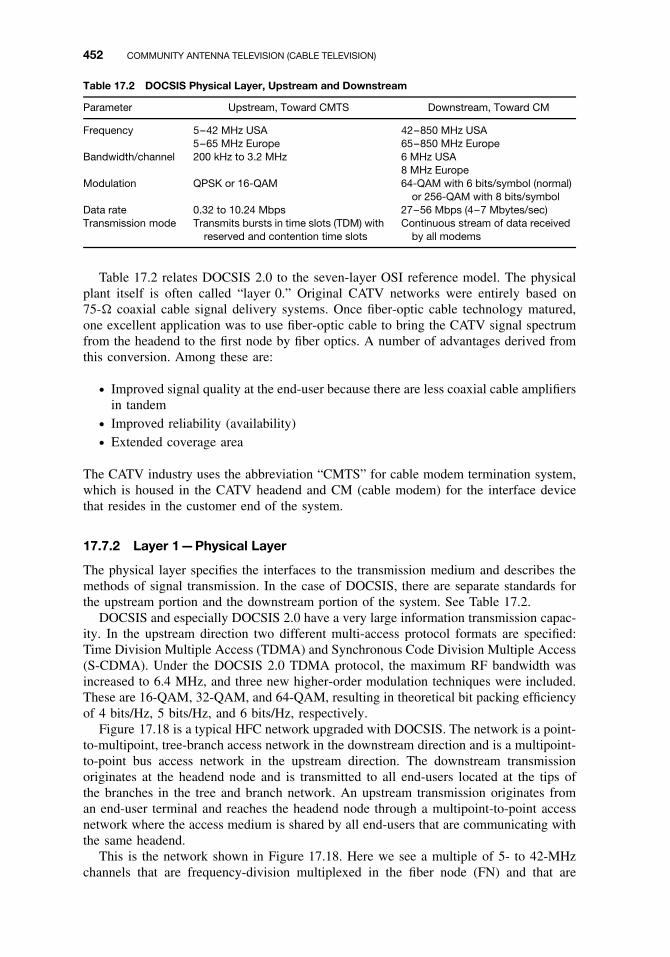
452 COMMUNITY ANTENNA TELEVISION (CABLE TELEVISION)
Table 17.2 DOCSIS Physical Layer, Upstream and Downstream
Parameter Upstream, Toward CMTS Downstream, Toward CM
Frequency 5–42 MHz USA 42–850 MHz USA5–65 MHz Europe 65–850 MHz Europe
Bandwidth/channel 200 kHz to 3.2 MHz 6 MHz USA8 MHz Europe
Modulation QPSK or 16-QAM 64-QAM with 6 bits/symbol (normal)or 256-QAM with 8 bits/symbol
Data rate 0.32 to 10.24 Mbps 27–56 Mbps (4–7 Mbytes/sec)Transmission mode Transmits bursts in time slots (TDM) with
reserved and contention time slotsContinuous stream of data received
by all modems
Table 17.2 relates DOCSIS 2.0 to the seven-layer OSI reference model. The physicalplant itself is often called “layer 0.” Original CATV networks were entirely based on75-� coaxial cable signal delivery systems. Once fiber-optic cable technology matured,one excellent application was to use fiber-optic cable to bring the CATV signal spectrumfrom the headend to the first node by fiber optics. A number of advantages derived fromthis conversion. Among these are:
ž Improved signal quality at the end-user because there are less coaxial cable amplifiersin tandem
ž Improved reliability (availability)ž Extended coverage area
The CATV industry uses the abbreviation “CMTS” for cable modem termination system,which is housed in the CATV headend and CM (cable modem) for the interface devicethat resides in the customer end of the system.
17.7.2 Layer 1—Physical Layer
The physical layer specifies the interfaces to the transmission medium and describes themethods of signal transmission. In the case of DOCSIS, there are separate standards forthe upstream portion and the downstream portion of the system. See Table 17.2.
DOCSIS and especially DOCSIS 2.0 have a very large information transmission capac-ity. In the upstream direction two different multi-access protocol formats are specified:Time Division Multiple Access (TDMA) and Synchronous Code Division Multiple Access(S-CDMA). Under the DOCSIS 2.0 TDMA protocol, the maximum RF bandwidth wasincreased to 6.4 MHz, and three new higher-order modulation techniques were included.These are 16-QAM, 32-QAM, and 64-QAM, resulting in theoretical bit packing efficiencyof 4 bits/Hz, 5 bits/Hz, and 6 bits/Hz, respectively.
Figure 17.18 is a typical HFC network upgraded with DOCSIS. The network is a point-to-multipoint, tree-branch access network in the downstream direction and is a multipoint-to-point bus access network in the upstream direction. The downstream transmissionoriginates at the headend node and is transmitted to all end-users located at the tips ofthe branches in the tree and branch network. An upstream transmission originates froman end-user terminal and reaches the headend node through a multipoint-to-point accessnetwork where the access medium is shared by all end-users that are communicating withthe same headend.
This is the network shown in Figure 17.18. Here we see a multiple of 5- to 42-MHzchannels that are frequency-division multiplexed in the fiber node (FN) and that are

17.7 TWO-WAY VOICE AND DATA OVER CATV SYSTEMS BASED ON THE DOCSIS 2.0 SPECIFICATION 453
Figure 17.18 A pictorial overview of the DOCSIS networks and their relationship with the outside world.
then transmitted by a single fiber trunk to the CATV headend. This operation is calledfrequency stacking.
17.7.3 Layer 2—Data-Link Layer
The data-link layer consists of two sublayers: the media access control (MAC) and theIEEE 802.2 Logical Link Control (LLC).
The MAC sublayer, besides conventional MAC functions, provides the additionalmechanisms that are necessary for sharing the cable. These include:

454 COMMUNITY ANTENNA TELEVISION (CABLE TELEVISION)
ž Ranging to compensate for different cable losses so that the CMTS receives all CMsignals at the same level
ž Ranging to compensate for different cable delaysž Assignment of frequencies to the CMž Allocation of time slots (TDMA) for upstream data flow
17.7.4 Layer 3 and Above
Standard TCP/IP protocols are used for the network layer and above. This ensures Internetcompatibility over the cable network.
17.8 SUBSPLIT/EXTENDED SUBSPLIT FREQUENCY PLAN
The majority of CATV systems, particularly in North America, are upgraded to sub-split8 (5–30 MHz) or extended subsplit (5–42 MHz) operation. This scenario representsthe worst-case design in terms of ingress noise and availability of the reverse channel(upstream) bandwidth. If the design can be deployed in this configuration, the infra-structure upgrade cost for cable systems will be minimal. In the future, the availabilityof midsplit or highsplit cable plants will enable a physical (PHY) layer with enhancedperformance.
17.9 OTHER GENERAL INFORMATION
17.9.1 Frequency Reuse
The assumption is made that the coaxial cable traffic for each service area will be able touse the entire 5–30/5–42-MHz reverse bandwidth. This could be done either by use ofa separate return fiber for each service area or by use of a single fiber for several serviceareas, whose return traffic streams would be combined using block frequency translationat the fiber node.
17.9.2 Cable Distance Limitations
The distance coverage of the system can be influenced by several factors such as thefiber-optic technology employed and the coaxial cable distribution topology. The limitingfactor could be the number of active amplifiers and the resulting noise parameters thatmust be bounded for an optimal physical design. To budget delay use 5 µsec/km foroptical fiber and 4 µsec/km for coaxial cable.
REVIEW EXERCISES
1. Define a CATV headend. What are its functions?
2. List at least three impairments we can expect from a broadband CATV amplifier(downstream).
3. A signal splitter divides a signal in half, splitting into two equal power levels. Ifthe input to a 3-dB splitter were −7 dBm (in the power domain), then the outputon each leg would be −10 dBm. Is this a true statement? What is missing here?
8Subsplit is a frequency division scheme that allows bidirectional traffic on a single cable. Reverse path signalscome to the headend from 5 to 30 MHz, and up to 42 MHz on newer systems. Forward path (downstream)signals go from the headend to end-users from 54 MHz to the upper frequency limit of the system in question.

REFERENCES 455
4. What was/is the purpose of LOS microwave at a CATV headend?
5. What is the purpose of a set-top converter?
6. What does the term beat mean in CATV parlance?
7. Define composite triple beat.
8. A signal level is measured at 0.5 volts rms. What is the equivalent value in dBmV?
9. What dBmV level can we expect in the CATV minimum noise model?
10. When calculating S/N for TV reception on a CATV system, what is the commonvalue of the noise weighting improvement factor?
11. If the C/N of a CATV system is 40 dB, what is the equivalent S/N?
12. There are 10 identical CATV broadband amplifiers in cascade. Each amplifier hasa 7-dB noise figure. What is the thermal noise level in dBmV at the output of thetenth amplifier? Use Eq. (15.8).
13. What is an acceptable level down (below wanted signal level) for Xm?
14. A certain CATV system has 22 amplifiers in cascade with an Xm per amplifier of−89 dB. What is Xmsys?
15. Why are levels on feeder systems usually higher than mainline trunk systems?
16. What does tilt mean when discussing coaxial cable (CATV parlance)? How do weovercome the tilt?
17. Give three advantages of a HFC CATV system over a straight coaxial cable system.
18. What is a tap?
19. Differentiate and give advantages/disadvantages of AM and FM fiber links as partof an HFC system.
20. From a bandwidth viewpoint, why is upstream disadvantaged over downstream?
21. Why is upstream at a disadvantage over downstream from a noise viewpoint?
22. What is ingress noise?
23. List at least four telecommunication services that the DOCSIS specification supports.
24. What is the purpose of ranging?
25. What are the two types of modulation that may be used on the upstream DOC-SIS network?
26. List at least four different impairments we might expect to encounter in the DOCSISupstream environment.
REFERENCES
1. W. O. Grant, Cable Television, 3rd ed., GWG Associates, Schoharie, NY, 1994.
2. K. Simons, Technical Handbook for CATV Systems, 3rd ed., Jerrold Electronics Corp., Hatboro,PA, 1968.
3. E. R. Bartlett, Cable Television Technology and Operations, McGraw-Hill, New York, 1990.

456 COMMUNITY ANTENNA TELEVISION (CABLE TELEVISION)
4. D. N. Carson, “CATV Amplifiers: Figure of Merit and the Coefficient System,” in 1966 IEEEInternational Convention Record, Part I, Wire and Data Communications, pp. 87–97, IEEE,New York, 1966.
5. Electrical Performance for Television Transmission Systems, EIA/TIA-250C, Telecommunica-tion Industry Association, Washington, DC, 1990.
6. Lightwave Buyers’ Guide Issue, Pennwell Publishing Co., Tulsa, OK, 1997.
7. Multimedia Modem Protocol for Hybrid Fiber—Coax Metropolitan Area Networks, IEEE Std.802.14, draft R2, IEEE, NY, 1997.
8. Private communication, Robert Fuller, Chairman, IEEE 802.14 Committee, April 4, 1997.
9. Digital Multi-Programme Systems for Television, Sound and Data Services for Cable Distribu-tion, ITU-T Rec. J.83, ITU Geneva, Sept. 1995.
10. R. L. Freeman, Telecommunication Transmission Handbook, 4th ed., Wiley, New York, 1998.

18
CELLULAR AND PCS RADIOSYSTEMS
18.1 INTRODUCTION
The cellular radio business has expanded explosively since 1980 and continues to expandrapidly. There are several explanations for this popularity. It adds a new dimension towired PSTN services. In our small spheres of everyday living, we are never away from thetelephone, no matter where we are. Outside of industrialized nations, there are long waitinglists for conventional (wired) telephone installations. Go down to the local cellular radiostore, and you will have telephone service within the hour. We have found that cellularservice augments local telephone service availability. When our local service failed forseveral days, our cellular telephone worked just fine, although air time was expensive.
Enter PCS (personal communications services). Does it supplement/complement cellu-lar radio or is it a competitor? It is an extension of cellular, certainly in concept. It usesmuch lower power and has a considerably reduced range. Rappaport (Ref. 1) points outthat cellular is hierarchical in nature when connecting to the PSTN; PCS is not. It is hier-archical in that an MTSO (mobile telephone switching office) controls and interfaces upto hundreds of base stations, which connect to mobile users. According to the reference,PCS base stations connect directly to the PSTN. However, a number of PCS strategieshave a hierarchy similar to cellular where an MSC (mobile switching center) provides theconnectivity to the PSTN. Cellular radio systems operate in the 800- and 900-MHz band;in the United States narrowband PCS operates in the 900-MHz band, and wideband PCSoperates in the 1850- to 1975-MHz band. Other PCS operations are specialized, such asthe wireless PABX, wireless LAN (WLAN), and wireless local loop (WLL). By WLL wemean a transmission method that will operate in lieu of, supplement, or complement thetelephone subscriber loop based on a wire pair.
18.1.1 Background
The earliest radio techniques served a mobile community, namely, ocean vessels. Thiswas followed by vehicular mobile including aircraft. Prior to World War II, there werepolice and ambulance dispatching systems followed by growth in the airline industry.However, not until Bell Telephone Laboratories published the famous issue of the Bell
Fundamentals of Telecommunications, Second Edition, by Roger L. FreemanISBN 0-471-71045-8 Copyright 2005 by Roger L. Freeman
457

458 CELLULAR AND PCS RADIO SYSTEMS
System Technical Journal devoted entirely to a new system called AMPS (advancedmobile phone system) did the cellular idea take hold. It tends to remain a major playerin the cellular radio scene in the United States and in some Latin American countries. Ituses FM radio allocating 30 kHz per voice channel.
AMPS set the scene for explosive cellular radio growth and usage. What set AMPSapart from previous mobile radio systems is that it was designed to interface with thePSTN. It was based on an organized scheme of adjoining cells and had a unique capabilityof handoff when a vehicle moves through one cell to another; or when another cell receivesa higher signal level from the vehicle, it will then take over the call. Vehicles can roamfrom one service area to another with appropriate handoffs.
In the late 1980s there was pressure to convert cellular radio from the bandwidth-wasteful AMPS to some sort of digital regime. As the reader reviews this chapter, it willbe seen that digital is also bandwidth-wasteful, even more so than analog FM. Variousways are described on how to remedy the situation: first by reducing the bandwidth ofa digital voice channel, and second by the access/modulation scheme proposed. Of thislatter proposal, two schemes are on the table in North America: a TDMA scheme and aCDMA scheme. They are radically different and competing.
Meanwhile, the Europeans critiqued our approaches and came up with a better mouse-trap. It is called Ground System Mobile (GSM) (from the French), and there is somepressure that it be adopted in the United States. GSM is a TDMA scheme, fairly differentfrom the U.S. TIA standard (IS-54C).
As we mentioned earlier, PCS is an outgrowth of cellular radio; it uses a cellularconcept. The cells, however, are much smaller, under 1 km in diameter. RF poweris much lower. As with cellular radio, TDMA and CDMA are vying for the nationalaccess/modulation method. Unlike the North American popular press that discriminatesbetween PCS and cellular radio, ITU-R takes a more mature and reasonable view of theaffair by placing the two in the same arena. Earlier, CCIR/ITU-R called their conceptualPCS Future Public Land Mobile Telecommunication System (FPLMTS). The name hasnow changed to UMTS (Universal Mobile Telecommunication System). FPLMTS/UMTSconcept breaks down into three terrestrial operational areas: (1) indoor environments(range to 100 m), (2) outdoor environments (100 m to 35 km) for more rural settings,and (3) an intermediate region called outdoor-to-indoor environments, where buildingpenetration is a major theme. They also describe satellite environments.
18.1.2 Scope and Objective
This chapter presents an overview of mobile and personal communications. Much of thediscussion deals with cellular radio and extends this thinking inside buildings. The cov-erage most necessarily includes propagation for the several environments, propagationimpairments, methods to mitigate those impairments, access techniques, bandwidth limi-tations, and ways around this problem. It will cover several mobile radio standards andcompare a number of existing and planned systems. The chapter objective is to providean appreciation of mobile/personal communications. Space limitations force us to confinethe discussion to what might loosely be called “land mobile systems.”
18.2 BASIC CONCEPTS OF CELLULAR RADIO
Cellular radio systems connect a mobile terminal to another user, usually through thePSTN. The “other user” most commonly is a telephone subscriber of the PSTN. However,

18.2 BASIC CONCEPTS OF CELLULAR RADIO 459
the other user may be another mobile terminal. Most of the connectivity is extending “plainold telephone service” (POTS) to mobile users. Data and facsimile services are in variousstages of implementation. Some of the terms used in this section have a strictly NorthAmerican flavor.
Figure 18.1 illustrates a conceptual layout of a cellular radio system. The heart ofthe system for a specific serving area is the MTSO (mobile telephone switching office).The MTSO is connected by a trunk group to a nearby telephone exchange providing aninterface to and connectivity with the PSTN.
The area to be served by a cellular geographic serving area (CGSA) is divided intosmall geographic cells, which ideally are hexagonal.1 Cells are initially laid out withcenters spaced about 4–8 m (6.4–12.8 km) apart. The basic system components are thecell sites, the MTSO, and mobile units. These mobile units may be hand-held or vehicle-mounted terminals.
Each cell has a radio facility housed in a building or shelter. The facility’s radio equip-ment can connect and control any mobile unit within the cell’s responsible geographicarea. Radio transmitters located at the cell site have a maximum effective radiated power(ERP) of 100 W.2 Combiners are used to connect multiple transmitters to a commonantenna on a radio tower, usually between 50 ft and 300 ft (15 m and 92 m) high. Com-panion receivers use a separate antenna system mounted on the same tower. The receiveantennas are often arranged in a space diversity configuration.
Figure 18.1 Conceptual layout of a cellular radio system.
1CGSA is a term coined by the U.S. FCC. We do not believe it is used in other countries.2Care must be taken with terminology. In this instance, ERP and EIRP are not the same. The reference antennain this case is the dipole, which has a 2.15-dBi gain.

460 CELLULAR AND PCS RADIO SYSTEMS
The MTSO provides switching and control functions for a group of cell sites. A methodof connectivity is required between the MTSO and the cell site facilities. The MTSO is anelectronic switch and carries out a fairly complex group of processing functions to controlcommunications to and from mobile units as they move between cells as well as to makeconnections with the PSTN. Besides making connectivity with the public network, theMTSO controls cell site activities and mobile actions through command-and-control datachannels. The connectivity between cell sites and the MTSO is often via DS1 on wirepairs or on microwave facilities, the latter being the most common.
A typical cellular mobile unit consists of a control unit, a radio transceiver, and anantenna. The control unit has a telephone handset, a push-button keypad to enter com-mands into the cellular/telephone network, and audio and visual indications for customeralerting and call progress. The transceiver permits full-duplex transmission and receptionbetween a mobile and cell sites. Its ERP is nominally 6 W. Hand-held terminals combineall functions into one small package that can easily be held in one hand. The ERP of ahand-held is a nominal 0.6 W.
In North America, cellular communication is assigned a 25-MHz band between 824 MHzand 849 MHz for mobile unit-to-base transmission and a similar band between 869 MHzand 894 MHz for transmission from base to mobile.
The first and most widely implemented North American cellular radio system wascalled AMPS (advanced mobile phone system). The original system description was con-tained in an entire issue of the Bell System Technical Journal (BSTJ) of January 1979. Thepresent AMPS is based on 30-kHz channel spacing using frequency modulation. The peakdeviation is 12 kHz. The cellular bands are each split into two to permit competition. Thusonly 12.5 MHz is allocated to one cellular operator for each direction of transmission.With 30-kHz spacing, this yields 416 channels. However, nominally 21 channels are usedfor control purposes with the remaining 395 channels available for cellular end-users.
Common practice with AMPS is to assign 10–50 channel frequencies to each cellfor mobile traffic. Of course the number of frequencies used depends on the expectedtraffic load and the blocking probability. Radiated power from a cell site is kept at arelatively low level with just enough antenna height to cover the cell area. This permitsfrequency reuse of these same channels in nonadjacent cells in the same CGSA with littleor no cochannel interference. A well-coordinated frequency reuse plan enables tens ofthousands of simultaneous calls over a CGSA.
Figure 18.2 illustrates one frequency reuse method. Here four channel frequency groupsare assigned in a way that avoids the same frequency set in adjacent cells. If therewere uniform terrain contours, this plan could be applied directly. However, real terrainconditions dictate further geographic separation of cells that use the same frequency set.Reuse plans with 7 or 12 sets of channel frequencies provide more physical separationand are often used depending on the shape of the antenna pattern employed.
With user growth in a particular CGSA, cells may become overloaded. This meansthat grade of service objectives are not being met due to higher than planned trafficlevels during the busy hour (BH; see Section 4.2.1). In these cases, congested cells canbe subdivided into smaller cells, each with its own base station, as shown in Figure 18.3.With smaller cells lower transmitter power and antennas with less height are used, thuspermitting greater frequency reuse. These subdivided cells can be split still further foreven greater frequency reuse. However, there is a practical limit to cell splitting, oftenwith cells with a 1-m (1.6-km) radius.
Radio system design for cellular operation differs from that used for LOS microwaveoperation. For one thing, mobility enters the picture. Path characteristics are constantlychanging. Mobile units experience multipath scattering, reflection, and/or diffraction by

18.2 BASIC CONCEPTS OF CELLULAR RADIO 461
Figure 18.2 Cell separation with four different sets of frequencies.
Figure 18.3 Staged growth by cell splitting (subdividing).
obstructions and buildings in the vicinity. There is shadowing, often very severe. Theresulting received signal under these conditions varies randomly as the sum of manyindividual waves with changing amplitude, phase, and direction of arrival. The statisticalautocorrelation distance is on the order of one-half wavelength (Ref. 1). Space diversityat the base station tends to mitigate these impairments.
In Figure 18.1, the MTSO is connected to each of its cell sites by a voice trunk foreach of the radio channels at the site. Also, two data links (AMPS design) connect theMTSO to each cell site. These data links transmit information for processing calls andfor controlling mobile units. In addition to its “traffic” radio equipment, each cell site hasinstalled signaling equipment, monitoring equipment, and a setup radio to establish calls.

462 CELLULAR AND PCS RADIO SYSTEMS
When a mobile unit becomes operational, it automatically selects the setup channel withthe highest signal level. It then monitors that setup channel for incoming calls destined forit. When an incoming call is sensed, the mobile terminal in question again samples signallevels of all appropriate setup channels so it can respond through the cell site offering thehighest signal level, and then tunes to that channel for response. The responsible MTSOassigns a vacant voice channel to the cell in question, which relays this information viathe setup channel to the mobile terminal. The mobile terminal subscriber is then alertedthat there is an incoming call. Outgoing calls from mobile terminals are handled in asimilar manner.
While a call is in progress, the serving cell site examines the mobile’s signal levelevery few seconds. If the signal level drops below a prescribed level, the system seeksanother cell to handle the call. When a more appropriate cell site is found, the MTSOsends a command, relayed by the old cell site, to change frequency for communicationwith the new cell site. At the same time, the landline subscriber is connected to the newcell site via the MTSO. The periodic monitoring of operating mobile units is known aslocating, and the act of changing channels is called handover. Of course, the functionsof locating and handover are to provide subscribers satisfactory service as a mobile unittraverses from cell to cell. When cells are made smaller, handovers are more frequent.
The management and control functions of a cellular system are quite complex. Han-dover and locating are managed by signaling and supervision techniques, which take placeon the setup channel. The setup channel uses a 10-kbps data stream that transmits paging,voice channel designation, and overhead messages to mobile units. In turn, the mobileunit returns page responses, origination messages, and order confirmations.
Both digital messages and continuous supervision tones are transmitted on the voiceradio channel. The digital messages are sent as a discontinuous “blank-and-burst” in-banddata stream at 10 kbps and include order and handover messages. The mobile unit returnsconfirmation and messages that contain dialed digits. Continuous positive supervision isprovided by an out-of-band 6-kHz tone, which is modulated onto the carrier along withthe speech transmission.
Roaming is a term used for a mobile unit that travels such distances that the routecovers more than one cellular organization or company. The cellular industry is movingtoward technical and tariffing standardization so that a cellular unit can operate anywherein the United States, Canada, and Mexico.
18.3 RADIO PROPAGATION IN THE MOBILE ENVIRONMENT
18.3.1 The Propagation Problem
Line-of-sight microwave and satellite communications covered in Chapter 9 dealt withfixed systems. Such systems are optimized. They are built up and away from obstacles.Sites are selected for best propagation.
This is not so with mobile systems. Motion and a third dimension are additionalvariables. The end-user terminal often is in motion; or the user is temporarily fixed, butthat point can be anywhere within a serving area of interest. Whereas before we dealtwith point-to-point, here we deal with point-to-multipoint.
One goal in line-of-sight microwave design is to stretch the distance as much aspossible between repeaters by using high towers. In this chapter there are some overridingcircumstances where we try to limit coverage extension by reducing tower heights, whatwe briefly introduced in Section 18.2. Even more importantly, coverage is area coverage,where shadowing is frequently encountered Examples are valleys, along streets with high

18.3 RADIO PROPAGATION IN THE MOBILE ENVIRONMENT 463
buildings on either side, verdure such as trees and inside buildings, to name a few typicalsituations. There are two notable results. Transmission loss increases notably and such anenvironment is rich with multipath scenarios. Paths can be highly dispersive, as much as10 µsec of delay spread (Ref. 2). If a user is in motion, Doppler shift can be expected.
The radio-frequency bands of interest are UHF, especially around 800 and 900 MHz,and 1700–2000 MHz. In certain parts of the world, there is usage in the 400-MHz band.
18.3.2 Propagation Models
We concentrate on cellular operation. There is a fixed station (FS) and mobile stations(MSs) moving through the cell. A cell is the area of responsibility of the fixed station, acell site. It usually is pictured as a hexagon in shape, although its propagation profile ismore like a circle with the fixed station in its center. Cell radii vary from 1 km (0.6 mi)in heavily built-up urban areas to 30 km (19 mi) or somewhat more in rural areas.
18.3.2.1 Path Loss or Transmission Loss. We recall the free-space loss (FSL)formula in Section 9.2.3. It simply stated that FSL was a function of the square of thedistance and the square of the frequency plus a constant. It is a very useful formula if thestrict rules of obstacle clearance are obeyed. Unfortunately, in the cellular situation, it isimpossible to obey these rules. Then to what extent must this free-space loss formula bemodified by the proximity of the earth and by the effects of trees, buildings, and hills in,or close to, the transmission path?
There have been a number of models that have been developed that are used as a basisfor the calculation of transmission loss, several assumptions are made:
ž That we will always use the same frequency band, often 800 or 900 MHz. Thus itis common to drop the frequency term (the 20 log F term) in the FSL formula andinclude a constant that covers the frequency term. If we wish to use the model foranother band, say 1800 MHz, a scaling factor is added.
ž That we will add a term to compensate for the usual great variance between the cellsite antenna height when compared to the mobile (or hand-held) antenna height. Weoften call this the height-gain function, and it tends to give us an advantage. It isoften expressed as −20 log(hThR), where hT is the height of the transmit antenna(cell site) and hR is the height of the receive antenna (on the mobile platform). Theseare comparative heights. Commonly, the mobile platform antenna height is taken as6 ft or 3 m.
ž That there is a catch-all term for the remainder of the losses, which in some referencesis expressed as β (in dB).
ž That at least three models express the free-space loss as just 40 log dm (dm is distancein meters).
18.3.2.2 The Okumura Model. Okumura et al. (Ref. 3) carried out a detailed anal-ysis for path predictions around Tokyo for mobile terminals. Hata (Ref. 4) published anempirical formula based on Okumura’s results to predict path loss. The Okumura/Hatamodel is probably one of the most widely applied path loss models in the world forcellular application. The formula and its application follow.
LdB = 69.55 + 26.16 log f − 13.82 log ht − A(hr)
+ (44.9 − 6.55 log ht) log d, (18.1)

464 CELLULAR AND PCS RADIO SYSTEMS
where r is between 150 MHz and 1500 MHz,ht is between 30 m and 300 m, andd is the path distance and is between 1 km and 20 km.
A(hr) is the correction factor for mobile antenna height and is computed as follows:For a small- or medium-size city,
A(hr) = (1.1 log f − 0.7)hr − (1.56 log f − 0.8)(dB), (18.2a)
where hr is between 1 and 10 m.For a large city,
A(hr) = 3.2[log(11.75hr)]2 − 4.97(dB), (18.2b)
where f ≥ 400 MHz.
Example. Let f = 900 MHz, ht = 40 m, hr = 5 m, and d = 10 km. Calculate A(hr) fora medium-size city.
A(hr) = 12.75 − 3.8 = 8.95 dB
LdB = 69.55 + 72.28 − 22.14 − 8.95 + 34.4
= 145.15 dB.
18.3.2.3 Building Penetration. For a modern multistory office building at 864 and1728 MHz, transmission loss (LdB) includes a value for clutter loss L(v) and is expressedas follows:
LdB = L(v) + 20 log d + nfaf + nwaw, (18.3)
where the attenuation in decibels of the floors and walls was af and aw, and the numberof floors and walls along the line d were nf and nw, respectively. The values of L(v) at864 MHz and 1728 MHz were 32 dB and 38 dB, with standard deviations of 3 dB and4 dB, respectively (Ref. 2).
Another source (Ref. 5) provided the following information: At 1650 MHz the floorloss factor was 14 dB, while the wall losses were 3–4 dB for double plasterboard and7–9 dB for breeze block or brick. The parameter L(v) was 29 dB. When the propagationfrequency was 900 MHz, the first floor factor was 12 dB and L(v) was 23 dB. Thehigher value for L(v) at 1650 MHz was attributed to a reduced antenna aperture at thisfrequency compared to 900 MHz. For a 100-dB path loss, the base station and mobileterminal distance exceeded 70 m on the same floor, was 30 m for the floor above, andwas 20 m for the floor above that, when the propagation frequency was 1650 MHz. Thecorresponding distances at 900 MHz were 70 m, 55 m, and 30 m. Results will vary frombuilding to building, depending on the type of construction of the building, the furnitureand equipment it houses, and the number and deployment of the people who populate it.
18.4 IMPAIRMENTS: FADING IN THE MOBILE ENVIRONMENT
18.4.1 Introduction
Fading in the mobile situation is quite different from the static line-of-sight (LOS)microwave situation discussed in Section 9.2.4. In this case radio paths are not opti-mized as in the LOS environment. The mobile terminal may be fixed throughout a

18.4 IMPAIRMENTS: FADING IN THE MOBILE ENVIRONMENT 465
mobile
DB
R
DIRECTIONTO ELEVATEDBASE STATION
building
Figure 18.4 Mobile terminal in an urban setting. R, reflection; D, diffraction.
telephone or data call, but is more apt to be in motion. Even the hand-held terminalmay well have micromotion. When a terminal is in motion, the path characteristics areconstantly changing.
Multipath propagation is the rule. Consider the simplified pictorial model in Figure 18.4.Commonly, multiple rays reach the receive antenna, each with its own delay. The construc-tive and destructive fading can become quite complex. We must deal with both reflectionand diffraction.3 Energy will arrive at the receive antenna reflected off sides of build-ings, towers, streets, and so on. Energy will also arrive diffracted from knife edges (e.g.,building corners) and rounded obstacles (e.g., water tanks, hill tops).
Because the same signal arrives over several paths, each with a different electricallength, the phases of each path will be different, resulting in constructive and destructiveamplitude fading. Fades of 20 dB are common, and even 30-dB fades can be expected.
On digital systems, the deleterious effects of multipath fading can be even more severe.Consider a digital bit stream to a mobile terminal with a transmission rate of 1000 bps.Assuming NRZ coding, the bit period would be 1 msec (bit period = 1/bit rate). We findthe typical multipath delay spread may be on the order of 10 µsec. Thus delayed energywill spill into a subsequent bit (or symbol) for the first 10 µsec of the bit period andwill have no negative effect on the bit decision. If the bit stream is 64,000 bps, then thebit period is 1/64,000 or 15 µsec. Destructive energy from the previous bit (symbol) willspill into the first two-thirds of the bit period, well beyond the midbit sampling point. Thisis typical intersymbol interference (ISI), and in this case there is a high probability thatthere will be a bit error. The bottom line is that the destructive potential of ISI increasesas the bit rate increases (i.e., as the bit period decreases).
18.4.2 Diversity: A Technique to Mitigate the Effects of Fading and Dispersion
18.4.2.1 Scope. We discuss diversity to reduce the effects of fading and to mitigatedispersion. Diversity was briefly covered in Section 9.2.5 where we dealt with LOSmicrowave. In that section we discussed frequency and space diversity. In principle, suchtechniques can be employed either at the base station and/or at the mobile unit, althoughdifferent problems have to be solved for each. The basic concept behind diversity is thattwo or more radio paths carrying the same information are relatively uncorrelated: Whenone path is in a fading condition, often the other path is not undergoing a fade. These
3Diffraction is defined by the IEEE (Ref. 6) as “the deviation of the direction of energy flow of a way (raybeam), not attributable to reflection or refraction, when it passes an obstacle, a restricted aperture, or otherinhomogeneities in a medium.
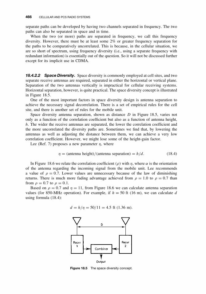
466 CELLULAR AND PCS RADIO SYSTEMS
separate paths can be developed by having two channels separated in frequency. The twopaths can also be separated in space and in time.
When the two (or more) paths are separated in frequency, we call this frequencydiversity. However, there must be at least some 2% or greater frequency separation forthe paths to be comparatively uncorrelated. This is because, in the cellular situation, weare so short of spectrum, using frequency diversity (i.e., using a separate frequency withredundant information) is essentially out of the question. So it will not be discussed furtherexcept for its implicit use in CDMA.
18.4.2.2 Space Diversity. Space diversity is commonly employed at cell sites, and twoseparate receive antennas are required, separated in either the horizontal or vertical plane.Separation of the two antennas vertically is impractical for cellular receiving systems.Horizontal separation, however, is quite practical. The space diversity concept is illustratedin Figure 18.5.
One of the most important factors in space diversity design is antenna separation toachieve the necessary signal decorrelation. There is a set of empirical rules for the cellsite, and there is another set of rules for the mobile unit.
Space diversity antenna separation, shown as distance D in Figure 18.5, varies notonly as a function of the correlation coefficient but also as a function of antenna height,h. The wider the receive antennas are separated, the lower the correlation coefficient andthe more uncorrelated the diversity paths are. Sometimes we find that, by lowering theantennas as well as adjusting the distance between them, we can achieve a very lowcorrelation coefficient. However, we might lose some of the height-gain factor.
Lee (Ref. 7) proposes a new parameter η, where
η = (antenna height)/(antenna separation) = h/d. (18.4)
In Figure 18.6 we relate the correlation coefficient (ρ) with η, where α is the orientationof the antenna regarding the incoming signal from the mobile unit. Lee recommendsa value of ρ = 0.7. Lower values are unnecessary because of the law of diminishingreturns. There is much more fading advantage achieved from ρ = 1.0 to ρ = 0.7 thanfrom ρ = 0.7 to ρ = 0.1.
Based on ρ = 0.7 and η = 11, from Figure 18.6 we can calculate antenna separationvalues (for 850-MHz operation). For example, if h = 50 ft (16 m), we can calculate d
using formula (18.4):
d = h/η = 50/11 = 4.5 ft (1.36 m).
Figure 18.5 The space diversity concept.

18.4 IMPAIRMENTS: FADING IN THE MOBILE ENVIRONMENT 467
Figure 18.6 Correlation coefficient ρ versus the parameter η for two receive antennas in differentorientations. (From Ref. 7, Figure 6.4, reprinted with permission.)
For an antenna 120-ft (36.9-m) high, we find that d = 120/11 = 10.9 ft (or 3.35 m) (fromRef. 7).
18.4.2.2.1 Space Diversity on a Mobile Platform. Lee (Ref. 7) discusses both ver-tically separated and horizontally separated antennas on a mobile unit. For the verticalcase, 1.5λ is recommended for the vertical separation case and 0.5λ for the horizontalseparation case.4 At 850 MHz, λ = 35.29 cm. Then 1.5λ = 1.36 ft or 52.9 cm. For 0.5λ,the value is 0.45 ft or 17.64 cm.
18.4.3 Cellular Radio Path Calculations
Consider the path from the fixed cell site to the mobile platform. There are severalmobile receiver parameters that must be considered. The first to be derived are signalquality minima from EIA/TIA IS-19B (Ref. 8).
The minimum SINAD (signal + interference + noise and distortion to interference +noise + distortion ratio) is 12 dB. This SINAD equates to a threshold of −116 dBm or7 µV/m. This assumes a cellular transceiver with an antenna with a net gain of 1 dBd(dB over a dipole). The gross antenna gain is 2.5 dBd with a 1.5-dB transmission lineloss. A 1-dBd gain is equivalent to a 3.16-dBi gain (i.e., 0 dBd = 2.15 dBi). Furthermore,this value equates to an isotropic receive level of −119.16 dBm (Ref. 8).
One design goal for a cellular system is to more or less maintain a cell boundary at the39-dB µ contour (Ref. 9). Note that 39 dBµ = −95 dBm (based on a 50-� impedance at850 MHz). Then at this contour, a mobile terminal would have a 24.16-dB fade margin.
If a cellular transmitter has a 10-W output per channel and an antenna gain of 12 dBiand 2-dB line loss, the EIRP would be +20 dBW or +50 dBm. The maximum path lossto the 39-dBµ contour would be +50 dBm − (−119.16 dBm) or 169 dB.5
4Remember that λ is the conventional notation for wavelength. Fλ = 3 × 10⁸m/s, where F is the frequency inHz and λ is the wavelength in meters.5The 39-dBµ contour is a threshold for good AMPS operation.

468 CELLULAR AND PCS RADIO SYSTEMS
18.5 THE CELLULAR RADIO BANDWIDTH DILEMMA
18.5.1 Background and Objectives
The present cellular radio bandwidth assignment in the 800- and 900-MHz bands cannotsupport the demand for cellular service, especially in urban areas in the United States andCanada. AMPS, widely used in North and South America and elsewhere, requires 30 kHzper voice channel. The system employs FDMA (frequency division multiple access), muchlike the FDMA/DAMA system described in Section 9.3.5.3. We remember that the analogvoice channel is a nominal 4-kHz channel, and 30 kHz is about seven times that value.
The trend is to convert cellular radio to a digital format. Digital transmission, asdescribed in Chapter 6, is notoriously wasteful of bandwidth, when compared to the 4-kHzanalog channel. We can show that conventional PCM requires 16 times more bandwidththan its 4-kHz analog channel counterpart. In other words, the standard PCM digital voicechannel occupies 64 kHz (assuming 1 bit per hertz of bandwidth).
Cellular system designers have taken two approaches to reduce the required bandwidth.First is to use voice compression on the digital voice channel. The second approach wasto use more efficient access techniques. We briefly review several techniques of speechcompression and then describe two distinctly different schemes for mobile station accessto the network. Of course the real objective is to increase the ratio of users per unitbandwidth when compared to the analog AMPS access method.
18.5.2 Bit Rate Reduction of the Digital Voice Channel
It became obvious to system designer that conversion to digital cellular required somedifferent technique for coding speech other than conventional PCM found in the PSTN anddescribed in Chapter 6. The following lists some techniques that have been considered orthat have been incorporated in the various systems in North America, Europe, and Japan(Ref. 10).
1. ADPCM (adaptive differential PCM). Good intelligibility and good quality; 32-kbpsdata transmission over the channel may be questionable.
2. Linear predictive vocoders (voice coders); 2400 bps. Adopted by U.S. Departmentof Defense. Good intelligibility, poor quality, especially speaker recognition.
3. Subband coding (SBC). Good intelligibility, even down to 4800 bps. Quality suffersbelow 9600 bps.
4. RELP (residual excited linear predictive) type coder. Good intelligibility down to4800 bps and fair to good quality. Quality improves as bit rate increases. Goodquality at 16 kbps.
5. CELP (codebook-excited linear predictive). Good intelligibility and surprisinglygood quality, even down to 4800 bps. At 8 kbps, near-toll quality speech.
18.6 NETWORK ACCESS TECHNIQUES
18.6.1 Introduction
The objective of a cellular radio operation is to provide a service where mobile subscriberscan communicate with any subscriber in the PSTN, where any subscriber in the PSTN cancommunicate with any mobile subscriber, and where mobile subscribers can communicateamong themselves via the cellular radio system. In all cases the service is full duplex.
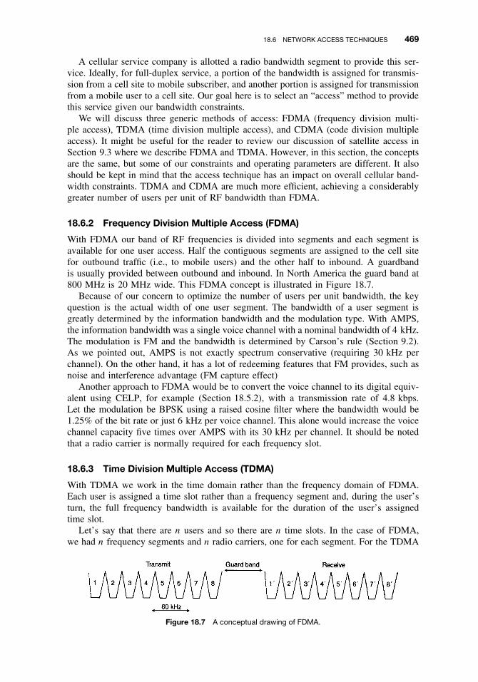
18.6 NETWORK ACCESS TECHNIQUES 469
A cellular service company is allotted a radio bandwidth segment to provide this ser-vice. Ideally, for full-duplex service, a portion of the bandwidth is assigned for transmis-sion from a cell site to mobile subscriber, and another portion is assigned for transmissionfrom a mobile user to a cell site. Our goal here is to select an “access” method to providethis service given our bandwidth constraints.
We will discuss three generic methods of access: FDMA (frequency division multi-ple access), TDMA (time division multiple access), and CDMA (code division multipleaccess). It might be useful for the reader to review our discussion of satellite access inSection 9.3 where we describe FDMA and TDMA. However, in this section, the conceptsare the same, but some of our constraints and operating parameters are different. It alsoshould be kept in mind that the access technique has an impact on overall cellular band-width constraints. TDMA and CDMA are much more efficient, achieving a considerablygreater number of users per unit of RF bandwidth than FDMA.
18.6.2 Frequency Division Multiple Access (FDMA)
With FDMA our band of RF frequencies is divided into segments and each segment isavailable for one user access. Half the contiguous segments are assigned to the cell sitefor outbound traffic (i.e., to mobile users) and the other half to inbound. A guardbandis usually provided between outbound and inbound. In North America the guard band at800 MHz is 20 MHz wide. This FDMA concept is illustrated in Figure 18.7.
Because of our concern to optimize the number of users per unit bandwidth, the keyquestion is the actual width of one user segment. The bandwidth of a user segment isgreatly determined by the information bandwidth and the modulation type. With AMPS,the information bandwidth was a single voice channel with a nominal bandwidth of 4 kHz.The modulation is FM and the bandwidth is determined by Carson’s rule (Section 9.2).As we pointed out, AMPS is not exactly spectrum conservative (requiring 30 kHz perchannel). On the other hand, it has a lot of redeeming features that FM provides, such asnoise and interference advantage (FM capture effect)
Another approach to FDMA would be to convert the voice channel to its digital equiv-alent using CELP, for example (Section 18.5.2), with a transmission rate of 4.8 kbps.Let the modulation be BPSK using a raised cosine filter where the bandwidth would be1.25% of the bit rate or just 6 kHz per voice channel. This alone would increase the voicechannel capacity five times over AMPS with its 30 kHz per channel. It should be notedthat a radio carrier is normally required for each frequency slot.
18.6.3 Time Division Multiple Access (TDMA)
With TDMA we work in the time domain rather than the frequency domain of FDMA.Each user is assigned a time slot rather than a frequency segment and, during the user’sturn, the full frequency bandwidth is available for the duration of the user’s assignedtime slot.
Let’s say that there are n users and so there are n time slots. In the case of FDMA,we had n frequency segments and n radio carriers, one for each segment. For the TDMA
Figure 18.7 A conceptual drawing of FDMA.

470 CELLULAR AND PCS RADIO SYSTEMS
Figure 18.8 A typical TDMA frame.
case, only one carrier is required. Each user gains access to the carrier for 1/n of the timeand there is generally an ordered sequence of time slot turns. A TDMA frame can bedefined as cycling through n users’ turns just once.
A typical TDMA frame is illustrated in Figure 18.8. One must realize that TDMAis only practical with a digital system such as PCM or any of those discussed inSection 18.5.2. As we said in Section 9.3.5.2, TDMA is a store and burst system.
Incoming user traffic is stored in memory, and when that user’s turn comes up, thataccumulated traffic is transmitted in a digital burst.
Suppose there are 10 users. Let each user’s bit rate be R, then a user’s burst mustbe at least 10R. Of course, the burst will be greater than 10R to accommodate a certainamount of overhead bits as shown in Figure 18.8.
We define downlink as outbound, base station to mobile station(s), and define uplinkas mobile station to base station. Typical frame periods are:
North American IS-54 40 msec for six time slotsEuropean GSM 4.615 msec for eight time slots
One problem with TDMA, often not appreciated by many, is delay. In particular, this isdelay on the uplink. Consider Figure 18.9, where we set up a scenario. A base stationreceives mobile time slots in a circular pattern and the radius of the circle of responsibilityof that base station is 10 km. Let the velocity of a radio wave be 3 × 10⁸ m/sec. Thetime for the wave to traverse 1 km is 1000 m/(3 × 108) or 3.333 µsec. In the uplinkframe we have a mobile station right on top of the base station with essentially no delayand another mobile right at 10 km with 10 × 3.33 µsec or 33.3 µsec delay. A GSM timeslot is about 576 µsec in duration. The terminal at the 10-km range will have its timeslot arriving 33.3 µsec late compared to the terminal with no delay. A GSM bit periodis about 3.69 µsec so that the late arrival mutilates about 10 bits, and unless somethingis done, the last bit of the burst will overlap the next burst (Refs. 2 and 11).
Figure 18.9 A TDMA delay scenario.

18.6 NETWORK ACCESS TECHNIQUES 471
Figure 18.10 GSM frame and burst structures. (From Figure 8.7, Ref. 2. Reprinted with permission.)
Refer now to Figure 18.10, which illustrates GSM burst structures. Note that the accessburst has a guard period of 68.25 bit durations or a slop of 3.69 × 68.25 µsec, whichwill well accommodate the later arrival of the 10-km mobile terminal of only 33.3 µsec.
To provide the same long guard period in the other bursts is a waste of valuable “spec-trum.”6 The GSM system overcomes this problem by using adaptive frame alignment.When the base station detects a 41-bit random access synchronization sequence with along guard period, it measures the received signal delay relative to the expected signalfrom a mobile station with zero range. This delay, called the timing advance, is transmit-ted to the mobile station using a 6-bit number. As a result, the mobile station advancesits time base over the range of 0–63 bits (i.e., in units of 3.69 µsec). By this processthe TDMA bursts arrive at the base station in their correct time slots and do not overlapwith adjacent ones. As a result, the guard period in all other bursts can be reduced to8.25 × 3.69 µsec or approximately 30.46 µsec, the equivalent of 8.25 bits only. Undernormal operations, the base station continuously monitors the signal delay from the mobilestation and thus instructs the mobile station to update its time advance parameter. In verylarge traffic cells there is an option to actively utilize every second time slot only to copewith the larger propagation delays. This is spectrally inefficient but, in large, low-trafficrural cells, admissible (from Ref. 2).
18.6.3.1 Comments on TDMA Efficiency. Multichannel FDMA can operate with abase station power amplifier for every channel, or with a common wideband amplifier forall channels. With the latter, we are setting up a typical generator of intermodulation (IM)products as these carriers mix in a comparatively nonlinear common power amplifier.To reduce the level of IM products, just like in satellite communications discussed inChapter 9, backoff of the power amplifier is required. This backoff can be in the orderof 3–6 dB.6We are equating bit rate or bit durations to bandwidth. One could assume 1 bit/Hz as a first-order estimate.

472 CELLULAR AND PCS RADIO SYSTEMS
With TDMA (downlink), only one carrier is present on the power amplifier, thusremoving most of the causes of IM noise generation. Thus with TDMA, the poweramplifier can be operated to full saturation, a distinct advantage. FDMA required someguardband between frequency segments; there are no guardbands with TDMA. However,as we saw previously, a guard time between uplink time slots is required to accommodatethe following situations:
ž Timing inaccuracies due to clock instabilitiesž Delay spread due to propagation7
ž Transmission delay due to propagation distance (Section 18.6.3)ž Tails of pulsed signals due to transient response
The longer the guard times are extended, the more inefficient a TDMA system becomes.
18.6.3.2 Advantages of TDMA. The introduction of TDMA results in a muchimproved transmission system and reduced cost compared to an FDMA counterpart.Assuming a 25-MHz bandwidth, up to 23.6 times capacity can be achieved with NorthAmerican TDMA compared to FDMA, typically AMPS (see Ref. 2, Table II.)
A mobile station can exchange system control signals with the base station withoutinterruption of speech (or data) transmission. This facilitates the introduction of newnetwork and user services. The mobile station can also check the signal level from nearbycells by momentarily switching to a new time slot and radio channel. This enables themobile station to assist with handover operations and thereby improve the continuityof service in response to motion or signal fading conditions. The availability of signalstrength information at both the base and mobile stations, together with suitable algorithmsin the station controllers, allows further spectrum efficiency through the use of dynamicchannel assignment and power control.
The cost of base stations using TDMA can be reduced if radio equipment is sharedby several traffic channels. A reduced number of transceivers leads to a reduction ofmultiplexer complexity. Outside the major metropolitan areas, the required traffic capacityfor a base station may, in many cases, be served by one or two transceivers. The savingin the number of transceivers results in a significantly reduced overall cost.
A further advantage of TDMA is increased system flexibility. Different voice andnonvoice services may be assigned a number of time slots appropriate to the service.For example, as more efficient speech CODECs are perfected, increased capacity may beachieved by the assignment of a reduced number of time slots for voice traffic. TDMA alsofacilitates the introduction of digital data and signaling services as well as the possible laterintroduction of such further capacity improvements as digital speech interpolation (DSI).
18.6.4 Code Division Multiple Access (CDMA)
CDMA means code division multiple access, which is a form of spread spectrum usingdirect sequence spreading. There is a second class of spread spectrum called frequencyhop, which is used in the GSM system, but is not an access technique.
Using spread spectrum techniques accomplishes just the opposite of what we weretrying to accomplish in Section 9.2.3.5. There bit packing was used to conserve bandwidthby packing as many bits as possible in 1 Hz of bandwidth. With spread spectrum we dothe reverse by spreading the information signal over a very wide bandwidth.
7Delay spread is a variance in delay due to dispersion; emitted signals on delayed paths due to reflection,diffraction/refraction. Lee reports a typical urban delay spread of about 3 µsec.

18.6 NETWORK ACCESS TECHNIQUES 473
Conventional AM requires about twice the bandwidth of the audio information signalwith its two sidebands of information (i.e., approximately ±4 kHz).8 On the other hand,depending on its modulation index, frequency modulation could be considered a type ofspread spectrum in that it produces a much wider bandwidth than its transmitted informa-tion requires. As with all other spread spectrum systems, a signal-to-noise advantage isgained with FM, depending on its modulation index. For example, with AMPS, a typicalFM system, 30 kHz is required to transmit the nominal 4-kHz voice channel.
If we are spreading a voice channel over a very wide frequency band, it would seemthat we are defeating the purpose of frequency conservation. With spread spectrum, withits powerful antijam properties, multiple users can transmit on the same frequency withonly some minimal interference one to another. This assumes that each user is employinga different key variable (i.e., in essence, using a different time code). At the receiver, theCDMA signals are separated using a correlator that accepts only signal energy from theselected key variable binary sequence (code) used at the transmitter and then despreadsits spectrum. CDMA signals with unmatching codes are not despread and only contributeto the random noise.
CDMA reportedly provides an increase in capacity 15 times that of its analog FMcounterpart. It can handle any digital format at the specified input bit rate such as facsimile,data, and paging. In addition, the amount of transmitter power required to overcomeinterference is comparatively low when utilizing CDMA. This translates into savings oninfrastructure (cell site) equipment and longer battery life for hand-held terminals. CDMAalso provides so-called soft handoffs from cell site to cell site that make the transitionvirtually inaudible to the user (Ref. 12).
Dixon (Ref. 14) lists some advantages of the spread spectrum:
1. Selective addressing capability2. Code division multiplexing is possible for multiple access3. Low-density power spectrum for signal hiding4. Message security5. Interference rejection
Of most importance for the cellular user (Ref. 13), “when codes are properly chosen forlow cross correlation, minimum interference occurs between users, and receivers set touse different codes are reached only by transmitters sending the correct code. Thus morethan one signal can be unambiguously transmitted at the same frequency and at the sametime; selective addressing and code-division multiplexing are implemented by the codedmodulation format.”
Processing gain is probably the most commonly used parameter to describe the perfor-mance of a spread spectrum system. It quantifies the signal-to-noise ratio improvementwhen a spread signal is passed through the appropriate processor. For instance, if a certainspread spectrum processor has an input S/N of 12 dB and an output S/N of 20 dB, thenits processing gain is 8 dB.
Gp = spread bandwidth in Hz
information bit rate. (18.5)
More commonly, processing gain is given in a decibel value; then
Gp(dB) = 10 log
(spread bandwidth in Hz
information bit rate
). (18.6)
8AM for “toll-quality” telephony.

474 CELLULAR AND PCS RADIO SYSTEMS
Example. A certain cellular system voice channel information rate is 9.6 kbps and theRF spread bandwidth is 9.6 MHz. What is the processing gain?
Gp(dB) = 10 log(9.6 × 10⁶) − 10 log 9600
= 69.8 − 39.8 (dB)
= 30 dB
It has been pointed out by Steele (Ref. 2) that the power control problem held backthe implementation of CDMA for cellular application. If the standard deviation of thereceived power from each mobile at the base station is not controlled to an accuracy ofapproximately ±1 dB relative to the target receive power, the number of users supportedby the system can be significantly reduced. Other problems to be overcome were syn-chronization and sufficient codes available for a large number of mobile users (Ref. 2;see also Ref. 14).
Qualcomm, a North American company, has a CDMA design that overcomes theseproblems and has fielded a cellular system based on CDMA. It operates at the top of theAMPS band using 1.23 MHz for each uplink and downlink. This is the equivalent of 41AMPS channels (i.e., 30 kHz × 41 = 1.23 MHz) deriving up to 62 CDMA channels (plusone pilot channel and one synchronization channel) or some 50% capacity increase. TheQualcomm system also operates in the 1.7 to 1.8-GHz band (Ref. 2). EIA/TIA IS-95 isbased on the Qualcomm system. Its processing gain, when using the 9600-bps informationrate, is 1.23 × 10⁶/9600 or about 21 dB.
18.6.4.1 Correlation: Key Concept in Direct Sequence Spread Spectrum. Indirect sequence (DS) spread spectrum systems, the chip rate is equivalent to the codegenerator clock rate. Simplistically, a chip can be considered an element of RF energywith a certain recognizable binary phase characteristic. A chip (or chips) is (are) a result ofdirect sequence spreading by biphase modulating an RF carrier. Being that each chip hasa biphase modulated characteristic, we can identify each one with a binary 1 or binary 0.
These chips derive from biphase (PSK) modulating a carrier where the modulation iscontrolled by a pseudorandom (PN) sequence. If the sequence is long enough, withoutrepeats, it is considered pseudorandom. The sequence is controlled by a key which isunique to our transmitter and its companion far-end receiver. Of course the receiver mustbe time-aligned and synchronized with its companion transmitter. A block diagram of thisoperation is shown in Figure 18.11. It is an in-line correlator.
Let’s look at an information bit divided into seven chips and coded by a PN sequence− − − + − + + and shown in Figure 18.12a. Now replace the in-line correlator with amatched filter. In this case the matched filter is an electrical delay line tapped at delayintervals, which correspond to the chip time duration. Each tap in the delay line feeds into
Figure 18.11 In-line correlator.

18.6 NETWORK ACCESS TECHNIQUES 475
1 2 3 4 5 6 7
BIT DURATION
+ = 0°− = 180°
(a)
6´7´ 5´ 4´ 3´ 2´ 1´
SIGNALINPUT
PHASESHIFTERS
DELAY LINE
ADDER
BANDPASSFILTER OUTPUT
(b)
+ + + − + − −
+ + + − + − −
+ + + + + + +
+NARROWBANDFILTER THRESHOLDMODULO2
ADDER
N/T 1/T
f0 f0SPREAD SIGNAL SPECTRUM COLLAPSED
SIGNAL SPECTRUM
RECEIVEDSIGNAL
REFERENCESIGNAL
MOD 2OUTPUT
BIT LENGTH, T
CHIP = T/N
(c)
Figure 18.12 (a) An information element divided into chips coded by a PN sequence; (b) matched filterfor 7-chip PN code; (c) the correlation process collapses the spread signal spectrum to that of the originalbit spectrum. (From Ref. 15. Reprinted with permission.)
an arithmetic operator matched in sign to each chip in the coded sequence. If each delayline tap has the same sign (phase shift) as the chips in the sequence, we have a match.This is illustrated in Figure 18.12b. As shown here, the short sequence of seven chips isenhanced with the desired signal seven times. This is the output of the modulo-2 adder,which has an output voltage seven times greater than the input voltage of one chip.

476 CELLULAR AND PCS RADIO SYSTEMS
Dr(t)
D
Dec.(δp)
Diversity combiner
D
Cross-correlatewith (s)t
Cross-correlatewith (s)t
Cross-correlatewith (s)t
Figure 18.13 A typical RAKE receiver used with direct sequence spread spectrum reception.
In Figure 18.12c we show the correlation process collapsing the spread signal spectrumto that of the original bit spectrum when the receiver reference signal, based on thesame key as the transmitter, is synchronized with the arriving signal at the receiver. Ofoverriding importance is that only the desired signal passes through the matched filterdelay line (adder). Other users on the same frequency have a different key and do notcorrelate. These “other” signals are rejected. Likewise, interference from other sources isspread; there is no correlation and those signals are also rejected.
Direct sequence spread spectrum offers two other major advantages for the systemdesigner. It is more forgiving in a multipath environment than conventional narrowbandsystems, and no intersymbol interference (ISI) will be generated if the coherent bandwidthis greater than the information symbol bandwidth.
If we use a RAKE receiver, which optimally combines the multipath components aspart of the decision process, we do not lose the dispersed multipath energy. Rather, theRAKE receiver turns it into useful energy to help in the decision process in conjunctionwith an appropriate combiner. Some texts call this implicit diversity or time diversity.
When sufficient spread bandwidth is provided (i.e., where the spread bandwidth isgreater or much greater than the correlation bandwidth), we can get two or more indepen-dent frequency diversity paths by using a RAKE receiver with an appropriate combinersuch as a maximal ratio combiner. Figure 18.13 is a block diagram of a RAKE receiver.
18.7 FREQUENCY REUSE
Because of the limited bandwidth allocated in the 800-MHz band for cellular radio com-munications, frequency reuse is crucial for its successful operation. A certain level ofinterference has to be tolerated. The major source of interference is cochannel interfer-ence from a “nearby” cell using the same frequency group as the cell of interest. For the30-kHz bandwidth AMPS system, Ref. 5 suggests that C/I be at least 18 dB. The primaryisolation derives from the distance between the two cells with the same frequency group.In Figure 18.2 there is only one cell diameter for interference protection.
Refer to Figure 18.14 for the definition of R and D. D is the distance between cellcenters of repeating frequency groups and R is the “radius” of a cell. We let
a = D/R. (18.7)
The D/R ratio is a basic frequency reuse planning parameter. If we keep the D/R ratiolarge enough, cochannel interference can be kept to an acceptable level. Lee (Ref. 7) callsa the cochannel reduction factor and relates path loss from the interference source to R−4.

18.7 FREQUENCY REUSE 477
Figure 18.14 Definitions of R and D.
A typical cell in question has six cochannel interferers, one on each side of the hexagon.So there are six equidistant cochannel interference sources. The goal is C/I ≥ 18 dB ora numeric of 63.1. So
C/I = C/�I = C/6I = R−4/6D−4 = a4/6≥63.1. (18.8)
Thena = 4.4.
This means that D must be 4.4 times the value of R. If R is 6 mi (9.6 km), then D =4.4 × 6 = 26.4 mi (42.25 km).
Lee (Ref. 7) reports that cochannel interference can be reduced by other means such asdirectional antennas, titled beam antennas, lowered antenna height, and an appropriatelyselected site.
One way we can protect a cell that is using the same frequency family as a nearby cellis by keeping that cell base station below line-of-sight of the nearby cell. In other words,we are making our own shadow conditions. Consider a 26.4-mi path, what is the height ofearth curvature midpath? From Section 9.2.3.3, h = 0.667(d/2)2/1.33 = 87.3 ft (26.9 m).Providing the cellular base station antennas are kept under 87 ft, the 40 dB/decade ruleof Lee holds. It holds so long as we are below line-of-sight conditions.
The total available (one-way) bandwidth is split up into N sets of channel groups. Thechannels are then allocated to cells, one channel set per cell on a regular pattern, whichrepeats to fill the number of cells required. As N increases, the distance between channelsets (D) increases, reducing the level of interference. As the number of channel sets(N ) increases, the number of channels per cell decreases, reducing the system capacity.Selecting the optimum number of channel sets is a compromise between capacity andquality. Note that only certain values of N lead to regular repeat patterns without gaps.These are N = 3, 4, 7, 9, 12, and then multiples thereof.
Figure 18.15 shows a repeating 7 pattern for frequency reuse. This means that N = 7or there are 7 different frequency sets (or families) for cell assignment.
Figure 18.15 A cell layout based on N = 7.

478 CELLULAR AND PCS RADIO SYSTEMS
Figure 18.16 Breaking a cell up into three sectors (left) and six sectors (right).
Cell splitting will take place, especially in urban areas, in some point in time becausethe present cell structure cannot support the busy hour traffic load. Cell splitting, in effect,provides more frequency slots for a given area and relieves the congestion problem.Macario (Ref. 10) reports that cells can be split as far down as 1 km in radius.
Cochannel interference tends to increase with cell splitting. Cell sectorization canreduce the interference level. Figure 18.15 shows a three- and a six-sector plan. Sector-ization breaks a cell into three or six parts each with a directional antenna. With a standardcell (using an omnidirectional antenna), cochannel interference enters from six directions.A six-sector plan can essentially reduce the interference to just one direction. A separatechannel frequency set is allocated to each sector.
The three-sector plan is often used with a seven-cell repeating pattern (Figure 18.16)resulting in an overall requirement for 21 channel sets. The six-sector plan with itsimproved cochannel performance and rejection of secondary interferers allows a four-cell repeat plan (Figure 18.2) to be employed. This results in an overall 24-channel setrequirement. Sectorization entails a larger number of channel sets and fewer channels persector. Outwardly it appears that there is less capacity with this approach; however, theability to use much smaller cells results in a higher capacity operation.
18.8 PERSONAL COMMUNICATIONS SERVICES (PCS)
18.8.1 Defining Personal Communications
Personal communications services (PCS) are wireless. This simply means that they areradio based. The user requires no tether. The conventional telephone is connected by awire pair through to the local serving switch. The wire pair is a tether. We can only walkas far with that telephone handset as the “tether” allows.
Both of the systems we have dealt with in the previous sections of this chapter canbe classified as PCS. Cellular radio, particularly with the hand-held terminal, gives theuser tetherless telephone communication. Paging systems provided the mobile/ambulatoryuser a means of being alerted that someone wishes to talk to that person on the telephoneor of receiving a short message. The cordless telephone is certainly another examplethat has extremely wide use around the world with a rough estimate of 600 million setsand growing. We provide a brief review of cordless telephone set technology below.Other examples are those governed by IEEE 802.11 series of specifications, 802.15 and802.16, which have been described earlier. The European-developed GSM, although listedas cellular, may also be included under the PCS umbrella. It not only is widely used inEurope, Africa, and Asia, but also is beginning to have deep penetration in North America.
18.8.2 Narrowband Microcell Propagation at PCS Distances
The microcells discussed here have a radial range of ≤ 1 km. One phenomenon is theFresnel break point, which is illustrated in Figure 18.17. This figure illustrates that signal
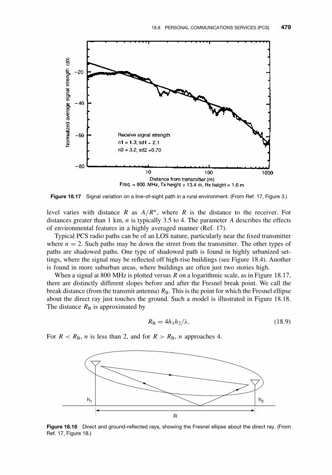
18.8 PERSONAL COMMUNICATIONS SERVICES (PCS) 479
Figure 18.17 Signal variation on a line-of-sight path in a rural environment. (From Ref. 17, Figure 3.)
level varies with distance R as A/Rn, where R is the distance to the receiver. Fordistances greater than 1 km, n is typically 3.5 to 4. The parameter A describes the effectsof environmental features in a highly averaged manner (Ref. 17).
Typical PCS radio paths can be of an LOS nature, particularly near the fixed transmitterwhere n = 2. Such paths may be down the street from the transmitter. The other types ofpaths are shadowed paths. One type of shadowed path is found in highly urbanized set-tings, where the signal may be reflected off high-rise buildings (see Figure 18.4). Anotheris found in more suburban areas, where buildings are often just two stories high.
When a signal at 800 MHz is plotted versus R on a logarithmic scale, as in Figure 18.17,there are distinctly different slopes before and after the Fresnel break point. We call thebreak distance (from the transmit antenna) RB. This is the point for which the Fresnel ellipseabout the direct ray just touches the ground. Such a model is illustrated in Figure 18.18.The distance RB is approximated by
RB = 4h1h2/λ. (18.9)
For R < RB, n is less than 2, and for R > RB, n approaches 4.
R
h2h1
Figure 18.18 Direct and ground-reflected rays, showing the Fresnel ellipse about the direct ray. (FromRef. 17, Figure 18.)

480 CELLULAR AND PCS RADIO SYSTEMS
It was found that on non-LOS paths in an urban environment with low base stationantennas and with users at street level, propagation takes place down streets and aroundcorners rather than over buildings. For these non-LOS paths the signal must turn cornersby multiple reflections and diffraction at vertical edges of buildings. Field tests reveal thatsignal level decreases by about 20 dB when turning a corner.
In the case of propagation inside buildings where the transmitter and receiver are onthe same floor, the key factor is the clearance height between the average tops of furnitureand the ceiling.
Bertoni et al. (Ref. 17) call this clearance W . Here building construction consists ofdrop ceilings of acoustical material supported by metal frames. That space between thedrop ceiling and the floor above contains light fixtures, ventilation ducts, pipes, sup-port beams, and so on. Because the acoustical material has a low dielectric constant,the rays incident on the ceiling penetrate the material and are strongly scattered by theirregular structure, rather than undergoing specular reflection. Floor-mounted buildingfurnishings such as desks, cubicle partitions, filing cabinets, and workbenches scatter therays and prevent them from reaching the floor, except in hallways. Thus it is concludedthat propagation takes place in the clear space, W .
Figure 18.19 shows a model of a typical floor layout in an office building. When boththe transmitter and receiver are located in the clear space, path loss can be related tothe Fresnel ellipse. If the Fresnel ellipse associated with the path lies entirely in theclear space, the path loss has LOS properties (1/L2). Now as the separation betweenthe transmitter and receiver increases, the Fresnel ellipse grows in size so that scattererslie within it. This is shown in Figure 18.20. Now the path loss becomes greater thanfree space.
Bertoni et al. report one measurement program where the scatterers have been simu-lated using absorbing screens. It was recognized that path loss will be highly dependenton nearby scattering objects. Figure 18.19 was developed from this program. The pathloss in excess of free space calculated at 900 and 1900 MHz where W = 1.5 m is plottedin Figure 18.20 as a function of path length L. The figure shows that the excess path loss(over LOS) is small at each frequency out to distances of about 20 to 40 m, respectively,where it increases dramatically.
Propagation between floors of a modern office building can be very complex. If thefloors are constructed of reinforced concrete or prefabricated concrete, transmission losscan be 10 dB or more. Floors constructed of concrete poured over steel panels showmuch greater loss. In this case (Ref. 17), signals may propagate over other paths involving
W
Fresnel zone
Ceiling
Floor
L
Figure 18.19 Fresnel zone for propagation between transmitter and receiver in clear space betweenbuilding furnishings and ceiling fixtures. (From Ref. 17, Figure 35.)

18.9 CORDLESS TELEPHONE TECHNOLOGY 481
5
0
−5
−10
−15
−20
−25
−30
−35
Clear space: 1.49 m
Excess path loss1900 MHz910 MHzTheoretical 900 MHzTheoretical 1800 MHz
Exc
ess
path
loss
(dB
)
Separation between transmitter and receiver1 10 100
Figure 18.20 Measured and calculated excess path loss at 900 and 1800 MHz for a large office buildinghaving head-high cubical partitions, but no floor-to-ceiling partitions. (From Ref. 17, Figure 36.)
diffraction rather than transmission through the floors. For instance, signals can exit thebuilding through windows and reenter on higher floors by diffraction mechanisms alongthe face of the building.
18.9 CORDLESS TELEPHONE TECHNOLOGY
18.9.1 Background
Cordless telephones began to become widely used in North America around 1981. Todaytheir popularity is worldwide with hundreds of millions of units in use. As the technologydevelops, they will begin to compete with cellular radio systems, where the cordlesstelephone will operate in microcells.
18.9.2 North American Cordless Telephones
The North American cordless telephone operates in the 50-MHz frequency band with25 frequency pairs using frequency modulation. Their ERP is on the order of 20 µW.Reference 18 suggests that this analog technology will continue for some time into thefuture because of the telephone’s low cost. These may be replaced by some form of thewireless local loop (WLL) operating in the 30- or 40-GHz band.
18.9.3 European Cordless Telephones
The first-generation European cordless telephone provided for eight channel pairs near1.7 MHz (base unit transmit) and 47.5 MHz (handset transmit). Most of these units couldonly access one or two channel pairs. Some called this “standard” CT0.
This was followed by another analog cordless telephone based on a standard known asCEPT/CT1. CT1 has 40 25-kHz duplex channel pairs operating in the bands 914–915 MHzand 959–960 MHz. There is also a CT1+ in the bands 885–887 MHz and 930–932 MHz,which do not overlap the GSM allocation. CT1 is called a coexistence standard (not acompatible standard), such that cordless telephones from different manufacturers do not

482 CELLULAR AND PCS RADIO SYSTEMS
interoperate. The present embedded base is about 50 million units with some 15 millionunits are expected to be sold in 2004.
Two digital standards have evolved in Europe: the CT2 Common Air Interface andDECT (digital European cordless telephone). In both standards, speech coding usesADPCM (adaptive differential PCM). The ADPCM speech and control data are mod-ulated onto a carrier at a rate of 72 kbps using Gaussian-filtered FSK (GFSK) and aretransmitted in 2-msec frames. One base-to-handset burst and one handset-to-base burstare included in each frame.
The frequency allocation for CT2 consists of 40 FDMA channels with 100-kHz spac-ing in the band 864–868 MHz. The maximum transmit power is 10 mW, and a two-levelpower control supports prevention of desensitization of base station receivers. As abyproduct, it contributes to frequency reuse. CT2 has a call reestablishment procedure onanother frequency after three seconds of unsuccessful attempts on the initial frequency.This gives a certain robustness to the system when in an interference environment. CT2supports up to 2400 bps of data transmission and higher rates when accessing the 32 kbpsunderlying bearer channels.
CT2 also is used for wireless pay telephones. When in this service it is called Telepoint.CT2 seems to have more penetration in Asia than in Europe.
Canada has its own version of CT2, called CT2+. It is more oriented toward the mobileenvironment, providing several of the missing mobility functions in CT2. For example,with CT2+, 5 of the 40 carriers are reserved for signaling, where each carrier provides12 common channel signaling channels (CSCs) using TDMA. These channels supportlocation registration, updating, and paging, and enable Telepoint subscribers to receivecalls. The CT2+ band is 944–948 MHz.
DECT takes on more of the cellular flavor than CT2. It uses a picocell concept andTDMA with handover, location registration, and paging. It can be used for Telepoint,radio local loop (RLL), and cordless PABX besides conventional cordless telephony. Itsspeech coding is similar to CT2, namely, ADPCM. For its initial implementation, 10carriers have been assigned in the band 1880–1900 MHz.
There are many areas where DECT will suffer interference in the assigned band,particularly from “foreign” mobiles. To help alleviate this problem, DECT uses two strate-gies: interference avoidance and interference confinement. The avoidance technique avoidstime/frequency slots with a significant level of interference by handover to another slot atthe same or another base station. This is very attractive for the uncoordinated operationof base stations because in many interference situations there is no other way around asituation but to change in both the time and frequency domains. The “confinement” con-cept involves the concentration of interference to a small time–frequency element evenat the expense of some system robustness.
Base stations must be synchronized in the DECT system. A control channel carriesinformation about access rights, base station capabilities, and paging messages. The DECTtransmission rate is 1152 kbps. As a result of this and a relatively wide bandwidth,either equalization or antenna diversity is typically needed for using DECT in the moredispersive microcells.
Japan has developed the personal handyphone system (PHS). Its frequency allocationis 77 channels, 300 kHz in width, in the band 1895–1918.1 MHz. The upper-half of theband, 1906.1–1918.1 MHz (40 frequencies), is used for public systems. The lower-halfof the band, 1895–1906.1 MHz, is reserved for home/office operations. An operationalchannel is autonomously selected by measuring the field strength and selecting a channelon which it meets certain level requirements. In other words, fully dynamic channelassignment is used. The modulation is π /4 DQPSK; average transmit power at the handset

18.10 WIRELESS LANS 483
Table 18.1 Digital Cordless Telephone Interface Summary
CT2 CT2 + DECT PHS PACS
Region Europe Canada Europe Japan United StatesDuplexing TDD TDD TDD FDDFrequency band (MHz) 864–868 944–948 1800–1900 1895–1918 1850–1910/1930–1990a
Carrier spacing (kHz) 100 1728 300 300/300Number of carriers 40 10 77 16 pairs/10 MHzBearer channels/carrier 1 12 4 8/pairChannel bit rate (kbps) 72 1152 384 384Modulation GFSK GFSK π /4 DQPSK π /4 QPSKSpeech coding 32 kbps 32 kbps 32 kbps 32 kbpsAverage handset
transmit power (mW)5 10 10 25
Peak handset transmitpower (mW)
10 250 80 200
Frame duration (msec) 2 10 5 2.5
aGeneral allocation to PCS; licensees may use PACS.
Source: Ref. 18, Table 2.
is 10 mW (80-mW peak power) and no greater than 500 mW (4-W peak power) for thecell site. The PHS frame duration is 5 msec. Its voice coding technique is 32-kbps ADPCM(Ref. 8).
In the United States, digital PCS was based on the wireless access communicationsystem (WACS), which has been modified to an industry standard called PACS (personalaccess communications services). It is intended for the licensed portion of the new 2-GHz spectrum. Its modulation is π /4 QPSK with coherent detection. Base stations areenvisioned as shoebox-size enclosures mounted on telephone poles, separated by some600 m. WACS/PACS has an air interface similar to other digital cordless interfaces, exceptit uses frequency division duplex (FDD) rather than time division duplex (TDD) and moreeffort has gone into optimizing frequency reuse and the link budget. It has two-branchpolarization diversity at both the handset and base station with feedback. This gives it anadvantage approaching four-branch receiver diversity. The PACS version has eight timeslots and a corresponding reduction in channel bit rate and a slight increase in frameduration over its predecessor, WACS. Table 18.1 summarizes the characteristics of theseseveral types of digital cordless telephones and their interfaces.
18.10 WIRELESS LANS
Wireless LANs (WLANs), much like their wired counterparts, operate in excess of1 Mbps. Signal coverage runs from 50 ft to less than 1000 ft. The transmission mediumcan be radiated light (around 800 nm to 900 nm) or radio frequency, unlicensed. Severalof these latter systems use spread spectrum with transmitter outputs of 1 W or less.
WLANs using radiated light do not require FCC licensing, a distinct advantage. Theyare immune to RF interference but are limited in range by office open spaces becausetheir light signals cannot penetrate walls. Shadowing can also be a problem.
One type of radiated light WLAN uses a directed light beam. These are best suited forfixed terminal installations because the transmitter beams and receivers must be carefullyaligned. The advantages for directed beam systems is improved S/N and fewer problemswith multipath. One such system is fully compliant with IEEE 802.5 token ring operationoffering 4- and 16-Mbps transmission rates.

484 CELLULAR AND PCS RADIO SYSTEMS
Spread spectrum WLANs use the 900-MHz, 2-GHz, and 5-GHz industrial, scientific,and medical (ISM) bands. Both direct sequence and frequency hop operation can be used.Directional antennas at the higher frequencies provide considerably longer range thanradiated light systems, up to several miles or more. No FCC license is required. A prin-cipal user of these higher-frequency bands is microwave ovens with their interferencepotential. CSMA and CSMA/CD (IEEE 802.3) protocols are often employed.
There is also a standard microwave WLAN (nonspread spectrum) that operates in theband 18–19 GHz. FCC licensing is required.
Building wall penetration loss is high. The basic application is for office open spaces.
18.11 MOBILE SATELLITE COMMUNICATIONS
18.11.1 Background and Scope
This section contains a brief review of low earth orbit (LEO) satellite systems serving thePCS/cellular market. Most LEO satellite systems discussed here utilize frequency reuseand are based on a cellular concept.
18.11.2 Advantages and Disadvantages of LEO Systems
Delay One-way delay to a GEO satellite is budgeted at 125 msec; one-way up anddown is double this value, or 250 msec. Round-trip delay is about 0.5 sec. Delayto a typical LEO satellite is 2.67 msec and round-trip delay is 4 × 2.67 msec orabout 10.66 msec. Calls to/from mobile users of such systems may be relayed stillagain by conventional satellite services. Data services do not have to be so restrictedon the use of “handshakes” and stop-and-wait ARQ as with similar services via aGEO system.
Higher Elevation Angles and “Full Earth Coverage.” The GEO satellite provides nocoverage above about 80◦ latitude and gives low-angle coverage of many of theworld’s great population centers because of their comparatively high latitude. Typ-ically, cities in Europe and Canada face this dilemma. LEO satellites, dependingon orbital plane spacing, can all provide elevation angles >40◦. This is particularlyattractive in urban areas with tall buildings. Coverage with GEO systems wouldonly be available on the south side of such buildings in the Northern Hemispherewith a clear shot to the horizon. Properly designed LEO systems will not have suchdrawbacks. Coverage will be available at any orientation.
Tracking, a Disadvantage of LEO and MEO9 Satellites At L-band quasiomnidirectionalantennas for the mobile user are fairly easy to design and produce. Although suchantennas display only modest gain of several decibels, links to a LEO satellitecan be easily closed with hand-held terminals. However, large feeder, fixed-earthterminals will require a good tracking capability as LEO satellites pass overhead.Handoff is also required as a LEO satellite disappears over the horizon and anothersatellite just appears over the opposite horizon. The handoff should be seamless.The quasi-omnidirectional user terminal antennas will not require tracking, and thehandoff should not be noticeable to the mobile user.
9 MEO stands for medium earth orbit.

REVIEW EXERCISES 485
REVIEW EXERCISES
1. What is the principal drawback in cellular radio considering its explosive growthover the past decade?
2. Why is transmission loss so much greater on a cellular path compared to a LOSmicrowave path on the same frequency covering the same distance?
3. What is the function of the MTSO or MSC in a cellular network?
4. What is the channel spacing in kHz of the AMPS system? What type of modulationdoes it employ?
5. Why are cell site antennas limited to just sufficient height to cover cell boundaries?
6. Why do we do cell splitting? What is the approximate minimum practical celldiameter (this limits splitting).
7. When is handover necessary?
8. Cellular transmission loss varies with what four factors besides distance and frequency?
9. What are some of the fade ranges (decibels) we might expect on a cellular link?
10. If the delay spread on a cellular link is about 10 µsec, up to about what bit rate willthere be little deleterious effects due to multipath fading?
11. Space diversity reception is common at cells sites. Antenna separation varies with?
12. For effective space diversity operation, there is a law of diminishing returns whenwe lower the correlation coefficient below what value?
13. What is the gain of a standard dipole over a reference isotropic antenna? DifferentiateERP and EIRP.
14. Cellular designers use a field strength contour of dBµ, which is equivalent todBm.
15. What would the maximum transmission loss to the 39-dBµ contour be if the cellsite EIRP is +52 dBm?
16. A cell site antenna has a gain of +14 dBd. What is the equivalent gain in dBi?
17. What are the three generic access techniques that might be considered for digitalcellular operation?
18. If we have 10 cellular users on a TDMA frame and the frame duration is 20 msec,what is the maximum burst duration without guard time considerations?
19. What are the two basic elements in digital cellular transmission with which we mayimprove users per unit bandwidth?
20. What power amplifier advantage do we have in a TDMA system we do not have inan FDMA system assuming a common power amplifier for all RF channels?
21. Cellular radio, particularly in urban areas, is gated by heavy interference conditions,especially cochannel from frequency reuse. In light of this, describe how we achievean interference advantage when using CDMA.

486 CELLULAR AND PCS RADIO SYSTEMS
22. A CDMA system has an information bit stream of 4800 bps which is spread 10 MHz.What is the processing gain?
23. For effective frequency reuse, the value of D/R must be kept large enough. DefineD and R. What value of D/R is large enough?
24. In congested urban areas where cell diameters are small, what measure can we taketo reduce C/I?
25. What is the effect of the Fresnel ellipse?
26. What range of transmitter output power can we expect from cordless telephone PCS?
27. Why would it be attractive to use CDMA with a RAKE receiver for PCS systems?
28. Speech coding is less stringent with PCS scenarios, typically 32 kbps. Why?
29. What are the two different transmission media used with WLANs?
30. Give two decided advantages of LEO satellite systems over their GEO counterparts.
REFERENCES
1. Telecommunications Transmission Engineering, 3rd ed., Bellcore, Piscataway, NJ, 1989.
2. Raymond Steele, ed., Mobile Radio Communications, IEEE Press, New York, and PentechPress, London, 1992.
3. Y. Okumura et al., “Field Strength and Its Variability in VHF and UHF Land Mobile Service,”Rec. Electr. Commun. Lab., 16, Tokyo, 1968.
4. M. Hata, “Empirical Formula for Propagation Loss in Land-Mobile Radio Services,” IEEETrans. Vehicular Technology, VT-20, 1980.
5. F. C. Owen and C. D. Pudney, “In-Building Propagation at 900 and 1650 MHz for DigitalCordless Telephones,” 6th International Conference on Antennas and Propagation, ICCAP, Pt.2, Propagation Conf. Pub. No. 301, 1989.
6. IEEE 100 The Authoritative Dictionary of IEEE Standards Terms, 7th ed., IEEE, Hoboken,2004.
7. W. C. Y. Lee, Mobile Communications Design Fundamentals, 2nd ed., Wiley, New York, 1993.
8. Recommended Minimum Standards for 800-MHz Cellular Subscriber Units , EIA Interim Stan-dard EIA/IS-19B, EIA, Washington, DC, 1988.
9. Cellular Radio Systems, a seminar given at the University of Wisconsin–Madison by AndrewH. Lamothe, Consultant, Leesbury, VA, 1993.
10. R. C. V. Macario, ed., Personal and Mobile Radio Systems, IEE/Peter Peregrinus, London,1991.
11. Woldemar F. Fuhrmann and Volker Brass, “Performance Aspects of the GSM System,” Proc.IEEE, 89(9), 1984.
12. Digital Cellular Public Land Mobile Telecommunication Systems (DCPLMTS), CCIR Rep.1156, Vol. VIII.1 XVIIth Plenary Assembly, Dusseldorf, 1990.
13. M. Engelson and J. Hebert, “Effective Characterization of CDMA Signals,” Wireless Rep.,London, Jan. 1995.
14. R. C. Dixon, Spread Spectrum Systems with Commercial Applications, 3rd ed., Wiley, NewYork, 1994.
15. C. E. Cook and H. S. Marsh, “An Introduction to Spread Spectrum,” IEEE CommunicationsMagazine, March 1983.
16. D. C. Cox, “Wireless Personal Communications. What Is It?” IEEE Personal Communications,2(2), 1995.

REFERENCES 487
17. H. L. Bertoni et al., “UHF Propagation Prediction for Wireless Personal Communication,”Proc. IEEE, 89(9), 1994.
18. J. C. Padgett, Cristoph G. Gunter, and Takeshi Hattori, “Overview of Wireless Personal Com-munications,” IEEE Communications Magazine, Jan. 1995.
19. R. L. Freeman, “Telecommunication System Engineering,” 4th ed, Wiley, Hoboken, NJ, 2004.


19
ADVANCED BROADBAND DIGITALTRANSPORT FORMATS
19.1 OBJECTIVE AND SCOPE
In the early 1980s, fiber-optic transmission links burst upon the telecommunication trans-port scene. The potential bit rate capacity of these new systems was so great that therewas no underlying digital format to accommodate such transmission rates. The maximumbit rate in the DS1 family of digital formats was DS4 at 274 Mbps; and for the E1 family,E4 at 139 Mbps. These data rates satisfied the requirements of the metallic transmissionplant, but the evolving fiber-optic plant had the promise of much greater capacity, in themultigigabit region.
In the mid-1980s ANSI and Bellcore began to develop a new digital format standardspecifically designed for the potential bit rates of fiber optics. The name of this structureis SONET, standing for Synchronous Optical Network.
As the development of SONET was proceeding, CEPT1 showed interest in the devel-opment of a European standard. In 1986 CCITT stepped in proposing a singular standardthat would accommodate U.S., European, and Japanese hierarchies. This unfortunatelywas not achieved due more to time constraints on the part of U.S. interests. As a result,there are two digital format standards: SONET and the synchronous digital hierarchy(SDH) espoused by CCITT.
It should be pointed out that these formats are optimized for voice operation with125-µsec frames. Both types commonly carry plesiochronous digital hierarchy (PDH)formats such as DS1 and E1, as well as ATM cells.2
In the general scheme of things, the interface from one to the other will take placeat North American gateways. In other words, international trunks are SDH-equipped, notSONET-equipped. The objective of this chapter is to provide a brief overview of bothSONET and SDH standards.
1CEPT stands for Conference European Post & Telegraph, a European telecommunication standardizationagency based in France. In 1990 the name of the agency was changed to ETSI—European TelecommunicationStandardization Institute.2Held (Ref. 9) defines plesiochronous as “a network with multiple stratum 1 primary reference sources.” SeeSection 6.12.1. In this context, when transporting these PCM formats, the underlying network timing andsynchronization must have stratum 1 traceability.
Fundamentals of Telecommunications, Second Edition, by Roger L. FreemanISBN 0-471-71045-8 Copyright 2005 by Roger L. Freeman
489

490 ADVANCED BROADBAND DIGITAL TRANSPORT FORMATS
19.2 SONET
19.2.1 Introduction and Background
The SONET standard was developed by the ANSI T1X1 committee with first publicationin 1988. The standard defines the features and functionality of a transport system based onthe principles of synchronous multiplexing. In essence this means that individual tributarysignals may be multiplexed directly into a higher rate SONET signal without intermediatestages of multiplexing.
DS1 and E1 digital hierarchies had rather limited overhead capabilities for networkmanagement, control, and monitoring. SONET (and SDH) provides a rich built-in capac-ity for advanced network management and maintenance capabilities. Nearly 5% of theSONET signal structure is allocated to supporting such management and maintenanceprocedures and practices.
SONET is capable of transporting all the tributary signals that have been defined forthe digital networks in existence today. This means that SONET can be deployed asan overlay to the existing network and, where appropriate, provide enhanced networkflexibility by transporting existing signal types. In addition, SONET has the flexibility toreadily accommodate the new types of customer service signals such as SMDS (switchedmultimegabit data service) and ATM (asynchronous transfer mode). Actually, it can carryany octet-based binary format such as TCP/IP, SNA, OSI regimes, X.25, frame relay, andvarious LAN formats, which have been packaged for long-distance transmission.
19.2.2 Synchronous Signal Structure
SONET is based on a synchronous signal comprised of 8-bit octets, which are organizedinto a frame structure. The frame can be represented by a two-dimensional map comprisingN rows and M columns, where each box so derived contains one octet (or byte). Theupper left-hand corner of the rectangular map representing a frame contains an identifiablemarker to tell the receiver it is the start of frame.
SONET consists of a basic, first-level, structure called STS-1, which is discussed inthe following. The definition of the first level also defines the entire hierarchy of SONETsignals because higher-level SONET signals are obtained by synchronously multiplexingthe lower-level modules. When lower-level modules are multiplexed together, the resultis denoted as STS-N (STS stands for synchronous transport signal), where N is an integer.The resulting format then can be converted to an OC-N (OC stands for optical carrier) orSTS-N electrical signal. There is an integer multiple relationship between the rate of thebasic module STS-1 and the OC-N electrical signals (i.e., the rate of an OC-N is equalto N times the rate of an STS-1). Only OC-1, -3, -12, -24, -48, and -192 are supportedby today’s SONET.
19.2.2.1 Basic Building Block Structure. The STS-1 frame is shown in Figure 19.1.STS-1 is the basic module and building block of SONET. It is a specific sequence of 810octets3 (6480 bits), which includes various overhead octets and an envelope capacity fortransporting payloads. STS-1 is depicted as a 90-column, 9-row structure with a frameperiod of 125 µsec (i.e., 8000 frames per second). STS-1 has a bit rate of 51.840 Mbps.Consider Figure 19.1. The order of transmission of octets is row-by-row, from left toright. In each octet of STS-1 the most significant bit is transmitted first.
3The reference publications use the term byte, meaning, in this context, an 8-bit sequence. We prefer to usethe term octet. The reason is that some argue that byte is ambiguous with conflicting definitions.

19.2 SONET 491
Figure 19.1 The STS-1 frame.
Figure 19.2 STS-1 synchronous payload envelope (SPE).
As illustrated in Figure 19.1, the first three columns of the STS-1 frame contain theTransport Overhead. These three columns have 27 octets (i.e., 9X3), of which nine areused for the section overhead and 18 octets contain the line overhead. The remaining 87columns make up the STS-1 Envelope Capacity as illustrated in Figure 19.2.
The STS-1 synchronous payload envelope (SPE) occupies the STS-1 envelope capacity.The STS-1 SPE consists of 783 octets and is depicted as an 87-column by 9-row structure.In that structure, column 1 contains 9 octets and is designated as the STS path overhead(POH). In the SPE columns 30 and 59 are not used for payload but are designated asfixed-stuff columns. The 756 octets in the remaining 84 columns are used for the actualSTS-1 payload capacity.
Figure 19.3 shows the fixed-stuff columns 30 and 59 inside the SPE. The referencedocument (Ref. 1) states that the octets in these fixed-stuff columns are undefined andare set to binary 0s. However, the values used to stuff these columns of each STS-1SPE will produce even parity in the calculation of the STS-1 Path BIP-8 (BIP = pathinterleaved parity).
The STS-1 SPE may begin anywhere in the STS-1 envelope capacity. Typically theSPE begins in one STS-1 frame and ends in the next. This is illustrated in Figure 19.4.However, on occasion the SPE may be wholly contained in one frame. The STS payloadpointer resides in the transport overhead. It designates the location of the next octet wherethe SPE begins. Payload pointers are described in the following paragraphs.

492 ADVANCED BROADBAND DIGITAL TRANSPORT FORMATS
Figure 19.3 POH and the STS-1 payload capacity within the STS-1 SPE. Note that the net payloadcapacity in the STS-1 frame is only 84 columns.
Figure 19.4 STS-1 SPE typically located in STS-1 frames. (From Ref. 2, courtesy of Hewlett-Packard.)
The STS POH (path overhead) is associated with each payload and is used to commu-nicate various pieces of information from the point where the payload is mapped into theSTS-1 SPE to the point where it is delivered. Among the pieces of information carriedin the POH are alarm and performance data.
19.2.2.2 STS-N Frames. Figure 19.5 illustrates the structure of an STS-N frame. Theframe consists of a specific sequence of NX810 octets. The STS-N frame is formedby octet-interleave STS-1 and STS-M (<N) modules. The transport overhead of theindividual STS-1 and STS-M modules are frame-aligned before interleaving, but theassociated STS SPEs are not required to be aligned because each STS-1 has a payloadpointer to indicate the location of the SPE or to indicate concatenation.

19.2 SONET 493
Figure 19.5 STS-N frame.
19.2.2.3 STS Concatenation. Superrate payloads require multiple STS-1 SPEs. FDDIand some B-ISDN payloads fall into this category. Concatenation means the linkingtogether. An STS-Nc module is formed by linking N constituent STS-1s together in afixed phase alignment. The superrate payload is then mapped into the resulting STS-NcSPE for transport. Such STS-Nc SPE requires an OC-N4 or an STS-N electrical signal.Concatenation indicators contained in the second through the N th STS payload pointerare used to show that the STS-1s of an STS-Nc are linked together.
There are NX783 octets in an STS-Nc. Such an STS-Nc arrangement is illustratedin Figure 19.6 and is depicted as an NX87 column by 9-row structure. Because of thelinkage, only one set of STS POH is required in the STS-Nc SPE. Here the STS POHalways appears in the first of the N STS-1s that make up the STS-Nc (Ref. 3).
Figure 19.7 shows the transport overhead assignment of an OC-3 carrying an STS-3c SPE.
Figure 19.6 STS-3c concatenated SPE. [Courtesy of Hewlett-Packard (Ref. 2).]
4OC-N stands for optical carrier at the N level. This has the same electrical signal as STS-N and the same bitrate and format structure.

494 ADVANCED BROADBAND DIGITAL TRANSPORT FORMATS
Figure 19.7 Transport overhead assignment showing OC-3 carrying an STS-3c SPE. (Based on Ref. 1,Figure 3-8 and updated to current practice.)
Figure 19.8 The virtual tributary (VT) concept. (From Ref. 2, courtesy of Hewlett-Packard.)
19.2.2.4 Structure of Virtual Tributaries (VTs). The SONET STS-1 SPE with achannel capacity of 50.11 Mbps has been designed specifically to transport a DS3 tribu-tary signal. To accommodate sub-STS-1 rate payloads such as DS1, the VT structure isused. It consists of four sizes: VT1.5 (1.728 Mbps) for DS1 transport, VT2 (2.304 Mbps)for E1 transport, VT3 (3.456 Mbps) for DS1C transport, and VT6 (6.912 Mbps) for DS2transport. The virtual tributary concept is illustrated in Figure 19.8. The four VT configu-rations are shown in Figure 19.9. In the 87-column by 9-row structure of the STS-1 SPE,the VTs occupy 3, 4, 6, and 12 columns, respectively.

19.2 SONET 495
Figure 19.9 The four sizes of virtual tributary frames. (From Ref. 2, courtesy of Hewlett-Packard.)
There are two VT operating modes: floating mode and locked mode. The floating modewas designed to minimize network delay and provide efficient cross-connects of transportsignals at the VT level within the synchronous network. This is achieved by allowing eachVT SPE to float with respect to the STS-1 SPE in order to avoid the use of unwantedslip buffers at each VT cross-connect point.5 Each VT SPE has its own payload pointer,which accommodates timing synchronization issues associated with the individual VTs.As a result, by allowing a selected VT1.5, for example, to be cross-connected betweendifferent transport systems without unwanted network delay, this mode allows a DS1 tobe transported effectively across a SONET network.
The locked mode minimizes interface complexity and supports bulk transport of DS1signals for digital switching applications. This is achieved by locking individual VT SPEsin fixed positions with respect to the STS-1 SPE. In this case, each VT1.5 SPE is notprovided with its own payload pointer. With the locked mode it is not possible to route aselected VT1.5 through the SONET network without unwanted network delay caused byhaving to provide slip buffers to accommodate the timing/synchronization issues.
19.2.2.5 The Payload Pointer. The STS payload pointer provides a method for allow-ing flexible and dynamic alignment of the STS SPE within the STS envelope capacity,independent of the actual contents of the SPE. SONET, by definition, is intended tobe synchronous. It derives its timing from the master network clock. See Chapter 6,Section 6.12.2.
Modern digital networks must make provision for more than one master clock.Examples in the United States are the several interexchange carriers that interface withlocal exchange carriers, each with their own master clock. Each master clock (stratum1) operates independently. And each of these master clocks has excellent stability (i.e.,better than 1 × 10⁻¹¹ per month), yet there may be some small variance in time amongthe clocks. Assuredly they will not be phase-aligned. Likewise, SONET must take intoaccount loss of master clock or a segment of its timing delivery system. In this case,switches fall back on lower-stability internal clocks. This situation must also be handledby SONET. Therefore synchronous transport must be able to operate effectively underthese conditions where network nodes are operating at slightly different rates.
5Slips are discussed in Chapter 6.

496 ADVANCED BROADBAND DIGITAL TRANSPORT FORMATS
To accommodate these clock offsets, the SPE can be moved (justified) in the positive ornegative direction one octet at a time with respect to the transport frame. This is achievedby recalculating or updating the payload pointer at each SONET network node. In additionto clock offsets, updating the payload pointer also accommodates any other timing phaseadjustments required between the input SONET signals and the timing reference at theSONET node. This is what is meant by dynamic alignment where the STS SPE is allowedto float within the STS envelope capacity.
The payload pointer is contained in the H1 and H2 octets in the line overhead (LOH)and designates the location of the octet where the STS SPE begins. These two octets areviewed in Figure 19.10. Bits 1 through 4 of the pointer word carry the new data flag, andbits 7 through 16 carry the pointer value. Bits 5 and 6 are undefined.
Let’s discuss bits 7 through 16, the actual pointer value. It is a binary number witha range of 0 to 782. It indicates the offset of the pointer word and the first octet of theSTS SPE (i.e., the J1 octet). The transport overhead octets are not counted in the offset.For example, a pointer value of 0 indicates that the STS SPE starts in the octet locationthat immediately follows the H3 octet, whereas an offset of 87 indicates that it startsimmediately after the K2 octet location.
Payload pointer processing introduces a signal impairment known as payload adjust-ment jitter. This impairment appears on a received tributary signal after recovery from aSPE that has been subjected to payload pointer changes. The operation of the networkequipment processing the tributary signal immediately downstream is influenced by thisexcessive jitter. By careful design of the timing distribution for the synchronous network,payload pointer adjustments can be minimized, thus reducing the level of tributary jitterthat can be accumulated through synchronous transport.
19.2.2.6 The Three Overhead Levels of SONET. The three embedded overheadlevels of SONET are
ž Path (POH)ž Line (LOH)ž Section (SOH)
These overhead levels, represented as spans, are illustrated in Figure 19.11. One importantfunction is to support network operation and maintenance (OAM).
The POH consists of 9 octets and occupies the first column of the SPE, as pointed outpreviously. It is created and included in the SPE as part of the SPE assembly process. ThePOH provides the facilities to support and maintain the transport of the SPE between pathterminations, where the SPE is assembled and disassembled. Among the POH specificfunctions are:
ž An 8-bit-wide (octet B3) BIP (bit-interleaved parity) check calculated over all bits ofthe previous SPE. The computed value is placed in the POH of the following frame.
ž Alarm and performance information (octet G1).ž A path signal label (octet C2); gives details of SPE structure. It is 8 bits wide, which
can identify up to 256 structures (28).ž One octet (J1) repeated through 64 frames can develop an alphanumeric message
associated with the path. This allows verification of continuity of connection to thesource of the path signal at any receiving terminal along the path by monitoring themessage string.

Fig
ure
19.1
0S
TSp
aylo
adp
oint
er(H
1,H
2)co
din
g.
497

498 ADVANCED BROADBAND DIGITAL TRANSPORT FORMATS
SPEAssembly
SonetMultiplexerTerminal
SonetDemultiplexerTerminal
DSXsignals
DSXsignals
SPEDisassembly
Line Line
Path
Section Section
Section
Section
Regenerator Regenerator Regenerator
SonetCross-section
Figure 19.11 SONET section, line and path definitions.
ž An orderwire for network operator communications between path equipment(octet F2).
Facilities to support and maintain the transport of the SPE between adjacent nodesare provided by the line and section overhead. These two overhead groups share the firstthree columns of the STS-1 frame (see Figure 19.1). The SOH occupies the top threerows (total of 9 octets) and the LOH occupies the bottom 6 rows (18 octets).
The line overhead functions include:
ž Payload pointer (octets H1, H2, and H3) (each STS-1 in an STS-N frame has itsown payload pointer).
ž Automatic protection switching control (octets K1 and K2).ž BIP parity check (octet B2).ž 576-kbps data channel (octets D4 through D12).ž Express orderwire (octet E2).
A section is defined in Figure 19.11. Among the section overhead functions are:
ž Frame alignment pattern (octets A1, A2).ž STS-1 identification (octet C1): a binary number corresponding to the order of
appearance in the STS-N frame, which can be used in the framing and deinter-leavingprocess to determine the position of other signals.
ž BIP-8 parity check (octet B1): section error monitoring.ž Data communications channel (octets D1, D2, and D3).ž Local orderwire channel (octet E1).ž User channel (octet F1).
19.2.2.7 The SPE Assembly/Disassembly Process. Payload mapping is the pro-cess of assembling a tributary signal into an SPE. It is fundamental to SONET operation.The payload capacity provided for each individual tributary signal is always slightlygreater than that required by the tributary signal. The mapping process, in essence, is tosynchronize the tributary signal with the payload capacity. This is achieved by addingstuffing bits to the bit stream as part of the mapping process.
An example might be a DS3 tributary signal at a nominal rate of 44.736 Mbps to besynchronized with a payload capacity of 49.54 Mbps provided by an STS-1 SPE. The

19.2 SONET 499
Figure 19.12 The SPE assembly process. (From Ref. 2, courtesy of Hewlett-Packard.)
Figure 19.13 The SPE disassembly process. (From Ref. 2, courtesy of Hewlett-Packard.)
addition of path overhead completes the assembly process of the STS-1 SPE and increasesthe bit rate of the composite signal to 50.11 Mbps. The SPE assembly process is showngraphically in Figure 19.12. At the terminus or drop point of the network, the originalDS3 payload must be recovered as in our example. The process of SPE Disassembly isshown in Figure 19.13. The term used here is payload demapping.
The demapping process desynchronizes the tributary signal from the composite SPEsignal by stripping off the path overhead and the added stuff bits. In the example, anSTS-1 SPE with a mapped DS3 payload arrives at the tributary disassembly locationwith a signal rate of 50.11 Mbps. The stripping process results in a discontinuous signalrepresenting the transported DS3 signal with an average signal rate of 44.74 Mbps. Thetiming discontinuities are reduced by means of a desynchronizing phase-locked loop,which then produces a continuous DS3 signal at the required average transmission rate(Refs. 1, 2).
19.2.2.8 Line Rates for Standard SONET Interface Signals. Table 19.1 shows thestandard line transmission rates for OC-N (OC = optical carrier) and STS-N.
19.2.3 Add–Drop Multiplexer
The SONET ADM multiplexes one or more DS-n signals into the SONET OC-N channel.An ADM can be configured for either the add–drop or terminal mode. In the ADM mode,it can operate when the low-speed DS1 signals terminating at the SONET derive timingfrom the same or equivalent source as (SONET) (i.e., synchronous) but do not derivetiming from asynchronous sources.
Figure 19.14 is an example of an ADM configured in the add–drop mode with DS1and OC-N interfaces. A SONET ADM interfaces with two full-duplex OC-N signals and

500 ADVANCED BROADBAND DIGITAL TRANSPORT FORMATS
Table 19.1 Line Rates for Standard SONETInterface Signals
OC-N Level STS-N Electrical Level Line Rate (Mbps)
OC-1 STS-1 electrical 51.84OC-3 STS-3 electrical 155.52OC-12 STS-12 electrical 622.08OC-24 STS-24 electrical 1244.16OC-48 STS-48 electrical 2488.32OC-192 STS-192 electrical 9953.28
Figure 19.14 SONET ADM add-drop configuration example.
one or more full-duplex DS1 signals. It may optionally provide low speed DS1C, DS2,DS3, or OC-M (M ≤ N) interfaces. There are nonpath-terminating information payloadsfrom each incoming OC-N signal, which are passed the SONET ADM and transmittedby the OC-N interface at the other side.
Timing for transmitted OC-N is derived from either (a) an external synchronizationsource, (b) an incoming OC-N signal, (c) each incoming OC-N signal in each direction(called through-timing), or (d) its local clock depending on the network application. EachDS1 interface reads data from an incoming OC-N and inserts data into an outgoingOC-N bit stream as required. Figure 19.14 is an example of an ADM configured in theadd–drop mode with DS1 and OC-N interfaces. A SONET ADM interfaces with twofull-duplex OC-N signals and one or more full-duplex DS1 signals. It may optionallyprovide low-speed DS1C, DS2, DS3, or OC-M (M ≤ N) interfaces. There is non-path-terminating information payloads from each incoming OC-N signal which are passed theSONET ADM and transmitted by the OC-N interface at the other side. Figure 19.14 alsoshows a synchronization interface for local switch application with external timing andan operations interface module (OIM) that provides local technician orderwire,6 localalarm, and an interface to remote operations systems. A controller is part of each SONETADM, which maintains and controls the ADM functions, to connect to local or remote
6Orderwire is a voice, teleprinter, or PC circuit for coordinating setup and maintenance activities amongtechnicians.

19.3 SYNCHRONOUS DIGITAL HIERARCHY 501
Figure 19.15 An ADM in a terminal configuration.
technician interfaces and to connect to required and optional operation links that permitmaintenance, provisioning, and testing.
Figure 19.15 shows an example of an ADM in the terminal mode of operation withDS1 interfaces. In this case, the ADM multiplexes up to Nx(28 DS1)7 or equivalentsignals into an OC-N bit stream. Timing for this terminal configuration is taken fromeither an external synchronization source, the received OC-N signal (called loop timing),or its own local clock depending on the network application.
19.3 SYNCHRONOUS DIGITAL HIERARCHY
19.3.1 Introduction
SDH was a European/CCITT development, whereas SONET was a North American devel-opment. They are very similar. One major difference is their initial line rate. STS-1/OC-1has an initial line rate of 51.84 Mbps; and SDH level 1 has a bit rate of 155,520 Mbps.These rates are the basic building blocks of each system. SONET’s STS-3/OC-3 line rateis the same as SDH STM-1 of 155.520 Mbps.
Another difference is in their basic digital line rates. In North America it is at theDS1 or DS3 lines rates; in SDH countries it is at the 2.048-, 34-, or 139-Mbps rates (seeChapter 6). This has been resolved in the SONET/SDH environment through the SDHadministrative unit (AU) at a 34-Mbps rate. Four such 34-Mbps AUs are “nested” (i.e.,joined) to form the SDH STM-1, the 155-Mbps basic building block. There is an AU3used with SDH to carry a SONET STS-1 or a DS3 signal. In such a way, a nominal50-Mbps AU3 can be transported on an STM-1 SDH signal.
19.3.2 SDH Standard Bit Rates
The standard SDH bits rates are shown in Table 19.2. ITU-T Rec. G.707 (Ref. 5) states“that the first level digital hierarchy shall be 155,520 kbps . . . and . . . higher syn-chronous digital hierarchy rates shall be obtained as integer multiples of the first levelbit rate.”7This implies a DS3 configuration. It contains 28 DS1s.

502 ADVANCED BROADBAND DIGITAL TRANSPORT FORMATS
Table 19.2 SDH Bit Rates with SONET Equivalents
SDH Levela SDH Bit Rate (kbps)SONET Equivalent
Line Rate
1 155,520 STS-3/OC-34 622,080 STS-12/OC-12
16 2,488,320 STS-48/OC48
aTwo other SDH hierarchical levels are under consideration by CCITT(Ref. 5):
Level 8 1,244,160 kbps;Level 12 1,866,240 kbps.
19.3.3 Interface and Frame Structure of SDH
Figure 19.16 illustrates the relationship between various multiplexing elements of SDHand shows generic multiplexing structures. Figure 19.17 illustrates one multiplexingexample for SDH, where there is direct multiplexing from container-1 using AU-3.
19.3.3.1 Definitions
Synchronous Transport Module (STM). An STM is the information structure used tosupport section layer connections in the SDH. It is analogous to STS in the SONETregime. STM consists of information payload and section overhead (SOH) informationfields organized in a block frame structure that repeats every 125 µsec. The infor-mation is suitably conditioned for serial transmission on selected media at a rate thatis synchronized to the network. A basic STM (STM-1) is defined at 155,520 kbps.Higher-capacity STMs are formed at rates equivalent to N times multiples of thisbasic rate. STM capacities for N = 4 and N = 16 are defined, and higher values areunder consideration by ITU-T. An STM comprises a single administrative unit group(AUG) together with the SOH. STM-N contains N AUGs together with SOH.
Container, C -n (n = 1 to n = 4). This element is a defined unit of payload capacity,which is dimensioned to carry any of the bit rates currently defined in Table 19.2, andmay also provide capacity for transport of broadband signals that are not yet definedby CCITT (ITU-T Organization) (Ref. 6).
Figure 19.16 Basic generalized SDH multiplexing structure. (From Ref. 7, Figure 1/G.709, ITU-T Rec.G.709.)

19.3 SYNCHRONOUS DIGITAL HIERARCHY 503
Figure 19.17 SDH multiplexing method directly from container-1 using AU-3. (From Ref. 6, Figure 2-3/G.708, ITU-T Rec. G.708.)
Virtual Container-n (VC-n). A virtual container is the information structure used tosupport path layer connection in the SDH. It consists of information payload and POHinformation fields organized in a block frame that repeats every 125 µsec or 500 µsec.Alignment information to identify VC-n frame start is provided by the server networklayer. Two types of virtual container have been identified:
1. Lower-Order Virtual Container-n, VC-n (n = 1, 2). This element comprises a singleC-n (n = 1, 2), plus the basic virtual container POH appropriate to that level.
2. Higher-Order Virtual Container-n, to VC-n (n = 3, 4). This element comprises asingle C-n (n = 3, 4), an assembly of tributary unit groups (TUG-2s), or an assemblyof TU-3s, together with virtual container POH appropriate to that level.
Administrative Unit-n (AU-n). An administrative unit is the information structure thatprovides adaptation between the higher-order path layer and the multiplex section. Itconsists of an information payload (the higher-order virtual container) and an adminis-trative unit pointer, which indicates the offset of the payload frame start relative to themultiplex section frame start. Two administrative units are defined. The AU-4 consistsof a VC-4 plus an administrative unit pointer, which indicates the phase alignmentof the VC-4 with respect to the STM-N frame. The AU-3 consists of a VC-3 plusan administrative unit pointer, which indicates the phase alignment of the VC-3 withrespect to the STM-N frame. In each case the administrative unit pointer location isfixed with respect to the STM-N frame (Ref. 6). One or more administrative unitsoccupying fixed, defined positions in a STM payload is termed an administrative unitgroup (AUG). An AUG consists of a homogeneous assembly of AU-3s or an AU-4.
Tributary Unit-n (TU-n). A tributary unit is an information structure that provides adap-tation between the lower-order path layer and the higher-order path layer. It consists of

504 ADVANCED BROADBAND DIGITAL TRANSPORT FORMATS
an information payload (the lower-order virtual container) and a tributary unit pointer,which indicates the offset of the payload frame start relative to the higher-order virtualcontainer frame start. The TU-n (n = 1, 2, 3) consists of a VC-n together with a trib-utary unit pointer. One or more tributary units occupying fixed, defined positions in ahigher-order VC-n payload is termed a tributary unit group (TUG). TUGs are definedin such a way that mixed-capacity payloads made up of different-size tributary unitscan be constructed to increase flexibility of the transport network. A TUG-2 consistsof a homogeneous assembly of identical TU-1s or a TU-2. A TUG-3 consists of ahomogeneous assembly of TUG-2s or a TU-3 (Ref. 6).
Container-n (n = 1–4). A container is the information structure that forms the networksynchronous information payload for a virtual container. For each of the defined virtualcontainers there is a corresponding container. Adaptation functions have been definedfor many common network rates into a limited number of standard containers (Refs. 6,7). These include standard E-1/DS-1 rates defined in ITU-T Rec. G.702 (Ref. 8).
19.3.3.2 Frame Structure. The basic frame structure of SDH is illustrated inFigure 19.18. The three principal areas of the STM-1 frame are section overhead, AUpointers, and STM-1 payload.
Section Overhead. Section overhead is contained in rows 1–3 and 5–9 of columns1–9 × N of the STM-N shown in Figure 19.18.
Administrative Unit (AU) Pointers. The AU-n pointer (like the SONET pointer) allowsflexible and dynamic alignment of the VC-n within the AU-n frame. Dynamic alignmentmeans that the VC-n floats within the AU-n frame. Thus the pointer is able to accom-modate differences, not only in the phases of the VC-n and the SOH but also in theframe rates.
Row 4 of columns 1–9 × N in Figure 19.18 is available for AU pointers. The AU-4 pointer is contained in octets H1, H2, and H3 as shown in Figure 19.19. The threeindividual AU-3 pointers are contained in three separate H1, H2, and H3 octets as shownin Figure 19.20.
The pointer contained in H1 and H2 designates the location of the octet where theVC-n begins. The two octets (or bytes) allocated to the pointer function can be viewed asone word as illustrated in Figure 19.21. The last ten bits (bits 7–16) of the pointer wordcarry the pointer value.
Figure 19.18 STM-N frame structure.

19.3 SYNCHRONOUS DIGITAL HIERARCHY 505
Figure 19.19 AU-4 pointer offset numbering. [From ITU-T Rec. G.709, Figure 3-1/G.709 (Ref. 7).]
Figure 19.20 AU-3 offset numbering. [From ITU-T Rec. G.709, Figure 3-2/G.709 (Ref. 7).]
As shown in Figure 19.21, the AU-4 pointer value is a binary number with a rangeof 0–782, which indicates offset, in three-octet increments, between the pointer and thefirst octet of the VC-4 (see Figure 19.19). Figure 19.21 also indicates one additional validpoint, the concatenation indication. This concatenation is given by the binary sequence1001 in bit positions 1–4; bits 5 and 6 are unspecified, and there are ten 1s in bit

506 ADVANCED BROADBAND DIGITAL TRANSPORT FORMATS
Figure 19.21 AU-n/TU-3 pointer (H1, H2, H3) coding. [From ITU-T Rec. G.709, Figure 3-3/G.709 (Ref. 7).]
positions 7–16. The AU-4 pointer is set to the concatenation indications for AU-4 con-catenation.
There are three AU-3s in an AUG, where each AU-3 has its own associated H1, H2,and H3 octets. As detailed in Figure 19.20, the H octets are shown in sequence. The firstH1, H2, H3 set refers to the first AU-3, the second set to the second AU-3, and so on. Forthe AU-3s, each pointer operates independently. In all cases the AU-n pointer octets arenot counted in the offset. For example, in an AU-4, the pointer value of 0 indicates thatthe VC-4 starts in the octet location that immediately follows the last H3 octet, whereasan offset of 87 indicates that the VC-4 starts three octets after the K2 octet (byte) (Ref. 7).Note the similarity to SONET here.
Frequency Justification. If there is a frequency offset between the frame rate of theAUG and that of the VC-n, then the pointer value will be incremented or decremented asneeded, accompanied by a corresponding positive or negative justification octet or octets.Consecutive pointer operations must be separated by at least three frames (i.e., everyfourth frame) in which the pointer values remain constant.
If the frame rate of the VC-n is too slow with respect to that of the AUG, then thealignment of the VC-n must periodically slip back in time and the pointer value mustbe incremented by one. This operation is indicated by inverting bits 7, 9, 11, 13, and 15(I bits) of the pointer word to allow 5-bit majority voting at the receiver. Three positivejustification octets appear immediately after the last H3 octet in the AU-4 frame containingthe inverted I-bits. Subsequent pointers will contain the new offset.
For AU-3 frames, a positive justification octet appears immediately after the individualH3 octet of the AU-3 frame containing inverted I-bits. Subsequent pointers will containthe new offset.
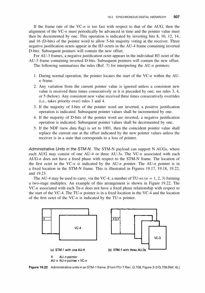
19.3 SYNCHRONOUS DIGITAL HIERARCHY 507
If the frame rate of the VC-n is too fast with respect to that of the AUG, then thealignment of the VC-n must periodically be advanced in time and the pointer value mustthen be decremented by one. This operation is indicated by inverting bits 8, 10, 12, 14,and 16 (D-bits) of the pointer word to allow 5-bit majority voting at the receiver. Threenegative justification octets appear in the H3 octets in the AU-4 frame containing invertedD-bits. Subsequent pointers will contain the new offset.
For AU-3 frames, a negative justification octet appears in the individual H3 octet of theAU-3 frame containing inverted D-bits. Subsequent pointers will contain the new offset.
The following summarizes the rules (Ref. 7) for interpreting the AU-n pointers:
1. During normal operation, the pointer locates the start of the VC-n within the AU-n frame.
2. Any variation from the current pointer value is ignored unless a consistent newvalue is received three times consecutively or it is preceded by one; see rules 3, 4,or 5 (below). Any consistent new value received three times consecutively overrides(i.e., takes priority over) rules 3 and 4.
3. If the majority of I-bits of the pointer word are inverted, a positive justificationoperation is indicated. Subsequent pointer values shall be incremented by one.
4. If the majority of D-bits of the pointer word are inverted, a negative justificationoperation is indicated. Subsequent pointer values shall be decremented by one.
5. If the NDF (new data flag) is set to 1001, then the coincident pointer value shallreplace the current one at the offset indicated by the new pointer values unless thereceiver is in a state that corresponds to a loss of pointer.
Administrative Units in the STM-N. The STM-N payload can support N AUGs, whereeach AUG may consist of one AU-4 or three AU-3s. The VC-n associated with eachAUG-n does not have a fixed phase with respect to the STM-N frame. The location ofthe first octet in the VC-n is indicated by the AU-n pointer. The AU-n pointer is ina fixed location in the STM-N frame. This is illustrated in Figures 19.17, 19.18, 19.22,and 19.23.
The AU-4 may be used to carry, via the VC-4, a number of TU-ns (n = 1, 2, 3) forminga two-stage multiplex. An example of this arrangement is shown in Figure 19.22. TheVC-n associated with each Tu-n does not have a fixed phase relationship with respect tothe start of the VC-4. The TU-n pointer is in a fixed location in the VC-4 and the locationof the first octet of the VC-n is indicated by the TU-n pointer.
Figure 19.22 Administrative units in an STM-1 frame. [From ITU-T Rec. Q.708, Figure 3-2/G.708 (Ref. 6).]

508 ADVANCED BROADBAND DIGITAL TRANSPORT FORMATS
Figure 19.23 Two-stage multiplex. [From ITU-T G.708, Figure 3-3/G.708 (Ref. 6).]
The AU-3 may be used to carry, via the VC-3, a number of TU-ns (n = 1, 2) form-ing a two-stage multiplex. An example of this arrangement is shown in Figure 19.22and 19.23b. The VC-n associated with each TU-n does not have a fixed phase relation-ship with respect to the start of the VC-3. The TU-n pointer is in a fixed location in theVC-3, and the location of the first octet of the VC-n is indicated by the TU-n pointer(Ref. 7).
19.3.3.3 Interconnection of STM-1s. SDH has been designed to be universal, allow-ing transport of a large variety of signals including those specified in ITU-T Rec. G.702(Ref. 8), such as the North American DS1 hierarchy and the European E-1 hierarchy.However, different structures can be employed for the transport of virtual containers. Thefollowing interconnection rules are used.
1. The rule for interconnecting two AUGs based on two different types of adminis-trative unit, namely, AU-4 and AU-3, is to use the AU-4 structure. Therefore theAUG based on AU-3 is demultiplexed to the TUG-2 or VC-3 level according tothe type of payload and is remultiplexed within an AUG via the TUG-3/VC-4/AU-4 route.
2. The rule for interconnecting VC-11s transported via different types of tributary unit,namely, TU-11 and TU-12, is to use the TU-11 structure. VC-11, TU-11, and TU-12are described in ITU-T Rec. G.709 (Ref. 7).
REVIEW EXERCISES
1. What was the principal driving force for the development of SONET?
2. Being that the frame period of SONET/SDH is 125 µsec, what service are theseformats optimized for?
3. Give at least five examples of digital services that can be transported on SONET.
4. Describe in words the basic SONET frame. Show its apparent payload and then itsactual payload and explain the differences.
REFERENCES 509
5. How can we calculate the bit rate of STS-3 if we know that the bit rate of STS-1is 51.84 Mbps?
6. Explain how STS-Nc concatenation operates and its purpose.
7. What are the two primary uses of the payload pointer?
8. What network impairment is introduced by the payload pointer? What is its cause?
9. What are the three overhead levels of SONET?
10. Name at least three specific functions of the POH.
11. What is payload mapping?
12. If the SONET line rate were OC-48, how could one calculate this bit rate?
13. What is the function of an add–drop multiplexer in the add–drop mode?
14. The SDH STM-1 bit rate equal what SONET line rate?
15. How do we derive higher line rates from the SDH STM-1?
16. What are the two types of pointers used in SDH?
17. When the frame rate of a VC-n is too slow with respect to that of the AUG,what happens to the alignment of the VC-n? What happens to the pointer value inthis example?
18. We change the value of an AU pointer. How many frames must go by beforechanging it again? Why can’t we change it right away, right on the next frame?
19. How many AU-3s or AU-4s may be contained in an AUG?
20. SDH was designed to carry the E1 hierarchy. Can it also carry the DS1 hierarchy?
REFERENCES
1. Synchronous Optical Network (SONET), Transport Systems, Common Generic Criteria, Bellcore,GR-253-CORE, Issue 1, Bellcore, Piscataway, NJ 1994.
2. Introduction to SONET, seminar, Hewlett-Packard Co., Burlington, MA, Nov. 1993.
3. Curtis A. Siller and Mansoor Shafi, eds., SONET/SDH, IEEE Press, New York, 1996.
4. SONET Add–Drop Multiplex Equipment (SONET ADM) Generic Criteria, Bellcore TR-TSY-000496, Issue 2, Bellcore, Piscataway, NJ 1989.
5. Synchronous Digital Hierarchy Bit Rates, ITU-T Rec. G.707, ITU Helsinki, 1993.
6. Network Node Interface for the Synchronous Digital Hierarchy, ITU-T Rec. G.708, ITU Helsinki,1993.
7. Synchronous Multiplexing Structure, ITU-T Rec. G.709, ITU Geneva 1993.
8. Digital Hierarchy Bit Rates, CCITT Rec. G.702, Fascicle III.4, IXth Plenary Assembly, Mel-bourne, 1988.
9. G. Held, Dictionary of Communications Technology, Wiley, Chichester, UK, 1995.


20
ASYNCHRONOUS TRANSFER MODE
20.1 EVOLVING TOWARD ATM
Frame relay (Section 12.5) began a march toward an optimized1 digital format formultimedia transmission (i.e., voice, data, video, and facsimile). There were new con-cepts in frame relay. Take, for example, the trend toward simplicity where the headerwas notably shortened. The header was pure overhead, so it was cut back as practicallypossible. The header also signified processing. By reducing the processing, delivery timeof a data frame is speeded up.
In the effort to speed up delivery, frames were unacknowledged (at least at the framerelay level); there was no operational error correction scheme. It was unnecessary becauseit was assumed that the underlying transport system had excellent error performance (BERbetter than 1 × 10⁻⁷).2 There was error detection for each frame, and a frame found inerror was thrown away. Now that was something that we would never do for those of ussteeped in old-time data communication. It is assumed that the higher OSI layers wouldrequest repeats of the few frames missing (i.e., thrown away). These higher OSI layers(i.e., layer 3 and above) were the customer’s responsibility, not the frame relay provider.
Frame relay also moved into the flow control arena with the BECN and FECN bitsand the CLLM. The method of handling flow control has a lot to do with its effectivenessin preventing buffer overflow. It also uses a discard eligibility (DE) bit, which set a typeof priority to a frame. If the DE bit was set, the frame would be among the first to bediscarded in a time of congestion.
DQDB (distributed queue dual bus) was another antecedent of ATM. It was developedby the IEEE as a simple and unique network access scheme. Even more important, itsdata transport format is based on the slot, which is called a cell in ATM. This slot has aformat very similar to the ATM cell, which we will discuss at length in this chapter. Iteven has the same number of octets, 53; 48 of these carry the payload. This is identicalto ATM. This “cell” idea even may be found in Bellcore’s SMDS (switched multimegabitdata service). In each case the slot or cell was 53 octets long. DQDB introduced acomparatively new concept of the HCS or header check sequence for detecting errorsin the header. In neither case was there a capability of detecting errors in the payload.SMDS/DQDB left it to layer 3. Slots or cells carry pieces of messages. The first “piece”
1Compromise might be a better term.2In North America, PSTN BER can be expected to be better than 5 × 10⁻¹⁰.
Fundamentals of Telecommunications, Second Edition, by Roger L. FreemanISBN 0-471-71045-8 Copyright 2005 by Roger L. Freeman
511

512 ASYNCHRONOUS TRANSFER MODE
of a message is identified by a BOM (beginning of message); all subsequent pieces, butnot the last, are identified with the COM (continuation of message), and the last pieceor slot is identified with an EOM (end of message). There is also an MID (messageidentifier) appended to all pieces of a common message. This is done so that there is noconfusion as to which transaction a cell belongs.
20.2 INTRODUCTION TO ATM
ATM is an outgrowth of the several data transmission format systems discussed above,although some may argue this point. Whereas the formats described above ostensibly wereto satisfy the needs of the data world,3 ATM (according to some) provides an optimumformat or protocol family for data, voice, and image communications, where cells of eachmedium can be intermixed through the network as illustrated in Figure 20.1. It wouldreally seem to be more of a compromise from our perspective. Typically, these ATMcells can be transported on SONET, SDH, E1/DS1, and other digital formats. Cells canalso be transported contiguously without an underlying digital network format.
Philosophically, voice and data are worlds apart regarding time sensitivity. Voice cannotwait for long processing and ARQ delays. Most types of data can. So ATM must dis-tinguish the type of service such as constant bit rate (CBR) and variable bit rate (VBR)services. Voice service is typical of constant bit rate or CBR service.
Signaling is another area of major philosophical difference. In data communications,“signaling” is carried out within the header of a data frame (or packet). As a minimum thesignaling will have the destination address, and quite often the source address as well. Andthis signaling information will be repeated over and over again on a long data file that isheavily segmented. On a voice circuit, a connectivity is set up and the destination address,and possibly the source address, is sent just once during call setup. There is also someform of circuit supervision to keep the circuit operational throughout the duration of atelephone call. ATM is a compromise, stealing a little from each of these separate worlds.
Like voice telephony, ATM is fundamentally a connection-oriented telecommunicationsystem. Here we mean that a connection must be established between two stations beforedata can be transferred between them. An ATM connection specifies the transmission path,allowing ATM cells to self-route through an ATM network. Being connection-orientedalso allows ATM to specify a guaranteed quality of service (QoS) for each connection.
Figure 20.1 An ATM link simultaneously carries a mix of voice, data, and image information. (FromRef. 1, courtesy of Hewlett-Packard Co.)
3DQDB can also transport voice in its PA (pre-arbitrated) segments.

20.2 INTRODUCTION TO ATM 513
By contrast, most LAN protocols are connectionless. This means that LAN nodessimply transmit traffic when they need to, without first establishing a specific connectionor route with the destination node.
In that ATM uses a connection-oriented protocol, cells are allocated only when theoriginating end user requests a connection. They are allocated from and idle-cell pool.This allows ATM to efficiently support a network’s aggregate demand by allocating cellcapacity on demand based on immediate user need. Indeed it is this concept that lies at theheart of the word asynchronous (as in asynchronous transfer mode). An analogy wouldhelp. Let’s say that New York City is connected to Washington, DC, by a pair of railroadtracks for passenger trains headed south and another pair of tracks for passenger trainsheaded north. On these two pair of tracks we’d like to accommodate everybody we canwhen they’d like to ride. The optimum for reach this goal is to have a continuous trainof coupled passenger cars. As the trains enters Union Station, it disgorges its passengersand connects around directly for the northward run to Pennsylvania Station and loadingpeople bound for New York. Passenger cars are identical in size, and each has the samenumber of identical seats.
Of course, at 2 A.M. the train will have very few passengers and many empty seats.Probably from 7 A.M. to 9 A.M. the train will be full, no standees allowed, so we’llhave to hold potential riders in the waiting room. They’ll ride later; those few who tryto be standees will be bumped. Others might seek alternate transportation to Washing-ton, DC.
Here we see that the railroad tracks are the transmission medium. Each passenger caris a SONET/SDH frame. The seats in each car are our ATM cells. Each seat can handle aperson no bigger than 53 units. Because of critical weight distribution, if a person is not 53units in size/weight, we’ll stick some bricks in the seat to bring the size/weight to 53 unitsexactly. Those bricks are removed at the destination. All kinds of people ride the trainbecause America is culturally diverse, analogous to the fact that ATM handles all formsof traffic. The empty seats represent idle or unassigned cells. The header informationis analogous to the passengers’ tickets. Keep in mind that the train can only fill to itsmaximum capacity of seats. We can imagine the SONET/SDH frame as being full of cellsin the payload, some cells busy and some idle/unassigned. At the peak traffic period, allcells will be busy, and some traffic (passengers) may have to be turned away.
We can go even further with this analogy. Both Washington, DC, and New YorkCity attract large groups of tourists, and other groups travel to business meetings orconventions. A tour group has a chief tour guide in the lead seat (cell) and an assistantguide in the last seat (cell). There may be so many in the group that they extend intoa second car or may just intermingle with other passengers on the train. The tour guideand assistant tour guide keep an exact count of people on the tour. The lead guide wearsa badge that says BOM, all tour members wear badges that say COM, and the assistanttour guide wears a badge that says EOM. Each group has a unique MID (message ID).We also see that service is connection-oriented (Washington, DC, to New York City).
Asynchronous means that we can keep filling seats on the train until we reach itsmaximum capacity. If we look up the word, it means nonperiodic whereas the familiarE1/DS1 are periodic (i.e., synchronous). One point that seems to get lost in the literatureis that the train has a maximum capacity. It is common to read that ATM provides“bandwidth” on demand. The underlying transmission medium has a fixed bandwidth. Webelieve the statement is supposed to mean “cell rate capacity” on demand. This is true ofcourse until we reach the maximum capacity. For example, if the underlying transmissionformat is SONET STS-1, it can provide 86 × 9 octets × 8000/(53) per second or about116,000 cells per second of payload (see Chapter 19).

514 ASYNCHRONOUS TRANSFER MODE
20.3 USER–NETWORK INTERFACE (UNI) AND ARCHITECTURE
ATM is the underlying packet technology of broadband ISDN (B-ISDN). At times in thissection, we will use the terms ATM and B-ISDN interchangeably. Figures 20.2 and 20.3interrelate the two. Figure 20.2 relates the B-ISDN access reference configuration with theATM user-network interface (UNI). Note the similarities of this figure with Figure 12.15,the reference model for ISDN. The only difference is that the block nomenclature hasa “B” placed in front to indicate broadband. Figure 20.3 is the traditional ITU-T Rec.I.121 (Ref. 2) B-ISDN protocol reference model showing the extra layer necessary forthe several services.
Returning to Figure 20.2, we see that there is an upper part and a lower part. The lowerpart shows the UNI boundaries. The upper part is the B-ISDN reference configurationwith four interface points. The interfaces at the reference points UB, TB, and SB arestandardized. These interfaces support all B-ISDN services.
There is only one interface per B-NT1 at the UB and one at the TB reference points.The physical media is point-to-point (in each case), in the sense that there is only onereceiver in front of one transmitter.
One or more interfaces per NT2 are present at the SB reference point. The interfaceat the SB reference point is point-to-point at the physical layer, in the sense that there isonly one receiver in front of one transmitter, and may be point-to-point at other layers.
Consider now the functional groupings in Figure 20.2. B-NT1 includes functionsbroadly equivalent to OSI layer 1, the physical layer. These functions include:
ž Line transmission terminationž Interface handling at TB and UB
ž OAM functions4
Figure 20.2 ATM reference model and user–network interface configuration. (Sources: Refs. 2, 3,and 6.)
4OAM stands for operations, administration, and maintenance.

20.3 USER–NETWORK INTERFACE (UNI) AND ARCHITECTURE 515
Figure 20.3 B-ISDN reference model. (From Ref. 6, reprinted with permission.)
The B-NT2 functional group includes functions broadly equivalent to OSI layer 1and higher OSI layers. The B-NT2 may be concentrated or distributed. In a particularaccess arrangement, the B-NT2 functions may consist of physical connections. Examplesof B-NT2 functions are:
ž Adaptation functions for different media and topologiesž Cell delineationž Concentration; bufferingž Multiplexing and demultiplexingž OAM functionsž Resource allocationž Signaling protocol handling
The functional group B-TE (TE stands for terminal equipment) also includes functionsof OSI layer 1 and higher OSI layers. Some of these functions are:
ž User/user and user/machine dialog and protocolž Protocol handling for signalingž Connection handling to other equipmentž Interface terminationž OAM functions
B-TE1 has an interface that complies with the B-ISDN interface. B-TE2, however, hasa noncompliant, B-ISDN interface. Compliance refers to ITU-T Recs. I.413 and I.432 aswell as ANSI T1.624-1993 (Refs. 4–6).

516 ASYNCHRONOUS TRANSFER MODE
The terminal adapter (B-TA) converts the B-TE2 interface into a compliant B-ISDNuser–network interface.
Four bit rates are specified at the UB, TB, and SB interfaces based on Ref. 5 (ANSIT1.624-1993). These are:
1. 51.840 Mbps (SONET STS-1)2. 155.520 Mbps (SONET STS-3 and SDH STM-1)3. 622.080 Mbps (SONET STS-12 and SDH STM-4)4. 44.736 Mbps (DS3)
These interfaces are discussed subsequently in this chapter.The following definitions refer to Figure 20.3.
User Plane (in other literature called the U-plane). The user plane provides for thetransfer of user application information. It contains physical layer, ATM layer, and mul-tiple ATM adaptation layers required for different service users such as CBR and VBRservice.
Control Plane (in other literature called the C-plane). The control plane protocols dealwith call-establishment and call-release and other connection-control functions necessaryfor providing switched services. The C-plane structure shares the physical and ATM layerswith the U-plane as shown in Figure 20.3. It also includes ATM adaptation proceduresand higher-layer signaling protocols.
Management plane (in other literature called the M-plane). The management planeprovides management functions and the capability to exchange information between theU-plane and the C-plane. The M-plane contains two sections: layer management and plantmanagement. The layer management performs layer-specific management functions, whilethe plane management performs management and coordination functions related to thecomplete system.
We will return to Figure 20.3 and B-ISDN/ATM layering and layer descriptions inSection 20.6.
20.4 THE ATM CELL: KEY TO OPERATION
20.4.1 ATM Cell Structure
As we mentioned earlier, the ATM cell consists of 53 octets, 5 of which make up theheader and 48 make up the payload or “info” portion of the cell.5 Figure 20.4 shows anATM cell stream, delineating the 5-octet header and 48-octet information field of eachcell. Figure 20.5 shows the detailed structure of cell headers at the user–network interface(UNI) (Figure 20.5a) and at the network–node interface (NNI)6 (Figure 20.5b).
We digress a moment to discuss why a cell was standardized at 53 octets. The cellheader contains only 5 octets. It was shortened as much as possible, designed to containthe minimum address and control functions for a working system. It is obvious that theoverhead is non-revenue-bearing. It is the information field that contains the revenue-bearing payload. For efficiency, we’d like the payload to be as long as possible. Yet the
5Under certain situations, there are 6 octets in the header and 47 octets in the payload.6NNI is variously called network–node interface or network–network interface. It is the interface between twoATM network nodes or switches.
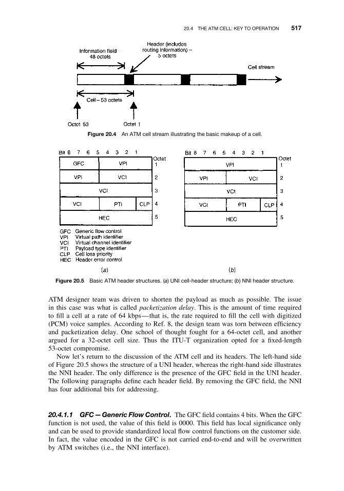
20.4 THE ATM CELL: KEY TO OPERATION 517
Figure 20.4 An ATM cell stream illustrating the basic makeup of a cell.
Figure 20.5 Basic ATM header structures. (a) UNI cell-header structure; (b) NNI header structure.
ATM designer team was driven to shorten the payload as much as possible. The issuein this case was what is called packetization delay. This is the amount of time requiredto fill a cell at a rate of 64 kbps—that is, the rate required to fill the cell with digitized(PCM) voice samples. According to Ref. 8, the design team was torn between efficiencyand packetization delay. One school of thought fought for a 64-octet cell, and anotherargued for a 32-octet cell size. Thus the ITU-T organization opted for a fixed-length53-octet compromise.
Now let’s return to the discussion of the ATM cell and its headers. The left-hand sideof Figure 20.5 shows the structure of a UNI header, whereas the right-hand side illustratesthe NNI header. The only difference is the presence of the GFC field in the UNI header.The following paragraphs define each header field. By removing the GFC field, the NNIhas four additional bits for addressing.
20.4.1.1 GFC—Generic Flow Control. The GFC field contains 4 bits. When the GFCfunction is not used, the value of this field is 0000. This field has local significance onlyand can be used to provide standardized local flow control functions on the customer side.In fact, the value encoded in the GFC is not carried end-to-end and will be overwrittenby ATM switches (i.e., the NNI interface).

518 ASYNCHRONOUS TRANSFER MODE
Two modes of operation have been defined for operation of the GFC field. These areuncontrolled access and controlled access. The uncontrolled access mode of operation isused in the early ATM environment. This mode has no impact on the traffic which a hostgenerates. Each host transmits the GFC field set to all zeros (0000). In order to avoidunwanted interactions between this mode and the controlled access mode, where hostsare expected to modify their transmissions according to the activity of the GFC field,it is required that all CPE (customer premise equipment) and public network equipmentmonitor the GFC field to ensure that attached equipment is operating in uncontrolled mode.A count of the number of nonzero GFC fields should be measured for nonoverlappingintervals of 30,000 ± 10,000 cell times. If ten or more nonzero values are received withinthis interval, an error is indicated to layer management (Ref. 3).
20.4.1.2 Routing Field (VPI/VCI). Twenty four bits are available for routing a cell.There are 8 bits for virtual path identifier (VPI) and 16 bits for virtual channel iden-tifier (VCI). Preassigned combinations of VPI and VCI are given in Table 20.1. Otherpreassigned values of VPI and VCI are for further study, according to the ITU-T Orga-nization. The VCI value of zero is not available for user virtual channel identification.The bits within the VPI and VCI fields are used for routing and are allocated using thefollowing rules:
ž The allocated bits of the VPI field are contiguous.ž The allocated bits of the VPI field are the least significant bits of the VPI field,
beginning at bit 5 of octet 2.ž The allocated bits of the VCI field are contiguous.ž The allocated bits of the VCI field are the least significant bits of the VCI field,
beginning at bit 5 of octet 4.
Table 20.1 Combination of Preassigned VPI, VCI and CLP Values at the UNI
Use VPI VCI PT CLP
Meta-signaling (refer to Rec. I.311) XXXXXXXXa 00000000 00000001e 0A0 CGeneral broadcast signaling (refer to Rec. I.311) XXXXXXXXa 00000000 00000010e 0AA CPoint-to-point signaling (refer to Rec. I.311) XXXXXXXXa 00000000 00000101e 0AA CSegment OAM F4 flow cell (refer to Rec. I.610) YYYYYYYYb 00000000 00000011d 0A0 AEnd-to-end OAM F4 flow cell (refer to Rec. I.610) YYYYYYYYb 00000000 00000100d 0A0 ASegment OAM F5 flow cell (refer to Rec. I.610) YYYYYYYYb ZZZZZZZZ ZZZZZZZZc 100 AEnd-to-end OAM F5 flow cell (refer to Rec. I.610) YYYYYYYYb ZZZZZZZZ ZZZZZZZZc 101 AResource management cell (refer to Rec. I.371) YYYYYYYYb ZZZZZZZZ ZZZZZZZZc 110 AUnassigned cell 00000000 00000000 00000000 BBB 0
The GFC field is available for use with all of these combinations.A Indicates that the bit may be 0 or 1 and is available for use by the appropriate ATM layer function.B Indicates the bit as a ‘‘don’t care’’ bit.C Indicates the originating signaling entity shall set the CLP bit to 0. The value may be changed by the network.
aXXXXXXXX: Any VPI value. For VPI value equal to 0, the specific VCI value specified is reserved for user signaling withthe local exchange. For VPI values other than 0, the specified VCI value is reserved for signaling with other signalingentities (e.g., other users or remote networks).bYYYYYYYY: Any VPI value.cZZZZZZZZ ZZZZZZZZ: Any VIC value other than 0.dTransparency is not guaranteed for the OAM F4 flows in a user-to-user VP.eThe VIC values are preassigned in every VPC at the UNI. The usage of these values depends on the actual signalingconfigurations. (See ITU-T Rec. I.311.)
Source: ITU-T Rec. I.361, Table 2/I.361, p. 3 (Ref. 9).

20.4 THE ATM CELL: KEY TO OPERATION 519
Table 20.2 PTI Coding
PTI Coding Interpretation
Bits4 3 20 0 0 User data cell, congestion not experienced.
ATM-user-to-ATM-user indication = 00 0 1 User data cell, congestion not experienced.
ATM-user-to-ATM-user indication = 10 1 0 User data cell, congestion experienced.
ATM-user-to-ATM-user indication = 00 1 1 User data cell, congestion experienced.
ATM-user-to-ATM-user indication = 11 0 0 OAM F5 segment associated cell1 0 1 OAM F5 end-to-end associated cell1 1 0 Resource management cell1 1 1 Reserved for future functions
Source: ITU-T Rec. I.361, p. 4, para. 2.2.4 (Ref. 9).
20.4.1.3 Payload-Type (PT) Field. Three bits are available for PT identification.Table 20.2 gives payload type identifier (PTI) coding. The principal purpose of the PTIis to discriminate between user cells (i.e., cells carrying information) and nonuser cells.The first four code groups (000-011) are used to indicate user cells. Within these four,2 and 3 (010 and 0111) are used to indicate congestion has been experienced. The fifthand sixth code groups (100 and 101) are used for virtual channel connection (VCC) levelmanagement functions.
Any congested network element, upon receiving a user data cell, may modify the PTIas follows: Cells received with PTI = 000 or PTI = 010 are transmitted with PTI = 010.Cells received with PTI = 001 or PTI = 011 are transmitted with PTI = 011. Noncon-gested network elements should not change the PTI.
20.4.1.4 Cell Loss Priority (CLP) Field. Depending on network conditions, cellswhere the CLP is set (i.e., CLP value is 1) are subject to discard prior to cells where theCLP is not set (i.e., CLP value is 0). The concept here is identical with that of frame relayand the DE (discard eligibility) bit. ATM switches may tag CLP = 0 cells detected bythe UPC (usage parameter control) to be in violation of the traffic contract by changingthe CLP bit from 0 to 1.
20.4.1.5 Header Error Control (HEC) Field. The HEC is an 8-bit field that coversthe entire cell header. The code used for this function is capable of either single-bit errorcorrection or multiple-bit error detection. Briefly, the transmitting side computes the HECfield value. The receiver has two modes of operation as shown in Figure 20.6. In thedefault mode there is the capability of single-bit error correction. Each cell header isexamined and, if an error is detected, one of two actions takes place. The action takendepends on the state of the receiver. In the correction mode, only single-bit errors canbe corrected and the receiver switches to the detection mode. In the detection mode, allcells with detected header errors are discarded. When a header is examined and foundnot to be in error, the receiver switches to the correction mode. The term no action inFigure 20.6 means no correction is performed and no cell is discarded.
It should be noted that there is no error protection for the payload of a cell. If an erroris found in the header of a cell which cannot be corrected, the cell is discarded. The error

520 ASYNCHRONOUS TRANSFER MODE
Figure 20.6 HEC: receiver modes of operation. (Based on ITU-T Rec. I.432.)
Table 20.3 Header Pattern for Idle Cell Identification
Octet 1 Octet 2 Octet 3 Octet 4 Octet 5
Header pattern 00000000 00000000 00000000 00000001 HEC = Valid code 01010010
Source: ITU-T Rec. 1.432, Table 4/1.432, p. 19 (Ref. 4).
protection function provided by the HEC allows for both recovery of single bit errors anda low probability of delivery of cells with errored headers, under bursty error conditions.
20.4.2 Idle Cells
Idle cells cause no action at a receiving node except for cell delineation including HECverification. They are inserted and extracted by the physical layer in order to adapt the cellflow rate7 at the boundary between the ATM layer and the physical layer to the availablepayload capacity of the transmission media. This is called cell rate decoupling. Idle cellsare identified by the standardized pattern for the cell header illustrated in Table 20.3. Thecontent of the information field is 01101010 repeated 48 times for an idle cell.
20.5 CELL DELINEATION AND SCRAMBLING
Cell delineation allows identification of the cell boundaries. The cell HEC field achievescell delineation. Keep in mind that the ATM signal must be self-supporting, in that it hasto be transparently transported on every network interface without any constraints fromthe transmission systems used. Scrambling is used to improve security and robustness ofthe HEC cell delineation mechanism discussed in the next paragraph. In addition, it helpsthe randomizing of data in the information field for possible improvement in transmissionperformance.
Cell delineation is performed by using correlation between the header bits to be pro-tected (the first four octets in the header) and the HEC octet. This octet is produced atthe originating end using a generating polynomial covering those first four octets of thecell. The generating polynomial is X8 + X2 + X + 1. There must be correlation at thereceiving end between those first four octets and the HEC octet, which we can call aremainder. This is only true, of course, if there is no error in the header. When there isan error, correlation cannot be achieved, and the processor just goes to the next cell.
7There must be a constant cell flow rate to keep the far-end node synchronized and aligned.

20.6 ATM LAYERING AND B-ISDN 521
20.6 ATM LAYERING AND B-ISDN
The B-ISDN reference model was given in Figure 20.3, and its several planes weredescribed. This section provides brief descriptions of the ATM layers and sublayers.Figure 20.7 illustrates B-ISDN/ATM layering and sublayering of the protocol referencemodel. It identifies functions of the physical layer, the ATM layer, and the AAL (ATMadaptation layer), and related sublayers.
20.6.1 Physical Layer
The physical layer consists of two sublayers. The physical medium (PM) sublayer includesonly physical medium-dependent functions. The transmission convergence (TC) sublayerperforms all functions required to transform a flow of cells into a flow of data units (i.e.,bits) which can be transmitted and received over a physical medium. The service data unit(SDU) crossing the boundary between the ATM layer and the physical layer is a flow ofvalid cells. The ATM layer is unique (independent of the underlying physical layer). Thedata flow inserted in the transmission system payload is physical medium-independent andself-supported. The physical layer merges the ATM cell flow with appropriate information
Figure 20.7 B-ISDN/ATM functional layering.

522 ASYNCHRONOUS TRANSFER MODE
for cell delineation, according to the cell delineation mechanism previously described, andcarries the operations, administration, and maintenance (OAM) information relating to thiscell flow.
The PM sublayer provides bit transmission capability including bit transfer and bitalignment, as well as line coding and electrical-optical transformation. Of course, theprincipal function is the generation and reception of waveforms suitable for the medium,the insertion and extraction of bit timing information, and line coding where required.
The primitives identified at the border between the PM and TC sublayers are a con-tinuous flow of logical bits or symbols with associated timing information.
20.6.1.1 Transmission Convergence Sublayer Functions. Among the importantfunctions of this sublayer is the generation and recovery of transmission frame. Anotherfunction is transmission frame adaptation, which includes the actions necessary to struc-ture the cell flow according to the payload structure of the transmission frame (transmitdirection), and to extract this cell flow out of the transmission frame (receive direction).The transmission frame may be a cell equivalent (i.e., no external envelope is added tothe cell flow), an SDH/SONET envelope, an E1/T1 envelope, and so on. In the transmitdirection, the HEC sequence is calculated and inserted in the header. In the receive direc-tion, we include cell header verification. Here cell headers are checked for errors and,if possible, header errors are corrected. Cells are discarded where it is determined thatheaders are errored and are not correctable.
Another transmission convergence function is cell rate decoupling. This involves theinsertion and removal of idle cells in order to adapt the rate of valid ATM cells to thepayload capacity of the transmission system. In other words, cells must be generated toexactly fill the payload of SDH/SONET, as an example, whether the cells are idle or busy.
Section 20.12.5 gives several examples of transporting cells using the convergencesublayer.
20.6.2 The ATM Layer
Table 20.4 shows the ATM layering functions supported at the UNI (U-plane). The ATMlayer is completely independent of the physical medium. One important function of thislayer is encapsulation. This includes cell header generation and extraction. In the transmitdirection, the cell header generation function receives a cell information field from a higherlayer and generates an appropriate ATM cell header except for the header error control(HEC) sequence. This function can also include the translation from a service access point(SAP) identifier to a VP (virtual path) and VC (virtual circuit) identifier.
In the receive direction, the cell header extraction function removes the ATM cellheader and passes the cell information field to a higher layer. As in the transmit direction,this function can also include a translation of a VPI and VCI into an SAP identifier.
Table 20.4 ATM Layer Functions Supported at the UNI
Functions Parameters
Multiplexing among different ATM connections VPI/VCICell rate decoupling (unassigned cells) Preassigned header field valuesCell discrimination based on predefined header field values Preassigned header field valuesPayload type discrimination PT fieldLoss priority indication and selective cell discarding CLP field, network congestion stateTraffic shaping Traffic descriptor
Source: Based on Refs. 3 and 8.

20.6 ATM LAYERING AND B-ISDN 523
In the case of the NNI, the GFC is applied at the ATM layer. The flow control infor-mation is carried in assigned and unassigned cells. Cells carrying this information aregenerated in the ATM layer.
In a switch the ATM layer determines where the incoming cells should be forwarded,resets the corresponding connection identifiers for the next link, and forwards the cell.The ATM layer also handles traffic-management functions between ATM nodes on bothsides of the UNI (i.e., single VP link segment) while the virtual channel identified by aVCI value = 4 can be used for VP level end-to-end (user ↔ user) management functions.
What are flows such as “F4 flows”? OAM (operations, administration, and manage-ment) flows deal with cells dedicated to fault and performance management of the totalsystem. Consider ATM as a hierarchy of levels, particularly in SDH/SONET, which arethe principal bearer formats for ATM. The lowest level where we have F1 flows is theregenerator section (called the section level in SONET). This is followed by F2 flowsat the digital section level (called the line level in SONET). There are the F3 flows forthe transmission path (called the path level in SONET). ATM adds F4 flows for virtualpaths (VPs) and F5 flows for virtual channels (VCs), where multiple VCs are completelycontained within a single VP. We discuss VPs and VCs in Section 20.8.
20.6.3 The ATM Adaptation Layer (AAL)
The basic purpose of the AAL is to isolate the higher layers from the specific character-istics of the ATM layer by mapping the higher-layer protocol data units (PDUs) into thepayload of the ATM cell and vice versa.
20.6.3.1 Sublayering of the AAL. To support services above the AAL, some inde-pendent functions are required of the AAL. These functions are organized in two logicalsublayers: the convergence sublayer (CS) and the segmentation and reassembly (SAR)sublayer. The primary functions of these layers are:
ž SAR—The segmentation of higher-layer information into a size suitable for the infor-mation field of an ATM cell. Reassembly of the contents of ATM cell informationfields into higher-layer information.
ž CS—Here the prime function is to provide the AAL service at the AAL-SAP (serviceaccess point). This sublayer is service dependent.
20.6.3.2 Service Classification of the AAL. Service classification is based on thefollowing parameters:
ž Timing relation between source and destination (this refers to urgency of traffic):required or not required.
ž Bit rate: constant or variable.ž Connection mode: connection-oriented or connectionless.
When we combine these parameters, four service classes emerge as shown in Figure 20.8.Examples of the services in the classes shown in Figure 20.8 are as follows.
ž Class A: constant bit rate such as uncompressed voice or video.ž Class B: variable bit rate video and audio, connection-oriented synchronous traffic.

524 ASYNCHRONOUS TRANSFER MODE
Figure 20.8 Services classifications of AAL. (Based on Refs. 2, 8, and 10.)
ž Class C: connection-oriented data transfer, variable bit rate, asynchronous traffic.ž Class D: connectionless data transfer, asynchronous traffic such as SMDS.
Note that SMDS stands for switched multimegabit data service. It is espoused by Bellcore(Telcordia) and is designed primarily for LAN interconnect.
20.6.3.3 AAL Categories or Types. There are five different AAL categories. Thesimplest of AAL-0. It just transmits cells down a pipe. That pipe is commonly a fiber-opticlink. Ideally, it would be attractive that the bit rate here be some multiple of 53 × 8 bitsor 424 bits. For example, 424 Mbps could handle 1 million cells per second.
AAL-1. AAL-1 is used to provide transport for synchronous bit streams. Its primaryapplication is to adapt ATM cell transmission to typically E1/DS1 and SDH/SONET cir-cuits. AAL-1 is specifically used for voice communications (POTS—plain old telephoneservice). AAL-1 robs one octet from the payload and adds it to the header, leaving only a47-octet payload. This additional octet in the header contains two major fields: sequencenumber (SN) and sequence number protection (SNP). The principal purpose of these twofields is to check that mis-sequencing of information does not occur by verifying a 3-bitsequence counter. It also allows for the original clock timing of the data received at thefar end of the link. The SAR-PDU format of AAL-1 is shown in Figure 20.9.8 The 4-bitsequence number (SN) is broken down into a 1-bit CSI (convergence sublayer indicator)and a sequence count. The SNP contains a 3-bit CRC and a parity bit. End-to-end syn-chronization is an important function for the type of traffic carried on AAL-1. With onemode of operation, clock recovery is via a synchronous residual time stamp (SRTS) andcommon network clock by means of a 4-bit residual time stamp extracted from CSI fromcells with odd sequence numbers. The residual time stamp is transmitted over eight cells.It supports DS1, DS3, and E1 digital streams. Another mode of operation is structureddata transfer (SDT). SDT supports an octet-structured nXDS0 service.
AAL-2. AAL-2 handles the variable bit rate (VBR) scenario such as MPEG (motionpicture experts group) video. It is still in the ITU-T organization definitive stages.
8SAR-PDU stands for segmentation and reassembly—protocol data unit.

20.6 ATM LAYERING AND B-ISDN 525
Figure 20.9 SAR-PDU format for AAL-1. This figure shows the content of a cell that contains anSAR-PDU. [From CCITT Rec. I.363, Figure 1/I.363, page 3 (Ref. 10).]
AAL-3/4. Initially, in ITU-T Rec I.363 (Ref. 10), there were two separate AALs, one forconnection-oriented variable bit rate data services (AAL-3) and one for connectionlessservice. As the specifications evolved, the same procedures turned out to be necessaryfor both of these services, and the specifications were merged to become the AAL-3/4standard. AAL-3/4 is used for ATM transport of SMDS, CBDS (connectionless broadbanddata services, an ETSI initiative), IP (Internet protocol) and frame relay.
AAL-3/4 has been designed to take variable-length frames/packets and segment theminto cells. The segmentation is done in a way that protects the transmitted data fromcorruption if cells are lost or mis-sequenced. Figure 20.10 shows the cell format of anAAL-3/4 cell. These types of cells have only a 44-octet payload, and additional overheadfields are added to the header and trailer.9 These carry, for example, the BOM, COM, andEOM indicators (carried in segment type [ST]) as well as a MID (multiplexing identifier)so that the original message, as set up in the convergence sublayer PDU (CS PDU),
Figure 20.10 SAR-PDU format for AAL-3/4. [From ITU-T Rec. I.363, page 13, Figure 6/I.363 (Ref. 10).]
9Trailer consists of overhead fields added to the end of a data frame or cell. A typical trailer is the CRC parityfield appended at the end of a frame.

526 ASYNCHRONOUS TRANSFER MODE
can be delineated. The header also includes a sequence number for protection againstmisordered delivery. There is the MID (multiplexing identification) subfield which isused to identify the CPCS (common part convergence sublayer) connection on a singleATM layer connection. This allows for more than one CPCS connection for a singleATM-layer connection. The SAR sublayer, therefore, provides the means for the transferof multiple, variable-length CS-PDUs concurrently over a single ATM layer connectionbetween AAL entities. The SAR PDU trailer contains a length indicator (LI) to identifyhow much of the cell payload is filled. The CRC field is a 10-bit sequence used to detecterrors across the whole SAR PDU. A complete CS PDU message is broken down intoone BOM cell, a number of COM cells and one EOM cell. If an entire message can fitinto one cell, it is called a single segment message (SSM), where the CS PDU is 44 orless octets long.
AAL-3/4 has several measures to ensure the integrity of the data which has beensegmented and transmitted as cells. The contents of the cell are protected by the CRC-10; sequence numbers protect against misordering. Still another measure to ensure againstcorrupted PDUs being delivered is EOM/BOM protection. If the EOM of one CPCS PDUand the BOM of the next are dropped for some reason, the resulting cell stream could beinterpreted as a valid PDU. To protect against these kinds of errors, the BEtag numericvalues in the CPCS PDU headers and trailers are compared, to ensure that they match.Two modes of service are defined for AAL-3/4:
1. Message Mode Service. This provides for the transport of one or more fixed-sizeAAL service data units in one or more CS-PDUs.
2. Streaming Mode Service. Here the AAL service data unit is passed across the AALinterface in one or more AAL interface data units (IDUs). The transfer of theseAAL-IDUs across the AAL interface may occur separated in time, and this serviceprovides the transport of variable-length AAL-SDUs. The streaming mode serviceincludes an abort service, by which the discarding of an AAL-SDU partially trans-ferred across the AAL interface can be requested. In other words, in the streamingmode, a single packet is passed to the AAL layer and transmitted in multiple CPCS-PDUs, when and as pieces of the packet are received. Streaming mode may be usedin intermediate switches or ATM-to-SMDS routers so they can begin retransmit-ting a packet being received before the entire packet has arrived. This reduces thelatency experienced by the entire packet.
AAL-5. This type of AAL was designed specifically to carry data traffic typically foundin today’s LANs. AAL-5 evolved after AAL-3/4, which was found to be too complex andinefficient for LAN traffic. Thus, AAL-5 got the name “SEAL” for simple and efficientAAL layer. Only a small amount of overhead is added to the CPCS PDU. There is noAAL level cell multiplexing. In AAL-5 all cells belonging to an AAL-5 CPCS PDUare sent sequentially. To simplify still further, the CPCS PDUs are padded10 to becomeintegral multiples of 48 octets, ensuring that there never will be a need to send partiallyfilled cells after segmentation.
20.7 SERVICES: CONNECTION-ORIENTED AND CONNECTIONLESS
The issues such as routing decisions and architectures have a major impact on connection-oriented services, where B-ISDN/ATM end nodes have to maintain or get access to lookuptables, which translate destination addresses into circuit paths. These circuit path lookup
10Padded means adding “dummy” octets, octets that do not carry any significance or information.

20.7 SERVICES: CONNECTION-ORIENTED AND CONNECTIONLESS 527
tables, which differ at every node, must be maintained in a quasi-real-time fashion. Thiswill have to be done by some kind of routing protocol.
One way to resolve this problem is to make it an internal network problem and usea connectionless service as described in ITU-T Rec. I.364 (Ref. 11). We must keep inmind that ATM is basically a connection-oriented service. Here we are going to adapt itto provide a connectionless service.
20.7.1 Functional Architecture
The provision of connectionless data service in the B-ISDN is carried out by means ofATM switches and connectionless service functions (CLSF). ATM switches support thetransport of connectionless data units in the B-ISDN between specific functional groupswhere the CLSF handles the connectionless protocol and provides for the adaptation ofthe connectionless data units into ATM cells to be transferred in a connection-orientedenvironment. It should be noted that CLSF functional groups may be located outside ofenvironment. It should be noted that CLSF functional groups may be located outside ofthe B-ISDN, in a private connectionless network or with a specialized service provider,or inside the B-ISDN.
The ATM switching is performed by the ATM nodes (ATM switch/cross-connect),which are a functional part of the ATM transport network. The CLSF functional groupterminates the B-ISDN connectionless protocol and includes functions for the adaptationof the connectionless protocol to the intrinsically connection-oriented ATM layer protocol.These latter functions are performed by the ATM adaptation layer type 3/4 (AAL-3/4),while the CLSF group terminations are carried out by the services layer above the AALcalled the CLNAP (connectionless network access protocol). The connectionless (CL)protocol includes functions such as routing, addressing, and QoS (quality of service)selection. In order to perform the routing of CL data units, the CLSF has to interact withthe control/management planes of the underlying ATM network.
The general protocol structure for the provision of connectionless (CL) data serviceis illustrated in Figure 20.11. Figure 20.12 shows the protocol architecture for support-ing connectionless layer service. The CLNAP (connectionless network access protocol)
Figure 20.11 General protocol structure for the provision of CL data service in B-ISDN.
Figure 20.12 Protocol architecture for supporting connectionless service. CLNAP stands for connec-tionless network access protocol.

528 ASYNCHRONOUS TRANSFER MODE
layer uses the type 3/4 AAL, employs unassured service, and includes the necessaryfunctionality for the connectionless layer service.
The CL service layer provides for transparent transfer of variable-sized data units froma source to one or more destinations in a manner such that lost or corrupted data units arenot retransmitted. This transfer is performed using a CL technique, including embeddingdestination and source addresses into each data unit.
20.8 B-ISDN/ATM ROUTING AND SWITCHING
An ATM transmission path supports virtual paths (VPs) and inside those virtual paths arevirtual channels (VCs) as illustrated in Figure 20.13. In Section 20.4.1 we described theATM cell header. Each cell header contains a label that explicitly identifies the VC towhich the cell belongs. This label consists of two parts: a virtual channel identifier (VCI)and a virtual path identifier (VPI).
20.8.1 The Virtual Channel Level
Virtual channel (VC) is a generic term used to describe a unidirectional communicationcapability for the transport of ATM cells. A VCI identifies a particular VC link for agiven virtual path connection (VPC). A specific value of VCI is assigned each time a VCis switched in the network. A VC link is a unidirectional capability for the transport ofATM cells between two consecutive ATM entities where the VCI value is translated. AVC link is originated or terminated by the assignment or removal of the VCI value.
Routing functions of virtual channels are done at the VC switch/cross-connect.11 Therouting involves translation of the VCI values of the incoming VCI links into the VCIvalues of the outgoing VC links.
Virtual channel links are concatenated to form a virtual channel connection (VCC).A VCC extends between two VCC end-points or, in the case of point-to-multipointarrangements, more than two VCC end-points. A VCC end-point is the point wherethe cell information field is exchanged between the ATM layer and the user of the ATMlayer service.
At the VC level, VCCs are provided for the purpose of user–user, user–network, ornetwork–network information transfer. Cell sequence integrity is preserved by the ATMlayer for cells belonging to the same VCC.
20.8.2 The Virtual Path Level
The virtual path (VP) is a generic term for a bundle of virtual channel links; all the linksin a bundle have the same endpoints. A VPI identifies a group of VC links, at a givenreference point, that share the same VPC. A specific value of VPI is assigned each timea VP is switched in the network. A VP link is a unidirectional capability for the transport
Figure 20.13 Relationship between VC and VP, and the transmission path.
11VC cross-connect : A network element which connects VC links. It terminates VPCs and translates VCI valuesand is directed by management plane function, not by control plane functions.

20.8 B-ISDN/ATM ROUTING AND SWITCHING 529
of ATM cells between two consecutive ATM entities where the VPI value is translated.A VP link is originated or terminated by the assignment or the removal of the VPI value.
Routing functions for VPs are performed at a VP switch/cross-connect. This routinginvolves translation of the VPI values of the incoming VP links into the VPI values ofthe outgoing VP links. VP links are concatenated to form a VPC. A VPC extends twoVPC end-points or, in the case of point-to-multipoint arrangements, more than two VPCend-points. A VPC end-point is the point where the VCIs are originated, translated, or ter-minated. At the VP level, VPCs are provided for the purpose of user–user, user–network,and network–network information transfer.
When VPCs are switched, the VPC supporting the incoming VC links are terminatedfirst and a new outgoing VPC is then created. Cell sequence integrity is preserved by theATM layer for cells belonging to the same VPC. Thus cell sequence integrity is preservedfor each VC link within a VPC.
Figure 20.14 is a representation of a VP and VC switching hierarchy where the physicallayer is the lowest layer composed of, from bottom up, a regenerator section level, a digital
Figure 20.14 Representation of the VP and VC switching hierarchy. (a) VC and VP; (b) VP switching.[From ITU-T Rec. I.311, Figure 4/I.311, p. 5 (Ref. 12).]

530 ASYNCHRONOUS TRANSFER MODE
section level, and a transmission path level. The ATM layer resides just above the physicallayer and is composed of the VP level, and just above that is the VC level.
20.9 SIGNALING REQUIREMENTS
20.9.1 Setup and Release of VCCs
The setup and release of VCCs at the user–network interface (UNI) can be performed invarious ways:
ž Without using signaling procedures. Circuits are set up at subscription with perma-nent or semipermanent connections.
ž By meta-signaling procedures, where a special VCC is used to establish or releasea VCC used for signaling. Meta-signaling is a simple protocol used to establishand remove signaling channels. All information interchanges in meta-signaling arecarried out via single cell messages.
ž User-to-network signaling procedures, such as a signaling VCC to establish or releasea VCC used for end-to-end connectivity.
ž User-to-user signaling procedures, such as a signaling VCC to establish or release aVCC within a preestablished VPC between two UNIs.
20.9.2 Signaling Virtual Channels
20.9.2.1 Requirements for Signaling Virtual Channels. For a point-to-point sig-naling configuration, the requirements for signaling virtual channels are as follows:
ž One virtual channel connection in each direction is allocated to each signaling entity.The same VPI/VCI value is used in both directions. A standardized VCI value isused for point-to-point signaling virtual channel (SVC).
ž In general, a signaling entity can control, by means of associated point-to-point SVCs,user-VCs belonging to any of the VPs terminated in the same network element.
ž As a network option, the user-VCs controlled by a signaling entity can be con-strained such that each controlled user-VC is in either upstream or downstream VPscontaining the point-to-point SVCs of the signaling entity.
For point-to-multipoint signaling configurations, the requirements for signaling virtualchannels are as follows:
ž Point-to-Point Signaling Virtual Channels. For point-to-point signaling, one virtualchannel connection in each direction is allocated to each signaling entity. The sameVPI/VCI value is used in both directions.
ž General Broadcast Signaling Virtual Channel. The general broadcast signaling vir-tual channel (GBSVC) may be used for call offering in all cases. In cases where the“point” does not implement service profiles or where “the multipoints” do not sup-port service profile identification, the GBSVC is used for call offering. The specificVCI value for general broadcast signaling is reserved per VP at the UNI. Only whenmeta-signaling is used in a VP is the GBSVC activated in the VP.
ž Selective Broadcast Signaling Virtual Channels. Instead of the GBSVC, a virtualchannel connection for selective broadcast signaling (SBS) can be used for calloffering, in cases where a specific service profile is used. No other uses for SBSVCsare foreseen.

20.10 QUALITY OF SERVICE (QOS) 531
20.10 QUALITY OF SERVICE (QOS)
20.10.1 ATM Quality of Service Review
A basic performance measure for any digital data communication system is bit error rate(BER). Well-designed fiber-optic links will predominate now and into the foreseeablefuture. We may expect BERs from such links on the order of 1 × 10⁻¹² and with end-to-end performance better than 5 × 10⁻¹⁰ (Ref. 14). Thus other performance issues maydominate the scene. These may be called ATM unique QoS items, namely:
ž Cell transfer delayž Cell delay variationž Cell loss ratiož Mean cell transfer delayž Cell error ratiož Severely errored cell block ratiož Cell misinsertion rate
20.10.2 Selected QoS Parameter Descriptions
20.10.2.1 Cell Transfer Delay. In addition to the normal delay through network ele-ments and transmission paths, extra delay is added to an ATM network at an ATM switch.The cause of the delay at this point is the statistical asynchronous multiplexing. Because ofthis, two cells can be directed toward the same output of an ATM switch or cross-connectresulting in output contention.
The result is that one cell or more is held in a buffer until the next available opportunityto continue transmission. We can see that the second cell will suffer additional delay. Thedelay of a cell will depend upon the amount of traffic within a switch and thus theprobability of contention.
The asynchronous path of each ATM cell also contributes to cell delay. Cells can bedelayed one or many cell periods, depending on traffic intensity, switch sizing, and thetransmission path taken through the network.
20.10.2.2 Cell Delay Variation (CDV). By definition, ATM traffic is asynchronous,magnifying transmission delay. Delay is also inconsistent across the network. It can be afunction of time (i.e., a moment in time), network design/switch design (such as buffersize), and traffic characteristics at that moment in time. The result is cell delay varia-tion (CDV).
CDV can have several deleterious effects. The dispersion effect, or spreading out,of cell interarrival times can impact signaling functions or the reassembly of cell userdata. Another effect is called clumping. This occurs when the interarrival times betweentransmitted cells shorten. One can imagine how this could affect the instantaneous networkcapacity and how it can impact other services using the network.
There are two performance parameters associated with cell delay variation: 1-point celldelay variation (1-point CDV) and 2-point cell delay variation (2-point CDV).
The 1-point CDV describes variability in the pattern of cell arrival events observedat a single boundary with reference to the negotiated peak rate 1/T as defined in ITU-TRec. I.371 (Ref. 13). The 2-point CDV describes variability in the pattern of cell arrivalevents as observed at the output of a connection portion (MP1).
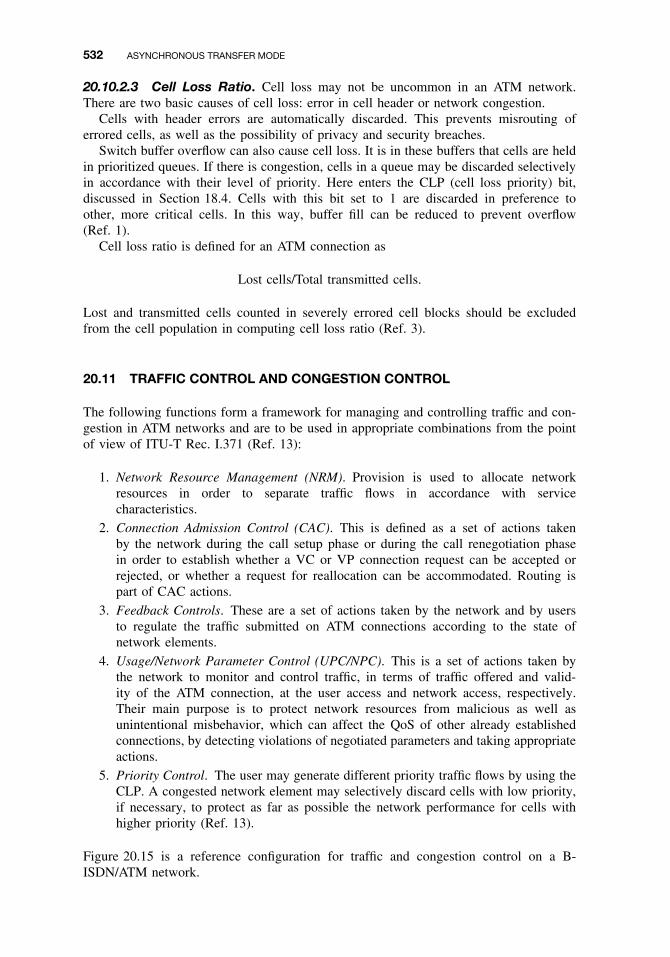
532 ASYNCHRONOUS TRANSFER MODE
20.10.2.3 Cell Loss Ratio. Cell loss may not be uncommon in an ATM network.There are two basic causes of cell loss: error in cell header or network congestion.
Cells with header errors are automatically discarded. This prevents misrouting oferrored cells, as well as the possibility of privacy and security breaches.
Switch buffer overflow can also cause cell loss. It is in these buffers that cells are heldin prioritized queues. If there is congestion, cells in a queue may be discarded selectivelyin accordance with their level of priority. Here enters the CLP (cell loss priority) bit,discussed in Section 18.4. Cells with this bit set to 1 are discarded in preference toother, more critical cells. In this way, buffer fill can be reduced to prevent overflow(Ref. 1).
Cell loss ratio is defined for an ATM connection as
Lost cells/Total transmitted cells.
Lost and transmitted cells counted in severely errored cell blocks should be excludedfrom the cell population in computing cell loss ratio (Ref. 3).
20.11 TRAFFIC CONTROL AND CONGESTION CONTROL
The following functions form a framework for managing and controlling traffic and con-gestion in ATM networks and are to be used in appropriate combinations from the pointof view of ITU-T Rec. I.371 (Ref. 13):
1. Network Resource Management (NRM). Provision is used to allocate networkresources in order to separate traffic flows in accordance with servicecharacteristics.
2. Connection Admission Control (CAC). This is defined as a set of actions takenby the network during the call setup phase or during the call renegotiation phasein order to establish whether a VC or VP connection request can be accepted orrejected, or whether a request for reallocation can be accommodated. Routing ispart of CAC actions.
3. Feedback Controls. These are a set of actions taken by the network and by usersto regulate the traffic submitted on ATM connections according to the state ofnetwork elements.
4. Usage/Network Parameter Control (UPC/NPC). This is a set of actions taken bythe network to monitor and control traffic, in terms of traffic offered and valid-ity of the ATM connection, at the user access and network access, respectively.Their main purpose is to protect network resources from malicious as well asunintentional misbehavior, which can affect the QoS of other already establishedconnections, by detecting violations of negotiated parameters and taking appropriateactions.
5. Priority Control. The user may generate different priority traffic flows by using theCLP. A congested network element may selectively discard cells with low priority,if necessary, to protect as far as possible the network performance for cells withhigher priority (Ref. 13).
Figure 20.15 is a reference configuration for traffic and congestion control on a B-ISDN/ATM network.
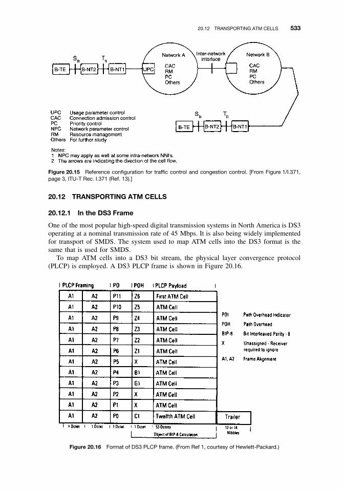
20.12 TRANSPORTING ATM CELLS 533
Figure 20.15 Reference configuration for traffic control and congestion control. [From Figure 1/I.371,page 3, ITU-T Rec. I.371 (Ref. 13).]
20.12 TRANSPORTING ATM CELLS
20.12.1 In the DS3 Frame
One of the most popular high-speed digital transmission systems in North America is DS3operating at a nominal transmission rate of 45 Mbps. It is also being widely implementedfor transport of SMDS. The system used to map ATM cells into the DS3 format is thesame that is used for SMDS.
To map ATM cells into a DS3 bit stream, the physical layer convergence protocol(PLCP) is employed. A DS3 PLCP frame is shown in Figure 20.16.
Figure 20.16 Format of DS3 PLCP frame. (From Ref 1, courtesy of Hewlett-Packard.)

534 ASYNCHRONOUS TRANSFER MODE
There are 12 cells in a PLCP frame. Each cell is preceded by a 2-octet framingpattern (A1, A2) to enable the receiver to synchronize to cells. After the framing patternthere is an indicator consisting of one of 12 fixed bit patterns used to identify the celllocation within the frame (POI). This is followed by an octet of overhead informationused for path management. The entire frame is then padded with either 13 or 14 nibbles(1 nibble = 4 bits) of trailer to bring the transmission rate up to the exact DS3 bit rate.The DS3 frame, as we are aware, has a 125-µsec duration.
DS3 has to contend with network slips (added/dropped frames to accommodate syn-chronization alignment). Thus PLCP is padded with a variable number of stuff (justifi-cation) bits to accommodate possible timing slips. The C1 overhead octet indicates thelength of padding. The BIP (bit-interleaved parity) checks the payload and overhead func-tions for errors and performance degradation. This performance information is transmittedin the overhead.
20.12.2 DS1 Mapping
One approach to mapping ATM cells into a DS1 frame is to use a similar procedure asused with the DS3 PLCP. In this case only 10 cells are bundled into a frame, and two ofthe Z overhead octets are removed. The padding of the frame is set at 6 octets. The entireframe takes 3 ms to transmit and spans many DS1 ESF (extended superframe) frames.This mapping is illustrated in Figure 20.17. The L2 PDU is terminology used with SMDS.It is the upper-level frame from which ATM cells derive through its segmentation.
One must also consider the arithmetic of the situation. Each DS1 timeslot is 8 bits longor 1 octet in length. By definition, there are 24 octets in a DS1 frame. This, of course,leads to a second method of transporting ATM cells in DS1, by directly mapping ATMcells in DS1, octet-for-octet (timeslot). This is done by groups of 53 octets (1 cell) andwould, by necessity, cross DS1 frame boundaries to transport a complete cell.
20.12.3 E1 Mapping
E1 PCM has a 2.048-Mbps transmission rate. An E1 frame has 256 bits representing 32channels or time slots, 30 of which carry traffic. Time slots (TS) 0 and 16 are reserved.
Figure 20.17 DS1 mapping with PLCP. (Courtesy of Hewlett-Packard.)

20.12 TRANSPORTING ATM CELLS 535
Figure 20.18 Mapping ATM cells directly into E1. (From Ref. 1, courtesy of Hewlett-Packard.)
Figure 20.19 Mapping ATM cells into STM-1 (155.520 Mbps rate), at the SDH-based UNI. [FromFigure 8/I.432, page 13, ITU-T Rec. I.432 (Ref. 4).]

536 ASYNCHRONOUS TRANSFER MODE
TS0 is used for synchronization and TS 16 for signaling. The E1 frame is illustrated inFigure 20.18. The sequences of bits from bit 9 to bit 128 and from bit 137 to bit 256may be used for ATM cell mapping. ATM cells can also be directly mapped into specialE3 and E4 frames. The first has 530 octets available for cells (i.e., exactly 10 cells) andthe second has 2160 octets (not evenly divisible).
20.12.4 Mapping ATM Cells into SDH
20.12.4.1 At the STM-1 Rate (155.520 Mbps). SDH was described in Section 19.2.Figure 20.19 illustrates the mapping procedure. The ATM cell stream is first mappedinto the C-4, which, in turn, is mapped into the VC-4 container along with VC-4 pathoverhead. The ATM cell boundaries are aligned with STM octet boundaries. Since theC-4 capacity (2340 octets) is not an integer multiple of the cell length (53 octets), a cellmay cross a C-4 boundaries. The AU-4 pointer (octets H1 and H2 in the SOH) is usedfor finding the first octet in the VC-4.
20.12.4.2 At the STM-4 Rate (622.080 Mbps). As shown in Figure 20.20, the ATMcell stream is first mapped into the C-4-4c and then packed into the VC-4-4c containeralong with the VC-4-4c overhead. The ATM cell boundaries are aligned with the STM-4octet boundaries. The C-4-4c capacity (9360 octets) is not an integer multiple of the celllength (53 octets); thus a cell may cross a C-4-4c boundary. The AU pointers are usedfor finding the first octet of the VC-4-4c.
Figure 20.20 Mapping ATM cells into the STM-4 (655.080 Mbps rate) frame structure for the SDH-basedUNI. [From Figure 10/I.432, page 15, ITU-T Rec. I.432 (Ref. 4).]
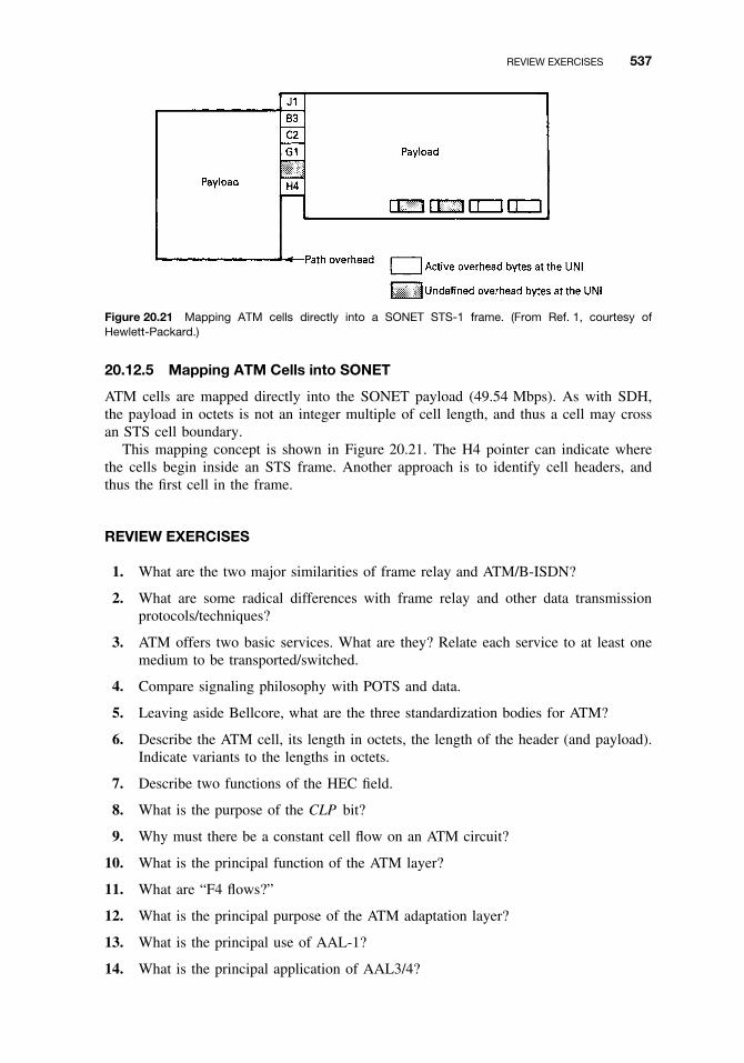
REVIEW EXERCISES 537
Figure 20.21 Mapping ATM cells directly into a SONET STS-1 frame. (From Ref. 1, courtesy ofHewlett-Packard.)
20.12.5 Mapping ATM Cells into SONET
ATM cells are mapped directly into the SONET payload (49.54 Mbps). As with SDH,the payload in octets is not an integer multiple of cell length, and thus a cell may crossan STS cell boundary.
This mapping concept is shown in Figure 20.21. The H4 pointer can indicate wherethe cells begin inside an STS frame. Another approach is to identify cell headers, andthus the first cell in the frame.
REVIEW EXERCISES
1. What are the two major similarities of frame relay and ATM/B-ISDN?
2. What are some radical differences with frame relay and other data transmissionprotocols/techniques?
3. ATM offers two basic services. What are they? Relate each service to at least onemedium to be transported/switched.
4. Compare signaling philosophy with POTS and data.
5. Leaving aside Bellcore, what are the three standardization bodies for ATM?
6. Describe the ATM cell, its length in octets, the length of the header (and payload).Indicate variants to the lengths in octets.
7. Describe two functions of the HEC field.
8. What is the purpose of the CLP bit?
9. Why must there be a constant cell flow on an ATM circuit?
10. What is the principal function of the ATM layer?
11. What are “F4 flows?”
12. What is the principal purpose of the ATM adaptation layer?
13. What is the principal use of AAL-1?
14. What is the principal application of AAL3/4?
538 ASYNCHRONOUS TRANSFER MODE
15. What does a VPI identify?
16. What service classification parameters is the AAL based on?
17. Where are routing functions of virtual channels done?
18. What happens to cells found with errors in their headers?
19. Name three of the four ways the setup and release of VCCs at the UNI canbe performed.
20. Name five of the seven ATM unique quality of service (QoS) items.
21. Cell transfer delay happens at an ATM switch. What is the cause of the delay?
22. Give three causes of CDV (cell delay variation).
23. Name and explain two effects of CDV.
24. What is user/network parameter control (UPC/NPC)?
25. ATM cells are transported on DS1, E1 hierarchies, SONET/SDH hierarchies? Withone exception, what is an unfortunate outcome of the 53-octet cell?
REFERENCES
1. Broadband Testing Technologies, Hewlett-Packard Co., Burlington, MA, Oct. 1993.
2. Broadband Aspects of ISDN, CCITT Rec. I.121, CCITT Geneva, 1991.
3. ATM User–Network Interface Specification, Version 3.0, The ATM Forum, PTR Prentice-Hall,Englewood Cliffs, NJ, 1993.
4. B-ISDN User–Network Interface—Physical Layer Specification, ITU-T Rec. I.432, ITU Ge-neva, 1993.
5. Broadband ISDN User–Network Interfaces—Rates and Formats Specifications, ANSI T1.624-1993, ANSI, New York, 1993.
6. B-ISDN User–Network Interface, CCITT Rec. I.413, ITU Geneva, 1991.
7. Broadband ISDN–ATM Layer Functionality and Specification, ANSI T1.627-1993, ANSI, NewYork, 1993.
8. D. E. McDysan and D. L. Spohn, ATM Theory and Application, McGraw-Hill, New York,1995.
9. B-ISDN ATM Layer Specification, ITU-T Rec. I.361, ITU Geneva, 1993.
10. B-ISDN ATM Adaptation Layer (AAL) Functional Description, ITU-T Rec. 363, ITU Geneva,1993.
11. Support of Broadband Connectionless Data Service on B-ISDN, ITU-T Rec. I.364, ITU Geneva,1993.
12. B-ISDN General Network Aspects, ITU-T Rec. I.311, ITU Geneva, 1993.
13. Traffic Control and Congestion Control in B-ISDN, ITU-T Rec. I.371, ITU Geneva, 1993.
14. Bellcore Notes on the Network, SR-2275, Issue 3, Bellcore, Piscataway, NJ, Dec. 1997.

21
NETWORK MANAGEMENT
21.1 WHAT IS NETWORK MANAGEMENT?
Effective network management optimizes a telecommunication network’s operationalcapabilities. The key word here is optimizes.
These are some of the connotations that can be derived:
ž It keeps the network operating at peak performance.ž It informs the operator of impending deterioration.ž It provides easy alternative routing and work-arounds when deterioration and/or
failure take place.ž It provides the tools for pinpointing cause/causes of performance deterioration or
failure.ž It serves as the front-line command post for network survivability.
There are numerous secondary functions of network management. They are importantbut, in our opinion, still secondary. Among these items are:
ž It informs in quasi-real time regarding network performance.ž It maintains and enforces network security, such as link encryption and issuance and
use of passwords.ž It gathers and files data on network usage.ž It performs a configuration management function.ž It also performs an administrative management function.
21.2 THE BIGGER PICTURE
Many seem to view network management as a manager of data circuits only. There is amuch bigger world out there. Numerous enterprise and government networks serve forthe switching and transport of multimedia communications. The underlying network willdirect (switch) and transport voice, data, and image traffic. Each will have a traffic profilenotably differing from the other. Nevertheless, they should be managed as an entity. If
Fundamentals of Telecommunications, Second Edition, by Roger L. FreemanISBN 0-471-71045-8 Copyright 2005 by Roger L. Freeman
539
540 NETWORK MANAGEMENT
for no other reason, it is more cost-effective to treat the whole rather than piecemeal byits parts.
There is a tendency in the enterprise scene to separate voice telephony, calling ittelecommunications, and another world, that of data communications. Perhaps that is whynetwork management seems to often operate on two separate planes. One is data andvery sophisticated, and the other is voice, which may have no management facilities atall. This next section treats network management as a whole consisting of its multimediaparts: voice, image, and data, which includes facsimile, telemetry, and CAD/CAM.
21.3 TRADITIONAL BREAKOUT BY TASKS
There are five tasks traditionally involved with network management:
ž Fault managementž Configuration managementž Performance managementž Security managementž Accounting management
21.3.1 Fault Management
This is a facility that provides information on the status of the network and subnetworks.The “information on the status” should not only display faults, meaning failures, and theirlocation, but should also provide information on deteriorated performance. One cause ofdeteriorated performance is congestion. Thus, ideally, we would also like to isolate thecause of the problem.
Fault management should include the means to (a) bypass troubled sections of a net-work and (b) patch in new equipment for deteriorated or failed equipment.
The complexity of modern telecommunication networks is such that as many networkmanagement tasks as possible should be automated. All displays, readouts, and hard copyrecords should be referenced to a network time base down to 0.1 sec.1 This helps incorrelating events, an important troubleshooting tool.
21.3.2 Configuration Management
Configuration management establishes an inventory of the resources to be managed. Itincludes resource provisioning (timely deployment of resources to satisfy an expectedservice demand) and service provisioning (assigning services and features to end-users).It identifies, exercises control over, collects data from, and provides data to the networkfor the purpose of preparing for, initializing, starting, and providing for the operation andtermination of services. Configuration management deals with equipment and services,subnetworks, networks, and interfaces. Its functions are closely tied to fault management,as we have defined it above.
21.3.3 Performance Management
Performance management is responsible for monitoring the network to ensure that it ismeeting specified performance. Some literature references (Ref. 1) add growth manage-ment. They then state that the objective of performance and growth management is toensure that sufficient capacity exists to support end-user communication requirements.
1Network time bases are usually much more precise and derive from a network clock, which may be externalto the network, such as GPS. Stratum #1 clock ±1 × 10⁻¹¹ per month.

21.4 SURVIVABILITY—WHERE NETWORK MANAGEMENT REALLY PAYS 541
Of course there is a fine line defining network capacity. If too much capacity exists,there will probably be few user complaints, but there is excess capacity. Excess capacityimplies wasted resources and, thus, wasted money. Excess capacity, of course, can accom-modate short-term growth. Therefore, performance/growth management supplies vitalinformation on network utilization. Such data provide the groundwork for future planning.
21.3.4 Security Management
Security management controls access to and protects both the network and the networkmanagement subsystem against intentional or accidental abuse, unauthorized access, andcommunication loss. It involves link encryption, changes in encryption keys, user authen-tication, passwords, firewalls, and unauthorized usage of telecommunication resources.
21.3.5 Accounting Management
Accounting management processes and records service and utilization information. Itgenerates customer billing reports for services rendered. It identifies costs and establishescharges for the use of services and resources in the network. It may also be a repositoryfor plant-in-place investment for telecommunications plant and provides reports to uppermanagement on return on that investment.
21.4 SURVIVABILITY—WHERE NETWORK MANAGEMENT REALLY PAYS
The network management center is the front-line command post for the battle for networksurvivability. We can model numerous catastrophic events affecting a telecommunicationsnetwork, whether the PSTN or a private/enterprise network. Among such events are fires,earthquakes, floods, hurricanes, terrorism, and public disorder. Telecommunications havebrought revolutionary efficiencies to the way we do business and is so very necessaryeven for life itself. Loss of these facilities could destroy a business, even possibly destroya nation. A properly designed network management system could mitigate losses, evensave a network almost in its entirety.
Cite the World Trade Center explosion (first attack) in New York City. The entirePABX telephone system survived, less the extensions in the immediate area of the bomb,simply because the PABX was mounted on the 6th floor. All offices in the building hadcommunications within the building and with the outside world. The vital communicationswere never lost.
This brings in the first rule toward survivability. A network management center is aplace of point failure. Here we mean that if the center is lost, probably nearly all meansof reconfiguring the network are lost. To avoid such a situation, a second network man-agement center should be installed. This second center should be geographically separatefrom the principal center. It is advisable that the second center share the network manage-ment load and be planned and sized to be able to take the entire load with the loss of theprincipal center. There should be a communications orderwire between the two centers.Both centers should be provided with no-break power and backup diesel generators.
One simple expedient for survivability is to back up circuits with an arrangement withthe local telephone company. This means that there must be compatibility between theenterprise network and the PSTN as well as one or more points of interface. A majorconcern is the network clock. One easy solution is to have the enterprise network deriveits clock from the digital PSTN. The local enterprise network should also be provided abackup clock in case effective timing is lost from the PSTN.

542 NETWORK MANAGEMENT
In the following chapter sections we will describe means to enhance survivabilitystill further.
21.4.1 Survivability Enhancement—Rapid Troubleshooting
An ideal network management system will advise the operator of one or more events,2
indicate where in the network they occurred, and provide other handy troubleshootingdata. In fact, the network management system should, in most cases, warn the operatorin advance of an impending fault/faults. This would be a boon to survivability.
Oftentimes the “ideal” is unachievable or only partially achievable. Human interventionwill be required. The troubleshooter should have available a number of units of testequipment, some more automated than others, to aid in the pinpointing the cause ofan event.
Steve Dauber’s article, Finding Fault (Ref. 3), describes four steps to correct networkfaults. These are:
1. Observing symptoms2. Developing an hypothesis3. Testing the hypothesis4. Forming conclusions
21.4.1.1 Observing Symptoms. It should be kept in mind that often many symptomswill appear at once, usually a chain reaction. We must be able to spot the real causal culpritor we may spend hours or even days chasing effects, not the root cause.
The reference article suggests these four reminders:
1. Find the range and scope of the symptoms. Does the problem affect all stations (allusers)? Does it affect random users or users in a given area? We’re looking for anarea pattern here.
2. Are there some temporal conditions to the problem? How often does it occur perday, per hour, and so on? Is the problem continuous or intermittent? What is itsregularity? Can we set our watches by its occurrence or is it random in the tempo-ral context?
3. Have there been recent rearrangements, additions to the network, reconfigurations?4. Software and hardware have different vintages what are called release dates. I write
this on WordPerfect 7.0, but what was its release date? The question one should askthen would be, Are all items of a certain genre affected in the same way? Differentrelease dates of a workstation may be affected differently, some release dates notat all. The problem may be peculiar to a certain release date. This is particularlytrue of software.
Before we can move forward in the troubleshooting analysis, we must have firmly athand the troublesome network’s baseline performance. What is meant here is that wemust have a clear idea of “normal” operation of the network so that we can really qualifyand quantify its anomalous operation. For example, what is the expected BER and is thevalue related to a time distribution? Can we express error performance in EFS (error freeseconds), ES (errored seconds), and SES (severely errored seconds)? These are definedin ITU-T Rec. G.821 (Ref. 4).
2We define an event as something out-of-the-ordinary that occurred.

21.4 SURVIVABILITY—WHERE NETWORK MANAGEMENT REALLY PAYS 543
In Ref. 3, Steven Dauber lists five network-specific characteristics that the trouble-shooter should have familiarity with or data on.
A. Network Utilization. What is the average network utilization? How does it varythrough the work day? Characteristics of congestion, if any, should be known.Also, where and under what circumstances might it be expected?
B. Network Applications. What are the dominant applications of the network? Whatversion numbers is it running?
C. Network Protocol Software. What protocols are running on the network? Whatare the performance characteristics of the software, and are these characteristicsbeing achieved?
D. Network Hardware. Who manufactured the network interface controllers, mediaattachment units, servers, hubs, and other connection hardware? What versions arethey? What are their performance characteristics? Expected? Met?
E. Internetworking Equipment. Who manufactured the repeaters, bridges, routers, andgateways on the network? What versions of software and firmware are they run-ning? What are the performance characteristics? What are the characteristics of theinterfaced network that are of interest?
21.4.1.2 Developing a Hypothesis. In this second step, we make a statement as tothe cause of the problem. We might say that T1 or E1 frame alignment is lost becauseof deep fades being experienced on the underlying microwave transport network. Orwe might say that excessive frames being dropped on a frame relay network is due tocongestion being experienced at Node B?
Such statements cannot be made without some strong bases to support the opinion.Here is where the knowledge and experience of the troubleshooter really pays. Cer-tainly there could be other causes of E1 or T1 frame misalignment, but if underlyingmicrowave is involved, that would be a most obvious place to look. There could be otherreasons for dropping frames in a frame relay system. Errored frames could be one strongreason.
21.4.1.3 Testing the Hypothesis. We made a statement, now we must back it upwith tests. One test I like is correlation. Are the fades on the microwave correlated withthe fade occurrences? That test can be done quite easily. If they are correlated, we havesome very strong backup that the problem is with the microwave. The frame relay problemmay be another matter. First, we could check the FECN and BECN bits to see if therewas a change of state passing Node B. If there is no change, assuming that flow controlis implemented, then congestion may not be the problem. Removing the frame relay fromthe system and carrying out a BERT (bit error rate test) over some period of time wouldprove or disprove the noise problem.
A network analyzer is certainly an excellent tool in assisting in the localization offaults. Some analyzers have pre-programmed tests that can save the troubleshooter timeand effort. Many networks today have some sort of network monitoring equipment incor-porated. This equipment may be used in lieu of or in conjunction with network analyzers.Again we stress the importance of separating cause and effects. Many times, networkanalyzers or network management monitors and testers will only show effects. The rootcause may not show at all and must be inferred, or separate tests must be carried out topinpoint the cause.

544 NETWORK MANAGEMENT
We might digress here to talk about what is often called tonterıas in Spanish. Thisrefers to “silly things.” Such tonterıas are often brought about by careless installationor careless follow-up repair. Coaxial cable connectors are some of my favorites. Lookfor intermittents and cold solder joints. A good tool, but not necessarily foolproof, is atime-domain reflectometer (TDR). It can spot where a break in a conductor is down to afew feet or less. It can do the same for an intermittent, when in the fault state. In fact,intermittents can prove to be a nightmare to locate. An electrically noisy environment canalso be very troublesome.
21.4.1.4 Conclusions. A conclusion or conclusions are drawn. As we say, “the proofof the pudding is in the eating.” The best proof that we were right on our conclusion isto fix the purported fault. Does it disappear? If so, our job is done, and the network isreturned to it “normal” (baseline) operation.
What “conclusions” can we draw from this exercise? There are two basic ingredientsto elemental network troubleshooting: expertise built on experience of the troubleshooterand the availability of essential test equipment. Troubleshooting time can be reduced(degraded operation or out-of-service time reduction) by having on-line network man-agement equipment. With ideal network management systems, this time can be cut tonearly zero.
21.5 SYSTEM DEPTH—A NETWORK MANAGEMENT PROBLEM
An isolated LAN is a fairly simple network management example. There is only a singulartransmission medium and, under normal operating conditions, only one user is transmit-ting information to one or several recipients. It is limited to only two OSI layers. Fortroubleshooting, often a protocol analyzer will suffice, although much more elaboratenetwork management schemes and equipment are available.
Now connect that LAN to the outside world by means of a bridge or router, andnetwork management becomes an interesting challenge. One example from experiencewas a VAX running DECNET that was a station on a CSMA/CD LAN. The LAN wasbridged to a frame relay box that fed a 384-kbps channel with an E1 hierarchy (i.e., 6 E0channels) via tandemed microwave links to a large facility at the distant end (550 km)with similar characteristics. This connectivity is shown diagrammatically in Figure 21.1.Such is typical of a fairly complex network requiring an overall network managementsystem. To make it even more difficult, portions of the network were leased from thelocal common carrier, but soon to be cutover to own ownership.
21.5.1 Aids in Network Management Provisioning
Modern E1 and T1 digital systems3 are provided a means for operational monitoringof performance. The monitoring is done in quasi-real time and while operational (i.e.,in traffic).
In Chapter 8 we discussed PCM systems and the digital network including T1 (DS1)and E1 hierarchies. Let us quickly review their in-service performance monitoringcapabilities.
3This capability is not unique to T1- and E1-type systems. For example, SONET and SDH have even moresophisticated capabilities, often referred to as OA&M (operations, administration, and maintenance). ATM is(will be) rich in such network management aids.

21.5 SYSTEM DEPTH—A NETWORK MANAGEMENT PROBLEM 545
Bridge
E3 multiplex
Framerelay
Bridge
Framerelay
384 kE1 channel
bank
E3 multiplex
384 kE1 channel
bank
Microwaveterminal
Microwaveterminal
RPTR RPTR
585 km
RPTR RPTR
VAX
DEC-NET
VAX
DEC-NET
CSMA/CD LAN CSMA/CD LAN
Figure 21.1 A typical multilevel network requiring a network management system. Note multipleconvergences.
DS1 or T1 has a frame rate of 8000 frames a second. Each frame is delineated witha framing bit or F-bit. With modern alignment and synchronization algorithms, to main-tain framing repetition of the F-bit 8000 times a second is excessive and unnecessary.Advantage was taken of F-bit redundancy by the development of the extended superframe(ESF). The ESF consists of 24 consecutive DS1 frames. With 24 frames we expect tohave 24 framing bits. Of these, only six bits need to be used for framing, six are used fora cyclic redundancy check (CRC-6) on the superframe, and the remaining 12 bits form a4-kbps data link for network control and maintenance. It is this channel that can serve astransport for network management information. It can also serve as an ad hoc test link.
Our present concern is in-service monitoring. For instance, we can get real-time errorperformance with the CRC-6, giving us a measure of errored seconds and severely erroredseconds in accordance with ITU-T Rec. G.821 (Ref 4). Such monitoring can be done withtest equipment such as the HP4 37702A or HP 37741A.
Permanent monitoring can be carried out using typically Newbridge network monitoringequipment, which can monitor an entire T1 or E1 network for frame alignment loss,
4HP stands for Hewlett-Packard, a well-known manufacturer of electronics test equipment. HP spun off thetest equipment line to Agilent Technologies.

546 NETWORK MANAGEMENT
errored seconds, and severely errored seconds. One can “look” at each link and examineits performance in 15-minute windows for a 24-hour period. The Newbridge equipmentcan also monitor selected other data services such as frame relay, which, in our exampleabove, rides on E1 aggregates. Such equipment can be a most important element in thenetwork management suite.
The E1 digital network hierarchy also provides capability of in-service monitoring andtest. We remember from Chapter 8 that E1 has 32 channels or time slots: 30 are used forthe payload and 2 channels or time slots serve as support channels. The first of these ischannel (or time slot) 0, and the second is channel (time slot) 16. This latter is used forsignaling. Time slot (channel) 0 is used from synchronization and framing. Figure 21.2shows the E1 multiframe structure.
The sequence of bits in the frame alignment (TS0) signal of successive frames isillustrated in Figure 21.2. In frames not containing the frame alignment signal, the firstbit is used to transmit the CRC multiframe signal (001011) that defines the start of thesub-multiframe (SMF). Alternate frames contain the frame alignment word (0011011)preceded by one of the CRC-4 bits. The CRC-4 remainder is calculated on all the 2048bits of the previous sub-multiframe (SMF), and the 4-bit word is sent as C1, C2, C3, C4of the current SMF. Note that the CRC-4 bits of the previous SMF are set to zero beforethe calculation is made.
At the receive end, the CRC remainder is recalculated for each SMF, and the result iscompared with the CRC-4 bits received in the next SMF. If they differ, then the checkedSMF is in error. What this is telling us is that a block of 2048 bits had one or more errors.One thousand CRC-4 block error checks are made every second. It should be noted thatthis in-service error detection scheme does not indicate BER unless one assumes a certainerror distribution (random or burst errors), to predict the average errors per block. Rather,it provides a block error measurement.
This is very useful for estimating percentage of errored seconds (%ES) that is usuallyconsidered the best indication of quality for data transmission—itself a block or frametransmission process. CRC-4 error checking is fairly reliable with the ability of detecting94% of errored blocks even under poor BER conditions (see ITU-T Rec. G.706, Ref. 5).
Sub-multiframe(SMF) Frame number
Multiframe
Bits 1 to 8 of the frame in timeslot 0
21 3 5 7 864
I
II
C1 0 0 1 1 0 1 11 A0 Sa4 Sa5 Sa6 Sa7 Sa80 0 1 1 0 1 1C21 A Sa4 Sa5 Sa6 Sa7 Sa800 0 1 1 0 1 1C31 A Sa4 Sa5 Sa6 Sa7 Sa810 0 1 1 0 1 1C41 A Sa4 Sa5 Sa6 Sa7 Sa80
C1 0 0 1 1 0 1 11 A1 Sa4 Sa5 Sa6 Sa7 Sa80 0 1 1 0 1 1C21 A Sa4 Sa5 Sa6 Sa7 Sa810 0 1 1 0 1 1C31 A Sa4 Sa5 Sa6 Sa7 Sa8E0 0 1 1 0 1 1C41 A Sa4 Sa5 Sa6 Sa7 Sa8E
01234567
89
101112131415
Figure 21.2 E1 multiframe, CRC-4 structure. Notes: E = CRC-4 error indication bits; Sa4 to Sa8 arespare bits. These bits may be used for a network management (maintenance) link. C1 to C4 are CRC-4bits. A stands for remote alarm indication. (From Table 4b/G.704, p. 81, CCITT Rec. G.704, Fascicle III.4,IXth Plenary Assembly, Melbourne, 1988.)

21.5 SYSTEM DEPTH—A NETWORK MANAGEMENT PROBLEM 547
Another powerful feature of E1 channel 0 (when equipped) is the provision of localindication of alarms and errors detected at the far end. When an errored SMF is detected atthe far end, one of the E-bits (see Figure 21.2) is changed from a 1 to a 0 in the return pathmultiframe (TS0). The local end, therefore, has exactly the same block error informationas the far-end CRC-4 checker. Counting E-bit changes is equivalent to counting CRC-4block errors. Thus the local end can monitor the performance of both the go and returnpaths. This can be carried out by the network equipment itself, or by a test set such as theHP 37722A monitoring the E1 2.048-Mbps data bit stream. In the same way, the A-bitsreturn alarm signals for loss of frame or loss of signal from the remote end.
Loopback testing is a fine old workhorse in our toolbox of digital data troubleshootingaids. There are two approaches for DS1 (T1) and E1 systems: intrusive and nonintrusive.Intrusive, of course, means that we interrupt traffic by taking one DS0 or E0 channel outof service, or the entire aggregate. We replace the channel with a PRBS (pseudo-randombinary sequence) or other sequence specifically designed to stress the system. Commonlywe use conventional BERT (bit error rate test) techniques looping back. This idea ofloopback is shown in Figures 21.3a and 21.3b.
ESF and channel 0 data channel testing is nonintrusive. It does not interfere withcustomer traffic. Trouble can also be isolated, whether in the “go” or “return” channel ofthe loopback. Both intrusive and nonintrusive testing could be automated in the networkmanagement suite.
Many frame relay equipments also have forms of in-service monitoring as well as asystem of fault alarms. In fact, most complex telecommunication equipment has built-inmonitoring and test features. The problem often is that these features are proprietary,whereas our discussion of DS1/E1 systems is they have been standardized by ITU-T andTelcordia recommendations and publications. This is probably the stickiest problem facingnetwork management systems. That is handling, centralizing, and controlling networkmanagement features in a multivendor environment.
21.5.2 Communication Channels for the Network Management System
A network management facility is usually centrally located. It must monitor and controldistant communications equipment. It must have some means of communicating with this
BERT
HP Telecomanalyzer in
BERT mode
DS1 channelbank
(near end)
DS1 channelbank
(far end)
E1 channelbank
E1 channelbank
(remote end)
DSO
DSO
(a)
(b)
2.048 Mbps
2.048 Mbps
4-kbps data channelderived from time slot 0
4kbps
Figure 21.3 (a) Loopback of a DS0 channel with BERT test in place, intrusive, or on spare DS0.(b) Loopback of 4 kbps data channel derived from ESF on DS1 or channel 0 on E1.

548 NETWORK MANAGEMENT
equipment, which may be widely dispersed geographically. We have seen where DS1 andE1 systems provide a data channel for (OAM) operations and maintenance. Higher levelsof the DS1 and E1 hierarchies have special communication channel(s) for OAM. So doSONET and SDH.
The solution for a LAN is comparatively straight-forward. The network managementfacility/LAN protocol analyzer becomes just another active station on the LAN. Networkmanagement traffic remains as any other revenue-bearing traffic on the LAN. Of course,the network management traffic should not overpower the LAN with message unit quantitythat we might call network management overhead.
WANs vary in their capacity to provide some form of communicating network man-agement information. X.25 provides certain types of frames or messages dedicated fornetwork control and management. However, these frames/messages are specific to X.25and do not give data on, say, error rate at a particular point in the network. Frame relayprovides none with the exception of flow control and the CLLM, which are specific toframe relay. For a true network management system, a separate network managementcommunication channel may have to be provided. It would have to be sandwiched intothe physical layer. However, SNMP (described below) was developed to typically usethe transport services of UDP/IP. (See Chapter 11 for a discussion of TCP/IP and relatedprotocols.) It is additional overhead, and care must be taken of the percentage of suchoverhead traffic compared to the percentage of “revenue-bearing” traffic. Some use theterm “in-band” when network management traffic is carried on separate frames on thesame medium, and they use the term “out-of-band” when a separate channel or time slotis used such as with E1/T1.
21.6 NETWORK MANAGEMENT FROM A PSTN PERSPECTIVE
21.6.1 Objectives and Functions
The term used by Telcordia (Ref. 12) for network management is “Surveillance andControl.” The major objectives for network surveillance and control organizations areas follows:
ž Maintain a high level of network utilizationž Minimize the effects of network overloadsž Supports the BOC’s5 National Security Emergency Preparedness commitment
There are three important functions that contribute to attaining these objectives:
ž Network traffic management (NTM)ž Network servicež Service evaluation
21.6.2 Network Traffic Management Center
An NTM center provides real time surveillance and control of message traffic6 in localaccess and transport area (LATA) telephone networks. The goal of an NTM center isto increase call completions and optimize the use of available trunks and switching
5BOC stands for Bell operating company, a local exchange carrier.6Message traffic in this context means telephone traffic.

21.6 NETWORK MANAGEMENT FROM A PSTN PERSPECTIVE 549
equipment. Several dedicated OSSs (operational support systems) are employed by anNTM center to achieve this goal by accumulating information on both the flow of traf-fic and the manual and automatic/dynamic control capabilities provided by the networkswitching elements. Using this information and call control capability, a network trafficmanager can optimize the call-carrying capacity of his/her network. The OSSs also enablethe network traffic manager to interact with the network to minimize the adverse effectsof traffic overloads and machine and/or facility failures.
21.6.3 Network Traffic Management Principles
NTM decisions are guided by four principles, which apply regardless of switching technol-ogy, network structure, signaling characteristics, or routing techniques. All NTM controlactions are based on at least one of the following principles:
1. Keep All Trunks Filled with Messages.7 Since the network is normally trunk-limited, it is important to optimize the ratio of messages to nonmessages on any trunkgroup. When unusual conditions occur in the network and cause increased short holding-time calls (nonmessages), the number of carried messages decreases because nonmessagetraffic is occupying a larger percentage of network capacity.
NTM controls are designed to reduce nonmessage traffic and allow more call comple-tions. This results in higher customer satisfaction and increased revenues from the network.
2. Give Priority to Single Link Connections. In a network designed to automaticallyalternate route calls, the most efficient use of available trunks occurs when traffic loadsare at or below normal engineered values. When the engineered traffic load is exceeded,more calls are alternate-routed and, therefore, must use more than one link to complete acall. During overload situations, the use of more than one link to complete a call occursmore often, and the possibility of a multilink call blocking other call attempts is greatlyincreased. Thus in some cases it becomes necessary to limit alternate routing to givefirst-routed traffic a reasonable chance to complete. Some NTM controls block a portionor all alternate-routed calls to give preference to first-routed traffic.
3. Use of Available Trunking. The network is normally engineered to accommodateaverage business day (ABD) busy-hour calling requirements. Focused overloads (e.g., dueto storms, floods, civil disturbances) and holiday calling often result in greatly increasedcalling and drastic changes from the calling patterns for which the network is engineered.This aberration can also be caused by facility failures and switching system outages. Inthese cases, some trunk groups are greatly overloaded, while others may be virtually idle.NTM controls can be activated in many of these cases to use the temporary idle capacityin the network. These controls are known as reroutes.
4. Inhibit Switching Congestion. A switching system is engineered to handle the ex-pected number of attempts generated over its trunk groups with little or no servicedegradation. However, large numbers of ineffective attempts that exceed the engineeredcapacity of the switching system can result in switching congestion. It this switchingcongestion is not relieved, it not only affects potential messages within the congestedswitching system, but it can also cause connected switching systems to become con-gested. Therefore, NTM controls are available that can remove the ineffective attemptsto a congested switching system. These controls will result in inhibiting the switchingcongestion and preventing its spread to adjacent switching systems.
7Telcordia, in Ref. 12, defines a message as a call that has a high probability of completion.

550 NETWORK MANAGEMENT
21.6.4 Network Traffic Management Functions
The following are several types of overloads for which network traffic management con-trols can provide complete or partial relief.
1. A general network overload is caused by changes in traffic patterns and/or increasedtraffic load. These changes may be generated by a reduced business week (heavier callingbefore and after an extended weekend), holiday traffic, local or seasonal changes such asan increase in tourist traffic, unanticipated growth, and natural or man-made disasters. Incases of general network overload, a large amount of the network capacity may be used toswitch calls that have a poor chance of completing. These calls are often regenerated manytimes by both the calling customers and switching systems before they are completed.This results in contention between the “poor completers” and those calls having a betterchance of completing. Because of the volume of regeneration to the poor completers,much of the available trunking and switching capacity is used in switching these calls toan overflow condition.
As NTM personnel identify poor completers, appropriate measures are instituted, whennecessary, to control congestion and remove some or all of these calls from the network.This is done by using code-blocking, call-gapping, and protective trunk group controls.The control of poor completers can greatly increase the number of messages handled by thenetwork. Figure 21.4 illustrates the typical network performance under a general overload.This figure shows the decrease of completed traffic when the offered load exceeds theengineered capacity and congestion is present, and it also shows the increased number ofcalls encountering switching delay.
2. A focused overload is generally directed toward a particular location and may resultfrom media stimulation (e.g., news programs, advertisements, call-in contests, telethons) orevents that cause mass calling to government or public service agencies, weather bureaus,or public utilities. Without the application of appropriate network controls, the effectsof these types of overloads could spread throughout the network. Focused overloads arenormally managed using code controls or, if anticipated, trunk-limited or choke networks.
3. A switching system overload occurs because each individual switch is engineeredto handle a specific load that is known as engineered capacity. The engineered capacity
1000 300020001800
Offered load (erlangs)
Car
ried
load
(er
lang
s)
2000
1800
0
Des
ign
load
No. of switching delays
Congestion
Overload
Figure 21.4 Network performance during overload conditions.
21.6 NETWORK MANAGEMENT FROM A PSTN PERSPECTIVE 551
is usually less than the total switching capacity. When the load is at or below engineeredcapacity, the switch handles calls in an efficient and reliable manner. However, when theload increases beyond the engineered capacity, delays can occur internal to the switch. Thisresulting internal congestion can spread, causing connected systems to wait for start-dialindications. This can also cause internal congestion in connected switching systems.
At the onset of overload, also known as circuit shortage, the dominant cause forcustomer blockage is the failure to find an idle circuit. Circuit blockage alone limits thenumber of extra calls that can be completed but does not cause a significant loss in call-carrying capacity of the network below its maximum. As the overload persists and thenetwork enters a congested state, regeneration-calling pressure changes customer blockagefrom circuit shortage to switching delays.
Switching delays cause timeout conditions during call setup and occur when switchesbecome severely overloaded. Timeouts are designed into switches to release common-control components after excessively long delay periods and provide the customer witha signal indicating call failure. Switching congestion timeouts with short holding-timeattempts on circuit groups replace normal holding-time calls. Switching delays spreadrapidly throughout the network.
A trunk-group overload usually occurs during general or focused overloads and/oratypical busy hours. Some of the overload causes not discussed above are facility outages,inadequate trunk provisioning, and routing errors. The results of trunk-group overload canbe essentially the same as those previously discussed for general overloads. However, theadverse effects are usually confined to the particular trunk group or the apex area formedby the trunk group and those groups that alternate-route to the overloaded trunk-group.Trunk-group overload problems can often be minimized or handled completely by the useof temporary NTM reroute controls until a more permanent solution can be provided.
21.6.5 Network Traffic Management Controls
21.6.5.1 Circuit-Switched Network Controls. There are two broad categories ofNTM controls:
ž Protective Controls. These controls remove traffic from the network during overloadconditions. This traffic is usually removed as close as possible to its origin, thusmaking more of the network available to other traffic with a higher probabilityof completion.
ž Expansive Controls. These controls reroute traffic from routes experiencing over-flows or failures to other parts of the network that are lightly loaded with trafficbecause of noncoincident trunk and switching system busy hours.
Implementation of either type of control can be accomplished on a manual or automaticbasis. For example, manual controls are activated by network traffic managers, and auto-matic controls are activated by network components. In some switches, these controls areimplemented on a planned control-response basis that is preprogrammed into the switch.In other systems, controls are available on a flexible basis, whereby any control can beassigned to any trunk group on a real-time basis.
The availability of any specific control, its allowable control percentages, and themethod of operation can vary with the specific type of switch. In many instances, these net-work controls can be activated with variable percentages of traffic affected (for example,25%, 50%, 75%, and 100%) to fine-tune the control to match the magnitude of the

552 NETWORK MANAGEMENT
problem. Some switches also allow further control selectivity by the use of hard-to-reach(HTR) code-determination algorithms or specification of alternate-routed traffic, direct-routed traffic, or combined direct- and alternate-routed traffic-control choices. The mostcommon manual controls are described below:
ž Cancel controls consist of two variations. “Cancel From” (CANF) potentially pre-vents overflow traffic from a selected trunk group from advancing to any alternateroute. “Cancel To” (CANT) potentially prevents all sources of traffic from access-ing a specific route. Some control arrangements permit CANF and CANT to beapplied to alternate-routed or direct-routed traffic or both. All cancel controls areimplemented on a percentage-of-traffic basis.
ž Skip route control directs a percentage of traffic to bypass a specific circuit group andadvance to the next route in its normal routing pattern. The control can be adjustedto affect alternate-routed or direct-routed traffic or both.
ž Code-block control blocks a percentage of calls routed to a specific destination code.In most cases, a code-block control can also be specified to include the called-stationaddress digits.
ž Call-gapping control, like code-block control, limits routing to a specific code orstation address. Call-gapping is more effective in controlling mass calling situationsthan the code-block control. Call-gapping consists of an adjustable timer that stops allcalls to a specified code for a time interval selected from 16 different time intervals.After the expiration of the time interval, one call to the specified code or addressis allowed access to the network, after which the call-gapping procedure is recycledfor another time interval.
ž Circuit-directionalization control changes 2-way circuits to 1-way operation.ž Circuit-turndown control removes 1- or 2-way circuits from service.ž Reroute controls serve in a variety of ways to redirect traffic from congested or failed
routes to other circuit groups not normally included in the route advance chain butthat have temporary idle capacity. Reroutes override the normal routing algorithmsin a switch. Reroutes can be used on a planned basis, such as on a recurring peak-calling day or in response to unexpected overloads or failures. “Regular reroute”affects traffic overflowing a trunk group. “Immediate reroute” (IRR) affects trafficbefore hunting the trunk group for an idle circuit. Reroute controls may redirecttraffic to a single or to multiple routes. The multiple option is referred to as a “sprayreroute.”
21.6.5.2 Automatic Controls in Modern Digital Switches. Current, computer-based switches may include the following types of automatic controls:
ž Selective dynamic overload control (SDOC)ž Selective trunk reservation (STR)ž Dynamic overload control (DOC)ž Trunk reservationž Selective incoming load control (SILC)
SDOC and STR are considered “selective” protective controls because they can selec-tively control traffic to HTR points8 more severely than other traffic. If the probability of
8HTR (hard to reach) points have 3- or 6-digit destination codes. Calls to these points have a low probabilityof completion.
21.7 NETWORK MANAGEMENT SYSTEMS IN ENTERPRISE NETWORKS 553
completing through the network is very low and the outgoing trunk groups or connectedswitches are overloaded, selective protective controls can prevent wasted usage of theseoverloaded network resources for traffic to HTR points. SDOC responds to switchingcongestion by dynamically controlling the amount and type offered to an overloaded orfailed switch. STR, conversely, responds to trunk congestion in the outgoing trunkingfield and is triggered on a particular trunk group when less than a certain number ofcircuits are idle in that group.
SDOC and STR are two-level control systems. The first level indicates less conges-tion than the second level. The first-level response is typically limited to control oftraffic destined for HTR points, whereas the second level applies controls to both HTRpoints and other traffic, typically alternate-routed traffic. HTR traffic can also be manuallyenabled.
HTR traffic is automatically detected by the AT&T 4ESS switch based on an analysisof destination-code completion statistics. This analysis is performed on a 3- and 6-digitbasis every five minutes. In Nortel DMS-100 and DMS-200/500 switches, HTR codescan also be manually selected and enabled.
Automatic controls, such as SDOC and STR, are intended to be activated by a switchingsystem within a matter of seconds in response to a switch or trunk-group overload. Thesecontrols provide rapid protection for the network and, by their code-selective basis, attemptto restrict traffic that has a low probability of completion. When automatic controls trigger,network traffic managers monitor their operations and adjust system parameters to dealwith the particular network condition, whether it is a general overload, a mass call-in,a natural disaster, or a major network-component failure. Among these parameters arecall-completion determinations that designate a code “HTR” and control-response optionsthat designate the amount of traffic to be controlled or trunks to be reserved at eachtriggering level. Since the optimum control response depends on the severity, geographicaldistribution, and type of overload, maximizing the calls carried by the network requirescoordination and combination of automatic and manual control responses.
21.7 NETWORK MANAGEMENT SYSTEMS IN ENTERPRISE NETWORKS
21.7.1 What Are Network Management Systems?
Ostensibly a network management system provides an automated means of remotelymonitoring a network for:
ž Quantification of performance (e.g., BER, loss of synchronization, etc.)ž Equipment, module, subassembly, card failures, circuit outagesž Levels of traffic, network usage
The impetus of the systems described below has come from the enterprise network envi-ronment, typically from the developer of TCP/IP (US DoD) and later from the OSIworld. There are now many proprietary network management systems available to theuser. Among these are Hewlett-Packard’s Openview, IBM’s Netview, and Digital Equip-ment Corporation EMA (Enterprise Management Architecture). There has been a distincttrend toward distributed processing in the network management arena.
Such network management systems, especially in the distributed processing environ-ment, require a means to communicate for monitoring and control of the enterprisenetwork. Four network management protocols have evolved for this purpose, which wedescribe below.
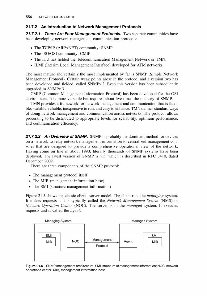
554 NETWORK MANAGEMENT
21.7.2 An Introduction to Network Management Protocols
21.7.2.1 There Are Four Management Protocols. Two separate communities havebeen developing network management communication protocols:
ž The TCP/IP (ARPANET) community: SNMPž The ISO/OSI community: CMIPž The ITU has fielded the Telecommunication Management Network or TMN.ž ILMI (Interim Local Management Interface) developed for ATM networks.
The most mature and certainly the most implemented by far is SNMP (Simple NetworkManagement Protocol). Certain weak points arose in the protocol and a version two hasbeen developed and fielded, called SNMPv.2. Even this version has been subsequentlyupgraded to SNMPv.3.
CMIP (Common Management Information Protocol) has been developed for the OSIenvironment. It is more versatile but requires about five times the memory of SNMP.
TMN provides a framework for network management and communication that is flexi-ble, scalable, reliable, inexpensive to run, and easy to enhance. TMN defines standard waysof doing network management and communication across networks. The protocol allowsprocessing to be distributed to appropriate levels for scalability, optimum performance,and communication efficiency.
21.7.2.2 An Overview of SNMP. SNMP is probably the dominant method for deviceson a network to relay network management information to centralized management con-soles that are designed to provide a comprehensive operational view of the network.Having come on line in about 1990, literally thousands of SNMP systems have beendeployed. The latest version of SNMP is v.3, which is described in RFC 3410, datedDecember 2002.
There are three components of the SNMP protocol:
ž The management protocol itselfž The MIB (management information base)ž The SMI (structure management information)
Figure 21.5 shows the classic client–server model. The client runs the managing system.It makes requests and is typically called the Network Management System (NMS) orNetwork Operation Center (NOC). The server is in the managed system. It executesrequests and is called the agent.
Management
ProtocolNOC
SMI SMI
MIB MIBAgent
Managing System Managed System
Figure 21.5 SNMP management architecture. SMI, structure of management information; NOC, networkoperations center. MIB, management information base.

21.7 NETWORK MANAGEMENT SYSTEMS IN ENTERPRISE NETWORKS 555
SMI. Structure of Management Information (SMI) defines the general framework withinwhich an MIB can be defined. In other words, SMI is the set of rules that define MIBobjects, including generic types used to describe management information. The SNMPSMI uses a subset of Abstract.
Syntax Notation One (ASN.1) specification language that the ISO (International Stan-dards Organization) developed for communications above the OSI Presentation Layer.Layer 7, for example, may use ASN.1 standards such as ITU-T Recs. X.400 and X.500.It was designed this way so that SNMP could be aligned with the OSI environment. TheSMI organizes MIB objects into an upside-down tree for naming purposes.
MIB. Management Information Base (MIB) is the set of managed objects or variablesthat can be managed. Each data element, such as a node table, is modeled as an object andgiven a unique name and identifier for management purposes. The complete definition of amanaged object includes its naming, syntax, definitions, access method (such as read-onlyor read-write) that can be used to protect sensitive data and status. By allowing a statusof “required” or “optional,” the SNMP formulating committee allowed for the possibilitythat some vendors may not wish to support optional variables. Products are obligated tosupport required objects if they wish to be compliant with the SNMP standard.
Figure 21.5 also shows an agent. One can imagine an agent in every data equipmentto be managed as shown in Figure 21.6. Here it shows that the (Network) ManagementConsole manages “agents.”
SNMP utilizes an architecture that depends heavily upon communication between oneor a small number of managers and a large number of remote agents scattered throughoutthe network. Agents use the MIB to provide a view of the local data that is available formanipulation by the Network Management Station. In order for a variable, such as theCPU utilization of a remote Sun workstation, to be monitored by the Network ManagementStation, it must be represented as an MIB object.
The management station sends get and set requests to remote agents. These agentsinitiate traps to the management station when an unexpected event occurs. In such a con-figuration, most of the burden for retrieving and analyzing data rests on the managementapplication. Unless data are requested in a proactive way, little information will be shown
Figure 21.6 The network management console manages agents.

556 NETWORK MANAGEMENT
at the management station. This poll-based approach increases network traffic, especiallyon the backbone where some users report a 5% to 10% increase in traffic due to SNMPnetwork management packets (or messages). SNMP is a connectionless protocol that ini-tially was designed to run over a UDP/IP stack (UDP stands for User Datagram Protocol).Because of its design, it is traditionally high in overhead, with the ratio of overhead tousable data running about ten bytes to one. A typical SNMP “message” (PDU) embeddedin a local network frame is shown in Figure 21.7.
Inside the frame in Figure 21.7 we find an IP (Internet Protocol; see Chapter 11)datagram that has a header. The header has an IP destination address that directs thedatagram to the intended recipient. Following the IP header, there is the User DatagramProtocol (UDP) that identifies the higher layer protocol process. This is the SNMP messageshown in Figure 21.7 as embedded in the UDP. The application here is typically forLANs. If the IP is too long for one frame, it is fragmented (segmented) into one or moreadditional frames.
Figure 21.8 shows a typical SNMP PDU structure that is valid for all messages butthe trap format. This structure is embedded as the “message” field of Figure 21.7. TheSNMP message itself is divided into two sections: (1) a version identifier plus community
LocalNetworkHeader
LocalNetworkTrailer
IPHeader
UDPHeader
SNMPMessage
UDP Datagram
IP Datagram
Local Network Frame
Figure 21.7 An SNMP ‘‘message’’ embedded in a local network frame.
Version
PDUType
RequestID
Community
Object 1, Value 1 Object 2, Value 2
GetRequest, GetNextRequest, GetResponseor SetRequest PDU
SNMP Message
ErrorStatus
ErrorIndex
Variable Bindings
. . .
Figure 21.8 An SNMP PDU structure for GetRequest, GetNext-Request, GetResponse, and Set-Response. (From Refs. 9, 13, and 14.)

21.7 NETWORK MANAGEMENT SYSTEMS IN ENTERPRISE NETWORKS 557
name and (2) a PDU. The version identifier and community name are sometimes referredto as the SNMP authentication header.
The Version field ensures that all parties in the management transaction are using thesame version of SNMP protocol. We must remember the origins of SNMP evolved fromTCP/IP described in Chapter 11, where we have already seen the use of a “version” field.
Each SNMP message contains a Community Name that is one of the only securitymechanisms in SNMP. The agent examines the Community Name to ensure it matchesone of the authorized Community Strings loaded in its configuration files or nonvolatilememory. Each SNMP PDU is one of five types (sometimes called verbs): GetRequest, Get-NextRequest, SetRequest, GetResponse, and Trap. The trap PDU is shown in Figure 21.9.
The PDU shown in Figure 21.8 has five initial fields. The first field is the PDU type.There are five types of PDU as we discussed previously. These are shown in Table 21.1.
The Request ID is the second field of the PDU field. It is an INTEGER-type field thatcorrelates the manager’s request with the agent’s response. INTEGER type is a primitivetype used in ASN.1.
The Error Status field is also an ASN.1 primitive type. It indicates normal operation(noError) or one of five error conditions as shown in Table 21.2.
Version
PDUType
AgentAddress
Community
Object 1, Value 1 Object 2, Value 2
Trap PDU
SNMP Message
SpecificTrap Type
GenericTrap Type Timestamp
Variable Bindings
. . .Enterprise
Figure 21.9 SNMP trap PDU format. (From Refs. 9, 13, and 14.)
Table 21.1 PDU-Type Field Values
GetRequest 0GetNextRequest 1GetResponse 2SetRequest 3Trap 4
Table 21.2 SNMP Error Codes
Error Type Value Description
noError 0 SuccesstooBig 1 Response too large to fit in single
datagramnoSuchName 2 Requested object unknown/unavailablebadValue 3 Object cannot be set to specified valuereadOnly 4 Object cannot be setgenErr 5 Some other error occurred

558 NETWORK MANAGEMENT
When an error occurs, the Error Index field identifies the entry within the variablebindings list that caused the error. If, for example, a readOnly error occurred, the errorindex returned would be 4.
A Variable Binding pairs a variable name with its value. A VarBindList is a list ofsuch pairings. Note that within the Variable Bindings field of the SNMP PDU, the wordObject identifies the variable name (OID* encoding of object type plus the instance) forwhich a value is being communicated.
A trap is an unsolicited packet sent from an agent to a manager after sensing a pre-specified condition such as a cold start, link down, authentication failure, or other suchevent. Agents always receive SNMP requests on UDP port 161, and network managementconsoles always receive traps on UDP port 162. This requirement means that multipleapplications on the same management station that wish to receive traps must usually passcontrol of this port to an intermediate software process. This process receives traps androutes them to the appropriate application.
Figure 21.9 illustrates the SNMP trap PDU structure. We must appreciate that the TrapPDU structure differs from the structure of the other four PDUs shown in Figure 21.8.Like the other PDU structure, the first field, PDU type, will be in this case PDU type = 4(see Table 21.1).
The next field is called the Enterprise Field and identifies the management enterpriseunder whose registration authority the trap was defined. As an example, the OID prefix{1.3.6.1.4.123} would identify Newbridge Networks Corporation as the enterprise sendingthe trap. Further identification is provided in the Agent Address field, which contains theIP address of the agent. In some circumstances a non-IP transport protocol is used. Inthis case the value 0.0.0.0 is returned.
After the Agent Address field in Figure 21.9, we find the Generic Trap Type whichprovides more specific information on the event being reported. There are seven definedvalues (enumerated INTEGER types) for this field as shown in Table 21.3.
The next field is the Time Stamp field that contains the value of the sysUpTime object.This represents the amount of time elapsed between the last re-initialization of the agent inquestion and the regeneration of the trap. As shown in Figure 21.8, the last field containsthe variable bindings.
A trap is generated by an agent to alert the manager that a predefined event hasoccurred. To generate a trap, the agent assigns PDU type = 4 and has to fill in enterprise,agent address, generic trap, specific trap type, time stamp fields, and variable bindings list.
Figure 21.10 gives an excellent summary overview of SNMP.
21.7.3 Remote Monitoring (RMON)
The tendency toward more and more distributed networks has become apparent. Thewide area distribution is both geographical and logical. One method of handling this
Table 21.3 SNMP Trap Codes
Trap Type Value
coldStart 0warmStart 1linkDown 2linkup 3authenticationFailure 4egpNeighborLoss 5enterpriseSpecific 6

21.7 NETWORK MANAGEMENT SYSTEMS IN ENTERPRISE NETWORKS 559
Figure 21.10 An overview of SNMP in place. (From Figure 2-4, Ref. 6, courtesy of IEEE Press.)
situation is to place remote management devices on the remote segments. These remotemanagement devices are sometimes called probes. These probes are the remote sensorsof the network management system, providing the centralized management station withthe required monitoring data dealing with network operation. There is remote networkmonitoring (RMON) MIB that standardizes the management information sent to/fromthese probes.
As an illustration the Ethernet RMON MIB contains nine groups. One of these groups,for example, is entitled “alarms.” It compares statistical samples with preset thresholdsand generating an alarm when a threshold is crossed. Another is “capture,” which allowspackets to be captured after they pass through a logical channel.
21.7.4 SNMP Version 2
SNMPv.2 design used the field experience gained by SNMP to sharpen and simplify themappings to different transports. The management protocol has been separated from thetransport environment, encouraging its use over practically any protocol stack.
One of the weaknesses of SNMP is in the unreliable manner of handling trap messages.Of course, management communications are most critical at times when the network is

560 NETWORK MANAGEMENT
least reliable. A manager’s communications with agents is vital. The use of UDP bySNMP means potentially unreliable transport. SNMP leaves the function of recoveryfrom loss to the manager application. The GET-RESPONSE frame confirms respectiveGET, GET-NEXT, and SET. A network manager can detect the loss of a request when aresponse does not return. For instance, it can repeat the request. Traps are another matter.Trap messages are generated by the agent and are not confirmed. If a trap is lost, theagent applications would not be aware that there is a problem, nor would the managerfor that matter. Since trap messages signal information that is often of great significance,securing their reliable delivery is very important.
Accordingly, SNMPv.2 has pursued an improved mechanism to handle event notifica-tions, namely, traps. For example, the trap primitive has been eliminated. It is replacedby an unsolicited GET-RESPONSE frame that is generated by an agent and directed tothe trap manager (UDP port 162). Now event notifications can be unified as responsesto virtual requests by event managers. In SNMPv.2, a special Trap MIB has been addedto unify event handling, subscription by managers to receive events, and repetitions toimprove reliable delivery.
In the case of SNMP over TCP/IP, we are looking, at what one might call in-bandcommunications. In other words, we are using the same communications channel fornetwork management as we use for “revenue-bearing” communications. This tends todefeat the purpose of network management. The problem can be somewhat alleviated ifthe access path to agents is somewhat protected from the entities that they manage.
Unlike SNMP, SNMPv.2 delivers an array of messaging options that enable agents tocommunicate more efficiently with management stations. Furthermore, SNMPv.2’s bulkretrieval mechanism lets management stations obtain reports from agents about a rangeof variables without issuing repeated requests (i.e., GetBulkRequest). This feature shouldcut down the level of packet activity dedicated to network management and yet improvenetwork management efficiency.
Another advantage of SNMPv.2 over its predecessor is manager-to-manager commu-nications, which allows a station to act as either manager or agent. This allows SNMPv.2systems to offer hierarchical management using mid-level managers to offload tasks fromthe central network management console.
SNMPv.2 does not have to rely on TCP/IP. It can run over a variety of protocol stacksincluding OSI and Internet packet exchange (IPX). It also has notably enhanced securityfeatures over its predecessor.
Figure 21.11 shows a generic SNMPv.2-managed configuration.
21.7.5 SNMP Version 3 (SNMPv.3)
SNMP Version 3, as described in RFC 3410 (Ref. 13), points up deficiencies in Version 2of SNMP. These were unmet design goals of Version 2 and included provision of securityand administration delivering so-called “commercial grade” security with:
ž Authentication: origin identification, message integrity, and some aspects of replayprotection
ž Privacy: confidentialityž Authorization and access controlž Suitable remote configuration and administration capabilities for these features
SNMPv.3 can be thought of as SNMPv.2 with additional security and administrationcapabilities. The documents that specify the SNMPv.3 management framework follow

21.7 NETWORK MANAGEMENT SYSTEMS IN ENTERPRISE NETWORKS 561
Figure 21.11 A generic SNMPv.2-managed configuration. (From Ref. 2, Chapter 3.)
the same architecture as previous versions and for expository purposes are organized intofour main categories as follows:
ž The data definition languagež Management information base (MIB) modulesž Protocol operationsž Security and administration
The first three categories are covered in SNMPv.2. The last category is new, and at thepublication date of RFC 3410 (Ref. 13) it includes seven documents:
ž RFC 3410, which is the referenced document of this section.ž STD 62, RFC 3411, “An Architecture for Describing Simple Network Management
Protocol (SNMP) Management Frameworks” describes the overall architecture forsecurity and administration.

562 NETWORK MANAGEMENT
ž STD 62, RFC 3412, “Message Processing and Dispatching for the Simple Net-work Management Protocol (SNMP)” describes the possibility of multiple messageprocessing models and the dispatcher portion that can be part of the SNMP proto-col engine.
ž STD 62, RFC 3413, “Simple Network Management Protocol Application,” describesthe five initial types of applications that can be associated with an SNMPv.3 enginesand their elements of procedure.
ž STD 62, RFC 3414, “User-Based Security Model (USM) for Version 3 of SNMP,”describes the threats against which protection is provided, as well as the mechanisms,protocols, and supporting data used to provide SNMP message-level security withthe user-based security model.
ž STD 62, RFC 3415, “View-Based Access Control Model (VCAM) for the SNMP,”describes how view-based access control can be applied with command responderand notification originator applications.
ž RFC 2576, “SNMPv.3 Coexistence and Transition,” describes coexistence betweenthe SNMPv.3 Management Framework, SNMPv.2 Management Framework, and theoriginal SNMPv.1 Management Framework and is in the process of being updated.
21.7.6 Common Management Information Protocol (CMIP)
SNMP was developed rapidly with an objective to serve as a network management com-munications standard until CMIP was issued. SNMP met such success that it now has alife of its own. CMIP remains with slow implementation. It hasn’t remotely reached thepopularity of SNMP.
CMIP is an ISO development and it is designed to operate in the OSI environment. Itis considerably more complex than its SNMP counterpart. Figure 21.12 illustrates the OSIManagement architecture that uses CMIP to access managed information. In Figure 21.12this managed information is provided by an agent in the LAN hub.
CMIP is part of the ITU-T X.700 OSI series of recommendations of the ITU. CMIPwas developed and funded by government and corporations to replace and make upfor the deficiencies of SNMP, thus improving the capabilities of network managementsystems.
CMIP uses different terminology than SNMP. An agent maintains a management infor-mation tree (MIT) as a database; it models platforms and devices using managed objects(MOs). These may represent LANs, ports, and interfaces. CMIP is used by a platform tochange, create, retrieve, or delete MOs in the MIT. It can invoke actions or receive eventnotifications.
Object-oriented system concepts that are applied to the CMIP objects include contain-ment, inheritance, and allomorphism. Containment refers to the characteristic of objectsbeing a repository of other objects and/or attributes. A high-level object for a commu-nication switch, for example, can contain several racks of equipment, each of which, inturn, can contain several slots for printed circuit boards. Here one might use the ITU-TM.3100 base class for a circuit pack to define the general features of modules withina communication switch. Object classes can then, in turn, be defined to represent thespecific modules. Items including line interface cards, switching elements, and processorscan be derived from the basic circuit pack definition. Each of these objects exhibits thebehavior, actions, and attributes of both the derived classes and the base class. Allomor-phism is a concept coined by the CMIP standards bodies to refer to the ability to interact

21.7 NETWORK MANAGEMENT SYSTEMS IN ENTERPRISE NETWORKS 563
Figure 21.12 A typical overall architecture of an OSI network management system. (From Figure 2-12,page 48, Ref. 6.)
with modules through a base set of interfaces, only to have the resulting behaviors cou-pled to the complete class definition. Disabling a power supply, for instance, may exhibitsignificantly different behavior than disabling a switching component (Ref. 16).
With CMIP and other OSI management schemes, there are three types of relationshipsbetween managed objects:
ž Inheritance Tree. This defines the managed object class super and subclasses, muchas C++ base and derived classes are related. When a class is inherited from asuperclass, it possesses all the characteristics of the superclass, with additional classspecific extensions (additional attributes, behaviors, and actions).
ž Containment Tree. This defines which managed objects are contained in othermanaged objects. As an example, a subnetwork can contain several managed ele-ments (ME).
ž Naming Tree. This defines the way in which individual objects are referenced withinthe constraints of the management architecture.
From Ref. 16.CMIP (i.e., OSI management communications) communications are very different
than those found in SNMP. These communications are embedded in the OSI applica-tion environment and they rely on conventional OSI peer layers for support. They use

564 NETWORK MANAGEMENT
Operationssystem
Exchange Exchange
Telecommunication network
NOTE - The TMN boundary represented by the dotted line may extend to and manage customer/user services and equipment.
T0405910-95
ExchangeTransmissionsystems
Transmissionsystems
Operationssystem
Operationssystem
TMN
To otherTMNs Data communication network Workstation
Figure 21.13 General relationship of a TMN to a telecommunication network. (From Figure 1/M.3010,Ref. 20.)
connection-oriented transport where SNMP uses the datagram (connectionless). In mostcases these communications are acknowledged.
21.8 TELECOMMUNICATION MANAGEMENT NETWORK (TMN)
Figure 21.13 shows the general relationship between a TMN and a telecommunicationsnetwork which it manages. A TMN is conceptually a separate network that interfaces atelecommunications network at several different points to send/receive information to/fromit and to control its operations. A TMN may use parts of the telecommunications networkto provide its communications.
The objective of the TMN is to provide a framework for telecommunications man-agement. By introducing the concept of generic network models for management, it ispossible to perform general management of diverse equipment, network and services usinggeneric information models and standard interfaces.
A TMN is intended to support a wide variety of management areas that cover the plan-ning, installation, operations, administration, maintenance, and provisioning of telecom-munication networks and services. ITU-T Rec. M.3200 (Refs. 18, 19) describes the scopeof management through the following two main concepts: Telecommunications managedareas and TMN management services. The former relates to the grouping of telecommu-nications resources being managed and the latter relates to the set of processes needed toachieve business objectives, namely, TMN Management Goals.
The specification and development of the required range and functionality of appli-cations to support the above management areas is a local matter and is not consideredwithin the scope of ITU-T Rec. M.3200 series. Some guidance, however, has been pro-vided by the ITU-T, which has categorized management into five broad managementfunctional areas (Rec. X.700, Ref. 21). These functional areas support the managementscope described by ITU-T Rec. M.3020 (Ref. 22). They provide a framework throughwhich the appropriate management services support the public telecommunication oper-ators (PTOs) business processes. Five management functional areas identified to data areas follows:

21.9 TMN FUNCTIONAL ARCHITECTURE 565
ž Performance managementž Fault managementž Configuration managementž Accounting managementž Security management
The classification of the information exchange within the TMN is independent of the usethat will be made of the information.
The TMN needs to be aware of telecommunications networks and services as col-lections of cooperating systems. The architecture is concerned with orchestrating themanagement of individual systems so as to have a coordinated effect upon the network.Introduction of TMNs gives PTOs the possibility to achieve a range of managementobjectives including the ability to:
ž Minimize management reaction times to network events.ž Minimize load caused by management traffic where the telecommunication network
is used to carry it.ž Allow for geographic dispersion of control over aspects of the network operation.ž Provide isolation mechanisms to minimize security risks.ž Provide isolation mechanisms to locate and contain network faults.ž Improve service assistance and interaction with customers.
21.9 TMN FUNCTIONAL ARCHITECTURE
The TMN functional architecture is structured from the following functional elements:
ž Function blocksž Management application functions (MAFs)ž TMN management function sets and TMN management functionsž Reference points
TMN management functionality to be implemented can then be described in terms ofthese fundamental elements.
21.9.1 Function Blocks
Figure 21.14 illustrates the different types of TMN function blocks and indicates that onlythe functions that are directly involved in management are part of a TMN. Some of thefunction blocks are partly in and partly out of a TMN; these TMN function blocks alsoperform functions outside of the TMN functional boundaries as discussed below.
The TMN function block is the smallest deployable unit of TMN management func-tionality. If the TMN function block contains a management application function, it mayonly contain one management application function.
Operations Systems Function (OSF) Block. The OSF processes information related tothe telecommunications management for the purpose of monitoring/coordinating and/orcontrolling telecommunication functions including management functions (i.e., the TMNitself).
Network Element Function (NEF) Block. The NEF is a functional block which com-municates with the TMN for the purpose of being monitored and/or controlled. The
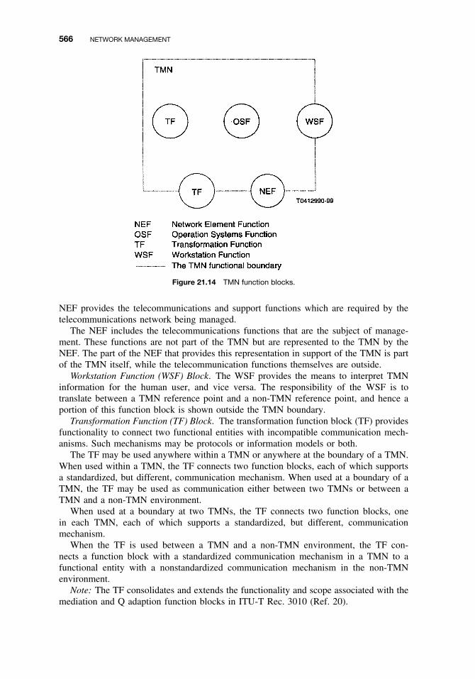
566 NETWORK MANAGEMENT
Figure 21.14 TMN function blocks.
NEF provides the telecommunications and support functions which are required by thetelecommunications network being managed.
The NEF includes the telecommunications functions that are the subject of manage-ment. These functions are not part of the TMN but are represented to the TMN by theNEF. The part of the NEF that provides this representation in support of the TMN is partof the TMN itself, while the telecommunication functions themselves are outside.
Workstation Function (WSF) Block. The WSF provides the means to interpret TMNinformation for the human user, and vice versa. The responsibility of the WSF is totranslate between a TMN reference point and a non-TMN reference point, and hence aportion of this function block is shown outside the TMN boundary.
Transformation Function (TF) Block. The transformation function block (TF) providesfunctionality to connect two functional entities with incompatible communication mech-anisms. Such mechanisms may be protocols or information models or both.
The TF may be used anywhere within a TMN or anywhere at the boundary of a TMN.When used within a TMN, the TF connects two function blocks, each of which supportsa standardized, but different, communication mechanism. When used at a boundary of aTMN, the TF may be used as communication either between two TMNs or between aTMN and a non-TMN environment.
When used at a boundary at two TMNs, the TF connects two function blocks, onein each TMN, each of which supports a standardized, but different, communicationmechanism.
When the TF is used between a TMN and a non-TMN environment, the TF con-nects a function block with a standardized communication mechanism in a TMN to afunctional entity with a nonstandardized communication mechanism in the non-TMNenvironment.
Note: The TF consolidates and extends the functionality and scope associated with themediation and Q adaption function blocks in ITU-T Rec. 3010 (Ref. 20).

21.9 TMN FUNCTIONAL ARCHITECTURE 567
21.9.2 TMN Functionality
Management Application Functionality. The management application functionality(MAF) represents (part of) the functionality of one or more TMN management services.ITU-T Rec. M.32xx-series enumerates the MAFs with respect to the technologies andservices supported by the TMN.
The management application functionality (MAF) may be identified with the typeof TMN function block in which they are implemented. The following MAFs maybe identified:
ž Operations systems functionality (OSF)ž Management application function (OSF-MAF)ž Network element functionality–management application function (NEF–MAF)ž Transformation functionality (TF)ž Management application function (TF-MAF)ž Workstation functionality–management application function (WSF–MAF)
Support Functionality. Support functions may optionally be found in a TMN functionblock. The support functionality is potentially common to more than one TMN functionblock within an implemented TMN. Some support functionality assist the MAF within aTMN function block in its interactions with other function blocks.
21.9.3 TMN Reference Points
A TMN reference point delineates one of several external views of functionality of afunction block; it defines that function block’s service boundary. This external view offunctionality is captured in the set of TMN management functions that will have visibilityfrom the function block.
Reference points have meaning in functional specification leading to an implemen-tation. A reference point can represent the interactions between a particular pair offunction blocks. Table 21.4 shows the relationships between the function blocks in termsof reference points between them. The reference point concept is important because it
Table 21.4 Relationships Between Logical Function Blocks Expressed as Reference Points
NEF OSF TF WSF non-TMN
NEF q q
OSF q q, xa q f
TF q q q f mc
WSF f f gb
non-TMN mc gb
ax reference point only applies when each OSF is in a different TMN.bThe g reference point lies between the WSF and the human user.cThe m reference point lies between the TF and the telecommunication functionality.Note: Any function may communicate at a non-TMN reference point. These non-TMN reference points may bestandardized by other groups/organizations for particular purposes.
Source: Table 1/M.3010, page 13, Ref. 20.

568 NETWORK MANAGEMENT
represents the aggregate of all of the abilities that a particular function block seeks fromanother particular function block, or the equivalent function blocks. It also representsthe aggregate of all the operations and/or notifications (as defined in ITU-T Rec. X.703(Ref. 23) that a function block can provide to a requesting function block.
A TMN functionality specified reference point usually corresponds to a to-be-imple-mented physical interface, in the physical architecture, if and only if the function blocksare implemented in different physical blocks.
21.10 NETWORK MANAGEMENT IN ATM
The ITU-T (CCITT) organization and ANSI have left local network management proce-dures in the M-plane for “further study.”
In the interim period until CCITT and ANSI have formulated such standards, SNMPand the ATM UNI Management Information Base (MIB) are required to provide anyATM user device with status and configuration information concerning virtual path andchannel connections available at its UNI. (See Chapter 20 for a discussion of ATM andclarification of the acronyms used here.)
The ATM Forum has developed the ILMI (Interim Local Management Interface Spec-ification). The ILMI fits into the overall management model for an ATM device shownin Figure 21.15 as clarified by the following principles and options.
1. Each ATM device supports one or more UNIs.2. ILMI functions for a UNI provide status, configuration, and control information
about link and physical layer parameters.3. ILMI functions for a UNI also provide for address registration across the UNI.4. There is a per-UNI set of managed objects, the UNI ILMI attributes, that is suffi-
cient to support the ILMI functions for each UNI.
Figure 21.15 Definition and context of ILMI. (From ATM Forum, Figure 4-1, page 106, Ref. 7.)

21.10 NETWORK MANAGEMENT IN ATM 569
5. The UNI ILMI attributes are organized in a standard MIB structure; there is oneUNI ILMI MIB structure instance for each UNI.
6. There is one MIB instance per ATM device, which contains one or more UNIILMI MIB structures. This supports the need for general network managementsystems to have access to the information in the UNI ILMI MIB structures.
7. For any ATM device, there is a UNI Management Entity (UME) associated witheach UNI that supports the ILMI functions for that UNI, including coordina-tion between the physical and ATM layer management entities associated withthat UNI.
8. When two ATM devices are connected across a (point-to-point) UNI, there are twoUNI management entities (UMEs) associated with the UNI, one UME for eachATM device, and two such UMEs defined as adjacent UMEs.
9. The ILMI communication takes place between adjacent ATM UMEs.10. The ILMI communication protocol is an open management protocol (i.e., SNMP/
AAL initially).11. A UNI management entity (UME) can access, via the ILMI communication pro-
tocol, the UNI ILMI MIB information associated with its adjacent UME.12. Separation of the MIB structure from the access methods allows for the use of
multiple access methods for management information. For the ILMI function, theaccess method is an open management protocol (i.e., SNMP/AAL) over a well-known VPI/VCI value. For example, general network management applications[e.g., from a network management station (NMS) performing generic customernetwork management (CNM) functions] of the access method is also an openmanagement protocol (e.g., SNMP/UDP/IP/AAL) over a specific VPI/VCI value(or a completely separate communications method) allocated to support the generalmanagement applications. The peer entity in an ATM device that communicatesdirectly with an NMS is a management agent, not a UME; however, since themanagement agent can access the MIB instance for the ATM device, it can accessall of the UNI ILMI MIB structure instances.
The Simple Network Management Protocol (SNMP) without UDP and IP addressingalong with ATM UNI management information base (MIB) were chosen for the ILMI.
21.10.1 Interim Local Management Interface (ILMI) Functions
An ILMI supports bi-directional exchange of management information between UNI man-agement entities (UMEs) related to UNI ATM layer and physical layer parameters. Thecommunication across the ILMI is protocol symmetric. In addition, each of the adjacentUMEs supporting ILMI will contain an agent application and may contain a managementapplication. Unless stated otherwise for specific portions of the MIB, both of the adjacentUMEs contain the same management information base (MIB). However, semantics ofsome MIB objects may be interpreted differently. As shown in Figure 21.16, an examplelist of the equipment that will use the ATM UNI ILMI include:
ž Higher-layer switches such as Internet routers, frame relay switches, or LAN bridgesthat transfer their frames within ATM cells and forward the cells across an ATMUNI to an ATM switch.
ž Workstations and computers with ATM interfaces that send their data in ATM cellsacross an ATM UNI to an ATM switch.

570 NETWORK MANAGEMENT
Customer Premises
Ethernet
IS
UNI
UNI
UNI
UNI
Ethernet
Customer Premises
IS
TokenRing
Private NetworkATM Switch
Private networkATM Switch
Public NetworkATM Switch
Public NetworkATM Switch
ATMNetwork
Customer Premises
Public NetworkATM Switch
FDDI
Figure 21.16 Examples of equipment implementing the ATM UNI ILMI. (From ATM Forum, Figure 4-2,page 109, Ref. 7.)
ž ATM network switches that send ATM cells across an ATM UNI to other ATMdevices.
21.10.2 ILMI Service Interface
The ILMI uses SNMP for monitoring and control operations of ATM management infor-mation across the UNI. The ATM UNI management information will be represented ina management information base (MIB). The types of management information will beavailable in the ATM UNI MIB are as follows:

REVIEW EXERCISES 571
ATM
PhysicalLayer
ATMLayer
ATMLayer
Statistics
NetworkPrefix
AddressVirtualPath
Connection
VirtualChannel
Connection
Common Specific
InterfaceIndex
InterfaceIndex
InterfaceIndex +
VPI
InterfaceIndex +Prefix
InterfaceIndex +Address
InterfaceIndex +
VPI + VCI
InterfaceIndex
UNI ILMI MIB
Figure 21.17 ILMI ATM UNI MIB tree structure. (From ATM Forum, Figure 4-3, page 111, Ref. 7.)
ž Virtual path (VP) connectionsž Virtual channel (VC) connectionsž Address registration information
The tree structure of the ATM UNI ILMI MIB is shown in Figure 21.17.
REVIEW EXERCISES
1. Give at least four major benefits to the network operator derived by implementinga network management system.
2. Name the five traditional tasks of network management.
3. Discuss fault management and describe some of the capability it should incorporate.
4. It has been said that a network management center is the front-line command postfor networks .
5. Give the four steps involved in finding a “fault” in a telecommunication network.
6. Describe how a well-engineered network management system can often cut the timealmost to zero for isolating faults.
7. A network management system should be built around on-line monitoring systemsthat are nonintrusive and that are found in (list such systems).
8. Explain how BERT works.
9. Network management systems require communications, especially to/from the net-work management center and remote equipment. Discuss concerns you might havewith such systems, particularly if they share revenue-traffic-bearing channels.
10. From a PSTN perspective, network management may be called “surveillance andcontrol.” What are the two major objectives of surveillance and control?

572 NETWORK MANAGEMENT
11. Distinguish “message traffic” from “non-message traffic.”
12. Describe at least three NTM controls.
13. Give some of the common causes of general network overload.
14. What is a focused overload? Name two measures to mitigate effects of focusedoverloads.
15. What are the two broad categories of NTM controls?
16. Describe the two variations of cancel controls.
17. List four of the automatic (traffic flow) controls one might encounter in a moderncomputer-controlled (SPC) switch.
18. There are really four distinguishable network management protocols. Name eachalong with its sponsoring agency.
19. What are the three components of SNMP? Use the acronyms and write out theirmeaning.
20. What does the MIB do for agents?
21. In SNMP, what does an agent do when an unexpected event occurs?
22. What is the efficiency of SNMP regarding overhead?
23. How does a probe fit into the network management operation?
24. The RAMON MIB contains nine groups. One of these groups is called “alarms.”How do they work?
25. What is the function of a trap?
26. How does SNMPv.2 improve upon SNMPv.1?
27. What are the two general areas where SNMPv.3 improves upon SNMPv.2?
28. Give two major reasons why CMIP has not achieved acceptance in the networkcommunity?
29. In the data communications community there are really two separate worlds. One ofthese has been handed down by the U.S. Department of Defense. Name these twoworlds. Name the network management protocols associated with each.
30. CMIP is based on what environment? (Think ISO).
31. TMN is under the auspices of what international organization?
32. Identify the five fundamental functional areas of TMN. (Return to the basics ofnetwork management itself.)
33. Name at least two of the four TMN function blocks.
34. What is now providing network management in ATM?
35. Name at least five principles and options of ILMI.
36. What types of management information will be available in the ATM UNI MIB?List at lest five items.

REFERENCES 573
37. Give a list of example equipment that would use ATM UNI ILMI (name at leastfour items).
REFERENCES
1. G. Held, Network Management: Techniques, Tools and Systems, Wiley, Chichester, UK 1992.
2. W. Stallings, Network Management, IEEE Computer Society Press, Los Alamitos, CA, 1993.
3. S. M. Dauber, “Finding Fault,” BYTE Magazine, March 1991.
4. Error Performance of an International Digital Connection Forming Part of an Integrated Ser-vices Digital Network, CCITT Rec. G.821, Fascicle III.5, IXth Plenary Assembly, Melbourne,1988.
5. Frame Alignment and Cyclic Redundancy Check (CRC) Procedures Relating to Basic FrameStructures Defined in Recommendation G.704, CCITT Rec. G.706, CCITT Geneva 1991.
6. S. Aidarous and T. Plevyak, Telecommunications Network Management into the 21st Century,IEEE Press, Piscataway, NJ, 1993.
7. ATM User–Network Interface Specification, Version 3.0, The ATM Forum, PTR Prentice-Hall,Englewood Cliffs, NJ, 1993.
8. Mark A. Miller, Managing Internetworks with SNMP, M&T Books, New York, 1993.
9. A Simple Network Management Protocol, RFC 1157, DDN Network Information Center, SRIInternational, Menlo Park, CA, May 1990.
10. Synchronous Frame Structures Used at Primary and Secondary Hierarchical Levels, CCITTRec. G.704, Fascicle III.4, IXth Plenary Assembly, Melbourne, 1988.
11. Information Processing Systems—Open Systems Interconnection, Abstract Syntax Notation One(ANS.1), ISO Std. 8824, Geneva, 1987.
12. BOC Notes on the LEC Networks—1994, Issue 2, Bellcore, Piscataway, NJ, April 1994.
13. G. Held, Network Management, Wiley, Chichester, UK, 1992.
14. Introduction and Applicability Statements for Internet Standard Management Framework,SNMPv.3, RFC 3410, IETF editor, Ann Arbor, Michigan, Dec. 2002.
15. Version.2 of the Protocol Operations for the Simple Network Management Protocol (SNMP),STD 62, RFC 3416, IETF editor, Ann Arbor, Michigan, Dec. 2002.
16. CMIP/CMIS—Object Oriented Network Management, from the world wide web www.cellsoft..de/telecom/CMIP.htm, Sept. 1, 2003.
17. Structure of Management Information—Management Information Model, CCITT Rec. X.720,ITU Geneva, Jan. 1992.
18. Generic Network Information Model, ITU-T Rec. M.3100, ITU Geneva, July 1995 (with 5amendments).
19. Telecommunication Management Functions, ITU-T Rec. N.3400, ITU Geneva, Feb. 2000.
20. Principles of a Telecommunication Management Network, ITU-T Rec. M.3010, ITU Geneva,Feb. 2000.
21. Management Framework for Open System Interconnection (OSI) for CCITT Applications, CCITTRec. X.700, ITU Geneva, 1992.
22. TMN Interface Specifications Methodology, ITU-T Rec. M.3020, ITU Geneva, 2000.
23. Information Technology—Open Distributed Management Architecture, ITU-T Rec. X.703, ITUGeneva, 1997.


APPENDIX A
REVIEW OF FUNDAMENTALSOF ELECTRICITY WITH
TELECOMMUNICATIONAPPLICATIONS
A.1 OBJECTIVE
For a better understanding of this text, a certain basic knowledge of electricity is essen-tial. The objective of the appendix is to cover only the necessary principles of electricity.Each principle is illustrated with one or several applications. Only minimal ac (alternatingcurrent) theory is presented. Where possible, these applications favor electrical communi-cations. Analogies to assist in the understanding of a concept are used where appropriate.
We cannot see electricity. We can feel its effects such as electrical shock, the generationof heat, and the buildup and decay of magnetic and electrical fields. For example, acompass will indicate the presence of a magnetic field.
It is assumed that the reader has had at least three years of high school mathematicsincluding algebra, trigonometry, and logarithms. For those who feel that their backgroundin mathematics is insufficient, Appendix B gives an overview of those basic essentials.
A.2 WHAT IS ELECTRICITY?
We define electricity as the movement of electrons through a conductor.1 Certain sub-stances are good conductors and other substances are poor conductors. Poor conductorsare called insulators. The various materials or substances we have here on earth run thegamut, from superb conductors such as platinum, gold, silver, and copper to extremelygood insulators such as glass, mica, polystyrene, and rubber.
The movement of electrons through a conductor is measured in amperes.2 In fact 1ampere is the flow of 6.24 × 10¹⁸ electrons per second past a given point in a conductor.
1Encyclopedia Brittanica defines electricity as “The phenomenon associated with positively and negativelycharged particles of matter at rest and in motion, individually or in great numbers.”2An ampere is a unit of electrical measurement. All units of electrical measurement are named for scientistscredited with discovering the particular phenomenon, and often providing a mathematical analysis of thatelectrical phenomenon. Ampere is one example.
Fundamentals of Telecommunications, Second Edition, by Roger L. FreemanISBN 0-471-71045-8 Copyright 2005 by Roger L. Freeman
575

576 REVIEW OF FUNDAMENTALS OF ELECTRICITY WITH TELECOMMUNICATION APPLICATIONS
Where the flow of electrons is continuous in one direction is called direct current (dc). Thecurrents of electrons may also periodically reverse their flow. This is called alternatingcurrent (ac). Our discussion starts with the traditional laws of direct current. Later webriefly discuss some basic principles of alternating currents.
A.2.1 Electromotive Force (EMF) and Voltage
We require a source of “electric pressure,” called electromotive force (emf), to establisha flow of electrical current. The standard analogy is to use water and its flow througha water circulating system. This is illustrated in Figure A.1. The figure shows the waterpressure source as a pump, two different-diameter pipes, and some sort of mechanismto measure water flow. Flow can be measured in several ways such as liters or gallonsper second or minute. The pump creates a difference in pressure between points x andy. Some will say that the pump sets up a “head of pressure.” This will cause water toflow from point x at the output of the pump up the large-diameter pipe, across the smalldiameter pipe, and down through another large-diameter pipe in which we installed a flowpressure gauge. The water returns to the low pressure side of the pump, shown as y inthe drawing. The amount of water that will flow (i.e., analogy to amperage) depends onthe difference in pressure between points x and y and the size of the small pipe. Thedifference in pressure is analogous to electromotive force.
Figure A.2 is an electrical representation of the circulating water system shown inFigure A.1. The battery (see Section 2.3.1) supplies the electrical pressure or emf. Itcauses the electricity to flow from the high potential side of the battery, labeled x, toits low potential side, labeled y in Figure A.2. The amount of current that will flow willdepend upon the emf and the nature of the resistor, shown between points x and y.
The difference of water pressure may be measured in units such as “difference in headin feet.” The emf of the electric circuit, on the other hand, is measured in terms of a unitcalled a volt.
Another important term is electric potential. In Figure A.2 we can say that the electricpotential at the positive terminal of the battery is higher than that of its negative terminal.The difference is the electromotive force of the battery or other source. The potential atpoint y will be lower than the potential at point x. Thus we say that there is a potentialbetween x and y. The potential drop is measured in volts and the magnitude of the dropdepends on the resistance of the conductors and the resistor.
Small-diameter pipe
Flowmeter
y
x Pump
Figure A.1 A water circulating system.
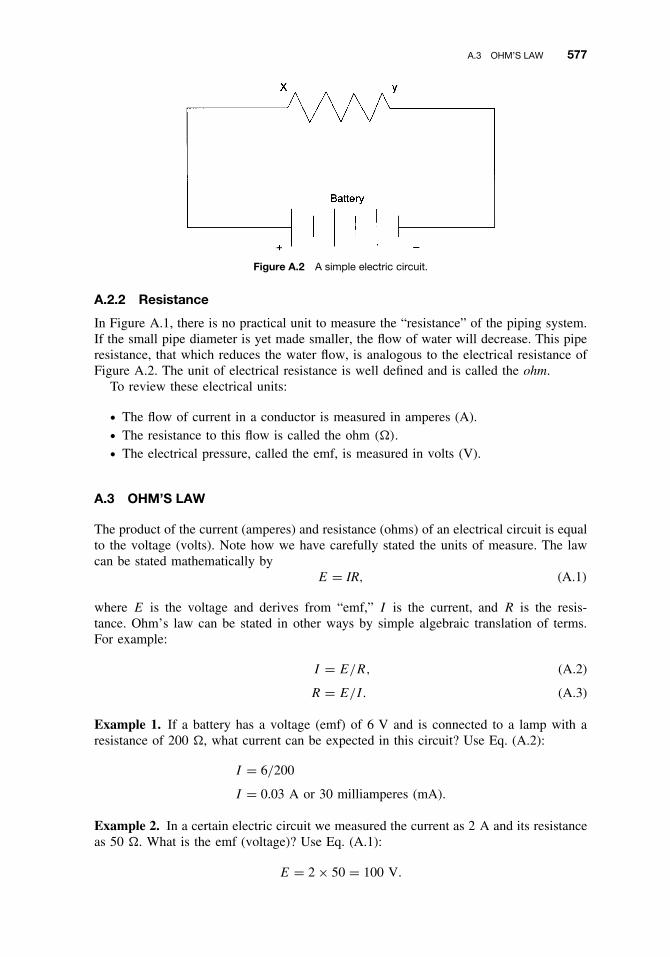
A.3 OHM’S LAW 577
Figure A.2 A simple electric circuit.
A.2.2 Resistance
In Figure A.1, there is no practical unit to measure the “resistance” of the piping system.If the small pipe diameter is yet made smaller, the flow of water will decrease. This piperesistance, that which reduces the water flow, is analogous to the electrical resistance ofFigure A.2. The unit of electrical resistance is well defined and is called the ohm.
To review these electrical units:
ž The flow of current in a conductor is measured in amperes (A).ž The resistance to this flow is called the ohm (�).ž The electrical pressure, called the emf, is measured in volts (V).
A.3 OHM’S LAW
The product of the current (amperes) and resistance (ohms) of an electrical circuit is equalto the voltage (volts). Note how we have carefully stated the units of measure. The lawcan be stated mathematically by
E = IR, (A.1)
where E is the voltage and derives from “emf,” I is the current, and R is the resis-tance. Ohm’s law can be stated in other ways by simple algebraic translation of terms.For example:
I = E/R, (A.2)
R = E/I. (A.3)
Example 1. If a battery has a voltage (emf) of 6 V and is connected to a lamp with aresistance of 200 �, what current can be expected in this circuit? Use Eq. (A.2):
I = 6/200
I = 0.03 A or 30 milliamperes (mA).
Example 2. In a certain electric circuit we measured the current as 2 A and its resistanceas 50 �. What is the emf (voltage)? Use Eq. (A.1):
E = 2 × 50 = 100 V.

578 REVIEW OF FUNDAMENTALS OF ELECTRICITY WITH TELECOMMUNICATION APPLICATIONS
A.3.1 Voltages and Resistances in a Closed Electric Circuit
Figure A.3 shows three resistances connected in series with a battery source of 48 V. Wedefine a closed circuit as one in which current flows; an open circuit is a circuit in whichno current flows. Figure A.3a is a closed circuit (i.e., the switch is in the closed position)and A.3b is an open circuit (i.e., the switch is in the open position).
Emf is measured with a voltmeter, as shown in Figure A.4, where the open circuitvoltage (emf) of a battery is measured. A voltmeter is also used to measure potential dropas shown in Figure A.3a. Here the voltmeter is connected across R3 (across points y andz). In later discussion we will also call this the IR drop. Remember Ohm’s law: E = IR.Regarding the potential drop across R3, if we know the resistance of R3 and we knowthe current passing through it, we know the potential or IR drop. This is one of the manyapplications of Ohm’s law.
In Figure A.3a, if we measure the potential drop (IR drop) in volts across each resis-tance and sum the values, this will equal the value of the battery emf in the closedcircuit condition.
Example of Series Resistances. Four resistors are connected in series. Their resistancevalues are 250, 375, 136, and 741 �. Suppose we were to replace these four with just oneresistor. The current through the circuit will be the same for one or for the four resistorsin series. What will be the value in ohms of the single replacement resistor?
Figure A.3a A closed circuit showing three resistances in series with a battery as an emf source. Avoltmeter is placed across R3, which measures the potential difference across that resistance.
Figure A.3b An open circuit with three resistances in series with emf source.

A.3 OHM’S LAW 579
Figure A.4 Measuring the voltage of a battery. (a) A typical dry cell. (b) Showing voltage measurementusing the standard battery drawing symbol. These are open circuit measurements.
Table A.1 American Wire Gauge (AWG) Versus WireDiameter and Resistance
AmericanWire Gauge
Diameter(mm)
Resistance (�/km)a
at 20◦C
11 2.305 4.13412 2.053 5.21013 1.828 6.57114 1.628 8.28415 1.450 10.4516 1.291 13.1817 1.150 16.6118 1.024 20.9519 0.9116 26.3920 0.8118 33.3021 0.7229 41.9922 0.6439 52.9523 0.5733 66.8024 0.5105 84.2225 0.4547 106.2026 0.4049 133.927 0.3607 168.928 0.3211 212.929 0.2859 268.630 0.2547 338.631 0.2268 426.832 0.2019 538.4
aThese figures must be doubled for loop/km. Remember it has a ‘‘go’’and ‘‘return’’ path.
We know that this resistor must have a value equal to four of these resistors if there isno change in current. Just sum the resistor values or 250 + 375 + 136 + 741 = 1502 �.The rule here is that when we want to calculate the equivalent resistance of resistors inseries, we just sum the resistances of each resistor.
A.3.2 Resistance of Conductors
The current we can expect through a conductor with a fixed emf source varies directlywith (1) the resistivity3 of the type of conductor, (2) the length of the conductor, and
3Resistivity is a unit constant used to determine the conductive properties of a material.
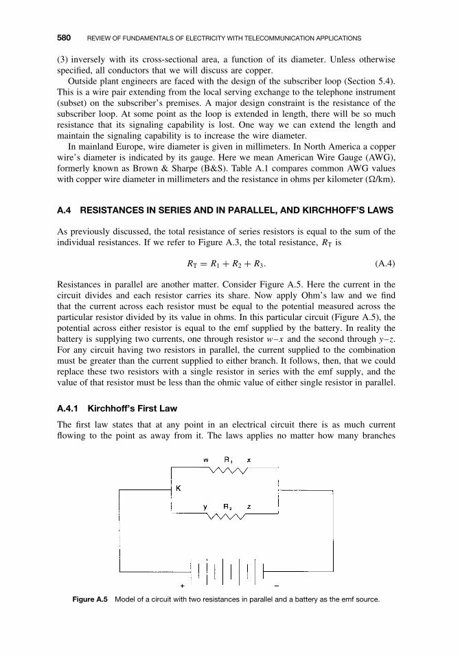
580 REVIEW OF FUNDAMENTALS OF ELECTRICITY WITH TELECOMMUNICATION APPLICATIONS
(3) inversely with its cross-sectional area, a function of its diameter. Unless otherwisespecified, all conductors that we will discuss are copper.
Outside plant engineers are faced with the design of the subscriber loop (Section 5.4).This is a wire pair extending from the local serving exchange to the telephone instrument(subset) on the subscriber’s premises. A major design constraint is the resistance of thesubscriber loop. At some point as the loop is extended in length, there will be so muchresistance that its signaling capability is lost. One way we can extend the length andmaintain the signaling capability is to increase the wire diameter.
In mainland Europe, wire diameter is given in millimeters. In North America a copperwire’s diameter is indicated by its gauge. Here we mean American Wire Gauge (AWG),formerly known as Brown & Sharpe (B&S). Table A.1 compares common AWG valueswith copper wire diameter in millimeters and the resistance in ohms per kilometer (�/km).
A.4 RESISTANCES IN SERIES AND IN PARALLEL, AND KIRCHHOFF’S LAWS
As previously discussed, the total resistance of series resistors is equal to the sum of theindividual resistances. If we refer to Figure A.3, the total resistance, RT is
RT = R1 + R2 + R3. (A.4)
Resistances in parallel are another matter. Consider Figure A.5. Here the current in thecircuit divides and each resistor carries its share. Now apply Ohm’s law and we findthat the current across each resistor must be equal to the potential measured across theparticular resistor divided by its value in ohms. In this particular circuit (Figure A.5), thepotential across either resistor is equal to the emf supplied by the battery. In reality thebattery is supplying two currents, one through resistor w–x and the second through y–z.For any circuit having two resistors in parallel, the current supplied to the combinationmust be greater than the current supplied to either branch. It follows, then, that we couldreplace these two resistors with a single resistor in series with the emf supply, and thevalue of that resistor must be less than the ohmic value of either single resistor in parallel.
A.4.1 Kirchhoff’s First Law
The first law states that at any point in an electrical circuit there is as much currentflowing to the point as away from it. The laws applies no matter how many branches
Figure A.5 Model of a circuit with two resistances in parallel and a battery as the emf source.

A.4 RESISTANCES IN SERIES AND IN PARALLEL, AND KIRCHHOFF’S LAWS 581
there are in the circuit. Figure A.5 shows point K in the circuit. Let I be the current beingsupplied by the battery emf source to the combination of the two resistors in parallel; I1
and I2 are the currents through the two resistors, respectively. We now can say, based onKirchhoff’s first law, that
I = I1 + I2. (A.5)
Again consider the circuit in Figure A.5. Let R be the equivalent resistance of the tworesistors in parallel. Applying Ohm’s law, we obtain
R = E/I.
Substitute Eq. (A.5). We then have
R = E/(I1 + I2). (A.6)
However, I1 = E/R1 and I2 = E/R2. As a consequence, we have
R = E/[(E/R1) + (E/R2)]. (A.7)
Divide Eq. (A.7) through by E and we now have
R = 1/[(1/R1) + (1/R2)]. (A.8)
Simplify the compound fraction and we have
R = R1 × R2/(R1 + R2). (A.9)
Example. There are two resistors connected in parallel. Their values are 500 � and700 �, respectively. What is the value of the equivalent combined resistance? UseEq. (A.9).
R = 500 × 700(500 + 700) = 350,000/(500 + 700) = 350,000/1200
= 291.6 �.
One self-check for resistances in parallel is that the equivalent combined resistance mustbe smaller than the value of either resistor.
Figure A.6 shows a group of three resistors in parallel with an emf source that isa battery. We encourage the use of a short-cut when there are more than two resistorsin parallel. We introduce a new term, conductance. Conductance, G, is the inverse ofresistance; stated in an equation:
R = 1/G. (A.10)
The unit of conductance is the mho, which the reader will note is “ohm” spelled backwards.To solve the equivalent total resistance problem of Figure A.6, convert each resistanceinto its equivalent conductance, sum the values, and invert the sum.
Example. The values of the resistances in Figure A.6 are 2000, 2500, and 3000 �; theclosed circuit emf of the battery is 24 V. What is the value of the current flowing out of thebattery? Use Eq. (A.10) and convert each resistance value to its equivalent conductance

582 REVIEW OF FUNDAMENTALS OF ELECTRICITY WITH TELECOMMUNICATION APPLICATIONS
Figure A.6 Model of a circuit with three resistors in parallel.
and sum:
G = G1 + G2 + G3
= 1/2000 + 1/2500 + 1/3000
= 0.0005 + 0.0004 + 0.00033
= 0.00123 mhos. (A.11)
Use the inverse of Eq. (A.11) or R = 1/G; then
R = 1/0.00123 = 813 �.
We know the voltage source is 24 V and the circuit resistance is 813 �. We now can applyOhm’s law to calculate the current flowing out of the battery. Use Eq. (A.2) or I = E/R:
I = 24/813 = 0.0295 A or 29.5 mA.
A.4.2 Kirchhoff’s Second Law
When current flows through a resistor, there is always a difference in potential whenmeasured across the resistor (i.e., between one end and the other of the resistor). Thevalue in volts of the difference in potential varies with the current flowing through theresistor and the resistance. In fact, as mentioned, the value is the product of the resistance(in ohms) and current (in amperes). This is just the statement of Ohm’s law, Eq. (A.1)(E = IR). In our previous discussion, it was called potential difference, voltage drop, orIR drop. This IR drop acts in the opposite direction to, or opposes, the emf which drivesthe current through the resistor.
Figure A.7 is a model of a circuit with three resistors in series and a battery emfsource. For reference, a voltmeter is shown measuring the voltage (the IR drop) acrossresistor R2. In such a closed circuit, the sum of the IR drops across the three resistorsmust be equal to the impressed emf. Let the IR drop across each resistor in Figure A.7be represented by V1, V2, and V3, respectively. This, then, is how we state Kirchhoff’ssecond law:
E = V1 + V2 + V3, (A.12)

A.4 RESISTANCES IN SERIES AND IN PARALLEL, AND KIRCHHOFF’S LAWS 583
Figure A.7 A model circuit for three resistors in series. A voltmeter measures the IR drop acrossresistor R2.
where E is the impressed emf or closed circuit battery voltage. In the case of Figure A.7,we can write
E = IR1 + IR2 + IR3. (A.13)
This equation can be restated as
E − IR1 − IR2 − IR3 = 0.
A.4.3 Hints on Solving dc Network Problems
Make a network drawing, much like we have in Figures A.1 through A.7. Then assignletters to all unknown values. This should be followed by arrows showing the directionof current flow. With the practical application of Kirchhoff’s laws, use correct algebraicsigns. There should be one sign (+ or −) given to the electromotive force in the directionof the current flow, and the opposite sign is then given to the IR drops. Often we acceptthe clockwise direction as positive, and the counterclockwise as negative. For instance,all emfs are labeled positive that tend to make the current flow in the positive direction;and all potential drops are labeled negative, due to this flow of current as well as anyemfs tending to make current flow in the opposite direction. When carrying out thisexercise, we may find a solution to an equation may be preceded by a minus sign. Thismerely means that the actual direction of flow of current is opposite to the directionwe assumed.
Example Calculation of a Series–Parallel Circuit. Figure A.8 is a model series–parallelcircuit. In other words, the circuit has a mix of resistances in series and in parallel. Hint :Replace all parallel resistors by their equivalent value first. Thus we end up with a circuitentirely of resistances in series. In other words, first calculate the equivalent resistance forresistors R1 and R2; then for R3, R4, and R5. We end up with four resistors in series: thefirst and second group of parallel resistors, the R6, and R7. The total resistance of the circuitis then the sum of these four resistances. Assign the following values to these resistances:R1 = 800 �; R2 = 1200 �; R3 = 3000 �; R4 = 5000 �; R5 = 4000 �; R6 = 600 �; andR7 = 900 �.

584 REVIEW OF FUNDAMENTALS OF ELECTRICITY WITH TELECOMMUNICATION APPLICATIONS
Figure A.8 A model for a circuit with series and parallel resistances with a battery as an emf source.
For the first group of parallel resistances we use formula (A.9):
R = 800 × 1200/(800 + 1200) = 960,000/2000
= 480 �.
For the second group of parallel resistances use formulas (A.10) and (A.11), as follows:Calculate the current flowing out of the 48-V battery?
G3 = 1/3000 = 0.000333; G4 = 1/5000 = 0.0002; G5 = 1/4000 = 0.00025.
Sum these values using Eq. (A.11) and
G = 0.000333 + 0.0002 + 0.00025
= 0.000783.
Use formula (A.10) to obtain the equivalent resistance
R = 1/G = 1/0.000783
= 1277.14 �.
Calculate the total resistance of the circuit with the four resistances, which includesthe derived resistances. Use formula (A.4):
RT = 480 + 1277.14 + 600 + 900(�)
= 3257.14 �.
To calculate the current flowing out of the battery, use Ohm’s law [Eq. (A.2)]:
I = E/R = 48/3257.14 = 0.0147 A or 14.7 mA.
A.5 ELECTRIC POWER IN dc CIRCUITS
Batteries store chemical energy. When the battery terminals are connected to supply emfto an electric circuit, the battery chemical energy is converted to electrical energy. This

A.6 INTRODUCTION TO ALTERNATING CURRENT CIRCUITS 585
manifests itself as power (work per unit time). The unit of power is the watt (W). Whenwe pay our electric bill, we pay for kilowatt-hours of expended electric power.
The resistors in Figures A.2–A.8 dissipate power in the form of heat. In fact, not onlyare resistors rated for their resistance in ohms, but also for their capability to dissipateheat measured in watts. Let us now examine the electric power dissipated by a resistor orother ohmic device.4 Let power, expressed in watts, be denoted by the notation P . Then:
P = EI. (A.14)
Stated in words: In an electric circuit, if we multiply the electromotive force in volts by thecurrent in amperes, we have an expression for the power in watts [Eq.(A.14)]. The wattmay, therefore, be defined as the power expended in a circuit having an electromotiveforce of one volt and a current of one ampere.
There are two variants of Eq. (A.14) by simple substitution of variants of Ohm’s law[Eqs. (A.1), (A.2), and (A.3)]:
P = EI = E(E/R) = E2/R (A.15)
andP = EI = IR(I ) = I 2R. (A.16)
Example 1. The current flowing through a 1000-� resistor is 50 mA. What is the powerdissipated by the resistor? Convert mA to A or 0.05 A. Use Eq. (A.16):
P = (0.05)2 × 1000
= 2.5 W.
Example 2. The potential drop across a 600-� resistor is 3 V. What power is beingdissipated by the resistor? Use Eq. (A.15):
P = E2/R = 32/600 = 0.015 W or 15 mW.
A.6 INTRODUCTION TO ALTERNATING CURRENT CIRCUITS
A.6.1 Magnetism and Magnetic Fields
The phenomenon of magnetism was known by the ancient Greeks when they discovereda type of iron ore called magnetite. Moorish navigators used a needle-shaped piece of thisore as the basis of a crude compass. It was found that when this needle-shaped piece ofmagnetite was suspended and allowed to move freely, it would always turn to the north.What we are dealing with here are permanent magnets. Remember, we used permanentmagnets in the telephone subset to set up a magnetic field in its earpiece (Section 5.3.2).Figure A.9 shows an artist’s rendition of the magnetic field around a bar magnet, the mostcommon form of permanent magnet.
In the early nineteenth century it was learned that this magnetic property can beartificially induced to a family of iron-related metals by means of an electric current.
4Electrical power, of course, can manifest itself or be useful in other ways besides the generation of heat. Forexample, it can rotate electric motors (mechanical energy) and it can be used to generate a radio wave.

586 REVIEW OF FUNDAMENTALS OF ELECTRICITY WITH TELECOMMUNICATION APPLICATIONS
Figure A.9 An artist’s rendition of the magnetic field around a bar magnet.
The magnetic field was maintained while current is flowing; it collapsed when the cur-rent stopped.
Magnets, as we know them today, are classed as either permanent magnets or electro-magnets. A typical permanent magnet is a hard steel bar that has been magnetized. It canbe magnetized by placing the bar in a magnetic field; the more intense the field, the moreintense is the induced magnetism in the steel bar. The influence of a magnetic field canbe detected in various ways, such as by a conventional compass or iron filings on paperwhere the magnet is placed below the paper.
With this latter approach with the iron filings we develop an arrangement of the filingsthat will appear almost identical with Figure A.9. The lines that develop are commonlyknown as lines of magnetic induction. All of the lines as a group are referred to as theflux, which is designated by the symbol φ. The flux per unit area is known as the fluxdensity and is designated by B. We arbitrarily call one end of the bar magnet the northpole, and the opposite end, the south pole. Many of us remember playing with magnetswhen we were children. It was fun to bring in a second bar magnet. It was noted that ifits south pole was brought into the vicinity of the first magnet’s south pole, the magnetsphysically repelled each other. On the contrary, when the north pole of one magnet wasbrought into the vicinity of the south pole of the other, they were attracted.
Suppose the strength of the magnet in Figure A.9 is increased. The magnetic field willbe strengthened in proportion, and is conventionally represented by a more congestedarrangement of lines of magnetic induction. The force that will be exerted upon a pole ofanother magnet located at any point in the magnetic field will depend upon the intensityof the field at that point. This field intensity is represented by the notation H .
In the preceding paragraphs we stated that the flux density B is the number of linesof magnetic induction passing through a unit area. By definition, unit flux density is oneline of magnetic induction per square centimeter in air. Thus, in air, field intensity H andthe flux density B have the same numerical value.
A.6.2 Electromagnetism
Any conductor where electrical current flows sets up a magnetic field. When the currentceases, the magnetic field collapses and disappears. If we form that wire conductor intoa loop and connect each end to an emf source, current will flow and a magnetic field isset up. Let’s say that the resulting magnetic field has an intensity H . Now take the loopand produce a second turn. The resulting magnetic field now has an intensity of 2H ; withthree turns, 3H , and so forth.

A.7 INDUCTANCE AND CAPACITANCE 587
Figure A.10 A magnetic field surrounding a solenoid with an air-core.
Figure A.10 shows a spool on which we can support the looped wire turns. Some willcall this spool arrangement a solenoid. If a solenoid is very long when compared with itsdiameter, the field intensity in the air inside the solenoid is directly proportional to theproduct of the number of turns and the current and inversely proportional to the lengthof the solenoid. This can be expressed by the following relationship:
H = k(NI)/ l, (A.17)
where l is the length of the solenoid, N is the number of turns, and I is the current.Parameter k adjusts the equation to the type of unit system used. When I is in amperesand l is in meters, then k = 1. H is defined as ampere-turns per meter. Of course, H isthe field intensity.
A.7 INDUCTANCE AND CAPACITANCE
A.7.1 What Happens When We Close a Switch on an Inductive Circuit?
Figure A.11 shows a simple circuit consisting of an air-core inductance, a battery emfsupply, and a switch. The resistance across the coil or inductance is 10 � and the batterysupply is 24 V. We close the switch, and calculate the current flowing in the circuit. UsingOhm’s law:
I = E/R = 24/10 = 2.4 A.
Off hand, one would say that at the very moment the switch is closed, the 2.4 A aredeveloped. That is not true. It takes a finite time to build from the zero value of current
Figure A.11 A simple circuit with an inductance or coil.

588 REVIEW OF FUNDAMENTALS OF ELECTRICITY WITH TELECOMMUNICATION APPLICATIONS
when the switch is open to the 2.4-A value when the switch is closed. This is a change ofstate, from off to on. For every electrical change of state there is a finite amount of timerequired to fully reach the changed-state condition. Imagine a steam-locomotive startingoff. It takes considerable time to bring the railroad train to full speed.
When there is an inductance in a circuit, such as in Figure A.11, the buildup is slowedstill further because a counter emf is being generated in the coil (L). This is due to thedynamics of the buildup. As current starts to flow in the circuit once the switch is closed,a magnetic field is developing in the coil windings. By definition, this field generatesa second field just in the windings themselves. This second magnetic field generates avoltage in the opposite direction of the voltage resulting from the primary field due tothe current flow in the circuit. This is called counter emf. This counter emf continuesso long as there is a dynamic condition, so long as there is a change in current flow.Once equilibrium is reached and we have a current flow of exactly 2 A, the counteremf disappears.
Now open the switch in Figure A.11. At the very moment of opening the switch we seean electric arc across the switch contacts. When the switch is opened there is no longersupport (i.e., no current flows in the circuit) for the magnetic field in coil L. The energystored in that field must dissipate somewhere. It dissipates back through the circuit againin the opposite direction of original current flow. Again we are faced with the fact thaton opening the switch, the current does not drop to zero immediately, but takes a finiteamount of time to drop to zero amperes. So a magnetic field of an electromagnet actuallystores electricity.
Regarding Figure A.11, we are faced with two conditions: first the buildup of currentto its steady-state value, and the decay of electric current to a zero value. It may be saidthat an electric circuit reacts to such current changes.
The magnitude of the induced emf, that reactive effect, is a function of two factors:
1. The first factor is the number of turns of wire in the coil; whether the coil has aniron core; and the properties of the iron core.
2. The second factor is the rate of change of current in the coil.
These two properties only come into play when the circuit is dynamic—its electricalconditions are changing. There are two such properties that remain latent under steady-state conditions, but come into play when the current attempts to change its value. Theseare inductance and capacitance. For analogies, let’s consider that inductance is somethinglike inertia in a mechanical device, and capacitance is like elasticity.
Inductance. The property of a circuit which we have called inductance is representedby the symbol L. Its unit of measure is the henry (H). The henry is defined as theinductance of a circuit that will cause an induced emf of 1 V to be set up in the circuitwhen the current is changing at the rate of 1 A per second. Now the following relationshipcan be written:
E1 = LI/t, (A.18)
where E1 is the induced emf; L is the inductance in henrys; I is the current in amperes;and t is time in seconds.
If we have coils in series, then to calculate the total inductance of the series combina-tion, add the inductances such as we add resistances for resistors in series. In a similarmanner, if we have inductances in parallel, use the same methodology as though theywere resistances in parallel.
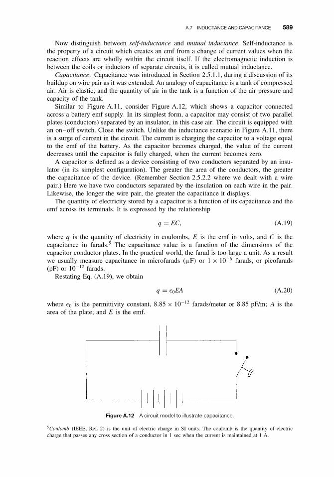
A.7 INDUCTANCE AND CAPACITANCE 589
Now distinguish between self-inductance and mutual inductance. Self-inductance isthe property of a circuit which creates an emf from a change of current values when thereaction effects are wholly within the circuit itself. If the electromagnetic induction isbetween the coils or inductors of separate circuits, it is called mutual inductance.
Capacitance. Capacitance was introduced in Section 2.5.1.1, during a discussion of itsbuildup on wire pair as it was extended. An analogy of capacitance is a tank of compressedair. Air is elastic, and the quantity of air in the tank is a function of the air pressure andcapacity of the tank.
Similar to Figure A.11, consider Figure A.12, which shows a capacitor connectedacross a battery emf supply. In its simplest form, a capacitor may consist of two parallelplates (conductors) separated by an insulator, in this case air. The circuit is equipped withan on–off switch. Close the switch. Unlike the inductance scenario in Figure A.11, thereis a surge of current in the circuit. The current is charging the capacitor to a voltage equalto the emf of the battery. As the capacitor becomes charged, the value of the currentdecreases until the capacitor is fully charged, when the current becomes zero.
A capacitor is defined as a device consisting of two conductors separated by an insu-lator (in its simplest configuration). The greater the area of the conductors, the greaterthe capacitance of the device. (Remember Section 2.5.2.2 where we dealt with a wirepair.) Here we have two conductors separated by the insulation on each wire in the pair.Likewise, the longer the wire pair, the greater the capacitance it displays.
The quantity of electricity stored by a capacitor is a function of its capacitance and theemf across its terminals. It is expressed by the relationship
q = EC, (A.19)
where q is the quantity of electricity in coulombs, E is the emf in volts, and C is thecapacitance in farads.5 The capacitance value is a function of the dimensions of thecapacitor conductor plates. In the practical world, the farad is too large a unit. As a resultwe usually measure capacitance in microfarads (µF) or 1 × 10⁻⁶ farads, or picofarads(pF) or 10−12 farads.
Restating Eq. (A.19), we obtain
q = ε0EA (A.20)
where ε0 is the permittivity constant, 8.85 × 10⁻¹² farads/meter or 8.85 pF/m; A is thearea of the plate; and E is the emf.
Figure A.12 A circuit model to illustrate capacitance.
5Coulomb (IEEE, Ref. 2) is the unit of electric charge in SI units. The coulomb is the quantity of electriccharge that passes any cross section of a conductor in 1 sec when the current is maintained at 1 A.

590 REVIEW OF FUNDAMENTALS OF ELECTRICITY WITH TELECOMMUNICATION APPLICATIONS
Substituting q from Eq. (A.19) in Eq. (A.20) and noting that the capacitance is inverselyproportional to the distance, d , between the parallel plates, we have
C = ε0(A/d) (A.21)
This tells us that capacitance is a function of geometry; it is directly proportional to thearea of the capacitor plates and inversely proportional to the distance between the plates.This assumes that the insulator between the plates is air.
Suppose the insulator between the plates is some other material. Table A.2 lists someof the typical materials used as insulators and their dielectric constant. The capacitanceincreases by a numerical factor κ , which is the dielectric constant. The dielectric constantof a vacuum is unity by definition. Because air is nearly “empty” space, its measureddielectric constant is only slightly greater than unity. The difference is insignificant.
Let L represent some geometric dimensions as a function of length. For a parallel platecapacitor with an air dielectric (insulator), L = A/d [from Eq. (A.21)]. Capacitance (C)can be related to dielectric constant, the geometrical property L, and a constant by
C = ε0κL (A.22)
where ε0 is the permittivity constant, 8.85 pf/m, and κ is the dielectric constant fromTable A.2.
Another effect of the introduction of a dielectric (insulator) including air is to limit thepotential difference between the conductors to some maximum voltage value. If this valueis substantially exceeded, the dielectric material will break down and form a conductingpath between the plates. Every dielectric material has a characteristic dielectric strength,which is the maximum value of the electric field that it can tolerate without breakdown.Several dielectric strengths are listed in Table A.2.
Capacitors in Series and in Parallel. When there is a combination of capacitors ina circuit, sometimes we can replace the combination with a single capacitor with an
Table A.2 Some Properties of Dielectrics (Insulators)
MaterialDielectric
Constant (κ)a
DielectricStrength(kV/mm)
Air (1 atm) 1.00054 3Polystyrene 2.6 24Paper 3.5 16Transformer oil 4.5Pyrex 4.7 14Ruby mica 5.4Porcelain 6.5Silicon 12Germanium 16Ethanol 25Water (20◦C) 80.4Water (25◦C) 78.5Titania ceramic 130Strontium titanate 310 8
For a vacuum, κ = unity.
aMeasured at room temperature, except for the water.Source: Fundamentals of Physics—Extended, 4th ed., p. 751,Table 27-2. (Ref. 3, reprinted with permission.)

A.7 INDUCTANCE AND CAPACITANCE 591
Figure A.13 Capacitors in parallel.
equivalent capacitance value. Just as resistances and inductances can be in series andin parallel, we can have capacitors in series and in parallel. Figure A.13 shows severalcapacitors in parallel. As we see in the figure, each capacitor has the same potentialdifference across its plates (i.e., the battery emf). By direct inference from the figurewe can see the equivalent capacitance of the three capacitors is the sum of each of theindividual capacitances or
Ceq = C1 + C2 + C3. (A.23)
Suppose the values of the capacitors were 2, 3, and 4 nF, respectively. What would theequivalent capacitance be? From Eq. (A.23), the value would be 9 nF.
Capacitors in series (see Fig. A.14) are handled in a similar manner as resistances inparallel. The total equivalent capacitance is
1/Ceq = 1/C1 + 1/C2 + 1/C3. (A.24)
Suppose, again, the values of the three capacitors were 2, 3, and 4 nF. What would theequivalent capacitance be?
1/Ceq = 1/2 + 1/3 + 1/4
= 6/12 + 4/12 + 3/12 = 13/12,
Ceq = 12/13 = 0.923 nF.
Figure A.14 Capacitors in series.

592 REVIEW OF FUNDAMENTALS OF ELECTRICITY WITH TELECOMMUNICATION APPLICATIONS
A.7.2 RC Circuits and the Time Constant
An RC circuit is illustrated in Figure A.15. The capacitor in the figure remains unchargeduntil the switch is closed. To charge it we throw the switch S to a closed position. Thecircuit consists of a resistor (R) and capacitor (C) in series. When we close the switch,there is a surge of current whose intensity decreases with time as the charge of thecapacitor builds up.
Figure A.16 shows the change in the value of the current with time after the switch isclosed. There is a corresponding change in the voltage drop across the capacitor C. Thisis illustrated with curve E. The instantaneous value of current, I , is determined solely bythe value of resistor, R. The total voltage drop is then across R and the drop across C
is zero. As the capacitor begins to charge, however, the voltage drop across C graduallybuilds up, the current decreases, and the voltage drop across R decreases correspondingly.When the capacitor reaches full charge and the current has fallen to a negligible value,the total voltage drop is now across the capacitor. Remember that at all times the sum ofthe voltage drops across R and C must be equal and opposite to the impressed voltage.
Where does time come into the picture (i.e., time constant)? It takes time for an RCcircuit (or an RL circuit) to reach a steady-state value. This time, we find, is a functionof the product of R and C. Actually, if we multiply the value of R in ohms by the valueof C in farads, it is equal to time in seconds. In a series RC circuit as illustrated inFigure A.15, the product RC is known as the time constant of the circuit. By definition,it is the time required to charge the capacitor to 63% of its final voltage. If we plot thecurve for voltage (E) in Figure A.16, we have an exponential function of time. This isexpressed mathematically as
Ei = Emax[1 − ε−t/RC], (A.25)
Figure A.15 An RC circuit.
Figure A.16 Current and voltage values as a function of time for an RC circuit.

A.8 ALTERNATING CURRENTS 593
where Ei is the instantaneous voltage across the capacitor at any time t , Emax is the finalvoltage, and ε is the natural number. This is the base of the natural logarithm or the Nape-rian logarithm.6 Its value is 2.718+. When t equals RC, the term in parentheses equals
1 − ε−1 = 1 − 1/ε = 1 − 2.718 = 0.63.
It should be noted that a similar relationship can be written for an RL circuit wherethe exponential buildup curve is current rather than voltage. However, here the exponentis L/R rather than RC. Again, it is the time required for the current to build up to 63%of its final value.
RC circuits have wide application in the telecommunications field. Because of theprecision with which resistors, capacitors, and inductors may be built, they enable thecircuit designer to readily control the timing of current pulses to better than 1-msecaccuracy. For such practical applications, the designer considers that currents and voltagesin RC and RL circuits reach their final value in a time equal to five times their time constant[i.e., 5 × RC or 5 × (L/R)]. It can be shown that at 5 × time constant the current orvoltage has reached 99.3 + % of its final value.
A.8 ALTERNATING CURRENTS
Alternating current (ac) is a current where the source emf is alternating, having a simpleand convenient waveform, namely, the sine wave. Such a sine wave is illustrated inFigure A.17. Any sine wave can be characterized by its frequency, phase, and amplitude.These were introduced in Section 2.3.3, and much of that information is repeated herefor direct continuity.
Note in the figure that half a cycle of the sine wave is designated by π and a full cycleby 2π . Remember that there are 2π radians in a circle or 360 degrees, and 1 π radianis 180 degrees. Therefore 1 radian is 180◦/π or 57.29582791 . . .
◦. That is an unwieldynumber and is not exact. That is why we like to stick to using π , and the value is exact.
In Figure A.17 the maximum amplitude is +A and −A; the common notation forwavelength is λ. To convert wavelength to frequency and vice versa we use the formulagiven in Section 2.3.3, or
Fλ = 3 × 10⁸m/sec. (A.26)
Figure A.17 A typical sine wave showing amplitude and wavelength.
6In this text, unless otherwise specified, logarithms are to the base ten. These are called common logarithms.Under certain circumstances we will also use logarithms to the base 2 (binary system of notation). In thecalculus, nearly all logarithms used are to the natural or Naperian base. This is named in honor of a Scottsmannamed Napier. However, Napier did not use the base ε but used a base approximately equal to ε−1.

594 REVIEW OF FUNDAMENTALS OF ELECTRICITY WITH TELECOMMUNICATION APPLICATIONS
We recognize the constant on the right-hand side of the equation as an accepted estimateof the velocity of light (or a radio wave). The period of a sine wave is the length of timeit takes to execute 1 cycle (1 Hz). We then relate frequency, F , to period, T , with:
F = 1/T , (A.27)
where F is in Hz and T is in seconds.Voltage and current may be out of phase one with the other. The voltage may lead the
current or lag the current depending on circuit characteristics, as we will see.When an ac circuit is resistive—there is negligible capacitance and inductance—the
voltage and current in the circuit will be in-phase. Figure A.18a is a typical ac resis-tive circuit. The phase relations between voltage (VR) and current (IR) is illustrated inFigure A.18b.
A simple inductive circuit is shown in Figure A.19a, and the current and voltagephase relationships of this circuit are shown in Figure A.19b. In this circuit, because it ispredominantly inductive, the potential difference (voltage VL) across the inductor leadsthe current by 90◦.
Figure A.20a is a simple ac capacitive circuit. In this case the current (IC) leads thevoltage (VC) by 90◦. This is illustrated in Figure A.20b.
The magnitudes of current and voltage at some moment in time are usually analyzedusing vectors. Vector analysis is beyond the scope of this appendix.
Effective Emf and Current Values. In a practical sense, an arbitrary standard has beenadopted so that only the value of current or voltage need be given to define it, its position in
Figure A.18a An ac circuit that is predominantly resistive.
Figure A.18b Phase relationship between voltage and current in an ac circuit that is resistive. Here thevoltage and current remain in phase.

A.8 ALTERNATING CURRENTS 595
Figure A.19a A simple ac inductive circuit. Here the current (IL) lags the potential difference (voltageVL) by 90◦. G is the ac emf source.
Figure A.19b Phase relationship between current (IL) and potential difference (voltage VL) in an acinductive circuit.
Figure A.20a A simple ac capacitive circuit.
time being understood by the convention adopted. One approach is to state the maximumvalue of voltage or current. However, this approach has some disadvantages. Another andoften more useful approach is the average value over a complete half-cycle (i.e., over π
radians). For a sine wave this value equals 0.636 of the maximum value.One of the most applicable values is based on the heating effect of a given value of
alternating current in a resistor that will be exactly the same as the heating value of directcurrent in the same resistor. This eliminates the disadvantage of thinking that the effectsof alternating and direct currents are different. This is known as the effective value and

596 REVIEW OF FUNDAMENTALS OF ELECTRICITY WITH TELECOMMUNICATION APPLICATIONS
Figure A.20b The phase relationship between current (IC) and emf (voltage, VC) for an ac capaci-tive circuit.
is equal to the square root of the average of the squares of the instantaneous values over1 cycle (2π radians). This results in 0.707 times the maximum value or
I = 0.707(Imax), (A.28a)
E = 0.707(Emax), (A.28b)
where E and I without subscripts are effective values. Unless otherwise stated, ac voltagesand currents are always given in terms of their effective values.
A.8.1 Calculating Power in ac Circuits
Equation (A.14) provided an expression for power in a dc circuit. The problem with accircuits is that the voltage and current are constantly changing their values as a functionof time. At any moment in time the power generated or dissipated by a circuit is
P = EI (A.29)
where P is expressed in watts, E in volts, and I in amperes.7 Also, Eqs. (A.15) and(A.16), Ohm’s law variants of Eq. (A.14), are also valid here.
Across a resistive circuit, such as in Figure A.18a, where by definition, the ac voltageand current are in phase, Eq. (A.29) expresses the power. Here, voltage and current areeffective values.
Now if the circuit that the ac generator looks into is inductive (Figure A.19a) orcapacitive (Figure A.20a), the calculation of power is somewhat more complicated. Theproblem is that the voltage and current are out of phase one with the other, as illus-trated in Figures A.19b and A.20b. The true power in such circuits will be less thanthe power calculated with Eq. (A.29) if the circuit were purely resistive. The powerin such circumstances can be calculated by applying the power factor. Equation (A.29)now becomes
P = EI cos θ, (A.30)
where θ is the phase angle, the angle that voltage leads or lags current. Earlier we wereexpressing phase angle in radians (see Figure A.17 and its discussion). Again, there are
7This equation is identical to Eq. (A.14).

A.8 ALTERNATING CURRENTS 597
2π radians in 360◦ or π radians in 180◦. It follows that 1 radian = 180◦/π , where π can
be approximated by 3.14159, or 1 radian is 57.296◦.We can look up the value of cos θ with our scientific calculator, given the value of θ ,
which will vary between 0◦ and 90◦. Between these two values, cos θ will vary between0 and 1. Note that when the power factor has a value of 1, cos θ is 1 and θ
◦. This tellsus that the voltage and current are completely in phase under these circumstances.
This leads to a discussion of impedance, which in most texts and reference books isexpressed by the letter Z. In numerous places in our text we have used the notation Z0.This is the characteristic impedance, which is the impedance we expect a circuit or deviceport to display. For example, we can expect the characteristic impedance of coaxial ableto be 75 �, of a subscriber loop to be either 600 � or 900 �, and so forth.
A.8.2 Ohm’s Law Applied to ac Circuits
We can freely use simple Ohm’s law relationships [Eqs. (A.14)–(A.16)], when ac currentand voltage are completely in phase. For example: R = E/I , where R is expressed in �,E in V, and I in A. Otherwise, we have to use the following variants:
Z = E/I, (A.31)
where Z is expressed in �.One must resort to the use of Eq. (A.31) if an ac circuit is reactive. A circuit is reactive
when we have to take into account the effects of capacitance and/or inductance in thecircuit to calculate the effective value of Z. Under these circumstances, Z is calculatedat a specified frequency. Our goal here is to reduce to a common expression in ohmsa circuit’s resistance in ohms, its inductance expressed in henrys, and its capacitanceexpressed in microfarads. Once we do this, a particular circuit or branch can be handledsimply as though it were a direct current circuit.
We define reactance as the effect of opposing the flow of current in an ac circuit due toits capacitance and/or inductance. There are two types of reactance: inductive reactanceand capacitive reactance.
Inductive Reactance. As we learned earlier, the value of current in an inductive circuitnot only varies with the inductance but also with the rate of change of current magnitude.This, of course, is frequency (f ). Now we can write an expression for a circuit’s inductivereactance, which we will call XL. It is measured in ohms.
XL = 2πf L, (A.32)
where L is the circuit’s inductance in henrys.
Example. Figure A.21 shows a simple inductive circuit where the frequency of the emfsource is 1020 Hz at 20 V, the inductance is 3.2 H. Calculate the effective current throughthe inductance. There is negligible resistance in the circuit. Use Eq. (A.32).
XL = 2 × 3.14159 × 1020 × 3.2
= 20,508.3 �;
I = 20/20, 508.3 = 0.000975 A or 0.975 mA.
In this circuit the voltage lags the current by 90◦.

598 REVIEW OF FUNDAMENTALS OF ELECTRICITY WITH TELECOMMUNICATION APPLICATIONS
Figure A.21 An ac circuit with inductance only.
Capacitive Reactance. Capacitive reactive has the opposite behavior of inductive reac-tance. In this case, the current lags the voltage by 90◦. Also, as the frequency increases,the capacitive reactance decreases, whereas with inductive reactance, as the frequencyincreases, the reactance increases. The following is an expression to calculate capaci-tive reactance:
XC = −1/2πf C (A.33a)
where f is in hertz and C is in farads.The more customary capacitance unit is the microfarad (µF). When we use this unit
of capacitance, the formula in Eq. (A.33a) becomes:
XC = −1 × 10⁶/2π fC �. (A.33b)
Example. Figure A.22 illustrates a capacitive reactance circuit with a standard capacitorof 2.16 µF and an emf of 20 V at 1020 Hz. Calculate the current in amperes flowing inthe circuit. Use formula (A.33b):
XC = −1 × 10⁶/2 × 3.14159 × 1020 × 2.16
= −72.24 �,
I = E/XC
I = −20/72.24 = −0.277 A (minus sign means leading current).
Circuits with Combined Inductive and Capacitive Reactance. To calculate the combinedor total reactance when an inductance and a capacitance are in series, the followingformula is applicable:
X = XL + XC (A.34a)
X = 2πf L − 1 × 10⁶/2πf C. (A.34b)
A word about signs: If the calculated value of X is positive, inductive reactance predom-inates, and if negative, capacitive reactance predominates.

A.8 ALTERNATING CURRENTS 599
Figure A.22 A simple ac circuit displaying capacitance only.
Example. Figure A.23 illustrates an example of a circuit with capacitance and inductancein series. The inductance value is 400 mH and the capacitance is 500 nF. The source emfis 20 V. The frequency is 1020 Hz. Calculate the current in the circuit. Assume theresistance is negligible.
Calculate the combined reactance X of the circuit using formula (A.34). Convert unitsfor capacitance to microfarads, and convert the units of inductance to henrys. That is0.5 µF and 0.4 H.
X = 2 × 3.14159 × 1020 × 0.4 − 1 × 10⁶/2 × 3.14159 × 1020 × 0.5
= 2563.537 − 1,000,000/3204.42
= 2563.537 − 312.068
= 2251.469 �.
Apply Ohm’s law variant to calculate current:
I = E/X = 20/2251.469
= 0.00888 A or 8.88 mA.
Figure A.23 A simple ac circuit with a coil (inductance) and capacitor in series.

600 REVIEW OF FUNDAMENTALS OF ELECTRICITY WITH TELECOMMUNICATION APPLICATIONS
A.8.3 Calculating Impedance
When we calculate impedance (Z), we must take into account resistance. All circuits areresistive, even though in some cases there is only a minuscule amount of resistance. Wefirst examine the two reactive possibilities; that is, a circuit with inductive reactance andthen a circuit with capacitive reactance. For the case with inductive reactance, we have
Z = (R2 + X2L)1/2. (A.35a)
Substituting, we obtainZ = [R2 + (2π fL)2]1/2. (A.35b)
For the case with capacitive reactance, we have
Z = (R2 + X2C)1/2. (A.36a)
Substituting, we obtain
Z = [R2 + (1,000,000/2πf C)2]1/2. (A.36b)
We can also state the impedance:
Z = (R2 + X2).
Substituting, we obtain
Z = [R2 + (2πf L − 1,000,000/2πf C)2]1/2. (A.37)
Example. Figure A.24 illustrates a simple ac circuit consisting of resistance (100 �),capacitance (2.16 µF), and inductance (400 mH) in series. The frequency is 1020 Hz and
Figure A.24 A simple ac circuit with resistance, capacitance, and inductance in series.

A.10 RESONANCE 601
the ac emf supply is 20 V. Calculate its impedance, and then calculate the current in thecircuit. Use formula (A.37):
Z = [10,000 + (2 × 3.14159 × 1020 × 0.4 − 1,000,000/2 × 3.14159 × 1020 × 2.16)2]1/2
= [10,000 + (2563.53 − 1,000,000/13843.1)2]1/2
= 2493.3 �.
To calculate the current in the circuit, again use the variant of Ohm’s law:
I = E/2493.3
= 20/2493.3 = 0.00802 A or 8.02 mA.
A.9 RESISTANCE IN ac CIRCUITS
In certain situations, ac resistance varies quite widely from the equivalent dc resistance,given the same circuit. For example, the resistance of a coil wound on an iron core wherethe magnetizing effect demonstrates hysteresis (“the holding back”) and resulting eddycurrents add to the dc resistance. We find that these effects are a function of frequency,the higher the frequency (f ), the greater are these effects. Certain comparable losses mayoccur in the dielectric materials of capacitors, which may have the effect of increasingthe apparent resistance of the circuit.
Still more important is the phenomenon called skin effect. As we increase frequencyof an ac current being transported by wire means, a magnetic field is set up around thewire, penetrating somewhat into the wire itself. Counter currents are set up in the wire asa result of the magnetic field, and as frequency increases field penetration decreases, andthe magnitude of the counter currents increases. The net effect is to force the current inthe wire to flow nearer the surface of the wire instead of being evenly distributed acrossthe cross section of the wire. Because the actual current flow is now through a smallerarea, the apparent ac resistance is considerably greater than its effective dc resistance.When working in the radio frequency (RF) domain, this resistance may be very muchgreater than dc resistance. However, when working with power line frequencies (i.e.,60 Hz in North America and 50 Hz in many other parts of the world), skin effect isnearly insignificant.
A.10 RESONANCE [Refs. 1 and 4]
As we are aware, the value of inductive reactance and the value of capacitive reactancedepend on frequency. When the frequency (f ) is increased, inductive reactance increases,and capacitive reaction decreases. We can say that at some frequency, the negative reac-tance XC becomes equal and opposite in value to XL. As a result the reactive componentbecomes zero, and this is where there is resonance. To determine this frequency, we setthe combined reactive component equal to zero or
2πf L − 1,000,000/2πf C = 0.
The resonant frequency, fr, is
fr = 1000/2π(LC)1/2. (A.38)

602 REVIEW OF FUNDAMENTALS OF ELECTRICITY WITH TELECOMMUNICATION APPLICATIONS
To determine the resonant frequency of a series circuit, all we have to know is thevalue of capacitance and inductance of the circuit.
Example. If the inductance of a particular circuit is 20 mH and the capacitance is 50 nF,what is the resonant frequency? Apply formula (A.38):
fr = 1000/2 × 3.14159(0.02 × 50 × 10−9)1/2
= 5,032,991 Hz or 5,032,991 MHz.
It should be noted that the units of capacitance have been changed to microfarads and thatthe units of inductance have been changed to henrys. These are the units of magnitude inEq. (A.38).
REFERENCES
1. Principles of Electricity Applied to Telephone and Telegraph Work, American Telephone & Tele-graph Co., New York, 1961.
2. IEEE Standard Dictionary of Electrical and Electronics Terms, 6th ed., IEEE Std. 100-1996,IEEE, New York, 1996.
3. D. Halliday et al., Fundamentals of Physics—Extended, 4th ed., Wiley, New York, 1993.
4. H. C. Ohanian, Physics, W. W. Norton & Company, New York, 1985.

APPENDIX B
A REVIEW OF MATHEMATICS FORTELECOMMUNICATION
APPLICATIONS
B.1 OBJECTIVE AND SCOPE
To derive the full benefit of this text, the reader should have a basic knowledge of algebra,logarithms, and some essentials of trigonometry. To that end we have developed thisappendix. The objective is to “bring the reader along,” and not to provide an exhaustiveprimer on basic mathematics. There are five subsections:
ž Introductionž Introductory Algebraž Logarithms to the Base 10ž Natural Logarithmsž Essentials of Trigonometry
B.2 INTRODUCTION
B.2.1 Symbols and Notation
A symbol is commonly used in algebra to represent a quantity. Symbols are also usedto indicate a mathematical operations such as +, −, ×, and ÷. A symbol also may beused to designate an absolute constant. For instance, the speed of light is often annotatedby the letter c. We frequently reach into the Greek alphabet; for example, π is used tocalculate the circumference or area of a circle given its diameter or radius.
Let’s say that notation is a specific symbol or specific symbols used in a particularprocedure or equation. For example, λ is nearly universally used for wavelength; F or f
for frequency. Z is used for impedance and Zo for characteristic impedance.As we said, a symbol in algebra represents a specific quantity. x is the unknown, or
x = the unknown (quantity). If there is a second unknown, we’re apt to call it y. Theserules are never hard and fast. For instance, if we are dealing with a geometrical figurewith height, length, and width, we would probably use H for height, L for length, and W
Fundamentals of Telecommunications, Second Edition, by Roger L. FreemanISBN 0-471-71045-8 Copyright 2005 by Roger L. Freeman
603

604 A REVIEW OF MATHEMATICS FOR TELECOMMUNICATION APPLICATIONS
for width; and we’d assign r for radius and d for diameter when dealing with somethingcircular. Angles are often represented by the symbols α and β, and θ is also widely usedto represent an angle. These are just more examples of utilizing the Greek alphabet aswell as the Roman.
Subscripts. A subscript tells us something about a symbol. For example, PdBW wouldprobably mean “the power expressed in dBW.” We might discuss the velocities of twocars. The velocity of car 1 may be expressed as V1, and the velocity of car 2 is expressedas V2. The use of the subscript allows us to distinguish between the two cars. Subscriptsare used widely in the text.
Independent and Dependent Variables. In the selection of symbols to solve a particularproblem, we must distinguish between constants and variables specific to the problem athand. Consider the volume of a circular cone where we keep its height constant (h). Theformula for its volume is V = πr2h/3, where r is the radius of the base circle. H , ofcourse, is constant for this problem, and just for this problem alone. r is the independentvariable and V is the dependent variable. h is referred to as a parameter.
B.2.2 The Function Concept
We remember the equation for power: P = I 2R. Let R be 75 �, then P = 75I 2. Whenthe value of I is known, we can calculate the power. For example, when I = 2 A, thepower will be
P = 75 × 2 × 2 = 300 W;
that is, the variable P depends on the variable I.In general, we can say that if a variable y depends on another variable x so that for
each value of x (in a suitable set), a corresponding value of y is determined. y then iscalled a function of x. In symbols, this is written as
y = f (x)
Read this as “y is the function of x” or just “y equals f of x.” Remember here that f isnot a qualitative symbol but an operative symbol.
Take the conversion formula from absolute temperature to centigrade: T = 273 + C.Here T = f (C). Another example is noise power. It is a function of absolute temperatureand bandwidth. Thus,
Pn = −228.6 dBW + 10 log T + 10 log BHz.
This is Eq. (9.12) from the text. Note the use of an absolute constant—in this case, Boltz-mann’s constant. Pn is the independent variable; T is the noise temperature in kelvins;and B, the bandwidth in hertz, are dependent variables. We could set the bandwidth at1 MHz. Then Pn = f (T ).
B.2.3 Using the Sigma Notation
The Greek letter � (capital sigma) indicates summation. The index of summation limitsthe number of items to be summed or added up. The letter i is often used for this purpose.Values for i are placed above and below sigma. The initial value is placed below, andthe final value is placed above the letter sigma. For example, we could have
�wi = w1 + w2 + w3 + w4 . . . + w9 + w10.
Here the initial value is 1 and the final value is 10.

B.3 INTRODUCTORY ALGEBRA 605
B.3 INTRODUCTORY ALGEBRA
B.3.1 Review of the Laws of Signs
ž If we multiply a + factor by another + factor, the product will have a + sign.ž If we divide a + factor by another + factor, the quotient will have a + sign.ž If we multiply a − factor by a + factor, the product will have a − sign (i.e., will
be negative).ž Likewise, if we multiply a + factor by a − factor, the product will have a − sign.ž If we divide a + factor by a − factor, the quotient will have a − sign.ž Likewise, if we divide a − factor by a + factor, the quotient will have a − sign.ž If we divide a − factor by a − factor, the quotient will have a + sign.
In other words, + × + = +; +/+ = +; − × + = −; + × − = −; −/+ = −; +/− = −;− × − = +; and −/− = +.
B.3.2 Conventions with Factors and Parentheses
Two symbols placed together imply multiplication. Each symbol or symbol grouping iscalled a factor. Examples:
xy means x multiplied by y.
x(y + 1) means x multiplied by the quantity (y + 1).
abc means a multiplied by b that is then multiplied by c.
The use of parentheses is vital in algebra. If a parentheses pair has a sign in front ofit, that sign is operative on each term inside the parentheses. If the sign is just a +, thenconsider that each term inside the parentheses is multiplied by +1. Here we just have aflow through.
Example. Simplify 3X + (7X + Y − 10) = 3X + 7X + Y − 10 = 10X + Y − 10.
Suppose there is a minus sign in front of the parentheses. Assume it is a −1. For theterms inside the parentheses, we change each sign and add.
Consider nearly the same example: Simplify 3X − (7X + Y − 10) = 3X − 7X − Y +10 = −4X − Y + 10.
One more example: Simplify 4.5K − (−27.3 + 2.5K) = 4.5K + 27.3 − 2.5K =2K + 27.3. We carry this one step further by placing a factor1 in front of the parentheses.
Example. Simplify: 4X − 5Y (X2 + 2XY + 10)− 36 = 4X − 5X2Y − 10XY 2 − 50Y − 36.Another example: Simplify: 4Q − 21(5Q2/3 − 3Q/6 − 4) = 4Q − 105Q2/3 +
63Q/6 + 84 = 4Q − 35Q2 + 21Q/2 + 84 = 29Q/2 − 35Q2 + 84.
An algebraic expression may have parentheses inside brackets. The rule is to clearthe “outside” first. In other words clear the brackets. Then clear the parentheses inthat order.
1A factor is a value, a symbol that we multiply by. To factor an expression is to break the expression upinto components and when these components are multiplied together, we derive the original expression. Forexample, 12 and 5 are factors of 60 because 12 × 5 = 60.
606 A REVIEW OF MATHEMATICS FOR TELECOMMUNICATION APPLICATIONS
Example. Simplify: (r − 3R) − [(2R − r) + 1] = (r − 3R) − (2R − r) − 1 = r − 3R −2R + r − 1 = 2r − 5R − 1.
Fractions. We review the adding and subtracting of fractions in arithmetic. Add: 3/4 +5/8 + 5/12. Remember that we look for the least common denominator (LCD). In thiscase it is 24. The reason: 24 is divisible by 4, 8, and 12. The three terms are now convertedto 24ths or:
18/24 + 15/24 + 10/24
Now add 18, 15, and 10, which is 43/24 or 1 + 19/24.Another example: Add 1/6 + 1/7 + 1/8. The best we can do here for the LCD is the
product of the three denominators 6 × 7 × 8 = 336, then convert to 336’s or 56/336 +48/336 + 42/336. Now add derived numerators or 56 + 48 + 42 = 146. Our new fractionafter addition is 146/336. Divide numerator and denominator by 2 and the answer is73/168.
Subtraction of fractions follows the same procedure, just follow the rules of signs.
Example. Calculate 1/4 − 1/5 + 2/3.
Procedure. Multiply the denominators together for the LCD, the value is 60. Converteach fraction to 60ths or 15/60 − 12/60 + 40/60. We now have a common denominatorso we can add the numerators: 15 − 12 + 40 = 43/60.
We apply the same procedure when we add/subtract algebraic symbols.
Example. Simplify 1/(X − 4) − 1/(X − 5).
Procedure. The LCD is the product (X − 4)(X − 5). We then have [(X − 5) − (X −4)]/(X − 4)(X − 5) = −1/(X2 − 9X + 20).
Then multiply the two factors (X − 4) and (X − 5). There are two approaches. Do“long” multiplication as we would do with arithmetic:
X − 4× X − 5
− 5X + 20X2 − 4X
sum X2 − 9X + 20
The second approach: (X − 4) × (X − 5). Multiply the leftmost terms (the Xs) and weget X2; multiply the right sides (−4 and −5) and we get +20; then multiply the meanstogether (−4X) and the extremes together (−5X) and add (−4X + −5X) = −9X. Placetogether in descending order:
X2 − 9X + 20.
There is a grouping we should recognize by inspection in the generic type of (X2 − K2),which factors into (X − K)(X + K). Here are several examples: (X2 − 1), which factorsinto (X + 1)(X − 1) or X2 − 64, which factors into (X + 8)(X − 8).
Adding and Subtracting Exponents. An exponent is a number at the right of and abovea symbol. The value assigned to the symbol with this number is called a power of thesymbol, although power is sometimes used in the same sense as exponent. If the exponent

B.3 INTRODUCTORY ALGEBRA 607
is a positive integer and x denotes the symbol, then xn means x if n = 1. When n > 1,31 = 3, 32 = 9, 3 = 27, and so on. Note that x0 = 1 if x itself is not zero.
Rules: When we multiply, we add exponents; when we divide, we subtract exponents.For the zero example above, we can think of it as X2/X2 = X0 = 1. This addition andsubtraction can be carried out so long as there is a common base. In this case it was x.For example, 23 × 22 = 25. Another example: X7/X5 = X2. Because it is division, wesubtracted exponents; it had the common base “x.”
A negative exponent indicates, in addition to the operations indicated by the numericalvalue of the exponent, that the quantity is to be made a reciprocal.
Example 1: 4−2 = 1/16.
Example 2: X−3 = 1/X3.
Furthermore, when addition is involved, and the numbers have a common exponent, wecan just add the base numbers. For example, 3.1 × 10⁻¹⁰ + 1.9 × 10−10 = 5.0 × 10⁻¹⁰.We cannot do this if there is not a common base and exponent. The power of 10 is usedwidely throughout the text.
If the exponent is a simple fraction such as 1/2 or 1/3, then we are dealing with a rootof the symbol or base number. For example, 91/2 = 3. Or (X2 + 2X + 1)1/2 = X + 1.
Carry this one step further. Suppose we have x2/3. First we square x and then takethe cube root of the result. The generalized case is Xp/q = (xp)l/q ; in other words, wefirst take the pth power and from that result we take the qth root. These calculations areparticularly easy to do with a scientific calculator as the xy function, where y can evenbe a decimal like −3.7.
B.3.3 Simple Linear Algebraic Equations
An equation is a statement of equality between two expressions. Equations are of twotypes: identities and conditional equations (or usually simply equations). A conditionalequation is true only for certain values of the variables involved; for example, x + 2 = 5is a true statement only when x = 3; and xy + y − 3 = 0 is true when x = 2 and y = 1,and for many other pairs of values of x and y; but for still others it is false.
Equation (9.20) in the text is an identity. It states that
G/T = G − 10 log T ,
where G is gain and T is noise temperature. Actually the right-hand side of the equationis just a restatement of the left-hand side; it doesn’t tell us anything new. In many cases,identities, such as this one, are very useful in analysis.
There are various rules for equations. An equation has a right-hand side and a left-handside. Maintaining equality is paramount. For example, if we add some value to the leftside, we must add the same value to the right side. Likewise, if we divide the (entire)left side by a value, we must divide the (entire) right by the same value. As we mightimagine, we must carry out similar procedures for subtraction and multiplication.
A linear equation is of the following form: Ax + B = 0 (A �= 0). This is an equationwith one unknown, X. A will be a fixed quantity, a number; so will B. However, in theparentheses it states that A may not be 0.
Let’s practice with some examples. In each case calculate the value of X.
X + 5 = 7.

608 A REVIEW OF MATHEMATICS FOR TELECOMMUNICATION APPLICATIONS
Clue: We want to have X alone on the left side. To do this we subtract 5 from the leftside, but following the rules, we must also subtract 5 from the right side. Thus,
X + 5 − 5 = 7 − 5 or
X = 2.
Another example is3X + 7 = 31.
Again, we want X alone. But first we must settle for 3X. Subtract 7 from both sides ofthe equation.
3X + 7 − 7 = 31 − 7,
3X = 24.
Again, we want X alone. To do this we can divide by 3 (each side).
3X/3 = 24/3,
X = 8.
Still another example:z2 + 1 = 65 (solve for z).
Subtract 1 from each side to get z2 alone.
z2 + 1 − 1 = 65 − 1,
z2 = 64.
Take the square root of each side. Thus,
z = 8.
More Complex Equations. Solve for R:
0.25(0.54R + 2.45) = 0.24(2.3R − 1.75),
0.135R + 0.7125 = 0.552R − 0.42,
−0.552R + 0.135R = −0.42 − 0.7125,
−0.417R = −1.0325,
R = 2.476.
Another example: Solve for x.
(x + 4)(x − 3) = (x − 9)(x − 2)
= x2 + x − 12 = x2 − 11x + 18,
12x = 30,
x = 2.5.

B.3 INTRODUCTORY ALGEBRA 609
B.3.4 Quadratic Equations
Quadratic equations will have one term with a square (e.g., X2) and they take the form
Ax2 + Bx + C = 0 (A �= 0),
where A, B, and C are constants (e.g., numbers). A quadratic equation should alwaysbe set to 0 before a solution is attempted. For instance, if we have an equation that is2x2 + 3x = −21, convert this equation to 2x2 + 3x + 21 = 0.
We will discuss two methods of solving a quadratic equation: by factoring and by thequadratic formula.
Factoring to Solve a Quadratic Equation. Suppose we have the simple relation x2 −1 = 0. We remember from above that this factors into (x − 1)(x + 1) = 0. This beingthe case, at least one of the factors must equal 0. If this is not understood, realize thatthere is no other way for the equation statement to be true. Keep in mind that anythingmultiplied by 0 will be 0. So there are two solutions to the equation:
x − 1 = 0, thus x = 1 or x + 1 = 0 and x = −1.
Proof that these are correct answers is by substituting them in the equation.Solve for x in this example:
x2 − 100x + 2400 = 0.
This factors into (x − 40)(x − 60) = 0. We now have two factors: x − 40 and x − 60,whose product is 0. This means that we must have either x − 40 = 0, where x = 40 orx − 60 = 0, and in this case x = 60. We can check our results by substitution that eitherof these values satisfies the equation.
Another example: Solve for x. (x − 3)(x − 2) = 12. Multiply the factors: x2 − 5x + 6,then x2 − 5x + 6 = 12. Subtract 12 from both sides of the equation so that we set theleft hand side equal to 0. Thus:
x2 − 5x − 6 = 0 factors into (x − 6)(x + 1) = 0.
Thenx − 6 = 0, x = 6 or x + 1 = 0, x = −1.
Quadratic Formula. This formula may be used on the conventional quadratic equationin the generic form of
Ax2 + Bx + C = 0 (A �= 0).
x is solved by simply manipulating the constants A, B, and C. The quadratic formula isstated as follows:
x = [−B ± (B2 − 4AC)1/2]/2A
or, rewritten with the radical sign:
x = −B ± √B2 − 4AC
2A.
Just like we did with the factoring method, the quadratic formula will produce two roots(two answers): one with the plus before the radical sign and one with the minus beforethe radical sign.

610 A REVIEW OF MATHEMATICS FOR TELECOMMUNICATION APPLICATIONS
Example 1: Solve for x: 3x2 − 2x − 5 = 0. Here A = 3, B = −2, and C = −5. Applythe quadratic formula.
x = (+2 ± 4 + 60)/6.
The first possibility is (+2 + 64)/6 = 10/6; the second possibility is (+2 − 8)/6 = −1.The quadratic formula will not handle the square root of a negative number. The squareroot of a negative number can usually be factored down to (−1)1/2, which, by definition,is the imaginary number i, and is beyond the scope of this appendix.
Example 2: Solve for E: E2 − 3E − 2 = 0. A = 1, B = −3, and C = −2. Thus E =(+3 ± 9 + 8)/2. The first possibility is (3 + 4.123)/2 and the second possibility is (3 −4.123)/2. Thus E = 3.562 or −0.562.
B.3.5 Solving Two Simultaneous Linear Equations with Two Unknowns
There are two methods of solving two simultaneous equations:
1. The graphical method where both equations are plotted and the intersection of theline derived is the common solution.
2. The algebraic solution.
We will concentrate on the algebraic solution. There are two approaches to solving twosimultaneous equations by the algebraic solution:
A. EliminationB. Substitution
The Elimination Method. With this method we manipulate one of the equations suchthat when the two equations are either added or subtracted, one of the unknowns iseliminated. We then solve for the other unknown. The solution is then substituted in oneof the original equations, and we solve for the other unknown.
Example.
2x + 3y − 8 = 0,
4x − 5y + 6 = 0.
Multiply each term by 2 in the upper equation, and we derive the following new equation:
4x + 6y − 16 = 0.
Place the second equation directly below this new equation, and subtract:
4x + 6y − 16 = 0,
4x − 5y + 6 = 0.
If we subtract the lower equation from the upper, we eliminate the 4x term. Now solvefor y.
+11y − 22 = 0,
11y = 22,
y = 2.
Substitute y = 2 in the original upper equation. Then 2x + 6 − 8 = 0, 2x = 2, and x = 1.

B.3 INTRODUCTORY ALGEBRA 611
So the solution of these equations is x = 1 and y = 2. Check the solutions by substi-tuting these values into the two original simultaneous equations.
Another example:
3x − 2y − 5 = 0,
6x + y + 12 = 0.
There are several possibilities to eliminate one of the unknowns. This time lets multiplyeach term in the lower equation by two and we get
12x + 2y + 24 = 0.
Place this new equation below the original upper equation:
3x − 2y − 5 = 0,
12x + 2y + 24 = 0.
Add the two equations and we get 15x + 19 = 0. Solve for x.
15x = −19.
x = −19/5.
Substitute this value in the upper equation and solve for y.
3(−19/15) − 2y − 5 = 0
− 57/15 − 75/15 = 2y
2y = −132/15 and y = −66/15 or − 22/5
The Substitution Method. Select one of the two simultaneous equations and solve forone of the unknowns in terms of the other.
Example. (Repeating the first example from above).
2x + 3y − 8 = 0,
4x − 5y + 6 = 0.
We can select either equation. Select the first equation. Then
2x = 8 − 3y,
x = (8 − 3y)/2.
Substitute this value for x in the second equation.
4(8 − 3y)/2 − 5y + 6 = 0,
16 − 6y − 5y + 6 = 0,
−11y = −22,
y = 2.
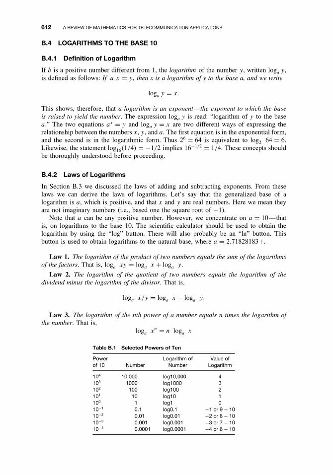
612 A REVIEW OF MATHEMATICS FOR TELECOMMUNICATION APPLICATIONS
B.4 LOGARITHMS TO THE BASE 10
B.4.1 Definition of Logarithm
If b is a positive number different from 1, the logarithm of the number y, written loga y,is defined as follows: If a x = y, then x is a logarithm of y to the base a, and we write
loga y = x.
This shows, therefore, that a logarithm is an exponent—the exponent to which the baseis raised to yield the number. The expression loga y is read: “logarithm of y to the basea.” The two equations ax = y and loga y = x are two different ways of expressing therelationship between the numbers x, y, and a. The first equation is in the exponential form,and the second is in the logarithmic form. Thus 26 = 64 is equivalent to log2 64 = 6.Likewise, the statement log16(1/4) = −1/2 implies 16−1/2 = 1/4. These concepts shouldbe thoroughly understood before proceeding.
B.4.2 Laws of Logarithms
In Section B.3 we discussed the laws of adding and subtracting exponents. From theselaws we can derive the laws of logarithms. Let’s say that the generalized base of alogarithm is a, which is positive, and that x and y are real numbers. Here we mean theyare not imaginary numbers (i.e., based one the square root of −1).
Note that a can be any positive number. However, we concentrate on a = 10—thatis, on logarithms to the base 10. The scientific calculator should be used to obtain thelogarithm by using the “log” button. There will also probably be an “ln” button. Thisbutton is used to obtain logarithms to the natural base, where a = 2.71828183+.
Law 1. The logarithm of the product of two numbers equals the sum of the logarithmsof the factors. That is, loga xy = loga x + loga y.
Law 2. The logarithm of the quotient of two numbers equals the logarithm of thedividend minus the logarithm of the divisor. That is,
loga x/y = loga x − loga y.
Law 3. The logarithm of the nth power of a number equals n times the logarithm ofthe number. That is,
loga xn = n loga x
Table B.1 Selected Powers of Ten
Powerof 10 Number
Logarithm ofNumber
Value ofLogarithm
104 10,000 log10,000 4103 1000 log1000 3102 100 log100 2101 10 log10 1100 1 log1 010−1 0.1 log0.1 −1 or 9 − 1010−2 0.01 log0.01 −2 or 8 − 1010−3 0.001 log0.001 −3 or 7 − 1010−4 0.0001 log0.0001 −4 or 6 − 10

B.4 LOGARITHMS TO THE BASE 10 613
Law 4. The logarithm of the pth root of a number is equal to the logarithm of thenumber divided by p. That is,
log(x)1/p = 1/p loga x
Remember that if x = 1, loga x = 0. Here is an exercise. Express log10(38)1/2(60)/
(29)3 = 1/2 log10(38) + log10(60) − 3 log10(29).The logarithm of a number has two components: its characteristic and its mantissa.
The characteristic is an integer and the mantissa is a decimal. If the number in question is10 or its multiple, the logarithm has a characteristic only, and its mantissa is .000000++.Consider Table B.1 containing selected the powers of 10.


APPENDIX C
LEARNING DECIBELS AND THEIRAPPLICATIONS
C.1 LEARNING DECIBEL BASICS
When working in the several disciplines of telecommunications, a clear understandingof the decibel (dB) is mandatory. The objective of this appendix is to facilitate thisunderstanding and to encourage the reader to take advantage of this useful tool.
The decibel relates to a ratio of two electrical quantities such as watts, volts, andamperes. If we pass a signal through some device, it will suffer a loss or achieve again. Such a device may be an attenuator, amplifier, mixer, transmission line, antenna,subscriber loop, trunk, or a telephone switch, among others. To simplify matters, let’s callthis generic device a network, which has an input port and an output port, as shown:
The input and output can be characterized by a signal level, which can be measured ineither watts (W), amperes (A), or volts (V). The decibel is a useful tool to compare input-to-output levels or vice versa. Certainly we can say that if the output level is greater thanthe input level, the device displays a gain. The signal has been amplified. If the outputhas a lower level than the input, the network displays a loss.
In our discussion we will indicate a gain with a positive sign (+) such as +3 dB,+11 dB, +37 dB; and a loss with a negative sign (−): −3 dB, −11 dB, −43 dB.
At the outset it will be more convenient to use the same unit at the output of a networkas at the input, such as watts. If we use watts, for example, it is watts or any of its metricderivatives. Remember:
1 W = 1000 milliwatts (mW),
1 W = 1,000,000 (1 × 10⁶) microwatts (µW),
1 W = 0.001 kilowatts (kW),
1000 mW = 1 W,
1 kW = 1000 W.
Fundamentals of Telecommunications, Second Edition, by Roger L. FreemanISBN 0-471-71045-8 Copyright 2005 by Roger L. Freeman
615
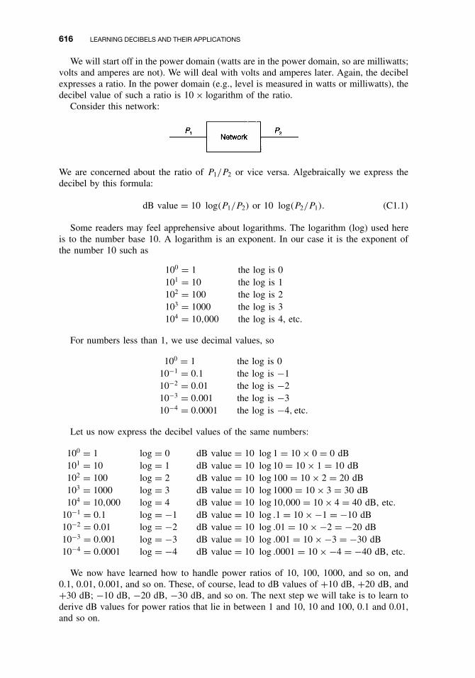
616 LEARNING DECIBELS AND THEIR APPLICATIONS
We will start off in the power domain (watts are in the power domain, so are milliwatts;volts and amperes are not). We will deal with volts and amperes later. Again, the decibelexpresses a ratio. In the power domain (e.g., level is measured in watts or milliwatts), thedecibel value of such a ratio is 10 × logarithm of the ratio.
Consider this network:
We are concerned about the ratio of P1/P2 or vice versa. Algebraically we express thedecibel by this formula:
dB value = 10 log(P1/P2) or 10 log(P2/P1). (C1.1)
Some readers may feel apprehensive about logarithms. The logarithm (log) used hereis to the number base 10. A logarithm is an exponent. In our case it is the exponent ofthe number 10 such as
100 = 1 the log is 0101 = 10 the log is 1102 = 100 the log is 2103 = 1000 the log is 3104 = 10,000 the log is 4, etc.
For numbers less than 1, we use decimal values, so
100 = 1 the log is 010−1 = 0.1 the log is −110−2 = 0.01 the log is −210−3 = 0.001 the log is −310−4 = 0.0001 the log is −4, etc.
Let us now express the decibel values of the same numbers:
100 = 1 log = 0 dB value = 10 log 1 = 10 × 0 = 0 dB101 = 10 log = 1 dB value = 10 log 10 = 10 × 1 = 10 dB102 = 100 log = 2 dB value = 10 log 100 = 10 × 2 = 20 dB103 = 1000 log = 3 dB value = 10 log 1000 = 10 × 3 = 30 dB104 = 10,000 log = 4 dB value = 10 log 10,000 = 10 × 4 = 40 dB, etc.
10−1 = 0.1 log = −1 dB value = 10 log .1 = 10 × −1 = −10 dB10−2 = 0.01 log = −2 dB value = 10 log .01 = 10 × −2 = −20 dB10−3 = 0.001 log = −3 dB value = 10 log .001 = 10 × −3 = −30 dB10−4 = 0.0001 log = −4 dB value = 10 log .0001 = 10 × −4 = −40 dB, etc.
We now have learned how to handle power ratios of 10, 100, 1000, and so on, and0.1, 0.01, 0.001, and so on. These, of course, lead to dB values of +10 dB, +20 dB, and+30 dB; −10 dB, −20 dB, −30 dB, and so on. The next step we will take is to learn toderive dB values for power ratios that lie in between 1 and 10, 10 and 100, 0.1 and 0.01,and so on.

C.1 LEARNING DECIBEL BASICS 617
One excellent recourse is the scientific calculator. Here we apply a formula (C1.1).For example, let us deal with the following situation:
Because the output of this network is greater than the input, the network has a gain. Keepin mind we are in the power domain; we are dealing with mW. Thus:
dB value = 10 log 4/2 = 10 log 2 = 10 × 0.3010 = +3.01 dB.
We usually roundoff this dB value to +3 dB. If we were to do this on our scientificcalculator, we enter 2 and press the log button. The value 0.3010—appears on the display.We then multiply (×) this value by 10, arriving at the +3.010 dB value.
This relationship should be memorized. The amplifying network has a 3-dB gainbecause the output power was double the input power (i.e., the output is twice as greatas the input).
For the immediately following discussion, we are going to show that under manysituations a scientific calculator is not needed and one can carry out these calculationsin his or her head. We learned the 3-dB rule. We learned the +10, +20, +30 dB; −10,−20, −30 (etc.) rules. One should be aware that with the 3-dB rule, there is a smallerror that occurs two places to the right of the decimal point. It is so small that it is hardto measure.
With the 3-dB rule, multiples of 3 are easy. If we have power ratios of 2, 4, and 8,we know that the equivalent (approximate) dB values are +3 dB, +6 dB, and +9 dB,respectively. Let us take the +9 dB as an example problem. A network has an input of6 mW and a gain of +9 dB. What power level in mW would we expect to measure atthe output port?
One thing that is convenient about dBs is that when we have networks in series, eachwith a loss or gain given in dB, we can simply sum the values algebraically. Likewise,we can do the converse: We can break down a network into hypothetical networks inseries, so long as the algebraic sum in dB of the gain/loss of each network making upthe whole is the same as that of the original network. We have a good example with thepreceding network displaying a gain of +9 dB. Obviously 3 × 3 = 9. We break down the+9-dB network into three networks in series, each with a gain of +3 dB. This is shownin the following diagram:
We should be able to do this now by inspection. Remember that +3 dB is double thepower; the power at the output of a network with +3-dB gain has 2× the power levelat the input. Obviously, the output of the first network is 12 mW (point A above). The
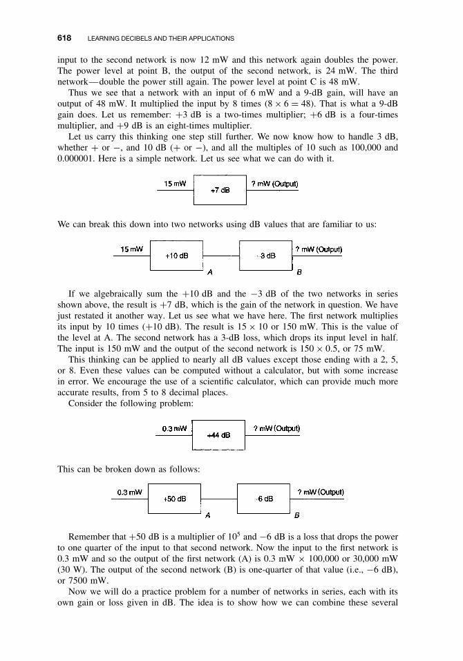
618 LEARNING DECIBELS AND THEIR APPLICATIONS
input to the second network is now 12 mW and this network again doubles the power.The power level at point B, the output of the second network, is 24 mW. The thirdnetwork—double the power still again. The power level at point C is 48 mW.
Thus we see that a network with an input of 6 mW and a 9-dB gain, will have anoutput of 48 mW. It multiplied the input by 8 times (8 × 6 = 48). That is what a 9-dBgain does. Let us remember: +3 dB is a two-times multiplier; +6 dB is a four-timesmultiplier, and +9 dB is an eight-times multiplier.
Let us carry this thinking one step still further. We now know how to handle 3 dB,whether + or −, and 10 dB (+ or −), and all the multiples of 10 such as 100,000 and0.000001. Here is a simple network. Let us see what we can do with it.
We can break this down into two networks using dB values that are familiar to us:
If we algebraically sum the +10 dB and the −3 dB of the two networks in seriesshown above, the result is +7 dB, which is the gain of the network in question. We havejust restated it another way. Let us see what we have here. The first network multipliesits input by 10 times (+10 dB). The result is 15 × 10 or 150 mW. This is the value ofthe level at A. The second network has a 3-dB loss, which drops its input level in half.The input is 150 mW and the output of the second network is 150 × 0.5, or 75 mW.
This thinking can be applied to nearly all dB values except those ending with a 2, 5,or 8. Even these values can be computed without a calculator, but with some increasein error. We encourage the use of a scientific calculator, which can provide much moreaccurate results, from 5 to 8 decimal places.
Consider the following problem:
This can be broken down as follows:
Remember that +50 dB is a multiplier of 105 and −6 dB is a loss that drops the powerto one quarter of the input to that second network. Now the input to the first network is0.3 mW and so the output of the first network (A) is 0.3 mW × 100,000 or 30,000 mW(30 W). The output of the second network (B) is one-quarter of that value (i.e., −6 dB),or 7500 mW.
Now we will do a practice problem for a number of networks in series, each with itsown gain or loss given in dB. The idea is to show how we can combine these several
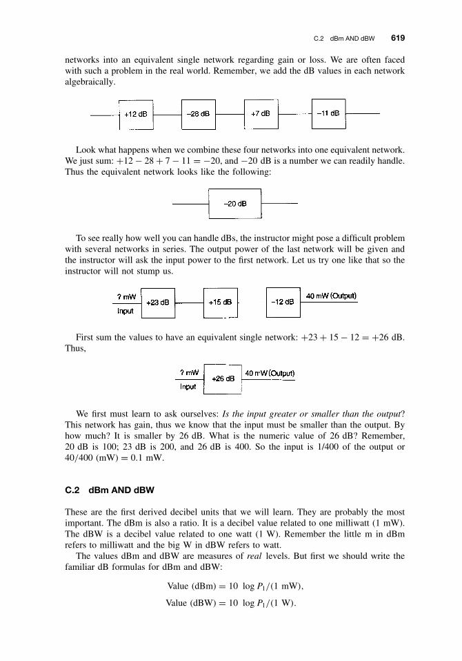
C.2 dBm AND dBW 619
networks into an equivalent single network regarding gain or loss. We are often facedwith such a problem in the real world. Remember, we add the dB values in each networkalgebraically.
Look what happens when we combine these four networks into one equivalent network.We just sum: +12 − 28 + 7 − 11 = −20, and −20 dB is a number we can readily handle.Thus the equivalent network looks like the following:
To see really how well you can handle dBs, the instructor might pose a difficult problemwith several networks in series. The output power of the last network will be given andthe instructor will ask the input power to the first network. Let us try one like that so theinstructor will not stump us.
First sum the values to have an equivalent single network: +23 + 15 − 12 = +26 dB.Thus,
We first must learn to ask ourselves: Is the input greater or smaller than the output?This network has gain, thus we know that the input must be smaller than the output. Byhow much? It is smaller by 26 dB. What is the numeric value of 26 dB? Remember,20 dB is 100; 23 dB is 200, and 26 dB is 400. So the input is 1/400 of the output or40/400 (mW) = 0.1 mW.
C.2 dBm AND dBW
These are the first derived decibel units that we will learn. They are probably the mostimportant. The dBm is also a ratio. It is a decibel value related to one milliwatt (1 mW).The dBW is a decibel value related to one watt (1 W). Remember the little m in dBmrefers to milliwatt and the big W in dBW refers to watt.
The values dBm and dBW are measures of real levels. But first we should write thefamiliar dB formulas for dBm and dBW:
Value (dBm) = 10 log P1/(1 mW),
Value (dBW) = 10 log P1/(1 W).

620 LEARNING DECIBELS AND THEIR APPLICATIONS
Here are a few good relationships to fix in our memories:
1 mW = 0 dBm (by definition),
1 W = 0 dBW (by definition),
+30 dBm = 0 dBW = 1 W,
−30 dBW = 0 dBm = 1 mW.
Who will hazard a guess what +3 dBm is in mW? Of course, it is 3 dB greater than0 dBm. Therefore it must be 2 mW. Of course, +6 dBm is 4 mW, and −3 dBm is halfof 0 dBm or 0.5 mW. A table is often helpful for the powers of 10:
1 mW = 100 mW = 0 dBm,
10 mW = 101 mW = +10 dBm,
100 mW = 102 mW = +20 dBm,
1000 mW = 103 mW = +30 dBm = 0 dBW,
10 W = 104 mW = +40 dBm = +10 dBW(etc.).
Likewise,
0.1 mW = 10−1 = −10 dBm,
0.01 mW = 10−2 = −20 dBm,
0.001 mW = 10−3 = −30 dBm,
0.0001 mW = 10−4 = −40 dBm.
Once we have a grasp of dBm and dBW, we will find it easier to work problems withnetworks in series. We now will give some examples.
First we convert the input, 8 mW to dBm. Look how simple it is: 2 mW = +3 dBm,4 mW = +6 dBm, and 8 mW = +9 dBm. Now watch this! To get the answer, the powerlevel at the output is +9 dBm +23 dB = +32 dBm.
Another problem will be helpful. In this case the unknown will be the input toa network.
In each case like this we ask ourselves, is the output greater than the input? Becausethe network is lossy, the input is 17 dB greater than the output. Convert the output todBm. It is +10 dBm. The input is 17 dB greater, or +27 dBm. We should also be able to

C.4 USING DECIBELS WITH SIGNAL CURRENTS AND VOLTAGES 621
say: “that’s half a watt.” Remember, +30 dBm = 1 W = 0 dBW. Then +27 dBm (“3 dBdown”) is half that value.
Several exercises are in order. The answers appear after the four exercises.
Exercise 1a .
Exercise 1b.
Exercise 1c.
Exercise 1d .
(Answers: 1a: +13 dBm = 20 mW; 1b: +29 dBW, 1c: +32 dBm, and 1d: +7 dBm =0.005 W).
C.3 VOLUME UNIT (VU)
The VU is the conventional unit for measurement of speech level. A VU can be relatedto a dBm only with a sinusoidal tone (a simple tone of one frequency) between 35 Hzand 10,000 Hz. The following relationship will be helpful:
Power level in dBm = VU − 1.4dB (for complex audio signals).
A complex audio signal is an audio signal composed of many sine waves (sinusoidaltones) or, if you will, many tones and their harmonics.
One might ask: If the level reading on a broadcaster’s program channel is −11 VU,what would the equivalent be in dBm? Reading in VU − 1.4 dB = reading in dBm. Thusthe answer is −11 VU − 1.4 dB = −12.4 dBm.
C.4 USING DECIBELS WITH SIGNAL CURRENTS AND VOLTAGES
The dB is based upon a power ratio, as discussed. We can also relate decibels to signalvoltages and to signal currents. The case for signal currents is treated first. We are dealing,

622 LEARNING DECIBELS AND THEIR APPLICATIONS
of course, with gains and losses for a device or several devices (called networks) that areinserted in a circuit. Follow the thinking behind this series of equations:
Gain/LossdB = 10 log P1/P2 = 10 log I 21 R1/I
22 R2 = 20 log I1/I2 = 10 log R1/R2.
If we let R1 = R2, then the term 10 log R1/R2 = 0. (Hint: The log of 1 = 0.)Remember from Ohm’s law that E = IR, and from the power law Pw = EI. Thus
Pw = I 2R = E2/R.To calculate gain or loss in dB when in the voltage/current domain, we derive the
following two formulas from the reasoning just shown:
Gain/LossdB = 20 log E1/E2 = 20 log I1/I2.
We see, in this case, that we multiply the log by the factor 20 rather than the factor10 as we did in the power domain (i.e., 20 log vs. 10 log) because we really are dealingwith power. Power is the function of the square of the signal voltage (E2/R) or signalcurrent (I 2R). We use traditional notation for voltage and current. Voltage is measuredin volts (E); current, in amperes (I ).
We must impress on the reader two important points: (1) Equations as written are onlyvalid when R1 = R2, and (2) validity holds only for terminations in pure resistance (thereare no reactive components).
Consider these network examples:Current (I ):
Voltage (E):
E1 and E2 are signal voltage drops across R1 and R2, respectively. The incisive readerwill tell us that signals at the input are really terminated in an impedance (Z), which shouldequal the characteristic impedance, Z0 (specified impedance). Such an impedance couldbe 600 �, for example. An impedance usually has a reactive component. Our argumentis only valid if, somehow, we can eliminate the reactive component. The validity onlyholds true for a pure resistance. About the closest thing we can find to a “pure” resistanceis a carbon resistor.
Turning back to our discussion, the input in the two cases cited may not be underour control, and there may be some reactive component. The output can be under ourcontrol. We can terminate the output port with a pure resistor, whose ohmic value equalsthe characteristic impedance. Our purpose for this discussion is to warn of possible smallerrors when reading input voltage or current.
Let’s discuss the calculation of decibels dealing with a gain or loss by an example.A certain network with equal impedances at its input and output ports displays a signal

C.5 CALCULATING A NUMERIC VALUE GIVEN A dB VALUE 623
voltage of 10 V at the input and 100 V at the output. The impedances are entirely resistive.What is the gain of the network?
GaindB = 20 log 100/10 = 20 dB.A similar network has a signal output of 40 V and a loss of 6 dB. What is the input
signal voltage? (Equal impedances assumed.)
−6 dB = 20 log 40/X.
We shortcut this procedure by remembering our 10 log values. With a voltage or amperagerelationship, the dB value is double (20 is twice the magnitude of 10). The value of X
is 80 V. Whereas in our 10 log regime 3 dB doubled (or halved), here 6 dB doublesor halves.
A more straightforward way of carrying out this procedure will be suggested in thenext section. X can be directly calculated.
C.5 CALCULATING A NUMERIC VALUE GIVEN A dB VALUE
The essence of the problem of calculating a numeric value given a dB value can be statedas such: If we are given the logarithm of a number, what is the number? To express this,two types of notation are given in the literature as follows:
(1A) log−1 0.3010 = 2, (2A) log−1 2 = 100,
(1B)antilog(0.3010) = 2, (2B)antilog2 = 100.
In the case of example 1, the logarithm is 0.3010, which corresponds to the number 2.If we were to take the log (base 10) of 2, the result is 0.3010. In example 2, the log of100 is 2 or, if you will, 2 is the logarithm of 100.
For our direct application we may be given a decibel value and be required to convertto its equivalent numeric value. If we turn to our introductory comments, when dealingin the power domain, we know that if we are given a decibel value of 20 dB, we areworking with a power gain or loss of 100; 23 dB, 200; 30 dB, 1000; 37 dB, 5000; andso on.
A scientific calculator is particularly valuable when we are not working directly withmultiples of 10. For instance, enter the logarithm of a number onto the calculator keypadand the calculator can output the equivalent numeric value. Many hand-held scientificcalculators use the same button for the log as for the antilog. Usually one can access theantilog function by first pressing the “2nd” button, something analogous to upper case ona keyboard. Often printed directly above the log button is “10x .”
On most calculators we first enter the logarithm on the numerical keypad, being sureto use the proper signs (+ or −). Press the “2nd” button; then press the “log” button.After a short processing interval, the equivalent number is shown on the display.
Let us get to the crux of the matter. We are interested in dBs. Let us suppose weare given 13 dB and we are asked to find its numeric equivalent (power domain). Thiscalculation is expressed by the following formula:
log−1(13/10) = 20.

624 LEARNING DECIBELS AND THEIR APPLICATIONS
Let us use a calculator and compute the following equivalent numeric values whengiven dB values:
1. −21.5 dB. Divide by 10 and we have −2.15. Enter this on the keyboard with thenegative sign. Press 2nd F (function) to access the upper case, which is the same asthe log button but marked right above “10x .” Press = button and the value 0.00708appears on the display.
2. +26.8 dB. Enter this number on the keypad and divide by 10; press = . Press 2ndF; press log button (10x) and press =. The equivalent numeric value appears on thedisplay. It is 478.63.
When working in the voltage or current domain, we divide the dB value by 20 ratherthan 10. Remember we are carrying out the reverse process that we used calculating adB value when given a number (numeric) (i.e., the result of dividing the two numbersmaking up the ratio). This is expressed by the following formula:
log−1(dB value/20) = equivalent numeric.
Consider this example. Convert 26 dB (voltage domain) to its equivalent numeric value.Enter 26 on the keypad and divide by 20. The result is 1.3. Press 2nd F button and pressthe log button (10x) and press =. The value 19.952 appears on the display. The readerprobably did this in his or her head and arrived at a value of 20.
Try the following six example problems, first in the power domain, and then in thevoltage/amperage domain. The correct answers appear just below.
1. −6 dB , . 2. +66 dB , .3. −22 dB , . 4. +17 dB , .5. −27 dB , . 6. +8.7 dB , .
Answers: 1: 0.251; 0.501. 2: 3,981,071.7; 1995.26. 3: 0.006309; 0.07943. 4: 50.118;7.07945. 5: 0.001995; 0.044668. 6: 7.413; 2.7227.
C.5.1 Calculating Watt and Milliwatt Values When Given dBW and dBmValues
We will find that the process of calculating numeric values in watts and milliwatts is verysimilar to calculating the numeric value of a ratio when given the equivalent value indecibels. Likewise, the greater portion of these conversions can be carried out without acalculator to a first-order estimation. In the case where the dB value is 10 or a multiplethereof, the value will be exact.
Remember: 0 dBm = 1 mW; 0 dBW = 1 W by definition. Furthermore, lest we forget:+3 dBm is twice as large as the equivalent 0 dBm value, thus where 0 dBm = 1 mW,+3 dBm = 2 mW.
Also, +10 dBm numeric value is 10 times the equivalent 0 dBm value (i.e., it is 10 dBlarger). So +10 dBm = 10 mW; −10 dBm = 0.1 mW; −20 dBm = 0.01 mW.
In addition, −17 dBm is twice the numeric magnitude of −20 dBm. So −17 dBm =0.02 mW, and so forth.
Try calculating the numeric equivalents of these dBm and dBW values without usinga calculator.

C.7 dB APPLIED TO THE VOICE CHANNEL 625
1. +13 dBm mW. 2. −13 dBm mW.3. +44 dBm dBW, W. 4. −21 dBm mW.5. +27 dBW W. 6. −14 dBW mW.7. −11 dBm mW. 8. +47 dBW kW.
Answers: 1: 20 mW. 2: 0.05 mW. 3: +14 dBW, 25 W. 4: 0.008 mW. 5: 500 W.6: 40 mW. 7: 0.08 mW. 8: 50 kW.
C.6 ADDITION OF dBs AND DERIVED UNITS
Suppose we have a combiner, a device that combines signals from two or more sources.This combiner has two signal inputs: +3 dBm and +6 dBm. Our combiner is an idealcombiner in that it displays no insertion loss. In other words, there is no deleterious effecton the combining action, it is “lossless.” What we want to find out is the output of thecombiner in dBm. It is not +9 dBm. The problem is shown diagrammatically as
Some texts provide a nomogram to solve such a problem. We believe the followingmethod is more accurate and, with the advent of affordable scientific calculators, easier.It is simple: Convert the input values to their respective numeric values in mW; add andconvert the sum to its equivalent value in dBm.
The +3 and +6 dBm values are so familiar that we convert them by inspection, namely,2 and 4 mW. The sum is 6 mW. Now we take 10 log 6 to convert back to dBm againand the answer is +7.78 dBm. Remembering that there is an error when we work “3s”(3, 6, 9, 1, 4 and 7 values), we recalculated using a scientific calculator throughout. Theanswer was +7.76 dBm showing a 0.02-dB error.
On occasion, we will have to combine a large number of input/outputs where each isof the same level. This is commonly done with frequency division multiplex equipmentor with multitone telegraphy or data.
Suppose we have an FDM group (12 voice channel inputs), where each input was−16 dBm. What is the composite output? This is stated as
Composite powerdBm = −16 dBm + 10 log 12,
= −16 dBm + 10.79 dB,
= −5.21 dBm.
The problem of adding two or more inputs in a combiner is pretty straightforward if wekeep in the power domain. If we delve into the voltage or current domain with equivalentdB values, such as dBmV (which we cover in Section 15.3.2), we recommend returningto the power domain if at all possible. If we do not, we can open Pandora’s box, becauseof the phase relationship(s) of the inputs. In the next section we will carry out someinteresting exercises in power addition.
C.7 dB APPLIED TO THE VOICE CHANNEL
The decibel is used to quantify gains and losses across a telecommunication network. Themost common and ubiquitous end-to-end highway across that network is the voice channel

626 LEARNING DECIBELS AND THEIR APPLICATIONS
(VF channel). A voice channel conjures up in our minds an analog channel, somethingour ear can hear. The transmit part (mouthpiece) of a telephone converts acoustic energyemanating from a human mouth to electrical energy, an analog signal. At the distantend of that circuit an audio equivalent of that analog energy is delivered to the receiver(earpiece) of the telephone subset with which we are communicating. This must also holdtrue for the all-digital network.
When dealing with the voice channel, there are a number of special aspects to beconsidered by the transmission engineer. In this section we will talk about these aspectsregarding frequency response across a well-defined voice channel. We will be required touse dBs, dB-derived units, and numeric units.
The basic voice channel is that inclusive band of frequencies where loss with regard tofrequency drops 10 dB relative to a reference frequency.1 There are two slightly differentdefinitions of the voice channel, North American and CCITT:
North America: 200 Hz to 3300 Hz (reference frequency, 1000 Hz).
CCITT: 300 Hz to 3400 Hz (reference frequency, 800 Hz).
We sometimes call this the nominal 4-kHz voice channel; some others call it a 3-kHzchannel. (Note: There is a 3-kHz channel, to further confuse the issue; it is used on HFradio and some old undersea cable systems.)
To introduce the subject of a “flat” voice channel and a “weighted” voice channelwe first must discuss some voice channel transmission impairments. These are noise andamplitude distortion.
We all know what noise is. It annoys the listener. At times it can be so disruptive thatintelligent information cannot be exchanged or the telephone circuit drops out and we geta dial tone. So we want to talk about how much noise will annoy the average listener.
Amplitude distortion is the same as frequency response. We define amplitude distortionas the variation of level (amplitude) with frequency across a frequency passband or band ofinterest. We often quantify amplitude distortion as a variation of level when compared tothe level (amplitude) at the reference frequency. The two common voice channel referencefrequencies are noted in the preceding list.
To further describe amplitude distortion, let us consider a hypothetical example. Ata test board (a place where we can electrically access a voice channel) in New Yorkwe have an audio signal generator available, which we will use to insert audio tones atdifferent frequencies. At a similar test board in Chicago we will measure the level ofthese frequencies in dBm. The audio tones inserted in New York are all inserted at a levelof −16 dBm, one at a time. In Chicago we measure these levels in dBm. We find thelevel at 1000 Hz to be +7 dBm, our reference frequency. We measure the 500-Hz toneat +3 dBm; 1200-Hz tone at +8 dBm; 2000-Hz tone +5 dBm, and the 2800-Hz tone at0 dBm. Any variation of level from the 1000-Hz reference value we may call amplitudedistortion. At 2800 Hz there was 7 dB variation. Of course, we can expect some of theworst-case excursion at band edges, which is usually brought about by filters or otherdevices that act like filters.
The human ear is a filter, as is the telephone receiver (earpiece). The two are in tandem,as we would expect. For the telephone listener, noise is an annoyance. Interestingly wefind that noise annoys a listener more near the reference frequencies of a voice channelthan at other frequencies. When using the North American 500-type telephone set withaverage listeners, a simple 0-dBm tone at 1000 Hz causes a certain level of annoyance.
1This value applies when looking toward the subscriber from the local serving exchange. Looking into thenetwork from the local serving exchange the value drops to 3 dB.

C.7 dB APPLIED TO THE VOICE CHANNEL 627
To cause the same level of annoyance, a 300-Hz tone would have to be at a level ofabout +17 dBm; a 400-Hz tone at about +11.5 dBm; a 600-Hz tone at about +4 dBm,and a 3000-Hz tone also at about +4 dBm for equal annoyance levels for a populationof average listeners.
The question arose of why should the transmission engineer be penalized in design ofa system for noise of equal level across the voice channel? We therefore have “shaped”the voice channel as a function of frequency and “annoyance.” This shaping is called aweighting curve.
For the voice channel we will be dealing with two types of weighting: (1) C-message,used in North America, and (2) psophometric weighting as recommended by CCITT.Figure C.1 shows these weighting curves.
Weighting networks have been developed to simulate the corresponding response of C-message and psophometric weighting. Now we want to distinguish between flat responseand weighted response. Of course, the curves in Figure C.1 show weighted response. Flatresponse, regarding a voice channel, has a low-pass response down 3 dB at 3 kHz androlls off at 12 dB per octave. An octave means twice the frequency, so that it would bedown 15 dB at 6 kHz and 27 dB at 12 kHz, and so on.
The term flat means equal response across a band of frequencies. Suppose a flat networkhas a loss of 3 dB. We insert a broad spectrum uniform signal at the input to the network.In the laboratory we generally use “white noise.” White noise is a signal that containscomponents of all frequencies inside a certain passband. We now measure the output ofour network at discrete frequencies and at whatever frequency we measure the output,the level is always the same. Figure C.1 shows frequency responses that are decidedlynot flat.
We return now to the problem of noise in the voice channel. If the voice channel is tobe used for speech telephony, which most of them are, then we should take into accountthe annoyance factor of noise to the human ear. Remember, when we measure noise ina voice channel, we look at the entire channel. Our noise measurement device reads thenoise integrated across the channel. As we said, certain frequency components (around800 Hz or 1000 Hz) are more annoying to the listener than other frequency components.
Figure C.1 Line weightings for telephone (voice) channel noise.

628 LEARNING DECIBELS AND THEIR APPLICATIONS
It is because of this that we have developed a set of noise measurement units that areweighted. There are two such units in use today:
1. C-message weighting, which uses the unit dBrnC,2. Psophometric weighting, which more commonly uses the numeric unit, the picowatt
(pWp) psophometrically weighted.
One interesting point that should be remembered is that the lowest discernible signalthat can be heard by a human being is −90 dBm (800 or 1000 Hz).
Another point is that it was decided that all weighted (dB derived) noise units shouldbe positive (i.e., not use a negative sign). First, remember these relationships:
1 W = 1012 pW = 109 mW,
1 pW = 1 × 10⁻¹² W = 1 × 10⁻⁹ mW = −90 dBm.
A weighted channel has less noise power than an unweighted channel if the two chan-nels have identical characteristics. C-message weighting has about 2 dB less noise than aflat channel; a psophometric weighted channel has 2.5 dB less noise than a flat channel.
Figure C.2 may help clarify the concept of noise weighting and the noise advantageit can provide. The figure shows the C-message weighting curve. Idealized flat responseis the heavy straight line at the arbitrary 0-dB point going right and left from 200 Hz to3300 Hz. The hatched area between that line and the C-message response curve we maycall the noise advantage (our terminology). There is approximately 2-dB advantage forC-message weight over flat response. If it were psophometric weighting, there would bea 2.5-dB advantage.
The dBrnC is the weighted noise measurement unit used in North America. The fol-lowing are useful relationships:
0 dBrnC = −92 dBm (with white noise loading of entire voice channel).
Figure C.2 Flat response (idealized) versus C-message weighting. The hatched area shows how wearrive at approximately a 2-dB noise advantage for C-message weighting. We can only take advantageof C-message improvement for speech telephony. For data transmission we must use flat response.

C.7 dB APPLIED TO THE VOICE CHANNEL 629
Think about this:
0 dBrnC = −90 dBm (1000 − Hz toned).
Figures C.1 and C.2 show the rationale.
Value in (−) dBm = 10 log(pW × 10−9),
Value in pWp = value in pW × 0.56,
−90 dBm = −2 dBrnC and thus −92 dBm = 0 dBrnc(white noise loading),
−92.5 dBmp = −90 dBm (flat, white noise),
1 pWp = −90 dBmp,
Value in dBm = 10 log(value in pWp × 10−9) + 2.5 dB,
dBrnC = 10(log pWp × 10−9) − 0.5 dB + 90 dB,
Value in pW × 0.56 = value in pWp,
Value in pWp/0.56 = value in pW.
Table C.1 summarizes some of the relationships we have covered for flat and weightednoise units.
Example 1. A hypothetical reference circuit shall accumulate no more than 10,000 pWpof noise. What are the equivalent values in dBrnC, dBm, and dBmp?
dBrnC = 10(log 10,000 × 10−9) − 0.5 dB + 90 dB
= 39.5 dBrnC,
(−) dBm = 10 log(10,000 × 10−9) + 2.5 dB
= −47.5 dBm,
dBmp = 10 log 10,000 pWp × 10−9
= −50 dBmp.
Table C.1 Comparison of Various Noise Units
Total Power of 0 dBm WidebandWhite Noise
Noise Unit 1000 HzWhite Noise0 kHz to 3 kHz
of−4.8 dBm/kHz
dBrnc 90.0 dBrnc 88.0 dBrnc 88.4 dBrncdBrn 3 kHz FLAT 90.0 dBrn 88.8 dBrn 90.3 dBrndBrn 15 kHz FLAT 90.0 dBrn 90.0 dBrn 97.3 dBrnPsophometric voltage
(600 �)870 mV 582 mV 604 mV
pWp 1.26 × 10⁹ pWp 5.62 × 10⁸ pWp 6.03 × 10⁸ pWpdBp 91.0 dBp 87.5 dBp 87.8 dBp
Source: Based on Table 4.2, p. 60, Ref. 1.

630 LEARNING DECIBELS AND THEIR APPLICATIONS
Example 2. We measure noise in the voice channel at 37 dBrnc. What is the equivalentnoise in pWp?
37 dBrnC = 10(log X × 10−9) − 0.5 + 90 dB,
−52.5 = 10(log X × 10−9),
−5.25 = log X × 10−9,
antilog(−5.25) = 5623 × 10−9,
X = 5623 pWp.
Carry out the following exercises. The answers follow.
1. −83 dBmp =? pWp 2. 47,000 pWp =? dBmp3. −47 dBm =? dBmp 4. 33 dBrnC =? dBmp5. 20,000 pWp =? dBrnC 6. 50,000 pWp =? dBm7. 2000 pW =? pWp 8. 4000 pWp =? dBrnC
Answers: 1: 5 pWp. 2: −43.28 dBmp. 3: −49.5 dBmp. 4: 2238 pWp = −56.5 dBmp =−54 dBm. 5: 42.5 dBrnC. 6: −43 dBmp = −40.5 dBm. 7: 1120 pWp. 8: 35.5 dBrnC.
C.8 INSERTION LOSS AND INSERTION GAIN
When dealing with the broad field of telecommunication engineering, we will oftenencounter the terms insertion loss and insertion gain. These terms give us importantinformation about a two-port network in place in a circuit. Two-port just means we havean input (port) and an output (port). A major characteristic of this device is that it willpresent a loss in the circuit or it will present a gain. Losses and gains are expressed in dB.In the following we show a simple circuit terminated in its characteristic impedance, Z0.
We now insert into this same circuit a two-port network as follows:
First for the case of insertion loss: Let us suppose the device is an attenuator, a length ofwaveguide, a mixer with loss, or any other lossy device. Suppose we are delivering powerp2 to the load ZL with the network in place and power p0 with the network removed.The ratio expressed in dB of p0 to p2 is called the insertion loss of the network:
Insertion lossdB = 10 log(p0/p2).
If ZL equals Z0, we can easily express insertion loss as a voltage ratio:
Insertion lossdB = 20 log(E0/E2).
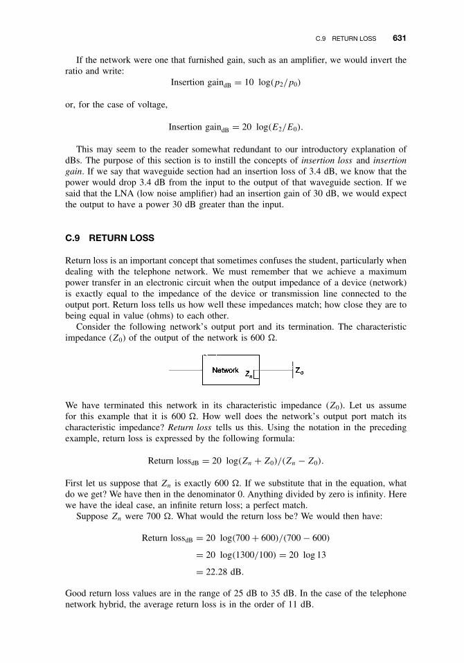
C.9 RETURN LOSS 631
If the network were one that furnished gain, such as an amplifier, we would invert theratio and write:
Insertion gaindB = 10 log(p2/p0)
or, for the case of voltage,
Insertion gaindB = 20 log(E2/E0).
This may seem to the reader somewhat redundant to our introductory explanation ofdBs. The purpose of this section is to instill the concepts of insertion loss and insertiongain. If we say that waveguide section had an insertion loss of 3.4 dB, we know that thepower would drop 3.4 dB from the input to the output of that waveguide section. If wesaid that the LNA (low noise amplifier) had an insertion gain of 30 dB, we would expectthe output to have a power 30 dB greater than the input.
C.9 RETURN LOSS
Return loss is an important concept that sometimes confuses the student, particularly whendealing with the telephone network. We must remember that we achieve a maximumpower transfer in an electronic circuit when the output impedance of a device (network)is exactly equal to the impedance of the device or transmission line connected to theoutput port. Return loss tells us how well these impedances match; how close they are tobeing equal in value (ohms) to each other.
Consider the following network’s output port and its termination. The characteristicimpedance (Z0) of the output of the network is 600 �.
We have terminated this network in its characteristic impedance (Z0). Let us assumefor this example that it is 600 �. How well does the network’s output port match itscharacteristic impedance? Return loss tells us this. Using the notation in the precedingexample, return loss is expressed by the following formula:
Return lossdB = 20 log(Zn + Z0)/(Zn − Z0).
First let us suppose that Zn is exactly 600 �. If we substitute that in the equation, whatdo we get? We have then in the denominator 0. Anything divided by zero is infinity. Herewe have the ideal case, an infinite return loss; a perfect match.
Suppose Zn were 700 �. What would the return loss be? We would then have:
Return lossdB = 20 log(700 + 600)/(700 − 600)
= 20 log(1300/100) = 20 log 13
= 22.28 dB.
Good return loss values are in the range of 25 dB to 35 dB. In the case of the telephonenetwork hybrid, the average return loss is in the order of 11 dB.

632 LEARNING DECIBELS AND THEIR APPLICATIONS
This diagram is the special situation of the 2-wire/4-wire conversion using the hybridtransformer, a 4-port device. Let us assume that the subscriber loop/local exchange charac-teristic impedance is 600 �. We usually can manage to maintain good impedance matchwith the 4-wire trunks, likewise for the balancing network, often called a compromisenetwork. However, the 2-wire side of the hybrid can be switched into very short, short,medium, and long loops, where the impedance can vary greatly.
We will set up the equation for return loss assuming that at this moment in time itis through connected to a short loop with an impedance of 450 �; the impedance ofthe balancing network is 600 �, which is Z0. We now calculate the return loss in thissituation:
Return loss dB = 20 log(600 + 450)/(600 − 450)
= 20 log(1050/150) = 20 log 2.333
= 7.36 dB.
This is a fairly typical case. The mean return loss in North America for this situationis again 11 dB. With the advent of an all-digital network to the subscriber, we should seereturn losses in excess of 30 dB or possibly we will be able to do away with the hybridall together.
C.10 RELATIVE POWER LEVEL: dBm0, pWp0, etc.
C.10.1 Definition of Relative Power Level
CCITT defines relative power level as the ratio, generally expressed in dB, between thepower of a signal at a point in a transmission channel and the same power at anotherpoint in the channel chosen as a reference point, generally at the origin of the channel.Unless otherwise specified (CCITT Recs. G.101, 223), the relative power level is the ratioof the power of a sinusoidal test signal (800 Hz or 1000 Hz) at a point in the channel tothe power of that reference signal at the transmission reference point.
C.10.2 Definition of Transmission Reference Point
In its old transmission plan, the CCITT had defined the zero relative level point as beingthe two-wire origin of a long-distance (toll) circuit. This is point 0 of Figure C.3a.
In the currently recommended transmission plan the relative level is −3.5 dBr at thevirtual switching point on the transmitting side of a four-wire international circuit. This ispoint V in Figure C.3b. The transmission reference point or zero relative level point (pointT in Figure C.3b) is a virtual two-wire point which would be connected to V through ahybrid transformer having a loss of 3.5 dB. The conventional load used for computation

C.10 RELATIVE POWER LEVEL: dBm0, pWp0, etc. 633
Figure C.3 The zero relative level point.
of noise on multichannel carrier systems corresponds to an absolute mean power level of−15 dBm at point T.
The 0 TLP (zero test level point) is an important concept. It remains with us even inthe age of the all-digital network. The concept seems difficult. It derives from the fact thata telephone network has a loss plan. Thus signal levels will vary at different points in anetwork, depending on the intervening losses. We quote from an older edition (1st ed.) ofTransmission Systems for Telecommunications (Bell Telephone Laboratories, New York,1959, Vol. I, pp. 2–3):
In order to specify the amplitudes of signals or interference, it is convenient to define themat some reference point in the system. The amplitudes at any other physical location canbe related to this reference point if we know the loss or gain (in dB) between them. In thelocal plant, for example, it is customary to make measurements at the jacks of the outgoingtrunk test panel, or (if one does not wish to include office effects) at the main frame. For aparticular set of measurements, one of these points might be taken as a reference point, andsignal or noise magnitudes at some other point in the plant predicted from a knowledge ofthe gains or losses involved.
In toll telephone practice, it is customary to define the toll transmitting switchboardas the reference point or “zero transmission level” point. To put this in the form ofa definition:
The transmission level at any point in a transmission system is the ratio of the power of atest signal at that point to the test signal power applied at some point in the system chosenas a reference point. This ratio is expressed in decibels. In toll systems, the transmitting tollswitchboard is usually taken as the zero level or reference point.
Frequently the specification of transmission level is confused with some absolute mea-sure of power at some point in the system. Let us make this perfectly clear. When wespeak of −9-dB transmission level point (often abbreviated “the −9 level”), we simplymean that the signal power at such a point is 9 dB below whatever signal power exists atthe zero level point. The transmission level does not specify the absolute power in dBmor in any other such power units. It is relative only. It should also be noted that, althoughthe reference power at the transmitting toll switchboard will be at an audio frequency,the corresponding signal power at any given point in a broadband carrier system may be

634 LEARNING DECIBELS AND THEIR APPLICATIONS
at some carrier frequency. We can, nevertheless, measure or compute this signal powerand specify its transmission level in accordance with the definition we have quoted. Thetransmission level at some particular point in a carrier system will often be a function ofthe carrier frequency associated with a particular channel.
Using this concept, the magnitude of a signal, a test tone, or an interference (level)can be specified as having a given power at a designated level point. For example, inthe past many long toll systems had 9-dB loss from the transmitting to the receivingswitchboard. In other words, the receiving switchboard was then commonly at the −9-dB transmission level. Since noise measurements on toll telephone systems were usuallymade at the receiving switchboard, noise objectives were frequently given in terms ofallowable noise at the −9-dB transmission level. Modern practice calls for keeping lossfrom the transmitting terminals to the receiving terminals as low as possible, as partof a general effort to improve message channel quality. As a result, the level at thereceiving switchboard, which will vary from circuit to circuit, may run as high as −4 dBor −6 dB. Because of this, requirements are most conveniently given in terms of theinterference that would be measured at zero level. If we know the transmission level atthe receiving switchboard, it is easy to translate this requirement into usable terms. If wesay, some tone is found to be −20 dBm at the zero level and we want to know whatit would be at the receiving switchboard at −6 level, the answer is simply −20 − 6 =−26 dBm.
Quoting from the 4th edition of Transmission Systems for Communications (Ref. 2):Expressing signal magnitude in dBm and system level in dB provides a simple method ofdetermining signal magnitude at any point in a system. In particular, the signal magnitudeat 0 TLP is S0 dBm, then the magnitude at a point whose level is Lx dB is
Sx = S0 + Lx
The abbreviation dBm0 is commonly used to indicate the signal magnitude in dBm at0 TLP. Of course, pWp0 takes on the same connotation, but is used as an absolute noiselevel (weighted).
Digital Level Plan. The concept of transmission level point applies strictly to analogtransmission. It has no real meaning in digital transmission, except where the signal is inanalog form. Nevertheless, the concept of TLP is a powerful one, which can be retained.
In North America, when there is cutover to an all-digital network, a fixed transmissionloss plan will be in place. The toll network will operate, end-to-end, with a 6-dB loss. Adigital toll connecting trunk will have a 3-dB loss. There are two toll connecting trunksin a built-up toll connection, by definition. The remaining intervening toll trunks willoperate at 0 dB loss/0 dB gain; thus the 6-dB total loss.
By the following, we can see that the 0 TLP concept still hangs on. We quote fromTelecommunication Transmission Engineering, Vol. 3 (AT&T, New York):
It is desirable in the fixed loss network to retain the 6-dB loss for test conditions so that alltrunks have an EML (expected measured loss) of 6 dB. To accomplish this, the transmittingand receiving test equipment at digital offices (exchanges) must be equipped with 3-dBpads with analog-digital converters. Because of the use of 3-dB test pads, the No. 4 ESS(ATT digital toll exchange) can be considered at −3 TLP even though signals are in digitalform. Since the path through the machine (digital switch) is lossless, the −3 TLP appliesto the incoming as well as the outgoing side of the machine, a feature unique to digitalswitching machines.

C.12 EIRP 635
C.11 dBi
The dBi is used to quantify the gain of an antenna. It stands for dB above (or below) anisotropic. If it is above, we will often use the plus (+) sign, and when below an isotropic,we will use a minus (−) sign. An isotropic is an imaginary reference antenna with uniformgain in all three dimensions. Thus, by definition, it has a gain of 1 dB or 0 dB. In thistext, and in others dealing with commercial telecommunications, all antennas will have a“positive” gain. In other words, the gain will be greater than an isotropic. For example,parabolic dish antennas can display gains from 15 dBi to over 60 dBi.
C.11.1 dBd
The dBd is another dB unit used to measure antenna gain. The abbreviation dBd stands fordB relative to a dipole. This dB unit is widely used in cellular and PCS radio technology.When compared to an isotropic, the dBd unit has a 2.15-dB gain over an isotropic. Forexample, +2 dBd = +4.15 dBi.
C.12 EIRP
EIRP stands for “effective isotropically radiated power.” We use the term to express howmuch transmitted power is radiated in the desired direction. The unit of measure is dBWor dBm, because we are talking about power.
EIRPdBW = Pt(dBW) + LL(dB) + antenna gain(dBi),
where Pt is the output power of the transmitter either in dBm or dBW. LL is the line lossin dB. That is the transmission line connecting the transmitter to the antenna. The thirdfactor is the antenna gain in dB.
Warning! Most transmitters give the output power in watts. This value must be con-verted to dBm or dBW.
Example 1. A transmitter has an output of 20 W, the line loss is 2.5 dB, and the antennahas 27-dB gain. What is the EIRP in dBW?
Convert the 20 W to dBW = +13 dBW. Now we simply algebraically add:
EIRP = +13 dBW − 2.5 dB + 27 dB
= +37.5 dBW.
Example 2. A transmitter has an output of 500 mW, the line losses are 5.5 dB, and theantenna gain is 39 dB. What is the EIRP in dBm?
Convert the transmitter output to dBm, which = +27 dBm. Now simply algebraicallyadd (Ref. 3):
EIRP = +27 dBm − 5.5 dB + 39 dB
= 60.5 dBm.

636 LEARNING DECIBELS AND THEIR APPLICATIONS
REFERENCES
1. Transmission Systems for Communications, 5th ed., Bell Telephone Laboratories, Holmdel, NJ,1982.
2. Transmission Systems for Communications, revised 4th ed., Bell Telephone Laboratories,Merrimack Valley, MA, 1971.
3. R. L. Freeman, Telecommunications Transmission Handbook, 4th ed., Wiley, New York, 1998.
APPENDIX D
ACRONYMS AND ABBREVIATIONS
0 TLP zero test level point2B1Q 2 binary to 1 quaternaryAAL ATM adaptation layerAAR automatic alternative routingABM asynchronous balanced modeABSBH average busy season busy hourac, AC alternating currentACK acknowledge, acknowledgmentA/D analog-to-digitalADM add–drop multiplexADPCM adaptive differential pulse code modulationADSL asymmetric digital subscriber lineAGC automatic gain controlAIS alarm indication signalALBO automatic line build-outAM amplitude modulationAMI alternate mark inversionAMPS advanced mobile phone systemANSI American National Standards InstituteAPD avalanche photodiodeAPL average picture levelARM asynchronous response modeARPA Advanced Research Projects AgencyARQ automatic repeat requestARP address resolution protocolARR automatic reroutingASCII American Standard Code for Information InterchangeASK amplitude shift keyingATB all trunks busyATM asynchronous transfer modeATSC Advanced Television System CommitteeAT&T American Telephone & Telegraph (Corp.)AU administrative unit, access unit
Fundamentals of Telecommunications, Second Edition, by Roger L. FreemanISBN 0-471-71045-8 Copyright 2005 by Roger L. Freeman
637

638 ACRONYMS AND ABBREVIATIONS
AUG administrative unit groupAUI attachment unit interfaceAWG American Wire GaugeAWGN additive white Gaussian noise
B3ZS, B6ZS, B8ZS binary 3 zero substitution, binary 6 zero substitution, binary 8zero substitution
BCC block check countBCD binary-coded decimalBCH Bose–Chaudhuri–Hocquenghem (a family of block codes)BECN backward explicit congestion notificationBellcore Bell Communications ResearchBER bit error rate, bit error ratioBERT bit error rate testBFSK binary frequency shift keyingBH busy hourBIP bit-interleaved parityB-ISDN broadband ISDNbit binary digitBITE built-in test equipmentBITS building-integrated timing supplyBIU baseband interface unitBNZS binary n-zeros substitutionBOC Bell Operating CompanyBOM beginning of messageBP bandpassBPS bits per secondBPSK binary phase shift keyingBPV bipolar violationBRA, BRI basic rate (interface)BSN backward sequence numberBSTJ Bell System Technical JournalBT bridged tapBTL Bell Telephone Laboratories
CAC connection admission controlCAP competitive access providerCATV community antenna televisionCBDS connectionless broadband data servicesCBR constant bit rateCCIR International Consultive Committee for RadioCCITT International Consultive Committee for Telephone and
Telegraphccs, CCS cent call secondCD compact disk; collision detectionCDMA code division multiple accessCDPD cellular digital packet dataCDV cell delay variationCED called station identification (fax)CELP codebook-excited linear predictive (coder)CEPT Conference European Post and Telegraph (from the French)

ACRONYMS AND ABBREVIATIONS 639
CGSA cellular geographic serving areaC/I carrier-to-interference (ratio)CIR committed information rateCL connectionlessCLLM consolidated link layer managementCLNAP connectionless network access protocolCLP cell loss priorityCLR circuit loudness ratingCLSF connectionless service functionsC/N0 carrier-to-noise in 1-Hz bandwidthC/N, CNR carrier-to-noise ratioCODEC, codec coder-decoderCOM continuation of messagecompander compressor–expanderCONUS contiguous United StatesCOT central office terminalCPCS common part convergence sublayerCPE customer premises equipmentCPU central processing unitCRC, crc cyclic redundancy checkCRE corrected reference equivalentCREG concentrated range extender with gainCRT cathode-ray tubeCS convergence sublayerCSA carrier serving areaCSI convergence sublayer indicatorCSMA, CSMA/CD carrier sense multiple access, carrier sense multiple access
with collision detectionCSO composite second-order (products)CT cordless telephoneC/T carrier (level)-to-noise temperature ratioCTB composite triple beatCUG closed user groupCVSD continuous variable slope delta modulation
D/A digital-to-analogDA destination addressDAMA demand assignment multiple accessDARPA, DARPANET Defense Advanced Research Projects Agency (network)dB decibeldBc decibels referenced to the carrier leveldBd dB referenced to a dipole (antenna)dBi dB over an isotropic (antenna)dBm dB referenced to a milliwattdBmP dBm psophometrically weighteddBmV dB referenced to a millivoltdBm0 dBm referenced to the zero test level point (0 TLP)DBPSK differential binary PSKdBr decibels above or below “reference”dBrnC dB reference noise C-message weighted

640 ACRONYMS AND ABBREVIATIONS
dBµ decibels referenced to a microvoltdBW decibels referenced to 1 wattdc, DC direct currentDCE data communications equipment, data circuit-terminating
equipmentDCPBH double channel planar buried heterostructureDCS digital cross-connect (system)DDS digital data systemDECT digital European cordless telephoneDFB distributed feedback (laser)DL data linkDLC digital loop carrierDLCI data link connection identifierDN directory numberDNHR dynamic nonhierarchical routingdNp decineperDoD Department of Defense (U.S.)DPC destination point codeDQDB distributed queue dual busDQPSK differential QPSKD/R distance/radiusDS0, DS1, DS1C, DS2 “digital system” 0, 1, 1C, etc., the North American PCM
hierarchyDS direct sequenceDSAP destination service access pointDSL digital subscriber loop, digital subscriber lineDSU digital service unitDTE data terminal equipmentDUP data user part
EB errored blockEBCDIC extended binary coded decimal interchange codeEb/I0 energy per bit per interference density ratioEb/N0 energy per bit per noise spectral density ratioEC earth curvature; earth coverageEDD envelope delay distortionEDFA erbium-doped fiber amplifierEFS error-free secondEHF extremely high frequency—the frequency spectrum range
30–300 GHzEIA Electronic Industries AssociationEIRP effective (equivalent) isotropically radiated powerEMC electromagnetic compatibilityEMI electromagnetic interferenceEN exchange numberEOM end of messageEOT end of textERL echo return lossERP effective radiated powerES end section, errored second

ACRONYMS AND ABBREVIATIONS 641
ESF extended superframeESS electronic switching systemETSI European Telecommunications Standardization Institute
FAS frame alignment signalFCC Federal Communications Commission (U.S.)FCS frame check sequenceFDD frequency division duplexFDDI fiber distributed data interfaceFDM frequency division multiplexFDMA frequency division multiple accessFEC forward error correctionFEXT far-end crosstalkFISU fill-in signal unitFLTR filterFM frequency modulationFPLMTS future public land mobile telecommunication systemFPS frames per secondFRAD frame relay access deviceFSK frequency shift keyingFSL free-space lossFSN forward sequence numberFTP file transfer protocol
GBLC Gaussian band-limited channelGbps gigabits per secondGBSVC general broadcast signaling virtual channelGEO geostationary earth orbitGFC generic flow controlGFSK Gaussian FSKGHz gigahertz (Hz × 109)GMSK Gaussian minimum shift keyingGMT Greenwich mean timeGPS geographical positioning systemGSM “group system mobile” (from the French; the digital European
cellular scheme), also called Global System for MobileCommunications
GSTN general switched telecommunications networkG/T gain (antenna)-to-noise temperature ratioGTE General Telephone & Electronics
HC headend controllerHDLC high-level data link controlHDTV high-definition televisionHEC header error controlHF high frequency; also the radio-frequency band range
3–30 MHzHFC hybrid fiber coaxHPA high-power amplifierHU high usage (route[s])Hz hertz

642 ACRONYMS AND ABBREVIATIONS
IAM initial address messageIBM International Business Machine (Inc.)ICMP Internet control message protocolIDR intermediate data rateIEEE Institute of Electrical and Electronics EngineersIF intermediate frequencyInGaAsP indium gallium arsenide phosphorusINTELSAT International Telecommunication Satellite (consortium)I/O input/output (device)IP Internet protocolIRL isotropic receive levelIS interim standardISC international switching centerISDN integrated services digital networksISI intersymbol interferenceISM industrial, scientific, and medical (band)ISO International Standards OrganizationISUP ISDN user partITT International Telephone and Telegraph Co.ITU International Telecommunication UnionITU-R ITU Radiocommunications BureauITU-T ITU Telecommunications Standardization SectorIXC interexchange carrier
kbps kilobits per secondkft kilofeetkHz kilohertzkm kilometer(s)
LAN local area networkLAP, LAPB, LAPD link access protocol; link access protocol, B-channel; link
access protocol, D-channelLATA local access and transport areaLBO line build-outLCC lost calls clearedLCD lost calls delayedLCH lost calls heldLD laser diodeLEA line-extender amplifierLEC local exchange carrierLED light-emitting diodeLEO low earth orbitLLC logical link controlLMDS local multipoint distribution systemln log to the natural baseLNA low-noise amplifierLOH line overheadLOS loss of signal; line-of-sightLR loudness ratingLRC longitudinal redundancy checkLRD long route design

ACRONYMS AND ABBREVIATIONS 643
LSB lower sidebandLSI large scale integrationLSSU link status signal unit
m metermA milliampere(s)MAC medium access controlMAN metropolitan area networkMAU medium attachment unitMbps megabits per secondMDF main distribution frameMF multifrequencyMFJ modification of final judgmentMFSK multilevel or M-ary FSKMHz megahertzMID message identifierMII medium independent interfaceMPSK multilevel or M-ary PSKMLP multilink procedureMLRD modified long route designMPEG Motion Picture Expert’s GroupMS mobile stationMSC mobile switching centermsec millisecondMSU message signal unitMTBF mean time between failuresMTP message transfer partMTSO mobile telephone switching officemV millivoltmW milliwattMW, M/W microwave
N/A not applicableNA numerical apertureNACK negative acknowledgmentNANP North American Numbering PlanNDF new data flagNEXT near-end crosstalkNF noise figurenm nautical mile; nanometerNMT network managementNNI network-network interface or network-node interfaceNPA numbering plan areaNPC network parameter controlNRM normal response mode; network resource managementNRZ nonreturn to zeroNSDU network services signaling data unitnsec nanosecond(s)NSP national signaling pointNT network terminationNTSC National Television System Committee

644 ACRONYMS AND ABBREVIATIONS
OAM, OA&M operations and maintenance; operations, administration, andmaintenance
OC optical carrier (OC-1, OC-3)OLR overall loudness ratingOPC originating point codeORE overall reference equivalentOSI open system interconnection
PA power amplifierPABX private automatic branch exchangePACS personal access communication servicesPAD packet assembler–disassemblerPAL phase-alternation linePAM pulse amplitude modulationPAR positive acknowledgment with retransmissionPBX private branch exchangePC personal computerPCB printed circuit boardPCI protocol control informationPCM pulse code modulationPCS personal communication services; physical coding sublayerPDH plesiochronous digital hierarchyPDN public data networkPDU protocol data unitPEL picture elementp/f poll-finalpfd picofaradPH packet handlingPHS personal handyphone systemPHY refers to the physical layer (OSI layer 1)PIN p-intrinsic-nPIXEL picture element (same as pel)PLCP physical layer convergence protocolPLS physical layer signalingPM phase modulation; physical mediumPMA physical medium attachmentPMD physical layer medium dependentPN pseudonoisePOH path overheadPOP/POT point of presence, point of terminationPOS point of salePOTS plain old telephone servicePRI primary service (ISDN)PRS primary reference sourcePSK phase shift keyingPSN public switched networkPSPDN packet-switched public data networkPSPDS packet-switched data transmission servicePSTN public switched telecommunication networkPTI payload type indicator (identifier)

ACRONYMS AND ABBREVIATIONS 645
PVC permanent virtual circuitpW picowatt(s)pWp picowatt(s) psophometrically weighted
QAM quadrature amplitude modulationQoS quality of serviceQPSK quadrature phase shift keying
RARP reverse address resolution protocolRBOC Regional Bell Operating CompanyRC resistance capacitance (time constant)RD resistance designRE reference equivalentRELP residual excited linear predictive (coder)RF radio frequencyRFI radio frequency interferenceRI route identifierRL return lossRLR receive loudness ratingrms root mean squareRNR receive not readyRR receive readyRRD revised resistance designRRE receive reference equivalentRS Reed–Solomon (code); reconciliation sublayerRSL receive signal levelRSU remote subscriber unitRT remote terminalRZ return to zero
SA source addressSANC signaling area/network codeSAP service access pointSAPI service access point identifierSAR segmentation and reassemblySBC sub-band codingSBS selective broadcast signalingSCADA supervisory control and data acquisitionSCCP signaling connection control partSCPC signal channel per carrierS/D signal-to-distortion ratioSDH synchronous digital hierarchySDLC synchronous data link controlSDT structured data transferSDU service data unitSECAM sequential color and memorySF signal frequency (signaling)SFD start of frame delimiterSINAD signal + noise + distortion-to-noise + distortion ratioSLC signaling link codeSLIC subscriber line interface cardSLP single link procedure

646 ACRONYMS AND ABBREVIATIONS
SLR send loudness ratingSMDS switched multimegabit data serviceSMPTE Society of Motion Picture and Television EngineersSMT station managementSN sequence numberS/N, SNR signal-to-noise ratioSNA system network architectureSNAP subnetwork access protocolSNP sequence number protectionSOH section overhead; start of headingSONET synchronous optical networkSP signaling pointSPC stored program controlSPE synchronous payload envelopeSREJ selective rejectSRTS synchronous residual time stampSSAP source service access pointSSB, SSBSC single sideband, single sideband suppressed carrierSSM single segment messageST segment typeSTL studio-to-transmitter link; Standard Telephone LaboratorySTM synchronous transport module; synchronous transfer modeSTP shielded twisted pairSTS synchronous transport signal; space–time–space (switch)SVC switched virtual circuitSXS step-by-step (switch)
TA terminal adapterTASO Television Allocation Study OrganizationTAT trans-atlantic (cable)TBD to be determinedTC transmission convergenceTCP/IP transmission control protocol/Internet protocolTDD time division duplexTDM time division multiplexTDMA time division multiple accessTE terminal equipmentTelCo telephone companyT&G trees & growthTHT token holding timerTHz terahertz (1 × 10¹² Hz)TIA Telecommunication Industry AssociationTLP test level pointTPDU transport protocol data unitTRE transmit reference equivalentTRT token rotation timerTS time slotTSI time slot interchangerTSTS time space time space (switching)TU tributary unit

ACRONYMS AND ABBREVIATIONS 647
TUG tributary unit groupTUP telephone user partTV televisionTVT valid transmission timerTWT traveling-wave tube
UHF ultra-high frequency (300–3000 MHz)ULP upper layer protocolUMTS universal mobile telecommunication systemUNI user–network interfaceUP user partUPC user parameter controlUT universal timeUTC universal time coordinated (coordinated universal time)UTP unshielded twisted pairµsec microsecondµV microvoltµW microwatt
VBR variable bit rateVC virtual container; virtual connection; virtual channelVCC virtual channel connectionVCI virtual channel identifierVF voice frequencyVHF very high frequency (30–300 MHz)VHSIC very high speed integrated circuitVLSI very large scale integrationVP virtual pathVPC virtual path connectionVPI virtual path identifierVRC vertical redundancy checkVSB vestigial sidebandVSWR voltage standing wave ratioVT virtual tributary
WACS wireless access communication systemWAN wide area networkWDM wave(length) division multiplexWLAN wireless LANWLL wireless local loop
Xm cross-modulation


INDEX
Boldface page number denotes in-depth coverage of a topic. Italic page number denotes a definition of a term.Page numbers followed by f denote figures.
AAL. See ATM adaptation layer (AAL)abort, 327absolute delay, 47absolute level, 51access customer, 16access point (AP), 342access protocols, LAN, 298–308ac circuits, 593–602
with combined inductive and capacitiveresistance, 598–599
inductance and capacitance in, 587–593resistance in, 601
accounting management, network, 541acknowledgment (ACK) packet/signal, 257, 343ac ringing voltage, telephone alerting device, 94adaptive differential PCM (ADPCM), 482adaptive differential PCM (ADPCM), 468adaptive routing schemes, 182–183ADC video systems, CATV trunk frame structure,
447add command, 399add–drop multiplex capability, 170add–drop multiplexer (ADM), 499–501
terminal mode of, 501fadd–drops, 199, 200faddress field extension (EA) bit, 332address (A) fields
addressing capacity of, 316–317frame relay frame structure, 331HDLC frame format, 285–286MAC frame, 302
address field variables, 332–333address resolution protocol (ARP), 323address signaling, 4, 149, 150, 154–158
multifrequency, 155–158ad hoc network, 342administrative unit group (AUG), 503administrative unit-n (AU-n), 503administrative unit (AU) pointers, 504–506
advanced broadband digital transport formats,489–509
SONET, 490–501synchronous digital hierarchy, 501–508
advanced mobile phone system (AMPS), 450, 458,460, 469
Advanced Television Systems Committee (ATSC)standards, 15, 420–422
agent, 554, 555agent address field, in SNMP messages, 558A-law companding, 113, 114alerting, 5, 150algebra, 605–611
symbols and notation in, 603–604Alliance for Telecommunication Industry
Solutions, 15–16all trunks busy (ATB) tone, 8, 14, 57, 68, 150alternate mark inversion (AMI), transmission
mode, 119–120alternating current (ac), 576, 593–602. See also ac
entriescircuits with, 33, 585–587
alternative (alternate) routing, 65–66AM broadcast band, 24American National Standards Institute, 15American Standard Code for Information
Interchange (ASCII), 31, 253f, 254American Wire Gauge (AWG), 94, 95AM fiber-optic system, link budget for, 442–443,
446ampere, 575–576amplifier, 32amplitude, 23–24amplitude distortion, 45, 46, 276, 626–627amplitude equalizer, 276amplitude–frequency response, 276
video, 410amplitude modulation (AM), 29, 30f, 81amplitude–phase relationships, 275amplitude shift keying (ASK), 268
Fundamentals of Telecommunications, Second Edition, by Roger L. FreemanISBN 0-471-71045-8 Copyright 2005 by Roger L. Freeman
649

650 INDEX
analog associated channel signaling, 162fanalog-channel digital transmission, 267–278
modulation-demodulation schemes in, 267–268analog signals, information content of, 107analog transmission, 29analog TV signal, PCM signal development from,
418analog voice channel, 89angle of incidence, 232, 233fangular degrees, 28
of rotation, 25angular frequency, 268ANSI frame relay, 330ANSI/IEEE LAN protocols, 295–298
logical link control, 297–298relation to OSI, 295–297
Answered operating condition, 157antenna aperture, increasing, 214. See also very-
small-aperture terminal (VSAT) networksantenna noise, 224antenna separation, space diversity, 466Appended bit, 135applications, in troubleshooting, 543a priori knowledge, 19area codes, 6, 67, 175ARP (address resolution protocol), 321–322ARPANET (Advanced Research Projects Agency
Network), 319ARP cache, 323ARQ error correction, 257–258aspect ratio, 404, 406associated channel signaling, 162–163associated mode of signaling, 362asymmetric digital subscriber line (ADSL), 128asynchronous balanced mode (ABM), HDLC,
284–285asynchronous transfer mode (ATM), 490, 511–538.
See also ATM entriescell delineation and scrambling, 520cell structure, 516–520cell transport, 533–537connection-oriented and connectionless services,
526–528defined, 513layering and B-ISDN, 521–526network management in, 568–571quality of service, 531–532routing and switching, 528–530signaling requirements, 530traffic/congestion control, 532–533user-network interface and architecture, 514–516
asynchronous transmission, 260–261AT&T (American Telephone and Telegraph), 16AT&T digital data system (DDS), 277–278AT&T 5ESS switch, 136ATM adaptation layer (AAL), 523–526
AAL-0 category, 524AAL-1 category, 524AAL-2 category, 524–525AAL-3/4 categories, 525–526AAL-5 category, 526
ATM cells, 516–520cell loss priority field, 519generic flow control field, 517–518header for, 528header error control field, 519–520idle, 520
mapping into SDH, 536mapping into SONET, 537payload-type field, 519routing field, 518structure of, 516–517transporting, 533–537
ATM convergence sublayer, MAC, 350ATM layering, 521–526ATM link, 512ATM nodes, 527atmospheric absorption, 226ATM reference model, 514ATM switching, 527attending–alerting local switch function, 70attenuation (loss), 32
coaxial cable, 245–246distortion, 45, 46, 269, 270fof loaded loops, 98
attenuation (loss) limitscalculating, 96–97subscriber loop, 94–95
attenuator, 32audible-visual call progress signaling, 149, 150audio feedback, 52audio program channel, 413AUIs, MAC frame, 303authentication header, SNMP, 557authorization key (AK) update protocol, 358automatic alternative routing (AAR), 183–184automatic equalization, 276automatic line build-out (ALBO) networks, 121“automatic protection switching” techniques, 342automatic rerouting (crankback, ARR), 184, 185automatic telephone switching systems, 71–72Autovon (automatic voice network), 192available frequency bands, satellite communication,
219–220available time, 199avalanche photodiode (APD), 238–239average, 60average busy season busy hour (ABSBH), 57
back porch, 408backward direction signaling, 150, 161backward explicit congestion notification (BECN)
bit, 331, 333, 335, 511backward indicator bit (BIB), 371backward information messages, 384backward sequence number (BSN), 370, 371balanced configuration, HDLC, 284balance return loss, 77, 78, 189balancing (impedance matching), 76–77balancing network (N), 76f, 77bandwidth, 34, 330
better use of, 328cellular radio, 468grant per connection, 355grant per subscriber station, 355modem selection and, 273, 274multiplexing and, 78–79radio system, 196RF, 36–37television, 403, 4063-dB power, 34fof a twisted pair, 34
bandwidth request message, 356fbandwidth requests, types of, 355–356

INDEX 651
bandwidth segments, 79baseband, bandwidth of, 414baseband response, bandwidth of, 414baseband transmission, 28
LAN, 292, 294–295base station (BS), 348basic error correction method, 369basic service set (BSS), 342batteries, in telegraph circuits, 23battery feed bridge, 4battery terminal, 21battery voltages, subscriber loop, 94baud, 263
period of, 263–264baud rate, 274baud-rate bandwidth, 210bearer channels, 330“beats,”, 434, 437Bellcore (Bell Communications Research), 16
slip performance, 143–144Bell operating company (BOC), 548Bell System, 1, 16“bent-pipe satellite systems,”, 217, 227BER performance, 211f. See also bit error rate
(BER)billing, frame relay network, 333–334binary codes, 114f, 115f, 116f, 254
digital symbols in, 264in pulse-code modulation, 109–113, 113–118
binary designations, equivalent, 252binary digit, 30, 31. See also bit (binary digit)binary digital signals, 29–31, 107binary digital transmission, 19binary system, 31binary transmission, 259–265binary transmission system, error rate of, 120bi-phase-L (Manchester) coding, 265bipolar bit streams, 119fbipolar transmission, 119–120bipolar waveform, 119f, 122B-ISDN/ATM layering, 521fB-ISDN/ATM routing/switching, 528–530bit alignment, synchronous systems, 262bit error accumulation, 127–128bit error rate (BER), 31, 44–45, 142, 143,198–199. See also BER performance,
ATM, 531in long-distance PCM transmission, 127–128
bit error rate test (BERT), 543bit packing, 37, 208, 209–210bit-rate allocation signal (BAS), 427, 428fbit rate/bandwidth requirements, line-of-sight
microwave, 210bit rate reduction, 420
digital voice channel, 468video transmission, 418–420
bit rates, 31synchronous digital hierarchy, 501–502
“bit robbing,”, 119bits (binary digits), 31, 107, 251
period of, 263–264bit sequences, 252, 255
integrity of, 193bit synchronization, 137blacker than black region, 408blanking level (pulse), 408blockage, 8, 11, 58
probability of, 58block check count (BCC), 255–256block codes, 256blocked call, 58blocked numbers, 6blocked operating condition, 157, 158blocking probability, 8, 142Bluetooth protocol stack, 347fBluetooth WPAN, 344, 345–346
packet, 346fpiconet, 346–347scatternet, 347
BNZS codes, 120Boltzmann, Ludwig, 48Boltzmann’s constant, 48, 226both-way circuits, 9–10broadband amplifiers, 433broadband ISDN (B-ISDN), 514. See also B-ISDN
entriesreference model for, 515f
“broadband” satellite systems, 484broadband services, 802.16 MAC design, 348–349broadband transmission, LAN, 292B-TE (terminal equipment) groups, 515–516buffer delay, 393buffer overflow, 11building penetration radio propagation model, 464built-in test equipment (BITE), 31bulk retrieval mechanism, SNMPv.2, 560bulk service queue discipline, 63burst errored seconds, 142, 143burst errors, 255burst frame mode, 221burst profiles, 353business traffic peaks, 14bus network topology, 292, 293fbusy-back, 5, 68, 150busy hour (BH), 7–8, 56–57
noncoincident, 14variations in, 13–14
“busy-out,”, 72“busy signal,”, 5busy test local switch function, 70
cableloaded, 97–98twisted pair, 32–33, 34
cable conductors, properties of, 99cable television (CATV), 2. See also CATV entries;
community antenna television (CATV)configurations, 196
cable television plant, coaxial cable in, 244–245call agents, 397–398call attempts, 57call-control procedures, 183call distribution, 71fcall-gapping control, 552calling habits, cultural factors and, 173calling rate, 56call-progress signaling, 5, 149, 150call-progress tones, 158
in North America, 158call routing. See leading register concept; routing
entriescall setup, 4
register occupancy time for, 160

652 INDEX
call store SPC function, 73, 74cancel controls, 552capacitance, 33–34, 587–593
defined, 589capacitive circuit, 33fcapacitive reactance, 598–599capacitors, 33, 589–591
in RC circuits, 592–593“capacity” formula, 272capacity utilization, PSTN, 7–8CAPs (competitive access providers), 17carbon transmitter, frequency response, 93carried traffic, 56carrier and clock timing recovery pattern, 221carrier frequency, 81carrier systems, 66
four-wire, 75–76out-of-band signaling on, 152
carrier-to-noise ratio (C/N), 226, 227in CATV systems, 437–438
carrier transmission, 28CATV (cable television)
amplifiers, gains and levels for, 439headends, 416standards, 15two-way systems, 448–451
CATV signals, digital transmission of, 447–448CATV trunks, transmitting uncompressed video on,
447–448C-bit, 277CCIR 5-point picture quality scale, 45. See also
International Consultative Committee forRadio (CCIR)
CCITT. See also International ConsultativeCommittee for Telephone and Telegraph(CCITT)
group formation, 82–83modulation plan, 81–83No. 5 signaling code, 152, 155, 156
CCITT Rec. V.110, data transmission based on,277–278
CCITT Signaling System No., 7, 13, 361–386architecture, 362–363, 364–367, 374–375connection control, 378–381data link layer, 367–368functions and messages, 372–374international signaling point code numbering
plan, 377–378link layer, 368–372message transfer, 375–377relationship to OSI, 363user parts, 381–384
CCITT supergroup, formation of, 83, 84fCCITT V modems, 274–275cell delay variation (CDV), ATM, 531cell delineation/scrambling, ATM, 520cell loss priority (CLP) field, 519cell loss ratio, ATM, 532cell rate decoupling, 520cell splitting, 478cell transfer delay, ATM, 531cellular digital packet data (CDPD), 450cellular geographic serving area (CGSA), 459, 460cellular mobile unit, 460cellular radio
bandwidth for, 468path calculations in, 467
RF bandwidth for, 37cellular radio network access techniques, 468–476
code division multiple access, 472–476frequency division multiple access, 469time division multiple access, 469–472
cellular radio systems, 457–478background of, 457–458
central office, 6codes, 6
central office termination (COT), 128central processor, in SPC, 73CEPT/CT1 standard, 481–482. See also
Conference European Post & Telegraph(CEPT)
channel banks, PCM, 118channel capacity, 272channel efficiency, versus redundancy, 254–255channel patching, 153channel signaling, 162–163Chappe semaphore, 20characteristic impedance, 77, 597check pointing, 287chip rate, 474chromatic dispersion, 243CIF picture scanning format, 424–425CIR (committed information rate), 334circuit-directionalization control, 552circuit group, 66
size versus efficiency in, 66circuit identification code (CIC), 382circuit loudness rating (CLR), 44circuit path lookup tables, 526–527circuits
alternating-current, 33coupling loss between, 50direct-current, 23one-way and two-way, 9–10PSTN, 9
circuit shortage, 551circuit-switched network controls, 551–552circuit-switched service, 318circuit-turndown control, 552circular routings, 184cladding, 232, 243clear back operating condition, 157clear DS0 channel, 278clear forward operating condition, 157clear-to-send (CTS) packet, 343clipping functions, 426clock recovery, Ethernet, 306clumping effect, 531CMTS (cable modem termination system), 452coaxial cable, 196, 244
distance limitations of, 454electrical characteristics of, 245–246
coaxial cable transmission, 34–35coaxial cable transmission systems, 244–246, 433
cable characteristics for, 245CATV, 439–440
cochannel interference, 476–477, 478code-block control, 552codebook-excited linear predictive (CELP)
technique, 468, 469codec (coder–decoder), 118–119. See also pX64
kbps codec,VoIP, 389–390

INDEX 653
code division multiple access (CDMA), 458,472–476
codes, forward-acting error correction, 256coding
digital television, 417–418in pulse code modulation, 113–118of written information, 252–254
coding control video, 427coexistence standard, 481–482collision detection, 343colorimetry, 422color subcarrier, 410color television, 403color transmission standards, 411–413combined station, HDLC, 284combiners, 459command/response (C/R) bit, 331, 332common (hard-wired) control, 73common logarithms, 593Common Management Information Protocol
(CMIP), 554, 562–564communication, human voice, 90–91. See also
communicationscommunication channels, 547–548communication links. See fiber-optic
communication linkscommunications. See also data communications
electricity concepts for, 20–28packet data, 318–319
communications at a distance, 1communication satellite transponder, 218fcommunity antenna television (CATV), 431–456.
See also cable television (CATV)digital signal transmission, 447–448DOCSIS 2.0 specification, 451–454early system layouts, 433–434evolution of, 432–434hybrid fiber-coax (HFC) systems, 441–447point-to-point transmission video, 413–414signal-to-noise ratio versus carrier-to-noise ratio
in, 436–438subsplit/extended subsplit frequency plan, 454system impairments and performance measures,
434–441thermal noise in, 435–436two-way systems, 448–451
community antenna television (CATV) system,440f
companding curve, 114fcompanding (compression and expansion)
technique, 113, 114compelled signaling, 158–160competitive local exchange carrier (CLEC), 2completed calls, 178component digital coding method, 417–418composite digital coding method, 417, 418composite signal, 407–409composite triple beat (CTB), 434, 438compressed video, 448compression, 113f
MPEG-2, 420–423video transmission, 418–420
computer-based design techniques, 180computer-based telephone switching, 67concatenation, 493
of local exchanges, 68, 70, 71
concentration with range extension and gain(CREG), 101
concentrators, 74, 75fconditional equations, 607conducted transmission, 19conductor gauges, loop resistance for, 96conductors, 33–34, 575
resistance of, 579–580Conference European Post & Telegraph (CEPT),
15, 489. See also CEPT/CT1 standardconference television, 403, 423–427configuration management, network, 540congested node, action at, 336congestion
network response to, 334–335user response to, 335
congestion control, 334–336ATM, 532–533
congestion-indicating signals, 184connection, 3–4connection admission control (CAC), 532connection control protocol function, 279, 284connectionless control, SCCP, 380connectionless network access protocol (CLNAP),
527–528connectionless (CL) services, 280, 316, 318
ATM, 526–528functional architecture of, 527–528SCCP, 378
connection management, 284connection mode services, logical link control, 297connection-oriented control, SCCP, 380connection-oriented data connectivity, 316connection-oriented data transfer, 324–325connection-oriented services, 318
ATM, 526–528SCCP, 378–379
connection-oriented telecommunication system,ATM as, 512–513
connection release functions, SCCP, 380connectivity, 3–5
computing device, 344subscriber-to-subscriber, 7ftandem and direct route, 7telephone, 67telephone numbers and, 6–7
connectors, optical fiber cable, 234–236consolidated link layer management (CLLM)
message, 335, 511constant bit rate (CBR) service, 512container (C − n), 502, 504containment, 562containment tree, 563context, 398, 399continuity, of analog signals, 107continuity pilot, 416continuous ARQ, 257continuous variable slope delta (CVSD)
modulation, 241control (C) field, HDLC frame format, 286control circuitry, telephone subset, 92fcontrolled access, 299controlled access mode, 518control local switch function, 70control memory time switch, 130control plane (C-plane), 516convergence sublayer (CS), 523

654 INDEX
convolutional codes, 256“cookbook” subscriber loop design methods,
98–102cordless telephone technology, 478, 481–483corrected reference equivalent (CRE), 43correlation, in direct sequence spread spectrum,
474–476coulomb, 589counter emf, 588coupler device, 433coupling loss, 50crankback, 184, 185critical angle, 232–233, 233fcrossbar markers, 73crossbar telephone switching, 71, 72cross-modulation (Xm), 438–439crosstalk, 32, 50–51, 269, 270
in long-distance PCM transmission, 128crowding, in geostationary orbits, 219CSMA/CA (carrier sense multiple access with
collision avoidance) protocol, 342–343CSMA/CD (carrier sense multiple access/collision
detection) LAN, 299, 300–306later versions of, 304–306propagation time for, 303
CSMA (carrier sense multiple access) LAN, 299,300–306
CT2 common air interface, 482CT2+ common air interace, 482cue channel, 413cultural factors, calling habits and, 173current
in ac circuits, 594–596early sources of, 20–21subscriber loop, 95
current flow, telephone, 93customer premise equipment (CPE), 169, 195customer satisfaction, 14cyclic redundancy check (CRC), 256
CRC-4, 546–547CRC-6, 545
dash, Morse code, 22data channel propagation time, 376data circuits
as a QoS parameter, 44–45signaling on, 388
data communication equipment (DCE). SeeDTE–DCE interface
data communications, 251–290binary convention in, 252binary transmission and time concept, 259–265coding in, 252–254data interface in, 265–267data protocols in, 278–287data transmission errors, 254–258dc nature of data transmission, 258–259defined, 251digital transmission on an analog channel,
267–278layers of, 280–281
data frame, 261f, 388fdatagram routing method, 318, 319. See also
internet datagramdata-link connection identifier (DLCI), 331, 333,
335data-link layers
OSI model, 282–283protocols for, 283TCP/IP and, 320–322
data messagescompatibility of, 317–318requirements for, 315–318routing, 316–317urgency of, 317
data modem, 48, 265data networks
optimizing return on, 278protocols for, 316
data protocols, 278–287latency of, 317
data rates, digital network, 277data terminal equipment (DTE), 300data traffic
intensity of, 89quantifying, 66–67
data transfer, 284. See also data transmissiondata transfer phase functions, SCCP, 379data transmission. See also data communications
attenuation distortion in, 269based on CCITT Rec. V.110, 277–278defined, 251on a digital network, 277–278noise in, 269–271on permanent virtual circuits, 388phase distortion in 268, 269versus digital telephony, 387–388
data user part (DUP), 364Dauber, Steven, 542, 543dBd values, 635. See also decibels (dB, dBm)dBi values, 635dBmC unit, 628–630dBm values, calculating, 619–621, 624–625dBmV values, 434–435dB values, calculating, 623–625dBW values, calculating, 619–621, 624–625dc (direct current) circuits, 23
electrical power in, 584–585dc loops, 258
calculating resistance in, 96dc networks, solving problems in, 583–584dc signaling, negative-impedance repeaters and,
104dc transmission, 258–259DDS signal subhierarchy, 278fdecibels (dB, dBm), 14, 41, 42, 51, 52, 615–635.
See also dB entriesbasics of, 615–619
decision circuit, 35decoding, 119DECT (digital European cordless telephone), 482degrees, time-scale, 27–28degrees of rotation, angular, 25dejitterizer, 393delay, 47. See also echo delay
LEO system, 484postdialing, 160probability of, 63TDMA, 470
delay distortion, 33delay equalizer, 276delay spread, 472delay time, 52

INDEX 655
demand-assigned multiple access (DAMA), 220,222–223
demodulation, 29dependent variables, 604design loop, 98
length of, 100desirable frequency bands, satellite communication,
219–220destination address, 316destination address field, MAC frame, 302destination-controlled transmitters, 335destination point code (DPC), 373destination points, 365destination service access point (DSAP), 298, 299fDHCP (Dynamic Host Configuration Protocol), 357“dial-switch” (telephone), 92dial tone delay, 14dielectric, 244dielectric constants, 590dielectric strength, 590differential gain, 410, 414–415differential phase, 410, 415diffraction, 465digital circuits, 387, 388digital communication, by satellite, 228–229digital data waveforms, 264–265digital hierarchies, international, 125fdigital links, fade margin in, 213digital loop carrier (DLC) design, 101–102digital loop carrier method, 128digital modulation, of LOS microwave radios,
208–211digital networks, 107–147. See also digital
switchingdata transmission on, 277–278digital loop carrier, 128higher-order PCM multiplex systems, 122–126line code and, 119–120long-distance PCM transmission, 126–128loss plan for, 193PCM system enhancements, 122PCM system operation, 118–119performance requirements of, 142–145pulse code modulation and, 108–118regenerative repeaters and, 121–122signal-to-Gaussian-noise ratio on PCM
repeatered lines, 120slips (impairment) in, 138–139technical requirements of, 137–142
digital radio systems, calculation of Eb/N0 in, 207digital signaling data link, 367, 368digital signals
binary, 29–31information content of, 107
digital subscriber line (DSL), 90new versions of, 128remote subscriber unit and, 170, 171f
digital switches. See also digital switchingarchitecture of, 129–135automatic controls in, 552–553higher-level multiplex structures in, 136–137
digital switching, 128–137advantages and issues in, 128–129approaches to, 129–135concepts related to, 135–137
digital switching systems, jitter in, 127digital symbols, 264
digital systems, multipath fading and, 465digital telephony, data transmission versus,
387–388digital television, 417–423
bit rate reduction, 418–420coding schemes, 417–418MPEG-2 compression technique, 420–423PCM signal development, 418
digital-to-analog conversion, 118digital transmission, 29. See also analog-channel
digital transmissionadvantages of, 107binary, 19of CATV signals, 447–448
digital TV system, 16-channel, 448fdigital voice channel, bit rate reduction of, 468dimensioning, 56
efficiency and, 63–66of trunks, 61, 62
dimensioning traffic paths, 56direct burial fiber-optic cable, 235fdirect current (dc), 576. See also dc entriesdirect current circuits, resistance in, 33direct progressive control, 71, 73direct route, 178, 181direct route connectivity, 7direct sequence spread spectrum, correlation in,
474–476disassociated channel signaling, 162–163discard eligibility (DE) indicator bit, 331, 333, 511disciplined oscillators, 140disconnect timing, 166discrete cosine transform, 426discrete states, in digital signals, 107dispersion, 60–61, 243
diversity technique for, 465–467dispersion-limited fiber-optic link, 233–234dispersion-limited fiber-optic systems, 35dispersion shifting, 242dissipation loss, hybrid device, 77distance limitations, baseband transmission, 28distance metric, 323–324distortion, in long-distance PCM transmission, 127distribution, of calls, 71fdistribution curves, 60–61DIUC (downlink interval usage code), 353diversity, 214, 215–216diversity technique, for fading and dispersion,
465–467DL-MAP message, 354DMS-100 switch, 135, 136f
with supernode/ENET, 136–137DNHR (dynamic nonhierarchical routing), 13DOCSIS (Data over Cable Service Interface
Specification), 450, 451–454data-link layer, 453–454physical layer, 452–453
DOCSIS 2.0 specification, two-way voice and dataover CATV systems based on, 451–454
DOCSIS networks, 452, 453fdot, Morse code, 22double seizure, 9“downlink channel descriptor,”, 353downlink-limited satellite communication, 223downlink power budget, 226–228downstream bit rates, 169

656 INDEX
downstream services, 448, 449DQDB (distributed queue dual bus), 511D/R ratio, 476dry cell batteries, 20–21
connected in series, 21fDS1 PCM line rate, 1.544-Mbps, 277DS1 (T1) PCM system, 108, 109
coding for, 115digital hierarchy in, 490enhancements to, 122format with, 489frame rate for, 545framing structure of, 116, 117fmapping, 534signals in, 500
DS2 frame, 125fDS2 higher-level multiplex, 122–124, 125fDS2 signal formation, 124fDS3 frame, 533–534DS3 tributary signal, 498–499DSS-1 (Digital Subscriber Signaling No. 1)
system, 151DSX (digital system cross-connect), 142, 143DTE–DCE interface, 265–267duplex operation, 9dynamic alignment, 496dynamic routing, 13, 176, 178, 182–183
examples of, 185–186
E1 PCM hierarchy (“European” system), 108, 109,124–126
companding curve and coding for, 114–115digital hierarchy in, 490, 546digital systems with, 544–547enhancements to, 122format for, 489framing and synchronization channel, 138framing structure of, 116, 117mapping, 534–536multiframe, 546f
E&M signaling, 153, 154earpiece (telephone receiver), 91, 93earth curvature (EC) calculation, 201earth station elevation angles, 223–224earth station link engineering, 223–228echo, 52, 75, 78
causes of, 188–189, 190fin long-distance telephony, 187–188round-trip delay criterion, 192transmission design to control, 190–191
echo cancelers, 189, 193echo control, 189, 190–191
VoIP, 395echo delay, 189, 190echo paths, 190fecho return loss (ERL), 189echo suppressor, 189echo tolerance, 190feffective emf, 594–595effective isotropically radiated power (EIRP), 204,
226, 635calculation of, 205per voice channel, 228
effective radiated power (ERP), 453efficiency
dimensioning and, 63–65TDMA, 471–472
versus circuit group size, 66EIA-232 DTE/DCE standard, 266EIA-530 DTE/DCE standard, 266–267EIA/TIA (Electronic Industries Association/
Telecommunication Industry Association)standards, 266–267
8-ary PSK, 274E-lead signaling systems, 154electrical coding, of binary signals, 264–265electrical communication, 1electrical latching, 72electrical signals, 19, 28–31electrical signal transport, 31–38
coaxial cable, 31, 34–35fiber-optic, 31, 35–36radio, 31, 36–38wire pair, 31–34
electrical telegraph, 20, 21–23electric current, 576. See also alternating current
(ac); ac entries; current entries; dc entriesmagnetism and, 585–586
electricity, 19, 575–577electricity concepts, 20–28
current sources, 20–21frequency, 23–28telegraph, 21–23
electric potential, 576electric power
in ac circuits, 596–597in dc circuits, 584–585
electrode, 21electroluminescence, 236electromagnetic compatibility (EMC), 217electromagnetism, 586–587electromagnets, 586electromotive force (emf), 576, 588. See also
effective emfElectronics Industries Association (EIA), 15electrons, 575–576elevation angles, earth station, 223–224elimination method, 610–611encapsulation, 281, 282f, 522encapsulation bridge, 309encapsulation delay, 393encapsulation protocol function, 279encryption control signal (ECS), 427, 428fend office, 11end-to-end signaling, 160–161end-user equipment, employing transmitters, 335end-users, 2–3energy per bit per noise spectral density ratio
(Eb/N0)calculation of, 207conversion to, 228notes on, 208
engineered capacity, 550–551enterprise field, in SNMP messages, 558enterprise networks. See also local area networks
(LANS); wide area networks (WANs)defined, 291functions of, 291network management systems in, 553–564
entity, 396envelope delay distortion (EDD), 47–48, 268, 276
modem selection and, 273envelope delay response, 276fequal access, 16

INDEX 657
equalization, 35, 245, 276regenerative repeaters and, 121in video transmission, 409
equalizers, CATV, 439–440equations, 607–611equipment. See also full equipment redundancy
call-setup, 160customer premise, 169, 195data communication, 265–267
erbium-doped fiber amplifiers (EDFAs), 239–240,240–241, 243
erlang, 7, 57Erlang, A. K., 57Erlang B loss formula, 61–63Erlang C formula, 63Erlang traffic formula, 61error accumulation, 127error codes, SNMP, 557ferror control protocol function, 280error correction, in frame relay, 511. See also error
recovery; feedback error correctionerror detection/correction signaling link layer,
369–370errored second ratio (ESR), 199errored seconds (ES), 142, 143, 199error-free seconds (EFS), 143error index field, in SNMP messages, 558error performance, 142–143, 254error rate, 120
minimizing, 254error recovery, 328. See also error correction
OSI model, 283errors
data-transmission, 254–258detection and correction of, 255–258types of, 255
error status field, in SNMP messages, 557Ethernet, 300. See also CSMA/CD (carrier sense
multiple access/collision detection) LAN100-Mbps, 305–3061000-Mbps, 306later versions of, 304–306
EtherType assignments, 320–321ETSI (European Telecommunication
Standardization Institute), 15Europe, cordless telephones in, 481–483European PCM system. See E1 PCM hierarchy
(“European” system)European regional signaling code (R-2 code),
156–158European Telecommunication Standardization
Institute (ETSI), 489even parity, 255event-dependent routing, 183
example of, 186“excessive level,”, 50exchange codes, 6exchange identification frame, 335exchange location, in long-distance network
design, 175exchange relationships, 177fexchanges
homing on, 12in one-way and two-way trunks, 9f, 10
exchange telecommunications functions, 16expansion, of local exchanges, 68, 71expansive controls, 551
explicit congestion notification, 336exponents, 606–607
logarithms as, 612extended binary-coded decimal interchange code
(EBCDIC), 253f, 254extended service set (ESS), 342, 343fextended subsplit frequency plan, 454extended superframe (ESF), 545, 547extended superframe groupings, 122external synchronization, 139f, 140
factors, in algebra, 605–607fade margin, 213, 214fading, 212–215
diversity technique for, 465–467mobile environment, 464–467out-of-phase conditions and, 214variations in, 215
fan-out, 176farad (F), 589far-end crosstalk (FEXT), 128fast frequency-hop transceiver, 346fault management, network, 540FCS field, MAC frame, 302FDM equipment, 84–85, 151, 153FDM link, 80fFDM systems
employment and disadvantages of, 85level control in, 84–85
FEC block boundaries, MAC PDU, 351Federal Communications Commission (FCC), radio
system regulation by, 196feedback controls, 532feedback error correction, 257–258feeder amplifiers, 439feeders, 200fiber distributed data interface (FDDI) protocol,
306–308fiber-optic cable, 196
transmission via, 35–36fiber-optic communication links, 231–244. See
also fiber-optic links; fiber-optic transmissionlinks; optical fiber
applications for, 231–232design of, 241–244light detectors for, 237–239light (photon) sources for, 236–237line-of-sight microwave versus, 196–197optical amplifiers for, 239–240optical fiber as a transmission medium, 232–234optical fiber types, 234splices and connectors for, 234–236wavelength division multiplexing and, 240–241
fiber-optic links, 35, 36f. See also fiber-opticcommunication links
applications for, 241design of, 241–244
fiber-optic pair, remote subscriber units and, 171f,172f
fiber-optic ring network, 341–342fiber-optic systems, regenerative repeaters in, 127fiber-optic transmission, 13, 441–442fiber-optic transmission links, 489. See also
fiber-optic communication links; fiber-opticlinks
fiber over metallic cable, 242field period, 405

658 INDEX
figure of merit (G/T ), satellite communicationsreceiving system, 223–226
fill-in signal unit (FISU), 370filters, attenuation distortion and, 46final (F) bit, 286–287final routes, 11, 178, 179ffinite traffic sources, 60first-come, first-served queue discipline, 63first trial, 585ESS switch, 136five-needle telegraph, 20fixed-gain devices, 101fixed routing scheme, 182fixed stuff columns, 491flat response, 627, 628ffloating mode, 495flow control, 284, 366–367
Ethernet full-duplex link, 305protocol function for, 279–280, 284signaling link layer, 370TCP, 326
flux, 586flyback, 407FM broadcast band, 24FM/fiber hub, 445fFM fiber-optic systems, 443–447
link performance of, 446ffocused overload, 550forced updating, 427format identifiers, HDLC, 286forums, 16forward-acting error correction (FEC), 256–257.
See also forward error correction (FEC)forward direction signaling, 150forward error correction (FEC), 214, 217forward explicit congestion notification (FECN)
bit, 331, 332, 335, 511forward indicator bit (FIB), 371forward sequence number (FSN), 370–371four-wire transmission, 75fractions, 606FRAD (frame relay access device), 331, 337fragmentation
MAC SDU, 351packing with, 353f
frame, 109, 115–118in digital format, 221
frame alignment, 119frame alignment signal (FAS), 427, 428fframe bursting, 304–305frame check sequence (FCS), 256, 332frame check sequence field, HDLC frame format,
287frame rate, 545
PCM, 122, 135in video transmission, 404–405
frame relay, 45, 328–337genesis of, 329–330network responsibilities for, 336–337operation of, 330–331quality of service parameters, 336trends in, 511
frame relay networks, 329ftraffic and billing on, 333–334
Frame Relay Forum, 329frame structure, 333
synchronous digital hierarchy, 504, 508
frame synchronization, 138frame transport, for video conferencing, 427–428framing, versus timing, 117–118framing and synchronization channel, 138framing bits, 116, 122free-run accuracy, 140free-space loss (FSL), 204, 205, 226, 463
calculating, 227frequencies. See also frequency
heterodyning (mixing) of, 80pilot, 85
frequency, 23with coaxial cable, 245–246human voice, 90music and, 24radio, 24, 25, 26fsound, 24
frequency assignment, 216frequency bands, satellite communication, 219–220frequency-delay response curve, 268, 269ffrequency diversity, 215–216, 466frequency division duplex, 348frequency division multiple access (FDMA), 220,
469advantages and disadvantages of, 222digital access by, 228
frequency division multiplexers (FDM), 51, 52,187. See also FDM entries; wavelengthdivision multiplexing (WDM)
frequency division multiplexing, 79–84CCITT modulation plan, 81–83line frequency, 83–84signal mixing, 80–81
frequency hop, 472frequency justification, synchronous digital
hierarchy, 506–507frequency modulation (FM), 29, 30ffrequency plans, 216–217
subsplit and extended subsplit, 454frequency reference exchange, 140frequency response, 269, 414frequency reuse, 454, 460, 461f
cellular radio, 476–478repeating 7 pattern for, 477f
frequency shift keying (FSK), 268Bluetooth WPAN, 346
frequency slots, 79frequency stacking, 453frequency translator (multiplexer), 80Fresnel break point, 478–479Fresnel ellipse, 479f, 480Fresnel zone clearance calculation, 201–202fringe area, 432front porch, 408full availability switching, 59full-duplex mode, 387full-duplex operation/transmission, 9
1000Base-T Ethernet, 306Ethernet, 305
full earth coverage, LEO system, 484full equipment redundancy, 216full-mesh network/topology, 10, 102fully compelled signaling, 159–160fully disassociated channel signaling, 163ffunction blocks, TMN, 565–566functions, 604

INDEX 659
Future Public Land Mobile TelecommunicationSystem (FPLMTS), 458
gain, 32, 223CATV amplifier, 437, 439insertion, 630–631parabolic dish antenna, 211–212VF repeater, 104
gaseous absorption loss, 226gateways, 176. See also VoIP gateway
control protocols, 395–400interface functions, 391, 392frouting decisions, 323
gating, 109gating pulses, 119Gaussian band-limited channel (GBLC), 272Gaussian distribution, 270, 271
of thermal noise, 48Gaussian noise, 120, 270, 271f, 272general broadcast signaling virtual channel
(GBSVC), 530generic flow control (GFC) field, 517–518Generic Trap Type field, in SNMP messages, 558geostationary orbit (GEO) communication
satellites, 217, 218RF bandwidth for, 37
GetNextRequest verb, 557GetRequest verb, 557GetResponse verb, 557gigahertz (GHz), 25glare, 164go-back-n ARQ, 257–258GPS (global positioning system), 140graceful close, 327graded-index fiber, 234, 235fgrade of service, 8, 14, 57, 58, 179
trunk-dimensioning information for, 62, 63–65trunk utilization and, 65
grading, 59grants, 354, 355ground, 23ground return, single-wire, 23ground-start signaling, 164ground system mobile (GSM), 15, 458
frame and burst structures with, 471fgroup delay, 47, 268guardbands, 241guided transmission, 36
half-duplex, 9, 348handover, 462handshake procedure, 326hardware
network, 543in troubleshooting, 543
hard-wired processor systems, 73harmonics, 49headends, CATV, 416, 431header error control (HEC) field, 519–520henry (H), 588hertz (Hz), 24Hertz, Heinrich, 24heterodyning, 80–81“hidden node” problem, 343hierarchical networks, 11, 12f
backbone of, 13f
rules of, 11–12trend away from, 13
hierarchical routing, 181, 182fhierarchy, in long-distance network design,
175–176, 178high frequency (HF), 83high-definition television (HDTV), 403high-density binary 3 (HDB3) code, 120high-density systems, 83higher-order PCM multiplex systems, 122–126
European, 124–126North American, 123–124stuffing (justification), 122–123
“high-frequency” signal, 36high-level data-link control (HDLC), 284–287
frame format in, 285–287high-power amplifiers (HPAs), 214, 228, 230high-usage (HU) routes, 11, 178, 180holding calls, 68holding time, 56, 57holdover stability, 141homing, 12hook-switch (telephone), 91–92hop, 323hop count, 323horizontal scanning generator, 408horizontal synchronizing interval, 408host, 324host computer, 324host protocols, 320hot splice, 236“hot-standby” technique, 216HTR (hard to reach) points, 552, 553hubs, 311human voice communication, 90–91hundred call-second (ccs), 57HU (high-usage) routes, 176hybrid circuits, 9f, 10hybrid fiber-coax (HFC) systems, 441–447
fiber-optic portion of, 441–447hybrid insertion loss, 77hybrid modulation scheme, 274hybrid transformer, 76–78
I-channel, 428identities, 607idle subscriber loops, 5IEEE 802 frame, 322f. See also Institute of
Electrical and Electronic Engineers (IEEE)IEEE 802 LAN protocols, 320IEEE 802.3 standard, 300IEEE 802.11 standard, versus IEEE, 802.15,
344–347IEEE 802.11 subset standards, 341, 342, 343–344IEEE 802.11 system, 342–344IEEE 802.15 standard, 341, 344–347
versus IEEE 802.11, 344–347IEEE 802.16 standard, 341, 348–359
MAC requirements for, 348–359reference model for, 348frequest/grant scheme, 355
IEEE LAN protocols. See ANSI/IEEE LANprotocols
impairments. See transmission system impairments,impedance (Z), 35, 600
coaxial cable, 34–35, 245matching, 76–77

660 INDEX
impedance (Z) (continued )mismatches, 187, 188
implicit diversity, 476impulse noise, 255, 269, 270, 271in-band signaling, 151–152inbound links, VSAT, 231independent basic service set (IBSS), 342independent variables, 604index of summation, 604indirect route, 181inductance, 587–593
defined, 588inductive loading, 101
subscriber loop, 97–98of wire-pair trunks (junctions), 102–103
inductive reactance, 597, 598–599infinite traffic sources, 60information. See also communications
conveying via electrical signals, 19encoded, 251useful, 28–29
information bandwidth, radio system, 196information capacity, binary system, 31information channels, 78
multiplexing methods for, 79information field
frame relay frame structure, 331–332HDLC frame format, 287
information frame, HDLC, 286information local switch function, 70infrastructure mode, 342ingress noise, CATV system, 451inheritance tree, 563initial address message (IAM), 382, 383f, 384inlets, 59, 67input/output (I/O) device, 2–3insertion gain, 630–631insertion loss, 443, 630–631
hybrid device, 77Institute of Electrical and Electronic Engineers
(IEEE), 802 series specifications, 15. See alsoIEEE entries
insulators, 33, 575integrated access device (IAD), 391intelligence
conveying over the telegraph, 22–23signal conveyance of, 19
intelligible crosstalk, 50INTELSAT
digital link parameters, 229FDMA and TDMA with, 221
INTELSAT standard, 220INTELSAT VIII satellites, 220interconnection local switch function, 70interexchange carrier network, 176interexchange carriers (IXCs), 16interexchange telecommunications functions, 16interference
analysis of, 216avoidance of, 482confinement of, 482
interframe coding techniques, 419Interim Local Management Interface (ILMI)
specification, 568–571functions, 569–570service interface, 570–571
interleaving, 405
intermediate data rate (IDR) carrier, QPSKcharacteristics and transmission parameters for,229
intermediate frequency (IF), 203intermodulation (IM) noise, 49–50, 269, 270intermodulation products, 49, 222, 434international connection bearer channel, controlled
slip performance, 145international connection links, 174finternational connectivity, 13International Consultative Committee for Radio
(CCIR), 15. See also CCIR 5-point picturequality scale
frequency plans, 216International Consultative Committee for
Telephone and Telegraph (CCITT), 15–16. Seealso CCITT entries
error performance parameters, 143, 144out-of-band frequency, 152slip performance recommendations, 144–145synchronization plans, 141–142
international digital hierarchies, 125finternational link synchronization, 141–142international Morse code, 22international signaling networks, 374–375international signaling point (ISP), 375international signaling point code (ISPC)
numbering plan, 377–378International Standards Organization (ISO),
278–279, 280international switching center (ISC), 176, 178, 181internet, data communications for, 251internet control message protocol (ICMP), 324internet datagram, 325. See also datagram routing
methodinternet protocol (IP), 319. See also IP entries;
transmission control protocol/internet protocol(TCP/IP)
internetworking equipment, in troubleshooting, 543interoffice signaling, 361interregister signaling, 150, 154, 155intersymbol interference (ISI), 214, 233, 234, 268,
272, 465, 476intraframe coding techniques, 419intranets, 292invalid frames, 332inverted sideband, 81IP connectivity, 357. See also internet protocol (IP)
IP layer, 325IP packets, 389, 393f
used for VoIP, 392IP routing algorithm, 322–324ISDN (Integrated Services Digital Network[s]), 13,
251, 327–328signaling system for, 151, 361protocols, 315
ISDN user part (ISUP), 364ISO (International Standardization Organization),
15isotropic receive level (IRL), 204, 206
calculation of, 205ITU (International Telecommunication Union), 15
Radiocommunication Sector (ITU-R), 15Telecommunication Standardization Sector
(ITU-T), 15ITU-R recommendations, 15

INDEX 661
ITU-T Rec.H.323 standard, 395, 396–397ITU-T recommendations, 15, 329, 330ITU-T(CCITT) Rec.X.25 protocols, 315
jacks, 69subscriber-line, 69–70
jitter, 121guidelines on, 143in long-distance PCM transmission, 127payload adjustment, 496slips due to, 139
Johnson noise, 270junction, 55junctors, 135justification, 122–123
positive/negative/zero, 125, 126
kelvins, 48key, 22, 23K-factor, 201, 202kilohertz (kHz), 25Kirchhoff’s first law, 580–582Kirchhoff’s second law, 582–583
LAN access protocols, 298–308CSMA and CSMA/CD access techniques,
300–306MAC frame, 301–304token ring and FDDI, 306–308
LAN bridges, 309–310land-line Morse code, 22LAN segmentation, 310LAN-to-WAN-to-LAN connectivities, 320fLAN transmission techniques, 292LAPB (link access protocol, B-channel), 315LAPD (link access protocol, D-channel), 315,
329–330core functions, 330–331
laser diode (LD), 236, 237last-come, first-served queue discipline, 63LATA (local access and transport area), 16, 176
connections, 193latching, 72laws of logarithms, 612–613laws of signs, 605layering
ATM, 521–526SS No. 7, 364–374
leading register concept, 160–161least common denominator (LCD), 606LEC (local exchange carrier), 16length field, MAC frame, 302length indicator (LI), 371level (signal magnitude), 51–52level-regulating pilots, 85level settings, CATV amplifier, 439light detectors, 237–239light-emitting diode (LED), 233, 236, 237, 243limited availability switching, 59linear equations, 607–608
simultaneous, 610–611linear predictive vocoders, 468line build-out (LBO), 103, 121
networks with, 103line code, 119–120line concentrators, 74
line frequency, 81–82formation of, 83–84
line-of-sight communications, 196, 197line-of-sight (LOS) microwave, 127, 196–197,
197–212, 462. See also LOS entriesfrequency bands, 216performance requirements for, 198–199RF bandwidth for, 36site selection and path profile preparation,
199–203video transmission over, 414–416
line-of-sight microwave link, design steps for,198–208
line-of-sight microwave systems, 197f, 200fline overhead (LOH), 491, 496, 498line signaling, 151–154. See also supervisory
signalinglines of magnetic induction, 586link budget, 198
AM fiber-optic system, 442–443, 446analysis, 223examples of, 226–228, 243–244line-of-sight microwave, 203–208
link-by-link signaling, 160link engineering, earth station, 223–228link gains/losses, line-of-sight microwave, 204flink-layer protocols, 282–283link margin, 213, 243links, 197
fiber-optic, 35, 36f, 233fin long-distance network design, 174–175line-of-sight microwave, 197overbuilding, 214satellite to earth, 219virtual channel, 528virtual path, 528–529
link set, 362link status signal unit (LSSU), 370, 372, 372“listen before transmit” concept, 300LLC data field, MAC frame, 302. See also logical
link control (LLC)LLC header, 320load coil spacing (distance), 100, 102–103load coil spacing code, 98loaded cables, 97–98loaded loops, attenuation (loss) of, 98loading
inductive, 101, 102–103subscriber loop, 97–98
load sharing, 185. See also signaling link selection(SLS) field
local access and transport areas (LATAs), 16, 176,193
local area connectivity, tandem switches in, 7local area networks (LANs), 3, 291–313. See also
LAN entries; local networksaccess protocols, 298–308ANSI/IEEE protocols, 295–298applications, 292baseband LAN transmission, 294–295communication channels for, 548defined, 291interworking via spanning devices, 308–312topologies, 292–294
local area wire-pair trunk (junction) design,102–103

662 INDEX
local bridges, 309–310local exchange carrier (LEC), 2local exchanges, concentration/expansion of, 68, 71local multipoint distribution system (LMDS), RF
bandwidth for, 37local networks, 169–173. See also local area
networks (LANs)design of, 170–173evolution of, 169–170
local switches, essential functions of, 68–70, 71local telephone switch, 67local trunk circuits, VF repeaters on, 104locating, 462locked mode, 495logarithmic curve laws, 113logarithms, 593, 612–613logical link control (LLC), 295–297, 300. See also
LLC entriescontrol field, 298, 299fPDU structure, 298user services of, 297–298
long-distance broadband systems, 85long-distance communication, telegraph as a form
of, 21, 22flong-distance connections, 75–76long-distance network design, 173–180. See also
national networksexchange location, 175hierarchy in, 175–176link limitation, 174–175numbering plan areas, 175procedures for, 176–180sample, 179f
long-distance PCM transmission, 126–128long-distance telephony
echo and singing in, 187–191transmission factors in, 187–193transmission-loss engineering and, 191–193
long-distance traffic, 14longitudinal redundancy check (LRC), 255long route design (LRD), 98, 101look-ahead delay, 393look-up table, 317loopback testing, 547loop design rules, North American, 101–102loop filter, 425–426loop formation, 308–309loop resistance, 101
for conductor gauges, 96loop signaling, 165loop-start signaling, 164LOS microwave antennas, tower height calculation
for, 200–203. See also line-of-sight (LOS)microwave
LOS microwave equipment/system parameters, 203LOS microwave radios, digital modulation of,
208–211loss (attenuation), 31–32. See also attenuation
(loss),insertion, 630–631return, 631–632in satellite communications, 218–219subscriber loop, 94–95telephone connection, 42
loss design, in fiber-optic links, 242–244loss-limited fiber-optic systems, 35loss limits. See attenuation (loss) limits
lost calls, 56, 58handling, 60
lost calls cleared (LCC) method, 60lost calls delayed (LCD) method, 60lost calls held (LCH) method, 60lost packet rate, 394loudness rating (LR), 14, 42–43
attenuation and, 94determination of, 44
low earth orbit (LEO) satellites, 197, 217, 219advantages and disadvantages of, 484–485
low-noise amplifiers (LNAs), 214, 223, 230low-pass filter, 80low trunk insertion losses, 102
M12 multiplexer, 122, 123MAC frame, 301–304. See also medium access
control (MAC)token ring, 307–308transmission requirements, 303–304
MAC header, 351, 352fmachines, in transmission systems, 3MAC layer, IEEE 802.11 standard, 342MAC PDUs, 349, 351fMAC protocol engine, 349MAC requirements, IEEE, 802.16, 348–359MAC SDUs, 351MAC sublayer, DOCSIS, 453magnetic fields, 585–586magnetism, 585–586main distribution frame (MDF), 169main frame facility, 102management, SCCP, 380management application functionality (MAF), 567management information base (MIB), 555, 568
information types available in, 571management plane (M-plane), 516management protocols, 554–558
Common Management Information Protocol,562–564
Simple Network Management Protocol, 554–558telecommunication management network,
564–568Manchester coding, 265, 300manual exchange switching functions, 69f“mark” (binary, 1), 117, 119, 120, 252marker (hard-wired processor) systems, 73mark-space convention table, 252master clocks, digital network, 495master clock synchronization, 138master/slave loop timing, Ethernet, 306material dispersion, 233, 243MAUs, MAC frame, 303, 304maximum transmission path, MAC frame, 303mean, 60, 61mechanical latching, 72media (medium), 1media gateway, 390–391media gateway controller (MGC), 395–400media gateway control protocol (MGCP), 396,
397–398media transmission, 5medium access control (MAC), 296–297, 300. See
also MAC entriesmedium earth orbit (MEO) satellites, 484–485

INDEX 663
Megaco (ITU-T Rec. H.248) protocol, 396,398–400
commands in, 399–400megahertz (MHz), 25message access, VSAT, 231message discrimination, 366, 373message distribution, 366, 373, 382message groups, 382message label, 365message mode service, 526message routing, 366
control, 366function, 373
message signal units (MSUs), 365, 370–372message transfer part (MTP), 362, 364, 375–377,
378metallic path, 93metallic trunk signaling, 165–166meta-signaling, 530metropolitan area networks (MANs), 341–360
defined, 341design approaches to, 341fiber-optic ring network, 341–342IEEE 802.11 system, 342–344IEEE 802.15 standard, 344–347IEEE 802.16 MAC requirements, 348–359IEEE 802.16 standard, 348
microcell propagation, narrowband, 478–481microwave, RF bandwidth for, 36military systems, external synchronization in, 140milli-erlang, 67millimeter radio, 25millimeter-wave region, 197minimum noise model, 436mixing, 80–81M-lead signaling systems, 154M×N array, 131–133mobile environment
fading in, 464–467radio propagation in, 462–464
mobile platform, space diversity on, 467mobile satellite communications, 484–485mobile switching center (MSC), 457mobile telephone switching office (MTSO), 457,
459, 460, 461, 462modal dispersion, 233modems, 265, 267–268
selection of, 272–275modification of final judgment (MFJ), 16modified long route design (MLRD), 101Modify command, 400modular hubs, 311modulating function, 29modulation, 19, 28–29, 29modulation-demodulation schemes, 267–268modulation implementation loss, 208modulation plan, 81–82modulation rate, bandwidth and, 273modulo-2 adders, 256–257Molina formula, 62–63monochrome TV, 403, 404monomode fiber, 234Morse, Samuel F. B., 19, 20Morse code, 22“mother” exchange, 74motion compensation coding, 419–420motion vectors, 425
mouthpiece (telephone transmitter), 91, 93MPEG-2 compression technique, 420–423µ-law companding, 114multifrequency (MF) signaling, 155–158
CCITT No. 5 signaling code, 155R-1 system, 155R-2 code, 156–158
multimedia communications, switching andtransport of, 539–540
multimode fiber, 234multipath conditions, as a cause of fading,
213–214multipath propagation, 465multiple access, to a communication satellite,
220–223multiple paths, repeaters in, 308fmultiple star network, 10, 11fmultiplexers, digital, 52multiplexing, 75, 78–85
frequency division, 79–84TCP, 326
multiplex systems, PCM, 122–126music, frequency and, 24mutual inductance, 589mutual synchronization, 139f, 140
naming tree, 563Naperian logarithm, 593narrowband microcell propagation, 478–481national network, traffic routing in, 180–186national signaling networks, 374–375national signaling point (NSP), 374National Television Systems Committee (NTSC)
color transmission standards of, 404 , 411–412standard, 403
national transmission plan for North America, 95near-end crosstalk (NEXT), 128needle telegraph, 20negative acknowledgment (NACK), 257, 371negative-impedance repeater, 104negative justification, 125, 126network access techniques, 468–476network applications, in troubleshooting, 543network capacity, 541network congestion control, 334–336network element function (NEF) block, 565–566network hardware, in troubleshooting, 543network layer, OSI model, 283network management, 539–573. See also network
resource management (NRM);telecommunication management network(TMN)
ATM, 568–571in enterprise networks, 553–564for multimedia communications, 539–540network survivability and, 541principles of, 185provisioning aids for, 544–547PSTN perspective on, 548–553purposes of, 539system depth and, 544–548tasks involved with, 540–541
Network Management System (NMS), 554network management systems
communication channels for, 547–548in enterprise networks, 553–564
network-node interface (NNI), 516, 517f, 523

664 INDEX
Network Operation Center (NOC), 554network overload, 550network protocol software, in troubleshooting, 543network-PSTN compatibility, 541network resource management (NRM), 532networks. See also digital networks; frame relay;
local networks; long-distance network design;network synchronization
grade of service for, 58automatic line build-out, 121lifespan of, 345line build-out, 103multilevel, 545fpacket-switched, 318size of, 8structure of, 137
network synchronization, 137–139methods of, 139–141
network time bases, 540network topologies, 10–13, 181
hierarchical network rules, 11–12trend away from hierarchical structure, 13
network traffic management (NTM). See also NTMcenter
controls on, 551–553functions of, 550–551principles of, 549
network troubleshooting, 542–544rapid, 542
network utilization, in troubleshooting, 543neutral dc transmission, 258–259neutral transmission, 264f, 2655Newbridge network monitoring equipment,
545–54619H66 cable, 98nodes, 3noise, 48–51, 626, 627–628
crosstalk, 50–51in data transmission, 269–271impulse, 50intermodulation, 49–50thermal, 48–49
noise accumulation, in FDM systems, 85noise advantage, 629noise figure (NF), 206, 224, 225
of a receiver, 49noise peak recurrence rate, 271noise spikes (hits), 50noise temperature, 223–224, 225noise units, 628–629noise weighting, 436“no links in tandem” connectivities, 174nonassociated mode of signaling, 362noncoincident busy hour, 14noncompelled signaling, 159nonhierarchical routing, 182non-LOS path propagation, 480nonsequential route selection, 183nonuniform numbering, 161, 162normal distribution curve, 61normal response mode (NRM)
HDLC, 284Nortel DMS-100 switch, 135, 136f
with supernode/ENET, 136–137North America. See also United States
cordless telephones in, 481multifrequency signaling in, 155
subscriber call progress tones and push-buttoncodes in, 158
North American higher-level multiplex, 123–124North American loop design rules, 101–102North American network
holdover and slip performance, 141synchronization plan stratum levels, 140–141
North American Numbering Plan (NANP), 6North American PCM standard, 108, 109, 114north pole, 586notation, 603–604Notify command, 400NPA (numbering plan area) codes, 6NRZ (nonreturn-to-zero) coding, 263–264, 265NTM center, 548–549null context, 398numbering
effects on signaling, 161–162trunk, 9
numbering capacity, theoretical, 6numbering plan areas (NPAs), in long-distance
network design, 175Nyquist bandwidth, 271Nyquist rate, 447Nyquist sampling theorem, 108–109
OC-N electrical signals, 490, 493, 500–501octets, 387, 388, 490odd parity, 255Oersted, Hans Christian, 20off-contour loss, 226offered traffic, 56, 61off-hook condition, 4, 68, 92, 95
minimum loop current during, 96office, 11ohm, 34, 35Ohm’s law, 577–580
in ac circuits, 597–599Okumura/Hata radio propagation model, 463–464one-frequency signaling, 151one-way circuits, 9–10on-hook condition, 68, 92open systems interconnection (OSI), 280–284
LAN protocols and, 295–297relation to TCP/IP with IEEE 802 LAN
protocol, 322frelationship to IEEE 802.15.1 standard, 345fSignaling System No. 7 relationship to, 363,
364fTCP/IP and, 319f
operational signaling data link, 367operation modes, HDLC, 284–285operations and maintenance (OAM), data channel,
548operations systems function (OSF) block, 565optical detector, 36optical distance, 198optical fiber
amplifiers for, 239–240splices and connectors for, 234–236transmission capacity of, 240as a transmission medium, 232–234types of, 234
optical horizon formula, 198optimization, in network management, 539ordered delivery protocol function, 279, 284orderwire, 500

INDEX 665
originating call control, 183originating/destination points, 365originating line appearances, 70, 71foriginating point code (OPC), 373, 382orthogonal frequency division multiplex
modulation (OFDM), 342OSI layering, 281, 282f
layer functions, 282–284OSI layers, incorporation into data-link layer
frame, 321fother provider, 2other services, 432outbound links, VSAT, 231outlets, 59, 67out-of-band (out-band) signaling, 152–154outside plant subscriber loop, 94overall loudness loss, 43overall loudness rating (OLR), 43, 44overall reference equivalent (ORE), 43overall telecommunications network, 2, 3foverflow, 11–12overhead, 281
PABX (private automatic branch exchange), 89switching system, 164
packet convergence sublayer, MAC, 350–351packet data communications, 318–319packet/frame forwarding, 310–311packetization delay, 517packet loss concealment (PLC) procedures, 394packets, 279. See also voice-over packetspacking, MAC SDU, 351–353PAD (packet assembler-disassembler), 279padding, 526PAD field, MAC frame, 302PAM5 symbols, 306parabolic dish antenna gain, 211–212parallel capacitors, 590–591parallel resistances, 580–584parentheses, in algebra, 605–607parity bit, 135parity check, 255par mechanism, TCP, 325–326partially compelled signaling, 160path analysis, 223
line-of-sight microwave, 203–208path calculations, cellular radio, 467path loss, 204, 205path loss radio propagation model, 463path overhead (POH), 496path profile, 198
chart, 202fline-of-sight microwave, 200–203steps in preparing, 200, 201–203
path/site survey, in line-of-sight microwave design,212
payload adjustment jitter, 496payload mapping/demapping, 498–499payload pointers, 491, 495–496payload-type (PT) field, 519PCM codec, 118f. See also pulse code modulation
(PCM)PCM multiplex systems. See higher-order PCM
multiplex systemsPCM repeatered lines, signal-to-Gaussian-noise
ratio on, 120PCM signal, quality of, 114
PCM signal development, from an analog TVsignal, 418
PCM switching, 128. See also digital switchingPCM time slot bit streams, 131PCM transmission, long-distance, 126–128PCM “words,”, 114–115PDUs (protocol data units), MAC, 349, 351f
structure of, 298peak-to-peak voltage, 43peak traffic loads, 576peers, 280peer-to-peer communication, 379percentage of errored seconds (%ES), 546perfect receiver, 49performance management, network, 540–541performance measures, CATV, 434–441performance requirements, line-of-sight
microwave, 198–199period, 594permanent magnets, 585permanent virtual circuit (PVC), 67, 388permanent virtual connections (PVCs), 319, 330permittivity constant, 589personal access communications services (PACS),
483personal area network (PAN), 344personal communications, 478personal communications services (PCS), 457, 458,
478–481radio paths, 479RF bandwidth for, 37
personal computers (PCs), 2data communications for, 251
personal handyphone system (PHS), 482–483phase, 25phase alternation line (PAL) color transmission
standards, 411, 412phase discontinuity, 142phase distortion, 46–48, 268–269phase jitter, 127phase modulation (PM), 29, 30fphase relation, 25–28phase-shift keying (PSK), 208, 209f, 268photodiodes, 237–239photon (light) sources, fiber-optic communication
system, 236–237PHY bursts, 351physical layer
ATM, 521–522OSI, 282
physical layer convergence protocol (PLCP),533–534
physical signaling sublayer (PLS), 300picofarad (pF), 589piconet, Bluetooth WPAN, 346–347picture element (pixel, pel), 406, 422picture quality scale, 45picture rate, 422picture scanning formats, 424–425pigtail, 237, 239, 243pilot tones, 84–85PIN photodiode, 237–239“pipes,”, 36

666 INDEX
plesiochronous digital hierarchy (PDH) formats,489
plesiochronous synchronization, 139, 141–142, 144point of presence (POP), 16–17point of termination (POT), 16point-to-multipoint full-duplex radio systems, 170point-to-point signaling virtual channel (SVC), 530point-to-point TV transmission parameters, 413Poisson distribution, 60Poisson, S. D., 60Poisson traffic formula, 62–63
trunk-loading capacity based on, 64polar dc transmission, 258, 259polar transmission, 265poles, of a magnet, 586poll (P) bit, 286–287POP (point of presence), 175ports, 326positive acknowledgment with retransmission
(PAR) mechanism, 325–326positive justification, 125, 126postdialing delay, 160, 363potential drop, 576POTS (plain old telephone service), 170, 318power budget, 243power factor, 596power levels, video transmission, 409power-limited fiber-optic link, 233power-limited system, 242power splitter, 433Preamble field, MAC frame, 302preemphasis, 414preventive cyclic retransmission error correction,
369–370primary station, HDLC, 284printed circuit board (PCB), 31priority control, 532priority service queue discipline, 63probability-distribution curves, 60–61probability of blockage, 58probability of delay, 63probes, 559“proceed-to-send” signal, 161processing gain, spread spectrum system, 473processing satellites, 217program channel, 108, 413
transmission methods, 413–414program store SPC function, 73, 74progressive call control, 183propagation, non-LOS path, 480propagation delay, 394propagation time, 262
in satellite communications, 218propagation velocity, 47, 377. See also velocity of
propagationin transmission-loss planning, 191–192
protective controls, 551protocol data unit (PDU), 281, 296, 297. See also
PDU structureprotocols, 278, 388. See also data protocols;
internet protocol (IP); management protocols;transmission control protocol/ internet protocol(TCP/IP)
data-link, 316functions of, 279–280media gateway controller, 395–400obsolete, 315
TCP/IP-related, 319–327pseudorandom (PN) sequence, 474, 475f“P” tables, 63public switched telecommunications network
(PSTN), 1, 2, 3f, 458, 459. See also telephonenetwork
as an all-digital network, 89, 107data communications via, 251digital circuits on, 388gateway support for, 391inefficiency of, 7makeup of, 169–173network management in, 548–553network topology of, 11North American, 137signal-to-noise ratio in, 42traffic profile of, 333fUnited States, 16–17waiting systems in, 63
pull-in/hold-in, 141pulse amplitude modulation (PAM) highway, 118pulse amplitude modulation wave, 109, 110fpulse code modulation (PCM), 108–118. See also
PCM entriescoding step in, 113–118quantization step in, 109–113sampling step in, 108–109standards, 108system enhancements for, 122system operation of, 118–119
pulse stuffing synchronization, 123fpush-button codes, 158push service, 326–327pX64 kbps codec, 423–427
source coder, 424–427video multiplex coder, 427
QPSK modulator, 210fquadratic equations, 609–610quadratic formula, 609–610quadrature-amplitude modulation (QAM), 209–210quadrature phase shift keying (QPSK), 208, 229,
273–274. See also QPSK modulatorQualcomm CDMA design, 474quality of service (QoS), 14–15, 41–45
ATM, 531–532data circuits and, 44–45frame relay, 336grant per subscriber station operation, 356in long-distance network design, 173signal-to-noise ratio and, 41–42video (television) and, 45voice transmission and, 42–44
quantization, 426in pulse code modulation, 109–113
quantizing distortion, 112quarter-CIF (QCIF) picture scanning format, 425quasiassociated mode, 362queue discipline, 63queueing, 63
delays in, 394
R-1 system, 155. See also link-by-link signalingas noncompelled signaling, 158–159
R-2 code, line conditions for, 157. See alsoEuropean regional signaling code (R-2 code)

INDEX 667
R-2 line signaling, 154radian frequency, 268radio, external synchronization via, 140Radiocommunication Sector of the ITU (ITU-R),
15, 458radio distance, 198radio frequencies, 24. See also RF entries
spectrum of, 25, 26fradio-frequency (RF) carriers, 80radio-frequency interference (RFI), 216–217radio-frequency technologies, 344radio horizon formula, 198radio link, 36, 37fradio propagation
mobile environment, 462–464models of, 463–464
Radio Regulations, 15radio specification, ground system mobile, 15radio systems, 196–217, 457–487
cellular, 458–462cellular radio bandwidth, 468cordless telephone technology, 481–483diversity and hot-standby, 215–216fades, fading, and fade margins, 212–215four-wire, 75–76frequency planning and assignment, 216–217frequency reuse, 476–478impairments in, 464–467line-of-sight microwave connectivity, 197–212in the mobile environment, 462–464mobile satellite communications, 484–485network access techniques, 468–476personal communications services, 478–481point-to-multipoint full-duplex, 170wireless LANs, 483–484
radio transmission, 28, 36–38, 196–197radio waves, 25rainfall attenuation, 220rainfall-restricted frequencies, 216RAKE receiver, 476random access, 299random errors, 255random noise, 270, 271frandom selection queue discipline, 63random write, sequential read time switch, 130,
131frange response (RNG-RSP), 356range extender (loop extender), 97, 101ranging requests (RNG-REQs), 354, 356rates and tariffs scheme, 175RC (resistor–capacitor) circuits, 592–593reactance, 597ready-to-send (RTS) packet, 343receive loudness rating (RLR), 44receive not ready (RNR) frame, 287receiver, perfect, 49receiver diode sensitivities, 238receive ready (RR) frame, 287receiver noise level (RNL), calculation of,
206–207receive signal level (RSL), 203, 204, 207–208, 226
calculation of, 205–206redundancy
in error detection and correction, 255versus channel efficiency, 254–255
reference equivalent, 43refractive index, 232
regenerative repeaters, 121–122jitter and, 127
regenerators, 107digital signal, 35
Regional Bell Operating Companies (RBOCs), 16register, 73register occupancy time, 160registration messages, 356–357reject (Rej) frame, 287relative power level, 632–634relay, 23relay open system, 283release dates, 542reliability, 213remote alarms, 122remote bridges, 310remote monitoring (RMON), 558–559remote subscriber unit (RSU), 170
feeds for, 171f, 172fremote telephone switching, 74remote terminal (RT), 128repeaters, 242, 308–309
negative-impedance, 104request/grant scheme, IEEE, 802.16, 355RequestID field, in SNMP messages, 557reroute controls, 552residential gateway, 398residual error rate, 255residual excited linear predictive (RELP) coder,
468resistance, 577
in closed circuits, 578–579, 580–584resistance-capacitance balancing network, 76resistance design (RD), 98–100resistance design boundary, 98
determining, 99resistance design limit, 98resistance limits
calculating, 96subscriber loop, 95
resistance noise, 270resistivity, 579resistors, in RC circuits, 592–593resolution, 404resonance, 601–602return loss, 77, 631–632
improving, 192relation to impedance match, 188–189on trunk facilities, 103
return-to-zero (RZ) transmission, 265reverse address resolution protocol (RARP), 323reverse-battery signaling, 165–166revised resistance design (RRD), 101RF bandwidths, 36–37. See also radio frequenciesRF/transmission, 421ring-back, 14, 150, 160ring-down signaling method, 70ring network topology, 292, 293fRL circuits, 592, 593rms (root-mean square), 271roaming, 462route identifier (RI) field, 309f, 310router addresses, 311routers, 310–311
LAN connection via, 320routes, high-usage (HU), 11route selection, 183

668 INDEX
routing. See also traffic routingalternative, 65–66decisions, 323direct and indirect, 181dynamic, 13SCCP, 381schemes, 169, 182–183structure, 181–182telephone, 5–7, 150virtual channel, 528virtual path, 529
routing field, 518routing label, 365, 373–374
format of, 381f, 382routing table, 318
types of routing performed by, 323RTCP (real-time control protocol), 396–397RTP (real-time protocol), 396, 397
sampling, in pulse code modulation, 108–109sampling rates, 422satellite communications, 13, 196, 197, 217–231
digital, 228–229distances involved in, 218earth station link engineering, 223–228frequency bands for, 219–220multiple access to satellite, 220–223receiving system figure of merit (G/T ), 223–226RF bandwidth for, 37technical problems of, 217–219very-small-aperture terminal networks, 229–231
satellite exchange, 74satellite links, signaling link delays over, 376–377satellite pointing loss, 226satellite reception, CATV, 434satellite relay, TV transmission by, 416–417satellites, 217. See also geostationary orbit (GEO)
communication satellites; INTELSAT; lowearth orbit (LEO) satellites
digital communication by, 228–229scanning, in video transmission, 404, 405fscanning generators, 408–409scatternet, Bluetooth WPAN, 347“scratch-pad” memory, 74“SEAL” (simple and efficient AAL layer), 526secondary station, HDLC, 284section overhead (SOH), 491, 498, 502, 504sectorization, 478security associations (SAs), 357security management, network, 541segmentation and reassemblyXprotocol data unit
(SAR-PDU), 524, 525fsegmentation and reassembly (SAR) protocol
functions, 279segmentation and reassembly sublayer, 523seized operating condition, 157selective (continuous) ARQ, 257selective broadcast signaling virtual channels
(SBSVCs), 530selective dynamic overload control (SDOC),
552–553selective reject (SRej) frame, 287selective trunk reservation (STR), 552–553self-healing ring (SHR) architecture, 170, 172fself-inductance, 589self-interference, 216semaphore, 20
semiconductor lasers, 236–237, 242, 243send loudness rating (SLR), 44send sequence number (N[R, S]), HDLC, 286, 287separate (quasi-associated) channel signaling, 162f,
163fsequence number (SN) field, 524, 525fsequence number protection (SNP) field, 524, 525fsequential color and memory (SECAM) color
transmission standards, 411, 413sequential route selection, 183sequential write, random read time switch, 130,
131fseries capacitors, 590–591series resistances, 578–579, 583–584service access points (SAPs), 281, 296service areas, 16service change command, 400service control points (SCPs), 363service data unit (SDU), 281service flow encodings, 357service indicator, 372service information octet (SIO), 372, 381–382service multiplex and transport, 421service observation, 14service quality, 14–15. See also quality of service
(QoS)serving area, telephone, 67serving time, 63session initiation protocol (SIP), 395, 397SetRequest verb, 557sidebands, 81sidetone, 93
level, 93sigma notation, 604signal currents, decibels with, 621–623signal drums, 20signal element duration parameter, 158–159signal energy, hybrid transformer, 76–77signal fires, 19–20signal generator, 24signal hills, 20signaling, 4, 55, 149–167
associated and disassociated channel signaling,162–163
call-progress, 5CCITT, 13compelled, 158–160on data circuits, 388effects of numbering on, 161–162evolution of, 151functional areas of, 149–150link-by-link versus end-to-end, 160–161metallic trunk, 165–166purpose of, 149in the subscriber loop, 164supervisory, 31techniques of, 150–158voice and data, 512
signaling area/network code (SANC), 378signaling bit rate, 368signaling connection control part (SCCP), 378–381
connection-oriented functions of, 379–380peer-to-peer communication and, 379services provided by, 378–379structure of, 380–381
signaling connections, temporary, 379–380signaling data link layer, 367–368

INDEX 669
signaling functions, structure of, 364fsignaling information, 365
conveying, 150signaling information field (SIF), 372, 381, 382signaling limits
calculating, 96in loop design, 98subscriber loop, 95
signaling link code (SLC), 374signaling link delays, 376–377signaling link functions, 364signaling link layer, 368–372
error correction function, 369–370error detection function, 369flow control function, 370signal unit delimitation and alignment function,
368signal unit format, 370–372
signaling link management, 367signaling links, 365, 374signaling link selection (SLS) field, 374, 382signaling message-handling functions, 365,
372–374signaling network functions, 365signaling network management, 366–367signaling network management functions, 365signaling network structure, 374–375signaling performance, message transfer part,
375–377signaling point codes, 374signaling points (SPs), 362, 365signaling relation, 365signaling requirements, ATM, 530signaling route management, 367signaling system performance, 363signaling systems, structure of, 364–367signaling traffic management, 366–367signaling transfer points (STPs), 362–363, 365,
373, 374postdial delay and, 363
signaling virtual channels (SVCs), 530signal level drops. See fadingsignal magnitude (intensity), 51–52signal message, 365signal mixing, 80–81signal output, regenerative repeater, 121signal paths, coupling between, 50signal power, 32signals. See also electrical signals; signaling
congestion-indicating, 184electrical, 19everyday, 19–20intelligence conveyance via, 19
signal splitting, 432–433signal strength information, base and mobile
station, 472signal structure, synchronous, 490signal-to-distortion ratio (S/D), 114signal-to-Gaussian-noise ratio, 120signal-to-noise ratio (SNR, S/N), 207
baseband LAN transmission, 294–295CATV, 434, 436–437FM system, 446–447as a QoS parameter, 41–42video, 415video transmission, 409, 410
signal transmission, 1
signal unit delimitation/alignment, 368signal unit format, signaling link layer, 370–372signs, in algebra, 605Simple Network Management Protocol (SNMP),
554–558. See also SNMP entriessimplex operation, 9simultaneous linear equations, 610–611SINAD ratio, 467sine wave, 23, 24f, 27f, 593–594singing (audio feedback), 52, 75, 78
causes of, 188–189control of, 189in long-distance telephony, 187, 188transmission design to control, 190–191
single-frequency (SF) signaling, 151, 153fsingle-frequency signaling circuit, block diagram
of, 152fsingle link connections, priority for, 549single mode fiber, 234single segment message (SSM), 526single-sideband suppressed carrier (SSBSC), 81
modulation techniques, 83single-wire ground return, 23site selection, line-of-sight microwave, 199–200skip route control, 552sky noise, 225slip performance, 143–145slips (digital network impairment), 127, 138–139
long-term mean rate of occurrence of, 142in speech telephony, 139
slot filters, signaling-tone-bypass, 152smearing, 50smooth earth path, 197SNAP (sub-network access protocol), 320Snell’s law, 232SNMP fields, 557–558SNMP PDU structure, 556–558SNMPv.2, 559–560SNMPv.3, 560–562Society of Cable Telecommunication Engineers, 15sockets, 326SOCOTEL signaling system, 159soft switch, 395software
network protocol, 543in troubleshooting, 543
solenoid, 587SONET (synchronous optical network), 196, 489,
490–501add–drop multiplexer, 499–501architecture, 170clock offsets and, 495–496mapping ATM cells into, 537overhead levels of, 496–498synchronous signal structure, 490–499
SONET interface signals, line rates for, 499SONET/SDH frame, 513sound frequency, 24sound waves, 25source address field, MAC frame, 302source coder, pX64 kbps codec, 424–427source coding and compression, 420–421source-controlled transmitters, 335source routing, 323source routing bridge, 309–310source service address point (SSAP), 298, 299fsouth pole, 586

670 INDEX
space, Morse code, 22space (0), 117, 252space array (cross-point matrix), 132f, 133space communication system parameters,
calculating, 226space diversity, 215, 220, 466–467space-division switching (S element), 129,
131–133space switch. See space-division switching (S
element)space–time–space (STS) switch, 134–135spanning devices, 308–312
hubs and switching hubs, 311–312LAN bridges, 309–310repeaters, 308–309routers, 310–311
spanning tree algorithm, 310SPC exchange, 74fSPE assembly/disassembly process, 498–499spectral line, 236–237spectral width, 237speech, energy and emotion distribution of, 90fspeech communications, 20
phase distortion and, 48speech memory time switch, 130speech telephony, 84–85“spill forward” system, 155splices, optical fiber cable, 234–236spot-beam antennas, 220spread spectrum techniques, 472, 473. See also
direct sequence spread spectrumspread spectrum WLANs, 484SS No. 7. See CCITT Signaling System No., 7stability, 189
data-transmission-system, 263standard CCITT group, formation of, 82–83standard CCITT supergroup, 83, 84fstandard deviation (σ ), 60–61standardization, in telecommunications, 15–16standardization agencies, 15standards, video transmission, 411–413star network, 10, 11f
topology of, 292, 293–294start–stop bit stream, 260f“start–stop” transmission, 260–261state-dependent routing, 182
example of, 185step-by-step (SXS) telephone switch, 71–72step-index fiber, 234, 235fSTM-1 rate, 536. See also synchronous transport
module (STM)STM-1s, interconnection of, 508STM-4 rate, 536STM-N frame, administrative units in, 507–508stop-and-wait ARQ, 257store and burst system, 470stored program control (SPC), 13, 60, 72, 73–74
switch for, 13stored program control switching system,
functional elements of, 73–74STPs. See signaling transfer points (STPs)streaming mode service, 526Strowger, Almon B., 71Strowger switch, 71Structure of Management Information (SMI), 555structured data transfer (SDT), 524
STS-1 (synchronous transport signal) frame,490–492
STS-1 SPE, 491, 492fSTS concatenation, 493STS envelope capacity, 491STS-Nc SPE, 493STS-N electrical signal, 490, 493STS-N frames, 492, 493fSTS path overhead (POH), 491, 492STS payload pointer, 491, 495–496, 497fstuffing (justification), 122–123stuffing bits, 123subband coding (SBC), 468subfields, signaling message, 382–384subscriber call progress tones, 158subscriber density, 170, 172subscriber line interface card (SLIC), 170subscriber-line jacks, 69–70subscriber loop current, 95subscriber loop design methods, 98–102
concentration with range extension and gain, 101digital loop carrier design, 101–102long route design, 98, 101modified long route design, 101North American loop design, 101resistance design, 98–100revised resistance design, 101
subscriber loop lengths, 94–95subscriber loops, 4, 5f, 74. See also telephone
subscriber loop designidle, 5inductive loading of, 97–98models of, 95fsignaling in, 164
subscriber plant, 169, 171fsubscriber set, 4
telephone numbers for, 6subscriber station (SS), 348, 355
authentication of, 357authorization of, 357–358
subscriber-to-subscriber connectivity, 7fsubscriber wire pairs, loss per unit length of, 96subscripts, 604subservice field, 372subsplit frequency plan, 454substitution method, 610, 611Subtract command, 399–400summation, notation for, 604superframe groupings, 122supernode/ENET, 136–137supervision local switch function, 70supervisory control and data acquisition (SCADA)
system, 3RF bandwidth for, 36
supervisory frames, HDLC, 287supervisory signaling, 31, 116, 119, 149–150,
151–154E&M, 154in-band, 151–152out-of-band, 152–154
support functionality, TMN, 567surveillance and control, objectives for, 548survivability
enhancing, 542–544network, 541–544
switch design limit, 98switched (dial-up) synchronous circuits, 263

INDEX 671
switched multimegabit data service (SMDS), 490,511, 524
switches, availability of, 59switching, 28, 55. See also switches; telephone
switchingsignaling and, 151
switching center levels, 178switching congestion, inhibiting, 549switching delays, 551switching hubs, 311–312switching matrix SPC function, 73switching nodes, ways to convey signals between,
195switching requirements, in long-distance network
design, 173–174switching system overload, 550–551switch size, traffic intensity and, 55–67switch supervisory limit, 98symbols, 603–604
period of, 263–264symbols per second, 263synchronization, 260synchronizing (sync) pulses, 408–409synchronous code division multiple access
(S-CDMA), 452synchronous data transmission, 261–262synchronous digital hierarchy (SDH), 196, 489,
501–508. See also SONET/SDH frameinterface and frame structure, 502–508mapping ATM cells into, 536
synchronous payload envelope (SPE), STS-1, 491fsynchronous transport module (STM), 502. See
also STM entriessyntax notation one (ASN.1) specification
language, 555system impairments, CATV, 434–441system levels, 51
T1 digital systems, 544–547T1 digital techniques, 101–102T1 frame rate, 545talk battery, 93“talk-down,” in-band signaling, 152tandem connectivity, 7tandem exchange, 12tandem links, 174–175tandem networks, equalization and, 276tandem switches, in local area connectivity, 7tandem/transit exchange, 68tap device, 433, 440–441TASO (Television Allocations Study Organization),
45, 409, 437TCP (transmission control protocol), 284, 324–327
mechanisms of, 325–326relationship to other layered protocols, 325f
TCP connection, 325TDMA burst frame format, 221f. See also Time
Division Multiple Access (TDMA)TDMA bursts, 353TDMA frame, 470fTDM bursts, 353TDM systems, 85Telcordia, 16
error performance parameters, 142–143telecommunication(s), 1, 19, 540
exchange and interexchange, 16standardization in, 15–16
Telecommunication Industry Association (TIA), 15telecommunication management network (TMN),
554, 564–568functional architecture of, 565–568
telecommunication planning period, 102telecommunications network, 195f
level in, 51–52Telecommunication Standardization Sector of the
ITU (ITU-T), 15telegraph, 20
as a form of long-distance communication, 21,22f
conveying intelligence over, 22–23dry cell batteries and, 20–21electrical, 21–23
telegraph circuit, 21, 22f, 22fwith ground return, 23f
telegraph hills, 20telephone calls
routing, 150supervisory information on, 149–150
telephone channel, 78telephone circuit, with two-wire to four-wire
operation, 187ftelephone density, 176telephone network. See also public switched
telecommunications network (PSTN)frequency response of, 91fsignaling in, 149
telephone number, 4, 5–6portability of, 5
telephonesloudness, 14, 43off-hook, 4ringing, 4–5, 14
telephone subscriber loop design, 93–102. See alsosubscriber loop
“cookbook” methods for, 98–102extending the loop, 97–98loop length limits, 94–95process of, 95–97
telephone subset operation, 91–93earpiece (receiver), 91, 93mouthpiece (transmitter), 91, 93
telephone switches, line appearances of, 70, 71ftelephone switching, 67–74
automatic systems, 71–72basic requirements, 67–68common control (hard-wired), 73concentration/expansion, 68, 70, 71essential functions of a local switch, 68–70functional elements of, 70–71remote, 74stored program control, 73–74
telephone timeout, 150telephone traffic, 57
carrying, 57measurement of, 57–58
telephone transmission, 75–78hybrid device, 76–78two-wire and four-wire, 75–76
telephone user part (TUP), 364, 381, 382–384Telepoint, 482television. See also video entries
interfacing standards for, 403picture quality, 45reception services, 433

672 INDEX
Television Allocations Study Organization (TASO),14, 437
picture ratings, 409television transmission, 403–430
broadcaster criteria in, 411–413composite signal in, 407–409conference, 423–427digital, 417–423factors in, 404–406frame transport for video conferencing, 427–428over LOS microwave, 414–416program channel transmission methods in,
413–414by satellite relay, 416–417video parameters in, 409–410
temporary signaling connections, 379–380terahertz (THz), 35terminal, battery, 21terminating line appearances, 70, 71fTerminationID, 400terminations, 398terrestrial links, signaling link delays over,
376–377tested routes, 181test level point (TLP), 51test tone, 42, 51tether, 478TFTP (Trivial File Transfer Protocol), 357theoretical design, 99, 100thermal noise, 120, 269–270, 48–49
in CATV systems, 435–436in long-distance PCM transmission, 127–128power level of, 207in upstream services, 451
three-level hierarchy network, 176, 177fthree-way handshake, 326, 327threshold circuits, 122through-timing, 500tilt, 439time availability, 199, 213time constant, 592time-dependent routing, 182
example of, 185–186time distribution, 198–199time diversity, 476time-division duplex (TDD) scheme, 346, 348,
349fTime Division Multiple Access (TDMA),
220–222, 469–472. See also TDMA entriesadvantages and disadvantages of, 222, 472DOCSIS 2.0, 452efficiency of, 471–472protocol for, 458
time-division multiplexing, 109time-division switching (T element), 129–131time-domain reflectometer (TDR), 544timing
data-transmission-system, 262–263versus framing, 117–118
timing error, 260asynchronous system, 259–260synchronous system, 261
timing jitter, 121timing recovery, 119timeout, 150, 162time slot (TS), 129–130, 427time-slot counter, 130
time-slot interchanger (time-switch, TSI), 129,130f, 131f, 132f)
functional blocks of, 130time–space–time (TST) switch, 133–134, 135Time Stamp field, in SNMP messages, 558time switch. See time-slot interchanger (time-
switch, TSI)time unavailability, 213TMN reference points, 567–568token-passing ring network, 306–307token ring protocol, 306–308toll connections, 75–76toll-connecting exchange, 175tone direction, 151“tone-off,”, 152, 157“tone on when idle,”, 151, 152topologies, 10, 292
LAN, 292–294network, 10–13
total capacity utilization, PSTN, 7tower height calculation, LOS microwave antenna,
200–203tracking, LEO system, 484–485traffic. See also data traffic; signaling traffic
managementadd–drops of, 199, 200fframe relay network, 333–334sources of, 60
traffic characteristics, message transfer part, 376traffic concentrator, 7traffic control, ATM, 532–533traffic flow, variations in, 13–14traffic formulas, 61–63traffic intensities, 55–67. See also traffic studies
busy hour, 8dimensioning and efficiency, 63–67Erlang and Poisson traffic formulas, 61–63waiting systems (queueing), 63
traffic matrix, 178, 180traffic path, 56traffic peakedness, 66ftraffic relation, 10
telephone, 67traffic routing
call-control procedures, 183logic of, 181–183in a national network, 180–186objective of, 180–181techniques in, 180–181
traffic studies, 55–61blockage, lost calls, and grade of service, 58–61telephone traffic measurement, 57–58
trailer, 525“trandem” exchanges, 176transaction data messages, 317transaction time, increase in, 317transcontinental communications, 173, 174transfer rate, 427transformation function (TF) block, 566transformer, hybrid, 76–78transient response, 410transit exchanges, 176transition (change of electrical state), 117transition timing, 262, 263transit switches, 67

INDEX 673
translation (mixing process), 81translation bridge, 309transmission, 5, 28, 55. See also multiplexing;
telephone transmission; voice telephonytransmission
adaptive, 173analog, 29asynchronous and synchronous, 260–262coaxial cable, 34–35conducted, 19digital, 29fiber-optic cable, 13, 35–36in long-distance telephony, 187–193optical fiber, 234radio, 36–38
transmission control protocol/internet protocol(TCP/IP), 319–327. See also internet protocol(IP); IP entries; TCP entries; voice over IPentries
data-link layers and, 320–322transmission convergence sublayer, ATM, 522transmission link capacity, traffic intensity and,
55–67transmission loss distributions, digital loop carrier
design, 102transmission-loss engineering, 191–192transmission loss radio propagation model, 463transmission media, 1
LAN, 291performance characteristics of, 246types of, 31
transmission parametersmessage transfer part, 376video, 409–410
transmission reference point, 632–634transmission system impairments, 45–51
amplitude distortion, 45, 46noise, 45, 48–51phase distortion, 45, 46–48
transmission systems, survivability of, 174. Seealso coaxial cable transmission systems
transmission transport, 195–249coaxial cable transmission systems, 244–245fiber-optic communication links, 231–244radio systems, 196–217satellite communications, 217–231transmission media summary, 246
transparency, frame, 332transparent bridge, 309transport layer, OSI model, 283–284trap, 558trap manager, 560trap messages, 560Trap verb, 557traveling-wave tubes (TWTs), 222tree network, 292, 294ftree structure, 310
ILMI ATM UNI MIB, 571ftributary unit group (TUG), 504tributary unit-n (TU-n), 503–504troubleshooting, network, 542–544trunk amplifiers, 439
coaxial cable, 437trunk-dimensioning information, 61, 62trunk facilities, return loss on, 103trunk gateway, 398trunk-group overload, 551
trunking, use of available, 549trunk numbering, 9trunk operation, one-way and two-way, 9–10trunk route, optimizing, 65trunks, 5, 6
concentration/expansion of, 68, 71determining the number of, 55–56junctions versus, 55
trunk signaling equipment, 154trunk supervision, 154trunk systems, CATV, 439TSI, 13620-erlang rule, 10twisted pair cable, 32–33
bandwidth of, 34two-frequency (2VF) signaling, 151–152two-way circuits, 9–10two-wire/four-wire conversion, 187, 188two-wire telephone transmission, 75
UDP/IP stack, 556UGS (unsolicited grant service), 355UIUCs (uplink interval usage codes), 354ULP modes, 326–327ULP synchronization, 326unacknowledged connectionless service, logical
link control, 297unbalanced configuration, HDLC, 284uncompressed video, transmitting on CATV trunks,
447–448uncontrolled access mode, 518uniform numbering, 161–162UNI management entities (UMEs), 569unintelligible crosstalk, 50unique field, 261unit call (UC), 57United States. See also American entries; North
Americadevelopment of telegraph system in, 20, 23digital network loss plan for, 193PSTN organization in, 16–17transcontinental communications in, 173, 174
universal coordinated time (UTC), 140Universal Mobile Telecommunication System
(UMTS), 458unknown quantities, 603–604U-plane, ATM layering at, 522, 523uplinks, satellite, 228uplink service classes, 354–355upper-layer protocols (ULPs), 323, 325. See also
ULP entriesupper sideband, 81upright (erect) sideband, 81upstream services, 448, 450
impairments related to, 451usable bandwidth, 273usage/network parameter control (UPC/NPC), 532User Datagram Protocol (UDP), 556user-network interface (UNI), 516, 517f, 522
ATM, 514–516ATM layering at, 522, 523ILMI functions for, 568–569
user parts, 364CCITT Signaling System No. 7, 381–384
user plane (U-plane), 516, 522

674 INDEX
VarBindList, 558Variable Binding field, in SNMP messages, 558variable bit rate (VBR) service, 512variance, 60VC cross-connect, 528velocity of propagation, 97. See also propagation
velocityof radio waves, 25
verbs, 557Version field, in SNMP messages, 557vertical lines, 422vertical redundancy checking (VRC), 255vertical scanning generator, 408–409vertical synchronizing pulses, 408–409very-small-aperture terminal (VSAT) networks,
229–231topology of, 230f
very-small-aperture terminal systems, 197VF (voice-frequency) channel, 90VF repeaters/amplifiers, 101VF (analog wire-pair) transmission, 102VF trunks (junctions), loading, 103fVHSIC (very high speed integrated circuit)
, 129video (television), as a QoS parameter, 45. See
also television entriesvideo compression, 421–423
standards for, 15video conferencing, frame transport for, 427–428.
See also conference televisionvideo multiplex coder, pX64 kbps codec, 427video preprocessing, 422video source coding algorithm, 425video transmission, 404–406
over LOS microwave, 414–416parameters in, 405–406, 409–410standards for, 411–413
virtual channel (VC), 528virtual channel connection (VCC), 528
setup and release of, 530virtual channel identifier (VCI), 518virtual connection, 318, 319virtual container-n (VC-n), 503, 506–507virtual path (VP), 528–530virtual path connection (VPC), 529virtual path identifier (VPI), 518virtual tributary (VT) structure, 494–495virtual tributary frame sizes, 495fvisual communication, 20VLAN2 tagging, 305vocoders (voice coders), 468voice-band channel, 90–91voice channels
amplitude distortion across, 46fanalog, 89differential delay across, 47fdecibels and, 625–630
voice channel transmission, 118–119voice currents, 93voice frequency (VF) repeaters (amplifiers),
103–104voice over IP (VoIP), 387, 389–395. See also VoIP
entriesdelay tradeoff in, 392–394lost packet rate in, 394
voice-over packets, 387–402drawbacks and challenges
of, 388–389media gateway controller and, 395–400
voice telephony, impulse noise and, 50voice telephony transmission, 89–105
subscriber loop design, 93–102telephone subset operation, 91–93VF repeaters (amplifiers), 103–104voice channel definition, 90–91
voice traffic, intensity of, 89voice transmission
as a QoS parameter, 42–44quantization in, 112–113
VoIP data traffic, 89. See also voice over IP (VoIP)VoIP gateway, 390–392
functions of, 391voltage, 576
in ac circuits, 594–596in closed circuit, 578–579decibels and, 621–623polarity, 166
voltage values, PAM waveform, 109–111volume unit (VU), 51
decibels and, 621VP/VC switching hierarchy, 529f
waiting systems (queueing), 63wander
in long-distance PCM transmission, 127slips due to, 139
watts, decibels and, 624–625wave division multiplexing methods (WDM)
, 35waveforms
digital data, 264–265neutral and polar, 259f
waveform separation, 409waveguide dispersion, 243wavelength (λ), 25h
in fiber optics, 35wavelength division multiplexing (WDM),
240–241weighting curve, 627, 628fwell-known sockets, 326white noise, 48, 270, 627wide area networks (WANs), 291, 315–339
communication channels for, 548deployment of, 315–318frame relay and, 328–337ISDN and, 327–328packet data communications in, 318–319in remote bridging, 310TCP/IP and related protocols, 319–327
wideband radio/coaxial cable systems, 187window, 326wire diameter, measuring, 95wireless, 2wireless access communication system (WACS),
483wireless LANs (WLANs), 291, 342, 483–484wireless local loop (WLL), 457, 481wireless personal area network (WPAN), 344wire pair transmission, 31–34wire-pair trunks (junctions). See also subscriber
wire pairs

INDEX 675
analog, 89inductive loading of, 102–103
WLAN networks, versus WPAN networks, 345workstation function (WSF) block, 566WPAN networks, versus WLAN networks, 345
XID frame, 335
zero bit insertion, 330zero justification, 125, 126zero test level point (0 TLP), 51, 633, 634