
Fundamentals of synchronization in chaotic systems, concepts, and applications
24
Fundamentals of synchronization in chaotic systems, concepts, and applications Louis M. Pecora, Thomas L. Carroll, Gregg A. Johnson, and Douglas J. Mar Code 6343, U.S. Naval Research Laboratory, Washington, District of Columbia 20375 James F. Heagy Institutes for Defense Analysis, Science and Technology Division, Alexandria, Virginia 22311-1772 ~Received 29 April 1997; accepted for publication 29 September 1997! The field of chaotic synchronization has grown considerably since its advent in 1990. Several subdisciplines and ‘‘cottage industries’’ have emerged that have taken on bona fide lives of their own. Our purpose in this paper is to collect results from these various areas in a review article format with a tutorial emphasis. Fundamentals of chaotic synchronization are reviewed first with emphases on the geometry of synchronization and stability criteria. Several widely used coupling configurations are examined and, when available, experimental demonstrations of their success ~generally with chaotic circuit systems! are described. Particular focus is given to the recent notion of synchronous substitution—a method to synchronize chaotic systems using a larger class of scalar chaotic coupling signals than previously thought possible. Connections between this technique and well-known control theory results are also outlined. Extensions of the technique are presented that allow so-called hyperchaotic systems ~systems with more than one positive Lyapunov exponent! to be synchronized. Several proposals for ‘‘secure’’ communication schemes have been advanced; major ones are reviewed and their strengths and weaknesses are touched upon. Arrays of coupled chaotic systems have received a great deal of attention lately and have spawned a host of interesting and, in some cases, counterintuitive phenomena including bursting above synchronization thresholds, destabilizing transitions as coupling increases ~short-wavelength bifurcations!, and riddled basins. In addition, a general mathematical framework for analyzing the stability of arrays with arbitrary coupling configurations is outlined. Finally, the topic of generalized synchronization is discussed, along with data analysis techniques that can be used to decide whether two systems satisfy the mathematical requirements of generalized synchronization. © 1997 American Institute of Physics. @S1054-1500~97!02904-2# Since the early 1990s researchers have realized that cha- otic systems can be synchronized. The recognized poten- tial for communications systems has driven this phenom- enon to become a distinct subfield of nonlinear dynamics, with the need to understand the phenomenon in its most fundamental form viewed as being essential. All forms of identical synchronization, where two or more dynamical system execute the same behavior at the same time, are really manifestations of dynamical behavior restricted to a flat hyperplane in the phase space. This is true whether the behavior is chaotic, periodic, fixed point, etc. This leads to two fundamental considerations in studying syn- chronization: „1… finding the hyperplane and „2… deter- mining its stability. Number „2… is accomplished by deter- mining whether perturbations transverse to the hyperplane damp out or are amplified. If they damp out, the motion is restricted to the hyperplane and the syn- chronized state is stable. Because the fundamental geo- metric requirement of an invariant hyperplane is so simple, many different types of synchronization schemes are possible in both unidirectional and bidirectional cou- pling scenarios. Many bidirectional cases display behav- ior that is counterintuitive: increasing coupling strength can destroy the synchronous state, the simple Lyapunov exponent threshold is not necessarily the most practical, and basins of attraction for synchronous attractors are not necessarily simple, leading to fundamental problems in predicting the final state of the whole dynamical sys- tem. Finally, detecting synchronization and related phe- nomena from a time series is not a trivial problem and requires the invention of new statistics that gauge the mathematical relations between attractors reconstructed from two times series, such as continuity and differentia- bility. I. INTRODUCTION: CHAOTIC SYSTEMS CAN SYNCHRONIZE Chaos has long-term unpredictable behavior. This is usu- ally couched mathematically as a sensitivity to initial conditions—where the system’s dynamics takes it is hard to predict from the starting point. Although a chaotic system can have a pattern ~an attractor! in state space, determining where on the attractor the system is at a distant, future time given its position in the past is a problem that becomes ex- ponentially harder as time passes. One way to demonstrate this is to run two, identical chaotic systems side by side, starting both at close, but not exactly equal initial conditions. 520 Chaos 7 (4), 1997 1054-1500/97/7(4)/520/24/$10.00 © 1997 American Institute of Physics Copyright ©2001. All Rights Reserved.
Transcript of Fundamentals of synchronization in chaotic systems, concepts, and applications

Fundamental s of synchronizatio n in chaoti c systems , concepts,and applications
Louis M. Pecora, Thomas L. Carroll, Gregg A. Johnson, and Douglas J. MarCode 6343, U.S. Naval Research Laboratory, Washington, District of Columbia 20375
James F. HeagyInstitutes for Defense Analysis, Science and Technology Division, Alexandria, Virginia 22311-1772
~Received 29 April 1997; accepted for publication 29 September 1997!
The field of chaotic synchronization has grown considerably since its advent in 1990. Severalsubdisciplines and ‘‘cottage industries’’ have emerged that have taken on bona fide lives of theirown. Our purpose in this paper is to collect results from these various areas in a review articleformat with a tutorial emphasis. Fundamentals of chaotic synchronization are reviewed first withemphases on the geometry of synchronization and stability criteria. Several widely used couplingconfigurations are examined and, when available, experimental demonstrations of their success~generally with chaotic circuit systems! are described. Particular focus is given to the recent notionof synchronous substitution—a method to synchronize chaotic systems using a larger class of scalarchaotic coupling signals than previously thought possible. Connections between this technique andwell-known control theory results are also outlined. Extensions of the technique are presented thatallow so-called hyperchaotic systems ~systems with more than one positive Lyapunov exponent! tobe synchronized. Several proposals for ‘‘secure’’ communication schemes have been advanced;major ones are reviewed and their strengths and weaknesses are touched upon. Arrays of coupledchaotic systems have received agreat deal of attention lately and have spawned a host of interestingand, in some cases, counterintuitive phenomena including bursting above synchronizationthresholds, destabilizing transitions as coupling increases ~short-wavelength bifurcations!, andriddled basins. In addition, a general mathematical framework for analyzing the stability of arrayswith arbitrary coupling configurations is outlined. Finally, the topic of generalized synchronizationis discussed, along with data analysis techniques that can be used to decide whether two systemssatisfy the mathematical requirements of generalized synchronization. © 1997 American Instituteof Physics. @S1054-1500~97!02904-2#
Since the early 1990s researchers have realized that cha-otic systems can be synchronized. The recognized poten-tial for communications systems has driven this phenom-enon to become adistinct subfield of nonlinear dynamics,with the need to understand the phenomenon in its mostfundamental form viewed as being essential. Al l forms ofidentical synchronization, where two or more dynamicalsystem execute the same behavior at the same time, arereally manifestations of dynamical behavior restricted toa flat hyperplane in the phase space. This is tru e whetherthe behavior is chaotic, periodic, fixed point, etc. Thisleads to two fundamental considerations in studying syn-chronization: „1… finding the hyperplane and „2… deter-mining its stability . Number „2… is accomplished by deter-mining whether perturbations transverse to thehyperplane damp out or are amplified. I f they damp out,the motion is restricted to the hyperplane and the syn-chronized state is stable. Because the fundamental geo-metric requirement of an invariant hyperplane is sosimple, many different types of synchronization schemesare possible in both unidirectional and bidirectional cou-pling scenarios. Many bidirectional cases display behav-ior that is counterintuitive: increasing coupling strengthcan destroy the synchronous state, the simple Lyapunov
Chaos 7 (4), 1997 1054-1500/97/7(4)/520/24/$10.00
Copyright ©2001. A
exponent threshold is not necessarily the most practical,and basins of attraction for synchronous attractor s arenot necessarily simple, leading to fundamental problemsin predicting the final state of the whole dynamical sys-tem. Finally , detecting synchronization and related phe-nomena from a time series is not a trivia l problem andrequires the invention of new statistics that gauge themathematical relations between attractor s reconstructedfrom two times series, such as continuity and differentia-bility.
I. INTRODUCTION: CHAOTIC SYSTEMS CANSYNCHRONIZE
Chaos has long-term unpredictable behavior. This is usu-ally couched mathematically as a sensitivity to initialconditions—where the system’s dynamics takes it is hard topredict from the starting point. Although a chaotic systemcan have a pattern ~an attractor! in state space, determiningwhere on the attractor the system is at a distant, future timegiven its position in the past is aproblem that becomes ex-ponentially harder as time passes. One way to demonstratethis is to run two, identical chaotic systems side by side,starting both at close, but not exactly equal initial conditions.
520 © 1997 American Institute of Physics
ll Rights Reserved.

521Pecora et al.: Fundamentals of synchronization
The systems soon diverge from each other, but both retainthe same attractor pattern. Where each is on its own attractorhas no relation to where the other system is.
An interesting question to ask is, can we force the twochaotic systems to follow the same path on the attractor?Perhaps we could ‘‘lock’ ’ one to the other and thereby causetheir synchronization? The answer is, yes.
Why would we want to do this? The noise-like behaviorof chaotic systems suggested early on that such behaviormight be useful in some type of private communications.One glance at the Fourier spectrum from a chaotic systemwil l suggest the same. There are typically no dominantpeaks, no special frequencies. The spectrum is broadband.
To use a chaotic signal in communications we are im-mediately led to the requirement that somehow the receivermust have aduplicate of the transmitter’s chaotic signal or,better yet, synchronize with the transmitter. In fact, synchro-nization is a requirement of many types of communicationsystems, not only chaotic ones. Unfortunately, if we look athow other signals are synchronized we wil l get very littleinsight as to how to do it with chaos. New methods aretherefore required.
There have been suggestions to use chaos in robotics orbiological implants. If we have several parts that we wouldlike to act together, although chaotically, we are again led tothe synchronization of chaos. For simplicity we would like tobe able to achieve such synchronization using a minimalnumber of signals between the synchronous parts, one signalpassed among them would be best.
In spatiotemporal systems we are often faced with thestudy of the transition from spatially uniform motion to spa-tially varying motion, perhaps even spatially chaotic. Forexample, the Belousov–Zhabotinskii chemical reaction canbe chaotic, but spatially uniform in a well-stirredexperiment.1 This means that all spatial sites are synchro-nized with each other—they are all doing the same thing atthe same time, even if it is chaotic motion. But in othercircumstances the uniformity can become unstable and spa-tial variations can surface. Such uniform to nonuniform bi-furcations are common in spatiotemporal systems. How dosuch transitions occur? What are the characteristics of thesebifurcations? We are asking physical and dynamical ques-tions regarding synchronized, chaotic states.
Early work on synchronous, coupled chaotic systemswas done by Yamada and Fujisaka.2,3 In that work, somesense of how the dynamics might change was brought out bya study of the Lyapunov exponents of synchronized, coupledsystems. Although Yamada and Fujisaka were the first toexploit local analysis for the study of synchronized chaos,their papers went relatively unnoticed. Later, a now-famouspaper by Afraimovich, Verichev, and Rabinovich4 exposedmany of the concepts necessary for analyzing synchronouschaos, although it was not until many years later that wide-spread study of synchronized, chaotic systems took hold. Webuild on the early work and our own studies5–10 to develop ageometric view of this behavior.
Chaos, Vol. 7,
Copyright ©2001. A
II. GEOMETRY: SYNCHRONIZATION HYPERPLANES
A. Simpl e example
Let us look at a simple example. Suppose we start withtwo Lorenz chaotic systems. Then we transmit a signal fromthe first to the second. Let this signal be the x component ofthe first system. In the second system everywhere we see anx component we replace it with the signal from the firstsystem. We call this construction complete replacement. Thisgives us a new five dimensional compound system:
dx1
dt52s~y12x1!,
dy1
dt52x1z11rx12y1 ,
dy2
dt52x1z21rx12y2 , ~1!
dz1
dt5x1y12bz1 ,
dz2
dt5x1y22bz2 ,
where we have used subscripts to label each system. Notethat we have replaced x2 by x1 in the second set of equationsand eliminated the x1 equation, since it is superfluous. Wecan think of the x1 variable as driving the second system.Figure 1shows this setup schematically. We use this view tolabel the first system the drive and the second system theresponse. If we start Eq. ~1! from arbitrary initial conditionswe wil l soon see that y2 converges to y1 and z2 converges toz1 as the systems evolve. After long times the motion causesthe two equalities y25y1 and z25z1 . The y and z compo-nents of both systems stay equal to each other as the systemevolves. We now have a set of synchronized, chaotic sys-tems. We refer to this situation as identical synchronizationsince both (y,z) subsystems are identical, which manifests inthe equality of the components.
We can get an idea of what the geometry of the synchro-nous attractor looks like in phase space using the above ex-ample. We plot the variables x1 , y1 , and y2 . Since y25y1
we see that the motion remains on the plane defined by thisequality. Similarly, the motion must remain on the planedefined by z25z1 . Such equalities define ahyperplane in thefive-dimensional state space. We see aprojection of this ~inthree dimensions! in Fig. 2. The constraint of motion to ahyperplane and the existence of identical synchronization are
FIG. 1. Original drive–response scheme for complete replacement synchro-nization.
No. 4, 1997
ll Rights Reserved.

522 Pecora et al.: Fundamentals of synchronization
really one and the same, as we show in the next section.From here on we refer to this hyperplane as the synchroni-zation manifold.
B. Some generalization s and identica l synchronization
We can make several generalizations about the synchro-nization manifold. There is identical synchronization in anysystem, chaotic or not, if the motion is continually confinedto ahyperplane in phase space. To see this, note that we canchange coordinates with aconstant linear transformation andkeep the same geometry. These transformations just repre-sent changes of variables in the equations of motion. We canassume that the hyperplane contains the origin of the coor-dinates since this is just a simple translation that also main-tains the geometry. The result of these observations is thatthe space orthogonal to the synchronization manifold, whichwe wil l call the transverse space, has coordinates that wil l bezero when the motion is on the synchronization manifold.Simple rotations between pairs of synchronization manifoldcoordinates and transverse manifold coordinates wil l thensuffice to give us sets of paired coordinates that are equalwhen the motion is on the synchronization manifold, as inthe examples above.
There is another other general property that we wil l note,since it can eliminate some confusion. The property of hav-ing a synchronization manifold is independent of whether thesystem is attracted to that manifold when started away fromit. The latter property is related to stability, and we take thatup below. The only thing we require now is that the synchro-nization manifold is invariant. That is, the dynamics of thesystem wil l keep us on the manifold if we start on the mani-fold. Whether the invariant manifold is stable is a separatequestion.
For a slightly different, but equivalent, approach oneshould examine the paper by Tresser et al.11 which ap-proaches the formulation of identical synchronization using
FIG. 2. A projection of the hyperplane on which the motion of the drive–response Lorenz systems takes place.
Chaos, Vol. 7,
Copyright ©2001. A
Cartesian products. Most of the geometric statements madehere can be couched in their formulation. They also considera more general type of chaotic driving in that formulation,which is similar to some variations we have examined.9,12,13
In this more general case a chaotic signal is used to driveanother, nonidentical system. Tresser et al. point out the con-sequences for that scheme when the driving is stable. This isalso similar to what is now being called ‘‘generalized syn-chronization’’ ~see below!. We wil l comment more on thisbelow.
III. DYNAMICS: SYNCHRONIZATION STABILITY
A. Stabilit y and the transvers e manifold
1. Stability for one-way coupling or driving
In our complete replacement ~CR! example of two syn-chronized Lorenz systems, we noted that the differencesuy12y2u→0 and uz12z2u→0 in the limi t of t→`, where tis time. This occurs because the synchronization manifold isstable. To see this let us transform to a new set of coordi-nates: x1 stays the same and we let y'5y12y2 , yi5y1
1y2 , and z'5z12z2 , zi5z11z2 . What we have done hereis to transform to a new set of coordinates in which threecoordinates are on the synchronization manifold (x1 ,yi ,zi)and two are on the transverse manifold ~y' and z'!.
We see that, at the very least, we need to have y' and z'
go to zero as t→`. Thus, the zero point ~0,0! in the trans-verse manifold must be a fixed point within that manifold.This leads to requiring that the dynamical subsystemsdy' /dt and dz' /dt be stable at the ~0,0! point. In the limitof small perturbations ~y' and z'! we end up with typicalvariational equations for the response: we approximate thedifferences in the vector fields by the Jacobian, the matrix ofpartial derivatives of the right-hand side of the (y-z) re-sponse system. The approximation is just a Taylor expansionof the vector field functions. If we let F be the ~two-dimensional! function that is the right-hand side of the re-sponse of Eq. ~1!, we have
S y'
z'D5F~y1 ,z1!2F~y2 ,z2!
'DF–S y'
z'D5S 21 2x1
x1 2b D •S y'
z'D , ~2!
where y' and z' are considered small. Solutions of theseequations wil l tell us about the stability—whether y' or z'
grow or shrink as t→`.The most general and, it appears the minimal condition
for stability, is to have the Lyapunov exponents associatedwith Eq. ~2! be negative for the transverse subsystem. Weeasily see that this is the same as requiring the responsesubsystem y2 and z2 to have negative exponents. That is, wetreat the response as a separate dynamical system driven byx1 and we calculate the Lyapunov exponents as usual for thatsubsystem alone. These exponents will , of course, depend onx1 and for that reason we call them conditional Lyapunovexponents.9
No. 4, 1997
ll Rights Reserved.

ts
523Pecora et al.: Fundamentals of synchronization
The signs of the conditional Lyapunov exponents areusually not obvious from the equations of motion. If we takethe same Lorenz equations and drive with the z1 variable,giving a dynamical system made from x1 , y1 , z1 , x2 , andy2 , we wil l get a neutrally stable response where one of theexponents is zero. In other systems, for example, the Rosslersystem that is a 3-D dynamical system, in the chaotic regimedriving with the x1 wil l generally not give a stable (y,z)response. Of course, these results wil l also be parameter de-pendent. We show above atable of the associated exponentsfor various subsystems ~Table I!. We see that using thepresent approach we cannot synchronize the Lorenz84 sys-tem. We shall see that this is not the only approach. Similartables can be made for other systems.
We can approach the synchronization of two chaotic sys-tems from a more general viewpoint in which the abovetechnique of CR is a special case. This is one-way, diffusivecoupling, also called negative feedback control. Several ap-proaches have been shown using this technique.15–20 Whatwe do is add a damping term to the response system thatconsists of a difference between the drive and response vari-ables:
dx1
dt5F~x1!
dx2
dt5F~x2!1aE~x12x2!, ~3!
where E is a matrix that determines the linear combination ofx components that wil l be used in the difference and a de-termines the strength of the coupling. For example, for twoRossler systems we might have
dx1
dt52~y11z1!,
dx2
dt52~y21z2!1a~x12x2!,
dy1
dt5x11ay1 ,
dy2
dt5x21ay2 ,
dz1
dt5b1z1~x12c!,
dz2
dt5b1z2~x22c!,
~4!
where in this case we have chosen
E5S 1 0 0
0 0 0
0 0 0D . ~5!
TABLE I. Conditional Lyapunov exponents for two drive-response systems,the Rossler ~a50.2, b50.2, c59.0! and the Lorenz84,14 which we seecannot be synchronized by the CR technique.
SystemDrivesignal
Responsesystem
ConditionalLyapunov exponents
Rossler x (y,z) ~10.2, 20.879!y (x,z) ~20.056, 28.81!z (x,y) ~10.0, 211.01!
Lorenz84 x (y,z) ~10.0622, 20.0662!y (x,z) ~10.893, 20.643!z (x,y) ~10.985, 20.716!
Chaos, Vol. 7,
Copyright ©2001. A
For any value of a we can calculate the Lyapunov exponenof the variational equation of Eq. ~4!, which is calculatedsimilar to that of Eq. ~2! except that it is three dimensional:
S dx'
dtdy'
dtdz'
dt
D 5S 2a 21 21
1 a 0
z 0 x2cD •S x'
y'
z'
D , ~6!
where the matrix in Eq. ~6! is the Jacobian of the full Rosslersystem plus the coupling term in the x equation. Recall Eq.~6! gives the dynamics of perturbations transverse to the syn-chronization manifold. We can use this to calculate the trans-verse Lyapunov exponents, which wil l tell us if these pertur-bations wil l damp out or not and hence whether thesynchronization state is stable or not. We really only need tocalculate the largest transverse exponent, since if this isnegative it wil l guarantee the stability of the synchronizedstate. We call this exponent lmax
' and it is a function of a. InFig. 3 we see the dependence of lmax
' on a. The effect ofadding coupling at first is to make lmax
' decrease. This iscommon and was shown to occur in most coupling situationsfor chaotic systems in Ref. 10. Thus, at some intermediatevalue of a, we will get the two Ro¨ssler systems to synchro-nize. However, at largea values we see thatlmax
' becomespositive and the synchronous state is no longer stable. Thisdesynchronization was noted in Refs. 10, 21, and 22. Atextremely largea we will slavex2 to x1 . This is like replac-ing all occurrences of x2 in the response with x1 , i.e. asa→` we asymptotically approach the CR method of syn-chronization first shown above for the Lorenz systems.Hence, diffusive, one-way coupling and CR are related16 andthe asymptotic value of lmax
' (a→`) tells us whether the CRmethod wil l work. Conversely, the asymptotic value of lmax
'
is determined by the stability of the subsystem that remainsuncoupled from the drive, as we derived from the CRmethod.
FIG. 3. The maximum transverse Lyapunov exponent lmax' as a function of
coupling strengtha in the Rossler system.
No. 4, 1997
ll Rights Reserved.

.
524 Pecora et al.: Fundamentals of synchronization
2. Stability for two-way or mutual coupling
Most of the analysis for one-way coupling wil l carrythrough for mutual coupling, but there are some differences.First, since the coupling is not one way the Lyapunov expo-nents of one of the subsystems wil l not be the same as theexponents for the transverse manifold, as is the case fordrive–response coupling. Thus, to be sure we are looking atthe right exponents we should always transform to coordi-nates in which the transverse manifold has its own equationsof motion. Then we can investigate these for stability:
dx1
dt52~y11z1!1a~x22x1!,
dx2
dt52~y21z2!
1a~x12x2!,
dy1
dt5x11ay1 ,
dy2
dt5x21ay2 ,
dz1
dt5b1z1~x12c!,
dz2
dt5b1z2~x22c!.
~7!
For coupled Rossler systems like Eq. ~7! we can perform thesame transformation as before. Let x'5x12x2 , xi5x11x2
and with similar definitions for y and z. Then examine theequations for x' , y' , and z' in the limi t where these vari-ables are very small. This leads to a variational equation asbefore, but one that now includes the coupling a littl e differ-ently:
S dx'
dtdy'
dtdz'
dt
D 5S 22a 21 21
1 a 0
z 0 x2cD •S x'
y'
z'
D . ~8!
Note that the coupling now has afactor of 2. However, thisis the only difference. Solving Eq. ~6! for Lyapunov expo-nents for variousa values will also give us solutions to Eq~8! for coupling values that are doubled. This use of varia-
FIG. 4. Attractor for the circuit-Rossler system.
Chaos, Vol. 7,
Copyright ©2001. A
tional equations in which we scale the coupling strength tocover other coupling schemes is much more general thanmight be expected. We show how it can become apowerfultool later in this paper.
The interesting thing that has emerged in the last severalyears of research is that the two methods we have shown sofar for linking chaotic systems to obtain synchronous behav-ior are far from the only approaches. In the next section weshow how one can design several versions of synchronized,chaotic systems.
IV. SYNCHRONIZING CHAOTIC SYSTEMS,VARIATIONS ON THEMES
A. Simpl e synchronizatio n circuit
If one drives only a single circuit subsystem to obtainsynchronization, as in Fig. 1, then the response system maybe completely linear. Linear circuits have been well studiedand are easy to match. Figure 5 is a schematic for a simplechaotic driving circuit driving a single linear subsystem.23
This circuit is similar to the circuit that we first used todemonstrate synchronization5 and is based on circuits devel-oped by Newcomb.24 The circuit may be modeled by theequations
dx1
[email protected]~x2!10.77x1#,
~9!dx2
The function g(x2) is a square hysteresis loop that switchesfrom 23.0 to 3.0 at x2522.0 and switches back at x252.0.The time factors are a5103 and b5102. Equation ~9! hastwo x1 terms because the second x1 term is an adjustabledamping factor. This factor is used to compensate for the factthat the actual hysteresis function is not a square loop as inthe g function.
The circuit acts as an unstable oscillator coupled to ahysteretic switching circuit. The amplitudes of x1 and x2 will
FIG. 5. Chaotic drive and response circuits for a simple chaotic systemdescribed by Eqs. ~9!.
No. 4, 1997
ll Rights Reserved.

525Pecora et al.: Fundamentals of synchronization
increase until x2 becomes large enough to cause the hyster-etic circuit to switch. After the switching, the increasing os-cillation of x1 and x2 begins again from a new center.
The response circuit in Fig. 5 consists of the x2 sub-system along with the hysteretic circuit. The x1 signal fromthe drive circuit is used as a driving signal. The signals x28and x18 are seen to synchronize with x2 and xs . In the syn-chronization, some glitches are seen because the hystereticcircuits in the drive and response do not match exactly. Sud-den switching elements, such as those used in this circuit, arenot easy to match. The matching of all elements is an impor-tant consideration in designing synchronizing circuits, al-though matching of nonlinear elements often presents themost difficult problem.
B. Cascade d drive-respons e synchronization
Once one views the creation of synchronous, chaoticsystems as simply ‘‘linking’ ’ various systems together, a‘‘buildin g block’’ approach can be taken to producing othertypes of synchronous systems. We can quickly build on ouroriginal CR scheme and produce an interesting variation thatwe call a cascaded drive-response system ~see Fig. 8!. Now,provided each response subsystem is stable ~has negativeconditional Lyapunov exponents!, both responses wil l syn-chronize with the drive and with each other.
A potentially useful outcome is that we have reproducedthe drive signal x1 by the synchronized x3 . Of course, wehave x15x3 only if all systems have the same parameters. Ifwe vary a parameter in the drive, the difference x12x3 willbecome nonzero. However, if we vary the responses’ param-eters in the same way as the drive, we wil l keep the nulldifference. Thus, by varying the response to null the differ-ence, we can follow the internal parameter changes in thedrive. If we envision the drive as a transmitter and the re-sponse as areceiver, we have away to communicate changesin internal parameters. We have shown how this wil l work inspecific systems ~e.g., Lorenz! and implemented parametervariation and following in a real set of synchronized, chaoticcircuits.6
With cascaded circuits, we are able to reproduce all ofthe drive signals. It is important in a cascaded response cir-cuit to reproduce all nonlinearities with sufficient accuracy,usually within a few percent, to observe synchronization.Nonlinear elements available for circuits depend on materialand device properties, which vary considerably between dif-ferent devices. To avoid these difficulties we have designedcircuits around piecewise linear functions, generated by di-odes and op amps. These nonlinear elements ~originally usedin analog computers25! are easy to reproduce. Figure 6 showsschematics for drive and response circuits similar to theRossler system but using piecewise linear nonlinearities.26
The drive circuit may be described by
dx
dt52a~Gx1by1lz!,
dy
dt52a~x2gy10.02y!,
Chaos, Vol. 7,
Copyright ©2001. A
dz
dt52a@2g~x!2z#,
~10!
g~x!5 H 0,mx,
x<3,x.3,
where the time factor a is 104 s21, g is 0.05,b is 0.5,l is1.0, l is 0.133, G50.05, andm is 15. In the response systemthe y signal drives the (x,z) subsystem, after which the ysubsystem is driven by x and y to produce y8. The extrafactor of 0.02y in the second of Eq. ~10! becomes 0.02y9 inthe response circuit in order to stabilize the op amp integra-tor.
C. Cuom o–Oppenhei m communication s scheme
A different form of cascading synchronization was ap-plied to a simple communications scheme early on byCuomo and Oppenheim.27,28 They built a circuit version ofthe Lorenz equations using analog multiplier chips. Theirsetup is shown schematically in Fig. 7. They transmitted thex signal from their drive circuit and added a small speechsignal. The speech signal was hidden under the broadbandLorenz signal in aprocess known as signal masking. At theirreceiver, the difference x2x8 was taken and found to be
FIG. 6. Piecewise linear Rossler circuits arranged for cascaded synchroni-zation. R15100 kV, R25200 kV, R35R1352 MV, R4575 kV,R5510 kV, R6510 kV, R75100 kV, R8510 kV, R9568 kV,R105150 kV, R115100 kV, R125100 kV, C15C25C350.001mF, andthe diode is a type MV2101.
FIG. 7. Schematic for the Cuomo–Oppenheim scheme.
No. 4, 1997
ll Rights Reserved.
526 Pecora et al.: Fundamentals of synchronization
approximately equal to the masked speech signal ~as long asthe speech signal was small!. Other groups later demon-strated other simple communications schemes.29–32 It hasbeen shown that the simple chaotic communication schemesare not ‘‘secure’’ in a technical sense.33,34 Other encodingschemes using chaos may be harder to break, although onemust consider that this description usually works by findingpatterns, and chaotic systems, because they are deterministic,are often pattern generators. Later we show how one mightavoid patterns in chaotic systems.
D. Nonautonomou s synchronization
Nonautonomous synchronization has been accomplishedin several nonautonomous systems and circuits,35–39 but themore difficult problem of synchronizing two nonautonomoussystems with separate, but identical, forcing functions hasnot been treated, except for the work by Carroll and Pecora.7
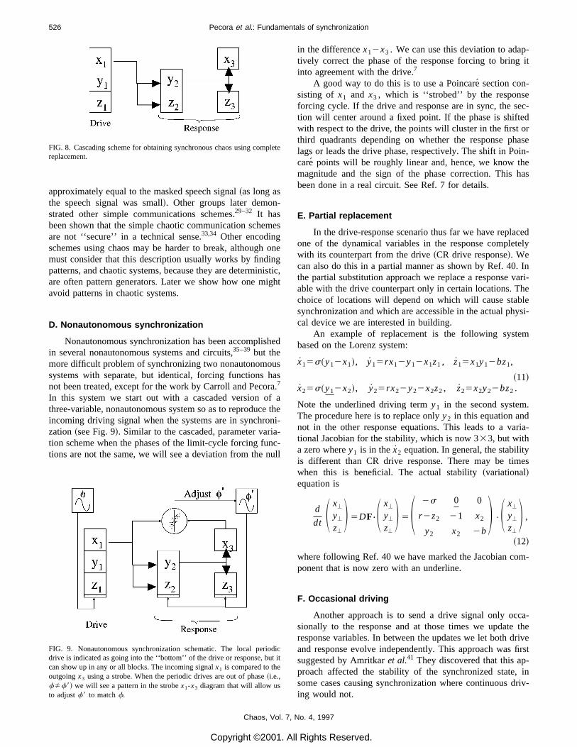
In this system we start out with a cascaded version of athree-variable, nonautonomous system so as to reproduce theincoming driving signal when the systems are in synchroni-zation ~see Fig. 9!. Similar to the cascaded, parameter varia-tion scheme when the phases of the limit-cycle forcing func-tions are not the same, we wil l see adeviation from the null
FIG. 8. Cascading scheme for obtaining synchronous chaos using completereplacement.
FIG. 9. Nonautonomous synchronization schematic. The local periodicdrive is indicated as going into the ‘‘bottom’ ’ of the drive or response, but itcan show up in any or all blocks. The incoming signal x1 is compared to theoutgoing x3 using a strobe. When the periodic drives are out of phase ~i.e.,fÞf8! we will see a pattern in the strobex1-x3 diagram that wil l allow usto adjustf8 to matchf.
Chaos, Vol. 7,
Copyright ©2001. A
in the difference x12x3 . We can use this deviation to adap-tively correct the phase of the response forcing to bring itinto agreement with the drive.7
A good way to do this is to use aPoincare´ section con-sisting of x1 and x3 , which is ‘‘strobed’’ by the responseforcing cycle. If the drive and response are in sync, the sec-tion wil l center around a fixed point. If the phase is shiftedwith respect to the drive, the points wil l cluster in the first orthird quadrants depending on whether the response phaselags or leads the drive phase, respectively. The shift in Poin-carepoints wil l be roughly linear and, hence, we know themagnitude and the sign of the phase correction. This hasbeen done in a real circuit. See Ref. 7 for details.
E. Partia l replacement
In the drive-response scenario thus far we have replacedone of the dynamical variables in the response completelywith its counterpart from the drive ~CR drive response!. Wecan also do this in a partial manner as shown by Ref. 40. Inthe partial substitution approach we replace aresponse vari-able with the drive counterpart only in certain locations. Thechoice of locations wil l depend on which wil l cause stablesynchronization and which are accessible in the actual physi-cal device we are interested in building.
An example of replacement is the following systembased on the Lorenz system:
x15s~y12x1!, y15rx12y12x1z1 , z15x1y12bz1,
~11!x25s~y12x2!, y25rx22y22x2z2 , z25x2y22bz2 .
Note the underlined driving term y1 in the second system.The procedure here is to replace only y2 in this equation andnot in the other response equations. This leads to a varia-tional Jacobian for the stability, which is now 333, but witha zero where y1 is in the x2 equation. In general, the stabilityis different than CR drive response. There may be timeswhen this is beneficial. The actual stability ~variational!equation is
d
dt S x'
y'
z'
D 5DF–S x'
y'
z'
D 5S 2s 0 0
r 2z2 21 x2
y2 x2 2bD •S x'
y'
z'
D ,
~12!
where following Ref. 40 we have marked the Jacobian com-ponent that is now zero with an underline.
F. Occasiona l driving
Another approach is to send a drive signal only occa-sionally to the response and at those times we update theresponse variables. In between the updates we let both driveand response evolve independently. This approach was firstsuggested by Amritkar et al.41 They discovered that this ap-proach affected the stability of the synchronized state, insome cases causing synchronization where continuous driv-ing would not.
No. 4, 1997
ll Rights Reserved.
527Pecora et al.: Fundamentals of synchronization
Later this idea was applied with a view toward commu-nications by Stojanovski et al.42,43 For private communica-tions, in principle, occasional driving should be more diffi-cult to decrypt or break since there is less informationtransmitted per unit time.
G. Synchronou s substitution
We are often in aposition of wanting several or all drivevariables at the response when we can only send one signal.For example, we might want to generate afunction of severaldrive variables at the response, but we only have one signalcoming from the drive. We show that we can sometimessubstitute a response variable for its drive counterpart toserve our purpose. This wil l work when the response is syn-chronized to the drive ~then the two variables are equal! andthe synchronization is stable ~the two variables stay equal!.We refer to this practice as synchronous substitution. Forexample, this approach allows us to send a signal to theresponse that is a function of the drive variables and use theinverse of that function at the response to generate variablesto use in driving the response. This wil l generally change thestability of the response.
The first application of this approach was given in Refs.44 and 45. Other variations have also been offered, includinguse of an active/passive decomposition.46
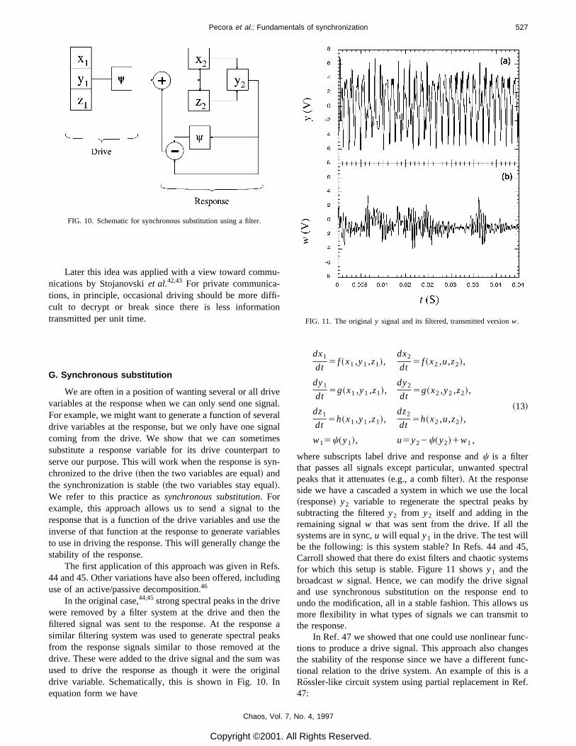
In theoriginal case,44,45strong spectral peaks in thedrivewere removed by a filter system at the drive and then thefiltered signal was sent to the response. At the response asimilar filtering system was used to generate spectral peaksfrom the response signals similar to those removed at thedrive. These were added to the drive signal and the sum wasused to drive the response as though it were the originaldrive variable. Schematically, this is shown in Fig. 10. Inequation form we have
FIG. 10. Schematic for synchronous substitution using a filter.
Chaos, Vol. 7,
Copyright ©2001. A
dx1
dt5 f ~x1 ,y1 ,z1!,
dx2
dt5 f ~x2 ,u,z2!,
dy1
dt5g~x1 ,y1 ,z1!,
dy2
dt5g~x2 ,y2 ,z2!,
dz1
dt5h~x1 ,y1 ,z1!,
dz2
dt5h~x2 ,u,z2!,
w15c~y1!, u5y22c~y2!1w1 ,
~13!
where subscripts label drive and response and c is a filterthat passes all signals except particular, unwanted spectralpeaks that it attenuates ~e.g., a comb filter!. At the responseside we have acascaded a system in which we use the local~response! y2 variable to regenerate the spectral peaks bysubtracting the filtered y2 from y2 itself and adding in theremaining signal w that was sent from the drive. If all thesystems are in sync, u wil l equal y1 in the drive. The test willbe the following: is this system stable? In Refs. 44 and 45,Carroll showed that there do exist filters and chaotic systemsfor which this setup is stable. Figure 11 shows y1 and thebroadcast w signal. Hence, we can modify the drive signaland use synchronous substitution on the response end toundo the modification, all in astable fashion. This allows usmore flexibility in what types of signals we can transmit tothe response.
In Ref. 47 we showed that one could use nonlinear func-tions to produce a drive signal. This approach also changesthe stability of the response since we have a different func-tional relation to the drive system. An example of this is aRossler-like circuit system using partial replacement in Ref.47:
FIG. 11. The original y signal and its filtered, transmitted version w.
No. 4, 1997
ll Rights Reserved.
528 Pecora et al.: Fundamentals of synchronization
dx1
dt52a~rx11by11z1!,
dx2
dt52a~rx21by21z2!,
dy1
dt52a~gy12x12ay1!,
dy2
dt52a~gy22x22ay!,
dz1
dt52a@z12g~x1!#,
dz2
dt52a@z22g~x2!#,
g~x1!5 H 0,15~x123!,
if x,3if x>3
g~x2!5same form as drive g,y52w~x214.2!,
w52y1
x114.2.
~14!
What we have done above is to take the usual situation ofpartial replacement of y2 with y1 and instead transform thedrive variables using the function w and send that signal tothe response. Then we invert w at the response to give us agood approximation to y1' y and drive the response usingpartial replacement with y. This, of course, changes the sta-bility . The Jacobian for the response becomes
2aS r b 1
211aw g 0
2g 0 1D . ~15!
With direct partial replacement ~i.e., sending y1 and using itin place of y above! the Jacobian would not have the 1awterm in the first column. The circuit we built using this tech-nique was stable.
We can write ageneral formulation of the synchronoussubstitution technique as used above.47 We start with ann-dimensional dynamical system dr /dt5F(r ), where r5(x,y,z,...). We use a general function T from Rn→R. Wesend the scalar signal w5T(x1 ,y1 ,z1 ...). At the responsewe invert T to give an approximation to the drive variablex1 , namely x5T1(w,y2 ,z2 ,...), where T1 is the inverse ofT in the first argument. By the implicit function theorem T1
wil l exist if ]T/]xÞ0. Synchronous substitution comes inT1
where we normally would need y1 ,z1 ,..., to invert T. Sincewe do not have access to those variables, we use their syn-chronous counterparts y2 ,z2 ,..., in the response.
Using this formulation in the case of partial replacementor complete replacement of x2 or some other functional de-pendence on w in the response we now have anew Jacobianin our variational equation:
ddr
dt5@D rF1DwF D rT1#–dr , ~16!
where we have assumed that the response vector field F hasan extra argument, w, to account for the synchronous substi-tution. In Eq. ~16! the first term is the usual Jacobian and the
Chaos, Vol. 7,
Copyright ©2001. A
second term comes from the dependence on w. Note that, ifwe use complete replacement of x2 with x1 , the DxF part ofthe first term in Eq. ~16! would be zero.
There are other variations on the theme of synchronoussubstitution. We introduce another here since it leads to aspecial case that is used in control theory and that we haverecently exploited. One way to guarantee synchronizationwould be to transmit all drive variables and couple them tothe response using negative feedback, viz.
dx~2!/dt5F~x~2!!1c~x~1!2x~2!!, ~17!
where, unlike before, we now use superscripts in parenthesesto refer to the drive ~1! and the response ~2! variables andx(1)5(x1
(1) ,x2(1) ,...,xn
(1)), etc. With the right choice of coup-ling strength c, we could always synchronize the response.But again we are limited in sending only one signal to theresponse. We do the following, which makes use of synchro-nous substitution.
Let S:Rn→Rn be a differentiable, invertible transforma-tion. We construct w5S(x(1)) at the drive and transmit thefirst component w1 to the response. At the response we gen-erate the vector u5S(x(2)). Near the synchronous state u'w. Thus we have approximations at the response to thecomponents wi that we do not have access to. We thereforeattempt to use Eq. ~17! by forming the following:
dx~2!
dt5F~x~2!!1c@S21~w!2x~2!#, ~18!
where in order to approximate c(x(1)2x(2)) we have usedsynchronous substitution to form w(w1 ,u2 ,u3 ,...,un) andapplied the inverse transformation S21.
Al l the rearrangements using synchronous substitutionand transformations may seem like a lot of pointless algebra,but the use of such approaches allows one to transmit onesignal and synchronize aresponse that might not be synchro-nizable otherwise as well as to guide in the design of syn-chronous systems. Moreover, a particular form of the Stransformation leads us to a commonly used control-theory
No. 4, 1997
ll Rights Reserved.

529Pecora et al.: Fundamentals of synchronization
method. The synchronous substitution formalism allows usto understand the origin of the control-theory approach. Weshow this in the next section.
H. Contro l theor y approaches , a specia l case ofsynchronou s substitution
Suppose in our above use of synchronous substitutionthe transformation S is a linear transformation. ThenS21(w)2S21(u)5S21(w2u), and since w2u has only itsfirst component as nonzero, we can write w2u5@KT(x(1)
2x(2)),0,0,...,0#, where KT is the first row of S. Then thecoupling term cS21(w2u) becomes BKT(x(1)2x(2)),where B is the first column of S21 and we have absorbed thecoupling constant c into B. This form of the coupling ~calledBK coupling from here on! is common in control theory.48
We can see where it comes from. It is an attempt to use alinear coordinate transformation (S) to stabilize the synchro-nous state. Because we can only transmit one signal ~onecoordinate! we are left with a simpler form of the couplingthat results from using response variables ~synchronous sub-stitution! in place of the missing drive variables.
Recently, experts in control theory have begun to applyBK and other control-theory concepts to the task of synchro-nizing chaotic systems. We wil l not go into all the detailshere, but good overviews and explanations on the stability ofsuch approaches can be found in Refs. 49–52. In the follow-ing sections we show several explicit examples of using theBK approach in synchronization.
I. Optimizatio n of BK coupling
Our own investigation of the BK method began withapplying it to the piecewise-linear Rossler circuits. As is usu-ally pointed out ~e.g., see Peng et al.53!, the problem is re-
FIG. 12. The BK method is demonstrated on the piecewise-linear Rosslercircuit. The difference in the X variables of receiver and transmitter isshown to converge to about 20 mV in under one cycle of the period-1 orbit~about 1 ms!. The plot is an average of 100 trials.
Chaos, Vol. 7,
Copyright ©2001. A
duced to finding an appropriate BK combination resulting innegative Lyapunov exponents at the receiver. The piecewise-linear Rossler systems ~see above! lend themselves well tothis task as the stability is governed by two constant Jacobianmatrices, and the Lyapunov exponents are readily deter-mined. To seek out the proper combinations of B’ s and K ’s,we employ an optimization routine in the six-dimensionalspace spanned by the coupling parameters. From a six-dimensional grid of starting points in BK space, we seek outlocal minima of the largest real part of the eigenvalue of theresponse Jacobian @J2BKT#.
By limiting the size of the coupling parameters and col-lecting all of the deeply negative minima, we find that wecan choose from a number of BK sets that ensure fast androbust synchronization. For example, the minimization rou-tine reveals, among others, the following pair of minima wellseparated in BK space: B15$22.04,0.08,0.06% K15$21.79,22.17,21.84%, and B25$0.460,2.41,0.156% K2
5$21.37,1.60,2.33%. The real parts of the eigenvalues forthese sets are 21.4 and 21.3, respectively. In Fig. 12, weshow the fast synchronization using B1K1
T as averaged over100 runs, switching on the coupling at t50. The time of theperiod-1 orbit in the circuit is about 1 ms, in which time thesynchronization error is drastically reduced by about two or-ders of magnitude.
Similarly, we can apply the method to the volume pre-serving hyperchaotic map system of section x. The only dif-ference is that we now wish to minimize the largest norm ofthe eigenvalues of the response Jacobian. With our optimi-zation routine, we are able to locate eigenvalues on the orderof 1024, corresponding to Lyapunov exponents around 29.
J. Hyperchao s synchronization
Most of the drive–response synchronous, chaotic sys-tems studied so far have had only one positive Lyapunovexponent. More recent work has shown that systems withmore than one positive Lyapunov exponent ~called hypercha-otic systems! can be synchronized using one drive signal.Here we display several other approaches.
A simple way to construct a hyperchaotic system is touse two, regular chaotic systems. They need not be coupled;just the amalgam of both is hyperchaotic. Tsimiring andSuschik54 recently made such a system and considered howone might synchronize a duplicate response. Their approachhas elements similar to the use of synchronous substitutionwe mentioned above. They transmit a signal, which is thesum of the two drive systems. This sum is coupled to a sumof the same variables from the response. When the systemsare in sync the coupling vanishes and the motion takes placeon an invariant hyperplane and hence is identical synchroni-zation.
An example of this situation using one-dimensional sys-tems is the following:54
No. 4, 1997
ll Rights Reserved.

530 Pecora et al.: Fundamentals of synchronization
x1~n11!5 f 1@x1~n!#, x2~n11!5 f 2@x2~n!#,
w5 f 1@x1~n!#1 f 2@x2~n!#2 f 1@y1~n!#2 f 2@y2~n!#
5transmitted signal,~19!
y1~n11!5 f 1@y1~n!#1e$ f 1@x1~n!#1 f 2@x2~n!#
2 f 1@y1~n!#2 f 2@y2~n!#%,
y2~n11!5 f 2@y2~n!#1e$ f 1@x1~n!#1 f 2@x2~n!#
2 f 1@y1~n!#2 f 2@y2~n!#%,
Linear stability analysis, as we introduced above, shows thatthe synchronization manifold is stable.54 Tsimring and Sus-chik investigated several one-dimensional maps ~tent, shift,logistic! and found that there were large ranges of couplinge, where the synchronization manifold was stable. For cer-tain cases they even got analytic formulas for the Lyapunovmultipliers. However, they did find that noise in the com-munications channel, represented by noise added to thetransmitted signal w, did degrade the synchronization se-verely, causing bursting. The same features showed up intheir study of a set of drive-response ODEs ~based on amodel of an electronic synchronizing circuit!. The reasonsfor the loss of synchronization and bursting are the same asin our study of the coupled oscillators below. There are localinstabilities that cause the systems to diverge momentarily,even above Lyapunov synchronization thresholds. Any slightnoise tends to keep the systems apart and ready to divergewhen the trajectories visit the unstable portions of the attrac-tors. Whether this can be ‘‘fixed’ ’ in practical devices so thatmultiplexing can be used is not clear. Our study below ofsynchronization thresholds for coupled systems suggests thatfor certain systems and coupling schemes we can avoidbursting, but more study of this phenomenon forhyperchaotic/multiplexed systems has to be done. Perhaps aBK approach may be better at eliminating bursts since it canbe optimized. This remains to be seen.
The issue of synchronizing hyperchaotic systems wasaddressed by Peng et al.53 They started with two identicalhyperchaotic systems, x5F(x) and y5F(y). Their approachwas to use the BK method to synchronize the systems. Asbefore, the transmitted signal was w5KTx and we add acoupling term to the y equations of motion: y5F(y)1B(w2 v), where v5KTy. Peng et al. show that for many casesone can choose K and B so that the y system synchronizeswith the x system. This and the work by Tsimring and Sus-chik solve a long-standing question about the relation be-tween the number of drive signals that need to be sent tosynchronize aresponse and the number of positive Lypunovexponents, namely that there is no relation, in principle.Many systems with a large number of positive exponents canstill be synchronized with one drive signal. Practical limita-tions wil l surely exist, however. The latter still need to beexplored.
Finally, we mention that synchronization of hypercha-otic systems has been achieved in experiments. Tamasevi-cius et al.25 have shown that such synchronization can be
Chaos, Vol. 7,
Copyright ©2001. A
accomplished in a circuit. They built circuits that consistedof either mutually coupled or unidirectionally coupled 4-Doscillators. They show that for either coupling both positiveconditional Lypunov exponents of the ‘‘uncoupled’’ sub-systems become negative as the coupling is increased. Theygo on to further show that they must be above acritical valueof coupling which is found by observing the absence of ablowout bifurcation.55–57 Such a demonstration in a circuit isimportant, since this proves at once that hyperchaos synchro-nization has some robustness in the presence of noise andparameter mismatch.
We constructed a four-dimensional piecewise-linear cir-cuit based on the hyperchaotic Rossler equations.53,58 Themodified equations are as follows:
dx
dt520.05x20.502y20.62z,
dy
dt5x10.117y10.402w,
dz
dt5g~x!21.96z,
dw
dt5h~w!20.148z10.18w,
where
g~x!510~x20.6!, x.0.6,
50, x,0.6,
h~w!520.412~w23.8!, w.3.8,
50, w,3.8.
One view of the hyperchaotic circuit is shown in the plot ofw vs y in Fig. 13. Again, as with the 3-D Rossler circuit, the4-D circuit is synchronized rapidly and robustly with the BKmethod. In this circuit, we are aided by the fact that thedynamics are most often driven by one particular matrix out
FIG. 13. A projection of the dynamics of the hyperchaotic circuit based onthe 4-D Rossler equations.
No. 4, 1997
ll Rights Reserved.

ill
531Pecora et al.: Fundamentals of synchronization
of the four possible Jacobians. We have found that minimi-zation of the real eigenvalues in the most-visited matrix istypically sufficient to provide overall stability. Undoubtedlythere are cases in which this fails, but we have had a highlevel of success using this technique. A more detailed sum-mary of this work wil l be presented elsewhere, so we brieflydemonstrate the robustness of the synchronization in Fig. 14.The coupling parameters in this circuit are given by B5$0.36,2.04,21.96,0.0% and K5$21.97,2.28,0,1.43%.
K. Synchronizatio n as a contro l theor y observerproblem
A control theory approach to observing a system is asimilar problem to synchronizing two dynamical systems.Often the underlying goal is the synchronization of the ob-server dynamical system with the observed system so theobserved system’s dynamical variables can be determinedfully from knowing only a few of the observed system’svariables or a few functions of those variables. Often wehave only a scalar variable ~or time series! from the observedsystem and we want to recreate all the observed system’svariables.
So, Ott, and Dayawansa follow such approaches in Ref.59. They showed that a local control theory approach basedessentially on the Ott–Grebogi–Yorke technique.60 Thetechnique does require knowledge of the local structure ofstable and unstable manifolds. In an approach that is closerto the ideas of drive-response synchronization presentedabove Brown et al.61–64 showed that one can observe acha-otic system by synchronizing a model to a time series orscalar signal from the original system. They showed furtherthat one could often determine aset of maps approximatingthe dynamics of the observed system with such an approach.Such maps could reliably calculate dynamical quantities suchas Lyapunov exponents. Brown et al. went much further andshowed that such methods could be robust to additive noise.
FIG. 14. The BK method as applied to the hyperchaotic circuit. The cou-pling is switched on when the pictured gate voltage is high, and B is effec-tively $0,0,0,0% when the gate voltage is low. The sample rate is 20 ms/sample.
Chaos, Vol. 7,
Copyright ©2001. A
Somewhat later, Parlitz also used these ideas to explore thedetermination of an observed system’s parameters.65
L. Volume-preservin g maps and communicationsissues
Most of the chaotic systems we describe here are basedon flows. It is also useful to work with chaotic circuits basedon maps. Using map circuits allows us to simulate volume-preserving systems. Since there is no attractor for a volume-preserving map, the map motion may cover a large fractionof the phase space, generating very broadband signals.
It seems counterintuitive that a nondissipative systemmay be made to synchronize, but in a multidimensionalvolume-preserving map, there must be at least one contract-ing direction so that volumes in phase space are conserved.We may use this one direction to generate a stable sub-system. We have used this technique to build a set of syn-chronous circuits based on the standard map.66
In hyperchaotic systems, there are more than one posi-tive Lyapunov exponent and for a map this may mean thatthe number of expanding directions exceeds the number ofcontracting directions, so that there are no simple stable sub-systems for a one-drive setup. We may, however, use theprinciple of synchronous substitution ~described in Sec. VIbelow! or its specialization to the BK to generate varioussynchronous subsystems. We have built a circuit to simulatethe following map:67
xn1152~ 43! xn1zn
yn115~ 13! yn1zn
zn115xn1yn
J mod 2, ~20!
where ‘‘mod~2!’ ’ means take the result modulus 62. Thismap is quite similar to the cat map68 or the Bernoulli shift inmany dimensions. The Lyapunov exponents for this map~determined from the eigenvalues of the Jacobian! are 0.683,0.300, and 20.986.
We may create astable subsystem of this map using themethod of synchronous substitution.47 We produce a newvariable wn5zn1gxn from the drive system variables, andreconstruct a driving signal zn at the response system:
wn5zn1gxn , zn5wn2gxn8 ,~21!
xn118 52~ 43! xn81 zn , yn118 5~ 1
3! yn81 zn ,
where the modulus function is assumed. In the circuit, weusedg524/3, although there is a range of values that wwork. We were able to synchronize the circuits adequately inspite of the difficulty of matching the modulus functions.
The transmitted signal from this circuit has essentially aflat power spectrum and approximately a delta-function au-tocorrelation, making the signal a good alternative to a con-ventional pseudonoise signal. Our circuit is in essence aself-synchronizing pseudonoise generator. We present moreinformation on this system, its properties and communica-tions issues in Refs. 67 and 69.
No. 4, 1997
ll Rights Reserved.

e
532 Pecora et al.: Fundamentals of synchronization
M. Usin g function s of driv e variable s and information
An interesting approach involving the generation of newsynchronizing vector fields was taken by Kocarev.70,71 Thisis an approach similar to synchronous substitution that usesan invertible function of the drive dynamical variables andthe information signal to drive the response, rather than justusing one of the variables itself as in the CR approach. Thenon the response the function is inverted using the fact that thesystem is close to synchronization.
Schematically, this looks as follows. On the drive endthere is adynamical system x5F(x,s), where s is the trans-mitted signal and is a function of x and the information i (t),s5h(x,i ). On the receiver end there is an identical dynami-cal system set up to extract the information: y5F(y,s) andi R5h21(y,s). When the systems are in sync i R5 i . We haveshown this is useful by using XOR as our h function in thevolume-preserving system.69
N. Synchronizatio n in othe r physica l systems
Until now we have concentrated on circuits as the physi-cal systems that we want to synchronize. Other work hasshown that one can also synchronize other physical systemssuch as lasers and ferrimagnetic materials undergoing cha-otic dynamics.
In Ref. 72 Roy and Thornburg showed that lasers thatwere behaving chaotically could be synchronized. Two solidstate lasers can couple through overlapping electromagneticlasing fields. The coupling is similar to mutual couplingshown in Sec. II I A 3, except that the coupling is negative.This causes the lasers to actually be in oppositely signedstates. That is, if we plot the electric field for one against theother we get a line at 245° rather than the usual 45°. This isstill a form of synchronization. Actually since Roy andThornburg only examined intensities the synchronizationwas still of the normal, 45° type. Colet and Roy continued topursue this phenomenon to the point of devising a commu-nications scheme using synchronized lasers.73 This work wasrecently implemented by Alsing et al.74 Such laser synchro-nization opens the way for potential uses in fiberoptics.
Peterman et al.75 showed anovel way to synchronize thechaotic, spin-wave motion in rf pumped yttrium iron garnet.In these systems there are fast and slow dynamics. The fastdynamics amounts to sinusoidal oscillations at GHz frequen-cies of the spin-wave amplitudes. The slow dynamics gov-erns the amplitude envelopes of the fast dynamics. The slowdynamics can be chaotic. Peterman et al. ran their experi-ments in the chaotic regimes and recorded the slow dynami-cal signal. They then ‘‘played the signals back’’ at a latertime to drive the system and cause it to synchronize with therecorded signals. This shows that materials with such high-frequency dynamics are amenable to synchronizationschemes.
O. Generalize d synchronization
In their original paper on synchronization Afraimovichet al. investigated the possibility of some type of synchroni-
Chaos, Vol. 7,
Copyright ©2001. A
zation when the parameters of the two coupled systems donot match. Such a situation wil l certainly occur in real,physical systems and is an important question. Their studyshowed that for certain systems, including the 2-D forcedsystem they studied, one could show that there was a moregeneral relation between the two coupled systems. This rela-tionship was expressed as a one-to-one, smooth mapping be-tween the phase space points in each subsystem. To put thismore mathematically, if the full system is described by a 4-Dvector (x1 ,y1 ,x2 ,y2), then there exists smooth, invertiblefunction f from (x1 ,y1) to (x2 ,y2).
Thus, knowing the state of one system enables one, inprinciple, to know the state of the other system, and viceversa. This situation is similar to identical synchronizationand has been called generalized synchronization. Except inspecial cases, like that of Afraimovich et al., rarely wil l onebe able to produce formulae exhibiting the mappingf. Prov-ing generalized synchronization from time series would be auseful capability and sometimes can be done. We show howbelow. The interested reader should examine Refs. 76–78 formore details.
Recently, several attempts have been made to generalizethe concept of general synchronization itself. These beginwith the papers by Rul’kov et al.76,79 and onto a paper byKocarev and Parlitz.80 The central idea in these papers is thatfor the drive-response setup, if the response is stable ~allLypunov exponents are negative!, then there exists a mani-fold in the joint drive-response phase space such that there isa function from the drive (X) to the response (Y), f:X→Y.In plain language, this means we can predict the responsestate from that of the drive ~there is one point on the re-sponse for each point on the drive’s attractor! and the pointsof the mappingf lie on a smooth surface~such is the defi-nition of a manifold!.
This is an intriguing idea and it is an attempt to answerthe question we posed in the beginning of this paper, namely,does stability determine geometry? These papers would an-swer yes, in the drive-response case the geometry is amani-fold that is ‘‘above’’ the drive subspace in the whole phasespace. The idea seems to have some verification in the stud-ies we have done so far on identical synchronization and inthe more particular case of Afraimovich–Verichev–Rabinovich generalized synchronization. However, there arecounterexamples that show that the conclusion cannot betrue.
First, we can show that there are stable drive-responsesystems in which the attractor for the whole system is not asmooth manifold. Consider the following system:
x5F~x! z52hz1x1 , ~22!
where x is a chaotic system andh.0. Thez system can beviewed as afilter ~LTI or low-pass type! and is obviously astable response to the drive x. It is now known that certainfilters of this type lead to an attractor in which there is a map~often called a graph! f of the drive to the response, but thmapping is not smooth. It is continuous and so the relationbetween the drive and response is similar to that of the real
No. 4, 1997
ll Rights Reserved.
533Pecora et al.: Fundamentals of synchronization
line and the Weierstrass function above it. This explains whycertain filters acting on a time series can increase the dimen-sion of the reconstructed attractor.81,82
We showed that certain statistics could detect thisrelationship,82 and we introduce those below. Several otherpapers have proven the nondifferentiability property rigor-ously and have investigated several types of stable filters ofchaotic systems.83–89 We note that the filter is just a specialcase of a stable response. The criteria for smoothness in anydrive-response scenario is that the least negative conditionalLypunov exponents of the response must be less than themost negative Lypunov exponents of the drive.87,90 One canget a smooth manifold if the response is uniformly contract-ing, that is, the stability exponents are locally alwaysnegative.87,91Note that if the drive is anoninvertible dynami-cal system, then things are ‘‘worse.’’ The drive-response re-lation may not even be continuous and may be many valued,in the latter case there is not even afunctionf from the driveto the response.
There is an even simpler counterexample that no oneseems to mention that shows that stability does not guaranteethatf exists and this is the case of period-2 behavior~or anymultiple period behavior!. If the drive is a limi t cycle and theresponse is a period doubled system ~or higher multiple-period system!, then for each point on the drive attractorthere are two ~or more! points on the response attractor. Onecannot have afunction under such conditions and there is noway to predict the state of the response from that of thedrive. Note that there is afunction from response to the drivein this case. Actually, any drive-response system that has theoverall attractor on an invariant manifold that is not diffeo-morphic to a hyperplane wil l have the same, multivaluedrelationship and there wil l be no function f.
Hence, the hope that a stable response results in a nice,smooth, predictable relation between the drive and responsecannot always be realized and the answer to our question ofwhether stability determines geometry is ‘‘no,’ ’ at least inthe sense that it does not determine one type of geometry.Many are possible. The term general synchronization in thiscase may be misleading in that it implies a simpler drive-
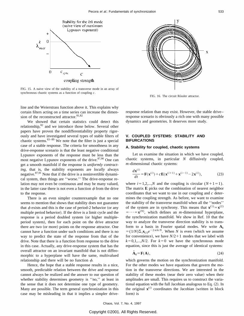
FIG. 15. A naive view of the stability of a transverse mode in an array ofsynchronous chaotic systems as afunction of coupling c.
Chaos, Vol. 7,
Copyright ©2001. A
response relation than may exist. However, the stable drive–response scenario is obviously a rich one with many possibledynamics and geometries. It deserves more study.
V. COUPLED SYSTEMS: STABILIT Y ANDBIFURCATIONS
A. Stabilit y for coupled , chaoti c systems
Let us examine the situation in which we have coupled,chaotic systems, in particular N diffusively coupled,m-dimensional chaotic systems:
dx~ i !
dt5F~x~ i !!1cE~x~ i 11!1x~ i 21!22x~ i !!, ~23!
where i 51,2,...,N and the coupling is circular (N1151).The matrix E picks out the combination of nearest neighborcoordinates that we want to use in our coupling and c deter-mines the coupling strength. As before, we want to examinethe stability of the transverse manifold when all the ‘‘nodes’’of the system are in synchrony. This means that x(1)5x(2)
5•••5x(N), which defines an m-dimensional hyperplane,the synchronization manifold. We show in Ref. 10 that theway to analyze the transverse direction stability is to trans-form to a basis in Fourier spatial modes. We write Ak
5(1/N)S ix( i )e22p ik/N. When N is even ~which we assume
for convenience!, we have N/211 modes that we label withk50,1,...,N/2. For k50 we have the synchronous modeequation, since this is just the average of identical systems:
A05F~A!, ~24!
which governs the motion on the synchronization manifold.For the other modes we have equations that govern the mo-tion in the transverse directions. We are interested in thestability of these modes ~near their zero value! when theiramplitudes are small. This requires us to construct the varia-tional equation with the full Jacobian analogous to Eq. ~2!. Inthe original x( i ) coordinates the Jacobian ~written in blockform! is
FIG. 16. The circuit Rossler attractor.
No. 4, 1997
ll Rights Reserved.

534 Pecora et al.: Fundamentals of synchronization
S DF22cE cE 0 ••• cE
cE DF22cE cE 0 •••
0 cE DF22cE cE •••
A A
cE ••• 0 cE DF22cE
D , ~25!
whereeach block is m3m and is associated with aparticular nodex( i ). In themodecoordinates theJacobian is block diagonal,which simplifies finding the stability conditions,
S DF 0 0 ••• c
0 DF24cE sin2@p/N# 0 0 •••
A A A A
0 ••• 0 DF24cE sin2@pk/N# •••
A
D , ~26!
i-
where each value of kÞ0 or kÞN/2 occurs twice, once forthe ‘‘sine’ ’ and once for the ‘‘cosine’’ modes. We want thetransverse modes represented by sine and cosine spatial dis-turbances to die out, leaving only the k50 mode on thesynchronization manifold. At first sight what we want forstability is for all the blocks with kÞ0 to have negativeLypunov exponents. We wil l see that things are not sosimple, but let us proceed with this naive view.
Figure 15 shows the naive view of how the maximumLypunov exponent for a particular mode block of a trans-verse mode might depend on coupling c. There are fourfeatures in the naive view that we wil l focus on.
~1! As the coupling increases from 0 we go from theLyapunov exponents of the free oscillator to decreasingexponents until for some threshold coupling csync themode becomes stable.
~2! Above this threshold we have stable synchronous chaos.~3! We suspect that as we increase the coupling the expo-
nents wil l continue to decrease.~4! We can now couple together as many chaotic oscillators
as we like using a coupling c.csync and always have astable synchronous state.
We already know from Fig. 3 that this view cannot be cor-rect @increasing c may desynchronize the array—feature ~3!#,but we wil l now investigate these issues in detail. Below wewil l use a particular coupled, chaotic system to show thatthere are counterexamples to all four of these ‘‘features.’’
We first note a scaling relation for Lypunov exponentsof modes with different k’s. Given any Jacobian block for amode k1 we can always write it in terms of the block foranother mode k2 , viz.,
DF24C sin2@pk1 /N#5DF24cES sin2@pk1 /N
sin2@pk2 /N# D3sin2@pk2 /N#, ~27!
where we see that the effect is to shift the coupling by thefactor sin2(pk1 /N)/sin2(pk2 /N). Hence, given any mode’s
Chaos, Vol. 7,
Copyright ©2001. A
stability plot ~as in Fig. 3! we can obtain the plot for anyother mode by rescaling the coupling. In particular, we needonly calculate the maximum Lypunov exponent for mode 1(lmax
1 ) and then the exponents for all other modes k.1 aregenerated by ‘‘squeezing’’ the lmax
1 plot to smaller couplingvalues.
This scaling relation, first shown in Ref. 10, shows thatas the mode’s Lypunov exponents decrease with increasing cvalues the longest-wavelength mode k1 wil l be the last tobecome stable. Hence, we first get the expected result thatthe longest wavelength ~with the largest coherence length! isthe least stable for small coupling.
B. Couplin g threshold s for synchronize d chao s andbursting
To test our four features we examine the following sys-tem of four Rossler-like oscillators diffusively coupled in acircle, which has a counterpart in a set of four circuits webuilt for experimental tests,10
dx/dt52a~Gx1by1lz!,
dy/dt5a~x1gy!, ~28!
dz/dt5a@g~x!2z#,
where g is a piece-wise linear function that ‘‘turns on’’ whenx crosses athreshold and causes the spiraling out behavior to‘‘fold’ ’ back toward the origin,
g~x!5 H 0,mx,
x<3,x.3. ~29!
For the values a5104 s21, G50.05, b50.5, l51.0, g50.133, andm515.0 we have a chaotic attractor very simlar to the Rossler attractor ~see Figs. 4 and 16!.
We couple four of these circuits through the y compo-nent by adding the following term to each system’s y equa-tion: c(yi 111yi 2122yi), where the indices are all mod 4.
No. 4, 1997
ll Rights Reserved.
535Pecora et al.: Fundamentals of synchronization
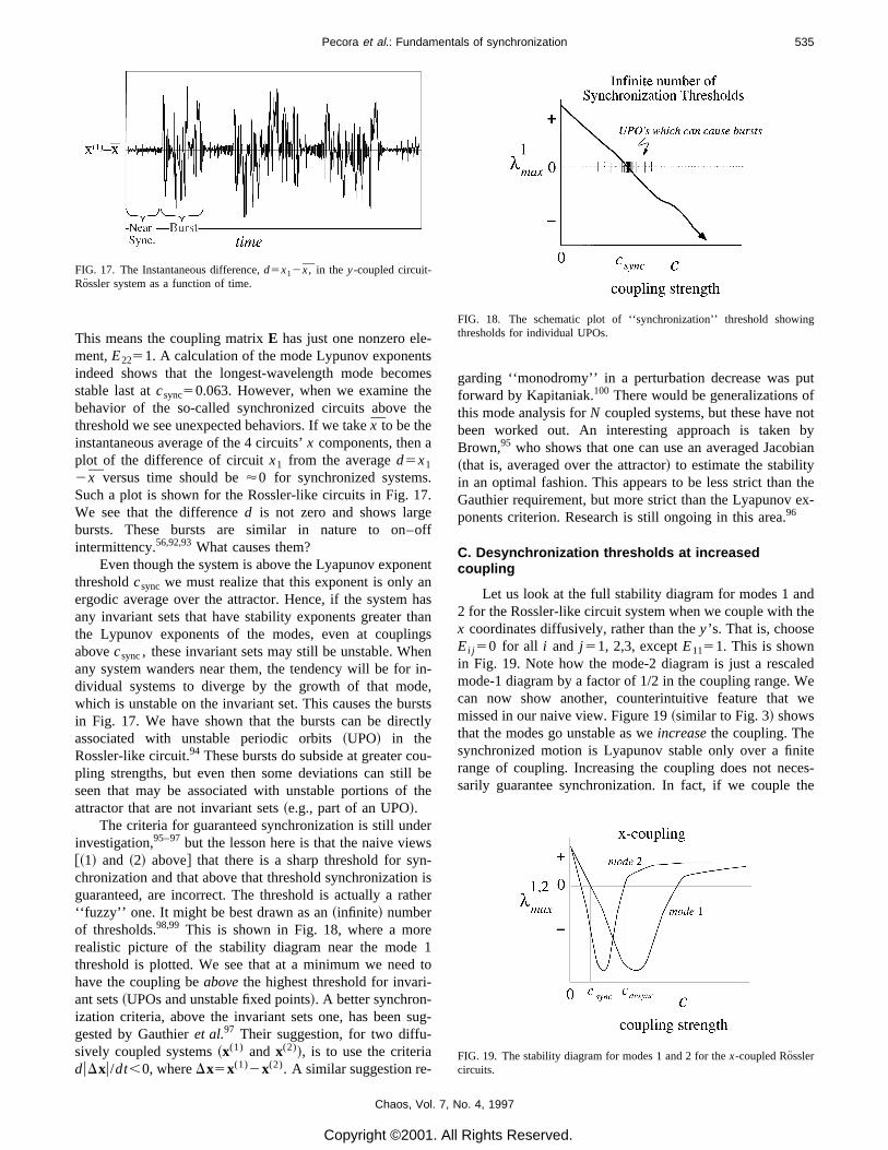
This means the coupling matrix E has just one nonzero ele-ment, E2251. A calculation of the mode Lypunov exponentsindeed shows that the longest-wavelength mode becomesstable last at csync50.063. However, when we examine thebehavior of the so-called synchronized circuits above thethreshold we see unexpected behaviors. If we take x to be theinstantaneous average of the 4 circuits’ x components, then aplot of the difference of circuit x1 from the average d5x1
2 x versus time should be '0 for synchronized systems.Such a plot is shown for the Rossler-like circuits in Fig. 17.We see that the difference d is not zero and shows largebursts. These bursts are similar in nature to on–offintermittency.56,92,93What causes them?
Even though the system is above the Lyapunov exponentthreshold csync we must realize that this exponent is only anergodic average over the attractor. Hence, if the system hasany invariant sets that have stability exponents greater thanthe Lypunov exponents of the modes, even at couplingsabove csync, these invariant sets may still be unstable. Whenany system wanders near them, the tendency wil l be for in-dividual systems to diverge by the growth of that mode,which is unstable on the invariant set. This causes the burstsin Fig. 17. We have shown that the bursts can be directlyassociated with unstable periodic orbits ~UPO! in theRossler-like circuit.94 These bursts do subside at greater cou-pling strengths, but even then some deviations can still beseen that may be associated with unstable portions of theattractor that are not invariant sets ~e.g., part of an UPO!.
The criteria for guaranteed synchronization is still underinvestigation,95–97 but the lesson here is that the naive views@~1! and ~2! above# that there is a sharp threshold for syn-chronization and that above that threshold synchronization isguaranteed, are incorrect. The threshold is actually a rather‘‘fuzzy’ ’ one. It might be best drawn as an ~infinite! numberof thresholds.98,99 This is shown in Fig. 18, where a morerealistic picture of the stability diagram near the mode 1threshold is plotted. We see that at a minimum we need tohave the coupling be above the highest threshold for invari-ant sets ~UPOs and unstable fixed points!. A better synchron-ization criteria, above the invariant sets one, has been sug-gested by Gauthier et al.97 Their suggestion, for two diffu-sively coupled systems ~x(1) and x(2)!, is to use the criteriaduDxu/dt,0, where Dx5x(1)2x(2). A similar suggestion re-
FIG. 17. The Instantaneous difference, d5x12 x, in the y-coupled circuit-Rossler system as afunction of time.
Chaos, Vol. 7,
Copyright ©2001. A
garding ‘‘monodromy’’ in a perturbation decrease was putforward by Kapitaniak.100 There would be generalizations ofthis mode analysis for N coupled systems, but these have notbeen worked out. An interesting approach is taken byBrown,95 who shows that one can use an averaged Jacobian~that is, averaged over the attractor! to estimate the stabilityin an optimal fashion. This appears to be less strict than theGauthier requirement, but more strict than the Lyapunov ex-ponents criterion. Research is still ongoing in this area.96
C. Desynchronizatio n threshold s at increasedcoupling
Let us look at the full stability diagram for modes 1 and2 for the Rossler-like circuit system when we couple with thex coordinates diffusively, rather than the y’s. That is, chooseEi j 50 for all i and j 51, 2,3, except E1151. This is shownin Fig. 19. Note how the mode-2 diagram is just a rescaledmode-1 diagram by a factor of 1/2 in the coupling range. Wecan now show another, counterintuitive feature that wemissed in our naive view. Figure 19 ~similar to Fig. 3! showsthat the modes go unstable as we increase the coupling. Thesynchronized motion is Lyapunov stable only over a finiterange of coupling. Increasing the coupling does not neces-sarily guarantee synchronization. In fact, if we couple the
FIG. 18. The schematic plot of ‘‘synchronization’’ threshold showingthresholds for individual UPOs.
FIG. 19. The stability diagram for modes 1and 2 for the x-coupled Rosslercircuits.
No. 4, 1997
ll Rights Reserved.
536 Pecora et al.: Fundamentals of synchronization
systems by the z variables we wil l never get synchronization,even when c5`. The latter case of infinite coupling is justthe CR drive response using z. We already know that in thatregime both the z and x drivings do not cause synchroniza-tion in the Rossler system. We now see why. Couplingthrough only one component does not guarantee asynchro-nous state and we have found a counterexample for number~3! in our naive views, that increasing the coupling wil l guar-antee a synchronous state.
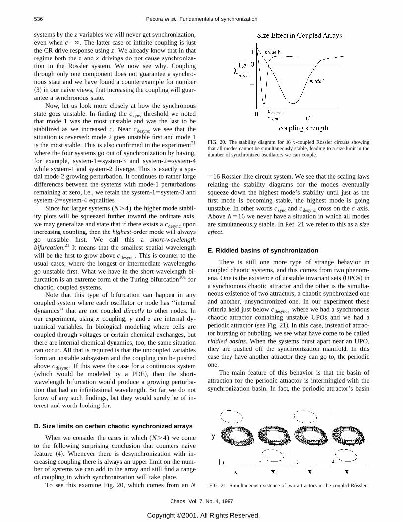
Now, let us look more closely at how the synchronousstate goes unstable. In finding the csync threshold we notedthat mode 1 was the most unstable and was the last to bestabilized as we increased c. Near cdesync we see that thesituation is reversed: mode 2 goes unstable first and mode 1is the most stable. This is also confirmed in the experiment21
where the four systems go out of synchronization by having,for example, system-15system-3 and system-25system-4while system-1 and system-2 diverge. This is exactly a spa-tial mode-2 growing perturbation. It continues to rather largedifferences between the systems with mode-1 perturbationsremaining at zero, i.e., we retain the system-15system-3 andsystem-25system-4 equalities.
Since for larger systems (N.4) the higher mode stabil-ity plots wil l be squeezed further toward the ordinate axis,we may generalize and state that if there exists a cdesyncuponincreasing coupling, then the highest-order mode wil l alwaysgo unstable first. We call this a short-wavelengthbifurcation.21 It means that the smallest spatial wavelengthwil l be the first to grow above cdesync. This is counter to theusual cases, where the longest or intermediate wavelengthsgo unstable first. What we have in the short-wavelength bi-furcation is an extreme form of the Turing bifurcation101 forchaotic, coupled systems.
Note that this type of bifurcation can happen in anycoupled system where each oscillator or node has ‘‘internaldynamics’’ that are not coupled directly to other nodes. Inour experiment, using x coupling, y and z are internal dy-namical variables. In biological modeling where cells arecoupled through voltages or certain chemical exchanges, butthere are internal chemical dynamics, too, the same situationcan occur. Al l that is required is that the uncoupled variablesform an unstable subsystem and the coupling can be pushedabove cdesync. If this were the case for a continuous system~which would be modeled by a PDE!, then the short-wavelength bifurcation would produce a growing perturba-tion that had an infinitesimal wavelength. So far we do notknow of any such findings, but they would surely be of in-terest and worth looking for.
D. Size limit s on certai n chaoti c synchronize d arrays
When we consider the cases in which (N.4) we cometo the following surprising conclusion that counters naivefeature ~4!. Whenever there is desynchronization with in-creasing coupling there is always an upper limi t on the num-ber of systems we can add to the array and still find a rangeof coupling in which synchronization wil l take place.
To see this examine Fig. 20, which comes from an N
Chaos, Vol. 7,
Copyright ©2001. A
516 Rossler-like circuit system. We see that the scaling lawsrelating the stability diagrams for the modes eventuallysqueeze down the highest mode’s stability until just as thefirst mode is becoming stable, the highest mode is goingunstable. In other words csync and cdesynccross on the c axis.Above N516 we never have asituation in which all modesare simultaneously stable. In Ref. 21 we refer to this as a sizeeffect.
E. Riddle d basin s of synchronization
There is still one more type of strange behavior incoupled chaotic systems, and this comes from two phenom-ena. One is the existence of unstable invariant sets ~UPOs! ina synchronous chaotic attractor and the other is the simulta-neous existence of two attractors, achaotic synchronized oneand another, unsynchronized one. In our experiment thesecriteria held just below cdesync, where we had asynchronouschaotic attractor containing unstable UPOs and we had aperiodic attractor ~see Fig. 21!. In this case, instead of attrac-tor bursting or bubbling, we see what have come to be calledriddled basins. When the systems burst apart near an UPO,they are pushed off the synchronization manifold. In thiscase they have another attractor they can go to, the periodicone.
The main feature of this behavior is that the basin ofattraction for the periodic attractor is intermingled with thesynchronization basin. In fact, the periodic attractor’s basin
FIG. 20. The stability diagram for 16 x-coupled Rossler circuits showingthat all modes cannot be simultaneously stable, leading to a size limi t in thenumber of synchronized oscillators we can couple.
FIG. 21. Simultaneous existence of two attractors in the coupled Rossler.
No. 4, 1997
ll Rights Reserved.

s
537Pecora et al.: Fundamentals of synchronization
riddles the synchronized attractor’s basin. This was first stud-ied theoretically by Alexander et al.102 and followed by sev-eral papers describing the theory of riddledbasins.56,57,98,103–105 Later direct experimental evidence forriddled basins was found by Heagy et al.22 Since then Lai106
has shown that parameter space can be riddled and othershave studied the riddling phenomena in other systems.107,108
In our experiment with four coupled, chaotic systems weused asetup that allowed us to examine what might be calleda cross section of the riddled basin. We varied initial condi-tions of the four oscillators so as to produce a 2-D basin mapthat was consistent with the short-wavelength instability thatshowed up in the bursts taking the overall system to the otherattractor off the synchronization manifold. Al l z variableswere set to the same value for all initial conditions. Al l fourx components were set to the same value that was variedfrom 23.42 to 6.58. A new variable u representing themode-2 perturbation was varied from 0.0 to 7.0 for eachinitial condition and the y variables were set to values thatmatched the mode-2 wave form: y15y35u and y25y4
52u. The variables x and u made up the 2-D initial condi-tion ‘‘grid’ ’ that was originally suggested by Ott.109 Varyingx changed all the system’s x components and kept the sys-tems on the synchronization manifold. Varying u away fromzero lifted the systems from the synchronization manifold.
When one of the initial conditions led to a final state ofsynchronization, it was colored white. When the final statewas the periodic, nonsynchronized attractor it was coloredblack. Figure 22 shows the result of this basin coloring forboth the experiment and numerical simulation.22 The basinof the synchronized state is indeed riddled with points fromthe basin of the periodic state. The riddling in these systemsis extreme in that even infinitesimally close to the synchro-nization manifold there are points in the basin of the periodicattractor. To put it another way, any open set containing partof the synchronization manifold wil l always contain points
FIG. 22. Simultaneous existence of two attractors in the coupled Rossler.
Chaos, Vol. 7,
Copyright ©2001. A
from the periodic attractor basin and those points wil l be ofnonzero measure.
Ott et al.57 have shown that near the synchronizationmanifold the densityr of the other attractor’s basin pointwil l scale as r;ua. In our numerical model we found a52.06 and in the experiment we found a52.03.
The existence of riddled basins means that the final stateis uncertain, even more uncertain than where there exist‘‘normal’ ’ fractal basin boundaries.110–113
F. Master stabilit y equatio n for linearl y coupledsystems
Recently we have explored synchronization in other cou-pling schemes. Surprisingly, large classes of coupled-systems problems can be solved by calculating once and forall a stability diagram unique to the oscillators used by usingscaling arguments similar to above. In fact, the scaling ap-proach of diffusively coupled systems is a special case of ourmore general solutions. Although we wil l be publishing de-tailed results elsewhere,114,115 we wil l outline the approachhere and show how the general master stability function soobtained can be used for any linear coupling scheme.
If we start with the particular coupling scheme in Eq.~25! and first decompose the matrix into a diagonal part~with F along the diagonal! and second ‘‘factor out’’ the Ematrix that is in all the remaining terms, we get an equationof motion,
dx
dt5F~x!1cG^ E–x, ~31!
where F~x! has F(x( i ) for the i th node block and avariational~stability! equation of the form
dj
dt5@1^ DF1cG^ E#–j, ~32!
where x5(x(1),x(2),...,x(N)), 1 is an N3N unit matrix, j5(j (1),j (2),...,j (N)) with eachj ( i ) a perturbation on the i thnode’s coordinates x( i ),) and G is given by
G5S 22 1 0 ••• 1
1 22 1 ••• 0
0 1 22 ••• 0
A A A A A
1 0 ••• 1 22
D . ~33!
The decomposition and factoring are rigorous since we dothe ‘‘multiplication’ ’ with a direct product of matrices ~^!.The E matrix operates on individual node components tochoose the same combination of dynamical variables fromeach node and the G matrix determines what combination ofnodes wil l feed into each individual node. To obtain theblock diagonal variational form of Eq. ~25! we have usedFourier modes to diagonalize the node matrix G.
We now make the observation that Eq. ~31! is the formfor any linear coupling scheme involving identical nodes inwhich we use the same linear combination of each node’s
No. 4, 1997
ll Rights Reserved.

538 Pecora et al.: Fundamentals of synchronization
variables. Therefore, in diagonalizing G we wil l always re-duce the variational problem to an m-dimensional ‘‘mode’’equation like
dj~k!
dt5@DF1cgkE#–j~k!, ~34!
wheregk is an eigenvalue of G.Now consider making the following stability diagram.
Start with the generic variational equation,
dz
dt5@DF1~a1 ib!E#–z, ~35!
and calculate the maximum Lyapunov exponents for all val-ues of a andb. The surface oflmax values over the complex~a,b! plane provides information on the stability forall thepossible linear couplings ~G! using the particular local vari-ables selected by E, and it gives the master stability functionwe mentioned above. Hence, given a G we diagonalize it~getting, in general, complex eigenvaluesgk! and for eachcomplex number cgk we merely examine the lmax surface ata1 ib5cgk to see if that eigenmode is stable. In this way,given E, we reduce the stability problem to a simple eigen-value problem for each linear coupling scheme G.
We produced such a plot for the Rossler oscillator. Thisis shown in Fig. 23. If we now want to couple N such oscil-lators using only the x components in an asymmetric, cyclicway:
E5S 1 0 0
0 0 0
0 0 0D , ~36!
FIG. 23. Contour map of the stability surface for a Rossler oscillator ~a5b50.2, c57.0!. The dashed lines demark negative ~stable! contours andthesolid lines demark positive ~unstable! contours. Thenumbered dots showthe value of the coupling constant times the eigenvalues for an array of fiveasymmetrically, diffusively coupled Rossler systems.
Chaos, Vol. 7,
Copyright ©2001. A
dx~ i !
dt52~y~ i !1z~ i !!1s~c1x~ i 11!1c2x~ i 21!22x~ i !!,
where c11c252, and i 51,...,N, we wil l get complex eigen-values for G: 2s@12cos(2pk/N)#6i2s(12c1)sin(2pk/N), k50,1,...,†@N/2#‡, where †@•#‡ means integer part of. If wechoose a coupling constant of s50.55, G components ofc151.4 and c250.6 and N55, we get the dots in Fig. 23.The number on each dot is the mode number. We see by thelocation of the dots that the synchronous state is just barelystable. Variations in the coupling constants can cause variousmodes to go unstable. We are presently working on this moregeneral approach and testing it with coupled chaotic circuits.We wil l report more on this elsewhere.
VI. DETECTION: TIMES SERIES, SYNCHRONIZATION,AND DYNAMICAL INTERDEPENDENCE
A. The genera l problem : Simultaneou s tim e series
Suppose we had simultaneous time series of all the vari-ables of two dynamical systems ~system 1 and system 2!with equal dimension. We could tell if they were in identicalsynchronization by plotting them in pairs ~system 1 variableversus system 2 variable! and seeing if all pairings gave a45° line. Suppose we suspected that the two systems werenot identical, but in some type of general synchronizationwith each other. For example, we suspect there is aone-to-one, smooth function f relating system 1 to system 2. Howcould we determine if such a f existed from the data?
In our recent papers77,78,82we considered such questionsas this. These questions come up quite often when analyzingtime series data, for example for determinism, effects of fil-tering, for synchronization or general synchronization, andcorrect embedding dimension. What we are asking can bebroken down to several simpler questions: is there afunctionf from system 1 to system 2 that is continuous? Does theinverse of f exist ~equivalently, isf21 continuous!? Is fsmooth ~differentiable!? Is f21 smooth ~differentiable!? Weshowed that one can develop statistics that directly gaugewhether two datasets are related by continuous and/orsmooth functions. These statistics have proven to be funda-mental in that questions about continuity and smoothnesscome up in different guises very often.
For example, what is the relationship of an attractor re-constructed from atime series to the reconstruction from thesame time series passed through a filter? Wil l both attractorshave the same fractal dimension? It is known that filters canchange the dimension of an attractor.81 But it is also knownthat if the relation between the unfiltered and filtered attrac-tor is continuously differentiable (C1),116 then the fractaldimension wil l not change. In this case it would be useful tohave a statistical quantity that could gauge if there existed aC1f that related the reconstructions.
We can also test determinism in time series using conti-nuity statistics. Determinism means that points in phasespace close in the present wil l be close in the future. This juststates the continuity property of a deterministic flow. Givenpure data, we do not know if there is a flow, so such a
No. 4, 1997
ll Rights Reserved.
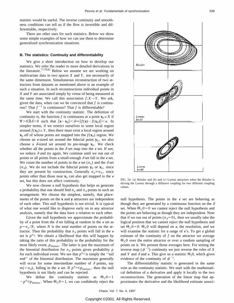
f
s
539Pecora et al.: Fundamentals of synchronization
statistic would be useful. The inverse continuity and smooth-ness conditions can tell us if the flow is invertible and dif-ferentiable, respectively.
There are other uses for such statistics. Below we showsome simple examples of how we can use them to determinegeneralized synchronization situations.
B. The statistics : Continuit y and differentiability
We give a short introduction on how to develop ourstatistics. We refer the reader to more detailed derivations inthe literature.77,78,82 Below we assume we are working onmultivariate data in two spaces X and Y, not necessarily ofthe same dimension. Simultaneous reconstruction of two at-tractors from datasets as mentioned above is an example ofsuch a situation. In such reconstructions individual points inX and Y are associated simply by virtue of being measured atthe same time. We call this association f :X→Y. We ask,given the data, when can we be convinced that f is continu-ous? That f 21 is continuous? That f is differentiable?
We start with the continuity statistic. The definition ofcontinuity is, the function f is continuous at a point x0PX if;.0'd.0 such thatix2x0i,d⇒i f (x)2 f (x0)i,e. Insimpler terms, if we restrict ourselves to some local regionaround f (x0)PY, then there must exist a local region aroundx0 all of whose points are mapped into the f (x0) region. Wechoose an e-sized set around the fiducial pointy0 , we alsochoose a d-sized set around its pre-imagex0 . We checkwhether all the points in the d set mapinto the e set. If not,we reduced and try again. We continue until we run out opoints or all points from asmall-enoughd set fall in thee set.We count the number of points in thee set (ne) and thed set(nd). We do not include the fiducial points y0 or x0 , sincethey are present by construction. Generally ne>nd , sincepoints other than those near x0 can also get mapped to the eset, but this does not affect continuity.
We now choose anull hypothesis that helps us generatea probability that one should find ne and nd points in such anarrangement. We choose the simplest, namely, that place-ments of the points on the x and y attractors are independentof each other. This null hypothesis is not trivial. It is typicalof what one would like to disprove early on in any attractoranalysis, namely that the data have arelation to each other.
Given the null hypothesis we approximate the probabil-ity of a point from the d set falling at random in thee set asp5ne /N, where N is the total number of points on the at-tractor. Then the probability that nd points wil l fall in the eset is pnd. We obtain a likelihood that this wil l happen bytaking the ratio of this probability to the probability for themost likely event, pbinmax. The latter is just the maximum ofthe binomial distribution for nd points given probability pfor each individual event. We see that pnd is simply the ‘‘tailend’’ of the binomial distribution. The maximum generallywil l occur for some intermediate number of d points, saym(,nd), falling in the e set. If pnd!pbinmax, then the nullhypothesis is not likely and can be rejected.
We define the continuity statistic as QC0512pnd/pbinmax. When QC0'1, we can confidently reject the
Chaos, Vol. 7,
Copyright ©2001. A
null hypothesis. The points in the e set are behaving athough they are generated by a continuous function on thedset. When QC0'0 we cannot reject the null hypothesis andthe points are behaving as though they are independent. Notethat if we run out of points (nd50), then we usually take thelogical position that we cannot reject the null hypothesis andset QC050. QC0 wil l depend on e, the resolution, and wewil l examine the statistic for a range of e’s. To get a globalestimate of the continuity of f on the attractor we averageQC0 over the entire attractor or over a random sampling ofpoints on it. We present those averages here. For testing theinverse map (f21) continuity we just reverse the roles of Xand Y andd ande. This give us a statisticQ I0, which givesevidence of the continuity of f21.
The differentiability statistic is generated in the samevein as the continuity statistic. We start with the mathemati-cal definition of a derivative and apply it locally to the tworeconstructions. The generation of the linear map that ap-proximates the derivative and the likelihood estimate associ-
FIG. 24. ~a! Rossler and ~b! and ~c! Lorenz attractors when the Rossler isdriving the Lorenz through a diffusive coupling for two different couplingvalues.
No. 4, 1997
ll Rights Reserved.

y.
or
m-
540 Pecora et al.: Fundamentals of synchronization
ated with it are more complex than for continuity.The definition of a derivative at a point x0 is that a linear
operator A exists such that ;e.0'd.0 for whichix2x0i,d⇒i f (x0)1A(x2x0)2 f (x)i,eix2x0i . Thismeans that there is a linear map that approximates the func-tion at nearby points with an error e in the approximationthat is proportional to the distance between those points.Note that e serves a purpose here different from continuit
The algorithm that we generate from this definition is tofirst choose an e ~error bound! and ad. Then we find all thepoints in the local d set $xi% and their y counterparts $y1%PY. We approximate the linear operator A as the leastsquares solution of the linear equations A(xi2x0)5(yi
2y0). The solution is accomplished by singular value de-composition ~SVD!.77 We check if iyi2y02A(xi2x0)i,eix2x0i . If not, we decreased and try again with fewer,but nearer points. We continue this until we have success orwe run out of points.
We choose the null hypothesis that the two sets of vec-tors $xi% and $yi% have zero correlation. We show77 that thisgenerates a likelihood that any two such sets wil l give theoperator A ‘‘b y accident’’ as e(1/2)(nd2r x)(nd2r y)r 2d, where r 2
is the usual multivariate statistical correlation between $xi%and $yi%, d5min(rx ,ry), and r x ,r y are the ranks of the x andy spaces that come out of the SVD.77 This is an asymptoticformula. The differentiability statistic QC1 is given by oneminus this likelihood. When QC1'1 we can reject the pos-sibility that the points are accidentally related by a linearoperator, a derivative. When QC1'0, we cannot reject thenull hypothesis. As before, when we shrink d so small thatno points other than x0 remain, we set QC150. Analogousto QC0, the statistic QC1 depends on e. We typically calcu-late QC1 for a range of e’s and average over the attractorover a random sampling of points on it. Similar to the con-tinuity situation we can test the differentiability of f21 byreversing X and Y and d and e roles. We call this statisticQ I1.
C. Generalize d synchronization
We examine the generalized synchronization situationwhen we have a Rossler system driving a Lorenz systemthrough a diffusive coupling with coupling constant k:
x52~y1z!, u52su1sn,
y5x1ay, n52uw1ru2n1k~y2n!,
x5b1z~x2c!, w5un2gw,
Rossler Lorenz,
~37!
where a5b50.2, c59.0, s510, r 560, andg58/3. Figure24 shows the Rossler attractor and two Lorenz attractors atk510 and k540. It appears impossible to tell what the rela-tion is between the Rossler and two Lorenz attractors. How-ever, the statistics indicate an interesting relationship.
At lower coupling (k510) there appears to be no func-tion f mapping the Ro¨ssler system into the Lorenz. Both thecontinuity statistic (QC0) and the differentiability statistic(QC1) are low, as shown in Fig. 25. But at k540 the con-
Chaos, Vol. 7,
Copyright ©2001. A
tinuity statistic approaches 1.0 even for small e sets. Thatmeans that we can be confident that the relation between theRossler and Lorenz is continuous for continuities abovee50.01, which is shown in Figs. 24~b! and 24~c!. This is asmall set. On the other hand, the differentiability statisticnever gets very high and falls off to zero rather quickly. Thisimplies that at k540 we have afunctional relation betweenthe drive and response that is C0, but not C1. It turns out thatthe response is most stable at k540 and increasing the cou-pling beyond that point wil l not improve the properties of f.This means that the fractal dimension of the entire Rossler–Lorenz attractor is larger than that of the Rossler itself.Points nearby on the Rossler are related to points nearby onthe Lorenz, but not in a smooth fashion.
C. Dynamica l interdependence
We see that to show synchronization we need to haveaccess to all the variables’ time series. Can we say anythingabout two simultaneously measured scalar time series andtheir corresponding reconstructed attractors? The answer is,yes, and it provides information that would be useful inmany experimental situations.
Our scenario is that we have an experiment in which wehave two ~or more! probes at spatially separate points pro-ducing dynamical signals that we are sampling and storing astwo, simultaneous time series. We use each to reconstruct anattractor. If the signals came from independent dynamicalsystems, we would expect generically no relationship be-tween them so that the statistics QC0 and QC1 and theirinverse versions would be low ~near zero!. However, if theycame from the same system, by Taken’s theorem each attrac-
FIG. 25. Continuity and differentiability statistics for a possible functionalrelationf: Rossler→Lorenz. The statistics were calculated for various nuber of points on the attractors ~16, 32, 64, and 128 K!. All e values arescaled to the standard deviation of the attractors.
No. 4, 1997
ll Rights Reserved.

541Pecora et al.: Fundamentals of synchronization
tor would be related by a diffeomorphism to the originalsystem’s phase space attractor. Since a relationship by dif-feomorphism is transitive ~i.e., if A is diffeomorphic to Band B is diffeomorphic to C, then A is diffeomorphic to C!.The reconstructions would be diffeomorphic. We can use ourstatistics to test for this.
We can calculate QC0, QC1, Q I0, and Q I1 for the twoattractors. If they are all near 1.0 for smalle values, we haveevidence that the two reconstructions are diffeomorphicallyrelated. Since the odds for this happening by chance to inde-pendent dynamical systems must be small, we make the con-clusion that our two time series were sampled from differentparts of the same dynamical system—we now have atest fordynamical interdependence. For example, we might samplesimultaneously the x and y components of the Lorenz sys-tem.
An interesting use of this test for dynamical interdepen-dence was done by Schiff et al. in an EEG time series.117
They showed that statistics similar to QC0 could be devel-oped in which each point would be compared to forward-time-shifted points on the other attractor. This mixes in pre-diction ~determinism! with direct, point-to-point continuityand differentiability. Their results show that dynamical inter-dependence could be seen where standard statistical tests~e.g., linear correlations! showed no relationships.
Finally, we note that these statistics would also be usefulin numerical work since we cannot always have a closedform functional relationship. In the example of the Rossler-driven Lorenz we did not have access to a function f:Rossler→Lorenz, but we could generate the time series forall variables. We could then test for evidence of functionalrelationships. Such evidence could guide rigorous attemptsto prove or disprove the existence of properties of such afunction.
1J.-C. Roux, R. H. Simoyi, and H. L. Swinney, ‘‘Observation of a strangeattractor,’’ Physica D 8, 257–266 ~1983!.
2T. Yamada and H. Fujisaka, ‘‘Stability theory of synchronized motion incoupled-oscillator systems. II,’ ’ Prog. Theor. Phys. 70, 1240 ~1983!.
3T. Yamada and H. Fujisaka, ‘‘Stability theory of synchronized motion incoupled-oscillator systems. III,’ ’ Prog. Theor. Phys. 72, 885 ~1984!.
4V. S. Afraimovich, N. N. Verichev, and M. I. Rabinovich, ‘‘Stochasticsynchronization of oscillations in dissipative systems,’’ Inv. VUZ Ra-siofiz. RPQAEC 29, 795–803 ~1986!.
5T. L. Carroll and L. M. Pecora, ‘‘Synchronizing chaotic circuits,’’ IEEETrans. CAS 38, 453 ~1991!.
6T. L. Carroll and L. M. Pecora, ‘‘Cascading synchronized chaotic sys-tems,’’ Physica D 67, 126–140 ~1993!.
7T. L. Carroll and L. M. Pecora, ‘‘Synchronizing nonautonomous chaoticcircuits,’’ IEEE Trans. Circuits Syst. 40, 646 ~1995!.
8L. M. Pecora and T. L. Carroll, ‘‘Synchronization in chaotic systems,’’Phys. Rev. Lett. 64, 821 ~1990!.
9L. M. Pecora and T. L. Carroll, ‘‘Drivin g systems with chaotic signals,’’Phys. Rev. A 44, 2374 ~1991!.
10J. F. Heagy, T. L. Carroll, and L. M. Pecora, ‘‘Synchronous chaos incoupled oscillator systems,’’ Phys. Rev. E 50, 1874 ~1994!.
11C. Tresser, P. A. Worfolk, and H. Bass, ‘‘Master-slave synchronizationfrom the point of view of global dynamics,’’ Chaos 5, 693 ~1995!.
12L. M. Pecora and T. L. Carroll, ‘‘Pseudoperiodic driving: Eliminatingmultiple domains of attraction using chaos,’’ Phys. Rev. Lett. 67, 945~1991!.
13L. Pecora and T. Carroll, ‘‘Synchronized chaotic signals and systems,’’SPIE 1992 Proceedings, San Diego CA ~SPIE—The International Society
Chaos, Vol. 7,
Copyright ©2001. A
for Optical Engineering, Bellingham, WA, 1992!, Vol. 1771, p. 389.14E. N. Lorenz, ‘‘Th e local structure of a chaotic attractor in pour dimen-
sions,’’ Physica D 13, 90 ~1984!.15N. F. Rul’kov, A. R. Volkovskii, A. Rodriguez-Lozano et al., ‘‘Mutual
synchronization of chaotic self-oscillators with dissipative coupling,’’ Int.J. Bifurcation Chaos Appl. Sci. Eng. 2, 669–676 ~1992!.
16M. Rabinovich ~private communication!.17V. S. Anishchenko, T. E. Vadivasova, D. E. Posnov et al., ‘‘Forced and
mutual synchronization of chaos,’’ Sov. J. Commun. Technol. Electron.36, 23 ~1991!.
18M. Ding and E. Ott, ‘‘Enhancing synchronism of chaotic systems,’’ Phys.Rev. E 49, R945 ~1994!.
19K. Pyragas, ‘‘Predictable chaos in slightly perturbed unpredictable chaoticsystems,’’ Phys. Lett. A 181, 203 ~1993!.
20C. W. Wu and L. O. Chua, ‘‘ A unified framework for synchronization andcontrol of dynamical systems,’’ Int. J. Bifurcations Chaos 4, 979 ~1994!.
21J. F. Heagy, L. M. Pecora, and T. L. Carroll, ‘‘Short wavelength bifurca-tions and size instabilities in coupled oscillator systems,’’ Phys. Rev. Lett.74, 4185 ~1994!.
22J. F. Heagy, T. L. Carroll, and L. M. Pecora, ‘‘Experimental and numeri-cal evidence for riddled basins in coupled chaotic oscillators,’’ Phys. Rev.Lett. 73, 3528 ~1995!.
23K. Ogata, Control Engineering ~Prentice–Hall, Englewood Cliffs, NJ,1990!.
24R. W. Newcomb and N. El-Leithy, ‘‘Chaos generation using binary hys-teresis,’’ Circuits Syst. Signal Process. 5, 321 ~1986!.
25A. Tamasevicius, G. Mykolaitis, A. Cenys et al., ‘‘Synchronization of 4Dhyperchaotic oscillators,’’ Electron. Lett. 32, 1536–1537 ~1996!.
26T. Carroll, ‘‘ A simple circuit for demonstrating regular and synchronizedchaos,’’ Am. J. Phys. 63, 377 ~1995!.
27K. Cuomo and A. V. Oppenheim, ‘‘Circui t implementation of synchro-nized chaos with applications to communications,’’ Phys. Rev. Lett. 71,65 ~1993!.
28K. M. Cuomo, A. V. Oppenheim, and S. H. Strogatz, ‘‘Synchronization ofLorenz-based chaotic circuits with applications to communications,’’IEEE Trans. Circuits Syst. 40, 626–633 ~1993!.
29Lj . Kocarev, K. S. Halle, K. Eckert et al., ‘‘Experimental demonstrationof secure communications via chaotic synchronization,’’ Int. J. Bifurca-tions Chaos 2, 709–713 ~1992!.
30K. Murali and M. Lakshmanan, ‘‘Transmission of signals by synchroni-zation in a chaotic Van der Pol–Duffing oscillator,’’ Phys. Rev. E 48,R1624 ~1993!.
31U. Parlitz, L. O. Chua, L. Kocarev et al., ‘‘Transmission of digital signalsby chaotic synchronization,’’ Int. J. Bifurcations Chaos 2, 973–977~1992!.
32R. H. Sherman and J. Gullicksen, ‘‘Chaotic communications in the pres-ence of noise,’’ SPIE Conference on Chaos in Communications Proceed-ings ~SPIE, Bellingham, WA, 1993!, Vol. 2038, pp. 141–152.
33G. Perez and H. A. Cerderia, ‘‘Extracting messages masked by chaos,’’Phys. Rev. Lett. 74, 1970 ~1995!.
34K. M. Short, ‘‘Steps toward unmasking secure communications,’’ Int. J.Bifurcations Chaos 4, 959 ~1994!.
35A. H. MacDonals and M. Plischke, ‘‘Study of the driven damped pendu-lum: Application to Josephson Junctions and charge-density-wave sys-tems,’’ Phys. Rev. B 27, 201 ~1983!.
36E. Brauer, S. Blochwitz, and H. Beige, ‘‘Periodic windows inside chaos—Experiment versus theory,’’ Int. J. Bifurcation Chaos 4, 1031–1039~1993!.
37S. Tankara, T. Matsumoto, and L. O. Chua, ‘‘Bifurcation scenario in adriven R-L-diode circuit,’’ Physica D 28, 317–344 ~1987!.
38C. Grebogi, E. Ott, and J. A. Yorke, ‘‘Attractors on an n-torus: Quasip-eriodicity versus chaos,’’ Physica D 15, 354–373 ~1985!.
39D. D’Humieres, M. R. Beasley, B. A. Huberman et al., ‘‘Chaotic statesand routes to chaos in the forced pendulum,’’ Phys. Rev. A 26, 3483~1982!.
40J. Guemez, M. A. Matas et al., ‘‘Modifie d method for synchronizing andcascading chaotic systems,’’ Phys. Rev. E 52, 2145 ~1995!.
41R. E. Amritkar and Neelima Gupte, ‘‘Synchronization of chaotic orbits:The effect of a finite time step,’’ Phys. Rev. E 47, 3889 ~1993!.
42T. Stojanovski, L. Kocarev, and U. Parlitz, ‘‘Drivin g and synchronizingby chaotic impulses,’’ Phys. Rev. E 54, 2128–2131 ~1996!.
No. 4, 1997
ll Rights Reserved.
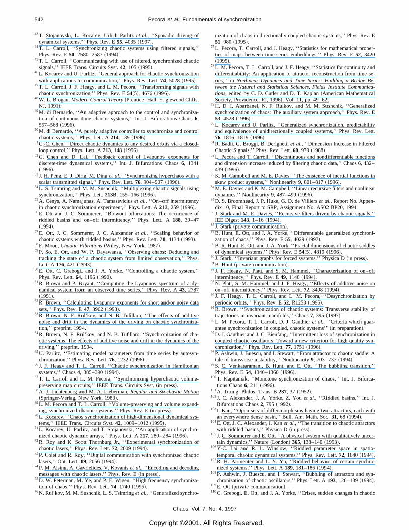
542 Pecora et al.: Fundamentals of synchronization
43T. Stojanovski, L. Kocarev, Urlich Parlitz et al., ‘‘Sporadic driving ofdynamical systems,’’ Phys. Rev. E 55, 4035 ~1997!.
44T. L. Carroll, ‘‘Synchronizing chaotic systems using filtered signals,’’Phys. Rev. E 50, 2580–2587 ~1994!.
45T. L. Carroll, ‘‘Communicating with use of filtered, synchronized chaoticsignals,’’ IEEE Trans. Circuits Syst. 42, 105 ~1995!.
46L. Kocarev and U. Parlitz, ‘‘General approach for chaotic synchronizationwith applications to communication,’’ Phys. Rev. Lett. 74, 5028 ~1995!.
47T. L. Carroll, J. F. Heagy, and L. M. Pecora, ‘‘Transforming signals withchaotic synchronization,’’ Phys. Rev. E 54~5!, 4676 ~1996!.
48W. L. Brogan, Modern Control Theory ~Prentice–Hall, Englewood Cliffs,NJ, 1991!.
49M. di Bernardo, ‘‘A n adaptive approach to the control and synchroniza-tion of continuous-time chaotic systems,’’ Int. J. Bifurcations Chaos 6,557–568 ~1996!.
50M. di Bernardo, ‘‘ A purely adaptive controller to synchronize and controlchaotic systems,’’ Phys. Lett. A 214, 139 ~1996!.
51C.-C. Chen, ‘‘Direct chaotic dynamics to any desired orbits via aclosed-loop control,’’ Phys. Lett. A 213, 148 ~1996!.
52G. Chen and D. Lai, ‘‘Feedback control of Lyapunov exponents fordiscrete-time dynamical systems,’’ Int. J. Bifurcations Chaos 6, 1341~1996!.
53J. H. Peng, E. J. Ding, M. Ding et al., ‘‘Synchronizing hyperchaos with ascalar transmitted signal,’’ Phys. Rev. Lett. 76, 904–907 ~1996!.
54L. S. Tsimring and M. M. Sushchik, ‘‘Multiplexin g chaotic signals usingsynchronization,’’ Phys. Lett. 213B, 155–166 ~1996!.
55A. Cenys, A. Namajunas, A. Tamasevicius et al., ‘‘O n–off intermittencyin chaotic synchronization experiment,’’ Phys. Lett. A 213, 259 ~1996!.
56E. Ott and J. C. Sommerer, ‘‘Blowout bifurcations: The occurrence ofriddled basins and on–off intermittency,’’ Phys. Lett. A 188, 39–47~1994!.
57E. Ott, J. C. Sommerer, J. C. Alexander et al., ‘‘Scaling behavior ofchaotic systems with riddled basins,’’ Phys. Rev. Lett. 71, 4134 ~1993!.
58F. Moon, Chaotic Vibrations ~Wiley, New York, 1987!.59P. So, E. Ott, and W. P. Dayawansa, ‘‘Observing chaos: Deducing and
tracking the state of a chaotic system from limited observation,’’ Phys.Lett. A 176, 421 ~1993!.
60E. Ott, C. Grebogi, and J. A. Yorke, ‘‘Controlling a chaotic system,’’Phys. Rev. Lett. 64, 1196 ~1990!.
61R. Brown and P. Bryant, ‘‘Computing the Lyapunov spectrum of a dy-namical system from an observed time series,’’ Phys. Rev. A 43, 2787~1991!.
62R. Brown, ‘‘Calculating Lyapunov exponents for short and/or noisy datasets,’’ Phys. Rev. E 47, 3962 ~1993!.
63R. Brown, N. F. Rul’kov, and N. B. Tufillaro, ‘‘Th e effects of additivenoise and drift in the dynamics of the driving on chaotic synchroniza-tion,’’ preprint, 1994.
64R. Brown, N. F. Rul’kov, and N. B. Tufillaro, ‘‘Synchronization of cha-otic systems. The effects of additive noise and drift in the dynamics of thedriving,’’ preprint, 1994.
65U. Parlitz, ‘‘Estimating model parameters from time series by autosyn-chronization,’’ Phys. Rev. Lett. 76, 1232 ~1996!.
66J. F. Heagy and T. L. Carroll, ‘‘Chaotic synchronization in Hamiltoniansystems,’’ Chaos 4, 385–390 ~1994!.
67T. L. Carroll and L. M. Pecora, ‘‘Synchronizing hyperchaotic volume-preserving map circuits,’’ IEEE Trans. Circuits Syst. ~in press!.
68A. J. Lichtenberg and M. A. Lieberman, Regular and Stochastic Motion~Springer-Verlag, New York, 1983!.
69L. M. Pecora and T. L. Carroll, ‘‘Volume-preserving and volume expand-ing, synchronized chaotic systems,’’ Phys. Rev. E ~in press!.
70L. Kocarev, ‘‘Chaos synchronization of high-dimensional dynamical sys-tems,’’ IEEE Trans. Circuits Syst. 42, 1009–1012 ~1995!.
71L. Kocarev, U. Parlitz, and T. Stojanovski, ‘‘A n application of synchro-nized chaotic dynamic arrays,’’ Phys. Lett. A 217, 280–284 ~1996!.
72R. Roy and K. Scott Thornburg Jr., ‘‘Experimental synchronization ofchaotic lasers,’’ Phys. Rev. Lett. 72, 2009 ~1994!.
73P. Colet and R. Roy, ‘‘Digita l communication with synchronized chaoticlasers,’’ Opt. Lett. 19, 2056 ~1994!.
74P. M. Alsing, A. Gavrielides, V. Kovanis et al., ‘‘Encoding and decodingmessages with chaotic lasers,’’ Phys. Rev. E ~in press!.
75D. W. Peterman, M. Ye, and P. E. Wigen, ‘‘Hig h frequency synchroniza-tion of chaos,’’ Phys. Rev. Lett. 74, 1740 ~1995!.
76N. Rul’kov, M. M. Sushchik, L. S. Tsimring et al., ‘‘Generalized synchro-
Chaos, Vol. 7,
Copyright ©2001. A
nization of chaos in directionally coupled chaotic systems,’’ Phys. Rev. E51, 980 ~1995!.
77L. Pecora, T. Carroll, and J. Heagy, ‘‘Statistics for mathematical proper-ties of maps between time-series embeddings,’’ Phys. Rev. E 52, 3420~1995!.
78L. M. Pecora, T. L. Carroll, and J. F. Heagy, ‘‘Statistics for continuity anddifferentiability: An application to attractor reconstruction from time se-ries,’’ in Nonlinear Dynamics and Time Series: Building a Bridge Be-tween the Natural and Statistical Sciences, Fields Institute Communica-tions, edited by C. D. Cutler and D. T. Kaplan ~American MathematicalSociety, Providence, RI, 1996!, Vol. 11, pp. 49–62.
79H. D. I. Abarbanel, N. F. Rulkov, and M. M. Sushchik, ‘‘Generalizedsynchronization of chaos: The auxiliary system approach,’’ Phys. Rev. E53, 4528 ~1996!.
80L. Kocarev and U. Parlitz, ‘‘Generalized synchronization, predictabilityand equivalence of unidirectionally coupled systems,’’ Phys. Rev. Lett.76, 1816–1819 ~1996!.
81R. Badii, G. Broggi, B. Derighetti et al., ‘‘Dimension Increase in FilteredChaotic Signals,’’ Phys. Rev. Lett. 60, 979 ~1988!.
82L. Pecora and T. Carroll, ‘‘Discontinuous and nondifferentiable functionsand dimension increase induced by filtering chaotic data,’’ Chaos 6, 432–439 ~1996!.
83K. M. Campbell and M. E. Davies, ‘‘Th e existence of inertial functions inskew product systems,’’ Nonlinearity 9, 801–817 ~1996!.
84M. E. Davies and K. M. Campbell, ‘‘Linear recursive filters and nonlineardynamics,’’ Nonlinearity 9, 487–499 ~1996!.
85D. S. Broomhead, J. P. Huke, G. D. de Villier s et al., Report No. Appen-dix 10, Final Report to SRP, Assignment No. AS02 BP20, 1994.
86J. Stark and M. E. Davies, ‘‘Recursive filters driven by chaotic signals,’’IEE Digest 143, 1–16 ~1994!.
87J. Stark ~private communication!.88B. Hunt, E. Ott, and J. A. Yorke, ‘‘Differentiable generalized synchroni-
zation of chaos,’’ Phys. Rev. E 55, 4029 ~1997!.89B. R. Hunt, E. Ott, and J. A. York, ‘‘Fractal dimensions of chaotic saddles
of dynamical systems,’’ Phys. Rev. E 54~5!, 4819 ~1996!.90J. Stark, ‘‘Invariant graphs for forced systems,’’ Physica D ~in press!.91B. Hunt ~private communication!.92J. F. Heagy, N. Platt, and S. M. Hammel, ‘‘Characterization of on–off
intermittency,’’ Phys. Rev. E 49, 1140 ~1994!.93N. Platt, S. M. Hammel, and J. F. Heagy, ‘‘Effects of additive noise on
on–off intermittency,’’ Phys. Rev. Lett. 72, 3498 ~1994!.94J. F. Heagy, T. L. Carroll, and L. M. Pecora, ‘‘Desynchronization by
periodic orbits,’’ Phys. Rev. E 52, R1253 ~1995!.95R. Brown, ‘‘Synchronization of chaotic systems: Transverse stability of
trajectories in invariant manifolds,’’ Chaos 7, 395 ~1997!.96L. M. Pecora, T. L. Carroll, D. J. Gauthier et al., ‘‘Criteri a which guar-
antee synchronization in coupled, chaotic systems’’ ~in preparation!.97D. J. Gauthier and J. C. Bienfang, ‘‘Intermittent loss of synchronization in
coupled chaotic oscillators: Toward a new criterion for high-quality syn-chronization,’’ Phys. Rev. Lett. 77, 1751 ~1996!.
98P. Ashwin, J. Buescu, and I. Stewart, ‘‘From attractor to chaotic saddle: Atale of transverse instability,’’ Nonlinearity 9, 703–737 ~1994!.
99S. C. Venkataramani, B. Hunt, and E. Ott, ‘‘Th e bubbling transition,’’Phys. Rev. E 54, 1346–1360 ~1996!.
100T. Kapitaniak, ‘‘Monotone synchronization of chaos,’’ Int. J. Bifurca-tions Chaos 6, 211 ~1996!.
101A. Turing, Philos. Trans. B 237, 37 ~1952!.102J. C. Alexander, J. A. Yorke, Z. You et al., ‘‘Riddled basins,’’ Int. J.
Bifurcations Chaos 2, 795 ~1992!.103I. Kan, ‘‘Open sets of diffeomorphisms having two attractors, each with
an everywhere dense basin,’’ Bull. Am. Math. Soc. 31, 68 ~1994!.104E. Ott, J. C. Alexander, I. Kan et al., ‘‘Th e transition to chaotic attractors
with riddled basins,’’ Physica D ~in press!.105J. C. Sommerer and E. Ott, ‘‘ A physical system with qualitatively uncer-
tain dynamics,’’ Nature ~London! 365, 138–140 ~1993!.106Y-C. Lai and R. L. Winslow, ‘‘Riddled parameter space in spatio-
temporal chaotic dynamical systems,’’ Phys. Rev. Lett. 72, 1640 ~1994!.107R. H. Parmenter and L. Y. Yu, ‘‘Riddled behavior of certain synchro-
nized systems,’’ Phys. Lett. A 189, 181–186 ~1994!.108P. Ashwin, J. Buescu, and I. Stewart, ‘‘Bubbling of attractors and syn-
chronization of chaotic oscillators,’’ Phys. Lett. A 193, 126–139 ~1994!.109E. Ott ~private communication!.110C. Grebogi, E. Ott, and J. A. Yorke, ‘‘Crises, sudden changes in chaotic
No. 4, 1997
ll Rights Reserved.

543Pecora et al.: Fundamentals of synchronization
attractors and transient chaos,’’ Physica D 7, 181 ~1983!.111T. L. Carroll, L. M. Pecora, and F. J. Rachford, ‘‘Chaotic transients and
multiple attractors in spin-wave experiments,’’ Phys. Rev. Lett. 59, 2891~1987!.
112S. W. McDonald, C. Grebogi, E. Ott et al., ‘‘Fractal basin boundaries,’’Physica D 17, 125 ~1985!.
113B.-S. Park, C. Grebogi, E. Ott et al., ‘‘Scaling of fractal basin boundariesnear intermittency transitions to chaos,’’ Phys. Rev. A 40, 1576 ~1989!.
114L. M. Pecora, ‘‘Synchronization conditions and desynchronizing patterns
Chaos, Vol. 7,
Copyright ©2001. A
in coupled limit-cycle and chaotic systems,’’ in preparation.115L. M. Pecora, T. L. Carroll, G. Johnson et al., ‘‘Master stability function
for synchronized coupled systems,’’ in preparation.116T. Sauer and J. A. Yorke, ‘‘Ar e the dimensions of a set and its image
equal under typical smooth functions?,’’ Ergodic Theory Dyn. Syst. ~inpress!.
117S. Schiff, P. So, T. Chang et al., ‘‘Detecting dynamical interdependenceand generalized synchrony through mutual prediction in a neural en-semble,’’ Phys. Rev. E 54, 6708–6724 ~1996!.
No. 4, 1997
ll Rights Reserved.