


Fundamentals of matrix analysis with applications
409
www.ebook3000.com
-
Upload
khangminh22 -
Category
Documents
-
view
4 -
download
0
Transcript of Fundamentals of matrix analysis with applications


FUNDAMENTALS OFMATRIX ANALYSISWITH APPLICATIONS
EDWARD BARRY SAFFDepartment of MathematicsCenter for Constructive ApproximationVanderbilt UniversityNashville, TN, USA
ARTHUR DAVID SNIDERDepartment of Electrical EngineeringUniversity of South FloridaTampa, FL, USA
www.ebook3000.com
Copyright © 2016 by John Wiley & Sons, Inc. All rights reserved
Published by John Wiley & Sons, Inc., Hoboken, New JerseyPublished simultaneously in Canada
No part of this publication may be reproduced, stored in a retrieval system, or transmitted in any form or by anymeans, electronic, mechanical, photocopying, recording, scanning, or otherwise, except as permitted underSection 107 or 108 of the 1976 United States Copyright Act, without either the prior written permission of thePublisher, or authorization through payment of the appropriate per-copy fee to the Copyright Clearance Center,Inc., 222 Rosewood Drive, Danvers, MA 01923, (978) 750-8400, fax (978) 750-4470, or on the web atwww.copyright.com. Requests to the Publisher for permission should be addressed to the PermissionsDepartment, John Wiley & Sons, Inc., 111 River Street, Hoboken, NJ 07030, (201) 748-6011, fax (201)748-6008, or online at http://www.wiley.com/go/permissions.
Limit of Liability/Disclaimer of Warranty: While the publisher and author have used their best efforts inpreparing this book, they make no representations or warranties with respect to the accuracy or completeness ofthe contents of this book and specifically disclaim any implied warranties of merchantability or fitness for aparticular purpose. No warranty may be created or extended by sales representatives or written sales materials.The advice and strategies contained herein may not be suitable for your situation. You should consult with aprofessional where appropriate. Neither the publisher nor author shall be liable for any loss of profit or any othercommercial damages, including but not limited to special, incidental, consequential, or other damages.
For general information on our other products and services or for technical support, please contact our CustomerCare Department within the United States at (800) 762-2974, outside the United States at (317) 572-3993 or fax(317) 572-4002.
Wiley also publishes its books in a variety of electronic formats. Some content that appears in print may not beavailable in electronic formats. For more information about Wiley products, visit our web site at www.wiley.com.
Library of Congress Cataloging-in-Publication Data:
Saff, E. B., 1944–Fundamentals of matrix analysis with applications / Edward Barry Saff, Center for Constructive Approximation,Vanderbilt University, Nashville, Tennessee, Arthur David Snider, Department of Electrical Engineering,University of South Florida, Tampa, Florida.
pages cmIncludes bibliographical references and index.ISBN 978-1-118-95365-5 (cloth)
1. Matrices. 2. Algebras, Linear. 3. Orthogonalization methods. 4. Eigenvalues.I. Snider, Arthur David, 1940– II. Title.
QA188.S194 2015512.9′434–dc23
2015016670
Printed in the United States of America
10 9 8 7 6 5 4 3 2 1
1 2015

To our brothers Harvey J. Saff, Donald J. Saff, and Arthur Herndon Snider. They haveset a high bar for us, inspired us to achieve, and extended helping hands when weneeded them to reach for those greater heights.
Edward Barry SaffArthur David Snider
www.ebook3000.com
CONTENTS
PREFACE ix
PART I INTRODUCTION: THREE EXAMPLES 1
1 Systems of Linear Algebraic Equations 5
1.1 Linear Algebraic Equations, 51.2 Matrix Representation of Linear Systems and the Gauss-Jordan
Algorithm, 171.3 The Complete Gauss Elimination Algorithm, 271.4 Echelon Form and Rank, 381.5 Computational Considerations, 461.6 Summary, 55
2 Matrix Algebra 58
2.1 Matrix Multiplication, 582.2 Some Physical Applications of Matrix Operators, 692.3 The Inverse and the Transpose, 762.4 Determinants, 862.5 Three Important Determinant Rules, 1002.6 Summary, 111Group Projects for Part IA. LU Factorization, 116B. Two-Point Boundary Value Problem, 118C. Electrostatic Voltage, 119
CONTENTS vii
D. Kirchhoff’s Laws, 120E. Global Positioning Systems, 122F. Fixed-Point Methods, 123
PART II INTRODUCTION: THE STRUCTURE OF GENERALSOLUTIONS TO LINEAR ALGEBRAIC EQUATIONS 129
3 Vector Spaces 133
3.1 General Spaces, Subspaces, and Spans, 1333.2 Linear Dependence, 1423.3 Bases, Dimension, and Rank, 1513.4 Summary, 164
4 Orthogonality 165
4.1 Orthogonal Vectors and the Gram–Schmidt Algorithm, 1654.2 Orthogonal Matrices, 1744.3 Least Squares, 1804.4 Function Spaces, 1904.5 Summary, 197Group Projects for Part IIA. Rotations and Reflections, 201B. Householder Reflectors, 201C. Infinite Dimensional Matrices, 202
PART III INTRODUCTION: REFLECT ON THIS 205
5 Eigenvectors and Eigenvalues 209
5.1 Eigenvector Basics, 2095.2 Calculating Eigenvalues and Eigenvectors, 2175.3 Symmetric and Hermitian Matrices, 2255.4 Summary, 232
6 Similarity 233
6.1 Similarity Transformations and Diagonalizability, 2336.2 Principle Axes and Normal Modes, 2446.3 Schur Decomposition and Its Implications, 2576.4 The Singular Value Decomposition, 2646.5 The Power Method and the QR Algorithm, 2826.6 Summary, 290
www.ebook3000.com
viii CONTENTS
7 Linear Systems of Differential Equations 293
7.1 First-Order Linear Systems, 2937.2 The Matrix Exponential Function, 3067.3 The Jordan Normal Form, 3167.4 Matrix Exponentiation via Generalized Eigenvectors, 3337.5 Summary, 339Group Projects for Part IIIA. Positive Definite Matrices, 342B. Hessenberg Form, 343C. Discrete Fourier Transform, 344D. Construction of the SVD, 346E. Total Least Squares, 348F. Fibonacci Numbers, 350
ANSWERS TO ODD NUMBERED EXERCISES 351
INDEX 393
PREFACE
Our goal in writing this book is to describe matrix theory from a geometric, physicalpoint of view. The beauty of matrices is that they can express so many things ina compact, suggestive vernacular. The drudgery of matrices lies in the meticulouscomputation of the entries. We think matrices are beautiful.
So we try to describe each matrix operation pictorially, and squeeze as much infor-mation out of this picture as we can before we turn it over to the computer for numbercrunching.
Of course we want to be the computer’s master, not its vassal; we want to knowwhat the computer is doing. So we have interspersed our narrative with glimpses of thecomputational issues that lurk behind the symbology.
Part I. The initial hurdle that a matrix textbook author has to face is the exposition ofGauss elimination. Some readers will be seeing this for the first time, and it is of primeimportance to spell out all the details of the algorithm. But students who have acquiredfamiliarity with the basics of solving systems of equations in high school need to bestimulated occasionally to keep them awake during this tedious (in their eyes) review.In Part I, we try to pique the interests of the latter by inserting tidbits of informationthat would not have occurred to them, such as operation counts and computer timing,pivoting, complex coefficients, parametrized solution descriptions of underdeterminedsystems, and the logical pitfalls that can arise when one fails to adhere strictly to Gauss’sinstructions.
The introduction of matrix formulations is heralded both as a notational shorthandand as a quantifier of physical operations such as rotations, projections, reflections,and Gauss’s row reductions. Inverses are studied first in this operator context beforeaddressing them computationally. The determinant is cast in its proper light as animportant concept in theory, but a cumbersome practical tool.
www.ebook3000.com
x PREFACE
Readers are guided to explore projects involving LU factorizations, the matrixaspects of finite difference modeling, Kirchhoff’s circuit laws, GPS systems, and fixedpoint methods.
Part II. We show how the vector space concepts supply an orderly organizationalstructure for the capabilities acquired in Part I. The many facets of orthogonality arestressed. To maintain computational perspective, a bit of attention is directed to thenumerical issues of rank fragility and error control through norm preservation. Projectsinclude rotational kinematics, Householder implementation of QR factorizations, andthe infinite dimensional matrices arising in Haar wavelet formulations.
Part III. We devote a lot of print to physical visualizations of eigenvectors—formirror reflections, rotations, row reductions, circulant matrices—before turning to thetedious issue of their calculation via the characteristic polynomial. Similarity transfor-mations are viewed as alternative interpretations of a matrix operator; the associatedtheorems address its basis-free descriptors. Diagonalization is heralded as a holy grail,facilitating scads of algebraic manipulations such as inversion, root extraction, andpower series evaluation. A physical experiment illustrating the stability/instability ofprincipal axis rotations is employed to stimulate insight into quadratic forms.
Schur decomposition, though ponderous, provides a valuable instrument for under-standing the orthogonal diagonalizability of normal matrices, as well as the Cayley–Hamilton theorem.
Thanks to invaluable input from our colleague Michael Lachance, Part III also pro-vides a transparent exposition of the properties and applications of the singular valuedecomposition, including rank reduction and the pseudoinverse.
The practical futility of eigenvector calculation through the characteristic polyno-mial is outlined in a section devoted to a bird’s-eye perspective of the QR algorithm.The role of luck in its implementation, as well as in the occurrence of defective matrices,is addressed.
Finally, we describe the role of matrices in the solution of linear systems of differen-tial equations with constant coefficients, via the matrix exponential. It can be masteredbefore the reader has taken a course in differential equations, thanks to the analogywith the simple equation of radioactive decay. We delineate the properties of the matrixexponential and briefly survey the issues involved in its computation.
The interesting question here (in theory, at least) is the exponential of a defec-tive matrix. Although we direct readers elsewhere for a rigorous proof of the Jordandecomposition theorem, we work out the format of the resulting exponential. Manyauthors ignore, mislead, or confuse their readers in the calculation of the generalizedeigenvector Jordan chains of a defective matrix, and we describe a straightforward andfoolproof procedure for this task. The alternative calculation of the matrix exponential,based on the primary decomposition theorem and forgoing the Jordan chains, is alsopresented.

PREFACE xi
Group projects for Part III address positive definite matrices, Hessenberg forms, thediscrete Fourier transform, and advanced aspects of the singular value decomposition.
Each part includes summaries, review problems, and technical writing exercises.
EDWARD BARRY SAFF ARTHUR DAVID SNIDERVanderbilt University University of South [email protected] [email protected]
www.ebook3000.com

PART I
INTRODUCTION: THREE EXAMPLES
Antarctic explorers face a problem that the rest of us wish we had. They need to con-sume lots of calories to keep their bodies warm. To ensure sufficient caloric intakeduring an upcoming 10-week expedition, a dietician wants her team to consume2300 ounces of milk chocolate and 1100 ounces of almonds. Her outfitter can sup-ply her with chocolate almond bars, each containing 1 ounce of milk chocolate and0.4 ounces of almonds, for $1.50 apiece, and he can supply bags of chocolate-coveredalmonds, each containing 2.75 ounces of chocolate and 2 ounces of almonds, for $3.75each. (For convenience, assume that she can purchase either item in fractional quanti-ties.) How many chocolate bars and covered almonds should she buy to meet the dietaryrequirements? How much does it cost?
If the dietician orders x1 chocolate bars and x2 covered almonds, she has 1x1 + 2.75x2
ounces of chocolate, and she requires 2300 ounces, so
1x1 + 2.75x2 = 2300. (1)
Similarly, the almond requirement is
0.4x1 + 2x2 = 1100. (2)
You’re familiar with several methods of solving simultaneous equations like (1) and(2): graphing them, substituting one into another, possibly even using determinants.You can calculate the solution to be x1 = 1750 bars of chocolate and x2 = 200 bags ofalmonds at a cost of $1.50x1 + $3.75x2 = $3375.00.
Fundamentals of Matrix Analysis with Applications,First Edition. Edward Barry Saff and Arthur David Snider.© 2016 John Wiley & Sons, Inc. Published 2016 by John Wiley & Sons, Inc.
www.ebook3000.com
2 PART I INTRODUCTION: THREE EXAMPLES
But did you see that for $238.63 less, she can meet or exceed the caloric requirementsby purchasing 836.36. . . bags of almonds and no chocolate bars? We’ll explore this inProblem 20, Exercises 1.3. Simultaneous equations, and the linear algebra they spawn,contain a richness that will occupy us for the entire book.
Another surprising illustration of the variety of phenomena that can occur arises inthe study of differential equations.
Two differentiations of the function cos t merely result in a change of sign; in otherwords, x(t) = cos t solves the second-order differential equation x′′ = −x. Anothersolution is sin t, and it is easily verified that every combination of the form
x(t) = c1 cos t + c2 sin t,
where c1 and c2 are arbitrary constants, is a solution. Find values of the constants (ifpossible) so that x(t) meets the following specifications:
x(0) = x(π/2) = 4; (3)
x(0) = x(π) = 4; (4)
x(0) = 4; x(π) = −4. (5)
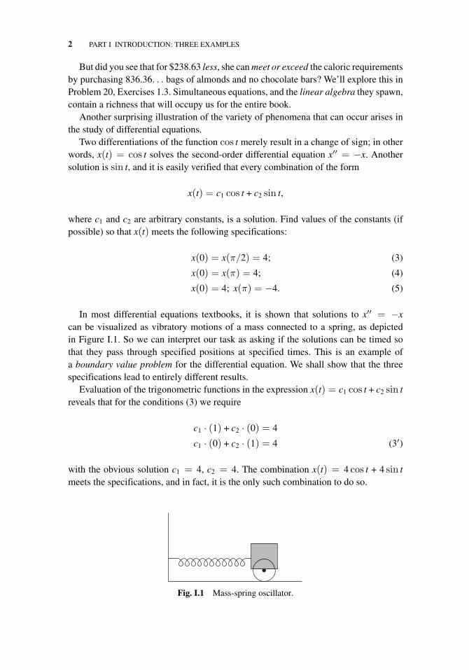
In most differential equations textbooks, it is shown that solutions to x′′ = −xcan be visualized as vibratory motions of a mass connected to a spring, as depictedin Figure I.1. So we can interpret our task as asking if the solutions can be timed sothat they pass through specified positions at specified times. This is an example ofa boundary value problem for the differential equation. We shall show that the threespecifications lead to entirely different results.
Evaluation of the trigonometric functions in the expression x(t) = c1 cos t + c2 sin treveals that for the conditions (3) we require
c1 · (1) + c2 · (0) = 4
c1 · (0) + c2 · (1) = 4 (3′)
with the obvious solution c1 = 4, c2 = 4. The combination x(t) = 4 cos t + 4 sin tmeets the specifications, and in fact, it is the only such combination to do so.
Fig. I.1 Mass-spring oscillator.
PART I INTRODUCTION: THREE EXAMPLES 3
Conditions (4) require that
c1 · (1) + c2 · (0) = 4,
c1 · (−1) + c2 · (0) = 4, (4′)
demanding that c1 be equal both to 4 and to −4. The specifications are incompatible,so no solution x(t) can satisfy (4).
The requirements of system (5) are
c1 · (1) + c2 · (0) = 4,
c1 · (−1) + c2 · (0) = −4. (5′)
Both equations demand that c1 equals 4, but no restrictions at all are placed on c2. Thusthere are infinite number of solutions of the form
x(t) = 4 cos t + c2 sin t.
Requirements (1, 2) and (3′, 4′, 5′) are examples of systems of linear algebraicequations, and although these particular cases are quite trivial to analyze, they demon-strate the varieties of solution categories that are possible. We can gain some perspectiveof the complexity of this topic by looking at another application governed by a linearsystem, namely, Computerized Axial Tomography (CAT).
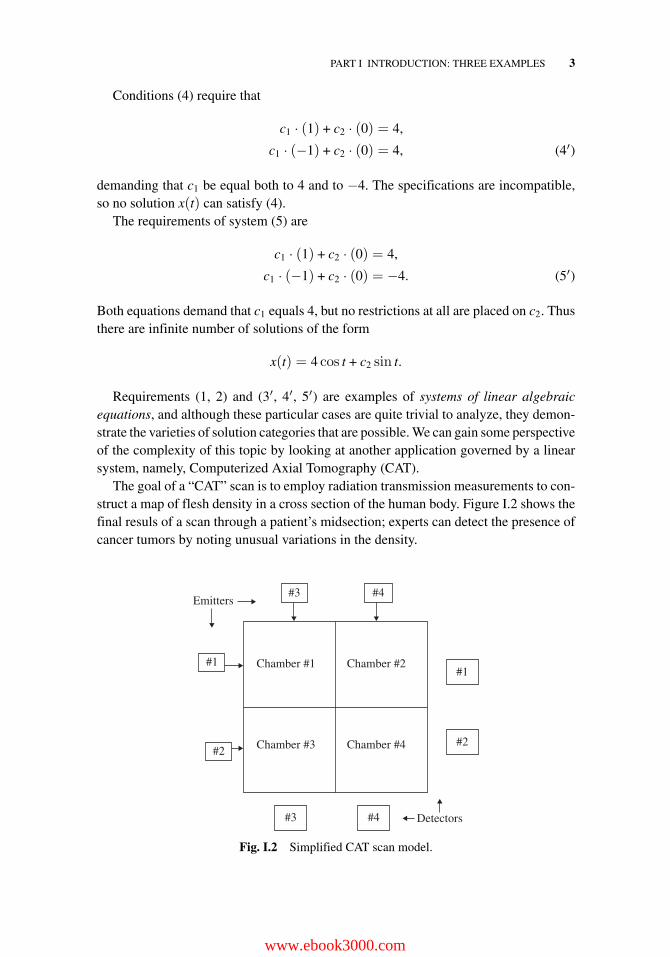
The goal of a “CAT” scan is to employ radiation transmission measurements to con-struct a map of flesh density in a cross section of the human body. Figure I.2 shows thefinal resuls of a scan through a patient’s midsection; experts can detect the presence ofcancer tumors by noting unusual variations in the density.
Emitters
Chamber #1#1#1
#2#2
#3 #4
#3 #4
Chamber #3 Chamber #4
Detectors
Chamber #2
Fig. I.2 Simplified CAT scan model.
www.ebook3000.com
4 PART I INTRODUCTION: THREE EXAMPLES
A simplified version of the technology is illustrated in Figure I.2. The stomach ismodeled very crudely as an assemblage of four chambers, each with its own density.(An effective three-dimensional model for detection of tiny tumors would require mil-lions of chambers.) A fixed dose of radiation is applied at each of the four indicatedemitter locations in turn, and the amounts of radiation measured at the four detectors arerecorded. We want to deduce, from this data, the flesh densities of the four subsections.
Now each chamber transmits a fraction ri of the radiation that strikes it. Thus if a unitdose of radiation is discharged by emitter #1, a fraction r1 of it is transmitted throughchamber #1 to chamber #2, and a fraction r2 of that is subsequently transmitted todetector #1. From biochemistry we can determine the flesh densities if we can find thetransmission coefficients ri.
So if, say, detector #1 measures a radiation intensity of 50%, and detectors #2, #3,and #4 measure intensities of 60%, 70%, and 55% respectively, then the followingequations hold:
r1r2 = 0.50; r3r4 = 0.60; r1r3 = 0.70; r2r4 = 0.55.
By taking logarithms of both sides of these equations and setting xi = ln ri, we find
x1 + x2 = ln 0.50
x3 + x4 = ln 0.60
x1 + x3 = ln 0.70
x2 + x4 = ln 0.55, (6)
which is a system of linear algebraic equations similar to (1, 2) and (3′, 4′, 5′). But theefficient solution of (6) is much more daunting—awesome, in fact, when one considersthat a realistic model comprises over 106 equations, and that it may possess no solutions,an infinity of solutions, or one unique solution.
In the first few chapters of this book, we will see how the basic tool of lin-ear algebra—namely, the matrix–can be used to provide an efficient and systematicalgorithm for analyzing and solving such systems. Indeed, matrices are employed in vir-tually every academic discipline to formulate and analyze questions of a quantitativenature. Furthermore, in Chapter Seven, we will study how linear algebra also facili-tates the description of the underlying structure of the solutions of linear differentialequations.
1SYSTEMS OF LINEARALGEBRAIC EQUATIONS
1.1 LINEAR ALGEBRAIC EQUATIONS
Systems of equations such as (1)–(2), (3′), (4′), (5′), and (6) given in the “Introduc-tion to Part I” are instances of a mathematical structure that pervades practically everyapplication of mathematics.
Systems of Linear Equations
Definition 1. An equation that can be put in the form
a1x1 + a2x2 + · · · + anxn = b,
where the coefficients ai and the right-hand side b are constants, is called a lin-ear algebraic equation in the variables x1, x2, . . . , xn. If m linear equations, eachhaving n variables, are all to be satisfied by the same set of values for the vari-ables, then the m equations constitute a system of linear algebraic equations (orsimply a linear system):
a11x1 + a12x2 + · · · + a1nxn = b1
a21x1 + a22x2 + · · · + a2nxn = b2
...
am1x1 + am2x2 + · · · + amnxn = bm (1)
Fundamentals of Matrix Analysis with Applications,First Edition. Edward Barry Saff and Arthur David Snider.© 2016 John Wiley & Sons, Inc. Published 2016 by John Wiley & Sons, Inc.
www.ebook3000.com
6 SYSTEMS OF LINEAR ALGEBRAIC EQUATIONS
One solution
One solution
No solutions
No solutions
Infinity of solutions
Infinity of solutions
(a) (b) (c)
(d) (e) (f)
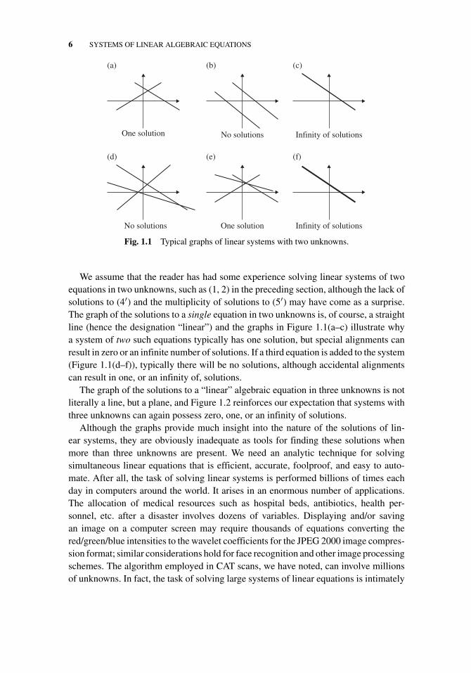
Fig. 1.1 Typical graphs of linear systems with two unknowns.
We assume that the reader has had some experience solving linear systems of twoequations in two unknowns, such as (1, 2) in the preceding section, although the lack ofsolutions to (4′) and the multiplicity of solutions to (5′) may have come as a surprise.The graph of the solutions to a single equation in two unknowns is, of course, a straightline (hence the designation “linear”) and the graphs in Figure 1.1(a–c) illustrate whya system of two such equations typically has one solution, but special alignments canresult in zero or an infinite number of solutions. If a third equation is added to the system(Figure 1.1(d–f)), typically there will be no solutions, although accidental alignmentscan result in one, or an infinity of, solutions.
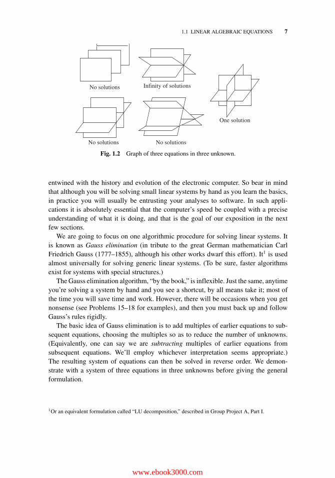
The graph of the solutions to a “linear” algebraic equation in three unknowns is notliterally a line, but a plane, and Figure 1.2 reinforces our expectation that systems withthree unknowns can again possess zero, one, or an infinity of solutions.
Although the graphs provide much insight into the nature of the solutions of lin-ear systems, they are obviously inadequate as tools for finding these solutions whenmore than three unknowns are present. We need an analytic technique for solvingsimultaneous linear equations that is efficient, accurate, foolproof, and easy to auto-mate. After all, the task of solving linear systems is performed billions of times eachday in computers around the world. It arises in an enormous number of applications.The allocation of medical resources such as hospital beds, antibiotics, health per-sonnel, etc. after a disaster involves dozens of variables. Displaying and/or savingan image on a computer screen may require thousands of equations converting thered/green/blue intensities to the wavelet coefficients for the JPEG 2000 image compres-sion format; similar considerations hold for face recognition and other image processingschemes. The algorithm employed in CAT scans, we have noted, can involve millionsof unknowns. In fact, the task of solving large systems of linear equations is intimately
1.1 LINEAR ALGEBRAIC EQUATIONS 7
No solutions
No solutions No solutions
One solution
Infinity of solutions
Fig. 1.2 Graph of three equations in three unknown.
entwined with the history and evolution of the electronic computer. So bear in mindthat although you will be solving small linear systems by hand as you learn the basics,in practice you will usually be entrusting your analyses to software. In such appli-cations it is absolutely essential that the computer’s speed be coupled with a preciseunderstanding of what it is doing, and that is the goal of our exposition in the nextfew sections.
We are going to focus on one algorithmic procedure for solving linear systems. Itis known as Gauss elimination (in tribute to the great German mathematician CarlFriedrich Gauss (1777–1855), although his other works dwarf this effort). It1 is usedalmost universally for solving generic linear systems. (To be sure, faster algorithmsexist for systems with special structures.)
The Gauss elimination algorithm, “by the book,” is inflexible. Just the same, anytimeyou’re solving a system by hand and you see a shortcut, by all means take it; most ofthe time you will save time and work. However, there will be occasions when you getnonsense (see Problems 15–18 for examples), and then you must back up and followGauss’s rules rigidly.
The basic idea of Gauss elimination is to add multiples of earlier equations to sub-sequent equations, choosing the multiples so as to reduce the number of unknowns.(Equivalently, one can say we are subtracting multiples of earlier equations fromsubsequent equations. We’ll employ whichever interpretation seems appropriate.)The resulting system of equations can then be solved in reverse order. We demon-strate with a system of three equations in three unknowns before giving the generalformulation.
1Or an equivalent formulation called “LU decomposition,” described in Group Project A, Part I.
www.ebook3000.com
8 SYSTEMS OF LINEAR ALGEBRAIC EQUATIONS
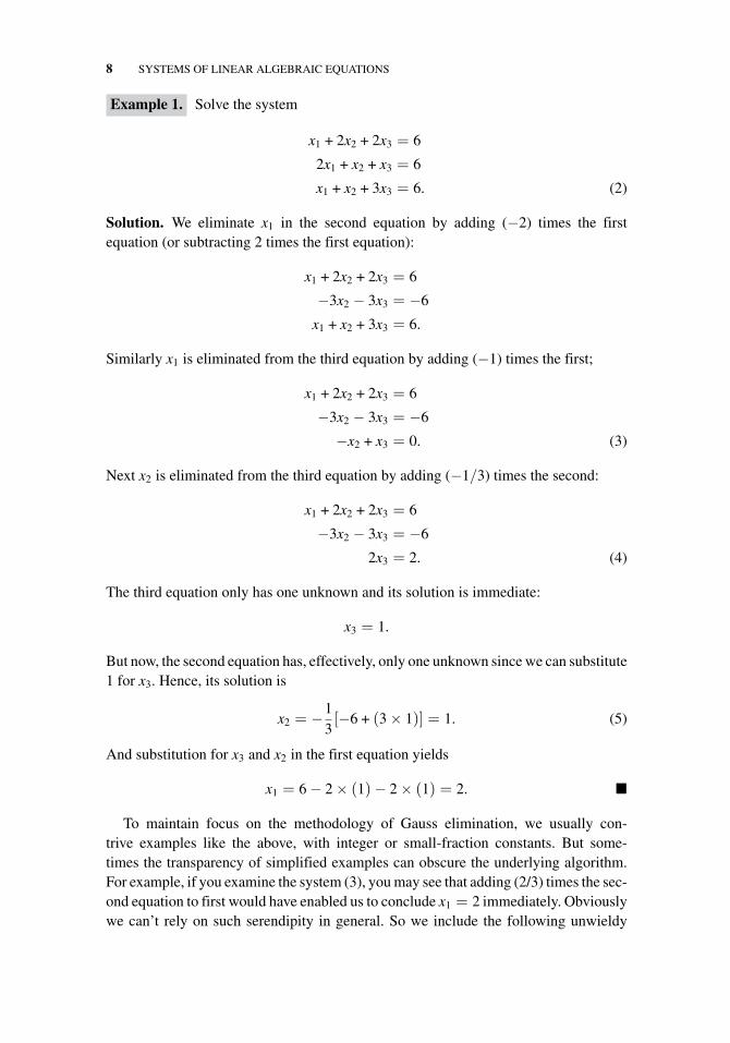
Example 1. Solve the system
x1 + 2x2 + 2x3 = 6
2x1 + x2 + x3 = 6
x1 + x2 + 3x3 = 6. (2)
Solution. We eliminate x1 in the second equation by adding (−2) times the firstequation (or subtracting 2 times the first equation):
x1 + 2x2 + 2x3 = 6
−3x2 − 3x3 = −6
x1 + x2 + 3x3 = 6.
Similarly x1 is eliminated from the third equation by adding (−1) times the first;
x1 + 2x2 + 2x3 = 6
−3x2 − 3x3 = −6
−x2 + x3 = 0. (3)
Next x2 is eliminated from the third equation by adding (−1/3) times the second:
x1 + 2x2 + 2x3 = 6
−3x2 − 3x3 = −6
2x3 = 2. (4)
The third equation only has one unknown and its solution is immediate:
x3 = 1.
But now, the second equation has, effectively, only one unknown since we can substitute1 for x3. Hence, its solution is
x2 = −13[−6 + (3 × 1)] = 1. (5)
And substitution for x3 and x2 in the first equation yields
x1 = 6 − 2 × (1)− 2 × (1) = 2. �
To maintain focus on the methodology of Gauss elimination, we usually con-trive examples like the above, with integer or small-fraction constants. But some-times the transparency of simplified examples can obscure the underlying algorithm.For example, if you examine the system (3), you may see that adding (2/3) times the sec-ond equation to first would have enabled us to conclude x1 = 2 immediately. Obviouslywe can’t rely on such serendipity in general. So we include the following unwieldy
1.1 LINEAR ALGEBRAIC EQUATIONS 9
example to focus your attention on the regimented steps of Gauss elimination. Don’tbother to follow the details of the arithmetic; just note the general procedure.
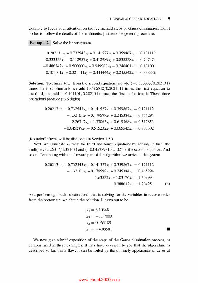
Example 2. Solve the linear system
0.202131x1 + 0.732543x2 + 0.141527x3 + 0.359867x4 = 0.171112
0.333333x1 − 0.112987x2 + 0.412989x3 + 0.838838x4 = 0.747474
−0.486542x1 + 0.500000x2 + 0.989989x3 − 0.246801x4 = 0.101001
0.101101x1 + 0.321111x2 − 0.444444x3 + 0.245542x4 = 0.888888
Solution. To eliminate x1 from the second equation, we add (−0.333333/0.202131)times the first. Similarly we add (0.486542/0.202131) times the first equation tothe third, and add (−0.101101/0.202131) times the first to the fourth. These threeoperations produce (to 6 digits)
0.202131x1 + 0.732543x2 + 0.141527x3 + 0.359867x4 = 0.171112
−1.32101x2 + 0.179598x3 + 0.245384x4 = 0.465294
2.26317x2 + 1.33063x3 + 0.619368x4 = 0.512853
−0.045289x2 − 0.515232x3 + 0.065545x4 = 0.803302
(Roundoff effects will be discussed in Section 1.5.)Next, we eliminate x2 from the third and fourth equations by adding, in turn, the
multiples (2.26317/1.32102) and (−0.045289/1.32102) of the second equation. Andso on. Continuing with the forward part of the algorithm we arrive at the system
0.202131x1 + 0.732543x2 + 0.141527x3 + 0.359867x4 = 0.171112
−1.32101x2 + 0.179598x3 + 0.245384x4 = 0.465294
1.63832x3 + 1.03176x4 = 1.30999
0.388032x4 = 1.20425 (6)
And performing “back substitution,” that is solving for the variables in reverse orderfrom the bottom up, we obtain the solution. It turns out to be
x4 = 3.10348
x3 = −1.17003
x2 = 0.065189
x1 = −4.09581 �
We now give a brief exposition of the steps of the Gauss elimination process, asdemonstrated in these examples. It may have occurred to you that the algorithm, asdescribed so far, has a flaw; it can be foiled by the untimely appearance of zeros at
www.ebook3000.com
10 SYSTEMS OF LINEAR ALGEBRAIC EQUATIONS
certain critical stages. But we’ll ignore this possibility for the moment. After you’vebecome more familiar with the procedure, we shall patch it up and streamline it(Section 1.3). Refer to Example 2 as you read the description below.
Gauss Elimination Algorithm (without anomalies) (n equations in n unknowns,no “zero denominators”)
1. Eliminate x1 from the second, third, . . ., nth equations by adding appropri-ate multiples of the first equation.
2. Eliminate x2 from the (new) third, . . ., nth equations by adding the appro-priate multiples of the (new) second equation.
3. Continue in this manner: eliminate xi from the subsequent equations byadding the appropriate multiples of the ith equation.
When xn−1 has been eliminated from the nth equation, the forward partof the algorithm is finished. The solution is completed by performing backsubstitution:
4. Solve the nth equation for xn.
5. Substitute the value of xn into the (n − 1)st equation and solve for xn−1.
6. Continue in this manner until x1 is determined.
Problems 15–18 at the end of this section demonstrate some of the common trapsthat people can fall into if they don’t follow the Gauss procedure rigorously. So how canwe be sure that we haven’t introduced new “solutions” or lost valid solutions with thisalgorithm? To prove this, let us define two systems of simultaneous linear equationsto be equivalent if, and only if, they have identical solution sets. Then we claim thatthe following three basic operations, which are at the core of the Gauss eliminationalgorithm, are guaranteed not to alter the solutions.
Basic Operations
Theorem 1. If any system of linear algebraic equations is modified by one of thefollowing operations, the resulting system is equivalent to the original (in otherwords, these operations leave the solution set intact):
(i) adding a constant multiple of one equation to another and replacing thelatter with the result;
(ii) multiplying an equation by a nonzero constant and replacing the originalequation with the result;
(iii) reordering the equations.
1.1 LINEAR ALGEBRAIC EQUATIONS 11
We leave the formal proof of this elementary theorem to the reader (Problem 14) andcontent ourselves here with some pertinent observations.
• We didn’t reorder equations in the examples of this section; it will becomenecessary for the more general systems discussed in Section 1.3.
• Multiplying an equation by a nonzero constant was employed in the back substitu-tion steps where we solve the single-unknown equations. It can’t compromise us,because we can always recover the original equation by dividing by that constant(that is, multiplying by its reciprocal).
• Similarly, we can always restore any equation altered by operation (i); we just addthe multiple of the other equation back in.
Notice that not only will we eventually have to make adjustments for untimely zeros,but also we will need the flexibility to handle cases when the number of equations doesnot match the number of unknowns, such as described in Problem 19.
Exercises 1.1
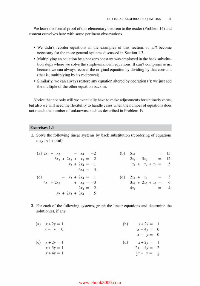
1. Solve the following linear systems by back substitution (reordering of equationsmay be helpful).
(a) 2x1 + x2 − x4 = −2 (b) 5x1 = 153x2 + 2x3 + x4 = 2 −2x1 − 3x2 = −12
x3 + 2x4 = −1 x1 + x2 + x3 = 54x4 = 4
(c) − x3 + 2x4 = 1 (d) 2x1 + x2 = 34x1 + 2x2 + x4 = −3 3x1 + 2x2 + x3 = 6
− 2x4 = −2 4x1 = 4x2 + 2x3 + 3x4 = 5
2. For each of the following systems, graph the linear equations and determine thesolution(s), if any.
(a) x + 2y = 1 (b) x + 2y = 1x − y = 0 x − 4y = 0
x − y = 0
(c) x + 2y = 1 (d) x + 2y = 1x + 3y = 1 −2x − 4y = −2x + 4y = 1 1
2 x + y = 12
www.ebook3000.com
12 SYSTEMS OF LINEAR ALGEBRAIC EQUATIONS
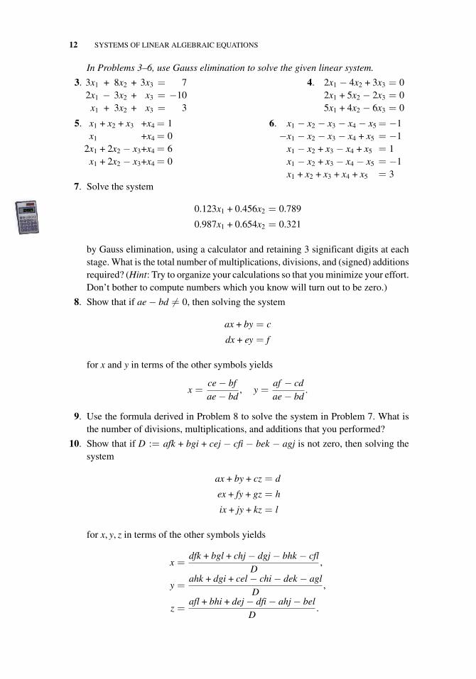
In Problems 3–6, use Gauss elimination to solve the given linear system.
3. 3x1 + 8x2 + 3x3 = 72x1 − 3x2 + x3 = −10
x1 + 3x2 + x3 = 3
4. 2x1 − 4x2 + 3x3 = 02x1 + 5x2 − 2x3 = 05x1 + 4x2 − 6x3 = 0
5. x1 + x2 + x3 +x4 = 1x1 +x4 = 0
2x1 + 2x2 − x3+x4 = 6x1 + 2x2 − x3+x4 = 0
6. x1 − x2 − x3 − x4 − x5 = −1−x1 − x2 − x3 − x4 + x5 = −1
x1 − x2 + x3 − x4 + x5 = 1x1 − x2 + x3 − x4 − x5 = −1x1 + x2 + x3 + x4 + x5 = 3
7. Solve the system
0.123x1 + 0.456x2 = 0.789
0.987x1 + 0.654x2 = 0.321
by Gauss elimination, using a calculator and retaining 3 significant digits at eachstage. What is the total number of multiplications, divisions, and (signed) additionsrequired? (Hint: Try to organize your calculations so that you minimize your effort.Don’t bother to compute numbers which you know will turn out to be zero.)
8. Show that if ae − bd �= 0, then solving the system
ax + by = c
dx + ey = f
for x and y in terms of the other symbols yields
x =ce − bfae − bd
, y =af − cdae − bd
.
9. Use the formula derived in Problem 8 to solve the system in Problem 7. What isthe number of divisions, multiplications, and additions that you performed?
10. Show that if D := afk + bgi + cej − cfi − bek − agj is not zero, then solving thesystem
ax + by + cz = d
ex + fy + gz = h
ix + jy + kz = l
for x, y, z in terms of the other symbols yields
x =dfk + bgl + chj − dgj − bhk − cfl
D,
y =ahk + dgi + cel − chi − dek − agl
D,
z =afl + bhi + dej − dfi − ahj − bel
D.
1.1 LINEAR ALGEBRAIC EQUATIONS 13
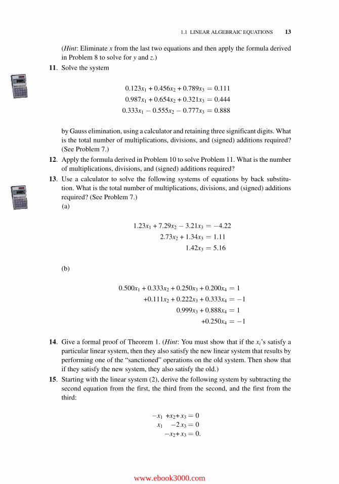
(Hint: Eliminate x from the last two equations and then apply the formula derivedin Problem 8 to solve for y and z.)
11. Solve the system
0.123x1 + 0.456x2 + 0.789x3 = 0.111
0.987x1 + 0.654x2 + 0.321x3 = 0.444
0.333x1 − 0.555x2 − 0.777x3 = 0.888
by Gauss elimination, using a calculator and retaining three significant digits. Whatis the total number of multiplications, divisions, and (signed) additions required?(See Problem 7.)
12. Apply the formula derived in Problem 10 to solve Problem 11. What is the numberof multiplications, divisions, and (signed) additions required?
13. Use a calculator to solve the following systems of equations by back substitu-tion. What is the total number of multiplications, divisions, and (signed) additionsrequired? (See Problem 7.)(a)
1.23x1 + 7.29x2 − 3.21x3 = −4.22
2.73x2 + 1.34x3 = 1.11
1.42x3 = 5.16
(b)
0.500x1 + 0.333x2 + 0.250x3 + 0.200x4 = 1
+0.111x2 + 0.222x3 + 0.333x4 = −1
0.999x3 + 0.888x4 = 1
+0.250x4 = −1
14. Give a formal proof of Theorem 1. (Hint: You must show that if the xi’s satisfy aparticular linear system, then they also satisfy the new linear system that results byperforming one of the “sanctioned” operations on the old system. Then show thatif they satisfy the new system, they also satisfy the old.)
15. Starting with the linear system (2), derive the following system by subtracting thesecond equation from the first, the third from the second, and the first from thethird:
−x1 +x2+ x3 = 0x1 −2 x3 = 0
−x2+ x3 = 0.
www.ebook3000.com
14 SYSTEMS OF LINEAR ALGEBRAIC EQUATIONS
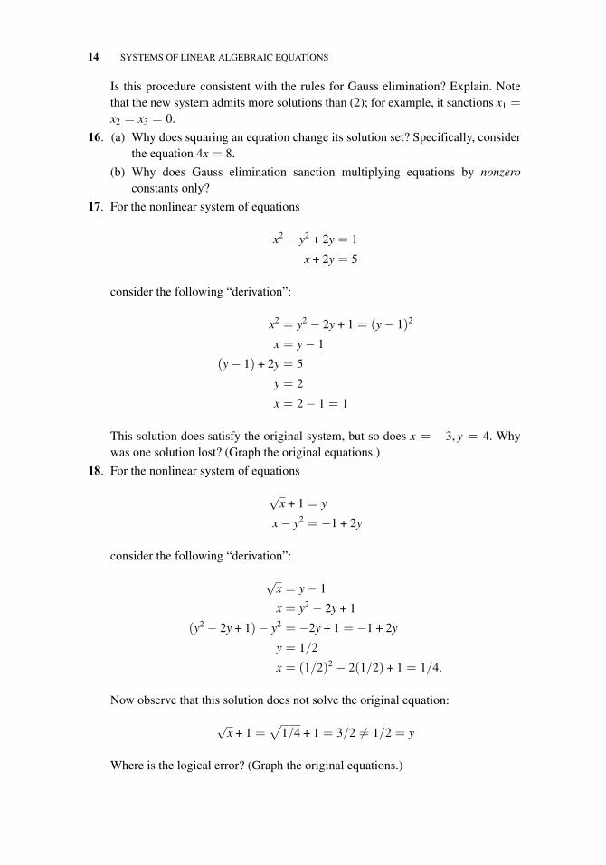
Is this procedure consistent with the rules for Gauss elimination? Explain. Notethat the new system admits more solutions than (2); for example, it sanctions x1 =x2 = x3 = 0.
16. (a) Why does squaring an equation change its solution set? Specifically, considerthe equation 4x = 8.
(b) Why does Gauss elimination sanction multiplying equations by nonzeroconstants only?
17. For the nonlinear system of equations
x2 − y2 + 2y = 1
x + 2y = 5
consider the following “derivation”:
x2 = y2 − 2y + 1 = (y − 1)2
x = y − 1
(y − 1) + 2y = 5
y = 2
x = 2 − 1 = 1
This solution does satisfy the original system, but so does x = −3, y = 4. Whywas one solution lost? (Graph the original equations.)
18. For the nonlinear system of equations
√x + 1 = y
x − y2 = −1 + 2y
consider the following “derivation”:
√x = y − 1
x = y2 − 2y + 1
(y2 − 2y + 1)− y2 = −2y + 1 = −1 + 2y
y = 1/2
x = (1/2)2 − 2(1/2) + 1 = 1/4.
Now observe that this solution does not solve the original equation:
√x + 1 =
√1/4 + 1 = 3/2 �= 1/2 = y
Where is the logical error? (Graph the original equations.)
1.1 LINEAR ALGEBRAIC EQUATIONS 15
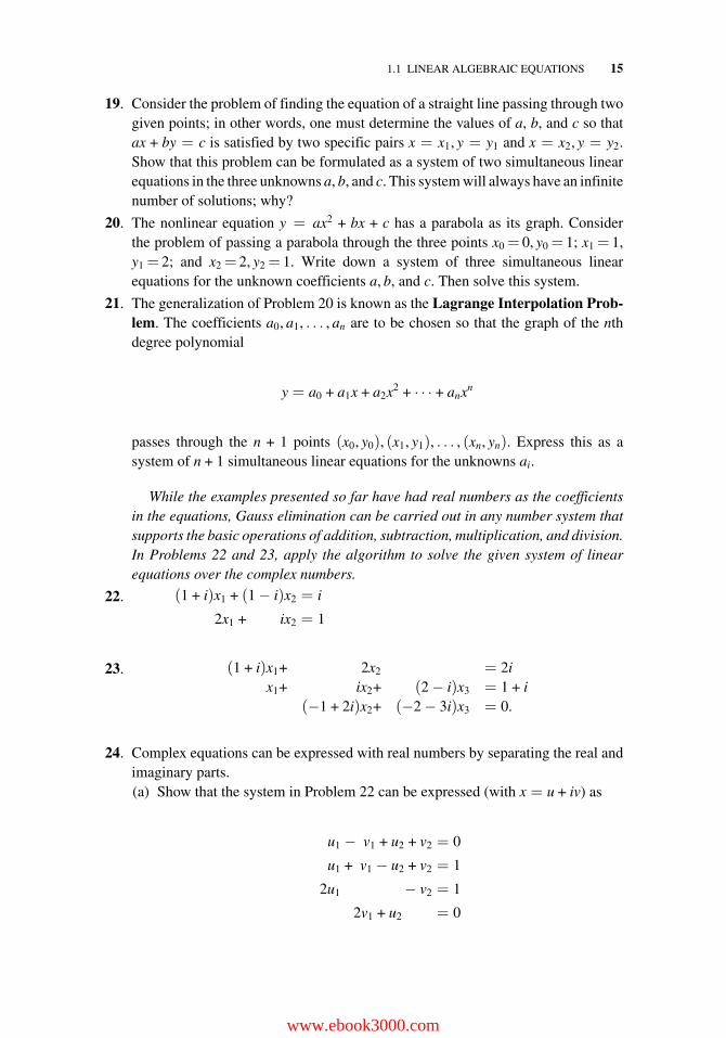
19. Consider the problem of finding the equation of a straight line passing through twogiven points; in other words, one must determine the values of a, b, and c so thatax + by = c is satisfied by two specific pairs x = x1, y = y1 and x = x2, y = y2.Show that this problem can be formulated as a system of two simultaneous linearequations in the three unknowns a, b, and c. This system will always have an infinitenumber of solutions; why?
20. The nonlinear equation y = ax2 + bx + c has a parabola as its graph. Considerthe problem of passing a parabola through the three points x0 = 0, y0 = 1; x1 = 1,y1 = 2; and x2 = 2, y2 = 1. Write down a system of three simultaneous linearequations for the unknown coefficients a, b, and c. Then solve this system.
21. The generalization of Problem 20 is known as the Lagrange Interpolation Prob-lem. The coefficients a0, a1, . . . , an are to be chosen so that the graph of the nthdegree polynomial
y = a0 + a1x + a2x2 + · · · + anxn
passes through the n + 1 points (x0, y0), (x1, y1), . . . , (xn, yn). Express this as asystem of n + 1 simultaneous linear equations for the unknowns ai.
While the examples presented so far have had real numbers as the coefficientsin the equations, Gauss elimination can be carried out in any number system thatsupports the basic operations of addition, subtraction, multiplication, and division.In Problems 22 and 23, apply the algorithm to solve the given system of linearequations over the complex numbers.
22. (1 + i)x1 + (1 − i)x2 = i
2x1 + ix2 = 1
23. (1 + i)x1+ 2x2 = 2ix1+ ix2+ (2 − i)x3 = 1 + i
(−1 + 2i)x2+ (−2 − 3i)x3 = 0.
24. Complex equations can be expressed with real numbers by separating the real andimaginary parts.(a) Show that the system in Problem 22 can be expressed (with x = u + iv) as
u1 − v1 + u2 + v2 = 0
u1 + v1 − u2 + v2 = 1
2u1 − v2 = 1
2v1 + u2 = 0
www.ebook3000.com
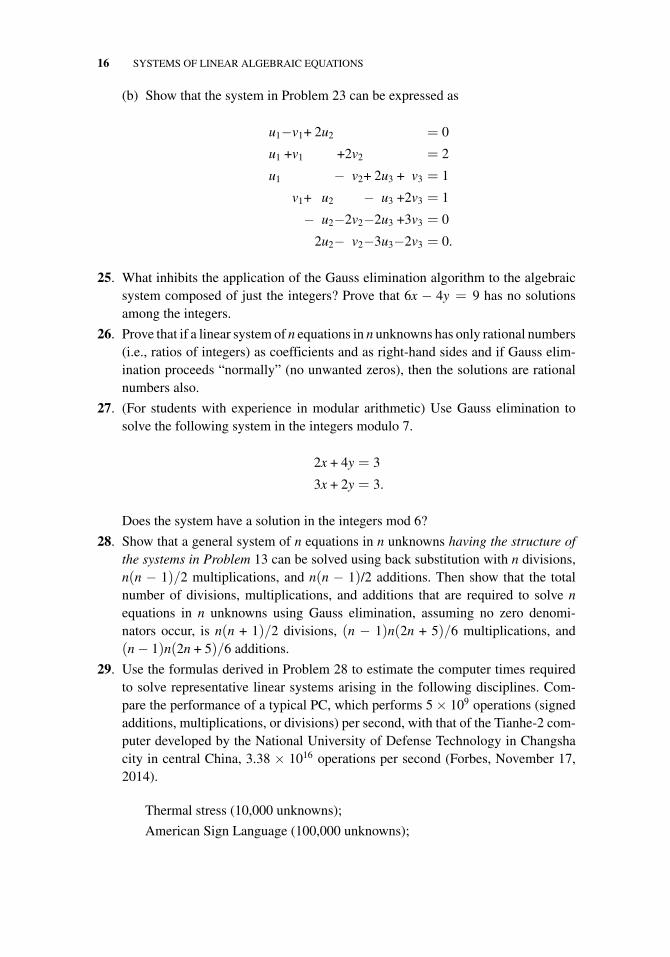
16 SYSTEMS OF LINEAR ALGEBRAIC EQUATIONS
(b) Show that the system in Problem 23 can be expressed as
u1−v1+ 2u2 = 0
u1 +v1 +2v2 = 2
u1 − v2+ 2u3 + v3 = 1
v1+ u2 − u3 +2v3 = 1
− u2−2v2−2u3 +3v3 = 0
2u2− v2−3u3−2v3 = 0.
25. What inhibits the application of the Gauss elimination algorithm to the algebraicsystem composed of just the integers? Prove that 6x − 4y = 9 has no solutionsamong the integers.
26. Prove that if a linear system of n equations in n unknowns has only rational numbers(i.e., ratios of integers) as coefficients and as right-hand sides and if Gauss elim-ination proceeds “normally” (no unwanted zeros), then the solutions are rationalnumbers also.
27. (For students with experience in modular arithmetic) Use Gauss elimination tosolve the following system in the integers modulo 7.
2x + 4y = 3
3x + 2y = 3.
Does the system have a solution in the integers mod 6?
28. Show that a general system of n equations in n unknowns having the structure ofthe systems in Problem 13 can be solved using back substitution with n divisions,n(n − 1)/2 multiplications, and n(n − 1)/2 additions. Then show that the totalnumber of divisions, multiplications, and additions that are required to solve nequations in n unknowns using Gauss elimination, assuming no zero denomi-nators occur, is n(n + 1)/2 divisions, (n − 1)n(2n + 5)/6 multiplications, and(n − 1)n(2n + 5)/6 additions.
29. Use the formulas derived in Problem 28 to estimate the computer times requiredto solve representative linear systems arising in the following disciplines. Com-pare the performance of a typical PC, which performs 5 × 10⁹ operations (signedadditions, multiplications, or divisions) per second, with that of the Tianhe-2 com-puter developed by the National University of Defense Technology in Changshacity in central China, 3.38 × 10¹⁶ operations per second (Forbes, November 17,2014).
Thermal stress (10,000 unknowns);
American Sign Language (100,000 unknowns);
1.2 MATRIX REPRESENTATION OF LINEAR SYSTEMS 17
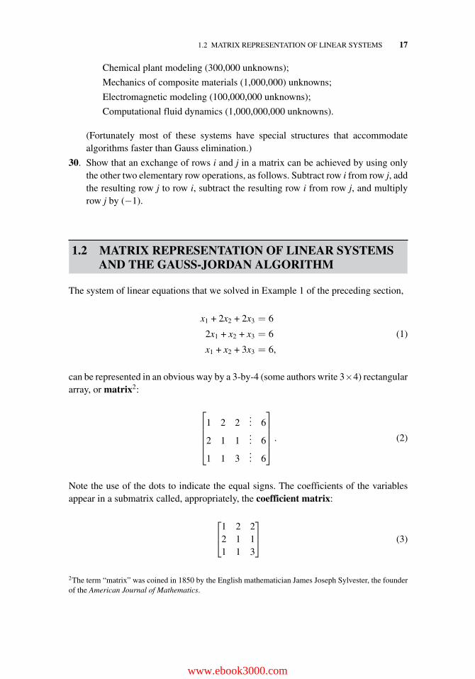
Chemical plant modeling (300,000 unknowns);
Mechanics of composite materials (1,000,000) unknowns;
Electromagnetic modeling (100,000,000 unknowns);
Computational fluid dynamics (1,000,000,000 unknowns).
(Fortunately most of these systems have special structures that accommodatealgorithms faster than Gauss elimination.)
30. Show that an exchange of rows i and j in a matrix can be achieved by using onlythe other two elementary row operations, as follows. Subtract row i from row j, addthe resulting row j to row i, subtract the resulting row i from row j, and multiplyrow j by (−1).
1.2 MATRIX REPRESENTATION OF LINEAR SYSTEMSAND THE GAUSS-JORDAN ALGORITHM
The system of linear equations that we solved in Example 1 of the preceding section,
x1 + 2x2 + 2x3 = 6
2x1 + x2 + x3 = 6
x1 + x2 + 3x3 = 6,
(1)
can be represented in an obvious way by a 3-by-4 (some authors write 3×4) rectangulararray, or matrix2:
⎡⎢⎢⎢⎣
1 2 2... 6
2 1 1... 6
1 1 3... 6
⎤⎥⎥⎥⎦ . (2)
Note the use of the dots to indicate the equal signs. The coefficients of the variablesappear in a submatrix called, appropriately, the coefficient matrix:
⎡⎣1 2 2
2 1 11 1 3
⎤⎦ (3)
2The term “matrix” was coined in 1850 by the English mathematician James Joseph Sylvester, the founderof the American Journal of Mathematics.
www.ebook3000.com
18 SYSTEMS OF LINEAR ALGEBRAIC EQUATIONS
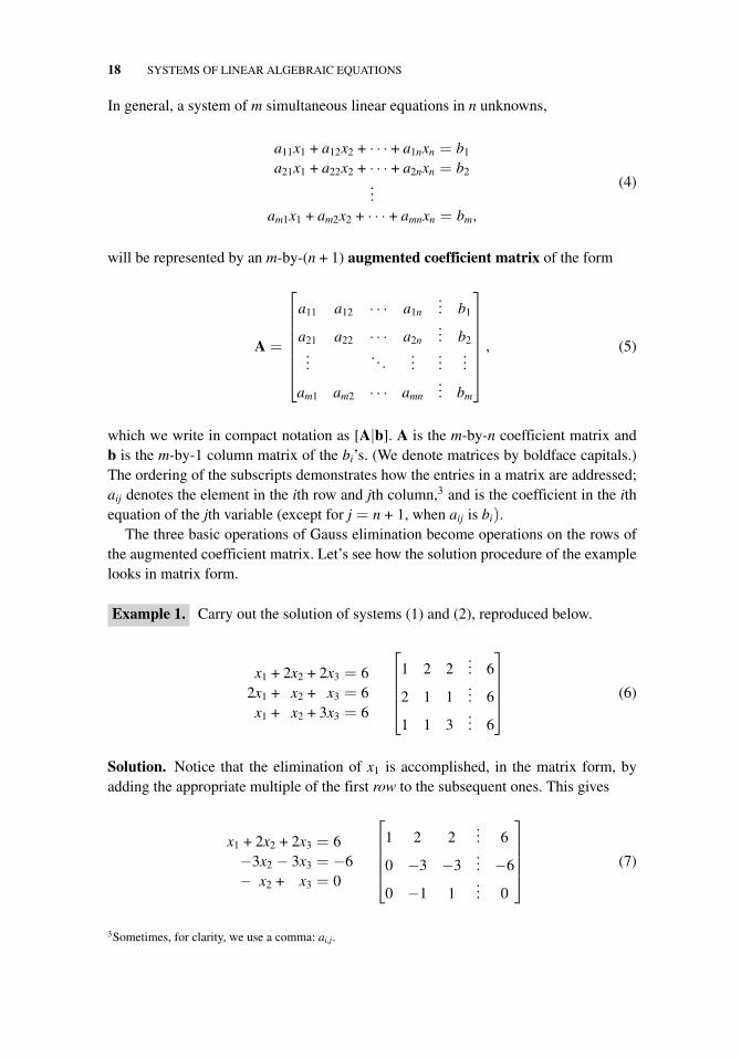
In general, a system of m simultaneous linear equations in n unknowns,
a11x1 + a12x2 + · · · + a1nxn = b1
a21x1 + a22x2 + · · · + a2nxn = b2...
am1x1 + am2x2 + · · · + amnxn = bm,
(4)
will be represented by an m-by-(n + 1) augmented coefficient matrix of the form
A =
⎡⎢⎢⎢⎢⎢⎢⎣
a11 a12 · · · a1n... b1
a21 a22 · · · a2n... b2
.... . .
......
...
am1 am2 · · · amn... bm
⎤⎥⎥⎥⎥⎥⎥⎦
, (5)
which we write in compact notation as [A|b]. A is the m-by-n coefficient matrix andb is the m-by-1 column matrix of the bi’s. (We denote matrices by boldface capitals.)The ordering of the subscripts demonstrates how the entries in a matrix are addressed;aij denotes the element in the ith row and jth column,3 and is the coefficient in the ithequation of the jth variable (except for j = n + 1, when aij is bi).
The three basic operations of Gauss elimination become operations on the rows ofthe augmented coefficient matrix. Let’s see how the solution procedure of the examplelooks in matrix form.
Example 1. Carry out the solution of systems (1) and (2), reproduced below.
x1 + 2x2 + 2x3 = 62x1 + x2 + x3 = 6x1 + x2 + 3x3 = 6
⎡⎢⎢⎢⎣
1 2 2... 6
2 1 1... 6
1 1 3... 6
⎤⎥⎥⎥⎦ (6)
Solution. Notice that the elimination of x1 is accomplished, in the matrix form, byadding the appropriate multiple of the first row to the subsequent ones. This gives
x1 + 2x2 + 2x3 = 6−3x2 − 3x3 = −6− x2 + x3 = 0
⎡⎢⎢⎢⎣
1 2 2... 6
0 −3 −3... −6
0 −1 1... 0
⎤⎥⎥⎥⎦ (7)
3Sometimes, for clarity, we use a comma: ai,j.
1.2 MATRIX REPRESENTATION OF LINEAR SYSTEMS 19
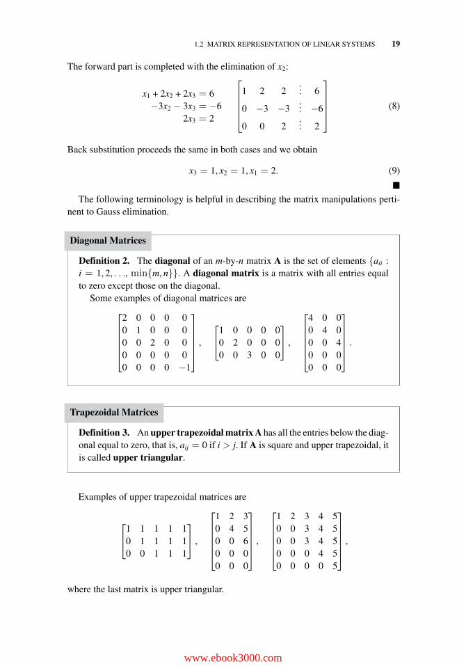
The forward part is completed with the elimination of x2:
x1 + 2x2 + 2x3 = 6−3x2 − 3x3 = −6
2x3 = 2
⎡⎢⎢⎢⎣
1 2 2... 6
0 −3 −3... −6
0 0 2... 2
⎤⎥⎥⎥⎦ (8)
Back substitution proceeds the same in both cases and we obtain
x3 = 1, x2 = 1, x1 = 2. (9)
�The following terminology is helpful in describing the matrix manipulations perti-
nent to Gauss elimination.
Diagonal Matrices
Definition 2. The diagonal of an m-by-n matrix A is the set of elements {aii :i = 1, 2, . . ., min{m, n}}. A diagonal matrix is a matrix with all entries equalto zero except those on the diagonal.
Some examples of diagonal matrices are⎡⎢⎢⎢⎢⎣
2 0 0 0 00 1 0 0 00 0 2 0 00 0 0 0 00 0 0 0 −1
⎤⎥⎥⎥⎥⎦ ,
⎡⎣1 0 0 0 0
0 2 0 0 00 0 3 0 0
⎤⎦ ,
⎡⎢⎢⎢⎢⎣
4 0 00 4 00 0 40 0 00 0 0
⎤⎥⎥⎥⎥⎦ .
Trapezoidal Matrices
Definition 3. An upper trapezoidal matrix A has all the entries below the diag-onal equal to zero, that is, aij = 0 if i > j. If A is square and upper trapezoidal, itis called upper triangular.
Examples of upper trapezoidal matrices are
⎡⎣1 1 1 1 1
0 1 1 1 10 0 1 1 1
⎤⎦ ,
⎡⎢⎢⎢⎢⎣
1 2 30 4 50 0 60 0 00 0 0
⎤⎥⎥⎥⎥⎦ ,
⎡⎢⎢⎢⎢⎣
1 2 3 4 50 0 3 4 50 0 3 4 50 0 0 4 50 0 0 0 5
⎤⎥⎥⎥⎥⎦ ,
where the last matrix is upper triangular.
www.ebook3000.com
20 SYSTEMS OF LINEAR ALGEBRAIC EQUATIONS
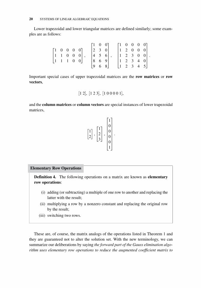
Lower trapezoidal and lower triangular matrices are defined similarly; some exam-ples are as follows:
⎡⎣1 0 0 0 0
1 1 0 0 01 1 1 0 0
⎤⎦ ,
⎡⎢⎢⎢⎢⎣
1 0 02 3 04 5 68 6 99 6 8
⎤⎥⎥⎥⎥⎦ ,
⎡⎢⎢⎢⎢⎣
1 0 0 0 01 2 0 0 01 2 3 0 01 2 3 4 01 2 3 4 5
⎤⎥⎥⎥⎥⎦ .
Important special cases of upper trapezoidal matrices are the row matrices or rowvectors,
[1 2], [1 2 3], [1 0 0 0 0 1],
and the column matrices or column vectors are special instances of lower trapezoidalmatrices,
[12
],
⎡⎣1
23
⎤⎦ ,
⎡⎢⎢⎢⎢⎢⎢⎢⎣
100001
⎤⎥⎥⎥⎥⎥⎥⎥⎦
.
Elementary Row Operations
Definition 4. The following operations on a matrix are known as elementaryrow operations:
(i) adding (or subtracting) a multiple of one row to another and replacing thelatter with the result;
(ii) multiplying a row by a nonzero constant and replacing the original rowby the result;
(iii) switching two rows.
These are, of course, the matrix analogs of the operations listed in Theorem 1 andthey are guaranteed not to alter the solution set. With the new terminology, we cansummarize our deliberations by saying the forward part of the Gauss elimination algo-rithm uses elementary row operations to reduce the augmented coefficient matrix to
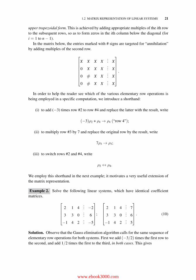
1.2 MATRIX REPRESENTATION OF LINEAR SYSTEMS 21
upper trapezoidal form. This is achieved by adding appropriate multiples of the ith rowto the subsequent rows, so as to form zeros in the ith column below the diagonal (fori = 1 to n − 1).
In the matrix below, the entries marked with # signs are targeted for “annihilation”by adding multiples of the second row.
⎡⎢⎢⎢⎢⎢⎢⎣
X X X X... X
0 X X X... X
0 # X X... X
0 # X X... X
⎤⎥⎥⎥⎥⎥⎥⎦
.
In order to help the reader see which of the various elementary row operations isbeing employed in a specific computation, we introduce a shorthand:
(i) to add (−3) times row #2 to row #4 and replace the latter with the result, write
(−3)ρ2 + ρ4 → ρ4 (“row 4”);
(ii) to multiply row #3 by 7 and replace the original row by the result, write
7ρ3 → ρ3;
(iii) to switch rows #2 and #4, write
ρ2 ↔ ρ4.
We employ this shorthand in the next example; it motivates a very useful extension ofthe matrix representation.
Example 2. Solve the following linear systems, which have identical coefficientmatrices.
⎡⎢⎢⎢⎣
2 1 4... −2
3 3 0... 6
−1 4 2... −5
⎤⎥⎥⎥⎦;
⎡⎢⎢⎢⎣
2 1 4... 7
3 3 0... 6
−1 4 2... 5
⎤⎥⎥⎥⎦ . (10)
Solution. Observe that the Gauss elimination algorithm calls for the same sequence ofelementary row operations for both systems. First we add (−3/2) times the first row tothe second, and add 1/2 times the first to the third, in both cases. This gives
www.ebook3000.com
22 SYSTEMS OF LINEAR ALGEBRAIC EQUATIONS
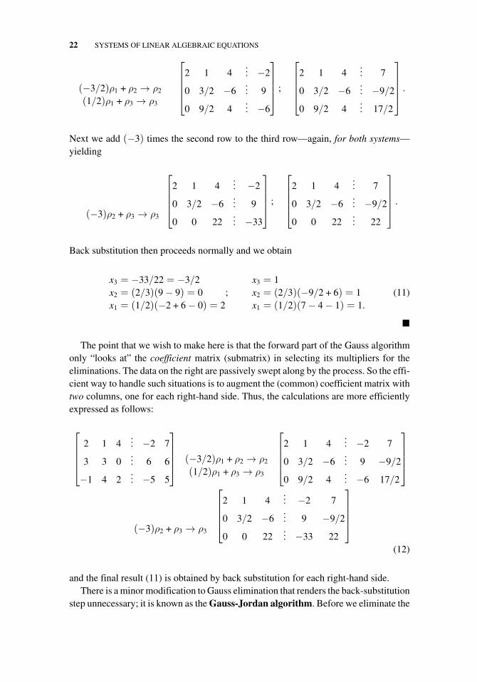
(−3/2)ρ1 + ρ2 → ρ2
(1/2)ρ1 + ρ3 → ρ3
⎡⎢⎢⎢⎣
2 1 4... −2
0 3/2 −6... 9
0 9/2 4... −6
⎤⎥⎥⎥⎦ ;
⎡⎢⎢⎢⎣
2 1 4... 7
0 3/2 −6... −9/2
0 9/2 4... 17/2
⎤⎥⎥⎥⎦ .
Next we add (−3) times the second row to the third row—again, for both systems—yielding
(−3)ρ2 + ρ3 → ρ3
⎡⎢⎢⎢⎣
2 1 4... −2
0 3/2 −6... 9
0 0 22... −33
⎤⎥⎥⎥⎦ ;
⎡⎢⎢⎢⎣
2 1 4... 7
0 3/2 −6... −9/2
0 0 22... 22
⎤⎥⎥⎥⎦ .
Back substitution then proceeds normally and we obtain
x3 = −33/22 = −3/2x2 = (2/3)(9 − 9) = 0x1 = (1/2)(−2 + 6 − 0) = 2
;x3 = 1x2 = (2/3)(−9/2 + 6) = 1x1 = (1/2)(7 − 4 − 1) = 1.
(11)
�
The point that we wish to make here is that the forward part of the Gauss algorithmonly “looks at” the coefficient matrix (submatrix) in selecting its multipliers for theeliminations. The data on the right are passively swept along by the process. So the effi-cient way to handle such situations is to augment the (common) coefficient matrix withtwo columns, one for each right-hand side. Thus, the calculations are more efficientlyexpressed as follows:
⎡⎢⎢⎢⎣
2 1 4... −2 7
3 3 0... 6 6
−1 4 2... −5 5
⎤⎥⎥⎥⎦ (−3/2)ρ1 + ρ2 → ρ2
(1/2)ρ1 + ρ3 → ρ3
⎡⎢⎢⎢⎣
2 1 4... −2 7
0 3/2 −6... 9 −9/2
0 9/2 4... −6 17/2
⎤⎥⎥⎥⎦
(−3)ρ2 + ρ3 → ρ3
⎡⎢⎢⎢⎣
2 1 4... −2 7
0 3/2 −6... 9 −9/2
0 0 22... −33 22
⎤⎥⎥⎥⎦
(12)
and the final result (11) is obtained by back substitution for each right-hand side.There is a minor modification to Gauss elimination that renders the back-substitution
step unnecessary; it is known as the Gauss-Jordan algorithm. Before we eliminate the
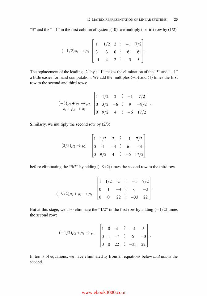
1.2 MATRIX REPRESENTATION OF LINEAR SYSTEMS 23
“3” and the “−1” in the first column of system (10), we multiply the first row by (1/2):
(−1/2)ρ1 → ρ1
⎡⎢⎢⎢⎣
1 1/2 2... −1 7/2
3 3 0... 6 6
−1 4 2... −5 5
⎤⎥⎥⎥⎦ .
The replacement of the leading “2” by a “1” makes the elimination of the “3” and “−1”a little easier for hand computation. We add the multiples (−3) and (1) times the firstrow to the second and third rows:
(−3)ρ1 + ρ2 → ρ2
ρ1 + ρ3 → ρ3
⎡⎢⎢⎢⎣
1 1/2 2... −1 7/2
0 3/2 −6... 9 −9/2
0 9/2 4... −6 17/2
⎤⎥⎥⎥⎦ .
Similarly, we multiply the second row by (2/3)
(2/3)ρ2 → ρ2
⎡⎢⎢⎢⎣
1 1/2 2... −1 7/2
0 1 −4... 6 −3
0 9/2 4... −6 17/2
⎤⎥⎥⎥⎦
before eliminating the “9/2” by adding (−9/2) times the second row to the third row.
(−9/2)ρ2 + ρ3 → ρ3
⎡⎢⎢⎢⎣
1 1/2 2... −1 7/2
0 1 −4... 6 −3
0 0 22... −33 22
⎤⎥⎥⎥⎦ .
But at this stage, we also eliminate the “1/2” in the first row by adding (−1/2) timesthe second row:
(−1/2)ρ2 + ρ1 → ρ1
⎡⎢⎢⎢⎣
1 0 4... −4 5
0 1 −4... 6 −3
0 0 22... −33 22
⎤⎥⎥⎥⎦ .
In terms of equations, we have eliminated x2 from all equations below and above thesecond.
www.ebook3000.com
24 SYSTEMS OF LINEAR ALGEBRAIC EQUATIONS
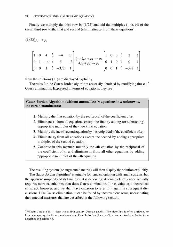
Finally we multiply the third row by (1/22) and add the multiples (−4), (4) of the(new) third row to the first and second (eliminating x3 from these equations):
(1/22)ρ3 → ρ3
⎡⎢⎢⎢⎣
1 0 4... −4 5
0 1 −4... 6 −3
0 0 1... −3/2 1
⎤⎥⎥⎥⎦(−4)ρ3 + ρ1 → ρ1
4ρ3 + ρ2 → ρ2
⎡⎢⎢⎢⎣
1 0 0... 2 1
0 1 0... 0 1
0 0 1... −3/2 1
⎤⎥⎥⎥⎦ .
Now the solutions (11) are displayed explicitly.The rules for the Gauss-Jordan algorithm are easily obtained by modifying those of
Gauss elimination. Expressed in terms of equations, they are
Gauss-Jordan Algorithm (without anomalies) (n equations in n unknowns,no zero denominators)
1. Multiply the first equation by the reciprocal of the coefficient of x1.
2. Eliminate x1 from all equations except the first by adding (or subtracting)appropriate multiples of the (new) first equation.
3. Multiply the (new) second equation by the reciprocal of the coefficient of x2.
4. Eliminate x2 from all equations except the second by adding appropriatemultiples of the second equation.
5. Continue in this manner: multiply the kth equation by the reciprocal ofthe coefficient of xk and eliminate xk from all other equations by addingappropriate multiples of the kth equation.
The resulting system (or augmented matrix) will then display the solution explicitly.The Gauss-Jordan algorithm4 is suitable for hand calculation with small systems, but
the apparent simplicity of its final format is deceiving; its complete execution actuallyrequires more calculations than does Gauss elimination. It has value as a theoreticalconstruct, however, and we shall have occasion to refer to it again in subsequent dis-cussions. Like Gauss elimination, it can be foiled by inconvenient zeros, necessitatingthe remedial measures that are described in the following section.
4Wilhelm Jordan (Yor’ - dan) was a 19th-century German geodist. The algorithm is often attributed tohis contemporary, the French mathematician Camille Jordan (Jor - dan’), who conceived the Jordan formdescribed in Section 7.3.
1.2 MATRIX REPRESENTATION OF LINEAR SYSTEMS 25
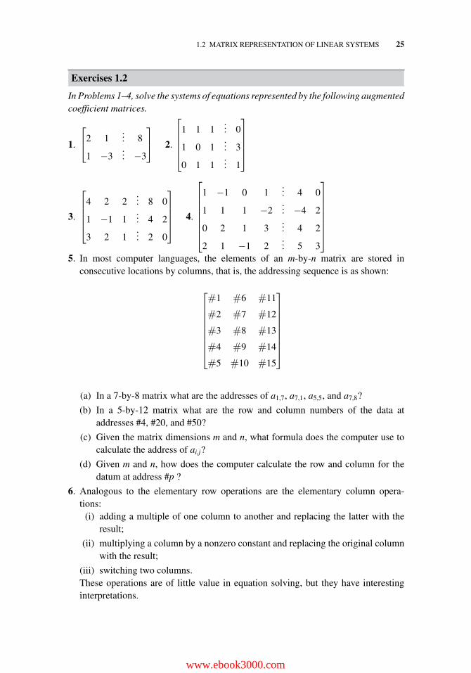
Exercises 1.2
In Problems 1–4, solve the systems of equations represented by the following augmentedcoefficient matrices.
1.
⎡⎣2 1
... 8
1 −3... −3
⎤⎦ 2.
⎡⎢⎢⎢⎣
1 1 1... 0
1 0 1... 3
0 1 1... 1
⎤⎥⎥⎥⎦
3.
⎡⎢⎢⎢⎣
4 2 2... 8 0
1 −1 1... 4 2
3 2 1... 2 0
⎤⎥⎥⎥⎦ 4.
⎡⎢⎢⎢⎢⎢⎢⎣
1 −1 0 1... 4 0
1 1 1 −2... −4 2
0 2 1 3... 4 2
2 1 −1 2... 5 3
⎤⎥⎥⎥⎥⎥⎥⎦
5. In most computer languages, the elements of an m-by-n matrix are stored inconsecutive locations by columns, that is, the addressing sequence is as shown:
⎡⎢⎢⎢⎢⎢⎢⎢⎣
#1 #6 #11
#2 #7 #12
#3 #8 #13
#4 #9 #14
#5 #10 #15
⎤⎥⎥⎥⎥⎥⎥⎥⎦
(a) In a 7-by-8 matrix what are the addresses of a1,7, a7,1, a5,5, and a7,8?
(b) In a 5-by-12 matrix what are the row and column numbers of the data ataddresses #4, #20, and #50?
(c) Given the matrix dimensions m and n, what formula does the computer use tocalculate the address of ai,j?
(d) Given m and n, how does the computer calculate the row and column for thedatum at address #p ?
6. Analogous to the elementary row operations are the elementary column opera-tions:
(i) adding a multiple of one column to another and replacing the latter with theresult;
(ii) multiplying a column by a nonzero constant and replacing the original columnwith the result;
(iii) switching two columns.These operations are of little value in equation solving, but they have interestinginterpretations.
www.ebook3000.com
26 SYSTEMS OF LINEAR ALGEBRAIC EQUATIONS
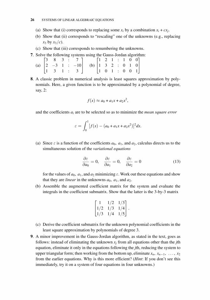
(a) Show that (i) corresponds to replacing some xi by a combination xi + cxj.
(b) Show that (ii) corresponds to “rescaling” one of the unknowns (e.g., replacingx3 by x3/c).
(c) Show that (iii) corresponds to renumbering the unknowns.
7. Solve the following systems using the Gauss-Jordan algorithm:
(a)
⎡⎣3 8 3 : 7
2 −3 1 : −101 3 1 : 3
⎤⎦ (b)
⎡⎣1 2 1 : 1 0 0
1 3 2 : 0 1 01 0 1 : 0 0 1
⎤⎦
8. A classic problem in numerical analysis is least squares approximation by poly-nomials. Here, a given function is to be approximated by a polynomial of degree,say, 2:
f (x) ≈ a0 + a1x + a2x2,
and the coefficients ai are to be selected so as to minimize the mean square error
ε =
∫ 1
0[ f (x)− (a0 + a1x + a2x2)]2dx.
(a) Since ε is a function of the coefficients a0, a1, and a2, calculus directs us to thesimultaneous solution of the variational equations
∂ε
∂a0= 0,
∂ε
∂a1= 0,
∂ε
∂a2= 0 (13)
for the values of a0, a1, and a2 minimizing ε. Work out these equations and showthat they are linear in the unknowns a0, a1, and a2.
(b) Assemble the augmented coefficient matrix for the system and evaluate theintegrals in the coefficient submatrix. Show that the latter is the 3-by-3 matrix
⎡⎣ 1 1/2 1/3
1/2 1/3 1/41/3 1/4 1/5
⎤⎦ .
(c) Derive the coefficient submatrix for the unknown polynomial coefficients in theleast square approximation by polynomials of degree 3.
9. A minor improvement in the Gauss-Jordan algorithm, as stated in the text, goes asfollows: instead of eliminating the unknown xj from all equations other than the jthequation, eliminate it only in the equations following the jth, reducing the system toupper triangular form; then working from the bottom up, eliminate xn, xn−1, . . . , x2
from the earlier equations. Why is this more efficient? (Hint: If you don’t see thisimmediately, try it on a system of four equations in four unknowns.)
1.3 THE COMPLETE GAUSS ELIMINATION ALGORITHM 27
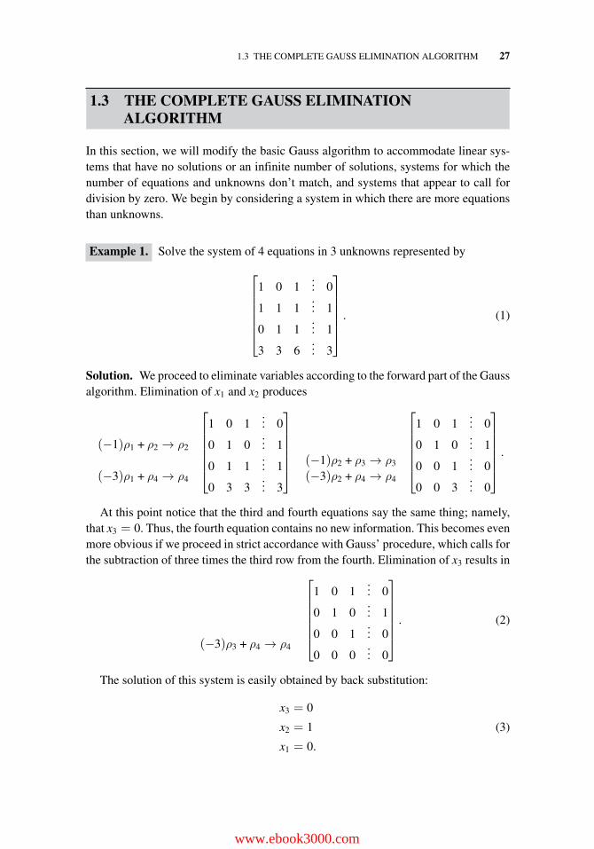
1.3 THE COMPLETE GAUSS ELIMINATIONALGORITHM
In this section, we will modify the basic Gauss algorithm to accommodate linear sys-tems that have no solutions or an infinite number of solutions, systems for which thenumber of equations and unknowns don’t match, and systems that appear to call fordivision by zero. We begin by considering a system in which there are more equationsthan unknowns.
Example 1. Solve the system of 4 equations in 3 unknowns represented by
⎡⎢⎢⎢⎢⎢⎣
1 0 1... 0
1 1 1... 1
0 1 1... 1
3 3 6... 3
⎤⎥⎥⎥⎥⎥⎦
. (1)
Solution. We proceed to eliminate variables according to the forward part of the Gaussalgorithm. Elimination of x1 and x2 produces
(−1)ρ1 + ρ2 → ρ2
(−3)ρ1 + ρ4 → ρ4
⎡⎢⎢⎢⎢⎢⎣
1 0 1... 0
0 1 0... 1
0 1 1... 1
0 3 3... 3
⎤⎥⎥⎥⎥⎥⎦ (−1)ρ2 + ρ3 → ρ3
(−3)ρ2 + ρ4 → ρ4
⎡⎢⎢⎢⎢⎢⎣
1 0 1... 0
0 1 0... 1
0 0 1... 0
0 0 3... 0
⎤⎥⎥⎥⎥⎥⎦
.
At this point notice that the third and fourth equations say the same thing; namely,that x3 = 0. Thus, the fourth equation contains no new information. This becomes evenmore obvious if we proceed in strict accordance with Gauss’ procedure, which calls forthe subtraction of three times the third row from the fourth. Elimination of x3 results in
(−3)ρ3 + ρ4 → ρ4
⎡⎢⎢⎢⎢⎢⎣
1 0 1... 0
0 1 0... 1
0 0 1... 0
0 0 0... 0
⎤⎥⎥⎥⎥⎥⎦
. (2)
The solution of this system is easily obtained by back substitution:
x3 = 0
x2 = 1 (3)
x1 = 0.
www.ebook3000.com
28 SYSTEMS OF LINEAR ALGEBRAIC EQUATIONS
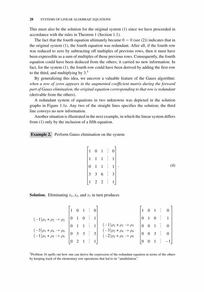
This must also be the solution for the original system (1) since we have proceeded inaccordance with the rules in Theorem 1 (Section 1.1).
The fact that the fourth equation ultimately became 0 = 0 (see (2)) indicates that inthe original system (1), the fourth equation was redundant. After all, if the fourth rowwas reduced to zero by subtracting off multiples of previous rows, then it must havebeen expressible as a sum of multiples of those previous rows. Consequently, the fourthequation could have been deduced from the others; it carried no new information. Infact, for the system (1), the fourth row could have been derived by adding the first rowto the third, and multiplying by 3.5
By generalizing this idea, we uncover a valuable feature of the Gauss algorithm:when a row of zeros appears in the augmented coefficient matrix during the forwardpart of Gauss elimination, the original equation corresponding to that row is redundant(derivable from the others).
A redundant system of equations in two unknowns was depicted in the solutiongraphs in Figure 1.1e. Any two of the straight lines specifies the solution; the thirdline conveys no new information.
Another situation is illustrated in the next example, in which the linear system differsfrom (1) only by the inclusion of a fifth equation.
Example 2. Perform Gauss elimination on the system
⎡⎢⎢⎢⎢⎢⎢⎢⎢⎢⎣
1 0 1... 0
1 1 1... 1
0 1 1... 1
3 3 6... 3
1 2 2... 1
⎤⎥⎥⎥⎥⎥⎥⎥⎥⎥⎦
. (4)
Solution. Eliminating x1, x2, and x3 in turn produces
(−1)ρ1 + ρ2 → ρ2
(−3)ρ1 + ρ4 → ρ4
(−1)ρ1 + ρ5 → ρ5
⎡⎢⎢⎢⎢⎢⎢⎢⎢⎢⎣
1 0 1... 0
0 1 0... 1
0 1 1... 1
0 3 3... 3
0 2 1... 1
⎤⎥⎥⎥⎥⎥⎥⎥⎥⎥⎦
(−1)ρ2 + ρ3 → ρ3
(−3)ρ2 + ρ4 → ρ4
(−2)ρ2 + ρ5 → ρ5
⎡⎢⎢⎢⎢⎢⎢⎢⎢⎢⎣
1 0 1... 0
0 1 0... 1
0 0 1... 0
0 0 3... 0
0 0 1... −1
⎤⎥⎥⎥⎥⎥⎥⎥⎥⎥⎦
5Problem 16 spells out how one can derive the expression of the redundant equation in terms of the othersby keeping track of the elementary row operations that led to its “annihilation.”
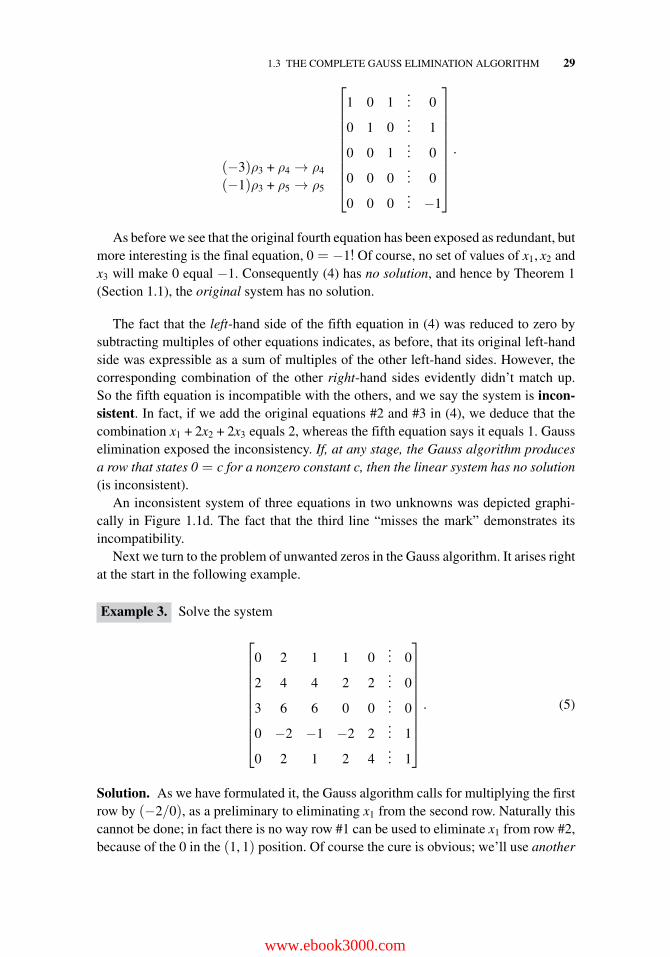
1.3 THE COMPLETE GAUSS ELIMINATION ALGORITHM 29
(−3)ρ3 + ρ4 → ρ4
(−1)ρ3 + ρ5 → ρ5
⎡⎢⎢⎢⎢⎢⎢⎢⎢⎢⎣
1 0 1... 0
0 1 0... 1
0 0 1... 0
0 0 0... 0
0 0 0... −1
⎤⎥⎥⎥⎥⎥⎥⎥⎥⎥⎦
.
As before we see that the original fourth equation has been exposed as redundant, butmore interesting is the final equation, 0 = −1! Of course, no set of values of x1, x2 andx3 will make 0 equal −1. Consequently (4) has no solution, and hence by Theorem 1(Section 1.1), the original system has no solution.
The fact that the left-hand side of the fifth equation in (4) was reduced to zero bysubtracting multiples of other equations indicates, as before, that its original left-handside was expressible as a sum of multiples of the other left-hand sides. However, thecorresponding combination of the other right-hand sides evidently didn’t match up.So the fifth equation is incompatible with the others, and we say the system is incon-sistent. In fact, if we add the original equations #2 and #3 in (4), we deduce that thecombination x1 + 2x2 + 2x3 equals 2, whereas the fifth equation says it equals 1. Gausselimination exposed the inconsistency. If, at any stage, the Gauss algorithm producesa row that states 0 = c for a nonzero constant c, then the linear system has no solution(is inconsistent).
An inconsistent system of three equations in two unknowns was depicted graphi-cally in Figure 1.1d. The fact that the third line “misses the mark” demonstrates itsincompatibility.
Next we turn to the problem of unwanted zeros in the Gauss algorithm. It arises rightat the start in the following example.
Example 3. Solve the system
⎡⎢⎢⎢⎢⎢⎢⎢⎢⎢⎣
0 2 1 1 0... 0
2 4 4 2 2... 0
3 6 6 0 0... 0
0 −2 −1 −2 2... 1
0 2 1 2 4... 1
⎤⎥⎥⎥⎥⎥⎥⎥⎥⎥⎦
. (5)
Solution. As we have formulated it, the Gauss algorithm calls for multiplying the firstrow by (−2/0), as a preliminary to eliminating x1 from the second row. Naturally thiscannot be done; in fact there is no way row #1 can be used to eliminate x1 from row #2,because of the 0 in the (1, 1) position. Of course the cure is obvious; we’ll use another
www.ebook3000.com
30 SYSTEMS OF LINEAR ALGEBRAIC EQUATIONS
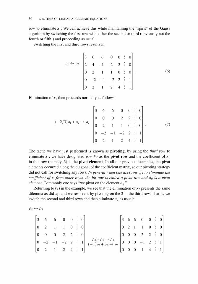
row to eliminate x1. We can achieve this while maintaining the “spirit” of the Gaussalgorithm by switching the first row with either the second or third (obviously not thefourth or fifth!) and proceeding as usual.
Switching the first and third rows results in
ρ1 ↔ ρ3
⎡⎢⎢⎢⎢⎢⎢⎢⎢⎢⎣
3 6 6 0 0... 0
2 4 4 2 2... 0
0 2 1 1 0... 0
0 −2 −1 −2 2... 1
0 2 1 2 4... 1
⎤⎥⎥⎥⎥⎥⎥⎥⎥⎥⎦
. (6)
Elimination of x1 then proceeds normally as follows:
(−2/3)ρ1 + ρ2 → ρ2
⎡⎢⎢⎢⎢⎢⎢⎢⎢⎢⎣
3 6 6 0 0... 0
0 0 0 2 2... 0
0 2 1 1 0... 0
0 −2 −1 −2 2... 1
0 2 1 2 4... 1
⎤⎥⎥⎥⎥⎥⎥⎥⎥⎥⎦
. (7)
The tactic we have just performed is known as pivoting; by using the third row toeliminate x1, we have designated row #3 as the pivot row and the coefficient of x1
in this row (namely, 3) is the pivot element. In all our previous examples, the pivotelements occurred along the diagonal of the coefficient matrix, so our pivoting strategydid not call for switching any rows. In general when one uses row #i to eliminate thecoefficient of xj from other rows, the ith row is called a pivot row and aij is a pivotelement. Commonly one says “we pivot on the element aij.”
Returning to (7) in the example, we see that the elimination of x2 presents the samedilemma as did x1, and we resolve it by pivoting on the 2 in the third row. That is, weswitch the second and third rows and then eliminate x2 as usual:
ρ2 ↔ ρ3
⎡⎢⎢⎢⎢⎢⎢⎢⎢⎢⎣
3 6 6 0 0... 0
0 2 1 1 0... 0
0 0 0 2 2... 0
0 −2 −1 −2 2... 1
0 2 1 2 4... 1
⎤⎥⎥⎥⎥⎥⎥⎥⎥⎥⎦ ρ2 + ρ4 → ρ4
(−1)ρ2 + ρ5 → ρ5
⎡⎢⎢⎢⎢⎢⎢⎢⎢⎢⎣
3 6 6 0 0... 0
0 2 1 1 0... 0
0 0 0 2 2... 0
0 0 0 −1 2... 1
0 0 0 1 4... 1
⎤⎥⎥⎥⎥⎥⎥⎥⎥⎥⎦
1.3 THE COMPLETE GAUSS ELIMINATION ALGORITHM 31
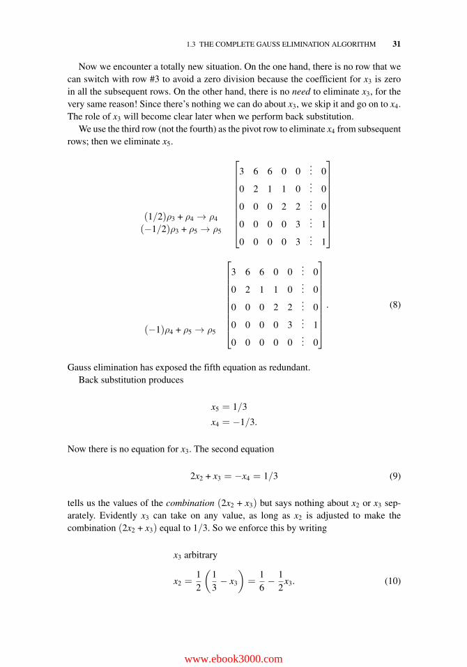
Now we encounter a totally new situation. On the one hand, there is no row that wecan switch with row #3 to avoid a zero division because the coefficient for x3 is zeroin all the subsequent rows. On the other hand, there is no need to eliminate x3, for thevery same reason! Since there’s nothing we can do about x3, we skip it and go on to x4.The role of x3 will become clear later when we perform back substitution.
We use the third row (not the fourth) as the pivot row to eliminate x4 from subsequentrows; then we eliminate x5.
(1/2)ρ3 + ρ4 → ρ4
(−1/2)ρ3 + ρ5 → ρ5
⎡⎢⎢⎢⎢⎢⎢⎢⎢⎢⎣
3 6 6 0 0... 0
0 2 1 1 0... 0
0 0 0 2 2... 0
0 0 0 0 3... 1
0 0 0 0 3... 1
⎤⎥⎥⎥⎥⎥⎥⎥⎥⎥⎦
(−1)ρ4 + ρ5 → ρ5
⎡⎢⎢⎢⎢⎢⎢⎢⎢⎢⎣
3 6 6 0 0... 0
0 2 1 1 0... 0
0 0 0 2 2... 0
0 0 0 0 3... 1
0 0 0 0 0... 0
⎤⎥⎥⎥⎥⎥⎥⎥⎥⎥⎦
. (8)
Gauss elimination has exposed the fifth equation as redundant.Back substitution produces
x5 = 1/3
x4 = −1/3.
Now there is no equation for x3. The second equation
2x2 + x3 = −x4 = 1/3 (9)
tells us the values of the combination (2x2 + x3) but says nothing about x2 or x3 sep-arately. Evidently x3 can take on any value, as long as x2 is adjusted to make thecombination (2x2 + x3) equal to 1/3. So we enforce this by writing
x3 arbitrary
x2 =12
(13− x3
)=
16− 1
2x3. (10)
www.ebook3000.com
32 SYSTEMS OF LINEAR ALGEBRAIC EQUATIONS
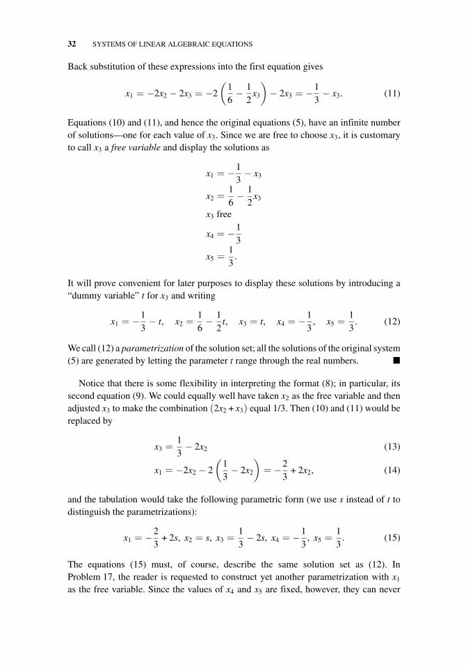
Back substitution of these expressions into the first equation gives
x1 = −2x2 − 2x3 = −2
(16− 1
2x3
)− 2x3 = −1
3− x3. (11)
Equations (10) and (11), and hence the original equations (5), have an infinite numberof solutions—one for each value of x3. Since we are free to choose x3, it is customaryto call x3 a free variable and display the solutions as
x1 = −13− x3
x2 =16− 1
2x3
x3 free
x4 = −13
x5 =13
.
It will prove convenient for later purposes to display these solutions by introducing a“dummy variable” t for x3 and writing
x1 = −13− t, x2 =
16− 1
2t, x3 = t, x4 = −1
3, x5 =
13
. (12)
We call (12) a parametrization of the solution set; all the solutions of the original system(5) are generated by letting the parameter t range through the real numbers. �
Notice that there is some flexibility in interpreting the format (8); in particular, itssecond equation (9). We could equally well have taken x2 as the free variable and thenadjusted x3 to make the combination (2x2 + x3) equal 1/3. Then (10) and (11) would bereplaced by
x3 =13− 2x2 (13)
x1 = −2x2 − 2
(13− 2x2
)= −2
3+ 2x2, (14)
and the tabulation would take the following parametric form (we use s instead of t todistinguish the parametrizations):
x1 = −23
+ 2s, x2 = s, x3 =13− 2s, x4 = −1
3, x5 =
13
. (15)
The equations (15) must, of course, describe the same solution set as (12). InProblem 17, the reader is requested to construct yet another parametrization with x1
as the free variable. Since the values of x4 and x5 are fixed, however, they can never
1.3 THE COMPLETE GAUSS ELIMINATION ALGORITHM 33
serve as free variables. (Problem 18 addresses the question of how one can deter-mine, in general, whether or not two different parameterizations describe the samesolution set.)
We summarize the considerations of this section, so far, as follows: when a variableis eliminated “prematurely” in the forward part of the Gauss procedure, it becomes afree variable in the solution set. Unless the system is inconsistent, the solution set willbe infinite.
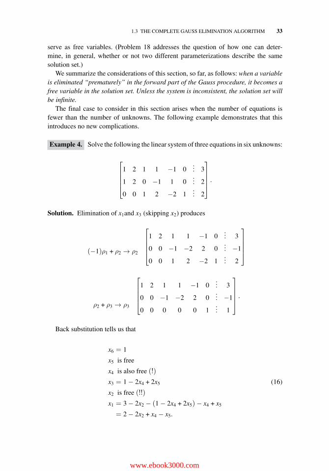
The final case to consider in this section arises when the number of equations isfewer than the number of unknowns. The following example demonstrates that thisintroduces no new complications.
Example 4. Solve the following the linear system of three equations in six unknowns:
⎡⎢⎢⎢⎣
1 2 1 1 −1 0... 3
1 2 0 −1 1 0... 2
0 0 1 2 −2 1... 2
⎤⎥⎥⎥⎦ .
Solution. Elimination of x1and x3 (skipping x2) produces
(−1)ρ1 + ρ2 → ρ2
⎡⎢⎢⎢⎣
1 2 1 1 −1 0... 3
0 0 −1 −2 2 0... −1
0 0 1 2 −2 1... 2
⎤⎥⎥⎥⎦
ρ2 + ρ3 → ρ3
⎡⎢⎢⎢⎣
1 2 1 1 −1 0... 3
0 0 −1 −2 2 0... −1
0 0 0 0 0 1... 1
⎤⎥⎥⎥⎦ .
Back substitution tells us that
x6 = 1
x5 is free
x4 is also free (!)
x3 = 1 − 2x4 + 2x5 (16)
x2 is free (!!)
x1 = 3 − 2x2 − (1 − 2x4 + 2x5)− x4 + x5
= 2 − 2x2 + x4 − x5.
www.ebook3000.com
34 SYSTEMS OF LINEAR ALGEBRAIC EQUATIONS
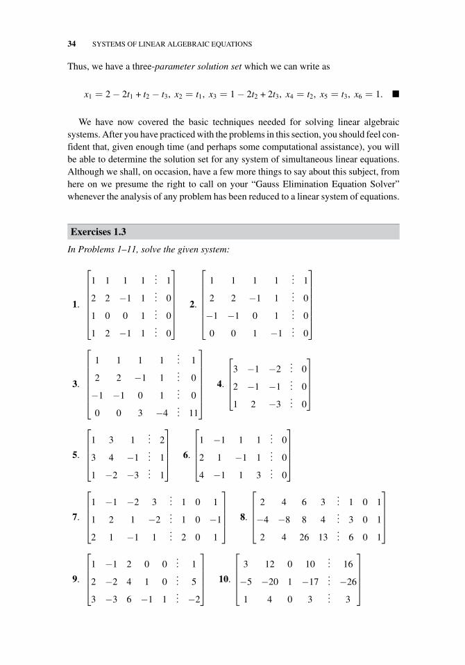
Thus, we have a three-parameter solution set which we can write as
x1 = 2 − 2t1 + t2 − t3, x2 = t1, x3 = 1 − 2t2 + 2t3, x4 = t2, x5 = t3, x6 = 1. �
We have now covered the basic techniques needed for solving linear algebraicsystems. After you have practiced with the problems in this section, you should feel con-fident that, given enough time (and perhaps some computational assistance), you willbe able to determine the solution set for any system of simultaneous linear equations.Although we shall, on occasion, have a few more things to say about this subject, fromhere on we presume the right to call on your “Gauss Elimination Equation Solver”whenever the analysis of any problem has been reduced to a linear system of equations.
Exercises 1.3
In Problems 1–11, solve the given system:
1.
⎡⎢⎢⎢⎢⎢⎢⎣
1 1 1 1... 1
2 2 −1 1... 0
1 0 0 1... 0
1 2 −1 1... 0
⎤⎥⎥⎥⎥⎥⎥⎦
2.
⎡⎢⎢⎢⎢⎢⎢⎣
1 1 1 1... 1
2 2 −1 1... 0
−1 −1 0 1... 0
0 0 1 −1... 0
⎤⎥⎥⎥⎥⎥⎥⎦
3.
⎡⎢⎢⎢⎢⎢⎢⎣
1 1 1 1... 1
2 2 −1 1... 0
−1 −1 0 1... 0
0 0 3 −4... 11
⎤⎥⎥⎥⎥⎥⎥⎦
4.
⎡⎢⎢⎢⎣
3 −1 −2... 0
2 −1 −1... 0
1 2 −3... 0
⎤⎥⎥⎥⎦
5.
⎡⎢⎢⎢⎣
1 3 1... 2
3 4 −1... 1
1 −2 −3... 1
⎤⎥⎥⎥⎦ 6.
⎡⎢⎢⎢⎣
1 −1 1 1... 0
2 1 −1 1... 0
4 −1 1 3... 0
⎤⎥⎥⎥⎦
7.
⎡⎢⎢⎢⎣
1 −1 −2 3... 1 0 1
1 2 1 −2... 1 0 −1
2 1 −1 1... 2 0 1
⎤⎥⎥⎥⎦ 8.
⎡⎢⎢⎢⎣
2 4 6 3... 1 0 1
−4 −8 8 4... 3 0 1
2 4 26 13... 6 0 1
⎤⎥⎥⎥⎦
9.
⎡⎢⎢⎢⎣
1 −1 2 0 0... 1
2 −2 4 1 0... 5
3 −3 6 −1 1... −2
⎤⎥⎥⎥⎦ 10.
⎡⎢⎢⎢⎣
3 12 0 10... 16
−5 −20 1 −17... −26
1 4 0 3... 3
⎤⎥⎥⎥⎦
1.3 THE COMPLETE GAUSS ELIMINATION ALGORITHM 35
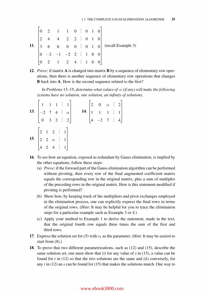
11.
⎡⎢⎢⎢⎢⎢⎢⎢⎢⎢⎣
0 2 1 1 0... 0 1 0
2 4 4 2 2... 0 1 0
3 6 6 0 0... 0 1 0
0 −2 −1 −2 2... 1 0 0
0 2 1 2 4... 1 0 0
⎤⎥⎥⎥⎥⎥⎥⎥⎥⎥⎦
(recall Example 3)
12. Prove: if matrix A is changed into matrix B by a sequence of elementary row oper-ations, then there is another sequence of elementary row operations that changesB back into A. How is the second sequence related to the first?
In Problems 13–15, determine what values of α (if any) will make the followingsystems have no solution, one solution, an infinity of solutions.
13.
⎡⎢⎢⎢⎣
1 1 1... 1
−2 7 4... α
0 3 2... 2
⎤⎥⎥⎥⎦ 14.
⎡⎢⎢⎢⎣
2 0 α... 2
1 1 1... 1
4 −2 7... 4
⎤⎥⎥⎥⎦
15.
⎡⎢⎢⎢⎣
2 1 2... 1
2 2 α... 1
4 2 4... 1
⎤⎥⎥⎥⎦
16. To see how an equation, exposed as redundant by Gauss elimination, is implied bythe other equations, follow these steps:(a) Prove: if the forward part of the Gauss elimination algorithm can be performed
without pivoting, then every row of the final augmented coefficient matrixequals the corresponding row in the original matrix, plus a sum of multiplesof the preceding rows in the original matrix. How is this statement modified ifpivoting is performed?
(b) Show how, by keeping track of the multipliers and pivot exchanges employedin the elimination process, one can explicitly express the final rows in termsof the original rows. (Hint: It may be helpful for you to trace the eliminationsteps for a particular example such as Example 3 or 4.)
(c) Apply your method to Example 1 to derive the statement, made in the text,that the original fourth row equals three times the sum of the first andthird rows.
17. Express the solution set for (5) with x1 as the parameter. (Hint: It may be easiest tostart from (8).)
18. To prove that two different parametrizations, such as (12) and (15), describe thesame solution set, one must show that (i) for any value of s in (15), a value can befound for t in (12) so that the two solutions are the same and (ii) conversely, forany t in (12) an s can be found for (15) that makes the solutions match. One way to
www.ebook3000.com
36 SYSTEMS OF LINEAR ALGEBRAIC EQUATIONS
do this is to consider the system formed by equating the corresponding parametricexpressions for each variable.
−1/3 − t = −2/3 + 2s
1/6 − t/2 = s
−1/3 = −1/3
1/3 = 1/3
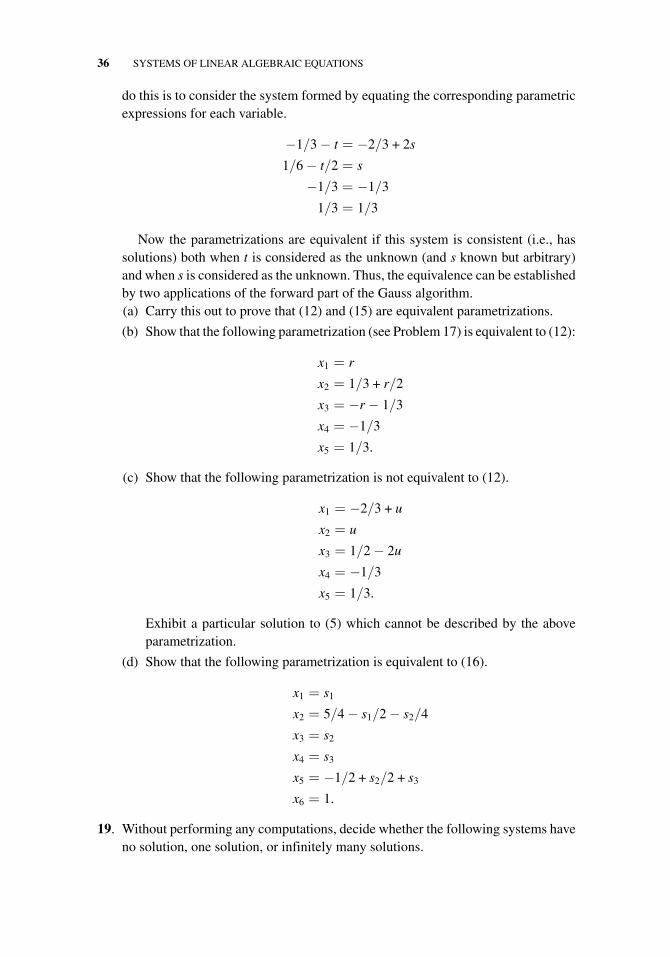
Now the parametrizations are equivalent if this system is consistent (i.e., hassolutions) both when t is considered as the unknown (and s known but arbitrary)and when s is considered as the unknown. Thus, the equivalence can be establishedby two applications of the forward part of the Gauss algorithm.(a) Carry this out to prove that (12) and (15) are equivalent parametrizations.
(b) Show that the following parametrization (see Problem 17) is equivalent to (12):
x1 = r
x2 = 1/3 + r/2
x3 = −r − 1/3
x4 = −1/3
x5 = 1/3.
(c) Show that the following parametrization is not equivalent to (12).
x1 = −2/3 + u
x2 = u
x3 = 1/2 − 2u
x4 = −1/3
x5 = 1/3.
Exhibit a particular solution to (5) which cannot be described by the aboveparametrization.
(d) Show that the following parametrization is equivalent to (16).
x1 = s1
x2 = 5/4 − s1/2 − s2/4
x3 = s2
x4 = s3
x5 = −1/2 + s2/2 + s3
x6 = 1.
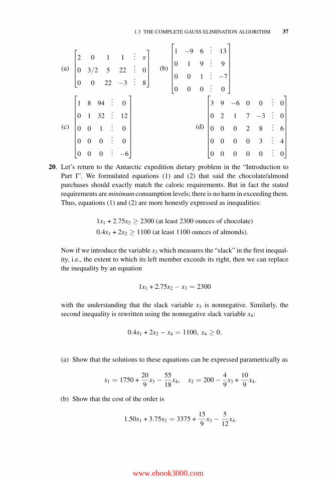
19. Without performing any computations, decide whether the following systems haveno solution, one solution, or infinitely many solutions.
1.3 THE COMPLETE GAUSS ELIMINATION ALGORITHM 37
(a)
⎡⎢⎢⎢⎣
2 0 1 1... π
0 3/2 5 22... 0
0 0 22 −3... 8
⎤⎥⎥⎥⎦ (b)
⎡⎢⎢⎢⎢⎢⎢⎣
1 −9 6... 13
0 1 9... 9
0 0 1... −7
0 0 0... 0
⎤⎥⎥⎥⎥⎥⎥⎦
(c)
⎡⎢⎢⎢⎢⎢⎢⎢⎢⎢⎣
1 8 94... 0
0 1 32... 12
0 0 1... 0
0 0 0... 0
0 0 0... −6
⎤⎥⎥⎥⎥⎥⎥⎥⎥⎥⎦
(d)
⎡⎢⎢⎢⎢⎢⎢⎢⎢⎢⎣
3 9 −6 0 0... 0
0 2 1 7 −3... 0
0 0 0 2 8... 6
0 0 0 0 3... 4
0 0 0 0 0... 0
⎤⎥⎥⎥⎥⎥⎥⎥⎥⎥⎦
20. Let’s return to the Antarctic expedition dietary problem in the “Introduction toPart I”. We formulated equations (1) and (2) that said the chocolate/almondpurchases should exactly match the caloric requirements. But in fact the statedrequirements are minimum consumption levels; there is no harm in exceeding them.Thus, equations (1) and (2) are more honestly expressed as inequalities:
1x1 + 2.75x2 ≥ 2300 (at least 2300 ounces of chocolate)
0.4x1 + 2x2 ≥ 1100 (at least 1100 ounces of almonds).
Now if we introduce the variable x3 which measures the “slack” in the first inequal-ity, i.e., the extent to which its left member exceeds its right, then we can replacethe inequality by an equation
1x1 + 2.75x2 − x3 = 2300
with the understanding that the slack variable x3 is nonnegative. Similarly, thesecond inequality is rewritten using the nonnegative slack variable x4:
0.4x1 + 2x2 − x4 = 1100, x4 ≥ 0.
(a) Show that the solutions to these equations can be expressed parametrically as
x1 = 1750 +209
x3 −5518
x4, x2 = 200 − 49
x3 +109
x4.
(b) Show that the cost of the order is
1.50x1 + 3.75x2 = 3375 +159
x3 −512
x4.
www.ebook3000.com
38 SYSTEMS OF LINEAR ALGEBRAIC EQUATIONS
(c) Keeping in mind that the slack variables x3 and x4 must be nonnegative, arguethat the cost can be decreased by choosing x3 = 0 and making x4 as largeas possible. Since the purchases x1 and x2 cannot be negative, the parametricequation for x1 limits x4. Show that the minimum cost is $3136.36 (rounded tocents), in accordance with the comment in the “Introduction to Part I”.
1.4 ECHELON FORM AND RANK
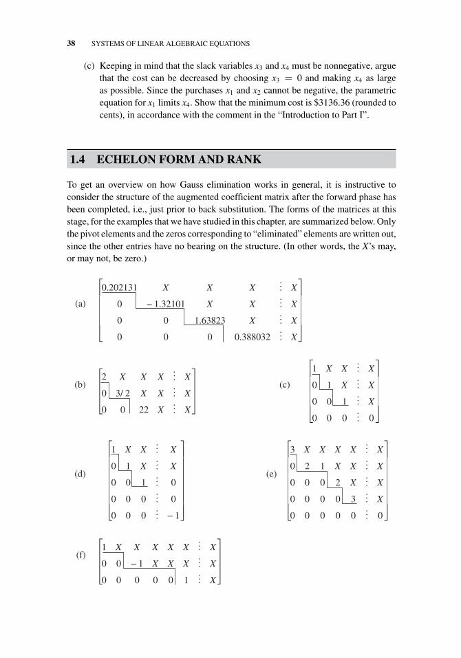
To get an overview on how Gauss elimination works in general, it is instructive toconsider the structure of the augmented coefficient matrix after the forward phase hasbeen completed, i.e., just prior to back substitution. The forms of the matrices at thisstage, for the examples that we have studied in this chapter, are summarized below. Onlythe pivot elements and the zeros corresponding to “eliminated” elements are written out,since the other entries have no bearing on the structure. (In other words, the X’s may,or may not, be zero.)
(a)
0.202131 X X X... X
0 − 1.32101 X X... X
0 0 1.63823 X... X
0 0 0 0.388032... X
(b)2 X X X
... X
0 3/ 2 X X... X
0 0 22 X... X
(c)
1 X X... X
0 1 X... X
0 0 1... X
0 0 0... 0
(d)
1 X X... X
0 1 X... X
0 0 1... 0
0 0 0... 0
0 0 0... − 1
(e)
3 X X X X... X
0 2 1 X X... X
0 0 0 2 X... X
0 0 0 0 3... X
0 0 0 0 0... 0
(f)1 X X X X X
... X
0 0 − 1 X X X... X
0 0 0 0 0 1... X
1.4 ECHELON FORM AND RANK 39
The first matrix displays the form when there are no “complications”—same numberof equations as unknowns, no zero pivots. The coefficient submatrix is upper triangu-lar and the augmented matrix is upper trapezoidal. However, the subsequent examplesreveal that the arrangement will be more complicated than this, in general. Ignoring theright-hand sides, we see that the zero entries of the coefficient matrix exhibit a staircase,or echelon, structure, with the steps occurring at the pivot elements.
Row-Echelon Form
Definition 5. Let A be an m-by-n matrix with the following property: startingfrom the second row, the first nonzero entry in each row lies to the right of the firstnonzero entry in the preceding row. Then A is said to be a row-echelon matrix,or a matrix in row-echelon form.6
Note that all the coefficient matrices that appear in (a) through (f) above are in row-echelon form and so are the augmented matrices except for (d). Indeed, one more rowswitch will bring (d) into conformity:
(d′)
⎡⎢⎢⎢⎢⎢⎢⎢⎢⎢⎣
1 X X... X
0 1 X... X
0 0 1... 0
0 0 0... −1
0 0 0... 0
⎤⎥⎥⎥⎥⎥⎥⎥⎥⎥⎦
Using the concept of row-echelon form, we summarize our equation-solving proce-dure as follows.
Synopsis of the Gauss Elimination Algorithm
In the forward part of the algorithm, elementary row operations are performedon the augmented coefficient matrix to reduce the coefficient submatrix to row-echelon form. Within the (resulting) coefficient submatrix, the first nonzero entryin each row is a pivot element and its corresponding variable is labeled a pivotvariable; all other variables are free variables. The rows of the augmented matrixthat state 0 = 0 are ignored. If any row states 0 = c and c is nonzero, the sys-tem is inconsistent. Otherwise one proceeds with back substitution, solving the
6The corresponding form for the Gauss- Jordan algorithm is often called the row-reduced echelon form.It differs from row-echelon form in that the entries above, as well as below, the first nonzero entry in eachrow are zero, and this nonzero entry is 1.
www.ebook3000.com
40 SYSTEMS OF LINEAR ALGEBRAIC EQUATIONS
equations in succession from the last to the first and expressing the pivot variablesin terms of the free variables.
For future reference, we record some useful facts that arise as “spinoffs” of the Gaussprocess. Theorem 2 summarizes our deliberations to this point.
Reduction to Row-Echelon Form
Theorem 2. Any matrix can be reduced to row-echelon form7 by a sequence ofelementary row operations.
Rank of Row-Echelon Matrices
Definition 6. If a matrix is in row-echelon form, we say that its rank equals thenumber of nonzero rows.8
Note that rank of a row-echelon matrix cannot exceed the number of its columns.Suppose that a linear system of equations with coefficient matrix A is represented by
the augmented matrix [A|b] and let [Aech|b′] denote the resulting row-echelon matrixafter appropriate row operations have been performed on the original (augmented)matrix. From the ranks of [Aech|b′] and Aech, we can glean some important informationabout the numbers of solutions for the system. For example, the inconsistency of thesystem (d′) can be attributed to the fact that after reduction to row-echelon form therank of the augmented matrix exceeds the rank of the coefficient matrix.
Furthermore, generalizing from the matrices in (a) and (c), we observe that if a sys-tem is consistent, it has a unique solution if the number of columns of Aech (i.e., thenumber of unknowns) equals its rank; in this case we say the coefficient matrix Aech hasfull rank. (See, for example, the matrices (a) and (c).) But the matrices in (b), (e), and(f) demonstrate that if the system is consistent, it has an infinite number of solutionswhenever the number of columns of Aech exceeds its rank. To summarize:
Characterization of Number of Solutions of a Linear System by Rank
Theorem 3. For a system of linear equations represented by the augmentedmatrix [A|b], let [Aech|b′] be an echelon form resulting from applying elementaryrow operations to [A|b].
7Or row-reduced echelon form.8In Section 3.3, we will generalize this definition to all matrices.
1.4 ECHELON FORM AND RANK 41
• If the rank of [Aech|b′] exceeds the rank of Aech, the linear system isinconsistent (has no solutions).
• If the ranks of [Aech|b′] and Aech are equal, then the linear system isconsistent, having
(i) exactly one solution when the (common) rank equals the number ofunknowns (which is the same as the number of columns of Aech);
(ii) infinitely many solutions if the (common) rank is less than thenumber of unknowns.
Example 1. A linear system of equations in x1, x2, x3, x4, and x5 is represented bythe augmented coefficient matrix
⎡⎢⎢⎢⎢⎢⎢⎣
3 9 −6 0 0... 1
0 2 7 8 3... 5
0 0 0 2 6... 9
0 0 0 0 0... 0
⎤⎥⎥⎥⎥⎥⎥⎦
. (1)
Verify that
# columns Aech = rank [Aech|b′] + # free parameters (2)
(the last term is the number of free parameters in the solution set).
Solution. The number of nonzero rows in (1) is clearly 3; so 3 is the rank. Back substi-tution would dictate that x5 is free, x4 is not, x3 is free, and x2 and x1 are not; the numberof free parameters is 2. Therefore, the right-hand member of (2) is 3 + 2 = 5, which isthe number of columns of Aech. �
In fact, equation (2) holds for all consistent systems in row-echelon form.(See Problem 16.) Section 3.3 will establish an important generalization of thisequation.
A useful spinoff of Theorem 3 occurs when the system is homogeneous, in accor-dance with the following:
www.ebook3000.com
42 SYSTEMS OF LINEAR ALGEBRAIC EQUATIONS
Linear Homogeneous System
Definition 7. A system of m equations in n unknowns that can be put in the form
a11x1 + a12x2+ · · · + a1nxn = 0
a21x1 + a22x2+ · · · + a2nxn = 0...
am1x1 + am2x2+ · · · + amnxn = 0,
(3)
where the right-hand sides are all zero, is called a linear homogeneous system.9
In two (three) dimensions, a linear homogeneous system represents lines (planes)passing through the origin.
The augmented matrix notation for a homogeneous system with coefficient matrixA is [A | 0]. Notice that a homogeneous system is always consistent since its solution(s)include x1 = x2 = · · · = xn = 0, the zero solution (or “trivial solution”). Therefore,part (ii) of Theorem 3 guarantees the following:
Corollary 1. A linear homogeneous system containing fewer equations thanunknowns has an infinite number of solutions.
Exercises 1.4
In Problems 1–6, determine whether the given matrix is in row-echelon form. If so,determine its rank.
1.
⎡⎣0 1 3
0 0 00 0 0
⎤⎦ 2.
⎡⎣2 0 0
0 0 00 0 1
⎤⎦ 3.
⎡⎣4 6 3 1
0 0 1 00 0 0 1
⎤⎦ 4.
⎡⎣0 3 0 0
1 0 0 00 0 0 0
⎤⎦
5.
[2 0 1 80 1 2 3
]6.
⎡⎣3 0
0 10 0
⎤⎦
In Problems 7–12, an augmented matrix [A | b] for a linear system with coef-ficient matrix A is given. Determine whether the system is consistent and, if so,whether the system has a unique solution or infinitely many solutions.
7.
⎡⎣4 0 9
... 1
0 0 3... 0
⎤⎦ 8.
⎡⎣0 1 5
... 0
0 0 2... 3
⎤⎦ 9.
⎡⎢⎢⎢⎣
0 8 7... 4
0 0 0... 0
0 0 0... 0
⎤⎥⎥⎥⎦
9Otherwise the system is said to be nonhomogeneous.
1.4 ECHELON FORM AND RANK 43
10.
⎡⎢⎢⎢⎣
2 3 8... 9
0 1 5... 2
0 0 0... 4
⎤⎥⎥⎥⎦
11.
⎡⎢⎢⎢⎢⎢⎢⎣
1 4 9 2... 0
0 3 6 9... 1
0 0 4 4... 2
0 0 0 1... 0
⎤⎥⎥⎥⎥⎥⎥⎦
12.
⎡⎢⎢⎢⎢⎢⎢⎣
2 3... 9
0 8... 2
0 0... 0
0 0... 0
⎤⎥⎥⎥⎥⎥⎥⎦
13. For what values of α will the following homogeneous systems have nontrivialsolutions?
(a)2x1 + 5x2+αx3 = 0x1 − 6x2+ x3 = 0
(b)x1 + x2+ x3 = 0αx1+ 4x2+ 3x3 = 04x1+ 3x2+ 2x3 = 0
14. Show that the homogeneous system
a11x1 + a12x2 = 0a21x1 + a22x2 = 0
has infinitely many solutions if and only if a11a22 − a12a21 = 0.
15. For the systems of equations represented by the given augmented matrices, verifythat equation (2) holds.
(a)
⎡⎢⎢⎢⎣
1 2 3... 0
0 5 6... 1
0 0 7... 2
⎤⎥⎥⎥⎦ (b)
⎡⎢⎢⎢⎣
3 5 0 0 0 1... 2
0 0 1 3 2 5... 0
0 0 0 0 0 1... 2
⎤⎥⎥⎥⎦
(c)
⎡⎢⎢⎢⎣
3 0 1 0 0 0... 2
0 0 1 0 0 5... 0
0 0 0 0 0 1... 2
⎤⎥⎥⎥⎦
16. Prove that if [Aech|b] is any consistent system, then equation (2) holds.
Problems 17–22 involve the sum or difference of two n-by-1 column matrices aswell as the scalar multiple of a column vector. Recall from calculus that
⎡⎢⎢⎢⎣
x1
x2...xn
⎤⎥⎥⎥⎦±
⎡⎢⎢⎢⎣
y1
y2...yn
⎤⎥⎥⎥⎦ =
⎡⎢⎢⎢⎣
x1 ± y1
x2 ± y2...xn ± yn
⎤⎥⎥⎥⎦ and c
⎡⎢⎢⎢⎣
x1
x2...xn
⎤⎥⎥⎥⎦ =
⎡⎢⎢⎢⎣
cx1
cx2...cxn
⎤⎥⎥⎥⎦ .
17. If A is an m-by-n matrix and x and y are each n-by-1 column vector solutions tothe homogeneous system [A | 0], show that x ± y is also a solution.
www.ebook3000.com
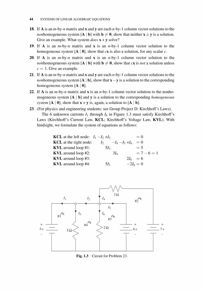
44 SYSTEMS OF LINEAR ALGEBRAIC EQUATIONS
18. If A is an m-by-n matrix and x and y are each n-by-1 column vector solutions to thenonhomogeneous system [A | b] with b �= 0, show that neither x± y is a solution.Give an example. What system does x + y solve?
19. If A is an m-by-n matrix and x is an n-by-1 column vector solution to thehomogeneous system [A | 0], show that cx is also a solution, for any scalar c.
20. If A is an m-by-n matrix and x is an n-by-1 column vector solution to thenonhomogeneous system [A | b] with b �= 0, show that cx is not a solution unlessc = 1. Give an example.
21. If A is an m-by-n matrix and x and y are each n-by-1 column vector solutions to thenonhomogeneous system [A | b], show that x−y is a solution to the correspondinghomogeneous system [A | 0].
22. If A is an m-by-n matrix and x is an n-by-1 column vector solution to the nonho-mogeneous system [A | b] and y is a solution to the corresponding homogeneoussystem [A | 0], show that x + y is, again, a solution to [A | b].
23. (For physics and engineering students: see Group Project D: Kirchhoff’s Laws).The 6 unknown currents I1 through I6 in Figure 1.3 must satisfy Kirchhoff’s
Laws (Kirchhoff’s Current Law, KCL; Kirchhoff’s Voltage Law, KVL). Withhindsight, we formulate the system of equations as follows:
KCL at the left node: I1 −I2 +I3 = 0KCL at the right node: I2 −I4 −I5 +I6 = 0KVL around loop #1: 5I3 = 5KVL around loop #2: 3I4 = 7 − 6 = 1KVL around loop #3: 2I6 = 6KVL around loop #4: 5I3 −2I6 = 0
+5 v
#1
#4
#3
#2I1 I2 I4
I3 I6
I5
5 Ω2 Ω
3 Ω
–
+6 v–
+7 v–
Fig. 1.3 Circuit for Problem 23.
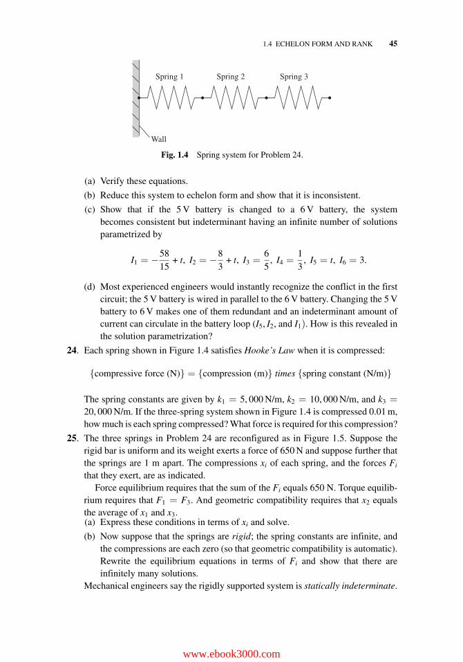
1.4 ECHELON FORM AND RANK 45
Wall
Spring 1 Spring 2 Spring 3
Fig. 1.4 Spring system for Problem 24.
(a) Verify these equations.
(b) Reduce this system to echelon form and show that it is inconsistent.
(c) Show that if the 5 V battery is changed to a 6 V battery, the systembecomes consistent but indeterminant having an infinite number of solutionsparametrized by
I1 = −5815
+ t, I2 = −83
+ t, I3 =65
, I4 =13
, I5 = t, I6 = 3.
(d) Most experienced engineers would instantly recognize the conflict in the firstcircuit; the 5 V battery is wired in parallel to the 6 V battery. Changing the 5 Vbattery to 6 V makes one of them redundant and an indeterminant amount ofcurrent can circulate in the battery loop (I5, I2, and I1). How is this revealed inthe solution parametrization?
24. Each spring shown in Figure 1.4 satisfies Hooke’s Law when it is compressed:
{compressive force (N)} = {compression (m)} times {spring constant (N/m)}
The spring constants are given by k1 = 5, 000 N/m, k2 = 10, 000 N/m, and k3 =20, 000 N/m. If the three-spring system shown in Figure 1.4 is compressed 0.01 m,how much is each spring compressed? What force is required for this compression?
25. The three springs in Problem 24 are reconfigured as in Figure 1.5. Suppose therigid bar is uniform and its weight exerts a force of 650 N and suppose further thatthe springs are 1 m apart. The compressions xi of each spring, and the forces Fi
that they exert, are as indicated.Force equilibrium requires that the sum of the Fi equals 650 N. Torque equilib-
rium requires that F1 = F3. And geometric compatibility requires that x2 equalsthe average of x1 and x3.(a) Express these conditions in terms of xi and solve.
(b) Now suppose that the springs are rigid; the spring constants are infinite, andthe compressions are each zero (so that geometric compatibility is automatic).Rewrite the equilibrium equations in terms of Fi and show that there areinfinitely many solutions.
Mechanical engineers say the rigidly supported system is statically indeterminate.
www.ebook3000.com
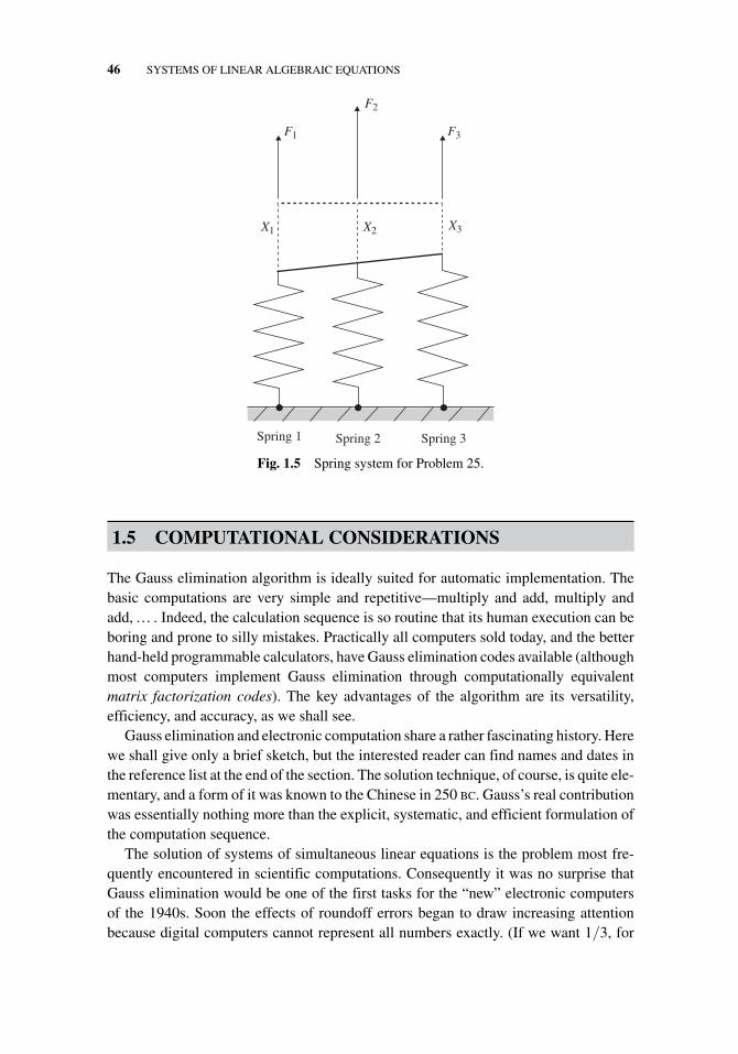
46 SYSTEMS OF LINEAR ALGEBRAIC EQUATIONS
Spring 1 Spring 2 Spring 3
X3X2X1
F1 F3
F2
Fig. 1.5 Spring system for Problem 25.
1.5 COMPUTATIONAL CONSIDERATIONS
The Gauss elimination algorithm is ideally suited for automatic implementation. Thebasic computations are very simple and repetitive—multiply and add, multiply andadd, … . Indeed, the calculation sequence is so routine that its human execution can beboring and prone to silly mistakes. Practically all computers sold today, and the betterhand-held programmable calculators, have Gauss elimination codes available (althoughmost computers implement Gauss elimination through computationally equivalentmatrix factorization codes). The key advantages of the algorithm are its versatility,efficiency, and accuracy, as we shall see.
Gauss elimination and electronic computation share a rather fascinating history. Herewe shall give only a brief sketch, but the interested reader can find names and dates inthe reference list at the end of the section. The solution technique, of course, is quite ele-mentary, and a form of it was known to the Chinese in 250 BC. Gauss’s real contributionwas essentially nothing more than the explicit, systematic, and efficient formulation ofthe computation sequence.
The solution of systems of simultaneous linear equations is the problem most fre-quently encountered in scientific computations. Consequently it was no surprise thatGauss elimination would be one of the first tasks for the “new” electronic computersof the 1940s. Soon the effects of roundoff errors began to draw increasing attentionbecause digital computers cannot represent all numbers exactly. (If we want 1/3, for
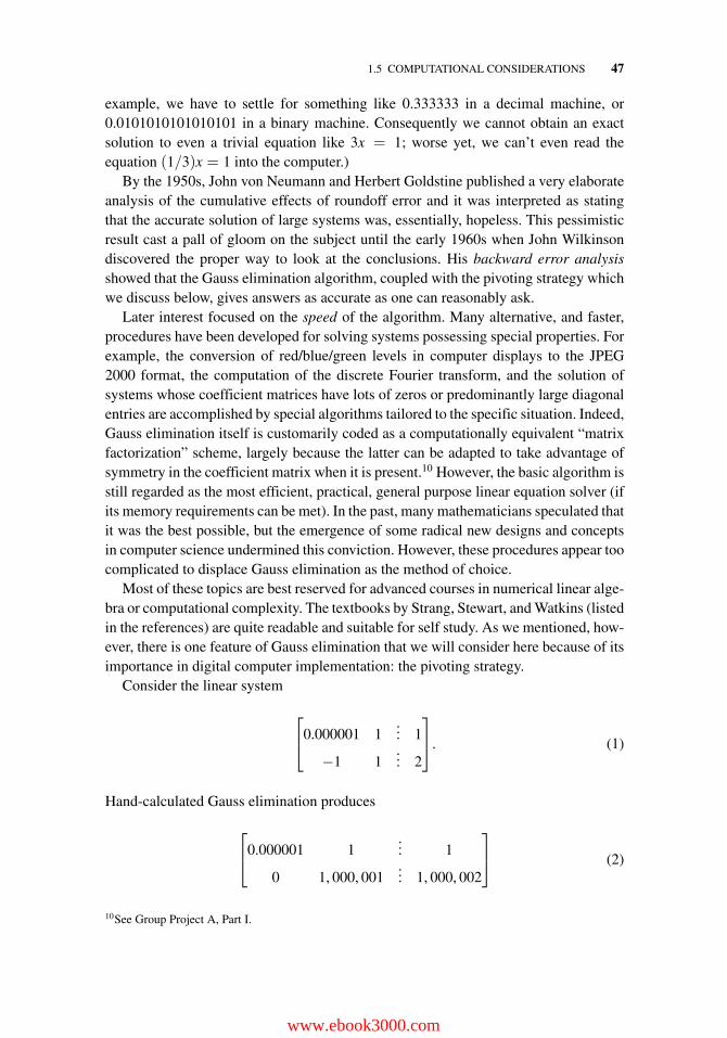
1.5 COMPUTATIONAL CONSIDERATIONS 47
example, we have to settle for something like 0.333333 in a decimal machine, or0.0101010101010101 in a binary machine. Consequently we cannot obtain an exactsolution to even a trivial equation like 3x = 1; worse yet, we can’t even read theequation (1/3)x = 1 into the computer.)
By the 1950s, John von Neumann and Herbert Goldstine published a very elaborateanalysis of the cumulative effects of roundoff error and it was interpreted as statingthat the accurate solution of large systems was, essentially, hopeless. This pessimisticresult cast a pall of gloom on the subject until the early 1960s when John Wilkinsondiscovered the proper way to look at the conclusions. His backward error analysisshowed that the Gauss elimination algorithm, coupled with the pivoting strategy whichwe discuss below, gives answers as accurate as one can reasonably ask.
Later interest focused on the speed of the algorithm. Many alternative, and faster,procedures have been developed for solving systems possessing special properties. Forexample, the conversion of red/blue/green levels in computer displays to the JPEG2000 format, the computation of the discrete Fourier transform, and the solution ofsystems whose coefficient matrices have lots of zeros or predominantly large diagonalentries are accomplished by special algorithms tailored to the specific situation. Indeed,Gauss elimination itself is customarily coded as a computationally equivalent “matrixfactorization” scheme, largely because the latter can be adapted to take advantage ofsymmetry in the coefficient matrix when it is present.10 However, the basic algorithm isstill regarded as the most efficient, practical, general purpose linear equation solver (ifits memory requirements can be met). In the past, many mathematicians speculated thatit was the best possible, but the emergence of some radical new designs and conceptsin computer science undermined this conviction. However, these procedures appear toocomplicated to displace Gauss elimination as the method of choice.
Most of these topics are best reserved for advanced courses in numerical linear alge-bra or computational complexity. The textbooks by Strang, Stewart, and Watkins (listedin the references) are quite readable and suitable for self study. As we mentioned, how-ever, there is one feature of Gauss elimination that we will consider here because of itsimportance in digital computer implementation: the pivoting strategy.
Consider the linear system
⎡⎣0.000001 1
... 1
−1 1... 2
⎤⎦. (1)
Hand-calculated Gauss elimination produces
⎡⎣0.000001 1
... 1
0 1, 000, 001... 1, 000, 002
⎤⎦ (2)
10See Group Project A, Part I.
www.ebook3000.com
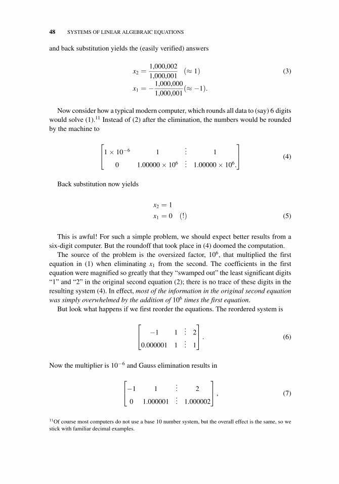
48 SYSTEMS OF LINEAR ALGEBRAIC EQUATIONS
and back substitution yields the (easily verified) answers
x2 =1,000,0021,000,001
(≈ 1) (3)
x1 = −1,000,0001,000,001
(≈ −1).
Now consider how a typical modern computer, which rounds all data to (say) 6 digitswould solve (1).11 Instead of (2) after the elimination, the numbers would be roundedby the machine to
⎡⎣1 × 10⁻⁶ 1
... 1
0 1.00000 × 10⁶... 1.00000 × 10⁶.
⎤⎦ (4)
Back substitution now yields
x2 = 1
x1 = 0 (!) (5)
This is awful! For such a simple problem, we should expect better results from asix-digit computer. But the roundoff that took place in (4) doomed the computation.
The source of the problem is the oversized factor, 106, that multiplied the firstequation in (1) when eliminating x1 from the second. The coefficients in the firstequation were magnified so greatly that they “swamped out” the least significant digits“1” and “2” in the original second equation (2); there is no trace of these digits in theresulting system (4). In effect, most of the information in the original second equationwas simply overwhelmed by the addition of 106 times the first equation.
But look what happens if we first reorder the equations. The reordered system is
⎡⎣ −1 1
... 2
0.000001 1... 1
⎤⎦ . (6)
Now the multiplier is 10−6 and Gauss elimination results in
⎡⎣−1 1
... 2
0 1.000001... 1.000002
⎤⎦ , (7)
11Of course most computers do not use a base 10 number system, but the overall effect is the same, so westick with familiar decimal examples.
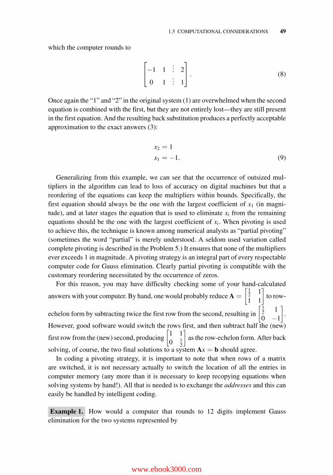
1.5 COMPUTATIONAL CONSIDERATIONS 49
which the computer rounds to
⎡⎣−1 1
... 2
0 1... 1
⎤⎦ . (8)
Once again the “1” and “2” in the original system (1) are overwhelmed when the secondequation is combined with the first, but they are not entirely lost—they are still presentin the first equation. And the resulting back substitution produces a perfectly acceptableapproximation to the exact answers (3):
x2 = 1
x1 = −1. (9)
Generalizing from this example, we can see that the occurrence of outsized mul-tipliers in the algorithm can lead to loss of accuracy on digital machines but that areordering of the equations can keep the multipliers within bounds. Specifically, thefirst equation should always be the one with the largest coefficient of x1 (in magni-tude), and at later stages the equation that is used to eliminate xi from the remainingequations should be the one with the largest coefficient of xi. When pivoting is usedto achieve this, the technique is known among numerical analysts as “partial pivoting”(sometimes the word “partial” is merely understood. A seldom used variation calledcomplete pivoting is described in the Problem 5.) It ensures that none of the multipliersever exceeds 1 in magnitude. A pivoting strategy is an integral part of every respectablecomputer code for Gauss elimination. Clearly partial pivoting is compatible with thecustomary reordering necessitated by the occurrence of zeros.
For this reason, you may have difficulty checking some of your hand-calculated
answers with your computer. By hand, one would probably reduce A =
[ 12 11 1
]to row-
echelon form by subtracting twice the first row from the second, resulting in
[ 12 10 −1
].
However, good software would switch the rows first, and then subtract half the (new)
first row from the (new) second, producing
[1 10 1
2
]as the row-echelon form. After back
solving, of course, the two final solutions to a system Ax = b should agree.In coding a pivoting strategy, it is important to note that when rows of a matrix
are switched, it is not necessary actually to switch the location of all the entries incomputer memory (any more than it is necessary to keep recopying equations whensolving systems by hand!). All that is needed is to exchange the addresses and this caneasily be handled by intelligent coding.
Example 1. How would a computer that rounds to 12 digits implement Gausselimination for the two systems represented by
www.ebook3000.com
50 SYSTEMS OF LINEAR ALGEBRAIC EQUATIONS
⎡⎣2 4/3
... 2 2
1 2/3... 1 2
⎤⎦? (10)
Solution. Before proceeding, notice that exact Gauss elimination shows that the firstsystem has an infinite number of solutions and the second has none:
⎡⎣2 4/3
... 2 2
0 0... 0 1
⎤⎦ . (11)
The original system (10), rounded to 12 digits, reads
⎡⎣2 1.333333333333
... 2 2
1 0.666666666667... 1 2
⎤⎦ . (12)
When the computer divides 1.3333333333 by 2 and retains 12 places, it gets0.666666666665. So subtracting half the first row from the second results in therow-echelon form
⎡⎣2 1.333333333333
... 2 2
0 2 × 10⁻¹²... 0 1
⎤⎦ . (13)
The computer concludes that the second equation is neither redundant nor inconsistent!With back substitution, we readily see that this sophisticated machine finds only
one of the infinite number of solutions of the consistent system and reports an absurdanswer for the inconsistent system. �
An intelligent numerical analyst, of course, would recognize the entry 2 × 10⁻¹² as“roundoff garbage” in (13) and reset this coefficient to zero before back substituting.For more complex systems, however, these decisions are not so transparent and a deeperunderstanding of the situation is necessary. Such matters are dealt with in specializedtexts.
Top-grade matrix computation software will alert the user if it encounters situationslike these, when the credibility of the computed answer should be scrutinized.
References on Computations
Of historical significance
1. Boyer, C.B. (1968). A History of Mathematics. Wiley, New York.
2. von Neumann, J. and Goldstine, H.H. (1947). Numerical inverting of matrices ofhigh order. Bull. Am. Math. Soc. 53, 1021–1099.
1.5 COMPUTATIONAL CONSIDERATIONS 51
3. Wilkinson, J.H. (1961). Error analysis of direct methods of matrix inversion. J.Assoc. Comput. Mach. 8, 281–330.
4. Strassen, V. (1969). Gauss elimination is not optimal. Numerische Mathematika13, 354–356.
Classic textbooks on numerical linear algebra5. Forsythe, G. and Moler, C.B. (1967). Computer Solution of Linear Algebraic
Systems. Prentice-Hall, Upper Saddle River, NJ.
6. Householder, A.S. (1964). The Theory of Matrices in Numerical Analysis. DoverPublications, Mineola, NY.
7. Stewart, G.W. (1973). Introduction to Matrix Computations. Elsevier, Amster-dam, Netherlands.
8. Strang, G. (1980). Linear Algebra and Its Applications (fourth edition).Wellesley-Cambridge Press, Wellesley, MA.
9. Wilkinson, J.H. (1965). The Algebraic Eigenvalue Problem. Oxford UniversityPress, London, UK.
Documentated computer codes10. Wilkinson, J.H. and Reinsch, C., eds. (1971). Handbook for Automatic Compu-
tation, Vol. II, Linear Algebra. Springer-Verlag, New York.
11. Dongarra, B., Moer, S. (1979). LINPACK. IMSL, Houston, TX.
Recent textbooks12. Golub, G.H. and van Loan, C.F. (2013). Matrix Computations (fourth edition).
The Johns Hopkins University Press, Baltimore, MD.
13. Higham, N.J. (2013). Accuracy and Stability of Numerical Algorithms (secondedition). Society for Industrial and Applied Mathematics, Philadelphia, PA.
14. Demmel, J. (1997). Applied Numerical Linear Algebra. Society for Industrial andApplied Mathematics, Philadelphia, PA.
15. Trefethen. L.N. and Bau, D. III (1997). Numerical Linear Algebra. Society forIndustrial and Applied Mathematics, Philadelphia, PA.
16. Watkins, D.S. Fundamentals of Matrix Computations (third edition). Wiley-Interscience, New York, 2010.
Exercises 1.5
1. With a calculator, simulate Gauss elimination as performed on a 4-digit machine,with and without partial pivoting, for the following system. Compare bothanswers with the exact solution: x1 = 10.00 and x2 = 1.000.
0.003000x1 + 59.14x2 = 59.17
5.291x1 − 6.130x2 = 46.78
www.ebook3000.com
52 SYSTEMS OF LINEAR ALGEBRAIC EQUATIONS
2. This problem analyzes pivoting from a theoretical, machine-free point of view.(a) Show that “symbolic” Gauss elimination generates the row-echelon form asshown:
⎡⎣ε 2
... 2
1 1... 2
⎤⎦ ⇒
⎡⎣ε 2
... 2
0 1 − 2ε
... 2 − 2ε
⎤⎦ , (14)
and derive the formula for the solution x = x(ε), y = y(ε). Show that as ε → 0 thesolutions tend to x = 1, y = 1.(b) Argue that on any finite-precision machine executing the algorithm without
pivoting, for sufficiently small ε, the computation indicated in (14) will berendered as
⎡⎣ε 2
... 2
1 1... 2
⎤⎦ ⇒
⎡⎣ε 2
... 2
0 1 − 2ε
... 2 − 2ε
⎤⎦ ⇒
⎡⎣ε 2
... 2
0 −2ε
... −2ε
⎤⎦ , (15)
resulting in the (unacceptable) solution x = 0, y = 1.
(c) Argue that with pivoting the machine will generate
⎡⎣ε 2
... 2
1 1... 2
⎤⎦⇒
⎡⎣1 1
... 2
ε 2... 2
⎤⎦⇒
⎡⎣1 1
... 2
0 2 − ε... 2 − 2ε
⎤⎦⇒
⎡⎣1 1
... 2
0 2... 2
⎤⎦
and produce the (acceptable) solution x = 1, y = 1.
3. A healthy scotch and soda contains 290 ml of liquid, consisting of x1 ml of lemonseltzer and x2 ml of scotch. A careful calorimetric analysis reveals that the high-ball contains 252.8 kcal. One ml of lemon seltzer contains 0.004 kcal and 1 ml ofscotch contains 2.8 kcal. Formulate two equations in x1 and x2 expressing (i) thecalorimetric content and (ii) the volume of the highball. Using a calculator, simulatethe solution of the equations via the Gauss algorithm, without pivoting, performedon a machine that retains 3 significant digits after each calculation. The repeat thesimulation with pivoting.
The exact solution is x1 = 200 ml, x2 = 90 ml. The machine retains 3 digitaccuracy on a very brief calculation; yet the answer reported without pivoting isonly accurate to 1 digit.
4. With a calculator, simulate Gauss elimination as performed on a 3-digit machine,with and without partial pivoting, for the following system. Compare bothanswers with the answer obtained using full calculator precision, then rounding.
1.5 COMPUTATIONAL CONSIDERATIONS 53
⎡⎢⎢⎢⎣
0.001 2 3... 1
−1 3.71 4.62... 2
−2 1.07 10.0... 3
⎤⎥⎥⎥⎦ .
5. The effect of a large number “swamping out” a small number under addition, whichplagued the calculation (4) when it was performed without pivoting, can still occurwith pivoting, due to growth of the coefficients. Consider the family of systemsdefined by the n-row version of the augmented matrix below, where s is an integersatisfying 1 ≤ s < 2n−1:
M =
⎡⎢⎢⎢⎢⎢⎢⎢⎢⎢⎣
1 0 0 0 1... 1
... 0... 1
−1 1 0 0 1... 1
... 0... 1
−1 −1 1 0 1... 1
... 0... 1
−1 −1 −1 1 1... 1
... 0... 1
−1 −1 −1 −1 1... 1
... s... 1 + s
⎤⎥⎥⎥⎥⎥⎥⎥⎥⎥⎦
Notice that the solution for the third right-hand side is the column sum of thesolutions for the first two (so you can forego its calculation in the following).(a) Perform the forward part of the Gauss elimination algorithm for the first two
right-hand sides, in the case of n = 5 rows as shown. Note that the computationis very easy and that pivoting is “naturally” satisfied. Observe that the largestentry that occurs is 16 in the final (5,5) and (5,6) positions.
(b) Repeat part (a) for the version of this problem containing 6, 7, … rows until youcan confidently conjecture the echelon form of the augmented matrix for then-row case. You should see that the largest entries in the echelon form are 2n−1,in positions (n, n) and (n, n + 1). What would be the largest entry in the thirdsystem?
(c) Back-solve the first two systems for 5, 6, … rows until you can confidently con-jecture the form of the solutions for the n-row case. (Did you anticipate theobvious solution for the first system?) Observe that the (n − 1)st entry of theanswer for the third system is always -s/2 and is the largest entry in magnitude.
(d) Now consider solving the third system on a finite precision machine. There willbe a value for n for which the computation of 2n−1 + s (in the final entry of therow-echelon form, part (b)) will “overflow;” that is, 2n−1 + s will be replaced by2n−1 + s’ for some s′ < s. Thus, the machine will either stop and issue an errorflag, or the row-echelon form will be in error, and back substitution will returnthe value s′/2 for the (n−1)st entry of the answer. In other words, even with thepivoting strategy, a finite-precision machine will either quit or commit an errorof magnitude at least 1/2 in the largest entry of the answer, due to unbridled
www.ebook3000.com
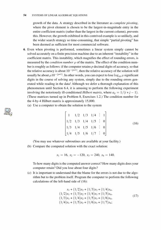
54 SYSTEMS OF LINEAR ALGEBRAIC EQUATIONS
growth of the data. A strategy described in the literature as complete pivoting,where the pivot element is chosen to be the largest-in-magnitude entry in theentire coefficient matrix (rather than the largest in the current column), preventsthis. However, the growth exhibited in this contrived example is so unlikely, andthe wider search strategy so time-consuming, that simple “partial pivoting” hasbeen deemed as sufficient for most commercial software.
6. Even when pivoting is performed, sometimes a linear system simply cannot besolved accurately on a finite precision machine due to an inherent “instability” in thecoefficient matrix. This instability, which magnifies the effect of rounding errors, ismeasured by the condition number μ of the matrix. The effect of the condition num-ber is roughly as follows: if the computer retains p decimal digits of accuracy, so thatthe relative accuracy is about 10−(p+1), then the relative accuracy of the solution willusually be about μ10−(p+1). In other words, you can expect to lose log10 μ significantdigits in the course of solving any system, simply due to the rounding errors gen-erated while reading in the data! Although we defer a thorough explanation of thisphenomenon until Section 6.4, it is amusing to perform the following experimentinvolving the notoriously ill-conditioned Hilbert matrix, where aij = 1/(i + j − 1).(These matrices turned up in Problem 8, Exercises 1.2.) The condition number forthe 4-by-4 Hilbert matrix is approximately 15,000.(a) Use a computer to obtain the solution to the system
⎡⎢⎢⎢⎢⎢⎢⎣
1 1/2 1/3 1/4... 1
1/2 1/3 1/4 1/5... 0
1/3 1/4 1/5 1/6... 0
1/4 1/5 1/6 1/7... 0
⎤⎥⎥⎥⎥⎥⎥⎦
(16)
(You may use whatever subroutines are available at your facility.)
(b) Compare the computed solution with the exact solution:
x1 = 16, x2 = −120, x3 = 240, x4 = 140.
To how many digits is the computed answer correct? How many digits does yourcomputer retain? Did you lose about four digits?
(c) It is important to understand that the blame for the errors is not due to the algo-rithm but to the problem itself. Program the computer to perform the followingcalculations of the left-hand side of (16):
x1 + (1/2)x2 + (1/3)x3 + (1/4)x4,(1/2)x1 + (1/3)x2 + (1/4)x3 + (1/5)x4,(1/3)x1 + (1/4)x2 + (1/5)x3 + (1/6)x4,(1/4)x1 + (1/5)x2 + (1/6)x3 + (1/7)x4;
(17)
1.6 SUMMARY 55
and
x1 + x2/2 + x3/3 + x4/4,x1/2 + x2/3 + x3/4 + x4/5,x1/3 + x2/4 + x3/5 + x4/6,x1/4 + x2/5 + x3/6 + x4/7.
(18)
Substitute the computed solution and the exact solution into (17). Observe thatthe exact solution does not “check” much better than the computed solution.(Indeed, if your facility’s equation-solving subroutine is fairly sophisticated, thecomputed solution may seem superior.) On the other hand, substituting thesesolutions into (18), which avoids the rounding errors in the coefficient matrix(at least, for the exact solution), clearly distinguishes the exact solution.
(d) Repeat these computations using double precision.
1.6 SUMMARY
The tasks of analyzing data sets such as CAT scans and of fitting solution expressionsfor a linear differential equation to specified auxiliary conditions are instances wheresolving linear algebraic systems is an essential step. Because the latter are pervasive inmathematics and applications, it is important to have a methodical, foolproof algorithmfor this problem that is suitable for implementation on computers. Gauss eliminationfills this need.
Gauss Elimination
Gauss elimination incorporates the familiar techniques of substitution, cross-multiplication and subtraction, and solution by inspection into a systematic sequenceof steps that result in explicit solutions to linear systems. The basic operations, whichare guaranteed not to alter the solution set, are
(i) reordering the equations;
(ii) adding (or subtracting) a constant multiple of one equation to another andreplacing the latter with the result;
(iii) multiplying an equation by a nonzero constant and replacing the originalequation with the result.
Augmented Matrix Formulation
The efficiency of the Gauss elimination algorithm for solving a system of m linearequations in n unknowns is enhanced by representing the linear system in an augmentedmatrix format. The m-by-(n+1) augmented matrix contains m rows and n+1 columns, in
www.ebook3000.com
56 SYSTEMS OF LINEAR ALGEBRAIC EQUATIONS
which the rows depict the (m) individual equations, the final ([n+1]st) column containsthe nonhomogeneous terms, and the first n columns (which constitute the coefficientmatrix) contain the coefficients of the unknowns.
Row-Echelon Form
In the forward part of the Gauss elimination algorithm, the basic operations are appliedto the rows of the augmented matrix to reduce it to a row-echelon form, in which thefirst nonzero entry in each row lies to the right of the first nonzero entry in the previousrow. From this form, one can identify redundant equations (a row containing all zeros)and inconsistent systems (the appearance of a row with exactly one nonzero element,in its last column).
Back Substitution
The back substitution part of the Gauss algorithm assembles the complete solution tothe system by solving the equations represented by the row-echelon form in order, fromlast to first. Unknowns corresponding to columns that contain no nonzero leading rowentries are classified as free variables and the other unknowns are expressed in termsof them through a parametric representation of the solution set.
Rank of Row-Echelon Form
The rank of a row-echelon matrix, that is the number of its nonzero rows, can be usedto classify the number of solutions of the system.
(i) If the rank of the augmented matrix equals the rank of the coefficient matrix,the system is consistent (has a solution); otherwise it is inconsistent.
(ii) If the system is consistent and the rank of the coefficient matrix equals itsnumber of columns (the number of unknowns), the system has a uniquesolution.
(iii) If the system is consistent and the rank of the coefficient matrix is less thanits number of columns (the number of unknowns), the system has an infinitenumber of solutions.
Linear Homogeneous Systems
A linear homogeneous system always possesses the trivial solution in which everyunknown equals zero. If the number of equations is less than the number of unknowns,it has an infnite number of solutions.

1.6 SUMMARY 57
Computational Considerations
Performing Gauss elimination on computers having finite precision can lead to unac-ceptable errors if large multiples of some equations are added to others. The effectis controlled by a partial pivoting strategy, which reorders the equations so that thesemultiples never exceed one, in absolute value.
www.ebook3000.com
2MATRIX ALGEBRA
2.1 MATRIX MULTIPLICATION
In this section we will be studying an algebraic system based on matrices. Although“matrix algebra” is interesting in its own right, the big payoff is that it gives us a new lex-icon that enables us to articulate many operations—physical (rotations, projections) andcomputational (the row operations)—in a compact format that facilitates understandingand utilization.
Matrix Products
The matrix product has proved to be one of the most useful inventions in mathe-matics. It undoubtedly was motivated by the desire to represent a system of linearalgebraic equations compactly in the form Ax = b. (As one would expect, wesay matrices are equal when their corresponding entries are equal.)
The system that we solved in Example 1 of Section 1.1,
x1 + 2x2 + 2x3 = 6
2x1 + x2 + x3 = 6 (1)
x1 + x2 + 3x3 = 6
has a coefficient matrix
A =
⎡⎣1 2 2
2 1 11 1 3
⎤⎦ .
Fundamentals of Matrix Analysis with Applications,First Edition. Edward Barry Saff and Arthur David Snider.© 2016 John Wiley & Sons, Inc. Published 2016 by John Wiley & Sons, Inc.
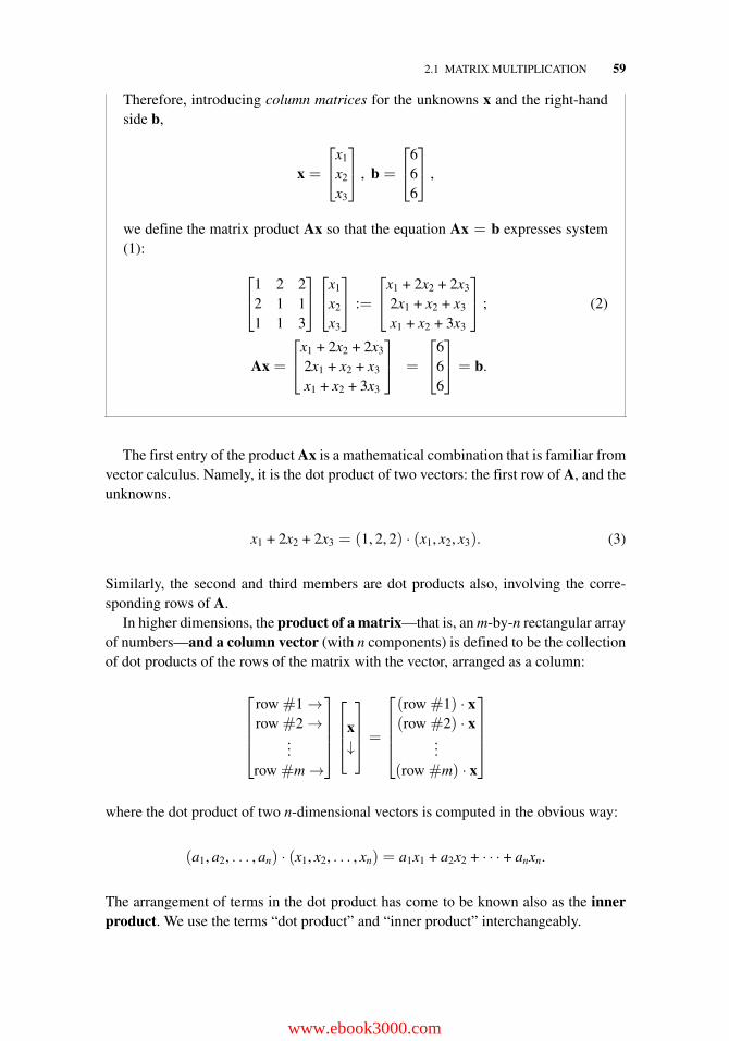
2.1 MATRIX MULTIPLICATION 59
Therefore, introducing column matrices for the unknowns x and the right-handside b,
x =
⎡⎣x1
x2
x3
⎤⎦ , b =
⎡⎣6
66
⎤⎦ ,
we define the matrix product Ax so that the equation Ax = b expresses system(1):
⎡⎣1 2 2
2 1 11 1 3
⎤⎦⎡⎣x1
x2
x3
⎤⎦ :=
⎡⎣x1 + 2x2 + 2x3
2x1 + x2 + x3
x1 + x2 + 3x3
⎤⎦ ; (2)
Ax =
⎡⎣x1 + 2x2 + 2x3
2x1 + x2 + x3
x1 + x2 + 3x3
⎤⎦ =
⎡⎣6
66
⎤⎦ = b.
The first entry of the product Ax is a mathematical combination that is familiar fromvector calculus. Namely, it is the dot product of two vectors: the first row of A, and theunknowns.
x1 + 2x2 + 2x3 = (1, 2, 2) · (x1, x2, x3). (3)
Similarly, the second and third members are dot products also, involving the corre-sponding rows of A.
In higher dimensions, the product of a matrix—that is, an m-by-n rectangular arrayof numbers—and a column vector (with n components) is defined to be the collectionof dot products of the rows of the matrix with the vector, arranged as a column:
⎡⎢⎢⎢⎣
row #1 →row #2 →
...row #m →
⎤⎥⎥⎥⎦
⎡⎢⎢⎣x↓
⎤⎥⎥⎦ =
⎡⎢⎢⎢⎣(row #1) · x(row #2) · x
...(row #m) · x
⎤⎥⎥⎥⎦
where the dot product of two n-dimensional vectors is computed in the obvious way:
(a1, a2, . . . , an) · (x1, x2, . . . , xn) = a1x1 + a2x2 + · · · + anxn.
The arrangement of terms in the dot product has come to be known also as the innerproduct. We use the terms “dot product” and “inner product” interchangeably.
www.ebook3000.com
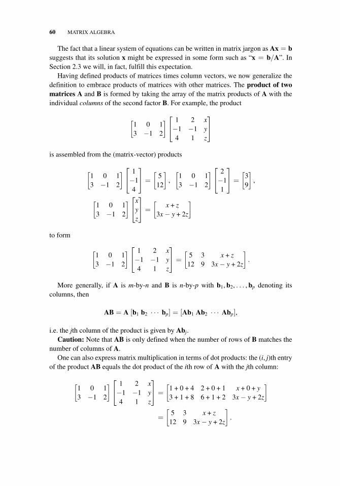
60 MATRIX ALGEBRA
The fact that a linear system of equations can be written in matrix jargon as Ax = bsuggests that its solution x might be expressed in some form such as “x = b/A”. InSection 2.3 we will, in fact, fulfill this expectation.
Having defined products of matrices times column vectors, we now generalize thedefinition to embrace products of matrices with other matrices. The product of twomatrices A and B is formed by taking the array of the matrix products of A with theindividual columns of the second factor B. For example, the product
[1 0 13 −1 2
]⎡⎣ 1 2 x−1 −1 y4 1 z
⎤⎦
is assembled from the (matrix-vector) products
[1 0 13 −1 2
]⎡⎣ 1−14
⎤⎦ =
[5
12
],
[1 0 13 −1 2
]⎡⎣ 2−11
⎤⎦ =
[39
],
[1 0 13 −1 2
]⎡⎣x
yz
⎤⎦ =
[x + z
3x − y + 2z
]
to form
[1 0 13 −1 2
]⎡⎣ 1 2 x−1 −1 y4 1 z
⎤⎦ =
[5 3 x + z
12 9 3x − y + 2z
].
More generally, if A is m-by-n and B is n-by-p with b1, b2, . . . , bp denoting itscolumns, then
AB = A [b1 b2 · · · bp] = [Ab1 Ab2 · · · Abp],
i.e. the jth column of the product is given by Abj.Caution: Note that AB is only defined when the number of rows of B matches the
number of columns of A.One can also express matrix multiplication in terms of dot products: the (i, j)th entry
of the product AB equals the dot product of the ith row of A with the jth column:
[1 0 13 −1 2
]⎡⎣ 1 2 x−1 −1 y4 1 z
⎤⎦ =
[1 + 0 + 4 2 + 0 + 1 x + 0 + y3 + 1 + 8 6 + 1 + 2 3x − y + 2z
]
=
[5 3 x + z
12 9 3x − y + 2z
].
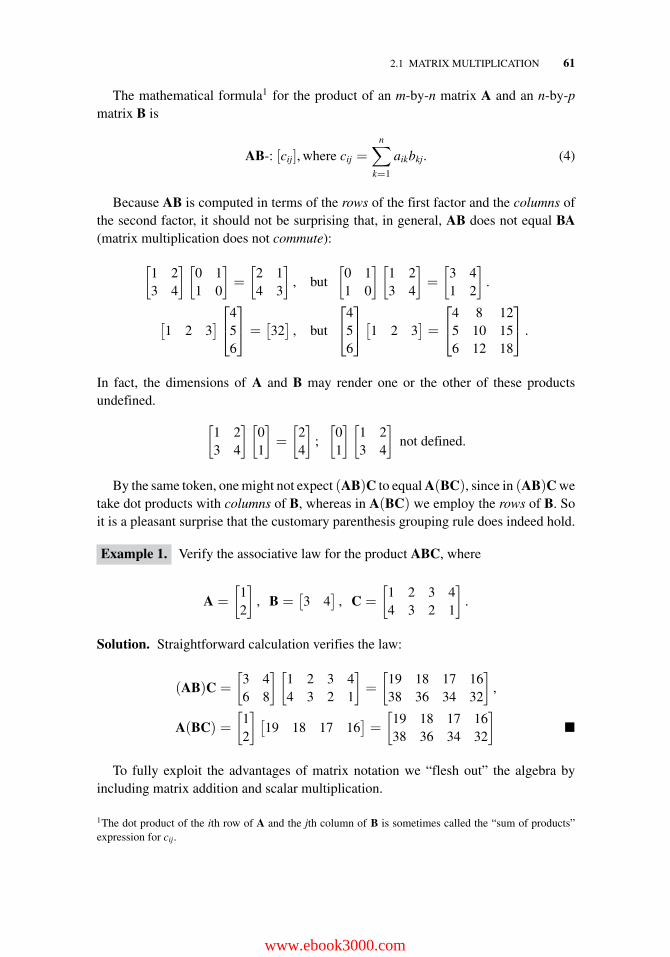
2.1 MATRIX MULTIPLICATION 61
The mathematical formula1 for the product of an m-by-n matrix A and an n-by-pmatrix B is
AB-: [cij], where cij =n∑
k=1
aikbkj. (4)
Because AB is computed in terms of the rows of the first factor and the columns ofthe second factor, it should not be surprising that, in general, AB does not equal BA(matrix multiplication does not commute):
[1 23 4
] [0 11 0
]=
[2 14 3
], but
[0 11 0
] [1 23 4
]=
[3 41 2
].
[1 2 3
]⎡⎣4
56
⎤⎦ =
[32
], but
⎡⎣4
56
⎤⎦ [
1 2 3]=
⎡⎣4 8 12
5 10 156 12 18
⎤⎦ .
In fact, the dimensions of A and B may render one or the other of these productsundefined.
[1 23 4
] [01
]=
[24
];
[01
] [1 23 4
]not defined.
By the same token, one might not expect (AB)C to equal A(BC), since in (AB)C wetake dot products with columns of B, whereas in A(BC) we employ the rows of B. Soit is a pleasant surprise that the customary parenthesis grouping rule does indeed hold.
Example 1. Verify the associative law for the product ABC, where
A =
[12
], B =
[3 4
], C =
[1 2 3 44 3 2 1
].
Solution. Straightforward calculation verifies the law:
(AB)C =
[3 46 8
] [1 2 3 44 3 2 1
]=
[19 18 17 1638 36 34 32
],
A(BC) =
[12
] [19 18 17 16
]=
[19 18 17 1638 36 34 32
]�
To fully exploit the advantages of matrix notation we “flesh out” the algebra byincluding matrix addition and scalar multiplication.
1The dot product of the ith row of A and the jth column of B is sometimes called the “sum of products”expression for cij.
www.ebook3000.com
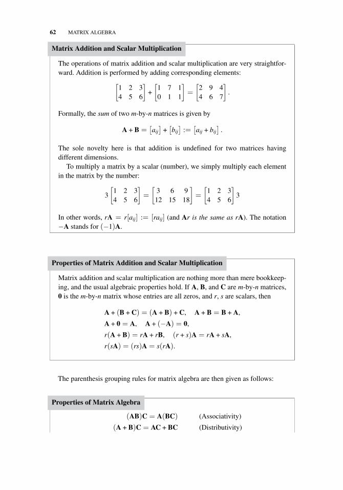
62 MATRIX ALGEBRA
Matrix Addition and Scalar Multiplication
The operations of matrix addition and scalar multiplication are very straightfor-ward. Addition is performed by adding corresponding elements:
[1 2 34 5 6
]+
[1 7 10 1 1
]=
[2 9 44 6 7
].
Formally, the sum of two m-by-n matrices is given by
A + B =[aij
]+[bij
]:=
[aij + bij
].
The sole novelty here is that addition is undefined for two matrices havingdifferent dimensions.
To multiply a matrix by a scalar (number), we simply multiply each elementin the matrix by the number:
3
[1 2 34 5 6
]=
[3 6 9
12 15 18
]=
[1 2 34 5 6
]3
In other words, rA = r[aij] := [raij] (and Ar is the same as rA). The notation−A stands for (−1)A.
Properties of Matrix Addition and Scalar Multiplication
Matrix addition and scalar multiplication are nothing more than mere bookkeep-ing, and the usual algebraic properties hold. If A, B, and C are m-by-n matrices,0 is the m-by-n matrix whose entries are all zeros, and r, s are scalars, then
A + (B + C) = (A + B) + C, A + B = B + A,
A + 0 = A, A + (−A) = 0,
r(A + B) = rA + rB, (r + s)A = rA + sA,
r(sA) = (rs)A = s(rA).
The parenthesis grouping rules for matrix algebra are then given as follows:
Properties of Matrix Algebra
(AB)C = A(BC) (Associativity)
(A + B)C = AC + BC (Distributivity)
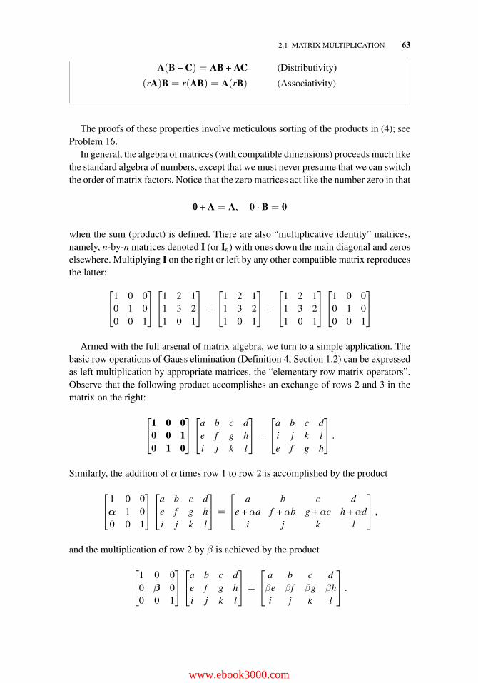
2.1 MATRIX MULTIPLICATION 63
A(B + C) = AB + AC (Distributivity)
(rA)B = r(AB) = A(rB) (Associativity)
The proofs of these properties involve meticulous sorting of the products in (4); seeProblem 16.
In general, the algebra of matrices (with compatible dimensions) proceeds much likethe standard algebra of numbers, except that we must never presume that we can switchthe order of matrix factors. Notice that the zero matrices act like the number zero in that
0 + A = A, 0 · B = 0
when the sum (product) is defined. There are also “multiplicative identity” matrices,namely, n-by-n matrices denoted I (or In) with ones down the main diagonal and zeroselsewhere. Multiplying I on the right or left by any other compatible matrix reproducesthe latter:
⎡⎣1 0 0
0 1 00 0 1
⎤⎦⎡⎣1 2 1
1 3 21 0 1
⎤⎦ =
⎡⎣1 2 1
1 3 21 0 1
⎤⎦ =
⎡⎣1 2 1
1 3 21 0 1
⎤⎦⎡⎣1 0 0
0 1 00 0 1
⎤⎦
Armed with the full arsenal of matrix algebra, we turn to a simple application. Thebasic row operations of Gauss elimination (Definition 4, Section 1.2) can be expressedas left multiplication by appropriate matrices, the “elementary row matrix operators”.Observe that the following product accomplishes an exchange of rows 2 and 3 in thematrix on the right:
⎡⎣1 0 0
0 0 10 1 0
⎤⎦⎡⎣a b c d
e f g hi j k l
⎤⎦ =
⎡⎣a b c d
i j k le f g h
⎤⎦ .
Similarly, the addition of α times row 1 to row 2 is accomplished by the product
⎡⎣1 0 0α 1 00 0 1
⎤⎦⎡⎣a b c d
e f g hi j k l
⎤⎦ =
⎡⎣ a b c d
e + αa f + αb g + αc h + αdi j k l
⎤⎦ ,
and the multiplication of row 2 by β is achieved by the product
⎡⎣1 0 0
0 β 00 0 1
⎤⎦⎡⎣a b c d
e f g hi j k l
⎤⎦ =
⎡⎣ a b c dβe βf βg βhi j k l
⎤⎦ .
www.ebook3000.com
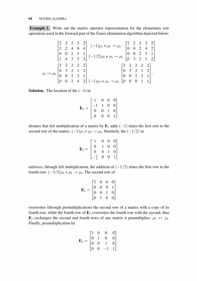
64 MATRIX ALGEBRA
Example 2. Write out the matrix operator representation for the elementary rowoperations used in the forward part of the Gauss elimination algorithm depicted below:
⎡⎢⎢⎣
2 2 2 2 22 2 4 6 40 0 2 3 11 4 3 2 3
⎤⎥⎥⎦
(−1)ρ1 + ρ2 → ρ2
(−1/2)ρ1 + ρ4 → ρ4
⎡⎢⎢⎣
2 2 2 2 20 0 2 4 20 0 2 3 10 3 2 1 2
⎤⎥⎥⎦
ρ2 ↔ ρ4
⎡⎢⎢⎣
2 2 2 2 20 3 2 1 20 0 2 3 10 0 2 4 2
⎤⎥⎥⎦(−1)ρ3 + ρ4 → ρ4
⎡⎢⎢⎣
2 2 2 2 20 3 2 1 20 0 2 3 10 0 0 1 1
⎤⎥⎥⎦ .
Solution. The location of the (−1) in
E1 =
⎡⎢⎢⎣
1 0 0 0−1 1 0 00 0 1 00 0 0 1
⎤⎥⎥⎦
dictates that left multiplication of a matrix by E1 adds (−1) times the first row to thesecond row of the matrix: (−1)ρ1 + ρ2 → ρ2. Similarly, the (−1/2) in
E2 =
⎡⎢⎢⎣
1 0 0 00 1 0 00 0 1 0− 1
2 0 0 1
⎤⎥⎥⎦
enforces, through left multiplication, the addition of (−1/2) times the first row to thefourth row: (−1/2)ρ1 + ρ4 → ρ4. The second row of
E3 =
⎡⎢⎢⎣
1 0 0 00 0 0 10 0 1 00 1 0 0
⎤⎥⎥⎦
overwrites (through premultiplication) the second row of a matrix with a copy of itsfourth row, while the fourth row of E3 overwrites the fourth row with the second; thusE3 exchanges the second and fourth rows of any matrix it premultiplies: ρ2 ↔ ρ4.Finally, premultiplication by
E4 =
⎡⎢⎢⎣
1 0 0 00 1 0 00 0 1 00 0 −1 1
⎤⎥⎥⎦ .
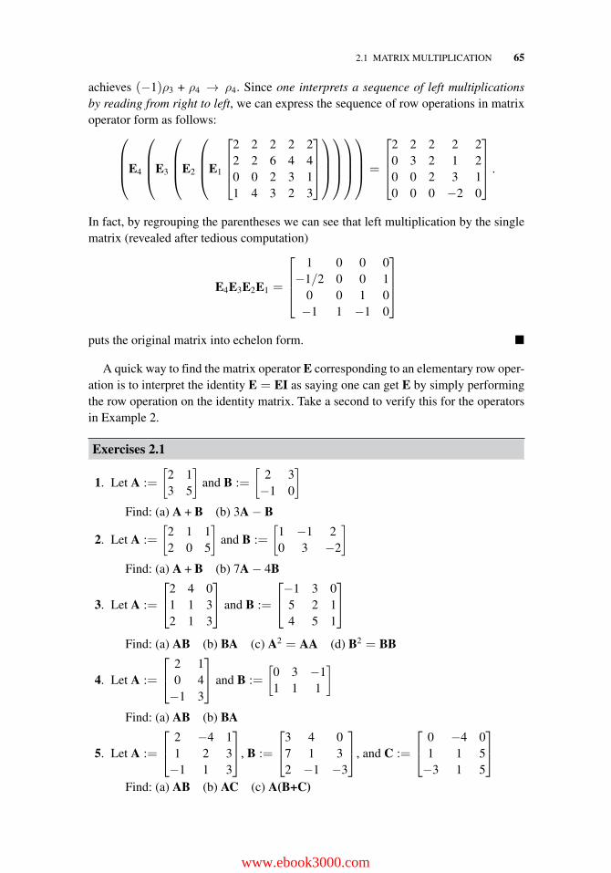
2.1 MATRIX MULTIPLICATION 65
achieves (−1)ρ3 + ρ4 → ρ4. Since one interprets a sequence of left multiplicationsby reading from right to left, we can express the sequence of row operations in matrixoperator form as follows:
⎛⎜⎜⎝E4
⎛⎜⎜⎝E3
⎛⎜⎜⎝E2
⎛⎜⎜⎝E1
⎡⎢⎢⎣
2 2 2 2 22 2 6 4 40 0 2 3 11 4 3 2 3
⎤⎥⎥⎦
⎞⎟⎟⎠
⎞⎟⎟⎠
⎞⎟⎟⎠
⎞⎟⎟⎠ =
⎡⎢⎢⎣
2 2 2 2 20 3 2 1 20 0 2 3 10 0 0 −2 0
⎤⎥⎥⎦ .
In fact, by regrouping the parentheses we can see that left multiplication by the singlematrix (revealed after tedious computation)
E4E3E2E1 =
⎡⎢⎢⎣
1 0 0 0−1/2 0 0 1
0 0 1 0−1 1 −1 0
⎤⎥⎥⎦
puts the original matrix into echelon form. �
A quick way to find the matrix operator E corresponding to an elementary row oper-ation is to interpret the identity E = EI as saying one can get E by simply performingthe row operation on the identity matrix. Take a second to verify this for the operatorsin Example 2.
Exercises 2.1
1. Let A :=
[2 13 5
]and B :=
[2 3−1 0
]
Find: (a) A + B (b) 3A − B
2. Let A :=
[2 1 12 0 5
]and B :=
[1 −1 20 3 −2
]
Find: (a) A + B (b) 7A − 4B
3. Let A :=
⎡⎣2 4 0
1 1 32 1 3
⎤⎦ and B :=
⎡⎣−1 3 0
5 2 14 5 1
⎤⎦
Find: (a) AB (b) BA (c) A2 = AA (d) B2 = BB
4. Let A :=
⎡⎣ 2 1
0 4−1 3
⎤⎦ and B :=
[0 3 −11 1 1
]
Find: (a) AB (b) BA
5. Let A :=
⎡⎣ 2 −4 1
1 2 3−1 1 3
⎤⎦, B :=
⎡⎣3 4 0
7 1 32 −1 −3
⎤⎦, and C :=
⎡⎣ 0 −4 0
1 1 5−3 1 5
⎤⎦
Find: (a) AB (b) AC (c) A(B+C)
www.ebook3000.com
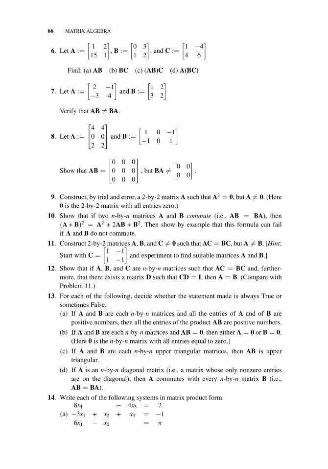
66 MATRIX ALGEBRA
6. Let A :=
[1 2
15 1
], B :=
[0 31 2
], and C :=
[1 −44 6
]
Find: (a) AB (b) BC (c) (AB)C (d) A(BC)
7. Let A :=
[2 −1−3 4
]and B :=
[1 23 2
]
Verify that AB �= BA.
8. Let A :=
⎡⎣4 4
0 02 2
⎤⎦ and B :=
[1 0 −1−1 0 1
]
Show that AB =
⎡⎣0 0 0
0 0 00 0 0
⎤⎦ , but BA �=
[0 00 0
].
9. Construct, by trial and error, a 2-by-2 matrix A such that A2 = 0, but A �= 0. (Here0 is the 2-by-2 matrix with all entries zero.)
10. Show that if two n-by-n matrices A and B commute (i.e., AB = BA), then(A + B)2 = A2 + 2AB + B2. Then show by example that this formula can failif A and B do not commute.
11. Construct 2-by-2 matrices A, B, and C �= 0 such that AC = BC, but A �= B. [Hint:
Start with C =
[1 −11 −1
]and experiment to find suitable matrices A and B.]
12. Show that if A, B, and C are n-by-n matrices such that AC = BC and, further-more, that there exists a matrix D such that CD = I, then A = B. (Compare withProblem 11.)
13. For each of the following, decide whether the statement made is always True orsometimes False.(a) If A and B are each n-by-n matrices and all the entries of A and of B are
positive numbers, then all the entries of the product AB are positive numbers.
(b) If A and B are each n-by-n matrices and AB = 0, then either A = 0 or B = 0.(Here 0 is the n-by-n matrix with all entries equal to zero.)
(c) If A and B are each n-by-n upper triangular matrices, then AB is uppertriangular.
(d) If A is an n-by-n diagonal matrix (i.e., a matrix whose only nonzero entriesare on the diagonal), then A commutes with every n-by-n matrix B (i.e.,AB = BA).
14. Write each of the following systems in matrix product form:
(a)8x1 − 4x3 = 2−3x1 + x2 + x3 = −16x1 − x2 = π
2.1 MATRIX MULTIPLICATION 67
(b)x + 2y + 6z − 8 = 03 + y + 4x + z = 0
x − 4 + y = 015. Write each of the following systems in matrix product form.
(a)x2 + 3x3 = 0
−x1 + 7x2 − 9x3 = −96x1 − 4x2 = 2
(b)3y − 2x + 7 = 0
−x + 2y − 6 + z = 03z − y − x + 3 = 0
16. Verify the associativity property of multiplication, that is (AB) C = A(BC), whereA = [aij] is an m-by-n matrix, B = [bjk] is n-by-p, and C = [ckr] is p-by-q. [Hint:Let D := (AB)C and E := A(BC) and show, using the formula (4), that the (i, r)thentry dir of D is given by
dir =n∑
j=1
aij
p∑k=1
bjkckr,
and then interchange the order of summations to show that this is the same as the(i, r)th entry of E.]
17. Let A :=
⎡⎣ 2 −4 1
1 2 3−1 1 3
⎤⎦ . Find a matrix operator B such the following elementary
row operations on A are accomplished via left multiplication by B.
(a) BA =
⎡⎣ 2 −4 1−1 1 31 2 3
⎤⎦,
(b) BA =
⎡⎣ 2 −4 1
0 4 52
−1 1 3
⎤⎦,
(c) BA =
⎡⎣ 2 −4 1
2 4 6−1 1 3
⎤⎦ .
18. Let A :=
⎡⎣0 0 −1 5
2 1 −1 46 −3 2 2
⎤⎦ . Find a matrix operator B such the following
elementary row operations on A are accomplished via left multiplication by B.
(a) BA =
⎡⎣6 −3 2 2
2 1 −1 40 0 −1 5
⎤⎦,
www.ebook3000.com
68 MATRIX ALGEBRA
(b) BA =
⎡⎣ 0 0 −1 5
2 1 −1 4−3 3
2 −1 −1
⎤⎦,
(c) BA =
⎡⎣0 0 −1 5
2 1 −1 40 −6 5 −10
⎤⎦ .
19. Transform the following matrices into row echelon form and display how this canbe accomplished by a sequence of left multiplications.
(a) A =
⎡⎣0 0 −1
2 1 −16 −3 2
⎤⎦,
(b) B =
⎡⎣2 0 −3 5
2 1 −1 46 −3 2 2
⎤⎦,
(c) C =
⎡⎣1 2 1 1 −1 0
1 2 0 −1 1 00 0 1 2 −2 1
⎤⎦.
20. Transform the following matrices into row echelon form and display how this canbe accomplished by a sequence of left multiplications.
(a) A =
⎡⎣2 −1 0
2 3 −10 −3 2
⎤⎦,
(b) B =
⎡⎣0 0 5 3
0 −2 −1 04 −3 1 2
⎤⎦,
(c) C =
⎡⎢⎢⎣
0 2 1 12 4 4 23 6 6 00 −2 −1 −2
⎤⎥⎥⎦.
21. Years of experience have taught a fisherman that a good day of fishing is followedby another good day 75% of the time, while a bad day of fishing is followed byanother bad day 40% of the time. So if Sunday is a good day, the probability thatMonday is a good day is 0.75 and the probability that it is bad is 0.25.(a) If Sunday is a good day, what are the probabilities for Tuesday?
(b) If xn =
[gn
bn
]gives the probabilities that day n is good (gn) or bad (bn), express
the probabilities xn+1 for day n + 1 as a matrix product xn+1 = Axn.
(c) What is the sum of the entries of the column vectors xn+1? What is the sum ofthe entries in each column of A?
(d) Suppose we refined the classification of fishing day quality to excellent, good,fair, and bad and modeled the probabilities as in (b). Would either of theanswers in (c) remain the same?
2.2 SOME PHYSICAL APPLICATIONS OF MATRIX OPERATORS 69
22. (Iteration of Stochastic Matrices) Problem 21 is generalized as follows. Ann-by-n stochastic matrix is a matrix for which each column vector has non-negativeentries that add up to 1 (such vectors are called probability vectors).(a) Show that if x is probability vector and A is a stochastic matrix, then Ax is a
probability vector.
(b) Starting with a probability vector x0 and a stochastic matrix A, the sequenceof probability vectors x0, x1 := Ax0, x2 := Ax1, etc. is called a Markov chainwhich can be represented by the iterative formula xk+1 := Axk, k = 0, 1, . . .Explain why xk = Akx0, where A0 := In.
(c) Using a computer software package for multiplication, predict the long-termbehavior (as k → ∞) of the Markov chain for
A =
⎡⎢⎢⎣
.33 .40 .32 .55
.11 .15 .41 .03
.11 .30 .12 .35
.45 .15 .15 .07
⎤⎥⎥⎦ , with x0 =
⎡⎢⎢⎣
.25
.25
.25
.25
⎤⎥⎥⎦ ,
that is, predict the limit of the entries in the xk as k → ∞. This limit vector iscalled a steady-state probability vector.
(d) Experiment with different starting probability measures x0, to see if thepredicted long-term behavior depends on the starting vector.
23. If A and B are n-by-n matrices and v is an n-by-1 vector, which of the followingcalculations is more efficient?(a) A(Bv) or (AB)v?
(b) (A + B)v or Av + Bv?[Hint: How many dot products are required in each of the four calculations?]
2.2 SOME PHYSICAL APPLICATIONS OF MATRIXOPERATORS
In this section we explore several ways matrix language is used to express some of theoperations performed in applied mathematics.
We will see that, while it is important to adhere strictly to the rules of matrix alge-bra as listed in the previous section, some applications call for a little flexibility. Forexample, sometimes the algebra requires the x,y coordinates of a point in the plane tobe listed as a row vector [x y], and other times as a column vector
[xy
].
The matrix transpose gives us this flexibility. When a is, say, a 1-by-m row vector, thesymbol aT denotes the m-by-1 column vector with the same entries; and similarly whenb is a column, bT is the corresponding row:
www.ebook3000.com
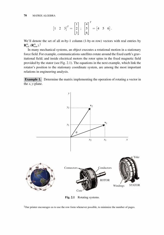
70 MATRIX ALGEBRA
[1 2 3
]T=
⎡⎣1
23
⎤⎦ ;
⎡⎣4
56
⎤⎦
T
=[4 5 6
].
We’ll denote the set of all m-by-1 column (1-by-m row) vectors with real entries byRm
col (Rmrow).2
In many mechanical systems, an object executes a rotational motion in a stationaryforce field. For example, communications satellites rotate around the fixed earth’s grav-itational field; and inside electrical motors the rotor spins in the fixed magnetic fieldprovided by the stator (see Fig. 2.1). The equations in the next example, which link therotator’s position to the stationary coordinate system, are among the most importantrelations in engineering analysis.
Example 1. Determine the matrix implementing the operation of rotating a vector inthe x, y-plane.
y
y1
y2
x2
θ
x1
v1
v2
x
Connectors Conductors
Core
Windings
ROTOR
STATOR
Yoke
Fig. 2.1 Rotating systems.
2Our printer encourages us to use the row form whenever possible, to minimize the number of pages.
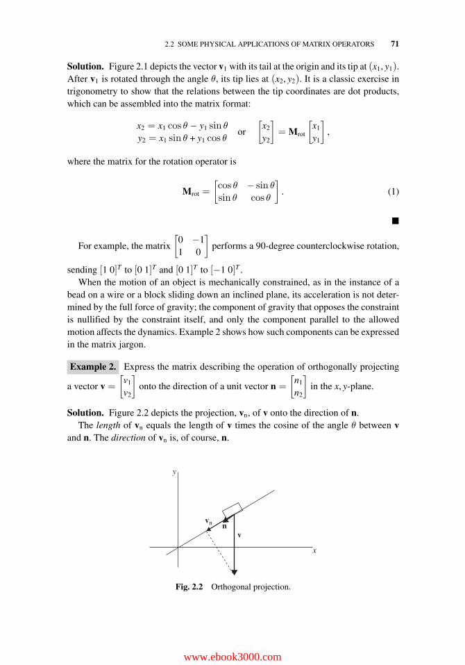
2.2 SOME PHYSICAL APPLICATIONS OF MATRIX OPERATORS 71
Solution. Figure 2.1 depicts the vector v1 with its tail at the origin and its tip at (x1, y1).After v1 is rotated through the angle θ, its tip lies at (x2, y2). It is a classic exercise intrigonometry to show that the relations between the tip coordinates are dot products,which can be assembled into the matrix format:
x2 = x1 cos θ − y1 sin θy2 = x1 sin θ + y1 cos θ
or
[x2
y2
]= Mrot
[x1
y1
],
where the matrix for the rotation operator is
Mrot =
[cos θ − sin θsin θ cos θ
]. (1)
�
For example, the matrix
[0 −11 0
]performs a 90-degree counterclockwise rotation,
sending [1 0]T to [0 1]T and [0 1]T to [−1 0]T .When the motion of an object is mechanically constrained, as in the instance of a
bead on a wire or a block sliding down an inclined plane, its acceleration is not deter-mined by the full force of gravity; the component of gravity that opposes the constraintis nullified by the constraint itself, and only the component parallel to the allowedmotion affects the dynamics. Example 2 shows how such components can be expressedin the matrix jargon.
Example 2. Express the matrix describing the operation of orthogonally projecting
a vector v =
[v1
v2
]onto the direction of a unit vector n =
[n1
n2
]in the x, y-plane.
Solution. Figure 2.2 depicts the projection, vn, of v onto the direction of n.The length of vn equals the length of v times the cosine of the angle θ between v
and n. The direction of vn is, of course, n.
y
x
v
vn n
Fig. 2.2 Orthogonal projection.
www.ebook3000.com
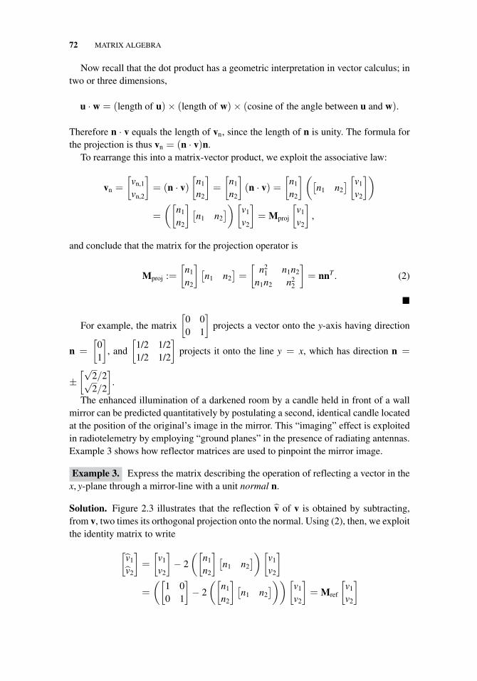
72 MATRIX ALGEBRA
Now recall that the dot product has a geometric interpretation in vector calculus; intwo or three dimensions,
u · w = (length of u)× (length of w)× (cosine of the angle between u and w).
Therefore n · v equals the length of vn, since the length of n is unity. The formula forthe projection is thus vn = (n · v)n.
To rearrange this into a matrix-vector product, we exploit the associative law:
vn =
[vn,1
vn,2
]= (n · v)
[n1
n2
]=
[n1
n2
](n · v) =
[n1
n2
]([n1 n2
] [v1
v2
])
=
([n1
n2
] [n1 n2
]) [v1
v2
]= Mproj
[v1
v2
],
and conclude that the matrix for the projection operator is
Mproj :=
[n1
n2
] [n1 n2
]=
[n2
1 n1n2
n1n2 n22
]= nnT . (2)
�
For example, the matrix
[0 00 1
]projects a vector onto the y-axis having direction
n =
[01
], and
[1/2 1/21/2 1/2
]projects it onto the line y = x, which has direction n =
±[√
2/2√2/2
].
The enhanced illumination of a darkened room by a candle held in front of a wallmirror can be predicted quantitatively by postulating a second, identical candle locatedat the position of the original’s image in the mirror. This “imaging” effect is exploitedin radiotelemetry by employing “ground planes” in the presence of radiating antennas.Example 3 shows how reflector matrices are used to pinpoint the mirror image.
Example 3. Express the matrix describing the operation of reflecting a vector in thex, y-plane through a mirror-line with a unit normal n.
Solution. Figure 2.3 illustrates that the reflection v of v is obtained by subtracting,from v, two times its orthogonal projection onto the normal. Using (2), then, we exploitthe identity matrix to write
[v1
v2
]=
[v1
v2
]− 2
([n1
n2
] [n1 n2
]) [v1
v2
]
=
([1 00 1
]− 2
([n1
n2
] [n1 n2
]))[v1
v2
]= Mref
[v1
v2
]
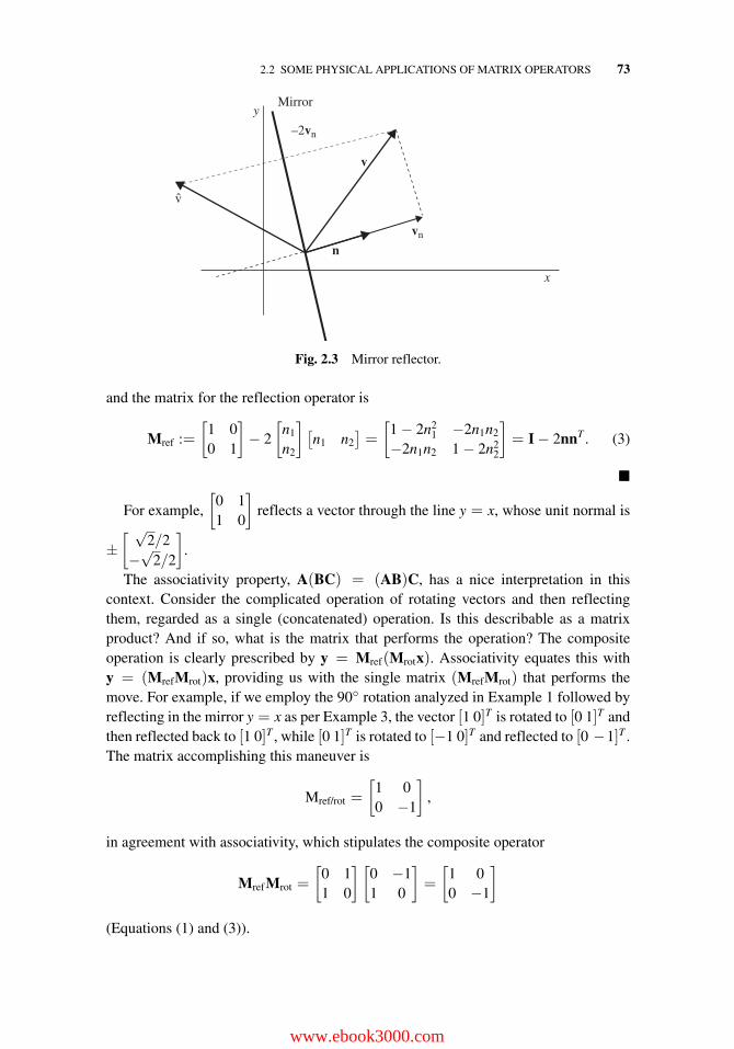
2.2 SOME PHYSICAL APPLICATIONS OF MATRIX OPERATORS 73
y
v
v
vn
n
–2vn
Mirror
x
Fig. 2.3 Mirror reflector.
and the matrix for the reflection operator is
Mref :=
[1 00 1
]− 2
[n1
n2
] [n1 n2
]=
[1 − 2n2
1 −2n1n2
−2n1n2 1 − 2n22
]= I − 2nnT . (3)
�
For example,
[0 11 0
]reflects a vector through the line y = x, whose unit normal is
±[ √
2/2−√
2/2
].
The associativity property, A(BC) = (AB)C, has a nice interpretation in thiscontext. Consider the complicated operation of rotating vectors and then reflectingthem, regarded as a single (concatenated) operation. Is this describable as a matrixproduct? And if so, what is the matrix that performs the operation? The compositeoperation is clearly prescribed by y = Mref(Mrotx). Associativity equates this withy = (MrefMrot)x, providing us with the single matrix (MrefMrot) that performs themove. For example, if we employ the 90◦ rotation analyzed in Example 1 followed byreflecting in the mirror y = x as per Example 3, the vector [1 0]T is rotated to [0 1]T andthen reflected back to [1 0]T , while [0 1]T is rotated to [−1 0]T and reflected to [0 −1]T .The matrix accomplishing this maneuver is
Mref/rot =
[1 00 −1
],
in agreement with associativity, which stipulates the composite operator
MrefMrot =
[0 11 0
] [0 −11 0
]=
[1 00 −1
]
(Equations (1) and (3)).
www.ebook3000.com
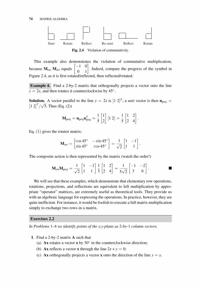
74 MATRIX ALGEBRA
Start Re-startRotate RotateReflect Reflect
Fig. 2.4 Violation of commutativity.
This example also demonstrates the violation of commutative multiplication,
because Mrot Mref equals
[−1 00 1
]. Indeed, compare the progress of the symbol in
Figure 2.4, as it is first rotated/reflected, then reflected/rotated.
Example 4. Find a 2-by-2 matrix that orthogonally projects a vector onto the liney = 2x, and then rotates it counterclockwise by 45◦.
Solution. A vector parallel to the line y = 2x is [1 2]T ; a unit vector is then nproj =
[1 2]T/√
5. Thus (Eq. (2))
Mproj = nprojnTproj =
15
[12
][1 2] =
15
[1 22 4
].
Eq. (1) gives the rotator matrix:
Mrot =
[cos 45◦ − sin 45◦
sin 45◦ cos 45◦
]=
1√2
[1 −11 1
].
The composite action is then represented by the matrix (watch the order!)
MrotMproj =1√2
[1 −11 1
]15
[1 22 4
]=
1
5√
2
[−1 −23 6
]. �
We will see that these examples, which demonstrate that elementary row operations,rotations, projections, and reflections are equivalent to left multiplication by appro-priate “operator” matrices, are extremely useful as theoretical tools. They provide uswith an algebraic language for expressing the operations. In practice, however, they arequite inefficient. For instance, it would be foolish to execute a full matrix multiplicationsimply to exchange two rows in a matrix.
Exercises 2.2
In Problems 1–4 we identify points of the x,y-plane as 2-by-1 column vectors.
1. Find a 2-by-2 matrix A such that(a) Ax rotates a vector x by 30◦ in the counterclockwise direction;
(b) Ax reflects a vector x through the line 2x + y = 0;
(c) Ax orthogonally projects a vector x onto the direction of the line y = x.
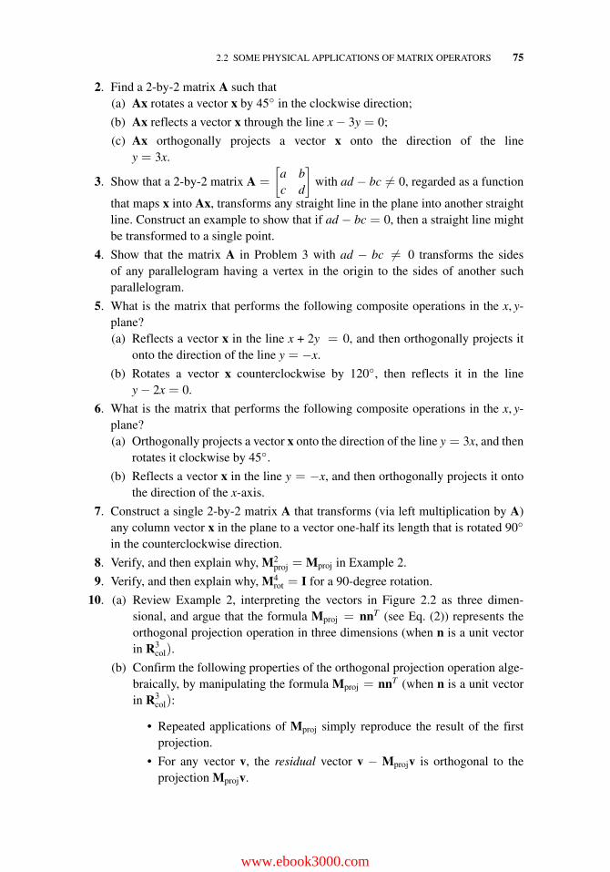
2.2 SOME PHYSICAL APPLICATIONS OF MATRIX OPERATORS 75
2. Find a 2-by-2 matrix A such that(a) Ax rotates a vector x by 45◦ in the clockwise direction;
(b) Ax reflects a vector x through the line x − 3y = 0;
(c) Ax orthogonally projects a vector x onto the direction of the liney = 3x.
3. Show that a 2-by-2 matrix A =
[a bc d
]with ad − bc �= 0, regarded as a function
that maps x into Ax, transforms any straight line in the plane into another straightline. Construct an example to show that if ad − bc = 0, then a straight line mightbe transformed to a single point.
4. Show that the matrix A in Problem 3 with ad − bc �= 0 transforms the sidesof any parallelogram having a vertex in the origin to the sides of another suchparallelogram.
5. What is the matrix that performs the following composite operations in the x, y-plane?(a) Reflects a vector x in the line x + 2y = 0, and then orthogonally projects it
onto the direction of the line y = −x.
(b) Rotates a vector x counterclockwise by 120◦, then reflects it in the liney − 2x = 0.
6. What is the matrix that performs the following composite operations in the x, y-plane?(a) Orthogonally projects a vector x onto the direction of the line y = 3x, and then
rotates it clockwise by 45◦.
(b) Reflects a vector x in the line y = −x, and then orthogonally projects it ontothe direction of the x-axis.
7. Construct a single 2-by-2 matrix A that transforms (via left multiplication by A)any column vector x in the plane to a vector one-half its length that is rotated 90◦
in the counterclockwise direction.
8. Verify, and then explain why, M2proj = Mproj in Example 2.
9. Verify, and then explain why, M4rot = I for a 90-degree rotation.
10. (a) Review Example 2, interpreting the vectors in Figure 2.2 as three dimen-sional, and argue that the formula Mproj = nnT (see Eq. (2)) represents theorthogonal projection operation in three dimensions (when n is a unit vectorin R3
col).
(b) Confirm the following properties of the orthogonal projection operation alge-braically, by manipulating the formula Mproj = nnT (when n is a unit vectorin R3
col):
• Repeated applications of Mproj simply reproduce the result of the firstprojection.
• For any vector v, the residual vector v − Mprojv is orthogonal to theprojection Mprojv.
www.ebook3000.com
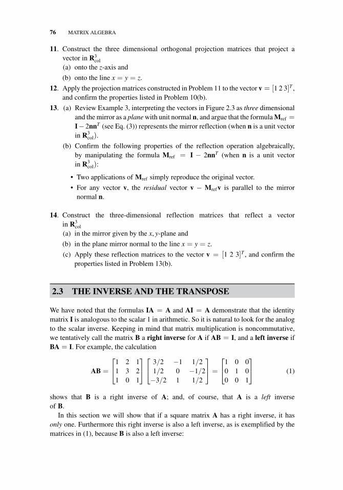
76 MATRIX ALGEBRA
11. Construct the three dimensional orthogonal projection matrices that project avector in R3
col
(a) onto the z-axis and
(b) onto the line x = y = z.
12. Apply the projection matrices constructed in Problem 11 to the vector v = [1 2 3]T ,and confirm the properties listed in Problem 10(b).
13. (a) Review Example 3, interpreting the vectors in Figure 2.3 as three dimensionaland the mirror as a plane with unit normal n, and argue that the formula Mref =I− 2nnT (see Eq. (3)) represents the mirror reflection (when n is a unit vectorin R3
col).
(b) Confirm the following properties of the reflection operation algebraically,by manipulating the formula Mref = I − 2nnT (when n is a unit vectorin R3
col):
• Two applications of Mref simply reproduce the original vector.
• For any vector v, the residual vector v − Mrefv is parallel to the mirrornormal n.
14. Construct the three-dimensional reflection matrices that reflect a vectorin R3
col
(a) in the mirror given by the x, y-plane and
(b) in the plane mirror normal to the line x = y = z.
(c) Apply these reflection matrices to the vector v = [1 2 3]T , and confirm theproperties listed in Problem 13(b).
2.3 THE INVERSE AND THE TRANSPOSE
We have noted that the formulas IA = A and AI = A demonstrate that the identitymatrix I is analogous to the scalar 1 in arithmetic. So it is natural to look for the analogto the scalar inverse. Keeping in mind that matrix multiplication is noncommutative,we tentatively call the matrix B a right inverse for A if AB = I, and a left inverse ifBA = I. For example, the calculation
AB =
⎡⎣1 2 1
1 3 21 0 1
⎤⎦⎡⎣ 3/2 −1 1/2
1/2 0 −1/2−3/2 1 1/2
⎤⎦ =
⎡⎣1 0 0
0 1 00 0 1
⎤⎦ (1)
shows that B is a right inverse of A; and, of course, that A is a left inverseof B.
In this section we will show that if a square matrix A has a right inverse, it hasonly one. Furthermore this right inverse is also a left inverse, as is exemplified by thematrices in (1), because B is also a left inverse:
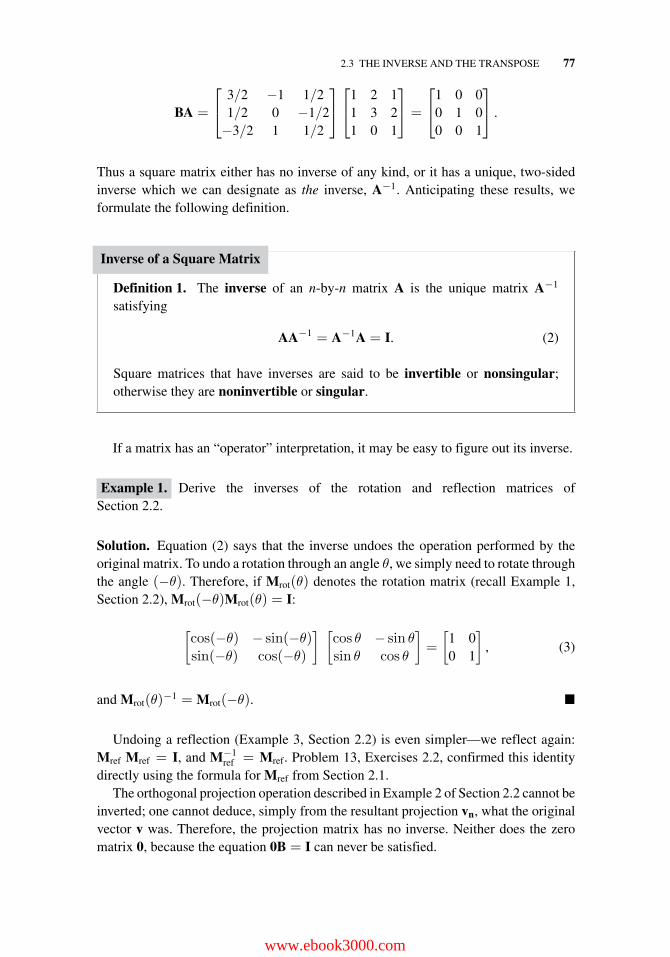
2.3 THE INVERSE AND THE TRANSPOSE 77
BA =
⎡⎣ 3/2 −1 1/2
1/2 0 −1/2−3/2 1 1/2
⎤⎦⎡⎣1 2 1
1 3 21 0 1
⎤⎦ =
⎡⎣1 0 0
0 1 00 0 1
⎤⎦ .
Thus a square matrix either has no inverse of any kind, or it has a unique, two-sidedinverse which we can designate as the inverse, A−1. Anticipating these results, weformulate the following definition.
Inverse of a Square Matrix
Definition 1. The inverse of an n-by-n matrix A is the unique matrix A−1
satisfying
AA−1 = A−1A = I. (2)
Square matrices that have inverses are said to be invertible or nonsingular;otherwise they are noninvertible or singular.
If a matrix has an “operator” interpretation, it may be easy to figure out its inverse.
Example 1. Derive the inverses of the rotation and reflection matrices ofSection 2.2.
Solution. Equation (2) says that the inverse undoes the operation performed by theoriginal matrix. To undo a rotation through an angle θ, we simply need to rotate throughthe angle (−θ). Therefore, if Mrot(θ) denotes the rotation matrix (recall Example 1,Section 2.2), Mrot(−θ)Mrot(θ) = I:
[cos(−θ) − sin(−θ)sin(−θ) cos(−θ)
] [cos θ − sin θsin θ cos θ
]=
[1 00 1
], (3)
and Mrot(θ)−1 = Mrot(−θ). �
Undoing a reflection (Example 3, Section 2.2) is even simpler—we reflect again:Mref Mref = I, and M−1
ref = Mref. Problem 13, Exercises 2.2, confirmed this identitydirectly using the formula for Mref from Section 2.1.
The orthogonal projection operation described in Example 2 of Section 2.2 cannot beinverted; one cannot deduce, simply from the resultant projection vn, what the originalvector v was. Therefore, the projection matrix has no inverse. Neither does the zeromatrix 0, because the equation 0B = I can never be satisfied.
www.ebook3000.com
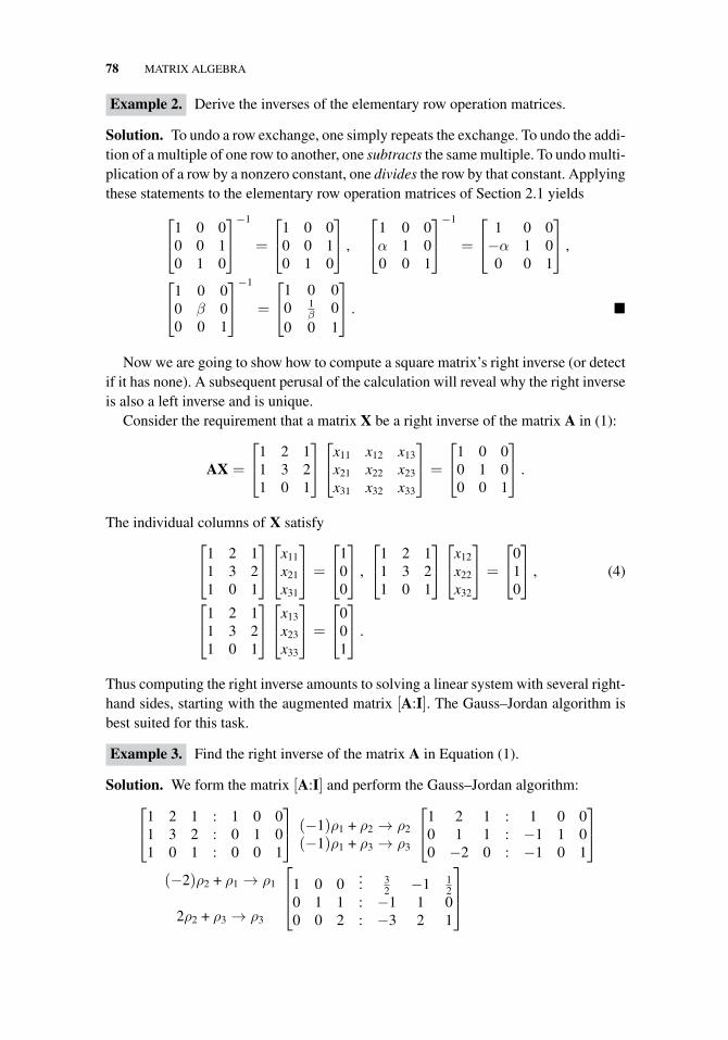
78 MATRIX ALGEBRA
Example 2. Derive the inverses of the elementary row operation matrices.
Solution. To undo a row exchange, one simply repeats the exchange. To undo the addi-tion of a multiple of one row to another, one subtracts the same multiple. To undo multi-plication of a row by a nonzero constant, one divides the row by that constant. Applyingthese statements to the elementary row operation matrices of Section 2.1 yields
⎡⎣1 0 0
0 0 10 1 0
⎤⎦−1
=
⎡⎣1 0 0
0 0 10 1 0
⎤⎦ ,
⎡⎣1 0 0α 1 00 0 1
⎤⎦−1
=
⎡⎣ 1 0 0−α 1 00 0 1
⎤⎦ ,
⎡⎣1 0 0
0 β 00 0 1
⎤⎦−1
=
⎡⎣1 0 0
0 1β 0
0 0 1
⎤⎦ . �
Now we are going to show how to compute a square matrix’s right inverse (or detectif it has none). A subsequent perusal of the calculation will reveal why the right inverseis also a left inverse and is unique.
Consider the requirement that a matrix X be a right inverse of the matrix A in (1):
AX =
⎡⎣1 2 1
1 3 21 0 1
⎤⎦⎡⎣x11 x12 x13
x21 x22 x23
x31 x32 x33
⎤⎦ =
⎡⎣1 0 0
0 1 00 0 1
⎤⎦ .
The individual columns of X satisfy⎡⎣1 2 1
1 3 21 0 1
⎤⎦⎡⎣x11
x21
x31
⎤⎦ =
⎡⎣1
00
⎤⎦ ,
⎡⎣1 2 1
1 3 21 0 1
⎤⎦⎡⎣x12
x22
x32
⎤⎦ =
⎡⎣0
10
⎤⎦ , (4)
⎡⎣1 2 1
1 3 21 0 1
⎤⎦⎡⎣x13
x23
x33
⎤⎦ =
⎡⎣0
01
⎤⎦ .
Thus computing the right inverse amounts to solving a linear system with several right-hand sides, starting with the augmented matrix [A:I]. The Gauss–Jordan algorithm isbest suited for this task.
Example 3. Find the right inverse of the matrix A in Equation (1).
Solution. We form the matrix [A:I] and perform the Gauss–Jordan algorithm:⎡⎣1 2 1 : 1 0 0
1 3 2 : 0 1 01 0 1 : 0 0 1
⎤⎦ (−1)ρ1 + ρ2 → ρ2
(−1)ρ1 + ρ3 → ρ3
⎡⎣1 2 1 : 1 0 0
0 1 1 : −1 1 00 −2 0 : −1 0 1
⎤⎦
(−2)ρ2 + ρ1 → ρ1
2ρ2 + ρ3 → ρ3
⎡⎢⎣1 0 0
... 32 −1 1
20 1 1 : −1 1 00 0 2 : −3 2 1
⎤⎥⎦
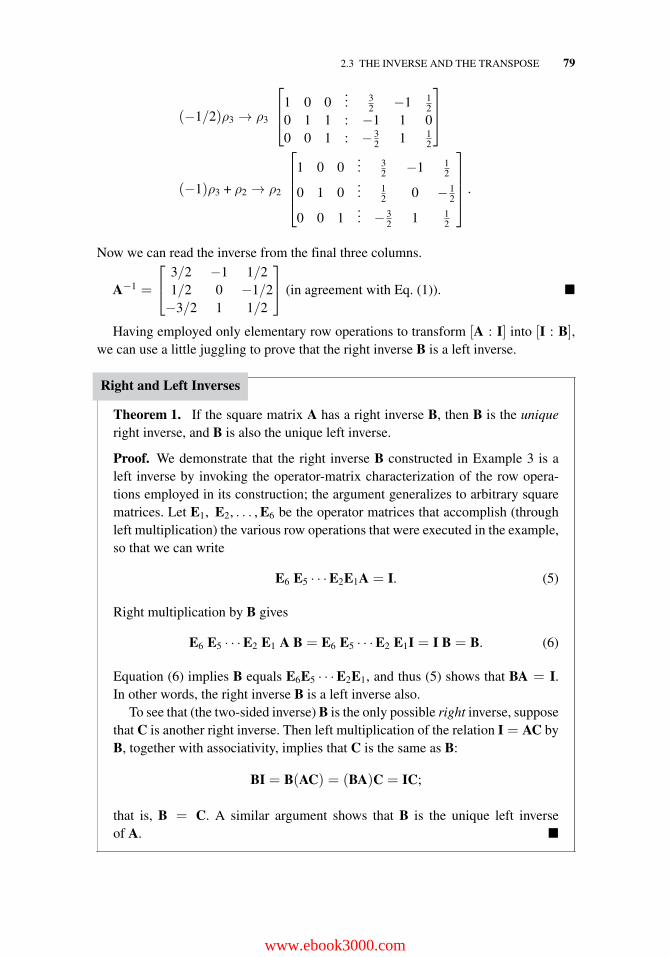
2.3 THE INVERSE AND THE TRANSPOSE 79
(−1/2)ρ3 → ρ3
⎡⎢⎣1 0 0
... 32 −1 1
20 1 1 : −1 1 00 0 1 : − 3
2 1 12
⎤⎥⎦
(−1)ρ3 + ρ2 → ρ2
⎡⎢⎢⎢⎣
1 0 0... 3
2 −1 12
0 1 0... 1
2 0 − 12
0 0 1... − 3
2 1 12
⎤⎥⎥⎥⎦ .
Now we can read the inverse from the final three columns.
A−1 =
⎡⎣ 3/2 −1 1/2
1/2 0 −1/2−3/2 1 1/2
⎤⎦ (in agreement with Eq. (1)). �
Having employed only elementary row operations to transform [A : I] into [I : B],we can use a little juggling to prove that the right inverse B is a left inverse.
Right and Left Inverses
Theorem 1. If the square matrix A has a right inverse B, then B is the uniqueright inverse, and B is also the unique left inverse.
Proof. We demonstrate that the right inverse B constructed in Example 3 is aleft inverse by invoking the operator-matrix characterization of the row opera-tions employed in its construction; the argument generalizes to arbitrary squarematrices. Let E1, E2, . . . , E6 be the operator matrices that accomplish (throughleft multiplication) the various row operations that were executed in the example,so that we can write
E6 E5 · · ·E2E1A = I. (5)
Right multiplication by B gives
E6 E5 · · ·E2 E1 A B = E6 E5 · · ·E2 E1I = I B = B. (6)
Equation (6) implies B equals E6E5 · · ·E2E1, and thus (5) shows that BA = I.In other words, the right inverse B is a left inverse also.
To see that (the two-sided inverse) B is the only possible right inverse, supposethat C is another right inverse. Then left multiplication of the relation I = AC byB, together with associativity, implies that C is the same as B:
BI = B(AC) = (BA)C = IC;
that is, B = C. A similar argument shows that B is the unique left inverseof A. �
www.ebook3000.com
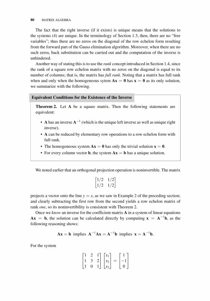
80 MATRIX ALGEBRA
The fact that the right inverse (if it exists) is unique means that the solutions tothe systems (4) are unique. In the terminology of Section 1.3, then, there are no “freevariables”; thus there are no zeros on the diagonal of the row echelon form resultingfrom the forward part of the Gauss elimination algorithm. Moreover, when there are nosuch zeros, back substitution can be carried out and the computation of the inverse isunhindered.
Another way of stating this is to use the rank concept introduced in Section 1.4, sincethe rank of a square row echelon matrix with no zeros on the diagonal is equal to itsnumber of columns; that is, the matrix has full rank. Noting that a matrix has full rankwhen and only when the homogeneous sytem Ax = 0 has x = 0 as its only solution,we summarize with the following.
Equivalent Conditions for the Existence of the Inverse
Theorem 2. Let A be a square matrix. Then the following statements areequivalent:
• A has an inverse A−1 (which is the unique left inverse as well as unique rightinverse).
• A can be reduced by elementary row operations to a row echelon form withfull rank.
• The homogeneous system Ax = 0 has only the trivial solution x = 0.
• For every column vector b, the system Ax = b has a unique solution.
We noted earlier that an orthogonal projection operation is noninvertible. The matrix
[1/2 1/21/2 1/2
]
projects a vector onto the line y = x, as we saw in Example 2 of the preceding section;and clearly subtracting the first row from the second yields a row echelon matrix ofrank one, so its noninvertibility is consistent with Theorem 2.
Once we know an inverse for the coefficient matrix A in a system of linear equationsAx = b, the solution can be calculated directly by computing x = A−1b, as thefollowing reasoning shows:
Ax = b implies A−1Ax = A−1b implies x = A−1b.
For the system
⎡⎣1 2 1
1 3 21 0 1
⎤⎦⎡⎣x1
x2
x3
⎤⎦ =
⎡⎣ 1−10
⎤⎦
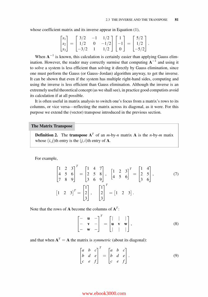
2.3 THE INVERSE AND THE TRANSPOSE 81
whose coefficient matrix and its inverse appear in Equation (1),⎡⎣x1
x2
x3
⎤⎦ =
⎡⎣ 3/2 −1 1/2
1/2 0 −1/2−3/2 1 1/2
⎤⎦⎡⎣ 1−10
⎤⎦ =
⎡⎣ 5/2
1/2−5/2
⎤⎦ .
When A−1 is known, this calculation is certainly easier than applying Gauss elim-ination. However, the reader may correctly surmise that computing A−1 and using itto solve a system is less efficient than solving it directly by Gauss elimination, sinceone must perform the Gauss (or Gauss–Jordan) algorithm anyway, to get the inverse.It can be shown that even if the system has multiple right-hand sides, computing andusing the inverse is less efficient than Gauss elimination. Although the inverse is anextremely useful theoretical concept (as we shall see), in practice good computists avoidits calculation if at all possible.
It is often useful in matrix analysis to switch one’s focus from a matrix’s rows to itscolumns, or vice versa—reflecting the matrix across its diagonal, as it were. For thispurpose we extend the (vector) transpose introduced in the previous section.
The Matrix Transpose
Definition 2. The transpose AT of an m-by-n matrix A is the n-by-m matixwhose (i, j)th entry is the (j, i)th entry of A.
For example,
⎡⎣1 2 3
4 5 67 8 9
⎤⎦
T
=
⎡⎣1 4 7
2 5 83 6 9
⎤⎦ ,
[1 2 34 5 6
]T
=
⎡⎣1 4
2 53 6
⎤⎦ , (7)
[1 2 3
]T=
⎡⎣1
23
⎤⎦ ,
⎡⎣1
23
⎤⎦
T
=[1 2 3
].
Note that the rows of A become the columns of AT :⎡⎣− u −− v −− w −
⎤⎦
T
=
⎡⎣ | | |
u v w| | |
⎤⎦ , (8)
and that when AT = A the matrix is symmetric (about its diagonal):
⎡⎣a b c
b d ec e f
⎤⎦
T
=
⎡⎣a b c
b d ec e f
⎤⎦ . (9)
www.ebook3000.com
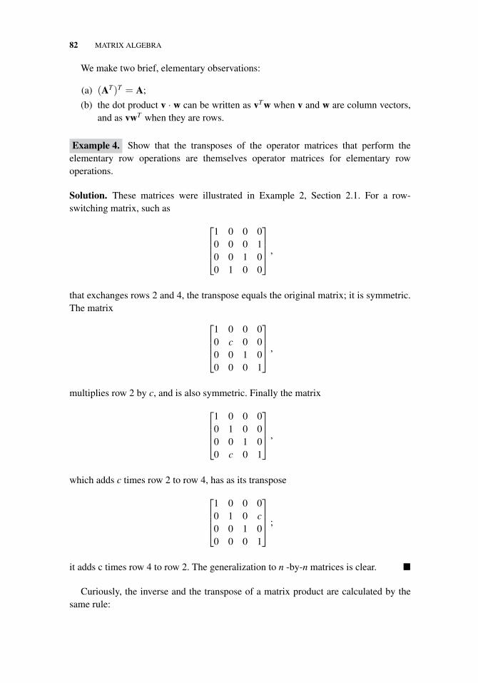
82 MATRIX ALGEBRA
We make two brief, elementary observations:
(a) (AT)T = A;
(b) the dot product v · w can be written as vTw when v and w are column vectors,and as vwT when they are rows.
Example 4. Show that the transposes of the operator matrices that perform theelementary row operations are themselves operator matrices for elementary rowoperations.
Solution. These matrices were illustrated in Example 2, Section 2.1. For a row-switching matrix, such as
⎡⎢⎢⎣
1 0 0 00 0 0 10 0 1 00 1 0 0
⎤⎥⎥⎦ ,
that exchanges rows 2 and 4, the transpose equals the original matrix; it is symmetric.The matrix
⎡⎢⎢⎣
1 0 0 00 c 0 00 0 1 00 0 0 1
⎤⎥⎥⎦ ,
multiplies row 2 by c, and is also symmetric. Finally the matrix
⎡⎢⎢⎣
1 0 0 00 1 0 00 0 1 00 c 0 1
⎤⎥⎥⎦ ,
which adds c times row 2 to row 4, has as its transpose
⎡⎢⎢⎣
1 0 0 00 1 0 c0 0 1 00 0 0 1
⎤⎥⎥⎦ ;
it adds c times row 4 to row 2. The generalization to n -by-n matrices is clear. �
Curiously, the inverse and the transpose of a matrix product are calculated by thesame rule:
2.3 THE INVERSE AND THE TRANSPOSE 83
Transpose and Inverse of the Matrix Product
Theorem 3. If the matrix product AB is defined, then we have
(AB)T = BTAT . (10)
Moreover, if A and B are invertible, then so is AB and
(AB)−1 = B−1A−1. (11)
Proof. The inverse property (11) is easier to prove; we simply need to confirmthat (B−1A−1)(AB) = I, and this follows from manipulation of parentheses (assanctioned by associativity): (B−1A−1)(AB) = B−1(A−1A)B = B−1B = I.
To see (10) requires some computation. Compare the calculation of the (2,3)entry of AB with the (3,2) entry of BTAT in the following:
AB =
[− − −s t u
]⎡⎣− − x −− − y −− − z −
⎤⎦ =
[− − − −− − ∗ −
],
BTAT =
⎡⎢⎢⎣− − −− − −x y z− − −
⎤⎥⎥⎦⎡⎣− s− t− u
⎤⎦ =
⎡⎢⎢⎣− −− −− ∗− −
⎤⎥⎥⎦ .
Both entries contain sx + ty + uz, the dot product of the second row of A (whichis the second column of AT ) with the third column of B (i.e., the third row ofBT ). Generalizing, we see that the computation of the (i, j)th entry of BTAT isidentical to that of the (j, i)th entry of AB, proving (10). �
Theorem 3 generalizes to extended products easily:
(A1A2 · · ·Ak−1Ak)−1 = A−1
k A−1k−1 · · ·A−1
2 A−11 (12)
(A1A2 · · ·Ak−1Ak)T = AT
k ATk−1 · · ·AT
2 AT1 ,
where in (12) we presume that all the inverses exist. (See Problems 21 and 22.)
Example 5. Show that the transpose of the inverse equals the inverse of the transpose;that is, for invertible matrices (A−1)T = (AT)−1.
Solution. By Equation (10), the transpose of the equation AA−1 = I is (A−1)TAT =IT = I. so (A−1)T is, indeed, the inverse of AT . �
www.ebook3000.com
84 MATRIX ALGEBRA
Exercises 2.3
In Problems 1–6, without performing any computations, find the inverse of the givenelementary row operation matrix.
1.
⎡⎣1 0 −5
0 1 00 0 1
⎤⎦ 2.
⎡⎣1 0 0
0 1 00 0 π
⎤⎦
3.
⎡⎣1 0 0
0 5 00 0 1
⎤⎦ 4.
⎡⎣1 0 0
0 0 10 1 0
⎤⎦
5.
⎡⎢⎢⎣
1 0 0 00 0 1 00 1 0 00 0 0 1
⎤⎥⎥⎦ 6.
⎡⎢⎢⎣
1 0 0 00 1 0 00 0 1 00 −18 0 1
⎤⎥⎥⎦
In Problems 7–12, compute the inverse of the given matrix, if it exists.
7.
[2 1−1 4
]8.
[4 15 9
]
9.
⎡⎣1 1 1
1 2 12 3 2
⎤⎦ 10.
⎡⎣1 1 1
1 2 30 1 1
⎤⎦
11.
⎡⎢⎢⎣
3 0 0 12 0 0 00 0 2 00 1 2 0
⎤⎥⎥⎦ 12.
⎡⎢⎢⎣
3 4 5 60 0 1 20 0 4 50 0 0 8
⎤⎥⎥⎦
13. Let A =
⎡⎣1 0 3
0 2 44 −3 8
⎤⎦. Compute A−1 and use it to solve each of the following
systems:
(a) Ax=[ 1 0 3]T (b) Ax = [−3 7 1]T (c) Ax = [0 − 4 1]T
14. Let A be the matrix in Problem 11. Use A−1 to solve the following systems:(a) Ax = [−1 0 2 1]T (b) Ax = [2 3 0 − 2]T
15. Let A be the matrix in Problem 10. Use A−1 to solve the following matrix equationfor X:
AX =
⎡⎣1 0 3
0 2 44 −3 8
⎤⎦ . (13)
16. Prove that if A and B are both m-by-n matrices, then (A+B)T= AT+BT .
2.3 THE INVERSE AND THE TRANSPOSE 85
17. For each of the following, determine whether the statement made is always Trueor sometimes False.(a) If A and B are n-by-n invertible matrices, then A+B is also invertible.
(b) If A is invertible, so is A3.
(c) If A is a symmetric matrix, then so is A2.
(d) If A is invertible, so is AT .
18. Prove that if A is any n-by-n matrix, then the matrices A + AT and AAT aresymmetric.
19. Prove that if A =
[a bc d
], then A is invertible if and only if ad − cb �= 0. Show
that if this condition holds, then
A−1 =1
ad − cb
[d −b−c a
].
20. Use the formula in Problem 19 to provide another proof that Mrot(θ)−1 =Mrot(−θ)and that M−1
ref =Mref (see Section 2.2).
21. Use Theorem 3 to prove that if A, B, and C are n-by-n matrices, then (ABC)T =CTBTAT .
22. Prove that if A, B, and C are invertible n-by-n matrices, then ABC is invertible and(ABC)−1 = C−1B−1A−1.
23. Show that the transpose of the rotation operator matrix Mrot discussed in Example 1is also the inverse of Mrot.
24. If A is a nilpotent matrix; that is, a square matrix such that Ak = 0 for somenonnegative integer k, prove that I − A is invertible and that
(I − A)−1 = I + A + A2 + · · · + Ak−1.
25. Verify the Sherman–Morrison–Woodbury formula:
(A + BCD)−1 = A−1 − A−1B(C−1 + DA−1B)−1A−1.
[Hint: Left-multiply the right-hand member by A + BCD, and judiciously insertI = CC−1.] This formula is helpful when the inverse is known for a matrix A, butthen A must be “updated” by adding BCD, with an easily invertible C. Let A bethe 5-by-5 identity matrix, B = [0 0 0 0 1]T, C = [0.1], and D = [1 1 1 1 1] toobtain a quick evaluation of
⎡⎢⎢⎢⎢⎣
1 0 0 0 00 1 0 0 00 0 1 0 00 0 0 1 0
0.1 0.1 0.1 0.1 1.1
⎤⎥⎥⎥⎥⎦
−1
.
www.ebook3000.com
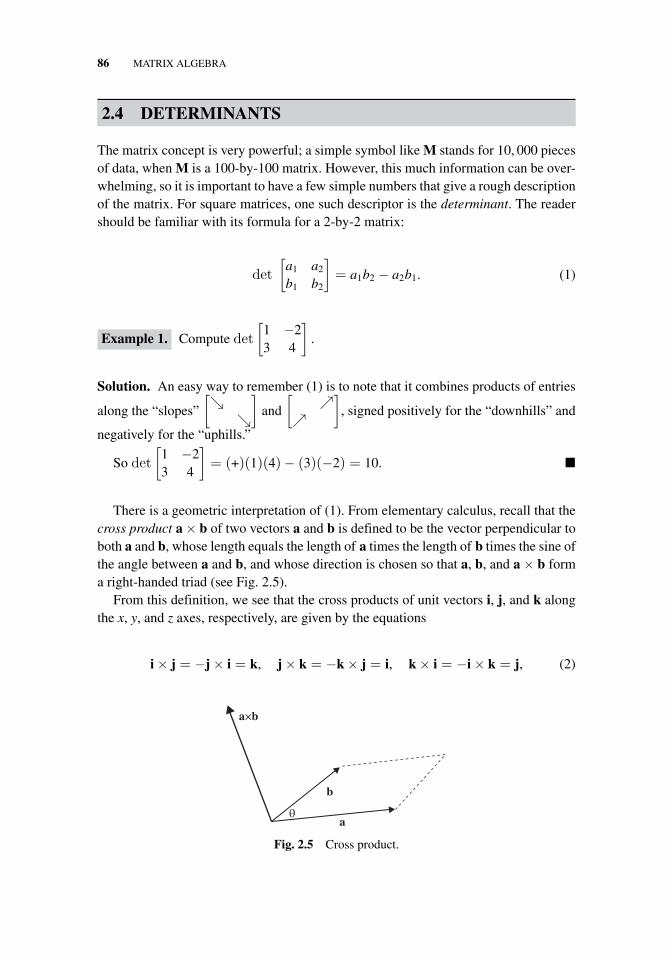
86 MATRIX ALGEBRA
2.4 DETERMINANTS
The matrix concept is very powerful; a simple symbol like M stands for 10, 000 piecesof data, when M is a 100-by-100 matrix. However, this much information can be over-whelming, so it is important to have a few simple numbers that give a rough descriptionof the matrix. For square matrices, one such descriptor is the determinant. The readershould be familiar with its formula for a 2-by-2 matrix:
det
[a1 a2
b1 b2
]= a1b2 − a2b1. (1)
Example 1. Compute det
[1 −23 4
].
Solution. An easy way to remember (1) is to note that it combines products of entries
along the “slopes”
[↘
↘
]and
[↗
↗
], signed positively for the “downhills” and
negatively for the “uphills.”
So det
[1 −23 4
]= (+)(1)(4)− (3)(−2) = 10. �
There is a geometric interpretation of (1). From elementary calculus, recall that thecross product a × b of two vectors a and b is defined to be the vector perpendicular toboth a and b, whose length equals the length of a times the length of b times the sine ofthe angle between a and b, and whose direction is chosen so that a, b, and a × b forma right-handed triad (see Fig. 2.5).
From this definition, we see that the cross products of unit vectors i, j, and k alongthe x, y, and z axes, respectively, are given by the equations
i × j = −j × i = k, j × k = −k × j = i, k × i = −i × k = j, (2)
aθ
b
a×b
Fig. 2.5 Cross product.
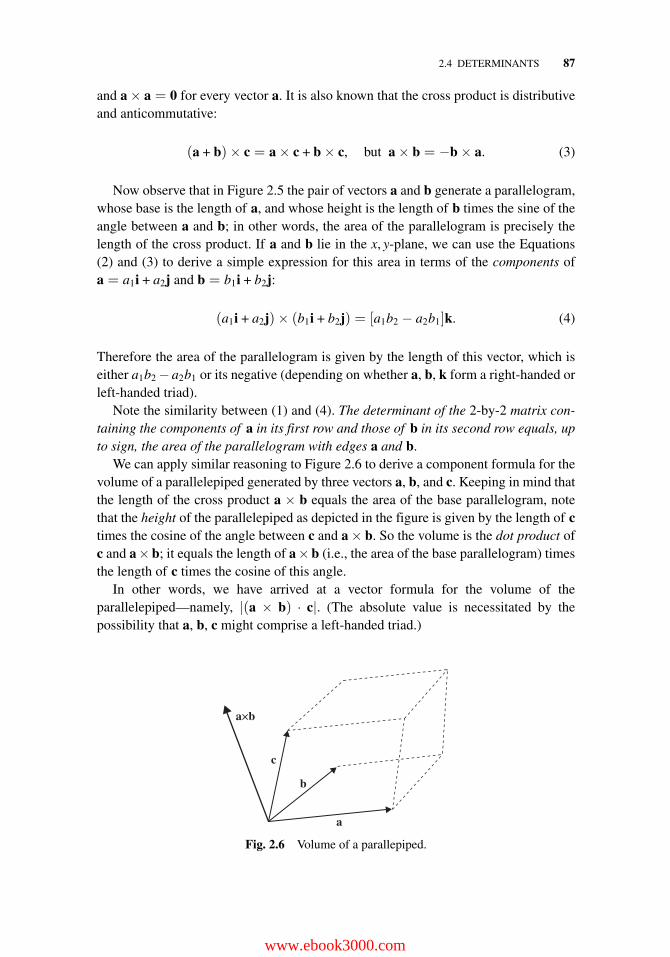
2.4 DETERMINANTS 87
and a × a = 0 for every vector a. It is also known that the cross product is distributiveand anticommutative:
(a + b)× c = a × c + b × c, but a × b = −b × a. (3)
Now observe that in Figure 2.5 the pair of vectors a and b generate a parallelogram,whose base is the length of a, and whose height is the length of b times the sine of theangle between a and b; in other words, the area of the parallelogram is precisely thelength of the cross product. If a and b lie in the x, y-plane, we can use the Equations(2) and (3) to derive a simple expression for this area in terms of the components ofa = a1i + a2j and b = b1i + b2j:
(a1i + a2j)× (b1i + b2j) = [a1b2 − a2b1]k. (4)
Therefore the area of the parallelogram is given by the length of this vector, which iseither a1b2 − a2b1 or its negative (depending on whether a, b, k form a right-handed orleft-handed triad).
Note the similarity between (1) and (4). The determinant of the 2-by-2 matrix con-taining the components of a in its first row and those of b in its second row equals, upto sign, the area of the parallelogram with edges a and b.
We can apply similar reasoning to Figure 2.6 to derive a component formula for thevolume of a parallelepiped generated by three vectors a, b, and c. Keeping in mind thatthe length of the cross product a × b equals the area of the base parallelogram, notethat the height of the parallelepiped as depicted in the figure is given by the length of ctimes the cosine of the angle between c and a × b. So the volume is the dot product ofc and a×b; it equals the length of a×b (i.e., the area of the base parallelogram) timesthe length of c times the cosine of this angle.
In other words, we have arrived at a vector formula for the volume of theparallelepiped—namely, |(a × b) · c|. (The absolute value is necessitated by thepossibility that a, b, c might comprise a left-handed triad.)
a
b
c
a×b
Fig. 2.6 Volume of a parallepiped.
www.ebook3000.com
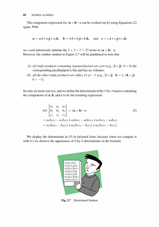
88 MATRIX ALGEBRA
The component expression for (a× b) · c can be worked out by using Equations (2)again. With
a = a1i + a2j + a3k, b = b1i + b2j + b3k, and c = c1i + c2j + c3k,
we could laboriously tabulate the 3 × 3 × 3 = 27 terms in (a × b) · c.However, the somber student in Figure 2.7 will be gladdened to note that
(i) all triple products containing repeated factors are zero (e.g., (i × j) · i = 0; thecorresponding parallepiped is flat and has no volume);
(ii) all the other triple products are either +1 or −1 (e.g., (i × j) · k = 1, (k × j) ·i = −1).
So only six terms survive, and we define the determinant of the 3-by-3 matrix containingthe components of a, b, and c to be the resulting expression:
det
⎡⎣a1 a2 a3
b1 b2 b3
c1 c2 c3
⎤⎦ = (a × b) · c (5)
= a1b2c3 − a1b3c2 + a2b3c1 − a2b1c3 + a3b1c2 − a3b2c1
= a1(b2c3 − b3c2) + a2(b3c1 − b1c3) + a3(b1c2 − b2c1).
We display the determinant in (5) in factored form, because when we compare itwith (1) we observe the appearance of 2-by-2 determinants in the formula:
a1b1c1ixii+a1b1c1jxii+a1b1c1kxi.i+a1b1c1ixji+a1b1c1jxji+a1b1c1kxk.i+a1b1c1kxi.i
Fig. 2.7 Determined Student.
2.4 DETERMINANTS 89
det
⎡⎣a1 a2 a3
b1 b2 b3
c1 c2 c3
⎤⎦ = a1 det
[b2 b3
c2 c3
]− a2 det
[b1 b3
c1 c3
]+ a3 det
[b1 b2
c1 c2
]. (6)
Notice the alternating signs, which we have introduced to maintain the original orderingof the columns.
Formula (6) is easy to remember by striking out the first row and successive columnsof the matrix:
det
⎡⎣a1 a2 a3
b1 b2 b3
c1 c2 c3
⎤⎦
a1
a1 a2 a3
b1 b2 b3
c1 c2 c3
a2
a1 a2 a3
b1 b2 b3
c1 c2 c3
a3
a1 a2 a3
b1 b2 b3
c1 c2 c3
.
Example 2. Compute det(A), where A =
⎡⎣1 2 3
4 5 67 8 9
⎤⎦ .
Solution. From (6), we obtain
det(A) = (1) det
[5 68 9
]− 2det
[4 67 9
]+ 3det
[4 57 8
]
= (45 − 48)− 2(36 − 42) + 3(32 − 35)
= −3 + 12 − 9 = 0. �
Now observe that a reduction identity similar to (6) arises when we juggle the 2-by-2determinant expression (1):
a1 a2
b1 b2a1b2 a2b1 a1
a1 a2
b1 b2a2
a1 a2
b1 b2(7)
(if we take the determinant of a 1-by-1 matrix to be simply the value of the entry).Since (6), (7) express 3-by-3 determinants in terms of 2-by-2’s and 2-by-2’s in terms
of 1-by-1’s, we can use the same pattern to define 4-by-4 determinants in terms of3-by-3’s, and so on, to formulate a recursive definition.
www.ebook3000.com
90 MATRIX ALGEBRA
Determinants
Definition 3. The determinant of a 1-by-1 matrix [a11] is simply a11, andthe determinant of an n-by-n matrix with n > 1 is defined via lower-orderdeterminants by
det(A) = det
⎡⎢⎢⎢⎢⎢⎣
a11 a12 a13 . . . a1n
a21 a22 a23 . . . a2n
a31 a32 a33 . . . a3n...
......
. . ....
an1 an2 an3 . . . ann
⎤⎥⎥⎥⎥⎥⎦
(8)
:= a11 det(A11)− a12 det(A12) + a13 det(A13)
− · · · + (−1)n+1a1n det(A1n)
=n∑
j=1
(−1)1+ja1j det(A1j),
where A1j is the (n − 1)-by-(n − 1) submatrix obtained by deleting the first rowand jth column of A.
Note that from this recursive definition it follows that the determinant of a diag-onal matrix is the product of the entries along the diagonal. This is consistent withour original volume interpretation of the determinant; we are inclined to postulate thata rectangle in n-dimensional space having edge lengths a1, a2, . . . , an along the axesshould have a volume given by a1a2 · · · an. Since its edge vectors would be representedby [a1 0 · · · 0], [0 a2 · · · 0], . . . , [0 0 · · · an], the determinant does indeed give thevolume:
det
⎡⎢⎢⎢⎣
a1 0 · · · 00 a2 · · · 0...
.... . .
...0 0 · · · an
⎤⎥⎥⎥⎦ = a1a2 · · · an.
Remark. An alternative notation for the determinant utilizes vertical bars:
∣∣∣∣∣∣∣a11 . . . a1n...
. . ....
an1 . . . ann
∣∣∣∣∣∣∣:= det
⎡⎢⎣
a11 . . . ann...
. . ....
an1 . . . ann
⎤⎥⎦
We employ this notation in the following example.
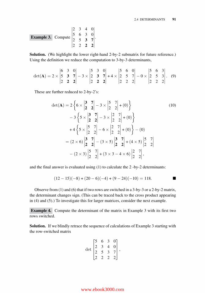
2.4 DETERMINANTS 91
Example 3. Compute
∣∣∣∣∣∣∣∣
2 3 4 05 6 3 02 5 3 72 2 2 2
∣∣∣∣∣∣∣∣.
Solution. (We highlight the lower right-hand 2-by-2 submatrix for future reference.)Using the definition we reduce the computation to 3-by-3 determinants,
det(A) = 2 ×
∣∣∣∣∣∣6 3 05 3 72 2 2
∣∣∣∣∣∣− 3 ×
∣∣∣∣∣∣5 3 02 3 72 2 2
∣∣∣∣∣∣ + 4 ×
∣∣∣∣∣∣5 6 02 5 72 2 2
∣∣∣∣∣∣− 0 ×
∣∣∣∣∣∣5 6 32 5 32 2 2
∣∣∣∣∣∣ . (9)
These are further reduced to 2-by-2’s:
det(A) = 2
{6 ×
∣∣∣∣3 72 2
∣∣∣∣− 3 ×∣∣∣∣5 72 2
∣∣∣∣ + (0)
}(10)
− 3
{5 ×
∣∣∣∣3 72 2
∣∣∣∣− 3 ×∣∣∣∣2 72 2
∣∣∣∣ + (0)
}
+ 4
{5 ×
∣∣∣∣5 72 2
∣∣∣∣− 6 ×∣∣∣∣2 72 2
∣∣∣∣ + (0)
}− (0)
= (2 × 6)
∣∣∣∣3 72 2
∣∣∣∣− (3 × 5)
∣∣∣∣3 72 2
∣∣∣∣ + (4 × 5)
∣∣∣∣5 72 2
∣∣∣∣− (2 × 3)
∣∣∣∣5 72 2
∣∣∣∣ + (3 × 3 − 4 × 6)
∣∣∣∣2 72 2
∣∣∣∣ ,
and the final answer is evaluated using (1) to calculate the 2 -by-2 determinants:
(12 − 15)(−8) + (20 − 6)(−4) + (9 − 24)(−10) = 118. �
Observe from (1) and (6) that if two rows are switched in a 3-by-3 or a 2-by-2 matrix,the determinant changes sign. (This can be traced back to the cross product appearingin (4) and (5).) To investigate this for larger matrices, consider the next example.
Example 4. Compute the determinant of the matrix in Example 3 with its first tworows switched.
Solution. If we blindly retrace the sequence of calculations of Example 3 starting withthe row-switched matrix
det
⎡⎢⎢⎣
5 6 3 02 3 4 02 5 3 72 2 2 2
⎤⎥⎥⎦ ,
www.ebook3000.com
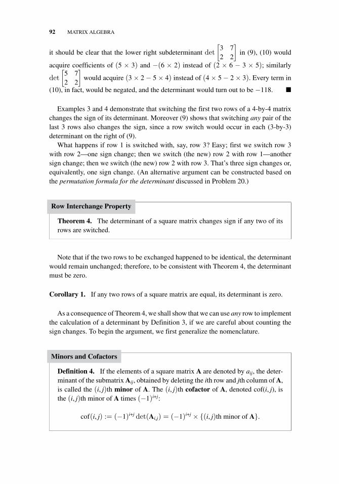
92 MATRIX ALGEBRA
it should be clear that the lower right subdeterminant det
[3 72 2
]in (9), (10) would
acquire coefficients of (5 × 3) and −(6 × 2) instead of (2 × 6 − 3 × 5); similarly
det
[5 72 2
]would acquire (3 × 2 − 5 × 4) instead of (4 × 5 − 2 × 3). Every term in
(10), in fact, would be negated, and the determinant would turn out to be −118. �
Examples 3 and 4 demonstrate that switching the first two rows of a 4-by-4 matrixchanges the sign of its determinant. Moreover (9) shows that switching any pair of thelast 3 rows also changes the sign, since a row switch would occur in each (3-by-3)determinant on the right of (9).
What happens if row 1 is switched with, say, row 3? Easy; first we switch row 3with row 2—one sign change; then we switch (the new) row 2 with row 1—anothersign change; then we switch (the new) row 2 with row 3. That’s three sign changes or,equivalently, one sign change. (An alternative argument can be constructed based onthe permutation formula for the determinant discussed in Problem 20.)
Row Interchange Property
Theorem 4. The determinant of a square matrix changes sign if any two of itsrows are switched.
Note that if the two rows to be exchanged happened to be identical, the determinantwould remain unchanged; therefore, to be consistent with Theorem 4, the determinantmust be zero.
Corollary 1. If any two rows of a square matrix are equal, its determinant is zero.
As a consequence of Theorem 4, we shall show that we can use any row to implementthe calculation of a determinant by Definition 3, if we are careful about counting thesign changes. To begin the argument, we first generalize the nomenclature.
Minors and Cofactors
Definition 4. If the elements of a square matrix A are denoted by aij, the deter-minant of the submatrix Aij, obtained by deleting the ith row and jth column of A,is called the (i, j)th minor of A. The (i, j)th cofactor of A, denoted cof(i, j), isthe (i, j)th minor of A times (−1)i+j:
cof(i, j) := (−1)i+j det(Ai,j) = (−1)i+j × {(i, j)th minor of A}.
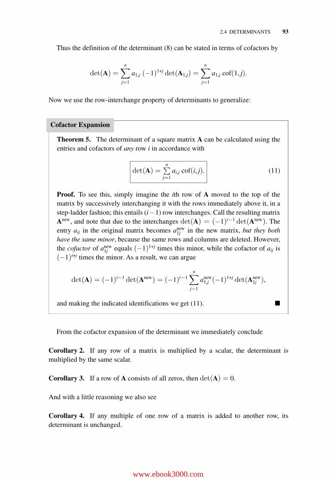
2.4 DETERMINANTS 93
Thus the definition of the determinant (8) can be stated in terms of cofactors by
det(A) =n∑
j=1
a1,j (−1)1+j det(A1,j) =n∑
j=1
a1,j cof(1, j).
Now we use the row-interchange property of determinants to generalize:
Cofactor Expansion
Theorem 5. The determinant of a square matrix A can be calculated using theentries and cofactors of any row i in accordance with
det(A) =n∑
j=1ai,j cof(i, j). (11)
Proof. To see this, simply imagine the ith row of A moved to the top of thematrix by successively interchanging it with the rows immediately above it, in astep-ladder fashion; this entails (i−1) row interchanges. Call the resulting matrixAnew, and note that due to the interchanges det(A) = (−1)i−1 det(Anew). Theentry aij in the original matrix becomes anew
1j in the new matrix, but they bothhave the same minor, because the same rows and columns are deleted. However,the cofactor of anew
1j equals (−1)1+j times this minor, while the cofactor of aij is(−1)i+j times the minor. As a result, we can argue
det(A) = (−1)i−1 det(Anew) = (−1)i−1n∑
j=1
anew1,j (−1)1+j det(Anew
1j ),
and making the indicated identifications we get (11). �
From the cofactor expansion of the determinant we immediately conclude
Corollary 2. If any row of a matrix is multiplied by a scalar, the determinant ismultiplied by the same scalar.
Corollary 3. If a row of A consists of all zeros, then det(A) = 0.
And with a little reasoning we also see
Corollary 4. If any multiple of one row of a matrix is added to another row, itsdeterminant is unchanged.
www.ebook3000.com
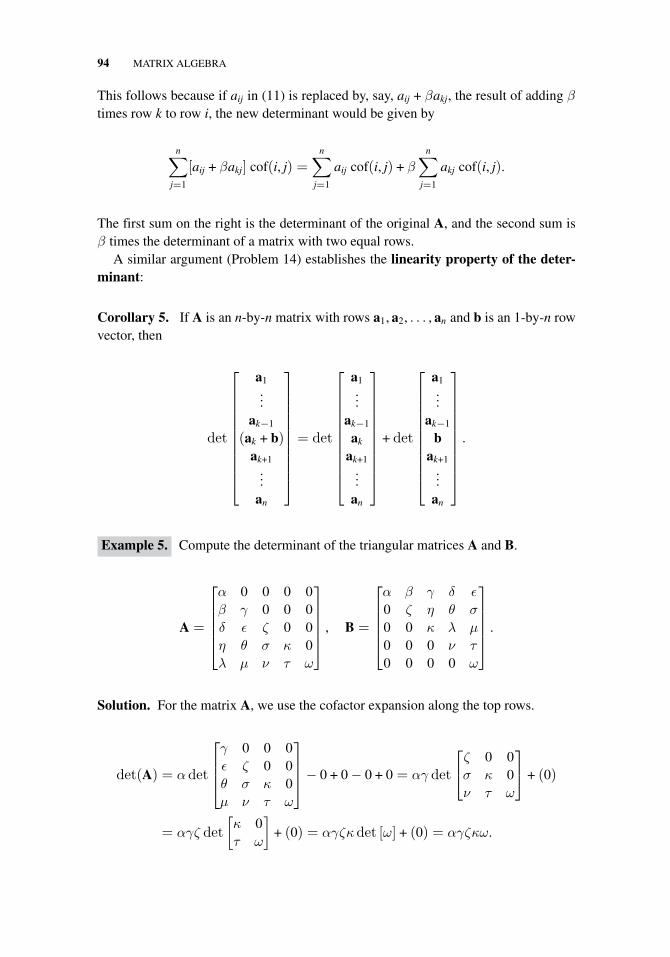
94 MATRIX ALGEBRA
This follows because if aij in (11) is replaced by, say, aij + βakj, the result of adding β
times row k to row i, the new determinant would be given by
n∑j=1
[aij + βakj] cof(i, j) =n∑
j=1
aij cof(i, j) + βn∑
j=1
akj cof(i, j).
The first sum on the right is the determinant of the original A, and the second sum isβ times the determinant of a matrix with two equal rows.
A similar argument (Problem 14) establishes the linearity property of the deter-minant:
Corollary 5. If A is an n-by-n matrix with rows a1, a2, . . . , an and b is an 1-by-n rowvector, then
det
⎡⎢⎢⎢⎢⎢⎢⎢⎢⎢⎢⎣
a1...
ak−1
(ak + b)ak+1
...an
⎤⎥⎥⎥⎥⎥⎥⎥⎥⎥⎥⎦= det
⎡⎢⎢⎢⎢⎢⎢⎢⎢⎢⎢⎣
a1...
ak−1
ak
ak+1...
an
⎤⎥⎥⎥⎥⎥⎥⎥⎥⎥⎥⎦
+ det
⎡⎢⎢⎢⎢⎢⎢⎢⎢⎢⎢⎣
a1...
ak−1
bak+1
...an
⎤⎥⎥⎥⎥⎥⎥⎥⎥⎥⎥⎦
.
Example 5. Compute the determinant of the triangular matrices A and B.
A =
⎡⎢⎢⎢⎢⎣
α 0 0 0 0β γ 0 0 0δ ε ζ 0 0η θ σ κ 0λ μ ν τ ω
⎤⎥⎥⎥⎥⎦ , B =
⎡⎢⎢⎢⎢⎣
α β γ δ ε
0 ζ η θ σ
0 0 κ λ μ
0 0 0 ν τ
0 0 0 0 ω
⎤⎥⎥⎥⎥⎦ .
Solution. For the matrix A, we use the cofactor expansion along the top rows.
det(A) = αdet
⎡⎢⎢⎣γ 0 0 0ε ζ 0 0θ σ κ 0μ ν τ ω
⎤⎥⎥⎦− 0 + 0 − 0 + 0 = αγ det
⎡⎣ζ 0 0σ κ 0ν τ ω
⎤⎦ + (0)
= αγζ det
[κ 0τ ω
]+ (0) = αγζκdet [ω] + (0) = αγζκω.
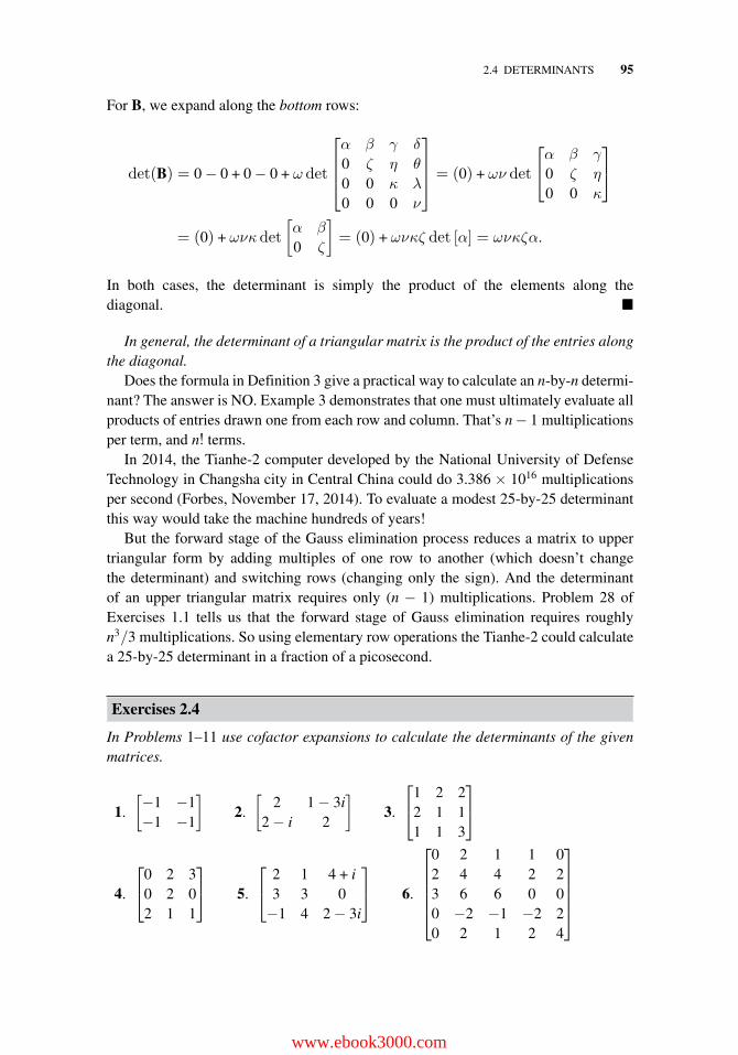
2.4 DETERMINANTS 95
For B, we expand along the bottom rows:
det(B) = 0 − 0 + 0 − 0 + ω det
⎡⎢⎢⎣α β γ δ
0 ζ η θ
0 0 κ λ
0 0 0 ν
⎤⎥⎥⎦ = (0) + ων det
⎡⎣α β γ
0 ζ η
0 0 κ
⎤⎦
= (0) + ωνκdet
[α β
0 ζ
]= (0) + ωνκζ det [α] = ωνκζα.
In both cases, the determinant is simply the product of the elements along thediagonal. �
In general, the determinant of a triangular matrix is the product of the entries alongthe diagonal.
Does the formula in Definition 3 give a practical way to calculate an n-by-n determi-nant? The answer is NO. Example 3 demonstrates that one must ultimately evaluate allproducts of entries drawn one from each row and column. That’s n − 1 multiplicationsper term, and n! terms.
In 2014, the Tianhe-2 computer developed by the National University of DefenseTechnology in Changsha city in Central China could do 3.386 × 10¹⁶ multiplicationsper second (Forbes, November 17, 2014). To evaluate a modest 25-by-25 determinantthis way would take the machine hundreds of years!
But the forward stage of the Gauss elimination process reduces a matrix to uppertriangular form by adding multiples of one row to another (which doesn’t changethe determinant) and switching rows (changing only the sign). And the determinantof an upper triangular matrix requires only (n − 1) multiplications. Problem 28 ofExercises 1.1 tells us that the forward stage of Gauss elimination requires roughlyn3/3 multiplications. So using elementary row operations the Tianhe-2 could calculatea 25-by-25 determinant in a fraction of a picosecond.
Exercises 2.4
In Problems 1–11 use cofactor expansions to calculate the determinants of the givenmatrices.
1.
[−1 −1−1 −1
]2.
[2 1 − 3i
2 − i 2
]3.
⎡⎣1 2 2
2 1 11 1 3
⎤⎦
4.
⎡⎣0 2 3
0 2 02 1 1
⎤⎦ 5.
⎡⎣ 2 1 4 + i
3 3 0−1 4 2 − 3i
⎤⎦ 6.
⎡⎢⎢⎢⎢⎣
0 2 1 1 02 4 4 2 23 6 6 0 00 −2 −1 −2 20 2 1 2 4
⎤⎥⎥⎥⎥⎦
www.ebook3000.com
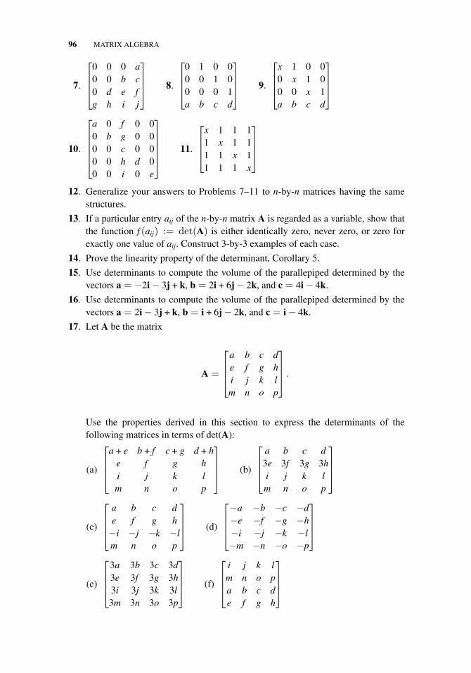
96 MATRIX ALGEBRA
7.
⎡⎢⎢⎣
0 0 0 a0 0 b c0 d e fg h i j
⎤⎥⎥⎦ 8.
⎡⎢⎢⎣
0 1 0 00 0 1 00 0 0 1a b c d
⎤⎥⎥⎦ 9.
⎡⎢⎢⎣
x 1 0 00 x 1 00 0 x 1a b c d
⎤⎥⎥⎦
10.
⎡⎢⎢⎢⎢⎣
a 0 f 0 00 b g 0 00 0 c 0 00 0 h d 00 0 i 0 e
⎤⎥⎥⎥⎥⎦ 11.
⎡⎢⎢⎣
x 1 1 11 x 1 11 1 x 11 1 1 x
⎤⎥⎥⎦
12. Generalize your answers to Problems 7–11 to n-by-n matrices having the samestructures.
13. If a particular entry aij of the n-by-n matrix A is regarded as a variable, show thatthe function f (aij) := det(A) is either identically zero, never zero, or zero forexactly one value of aij. Construct 3-by-3 examples of each case.
14. Prove the linearity property of the determinant, Corollary 5.
15. Use determinants to compute the volume of the parallepiped determined by thevectors a = −2i − 3j + k, b = 2i + 6j − 2k, and c = 4i − 4k.
16. Use determinants to compute the volume of the parallepiped determined by thevectors a = 2i − 3j + k, b = i + 6j − 2k, and c = i − 4k.
17. Let A be the matrix
A =
⎡⎢⎢⎣
a b c de f g hi j k lm n o p
⎤⎥⎥⎦ .
Use the properties derived in this section to express the determinants of thefollowing matrices in terms of det(A):
(a)
⎡⎢⎢⎣
a + e b + f c + g d + he f g hi j k lm n o p
⎤⎥⎥⎦ (b)
⎡⎢⎢⎣
a b c d3e 3f 3g 3hi j k lm n o p
⎤⎥⎥⎦
(c)
⎡⎢⎢⎣
a b c de f g h−i −j −k −lm n o p
⎤⎥⎥⎦ (d)
⎡⎢⎢⎣−a −b −c −d−e −f −g −h−i −j −k −l−m −n −o −p
⎤⎥⎥⎦
(e)
⎡⎢⎢⎣
3a 3b 3c 3d3e 3f 3g 3h3i 3j 3k 3l3m 3n 3o 3p
⎤⎥⎥⎦ (f)
⎡⎢⎢⎣
i j k lm n o pa b c de f g h
⎤⎥⎥⎦
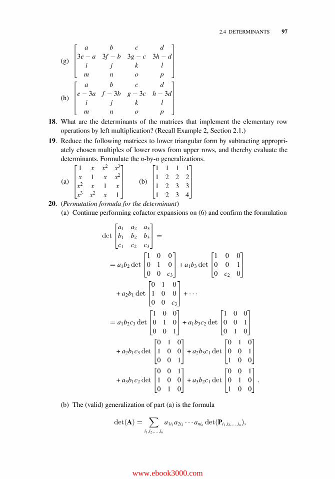
2.4 DETERMINANTS 97
(g)
⎡⎢⎢⎣
a b c d3e − a 3f − b 3g − c 3h − d
i j k lm n o p
⎤⎥⎥⎦
(h)
⎡⎢⎢⎣
a b c de − 3a f − 3b g − 3c h − 3d
i j k lm n o p
⎤⎥⎥⎦
18. What are the determinants of the matrices that implement the elementary rowoperations by left multiplication? (Recall Example 2, Section 2.1.)
19. Reduce the following matrices to lower triangular form by subtracting appropri-ately chosen multiples of lower rows from upper rows, and thereby evaluate thedeterminants. Formulate the n-by-n generalizations.
(a)
⎡⎢⎢⎣
1 x x2 x3
x 1 x x2
x2 x 1 xx3 x2 x 1
⎤⎥⎥⎦ (b)
⎡⎢⎢⎣
1 1 1 11 2 2 21 2 3 31 2 3 4
⎤⎥⎥⎦
20. (Permutation formula for the determinant)(a) Continue performing cofactor expansions on (6) and confirm the formulation
det
⎡⎣a1 a2 a3
b1 b2 b3
c1 c2 c3
⎤⎦ =
= a1b2 det
⎡⎣1 0 0
0 1 00 0 c3
⎤⎦ + a1b3 det
⎡⎣1 0 0
0 0 10 c2 0
⎤⎦
+ a2b1 det
⎡⎣0 1 0
1 0 00 0 c3
⎤⎦ + · · ·
= a1b2c3 det
⎡⎣1 0 0
0 1 00 0 1
⎤⎦ + a1b3c2 det
⎡⎣1 0 0
0 0 10 1 0
⎤⎦
+ a2b1c3 det
⎡⎣0 1 0
1 0 00 0 1
⎤⎦ + a2b3c1 det
⎡⎣0 1 0
0 0 11 0 0
⎤⎦
+ a3b1c2 det
⎡⎣0 0 1
1 0 00 1 0
⎤⎦ + a3b2c1 det
⎡⎣0 0 1
0 1 01 0 0
⎤⎦ .
(b) The (valid) generalization of part (a) is the formula
det(A) =∑
i1,i2,...,in
a1i1 a2i2 · · · anin det(Pi1,i2,...,in),
www.ebook3000.com
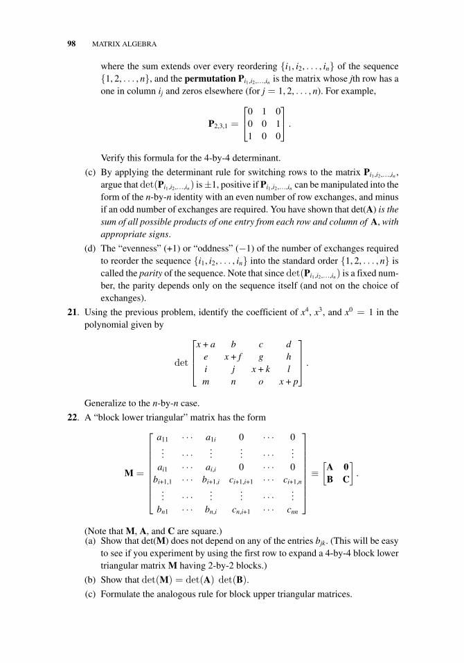
98 MATRIX ALGEBRA
where the sum extends over every reordering {i1, i2, . . . , in} of the sequence{1, 2, . . . , n}, and the permutation Pi1,i2,...,in is the matrix whose jth row has aone in column ij and zeros elsewhere (for j = 1, 2, . . . , n). For example,
P2,3,1 =
⎡⎣0 1 0
0 0 11 0 0
⎤⎦ .
Verify this formula for the 4-by-4 determinant.
(c) By applying the determinant rule for switching rows to the matrix Pi1,i2,...,in ,argue that det(Pi1,i2,...,in) is±1, positive if Pi1,i2,...,in can be manipulated into theform of the n-by-n identity with an even number of row exchanges, and minusif an odd number of exchanges are required. You have shown that det(A) is thesum of all possible products of one entry from each row and column of A, withappropriate signs.
(d) The “evenness” (+1) or “oddness” (−1) of the number of exchanges requiredto reorder the sequence {i1, i2, . . . , in} into the standard order {1, 2, . . . , n} iscalled the parity of the sequence. Note that since det(Pi1,i2,...,in) is a fixed num-ber, the parity depends only on the sequence itself (and not on the choice ofexchanges).
21. Using the previous problem, identify the coefficient of x4, x3, and x0 = 1 in thepolynomial given by
det
⎡⎢⎢⎣
x + a b c de x + f g hi j x + k lm n o x + p
⎤⎥⎥⎦ .
Generalize to the n-by-n case.
22. A “block lower triangular” matrix has the form
M =
⎡⎢⎢⎢⎢⎢⎢⎢⎢⎣
a11 · · · a1i 0 · · · 0... · · ·
...... · · ·
...ai1 · · · ai,i 0 · · · 0
bi+1,1 · · · bi+1,i ci+1,i+1 · · · ci+1,n... · · ·
...... · · ·
...bn1 · · · bn,i cn,i+1 · · · cnn
⎤⎥⎥⎥⎥⎥⎥⎥⎥⎦≡
[A 0B C
].
(Note that M, A, and C are square.)(a) Show that det(M) does not depend on any of the entries bjk. (This will be easy
to see if you experiment by using the first row to expand a 4-by-4 block lowertriangular matrix M having 2-by-2 blocks.)
(b) Show that det(M) = det(A) det(B).
(c) Formulate the analogous rule for block upper triangular matrices.
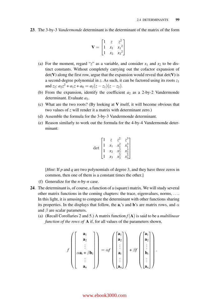
2.4 DETERMINANTS 99
23. The 3-by-3 Vandermonde determinant is the determinant of the matrix of the form
V =
⎡⎣1 z z2
1 x1 x12
1 x2 x22
⎤⎦
(a) For the moment, regard “z” as a variable, and consider x1 and x2 to be dis-tinct constants. Without completely carrying out the cofactor expansion ofdet(V) along the first row, argue that the expansion would reveal that det(V) isa second-degree polynomial in z. As such, it can be factored using its roots z1
and z2: a2z2 + a1z + a0 = a2(z − z1)(z − z2).
(b) From the expansion, identify the coefficient a2 as a 2-by-2 Vandermondedeterminant. Evaluate a2.
(c) What are the two roots? (By looking at V itself, it will become obvious thattwo values of z will render it a matrix with determinant zero.)
(d) Assemble the formula for the 3-by-3 Vandermonde determinant.
(e) Reason similarly to work out the formula for the 4-by-4 Vandermonde deter-minant:
det
⎡⎢⎢⎣
1 z z2 z3
1 x1 x21 x3
1
1 x2 x22 x3
2
1 x3 x23 x3
3
⎤⎥⎥⎦
[Hint: If p and q are two polynomials of degree 3, and they have three zeros incommon, then one of them is a constant times the other.]
(f) Generalize for the n-by-n case.
24. The determinant is, of course, a function of a (square) matrix. We will study severalother matrix functions in the coming chapters: the trace, eigenvalues, norms, . . ..In this light, it is amusing to compare the determinant with other functions sharingits properties. In the displays that follow, the ai’s and b’s are matrix rows, and α
and β are scalar parameters.(a) (Recall Corollaries 2 and 5.) A matrix function f (A) is said to be a multilinear
function of the rows of A if, for all values of the parameters shown,
f
⎛⎜⎜⎜⎜⎜⎜⎜⎜⎝
⎡⎢⎢⎢⎢⎢⎢⎢⎢⎣
a1
a2...
αai + βbi...
an
⎤⎥⎥⎥⎥⎥⎥⎥⎥⎦
⎞⎟⎟⎟⎟⎟⎟⎟⎟⎠
= αf
⎛⎜⎜⎜⎜⎜⎜⎜⎜⎝
⎡⎢⎢⎢⎢⎢⎢⎢⎢⎣
a1
a2...ai...
an
⎤⎥⎥⎥⎥⎥⎥⎥⎥⎦
⎞⎟⎟⎟⎟⎟⎟⎟⎟⎠
+ βf
⎛⎜⎜⎜⎜⎜⎜⎜⎜⎝
⎡⎢⎢⎢⎢⎢⎢⎢⎢⎣
a1
a2...
bi...
an
⎤⎥⎥⎥⎥⎥⎥⎥⎥⎦
⎞⎟⎟⎟⎟⎟⎟⎟⎟⎠
.
www.ebook3000.com
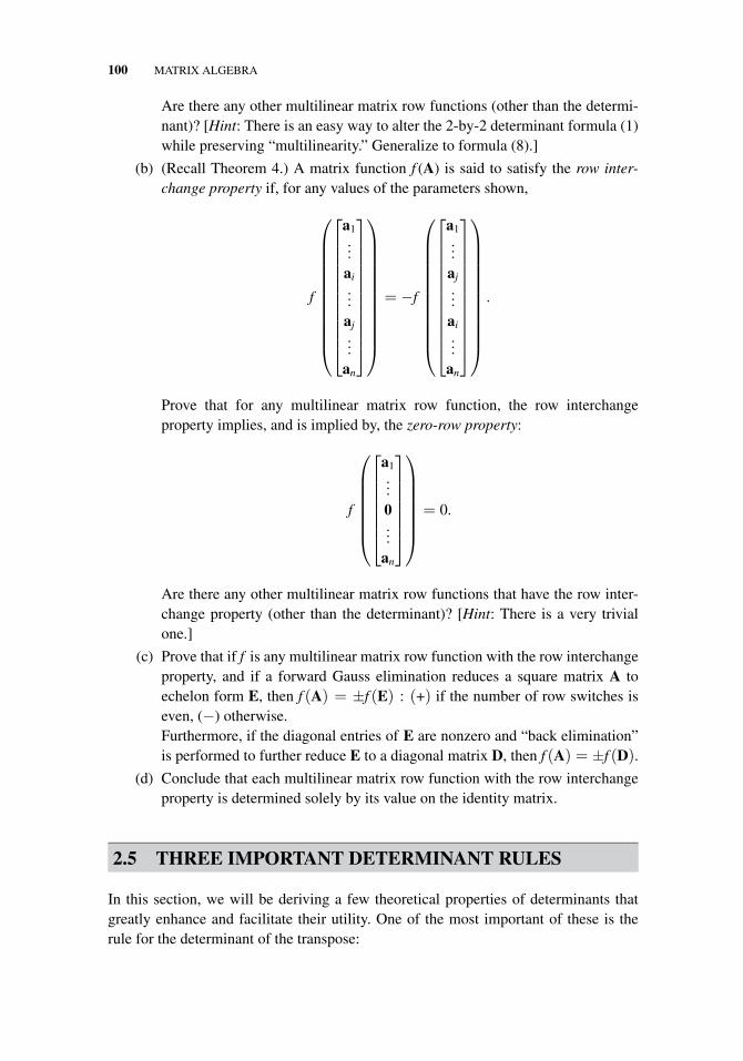
100 MATRIX ALGEBRA
Are there any other multilinear matrix row functions (other than the determi-nant)? [Hint: There is an easy way to alter the 2-by-2 determinant formula (1)while preserving “multilinearity.” Generalize to formula (8).]
(b) (Recall Theorem 4.) A matrix function f (A) is said to satisfy the row inter-change property if, for any values of the parameters shown,
f
⎛⎜⎜⎜⎜⎜⎜⎜⎜⎜⎜⎜⎝
⎡⎢⎢⎢⎢⎢⎢⎢⎢⎢⎢⎢⎣
a1...ai...aj...
an
⎤⎥⎥⎥⎥⎥⎥⎥⎥⎥⎥⎥⎦
⎞⎟⎟⎟⎟⎟⎟⎟⎟⎟⎟⎟⎠
= −f
⎛⎜⎜⎜⎜⎜⎜⎜⎜⎜⎜⎜⎝
⎡⎢⎢⎢⎢⎢⎢⎢⎢⎢⎢⎢⎣
a1...aj...ai...
an
⎤⎥⎥⎥⎥⎥⎥⎥⎥⎥⎥⎥⎦
⎞⎟⎟⎟⎟⎟⎟⎟⎟⎟⎟⎟⎠
.
Prove that for any multilinear matrix row function, the row interchangeproperty implies, and is implied by, the zero-row property:
f
⎛⎜⎜⎜⎜⎜⎜⎝
⎡⎢⎢⎢⎢⎢⎢⎣
a1...0...
an
⎤⎥⎥⎥⎥⎥⎥⎦
⎞⎟⎟⎟⎟⎟⎟⎠
= 0.
Are there any other multilinear matrix row functions that have the row inter-change property (other than the determinant)? [Hint: There is a very trivialone.]
(c) Prove that if f is any multilinear matrix row function with the row interchangeproperty, and if a forward Gauss elimination reduces a square matrix A toechelon form E, then f (A) = ±f (E) : (+) if the number of row switches iseven, (−) otherwise.Furthermore, if the diagonal entries of E are nonzero and “back elimination”is performed to further reduce E to a diagonal matrix D, then f (A) = ±f (D).
(d) Conclude that each multilinear matrix row function with the row interchangeproperty is determined solely by its value on the identity matrix.
2.5 THREE IMPORTANT DETERMINANT RULES
In this section, we will be deriving a few theoretical properties of determinants thatgreatly enhance and facilitate their utility. One of the most important of these is therule for the determinant of the transpose:
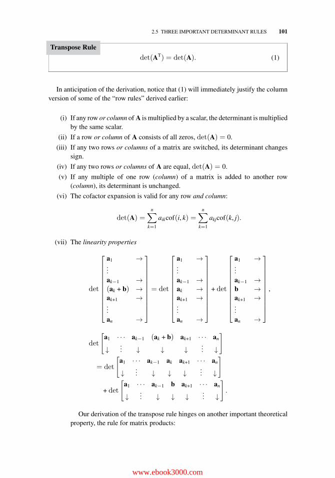
2.5 THREE IMPORTANT DETERMINANT RULES 101
Transpose Rule
det(AT) = det(A). (1)
In anticipation of the derivation, notice that (1) will immediately justify the columnversion of some of the “row rules” derived earlier:
(i) If any row or column of A is multiplied by a scalar, the determinant is multipliedby the same scalar.
(ii) If a row or column of A consists of all zeros, det(A) = 0.
(iii) If any two rows or columns of a matrix are switched, its determinant changessign.
(iv) If any two rows or columns of A are equal, det(A) = 0.
(v) If any multiple of one row (column) of a matrix is added to another row(column), its determinant is unchanged.
(vi) The cofactor expansion is valid for any row and column:
det(A) =n∑
k=1
aikcof(i, k) =n∑
k=1
akjcof(k, j).
(vii) The linearity properties
det
⎡⎢⎢⎢⎢⎢⎢⎢⎢⎢⎢⎣
a1 →...ak−1 →(ak + b) →ak+1 →...an →
⎤⎥⎥⎥⎥⎥⎥⎥⎥⎥⎥⎦= det
⎡⎢⎢⎢⎢⎢⎢⎢⎢⎢⎢⎣
a1 →...ak−1 →ak →ak+1 →...an →
⎤⎥⎥⎥⎥⎥⎥⎥⎥⎥⎥⎦
+ det
⎡⎢⎢⎢⎢⎢⎢⎢⎢⎢⎢⎣
a1 →...ak−1 →b →ak+1 →...an →
⎤⎥⎥⎥⎥⎥⎥⎥⎥⎥⎥⎦
,
det
[a1 · · · ak−1 (ak + b) ak+1 · · · an
↓... ↓ ↓ ↓
... ↓
]
= det
[a1 · · · ak−1 ak ak+1 · · · an
↓... ↓ ↓ ↓
... ↓
]
+ det
[a1 · · · ak−1 b ak+1 · · · an
↓... ↓ ↓ ↓
... ↓
].
Our derivation of the transpose rule hinges on another important theoreticalproperty, the rule for matrix products:
www.ebook3000.com
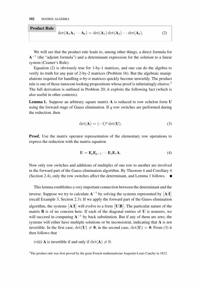
102 MATRIX ALGEBRA
Product Ruledet(A1A2 · · ·Ak) = det(A1) det(A2) · · ·det(Ak). (2)
We will see that the product rule leads to, among other things, a direct formula forA−1 (the “adjoint formula”) and a determinant expression for the solution to a linearsystem (Cramer’s Rule).
Equation (2) is obviously true for 1-by-1 matrices, and one can do the algebra toverify its truth for any pair of 2-by-2 matrices (Problem 16). But the algebraic manip-ulations required for handling n-by-n matrices quickly become unwieldy. The productrule is one of those innocent-looking propositions whose proof is infuriatingly elusive.3
The full derivation is outlined in Problem 20; it exploits the following fact (which isalso useful in other contexts).
Lemma 1. Suppose an arbitrary square matrix A is reduced to row echelon form Uusing the forward stage of Gauss elimination. If q row switches are performed duringthe reduction, then
det(A) = (−1)q det(U). (3)
Proof. Use the matrix operator representation of the elementary row operations toexpress the reduction with the matrix equation
U = EpEp−1 · · ·E2E1A. (4)
Now only row switches and additions of multiples of one row to another are involvedin the forward part of the Gauss elimination algorithm. By Theorem 4 and Corollary 4(Section 2.4), only the row switches affect the determinant, and Lemma 1 follows.
This lemma establishes a very important connection between the determinant and the
inverse. Suppose we try to calculate A−1 by solving the systems represented by[A
...I]
(recall Example 3, Section 2.3). If we apply the forward part of the Gauss elimination
algorithm, the systems[A
...I]
will evolve to a form[U
...B]. The particular nature of the
matrix B is of no concern here. If each of the diagonal entries of U is nonzero, wewill succeed in computing A−1 by back substitution. But if any of them are zero, thesystems will either have multiple solutions or be inconsistent, indicating that A is notinvertible. In the first case, det(U) �= 0; in the second case, det(U) = 0. From (3) itthen follows that
(viii) A is invertible if and only if det(A) �= 0.
3The product rule was first proved by the great French mathematician Augustin-Louis Cauchy in 1812.
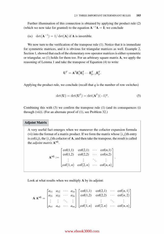
2.5 THREE IMPORTANT DETERMINANT RULES 103
Further illumination of this connection is obtained by applying the product rule (2)(which we now take for granted) to the equation A−1A = I; we conclude
(ix) det(A−1) = 1/det(A) if A is invertible.
We now turn to the verification of the transpose rule (1). Notice that it is immediatefor symmetric matrices, and it is obvious for triangular matrices as well. Example 2,Section 1, showed that each of the elementary row operator matrices is either symmetricor triangular, so (1) holds for them too. For an arbitrary square matrix A, we apply thereasoning of Lemma 1 and take the transpose of Equation (4) to write
UT = ATET1 ET
2 · · ·ETp−1ET
p .
Applying the product rule, we conclude (recall that q is the number of row switches)
det(U) = det(UT) = det(AT)(−1)q. (5)
Combining this with (3) we confirm the transpose rule (1) (and its consequences (i)through (vii)). (For an alternate proof of (1), see Problem 32.)
Adjoint Matrix
A very useful fact emerges when we maneuver the cofactor expansion formula(vi) into the format of a matrix product. If we form the matrix whose (i, j)th entryis cof(i,j), the (i, j)th cofactor of A, and then take the transpose, the result is calledthe adjoint matrix Aadj.
Aadj :=
⎡⎢⎢⎢⎣
cof(1,1) cof(2,1) · · · cof(n,1)cof(1,2) cof(2,2) · · · cof(n,2)
......
. . ....
cof(1, n) cof(2, n) · · · cof(n, n)
⎤⎥⎥⎥⎦ .
Look at what results when we multiply A by its adjoint:
A Aadj =
⎡⎢⎢⎢⎣
a11 a12 · · · a1n
a21 a22 · · · a2n...
.... . .
...an1 an2 · · · ann
⎤⎥⎥⎥⎦
⎡⎢⎢⎢⎣
cof(1,1) cof(2,1) · · · cof(n, 1)cof(1,2) cof(2,2) · · · cof(n, 2)
......
. . ....
cof(1, n) cof(2, n) · · · cof(n, n)
⎤⎥⎥⎥⎦
www.ebook3000.com
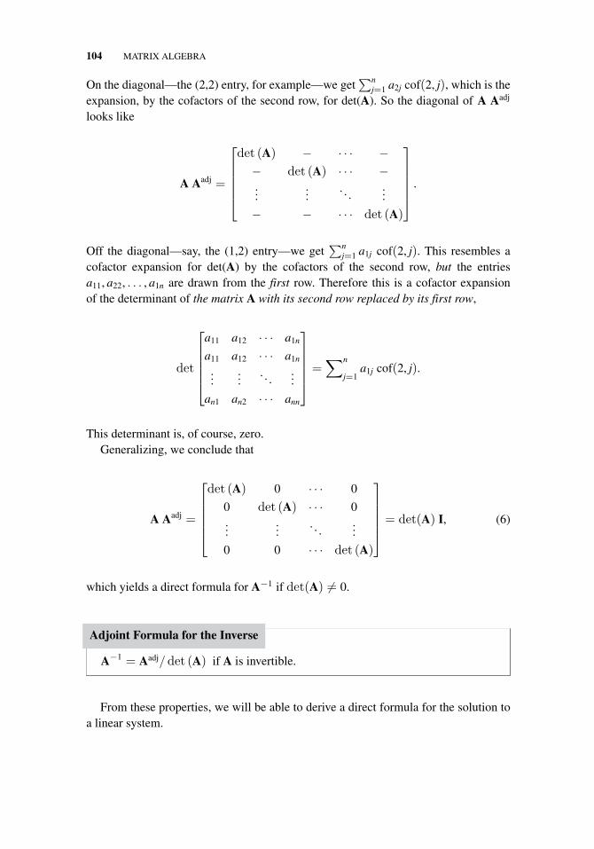
104 MATRIX ALGEBRA
On the diagonal—the (2,2) entry, for example—we get∑n
j=1 a2j cof(2, j), which is theexpansion, by the cofactors of the second row, for det(A). So the diagonal of A Aadj
looks like
A Aadj =
⎡⎢⎢⎢⎢⎣
det (A) − · · · −− det (A) · · · −...
.... . .
...
− − · · · det (A)
⎤⎥⎥⎥⎥⎦ .
Off the diagonal—say, the (1,2) entry—we get∑n
j=1 a1j cof(2, j). This resembles acofactor expansion for det(A) by the cofactors of the second row, but the entriesa11, a22, . . . , a1n are drawn from the first row. Therefore this is a cofactor expansionof the determinant of the matrix A with its second row replaced by its first row,
det
⎡⎢⎢⎢⎢⎣
a11 a12 · · · a1n
a11 a12 · · · a1n
......
. . ....
an1 an2 · · · ann
⎤⎥⎥⎥⎥⎦ =
∑n
j=1a1j cof(2, j).
This determinant is, of course, zero.Generalizing, we conclude that
A Aadj =
⎡⎢⎢⎢⎢⎣
det (A) 0 · · · 0
0 det (A) · · · 0...
.... . .
...
0 0 · · · det (A)
⎤⎥⎥⎥⎥⎦ = det(A) I, (6)
which yields a direct formula for A−1 if det(A) �= 0.
Adjoint Formula for the Inverse
A−1 = Aadj/det (A) if A is invertible.
From these properties, we will be able to derive a direct formula for the solution toa linear system.
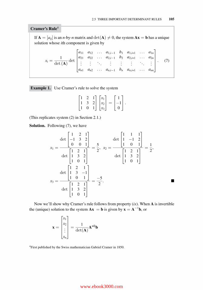
2.5 THREE IMPORTANT DETERMINANT RULES 105
Cramer’s Rule4
If A = [aij] is an n-by-n matrix and det(A) �= 0, the system Ax = b has a uniquesolution whose ith component is given by
xi =1
det (A)det
⎡⎢⎢⎢⎣
a11 a12 . . . a1,i−1 b1 a1,i+1 . . . a1n
a21 a22 . . . a2,i−1 b2 a2,i+1 . . . a2n...
.... . .
......
.... . .
...an1 an2 . . . an,i−1 bn an,i+1 . . . ann
⎤⎥⎥⎥⎦ . (7)
Example 1. Use Cramer’s rule to solve the system
⎡⎣1 2 1
1 3 21 0 1
⎤⎦⎡⎣x1
x2
x3
⎤⎦ =
⎡⎣ 1−10
⎤⎦ .
(This replicates system (2) in Section 2.1.)
Solution. Following (7), we have
x1 =
det
⎡⎣ 1 2 1−1 3 20 0 1
⎤⎦
det
⎡⎣1 2 1
1 3 21 0 1
⎤⎦
=52
, x2 =
det
⎡⎣1 1 1
1 −1 21 0 1
⎤⎦
det
⎡⎣1 2 1
1 3 21 0 1
⎤⎦
=12
,
x3 =
det
⎡⎣1 2 1
1 3 −11 0 1
⎤⎦
det
⎡⎣1 2 1
1 3 21 0 1
⎤⎦
=−52
. �
Now we’ll show why Cramer’s rule follows from property (ix). When A is invertiblethe (unique) solution to the system Ax = b is given by x = A−1b, or
x =
⎡⎢⎢⎢⎣
x1
x2...
xn
⎤⎥⎥⎥⎦ =
1det(A)
Aadjb
4First published by the Swiss mathematician Gabriel Cramer in 1850.
www.ebook3000.com
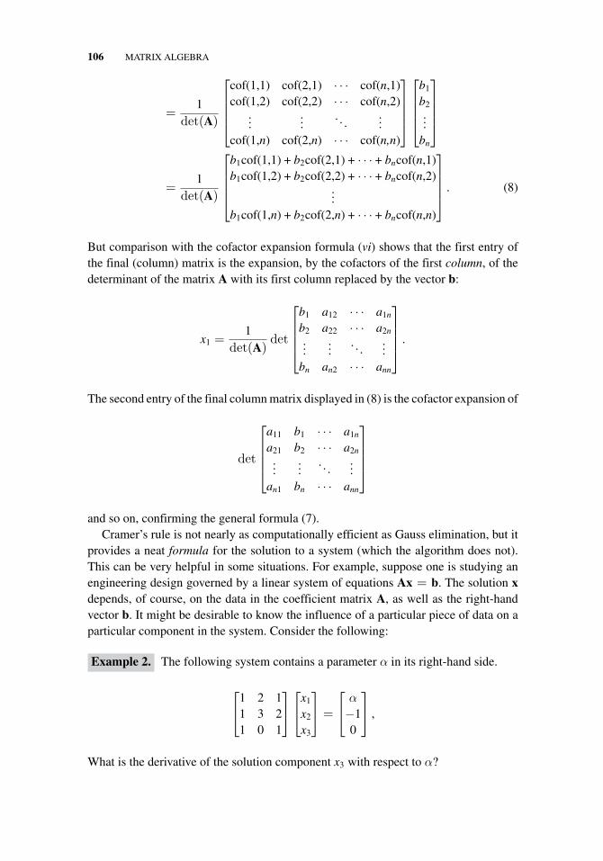
106 MATRIX ALGEBRA
=1
det(A)
⎡⎢⎢⎢⎣
cof(1,1) cof(2,1) · · · cof(n,1)cof(1,2) cof(2,2) · · · cof(n,2)
......
. . ....
cof(1,n) cof(2,n) · · · cof(n,n)
⎤⎥⎥⎥⎦
⎡⎢⎢⎢⎣
b1
b2...
bn
⎤⎥⎥⎥⎦
=1
det(A)
⎡⎢⎢⎢⎣
b1cof(1,1) + b2cof(2,1) + · · · + bncof(n,1)b1cof(1,2) + b2cof(2,2) + · · · + bncof(n,2)
...b1cof(1,n) + b2cof(2,n) + · · · + bncof(n,n)
⎤⎥⎥⎥⎦ . (8)
But comparison with the cofactor expansion formula (vi) shows that the first entry ofthe final (column) matrix is the expansion, by the cofactors of the first column, of thedeterminant of the matrix A with its first column replaced by the vector b:
x1 =1
det(A)det
⎡⎢⎢⎢⎣
b1 a12 · · · a1n
b2 a22 · · · a2n...
.... . .
...bn an2 · · · ann
⎤⎥⎥⎥⎦ .
The second entry of the final column matrix displayed in (8) is the cofactor expansion of
det
⎡⎢⎢⎢⎣
a11 b1 · · · a1n
a21 b2 · · · a2n...
.... . .
...an1 bn · · · ann
⎤⎥⎥⎥⎦
and so on, confirming the general formula (7).Cramer’s rule is not nearly as computationally efficient as Gauss elimination, but it
provides a neat formula for the solution to a system (which the algorithm does not).This can be very helpful in some situations. For example, suppose one is studying anengineering design governed by a linear system of equations Ax = b. The solution xdepends, of course, on the data in the coefficient matrix A, as well as the right-handvector b. It might be desirable to know the influence of a particular piece of data on aparticular component in the system. Consider the following:
Example 2. The following system contains a parameter α in its right-hand side.
⎡⎣1 2 1
1 3 21 0 1
⎤⎦⎡⎣x1
x2
x3
⎤⎦ =
⎡⎣ α
−10
⎤⎦ ,
What is the derivative of the solution component x3 with respect to α?
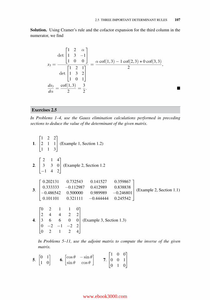
2.5 THREE IMPORTANT DETERMINANT RULES 107
Solution. Using Cramer’s rule and the cofactor expansion for the third column in thenumerator, we find
x3 =
det
⎡⎣1 2 α
1 3 −11 0 0
⎤⎦
det
⎡⎣1 2 1
1 3 21 0 1
⎤⎦
=α cof(1, 3)− 1 cof(2, 3) + 0 cof(3, 3)
2,
dx3
dα=
cof(1, 3)2
=32
. �
Exercises 2.5
In Problems 1–4, use the Gauss elimination calculations performed in precedingsections to deduce the value of the determinant of the given matrix.
1.
⎡⎣1 2 2
2 1 11 1 3
⎤⎦ (Example 1, Section 1.2)
2.
⎡⎣ 2 1 4
3 3 0−1 4 2
⎤⎦ (Example 2, Section 1.2
3.
⎡⎢⎢⎣
0.202131 0.732543 0.141527 0.3598670.333333 −0.112987 0.412989 0.838838−0.486542 0.500000 0.989989 −0.2468010.101101 0.321111 −0.444444 0.245542
⎤⎥⎥⎦ (Example 2, Section 1.1)
4.
⎡⎢⎢⎢⎢⎣
0 2 1 1 02 4 4 2 23 6 6 0 00 −2 −1 −2 20 2 1 2 4
⎤⎥⎥⎥⎥⎦ (Example 3, Section 1.3)
In Problems 5–11, use the adjoint matrix to compute the inverse of the givenmatrix.
5.
[0 11 0
]6.
[cos θ − sin θsin θ cos θ
]7.
⎡⎣1 0 0
0 0 10 1 0
⎤⎦
www.ebook3000.com
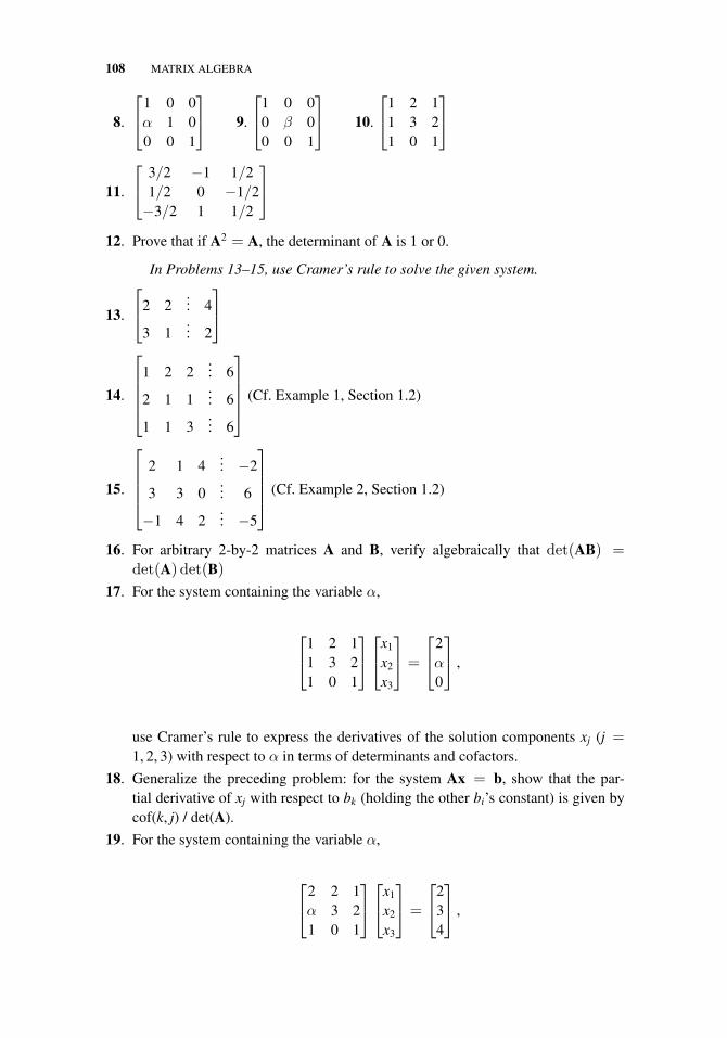
108 MATRIX ALGEBRA
8.
⎡⎣1 0 0α 1 00 0 1
⎤⎦ 9.
⎡⎣1 0 0
0 β 00 0 1
⎤⎦ 10.
⎡⎣1 2 1
1 3 21 0 1
⎤⎦
11.
⎡⎣ 3/2 −1 1/2
1/2 0 −1/2−3/2 1 1/2
⎤⎦
12. Prove that if A2 = A, the determinant of A is 1 or 0.
In Problems 13–15, use Cramer’s rule to solve the given system.
13.
⎡⎣2 2
... 4
3 1... 2
⎤⎦
14.
⎡⎢⎢⎢⎣
1 2 2... 6
2 1 1... 6
1 1 3... 6
⎤⎥⎥⎥⎦ (Cf. Example 1, Section 1.2)
15.
⎡⎢⎢⎢⎣
2 1 4... −2
3 3 0... 6
−1 4 2... −5
⎤⎥⎥⎥⎦ (Cf. Example 2, Section 1.2)
16. For arbitrary 2-by-2 matrices A and B, verify algebraically that det(AB) =det(A) det(B)
17. For the system containing the variable α,
⎡⎣1 2 1
1 3 21 0 1
⎤⎦⎡⎣x1
x2
x3
⎤⎦ =
⎡⎣2α
0
⎤⎦ ,
use Cramer’s rule to express the derivatives of the solution components xj (j =1, 2, 3) with respect to α in terms of determinants and cofactors.
18. Generalize the preceding problem: for the system Ax = b, show that the par-tial derivative of xj with respect to bk (holding the other bi’s constant) is given bycof(k, j) / det(A).
19. For the system containing the variable α,
⎡⎣2 2 1α 3 21 0 1
⎤⎦⎡⎣x1
x2
x3
⎤⎦ =
⎡⎣2
34
⎤⎦ ,
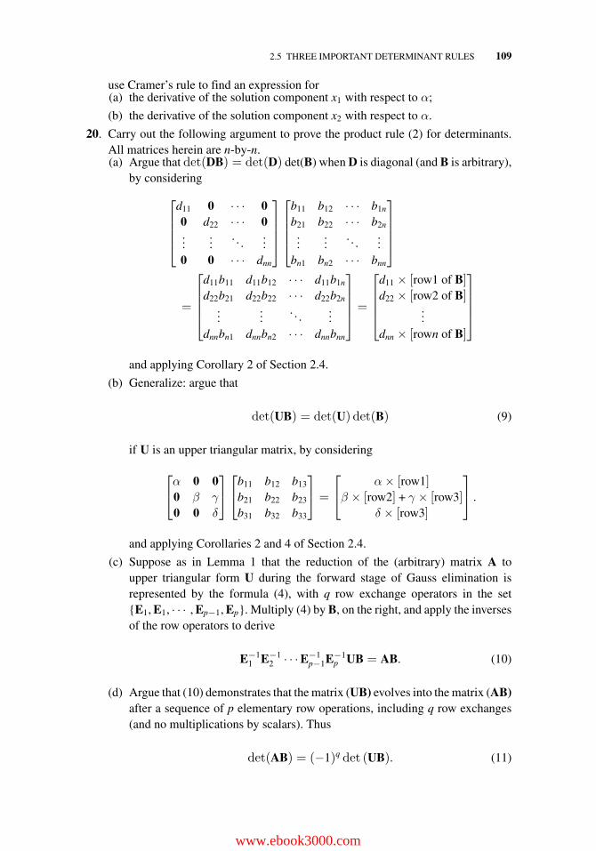
2.5 THREE IMPORTANT DETERMINANT RULES 109
use Cramer’s rule to find an expression for(a) the derivative of the solution component x1 with respect to α;
(b) the derivative of the solution component x2 with respect to α.
20. Carry out the following argument to prove the product rule (2) for determinants.All matrices herein are n-by-n.(a) Argue that det(DB) = det(D) det(B) when D is diagonal (and B is arbitrary),
by considering
⎡⎢⎢⎢⎣
d11 0 · · · 00 d22 · · · 0...
.... . .
...0 0 · · · dnn
⎤⎥⎥⎥⎦
⎡⎢⎢⎢⎣
b11 b12 · · · b1n
b21 b22 · · · b2n...
.... . .
...bn1 bn2 · · · bnn
⎤⎥⎥⎥⎦
=
⎡⎢⎢⎢⎣
d11b11 d11b12 · · · d11b1n
d22b21 d22b22 · · · d22b2n...
.... . .
...dnnbn1 dnnbn2 · · · dnnbnn
⎤⎥⎥⎥⎦ =
⎡⎢⎢⎢⎣
d11 × [row1 of B]d22 × [row2 of B]
...dnn × [rown of B]
⎤⎥⎥⎥⎦
and applying Corollary 2 of Section 2.4.
(b) Generalize: argue that
det(UB) = det(U) det(B) (9)
if U is an upper triangular matrix, by considering
⎡⎣α 0 0
0 β γ
0 0 δ
⎤⎦⎡⎣b11 b12 b13
b21 b22 b23
b31 b32 b33
⎤⎦ =
⎡⎣ α× [row1]β × [row2] + γ × [row3]
δ × [row3]
⎤⎦ .
and applying Corollaries 2 and 4 of Section 2.4.
(c) Suppose as in Lemma 1 that the reduction of the (arbitrary) matrix A toupper triangular form U during the forward stage of Gauss elimination isrepresented by the formula (4), with q row exchange operators in the set{E1, E1, · · · , Ep−1, Ep}. Multiply (4) by B, on the right, and apply the inversesof the row operators to derive
E−11 E−1
2 · · ·E−1p−1E−1
p UB = AB. (10)
(d) Argue that (10) demonstrates that the matrix (UB) evolves into the matrix (AB)after a sequence of p elementary row operations, including q row exchanges(and no multiplications by scalars). Thus
det(AB) = (−1)q det (UB). (11)
www.ebook3000.com
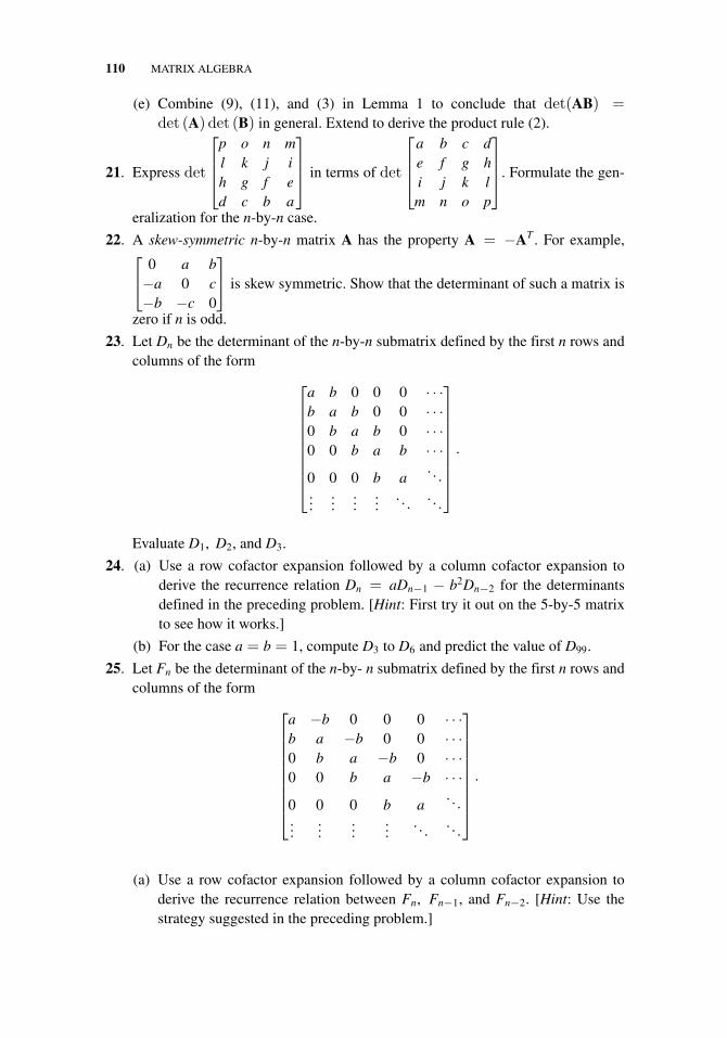
110 MATRIX ALGEBRA
(e) Combine (9), (11), and (3) in Lemma 1 to conclude that det(AB) =det (A) det (B) in general. Extend to derive the product rule (2).
21. Express det
⎡⎢⎢⎣
p o n ml k j ih g f ed c b a
⎤⎥⎥⎦ in terms of det
⎡⎢⎢⎣
a b c de f g hi j k lm n o p
⎤⎥⎥⎦. Formulate the gen-
eralization for the n-by-n case.
22. A skew-symmetric n-by-n matrix A has the property A = −AT . For example,⎡⎣ 0 a b−a 0 c−b −c 0
⎤⎦ is skew symmetric. Show that the determinant of such a matrix is
zero if n is odd.
23. Let Dn be the determinant of the n-by-n submatrix defined by the first n rows andcolumns of the form
⎡⎢⎢⎢⎢⎢⎢⎢⎢⎣
a b 0 0 0 · · ·b a b 0 0 · · ·0 b a b 0 · · ·0 0 b a b · · ·0 0 0 b a
. . ....
......
.... . .
. . .
⎤⎥⎥⎥⎥⎥⎥⎥⎥⎦
.
Evaluate D1, D2, and D3.
24. (a) Use a row cofactor expansion followed by a column cofactor expansion toderive the recurrence relation Dn = aDn−1 − b2Dn−2 for the determinantsdefined in the preceding problem. [Hint: First try it out on the 5-by-5 matrixto see how it works.]
(b) For the case a = b = 1, compute D3 to D6 and predict the value of D99.
25. Let Fn be the determinant of the n-by- n submatrix defined by the first n rows andcolumns of the form
⎡⎢⎢⎢⎢⎢⎢⎢⎢⎣
a −b 0 0 0 · · ·b a −b 0 0 · · ·0 b a −b 0 · · ·0 0 b a −b · · ·0 0 0 b a
. . ....
......
.... . .
. . .
⎤⎥⎥⎥⎥⎥⎥⎥⎥⎦
.
(a) Use a row cofactor expansion followed by a column cofactor expansion toderive the recurrence relation between Fn, Fn−1, and Fn−2. [Hint: Use thestrategy suggested in the preceding problem.]
2.6 SUMMARY 111
(b) Write out six members of the sequence {Fn} for the case a = b = 1. Do yourecognize them as members of the Fibonacci sequence?
26. (a) Use the adjoint matrix to argue that if A has all integer entries and det(A) =±1, then A−1 also has all integer entries. Construct a nondiagonal 3-by-3integer matrix illustrating this fact.
(b) Conversely, show that if A and A−1 both have all integer entries, thendet(A) = ±1.
27. For each of the following decide whether the statement made is always True orsometimes False.(a) If A is a square matrix satisfying ATA = I, then det(A) = ±1.
(b) The (i, j)th cofactor of a matrix A is the determinant of the matrix obtained bydeleting the ith row and jth column of A.
(c) If A and S are n-by-n matrices and S is invertible, then det(A) = det(S−1AS).
(d) If det(A) = 0, then there is at least one column vector x �= 0 such thatAx = 0.
28. Suppose A, B, and C are square matrices of the same size whose product ABCis invertible. Use the properties of determinants to prove that the matrix B isinvertible.
29. Use the adjoint matrix to construct the inverse of the following matrices:
(a)
⎡⎣1 2 3
0 4 50 0 6
⎤⎦ (b)
⎡⎣1 2 3
2 3 43 4 1
⎤⎦
30. Use Problem 29 as a guide to(a) show that if A is upper (lower) triangular and invertible, then so is A−1;
(b) show that if A is symmetric and invertible, then so is A−1.
31. If A and B are n-by-n matrices and B is invertible, express det(BAB−1) anddet(BABT) in terms of det(A) and det(B).
32. Use the permutation representation of the determinant, Problem 20 of Exercises2.4, to give an alternative proof of the transpose rule (1).
2.6 SUMMARY
Matrix Algebra and Operators
Comparison of the augmented matrix representation and the customary display of a sys-tem of linear equations motivates the definition of the matrix product, which enablesthe system to be compactly represented as Ax = b. The product, coupled with the nat-ural definition of matrix addition, gives rise to an algebra that facilitates the formulationand solution of linear systems, as well as providing a convenient instrument for ana-lyzing the operators involved in Gauss elimination, orthogonal projections, rotations,
www.ebook3000.com
112 MATRIX ALGEBRA
plane mirror reflections, and many other applications that will be explored in subse-quent chapters. This algebra adheres to most of the familiar rules of computation exceptfor the complications introduced by the noncommutativity of the product and the pre-carious nature of the multiplicative inverse; indeed, the very existence of the latter isintimately tied to the issues of solvability of the system Ax = b. The notion of thetranspose of a matrix further enriches the utility of the algebra.
Determinants
The definition of the determinant of a square matrix A generalizes the expression for thevolume of a parallelepiped in terms of the Cartesian components of its edge vectors.The following summarizes its basic properties:
1. If any row or column of A is multiplied by a scalar, the deteminant is multipliedby the same scalar.
2. If a row or column of A consists of all zeros, det(A) = 0.
3. If any two rows or columns of a matrix are switched, the deteminant changes sign.
4. If any two rows or columns of A are equal, det(A) = 0.
5. If any multiple of one row (column) of a matrix is added to another row (column),the deteminant is unchanged.
6. The determinant of a triangular matrix equals the product of the entries along itsdiagonal.
7. Product rule: det(A1A2 · · ·Ak) = det(A1) det(A2) · · ·det(Ak).
8. det(A) = (−1)q det(U), if A is reduced to the upper triangular matrix U with qrow exchanges in the forward part of the Gauss elimination algorithm.
9. A is invertible if and only if det(A) �= 0, and det(A−1) = 1/det(A).
10. Transpose rule: det(AT) = det(A).
11. The cofactor expansion is valid for any row and column:
det(A) =n∑
k=1
aikcof(i, k) =n∑
k=1
akjcof(k, j)
where cof(i, k) denotes (−1)i+k det(Aik)when Aik is obtained from A by deletingthe ith row and kth column.
12. The adjoint matrix Aadj associated with A is the matrix whose (i, j)th entry iscof(j, i). Furthermore, A−1 = Aadj/det(A) if A is invertible.
13. Cramer’s rule. If det(A) �= 0, the system Ax = b has a unique solution whose ithcomponent is given by
xi =det[a1 a2 · · · ai−1 b ai+1 · · · an]
det (A), where aj is the jth column of A.
REVIEW PROBLEMS FOR PART I 113
REVIEW PROBLEMS FOR PART I
1. For which values of γ does the following system possesses solutions?⎡⎢⎢⎢⎣−3 2 1
... 4
1 −1 2... 1
−2 1 3... γ
⎤⎥⎥⎥⎦
Are the solutions unique?
2. (a) Construct a linear system of equations for the coefficients a, b, c in thepolynomial ax2 + bx + c that matches ex at the points x = 0, 1, and 2.
(b) Construct a linear system of equations for the coefficients a, b, c in the poly-nomial ax2 + bx + c whose value, first derivative, and second derivative matchthose of ex at the point x = 1.
(c) Construct a linear system of equations for the coefficients a, b, c in the poly-nomial a(x − 1)2 + b(x − 1) + c whose value, first derivative, and secondderivative match those of ex at the point x = 1.
3. Compute the following matrix products:
(a)
[2 3 −14 2 3
]⎡⎣2
46
⎤⎦ (b) [2 3 − 1]
⎡⎣2 0 1
4 2 −16 2 3
⎤⎦ (c)
⎡⎣2
3−1
⎤⎦ [2 4 6]
(d)
[2 3 − 14 2 3
]⎡⎣1 0 0
0 1 00 0 1
⎤⎦ (e)
⎡⎢⎢⎣
0 1 0 01 0 0 00 0 0 10 0 1 0
⎤⎥⎥⎦
3
(f)
⎡⎣−1 0 1
0 1 00 0 −1
⎤⎦
25
4. By experimentation, find all powers
[1 10 1
]n
, for positive and negative integers n.
5. Construct a pair of real, nonzero 2-by-2 matrices A and B such that A2 + B2 = 0.
6. Show that if A is a 2-by-2 matrix satisfying AB = BA for every (2-by-2) matrix
B, then A is a multiple of the (2-by-2) identity. [Hint: Pick B1 =
[1 00 − 1
]and
B2 =
[0 11 0
].]
7. Let E be a matrix that performs an elementary row operation on a matrix Athrough left multiplication EA, as described in Example 2 of Section 2.1.(a) Describe the form of E for each of the three elementary row operations
corresponding to the operations listed in Theorem 1, Section 1.1.
(b) Describe the form of E−1 for the matrices in (a).
(c) Describe the effect of right multiplication AE on the columns of A, for thematrices in (a).
www.ebook3000.com
114 MATRIX ALGEBRA
(d) If A′ is formed by switching two rows of A, how does one form (A′)−1 fromA−1? [Hint: exploit the relation (EA)−1 = A−1E−1.]
(e) If A′ is formed by multiplying the second row of A by 7, how does one form(A′)−1 from A−1?
(f) If A′ is formed by adding the first row of A to its second row, how does oneform (A′)−1 from A−1?
8. Suppose the second row of A equals twice its first row. Prove the same is true ofany product AB.
9. Find matrices A and B such that AMB equals the (i, j)th entry of M.
10. For the system
2u + 3v + 7w − x + 2y = 3−u + 2v + w + 2x + y = 2,
express x and y in terms of u, v, and w by first rewriting the system in the matrixform
A[
xy
]+ B
⎡⎣u
vw
⎤⎦ = C
and then multiplying by A−1.
11. For each of the following, determine if the statement made is always True orsometimes False.(a) If A is invertible, then so is A2.
(b) If x is an n-by-1 column vector and y is an 1-by-n row vector, with n ≥ 2,then xy is an n-by-n singular matrix.
(c) If the n-by-n row echelon matrix A is invertible, then it has rank n.
(d) If A and B are n-by-n matrices satisfying AB = 0, then either A = 0 orB = 0.
(e) If x is a vector in R3row, then x is a linear combination of vectors [1 3 − 1],
[4 6 1], and [1 − 3 4].
(f) If A is an n-by-n matrix, then A and AT commute.
12. Find necessary and sufficient conditions on the values of c and d so that the system
⎡⎢⎢⎢⎣
1 0 1... b1
0 c 1... b2
0 1 d... b3
⎤⎥⎥⎥⎦
always has a solution (for any b1, b2, b3).
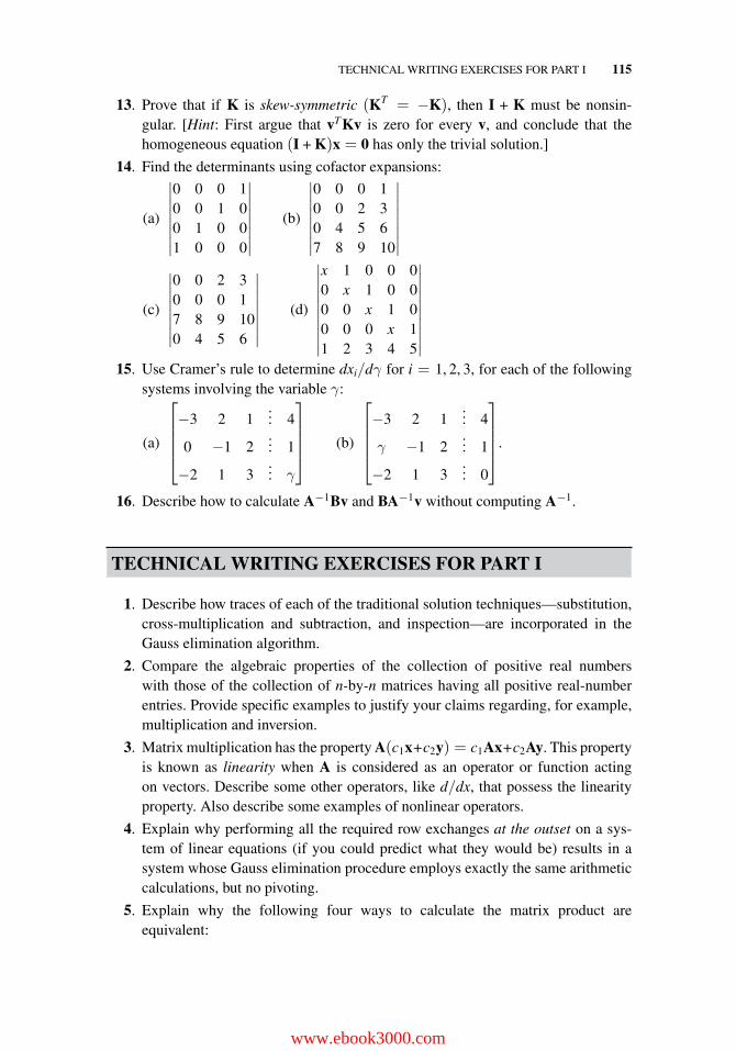
TECHNICAL WRITING EXERCISES FOR PART I 115
13. Prove that if K is skew-symmetric (KT = −K), then I + K must be nonsin-gular. [Hint: First argue that vTKv is zero for every v, and conclude that thehomogeneous equation (I + K)x = 0 has only the trivial solution.]
14. Find the determinants using cofactor expansions:
(a)
∣∣∣∣∣∣∣∣
0 0 0 10 0 1 00 1 0 01 0 0 0
∣∣∣∣∣∣∣∣(b)
∣∣∣∣∣∣∣∣
0 0 0 10 0 2 30 4 5 67 8 9 10
∣∣∣∣∣∣∣∣
(c)
∣∣∣∣∣∣∣∣
0 0 2 30 0 0 17 8 9 100 4 5 6
∣∣∣∣∣∣∣∣(d)
∣∣∣∣∣∣∣∣∣∣
x 1 0 0 00 x 1 0 00 0 x 1 00 0 0 x 11 2 3 4 5
∣∣∣∣∣∣∣∣∣∣15. Use Cramer’s rule to determine dxi/dγ for i = 1, 2, 3, for each of the following
systems involving the variable γ:
(a)
⎡⎢⎢⎢⎣−3 2 1
... 4
0 −1 2... 1
−2 1 3... γ
⎤⎥⎥⎥⎦ (b)
⎡⎢⎢⎢⎣−3 2 1
... 4
γ −1 2... 1
−2 1 3... 0
⎤⎥⎥⎥⎦.
16. Describe how to calculate A−1Bv and BA−1v without computing A−1.
TECHNICAL WRITING EXERCISES FOR PART I
1. Describe how traces of each of the traditional solution techniques—substitution,cross-multiplication and subtraction, and inspection—are incorporated in theGauss elimination algorithm.
2. Compare the algebraic properties of the collection of positive real numberswith those of the collection of n-by-n matrices having all positive real-numberentries. Provide specific examples to justify your claims regarding, for example,multiplication and inversion.
3. Matrix multiplication has the property A(c1x+c2y) = c1Ax+c2Ay. This propertyis known as linearity when A is considered as an operator or function actingon vectors. Describe some other operators, like d/dx, that possess the linearityproperty. Also describe some examples of nonlinear operators.
4. Explain why performing all the required row exchanges at the outset on a sys-tem of linear equations (if you could predict what they would be) results in asystem whose Gauss elimination procedure employs exactly the same arithmeticcalculations, but no pivoting.
5. Explain why the following four ways to calculate the matrix product areequivalent:
www.ebook3000.com
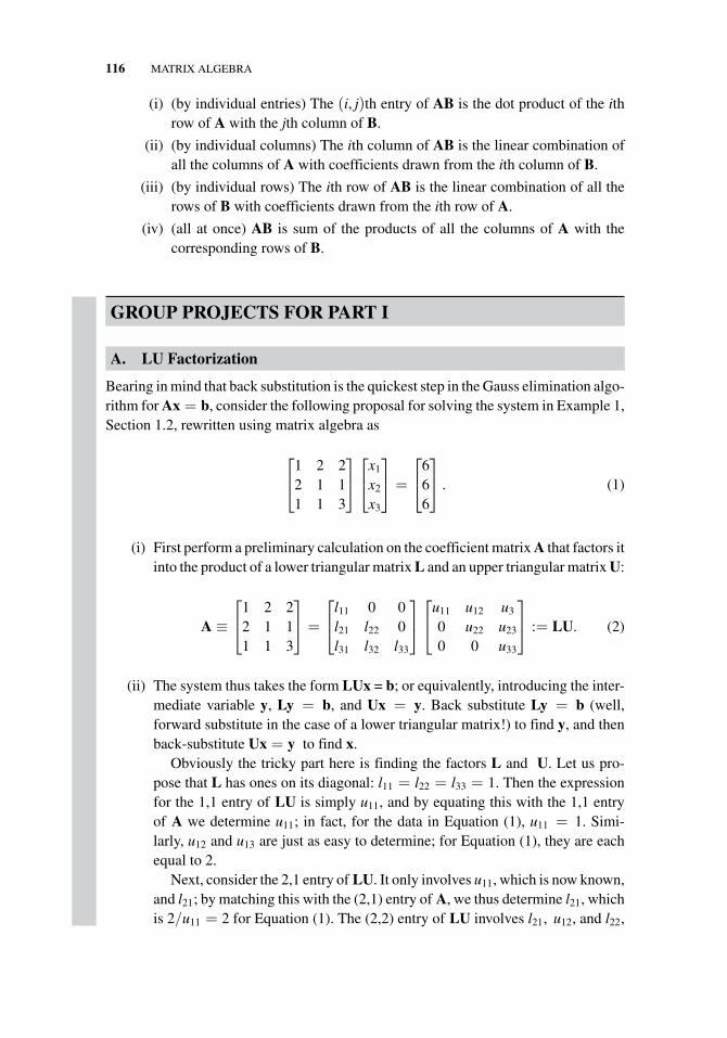
116 MATRIX ALGEBRA
(i) (by individual entries) The (i, j)th entry of AB is the dot product of the ithrow of A with the jth column of B.
(ii) (by individual columns) The ith column of AB is the linear combination ofall the columns of A with coefficients drawn from the ith column of B.
(iii) (by individual rows) The ith row of AB is the linear combination of all therows of B with coefficients drawn from the ith row of A.
(iv) (all at once) AB is sum of the products of all the columns of A with thecorresponding rows of B.
GROUP PROJECTS FOR PART I
A. LU Factorization
Bearing in mind that back substitution is the quickest step in the Gauss elimination algo-rithm for Ax = b, consider the following proposal for solving the system in Example 1,Section 1.2, rewritten using matrix algebra as
⎡⎣1 2 2
2 1 11 1 3
⎤⎦⎡⎣x1
x2
x3
⎤⎦ =
⎡⎣6
66
⎤⎦ . (1)
(i) First perform a preliminary calculation on the coefficient matrix A that factors itinto the product of a lower triangular matrix L and an upper triangular matrix U:
A ≡
⎡⎣1 2 2
2 1 11 1 3
⎤⎦ =
⎡⎣l11 0 0
l21 l22 0l31 l32 l33
⎤⎦⎡⎣u11 u12 u3
0 u22 u23
0 0 u33
⎤⎦ := LU. (2)
(ii) The system thus takes the form LUx = b; or equivalently, introducing the inter-mediate variable y, Ly = b, and Ux = y. Back substitute Ly = b (well,forward substitute in the case of a lower triangular matrix!) to find y, and thenback-substitute Ux = y to find x.
Obviously the tricky part here is finding the factors L and U. Let us pro-pose that L has ones on its diagonal: l11 = l22 = l33 = 1. Then the expressionfor the 1,1 entry of LU is simply u11, and by equating this with the 1,1 entryof A we determine u11; in fact, for the data in Equation (1), u11 = 1. Simi-larly, u12 and u13 are just as easy to determine; for Equation (1), they are eachequal to 2.
Next, consider the 2,1 entry of LU. It only involves u11, which is now known,and l21; by matching this with the (2,1) entry of A, we thus determine l21, whichis 2/u11 = 2 for Equation (1). The (2,2) entry of LU involves l21, u12, and l22,
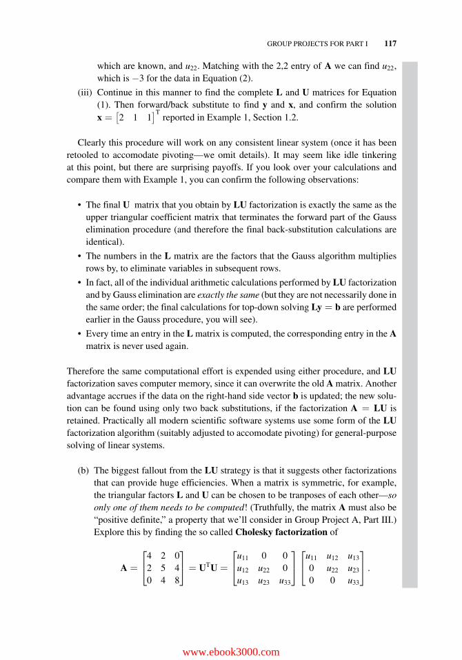
GROUP PROJECTS FOR PART I 117
which are known, and u22. Matching with the 2,2 entry of A we can find u22,which is −3 for the data in Equation (2).
(iii) Continue in this manner to find the complete L and U matrices for Equation(1). Then forward/back substitute to find y and x, and confirm the solutionx =
[2 1 1
]Treported in Example 1, Section 1.2.
Clearly this procedure will work on any consistent linear system (once it has beenretooled to accomodate pivoting—we omit details). It may seem like idle tinkeringat this point, but there are surprising payoffs. If you look over your calculations andcompare them with Example 1, you can confirm the following observations:
• The final U matrix that you obtain by LU factorization is exactly the same as theupper triangular coefficient matrix that terminates the forward part of the Gausselimination procedure (and therefore the final back-substitution calculations areidentical).
• The numbers in the L matrix are the factors that the Gauss algorithm multipliesrows by, to eliminate variables in subsequent rows.
• In fact, all of the individual arithmetic calculations performed by LU factorizationand by Gauss elimination are exactly the same (but they are not necessarily done inthe same order; the final calculations for top-down solving Ly = b are performedearlier in the Gauss procedure, you will see).
• Every time an entry in the L matrix is computed, the corresponding entry in the Amatrix is never used again.
Therefore the same computational effort is expended using either procedure, and LUfactorization saves computer memory, since it can overwrite the old A matrix. Anotheradvantage accrues if the data on the right-hand side vector b is updated; the new solu-tion can be found using only two back substitutions, if the factorization A = LU isretained. Practically all modern scientific software systems use some form of the LUfactorization algorithm (suitably adjusted to accomodate pivoting) for general-purposesolving of linear systems.
(b) The biggest fallout from the LU strategy is that it suggests other factorizationsthat can provide huge efficiencies. When a matrix is symmetric, for example,the triangular factors L and U can be chosen to be tranposes of each other—soonly one of them needs to be computed! (Truthfully, the matrix A must also be“positive definite,” a property that we’ll consider in Group Project A, Part III.)Explore this by finding the so called Cholesky factorization of
A =
⎡⎣4 2 0
2 5 40 4 8
⎤⎦ = UTU =
⎡⎣u11 0 0
u12 u22 0u13 u23 u33
⎤⎦⎡⎣u11 u12 u13
0 u22 u23
0 0 u33
⎤⎦ .
www.ebook3000.com
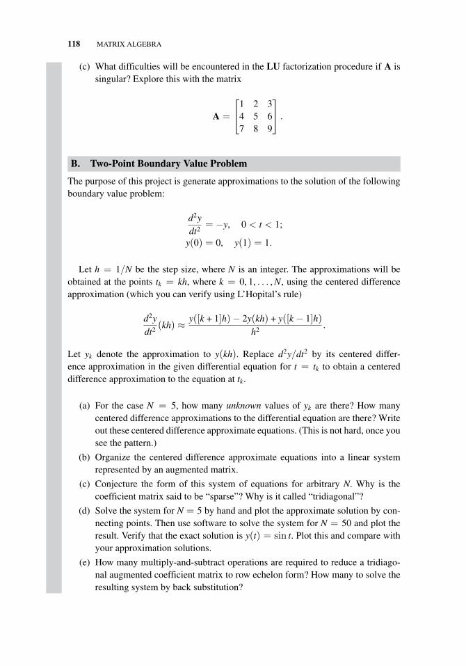
118 MATRIX ALGEBRA
(c) What difficulties will be encountered in the LU factorization procedure if A issingular? Explore this with the matrix
A =
⎡⎣1 2 3
4 5 67 8 9
⎤⎦ .
B. Two-Point Boundary Value Problem
The purpose of this project is generate approximations to the solution of the followingboundary value problem:
d2ydt2
= −y, 0 < t < 1;
y(0) = 0, y(1) = 1.
Let h = 1/N be the step size, where N is an integer. The approximations will beobtained at the points tk = kh, where k = 0, 1, . . . , N, using the centered differenceapproximation (which you can verify using L’Hopital’s rule)
d2ydt2
(kh) ≈ y([k + 1]h)− 2y(kh) + y([k − 1]h)h2
.
Let yk denote the approximation to y(kh). Replace d2y/dt2 by its centered differ-ence approximation in the given differential equation for t = tk to obtain a centereddifference approximation to the equation at tk.
(a) For the case N = 5, how many unknown values of yk are there? How manycentered difference approximations to the differential equation are there? Writeout these centered difference approximate equations. (This is not hard, once yousee the pattern.)
(b) Organize the centered difference approximate equations into a linear systemrepresented by an augmented matrix.
(c) Conjecture the form of this system of equations for arbitrary N. Why is thecoefficient matrix said to be “sparse”? Why is it called “tridiagonal”?
(d) Solve the system for N = 5 by hand and plot the approximate solution by con-necting points. Then use software to solve the system for N = 50 and plot theresult. Verify that the exact solution is y(t) = sin t. Plot this and compare withyour approximation solutions.
(e) How many multiply-and-subtract operations are required to reduce a tridiago-nal augmented coefficient matrix to row echelon form? How many to solve theresulting system by back substitution?
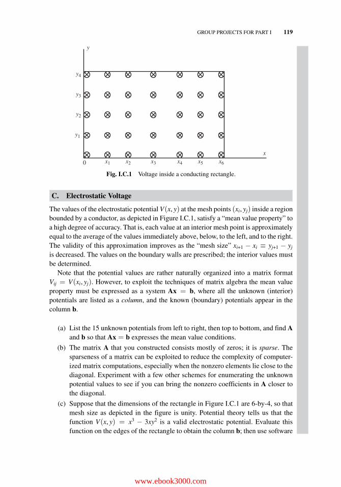
GROUP PROJECTS FOR PART I 119
0 x1
y2
y3
y4
y
y1
x2 x3 x4 x5 x6
x
Fig. I.C.1 Voltage inside a conducting rectangle.
C. Electrostatic Voltage
The values of the electrostatic potential V(x, y) at the mesh points (xi, yj) inside a regionbounded by a conductor, as depicted in Figure I.C.1, satisfy a “mean value property” toa high degree of accuracy. That is, each value at an interior mesh point is approximatelyequal to the average of the values immediately above, below, to the left, and to the right.The validity of this approximation improves as the “mesh size” xi+1 − xi ≡ yj+1 − yj
is decreased. The values on the boundary walls are prescribed; the interior values mustbe determined.
Note that the potential values are rather naturally organized into a matrix formatVij = V(xi, yj). However, to exploit the techniques of matrix algebra the mean valueproperty must be expressed as a system Ax = b, where all the unknown (interior)potentials are listed as a column, and the known (boundary) potentials appear in thecolumn b.
(a) List the 15 unknown potentials from left to right, then top to bottom, and find Aand b so that Ax = b expresses the mean value conditions.
(b) The matrix A that you constructed consists mostly of zeros; it is sparse. Thesparseness of a matrix can be exploited to reduce the complexity of computer-ized matrix computations, especially when the nonzero elements lie close to thediagonal. Experiment with a few other schemes for enumerating the unknownpotential values to see if you can bring the nonzero coefficients in A closer tothe diagonal.
(c) Suppose that the dimensions of the rectangle in Figure I.C.1 are 6-by-4, so thatmesh size as depicted in the figure is unity. Potential theory tells us that thefunction V(x, y) = x3 − 3xy2 is a valid electrostatic potential. Evaluate thisfunction on the edges of the rectangle to obtain the column b; then use software
www.ebook3000.com
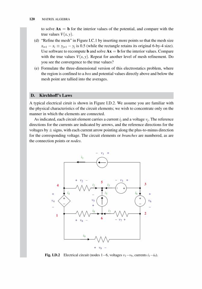
120 MATRIX ALGEBRA
to solve Ax = b for the interior values of the potential, and compare with thetrue values V(x, y).
(d) “Refine the mesh” in Figure I.C.1 by inserting more points so that the mesh sizexi+1 − xi ≡ yj+1 − yj is 0.5 (while the rectangle retains its original 6-by-4 size).Use software to recompute b and solve Ax = b for the interior values. Comparewith the true values V(x, y). Repeat for another level of mesh refinement. Doyou see the convergence to the true values?
(e) Formulate the three-dimensional version of this electrostatics problem, wherethe region is confined to a box and potential values directly above and below themesh point are tallied into the averages.
D. Kirchhoff’s Laws
A typical electrical ciruit is shown in Figure I.D.2. We assume you are familiar withthe physical characteristics of the circuit elements; we wish to concentrate only on themanner in which the elements are connected.
As indicated, each circuit element carries a current ij and a voltage vj. The referencedirections for the currents are indicated by arrows, and the reference directions for thevoltages by ± signs, with each current arrow pointing along the plus-to-minus directionfor the corresponding voltage. The circuit elements or branches are numbered, as arethe connection points or nodes.
i1
i2 i3
i4 i5 i6
i8 i71 2
345
6
i9
v1
v2 v3
v4 v5 v6
v7
+
+
++
+
–––
+
+–
–
–
++
+
––
–
+ –
+ –
v8
v9
–
Fig. I.D.2 Electrical circuit (nodes 1−6, voltages v1−v9, currents i1−i9).
GROUP PROJECTS FOR PART I 121
The incidence matrix A for the circuit completely specifies the connection topology,in accordance with
aij = 1 if current j leaves node i,
aij = −1 if current j enters node i,
aij = 0 otherwise.
So for the circuit in Figure I.D.2,
A =
⎡⎢⎢⎢⎢⎢⎢⎢⎣
0 0 0 −1 0 0 0 1 10 0 0 0 0 −1 1 0 −11 0 1 0 0 1 0 0 0−1 1 0 1 0 0 0 0 00 −1 −1 0 −1 0 0 0 00 0 0 0 1 0 −1 −1 0
⎤⎥⎥⎥⎥⎥⎥⎥⎦
.
A has a column for every current and a row for every node in the circuit.
(a) Explain why every column of the incidence matrix always contains one +1 andone −1.
Kirchhoff’s current law states that the sum of all currents leaving any node mustequal zero.
(b) Argue that the current law is expressed by the equation Ai = 0, where i is thecolumn vector of branch currents i =
[i1 i2 · · · in
]T.
A loop in the circuit is a sequence of connected nodes starting and ending on thesame node. For example, one loop in the circuit of Figure I.D.2 would run sequentiallythrough nodes 1, 6, 5, 4, and back to 1. We restrict ourselves to simple loops which visitno node, other than the initial and final, more than once. The loop can be characterizedby the currents that comprise its path; for example the loop through nodes {1,6,5,4,1}is “carried” by the currents i8, i5,−i2, and i4. We tagged i2 with a minus sign to indicatethat the direction of travel in the loop ran opposite to the indicated direction of i2. Inthis manner any loop can be characterized by a column vector �, with
�j = 1 if current j is part of the loop and directed along it,�j = −1 if current j is part of the loop and directed oppositely, and�j = 0 otherwise.
Thus, the loop through nodes {1,6,5,4,1} generates the loop vector
� =[0 −1 0 1 1 0 0 1 0
]T.
www.ebook3000.com
122 MATRIX ALGEBRA
Of course the loop vector does not “know” which node was the starting point; this isseldom important for a loop.
(c) Show that A�= 0 for any such loop, by interpreting A� as a sum of (signed)columns of A. Add the columns in the order that they appear in the loop, andargue that every partial sum contains one +1 and one −1 except for the finalsum, which is all zeros.
Kirchhoff’s voltage law states that the sum of the voltage drops around every loopmust equal zero. The voltage drop in branch j equals vj if the direction of the current ijis along the direction of the loop, and equals −vj if the current direction is opposite tothe loop.
(d) Argue that if v is the row vector of branch voltages v =[v1 v2 · · · vn
]then
the voltage law implies v�= 0 for any loop.
The similarity of the topological law A�= 0 and the physical law v�= 0 indicatesthat there is a relation between A and v. To explore this, designate one of the nodes inthe circuit as the reference node (or “ground” node). For example in Figure I.D.2 wetake node #1 as the reference node. Then define a node voltage ek at each node (k) bychoosing a path along the circuit elements connecting the reference node to node #k,and adding up the branch voltage rises along the path. For instance, if we choose thepath in Figure I.D.2 connecting node #1 to node #3 to include the nodes {1,6,2,3} inorder, then we define e3 to be −v8 + v7 + v6.
(e) Argue that Kirchhoff’s voltage law implies that the values calculated for thenode voltages are independent of the choice of paths used to evaluate them.For example, the same value for e3 would have been assigned if we calculatedv4 − v2 + v3.
(f) Argue that if the node voltages are assembled into a row vector e =[e1 e2 · · · em
], then the branch voltages are given by v = eA.
The relation v= eA demonstrates that the voltage law v�= 0 is impliedby the topological law A�= 0. In summary, both of Kirchhoff’s lawsare expressible using the incidence matrix via Ai= 0 and v= eA. Thisenables the translation of the topology of electric circuit connections intocomputer code.
E. Global Positioning Systems
This project explores some the mathematical features of a GPS system.
(a) A fixed transmitter emits electromagnetic pulses that propagate in all directionsat the speed of light c (taken to be a known constant). A traveler would like to beable to figure how far he/she is from the emitter, upon receiving the pulse. What
GROUP PROJECTS FOR PART I 123
kind of information can the emitter encode in the pulses, so that all travelers areaccommodated?
(b) For motion in the plane, the locus of possible positions for a traveler at a knowndistance from an emitter is, of course, a circle. Write the equation relating thetraveler’s position (x, y), the emitter’s position (x1, y1), and the distance fromthe emitter r1.
(c) If the distance r2 from a second emitter located at (x2, y2) is also known, howmany solutions can the system of two equations describing the locus have? Whydoes the (0, 1,∞) rule (Theorem 3, Section 1.4) not apply?
(d) Now assume the traveler knows the distance r3 from a third emitter located at(x3, y3). Reasoning geometrically, argue that all ambiguity about the traveler’sposition is removed, as long as the three emitters avoid certain configurations;what are these configurations?
(e) The system of three “locus” equations (in two unknowns x, y) is not linear, and ishard to solve. But luckily the differences of any two of them turn out to be linear.Formulate the three locus equations, form the differences of any two pairs, andshow that Gauss elimination can be used to find x, y as long as the troublesomeemitter configurations are not present.
(f) What changes need to be made to this scheme in three dimensions?More thorough descriptions of the subtleties of global positioning systems
are available on the internet; see, for example,http://www.aero.org/education/primers/gps orhttp://www.trimble.com/gps/index.shtml
F. Fixed-Point Methods
Bruce W. Atkinson, Samford UniversityIn this project, you will be introduced to the fixed point method for approximat-
ing solutions to equations in one variable. Then you will extend this technique forapproximating solutions to a linear system of equations.
(a) Let f (x) be a function of one variable. A real number a is called a fixed point of fif f (a) = a. A well-known method of approximating a fixed point is function iteration.The basic idea is as follows: Let x0 be an initial “guess” for a fixed point. Define asequence of estimates (xn), for n ≥ 1, by letting xn+1 := f (xn). Thus x1 = f (x0), x2 =f (f (x0)), x3 = f (f (f (x0))), etc. xn is the nth iterate of f with initial value x0. Now if fis continuous and a = limn→∞ xn exists it follows that
f (a) = f ( limn→∞
xn) = limn→∞
f (xn) = limn→∞
xn+1 = a.
Therefore limn→∞ xn is a fixed point of f , and the sequence can be used to approximatethe fixed point.
www.ebook3000.com
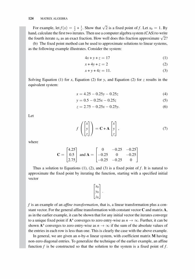
124 MATRIX ALGEBRA
For example, let f (x) = x2 + 1
x . Show that√
2 is a fixed point of f . Let x0 = 1. Byhand, calculate the first two iterates. Then use a computer algebra system (CAS) to writethe fourth iterate x4 as an exact fraction. How well does this fraction approximate
√2?
(b) The fixed point method can be used to approximate solutions to linear systems,as the following example illustrates. Consider the system:
4x + y + z = 17 (1)
x + 4y + z = 2 (2)
x + y + 4z = 11. (3)
Solving Equation (1) for x, Equation (2) for y, and Equation (2) for z results in theequivalent system:
x = 4.25 − 0.25y − 0.25z (4)
y = 0.5 − 0.25x − 0.25z (5)
z = 2.75 − 0.25x − 0.25y. (6)
Let
f
⎛⎝⎡⎣x
yz
⎤⎦⎞⎠ = C + A
⎡⎣x
yz
⎤⎦ , (7)
where
C =
⎡⎣4.25
0.52.75
⎤⎦ and A =
⎡⎣ 0 −0.25 −0.25−0.25 0 −0.25−0.25 −0.25 0
⎤⎦
Thus a solution to Equations (1), (2), and (3) is a fixed point of f . It is natural toapproximate the fixed point by iterating the function, starting with a specified initialvector ⎡
⎣x0
y0
z0
⎤⎦ .
f is an example of an affine transformation, that is, a linear transformation plus a con-stant vector. For the general affine transformation with constant vector C and matrix A,as in the earlier example, it can be shown that for any initial vector the iterates convergeto a unique fixed point if An converges to zero entry-wise as n → ∞. Further, it can beshown An converges to zero entry-wise as n → ∞ if the sum of the absolute values ofthe entries in each row is less than one. This is clearly the case with the above example.
In general, we are given an n-by-n linear system, with coefficient matrix M havingnon-zero diagonal entries. To generalize the technique of the earlier example, an affinefunction f is be constructed so that the solution to the system is a fixed point of f .
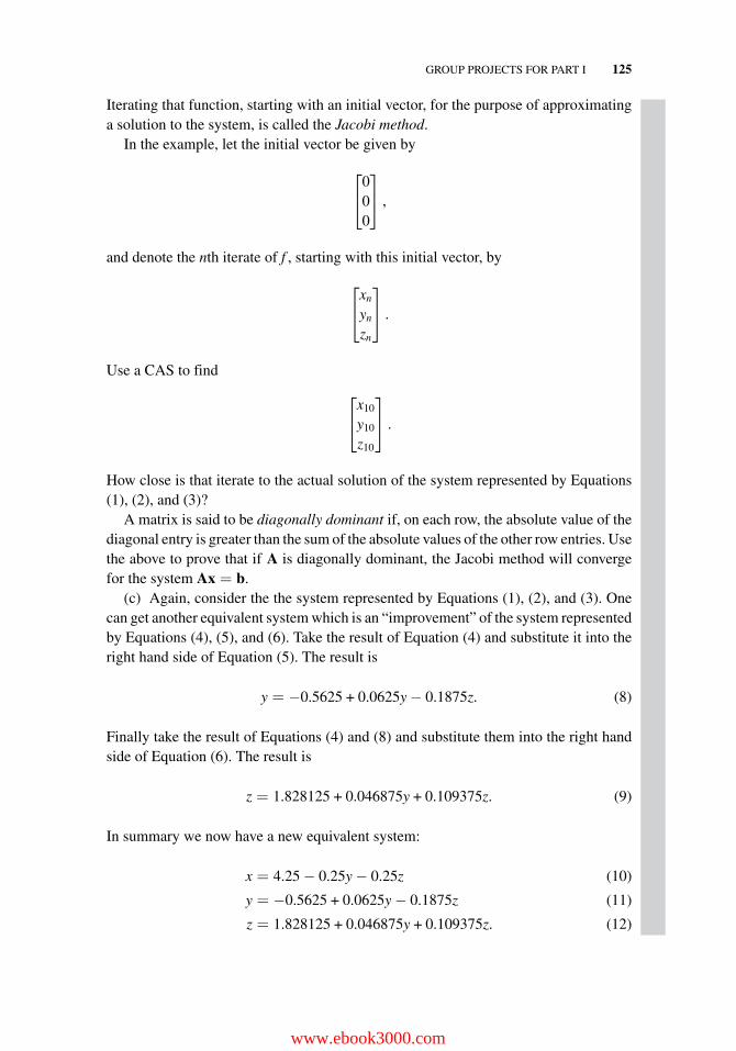
GROUP PROJECTS FOR PART I 125
Iterating that function, starting with an initial vector, for the purpose of approximatinga solution to the system, is called the Jacobi method.
In the example, let the initial vector be given by
⎡⎣0
00
⎤⎦ ,
and denote the nth iterate of f , starting with this initial vector, by
⎡⎣xn
yn
zn
⎤⎦ .
Use a CAS to find
⎡⎣x10
y10
z10
⎤⎦ .
How close is that iterate to the actual solution of the system represented by Equations(1), (2), and (3)?
A matrix is said to be diagonally dominant if, on each row, the absolute value of thediagonal entry is greater than the sum of the absolute values of the other row entries. Usethe above to prove that if A is diagonally dominant, the Jacobi method will convergefor the system Ax = b.
(c) Again, consider the the system represented by Equations (1), (2), and (3). Onecan get another equivalent system which is an “improvement” of the system representedby Equations (4), (5), and (6). Take the result of Equation (4) and substitute it into theright hand side of Equation (5). The result is
y = −0.5625 + 0.0625y − 0.1875z. (8)
Finally take the result of Equations (4) and (8) and substitute them into the right handside of Equation (6). The result is
z = 1.828125 + 0.046875y + 0.109375z. (9)
In summary we now have a new equivalent system:
x = 4.25 − 0.25y − 0.25z (10)
y = −0.5625 + 0.0625y − 0.1875z (11)
z = 1.828125 + 0.046875y + 0.109375z. (12)
www.ebook3000.com
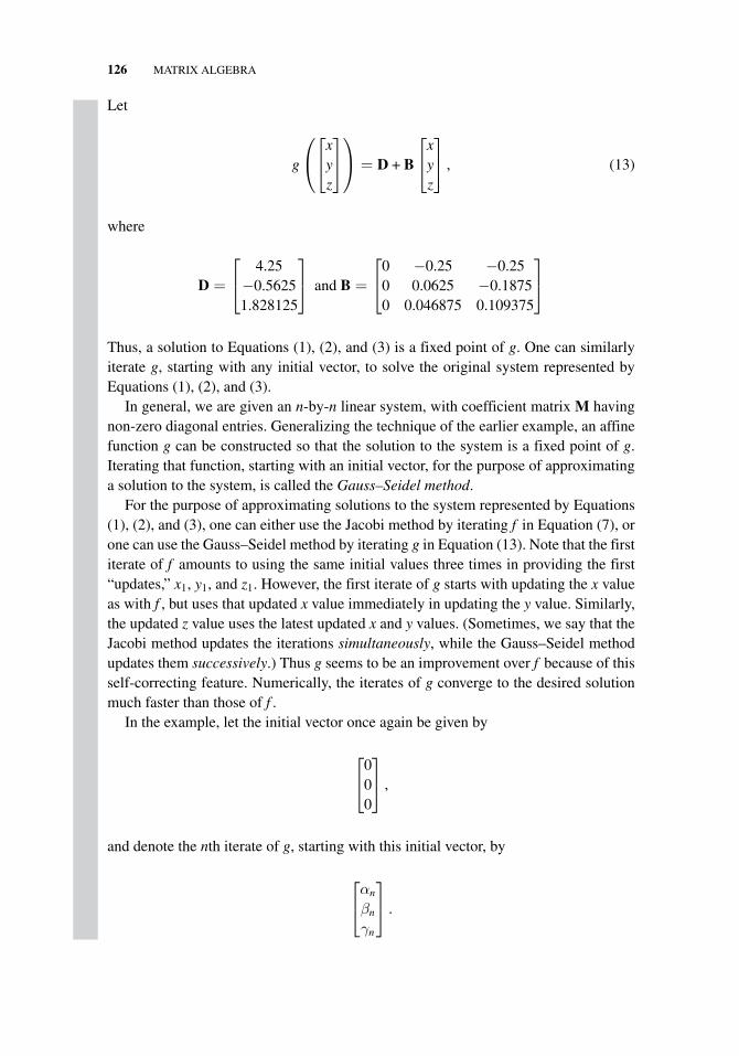
126 MATRIX ALGEBRA
Let
g
⎛⎝⎡⎣x
yz
⎤⎦⎞⎠ = D + B
⎡⎣x
yz
⎤⎦ , (13)
where
D =
⎡⎣ 4.25−0.56251.828125
⎤⎦ and B =
⎡⎣0 −0.25 −0.25
0 0.0625 −0.18750 0.046875 0.109375
⎤⎦
Thus, a solution to Equations (1), (2), and (3) is a fixed point of g. One can similarlyiterate g, starting with any initial vector, to solve the original system represented byEquations (1), (2), and (3).
In general, we are given an n-by-n linear system, with coefficient matrix M havingnon-zero diagonal entries. Generalizing the technique of the earlier example, an affinefunction g can be constructed so that the solution to the system is a fixed point of g.Iterating that function, starting with an initial vector, for the purpose of approximatinga solution to the system, is called the Gauss–Seidel method.
For the purpose of approximating solutions to the system represented by Equations(1), (2), and (3), one can either use the Jacobi method by iterating f in Equation (7), orone can use the Gauss–Seidel method by iterating g in Equation (13). Note that the firstiterate of f amounts to using the same initial values three times in providing the first“updates,” x1, y1, and z1. However, the first iterate of g starts with updating the x valueas with f , but uses that updated x value immediately in updating the y value. Similarly,the updated z value uses the latest updated x and y values. (Sometimes, we say that theJacobi method updates the iterations simultaneously, while the Gauss–Seidel methodupdates them successively.) Thus g seems to be an improvement over f because of thisself-correcting feature. Numerically, the iterates of g converge to the desired solutionmuch faster than those of f .
In the example, let the initial vector once again be given by
⎡⎣0
00
⎤⎦ ,
and denote the nth iterate of g, starting with this initial vector, by
⎡⎣αn
βn
γn
⎤⎦ .
GROUP PROJECTS FOR PART I 127
Use a CAS to find
⎡⎣α1
β1
γ1
⎤⎦ ,
⎡⎣α2
β2
γ2
⎤⎦ ,
⎡⎣α3
β3
γ3
⎤⎦ , and
⎡⎣α4
β4
γ4
⎤⎦ .
How close are these iterates to the actual solution of the system represented byEquations (1), (2), and (3)? Do these iterates support the claim that the Gauss-Seidelmethod is an improvement over the Jacobi method?
(d) Let M be the coefficient matrix for the system represented by equations (1), (2),and (3), that is
M =
⎡⎣4 1 1
1 4 11 1 4
⎤⎦ .
Explain how you can use the Gauss–Seidel method to approximate M−1.
www.ebook3000.com

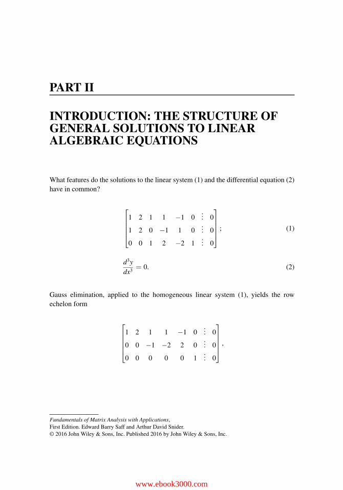
PART II
INTRODUCTION: THE STRUCTURE OFGENERAL SOLUTIONS TO LINEARALGEBRAIC EQUATIONS
What features do the solutions to the linear system (1) and the differential equation (2)have in common?
⎡⎢⎢⎢⎣
1 2 1 1 −1 0... 0
1 2 0 −1 1 0... 0
0 0 1 2 −2 1... 0
⎤⎥⎥⎥⎦ ; (1)
d3ydx3
= 0. (2)
Gauss elimination, applied to the homogeneous linear system (1), yields the rowechelon form
⎡⎢⎢⎢⎣
1 2 1 1 −1 0... 0
0 0 −1 −2 2 0... 0
0 0 0 0 0 1... 0
⎤⎥⎥⎥⎦ ,
Fundamentals of Matrix Analysis with Applications,First Edition. Edward Barry Saff and Arthur David Snider.© 2016 John Wiley & Sons, Inc. Published 2016 by John Wiley & Sons, Inc.
www.ebook3000.com
130 PART II INTRODUCTION: THE STRUCTURE OF GENERAL SOLUTIONS
which has a three-parameter solution family
x1 = −2t1 + t2 − t3x2 = t1x3 = −2t2 + 2t3x4 = t2x5 = t3x6 = 0
or
⎡⎢⎢⎢⎢⎢⎢⎢⎣
x1
x2
x3
x4
x5
x6
⎤⎥⎥⎥⎥⎥⎥⎥⎦= t1
⎡⎢⎢⎢⎢⎢⎢⎢⎣
−210000
⎤⎥⎥⎥⎥⎥⎥⎥⎦
+ t2
⎡⎢⎢⎢⎢⎢⎢⎢⎣
10−2100
⎤⎥⎥⎥⎥⎥⎥⎥⎦
+ t3
⎡⎢⎢⎢⎢⎢⎢⎢⎣
−102010
⎤⎥⎥⎥⎥⎥⎥⎥⎦
. (3)
We do not presume that the reader has studied differential equations, but equation(2) is very simple to analyze. Indefinite integration yields, in turn,
y′′ = c1; (4)
y′ = c1x + c2;
y = c1x2/2 + c2x + c3.
Although the displays (3) and (4) refer to quite different mathematical objects, theyare instances of a concept known as a vector space. By focusing attention in this chapteron the abstract notion of vector spaces, we will be able to establish general principlesthat can be handily applied in many diverse areas.
So let us list three apparent features that the general solutions (3) and (4) have incommon. Remember that in both cases, the coefficients {ti}, {ci} can take any realvalues; in Section 1.3, the coefficients {ti} were called “parameters;” of course, thecoefficients {ci} are “constants of integration.”
(i) Zero is a solution. Here we have already begun to universalize our language;“zero” for (3) means the six-component vector with all entries zero, but “zero”for (4) means the identically zero function.
(ii) The sum of any two solutions is also a solution.
(iii) Any constant multiple of a solution is also a solution.
What other mathematical structures satisfy (i)–(iii)? A familiar example is the set ofvectors (directed line segments) in the x, y-plane. The sum of two vectors, as well asthe multiplication of a vector by a constant, is depicted in Figure II.1.
In fact, the set of all vectors in three-dimensional space—or, all vectors along a line,or in a plane—satisfy (i)–(iii). However, any finite collection of such vectors wouldnot meet the closure conditions (ii), (iii); such sets are not “closed” under additionand scalar multiplication. (Exception: The single zero vector does, trivially, satisfy (ii),(iii).) Similarly, the set of all vectors in the plane pointing into the first quadrant failsto have the closure property.

PART II INTRODUCTION: THE STRUCTURE OF GENERAL SOLUTIONS 131
a
b
a+b
2a
–a
Fig. II.1 Vector addition.
In subsequent sections, we will formalize and generalize the concept of a vectorspace and establish general tools that can be utilized in the analysis of algebraic anddifferential equations, matrices, geometry, and many other areas.
www.ebook3000.com

3VECTOR SPACES
3.1 GENERAL SPACES, SUBSPACES, AND SPANS
In the Introduction to Part II, we noted that solutions to linear homogeneous algebraicsystems, solutions of certain linear differential equations, and geometric space vectorshave some algebraic features in common. In rough terms,
• The objects themselves (call them v’s) enjoy an “addition” operation whichsatisfies the customary algebraic laws;
• These objects interact with another algebraic collection called the scalars (hereindenoted by c’s) through scalar multiplication cv, and this operation also satisfiesthe expected parenthesis rules. The real numbers have played the role of the scalarsin the examples we have seen so far, but in subsequent applications we shall usecomplex numbers. The specifics are given in the following defintion.
Then V is said to be a vector space over the field of scalars F.
Vector Space
Definition 1. Let V be a collection of objects which we call vectors (typicallydenoted by boldface lower case Latin letters v, w, a, etc.), and let F be the setof real, or the set of complex, numbers; the elements of F will be designated asscalars (c1, c2, c3, etc.). Suppose there is an operation called vector addition,written as v1 + v2, that combines pairs of vectors, and another operation called
Fundamentals of Matrix Analysis with Applications,First Edition. Edward Barry Saff and Arthur David Snider.© 2016 John Wiley & Sons, Inc. Published 2016 by John Wiley & Sons, Inc.
www.ebook3000.com
134 VECTOR SPACES
scalar multiplication, written cv, that combines scalars with vectors, such thatfor any v, v1, v2, v3 in V and any c, c1, c2 in F,
(i) v1 + v2 belongs to V (“V is closed under vector addition”);
(ii) cv belongs to V (“V is closed under scalar multiplication”);
(iii) V contains an additive identity vector 0 such that 0 + v = v for all vin V;
(iv) −1v, also denoted by −v, is the additive inverse of v (−v + v = 0);
(v) v1 + v2 = v2 + v1;
(vi) v1 + (v2 + v3) = (v1 + v2) + v3;
(vii) c1(c2v) = (c1c2)v;
(viii) c(v1 + v2) = cv1 + cv2 and (c1 + c2)v = c1v + c2v;
(ix) 1v = v.
If the context is clear, we shorten “vector space” to, simply, “space.” Note that (i)and (ii) together can be more compactly expressed as
(i′) c1v1 + c2v2 belongs to V .
Furthermore, it is easy to prove from the above axioms that the zero scalar timesany vector equals the zero vector:
(x) 0v = 0 for all v
(see Problem 10.)
The most common examples of vector spaces are the geometric vectors discussedin the Introduction (Figure II.1). Indeed, they gave rise to the nomenclature “vectorspace.” Another ubiquitous example is the set of all column matrices with a fixednumber of entries; the set of all m-by-1 column matrices with real-valued entries isa vector space over the field of real numbers, and the set of all m-by-1 column matri-ces with complex-valued entries is a vector space over the field of complex numbers.Note that the additive identity in these examples is the m-by-1 matrix of zeros (not thenumber zero!).
Of course row matrices also form vector spaces. In fact the set of all m-by-n rectan-gular matrices is a vector space over the appropriate scalar field (real matrices over thereal numbers, complex matrices over the complex numbers).
A more abstract example is the set of all continuous functions on a fixed interval(a, b). Elementary calculus tells us that sums and scalar multiples of continuous func-tions are continuous, and the other properties are simple algebraic identities. Note thatthe “additive identity” in this case is the identically zero function.

3.1 GENERAL SPACES, SUBSPACES, AND SPANS 135
The following examples of vector spaces occur frequently enough to merit specialnomenclature:
Some Common Vector Spaces
• Rmcol (Rm
row) (Section 2.2) is the set of all m-by-1 column (1-by-m row)matrices with real entries, over the real numbers;
• Cmcol (Cm
row) denotes the set of all m-by-1 column (1-by-m row) matrices withcomplex entries, over the complex numbers;
• Rm,n denotes the set of all m-by-n matrices with real entries, over the realnumbers;
• Cm,n denotes the set of all m-by-n matrices with complex entries, over thecomplex numbers;
• C(a, b) denotes the set of all real-valued continuous functions on the openinterval (a, b), over the real numbers (and similarly C[a, b] denotes suchfunctions on the closed interval [a, b]).
• Pn denotes the collection of all polynomial functions of degree at most n,with real coefficients. That is,
Pn := {a0 + a1x + · · · + anxn| ai’s are real numbers}.
A subspace of a vector space is (just what you’d guess) a nonempty subset of thespace which, itself, satisfies all the vector space properties. Most of these will be “inher-ited” from the original space; in fact, a nonempty subset of a vector space is a subspaceif, and only if, it is closed under vector addition and scalar multiplication. In manycases, checking closure for a set is a simple mental exercise.
Example 1. Determine which of the following are subspaces of R5row:
(a) All vectors of the form [a b c b a];
(b) All vectors of the form [a b 0 −b −a];
(c) Those vectors all of whose entries are the same [a a a a a];
(d) Those vectors whose second entry is zero [a 0 b c d];
(e) Those vectors whose middle entry is positive [a b c(>0) d e];
(f) Those vectors whose entries are integers;
(g) Those vectors whose entries are nonnegative real numbers;
(h) The (single) zero vector 0 = [0 0 0 0 0].
Solution. Combinations of the form c1v1 + c2v2 will preserve the symmetries (a), (b),and (c) as well as the zero in (d); these subsets are subspaces. But forming the scalar
www.ebook3000.com
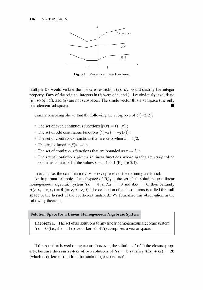
136 VECTOR SPACES
f(x) + g(x)
f(x)
g(x)
–1 1
Fig. 3.1 Piecewise linear functions.
multiple 0v would violate the nonzero restriction (e), v/2 would destroy the integerproperty if any of the original integers in (f) were odd, and (−1)v obviously invalidates(g); so (e), (f), and (g) are not subspaces. The single vector 0 is a subspace (the onlyone-element subspace). �
Similar reasoning shows that the following are subspaces of C(−2, 2):
• The set of even continuous functions [f (x) = f (−x)];
• The set of odd continuous functions [f (−x) = −f (x)];
• The set of continuous functions that are zero when x = 1/2;
• The single function f (x) ≡ 0;
• The set of continuous functions that are bounded as x → 2−;
• The set of continuous piecewise linear functions whose graphs are straight-linesegments connected at the values x = −1, 0, 1 (Figure 3.1).
In each case, the combination c1v1 + c2v2 preserves the defining credential.An important example of a subspace of Rm
col is the set of all solutions to a linearhomogeneous algebraic system Ax = 0; if Ax1 = 0 and Ax2 = 0, then certainlyA(c1x1 + c2x2) = 0 (= c10 + c20). The collection of such solutions is called the nullspace or the kernel of the coefficient matrix A. We formalize this observation in thefollowing theorem.
Solution Space for a Linear Homogeneous Algebraic System
Theorem 1. The set of all solutions to any linear homogeneous algebraic systemAx = 0 (i.e., the null space or kernel of A) comprises a vector space.
If the equation is nonhomogeneous, however, the solutions forfeit the closure prop-erty, because the sum x1 + x2 of two solutions of Ax = b satisfies A(x1 + x2) = 2b(which is different from b in the nonhomogeneous case).
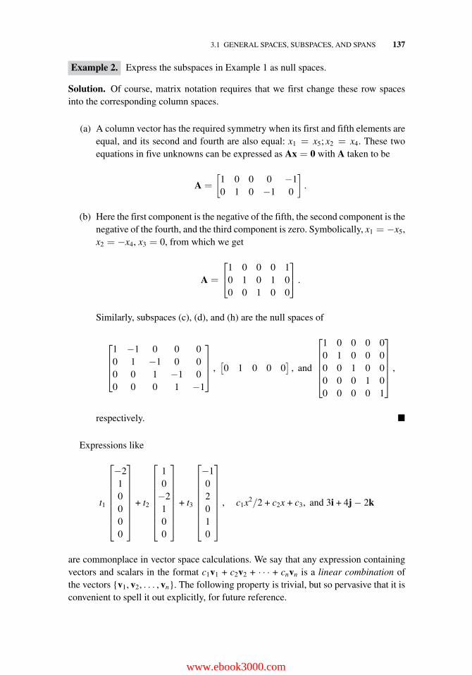
3.1 GENERAL SPACES, SUBSPACES, AND SPANS 137
Example 2. Express the subspaces in Example 1 as null spaces.
Solution. Of course, matrix notation requires that we first change these row spacesinto the corresponding column spaces.
(a) A column vector has the required symmetry when its first and fifth elements areequal, and its second and fourth are also equal: x1 = x5; x2 = x4. These twoequations in five unknowns can be expressed as Ax = 0 with A taken to be
A =
[1 0 0 0 −10 1 0 −1 0
].
(b) Here the first component is the negative of the fifth, the second component is thenegative of the fourth, and the third component is zero. Symbolically, x1 = −x5,x2 = −x4, x3 = 0, from which we get
A =
⎡⎣1 0 0 0 1
0 1 0 1 00 0 1 0 0
⎤⎦ .
Similarly, subspaces (c), (d), and (h) are the null spaces of
⎡⎢⎢⎣
1 −1 0 0 00 1 −1 0 00 0 1 −1 00 0 0 1 −1
⎤⎥⎥⎦ ,
[0 1 0 0 0
], and
⎡⎢⎢⎢⎢⎣
1 0 0 0 00 1 0 0 00 0 1 0 00 0 0 1 00 0 0 0 1
⎤⎥⎥⎥⎥⎦ ,
respectively. �
Expressions like
t1
⎡⎢⎢⎢⎢⎢⎢⎢⎣
−210000
⎤⎥⎥⎥⎥⎥⎥⎥⎦
+ t2
⎡⎢⎢⎢⎢⎢⎢⎢⎣
10−2100
⎤⎥⎥⎥⎥⎥⎥⎥⎦
+ t3
⎡⎢⎢⎢⎢⎢⎢⎢⎣
−102010
⎤⎥⎥⎥⎥⎥⎥⎥⎦
, c1x2/2 + c2x + c3, and 3i + 4j − 2k
are commonplace in vector space calculations. We say that any expression containingvectors and scalars in the format c1v1 + c2v2 + · · · + cnvn is a linear combination ofthe vectors {v1, v2, . . . , vn}. The following property is trivial, but so pervasive that it isconvenient to spell it out explicitly, for future reference.
www.ebook3000.com
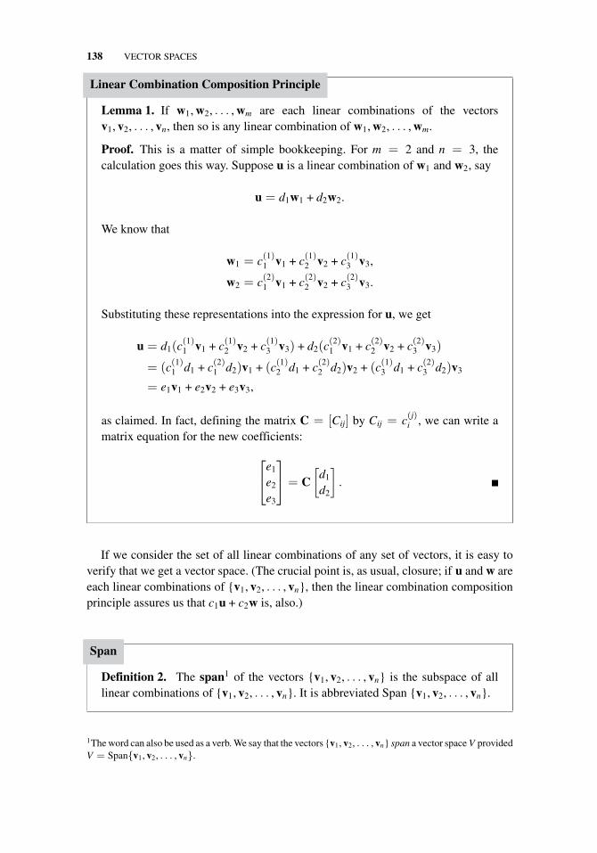
138 VECTOR SPACES
Linear Combination Composition Principle
Lemma 1. If w1, w2, . . . , wm are each linear combinations of the vectorsv1, v2, . . . , vn, then so is any linear combination of w1, w2, . . . , wm.
Proof. This is a matter of simple bookkeeping. For m = 2 and n = 3, thecalculation goes this way. Suppose u is a linear combination of w1 and w2, say
u = d1w1 + d2w2.
We know that
w1 = c(1)1 v1 + c(1)
2 v2 + c(1)3 v3,
w2 = c(2)1 v1 + c(2)
2 v2 + c(2)3 v3.
Substituting these representations into the expression for u, we get
u = d1(c(1)1 v1 + c(1)
2 v2 + c(1)3 v3) + d2(c
(2)1 v1 + c(2)
2 v2 + c(2)3 v3)
= (c(1)1 d1 + c(2)
1 d2)v1 + (c(1)2 d1 + c(2)
2 d2)v2 + (c(1)3 d1 + c(2)
3 d2)v3
= e1v1 + e2v2 + e3v3,
as claimed. In fact, defining the matrix C = [Cij] by Cij = c(j)i , we can write a
matrix equation for the new coefficients:
⎡⎣e1
e2
e3
⎤⎦ = C
[d1
d2
].
If we consider the set of all linear combinations of any set of vectors, it is easy toverify that we get a vector space. (The crucial point is, as usual, closure; if u and w areeach linear combinations of {v1, v2, . . . , vn}, then the linear combination compositionprinciple assures us that c1u + c2w is, also.)
Span
Definition 2. The span1 of the vectors {v1, v2, . . . , vn} is the subspace of alllinear combinations of {v1, v2, . . . , vn}. It is abbreviated Span {v1, v2, . . . , vn}.
1The word can also be used as a verb. We say that the vectors {v1, v2, . . . , vn} span a vector space V providedV = Span{v1, v2, . . . , vn}.
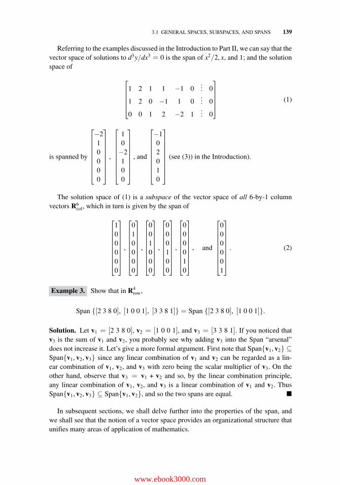
3.1 GENERAL SPACES, SUBSPACES, AND SPANS 139
Referring to the examples discussed in the Introduction to Part II, we can say that thevector space of solutions to d3y/dx3 = 0 is the span of x2/2, x, and 1; and the solutionspace of
⎡⎢⎢⎢⎣
1 2 1 1 −1 0... 0
1 2 0 −1 1 0... 0
0 0 1 2 −2 1... 0
⎤⎥⎥⎥⎦ (1)
is spanned by
⎡⎢⎢⎢⎢⎢⎢⎢⎣
−210000
⎤⎥⎥⎥⎥⎥⎥⎥⎦
,
⎡⎢⎢⎢⎢⎢⎢⎢⎣
10−2100
⎤⎥⎥⎥⎥⎥⎥⎥⎦
, and
⎡⎢⎢⎢⎢⎢⎢⎢⎣
−102010
⎤⎥⎥⎥⎥⎥⎥⎥⎦
(see (3)) in the Introduction).
The solution space of (1) is a subspace of the vector space of all 6-by-1 columnvectors R6
col, which in turn is given by the span of
⎡⎢⎢⎢⎢⎢⎢⎢⎣
100000
⎤⎥⎥⎥⎥⎥⎥⎥⎦
,
⎡⎢⎢⎢⎢⎢⎢⎢⎣
010000
⎤⎥⎥⎥⎥⎥⎥⎥⎦
,
⎡⎢⎢⎢⎢⎢⎢⎢⎣
001000
⎤⎥⎥⎥⎥⎥⎥⎥⎦
,
⎡⎢⎢⎢⎢⎢⎢⎢⎣
000100
⎤⎥⎥⎥⎥⎥⎥⎥⎦
,
⎡⎢⎢⎢⎢⎢⎢⎢⎣
000010
⎤⎥⎥⎥⎥⎥⎥⎥⎦
, and
⎡⎢⎢⎢⎢⎢⎢⎢⎣
000001
⎤⎥⎥⎥⎥⎥⎥⎥⎦
. (2)
Example 3. Show that in R4row,
Span {[2 3 8 0], [1 0 0 1], [3 3 8 1]} = Span {[2 3 8 0], [1 0 0 1]}.
Solution. Let v1 = [2 3 8 0], v2 = [1 0 0 1], and v3 = [3 3 8 1]. If you noticed thatv3 is the sum of v1 and v2, you probably see why adding v3 into the Span “arsenal”does not increase it. Let’s give a more formal argument. First note that Span{v1, v2} ⊆Span{v1, v2, v3} since any linear combination of v1 and v2 can be regarded as a lin-ear combination of v1, v2, and v3 with zero being the scalar multiplier of v3. On theother hand, observe that v3 = v1 + v2 and so, by the linear combination principle,any linear combination of v1, v2, and v3 is a linear combination of v1 and v2. ThusSpan{v1, v2, v3} ⊆ Span{v1, v2}, and so the two spans are equal. �
In subsequent sections, we shall delve further into the properties of the span, andwe shall see that the notion of a vector space provides an organizational structure thatunifies many areas of application of mathematics.
www.ebook3000.com
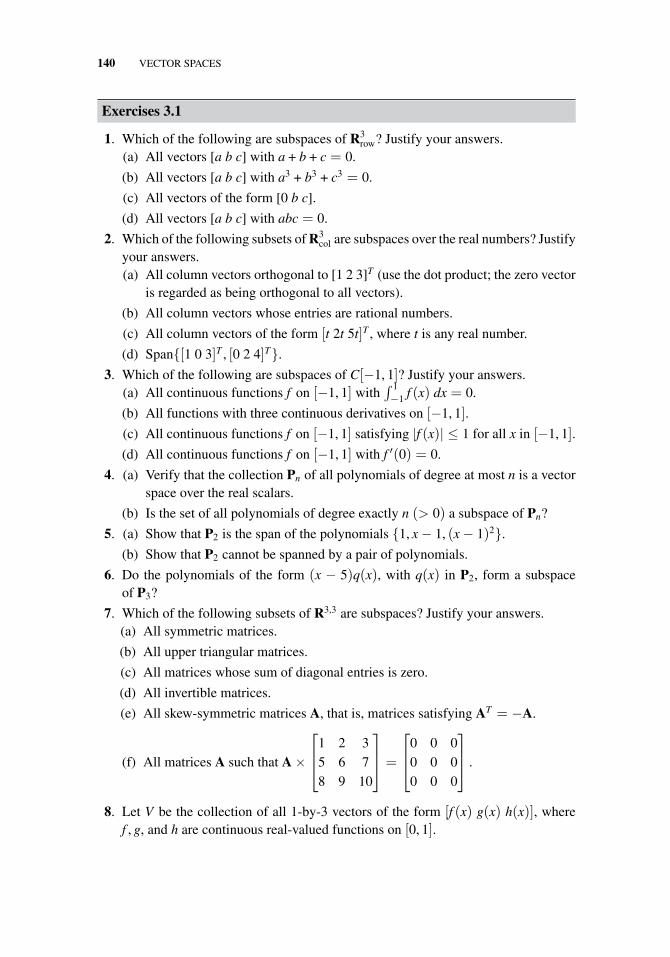
140 VECTOR SPACES
Exercises 3.1
1. Which of the following are subspaces of R3row? Justify your answers.
(a) All vectors [a b c] with a + b + c = 0.
(b) All vectors [a b c] with a3 + b3 + c3 = 0.
(c) All vectors of the form [0 b c].
(d) All vectors [a b c] with abc = 0.
2. Which of the following subsets of R3col are subspaces over the real numbers? Justify
your answers.(a) All column vectors orthogonal to [1 2 3]T (use the dot product; the zero vector
is regarded as being orthogonal to all vectors).
(b) All column vectors whose entries are rational numbers.
(c) All column vectors of the form [t 2t 5t]T , where t is any real number.
(d) Span{[1 0 3]T , [0 2 4]T}.
3. Which of the following are subspaces of C[−1, 1]? Justify your answers.(a) All continuous functions f on [−1, 1] with
∫ 1−1 f (x) dx = 0.
(b) All functions with three continuous derivatives on [−1, 1].
(c) All continuous functions f on [−1, 1] satisfying |f (x)| ≤ 1 for all x in [−1, 1].
(d) All continuous functions f on [−1, 1] with f ′(0) = 0.
4. (a) Verify that the collection Pn of all polynomials of degree at most n is a vectorspace over the real scalars.
(b) Is the set of all polynomials of degree exactly n (> 0) a subspace of Pn?
5. (a) Show that P2 is the span of the polynomials {1, x − 1, (x − 1)2}.
(b) Show that P2 cannot be spanned by a pair of polynomials.
6. Do the polynomials of the form (x − 5)q(x), with q(x) in P2, form a subspaceof P3?
7. Which of the following subsets of R3,3 are subspaces? Justify your answers.(a) All symmetric matrices.
(b) All upper triangular matrices.
(c) All matrices whose sum of diagonal entries is zero.
(d) All invertible matrices.
(e) All skew-symmetric matrices A, that is, matrices satisfying AT = −A.
(f) All matrices A such that A ×
⎡⎢⎣
1 2 35 6 78 9 10
⎤⎥⎦ =
⎡⎢⎣
0 0 00 0 00 0 0
⎤⎥⎦ .
8. Let V be the collection of all 1-by-3 vectors of the form [f (x) g(x) h(x)], wheref , g, and h are continuous real-valued functions on [0, 1].
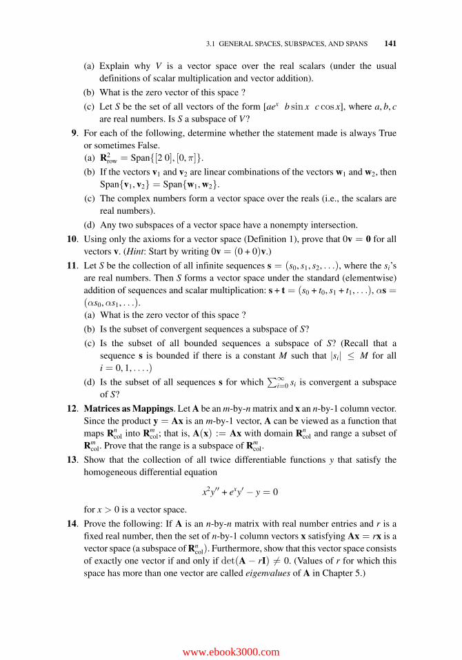
3.1 GENERAL SPACES, SUBSPACES, AND SPANS 141
(a) Explain why V is a vector space over the real scalars (under the usualdefinitions of scalar multiplication and vector addition).
(b) What is the zero vector of this space ?
(c) Let S be the set of all vectors of the form [aex b sin x c cos x], where a, b, care real numbers. Is S a subspace of V?
9. For each of the following, determine whether the statement made is always Trueor sometimes False.(a) R2
row = Span{[2 0], [0,π]}.
(b) If the vectors v1 and v2 are linear combinations of the vectors w1 and w2, thenSpan{v1, v2} = Span{w1, w2}.
(c) The complex numbers form a vector space over the reals (i.e., the scalars arereal numbers).
(d) Any two subspaces of a vector space have a nonempty intersection.
10. Using only the axioms for a vector space (Definition 1), prove that 0v = 0 for allvectors v. (Hint: Start by writing 0v = (0 + 0)v.)
11. Let S be the collection of all infinite sequences s = (s0, s1, s2, . . .), where the si’sare real numbers. Then S forms a vector space under the standard (elementwise)addition of sequences and scalar multiplication: s + t = (s0 + t0, s1 + t1, . . .), αs =(αs0,αs1, . . .).(a) What is the zero vector of this space ?
(b) Is the subset of convergent sequences a subspace of S?
(c) Is the subset of all bounded sequences a subspace of S? (Recall that asequence s is bounded if there is a constant M such that |si| ≤ M for alli = 0, 1, . . . .)
(d) Is the subset of all sequences s for which∑∞
i=0 si is convergent a subspaceof S?
12. Matrices as Mappings. Let A be an m-by-n matrix and x an n-by-1 column vector.Since the product y = Ax is an m-by-1 vector, A can be viewed as a function thatmaps Rn
col into Rmcol; that is, A(x) := Ax with domain Rn
col and range a subset ofRm
col. Prove that the range is a subspace of Rmcol.
13. Show that the collection of all twice differentiable functions y that satisfy thehomogeneous differential equation
x2y′′ + exy′ − y = 0
for x > 0 is a vector space.
14. Prove the following: If A is an n-by-n matrix with real number entries and r is afixed real number, then the set of n-by-1 column vectors x satisfying Ax = rx is avector space (a subspace of Rn
col). Furthermore, show that this vector space consistsof exactly one vector if and only if det(A − rI) �= 0. (Values of r for which thisspace has more than one vector are called eigenvalues of A in Chapter 5.)
www.ebook3000.com
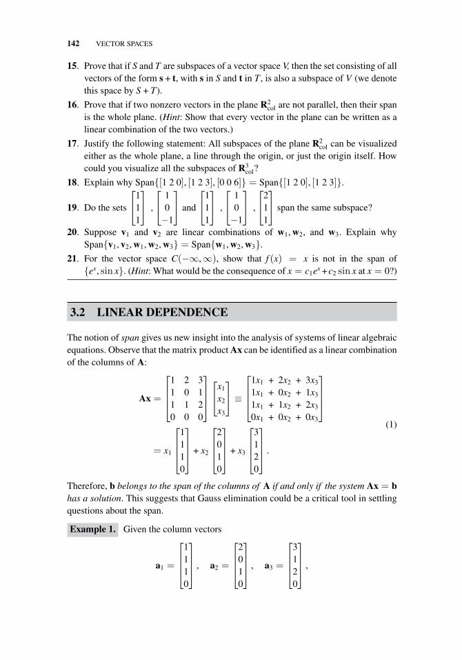
142 VECTOR SPACES
15. Prove that if S and T are subspaces of a vector space V, then the set consisting of allvectors of the form s + t, with s in S and t in T , is also a subspace of V (we denotethis space by S + T).
16. Prove that if two nonzero vectors in the plane R2col are not parallel, then their span
is the whole plane. (Hint: Show that every vector in the plane can be written as alinear combination of the two vectors.)
17. Justify the following statement: All subspaces of the plane R2col can be visualized
either as the whole plane, a line through the origin, or just the origin itself. Howcould you visualize all the subspaces of R3
col?
18. Explain why Span{[1 2 0], [1 2 3], [0 0 6]} = Span{[1 2 0], [1 2 3]}.
19. Do the sets
⎡⎣1
11
⎤⎦ ,
⎡⎣ 1
0−1
⎤⎦ and
⎡⎣1
11
⎤⎦ ,
⎡⎣ 1
0−1
⎤⎦ ,
⎡⎣2
11
⎤⎦ span the same subspace?
20. Suppose v1 and v2 are linear combinations of w1, w2, and w3. Explain whySpan{v1, v2, w1, w2, w3} = Span{w1, w2, w3}.
21. For the vector space C(−∞,∞), show that f (x) = x is not in the span of{ex, sin x}. (Hint: What would be the consequence of x = c1ex +c2 sin x at x = 0?)
3.2 LINEAR DEPENDENCE
The notion of span gives us new insight into the analysis of systems of linear algebraicequations. Observe that the matrix product Ax can be identified as a linear combinationof the columns of A:
Ax =
⎡⎢⎢⎣
1 2 31 0 11 1 20 0 0
⎤⎥⎥⎦⎡⎣x1
x2
x3
⎤⎦ ≡
⎡⎢⎢⎣
1x1 + 2x2 + 3x3
1x1 + 0x2 + 1x3
1x1 + 1x2 + 2x3
0x1 + 0x2 + 0x3
⎤⎥⎥⎦
= x1
⎡⎢⎢⎣
1110
⎤⎥⎥⎦ + x2
⎡⎢⎢⎣
2010
⎤⎥⎥⎦ + x3
⎡⎢⎢⎣
3120
⎤⎥⎥⎦ .
(1)
Therefore, b belongs to the span of the columns of A if and only if the system Ax = bhas a solution. This suggests that Gauss elimination could be a critical tool in settlingquestions about the span.
Example 1. Given the column vectors
a1 =
⎡⎢⎢⎣
1110
⎤⎥⎥⎦ , a2 =
⎡⎢⎢⎣
2010
⎤⎥⎥⎦ , a3 =
⎡⎢⎢⎣
3120
⎤⎥⎥⎦ ,
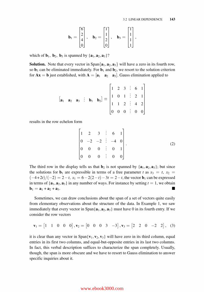
3.2 LINEAR DEPENDENCE 143
b1 =
⎡⎢⎢⎣
6240
⎤⎥⎥⎦ , b2 =
⎡⎢⎢⎣
1120
⎤⎥⎥⎦ , b3 =
⎡⎢⎢⎣
1111
⎤⎥⎥⎦ ,
which of b1, b2, b3 is spanned by {a1, a2, a3}?
Solution. Note that every vector in Span{a1, a2, a3} will have a zero in its fourth row,so b3 can be eliminated immediately. For b1 and b2, we resort to the solution criterionfor Ax = b just established, with A = [a1 a2 a3]. Gauss elimination applied to
[a1 a2 a3
... b1 b2
]≡
⎡⎢⎢⎢⎢⎢⎢⎣
1 2 3... 6 1
1 0 1... 2 1
1 1 2... 4 2
0 0 0... 0 0
⎤⎥⎥⎥⎥⎥⎥⎦
results in the row echelon form
⎡⎢⎢⎢⎢⎢⎢⎣
1 2 3... 6 1
0 −2 −2... −4 0
0 0 0... 0 1
0 0 0... 0 0
⎤⎥⎥⎥⎥⎥⎥⎦
. (2)
The third row in the display tells us that b2 is not spanned by {a1, a2, a3}; but sincethe solutions for b1 are expressible in terms of a free parameter t as x3 = t, x2 =(−4+2t)/(−2) = 2− t, x1 = 6−2(2− t)−3t = 2− t, the vector b1 can be expressedin terms of {a1, a2, a3} in any number of ways. For instance by setting t = 1, we obtainb1 = a1 + a2 + a3. �
Sometimes, we can draw conclusions about the span of a set of vectors quite easilyfrom elementary observations about the structure of the data. In Example 1, we sawimmediately that every vector in Span{a1, a2, a3} must have 0 in its fourth entry. If weconsider the row vectors
v1 =[1 1 0 0 0
], v2 =
[0 0 0 3 −3
], v3 =
[2 2 0 −2 2
], (3)
it is clear than any vector in Span{v1, v2, v3} will have zero in its third column, equalentries in its first two columns, and equal-but-opposite entries in its last two columns.In fact, this verbal description suffices to characterize the span completely. Usually,though, the span is more obscure and we have to resort to Gauss elimination to answerspecific inquiries about it.
www.ebook3000.com
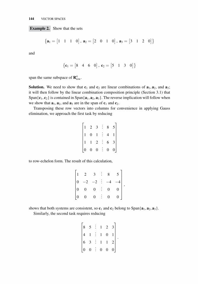
144 VECTOR SPACES
Example 2. Show that the sets
{a1 =
[1 1 1 0
], a2 =
[2 0 1 0
], a3 =
[3 1 2 0
]}
and
{c1 =
[8 4 6 0
], c2 =
[5 1 3 0
]}
span the same subspace of R4row.
Solution. We need to show that c1 and c2 are linear combinations of a1, a2, and a3;it will then follow by the linear combination composition principle (Section 3.1) thatSpan{c1, c2} is contained in Span{a1, a2, a3}. The reverse implication will follow whenwe show that a1, a2, and a3 are in the span of c1 and c2.
Transposing these row vectors into columns for convenience in applying Gausselimination, we approach the first task by reducing
⎡⎢⎢⎢⎢⎢⎢⎣
1 2 3... 8 5
1 0 1... 4 1
1 1 2... 6 3
0 0 0... 0 0
⎤⎥⎥⎥⎥⎥⎥⎦
to row-echelon form. The result of this calculation,
⎡⎢⎢⎢⎢⎢⎢⎣
1 2 3... 8 5
0 −2 −2... −4 −4
0 0 0... 0 0
0 0 0... 0 0
⎤⎥⎥⎥⎥⎥⎥⎦
,
shows that both systems are consistent, so c1 and c2 belong to Span{a1, a2, a3}.Similarly, the second task requires reducing
⎡⎢⎢⎢⎢⎢⎢⎣
8 5... 1 2 3
4 1... 1 0 1
6 3... 1 1 2
0 0... 0 0 0
⎤⎥⎥⎥⎥⎥⎥⎦
.
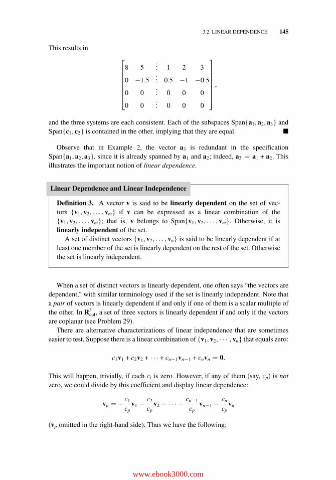
3.2 LINEAR DEPENDENCE 145
This results in
⎡⎢⎢⎢⎢⎢⎢⎣
8 5... 1 2 3
0 −1.5... 0.5 −1 −0.5
0 0... 0 0 0
0 0... 0 0 0
⎤⎥⎥⎥⎥⎥⎥⎦
,
and the three systems are each consistent. Each of the subspaces Span{a1, a2, a3} andSpan{c1, c2} is contained in the other, implying that they are equal. �
Observe that in Example 2, the vector a3 is redundant in the specificationSpan{a1, a2, a3}, since it is already spanned by a1 and a2; indeed, a3 = a1 + a2. Thisillustrates the important notion of linear dependence.
Linear Dependence and Linear Independence
Definition 3. A vector v is said to be linearly dependent on the set of vec-tors {v1, v2, . . . , vm} if v can be expressed as a linear combination of the{v1, v2, . . . , vm}; that is, v belongs to Span{v1, v2, . . . , vm}. Otherwise, it islinearly independent of the set.
A set of distinct vectors {v1, v2, . . . , vn} is said to be linearly dependent if atleast one member of the set is linearly dependent on the rest of the set. Otherwisethe set is linearly independent.
When a set of distinct vectors is linearly dependent, one often says “the vectors aredependent,” with similar terminology used if the set is linearly independent. Note thata pair of vectors is linearly dependent if and only if one of them is a scalar multiple ofthe other. In R3
col, a set of three vectors is linearly dependent if and only if the vectorsare coplanar (see Problem 29).
There are alternative characterizations of linear independence that are sometimeseasier to test. Suppose there is a linear combination of {v1, v2, · · · , vn} that equals zero:
c1v1 + c2v2 + · · · + cn−1vn−1 + cnvn = 0.
This will happen, trivially, if each ci is zero. However, if any of them (say, cp) is notzero, we could divide by this coefficient and display linear dependence:
vp = −c1
cpv1 −
c2
cpv2 − · · · − cn−1
cpvn−1 −
cn
cpvn
(vp omitted in the right-hand side). Thus we have the following:
www.ebook3000.com
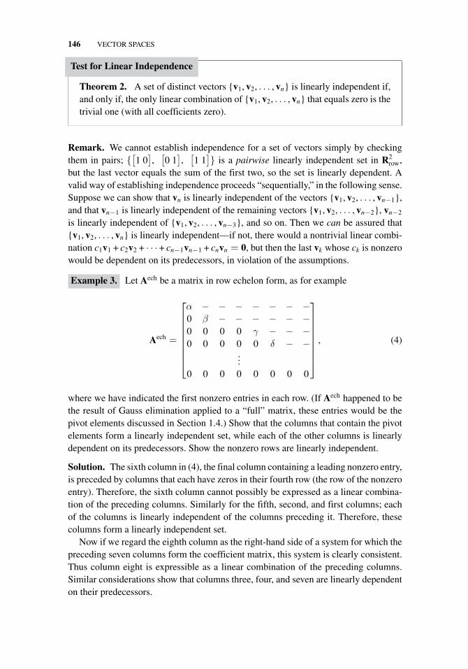
146 VECTOR SPACES
Test for Linear Independence
Theorem 2. A set of distinct vectors {v1, v2, . . . , vn} is linearly independent if,and only if, the only linear combination of {v1, v2, . . . , vn} that equals zero is thetrivial one (with all coefficients zero).
Remark. We cannot establish independence for a set of vectors simply by checkingthem in pairs; {
[1 0
],[0 1
],[1 1
]} is a pairwise linearly independent set in R2
row,but the last vector equals the sum of the first two, so the set is linearly dependent. Avalid way of establishing independence proceeds “sequentially,” in the following sense.Suppose we can show that vn is linearly independent of the vectors {v1, v2, . . . , vn−1},and that vn−1 is linearly independent of the remaining vectors {v1, v2, . . . , vn−2}, vn−2
is linearly independent of {v1, v2, . . . , vn−3}, and so on. Then we can be assured that{v1, v2, . . . , vn} is linearly independent—if not, there would a nontrivial linear combi-nation c1v1 + c2v2 + · · · + cn−1vn−1 + cnvn = 0, but then the last vk whose ck is nonzerowould be dependent on its predecessors, in violation of the assumptions.
Example 3. Let Aech be a matrix in row echelon form, as for example
Aech =
⎡⎢⎢⎢⎢⎢⎢⎢⎣
α − − − − − − −0 β − − − − − −0 0 0 0 γ − − −0 0 0 0 0 δ − −
...0 0 0 0 0 0 0 0
⎤⎥⎥⎥⎥⎥⎥⎥⎦
, (4)
where we have indicated the first nonzero entries in each row. (If Aech happened to bethe result of Gauss elimination applied to a “full” matrix, these entries would be thepivot elements discussed in Section 1.4.) Show that the columns that contain the pivotelements form a linearly independent set, while each of the other columns is linearlydependent on its predecessors. Show the nonzero rows are linearly independent.
Solution. The sixth column in (4), the final column containing a leading nonzero entry,is preceded by columns that each have zeros in their fourth row (the row of the nonzeroentry). Therefore, the sixth column cannot possibly be expressed as a linear combina-tion of the preceding columns. Similarly for the fifth, second, and first columns; eachof the columns is linearly independent of the columns preceding it. Therefore, thesecolumns form a linearly independent set.
Now if we regard the eighth column as the right-hand side of a system for which thepreceding seven columns form the coefficient matrix, this system is clearly consistent.Thus column eight is expressible as a linear combination of the preceding columns.Similar considerations show that columns three, four, and seven are linearly dependenton their predecessors.
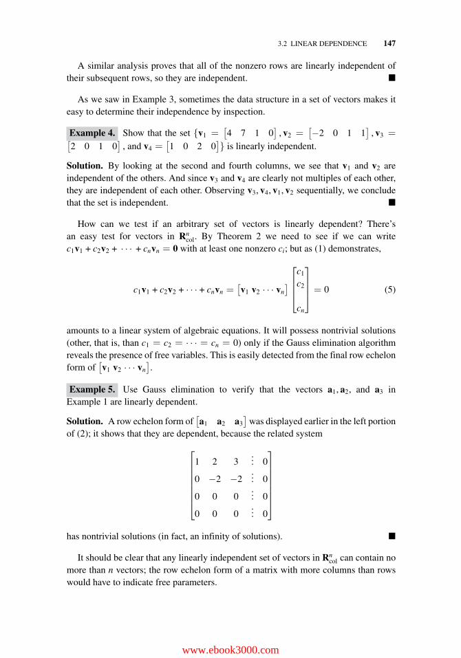
3.2 LINEAR DEPENDENCE 147
A similar analysis proves that all of the nonzero rows are linearly independent oftheir subsequent rows, so they are independent. �
As we saw in Example 3, sometimes the data structure in a set of vectors makes iteasy to determine their independence by inspection.
Example 4. Show that the set {v1 =[4 7 1 0
], v2 =
[−2 0 1 1
], v3 =[
2 0 1 0]
, and v4 =[1 0 2 0
]} is linearly independent.
Solution. By looking at the second and fourth columns, we see that v1 and v2 areindependent of the others. And since v3 and v4 are clearly not multiples of each other,they are independent of each other. Observing v3, v4, v1, v2 sequentially, we concludethat the set is independent. �
How can we test if an arbitrary set of vectors is linearly dependent? There’san easy test for vectors in Rn
col. By Theorem 2 we need to see if we can writec1v1 + c2v2 + · · · + cnvn = 0 with at least one nonzero ci; but as (1) demonstrates,
c1v1 + c2v2 + · · · + cnvn =[v1 v2 · · · vn
]⎡⎢⎢⎣
c1
c2
cn
⎤⎥⎥⎦ = 0 (5)
amounts to a linear system of algebraic equations. It will possess nontrivial solutions(other, that is, than c1 = c2 = · · · = cn = 0) only if the Gauss elimination algorithmreveals the presence of free variables. This is easily detected from the final row echelonform of
[v1 v2 · · · vn
].
Example 5. Use Gauss elimination to verify that the vectors a1, a2, and a3 inExample 1 are linearly dependent.
Solution. A row echelon form of[a1 a2 a3
]was displayed earlier in the left portion
of (2); it shows that they are dependent, because the related system
⎡⎢⎢⎢⎢⎢⎢⎣
1 2 3... 0
0 −2 −2... 0
0 0 0... 0
0 0 0... 0
⎤⎥⎥⎥⎥⎥⎥⎦
has nontrivial solutions (in fact, an infinity of solutions). �
It should be clear that any linearly independent set of vectors in Rncol can contain no
more than n vectors; the row echelon form of a matrix with more columns than rowswould have to indicate free parameters.
www.ebook3000.com
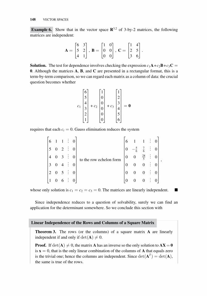
148 VECTOR SPACES
Example 6. Show that in the vector space R3,2 of 3-by-2 matrices, the followingmatrices are independent:
A =
⎡⎣6 3
5 24 1
⎤⎦ , B =
⎡⎣1 0
0 00 0
⎤⎦ , C =
⎡⎣1 4
2 53 6
⎤⎦ .
Solution. The test for dependence involves checking the expression c1A+c2B+c3C =0. Although the matrices A, B, and C are presented in a rectangular format, this is aterm-by-term comparison, so we can regard each matrix as a column of data: the crucialquestion becomes whether
c1
⎡⎢⎢⎢⎢⎢⎢⎢⎣
654321
⎤⎥⎥⎥⎥⎥⎥⎥⎦
+ c2
⎡⎢⎢⎢⎢⎢⎢⎢⎣
100000
⎤⎥⎥⎥⎥⎥⎥⎥⎦
+ c3
⎡⎢⎢⎢⎢⎢⎢⎢⎣
123456
⎤⎥⎥⎥⎥⎥⎥⎥⎦= 0
requires that each ci = 0. Gauss elimination reduces the system
⎡⎢⎢⎢⎢⎢⎢⎢⎢⎢⎢⎢⎢⎣
6 1 1... 0
5 0 2... 0
4 0 3... 0
3 0 4... 0
2 0 5... 0
1 0 6... 0
⎤⎥⎥⎥⎥⎥⎥⎥⎥⎥⎥⎥⎥⎦
to the row echelon form
⎡⎢⎢⎢⎢⎢⎢⎢⎢⎢⎢⎢⎢⎣
6 1 1... 0
0 − 56
76
... 0
0 0 285
... 0
0 0 0... 0
0 0 0... 0
0 0 0... 0
⎤⎥⎥⎥⎥⎥⎥⎥⎥⎥⎥⎥⎥⎦
,
whose only solution is c1 = c2 = c3 = 0. The matrices are linearly independent. �
Since independence reduces to a question of solvability, surely we can find anapplication for the determinant somewhere. So we conclude this section with
Linear Independence of the Rows and Columns of a Square Matrix
Theorem 3. The rows (or the columns) of a square matrix A are linearlyindependent if and only if det(A) �= 0.
Proof. If det(A) �= 0, the matrix A has an inverse so the only solution to AX= 0is x = 0, that is the only linear combination of the columns of A that equals zerois the trivial one; hence the columns are independent. Since det(AT) = det(A),the same is true of the rows.
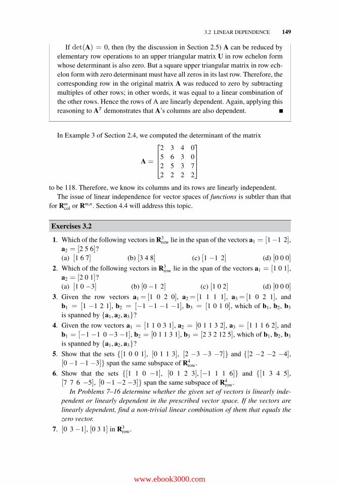
3.2 LINEAR DEPENDENCE 149
If det(A) = 0, then (by the discussion in Section 2.5) A can be reduced byelementary row operations to an upper triangular matrix U in row echelon formwhose determinant is also zero. But a square upper triangular matrix in row ech-elon form with zero determinant must have all zeros in its last row. Therefore, thecorresponding row in the original matrix A was reduced to zero by subtractingmultiples of other rows; in other words, it was equal to a linear combination ofthe other rows. Hence the rows of A are linearly dependent. Again, applying thisreasoning to AT demonstrates that A’s columns are also dependent.
In Example 3 of Section 2.4, we computed the determinant of the matrix
A =
⎡⎢⎢⎣
2 3 4 05 6 3 02 5 3 72 2 2 2
⎤⎥⎥⎦
to be 118. Therefore, we know its columns and its rows are linearly independent.The issue of linear independence for vector spaces of functions is subtler than that
for Rmcol or Rm,n. Section 4.4 will address this topic.
Exercises 3.2
1. Which of the following vectors in R3row lie in the span of the vectors a1 = [1 −1 2],
a2 = [2 5 6]?(a) [1 6 7] (b) [3 4 8] (c) [1 −1 2] (d) [0 0 0]
2. Which of the following vectors in R3row lie in the span of the vectors a1 = [1 0 1],
a2 = [2 0 1]?(a) [1 0 −3] (b) [0 −1 2] (c) [1 0 2] (d) [0 0 0]
3. Given the row vectors a1 = [1 0 2 0], a2 = [1 1 1 1], a3 = [1 0 2 1], andb1 = [1 −1 2 1], b2 = [−1 −1 −1 −1], b3 = [1 0 1 0], which of b1, b2, b3
is spanned by {a1, a2, a3}?
4. Given the row vectors a1 = [1 1 0 3 1], a2 = [0 1 1 3 2], a3 = [1 1 1 6 2], andb1 = [−1 −1 0 −3 −1], b2 = [0 1 1 3 1], b3 = [2 3 2 12 5], which of b1, b2, b3
is spanned by {a1, a2, a3}?
5. Show that the sets {[1 0 0 1], [0 1 1 3], [2 −3 −3 −7]} and {[2 −2 −2 −4],[0 −1 −1 −3]} span the same subspace of R4
row.
6. Show that the sets {[1 1 0 −1], [0 1 2 3], [−1 1 1 6]} and {[1 3 4 5],[7 7 6 −5], [0 −1 −2 −3]} span the same subspace of R4
row.In Problems 7–16 determine whether the given set of vectors is linearly inde-
pendent or linearly dependent in the prescribed vector space. If the vectors arelinearly dependent, find a non-trivial linear combination of them that equals thezero vector.
7. [0 3 −1], [0 3 1] in R3row.
www.ebook3000.com
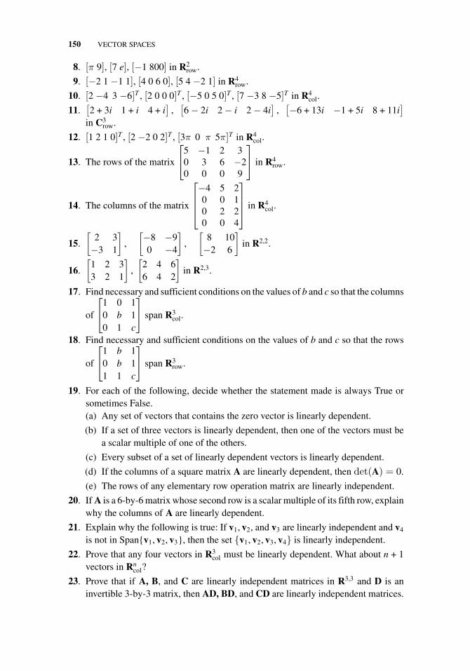
150 VECTOR SPACES
8. [π 9], [7 e], [−1 800] in R2row.
9. [−2 1 −1 1], [4 0 6 0], [5 4 −2 1] in R4row.
10. [2 −4 3 −6]T , [2 0 0 0]T , [−5 0 5 0]T , [7 −3 8 −5]T in R4col.
11.[2 + 3i 1 + i 4 + i
],[6 − 2i 2 − i 2 − 4i
],[−6 + 13i −1 + 5i 8 + 11i
]in C3
row.
12. [1 2 1 0]T , [2 −2 0 2]T , [3π 0 π 5π]T in R4col.
13. The rows of the matrix
⎡⎣5 −1 2 3
0 3 6 −20 0 0 9
⎤⎦ in R4
row.
14. The columns of the matrix
⎡⎢⎢⎣−4 5 20 0 10 2 20 0 4
⎤⎥⎥⎦ in R4
col.
15.
[2 3−3 1
],
[−8 −90 −4
],
[8 10−2 6
]in R2,2.
16.
[1 2 33 2 1
],
[2 4 66 4 2
]in R2,3.
17. Find necessary and sufficient conditions on the values of b and c so that the columns
of
⎡⎣1 0 1
0 b 10 1 c
⎤⎦ span R3
col.
18. Find necessary and sufficient conditions on the values of b and c so that the rows
of
⎡⎣1 b 1
0 b 11 1 c
⎤⎦ span R3
row.
19. For each of the following, decide whether the statement made is always True orsometimes False.(a) Any set of vectors that contains the zero vector is linearly dependent.
(b) If a set of three vectors is linearly dependent, then one of the vectors must bea scalar multiple of one of the others.
(c) Every subset of a set of linearly dependent vectors is linearly dependent.
(d) If the columns of a square matrix A are linearly dependent, then det(A) = 0.
(e) The rows of any elementary row operation matrix are linearly independent.
20. If A is a 6-by-6 matrix whose second row is a scalar multiple of its fifth row, explainwhy the columns of A are linearly dependent.
21. Explain why the following is true: If v1, v2, and v3 are linearly independent and v4
is not in Span{v1, v2, v3}, then the set {v1, v2, v3, v4} is linearly independent.
22. Prove that any four vectors in R3col must be linearly dependent. What about n + 1
vectors in Rncol?
23. Prove that if A, B, and C are linearly independent matrices in R3,3 and D is aninvertible 3-by-3 matrix, then AD, BD, and CD are linearly independent matrices.
3.3 BASES, DIMENSION, AND RANK 151
24. Prove that if v1, v2, v3 are the columns of an n-by-3 matrix A and B is an invertible3-by-3 matrix, then the span of the columns of AB is identical to Span{v1, v2, v3}.
25. Let A be an n-by-n matrix and x be an n-by-1 column vector. Explain why thecolumns of Ax, A2x, A3x, . . . all lie in the span of the columns of A.
26. Let A be an n-by-n matrix and B be an invertible n-by-n matrix. Prove that if thecolumn vectors of A are linearly independent, then so are the columns vectorsof AB.
27. Given that the vectors v1, v2, v3 are linearly independent, show that the followingvectors are also linearly independent:(a) w1 = 2v1 − 3v2, w2 = 4v1 − 3v2
(b) w1 = v1 − 3v2, w2 = 4v1 − 3v3, w3 = 2v2 − 3v3.
28. Prove that an n-by-n matrix A is invertible if and only if for any set of n lin-early independent vectors v1, v2, . . . , vn in Rn
col, the set Av1, Av2, . . . , Avn is linearlyindependent.
29. Prove that three vectors in R3col are linearly dependent if and only if they are copla-
nar.(Hint: If v1, v2, and v3 are coplanar, and n is a normal to the plane in which
they lie, then the dot products vi · n are zero for i = 1, 2, 3. What does this implyabout the determinant of the matrix [v1 v2 v3]?
)
3.3 BASES, DIMENSION, AND RANK
In Section 3.1 we noted that the span of any set of vectors constitutes a subspace. Weobserved that the solution space of the homogeneous system
⎡⎢⎢⎢⎣
1 2 1 1 −1 0... 0
1 2 0 −1 1 0... 0
0 0 1 2 −2 1... 0
⎤⎥⎥⎥⎦ (1)
(the “null space” of its coefficient matrix) is given by
Span{[−2 1 0 0 0 0
]T,[1 0 −2 1 0 0
]T,[−1 0 2 0 1 0
]T},(2)
and the solution space of the homogeneous differential equation
d3y/dx3 = 0
is given by Span{x2/2, x, 1}.Now consider the subspace of R5
row spanned by
v1 =[1 1 0 0 0
], v2 =
[0 0 0 3 −3
], v3 =
[2 2 0 −2 2
], (3)
www.ebook3000.com
152 VECTOR SPACES
which could be described as the subspace in which the first two entries were equal,the final two negatives of each other, and the third entry zero. Observe that v3 can begenerated by taking 2v1 − 2v2/3. This means that v3 is redundant in Span{v1, v2, v3},since (by the linear combination composition principle) any vector expressible as alinear combination of v1, v2, and v3 can be rearranged into a linear combination ofv1 and v2 alone. So it would be economical to drop v3 and regard the subspace asSpan{v1, v2}. But we can’t economize any further, since v1 and v2 are independent ofeach other (since v2 is not a scalar times v1). We formalize this idea:
Basis
Definition 4. A basis for a space (or subspace) is a linearly independent set ofvectors that spans the (sub)space.
A basis for a (sub)space is therefore a “minimal spanning set,” in the sense that if anyvector is dropped from the basis, it will no longer span the space (the dropped vectoritself, for example, cannot be expressed as a linear combination of the others). It canalso be characterized as a “maximal linearly independent set,” in the sense that thereare no other vectors in the subspace that are independent of the basis (otherwise, thebasis wouldn’t have spanned the space).
An obvious basis for, say, R4col (or, for that matter, C4
col) would the “canonical basis.”
⎡⎢⎢⎣
1000
⎤⎥⎥⎦,
⎡⎢⎢⎣
0100
⎤⎥⎥⎦,
⎡⎢⎢⎣
0010
⎤⎥⎥⎦, and
⎡⎢⎢⎣
0001
⎤⎥⎥⎦.
However the columns of any nonsingular square n-by-n matrix comprise a basis forRn
col; indeed, since the determinant of the matrix is nonzero, Cramer’s rule implies bothlinear independence and the spanning property.
Example 1. Construct bases for the subspaces of R5row considered in Example 1 of
Section 3.1:
(a) All “symmetric” vectors of the form[a b c b a
];
(b) All “antisymmetric” vectors of the form[a b 0 −b −a
];
(c) Those vectors all of whose entries are the same[a a a a a
];
(d) Those vectors whose second entry is zero[a 0 b c d
].
Solution. (a) Two obvious vectors in the subspace are v1 =[1 0 0 0 1
]and
v2 =[0 1 0 1 0
]. However, they don’t span the subspace, since everything in
Span{ v1, v2} will have zero in its third entry. So we throw in v3 =[0 0 1 0 0
].
3.3 BASES, DIMENSION, AND RANK 153
The set {v1, v2, v3} is clearly independent because of the location of the zeros, and itspans the space, as witnessed by the display
[a b c b a
]= av1 + bv2 + cv3.
(b) Proceeding similarly to (a), we find the basis[1 0 0 0 −1
]and[
0 1 0 −1 0].
(c) The single vector[1 1 1 1 1
]spans the subspace.
(d) This space is spanned by the independent vectors[1 0 0 0 0
],[
0 0 1 0 0],[0 0 0 1 0
], and
[0 0 0 0 1
]. �
Example 2. Find a basis for the subspace of R4col of vectors whose entries add
up to zero.
Solution. This subspace is the null space for the matrix A =[1 1 1 1
]. Since A
is already in row echelon form, the solutions to Ax = 0 are parametrized by back-solving the augmented system
[1 1 1 1
... 0], yielding x4 = t1, x3 = t2, x2 =
t3, x1 = −t1 − t2 − t3, or
x =
⎡⎢⎢⎣
x1
x2
x3
x4
⎤⎥⎥⎦ = t1
⎡⎢⎢⎣−1001
⎤⎥⎥⎦ + t2
⎡⎢⎢⎣−1010
⎤⎥⎥⎦ + t3
⎡⎢⎢⎣−1100
⎤⎥⎥⎦ , (4)
and the vectors in this display form a basis. �
Change of Coordinates
In Example 2 of Section 3.2, we saw how to test whether a vector v in Rncol lies in
the subspace spanned by {w1, w2, . . . , wk}; indeed, the possibility of a relation
v = c1w1 + c2w2 + · · · + ckwk (5)
is easily resolved by Gauss elimination, since (5) amounts to a linear system of nequations in k unknowns:
[v
]= c1
[w1
]+ c2
[w2
]+ · · · + ck
[wk
]=
[w1 w2 · · · wk
]⎡⎢⎢⎢⎣
c1
c2...
ck
⎤⎥⎥⎥⎦
[v
]=
[w1 w2 · · · wk
][c
]. (6)
Gauss elimination decides the issue and supplies the values of the coefficientscj when appropriate. For example, to express [2 4]T in terms of the vectors{[1 1]T , [1−1]T} (which are independent and form a basis), we solve
www.ebook3000.com
154 VECTOR SPACES
[24
]=
[1 11 −1
] [c1
c2
](7)
and calculate [c1 c2]T = [3 −1]T .
Let’s focus on the relationship between v = [2 4]T and c = [3 −1]T inequations (5–7). They are different vectors, of course; [3 −1]T is not the same,numerically, as [2 4]T . But (5) states that [3 −1]T represents [2 4]T with respectto the basis {[1 1]T , [1 −1]T}. We say that c = [3 −1]T gives the coordinates ofv = [2 4]T in the basis {w1, w2} = {[1 1]T , [1 −1]T}.
In fact, the “original” vector [2 4]T can be interpreted as giving the coordinatesof v in the canonical basis {[1 0]T , [0 1]T}. With this jargon, we interpret (6)as a coordinate transformation from the {wj} basis to the canonical basis, with[
w1 w2 · · · wk
]playing the role of a transition matrix.
If the {wj} basis spans the whole space Rncol, that is, if k = n, (6) implies that[
w1 w2 · · · wn
]is invertible, and that its inverse is a transition matrix from canonical
coordinates to {wj} coordinates. The Gauss elimination that we performed on (7) was,of course, equivalent to multiplying by the inverse.
Now let’s address the issue of a general change of coordinates. That is, we havetwo different (non)canonical bases, {w1, w2, . . . , wp} and {u1, u2, . . . , uq} for the samesubspace of Rn
col, and a vector v lying in the subspace. Thus
v = c1 w1 + c2 w2 + · · · + cp wp = d1 u1 + d2 u2 + · · · + dq uq. (8)
How are its coordinates c in the {wj} basis related to its coordinates d in the {uj} basis?Again, matrix algebra resolves the problem easily; (8) is equivalent to[
w1 w2 · · · wp
][c
]=
[u1 u2 · · · uq
][d
]. (9)
The right-hand side is given, so Gauss elimination answers our question.
Example 3. The subspaces of R3col spanned by {[1 1 0]T , [0 1 1]T} and by
{[1 2 1]T , [1 0 −1]T} can be shown to be the same by the method of Example 2,Section 3.2. Find the coordinates in the first basis for the vector whose coordinatesin the second basis are [1 2]T .
Solution. Inserting our data into equation (9) gives⎡⎣1 0
1 10 1
⎤⎦[
c1
c2
]=
⎡⎣1 1
2 01 −1
⎤⎦[
12
]=
⎡⎣ 3
2−1
⎤⎦ (10)
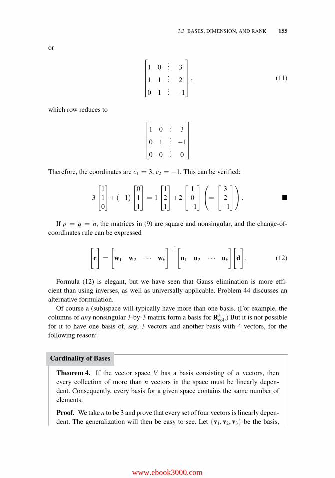
3.3 BASES, DIMENSION, AND RANK 155
or
⎡⎢⎢⎢⎣
1 0... 3
1 1... 2
0 1... −1
⎤⎥⎥⎥⎦ , (11)
which row reduces to
⎡⎢⎢⎢⎣
1 0... 3
0 1... −1
0 0... 0
⎤⎥⎥⎥⎦
Therefore, the coordinates are c1 = 3, c2 = −1. This can be verified:
3
⎡⎣1
10
⎤⎦ + (−1)
⎡⎣0
11
⎤⎦ = 1
⎡⎣1
21
⎤⎦ + 2
⎡⎣ 1
0−1
⎤⎦⎛⎝=
⎡⎣ 3
2−1
⎤⎦⎞⎠ . �
If p = q = n, the matrices in (9) are square and nonsingular, and the change-of-coordinates rule can be expressed
[c
]=
[w1 w2 · · · wk
]−1[u1 u2 · · · uk
][d
]. (12)
Formula (12) is elegant, but we have seen that Gauss elimination is more effi-cient than using inverses, as well as universally applicable. Problem 44 discusses analternative formulation.
Of course a (sub)space will typically have more than one basis. (For example, thecolumns of any nonsingular 3-by-3 matrix form a basis for R3
col.) But it is not possiblefor it to have one basis of, say, 3 vectors and another basis with 4 vectors, for thefollowing reason:
Cardinality of Bases
Theorem 4. If the vector space V has a basis consisting of n vectors, thenevery collection of more than n vectors in the space must be linearly depen-dent. Consequently, every basis for a given space contains the same number ofelements.
Proof. We take n to be 3 and prove that every set of four vectors is linearly depen-dent. The generalization will then be easy to see. Let {v1, v2, v3} be the basis,
www.ebook3000.com
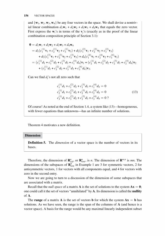
156 VECTOR SPACES
and {w1, w2, w3, w4} be any four vectors in the space. We shall devise a nontriv-ial linear combination d1w1 + d2w2 + d3w3 + d4w4 that equals the zero vector.First express the wi’s in terms of the vj’s (exactly as in the proof of the linearcombination composition principle of Section 3.1):
0 = d1w1 + d2w2 + d3w3 + d4w4
= d1(c(1)1 v1 + c(1)
2 v2 + c(1)3 v3) + d2(c
(2)1 v1 + c(2)
2 v2 + c(2)3 v3)
+ d3(c(3)1 v1 + c(3)
2 v2 + c(3)3 v3) + d4(c
(4)1 v1 + c(4)
2 v2 + c(4)3 v3)
= (c(1)1 d1 + c(2)
1 d2 + c(3)1 d3 + c(4)
1 d4)v1 + (c(1)2 d1 + c(2)
2 d2 + c(3)2 d3 + c(4)
2 d4)v2
+ (c(1)3 d1 + c(2)
3 d2 + c(3)3 d3 + c(4)
3 d4)v3.
Can we find dj’s not all zero such that
c(1)1 d1 + c(2)
1 d2 + c(3)1 d3 + c(4)
1 d4 = 0
c(1)2 d1 + c(2)
2 d2 + c(3)2 d3 + c(4)
2 d4 = 0 (13)
c(1)3 d1 + c(2)
3 d2 + c(3)3 d3 + c(4)
3 d4 = 0 ?
Of course! As noted at the end of Section 1.4, a system like (13)—homogeneous,with fewer equations than unknowns—has an infinite number of solutions.
Theorem 4 motivates a new definition.
Dimension
Definition 5. The dimension of a vector space is the number of vectors in itsbases.
Therefore, the dimension of Rncol, or Rn
row, is n. The dimension of Rm,n is mn. Thedimensions of the subspaces of R5
row in Example 1 are 3 for symmetric vectors, 2 forantisymmetric vectors, 1 for vectors with all components equal, and 4 for vectors withzero in the second entry.
Now we are going to turn to a discussion of the dimension of some subspaces thatare associated with a matrix.
Recall that the null space of a matrix A is the set of solutions to the system Ax = 0;one could call it the set of vectors “annihilated” by A. Its dimension is called the nullityof A.
The range of a matrix A is the set of vectors b for which the system Ax = b hassolutions. As we have seen, the range is the span of the columns of A (and hence is avector space). A basis for the range would be any maximal linearly independent subset
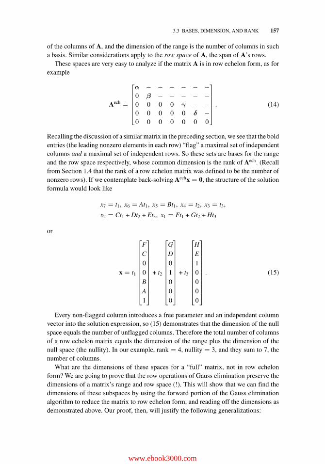
3.3 BASES, DIMENSION, AND RANK 157
of the columns of A, and the dimension of the range is the number of columns in sucha basis. Similar considerations apply to the row space of A, the span of A’s rows.
These spaces are very easy to analyze if the matrix A is in row echelon form, as forexample
Aech =
⎡⎢⎢⎢⎢⎣
α − − − − − −0 β − − − − −0 0 0 0 γ − −0 0 0 0 0 δ −0 0 0 0 0 0 0
⎤⎥⎥⎥⎥⎦ . (14)
Recalling the discussion of a similar matrix in the preceding section, we see that the boldentries (the leading nonzero elements in each row) “flag” a maximal set of independentcolumns and a maximal set of independent rows. So these sets are bases for the rangeand the row space respectively, whose common dimension is the rank of Aech. (Recallfrom Section 1.4 that the rank of a row echelon matrix was defined to be the number ofnonzero rows). If we contemplate back-solving Aechx = 0, the structure of the solutionformula would look like
x7 = t1, x6 = At1, x5 = Bt1, x4 = t2, x3 = t3,
x2 = Ct1 + Dt2 + Et3, x1 = Ft1 + Gt2 + Ht3
or
x = t1
⎡⎢⎢⎢⎢⎢⎢⎢⎢⎢⎢⎣
F
C
00B
A
1
⎤⎥⎥⎥⎥⎥⎥⎥⎥⎥⎥⎦
+ t2
⎡⎢⎢⎢⎢⎢⎢⎢⎢⎢⎢⎣
G
D
01000
⎤⎥⎥⎥⎥⎥⎥⎥⎥⎥⎥⎦
+ t3
⎡⎢⎢⎢⎢⎢⎢⎢⎢⎢⎢⎣
H
E
10000
⎤⎥⎥⎥⎥⎥⎥⎥⎥⎥⎥⎦
. (15)
Every non-flagged column introduces a free parameter and an independent columnvector into the solution expression, so (15) demonstrates that the dimension of the nullspace equals the number of unflagged columns. Therefore the total number of columnsof a row echelon matrix equals the dimension of the range plus the dimension of thenull space (the nullity). In our example, rank = 4, nullity = 3, and they sum to 7, thenumber of columns.
What are the dimensions of these spaces for a “full” matrix, not in row echelonform? We are going to prove that the row operations of Gauss elimination preserve thedimensions of a matrix’s range and row space (!). This will show that we can find thedimensions of these subspaces by using the forward portion of the Gauss eliminationalgorithm to reduce the matrix to row echelon form, and reading off the dimensions asdemonstrated above. Our proof, then, will justify the following generalizations:
www.ebook3000.com
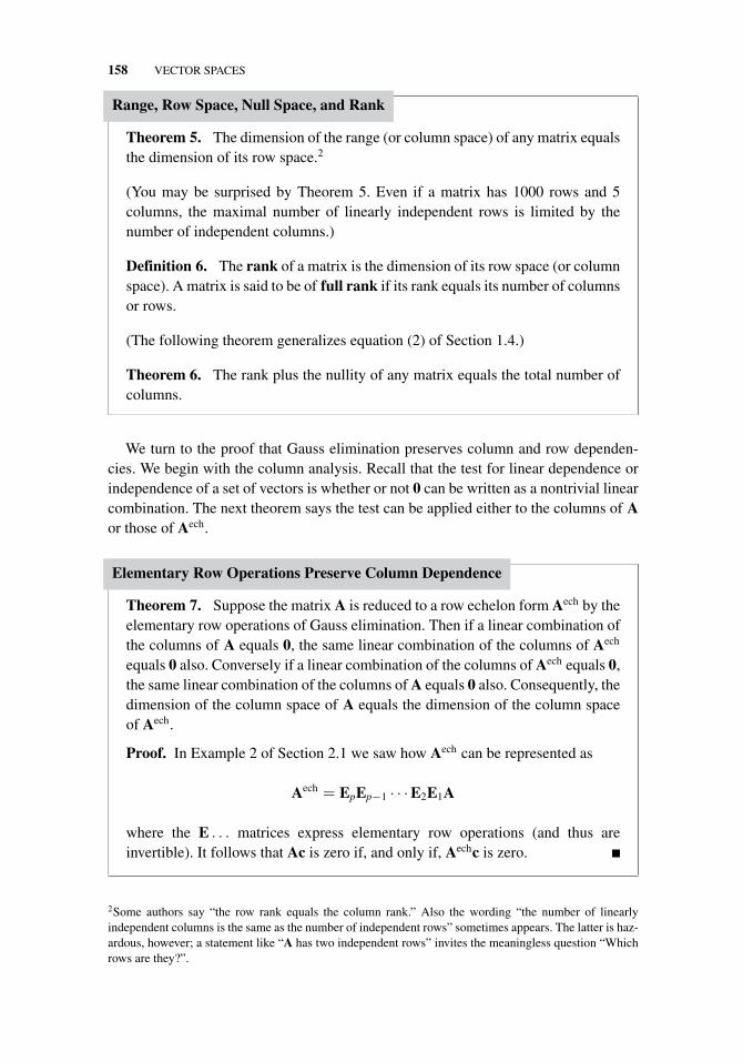
158 VECTOR SPACES
Range, Row Space, Null Space, and Rank
Theorem 5. The dimension of the range (or column space) of any matrix equalsthe dimension of its row space.2
(You may be surprised by Theorem 5. Even if a matrix has 1000 rows and 5columns, the maximal number of linearly independent rows is limited by thenumber of independent columns.)
Definition 6. The rank of a matrix is the dimension of its row space (or columnspace). A matrix is said to be of full rank if its rank equals its number of columnsor rows.
(The following theorem generalizes equation (2) of Section 1.4.)
Theorem 6. The rank plus the nullity of any matrix equals the total number ofcolumns.
We turn to the proof that Gauss elimination preserves column and row dependen-cies. We begin with the column analysis. Recall that the test for linear dependence orindependence of a set of vectors is whether or not 0 can be written as a nontrivial linearcombination. The next theorem says the test can be applied either to the columns of Aor those of Aech.
Elementary Row Operations Preserve Column Dependence
Theorem 7. Suppose the matrix A is reduced to a row echelon form Aech by theelementary row operations of Gauss elimination. Then if a linear combination ofthe columns of A equals 0, the same linear combination of the columns of Aech
equals 0 also. Conversely if a linear combination of the columns of Aech equals 0,the same linear combination of the columns of A equals 0 also. Consequently, thedimension of the column space of A equals the dimension of the column spaceof Aech.
Proof. In Example 2 of Section 2.1 we saw how Aech can be represented as
Aech = EpEp−1 · · ·E2E1A
where the E . . . matrices express elementary row operations (and thus areinvertible). It follows that Ac is zero if, and only if, Aechc is zero.
2Some authors say “the row rank equals the column rank.” Also the wording “the number of linearlyindependent columns is the same as the number of independent rows” sometimes appears. The latter is haz-ardous, however; a statement like “A has two independent rows” invites the meaningless question “Whichrows are they?”.
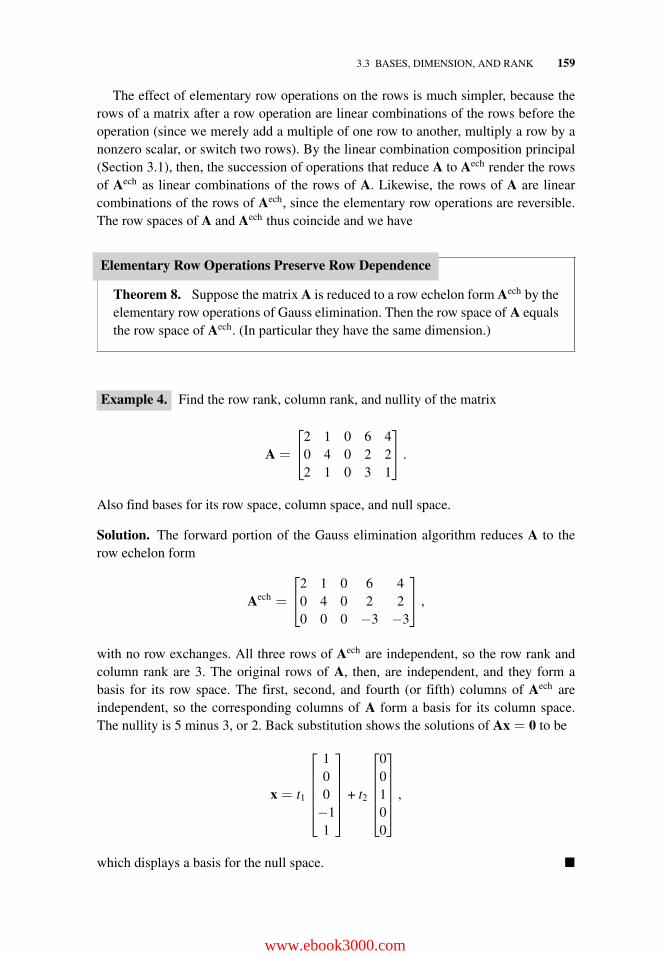
3.3 BASES, DIMENSION, AND RANK 159
The effect of elementary row operations on the rows is much simpler, because therows of a matrix after a row operation are linear combinations of the rows before theoperation (since we merely add a multiple of one row to another, multiply a row by anonzero scalar, or switch two rows). By the linear combination composition principal(Section 3.1), then, the succession of operations that reduce A to Aech render the rowsof Aech as linear combinations of the rows of A. Likewise, the rows of A are linearcombinations of the rows of Aech, since the elementary row operations are reversible.The row spaces of A and Aech thus coincide and we have
Elementary Row Operations Preserve Row Dependence
Theorem 8. Suppose the matrix A is reduced to a row echelon form Aech by theelementary row operations of Gauss elimination. Then the row space of A equalsthe row space of Aech. (In particular they have the same dimension.)
Example 4. Find the row rank, column rank, and nullity of the matrix
A =
⎡⎣2 1 0 6 4
0 4 0 2 22 1 0 3 1
⎤⎦ .
Also find bases for its row space, column space, and null space.
Solution. The forward portion of the Gauss elimination algorithm reduces A to therow echelon form
Aech =
⎡⎣2 1 0 6 4
0 4 0 2 20 0 0 −3 −3
⎤⎦ ,
with no row exchanges. All three rows of Aech are independent, so the row rank andcolumn rank are 3. The original rows of A, then, are independent, and they form abasis for its row space. The first, second, and fourth (or fifth) columns of Aech areindependent, so the corresponding columns of A form a basis for its column space.The nullity is 5 minus 3, or 2. Back substitution shows the solutions of Ax = 0 to be
x = t1
⎡⎢⎢⎢⎢⎣
100−11
⎤⎥⎥⎥⎥⎦ + t2
⎡⎢⎢⎢⎢⎣
00100
⎤⎥⎥⎥⎥⎦ ,
which displays a basis for the null space. �
www.ebook3000.com
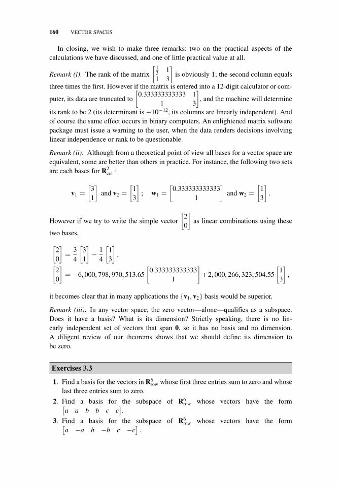
160 VECTOR SPACES
In closing, we wish to make three remarks: two on the practical aspects of thecalculations we have discussed, and one of little practical value at all.
Remark (i). The rank of the matrix
[ 13 11 3
]is obviously 1; the second column equals
three times the first. However if the matrix is entered into a 12-digit calculator or com-
puter, its data are truncated to
[0.333333333333 1
1 3
], and the machine will determine
its rank to be 2 (its determinant is −10−12, its columns are linearly independent). Andof course the same effect occurs in binary computers. An enlightened matrix softwarepackage must issue a warning to the user, when the data renders decisions involvinglinear independence or rank to be questionable.
Remark (ii). Although from a theoretical point of view all bases for a vector space areequivalent, some are better than others in practice. For instance, the following two setsare each bases for R2
col :
v1 =
[31
]and v2 =
[13
]; w1 =
[0.333333333333
1
]and w2 =
[13
].
However if we try to write the simple vector
[20
]as linear combinations using these
two bases,
[20
]=
34
[31
]− 1
4
[13
],
[20
]= −6, 000, 798, 970, 513.65
[0.333333333333
1
]+ 2, 000, 266, 323, 504.55
[13
],
it becomes clear that in many applications the {v1, v2} basis would be superior.
Remark (iii). In any vector space, the zero vector—alone—qualifies as a subspace.Does it have a basis? What is its dimension? Strictly speaking, there is no lin-early independent set of vectors that span 0, so it has no basis and no dimension.A diligent review of our theorems shows that we should define its dimension tobe zero.
Exercises 3.3
1. Find a basis for the vectors in R6row whose first three entries sum to zero and whose
last three entries sum to zero.
2. Find a basis for the subspace of R6row whose vectors have the form[
a a b b c c].
3. Find a basis for the subspace of R6row whose vectors have the form[
a −a b −b c −c]
.
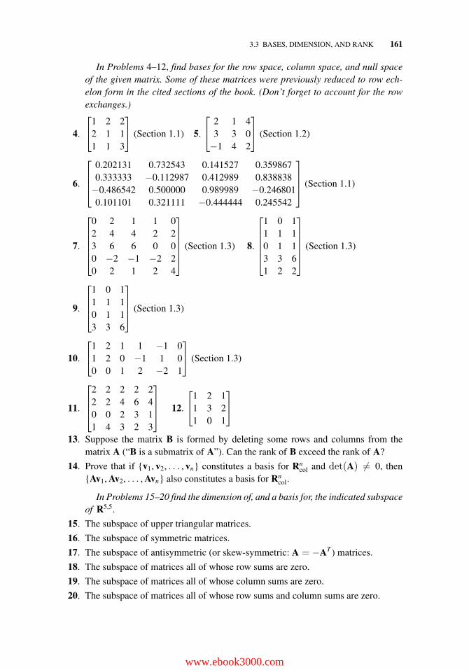
3.3 BASES, DIMENSION, AND RANK 161
In Problems 4–12, find bases for the row space, column space, and null spaceof the given matrix. Some of these matrices were previously reduced to row ech-elon form in the cited sections of the book. (Don’t forget to account for the rowexchanges.)
4.
⎡⎣1 2 2
2 1 11 1 3
⎤⎦ (Section 1.1) 5.
⎡⎣ 2 1 4
3 3 0−1 4 2
⎤⎦ (Section 1.2)
6.
⎡⎢⎢⎣
0.202131 0.732543 0.141527 0.3598670.333333 −0.112987 0.412989 0.838838−0.486542 0.500000 0.989989 −0.2468010.101101 0.321111 −0.444444 0.245542
⎤⎥⎥⎦ (Section 1.1)
7.
⎡⎢⎢⎢⎢⎣
0 2 1 1 02 4 4 2 23 6 6 0 00 −2 −1 −2 20 2 1 2 4
⎤⎥⎥⎥⎥⎦ (Section 1.3) 8.
⎡⎢⎢⎢⎢⎣
1 0 11 1 10 1 13 3 61 2 2
⎤⎥⎥⎥⎥⎦ (Section 1.3)
9.
⎡⎢⎢⎣
1 0 11 1 10 1 13 3 6
⎤⎥⎥⎦ (Section 1.3)
10.
⎡⎣1 2 1 1 −1 0
1 2 0 −1 1 00 0 1 2 −2 1
⎤⎦ (Section 1.3)
11.
⎡⎢⎢⎣
2 2 2 2 22 2 4 6 40 0 2 3 11 4 3 2 3
⎤⎥⎥⎦ 12.
⎡⎣1 2 1
1 3 21 0 1
⎤⎦
13. Suppose the matrix B is formed by deleting some rows and columns from thematrix A (“B is a submatrix of A”). Can the rank of B exceed the rank of A?
14. Prove that if {v1, v2, . . . , vn} constitutes a basis for Rncol and det(A) �= 0, then
{Av1, Av2, . . . , Avn} also constitutes a basis for Rncol.
In Problems 15–20 find the dimension of, and a basis for, the indicated subspaceof R5,5.
15. The subspace of upper triangular matrices.
16. The subspace of symmetric matrices.
17. The subspace of antisymmetric (or skew-symmetric: A = −AT ) matrices.
18. The subspace of matrices all of whose row sums are zero.
19. The subspace of matrices all of whose column sums are zero.
20. The subspace of matrices all of whose row sums and column sums are zero.
www.ebook3000.com
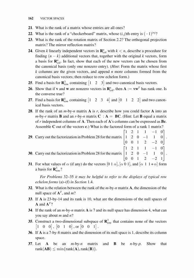
162 VECTOR SPACES
21. What is the rank of a matrix whose entries are all ones?
22. What is the rank of a “checkerboard” matrix, whose (i, j)th entry is (−1)i+j?
23. What is the rank of the rotation matrix of Section 2.2? The orthogonal projectionmatrix? The mirror reflection matrix?
24. Given k linearly independent vectors in Rncol with k < n, describe a procedure for
finding (n − k) additional vectors that, together with the original k vectors, forma basis for Rn
col. In fact, show that each of the new vectors can be chosen fromthe canonical basis (only one nonzero entry). (Hint: Form the matrix whose firstk columns are the given vectors, and append n more columns formed from thecanonical basis vectors; then reduce to row echelon form.)
25. Find a basis for R3row containing
[1 2 3
]and two canonical basis vectors.
26. Show that if v and w are nonzero vectors in Rncol, then A := vwT has rank one. Is
the converse true?
27. Find a basis for R4row containing
[1 2 3 4
]and
[0 1 2 2
]and two canon-
ical basis vectors.
28. If the rank of an m-by-n matrix A is r, describe how you could factor A into anm-by-r matrix B and an r-by-n matrix C : A = BC. (Hint: Let B equal a matrixof r independent columns of A. Then each of A’s columns can be expressed as Bc.Assemble C out of the vectors c.) What is the factored form of a rank 1 matrix?
29. Carry out the factorization in Problem 28 for the matrix
⎡⎣1 2 1 1 −1 0
1 2 0 −1 1 00 0 1 2 −2 0
⎤⎦ .
30. Carry out the factorization in Problem 28 for the matrix
⎡⎣1 2 1 1 −1 0
1 2 0 −1 1 00 0 1 2 −2 1
⎤⎦ .
31. For what values of α (if any) do the vectors [0 1 α], [α 0 1], and [α 1 1 +α] forma basis for R3
row?
For Problems 32–35 it may be helpful to refer to the displays of typical rowechelon forms (a)–(f) in Section 1.4.
32. What is the relation between the rank of the m-by-n matrix A, the dimension of thenull space of AT , and m?
33. If A is 23-by-14 and its rank is 10, what are the dimensions of the null spaces ofA and AT?
34. If the rank of an m-by-n matrix A is 7 and its null space has dimension 4, what canyou say about m and n?
35. Construct a two-dimensional subspace of R3row that contains none of the vectors[
1 0 0]
,[0 1 0
], or
[0 0 1
].
36. If A is a 7-by-8 matrix and the dimension of its null space is 1, describe its columnspace.
37. Let A be an m-by-n matrix and B be n-by-p. Show thatrank(AB) ≤ min{rank(A), rank(B)}.
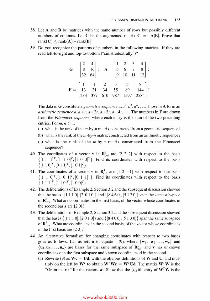
3.3 BASES, DIMENSION, AND RANK 163
38. Let A and B be matrices with the same number of rows but possibly differentnumbers of columns. Let C be the augmented matrix C = [A|B]. Prove thatrank(C) ≤ rank(A) + rank(B).
39. Do you recognize the patterns of numbers in the following matrices, if they areread left-to-right and top-to-bottom (“sinistrodextrally”)?
G =
⎡⎣ 2 4
8 1632 64
⎤⎦ ; A =
⎡⎣1 2 3 4
5 6 7 89 10 11 12
⎤⎦ ;
F =
⎡⎣ 1 1 2 3 5 8
13 21 34 55 89 144233 377 610 987 1597 2584
⎤⎦?
The data in G constitute a geometric sequence a, a2, a3, a4, . . .. Those in A form anarithmetic sequence a, a + r, a + 2r, a + 3r, a + 4r, . . .. The numbers in F are drawnfrom the Fibonacci sequence, where each entry is the sum of the two precedingentries. For m, n > 1,(a) what is the rank of the m-by-n matrix constructed from a geometric sequence?
(b) what is the rank of the m-by-n matrix constructed from an arithmetic sequence?
(c) what is the rank of the m-by-n matrix constructed from the Fibonaccisequence?
40. The coordinates of a vector v in R3col are [2 2 2] with respect to the basis
{[1 1 1]T , [1 1 0]T , [1 0 0]T}. Find its coordinates with respect to the basis{[1 1 0]T , [0 1 1]T , [1 0 1]T}.
41. The coordinates of a vector v in R3col are [1 2 −1] with respect to the basis
{[1 1 0]T , [1 0 1]T , [0 1 1]T}. Find its coordinates with respect to the basis{[1 1 1]T , [1 1 0]T , [1 0 0]T}.
42. The deliberations of Example 2, Section 3.2 and the subsequent discussion showedthat the bases {[1 1 1 0], [2 0 1 0]} and {[8 4 6 0], [5 1 3 0]} span the same subspaceof R4
row. What are coordinates, in the first basis, of the vector whose coordinates inthe second basis are [2 0]?
43. The deliberations of Example 2, Section 3.2 and the subsequent discussion showedthat the bases {[1 1 1 0], [2 0 1 0]} and {[8 4 6 0], [5 1 3 0]} span the same subspaceof R4
row. What are coordinates, in the second basis, of the vector whose coordinatesin the first basis are [2 2]?
44. An alternative formalism for changing coordinates with respect to two basesgoes as follows. Let us return to equation (9), where {w1, w2, . . . , wp} and{u1, u2, . . . , uq} are bases for the same subspace of Rn
col, and v has unknowncoordinates c in the first subspace and known coordinates d in the second.(a) Rewrite (9) as Wc = Ud, with the obvious definitions of W and U, and mul-
tiply on the left by WT to obtain WTWc = WTUd. The matrix WTW is the“Gram matrix” for the vectors wj. Show that the (i, j)th entry of WTW is the
www.ebook3000.com
164 VECTOR SPACES
dot product of wi and wj, and that the (i, j)th entry of WTU is the dot productof wi and uj.
(b) Show that the Gram matrix of a set of linearly independent vectors is alwaysnonsingular. (Hint: if WTWx = 0 then xTWTWx = (Wx) · (Wx) = 0;consider the implications when {w1, w2, . . . , wp} are independent.)
(c) Derive the rule for changing coordinates c = (WTW)−1WTUd.
3.4 SUMMARY
The structural similarities shared by solution sets of linear algebraic equations, gen-eral solutions of linear differential equations, and vectors in two and three dimensionsgive rise to the concept of an abstract vector space, characterized by the operations ofaddition of vectors to vectors and multiplication of vectors by scalars. Indeed, vectorspace theory can be summarized in a nutshell as the study of the varieties and propertiesof the linear combinations c1v1 + c2v2 + · · · + cnvn, where the ci’s are scalars and thevi’s are vectors. A subset of a vector space is a subspace if it contains all of its linearcombinations. The set of all linear combinations of a given set of vectors is a subspaceknown as the span of the set.
Linear Independence
A set of distinct vectors is said to be linearly independent if none of the vectors can beexpressed as a linear combination of the others; or, equivalently, if the only linear com-bination that equals zero is the trivial one (with all coefficients zero). Gauss eliminationcan be used to decide the independence of a set of column vectors. If a matrix is in rowechelon form, all of its nonzero rows are independent, as are all of its columns thatcontain pivot elements. The rows and the columns of a square matrix are independentif and only if its determinant is nonzero.
Bases, Dimension, and Rank
A basis for a (sub)space is a linearly independent set that spans the (sub)space. All basesfor a particular (sub)space contain the same number of elements, and this number is thedimension of the (sub)space. The dimension of the span of the columns of any matrixequals the dimension of the span of its rows. The rank of the matrix, which is thiscommon dimension, is preserved by the elementary row operations. The nullity of amatrix A is the dimension of the subspace of vectors x such that Ax = 0. The numberof columns of A equals the sum of its rank and its nullity.
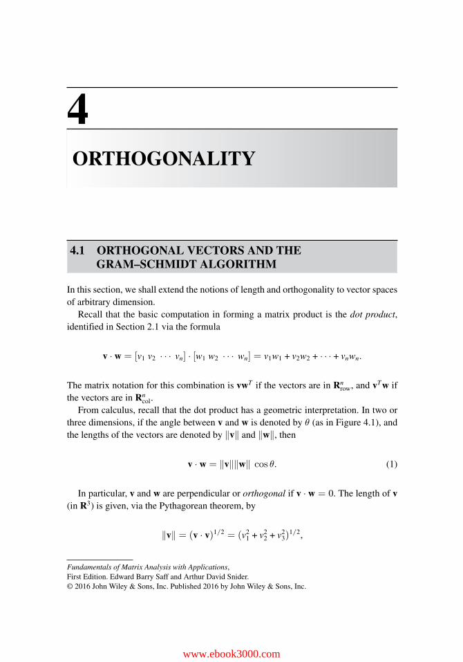
4ORTHOGONALITY
4.1 ORTHOGONAL VECTORS AND THEGRAM–SCHMIDT ALGORITHM
In this section, we shall extend the notions of length and orthogonality to vector spacesof arbitrary dimension.
Recall that the basic computation in forming a matrix product is the dot product,identified in Section 2.1 via the formula
v · w = [v1 v2 · · · vn] · [w1 w2 · · · wn] = v1w1 + v2w2 + · · · + vnwn.
The matrix notation for this combination is vwT if the vectors are in Rnrow, and vTw if
the vectors are in Rncol.
From calculus, recall that the dot product has a geometric interpretation. In two orthree dimensions, if the angle between v and w is denoted by θ (as in Figure 4.1), andthe lengths of the vectors are denoted by ‖v‖ and ‖w‖, then
v · w = ‖v‖‖w‖ cos θ. (1)
In particular, v and w are perpendicular or orthogonal if v · w = 0. The length of v(in R3) is given, via the Pythagorean theorem, by
‖v‖ = (v · v)1/2 = (v21 + v2
2 + v23)
1/2,
Fundamentals of Matrix Analysis with Applications,First Edition. Edward Barry Saff and Arthur David Snider.© 2016 John Wiley & Sons, Inc. Published 2016 by John Wiley & Sons, Inc.
www.ebook3000.com
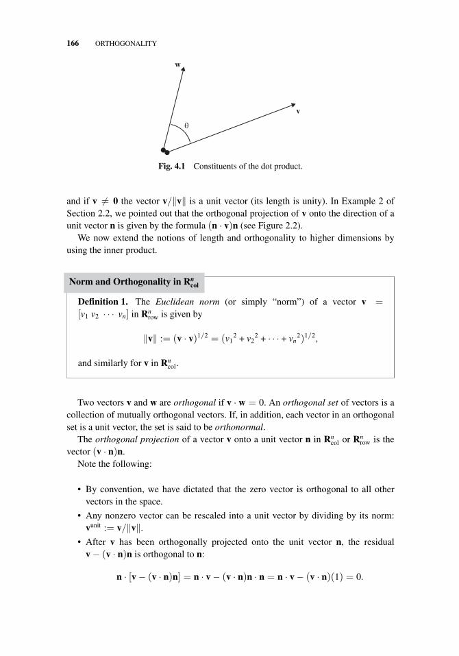
166 ORTHOGONALITY
w
v
θ
Fig. 4.1 Constituents of the dot product.
and if v �= 0 the vector v/‖v‖ is a unit vector (its length is unity). In Example 2 ofSection 2.2, we pointed out that the orthogonal projection of v onto the direction of aunit vector n is given by the formula (n · v)n (see Figure 2.2).
We now extend the notions of length and orthogonality to higher dimensions byusing the inner product.
Norm and Orthogonality in Rncol
Definition 1. The Euclidean norm (or simply “norm”) of a vector v =[v1 v2 · · · vn] in Rn
row is given by
‖v‖ := (v · v)1/2 = (v12 + v2
2 + · · · + vn2)1/2,
and similarly for v in Rncol.
Two vectors v and w are orthogonal if v · w = 0. An orthogonal set of vectors is acollection of mutually orthogonal vectors. If, in addition, each vector in an orthogonalset is a unit vector, the set is said to be orthonormal.
The orthogonal projection of a vector v onto a unit vector n in Rncol or Rn
row is thevector (v · n)n.
Note the following:
• By convention, we have dictated that the zero vector is orthogonal to all othervectors in the space.
• Any nonzero vector can be rescaled into a unit vector by dividing by its norm:vunit := v/‖v‖.
• After v has been orthogonally projected onto the unit vector n, the residualv − (v · n)n is orthogonal to n:
n · [v − (v · n)n] = n · v − (v · n)n · n = n · v − (v · n)(1) = 0.
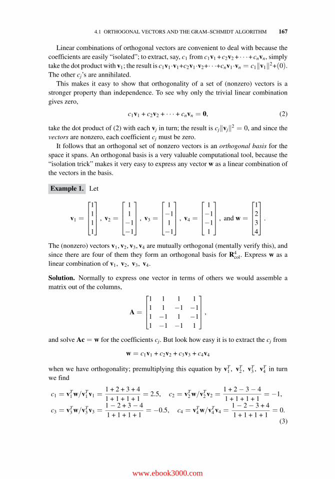
4.1 ORTHOGONAL VECTORS AND THE GRAM–SCHMIDT ALGORITHM 167
Linear combinations of orthogonal vectors are convenient to deal with because thecoefficients are easily “isolated”; to extract, say, c1 from c1v1 +c2v2 + · · ·+cnvn, simplytake the dot product with v1; the result is c1v1·v1+c2v1·v2+· · ·+cnv1·vn = c1‖v1‖2+(0).The other cj’s are annihilated.
This makes it easy to show that orthogonality of a set of (nonzero) vectors is astronger property than independence. To see why only the trivial linear combinationgives zero,
c1v1 + c2v2 + · · · + cnvn = 0, (2)
take the dot product of (2) with each vj in turn; the result is cj‖vj‖2 = 0, and since thevectors are nonzero, each coefficient cj must be zero.
It follows that an orthogonal set of nonzero vectors is an orthogonal basis for thespace it spans. An orthogonal basis is a very valuable computational tool, because the“isolation trick” makes it very easy to express any vector w as a linear combination ofthe vectors in the basis.
Example 1. Let
v1 =
⎡⎢⎢⎣
1111
⎤⎥⎥⎦ , v2 =
⎡⎢⎢⎣
11−1−1
⎤⎥⎥⎦ , v3 =
⎡⎢⎢⎣
1−11−1
⎤⎥⎥⎦ , v4 =
⎡⎢⎢⎣
1−1−11
⎤⎥⎥⎦ , and w =
⎡⎢⎢⎣
1234
⎤⎥⎥⎦ .
The (nonzero) vectors v1, v2, v3, v4 are mutually orthogonal (mentally verify this), andsince there are four of them they form an orthogonal basis for R4
col. Express w as alinear combination of v1, v2, v3, v4.
Solution. Normally to express one vector in terms of others we would assemble amatrix out of the columns,
A =
⎡⎢⎢⎣
1 1 1 11 1 −1 −11 −1 1 −11 −1 −1 1
⎤⎥⎥⎦ ,
and solve Ac = w for the coefficients cj. But look how easy it is to extract the cj from
w = c1v1 + c2v2 + c3v3 + c4v4
when we have orthogonality; premultiplying this equation by vT1 , vT
2 , vT3 , vT
4 in turnwe find
c1 = vT1 w/vT
1 v1 =1 + 2 + 3 + 41 + 1 + 1 + 1
= 2.5, c2 = vT2 w/vT
2 v2 =1 + 2 − 3 − 41 + 1 + 1 + 1
= −1,
c3 = vT3 w/vT
3 v3 =1 − 2 + 3 − 41 + 1 + 1 + 1
= −0.5, c4 = vT4 w/vT
4 v4 =1 − 2 − 3 + 41 + 1 + 1 + 1
= 0.
(3)
www.ebook3000.com
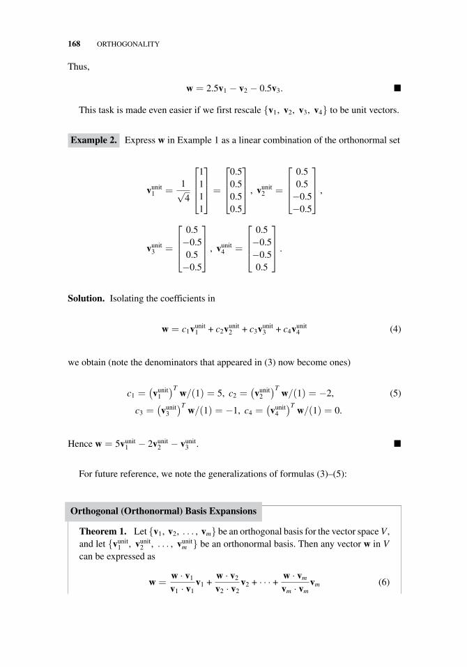
168 ORTHOGONALITY
Thus,
w = 2.5v1 − v2 − 0.5v3. �
This task is made even easier if we first rescale {v1, v2, v3, v4} to be unit vectors.
Example 2. Express w in Example 1 as a linear combination of the orthonormal set
vunit1 =
1√4
⎡⎢⎢⎣
1111
⎤⎥⎥⎦ =
⎡⎢⎢⎣
0.50.50.50.5
⎤⎥⎥⎦ , vunit
2 =
⎡⎢⎢⎣
0.50.5−0.5−0.5
⎤⎥⎥⎦ ,
vunit3 =
⎡⎢⎢⎣
0.5−0.50.5−0.5
⎤⎥⎥⎦ , vunit
4 =
⎡⎢⎢⎣
0.5−0.5−0.50.5
⎤⎥⎥⎦ .
Solution. Isolating the coefficients in
w = c1vunit1 + c2vunit
2 + c3vunit3 + c4vunit
4 (4)
we obtain (note the denominators that appeared in (3) now become ones)
c1 =(vunit
1
)Tw/(1) = 5, c2 =
(vunit
2
)Tw/(1) = −2, (5)
c3 =(vunit
3
)Tw/(1) = −1, c4 =
(vunit
4
)Tw/(1) = 0.
Hence w = 5vunit1 − 2vunit
2 − vunit3 . �
For future reference, we note the generalizations of formulas (3)–(5):
Orthogonal (Orthonormal) Basis Expansions
Theorem 1. Let {v1, v2, . . . , vm} be an orthogonal basis for the vector space V ,and let {vunit
1 , vunit2 , . . . , vunit
m } be an orthonormal basis. Then any vector w in Vcan be expressed as
w =w · v1
v1 · v1v1 +
w · v2
v2 · v2v2 + · · · +
w · vm
vm · vmvm (6)
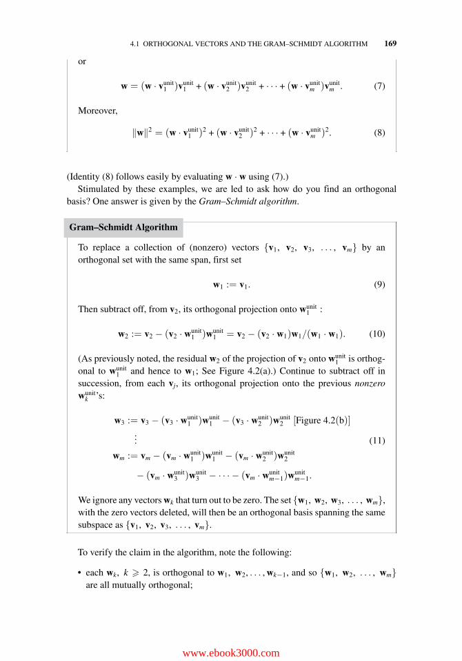
4.1 ORTHOGONAL VECTORS AND THE GRAM–SCHMIDT ALGORITHM 169
or
w = (w · vunit1 )vunit
1 + (w · vunit2 )vunit
2 + · · · + (w · vunitm )vunit
m . (7)
Moreover,
‖w‖2 = (w · vunit1 )2 + (w · vunit
2 )2 + · · · + (w · vunitm )2. (8)
(Identity (8) follows easily by evaluating w · w using (7).)Stimulated by these examples, we are led to ask how do you find an orthogonal
basis? One answer is given by the Gram–Schmidt algorithm.
Gram–Schmidt Algorithm
To replace a collection of (nonzero) vectors {v1, v2, v3, . . . , vm} by anorthogonal set with the same span, first set
w1 := v1. (9)
Then subtract off, from v2, its orthogonal projection onto wunit1 :
w2 := v2 − (v2 · wunit1 )wunit
1 = v2 − (v2 · w1)w1/(w1 · w1). (10)
(As previously noted, the residual w2 of the projection of v2 onto wunit1 is orthog-
onal to wunit1 and hence to w1; See Figure 4.2(a).) Continue to subtract off in
succession, from each vj, its orthogonal projection onto the previous nonzerowunit
k ’s:
w3 := v3 − (v3 · wunit1 )wunit
1 − (v3 · wunit2 )wunit
2 [Figure 4.2(b)]... (11)
wm := vm − (vm · wunit1 )wunit
1 − (vm · wunit2 )wunit
2
− (vm · wunit3 )wunit
3 − · · · − (vm · wunitm−1)w
unitm−1.
We ignore any vectors wk that turn out to be zero. The set {w1, w2, w3, . . . , wm},with the zero vectors deleted, will then be an orthogonal basis spanning the samesubspace as {v1, v2, v3, . . . , vm}.
To verify the claim in the algorithm, note the following:
• each wk, k � 2, is orthogonal to w1, w2, . . . , wk−1, and so {w1, w2, . . . , wm}are all mutually orthogonal;
www.ebook3000.com
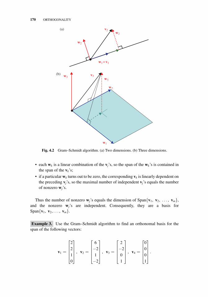
170 ORTHOGONALITY
w2
w1 =v1
w2
v2(a)
w3 w3
w2
w1
v3(b)
Fig. 4.2 Gram–Schmidt algorithm. (a) Two dimensions. (b) Three dimensions.
• each wk is a linear combination of the vj’s, so the span of the wk’s is contained inthe span of the vk’s;
• if a particular wk turns out to be zero, the corresponding vk is linearly dependent onthe preceding vj’s, so the maximal number of independent vj’s equals the numberof nonzero wj’s.
Thus the number of nonzero wj’s equals the dimension of Span{v1, v2, . . . , vm},and the nonzero wj’s are independent. Consequently, they are a basis forSpan{v1, v2, . . . , vm}.
Example 3. Use the Gram–Schmidt algorithm to find an orthonomal basis for thespan of the following vectors:
v1 =
⎡⎢⎢⎢⎣
2
2
1
0
⎤⎥⎥⎥⎦ , v2 =
⎡⎢⎢⎢⎣
6
−2
1
−2
⎤⎥⎥⎥⎦ , v3 =
⎡⎢⎢⎢⎣
2
−2
0
1
⎤⎥⎥⎥⎦ , v4 =
⎡⎢⎢⎢⎣
0
0
0
1
⎤⎥⎥⎥⎦ .
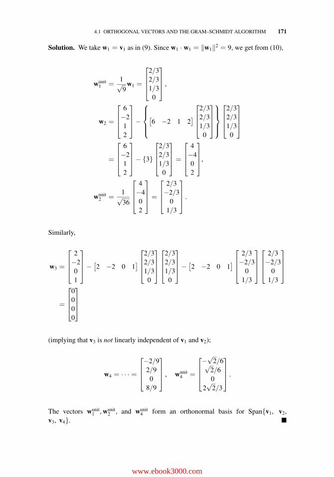
4.1 ORTHOGONAL VECTORS AND THE GRAM–SCHMIDT ALGORITHM 171
Solution. We take w1 = v1 as in (9). Since w1 · w1 = ‖w1‖2 = 9, we get from (10),
wunit1 =
1√9
w1 =
⎡⎢⎢⎣
2/32/31/3
0
⎤⎥⎥⎦ ,
w2 =
⎡⎢⎢⎣
6−212
⎤⎥⎥⎦−
⎧⎪⎪⎨⎪⎪⎩[6 −2 1 2
]⎡⎢⎢⎣
2/32/31/3
0
⎤⎥⎥⎦
⎫⎪⎪⎬⎪⎪⎭
⎡⎢⎢⎣
2/32/31/3
0
⎤⎥⎥⎦
=
⎡⎢⎢⎣
6−212
⎤⎥⎥⎦− {3}
⎡⎢⎢⎣
2/32/31/3
0
⎤⎥⎥⎦ =
⎡⎢⎢⎣
4−402
⎤⎥⎥⎦,
wunit2 =
1√36
⎡⎢⎢⎣
4−402
⎤⎥⎥⎦ =
⎡⎢⎢⎣
2/3−2/3
01/3
⎤⎥⎥⎦ .
Similarly,
w3 =
⎡⎢⎢⎣
2−201
⎤⎥⎥⎦−
[2 −2 0 1
]⎡⎢⎢⎣
2/32/31/3
0
⎤⎥⎥⎦
⎡⎢⎢⎣
2/32/31/3
0
⎤⎥⎥⎦−
[2 −2 0 1
]⎡⎢⎢⎣
2/3−2/3
01/3
⎤⎥⎥⎦
⎡⎢⎢⎣
2/3−2/3
01/3
⎤⎥⎥⎦
=
⎡⎢⎢⎣
0000
⎤⎥⎥⎦
(implying that v3 is not linearly independent of v1 and v2);
w4 = · · · =
⎡⎢⎢⎣−2/92/9
08/9
⎤⎥⎥⎦ , wunit
4 =
⎡⎢⎢⎣−√
2/6√2/60
2√
2/3
⎤⎥⎥⎦ .
The vectors wunit1 , wunit
2 , and wunit4 form an orthonormal basis for Span{v1, v2,
v3, v4}. �
www.ebook3000.com
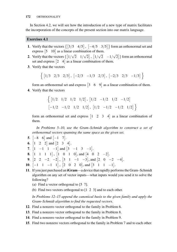
172 ORTHOGONALITY
In Section 4.2, we will see how the introduction of a new type of matrix facilitatesthe incorporation of the concepts of the present section into our matrix language.
Exercises 4.1
1. Verify that the vectors{[
3/5 4/5]
,[−4/5 3/5
]}form an orthonormal set and
express[5 10
]as a linear combination of them.
2. Verify that the vectors {[1/√
2 1/√
2]
,[1/√
2 −1/√
2]} form an orthonormal
set and express[2 4
]as a linear combination of them.
3. Verify that the vectors{ [
1/3 2/3 2/3]
,[−2/3 −1/3 2/3
],[−2/3 2/3 −1/3
] }
form an orthonormal set and express[3 6 9
]as a linear combination of them.
4. Verify that the vectors{ [
1/2 1/2 1/2 1/2]
,[1/2 −1/2 1/2 −1/2
][−1/2 −1/2 1/2 1/2
],[1/2 −1/2 −1/2 1/2
] }
form an orthonormal set and express[1 2 3 4
]as a linear combination of
them.
In Problems 5–10, use the Gram–Schmidt algorithm to construct a set oforthonormal vectors spanning the same space as the given set.
5.[−8 6
]and
[−1 7
].
6.[1 2 2
]and
[2 3 4
].
7.[1 −1 1 −1
]and
[3 −1 3 −1
].
8.[1 1 1 1
],[1 0 1 0
], and
[4 0 2 −2
].
9.[2 2 −2 −2
],[3 1 −1 −3
], and
[2 0 −2 −4
].
10.[−1 1 −1 1
],[2 0 2 0
], and
[3 1 1 −1
].
11. If you just purchased an iGram—a device that rapidly performs the Gram–Schmidtalgorithm on any set of vector inputs—what inputs would you send it to solve thefollowing?(a) Find a vector orthogonal to [5 7].
(b) Find two vectors orthogonal to [1 2 3] and to each other.
In Problems 12–15 append the canonical basis to the given family and apply theGram–Schmidt algorithm to find the requested vectors.
12. Find a nonzero vector orthogonal to the family in Problem 6.
13. Find a nonzero vector orthogonal to the family in Problem 8.
14. Find a nonzero vector orthogonal to the family in Problem 9.
15. Find two nonzero vectors orthogonal to the family in Problem 7 and to each other.
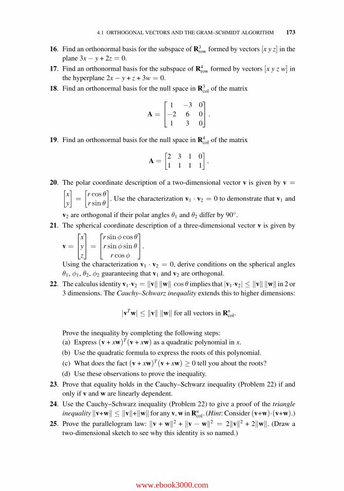
4.1 ORTHOGONAL VECTORS AND THE GRAM–SCHMIDT ALGORITHM 173
16. Find an orthonormal basis for the subspace of R3row formed by vectors [x y z] in the
plane 3x − y + 2z = 0.
17. Find an orthonormal basis for the subspace of R4row formed by vectors [x y z w] in
the hyperplane 2x − y + z + 3w = 0.
18. Find an orthonormal basis for the null space in R3col of the matrix
A =
⎡⎣ 1 −3 0−2 6 01 3 0
⎤⎦ .
19. Find an orthonormal basis for the null space in R4col of the matrix
A =
[2 3 1 01 1 1 1
].
20. The polar coordinate description of a two-dimensional vector v is given by v =[xy
]=
[r cos θr sin θ
]. Use the characterization v1 · v2 = 0 to demonstrate that v1 and
v2 are orthogonal if their polar angles θ1 and θ2 differ by 90◦.
21. The spherical coordinate description of a three-dimensional vector v is given by
v =
⎡⎣x
yz
⎤⎦ =
⎡⎣r sinφ cos θ
r sinφ sin θr cosφ
⎤⎦.
Using the characterization v1 · v2 = 0, derive conditions on the spherical anglesθ1, φ1, θ2, φ2 guaranteeing that v1 and v2 are orthogonal.
22. The calculus identity v1·v2 = ‖v‖ ‖w‖ cos θ implies that |v1·v2| ≤ ‖v‖ ‖w‖ in 2 or3 dimensions. The Cauchy–Schwarz inequality extends this to higher dimensions:
|vTw| ≤ ‖v‖ ‖w‖ for all vectors in Rncol.
Prove the inequality by completing the following steps:(a) Express (v + xw)T(v + xw) as a quadratic polynomial in x.
(b) Use the quadratic formula to express the roots of this polynomial.
(c) What does the fact (v + xw)T(v + xw) ≥ 0 tell you about the roots?
(d) Use these observations to prove the inequality.
23. Prove that equality holds in the Cauchy–Schwarz inequality (Problem 22) if andonly if v and w are linearly dependent.
24. Use the Cauchy–Schwarz inequality (Problem 22) to give a proof of the triangleinequality ‖v+w‖ ≤ ‖v‖+‖w‖ for any v, w in Rn
col. (Hint: Consider (v+w)·(v+w).)
25. Prove the parallelogram law: ‖v + w‖2 + ‖v − w‖2 = 2‖v‖2 + 2‖w‖. (Draw atwo-dimensional sketch to see why this identity is so named.)
www.ebook3000.com
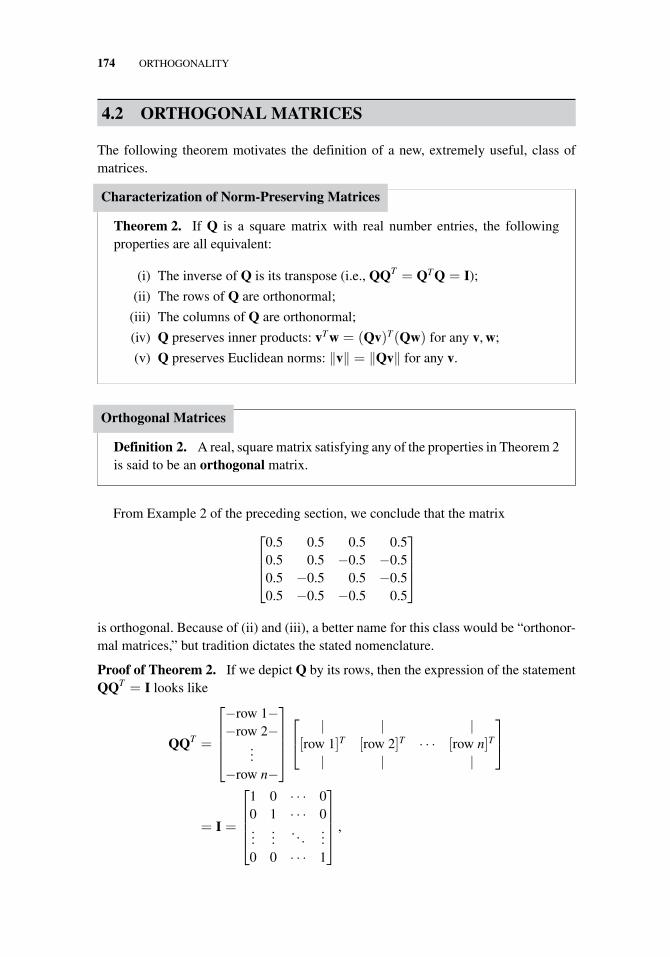
174 ORTHOGONALITY
4.2 ORTHOGONAL MATRICES
The following theorem motivates the definition of a new, extremely useful, class ofmatrices.
Characterization of Norm-Preserving Matrices
Theorem 2. If Q is a square matrix with real number entries, the followingproperties are all equivalent:
(i) The inverse of Q is its transpose (i.e., QQT = QTQ = I);
(ii) The rows of Q are orthonormal;
(iii) The columns of Q are orthonormal;
(iv) Q preserves inner products: vTw = (Qv)T(Qw) for any v, w;
(v) Q preserves Euclidean norms: ‖v‖ = ‖Qv‖ for any v.
Orthogonal Matrices
Definition 2. A real, square matrix satisfying any of the properties in Theorem 2is said to be an orthogonal matrix.
From Example 2 of the preceding section, we conclude that the matrix⎡⎢⎢⎣
0.5 0.5 0.5 0.50.5 0.5 −0.5 −0.50.5 −0.5 0.5 −0.50.5 −0.5 −0.5 0.5
⎤⎥⎥⎦
is orthogonal. Because of (ii) and (iii), a better name for this class would be “orthonor-mal matrices,” but tradition dictates the stated nomenclature.
Proof of Theorem 2. If we depict Q by its rows, then the expression of the statementQQT = I looks like
QQT =
⎡⎢⎢⎢⎣−row 1−−row 2−
...−row n−
⎤⎥⎥⎥⎦⎡⎣ | | |[row 1]T [row 2]T · · · [row n]T
| | |
⎤⎦
= I =
⎡⎢⎢⎢⎣
1 0 · · · 00 1 · · · 0...
.... . .
...0 0 · · · 1
⎤⎥⎥⎥⎦ ,
4.2 ORTHOGONAL MATRICES 175
Thus the condition QQT = I says no more, and no less, than that the rows of Q areorthonormal. Similarly, QTQ = I states that the columns of Q are orthonormal; thus(i), (ii). and (iii) are all equivalent.
Statements (iv) and (v) are equivalent, because the norm and the inner product canbe expressed in terms of each other:
‖v‖ = (v · v)1/2 and 2v · w = ‖v + w‖2 − ‖v‖2 − ‖w‖2
(the latter is easily verified by writing the norms as inner products). So our proof willbe complete if we can show, for instance, that (i) implies (iv) and (iv) implies (iii).
The right-hand member in (iv) equals vTQTQw, so (iv) holds whenever QTQ = I;that is, (i) implies (iv). And if ei denotes the ith column of the identity matrix, then Qei
is the ith column of Q; so applying (iv) when v = ei and w = ej, we conclude that thecolumns of Q have the same orthonormality properties as the columns of I when (iv)holds. Thus (iv) implies (iii).
Note that Theorem 2 implies that inverses, transposes, and products of orthogonalmatrices are, again, orthogonal.
Property (v) is the key to many of the applications of orthogonal matrices. For exam-ple, since rotations and mirror reflections preserve lengths, we can immediately statethat the corresponding matrix operators are orthogonal. In fact, it can be shown thatin two or three dimensions the most general orthogonal matrix can be considered as asequence of rotations and reflections (See Group Project A at the end of Part II).
Example 1. Verify that the transpose of the reflection operator in Example 3 ofSection 2.2 is equal to its inverse.
Solution. If n denotes the column matrix representing the unit normal to the mirror,formula (3) in Section 2.2 for the reflector operator states
Mref = I − 2nnT . (1)
Then we can verify
MTrefMref = {I − 2nnT}T{I − 2nnT} = {IT − 2nTTnT}{I − 2nnT} (2)
= {I − 2nnT}{I − 2nnT} = I − 2nnT − 2nnT + 4nnTnnT
= I − 2nnT − 2nnT + 4n(1)nT = I − 4nnT + 4nnT = I. �
Note that although the formula (1) was derived for reflections in two dimensions,the calculation is independent of the number of dimensions. Accordingly, we say that
www.ebook3000.com
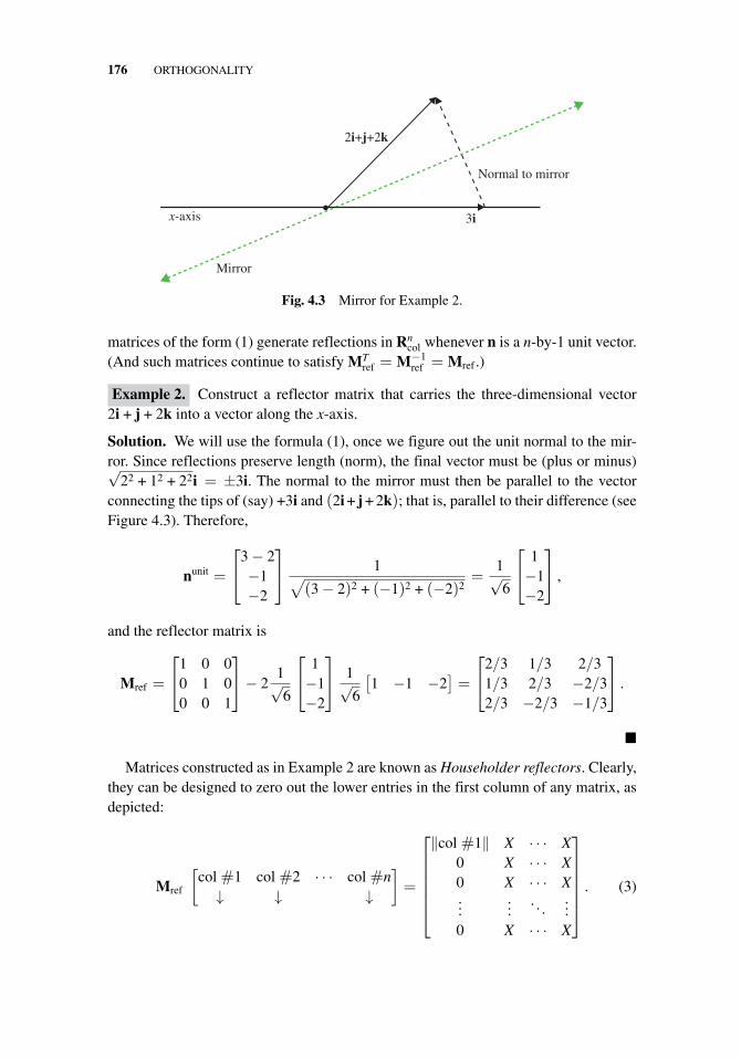
176 ORTHOGONALITY
Normal to mirror
3i
Mirror
x-axis
2i+j+2k
Fig. 4.3 Mirror for Example 2.
matrices of the form (1) generate reflections in Rncol whenever n is a n-by-1 unit vector.
(And such matrices continue to satisfy MTref = M−1
ref = Mref .)
Example 2. Construct a reflector matrix that carries the three-dimensional vector2i + j + 2k into a vector along the x-axis.
Solution. We will use the formula (1), once we figure out the unit normal to the mir-ror. Since reflections preserve length (norm), the final vector must be (plus or minus)√
22 + 12 + 22i = ±3i. The normal to the mirror must then be parallel to the vectorconnecting the tips of (say) +3i and (2i + j + 2k); that is, parallel to their difference (seeFigure 4.3). Therefore,
nunit =
⎡⎣3 − 2
−1−2
⎤⎦ 1√
(3 − 2)2 + (−1)2 + (−2)2=
1√6
⎡⎣ 1−1−2
⎤⎦ ,
and the reflector matrix is
Mref =
⎡⎣1 0 0
0 1 00 0 1
⎤⎦− 2
1√6
⎡⎣ 1−1−2
⎤⎦ 1√
6
[1 −1 −2
]=
⎡⎣2/3 1/3 2/3
1/3 2/3 −2/32/3 −2/3 −1/3
⎤⎦ .
�
Matrices constructed as in Example 2 are known as Householder reflectors. Clearly,they can be designed to zero out the lower entries in the first column of any matrix, asdepicted:
Mref
[col #1 col #2 · · · col #n
↓ ↓ ↓
]=
⎡⎢⎢⎢⎢⎢⎣
‖col #1‖ X · · · X0 X · · · X0 X · · · X...
.... . .
...0 X · · · X
⎤⎥⎥⎥⎥⎥⎦
. (3)
4.2 ORTHOGONAL MATRICES 177
A little thought (Group Project B at the end of Part II) will reveal that a sequence ofwell-chosen reflectors can render the original matrix into row echelon form, producinga competitor to the Gauss elimination algorithm! (And pivoting is unnecessary.) In fact,Householder reflector schemes can also replace the Gram–Schmidt algorithm.
The use of orthogonal matrices in matrix computations has very important advan-tages with regard to computational accuracy, because property (v) in Theorem 2 impliesthat multiplication by orthogonal matrices does not increase errors. For example, if wewere to solve a system Ax = b using exact arithmetic (so that x = A−1b), but we laterlearned that the vector b contained a measurement error δb, then our answer wouldbe in error by δx = A−1(b + δb) − A−1x = A−1δb. If A−1 is orthogonal, we have‖δx‖ = ‖A−1δb‖ = ‖δb‖, showing that the error norm in the solution is no biggerthan the error norm in the data.
Most enlightened matrix software packages contain options for some computationsthat use only orthogonal matrix multiplications. They usually require more arith-metic operations, but the increased “numerical stability” may warrant the effort fora particular application.1
Example 3. Calculate the matrix expressing the result of rotating a three-dimensionalvector through an angle θ around the z-axis, followed by a rotation through φ aroundthe x-axis.
Solution. In Example 1 of Section 2.2, we pointed out that the (x, y) coordinates of avector v1 are changed when it is rotated to the position v2 as in Figure 4.4a, according to
x2 = x1 cos θ − y1 sin θ (4)
y2 = x1 sin θ + y1 cos θ.
Since the z-coordinate is unchanged, as a three-dimensional rotation (4) has the matrixformulation
⎡⎣x2
y2
z2
⎤⎦ =
⎡⎣cos θ − sin θ 0sin θ cos θ 0
0 0 1
⎤⎦⎡⎣x1
y1
z1
⎤⎦ . (5)
To modify these equations for rotations around the x-axis, we redraw the diagram withthe x-axis coming out of the page, as in Figure 4.4b. We conclude x3 = x2 and simplycopy (4) with the variables appropriately renamed:
y3 = y2 cosφ− z2 sinφ, z3 = y2 sinφ + z2 cosφ;
1In 1977, one of the authors was directed to program a reflector matrix algorithm to replace Gausselimination for onboard guidance control calculations in the space shuttle, to ensure reliability.
www.ebook3000.com
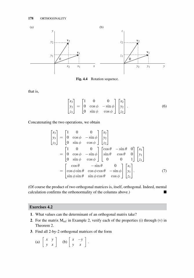
178 ORTHOGONALITY
y
v1
v2y2
y1
x1x2 x
θ ϕ
(a) (b)z
v1
v2z2
z1
y1y2 y
Fig. 4.4 Rotation sequence.
that is,
⎡⎣x3
y3
z3
⎤⎦ =
⎡⎣1 0 0
0 cosφ − sinφ0 sinφ cosφ
⎤⎦⎡⎣x2
y2
z2
⎤⎦ . (6)
Concatenating the two operations, we obtain
⎡⎣x3
y3
z3
⎤⎦ =
⎡⎣1 0 0
0 cosφ − sinφ0 sinφ cosφ
⎤⎦⎡⎣x2
y2
z2
⎤⎦
=
⎡⎣1 0 0
0 cosφ − sinφ0 sinφ cosφ
⎤⎦⎡⎣cos θ − sin θ 0sin θ cos θ 0
0 0 1
⎤⎦⎡⎣x1
y1
z1
⎤⎦
=
⎡⎣ cos θ − sin θ 0cosφ sin θ cosφ cos θ − sinφsinφ sin θ sinφ cos θ cosφ
⎤⎦⎡⎣x1
y1
z1
⎤⎦. (7)
(Of course the product of two orthogonal matrices is, itself, orthogonal. Indeed, mentalcalculation confirms the orthonormality of the columns above.) �
Exercises 4.2
1. What values can the determinant of an orthogonal matrix take?
2. For the matrix Mref in Example 2, verify each of the properties (i) through (v) inTheorem 2.
3. Find all 2-by-2 orthogonal matrices of the form
(a)
[x yy x
](b)
[x −yy x
].
4.2 ORTHOGONAL MATRICES 179
4. Show that if Q is orthogonal and symmetric, then Q2 = I.
5. Find the 3-by-3 rotation matrix that rotates every vector through ψ radians aboutthe y-axis.
6. Determine all 2-by-2 orthogonal matrices all of whose entries are either zero or one.
7. Determine all 3-by-3 orthogonal matrices all of whose entries are either zero or one.
8. Prove that the jth column of any square invertible matrix A is orthogonal to everyrow of A−1, except the jth.
9. Construct a reflector matrix that carries the 3-dimensional vector 5i + 12j + 13kinto a vector along the x-axis.
10. Construct a reflector matrix that carries the 3-dimensional vector 5i + 12j + 13kinto a vector along the y-axis.
11. Construct a reflector matrix that carries the 4-dimensional vector[1 1 1 1
]into a vector having all entries zero except the first.
12. Find a 3-by-3 Householder reflector matrix Mref that, through left multiplication,zeros out all entries below the first entry, in the first column of
A =
⎡⎢⎣
1 0 2
2 1 0
3 0 −1
⎤⎥⎦ .
13. Find a Householder reflector matrix Mref that, through left multiplication, zerosout all entries below the first entry, in the second column of
A =
⎡⎢⎣
4 2 0
0 1 1
0 3 0
⎤⎥⎦ . (8)
Is the zero pattern in the first column preserved?
14. Find a Householder reflector matrix Mref that, through left multiplication, zeros outall entries above and below the second entry, in the second column of the matrix in(8). (In other words, all nondiagonal entries in the second column will become 0.) Isthe zero pattern in the first column preserved? (Hint: Bearing in mind the reflectorpreserves norms, decide to which vector the second column will be reflected, andthen figure out the mirror normal.)
15. Find a Householder reflector matrix Mref that, through left multiplication, zerosout all entries below the second entry, in the second column of the matrix in (8),and at the same time leaves the first entry in the second column intact. Is the zeropattern in the first column preserved? (Hint: Bearing in mind the reflector preservesnorms, decide to which vector the second column will be reflected, and then figureout the mirror normal.)
www.ebook3000.com
180 ORTHOGONALITY
16. (An alternative to Gauss elimination) Describe how a sequence of n Householderreflectors can be constructed to render, through left multiplication, an n-by-nmatrix into upper triangular form. (Hint: See Problem 15.)
17. Is reflection matrix multiplication commutative (Mref1Mref2 = Mref2Mref1)?Resolve this question in two ways:
(a) Express the reflections using formula (1) in two dimensions and carry out themultiplications.
(b) Compare a succession of reflections through the line y = x and through they-axis, in both orders.
18. Is rotation matrix multiplication in three dimensions commutative(Mrot1Mrot2 = Mrot2Mrot1)? Resolve this question in two ways:
(a) Reevaluate the final matrix in Example 3 if the x rotation is performed first;
(b) Execute a succession of 90◦ rotations of your textbook about a set of z, x-axes,in both orders.
19. Show that if A = −AT , then
(a) (I − A) is invertible. (Hint: First prove ||(I − A)v||2 = ||v||2 + ||Av||2.)
(b) (I−A)−1(I + A) is orthogonal. (Hint: Multiply the matrix by its transpose anduse the identity (M−1)T = (MT)−1 (Example 5, Section 2.3).)
20. In modern algebra, a set G with a binary operation ∗ is said to be a group if itsatisfies the following properties:
(i) Closure: If a, b belong to G, so does a ∗ b;
(ii) Associativity: If a, b, c belong to G then (a ∗ b) ∗ c = a ∗ (b ∗ c);
(iii) Identity: There is an element e in G such that e ∗ a = a ∗ e forevery a in G;
(iv) Inverse: For each a in G there is a b in G such that a ∗ b = b ∗ a = e;Which of the following sets forms a group under the operation of matrixmultiplication?
(a) All n-by-n matrices;
(b) All invertible n-by-n matrices;
(c) All orthogonal n-by-n matrices.
4.3 LEAST SQUARES
The formula vn = n(n · v) orthogonally projects v onto the direction specified by theunit vector n; that is, onto the one-dimensional subspace spanned by n. And indeed,the residual (v − vn) is orthogonal to every vector in the subspace (Figure 4.5a). Nowwe generalize this by employing the Gram–Schmidt algorithm to project v onto higherdimensional subspaces (Figure 4.5b).
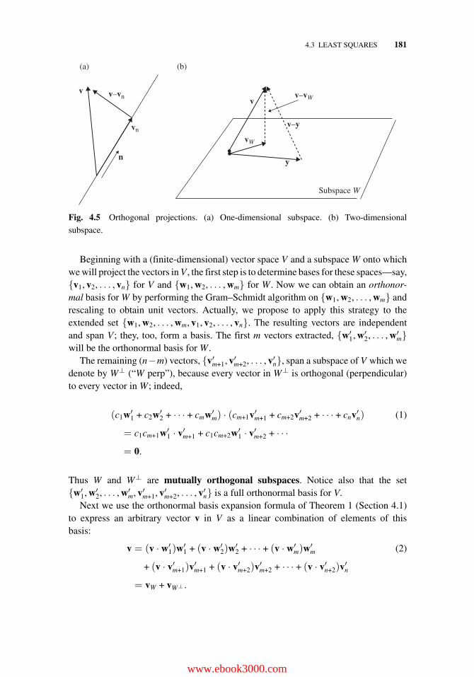
4.3 LEAST SQUARES 181
vv–vW
vW
v–y
y
Subspace W
(b)(a)
v v–vn
vn
n
Fig. 4.5 Orthogonal projections. (a) One-dimensional subspace. (b) Two-dimensional
subspace.
Beginning with a (finite-dimensional) vector space V and a subspace W onto whichwe will project the vectors in V , the first step is to determine bases for these spaces—say,{v1, v2, . . . , vn} for V and {w1, w2, . . . , wm} for W. Now we can obtain an orthonor-mal basis for W by performing the Gram–Schmidt algorithm on {w1, w2, . . . , wm} andrescaling to obtain unit vectors. Actually, we propose to apply this strategy to theextended set {w1, w2, . . . , wm, v1, v2, . . . , vn}. The resulting vectors are independentand span V; they, too, form a basis. The first m vectors extracted, {w′
1, w′2, . . . , w′
m}will be the orthonormal basis for W.
The remaining (n−m) vectors, {v′m+1, v′
m+2, . . . , v′n}, span a subspace of V which we
denote by W⊥ (“W perp”), because every vector in W⊥ is orthogonal (perpendicular)to every vector in W; indeed,
(c1w′1 + c2w′
2 + · · · + cmw′m) · (cm+1v′m+1 + cm+2v′m+2 + · · · + cnv′n) (1)
= c1cm+1w′1 · v′m+1 + c1cm+2w′
1 · v′m+2 + · · ·
= 0.
Thus W and W⊥ are mutually orthogonal subspaces. Notice also that the set{w′
1, w′2, . . . , w′
m, v′m+1, v′
m+2, . . . , v′n} is a full orthonormal basis for V.
Next we use the orthonormal basis expansion formula of Theorem 1 (Section 4.1)to express an arbitrary vector v in V as a linear combination of elements of thisbasis:
v = (v · w′1)w
′1 + (v · w′
2)w′2 + · · · + (v · w′
m)w′m (2)
+ (v · v′m+1)v′m+1 + (v · v′m+2)v
′m+2 + · · · + (v · v′n+2)v
′n
= vW + vW⊥ .
www.ebook3000.com
182 ORTHOGONALITY
This construction—orthogonalizing a basis for W and extending it to an orthonormalbasis for V, spawning identity (2)—demonstrates the decomposition of a vector spaceinto orthogonal subspaces. To summarize:
Orthogonal Subspace Decomposition
When W is a subspace of the vector space V, the notation
V = W ⊕ W⊥, (3)
signifies the following:
• Every vector in V can be decomposed into a sum of a vector in W plus onein W⊥;
• W and W⊥ are mutually orthogonal subspaces.
Moreover, it is easy to prove that the decomposition is unique, and that the zerovector is the only vector that W and W⊥ have in common; see Problem 22. Note that ifv = vW + vW⊥ as in (2), then the orthonormal basis expansion given in equation (8) ofTheorem 1, Section 4.1, implies that
‖v‖2 = ‖vW‖2 + ‖vW⊥‖2. (4)
Of course we have discussed the orthogonal projection of a vector onto another vec-tor many times. Now we can call the “W-part” of (2), vW = c1w′
1 + c2w′2 + · · · + cmw′
m,the orthogonal projection of v onto the subspace W. This orthogonal projectionhas a remarkable property; it’s the nearest vector to v among all the vectors in thesubspace W:
Best Approximation
Theorem 3. Let V = W ⊕ W⊥ and let vW be the orthogonal projection of thevector v into the subspace W. If y is any other vector in W, then
‖v − vW‖ < ‖v − y‖.
In other words, of all vectors in W the orthogonal projection vW is the best approxi-mation to the vector v (as measured by the Euclidean norm). As illustrated in Figure 4.5,this is just a generalization of the familiar fact that the shortest distance from a point toa plane is the length of the perpendicular from the point to the plane.
4.3 LEAST SQUARES 183
Proof of Theorem 3. First observe that for any y in W, we can write
v − y = (v − vW) + (vW − y). (5)
The vector (v−vW) lies in the subspace W⊥ (in fact, it is vW⊥), while the vector (vW−y)lies in W. So applying (4) to (5) we learn that
‖v − y‖2 = ‖v − vW‖2 + ‖vW − y‖2,
demonstrating that ‖v − y‖ exceeds ‖v − vW‖ unless y is, in fact, vW .
Theorem 3 is used in many areas of applied mathematics. For our purposes, itprovides an immediate answer to the dilemma of what to do about inconsistent systems.
Suppose an engineering design has led to a system Ax = b that turns out to haveno solutions. (For instance, it may have more equations than unknowns.) Rather thanabandon the design, the engineer may be willing to accept a “solution” vector x thatbrings Ax as close to b as possible. We have seen that the product Ax can be inter-preted as a linear combination of the columns of A, with coefficients given by x. Soour “compromise solution” will be to find the linear combination of columns of A thatbest approximates b. In other words, we have the subspace W, given by the span of thecolumns of A, and we seek the vector in that subspace that is closest to b. Theorem 3says that the best approximation to b will be the orthogonal projection bW of b onto W.So we tentatively formulate the following procedure:
Least-Squares Solution to Ax = b
To find a vector x providing the best approximation to a solution of the inconsis-tent system expressed as Ax = b,2
(i) Compute an orthonormal basis for the subspace spanned by the columnsof A (using, for instance, the Gram–Schmidt algorithm);
(ii) Find the orthogonal projection bcolA of b onto this subspace (using, forinstance, (2));
(iii) Solve the (consistent) system Ax = bcolA.
Then the Euclidean norm of (b − Ax) will be less than or equal to ‖b − Ay‖ forany vector y.
Note that the square of the Euclidean norm of the vector Ax−b is given by the sumof the squares of its entries, which is precisely the sum of the squares of the differencesbetween the left- and right-hand sides of the “equations” represented by Ax = b. This
2Rigorously speaking, since the system is inconsistent, we honestly should refrain from writing “Ax = b”.
www.ebook3000.com
184 ORTHOGONALITY
is commonly known as the sum of squares of errors, from which the procedure derivesits name, “Least Squares.”
Rather than display an example of this procedure as formulated, we turn directly to ashort cut. Since bcolA is the orthogonal projection of b onto the subspace spanned by thecolumns of A, the residual b− bcolA is orthogonal to this subspace, and hence to everycolumn of A. There’s an easy way to express this orthogonality using the transpose:
A =
⎡⎣ | | | |
col 1 col 2 · · · col n| | | |
⎤⎦ , AT =
⎡⎢⎢⎢⎣− [col 1]T −− [col 2]T−
...−[col n]T−
⎤⎥⎥⎥⎦
and therefore
AT(b − Ax) =
⎡⎢⎢⎢⎣− [col 1]T −− [col 2]T−
...−[col n]T−
⎤⎥⎥⎥⎦ (b − Ax) = 0
expresses the orthogonality.Theorem 4 summarizes these observations. We leave it to the reader (Problem 21)
to provide the details of the proof.
Characterization of Least Squares Approximation
Theorem 4. The vector x provides a least squares approximation for the(m-by-n) system Ax = b if and only if AT{b − Ax} = 0 or, equivalently,
AT Ax = AT b. (6)
Equations (6) are called the normal equations for the system represented by Ax = b.The normal equations provide an alternative to the least squares procedure describedearlier.
Example 1. Find a vector x providing the least-squares approximation to the systemexpressed by
⎡⎢⎢⎢⎢⎢⎢⎣
1 −1 1... 1
1 1 3... 0
1 1 3... 1
1 1 3... 2
⎤⎥⎥⎥⎥⎥⎥⎦
. (7)
4.3 LEAST SQUARES 185
Solution. Note that the last three equations in (7) are blatantly inconsistent. The normalequations for this system are
ATAx =
⎡⎣ 1 1 1 1−1 1 1 11 3 3 3
⎤⎦⎡⎢⎢⎣
1 −1 11 1 31 1 31 1 3
⎤⎥⎥⎦⎡⎣x1
x2
x3
⎤⎦ = ATb =
⎡⎣ 1 1 1 1−1 1 1 11 3 3 3
⎤⎦⎡⎢⎢⎣
1012
⎤⎥⎥⎦ ,
which, after multiplication, take the following augmented matrix form:
⎡⎢⎢⎢⎣
4 2 10... 4
2 4 8... 2
10 8 28... 10
⎤⎥⎥⎥⎦ .
Gauss elimination reveals the solutions to this system to be
⎡⎣x1
x2
x3
⎤⎦ =
⎡⎣1 − 2t
−tt
⎤⎦ =
⎡⎣1
00
⎤⎦ + t
⎡⎣−2−11
⎤⎦ .
The quality of the solution is exhibited by the “error” or “residual” b − Ax:
b =
⎡⎢⎢⎣
1012
⎤⎥⎥⎦ , bcolA = Ax =
⎡⎢⎢⎣
1111
⎤⎥⎥⎦ , error = b − Ax =
⎡⎢⎢⎣
0−101
⎤⎥⎥⎦ . �
Example 1 highlights several noteworthy points about least squares approxima-tions:
• The error b − Ax is always orthogonal to the best approximation Ax;
• The coefficient matrix ATA for the normal equations is always square andsymmetric;
• The normal equations are always consistent;
• The best approximation to b, namely bcolA =Ax, is unique. However the “solution”vector x, that provides the best approximation to Ax= b, might not be unique.3
In Problem 15, it is demonstrated that the rank of ATA equals the rank of A. There-fore if the columns of A are linearly independent, ATA is invertible and the least
3The “pseudoinverse” of A, described in Section 6.4, provides the solution vector x of minimal norm. ForExample 1, this would be [1/3 −1/3 1/3]T (for t = 1/3).
www.ebook3000.com
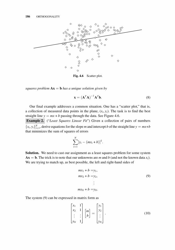
186 ORTHOGONALITY
Fig. 4.6 Scatter plot.
squares problem Ax = b has a unique solution given by
x = (ATA)−1ATb. (8)
Our final example addresses a common situation. One has a “scatter plot,” that is,a collection of measured data points in the plane, (xi, yi). The task is to find the beststraight line y = mx + b passing through the data. See Figure 4.6.Example 2. (“Least Squares Linear Fit”) Given a collection of pairs of numbers
{xi, yi}Ni=1, derive equations for the slope m and intercept b of the straight line y = mx+b
that minimizes the sum of squares of errors
N∑i=1
[yi − (mxi + b)]2.
Solution. We need to cast our assignment as a least squares problem for some systemAx = b. The trick is to note that our unknowns are m and b (and not the known data xi).We are trying to match up, as best possible, the left and right-hand sides of
mx1 + b =y1,
mx2 + b =y2, (9)...
mxN + b =yN .
The system (9) can be expressed in matrix form as⎡⎢⎢⎢⎣
x1 1x2 1...
...xN 1
⎤⎥⎥⎥⎦[
mb
]=
⎡⎢⎢⎢⎣
y1
y2...
yN
⎤⎥⎥⎥⎦ . (10)
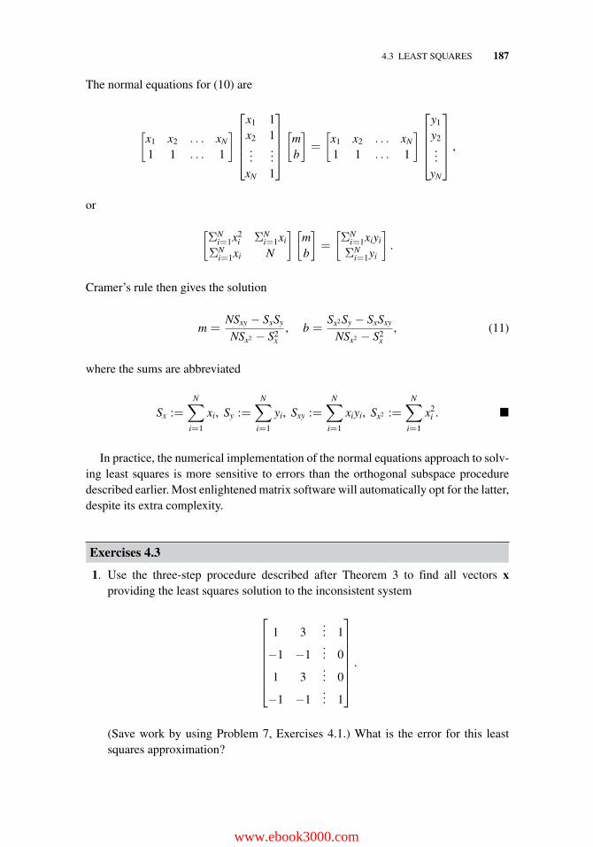
4.3 LEAST SQUARES 187
The normal equations for (10) are
[x1 x2 . . . xN
1 1 . . . 1
]⎡⎢⎢⎢⎣
x1 1x2 1...
...xN 1
⎤⎥⎥⎥⎦[
mb
]=
[x1 x2 . . . xN
1 1 . . . 1
]⎡⎢⎢⎢⎣
y1
y2...
yN
⎤⎥⎥⎥⎦ ,
or
[ΣN
i=1x2i ΣN
i=1xi
ΣNi=1xi N
] [mb
]=
[ΣN
i=1xiyi
ΣNi=1yi
].
Cramer’s rule then gives the solution
m =NSxy − SxSy
NSx2 − S2x
, b =Sx2 Sy − SxSxy
NSx2 − S2x
, (11)
where the sums are abbreviated
Sx :=N∑
i=1
xi, Sy :=N∑
i=1
yi, Sxy :=N∑
i=1
xiyi, Sx2 :=N∑
i=1
x2i . �
In practice, the numerical implementation of the normal equations approach to solv-ing least squares is more sensitive to errors than the orthogonal subspace proceduredescribed earlier. Most enlightened matrix software will automatically opt for the latter,despite its extra complexity.
Exercises 4.3
1. Use the three-step procedure described after Theorem 3 to find all vectors xproviding the least squares solution to the inconsistent system
⎡⎢⎢⎢⎢⎢⎢⎣
1 3... 1
−1 −1... 0
1 3... 0
−1 −1... 1
⎤⎥⎥⎥⎥⎥⎥⎦
.
(Save work by using Problem 7, Exercises 4.1.) What is the error for this leastsquares approximation?
www.ebook3000.com
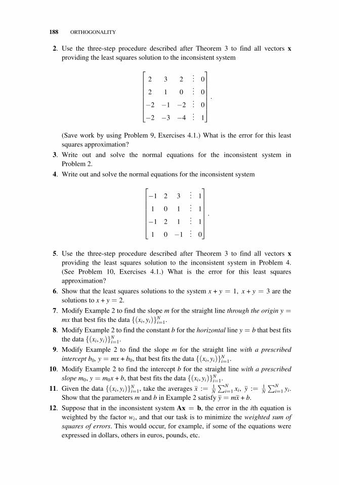
188 ORTHOGONALITY
2. Use the three-step procedure described after Theorem 3 to find all vectors xproviding the least squares solution to the inconsistent system
⎡⎢⎢⎢⎢⎢⎢⎣
2 3 2... 0
2 1 0... 0
−2 −1 −2... 0
−2 −3 −4... 1
⎤⎥⎥⎥⎥⎥⎥⎦
.
(Save work by using Problem 9, Exercises 4.1.) What is the error for this leastsquares approximation?
3. Write out and solve the normal equations for the inconsistent system inProblem 2.
4. Write out and solve the normal equations for the inconsistent system
⎡⎢⎢⎢⎢⎢⎢⎣
−1 2 3... 1
1 0 1... 1
−1 2 1... 1
1 0 −1... 0
⎤⎥⎥⎥⎥⎥⎥⎦
.
5. Use the three-step procedure described after Theorem 3 to find all vectors xproviding the least squares solution to the inconsistent system in Problem 4.(See Problem 10, Exercises 4.1.) What is the error for this least squaresapproximation?
6. Show that the least squares solutions to the system x + y = 1, x + y = 3 are thesolutions to x + y = 2.
7. Modify Example 2 to find the slope m for the straight line through the origin y =mx that best fits the data {(xi, yi)}N
i=1.
8. Modify Example 2 to find the constant b for the horizontal line y = b that best fitsthe data {(xi, yi)}N
i=1.
9. Modify Example 2 to find the slope m for the straight line with a prescribedintercept b0, y = mx + b0, that best fits the data {(xi, yi)}N
i=1.
10. Modify Example 2 to find the intercept b for the straight line with a prescribedslope m0, y = m0x + b, that best fits the data {(xi, yi)}N
i=1.
11. Given the data {(xi, yi)}Ni=1, take the averages x := 1
N
∑Ni=1 xi, y := 1
N
∑Ni=1 yi.
Show that the parameters m and b in Example 2 satisfy y = mx + b.
12. Suppose that in the inconsistent system Ax = b, the error in the ith equation isweighted by the factor wi, and that our task is to minimize the weighted sum ofsquares of errors. This would occur, for example, if some of the equations wereexpressed in dollars, others in euros, pounds, etc.
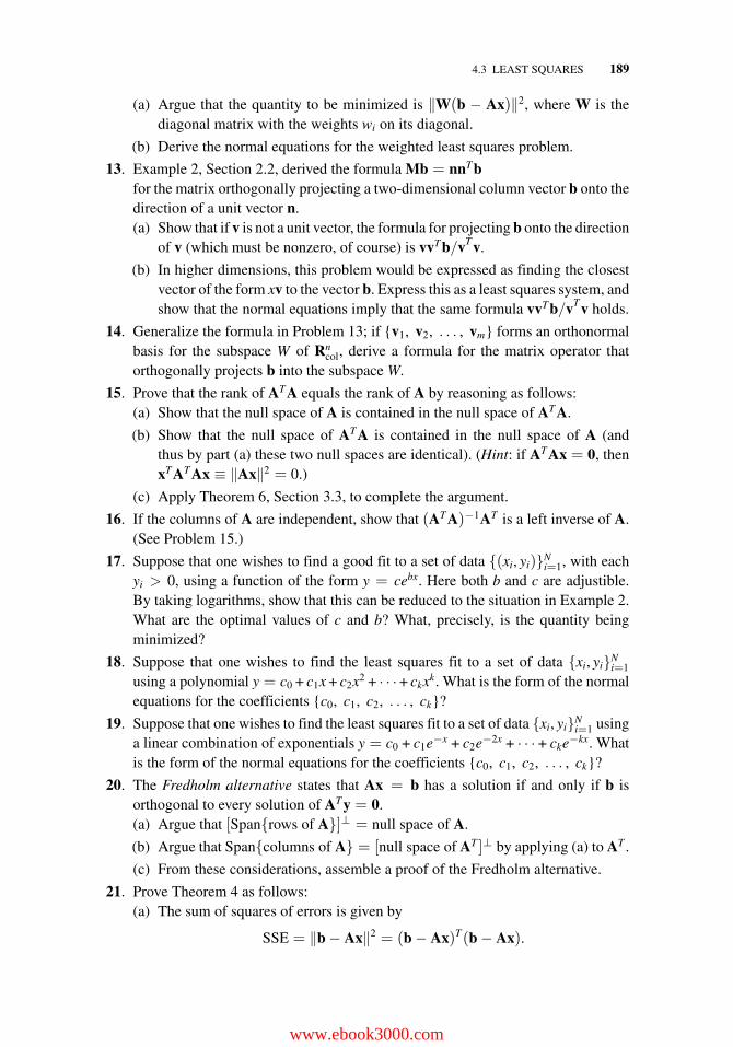
4.3 LEAST SQUARES 189
(a) Argue that the quantity to be minimized is ‖W(b − Ax)‖2, where W is thediagonal matrix with the weights wi on its diagonal.
(b) Derive the normal equations for the weighted least squares problem.
13. Example 2, Section 2.2, derived the formula Mb = nnTbfor the matrix orthogonally projecting a two-dimensional column vector b onto thedirection of a unit vector n.(a) Show that if v is not a unit vector, the formula for projecting b onto the direction
of v (which must be nonzero, of course) is vvTb/vTv.
(b) In higher dimensions, this problem would be expressed as finding the closestvector of the form xv to the vector b. Express this as a least squares system, andshow that the normal equations imply that the same formula vvTb/vTv holds.
14. Generalize the formula in Problem 13; if {v1, v2, . . . , vm} forms an orthonormalbasis for the subspace W of Rn
col, derive a formula for the matrix operator thatorthogonally projects b into the subspace W.
15. Prove that the rank of ATA equals the rank of A by reasoning as follows:(a) Show that the null space of A is contained in the null space of ATA.
(b) Show that the null space of ATA is contained in the null space of A (andthus by part (a) these two null spaces are identical). (Hint: if ATAx = 0, thenxTATAx ≡ ‖Ax‖2 = 0.)
(c) Apply Theorem 6, Section 3.3, to complete the argument.
16. If the columns of A are independent, show that (ATA)−1AT is a left inverse of A.(See Problem 15.)
17. Suppose that one wishes to find a good fit to a set of data {(xi, yi)}Ni=1, with each
yi > 0, using a function of the form y = cebx. Here both b and c are adjustible.By taking logarithms, show that this can be reduced to the situation in Example 2.What are the optimal values of c and b? What, precisely, is the quantity beingminimized?
18. Suppose that one wishes to find the least squares fit to a set of data {xi, yi}Ni=1
using a polynomial y = c0 + c1x + c2x2 + · · ·+ ckxk. What is the form of the normalequations for the coefficients {c0, c1, c2, . . . , ck}?
19. Suppose that one wishes to find the least squares fit to a set of data {xi, yi}Ni=1 using
a linear combination of exponentials y = c0 + c1e−x + c2e−2x + · · · + cke−kx. Whatis the form of the normal equations for the coefficients {c0, c1, c2, . . . , ck}?
20. The Fredholm alternative states that Ax = b has a solution if and only if b isorthogonal to every solution of ATy = 0.(a) Argue that [Span{rows of A}]⊥ = null space of A.
(b) Argue that Span{columns of A} = [null space of AT ]⊥ by applying (a) to AT .
(c) From these considerations, assemble a proof of the Fredholm alternative.
21. Prove Theorem 4 as follows:(a) The sum of squares of errors is given by
SSE = ‖b − Ax‖2 = (b − Ax)T(b − Ax).
www.ebook3000.com
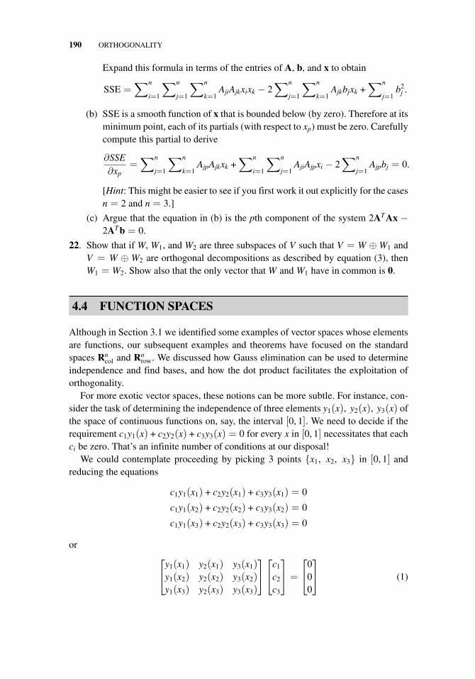
190 ORTHOGONALITY
Expand this formula in terms of the entries of A, b, and x to obtain
SSE =∑n
i=1
∑n
j=1
∑n
k=1AjiAjkxixk − 2
∑n
j=1
∑n
k=1Ajkbjxk +
∑n
j=1b2
j .
(b) SSE is a smooth function of x that is bounded below (by zero). Therefore at itsminimum point, each of its partials (with respect to xp) must be zero. Carefullycompute this partial to derive
∂SSE∂xp
=∑n
j=1
∑n
k=1AjpAjkxk +
∑n
i=1
∑n
j=1AjiAjpxi − 2
∑n
j=1Ajpbj = 0.
[Hint: This might be easier to see if you first work it out explicitly for the casesn = 2 and n = 3.]
(c) Argue that the equation in (b) is the pth component of the system 2ATAx −2ATb = 0.
22. Show that if W, W1, and W2 are three subspaces of V such that V = W ⊕ W1 andV = W ⊕ W2 are orthogonal decompositions as described by equation (3), thenW1 = W2. Show also that the only vector that W and W1 have in common is 0.
4.4 FUNCTION SPACES
Although in Section 3.1 we identified some examples of vector spaces whose elementsare functions, our subsequent examples and theorems have focused on the standardspaces Rn
col and Rnrow. We discussed how Gauss elimination can be used to determine
independence and find bases, and how the dot product facilitates the exploitation oforthogonality.
For more exotic vector spaces, these notions can be more subtle. For instance, con-sider the task of determining the independence of three elements y1(x), y2(x), y3(x) ofthe space of continuous functions on, say, the interval [0, 1]. We need to decide if therequirement c1y1(x) + c2y2(x) + c3y3(x) = 0 for every x in [0, 1] necessitates that eachci be zero. That’s an infinite number of conditions at our disposal!
We could contemplate proceeding by picking 3 points {x1, x2, x3} in [0, 1] andreducing the equations
c1y1(x1) + c2y2(x1) + c3y3(x1) = 0
c1y1(x2) + c2y2(x2) + c3y3(x2) = 0
c1y1(x3) + c2y2(x3) + c3y3(x3) = 0
or⎡⎣y1(x1) y2(x1) y3(x1)
y1(x2) y2(x2) y3(x2)y1(x3) y2(x3) y3(x3)
⎤⎦⎡⎣c1
c2
c3
⎤⎦ =
⎡⎣0
00
⎤⎦ (1)
4.4 FUNCTION SPACES 191
to row echelon form. If this reveals that (1) has only the zero solution, we willhave shown that the only way c1y1(x) + c2y2(x) + c3y3(x) ≡ 0 can hold is ifc1 = c2 = c3 = 0, and thus the functions must be independent. However, ifnontrivial solutions do exist, we could not conclude that the functions are depen-dent, because we could never be sure that a different selection of {x1, x2, x3}might have established independence. So Gauss elimination may prove independence,if we’re lucky in our choice of test values for x, but it can never establishdependence.
Example 1. Show that the functions 1, x2, and x4 are linearly independent on(−∞,∞).
Solution. If we test for independence at the points {−1, 0, 1}, the system (1)becomes
⎡⎢⎣
1 1 1
1 0 0
1 1 1
⎤⎥⎦⎡⎢⎣
c1
c2
c3
⎤⎥⎦ =
⎡⎢⎣
0
0
0
⎤⎥⎦ ,
which has nontrivial solutions: for example, c1 = 0, c2 = −1, c3 = 1. Sothe test is inconclusive. But if we had chosen {0, 1, 2}, the condition would havebeen
⎡⎢⎣
1 0 0
1 1 1
1 4 16
⎤⎥⎦⎡⎢⎣
c1
c2
c3
⎤⎥⎦ =
⎡⎢⎣
0
0
0
⎤⎥⎦ ;
the determinant of the coefficient matrix is 12 (nonzero), so only the trivial solution ispossible for {c1, c2, c3}, implying the functions are independent. �
The basic villain here is that many function spaces are infinite dimensional. Theyhave no finite bases; no one who has taken calculus will believe that you can generateevery continuous function on (−∞,∞) by taking linear combinations of a paltry collec-tion of, say, only 7, or 8, or 20 billion, of them. One of the aims of the discipline knownas functional analysis is to establish bases for the function spaces, but since such basescontain an infinite number of elements, the notion of convergence is a prerequisite toany analysis involving linear combinations.
This feature—the infinite dimensionality—is made more concrete by consideringtabulations of continuous functions on, say, a spread sheet:
www.ebook3000.com
192 ORTHOGONALITY
⎡⎢⎢⎢⎢⎢⎢⎢⎢⎢⎢⎢⎢⎢⎢⎢⎢⎢⎢⎢⎢⎢⎢⎣
t cos t sin t0 1.000 0
π/6 0.866 0.5002π/6 0.500 0.8663π/6 0 1.0004π/6 −0.500 0.8665π/6 −0.866 0.500π −1.000 0
7π/6 −0.866 −0.5008π/6 −0.500 −0.8669π/6 0 −1.00010π/6 0.500 −0.86611π/6 0.866 −0.500
⎤⎥⎥⎥⎥⎥⎥⎥⎥⎥⎥⎥⎥⎥⎥⎥⎥⎥⎥⎥⎥⎥⎥⎦
(2)
In computational practice, each function is reduced to a column vector. Indeed wewould tabulate 3 cos t + 4 sin t by forming linear combinations of the second and thirdcolumns of (2). But we cannot completely trust any mathematical conclusion concern-ing cos t and sin t based on only a finite number of sampled values. Therefore we needto employ other tools to decide, rigorously, the independence of sets of functions.
In some cases, we can use the growth rate. For example, the linear independence of1, x2, and x4 on (−∞,∞) is easily established as follows. If c11 + c2x2 + c3x4 = 0 forall x , we can conclude that c3 = 0 by dividing by x4 and letting x → ∞;
c3 = limx→∞
[−c1
x4− c2
x2
]= 0.
Then we apply the same reasoning to c11+c2x2 to get c2 = 0, and so on. This argumentis easily extended to show that any finite set of polynomials of differing degrees islinearly independent on (−∞,∞).
Example 2. Verify the claim that any finite set of exponential functions with differentdecay times is linearly independent on (−∞,∞).
Solution. We need to show that the equality
c1eα1x + c2eα2x + · · · + cneαnx = 0 (3)
(all αi distinct) can only hold if each ci = 0. We exploit the growth rates again. Supposeαj is the largest (in the algebraic sense) of the αi’s. Dividing (3) by eαjx and lettingx → ∞, we see that cj must be zero. Now carry out the same argument with the secondlargest of the αi’s, and so on, to conclude that every ci is zero. �
We remark that the growth rate argument will not work in analyzing linear inde-pendence over a finite interval. Indeed, it is possible for a collection of functions to
4.4 FUNCTION SPACES 193
be linearly independent over (−∞,∞), but linearly dependent over some subinterval(a, b). See Problem 20.
For future reference, it is useful to note that the following sets of functions arelinearly independent on every open interval (a, b):
• {1, x, x2, . . . , xn}• {1, cos x, sin x, cos 2x, sin 2x, . . . , cos nx, sin nx}• {eα1x, eα2x, . . . , eαnx} (for distinct constants αi)
(see Problems 4, 8, and 9).Although Gauss elimination is ineffectual as a tool for analyzing function spaces,
the notion of orthogonality and its attendant features carry over quite nicely. How dowe form a dot product of the functions cos t and sin t (over the interval [0, 2π])? Againtaking a computational point of view, we could start by forming the dot product of thesecond and third columns in (2), and contemplate the limit of such dot products as thenumber of tabulations increases:
(cos t) · (sin t)?= lim
N→∞
N∑i=1
cos ti sin ti. (4)
Sums of the form (4) diverge as N → ∞, but with the insertion of a constant factorΔt := ti+1 − ti = 2π/N we observe the emergence of an old friend, the Riemann sum:
(cos t) · (sin t) = limN→∞
N∑i=1
cos ti sin ti Δt =∫ 2π
0cos t sin t dt. (5)
Accordingly, one defines the inner product of two continuous functions on [a, b] to be
< f , g >:=∫ b
af (t) g(t) dt (6)
with the associated norm
‖f‖ :=
[∫ b
af (t)2 dt
]1/2
. (7)
Through the inner product such concepts as the Gram–Schmidt algorithm, orthogonalprojection, and least squares approximations are enabled in function spaces. Fourierseries and eigenfunction expansions of solutions of partial differential equations aresome of the advanced techniques based on these considerations.4
4The term Hilbert Spaces refers to function spaces endowed with inner products (and a few other properties).
www.ebook3000.com
194 ORTHOGONALITY
Example 3. Show that the (infinite) collection {sin x, sin 2x, sin 3x, . . .} is an orthog-onal family of functions in the interval (0,π).
Solution. The inner products (6) for this family are
π
∫0sinmx sin nx dx =
[sin(m − n)x
2(m − n)− sin(m + n)x
2(m + n)
]π0
= 0 for m �= n. �
Example 4. Apply the Gram–Schmidt algorithm to the collection of functions{1, x, x2} on the interval (−1, 1).
Solution. Executing the procedure described in Section 4.1 with the substitution of (6)for the dot product v · w, we calculate
w1 = v1 = 1.
w2 = v2 − (v2 · w1)w1/w1 · w1 = x −[
1∫−1(x)(1) dx
]1/
[1∫−1(1)(1) dx
]= x.
w3 := v3 − (v3 · w1)w1/w1 · w1 − (v3 · w2)w2/w2 · w2
= x2 −[
1∫−1(x2)(1) dx
]1/
[1∫−1(1)(1) dx
]−
[1∫−1(x2)(x) dx
]x/
[1∫−1(x)(x) dx
]
= x2 − 13
.
If these functions were rescaled to take the value one when x = 1, they would be thefirst three Legendre polynomials. �
Exercises 4.4
1. Decide if the following sets of functions are linearly independent on the indicatedintervals.(a) 1, sin2 x, cos2 x on [0, 2π]. (d) x, x2, 1 − 2x2 on [−2, 2].
(b) x, |x| on [−1, 1]. (e) x, xex, 1 on (−∞,∞).
(c) x, |x| on [−1, 0]. (f) 1/x,√
x, x on (0,∞).
2. Perform the Gram–Schmidt algorithm on the set 1, ex, e−x to construct 3 functionsthat are orthogonal on the interval (0, 1).
3. Perform the Gram–Schmidt algorithm on the set 1, x, x2 to construct 3 polynomialsthat are orthogonal on the interval (0, 1).
4. Prove that the set of functions {1, x, x2, . . . , xn} is linearly independent over everyopen interval (a, b). (Hint: If c0 + c1x + · · · + cnxn = 0 in an interval, differentiaten times to show cn = 0.)
4.4 FUNCTION SPACES 195
5. Use the strategy of Problem 4 to argue that {1, (x − 1), (x − 1)2, . . . , (x − 1)n} isa basis for Pn (the space of all polynomials of degree at most n).
6. Express the polynomial xn as a linear combination of the basis elements inProblem 5. (Hint: Consider the Taylor series.)
7. (a) Rescale the functions computed in Example 4 so that they take the value oneat x = 1.
(b) Extend the computations in Example 4 to find the Legendre polynomial ofdegree 3.
8. Prove that the set of functions {1, cos x, sin x, cos 2x, sin 2x, . . . , cos nx, sin nx} islinearly independent over every open interval (a,b). (Hint: If c0 +c1 cos x+d1 sin x+· · · + cn cos nx + dn sin nx = 0 in an interval, differentiate 2n times and write theresulting 2n+1 equations (regarding the cj’s and dj’s as unknowns) in matrix form.Row operations will reduce the matrix to one with 2-by-2 blocks along the diagonaland zeros below; the determinant will be seen to be positive.)
9. Prove that the set of functions {eα1x, eα2x, . . . , eαnx} (for distinct constants αi) islinearly independent over every open interval (a,b). (Hint: If c1eα1x + c2eα2x +· · · + cneαnx = 0 in an interval, differentiate n − 1 times and write the result-ing n equations (regarding the cj’s as unknowns) in matrix form. Factor as⎡⎢⎢⎢⎢⎣
1 1 · · · 1α1 α2 · · · αn...
.... . .
...
αn−11 αn−1
2 · · · αn−1n
⎤⎥⎥⎥⎥⎦
⎡⎢⎢⎢⎢⎢⎣
eα1x 0 · · · 0
0 eα2x · · · 0...
.... . .
...
0 0 · · · eαnx
⎤⎥⎥⎥⎥⎥⎦
⎡⎢⎢⎢⎢⎣
c1
c2
...cn
⎤⎥⎥⎥⎥⎦ = 0
and consider determinants (recall Problem 23, Exercises 2.4).)
10. Prove that x, |x|, and x2 are linearly independent on (−1, 1).
11. Utilize the growth rates to show the following sets of functions are linearlyindependent on (0,∞):(a) {1, ln x, ex}
(b) {ex, xex, x2ex}
12. Consider the problem of approximating a function f (x) over an interval (a, b) bya linear combination of other functions c1y1(x) + c2y2(x) + · · · + cnyn(x), so as tominimize the integrated squared error
∫ b
a{f (x)− [c1y1(x) + c2y2(x) + · · · + cnyn(x)]}2 dx.
(a) Recast this task as the problem of orthogonally projecting f (x) intoSpan{y1(x), y2(x), . . . , yn(x)} using the inner product (6).
(b) Retrace the discussion in Section 4.1 to argue that the remainder{f (x) − [c1y1(x) + c2y2(x) + · · · + cnyn(x)]} must be orthogonal to each ofthe functions {y1(x), y2(x), . . . , yn(x)}.
www.ebook3000.com
196 ORTHOGONALITY
(c) Express the system of n equations in the n unknowns {c1, c2, . . . , cn} enforc-ing (b), in matrix form. This is the analog of the normal equations for functionspaces. The coefficient matrix is called a Gram matrix.
13. Use the normal equations derived in Problem 12 to find the least squares approx-imation of cos3 x by a combination of sin x and cos x, over the interval (0, 2π).Sketch the graphs of cos3 x and the approximation.
14. Repeat Problem 13 using a combination of the functions 1 and x.
15. (a) Express the normal equations derived in Problem 12 to find the least squaresapproximation of f (x) by a straight line mx+b, over the interval (a, b). Comparewith Example 2 in Section 4.3.
(b) Find the straight line that provides the least squares approximation to x2 overthe interval (0, 1).
(c) The linear Chebyshev approximation to x2 over the interval (0, 1) is the straightline y = mx + b whose maximal vertical deviation from y = x2 over the inter-val is least (a “minimax” approximation). Find this Chebyshev approximation.(Hint: Do it graphically; place a ruler on the graph of y = x2 and adjust it untilthe criterion is met.)
(d) Plot x2, its least squares approximation, and its Chebyshev approximation over(0, 1) on the same graph.
16. Formulate the normal equations derived in Problem 12 for the task of findingthe least squares approximation to f (x) by a combination of 1, x, x2, . . . , xn. Thecoefficient matrix was identified as the Hilbert matrix in Problem 6, Exercises 1.5.
17. Show that the functions {1, cos x, sin x, cos 2x, sin 2x, . . . , cos nx, sin nx} areorthogonal on the interval (0,2π).
18. Show that any sequence of elementary row operations performed on the columnvector [1, x, x2, . . . , xn]T yields a vector whose entries constitute a basis for Pn.
19. By Problem 4 the set {1, x, x2, . . . , xn} is a basis for the space Pn of all polynomialsof degree less than or equal to n.(a) Find another basis for Pn whose elements are all polynomials of the same
degree.
(b) Find a basis for the subspace of Pn consisting of all polynomials taking thevalue zero at x = 0.
(c) Find a basis for the subspace of Pn consisting of all polynomials taking thevalue zero at x = 1.
20. Argue that the functions
f1(x) = x; f2(x) =
{x if − 1 < x < 1x3 otherwise
;
f3(x) =
{x3 if − 1 < x < 1x otherwise
are linearly dependent on [−1, 1] but linearly independent on (−∞,∞).
4.5 SUMMARY 197
21. Prove that any n + 1 polynomials pk, k = 0, 1, . . . , n, with degree of each pk
precisely k, forms a basis for Pn.
4.5 SUMMARY
Orthogonality
The familiar notion of orthogonality in two and three dimensions is extended to higherdimensions via the dot product criterion, which for real column vectors takes the formvTw= 0. Similarly, the notion of length is generalized as the Euclidean norm ‖v‖ =(vTv)1/2, and mutually orthogonal vectors having unit norm are called orthonormal. Amutually orthogonal set of nonzero vectors must be linearly independent, and indeedthe coefficients in a linear combination of these, w = c1v1 + c2v2 + · · · + cnvn, are easyto compute: ci = vT
i w/vTi vi. The Gram–Schmidt algorithm is used to replace a given
set of vectors by a linearly independent mutually orthogonal set that is “equivalent,” inthe sense that it spans the same subspace.
Orthogonal matrices are characterized by the following equivalent properties:
(i) The inverse equals the transpose;
(ii) The rows are orthonormal;
(iii) The columns are orthonormal;
(iv) Multiplication by the matrix preserves inner products;
(v) Multiplication by the matrix preserves Euclidean norms.
Least Squares
A least squares solution to an inconsistent linear system Ax = b is a vector x thatminimizes the sum of the squares of the differences between its left and right handmembers. The left-hand side Ax is a best approximation, among the vectors in thespan of the columns of A, to the vector b, in the Euclidean norm. In general, a best(Euclidean) approximation w to a vector b among all vectors in a given subspace W ischaracterized by the property that the residual (b − w) is orthogonal to all the vectorsin the subspace.
An orthogonal decomposition V = W ⊕ W⊥ of a vector space V gives a uniquerepresentation of every vector v in V as a sum of mutually orthogonal vectors w in thesubspace W and w⊥ in the suspace W⊥. Then w is the best approximation in W to thevector v and the residual w⊥ is orthogonal to W.
It follows that a least squares solution x to an inconsistent m-by-n linear systemAx = b will be a (genuine) solution to the (consistent) normal equations ATAx =AT b.
www.ebook3000.com
198 ORTHOGONALITY
Function Spaces
Some collections of functions may possess the properties of a vector space. Variousclasses of polynomials, for example, are closed under addition and scalar multiplica-tion. We can then exploit the attendant notions of independence, spans, and bases tostudy them. Most function spaces are infinite-dimensional, however, and such conceptsare complicated by issues of convergence. Independence can sometimes be establishedby considerations of growth rates, for functions defined on an infinite domain.
The similarity between the dot product of vectors in high-dimensional spaces and theRiemann sum for functional integrals suggests the extension of the idea of orthogonalityto function spaces via the inner product < f , g >:=
∫ ba f (t)g(t)dt and the associated
norm ‖f‖2 :=∫ b
a f 2(t)dt.
REVIEW PROBLEMS FOR PART II
1. (a) Write a matrix equation expressing the condition that all the row sums ofthe matrix A are equal; use only the symbol A (and not its entries aij).
(b) Write a matrix equation expressing the conditions that all the column sumsof the matrix A are equal.
(c) What further properties are exhibited by the “magic square” inAlbrecht Durer’s Melancolia (Figure 4.7) (http://en.wikipedia.org/wiki/Melencolia_I)?
2. Is [1 2 3] spanned by [3 2 1] and [1 1 1]?
3. Find a nonzero vector that lies in both the span of [1 1 2] and [1 0 1], and thespan of [2 13 23] and [2 1 33].
4. Which of these subsets of R4row are subspaces?
(a) The vectors whose entries all have the same sign.
(b) The vectors orthogonal to [1 1 1 1].
(c) The vectors [a b c d] satisfying ab = 0.
(d) The vectors [a b c d] satisfying a + 2b + 3c = d.
(e) The intersection of two arbitrary subspaces (i.e., the set of vectors belongingto both subspaces);
(f) The union of two arbitrary subspaces (i.e., the set of vectors belonging toone subspace or the other).
16
5
9
4
3
10
6
15
2
11
7
14
13
8
12
1
Fig. 4.7 Magic Square in Albrecht Durer’s Melancolia.
REVIEW PROBLEMS FOR PART II 199
5. Which of these subsets of R4,4 are subspaces?(a) The orthogonal matrices;
(b) The diagonal matrices;
(c) The reflection matrices;
(d) The Gauss-elimination row operators;
(e) The nonsingular matrices.
6. What are the dimensions of these subspaces of R4,4? Find bases for each.(a) The symmetric matrices;
(b) The skew-symmetric matrices;
(c) The upper triangular matrices.
7. Find 2 vectors that, together with[1 2 3 4
]and
[4 3 2 1
], form a basis
for R4row.
8. If v1, v2, . . . , vn are linearly independent, which of the following are indepen-dent:(a) The sums v1 + v2, v2 + v3, . . . , vn−1 + vn, v1 + vn ;
(b) The differences v1 − v2, v2 − v3, . . . , vn−1 − vn, v1 − vn?
9. Prove that any two three-dimensional subspaces of R5col must have a nonzero
vector in common.
10. If V is the vector space of all polynomials of degree two or less, find a subset of{1 + 2x + 3x2, 4 − x2, 1 + 2x, 2 − x, 1} that is a basis for V .
11. Find a basis for the space spanned by sin 2t, cos 2t, sin2 t, cos2 t, for−∞ < t < ∞.
12. In the Introduction to Part II, we observed that the differential equationd3y/dx3 = 0 has a set of solutions y = c1x2/2 + c2x + c3 comprising a three-dimensional vector space. Find a set of three solutions that are orthogonal on[0,1].
13. Prove that if A is 5-by-3 and B is 3-by-5, then AB is singular.
14. Prove that if the rank of A equals one, then A2 is a scalar multiple of A .
15. Is the following a basis for R2,2?
[1 11 0
],
[2 03 1
],
[0 02 −1
],
[−2 03 0
].
16. (Controllability) Many control systems can be described by the equationxp+1 = Axp + Bup, where the vector xp describes the state of the system at timep (so the entries of xp may be positions, angles, temperatures, currents, etc.);A and B are appropriately dimensioned matrices characterizing the particularsystem, and up is the input vector (at time p) selected by the system operator.(a) Show that any state vector x lying in the span of the columns of
[Ax0, B, AB, A2B, . . . , AkB] can be reached within k + 1 time steps by
www.ebook3000.com
200 ORTHOGONALITY
proper choices of inputs [u0, u1, u2, . . . , uk]. (Hint: Derive, extend, andexploit the relation x2 = A2x0 + ABu0 + Bu1.)
(b) If A is n − by − n, show that the system is “controllable,” that is, can bedriven into any state x from any initial state x0, if the rank of
[B, AB, A2B, . . . , AsB] equals n for some s.
(c) Find a sequence of inputs u0, u1, u2 that will drive the initial state x0 =[1 1 1]T to the state x = [1 0 −1]T in three time steps for the systemcharacterized by
A =
⎡⎣ 0 0 0
1 0 00 1 0
⎤⎦ , B =
⎡⎣ 1
00
⎤⎦ .
17. Prove that if A is symmetric and uTAu = uTu for every vector u, then A is theidentity matrix. (Hint: First apply the equation with vectors u having all zeroentries except for a single “one”; then repeat, for vectors having two “ones.”)
18. (a) Describe how to express an arbitrary square matrix as a sum of a symmetricmatrix (A = AT) and a skew-symmetric matrix (A = −AT).
(b) Describe how to express an arbitrary square matrix as a sum of a symmetricmatrix and an upper triangular matrix.
(c) Is either of these decompositions unique?
19. What is u · v if ‖u‖ = ‖v‖ = ‖u + v‖ = 2?
20. Find the least squares best approximation over the interval [−1, 1] to x3 in theform a1 + a2x + a3x2. (Hint: Use the results of Problem 12, Exercises 4.4.) Howis your answer the Legendre polynomial of degree three?
TECHNICAL WRITING EXERCISES FOR PART II
1. Discuss the fact that the intersection of two subspaces of a vector space is also asubspace, but their union need not be a subspace. Illustrate with planes and lines.
2. Most mainframe, desktop, and laptop computers are binary machines; theyperform arithmetic in the base-2 system, using finite-precision binary approx-imations to fractional numbers. However most calculators are binary-codeddecimal machines; they perform decimal arithmetic using finite-precision dec-imal approximations, although the decimal digits are encoded in binary form.(See http://en.wikipedia.org/wiki/Binary-coded_decimal for example.) Discussthe nature of the numbers that are encoded exactly in each of the two systems, anddescribe a matrix whose rank might be reported differently by two such machines.
GROUP PROJECTS FOR PART II 201
GROUP PROJECTS FOR PART II
A. Rotations and Reflections
Your objective in this project is to demonstrate that every 3-by-3 orthogonal matrixQ can be expressed as a product of rotation and reflection matrices. The followingobservations will help you construct the argument.
(a) The orthonormal triad i = [1 0 0]T , j = [0 1 0]T , and k = [0 0 1]T represent unitvectors along each of the three axes.
(b) The three columns iQ, jQ, and kQ of Q are the images, under multiplicationby Q, of these three unit vectors. They also form an orthonormal triad, sokQ = (±) iQ × jQ. For our purposes, one can take kQ = iQ × jQ withoutloss of generality by introducing, if necessary, a reflection through the xy plane.Thus the resulting orthogonal matrix is completely determined by its first twocolumns.
(c) Take a basketball or soccerball and imagine that the origin of the xyz axis systemlies at its center. Draw dots on the ball’s surface at the points where you estimatei and j penetrate the ball; also draw dots where iQ and jQ penetrate the ball.
(d) Let M1 denote any rotation of the ball that carries i to iQ. Let j′ be the image ofj under this rotation.
(e) Argue that it must be possible to carry j′ to jQ by an additional rotation of theball about the axis through iQ. Call this rotation M2.
(f) Argue that the concatenation of these two rotations and the reflection (if needed)qualifies as an orthogonal transformation because of Theorem 2, and that the firsttwo columns of its matrix are iQ and jQ; thus it must equal the original orthogonalmatrix.
B. Householder Reflectors
In this project, you will see how an extension of the reasoning employed in Example 2of Section 4.2 generates alternative algorithms for solving linear systems, performingGram–Schmidt reductions, and finding least squares solutions.
(a) Show that a second Householder reflector M′ref can be constructed to reduce the
second column of the matrix in Equation (3), Section 4.2, to the form shown:
M′refMref
[col #1 col #2 · · · col #n
↓ ↓ ↓
]=M′
ref
⎡⎢⎢⎢⎢⎢⎣
‖col #1‖ a12 · · · X0 a22 · · · X0 a32 · · · X...
.... . .
...0 an2 · · · X
⎤⎥⎥⎥⎥⎥⎦
,
www.ebook3000.com
202 ORTHOGONALITY
M′ref
⎡⎢⎢⎢⎢⎢⎣
‖col #1‖ a12 · · · X0 a22 · · · X0 a32 · · · X...
.... . .
...0 an2 · · · X
⎤⎥⎥⎥⎥⎥⎦=
⎡⎢⎢⎢⎢⎣
‖col #1‖ a12 X · · · X0 β X · · · X0 0 X · · · X0 0 X · · · X0 0 X · · · X
⎤⎥⎥⎥⎥⎦ .
(Hint: You need a reflector that leaves the first component of every vector intact,but reflects the remaining components to the second axis.) Argue that the normalto the corresponding mirror is given by [0 β 0 · · · 0]T − [0 a22 a32 · · · an2]T ,where β = ± (a2
22 + a232 + · · · + a2
n2)1/2.
(b) Extend this to argue that any matrix A can be reduced to a row-echelonform R by premultiplication by a sequence of Householder reflectors R =Mref
(m)Mref(m−1) · · ·Mref
(1)A.
(c) Argue that this shows any matrix A admits a factorization into an orthogonalmatrix Q times a matrix in row echelon form R. A = QR is known as “the QRfactorization.”
(d) Explain how the QR factorization spawns an alternative for the forward part ofthe Gauss elimination algorithm for solving a linear system Ax = b, replacingthe elementary row operations by premultiplication by Householder reflectors.(Hint: Ax = b is equivalent to Rx = Q−1b.)
(e) Explain why pivoting is unnecessary in this procedure.
(f) For inconsistent systems, explain why the (Euclidean) norm ‖Ax − b‖ is thesame as ‖Rx − Q−1b‖, and that a vector x minimizing the latter is obvious.Thus state an alternative procedure for finding least squares solutions.
C. Infinite Dimensional Matrices
In Section 4.4 we pointed out that function spaces typically are infinite-dimensional,and we shied away from any reference to matrices in that context. Another, lessformidable, infinite-dimensional vector space is the set of all doubly infinite sequencesv = [· · · , v−2, v−1, v0, v1, v2, · · · ], manipulated formally like row vectors. We keeptrack of the addresses of the elements by underlining the entry in column #0.
The Haar wavelet transform extracts (backward) sums and differences from asequence according to
sum = [· · · , v−4 + v−5, v−2 + v−3, v0 + v−1, v2 + v1, · · · ],
diff = [· · · , v−4 − v−5, v−2 − v−3, v0 − v−1, v2 − v1, · · · ].
It is amusing to express the equations for the Haar transform in matrix notation.
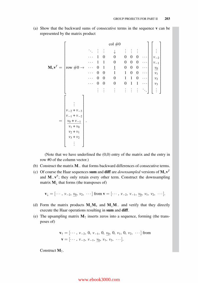
GROUP PROJECTS FOR PART II 203
(a) Show that the backward sums of consecutive terms in the sequence v can berepresented by the matrix product
M+vT =
⎡⎢⎢⎢⎢⎢⎢⎢⎢⎢⎢⎢⎢⎢⎢⎢⎣
col #0. . .
...... ↓
......
...· · · 1 0 0 0 0 0 · · ·· · · 1 1 0 0 0 0 · · ·
row #0 → · · · 0 1 1 0 0 0 · · ·· · · 0 0 1 1 0 0 · · ·· · · 0 0 0 1 1 0 · · ·· · · 0 0 0 0 1 1 · · ·
......
......
......
. . .
⎤⎥⎥⎥⎥⎥⎥⎥⎥⎥⎥⎥⎥⎥⎥⎥⎦
⎡⎢⎢⎢⎢⎢⎢⎢⎢⎢⎢⎢⎢⎢⎢⎢⎣
...v−2
v−1
v0
v1
v2
v3...
⎤⎥⎥⎥⎥⎥⎥⎥⎥⎥⎥⎥⎥⎥⎥⎥⎦
=
⎡⎢⎢⎢⎢⎢⎢⎢⎢⎢⎢⎢⎢⎢⎢⎢⎣
...v−2 + v−3
v−1 + v−2
v0 + v−1
v1 + v0
v2 + v1
v3 + v2...
⎤⎥⎥⎥⎥⎥⎥⎥⎥⎥⎥⎥⎥⎥⎥⎥⎦
.
(Note that we have underlined the (0,0) entry of the matrix and the entry inrow #0 of the column vector.)
(b) Construct the matrix M− that forms backward differences of consecutive terms.
(c) Of course the Haar sequences sum and diff are downsampled versions of M+vT
and M−vT ; they only retain every other term. Construct the downsamplingmatrix M↓ that forms (the transposes of)
v↓ = [· · · , v−2, v0, v2, · · · ] from v = [· · · , v−2, v−1, v0, v1, v2, · · · ].
(d) Form the matrix products M↓M+ and M↓M− and verify that they directlyexecute the Haar operations resulting in sum and diff.
(e) The upsampling matrix M↑ inserts zeros into a sequence, forming (the trans-poses of)
v↑ = [· · · , v−2, 0, v−1, 0, v0, 0, v1, 0, v2, · · · ] from
v = [· · · , v−2, v−1, v0, v1, v2, · · · ].
Construct M↑.
www.ebook3000.com

204 ORTHOGONALITY
(f) The left-shift matrix M← forms v← = [· · · , v−1, v0, v1, v2, v3, · · · ] fromv = [· · · , v−2, v−1, v0, v1, v2, · · · ]. Construct M←.
(g) An important property of the Haar transform is that it is easily inverted; thesequences sum+diff
2 and sum−diff2 , when properly interleaved, restore the original
sequence. Devise a combination of M↑, M←, sum+diff2 and sum−diff
2 , that equals v.Verify that the identity matrix results when M+, M−, M↑, and M← are properlycombined.
(h) In signal processing, the left-shift operation corresponds to a time advance andis physically impossible. Define the time delay matrix M→ and argue that acombination of M↑, M→, sum+diff
2 and sum−diff2 can be constructed to yield a
time-delayed version of the original sequence v.
PART III
INTRODUCTION: REFLECT ON THIS
A mirror passes through the origin of the x, y-plane. It reflects the unit vector [1 0]T
into the vector [0.8 0.6]T (Fig. III.1a), and the vector [0 1]T is reflected to [0.6 −0.8]T
(Fig. III.1b). Find a vector normal to the mirror.The specifications of this problem give us sufficient information to write down the
reflector matrix Mref (or simply M): since M[
10
]equals the first column of M and
M[
01
]equals the second,
M =
[0.8 0.60.6 −0.8
]. (1)
In this section our strategy for finding a normal to the mirror is based on the observationthat the mirror reflection of a normal n is –n:
Mn = −n (2)
(Fig. III.1c).Equation (2) can be rewritten, using the identity matrix I, as an equation for a null
vector of M + I:
Mn + n = (M + I)n = 0. (3)
Fundamentals of Matrix Analysis with Applications,First Edition. Edward Barry Saff and Arthur David Snider.© 2016 John Wiley & Sons, Inc. Published 2016 by John Wiley & Sons, Inc.
www.ebook3000.com
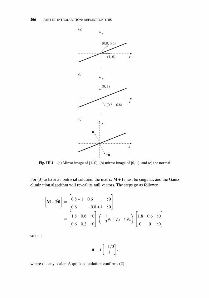
206 PART III INTRODUCTION: REFLECT ON THIS
y
x
(0.8, 0.6)
(1, 0)
(a)
x
(b)y
(0, 1)
(0.6, –0.8)
(c)y
x
–n
n
Fig. III.1 (a) Mirror image of [1, 0], (b) mirror image of [0, 1], and (c) the normal.
For (3) to have a nontrivial solution, the matrix M + I must be singular, and the Gausselimination algorithm will reveal its null vectors. The steps go as follows:
[M + I
...0]=
⎡⎣0.8 + 1 0.6
... 0
0.6 −0.8 + 1... 0
⎤⎦
=
⎡⎣1.8 0.6
... 0
0.6 0.2... 0
⎤⎦(−1
3ρ1 + ρ2 → ρ2
)⎡⎣1.8 0.6
... 0
0 0... 0
⎤⎦ ,
so that
n = t
[−1/3
1
],
where t is any scalar. A quick calculation confirms (2).
PART III INTRODUCTION: REFLECT ON THIS 207
In fact, insertion of the unit normal [−1, 3]T 1√10
into Equation (3) of Section 2.2reproduces the matrix M in (1), confirming that it is, indeed, a reflector operator.
Now we generalize. Whenever the direction of a vector is unchanged (or reversed)by a matrix multiplication, we say that the vector is an eigenvector of the matrix. Morespecifically, if v is an eigenvector, Mv is simply a scalar multiple of v:
Mv = rv, (4)
and the scalar r is called the eigenvalue corresponding to v. In (4), we allow the pos-sibility that the eigenvalue r can be negative or zero or even complex. But the zerovector, since it has no “direction,” is excluded from the family of eigenvectors, althoughit trivially satisfies (4) (for every scalar r). The mirror’s normal n is an eigenvectorcorresponding to the eigenvalue −1 because of Equation (2).
In fact, any vector parallel to the mirror in Figure III.1 is also an eigenvector, sinceit is unchanged by reflection; its eigenvalue is +1.
It is extremely profitable to know a matrix’s eigenvectors, mainly because an n-by-nmatrix—despite all its n2 pieces of data—simply acts like a scalar when multiplying aneigenvector, and this can be exploited in a myriad of applications (including differen-tial equations). In this chapter, we will examine the eigenvector–eigenvalue theory formatrices.
www.ebook3000.com

5EIGENVECTORS ANDEIGENVALUES
5.1 EIGENVECTOR BASICS
We formalize the deliberations of the introduction to Part III as follows:
Eigenvectors and Eigenvalues
Definition 1. Let A = [aij] be a square matrix. The eigenvalues of A are thosereal or complex numbers r for which the equation
Au = ru or, equivalently, (A − rI) u = 0, (1)
has at least one nontrivial (nonzero) solution u. The nontrivial solutions are calledthe eigenvectors of A associated with r.
We have seen that the vectors normal and parallel to a mirror are eigenvectors ofthe reflector matrix. The normal vectors share the eigenvalue −1 and form a one-dimensional subspace, and the vectors parallel to the mirror share the eigenvalue +1and also form a one-dimensional subspace (in two dimensions). (In three-dimensionalspace the vectors parallel to the mirror form, of course, a two-dimensional subspace.)
Here are some other examples of eigenvectors and eigenvalues.
(i) A matrix that performs a rotation in three-dimensional space has, as eigen-vectors, all vectors parallel to the axis of rotation (what is the eigenvalue?).
Fundamentals of Matrix Analysis with Applications,First Edition. Edward Barry Saff and Arthur David Snider.© 2016 John Wiley & Sons, Inc. Published 2016 by John Wiley & Sons, Inc.
www.ebook3000.com
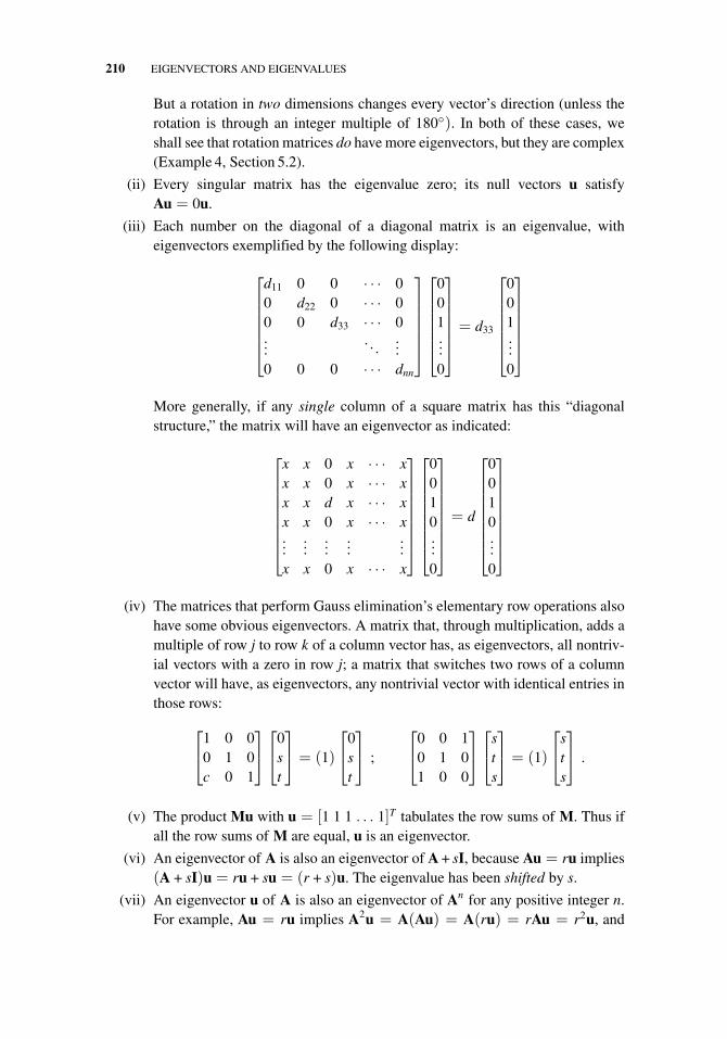
210 EIGENVECTORS AND EIGENVALUES
But a rotation in two dimensions changes every vector’s direction (unless therotation is through an integer multiple of 180◦). In both of these cases, weshall see that rotation matrices do have more eigenvectors, but they are complex(Example 4, Section 5.2).
(ii) Every singular matrix has the eigenvalue zero; its null vectors u satisfyAu = 0u.
(iii) Each number on the diagonal of a diagonal matrix is an eigenvalue, witheigenvectors exemplified by the following display:
⎡⎢⎢⎢⎢⎢⎣
d11 0 0 · · · 00 d22 0 · · · 00 0 d33 · · · 0...
. . ....
0 0 0 · · · dnn
⎤⎥⎥⎥⎥⎥⎦
⎡⎢⎢⎢⎢⎢⎣
001...0
⎤⎥⎥⎥⎥⎥⎦= d33
⎡⎢⎢⎢⎢⎢⎣
001...0
⎤⎥⎥⎥⎥⎥⎦
More generally, if any single column of a square matrix has this “diagonalstructure,” the matrix will have an eigenvector as indicated:
⎡⎢⎢⎢⎢⎢⎢⎢⎣
x x 0 x · · · xx x 0 x · · · xx x d x · · · xx x 0 x · · · x...
......
......
x x 0 x · · · x
⎤⎥⎥⎥⎥⎥⎥⎥⎦
⎡⎢⎢⎢⎢⎢⎢⎢⎣
0010...0
⎤⎥⎥⎥⎥⎥⎥⎥⎦= d
⎡⎢⎢⎢⎢⎢⎢⎢⎣
0010...0
⎤⎥⎥⎥⎥⎥⎥⎥⎦
(iv) The matrices that perform Gauss elimination’s elementary row operations alsohave some obvious eigenvectors. A matrix that, through multiplication, adds amultiple of row j to row k of a column vector has, as eigenvectors, all nontriv-ial vectors with a zero in row j; a matrix that switches two rows of a columnvector will have, as eigenvectors, any nontrivial vector with identical entries inthose rows:
⎡⎣1 0 0
0 1 0c 0 1
⎤⎦⎡⎣0
st
⎤⎦ = (1)
⎡⎣0
st
⎤⎦ ;
⎡⎣0 0 1
0 1 01 0 0
⎤⎦⎡⎣s
ts
⎤⎦ = (1)
⎡⎣s
ts
⎤⎦ .
(v) The product Mu with u = [1 1 1 . . . 1]T tabulates the row sums of M. Thus ifall the row sums of M are equal, u is an eigenvector.
(vi) An eigenvector of A is also an eigenvector of A + sI, because Au = ru implies(A + sI)u = ru + su = (r + s)u. The eigenvalue has been shifted by s.
(vii) An eigenvector u of A is also an eigenvector of An for any positive integer n.For example, Au = ru implies A2u = A(Au) = A(ru) = rAu = r2u, and
5.1 EIGENVECTOR BASICS 211
analogous calculations hold for An; the eigenvalue is rn. In fact if A is invertible,it follows easily that A−1u = r−1u; and u is an eigenvector of A−n also.
(viii) Similarly,
(anAn + an−1An−1 + · · · + a1A + a0I
)u =
(anrn + an−1rn−1 + · · · + a1r + a0
)u
for an eigenvector u. Thus for any polynomial p(t), u is an eigenvector of p(A)with eigenvalue p(r).
It is important to note that any (nonzero) multiple of an eigenvector is also an eigen-vector, with the same eigenvalue. (So eigenvectors are really “eigendirections,” but thisnomenclature has never caught on.) In fact if u1, u2, . . ., uk each satisfy Au = ru withthe same eigenvalue r, so does any linear combination:
A (c1u1 + c2u2 + · · · + ckuk) = c1Au1 + c2Au2 + · · · + ckAuk
= c1ru1 + c2ru2 + · · · + ckruk
= r (c1u1 + c2u2 + · · · + ckuk) .
Therefore the set of all eigenvectors with the same eigenvalue, together with thezero vector (which we have excluded as an “eigenvector”), form a subspace—an“eigenspace.”
On the other hand, eigenvectors with different eigenvalues are linearly independent.To see this, suppose that we have a collection of eigenvectors {ui}, each having a dis-tinct eigenvalue (ri). Choose any two; they will be independent, because if one werea multiple of the other they would have the same eigenvalue. Now keep adding, oneby one, more eigenvectors from the collection as long they are independent of the setalready accumulated, until you have a maximal independent set u1, u2, . . ., uk. If thereis one left over, uk+1, it would be linearly dependent on the set and expressible as
uk+1 = c1u1 + c2u2 + · · · + ckuk (2)
with not all the ci’s zero (since uk+1 is not the zero vector). But multiplication of (2) byA − rk+1I would yield
(rk+1 − rk+1) uk+1 = c1 (r1 − rk+1) u1 + c2 (r2 − rk+1) u2 + · · · + ck (rk − rk+1) uk. (3)
Since (3) displays a nontrivial linear combination of u1 through uk that equals 0, thepostulated independence of u1 through uk would be contradicted. We summarize ourfindings in the following theorems.
www.ebook3000.com
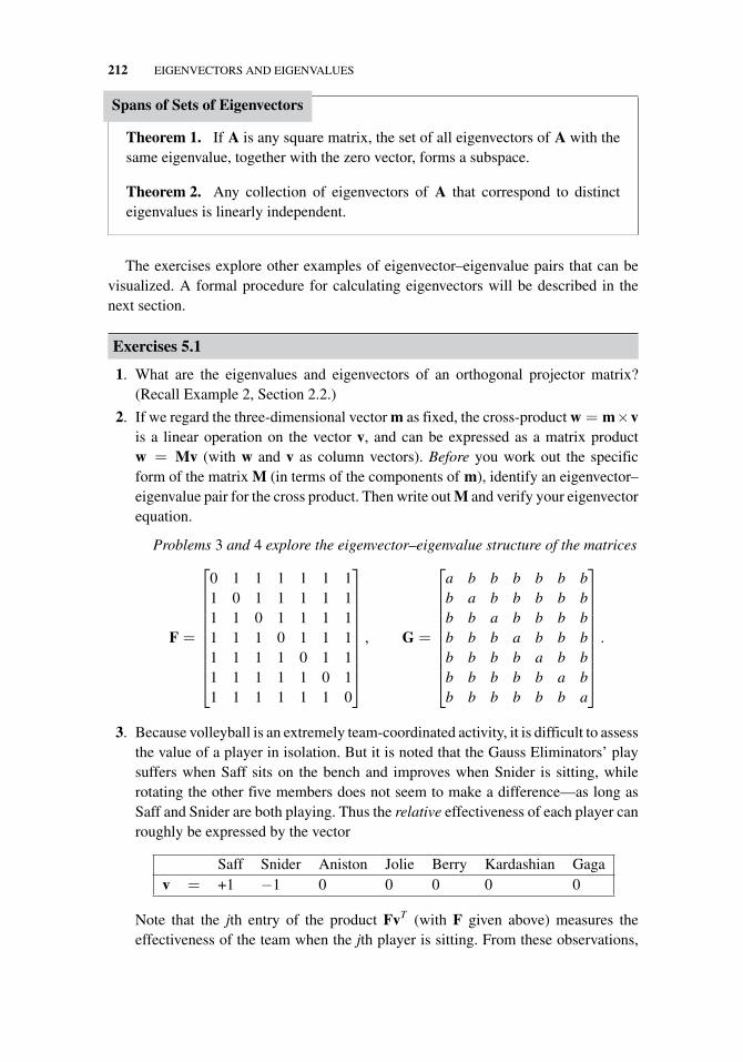
212 EIGENVECTORS AND EIGENVALUES
Spans of Sets of Eigenvectors
Theorem 1. If A is any square matrix, the set of all eigenvectors of A with thesame eigenvalue, together with the zero vector, forms a subspace.
Theorem 2. Any collection of eigenvectors of A that correspond to distincteigenvalues is linearly independent.
The exercises explore other examples of eigenvector–eigenvalue pairs that can bevisualized. A formal procedure for calculating eigenvectors will be described in thenext section.
Exercises 5.1
1. What are the eigenvalues and eigenvectors of an orthogonal projector matrix?(Recall Example 2, Section 2.2.)
2. If we regard the three-dimensional vector m as fixed, the cross-product w = m×vis a linear operation on the vector v, and can be expressed as a matrix productw = Mv (with w and v as column vectors). Before you work out the specificform of the matrix M (in terms of the components of m), identify an eigenvector–eigenvalue pair for the cross product. Then write out M and verify your eigenvectorequation.
Problems 3 and 4 explore the eigenvector–eigenvalue structure of the matrices
F =
⎡⎢⎢⎢⎢⎢⎢⎢⎢⎢⎣
0 1 1 1 1 1 11 0 1 1 1 1 11 1 0 1 1 1 11 1 1 0 1 1 11 1 1 1 0 1 11 1 1 1 1 0 11 1 1 1 1 1 0
⎤⎥⎥⎥⎥⎥⎥⎥⎥⎥⎦
, G =
⎡⎢⎢⎢⎢⎢⎢⎢⎢⎢⎣
a b b b b b bb a b b b b bb b a b b b bb b b a b b bb b b b a b bb b b b b a bb b b b b b a
⎤⎥⎥⎥⎥⎥⎥⎥⎥⎥⎦
.
3. Because volleyball is an extremely team-coordinated activity, it is difficult to assessthe value of a player in isolation. But it is noted that the Gauss Eliminators’ playsuffers when Saff sits on the bench and improves when Snider is sitting, whilerotating the other five members does not seem to make a difference—as long asSaff and Snider are both playing. Thus the relative effectiveness of each player canroughly be expressed by the vector
Saff Snider Aniston Jolie Berry Kardashian Gagav = +1 −1 0 0 0 0 0
Note that the jth entry of the product FvT (with F given above) measures theeffectiveness of the team when the jth player is sitting. From these observations,
5.1 EIGENVECTOR BASICS 213
construct six linearly independent eigenvectors of F with the eigenvalue −1. Whatis the remaining eigenvalue (and a corresponding eigenvector)?
4. What are the eigenvectors and eigenvalues of G? [Hint: Express G in terms of Fand I.]
5. What are the eigenvectors of the Gauss-elimination matrix that multiplies one rowof a matrix vector by a constant?
6. In this problem you will prove that all of the diagonal entries of a triangular matrixare eigenvalues. To fix our ideas let’s look at the 4-by-4 upper triangular case:
U =
⎡⎢⎢⎣
u11 u12 u13 u14
0 u22 u23 u24
0 0 u33 u34
0 0 0 u44
⎤⎥⎥⎦
(a) Find an eigenvector with u11 as eigenvalue. [Hint: This is easy; look for aneigenvector with only one nonzero entry.]
(b) Try to find an eigenvector corresponding to u22, of the form v =[x 1 0 0]T . Show that the equation Uv = u22v only requires u11x + u12 =u22x, or x = u12/(u22 − u11) if u22 �= u11. And if u22 does equal u11, we havealready proved it is an eigenvalue.
(c) Show that if u33 is not a duplicate of one of the earlier diagonal entries, then ithas an eigenvector of the form [x y 1 0]. And so on.
7. Following the strategy of the preceding problem, show that
U =
⎡⎢⎢⎣
1 1 1 10 2 α 10 0 2 10 0 0 4
⎤⎥⎥⎦
has an eigenvector corresponding to the eigenvalue 2, of the form [x 1 0 0]T ;but it only has an eigenvector of the form [y z 1 0]T if α = 0.
The entries of the complex vector u4 = [i − 1 − i 1]T , depicted inFigure 5.1, are the 4th roots of unity, 4
√1. If they are regarded cyclically counter-
clockwise (so that i “follows” 1), they have some properties that can be expressedas eigenvector equations. Refer to Figure 5.1 to assist in answering Problems 8–11.
8. From Figure 5.1, note that each root equals i times the previous root. Interpret thisas an eigenvector statement for the matrix
A =
⎡⎢⎢⎣
0 1 0 00 0 1 00 0 0 11 0 0 0
⎤⎥⎥⎦ .
www.ebook3000.com
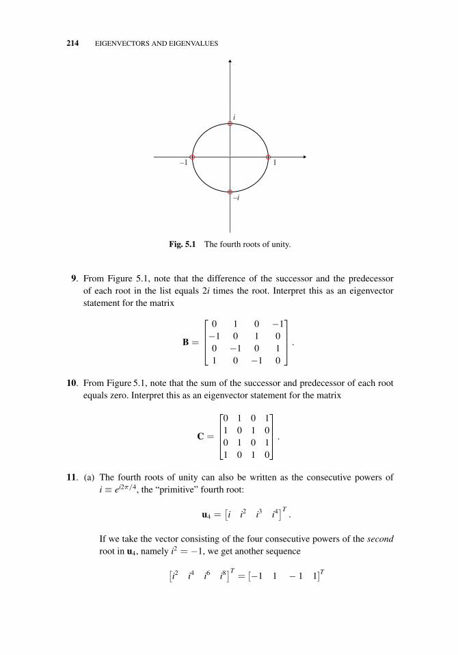
214 EIGENVECTORS AND EIGENVALUES
1–1
i
–i
Fig. 5.1 The fourth roots of unity.
9. From Figure 5.1, note that the difference of the successor and the predecessorof each root in the list equals 2i times the root. Interpret this as an eigenvectorstatement for the matrix
B =
⎡⎢⎢⎣
0 1 0 −1−1 0 1 00 −1 0 11 0 −1 0
⎤⎥⎥⎦ .
10. From Figure 5.1, note that the sum of the successor and predecessor of each rootequals zero. Interpret this as an eigenvector statement for the matrix
C =
⎡⎢⎢⎣
0 1 0 11 0 1 00 1 0 11 0 1 0
⎤⎥⎥⎦ .
11. (a) The fourth roots of unity can also be written as the consecutive powers ofi ≡ ei2π/4, the “primitive” fourth root:
u4 =[i i2 i3 i4
]T.
If we take the vector consisting of the four consecutive powers of the secondroot in u4, namely i2 = −1, we get another sequence
[i2 i4 i6 i8
]T= [−1 1 − 1 1]T
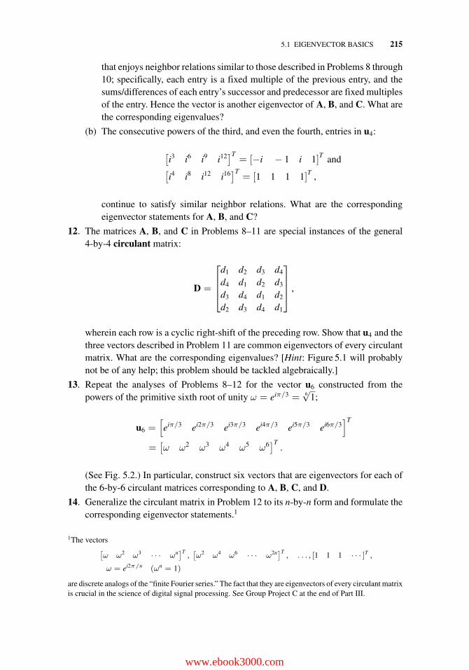
5.1 EIGENVECTOR BASICS 215
that enjoys neighbor relations similar to those described in Problems 8 through10; specifically, each entry is a fixed multiple of the previous entry, and thesums/differences of each entry’s successor and predecessor are fixed multiplesof the entry. Hence the vector is another eigenvector of A, B, and C. What arethe corresponding eigenvalues?
(b) The consecutive powers of the third, and even the fourth, entries in u4:
[i3 i6 i9 i12
]T= [−i − 1 i 1]T and[
i4 i8 i12 i16]T
= [1 1 1 1]T ,
continue to satisfy similar neighbor relations. What are the correspondingeigenvector statements for A, B, and C?
12. The matrices A, B, and C in Problems 8–11 are special instances of the general4-by-4 circulant matrix:
D =
⎡⎢⎢⎣
d1 d2 d3 d4
d4 d1 d2 d3
d3 d4 d1 d2
d2 d3 d4 d1
⎤⎥⎥⎦ ,
wherein each row is a cyclic right-shift of the preceding row. Show that u4 and thethree vectors described in Problem 11 are common eigenvectors of every circulantmatrix. What are the corresponding eigenvalues? [Hint: Figure 5.1 will probablynot be of any help; this problem should be tackled algebraically.]
13. Repeat the analyses of Problems 8–12 for the vector u6 constructed from thepowers of the primitive sixth root of unity ω = eiπ/3 = 6
√1;
u6 =[eiπ/3 ei2π/3 ei3π/3 ei4π/3 ei5π/3 ei6π/3
]T
=[ω ω2 ω3 ω4 ω5 ω6
]T.
(See Fig. 5.2.) In particular, construct six vectors that are eigenvectors for each ofthe 6-by-6 circulant matrices corresponding to A, B, C, and D.
14. Generalize the circulant matrix in Problem 12 to its n-by-n form and formulate thecorresponding eigenvector statements.1
1The vectors[ω ω2 ω3 · · · ωn
]T ,[ω2 ω4 ω6 · · · ω2n
]T , . . . , [1 1 1 · · · ]T ,
ω = ei2π/n (ωn = 1)
are discrete analogs of the “finite Fourier series.” The fact that they are eigenvectors of every circulant matrixis crucial in the science of digital signal processing. See Group Project C at the end of Part III.
www.ebook3000.com
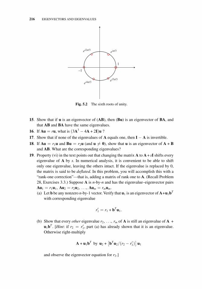
216 EIGENVECTORS AND EIGENVALUES
eiπ/3
ei5π/3
1
–1
ei4π/3
ei2π/3
Fig. 5.2 The sixth roots of unity.
15. Show that if u is an eigenvector of (AB), then (Bu) is an eigenvector of BA, andthat AB and BA have the same eigenvalues.
16. If Au = ru, what is (3A3 − 4A + 2I)u ?
17. Show that if none of the eigenvalues of A equals one, then I − A is invertible.
18. If Au = r1u and Bu = r2u (and u �= 0), show that u is an eigenvector of A + Band AB. What are the corresponding eigenvalues?
19. Property (vi) in the text points out that changing the matrix A to A + sI shifts everyeigenvalue of A by s. In numerical analysis, it is convenient to be able to shiftonly one eigenvalue, leaving the others intact. If the eigenvalue is replaced by 0,the matrix is said to be deflated. In this problem, you will accomplish this with a“rank-one correction”—that is, adding a matrix of rank one to A. (Recall Problem28, Exercises 3.3.) Suppose A is n-by-n and has the eigenvalue–eigenvector pairsAu1 = r1u1, Au2 = r2u2, . . ., Aum = rmum.(a) Let b be any nonzero n-by-1 vector. Verify that u1 is an eigenvector of A+u1bT
with corresponding eigenvalue
r′1 = r1 + bTu1.
(b) Show that every other eigenvalue r2, . . ., rm of A is still an eigenvalue of A +u1bT . [Hint: if r2 = r′1, part (a) has already shown that it is an eigenvalue.Otherwise right-multiply
A + u1bT by u2 +[bTu2/(r2 − r′1)
]u1
and observe the eigenvector equation for r2.]
5.2 CALCULATING EIGENVALUES AND EIGENVECTORS 217
20. Show that every n-by-n matrix having u as an eigenvector with r as the correspond-ing eigenvalue can be constructed by assembling n vectors orthogonal to u into therows of a matrix, and adding r to each diagonal entry.
5.2 CALCULATING EIGENVALUES ANDEIGENVECTORS
How can we find eigenvalues and eigenvectors? The complete story2 is contained inthe relation [A − rI]u = 0:
(i) the eigenvalue r must be a number that renders A − rI singular—that is,det(A − rI) = 0;
(ii) with r specified, the eigenvectors u are found by solving [A− rI]u = 0 throughGauss elimination.
As seen from the cofactor expansion theorem (Theorem 5 of Section 2.4), the deter-minant of a matrix is a sum/difference of terms that are products of its entries, exactlyone from each row and column. So for an n-by-n matrix A, the term containing thehighest number of occurrences of the parameter r in det(A − rI) is the product of thediagonal entries, generating (−r)n. Therefore, det(A−rI) is an nth degree polynomialin r, and finding the eigenvalues of a matrix is equivalent to finding the zeros of itscharacteristic polynomial p(r),
p(r) := det(A − rI) = (−r)n + cn−1rn−1 + · · · + c0
= (−1)n(r − r1) · · · (r − rn). (1)
The equation p(r) = 0 known as the characteristic equation of A.Problem 6 in Exercises 5.1 argued that the eigenvalues of a triangular matrix are its
diagonal entries. This is readily confirmed by observing the characteristic polynomial.For an upper triangular matrix,
det
⎡⎢⎢⎢⎣
a11 − r a12 a13 . . . a1n
0 a22 − r a23 . . . a2n...
0 0 0 ann − r
⎤⎥⎥⎥⎦ = (a11 − r) (a22 − r) . . . (ann − r) .
The following examples of eigenvector calculations illustrate the basic procedureand the complications that result when the characteristic equation has complex ormultiple roots.
2Section 6.5 addresses some important practical computational issues.
www.ebook3000.com
218 EIGENVECTORS AND EIGENVALUES
Example 1. Find the eigenvalues and eigenvectors of the matrix
A :=
[2 1−3 −2
].
Solution. The characteristic equation for A is
|A − rI| =[
2 − r 1−3 −2 − r
]= (2 − r)(−2 − r) + 3 = r2 − 1 = 0 .
Hence the eigenvalues of A are r1 = 1, r2 = −1. To find the eigenvectors corre-sponding to r1 = 1, we must solve (A − r1I)u = 0. Substituting for A and r1
gives
[1 1−3 −3
] [u1
u2
]=
[00
]. (2)
Gauss elimination (or mental arithmetic) shows the solutions to (2) are given by u2 = s,u1 = −s. Consequently, the eigenvectors associated with r1 = 1 can be expressed as
u1 = s
[−11
]. (3)
For r2 = −1, the equation (A − r2I)u = 0 becomes
[3 1−3 −1
] [u1
u2
]=
[00
].
Solving, we obtain u1 = −t and u2 = 3t, with t arbitrary. Therefore, the eigenvectorsassociated with the eigenvalue r2 = −1 are
u2 = t
[−13
]. (4)
�
Example 2. Find the eigenvalues and eigenvectors of the matrix
A :=
⎡⎣1 2 −1
1 0 14 −4 5
⎤⎦ .
5.2 CALCULATING EIGENVALUES AND EIGENVECTORS 219
Solution. The characteristic equation for A is
|A − rI| =
⎡⎣1 − r 2 −1
1 −r 14 −4 5 − r
⎤⎦ = 0,
which simplifies to (r− 1)(r− 2)(r− 3) = 0. Hence, the eigenvalues of A are r1 = 1,r2 = 2, and r3 = 3. To find the eigenvectors corresponding to r1 = 1, we set r = 1 in(A − rI)u = 0. This gives
⎡⎣0 2 −1
1 −1 14 −4 4
⎤⎦⎡⎣u1
u2
u3
⎤⎦ =
⎡⎣0
00
⎤⎦ . (5)
Gauss elimination readily provides a parametrization of the solution set for (5).However the system is so transparent that, again, mental arithmetic suffices. The thirdequation is clearly redundant since it’s a multiple of the second equation. And forwardsubstitution reveals the solutions to the first two equations to be
u2 = s,
u3 = 2s, u1 = −s.
Hence, the eigenvectors associated with r1 = 1 are
u1 = s
⎡⎣−1
12
⎤⎦ . (6)
For r2 = 2 we solve
⎡⎣−1 2 −1
1 −2 14 −4 3
⎤⎦
⎡⎣u1
u2
u3
⎤⎦ =
⎡⎣0
00
⎤⎦
in a similar fashion to obtain the eigenvectors
u2 = s
⎡⎣−2
14
⎤⎦ . (7)
Finally, for r3 = 3 we solve
⎡⎣−2 2 −1
1 −3 14 −4 2
⎤⎦
⎡⎣u1
u2
u3
⎤⎦ =
⎡⎣0
00
⎤⎦
www.ebook3000.com
220 EIGENVECTORS AND EIGENVALUES
and get the eigenvectors
u3 = s
⎡⎣−1
14
⎤⎦ . (8)
�
Example 3. Find the eigenvalues and eigenvectors for
A =
⎡⎣1 2 0
0 1 −22 2 −1
⎤⎦ .
Solution. The characteristic equation,
|A − rI| =
∣∣∣∣∣∣1 − r 2 0
0 1 − r −22 2 −1 − r
∣∣∣∣∣∣ = −r3 + r2 − 3r − 5 = 0,
simplifies to
(r + 1)(r2 − 2r + 5
)= (r + 1)(r − [1 + 2i])(r − [1 − 2i]) = 0.
Thus the eigenvectors satisfy (A− rI)u = 0 for each of the eigenvalues −1, 1 + 2i, and1 − 2i:
⎡⎣1 − (−1) 2 0
0 1 − (−1) −22 2 −1 − (−1)
⎤⎦⎡⎣u1
u2
u3
⎤⎦ =
⎡⎣0
00
⎤⎦ ,
⎡⎣1 − (1 + 2i) 2 0
0 1 − (1 + 2i) −22 2 −1 − (1 + 2i)
⎤⎦⎡⎣u1
u2
u3
⎤⎦ =
⎡⎣0
00
⎤⎦,
⎡⎣1 − (1 − 2i) 2 0
0 1 − (1 − 2i) −22 2 −1 − (1 − 2i)
⎤⎦⎡⎣u1
u2
u3
⎤⎦ =
⎡⎣0
00
⎤⎦.
The first system has solutions t[−1 1 1]T . The second and third systems havecoefficient matrices that are complex conjugates of each other, and Gauss elimina-tion (with complex numbers) produces the conjugate solutions t[1 (±i) 1]T . Quickmental calculation confirms that
5.2 CALCULATING EIGENVALUES AND EIGENVECTORS 221
⎡⎣1 2 0
0 1 −22 2 −1
⎤⎦⎡⎣−1
11
⎤⎦ = (−1)
⎡⎣−1
11
⎤⎦ ,
⎡⎣1 2 0
0 1 −22 2 −1
⎤⎦⎡⎣1
i1
⎤⎦ = (1 + 2i)
⎡⎣1
i1
⎤⎦,
⎡⎣1 2 0
0 1 −22 2 −1
⎤⎦⎡⎣ 1−i1
⎤⎦ = (1 − 2i)
⎡⎣ 1−i1
⎤⎦ . �
Example 4. Find the eigenvalues and eigenvectors for the rotation matrices
A =
[cos θ − sin θsin θ cos θ
]and B =
⎡⎣0 0 1
1 0 00 1 0
⎤⎦
Solution. The form of the two-dimensional rotation matrix A was derived in Example 1of Section 2.2. Its characteristic equation,
|A − rI| =∣∣∣∣cos θ − r − sin θsin θ cos θ − r
∣∣∣∣ = (cos θ − r)2 + sin2 θ = r2 − 2r cos θ + 1 = 0,
has the roots
r =2 cos θ ±
√4 cos2 θ − 42
= cos θ ± i sin θ = e±iθ,
which are complex unless θ = 0 or π (in which case A = ±I). Complex eigenvectorscorresponding to e±iθ are easily seen to be [1 ∓ i]T .
In Figure 5.3, the matrix B takes the position vector [x y z]T into [z x y]T ; itcycles the axes (x → y → z → x), and thus it is a rotation about the direction makingequal angles with the axes: namely, [1 1 1]T . The characteristic equation,
|B − rI| =
∣∣∣∣∣∣−r 0 11 −r 00 1 −r
∣∣∣∣∣∣ = (−r)3 + 1 = 0,
shows that the eigenvalues are the cube roots of unity: namely, r1 = 1, r2 = ei2π/3,and r3 = e−i2π/3. The direction of the axis of rotation [1 1 1]T is easily seen tobe an eigenvector corresponding to r1 = 1, as predicted in Section 5.1. The complexeigenvectors are of little interest to us at this point. �
The next example demonstrates some curious aberrations that we will explore laterin this book.
www.ebook3000.com
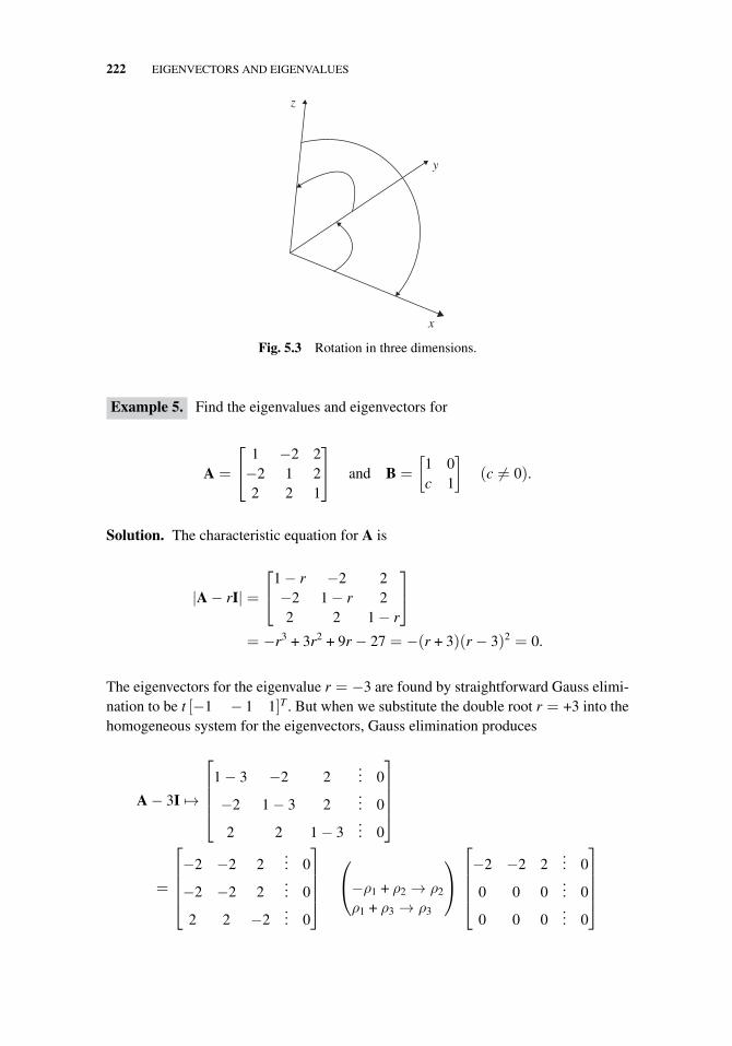
222 EIGENVECTORS AND EIGENVALUES
z
y
x
Fig. 5.3 Rotation in three dimensions.
Example 5. Find the eigenvalues and eigenvectors for
A =
⎡⎣ 1 −2 2−2 1 22 2 1
⎤⎦ and B =
[1 0c 1
](c �= 0).
Solution. The characteristic equation for A is
|A − rI| =
⎡⎣1 − r −2 2
−2 1 − r 22 2 1 − r
⎤⎦
= −r3 + 3r2 + 9r − 27 = −(r + 3)(r − 3)2 = 0.
The eigenvectors for the eigenvalue r = −3 are found by straightforward Gauss elimi-nation to be t [−1 − 1 1]T . But when we substitute the double root r = +3 into thehomogeneous system for the eigenvectors, Gauss elimination produces
A − 3I �→
⎡⎢⎢⎢⎣
1 − 3 −2 2... 0
−2 1 − 3 2... 0
2 2 1 − 3... 0
⎤⎥⎥⎥⎦
=
⎡⎢⎢⎢⎣−2 −2 2
... 0
−2 −2 2... 0
2 2 −2... 0
⎤⎥⎥⎥⎦
⎛⎝−ρ1 + ρ2 → ρ2
ρ1 + ρ3 → ρ3
⎞⎠
⎡⎢⎢⎢⎣−2 −2 2
... 0
0 0 0... 0
0 0 0... 0
⎤⎥⎥⎥⎦
5.2 CALCULATING EIGENVALUES AND EIGENVECTORS 223
indicating that the double eigenvalue has a two-dimensional eigenspace,
t1
⎡⎣1
01
⎤⎦ + t2
⎡⎣−1
10
⎤⎦ .
For B the characteristic equation also has a double root:
|B − rI| =[
1 − r 0c 1 − r
]= (1 − r)2, (9)
but its eigenspace is only one-dimensional:
B − (1)I �→
⎡⎣1 − 1 0
... 0
c 1 − 1... 0
⎤⎦ ρ1 ↔ ρ2
⎡⎣c 0
... 0
0 0... 0
⎤⎦
has t[0 1]T as its only solutions.3 �
To obtain some perspective for our further study, let’s summarize the observationswe have made so far.
• Every n-by-n matrix has at least one and at most n (possibly complex) eigenvalues.Why? Because they are the roots of a polynomial of degree n (the characteristicpolynomial, Equation (1)).
• Every eigenvalue has at least one eigenvector—or, better, at least a one-dimensional eigenspace. Why? Because the eigenvectors are solutions of asingular, homogeneous system.
• If an eigenvalue of a real matrix is real, its eigenvectors can be taken to be realas well. Why? Because they can be computed using the Gauss elimination algo-rithm (which does not need complex numbers to reduce a real matrix). (Since anynonzero multiple of an eigenvector is also an eigenvector, we could (maliciously)make a real eigenvector complex by multiplying it by i (or any other complexnumber); the eigenvalue, though, would remain real.)
• Multiple (repeated) eigenvalues may, or may not, have eigenspaces of dimensionhigher than one.
• Eigenvectors corresponding to distinct eigenvalues are linearly independent. Thusif there are no multiple eigenvalues, we can create a full basis of n eigenvectors—one for each eigenvalue. Or, if each multiple eigenvalue has an eigenspace whose
3Did you recognize B as an elementary row operator matrix?
www.ebook3000.com
224 EIGENVECTORS AND EIGENVALUES
dimension is equal to its multiplicity (as a root of the characteristic equation),again we can create a basis of eigenvectors.
• The eigenvalues of a triangular matrix are its diagonal entries.
We will show later that real, symmetric matrices have only real eigenvalues, andeach multiple eigenvalue has its “full set” of eigenvectors—that is, the dimension ofits eigenspace equals the multiplicity of the eigenvalue. But if a matrix is defective,not having a full set of eigenvectors for each eigenvalue, we will see that we haveto settle for a basis consisting partially of eigenvectors, and partially of generalizedeigenvectors satisfying a “watered-down” version of the eigenvector equation (namely,(A − rI)ku = 0 for some k > 1).
Exercises 5.2
The matrices in Problems 1 through 8 have distinct eigenvalues. Find these eigenvaluesand corresponding eigenvectors.
1.
[9 −3−2 4
]2.
[−1 −34 7
]3.
[1 −2−2 1
]4.
[−3 2−5 4
]5.
[1 11 1
]
6.
⎡⎣1 0 2
3 4 20 0 0
⎤⎦ 7.
⎡⎣4 −1 −2
2 1 −21 −1 1
⎤⎦ 8.
⎡⎣ 2 −1 −1−1 3 0−1 0 3
⎤⎦
The matrices in Problems 9–12 have complex eigenvalues. Find the eigenvalues andeigenvectors.
9.
[0 −11 0
]10.
[0 1
−1 + i −1
]11.
[1 2i−1 3 + i
]12.
⎡⎣−6 2 16−3 1 11−3 1 7
⎤⎦
The matrices in Problems 13–20 have multiple eigenvalues. Some are defective. Findthe eigenvalues and eigenvectors.
13.
[10 −44 2
]14.
[1 −11 3
]15.
[3 2−2 7
]16.
[0 −ii 2i
]
17.
⎡⎣0 1 1
1 0 11 1 0
⎤⎦ 18.
⎡⎣ 1 2 6−1 4 6−1 2 8
⎤⎦ 19.
⎡⎣1 0 0
0 2 31 0 2
⎤⎦ 20.
⎡⎣ 1 2 2
2 4 3−2 −1 0
⎤⎦
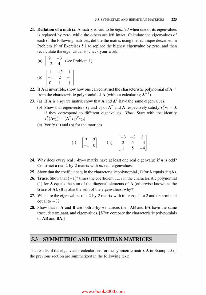
5.3 SYMMETRIC AND HERMITIAN MATRICES 225
21. Deflation of a matrix. A matrix is said to be deflated when one of its eigenvaluesis replaced by zero, while the others are left intact. Calculate the eigenvalues ofeach of the following matrices, deflate the matrix using the technique described inProblem 19 of Exercises 5.1 to replace the highest eigenvalue by zero, and thenrecalculate the eigenvalues to check your work.
(a)
[9 −3−2 4
](see Problem 1)
(b)
⎡⎣ 1 −2 1−1 2 −10 1 1
⎤⎦
22. If A is invertible, show how one can construct the characteristic polynomial of A−1
from the characteristic polynomial of A (without calculating A−1).
23. (a) If A is a square matrix show that A and AT have the same eigenvalues.
(b) Show that eigenvectors v1 and v2 of AT and A respectively satisfy vT2 v1 = 0,
if they correspond to different eigenvalues. [Hint: Start with the identityvT
1 (Av2) = (ATv1)Tv2.]
(c) Verify (a) and (b) for the matrices
(i)
[3 2−1 0
](ii)
⎡⎣−3 −2 2
2 5 −41 5 −4
⎤⎦ .
24. Why does every real n-by-n matrix have at least one real eigenvalue if n is odd?Construct a real 2-by-2 matrix with no real eigenvalues.
25. Show that the coefficient c0 in the characteristic polynomial (1) for A equals det(A).
26. Trace. Show that (−1)n times the coefficient cn−1 in the characteristic polynomial(1) for A equals the sum of the diagonal elements of A (otherwise known as thetrace of A). (It is also the sum of the eigenvalues; why?)
27. What are the eigenvalues of a 2-by-2 matrix with trace equal to 2 and determinantequal to −8?
28. Show that if A and B are both n-by-n matrices then AB and BA have the sametrace, determinant, and eigenvalues. [Hint: compare the characteristic polynomialsof AB and BA.]
5.3 SYMMETRIC AND HERMITIAN MATRICES
The results of the eigenvector calculations for the symmetric matrix A in Example 5 ofthe previous section are summarized in the following text:
www.ebook3000.com
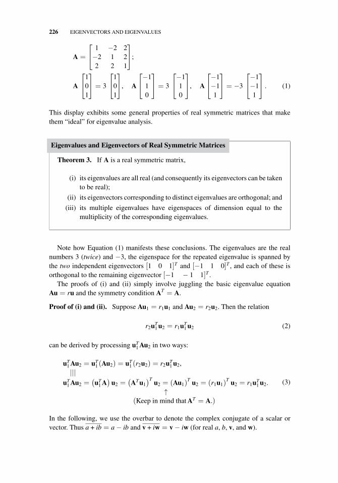
226 EIGENVECTORS AND EIGENVALUES
A =
⎡⎣ 1 −2 2−2 1 22 2 1
⎤⎦;
A
⎡⎣1
01
⎤⎦ = 3
⎡⎣1
01
⎤⎦, A
⎡⎣−1
10
⎤⎦ = 3
⎡⎣−1
10
⎤⎦, A
⎡⎣−1−11
⎤⎦ = −3
⎡⎣−1−11
⎤⎦ . (1)
This display exhibits some general properties of real symmetric matrices that makethem “ideal” for eigenvalue analysis.
Eigenvalues and Eigenvectors of Real Symmetric Matrices
Theorem 3. If A is a real symmetric matrix,
(i) its eigenvalues are all real (and consequently its eigenvectors can be takento be real);
(ii) its eigenvectors corresponding to distinct eigenvalues are orthogonal; and
(iii) its multiple eigenvalues have eigenspaces of dimension equal to themultiplicity of the corresponding eigenvalues.
Note how Equation (1) manifests these conclusions. The eigenvalues are the realnumbers 3 (twice) and −3, the eigenspace for the repeated eigenvalue is spanned bythe two independent eigenvectors [1 0 1]T and [−1 1 0]T , and each of these isorthogonal to the remaining eigenvector [−1 − 1 1]T .
The proofs of (i) and (ii) simply involve juggling the basic eigenvalue equationAu = ru and the symmetry condition AT = A.
Proof of (i) and (ii). Suppose Au1 = r1u1 and Au2 = r2u2. Then the relation
r2uT1 u2 = r1uT
1 u2 (2)
can be derived by processing uT1 Au2 in two ways:
uT1 Au2 = uT
1 (Au2) = uT1 (r2u2) = r2uT
1 u2,|||
uT1 Au2 =
(uT
1 A)
u2 =(ATu1
)Tu2 = (Au1)
T u2 = (r1u1)T u2 = r1uT
1 u2.↑
(Keep in mind that AT = A.)
(3)
In the following, we use the overbar to denote the complex conjugate of a scalar orvector. Thus a + ib = a − ib and v + iw = v − iw (for real a, b, v, and w).
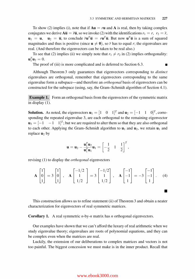
5.3 SYMMETRIC AND HERMITIAN MATRICES 227
To show (2) implies (i), note that if Au = ru and A is real, then by taking complexconjugates we derive Au = ru, so we invoke (2) with the identifications r1 = r, r2 = r,u1 = u, u2 = u, to conclude ruTu = ruTu. But now uTu is a sum of squaredmagnitudes and thus is positive (since u �= 0), so r has to equal r; the eigenvalues arereal. (And therefore the eigenvectors can be taken to be real also.)
To see that (2) implies (ii) we simply note that r1 �= r2 in (2) implies orthogonality:uT
1 u2 = 0.The proof of (iii) is more complicated and is deferred to Section 6.3.
Although Theorem 3 only guarantees that eigenvectors corresponding to distincteigenvalues are orthogonal, remember that eigenvectors corresponding to the sameeigenvalue form a subspace—and therefore an orthogonal basis of eigenvectors can beconstructed for the subspace (using, say, the Gram–Schmidt algorithm of Section 4.1).
Example 1. Form an orthogonal basis from the eigenvectors of the symmetric matrixin display (1).
Solution. As noted, the eigenvectors u1 = [1 0 1]T and u2 = [−1 1 0]T , corre-sponding the repeated eigenvalue 3, are each orthogonal to the remaining eigenvectoru3 = [−1 −1 1]T ; but we are required to alter them so that they are also orthogonalto each other. Applying the Gram–Schmidt algorithm to u1 and u2, we retain u1 andreplace u2 by
u = u2 −uT
1 u2
uT1 u1
u1 =
[−1
21
12
]T
,
revising (1) to display the orthogonal eigenvectors
A
⎡⎣1
01
⎤⎦ = 3
⎡⎣1
01
⎤⎦ , A
⎡⎣−1/2
11/2
⎤⎦ = 3
⎡⎣−1/2
11/2
⎤⎦ , A
⎡⎣−1−11
⎤⎦ = −3
⎡⎣−1−11
⎤⎦ . (4)
�
This construction allows us to refine statement (ii) of Theorem 3 and obtain a neatercharacterization for eigenvectors of real symmetric matrices.
Corollary 1. A real symmetric n-by-n matrix has n orthogonal eigenvectors.
Our examples have shown that we can’t afford the luxury of real arithmetic when westudy eigenvalue theory; eigenvalues are roots of polynomial equations, and they canbe complex even when the matrices are real.
Luckily, the extension of our deliberations to complex matrices and vectors is nottoo painful. The biggest concession we must make is in the inner product. Recall that
www.ebook3000.com
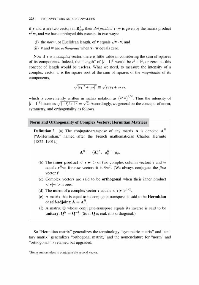
228 EIGENVECTORS AND EIGENVALUES
if v and w are two vectors in R3col, their dot product v ·w is given by the matrix product
vTw, and we have employed this concept in two ways:
(i) the norm, or Euclidean length, of v equals√
v · v, and
(ii) v and w are orthogonal when v · w equals zero.
Now if v is a complex vector, there is little value in considering the sum of squaresof its components. Indeed, the “length” of [i 1]T would be i2 + 12, or zero; so thisconcept of length would be useless. What we need, to measure the intensity of acomplex vector v, is the square root of the sum of squares of the magnitudes of itscomponents,
√|v1|2 + |v2|2 ≡
√v1 v1 + v2 v2,
which is conveniently written in matrix notation as(vTv
)1/2. Thus the intensity of
[i 1]T becomes√(−i)i + 12 =
√2. Accordingly, we generalize the concepts of norm,
symmetry, and orthogonality as follows.
Norm and Orthogonality of Complex Vectors; Hermitian Matrices
Definition 2. (a) The conjugate-transpose of any matrix A is denoted AH
[“A-Hermitian,” named after the French mathematician Charles Hermite(1822–1901).]
AH := (A)T , aHij = aji.
(b) The inner product < v|w > of two complex column vectors v and wequals vHw; for row vectors it is vwT . (We always conjugate the firstvector.)4
(c) Complex vectors are said to be orthogonal when their inner product< v|w > is zero.
(d) The norm of a complex vector v equals < v|v >1/2.
(e) A matrix that is equal to its conjugate-transpose is said to be Hermitianor self-adjoint: A = AH .
(f) A matrix Q whose conjugate-transpose equals its inverse is said to beunitary: QH = Q−1. (So if Q is real, it is orthogonal.)
So “Hermitian matrix” generalizes the terminology “symmetric matrix” and “uni-tary matrix” generalizes “orthogonal matrix,” and the nomenclature for “norm” and“orthogonal” is retained but upgraded.
4Some authors elect to conjugate the second vector.
5.3 SYMMETRIC AND HERMITIAN MATRICES 229
The rule for rearranging factors when taking conjugate-transposes is quite pre-dictable:
(ABC)H = (ABC)T= (A B C)T = C
TB
TA
T= CHBHAH , (5)
and it follows as usual that the product of unitary matrices is unitary:
(Q1Q2Q3)−1 = Q−1
3 Q−12 Q−1
1 = QH3 QH
2 QH1 = (Q1Q2Q3)
H . (6)
The proof of Theorem 3, asserting that eigenvectors corresponding to distinct eigen-values of a symmetric matrix are orthogonal, is easily extended to the Hermitian case.The basic equality
r2uH1 u2 = r1 uH
1 u2 (7)
(analogous to (2)) is derived by adapting (3) for a Hermitian matrix as shown:
uH1 Au2 = uH
1 (Au2) = uH1 (r2u2) = r2uH
1 u2,|||
uH1 Au2 = (u1
TA)u2 = (AT u1)T u2 = (A
Tu1)
T
u2 = (Au1)Tu2 = (r1u1)
T u2 = r1uH1 u2.︷ ︸︸ ︷
(AT= AH = A) .
.
So if u1 = u2 in (7), we conclude that every eigenvalue r1 is real, while if r1 �= r2
we conclude that the eigenvectors are orthogonal. As with real symmetric matrices, wehave the following.
Eigenvalues and Eigenvectors of Hermitian Matrices
Theorem 4. If A is a Hermitian matrix,
(i) its eigenvalues are all real [note that this implies the coefficients in itscharacteristic polynomial, which can be displayed by multiplying out
p(r) = |A − rI| = (r1 − r)(r2 − r) · · · (rn − r),
are also real—although A itself may be complex.]
(ii) its eigenvectors corresponding to distinct eigenvalues are orthogonal; and
(iii) (to be proved in Section 6.3) its multiple eigenvalues have eigenspaces ofdimension equal to the multiplicity of the corresponding eigenvalues.
www.ebook3000.com
230 EIGENVECTORS AND EIGENVALUES
Finally, we note that the Gram–Schmidt algorithm of Section 4.1 for extractingorthogonal vectors is easily adapted to the complex case. One simply changes the matrixtransposes in Equations (9–11) of that section to conjugate transposes (See Problem 14).
Example 2. Find three orthogonal eigenvectors for the Hermitian matrix.
A =
⎡⎣0 0 0
0 1 −1 + i0 −1 − i 2
⎤⎦ .
Solution. The eigenvalues are the roots of the characteristic polynomial
p(r) = |A − rI| = −r3 + 3r2 = −r2(r − 3).
The eigenvectors corresponding to r = 0 and r = 3 satisfy, respectively,
Au = 0 or
⎡⎢⎢⎢⎣
0 0 0... 0
0 1 −1 + i... 0
0 −1 − i 2... 0
⎤⎥⎥⎥⎦ and
(A − 3I)u = 0 or
⎡⎢⎢⎢⎣−3 0 0
... 0
0 −2 −1 + i... 0
0 −1 − i −1... 0
⎤⎥⎥⎥⎦ ,
and Gauss elimination yields the corresponding solutions t1[0 1 − i 1]T +t2[1 0 0]T and t3[0 − 1 + i 2]T . As predicted by Theorem 4, the subspace ofeigenvectors for the double eigenvalue 0 has dimension 2; the choices t1 = 0, t2 = 1and t1 = 1, t2 = 0 yield mutually orthogonal eigenvectors in this subspace, eachorthogonal to the third eigenvector.5 �
By applying the Gram–Schmidt algorithm to the multidimensional eigenspace inTheorem 4 we arrive at the more economical formulation:
Corollary 2. A Hermitian n-by-n matrix has n orthogonal eigenvectors.
5Since these eigenvectors are already orthogonal, the Gram–Schmidt algorithm is unnecessary.
5.3 SYMMETRIC AND HERMITIAN MATRICES 231
A fairly safe rule of thumb: to complexify (yes, that is a word) any statement aboutreal matrices, change all transposes to conjugate transposes. (But see Problem 13.) Alsonote that for complex scalars c,
< cv|w >= c < v|w > but < v|cw >= c < v|w > .
Exercises 5.3
Find two orthogonal eigenvectors for the symmetric matrices in Problems 1–2.
1.
[−7 66 2
]2.
[4 11 4
]
Find three orthogonal eigenvectors for the symmetric matrices in Problems 3–6.
3.
⎡⎣1 4 3
4 1 03 0 1
⎤⎦ 4.
⎡⎣ 2 0 −1
0 2 −1−1 −1 3
⎤⎦ 5.
⎡⎣2 1 1
1 2 −11 −1 2
⎤⎦ 6.
⎡⎣0 1 1
1 0 11 1 0
⎤⎦
Find two orthogonal eigenvectors for the Hermitian matrices in Problems 7–8.
7.
[0 i−i 0
]8.
[4 2 + i
2 − i 0
]
Find three orthogonal eigenvectors for the Hermitian matrices in Problems9–12.
9.
⎡⎣ −1 0 −1 + i
0 −1 0−1 − i 0 0
⎤⎦ 10.
⎡⎣2 0 −i
0 3 0i 0 2
⎤⎦ 11.
⎡⎣0 0 −i
0 0 ii −i 0
⎤⎦
12.
⎡⎣ 0 −2 − i −1 + i−2 + i −3 3i−1 − i −3i 0
⎤⎦
13. Violation of the rule of thumb. Show by example that A and AH do not alwayspossess the same eigenvalues. Then prove that the eigenvalues of AH are complexconjugates of eigenvalues of A. Show that if Av= rv and AHw= sw, then wHv= 0unless r and s are conjugate.
14. Verify the statement that changing transposes to conjugate transposes in the Gram–Schmidt algorithm results in a set of vectors that are orthogonal in the senseof Definition 2. [Hint: Simply modify the analysis of the algorithm as given inSection 4.1.]
15. Perform the Gram–Schmidt algorithm on the vectors [i 0 0], [i 1 1], and[i i 1] to extract an orthonormal set spanning C3
row.
16. Are there any Hermitian matrices, other than multiples of the identity, with onlyone eigenvalue?
www.ebook3000.com
232 EIGENVECTORS AND EIGENVALUES
17. You may have caught the slight gap between real symmetric matrices and (com-plex) Hermitian matrices: namely, matrices that are complex and symmetric.
Explore the example
[6i −1 − 5i
−1 − 5i 4i
]to argue that such matrices have no
special properties:(a) Are the eigenvalues real?
(b) Do the eigenvalues occur in complex conjugate pairs?
(c) Are the eigenvectors corresponding to distinct eigenvalues orthogonal(vH
1 v2 = 0)?
(d) Are the eigenvectors corresponding to distinct eigenvalues orthogonal in the“old” sense (vT
1 v2 = 0)? Explain. (Recall Equation (2).)
18. Prove that a skew-symmetric matrix, that is, one that satisfies A = −AT , hasonly pure imaginary eigenvalues, and eigenvectors corresponding to differenteigenvalues are orthogonal. [Hint: Consider iA.]
5.4 SUMMARY
An eigenvector u for a square matrix A is a vector whose direction is unchanged (or,possibly, reversed) by multiplication by A. Thus if Au = ru (and u �= 0), then u isan eigenvector and the scalar r is the associated eigenvalue. Sometimes the eigenvec-tors can be visualized for familiar matrix operators, but they can always be gleanedby examining the matrix A − rI; the eigenvalues of A are the scalars r that make thedeterminant |A − rI| (the characteristic polynomial) equal to zero, and its null vectorsfor such r are the eigenvectors.
An n-by-n matrix always has n eigenvalues (real and complex) if the multiplicitiesare counted. Each eigenvalue has at least one eigenvector—more precisely, a one-dimensional subspace of eigenvectors, since only the direction of u is significant. Andeigenvectors corresponding to distinct eigenvalues are linearly independent. Thereforeall matrices possessing n distinct eigenvalues have n linearly independent eigenvectors,but some matrices with multiple eigenvalues may be defective, possessing fewer thann independent eigenvectors.
Symmetric and Hermitian Matrices
Real symmetric matrices have favorable eigenvector properties: their eigenvalues arereal, the associated eigenvectors can be taken to be real, and a complete orthogonalbasis for the vector space can be assembled out of the eigenvectors.
A handy and highly reliable rule of thumb for dealing with complex matrices isto replace “transpose” in the theorems and definitions for real matrices by “conjugatetranspose.” With this proviso, the favorable eigenvector properties of real symmetricmatrices extend to Hermitian matrices.
6SIMILARITY
6.1 SIMILARITY TRANSFORMATIONSAND DIAGONALIZABILITY
The similarity transformation is an important concept in linear algebra. We have amatrix A that describes a certain operation in Rn, but we would like to know the formthat the matrix will take if we employ a different basis for Rn; that is, we seek to translatethe action of the given matrix into the “language” associated with a different basis.
To be specific, in Example 3 of Section 2.2, we saw that the matrix
Mref =
[0 11 0
](1)
effects a reflection in the mirror lying on the line y = x (Fig. 6.1a). That is, if [x y]T givesthe coordinates of a point before the reflection, then after the reflection its coordinatesare [y x]T = Mref[x y]T .
But suppose we wish to describe points in a different coordinate system; say, onethat is rotated counterclockwise 30◦ around the origin as in Figure 6.1b. If [x′, y′]T
designates a point’s coordinates in the new system before the mirror reflection, thenwhat are the coordinates (in the new system) after the reflection?
One way to answer this question would be to compute the mirror’s normal in the newcoordinates and carry out the calculation of the revised reflector matrix (by the processdescribed in Example 3 of Section 2.2). However at this point, we prefer to employ an
Fundamentals of Matrix Analysis with Applications,First Edition. Edward Barry Saff and Arthur David Snider.© 2016 John Wiley & Sons, Inc. Published 2016 by John Wiley & Sons, Inc.
www.ebook3000.com
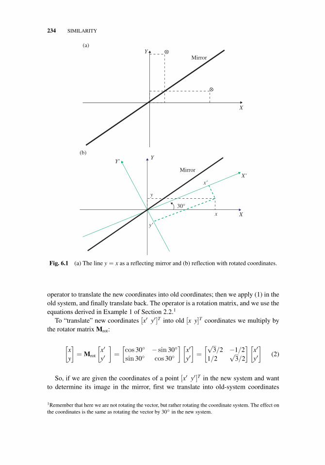
234 SIMILARITY
Mirror
X
Y(a)
Mirror
(b)Y
y
Y'
y'
x'X'
Xx30°
Fig. 6.1 (a) The line y = x as a reflecting mirror and (b) reflection with rotated coordinates.
operator to translate the new coordinates into old coordinates; then we apply (1) in theold system, and finally translate back. The operator is a rotation matrix, and we use theequations derived in Example 1 of Section 2.2.1
To “translate” new coordinates [x′ y′]T into old [x y]T coordinates we multiply bythe rotator matrix Mrot:
[xy
]= Mrot
[x′
y′
]=
[cos 30◦ − sin 30◦
sin 30◦ cos 30◦
] [x′
y′
]=
[√3/2 −1/2
1/2√
3/2
] [x′
y′
](2)
So, if we are given the coordinates of a point [x′ y′]T in the new system and wantto determine its image in the mirror, first we translate into old-system coordinates
1Remember that here we are not rotating the vector, but rather rotating the coordinate system. The effect onthe coordinates is the same as rotating the vector by 30◦ in the new system.
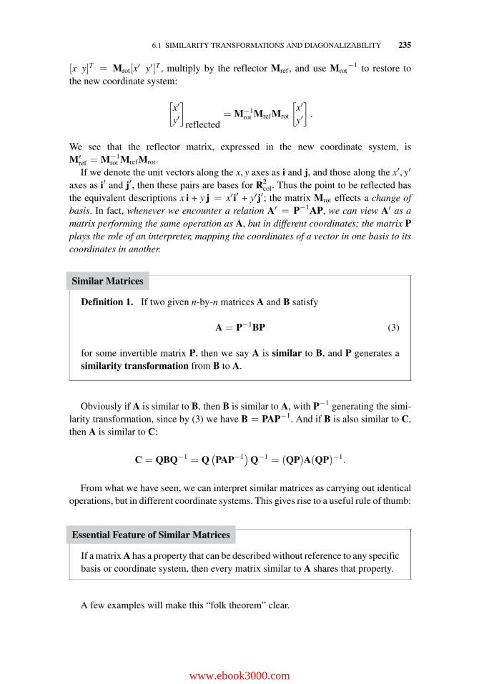
6.1 SIMILARITY TRANSFORMATIONS AND DIAGONALIZABILITY 235
[x y]T = Mrot[x′ y′]T , multiply by the reflector Mref , and use Mrot−1 to restore to
the new coordinate system:
[x′
y′
]reflected
= M−1rot MrefMrot
[x′
y′
].
We see that the reflector matrix, expressed in the new coordinate system, isM′
ref = M−1rot MrefMrot.
If we denote the unit vectors along the x, y axes as i and j, and those along the x′, y′
axes as i′ and j′, then these pairs are bases for R2col. Thus the point to be reflected has
the equivalent descriptions x i + y j = x′i′ + y′j′; the matrix Mrot effects a change ofbasis. In fact, whenever we encounter a relation A′ = P−1AP, we can view A′ as amatrix performing the same operation as A, but in different coordinates; the matrix Pplays the role of an interpreter, mapping the coordinates of a vector in one basis to itscoordinates in another.
Similar Matrices
Definition 1. If two given n-by-n matrices A and B satisfy
A = P−1BP (3)
for some invertible matrix P, then we say A is similar to B, and P generates asimilarity transformation from B to A.
Obviously if A is similar to B, then B is similar to A, with P−1 generating the simi-larity transformation, since by (3) we have B = PAP−1. And if B is also similar to C,then A is similar to C:
C = QBQ−1 = Q(PAP−1)Q−1 = (QP)A(QP)−1.
From what we have seen, we can interpret similar matrices as carrying out identicaloperations, but in different coordinate systems. This gives rise to a useful rule of thumb:
Essential Feature of Similar Matrices
If a matrix A has a property that can be described without reference to any specificbasis or coordinate system, then every matrix similar to A shares that property.
A few examples will make this “folk theorem” clear.
www.ebook3000.com
236 SIMILARITY
Corollary 1. If A and B are similar matrices, then the following hold:
• A and B have the same eigenvalues.
• If A has k linearly independent eigenvectors corresponding to the eigenvaluer, then B also has k linearly independent eigenvectors corresponding to theeigenvalue r.
• A and B are both singular or both nonsingular.
• A and B have the same rank.
Folk proof: “A has the eigenvalue r” means there is at least a one-dimensional familyof solutions to the equation Au = ru. This statement contains no reference to anycoordinate system or basis, so it applies to any matrix similar to A.
Similarly, the statement “A has a k-dimensional family of solutions to Au = ru” isbasis-free; as is the claim that A has a nontrivial null vector. Finally, recall that the rankis the range’s dimension, which is basis-free.
Example 1. Construct a rigorous proof demonstrating that similar matrices have thesame eigenvalues.
Solution. If Au = ru, then Pu is an eigenvector for PAP−1 with eigenvalue r, since[(PAP−1)(Pu) = PAu = P(ru) = r(Pu)]. �
Indeed, the same logic readily verifies the other claims of Corollary 1. The gen-eralization “similar matrices have the same eigenvectors” is not justified, because astatement like “A has an eigenvector [1 0 1]T” refers specifically to the coordi-nates of the eigenvector. (In fact Example 1 shows that the eigenvector of PAP−1 thatcorresponds to u is Pu.)
Other, more subtle properties shared by similar matrices are described in Corollary 2.
Corollary 2. If A and B are similar, they have the same characteristic polynomial,determinant, and trace.
Proof. The relation between the characteristic polynomials pA(r) and pB(r) is revealedby a chain of reasoning exploiting the determinant properties:
pA(r) = det(A − rI) = det(P−1BP − rI
)= det
(P−1BP − rP−1IP
)= det
(P−1[B − rI]P
)= det
(P−1)det(B − rI) det(P) = det(B − rI) = pB(r).
Problems 25 and 26 of Exercises 5.2 showed that the determinant and the trace (thesum of the diagonal elements) of a matrix appear as coefficients in its characteristicpolynomial.
Since the simplest matrices to compute with are the diagonal matrices, the mostimportant similarity transformations are those that render a matrix diagonal. Such trans-formations are generated by matrices made up of linearly independent eigenvectors, asshown by the following:
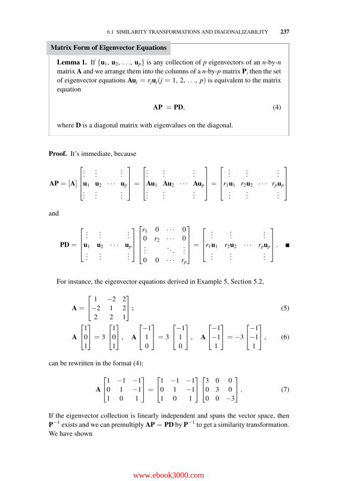
6.1 SIMILARITY TRANSFORMATIONS AND DIAGONALIZABILITY 237
Matrix Form of Eigenvector Equations
Lemma 1. If {u1, u2, . . ., up} is any collection of p eigenvectors of an n-by-nmatrix A and we arrange them into the columns of a n-by-p matrix P, then the setof eigenvector equations Auj = rjuj(j = 1, 2, . . ., p) is equivalent to the matrixequation
AP = PD, (4)
where D is a diagonal matrix with eigenvalues on the diagonal.
Proof. It’s immediate, because
AP = [A]
⎡⎢⎢⎣
......
...u1 u2 · · · up...
......
⎤⎥⎥⎦ =
⎡⎢⎢⎣
......
...Au1 Au2 · · · Aup...
......
⎤⎥⎥⎦ =
⎡⎢⎢⎣
......
...r1u1 r2u2 · · · rpup
......
...
⎤⎥⎥⎦
and
PD =
⎡⎢⎢⎣
......
...u1 u2 · · · up...
......
⎤⎥⎥⎦
⎡⎢⎢⎢⎣
r1 0 · · · 00 r2 · · · 0...
. . ....
0 0 · · · rp
⎤⎥⎥⎥⎦ =
⎡⎢⎢⎣
......
...r1u1 r2u2 · · · rpup
......
...
⎤⎥⎥⎦ .
For instance, the eigenvector equations derived in Example 5, Section 5.2,
A =
⎡⎣ 1 −2 2−2 1 22 2 1
⎤⎦ ; (5)
A
⎡⎣1
01
⎤⎦ = 3
⎡⎣1
01
⎤⎦ , A
⎡⎣−1
10
⎤⎦ = 3
⎡⎣−1
10
⎤⎦ , A
⎡⎣−1−11
⎤⎦ = −3
⎡⎣−1−11
⎤⎦ , (6)
can be rewritten in the format (4):
A
⎡⎣1 −1 −1
0 1 −11 0 1
⎤⎦ =
⎡⎣1 −1 −1
0 1 −11 0 1
⎤⎦⎡⎣3 0 0
0 3 00 0 −3
⎤⎦ . (7)
If the eigenvector collection is linearly independent and spans the vector space, thenP−1 exists and we can premultiply AP = PD by P−1 to get a similarity transformation.We have shown
www.ebook3000.com
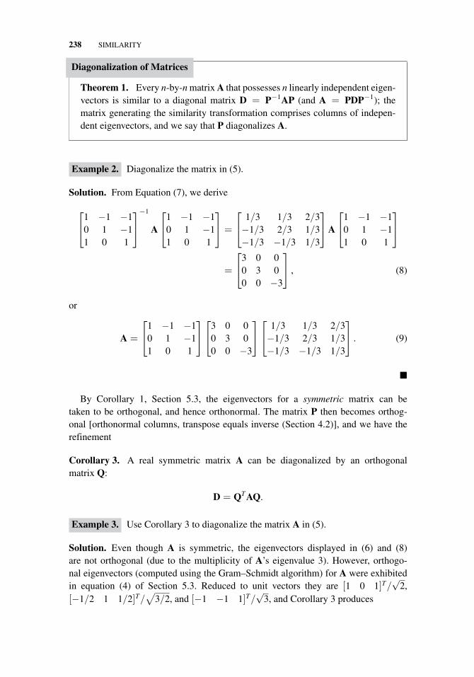
238 SIMILARITY
Diagonalization of Matrices
Theorem 1. Every n-by-n matrix A that possesses n linearly independent eigen-vectors is similar to a diagonal matrix D = P−1AP (and A = PDP−1); thematrix generating the similarity transformation comprises columns of indepen-dent eigenvectors, and we say that P diagonalizes A.
Example 2. Diagonalize the matrix in (5).
Solution. From Equation (7), we derive
⎡⎣1 −1 −1
0 1 −11 0 1
⎤⎦−1
A
⎡⎣1 −1 −1
0 1 −11 0 1
⎤⎦ =
⎡⎣ 1/3 1/3 2/3−1/3 2/3 1/3−1/3 −1/3 1/3
⎤⎦A
⎡⎣1 −1 −1
0 1 −11 0 1
⎤⎦
=
⎡⎣3 0 0
0 3 00 0 −3
⎤⎦ , (8)
or
A =
⎡⎣1 −1 −1
0 1 −11 0 1
⎤⎦⎡⎣3 0 0
0 3 00 0 −3
⎤⎦⎡⎣ 1/3 1/3 2/3−1/3 2/3 1/3−1/3 −1/3 1/3
⎤⎦ . (9)
�
By Corollary 1, Section 5.3, the eigenvectors for a symmetric matrix can betaken to be orthogonal, and hence orthonormal. The matrix P then becomes orthog-onal [orthonormal columns, transpose equals inverse (Section 4.2)], and we have therefinement
Corollary 3. A real symmetric matrix A can be diagonalized by an orthogonalmatrix Q:
D = QTAQ.
Example 3. Use Corollary 3 to diagonalize the matrix A in (5).
Solution. Even though A is symmetric, the eigenvectors displayed in (6) and (8)are not orthogonal (due to the multiplicity of A’s eigenvalue 3). However, orthogo-nal eigenvectors (computed using the Gram–Schmidt algorithm) for A were exhibitedin equation (4) of Section 5.3. Reduced to unit vectors they are [1 0 1]T/
√2,
[−1/2 1 1/2]T/√
3/2, and [−1 −1 1]T/√
3, and Corollary 3 produces
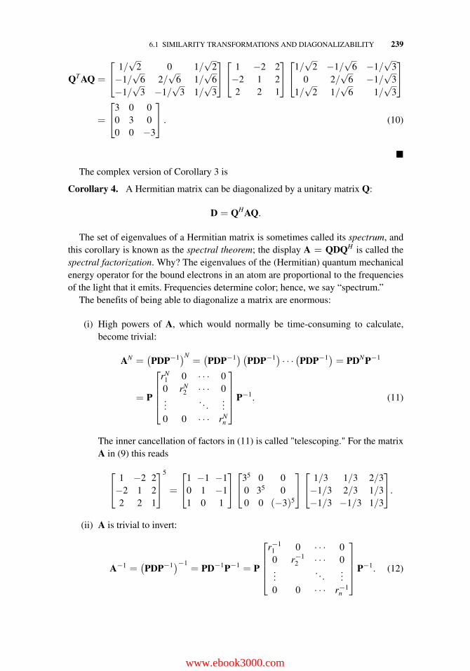
6.1 SIMILARITY TRANSFORMATIONS AND DIAGONALIZABILITY 239
QTAQ =
⎡⎣ 1/
√2 0 1/
√2
−1/√
6 2/√
6 1/√
6−1/
√3 −1/
√3 1/
√3
⎤⎦⎡⎣ 1 −2 2−2 1 22 2 1
⎤⎦⎡⎣1/
√2 −1/
√6 −1/
√3
0 2/√
6 −1/√
31/√
2 1/√
6 1/√
3
⎤⎦
=
⎡⎣3 0 0
0 3 00 0 −3
⎤⎦ . (10)
�The complex version of Corollary 3 is
Corollary 4. A Hermitian matrix can be diagonalized by a unitary matrix Q:
D = QHAQ.
The set of eigenvalues of a Hermitian matrix is sometimes called its spectrum, andthis corollary is known as the spectral theorem; the display A = QDQH is called thespectral factorization. Why? The eigenvalues of the (Hermitian) quantum mechanicalenergy operator for the bound electrons in an atom are proportional to the frequenciesof the light that it emits. Frequencies determine color; hence, we say “spectrum.”
The benefits of being able to diagonalize a matrix are enormous:
(i) High powers of A, which would normally be time-consuming to calculate,become trivial:
AN =(PDP−1)N
=(PDP−1) (PDP−1) · · · (PDP−1) = PDNP−1
= P
⎡⎢⎢⎢⎣
rN1 0 · · · 00 rN
2 · · · 0...
. . ....
0 0 · · · rNn
⎤⎥⎥⎥⎦P−1. (11)
The inner cancellation of factors in (11) is called "telescoping." For the matrixA in (9) this reads
⎡⎣ 1 −2 2−2 1 22 2 1
⎤⎦
5
=
⎡⎣1 −1 −1
0 1 −11 0 1
⎤⎦⎡⎣35 0 0
0 35 00 0 (−3)5
⎤⎦⎡⎣ 1/3 1/3 2/3−1/3 2/3 1/3−1/3 −1/3 1/3
⎤⎦.
(ii) A is trivial to invert:
A−1 =(PDP−1)−1
= PD−1P−1 = P
⎡⎢⎢⎢⎣
r−11 0 · · · 00 r−1
2 · · · 0...
. . ....
0 0 · · · r−1n
⎤⎥⎥⎥⎦P−1. (12)
www.ebook3000.com
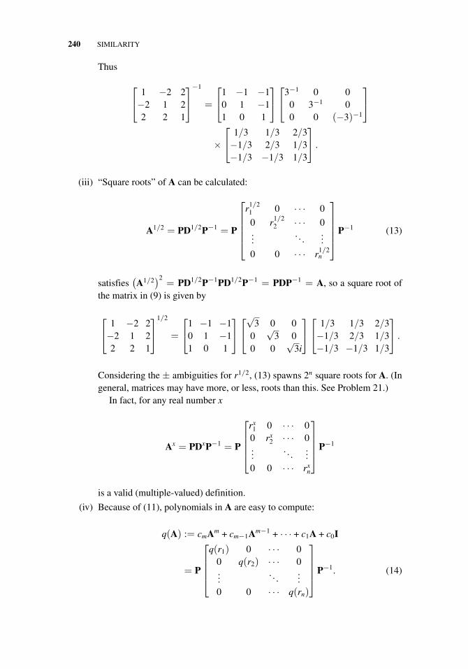
240 SIMILARITY
Thus
⎡⎣ 1 −2 2−2 1 22 2 1
⎤⎦−1
=
⎡⎣1 −1 −1
0 1 −11 0 1
⎤⎦⎡⎣3−1 0 0
0 3−1 00 0 (−3)−1
⎤⎦
×
⎡⎣ 1/3 1/3 2/3−1/3 2/3 1/3−1/3 −1/3 1/3
⎤⎦ .
(iii) “Square roots” of A can be calculated:
A1/2 = PD1/2P−1 = P
⎡⎢⎢⎢⎢⎣
r1/21 0 · · · 0
0 r1/22 · · · 0
.... . .
...
0 0 · · · r1/2n
⎤⎥⎥⎥⎥⎦P−1 (13)
satisfies(A1/2
)2= PD1/2P−1PD1/2P−1 = PDP−1 = A, so a square root of
the matrix in (9) is given by
⎡⎣ 1 −2 2−2 1 22 2 1
⎤⎦
1/2
=
⎡⎣1 −1 −1
0 1 −11 0 1
⎤⎦⎡⎣√
3 0 00
√3 0
0 0√
3i
⎤⎦⎡⎣ 1/3 1/3 2/3−1/3 2/3 1/3−1/3 −1/3 1/3
⎤⎦ .
Considering the ± ambiguities for r1/2, (13) spawns 2n square roots for A. (Ingeneral, matrices may have more, or less, roots than this. See Problem 21.)
In fact, for any real number x
Ax = PDxP−1 = P
⎡⎢⎢⎢⎣
rx1 0 · · · 00 rx
2 · · · 0...
. . ....
0 0 · · · rxn
⎤⎥⎥⎥⎦P−1
is a valid (multiple-valued) definition.
(iv) Because of (11), polynomials in A are easy to compute:
q(A) := cmAm + cm−1Am−1 + · · · + c1A + c0I
= P
⎡⎢⎢⎢⎣
q(r1) 0 · · · 00 q(r2) · · · 0...
. . ....
0 0 · · · q(rn)
⎤⎥⎥⎥⎦P−1. (14)
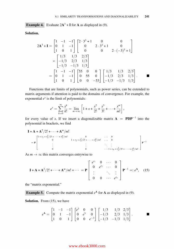
6.1 SIMILARITY TRANSFORMATIONS AND DIAGONALIZABILITY 241
Example 4. Evaluate 2A3 + I for A as displayed in (9).
Solution.
2A3 + I =
⎡⎣1 −1 −1
0 1 −11 0 1
⎤⎦⎡⎣2 · 33 + 1 0 0
0 2 · 33 + 1 00 0 2 · (−3)3 + 1
⎤⎦
×
⎡⎣ 1/3 1/3 2/3−1/3 2/3 1/3−1/3 −1/3 1/3
⎤⎦
=
⎡⎣1 −1 −1
0 1 −11 0 1
⎤⎦⎡⎣55 0 0
0 55 00 0 −53
⎤⎦⎡⎣ 1/3 1/3 2/3−1/3 2/3 1/3−1/3 −1/3 1/3
⎤⎦ . �
Functions that are limits of polynomials, such as power series, can be extended tomatrix arguments if attention is paid to the domains of convergence. For example, theexponential ex is the limit of polynomials:
ex =∞∑
k=0
xk
k!= lim
m→∞
[1 + x +
x2
2!+
x3
3!+ · · · +
xm
m!
],
for every value of x. If we insert a diagonalizable matrix A = PDP−1 into thepolynomial in brackets, we find
I + A + A2/2! + · · · + Am/m!
= P
⎡⎢⎢⎢⎢⎣
1 + r1 + r21/2! + · · · + rm
1 /m! 0 . . . 00 1 + r2 + r2
2/2! + · · · + rm2 /m! . . . 0
.
.
....
. . ....
0 0 · · · 1 + rn + r2n/2! + · · · + rm
n /m!
⎤⎥⎥⎥⎥⎦ P−1
As m → ∞ this matrix converges entrywise to
I + A + A2/2! + · · · + Am/m! + · · · = P
⎡⎢⎢⎢⎣
er1 0 · · · 00 er2 · · · 0...
. . ....
0 0 · · · ern
⎤⎥⎥⎥⎦P−1 =: eA, (15)
the “matrix exponential.”
Example 5. Compute the matrix exponential eA for A as displayed in (9).
Solution. From (15), we have
eA =
⎡⎣1 −1 −1
0 1 −11 0 1
⎤⎦⎡⎣e3 0 0
0 e3 00 0 e−3
⎤⎦⎡⎣ 1/3 1/3 2/3−1/3 2/3 1/3−1/3 −1/3 1/3
⎤⎦ . �
www.ebook3000.com
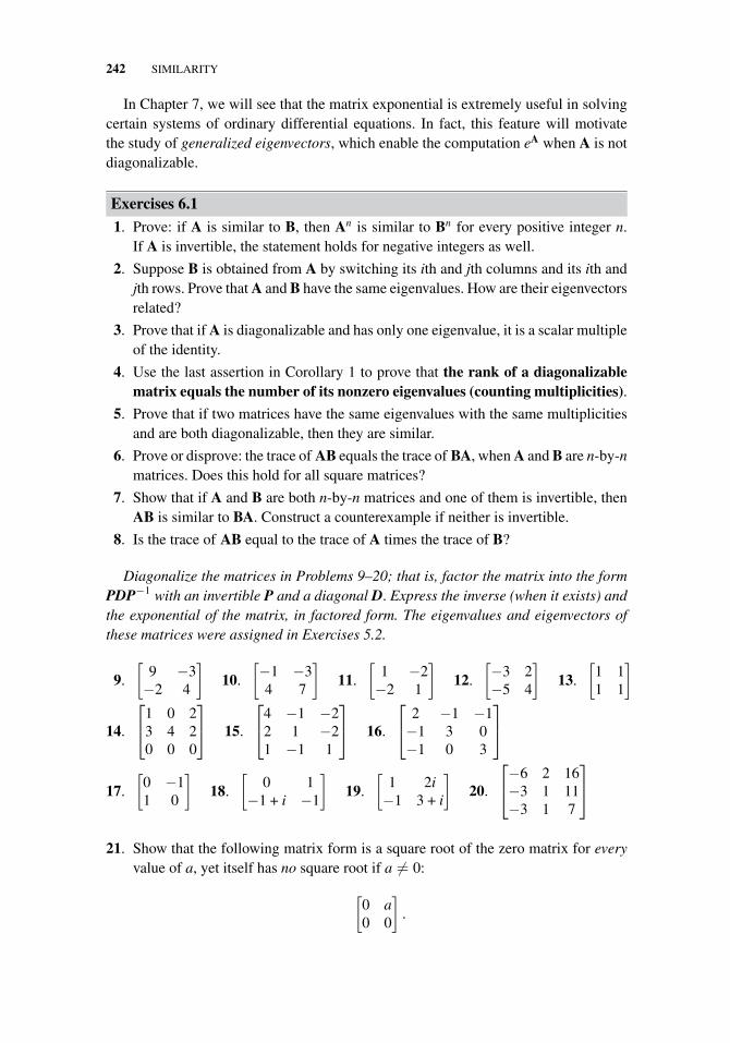
242 SIMILARITY
In Chapter 7, we will see that the matrix exponential is extremely useful in solvingcertain systems of ordinary differential equations. In fact, this feature will motivatethe study of generalized eigenvectors, which enable the computation eA when A is notdiagonalizable.
Exercises 6.1
1. Prove: if A is similar to B, then An is similar to Bn for every positive integer n.If A is invertible, the statement holds for negative integers as well.
2. Suppose B is obtained from A by switching its ith and jth columns and its ith andjth rows. Prove that A and B have the same eigenvalues. How are their eigenvectorsrelated?
3. Prove that if A is diagonalizable and has only one eigenvalue, it is a scalar multipleof the identity.
4. Use the last assertion in Corollary 1 to prove that the rank of a diagonalizablematrix equals the number of its nonzero eigenvalues (counting multiplicities).
5. Prove that if two matrices have the same eigenvalues with the same multiplicitiesand are both diagonalizable, then they are similar.
6. Prove or disprove: the trace of AB equals the trace of BA, when A and B are n-by-nmatrices. Does this hold for all square matrices?
7. Show that if A and B are both n-by-n matrices and one of them is invertible, thenAB is similar to BA. Construct a counterexample if neither is invertible.
8. Is the trace of AB equal to the trace of A times the trace of B?
Diagonalize the matrices in Problems 9–20; that is, factor the matrix into the formPDP−1 with an invertible P and a diagonal D. Express the inverse (when it exists) andthe exponential of the matrix, in factored form. The eigenvalues and eigenvectors ofthese matrices were assigned in Exercises 5.2.
9.
[9 −3−2 4
]10.
[−1 −34 7
]11.
[1 −2−2 1
]12.
[−3 2−5 4
]13.
[1 11 1
]
14.
⎡⎣1 0 2
3 4 20 0 0
⎤⎦ 15.
⎡⎣4 −1 −2
2 1 −21 −1 1
⎤⎦ 16.
⎡⎣ 2 −1 −1−1 3 0−1 0 3
⎤⎦
17.
[0 −11 0
]18.
[0 1
−1 + i −1
]19.
[1 2i−1 3 + i
]20.
⎡⎣−6 2 16−3 1 11−3 1 7
⎤⎦
21. Show that the following matrix form is a square root of the zero matrix for everyvalue of a, yet itself has no square root if a �= 0:
[0 a0 0
].
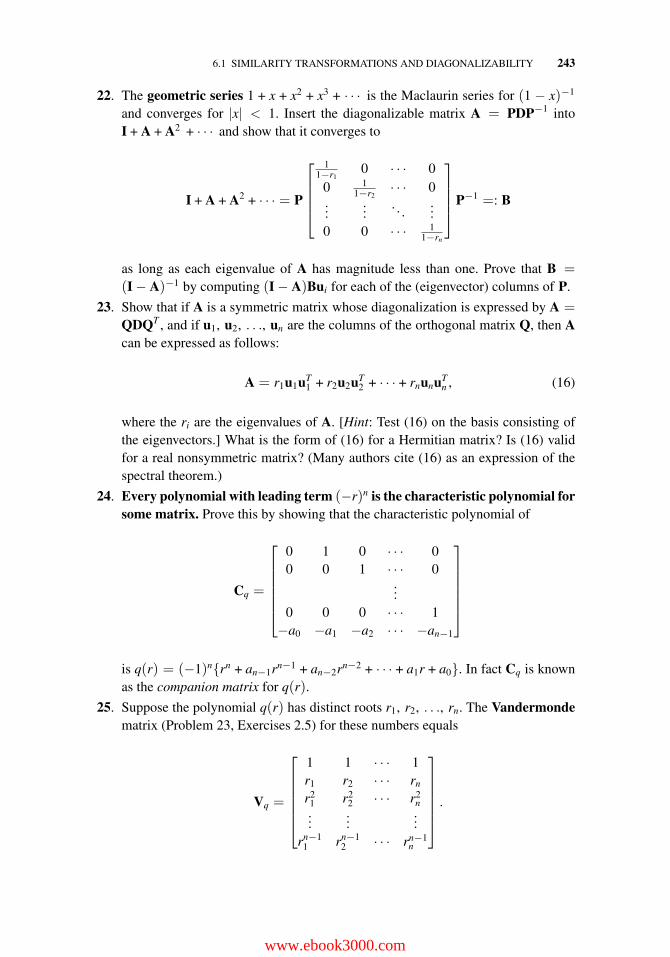
6.1 SIMILARITY TRANSFORMATIONS AND DIAGONALIZABILITY 243
22. The geometric series 1 + x + x2 + x3 + · · · is the Maclaurin series for (1 − x)−1
and converges for |x| < 1. Insert the diagonalizable matrix A = PDP−1 intoI + A + A2 + · · · and show that it converges to
I + A + A2 + · · · = P
⎡⎢⎢⎢⎣
11−r1
0 · · · 00 1
1−r2· · · 0
......
. . ....
0 0 · · · 11−rn
⎤⎥⎥⎥⎦P−1 =: B
as long as each eigenvalue of A has magnitude less than one. Prove that B =(I − A)−1 by computing (I − A)Bui for each of the (eigenvector) columns of P.
23. Show that if A is a symmetric matrix whose diagonalization is expressed by A =QDQT , and if u1, u2, . . ., un are the columns of the orthogonal matrix Q, then Acan be expressed as follows:
A = r1u1uT1 + r2u2uT
2 + · · · + rnunuTn , (16)
where the ri are the eigenvalues of A. [Hint: Test (16) on the basis consisting ofthe eigenvectors.] What is the form of (16) for a Hermitian matrix? Is (16) validfor a real nonsymmetric matrix? (Many authors cite (16) as an expression of thespectral theorem.)
24. Every polynomial with leading term (−r)n is the characteristic polynomial forsome matrix. Prove this by showing that the characteristic polynomial of
Cq =
⎡⎢⎢⎢⎢⎢⎣
0 1 0 · · · 00 0 1 · · · 0
...0 0 0 · · · 1
−a0 −a1 −a2 · · · −an−1
⎤⎥⎥⎥⎥⎥⎦
is q(r) = (−1)n{rn + an−1rn−1 + an−2rn−2 + · · · + a1r + a0}. In fact Cq is knownas the companion matrix for q(r).
25. Suppose the polynomial q(r) has distinct roots r1, r2, . . ., rn. The Vandermondematrix (Problem 23, Exercises 2.5) for these numbers equals
Vq =
⎡⎢⎢⎢⎢⎢⎣
1 1 · · · 1r1 r2 · · · rn
r21 r2
2 · · · r2n
......
...rn−1
1 rn−12 · · · rn−1
n
⎤⎥⎥⎥⎥⎥⎦
.
www.ebook3000.com
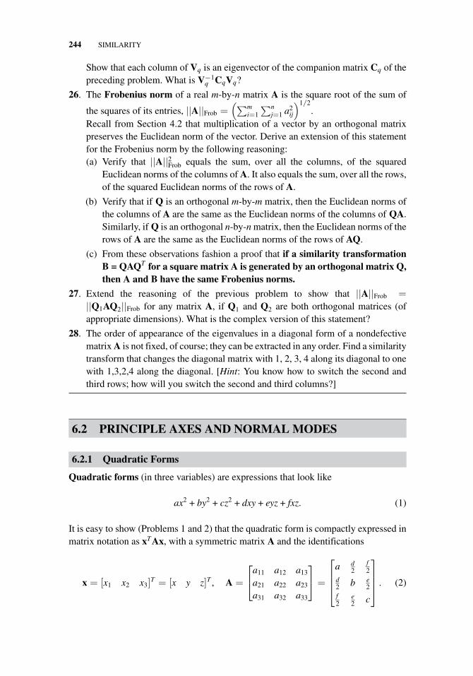
244 SIMILARITY
Show that each column of Vq is an eigenvector of the companion matrix Cq of thepreceding problem. What is V−1
q CqVq?
26. The Frobenius norm of a real m-by-n matrix A is the square root of the sum of
the squares of its entries, ||A||Frob =(∑m
i=1
∑nj=1 a2
ij
)1/2.
Recall from Section 4.2 that multiplication of a vector by an orthogonal matrixpreserves the Euclidean norm of the vector. Derive an extension of this statementfor the Frobenius norm by the following reasoning:(a) Verify that ||A||2Frob equals the sum, over all the columns, of the squared
Euclidean norms of the columns of A. It also equals the sum, over all the rows,of the squared Euclidean norms of the rows of A.
(b) Verify that if Q is an orthogonal m-by-m matrix, then the Euclidean norms ofthe columns of A are the same as the Euclidean norms of the columns of QA.Similarly, if Q is an orthogonal n-by-n matrix, then the Euclidean norms of therows of A are the same as the Euclidean norms of the rows of AQ.
(c) From these observations fashion a proof that if a similarity transformationB = QAQT for a square matrix A is generated by an orthogonal matrix Q,then A and B have the same Frobenius norms.
27. Extend the reasoning of the previous problem to show that ||A||Frob =||Q1AQ2||Frob for any matrix A, if Q1 and Q2 are both orthogonal matrices (ofappropriate dimensions). What is the complex version of this statement?
28. The order of appearance of the eigenvalues in a diagonal form of a nondefectivematrix A is not fixed, of course; they can be extracted in any order. Find a similaritytransform that changes the diagonal matrix with 1, 2, 3, 4 along its diagonal to onewith 1,3,2,4 along the diagonal. [Hint: You know how to switch the second andthird rows; how will you switch the second and third columns?]
6.2 PRINCIPLE AXES AND NORMAL MODES
6.2.1 Quadratic Forms
Quadratic forms (in three variables) are expressions that look like
ax2 + by2 + cz2 + dxy + eyz + fxz. (1)
It is easy to show (Problems 1 and 2) that the quadratic form is compactly expressed inmatrix notation as xTAx, with a symmetric matrix A and the identifications
x = [x1 x2 x3]T = [x y z]T , A =
⎡⎣a11 a12 a13
a21 a22 a23
a31 a32 a33
⎤⎦ =
⎡⎢⎢⎣
a d2
f2
d2 b e
2f2
e2 c
⎤⎥⎥⎦ . (2)
6.2 PRINCIPLE AXES AND NORMAL MODES 245
The slightly more general quadratic polynomials (in three variables) incorporateadditional linear terms and a constant:
(ax2 + by2 + cz2 + dxy + eyz + fxz) + (gx + hy + jz) + (k) = xTAx + bTx + (k). (3)
These notions generalize to n dimensions, of course. The n-dimensional quadraticpolynomial is xTAx + bTx + k with x and b in Rn
col and A symmetric in Rn,n.Quadratic polynomials arise in formulas for moments of inertia, potential energy
(elastic, electromagnetic), and surface functions (i.e., their level surfaces describefamiliar shapes such as spheres, cylinders, cones, and ellipsoids). Before we exploretheir interaction with similarity transforms, it is convenient to tabulate two elementaryproperties. The first generalizes the familiar process of “completing the square,” andeffectively reduces quadratic polynomials to quadratic forms (plus constants).
Lemma 1. If A is symmetric and invertible and y = (x + A−1b /2), then
xTAx + bTx + k = yTAy +(k − bTA−1b/4
). (4)
Proof. Start with the quadratic form in y:
yTAy =(x + A−1b/2
)TA(x + A−1b/2
)= xTAx +
12
xTAA−1b +12
bT(A−1)T
Ax +14
bT(A−1)T
AA−1b.
Since A (and its inverse) is symmetric, this reduces to
yTAy = xTAx + bTx + bTA−1b/4;
transpose the constant and add k, to derive (4).
For example, Problem 1(b) asks you to confirm that
[x1 x2
] [1 22 3
] [x1
x2
]+[4 6
] [x1
x2
]=[y1 y2
] [1 22 3
] [y1
y2
]− 3 if y = x +
[01
].
(5)
The second property is the formula for differentiating a quadratic polynomial.(A matrix function A(t) = [aij(t)] is differentiated entrywise: A′(t) = [a′ij(t)].)
Lemma 2. If A(t) and B(t) are differentiable matrices, then the product ruleholds:
ddt[A(t)B(t)] =
[ddt
A(t)
]B(t) + A(t)
ddt[B(t)]. (6)
(Note that we are careful to respect the order of appearance of A and B, becausematrix multiplication is noncommutative.)
www.ebook3000.com
246 SIMILARITY
Proof. This is simple bookkeeping. Recall that the (i, j)th entry of AB is given by
[AB]ij =p∑
k=1
aikbkj,
so its derivative is[
d(AB)dt
]ij
=
p∑k=1
[daik
dtbkj + aik
dbkj
dt
]=
[dAdt
B + AdBdt
]ij
.
(The derivative of a sum of matrices is simply the sum of their derivatives.)Now if x is a vector in Rn
col and f (x) is a scalar-valued function, the gradient of f isthe column vector of its partial derivatives.
grad f =
[∂f∂x1
∂f∂x2
. . .∂f∂xn
]T
.
What is the formula for the gradient of the quadratic polynomial (3)?
Lemma 3. If A is a constant symmetric n-by-n matrix and b is a constant n-by-1vector, then
grad(xTAx + bTx
)= 2Ax + b. (7)
Proof. Using the product rule to differentiate with respect to x2 (for example), we findthat
∂
∂x2bTx = bT ∂
∂x2x = bT ∂
∂x2
⎡⎢⎢⎢⎢⎢⎣
x1
x2
x3...
xn
⎤⎥⎥⎥⎥⎥⎦= bT
⎡⎢⎢⎢⎢⎢⎣
010...0
⎤⎥⎥⎥⎥⎥⎦= [b1 b2 . . . bn]
⎡⎢⎢⎢⎢⎢⎣
010...0
⎤⎥⎥⎥⎥⎥⎦
,
which simply “extracts” the second component of b. Generalizing from this, we see
grad bTx =
[∂bTx∂x1
∂bTx∂x2
. . .∂bTx∂xn
]T
= b.
For the quadratic form we have
∂
∂x2xTAx =
∂xT
∂x2Ax + xTA
∂x∂x2
= [0 1 0 0 · · · 0]Ax + xTA
⎡⎢⎢⎢⎣
01...0
⎤⎥⎥⎥⎦ ,
6.2 PRINCIPLE AXES AND NORMAL MODES 247
extracting the second component of Ax plus the second component of xTA—which areidentical, since A is symmetric ([Ax]T = xTAT = xTA). In general, then,
grad xTAx =
[∂xTAx∂x1
∂xTAx∂x2
· · · ∂xTAx∂xn
]T
= 2Ax.
For instance, it is easy to confirm that
grad{[x1 x2]
[1 22 3
] [x1
x2
]+ [4 6]
[x1
x2
]}= grad
{x2
1 + 4x1x2 + 3x22 + 4x1 + 6x2
}
=
[2x1 + 4x2 + 44x1 + 6x2 + 6
]
= 2
[1 22 3
] [x1
x2
]+
[46
].
What do similarity transformations have to do with quadratic forms? Suppose werotate our coordinate system, as we did in the previous section (Fig. 6.1b), so that thenew coordinates of a point (x′) are related to its old coordinates (x) through a matrixequation x = Qx′, where Q is an orthogonal matrix. Then the quadratic form becomesexpressed in the new coordinates as
xTAx = (Qx′)TA(Qx′) = x′T
QTAQx′ = x′T(QTAQ)x′ = x′T(Q−1AQ)x′.
The symmetric matrix A in the quadratic form is replaced by the similar matrixQ−1AQ. But more importantly, because A is symmetric we could use the matrix ofits (unit) eigenvectors to define the generator Q—in which case by Corollary 3 of theprevious section the matrix Q−1AQ would be diagonal, and there would be no crossterms in the quadratic form! Indeed, the coefficients of the surviving terms would bethe eigenvalues. The eigenvector directions are the principal axes of A.
Principal Axes Theorem
Theorem 2. If A is a real symmetric matrix, its eigenvectors generate an orthog-onal change of coordinates that transforms the quadratic form xTAx into aquadratic form with no cross terms.
Corollary 5. If A is a Hermitian matrix, its eigenvectors generate a unitary changeof coordinates that transforms the quadratic form xHAx into a quadratic form with nocross terms.
The following example brings to bear all of the important features of the theory ofreal quadratic forms.
www.ebook3000.com
248 SIMILARITY
Example 1. Rewrite x21 + x2
2 + x23 − 4x1x2 + 4x1x3 + 4x2x3 in new coordinates so that
it has no cross terms. Determine its maximum and minimum values on the spherex2
1 + x22 + x2
3 = 1.
Solution. From (1) and (2), we determine that the symmetric matrix appearing in thequadratic form is the same matrix A that we used in Example 5, Section 5.2; that is,
x21 + x2
2 + x23 − 4x1x2 + 4x1x3 + 4x2x3 = [x1 x2 x2]
⎡⎣ 1 −2 2−2 1 22 2 1
⎤⎦⎡⎣x1
x2
x3
⎤⎦ = xTAx.
Its diagonalization via the (orthogonal) matrix of eigenvectors is displayed in Section 6.1Equation (10). Implementing the construction described above Theorem 2, we find
xTAx = xT(QQT)A
(QQT) x =
(QTx
)TQTAQ
(QTx
)
=(QTx
)T
⎡⎣ 1/
√2 0 1/
√2
−1/√
6 2/√
6 1/√
6−1/
√3 −1/
√3 1/
√3
⎤⎦⎡⎣ 1 −2 2−1 1 22 2 1
⎤⎦
×
⎡⎣1/
√2 −1/
√6 −1/
√3
0 2/√
6 −1/√
31/√
2 1/√
6 1/√
3
⎤⎦ (QTx)
= yT
⎡⎣3 0 0
0 3 00 0 −3
⎤⎦ y = 3y2
1 + 3y22 − 3y2
3,
where y = QTx. The principal axes, in y coordinates, are [1 0 0]T , [0 1 0]T , and [0 0 1]T ;in the original x coordinates they are the columns of Q (i.e., the eigenvectors), becausex = Qy.
Since multiplication by orthogonal matrices preserves lengths (Euclidean norms), theset of points where x2
1 +x22 +x2
3 = 1 is the same as the set where y21+y2
2+y23 = 1. The max-
imum and minimum of 3y21 + 3y2
2 −3y23 (= 3−6y2
3) are obviously 3 and −3, the largestand smallest eigenvalues. �
6.2.2 Normal Modes
Figure 6.2a shows an old (1920–1940) microphone used in radio broadcasting. (Amockup of a similar microphone was used in “The King’s Speech,” the academyaward-winning movie produced in 2011.) The mounting is spring loaded to cushionthe microphone from environmental vibrations. Example 2 will demonstrate the useof eigenvectors and similarity transformations to analyze the oscillations. To keep ourcalculations down to a manageable size, we employ the simplified geometry shown inFigure 6.2b.
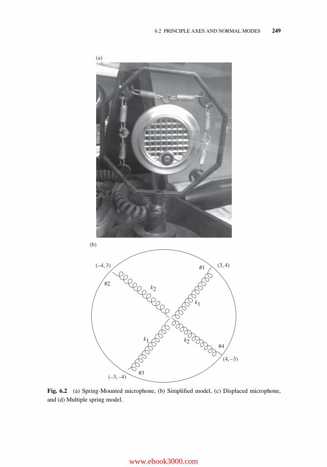
6.2 PRINCIPLE AXES AND NORMAL MODES 249
(a)
(3, 4)(–4, 3)
(4, –3)
(–3, –4)
#1
#2
#3
#4
k2
k1
k2k1
(b)
Fig. 6.2 (a) Spring-Mounted microphone, (b) Simplified model, (c) Displaced microphone,
and (d) Multiple spring model.
www.ebook3000.com
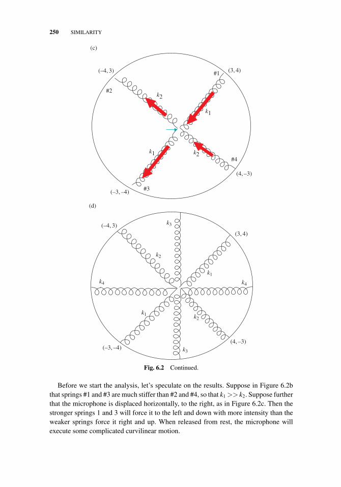
250 SIMILARITY
#1
#2
#3
#4
k2
k1
k2k1
(c)
(3, 4)(–4, 3)
(4, –3)
(–3, –4)
(d)
(3, 4)(–4, 3)
(4, –3)(–3, –4)
k2
k1
k4k4
k2k1
k3
k3
Fig. 6.2 Continued.
Before we start the analysis, let’s speculate on the results. Suppose in Figure 6.2bthat springs #1 and #3 are much stiffer than #2 and #4, so that k1 >> k2. Suppose furtherthat the microphone is displaced horizontally, to the right, as in Figure 6.2c. Then thestronger springs 1 and 3 will force it to the left and down with more intensity than theweaker springs force it right and up. When released from rest, the microphone willexecute some complicated curvilinear motion.
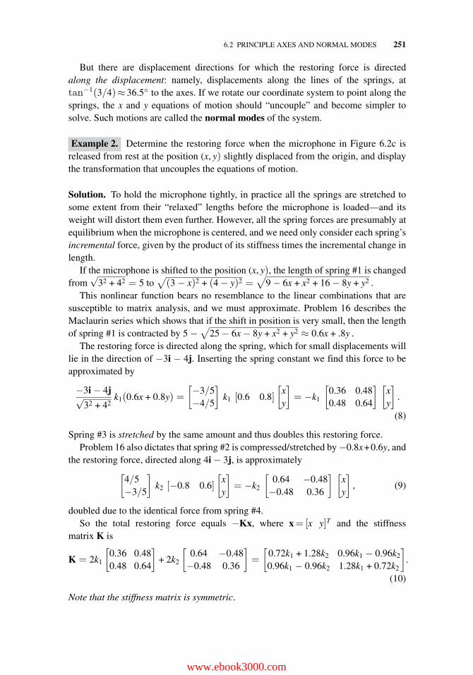
6.2 PRINCIPLE AXES AND NORMAL MODES 251
But there are displacement directions for which the restoring force is directedalong the displacement: namely, displacements along the lines of the springs, attan−1(3/4)≈ 36.5◦ to the axes. If we rotate our coordinate system to point along thesprings, the x and y equations of motion should “uncouple” and become simpler tosolve. Such motions are called the normal modes of the system.
Example 2. Determine the restoring force when the microphone in Figure 6.2c isreleased from rest at the position (x, y) slightly displaced from the origin, and displaythe transformation that uncouples the equations of motion.
Solution. To hold the microphone tightly, in practice all the springs are stretched tosome extent from their “relaxed” lengths before the microphone is loaded—and itsweight will distort them even further. However, all the spring forces are presumably atequilibrium when the microphone is centered, and we need only consider each spring’sincremental force, given by the product of its stiffness times the incremental change inlength.
If the microphone is shifted to the position (x, y), the length of spring #1 is changedfrom
√32 + 42 = 5 to
√(3 − x)2 + (4 − y)2 =
√9 − 6x + x2 + 16 − 8y + y2 .
This nonlinear function bears no resemblance to the linear combinations that aresusceptible to matrix analysis, and we must approximate. Problem 16 describes theMaclaurin series which shows that if the shift in position is very small, then the lengthof spring #1 is contracted by 5 −
√25 − 6x − 8y + x2 + y2 ≈ 0.6x + .8y .
The restoring force is directed along the spring, which for small displacements willlie in the direction of −3i − 4j. Inserting the spring constant we find this force to beapproximated by
−3i − 4j√32 + 42
k1(0.6x + 0.8y) =
[−3/5−4/5
]k1 [0.6 0.8]
[xy
]= −k1
[0.36 0.480.48 0.64
] [xy
].
(8)
Spring #3 is stretched by the same amount and thus doubles this restoring force.Problem 16 also dictates that spring #2 is compressed/stretched by −0.8x+0.6y, and
the restoring force, directed along 4i − 3j, is approximately[
4/5−3/5
]k2 [−0.8 0.6]
[xy
]= −k2
[0.64 −0.48−0.48 0.36
] [xy
], (9)
doubled due to the identical force from spring #4.So the total restoring force equals −Kx, where x= [x y]T and the stiffness
matrix K is
K = 2k1
[0.36 0.480.48 0.64
]+ 2k2
[0.64 −0.48−0.48 0.36
]=
[0.72k1 + 1.28k2 0.96k1 − 0.96k2
0.96k1 − 0.96k2 1.28k1 + 0.72k2
].
(10)
Note that the stiffness matrix is symmetric.
www.ebook3000.com
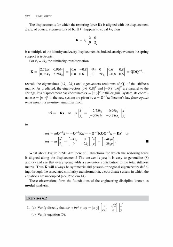
252 SIMILARITY
The displacements for which the restoring force Kx is aligned with the displacementx are, of course, eigenvectors of K. If k1 happens to equal k2, then
K = k2
[2 00 2
]
is a multiple of the identity and every displacement is, indeed, an eigenvector; the springsupport is isotropic.
For k1 = 2k2 the similarity transformation
K =
[2.72k2 0.96k2
0.96 k2 3.28k2
]=
[0.6 −0.80.8 0.6
] [4k2 00 2k2
] [0.6 0.8−0.8 0.6
]= QDQ−1.
reveals the eigenvalues (4k2, 2k2) and eigenvectors (columns of Q) of the stiffnessmatrix. As predicted, the eigenvectors [0.6 0.8]T and [−0.8 0.6]T are parallel to thesprings. If a displacement has coordinates x = [x y]T in the original system, its coordi-nates z = [u v]T in the new system are given by z = Q−1x; Newton’s law force equalsmass times acceleration simplifies from
mx = −Kx or m
[xy
]=
[−2.72k2 −0.96k2
−0.96 k2 −3.28k2
] [xy
]
to
mz = mQ−1x = −Q−1Kx = −Q−1KQQ−1x = Dz′ or
mz = m
[uv
]=
[−4k2 0
0 −2k2
] [uv
]=
[−4k2u−2k2v
]. �
What about Figure 6.2d? Are there still directions for which the restoring forceis aligned along the displacement? The answer is yes; it is easy to generalize (8)and (9) and see that every spring adds a symmetric contribution to the total stiffnessmatrix. Thus K will always be symmetric and possess orthogonal eigenvectors defin-ing, through the associated similarity transformation, a coordinate system in which theequations are uncoupled (see Problem 14).
These observations form the foundations of the engineering discipline known asmodal analysis.
Exercises 6.2
1. (a) Verify directly that ax2 + by2 + cxy = [x y]
[a c/2
c/2 b
] [xy
]
(b) Verify equation (5).
6.2 PRINCIPLE AXES AND NORMAL MODES 253
2. (a) Show that if v is a column vector with all zeros except for a “1” in its ith entry,and if w is a column vector with all zeros except for a “1” in its jth entry, thenvTAw equals the isolated entry aij.
(b) Use (a) to show that in the product xTAx appearing in (3) the term aij appearswith the factors xi and xj. [Hint: Observe
xT = [x1 x2 · · · xn]
= [x1 0 · · · 0] + [0 x2 · · · 0] + · · · + [0 0 · · · xn]
and apply the distributive law of matrix multiplication.]
(c) Use (b) to show that formula (1) and xTAx are identical expressions if a11 =a, a12 + a21 = d, etc.
Note that we don’t have to select equal values for a12 and a21 (namely d/2),but doing so gives us the desirable eigenvector properties of a symmetric matrix,leading to the principal axes theorem.
Find a change of coordinates that eliminates the cross terms in the quadraticforms in Problems 3–7, and find the maximum and minimum of the forms on theunit circle (x2
1 + x22 = 1) or sphere (x2
1 + x22 + x2
3 = 1), whichever is appropriate.[Hint: Check Problems 1–6, Exercises 5.3, to see if you have already diagonalizedthe matrix.]
3. −7x21 + 2x2
2 + 12x1x2 4. 4x21 + 4x2
2 + 2x1x2 5. x21 + x2
2 + x23 + 8x1x2 + 6x1x3
6. 2x21 + 2x2
2 + 3x23 − 2x2x3 − 2x1x3 7. 2x2
1 + 2x22 + 2x2
3 + 2x1x2 + 2x1x3 − 2x2x3
8. Find the maximum on the “unit hypersphere” (x21 +x2
2 +x23 +x2
4 = 1) of the quadraticform 4x2
1 + 4x22 − 7x2
3 + 2x24 + 2x1x2 + 12x3x4.
9. Rayleigh Quotient Suppose the eigenvalues of A are distinct and are ordered asr1 > r2 > · · · > rn.(a) Show that the quadratic form vTAv achieves its maximum value, over all
unit vectors v, when v is an eigenvector u1 corresponding to the maximumeigenvalue r1 of A; and that this maximum value is r1.
(b) Show that vTAv achieves its maximum value, over all unit vectors v orthog-onal to u1, when v is an eigenvector u2 corresponding to the second largesteigenvalue r2; and that this maximum value is r2.
(c) Characterize the eigenvalue ri(i > 2) similarly, in turns of vTAv.
(d) Argue that if we replace vTAv by the Rayleigh Quotient, vTAv/vTv, in (a–c)above, we don’t have to restrict the search to unit vectors.
10. Combine what you have learned about the Rayleigh Quotient (in the previousproblem), quadratic forms, and eigenvalues of circulant matrices (Problem 14,Exercises 5.1) to deduce the maximum of the expression x1x2 + x2x3 + x3x4 + · · · +xn−1xn + xnx1 when x2
1 + x22 + · · · + x2
n = 1.
www.ebook3000.com
254 SIMILARITY
11. Replace the quadratic form in the previous problem by the sum of xixj overall unmatched indices x1x2 + x2x3 + x1x3 + x3x4 + x2x4 + x1x4 · · · + xn−1xn =∑n
i=1
∑nj=1j�=i
xixj, and rework it.
12. Linear Invariant Discrete Time Systems (homogeneous). A sequence of vectorsxn := x(n Δt) (0 ≤ n < ∞, n integer) that describe the state of some system atmultiples of a given time step Δt is called a discrete-time signal. If xn evolvesaccording to the transition equation
xn+1 = Axn (11)
with a constant m-by-m matrix A, then the discrete time system is said to be linearhomogenous time-invariant. An example is the Markov chain described in Problem22 of Section 2.1. Note that we easily derive xn = Anx0. For simplification, assumethat A is diagonalizable.(a) Let the initial state x0 be expressed in terms of m linearly independent
eigenvectors {ui} of A as x0 = c1u1 + c2u2 + · · · cmum. Show that
xn = c1rn1u1 + c2rn
2u2 + · · · + cmrnmum (12)
for any n > 0, where ri is the eigenvalue corresponding to ui.
(b) Show that if x0 is an eigenvector of A whose corresponding eigenvalue equalsone, then x0 is a stationary state in the sense that the constant signal xn ≡ x0
is a solution of (11).
(c) Show that if some of the eigenvalues of A equal one and all of the others areless than one in magnitude, then every solution of (11) approaches either 0or a stationary state as n → ∞. The system is said to be stable under suchconditions.
(d) What are the solution possibilities if some of the eigenvalues of A are greaterthan 1 in magnitude?
13. Linear Invariant Discrete-Time Systems (nonhomogeneous). If the transitionequation of the system in the previous problem takes the form xn+1 = Axn +bn witha constant m-by-m matrix A, the discrete system is called linear nonhomogeneoustime-invariant, even if the vectors bn vary with n. For simplicity, we address thesituation where the bn are constant, bn ≡ b:
xn+1 = Axn + b. (13)
As in the previous problem, assume A is diagonalizable.(a) Verify that xn ≡ (I − A)−1b is a stationary solution to (13) if none of the
eigenvalues of A equals one.
(b) Show that all solutions of (13) can be represented as xn = Anx0 +(An−1 + An−2 + · · · + A + I
)b.
6.2 PRINCIPLE AXES AND NORMAL MODES 255
(c) Apply the geometric series discussed in Problem 22 of Exercises 6.1 to showthat the solutions in (b) approach (I−A)−1b if all of the eigenvalues of A havemagnitude less than one.
(d) Show that if xn satisfies the nonhomogeneous equation (13), then yn satisfiesthe homogeneous equation yn+1 = Byn where
[yn] :=
[xn
1
], [B] =
⎡⎣ A
... b
0 · · · 0... 1
⎤⎦ . (14)
(e) Conversely, show that if yn+1 = Byn then the (m + 1)st component of yn isconstant; and if this constant is not zero a solution to (13) can be extractedfrom a solution to (14) by dividing yn by this constant and taking the first mcomponents.
(f) How are the eigenvalues of A and B related?
(g) How are the eigenvectors of A and B related? For simplicity, assume that oneis not an eigenvalue of A. [Hint: Consider the eigenvectors of A, padded witha final zero, and the vector (I − A)−1b, padded with a final one.]
(h) Put this all together: given an initial state x0 for the nonhomogeneousequation (13), explain thoroughly how to combine the reformulation in (d),the eigenvectors uncovered in (g), the technique for solving homogeneoustransition equations described in the previous problem, and the extraction pro-cedure in (e) to find an expression generalizing (12) to the nonhomogeneouscase.
14. Construct the stiffness matrix for the microphone support in Figure 6.2d and ver-ify that it is symmetric. Find its eigenvectors and sketch the directions in whichuncoupled oscillations are possible.
15. The inertia tensor I of a rigid body is a symmetric matrix calculated from the body’smass density function ρ(x, y, z) (grams per cubic centimeter): with the coordinatesenumerated as (x, y, z) = (x1, x2, x3), we have
I = [Iij] =
{∫ ∫ ∫ρ(x1, x2, x3) xixj dx1 dx2 dx3
}(i, j = 1, 2, 3).
For any unit vector n (in R3col) the quadratic form nTIn gives the moment of inertia
of the body about the axis n. If I is diagonalized by an orthogonal matrix Q, thenclassical mechanics shows that (due to the absence of the off-diagonal "productsof inertia") the body can spin smoothly about its principal axes (columns of Q)without wobbling. (Think of a spiral pass or an end-over-end placement kick of afootball. A punt, however, typically imparts a spin about a random axis, and theresult is a wobbly motion.)
www.ebook3000.com
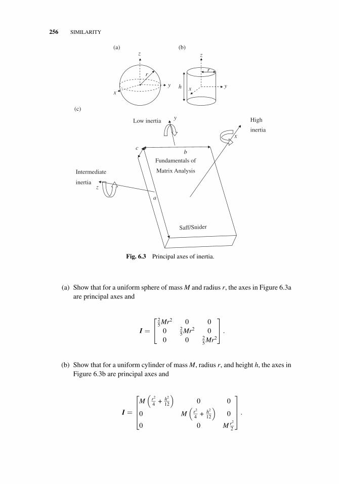
256 SIMILARITY
z
yx
r
z
r
yxh
(b)(a)
(c)
Low inertia High
inertia
Fundamentals of
Matrix Analysis
b
y
c
Intermediate
inertia
Saff/Snider
a
x
z
Fig. 6.3 Principal axes of inertia.
(a) Show that for a uniform sphere of mass M and radius r, the axes in Figure 6.3aare principal axes and
I =
⎡⎣
25 Mr2 0 0
0 25 Mr2 0
0 0 25 Mr2
⎤⎦ .
(b) Show that for a uniform cylinder of mass M, radius r, and height h, the axes inFigure 6.3b are principal axes and
I =
⎡⎢⎢⎣
M(
r2
4 + h2
12
)0 0
0 M(
r2
4 + h2
12
)0
0 0 M r2
2
⎤⎥⎥⎦ .
6.3 SCHUR DECOMPOSITION AND ITS IMPLICATIONS 257
(c) Show that for a uniform rectangular prism as shown in Figure 6.3c thedisplayed axes are principal axes and
I =
⎡⎢⎢⎣
112 M(a2 + b2) 0 0
0 112 M(c2 + b2) 0
0 0 112 M(a2 + c2)
⎤⎥⎥⎦ .
You can experiment with the moments of inertia of your (hardcopy) text-book by tying it shut with a rubber band and tossing it in the air. You will beable to spin it smoothly around the “high inertia” and “low inertia” axes; buteven though the “intermediate inertia” axis is a principal axis, the revolutionsare unstable with respect to small perturbations. Try it out.
16. The first-order expansion of the Maclauren series for a suitably smoothfunction f is given by
f (x, y) = f (0, 0) +∂f (0, 0)
∂xx +
∂f (0, 0)∂y
y + O(x2 + y2
),
where O(x2 + y2) is a term bounded by a constant times (x2 + y2). Apply thisto the length functions in Example 2 to justify the approximations made there.
6.3 SCHUR DECOMPOSITION AND ITS IMPLICATIONS
Section 6.1 demonstrated that the diagonalization of a matrix is extremely useful infacilitating computations. But the goal of attaining a diagonal D = P−1AP, with aninvertible P, is not always possible, since Example 5 of Section 5.2 showed that not allmatrices possess a full basis of eigenvectors (the columns of P); such matrices are saidto be defective. If we can’t get a diagonal matrix, what is the simplest matrix form thatwe can get, using similarity transformations?2
One answer is provided by a result known as the Schur decomposition.3 The formit achieves, upper triangular, may seem a far cry from diagonal, but (as we shall see)the result is quite powerful, the diagonalizing matrix P is unitary (and thus easy andaccurate to invert), and the derivation is not hard.
2The upper triangular matrix U produced by the A = LU factorization using Gauss elimination (Project A,Part I) is not similar to A (there is no right multiplier L−1).3Issai Schur (1875–1941) is most remembered for this decomposition and his Lemma on group represen-tations.
www.ebook3000.com
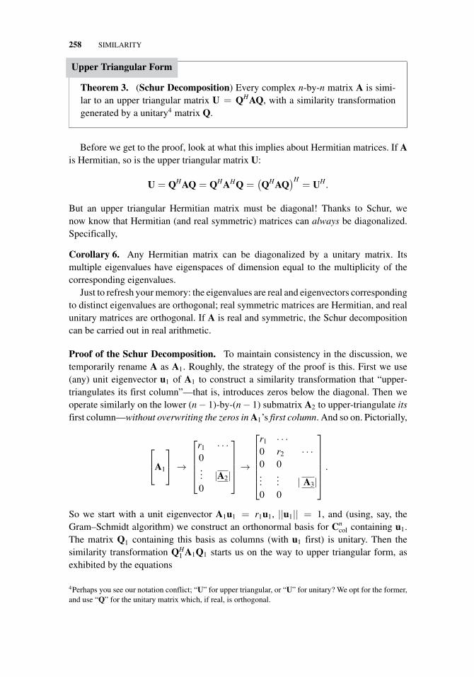
258 SIMILARITY
Upper Triangular Form
Theorem 3. (Schur Decomposition) Every complex n-by-n matrix A is simi-lar to an upper triangular matrix U = QHAQ, with a similarity transformationgenerated by a unitary4 matrix Q.
Before we get to the proof, look at what this implies about Hermitian matrices. If Ais Hermitian, so is the upper triangular matrix U:
U = QHAQ = QHAHQ =(QHAQ
)H= UH .
But an upper triangular Hermitian matrix must be diagonal! Thanks to Schur, wenow know that Hermitian (and real symmetric) matrices can always be diagonalized.Specifically,
Corollary 6. Any Hermitian matrix can be diagonalized by a unitary matrix. Itsmultiple eigenvalues have eigenspaces of dimension equal to the multiplicity of thecorresponding eigenvalues.
Just to refresh your memory: the eigenvalues are real and eigenvectors correspondingto distinct eigenvalues are orthogonal; real symmetric matrices are Hermitian, and realunitary matrices are orthogonal. If A is real and symmetric, the Schur decompositioncan be carried out in real arithmetic.
Proof of the Schur Decomposition. To maintain consistency in the discussion, wetemporarily rename A as A1. Roughly, the strategy of the proof is this. First we use(any) unit eigenvector u1 of A1 to construct a similarity transformation that “upper-triangulates its first column”—that is, introduces zeros below the diagonal. Then weoperate similarly on the lower (n − 1)-by-(n − 1) submatrix A2 to upper-triangulate itsfirst column—without overwriting the zeros in A1’s first column. And so on. Pictorially,
⎡⎣A1
⎤⎦ →
⎡⎢⎢⎢⎣
r1 · · ·0... |A2|0
⎤⎥⎥⎥⎦→
⎡⎢⎢⎢⎢⎢⎣
r1 · · ·0 r2 · · ·0 0...
... | A3|0 0
⎤⎥⎥⎥⎥⎥⎦
.
So we start with a unit eigenvector A1u1 = r1u1, ||u1|| = 1, and (using, say, theGram–Schmidt algorithm) we construct an orthonormal basis for Cn
col containing u1.The matrix Q1 containing this basis as columns (with u1 first) is unitary. Then thesimilarity transformation QH
1 A1Q1 starts us on the way to upper triangular form, asexhibited by the equations
4Perhaps you see our notation conflict; “U” for upper triangular, or “U” for unitary? We opt for the former,and use “Q” for the unitary matrix which, if real, is orthogonal.
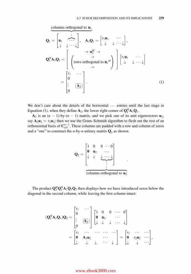
6.3 SCHUR DECOMPOSITION AND ITS IMPLICATIONS 259
columns orthogonal to u1︸ ︷︷ ︸Q1 =
⎡⎣u1
|︷︸︸︷· · ·
↓ ↓ · · · ↓
⎤⎦, A1Q1 =
[r1u1 · · ·↓ ↓ · · · ↓
],
QH1 A1Q1 =
⎡⎢⎢⎣
→ uH1 →⎛
⎝ →rows orthogonal to u1
H
→
⎞⎠
⎤⎥⎥⎦[
r1u1 · · ·↓ ↓ · · · ↓
]
=
⎡⎢⎢⎢⎣
r1 · · ·0... |A2 |0
⎤⎥⎥⎥⎦ . (1)
We don’t care about the details of the horizontal · · · entries until the last stage inEquation (1), when they define A2, the lower right corner of QH
1 A1Q1.A2 is an (n − 1)-by-(n − 1) matrix, and we pick one of its unit eigenvectors u2,
say A2u2 = r2u2; then we use the Gram–Schmidt algorithm to flesh out the rest of anorthonormal basis of Cn−1
col . These columns are padded with a row and column of zerosand a “one” to construct the n-by-n unitary matrix Q2 as shown:
Q2 =
⎡⎢⎢⎢⎣
1 0 0 · · · 00 u2 · · ·↓ ↓ ↓ · · · ↓︸ ︷︷ ︸
|
⎤⎥⎥⎥⎦
|︷ ︸︸ ︷columns orthogonal to u2
.
The product QH2 QH
1 A1Q1Q2 then displays how we have introduced zeros below thediagonal in the second column, while leaving the first column intact:
(QH1 A1Q1)Q2 =
⎡⎢⎢⎢⎣
r1 · · ·0... |A2 |0
⎤⎥⎥⎥⎦⎡⎣1 0 0 · · · 0
0 u2 · · ·↓ ↓ ↓ · · · ↓
⎤⎦
=
⎡⎣r1 · · · · · · · · · · · ·
0 A2u2 · · ·↓ ↓ ↓ · · · ↓
⎤⎦ =
⎡⎣r1 · · · · · ·
0 r2u2 · · ·↓ ↓ · · ·
⎤⎦,
www.ebook3000.com
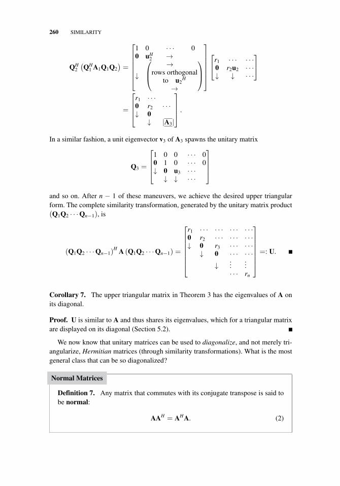
260 SIMILARITY
QH2
(QH
1 A1Q1Q2)=
⎡⎢⎢⎢⎢⎢⎣
1 0 · · · 00 uH
2 →
↓
⎛⎜⎝
→rows orthogonal
to u2H
→
⎞⎟⎠
⎤⎥⎥⎥⎥⎥⎦
⎡⎣r1 · · · · · ·
0 r2u2 · · ·↓ ↓ · · ·
⎤⎦
=
⎡⎢⎢⎣
r1 · · ·0 r2 · · ·↓ 0
↓ |A3|
⎤⎥⎥⎦ .
In a similar fashion, a unit eigenvector v3 of A3 spawns the unitary matrix
Q3 =
⎡⎢⎢⎣
1 0 0 · · · 00 1 0 · · · 0↓ 0 u3 · · ·
↓ ↓ · · ·
⎤⎥⎥⎦
and so on. After n − 1 of these maneuvers, we achieve the desired upper triangularform. The complete similarity transformation, generated by the unitary matrix product(Q1Q2 · · ·Qn−1), is
(Q1Q2 · · ·Qn−1)H A (Q1Q2 · · ·Qn−1) =
⎡⎢⎢⎢⎢⎢⎢⎣
r1 · · · · · · · · · · · ·0 r2 · · · · · · · · ·↓ 0 r3 · · · · · ·
↓ 0 · · · · · ·↓
......
· · · rn
⎤⎥⎥⎥⎥⎥⎥⎦=: U.
Corollary 7. The upper triangular matrix in Theorem 3 has the eigenvalues of A onits diagonal.
Proof. U is similar to A and thus shares its eigenvalues, which for a triangular matrixare displayed on its diagonal (Section 5.2).
We now know that unitary matrices can be used to diagonalize, and not merely tri-angularize, Hermitian matrices (through similarity transformations). What is the mostgeneral class that can be so diagonalized?
Normal Matrices
Definition 7. Any matrix that commutes with its conjugate transpose is said tobe normal:
AAH = AHA. (2)
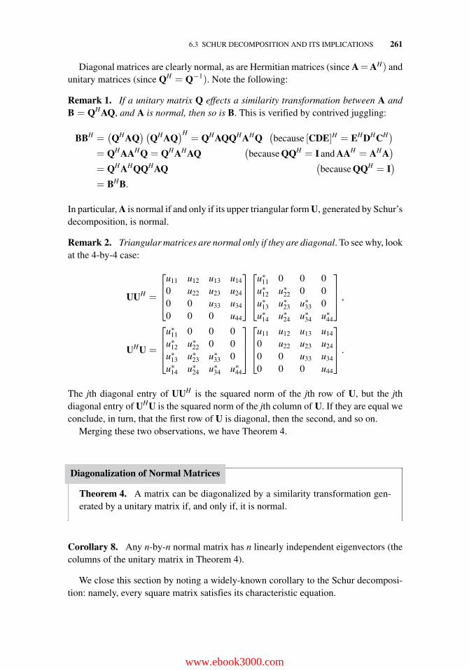
6.3 SCHUR DECOMPOSITION AND ITS IMPLICATIONS 261
Diagonal matrices are clearly normal, as are Hermitian matrices (since A=AH) andunitary matrices (since QH = Q−1). Note the following:
Remark 1. If a unitary matrix Q effects a similarity transformation between A andB = QHAQ, and A is normal, then so is B. This is verified by contrived juggling:
BBH =(QHAQ
) (QHAQ
)H= QHAQQHAHQ
(because [CDE]H = EHDHCH)
= QHAAHQ = QHAHAQ(because QQH = I and AAH = AHA
)= QHAHQQHAQ
(because QQH = I
)= BHB.
In particular, A is normal if and only if its upper triangular form U, generated by Schur’sdecomposition, is normal.
Remark 2. Triangular matrices are normal only if they are diagonal. To see why, lookat the 4-by-4 case:
UUH =
⎡⎢⎢⎣
u11 u12 u13 u14
0 u22 u23 u24
0 0 u33 u34
0 0 0 u44
⎤⎥⎥⎦
⎡⎢⎢⎣
u∗11 0 0 0u∗12 u∗22 0 0u∗
13 u∗23 u∗33 0u∗
14 u∗24 u∗34 u∗44
⎤⎥⎥⎦ ,
UHU =
⎡⎢⎢⎣
u∗11 0 0 0u∗12 u∗22 0 0u∗
13 u∗23 u∗33 0u∗
14 u∗24 u∗34 u∗44
⎤⎥⎥⎦
⎡⎢⎢⎣
u11 u12 u13 u14
0 u22 u23 u24
0 0 u33 u34
0 0 0 u44
⎤⎥⎥⎦ .
The jth diagonal entry of UUH is the squared norm of the jth row of U, but the jthdiagonal entry of UHU is the squared norm of the jth column of U. If they are equal weconclude, in turn, that the first row of U is diagonal, then the second, and so on.
Merging these two observations, we have Theorem 4.
Diagonalization of Normal Matrices
Theorem 4. A matrix can be diagonalized by a similarity transformation gen-erated by a unitary matrix if, and only if, it is normal.
Corollary 8. Any n-by-n normal matrix has n linearly independent eigenvectors (thecolumns of the unitary matrix in Theorem 4).
We close this section by noting a widely-known corollary to the Schur decomposi-tion: namely, every square matrix satisfies its characteristic equation.
www.ebook3000.com
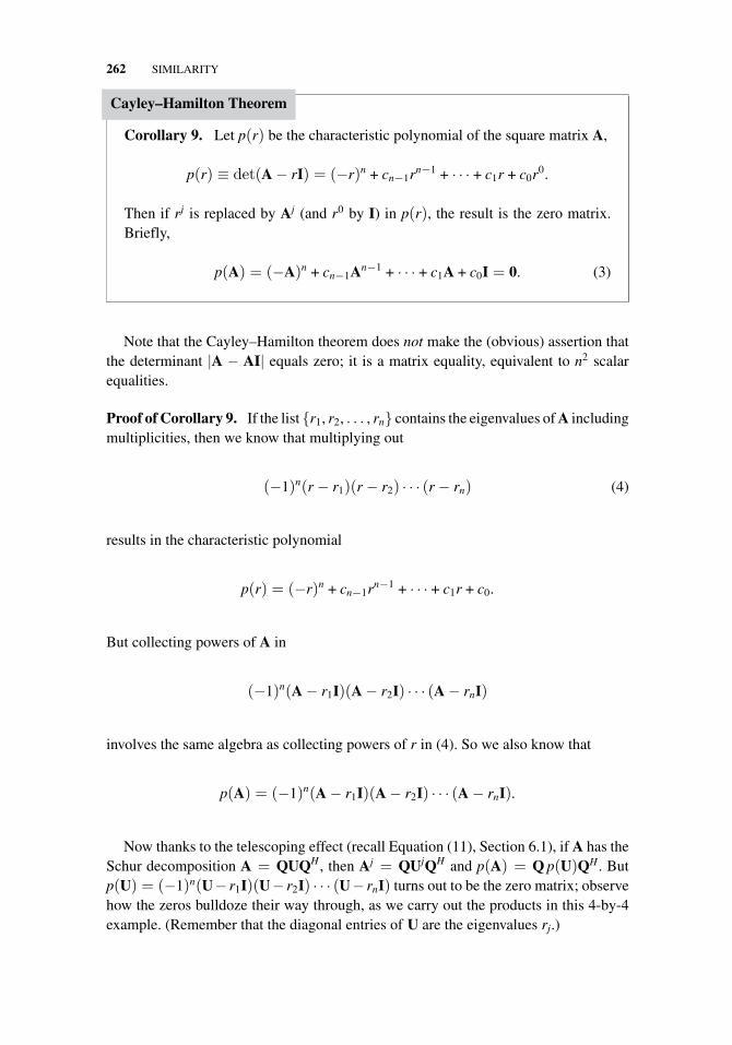
262 SIMILARITY
Cayley–Hamilton Theorem
Corollary 9. Let p(r) be the characteristic polynomial of the square matrix A,
p(r) ≡ det(A − rI) = (−r)n + cn−1rn−1 + · · · + c1r + c0r0.
Then if rj is replaced by Aj (and r0 by I) in p(r), the result is the zero matrix.Briefly,
p(A) = (−A)n + cn−1An−1 + · · · + c1A + c0I = 0. (3)
Note that the Cayley–Hamilton theorem does not make the (obvious) assertion thatthe determinant |A − AI| equals zero; it is a matrix equality, equivalent to n2 scalarequalities.
Proof of Corollary 9. If the list {r1, r2, . . . , rn} contains the eigenvalues of A includingmultiplicities, then we know that multiplying out
(−1)n(r − r1)(r − r2) · · · (r − rn) (4)
results in the characteristic polynomial
p(r) = (−r)n + cn−1rn−1 + · · · + c1r + c0.
But collecting powers of A in
(−1)n(A − r1I)(A − r2I) · · · (A − rnI)
involves the same algebra as collecting powers of r in (4). So we also know that
p(A) = (−1)n(A − r1I)(A − r2I) · · · (A − rnI).
Now thanks to the telescoping effect (recall Equation (11), Section 6.1), if A has theSchur decomposition A = QUQH , then Aj = QUjQH and p(A) = Q p(U)QH . Butp(U) = (−1)n(U− r1I)(U− r2I) · · · (U− rnI) turns out to be the zero matrix; observehow the zeros bulldoze their way through, as we carry out the products in this 4-by-4example. (Remember that the diagonal entries of U are the eigenvalues rj.)
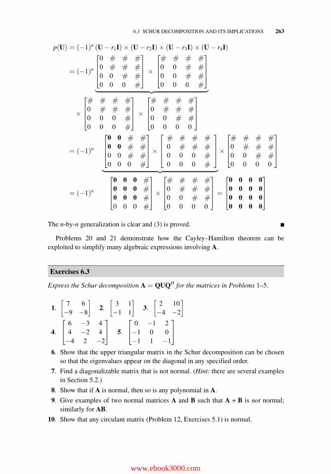
6.3 SCHUR DECOMPOSITION AND ITS IMPLICATIONS 263
p(U) = (−1)n (U − r1I)× (U − r2I)× (U − r3I)× (U − r4I)
= (−1)n
⎡⎢⎢⎣
0 # # #0 # # #0 0 # #0 0 0 #
⎤⎥⎥⎦ ×
⎡⎢⎢⎣# # # #0 0 # #0 0 # #0 0 0 #
⎤⎥⎥⎦
︸ ︷︷ ︸
×
⎡⎢⎢⎣# # # #0 # # #0 0 0 #0 0 0 #
⎤⎥⎥⎦ ×
⎡⎢⎢⎣# # # #0 # # #0 0 # #0 0 0 0
⎤⎥⎥⎦
= (−1)n
⎡⎢⎢⎣
0 0 # #0 0 # #0 0 # #0 0 0 #
⎤⎥⎥⎦×
⎡⎢⎢⎣
# # # #0 # # #0 0 0 #0 0 0 #
⎤⎥⎥⎦
︸ ︷︷ ︸×
⎡⎢⎢⎣# # # #0 # # #0 0 # #0 0 0 0
⎤⎥⎥⎦
= (−1)n
⎡⎢⎢⎣
0 0 0 #0 0 0 #0 0 0 #0 0 0 #
⎤⎥⎥⎦×
⎡⎢⎢⎣# # # #0 # # #0 0 # #0 0 0 0
⎤⎥⎥⎦ =
⎡⎢⎢⎣
0 0 0 00 0 0 00 0 0 00 0 0 0
⎤⎥⎥⎦
The n-by-n generalization is clear and (3) is proved.
Problems 20 and 21 demonstrate how the Cayley–Hamilton theorem can beexploited to simplify many algebraic expressions involving A.
Exercises 6.3
Express the Schur decomposition A = QUQH for the matrices in Problems 1–5.
1.
[7 6−9 −8
]2.
[3 1−1 1
]3.
[2 10−4 −2
]
4.
⎡⎣ 6 −3 4
4 −2 4−4 2 −2
⎤⎦ 5.
⎡⎣ 0 −1 2−1 0 0−1 1 −1
⎤⎦
6. Show that the upper triangular matrix in the Schur decomposition can be chosenso that the eigenvalues appear on the diagonal in any specified order.
7. Find a diagonalizable matrix that is not normal. (Hint: there are several examplesin Section 5.2.)
8. Show that if A is normal, then so is any polynomial in A.
9. Give examples of two normal matrices A and B such that A + B is not normal;similarly for AB.
10. Show that any circulant matrix (Problem 12, Exercises 5.1) is normal.
www.ebook3000.com
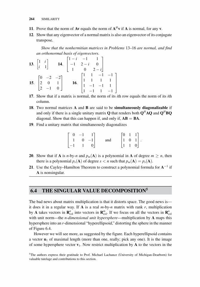
264 SIMILARITY
11. Prove that the norm of Av equals the norm of AHv if A is normal, for any v.
12. Show that any eigenvector of a normal matrix is also an eigenvector of its conjugatetranspose.
Show that the nonhermitian matrices in Problems 13–16 are normal, and findan orthonormal basis of eigenvectors.
13.
[1 ii 1
]14.
⎡⎣1 − i −1 1
−1 2 − i 01 0 2 − i
⎤⎦
15.
⎡⎣0 −2 −2
2 0 12 −1 0
⎤⎦ 16.
⎡⎢⎢⎣
1 1 −1 −11 1 1 11 −1 −1 11 −1 1 −1
⎤⎥⎥⎦
17. Show that if a matrix is normal, the norm of its ith row equals the norm of its ithcolumn.
18. Two normal matrices A and B are said to be simultaneously diagonalizable ifand only if there is a single unitary matrix Q that renders both QHAQ and QHBQdiagonal. Show that this can happen if, and only if, AB = BA.
19. Find a unitary matrix that simultaneously diagonalizes
⎡⎣ 0 −1 1
1 0 −1−1 1 0
⎤⎦ and
⎡⎣0 1 1
1 0 11 1 0
⎤⎦ .
20. Show that if A is n-by-n and pm(A) is a polynomial in A of degree m ≥ n, thenthere is a polynomial ps(A) of degree s < n such that pm(A) = ps(A).
21. Use the Cayley–Hamilton Theorem to construct a polynomial formula for A−1 ifA is nonsingular.
6.4 THE SINGULAR VALUE DECOMPOSITION5
The bad news about matrix multiplication is that it distorts space. The good news is—it does it in a regular way. If A is a real m-by-n matrix with rank r, multiplicationby A takes vectors in Rn
col into vectors in Rmcol. If we focus on all the vectors in Rn
col
with unit norm—the n-dimensional unit hypersphere—multiplication by A maps thishypersphere into an r-dimensional “hyperellipsoid,” distorting the sphere in the mannerof Figure 6.4.
However we will see more, as suggested by the figure. Each hyperellipsoid containsa vector u1 of maximal length (more than one, really; pick any one). It is the imageof some hypersphere vector v1. Now restrict multiplication by A to the vectors in the
5The authors express their gratitude to Prof. Michael Lachance (University of Michigan-Dearborn) forvaluable tutelage and contributions to this section.
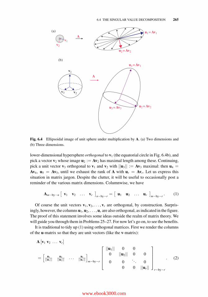
6.4 THE SINGULAR VALUE DECOMPOSITION 265
v1v2
u2 =Av2
u1 =Av1A
v1
v2v3
u1 =Av1
u2 =Av2u3 =Av3
A
(a)
(b)
Fig. 6.4 Ellipsoidal image of unit sphere under multiplication by A. (a) Two dimensions and
(b) Three dimensions.
lower-dimensional hypersphere orthogonal to v1 (the equatorial circle in Fig. 6.4b), andpick a vector v2 whose image u2 := Av2 has maximal length among these. Continuing,pick a unit vector v3 orthogonal to v1 and v2 with ||u3|| := Av3 maximal: then u4 =Av4, u5 = Av5, until we exhaust the rank of A with ur = Avr. Let us express thissituation in matrix jargon. Despite the clutter, it will be useful to occasionally post areminder of the various matrix dimensions. Columnwise, we have
Am−by−n[
v1 v2 . . . vr
]n−by−r
=[
u1 u2 . . . ur
]m−by−r
. (1)
Of course the unit vectors v1, v2, . . . , vr are orthogonal, by construction. Surpris-ingly, however, the columns u1, u2, . . . , ur are also orthogonal, as indicated in the figure.The proof of this statement involves some ideas outside the realm of matrix theory. Wewill guide you through them in Problems 25–27. For now let’s go on, to see the benefits.
It is traditional to tidy up (1) using orthogonal matrices. First we render the columnsof the u-matrix so that they are unit vectors (like the v-matrix):
A [v1 v2 . . . vr]
=[
u1||u1||
u2||u2|| . . . ur
||ur||
]m−by−r
⎡⎢⎢⎢⎣
||u1|| 0 00 ||u2|| 0 0
0 0. . . 0
0 0 ||ur||
⎤⎥⎥⎥⎦
r−by−r
. (2)
www.ebook3000.com
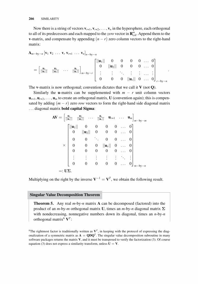
266 SIMILARITY
Now there is a string of vectors vr+1, vr+2, . . . , vn in the hypersphere, each orthogonalto all of its predecessors and each mapped to the zero vector in Rm
col. Append them to thev-matrix, and compensate by appending (n − r) zero column vectors to the right-handmatrix:
Am−by−n [v1 v2 . . . vr vr+1 . . . vn]n−by−n
=[
u1||u1||
u2||u2|| . . . ur
||ur||
]m−by−r
⎡⎢⎢⎢⎣||u1|| 0 0 0 0 . . . 0
0 ||u2|| 0 0 0 . . . 0...
.... . .
...... . . .
...0 0 0 ||ur|| 0 . . . 0
⎤⎥⎥⎥⎦
r−by−n
.
The v-matrix is now orthogonal; convention dictates that we call it V (not Q).Similarly the u-matrix can be supplemented with m − r unit column vectors
ur+1, ur+2, . . . , um to create an orthogonal matrix, U (convention again); this is compen-sated by adding (m − r) zero row vectors to form the right-hand side diagonal matrix. . . diagonal matrix bold capital Sigma:
AV =[
u1||u1||
u2||u2|| . . . ur
||ur|| ur+1 . . . um
]m−by−m
×
⎡⎢⎢⎢⎢⎢⎢⎢⎢⎢⎢⎢⎣
||u1|| 0 0 0 0 . . . 00 ||u2|| 0 0 0 . . . 0
0 0. . . 0 0 . . . 0
0 0 0 ||ur|| 0 . . . 00 0 0 0 0 . . . 0...
......
......
. . ....
0 0 0 0 0 . . . 0
⎤⎥⎥⎥⎥⎥⎥⎥⎥⎥⎥⎥⎦
m−by−n
=: UΣ.
Multiplying on the right by the inverse V−1 = VT , we obtain the following result.
Singular Value Decomposition Theorem
Theorem 5. Any real m-by-n matrix A can be decomposed (factored) into theproduct of an m-by-m orthogonal matrix U, times an m-by-n diagonal matrix Σ
with nondecreasing, nonnegative numbers down its diagonal, times an n-by-northogonal matrix6 VT :
6The rightmost factor is traditionally written as VT , in keeping with the protocol of expressing the diag-onalization of a symmetric matrix as A = QDQT . The singular value decomposition subroutine in manysoftware packages returns the matrix V, and it must be transposed to verify the factorization (3). Of courseequation (3) does not express a similarity transform, unless U = V.
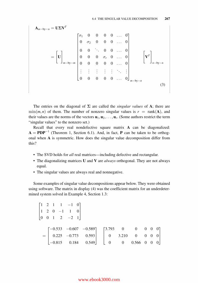
6.4 THE SINGULAR VALUE DECOMPOSITION 267
Am−by−n = UΣVT
=
[U
]
m−by−m
⎡⎢⎢⎢⎢⎢⎢⎢⎢⎢⎢⎢⎢⎢⎣
σ1 0 0 0 0 . . . 0
0 σ2 0 0 0 . . . 0
0 0. . . 0 0 . . . 0
0 0 0 σr 0 . . . 0
0 0 0 0 0 . . . 0...
......
......
. . ....
0 0 0 0 0 . . . 0
⎤⎥⎥⎥⎥⎥⎥⎥⎥⎥⎥⎥⎥⎥⎦
m−by−n
[VT
]
n−by−n
(3)
The entries on the diagonal of Σ are called the singular values of A; there aremin(m, n) of them. The number of nonzero singular values is r = rank(A), andtheir values are the norms of the vectors u1, u2, . . . , ur. (Some authors restrict the term“singular values” to the nonzero set.)
Recall that every real nondefective square matrix A can be diagonalized:A = PDP−1 (Theorem 1, Section 6.1). And, in fact, P can be taken to be orthog-onal when A is symmetric. How does the singular value decomposition differ fromthis?
• The SVD holds for all real matrices—including defective and rectangular.
• The diagonalizing matrices U and V are always orthogonal. They are not alwaysequal.
• The singular values are always real and nonnegative.
Some examples of singular value decompositions appear below. They were obtainedusing software. The matrix in display (4) was the coefficient matrix for an underdeter-mined system solved in Example 4, Section 1.3:
⎡⎢⎣
1 2 1 1 −1 0
1 2 0 −1 1 0
0 0 1 2 −2 1
⎤⎥⎦
=
⎡⎢⎣−0.533 −0.607 −0.589
0.225 −0.773 0.593
−0.815 0.184 0.549
⎤⎥⎦
⎡⎢⎣
3.793 0 0 0 0 0
0 3.210 0 0 0 0
0 0 0.566 0 0 0
⎤⎥⎦
www.ebook3000.com
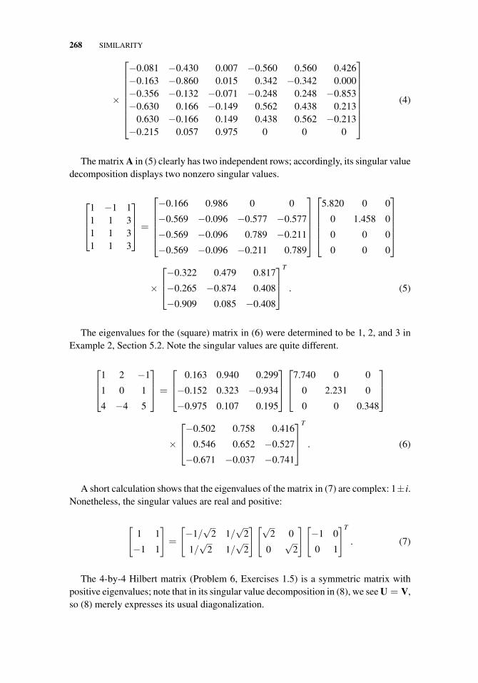
268 SIMILARITY
×
⎡⎢⎢⎢⎢⎢⎢⎢⎣
−0.081 −0.430 0.007 −0.560 0.560 0.426−0.163 −0.860 0.015 0.342 −0.342 0.000−0.356 −0.132 −0.071 −0.248 0.248 −0.853−0.630 0.166 −0.149 0.562 0.438 0.213
0.630 −0.166 0.149 0.438 0.562 −0.213−0.215 0.057 0.975 0 0 0
⎤⎥⎥⎥⎥⎥⎥⎥⎦
(4)
The matrix A in (5) clearly has two independent rows; accordingly, its singular valuedecomposition displays two nonzero singular values.
⎡⎢⎢⎣
1 −1 11 1 31 1 31 1 3
⎤⎥⎥⎦ =
⎡⎢⎢⎢⎢⎣
−0.166 0.986 0 0
−0.569 −0.096 −0.577 −0.577
−0.569 −0.096 0.789 −0.211
−0.569 −0.096 −0.211 0.789
⎤⎥⎥⎥⎥⎦
⎡⎢⎢⎢⎢⎣
5.820 0 0
0 1.458 0
0 0 0
0 0 0
⎤⎥⎥⎥⎥⎦
×
⎡⎢⎣−0.322 0.479 0.817
−0.265 −0.874 0.408
−0.909 0.085 −0.408
⎤⎥⎦
T
. (5)
The eigenvalues for the (square) matrix in (6) were determined to be 1, 2, and 3 inExample 2, Section 5.2. Note the singular values are quite different.
⎡⎢⎣
1 2 −1
1 0 1
4 −4 5
⎤⎥⎦ =
⎡⎢⎣
0.163 0.940 0.299
−0.152 0.323 −0.934
−0.975 0.107 0.195
⎤⎥⎦⎡⎢⎣
7.740 0 0
0 2.231 0
0 0 0.348
⎤⎥⎦
×
⎡⎢⎣−0.502 0.758 0.416
0.546 0.652 −0.527
−0.671 −0.037 −0.741
⎤⎥⎦
T
. (6)
A short calculation shows that the eigenvalues of the matrix in (7) are complex: 1±i.Nonetheless, the singular values are real and positive:
[1 1
−1 1
]=
[−1/
√2 1/
√2
1/√
2 1/√
2
][√2 0
0√
2
][−1 0
0 1
]T
. (7)
The 4-by-4 Hilbert matrix (Problem 6, Exercises 1.5) is a symmetric matrix withpositive eigenvalues; note that in its singular value decomposition in (8), we see U = V,so (8) merely expresses its usual diagonalization.
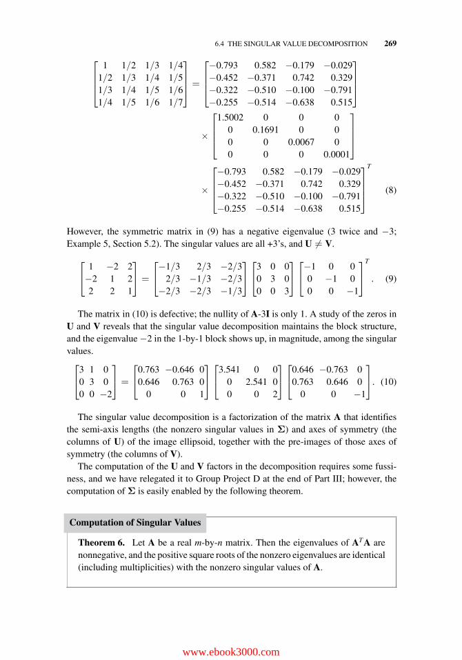
6.4 THE SINGULAR VALUE DECOMPOSITION 269
⎡⎢⎢⎣
1 1/2 1/3 1/41/2 1/3 1/4 1/51/3 1/4 1/5 1/61/4 1/5 1/6 1/7
⎤⎥⎥⎦ =
⎡⎢⎢⎣−0.793 0.582 −0.179 −0.029−0.452 −0.371 0.742 0.329−0.322 −0.510 −0.100 −0.791−0.255 −0.514 −0.638 0.515
⎤⎥⎥⎦
×
⎡⎢⎢⎣
1.5002 0 0 00 0.1691 0 00 0 0.0067 00 0 0 0.0001
⎤⎥⎥⎦
×
⎡⎢⎢⎣−0.793 0.582 −0.179 −0.029−0.452 −0.371 0.742 0.329−0.322 −0.510 −0.100 −0.791−0.255 −0.514 −0.638 0.515
⎤⎥⎥⎦
T
(8)
However, the symmetric matrix in (9) has a negative eigenvalue (3 twice and −3;Example 5, Section 5.2). The singular values are all +3’s, and U �= V.
⎡⎣ 1 −2 2−2 1 22 2 1
⎤⎦ =
⎡⎣−1/3 2/3 −2/3
2/3 −1/3 −2/3−2/3 −2/3 −1/3
⎤⎦⎡⎣3 0 0
0 3 00 0 3
⎤⎦⎡⎣−1 0 0
0 −1 00 0 −1
⎤⎦
T
. (9)
The matrix in (10) is defective; the nullity of A-3I is only 1. A study of the zeros inU and V reveals that the singular value decomposition maintains the block structure,and the eigenvalue −2 in the 1-by-1 block shows up, in magnitude, among the singularvalues.⎡⎣3 1 0
0 3 00 0 −2
⎤⎦ =
⎡⎣0.763 −0.646 0
0.646 0.763 00 0 1
⎤⎦⎡⎣3.541 0 0
0 2.541 00 0 2
⎤⎦⎡⎣0.646 −0.763 0
0.763 0.646 00 0 −1
⎤⎦. (10)
The singular value decomposition is a factorization of the matrix A that identifiesthe semi-axis lengths (the nonzero singular values in Σ) and axes of symmetry (thecolumns of U) of the image ellipsoid, together with the pre-images of those axes ofsymmetry (the columns of V).
The computation of the U and V factors in the decomposition requires some fussi-ness, and we have relegated it to Group Project D at the end of Part III; however, thecomputation of Σ is easily enabled by the following theorem.
Computation of Singular Values
Theorem 6. Let A be a real m-by-n matrix. Then the eigenvalues of ATA arenonnegative, and the positive square roots of the nonzero eigenvalues are identical(including multiplicities) with the nonzero singular values of A.
www.ebook3000.com
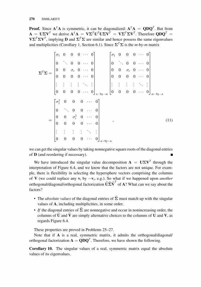
270 SIMILARITY
Proof. Since ATA is symmetric, it can be diagonalized: ATA = QDQT . But fromA = UΣVT we derive ATA = VΣTUTUΣVT = VΣTΣVT . Therefore QDQT =VΣTΣVT , implying D and ΣTΣ are similar and hence possess the same eigenvaluesand multiplicities (Corollary 1, Section 6.1). Since ΣTΣ is the m-by-m matrix
ΣTΣ =
⎡⎢⎢⎢⎢⎢⎢⎢⎢⎢⎢⎢⎣
σ1 0 0 0 · · · 0
0. . . 0 0 · · · 0
0 0 σr 0 · · · 0
0 0 0 0 · · · 0...
......
.... . .
...
0 0 0 0 · · · 0
⎤⎥⎥⎥⎥⎥⎥⎥⎥⎥⎥⎥⎦
n−by−m
⎡⎢⎢⎢⎢⎢⎢⎢⎢⎢⎢⎢⎣
σ1 0 0 0 · · · 0
0. . . 0 0 · · · 0
0 0 σr 0 · · · 0
0 0 0 0 · · · 0...
......
.... . .
...
0 0 0 0 · · · 0
⎤⎥⎥⎥⎥⎥⎥⎥⎥⎥⎥⎥⎦
m−by−n
=
⎡⎢⎢⎢⎢⎢⎢⎢⎢⎢⎢⎢⎣
σ21 0 0 0 · · · 0
0. . . 0 0 · · · 0
0 0 σ2r 0 · · · 0
0 0 0 0 · · · 0...
......
.... . .
...
0 0 0 0 · · · 0
⎤⎥⎥⎥⎥⎥⎥⎥⎥⎥⎥⎥⎦
n−by−n
, (11)
we can get the singular values by taking nonnegative square roots of the diagonal entriesof D (and reordering if necessary).
We have introduced the singular value decomposition A = UΣVT through theinterpretation of Figure 6.4, and we know that the factors are not unique. For exam-ple, there is flexibility in selecting the hypersphere vectors comprising the columnsof V (we could replace any vi by −vi, e.g.). So what if we happened upon another
orthogonal/diagonal/orthogonal factorization UΣVT
of A? What can we say about thefactors?
• The absolute values of the diagonal entries of Σ must match up with the singularvalues of A, including multiplicities, in some order.
• If the diagonal entries of Σ are nonnegative and occur in nonincreasing order, thecolumns of U and V are simply alternative choices to the columns of U and V, asregards Figure 6.4.
These properties are proved in Problems 25–27.Note that if A is a real, symmetric matrix, it admits the orthogonal/diagonal/
orthogonal factorization A = QDQT . Therefore, we have shown the following.
Corollary 10. The singular values of a real, symmetric matrix equal the absolutevalues of its eigenvalues.
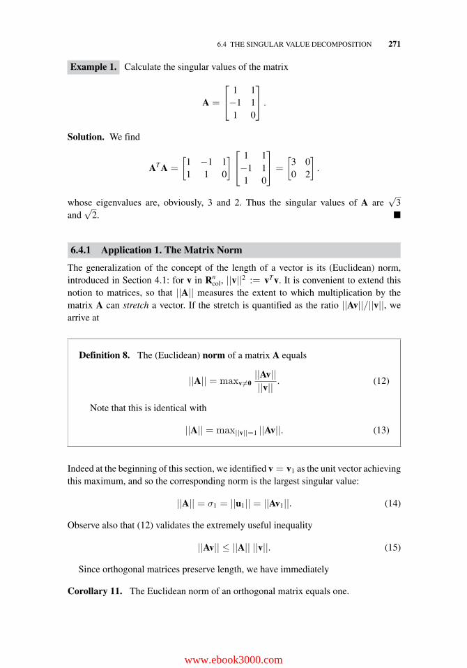
6.4 THE SINGULAR VALUE DECOMPOSITION 271
Example 1. Calculate the singular values of the matrix
A =
⎡⎣ 1 1−1 11 0
⎤⎦ .
Solution. We find
ATA =
[1 −1 11 1 0
]⎡⎣ 1 1−1 11 0
⎤⎦ =
[3 00 2
].
whose eigenvalues are, obviously, 3 and 2. Thus the singular values of A are√
3and
√2. �
6.4.1 Application 1. The Matrix Norm
The generalization of the concept of the length of a vector is its (Euclidean) norm,introduced in Section 4.1: for v in Rn
col, ||v||2 := vTv. It is convenient to extend thisnotion to matrices, so that ||A|| measures the extent to which multiplication by thematrix A can stretch a vector. If the stretch is quantified as the ratio ||Av||/||v||, wearrive at
Definition 8. The (Euclidean) norm of a matrix A equals
||A|| = maxv�=0||Av||||v|| . (12)
Note that this is identical with
||A|| = max||v||=1 ||Av||. (13)
Indeed at the beginning of this section, we identified v = v1 as the unit vector achievingthis maximum, and so the corresponding norm is the largest singular value:
||A|| = σ1 = ||u1|| = ||Av1||. (14)
Observe also that (12) validates the extremely useful inequality
||Av|| ≤ ||A|| ||v||. (15)
Since orthogonal matrices preserve length, we have immediately
Corollary 11. The Euclidean norm of an orthogonal matrix equals one.
www.ebook3000.com
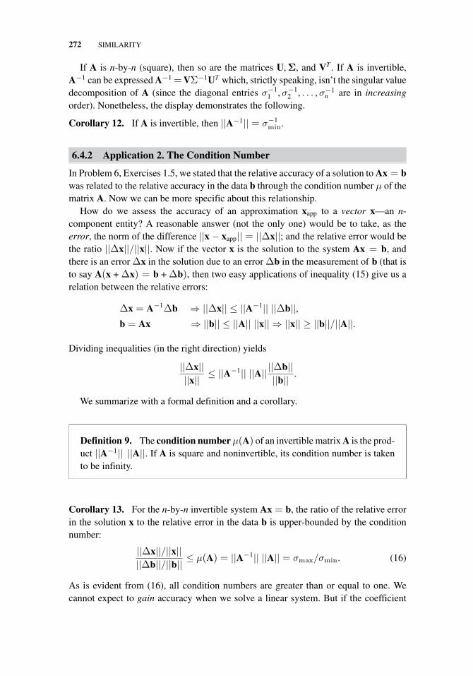
272 SIMILARITY
If A is n-by-n (square), then so are the matrices U,Σ, and VT . If A is invertible,A−1 can be expressed A−1 =VΣ−1UT which, strictly speaking, isn’t the singular valuedecomposition of A (since the diagonal entries σ−1
1 ,σ−12 , . . . ,σ−1
n are in increasingorder). Nonetheless, the display demonstrates the following.
Corollary 12. If A is invertible, then ||A−1|| = σ−1min.
6.4.2 Application 2. The Condition Number
In Problem 6, Exercises 1.5, we stated that the relative accuracy of a solution to Ax = bwas related to the relative accuracy in the data b through the condition number μ of thematrix A. Now we can be more specific about this relationship.
How do we assess the accuracy of an approximation xapp to a vector x—an n-component entity? A reasonable answer (not the only one) would be to take, as theerror, the norm of the difference ||x − xapp|| = ||Δx||; and the relative error would bethe ratio ||Δx||/||x||. Now if the vector x is the solution to the system Ax = b, andthere is an error Δx in the solution due to an error Δb in the measurement of b (that isto say A(x + Δx) = b + Δb), then two easy applications of inequality (15) give us arelation between the relative errors:
Δx = A−1Δb ⇒ ||Δx|| ≤ ||A−1|| ||Δb||,b = Ax ⇒ ||b|| ≤ ||A|| ||x|| ⇒ ||x|| ≥ ||b||/||A||.
Dividing inequalities (in the right direction) yields
||Δx||||x|| ≤ ||A−1|| ||A|| ||Δb||
||b|| .
We summarize with a formal definition and a corollary.
Definition 9. The condition numberμ(A) of an invertible matrix A is the prod-uct ||A−1|| ||A||. If A is square and noninvertible, its condition number is takento be infinity.
Corollary 13. For the n-by-n invertible system Ax = b, the ratio of the relative errorin the solution x to the relative error in the data b is upper-bounded by the conditionnumber:
||Δx||/||x||||Δb||/||b|| ≤ μ(A) = ||A−1|| ||A|| = σmax/σmin. (16)
As is evident from (16), all condition numbers are greater than or equal to one. Wecannot expect to gain accuracy when we solve a linear system. But if the coefficient
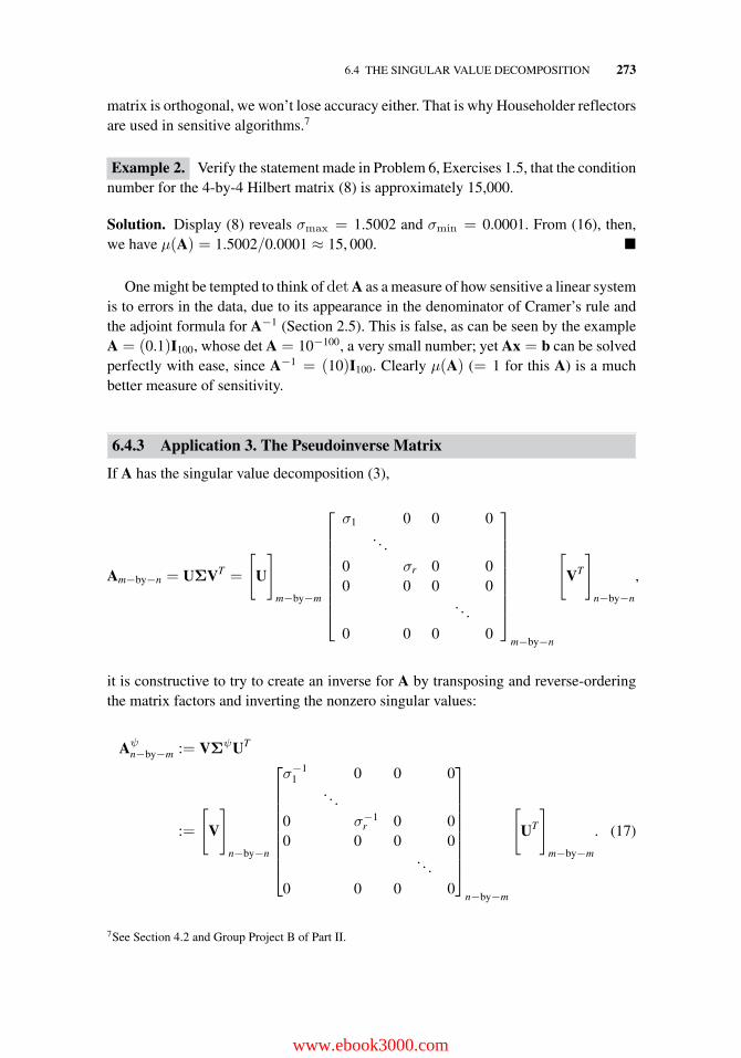
6.4 THE SINGULAR VALUE DECOMPOSITION 273
matrix is orthogonal, we won’t lose accuracy either. That is why Householder reflectorsare used in sensitive algorithms.7
Example 2. Verify the statement made in Problem 6, Exercises 1.5, that the conditionnumber for the 4-by-4 Hilbert matrix (8) is approximately 15,000.
Solution. Display (8) reveals σmax = 1.5002 and σmin = 0.0001. From (16), then,we have μ(A) = 1.5002/0.0001 ≈ 15, 000. �
One might be tempted to think of detA as a measure of how sensitive a linear systemis to errors in the data, due to its appearance in the denominator of Cramer’s rule andthe adjoint formula for A−1 (Section 2.5). This is false, as can be seen by the exampleA = (0.1)I100, whose det A = 10−100, a very small number; yet Ax = b can be solvedperfectly with ease, since A−1 = (10)I100. Clearly μ(A) (= 1 for this A) is a muchbetter measure of sensitivity.
6.4.3 Application 3. The Pseudoinverse Matrix
If A has the singular value decomposition (3),
Am−by−n = UΣVT =
[U
]
m−by−m
⎡⎢⎢⎢⎢⎢⎢⎢⎢⎣
σ1 0 0 0. . .
0 σr 0 00 0 0 0
. . .0 0 0 0
⎤⎥⎥⎥⎥⎥⎥⎥⎥⎦
m−by−n
[VT
]
n−by−n
,
it is constructive to try to create an inverse for A by transposing and reverse-orderingthe matrix factors and inverting the nonzero singular values:
Aψn−by−m := VΣψUT
:=
[V
]
n−by−n
⎡⎢⎢⎢⎢⎢⎢⎢⎢⎣
σ−11 0 0 0
. . .0 σ−1
r 0 00 0 0 0
. . .0 0 0 0
⎤⎥⎥⎥⎥⎥⎥⎥⎥⎦
n−by−m
[UT
]
m−by−m
. (17)
7See Section 4.2 and Group Project B of Part II.
www.ebook3000.com
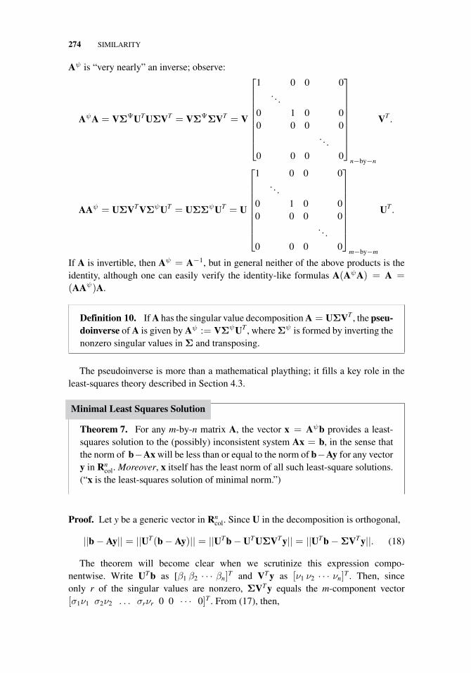
274 SIMILARITY
Aψ is “very nearly” an inverse; observe:
AψA = VΣΨUTUΣVT = VΣΨΣVT = V
⎡⎢⎢⎢⎢⎢⎢⎢⎢⎣
1 0 0 0. . .
0 1 0 00 0 0 0
. . .0 0 0 0
⎤⎥⎥⎥⎥⎥⎥⎥⎥⎦
n−by−n
VT .
AAψ = UΣVTVΣψUT = UΣΣψUT = U
⎡⎢⎢⎢⎢⎢⎢⎢⎢⎣
1 0 0 0. . .
0 1 0 00 0 0 0
. . .0 0 0 0
⎤⎥⎥⎥⎥⎥⎥⎥⎥⎦
m−by−m
UT .
If A is invertible, then Aψ = A−1, but in general neither of the above products is theidentity, although one can easily verify the identity-like formulas A(AψA) = A =(AAψ)A.
Definition 10. If A has the singular value decomposition A = UΣVT , the pseu-doinverse of A is given by Aψ := VΣψUT , where Σψ is formed by inverting thenonzero singular values in Σ and transposing.
The pseudoinverse is more than a mathematical plaything; it fills a key role in theleast-squares theory described in Section 4.3.
Minimal Least Squares Solution
Theorem 7. For any m-by-n matrix A, the vector x = Aψb provides a least-squares solution to the (possibly) inconsistent system Ax = b, in the sense thatthe norm of b−Ax will be less than or equal to the norm of b−Ay for any vectory in Rn
col. Moreover, x itself has the least norm of all such least-square solutions.(“x is the least-squares solution of minimal norm.”)
Proof. Let y be a generic vector in Rncol. Since U in the decomposition is orthogonal,
||b − Ay|| = ||UT(b − Ay)|| = ||UTb − UTUΣVTy|| = ||UTb −ΣVTy||. (18)
The theorem will become clear when we scrutinize this expression compo-nentwise. Write UTb as [β1 β2 · · · βn]T and VTy as [ν1 ν2 · · · νn]T . Then, sinceonly r of the singular values are nonzero, ΣVTy equals the m-component vector[σ1ν1 σ2ν2 . . . σrνr 0 0 · · · 0]T . From (17), then,
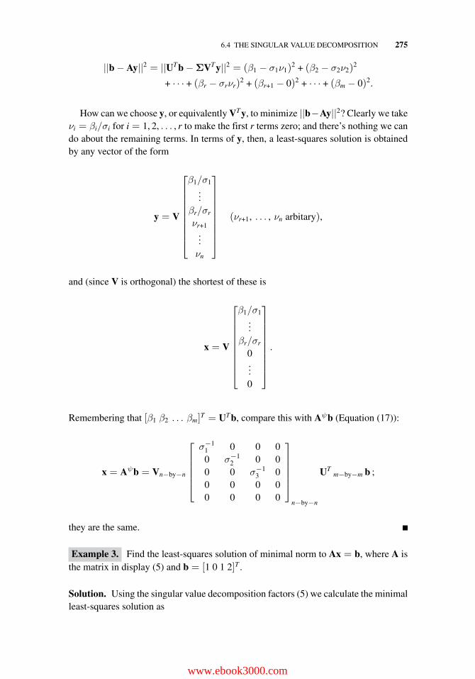
6.4 THE SINGULAR VALUE DECOMPOSITION 275
||b − Ay||2 = ||UTb −ΣVTy||2 = (β1 − σ1ν1)2 + (β2 − σ2ν2)
2
+ · · · + (βr − σrνr)2 + (βr+1 − 0)2 + · · · + (βm − 0)2.
How can we choose y, or equivalently VTy, to minimize ||b−Ay||2? Clearly we takeνi = βi/σi for i = 1, 2, . . . , r to make the first r terms zero; and there’s nothing we cando about the remaining terms. In terms of y, then, a least-squares solution is obtainedby any vector of the form
y = V
⎡⎢⎢⎢⎢⎢⎢⎢⎢⎣
β1/σ1...
βr/σr
νr+1...νn
⎤⎥⎥⎥⎥⎥⎥⎥⎥⎦
(νr+1, . . . , νn arbitary),
and (since V is orthogonal) the shortest of these is
x = V
⎡⎢⎢⎢⎢⎢⎢⎢⎢⎣
β1/σ1...
βr/σr
0...0
⎤⎥⎥⎥⎥⎥⎥⎥⎥⎦
.
Remembering that [β1 β2 . . . βm]T = UTb, compare this with Aψb (Equation (17)):
x = Aψb = Vn−by−n
⎡⎢⎢⎢⎢⎣
σ−11 0 0 00 σ−1
2 0 00 0 σ−1
3 00 0 0 00 0 0 0
⎤⎥⎥⎥⎥⎦
n−by−n
UTm−by−m b ;
they are the same.
Example 3. Find the least-squares solution of minimal norm to Ax = b, where A isthe matrix in display (5) and b = [1 0 1 2]T .
Solution. Using the singular value decomposition factors (5) we calculate the minimalleast-squares solution as
www.ebook3000.com
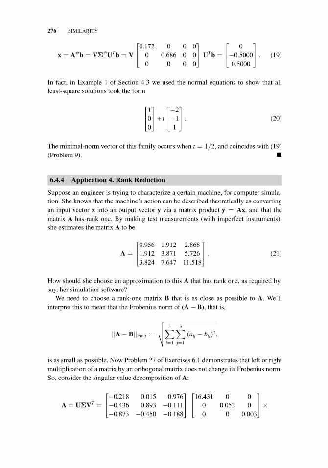
276 SIMILARITY
x = Aψb = VΣψUTb = V
⎡⎣0.172 0 0 0
0 0.686 0 00 0 0 0
⎤⎦ UTb =
⎡⎣ 0−0.50000.5000
⎤⎦ . (19)
In fact, in Example 1 of Section 4.3 we used the normal equations to show that allleast-square solutions took the form
⎡⎣1
00
⎤⎦ + t
⎡⎣−2−11
⎤⎦ . (20)
The minimal-norm vector of this family occurs when t = 1/2, and coincides with (19)(Problem 9). �
6.4.4 Application 4. Rank Reduction
Suppose an engineer is trying to characterize a certain machine, for computer simula-tion. She knows that the machine’s action can be described theoretically as convertingan input vector x into an output vector y via a matrix product y = Ax, and that thematrix A has rank one. By making test measurements (with imperfect instruments),she estimates the matrix A to be
A =
⎡⎣0.956 1.912 2.868
1.912 3.871 5.7263.824 7.647 11.518
⎤⎦ . (21)
How should she choose an approximation to this A that has rank one, as required by,say, her simulation software?
We need to choose a rank-one matrix B that is as close as possible to A. We’llinterpret this to mean that the Frobenius norm of (A − B), that is,
||A − B||Frob :=
√√√√ 3∑i=1
3∑j=1
(aij − bij)2,
is as small as possible. Now Problem 27 of Exercises 6.1 demonstrates that left or rightmultiplication of a matrix by an orthogonal matrix does not change its Frobenius norm.So, consider the singular value decomposition of A:
A = UΣVT =
⎡⎣−0.218 0.015 0.976−0.436 0.893 −0.111−0.873 −0.450 −0.188
⎤⎦⎡⎣16.431 0 0
0 0.052 00 0 0.003
⎤⎦×
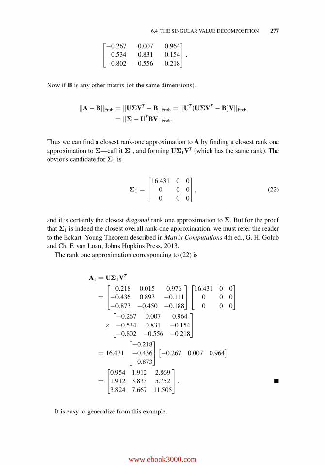
6.4 THE SINGULAR VALUE DECOMPOSITION 277
⎡⎣−0.267 0.007 0.964−0.534 0.831 −0.154−0.802 −0.556 −0.218
⎤⎦ .
Now if B is any other matrix (of the same dimensions),
||A − B||Frob = ||UΣVT − B||Frob = ||UT(UΣVT − B)V||Frob
= ||Σ− UTBV||Frob.
Thus we can find a closest rank-one approximation to A by finding a closest rank oneapproximation to Σ—call it Σ1, and forming UΣ1VT (which has the same rank). Theobvious candidate for Σ1 is
Σ1 =
⎡⎣16.431 0 0
0 0 00 0 0
⎤⎦ , (22)
and it is certainly the closest diagonal rank one approximation to Σ. But for the proofthat Σ1 is indeed the closest overall rank-one approximation, we must refer the readerto the Eckart–Young Theorem described in Matrix Computations 4th ed., G. H. Goluband Ch. F. van Loan, Johns Hopkins Press, 2013.
The rank one approximation corresponding to (22) is
A1 = UΣ1VT
=
⎡⎣−0.218 0.015 0.976−0.436 0.893 −0.111−0.873 −0.450 −0.188
⎤⎦⎡⎣16.431 0 0
0 0 00 0 0
⎤⎦
×
⎡⎣−0.267 0.007 0.964−0.534 0.831 −0.154−0.802 −0.556 −0.218
⎤⎦
= 16.431
⎡⎣−0.218−0.436−0.873
⎤⎦ [−0.267 0.007 0.964
]
=
⎡⎣0.954 1.912 2.869
1.912 3.833 5.7523.824 7.667 11.505
⎤⎦ . �
It is easy to generalize from this example.
www.ebook3000.com
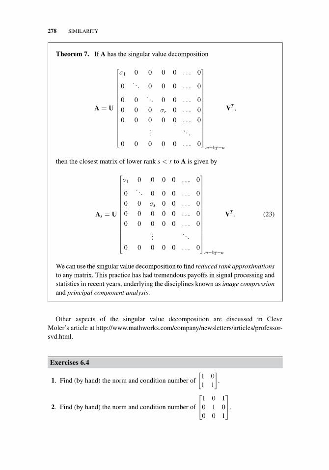
278 SIMILARITY
Theorem 7. If A has the singular value decomposition
A = U
⎡⎢⎢⎢⎢⎢⎢⎢⎢⎢⎢⎢⎢⎢⎣
σ1 0 0 0 0 . . . 0
0. . . 0 0 0 . . . 0
0 0. . . 0 0 . . . 0
0 0 0 σr 0 . . . 0
0 0 0 0 0 . . . 0...
. . .
0 0 0 0 0 . . . 0
⎤⎥⎥⎥⎥⎥⎥⎥⎥⎥⎥⎥⎥⎥⎦
m−by−n
VT ,
then the closest matrix of lower rank s < r to A is given by
As = U
⎡⎢⎢⎢⎢⎢⎢⎢⎢⎢⎢⎢⎢⎢⎣
σ1 0 0 0 0 . . . 0
0. . . 0 0 0 . . . 0
0 0 σs 0 0 . . . 0
0 0 0 0 0 . . . 0
0 0 0 0 0 . . . 0...
. . .
0 0 0 0 0 . . . 0
⎤⎥⎥⎥⎥⎥⎥⎥⎥⎥⎥⎥⎥⎥⎦
m−by−n
VT . (23)
We can use the singular value decomposition to find reduced rank approximationsto any matrix. This practice has had tremendous payoffs in signal processing andstatistics in recent years, underlying the disciplines known as image compressionand principal component analysis.
Other aspects of the singular value decomposition are discussed in CleveMoler’s article at http://www.mathworks.com/company/newsletters/articles/professor-svd.html.
Exercises 6.4
1. Find (by hand) the norm and condition number of
[1 01 1
].
2. Find (by hand) the norm and condition number of
⎡⎣1 0 1
0 1 00 0 1
⎤⎦.
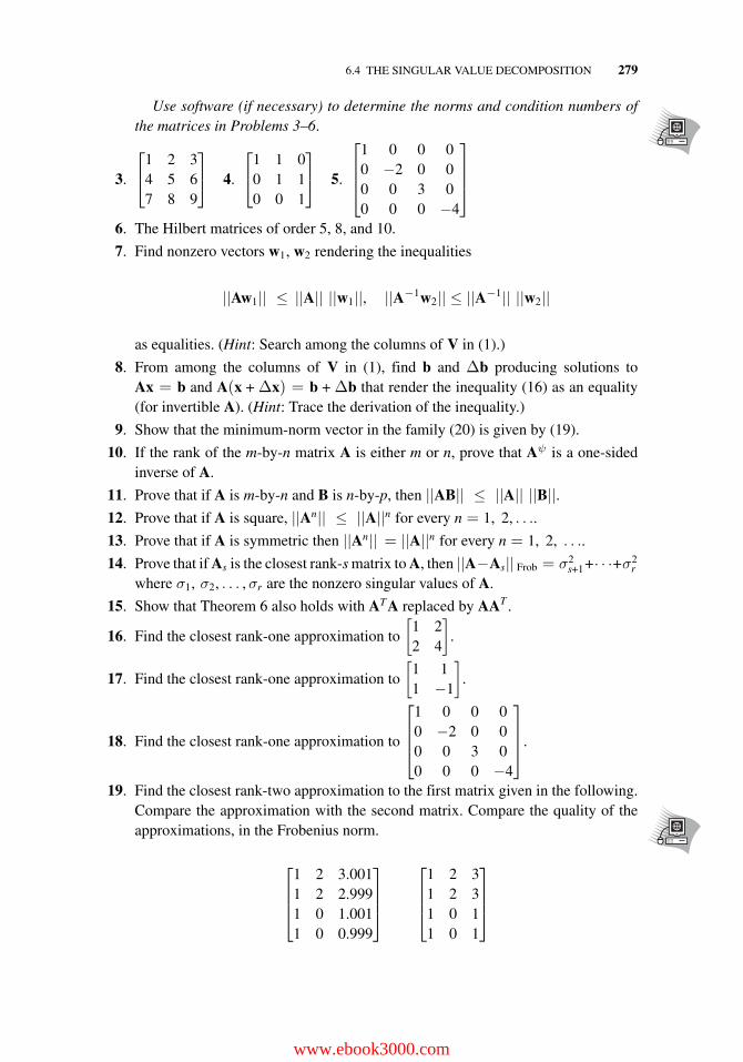
6.4 THE SINGULAR VALUE DECOMPOSITION 279
Use software (if necessary) to determine the norms and condition numbers ofthe matrices in Problems 3–6.
3.
⎡⎣1 2 3
4 5 67 8 9
⎤⎦ 4.
⎡⎣1 1 0
0 1 10 0 1
⎤⎦ 5.
⎡⎢⎢⎣
1 0 0 00 −2 0 00 0 3 00 0 0 −4
⎤⎥⎥⎦
6. The Hilbert matrices of order 5, 8, and 10.
7. Find nonzero vectors w1, w2 rendering the inequalities
||Aw1|| ≤ ||A|| ||w1||, ||A−1w2|| ≤ ||A−1|| ||w2||
as equalities. (Hint: Search among the columns of V in (1).)
8. From among the columns of V in (1), find b and Δb producing solutions toAx = b and A(x + Δx) = b + Δb that render the inequality (16) as an equality(for invertible A). (Hint: Trace the derivation of the inequality.)
9. Show that the minimum-norm vector in the family (20) is given by (19).
10. If the rank of the m-by-n matrix A is either m or n, prove that Aψ is a one-sidedinverse of A.
11. Prove that if A is m-by-n and B is n-by-p, then ||AB|| ≤ ||A|| ||B||.12. Prove that if A is square, ||An|| ≤ ||A||n for every n = 1, 2, . . ..
13. Prove that if A is symmetric then ||An|| = ||A||n for every n = 1, 2, . . ..
14. Prove that if As is the closest rank-s matrix to A, then ||A−As|| Frob = σ2s+1+· · ·+σ2
r
where σ1, σ2, . . . ,σr are the nonzero singular values of A.
15. Show that Theorem 6 also holds with ATA replaced by AAT .
16. Find the closest rank-one approximation to
[1 22 4
].
17. Find the closest rank-one approximation to
[1 11 −1
].
18. Find the closest rank-one approximation to
⎡⎢⎢⎣
1 0 0 00 −2 0 00 0 3 00 0 0 −4
⎤⎥⎥⎦.
19. Find the closest rank-two approximation to the first matrix given in the following.Compare the approximation with the second matrix. Compare the quality of theapproximations, in the Frobenius norm.
⎡⎢⎢⎣
1 2 3.0011 2 2.9991 0 1.0011 0 0.999
⎤⎥⎥⎦
⎡⎢⎢⎣
1 2 31 2 31 0 11 0 1
⎤⎥⎥⎦
www.ebook3000.com
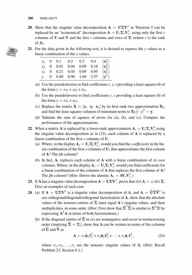
280 SIMILARITY
20. Show that the singular value decomposition A = UΣVT in Theorem 5 can bereplaced by an “economical” decomposition A = UrΣrVT
r , using only the first rcolumns of U and V and the first r columns and rows of Σ (where r is the rankof A).
21. For the data given in the following text, it is desired to express the y values as alinear combination of the x values.
x1 0 0.1 0.2 0.3 0.4 (xT1 )
x2 0 0.01 0.04 0.09 0.16 (xT2 )
x3 0 0.21 0.44 0.69 0.95 (xT3 )
y 0 0.40 0.96 1.69 2.57 (yT)
(a) Use the pseudoinverse to find coefficients r, s, t providing a least squares fit ofthe form y = rx1 + sx2 + tx3.
(b) Use the pseudoinverse to find coefficients r, s providing a least squares fit ofthe form y = rx1 + sx2.
(c) Replace the matrix X = [x1 x2 x3] by its best rank two approximation X2,and find the least squares solution of minimum norm to X2[r s]T = y.
(d) Tabulate the sum of squares of errors for (a), (b), and (c). Compare theperformance of the approximations.
22. When a matrix A is replaced by a lower-rank approximation As = UsΣsVTs using
the singular value decomposition as in (23), each column of A is replaced by alinear combination of the first s columns of U.(a) Where, in the display As = UsΣsVT
s , would you find the coefficients in the lin-ear combination of the first s columns of Us that approximates the first columnof A? The jth column?
(b) In fact, As replaces each column of A with a linear combination of its owncolumns. Where, in the display As = UsΣsVT
s , would you find coefficients fora linear combination of the columns of A that replaces the first column of A?The jth column? (Hint: Derive the identity As = AVsV
Ts .)
23. If A has a singular value decomposition A = UΣVT , prove that detA = ±detΣ.Give an examples of each case.
24. (a) If A = UΣVT is a singular value decomposition of A, and A = UΣVT isany orthogonal/diagonal/orthogonal factorization of A, show that the absolutevalues of the nonzero entries of Σ must equal A’s singular values, and theirmultiplicities, in some order. (Hint: First show that Σ
TΣ is similar to ΣTΣ by
expressing ATA in terms of both factorizations.)
(b) If the diagonal entries of Σ in (a) are nonnegative and occur in nonincreasingorder (implying Σ = Σ), show that A can be written in terms of the columnsof U and V as
A = σ1u1vT1 + σ2u2vT
2 + · · · + σrurvTr , (24)
where σ1,σ2, . . . ,σr are the nonzero singular values of A. (Hint: RecallProblem 23, Section 6.1.)
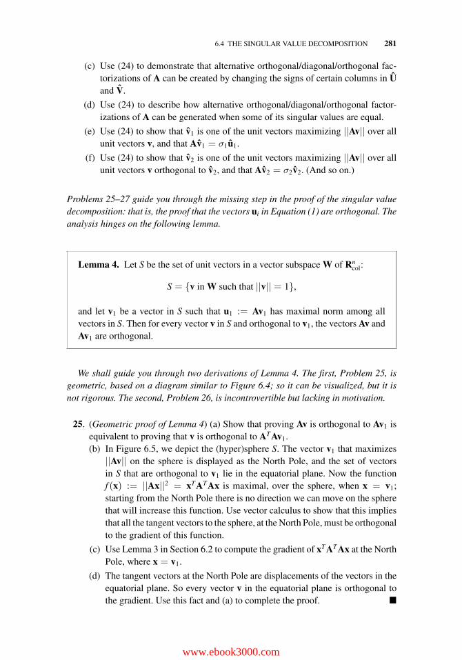
6.4 THE SINGULAR VALUE DECOMPOSITION 281
(c) Use (24) to demonstrate that alternative orthogonal/diagonal/orthogonal fac-torizations of A can be created by changing the signs of certain columns in Uand V.
(d) Use (24) to describe how alternative orthogonal/diagonal/orthogonal factor-izations of A can be generated when some of its singular values are equal.
(e) Use (24) to show that v1 is one of the unit vectors maximizing ||Av|| over allunit vectors v, and that Av1 = σ1u1.
(f) Use (24) to show that v2 is one of the unit vectors maximizing ||Av|| over allunit vectors v orthogonal to v2, and that Av2 = σ2v2. (And so on.)
Problems 25–27 guide you through the missing step in the proof of the singular valuedecomposition: that is, the proof that the vectors ui in Equation (1) are orthogonal. Theanalysis hinges on the following lemma.
Lemma 4. Let S be the set of unit vectors in a vector subspace W of Rncol:
S = {v in W such that ||v|| = 1},
and let v1 be a vector in S such that u1 := Av1 has maximal norm among allvectors in S. Then for every vector v in S and orthogonal to v1, the vectors Av andAv1 are orthogonal.
We shall guide you through two derivations of Lemma 4. The first, Problem 25, isgeometric, based on a diagram similar to Figure 6.4; so it can be visualized, but it isnot rigorous. The second, Problem 26, is incontrovertible but lacking in motivation.
25. (Geometric proof of Lemma 4) (a) Show that proving Av is orthogonal to Av1 isequivalent to proving that v is orthogonal to ATAv1.(b) In Figure 6.5, we depict the (hyper)sphere S. The vector v1 that maximizes
||Av|| on the sphere is displayed as the North Pole, and the set of vectorsin S that are orthogonal to v1 lie in the equatorial plane. Now the functionf (x) := ||Ax||2 = xTATAx is maximal, over the sphere, when x = v1;starting from the North Pole there is no direction we can move on the spherethat will increase this function. Use vector calculus to show that this impliesthat all the tangent vectors to the sphere, at the North Pole, must be orthogonalto the gradient of this function.
(c) Use Lemma 3 in Section 6.2 to compute the gradient of xTATAx at the NorthPole, where x = v1.
(d) The tangent vectors at the North Pole are displacements of the vectors in theequatorial plane. So every vector v in the equatorial plane is orthogonal tothe gradient. Use this fact and (a) to complete the proof. �
www.ebook3000.com
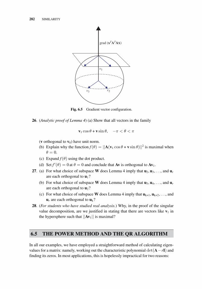
282 SIMILARITY
v1
v3 v2
grad (xTATAX)
Fig. 6.5 Gradient vector configuration.
26. (Analytic proof of Lemma 4) (a) Show that all vectors in the family
v1 cos θ + v sin θ, −π < θ < π
(v orthogonal to v0) have unit norm.(b) Explain why the function f (θ) = ||A(v1 cos θ + v sin θ)||2 is maximal when
θ = 0.
(c) Expand f (θ) using the dot product.
(d) Set f ′(θ) = 0 at θ = 0 and conclude that Av is orthogonal to Av1.
27. (a) For what choice of subspace W does Lemma 4 imply that u2, u3, . . ., and ur
are each orthogonal to u1?
(b) For what choice of subspace W does Lemma 4 imply that u3, u4, . . ., and ur
are each orthogonal to u2?
(c) For what choice of subspace W does Lemma 4 imply that uk+1, uk+2, . . ., andur are each orthogonal to uk?
28. (For students who have studied real analysis.) Why, in the proof of the singularvalue decomposition, are we justified in stating that there are vectors like v1 inthe hypersphere such that ||Av1|| is maximal?
6.5 THE POWER METHOD AND THE QR ALGORITHM
In all our examples, we have employed a straightforward method of calculating eigen-values for a matrix: namely, working out the characteristic polynomial det(A−rI) andfinding its zeros. In most applications, this is hopelessly impractical for two reasons:
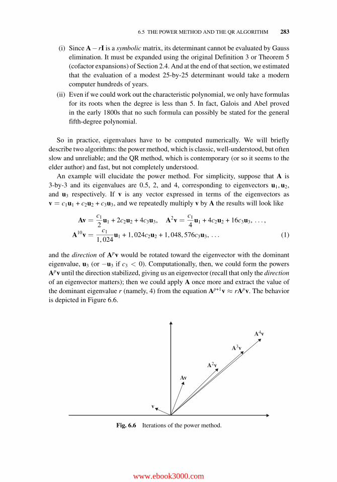
6.5 THE POWER METHOD AND THE QR ALGORITHM 283
(i) Since A− rI is a symbolic matrix, its determinant cannot be evaluated by Gausselimination. It must be expanded using the original Definition 3 or Theorem 5(cofactor expansions) of Section 2.4. And at the end of that section, we estimatedthat the evaluation of a modest 25-by-25 determinant would take a moderncomputer hundreds of years.
(ii) Even if we could work out the characteristic polynomial, we only have formulasfor its roots when the degree is less than 5. In fact, Galois and Abel provedin the early 1800s that no such formula can possibly be stated for the generalfifth-degree polynomial.
So in practice, eigenvalues have to be computed numerically. We will brieflydescribe two algorithms: the power method, which is classic, well-understood, but oftenslow and unreliable; and the QR method, which is contemporary (or so it seems to theelder author) and fast, but not completely understood.
An example will elucidate the power method. For simplicity, suppose that A is3-by-3 and its eigenvalues are 0.5, 2, and 4, corresponding to eigenvectors u1, u2,and u3 respectively. If v is any vector expressed in terms of the eigenvectors asv = c1u1 + c2u2 + c3u3, and we repeatedly multiply v by A the results will look like
Av =c1
2u1 + 2c2u2 + 4c3u3, A2v =
c1
4u1 + 4c2u2 + 16c3u3, . . . ,
A10v =c1
1, 024u1 + 1, 024c2u2 + 1, 048, 576c3u3, . . . (1)
and the direction of Apv would be rotated toward the eigenvector with the dominanteigenvalue, u3 (or −u3 if c3 < 0). Computationally, then, we could form the powersApv until the direction stabilized, giving us an eigenvector (recall that only the directionof an eigenvector matters); then we could apply A once more and extract the value ofthe dominant eigenvalue r (namely, 4) from the equation Ap+1v ≈ rApv. The behavioris depicted in Figure 6.6.
A3v
A2v
Av
v
A4v
Fig. 6.6 Iterations of the power method.
www.ebook3000.com
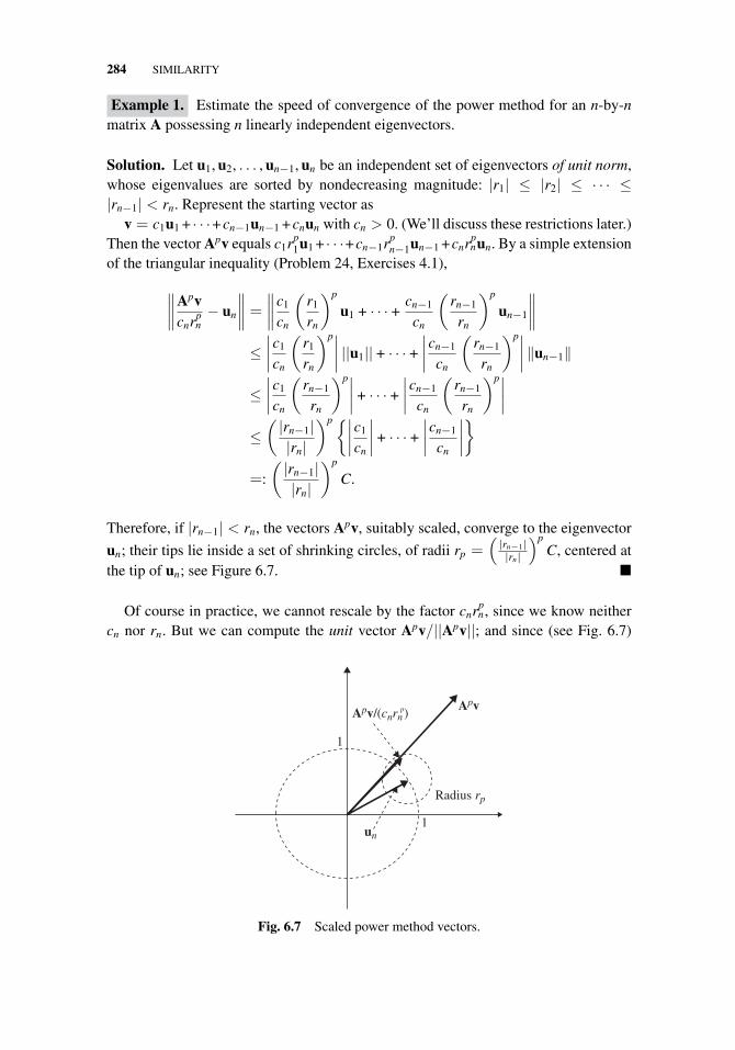
284 SIMILARITY
Example 1. Estimate the speed of convergence of the power method for an n-by-nmatrix A possessing n linearly independent eigenvectors.
Solution. Let u1, u2, . . . , un−1, un be an independent set of eigenvectors of unit norm,whose eigenvalues are sorted by nondecreasing magnitude: |r1| ≤ |r2| ≤ · · · ≤|rn−1| < rn. Represent the starting vector as
v = c1u1 + · · ·+ cn−1un−1 + cnun with cn > 0. (We’ll discuss these restrictions later.)Then the vector Apv equals c1rp
1u1 + · · ·+cn−1rpn−1un−1 +cnrp
nun. By a simple extensionof the triangular inequality (Problem 24, Exercises 4.1),
∥∥∥∥Apvcnrp
n− un
∥∥∥∥ =∥∥∥∥c1
cn
(r1
rn
)p
u1 + · · · +cn−1
cn
(rn−1
rn
)p
un−1
∥∥∥∥≤∣∣∣∣c1
cn
(r1
rn
)p∣∣∣∣ ||u1|| + · · · +
∣∣∣∣cn−1
cn
(rn−1
rn
)p∣∣∣∣ ‖un−1‖
≤∣∣∣∣c1
cn
(rn−1
rn
)p∣∣∣∣ + · · · +
∣∣∣∣cn−1
cn
(rn−1
rn
)p∣∣∣∣≤(|rn−1||rn|
)p{∣∣∣∣c1
cn
∣∣∣∣ + · · · +
∣∣∣∣cn−1
cn
∣∣∣∣}
=:
(|rn−1||rn|
)p
C.
Therefore, if |rn−1| < rn, the vectors Apv, suitably scaled, converge to the eigenvector
un; their tips lie inside a set of shrinking circles, of radii rp =(
|rn−1||rn|
)pC, centered at
the tip of un; see Figure 6.7. �
Of course in practice, we cannot rescale by the factor cnrpn, since we know neither
cn nor rn. But we can compute the unit vector Apv/||Apv||; and since (see Fig. 6.7)
Radius rp
un
1
1
ApvApv/(cnrnp)
Fig. 6.7 Scaled power method vectors.
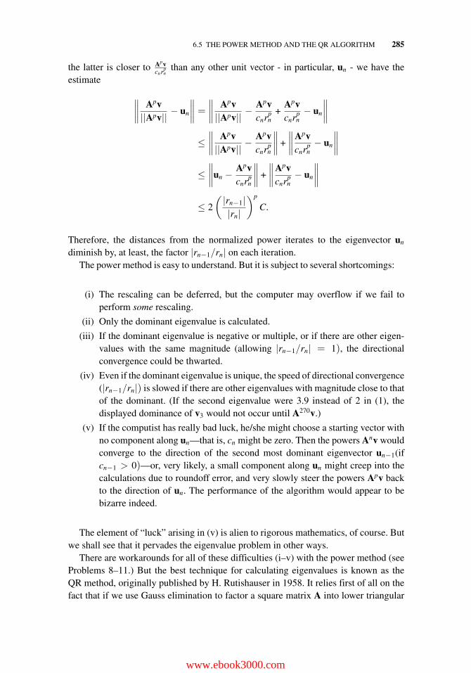
6.5 THE POWER METHOD AND THE QR ALGORITHM 285
the latter is closer to Apvcnrp
nthan any other unit vector - in particular, un - we have the
estimate
∥∥∥∥ Apv||Apv|| − un
∥∥∥∥ =∥∥∥∥ Apv||Apv|| −
Apvcnrp
n+
Apvcnrp
n− un
∥∥∥∥≤∥∥∥∥ Apv||Apv|| −
Apvcnrp
n
∥∥∥∥ +
∥∥∥∥Apvcnrp
n− un
∥∥∥∥≤∥∥∥∥un −
Apvcnrp
n
∥∥∥∥ +
∥∥∥∥Apvcnrp
n− un
∥∥∥∥≤ 2
(|rn−1||rn|
)p
C.
Therefore, the distances from the normalized power iterates to the eigenvector un
diminish by, at least, the factor |rn−1/rn| on each iteration.The power method is easy to understand. But it is subject to several shortcomings:
(i) The rescaling can be deferred, but the computer may overflow if we fail toperform some rescaling.
(ii) Only the dominant eigenvalue is calculated.
(iii) If the dominant eigenvalue is negative or multiple, or if there are other eigen-values with the same magnitude (allowing |rn−1/rn| = 1), the directionalconvergence could be thwarted.
(iv) Even if the dominant eigenvalue is unique, the speed of directional convergence(|rn−1/rn|) is slowed if there are other eigenvalues with magnitude close to thatof the dominant. (If the second eigenvalue were 3.9 instead of 2 in (1), thedisplayed dominance of v3 would not occur until A270v.)
(v) If the computist has really bad luck, he/she might choose a starting vector withno component along un—that is, cn might be zero. Then the powers Anv wouldconverge to the direction of the second most dominant eigenvector un−1(ifcn−1 > 0)—or, very likely, a small component along un might creep into thecalculations due to roundoff error, and very slowly steer the powers Apv backto the direction of un. The performance of the algorithm would appear to bebizarre indeed.
The element of “luck” arising in (v) is alien to rigorous mathematics, of course. Butwe shall see that it pervades the eigenvalue problem in other ways.
There are workarounds for all of these difficulties (i–v) with the power method (seeProblems 8–11.) But the best technique for calculating eigenvalues is known as theQR method, originally published by H. Rutishauser in 1958. It relies first of all on thefact that if we use Gauss elimination to factor a square matrix A into lower triangular
www.ebook3000.com
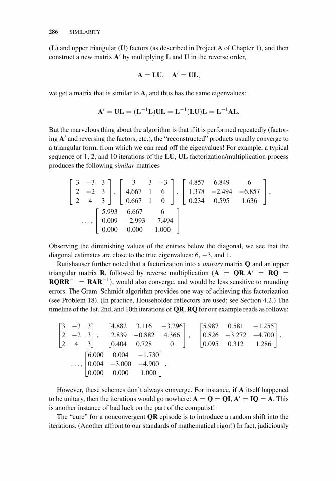
286 SIMILARITY
(L) and upper triangular (U) factors (as described in Project A of Chapter 1), and thenconstruct a new matrix A′ by multiplying L and U in the reverse order,
A = LU, A′ = UL,
we get a matrix that is similar to A, and thus has the same eigenvalues:
A′ = UL = (L−1L)UL = L−1(LU)L = L−1AL.
But the marvelous thing about the algorithm is that if it is performed repeatedly (factor-ing A′ and reversing the factors, etc.), the “reconstructed” products usually converge toa triangular form, from which we can read off the eigenvalues! For example, a typicalsequence of 1, 2, and 10 iterations of the LU, UL factorization/multiplication processproduces the following similar matrices
⎡⎣ 3 −3 3
2 −2 32 4 3
⎤⎦ ,
⎡⎣ 3 3 −3
4.667 1 60.667 1 0
⎤⎦ ,
⎡⎣ 4.857 6.849 6
1.378 −2.494 −6.8570.234 0.595 1.636
⎤⎦ ,
. . . ,
⎡⎣ 5.993 6.667 6
0.009 −2.993 −7.4940.000 0.000 1.000
⎤⎦
Observing the diminishing values of the entries below the diagonal, we see that thediagonal estimates are close to the true eigenvalues: 6, −3, and 1.
Rutishauser further noted that a factorization into a unitary matrix Q and an uppertriangular matrix R, followed by reverse multiplication (A = QR, A′ = RQ =RQRR−1 = RAR−1), would also converge, and would be less sensitive to roundingerrors. The Gram–Schmidt algorithm provides one way of achieving this factorization(see Problem 18). (In practice, Householder reflectors are used; see Section 4.2.) Thetimeline of the 1st, 2nd, and 10th iterations of QR, RQ for our example reads as follows:
⎡⎣3 −3 3
2 −2 32 4 3
⎤⎦ ,
⎡⎣4.882 3.116 −3.296
2.839 −0.882 4.3660.404 0.728 0
⎤⎦ ,
⎡⎣5.987 0.581 −1.255
0.826 −3.272 −4.7000.095 0.312 1.286
⎤⎦ ,
. . . ,
⎡⎣6.000 0.004 −1.730
0.004 −3.000 −4.9000.000 0.000 1.000
⎤⎦ .
However, these schemes don’t always converge. For instance, if A itself happenedto be unitary, then the iterations would go nowhere: A = Q = QI, A′ = IQ = A. Thisis another instance of bad luck on the part of the computist!
The “cure” for a nonconvergent QR episode is to introduce a random shift into theiterations. (Another affront to our standards of mathematical rigor!) In fact, judiciously
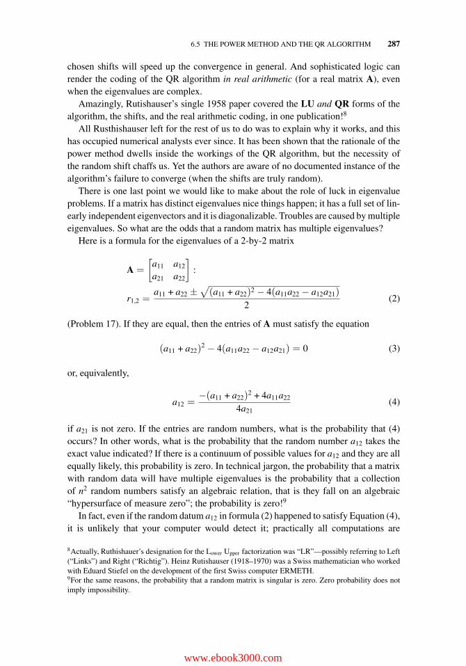
6.5 THE POWER METHOD AND THE QR ALGORITHM 287
chosen shifts will speed up the convergence in general. And sophisticated logic canrender the coding of the QR algorithm in real arithmetic (for a real matrix A), evenwhen the eigenvalues are complex.
Amazingly, Rutishauser’s single 1958 paper covered the LU and QR forms of thealgorithm, the shifts, and the real arithmetic coding, in one publication!8
All Rusthishauser left for the rest of us to do was to explain why it works, and thishas occupied numerical analysts ever since. It has been shown that the rationale of thepower method dwells inside the workings of the QR algorithm, but the necessity ofthe random shift chaffs us. Yet the authors are aware of no documented instance of thealgorithm’s failure to converge (when the shifts are truly random).
There is one last point we would like to make about the role of luck in eigenvalueproblems. If a matrix has distinct eigenvalues nice things happen; it has a full set of lin-early independent eigenvectors and it is diagonalizable. Troubles are caused by multipleeigenvalues. So what are the odds that a random matrix has multiple eigenvalues?
Here is a formula for the eigenvalues of a 2-by-2 matrix
A =
[a11 a12
a21 a22
]:
r1,2 =a11 + a22 ±
√(a11 + a22)2 − 4(a11a22 − a12a21)
2(2)
(Problem 17). If they are equal, then the entries of A must satisfy the equation
(a11 + a22)2 − 4(a11a22 − a12a21) = 0 (3)
or, equivalently,
a12 =−(a11 + a22)2 + 4a11a22
4a21(4)
if a21 is not zero. If the entries are random numbers, what is the probability that (4)occurs? In other words, what is the probability that the random number a12 takes theexact value indicated? If there is a continuum of possible values for a12 and they are allequally likely, this probability is zero. In technical jargon, the probability that a matrixwith random data will have multiple eigenvalues is the probability that a collectionof n2 random numbers satisfy an algebraic relation, that is they fall on an algebraic“hypersurface of measure zero”; the probability is zero!9
In fact, even if the random datum a12 in formula (2) happened to satisfy Equation (4),it is unlikely that your computer would detect it; practically all computations are
8Actually, Ruthishauer’s designation for the Lower Upper factorization was “LR”—possibly referring to Left(“Links”) and Right (“Richtig”). Heinz Rutishauser (1918–1970) was a Swiss mathematician who workedwith Eduard Stiefel on the development of the first Swiss computer ERMETH.9For the same reasons, the probability that a random matrix is singular is zero. Zero probability does notimply impossibility.
www.ebook3000.com
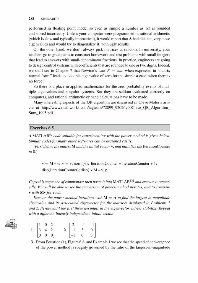
288 SIMILARITY
performed in floating point mode, so even as simple a number as 1/3 is roundedand stored incorrectly. Unless your computer were programmed in rational arithmetic(which is slow and typically impractical), it would report that A had distinct, very closeeigenvalues and would try to diagonalize it, with ugly results.
On the other hand, we don’t always pick matrices at random. In university, yourteachers go to great pains to construct homework and test problems with small integersthat lead to answers with small-denominator fractions. In practice, engineers are goingto design control systems with coefficients that are rounded to one or two digits. Indeed,we shall see in Chapter 7 that Newton’s Law F = ma, when expressed in “matrixnormal form,” leads to a double eigenvalue of zero for the simplest case, when there isno force!
So there is a place in applied mathematics for the zero-probability events of mul-tiple eigenvalues and singular systems. But they are seldom evaluated correctly oncomputers, and rational arithmetic or hand calculations have to be made.
Many interesting aspects of the QR algorithm are discussed in Cleve Moler’s arti-cle at http://www.mathworks.com/tagteam/72899_92026v00Cleve_QR_Algorithm_Sum_1995.pdf .
Exercises 6.5
A MATLAB� code suitable for experimenting with the power method is given below.Similar codes for many other softwares can be designed easily.
(First define the matrix M and the initial vector v, and initialize the IterationCounterto 0.)
v = M ∗ v; v = v/norm(v); IterationCounter = IterationCounter + 1;
disp(IterationCounter); disp([v M ∗ v]);
Copy this sequence of commands; then paste it into MATLABTM and execute it repeat-edly. You will be able to see the succession of power-method iterates, and to comparev with Mv for each.
Execute the power-method iterations with M = A to find the largest-in-magnitudeeigenvalue and its associated eigenvector for the matrices displayed in Problems 1and 2. Iterate until the first three decimals in the eigenvector entries stabilize. Repeatwith a different, linearly independent, initial vector.
1.
⎡⎣1 0 2
3 4 20 0 0
⎤⎦ 2.
⎡⎣ 2 −1 −1−1 3 0−1 0 3
⎤⎦
3. From Equation (1), Figure 6.6, and Example 1 we see that the speed of convergenceof the power method is roughly governed by the ratio of the largest-in-magnitude
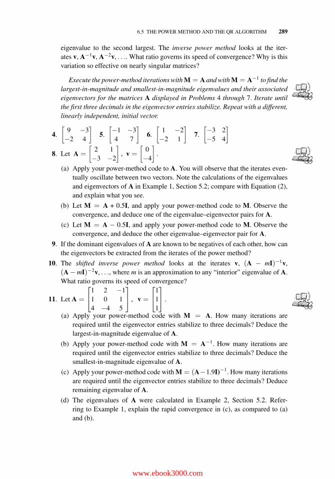
6.5 THE POWER METHOD AND THE QR ALGORITHM 289
eigenvalue to the second largest. The inverse power method looks at the iter-ates v, A−1v, A−2v, . . .. What ratio governs its speed of convergence? Why is thisvariation so effective on nearly singular matrices?
Execute the power-method iterations with M = A and with M = A−1 to find thelargest-in-magnitude and smallest-in-magnitude eigenvalues and their associatedeigenvectors for the matrices A displayed in Problems 4 through 7. Iterate untilthe first three decimals in the eigenvector entries stabilize. Repeat with a different,linearly independent, initial vector.
4.
[9 −3−2 4
]5.
[−1 −34 7
]6.
[1 −2−2 1
]7.
[−3 2−5 4
]
8. Let A =
[2 1−3 −2
], v =
[0−4
].
(a) Apply your power-method code to A. You will observe that the iterates even-tually oscillate between two vectors. Note the calculations of the eigenvaluesand eigenvectors of A in Example 1, Section 5.2; compare with Equation (2),and explain what you see.
(b) Let M = A + 0.5I, and apply your power-method code to M. Observe theconvergence, and deduce one of the eigenvalue–eigenvector pairs for A.
(c) Let M = A − 0.5I, and apply your power-method code to M. Observe theconvergence, and deduce the other eigenvalue–eigenvector pair for A.
9. If the dominant eigenvalues of A are known to be negatives of each other, how canthe eigenvectors be extracted from the iterates of the power method?
10. The shifted inverse power method looks at the iterates v, (A − mI)−1v,(A − mI)−2v, . . ., where m is an approximation to any “interior” eigenvalue of A.What ratio governs its speed of convergence?
11. Let A =
⎡⎣1 2 −1
1 0 14 −4 5
⎤⎦ , v =
⎡⎣1
11
⎤⎦ .
(a) Apply your power-method code with M = A. How many iterations arerequired until the eigenvector entries stabilize to three decimals? Deduce thelargest-in-magnitude eigenvalue of A.
(b) Apply your power-method code with M = A−1. How many iterations arerequired until the eigenvector entries stabilize to three decimals? Deduce thesmallest-in-magnitude eigenvalue of A.
(c) Apply your power-method code with M = (A−1.9I)−1. How many iterationsare required until the eigenvector entries stabilize to three decimals? Deduceremaining eigenvalue of A.
(d) The eigenvalues of A were calculated in Example 2, Section 5.2. Refer-ring to Example 1, explain the rapid convergence in (c), as compared to (a)and (b).
www.ebook3000.com
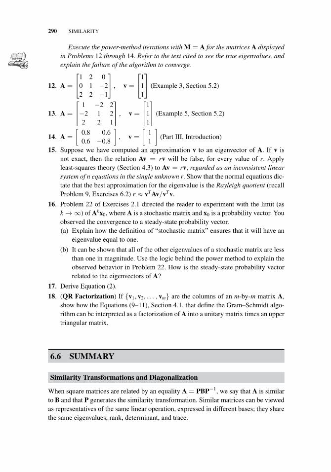
290 SIMILARITY
Execute the power-method iterations with M = A for the matrices A displayedin Problems 12 through 14. Refer to the text cited to see the true eigenvalues, andexplain the failure of the algorithm to converge.
12. A =
⎡⎣1 2 0
0 1 −22 2 −1
⎤⎦ , v =
⎡⎣1
11
⎤⎦ (Example 3, Section 5.2)
13. A =
⎡⎣ 1 −2 2−2 1 22 2 1
⎤⎦ , v =
⎡⎣1
11
⎤⎦ (Example 5, Section 5.2)
14. A =
[0.8 0.60.6 −0.8
], v =
[11
](Part III, Introduction)
15. Suppose we have computed an approximation v to an eigenvector of A. If v isnot exact, then the relation Av = rv will be false, for every value of r. Applyleast-squares theory (Section 4.3) to Av = rv, regarded as an inconsistent linearsystem of n equations in the single unknown r. Show that the normal equations dic-tate that the best approximation for the eigenvalue is the Rayleigh quotient (recallProblem 9, Exercises 6.2) r ≈ vTAv/vTv.
16. Problem 22 of Exercises 2.1 directed the reader to experiment with the limit (ask → ∞) of Akx0, where A is a stochastic matrix and x0 is a probability vector. Youobserved the convergence to a steady-state probability vector.(a) Explain how the definition of “stochastic matrix” ensures that it will have an
eigenvalue equal to one.
(b) It can be shown that all of the other eigenvalues of a stochastic matrix are lessthan one in magnitude. Use the logic behind the power method to explain theobserved behavior in Problem 22. How is the steady-state probability vectorrelated to the eigenvectors of A?
17. Derive Equation (2).
18. (QR Factorization) If {v1, v2, . . . , vm} are the columns of an m-by-m matrix A,show how the Equations (9–11), Section 4.1, that define the Gram–Schmidt algo-rithm can be interpreted as a factorization of A into a unitary matrix times an uppertriangular matrix.
6.6 SUMMARY
Similarity Transformations and Diagonalization
When square matrices are related by an equality A = PBP−1, we say that A is similarto B and that P generates the similarity transformation. Similar matrices can be viewedas representatives of the same linear operation, expressed in different bases; they sharethe same eigenvalues, rank, determinant, and trace.
6.6 SUMMARY 291
The most important similarity transformations are those that produce a diagonalmatrix D, and the relation AP = PD explicitly displays the fact that the columns ofa matrix P diagonalizing A are eigenvectors of A. Thus diagonalization is only possi-ble if A is not defective. The telescoping of the adjacent factors of P and P−1 in powersAn = (PDP−1)n reduces the computation of matrix polynomials and power series tomere evaluation of the corresponding scalar functions, for each of the eigenvalues.
Besides their role in facilitating the computation of the important matrix exponentialfunction, similarity transformations are used in uncoupling the degrees of freedom ofvibrating systems and eliminating cross terms in bilinear forms.
Schur Decomposition
The full diagonalization of a matrix via a similarity transformation generated by a uni-tary matrix is only possible if the matrix is normal, that is, commutes with its conjugatetranspose. But in fact, any matrix can be upper-triangularized by a unitary matrix. Thistheorem of Schur can be used to show that every matrix satisfies its own characteris-tic equation—the Cayley–Hamilton theorem. As a result, any integer power Am of ann-by-n matrix A can be expressed as a combination of lower powers, if m equals orexceeds n.
The Singular Value Decomposition
Any m-by-n matrix A can be decomposed (factored) into the product of an m-by-m orthogonal matrix U, times an m-by-n diagonal matrix Σ with nondecreasing,nonnegative numbers down its diagonal (the singular values), times an n-by-n orthog-onal matrix VT .
From the singular values one can deduce the matrix’s norm and its condition number.Further, the decomposition enables one to devise optimal lower-rank approximationsto the matrix, and to express minimal least squares solutions using the pseudoinverse.
Numerical Computations
The exact calculation of the eigenvalues of a matrix of dimension larger than 4 is,in general, not possible, according to the insolvability theory of Abel and Galois.The power method for estimating eigenvalues is based on the observation that suc-cessive multiplications of a vector v by higher and higher powers of the matrix Atend to steer v into the direction of the eigenvector of A of dominant eigenvalue.And adjustments of this strategy have been devised to accommodate most of theexceptional cases.
However, the prevailing procedure for approximating the eigenvalues is the QRalgorithm, which is based on two observations:
www.ebook3000.com

292 SIMILARITY
(i) if A is factored into the product of a unitary and an upper triangular matrixA = QR, the matrix A′ = RQ is similar to A;
(ii) repetition of step (i) typically results in a near-upper-triangular matrix A′, fromwhich the eigenvalues can easily be estimated;
Failure of (ii) to converge (and sluggishness in its convergence rate) can be overcomeby suitable shifting strategies applied to A.
Nonetheless, the presence of multiple eigenvalues - which, indeed, may be a symp-tom of nondiagonalizability - can thwart the algorithm. Although such coincidencescan result from human choices, they rarely occur in random matrices.
7LINEAR SYSTEMS OFDIFFERENTIAL EQUATIONS
7.1 FIRST-ORDER LINEAR SYSTEMS
Although our textbook does not presume familiarity with differential equations, thereis one type of equation whose resolution is so simple that mere calculus suffices tosolve it completely. And fortunately, the matrix version of that equation pervades manyof the advanced applications of matrix analysis. The scalar version is illustrated in thefollowing radioactive decay example.
Example 1. The plutonium isotope with the shortest half-life, 20 min, is Pu-233.Formulate a differential equation for the time evolution of a sample of PU-233 ofmass x(t).
Solution. The mass of a substance with a half-life of 20 min decays to one-half of itsvalue every 20 min, so it seems reasonable to propose that the decay rate is proportionalto the amount of substance currently available:
dxdt
= ax, (1)
with a < 0. We can solve Equation (1) using a simple calculus trick. Notice that by theproduct rule for differentiation,
ddt[e−atx] = e−at[−ax] + e−at dx
dt= e−at
[dxdt
− ax
], (2)
Fundamentals of Matrix Analysis with Applications,First Edition. Edward Barry Saff and Arthur David Snider.© 2016 John Wiley & Sons, Inc. Published 2016 by John Wiley & Sons, Inc.
www.ebook3000.com
294 LINEAR SYSTEMS OF DIFFERENTIAL EQUATIONS
which is zero according to (1). Therefore, for any two times t1 and t2,
e−at2 x(t2)− e−at1 x(t1) =
t2∫t1
ddt[e−atx] dt =
t2∫t1
[0] dt = 0,
or
x(t2) = ea(t2−t1)x(t1). (3)
Thus x(t2) will be one-half of x(t1) whenever ea(t2−t1) = 1/2; that is, whenever thetime interval a(t2 − t1) equals loge(1/2). Equation (3) does indeed imply a half-life forx(t) of 20 min if
a =loge(1/2)
20≈ −0.0347 min−1. �
Equation (1) describes a host of physical phenomena besides radioactive decay. Anyprocess whose growth or decay rate is proportional to its size will exhibit the expo-nential behavior predicted by (3). This includes the Malthusian model for populationgrowth, Newtonian cooling, compound interest, resistive electromagnetic attenuation,and dielectric relaxation.
In the parlance of differential equations, (1) is known as a linear homogeneous dif-ferential equation of first order with constant coefficient (a). Its nonhomogeneousform is
dxdt
= ax + f (t), (4)
where f (t) is a known function; one can interpret (4) physically as describing a materialdecaying radioactively while being replenished at the rate f (t). The calculus trick foranalyzing (4) is almost as simple as that for the homogeneous equations:
ddt[e−atx] = e−at[−ax] + e−at dx
dt= e−at
[dxdt
− ax
]= e−atf (t),
so
e−at2 x(t2)− e−at1 x(t1) =
t2∫t1
ddt[e−atx] dt =
t2∫t1
[e−atf (t)] dt
or
x(t2) = ea(t2−t1)x(t1) + eat2
t2∫t1
[e−atf (t)] dt. (5)
7.1 FIRST-ORDER LINEAR SYSTEMS 295
Thus x(t2) can be expressed in terms of x(t1) for any interval [t1, t2] in which f (t) isknown (and integrable).
Since a differential equation is an equation for the derivative, or rate of change, of afunction, it is not surprising that it would yield an expression for the new value, x(t2),in terms of the original value x(t1). Commonly t1 is taken to be zero and x(t1) is calledthe initial value.
Now a linear nonhomogeneous system of differential equations of first orderwith constant coefficients is formally identical to (4), with a, x, and f replaced by(appropriately sized) matrices:
dxdt
= Ax + f(t); (6)
here the coefficient matrix A is constant, and the system is homogeneous if f(t) is iden-tically zero. Let’s be sure the interpretation of everything in (6) is clear. The symbolsx and f are matrix column functions—each entry is a function of t. And the entries indx/dt are the derivatives of the entries of x:
x =
⎡⎢⎢⎢⎣
x1(t)x2(t)
...xn(t)
⎤⎥⎥⎥⎦ ; f =
⎡⎢⎢⎢⎣
f1(t)f2(t)
...fn(t)
⎤⎥⎥⎥⎦ ;
dxdt
=
⎡⎢⎢⎢⎣
dx1(t)/dtdx2(t)/dt
...dxn(t)/dt
⎤⎥⎥⎥⎦
Similarly, integrals of matrix functions are evaluated entrywise:
∫A(t) dt =
∫ ⎡⎢⎣
a11(t) a12(t) · · · a1n(t)...
......
...am1(t) am2(t) · · · amn(t)
⎤⎥⎦ dt
=
⎡⎢⎣
∫a11(t) dt
∫a12(t) dt · · ·
∫a1n(t) dt
......
...∫am1(t) dt
∫am2(t) dt · · ·
∫amn(t) dt
⎤⎥⎦ .
Example 2. Show that x(t) =
[cosωt
−ω sinωt
]is a solution of the matrix differential
equation dx/dt = Ax, where A =
[0 1
−ω2 0
].
Solution. We simply check that dx/dt and Ax(t) are the same vector function:
dx(t)dt
=
[−ω sinωt−ω2 cosωt
];
Ax =
[0 1
−ω2 0
] [cosωt
−ω sinωt
]=
[−ω sinωt−ω2 cosωt
]. �
www.ebook3000.com
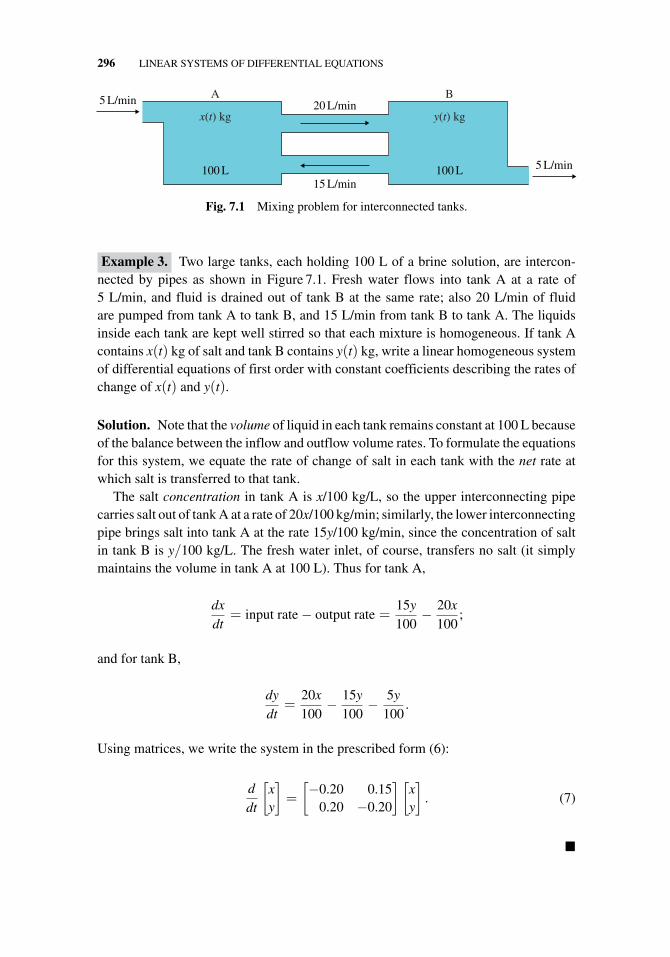
296 LINEAR SYSTEMS OF DIFFERENTIAL EQUATIONS
100 L15 L/min
20 L/min5 L/min
5 L/min100 L
x(t) kg y(t) kg
A B
Fig. 7.1 Mixing problem for interconnected tanks.
Example 3. Two large tanks, each holding 100 L of a brine solution, are intercon-nected by pipes as shown in Figure 7.1. Fresh water flows into tank A at a rate of5 L/min, and fluid is drained out of tank B at the same rate; also 20 L/min of fluidare pumped from tank A to tank B, and 15 L/min from tank B to tank A. The liquidsinside each tank are kept well stirred so that each mixture is homogeneous. If tank Acontains x(t) kg of salt and tank B contains y(t) kg, write a linear homogeneous systemof differential equations of first order with constant coefficients describing the rates ofchange of x(t) and y(t).
Solution. Note that the volume of liquid in each tank remains constant at 100 L becauseof the balance between the inflow and outflow volume rates. To formulate the equationsfor this system, we equate the rate of change of salt in each tank with the net rate atwhich salt is transferred to that tank.
The salt concentration in tank A is x/100 kg/L, so the upper interconnecting pipecarries salt out of tank A at a rate of 20x/100 kg/min; similarly, the lower interconnectingpipe brings salt into tank A at the rate 15y/100 kg/min, since the concentration of saltin tank B is y/100 kg/L. The fresh water inlet, of course, transfers no salt (it simplymaintains the volume in tank A at 100 L). Thus for tank A,
dxdt
= input rate − output rate =15y100
− 20x100
;
and for tank B,
dydt
=20x100
− 15y100
− 5y100
.
Using matrices, we write the system in the prescribed form (6):
ddt
[xy
]=
[−0.20 0.15
0.20 −0.20
] [xy
]. (7)
�
7.1 FIRST-ORDER LINEAR SYSTEMS 297
There are two remarkable observations to be made about the system (6):
(i) It is far more general than it seems, because differential equations of order higherthan one can be recast in this form;
(ii) Employing the matrix exponential function, we can execute the solution for (6)almost as easily as for (4).
We shall elaborate on (i) in the remainder of this section. The rest of Chapter 7 willdescribe the matrix exponential solution for linear systems.
Example 4. The mass-spring oscillator depicted in Figure I.1 in the introduction toPart I obeys Newton’s law, force equals mass time acceleration, or m d2x/dt2. The forceson the mass include the spring force −kx (Hooke’s law, with k > 0 denoting the springconstant) and damping −b dx/dt with damping constant b ≥ 0. Therefore Newton’slaw becomes
md2xdt2
= −kx − bdxdt
. (8)
Express (8) as a linear homogeneous system of differential equations of first order withconstant coefficients.
Solution. Observe that Equation (8) is of second order; it involves the second deriva-tive of x(t). To recast it in terms of first derivatives, we are going to utilize theformula
v = dx/dt (9)
in two ways:
(a) It defines an “artificial” new variable v whose first derivative can replace thesecond derivative of x.
(b) It creates a new differential equation which we append to (8) to form anequivalent linear first-order system.
dxdt
= v
mdvdt
= −kx − bvor
ddt
[xv
]=
[0 1
−k/m −b/m
] [xv
]. (10)
A solution to (8) generates a solution to (10) through the substitution (9), and the xcomponent of a solution to (10) is a solution to (8). They are equivalent. �
The same rule can be applied to a third order equation, or a system of coupled second-order equations.
www.ebook3000.com
298 LINEAR SYSTEMS OF DIFFERENTIAL EQUATIONS
Example 5. Write the following as linear systems of differential equations of firstorder:
d3xdt3
+ 4d2xdt2
+ 6dxdt
+ 8x = f (t); (11)
⎧⎨⎩
d2xdt2 = −2x + y,
d2ydt2 = −2y + x
. (12)
Solution. For (11) the identifications
v = x, a = x
(motivated by “velocity” and “acceleration”) spawn the system
dxdt
= v
dvdt
= a
dadt
= −4a − 6v − 8x + f (t)
orddt
⎡⎣x
va
⎤⎦ =
⎡⎣ 0 1 0
0 0 1−8 −6 −4
⎤⎦⎡⎣x
va
⎤⎦ +
⎡⎣ 0
0f (t)
⎤⎦ .
For (12) the expedient tabulation
x1 = x, x2 =dxdt
, x3 = y, x4 =dydt
results in the system
dx1
dt= x2
dx2
dt= −2x1 + x3
dx3
dt= x4
dx4
dt= −2x3 + x1
orddt
⎡⎢⎢⎣
x1
x2
x3
x4
⎤⎥⎥⎦ =
⎡⎢⎢⎣
0 1 0 0−2 0 1 00 0 0 11 0 −2 0
⎤⎥⎥⎦
⎡⎢⎢⎣
x1
x2
x3
x4
⎤⎥⎥⎦ . �
Equations (12) can be interpreted as describing the motion of a pair of coupledmass-spring oscillators.
As the differential equation textbooks show, matrix reformulations can be helpful inconsolidating the theory and computer algorithms for this subject. But the full power ofthe matrix approach is unleashed in the case of linear first-order systems with constantcoefficients. We devote the remainder of our book to this topic.
7.1 FIRST-ORDER LINEAR SYSTEMS 299
Exercises 7.1
In Problems 1 and 2, find dX/dt for the given matrix functions.
1. X(t) =
[e5t 3e5t
−2e5t −e5t
]2. X(t) =
⎡⎣ sin 2t cos 2t e−2t
− sin 2t 2 cos 2t 3e−2t
3 sin 2t cos 2t e−2t
⎤⎦
In Problems 3 and 4, the matrices A(t) and B(t) are given. Find
(a)∫
A(t) dt. (b)1∫
0B(t) dt. (c)
ddt[A(t)B(t)].
3. A(t) =
[t et
1 et
], B(t) =
[cos t − sin tsin t cos t
].
4. A(t) =
[1 e−2t
3 e−2t
], B(t) =
[e−t e−t
−e−t 3e−t
].
In Problems 5 and 6, verify that the given vector function satisfies the given system.
5. x′ =
[1 1−2 4
]x, x(t) =
[e3t
2e3t
].
6. x′ =
⎡⎣0 0 0
0 1 01 0 1
⎤⎦ x, x(t) =
⎡⎣ 0
et
−3et
⎤⎦.
In Problems 7 and 8, verify that the given matrix function satisfies the given matrixdifferential equation.
7. X′ =
[1 −12 4
]X, X(t) =
[e2t e3t
−e2t −2e3t
].
8. X′ =
⎡⎣1 0 0
0 3 −20 −2 3
⎤⎦X, X(t) =
⎡⎣et 0 0
0 et e5t
0 et −e5t
⎤⎦ .
9. Verify that the vector functions
x1 =[et et
]Tand x2 =
[e−t 3e−t
]T
are solutions to the homogeneous system
x′ = Ax =
[2 −13 −2
]x
on (−∞,∞) and that
xp =32
[tet
tet
]− 1
4
[et
3et
]+
[t2t
]−
[01
]
is a solution to the nonhomogeneous system x′ = Ax + f(t), where f(t) = [et 1]T .
www.ebook3000.com
300 LINEAR SYSTEMS OF DIFFERENTIAL EQUATIONS
10. Verify that the vector functions
x1 =
⎡⎣e3t
0e3t
⎤⎦ , x2 =
⎡⎣−e3t
e3t
0
⎤⎦ , x3 =
⎡⎣−e−3t
−e−3t
e−3t
⎤⎦
are solutions to the homogeneous system
x′ = Ax =
⎡⎣ 1 −2 2−2 1 22 2 1
⎤⎦ x
on (−∞, ∞) and that
xp =
⎡⎣5t + 1
2t4t + 2
⎤⎦
is a solution to x′ = Ax + f(t), where f(t) = [−9t 0 − 18t]T .
In Problems 11–14, express the given system of differential equations in the matrixform x′ = Ax.
11. x′ = 7x + 2y,y′ = 3x − 2y.
12. x′ = y,y′ = −x.
13. x′ = x + y + z,y′ = 2z − x,z′ = 4y.
14. x′1 = x1 − x2 + x3 − x4,x′2 = x1 + x4,x′3 =
√πx1 − x3,
x′4 = 0.
In Problems 15–17, write the given system in the matrix form x′ = Ax + f.
15. x′(t) = 3x(t)− y(t) + t2,y′(t) = −x(t) + 2y(t) + et.
16. r′(t) = 2r(t) + sin t,θ′(t) = r(t)− θ(t) + 1.
17. x′ = x + y + z + 3,y′ = 2x − y + 3z + sin t,z′ = x + 5z.
In Problems 18 and 19, express the given system of higher-order differentialequations as a first-order matrix system.
18. x′′ + 3x + 2y = 0,y′′ − 2x = 0.
19. x′′ + 3x′ − y′ + 2y = 0,y′′ + x′ + 3y′ + y = 0.
7.1 FIRST-ORDER LINEAR SYSTEMS 301
In Problems 20–23, rewrite the given scalar equation as a first-order linear system.Express the system in the matrix form x′ = Ax + f.
20. y′′(t)− 3y′(t)− 10y(t) = sin t.
21. x′′(t) + x(t) = t2.
22.d4wdt4
+ w = t2.
23.d3ydt3
− dydt
+ y = cos t.
24. Two large tanks, each holding 50 L of liquid, are interconnected by pipes, with theliquid flowing from tank A into tank B at a rate of 3 L/min and from B into A ata rate of 1 L/min (see Fig. 7.2). The liquid inside each tank is kept well stirred. Abrine solution with a concentration of 0.2 kg/L of salt flows into tank A at a rateof 5 L/min. The (diluted) solution flows out of the system from tank A at 3 L/minand from tank B at 2 L/min. Write a system of differential equations in the formx′ = Ax + f for the mass of salt in each tank.
25. Two tanks A and B, each holding 75 L of liquid, are interconnected by pipes. Theliquid flows from tank A into tank B at a rate of 4 L/min and from B into A at arate of 1 L/min (see Fig. 7.3). The liquid inside each tank is kept well stirred. Abrine solution that has a concentration of 0.2 kg/L of salt flows into tank A at arate of 4 L/min. A brine solution that has a concentration of 0.1 kg/L of salt flowsinto tank B at a rate of 1 L/min. The solutions flow out of the system from bothtanks—from tank A at 1 L/min and from tank B at 5 L/min. (So the volume in tankB decreases.) Write a system of differential equations in the form x′ = Ax + f forthe mass of salt in each tank (until tank B is depleted).
50 L
1 L/min
3 L/min5 L/minA B
3 L/min
0.2 kg/L
2 L/min
50 L
x1(t) kg x2(t) kg
Fig. 7.2 Mixing problem for interconnected tanks.
75 L
1 L/min
4 L/min4 L/min
1 L/min
1 L/min
0.2 kg/L 0.1 kg/L
5 L/min
75 L
x1(t) kg x2(t) kg
A B
Fig. 7.3 Mixing problem for interconnected tanks.
www.ebook3000.com
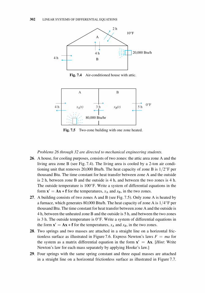
302 LINEAR SYSTEMS OF DIFFERENTIAL EQUATIONS
A
4 h4 h
2 h10°F
20,000 Btu/h
B
Fig. 7.4 Air-conditioned house with attic.
A
4 h 3 h 5 h
B
0°FxA(t) xB(t)
80,000 Btu/hr
Fig. 7.5 Two-zone building with one zone heated.
Problems 26 through 32 are directed to mechanical engineering students.
26. A house, for cooling purposes, consists of two zones: the attic area zone A and theliving area zone B (see Fig. 7.4). The living area is cooled by a 2-ton air condi-tioning unit that removes 20,000 Btu/h. The heat capacity of zone B is 1/2◦F perthousand Btu. The time constant for heat transfer between zone A and the outsideis 2 h, between zone B and the outside is 4 h, and between the two zones is 4 h.The outside temperature is 100◦F. Write a system of differential equations in theform x′ = Ax + f for the temperatures, xA and xB, in the two zones.
27. A building consists of two zones A and B (see Fig. 7.5). Only zone A is heated bya furnace, which generates 80,000 Btu/h. The heat capacity of zone A is 1/4◦F perthousand Btu. The time constant for heat transfer between zone A and the outside is4 h, between the unheated zone B and the outside is 5 h, and between the two zonesis 3 h. The outside temperature is 0◦F. Write a system of differential equations inthe form x′ = Ax + f for the temperatures, xA and xB, in the two zones.
28. Two springs and two masses are attached in a straight line on a horizontal fric-tionless surface as illustrated in Figure 7.6. Express Newton’s laws F = ma forthe system as a matrix differential equation in the form x′ = Ax. [Hint: WriteNewton’s law for each mass separately by applying Hooke’s law.]
29. Four springs with the same spring constant and three equal masses are attachedin a straight line on a horizontal frictionless surface as illustrated in Figure 7.7.
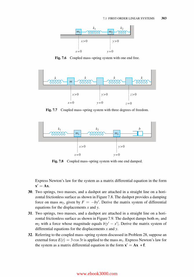
7.1 FIRST-ORDER LINEAR SYSTEMS 303
m1 m2
x > 0
k1 k2
y > 0
y = 0x = 0
Fig. 7.6 Coupled mass–spring system with one end free.
y = 0 z = 0x = 0
x > 0 y > 0 z > 0
k k km
k
Fig. 7.7 Coupled mass–spring system with three degrees of freedom.
y = 0x = 0
x > 0
k1m1 m2
bk2
y > 0
Fig. 7.8 Coupled mass–spring system with one end damped.
Express Newton’s law for the system as a matrix differential equation in the formx′ = Ax.
30. Two springs, two masses, and a dashpot are attached in a straight line on a hori-zontal frictionless surface as shown in Figure 7.8. The dashpot provides a dampingforce on mass m2, given by F = −by′. Derive the matrix system of differentialequations for the displacements x and y.
31. Two springs, two masses, and a dashpot are attached in a straight line on a hori-zontal frictionless surface as shown in Figure 7.9. The dashpot damps both m1 andm2 with a force whose magnitude equals b|y′ − x′|. Derive the matrix system ofdifferential equations for the displacements x and y.
32. Referring to the coupled mass–spring system discussed in Problem 28, suppose anexternal force E(t) = 3 cos 3t is applied to the mass m1. Express Newton’s law forthe system as a matrix differential equation in the form x′ = Ax + f.
www.ebook3000.com
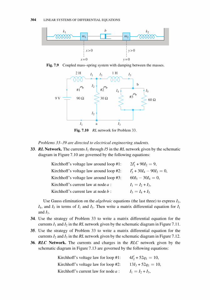
304 LINEAR SYSTEMS OF DIFFERENTIAL EQUATIONS
y = 0x = 0
x > 0
k1m1 m2
b k2
y > 0
Fig. 7.9 Coupled mass–spring system with damping between the masses.
I1
I2
I2
I1 I3 I3
I4 I5
I3
60 Ω30 Ω90 Ω9 V
2 H 1 H
b
a
#1 #2
#3
Fig. 7.10 RL network for Problem 33.
Problems 33–39 are directed to electrical engineering students.
33. RL Network. The currents I1 through I5 in the RL network given by the schematicdiagram in Figure 7.10 are governed by the following equations:
Kirchhoff’s voltage law around loop #1: 2I′1 + 90I2 = 9,
Kirchhoff’s voltage law around loop #2: I′3 + 30I4 − 90I2 = 0,
Kirchhoff’s voltage law around loop #3: 60I5 − 30I4 = 0,
Kirchhoff’s current law at node a : I1 = I2 + I3,
Kirchhoff’s current law at node b : I3 = I4 + I5.
Use Gauss elimination on the algebraic equations (the last three) to express I2,I4, and I5 in terms of I1 and I3. Then write a matrix differential equation for I1
and I3.
34. Use the strategy of Problem 33 to write a matrix differential equation for thecurrents I1 and I2 in the RL network given by the schematic diagram in Figure 7.11.
35. Use the strategy of Problem 33 to write a matrix differential equation for thecurrents I2 and I3 in the RL network given by the schematic diagram in Figure 7.12.
36. RLC Network. The currents and charges in the RLC network given by theschematic diagram in Figure 7.13 are governed by the following equations:
Kirchhoff’s voltage law for loop #1: 4I′2 + 52q1 = 10,
Kirchhoff’s voltage law for loop #2: 13I3 + 52q1 = 10,
Kirchhoff’s current law for node a : I1 = I2 + I3,
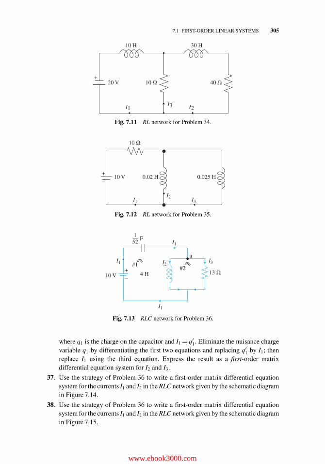
7.1 FIRST-ORDER LINEAR SYSTEMS 305
I1I3 I2
10 Ω
10 H 30 H
20 V+
–40 Ω
Fig. 7.11 RL network for Problem 34.
I1I2 I3
10 Ω
0.02 H10 V 0.025 H+
–
Fig. 7.12 RL network for Problem 35.
I1
I1
I1 I2I3
13 Ω
a
10 V 4 H
F152
#1#2+
–
Fig. 7.13 RLC network for Problem 36.
where q1 is the charge on the capacitor and I1 = q′1. Eliminate the nuisance chargevariable q1 by differentiating the first two equations and replacing q′1 by I1; thenreplace I1 using the third equation. Express the result as a first-order matrixdifferential equation system for I2 and I3.
37. Use the strategy of Problem 36 to write a first-order matrix differential equationsystem for the currents I1 and I2 in the RLC network given by the schematic diagramin Figure 7.14.
38. Use the strategy of Problem 36 to write a first-order matrix differential equationsystem for the currents I1 and I2 in the RLC network given by the schematic diagramin Figure 7.15.
www.ebook3000.com
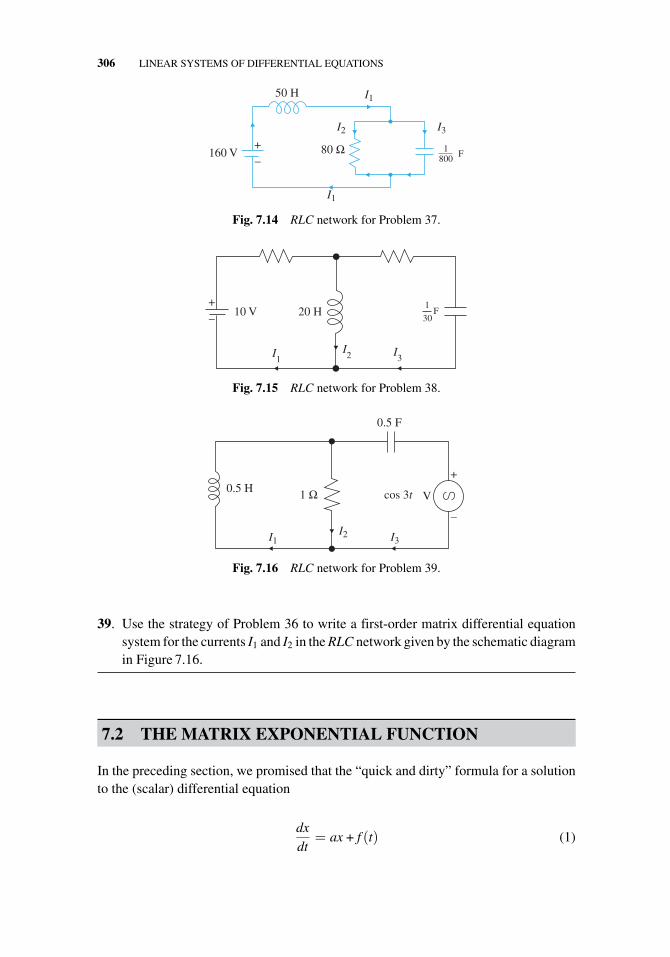
306 LINEAR SYSTEMS OF DIFFERENTIAL EQUATIONS
50 H
80 Ω160 V
I1
I1
I2 I3
F1800
+–
Fig. 7.14 RLC network for Problem 37.
I1
I2 I
3
10 V 20 H1
F30
+–
Fig. 7.15 RLC network for Problem 38.
0.5 F
0.5 H cos 3t
I3I2I1
1 Ω V
+
–
Fig. 7.16 RLC network for Problem 39.
39. Use the strategy of Problem 36 to write a first-order matrix differential equationsystem for the currents I1 and I2 in the RLC network given by the schematic diagramin Figure 7.16.
7.2 THE MATRIX EXPONENTIAL FUNCTION
In the preceding section, we promised that the “quick and dirty” formula for a solutionto the (scalar) differential equation
dxdt
= ax + f (t) (1)
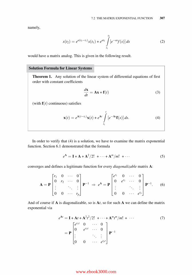
7.2 THE MATRIX EXPONENTIAL FUNCTION 307
namely,
x(t2) = ea(t2−t1)x(t1) + eat2
t2∫t1
[e−asf (s)] ds (2)
would have a matrix analog. This is given in the following result.
Solution Formula for Linear Systems
Theorem 1. Any solution of the linear system of differential equations of firstorder with constant coefficients
dxdt
= Ax + f(t) (3)
(with f(t) continuous) satisfies
x(t) = eA(t−t1)x(t) + eAt
t∫t1
[e−Asf(s)] ds. (4)
In order to verify that (4) is a solution, we have to examine the matrix exponentialfunction. Section 6.1 demonstrated that the formula
eA = I + A + A2/2! + · · · + Am/m! + · · · (5)
converges and defines a legitimate function for every diagonalizable matrix A:
A = P
⎡⎢⎢⎢⎣
r1 0 · · · 00 r2 · · · 0...
. . ....
0 0 · · · rp
⎤⎥⎥⎥⎦P−1 ⇒ eA = P
⎡⎢⎢⎢⎣
er1 0 · · · 00 er2 · · · 0...
. . ....
0 0 · · · erp
⎤⎥⎥⎥⎦P−1. (6)
And of course if A is diagonalizable, so is At, so for such A we can define the matrixexponential via
eAt = I + At + A2t2/2! + · · · + Amtm/m! + · · · (7)
= P
⎡⎢⎢⎢⎣
er1t 0 · · · 00 er2t · · · 0...
. . ....
0 0 · · · erpt
⎤⎥⎥⎥⎦P−1
www.ebook3000.com
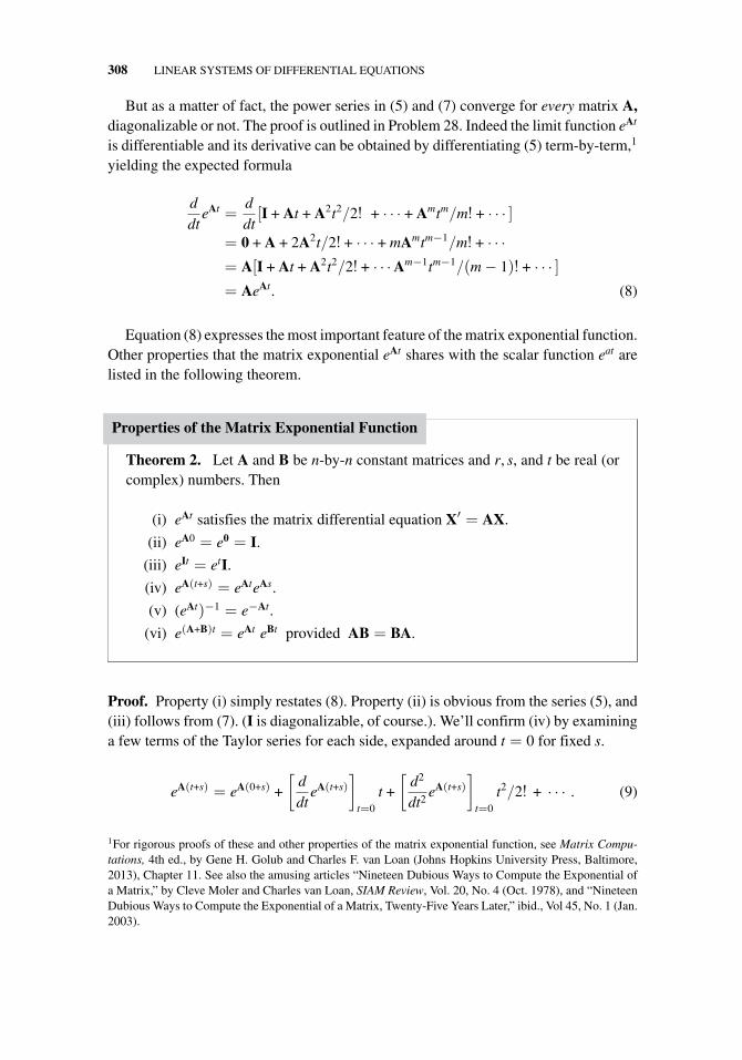
308 LINEAR SYSTEMS OF DIFFERENTIAL EQUATIONS
But as a matter of fact, the power series in (5) and (7) converge for every matrix A,diagonalizable or not. The proof is outlined in Problem 28. Indeed the limit function eAt
is differentiable and its derivative can be obtained by differentiating (5) term-by-term,1
yielding the expected formula
ddt
eAt =ddt[I + At + A2t2/2! + · · · + Amtm/m! + · · · ]
= 0 + A + 2A2t/2! + · · · + mAmtm−1/m! + · · ·= A[I + At + A2t2/2! + · · ·Am−1tm−1/(m − 1)! + · · · ]= AeAt. (8)
Equation (8) expresses the most important feature of the matrix exponential function.Other properties that the matrix exponential eAt shares with the scalar function eat arelisted in the following theorem.
Properties of the Matrix Exponential Function
Theorem 2. Let A and B be n-by-n constant matrices and r, s, and t be real (orcomplex) numbers. Then
(i) eAt satisfies the matrix differential equation X′ = AX.
(ii) eA0 = e0 = I.
(iii) eIt = etI.
(iv) eA(t+s) = eAteAs.
(v) (eAt)−1 = e−At.
(vi) e(A+B)t = eAt eBt provided AB = BA.
Proof. Property (i) simply restates (8). Property (ii) is obvious from the series (5), and(iii) follows from (7). (I is diagonalizable, of course.). We’ll confirm (iv) by examininga few terms of the Taylor series for each side, expanded around t = 0 for fixed s.
eA(t+s) = eA(0+s) +
[ddt
eA(t+s)
]t=0
t +
[d2
dt2eA(t+s)
]t=0
t2/2! + · · · . (9)
1For rigorous proofs of these and other properties of the matrix exponential function, see Matrix Compu-tations, 4th ed., by Gene H. Golub and Charles F. van Loan (Johns Hopkins University Press, Baltimore,2013), Chapter 11. See also the amusing articles “Nineteen Dubious Ways to Compute the Exponential ofa Matrix,” by Cleve Moler and Charles van Loan, SIAM Review, Vol. 20, No. 4 (Oct. 1978), and “NineteenDubious Ways to Compute the Exponential of a Matrix, Twenty-Five Years Later,” ibid., Vol 45, No. 1 (Jan.2003).
7.2 THE MATRIX EXPONENTIAL FUNCTION 309
By the chain rule and formula (7),
[ddt
eA(t+s)
]t=0
=
[(d
d(t + s)eA(t+s)
)d(t + s)
dt
]t=0
=[(AeA(t+s))(1)
]t=0
= AeAs,[
d2
dt2eA(t+s)
]t=0
=
[d
d(t + s)(AeA(t+s))
d(t + s)dt
]t=0
= [(A2eA(t+s))(1)]t=0 = A2eAs
and so on, leading to the series
eA(t+s) = eAs + AeAst + A2eAst2/2! + · · · . (10)
However from (7) we have
eAteAs = {I + At + A2t2/2! + · · · }eAs, (11)
which matches up with (10).We confirm (v) by letting s = −t in (iv) and invoking (ii).Finally, the first three terms of the Taylor series expansions of the members in (vi)
demonstrate the need for the proviso:
e(A+B)t = I + (A + B)t + (A + B)2t2/2! + · · · (12)
by (7); on the other hand,
eAteBt = eA0eB0 +
[ddt(eAteBt)
]t=0
t +
[d2
dt2(eAteBt)
]t=0
t2/2! + · · ·
= I + [AeAteBt + eAtBeBt]t=0 t (product rule, Section 6.2)
+ [A2eAteBt + AeAtBeBt + AeAtBeBt + eAtB2eBt]t=0 t2/2! + · · ·
= I + (A + B)t + (A2 + 2AB + B2) t2/2! + · · · .
(13)
Note that (A + B)2 = A2 + AB + BA + B2 in (12), and this equals A2 + 2AB + B2 in(13) only if AB = BA.
Indeed, any algebraic proof of (vi) for the scalar case can be directly translated intothe matrix case as long as AB = BA. A slick proof that exploits differential equationtheory is given in Problem 30.
www.ebook3000.com
310 LINEAR SYSTEMS OF DIFFERENTIAL EQUATIONS
The serendipity of properties (i) through (v) tempts us to try to derive the promisedformula (4) by reinterpreting the scalar derivation:
dxdt
= Ax + f(t) ⇒ x(t2) = eA(t2−t1)x(t1) + eAt2
t2∫t1
[e−Asf(s)] ds. (14)
Proof of (14). The differential equation is equivalent to
ddt
[e−Atx
]= −Ae−Atx + e−At dx
dt= e−At
[dxdt
− Ax]= e−Atf (15)
(since Ae−At = e−AtA; look at the power series), and hence
e−At2 x(t2)− e−At1 x(t1) =
t2∫t1
[e−Atf(t)] dt,
implying (14) and hence, Theorem 1.
We have seen how to compute eAt when A is diagonalizable:
eAt = P
⎡⎢⎢⎢⎣
er1t 0 · · · 00 er2t · · · 0...
. . ....
0 0 · · · erpt
⎤⎥⎥⎥⎦P−1.
Thus we can see that the corresponding solutions to a homogeneous (f = 0) linearconstant coefficient system are combinations of constant vectors times exponentials(erit) for diagonalizable A. Of course, these will be oscillatory if the eigenvalues ri arecomplex.
Example 1. Example 2 of Section 7.1 demonstrated that
x(t) =[
cosωt−ω sinωt
](16)
is a solution of the matrix differential equation dx/dt = Ax, where
A =
[0 1
−ω2 0
]
Verify this solution using Equation (4) of Theorem 1.
7.2 THE MATRIX EXPONENTIAL FUNCTION 311
Solution. Taking t1 = 0 (and f(t) = 0) in (4) produces
x(t) = eAtx(0) = eAt
[10
]
for the proposed x(0) (specified by equation 16). Since
det(A − rI) = det
[−r 1−ω2 −r
]= r2 + ω2,
the eigenvalues of A are±iω. The corresponding eigenvectors are found to be [1 ±iω]T ,and the diagonal form of A is
A = P[
r1 00 r2
]P−1 =
[1 1iω −iω
] [iω 00 −iω
] ⎡⎢⎣
12
− i2ω
12
i2ω
⎤⎥⎦ ,
so that
eAt =
[1 1iω −iω
] [eiωt 00 e−iωt
] ⎡⎢⎣
12
− i2ω
12
i2ω
⎤⎥⎦ .
Hence,
eAtx(0) =[
1 1iω −iω
] [eiωt 00 e−iωt
] ⎡⎢⎣
12
− i2ω
12
i2ω
⎤⎥⎦[
10
]
=
[1 1iω −iω
] [eiωt 00 e−iωt
] [1/2
1/2
]
=
[1 1iω −iω
] [eiωt/2e−iωt/2
]
=
[eiωt/2 + e−iωt/2iω (eiωt/2 − e−iωt/2)
]=
[cosωt−ω sinωt
],
the oscillatory solution promised in (16). �
What if A cannot be diagonalized? There are other methods for numerically com-puting eAt; indeed, with patience we can sum the power series (7) (but see Problem 31).However it would be nice to know the nature of the solutions for defective (Section 5.2)coefficient matrices A; if they’re not constants times exponentials, what are they? The
www.ebook3000.com
312 LINEAR SYSTEMS OF DIFFERENTIAL EQUATIONS
Jordan normal form that we will describe in the next section answers this questioncompletely. (They are constants times exponentials times polynomials.)
Final Remarks for Readers with Differential Equations Experience
1. Formula (4) settles the existence and uniqueness issues for linear first-ordersystems with constant coefficients. The explicit formula is a solution, andits derivation demonstrates that it is the only one.
2. The individual columns of eAt are solutions to dx/dt = Ax. They are lin-early independent matrix functions; Theorem 2 states that eAt is invertibleand therefore nonsingular (for every t). Therefore if c is a generic constantcolumn vector, eAtc is a general solution and eAt is a fundamental matrix.
3. The matrix function e−At plays the role of an integrating factor in (15). Thedisplay (4) can be interpreted as an instance of the variation of parametersformula.
Exercises 7.2
Compute eAt for the matrices in Problems 1–12 using diagonalizability. [Hint: Theireigenvalues and eigenvectors were calculated in Exercises 6.1.]
1.
[9 −3−2 4
]2.[−1 −34 7
]3.
[1 −2−2 1
]4.
[−3 2−5 4
]5.
[1 11 1
]
6.
⎡⎣1 0 2
3 4 20 0 0
⎤⎦ 7.
⎡⎣4 −1 −2
2 1 −21 −1 1
⎤⎦ 8.
⎡⎣ 2 −1 −1−1 3 0−1 0 3
⎤⎦
9.
[0 −11 0
]10.
[0 1
−1 + i −1
]11.
[1 2i−1 3 + i
]12.
⎡⎣−6 2 16−3 1 11−3 1 7
⎤⎦
If a matrix has only one eigenvalue (i.e., all of its eigenvalues are equal), then there isa slick trick enabling the easy computation of its exponential:
(i) its characteristic polynomial (Section 5.2) must take the form p(r) = (r1 − r)n;
(ii) by the Cayley–Hamilton theorem (Corollary 9, Section 6.3), (A − r1I)n = 0;
(iii) the power series for e(A−r1I) terminates:
e(A−r1I) = I + (A − r1I) + (A − r1I)2/2! + · · ·+ (A − r1I)n−1/(n − 1)! + 0 + 0 + · · ·
7.2 THE MATRIX EXPONENTIAL FUNCTION 313
(iv) eA = er1Ie(A−r1I) = er1 e(A−r1I) provides a terminating power series for eA.
Use this trick to find the matrix exponential eAt for the matrices in Problems 13through 18
13.
[1 −11 3
]14.
[3 −20 3
]15.
⎡⎣ 2 1 −1−3 −1 19 3 −4
⎤⎦ 16.
⎡⎣2 1 3
0 2 −10 0 2
⎤⎦
17.
⎡⎣ 0 1 0
0 0 1−1 −3 −3
⎤⎦ 18.
⎡⎣−2 0 0
4 −2 01 0 −2
⎤⎦ .
19. Use the results of Problem 15 and formula (4) to find the solution to the initial-valueproblem
x′(t) =
⎡⎣ 2 1 −1−3 −1 19 3 −4
⎤⎦ x(t) +
⎡⎣0
t0
⎤⎦ , x(0) =
⎡⎣0
30
⎤⎦ .
20. Use the result of Problem 18 to find the solution to the initial-value problem
x′(t) =
⎡⎣−2 0 0
4 −2 01 0 −2
⎤⎦ x(t), x(0) =
⎡⎣ 1
1−1
⎤⎦ .
21. Use the result of Problem 17 to find the solution to the initial-value problem
x′(t) =
⎡⎣ 0 1 0
0 0 1−1 −3 −3
⎤⎦ x(t) + t
⎡⎣ 1−12
⎤⎦ +
⎡⎣3
10
⎤⎦ , x(0) = 0.
In Problems 22–27, use formula (4) to determine a solution of the system x′(t) =Ax(t) + f(t), where A and f(t) are given. Take x(0) = 0.
22. A =
[0 12 0
], f (t) =
[sin 3t
t
].
23. A =
[−1 02 2
], f (t) =
[t2
t + 1
].
24. A =
⎡⎣ 0 −1 0−1 0 10 0 1
⎤⎦ , f(t) =
⎡⎣0
01
⎤⎦ .
www.ebook3000.com
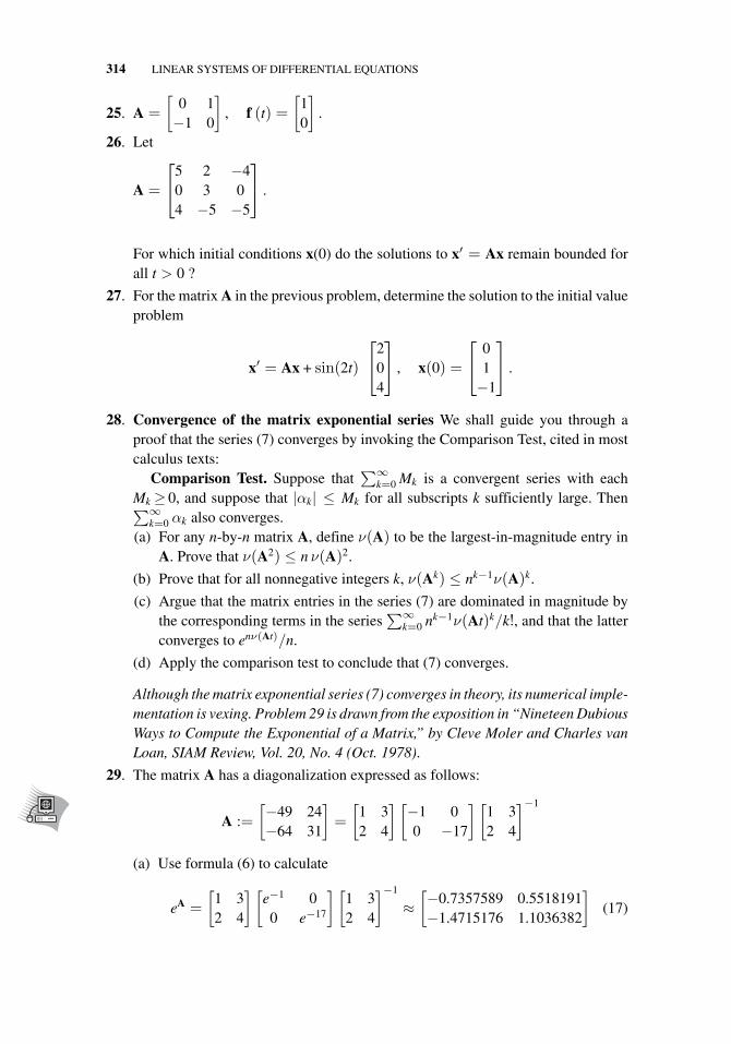
314 LINEAR SYSTEMS OF DIFFERENTIAL EQUATIONS
25. A =
[0 1−1 0
], f (t) =
[10
].
26. Let
A =
⎡⎣5 2 −4
0 3 04 −5 −5
⎤⎦ .
For which initial conditions x(0) do the solutions to x′ = Ax remain bounded forall t > 0 ?
27. For the matrix A in the previous problem, determine the solution to the initial valueproblem
x′ = Ax + sin(2t)
⎡⎣2
04
⎤⎦ , x(0) =
⎡⎣ 0
1−1
⎤⎦ .
28. Convergence of the matrix exponential series We shall guide you through aproof that the series (7) converges by invoking the Comparison Test, cited in mostcalculus texts:
Comparison Test. Suppose that∑∞
k=0 Mk is a convergent series with eachMk ≥ 0, and suppose that |αk| ≤ Mk for all subscripts k sufficiently large. Then∑∞
k=0 αk also converges.(a) For any n-by-n matrix A, define ν(A) to be the largest-in-magnitude entry in
A. Prove that ν(A2) ≤ n ν(A)2.
(b) Prove that for all nonnegative integers k, ν(Ak) ≤ nk−1ν(A)k.
(c) Argue that the matrix entries in the series (7) are dominated in magnitude bythe corresponding terms in the series
∑∞k=0 nk−1ν(At)k/k!, and that the latter
converges to enν(At)/n.
(d) Apply the comparison test to conclude that (7) converges.
Although the matrix exponential series (7) converges in theory, its numerical imple-mentation is vexing. Problem 29 is drawn from the exposition in “Nineteen DubiousWays to Compute the Exponential of a Matrix,” by Cleve Moler and Charles vanLoan, SIAM Review, Vol. 20, No. 4 (Oct. 1978).
29. The matrix A has a diagonalization expressed as follows:
A :=
[−49 24−64 31
]=
[1 32 4
] [−1 00 −17
] [1 32 4
]−1
(a) Use formula (6) to calculate
eA =
[1 32 4
] [e−1 00 e−17
] [1 32 4
]−1
≈[−0.7357589 0.5518191−1.4715176 1.1036382
](17)
7.2 THE MATRIX EXPONENTIAL FUNCTION 315
(b) Use a computer to show that, in the power series
eA = I + A + A2/2! + · · · + Am/m! + · · · ,
the 16th and 17th terms are approximately given by
A16
16!≈
[6, 977, 251.906101090 −3, 488, 625.9530505459, 303, 002.541468118 −4, 651, 501.270734060
]
A17
17!≈
[−6, 977, 251.906101089 3, 488, 625.953050546−9, 303, 002.541468109 4, 651, 501.270734056
]
Hence in the summation (A16/16! + A17/17!), 15 significant (decimal) dig-its are lost through cancellation. A 16-digit computer has no chance ofperforming this summation correctly.
(c) Moler and van Loan reported that on their 1978 computer, the first 59 terms ofthe series
eA = I + A + A2/2! + · · · + Am/m! + · · ·
resulted in the horrible approximation
eA ≈[−22.25880 −1.432766−61.49931 −3.474280
]
(compare with (17)). Today’s computers are much more accurate. Write aprogram to calculate
I + A + A2/2! + · · · + Am/m!
for any input m. How many terms must be summed to obtain an answer closeto the true value (17) on your computer?
(d) Change A to
A :=
[−100 49.5−132 65
]=
[1 32 4
] [−1 00 −34
] [1 32 4
]−1
and use the diagonal form to show that
eA ≈[−0.7357589 0.5518192−1.4715178 1.1036383
](18)
(e) Now how many terms of
eA = I + A + A2/2! + · · · + Am/m! + · · ·
must be summed to obtain an answer close to the true value on your computer?
www.ebook3000.com
316 LINEAR SYSTEMS OF DIFFERENTIAL EQUATIONS
30. Theorem 1 implies that the initial value problem
x′ = Mx, x(0) = c
has one, and only one, solution, given by equation (4) in the theorem (with f and t1each zero), when M and c are any constant matrices of the appropriate dimensions.Use this to prove statement (vi) in Theorem 2 by demonstrating that e(A+B)tc andeAteBtc both satisfy x′ = (A + B)x, x(0) = c. [Hint: argue that
ddt
eAteBt = AeAteBt + eAtBeBt
and also that eAtBeBt = BeAteBt if AB = BA.]
31. Let A =
[1 2−1 3
]and B =
[2 10 1
].
(a) Show that AB �= BA.
(b) Show that property (vi) in Theorem 2 does not hold for these matrices. That is,show that e(A+B)t �= eAteBt.
In Problems 32–35, use a linear algebra software package for help indetermining eAt
32. A =
⎡⎢⎢⎢⎢⎣
0 1 0 0 00 0 1 0 01 −3 3 0 00 0 0 0 10 0 0 −1 0
⎤⎥⎥⎥⎥⎦ . 33. A =
⎡⎢⎢⎢⎢⎣
1 0 0 0 00 0 1 0 00 −1 −2 0 00 0 0 0 10 0 0 −1 0
⎤⎥⎥⎥⎥⎦ .
34. A =
⎡⎢⎢⎢⎢⎣
0 1 0 0 00 0 1 0 0−1 −3 −3 0 00 0 0 0 10 0 0 −4 −4
⎤⎥⎥⎥⎥⎦ . 35. A =
⎡⎢⎢⎢⎢⎣
−1 0 0 0 00 0 1 0 00 −1 −2 0 00 0 0 0 10 0 0 −4 −4
⎤⎥⎥⎥⎥⎦ .
7.3 THE JORDAN NORMAL FORM
We have seen three possibilities for the set of eigenvalues of an arbitrary n-by-nmatrix A:
(i) A has n distinct eigenvalues. Then A must have n linearly independent eigen-vectors, and it can be diagonalized by a similarity transformation generated bya matrix P of eigenvectors: A = PDP−1.
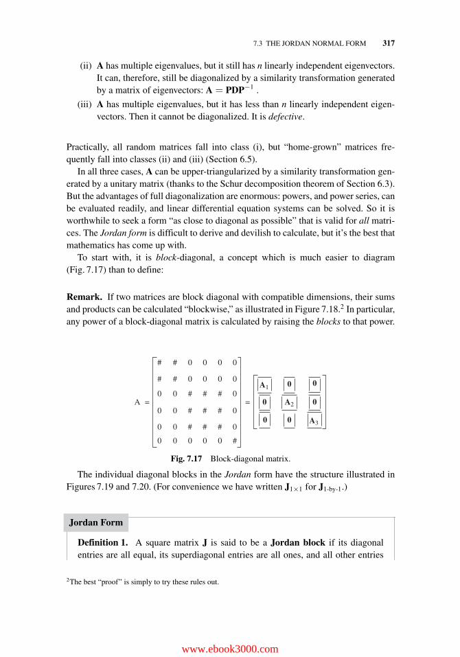
7.3 THE JORDAN NORMAL FORM 317
(ii) A has multiple eigenvalues, but it still has n linearly independent eigenvectors.It can, therefore, still be diagonalized by a similarity transformation generatedby a matrix of eigenvectors: A = PDP−1 .
(iii) A has multiple eigenvalues, but it has less than n linearly independent eigen-vectors. Then it cannot be diagonalized. It is defective.
Practically, all random matrices fall into class (i), but “home-grown” matrices fre-quently fall into classes (ii) and (iii) (Section 6.5).
In all three cases, A can be upper-triangularized by a similarity transformation gen-erated by a unitary matrix (thanks to the Schur decomposition theorem of Section 6.3).But the advantages of full diagonalization are enormous: powers, and power series, canbe evaluated readily, and linear differential equation systems can be solved. So it isworthwhile to seek a form “as close to diagonal as possible” that is valid for all matri-ces. The Jordan form is difficult to derive and devilish to calculate, but it’s the best thatmathematics has come up with.
To start with, it is block-diagonal, a concept which is much easier to diagram(Fig. 7.17) than to define:
Remark. If two matrices are block diagonal with compatible dimensions, their sumsand products can be calculated “blockwise,” as illustrated in Figure 7.18.2 In particular,any power of a block-diagonal matrix is calculated by raising the blocks to that power.
A = =
# # 0 0
0
0 0
0
00
0 0
0 0 # # # 0
0 0 # # #
0 0 0
0
0 0 0 0 0 #
# # 0 0 0 0
# # #
A1
A2
A3
Fig. 7.17 Block-diagonal matrix.
The individual diagonal blocks in the Jordan form have the structure illustrated inFigures 7.19 and 7.20. (For convenience we have written J1×1 for J1-by-1.)
Jordan Form
Definition 1. A square matrix J is said to be a Jordan block if its diagonalentries are all equal, its superdiagonal entries are all ones, and all other entries
2The best “proof” is simply to try these rules out.
www.ebook3000.com
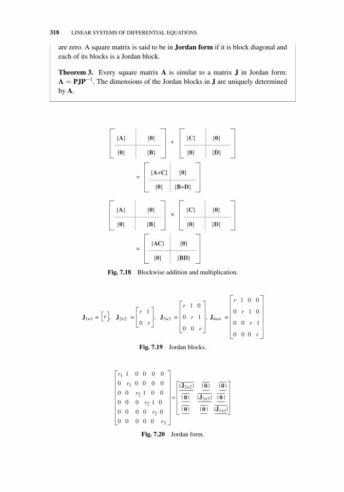
318 LINEAR SYSTEMS OF DIFFERENTIAL EQUATIONS
are zero. A square matrix is said to be in Jordan form if it is block diagonal andeach of its blocks is a Jordan block.
Theorem 3. Every square matrix A is similar to a matrix J in Jordan form:A = PJP−1. The dimensions of the Jordan blocks in J are uniquely determinedby A.
×
=
[C] [0]
[0] [D]
[A] [0]
[0] [B]
+
[C] [0]
[0] [D]
[A] [0]
[0] [B]
[AC] [0]
[0] [BD]
[A+C] [0]
[0] [B+D]
=
Fig. 7.18 Blockwise addition and multiplication.
====
r
r
r
r
r
r
r
r
rr
000
100
010
001
,
00
10
01
0
1, , J4×4J3×3J2×2J1×1
Fig. 7.19 Jordan blocks.
=
||||||
||||||
||||||
00000
00000
01000
00100
00000
00001
J1×100
0J3×30
00J2×2
r3
r2
r2
r2
r1
r1
Fig. 7.20 Jordan form.
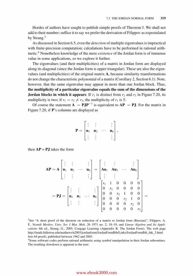
7.3 THE JORDAN NORMAL FORM 319
Hordes of authors have sought to publish simple proofs of Theorem 3. We shall notadd to their number; suffice it to say we prefer the derivation of Filippov as expostulatedby Strang.3
As discussed in Section 6.5, even the detection of multiple eigenvalues is impracticalwith finite-precision computation; calculations have to be performed in rational arith-metic.4 Nonetheless knowledge of the mere existence of the Jordan form is of immensevalue in some applications, so we explore it further.
The eigenvalues (and their multiplicities) of a matrix in Jordan form are displayedalong its diagonal (since the Jordan form is upper triangular). These are also the eigen-values (and multiplicities) of the original matrix A, because similarity transformationsdo not change the characteristic polynomial of a matrix (Corollary 2, Section 6.1). Note,however, that the same eigenvalue may appear in more than one Jordan block. Thus,the multiplicity of a particular eigenvalue equals the sum of the dimensions of theJordan blocks in which it appears. If r1 is distinct from r2 and r3 in Figure 7.20, itsmultiplicity is two; if r1 = r2 �= r3, the multiplicity of r1 is 5.
Of course the statement A = PJP−1 is equivalent to AP = PJ. For the matrix inFigure 7.20, if P’s columns are displayed as
P =
⎡⎢⎢⎣
......
...u1 u2 · · · u6...
......
⎤⎥⎥⎦ ,
then AP = PJ takes the form
AP = A
⎡⎢⎢⎣
......
...u1 u2 · · · u6...
......
⎤⎥⎥⎦ =
⎡⎢⎢⎣
......
...Au1 Au2 · · · Au6
......
⎤⎥⎥⎦
= PJ =
⎡⎢⎢⎣
......
...u1 u2 · · · u6...
......
⎤⎥⎥⎦
⎡⎢⎢⎢⎢⎢⎢⎢⎣
r1 1 0 0 0 00 r1 0 0 0 00 0 r2 1 0 00 0 0 r2 1 00 0 0 0 r2 00 0 0 0 0 r3
⎤⎥⎥⎥⎥⎥⎥⎥⎦=
3See “A short proof of the theorem on reduction of a matrix to Jordan form (Russian)”, Filippov, A.F., Vestnik Moskov. Univ. Ser. I Mat. Meh. 26 1971 no. 2, 18–19; and Linear Algebra and Its Appli-cations 4th ed., Strang, G., 2005, Cengage Learning (Appendix B. The Jordan Form). The web pagehttp://math.fullerton.edu/mathews/n2003/jordanform/JordanFormBib/Links/JordanFormBib_lnk_3.htmllists 64 proofs, published between 1962 and 2003.4Some software codes perform rational arithmetic using symbol manipulation in their Jordan subroutines.The resulting slowdown is apparent to the user.
www.ebook3000.com
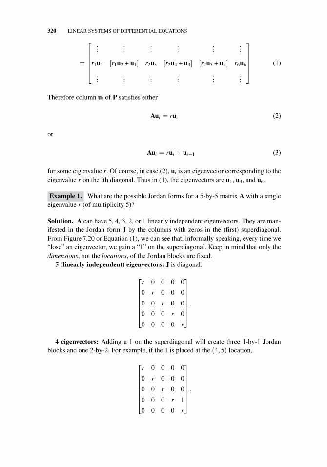
320 LINEAR SYSTEMS OF DIFFERENTIAL EQUATIONS
=
⎡⎢⎢⎢⎢⎣
......
......
......
r1u1 [r1u2 + u1] r2u3 [r2u4 + u3] [r2u5 + u4] r6u6
......
......
......
⎤⎥⎥⎥⎥⎦ (1)
Therefore column ui of P satisfies either
Aui = rui (2)
or
Aui = rui + ui−1 (3)
for some eigenvalue r. Of course, in case (2), ui is an eigenvector corresponding to theeigenvalue r on the ith diagonal. Thus in (1), the eigenvectors are u1, u3, and u6.
Example 1. What are the possible Jordan forms for a 5-by-5 matrix A with a singleeigenvalue r (of multiplicity 5)?
Solution. A can have 5, 4, 3, 2, or 1 linearly independent eigenvectors. They are man-ifested in the Jordan form J by the columns with zeros in the (first) superdiagonal.From Figure 7.20 or Equation (1), we can see that, informally speaking, every time we“lose” an eigenvector, we gain a “1” on the superdiagonal. Keep in mind that only thedimensions, not the locations, of the Jordan blocks are fixed.
5 (linearly independent) eigenvectors: J is diagonal:
⎡⎢⎢⎢⎢⎢⎢⎣
r 0 0 0 0
0 r 0 0 0
0 0 r 0 0
0 0 0 r 0
0 0 0 0 r
⎤⎥⎥⎥⎥⎥⎥⎦
.
4 eigenvectors: Adding a 1 on the superdiagonal will create three 1-by-1 Jordanblocks and one 2-by-2. For example, if the 1 is placed at the (4, 5) location,
⎡⎢⎢⎢⎢⎢⎢⎣
r 0 0 0 0
0 r 0 0 0
0 0 r 0 0
0 0 0 r 1
0 0 0 0 r
⎤⎥⎥⎥⎥⎥⎥⎦
.
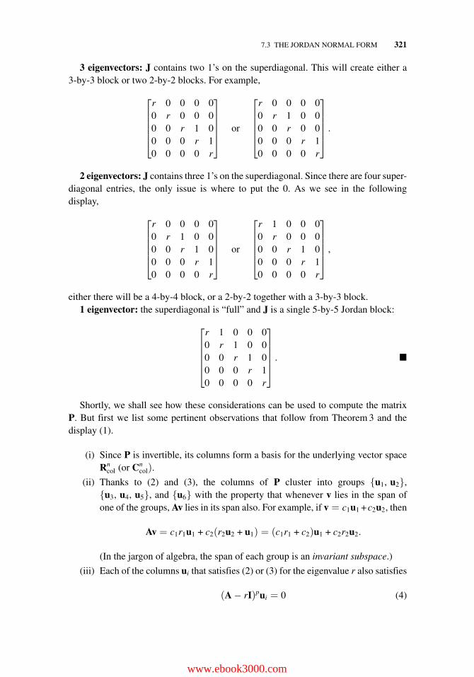
7.3 THE JORDAN NORMAL FORM 321
3 eigenvectors: J contains two 1’s on the superdiagonal. This will create either a3-by-3 block or two 2-by-2 blocks. For example,
⎡⎢⎢⎢⎢⎣
r 0 0 0 00 r 0 0 00 0 r 1 00 0 0 r 10 0 0 0 r
⎤⎥⎥⎥⎥⎦ or
⎡⎢⎢⎢⎢⎣
r 0 0 0 00 r 1 0 00 0 r 0 00 0 0 r 10 0 0 0 r
⎤⎥⎥⎥⎥⎦ .
2 eigenvectors: J contains three 1’s on the superdiagonal. Since there are four super-diagonal entries, the only issue is where to put the 0. As we see in the followingdisplay,
⎡⎢⎢⎢⎢⎣
r 0 0 0 00 r 1 0 00 0 r 1 00 0 0 r 10 0 0 0 r
⎤⎥⎥⎥⎥⎦ or
⎡⎢⎢⎢⎢⎣
r 1 0 0 00 r 0 0 00 0 r 1 00 0 0 r 10 0 0 0 r
⎤⎥⎥⎥⎥⎦ ,
either there will be a 4-by-4 block, or a 2-by-2 together with a 3-by-3 block.1 eigenvector: the superdiagonal is “full” and J is a single 5-by-5 Jordan block:
⎡⎢⎢⎢⎢⎣
r 1 0 0 00 r 1 0 00 0 r 1 00 0 0 r 10 0 0 0 r
⎤⎥⎥⎥⎥⎦ . �
Shortly, we shall see how these considerations can be used to compute the matrixP. But first we list some pertinent observations that follow from Theorem 3 and thedisplay (1).
(i) Since P is invertible, its columns form a basis for the underlying vector spaceRn
col (or Cncol).
(ii) Thanks to (2) and (3), the columns of P cluster into groups {u1, u2},{u3, u4, u5}, and {u6} with the property that whenever v lies in the span ofone of the groups, Av lies in its span also. For example, if v = c1u1 +c2u2, then
Av = c1r1u1 + c2(r2u2 + u1) = (c1r1 + c2)u1 + c2r2u2.
(In the jargon of algebra, the span of each group is an invariant subspace.)
(iii) Each of the columns ui that satisfies (2) or (3) for the eigenvalue r also satisfies
(A − rI)pui = 0 (4)
www.ebook3000.com
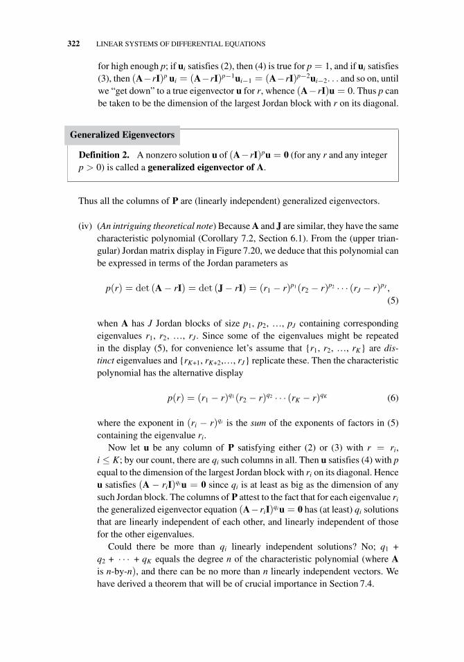
322 LINEAR SYSTEMS OF DIFFERENTIAL EQUATIONS
for high enough p; if ui satisfies (2), then (4) is true for p = 1, and if ui satisfies(3), then (A−rI)p ui = (A−rI)p−1ui−1 = (A−rI)p−2ui−2. . . and so on, untilwe “get down” to a true eigenvector u for r, whence (A− rI)u = 0. Thus p canbe taken to be the dimension of the largest Jordan block with r on its diagonal.
Generalized Eigenvectors
Definition 2. A nonzero solution u of (A−rI)pu = 0 (for any r and any integerp > 0) is called a generalized eigenvector of A.
Thus all the columns of P are (linearly independent) generalized eigenvectors.
(iv) (An intriguing theoretical note) Because A and J are similar, they have the samecharacteristic polynomial (Corollary 7.2, Section 6.1). From the (upper trian-gular) Jordan matrix display in Figure 7.20, we deduce that this polynomial canbe expressed in terms of the Jordan parameters as
p(r) = det (A − rI) = det (J − rI) = (r1 − r)p1(r2 − r)p2 · · · (rJ − r)pJ ,(5)
when A has J Jordan blocks of size p1, p2, …, pJ containing correspondingeigenvalues r1, r2, …, rJ . Since some of the eigenvalues might be repeatedin the display (5), for convenience let’s assume that {r1, r2, …, rK} are dis-tinct eigenvalues and {rK+1, rK+2,…, rJ} replicate these. Then the characteristicpolynomial has the alternative display
p(r) = (r1 − r)q1(r2 − r)q2 · · · (rK − r)qK (6)
where the exponent in (ri − r)qi is the sum of the exponents of factors in (5)containing the eigenvalue ri.
Now let u be any column of P satisfying either (2) or (3) with r = ri,i ≤ K; by our count, there are qi such columns in all. Then u satisfies (4) with pequal to the dimension of the largest Jordan block with ri on its diagonal. Henceu satisfies (A − riI)qi u = 0 since qi is at least as big as the dimension of anysuch Jordan block. The columns of P attest to the fact that for each eigenvalue ri
the generalized eigenvector equation (A− riI)qi u = 0 has (at least) qi solutionsthat are linearly independent of each other, and linearly independent of thosefor the other eigenvalues.
Could there be more than qi linearly independent solutions? No; q1 +q2 + · · · + qK equals the degree n of the characteristic polynomial (where Ais n-by-n), and there can be no more than n linearly independent vectors. Wehave derived a theorem that will be of crucial importance in Section 7.4.
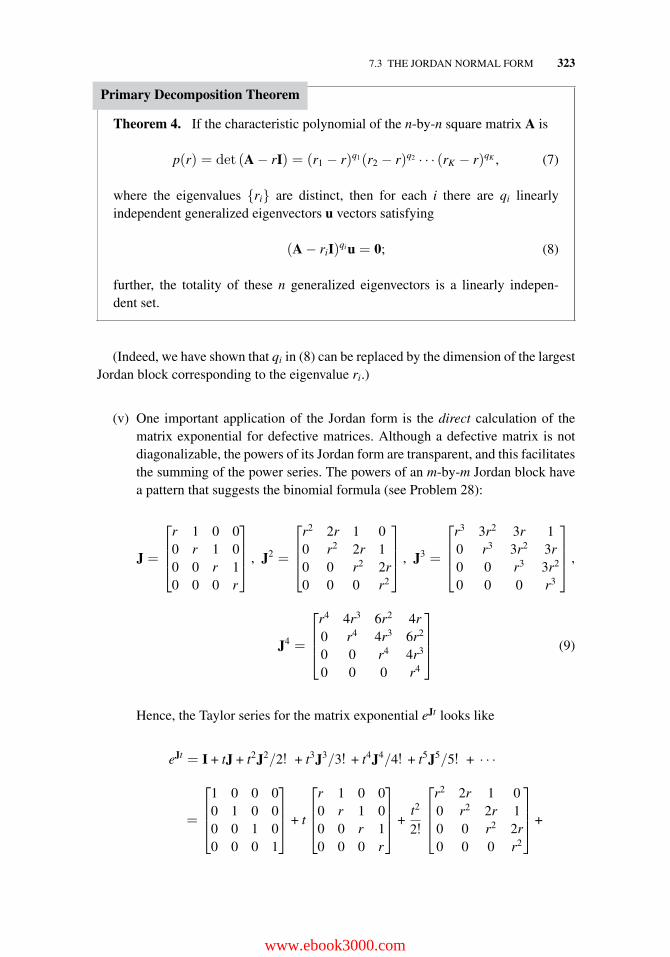
7.3 THE JORDAN NORMAL FORM 323
Primary Decomposition Theorem
Theorem 4. If the characteristic polynomial of the n-by-n square matrix A is
p(r) = det (A − rI) = (r1 − r)q1(r2 − r)q2 · · · (rK − r)qK , (7)
where the eigenvalues {ri} are distinct, then for each i there are qi linearlyindependent generalized eigenvectors u vectors satisfying
(A − riI)qi u = 0; (8)
further, the totality of these n generalized eigenvectors is a linearly indepen-dent set.
(Indeed, we have shown that qi in (8) can be replaced by the dimension of the largestJordan block corresponding to the eigenvalue ri.)
(v) One important application of the Jordan form is the direct calculation of thematrix exponential for defective matrices. Although a defective matrix is notdiagonalizable, the powers of its Jordan form are transparent, and this facilitatesthe summing of the power series. The powers of an m-by-m Jordan block havea pattern that suggests the binomial formula (see Problem 28):
J =
⎡⎢⎢⎣
r 1 0 00 r 1 00 0 r 10 0 0 r
⎤⎥⎥⎦ , J2 =
⎡⎢⎢⎣
r2 2r 1 00 r2 2r 10 0 r2 2r0 0 0 r2
⎤⎥⎥⎦ , J3 =
⎡⎢⎢⎣
r3 3r2 3r 10 r3 3r2 3r0 0 r3 3r2
0 0 0 r3
⎤⎥⎥⎦ ,
J4 =
⎡⎢⎢⎣
r4 4r3 6r2 4r0 r4 4r3 6r2
0 0 r4 4r3
0 0 0 r4
⎤⎥⎥⎦ (9)
Hence, the Taylor series for the matrix exponential eJt looks like
eJt = I + tJ + t2J2/2! + t3J3/3! + t4J4/4! + t5J5/5! + · · ·
=
⎡⎢⎢⎣
1 0 0 00 1 0 00 0 1 00 0 0 1
⎤⎥⎥⎦ + t
⎡⎢⎢⎣
r 1 0 00 r 1 00 0 r 10 0 0 r
⎤⎥⎥⎦ +
t2
2!
⎡⎢⎢⎣
r2 2r 1 00 r2 2r 10 0 r2 2r0 0 0 r2
⎤⎥⎥⎦+
www.ebook3000.com
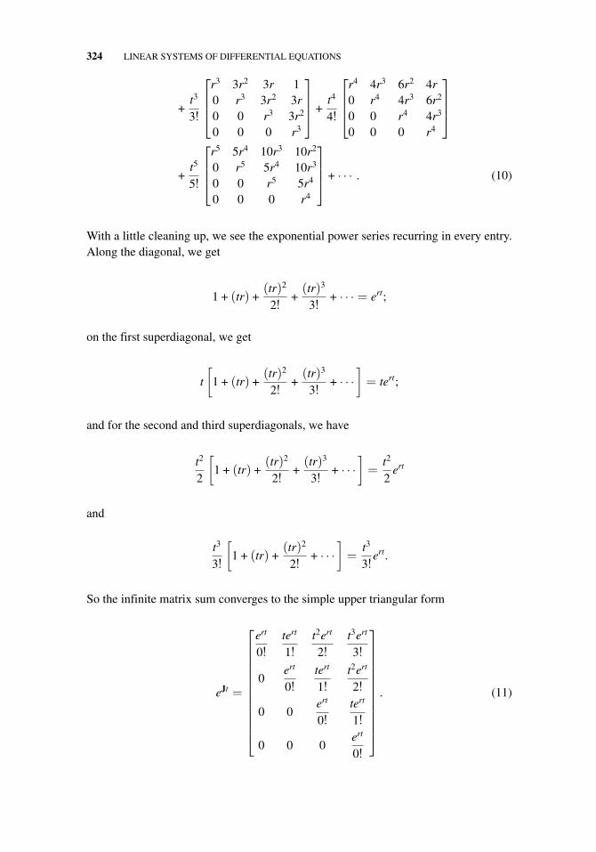
324 LINEAR SYSTEMS OF DIFFERENTIAL EQUATIONS
+t3
3!
⎡⎢⎢⎣
r3 3r2 3r 10 r3 3r2 3r0 0 r3 3r2
0 0 0 r3
⎤⎥⎥⎦ +
t4
4!
⎡⎢⎢⎣
r4 4r3 6r2 4r0 r4 4r3 6r2
0 0 r4 4r3
0 0 0 r4
⎤⎥⎥⎦
+t5
5!
⎡⎢⎢⎣
r5 5r4 10r3 10r2
0 r5 5r4 10r3
0 0 r5 5r4
0 0 0 r4
⎤⎥⎥⎦ + · · · . (10)
With a little cleaning up, we see the exponential power series recurring in every entry.Along the diagonal, we get
1 + (tr) +(tr)2
2!+(tr)3
3!+ · · · = ert;
on the first superdiagonal, we get
t
[1 + (tr) +
(tr)2
2!+(tr)3
3!+ · · ·
]= tert;
and for the second and third superdiagonals, we have
t2
2
[1 + (tr) +
(tr)2
2!+(tr)3
3!+ · · ·
]=
t2
2ert
and
t3
3!
[1 + (tr) +
(tr)2
2!+ · · ·
]=
t3
3!ert.
So the infinite matrix sum converges to the simple upper triangular form
eJt =
⎡⎢⎢⎢⎢⎢⎢⎢⎢⎢⎢⎢⎣
ert
0!tert
1!t2ert
2!t3ert
3!
0ert
0!tert
1!t2ert
2!
0 0ert
0!tert
1!
0 0 0ert
0!
⎤⎥⎥⎥⎥⎥⎥⎥⎥⎥⎥⎥⎦
. (11)
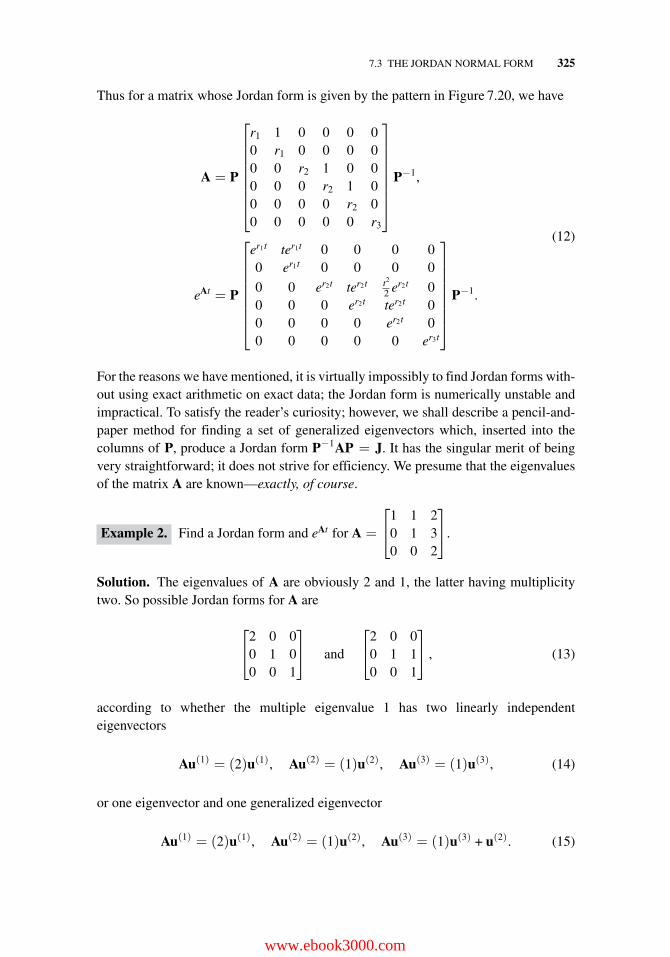
7.3 THE JORDAN NORMAL FORM 325
Thus for a matrix whose Jordan form is given by the pattern in Figure 7.20, we have
A = P
⎡⎢⎢⎢⎢⎢⎢⎢⎣
r1 1 0 0 0 00 r1 0 0 0 00 0 r2 1 0 00 0 0 r2 1 00 0 0 0 r2 00 0 0 0 0 r3
⎤⎥⎥⎥⎥⎥⎥⎥⎦
P−1,
eAt = P
⎡⎢⎢⎢⎢⎢⎢⎢⎣
er1t ter1t 0 0 0 00 er1t 0 0 0 0
0 0 er2t ter2t t2
2 er2t 00 0 0 er2t ter2t 00 0 0 0 er2t 00 0 0 0 0 er3t
⎤⎥⎥⎥⎥⎥⎥⎥⎦
P−1.
(12)
For the reasons we have mentioned, it is virtually impossibly to find Jordan forms with-out using exact arithmetic on exact data; the Jordan form is numerically unstable andimpractical. To satisfy the reader’s curiosity; however, we shall describe a pencil-and-paper method for finding a set of generalized eigenvectors which, inserted into thecolumns of P, produce a Jordan form P−1AP = J. It has the singular merit of beingvery straightforward; it does not strive for efficiency. We presume that the eigenvaluesof the matrix A are known—exactly, of course.
Example 2. Find a Jordan form and eAt for A =
⎡⎣1 1 2
0 1 30 0 2
⎤⎦.
Solution. The eigenvalues of A are obviously 2 and 1, the latter having multiplicitytwo. So possible Jordan forms for A are
⎡⎣2 0 0
0 1 00 0 1
⎤⎦ and
⎡⎣2 0 0
0 1 10 0 1
⎤⎦ , (13)
according to whether the multiple eigenvalue 1 has two linearly independenteigenvectors
Au(1) = (2)u(1), Au(2) = (1)u(2), Au(3) = (1)u(3), (14)
or one eigenvector and one generalized eigenvector
Au(1) = (2)u(1), Au(2) = (1)u(2), Au(3) = (1)u(3) + u(2). (15)
www.ebook3000.com
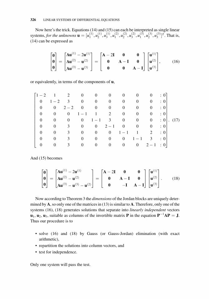
326 LINEAR SYSTEMS OF DIFFERENTIAL EQUATIONS
Now here’s the trick. Equations (14) and (15) can each be interpreted as single linearsystems, for the unknowns u = [u(1)
1 , u(1)2 , u(1)
3 , u(2)1 , u(2)
2 , u(2)3 , u(3)
1 , u(3)2 , u(3)
3 ]T . That is,(14) can be expressed as
⎡⎢⎣
000
⎤⎥⎦ =
⎡⎢⎣
Au(1) − 2u(1)
Au(2) − u(2)
Au(3) − u(3)
⎤⎥⎦ =
⎡⎢⎣
A − 2I 0 0
0 A − I 0
0 0 A − I
⎤⎥⎦⎡⎢⎣
u(1)
u(2)
u(3)
⎤⎥⎦, (16)
or equivalently, in terms of the components of u,
⎡⎢⎢⎢⎢⎢⎢⎢⎢⎢⎢⎢⎢⎢⎢⎢⎣
1 − 2 1 2 0 0 0 0 0 0 : 0
0 1 − 2 3 0 0 0 0 0 0 : 0
0 0 2 − 2 0 0 0 0 0 0 : 0
0 0 0 1 − 1 1 2 0 0 0 : 0
0 0 0 0 1 − 1 3 0 0 0 : 0
0 0 3 0 0 2 − 1 0 0 0 : 0
0 0 3 0 0 0 1 − 1 1 2 : 0
0 0 3 0 0 0 0 1 − 1 3 : 0
0 0 3 0 0 0 0 0 2 − 1 : 0
⎤⎥⎥⎥⎥⎥⎥⎥⎥⎥⎥⎥⎥⎥⎥⎥⎦
. (17)
And (15) becomes
⎡⎢⎣
000
⎤⎥⎦ =
⎡⎢⎣
Au(1) − 2u(1)
Au(2) − u(2)
Au(3) − u(3) − u(2)
⎤⎥⎦ =
⎡⎢⎣
A − 2I 0 0
0 A − I 0
0 −I A − I
⎤⎥⎦⎡⎢⎣
u(1)
u(2)
u(3)
⎤⎥⎦ . (18)
Now according to Theorem 3 the dimensions of the Jordan blocks are uniquely deter-mined by A, so only one of the matrices in (13) is similar to A. Therefore, only one of thesystems (16), (18) generates solutions that separate into linearly independent vectorsu1, u2, u3, suitable as columns of the invertible matrix P in the equation P−1AP = J.Thus our procedure is to
• solve (16) and (18) by Gauss (or Gauss-Jordan) elimination (with exactarithmetic),
• repartition the solutions into column vectors, and
• test for independence.
Only one system will pass the test.
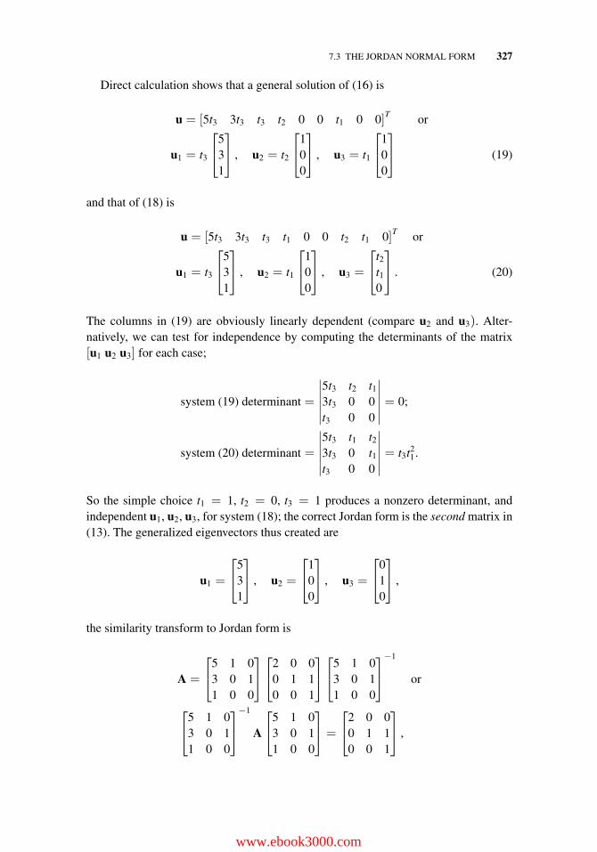
7.3 THE JORDAN NORMAL FORM 327
Direct calculation shows that a general solution of (16) is
u = [5t3 3t3 t3 t2 0 0 t1 0 0]T or
u1 = t3
⎡⎣5
31
⎤⎦ , u2 = t2
⎡⎣1
00
⎤⎦ , u3 = t1
⎡⎣1
00
⎤⎦ (19)
and that of (18) is
u = [5t3 3t3 t3 t1 0 0 t2 t1 0]T or
u1 = t3
⎡⎣5
31
⎤⎦ , u2 = t1
⎡⎣1
00
⎤⎦ , u3 =
⎡⎣t2
t10
⎤⎦ . (20)
The columns in (19) are obviously linearly dependent (compare u2 and u3). Alter-natively, we can test for independence by computing the determinants of the matrix[u1 u2 u3] for each case;
system (19) determinant =
∣∣∣∣∣∣5t3 t2 t13t3 0 0t3 0 0
∣∣∣∣∣∣ = 0;
system (20) determinant =
∣∣∣∣∣∣5t3 t1 t23t3 0 t1t3 0 0
∣∣∣∣∣∣ = t3t21.
So the simple choice t1 = 1, t2 = 0, t3 = 1 produces a nonzero determinant, andindependent u1, u2, u3, for system (18); the correct Jordan form is the second matrix in(13). The generalized eigenvectors thus created are
u1 =
⎡⎣5
31
⎤⎦ , u2 =
⎡⎣1
00
⎤⎦ , u3 =
⎡⎣0
10
⎤⎦ ,
the similarity transform to Jordan form is
A =
⎡⎣5 1 0
3 0 11 0 0
⎤⎦⎡⎣2 0 0
0 1 10 0 1
⎤⎦⎡⎣5 1 0
3 0 11 0 0
⎤⎦−1
or
⎡⎣5 1 0
3 0 11 0 0
⎤⎦−1
A
⎡⎣5 1 0
3 0 11 0 0
⎤⎦ =
⎡⎣2 0 0
0 1 10 0 1
⎤⎦ ,
www.ebook3000.com
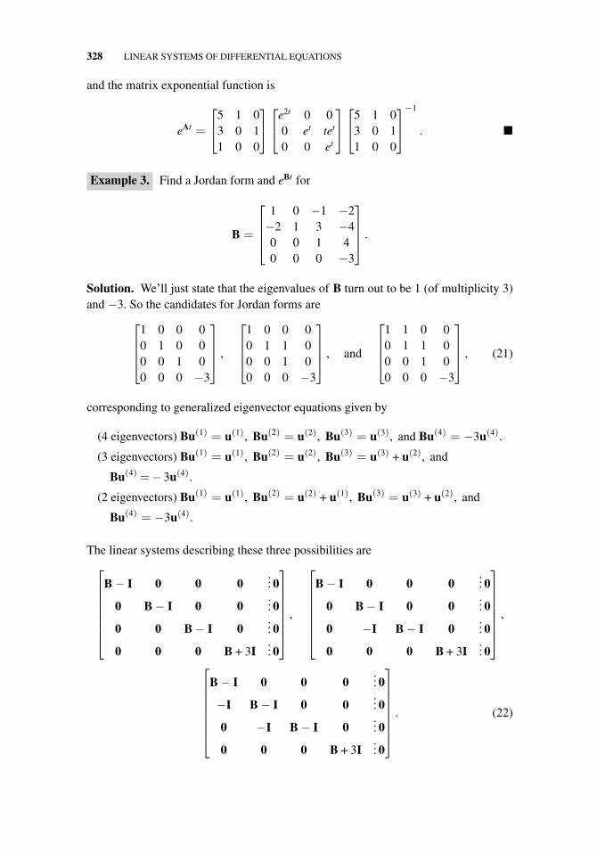
328 LINEAR SYSTEMS OF DIFFERENTIAL EQUATIONS
and the matrix exponential function is
eAt =
⎡⎣5 1 0
3 0 11 0 0
⎤⎦⎡⎣e2t 0 0
0 et tet
0 0 et
⎤⎦⎡⎣5 1 0
3 0 11 0 0
⎤⎦−1
. �
Example 3. Find a Jordan form and eBt for
B =
⎡⎢⎢⎣
1 0 −1 −2−2 1 3 −40 0 1 40 0 0 −3
⎤⎥⎥⎦ .
Solution. We’ll just state that the eigenvalues of B turn out to be 1 (of multiplicity 3)and −3. So the candidates for Jordan forms are
⎡⎢⎢⎣
1 0 0 00 1 0 00 0 1 00 0 0 −3
⎤⎥⎥⎦ ,
⎡⎢⎢⎣
1 0 0 00 1 1 00 0 1 00 0 0 −3
⎤⎥⎥⎦ , and
⎡⎢⎢⎣
1 1 0 00 1 1 00 0 1 00 0 0 −3
⎤⎥⎥⎦ , (21)
corresponding to generalized eigenvector equations given by
(4 eigenvectors) Bu(1) = u(1), Bu(2) = u(2), Bu(3) = u(3), and Bu(4) = −3u(4).
(3 eigenvectors) Bu(1) = u(1), Bu(2) = u(2), Bu(3) = u(3) + u(2), and
Bu(4)=− 3u(4).
(2 eigenvectors) Bu(1) = u(1), Bu(2) = u(2) + u(1), Bu(3) = u(3) + u(2), and
Bu(4) = −3u(4).
The linear systems describing these three possibilities are⎡⎢⎢⎢⎢⎢⎢⎣
B − I 0 0 0... 0
0 B − I 0 0... 0
0 0 B − I 0... 0
0 0 0 B + 3I... 0
⎤⎥⎥⎥⎥⎥⎥⎦
,
⎡⎢⎢⎢⎢⎢⎢⎣
B − I 0 0 0... 0
0 B − I 0 0... 0
0 −I B − I 0... 0
0 0 0 B + 3I... 0
⎤⎥⎥⎥⎥⎥⎥⎦
,
⎡⎢⎢⎢⎢⎢⎢⎣
B − I 0 0 0... 0
−I B − I 0 0... 0
0 −I B − I 0... 0
0 0 0 B + 3I... 0
⎤⎥⎥⎥⎥⎥⎥⎦
. (22)
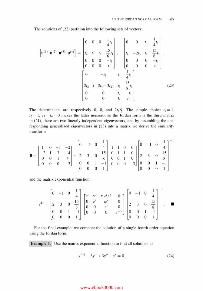
7.3 THE JORDAN NORMAL FORM 329
The solutions of (22) partition into the following sets of vectors:
[u(1) u(2) u(3) u(4)
]=
⎡⎢⎢⎢⎢⎢⎢⎣
0 0 014
t1
t4 t3 t2156
t1
0 0 0 −t10 0 0 t1
⎤⎥⎥⎥⎥⎥⎥⎦
,
⎡⎢⎢⎢⎢⎢⎢⎣
0 0 t314
t1
t4 −2t3 t2156
t1
0 0 0 −t10 0 0 t1
⎤⎥⎥⎥⎥⎥⎥⎦
,
⎡⎢⎢⎢⎢⎢⎢⎣
0 −t2 t414
t1
2t2 (−2t4 + 3t2) t3158
t1
0 0 t2 −t10 0 0 t1
⎤⎥⎥⎥⎥⎥⎥⎦
(23)
The determinants are respectively 0, 0, and 2t1t32. The simple choice t1 = 1,
t2 = 1, t3 = t4 = 0 makes the latter nonzero; so the Jordan form is the third matrixin (21), there are two linearly independent eigenvectors, and by assembling the cor-responding generalized eigenvectors in (23) into a matrix we derive the similaritytransform
B=
⎡⎢⎢⎣
1 0 −1 −2−2 1 3 −40 0 1 40 0 0 −3
⎤⎥⎥⎦=
⎡⎢⎢⎢⎢⎢⎢⎣
0 −1 014
2 3 0158
0 0 1 −10 0 0 1
⎤⎥⎥⎥⎥⎥⎥⎦
⎡⎢⎢⎣
1 1 0 00 1 1 00 0 1 00 0 0 −3
⎤⎥⎥⎦
⎡⎢⎢⎢⎢⎢⎢⎣
0 −1 014
2 3 0158
0 0 1 −10 0 0 1
⎤⎥⎥⎥⎥⎥⎥⎦
−1
and the matrix exponential function
eBt =
⎡⎢⎢⎢⎢⎢⎢⎣
0 −1 014
2 3 0158
0 0 1 −10 0 0 1
⎤⎥⎥⎥⎥⎥⎥⎦
⎡⎢⎢⎣
et tet t2 et/2 00 et tet 00 0 et 00 0 0 e−3t
⎤⎥⎥⎦
⎡⎢⎢⎢⎢⎢⎢⎣
0 −1 014
2 3 0158
0 0 1 −10 0 0 1
⎤⎥⎥⎥⎥⎥⎥⎦
−1
. �
For the final example, we compute the solution of a single fourth-order equationusing the Jordan form.
Example 4. Use the matrix exponential function to find all solutions to
y(iv) − 3y′′′ + 3y′′ − y′ = 0. (24)
www.ebook3000.com
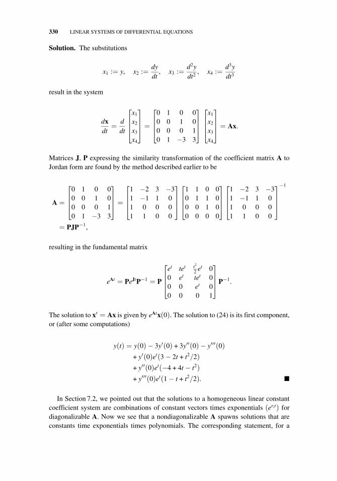
330 LINEAR SYSTEMS OF DIFFERENTIAL EQUATIONS
Solution. The substitutions
x1 := y, x2 :=dydt
, x3 :=d2ydt2
, x4 :=d3ydt3
result in the system
dxdt
=ddt
⎡⎢⎢⎣
x1
x2
x3
x4
⎤⎥⎥⎦ =
⎡⎢⎢⎣
0 1 0 00 0 1 00 0 0 10 1 −3 3
⎤⎥⎥⎦
⎡⎢⎢⎣
x1
x2
x3
x4
⎤⎥⎥⎦ = Ax.
Matrices J, P expressing the similarity transformation of the coefficient matrix A toJordan form are found by the method described earlier to be
A =
⎡⎢⎢⎣
0 1 0 00 0 1 00 0 0 10 1 −3 3
⎤⎥⎥⎦ =
⎡⎢⎢⎣
1 −2 3 −31 −1 1 01 0 0 01 1 0 0
⎤⎥⎥⎦
⎡⎢⎢⎣
1 1 0 00 1 1 00 0 1 00 0 0 0
⎤⎥⎥⎦
⎡⎢⎢⎣
1 −2 3 −31 −1 1 01 0 0 01 1 0 0
⎤⎥⎥⎦−1
= PJP−1,
resulting in the fundamental matrix
eAt = PeJtP−1 = P
⎡⎢⎢⎣
et tet t2
2 et 00 et tet 00 0 et 00 0 0 1
⎤⎥⎥⎦P−1.
The solution to x′ = Ax is given by eAtx(0). The solution to (24) is its first component,or (after some computations)
y(t) = y(0)− 3y′(0) + 3y′′(0)− y′′′(0)
+ y′(0)et(3 − 2t + t2/2)
+ y′′(0)et(−4 + 4t − t2)
+ y′′′(0)et(1 − t + t2/2). �
In Section 7.2, we pointed out that the solutions to a homogeneous linear constantcoefficient system are combinations of constant vectors times exponentials (erit) fordiagonalizable A. Now we see that a nondiagonalizable A spawns solutions that areconstants time exponentials times polynomials. The corresponding statement, for a
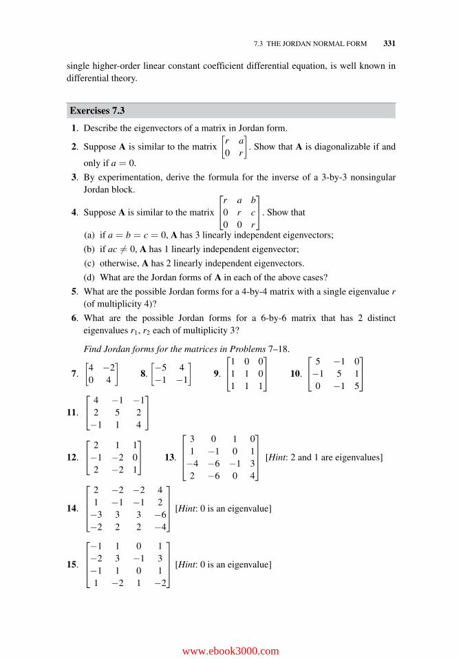
7.3 THE JORDAN NORMAL FORM 331
single higher-order linear constant coefficient differential equation, is well known indifferential theory.
Exercises 7.3
1. Describe the eigenvectors of a matrix in Jordan form.
2. Suppose A is similar to the matrix
[r a0 r
]. Show that A is diagonalizable if and
only if a = 0.
3. By experimentation, derive the formula for the inverse of a 3-by-3 nonsingularJordan block.
4. Suppose A is similar to the matrix
⎡⎣r a b
0 r c0 0 r
⎤⎦. Show that
(a) if a = b = c = 0, A has 3 linearly independent eigenvectors;
(b) if ac �= 0, A has 1 linearly independent eigenvector;
(c) otherwise, A has 2 linearly independent eigenvectors.
(d) What are the Jordan forms of A in each of the above cases?
5. What are the possible Jordan forms for a 4-by-4 matrix with a single eigenvalue r(of multiplicity 4)?
6. What are the possible Jordan forms for a 6-by-6 matrix that has 2 distincteigenvalues r1, r2 each of multiplicity 3?
Find Jordan forms for the matrices in Problems 7–18.
7.
[4 −20 4
]8.
[−5 4−1 −1
]9.
⎡⎣1 0 0
1 1 01 1 1
⎤⎦ 10.
⎡⎣ 5 −1 0−1 5 10 −1 5
⎤⎦
11.
⎡⎣ 4 −1 −1
2 5 2−1 1 4
⎤⎦
12.
⎡⎣ 2 1 1−1 −2 02 −2 1
⎤⎦ 13.
⎡⎢⎢⎣
3 0 1 01 −1 0 1−4 −6 −1 32 −6 0 4
⎤⎥⎥⎦ [Hint: 2 and 1 are eigenvalues]
14.
⎡⎢⎢⎣
2 −2 −2 41 −1 −1 2−3 3 3 −6−2 2 2 −4
⎤⎥⎥⎦ [Hint: 0 is an eigenvalue]
15.
⎡⎢⎢⎣−1 1 0 1−2 3 −1 3−1 1 0 11 −2 1 −2
⎤⎥⎥⎦ [Hint: 0 is an eigenvalue]
www.ebook3000.com
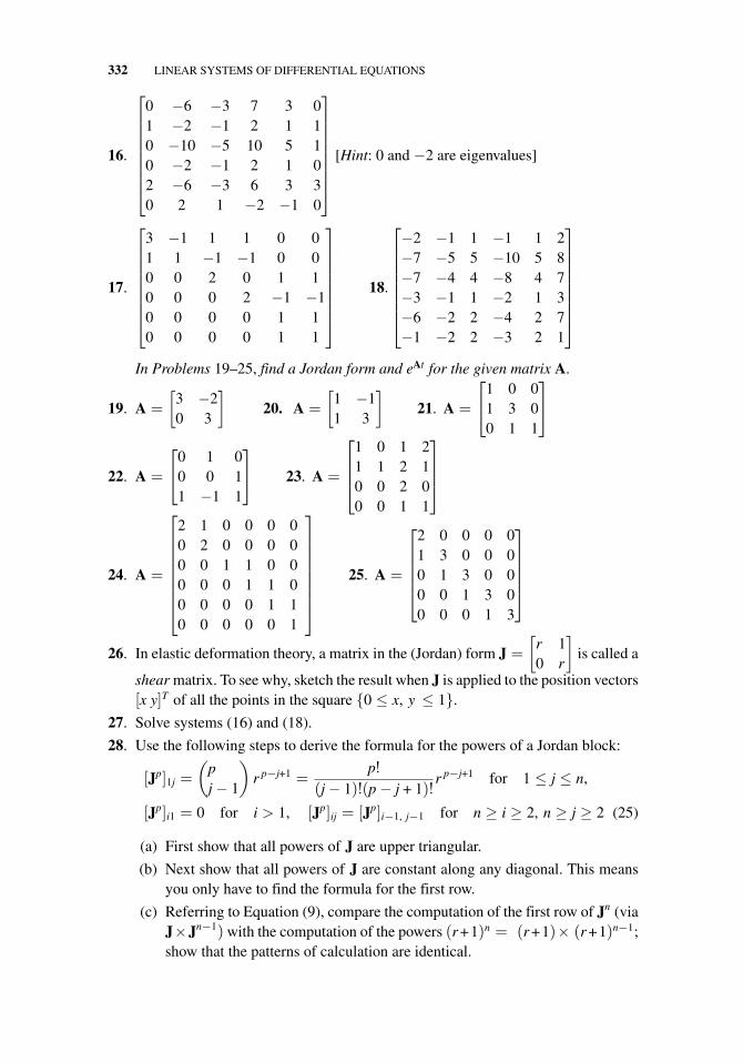
332 LINEAR SYSTEMS OF DIFFERENTIAL EQUATIONS
16.
⎡⎢⎢⎢⎢⎢⎢⎢⎣
0 −6 −3 7 3 01 −2 −1 2 1 10 −10 −5 10 5 10 −2 −1 2 1 02 −6 −3 6 3 30 2 1 −2 −1 0
⎤⎥⎥⎥⎥⎥⎥⎥⎦
[Hint: 0 and −2 are eigenvalues]
17.
⎡⎢⎢⎢⎢⎢⎢⎢⎣
3 −1 1 1 0 01 1 −1 −1 0 00 0 2 0 1 10 0 0 2 −1 −10 0 0 0 1 10 0 0 0 1 1
⎤⎥⎥⎥⎥⎥⎥⎥⎦
18.
⎡⎢⎢⎢⎢⎢⎢⎢⎣
−2 −1 1 −1 1 2−7 −5 5 −10 5 8−7 −4 4 −8 4 7−3 −1 1 −2 1 3−6 −2 2 −4 2 7−1 −2 2 −3 2 1
⎤⎥⎥⎥⎥⎥⎥⎥⎦
In Problems 19–25, find a Jordan form and eAt for the given matrix A.
19. A =
[3 −20 3
]20. A =
[1 −11 3
]21. A =
⎡⎣1 0 0
1 3 00 1 1
⎤⎦
22. A =
⎡⎣0 1 0
0 0 11 −1 1
⎤⎦ 23. A =
⎡⎢⎢⎣
1 0 1 21 1 2 10 0 2 00 0 1 1
⎤⎥⎥⎦
24. A =
⎡⎢⎢⎢⎢⎢⎢⎢⎣
2 1 0 0 0 00 2 0 0 0 00 0 1 1 0 00 0 0 1 1 00 0 0 0 1 10 0 0 0 0 1
⎤⎥⎥⎥⎥⎥⎥⎥⎦
25. A =
⎡⎢⎢⎢⎢⎣
2 0 0 0 01 3 0 0 00 1 3 0 00 0 1 3 00 0 0 1 3
⎤⎥⎥⎥⎥⎦
26. In elastic deformation theory, a matrix in the (Jordan) form J =
[r 10 r
]is called a
shear matrix. To see why, sketch the result when J is applied to the position vectors[x y]T of all the points in the square {0 ≤ x, y ≤ 1}.
27. Solve systems (16) and (18).
28. Use the following steps to derive the formula for the powers of a Jordan block:
[Jp]1j =
(pj − 1
)r p−j+1 =
p!(j − 1)!(p − j + 1)!
r p−j+1 for 1 ≤ j ≤ n,
[Jp]i1 = 0 for i > 1, [Jp]ij = [Jp]i−1, j−1 for n ≥ i ≥ 2, n ≥ j ≥ 2 (25)
(a) First show that all powers of J are upper triangular.
(b) Next show that all powers of J are constant along any diagonal. This meansyou only have to find the formula for the first row.
(c) Referring to Equation (9), compare the computation of the first row of Jn (viaJ×Jn−1) with the computation of the powers (r +1)n = (r +1)× (r +1)n−1;show that the patterns of calculation are identical.
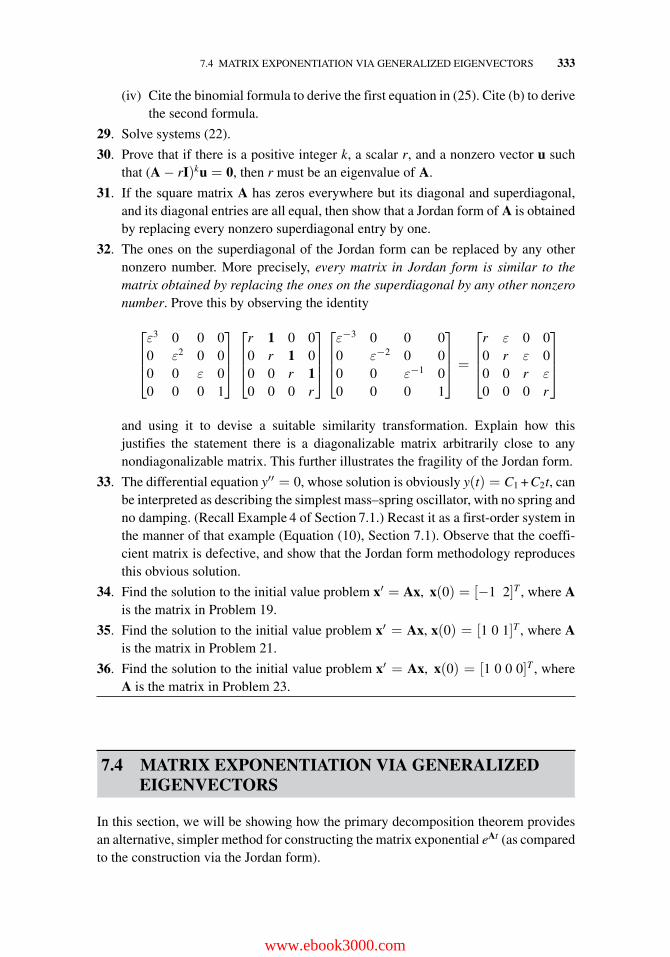
7.4 MATRIX EXPONENTIATION VIA GENERALIZED EIGENVECTORS 333
(iv) Cite the binomial formula to derive the first equation in (25). Cite (b) to derivethe second formula.
29. Solve systems (22).
30. Prove that if there is a positive integer k, a scalar r, and a nonzero vector u suchthat (A − rI)ku = 0, then r must be an eigenvalue of A.
31. If the square matrix A has zeros everywhere but its diagonal and superdiagonal,and its diagonal entries are all equal, then show that a Jordan form of A is obtainedby replacing every nonzero superdiagonal entry by one.
32. The ones on the superdiagonal of the Jordan form can be replaced by any othernonzero number. More precisely, every matrix in Jordan form is similar to thematrix obtained by replacing the ones on the superdiagonal by any other nonzeronumber. Prove this by observing the identity
⎡⎢⎢⎣ε3 0 0 00 ε2 0 00 0 ε 00 0 0 1
⎤⎥⎥⎦
⎡⎢⎢⎣
r 1 0 00 r 1 00 0 r 10 0 0 r
⎤⎥⎥⎦
⎡⎢⎢⎣ε−3 0 0 00 ε−2 0 00 0 ε−1 00 0 0 1
⎤⎥⎥⎦ =
⎡⎢⎢⎣
r ε 0 00 r ε 00 0 r ε
0 0 0 r
⎤⎥⎥⎦
and using it to devise a suitable similarity transformation. Explain how thisjustifies the statement there is a diagonalizable matrix arbitrarily close to anynondiagonalizable matrix. This further illustrates the fragility of the Jordan form.
33. The differential equation y′′ = 0, whose solution is obviously y(t) = C1 + C2t, canbe interpreted as describing the simplest mass–spring oscillator, with no spring andno damping. (Recall Example 4 of Section 7.1.) Recast it as a first-order system inthe manner of that example (Equation (10), Section 7.1). Observe that the coeffi-cient matrix is defective, and show that the Jordan form methodology reproducesthis obvious solution.
34. Find the solution to the initial value problem x′ = Ax, x(0) = [−1 2]T , where Ais the matrix in Problem 19.
35. Find the solution to the initial value problem x′ = Ax, x(0) = [1 0 1]T , where Ais the matrix in Problem 21.
36. Find the solution to the initial value problem x′ = Ax, x(0) = [1 0 0 0]T , whereA is the matrix in Problem 23.
7.4 MATRIX EXPONENTIATION VIA GENERALIZEDEIGENVECTORS
In this section, we will be showing how the primary decomposition theorem providesan alternative, simpler method for constructing the matrix exponential eAt (as comparedto the construction via the Jordan form).
www.ebook3000.com
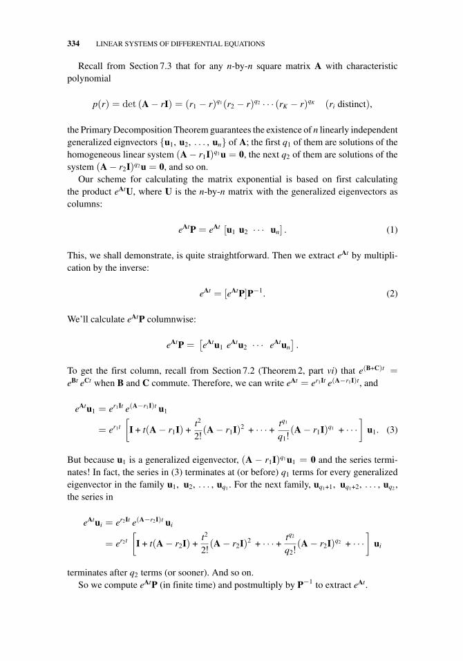
334 LINEAR SYSTEMS OF DIFFERENTIAL EQUATIONS
Recall from Section 7.3 that for any n-by-n square matrix A with characteristicpolynomial
p(r) = det (A − rI) = (r1 − r)q1(r2 − r)q2 · · · (rK − r)qK (ri distinct),
the Primary Decomposition Theorem guarantees the existence of n linearly independentgeneralized eignvectors {u1, u2, . . . , un} of A; the first q1 of them are solutions of thehomogeneous linear system (A − r1I)q1 u = 0, the next q2 of them are solutions of thesystem (A − r2I)q2 u = 0, and so on.
Our scheme for calculating the matrix exponential is based on first calculatingthe product eAtU, where U is the n-by-n matrix with the generalized eigenvectors ascolumns:
eAtP = eAt [u1 u2 · · · un] . (1)
This, we shall demonstrate, is quite straightforward. Then we extract eAt by multipli-cation by the inverse:
eAt = [eAtP]P−1. (2)
We’ll calculate eAtP columnwise:
eAtP =[eAtu1 eAtu2 · · · eAtun
].
To get the first column, recall from Section 7.2 (Theorem 2, part vi) that e(B+C)t =eBt eCt when B and C commute. Therefore, we can write eAt = er1It e(A−r1I)t, and
eAtu1 = er1It e(A−r1I)t u1
= er1t
[I + t(A − r1I) +
t2
2!(A − r1I)2 + · · · +
tq1
q1!(A − r1I)q1 + · · ·
]u1. (3)
But because u1 is a generalized eigenvector, (A − r1I)q1 u1 = 0 and the series termi-nates! In fact, the series in (3) terminates at (or before) q1 terms for every generalizedeigenvector in the family u1, u2, . . . , uq1 . For the next family, uq1+1, uq1+2, . . . , uq2 ,the series in
eAtui = er2It e(A−r2I)t ui
= er2t
[I + t(A − r2I) +
t2
2!(A − r2I)2 + · · · +
tq2
q2!(A − r2I)q2 + · · ·
]ui
terminates after q2 terms (or sooner). And so on.So we compute eAtP (in finite time) and postmultiply by P−1 to extract eAt.
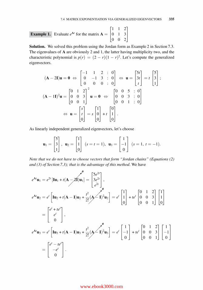
7.4 MATRIX EXPONENTIATION VIA GENERALIZED EIGENVECTORS 335
Example 1. Evaluate eAt for the matrix A =
⎡⎣1 1 2
0 1 30 0 2
⎤⎦
Solution. We solved this problem using the Jordan form as Example 2 in Section 7.3.The eigenvalues of A are obviously 2 and 1, the latter having multiplicity two, and thecharacteristic polynomial is p(r) = (2 − r)(1 − r)2. Let’s compute the generalizedeigenvectors.
(A − 2I)u = 0 ⇔
⎡⎣−1 1 2 : 0
0 −1 3 : 00 0 0 : 0
⎤⎦ ⇔ u =
⎡⎣5t
3tt
⎤⎦ = t
⎡⎣5
31
⎤⎦ ;
(A − 1I)2u =
⎡⎣0 1 2
0 0 30 0 1
⎤⎦
2
u = 0 ⇔
⎡⎣0 0 5 : 0
0 0 3 : 00 0 1 : 0
⎤⎦
⇔ u =
⎡⎣s
t0
⎤⎦ = s
⎡⎣1
00
⎤⎦ + t
⎡⎣0
10
⎤⎦ .
As linearly independent generalized eigenvectors, let’s choose
u1 =
⎡⎣5
31
⎤⎦ , u2 =
⎡⎣1
10
⎤⎦ (s = t = 1), u3 =
⎡⎣ 1−10
⎤⎦ (s = 1, t = −1).
Note that we do not have to choose vectors that form “Jordan chains” (Equations (2)and (3) of Section 7.3); that is the advantage of this method. We have
eAtu1 = e2t [Iu1 + t(A −���� ��
0
2I)u1] =
⎡⎣5e2t
3e2t
e2t
⎤⎦ ,
eAtu2 = et
[Iu2 + t(A − I)u2 +
t2
2!(A���� ��
0
− I)2u2
]= et
⎡⎣1
10
⎤⎦ + tet
⎡⎣0 1 2
0 0 30 0 1
⎤⎦⎡⎣1
10
⎤⎦
=
⎡⎣et + tet
et
0
⎤⎦ ,
eAtu3 = et
[Iu3 + t(A − I)u3 +
t2
2!(A���� ��
0
− I)2u3
]= et
⎡⎣ 1−10
⎤⎦ + tet
⎡⎣0 1 2
0 0 30 0 1
⎤⎦⎡⎣ 1−10
⎤⎦
=
⎡⎣et − tet
−et
0
⎤⎦ .
www.ebook3000.com
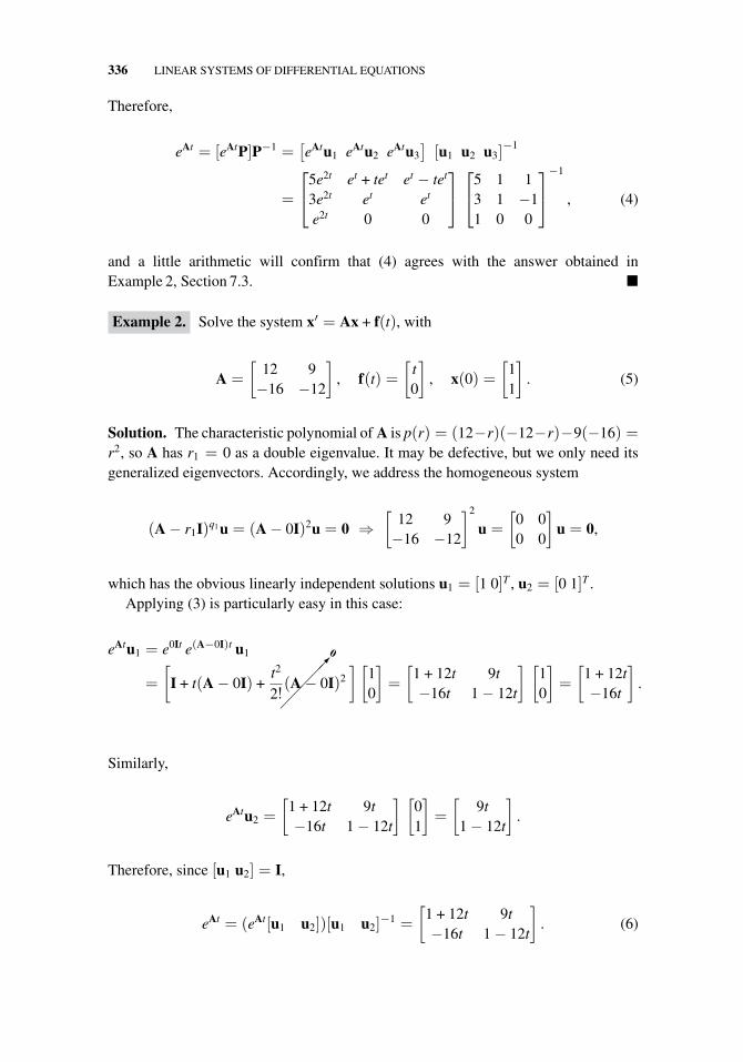
336 LINEAR SYSTEMS OF DIFFERENTIAL EQUATIONS
Therefore,
eAt = [eAtP]P−1 =[eAtu1 eAtu2 eAtu3
][u1 u2 u3]
−1
=
⎡⎣5e2t et + tet et − tet
3e2t et et
e2t 0 0
⎤⎦⎡⎣5 1 1
3 1 −11 0 0
⎤⎦−1
, (4)
and a little arithmetic will confirm that (4) agrees with the answer obtained inExample 2, Section 7.3. �
Example 2. Solve the system x′ = Ax + f(t), with
A =
[12 9−16 −12
], f(t) =
[t0
], x(0) =
[11
]. (5)
Solution. The characteristic polynomial of A is p(r) = (12−r)(−12−r)−9(−16) =r2, so A has r1 = 0 as a double eigenvalue. It may be defective, but we only need itsgeneralized eigenvectors. Accordingly, we address the homogeneous system
(A − r1I)q1 u = (A − 0I)2u = 0 ⇒[
12 9−16 −12
]2
u =
[0 00 0
]u = 0,
which has the obvious linearly independent solutions u1 = [1 0]T , u2 = [0 1]T .Applying (3) is particularly easy in this case:
eAtu1 = e0It e(A−0I)t u1
=
[I + t(A − 0I) +
t2
2!(A���� ��
0
− 0I)2
] [10
]=
[1 + 12t 9t−16t 1 − 12t
] [10
]=
[1 + 12t−16t
].
Similarly,
eAtu2 =
[1 + 12t 9t−16t 1 − 12t
] [01
]=
[9t
1 − 12t
].
Therefore, since [u1 u2] = I,
eAt = (eAt[u1 u2])[u1 u2]−1 =
[1 + 12t 9t−16t 1 − 12t
]. (6)
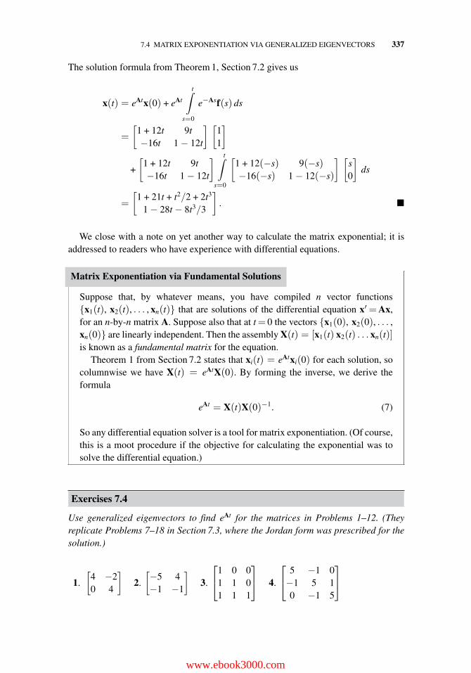
7.4 MATRIX EXPONENTIATION VIA GENERALIZED EIGENVECTORS 337
The solution formula from Theorem 1, Section 7.2 gives us
x(t) = eAtx(0) + eAt
t∫s=0
e−Asf(s) ds
=
[1 + 12t 9t−16t 1 − 12t
] [11
]
+
[1 + 12t 9t−16t 1 − 12t
] t∫s=0
[1 + 12(−s) 9(−s)−16(−s) 1 − 12(−s)
] [s0
]ds
=
[1 + 21t + t2/2 + 2t3
1 − 28t − 8t3/3
]. �
We close with a note on yet another way to calculate the matrix exponential; it isaddressed to readers who have experience with differential equations.
Matrix Exponentiation via Fundamental Solutions
Suppose that, by whatever means, you have compiled n vector functions{x1(t), x2(t), . . . , xn(t)} that are solutions of the differential equation x′=Ax,for an n-by-n matrix A. Suppose also that at t= 0 the vectors {x1(0), x2(0), . . . ,xn(0)} are linearly independent. Then the assembly X(t) = [x1(t) x2(t) . . . xn(t)]is known as a fundamental matrix for the equation.
Theorem 1 from Section 7.2 states that xi(t) = eAtxi(0) for each solution, socolumnwise we have X(t) = eAtX(0). By forming the inverse, we derive theformula
eAt = X(t)X(0)−1. (7)
So any differential equation solver is a tool for matrix exponentiation. (Of course,this is a moot procedure if the objective for calculating the exponential was tosolve the differential equation.)
Exercises 7.4
Use generalized eigenvectors to find eAt for the matrices in Problems 1–12. (Theyreplicate Problems 7–18 in Section 7.3, where the Jordan form was prescribed for thesolution.)
1.
[4 −20 4
]2.
[−5 4−1 −1
]3.
⎡⎣1 0 0
1 1 01 1 1
⎤⎦ 4.
⎡⎣ 5 −1 0−1 5 10 −1 5
⎤⎦
www.ebook3000.com
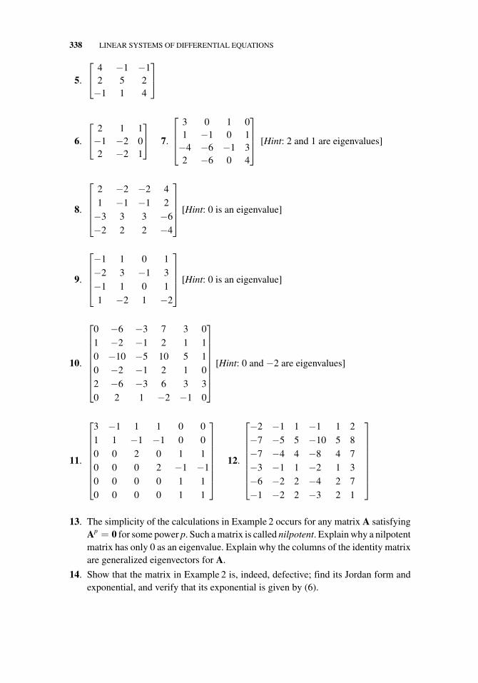
338 LINEAR SYSTEMS OF DIFFERENTIAL EQUATIONS
5.
⎡⎣ 4 −1 −1
2 5 2−1 1 4
⎤⎦
6.
⎡⎣ 2 1 1−1 −2 02 −2 1
⎤⎦ 7.
⎡⎢⎢⎣
3 0 1 01 −1 0 1−4 −6 −1 32 −6 0 4
⎤⎥⎥⎦ [Hint: 2 and 1 are eigenvalues]
8.
⎡⎢⎢⎢⎣
2 −2 −2 41 −1 −1 2−3 3 3 −6−2 2 2 −4
⎤⎥⎥⎥⎦ [Hint: 0 is an eigenvalue]
9.
⎡⎢⎢⎢⎣−1 1 0 1−2 3 −1 3−1 1 0 11 −2 1 −2
⎤⎥⎥⎥⎦ [Hint: 0 is an eigenvalue]
10.
⎡⎢⎢⎢⎢⎢⎢⎢⎣
0 −6 −3 7 3 01 −2 −1 2 1 10 −10 −5 10 5 10 −2 −1 2 1 02 −6 −3 6 3 30 2 1 −2 −1 0
⎤⎥⎥⎥⎥⎥⎥⎥⎦
[Hint: 0 and −2 are eigenvalues]
11.
⎡⎢⎢⎢⎢⎢⎢⎢⎣
3 −1 1 1 0 01 1 −1 −1 0 00 0 2 0 1 10 0 0 2 −1 −10 0 0 0 1 10 0 0 0 1 1
⎤⎥⎥⎥⎥⎥⎥⎥⎦
12.
⎡⎢⎢⎢⎢⎢⎢⎢⎣
−2 −1 1 −1 1 2−7 −5 5 −10 5 8−7 −4 4 −8 4 7−3 −1 1 −2 1 3−6 −2 2 −4 2 7−1 −2 2 −3 2 1
⎤⎥⎥⎥⎥⎥⎥⎥⎦
13. The simplicity of the calculations in Example 2 occurs for any matrix A satisfyingAp = 0 for some power p. Such a matrix is called nilpotent. Explain why a nilpotentmatrix has only 0 as an eigenvalue. Explain why the columns of the identity matrixare generalized eigenvectors for A.
14. Show that the matrix in Example 2 is, indeed, defective; find its Jordan form andexponential, and verify that its exponential is given by (6).
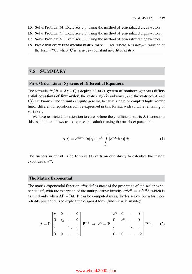
7.5 SUMMARY 339
15. Solve Problem 34, Exercises 7.3, using the method of generalized eigenvectors.
16. Solve Problem 35, Exercises 7.3, using the method of generalized eigenvectors.
17. Solve Problem 36, Exercises 7.3, using the method of generalized eigenvectors.
18. Prove that every fundamental matrix for x′ = Ax, where A is n-by-n, must be ofthe form eAtC, where C is an n-by-n constant invertible matrix.
7.5 SUMMARY
First-Order Linear Systems of Differential Equations
The formula dx/dt = Ax + f(t) depicts a linear system of nonhomogeneous differ-ential equations of first order; the matrix x(t) is unknown, and the matrices A andf(t) are known. The formula is quite general, because single or coupled higher-orderlinear differential equations can be expressed in this format with suitable renaming ofvariables.
We have restricted our attention to cases where the coefficient matrix A is constant;this assumption allows us to express the solution using the matrix exponential:
x(t) = eA(t−t1)x(t1) + eAt
t∫t1
[e−Asf(s)] ds (1)
The success in our utilizing formula (1) rests on our ability to calculate the matrixexponential eAt.
The Matrix Exponential
The matrix exponential function eAtsatisfies most of the properties of the scalar expo-nential eat, with the exception of the multiplicative identity eAteBt = e(A+B)t, which isassured only when AB = BA. It can be computed using Taylor series, but a far morereliable procedure is to exploit the diagonal form (when it is available):
A = P
⎡⎢⎢⎢⎢⎣
r1 0 · · · 0
0 r2 · · · 0...
. . ....
0 0 · · · rp
⎤⎥⎥⎥⎥⎦P−1 ⇒ eA = P
⎡⎢⎢⎢⎢⎣
er1 0 · · · 0
0 er2 · · · 0...
. . ....
0 0 · · · erp
⎤⎥⎥⎥⎥⎦P−1. (2)
www.ebook3000.com
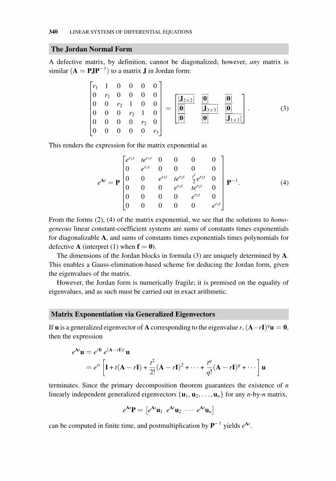
340 LINEAR SYSTEMS OF DIFFERENTIAL EQUATIONS
The Jordan Normal Form
A defective matrix, by definition, cannot be diagonalized; however, any matrix issimilar (A = PJP−1) to a matrix J in Jordan form:
⎡⎢⎢⎢⎢⎢⎢⎢⎣
r1 1 0 0 0 00 r1 0 0 0 00 0 r2 1 0 00 0 0 r2 1 00 0 0 0 r2 00 0 0 0 0 r3
⎤⎥⎥⎥⎥⎥⎥⎥⎦=
⎡⎢⎣|J2×2| |0| |0||0| |J3×3| |0||0| |0| |J1×1|
⎤⎥⎦ . (3)
This renders the expression for the matrix exponential as
eAt = P
⎡⎢⎢⎢⎢⎢⎢⎢⎣
er1t ter1t 0 0 0 00 er1t 0 0 0 0
0 0 er2t ter2t t2
2 er2t 00 0 0 er2t ter2t 00 0 0 0 er2t 00 0 0 0 0 er3t
⎤⎥⎥⎥⎥⎥⎥⎥⎦
P−1. (4)
From the forms (2), (4) of the matrix exponential, we see that the solutions to homo-geneous linear constant-coefficient systems are sums of constants times exponentialsfor diagonalizable A, and sums of constants times exponentials times polynomials fordefective A (interpret (1) when f = 0).
The dimensions of the Jordan blocks in formula (3) are uniquely determined by A.This enables a Gauss-elimination-based scheme for deducing the Jordan form, giventhe eigenvalues of the matrix.
However, the Jordan form is numerically fragile; it is premised on the equality ofeigenvalues, and as such must be carried out in exact arithmetic.
Matrix Exponentiation via Generalized Eigenvectors
If u is a generalized eigenvector of A corresponding to the eigenvalue r, (A−rI)qu = 0,then the expression
eAtu = erIt e(A−rI)t u
= ert
[I + t(A − rI) +
t2
2!(A − rI)2 + · · · +
tq
q!(A − rI)q + · · ·
]u
terminates. Since the primary decomposition theorem guarantees the existence of nlinearly independent generalized eigenvectors {u1, u2, . . . , un} for any n-by-n matrix,
eAtP =[eAtu1 eAtu2 · · · eAtun
]
can be computed in finite time, and postmultiplication by P−1 yields eAt.
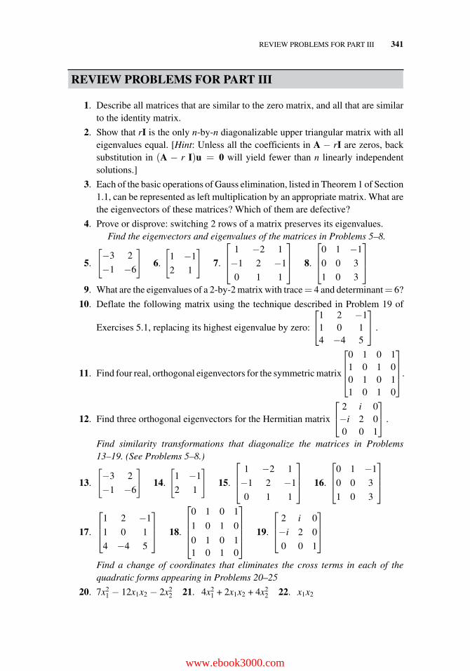
REVIEW PROBLEMS FOR PART III 341
REVIEW PROBLEMS FOR PART III
1. Describe all matrices that are similar to the zero matrix, and all that are similarto the identity matrix.
2. Show that rI is the only n-by-n diagonalizable upper triangular matrix with alleigenvalues equal. [Hint: Unless all the coefficients in A − rI are zeros, backsubstitution in (A − r I)u = 0 will yield fewer than n linearly independentsolutions.]
3. Each of the basic operations of Gauss elimination, listed in Theorem 1 of Section1.1, can be represented as left multiplication by an appropriate matrix. What arethe eigenvectors of these matrices? Which of them are defective?
4. Prove or disprove: switching 2 rows of a matrix preserves its eigenvalues.Find the eigenvectors and eigenvalues of the matrices in Problems 5–8.
5.
[−3 2
−1 −6
]6.
[1 −1
2 1
]7.
⎡⎢⎣
1 −2 1
−1 2 −1
0 1 1
⎤⎥⎦ 8.
⎡⎢⎣
0 1 −1
0 0 3
1 0 3
⎤⎥⎦
9. What are the eigenvalues of a 2-by-2 matrix with trace= 4 and determinant= 6?
10. Deflate the following matrix using the technique described in Problem 19 of
Exercises 5.1, replacing its highest eigenvalue by zero:
⎡⎣1 2 −1
1 0 14 −4 5
⎤⎦ .
11. Find four real, orthogonal eigenvectors for the symmetric matrix
⎡⎢⎢⎣
0 1 0 11 0 1 00 1 0 11 0 1 0
⎤⎥⎥⎦.
12. Find three orthogonal eigenvectors for the Hermitian matrix
⎡⎣ 2 i 0−i 2 00 0 1
⎤⎦ .
Find similarity transformations that diagonalize the matrices in Problems13–19. (See Problems 5–8.)
13.
[−3 2
−1 −6
]14.
[1 −1
2 1
]15.
⎡⎢⎣
1 −2 1
−1 2 −1
0 1 1
⎤⎥⎦ 16.
⎡⎢⎣
0 1 −1
0 0 3
1 0 3
⎤⎥⎦
17.
⎡⎢⎣
1 2 −1
1 0 1
4 −4 5
⎤⎥⎦ 18.
⎡⎢⎢⎢⎣
0 1 0 1
1 0 1 0
0 1 0 11 0 1 0
⎤⎥⎥⎥⎦ 19.
⎡⎢⎣
2 i 0
−i 2 0
0 0 1
⎤⎥⎦
Find a change of coordinates that eliminates the cross terms in each of thequadratic forms appearing in Problems 20–25
20. 7x21 − 12x1x2 − 2x2
2 21. 4x21 + 2x1x2 + 4x2
2 22. x1x2
www.ebook3000.com
342 LINEAR SYSTEMS OF DIFFERENTIAL EQUATIONS
23. 2x21 + 2x1x2 + 2x2
2 + 2x1x3 − 2x2x3 + 2x23
24. 2x21 + 2x2
2 − 2x1x3 − 2x2x3 + 3x23 25. x1x2 + x1x3 + x2x3
26. Express the Schur decomposition A = QUQH for the matrix
⎡⎣ 2 2 −1−6 −5 6−2 −1 3
⎤⎦.
27. For what value of a is the matrix
⎡⎣ 0 −1 2
a 0 2−2 −2 0
⎤⎦ normal? Find an orthogonal
basis of eigenvectors for the resulting matrix.
TECHNICAL WRITING EXERCISES FOR PART III
1. The matrix A =
[1 01 1
], as we saw in Example 5 of Section 5.2, has only
one independent eigenvector for its double eigenvalue r = 1. Graph pairs of
independent eigenvectors for the matrices
[1 01 0.9
],
[1 01 0.99
],
[1 01 0.999
]
approximating A. Do the same for the matrices
[1 00 0.9
],
[1 00 0.99
],
[1 00 0.999
]
approximating the identity matrix I =
[1 00 1
]. Write a short paper describing
how one of the eigenvectors “disappears” for the matrix A, but not for I.
2. Suppose that the “second” hand on a stopwatch represents the vector v, and thatanother hand points in the direction of Av, for some 2-by-2 matrix A. Writea paragraph describing the motions of these hands during the course of oneminute, describing in particular what happens as v approaches an eigenvector ofA. Consider the possibilities that A is singular, defective, symmetric, or antisym-metric. (The MATLAB® function “eigshow.m” demonstrates this for a variety ofmatrices A.)
GROUP PROJECTS FOR PART III
A. Positive Definite Matrices
A positive definite matrix is any real n-by-n symmetric matrix A with the propertythat
vTAv > 0, for every vector v in Rncol other than zero. (1)
If every such vTAv is nonnegative, A is said to be positive semidefinite; and A isnegative definite if−A is positive definite. The concept of positive definiteness extendsreadily to Hermitian matrices, via the criterion vHAv > 0.
GROUP PROJECTS FOR PART III 343
Which of the following properties are necessary and/or sufficient for A to be positivedefinite?
(a) The eigenvalues of A are positive. [Hint: Apply (1) to the equation Av = λv, andto the similarity transform equation A = QDQT in Corollary 3, Section 6.1.]
(b) The determinant of A is positive. [Hint: How is the determinant related to theeigenvalues?]
(c) All the entries of A are positive (nonnegative?). [Hint: Experiment.]
(d) All of the square submatrices centered on the diagonal of A are positivedefinite. [Hint: Apply (1) with vectors having appropriate zeros, like v =[0 0 x3 x4 x5 0 0].]
(e) A is a Gram matrix: that is, the (i, j)th entry of A is uTi uj, where {u1, u2, . . ., un}
is any basis for Rncol. (Hint: Convince yourself that A = PTP, where the columns
of P are the basis vectors; then apply (1). Why must the columns be linearlyindependent?)
(f) All of the square submatrices of A “anchored at the upper left corner” havepositive determinants. [Hint: This is known as Sylvester’s Criterion, and thedeterminants are called principal minors. You may find this problem difficult;get help from the Internet.]
(g) (Recall Project A, Part I) A admits an LU factorization where U = LT (thatis, A = LLT), with L real and nonsingular. [Hint: This is called the Choleskyfactorization. It roughly halves the computer time and memory to solve systemsAx = b. Use the Internet if necessary.]
The most common application of positive definiteness occurs in optimization prob-lems, when the “cost” function to be optimized can be expressed (or approximated) bya quadratic polynomial f (x) = xTAx + bTx + k. Use Lemma 1, Section 6.2, to showthat if A is positive definite, f (x) has a unique minimum point at x = −A−1b/2.
B. Hessenberg Form
As mentioned at the beginning of Section 6.3, although Gauss elimination reduces asquare matrix A to upper triangular form, the resulting matrix is not similar to A (sothe eigenvalues are altered in the process). Now recall (Section 2.1, Example 2) thateach operation in Gauss elimination is equivalent to left-multiplication by a matrix; soif we right-multiplied by the inverse of that matrix, we would complete a similaritytransformation (and preserve the eigenvalues).
(a) Show that if left multiplication of the matrix A by the matrix E eliminates the(2,1) entry of A (by adding an appropriate multiple of the first row to the second),right multiplication by E−1 adds a multiple of the second column to the first, andthus “undoes” the elimination.
www.ebook3000.com
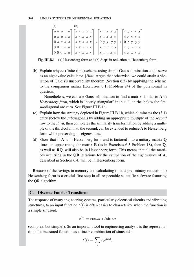
344 LINEAR SYSTEMS OF DIFFERENTIAL EQUATIONS
(a)
a a a a a
a a a a a
0
0 0
0 0 0
a a a a
a a a
a a
(b)
x z x x x
x z x x x
0 z y y y
x z x x x
x z x x x
x x x x x
x x x x x
0 y y y y
x x x x x
x x x x x
x x x x x
x x x x x
x x x x x
x x x x x
x x x x x
Fig. III.B.1 (a) Hessenberg form and (b) Steps in reduction to Hessenberg form.
(b) Explain why no (finite-time) scheme using simple Gauss elimination could serveas an eigenvalue calculator. [Hint: Argue that otherwise, we could attain a vio-lation of Galois’s unsolvability theorem (Section 6.5) by applying the schemeto the companion matrix (Exercises 6.1, Problem 24) of the polynomial inquestion.]
Nonetheless, we can use Gauss elimination to find a matrix similar to A inHessenberg form, which is “nearly triangular” in that all entries below the firstsubdiagonal are zero. See Figure III.B.1a.
(c) Explain how the strategy depicted in Figure III.B.1b, which eliminates the (3,1)entry (below the subdiagonal) by adding an appropriate multiple of the secondrow to the third, then completes the similarity transformation by adding a multi-ple of the third column to the second, can be extended to reduce A to Hessenbergform while preserving its eigenvalues.
(d) Show that if A is in Hessenberg form and is factored into a unitary matrix Qtimes an upper triangular matrix R (as in Exercises 6.5 Problem 18), then Q,as well as RQ, will also be in Hessenberg form. This means that all the matri-ces occurring in the QR iterations for the estimation of the eigenvalues of A,described in Section 6.4, will be in Hessenberg form.
Because of the savings in memory and calculating time, a preliminary reduction toHessenberg form is a crucial first step in all respectable scientific software featuringthe QR algorithm.
C. Discrete Fourier Transform
The response of many engineering systems, particularly electrical circuits and vibratingstructures, to an input function f (t) is often easier to characterize when the function isa simple sinusoid,
eiωt = cosωt + i sinωt
(complex, but simple!). So an important tool in engineering analysis is the representa-tion of a measured function as a linear combination of sinusoids:
f (t) =∑
n
cneiωnt.
GROUP PROJECTS FOR PART III 345
The evaluation of the coefficients cn is particularly convenient when the followingconditions are met:
• the function f (t) has been measured (“sampled”) at N discrete timest0, t1, . . ., tN−1;
• the sampling times are uniform, tj = jΔt : j = 0, 1, . . . , N − 1;
• the angular frequencies ωn are integer multiples (“harmonics”) of the fundamentalfrequency ωa := 2π/(NΔt), ωn = nωa, n = 0, 1, . . . , N − 1 .
In such a case, the set of coefficients cn is called the discrete Fourier transform of thedata f (tj).
(a) Formulate the conditions
f (tj) =∑
ncneiωntj
as a matrix equation for the unknown numbers cn.
(b) Identify the rows of the coefficient matrix for the system in (a) as rescaled (andtransposed) eigenvectors of the N-by-N circulant matrices described in Problem12 of Exercises 5.1.
(c) Use the geometric sum formula
m∑j=0
rj = (1 − rm+1)/(1 − r)
to prove that the rows of the coefficient matrix are orthogonal. What are theirnorms?
(d) Construct F, the Hermitian circulant matrix whose first row comprises thesampled values f (tj). Show that the eigenvalues of F are the elements cn
of the discrete Fourier transform of the data f (tj). Use this observation toconstruct another proof of the orthogonality of the rows of the coefficientmatrix.
(e) Using the orthogonality, construct the inverse of the coefficient matrix, andthereby formulate an explicit formula for the discrete Fourier transform of thesampled values f (tj).
Note that the resulting formula involves taking inner products of the sampled valuesof f (t) with sampled values of eiωnt. By taking advantage of the redundancies exhibitedin the following table, one can considerably accelerate the speed of the calculation; thisis the essence of the Fast Fourier Transform.
www.ebook3000.com
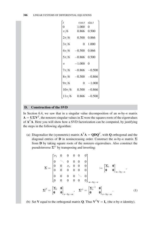
346 LINEAR SYSTEMS OF DIFFERENTIAL EQUATIONS
⎡⎢⎢⎢⎢⎢⎢⎢⎢⎢⎢⎢⎢⎢⎢⎢⎢⎢⎢⎢⎢⎢⎢⎢⎢⎢⎢⎢⎢⎢⎢⎢⎢⎢⎣
t cos t sin t0 1.000 0π/6 0.866 0.500
2π/6 0.500 0.866
3π/6 0 1.000
4π/6 −0.500 0.866
5π/6 −0.866 0.500
π −1.000 0
7π/6 −0.866 −0.500
8π/6 −0.500 −0.866
9π/6 0 −1.000
10π/6 0.500 −0.866
11π/6 0.866 −0.500
⎤⎥⎥⎥⎥⎥⎥⎥⎥⎥⎥⎥⎥⎥⎥⎥⎥⎥⎥⎥⎥⎥⎥⎥⎥⎥⎥⎥⎥⎥⎥⎥⎥⎥⎦
D. Construction of the SVD
In Section 6.4, we saw that in a singular value decomposition of an m-by-n matrixA = UΣVT , the nonzero singular values in Σ were the squares roots of the eigenvaluesof ATA. Here you will show how a SVD factorization can be computed, by justifyingthe steps in the following algorithm:
(a) Diagonalize the (symmetric) matrix ATA = QDQT , with Q orthogonal and thediagonal entries of D in nonincreasing order. Construct the m-by-n matrix Σ
from D by taking square roots of the nonzero eigenvalues. Also construct thepseudoinverse Σψ by transposing and inverting:
Σ =
⎡⎢⎢⎢⎢⎢⎢⎢⎢⎣
σ1 0 0 0 0 0
0. . . 0 0 0 0
0 0 σr 0 0 00 0 0 0 0 0
0 0 0 0. . . 0
0 0 0 0 0 0
⎤⎥⎥⎥⎥⎥⎥⎥⎥⎦
m−by−n
:=
[Σr 00 0
]m−by−n
,
ΣT =
[Σr 00 0
]n−by−m
, Σψ =
[Σ−1
r 00 0
]n−by−m
. (1)
(b) Set V equal to the orthogonal matrix Q. Thus VTV = In (the n-by-n identity).
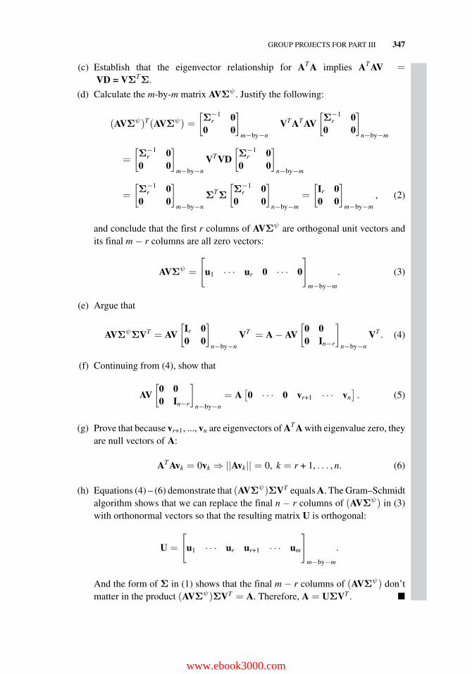
GROUP PROJECTS FOR PART III 347
(c) Establish that the eigenvector relationship for ATA implies ATAV =VD = VΣTΣ.
(d) Calculate the m-by-m matrix AVΣψ. Justify the following:
(AVΣψ)T(AVΣψ) =
[Σ−1
r 00 0
]m−by−n
VTATAV[Σ−1
r 00 0
]n−by−m
=
[Σ−1
r 00 0
]m−by−n
VTVD[Σ−1
r 00 0
]n−by−m
=
[Σ−1
r 00 0
]m−by−n
ΣTΣ
[Σ−1
r 00 0
]n−by−m
=
[Ir 00 0
]m−by−m
, (2)
and conclude that the first r columns of AVΣψ are orthogonal unit vectors andits final m − r columns are all zero vectors:
AVΣψ =
[u1 · · · ur 0 · · · 0
]
m−by−m
. (3)
(e) Argue that
AVΣψΣVT = AV[
Ir 00 0
]n−by−n
VT = A − AV[
0 00 In−r
]n−by−n
VT . (4)
(f) Continuing from (4), show that
AV[
0 00 In−r
]n−by−n
= A[0 · · · 0 vr+1 · · · vn
]. (5)
(g) Prove that because vr+1, ..., vn are eigenvectors of ATA with eigenvalue zero, theyare null vectors of A:
ATAvk = 0vk ⇒ ||Avk|| = 0, k = r + 1, . . . , n. (6)
(h) Equations (4) – (6) demonstrate that (AVΣψ)ΣVT equals A. The Gram–Schmidtalgorithm shows that we can replace the final n − r columns of (AVΣψ) in (3)with orthonormal vectors so that the resulting matrix U is orthogonal:
U =
[u1 · · · ur ur+1 · · · um
]
m−by−m
.
And the form of Σ in (1) shows that the final m − r columns of (AVΣψ) don’tmatter in the product (AVΣψ)ΣVT = A. Therefore, A = UΣVT . �
www.ebook3000.com
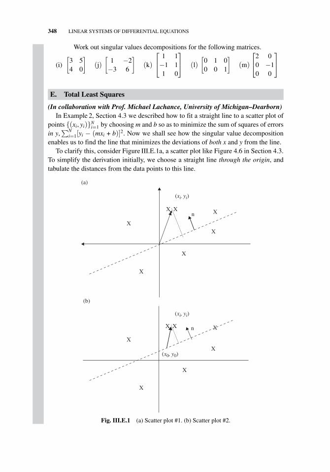
348 LINEAR SYSTEMS OF DIFFERENTIAL EQUATIONS
Work out singular values decompositions for the following matrices.
(i)
[3 54 0
](j)
[1 −2−3 6
](k)
⎡⎣ 1 1−1 11 0
⎤⎦ (l)
[0 1 00 0 1
](m)
⎡⎣2 0
0 −10 0
⎤⎦
E. Total Least Squares
(In collaboration with Prof. Michael Lachance, University of Michigan–Dearborn)In Example 2, Section 4.3 we described how to fit a straight line to a scatter plot of
points {(xi, yi)}Ni=1 by choosing m and b so as to minimize the sum of squares of errors
in y,∑N
i=1[yi − (mxi + b)]2. Now we shall see how the singular value decompositionenables us to find the line that minimizes the deviations of both x and y from the line.
To clarify this, consider Figure III.E.1a, a scatter plot like Figure 4.6 in Section 4.3.To simplify the derivation initially, we choose a straight line through the origin, andtabulate the distances from the data points to this line.
(xi, yi)
(a)
n
X
X
X
X
X
XX
n
(xi, yi)
(b)
(x0, y0)
X
X
X
X
XXX
Fig. III.E.1 (a) Scatter plot #1. (b) Scatter plot #2.
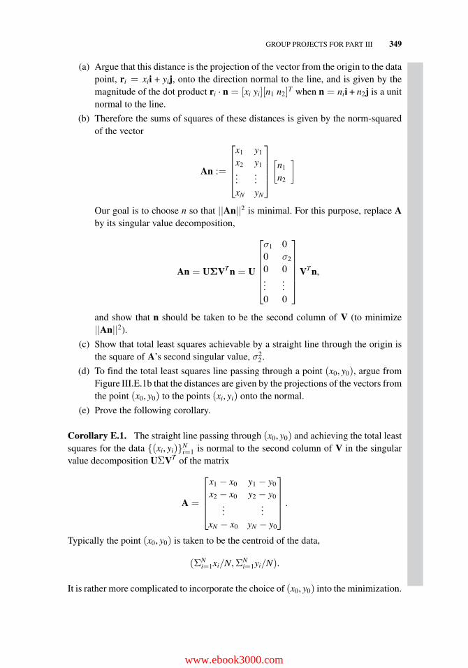
GROUP PROJECTS FOR PART III 349
(a) Argue that this distance is the projection of the vector from the origin to the datapoint, ri = xii + yij, onto the direction normal to the line, and is given by themagnitude of the dot product ri · n = [xi yi][n1 n2]T when n = nii + n2j is a unitnormal to the line.
(b) Therefore the sums of squares of these distances is given by the norm-squaredof the vector
An :=
⎡⎢⎢⎢⎣
x1 y1
x2 y1...
...xN yN
⎤⎥⎥⎥⎦[
n1
n2
]
Our goal is to choose n so that ||An||2 is minimal. For this purpose, replace Aby its singular value decomposition,
An = UΣVTn = U
⎡⎢⎢⎢⎢⎢⎣
σ1 00 σ2
0 0...
...0 0
⎤⎥⎥⎥⎥⎥⎦
VTn,
and show that n should be taken to be the second column of V (to minimize||An||2).
(c) Show that total least squares achievable by a straight line through the origin isthe square of A’s second singular value, σ2
2.
(d) To find the total least squares line passing through a point (x0, y0), argue fromFigure III.E.1b that the distances are given by the projections of the vectors fromthe point (x0, y0) to the points (xi, yi) onto the normal.
(e) Prove the following corollary.
Corollary E.1. The straight line passing through (x0, y0) and achieving the total leastsquares for the data {(xi, yi)}N
i=1 is normal to the second column of V in the singularvalue decomposition UΣVT of the matrix
A =
⎡⎢⎢⎢⎣
x1 − x0 y1 − y0
x2 − x0 y2 − y0...
...xN − x0 yN − y0
⎤⎥⎥⎥⎦ .
Typically the point (x0, y0) is taken to be the centroid of the data,
(ΣNi=1xi/N,ΣN
i=1yi/N).
It is rather more complicated to incorporate the choice of (x0, y0) into the minimization.
www.ebook3000.com
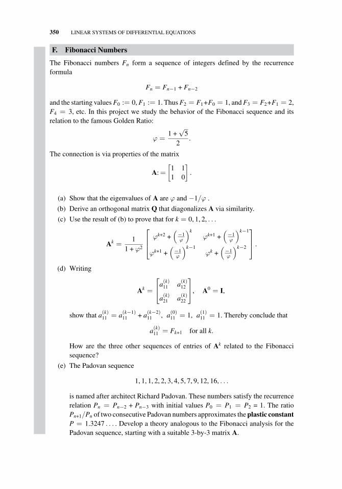
350 LINEAR SYSTEMS OF DIFFERENTIAL EQUATIONS
F. Fibonacci Numbers
The Fibonacci numbers Fn form a sequence of integers defined by the recurrenceformula
Fn = Fn−1 + Fn−2
and the starting values F0 := 0, F1 := 1. Thus F2 = F1+F0 = 1, and F3 = F2+F1 = 2,F4 = 3, etc. In this project we study the behavior of the Fibonacci sequence and itsrelation to the famous Golden Ratio:
ϕ =1 +
√5
2.
The connection is via properties of the matrix
A:=
[1 11 0
].
(a) Show that the eigenvalues of A are ϕ and −1/ϕ .
(b) Derive an orthogonal matrix Q that diagonalizes A via similarity.
(c) Use the result of (b) to prove that for k = 0, 1, 2, . . .
Ak =1
1 + ϕ2
⎡⎢⎣ ϕk+2 +
(−1ϕ
)kϕk+1 +
(−1ϕ
)k−1
ϕk+1 +(
−1ϕ
)k−1ϕk +
(−1ϕ
)k−2
⎤⎥⎦ .
(d) Writing
Ak =
⎡⎣a(k)
11 a(k)12
a(k)21 a(k)
22
⎤⎦, A0 = I,
show that a(k)11 = a(k−1)
11 + a(k−2)11 , a(0)
11 = 1, a(1)11 = 1. Thereby conclude that
a(k)11 = Fk+1 for all k.
How are the three other sequences of entries of Ak related to the Fibonaccisequence?
(e) The Padovan sequence
1, 1, 1, 2, 2, 3, 4, 5, 7, 9, 12, 16, . . .
is named after architect Richard Padovan. These numbers satisfy the recurrencerelation Pn = Pn−2 + Pn−3 with initial values P0 = P1 = P2 = 1. The ratioPn+1/Pn of two consecutive Padovan numbers approximates the plastic constantP = 1.3247 . . . . Develop a theory analogous to the Fibonacci analysis for thePadovan sequence, starting with a suitable 3-by-3 matrix A.
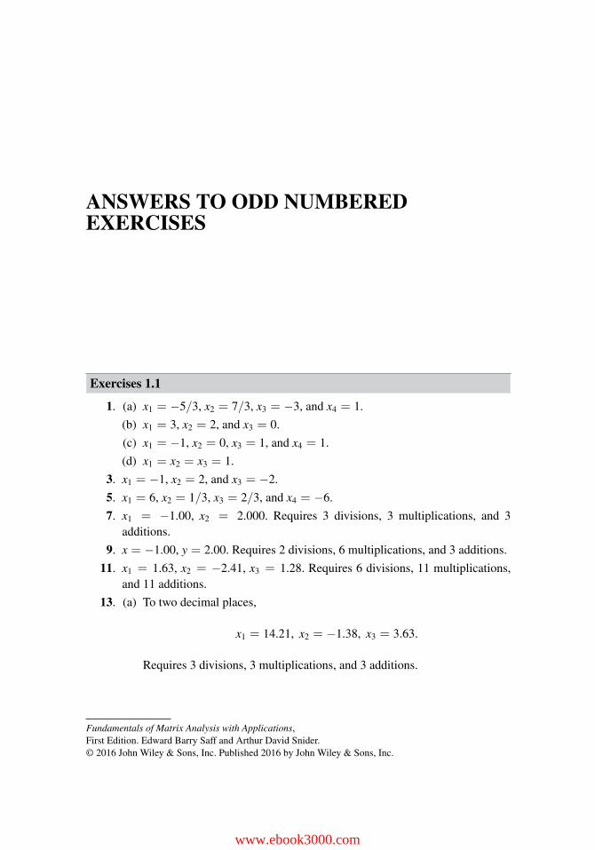
ANSWERS TO ODD NUMBEREDEXERCISES
Exercises 1.1
1. (a) x1 = −5/3, x2 = 7/3, x3 = −3, and x4 = 1.
(b) x1 = 3, x2 = 2, and x3 = 0.
(c) x1 = −1, x2 = 0, x3 = 1, and x4 = 1.
(d) x1 = x2 = x3 = 1.
3. x1 = −1, x2 = 2, and x3 = −2.
5. x1 = 6, x2 = 1/3, x3 = 2/3, and x4 = −6.
7. x1 = −1.00, x2 = 2.000. Requires 3 divisions, 3 multiplications, and 3additions.
9. x = −1.00, y = 2.00. Requires 2 divisions, 6 multiplications, and 3 additions.
11. x1 = 1.63, x2 = −2.41, x3 = 1.28. Requires 6 divisions, 11 multiplications,and 11 additions.
13. (a) To two decimal places,
x1 = 14.21, x2 = −1.38, x3 = 3.63.
Requires 3 divisions, 3 multiplications, and 3 additions.
Fundamentals of Matrix Analysis with Applications,First Edition. Edward Barry Saff and Arthur David Snider.© 2016 John Wiley & Sons, Inc. Published 2016 by John Wiley & Sons, Inc.
www.ebook3000.com
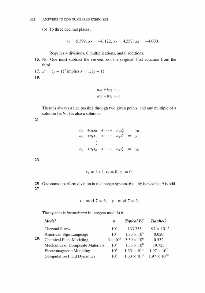
352 ANSWERS TO ODD NUMBERED EXERCISES
(b) To three decimal places,
x1 = 5.399, x2 = −6.122, x3 = 4.557, x4 = −4.000.
Requires 4 divisions, 6 multiplications, and 6 additions.
15. No. One must subtract the current, not the original, first equation from thethird.
17. x2 = (y − 1)2 implies x = ±(y − 1).
19.
ax1 + by1 = c
ax2 + by2 = c.
There is always a line passing through two given points, and any multiple of asolution (a, b, c) is also a solution.
21.
a0 +a1x0 + · · ·+ anxn0 = y0
a0 +a1x1 + · · ·+ anxn1 = y1
...a0 +a1xn + · · ·+ anxn
n = yn
23.
x1 = 1 + i, x2 = 0, x3 = 0.
25. One cannot perform division in the integer system. 6x− 4y is even but 9 is odd.27.
x mod 7 = 6, y mod 7 = 3.
The system is inconsistent in integers modulo 6.
29.
Model n Typical PC Tianhe-2
Thermal Stress 104 133.333 1.97 × 10⁻⁵
American Sign Language 105 1.33 × 10⁵ 0.020Chemical Plant Modeling 3 × 10⁵ 3.59 × 10⁶ 0.532Mechanics of Composite Materials 106 1.33 × 10⁸ 19.723Electromagnetic Modeling 108 1.33 × 10¹⁴ 1.97 × 10⁷
Computation Fluid Dynamics 109 1.33 × 10¹⁷ 1.97 × 10¹⁰
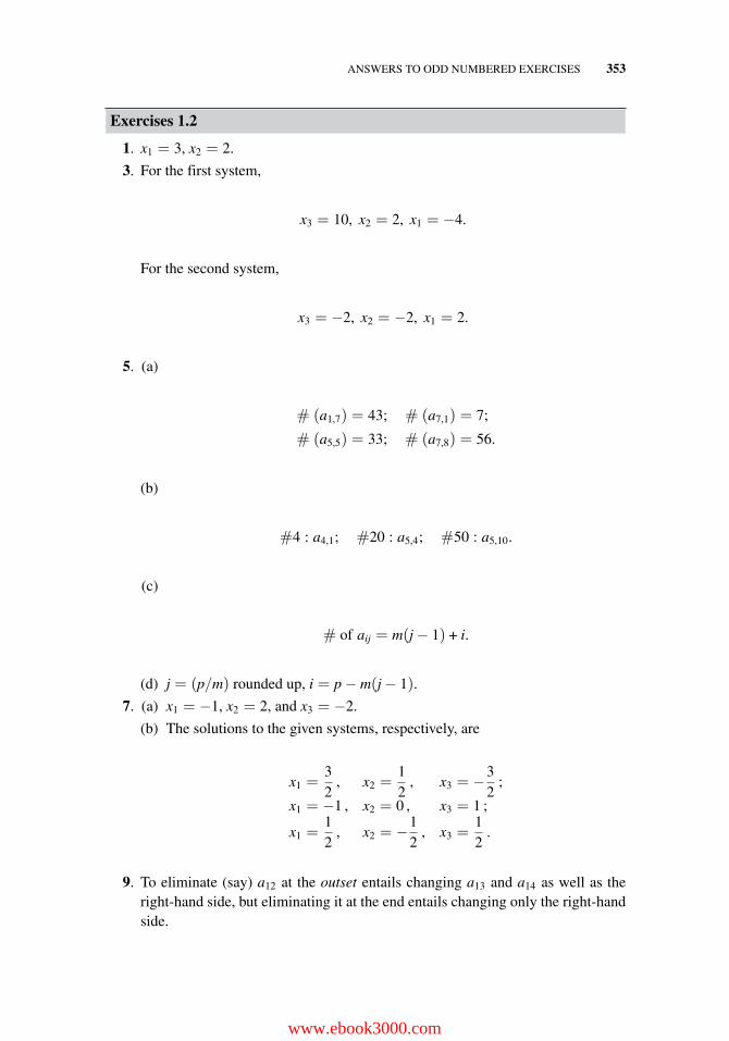
ANSWERS TO ODD NUMBERED EXERCISES 353
Exercises 1.2
1. x1 = 3, x2 = 2.
3. For the first system,
x3 = 10, x2 = 2, x1 = −4.
For the second system,
x3 = −2, x2 = −2, x1 = 2.
5. (a)
# (a1,7) = 43; # (a7,1) = 7;
# (a5,5) = 33; # (a7,8) = 56.
(b)
#4 : a4,1; #20 : a5,4; #50 : a5,10.
(c)
# of aij = m(j − 1) + i.
(d) j = (p/m) rounded up, i = p − m(j − 1).
7. (a) x1 = −1, x2 = 2, and x3 = −2.
(b) The solutions to the given systems, respectively, are
x1 =32
, x2 =12
, x3 = −32
;
x1 = −1 , x2 = 0 , x3 = 1 ;
x1 =12
, x2 = −12
, x3 =12
.
9. To eliminate (say) a12 at the outset entails changing a13 and a14 as well as theright-hand side, but eliminating it at the end entails changing only the right-handside.
www.ebook3000.com
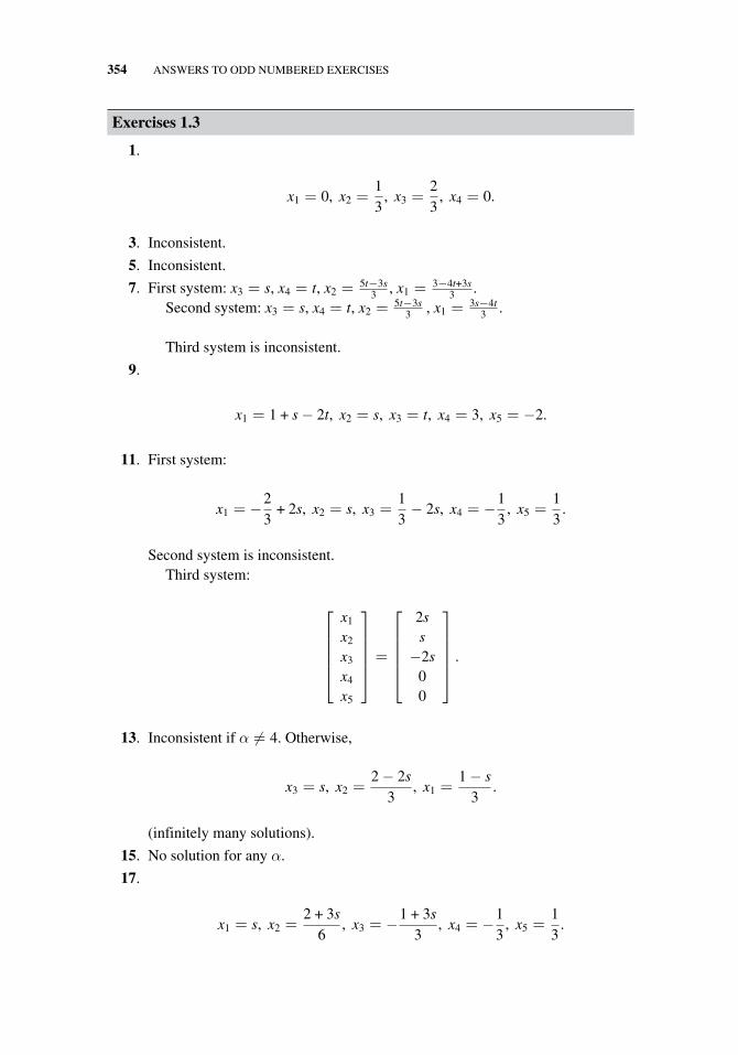
354 ANSWERS TO ODD NUMBERED EXERCISES
Exercises 1.3
1.
x1 = 0, x2 =13
, x3 =23
, x4 = 0.
3. Inconsistent.
5. Inconsistent.
7. First system: x3 = s, x4 = t, x2 =5t−3s
3 , x1 =3−4t+3s
3 .Second system: x3 = s, x4 = t, x2 =
5t−3s3 , x1 =
3s−4t3 .
Third system is inconsistent.
9.
x1 = 1 + s − 2t, x2 = s, x3 = t, x4 = 3, x5 = −2.
11. First system:
x1 = −23
+ 2s, x2 = s, x3 =13− 2s, x4 = −1
3, x5 =
13
.
Second system is inconsistent.Third system:
⎡⎢⎢⎢⎢⎣
x1
x2
x3
x4
x5
⎤⎥⎥⎥⎥⎦ =
⎡⎢⎢⎢⎢⎣
2ss
−2s00
⎤⎥⎥⎥⎥⎦ .
13. Inconsistent if α �= 4. Otherwise,
x3 = s, x2 =2 − 2s
3, x1 =
1 − s3
.
(infinitely many solutions).
15. No solution for any α.
17.
x1 = s, x2 =2 + 3s
6, x3 = −1 + 3s
3, x4 = −1
3, x5 =
13
.
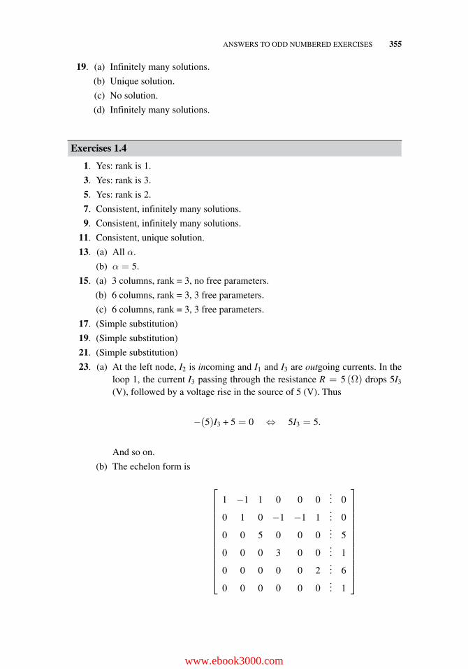
ANSWERS TO ODD NUMBERED EXERCISES 355
19. (a) Infinitely many solutions.
(b) Unique solution.
(c) No solution.
(d) Infinitely many solutions.
Exercises 1.4
1. Yes: rank is 1.
3. Yes: rank is 3.
5. Yes: rank is 2.
7. Consistent, infinitely many solutions.
9. Consistent, infinitely many solutions.
11. Consistent, unique solution.
13. (a) All α.
(b) α = 5.
15. (a) 3 columns, rank = 3, no free parameters.
(b) 6 columns, rank = 3, 3 free parameters.
(c) 6 columns, rank = 3, 3 free parameters.
17. (Simple substitution)
19. (Simple substitution)
21. (Simple substitution)
23. (a) At the left node, I2 is incoming and I1 and I3 are outgoing currents. In theloop 1, the current I3 passing through the resistance R = 5 (Ω) drops 5I3
(V), followed by a voltage rise in the source of 5 (V). Thus
−(5)I3 + 5 = 0 ⇔ 5I3 = 5.
And so on.
(b) The echelon form is
⎡⎢⎢⎢⎢⎢⎢⎢⎢⎢⎢⎢⎢⎣
1 −1 1 0 0 0... 0
0 1 0 −1 −1 1... 0
0 0 5 0 0 0... 5
0 0 0 3 0 0... 1
0 0 0 0 0 2... 6
0 0 0 0 0 0... 1
⎤⎥⎥⎥⎥⎥⎥⎥⎥⎥⎥⎥⎥⎦
www.ebook3000.com
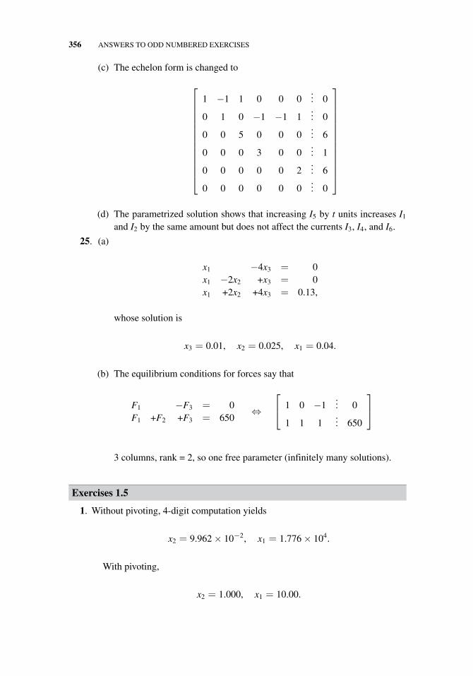
356 ANSWERS TO ODD NUMBERED EXERCISES
(c) The echelon form is changed to
⎡⎢⎢⎢⎢⎢⎢⎢⎢⎢⎢⎢⎢⎣
1 −1 1 0 0 0... 0
0 1 0 −1 −1 1... 0
0 0 5 0 0 0... 6
0 0 0 3 0 0... 1
0 0 0 0 0 2... 6
0 0 0 0 0 0... 0
⎤⎥⎥⎥⎥⎥⎥⎥⎥⎥⎥⎥⎥⎦
(d) The parametrized solution shows that increasing I5 by t units increases I1
and I2 by the same amount but does not affect the currents I3, I4, and I6.
25. (a)
x1 −4x3 = 0x1 −2x2 +x3 = 0x1 +2x2 +4x3 = 0.13,
whose solution is
x3 = 0.01, x2 = 0.025, x1 = 0.04.
(b) The equilibrium conditions for forces say that
F1 −F3 = 0F1 +F2 +F3 = 650
⇔
⎡⎣ 1 0 −1
... 0
1 1 1... 650
⎤⎦
3 columns, rank = 2, so one free parameter (infinitely many solutions).
Exercises 1.5
1. Without pivoting, 4-digit computation yields
x2 = 9.962 × 10⁻², x1 = 1.776 × 10⁴.
With pivoting,
x2 = 1.000, x1 = 10.00.
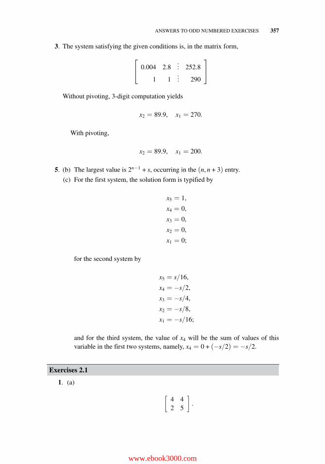
ANSWERS TO ODD NUMBERED EXERCISES 357
3. The system satisfying the given conditions is, in the matrix form,
⎡⎣ 0.004 2.8
... 252.8
1 1... 290
⎤⎦
Without pivoting, 3-digit computation yields
x2 = 89.9, x1 = 270.
With pivoting,
x2 = 89.9, x1 = 200.
5. (b) The largest value is 2n−1 + s, occurring in the (n, n + 3) entry.
(c) For the first system, the solution form is typified by
x5 = 1,
x4 = 0,
x3 = 0,
x2 = 0,
x1 = 0;
for the second system by
x5 = s/16,
x4 = −s/2,
x3 = −s/4,
x2 = −s/8,
x1 = −s/16;
and for the third system, the value of x4 will be the sum of values of thisvariable in the first two systems, namely, x4 = 0 + (−s/2) = −s/2.
Exercises 2.1
1. (a)
[4 42 5
].
www.ebook3000.com
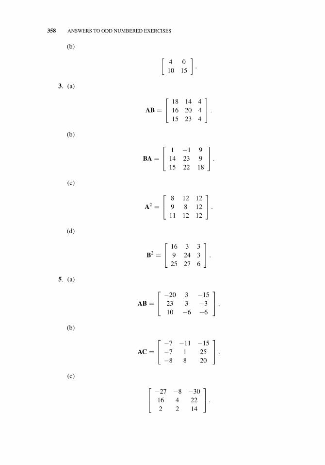
358 ANSWERS TO ODD NUMBERED EXERCISES
(b)
[4 010 15
].
3. (a)
AB =
⎡⎣ 18 14 4
16 20 415 23 4
⎤⎦ .
(b)
BA =
⎡⎣ 1 −1 9
14 23 915 22 18
⎤⎦ .
(c)
A2 =
⎡⎣ 8 12 12
9 8 1211 12 12
⎤⎦ .
(d)
B2 =
⎡⎣ 16 3 3
9 24 325 27 6
⎤⎦ .
5. (a)
AB =
⎡⎣ −20 3 −15
23 3 −310 −6 −6
⎤⎦ .
(b)
AC =
⎡⎣ −7 −11 −15
−7 1 25−8 8 20
⎤⎦ .
(c)
⎡⎣ −27 −8 −30
16 4 222 2 14
⎤⎦ .
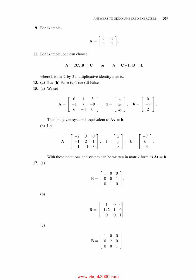
ANSWERS TO ODD NUMBERED EXERCISES 359
9. For example,
A =
[1 −11 −1
].
11. For example, one can choose
A = 2C, B = C or A = C + I, B = I,
where I is the 2-by-2 multiplicative identity matrix.
13. (a) True (b) False (c) True (d) False
15. (a) We set
A =
⎡⎣ 0 1 3
−1 7 −96 −4 0
⎤⎦ , x =
⎡⎣ x1
x2
x3
⎤⎦ , b =
⎡⎣ 0
−92
⎤⎦ .
Then the given system is equivalent to Ax = b.
(b) Let
A =
⎡⎣ −2 3 0
−1 2 1−1 −1 3
⎤⎦ , t =
⎡⎣ x
yz
⎤⎦ , b =
⎡⎣ −7
6−3
⎤⎦ .
With these notations, the system can be written in matrix form as At = b.
17. (a)
B =
⎡⎣ 1 0 0
0 0 10 1 0
⎤⎦ .
(b)
B =
⎡⎣ 1 0 0−1/2 1 0
0 0 1
⎤⎦ .
(c)
B =
⎡⎣ 1 0 0
0 2 00 0 1
⎤⎦ .
www.ebook3000.com
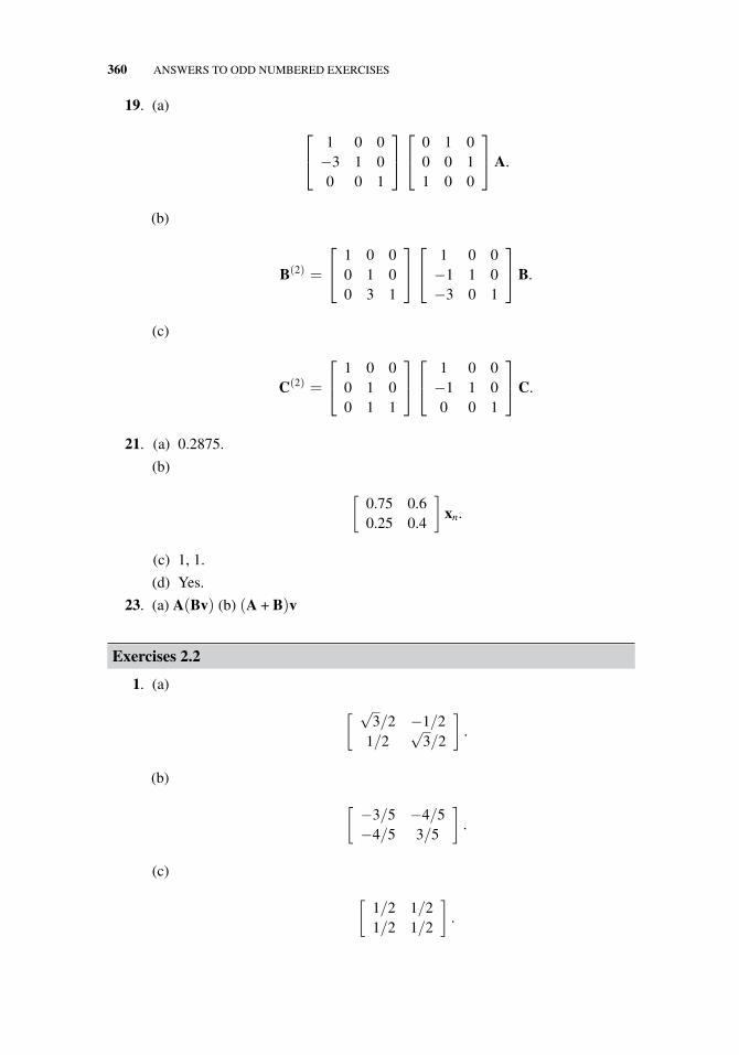
360 ANSWERS TO ODD NUMBERED EXERCISES
19. (a)
⎡⎣ 1 0 0
−3 1 00 0 1
⎤⎦⎡⎣ 0 1 0
0 0 11 0 0
⎤⎦A.
(b)
B(2) =
⎡⎣ 1 0 0
0 1 00 3 1
⎤⎦⎡⎣ 1 0 0
−1 1 0−3 0 1
⎤⎦B.
(c)
C(2) =
⎡⎣ 1 0 0
0 1 00 1 1
⎤⎦⎡⎣ 1 0 0
−1 1 00 0 1
⎤⎦C.
21. (a) 0.2875.
(b)
[0.75 0.60.25 0.4
]xn.
(c) 1, 1.
(d) Yes.
23. (a) A(Bv) (b) (A + B)v
Exercises 2.2
1. (a)
[ √3/2 −1/2
1/2√
3/2
].
(b)
[−3/5 −4/5−4/5 3/5
].
(c)
[1/2 1/21/2 1/2
].
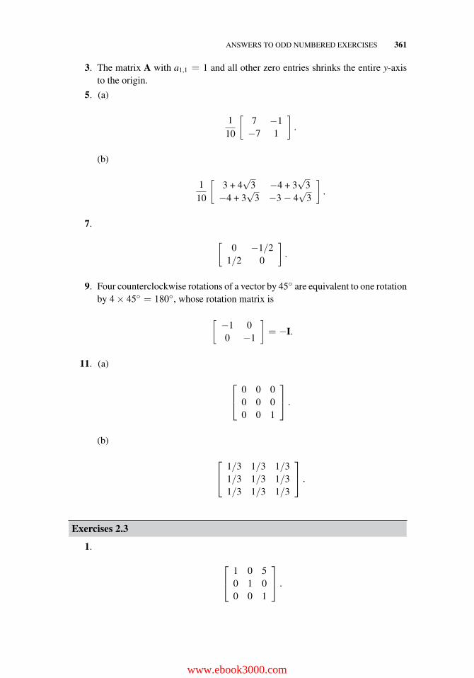
ANSWERS TO ODD NUMBERED EXERCISES 361
3. The matrix A with a1,1 = 1 and all other zero entries shrinks the entire y-axisto the origin.
5. (a)
110
[7 −1−7 1
].
(b)
110
[3 + 4
√3 −4 + 3
√3
−4 + 3√
3 −3 − 4√
3
].
7.
[0 −1/2
1/2 0
].
9. Four counterclockwise rotations of a vector by 45◦ are equivalent to one rotationby 4 × 45◦ = 180◦, whose rotation matrix is
[−1 00 −1
]= −I.
11. (a)
⎡⎣ 0 0 0
0 0 00 0 1
⎤⎦ .
(b)
⎡⎣ 1/3 1/3 1/3
1/3 1/3 1/31/3 1/3 1/3
⎤⎦ .
Exercises 2.3
1.
⎡⎣ 1 0 5
0 1 00 0 1
⎤⎦ .
www.ebook3000.com
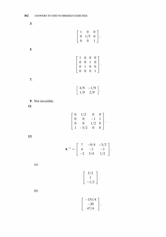
362 ANSWERS TO ODD NUMBERED EXERCISES
3.
⎡⎣ 1 0 0
0 1/5 00 0 1
⎤⎦ .
5.
⎡⎢⎢⎣
1 0 0 00 0 1 00 1 0 00 0 0 1
⎤⎥⎥⎦ .
7.
[4/9 −1/91/9 2/9
].
9. Not invertible.
11.
⎡⎢⎢⎣
0 1/2 0 00 0 −1 10 0 1/2 01 −3/2 0 0
⎤⎥⎥⎦ .
13.
A−1 =
⎡⎣ 7 −9/4 −3/2
4 −1 −1−2 3/4 1/2
⎤⎦ .
(a)
⎡⎣ 5/2
1−1/2
⎤⎦ .
(b)
⎡⎣ −153/4
−2047/4
⎤⎦ .
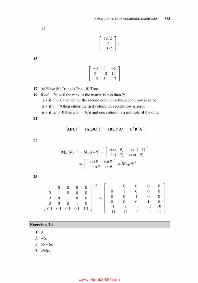
ANSWERS TO ODD NUMBERED EXERCISES 363
(c)
⎡⎣ 15/2
3−5/2
⎤⎦ .
15.
⎡⎣ −3 3 −5
9 −8 15−5 5 −7
⎤⎦ .
17. (a) False (b) True (c) True (d) True.
19. If ad − bc = 0 the rank of the matrix is less than 2:(i) if d = 0 then either the second column or the second row is zero;
(ii) if c = 0 then either the first column or second row is zero;
(iii) if cd �= 0 then a/c = b/d and one column is a multiple of the other.
21.
(ABC)T = (A(BC))T = (BC)TAT = CTBTAT .
23.
Mrot(θ)−1 = Mrot(−θ) =
[cos(−θ) − sin(−θ)sin(−θ) cos(−θ)
]
=
[cos θ sin θ− sin θ cos θ
]= Mrot(θ)
T .
25.
⎡⎢⎢⎢⎢⎣
1 0 0 0 00 1 0 0 00 0 1 0 00 0 0 1 0
0.1 0.1 0.1 0.1 1.1
⎤⎥⎥⎥⎥⎦
−1
=
⎡⎢⎢⎢⎢⎢⎢⎣
1 0 0 0 00 1 0 0 00 0 1 0 00 0 0 1 0
− 111
− 111
− 111
− 111
1011
⎤⎥⎥⎥⎥⎥⎥⎦
.
Exercises 2.4
1. 0.
3. −6.
5. 66 + 6i.
7. abdg.
www.ebook3000.com
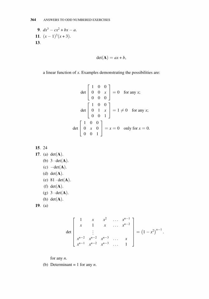
364 ANSWERS TO ODD NUMBERED EXERCISES
9. dx3 − cx2 + bx − a.
11. (x − 1)3(x + 3).
13.
det(A) = ax + b,
a linear function of x. Examples demonstrating the possibilities are:
det
⎡⎣ 1 0 0
0 0 x0 0 0
⎤⎦ = 0 for any x;
det
⎡⎣ 1 0 0
0 1 x0 0 1
⎤⎦ = 1 �= 0 for any x;
det
⎡⎣ 1 0 0
0 x 00 0 1
⎤⎦ = x = 0 only for x = 0.
15. 24
17. (a) det(A).
(b) 3 · det(A).
(c) −det(A).
(d) det(A).
(e) 81 · det(A).
(f) det(A).
(g) 3 · det(A).
(h) det(A).
19. (a)
det
⎡⎢⎢⎢⎢⎢⎣
1 x x2 . . . xn−1
x 1 x . . . xn−2
...xn−2 xn−2 xn−3 . . . xxn−1 xn−2 xn−3 . . . 1
⎤⎥⎥⎥⎥⎥⎦=(1 − x2
)n−1.
for any n.
(b) Determinant = 1 for any n.
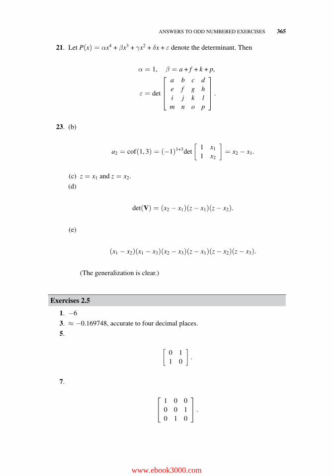
ANSWERS TO ODD NUMBERED EXERCISES 365
21. Let P(x) = αx4 + βx3 + γx2 + δx + ε denote the determinant. Then
α = 1, β = a + f + k + p,
ε = det
⎡⎢⎢⎣
a b c de f g hi j k lm n o p
⎤⎥⎥⎦ .
23. (b)
a2 = cof(1, 3) = (−1)1+3det
[1 x1
1 x2
]= x2 − x1.
(c) z = x1 and z = x2.
(d)
det(V) = (x2 − x1)(z − x1)(z − x2).
(e)
(x1 − x2)(x1 − x3)(x2 − x3)(z − x1)(z − x2)(z − x3).
(The generalization is clear.)
Exercises 2.5
1. −6
3. ≈ −0.169748, accurate to four decimal places.
5.
[0 11 0
].
7.
⎡⎣ 1 0 0
0 0 10 1 0
⎤⎦ .
www.ebook3000.com
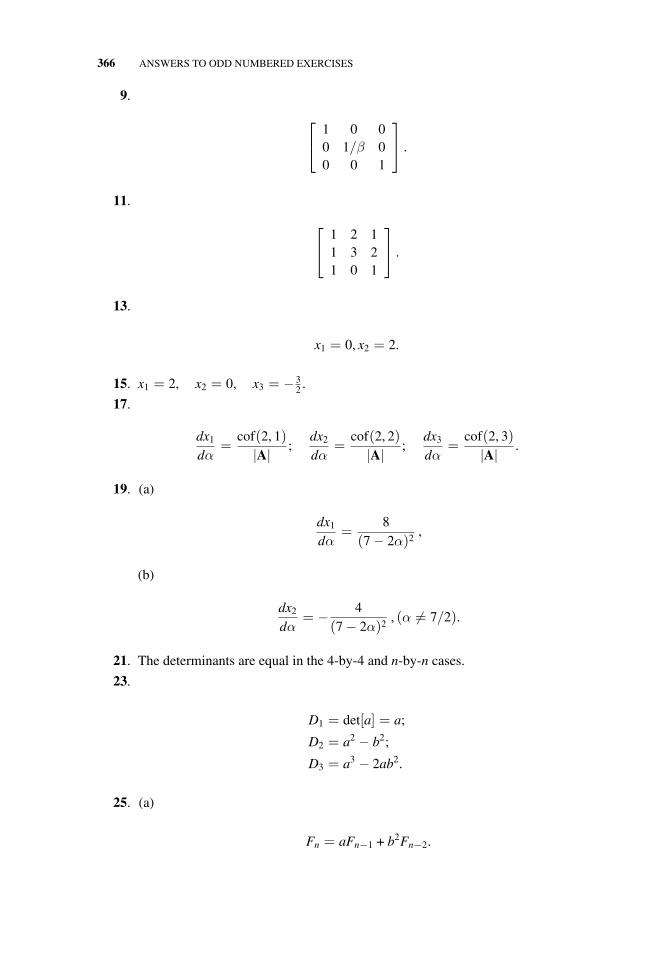
366 ANSWERS TO ODD NUMBERED EXERCISES
9.
⎡⎣ 1 0 0
0 1/β 00 0 1
⎤⎦ .
11.
⎡⎣ 1 2 1
1 3 21 0 1
⎤⎦ .
13.
x1 = 0, x2 = 2.
15. x1 = 2, x2 = 0, x3 = − 32 .
17.
dx1
dα=
cof(2, 1)|A| ;
dx2
dα=
cof(2, 2)|A| ;
dx3
dα=
cof(2, 3)|A| .
19. (a)
dx1
dα=
8(7 − 2α)2
,
(b)
dx2
dα= − 4
(7 − 2α)2, (α �= 7/2).
21. The determinants are equal in the 4-by-4 and n-by-n cases.
23.
D1 = det[a] = a;
D2 = a2 − b2;
D3 = a3 − 2ab2.
25. (a)
Fn = aFn−1 + b2Fn−2.
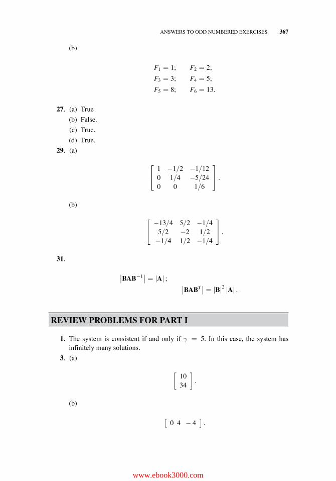
ANSWERS TO ODD NUMBERED EXERCISES 367
(b)
F1 = 1; F2 = 2;
F3 = 3; F4 = 5;
F5 = 8; F6 = 13.
27. (a) True
(b) False.
(c) True.
(d) True.
29. (a)
⎡⎣ 1 −1/2 −1/12
0 1/4 −5/240 0 1/6
⎤⎦ .
(b)
⎡⎣ −13/4 5/2 −1/4
5/2 −2 1/2−1/4 1/2 −1/4
⎤⎦ .
31.
∣∣BAB−1∣∣ = |A| ; ∣∣BABT
∣∣ = |B|2 |A| .
REVIEW PROBLEMS FOR PART I
1. The system is consistent if and only if γ = 5. In this case, the system hasinfinitely many solutions.
3. (a)
[1034
].
(b)
[0 4 − 4
].
www.ebook3000.com
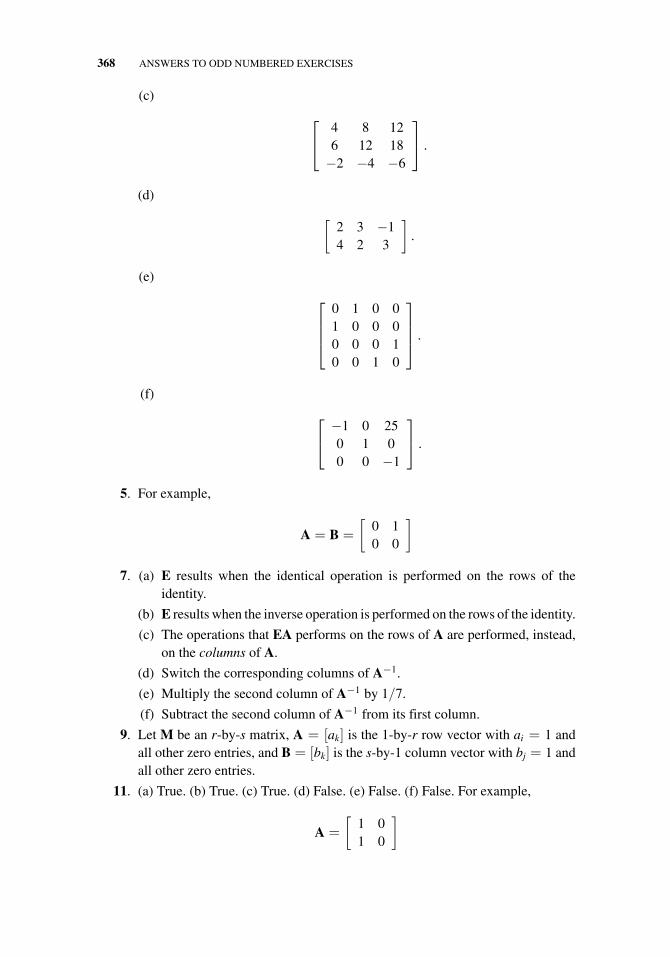
368 ANSWERS TO ODD NUMBERED EXERCISES
(c)
⎡⎣ 4 8 12
6 12 18−2 −4 −6
⎤⎦ .
(d)
[2 3 −14 2 3
].
(e)
⎡⎢⎢⎣
0 1 0 01 0 0 00 0 0 10 0 1 0
⎤⎥⎥⎦ .
(f)
⎡⎣ −1 0 25
0 1 00 0 −1
⎤⎦ .
5. For example,
A = B =
[0 10 0
]
7. (a) E results when the identical operation is performed on the rows of theidentity.
(b) E results when the inverse operation is performed on the rows of the identity.
(c) The operations that EA performs on the rows of A are performed, instead,on the columns of A.
(d) Switch the corresponding columns of A−1.
(e) Multiply the second column of A−1 by 1/7.
(f) Subtract the second column of A−1 from its first column.
9. Let M be an r-by-s matrix, A = [ak] is the 1-by-r row vector with ai = 1 andall other zero entries, and B = [bk] is the s-by-1 column vector with bj = 1 andall other zero entries.
11. (a) True. (b) True. (c) True. (d) False. (e) False. (f) False. For example,
A =
[1 01 0
]
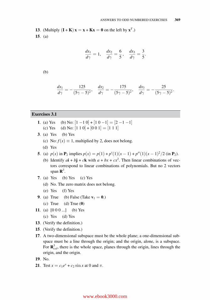
ANSWERS TO ODD NUMBERED EXERCISES 369
13. (Multiply (I + K) x = x + Kx = 0 on the left by xT .)
15. (a)
dx1
dγ= 1,
dx2
dγ=
65
,dx3
dγ=
35
.
(b)
dx1
dγ= − 125
(5γ − 5)2,
dx2
dγ= − 175
(5γ − 5)2,
dx3
dγ= − 25
(5γ − 5)2.
Exercises 3.1
1. (a) Yes (b) No: [1 −1 0] + [1 0 −1] = [2 −1 −1](c) Yes (d) No: [1 1 0] + [0 0 1] = [1 1 1]
3. (a) Yes (b) Yes
(c) No: f (x) ≡ 1, multiplied by 2, does not belong.
(d) Yes
5. (a) p(x) in P2 implies p(x) = p(1) + p′(1)(x − 1) + p′′(1)(x − 1)2/2 (in P2).
(b) Identify ai + bj + ck with a + bx + cx2. Then linear combinations of vec-tors correspond to linear combinations of polynomials. But no 2 vectorsspan R3.
7. (a) Yes (b) Yes (c) Yes
(d) No. The zero matrix does not belong.
(e) Yes (f) Yes
9. (a) True (b) False (Take v1 = 0.)
(c) True (d) True (0)
11. (a) [0 0 0 ...] (b) Yes
(c) Yes (d) Yes
13. (Verify the definition.)
15. (Verify the definition.)
17. A two-dimensional subspace must be the whole plane; a one-dimensional sub-space must be a line through the origin; and the origin, alone, is a subspace.For R3
col, there is the whole space, planes through the origin, lines through theorigin, and the origin.
19. No.
21. Test x = c1ex + c2 sin x at 0 and π.
www.ebook3000.com
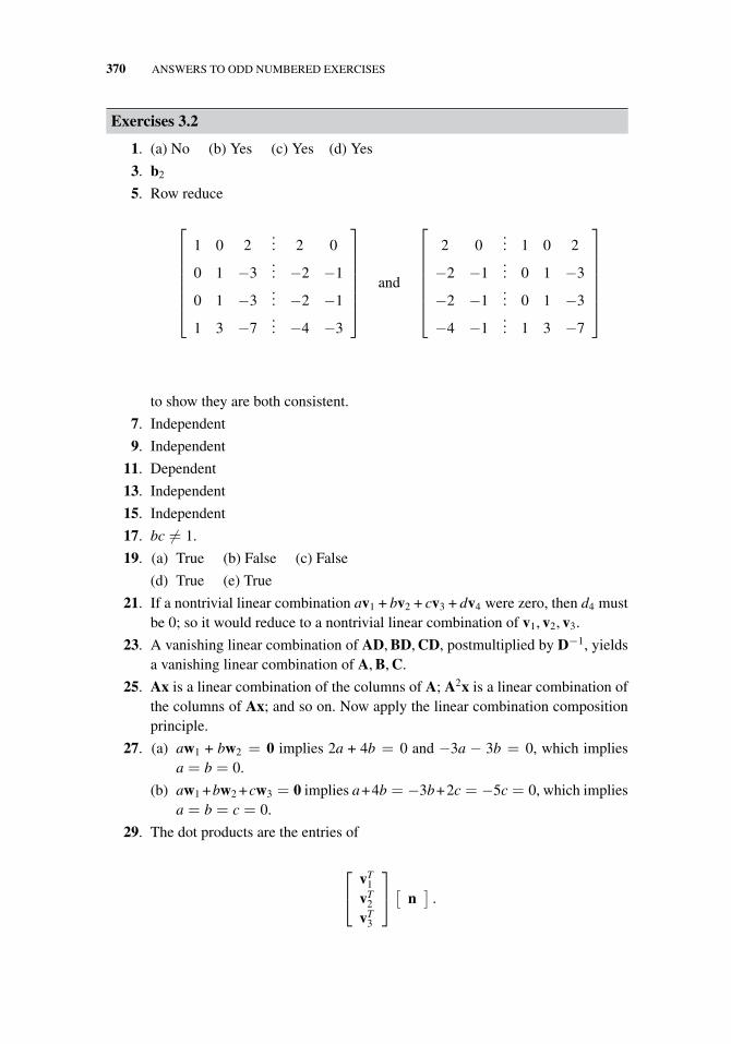
370 ANSWERS TO ODD NUMBERED EXERCISES
Exercises 3.2
1. (a) No (b) Yes (c) Yes (d) Yes
3. b2
5. Row reduce
⎡⎢⎢⎢⎢⎢⎢⎣
1 0 2... 2 0
0 1 −3... −2 −1
0 1 −3... −2 −1
1 3 −7... −4 −3
⎤⎥⎥⎥⎥⎥⎥⎦
and
⎡⎢⎢⎢⎢⎢⎢⎣
2 0... 1 0 2
−2 −1... 0 1 −3
−2 −1... 0 1 −3
−4 −1... 1 3 −7
⎤⎥⎥⎥⎥⎥⎥⎦
to show they are both consistent.
7. Independent
9. Independent
11. Dependent
13. Independent
15. Independent
17. bc �= 1.
19. (a) True (b) False (c) False
(d) True (e) True
21. If a nontrivial linear combination av1 + bv2 + cv3 + dv4 were zero, then d4 mustbe 0; so it would reduce to a nontrivial linear combination of v1, v2, v3.
23. A vanishing linear combination of AD, BD, CD, postmultiplied by D−1, yieldsa vanishing linear combination of A, B, C.
25. Ax is a linear combination of the columns of A; A2x is a linear combination ofthe columns of Ax; and so on. Now apply the linear combination compositionprinciple.
27. (a) aw1 + bw2 = 0 implies 2a + 4b = 0 and −3a − 3b = 0, which impliesa = b = 0.
(b) aw1 +bw2 +cw3 = 0 implies a+4b = −3b+2c = −5c = 0, which impliesa = b = c = 0.
29. The dot products are the entries of
⎡⎣ vT
1
vT2
vT3
⎤⎦ [ n
].
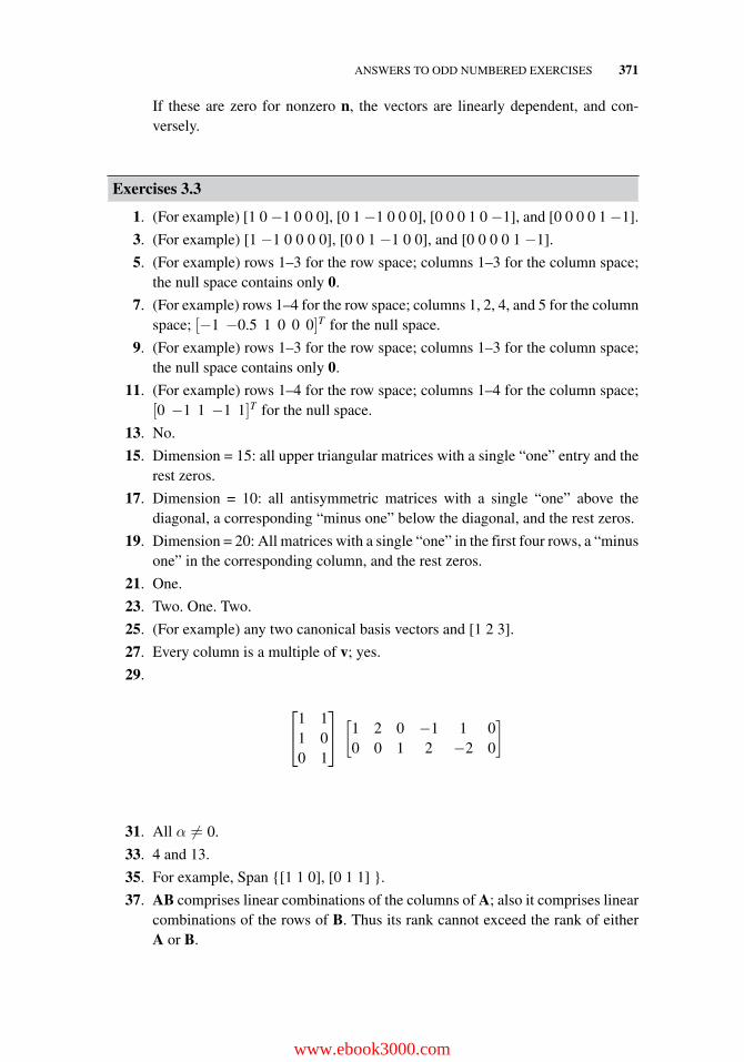
ANSWERS TO ODD NUMBERED EXERCISES 371
If these are zero for nonzero n, the vectors are linearly dependent, and con-versely.
Exercises 3.3
1. (For example) [1 0 −1 0 0 0], [0 1 −1 0 0 0], [0 0 0 1 0 −1], and [0 0 0 0 1 −1].
3. (For example) [1 −1 0 0 0 0], [0 0 1 −1 0 0], and [0 0 0 0 1 −1].
5. (For example) rows 1–3 for the row space; columns 1–3 for the column space;the null space contains only 0.
7. (For example) rows 1–4 for the row space; columns 1, 2, 4, and 5 for the columnspace; [−1 −0.5 1 0 0 0]T for the null space.
9. (For example) rows 1–3 for the row space; columns 1–3 for the column space;the null space contains only 0.
11. (For example) rows 1–4 for the row space; columns 1–4 for the column space;[0 −1 1 −1 1]T for the null space.
13. No.
15. Dimension = 15: all upper triangular matrices with a single “one” entry and therest zeros.
17. Dimension = 10: all antisymmetric matrices with a single “one” above thediagonal, a corresponding “minus one” below the diagonal, and the rest zeros.
19. Dimension = 20: All matrices with a single “one” in the first four rows, a “minusone” in the corresponding column, and the rest zeros.
21. One.
23. Two. One. Two.
25. (For example) any two canonical basis vectors and [1 2 3].
27. Every column is a multiple of v; yes.
29.
⎡⎣1 1
1 00 1
⎤⎦[
1 2 0 −1 1 00 0 1 2 −2 0
]
31. All α �= 0.
33. 4 and 13.
35. For example, Span {[1 1 0], [0 1 1] }.
37. AB comprises linear combinations of the columns of A; also it comprises linearcombinations of the rows of B. Thus its rank cannot exceed the rank of eitherA or B.
www.ebook3000.com
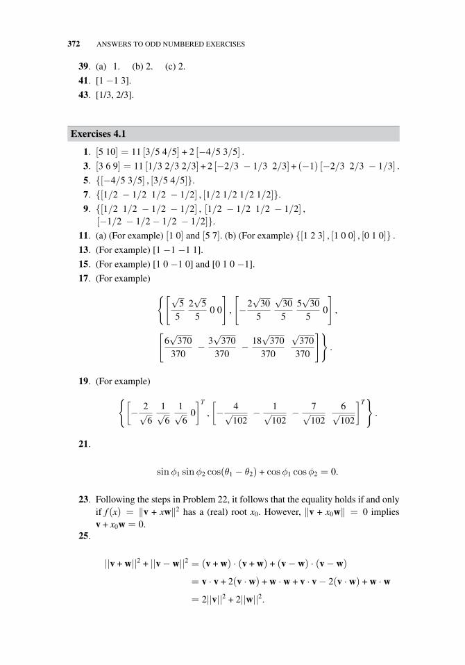
372 ANSWERS TO ODD NUMBERED EXERCISES
39. (a) 1. (b) 2. (c) 2.
41. [1 −1 3].
43. [1/3, 2/3].
Exercises 4.1
1. [5 10] = 11 [3/5 4/5] + 2 [−4/5 3/5] .
3. [3 6 9] = 11 [1/3 2/3 2/3]+ 2 [−2/3 − 1/3 2/3]+ (−1) [−2/3 2/3 − 1/3] .
5. {[−4/5 3/5] , [3/5 4/5]}.
7. {[1/2 − 1/2 1/2 − 1/2] , [1/2 1/2 1/2 1/2]}.
9. {[1/2 1/2 − 1/2 − 1/2] , [1/2 − 1/2 1/2 − 1/2] ,[−1/2 − 1/2 − 1/2 − 1/2]}.
11. (a) (For example) [1 0] and [5 7]. (b) (For example) {[1 2 3] , [1 0 0] , [0 1 0]} .
13. (For example) [1 −1 −1 1].
15. (For example) [1 0 −1 0] and [0 1 0 −1].
17. (For example)
{[√5
52√
55
0 0
],
[−2
√30
5
√305
5√
305
0
],
[6√
370370
− 3√
370370
− 18√
370370
√370
370
]}.
19. (For example)
{[− 2√
6
1√6
1√6
0
]T
,
[− 4√
102− 1√
102− 7√
102
6√102
]T}
.
21.
sinφ1 sinφ2 cos(θ1 − θ2) + cosφ1 cosφ2 = 0.
23. Following the steps in Problem 22, it follows that the equality holds if and onlyif f (x) = ‖v + xw‖2 has a (real) root x0. However, ‖v + x0w‖ = 0 impliesv + x0w = 0.
25.
||v + w||2 + ||v − w||2 = (v + w) · (v + w) + (v − w) · (v − w)
= v · v + 2(v · w) + w · w + v · v − 2(v · w) + w · w
= 2||v||2 + 2||w||2.
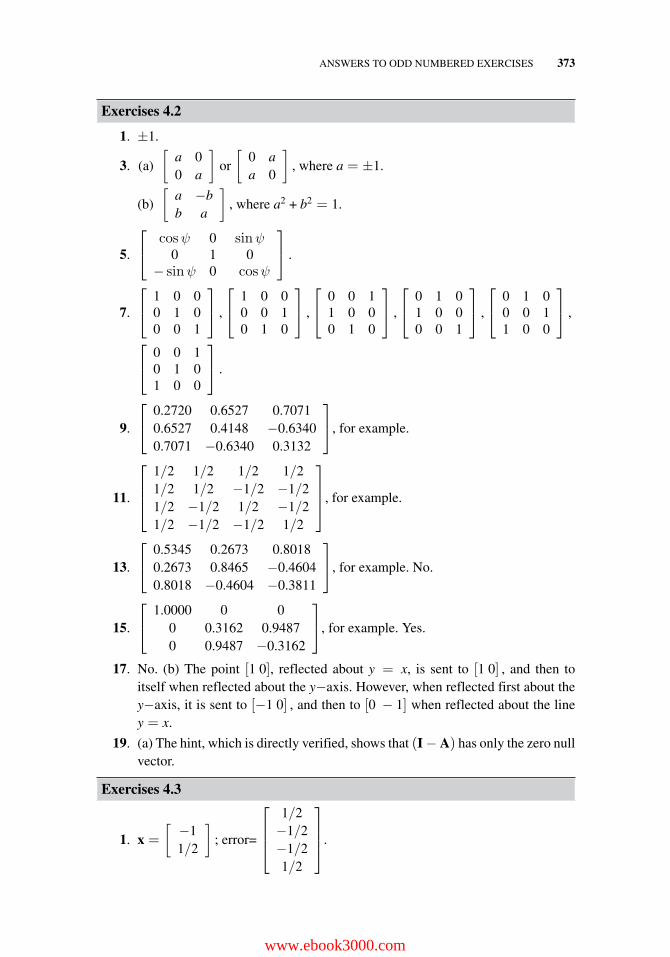
ANSWERS TO ODD NUMBERED EXERCISES 373
Exercises 4.2
1. ±1.
3. (a)
[a 00 a
]or
[0 aa 0
], where a = ±1.
(b)
[a −bb a
], where a2 + b2 = 1.
5.
⎡⎣ cosψ 0 sinψ
0 1 0− sinψ 0 cosψ
⎤⎦ .
7.
⎡⎣ 1 0 0
0 1 00 0 1
⎤⎦ ,
⎡⎣ 1 0 0
0 0 10 1 0
⎤⎦ ,
⎡⎣ 0 0 1
1 0 00 1 0
⎤⎦ ,
⎡⎣ 0 1 0
1 0 00 0 1
⎤⎦ ,
⎡⎣ 0 1 0
0 0 11 0 0
⎤⎦ ,
⎡⎣ 0 0 1
0 1 01 0 0
⎤⎦ .
9.
⎡⎣ 0.2720 0.6527 0.7071
0.6527 0.4148 −0.63400.7071 −0.6340 0.3132
⎤⎦, for example.
11.
⎡⎢⎢⎣
1/2 1/2 1/2 1/21/2 1/2 −1/2 −1/21/2 −1/2 1/2 −1/21/2 −1/2 −1/2 1/2
⎤⎥⎥⎦, for example.
13.
⎡⎣ 0.5345 0.2673 0.8018
0.2673 0.8465 −0.46040.8018 −0.4604 −0.3811
⎤⎦, for example. No.
15.
⎡⎣ 1.0000 0 0
0 0.3162 0.94870 0.9487 −0.3162
⎤⎦, for example. Yes.
17. No. (b) The point [1 0], reflected about y = x, is sent to [1 0] , and then toitself when reflected about the y−axis. However, when reflected first about they−axis, it is sent to [−1 0] , and then to [0 − 1] when reflected about the liney = x.
19. (a) The hint, which is directly verified, shows that (I − A) has only the zero nullvector.
Exercises 4.3
1. x =
[−11/2
]; error=
⎡⎢⎢⎣
1/2−1/2−1/21/2
⎤⎥⎥⎦.
www.ebook3000.com
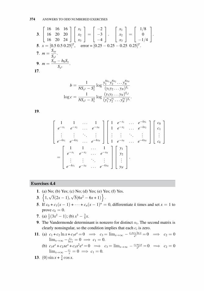
374 ANSWERS TO ODD NUMBERED EXERCISES
3.
⎡⎣ 16 16 16
16 20 2016 20 24
⎤⎦⎡⎣ x1
x2
x3
⎤⎦ =
⎡⎣ −2
−3−4
⎤⎦ .
⎡⎣ x1
x2
x3
⎤⎦ =
⎡⎣ 1/8
0−1/4
⎤⎦.
5. x = [0.5 0.5 0.25]T , error = [0.25 − 0.25 − 0.25 0.25]T .
7. m =Sxy
Sx2.
9. m =Sxy − b0Sx
Sx2.
17.
b =1
NSx2 − S2xlog
yNx11 yNx2
2 . . . yNxNN
(y1y2 . . . yN)Sx
log c =1
NSx2 − S2xlog
(y1y2 . . . yN)Sx2
(yx11 yx2
2 . . . yxNN )Sx
.
19.
⎡⎢⎢⎢⎣
1 1 . . . 1e−x1 e−x2 . . . e−xN
......
. . ....
e−kx1 e−kx2 . . . e−kxN
⎤⎥⎥⎥⎦
⎡⎢⎢⎢⎣
1 e−x1 . . . e−kx1
1 e−x2 . . . e−kx2
......
. . ....
1 e−xN . . . e−kxN
⎤⎥⎥⎥⎦
⎡⎢⎢⎢⎣
c0
c1...
ck
⎤⎥⎥⎥⎦
=
⎡⎢⎢⎢⎣
1 1 . . . 1e−x1 e−x2 . . . e−xN
......
. . ....
e−kx1 e−xN . . . e−kxN
⎤⎥⎥⎥⎦
⎡⎢⎢⎢⎣
y1
y2...
yN
⎤⎥⎥⎥⎦ .
Exercises 4.4
1. (a) No; (b) Yes; (c) No; (d) Yes; (e) Yes; (f) Yes.
3.{
1,√
3(2x − 1),√
5(6x2 − 6x + 1)}
.
5. If c0 + c1(x − 1) + · · · + cn(x − 1)n = 0, differentiate k times and set x = 1 toprove ck = 0.
7. (a) 12(3x2 − 1); (b) x3 − 3
5 x.
9. The Vandermonde determinant is nonzero for distinct αi. The second matrix isclearly nonsingular, so the condition implies that each ci is zero.
11. (a) c1 + c2 ln x + c3ex = 0 =⇒ c3 = limx→∞ − c1+c2 ln xex = 0 =⇒ c2 = 0
limx→∞ − c1ln x = 0 =⇒ c1 = 0.
(b) c1ex + c2xex + c3x2ex = 0 =⇒ c3 = limx→∞ − c1+c2xx2 = 0 =⇒ c2 = 0
limx→∞ − c1x = 0 =⇒ c1 = 0.
13. (0) sin x + 34 cos x.
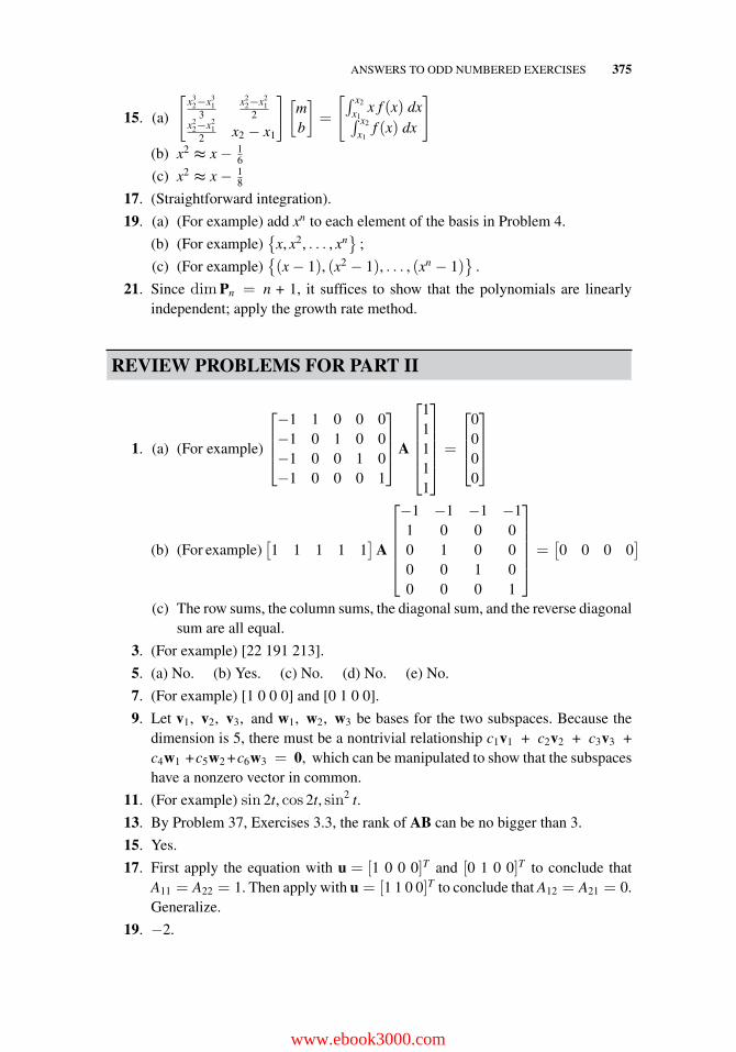
ANSWERS TO ODD NUMBERED EXERCISES 375
15. (a)
[x3
2−x31
3x2
2−x21
2x2
2−x21
2 x2 − x1
] [mb
]=
[∫ x2
x1x f (x) dx∫ x2
x1f (x) dx
]
(b) x2≈ x − 1
6
(c) x2≈ x − 1
8
17. (Straightforward integration).
19. (a) (For example) add xn to each element of the basis in Problem 4.
(b) (For example){
x, x2, . . . , xn}
;
(c) (For example){(x − 1), (x2 − 1), . . . , (xn − 1)
}.
21. Since dimPn = n + 1, it suffices to show that the polynomials are linearlyindependent; apply the growth rate method.
REVIEW PROBLEMS FOR PART II
1. (a) (For example)
⎡⎢⎢⎣−1 1 0 0 0−1 0 1 0 0−1 0 0 1 0−1 0 0 0 1
⎤⎥⎥⎦A
⎡⎢⎢⎢⎢⎣
11111
⎤⎥⎥⎥⎥⎦ =
⎡⎢⎢⎣
0000
⎤⎥⎥⎦
(b) (For example)[1 1 1 1 1
]A
⎡⎢⎢⎢⎢⎣
−1 −1 −1 −11 0 0 00 1 0 00 0 1 00 0 0 1
⎤⎥⎥⎥⎥⎦ =
[0 0 0 0
]
(c) The row sums, the column sums, the diagonal sum, and the reverse diagonalsum are all equal.
3. (For example) [22 191 213].
5. (a) No. (b) Yes. (c) No. (d) No. (e) No.
7. (For example) [1 0 0 0] and [0 1 0 0].
9. Let v1, v2, v3, and w1, w2, w3 be bases for the two subspaces. Because thedimension is 5, there must be a nontrivial relationship c1v1 + c2v2 + c3v3 +c4w1 +c5w2 +c6w3 = 0, which can be manipulated to show that the subspaceshave a nonzero vector in common.
11. (For example) sin 2t, cos 2t, sin2 t.
13. By Problem 37, Exercises 3.3, the rank of AB can be no bigger than 3.
15. Yes.
17. First apply the equation with u = [1 0 0 0]T and [0 1 0 0]T to conclude thatA11 = A22 = 1. Then apply with u = [1 1 0 0]T to conclude that A12 = A21 = 0.Generalize.
19. −2.
www.ebook3000.com
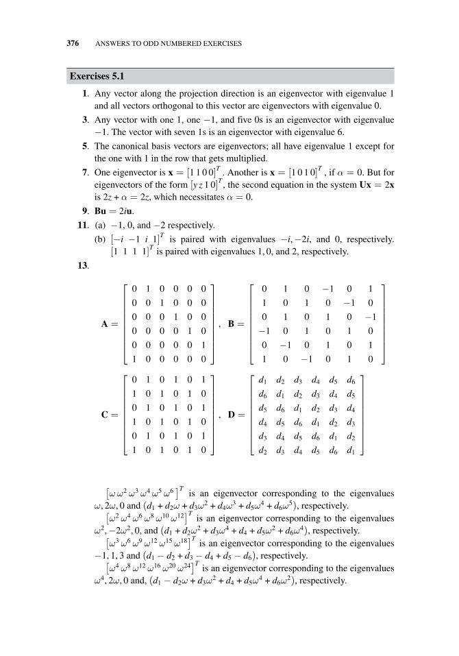
376 ANSWERS TO ODD NUMBERED EXERCISES
Exercises 5.1
1. Any vector along the projection direction is an eigenvector with eigenvalue 1and all vectors orthogonal to this vector are eigenvectors with eigenvalue 0.
3. Any vector with one 1, one −1, and five 0s is an eigenvector with eigenvalue−1. The vector with seven 1s is an eigenvector with eigenvalue 6.
5. The canonical basis vectors are eigenvectors; all have eigenvalue 1 except forthe one with 1 in the row that gets multiplied.
7. One eigenvector is x = [1 1 0 0]T . Another is x = [1 0 1 0]T , if α = 0. But foreigenvectors of the form [y z 1 0]T , the second equation in the system Ux = 2xis 2z + α = 2z, which necessitates α = 0.
9. Bu = 2iu.
11. (a) −1, 0, and −2 respectively.
(b) [−i −1 i 1]T is paired with eigenvalues −i,−2i, and 0, respectively.[1 1 1 1]T is paired with eigenvalues 1, 0, and 2, respectively.
13.
A =
⎡⎢⎢⎢⎢⎢⎢⎢⎢⎣
0 1 0 0 0 0
0 0 1 0 0 0
0 0 0 1 0 0
0 0 0 0 1 0
0 0 0 0 0 1
1 0 0 0 0 0
⎤⎥⎥⎥⎥⎥⎥⎥⎥⎦
, B =
⎡⎢⎢⎢⎢⎢⎢⎢⎢⎣
0 1 0 −1 0 1
1 0 1 0 −1 0
0 1 0 1 0 −1
−1 0 1 0 1 0
0 −1 0 1 0 1
1 0 −1 0 1 0
⎤⎥⎥⎥⎥⎥⎥⎥⎥⎦
C =
⎡⎢⎢⎢⎢⎢⎢⎢⎢⎣
0 1 0 1 0 1
1 0 1 0 1 0
0 1 0 1 0 1
1 0 1 0 1 0
0 1 0 1 0 1
1 0 1 0 1 0
⎤⎥⎥⎥⎥⎥⎥⎥⎥⎦
, D =
⎡⎢⎢⎢⎢⎢⎢⎢⎢⎣
d1 d2 d3 d4 d5 d6
d6 d1 d2 d3 d4 d5
d5 d6 d1 d2 d3 d4
d4 d5 d6 d1 d2 d3
d3 d4 d5 d6 d1 d2
d2 d3 d4 d5 d6 d1
⎤⎥⎥⎥⎥⎥⎥⎥⎥⎦
[ω ω2 ω3 ω4 ω5 ω6
]Tis an eigenvector corresponding to the eigenvalues
ω, 2ω, 0 and (d1 + d2ω + d3ω2 + d4ω
3 + d5ω4 + d6ω
5), respectively.[ω2 ω4 ω6 ω8 ω10 ω12
]Tis an eigenvector corresponding to the eigenvalues
ω2,−2ω2, 0, and (d1 + d2ω2 + d3ω
4 + d4 + d5ω2 + d6ω
4), respectively.[ω3 ω6 ω9 ω12 ω15 ω18
]Tis an eigenvector corresponding to the eigenvalues
−1, 1, 3 and (d1 − d2 + d3 − d4 + d5 − d6), respectively.[ω4 ω8 ω12 ω16 ω20 ω24
]Tis an eigenvector corresponding to the eigenvalues
ω4, 2ω, 0 and, (d1 − d2ω + d3ω2 + d4 + d5ω
4 + d6ω2), respectively.
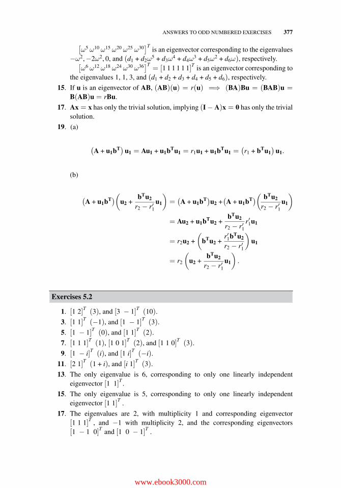
ANSWERS TO ODD NUMBERED EXERCISES 377
[ω5 ω10 ω15 ω20 ω25 ω30
]Tis an eigenvector corresponding to the eigenvalues
−ω2,−2ω2, 0, and (d1 + d2ω5 + d3ω
4 + d4ω3 + d5ω
2 + d6ω), respectively.[ω6 ω12 ω18 ω24 ω30 ω36
]T= [1 1 1 1 1 1]T is an eigenvector corresponding to
the eigenvalues 1, 1, 3, and (d1 + d2 + d3 + d4 + d5 + d6), respectively.
15. If u is an eigenvector of AB, (AB)(u) = r(u) =⇒ (BA)Bu = (BAB)u =B(AB)u = rBu.
17. Ax = x has only the trivial solution, implying (I − A)x = 0 has only the trivialsolution.
19. (a)
(A + u1bT) u1 = Au1 + u1bTu1 = r1u1 + u1bTu1 =
(r1 + bTu1
)u1.
(b)
(A + u1bT)(u2 +
bTu2
r2 − r′1u1
)=(A + u1bT)u2 +
(A + u1bT)( bTu2
r2 − r′1u1
)
= Au2 + u1bTu2 +bTu2
r2 − r′1r′1u1
= r2u2 +
(bTu2 +
r′1bTu2
r2 − r′1
)u1
= r2
(u2 +
bTu2
r2 − r′1u1
).
Exercises 5.2
1. [1 2]T (3), and [3 − 1]T (10).
3. [1 1]T (−1), and [1 − 1]T (3).
5. [1 − 1]T (0), and [1 1]T (2).
7. [1 1 1]T (1), [1 0 1]T (2), and [1 1 0]T (3).
9. [1 − i]T (i), and [1 i]T (−i).
11. [2 1]T (1 + i), and [i 1]T (3).
13. The only eigenvalue is 6, corresponding to only one linearly independenteigenvector [1 1]T .
15. The only eigenvalue is 5, corresponding to only one linearly independenteigenvector [1 1]T .
17. The eigenvalues are 2, with multiplicity 1 and corresponding eigenvector[1 1 1]T , and −1 with multiplicity 2, and the corresponding eigenvectors[1 − 1 0]T and [1 0 − 1]T .
www.ebook3000.com
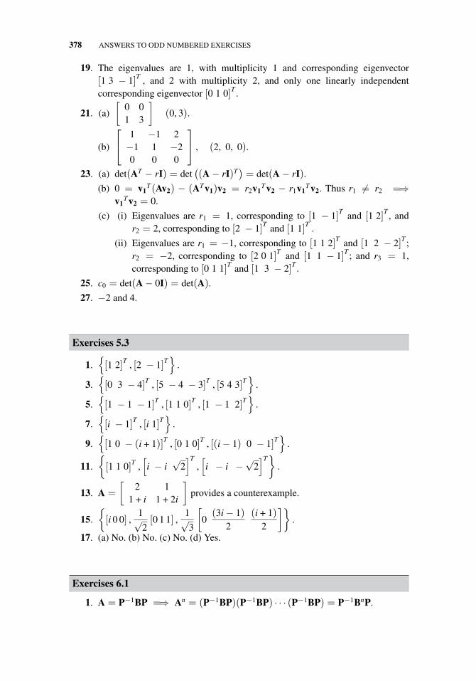
378 ANSWERS TO ODD NUMBERED EXERCISES
19. The eigenvalues are 1, with multiplicity 1 and corresponding eigenvector[1 3 − 1]T , and 2 with multiplicity 2, and only one linearly independentcorresponding eigenvector [0 1 0]T .
21. (a)
[0 01 3
](0, 3).
(b)
⎡⎣ 1 −1 2
−1 1 −20 0 0
⎤⎦ , (2, 0, 0).
23. (a) det(AT − rI) = det((A − rI)T
)= det(A − rI).
(b) 0 = v1T(Av2) − (ATv1)v2 = r2v1
Tv2 − r1v1Tv2. Thus r1 �= r2 =⇒
v1Tv2 = 0.
(c) (i) Eigenvalues are r1 = 1, corresponding to [1 − 1]T and [1 2]T , andr2 = 2, corresponding to [2 − 1]T and [1 1]T .
(ii) Eigenvalues are r1 = −1, corresponding to [1 1 2]T and [1 2 − 2]T ;r2 = −2, corresponding to [2 0 1]T and [1 1 − 1]T ; and r3 = 1,corresponding to [0 1 1]T and [1 3 − 2]T .
25. c0 = det(A − 0I) = det(A).
27. −2 and 4.
Exercises 5.3
1.{[1 2]T , [2 − 1]T
}.
3.{[0 3 − 4]T , [5 − 4 − 3]T , [5 4 3]T
}.
5.{[1 − 1 − 1]T , [1 1 0]T , [1 − 1 2]T
}.
7.{[i − 1]T , [i 1]T
}.
9.{[1 0 − (i + 1)]T , [0 1 0]T , [(i − 1) 0 − 1]T
}.
11.
{[1 1 0]T ,
[i − i
√2]T
,[i − i −
√2]T}
.
13. A =
[2 1
1 + i 1 + 2i
]provides a counterexample.
15.
{[i 0 0] ,
1√2[0 1 1] ,
1√3
[0(3i − 1)
2(i + 1)
2
]}.
17. (a) No. (b) No. (c) No. (d) Yes.
Exercises 6.1
1. A = P−1BP =⇒ An = (P−1BP)(P−1BP) · · · (P−1BP) = P−1BnP.
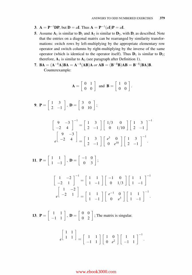
ANSWERS TO ODD NUMBERED EXERCISES 379
3. A = P−1DP, but D = aI. Thus A = P−1(aI)P = aI.
5. Assume A1 is similar to D1 and A2 is similar to D2, with Di as described. Notethat the entries on a diagonal matrix can be rearranged by similarity transfor-mations: switch rows by left-multiplying by the appropriate elementary rowoperator and switch columns by right-multiplying by the inverse of the sameoperator (which is identical to the operator itself). Thus D1 is similar to D2;therefore, A1 is similar to A2 (see paragraph after Definition 1).
7. BA = (A−1A)BA = A−1(AB)A or AB = (B−1B)AB = B−1(BA)B.Counterexample:
A =
[0 10 0
]and B =
[1 00 0
].
9. P =
[1 32 −1
], D =
[3 00 10
];
[9 −3−2 4
]−1
=
[1 32 −1
] [1/3 0
0 1/10
] [1 32 −1
]−1
e
⎡⎣ 9 −3−2 4
⎤⎦=
[1 32 −1
] [e3 00 e10
] [1 32 −1
]−1
.
11. P =
[1 11 −1
], D =
[−1 00 3
];
[1 −2−2 1
]−1
=
[1 11 −1
] [−1 00 1/3
] [1 11 −1
]−1
e
⎡⎣ 1 −2−2 1
⎤⎦=
[1 11 −1
] [e−1 00 e3
] [1 11 −1
]−1
.
13. P =
[1 1−1 1
], D =
[0 00 2
]; The matrix is singular.
e
⎡⎣ 1 1
1 1
⎤⎦=
[1 1−1 1
] [1 00 e2
] [1 1−1 1
]−1
.
www.ebook3000.com
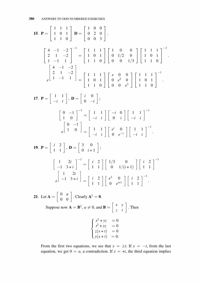
380 ANSWERS TO ODD NUMBERED EXERCISES
15. P =
⎡⎣ 1 1 1
1 0 11 1 0
⎤⎦ D =
⎡⎣ 1 0 0
0 2 00 0 3
⎤⎦ .
⎡⎣ 4 −1 −2
2 1 −21 −1 1
⎤⎦−1
=
⎡⎣ 1 1 1
1 0 11 1 0
⎤⎦⎡⎣ 1 0 0
0 1/2 00 0 1/3
⎤⎦⎡⎣ 1 1 1
1 0 11 1 0
⎤⎦−1
.
e
⎡⎢⎢⎢⎣
4 −1 −22 1 −21 −1 1
⎤⎥⎥⎥⎦=
⎡⎣ 1 1 1
1 0 11 1 0
⎤⎦⎡⎣ e 0 0
0 e2 00 0 e3
⎤⎦⎡⎣ 1 1 1
1 0 11 1 0
⎤⎦−1
.
17. P =
[1 1−i i
], D =
[i 00 −i
];
[0 −11 0
]−1
=
[1 1−i i
] [−i 00 i
] [1 1−i i
]−1
e
⎡⎣ 0 −1
1 0
⎤⎦=
[1 1−i i
] [ei 00 e−i
] [1 1−i i
]−1
.
19. P =
[i 21 1
], D =
[3 00 i + 1
];
[1 2i−1 3 + i
]−1
=
[i 21 1
] [1/3 0
0 1/(i + 1)
] [i 21 1
]−1
e
⎡⎣ 1 2i−1 3 + i
⎤⎦=
[i 21 1
] [e3 00 ei+1
] [i 21 1
]−1
.
21. Let A =
[0 a0 0
]. Clearly A2 = 0.
Suppose now A = B2, a �= 0, and B =
[x yz t
]. Then
⎧⎪⎪⎨⎪⎪⎩
x2 + yz = 0t2 + yz = 0z(x + t) = 0y(x + t) = 0.
From the first two equations, we see that x = ±t. If x = −t, from the lastequation, we get 0 = a, a contradiction. If x = +t, the third equation implies
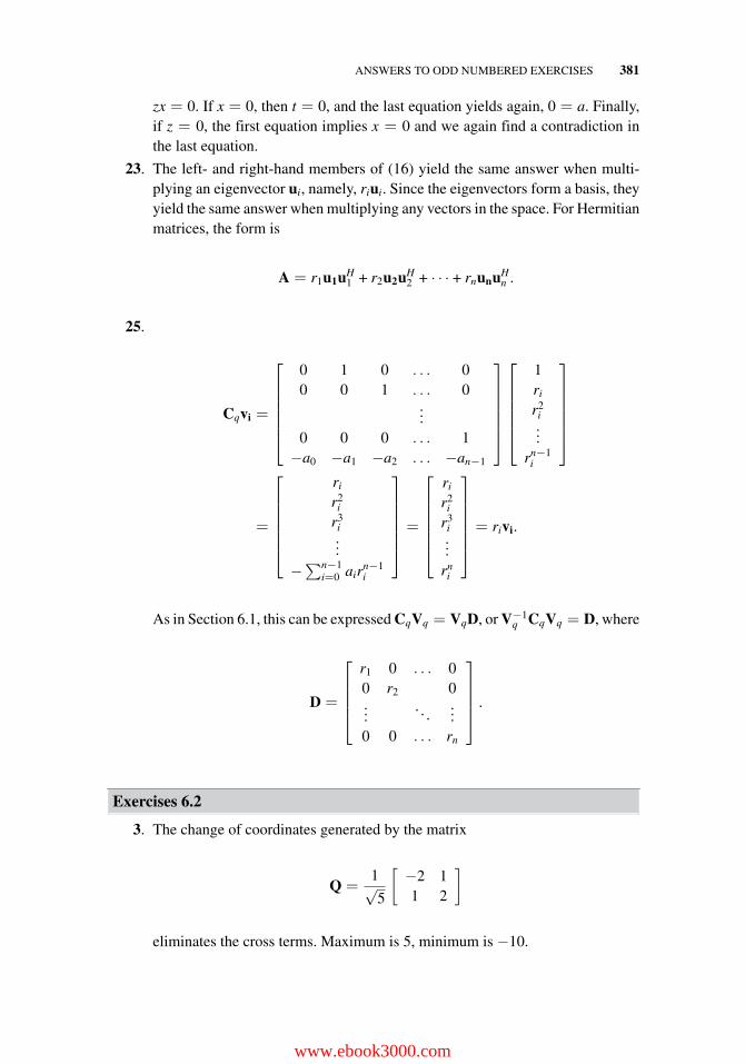
ANSWERS TO ODD NUMBERED EXERCISES 381
zx = 0. If x = 0, then t = 0, and the last equation yields again, 0 = a. Finally,if z = 0, the first equation implies x = 0 and we again find a contradiction inthe last equation.
23. The left- and right-hand members of (16) yield the same answer when multi-plying an eigenvector ui, namely, riui. Since the eigenvectors form a basis, theyyield the same answer when multiplying any vectors in the space. For Hermitianmatrices, the form is
A = r1u1uH1 + r2u2uH
2 + · · · + rnunuHn .
25.
Cqvi =
⎡⎢⎢⎢⎢⎢⎣
0 1 0 . . . 00 0 1 . . . 0
...0 0 0 . . . 1
−a0 −a1 −a2 . . . −an−1
⎤⎥⎥⎥⎥⎥⎦
⎡⎢⎢⎢⎢⎢⎣
1ri
r2i...
rn−1i
⎤⎥⎥⎥⎥⎥⎦
=
⎡⎢⎢⎢⎢⎢⎣
ri
r2i
r3i...
−∑n−1
i=0 airn−1i
⎤⎥⎥⎥⎥⎥⎦=
⎡⎢⎢⎢⎢⎢⎣
ri
r2i
r3i...
rni
⎤⎥⎥⎥⎥⎥⎦= rivi.
As in Section 6.1, this can be expressed CqVq = VqD, or V−1q CqVq = D, where
D =
⎡⎢⎢⎢⎣
r1 0 . . . 00 r2 0...
. . ....
0 0 . . . rn
⎤⎥⎥⎥⎦ .
Exercises 6.2
3. The change of coordinates generated by the matrix
Q =1√5
[−2 11 2
]
eliminates the cross terms. Maximum is 5, minimum is −10.
www.ebook3000.com
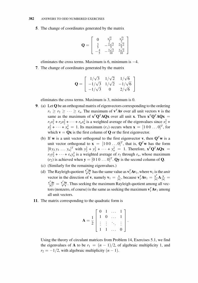
382 ANSWERS TO ODD NUMBERED EXERCISES
5. The change of coordinates generated by the matrix
Q =
⎡⎢⎣
0√
22
√2
235 − 2
√2
52√
25
− 45 − 3
√2
103√
210
⎤⎥⎦
eliminates the cross terms. Maximum is 6, minimum is −4.
7. The change of coordinates generated by the matrix
Q =
⎡⎣ 1/
√3 1/
√2 1/
√6
−1/√
3 1/√
2 −1/√
6−1/
√3 0 2/
√6
⎤⎦
eliminates the cross terms. Maximum is 3, minimum is 0.
9. (a) Let Q be an orthogonal matrix of eigenvectors corresponding to the orderingr1 ≥ r2 ≥ · · · ≥ rn. The maximum of vTAv over all unit vectors v is thesame as the maximum of xTQTAQx over all unit x. Then xTQTAQx =r1x2
1 + r2x22 + · · · + rnx2
n is a weighted average of the eigenvalues since x21 +
x22 + · · · + x2
n = 1. Its maximum (r1) occurs when x = [1 0 0 . . . 0]T , forwhich v = Qx is the first column of Q or the first eigenvector.
(b) If w is a unit vector orthogonal to the first eigenvector v, then QTw is aunit vector orthogonal to x = [1 0 0 . . . 0]T , that is, QTw has the form[0 y2 y3 . . . yn]T with y2
2 + y23 + · · · + y2
n = 1. Therefore, xTQTAQx =r2y2
2 + · · · + rny2n is a weighted average of r2 through rn, whose maximum
(r2) is achieved when y = [0 1 0 . . . 0]T . Qy is the second column of Q.
(c) (Similarly for the remaining eigenvalues.)
(d) The Rayleigh quotient vT AvvT v has the same value as vT
1 Av1, where v1 is the unit
vector in the direction of v, namely v1 = v|v| , because vT
1 Av1 = vT
|v|Av|v| =
vT Av|v|2 = vT Av
vT v . Thus seeking the maximum Rayleigh quotient among all vec-tors (nonzero, of course) is the same as seeking the maximum vT
1 Av1 amongall unit vectors.
11. The matrix corresponding to the quadratic form is
A =12
⎡⎢⎢⎢⎣
0 1 . . . 11 0 . . . 1...
.... . .
...1 1 . . . 0
⎤⎥⎥⎥⎦ .
Using the theory of circulant matrices from Problem 14, Exercises 5.1, we findthe eigenvalues of A to be r1 = (n − 1)/2, of algebraic multiplicity 1, andr2 = −1/2, with algebraic multiplicity (n − 1).
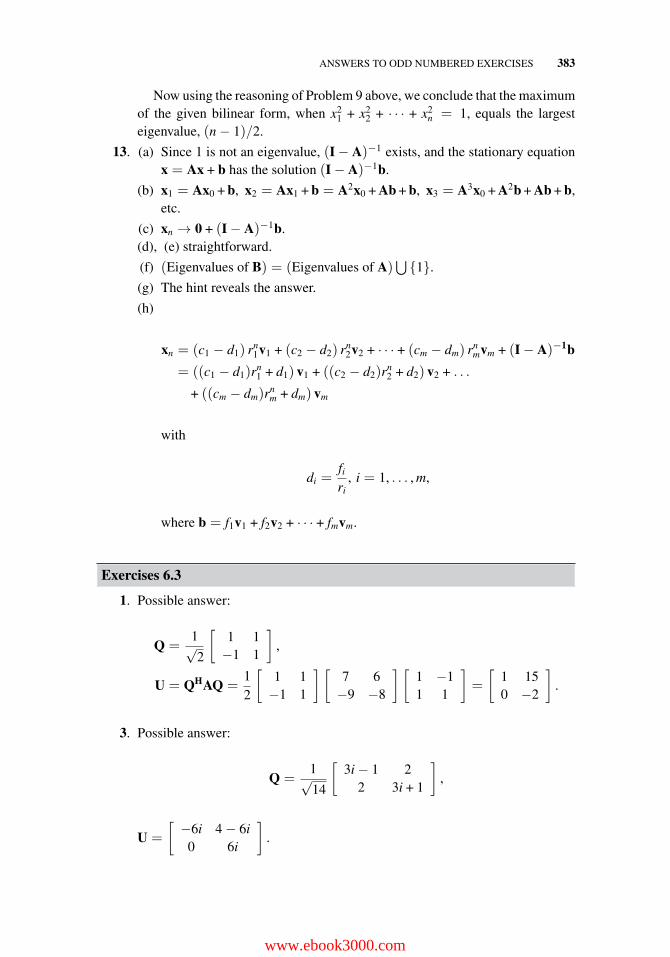
ANSWERS TO ODD NUMBERED EXERCISES 383
Now using the reasoning of Problem 9 above, we conclude that the maximumof the given bilinear form, when x2
1 + x22 + · · · + x2
n = 1, equals the largesteigenvalue, (n − 1)/2.
13. (a) Since 1 is not an eigenvalue, (I − A)−1 exists, and the stationary equationx = Ax + b has the solution (I − A)−1b.
(b) x1 = Ax0 + b, x2 = Ax1 + b = A2x0 + Ab + b, x3 = A3x0 + A2b + Ab + b,etc.
(c) xn → 0 + (I − A)−1b.(d), (e) straightforward.
(f) (Eigenvalues of B) = (Eigenvalues of A)⋃
{1}.
(g) The hint reveals the answer.
(h)
xn = (c1 − d1) rn1v1 + (c2 − d2) rn
2v2 + · · · + (cm − dm) rnmvm + (I − A)−1b
= ((c1 − d1)rn1 + d1) v1 + ((c2 − d2)r
n2 + d2) v2 + . . .
+ ((cm − dm)rnm + dm) vm
with
di =firi
, i = 1, . . . , m,
where b = f1v1 + f2v2 + · · · + fmvm.
Exercises 6.3
1. Possible answer:
Q =1√2
[1 1−1 1
],
U = QHAQ =12
[1 1−1 1
] [7 6−9 −8
] [1 −11 1
]=
[1 150 −2
].
3. Possible answer:
Q =1√14
[3i − 1 2
2 3i + 1
],
U =
[−6i 4 − 6i
0 6i
].
www.ebook3000.com
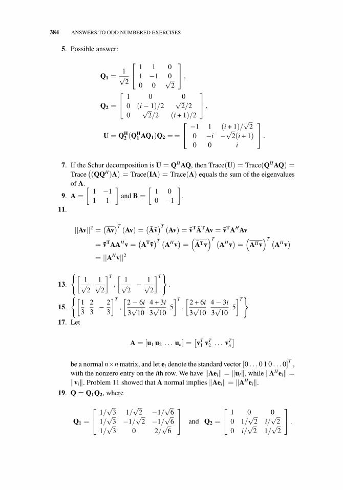
384 ANSWERS TO ODD NUMBERED EXERCISES
5. Possible answer:
Q1 =1√2
⎡⎣ 1 1 0
1 −1 00 0
√2
⎤⎦ ,
Q2 =
⎡⎣ 1 0 0
0 (i − 1)/2√
2/20
√2/2 (i + 1)/2
⎤⎦ ,
U = QH2 (Q
H1 AQ1)Q2 ==
⎡⎣ −1 1 (i + 1)/
√2
0 −i −√
2(i + 1)0 0 i
⎤⎦ .
7. If the Schur decomposition is U = QHAQ, then Trace(U) = Trace(QHAQ) =Trace
((QQH)A
)= Trace(IA) = Trace(A) equals the sum of the eigenvalues
of A.
9. A =
[1 −11 1
]and B =
[1 00 −1
].
11.
||Av||2 =(Av)T
(Av) =(Av)T
(Av) = vTATAv = vTAHAv
= vTAAHv =(ATv)T (
AHv)=(
ATv)T (
AHv)=(
AHv)T (
AHv)
= ||AHv||2
13.
{[1√2
1√2
]T
,
[1√2
− 1√2
]T}
.
15.
{[13
23
− 23
]T
,
[2 − 6i
3√
10
4 + 3i
3√
105
]T
,
[2 + 6i
3√
10
4 − 3i
3√
105
]T}
17. Let
A = [u1 u2 . . . un] =[vT
1 vT2 . . . vT
n
]
be a normal n×n matrix, and let ei denote the standard vector [0 . . . 0 1 0 . . . 0]T ,with the nonzero entry on the ith row. We have ‖Aei‖ = ‖ui‖, while ‖AHei‖ =‖vi‖. Problem 11 showed that A normal implies ‖Aei‖ = ‖AHei‖.
19. Q = Q1Q2, where
Q1 =
⎡⎣ 1/
√3 1/
√2 −1/
√6
1/√
3 −1/√
2 −1/√
61/√
3 0 2/√
6
⎤⎦ and Q2 =
⎡⎣ 1 0 0
0 1/√
2 i/√
20 i/
√2 1/
√2
⎤⎦ .

ANSWERS TO ODD NUMBERED EXERCISES 385
21.
A−1 =1c0
((−A)
n−1 − cn−1An−2 − · · · − c1I)
.
Exercises 6.4
1. Norm = 1+√
52 , cond = 3+
√5
2 .
3. Norm = 16.848; cond = ∞.
5. Norm = 4; cond = 4.
7. w1 = v1; w2 = vr.
9. Minimize (1 − 2t)2 + (−t)2 + (t)2.
11. ||AB|| = max||v||=1||(AB)v|| ≤ ||A|| ||Bv|| ≤ ||A|| ||B|| (1).13. Equation (14) and Corollary 10.
15. The transpose of the SVD for A is an SVD for AT and demonstrates that thenonzero singular values of A are the same as those of AT . Now apply Theorem6 to AT .
17.
[0 10 −1
],
[1 01 0
], and
[1 10 0
]
are equally close rank 1 approximations.
19.
⎡⎢⎢⎣
1.0003 2.0003 3.00070.9997 1.9997 2.99931.0003 0.0003 1.00070.9997 −0.0003 0.9993
⎤⎥⎥⎦
is the closest rank 2 approximation. The Frobenius norms of the differences are0.0012 and 0.0020.
21. (a) r = 0.7395, s = 7.0263, t = 1.2105.
(b) r = 3.1965, s = 8.0806.
(c) r = 0, s = 6.7089, t = 1.5749.
(d) (a) 5.2632e-06 (b) 2.3226e-05 (c) 1.9846e-05. Part (b) constructed a rank2 approximation by eliminating the third unknown (x3); but part (c) utilizedthe best rank 2 approximation.
23. For square A, all of the matrices have the same dimension; therefore, detA =(detU)(detΣ)(detU) and the unitary matrices have determinant ±1. The simple1-by-1 matrices [1] and [−1] demonstrate the two possibilities.
www.ebook3000.com
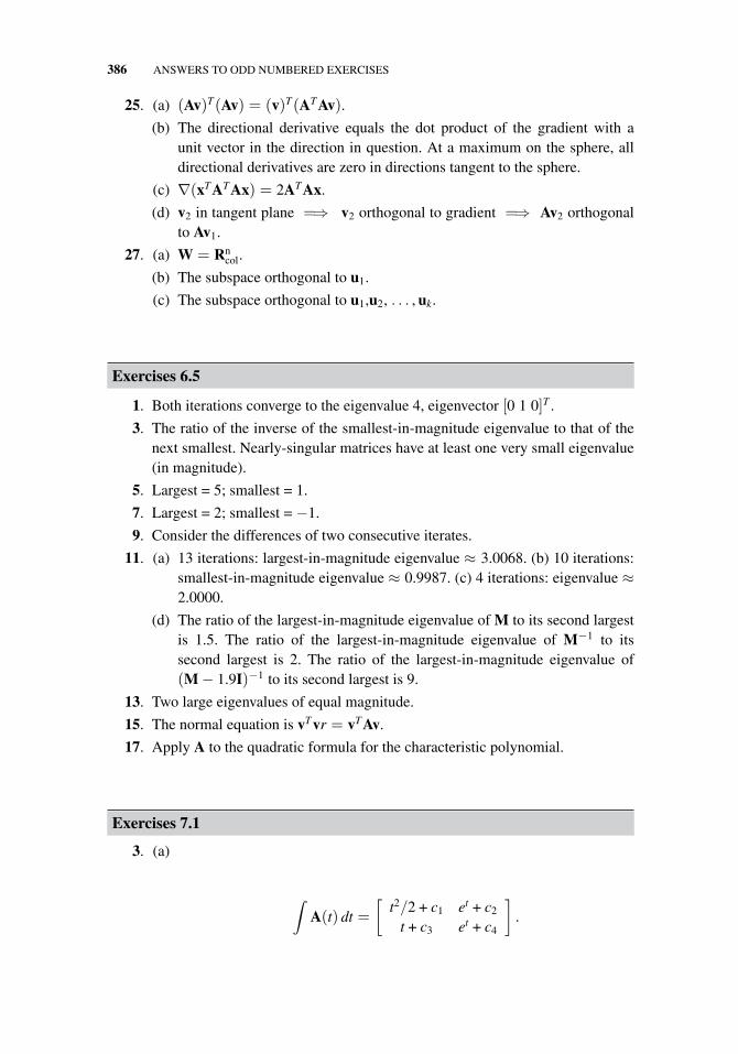
386 ANSWERS TO ODD NUMBERED EXERCISES
25. (a) (Av)T(Av) = (v)T(ATAv).
(b) The directional derivative equals the dot product of the gradient with aunit vector in the direction in question. At a maximum on the sphere, alldirectional derivatives are zero in directions tangent to the sphere.
(c) ∇(xTATAx) = 2ATAx.
(d) v2 in tangent plane =⇒ v2 orthogonal to gradient =⇒ Av2 orthogonalto Av1.
27. (a) W = Rncol.
(b) The subspace orthogonal to u1.
(c) The subspace orthogonal to u1,u2, . . . , uk.
Exercises 6.5
1. Both iterations converge to the eigenvalue 4, eigenvector [0 1 0]T .
3. The ratio of the inverse of the smallest-in-magnitude eigenvalue to that of thenext smallest. Nearly-singular matrices have at least one very small eigenvalue(in magnitude).
5. Largest = 5; smallest = 1.
7. Largest = 2; smallest = −1.
9. Consider the differences of two consecutive iterates.
11. (a) 13 iterations: largest-in-magnitude eigenvalue ≈ 3.0068. (b) 10 iterations:smallest-in-magnitude eigenvalue ≈ 0.9987. (c) 4 iterations: eigenvalue ≈2.0000.
(d) The ratio of the largest-in-magnitude eigenvalue of M to its second largestis 1.5. The ratio of the largest-in-magnitude eigenvalue of M−1 to itssecond largest is 2. The ratio of the largest-in-magnitude eigenvalue of(M − 1.9I)−1 to its second largest is 9.
13. Two large eigenvalues of equal magnitude.
15. The normal equation is vTvr = vTAv.
17. Apply A to the quadratic formula for the characteristic polynomial.
Exercises 7.1
3. (a)
∫A(t) dt =
[t2/2 + c1 et + c2
t + c3 et + c4
].
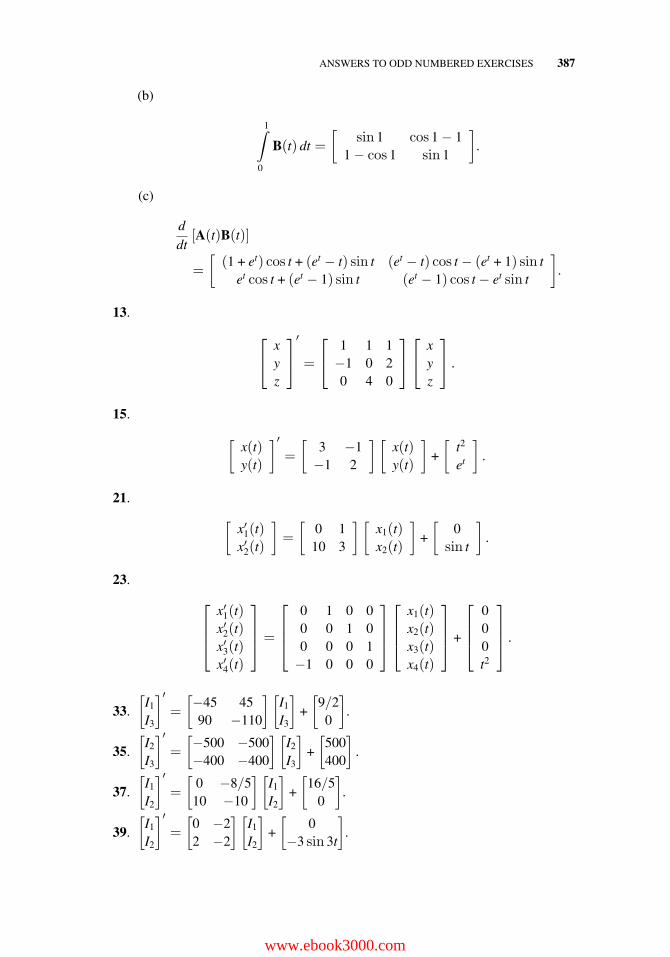
ANSWERS TO ODD NUMBERED EXERCISES 387
(b)
1∫0
B(t) dt =
[sin 1 cos 1 − 1
1 − cos 1 sin 1
].
(c)
ddt
[A(t)B(t)]
=
[(1 + et) cos t + (et − t) sin t (et − t) cos t − (et + 1) sin t
et cos t + (et − 1) sin t (et − 1) cos t − et sin t
].
13.
⎡⎣ x
yz
⎤⎦′
=
⎡⎣ 1 1 1
−1 0 20 4 0
⎤⎦⎡⎣ x
yz
⎤⎦ .
15.
[x(t)y(t)
]′=
[3 −1−1 2
] [x(t)y(t)
]+
[t2
et
].
21.
[x′1(t)x′2(t)
]=
[0 1
10 3
] [x1(t)x2(t)
]+
[0
sin t
].
23.
⎡⎢⎢⎣
x′1(t)x′2(t)x′3(t)x′4(t)
⎤⎥⎥⎦ =
⎡⎢⎢⎣
0 1 0 00 0 1 00 0 0 1−1 0 0 0
⎤⎥⎥⎦
⎡⎢⎢⎣
x1(t)x2(t)x3(t)x4(t)
⎤⎥⎥⎦ +
⎡⎢⎢⎣
000t2
⎤⎥⎥⎦ .
33.
[I1
I3
]′=
[−45 4590 −110
] [I1
I3
]+
[9/2
0
].
35.
[I2
I3
]′=
[−500 −500−400 −400
] [I2
I3
]+
[500400
].
37.
[I1
I2
]′=
[0 −8/5
10 −10
] [I1
I2
]+
[16/5
0
].
39.
[I1
I2
]′=
[0 −22 −2
] [I1
I2
]+
[0
−3 sin 3t
].
www.ebook3000.com
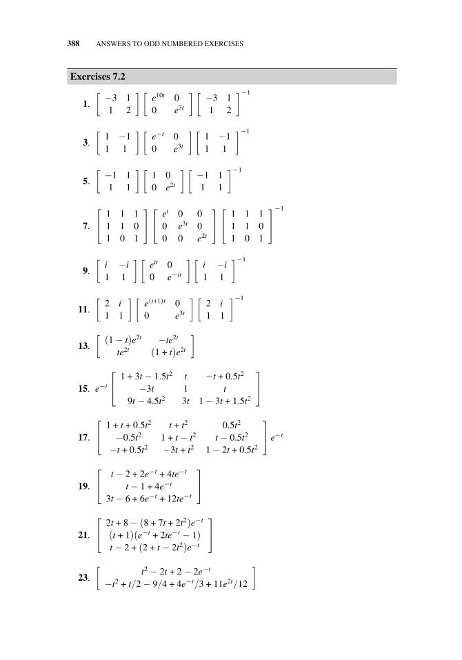
388 ANSWERS TO ODD NUMBERED EXERCISES
Exercises 7.2
1.
[−3 11 2
] [e10t 00 e3t
] [−3 11 2
]−1
3.
[1 −11 1
] [e−t 00 e3t
] [1 −11 1
]−1
5.
[−1 11 1
] [1 00 e2t
] [−1 11 1
]−1
7.
⎡⎣ 1 1 1
1 1 01 0 1
⎤⎦⎡⎣ et 0 0
0 e3t 00 0 e2t
⎤⎦⎡⎣ 1 1 1
1 1 01 0 1
⎤⎦−1
9.
[i −i1 1
] [eit 00 e−it
] [i −i1 1
]−1
11.
[2 i1 1
] [e(i+1)t 00 e3t
] [2 i1 1
]−1
13.
[(1 − t)e2t −te2t
te2t (1 + t)e2t
]
15. e−t
⎡⎣ 1 + 3t − 1.5t2 t −t + 0.5t2
−3t 1 t9t − 4.5t2 3t 1 − 3t + 1.5t2
⎤⎦
17.
⎡⎣ 1 + t + 0.5t2 t + t2 0.5t2
−0.5t2 1 + t − t2 t − 0.5t2
−t + 0.5t2 −3t + t2 1 − 2t + 0.5t2
⎤⎦ e−t
19.
⎡⎣ t − 2 + 2e−t + 4te−t
t − 1 + 4e−t
3t − 6 + 6e−t + 12te−t
⎤⎦
21.
⎡⎣ 2t + 8 − (8 + 7t + 2t2)e−t
(t + 1)(e−t + 2te−t − 1)t − 2 + (2 + t − 2t2)e−t
⎤⎦
23.
[t2 − 2t + 2 − 2e−t
−t2 + t/2 − 9/4 + 4e−t/3 + 11e2t/12
]
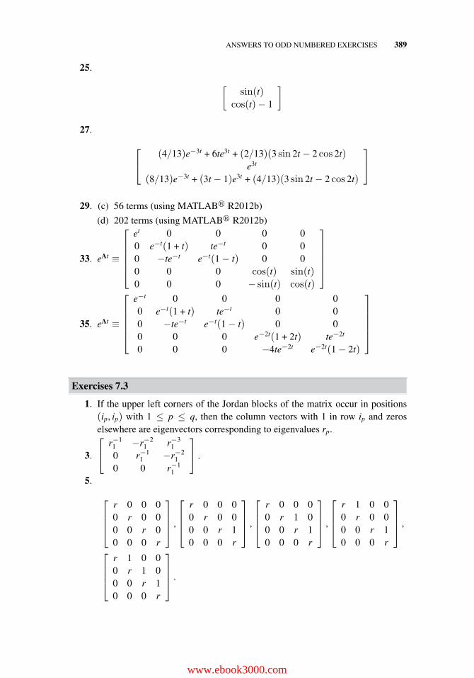
ANSWERS TO ODD NUMBERED EXERCISES 389
25.
[sin(t)
cos(t)− 1
]
27.
⎡⎣ (4/13)e−3t + 6te3t + (2/13)(3 sin 2t − 2 cos 2t)
e3t
(8/13)e−3t + (3t − 1)e3t + (4/13)(3 sin 2t − 2 cos 2t)
⎤⎦
29. (c) 56 terms (using MATLAB� R2012b)
(d) 202 terms (using MATLAB� R2012b)
33. eAt ≡
⎡⎢⎢⎢⎢⎣
et 0 0 0 00 e−t(1 + t) te−t 0 00 −te−t e−t(1 − t) 0 00 0 0 cos(t) sin(t)0 0 0 − sin(t) cos(t)
⎤⎥⎥⎥⎥⎦
35. eAt ≡
⎡⎢⎢⎢⎢⎣
e−t 0 0 0 00 e−t(1 + t) te−t 0 00 −te−t e−t(1 − t) 0 00 0 0 e−2t(1 + 2t) te−2t
0 0 0 −4te−2t e−2t(1 − 2t)
⎤⎥⎥⎥⎥⎦
Exercises 7.3
1. If the upper left corners of the Jordan blocks of the matrix occur in positions(ip, ip) with 1 ≤ p ≤ q, then the column vectors with 1 in row ip and zeroselsewhere are eigenvectors corresponding to eigenvalues rp.
3.
⎡⎣ r−1
1 −r−21 r−3
1
0 r−11 −r−2
1
0 0 r−11
⎤⎦ .
5.
⎡⎢⎢⎣
r 0 0 00 r 0 00 0 r 00 0 0 r
⎤⎥⎥⎦ ,
⎡⎢⎢⎣
r 0 0 00 r 0 00 0 r 10 0 0 r
⎤⎥⎥⎦ ,
⎡⎢⎢⎣
r 0 0 00 r 1 00 0 r 10 0 0 r
⎤⎥⎥⎦ ,
⎡⎢⎢⎣
r 1 0 00 r 0 00 0 r 10 0 0 r
⎤⎥⎥⎦ ,
⎡⎢⎢⎣
r 1 0 00 r 1 00 0 r 10 0 0 r
⎤⎥⎥⎦ .
www.ebook3000.com
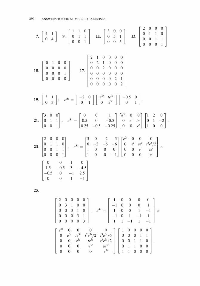
390 ANSWERS TO ODD NUMBERED EXERCISES
7.
[4 10 4
]9.
⎡⎣ 1 1 0
0 1 10 0 1
⎤⎦ 11.
⎡⎣ 3 0 0
0 5 10 0 5
⎤⎦ 13.
⎡⎢⎢⎣
2 0 0 00 1 1 00 0 1 10 0 0 1
⎤⎥⎥⎦
15.
⎡⎢⎢⎣
0 1 0 00 0 0 00 0 0 10 0 0 0
⎤⎥⎥⎦ 17.
⎡⎢⎢⎢⎢⎢⎢⎢⎣
2 1 0 0 0 00 2 1 0 0 00 0 2 0 0 00 0 0 0 0 00 0 0 0 2 10 0 0 0 0 2
⎤⎥⎥⎥⎥⎥⎥⎥⎦
19.
[3 10 3
]; eAt =
[−2 00 1
] [e3t te3t
0 e3t
] [−0.5 0
0 1
].
21.
⎡⎣3 0 0
0 1 10 0 1
⎤⎦ ; eAt =
⎡⎣ 0 0 1
0.5 0 −0.50.25 −0.5 −0.25
⎤⎦⎡⎣e3t 0 0
0 et tet
0 0 et
⎤⎦⎡⎣1 2 0
0 1 −21 0 0
⎤⎦ .
23.
⎡⎢⎢⎣
2 0 0 00 1 1 00 0 1 10 0 0 1
⎤⎥⎥⎦ ; eAt =
⎡⎢⎢⎣
3 0 −2 −56 −2 −6 −61 0 0 01 0 0 −1
⎤⎥⎥⎦
⎡⎢⎢⎣
e2t 0 0 00 et tet t2et/20 0 et tet
0 0 0 et
⎤⎥⎥⎦×
⎡⎢⎢⎣
0 0 1 01.5 −0.5 3 −4.5−0.5 0 −1 2.5
0 0 1 −1
⎤⎥⎥⎦
25.
⎡⎢⎢⎢⎢⎣
2 0 0 0 00 3 1 0 00 0 3 1 00 0 0 3 10 0 0 0 3
⎤⎥⎥⎥⎥⎦ ; eAt =
⎡⎢⎢⎢⎢⎣
1 0 0 0 0−1 0 0 0 11 0 0 1 −1−1 0 1 −1 11 1 −1 1 −1
⎤⎥⎥⎥⎥⎦×
⎡⎢⎢⎢⎢⎣
e2t 0 0 0 00 e3t te3t t2e3t/2 t3e3t/60 0 e3t te3t t3e3t/20 0 0 e3t te3t
0 0 0 0 e3t
⎤⎥⎥⎥⎥⎦
⎡⎢⎢⎢⎢⎣
1 0 0 0 00 0 0 1 10 0 1 1 00 1 1 0 01 1 0 0 0
⎤⎥⎥⎥⎥⎦ .
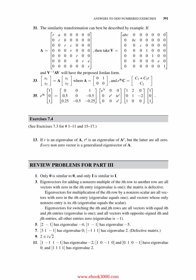
ANSWERS TO ODD NUMBERED EXERCISES 391
31. The similarity transformation can best be described by example. If
A =
⎡⎢⎢⎢⎢⎢⎢⎢⎢⎢⎣
r a 0 0 0 0 00 r b 0 0 0 00 0 r c 0 0 00 0 0 r 0 0 00 0 0 0 r 0 00 0 0 0 r e0 0 0 0 0 0 r
⎤⎥⎥⎥⎥⎥⎥⎥⎥⎥⎦
, then take V =
⎡⎢⎢⎢⎢⎢⎢⎢⎢⎢⎣
abc 0 0 0 0 0 00 bc 0 0 0 0 00 0 c 0 0 0 00 0 0 1 0 0 00 0 0 0 1 0 00 0 0 0 0 e 00 0 0 0 0 0 1
⎤⎥⎥⎥⎥⎥⎥⎥⎥⎥⎦
and V−1AV will have the proposed Jordan form.
33.
[x1
x2
]= A
[x1
x2
]where A =
[0 10 0
], and eAtC =
[C1 + C2t
C2
]
35. eAt
⎡⎣1
01
⎤⎦ =
⎡⎣ 0 0 1
0.5 0 −0.50.25 −0.5 −0.25
⎤⎦⎡⎣e3t 0 0
0 et tet
0 0 et
⎤⎦⎡⎣1 2 0
0 1 −21 0 0
⎤⎦⎡⎣1
01
⎤⎦ .
Exercises 7.4
(See Exercises 7.3 for # 1–11 and 15–17.)
13. If r is an eigenvalue of A, rp is an eigenvalue of Ap, but the latter are all zero.Every non zero vector is a generalized eigenvector of A.
REVIEW PROBLEMS FOR PART III
1. Only 0 is similar to 0, and only I is similar to I.
3. Eigenvectors for adding a nonzero multiple of the ith row to another row are allvectors with zero in the ith entry (eigenvalue is one); the matrix is defective.
Eigenvectors for multiplication of the ith row by a nonzero scalar are all vec-tors with zero in the ith entry (eigenvalue equals one); and vectors whose onlynonzero entry is its ith (eigenvalue equals the scalar).
Eigenvectors for switching the ith and jth rows are all vectors with equal ithand jth entries (eigenvalue is one); and all vectors with opposite-signed ith andjth entries, all other entries zero (eigenvalue is −1).
5. [2 − 1] has eigenvalue −4; [1 − 1] has eigenvalue −5.
7. [3 1 − 1] has eigenvalue 0; [−1 1 1] has eigenvalue 2. (Defective matrix.)
9. 2 ± i√
2
11. [1 −1 1 −1] has eigenvalue −2; [1 0 −1 0] and [0 1 0 −1] have eigenvalue0; and [1 1 1 1] has eigenvalue 2.
www.ebook3000.com
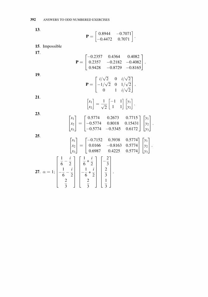
392 ANSWERS TO ODD NUMBERED EXERCISES
13.
P =
[0.8944 −0.7071−0.4472 0.7071
].
15. Impossible
17.
P =
⎡⎣−0.2357 0.4364 0.4082
0.2357 −0.2182 −0.40820.9428 −0.8729 −0.8165
⎤⎦ .
19.
P =
⎡⎣ i/
√2 0 i/
√2
−1/√
2 0 1/√
20 1 i/
√2
⎤⎦ .
21. [x1
x2
]=
1√2
[−1 11 1
] [y1
y2
].
23. ⎡⎣x1
x2
x3
⎤⎦ =
⎡⎣ 0.5774 0.2673 0.7715−0.5774 0.8018 0.15431−0.5774 −0.5345 0.6172
⎤⎦⎡⎣y1
y2
y3
⎤⎦ .
25. ⎡⎣x1
x2
x3
⎤⎦ =
⎡⎣−0.7152 0.3938 0.5774
0.0166 −0.8163 0.57740.6987 0.4225 0.5774
⎤⎦⎡⎣y1
y2
y3
⎤⎦ .
27. α = 1;
⎡⎢⎢⎢⎢⎢⎢⎣
16− i
2
−16− i
223
⎤⎥⎥⎥⎥⎥⎥⎦
⎡⎢⎢⎢⎢⎢⎢⎣
16
+i2
−16
+i2
23
⎤⎥⎥⎥⎥⎥⎥⎦
⎡⎢⎢⎢⎢⎢⎢⎣
−23
2313
⎤⎥⎥⎥⎥⎥⎥⎦
.

INDEX
adjoint, 103–4affine transformations, 123–7associative law, 61–3, 67augmented coefficient matrix, 18
back substitution, 9basis, 152, 155best approximation, 182block diagonal matrix, 317block matrix, 98boundary value problem, 2, 118–19
C(a,b), 135canonical basis, 152CAT (computerized axial tomography), 3Cauchy–Schwarz inequality, 173Cayley–Hamilton theorem, 262, 264change of coordinate, 153–4characteristic equation, polynomial, 217, 243Cholesky factorization, 117, 343circulant matrix, 215, 253, 345coefficient matrix, 17cofactor, 92–3commutative law, 61completing the square, 245complex equations, 15
Fundamentals of Matrix Analysis with Applications,First Edition. Edward Barry Saff and Arthur David Snider.© 2016 John Wiley & Sons, Inc. Published 2016 by John Wiley & Sons, Inc.
condition number, 54, 272consistent systent, 29, 42controllability, 199–200Cramer’s rule, 105Cm
row (Cncol) (Cm,n), 135
defective matrix, 224deflated matrix, 216, 225determinant, 90, 97, 101–2, 112, 148diagonal matrix, 19diagonalization of matrix, 238diagonally dominant, 125diet, antarctic, 1, 37dimension, 156, 191, 202–4discrete Fourier transform, 345discrete time system, signal, 254distributive law, 62–3dot product, 59Durer, A., 198
echelon form, 39eigenvalue, eigenvector, 209, 223, 322electrical circuit, 40, 304–6elementary column operations, 25, 158elementary row matrix operator, 63elementary row operations, 20, 63, 158
www.ebook3000.com

394 INDEX
fast Fourier transform, 345Fibonacci sequence, 163, 350fixed point method, 123–7Fredholm alternative, 189free variable, 32, 39Frobenius norm, 244function space, 190fundamental matrix, 312
Gauss elimination, 7–10, 27–34, 39back substitution, 9basic operations, 10operations count, 12–13, 16
Gauss, C. F., 7Gauss–Jordan algorithm, 22–4Gauss–Seidel, 126generalized eigenvector, 224,
322–3, 334geometric series, 243, 255global positioning systems, 122–3golden ratio, 350Goldstine, H., 47, 50gradient, 246, 281Gram matrix, 163, 196, 343Gram–Schmidt algorithm, 169
Haar, 202–4heat transfer, 302Hermitian matrix, 228–9, 258Hessenberg form, 344Hilbert matrix, 54, 196Hilbert space, 193homogeneous system, 42Hooke’s law, 2, 45Householder reflectors, 176,
179, 201
identity matrix, 63incidence matrix, 121inconsistent system, 29, 45inertia tensor, 255inner product, 59inner product, 193integer equations, 16integrating factor, 312interconnected tanks, 296, 301interpolation, 15inverse, 76–80, 83, 85invertible, 77
Jacobi, 125Jordan block, 318
Jordan chain, 336Jordan form, 318, 333Jordan, W., 24
kernel, 136Kirchhoff’s laws, 44, 120–122
Lagrange interpolation problem, 15least squares, 183, 185, 274, 348
polynomial approximation, 26least squares fit, straight line, 186left inverse, 76–9Legendre polynomial, 194linear algebraic equations, 5
graphs, 6, 7linear combination, 137
combination principle, 138linear dependence (independence), 145, 147,
191–3linear systems, 5lower trapezoidal matrix, 19lower triangular matrix, 19LU factorization, 116–18, 286
magic square, 198mappings, 141mass-spring system, 2, 45, 248–52, 297,
302–3, 333matrix
addition, 62addresses, 25augmented coefficient, 18block, 98coefficient, 17column, 20diagonal, 19differential equation, 295, 307, 329, 336exponential, 241, 307, 308, 311, 314,
323–5, 337incidence, 121inverse, 76multiplication, 58–61, 115–16nilpotent, 85representation, 17row, 20scalar multiplication, 62skew-symmetric, 110stochastic, 69symmetric, 226, 258trapezoidal, 19triangular, 19
matrix operator

INDEX 395
elementary row, 63mirror reflection, 72–3, 76, 201orthogonal projection, 71–2, 75rotation, 70–71, 201
matrix square root, 240minor, 92, 343modal analysis, 252
nilpotent, 85matrix, 338
norm, 166, 174, 228, 244, 271normal equations, 184normal matrix, 260, 261, 264normal modes, 251null space, 136nullity, 156, 158
operations count, 12–13, 16orthogonal, 166, 228
matrices, 174, 201subspace decomposition, 182
Padovan sequence, 351parallelogram law, 173parametrization of silutions, 32, 35–6permutation, 97pivot
complete, 54element, 30, 39, 49, 52partial, 49, 52, 53
plastic constant, 351Pn, 135positive definite matrix, 342–3power method, 283primary decomposition theorem, 323principal axes, 247principal component analysis, 278products of inertia, 255pseudoinverse, 274
QRfactorization, 201–2, 290method, 285
quadratic form, 244quadratic polynomial, 245
range, 156, 158rank, 40
reduction, 278rank one matrix, 162, 216Rayleigh quotient, 253, 290redundant system, 28
reflection, 201right inverse, 76–9rotation, 201, 221roundoff, 46–50row echelon form, 39–40row space, 158row-reduced echelon form, 39Rm
row (Rmcol) (Rm,n), 135
scalar multiplication, 133Schur decomposition, 258self-adjoint, 228shear matrix, 332Sherman–Morrison–Woodbury, 85shifted eigenvalue, 210similarity transformation, 235singular, 77singular value decomposition, 266, 269,
279, 346skew-symmetric, 110, 232span, 138spectral factorization, theorem, 239speed, 16stiffness matrix, 251, 255stochastic matrix, 69, 290subspace, 135Sylvester, j. j., 17Sylvester’s criterion, 343symmetric matrix, 226, 258systems of linear equations, 5
time, computation, 16, 95total least squares, 348trace, 225transpose, 69–70, 81, 83trapezoidal matrix, 19triangle inequality, 173triangular matrix, 19, 213, 217
unitary matrix, 228, 258, 260upper trapezoidal matrix, 19upper triangular matrix, 19, 258
Vandermonde, 99, 195, 243variation of parameters, 312vector (row, column), 20vector space, 133von Neumann, 47, 50
wavelet, 202–4weighted least squares, 188Wilkinson, J., 47, 51
www.ebook3000.com