Fuel Burn Estimation Using Real Track Data

Fuel Burn Estimation Using Real Track Data

Journal: 11th AIAA ATIO Conference, AIAA Centennial of Naval Aviation

Forum

Manuscript ID: Draft

luMeetingID: 2511

Date Submitted by the Author:

n/a

Contact Author: Chatterji, Gano Broto

http://mc.manuscriptcentral.com/aiaa-matio11

11th AIAA ATIO Conference, AIAA Centennial of Naval Aviation Forum

American Institute of Aeronautics and Astronautics

1

Fuel Burn Estimation Using Real Track Data

Gano B. Chatterji* University of California Santa Cruz, Moffett Field, CA, 94035-1000

A procedure for estimating fuel burned based on actual flight track data, and drag and fuel-flow models is described. The procedure consists of estimating aircraft and wind states, lift, drag and thrust. Fuel-flow for jet aircraft is determined in terms of thrust, true airspeed and altitude as prescribed by the Base of Aircraft Data fuel-flow model. This paper provides a theoretical foundation for computing fuel-flow with most of the information derived from actual flight data. The procedure does not require an explicit model of thrust and calibrated airspeed/Mach profile which are typically needed for trajectory synthesis. To validate the fuel computation method, flight test data provided by the Federal Aviation Administration were processed. Results from this method show that fuel consumed can be estimated within 1% of the actual fuel consumed in the flight test. Next, fuel consumption was estimated with simplified lift and thrust models. Results show negligible difference with respect to the full model without simplifications. An iterative takeoff weight estimation procedure is described for estimating fuel consumption, when takeoff weight is unavailable, and for establishing fuel consumption uncertainty bounds. Finally, the suitability of using radar-based position information for fuel estimation is examined. It is shown that fuel usage could be estimated within 5.4% of the actual value using positions reported in the Airline Situation Display to Industry data with simplified models and iterative takeoff weight computation.

I. Introduction he amount of fuel consumed is an important metric for benefit assessment of air traffic management concepts being considered for improving throughput, increasing capacity and reducing delays. It is also an important

metric for environmental impact because for each kilogram of fuel consumed, three kilograms of carbon dioxide, a greenhouse gas, is generated. The main motivations for developing the fuel estimation method is to establish a baseline for the current operations and based on it determine benefits of the proposed four-dimensional trajectory management concepts in terms of fuel usage. Alternative procedures for efficient descent, terminal area scheduling and spacing, and departure release can also be evaluated based on fuel consumption. Four prior related publications on the subject of fuel estimation are cited here as Refs. 1-4. References 1 and 2 are focused on departure and arrival fuel consumption below 10,000 feet altitude. Reference 1 compares the International Civil Aviation Organization (ICAO) time-in-mode method based fuel consumption with the actual fuel consumption reported in Flight Data Recorders. Fuel flow-rate patterns were found to be quite different than the ICAO model estimates due to airline climb/descent procedures. This suggests that a fuel consumption model should include aircraft state information such as airspeed. Reference 2 presents thrust specific fuel consumption models for climb and descent. Model parameters are adjusted to fit the aircraft manufacturer data. Thrust specific fuel consumption is multiplied with thrust to determine fuel consumption. Their method assumes nominal climb/descent profiles; it does not consider airline and air traffic control specific operational procedures. Furthermore, the method is only applicable to lower altitudes. Reference 3 describes a closed-form takeoff weight estimation method developed using the constant-altitude-cruise range equation and aircraft design principles. It needs flight-plan data and aircraft performance model to estimate the takeoff weight of the aircraft. The amount of fuel needed for climb, cruise and descent phases of flight and the maximum load factor are computed as a part of the procedure. The method described in this paper differs from Ref. 3 in that it uses the actual flight track data and does not require a model for climb and descent; thus, it is more data driven than model based. Reference 4 describes a fuel estimation procedure using actual trajectory of aircraft, and Base of Aircraft Data (BADA) drag and fuel-flow models. Their procedure is close to the method described here. The main difference is that the fuel estimation procedure is derived

* Scientist and Task Manager, U. C. Santa Cruz, MS 210-8, Associate Fellow.

T

Page 1 of 17




2

Figure 1. Fuel burn estimation procedure.

from nonlinear equations of motion with point-mass assumptions as opposed to approximations adopted in Ref. 4. Additional contribution of the present work is estimation of aircraft and wind states. Main contribution of this paper is development of the fuel estimation procedure from basic principles without simplifications. The procedure was validated against flight test data provided by the Federal Aviation Administration. A takeoff weight estimation procedure is developed for estimating fuel usage and establishing fuel usage uncertainty bounds when the takeoff weight of the aircraft is unknown. Finally, the adequacy of using position data acquired by air traffic control radar systems for fuel estimation is examined. Results show that in spite of bias, noise and data drop issues, position data could be conditioned for obtaining decent fuel estimates. Section II describes the fuel estimation procedure. The BADA fuel-flow model is discussed in Section III. The equations of motion are given in Section IV. This section also lists an expression for thrust in terms of drag, and aircraft and wind states. Section V provides the BADA drag model. Expressions for lift and bank angle estimation are listed in Section VI. Aircraft state estimation is described in Section VII. Results are discussed in Section VIII. The paper is concluded in Section IX.

II. Fuel Burn Estimation Procedure To determine the amount of fuel consumed, altitude, airspeed and thrust have to be estimated. Altitude is obtained from the trajectory. Airspeed is estimated using a sequence of latitude (! ), longitude (! ) and altitude ( h ) reports as a function of time that define the four-dimensional trajectory and wind velocity. Computation of thrust requires an estimate of drag, which depends on lift. Lift depends on estimated aircraft and wind states, and weight. Once lift is determined, the lift induced drag coefficient can be computed. Drag is a function of airspeed, air density, and the drag coefficient, which depends on the aerodynamic configuration of the aircraft. Thrust is determined using estimates of aircraft and wind states, drag and weight. Fuel-flow rate is then obtained using altitude, airspeed and thrust estimates. Weight of the aircraft at a point in time is obtained by subtracting the amount of fuel consumed up to that time from the initial weight (takeoff weight). Fig. 1 shows the steps of the fuel burn estimation procedure.

III. BADA Fuel Consumption Model The BADA fuel consumption model is described for nominal and idle thrust conditions. The nominal fuel-flow

rate for jets and turboprops is determined by the product of the thrust specific fuel consumption and thrust, T . Thrust specific fuel consumption for jets is modeled as a linear function of airspeed, V , and for turboprops as a quadratic function of airspeed. Fuel-flow rate is independent of airspeed and thrust for aircraft with piston engines. A generalized expression for the nominal fuel-flow rate for these three different aircraft types can be written in the following form5:

( )TVfVffffnom2

3210!++= (1)

where the coefficients in Eq. (1) are given in terms of the BADA coefficients 1fC and

2fC in Table 1. Units of the BADA coefficients are provided in the Appendix for completeness. Fuel-flow rate is in kg/s with airspeed in knots and thrust in Newtons. The minimum fuel-flow rate for idle thrust is modeled as a linear function of altitude, h , for jet and turboprop engine types and as a constant for piston engine. This model is described by the following equation:

hfff54min

!= (2)

Page 2 of 17




3

Altitude is in feet. The coefficients are again defined in terms of BADA coefficients 3fC and

4fC in Table 2. Units of these BADA coefficients are also listed in the Appendix. Fuel-flow rate coefficients for a jet, a turboprop and a piston aircraft are listed in Table 6 of the Appendix to give the reader a feel for the contribution of these coefficients to fuel-flow rate in Eqs. (1) and (2).

The nominal and the minimum fuel-flow rate models can be combined into a single expression,

( )nomfcr fCff min,max= (3)

The fraction of fuel-flow rate during the cruise phase is fcrC . Its numerical value is 1 during the other flight phases. Equations (1) through (3) show that to estimate fuel-flow rate for jets and turboprops, altitude, airspeed, thrust and the phase of flight (in cruise or not) needs to be known. Altitude is directly available from position reports; airspeed, thrust and the phase of flight have to be estimated. Airspeed can be estimated using the reported position and wind data. Equations of motion, which are discussed in the next section, have to be used for thrust estimation. The amount of fuel consumed can be determined by integrating the fuel-flow rate as

!=ft

f dtfm0

(4)

Table 2. Minimum fuel-flow rate model coefficients.

Engine Type 4f 5

f

Jet 3

60

1

fC!"

#$%

&

!!

"

#

$$

%

&!"

#$%

&

4

3

60

1

f

f

C

C

Turboprop 3

60

1

fC!"

#$%

&

!!

"

#

$$

%

&!"

#$%

&

4

3

60

1

f

f

C

C

Piston 3

60

1

fC!"

#$%

&

0

Table 1. Nominal fuel-flow rate model coefficients.

Engine Type 0f

1f 2

f 3f

Jet 0 14

106

1

fC!"

#$%

&

'

!!

"

#

$$

%

&!"

#$%

&

'2

1

4106

1

f

f

C

C 0

Turboprop 0 0 17

106

1

fC!"

#$%

&

'

!!

"

#

$$

%

&!"

#$%

&

'2

1

7106

1

f

f

C

C

Piston 1

60

1

fC!"

#$%

& 0 0 0

Page 3 of 17




4

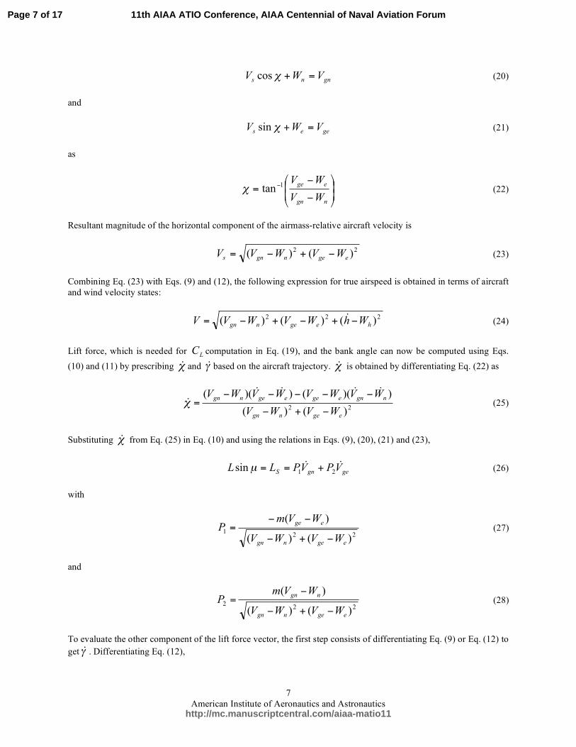
Figure 2. Velocity triangle.

where ft is the flight time.

IV. Equations of Motion The motion of aircraft, modeled as a point mass, is often described by the following three equations (see Ref.

6):

gnVhR )(

1

+=!& (5)

geVhR !

"cos)(

1

+=& (6)

and

hVh =& (7)

! is the latitude, ! is the longitude, h is the geometric altitude and R is the mean radius of the Earth. gnV and

geV are the north and east components of the ground-relative aircraft velocity. hV is the climb or descent rate

depending on whether it is positive or negative. The horizontal velocity of the aircraft with respect to the ground is the resultant of the horizontal components of the airmass-relative velocity of the aircraft and the wind velocity. This relationship is shown in Fig. 2, where

gV and s

W are the magnitudes of the horizontal

components of the ground-relative aircraft velocity and the wind velocity, and

sV is the magnitude of the

horizontal component of the airmass-relative aircraft velocity.

g! is the heading angle of the ground-relative

aircraft velocity with respect to the local north direction. ! and

w! are the heading angles of the airmass-relative

aircraft velocity and ground-relative wind velocity also with respect to the local north direction.

nW ,

eW and

hW as the north, east and up components of the wind velocity vector. The magnitude of the airmass-relative acceleration resulting from the thrust, drag, lift and gravitational forces on the aircraft modeled as a point mass is

!!"!"!#

sincossincoscossincos

hen WWWgm

DTV &&&& $$$$

$= (8)

where V is airmass-relative speed (true airspeed), T is thrust, D is drag, ! is angle-of-attack, m is mass, g is acceleration due to gravity and ! is flight path angle. Note that

!cosVVs= (9)

The kinetic equations for airmass-relative heading angle and flight path angle are

Page 4 of 17




5

!

"

!

"

!

µµ#"

cos

cos

cos

sin

cos

sinsinsin

V

W

V

W

mV

LTen

&&& $+

+= (10)

and

V

W

V

W

V

W

V

g

mV

LT hen !!"!"!µµ#!

cossinsinsincoscoscoscossin &&&& $++$

+= (11)

µ is bank angle and L is lift. Equations (9), (10) and (11) are derived assuming flat Earth, constant gravitational acceleration and slowly changing mass. The altitude rate, Eq. (7), can be written in terms of the airspeed, flight path angle and the vertical component of the wind velocity as

hh

WVVh +== !sin& (12)

Since wind varies both with position and time, the time derivative of the north, east and up components of the wind velocity can be determined as

handenihh

WWW

t

WW

iiii

i,; =

!

!+

!

!+

!

!+

!

!= &&&& "

"#

# (13)

Observe that !& , !& and h& are defined in Eqs. (5) through (7). Assuming the angle of attack to be zero in Eq. (8),

( ) ( )!"

!#

$

!%

!&

'

(()

*++,

- ..++

.+++=

2

1sincosV

WhWW

V

WhWgVmDT h

enh

h

&&&

&&& // (14)

This expressions shows that thrust estimate depends on drag, mass, altitude rate, airspeed, rate of change of airspeed, wind terms and the airmass-relative heading angle. Dropping the wind terms, the following simplified expression is obtained:

V

hmgVmDT

&& ++= (15)

It is now easy to see that the thrust required for balancing the right hand side of Eq. (15) during deceleration and descent can be less than the minimum thrust generated by the engines due to errors in the drag model and aircraft weight. A minimum thrust model is required in these instances. It can be constructed by equating Eq. (1) to Eq. (2) assuming the BADA fuel model to be consistent. Thus for jets and turboprops, the minimum thrust is obtained as,

2

321

504

min

VfVff

hfffT

!+

!!= (16)

Note that Eq. (16) cannot be used for piston engines because nominal, minimum and cruise fuel-flow are specified to be a constants for piston engines in BADA.

Page 5 of 17




6

V. Drag Model Aerodynamic drag force is obtained as the product of the drag coefficient,

DC , and the dynamic pressure as

SVCDD

2

2

1!= (17)

where ! is the density of air and S is the wing reference area. DC is given as the sum of the zero-lift drag

coefficient, 0D

C , and the induced drag coefficient, which is a quadratic function of the lift coefficient, LC . Thus,

2

20 LDDDCCCC += (18)

0DC and

2DC are functions of aerodynamic configuration of the aircraft. BADA coefficients associated with the

aerodynamic configuration are listed in Table 3. Traditionally drag coefficients are given as a function of Mach number and Reynolds number. BADA models these values as constants; it does not take Mach and Reynolds number effects into account. Note that the additional term

LDGDC !,0 represents drag rise due to deployment of the

landing gear. During the approach and landing configurations, drag coefficients are adjusted for flap setting. One of difficulties of drag computation is determining the aerodynamic configuration. BADA specifies conditions based on stall speeds and maximum altitude thresholds that have to be met based on airspeed and altitude to determine the aerodynamic configuration. The only remaining parameter that needs to be specified for drag computation is

LC ,

which can be obtained using the definition of the lift force as

SV

LCL 2

2

!= (19)

The lift force needed is related to heading angle and flight path angle rates as shown in Eqs. (10) and (11), therefore assumptions have to be made about the trajectory being followed. This is discussed in the next section.

VI. Trajectory Assumptions To stay on course in a wind field, the aircraft has to crab such that the across-track component of the wind is cancelled. The airmass-relative heading angle needed to stay on the path specified by the course angle

g! is

obtained from the two relations based on Fig. 2:

Table 3. Drag coefficients as a function of aerodynamic configuration.

Aerodynamic Configuration 0D

C 2D

C

Takeoff TODC

,0

TODC

,2

Initial Climb ICDC

,0

ICDC

,2

Clean CRDC

,0

CRDC

,2

Approach APDC

,0

APDC

,2

Landing LDGDLDDCC !+

,0,0

LDDC

,2

Page 6 of 17




7

gnns VWV =+!cos (20)

and

gees VWV =+!sin (21)

as

!!

"

#

$$

%

&

'

'=

'

ngn

ege

WV

WV1

tan( (22)

Resultant magnitude of the horizontal component of the airmass-relative aircraft velocity is

22 )()( egengns WVWVV !+!= (23)

Combining Eq. (23) with Eqs. (9) and (12), the following expression for true airspeed is obtained in terms of aircraft and wind velocity states:

222 )()()( hegengn WhWVWVV !+!+!= & (24)

Lift force, which is needed for LC computation in Eq. (19), and the bank angle can now be computed using Eqs.

(10) and (11) by prescribing !& and !& based on the aircraft trajectory. !& is obtained by differentiating Eq. (22) as

22 )()(

))(())((

egengn

ngnegeegengn

WVWV

WVWVWVWV

!+!

!!!!!=

&&&&

&" (25)

Substituting !& from Eq. (25) in Eq. (10) and using the relations in Eqs. (9), (20), (21) and (23),

gegnS VPVPLL &&21

sin +==µ (26)

with

22

1

)()(

)(

egengn

ege

WVWV

WVmP

!+!

!!= (27)

and

22

2

)()(

)(

egengn

ngn

WVWV

WVmP

!+!

!= (28)

To evaluate the other component of the lift force vector, the first step consists of differentiating Eq. (9) or Eq. (12) to get!& . Differentiating Eq. (12),

Page 7 of 17




8

!

!!

cos

sin

V

VWhh

&&&&

&""

= (29)

Substituting in Eq. (11) and using Eqs. (9), (12), (20) and (21),

gPhVPhVPhPVPVPLL gegngegnC 576543cos +++++== &&&&&&&&µ (30)

with

22222

3

)()()()()(

)(

hegengnegengn

hngn

WhWVWVWVWV

WWVmP

!+!+!!+!

!=

& (31)

22222

4

)()()()()(

)(

hegengnegengn

hege

WhWVWVWVWV

WWVmP

!+!+!!+!

!=

& (32)

222

22

5

)()()(

)()(

hegengn

egengn

WhWVWV

WVWVmP

!+!+!

!+!=

& (33)

22222

6

)()()()()(

)(

hegengnegengn

ngn

WhWVWVWVWV

WVmP

!+!+!!+!

!!=

& (34)

and

22222

7

)()()()()(

)(

hegengnegengn

ege

WhWVWVWVWV

WVmP

!+!+!!+!

!!=

& (35)

Lift force and the bank angle can be determined using Eq. (26) and (30);

22

CSLLL += (36)

!!"

#$$%

&= '

C

S

L

L1

tanµ (37)

LC can now be obtained using Eq. (19) with lift force determined using Eq. (36). Drag force can be determined using Eqs. (18) and (17). Finally, thrust can be computed using Eq. (14). Note that the airspeed and airmass-relative acceleration in Eq. (14) can be replaced by ground-relative terms using Eqs. (20), (21), (23) and (24) as described in the Appendix. The fuel-flow rate is determined using Eq. (3) via Eqs. (1) and (2), and the fuel consumed is obtained using Eq. (4).

Page 8 of 17




9

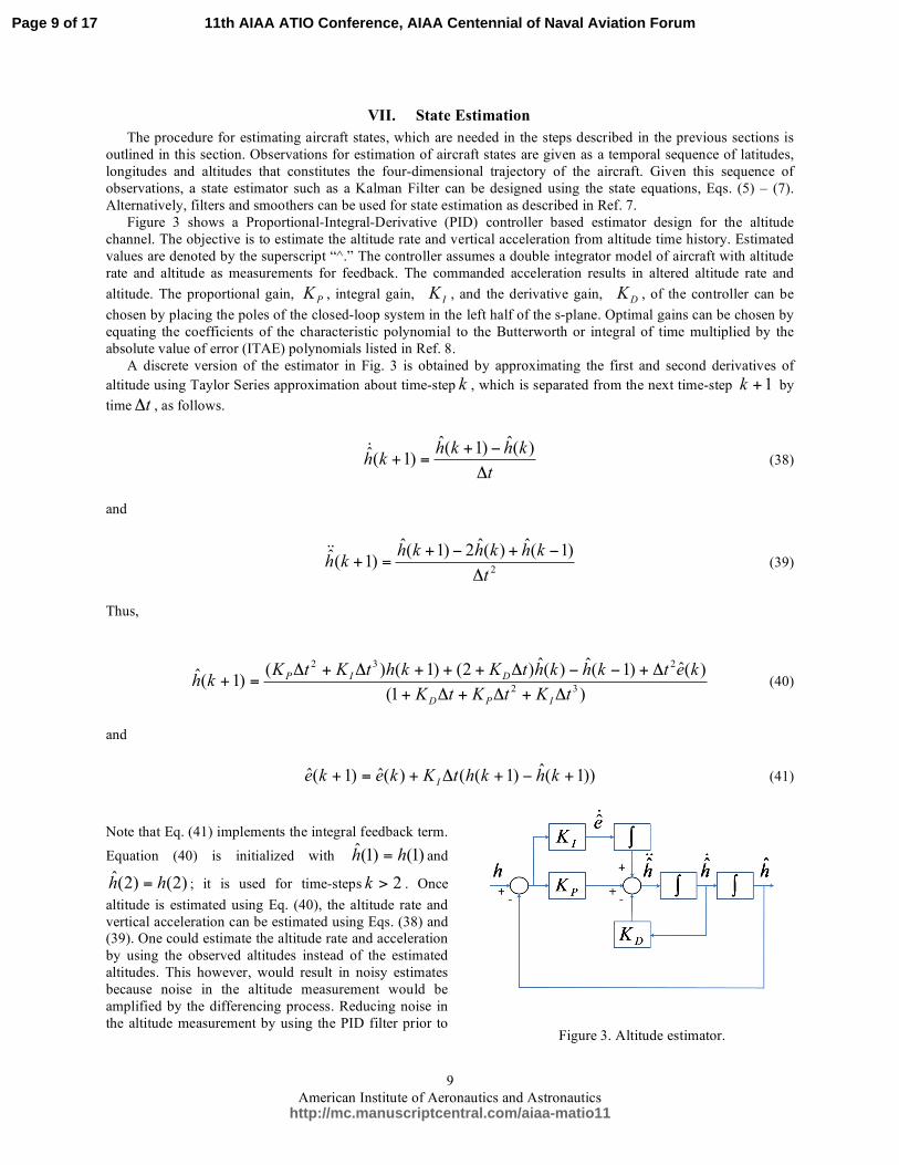
Figure 3. Altitude estimator.

VII. State Estimation The procedure for estimating aircraft states, which are needed in the steps described in the previous sections is outlined in this section. Observations for estimation of aircraft states are given as a temporal sequence of latitudes, longitudes and altitudes that constitutes the four-dimensional trajectory of the aircraft. Given this sequence of observations, a state estimator such as a Kalman Filter can be designed using the state equations, Eqs. (5) – (7). Alternatively, filters and smoothers can be used for state estimation as described in Ref. 7. Figure 3 shows a Proportional-Integral-Derivative (PID) controller based estimator design for the altitude channel. The objective is to estimate the altitude rate and vertical acceleration from altitude time history. Estimated values are denoted by the superscript “^.” The controller assumes a double integrator model of aircraft with altitude rate and altitude as measurements for feedback. The commanded acceleration results in altered altitude rate and altitude. The proportional gain,

PK , integral gain,

IK , and the derivative gain,

DK , of the controller can be

chosen by placing the poles of the closed-loop system in the left half of the s-plane. Optimal gains can be chosen by equating the coefficients of the characteristic polynomial to the Butterworth or integral of time multiplied by the absolute value of error (ITAE) polynomials listed in Ref. 8. A discrete version of the estimator in Fig. 3 is obtained by approximating the first and second derivatives of altitude using Taylor Series approximation about time-step k , which is separated from the next time-step 1+k by time t! , as follows.

t

khkhkh

!

"+=+

)(ˆ)1(ˆ)1(

&̂ (38)

and

2

)1(ˆ)(ˆ2)1(ˆ)1(ˆ

t

khkhkhkh

!

"+"+=+

&& (39)

Thus,

)1(

)(ˆ)1(ˆ)(ˆ)2()1()()1(ˆ

32

232

tKtKtK

ketkhkhtKkhtKtKkh

IPD

DIP

!+!+!+

!+""!+++!+!=+ (40)

and

))1(ˆ)1(()(ˆ)1(ˆ +!+"+=+ khkhtKkekeI

(41)

Note that Eq. (41) implements the integral feedback term.

Equation (40) is initialized with )1()1(ˆ hh = and

)2()2(ˆ hh = ; it is used for time-steps 2>k . Once altitude is estimated using Eq. (40), the altitude rate and vertical acceleration can be estimated using Eqs. (38) and (39). One could estimate the altitude rate and acceleration by using the observed altitudes instead of the estimated altitudes. This however, would result in noisy estimates because noise in the altitude measurement would be amplified by the differencing process. Reducing noise in the altitude measurement by using the PID filter prior to

Page 9 of 17




10

Figure 4. Actual latitude/longitude position history.

taking differences results in smoother altitude rate and acceleration estimates. The estimator implemented by Eqs. (38) through (41) is also used for the latitude and longitude channels with latitude and longitude measurements. These independent estimators provide estimates of angles, angular rates and

angular accelerations: !̂ , !&̂

, !&&̂

, !̂ , !&̂ and !&&̂ . The horizontal components of the aircraft velocity vector can now be estimated using Eqs. (5) and (6). Finally, the acceleration terms can be estimated using derivatives of Eqs. (5) and (6) as follows:

!!&&&&& ˆˆˆ)ˆ(ˆ hhRVgn ++= (42)

and

!"!""!" &&&&&&&ˆˆˆcosˆˆˆsin)ˆ(ˆˆcos)ˆ(ˆ hhRhRVge ++#+= (43)

With the aircraft states computed using the altitude and the latitude/longitude estimators, and the wind related estimates obtained using Eq. (13), lift, drag, thrust and fuel-flow rate can be computed. The north and east components of the wind velocity vector can be obtained as a function of time, latitude, longitude and altitude from the Rapid Update Cycle (RUC) data, which are provided by the National Oceanic and Atmospheric Administration (NOAA). The vertical wind velocity can be computed by post processing RUC data using the relation described on page 480 of Ref. 9.

hW is small relative to

nW and

eW ; it can be assumed to be zero.

VIII. Results This section is organized into five subsections. The first subsection on validation describes the flight test

conditions and compares the estimated states with the actual states from the Flight Data Recorder (FDR). Fuel estimation accuracy is examined for the climb, cruise and descent phases of the flight in the second subsection. The next subsection discusses model simplification and its effect on fuel usage estimate. A procedure for takeoff weight estimation that starts by setting the takeoff weight to the maximum zero-fuel weight and then iteratively improves the estimate by adding reserve fuel and fuel consumed is discussed in the fourth subsection. Suitability of using radar-based position data for fuel estimation is explored in the fifth subsection.

Aircraft State Estimation Validation To validate the fuel estimation procedure described in Fig. 1, FDR data from an actual flight of the Federal

Aviation Administration (FAA) owned Bombardier Global 5000 aircraft from Atlantic City International airport (ACY) in New Jersey to Los Angeles International airport (LAX) in California on 4/17/2009 were used. These data were sampled at 4 second intervals. The dry weight of the aircraft was 23,509 kg (51,828 lb) and the initial fuel weight was 15,853 kg (34,950 lb). The total amount of fuel burnt during the flight test was 8,097 kg (17,850 lb). The FDR provided latitude/longitude position history is shown in Fig. 4 and the altitude time history is shown in Fig. 5. The temporal sequence of latitude, longitude and altitude derived from the FDR data were input to the latitude, longitude and altitude estimators, that were discussed in the previous section, to estimate latitude, longitude and altitude rates. Components of the ground-relative aircraft velocity computed via Eqs. (5) and (6) with these rates were then used to estimate the groundspeed. FDR reported groundspeed is shown in Fig. 6 and the error of the estimated groundspeed with respect to it is shown as a function of flight time in Fig. 7. Groundspeed estimation error was found to have a mean of -0.5 knots, standard deviation of 3.6 knots and extremal values of -62.7 knots and 36.1 knots. These

Page 10 of 17




11

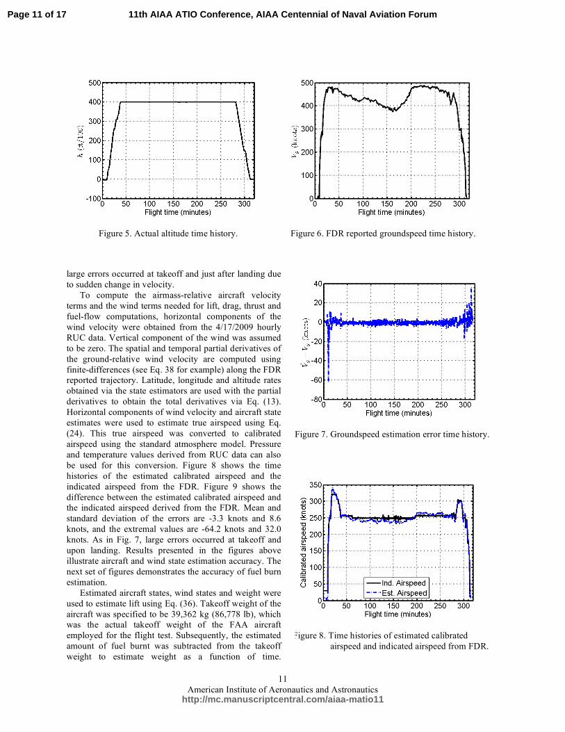
Figure 5. Actual altitude time history.

Figure 7. Groundspeed estimation error time history.

Figure 6. FDR reported groundspeed time history.

Figure 8. Time histories of estimated calibrated airspeed and indicated airspeed from FDR.

large errors occurred at takeoff and just after landing due to sudden change in velocity. To compute the airmass-relative aircraft velocity terms and the wind terms needed for lift, drag, thrust and fuel-flow computations, horizontal components of the wind velocity were obtained from the 4/17/2009 hourly RUC data. Vertical component of the wind was assumed to be zero. The spatial and temporal partial derivatives of the ground-relative wind velocity are computed using finite-differences (see Eq. 38 for example) along the FDR reported trajectory. Latitude, longitude and altitude rates obtained via the state estimators are used with the partial derivatives to obtain the total derivatives via Eq. (13). Horizontal components of wind velocity and aircraft state estimates were used to estimate true airspeed using Eq. (24). This true airspeed was converted to calibrated airspeed using the standard atmosphere model. Pressure and temperature values derived from RUC data can also be used for this conversion. Figure 8 shows the time histories of the estimated calibrated airspeed and the indicated airspeed from the FDR. Figure 9 shows the difference between the estimated calibrated airspeed and the indicated airspeed derived from the FDR. Mean and standard deviation of the errors are -3.3 knots and 8.6 knots, and the extremal values are -64.2 knots and 32.0 knots. As in Fig. 7, large errors occurred at takeoff and upon landing. Results presented in the figures above illustrate aircraft and wind state estimation accuracy. The next set of figures demonstrates the accuracy of fuel burn estimation. Estimated aircraft states, wind states and weight were used to estimate lift using Eq. (36). Takeoff weight of the aircraft was specified to be 39,362 kg (86,778 lb), which was the actual takeoff weight of the FAA aircraft employed for the flight test. Subsequently, the estimated amount of fuel burnt was subtracted from the takeoff weight to estimate weight as a function of time.

Page 11 of 17




12

Figure 9. Estimated calibrated airspeed error time history.

Figure 11. Estimated and FDR fuel-flow rate during cruise.

Figure 10. Estimated and FDR fuel-flow rate during climb.

Estimated lift was then used in Eq. (19) to estimate the coefficient of lift. Reference area value of 94.9 m2 based on Ref. 10 and density of air based on standard atmosphere model were used in Eq. (19). The density of air can be computed from pressure and temperature derived from RUC data.

DC was then calculated using

Eq. (18). Since BADA 3.7 does not have a native model for Global 5000, the Bombardier RJ-900 Regional Jet model drag coefficients and fuel-flow coefficients were used. This same model was also used in Ref. 4. Unfortunately, the BADA RJ-900 model only provides

0DC and

2DC values for the cruise condition. Values for

takeoff, initial climb, approach and landing configurations were determined by scaling the average values with the cruise values, where the average values were obtained by analyzing the

0DC and

2DC values of

the 69 jet aircraft models in BADA 3.7 for the different configurations. Drag estimated using Eq. (17) was then used with the estimated aircraft states, wind states and weight to estimate thrust using Eqs. (14) and (16). V& was set to zero for cruise. Thrust estimates were found to be noisy, so they were smoothed using the procedure described in Section VII. The smoothed estimates were then used in Eq. (1) to estimate the fuel-flow rate.

Fuel Estimation Validation Estimated fuel-flow rate and fuel-flow rate from the FDR during the climb phase are shown in Fig. 10. Notice

the low fuel-flow rate in Fig. 10 and the flat altitude in Fig. 5 for the first 10 minutes; they correspond to taxi on the ground. During the cruise phase are shown in Fig. 11. Fuel-flow rates for the descent phase are given in Fig. 12. Observe the big spike in fuel-flow rate from FDR after the 312 minute mark; it is most likely due to increased thrust

accompanied with thrust reverser deployment for speed reduction to taxi speed. Based on this observation, the negative estimated thrust is considered to be positive thrust with thrust reverser deployed after landing. The resulting fuel-flow rate value was estimated to be 0.38 kg/s compared with 0.72 kg/s reported in FDR data. For reference, aircraft altitude is about 14,770 feet at the 301 minute mark, 8,000 feet at the 305 minute mark and zero at the 312 minute mark. The aircraft needs to be below 8,000 feet for approach configuration and at or below 3,000 feet for landing configuration. As expected, thrust and fuel-flow rate were found to be strongly correlated.

Page 12 of 17




13

Figure 13. Estimated and FDR reported fuel consumption time history.

Figure 12. Estimated and FDR fuel-flow rate during descent.

Figure 14. Percentage error with respect to actual fuel usage.

Finally, Fig. 13 shows the estimate of the amount of fuel consumed and the FDR reported values as a function of time. It is difficult to assess the error from this figure therefore Fig. 14 is provided to show the relative error. Relative error drops below 20% seven minutes into flight when the aircraft is at about 11,000 feet altitude. Mean and standard deviation of the fuel burn error were found to be -1.4% and 10.6%. Extremal values were determined to be -79.4% and 36.1%. These values occur prior to takeoff. The total amount of fuel consumed during the flight was estimated to be 8,099 kg, which is only two kilograms more than the FDR value. To get this close match, the Bombardier RJ-900 Regional Jet model fuel-flow coefficients were multiplied by a factor of 0.853.This value was obtained by trial and error. The fuel consumed estimate is lowered to 8,072 kg with a factor 0.85. The error with respect to the FDR value of 25 kg is

reasonable based on the observed uncertainty of 50 pounds (23 kg) in the FDR fuel consumed data. The other meaningful measure is the mean of the relative error shown in Fig. 14. Considering relative error beyond 100 minutes, the mean value is 0.86%; thus, it is fair to assume that the error in the estimated amount of fuel consumed is within 1% of the actual amount of fuel consumed in the flight test. This result validates the fuel estimation procedure described in the paper.

Model Simplification To determine if the simpler model used in Ref. 4 is adequate for fuel estimation, lift was set equal to weight in

all phases of flight and thrust was modeled using Eqs. (15) and (16). This means that the wind terms in Eq. (14) were dropped. As in the complete model, described in the previous section, V& was set to zero for cruise. Other than replacing the lift and thrust models with simpler models, all the steps described for obtaining the results in the previous section were followed. Results obtained on the flight test data matched the results in the previous section. Differences between these two sets of results were found to be negligible. Mean and the standard deviation of the fuel burn error were found to be -1.35% and 10.65% compared to -1.42% and 10.62% for the data in Fig. 14. Based on these results, the simpler lift and thrust models are adequate for fuel burn estimation.

Takeoff Weight Estimation and Uncertainty The results described in the previous section were based on the actual takeoff weight of the test aircraft. In most

instances, the actual takeoff weight of the aircraft will not be known therefore, a procedure is needed for estimating

Page 13 of 17




14

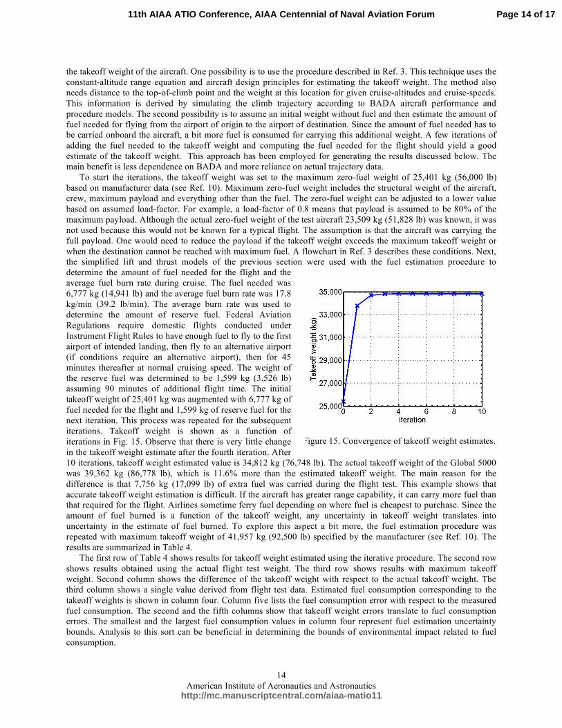
Figure 15. Convergence of takeoff weight estimates.

the takeoff weight of the aircraft. One possibility is to use the procedure described in Ref. 3. This technique uses the constant-altitude range equation and aircraft design principles for estimating the takeoff weight. The method also needs distance to the top-of-climb point and the weight at this location for given cruise-altitudes and cruise-speeds. This information is derived by simulating the climb trajectory according to BADA aircraft performance and procedure models. The second possibility is to assume an initial weight without fuel and then estimate the amount of fuel needed for flying from the airport of origin to the airport of destination. Since the amount of fuel needed has to be carried onboard the aircraft, a bit more fuel is consumed for carrying this additional weight. A few iterations of adding the fuel needed to the takeoff weight and computing the fuel needed for the flight should yield a good estimate of the takeoff weight. This approach has been employed for generating the results discussed below. The main benefit is less dependence on BADA and more reliance on actual trajectory data.

To start the iterations, the takeoff weight was set to the maximum zero-fuel weight of 25,401 kg (56,000 lb) based on manufacturer data (see Ref. 10). Maximum zero-fuel weight includes the structural weight of the aircraft, crew, maximum payload and everything other than the fuel. The zero-fuel weight can be adjusted to a lower value based on assumed load-factor. For example, a load-factor of 0.8 means that payload is assumed to be 80% of the maximum payload. Although the actual zero-fuel weight of the test aircraft 23,509 kg (51,828 lb) was known, it was not used because this would not be known for a typical flight. The assumption is that the aircraft was carrying the full payload. One would need to reduce the payload if the takeoff weight exceeds the maximum takeoff weight or when the destination cannot be reached with maximum fuel. A flowchart in Ref. 3 describes these conditions. Next, the simplified lift and thrust models of the previous section were used with the fuel estimation procedure to determine the amount of fuel needed for the flight and the average fuel burn rate during cruise. The fuel needed was 6,777 kg (14,941 lb) and the average fuel burn rate was 17.8 kg/min (39.2 lb/min). The average burn rate was used to determine the amount of reserve fuel. Federal Aviation Regulations require domestic flights conducted under Instrument Flight Rules to have enough fuel to fly to the first airport of intended landing, then fly to an alternative airport (if conditions require an alternative airport), then for 45 minutes thereafter at normal cruising speed. The weight of the reserve fuel was determined to be 1,599 kg (3,526 lb) assuming 90 minutes of additional flight time. The initial takeoff weight of 25,401 kg was augmented with 6,777 kg of fuel needed for the flight and 1,599 kg of reserve fuel for the next iteration. This process was repeated for the subsequent iterations. Takeoff weight is shown as a function of iterations in Fig. 15. Observe that there is very little change in the takeoff weight estimate after the fourth iteration. After 10 iterations, takeoff weight estimated value is 34,812 kg (76,748 lb). The actual takeoff weight of the Global 5000 was 39,362 kg (86,778 lb), which is 11.6% more than the estimated takeoff weight. The main reason for the difference is that 7,756 kg (17,099 lb) of extra fuel was carried during the flight test. This example shows that accurate takeoff weight estimation is difficult. If the aircraft has greater range capability, it can carry more fuel than that required for the flight. Airlines sometime ferry fuel depending on where fuel is cheapest to purchase. Since the amount of fuel burned is a function of the takeoff weight, any uncertainty in takeoff weight translates into uncertainty in the estimate of fuel burned. To explore this aspect a bit more, the fuel estimation procedure was repeated with maximum takeoff weight of 41,957 kg (92,500 lb) specified by the manufacturer (see Ref. 10). The results are summarized in Table 4.

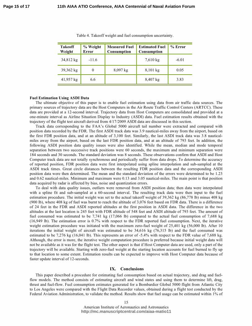
The first row of Table 4 shows results for takeoff weight estimated using the iterative procedure. The second row shows results obtained using the actual flight test weight. The third row shows results with maximum takeoff weight. Second column shows the difference of the takeoff weight with respect to the actual takeoff weight. The third column shows a single value derived from flight test data. Estimated fuel consumption corresponding to the takeoff weights is shown in column four. Column five lists the fuel consumption error with respect to the measured fuel consumption. The second and the fifth columns show that takeoff weight errors translate to fuel consumption errors. The smallest and the largest fuel consumption values in column four represent fuel estimation uncertainty bounds. Analysis to this sort can be beneficial in determining the bounds of environmental impact related to fuel consumption.

Page 14 of 17




15

Fuel Estimation Using ASDI Data The ultimate objective of this paper is to enable fuel estimation using data from air traffic data sources. The

primary sources of trajectory data are the Host Computers in the Air Route Traffic Control Centers (ARTCC). These data are provided at a 12-second interval. Trajectory data from Host Computers are consolidated and provided at a one-minute interval as Airline Situation Display to Industry (ASDI) data. Fuel estimation results obtained with the trajectory of the flight test aircraft derived from 4/17/2009 ASDI data are discussed in this section.

Track data corresponding to the FAA’s Global 5000 aircraft tail number were extracted and compared with position data recorded by the FDR. The first ASDI track data was 3.9 nautical-miles away from the airport, based on the first FDR position data, and at an altitude of 3,100 feet. Similarly, the last ASDI track data was 3.8 nautical-miles away from the airport, based on the last FDR position data, and at an altitude of 793 feet. In addition, the following ASDI position data quality issues were also identified. While the mean, median and mode temporal separation between two successive track positions were 60 seconds, the maximum and minimum separation were 184 seconds and 30 seconds. The standard deviation was 8 seconds. These observations confirm that ASDI and Host Computer track data are not totally synchronous and periodically suffer from data drops. To determine the accuracy of reported position, FDR position data were first interpolated using spline interpolation and sub-sampled at the ASDI track times. Great circle distances between the resulting FDR position data and the corresponding ASDI position data were then determined. The mean and the standard deviation of the errors were determined to be 1.23 and 0.62 nautical-miles. Minimum and maximum were 0.13 and 3.05 nautical-miles. The main point is that position data acquired by radar is affected by bias, noise and quantization errors.

To deal with data quality issues, outliers were removed from ASDI position data; then data were interpolated with a spline fit and sub-sampled at a 60-second interval. The resulting track data were then input to the fuel estimation procedure. The initial weight was set to the actual takeoff weight of 39,362 kg (86,778 lb) minus 408 kg (900 lb), where 408 kg of fuel was burnt to reach the altitude of 3,076 feet based on FDR data. There is a difference of 24 feet in the FDR and ASDI reported altitudes at the first position in ASDI data. The difference in the two altitudes at the last location is 245 feet with FDR altitude of 548 feet and ASDI altitude of 793 feet. The amount of fuel consumed was estimated to be 7,741 kg (17,066 lb) compared to the actual fuel consumption of 7,688 kg (16,949 lb). The estimation error is 0.7% with respect to the FDR reported fuel consumption. Next, the iterative weight estimation procedure was initiated with the maximum zero-fuel weight of 25,401 kg (56,000 lb). After 10 iterations the initial weight of aircraft was estimated to be 34,616 kg (76,315 lb) and the fuel consumed was estimated to be 7,276 kg (16,041 lb). This represents an error of -5.4% with respect to the FDR value of 7,688 kg. Although, the error is more, the iterative weight computation procedure is preferred because initial weight data will not be available as it was for the flight test. The other aspect is that if Host Computer data are used, only a part of the trajectory will be available. Starting with zero-fuel weight at the starting location accounts for fuel burned to fly up to that location to some extent. Estimation results can be expected to improve with Host Computer data because of faster update interval of 12-seconds.

IX. Conclusions This paper described a procedure for estimating fuel consumption based on actual trajectory, and drag and fuel-

flow models. The method consists of estimating aircraft and wind states and using them to determine lift, drag, thrust and fuel-flow. Fuel consumption estimates generated for a Bombardier Global 5000 flight from Atlantic City to Los Angeles were compared with the Flight Data Recorder values, obtained during a flight test conducted by the Federal Aviation Administration, to validate the method. Results show that fuel usage can be estimated within 1% of

Table 4. Takeoff weight and fuel consumption uncertainty.

Takeoff Weight

% Weight Error

Measured Fuel Consumption

Estimated Fuel Consumption

% Error

34,812 kg -11.6 7,610 kg -6.01

39,362 kg 0 8,097 kg 8,101 kg 0.05

41,957 kg 6.6 8,407 kg 3.83

Page 15 of 17




16

the actual value when the takeoff weight is known. The procedure was simplified by setting lift equal to weight and by removing the wind terms from thrust. This simplification did not degrade fuel estimation accuracy. A procedure for estimating takeoff weight was then introduced. Starting with an initial estimate of takeoff weight, this procedure used reserve fuel requirements to iteratively improve the takeoff weight and fuel estimates. The method was found to converge within five iterations. It was shown that fuel usage uncertainty bounds can be determined by varying the takeoff weight. Finally, the adequacy of using trajectory data obtained by air traffic control systems was examined. Trajectory data for the Atlantic City to Los Angeles flight obtained from Airline Situation Display to Industry data were used for estimating fuel usage. Although these data suffered from bias, noise, asynchronous update, and data drops, it was possible to condition the data for obtaining reasonable fuel estimates. Fuel usage could be estimated within 5.4% of the actual value using Airline Situation Display to Industry data with simplified models and the iterative takeoff weight estimation method.

X. References 1Patterson, J., Noel, G. J., Senzig, D. A., Roof, C. J., and Fleming, G. G., “Analysis of Departure and Arrival Profiles Using

Real-Time Aircraft Data,” Journal of Aircraft, Vol. 46, No. 4, July-August 2009, pp. 1094-1103. 2Senzig, D. A., Fleming, G. G., and Iovinelli, R. J., “Modeling of Terminal-Area Airplane Fuel Consumption,” Journal of

Aircraft, Vol. 46, No. 4, July-August 2009, pp. 1089-1093. 3Lee, Hak-Tae., and Chatterji, G. B., “Closed-Form Takeoff Weight Estimation Model for Air Transportation Simulation,”

AIAA 2010-8164, Proc. 10th AIAA Aviation Technology, Integration and Operations Conference (ATIO), Fort Worth, TX, September 13-15, 2010.

4Oaks, R. D., and Paglione, M., “Prototype Implementation and Concept Validation of a 4-D Trajectory Fuel Burn Model Application,” AIAA 2010-8164, Proc. AIAA Guidance, Navigation, and Control Conference, Toronto, Ontario, Canada, August 2-5, 2010.

5Eurocontrol, “Base of Aircraft Data (BADA) Aircraft Performance Modelling Report,” EEC Technical/Scientific Report No. 2009-009, Eurocontrol Experimental Centre, B. P. 15, F-91222 Bretigny-sur-Orge, France, March 2009.

6Chatterji, G. B., Sridhar, B., and Bilimoria, K. D., “En-route Flight Trajectory Prediction for Conflict Avoidance and Traffic Management,” AIAA 96-3766, Proc. AIAA Guidance, Navigation, and Control Conference, San Diego, CA, July 29-31, 1996.

7Chatterji, G. B., “Short-Term Trajectory Prediction Methods,” AIAA 99-4233, Proc. AIAA Guidance, Navigation, and Control Conference, Portland, OR, 1999.

8D’Azzo, J. J., and Houpis, H., Linear Control System Analysis & Design, McGraw-Hill Book Company, New York, NY, 1988.

9Benjamin, S. G., Grell, G. G., Brown, J. M., Smirnova, T. G., and Bleck, R., “Mesoscale Weather Prediction with the RUC Hybrid Isentropic-Terrain-Following Coordinate Model,” Monthly Weather Review, Vol. 132, February 2004, pp. 473-494.

10URL: http://www2.bombardier.com/en/3_0/3_2/pdf/global_5000_factsheet.pdf [cited 20 July 2011].

Acknowledgements The author thanks Confesor Santiago of NASA Ames Research Center (he was formerly at Federal Aviation

Administration) and Mike Paglione of Federal Aviation Administration, and Robert Oaks of General Dynamics Information Technology for providing the flight test data and taking the time to answer questions.

Appendix

The airmass-relative terms in the thrust equation,

( ) ( )!"

!#

$

!%

!&

'

(()

*++,

- ..++

.+++=

2

1sincosV

WhWW

V

WhWgVmDT h

enh

h

&&&

&&& // (A-1)

can be replaced by ground-relative terms as follows. Airmass-relative acceleration obtained by differentiating Eq. (24) is

222 )()()(

))(())(())((

hegengn

hhegeegengnngn

WhWVWV

WhWhWVWVWVWVV

!+!+!

!!+!!+!!=

&

&&&&&&&&& (A-2)

The airmass-relative heading terms can be replaced using Eqs. (20), (21) and (23) as follows.

Page 16 of 17




17

22 )()(

)()(sincos

egengn

egeengnn

en

WVWV

WVWWVWWW

!+!

!+!=+

&&&& "" (A-3)

V is given in terms of ground-relative quantities in Eq. (24). Thrust can therefore be computed in terms of ground-relative terms. Units of BADA fuel-flow coefficients are given in Table 5.

Fuel-flow rate coefficients for a jet, a turboprop and piston engine types are given in Table 6.

Table 6. Fuel-flow rate coefficients for a jet, a turboprop and a piston aircraft.

Aircraft Type Manufacturer 1fC 2fC

3fC 4fC fcrC

CRJ-900 Bombardier 0.61472 369.75 8.2151 355,910 1

EMB-120 Brasilia Embraer 4.5662 664.15 6.5559 43,048 1

PA-28-161 Cherokee Piper 0.44515 -- 0.30872 -- 0.87274

Table 5. Units of BADA fuel-flow rate coefficients.

Engine Type 1fC 2fC

3fC 4fC fcrC

Jet kg/(min*kN) knots kg/min feet dimensionless

Turboprop kg/(min*kN*knot) knots kg/min feet dimensionless

Piston kg/min -- kg/min -- dimensionless

Page 17 of 17



Fuel Burn Estimation Using Real Track Data

Documents

Transcript of Fuel Burn Estimation Using Real Track Data