
IMPACT OF ENGINE DEGRADATION ON FUEL BURN AND ...
204
CRANFIELD UNIVERSITY BENJAMIN VENEDIGER CIVIL AIRCRAFT TRAJECTORY ANALYSES - IMPACT OF ENGINE DEGRADATION ON FUEL BURN AND EMISSIONS SCHOOL OF ENGINEERING Thermal Power MSc by Research MSc by Research Academic Year: 2010 - 2013 Supervisor: Dr. Vishal Sethi May 2013
-
Upload
khangminh22 -
Category
Documents
-
view
4 -
download
0
Transcript of IMPACT OF ENGINE DEGRADATION ON FUEL BURN AND ...

CRANFIELD UNIVERSITY
BENJAMIN VENEDIGER
CIVIL AIRCRAFT TRAJECTORY ANALYSES - IMPACT OF ENGINE
DEGRADATION ON FUEL BURN AND EMISSIONS
SCHOOL OF ENGINEERING
Thermal Power MSc by Research
MSc by Research
Academic Year: 2010 - 2013
Supervisor: Dr. Vishal Sethi
May 2013


CRANFIELD UNIVERSITY
SCHOOL OF ENGINEERING
Thermal Power MSc by Research
MSc by Research Thesis
Academic Year 2010 - 2013
BENJAMIN VENEDIGER
CIVIL AIRCRAFT TRAJECTORY ANALYSES - IMPACT OF ENGINE
DEGRADATION ON FUEL BURN AND EMISSIONS
Supervisor: Dr. Vishal Sethi
May 2013
This thesis is submitted in partial fulfilment of the requirements for the
degree of Master of Science
© Cranfield University 2013. All rights reserved. No part of this publication
may be reproduced without the written permission of the copyright
owner.

i
ABSTRACT
Commercial aviation and air traffic is still expected to grow by 4-5% annually in the
future and thus the effect of aircraft operation on the environment and its
consequences for the climate change is a major concern for all parties involved in the
aviation industry. One important aspect of aircraft engine operation is the
performance degradation of such engines over their lifetime while another aspect
involves the aircraft flight trajectory itself. Therefore, the first aim of this work is to
evaluate and quantify the effect of engine performance degradation on the overall
aircraft flight mission and hence quantify the impact on the environment with regards
to the following two objectives: fuel burned and NOx emissions. The second part of this
study then aims at identifying the potential for optimised aircraft flight trajectories
with respect to those two objectives.
A typical two-spool high bypass ratio turbofan engine in three thrust variants (low,
medium and high) and a typical narrow body single-aisle aircraft similar to the A320
series were modelled as a basis for this study. In addition, an existing emissions
predictions model has been adapted for the three engine variants. Detailed parametric
and off-design analyses were carried out to define and validate the performance of the
aircraft, engine and emissions models. The obtained results from a short and medium
range flight missions study showed that engine degradation and engine take-off thrust
reduction significantly affect total mission fuel burn and total mission NOx emissions
(including take-off) generated. A 2% degradation of compressor, combustor and
turbine component parameters caused an increase in total mission fuel burn of up to
5.3% and an increase in NOx emissions of up to 5.9% depending on the particular
mission and aircraft. However, take-off thrust reduction led to a decrease in NOx
emissions of up to 41% at the expense of an increase in take-off distance of up to 12%.
Subsequently, a basic multi-disciplinary aircraft trajectory optimisation framework was
developed and employed to analyse short and medium range flight trajectories using
one aircraft and engine configuration. Two different optimisation case studies were
performed: (1) fuel burned vs. flight time and (2) fuel burned vs. NOx emitted. The
ii
results from a short range flight mission suggested a trade-off between fuel burned
versus flight time and showed a fuel burn reduction of 3.0% or a reduction in flight
time of 6.7% when compared to a “non-optimised” trajectory. Whereas the
optimisation of fuel burn versus NOx emissions revealed those objectives to be non-
conflicting. The medium range mission showed similar results with fuel burn
reductions of 1.8% or flight time reductions of 7.7% when compared to a “non-
optimised” trajectory. Accordingly, non-conflicting solutions for fuel burn versus NOx
emissions have been achieved. Based on the assumptions introduced for the trajectory
optimisation analyses, the identified optimised trajectories represent possible
solutions with the potential to reduce the environmental impact.
In order to increase the simulation quality in the future and to provide more
comprehensive results, a refinement and extension of the framework also with
additional models taking into account engine life, noise, weather or operational
procedures, is required. This will then also allow the assessment of the implications for
airline operators in terms of Direct Operating Costs (DOC). In addition, the degree of
optimisation could be improved by increasing the number and type of optimisation
variables.
Keywords:
Aircraft Trajectory, Engine Degradation, Fuel Burn, Emissions, Optimisation

iii
ACKNOWLEDGEMENTS
First of all, I would like to thank my supervisor Dr Vishal Sethi for his continuous
support, valuable advice and guidance throughout the development of this work. I also
would like to extend my thanks to Cranfield University PhD candidates Nqobile Khani
and Hugo Pervier for their valuable support, suggestions and advice without which this
work would not have been possible.
Furthermore, I would like to express my gratitude to all colleagues from the
Engineering Department and the Flight Safety Department at Airberlin for their
support, the fruitful discussions and their helpful comments.
I would also like to thank the School of Engineering and the Department of Power and
Propulsion, who made it possible for me to pursue this MSc degree at Cranfield
University.
Finally, I would like to thank all Cranfield University administrative staff for their
prompt support regarding all administrative matters which enabled me to complete
my work on time.
The research leading to the results presented herein has contributed to the European
Union's Seventh Framework Program (FP7/2007-2013) for the Clean Sky Joint
Technology Initiative under grant agreement n° CJSU-GAM-SGO-2008-001. Cranfield
University also got valuable support from partners of Clean Sky, through the GSAF
(Green Systems for Aircraft Foundation) group which include mainly the University of
Malta, TU Delft and the Dutch Research Center (NLR).

iv
TABLE OF CONTENTS
ABSTRACT ................................................................................................................. i
ACKNOWLEDGEMENTS............................................................................................ iii
LIST OF FIGURES ..................................................................................................... vii
LIST OF TABLES........................................................................................................ xi
LIST OF ABBREVIATIONS ........................................................................................ xiii
LIST OF SYMBOLS ................................................................................................... xv
1 Introduction .......................................................................................................... 1
1.1 Background............................................................................................................. 1
1.2 Context ................................................................................................................... 2
1.3 Scope ...................................................................................................................... 8
1.4 Objectives ............................................................................................................... 9
1.5 Outline .................................................................................................................. 10
2 Literature Review ................................................................................................ 12
2.1 Aircraft Technology .............................................................................................. 12
2.1.1 Aircraft Performance ..................................................................................... 12
2.1.2 Aircraft Operation and Procedures ............................................................... 15
2.2 Engine Technology................................................................................................ 17
2.2.1 Turbofan Engine Performance ...................................................................... 18
2.2.2 Thermal Efficiency ......................................................................................... 19
2.2.3 Propulsive Efficiency...................................................................................... 20
2.2.4 Overall Efficiency ........................................................................................... 21
2.3 Gas Turbine Engine Emissions .............................................................................. 21
2.3.1 Carbon Dioxide .............................................................................................. 23
2.3.2 Carbon Monoxide.......................................................................................... 23
2.3.3 Oxides of Nitrogen (NOx) ............................................................................... 24
2.3.4 Oxides of Sulphur (SOx).................................................................................. 26
2.3.5 Unburned Hydrocarbons............................................................................... 26
2.3.6 Soot................................................................................................................ 27
2.4 Gas Turbine Engine Degradation.......................................................................... 27
2.4.1 Typical Mechanisms of Engine Degradation ................................................. 29
2.4.2 Thermal Distress ............................................................................................ 29
2.4.3 Mechanical Wear........................................................................................... 30
2.4.4 Corrosion, Erosion and Abrasion................................................................... 31
2.5 Effects of Engine Degradation .............................................................................. 31
2.5.1 Effects on Engine Components...................................................................... 33
2.5.2 Effects on Engine Performance ..................................................................... 35
2.5.3 Effects on Engine Life .................................................................................... 35
v
2.6 Principles of Optimisation Processes ................................................................... 37
2.6.1 Optimisation Problems.................................................................................. 37
2.6.2 Optimisation Methods................................................................................... 38
2.7 Numerical Methods for Trajectory Optimisation................................................. 39
2.7.1 Hill Climbing Methods ................................................................................... 40
2.7.2 Random Search Methods .............................................................................. 41
2.7.3 Evolutionary Methods ................................................................................... 42
2.8 Genetic Algorithms ............................................................................................... 42
2.9 Multi Objective Trajectory Optimisation.............................................................. 44
2.10 NSGAMO Genetic Optimiser .............................................................................. 46
3 Problem Definition .............................................................................................. 49
3.1 General Considerations ........................................................................................ 49
3.1.1 Short-to-Medium Range Aircraft Configurations.......................................... 50
3.1.2 Aircraft Speeds .............................................................................................. 50
3.1.3 Aircraft Trajectory Definition ........................................................................ 55
3.1.4 Optimised Aircraft Trajectory........................................................................ 58
3.2 Assumptions and Statements............................................................................... 59
3.3 Past Experience on Trajectory Analysis and Optimisation................................... 60
4 Framework Tools ................................................................................................. 64
4.1 Engine Performance Model (Turbomatch)........................................................... 64
4.1.1 Turbomatch Engine Model............................................................................ 65
4.1.2 Engine Design Point Selection and Performance .......................................... 67
4.1.3 Engine Off-Design Performance .................................................................... 71
4.1.4 Degraded Engine Performance ..................................................................... 87
4.1.5 Engine Model Verification ............................................................................. 93
4.2 Aircraft Performance Model (Hermes)................................................................. 93
4.2.1 Hermes Aircraft Model .................................................................................. 95
4.2.2 Aircraft Model Verification............................................................................ 98
4.3 Emissions Predictions Model (Hephaestus/P3T3).............................................. 100
4.3.1 P3T3 Emissions Prediction Model ............................................................... 101
4.3.2 Emissions Model Verification ...................................................................... 104
4.4 Optimisation Framework.................................................................................... 107
4.4.1 GATAC Optimisation Suite........................................................................... 108
4.4.2 Optimisation Suite Verification ................................................................... 108
4.5 Model Interaction............................................................................................... 111
5 Aircraft Trajectory Analysis and Results ............................................................. 113
5.1 Summary of Analysed Scenarios......................................................................... 113
5.2 Short Range Flight (Clean Engine) ...................................................................... 115
5.2.1 General Description..................................................................................... 115
5.2.2 Results ......................................................................................................... 115
vi
5.3 Short Range Flight (Degraded Engine)................................................................ 117
5.3.1 General Description..................................................................................... 117
5.3.2 Results ......................................................................................................... 118
5.4 Short Range Results Comparison ....................................................................... 121
5.5 Medium Range Flight (Clean Engine) ................................................................. 128
5.5.1 General Description..................................................................................... 128
5.5.2 Results ......................................................................................................... 128
5.6 Medium Range Flight (Degraded Engine)........................................................... 130
5.6.1 General Description..................................................................................... 130
5.6.2 Results ......................................................................................................... 130
5.7 Medium Range Results Comparison................................................................... 133
6 Trajectory Optimisation Studies and Results ...................................................... 141
6.1 Summary of Case Studies ................................................................................... 141
6.2 Short Range Multi Objective Optimisation......................................................... 142
6.2.1 General Description..................................................................................... 142
6.2.2 Fuel vs. Time Optimisation Results.............................................................. 143
6.2.3 Fuel vs. NOx Optimisation Results ............................................................... 149
6.3 Medium Range Multi Objective Optimisation.................................................... 150
6.3.1 General Description..................................................................................... 150
6.3.2 Fuel vs. Time Optimisation Results.............................................................. 151
6.3.3 Fuel vs. NOx Optimisation Results ............................................................... 157
7 Conclusions, Recommendations for Further Work and Outlook.......................... 159
7.1 Achievements ..................................................................................................... 159
7.2 Conclusions......................................................................................................... 160
7.3 Limitations and Recommendations for Further Work ....................................... 161
7.4 Outlook ............................................................................................................... 165
7.4.1 Airline Operational Procedures ................................................................... 165
7.4.2 Engine Health Management........................................................................ 166
REFERENCES ......................................................................................................... 167
APPENDICES ......................................................................................................... 178
A.1 CUSA-S, CUSA-M, CUSA-L Block fuel and Block NOx ......................................... 178
A.2 Trajectory plots for 1800 km mission .............................................................. 179
A.3 Trajectory plots for 4600 km mission .............................................................. 182
vii
LIST OF FIGURES
Figure 1-1: Worldwide passenger traffic history and forecast (ICAO) ............................. 3
Figure 2-1: Landing and Take-off (LTO) cycle [30].......................................................... 15
Figure 2-2: Typical two-shaft turbofan engine schematic.............................................. 17
Figure 2-3: Effect of ambient temperature on engine EGT (flat-rated engine) ............. 33
Figure 2-4: Overview of optimisation strategies (adapted from Schwefel [60]) ........... 40
Figure 2-5: Main features of the genetic algorithm (adapted from Lipowsky [49]) ...... 44
Figure 2-6: Example Pareto curve [67] ........................................................................... 46
Figure 2-7: Optimisation flowchart [71]......................................................................... 48
Figure 3-1: Typical flight mission profile and flight phases ............................................ 50
Figure 3-2: Aircraft velocity interdependencies (adapted from Scheiderer [72]).......... 51
Figure 3-3: Ambient temperature vs. altitude ............................................................... 54
Figure 3-4: Ambient pressure vs. altitude ...................................................................... 54
Figure 3-5: Air density vs. altitude.................................................................................. 54
Figure 3-6: Flight profile with engine fuel flow (Airbus A321); courtesy of Airberlin .... 56
Figure 3-7: Flight profile with engine EGT (Airbus A321); courtesy of Airberlin............ 57
Figure 4-1: Typical two-spool high bypass turbofan engine configuration.................... 66
Figure 4-2: Basic engine component data (Turbomatch)............................................... 66
Figure 4-3: Ideal cycle and ambient temperature effects.............................................. 71
Figure 4-4: CU2STF-LT – SFC vs. Mach number at constant TET (1500K) ...................... 72
Figure 4-5: CU2STF-LT – Net thrust vs. Mach number at constant TET (1500K)............ 73
Figure 4-6: CU2STF-LT – Net thrust vs. TET at SLS conditions........................................ 75
Figure 4-7: CU2STF-LT – SFC vs. TET at SLS conditions................................................... 75
Figure 4-8: CU2STF-MT – SFC vs. Mach number at constant TET (1575K)..................... 76
Figure 4-9: CU2STF-MT – Net thrust vs. Mach number at constant TET (1575K).......... 77
Figure 4-10: CU2STF-MT – Net thrust vs. TET at SLS conditions .................................... 77
Figure 4-11: CU2STF-MT – SFC vs. TET at SLS conditions............................................... 78
Figure 4-12: CU2STF-HT – SFC vs. Mach number at constant TET (1760K).................... 79

viii
Figure 4-13: CU2STF-HT – Net thrust vs. Mach number at constant TET (1760K)......... 79
Figure 4-14: CU2STF-HT – Net thrust vs. TET at SLS conditions ..................................... 80
Figure 4-15: CU2STF-HT – SFC vs. TET at SLS conditions................................................ 80
Figure 4-16: CU2STF-LT Fan map (running line at TOC) ................................................. 81
Figure 4-17: CU2STF-LT LPC map (running line at TOC) ................................................. 82
Figure 4-18: CU2STF-LT HPC map (running line at TOC) ................................................ 82
Figure 4-19: CU2STF-MT Fan map (running line at TOC) ............................................... 83
Figure 4-20: CU2STF-MT LPC map (running line at TOC) ............................................... 83
Figure 4-21: CU2STF-MT HPC map (running line at TOC)............................................... 84
Figure 4-22: CU2STF-HT Fan map (running line at TOC) ................................................ 84
Figure 4-23: CU2STF-HT LPC map (running line at TOC) ................................................ 85
Figure 4-24: CU2STF-HT HPC map (running line at TOC)................................................ 85
Figure 4-25: TET and Fuel Flow over T/O Thrust ............................................................ 86
Figure 4-26: TET over net thrust at T/O conditions (Ma=0)........................................... 90
Figure 4-27: Engine T/O TET for clean, degraded and derated conditions.................... 90
Figure 4-28: Take-off EGTM loss over engine flight cycles............................................. 92
Figure 4-29: Hermes aircraft performance model (inputs and outputs) ....................... 94
Figure 4-30: CUSA family schematic............................................................................... 96
Figure 4-31: CUSA-S Payload-Range diagram................................................................. 99
Figure 4-32: CUSA-M Payload-Range diagram ............................................................... 99
Figure 4-33: CUSA-L Payload-Range diagram............................................................... 100
Figure 4-34: P3T3 methodology (adapted from Norman et al. [48]) ........................... 102
Figure 4-35: CU2STF-LT - Fuel Flow versus Net Thrust................................................. 105
Figure 4-36: CU2STF-MT - Fuel Flow versus Net Thrust............................................... 105
Figure 4-37: CU2STF-HT - Fuel Flow versus Net Thrust................................................ 106
Figure 4-38: Optimisation framework.......................................................................... 107
Figure 4-39: GATAC framework structure [71]............................................................. 108
Figure 4-40: Scenario 1 - Fuel vs. Time......................................................................... 111

ix
Figure 4-41: Scenario 2 - Fuel vs. NOx .......................................................................... 112
Figure 5-1: Real flight profile and engine FF vs. CUSA-L model ................................... 114
Figure 5-2: Real flight profile and engine EGT vs. CUSA-L model................................. 114
Figure 5-3: CUSA-S engine FF variation during flight (1800 km) .................................. 116
Figure 5-4: CUSA-S engine TET variation during flight (1800 km)................................ 117
Figure 5-5: CUSA-L engine TET variation during climb ................................................. 118
Figure 5-6: CUSA-L engine power setting and thrust during climb.............................. 119
Figure 5-7: CUSA-S with CU2STF-LT.............................................................................. 123
Figure 5-8: CUSA-M with CU2STF-MT .......................................................................... 123
Figure 5-9: CUSA-L with CU2STF-HT ............................................................................. 124
Figure 5-10: CUSA-L with CU2STF-HT engine (clean and degraded)............................ 124
Figure 5-11: T/O distance comparison ......................................................................... 126
Figure 5-12: T/O fuel burn comparison........................................................................ 126
Figure 5-13: T/O NOx emissions comparison................................................................ 126
Figure 5-14: Fuel burned comparison .......................................................................... 127
Figure 5-15: NOx emissions comparison....................................................................... 127
Figure 5-16: CUSA-L engine FF variation during flight (4600 km) ................................ 129
Figure 5-17: CUSA-L engine TET variation during flight (4600 km) .............................. 129
Figure 5-18: CUSA-M engine TET variation during climb ............................................. 131
Figure 5-19: CUSA-M engine power setting and thrust during climb .......................... 131
Figure 5-20: CUSA-S with CU2STF-LT............................................................................ 135
Figure 5-21: CUSA-M with CU2STF-MT ........................................................................ 136
Figure 5-22: CUSA-L with CU2STF-HT ........................................................................... 136
Figure 5-23: CUSA-M with CU2STF-MT engine (clean and degraded) ......................... 137
Figure 5-24: T/O distance comparison ......................................................................... 139
Figure 5-25: T/O fuel burn comparison........................................................................ 139
Figure 5-26: T/O NOx emissions comparison................................................................ 139
Figure 5-27: Fuel burned comparison .......................................................................... 140

x
Figure 5-28: NOx emissions comparison....................................................................... 140
Figure 6-1: Fuel vs. time Pareto fronts for short range mission................................... 144
Figure 6-2: CUSA-M short range flight profile comparison (fuel vs. time)................... 145
Figure 6-3: CUSA-M True Air Speed (TAS) variation during climb (short range).......... 147
Figure 6-4: CUSA-M climb profile and engine thrust (short range) ............................. 148
Figure 6-5: Fuel burned vs NOx (0.75) .......................................................................... 150
Figure 6-6: Fuel burned vs NOx (0.85) .......................................................................... 150
Figure 6-7: Fuel vs. time Pareto fronts for medium range mission.............................. 152
Figure 6-8: CUSA-M medium range flight profile comparison (fuel vs. time).............. 153
Figure 6-9: CUSA-M True Air Speed (TAS) variation during climb (medium range)..... 154
Figure 6-10: CUSA-M climb profile and engine thrust (medium range) ...................... 155
Figure 6-11: CUSA-M TET variation (medium range) ................................................... 156
Figure 6-12: Fuel burned vs NOx (0.75) ........................................................................ 158
Figure 6-13: Fuel burned vs NOx (0.85) ........................................................................ 158
xi
LIST OF TABLES
Table 2-1: Typical turbofan exhaust gas composition (according to Bräunling [39]) .... 23
Table 2-2: Methods of Operations Research (adapted from Rao [59]) ......................... 39
Table 4-1: Engine specification comparison CU2STF-LT (CFM56-5B6) [87] ................... 69
Table 4-2: Engine specification comparison CU2STF-MT (CFM56-5B4) [87] ................. 69
Table 4-3: Engine specification comparison CU2STF-HT (CFM56-5B3) [87] .................. 70
Table 4-4: Engine model design point parameter.......................................................... 70
Table 4-5: CU2STF-LT degraded performance (2% degradation)................................... 88
Table 4-6: CU2STF-MT degraded performance (2% degradation)................................. 88
Table 4-7: CU2STF-HT degraded performance (2% degradation).................................. 89
Table 4-8: Aircraft specification comparison CUSA-S..................................................... 96
Table 4-9: Aircraft specification comparison CUSA-M .................................................. 97
Table 4-10: Aircraft specification comparison CUSA-L................................................... 97
Table 4-11: ICAO Database exhaust emissions CFM56-5B3/P..................................... 103
Table 4-12: ICAO Database exhaust emissions CFM56-5B4/P..................................... 103
Table 4-13: ICAO Database exhaust emissions CFM56-5B6/P..................................... 103
Table 4-14:ZDT1, ZDT3 and ZDT6 test functions (adapted from Deb et al. [66])......... 110
Table 5-1: Short range mission characteristics (clean engine)..................................... 115
Table 5-2: Short range mission characteristics (degraded engine).............................. 118
Table 5-3: Climb fuel burn and NOx emissions comparison (short range flight).......... 120
Table 5-4: CUSA-S short range mission results............................................................. 121
Table 5-5: CUSA-M short range mission results ........................................................... 121
Table 5-6: CUSA-L short range mission results............................................................. 122
Table 5-7: Fuel Economy,PEE and PFEE comparison for the short range mission....... 125
Table 5-8: Total fuel burn and NOx emissions comparison (short range flight)........... 125
Table 5-9: Medium range mission characteristics (clean engine)................................ 128
Table 5-10: Medium range mission characteristics (degraded engine)....................... 130
Table 5-11: Climb fuel burn and NOx emissions comparison (medium range flight)... 132
xii
Table 5-12: CUSA-S medium range mission results...................................................... 133
Table 5-13: CUSA-M medium range mission results .................................................... 134
Table 5-14: CUSA-L medium range mission results...................................................... 134
Table 5-15: Fuel Economy, PEE and PFEE comparison for the medium range mission138
Table 5-16: Fuel burn and NOx emissions comparison (medium range flight) ............ 138
Table 6-1: GATAC decision variables for climb and cruise ........................................... 141
Table 6-2: Optimisation extreme solutions compared to reference flight (1800 km). 145
Table 6-3: Flight comparison for fixed fuel burned value (short range) ...................... 148
Table 6-4: Reprocessed fuel burned and NOx values (short range) ............................. 150
Table 6-5: Optimisation extreme solutions compared to reference flight (4600 km). 153
Table 6-6: Flight comparison for fixed fuel burned value (medium range) ................. 156
Table 6-7: Reprocessed fuel burned and NOx values (short range) ............................. 158
xiii
LIST OF ABBREVIATIONS
ACARE Advisory Council for Aeronautics Research in Europe
ATM Air Traffic Management
CC Combustion Chamber
CFD Computational Fluid Dynamics
CO Carbon monoxide
CP Corner Point
CO2 Carbon dioxide
CU Cranfield University
CU2STF-HT Cranfield University 2 Spool Turbofan-High thrust (Turbomatch)
CU2STF-LT Cranfield University 2 Spool Turbofan-Low thrust (Turbomatch)
CU2STF-MT Cranfield University 2 Spool Turbofan-Medium thrust (Turbomatch)
CUSA-L Cranfield University Single Aisle-Long (Hermes)
CUSA-M Cranfield University Single Aisle-Medium (Hermes)
CUSA-S Cranfield University Single Aisle-Short (Hermes)
DOC Direct Operating Costs
DP Design Point
EGT Exhaust Gas Temperature
EGTM Exhaust Gas Temperature Margin
EHM Engine Health Management/Engine Health Monitoring
FF Fuel Flow
GA Genetic Algorithm
GATAC Green Aircraft Trajectories under ATM Constraints
GPHM Gas Path Health Management
GWP Global Warming Potential
H2O Water
HPC High Pressure Compressor
HPT High Pressure Turbine
ICAO International Civil Aviation Organisation
ISA International Standard Atmosphere
ITD Integrated Technology Demonstrator
JTI Joint Technology Initiative
LPC Low Pressure Compressor
LPT Low Pressure Turbine
LTO Landing and Take-off cycle
MDO Multi Disciplinary Optimisation

xiv
MTOW Maximum Take-off Weight
N Nitrogen
NO Nitric oxide
NO2 Nitrogen dioxide
NOX Oxides of nitrogen
NSGAMO Non-dominated Sorting Genetic Algorithm Multi-Objective
O Oxygen
OAT Outside Air Temperature
O2 Molecular oxygen
OD Off-Design
OEW Operating Empty Weight
PARTNER Partnership for AiR Transportation Noise and Emissions Reduction
PCN Shaft Speed (rpm/rpm(DP)
PEE Payload Emissions Efficiency
PFEE Payload Fuel Energy Efficiency
RPK Revenue Passenger Kilometres
SBX Simulated Binary Crossover
SESAR Single European Sky ATM Research
SGO System for Green Operations
SLS Sea Level Static
SO2 Sulphur dioxide
T/O Take-Off
TBC Thermal Barrier Coating
TERA Techno-economic Environmental Risk Analysis
TOC Top Of Climb
TOD Top Of Descent
VBV Variable Bleed Valve
VSV Variable Stator Vanes
xv
LIST OF SYMBOLS
Symbol Definition Unit
a Speed of sound m/s
A0 Inlet flow area m²
Alt Altitude m
AR Wing aspect ratio -
BPR Bypass Ratio -
c Number of constraints -
c0 Inlet flow velocity m/s
CAS Calibrated Air Speed m/s
CD Drag coefficient -
CD0 Zero lift drag coefficient -
CDI Induced drag coefficient -
Cfc Skin friction coefficient -
CL Lift coefficient -
Cp Specific heat (constant pressure) J kg-1 K-1
CV Specific heat (constant volume) J kg-1 K-1
C1 Wing plan form geometry coefficient -
C2 Wing plan form geometry coefficient -
C3 Non-optimum wing twist coefficient -
C4 Viscous effects coefficient -
CMF Corrected Mass-Flow kg/s
DAS Density Air Spped m/s
EAS Equivalent Airspeed m/s
EGT Exhaust Gas Temperature °C
EGTM Exhaust Gas Temperature Margin °C
EI Emissions Index (Indices) g(emissions)/kg(fuel)
f(X) Objective function -
gj(X) Inequality constraints (vector) -
hl(X) Equality constraints (vector) -
FAR Fuel-Air-Ratio kg(fuel)/kg(air)
FHV Fuel Heating Value J/kg
FNNetthrust
kN
FPR Fan Pressure Ratio -
IAS Indicated Air Speed m/s

xvi
M Mach number -
Ma0 Inlet Mach number -
ṁ Mass flow kg/s
OPR Overall Pressure Ratio -
pinlet Component inlet pressure Pa
poutlet Component outlet pressure Pa
p0 Ambient pressure Pa
P Power J/s
PSLS Pressure (Sea Level Static) Pa
Qc Component interference drag coefficient -
r Radius m
R Gas constant (dry air) J kg-1 K-1
SFC Specific Fuel Consumption mg/Ns
Sc,wetted Component wetted surface area m²
Sref Plan form area m²
t Temperature (static) K
T Temperature (total) K
Thot day Temperature at Sea Level (ISA+30 conditions) K
Tinlet Component inlet temperature K
Tmin Minimum temperature K
Tmax Maximum temperature K
Toutlet Component outlet temperature K
Tstandard day Temperature at Sea Level (ISA conditions) K
TSLS Temperature (Sea Level Static) K
T;‾th Thermodynamic average temperature K
T0 Ambient temperature K
Tt3 Maximum compressor exit temperature K
Tt4 Maximum turbine entry temperature K
TAS True Air Speed m/s
TET Turbine Entry Temperature K
V0 Flight velocity m/s
VjJetvelocity
m/s
W Mass flow kg/s
WI Core mass flow kg/s
wf Fuel flow kg/s
X Design vector (n-dimensional) -
xvii
Greek Symbol Definition Unit
γ Isentropic exponent -
ƞ Efficiency -
ƞcomb Combustion efficiency -
ƞoverall Overall efficiency -
ƞth Thermal efficiency -
ƞth,opt Optimum thermal efficiency -
ƞprop Propulsive efficiency -
μ Bypass Ratio -
π Pressure ratio -
ρ Density kg/m³
ϕc Component form factor -

Introduction
1
1 Introduction
The first chapter provides a general introduction to the topic of this research project
and specifies the context in which the subject research project was carried out. It
furthermore describes the main objectives addressed in this work as well as the scope
and a brief outline of the same.
1.1 Background
Today’s need for reliable, fast global transportation is increasing and has set new
standards for the aviation industry, and at the same time is creating new challenges in
the field of science and technology. Commercial aviation is still expected to grow
significantly in the future and thus the effect of aircraft operation on the environment
and its consequences for climate change is a major concern and must be addressed at
all levels in the aviation industry and beyond.
One key issue that must be addressed to contribute to a more sustainable
environment is the reduction of aircraft engine CO2 emissions and directly related to
that a reduction in fuel burn as well as the reduction of aircraft engine NOx emissions.
The civil aero-engine market is highly competitive and engine manufacturers, engine
maintenance providers and aircraft operators alike have to look for technological and
economical improvements as well as determining environmental impacts of their
products and operations. Those are two major requirements which are the basis for
future gas turbine engine concepts and configurations powering next-generation
aircraft. New engine designs or major alterations are high risk strategies for the engine
manufacturers and operators due to the inherent cost of development and
implementation. Many different novel or evolved gas turbine propulsion system
solutions for commercial aircraft applications are being proposed by various engine
manufacturers. These novel and evolved engine designs like geared fan designs have
the potential to significantly improve environmental effects and to improve the
economic impact of aircraft operations in the long term compared to the current state
[1].

Introduction
2
On the other side, there are existing aircraft and engine configurations in service
today, which are expected to be operated for a considerable amount of time into the
future. With a view to the commercial aviation sector and aircraft fleets being in
operation today, there is a big potential to find solutions which can be proposed and
applied to existing fleet operations in the short term. The analysis of existing aircraft
and engine configurations and the identification of feasible solutions and strategies
which yield the biggest efficiency improvements with regards to aircraft operations is
one possible way to achieve a reduction in emissions. Due to the limitations in creating
fundamental aircraft and engine design changes in the short term, those analyses must
aim at operational aspects of air transportation. One major aspect is aircraft flight
trajectories that allow for minimum pollutant emissions for a certain flight profile. The
other important aspect of the analysis must deal with engine maintenance issues and
its impact on the environment as well as its impact on the total engine life cycle.
1.2 Context
Global economic growth and a constant increase in worldwide air travel demand are
directly associated with an increased public awareness of environmental issues such as
air pollution, noise and climate change [2]. According to the 2011 ICAO (International
Civil Aviation Organization) worldwide scheduled services forecast, passenger traffic is
expected to grow by about 4-5 % annually till the year 2030. Figure 1-1 shows the
historic growth in Revenue Passenger Kilometres (RPK) and passengers carried since
the year 2000. It also shows the expected future development for these two figures till
the year 2030. Several studies initiated by EUROCONTROL, dealing with the strategic
research on air transport evolution present the future challenges for air traffic
developments up to the year 2030, also in the light of global climate changes [3]. They
stress the fact that adaptation is only one strategy to cope with climate change.
Another important aspect is mitigation of factors that drive climate change to strongly
reduce the effects on climate change [4]. Since aero-engines are largely contributing to
the atmospheric pollution via emissions of CO2, NOx and other chemical compounds
the aviation industry is investigating new solutions in order to address those
environmental problems [5]. Detailed aero engine emission information is available in

Introduction
3
references [6] and [7]. A comprehensive assessment of typical commercial aero engine
combustors as listed in reference [6] and [7] has been conducted in reference [8] and
the results underline the continuous reductions which have been achieved by engine
manufacturers. An assessment of commercial aviation fuel efficiency on a fleet-wide
basis, by means of the measure of Payload Fuel Energy Efficiency (PFEE), is presented
in reference [9]. The study also suggests extending the assessment by including
environmental performance metrics, which for example can account for NOx
emissions, to identify operational inefficiencies. The investigation of these aspects can
be accomplished through collaborative international networks and projects that focus
on the coordination of efforts in order to promote those improvements in commercial
aviation.
Figure 1-1: Worldwide passenger traffic history and forecast (ICAO)
The ICAO bundles its environmental activities through the Committee on Aviation
Environmental Protection (CAEP) which is divided into several working and support
groups covering a wide range of technical and operational aspects. The output
provided by the different groups serves as basis for new standards on aircraft
emissions set by ICAO. The current status, future goals and developments in mitigation
0.0
1.0
2.0
3.0
4.0
5.0
6.0
7.0
0
2000
4000
6000
8000
10000
12000
14000
2000 2005 2010 2015 2020 2025 2030
Pas
sen
gers
carr
ied
[in
bill
ion
s]
Re
ven
ue
Pas
sen
ger
Kilo
me
tre
s(R
PK
)[i
nb
illio
ns]
Year
RPK Passengers carried
ForecastHistory
Introduction
4
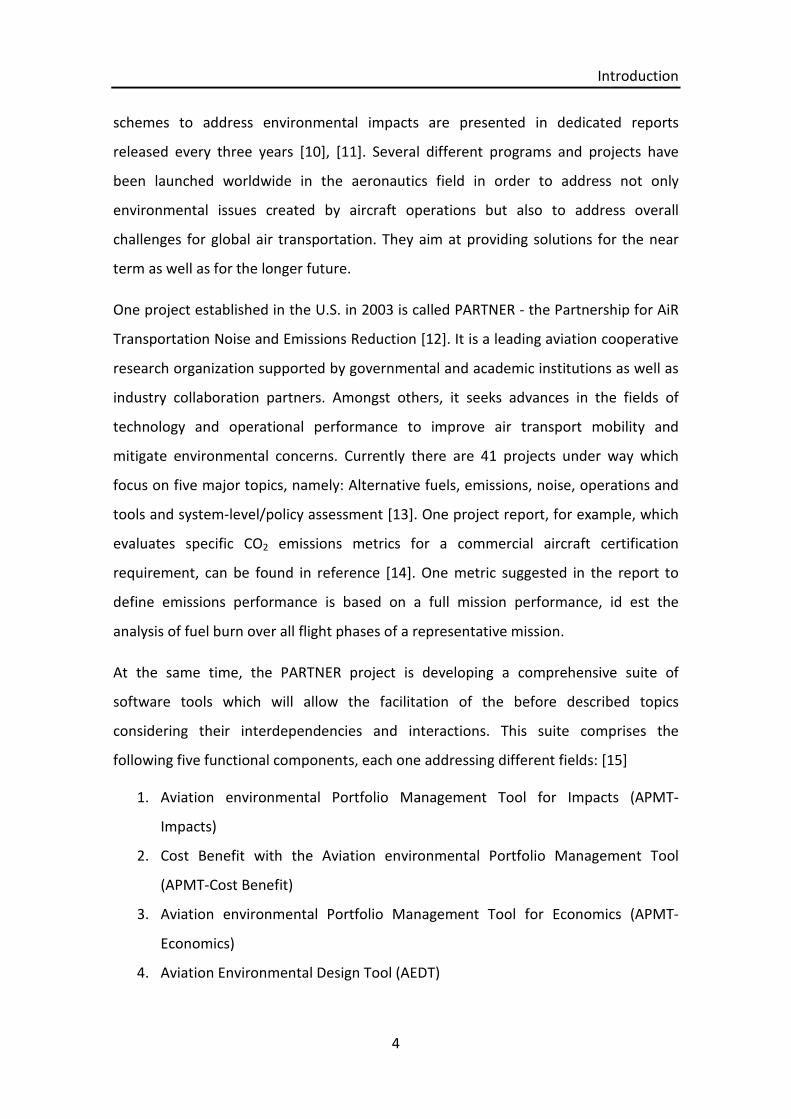
schemes to address environmental impacts are presented in dedicated reports
released every three years [10], [11]. Several different programs and projects have
been launched worldwide in the aeronautics field in order to address not only
environmental issues created by aircraft operations but also to address overall
challenges for global air transportation. They aim at providing solutions for the near
term as well as for the longer future.
One project established in the U.S. in 2003 is called PARTNER - the Partnership for AiR
Transportation Noise and Emissions Reduction [12]. It is a leading aviation cooperative
research organization supported by governmental and academic institutions as well as
industry collaboration partners. Amongst others, it seeks advances in the fields of
technology and operational performance to improve air transport mobility and
mitigate environmental concerns. Currently there are 41 projects under way which
focus on five major topics, namely: Alternative fuels, emissions, noise, operations and
tools and system-level/policy assessment [13]. One project report, for example, which
evaluates specific CO2 emissions metrics for a commercial aircraft certification
requirement, can be found in reference [14]. One metric suggested in the report to
define emissions performance is based on a full mission performance, id est the
analysis of fuel burn over all flight phases of a representative mission.
At the same time, the PARTNER project is developing a comprehensive suite of
software tools which will allow the facilitation of the before described topics
considering their interdependencies and interactions. This suite comprises the
following five functional components, each one addressing different fields: [15]
1. Aviation environmental Portfolio Management Tool for Impacts (APMT-
Impacts)
2. Cost Benefit with the Aviation environmental Portfolio Management Tool
(APMT-Cost Benefit)
3. Aviation environmental Portfolio Management Tool for Economics (APMT-
Economics)
4. Aviation Environmental Design Tool (AEDT)
Introduction
5
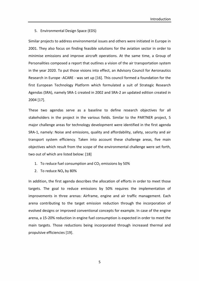
5. Environmental Design Space (EDS)
Similar projects to address environmental issues and others were initiated in Europe in
2001. They also focus on finding feasible solutions for the aviation sector in order to
minimise emissions and improve aircraft operations. At the same time, a Group of
Personalities composed a report that outlines a vision of the air transportation system
in the year 2020. To put those visions into effect, an Advisory Council for Aeronautics
Research in Europe -ACARE - was set up [16]. This council formed a foundation for the
first European Technology Platform which formulated a suit of Strategic Research
Agendas (SRA), namely SRA-1 created in 2002 and SRA-2 an updated edition created in
2004 [17].
These two agendas serve as a baseline to define research objectives for all
stakeholders in the project in the various fields. Similar to the PARTNER project, 5
major challenge areas for technology development were identified in the first agenda
SRA-1, namely: Noise and emissions, quality and affordability, safety, security and air
transport system efficiency. Taken into account these challenge areas, five main
objectives which result from the scope of the environmental challenge were set forth,
two out of which are listed below: [18]
1. To reduce fuel consumption and CO2 emissions by 50%
2. To reduce NOx by 80%
In addition, the first agenda describes the allocation of efforts in order to meet those
targets. The goal to reduce emissions by 50% requires the implementation of
improvements in three arenas: Airframe, engine and air traffic management. Each
arena contributing to the target emission reduction through the incorporation of
evolved designs or improved conventional concepts for example. In case of the engine
arena, a 15-20% reduction in engine fuel consumption is expected in order to meet the
main targets. Those reductions being incorporated through increased thermal and
propulsive efficiencies [19].

Introduction
6
Furthermore, the updated Strategic Research Agenda SRA-2 which was released in
2004 extended the approach and contents of the first edition and added a number of
development scenarios. Following the strategy of the first agenda and recalling its
objectives, the second edition also refines existing targets and determines a series of 5
High Level Target Concepts (HLTC), each of them addressing a major concern of the air
transportation system. In short they can be listed as follows:
1. Highly Customer Oriented HLTC
2. Highly Time Efficient HLTC
3. Highly Cost Efficient HLTC
4. Ultra Green HLTC
5. Ultra Secure HLTC
To keep pace with changing trends in the aviation sector worldwide and to implement
already achieved goals into the concept of the major strategic agendas, an Addendum
was released in 2008 to recall the main objectives and to update priorities with regards
to newly arisen economic and environmental issues.
In alignment with the before described air transportation improvement objectives, the
Clean Sky project was initiated to demonstrate and validate technology advances in
order to meet the goals set by ACARE which will ensure the attainment of the aspired
environmental improvements [20]. This research project being a public-private
partnership, involves the support of industries, universities and research organizations
alike. By its combined research activities, it will contribute towards meeting the
objectives of ACARE HLT concept number 3 and 4 (see above), i.e. Highly Cost Efficient
and Ultra Green air transportation systems.
The structure of the project is composed of 6 Integrated Technology Demonstrators
(ITD), which focus on different technology improvement areas of the air transportation
system. Those 6 ITDs are briefly described as follows: [20]
1. Green Regional Aircraft [GRA]
2. SMART Fixed-Wing Aircraft
3. Green Rotorcraft

Introduction
7
4. Sustainable and Green Engines
5. Systems for Green Operation
6. Eco-Design
Those ITDs are linked through a simulation network to a Technology Evaluator which
assesses the performance of the technologies developed within a certain Integrated
Technology Demonstrator (ITD) and allows early appraisal of the results and
comparison against the initial targets. This also means that necessary re-adjustments
of particular technological advancements can be implemented and fed back into the
on-going work. The fifth ITD (Systems for Green Operation) in particular deals primarily
with the management of aircraft energy and the management of missions and
trajectories. Especially the analysis of the different flight phases of an aircraft like
cruise, take-off, approach and departure with respect to fuel consumption can deliver
insight into the various environmental effects. Extensive research in mission and
energy management can assist in reaching the higher level targets set by the Clean Sky
project.
Cranfield University (CU) currently contributes to the above mentioned research topics
through the development of advanced and optimised aircraft trajectories and
consequent validation of their effectiveness. A concept called TERA (Techno-economic
and Environmental Risk Assessment) was invented at Cranfield University [21]. The
TERA concept incorporates several modules which allow modelling of gas turbine and
aircraft performance, estimating noise and emissions, as well as environmental impact.
An integrated optimiser enables detailed cycle studies taking into account a multi-
disciplinary model scenario [22].
The importance of these integrated multi-disciplinary modelling tools becomes
apparent when detailed and comprehensive analysis results are to be compiled. In
order to effectively analyse the possibilities of more environmental friendly aircraft
and engine operations it is necessary to create a framework which determines the
boundaries for the analysis. This framework includes all modules which are considered

Introduction
8
important for an accurate model, such as engines and airframes used or external
conditions and restrictions, they could be technical or economical for example.
Those tools then allow the assessment of aircraft trajectories in terms of the key
factors such as flight time, fuel consumption and emission of pollutants harmful to the
environment. In order to identify an optimised aircraft trajectory it is necessary to
create a working environment which contains all factors that can affect the aircraft
trajectory. This includes engine performance models, aircraft performance models and
models of the surrounding conditions. The so created framework can then be used for
aircraft trajectory simulations and consequent optimisations. These optimisations can
be carried out by different types of optimisers which are either generic or specific to
the problem. Consequently, the application of different optimisation methods can
yield varying results depending on the optimiser used. A basic optimisation framework
approach for aircraft trajectory studies as described above has been setup and
validated in the recent works by Zolata [23] and Marzal [24].
Since aircraft trajectory optimisation is a multi-objective problem, it is required to
undertake trade-off analyses to be able to balance possible conflicting objectives.
Many optimisation studies have been developed and carried out in the past with
emphases on different objectives. For example, there are studies that focus to a
greater extent on emissions reduction potential [25] or studies which emphasize on
the economic aspects of trajectory optimisation [26]
1.3 Scope
The particular aircraft and engines investigated in this study only represent certain
possible configurations based on publicly available data and assumptions supported by
the applicable literature and thus may not necessarily be considered as feasible
configurations per se. Furthermore, for all aircraft trajectory studies performed in this
work only the flight mission itself has been considered and any other operational
aspects such as air traffic management restrictions, airport procedures, or
environmental aspects such as weather conditions or obstacles etc. have not been
accounted for.

Introduction
9
1.4 Objectives
The most important contributions to knowledge of the present work comprise five
main aspects: (i) development of three aircraft engine models and subsequent
comprehensive analysis of the engine performance in comparison to real engine data;
(ii) implementation of an engine degradation scenario for the three developed engine
models; (iii) combination of the created engine models with suitable aircraft models
and execution of basic aircraft trajectory studies incorporating an engine emissions
model; (iv) integration of the engine, aircraft and emissions models into a simple multi-
disciplinary optimisation framework; (v) determination and assessment of optimum
aircraft trajectories with respect to total flight time, total fuel burned and total
pollutants emitted.
Based on those five aspects described above the main objectives of this work can be
derived as follows:
Model and adapt three different aircraft/engine configurations taking into
account the effects of engine degradation.
Evaluate basic aircraft trajectories and quantify their performance in terms of
total flight time, total fuel burned and total pollutants (NOx) emitted also
considering engine degradation and engine derating.
Adapt a multi-disciplinary optimisation framework for preliminary aircraft
trajectory studies using Cranfield University simulation tools (Turbomatch,
Hermes, Hephaestus/P3T3 and GATAC)
Perform multi-objective aircraft trajectory studies focussing on total flight time,
total fuel burned and total pollutants (NOx) emitted to identify possible
“greener” trajectories.
Add basic quantitative results to the current trajectory analysis research and
identify opportunities for future trajectory optimisation studies.
Introduction
10
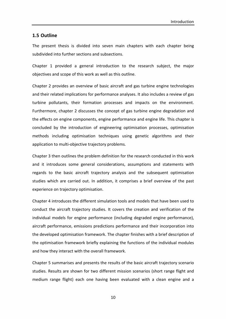
1.5 Outline
The present thesis is divided into seven main chapters with each chapter being
subdivided into further sections and subsections.
Chapter 1 provided a general introduction to the research subject, the major
objectives and scope of this work as well as this outline.
Chapter 2 provides an overview of basic aircraft and gas turbine engine technologies
and their related implications for performance analyses. It also includes a review of gas
turbine pollutants, their formation processes and impacts on the environment.
Furthermore, chapter 2 discusses the concept of gas turbine engine degradation and
the effects on engine components, engine performance and engine life. This chapter is
concluded by the introduction of engineering optimisation processes, optimisation
methods including optimisation techniques using genetic algorithms and their
application to multi-objective trajectory problems.
Chapter 3 then outlines the problem definition for the research conducted in this work
and it introduces some general considerations, assumptions and statements with
regards to the basic aircraft trajectory analysis and the subsequent optimisation
studies which are carried out. In addition, it comprises a brief overview of the past
experience on trajectory optimisation.
Chapter 4 introduces the different simulation tools and models that have been used to
conduct the aircraft trajectory studies. It covers the creation and verification of the
individual models for engine performance (including degraded engine performance),
aircraft performance, emissions predictions performance and their incorporation into
the developed optimisation framework. The chapter finishes with a brief description of
the optimisation framework briefly explaining the functions of the individual modules
and how they interact with the overall framework.
Chapter 5 summarises and presents the results of the basic aircraft trajectory scenario
studies. Results are shown for two different mission scenarios (short range flight and
medium range flight) each one having been evaluated with a clean engine and a

Introduction
11
degraded engine configuration. Furthermore, an engine derate scenario is included in
this analysis as well. The results are assessed in terms of total flight time, total fuel
burned and total pollutants (NOx) emitted.
Chapter 6 summarises and presents the results of the preliminary aircraft trajectory
optimisation studies. Similar to the approach used in chapter 5, the results are shown
for two different mission scenarios (short range flight and medium range flight) for one
aircraft variant.
Chapter 7 contains the discussion of the results, a summary of the achievements and
the conclusions as well as a discussion of the existing limitations of this study. Based on
these observations, recommendations for future work are discussed. Lastly, an outlook
to future developments in aircraft and engine operation focussing on advancements in
aircraft operational procedures and engine health monitoring techniques concludes
this study.

Literature Review
12
2 Literature Review
This chapter forms the basis for the present study and aims to provide a basic
overview of the current state commercial aircraft and engine technology. In addition,
and to better understand the research approach of this work, it provides a detailed
background of the relevant subjects which are addressed throughout this study. This
includes discussions of gas turbine emissions, gas turbine degradation and their
environmental effects as well as an introduction to engineering optimisation
methodologies applicable to multi-objective trajectory optimisation.
2.1 Aircraft Technology
Conventional narrow-body twin-engine aircraft represent the major airframe
configuration used in the short-to-medium range civil passenger transport market
today. This aircraft type is, due to its initial design development and its long service
history and thus the available previous experience, the standard aircraft design which
is continuously being improved to increase airframe efficiency (best lift/drag ratio).
These improvements arise from the use of new materials, advanced control systems
and more effective lift devices. The propulsion systems of those aircraft are typically
arranged in an under wing pylon mounted configuration which dictates certain aircraft
features such as wing or landing gear design. This basic aircraft design is expected to
remain in operation for a considerable amount of time into the future due to its large
application base and its relatively low replacement rate in the worldwide fleet [27].
Current aircraft lifetimes can reach 25-35 years and may be extended even further in
the future. At the same time, aggravated aviation legislations or increasing fuel prices
may accelerate the replacement rate because more modern and efficient aircraft
designs may have the potential to significantly reduce operating costs.
2.1.1 Aircraft Performance
Aircraft performance can be defined as an aircrafts’ ability to accomplish a certain
flight mission while considering all influencing factors. Two major influencing factors to
be considered are the aircraft design and the propulsion system. They will have a

Literature Review
13
significant effect on the whole aircraft performance characteristics, since parameters
such as flight speed or maximum capacity are directly linked to those factors. The
environmental envelope, in which the aircraft’s performance has been established, on
the other hand, features the pressure altitude and temperature limitations. For civil
passenger transportation aircraft three different aspects of aircraft performance can
be addressed which mainly define the overall operational performance [28].
1. The physical aspect: Flight mechanics, aerodynamics, altimetry, external
parameters influencing aircraft performance
2. The operational aspect: Operational methods, aircraft computer logics,
operational procedures, pilot’s actions
3. The regulatory aspect: Aviation regulations certification and operating rules,
establishment of limitations
In the following the major physical aspects and principals, which affect aircraft
performance, are briefly discussed. The operational aspect of aircraft performance will
be addressed in more detail in the next chapter, highlighting important aspects of
current civil aircraft operation and its underlying procedures. The regulatory aspect,
even though of equivalent importance for aircraft operation, will only be briefly
addressed in the next chapter.
In order to assess the basic performance of an aircraft configuration its aerodynamic
properties and the cruising performance have to be estimated. Considering the cruise
performance is important since this is typically the flight phase where most of the fuel
is consumed. In addition, other flight phases like take-off, climb and descent have to
be considered to analyse the aircraft performance for a complete flight mission [29].
The relationship between aircraft lift and drag can be described by the use of a drag
polar which accounts for the dependence of the lift coefficient on the drag coefficient.
For a particular flight phase the aerodynamic performance can be expressed by the
total drag coefficient CD as follows:
ܥ = ܥ + ூܥ (2-1)

Literature Review
14
This where CD0 is called the zero lift drag coefficient (dependent on lift) and CDI is called
the induced drag coefficient (independent on lift).
The explicit equation of the zero lift drag coefficient can be estimated as described
below:
=ூܥ ൬ଵܥ
ଶܥ × ×ߨ ܣ൰+ ଷܥ + ସܥ × ×൨ܥ ܥ
ଶ (2-2)
C1 and C2 are coefficients that account for the wing plan form geometry and C3 and C4
are coefficients that take into account the non-optimum wing twist and viscous effects.
AR represents the wing aspect ratio and CL is the lift coefficient.
The zero lift drag coefficient for an aircraft component such as the fuselage or wing
can be expressed using the following equation:
ܥ =∑൫ܥ ,,, ,௪௧௧ௗ൯
(2-3)
The overall zero lift drag coefficient of the aircraft is the sum of the CD0 of all individual
components and factors. Cfc is the skin friction coefficient and ϕc is the form factor
both necessary to estimate the subsonic profile drag of the particular component. Qc
accounts for the interference drag of the component and Sc,wetted represents the
wetted surface area of the component. The total drag is then divided by Sref which is
the plan form area.
During horizontal cruise flight with constant speed, where the engine thrust equals the
aerodynamic drag, the aerodynamic efficiency E (lift to drag ratio) can be written as
follows:
ܧ =
12 × ×ߩ ܥ × ଶ ×
12 × ×ߩ ܥ × ଶ ×
=ܥܥ
(2-4)
This is where ρ is the density of the air, CL is the lift coefficient, CD the drag coefficient,
V the aircraft speed and Sref the plan form area.

Literature Review
15
2.1.2 Aircraft Operation and Procedures
As described in the previous chapter, efficient aircraft usage depends not only on the
physical aspects but also on operational and regulatory aspects. In the following
section a brief outline of the operational aspects will be provided. Aircraft operation
and operational procedures are continuously revised in order to accommodate
changes which become necessary due to aircraft design modifications, airworthiness
regulatory changes or the evolution of aviation policies. The latter being an important
factor when environmental effects such as gaseous or noise emissions in aircraft
operation are concerned. The Committee on Aviation Environmental Protection (CAEP)
regularly updates policies and standards on aircraft engine emissions which, for
example, address the engine certification requirements in terms of pollutants emitted
at specified operational conditions. Currently, these conditions are consolidated in the
specific Landing and Take-off (LTO) cycle shown in figure 2-1, which accounts for
emissions at typical operation modes. It makes allowance for engine power settings at
idle, take-off, climb and approach conditions but omits cruise conditions.
Figure 2-1: Landing and Take-off (LTO) cycle [30]
For example, countries like Switzerland and Sweden have enacted legislations which
allow airports to introduce emission-based landing fees, based on the amount of
nitrogen oxides emitted, to reduce pollutant emissions [31]. The resulting airspace
concepts are prevalently driven by one or more of the following strategic objectives:
(1) Safety, (2) capacity, (3) efficiency, (4) access and (5) environment [32]. The
Literature Review
16
International Civil Aviation Organization (ICAO) has published comprehensive material
including descriptions of guidelines to construct visual and instrument flight
procedures while maintaining acceptable levels of safety [33], [34]. These guidelines
cover standard operating procedures such as regular departure, en-route or approach
profiles as well as more specific procedures such as noise abatement flight profiles for
take-off and approach. Reference [35] summarises and reviews numerous operational
opportunities for civil aircraft operators to minimise fuel consumption and
consequently emissions. The document not only addresses aircraft and engine specific
opportunities, such as maintenance techniques and flight profile optimisation, but also
covers airport operations, air traffic management or route planning. Several primary
considerations are examined related to operational opportunities and the associated
advantages and technical limitations are reviewed. Since environmental issues become
more and more important for all parties involved in the aviation sector, a continuous
adaption of new procedures is necessary to address changes imposed by those issues.
Aircraft operators also play a major role when it comes to the implementation of new,
more environmental friendly operating procedures. A high level of preparedness and
the availability of highly developed computer and network systems and its dense
global interconnection can allow aircraft operators to enhance their operational
procedures and launch significant operational initiatives [36]. These initiatives can
include improvements of single aircraft flight trajectories as well as more
encompassing alterations. Such improvements can be derived from the ITDs described
in section 1.2 and can focus, for example, on the overall flight and fleet management.
Another factor which influences aircraft operations is air traffic management and air
traffic control. As outlined in the introductory chapter of this work air traffic has
significantly grown in the past and is expected to continue this trend in the future and
associated with this there will be an increasing demand for innovations in air traffic
management. Not only will the traffic on existing routes increase due to the increase in
passengers but also new routes have to be implemented into the existing network
structure. Again, improvements in this field require a multi-disciplinary approach as set
forth by the Clean Sky project.

Literature Review
17
2.2 Engine Technology
Gas turbine engines are the major propulsion system for civil aircraft in service today
with turbofan engines being the most widely used engine variant for short-to-medium
as well as for long range applications. This engine type offers the greatest advantages
in terms of fuel burn efficiency and noise levels over conventional turbojet engines. In
terms of flight velocity, which allows efficient operation up to Mach numbers of 0.85,
turbofan engines also provide an advantage over turboprop engines. Medium to high
bypass ratio direct drive turbofan engines with a two or three spool design represent
the current state of technology. Those engines comprise a conventional architecture
with a large single-stage fan, a multi-stage Low Pressure Compressor (LPC, Booster), a
multi-stage high pressure compressor, an annular combustor, a single or multi-stage
high pressure turbine and a multi-stage Low Pressure Turbine as shown in figure 2-2
[37].
Figure 2-2: Typical two-shaft turbofan engine schematic

Literature Review
18
2.2.1 Turbofan Engine Performance
Engine performance encompasses the overall engine operability in terms of key
parameters which are necessary to meet a given design specification. For aircraft gas
turbine engines two key parameters which describe the engine performance are net
thrust (FN) and specific fuel consumption (SFC). SFC is influenced by factors such as
thermal efficiency, propulsive efficiency and combustion efficiency [38]. The three
main design parameters of a turbofan engine are turbine entry temperature (TET),
overall pressure ratio (OPR) and bypass ratio (BPR). A change in these three
parameters will have an effect on the engine thermal and propulsive efficiency.
The maximum turbine entry temperature (TET) in aero engine combustors is limited by
the mechanical integrity of the combustion chamber and turbine parts which are
exposed to the highest gas temperatures in the engine. The material used for
conventional combustor parts such as liners and domes and turbine parts such as
blades, shrouds and vanes have a detrimental effect on the achievable maximum
engine performance. Apart from the materials used for manufacturing, active cooling
of these highly stressed engine parts is vital to ensure efficient operation. Thus, an
engine design allowing higher turbine entry temperatures will normally yield an
improved thermal efficiency.
The overall pressure ratio (OPR) of a gas turbine represents the total pressure at
compressor exit in relation to the total pressure at engine inlet and thus depends on
the number of compressors and the individual compressor design in a particular
engine configuration. Maximum overall pressure ratios in aero engines are limited by
the maximum permissible engine weight and the operating ranges of the combustor
and the turbines. Aero engines typically feature an axial compressor arrangement
which delivers the highest pressure rise per stage for a given compressor efficiency.
The engine bypass ratio (BPR) is defined as the ratio between the mass flow rate of air
which bypasses the core engine, to the mass flow rate which is passing through the
core engine which is involved in the combustion process. Maximum engine bypass
ratios in aero engines are mainly limited by the increase in the size of the fan diameter

Literature Review
19
or by the decrease in size of the core engine diameter. Very large fan diameters will
disproportionally increase aircraft total drag and increase the weight of the fan section
which includes fan blades and the fan hub. In addition, a larger diameter will require
additional Low Pressure Turbine stages to drive the fan at desired speed. On the other
hand, decreasing the size of the core engine is limited by compressor stage pressure
ratios and the size of the combustion chamber to achieve acceptable compressor and
combustion efficiencies.
A much more detailed elaboration of the correlations between engine overall pressure
ratio (OPR), bypass ratio (BPR) and fan pressure ratio (FPR) and detailed parametric
analyses can be found in the works of Fletcher and Walsh [38] and in the work of
Bräunling [39]. In addition, reference [40] specifically addresses flow characteristics in
turbine engine components, such as inlets and nozzles and their related gas dynamic
problems.
2.2.2 Thermal Efficiency
The thermal efficiency of an aero-engine is described as follows (equation 2-1):
௧ߟ =ଶ−
ଶ
ܣܨ × ܪܨ(2-5)
V0 is the flight velocity, Vj is the jet velocity, FAR is the fuel-air ratio and FHV is the fuel
heating value. The thermal efficiency provides information about the quality of the
engine thermodynamic cycle which in this form means conclusions about how
effectively thermal energy is converted into useful work [39]. Since the thermal
efficiency is dependent on pressures, temperatures, component efficiencies and other
associated losses an improvement of those cycle parameters and thus an improvement
in thermal efficiency will result in an increase in jet velocity [41]. The optimum
achievable thermal efficiency of a heat machine based on a reversible process which,
for example, could be an ideal cycle gas turbine can be described as follows:
௧,௧ߟ = 1 −
௫
(2-6)
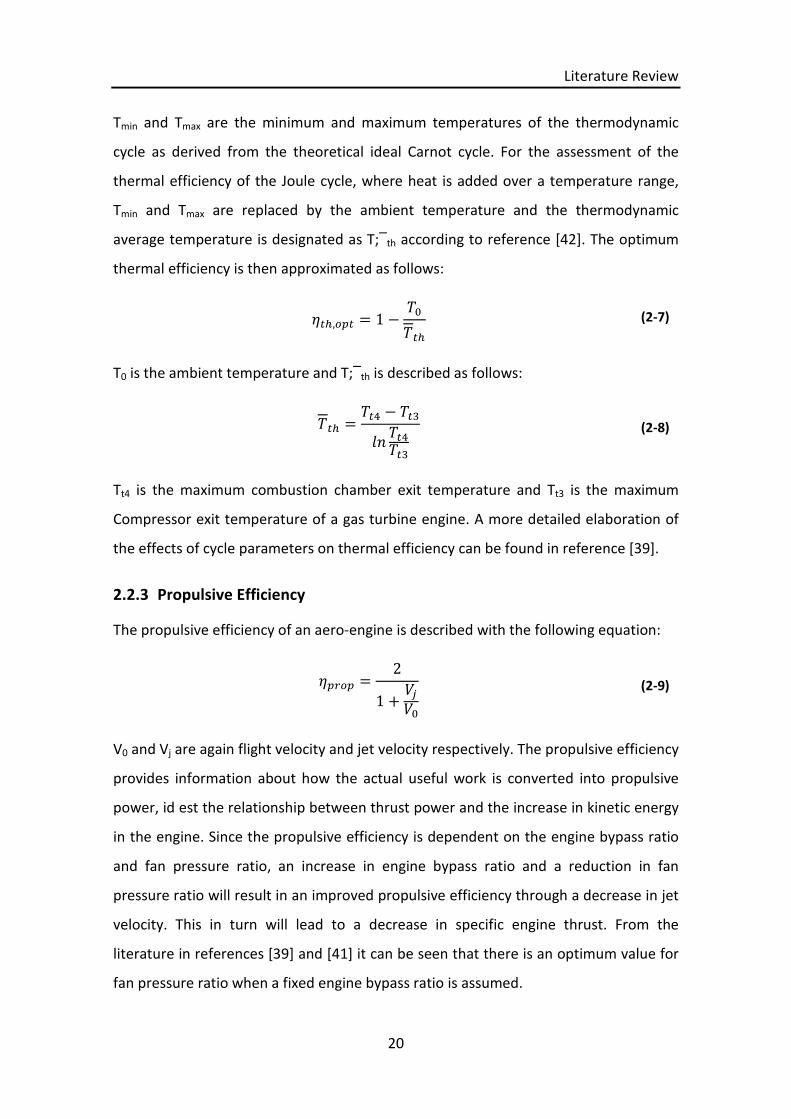
Literature Review
20
Tmin and Tmax are the minimum and maximum temperatures of the thermodynamic
cycle as derived from the theoretical ideal Carnot cycle. For the assessment of the
thermal efficiency of the Joule cycle, where heat is added over a temperature range,
Tmin and Tmax are replaced by the ambient temperature and the thermodynamic
average temperature is designated as T;‾th according to reference [42]. The optimum
thermal efficiency is then approximated as follows:
௧,௧ߟ = 1 −
௧(2-7)
T0 is the ambient temperature and T;‾th is described as follows:
௧ =௧ସ− ௧ଷ
௧ସ
௧ଷ
(2-8)
Tt4 is the maximum combustion chamber exit temperature and Tt3 is the maximum
Compressor exit temperature of a gas turbine engine. A more detailed elaboration of
the effects of cycle parameters on thermal efficiency can be found in reference [39].
2.2.3 Propulsive Efficiency
The propulsive efficiency of an aero-engine is described with the following equation:
ߟ =2
1 +
(2-9)
V0 and Vj are again flight velocity and jet velocity respectively. The propulsive efficiency
provides information about how the actual useful work is converted into propulsive
power, id est the relationship between thrust power and the increase in kinetic energy
in the engine. Since the propulsive efficiency is dependent on the engine bypass ratio
and fan pressure ratio, an increase in engine bypass ratio and a reduction in fan
pressure ratio will result in an improved propulsive efficiency through a decrease in jet
velocity. This in turn will lead to a decrease in specific engine thrust. From the
literature in references [39] and [41] it can be seen that there is an optimum value for
fan pressure ratio when a fixed engine bypass ratio is assumed.

Literature Review
21
2.2.4 Overall Efficiency
Based on the considerations of sections 2.2.2 and 2.2.3 the overall engine efficiency is
described as follows:
=௩ߟ ௧ߟ × ߟ (2-10)
The overall engine efficiency is the product of thermal efficiency and propulsive
efficiency and represents the relationship between specific thrust performance and
specific heat energy of the fuel. If the fuel heating value (FHV) is assumed constant, the
overall efficiency can be expressed as the inverse of the specific fuel consumption
(SFC) for a given flight velocity:
~ܥܨ1
௩ߟ(2-11)
An improvement in thermal and/or propulsive efficiency will result in improved overall
engine efficiency.
2.3 Gas Turbine Engine Emissions
All gas turbine engines which burn fossil fuels emit pollutants that originate from the
combustion products generated during engine operation. Many of the pollutants are
hazardous to the environment and the human health while many of the harmful
pollutants have been identified to cause measureable changes in the global
atmosphere, local air quality and can be the cause for several diseases [43]. In a
conventional gas turbine combustor a mixture of air and kerosene (hydrocarbon) is
burned and the chemical energy contained in the fuel is converted into heat energy.
Through the combustion process this hydrocarbon is converted to carbon dioxide (CO2)
and water vapour (H2O), ideally in a Stoichiometric combustion that is described with
the following reaction equation:
ଶସܪଵଶܥ + 18 ൬ ଶ +79
21ଶ൰ → ଶܥ12 + ଶܪ12 + 18൬
79
21൰ଶ
(2-12)
Literature Review
22
One mole of kerosene requires the existence of eighteen mole of oxygen for the
Stoichiometric combustion to be complete which will then release carbon dioxide
(CO2), water vapour (H2O) and nitrogen (N2) in the exhaust gas. In addition, a real
combustion process will also release carbon monoxide (CO), oxides of nitrogen (NOx),
oxides of sulphur (SOx) and unburned hydrocarbons (UHC). Most of the gas turbine
pollutants and their concentrations can be directly related to the temperature in the
combustor and the residence time in the combustor [44]. For example, NOx emissions
will decrease with lower residence times while higher combustion temperatures will
cause NOx emissions to rise. Higher temperatures will increase combustion efficiency
but will increase NOx emissions at the same time. On the other hand, a reduction in
residence time and decrease in temperature will cause CO emissions to rise.
It can be differentiated between ground or near ground emissions designated as local
air quality pollutants and emissions occurring at altitude which are considered as
greenhouse gases. The ground or near ground emissions are controlled by an idealised
standard LTO (Landing and Take-Off) cycle set forth by the International Civil Aviation
Organization (ICAO) while cruise emissions are not regulated through specifications
and thus are not considered by any policy instruments [45].The five main types of gas
turbine emissions will be briefly described in the following chapters primarily focusing
on their formation mechanisms and their effect on the atmospheric environment. Even
though the release of water vapour can under given conditions cause the formation of
vapour trails in the atmosphere and foster the formation of artificial cirrus clouds,
which may contribute to changes of the atmosphere that abet the greenhouse effect,
it will not be addressed further in this work. Table 2-1 exemplifies the typical exhaust
gas composition of a conventional turbofan engine [39]. From this data one can also
see that carbon monoxide concentrations and concentrations of unburned
hydrocarbons are highest at low power conditions (idle power) and decrease with high
power conditions (take-off). This is due to the fact that CO and UHC emissions will
form as a result of incomplete combustion which occurs at lower power conditions in
conventional combustors [39]. However it must also be kept in mind that engine

Literature Review
23
emission levels have a close relationship to basic cycle parameters such as pressure
ratio and turbine inlet temperature.
Table 2-1: Typical turbofan exhaust gas composition (according to Bräunling [39])
Idle power Take-off power
Oxygen O2 18.54 % 15.06 %
Carbon Dioxide CO2 1.60 % 3.66 %
Nitrogen N2, Inert Gases Ar, Ne and Water H2O, 79.86 % 81.28 %
Carbon Monoxide CO, Oxides of Nitrogen NOx,
Unburned Hydrocarbons UHC
2.3.1 Carbon Dioxide
The formation of carbon dioxide (CO2) is a direct consequence of the complete
combustion of the fuel in the combustor and its emission as such is inevitable. Due to
its stability and the subsequent relatively long residence time in the atmosphere
carbon dioxide is identified to be a significant contributor to global warming by
boosting the greenhouse effect [44].
Since the amount of carbon dioxide emitted during the combustion process is directly
linked to the amount of fuel burned, an emission reduction can only be achieved by
increasing fuel efficiency and/or fuel savings.
2.3.2 Carbon Monoxide
Carbon monoxide (CO) is produced during the combustion process if there is not
enough oxygen to form carbon dioxide, id est if no complete combustion takes place.
Two preconditions which lead to formation of carbon monoxide are low combustion
zone temperatures and/or insufficient time for combustion. These conditions can be
caused by inadequate burning rates due to a low fuel/air ratio, inadequate mixing of
fuel and air in the combustor with regions of weak or over-rich mixture strengths, or
by quenching of combustion products which are entrained by the cooling air flow of
the combustion chamber liners [44]. The fuel and air mixture strength in the

Literature Review
24
combustion zone will also have an effect on the CO concentration and mixtures being
close to Stoichiometric cause high amounts of CO due to dissociation of carbon
dioxide. An effective control of the fuel and air mixture in the combustor over a wide
range of power settings will be beneficial for the overall combustion efficiency.
2.3.3 Oxides of Nitrogen (NOx)
The formation of oxides of nitrogen results from the oxidation of atmospheric nitrogen
in high-temperature regions of the flame in the combustor [44]. NOx in this context
refers to the sum of NO and NO2 emissions. Nitric oxide represents one major
pollutant compound of these oxides and it is formed in the high temperature regions
of the combustor with temperatures above 1800K during high power conditions.
The NO formation follows the Zeldovich chain mechanism which can be described in
three steps as shown below:
ଶ ⇌ 2
+ ଶ ⇌ � +
+ ଶ ⇌ +
(2-13)
Three different mechanisms, which are listed below, contribute to the NO formation:
1. “Thermal” NO: Thermal NO is characterised through its relatively high initiation
temperatures which then lead to the formation reaction where atmospheric
nitrogen is oxidised in the post-flame gases. In combustion engines NOx
formation starts with temperatures around 1200K.
2. “Prompt” NO: Prompt NO is generated through very fast formation reactions in
low-temperature, fuel-rich flames. However, the formation mechanisms are
very complex and have not been completely investigated and understood.
3. “Fuel” NO: The sources of fuel NO are the nitrogen portions bound in the fuel
which transforms into NOx during the combustion process. Thus the amount of
generated fuel NOx highly depends on the nitrogen content of the particular
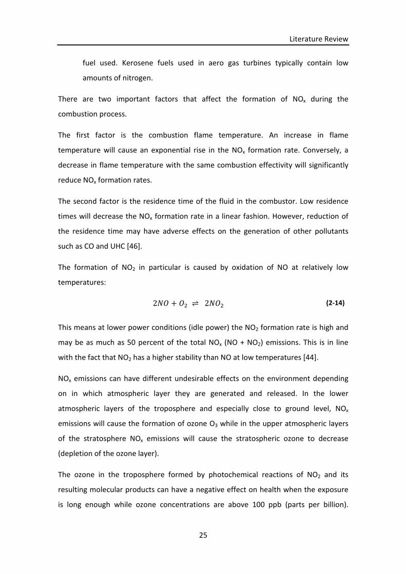
Literature Review
25
fuel used. Kerosene fuels used in aero gas turbines typically contain low
amounts of nitrogen.
There are two important factors that affect the formation of NOx during the
combustion process.
The first factor is the combustion flame temperature. An increase in flame
temperature will cause an exponential rise in the NOx formation rate. Conversely, a
decrease in flame temperature with the same combustion effectivity will significantly
reduce NOx formation rates.
The second factor is the residence time of the fluid in the combustor. Low residence
times will decrease the NOx formation rate in a linear fashion. However, reduction of
the residence time may have adverse effects on the generation of other pollutants
such as CO and UHC [46].
The formation of NO2 in particular is caused by oxidation of NO at relatively low
temperatures:
2 + ଶ ⇌ 2ଶ (2-14)
This means at lower power conditions (idle power) the NO2 formation rate is high and
may be as much as 50 percent of the total NOx (NO + NO2) emissions. This is in line
with the fact that NO2 has a higher stability than NO at low temperatures [44].
NOx emissions can have different undesirable effects on the environment depending
on in which atmospheric layer they are generated and released. In the lower
atmospheric layers of the troposphere and especially close to ground level, NOx
emissions will cause the formation of ozone O3 while in the upper atmospheric layers
of the stratosphere NOx emissions will cause the stratospheric ozone to decrease
(depletion of the ozone layer).
The ozone in the troposphere formed by photochemical reactions of NO2 and its
resulting molecular products can have a negative effect on health when the exposure
is long enough while ozone concentrations are above 100 ppb (parts per billion).

Literature Review
26
Respiratory illnesses, impaired vision and other disorders can be the consequence of
such exposure. Its relatively long residence time of about 10 month in the atmosphere
amplifies its effect on the environment [47].
The NOx emissions in the higher atmospheric layers of the stratosphere on the
contrary cause a depletion of the existing ozone layer. The atmospheric ozone reacts
with the nitric oxides and forms nitrous oxide and molecular oxygen. The newly
formed nitrous oxide then again reacts with atomic oxygen to regenerate nitric oxides.
Stable atmospheric conditions in the stratosphere foster this process since only very
little mixing takes place and particles can remain in these layers for longer times. A
reduction of the ozone layer causes an increase in ultra-violet radiation at ground level
since there is less ozone available to absorb the radiation from the sun. An increased
risk for skin cancer can be one consequence of this ozone layer depletion [47]. A
detailed elaboration of the atmospheric effects initiated by the above described
pollutants as well as their formation mechanism can be found in reference [5] while
reference [27] provides a projection for future growth of aviation emissions and in
particular NOx emissions.
2.3.4 Oxides of Sulphur (SOx)
Oxides of sulphur, and sulphur dioxide SO2 in particular is generated during the
reaction of the sulphur contained in the fuel with the oxygen in the air. Thus the
amount of SO2 generated during the combustion process mainly depends on the
sulphur content of the fuel used. Since oxides of sulphur are toxic and corrosive high
contents in the fuel will have a negative effect on the engine life and durability.
However, minimum amounts of sulphur in the fuel are desired to maintain fuel
lubricity and to prevent fuel system corrosion. The maximum permitted concentration
for aviation kerosene is 0.3% by mass.
2.3.5 Unburned Hydrocarbons
Unburned hydrocarbons are formed during an incomplete combustion process mainly
due to insufficient fuel atomization or inadequate burning rates. The amount of

Literature Review
27
generated unburned hydrocarbon products depends on the engine power conditions.
Higher power conditions will reduce UHC emissions through an increased chemical
reaction rate caused by higher combustor inlet temperatures and pressures [44].
2.3.6 Soot
Soot is produced during incomplete combustion of hydrocarbons in the fuel-rich
regions of the combustor and where mixing is inadequate. Soot becomes visible as
smoke when it is emitted through the engine exhaust nozzle in the atmosphere and
consists of small particles of different size and form that make up aerosols [48]. Soot
emissions in airport vicinities as well as soot emissions at altitude are of concern due
to the effects of visible pollution on ground and the potential to affect contrails and
cloud formation at altitude. A drastic reduction in soot emissions can be achieved by
increasing the amount of air injected into the combustion zone which results in lower
temperatures and more oxygen being available for combustion. Further strategies to
reduce soot emissions focus on the improvement of fuel injection system to obtain
adequate atomisation and better aeration of the fuel in the combustor [44].
2.4 Gas Turbine Engine Degradation
As outlined in the previous section 2.2, overall engine performance relies on many
different matched component parameters such as compressor pressure ratios,
combustion temperatures or turbine entry temperatures and thus changes of which
will have a discernible effect on engine performance. Since a mechanical
turbomachinery such as an aero-engine will exhibit substantial wear and tear over its
service life it is essential to monitor and assess the condition of an engine continuously
to ensure reliable operation within design and certification parameters. Engine
degradation monitoring or Engine Health Monitoring (EHM) is an integral instrument
for gas turbine operation and is necessary to determine engine performance at any
given time and also to allow a prognosis for future performance trends. This trend
monitoring is achieved through continuous recording of engine component data during
the engine running envelope. Typically, the minimum essential data that is recorded
for performance analysis consists of pressures and temperatures of the engine gas

Literature Review
28
path at discrete locations as well as shaft rotational speeds and engine fuel flow. In
addition, engine oil temperature and oil pressure as well as engine vibration data
(frequency and amplitude of shaft vibration) is recorded and analysed as part of the
engine condition monitoring process [49]. Apart from those data based parameters
which can be remotely analysed the actual visual inspections and gas path borescope
inspections of the engine form another crucial element of an engine health monitoring
concept [50]. One measure primarily used to determine the actual engine condition in
terms of operational performance is the measurement of the engine Exhaust Gas
Temperature (EGT). It is typically measured at locations after the High Pressure
Turbine exit or at the first stages of the Low Pressure Turbine where gas path
temperatures are relatively low to allow installation of appropriate sensors. From
these exhaust gas temperature measurements one can infer the turbine entry
temperature which in turn correlates with a certain engine thrust (shaft rotational
speed). Two main categories can be established to classify engine degradation
mechanisms:
1. A considerable amount of the overall engine degradation is caused by normal
engine operation in different layers (altitudes) of atmospheric air. This includes
deterioration of the engine due to natural ageing and constitutes a process
which cannot be avoided ultimately.
2. Other significant drivers of engine degradation are either single random events
such as foreign object damage (FOD) or material failures as well as engine
operational procedures such as take-off derate, engine taxi policies and warm-
up and cool down times. This also includes maintenance procedures to
preserve the engine condition, id est engine washing or engine control system
maintenance.
The analysis and quantification of engine degradation over time is an important factor
for reliable and efficient engine operation. The prediction of engine performance
degradation based on the change of characteristic engine parameters can offer
valuable clues to expected engine operational life and its associated performance
behaviour. The identification of the main influencing parameters is thus essential to

Literature Review
29
allow for accurate prediction results [51]. A probabilistic approach to engine
degradation is presented in reference [52] where characteristic engine parameters
such as temperatures, pressures etc., but also component tolerances and production
data, are gathered to model the engine condition. A stochastic Monte-Carlo simulation
is then applied to the pre-processed distribution functions of the characteristic
parameters to generate plots that describe the change of global performance
parameters, such as SFC, over time.
2.4.1 Typical Mechanisms of Engine Degradation
The two main categories of engine degradation described in the previous chapter are
initiated and evoked by the alteration of several mechanical and/or chemical
properties of the gas turbine engine parts. The degradation of aerodynamic
components, such as the engine compressor, the combustor, and the turbine which all
operate in harsh environments, is a major driver for engine performance deterioration.
This is due to the fact that all of the below mentioned degradation modes will cause a
change of the parts original shape, properties and condition [53]. A general overview
of these mechanisms and their effects are presented in this chapter.
The selection of the degradation mechanisms examined in the present work is based
on their effect on the gradual, long-term engine wear which is anticipated when a
normal engine operation is taken as a basis. In turn this means degradation effects
caused by single events such as foreign object damage (FOD), excessive flight loads,
component malfunctions or sudden changes in environmental conditions (volcanic
ash), all of which may lead to significant and rapid deterioration of the engine
performance and/or integrity, are not reviewed as part of this study.
2.4.2 Thermal Distress
Mainly parts of the combustor and turbine are subjected to very high temperatures
either directly by exposition to hot flow path gases or indirectly by their proximity to
the engine hot section. This includes stationary mechanical parts such as combustion
chamber liners, turbine vanes and structural turbine cases and frames as well as

Literature Review
30
rotating engine parts such as turbine disks, turbine blades and rotating seals. Even
components like fuel nozzles and instrumentation devices for engine condition
monitoring are affected by thermal distress.
Hot corrosion is one common mechanism which will cause a material loss of the
affected component over time due to the chemical reaction between the base material
and substances carried in the hot gas. These substances can originate from the fuel or
from sources external to the engine such as sulphates or salts. This type of corrosion is
designated as sulphidation. The integrity of hot section engine parts such as high alloy
HPT blades and vanes will be impacted by this type of corrosion which is induced by a
combination of sodium chloride from the inlet air and sulphur from the fuel. Another
known distress mechanism is high temperature oxidation which is caused by a
chemical reaction between the base material and free oxygen from the hot gaseous
environment. This reaction will also lead to a removal of component material. In
addition burn-off with significant material detachment due to excessive temperatures
can occur in the combustion and turbine section [54]. Spalling and removal of the
Thermal Barrier Coating (TBC) of the high pressure turbine blades will cause an
immediate failure of the part due to the exposition of the base material to the high,
beyond melting point temperatures.
2.4.3 Mechanical Wear
Engine air and oil seals in all parts of the engine are mostly affected by mechanical
wear which causes an increase in leakage flow over time. But also engine bearings,
gearboxes and other moving parts are subject to mechanical wear and many of the
resulting effects are being researched in the domain of tribology. Continuous rubbing
of the engine seals against each other during engine operation due to rotation or
vibration leads to base material removal and consequently an increase in gaps. Cyclic
operation (acceleration and deceleration) of the engine amplifies this abrasive wear
effect and promotes leakages and mechanical wear.

Literature Review
31
2.4.4 Corrosion, Erosion and Abrasion
Corrosive distress arises on parts by chemical reaction of the base material with its
environment. In most cases this is electrochemical oxidation of the exposed metal part
reacting with oxygen from the surrounding air and/or moisture in the air. This type of
corrosion can affect cold section engine parts such as steel alloy LPC blades and vanes
where it can compromise their integrity.
Erosion of parts is caused by hard particles impinging a surface, thus rubbing away
material and diminishing the parts’ original thickness. It will mainly occur in airfoils
which are in direct contact with the flow-path air. The ingested particles typically have
to be larger than 10 μm in diameter to have an abrasive effect [54]. Dust, sand or other
floating particles are common examples for these particles. Apart from airfoils, any
other stationary or rotating part can be affected by erosion if it is exposed to an airflow
which carries abrasive particles. Especially cooling air passages and cavities within the
engine, where air circulates constantly, are prone to severe erosion.
In the context of this work abrasion is defined as material removal due to the rubbing
of a moving blade tip against its stationary lining surface or due to the rubbing of a
rotating interstage seal against its stationary counterpart. Those rubs can originate
from flight loads and gyroscopic effects causing engine shafts and cases to deflect from
their original positions and thus increasing or decreasing blade tip and seal clearances.
In addition, rubbing can particularly occur in the engine turbines where material
contractions are amplified due to the high temperature environment.
2.5 Effects of Engine Degradation
This chapter is focused on the effects of the previously described engine degradation
mechanisms. The first subsection addresses the impact on the engine components or
subsystems and their individual performances in terms of design and operational
parameters. The second subsection will address the expected effect on the overall
engine performance and the last section will deal with the implications on the life of
the engine.

Literature Review
32
A degraded engine which has operated for a particular amount of time in service will
show a higher fuel consumption compared to the initial fuel consumption values
achieved right after engine production assuming the same amount of engine take-off
thrust. This means over time the engine SFC will increase due to degradation of the
engine component efficiencies, mainly of the compressor, the combustor and the
turbine modules.
A parameter which is commonly used to describe the engine condition is called “EGT
margin”. This value is calculated by subtracting the maximum allowable EGT provided
by the engine manufacturer from the actual EGT measured during engine operation.
As described in section 2.4, the TET is directly linked to the engine EGT. The maximum
allowable EGT (EGT redline) represents the limit established by the engine
manufacturer during certification tests and marks the maximum acceptable
temperature at which the engine can operate without suffering rapid deterioration.
Peak EGT values are usually reached at or shortly after take-off and thus depend on
the OAT (Outside Air Temperature). One method utilised in modern turbofan engines
to control the engine EGT is accomplished by flat-rating the engine at a certain
ambient temperature. This means the engine will be able to provide maximum take-off
thrust up to a specific ambient temperature, named “Corner Point” or CP (e.g.
ISA+30°C) and beyond this point fuel flow will be limited to maintain a constant EGT
and thus thrust will decrease. Figure 2-3 shows this effect on the EGT margin for a
clean and degraded engine at corner point conditions. The degraded engine will have a
lower EGT margin than the clean engine during a take-off at Corner Point conditions
and thus operates with decreased performance margins.

Literature Review
33
Figure 2-3: Effect of ambient temperature on engine EGT (flat-rated engine)
2.5.1 Effects on Engine Components
Engine component performance characteristics depend on their established design
performance parameters. These parameters are determined during the matching of
individual engine components in order to assemble a complete engine system. Five
important performance parameters are listed below:
1. Compressor efficiency
2. Compressor flow capacity
3. Compressor pressure ratio
4. Combustion efficiency
5. Turbine efficiency
In the following, degradation effects of the two major engine components, the high
pressure compressor and the high pressure turbine, will be briefly analysed. One main
cause for compressor degradation is airfoil erosion which leads to an increase in
surface roughness and a decrease in airfoil chord [55]. In the simplified form, the
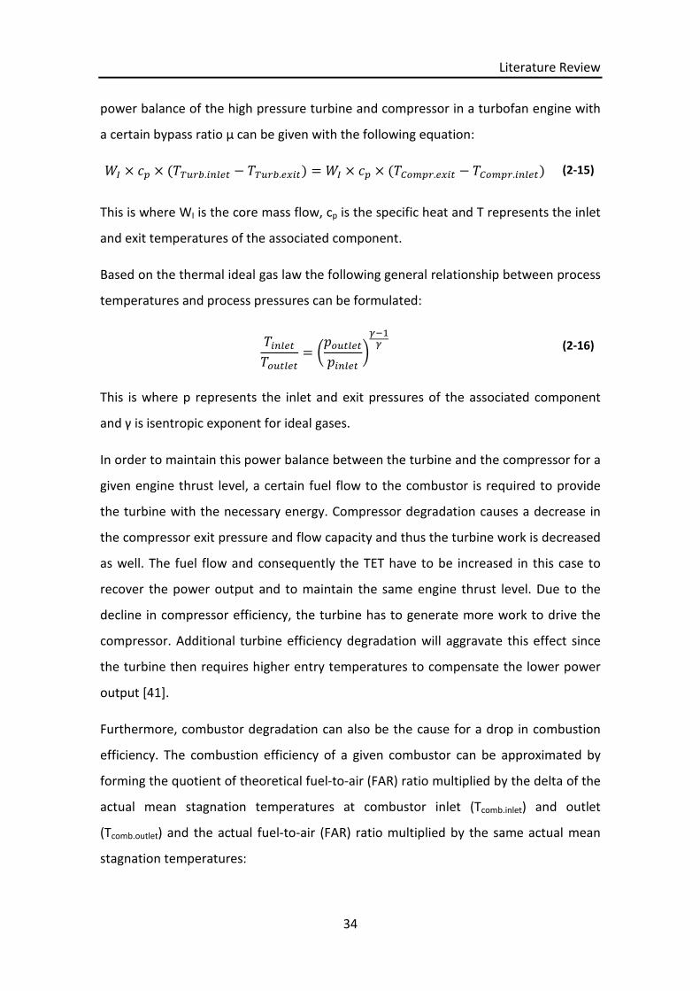
Literature Review
34
power balance of the high pressure turbine and compressor in a turbofan engine with
a certain bypass ratio μ can be given with the following equation:
ூ× × ( ௨.௧− ௨.௫௧) = ூ× × ( .௫௧− .௧) (2-15)
This is where WI is the core mass flow, cp is the specific heat and T represents the inlet
and exit temperatures of the associated component.
Based on the thermal ideal gas law the following general relationship between process
temperatures and process pressures can be formulated:
௧
௨௧௧= ൬
௨௧௧௧
൰
ఊଵఊ (2-16)
This is where p represents the inlet and exit pressures of the associated component
and γ is isentropic exponent for ideal gases.
In order to maintain this power balance between the turbine and the compressor for a
given engine thrust level, a certain fuel flow to the combustor is required to provide
the turbine with the necessary energy. Compressor degradation causes a decrease in
the compressor exit pressure and flow capacity and thus the turbine work is decreased
as well. The fuel flow and consequently the TET have to be increased in this case to
recover the power output and to maintain the same engine thrust level. Due to the
decline in compressor efficiency, the turbine has to generate more work to drive the
compressor. Additional turbine efficiency degradation will aggravate this effect since
the turbine then requires higher entry temperatures to compensate the lower power
output [41].
Furthermore, combustor degradation can also be the cause for a drop in combustion
efficiency. The combustion efficiency of a given combustor can be approximated by
forming the quotient of theoretical fuel-to-air (FAR) ratio multiplied by the delta of the
actual mean stagnation temperatures at combustor inlet (Tcomb.inlet) and outlet
(Tcomb.outlet) and the actual fuel-to-air (FAR) ratio multiplied by the same actual mean
stagnation temperatures:

Literature Review
35
ߟ =×௧௧ܣܨ ( .௨௧௧− .௧)
×௧௨ܣܨ ( .௨௧௧− .௧)< 1 (2-17)
However, it must be noted that this definition is not in line with the fundamental
definition based on the ratio of actual energy released to the theoretical quantity
obtainable [46].
2.5.2 Effects on Engine Performance
From a bare engine stand point there are two important factors which determine the
engine performance and which have an effect on the engine condition: (1) The first
factor is the engine operational design scope with regards to maximum take-off thrust
levels at a maximum ambient temperature representing the engine limitations. These
limitations are directly linked to the maximum achievable combustion temperatures in
the combustor, and thus directly linked to the turbine entry temperature TET. For
example, continuous high power take-offs at high ambient temperatures will cause
accelerated degradation of the engine. (2) The second factor is the engine utilisation
rate in terms of hour to cycle ratio (stage length) and the engine operational envelope
in terms of environmental and climatic conditions. For example, high daily aircraft
utilisation in terms of cycles flown will increase the cyclic degradation of the engine.
On the other hand, environmental conditions differ depending on the global region
and the amount of erosive or anthropogenic pollutants in the air has a substantial
effect on engine performance degradation [56]. Both factors combined will determine
the overall engine degradation over time and thus are key elements to address for
engine performance preservation strategies.
2.5.3 Effects on Engine Life
Aero engine life is on the one hand prescribed by the engine manufacturers who limit
the life of certain parts based on load and stress calculations, engine thermal
behaviour, material behaviour, engine long-time endurance testing and safety factors
and requirements. For example, airworthiness standards prescribe part life limits in
such way that cracks do not initiate. On the other hand engine life largely depends on

Literature Review
36
the operational conditions it is exposed to also in terms of maintenance and usage.
This means for example that predetermined life limits of engine parts may change
(increase/decrease) during the course of an engine model lifetime based on the
operational experience. In the context of this work the definition of engine life is
considered with respect to the fatigue life and thermal degradation of critical engine
parts. In the following only two prevailing distress modes which affect gas turbine
engine life will be briefly addressed in order to provide a context to the results of this
work. In particular it is confined to the low-cycle fatigue (LCF) life and thermal fatigue
which determine the maximum operational life of an engine component before it has
to be removed for repair or retirement. In addition to cyclic fatigue, hot section parts
such as turbine blades, turbine vanes, disks and combustor components are directly
affected by thermal fatigue, hot corrosion and oxidation.
Low-cycle fatigue (LCF) life limitations are mainly determined by the number of cycles
under high load conditions (high stresses). Particularly the amount of change in the
material properties under a peak stress condition will have an effect on LCF.
Particularly in short range applications low cycle fatigue becomes the limiting factor for
the total life of rotating engine parts, whereas on longer range applications the creep
life of the parts may become the limiter. Other factors which affect the fatigue
behaviour are type and nature of loading, component size, surface finish and stress or
strain concentrations [57]. In aero engines this condition is reached during take-off
power settings imposing the highest stress on all engine parts. The reduction of take-
off thrust can consequently lower the peak stresses and in turn positively affect LCF
life.
This thrust reduction is also accompanied by a reduction in peak temperatures in the
engine hot section. A lower turbine entry temperature (TET) will decrease the amount
of thermal fatigue and the degree of engine degradation. On the opposite, engine
degradation over time due to normal operation will increase the TET to maintain the
same engine take-off thrust. Thus, over time, thermal stresses in the hot section will
increase and both LCF life and thermal fatigue will be negatively influenced.

Literature Review
37
The above mentioned considerations only describe the basic aspects of two particular
mechanisms which affect the engine life. Further detailed information about engine
life assessments and lifing models can be found in reference [58].
2.6 Principles of Optimisation Processes
This section aims at providing a brief introduction into the major principles of
optimisation processes and their application in practical engineering problems. This
includes a general characterization of different optimisation problems as well as the
assessment of appropriate and suitable optimisation methods.
2.6.1 Optimisation Problems
In general, an optimisation process represents the search for an optimal solution for a
given problem while taking into account all known influencing factors. Using a
mathematical approach it can be regarded as the process of finding the variables that
lead to an optimal value of a given function which is to be optimised. Ultimately, the
solution to an engineering optimisation problem will always involve the minimisation
of the efforts required or the maximisation of the desired benefit [59].
According to Rao [59] optimisation problems can be classified in several ways
depending on the particular problem to be addressed. An overview, as adapted from
Rao, of the different optimisation problems is provided below:
Classification based on the existence of constraints
Classification based on the nature of the design variables
Classification based on the physical structure of the problem
Classification based on the nature of the equations involved
Classification based on the permissible values of the design variables
Classification based on the deterministic nature of the variables
Classification based on the separability of the functions
Classification based on the number of objective functions
Literature Review
38
For the purpose of this study and to put the above mentioned classifications into the
research context, a generic optimisation problem can be defined in mathematical
terms as follows:
= ൞
ଵݔଶݔ⋮ݔ
which minimises f(X)
Subject to c constraints:
() ≤ 0,��� = 1,2,3, … ,
ℎ() = 0, = + 1, + 2, … ,
(2-18)
This is where f(X) is the objective function, X is the design vector, gj(X) is the function
defining the inequality constraints and hl(X) is the function defining the equality
constraints. The design vector X contains all decision variables xi, i=1,2,…n of the
optimisation problem. The number of constraints c and/or m and the number of
decision variables does not necessarily need to correlate and can be arbitrary.
For engineering problems such as aircraft trajectory optimisation problems, the
objective functions can be regarded as surrogates for real goals which are to be
approximated during the optimisation process and which will have to satisfy the
requirements of the problem. These requirements then also impose limitations on the
range of the specific values of the decision variables.
2.6.2 Optimisation Methods
There are different ways to address the optimisation problems defined in the previous
chapter. Depending on the particular optimisation problem multiple methods may be
suitable which may all be able to deliver satisfactory results. This means, the selection
of an appropriate optimisation method requires the assessment of the particular
problem in advance to ensure that the most feasible results can be obtained. For
example, mathematical programming, also called mathematical optimisation, is one
optimisation method that employs the search for an optimum solution from an
available solution space. According to Rao [59] the field of mathematical programming
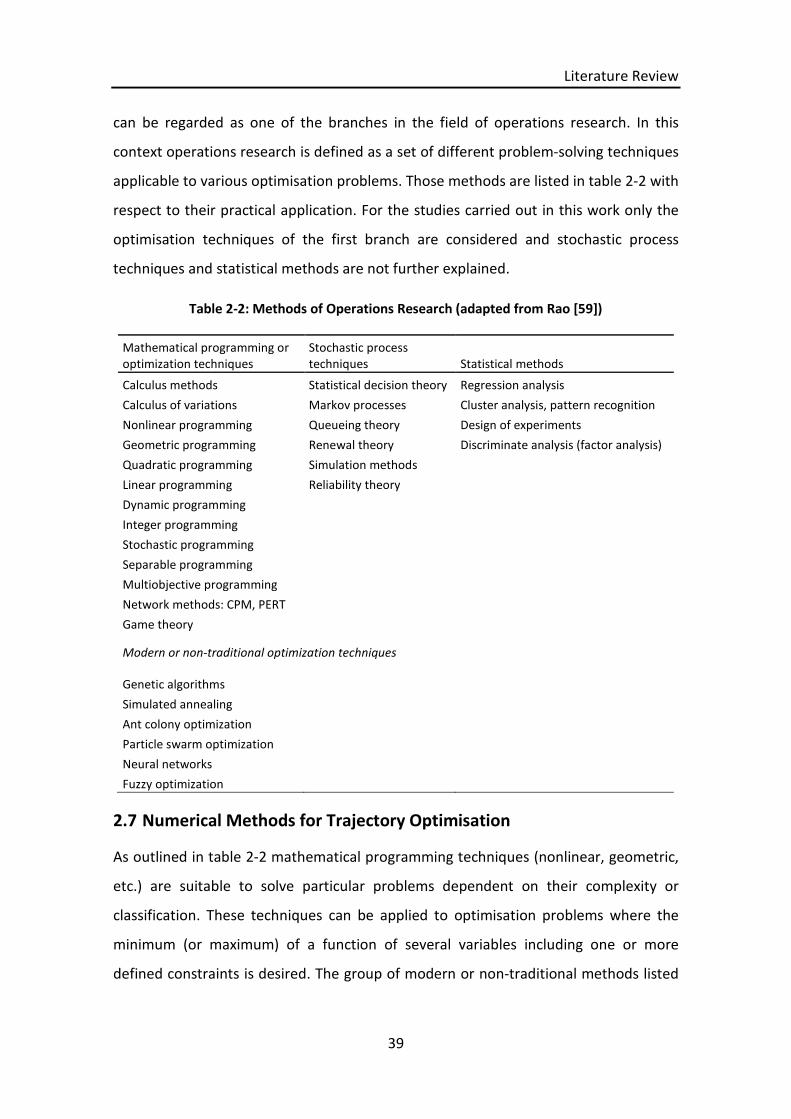
Literature Review
39
can be regarded as one of the branches in the field of operations research. In this
context operations research is defined as a set of different problem-solving techniques
applicable to various optimisation problems. Those methods are listed in table 2-2 with
respect to their practical application. For the studies carried out in this work only the
optimisation techniques of the first branch are considered and stochastic process
techniques and statistical methods are not further explained.
Table 2-2: Methods of Operations Research (adapted from Rao [59])
Mathematical programming oroptimization techniques
Stochastic processtechniques Statistical methods
Calculus methods Statistical decision theory Regression analysis
Calculus of variations Markov processes Cluster analysis, pattern recognition
Nonlinear programming Queueing theory Design of experiments
Geometric programming Renewal theory Discriminate analysis (factor analysis)
Quadratic programming Simulation methods
Linear programming Reliability theory
Dynamic programming
Integer programming
Stochastic programming
Separable programming
Multiobjective programming
Network methods: CPM, PERT
Game theory
Modern or non-traditional optimization techniques
Genetic algorithms
Simulated annealing
Ant colony optimization
Particle swarm optimization
Neural networks
Fuzzy optimization
2.7 Numerical Methods for Trajectory Optimisation
As outlined in table 2-2 mathematical programming techniques (nonlinear, geometric,
etc.) are suitable to solve particular problems dependent on their complexity or
classification. These techniques can be applied to optimisation problems where the
minimum (or maximum) of a function of several variables including one or more
defined constraints is desired. The group of modern or non-traditional methods listed

Literature Review
40
in table 2-2 represent more recent optimisation techniques, some of which are
inspired by processes of nature (genetic algorithm) or by theories which are based on
artificial models of uncertainties experienced in common processes (fuzzy logic). With
regards to the requirements of solving an aircraft trajectory optimisation problem
several techniques can be suitable due to their inherent solving mechanisms.
The following subsections discuss the three most important methods as grouped by
Schwefel [60] and as used by Celis [61] and Zolata [23]. Those are hill climbing
methods, random search methods and evolutionary methods. A schematic overview is
presented in figure 2-4.
Figure 2-4: Overview of optimisation strategies (adapted from Schwefel [60])
2.7.1 Hill Climbing Methods
Hill climbing optimisation methods employ an iterative approach to finding a solution
for a particular optimisation problem. It is characterised as a local search technique
which means that, depending on if a maximum or minimum objective function value is
sought after, the optimiser will incrementally change an element of the solution to find
the best among a number of candidate solutions. Hill climbing methods can be used
for one-dimensional and multi-dimensional optimisation problems. The solving
techniques for multi-dimensional problems can be further divided into direct search
methods, gradient methods and newton methods.
Literature Review
41
Direct search methods only use the value of the objective function without
information about the gradient of the objective function to search for solutions
superior to the current one. Thus it allows the application of this method to problems
where the objective function is not differentiable or not continuous which in turn
makes its use relatively simple. This simplicity on the other hand can have a negative
impact on the optimisation performance as it may provide insufficient solutions for
problems where numerous local maxima are present in the solution space.
Gradient methods also use the first partial derivative of the objective function
assuming that it is differentiable. This means information inherent to the objective
function, id est the gradient of the function, is necessary in order to approximate a
numerical solution in the solution space while taking into account the search
directions.
The first and second partial derivative is used in Newton methods which require a
higher order of differentiability of the objective function. The optimisation process
employs the second order partial derivatives of a quadratic function which are
subsequently used in the inverted Hessian matrix to calculate the results.
2.7.2 Random Search Methods
Random search strategies for optimisation problems make use of probabilistic rather
than deterministic rules to vary the parameters of the optimisation process. This
means the parameters are subject to randomness which, however, does not
necessarily imply arbitrariness [60]. The randomness of the optimisation parameters
allows the process to explore solutions in many different directions independent of the
structure of the objective function. On the other hand, due to the randomness the
optimisation process does not take optimal steps towards the solution and hence may
require a significant amount of computational resources. The relative simplicity of the
random search method and its independence from the information about the
objective function make them applicable to every case. Further information about
random search methods and application examples can be found in reference [60].
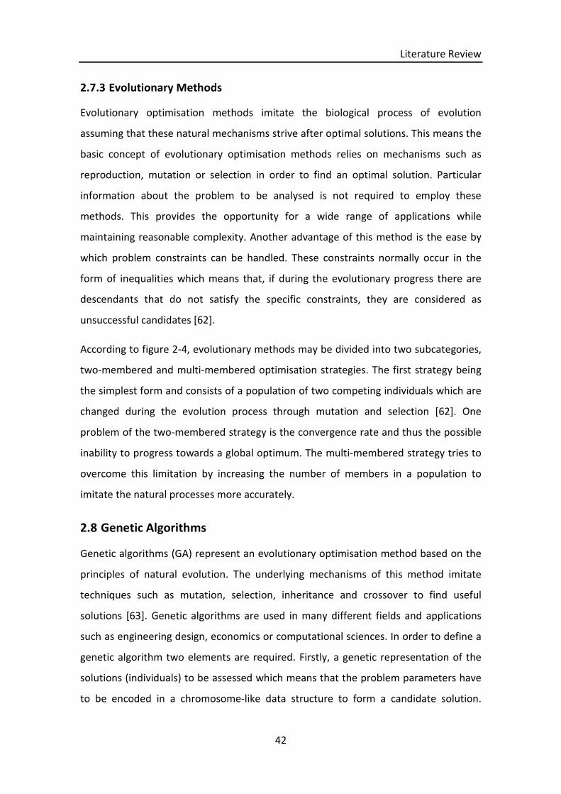
Literature Review
42
2.7.3 Evolutionary Methods
Evolutionary optimisation methods imitate the biological process of evolution
assuming that these natural mechanisms strive after optimal solutions. This means the
basic concept of evolutionary optimisation methods relies on mechanisms such as
reproduction, mutation or selection in order to find an optimal solution. Particular
information about the problem to be analysed is not required to employ these
methods. This provides the opportunity for a wide range of applications while
maintaining reasonable complexity. Another advantage of this method is the ease by
which problem constraints can be handled. These constraints normally occur in the
form of inequalities which means that, if during the evolutionary progress there are
descendants that do not satisfy the specific constraints, they are considered as
unsuccessful candidates [62].
According to figure 2-4, evolutionary methods may be divided into two subcategories,
two-membered and multi-membered optimisation strategies. The first strategy being
the simplest form and consists of a population of two competing individuals which are
changed during the evolution process through mutation and selection [62]. One
problem of the two-membered strategy is the convergence rate and thus the possible
inability to progress towards a global optimum. The multi-membered strategy tries to
overcome this limitation by increasing the number of members in a population to
imitate the natural processes more accurately.
2.8 Genetic Algorithms
Genetic algorithms (GA) represent an evolutionary optimisation method based on the
principles of natural evolution. The underlying mechanisms of this method imitate
techniques such as mutation, selection, inheritance and crossover to find useful
solutions [63]. Genetic algorithms are used in many different fields and applications
such as engineering design, economics or computational sciences. In order to define a
genetic algorithm two elements are required. Firstly, a genetic representation of the
solutions (individuals) to be assessed which means that the problem parameters have
to be encoded in a chromosome-like data structure to form a candidate solution.

Literature Review
43
Secondly, a fitness function that allows evaluation of the progress of the solutions. In
standard problems, the fitness function is the objective function to be optimised.
The methodology of genetic algorithms can be briefly described using the following
steps:
1. Initialization: Form an initial population of randomly generated individuals.
2. Genetic operation: Select, recombine and mutate existing populations to
generate a second generation population which is different from the first one.
The genetic algorithm determines suitable solutions based on the requirements
established in the fitness function.
3. Termination: Reach a predefined satisfactory stopping criteria or convergence
of the solution.
The initial population is generally formed by a random generation of individuals which
constitute the initial population for the optimisation process. If there are reliable, pre-
existing solutions for a given problem, then those solutions can be utilised instead of a
randomly generated population. This may improve the quality of the optimisation
process and reduce computing time. The three main features or mechanisms of the
genetic algorithm, named under point two, to advance a population towards a
population consisting of individuals who represent the most suitable solutions are
illustrated in figure 2-5. This iterative process forms one major element of the
optimisation and has an influence on the performance of the genetic algorithm. The
termination of the optimisation process can be based on different criteria and the
most viable option depends on the particular optimisation problem. The process can
be stopped by reaching, for example, a given fitness limit, a maximum number of
generations or a maximum number of evaluations.
Two key parameters that define the optimisation performance are selection pressure
and population diversity. A too high selection pressure may lead to premature
convergence of the solution and low population diversity may limit the search space
and the number of possible solutions.

Literature Review
44
Figure 2-5: Main features of the genetic algorithm (adapted from Lipowsky [49])
According to Zitzler [64] genetic algorithms possess several desirable characteristics to
address problems which involve multiple objectives and intractably large search
spaces. Furthermore, Mitsuo in reference [65] states that genetic algorithms are able
to maintain a population of potential solutions throughout the evolution generation
process and thus are being useful when Pareto-solutions are evaluated. This
evolutionary nature also becomes advantageous when solutions to complex problems
are being searched because detailed information about the problem is not required.
2.9 Multi Objective Trajectory Optimisation
To define the aircraft trajectory optimisation problem addressed in this work and to
highlight its main characteristics, the following list provides an overview of the most
important classification elements. The aircraft trajectory optimisation problem can be
described as:
Constrained (one or more constraints)
Dynamic (one or more function parameter(s))
Optimal control (gradual progression)
Non-linear (functions inputs and outputs)
Real-valued (design variables)
Deterministic (most parameters are deterministic)
Multi-objective (two optimisation objectives)

Literature Review
45
Since the aircraft trajectory optimisation will involve the processing of multiple
parameters the problem can be treated as multi-dimensional. The optimisation
working space is not circumscribed in advance and thus the solutions are assumed to
have several extreme points (local minima or maxima), id est the problem is
considered to be multi-modal.
Furthermore the selection of the most suitable optimisation method depends on the
characteristics of the objective function on the one side and the individual constraints
defined on the other side. Considering the classification elements described above and
taking into account the constraints of the problem, the objective function, even
though being unknown, can be described as having the following properties:
Highly non-linear (outputs and inputs are not directly proportional)
Non-smooth/Non-differentiable (significant discontinuities)
An appropriate definition of the problem constraints will effectively narrow down the
search space for the optimisation process.
If an optimisation problem consists of multiple objectives there will be not one optimal
solution but instead there will be a set of solutions for the given problem [66]. These
solutions are known as Pareto-optimal solutions. In relation to optimisation problems
where sets of Pareto optimal solutions are obtained, those can be described in
mathematical terms for a two-objective optimisation problem as follows: [67]
ܨ = { ଵ(), ଶ()}
∈ = { ∈ :ℎ() = 0,() ≥ 0}(2-19)
This is where f1(X) and f2(X) are scalar functions and S is the set of implicit constraints.
The objective vector to be minimised is part of the objective space and the image of
the search space under F can be denoted as follows:
ܥ = ݕ} ∈ :ݕ= (), ∈ } (2-20)
The resulting Pareto front or Pareto curve as shown in figure 2-6 is made up of the
image of all efficient solutions and the particular shape of the curve represents the

Literature Review
46
kind of trade-off between the two objective functions. All points between (f2(x;ˆ),f1(x;ˆ
)) and (f2(x;˜),f1(x;˜)) form the Pareto curve and each point of the curve stands for a
non-dominated solution of the two-objective optimisation problem. This means an
improvement of the objective represented by f1(X) will lead to a worsening of the
objective represented by f2(X) [67].
Figure 2-6: Example Pareto curve [67]
A comprehensive introduction to multi-objective evolutionary algorithms is presented
in the paper in reference [68]. In this paper, evolutionary algorithms are classified
based on the type of selection mechanism, which, for example, can be populations-
based or Pareto-based. Reference [69] provides a detailed insight into solving multi-
objective optimisation problems based on evolutionary algorithms. It presents and
analyses in detail the research of contemporary multi-objective evolutionary
algorithms and discusses associated multi-objective optimisation problems.
2.10 NSGAMO Genetic Optimiser
One particular genetic algorithm-based optimiser which has been proposed and
developed by the authors in reference [66] and which is widely used for optimisation
problems is called NSGA-II (Non-dominated Sorting Genetic Algorithm II). An updated

Literature Review
47
version of this algorithm, namely NSGAMO, is used in the GATAC (Green Aircraft
Trajectories under ATM Constraints) optimisation suite. This suite is jointly used by
Cranfield University and the University of Malta. The structure and application of the
genetic operators of the GATAC optimiser differ in two ways from the original NSGA-II.
Firstly, it uses a different selection process to form the mating pool and secondly, it
uses a different sequence of genetic operators (SBX crossover and polynomial
mutation) [70]. The basic optimisation flowchart of the NSGAMO optimiser is shown in
figure 2-7.
The algorithm begins its calculation with an initial population which is randomly
created. The population size multiplied by the initialisation ratio determines the
number of cases to be sent to the optimisation framework for evaluation. Larger
population sizes will increase the number of possible solutions on the one hand and on
the other hand it will increase the number of evolutions and thus computing time to
calculate the next generation. According to the defined fitness function for the specific
case the algorithm will then reduce the population size to the specified value. Then the
optimiser checks if the optimisation process is complete, which depends on if the
maximum number of generations has been reached or the criteria of the fitness or
objective function have been reached. At this point the optimiser enters an iterative
loop to create new cases by applying genetic operators specific to the optimiser and
sending these new cases to the framework for evaluation. The results are joined into
the existing population and qualified based on their suitability. Another trimming of
the population is carried out and the loop will continue until one of the final stopping
criteria is met [71].
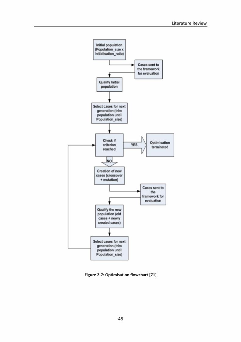
Literature Review
48
Figure 2-7: Optimisation flowchart [71]

Problem Definition
49
3 Problem Definition
This chapter aims to define the problem statement of this work on the one hand and
on the other hand aims to provide an interface between the fundamental information
from the literature review and the specific requirements of the aircraft trajectory
studies to be carried out and analysed in the following chapters. This involves a brief
discussion of some general considerations with regards to the aircraft configurations
and aircraft performance parameters as well as the flight trajectory itself.
Furthermore, a definition of a simplified aircraft trajectory is provided and the
requirements for the trajectory analyses and optimisations are discussed. This also
includes the assumptions and statements made for models and frameworks developed
in this study. The chapter concludes with a review of past works which have already
addressed the subject of aircraft trajectory optimisation.
3.1 General Considerations
The analysis of aircraft trajectories makes it necessary to briefly introduce some
general aspects of commercial aircraft operations. In a real environment there are
many factors which influence an aircraft mission and consequently its performance
from the beginning at the departure point till the arrival at the final destination. Figure
3-1 schematically illustrates a typical flight profile of a commercial passenger aircraft
with its five particular flight phases namely (1) take-off, (2) climb, (3) cruise, (4)
descent and (5) approach. Normally the cruise altitude and the range (travel distance)
are interdependent in a way that shorter flight ranges will result in lower cruise
altitudes and longer flight ranges will result in higher cruise altitudes. This is assuming
that time spent in take-off and climb phases as well as the time spent in descent and
approach phases are nearly constant. Since the cruise phase usually represents the
flight phase where the engine and aircraft operate in their respective design points it is
desirable to spend as much time of the whole flight in this condition.

Problem Definition
50
Figure 3-1: Typical flight mission profile and flight phases
3.1.1 Short-to-Medium Range Aircraft Configurations
The aircraft configurations considered in the following studies are based on publicly
available information of the Airbus A320 family. This family represents a typical short
to medium range, twin-engine commercial passenger aircraft that is widely used and
also represents a significant share of the total worldwide fleet for this aircraft class. It
comprises a narrow-body design with a retractable tricycle landing gear, low-wing
cantilever monoplanes, a single vertical stabiliser and rudder mounted on a
conventional tail unit. The passenger capacity for the different models ranges from 124
to 220 seats depending on class configuration and model.
3.1.2 Aircraft Speeds
One important characteristic performance value for aircraft trajectory analyses is the
actual aircraft velocity. The setup of the aircraft trajectories in this study will require
the definition of specific aircraft velocities in certain phases of the flight depending on
the actual altitude. A brief overview of aircraft velocity definitions and their usages is
given in the following.

Problem Definition
51
Aircraft velocity can be expressed in different forms depending on the required
application or the context it is used in. Some common forms are listed below: [72]
Indicated Airspeed (IAS)
Calibrated Airspeed (CAS)
Density Airspeed (DAS)
Equivalent Airspeed (EAS)
True Airspeed (TAS)
Mach Number (M)
The dependencies of these different forms of aircraft velocity are illustrated in figure
3-2 below. The Density Airspeed (DAS) is only shown for the sake of completeness and
will not be explained in more detail.
Figure 3-2: Aircraft velocity interdependencies (adapted from Scheiderer [72])
The Indicated Airspeed (IAS) is the aircraft velocity shown on an airspeed indicator
which is calibrated for ISA conditions. IAS is commonly used in aircraft performance
tables. The Calibrated Airspeed (CAS) results from the correction of the IAS to account
for errors of the static pressure gauging system. In the subsonic region the CAS is
defined as follows:

Problem Definition
52
=ܣܥ ඩߛ2
−ߛ 1×ߩ൬−௧ ௦
+ 1൰
ఊଵఊ− 1൩ (3-1)
As aircraft altitude and Mach number increase, the indication of the CAS will contain
an error which is corrected by introducing the Equivalent Airspeed (EAS). The EAS
accounts for these compressibility effects and a constant EAS corresponds to a
constant dynamic pressure. It is defined as follows:
=ܣܧ ඩߛ2
−ߛ 1×௦ߩ൬−௧ ௦
+ 1൰
ఊଵఊ− 1൩ (3-2)
Subsequently, the True Airspeed (TAS) is arrived at by allowing for air density
corrections. The TAS is then defined as follows:
=ܣܧ ඩߛ2
−ߛ 1×௦௦ߩ൬−௧ ௦௦
+ 1൰
ఊଵఊ− 1൩ (3-3)
The TAS can also be directly derived from the EAS by using the following equation:
=ܣܣܧ
ඥߩ(3-4)
The Mach number M is often referred to in aircraft cruise conditions and is described
as ratio of the True Airspeed (TAS) and the local speed of sound a:
ܯ =ܣ
(3-5)
The local speed of sound depends on the atmospheric temperature t0, the isentropic
exponent γ, and the gas constant R for dry air.
= ඥߛ× × ݐ (3-6)

Problem Definition
53
Since airspeed velocity measurements are based on the actual atmospheric conditions
(temperature, pressure and density) the changes of these conditions with varying
altitude must be taken into account as mentioned at the beginning of this section. To
illustrate these changes, figures 3-3, 3-4 and 3-5 below depict the vertical distribution
of temperature, pressure and density respectively in the International Standard
Atmosphere (ISA) up to an altitude of 20 km [73]. The ambient temperature linearly
decreases from sea level to an altitude of about 11 km after which it will remain
constant up to an altitude of about 20 km. The ambient pressure and density decrease
gradually from sea level to an altitude of 20 km. The referenced figures only cover the
lowest layers of the atmosphere, namely the troposphere which reaches from sea level
up to an altitude of about 11 km and the stratosphere which extends from there up to
an altitude of 20 km. Both layers are commonly used for commercial aircraft
operation.
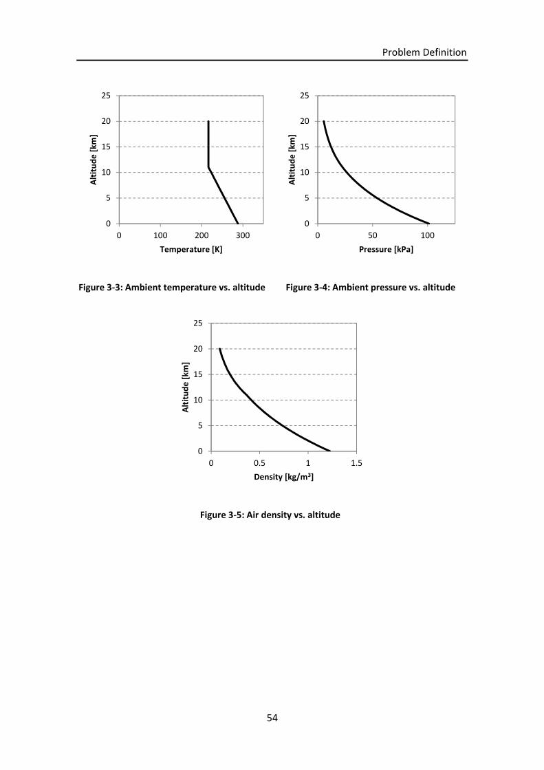
Problem Definition
54
Figure 3-3: Ambient temperature vs. altitude Figure 3-4: Ambient pressure vs. altitude
Figure 3-5: Air density vs. altitude
0
5
10
15
20
25
0 100 200 300
Alt
itu
de
[km
]
Temperature [K]
0
5
10
15
20
25
0 50 100
Alt
itu
de
[km
]
Pressure [kPa]
0
5
10
15
20
25
0 0.5 1 1.5
Alt
itu
de
[km
]
Density [kg/m3]

Problem Definition
55
3.1.3 Aircraft Trajectory Definition
For the purpose of the scenario studies analysed in this work it is necessary to evaluate
and analyse typical aircraft trajectories applied in current flight operation. In this study
a typical flight trajectory, i.e. the mission profile, is comprised of the five previously
mentioned flight phases. For each of the phases certain minimum and maximum
operational limitations in terms of aircraft speed and rate of climb or descend exist.
These limitations are imposed by influencing parameters such as the altitude effect,
the temperature effect and the weight effect [28].
Since this study focuses on the first parts of the flight trajectory (take-off and climb) a
brief review of those two flight phases will be provided in the following.
Even though the aircraft take-off phase depends on given external factors such as
runway length or obstacles and variable conditions such as weather or airport
restrictions, it can be broadly defined in two ways, namely take-off path (1) and take-
off flight path (2). They can be described as follows: [28]
1. A standing start point to a point where the aircraft is at height (typically 1500
feet)
2. A point 35 feet above take-off surface at the end of the take-off distance
Since the aircraft take-off weight is in many cases below the maximum possible take-
off weight due to the aircraft load condition it is possible to reduce the engine take-off
thrust and thus reduce fuel burn and engine degradation.
According to reference [28] a climb is generally carried out at a constant Indicated Air
Speed (IAS) and Mach number. The climb profile and technique can be divided into 3
phases which have a direct effect on fuel burn [74]:
1. Climb at constant IAS = 250 knots up to 10000 feet
2. Climb at constant IAS = 300 knots above 10000 feet
3. Climb at constant Mach number = 0.78 above crossover altitude
This is where the crossover altitude is the altitude where 300 knots IAS is equal to
Mach 0.78.

Problem Definition
56
For the sake of completeness the cruise and descent phase are briefly described in the
following. The most important parameters which define the cruise phase are altitude
(flight level) and aircraft cruise speed (Mach number) [74]. Depending on the aircraft
weight, mission range, winds and atmospheric conditions different optimum speeds
and altitudes with respect to fuel consumption and flight time can be identified.
Similar to the climb phase the descent phase is generally carried out a constant IAS and
Mach number. The descent is caused by a thrust reduction where the difference
between engine thrust and aircraft aerodynamic drag becomes negative and thus the
descent gradient and rate of descent becomes negative as well. Furthermore, to better
understand typical aircraft flight profiles and to support the trajectory definitions
mentioned above, a real flight trajectory for a typical single aisle aircraft configuration
is referenced in figure 3-6 and 3-7. The flight distance of the mission is approximately
1400 km. Figure 3-6 shows the fuel flow trend over time and along the flight profile in
percent of the take-off fuel flow. Correspondingly, figure 3-7 illustrates the engine EGT
trend in percent of the applicable EGT redline of the number one engine for the same
flight.
Figure 3-6: Flight profile with engine fuel flow (Airbus A321); courtesy of Airberlin
0
10
20
30
40
50
60
70
80
90
100
0
2000
4000
6000
8000
10000
12000
0 2000 4000 6000 8000 10000
Fue
lflo
win
%o
fm
axim
um
T/O
fue
lflo
w
Alt
itu
de
[m]
Time [seconds]
Flight profile Engine #1 FF
Problem Definition
57
Figure 3-7: Flight profile with engine EGT (Airbus A321); courtesy of Airberlin
Based on the previously described information a baseline trajectory has been defined
as a reference to allow a comparison of the different analysed scenarios. The basic
points of the trajectory can be summarised as follows:
1 minute take-off phase to 457 m altitude (1500 feet)
Climb from 457 m to 3048 m at constant EAS = 250 knots
Accelerate from EAS = 250 knots to 300 knots at constant altitude (3048 m)
Continue climb from 3048 m to cruise altitude 10668 m
Cruise at constant Mach number = 0.785
Descent slope is based on aircraft cruise altitude
In case of the engine derate scenario a 15% take-off thrust reduction has been
assumed. This assumption represents a typical value derived from real engine flight
data. These basic points have been used as inputs for the aircraft performance model
Hermes which calculates the aircraft trajectory based on the defined parameters. The
aircraft performance model will be explained in more detail in section 4.2.
0
10
20
30
40
50
60
70
80
90
100
0
2000
4000
6000
8000
10000
12000
0 2000 4000 6000 8000 10000
EGT
in%
of
EGT
red
line
Alt
itu
de
[m]
Time [seconds]
Flight profile Engine #1 EGT

Problem Definition
58
3.1.4 Optimised Aircraft Trajectory
Optimised aircraft trajectories aim at providing the most suitable flight profile for a
given mission in terms of flight time, fuel burned and emissions generated. It becomes
clear that these three goals are not always complementing each other but rather
represent conflicting objectives. This results in a search for a trade-off between these
goals for the particular flight mission. Thus one major aim of this research work is to
analyse aircraft trajectories with regards to the above mentioned objectives and in a
second step to find optimised trajectories. These optimised trajectories or so called
“greener” trajectories aim at a reduction in fuel burn and emissions by introducing a
variation in the climb profile and cruise phase while maintaining feasible results in
terms of flight time and operability. This means the trajectory optimisation cases
addressed in this work focus on the climb profile and cruise phase.
Many existing studies on aircraft flight trajectory analysis and optimisation also focus
only on particular flight phases and address these in detail due to the significant
increase in complexity when dealing with complete flight trajectories. Clarke [75]
analyses in his study the feasibility of an airport specific continuous descent approach
(CDA) procedure mainly to achieve an arrival noise reduction but which also resulted in
a substantial reduction in NOx emissions below 3000 feet (915 m). Patterson [76]
analysed real-time aircraft data for departure and arrival profiles with respect to
engine fuel burn and emissions. Actual operational fuel flow data from several aircraft
has been compared to ICAO standard cycle data. It was found that actual fuel burn
data for these profiles significantly deviated from the ICAO data and was generally
overestimated. Another study on CDA has been carried out by Alam et al. [77]. They
propose a methodology to compute dynamic CDA aircraft routes which are laterally
and vertically optimised on particular objectives such as noise, emissions and fuel
burn. The results indicate that a reduction in noise, emissions and fuel burn can be
accomplished at the same time when employing dynamic CDA routes. Environmentally
friendly departure procedures for civil aircraft have been investigated by Torres et al.
[78] using a multiobjective, constrained, nonlinear optimisation methodology. These
results also indicate possible noise and emissions reductions achieved through
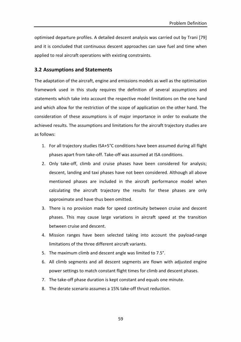
Problem Definition
59
optimised departure profiles. A detailed descent analysis was carried out by Trani [79]
and it is concluded that continuous descent approaches can save fuel and time when
applied to real aircraft operations with existing constraints.
3.2 Assumptions and Statements
The adaptation of the aircraft, engine and emissions models as well as the optimisation
framework used in this study requires the definition of several assumptions and
statements which take into account the respective model limitations on the one hand
and which allow for the restriction of the scope of application on the other hand. The
consideration of these assumptions is of major importance in order to evaluate the
achieved results. The assumptions and limitations for the aircraft trajectory studies are
as follows:
1. For all trajectory studies ISA+5°C conditions have been assumed during all flight
phases apart from take-off. Take-off was assumed at ISA conditions.
2. Only take-off, climb and cruise phases have been considered for analysis;
descent, landing and taxi phases have not been considered. Although all above
mentioned phases are included in the aircraft performance model when
calculating the aircraft trajectory the results for these phases are only
approximate and have thus been omitted.
3. There is no provision made for speed continuity between cruise and descent
phases. This may cause large variations in aircraft speed at the transition
between cruise and descent.
4. Mission ranges have been selected taking into account the payload-range
limitations of the three different aircraft variants.
5. The maximum climb and descent angle was limited to 7.5°.
6. All climb segments and all descent segments are flown with adjusted engine
power settings to match constant flight times for climb and descent phases.
7. The take-off phase duration is kept constant and equals one minute.
8. The derate scenario assumes a 15% take-off thrust reduction.

Problem Definition
60
For the optimisation framework (GATAC) and the trajectory optimisation studies itself
the following modified assumptions and limitations, differing from the previously
mentioned, apply:
1. There is no limitation to the maximum climb and descent angle.
2. All climb segments are flown with maximum climb engine power settings.
3. Descent segments are flown with constant preset engine power settings.
4. There is no speed continuity during acceleration from one climb segment to the
next.
3.3 Past Experience on Trajectory Analysis and Optimisation
This section is intended to provide a brief review of aircraft trajectory optimisation
studies that have been carried out at Cranfield University in the past. The studies
constitute the basis for the optimisation approach adapted in the present work
utilising a similar optimisation framework and algorithm. Highlights from three past
works undertaken by Cesar Celis, Hasan Zolata and Roman Marzal are further
described to set up the context for the developments of the present study.
In his work [61], Cesar Celis investigates suitable methodologies for aircraft trajectory
optimisation and subsequently develops simulation models which are then
implemented into a multi-disciplinary optimisation framework to evaluate more
environmentally friendly operational procedures. The framework contains models for
aircraft performance, engine performance and emissions performance. Furthermore,
his study also includes the optimisation of aircraft engine cycles and its inherent design
trade-offs which originate from conflicting objectives such as low operating costs or
low environmental impacts. To solve the aircraft trajectory optimisation problem, Celis
employs evolutionary methods based on genetic algorithms (GA) due to their
robustness, their simplicity and their suitability for problems involving a number of
constraints and objectives and where the space of potential solutions is large. Several
case studies are presented which focus on the minimisation of total flight time, total
fuel burned and total NOx emissions. The results of those case studies illustrate the
interaction of the major influencing parameters that have to be considered for aircraft
Problem Definition
61
trajectory analyses. Those parameters are aircraft speed, cruise altitude and the
maximum thrust requirements during climb to reach this altitude.
A further multi-disciplinary approach to aircraft trajectory optimisation is presented by
Hasan Zolata [23]. His work also addresses the trajectory optimisation problem
through the implementation of a multi-disciplinary simulation framework and the use
of a commercially available genetic optimisation algorithm. To identify more
environmentally friendly flight trajectories, in terms of fuel burn and pollutant
emissions, a number of case studies have been carried out. These studies include the
optimisation of a whole flight as well as the optimisation of a particular flight phase,
namely the climb segment. The results indicate that aircraft trajectories with minimum
environmental impact can be identified by employing the developed multi-disciplinary
simulation framework. It was also found that trajectories optimised for minimum fuel
were generally in conflict with trajectories optimised for minimum pollutant emissions.
Similar to the two previously mentioned studies, Roman Marzal [24] investigates in his
study the suitability of a particular genetic algorithm-based aircraft trajectory
optimisation tool. In the initial part of the study two different commercial optimisers,
namely Matlab NSGA-II and Matlab MOGA were benchmarked against the GATAC
optimisation suite in order to validate its performance. The benchmarking studies
included different standard test problems which aim at testing individual properties of
the optimiser with regards to quality of the solutions achieved. After confirming the
suitability of the GATAC optimisation suite for multi-objective optimisation problems a
two-objective aircraft trajectory optimisation study has been performed to test its
capabilities. The analysed scenarios also focused on fuel burn and emissions
improvements through optimisation of the climb phase. The results indicate that more
efficient trajectories can be found when taking into account that optimisation
objectives can be opposing.
The above mentioned studies are three current examples of trajectory optimisation
research approaches from Cranfield University and have been selected due to the
influence on the present work. Further studies which dealt with the analysis and
Problem Definition
62
assessment of aircraft trajectory optimisations, but which are not covered in detail
here, have been carried out in the past.
Matthew Sammut [80] conducted in his study a multivariable parameter optimization
of flight trajectories focusing on economical climb trajectories for different aircraft
variants. Several characteristic trajectories have been modelled, evaluated and
compared in terms of climb fuel consumption. Results of the optimised trajectories
confirmed the suitability of the employed optimisation methodology.
A multidisciplinary aero-engine exhaust study has been carried out by Shakariyans et
al. [81] investigating the effects of flight conditions, power settings and combustor
parameters on the engine emissions. Multi-reactor combustor models were used to
predict pollutant emissions and then benchmarked against certification data. On
ground and in-flight emission profiles have successfully been simulated. In a
subsequent study by Shakariyans et al. [82] an engine deterioration scenario was also
included in the emissions prediction analysis.
Antonio Filippone [83] carried out a comprehensive analysis of transport aircraft flight
performance by adapting a multidisciplinary approach including various models to
simulate aircraft performance, engine performance and noise performance. The
analyses indicated that an accurate engine performance model will be the most critical
aspect with respect to aircraft performance calculations.
A study, which focusses on adaptive engine technologies, such as fan and compressor
flow control, blade clearance control or combustion control to reduce engine
emissions, has been conducted by Mercer et al [84]. Potential positive and negative
impacts of these technologies have been quantified one at a time and the results show
that fuel burn can be reduced through improved propulsive efficiency and/or drag
reduction depending on the technology applied.
A comparison of open-rotor engine concepts and conventional turbofan engines used
in short range aircraft applications has been presented by Adam Waldowski [85] in his
work also focusing on mission fuel burn and pollutant emissions. The open-rotor

Problem Definition
63
engine concept yields promising results which indicate an improvement in fuel burn
and pollutant emissions in comparison to conventional turbofans for shorter missions
ranges.

Framework Tools
64
4 Framework Tools
This chapter provides an introduction to the simulation tools and models for the
engine, the aircraft and the emissions assessment used to carry out the basic aircraft
trajectory studies. It also includes a description of the adapted trajectory optimisation
framework and its operating principles.
4.1 Engine Performance Model (Turbomatch)
The engine configuration that is used throughout this study represents a two-spool
high bypass ratio turbofan with separate exhaust nozzles. The basic configuration is
shown in figure 4-1 in the next section. The basic engine model was developed in
Cranfield University based on publicly available information and was adapted for the
work carried out in this study [86]. Three engine configurations were derived from the
basic engine model, one representing a low thrust configuration shortly addressed as
CU2STF-LT, another a medium thrust configuration addressed as CU2STF-MT and a
high thrust configuration addressed as CU2STF-HT. All three configurations encompass
the same fixed mechanical and dimensional engine design like fan diameter and two-
spool architecture. The three engine models were used for steady state design point
and off design point simulations and the results were compared with engine
specifications of the CFM56-5B engine series [87]. The CFM56-5B series engine powers
the Airbus A320 Family of aircraft and is available with different thrust ratings, for
example CFM56-5B6 (low thrust) and CFM56-5B4 (medium thrust) and CFM56-5B3
(high thrust). The thrust rating relates to the maximum engine take-off thrust.
The below described engine model performance results were achieved by using the
Cranfield University in-house simulation code Turbomatch [88]. This program is used
for engine modelling and engine parametric studies. The code allows a high engine
modelling accuracy and comprises all basic gas turbine performance simulation
features as well as advanced simulation capabilities. It has a modular design to model
various gas turbine components (e.g. Compressors, Burners, and Turbines) and to carry
out performance calculations with subsequent result plotting including component
maps. It allows analysis of degraded engine performance through alteration of certain

Framework Tools
65
engine components providing the opportunity to simulate a wide range of engine
operating conditions.
Other programs that provide similar functionality to perform gas turbine performance
simulations are, for example, GasTurb developed by Joachim Kurzke [89] and GSP (Gas
Turbine Simulation Program) developed by the Dutch aerospace knowledge enterprise
NLR (Nationaal Lucht- en Ruimtevaartlaboratorium) [90].
4.1.1 Turbomatch Engine Model
The basic engine model structure of the CU2STF model is depicted in figure 4-1 while
figure 4-2 shows the engine component structure as used in the Turbomatch
simulation code. It is a two-shaft design where the Low Pressure Turbine (LPT) drives
the fan and the Low Pressure Compressor (LPC; Booster) and the High Pressure
Turbine (HPT) drives the High Pressure Compressor (HPC). After the intake the air
propelled by the fan is split into the core flow and the bypass flow. The core flow
provides air for the gas generator which is comprised of LPC, HPC, Combustor, HPT and
LPT and is then discharged through the Core Nozzle. The bypass flow is ducted and
discharged through the Bypass Nozzle. Air is bled from the LP Compressor (LPC exit air)
and is discharged into the bypass flow to allow adjustment of the LP Compressor outlet
flow and thus allows handling of the inlet conditions of the HP Compressor.
Furthermore it ensures that the LPC will operate within its design limits. For normal
operation, the handling bleed will be utilised during transient engine operation with
lower engine power settings while no air is bled during take-off or cruise conditions.
Also, air is bled from the HP Compressor (HPC exit air) to cool the HP Turbine. An
additional 200KW of work is extracted from the HP Turbine to account for the drive of
the engine auxiliary systems such as fuel and oil pumps and electrical generators.
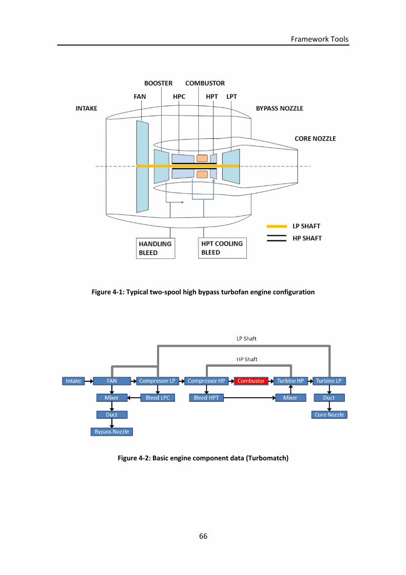
Framework Tools
66
Figure 4-1: Typical two-spool high bypass turbofan engine configuration
Figure 4-2: Basic engine component data (Turbomatch)
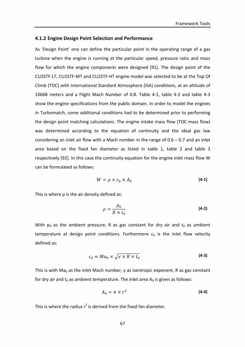
Framework Tools
67
4.1.2 Engine Design Point Selection and Performance
As ‘Design Point’ one can define the particular point in the operating range of a gas
turbine when the engine is running at the particular speed, pressure ratio and mass
flow for which the engine components were designed [91]. The design point of the
CU2STF-LT, CU2STF-MT and CU2STF-HT engine model was selected to be at the Top Of
Climb (TOC) with International Standard Atmosphere (ISA) conditions, at an altitude of
10668 meters and a Flight Mach Number of 0.8. Table 4-1, table 4-2 and table 4-3
show the engine specifications from the public domain. In order to model the engines
in Turbomatch, some additional conditions had to be determined prior to performing
the design point matching calculations. The engine intake mass flow (TOC mass flow)
was determined according to the equation of continuity and the ideal gas law
considering an inlet air flow with a Mach number in the range of 0.6 – 0.7 and an inlet
area based on the fixed fan diameter as listed in table 1, table 2 and table 3
respectively [92]. In this case the continuity equation for the engine inlet mass flow W
can be formulated as follows:
= ×ߩ × ܣ (4-1)
This is where ρ is the air density defined as:
=ߩ
× ݐ(4-2)
With p0 as the ambient pressure, R as gas constant for dry air and t0 as ambient
temperature at design point conditions. Furthermore c0 is the inlet flow velocity
defined as:
= ܯ × ඥߛ× × ݐ (4-3)
This is with Ma0 as the inlet Mach number, γ as isentropic exponent, R as gas constant
for dry air and t0 as ambient temperature. The inlet area A0 is given as follows:
ܣ = ×ߨ ଶݎ (4-4)
This is where the radius r2 is derived from the fixed fan diameter.

Framework Tools
68
Using the described approach the inlet mass flow was calculated to W=179 kg/s. These
assumptions and the listed engine specifications are also supported by the literature
reference [39] and [93].
The design point TET was adjusted based on the overall pressure ratio (OPR) and the
net thrust at the design point. In addition, for typical turbofan engines as depicted in
figure 4-1 there are three main design parameters which affect the engine thrust and
specific fuel consumption (SFC). Those are bypass ratio (BPR), overall pressure ratio
(OPR) and turbine entry temperature (TET). The overall pressure ratio (OPR) and the
thrust at the Top Of Climb were the basis for the determination of the engine design
point parameters for turbine entry temperature (TET) and bypass ratio (BPR). The
optimum fan pressure ratio (FPR) was determined according to the calculated TET,
OPR and BPR at design point conditions with Flight Mach Number of 0,8 [94]. To avoid
design and handling problems a FPR lower than the optimum was chosen.
In all below described characteristic maps the mass flow is given as Corrected Mass
Flow which corresponds to a pressure and temperature correction to Sea Level Static
(SLS) conditions. The Corrected Mass Flow (CMF) is given as follows:
ݎݎܥ ݐ ܯ ܨݏݏ ݓ = ට
ௌௌ
ௌௌ
(4-5)
W is the actual mass flow, and T and P are the actual temperature and pressure
respectively. Temperature and pressure are corrected to Sea Level Standard and ISA
conditions as follows:
ௌௌ = 288.15 ܭ (4-6)
ௌௌ = 101.325 (4-7)
A tabular summary of the engine specifications at design point conditions (Top Of
Climb) and take-off conditions for each engine variant is listed in the following tables
4-1, 4-2 and 4-3.

Framework Tools
69
Table 4-1: Engine specification comparison CU2STF-LT (CFM56-5B6) [87]
Engine Model Take-off Performance
Flight Mach Number: Ma 0,0 Altitude: 0 m ISA conditions + 30°C
Unit Engine specification CU Turbomatch Delta
T/O thrust N 104500 104510 0.01%
T/O mass flow kg/s 382.8 377.9 -1.30%
T/O BPR - 5.90 5.87 -0.51%
T/O TET K - 1500 -
T/O fuel flow kg/s - 0.920 -
Engine Model Design Point Performance (Top Of Climb)
Flight Mach Number: Ma 0,8 Altitude: 10670 m ISA conditions
Unit Engine specification CU Turbomatch Delta
TOC thrust N 25040 25075 0.14%
TOC mass flow kg/s - 179.0 -
TOC SFC g/kN s - 16.65 -
TOC BPR - - 5.45 -
TOC TET K - 1345 -
TOC OPR - 32.6 32.6 0.00%
Fan diameter m 1.73 - -
Table 4-2: Engine specification comparison CU2STF-MT (CFM56-5B4) [87]
Engine Model Take-off Performance
Flight Mach Number: Ma 0,0 Altitude: 0 m ISA conditions + 30°C
Unit Engine specification CU Turbomatch Delta
T/O thrust N 120100 120550 0.37%
T/O mass flow kg/s 406.8 404.3 -0.62%
T/O BPR - 5.70 5.60 -1.79%
T/O TET K - 1575 -
T/O fuel flow kg/s - 1.101 -
Engine Model Design Point Performance (Top Of Climb)
Flight Mach Number: Ma 0,8 Altitude: 10670 m ISA conditions
Unit Engine specification CU Turbomatch Delta
TOC thrust N 25040 25075 0.14%
TOC mass flow kg/s - 179.00 -
TOC SFC g/kN s - 16.65 -
TOC BPR - - 5.45 -
TOC TET K - 1345 -
TOC OPR - 32.6 32.6 0.00%
Fan diameter m 1.73 - -
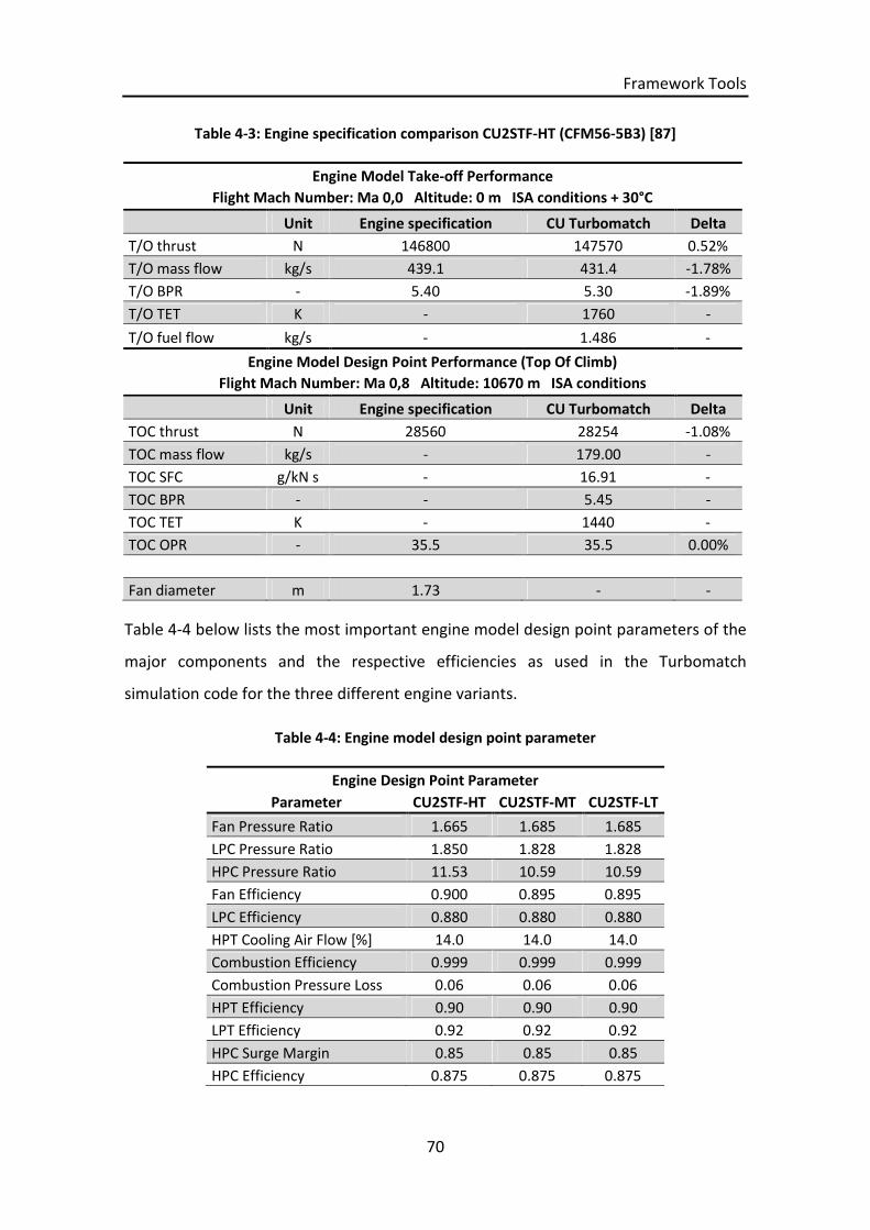
Framework Tools
70
Table 4-3: Engine specification comparison CU2STF-HT (CFM56-5B3) [87]
Engine Model Take-off Performance
Flight Mach Number: Ma 0,0 Altitude: 0 m ISA conditions + 30°C
Unit Engine specification CU Turbomatch Delta
T/O thrust N 146800 147570 0.52%
T/O mass flow kg/s 439.1 431.4 -1.78%
T/O BPR - 5.40 5.30 -1.89%
T/O TET K - 1760 -
T/O fuel flow kg/s - 1.486 -
Engine Model Design Point Performance (Top Of Climb)
Flight Mach Number: Ma 0,8 Altitude: 10670 m ISA conditions
Unit Engine specification CU Turbomatch Delta
TOC thrust N 28560 28254 -1.08%
TOC mass flow kg/s - 179.00 -
TOC SFC g/kN s - 16.91 -
TOC BPR - - 5.45 -
TOC TET K - 1440 -
TOC OPR - 35.5 35.5 0.00%
Fan diameter m 1.73 - -
Table 4-4 below lists the most important engine model design point parameters of the
major components and the respective efficiencies as used in the Turbomatch
simulation code for the three different engine variants.
Table 4-4: Engine model design point parameter
Engine Design Point Parameter
Parameter CU2STF-HT CU2STF-MT CU2STF-LT
Fan Pressure Ratio 1.665 1.685 1.685
LPC Pressure Ratio 1.850 1.828 1.828
HPC Pressure Ratio 11.53 10.59 10.59
Fan Efficiency 0.900 0.895 0.895
LPC Efficiency 0.880 0.880 0.880
HPT Cooling Air Flow [%] 14.0 14.0 14.0
Combustion Efficiency 0.999 0.999 0.999
Combustion Pressure Loss 0.06 0.06 0.06
HPT Efficiency 0.90 0.90 0.90
LPT Efficiency 0.92 0.92 0.92
HPC Surge Margin 0.85 0.85 0.85
HPC Efficiency 0.875 0.875 0.875
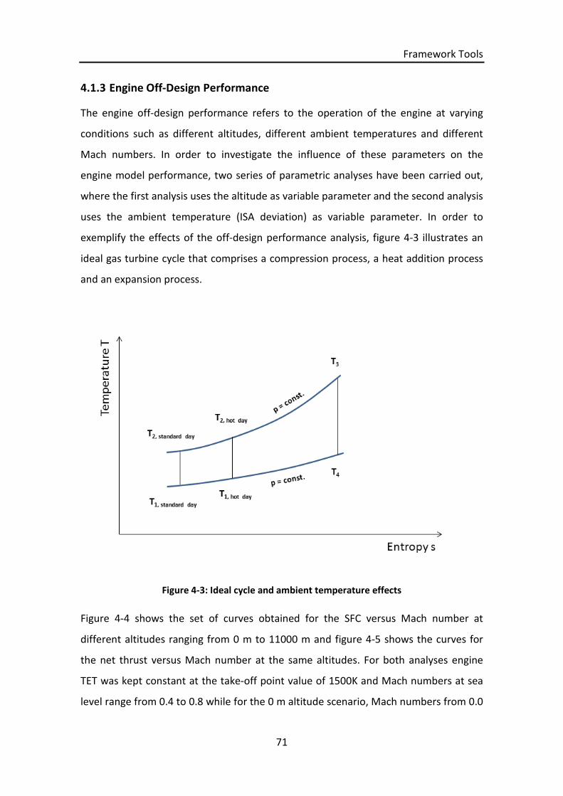
Framework Tools
71
4.1.3 Engine Off-Design Performance
The engine off-design performance refers to the operation of the engine at varying
conditions such as different altitudes, different ambient temperatures and different
Mach numbers. In order to investigate the influence of these parameters on the
engine model performance, two series of parametric analyses have been carried out,
where the first analysis uses the altitude as variable parameter and the second analysis
uses the ambient temperature (ISA deviation) as variable parameter. In order to
exemplify the effects of the off-design performance analysis, figure 4-3 illustrates an
ideal gas turbine cycle that comprises a compression process, a heat addition process
and an expansion process.
Figure 4-3: Ideal cycle and ambient temperature effects
Figure 4-4 shows the set of curves obtained for the SFC versus Mach number at
different altitudes ranging from 0 m to 11000 m and figure 4-5 shows the curves for
the net thrust versus Mach number at the same altitudes. For both analyses engine
TET was kept constant at the take-off point value of 1500K and Mach numbers at sea
level range from 0.4 to 0.8 while for the 0 m altitude scenario, Mach numbers from 0.0

Framework Tools
72
to 0.8 are plotted. At higher altitudes (≥ 6000m), plots for Mach numbers below 0.4
have been omitted since those scenarios do not reflect feasible engine performance
points.
Assuming a constant altitude, an increase in flight Mach number causes a linear
increase in engine SFC as shown in figure 4-4, which is related to the reduction in
propulsive efficiency. Also, SFC will improve with increase in altitude assuming a
constant flight Mach number. At higher altitudes the ambient temperatures decreases
(refer to figure 3-3) which leads to an improved thermal efficiency causing an
improvement in SFC.
Figure 4-4: CU2STF-LT – SFC vs. Mach number at constant TET (1500K)
As illustrated in figure 4-5, an increase in flight Mach number at constant altitude
reduces engine net thrust. The flight Mach number or velocity has three major effects
on the engine net thrust performance. Firstly, an increase in velocity raises the
incoming air momentum flow (momentum drag). Assuming a constant gross thrust, an
increase in momentum drag leads to a net thrust decay. Secondly, an increase in
velocity increases the exhaust nozzle pressure ratio and causes an inlet pressure rise,
0
2
4
6
8
10
12
14
16
18
20
0 0.1 0.2 0.3 0.4 0.5 0.6 0.7 0.8 0.9
SFC
[mg/
Ns]
Mach number [-]
0 m 6000 m 8000 m 11000 m

Framework Tools
73
called ram compression. The inlet pressure rise consequently causes an increase in air
density and inlet mass flow leading to a net thrust increase. Thirdly, at higher velocity a
temperature rise at the fan inlet occurs which is related to the isentropic relationship
of static and total temperature. Assuming constant TET and shaft rotational speed, this
causes a decrease in net thrust. For lower flight Mach numbers up to 0.3 the
momentum drag is predominant while the influence of ram compression and inlet
temperature rise will come into effect at Mach numbers above 0.3.
The altitude also affects the engine net thrust performance. As air density and
pressure decrease with increasing altitude a reduction in engine mass flow and engine
pressure ratio is observed. However, the lower ambient temperature at altitude leads
to an increased ratio of TET and inlet temperature which positively affects the engine
thrust and offsets the thrust decay at higher altitudes.
Figure 4-5: CU2STF-LT – Net thrust vs. Mach number at constant TET (1500K)
Figure 4-6 shows the set of curves obtained for the net thrust versus TET at different
ambient temperatures ranging from ISA -30 to ISA +30 and figure 4-7 shows the curves
for the SFC versus TET at the same ambient temperatures. Sea Level Static (SLS)
0
20
40
60
80
100
120
140
0 0.1 0.2 0.3 0.4 0.5 0.6 0.7 0.8 0.9
Ne
tTh
rust
[kN
]
Mach number [-]
0 m 6000 m 8000 m 11000 m

Framework Tools
74
conditions with an altitude of 0 m and a Mach number of 0.0 apply to both analyses
and the lower TET limit was kept at 1200K and the upper TET limit at 1800K, which is
close to the take-off condition.
As TET increases, the thermal efficiency of the engine improves which consequently
causes engine SFC to improve. At the same time, the propulsive efficiency of the
engine degrades with increasing TET. The lowest points of the curves in figure 4-7
represent the highest overall engine efficiency and thus lowest SFC. A further increase
in engine TET then causes a further degradation of propulsive efficiency which in turn
exceeds the effects of increased thermal efficiency and leads to an increase in SFC. At
constant engine TET, an increase in ambient temperature causes engine net thrust to
decrease. On the other hand, at constant ambient temperature conditions, an increase
in engine TET causes the net thrust to increase. Hotter ambient conditions require
more work to be extracted from the compressor as illustrated in figure 4-3, where the
inlet temperature conditions move from T1, standard day to T1, hot day. However, since
turbine work remains constant, the difference between turbine work and compressor
work reduces and net thrust will decrease. This means, if engine TET is kept constant,
the net thrust will drop. In order to compensate for the increased compressor work,
the turbine has to produce more work and thus the engine TET has to be increased to
maintain the same level of thrust.
Another effect that causes net thrust to drop with increasing ambient temperature
conditions is related to the operating conditions of the compressor. The corrected
rotational speed of the compressor, which is defined as speed N over root T, will
decrease with hotter ambient temperatures when constant shaft speed is assumed.
This results in the compressor operating at a lower compressor pressure ratio and
lower corrected mass flow compared to standard ambient conditions.

Framework Tools
75
Figure 4-6: CU2STF-LT – Net thrust vs. TET at SLS conditions
Figure 4-7: CU2STF-LT – SFC vs. TET at SLS conditions
0
50
100
150
200
250
0 200 400 600 800 1000 1200 1400 1600 1800 2000
Ne
tTh
rust
[kN
]
TET [K]
ISA -30 ISA -20 ISA -10 ISA ISA +10 ISA +20 ISA +30
0
2
4
6
8
10
12
0 200 400 600 800 1000 1200 1400 1600 1800 2000
SFC
[mg/
Ns]
TET [K]
ISA -30 ISA -20 ISA -10 ISA ISA +10 ISA +20 ISA +30

Framework Tools
76
Figures 4-8 to 4-11 show the same set of result plots for the medium thrust engine
variant, namely CU2STF-MT. The results of the engine SFC performance correspond to
the concurrent increase in TET which was necessary to achieve the desired increase in
net thrust.
Figure 4-8: CU2STF-MT – SFC vs. Mach number at constant TET (1575K)
0
2
4
6
8
10
12
14
16
18
20
0 0.1 0.2 0.3 0.4 0.5 0.6 0.7 0.8 0.9
SFC
[mg/
Ns]
Mach number [-]
0 m 6000 m 8000 m 11000 m

Framework Tools
77
Figure 4-9: CU2STF-MT – Net thrust vs. Mach number at constant TET (1575K)
Figure 4-10: CU2STF-MT – Net thrust vs. TET at SLS conditions
0
20
40
60
80
100
120
140
160
0 0.1 0.2 0.3 0.4 0.5 0.6 0.7 0.8 0.9
Ne
tTh
rust
[kN
]
Mach number [-]
0 m 6000 m 8000 m 11000 m
0
50
100
150
200
250
0 200 400 600 800 1000 1200 1400 1600 1800 2000
Ne
tTh
rust
[kN
]
TET [K]
ISA -30 ISA -20 ISA -10 ISA ISA +10 ISA +20 ISA +30

Framework Tools
78
Figure 4-11: CU2STF-MT – SFC vs. TET at SLS conditions
Lastly, figures 4-12 to 4-15 show the result plots for the high thrust engine variant,
namely CU2STF-HT. These results also follow the trends of the medium thrust engine
results so that the further rise in engine TET leads to an increase of net thrust output
and in parallel to a further increase of the engine SFC.
The off-design performance simulations for all three engine variants yielded in general
the expected engine characteristics in terms of specific fuel consumption and net
thrust, when variations in altitude, flight Mach number, ambient temperature and
turbine entry temperature (TET) are implemented. References [41], [46] and [39]
provide in-depth descriptions of the effects of various parameters, such as altitude,
turbine entry temperature etc. on gas turbine performance. They also elaborate the
typical trade-offs between thermal efficiency and propulsive efficiency for high bypass
ratio turbofan engines.
0
2
4
6
8
10
12
0 200 400 600 800 1000 1200 1400 1600 1800 2000
SFC
[mg/
Ns]
TET [K]
ISA -30 ISA -20 ISA -10 ISA ISA +10 ISA +20 ISA +30

Framework Tools
79
Figure 4-12: CU2STF-HT – SFC vs. Mach number at constant TET (1760K)
Figure 4-13: CU2STF-HT – Net thrust vs. Mach number at constant TET (1760K)
0
5
10
15
20
25
0 0.1 0.2 0.3 0.4 0.5 0.6 0.7 0.8 0.9
SFC
[mg/
Ns]
Mach number [-]
0 m 6000 m 8000 m 11000 m
0
20
40
60
80
100
120
140
160
180
0 0.1 0.2 0.3 0.4 0.5 0.6 0.7 0.8 0.9
Ne
tTh
rust
[kN
]
Mach number [-]
0 m 6000 m 8000 m 11000 m

Framework Tools
80
Figure 4-14: CU2STF-HT – Net thrust vs. TET at SLS conditions
Figure 4-15: CU2STF-HT – SFC vs. TET at SLS conditions
0
50
100
150
200
250
0 200 400 600 800 1000 1200 1400 1600 1800 2000
Ne
tTh
rust
[kN
]
TET [K]
ISA -30 ISA -20 ISA -10 ISA ISA +10 ISA +20 ISA +30
0
2
4
6
8
10
12
0 200 400 600 800 1000 1200 1400 1600 1800 2000
SFC
[mg/
Ns]
TET [K]
ISA -30 ISA -20 ISA -10 ISA ISA +10 ISA +20 ISA +30

Framework Tools
81
Figures 4-16, 4-17 and 4-18 show the characteristic maps (including running line, surge
line and design point) of the CU2STF-LT engine fan, Low Pressure Compressor (LPC)
and High Pressure Compressor (HPC) at TOC power settings. The engine component
running line can be obtained by simulating a change in engine fuel flow which in turn
causes a change in TET, rotational speed and consequently results in a change in
engine mass flow and a shift of the operating point. Figure 4-17 shows the distinctive
running line of the LPC which approaches the surge line at lower engine power settings
thus requiring flow adjustments through a handling bleed as previously described.
Figure 4-18 shows the distinctive running line of the HPC with the operating points
moving in parallel to the surge line. In addition, the running line of a degraded HPC
(dashed line) is shown for reference. The engine degradation analysis will be explained
in subsection 4.1.4 in more detail. Figures 4-19 to 4-24 show the same characteristic
maps for the CU2STF-MT and CU2STF-HT engine variant respectively.
Figure 4-16: CU2STF-LT Fan map (running line at TOC)
0
0.5
1
1.5
2
2.5
0 100 200 300 400 500 600
Pre
ssu
reR
atio
Corrected Mass Flow
PCN=0,3 PCN=0,4 PCN=0,5 PCN=0,6
PCN=0,7 PCN=0,8 PCN=0,9 PCN=1,0
PCN=1,1 Running line Surge line Design point

Framework Tools
82
Figure 4-17: CU2STF-LT LPC map (running line at TOC)
Figure 4-18: CU2STF-LT HPC map (running line at TOC)
0
0.5
1
1.5
2
2.5
0 10 20 30 40 50 60
Pre
ssu
reR
atio
Corrected Mass Flow
PCN=0,3 PCN=0,4 PCN=0,5 PCN=0,6
PCN=0,7 PCN=0,8 PCN=0,9 PCN=1,0
PCN=1,1 Running line Surge line Design point
0
2
4
6
8
10
12
14
16
0 5 10 15 20 25 30 35
Pre
ssu
reR
atio
Corrected Mass Flow
PCN=0,5 PCN=0,6 PCN=0,7
PCN=0,8 PCN=0,89 PCN=0,92
PCN=0,95 PCN=1,0 PCN=1,1
Running line Surge line Running line degraded
Design point

Framework Tools
83
Figure 4-19: CU2STF-MT Fan map (running line at TOC)
Figure 4-20: CU2STF-MT LPC map (running line at TOC)
0
0.5
1
1.5
2
2.5
0 100 200 300 400 500 600
Pre
ssu
reR
atio
Corrected Mass flow
PCN=0,3 PCN=0,4 PCN=0,5 PCN=0,6
PCN=0,7 PCN=0,8 PCN=0,9 PCN=1,0
PCN=1,1 Running line Surge line Design point
0
0.5
1
1.5
2
2.5
0 10 20 30 40 50 60
Pre
ssu
reR
atio
Corrected Mass flow
PCN=0,3 PCN=0,4 PCN=0,5 PCN=0,6
PCN=0,7 PCN=0,8 PCN=0,9 PCN=1,0
PCN=1,1 Running line Surge line Design point

Framework Tools
84
Figure 4-21: CU2STF-MT HPC map (running line at TOC)
Figure 4-22: CU2STF-HT Fan map (running line at TOC)
0
2
4
6
8
10
12
14
16
0 5 10 15 20 25 30 35
Pre
ssu
reR
atio
Corrected Mass Flow
PCN=0,5 PCN=0,6 PCN=0,7
PCN=0,8 PCN=0,89 PCN=0,92
PCN=0,95 PCN=1,0 PCN=1,1
Running line Surge line Running line degraded
Design point
0
0.5
1
1.5
2
2.5
0 100 200 300 400 500 600
Pre
ssu
reR
atio
Corrected Mass Flow
PCN=0,3 PCN=0,4 PCN=0,5 PCN=0,6
PCN=0,7 PCN=0,8 PCN=0,9 PCN=1,0
PCN=1,1 Running line Surge line Design point
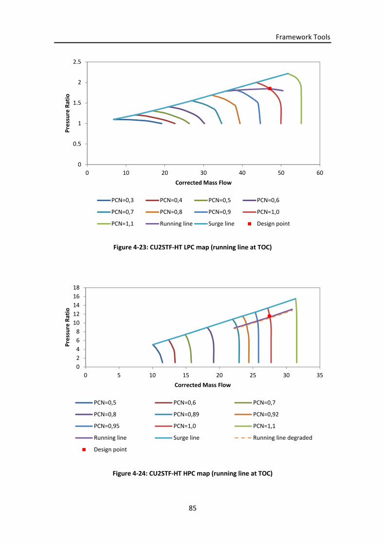
Framework Tools
85
Figure 4-23: CU2STF-HT LPC map (running line at TOC)
Figure 4-24: CU2STF-HT HPC map (running line at TOC)
0
0.5
1
1.5
2
2.5
0 10 20 30 40 50 60
Pre
ssu
reR
atio
Corrected Mass Flow
PCN=0,3 PCN=0,4 PCN=0,5 PCN=0,6
PCN=0,7 PCN=0,8 PCN=0,9 PCN=1,0
PCN=1,1 Running line Surge line Design point
0
2
4
6
8
10
12
14
16
18
0 5 10 15 20 25 30 35
Pre
ssu
reR
atio
Corrected Mass Flow
PCN=0,5 PCN=0,6 PCN=0,7
PCN=0,8 PCN=0,89 PCN=0,92
PCN=0,95 PCN=1,0 PCN=1,1
Running line Surge line Running line degraded
Design point

Framework Tools
86
It can also be noted that an increase in take-off thrust from the low thrust engine
variant (104.5 kN T/O thrust) to the medium thrust engine variant (120.1 kN T/O
thrust) requires a rise in turbine entry temperature (TET) of 5%. A further increase in
thrust from the medium thrust engine variant to the highest thrust variant (146.8 kN
T/O thrust) then requires a rise in TET of about 12%. Figure 4-25 shows the expected
correlations between turbine and entry temperature (TET) and T/O thrust and
between fuel flow and T/O thrust for all three engine variants.
However, it must be kept in mind that not only the TET was adjusted between the
individual engine models but also changes to the pressure ratios of the Fan, the LPC
and the HPC have been incorporated to match the engine design point and take-off
conditions.
Figure 4-25: TET and Fuel Flow over T/O Thrust
0.0
0.2
0.4
0.6
0.8
1.0
1.2
1.4
1.6
1.8
2.0
0
500
1000
1500
2000
80 90 100 110 120 130 140 150 160
Fue
lFlo
w[k
g/s]
TET
[K]
T/O thrust [kN]
TET Fuel flow
CU2STF-LT
CU2STF-MT
CU2STF-HT

Framework Tools
87
4.1.4 Degraded Engine Performance
Based on the three created engine model variants, an additional degraded engine
model has been implemented for each engine variant. To simulate the degraded
engine performance in a simplified manner, specific engine component data has been
arbitrarily changed in such a way that the engine performance characteristics will
reflect those of a deteriorated engine. On the basis of the considerations made in
section 2.4 and 2.5 the degradation was achieved by altering the following 4 engine
component design parameters thus creating artificial engine performance
deterioration:
1. High Pressure Compressor (HPC) Pressure Ratio
2. High Pressure Compressor (HPC) Efficiency
3. Combustion Efficiency
4. High Pressure Turbine (HPT) Efficiency
It must be noted that no adjustment of the flow capacity of the degraded components
in relation to the design point values has been made which would cause a decrease in
Corrected Mass Flow in turn. A decrease of the 4 above mentioned parameters due to
degradation will cause the engine to be less efficient in producing the same amount of
thrust than the clean baseline engine model would be. Lower efficiencies of the HPC,
the Combustor and the HPT will require the turbine work to increase in order to
compensate for the loss in compressor flow capacity and discharge pressure.
Consequently, this is accompanied by an increase in engine fuel flow and specific fuel
consumption. The increase in fuel flow then leads to an increase in TET.
Tables 4-5, 4-6 and 4-7 show the engine performance changes if a 2% degradation of
the above mentioned engine component parameters is assumed. The design point TET
for all three engine variants increases by more than 1.3% and the SFC increases by
more than 4%. At take-off conditions the TET increases by at least 1.4% and the fuel
flow increases by more than 4.4%. Figures 4-18, 4-21 and 4-24 in the previous section
4.1.2 also show the shift of the engine running line in the HPC map due to the
degradation effects.

Framework Tools
88
Table 4-5: CU2STF-LT degraded performance (2% degradation)
Engine Design Point Parameter degraded
Parameter Degradation Baseline Degraded
HPC Pressure Ratio -2% 10.59 10.37
Combustion Efficiency -2% 0.999 0.979
HPT Efficiency -2% 0.90 0.88
HPC Efficiency -2% 0.875 0.855
Engine Model Design Point degraded
Parameter CU Turbomatch Degraded/Recovered Delta [%]
TOC thrust [N] 25075 25180 0.42%
TOC SFC [g/kN sec] 16.65 17.42 4.42%
TOC TET [K] 1345 1365 1.47%
Engine Model Take-Off degraded
CU Turbomatch Degraded/Recovered Delta [%]
T/O thrust [N] 104510 104430 -0.08%
T/O TET [K] 1500 1525 1.64%
T/O fuel flow [kg/s] 0.920 0.972 5.35%
Table 4-6: CU2STF-MT degraded performance (2% degradation)
Engine Design Point Parameter degraded
Parameter Degradation Baseline Degraded
HPC Pressure Ratio -2% 10.59 10.37
Combustion Efficiency -2% 0.999 0.979
HPT Efficiency -2% 0.90 0.88
HPC Efficiency -2% 0.875 0.855
Engine Model Design Point degraded
Parameter CU Turbomatch Degraded/Recovered Delta [%]
TOC thrust [N] 25075 25180 0.42%
TOC SFC [g/kN s] 16.65 17.42 4.42%
TOC TET [K] 1345 1365 1.47%
Engine Model Take-Off degraded
Parameter CU Turbomatch Degraded/Recovered Delta [%]
T/O thrust [N] 120550 121050 0.41%
T/O TET [K] 1575 1605 1.87%
T/O fuel flow [kg/s] 1.101 1.169 5.82%

Framework Tools
89
Table 4-7: CU2STF-HT degraded performance (2% degradation)
Engine Design Point Parameter degraded
Parameter Degradation Baseline Degraded
HPC Pressure Ratio -2% 11.53 11.30
Combustion Efficiency -2% 0.999 0.979
HPT Efficiency -2% 0.90 0.88
HPC Efficiency -2% 0.875 0.855
Engine Model Design Point degraded
Parameter CU Turbomatch Degraded/Recovered Delta [%]
TOC thrust [N] 28254 28502 0.87%
TOC SFC [g/kN s] 16.91 17.68 4.36%
TOC TET [K] 1440 1460 1.37%
Engine Model Take-Off degraded
Parameter CU Turbomatch Degraded/Recovered Delta [%]
T/O thrust [N] 147570 147160 -0.28%
T/O TET [K] 1760 1785 1.40%
T/O fuel flow [kg/s] 1.486 1.555 4.44%
For figures 4-5 to 4-7, it must be noted that the net thrust values at TOC and T/O
achieved after recovery of the degradation condition were matched as close as
possible to the initial CU Turbomatch model values. It can be seen that, depending on
the engine running point (TOC or T/O) and the engine variant, these matched net
thrust values may be slightly lower or slightly higher than the initial values of the non-
degraded engine model.
In figure 4-26 the engine TET is plotted over the net thrust range at take-off conditions
(Mach number = 0). An increase in TET can be observed over the take-off thrust range
for the degraded engine configuration compared to the clean configuration. Figure 4-
27 shows the peak take-off TET for the clean, the degraded and the derated (15% take-
off thrust reduction) engine configuration at ISA+30°C conditions. Thrust reduction
reduces take-off TET by approximately 4% for the CU2STF-LT, by 5.7% for the CU2STF-
MT and by about 7.9% for the CU2STF-HT.
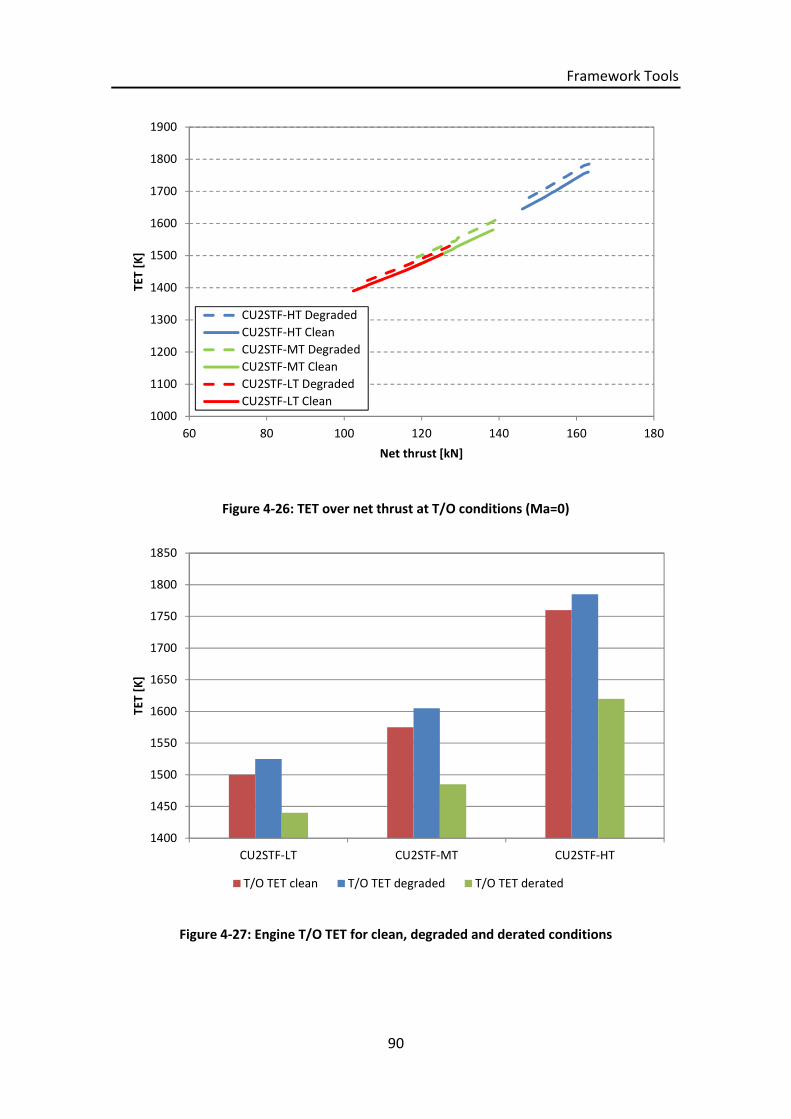
Framework Tools
90
Figure 4-26: TET over net thrust at T/O conditions (Ma=0)
Figure 4-27: Engine T/O TET for clean, degraded and derated conditions
1000
1100
1200
1300
1400
1500
1600
1700
1800
1900
60 80 100 120 140 160 180
TET
[K]
Net thrust [kN]
CU2STF-HT Degraded
CU2STF-HT Clean
CU2STF-MT Degraded
CU2STF-MT Clean
CU2STF-LT Degraded
CU2STF-LT Clean
1400
1450
1500
1550
1600
1650
1700
1750
1800
1850
CU2STF-LT CU2STF-MT CU2STF-HT
TET
[K]
T/O TET clean T/O TET degraded T/O TET derated

Framework Tools
91
To estimate the engine in-service life in terms of flight cycles after which the above
described degradation condition can be observed, the engine EGT margin (EGTM) may
be used as performance indicator. Off-design performance analysis of the three engine
variants revealed a nearly constant ratio of HP Turbine Entry Temperature to LP
Turbine Exit Temperature over the engine thrust range with an approximate value of
1.4. This allows conversion of the engine TET to an approximate engine EGT value.
According to reference [95] an average take-off EGTM deterioration of about 5-6°C per
1000 flight cycles is expected for the CFM56-5B series engine. Actual deterioration
rates depend on engine thrust rating and utilisation.
The EGT increase between the clean configuration and the degraded configuration has
been calculated for the three engine models as follows:
ܩܧ ௗௗௗ − ܩܧ = ܯܩܧ +ݏݏ ௗௗௗ,௧ܯܩܧ (4-8)
Assuming a degradation rate of 5°C EGTM per 1000 cycles for the CU2STF-LT engine
variant, 5.5°C EGTM per 1000 cycles for the CU2STF-MT variant and 6°C EGTM per
1000 cycles for the CU2STF-HT variant, and assuming an initial EGTM degradation of
12°C, 12,5°C and 13°C respectively for the first 1000 cycles, the corresponding
accumulated engine life in flight cycles can be estimated as shown in figure 4-28. Based
on these assumptions, the degradation of CU2STF-LT variant would roughly equal 4600
flight cycles, the degradation of the CU2STF-MT variant would equal about 5000 flight
cycles and the degradation of the CU2STF-HT would be equal to 4000 flight cycles.
Since an equal 2 percent degradation scenario has been assumed for all three engine
models, an accretion in total flight cycles from the highest thrust variant (CU2STF-HT)
to the lowest thrust variant (CU2STF-LT) would have been expected. However, as
illustrated in figure 4-28, it can be seen that the 2 percent degradation scenario equals
with an in-service life of nearly 5000 flight cycles for medium thrust variant (CU2STF-
MT). This is due to the fact that this engine model variant experienced the highest
take-off TET increase (+30K) when degradation was induced causing the highest loss in
EGTM. It must be noted that this approach only represents a rough estimation based
on assumptions for initial EGTM degradation and per cycle based degradation as well
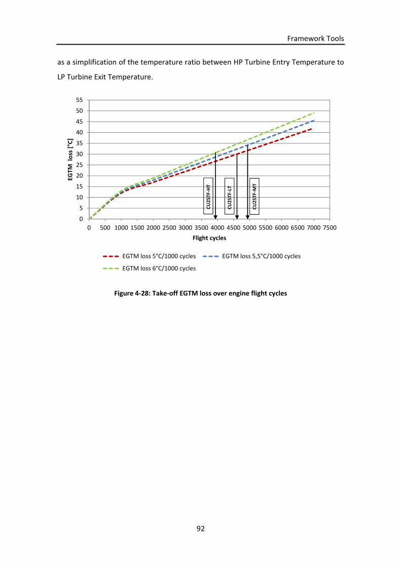
Framework Tools
92
as a simplification of the temperature ratio between HP Turbine Entry Temperature to
LP Turbine Exit Temperature.
Figure 4-28: Take-off EGTM loss over engine flight cycles
0
5
10
15
20
25
30
35
40
45
50
55
0 500 1000 1500 2000 2500 3000 3500 4000 4500 5000 5500 6000 6500 7000 7500
EGTM
loss
[°C
]
Flight cycles
EGTM loss 5°C/1000 cycles EGTM loss 5,5°C/1000 cycles
EGTM loss 6°C/1000 cycles
CU
2ST
F-LT
CU
2ST
F-M
T
CU
2ST
F-H
T
Aircraft Trajectory Analysis and Results
93
4.1.5 Engine Model Verification
As initially stated, the above described engine model performance results were
achieved by using the Cranfield University in-house code Turbomatch. Even though the
engine performance calculations which were carried out yielded consistent results in
terms of accuracy and comparability, some limitations must be considered when it
comes to interpreting those engine performance calculations. It must be noted that
the above created models only represent a basic engine design with certain
simplifications. Especially since not all engine parameters are publicly available, some
assumptions made, may still deviate from the original engine configuration. Also,
dynamic engine off design performance scenarios and transient behaviour are not
accounted for in this study. This is also due to the fact that engine features which exist
in engines in operation such as variable stator vanes (VSV) or active bleed distribution
were not integrated in the engine models. A comprehensive overview of engine
control systems and their components in commercial turbofan applications can be
found in reference [96]. It describes in depth all major engine control elements, their
functions and the effect on engine operation.
4.2 Aircraft Performance Model (Hermes)
The aircraft configuration that is used throughout this study represents a narrow body
single-aisle aircraft for use in short to medium range applications. The aircraft model
has been created based on publicly available information and was adapted for the
work carried out in this study. Three aircraft configurations were modelled, each
configuration representing a different aircraft size and thus each one having a different
maximum payload [97], [98], [99]. The models are designated as CUSA-S (Cranfield
University Single Aisle Short), CUSA-M (Cranfield University Single Aisle Medium) and
CUSA-L (Cranfield University Single Aisle Long). All three configurations encompass the
same basic aircraft design like wing geometry, high lift systems and landing gear
characteristics. Only the fuselage geometry, in this study the length, was altered to
meet the three different model requirements. The model requirements are based on

Aircraft Trajectory Analysis and Results
94
the Airbus A320 aircraft series which is a common commercial aircraft available in
different configurations.
The described aircraft model performance results were achieved by using the Cranfield
University in-house code Hermes. This aircraft/engine performance model
incorporates an aircraft aerodynamic and performance model and also connects with
the Turbomatch engine performance model [100]. Figure 4-29 shows the basic
structure of the Hermes input and output data flow. Hermes requires input from the
engine model (engine performance input) as well as input from the aircraft model and
its operational limits (aircraft model input and aircraft mission input). The two main
output files contain the calculated aircraft performance (aircraft trajectory
performance) including all major engine parameters throughout the trajectory.
Figure 4-29: Hermes aircraft performance model (inputs and outputs)
The main inputs for the aircraft performance calculations are summarised below:
(Refer also to tables 4-8, 4-9 and 4-10 in the next section)
Engine performance data including: Design point and off-design performance
(clean and degraded configuration).
Aircraft mission data including: 17 climb segments, 11 descent segments, 1
fixed take-off segment and 86-285 cruise segments (depending on range).
Aircraft Trajectory Analysis and Results
95
Aircraft model data including: aircraft geometry specifications and aircraft
weight specifications.
The Hermes aircraft/engine model uses the following user specified information to
calculate the flight path performance of the particular phase:
Climb segments: Altitude, ISA temperature deviation, EAS, engine power
Cruise segments: Altitude, ISA temperature deviation, Mach number
Descent segments: ISA temperature deviation, TAS, engine power
The input specifications of the climb phase and descent phase differ due to the fact
that Hermes internally calculates the descent altitudes by interpolating between the
cruise altitude and the landing altitude. This means there is no provision to select a
descent path based on specific altitudes. Aircraft speed and engine power settings can
similarly be adjusted for climb and descent segments.
A simulation program that provides similar functionality to perform flight mission
analysis is called Varmission and has been developed by DLR (Deutsches Zentrum für
Luft -und Raumfahrt) Institute of Propulsion Technology. Another commercially
available software suite to perform flight mission studies is called Pacelab Mission
developed by PACE which offers comprehensive functionality for aircraft route and
performance analyses. Also aircraft manufacturers such as Airbus or Boeing provide
comprehensive analysis suites to airline operators based on their own aircraft models
and flight test data.
4.2.1 Hermes Aircraft Model
The basic aircraft model structure of the CUSA model is depicted in figure 4-30. It is a
single-aisle narrow body aircraft design. Each version, according to the length, reflects
a different passenger capacity and thus a different aircraft OEW, maximum payload
weight and maximum take-off weight. The passenger weight has been assumed with a
mean value for all adults of 86kg according to a survey on standard passenger weights
and baggage performed at 8 different airports in the European region in 2008 and
2009 [101].
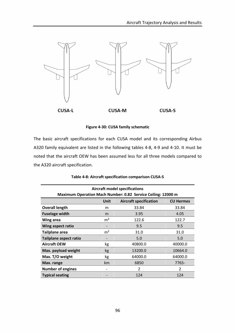
Aircraft Trajectory Analysis and Results
96
Figure 4-30: CUSA family schematic
The basic aircraft specifications for each CUSA model and its corresponding Airbus
A320 family equivalent are listed in the following tables 4-8, 4-9 and 4-10. It must be
noted that the aircraft OEW has been assumed less for all three models compared to
the A320 aircraft specification.
Table 4-8: Aircraft specification comparison CUSA-S
Aircraft model specifications
Maximum Operation Mach Number: 0.82 Service Ceiling: 12000 m
Unit Aircraft specification CU Hermes
Overall length m 33.84 33.84
Fuselage width m 3.95 4.05
Wing area m² 122.6 122.7
Wing aspect ratio - 9.5 9.5
Tailplane area m² 31.0 31.0
Tailplane aspect ratio - 5.0 5.0
Aircraft OEW kg 40800.0 40000.0
Max. payload weight kg 13200.0 10664.0
Max. T/O weight kg 64000.0 64000.0
Max. range km 6850 7765-
Number of engines - 2 2
Typical seating - 124 124
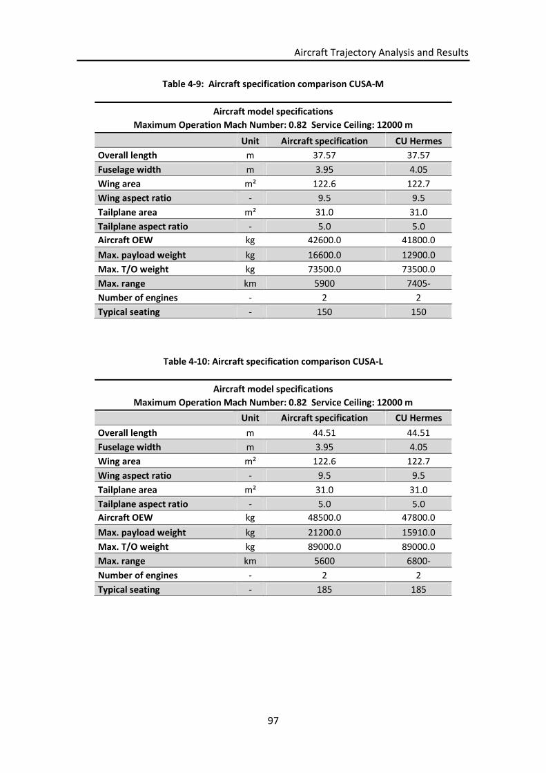
Aircraft Trajectory Analysis and Results
97
Table 4-9: Aircraft specification comparison CUSA-M
Aircraft model specifications
Maximum Operation Mach Number: 0.82 Service Ceiling: 12000 m
Unit Aircraft specification CU Hermes
Overall length m 37.57 37.57
Fuselage width m 3.95 4.05
Wing area m² 122.6 122.7
Wing aspect ratio - 9.5 9.5
Tailplane area m² 31.0 31.0
Tailplane aspect ratio - 5.0 5.0
Aircraft OEW kg 42600.0 41800.0
Max. payload weight kg 16600.0 12900.0
Max. T/O weight kg 73500.0 73500.0
Max. range km 5900 7405-
Number of engines - 2 2
Typical seating - 150 150
Table 4-10: Aircraft specification comparison CUSA-L
Aircraft model specifications
Maximum Operation Mach Number: 0.82 Service Ceiling: 12000 m
Unit Aircraft specification CU Hermes
Overall length m 44.51 44.51
Fuselage width m 3.95 4.05
Wing area m² 122.6 122.7
Wing aspect ratio - 9.5 9.5
Tailplane area m² 31.0 31.0
Tailplane aspect ratio - 5.0 5.0
Aircraft OEW kg 48500.0 47800.0
Max. payload weight kg 21200.0 15910.0
Max. T/O weight kg 89000.0 89000.0
Max. range km 5600 6800-
Number of engines - 2 2
Typical seating - 185 185
Aircraft Trajectory Analysis and Results
98
4.2.2 Aircraft Model Verification
To assess the performance characteristics of the adapted aircraft models a series of
basic trajectory calculations with Hermes has been performed. In this way the
maximum operational limits in terms of payload and range have been determined for
each of the three aircraft variants. Based on the aircraft model specifications provided
in the previous section Hermes calculates the maximum mission ranges depending on
the selected payload and while taking into account aircraft fuel weight limitations.
Figure 4-31 shows the payload-range diagram for the CUSA-S aircraft variant. Three
key points of the payload-range curve have been plotted in the diagram, each point
representing a particular load configuration in terms of payload weight and fuel
weight. (1) The maximum range with maximum take-off weight and maximum payload
weight is designated as maximum payload range. (2) The maximum range with
maximum take-off weight and maximum fuel weight is designated as maximum
economic range. (3) The maximum range with no payload weight and maximum fuel
weight is designated as maximum ferry range. Figure 4-32 shows the payload-range
diagram for the CUSA-M aircraft variant in a similar fashion. The payload-range
diagram for the CUSA-L aircraft variant is shown in figure 4-33. This aircraft variant
does not have a particular maximum economic range, id est the maximum payload
range and maximum economic range fall in the same point since the aircraft is only
limited by the maximum fuel weight. In addition, all diagrams show the respective
payload-range points for the two mission analysed in chapter 5.
The depicted payload-range diagrams have been plotted assuming the following
conditions [102], [103], [104]:
ISA+10°C conditions
Cruise altitude of 10668 m
Cruise Mach number of 0.76
No diversion mission
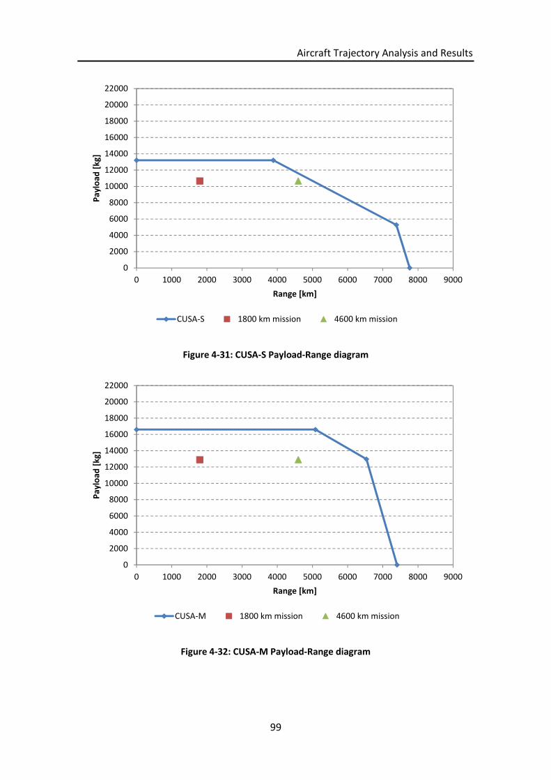
Aircraft Trajectory Analysis and Results
99
Figure 4-31: CUSA-S Payload-Range diagram
Figure 4-32: CUSA-M Payload-Range diagram
0
2000
4000
6000
8000
10000
12000
14000
16000
18000
20000
22000
0 1000 2000 3000 4000 5000 6000 7000 8000 9000
Pay
load
[kg]
Range [km]
CUSA-S 1800 km mission 4600 km mission
0
2000
4000
6000
8000
10000
12000
14000
16000
18000
20000
22000
0 1000 2000 3000 4000 5000 6000 7000 8000 9000
Pay
load
[kg]
Range [km]
CUSA-M 1800 km mission 4600 km mission

Aircraft Trajectory Analysis and Results
100
Figure 4-33: CUSA-L Payload-Range diagram
4.3 Emissions Predictions Model (Hephaestus/P3T3)
For the assessment of engine emissions during, id est pollutant emitted during the
combustion process in the combustor, there are three common methods available to
predict those emissions: The empirical correlation based method, the numerical
simulation through CFD calculations, and calculations based on stirred reactor models
(physics-based models) [105]. Empirical correlation based models are typically less
demanding in terms of computational resources and they are generally suitable for
existing fixed combustors where particular data is available. This means these models
are adequate for predicting emissions, especially NOx, when there pre-exists historical
certification data for that specific engine type [106]. The more sophisticated and
complex numerical and calculations based models are generally more computationally
intensive because of their high level of detail in mapping a particular combustor
design. This makes them especially suitable for new combustor designs for which no
historical data points exist but detailed information like combustor geometries and
0
2000
4000
6000
8000
10000
12000
14000
16000
18000
20000
22000
0 1000 2000 3000 4000 5000 6000 7000 8000 9000
Pay
load
[kg]
Range [km]
CUSA-L 1800 km mission 4600 km mission
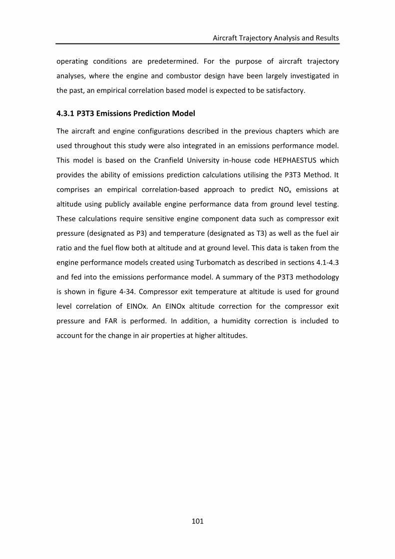
Aircraft Trajectory Analysis and Results
101
operating conditions are predetermined. For the purpose of aircraft trajectory
analyses, where the engine and combustor design have been largely investigated in
the past, an empirical correlation based model is expected to be satisfactory.
4.3.1 P3T3 Emissions Prediction Model
The aircraft and engine configurations described in the previous chapters which are
used throughout this study were also integrated in an emissions performance model.
This model is based on the Cranfield University in-house code HEPHAESTUS which
provides the ability of emissions prediction calculations utilising the P3T3 Method. It
comprises an empirical correlation-based approach to predict NOx emissions at
altitude using publicly available engine performance data from ground level testing.
These calculations require sensitive engine component data such as compressor exit
pressure (designated as P3) and temperature (designated as T3) as well as the fuel air
ratio and the fuel flow both at altitude and at ground level. This data is taken from the
engine performance models created using Turbomatch as described in sections 4.1-4.3
and fed into the emissions performance model. A summary of the P3T3 methodology
is shown in figure 4-34. Compressor exit temperature at altitude is used for ground
level correlation of EINOx. An EINOx altitude correction for the compressor exit
pressure and FAR is performed. In addition, a humidity correction is included to
account for the change in air properties at higher altitudes.
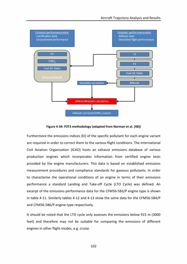
Aircraft Trajectory Analysis and Results
102
Figure 4-34: P3T3 methodology (adapted from Norman et al. [48])
Furthermore the emissions indices (EI) of the specific pollutant for each engine variant
are required in order to correct them to the various flight conditions. The International
Civil Aviation Organization (ICAO) hosts an exhaust emissions database of various
production engines which incorporates information from certified engine tests
provided by the engine manufacturers. This data is based on established emissions
measurement procedures and compliance standards for gaseous pollutants. In order
to characterise the operational conditions of an engine in terms of their emissions
performance a standard Landing and Take-off Cycle (LTO Cycle) was defined. An
excerpt of the emissions performance data for the CFM56-5B3/P engine type is shown
in table 4-11. Similarly tables 4-12 and 4-13 show the same data for the CFM56-5B4/P
and CFM56-5B6/P engine type respectively.
It should be noted that the LTO cycle only assesses the emissions below 915 m (3000
feet) and therefore may not be suitable for comparing the emissions of different
engines in other flight modes, e.g. cruise.

Aircraft Trajectory Analysis and Results
103
Table 4-11: ICAO Database exhaust emissions CFM56-5B3/P
Mode Power Setting Time Fuel Flow Emissions Indices [g/kg]
[% T/O Thrust] [min] [kg/s] HC CO NOx
Take-off 100 0.7 1.430 0.1 0.8 37.3
Climb out 85 2.2 1.141 0.2 0.9 28.5
Approach 30 4.0 0.366 0.5 1.7 11.2
Idle 7 26.0 0.115 3.5 19.2 4.7
Table 4-12: ICAO Database exhaust emissions CFM56-5B4/P
Mode Power Setting Time Fuel Flow Emissions Indices [g/kg]
[% T/O Thrust] [min] [kg/s] HC CO NOx
Take-off 100 0.7 1.132 0.2 0.9 28.0
Climb out 85 2.2 0.935 0.2 0.9 23.2
Approach 30 4.0 0.312 0.5 2.3 10.0
Idle 7 26.0 0.104 4.6 23.4 4.3
Table 4-13: ICAO Database exhaust emissions CFM56-5B6/P
Mode Power Setting Time Fuel Flow Emissions Indices [g/kg]
[% T/O Thrust] [min] [kg/s] HC CO NOx
Take-off 100 0.7 0.961 0.2 0.9 23.6
Climb out 85 2.2 0.799 0.2 1.0 19.6
Approach 30 4.0 0.275 0.6 2.9 9.2
Idle 7 26.0 0.097 5.5 27.7 4.0
The P3T3 model utilises both, engine model performance data as well as the ground
level exhaust emissions data published by the engine manufacturers to establish the
emissions indices at certain altitudes and flight speeds. The resulting total NOx
emissions in kilogram can then be calculated according formula 4-9:
For this study, only the emissions index (EI) for the NOx emissions is of interest and
other pollutants are not considered.

Aircraft Trajectory Analysis and Results
104
௫ = ݓ) × ) × ܫܧ ௫ (4-9)
This is where wf is the fuel flow given in kilogram per second, time is given in seconds
and EINOx in gram/kilogram.
4.3.2 Emissions Model Verification
In order to verify the emissions performance of the three engine variants they have
been matched and compared with existing equivalent engine models from the ICAO
database. The Hephaestus tool has been used to calculate the emissions based on this
ICAO data. The fuel flow at the four discrete power settings provided in the ICAO
database for each engine variant (refer to table 4-11, 4-12, 4-13) has been used as
target value to match the engine performance of the created engine models. Data
from the previously performed engine off-design studies was used to find the
respective fuel flow at the different power settings for each model by adjusting the
TET. The corresponding values of burner inlet temperature (T3) and burner inlet
pressure (P3) as well as the fuel/air ratio have then been used as input parameters for
the emissions model. Figures 4-35, 4-36 and 4-37 show the fuel flow comparison of the
ICAO data and the engine models at the different power settings (the four discrete
power settings have been converted to the actual net thrust value given in kN). It can
be noted from figures 4-35, 4-36 and 4-37 that the engine model results at T/O, climb,
approach and idle power settings are generally following the trend of the ICAO data
and can be considered acceptable for the purpose of this study. The results at idle
power settings however have only limited validity. One reason for this behaviour arises
from the limitations of the created engine models which did not return viable engine
performance results at very low power settings. Figure A.1-1 in the appendix illustrates
a comparison between the block fuel and block NOx plotted over the payload
conditions for the three aircraft variants as simulated in the following chapter 5.

Aircraft Trajectory Analysis and Results
105
Figure 4-35: CU2STF-LT - Fuel Flow versus Net Thrust
Figure 4-36: CU2STF-MT - Fuel Flow versus Net Thrust
0.000
0.200
0.400
0.600
0.800
1.000
1.200
1.400
1.600
0 20 40 60 80 100 120 140 160
Fue
lFlo
w[k
g/s]
Net Thrust [kN]
ICAO Database CFM56-5B6/P CU2STF-LT
0.000
0.200
0.400
0.600
0.800
1.000
1.200
1.400
1.600
0 20 40 60 80 100 120 140 160
Fue
lFlo
w[k
g/s]
Net Thrust [kN]
ICAO Database CFM56-5B4/P CU2STF-MT

Aircraft Trajectory Analysis and Results
106
Figure 4-37: CU2STF-HT - Fuel Flow versus Net Thrust
0.000
0.200
0.400
0.600
0.800
1.000
1.200
1.400
1.600
0 20 40 60 80 100 120 140 160
Fue
lFlo
w[k
g/s]
Net Thrust [kN]
ICAO Database CFM56-5B3/P CU2STF-HT

Aircraft Trajectory Analysis and Results
107
4.4 Optimisation Framework
The framework for the aircraft trajectory optimisation case studies used in this work is
comprised of the aircraft, engine and emissions models and an optimisation suite. The
framework provides the interfaces between the individual models and the
optimisation algorithm. Figure 4-38 shows a schematic diagram of the optimisation
framework including the engine, aircraft and emissions model, the optimiser and the
two optimisation scenarios (fuel vs. time and fuel vs. NOx). Depending on the
configuration loaded in the optimiser, the framework will run calculations to find
results for either scenario 1 or scenario 2. The two different scenarios will be
addressed in detail in the following sections 4.5.
Figure 4-38: Optimisation framework

Aircraft Trajectory Analysis and Results
108
4.4.1 GATAC Optimisation Suite
As described in chapter 2 section 10, the GATAC optimisation suite utilises the genetic
based optimiser called NSGAMO. This optimisation suite provides the functionality to
perform multi-objective constrained optimisation calculations. The optimisation
algorithm utilised within the GATAC suite has been collaboratively designed,
implemented and tested by Airbus France and Cranfield University. It is written in the
object oriented programming language JAVA and has been benchmarked and tested by
Cranfield University for the use in the Clean Sky project [70]. The requirements, design
concept and key features of the GATAC optimisation suite for aircraft flight trajectory
optimisation have been evaluated and are presented in the paper in reference [107].
An overview of the framework structure is shown in figure 4-39.
Figure 4-39: GATAC framework structure [71]
4.4.2 Optimisation Suite Verification
Several benchmark studies of the GATAC optimiser have been performed in the past to
validate the suitability for multi-objective aircraft trajectory optimisation. In order to
be able to verify the actual performance of a particular optimiser predefined test
problems must be used where the true Pareto optimal front is known. The results of
the optimiser to be benchmarked can then be compared to the known solutions.

Aircraft Trajectory Analysis and Results
109
Common test problems which have been used in the past were standard mathematical
test functions according to Zitzler, Deb and Thiele, short ZDT functions [108]. Several
different ZDT test functions have been established and are described in detail in
reference [66]. The different ZDT functions aim at testing the ability of the optimiser to
handle some or all of the below mentioned difficulties while delivering a diverse set of
solutions within the range of the Pareto optimal front:
Large number of decision variables
Discontinuous Pareto optimal fronts
Non-uniform density Pareto optimal fronts with few solutions
Two goals in multi-objective optimisation problems can be identified which define the
performance of the optimiser. One goal is the convergence of the results to the Pareto
optimal set and the other goal is to maintain diversity in solutions of the Pareto
optimal set [a fast and elitist].Thus the diversity metric (Δ) and the convergence metric
(γ) are used to measure and assess the ability of the optimiser to reach these goals
handle the above described problems. The diversity metric provides a measure of the
spread of obtained solutions with regards to the entire Pareto optimal region. A set of
solutions which covers the complete Pareto optimal region is desirable for satisfactory
results. The convergence metric provides a measure of how close the obtained
solutions lie in relation to a known set of Pareto optimal solutions. In the referenced
study, three test functions (ZDT1, ZDT3 and ZDT6) have been utilised to benchmark the
GATAC optimiser used for this study. A summary of the ZDT test functions, adapted
from [66] is given in table 4-14. As part of the described study the GATAC optimiser
was also benchmarked against two other genetic optimisers namely Matlab NSGA-II
and Matlab MOGA. A detailed description of the benchmark studies mentioned above
can be found in reference [70].
For the purpose of this study only the main conclusions of the benchmark studies will
be highlighted here to reinforce the suitability of the GATAC optimiser for aircraft
trajectory optimisation studies. For all three ZDT test functions it was found that the
GATAC optimiser was able to deliver very good convergence and diversity with respect
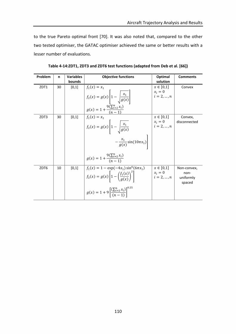
Aircraft Trajectory Analysis and Results
110
to the true Pareto optimal front [70]. It was also noted that, compared to the other
two tested optimiser, the GATAC optimiser achieved the same or better results with a
lesser number of evaluations.
Table 4-14:ZDT1, ZDT3 and ZDT6 test functions (adapted from Deb et al. [66])
Problem n Variablesbounds
Objective functions Optimalsolution
Comments
ZDT1 30 [0,1] ଵ(ݔ) = ଵݔ
ଶ(ݔ) = 1(ݔ) − ඨଵݔ(ݔ)
(ݔ) = 1 +9(∑ ݔ
ୀଶ )
(− 1)
∋ݔ [0,1]=ݔ 0= 2, … ,
Convex
ZDT3 30 [0,1] ଵ(ݔ) = ଵݔ
ଶ(ݔ) = 1(ݔ) − ඨଵݔ(ݔ)
−ଵݔ(ݔ)
sin(10ݔߨଵ)
(ݔ) = 1 +9(∑ ݔ
ୀଶ )
(− 1)
∋ݔ [0,1]=ݔ 0= 2, … ,
Convex,disconnected
ZDT6 10 [0,1] ଵ(ݔ) = 1 − exp(−4ݔଵ) sin(6ݔߨଵ)
ଶ(ݔ) = 1(ݔ) − ቆଵ(ݔ)
(ݔ)ቇ
ଶ
൩
(ݔ) = 1 + 9ቈ(∑ ݔ
ୀଶ )
(− 1)
.ଶହ
∋ݔ [0,1]=ݔ 0= 2, … ,
Non-convex,non-
uniformlyspaced

Aircraft Trajectory Analysis and Results
111
4.5 Model Interaction
Two different framework setups have been used in this study to address two different
optimisation scenarios. The first scenario aims at analysing the trajectory optimisation
with regards to the two objectives, namely fuel and time. The second scenario looks at
the optimisation of the two objectives fuel and NOx.
Figure 4-40 shows the optimisation framework setup and its calculation sequence for
the fuel-time scenario (scenario 1). The optimisation loop consists of the GATAC
optimisation suite which includes the NSGAMO optimiser and the Hermes
aircraft/engine performance model for the flight path calculations. After initialising the
setup with a defined population the optimiser sends particular decision variable values
to aircraft/engine performance model as input to calculate the flight trajectories. The
optimiser then extracts the values for total fuel burned and total flight time from the
calculated output and processes these results by applying genetic operations to
identify suitable values for the next optimisation loop.
Figure 4-40: Scenario 1 - Fuel vs. Time
The same approach as previously described for the fuel-time scenario (scenario 1)
applies to the fuel-NOx scenario (scenario 2). Figure 4-41 shows the framework setup
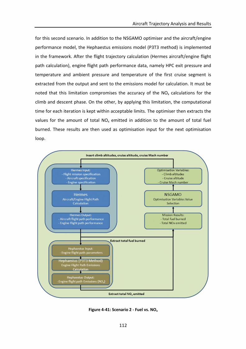
Aircraft Trajectory Analysis and Results
112
for this second scenario. In addition to the NSGAMO optimiser and the aircraft/engine
performance model, the Hephaestus emissions model (P3T3 method) is implemented
in the framework. After the flight trajectory calculation (Hermes aircraft/engine flight
path calculation), engine flight path performance data, namely HPC exit pressure and
temperature and ambient pressure and temperature of the first cruise segment is
extracted from the output and sent to the emissions model for calculation. It must be
noted that this limitation compromises the accuracy of the NOx calculations for the
climb and descent phase. On the other, by applying this limitation, the computational
time for each iteration is kept within acceptable limits. The optimiser then extracts the
values for the amount of total NOx emitted in addition to the amount of total fuel
burned. These results are then used as optimisation input for the next optimisation
loop.
Figure 4-41: Scenario 2 - Fuel vs. NOx

Aircraft Trajectory Analysis and Results
113
5 Aircraft Trajectory Analysis and Results
This chapter summarises the results of the basic trajectory analyses that have been
conducted with the three different CUSA aircraft/engine configurations introduced in
chapters 4.1 and 4.2, and their respective emissions models introduced in chapter 4.3.
The trajectories analysed base on the aircraft trajectory definition made in chapter
3.1.3 and the assumptions and statements defined in chapter 3.2.
5.1 Summary of Analysed Scenarios
For the aircraft trajectory analyses two different flight distances have been selected
which represent typical short-to-medium range flight missions. One 1800 km short
range mission and one 4600 km medium range mission. The three aircraft variants
with their respective engine variants have been used for the individual flight missions
analysed. Each flight mission was completed with the engines in “clean” condition and
with the engines in “degraded” condition. The engine degradation scenario is based on
the assumptions introduced in chapter 4.1.2. The detailed “clean” engine condition
and performance characteristics can be reviewed in chapter 4.1.3 and the detailed
“degraded” engine condition and performance characteristics can be reviewed in
chapter 4.1.4. For meaningful comparisons the duration of the different flight phases
(take-off, climb, cruise, descent) for each flight mission and aircraft/engine
configuration have been kept almost equal. This was achieved by adjusting the engine
power settings for the climb and descent phase. The same adjustments were also
made for each flight mission with the degraded engine configuration. The results are
divided into two main sections: The first section covers the short range mission
analysis in subchapters 5.2, 5.3 and 5.4. The second section covers the medium range
mission analysis in subchapters 5.5, 5.6 and 5.7.
As an introduction to the results section, figure 5-1 and figure 5-2 show and overlay
comparison between the real flight profile introduced in section 3.1.3 and the flight
profile modelled with the Hermes aircraft performance code. The flight profiles, as well
as the trend for fuel flow and EGT are in general agreement with the real flight data.

Aircraft Trajectory Analysis and Results
114
Figure 5-1: Real flight profile and engine FF vs. CUSA-L model
Figure 5-2: Real flight profile and engine EGT vs. CUSA-L model
0
10
20
30
40
50
60
70
80
90
100
0
2000
4000
6000
8000
10000
12000
0 2000 4000 6000 8000 10000
Fue
lflo
win
%o
fm
axim
um
T/O
fue
lflo
w
Alt
itu
de
[m]
Time [seconds]
CUSA-L flight profile Engine #1 FF Flight profile CU2STF-HT FF
0
10
20
30
40
50
60
70
80
90
100
0
2000
4000
6000
8000
10000
12000
0 2000 4000 6000 8000 10000
EGT
in%
of
EGT
red
line
Alt
itu
de
[m]
Time [seconds]
CUSA-L flight profile CU2STF-HT EGT Flight profile Engine #1 EGT

Aircraft Trajectory Analysis and Results
115
5.2 Short Range Flight (Clean Engine)
The first case that is being looked at is the 1800 km short range flight mission with a
clean engine configuration. This means the engine parameters correspond to the
configurations as listed in tables 4-1, 4-2, 4-3 and 4-4 in chapter 4. All three aircraft
variants CUSA-S, CUSA-M and CUSA-L with its respective engine variants CU2STF-LT,
CU2STF-MT and CU2STF-HT performed the same flight mission.
5.2.1 General Description
The default settings of the 1800 km short range mission are summarised in table 5-1.
The payload for each aircraft/engine configuration was set according to the maximum
seating capacity assuming no luggage or other cargo. The values for cruise Mach
number and cruise altitude were kept the same for all three aircraft variants. The
achieved total flight time was also kept almost equal to permit direct comparisons of
the flights.
Table 5-1: Short range mission characteristics (clean engine)
Mission 1800 KM (clean engine)
Aircraft CUSA-S CUSA-M CUSA-L
Engine CU2STF-LT CU2STF-MT CU2STF-HT
Payload [kg] 10664 12900 15910
Cruise Mach number [-] 0.785
Cruise altitude [m] 10668
Flight duration [min] 133.6 133.7 133.9
5.2.2 Results
Figure 5-3 shows the calculated short range mission trajectory for the CUSA-S aircraft
variant and the engine fuel flow trend throughout the flight. It can be seen that the
trajectory flown is general in agreement with the real flight profile referenced in figure
3-6. The engine fuel flow trend at take-off, climb and cruise also follows a comparable
pattern while the values during the descent phase deviate from the real trajectory to a
larger extent. Engine fuel flow values and subsequently TET reach values equivalent to
an engine power setting of about 85%. This is due to the fact that the engine power
settings for the final segments of the descent have been selected to be at their

Aircraft Trajectory Analysis and Results
116
maximum permissible values. Figure 5-4 shows the engine TET trend along the flight
path for the same aircraft variant following a corresponding pattern. It should be
noted that for illustrative purposes the plot in figure 5-3 has been offset by 120
seconds before the take-off point. This allows adequate depiction of the peak fuel
flow. This offset applies to all following plots where time in seconds is plotted on the
horizontal coordinate axis.
Figure 5-3: CUSA-S engine FF variation during flight (1800 km)
0
0.2
0.4
0.6
0.8
1
1.2
1.4
0
2000
4000
6000
8000
10000
12000
0 2000 4000 6000 8000 10000
Fue
lFlo
w[k
g/s]
Alt
itu
de
[m]
Time [seconds]
Flight profile Engine FF

Aircraft Trajectory Analysis and Results
117
Figure 5-4: CUSA-S engine TET variation during flight (1800 km)
The results for the two other aircraft variants CUSA-M and CUSA-L can be found in
appendix A.2.1. They follow the same pattern in all flight phases as the results of the
CUSA-S while differences in peak values for fuel flow and TET can be observed due to
the increased thrust requirements caused by the increased aircraft weight.
5.3 Short Range Flight (Degraded Engine)
The second case analysed is the 1800 km short range flight mission with a degraded
engine configuration. This means the engine parameters correspond to the
configurations as listed in tables 4-5, 4-6 and 4-7 in chapter 4. All three aircraft variants
CUSA-S, CUSA-M and CUSA-L with its respective engine variants CU2STF-LT, CU2STF-
MT and CU2STF-HT performed the same flight mission.
5.3.1 General Description
The default settings of the 1800 km short range mission with the degraded engines are
listed in table 5-2 and follow the structure of the clean engine configuration as
described in chapter 5.2.1.
0
200
400
600
800
1000
1200
1400
1600
0
2000
4000
6000
8000
10000
12000
0 2000 4000 6000 8000 10000
TET
[K]
Alt
itu
de
[m]
Time [seconds]
Flight profile Engine TET Clean
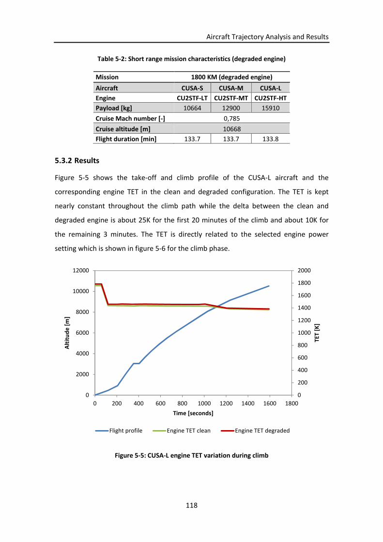
Aircraft Trajectory Analysis and Results
118
Table 5-2: Short range mission characteristics (degraded engine)
Mission 1800 KM (degraded engine)
Aircraft CUSA-S CUSA-M CUSA-L
Engine CU2STF-LT CU2STF-MT CU2STF-HT
Payload [kg] 10664 12900 15910
Cruise Mach number [-] 0,785
Cruise altitude [m] 10668
Flight duration [min] 133.7 133.7 133.8
5.3.2 Results
Figure 5-5 shows the take-off and climb profile of the CUSA-L aircraft and the
corresponding engine TET in the clean and degraded configuration. The TET is kept
nearly constant throughout the climb path while the delta between the clean and
degraded engine is about 25K for the first 20 minutes of the climb and about 10K for
the remaining 3 minutes. The TET is directly related to the selected engine power
setting which is shown in figure 5-6 for the climb phase.
Figure 5-5: CUSA-L engine TET variation during climb
0
200
400
600
800
1000
1200
1400
1600
1800
2000
0
2000
4000
6000
8000
10000
12000
0 200 400 600 800 1000 1200 1400 1600 1800
TET
[K]
Alt
itu
de
[m]
Time [seconds]
Flight profile Engine TET clean Engine TET degraded

Aircraft Trajectory Analysis and Results
119
Figure 5-6: CUSA-L engine power setting and thrust during climb
In this figure, the engine power setting in percent of the maximum take-off thrust is
plotted against the engine thrust for the clean and degraded engine configuration. In
order to maintain an equivalent flight path (equivalent climb duration) for both
configurations, the engine power setting for the degraded engine had to be increased
to maintain the same thrust level for the climb as the clean engine configuration. It can
also be noticed that the engine power setting for the last 3 minutes of the climb was
not changed and remained at 80%. This is also in line with the TET trend shown in
previous figure 5-5. Similar trends for TET and thrust levels can be observed for the
CUSA-M and CUSA- S aircraft variants.
The increase in TET to maintain the thrust level translates into an increase in fuel burn
and consequently causes the NOx emissions to increase. Table 5-3 lists the percentage
increase in fuel burn and NOx emissions throughout the climb for the short range
mission for all three aircraft variants. The CUSA-L aircraft with degraded engines will
burn about 4.7% more fuel compared to the clean engine configuration. At the same
time the NOx emissions will increase by about 5.8%. The CUSA-M aircraft climb
0
20
40
60
80
100
120
140
160
180
200
0%
20%
40%
60%
80%
100%
0 200 400 600 800 1000 1200 1400 1600 1800
Thru
st[k
N]
Engi
ne
po
we
rse
ttin
gin
%o
fm
axim
um
T/O
thru
st
Time [seconds]
Engine power setting clean Engine power setting degraded
Engine thrust clean Engine thrust degraded
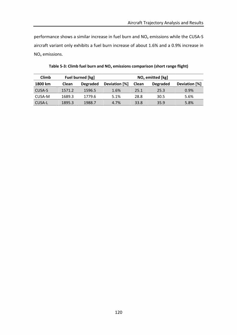
Aircraft Trajectory Analysis and Results
120
performance shows a similar increase in fuel burn and NOx emissions while the CUSA-S
aircraft variant only exhibits a fuel burn increase of about 1.6% and a 0.9% increase in
NOx emissions.
Table 5-3: Climb fuel burn and NOx emissions comparison (short range flight)
Climb Fuel burned [kg] NOx emitted [kg]
1800 km Clean Degraded Deviation [%] Clean Degraded Deviation [%]
CUSA-S 1571.2 1596.5 1.6% 25.1 25.3 0.9%
CUSA-M 1689.3 1779.6 5.1% 28.8 30.5 5.6%
CUSA-L 1895.3 1988.7 4.7% 33.8 35.9 5.8%

Aircraft Trajectory Analysis and Results
121
5.4 Short Range Results Comparison
The results for the short range flight mission scenarios with clean, degraded and
derated engines are listed in tables 5-4, 5-5 and 5-6 for the three different aircraft
variants. For the CUSA-S aircraft the increase in take-off fuel and take-off NOx
emissions due to engine degradation is approximately 3.6%. The increase in main block
fuel is about 1.1% and the increase in total block NOx emissions is about 0.4%. The
introduction of a take-off thrust decrease (derate) reduces the take-off fuel burn by
about 20% and reduces take-off NOx emissions by about 33%. The main block fuel and
total block NOx emissions remain almost equal in the derated scenario. The results are
summarised in in table 5-4 below.
Table 5-4: CUSA-S short range mission results
Mission 1800 KM
Aircraft CUSA-S (CU2STF-LT engine)
Engine condition Clean Degraded Degraded + T/O derate
Take-off fuel [kg] 135.1 140.2 112.6
Take-off NOx [kg] 3.2 3.3 2.2
Main block fuel [kg] 5545.5 5608.0 5609.4
Total block NOx [kg] 70.16 70.47 70.50
Correspondingly, for the CUSA-M aircraft the increase in take-off fuel and take-off NOx
emissions due to engine degradation is approximately 5.6%. The increase in main block
fuel amounts to about 5.3% and the increase in total block NOx emissions is about
5.7%. In this case the take-off thrust derate reduces take-off fuel burn by about 21%
and reduces take-off NOx emissions by nearly 35%. The main block fuel and total block
NOx emissions remain almost constant. The results are summarised in table 5-5 below.
Table 5-5: CUSA-M short range mission results
Mission 1800 KM
Aircraft CUSA-M (CU2STF-MT engine)
Engine condition Clean Degraded Degraded + T/O derate
Take-off fuel [kg] 156.8 166.2 131.1
Take-off NOx [kg] 4.4 4.7 3.0
Main block fuel [kg] 5863.2 6189.4 6191.2
Total block NOx [kg] 79.1 83.9 83.9

Aircraft Trajectory Analysis and Results
122
For the largest aircraft variant CUSA-L the increase in take-off fuel and take-off NOx
emissions due to engine degradation amount to 4.5%. The increase in main block fuel
is about 4.9% and the increase in total block NOx emissions is approximately 5.6%. The
effect of take-off thrust reduction causes the take-off fuel burn to drop by almost 23%
and causes take-off NOx emissions to drop by about 41% compared to a full power
take-off. The results are summarised in table 5-6 below.
Table 5-6: CUSA-L short range mission results
Mission 1800 KM
Aircraft CUSA-L (CU2STF-HT engine)
Engine condition Clean Degraded Degraded + T/O derate
Take-off fuel [kg] 202.9 212.6 164.2
Take-off NOx [kg] 7.6 7.9 4.7
Main block fuel [kg] 6597.6 6934.9 6937.8
Total block NOx [kg] 94.9 100.5 100.6
To highlight the fuel burn characteristic in the course of the total flight distance figures
5-7, 5-8 and 5-9 below compare the total fuel burn of the clean engine configuration
with the degraded engine configuration for each aircraft variant. The negative effect of
degradation accumulates with increasing cruise duration and leads to the
characteristic fuel burned curves which progressively diverge over time. The effect is
hardly noticeable for the CUSA-S aircraft variant but is pronounced for the largest
aircraft variant CUSA-L as illustrated in figure 5-9. This is because the CUSA-S aircraft is
the lightest variant, carries the least payload and thus has the lowest thrust
requirements compared to the CUSA-M and CUSA-L variants. This in turn attenuates
the effect of degradation on the engine performance which is reflected in the total fuel
burn.
For the sake of completeness, TET variations throughout the total flight for the CUSA-L
aircraft with clean and degraded engine configuration are shown in figure 5-10. Similar
trends for TET variations can be observed for the CUSA-M and CUSA- S aircraft variants
and detailed plots are listed in appendix A.2.1.
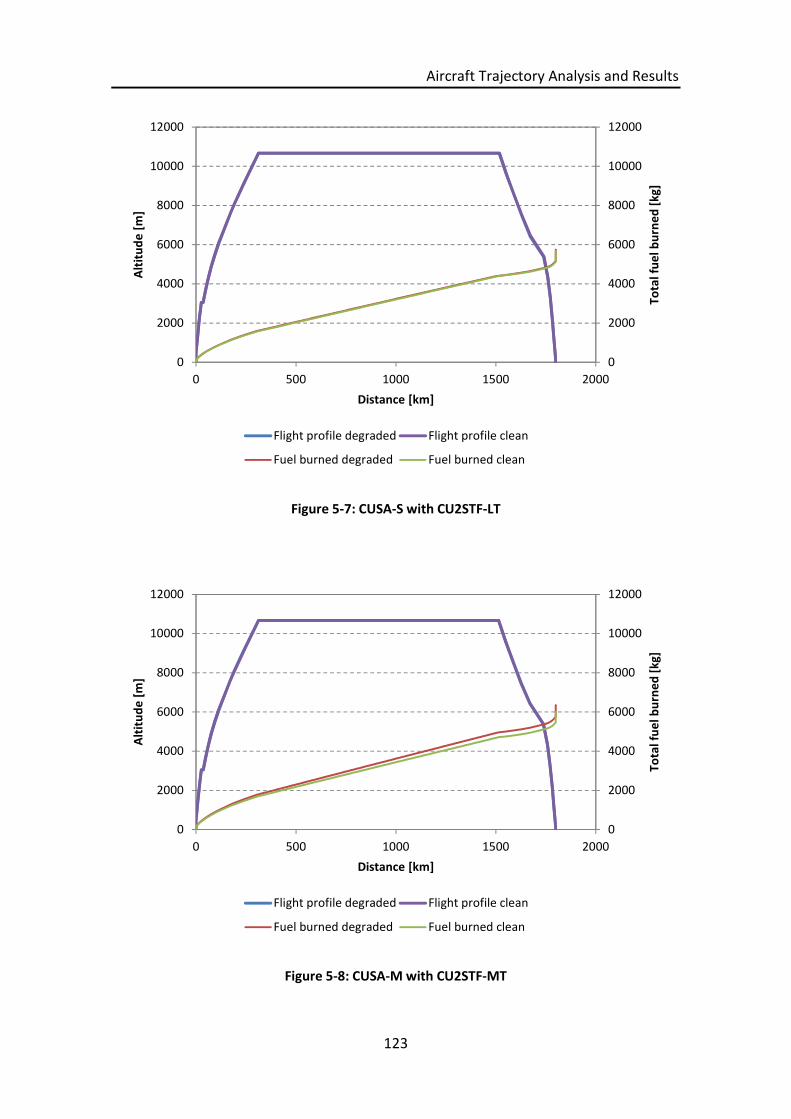
Aircraft Trajectory Analysis and Results
123
Figure 5-7: CUSA-S with CU2STF-LT
Figure 5-8: CUSA-M with CU2STF-MT
0
2000
4000
6000
8000
10000
12000
0
2000
4000
6000
8000
10000
12000
0 500 1000 1500 2000
Tota
lfu
elb
urn
ed
[kg]
Alt
itu
de
[m]
Distance [km]
Flight profile degraded Flight profile clean
Fuel burned degraded Fuel burned clean
0
2000
4000
6000
8000
10000
12000
0
2000
4000
6000
8000
10000
12000
0 500 1000 1500 2000
Tota
lfu
elb
urn
ed
[kg]
Alt
itu
de
[m]
Distance [km]
Flight profile degraded Flight profile clean
Fuel burned degraded Fuel burned clean
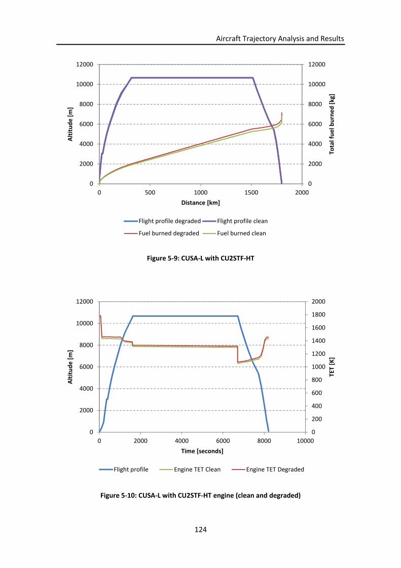
Aircraft Trajectory Analysis and Results
124
Figure 5-9: CUSA-L with CU2STF-HT
Figure 5-10: CUSA-L with CU2STF-HT engine (clean and degraded)
0
2000
4000
6000
8000
10000
12000
0
2000
4000
6000
8000
10000
12000
0 500 1000 1500 2000
Tota
lfu
elb
urn
ed
[kg]
Alt
itu
de
[m]
Distance [km]
Flight profile degraded Flight profile clean
Fuel burned degraded Fuel burned clean
0
200
400
600
800
1000
1200
1400
1600
1800
2000
0
2000
4000
6000
8000
10000
12000
0 2000 4000 6000 8000 10000
TET
[K]
Alt
itu
de
[m]
Time [seconds]
Flight profile Engine TET Clean Engine TET Degraded
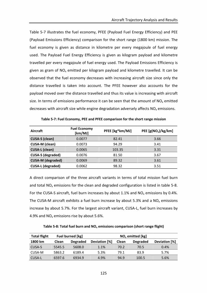
Aircraft Trajectory Analysis and Results
125
Table 5-7 illustrates the fuel economy, PFEE (Payload Fuel Energy Efficiency) and PEE
(Payload Emissions Efficiency) comparison for the short range (1800 km) mission. The
fuel economy is given as distance in kilometre per every megajoule of fuel energy
used. The Payload Fuel Energy Efficiency is given as kilogram payload and kilometre
travelled per every megajoule of fuel energy used. The Payload Emissions Efficiency is
given as gram of NOx emitted per kilogram payload and kilometre travelled. It can be
observed that the fuel economy decreases with increasing aircraft size since only the
distance travelled is taken into account. The PFEE however also accounts for the
payload moved over the distance travelled and thus its value is increasing with aircraft
size. In terms of emissions performance it can be seen that the amount of NOx emitted
decreases with aircraft size while engine degradation adversely affects NOx emissions.
Table 5-7: Fuel Economy, PEE and PFEE comparison for the short range mission
AircraftFuel Economy
[km/MJ]PFEE [kg*km/MJ] PEE [g(NOx)/kg/km]
CUSA-S (clean) 0.0077 82.41 3.66
CUSA-M (clean) 0.0073 94.29 3.41
CUSA-L (clean) 0.0065 103.35 3.31
CUSA-S (degraded) 0.0076 81.50 3.67
CUSA-M (degraded) 0.0069 89.32 3.61
CUSA-L (degraded) 0.0062 98.32 3.51
A direct comparison of the three aircraft variants in terms of total mission fuel burn
and total NOx emissions for the clean and degraded configuration is listed in table 5-8.
For the CUSA-S aircraft, fuel burn increases by about 1.1% and NOx emissions by 0.4%.
The CUSA-M aircraft exhibits a fuel burn increase by about 5.3% and a NOx emissions
increase by about 5.7%. For the largest aircraft variant, CUSA-L, fuel burn increases by
4.9% and NOx emissions rise by about 5.6%.
Table 5-8: Total fuel burn and NOx emissions comparison (short range flight)
Total flight Fuel burned [kg] NOx emitted [kg]
1800 km Clean Degraded Deviation [%] Clean Degraded Deviation [%]
CUSA-S 5545.5 5608.0 1.1% 70.2 70.5 0.4%
CUSA-M 5863.2 6189.4 5.3% 79.1 83.9 5.7%
CUSA-L 6597.6 6934.9 4.9% 94.9 100.5 5.6%

Aircraft Trajectory Analysis and Results
126
Furthermore, an overview of the short mission take-off performance characteristics of
each aircraft variant is shown in figures 5-11, 5-12 and 5-13. Figure 5-11 shows the
take-off distance in kilometres required by each aircraft variant. There is only a
negligible difference in take-off distance observed between the clean and degraded
configuration, while the engine take-off derate shows to have a significant effect on
the distance travelled. The take-off distance in this case then increases for all aircraft
variants by about 12%.
Figure 5-11: T/O distance comparison Figure 5-12: T/O fuel burn comparison
Figure 5-13: T/O NOx emissions comparison
00.5
11.5
22.5
33.5
44.5
CUSA-S CUSA-M CUSA-L
T/O
Dis
tan
ce[k
m]
clean engine
degraded engine
degraded engine derated
0
50
100
150
200
250
CUSA-S CUSA-M CUSA-L
Fue
lbu
rne
d[k
g]
clean engine
degraded engine
degraded engine derated
0
2
4
6
8
10
CUSA-S CUSA-M CUSA-L
NO
xe
mis
sio
ns[
kg]
clean engine
degraded engine
degraded engine derated
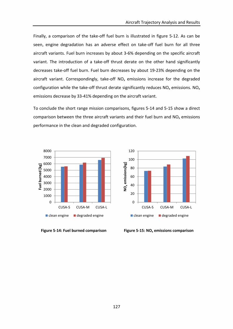
Aircraft Trajectory Analysis and Results
127
Finally, a comparison of the take-off fuel burn is illustrated in figure 5-12. As can be
seen, engine degradation has an adverse effect on take-off fuel burn for all three
aircraft variants. Fuel burn increases by about 3-6% depending on the specific aircraft
variant. The introduction of a take-off thrust derate on the other hand significantly
decreases take-off fuel burn. Fuel burn decreases by about 19-23% depending on the
aircraft variant. Correspondingly, take-off NOx emissions increase for the degraded
configuration while the take-off thrust derate significantly reduces NOx emissions. NOx
emissions decrease by 33-41% depending on the aircraft variant.
To conclude the short range mission comparisons, figures 5-14 and 5-15 show a direct
comparison between the three aircraft variants and their fuel burn and NOx emissions
performance in the clean and degraded configuration.
Figure 5-14: Fuel burned comparison Figure 5-15: NOx emissions comparison
0
1000
2000
3000
4000
5000
6000
7000
8000
CUSA-S CUSA-M CUSA-L
Fue
lbu
rne
d[k
g]
clean engine degraded engine
0
20
40
60
80
100
120
CUSA-S CUSA-M CUSA-L
NO
xe
mis
sio
ns[
kg]
clean engine degraded engine

Aircraft Trajectory Analysis and Results
128
5.5 Medium Range Flight (Clean Engine)
The third case as part of this analysis is the 4600 km medium range flight mission with
a clean engine configuration. Again, all three aircraft variants CUSA-S, CUSA-M and
CUSA-L with its respective engine variants CU2STF-LT, CU2STF-MT and CU2STF-HT
performed the same flight mission.
5.5.1 General Description
A brief listing of the default settings of the 4600 km medium range mission with the
clean engines is provided in table 5-8. It follows the same structure as the previous two
scenarios.
Table 5-9: Medium range mission characteristics (clean engine)
Mission 4600 km (clean engine)
Aircraft CUSA-S CUSA-M CUSA-L
Payload [kg] 10664 12900 15910
Cruise Mach number [-] 0.785
Cruise altitude [m] 10668
Flight duration [min] 331.6 331.6 331.9
5.5.2 Results
Figure 5-14 shows the calculated medium range mission trajectory for the CUSA-L
aircraft variant and the engine fuel flow trend throughout the flight. It can be seen that
the trajectory flown follows the same basic trend as the short range mission profile
shown in figure 5-1. The engine fuel flow trend at take-off, climb and cruise also
follows a comparable pattern. Again, engine fuel flow values and subsequently TET
during descent reach values equivalent to an engine power setting of about 85%. This
is due to the fact that the engine power settings for the final segments of the descent
have been selected to be at their maximum permissible values. Figure 5-2 shows the
engine TET trend along the flight path for the same aircraft variant following a
corresponding pattern.

Aircraft Trajectory Analysis and Results
129
Figure 5-16: CUSA-L engine FF variation during flight (4600 km)
Figure 5-17: CUSA-L engine TET variation during flight (4600 km)
0
0.2
0.4
0.6
0.8
1
1.2
1.4
1.6
0
2000
4000
6000
8000
10000
12000
0 2000 4000 6000 8000 10000 12000 14000 16000 18000 20000 22000
Fue
lFlo
w[k
g/s]
Alt
itu
de
[m]
Time [seconds]
Flight profile Engine FF
0
200
400
600
800
1000
1200
1400
1600
0
2000
4000
6000
8000
10000
12000
0 2000 4000 6000 8000 10000 12000 14000 16000 18000 20000 22000
TET
[K]
Alt
itu
de
[m]
Time [seconds]
Flight profile Engine TET Clean

Aircraft Trajectory Analysis and Results
130
The results for the two other aircraft variants CUSA-S and CUSA-M can be found in
appendix A.3.1. They follow the same pattern in all flight phases as the results of the
CUSA-L while differences in peak values for fuel flow and TET can be observed due to
the increased thrust requirements caused by the increased aircraft weight and the
increase in initial fuel weight due to the longer mission range.
5.6 Medium Range Flight (Degraded Engine)
The fourth case evaluated is the 4600 km medium range flight mission with a degraded
engine configuration. Again, all three aircraft variants CUSA-S, CUSA-M and CUSA-L
with its respective engine variants CU2STF-LT, CU2STF-MT and CU2STF-HT performed
the same flight mission.
5.6.1 General Description
The default settings of the 4600 km short range mission with the degraded engines are
listed in table 5-10 and follow the structure of the clean engine configuration as
described in chapter 5.5.1.
Table 5-10: Medium range mission characteristics (degraded engine)
Mission 4600 km (degraded engine)
Aircraft CUSA-S CUSA-M CUSA-L
Payload [kg] 10664 12900 15910
Cruise Mach number [-] 0.785
Cruise altitude [m] 10668
Flight duration [min] 331.5 331.5 332.0
5.6.2 Results
Figure 5-18 shows the take-off and climb profile of the CUSA-M aircraft and the
corresponding engine TET in the clean and degraded configuration. The TET is kept
nearly constant for the first part of the climb while the TET is then reduced during the
second part of the climb. The difference in TET between the clean and degraded
engine is about 35K for the first 12 minutes of the climb and about 20K for the
remaining 11 minutes. The TET is directly related to the selected engine power setting
which is shown in figure 5-19 for the climb phase.

Aircraft Trajectory Analysis and Results
131
Figure 5-18: CUSA-M engine TET variation during climb
Figure 5-19: CUSA-M engine power setting and thrust during climb
0
200
400
600
800
1000
1200
1400
1600
1800
0
2000
4000
6000
8000
10000
12000
0 200 400 600 800 1000 1200 1400 1600 1800
TET
[K]
Alt
itu
de
[m]
Time [seconds]
Flight profile Engine TET clean Engine TET degraded
0
20
40
60
80
100
120
140
160
180
200
0%
20%
40%
60%
80%
100%
0 200 400 600 800 1000 1200 1400 1600 1800
Thru
st[k
N]
Engi
ne
po
we
rse
ttin
gin
%o
fm
axim
um
T/O
thru
st
Time [seconds]
Engine power setting clean Engine power setting degraded
Engine thrust clean Engine thrust degraded
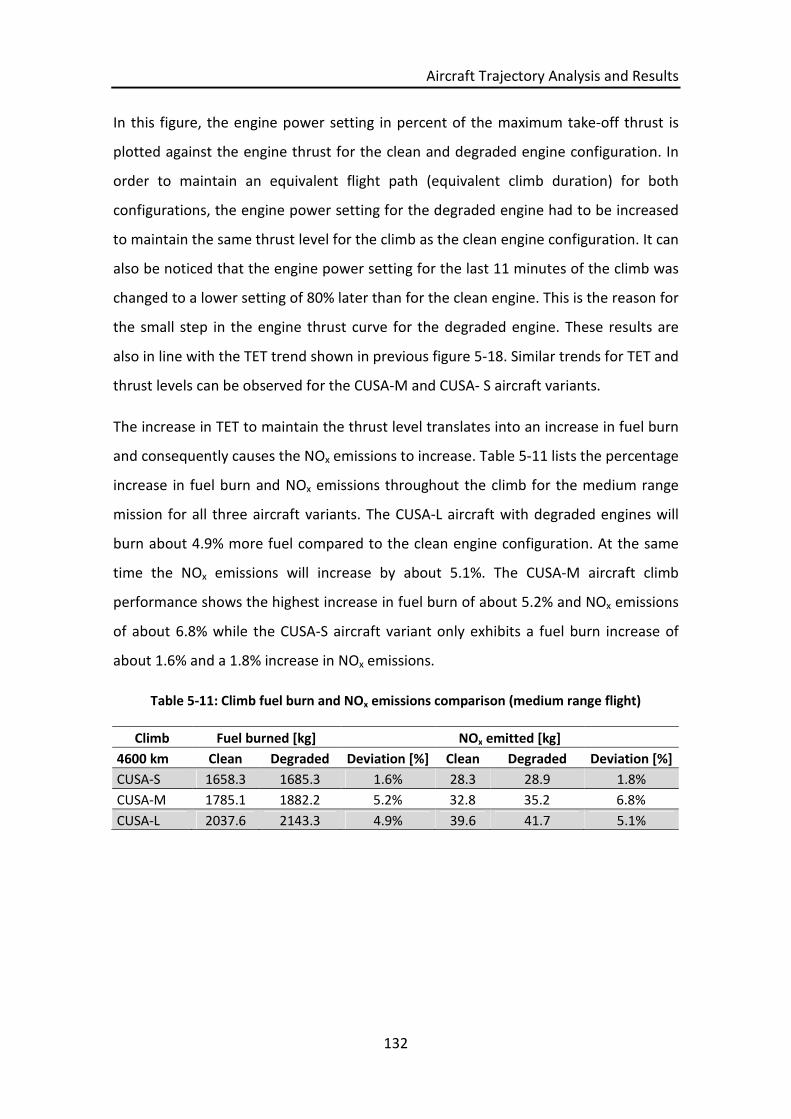
Aircraft Trajectory Analysis and Results
132
In this figure, the engine power setting in percent of the maximum take-off thrust is
plotted against the engine thrust for the clean and degraded engine configuration. In
order to maintain an equivalent flight path (equivalent climb duration) for both
configurations, the engine power setting for the degraded engine had to be increased
to maintain the same thrust level for the climb as the clean engine configuration. It can
also be noticed that the engine power setting for the last 11 minutes of the climb was
changed to a lower setting of 80% later than for the clean engine. This is the reason for
the small step in the engine thrust curve for the degraded engine. These results are
also in line with the TET trend shown in previous figure 5-18. Similar trends for TET and
thrust levels can be observed for the CUSA-M and CUSA- S aircraft variants.
The increase in TET to maintain the thrust level translates into an increase in fuel burn
and consequently causes the NOx emissions to increase. Table 5-11 lists the percentage
increase in fuel burn and NOx emissions throughout the climb for the medium range
mission for all three aircraft variants. The CUSA-L aircraft with degraded engines will
burn about 4.9% more fuel compared to the clean engine configuration. At the same
time the NOx emissions will increase by about 5.1%. The CUSA-M aircraft climb
performance shows the highest increase in fuel burn of about 5.2% and NOx emissions
of about 6.8% while the CUSA-S aircraft variant only exhibits a fuel burn increase of
about 1.6% and a 1.8% increase in NOx emissions.
Table 5-11: Climb fuel burn and NOx emissions comparison (medium range flight)
Climb Fuel burned [kg] NOx emitted [kg]
4600 km Clean Degraded Deviation [%] Clean Degraded Deviation [%]
CUSA-S 1658.3 1685.3 1.6% 28.3 28.9 1.8%
CUSA-M 1785.1 1882.2 5.2% 32.8 35.2 6.8%
CUSA-L 2037.6 2143.3 4.9% 39.6 41.7 5.1%
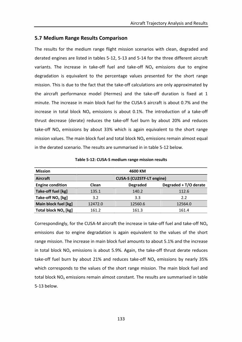
Aircraft Trajectory Analysis and Results
133
5.7 Medium Range Results Comparison
The results for the medium range flight mission scenarios with clean, degraded and
derated engines are listed in tables 5-12, 5-13 and 5-14 for the three different aircraft
variants. The increase in take-off fuel and take-off NOx emissions due to engine
degradation is equivalent to the percentage values presented for the short range
mission. This is due to the fact that the take-off calculations are only approximated by
the aircraft performance model (Hermes) and the take-off duration is fixed at 1
minute. The increase in main block fuel for the CUSA-S aircraft is about 0.7% and the
increase in total block NOx emissions is about 0.1%. The introduction of a take-off
thrust decrease (derate) reduces the take-off fuel burn by about 20% and reduces
take-off NOx emissions by about 33% which is again equivalent to the short range
mission values. The main block fuel and total block NOx emissions remain almost equal
in the derated scenario. The results are summarised in in table 5-12 below.
Table 5-12: CUSA-S medium range mission results
Mission 4600 KM
Aircraft CUSA-S (CU2STF-LT engine)
Engine condition Clean Degraded Degraded + T/O derate
Take-off fuel [kg] 135.1 140.2 112.6
Take-off NOx [kg] 3.2 3.3 2.2
Main block fuel [kg] 12472.0 12560.6 12564.0
Total block NOx [kg] 161.2 161.3 161.4
Correspondingly, for the CUSA-M aircraft the increase in take-off fuel and take-off NOx
emissions due to engine degradation is again equivalent to the values of the short
range mission. The increase in main block fuel amounts to about 5.1% and the increase
in total block NOx emissions is about 5.9%. Again, the take-off thrust derate reduces
take-off fuel burn by about 21% and reduces take-off NOx emissions by nearly 35%
which corresponds to the values of the short range mission. The main block fuel and
total block NOx emissions remain almost constant. The results are summarised in table
5-13 below.

Aircraft Trajectory Analysis and Results
134
Table 5-13: CUSA-M medium range mission results
Mission 4600 KM
Aircraft CUSA-M (CU2STF-MT engine)
Engine condition Clean Degraded Degraded + T/O derate
Take-off fuel [kg] 156.8 166.2 131.1
Take-off NOx [kg] 4.4 4.7 3.0
Main block fuel [kg] 13288.1 14007.5 14012.0
Total block NOx [kg] 183.6 195.0 195.1
For the largest aircraft variant CUSA-L the increase in take-off fuel and take-off NOx
emissions corresponds to the short range mission values. The increase in main block
fuel is about 4.9% and the increase in total block NOx emissions is approximately 5.6%.
The effect of take-off thrust reduction causes the take-off fuel burn to drop by almost
23% and causes take-off NOx emissions to drop by about 41% compared to a full power
take-off, which again equals the values of the short range mission. The results are
summarised in table 5-14 below.
Table 5-14: CUSA-L medium range mission results
Mission 4600 KM
Aircraft CUSA-L (CU2STF-HT engine)
Engine condition Clean Degraded Degraded + T/O derate
Take-off fuel [kg] 202.9 212.6 164.2
Take-off NOx [kg] 7.6 7.9 4.7
Main block fuel [kg] 15067.0 15848.2 15855.9
Total block NOx [kg] 221.5 234.7 234.9
To highlight the fuel burn characteristic in the course of the total flight distance figures
5-20, 5-21 and 5-22 compare the total fuel burn of the clean engine configuration with
the degraded engine configuration for each aircraft variant. Similar to the results of the
range mission, the negative effect of degradation accumulates with increasing cruise
duration and leads to the characteristic fuel burned curves which progressively diverge
over time. The effect is again hardly noticeable for the CUSA-S aircraft variant but is
pronounced for the largest aircraft variant CUSA-L as illustrated in figure 5-22. This is
because the CUSA-S aircraft is the lightest variant, carries the least payload and thus
has the lowest thrust requirements compared to the CUSA-M and CUSA-L variants.

Aircraft Trajectory Analysis and Results
135
This in turn attenuates the effect of degradation on the engine performance which is
reflected in the total fuel burn. In fact, due to the increased range, the effect of
degradation on total mission fuel burn becomes less severe since relative time spent in
the climb phase, where degradation has a more pronounced effect, becomes less.
For the sake of completeness, TET variations throughout the total flight for the CUSA-
M aircraft with clean and degraded engine configuration are shown in figure 5-23.
Similar trends for TET variations can be observed for the CUSA-M and CUSA- S aircraft
variants and detailed plots are listed in appendix A.3.1.
Figure 5-20: CUSA-S with CU2STF-LT
0
2000
4000
6000
8000
10000
12000
14000
16000
18000
0
2000
4000
6000
8000
10000
12000
0 1000 2000 3000 4000 5000
Tota
lfu
elb
urn
ed
[kg]
Alt
itu
de
[m]
Distance [km]
Flight profile degraded Flight profile clean
Fuel burn degraded Fuel burn clean
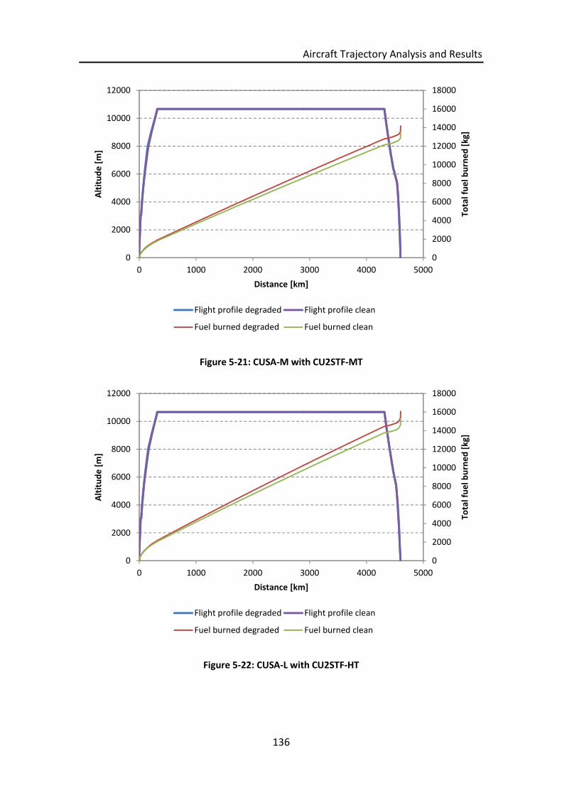
Aircraft Trajectory Analysis and Results
136
Figure 5-21: CUSA-M with CU2STF-MT
Figure 5-22: CUSA-L with CU2STF-HT
0
2000
4000
6000
8000
10000
12000
14000
16000
18000
0
2000
4000
6000
8000
10000
12000
0 1000 2000 3000 4000 5000
Tota
lfu
elb
urn
ed
[kg]
Alt
itu
de
[m]
Distance [km]
Flight profile degraded Flight profile clean
Fuel burned degraded Fuel burned clean
0
2000
4000
6000
8000
10000
12000
14000
16000
18000
0
2000
4000
6000
8000
10000
12000
0 1000 2000 3000 4000 5000
Tota
lfu
elb
urn
ed
[kg]
Alt
itu
de
[m]
Distance [km]
Flight profile degraded Flight profile clean
Fuel burned degraded Fuel burned clean

Aircraft Trajectory Analysis and Results
137
Figure 5-23: CUSA-M with CU2STF-MT engine (clean and degraded)
Table 5-15 illustrates the fuel economy, PFEE (Payload Fuel Energy Efficiency) and PEE
(Payload Emissions Efficiency) comparison for the short range (4600 km) mission. The
fuel economy is given as distance in kilometre per every megajoule of fuel energy
used. The Payload Fuel Energy Efficiency is given as kilogram payload and kilometre
travelled per every megajoule of fuel energy used. The Payload Emissions Efficiency is
given as gram of NOx emitted per kilogram payload and kilometre travelled. Similar to
the short range mission results, it can be observed that the fuel economy is decreasing
with increasing aircraft size since only the distance travelled is taken into account. The
PFEE however also accounts for the payload moved over the distance travelled and
thus its value is increasing with aircraft size. In terms of emissions performance it can
be seen that the amount of NOx emitted decreases only for the CUSA-M and CUSA-L
aircraft variant. When comparing the absolute PEE values with the results of the short
range mission it can be noted that the amount of NOx emissions per kilogram and
kilometre declines.
0
200
400
600
800
1000
1200
1400
1600
1800
0
2000
4000
6000
8000
10000
12000
0 2000 4000 6000 8000 10000 12000 14000 16000 18000 20000 22000
TET
[K]
Alt
itu
de
[m]
Time [seconds]
Flight profile Engine TET Clean Engine TET Degraded

Aircraft Trajectory Analysis and Results
138
Table 5-15: Fuel Economy, PEE and PFEE comparison for the medium range mission
AircraftFuel Economy
[km/MJ]PFEE [kg*km/MJ] PEE [g NOx/kg/km]
CUSA-S (clean) 0.0088 93.65 3.29
CUSA-M (clean) 0.0082 106.32 3.09
CUSA-L (clean) 0.0073 115.65 3.03
CUSA-S (degraded) 0.0087 92.99 3.29
CUSA-M (degraded) 0.0078 100.86 3.29
CUSA-L (degraded) 0.0069 109.95 3.21
A direct comparison of the three aircraft variants in terms of total mission fuel burn
and total NOx emissions for the clean and degraded configuration is listed in table 5-
16. For the CUSA-S aircraft, fuel burn increases by about 0.7% and NOx emissions by
0.1%. The CUSA-M aircraft exhibits a fuel burn increase by about 5.1% and a NOx
emissions increase by about 5.9%. For the largest aircraft variant, CUSA-L, fuel burn
increases by 4.9% and NOx emissions rise by about 5.6%.
Table 5-16: Fuel burn and NOx emissions comparison (medium range flight)
Total flight Fuel burned [kg] NOx emitted [kg]
4600 km Clean Degraded Deviation [%] Clean Degraded Deviation [%]
CUSA-S 12472.0 12560.6 0.7% 161.2 161.3 0.1%
CUSA-M 13288.1 14007.5 5.1% 183.6 195.0 5.8%
CUSA-L 15067.0 15848.2 4.9% 221.5 234.7 5.6%
Furthermore, an overview of the medium mission take-off performance characteristics
of each aircraft variant is shown in figures 5-24, 5-25 and 5-26. Figure 5-24 shows the
take-off distance in kilometres required by each aircraft variant. The take-off distance
remains almost equal when compared between the clean and degraded configuration,
while the engine take-off derate shows to have a significant effect on the distance
travelled. The take-off distance in this case then increases for all aircraft variants by
about 14%.

Aircraft Trajectory Analysis and Results
139
Figure 5-24: T/O distance comparison Figure 5-25: T/O fuel burn comparison
Figure 5-26: T/O NOx emissions comparison
Finally, a comparison of the take-off fuel burn is illustrated in figure 5-25. As can be
seen, engine degradation has an adverse effect on take-off fuel burn for all three
aircraft variants. Fuel burn increases by about 3-6% depending on the specific aircraft
variant. The introduction of a take-off thrust derate on the other hand significantly
decreases take-off fuel burn. Fuel burn decreases by about 19-23% depending on the
aircraft variant. Correspondingly, take-off NOx emissions increase for the degraded
configuration while the take-off thrust derate significantly reduces NOx emissions. NOx
emissions decrease by 33-41% depending on the aircraft variant.
00.5
11.5
22.5
33.5
44.5
CUSA-S CUSA-M CUSA-L
T/O
Dis
tan
ce[k
m]
clean engine
degraded engine
degraded engine derated
0
50
100
150
200
250
CUSA-S CUSA-M CUSA-L
Fue
lbu
rne
d[k
g]
clean engine
degraded engine
degraded engine derated
0
2
4
6
8
10
CUSA-S CUSA-M CUSA-L
NO
xe
mis
sio
ns[
kg]
clean engine
degraded engine
degraded engine derated

Aircraft Trajectory Analysis and Results
140
To conclude the medium range mission comparisons, figures 5-27 and 5-28 show a
direct comparison between the three aircraft variants and their fuel burn and NOx
emissions performance in the clean and degraded configuration.
Figure 5-27: Fuel burned comparison Figure 5-28: NOx emissions comparison
0
2000
4000
6000
8000
10000
12000
14000
16000
18000
CUSA-S CUSA-M CUSA-L
Fue
lbu
rne
d[k
g]
clean engine degraded engine
0
50
100
150
200
250
CUSA-S CUSA-M CUSA-LN
Ox
em
issi
on
s[kg
]
clean engine degraded engine

Trajectory Optimisation Studies and Results
141
6 Trajectory Optimisation Studies and Results
This chapter addresses the two-objective trajectory optimisation study which is based
on the GATAC optimisation framework introduced in section 4.4. Two flight missions
(short and medium range) of the CUSA-M aircraft have been considered for
optimisation which base on the aircraft trajectories analysed in the previous chapter 5
and the assumptions and statements defined in section 3.2. The optimisation process
and the framework are setup as described in section 4.5.
6.1 Summary of Case Studies
Two different scenarios have been analysed for each mission: Fuel vs. time and fuel vs.
NOx. Both scenarios aim at identifying flight mission trade-offs between total fuel
burned and total flight time, and between total fuel burned and total NOx emissions
respectively. The optimisation variables, which represent explicit constraints of the
optimisation problem, and their applicable boundaries, are listed in table 6-1.
Table 6-1: GATAC decision variables for climb and cruise
Decision variable Lower bound Upper bound
Altitude 1 [m] 457 1125
Altitude 2 [m] 1126 1792
Altitude 3 [m] 1793 2459
Altitude 4 [m] 2460 3126
Altitude 5 [m] 3127 3128
Altitude 6 [m] 3129 3130
Altitude 7 [m] 3131 3795
Altitude 8 [m] 3796 4462
Altitude 9 [m] 4463 5129
Altitude 10 [m] 5130 5796
Altitude 11 [m] 5797 6463
Altitude 12 [m] 6464 7130
Altitude 13 [m] 7131 7797
Altitude 14 [m] 7798 8464
Altitude 15 [m] 8465 9131
Altitude 16 [m] 9132 9999
Cruise altitude [m] 10059 11000

Trajectory Optimisation Studies and Results
142
The array of each climb altitude has been set at 666 m from altitude 1 to altitude 15.
For altitude 16 the array has been set at 867 m. The array of the final cruise altitude
has been set between 10059 m and 11000 m. The 60 m gap between the last climb
altitude and the minimum cruise altitude results from the adaption of the climb profile
from the studies carried out in chapter 5. An additional variable (altitude 17) had been
implemented into the optimisation framework but is not taken into account during the
trajectory calculations. The maximum cruise altitude has been limited to 11000 m to
stay well below critical altitudes at which outside temperatures and thus the speed of
sound decrease to values low enough to affect subsonic aircraft operability. In
addition, the off-design performance of engine models adapted for this study has only
been validated up to an altitude of 11000 m. Furthermore, three different Mach
number cases have been analysed (0.75, 0.80 and 0.85). Engine performance data has
then been created once for each Mach number case as input for the optimiser. This
setup ensures that feasible trajectories with a constant altitude increase are computed
by the optimiser and it also takes into account the constraints of the utilised
optimisation framework.
For the purpose of brevity, in this chapter, flights that were optimised to minimise the
total amount of fuel burned for a given mission are denominated as minimum fuel
flight and, correspondingly, flights that were optimised to minimise the total flight
time of a given mission are denominated as minimum time flight.
6.2 Short Range Multi Objective Optimisation
The first scenario addresses the optimisation of the short range mission with regards
to the two objectives, (1) total fuel burned and (2) total flight time. The second
scenario then addresses the optimisation of the short range mission with regards to (1)
total fuel burned and (2) total NOx emissions generated.
6.2.1 General Description
The first case aims to optimise a short range (1800 km) aircraft mission in order to
minimise total fuel burned or to minimise total flight time. This is achieved by altering

Trajectory Optimisation Studies and Results
143
the aircraft climb profile (altitudes of 16 climb segments) and cruise altitude in such a
way that either total fuel burned or total flight time becomes minimum. The
optimisation is carried out three times at three different fixed Mach numbers (0.75,
0.80 and 0.85).
The second case then looks at the optimisation of the short range mission in order to
minimise fuel burned or to minimise NOx emissions. It uses the same methodology as
has been deployed on the fuel vs. time optimisation case but only two different Mach
numbers (0.75 and 0.85) are considered.
6.2.2 Fuel vs. Time Optimisation Results
Figure 6-1 shows the Pareto fronts for the short range mission of the CUSA-M aircraft
performing the 1800 km mission at varying climb altitudes (altitude 1 to altitude 16 as
listed in table 6-1), varying cruise altitudes (10059 m - 11000 m) and 3 different cruise
Mach numbers (0.75, 0.80 and 0.85) and illustrates the influence on flight time and
fuel burned. Each Pareto front comprises a set of non-dominated solutions which
represents a trade-off between flight time and fuel burned. The shortest mission flight
time (124.2 min) requires flying at the lowest possible altitude (10059 m) with the
highest possible Mach number of 0.85. The lowest mission fuel burn (5587 kg) requires
flying at the highest possible altitude (11000 m) with the lowest possible Mach number
of 0.75. Increasing Mach number from 0.75 by 0.05 increments up to 0.85 reduces
flight time by about 6 minutes per each increment. Figure 6-2 illustrates the
corresponding flight profiles (climb, cruise and descent) and fuel burn curves for the
minimum time and minimum fuel case. The solid green profile represents the
minimum fuel trajectory and the dashed green line shows the corresponding fuel burn
accumulation along the flight. The minimum time trajectory is plotted in red lines
accordingly. It can be seen that the minimum fuel flight reaches its final cruise altitude
after having travelled a shorter range than the minimum fuel flight. Since the final
cruise altitude of the minimum fuel flight is higher than the cruise altitude of the
minimum time flight, a higher climb gradient is recognised. Both flight profiles shown
in figure 6-2 contain the information about the decision variables used by the GATAC

Trajectory Optimisation Studies and Results
144
optimiser. The aircraft performance model (Hermes) uses the climb altitudes as inputs
to calculate the individual range of the climb segments up to the cruise altitude. Since
the distance travelled per segment may vary a listing of individual climb altitudes is not
shown.
Figure 6-1: Fuel vs. time Pareto fronts for short range mission
Table 6-2 summarises the optimisation objective values (flight time and fuel burned)
for the two extreme cases (minimum flight time and minimum fuel burned) as well as
the resulting flight trajectory key performance points. In addition, it provides a
comparison of those performance points to a reference flight which is based on the
“non-optimised” trajectory analysed in previous chapter 5. To allow for a meaningful
comparison, the power settings during all climb segments have been adjusted to
maximum climb power settings as opposed to the predefined settings used in the
“non-optimised” trajectory. Flight time is reduced by 6.7% for the minimum time flight
at the expense of 4.4% increase in fuel burn. Fuel burned is reduced by 3.0% for the
minimum fuel flight at the expense of a 4.0% increase in flight time. Both flights
considered in relation to the reference flight. Moreover, the cruise duration for the
122
124
126
128
130
132
134
136
138
140
5550 5600 5650 5700 5750 5800 5850 5900 5950 6000 6050
Flig
ht
tim
e[m
in]
Fuel burned [kg]
Mach 0.75 Mach 0.80 Mach 0.85

Trajectory Optimisation Studies and Results
145
minimum time flight decreased by 7.8% and increased by 7.0% for the minimum fuel
flight. Fuel consumption value till TOC for the minimum time flight increased by 1.2%
while the same value decreased by 18.0% for the minimum fuel flight.
Table 6-2: Optimisation extreme solutions compared to reference flight (1800 km)
CUSA-M1800 km
Referenceflight
Minimumtime flight
Delta [%]Minimumfuel flight
Delta [%]
Fuel burned [kg] 5760.4 6014.7 4.4 5586.4 -3.0
Flight time [min] 133.1 124.2 -6.7 138.4 3.9
Cruise altitude [m] 10668.0 10059.0 - 10999.4 -
Cruise Mach [-] 0.785 0.850 - 0.750 -
Cruise duration [min] 96.7 89.2 -7.8 103.5 7.0
Fuel till TOC [kg] 1019.1 1031.0 1.2 836.3 -17.9
Fuel for cruise [kg] 3433.3 3691.6 7.5 3412.5 -0.6
Figure 6-2: CUSA-M short range flight profile comparison (fuel vs. time)
0
1000
2000
3000
4000
5000
6000
7000
0
2000
4000
6000
8000
10000
12000
0 500 1000 1500 2000
Fue
lbu
rne
d[k
g]
Alt
itu
de
[m]
Distance [km]
Flight profile (minimum fuel) Flight profile (minimum time)
Fuel burned (minimum fuel) Fuel burned (minimum time)

Trajectory Optimisation Studies and Results
146
In order for the optimiser to minimise either flight time or fuel burned, it selects the
most suitable combination of decision variables (climb altitudes and cruise altitude)
yielding a flight trajectory with an improvement in flight time or fuel burned. Since the
bounds of the climb altitudes (altitude 1 to altitude 15) are kept relatively narrow and
due to the fact that the individual calculated climb ranges vary to allow for reasonable
climb profiles, the optimiser emphasises on the last climb altitude and the cruise
altitude as crucial decision variables. The aircraft cruise altitude has a direct influence
on the True Air Speed. At constant flight Mach number TAS increases with decreasing
altitude due to an increase in speed of sound caused by an increment in ambient
temperature (TAS = M · a). This approach is illustrated in figure 6-1 where cruise
altitude decreases from left to right for each of the three constant Mach number
Pareto fronts. On the other hand, at constant altitude (constant speed of sound), an
increase in flight Mach number causes an increase in TAS in the same manner. This
approach is represented in figure 6-1 by each Mach number specific Pareto front which
indicates a step change in flight time. Figure 6-3 illustrates the TAS variation during the
climb profile and at initial cruise conditions. For the minimum fuel flight (solid orange
line), the cruise Mach number (0.75) is reached earlier during the climb (at a lower
altitude) and thus, TAS slightly decreases throughout the remaining climb as altitude
still increases. The same process occurs for the minimum time flight (solid green line)
only at a later point of the climb since the final cruise Mach number is higher (0.85).

Trajectory Optimisation Studies and Results
147
Figure 6-3: CUSA-M True Air Speed (TAS) variation during climb (short range)
Figure 6-4 furthermore shows that the initial climb phase for both trajectories is very
similar due to the narrow bounds of the decision variables (climb altitudes) to be
selected by the optimiser and the way the aircraft performance model (Hermes)
computes a feasible climb profile. Following the TAS trends presented in figure 6-3,
figure 6-4 illustrates the corresponding engine thrust trend of the two extreme climb
profiles (minimum time and minimum fuel). Both figures also show a speed
discontinuity (step change) during the climb phase which is related to a fixed increase
in EAS from 250 to 320 knots as setup in the aircraft performance model.
In order to further highlight the results of the optimiser for the fuel versus time study,
table 6-4 lists a comparison of three different short range flights selected from the
three Pareto fronts (refer to figure 6-1) assuming a constant mission fuel burn value. It
can be noted that overall flight time decreases with an increase in Mach number and
an increase in cruise altitude. This means, for a fixed value of fuel burned and
depending on the determinative objective of the individual flight mission, cruise
altitude and cruise Mach number can be adjusted as suggested to reach this objective.
0
50
100
150
200
250
300
0
2000
4000
6000
8000
10000
12000
0 50 100 150 200 250 300
TAS
[m/s
]
Alt
itu
de
[m]
Distance [km]
Climb profile (minimum fuel) Climb profile (minimum time)
TAS (minimum fuel) TAS (minimum time)
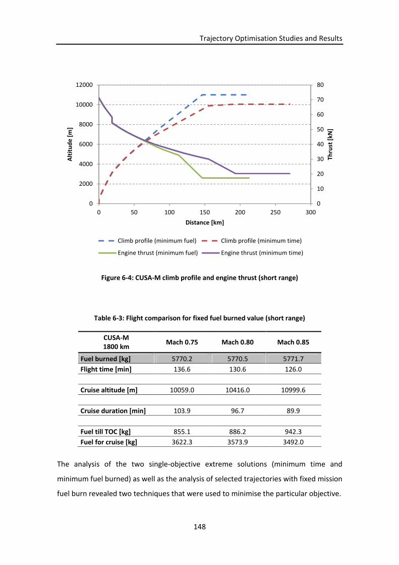
Trajectory Optimisation Studies and Results
148
Figure 6-4: CUSA-M climb profile and engine thrust (short range)
Table 6-3: Flight comparison for fixed fuel burned value (short range)
CUSA-M1800 km
Mach 0.75 Mach 0.80 Mach 0.85
Fuel burned [kg] 5770.2 5770.5 5771.7
Flight time [min] 136.6 130.6 126.0
Cruise altitude [m] 10059.0 10416.0 10999.6
Cruise duration [min] 103.9 96.7 89.9
Fuel till TOC [kg] 855.1 886.2 942.3
Fuel for cruise [kg] 3622.3 3573.9 3492.0
The analysis of the two single-objective extreme solutions (minimum time and
minimum fuel burned) as well as the analysis of selected trajectories with fixed mission
fuel burn revealed two techniques that were used to minimise the particular objective.
0
10
20
30
40
50
60
70
80
0
2000
4000
6000
8000
10000
12000
0 50 100 150 200 250 300
Thru
st[k
N]
Alt
itu
de
[m]
Distance [km]
Climb profile (minimum fuel) Climb profile (minimum time)
Engine thrust (minimum fuel) Engine thrust (minimum time)

Trajectory Optimisation Studies and Results
149
The first technique, which is applied by the GATAC optimiser, involves the
adjustment of the True Air Speed (TAS) by changing the cruise altitude.
The second technique, which is based on predetermined inputs for the GATAC
optimiser, involves the selection of specific cruise Mach numbers.
6.2.3 Fuel vs. NOx Optimisation Results
Figures 6-5 and 6-6 show the optimiser output for the short range mission of the
CUSA-M aircraft performing the 1800 km mission at varying climb altitudes (altitude 1
to altitude 16 as listed in table 6-1), varying cruise altitudes (10059 m - 11000 m) and 2
different cruise Mach numbers (0.75 and 0.85) with respect to fuel burned and NOx
emissions. In this case, each plot represents an optimal solution for the respective
Mach number case. This means, the results of the optimiser converge towards one
particular condition which indicates that both objectives (fuel burned and NOx
emissions) concur with each other. Differences in fuel burned for each solution is less
than 0.1 kg and differences in NOx emissions for each solution are less than 1 g. Since
there is no trade-off between the two objectives, the optimiser does not find a set of
non-dominated solutions. In both optimal cases, the optimiser selects the highest
possible cruise altitude (11000 m) to achieve both, minimum fuel burn and minimum
NOx emissions for a given Mach number. As evaluated in the previous fuel vs. time
optimisation study, minimum mission fuel burn is reached when flying at the highest
possible altitude (11000 m) with the lowest possible cruise Mach number (0.75).
Indeed, the same requirements apply to minimise NOx emissions. The amount of NOx
emissions generated during the flight is directly related to the engine TET.
Consequently, the mission flown at 0.75 Mach number will yield less NOx emissions
compared to the same mission flown at 0.85 Mach number. Since the values shown in
figure 6-5 and 6-6 for fuel burned and NOx emitted are based on a simplified
calculation procedure using only the EINOx value of the initial cruise segment and
fewer cruise increments to compute the total NOx generated throughout the mission,
the trajectory suggested by the GATAC optimiser has been reprocessed to establish the
generated NOx emissions for all flight phases using the respective EINOx values. The
corrected values which account for these changes are listed in table 6-4.
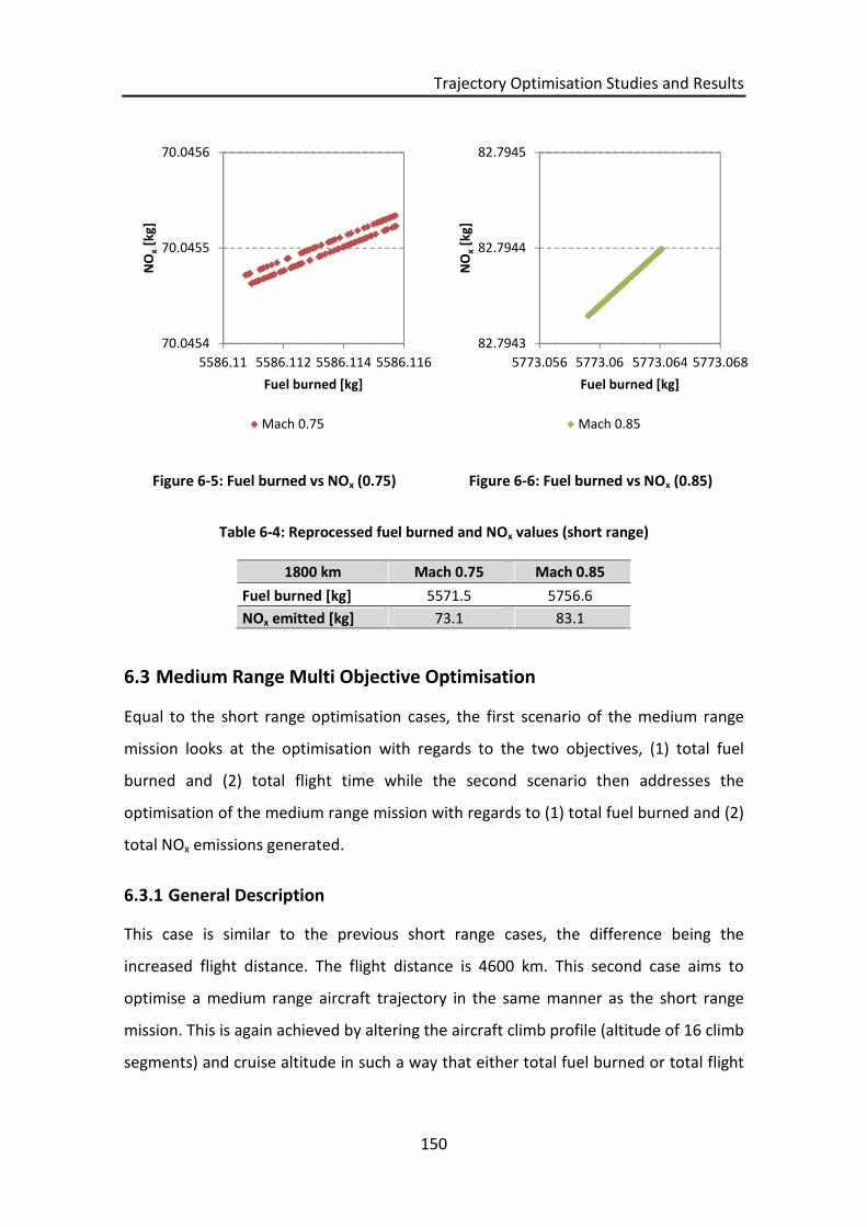
Trajectory Optimisation Studies and Results
150
Figure 6-5: Fuel burned vs NOx (0.75) Figure 6-6: Fuel burned vs NOx (0.85)
Table 6-4: Reprocessed fuel burned and NOx values (short range)
1800 km Mach 0.75 Mach 0.85
Fuel burned [kg] 5571.5 5756.6
NOx emitted [kg] 73.1 83.1
6.3 Medium Range Multi Objective Optimisation
Equal to the short range optimisation cases, the first scenario of the medium range
mission looks at the optimisation with regards to the two objectives, (1) total fuel
burned and (2) total flight time while the second scenario then addresses the
optimisation of the medium range mission with regards to (1) total fuel burned and (2)
total NOx emissions generated.
6.3.1 General Description
This case is similar to the previous short range cases, the difference being the
increased flight distance. The flight distance is 4600 km. This second case aims to
optimise a medium range aircraft trajectory in the same manner as the short range
mission. This is again achieved by altering the aircraft climb profile (altitude of 16 climb
segments) and cruise altitude in such a way that either total fuel burned or total flight
70.0454
70.0455
70.0456
5586.11 5586.112 5586.114 5586.116
NO
x[k
g]
Fuel burned [kg]
Mach 0.75
82.7943
82.7944
82.7945
5773.056 5773.06 5773.064 5773.068
NO
x[k
g]
Fuel burned [kg]
Mach 0.85

Trajectory Optimisation Studies and Results
151
time becomes minimum. The optimisation is carried out three times at three different
fixed Mach numbers (0.75, 0.80 and 0.85).
The second case then looks at the optimisation of the medium range mission in order
to minimise fuel burned or to minimise NOx emissions. It uses the same methodology
as has been deployed on the short range fuel versus NOx emissions optimisation study.
6.3.2 Fuel vs. Time Optimisation Results
Figure 6-6 shows the Pareto fronts for the short range mission of the CUSA-M aircraft
performing the 4600 km mission at varying climb altitudes (altitude 1 to altitude 16 as
listed in table 6-1), varying cruise altitudes (10059 m - 11000 m) and 3 different cruise
Mach numbers (0.75, 0.80 and 0.85) and illustrates the influence on flight time and
fuel burned. The results follow the same general trend as the Pareto fronts for the
short range mission. Each Pareto front comprises a set of non-dominated solutions
which represents a trade-off between flight time and fuel burned. The shortest mission
flight time (305.9 min) requires flying at the lowest possible altitude (10059 m) with
the highest possible Mach number of 0.85. The lowest mission fuel burn (13002 kg)
requires flying at the highest possible altitude (11000) with the lowest possible Mach
number of 0.75. Increasing Mach number from 0.75 by 0.05 increments up to 0.85
reduces flight time by about 22 minutes per each increment. Figure 6-7 illustrates the
corresponding flight profiles (climb, cruise and descent) and fuel burn curves for the
minimum time and minimum fuel case. The solid green profile represents the
minimum fuel trajectory and the dashed green line shows the corresponding fuel burn
accumulation along the flight. The minimum time trajectory is plotted in red lines
accordingly. Both flight profiles shown in figure 6-7 contain the information about the
decision variables used by the GATAC optimiser as previously described for the short
range mission.

Trajectory Optimisation Studies and Results
152
Figure 6-7: Fuel vs. time Pareto fronts for medium range mission
The optimisation objective values (flight time and fuel burned) for the two extreme
points as well as the corresponding trajectory performance points are summarised in
table 6-5 in the same fashion as for the short range mission. In addition, it provides a
comparison of those performance points to a reference flight which is based on the
“non-optimised” trajectory analysed in previous chapter 5. The reference flight is setup
in the same manner as the reference flight introduced in the previous short range
mission study. In this case, flight time is reduced by 7.7% for the minimum time flight
at the expense of 5.7% increase in fuel burn. Fuel burned is reduced by 1.8% for the
minimum fuel flight at the expense of a 4.7% increase in flight time. Both flights
considered in relation to the reference flight. Furthermore, the cruise duration for the
minimum time flight decreased by 8.3% and increased by 6.0% for the minimum fuel
flight. Fuel consumption value till TOC for the minimum time flight increased by 2.5%
while the same value decreased by 18.4% for the minimum fuel flight.
300
305
310
315
320
325
330
335
340
345
350
12800 13000 13200 13400 13600 13800 14000
Flig
ht
tim
e[m
in]
Fuel burned [kg]
Mach 0.75 Mach 0.80 Mach 0.85

Trajectory Optimisation Studies and Results
153
Table 6-5: Optimisation extreme solutions compared to reference flight (4600 km)
CUSA-M4600 km
Referenceflight
Minimumtime flight
Delta [%]Minimumfuel flight
Delta [%]
Fuel burned [kg] 13244.6 13943.0 5.3 13001.5 -1.8
Flight time [min] 331.5 305.9 -7.7 346.9 4.7
Cruise altitude [m] 10668.0 10059.0 - 10999.9 -
Cruise Mach [-] 0.785 0.850 - 0.750 -
Cruise duration [min] 293.0 268.6 -8.3 310.4 6.0
Fuel till TOC [kg] 1199.3 1229.0 2.5 978.3 -18.4
Fuel for cruise [kg] 10737.2 11385.4 6.0 10633.5 -1.0
Figure 6-8: CUSA-M medium range flight profile comparison (fuel vs. time)
In this medium range case the optimiser follows the same strategy of optimising TAS
by adjusting the climb and cruise altitudes, as described for the short range results. In
order to minimise flight time the cruise altitude decreases progressively from the
highest possible value (11000 m) to the lowest possible value (10059 m). Concurrently,
0
2000
4000
6000
8000
10000
12000
14000
16000
0
2000
4000
6000
8000
10000
12000
0 1000 2000 3000 4000 5000
Fue
lbu
rne
d[k
g]
Alt
itu
de
[m]
Distance [km]
Flight profile (minimum fuel) Flight profile (minimum time)
Fuel burned (minimum fuel) Fuel burned (minimum time)

Trajectory Optimisation Studies and Results
154
every step increment in Mach number (from 0.75 to 0.85) increases TAS during cruise
and thus minimises flight time accordingly. The opposite effects take place if the
objective of the optimisation is to minimise fuel burned. Figure 6-8 illustrates the TAS
variation during the climb profile and at initial cruise conditions for the medium range
flight. For the minimum fuel flight (solid orange line), the cruise Mach number (0.75) is
reached earlier during the climb (at a lower altitude) and thus, TAS slightly decreases
throughout the remaining climb as altitude still increases. The same process occurs for
the minimum time flight (solid green line) only at a later point in the climb since the
final cruise Mach number is higher (0.85). The final cruise altitude (10059 m) of the
minimum time flight is reached later than in the minimum fuel case since the optimiser
selects the final climb altitudes so as to prolong the climb duration at the lowest
possible altitude.
Figure 6-9: CUSA-M True Air Speed (TAS) variation during climb (medium range)
Figure 6-9 furthermore shows that the initial climb phase for both trajectories is very
similar due to the narrow bounds of the decision variables (climb altitudes) to be
selected by the optimiser and the way the aircraft performance model (Hermes)
0
50
100
150
200
250
300
0
2000
4000
6000
8000
10000
12000
0 50 100 150 200 250 300 350
TAS
[m/s
]
Alt
itu
de
[m]
Distance [km]
Climb profile (minimum fuel) Climb profile (minimum time)
TAS (minimum fuel) TAS (minimum time)

Trajectory Optimisation Studies and Results
155
computes a feasible climb profile. Figure 6-9 illustrates the corresponding engine
thrust trend of the two extreme climb profiles (minimum time and minimum fuel).
Both figures also show the same speed discontinuity (step change) during the climb
phase that has been experienced in the short range mission and which is related to a
fixed increase in EAS from 250 to 320 knots as setup in the aircraft performance
model. Moreover, based on the lower cruise Mach number for the minimum fuel flight
engine TET is decreased during that phase as well in comparison to the minimum time
flight. Taking into account the results from the trajectory analysis performed in
previous chapter 5, where engine degradation has been simulated, flying at slower
Mach numbers and higher altitudes might alleviate engine degradation over time.
Figure 6-10: CUSA-M climb profile and engine thrust (medium range)
To also highlight the results of the optimiser for the medium range mission, table 6-6
lists a comparison of three different medium range flights selected from the three
Pareto fronts (refer to figure 6-6) assuming a constant mission fuel burn value. It can
be noted that overall flight time decreases with an increase in Mach number and an
increase in cruise altitude. This means, for a fixed value of fuel burned and depending
0
10
20
30
40
50
60
70
80
0
2000
4000
6000
8000
10000
12000
0 50 100 150 200 250 300 350
Thru
st[k
N]
Alt
itu
de
[m]
Distance [km]
Climb profile (minimum fuel) Climb profile (minimum time)
Engine thrust (minimum fuel) Engine thrust (minimum time)

Trajectory Optimisation Studies and Results
156
on the determinative objective of the individual flight mission, cruise altitude and
cruise Mach number can be adjusted as suggested to reach this objective.
Figure 6-11: CUSA-M TET variation (medium range)
Table 6-6: Flight comparison for fixed fuel burned value (medium range)
CUSA-M4600 km
Mach 0.75 Mach 0.80 Mach 0.85
Fuel burned [kg] 13362.0 13360.3 13360.7
Flight time [min] 342.9 324.8 310.1
Cruise altitude [m] 10181.5 10478.3 10999.9
Cruise duration [min] 308.5 289.0 272.1
Fuel till TOC [kg] 987.7 1041.0 1109.1
Fuel for cruise [kg] 11028.5 10960.9 10873.3
0
200
400
600
800
1000
1200
1400
1600
0
2000
4000
6000
8000
10000
12000
0 1000 2000 3000 4000 5000
TET
[K]
Alt
itu
de
[m]
Distance [km]
Flight profile (minimum fuel) Flight profile (minimum time)
Engine TET (minimum fuel) Engine TET (minimum time)
Trajectory Optimisation Studies and Results
157
6.3.3 Fuel vs. NOx Optimisation Results
Figures 6-11 and 6-12 show the optimiser output for CUSA-M aircraft performing the
4600 km mission at varying climb altitudes (altitude 1 to altitude 16 as listed in table 6-
1), varying cruise altitudes (10059 m - 11000 m) and 2 different cruise Mach numbers
(0.75 and 0.85) with respect to fuel burned and NOx emissions generated. As in the
previous case, each plot represents an optimal solution for the respective Mach
number case. This means, the results of the optimiser converge towards one particular
condition which indicates that both objectives (fuel burned and NOx emissions) concur
with each other. Again, differences in fuel burned for each solution is less than 0.1 kg
and differences in NOx emissions for each solution are less than 1 g. Since there is no
trade-off between the two objectives, the optimiser does not find a set of non-
dominated solutions. In both optimal cases, the optimiser selects the highest possible
cruise altitude (11000 m) to achieve both, minimum fuel burn and minimum NOx
emissions for a given Mach number. The results for the medium range flight follow the
same pattern as for the short range case as illustrated in figures 6-11 and 6-12 and
have been reprocessed in the same way to correct the values of NOx emissions and
fuel burned. Correspondingly, the corrected values which account for these changes
are listed in table 6-7.

Trajectory Optimisation Studies and Results
158
Figure 6-12: Fuel burned vs NOx (0.75) Figure 6-13: Fuel burned vs NOx (0.85)
Table 6-7: Reprocessed fuel burned and NOx values (short range)
4600 km Mach 0.75 Mach 0.85
Fuel burned [kg] 12934.6 13304.7
NOx emitted [kg] 170.6 196.4
173.5530
173.5532
173.5534
13001.08 13001.09 13001.1
NO
x[k
g]
Fuel burned [kg]
Mach 0.75
201.1652
201.1654
201.1656
13360.37 13360.38 13360.39
NO
x[k
g]
Fuel burned [kg]
Mach 0.85

Conclusions, Recommendations for Further Work
159
7 Conclusions, Recommendations for Further Work and Outlook
This chapter summarises the main achievements and conclusions of the present
research work and also addresses its limitations. Furthermore, some recommendations
for future work are listed based on the results of this work.
7.1 Achievements
In the present research work, an analysis of aircraft trajectories with different
aircraft/engine configurations has been conducted in order to verify and quantify their
fuel burn and emissions performance. This has been achieved by adapting
representative engine models, aircraft models and emissions predictions models to
simulate commercial aircraft flight trajectories. All models have been compared to
publicly available data in order to validate their suitability. Furthermore, the impact of
engine degradation on the fuel burn and emissions has been investigated. In
conjunction with the degradation analysis, the influence of derated take-offs has been
considered as well. Two different flight missions, a short range mission (1800 km) and
a medium range mission (4600 km) have been evaluated to estimate the values for
mission fuel burn, NOx emissions and flight time. The scenarios investigated included
three different aircraft variants similar to the Airbus A320 family, and correspondingly
three different engine variants similar to the CFM56-5B engine series. Moreover, an
existing emissions predictions model based on correlations of ground level emission
data has been customised for each engine variant.
Furthermore, a simple multi-disciplinary optimisation framework has been developed
to perform aircraft trajectory optimisation studies. All models (engine model, aircraft
model and emissions predictions model) have been integrated into this framework
which then provided the capability to perform preliminary aircraft trajectory
optimisation studies. Two different trajectory scenarios have been investigated which
focus on the minimisation of fuel burned versus flight time and fuel burned versus NOx
emissions.

Conclusions, Recommendations for Further Work
160
7.2 Conclusions
With regards to the aircraft trajectory analyses carried out at the initial part of the
study it can be concluded that the effect of engine degradation on total mission fuel
burn and emissions amplifies with flight distance and that it can considerably increase
either of these values. Degradation affects the engine performance in all analysed
flight phases (take-off, climb and cruise) and has its most adverse effect during take-off
when engine TET is already elevated and reaches values which are close to operational
limitations. The amounts of engine degradation (2% compressor, combustor and
turbine degradation) simulated in this study were arbitrarily selected and thus cannot
directly be correlated to a specific engine age. It can furthermore be inferred that a
take-off thrust reduction of 15% (as a consequence of engine degradation) can
significantly lower fuel burn and NOx emissions during this flight phase while having
only negligible negative impact on the total mission fuel burn and total mission NOx
emissions. The benefits achieved by reducing the maximum take-off power are
consequently accompanied by a decrease in engine TET which in turn has a positive
impact on engine life. Furthermore, it was observed that the amount of NOx emissions
per kilogram payload and kilometre decreases with aircraft size. This effect could in
turn be considered by airline operators who utilise different aircraft variants of the
same series in their fleets. Engines may then be swapped from larger aircraft variants
(with higher thrust engine configurations) to smaller aircraft variants (with lower
thrust configurations) to alleviate the effects of degradation on emissions.
The preliminary aircraft trajectory optimisation studies carried out as described in
chapter 6 enabled the assessment of improved flight trajectories with the objective to
minimise mission fuel burn, fight time or NOx emissions generated. The deployment of
a basic optimisation framework allowed the investigation of improved flight
trajectories with regards to the selected optimisation of variables such as aircraft
speed, aircraft climb altitudes and cruise altitude. The achieved results suggest that
flight trajectories with reduced environmental impact (less fuel burned or less NOx
emitted) exist when compared to a “non-optimised” reference flight.

Conclusions, Recommendations for Further Work
161
7.3 Limitations and Recommendations for Further Work
The results of the trajectory studies are subject to assumptions and limitations
introduced in order to perform feasible and comparable analyses. The limitations
imposed originate from various circumstances inherent to the simulation models and
the optimisation framework respectively.
The aircraft performance model Hermes only employs a single fixed climb profile for
the initial trajectory analyses which is based on a real example flight trajectory. Engine
power settings for this climb profile are also fixed at predefined values. Take-off,
landing and taxi phases are simulated in a simplified manner within the Hermes code
and the resulting values should only be considered as reference points. In addition, the
descent phase has been kept constant in terms of descent profile and power settings
for all cases analysed.
The engine performance model Turbomatch provides many options to adapt various
different engine designs and architectures to allow maximum simulation depth. For
the purpose of this study, the adapted engine models have been developed with as
many details as necessary to achieve a practical representation of the desired real
engine variants. For example, no provision has been made for variable engine
geometry or advanced bleed air control which may allow a more realistic engine
simulation also in terms of transient engine performance. Thus, the engine
performance model Turbomatch only yielded approximate results when simulating the
engine off-design performance at very low power settings equivalent to idle
conditions.
The emissions predictions model used in this study employs a correlations based
approach (P3T3 method) to predict combustor NOx emissions at different engine
power settings. Other emissions such as CO or UHC have not been investigated as part
of this study.
The current basic GATAC optimisation framework developed provides only capabilities
to conduct preliminary optimisation studies since the setup requires refinement in
Conclusions, Recommendations for Further Work
162
terms of input and output handling of the model parameters as well the amount of
optimisation variables applied. In addition, the developed framework is subject to
constraints inherent to the setup (model integration), as well as to the individual
models and thus, the achieved optimisation results only represent a very limited range
of possible solutions within the scope of the developed framework. In the current
optimisation study, no provision for the speed con
Furthermore, parameter settings of the GATAC optimiser such as population size,
creation rates or selection pressure have been kept equal for all cases analysed.
Adjustment of these parameters for each optimisation scenario might improve the
convergence of the results and reduce computational time.
The flight trajectory analyses carried out in the present work focused on certain
aspects of an aircraft flight mission while other aspects have been excluded or
neglected in order to create a manageable framework. For a more realistic
representation of aircraft flight procedures and to increase and improve the validity of
the simulation framework results, several recommendations for further work required
are listed in the following:
Extend the scope of the optimisation framework to include further models,
such as noise models, weather models, lifing models and models for
operational constraints such as air traffic management or particular airport
restrictions.
Investigate the implications of optimised trajectories on airlines’ Direct
Operating Costs (DOC) using a more all-encompassing approach, including
factors like aircraft and engine maintenance costs, costs for flight operations
and possible increased fuel prices and future emission taxes.
Extend and improve the engine degradation model and scenarios to account
for degradation of particular components and to investigate long-term effects.
Extend the engine degradation model to account for flow capacity changes in
the compressors and turbines (compressor and turbine fouling).
Conclusions, Recommendations for Further Work
163
Incorporate additional aircraft and engine models into the framework to
investigate very short range and long range flight trajectories.
Incorporate additional aircraft payload conditions which take into account a
wider range of possible loading scenarios.
Include all flight phases in the analyses and optimisation framework: Ground
taxi-out, take-off, climb, cruise, descent, approach, landing, ground taxi-in. At
the same time, extend the capability of the aircraft performance model to
allow increased simulation accuracy for taxi, take-off and landing phases.
Extend the emissions predictions model to allow modelling of different types of
combustors (conventional or new design).
Implement different emissions prediction models based on numerical
simulations or physics based models.
Include and quantify other pollutants, such as CO, UHC and soot.
Allow optimisation of trajectory scenarios with more than two objectives (for
example trade-offs between noise, NOx emissions and fuel burn be particularly
interesting in the LTO cycle).
Investigate additional alternative multi-objective genetic algorithms.
Adjust and refine the parameter settings of the GATAC optimiser for each
optimisation scenario to improve the optimisation performance.
Extend the type of optimisation variables to include the variation engine power
settings during climb or the amount of take-off derate applied.
Increase the number and/or combination of optimisation variables used for
each optimisation scenario (fuel vs. time, fuel vs. NOx).
Investigate the possibility of incremental trajectory optimisation where flight
phases are optimised individually to safe computing time and/or increase the
fidelity of the results. Each flight phase could then be optimised with respect to
the objectives which are of paramount importance in that particular phase (for
example, noise during take-off and NOx emissions during cruise).

Conclusions, Recommendations for Further Work
164
Implement the engine degradation model into the optimisation framework to
investigate the effect on optimum trajectories with respect to fuel burned or
NOx emitted.
Outlook
165
7.4 Outlook
A brief outlook on two important aspects of aircraft and engine operation is presented
in this last section in order to highlight their importance for future developments and
advancements in those fields. The first aspect deals with airline specific operational
procedures and the second aspect focuses on engine health monitoring strategies.
7.4.1 Airline Operational Procedures
Many assumptions made throughout this study depend on custom airline procedures
or operational restrictions imposed on airlines due to environmental constraints.
Aircraft climb profiles or cruise altitudes are prescribed by local conditions of
aerodromes and airspace controllers for example depending on aircraft speed and
destination. Descent profiles are affected in the same way where certain flight paths
have to be followed due to noise restrictions or traffic separation close to airports. An
improvement of those procedures is investigated by one of the Clean Sky ITDs, the
Systems for Green Operations (SGO). Three concepts are adopted for an overall
optimisation of the aircraft and systems [20]. (1) Green Trajectories, including 3-
dimensional flight paths and optimisation for minimum noise and emissions. (2) A
Green Mission from start to finish, including management of climb, cruise and descent
and multi-criteria optimisation (noise, emissions, fuel, time). (3) Smart Operations on
Ground, including new ground procedures to reduce engine fuel consumption. The
implementation of the before described mission optimisation systems will enable
airlines to accurately predict complete flight missions in real-time and consequently
assess their environmental impact.
With respect to engine operation and especially with respect to engine degradation
one operational initiative which can significantly reduce the rate of engine degradation
and in turn increase the engine on-wing life is regular engine gas path washing. Over
time, dirt and other environmental pollutants accumulate in the engine air flow path
and deposit on compressor blades and vanes. Washing of the engine compressor and
airfoils can to some extent recover the engine performance by improving the surface
finish of the blades and thus the aerodynamic contour which has a positive effect on

Outlook
166
compressor efficiency. The work in reference [109] analyses the particular effects of
engine washing on engine performance and in a second step identifies significant
benefits of washing an engine at predetermined intervals.
7.4.2 Engine Health Management
As discussed in chapters 2.2, 2.3 and 2.4 of this study, engine performance degradation
is continuously monitored to identify trend shifts or to detect faults ahead of time. This
is usually achieved by analysing certain engine performance data points of every flight
performed at a given day. Engine data such as temperatures, pressures and others are
collected together with aircraft and atmospheric data to compute a smoothed engine
performance trend. Normally these computations are carried out in retrospect, this
means, when the aircraft has landed and data has been transmitted to centralised
servers on ground. This means that these systems normally have inherent diagnostics
latency. Due to the continuing advances in avionics, portions of the current on-ground
monitoring activities and diagnostics data may be shifted to health management
systems on-board the aircraft which would allow real-time monitoring of engine
performance or early detection of faults. The paper in reference [110] describes this
approach in detail and investigates an enhanced on-board model based GPHM (Gas
Path Health Management) architecture.
Future Engine Health Management (EHM) Systems are expected to make propulsion
system operation more intelligent, self-diagnostic, self-optimising and mission
adaptable. Engine life cycle costs, fuel efficiency and reliability are major focus areas
when new engine control and health management systems are investigated and are
expected to have a significant potential to improve overall operational performance.
The paper in reference [111] summarises specific engine health management
technologies that are currently under development, which will enable efficient aircraft
propulsion system operation. One common goal of those technologies is to operate an
engine to achieve optimal performance while considering the actual engine condition
and the current mission of the aircraft.

167
REFERENCES
1. Tillmann, C. G, . et. al. Zusammenfassende Darstellung der Effizienzpotenziale bei
Flugzeugen unter besonderer Berücksichtigung der aktuellen Triebwerkstechnik sowie
der absehbaren mittelfristigen Entwicklungen. FKZ UM 07 06 602/01 März 2008.
2. Lee, D.S., et al. Aviation and global climate change in the 21st century. Atmospheric
Environment (2009).
3. (EUROCONTROL), The European Organisation for the Safety of Air Navigation.
Challenges of Air Transport 2030, Survey of experts’ views, July 2009.
4. (EUROCONTROL), European Organisation for the Safety of Air Navigation.
“Challenges of growth” environmental update study, January 2009.
5. Brasseur, G. P., et al. European Scientific Assessment of the Atmospheric Effects of
Aircraft Emissions. Atmospheric Environment Vol. 32, No. 13, pp. 2329—2418, 1998.
6. (ICAO), International Civil Aviation Organization. ICAO Engine Emissions Databank.
http://www.caa.co.uk/default.aspx, (accessed 25th October, 2011).
7. (CAEP), Committee on Aviation Environmental Protection. Correlation between LTO
NOx and Cruise/Climb NOx . Seventh Meeting, February 2007 .
8. Mongia, H. C. On Continuous NOx Reduction of Aero-propulsion Engines. 48th AIAA
Aerospace Sciences Meeting Including the New Horizons Forum and Aerospace
Exposition, Orlando, Florida, 2010.
9. Hileman, J., I., et al. Payload Fuel Energy Efficiency as a Metric for Aviation
Environmental Performance. 26th International Congress of the Aeronautical Sciences,
2008.
10. (CAEP), Committee On Aviation Environmental Protection (1). CAEP/7
Environmental Design Spsace (EDS) Progress. Seventh Meeting, February 2007.

168
11. (CAEP), Committee On Aviation Environmental Protection (2). CAEP/8 NOx
Stringency Cost-Benefit Analysis Demonstration Using APMT-Impacts. Eighth Meeting,
February 2010.
12. (PARTNER), Partnership for AiR Transporatation Noise and Emissions Reduction
(1). About PARTNER. http://web.mit.edu/aeroastro/partner/about/index.html
(accessed 20th January, 2011).
13. (PARTNER), Partnership for AiR Transporatation Noise and Emissions Reduction
(3). Projects PARTNER. http://web.mit.edu/aeroastro/partner/projects/index.html
(accessed 20th January, 2011).
14. Yutko, B., Hansman, R. J., Mozdzanowska, A., et. al. Assessment of CO2 Emission
Metrics for a Commercial Aircraft Certification Requirement. PARTNER Project 30
Interim Report, December 2010.
15. (PARTNER), Partnership for AiR Transporatation Noise and Emissions Reduction
(2). Aviation Environmental Portfolio Management Tool PARTNER.
http://web.mit.edu/aeroastro/partner/apmt/index.html (accessed 20th January,
2011).
16. Personalities, Report of the Group of. European Aeronautics: A Vision for 2020,
Meeting society’s needs and winning global leadership. January 2001.
17. (ACARE), Advisory Council for Aeronautics Research in Europe. ACARE Strategic
Research Agendas SRA-1 and SRA-2, ACARE SRA-2 Excecutive Summary.
http://www.acare4europe.org/documents/rarchive (accessed 31st Marchr, 2013).
18. Addendum to the Strategic Research Agenda. Advisory Council for Aeronautics
Research in Europe. 2008.
19. Donnerhack, Dr.-Ing. S. Beiträge der Flugtriebwerke zur Schadstoffreduktion im
Luftverkehr. Workshop “Flugverkehr und Luftqualität - Partikel- und
Stickoxidemissionen“ beim UBA Berlin, 14.06.2005.

169
20. Clean Sky JTI Joint Technology Initiatve. CleanSky. http://www.cleansky.eu,
(accessed 20th January, 2011).
21. Ogaji, S., Pilidis, P., Hales, R. TERA- A Tool for Aero-engine Modelling and
Management. 2nd World Congress on Engineering Asset Management and 4th
International Conference On Condition Monitoring, 11-14th June 2007, Harrogate, UK.
22. Celis, C., Long, R., Sethi, V., Zammit-Mangion, D. On Trajectory Optimization for
Reducing the Impact of Commercial Aircraft Operations on the Environment. ISABE-
2009-1118.
23. Zolata, H. Development of a Multi-Disciplinary Aircraft Trajectory Optimisation
Simulation Framework. MSc Thesis, School of Engineering, Cranfield University 2009,
MK43 0AL, Bedfordshire, UK.
24. Marzal Espi, R. Benchmarking and Testing of different Genetic Algorithms for Multi-
Disciplinary Aircraft Trajectory Optimisation Studies. MSc Thesis, School of Engineering,
Cranfield University 2010, MK43 0AL, Bedfordshire, UK.
25. Döpelheuer, A., Lecht, M. Influence of Engine Performance on Emission
Characteristics. German Aerospace Center, Institute of Propulsion Technology, Engine
Systems, D-51147 Cologne, Germany.
26. Bower, G. C., Kroo, I. M. Multi-Objective Aircraft Optimization for Minimum Cost
and Emissions over Specific Route Networks: European Aeronautics. 26th International
Congress of the Aeronautical Sciences, Stanford University, Department of Aeronautics
and Astronautics, 2008.
27. Penner, J.E., Lister, D.H., Griggs, D.J., Dokken, D.J., McFarland, M. Aviation and
the Global Atmosphere. A Special Report of IPCC Working Groups I and III, 1999.
28. AIRBUS Flight Operations Support & Line Assistance. Getting to grips with aircraft
performance. January 2002.
29. Lawson, C. P. Aircraft Performance for Propulsion Systems Engineers. Lecture
Notes, Cranfield University, MK43 0AL, Bedfordshire, UK.

170
30. Daggett, D. L. Water Misting and Injection of Commercial Aircraft Engines to
REduce Airport NOx. National Aeronatuics and Space Administration (NASA), Glenn
Research Center, 2004, NASA/CR-2004-212957.
31. (GAO), US General Accounting Office. Aviation And The Environment - Strategic
Framework Needed to Address Challenges Posed by Aircraft Emissions. Report to the
Chairman, Subcommittee on Aviation, Committee on Transportation and
Infrastructure, February 2003.
32. (ICAO), International Civil Aviation Organization. Continuous Descent Operations
(CDO) Manual. Doc 9931, AN/476.
33. (ICAO), International Civil Aviation Organization (1). Procedures for Air Navigation
Services - Aircraft Operations - Flight Procedures - Volume I. Fifth Edition, 2006.
34. (ICAO), International Civil Aviation Organization (2). Procedures for Air Navigation
Services - Aircraft Operations - Construction of Visual and Instrument Flight Procedures
- Volume II. Fifth Edition, 2006.
35. (ICAO), International Civil Aviation Organization. Operational Opportunities to
Minimize Fuel Use and Reduce Emissions. February 2003.
36. AIRBUS Flight Operations Support & Services. Getting to grips with A320
performance retention and fuel savings. Issue 2, January 2008.
37. Grieb, H. Projektierung von Turboflugtriebwerken. Birkhäuser Verlag 2004 , Basel,
Switzerland.
38. Walsh, P.P., Fletcher, P. Gas Turbine Performance. Second Edition, Blackwell
Publishing, 2004, UK.
39. Bräunling, W. J. G. Flugzeugtriebwerke. Grundlagen, Aero-Thermodynamik, ideale
und reale Kreisprozesse, Thermische Turbomaschinen, Komponenten, Emissionen und
Systeme, 3., vollständig überarbeitete und erweiterte Auflage, Springer, Berlin,
Heidelberg 2009.
171
40. Wörrlein, K. Gasdynamische Probleme bei Flugantrieben. Fachgebiet Gasturbinen
und Flugantriebe, Technische Universität Darmstadt, 1. Auflage SS 2001.
41. Pilidis, P., Palmer, J.P. Gas Turbine Theory and Performance. MSc Lecture Notes,
School of Engineering, Cranfield University 2008, MK43 0AL, Bedfordshire, UK.
42. Baehr, H. D., Kabelac, S. Thermodynamik. Springer Verlag Berlin, Heidelber 2012.
43. ICF Consulting Group. Evaluation of Air Pollutant Emissions from Subsonic
Commercial Jet Aircraft. Engine Programs and Compliance Division, Office of Mobile
Sources, U.S. Environmental Protection Agency, April 1999.
44. Singh, R. Gas Turbine Combustors Volume 1. School of Engineering, Cranfield
University, October 2009, MK43 0AL, Bedfordshire, UK.
45. Faber, J., Greenwood, D., Lee, D., et. al. Lower NOx at Higher Altitudes - Policies to
Reduce the Climate Impact of Aviation NOx Emission . Delft, CE Delft, October 2008.
46. Saravanamuttoo, I., et al. Gas Turbine Theory. Sixth edition 2009.
47. Singh, R. Gas Turbine Combustors Volume 2. School of Engineering, Cranfield
University, 2009, MK43 0AL, Bedfordshire, UK.
48. Norman, P. D., et al. Development of the technical basis for a New Emissions
Parameter covering the whole AIRcraft operation: NEPAIR. NEPAIR/WP4/WPR/01,
September 2003.
49. Lipowsky, H. Entwicklung und Demonstration eines integrierten Systems zur
Zustandsüberwachung von Gasturbinen. Institut für Luftfahrtantriebe der Universität
Stuttgart, 2010.
50. Li, Y. G. Performance-analysis-based gas turbine diagnostics: A review. Proceedings
of the Institution of Mechanical Engineers, Part A: Journal of Power and Energy, 2002.
51. B. A., Roth, D. L., Doel, J. J., Cissell. Probabilistic Matching of Turbofan Engine
Performance Models to Test Data. GT2005-68201, Proceedings of ASME Turbo Expo
2005: Land Sea & Air.
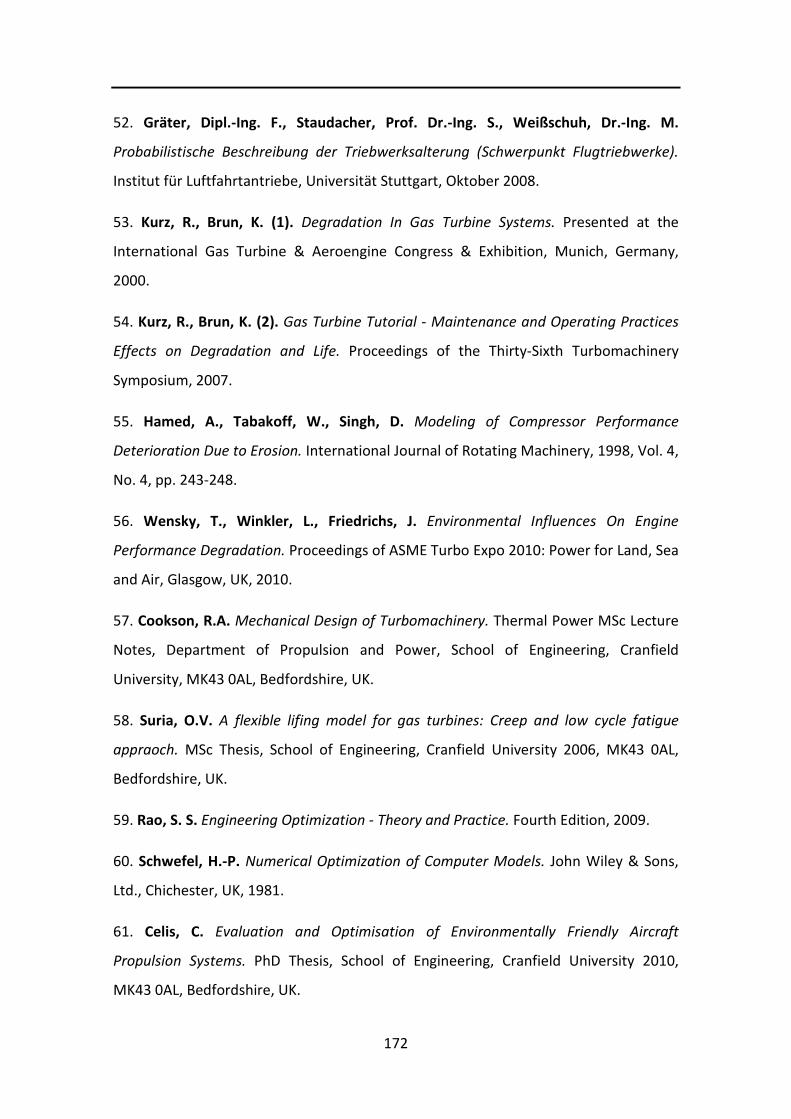
172
52. Gräter, Dipl.-Ing. F., Staudacher, Prof. Dr.-Ing. S., Weißschuh, Dr.-Ing. M.
Probabilistische Beschreibung der Triebwerksalterung (Schwerpunkt Flugtriebwerke).
Institut für Luftfahrtantriebe, Universität Stuttgart, Oktober 2008.
53. Kurz, R., Brun, K. (1). Degradation In Gas Turbine Systems. Presented at the
International Gas Turbine & Aeroengine Congress & Exhibition, Munich, Germany,
2000.
54. Kurz, R., Brun, K. (2). Gas Turbine Tutorial - Maintenance and Operating Practices
Effects on Degradation and Life. Proceedings of the Thirty-Sixth Turbomachinery
Symposium, 2007.
55. Hamed, A., Tabakoff, W., Singh, D. Modeling of Compressor Performance
Deterioration Due to Erosion. International Journal of Rotating Machinery, 1998, Vol. 4,
No. 4, pp. 243-248.
56. Wensky, T., Winkler, L., Friedrichs, J. Environmental Influences On Engine
Performance Degradation. Proceedings of ASME Turbo Expo 2010: Power for Land, Sea
and Air, Glasgow, UK, 2010.
57. Cookson, R.A. Mechanical Design of Turbomachinery. Thermal Power MSc Lecture
Notes, Department of Propulsion and Power, School of Engineering, Cranfield
University, MK43 0AL, Bedfordshire, UK.
58. Suria, O.V. A flexible lifing model for gas turbines: Creep and low cycle fatigue
appraoch. MSc Thesis, School of Engineering, Cranfield University 2006, MK43 0AL,
Bedfordshire, UK.
59. Rao, S. S. Engineering Optimization - Theory and Practice. Fourth Edition, 2009.
60. Schwefel, H.-P. Numerical Optimization of Computer Models. John Wiley & Sons,
Ltd., Chichester, UK, 1981.
61. Celis, C. Evaluation and Optimisation of Environmentally Friendly Aircraft
Propulsion Systems. PhD Thesis, School of Engineering, Cranfield University 2010,
MK43 0AL, Bedfordshire, UK.

173
62. Koumoutsakos, P., Freund, J., Parekh, D. Evolution strategies for parameter
optimization in jet flow control. Center for Turbulence Research, Proceedings of the
Summer Program 1998.
63. Charbonneau, P. An Introduction to Genetic Algorithms for Numerical
Optimization. National Center for Atmospheric Research, Boulder, Colorado, March
2002.
64. Zitzler, E., Laumanns, M., Bleuler, S. A Tutorial on Evolutionary Multiobjective
Optimization. Swiss Federal Institute of Technology (ETH) Zurich, Computer
Engineering and Networks Laboratory, Gloriastrasse 35, CH-8092 Zurich, Switzerland.
65. Mitsuo, G., Runwei, C. Genetic Algorithms and Engineering Optimization. First
edition, December 28, 1999.
66. Deb, K., et al. A Fast and Elitist Multiobjective Genetic Algorithm: NSGA-II, IEEE
Transactions on Evolutionary Computation. Vol.6, No.2, April 2002.
67. Caramia, M., Dell'Olmo, P. Multi-Objective Management in Freight Logistics
Increasing Capacity, Service Level and Safety with Optimization Algorithms. Springer,
2008.
68. Coello Coello, C. A., Lamont, G. B. An Iintroduction to Multi-Objective Evolutionary
Alogorithms and Their Applications.
69. Van Veldhuizen, D.A., Lamont, G.B. Multiobjective Evolutionary Algorithm
Research: A History and Analysis. October 14, 1998, Graduate School of Engineering,
Air Force Institute of Technology, Wright-Patterson AFB, USA.
70. Pervier, H., Nalianda, D., Espi, R., Sethi, V. Pilidis, P., et. al. Application of Genetic
Algorithm for Preliminary Trajectory Optimization. SAE International, 2011-01-2594,
2011.
71. Dimech, E., Chircop, K., Xuereb, M., Muscat, R. GATAC User Manual V2. Clean Sky,
Systems for Green Operations ITD, March 2011.

174
72. Scheiderer, J. Angewandte Flugleistung, Eine Einführung in die operationelle
Flugleistung vom Start bis zur Landung. Springer, Berlin Heidelberg, 2008.
73. NASA, National Aeronautics and Space Administartion. U.S. Standard Atmosphere.
1976. NASA-TM-X-74335, U.S. Government Printing Office, Washington.
74. AIRBUS Flight Operations Support & Line Assistance. Getting to grips with fuel
economy. Issue 4, October 2004.
75. Clarke, J.-P., et al. Development, design, and flight test evaluation of a continuous
descent approach procedure for nighttime operation at Louisville International Airport.
January 2006.
76. Patterson, J., et. al. Analysis of Departure and Arrival Profiles Using Real-Time
Aircraft Data. Journal Of Aircraft, Vol. 46, No. 4, July – August 2009.
77. Alam, S., Nguyen, M. H., Abbass, H. A., Lokan , C., et. al. A Dynamic Continous
Descent Approach Methodology For Low Noise And Emission. IEEE 2010.
78. Torres, R., Chaptal, J., Bès, C., Hiriart-Urruty, J.-B. Optimal, Environmentally
Friendly Departure Procedures for Civil Aircraft. Journal Of Aircraft, Vol. 48, 2011.
79. Trani, A.A. Aircraft Performance Calculations: Descent Analysis. CEE 5614, Analysis
of Air Transportation Systems, Virginia Tech, Air Transportation Systems Laboratory.
80. Sammut, M. Multivariable Parameter Optimization Of Flight Trajectories. Cranfield
University, School of Engineering, August 2011 .
81. Shakariyants, S. A., van Buijtenen, J. P., Visser, W. P. J., Tarasov, A. (1). A
Multidisciplinary Aero-Engine Exhaust Emission Study. Proceedings of GT 2006 ASME
Turbo Expo 2006: Power for Land, Sea and Air, Barcelona, Spain, 2006.
82. Shakariyants, S. A., van Buijtenen, J. P., Visser, W. P. J., Tarasov, A. (2). Generic
Airplane And Aero-Engine Simulation Procedures For Exhaust Emission Studies.
Proceedings of GT2007 ASME Turbo Expo 2007: Power for Land, Sea and Air, Montreal,
Canada, 2007.

175
83. Filippone, A. Comprehensive analysis of transport aircraft flight performance.
Progress in Aerospace Sciences 44 (2008) 192–236.
84. Mercer, C. R., Haller, W. J. Adaptive Engine Technologies for Aviation CO2
Emissions Reduction. 42nd AIAA/ASME/SAE/ASEE Joint Propulsion Conference &
Exhibit, Sacramento, California, 2006.
85. Waldowski, A. Potenzialbewertung von Open-Rotor-Triebwerken. Deutsches
Zentrum für Luft- und Raumfahrt, Technische Universität Berlin, 2009.
86. Najafi, E., Sethi, V., Celis, C. Preliminary Specification of the CUTSTF Engine
Performance Model for Use in GATAC V1. System for Green Operations (SGO) ITD,
September 2009.
87. CFM The Power of Flight. Engine Technology, CFM56-5B Series Turbofan Engines.
http://www.cfm56.com/products/cfm56-5b/cfm56-5b-technology, (accessed 20th
October, 2011).
88. The TURBOMATCH Theme. For Aero/Industrial Gas Turbine Engine Design
Point/Off Design Performance Calculation. Department of Power and Propulsion,
October 1999, School of Engineering, Cranfield University, MK43 0AL, UK.
89. Kurzke, J. The GasTurb Program. http://www.gasturb.de, (accessed 15th August,
2012).
90. NLR, Nationaal Lucht- en Ruimtevaartlaboratorium. Gas Turbine Simulation
Program. http://www.gspteam.com (accessed 15th August, 2012).
91. Pachidis, V. A. Gas Turbine Performance Simulation. Thermal Power MSc Course
Notes, Department of Power Propulsion and Aerospace Engineering, School of
Engineering, Cranfield University, MK43 0AL, Bedfordshire, UK.
92. Pilidis, P., et al. Propulsion Systems Performance and Integration. Lecture Notes
Volume One, School of Engineering, Cranfield University 2008, MK43 0AL,
Bedfordshire, UK.

176
93. Matingly, J.D. Elements of Gas Turbine Propulsion. International Editions 1996,
McGraw-Hill, Singapore.
94. Guha, A. Optimum Fan Pressure Ratio for Bypass Engines with Separate or Mixed
Exhaust Streams. University of Bristol, UK.
95. Commerce, Aircraft. Aircraft Owner’s & Operator’s Guide: A320 Family. Issue No.
44 • February/March 2006.
96. Bauernfeind, K. Steuerung und Regelung der Turboflugtriebwerke. Birkhäuser
1999, Berlin.
97. AIRBUS, A320 Family (1). Dimensions & Key Data A319 Aircraft.
http://airbus.com/aircraftfamilies/passe-ngeraircraft/a320family/a319/specifications,
(accessed 20th October, 2011).
98. AIRBUS, A320 Family (2). Dimensions & Key Data A320 Aircraft.
http://airbus.com/aircraftfamilies/passe-ngeraircraft/a320family/a320/specifications,
(accessed 20th October, 2011.
99. AIRBUS, A320 Family (3). Dimensions & Key Data A321 Aircraft.
http://airbus.com/aircraftfamilies/passe-ngeraircraft/a320family/a321/specifications,
(accessed 20th October, 2011).
100. University, Cranfield. Hermes V5 & TmatchCalls V3 User Manual. September
2009, School of Engineering, Cranfield University, MK43 0AL, Bedfordshire, UK.
101. Berdowski, Z., et al. Survey on standard weights of passengers and baggage -
Final report. Reference EASA 2008.C.06/30800/R20090095/30800000/FBR/RLO ,
Zoetermeer, May 2009.
102. AIRBUS, A319. Airplane Characteristics for Airport Planning, AIRBUS S.A.S.
Technical Data Support and Services, 31707 Blagnac Cedex, France, Revision May 01,
2011.

177
103. AIRBUS, A320. Airplane Characteristics for Airport Planning, AIRBUS S.A.S.
Technical Data Support and Services, 31707 Blagnac Cedex, France, Revision May 01,
2011.
104. AIRBUS, A321. Airplane Characteristics for Airport Planning, AIRBUS S.A.S.
Technical Data Support and Services, 31707 Blagnac Cedex, France, Revision May 01,
2011.
105. Celis, C., Moss, B., Pilidis, P. Emissions Modelling for the Optimisation of Greener
Aircraft Operations. Proceedings of ASME Turbo Expo 2009, Power for Land, Sea and
Air, Orlando, Florida, USA, GT2009-59211.
106. Allaire, D. L. A Physics-Based Emissions Model for Aircraft Gas Turbine
Combustors. Massachusetts Institute Of Technology, May 2006.
107. Chircop, K., Xuereb, M., Zammit-Mangio, D., Cachia, E. A Generic Framework for
Multi-Parameter Optimization of Flight Trajectories. 27th International Congress of the
Aeronautical Sciences, 2010.
108. Zitzler, E., Deb, K., Thiele, L. Comparison of Multiobjective Evolutionary
Algorithms: Empirical Results. Massachusetts Institute of Technology, 2000.
109. Giesecke, D. On-Wing Compressor Washing Of A Short-Range Aircraft. Cranfield
University, School of Engineering, 2011.
110. Simon, D. L. An Integrated Architecture for On-Board Aircraft Engine Performance
Trend Monitoring and Gas Path Fault Diagnostics. NASA/TM—2010-216358, Glenn
Research Center, Cleveland, Ohio.
111. Litt, J. S., et al. A Survey of Intelligent Control and Health Management
Technologies for Aircraft Propulsion Systems. NASA/TM-2005-213622, Glenn Research
Center, Cleveland, Ohio.
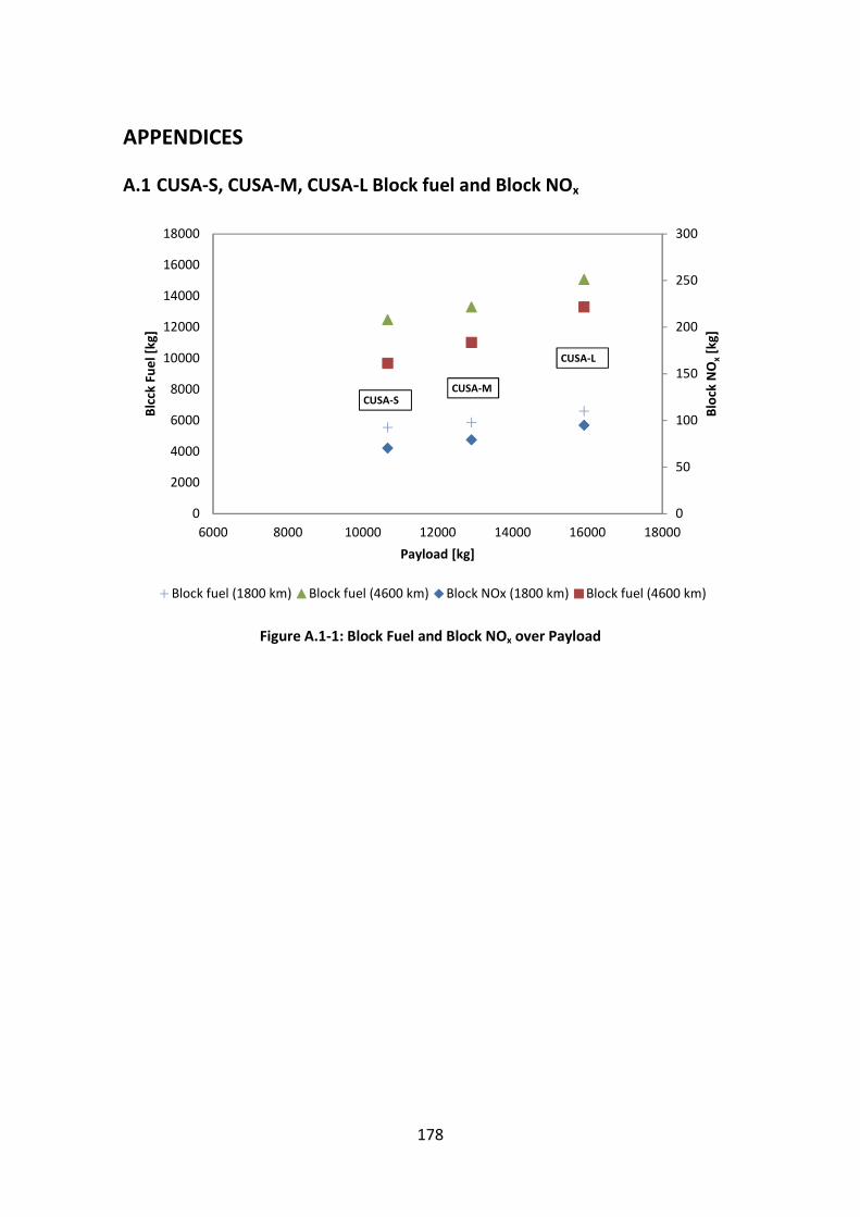
178
APPENDICES
A.1 CUSA-S, CUSA-M, CUSA-L Block fuel and Block NOx
Figure A.1-1: Block Fuel and Block NOx over Payload
0
50
100
150
200
250
300
0
2000
4000
6000
8000
10000
12000
14000
16000
18000
6000 8000 10000 12000 14000 16000 18000
Blo
ckN
Ox
[kg]
Blc
ckFu
el[
kg]
Payload [kg]
Block fuel (1800 km) Block fuel (4600 km) Block NOx (1800 km) Block fuel (4600 km)
CUSA-SCUSA-M
CUSA-L

179
A.2 Trajectory plots for 1800 km mission
Figure A.2-1: CUSA-M engine FF variation during flight (1800 km)
Figure A.2-2: CUSA-M engine TET variation during flight (1800 km)
0
0.2
0.4
0.6
0.8
1
1.2
1.4
1.6
0
2000
4000
6000
8000
10000
12000
0 2000 4000 6000 8000 10000
Fue
lFlo
w[k
g/s]
Alt
itu
de
[m]
Time [seconds]
Flight profile Engine FF
0
200
400
600
800
1000
1200
1400
1600
1800
0
2000
4000
6000
8000
10000
12000
0 2000 4000 6000 8000 10000
TET
[K]
Alt
itu
de
[m]
Time [seconds]
Flight profile Engine TET Clean

180
Figure A.2-3: CUSA-L engine FF variation during flight (1800 km)
Figure A.2-4: CUSA-L engine TET variation during flight (1800 km)
0
0.2
0.4
0.6
0.8
1
1.2
1.4
1.6
1.8
2
0
2000
4000
6000
8000
10000
12000
0 2000 4000 6000 8000 10000
Fue
lFlo
w[k
g/s]
Alt
itu
de
[m]
Time [seconds]
Flight profile Engine FF
0
200
400
600
800
1000
1200
1400
1600
1800
2000
0
2000
4000
6000
8000
10000
12000
0 2000 4000 6000 8000 10000
TET
[K]
Alt
itu
de
[m]
Time [seconds]
Flight profile Engine TET Clean
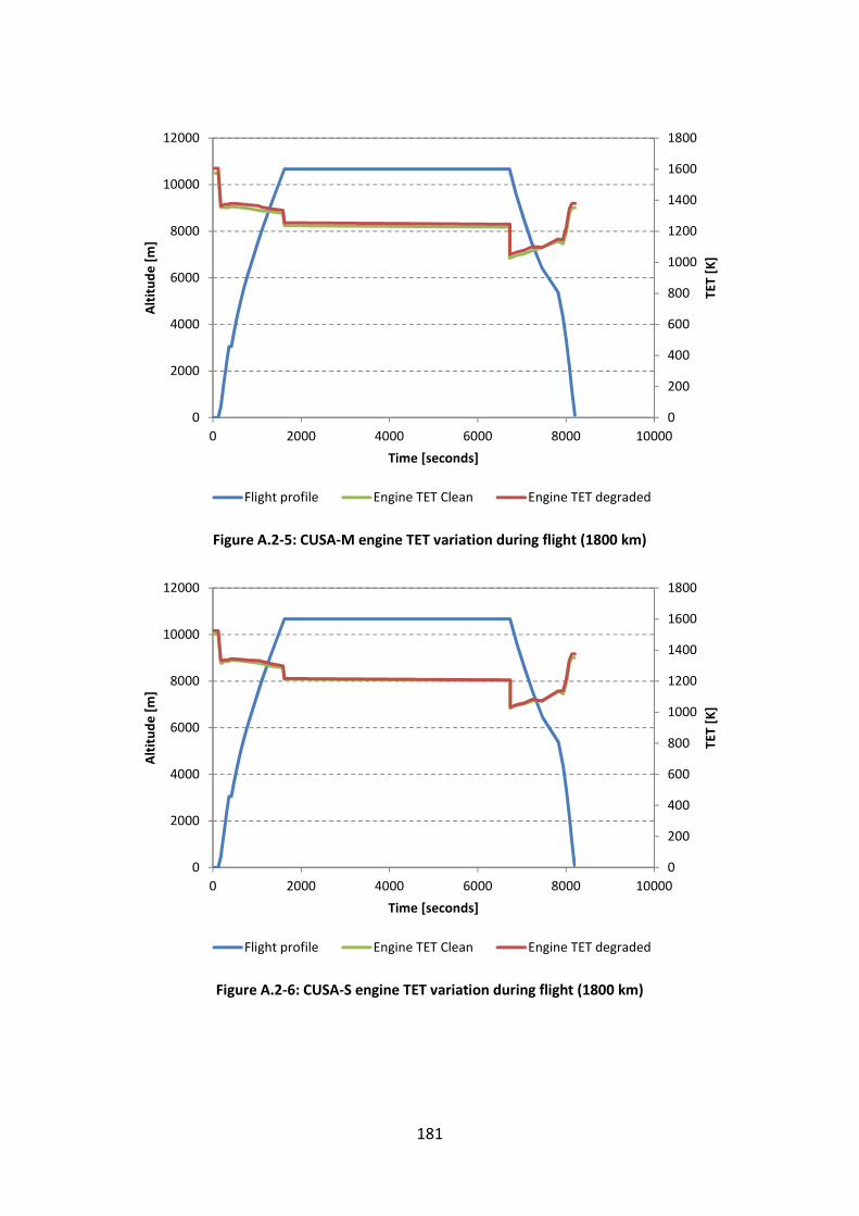
181
Figure A.2-5: CUSA-M engine TET variation during flight (1800 km)
Figure A.2-6: CUSA-S engine TET variation during flight (1800 km)
0
200
400
600
800
1000
1200
1400
1600
1800
0
2000
4000
6000
8000
10000
12000
0 2000 4000 6000 8000 10000
TET
[K]
Alt
itu
de
[m]
Time [seconds]
Flight profile Engine TET Clean Engine TET degraded
0
200
400
600
800
1000
1200
1400
1600
1800
0
2000
4000
6000
8000
10000
12000
0 2000 4000 6000 8000 10000
TET
[K]
Alt
itu
de
[m]
Time [seconds]
Flight profile Engine TET Clean Engine TET degraded
182
A.3 Trajectory plots for 4600 km mission
Figure A.3-1: CUSA-S engine FF variation during flight (4600 km)
Figure A.3-2: CUSA-S engine TET variation during flight (4600 km)
0
0.2
0.4
0.6
0.8
1
1.2
1.4
0
2000
4000
6000
8000
10000
12000
0 2000 4000 6000 8000 10000 12000 14000 16000 18000 20000 22000
Fue
lFlo
w[k
g/s]
Alt
itu
de
[m]
Time [seconds]
Flight profile Engine FF
0
200
400
600
800
1000
1200
1400
1600
0
2000
4000
6000
8000
10000
12000
0 2000 4000 6000 8000 10000 12000 14000 16000 18000 20000 22000
TET
[K]
Alt
itu
de
[m]
Time [seconds]
Flight profile Engine TET Clean
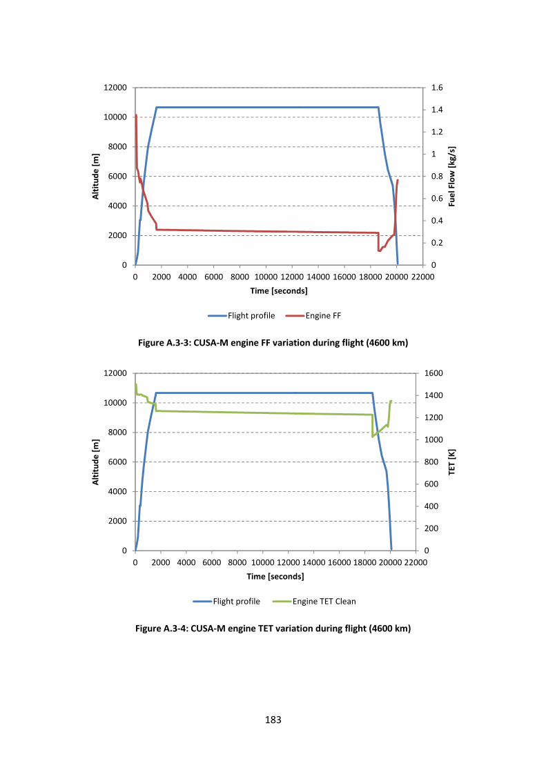
183
Figure A.3-3: CUSA-M engine FF variation during flight (4600 km)
Figure A.3-4: CUSA-M engine TET variation during flight (4600 km)
0
0.2
0.4
0.6
0.8
1
1.2
1.4
1.6
0
2000
4000
6000
8000
10000
12000
0 2000 4000 6000 8000 10000 12000 14000 16000 18000 20000 22000
Fue
lFlo
w[k
g/s]
Alt
itu
de
[m]
Time [seconds]
Flight profile Engine FF
0
200
400
600
800
1000
1200
1400
1600
0
2000
4000
6000
8000
10000
12000
0 2000 4000 6000 8000 10000 12000 14000 16000 18000 20000 22000
TET
[K]
Alt
itu
de
[m]
Time [seconds]
Flight profile Engine TET Clean

184
Figure A.3-5: CUSA-S engine TET variation during flight (4600 km)
Figure A.3-6: CUSA-L engine TET variation during flight (4600 km)
0
200
400
600
800
1000
1200
1400
1600
1800
0
2000
4000
6000
8000
10000
12000
0 2000 4000 6000 8000 10000 12000 14000 16000 18000 20000 22000
TET
[K]
Alt
itu
de
[m]
Time [seconds]
Flight profile Engine TET Clean Engine TET degraded
0
200
400
600
800
1000
1200
1400
1600
1800
2000
0
2000
4000
6000
8000
10000
12000
0 2000 4000 6000 8000 10000 12000 14000 16000 18000 20000 22000
TET
[K]
Alt
itu
de
[m]
Time [seconds]
Flight profile Engine TET Clean Engine TET degraded