
Dynamic water vapour sorption properties of wood treated with glutaraldehyde
Upload
khangminh22Category
view
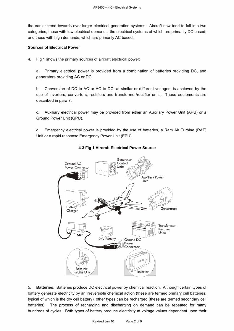
2download
0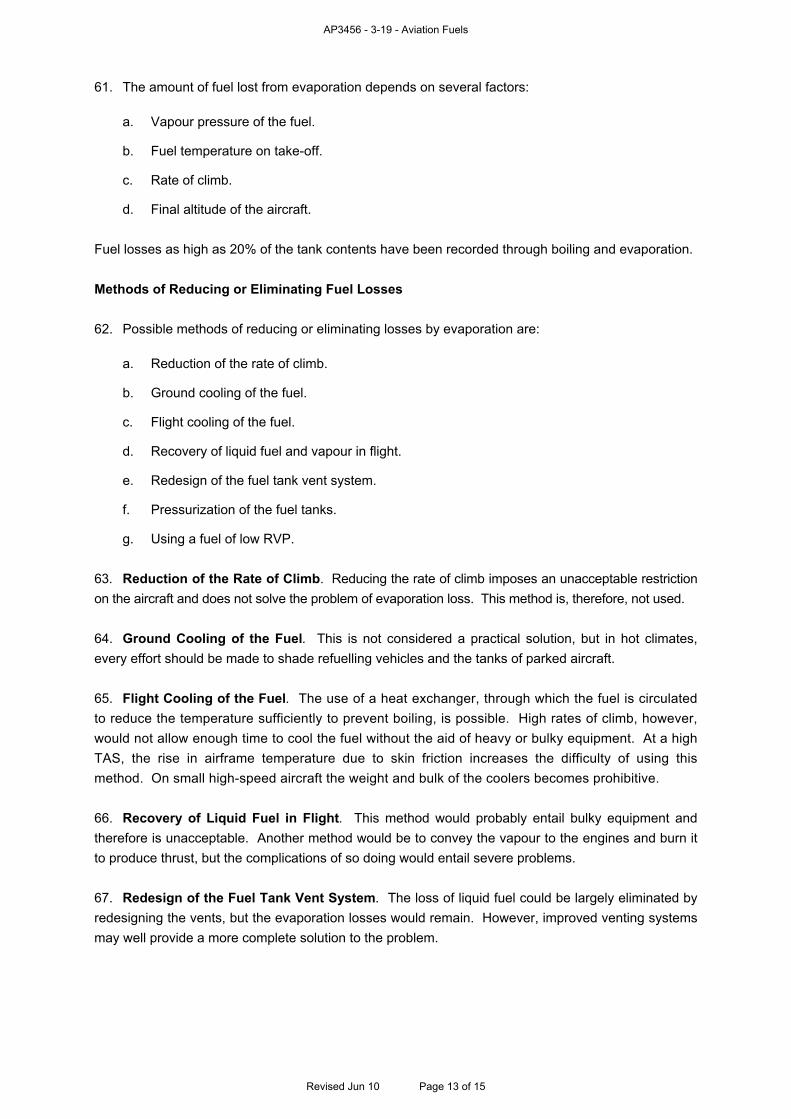
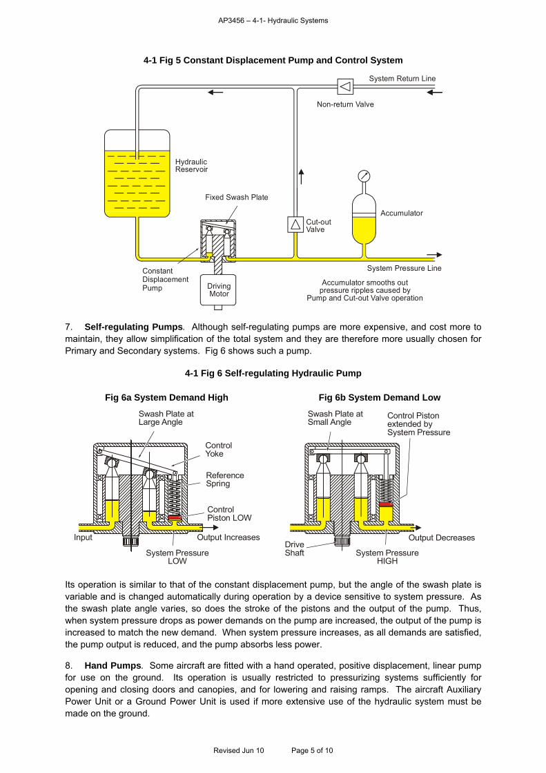
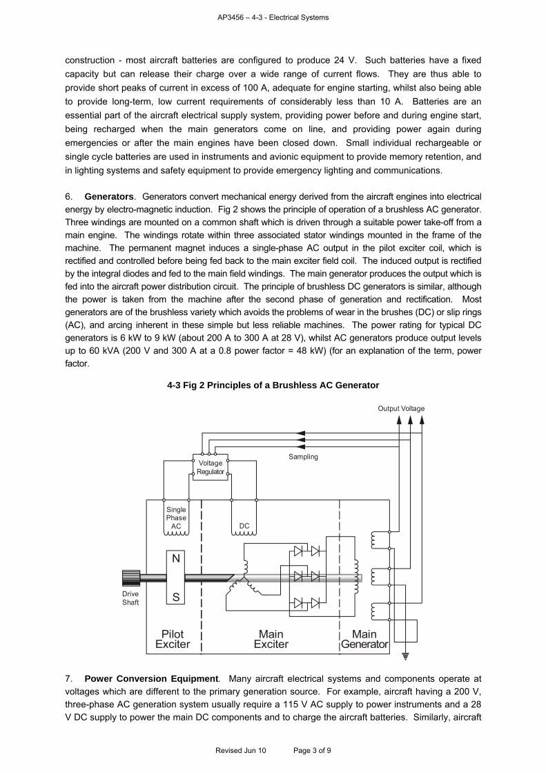
AP3456 - 3-19 - Aviation Fuels
61. The amount of fuel lost from evaporation depends on several factors:
a. Vapour pressure of the fuel. b. Fuel temperature on take-off. c. Rate of climb. d. Final altitude of the aircraft.
Fuel losses as high as 20% of the tank contents have been recorded through boiling and evaporation. Methods of Reducing or Eliminating Fuel Losses 62. Possible methods of reducing or eliminating losses by evaporation are:
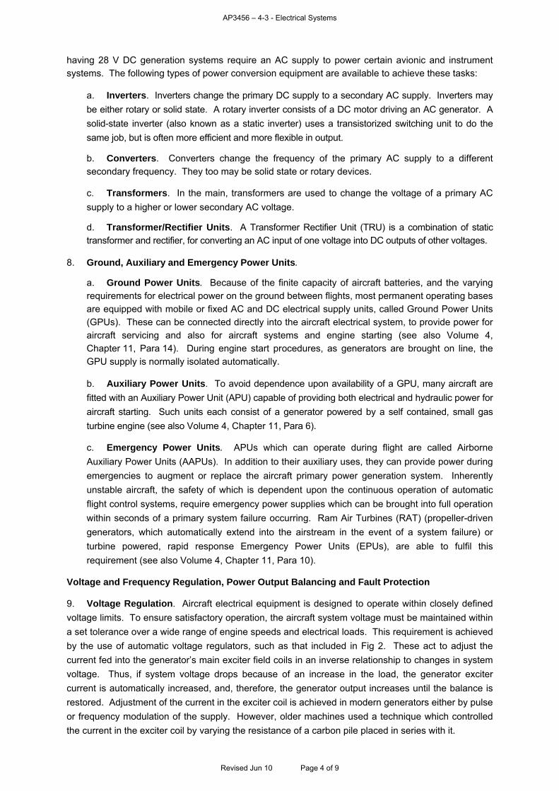
a. Reduction of the rate of climb. b. Ground cooling of the fuel. c. Flight cooling of the fuel. d. Recovery of liquid fuel and vapour in flight. e. Redesign of the fuel tank vent system. f. Pressurization of the fuel tanks. g. Using a fuel of low RVP.
63. Reduction of the Rate of Climb. Reducing the rate of climb imposes an unacceptable restriction on the aircraft and does not solve the problem of evaporation loss. This method is, therefore, not used. 64. Ground Cooling of the Fuel. This is not considered a practical solution, but in hot climates, every effort should be made to shade refuelling vehicles and the tanks of parked aircraft. 65. Flight Cooling of the Fuel. The use of a heat exchanger, through which the fuel is circulated to reduce the temperature sufficiently to prevent boiling, is possible. High rates of climb, however, would not allow enough time to cool the fuel without the aid of heavy or bulky equipment. At a high TAS, the rise in airframe temperature due to skin friction increases the difficulty of using this method. On small high-speed aircraft the weight and bulk of the coolers becomes prohibitive. 66. Recovery of Liquid Fuel in Flight. This method would probably entail bulky equipment and therefore is unacceptable. Another method would be to convey the vapour to the engines and burn it to produce thrust, but the complications of so doing would entail severe problems. 67. Redesign of the Fuel Tank Vent System. The loss of liquid fuel could be largely eliminated by redesigning the vents, but the evaporation losses would remain. However, improved venting systems may well provide a more complete solution to the problem.
Revised Jun 10 Page 13 of 15
AP3456 - 3-19 - Aviation Fuels
68. Pressurization of the Fuel Tanks. There are two ways in which fuel tanks can be pressurized:
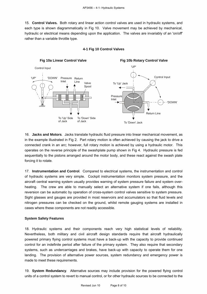
a. Complete Pressurization. Keeping the absolute pressure in the tanks greater than the vapour pressure at the maximum fuel temperature likely to be encountered eliminates all losses. However, with gasoline type fuels, a pressure of about 55 kPa absolute would have to be maintained at altitude and the tanks would be subjected to a pressure differential of 45 kPa at 50,000 feet. The disadvantage is that this would involve stronger and heavier tanks, and a strengthened structure to hold them. b. Partial Pressurization. This prevents all liquid loss and reduces the evaporation loss. It also involves strengthening the tanks and structure, and the fitting of relief valves.
69. Use of a Fuel of Low RVP. The disadvantage of kerosene lies chiefly in its limitations at low temperatures. At temperatures below –47 ºC, the waxes in the fuel begin to crystallize and may lead to blockage of filters unless remedial measures such as fuel heating are introduced. Starting difficulties under very cold conditions would also have to be solved. Fuel System Icing Inhibitor 70. All service turbine-powered aircraft should use fuel containing FSII to inhibit fuel system icing. If fuel containing FSII is not available, aircrew should follow local instructions. In general, operation is usually permitted for a limited period, provided that:
a. The maximum period on fuel not containing FSII does not exceed 14 days, and is followed by an equivalent period on inhibited fuel. b. The risk of ice formation is acceptable to the operational commander. c. Uplifts of non-inhibited fuel are recorded in the aircraft F700.
71. Present in all turbine fuels is a microbiological fungus called Cladasporium Resinae. This fungus can grow rapidly in the presence of water and warmth, forming long green filaments which can block fuel system components. The waste products of the fungus can be corrosive, especially to the fuel tank sealing components. The inclusion of FSII in fuel suppresses fungal growth. Aviation Turbine Fuel Additives 72. Aircrew should be aware of the following important fuel additives:
a. AL 41. AL 41 is an FSII additive. b. AL 61. AL 61 is an additive which enhances lubricity. In addition, AL 61 will prevent pipeline corrosion (AVTUR has its own in-built anti-corrosive agents). c. AL 48. AL 48 is an additive which is present in all turbine fuels obtained from RAF sources. Its purpose is to inhibit fuel system icing, prevent fungal growth, and add to the lubricity of the fuel. It is a blend of AL 41 and AL 61. If it is not possible to obtain fuel containing AL 48, the additive can be mixed with the fuel (in correct proportions) prior to refuelling. If that is not possible, then the limitations stated in paras 56 and 70 apply.
Revised Jun 10 Page 14 of 15

AP3456 - 3-19 - Aviation Fuels
Revised Jun 10 Page 15 of 15
73. AL 48 may be held at some units in a ready-blended state. Some foreign countries do not allow this ready-blended mix to be stored. In such circumstances, if aircrew are offered AL 41 plus AL 61, this equates to AL 48 when blended in the correct proportions. 74. During distillation and early stages of transportation, F35 and F34 are the same. At some point during delivery to military users, AL 48 (or AL 41 plus AL 61) is blended with F35 to transform it into F34. Approved Types of Gas Turbine Fuel 75. Information on the fuels approved (both normal fuel and emergency substitutes) for a particular in-service aircraft type should be obtained from the 'Release to Service' ('Deviations from the Military Aircraft Release' for RN aircraft), the Aircrew Manual, or from the Service engineering sponsor, as appropriate. Refer to Table 1 for examples of some types of fuel that are available and to Volume 8, Chapter 4 for details on airworthiness and aircrew documentation.

AP3456 - 3-20 - Engine Health Monitoring and Maintenance
CHAPTER 20 - ENGINE HEALTH MONITORING AND MAINTENANCE Contents Page Introduction.............................................................................................................................................. 1 Factors Affecting Component Life and Engine Overhaul........................................................................ 1 Engine Usage, Condition and Maintenance Systems (EUCAMS).......................................................... 2 Engine Health Monitoring ........................................................................................................................ 2 Engine Maintenance................................................................................................................................ 4 Table of Figures 3-20 Fig 1 Trend Graph of Bearing Wear................................................................................................ 2 3-20 Fig 2 Magnetic Plug Debris ............................................................................................................. 3 3-20 Fig 3 A typical High Ratio By-pass Modular Engine ....................................................................... 4 Introduction 1. The condition and, consequently, performance of aircraft engines deteriorates with their use, and such deterioration can eventually lead to failure. Other factors such as fatigue and creep can also eventually lead to failure. It is therefore necessary to carry out maintenance on engines, to ensure that failures do not occur and that airworthiness and performance do not deteriorate below acceptable operational levels. The maintenance consists of routinely monitoring condition and performance, replacing components which have degraded to an unacceptable level and also replacing components which are nearing the end of their safe fatigue lives. Such maintenance must be carefully controlled both to optimize the operational availability of engines and to minimize costs. This Chapter considers the factors affecting engine lifing and maintenance, and it covers the main techniques used to monitor engine health and the effectiveness of engine maintenance. Maintenance and Health Monitoring are topics which apply not only to engines but also to airframe systems and helicopter transmissions. Therefore, although this chapter refers only to the gas turbine engine, its content is relevant to the majority of aircraft mechanical components. Factors Affecting Component Life and Engine Overhaul 2. Fatigue and Creep. Creep is a phenomenon which occurs in most materials exposed for long periods to high temperature and high stresses. A form of molecular distortion takes place which can eventually lead to failure. It affects the components of the turbine operating at high temperatures and at high centrifugal and axial loads. The adverse effects of creep occurring during normal operation of the engine are avoided by careful design. Engine components are also subjected to three different forms of fatigue. Aerofoil sections within the engine are subjected to high cycle fatigue (HCF) caused by exposure to perturbations in the gas flow. As with creep, the effects of HCF are avoided by careful design. Thermal cycles occurring in the engine lead to thermal fatigue in the hot section, but other causes of damage are invariably more significant in setting the safe lives of affected components. The stresses caused by engine acceleration during start up and operation cause low cycle fatigue (LCF) in components of the main rotating assembly. Because it cannot be detected, this form of fatigue is a major factor in calculating engine life. 3. Degradation. During normal engine operation, a number of factors adversely affect the condition of a gas turbine. These include corrosion, erosion and mechanical wear, the effects of which are normally monitored by routine inspection or testing. Where possible, a policy of condition-based maintenance is applied to engines. That is, maintenance is only carried out when justified by the perceived condition of the engine. Such on condition maintenance (OCM) ensures that any critical components which have deteriorated to the limits of acceptability are replaced.
Revised Jun 10 Page 1 of 5

AP3456 - 3-20 - Engine Health Monitoring and Maintenance
Engine Usage, Condition and Maintenance Systems (EUCAMS) 4. Concepts. To implement a condition-based maintenance policy, it is necessary to monitor engine usage, condition and performance. EUCAMS therefore record life cycles consumed, detect incipient failures, monitor wear and corrosion, and measure engine performance against a standard. The majority of monitoring techniques are able to detect failure or imminent failure of a component, and they therefore provide essential information to the crew. However, equally useful is their ability to provide a consistent stream of incremental data, the correlation of which allows trends in component condition to be observed. Such trend analysis will reveal incipient failure of a component or its gradual loss of effectiveness. A typical trend graph is shown at Fig 1. It depicts the rate of wear of a bearing in an engine. Remedial action will be initiated when the trend line crosses the threshold value shown, and the observed condition of the engine thus justifies deeper maintenance being carried out. The monitoring process allows OCM to be carried out at a time convenient to operational commitments. Thus little loss of availability is incurred and costs can be minimized. Without OCM, at best the availability of the aircraft would be lost to allow the engine to be removed more frequently for deep inspections to take place, or at worst the engine bearing would fail in flight with no obvious prior symptoms of its state of distress.
3-20 Fig 1 Trend Graph of Bearing Wear
'Wear-in' Phase
Effective Safe Working Life
'Wear-out' Phase
Failure
(Mas
s of
deb
ris c
aptu
red
per l
itre
insp
ectio
n cy
cle)
0 50 100Engine Running Hours
(x 10,000)
Wea
r Rat
e
5. Low Cycle Fatigue Monitoring. Counters (LCFCs) monitoring low cycle fatigue are fitted to most major engines. They are analogous to airframe fatigue meters and continuously calculate and display LCF usage. For engines not fitted with LCFCs, information from other instrumentation or from technical records must be analysed and factored to produce equivalent cycle consumption data. Engine Health Monitoring 6. Optical Inspection Techniques. The components which are continually washed by the gas flow through an engine are prone to corrosion and erosion. Combustion chambers and turbine blades are usually made from materials resistant to these effects. However, compressors and their casings are often manufactured from aluminium or magnesium alloys which are very susceptible to corrosion. Also, the ingestion of hard foreign objects causes erosion and can cause severe damage to the compressor blades. Even if such damage does not cause an immediate reduction in performance, it can, if not repaired, cause subsequent failure. Routine inspection for such erosion, corrosion and damage can normally be carried out with the naked eye or with the assistance of fibre optic viewers inserted into the compressor through ports in the casing.
Revised Jun 10 Page 2 of 5
AP3456 - 3-20 - Engine Health Monitoring and Maintenance
7. Magnetic Particle Detectors. The majority of engine bearings are constructed from steel. As the bearings wear, ferrous particles are washed away into the engine lubrication system. Small magnetic plugs (mag-plugs) placed strategically in the lubrication system trap the particles. Subsequent analysis of this debris can reveal not only its source but also the rate of wear occurring. Fig 2 shows a debris sample captured by a magnetic plug positioned in an engine auxiliary gearbox. The thin spines of debris are typical products of gear tooth wear. Most magnetic plugs incorporate electrical contacts which become bridged by any significant build-up of debris, thus closing the circuit and activating a warning caption in the cockpit.
3-20 Fig 2 Magnetic Plug Debris
Oil Seal
Magnet
Typical debris comprising minute particles and largerslivers of material
Bayonet TypeLock Pin
KnurledHandle
8. Filter Inspections. Non-ferrous debris washed into the lubrication system filters can provide similar information upon the location and rate of wear as does ferrous debris trapped by the magnetic particle detectors. Although analysis of filter debris is not so relevant for gas turbine engines which have few non-ferrous components washed by the lubrication oil, the technique is an important tool for use in monitoring the health of piston engines and helicopter transmissions. 9. Spectrometric Oil Analysis. Magnetic plugs and oil filters are relatively coarse detection devices, whereas spectrometric analysis of the oil will reveal even minute trace materials. Spectrometric oil analysis programmes (SOAP) are used to monitor samples of lubrication oils and hydraulic fluids taken from aircraft at periodic intervals. The light spectra obtained when such samples are burned show the existence and quantity of trace elements, and this information can be related to the materials used in construction of the related systems. The trend in levels of such trace elements is an indication of wear rates and, as with other monitoring techniques, this information set against action threshold values allows OCM to be undertaken well before system health becomes critical. 10. Vibration Analysis. The rotating components in a gas turbine are dynamically balanced on assembly to minimize vibration. Any subsequent wear or damage to these components will lead to an increase in vibration of the engine. By using suitable test equipment at routine intervals, it is possible to detect quite small changes in the frequency and amplitude of such vibrations, and the changing vibration signature of an engine can be used as a health monitoring parameter. Most aircraft types have engine vibration analysis equipment permanently installed. If vibration levels suddenly exceed preset limits during flight, the crew can be alerted.
Revised Jun 10 Page 3 of 5
AP3456 - 3-20 - Engine Health Monitoring and Maintenance
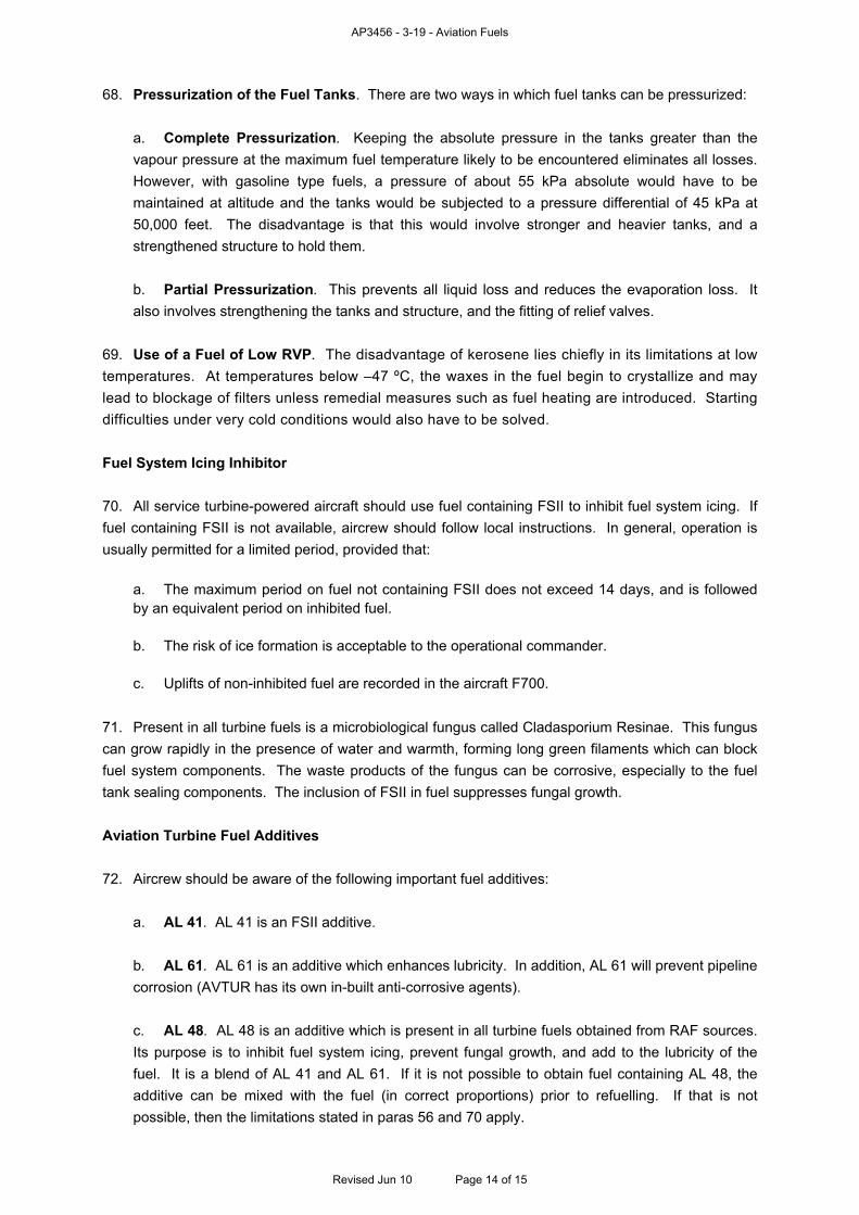
11. In-flight Performance Monitoring. Monitoring the performance of engines in flight offers the considerable advantage of observing the engine in its designed-for condition whilst avoiding the loss of aircraft availability and the inadequacies of ground testing. The automatic recording of engine parameters available through such systems as Engine Monitoring System (EMS) and Aircraft Integrity Monitoring System (AIMS) allows engine performance data to be recorded and performance figures computed. The system imposes no additional work load upon the crew and does not require specific test sorties to be flown. Signals representing engine performance parameters, such as temperatures and pressures, fuel flows, thrust or torque and air temperatures, air speeds and pressure altitudes, are picked off from the aircraft instrumentation. Such signals are computed in real time and presented as performance assurance to the crew. They are also recorded to be down-loaded after completion of the flight and used for health trend analysis and condition monitoring. Engine Maintenance 12. The scheduled deep routine maintenance of engines and other major equipments is termed overhaul. Those components which have degraded to the limit of acceptability and those nearing the end of their safe working lives are replaced at this point. The overhaul periodicity is therefore dictated by the component with the shortest safe working life. Engines based on a modular design avoid this restriction, because each module may be removed and replaced without necessitating the whole engine to be removed from service. The majority of engines are either fully or semi-modular, and can therefore be repaired and reconditioned by module replacement at unit level. In addition, many modules can themselves be repaired and overhauled at unit level. 13. Modular Design. A modular engine comprises several major line replacement assemblies, each of which can be maintained independent of the others at differing periodicities. Fig 3 shows the modules within a typical high by-pass gas turbine engine. Although the repair of such engines at unit level requires additional financial outlay in tooling, training and facilities, it affords many advantages including a reduction in the number of spare engines required, increased unit skill levels and better in-service control of engine assets.
3-20 Fig 3 A typical High Ratio By-pass Modular Engine
Reverse FlowCombustion Chamber
Combustor TurbineModule
Gas GeneratorModule
Fan ReductionGearing
Fan Module
Fan
Slots in Combustion Chamber
Fuel Injector/Igniter
AccesoryGearboxModule
Revised Jun 10 Page 4 of 5

AP3456 - 3-20 - Engine Health Monitoring and Maintenance
Revised Jun 10 Page 5 of 5
14. Engine Testing. After significant maintenance activities have been carried out on a gas turbine engine, testing is required to ensure that required performance criteria are met. The tests may be carried out in an engine test facility or with the engine installed in the aircraft. Unless the testing is required for simple diagnostic purposes or is necessary to confirm system integrity after installation, engine testing in an aircraft is rarely cost effective and, more significantly, removes the aircraft from operational availability. Most units are therefore equipped with uninstalled engine test facilities (UETF). These consist of a fixed stand with a gimbal mounted frame into which the engine is installed. Reaction between the stand and the frame when the engine is running allows thrust levels to be measured. The whole is surrounded by an acoustic enclosure fitted with noise attenuating air intake and exhaust systems. An adjacent control cabin provides adequate environmental protection for the testing technicians, and it includes the controls, instrumentation and recording equipment necessary for detailed testing and diagnosis to take place.
OFFICIAL
UNCONTROLLED DOCUMENT WHEN PRINTED
AP3456 The Central Flying School (CFS)
Manual of Flying
Version 10.0 – 2018
Volume 4 – Aircraft Systems
AP3456 is sponsored by the Commandant Central Flying School

OFFICIAL
UNCONTROLLED DOCUMENT WHEN PRINTED
Contents
Commandant CFS - Foreword
Introduction and Copyright Information
AP3456 Contact Details
Chapter Revised
4-1 Hydraulic Systems May 2010
4-2 Pneumatic Systems May 2010
4-3 Electrical Systems May 2010
4-4 Powered Flying Controls May 2010
4-5 Cabin Pressurization and Air Conditioning
Systems May 2010
4-6 Undercarriages May 2010
4-7 Automatic Flight Control Systems May 2010
4-8 Fire Warning and Extinguisher Systems Jun 2010
4-9 Ice and Rain Protection Systems May 2010
4-10 Aircraft Fuel Systems May 2010
4-11 Secondary Power Systems, Auxiliary and
Emergency Power Units May 2010
4-12 Engine Starter Systems May 2010

AP3456 – 4-1- Hydraulic Systems
CHAPTER 1 - HYDRAULIC SYSTEMS Contents Page
Introduction.............................................................................................................................................. 1 Principles ................................................................................................................................................. 1 Typical System ........................................................................................................................................ 3 System Components ............................................................................................................................... 4 System Safety Features .......................................................................................................................... 8 Limiting Factors ....................................................................................................................................... 9 System Health Monitoring and Maintenance .......................................................................................... 9 Table of Figures
4-1 Fig 1 Simple Closed Hydraulic System............................................................................................. 2 4-1 Fig 2 Simplified Pump-powered Hydraulic System........................................................................... 2 4-1 Fig 3 Typical Hydraulic Power System ............................................................................................. 3 4-1 Fig 4 Principle of a Swash Plate Pump............................................................................................. 4 4-1 Fig 5 Constant Displacement Pump and Control System................................................................. 5 4-1 Fig 6 Self-regulating Hydraulic Pump ............................................................................................... 5 4-1 Fig 7 Typical Hydraulic Accumulator................................................................................................. 6 4-1 Fig 8 Construction of a Reservoir ..................................................................................................... 6 4-1 Fig 9 Principle of a Non-return Valve ................................................................................................ 7 4-1 Fig 10 Control Valves........................................................................................................................ 8 Introduction
1. Hydraulic power has unique characteristics which influence its selection to power aircraft systems instead of electrics and pneumatics, the other available secondary power systems. The advantages of hydraulic power are that:
a. It is capable of transmitting very high forces.
b. It has rapid and precise response to input signals.
c. It has good power to weight ratio.
d. It is simple and reliable.
e. It is not affected by electro-magnetic interference.
Although it is less versatile than present generation electric/electronic systems, hydraulic power is the normal secondary power source used in aircraft for operation of those aircraft systems which require large power inputs and precise and rapid movement. These include flying controls, flaps, retractable undercarriages and wheel brakes. Principles
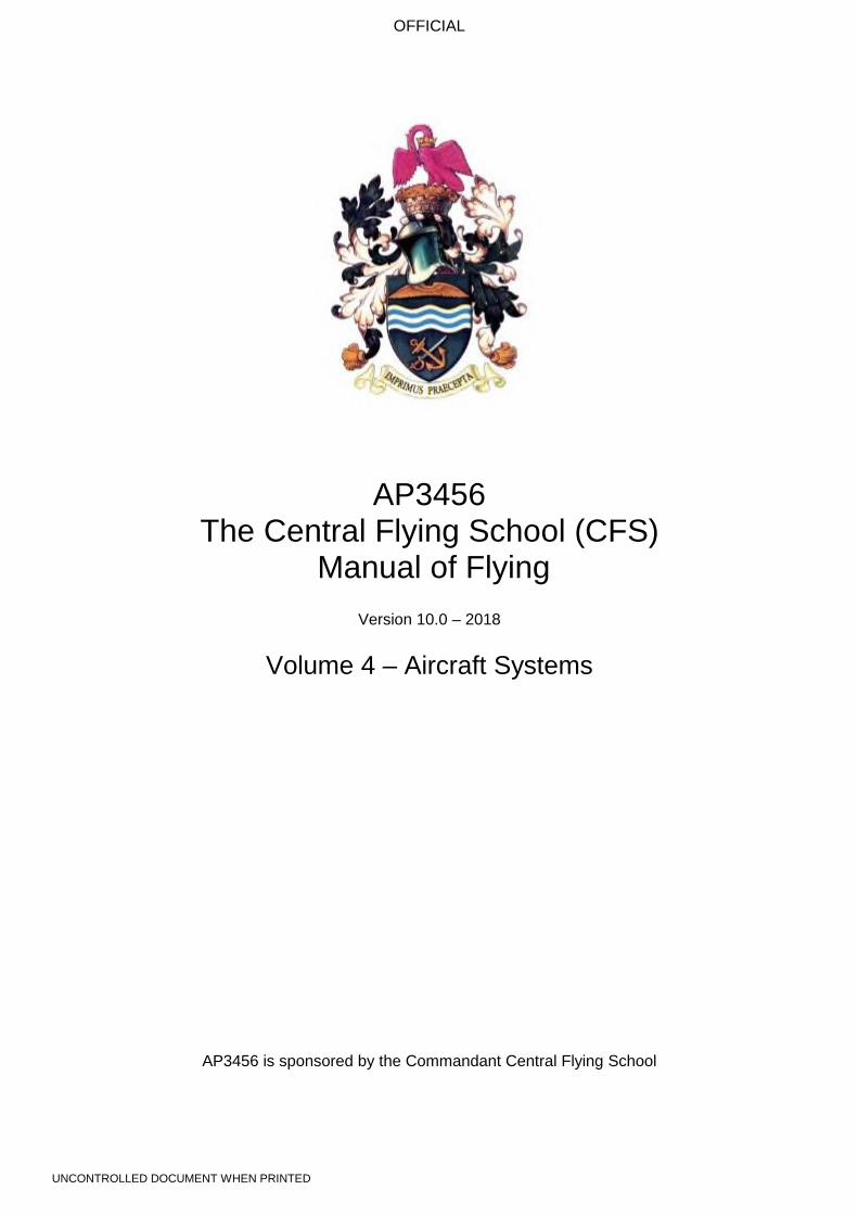
2. Basic Power Transmission. A simple practical application of hydraulic power is shown in Fig 1 which depicts a closed system typical of that used to operate light aircraft wheel brakes. When the force on the master cylinder piston is increased slightly by light operation of the brake pedals, the slave piston will extend until the brake shoe contacts the brake drum. This restriction will prevent
Revised Jun 10 Page 1 of 10
AP3456 – 4-1- Hydraulic Systems
further movement of the slave and the master cylinder. However, any increase in force on the master cylinder will increase pressure in the fluid, and it will therefore increase the braking force acting on the shoes. When braking is complete, removal of the load from the master cylinder will reduce hydraulic pressure, and the brake shoe will retract under spring tension. The system is limited both by the relatively small driving force which in practice can be applied to the master cylinder and the small distance which it can be moved.
4-1 Fig 1 Simple Closed Hydraulic System
BrakeShoes
Master Cylinder
ReservoirBrake Pedal
Brake Drum
Slave Cylinder
ReturnSpring
Piston
Piston
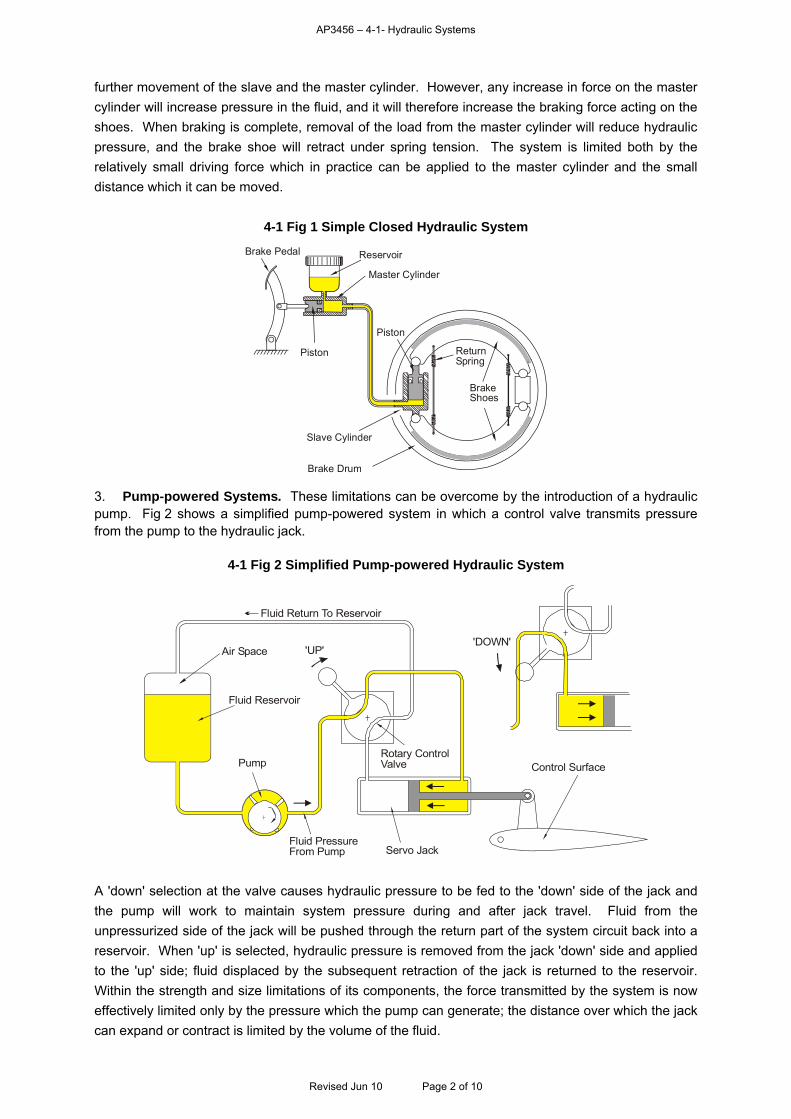
3. Pump-powered Systems. These limitations can be overcome by the introduction of a hydraulic pump. Fig 2 shows a simplified pump-powered system in which a control valve transmits pressure from the pump to the hydraulic jack.
4-1 Fig 2 Simplified Pump-powered Hydraulic System
Fluid Return To Reservoir
'UP'
Rotary ControlValve Control Surface
Servo JackFluid PressureFrom Pump
Pump
Fluid Reservoir
Air Space'DOWN'
A 'down' selection at the valve causes hydraulic pressure to be fed to the 'down' side of the jack and the pump will work to maintain system pressure during and after jack travel. Fluid from the unpressurized side of the jack will be pushed through the return part of the system circuit back into a reservoir. When 'up' is selected, hydraulic pressure is removed from the jack 'down' side and applied to the 'up' side; fluid displaced by the subsequent retraction of the jack is returned to the reservoir. Within the strength and size limitations of its components, the force transmitted by the system is now effectively limited only by the pressure which the pump can generate; the distance over which the jack can expand or contract is limited by the volume of the fluid.
Revised Jun 10 Page 2 of 10
AP3456 – 4-1- Hydraulic Systems
Typical System
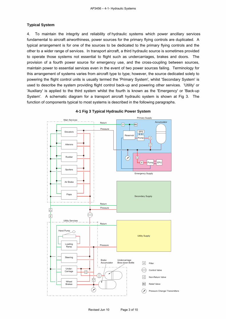
4. To maintain the integrity and reliability of hydraulic systems which power ancillary services fundamental to aircraft airworthiness, power sources for the primary flying controls are duplicated. A typical arrangement is for one of the sources to be dedicated to the primary flying controls and the other to a wider range of services. In transport aircraft, a third hydraulic source is sometimes provided to operate those systems not essential to flight such as undercarriages, brakes and doors. The provision of a fourth power source for emergency use, and the cross-coupling between sources, maintain power to essential services even in the event of two power sources failing. Terminology for this arrangement of systems varies from aircraft type to type; however, the source dedicated solely to powering the flight control units is usually termed the 'Primary System', whilst 'Secondary System' is used to describe the system providing flight control back-up and powering other services. 'Utility' or 'Auxiliary' is applied to the third system whilst the fourth is known as the 'Emergency' or 'Back-up System'. A schematic diagram for a transport aircraft hydraulic system is shown at Fig 3. The function of components typical to most systems is described in the following paragraphs.
4-1 Fig 3 Typical Hydraulic Power System
F
F
F
F
F
RV
RV
EPUPump
Emergency Supply
Elevators
Ailerons
Rudder
Spoilers
Air Brake
Flaps
Return
Pressure
Return
Return
Pressure
Utility Services
Hand Pump
LoadingRamp
Steering
Under-Carriage
WheelBrakes
Pressure
BrakeAccumulator
UndercarriageBlow-down Bottle Filter
Control Valve
Non-Return Valve
Relief Valve
Pressure Change/ Transmitters
Secondary Supply
Utility Supply
Main ServicesAccumulator
Primary Supply
Pump
SPS
Reservoir
Revised Jun 10 Page 3 of 10
AP3456 – 4-1- Hydraulic Systems
System Components
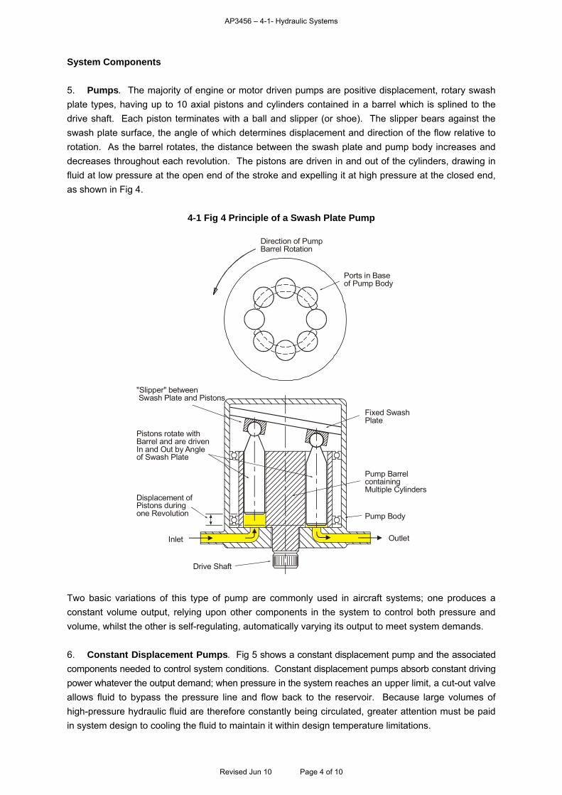
5. Pumps. The majority of engine or motor driven pumps are positive displacement, rotary swash plate types, having up to 10 axial pistons and cylinders contained in a barrel which is splined to the drive shaft. Each piston terminates with a ball and slipper (or shoe). The slipper bears against the swash plate surface, the angle of which determines displacement and direction of the flow relative to rotation. As the barrel rotates, the distance between the swash plate and pump body increases and decreases throughout each revolution. The pistons are driven in and out of the cylinders, drawing in fluid at low pressure at the open end of the stroke and expelling it at high pressure at the closed end, as shown in Fig 4.
4-1 Fig 4 Principle of a Swash Plate Pump
Fixed Swash Plate
Pump BarrelcontainingMultiple Cylinders
Pump Body
Outlet
Drive Shaft
Inlet
Displacement of Pistons during one Revolution
Pistons rotate withBarrel and are drivenIn and Out by Angleof Swash Plate
"Slipper" between Swash Plate and Pistons
Direction of PumpBarrel Rotation
Ports in Baseof Pump Body
Two basic variations of this type of pump are commonly used in aircraft systems; one produces a constant volume output, relying upon other components in the system to control both pressure and volume, whilst the other is self-regulating, automatically varying its output to meet system demands. 6. Constant Displacement Pumps. Fig 5 shows a constant displacement pump and the associated components needed to control system conditions. Constant displacement pumps absorb constant driving power whatever the output demand; when pressure in the system reaches an upper limit, a cut-out valve allows fluid to bypass the pressure line and flow back to the reservoir. Because large volumes of high-pressure hydraulic fluid are therefore constantly being circulated, greater attention must be paid in system design to cooling the fluid to maintain it within design temperature limitations.
Revised Jun 10 Page 4 of 10
AP3456 – 4-1- Hydraulic Systems
4-1 Fig 5 Constant Displacement Pump and Control System
HydraulicReservoir
Accumulator smooths outpressure ripples caused by
Pump and Cut-out Valve operation
Cut-outValve
Fixed Swash Plate
Non-return Valve
DrivingMotor
System Return Line
ConstantDisplacementPump
System Pressure Line
Accumulator
7. Self-regulating Pumps. Although self-regulating pumps are more expensive, and cost more to maintain, they allow simplification of the total system and they are therefore more usually chosen for Primary and Secondary systems. Fig 6 shows such a pump.
4-1 Fig 6 Self-regulating Hydraulic Pump
Fig 6a System Demand High Fig 6b System Demand Low
Swash Plate atLarge Angle
ControlYoke
ReferenceSpring
ControlPiston LOW
Input
System PressureLOW
Output Increases
DriveShaft
Swash Plate atSmall Angle
System PressureHIGH
Control Piston extended bySystem Pressure
Output Decreases
Its operation is similar to that of the constant displacement pump, but the angle of the swash plate is variable and is changed automatically during operation by a device sensitive to system pressure. As the swash plate angle varies, so does the stroke of the pistons and the output of the pump. Thus, when system pressure drops as power demands on the pump are increased, the output of the pump is increased to match the new demand. When system pressure increases, as all demands are satisfied, the pump output is reduced, and the pump absorbs less power. 8. Hand Pumps. Some aircraft are fitted with a hand operated, positive displacement, linear pump for use on the ground. Its operation is usually restricted to pressurizing systems sufficiently for opening and closing doors and canopies, and for lowering and raising ramps. The aircraft Auxiliary Power Unit or a Ground Power Unit is used if more extensive use of the hydraulic system must be made on the ground.
Revised Jun 10 Page 5 of 10

AP3456 – 4-1- Hydraulic Systems
9. Accumulators. As illustrated in Fig 5, hydraulic systems include an accumulator, the purpose of which is to absorb shocks and sudden changes in system pressure. A typical nitrogen filled hydraulic accumulator is shown in Fig 7.
4-1 Fig 7 Typical Hydraulic Accumulator
Pressure Gauge
and Charging Point
Nitrogen
Input fromPump Output to
System
NRV
Fluid Separatedfrom Nitrogenby Free Piston
Compressibility of the nitrogen allows the accumulator to absorb and smooth out the pressure ripples caused by pump operation and also the sudden changes in pressure caused by operation of components such as jacks and valves. It also acts to maintain pressure, to the limit of its piston movement, when the pump ceases to operate. This facility is used, for example, to maintain aircraft parking brake pressure for long periods. When the hydraulic system is not pressurized by the pumps, the gas pressure is typically 70 Bar (1,000 psi). 10. Reservoir. Hydraulic systems require a reservoir in which the fluid displaced when the servo jacks are retracted is stored until required again. Obviously, the capacity must be designed to accommodate fluid displaced when all the system jacks are retracted simultaneously. The reservoir performs the secondary functions of cooling the fluid and allowing any air absorbed to separate out. The construction of a typical reservoir is shown at Fig 8.
4-1 Fig 8 Construction of a Reservoir
Revised Jun 10 Page 6 of 10
AP3456 – 4-1- Hydraulic Systems
Reservoirs are usually pressurized either with nitrogen or by system hydraulic pressure acting on a piston. This pressure, of between 3 and 7 Bar, prevents the fluid foaming and provides a boost pressure at the pump inlet. A relief valve is fitted to prevent excessive pressure build up due to heating or system malfunction. The body of the reservoir may contain horizontal baffles both to prevent fluid surging during aircraft manoeuvre and to promote de-aeration of returning fluid. 11. Heat Exchangers and Temperature Warning Systems. As described in para 22, hydraulic system performance is adversely affected by the presence of either air or vapour absorbed in or mixed with the fluid, and additional heat exchangers are usually included in high performance systems to keep the fluid well below its vaporization point. Such systems also include temperature sensors and warning systems to alert the crew if excessive temperature excursions do occur. For normal fluids, such warning systems are activated at temperatures of about 100 ºC. 12. Filtration. To prevent fluid leakage and loss of pressure, the clearances between the moving parts of a hydraulic component are minute, and the inclusion of even the smallest particles in the fluid would cause damage to its precise surfaces. High levels of filtration are therefore applied to the fluid. Several filters are included in most systems, so that each major component can be protected from debris generated upstream of it. 13. Pressure and Thermal Relief Valves. The use of a cut-out valve to regulate the output pressure of a constant displacement hydraulic pump was discussed in para 6. Because hydraulic fluid is incompressible and mechanical damage can be caused to components if over-pressurization occurs, further pressure relief valves are situated at critical points in the system. They are frequently termed 'fuses' because of this protective role, and they operate by balancing system pressure against an internal reference spring. If system pressure rises above spring pressure, the valve opens allowing fluid to escape into the system return pipes thus reducing pressure. The valve re-seals automatically once system pressure returns to below the reference level. 14. Non-return Valves. There are areas in most hydraulic systems in which it is necessary to allow fluid to flow to a component but to prevent that fluid returning along the same pipe. Non-return valves are used for this purpose, and several are included in the system in Fig 3. Such valves are similar in construction to relief valves, and the principle of operation is shown at Fig 9. The valve poppet is held closed by a weak internal reference spring. Pressure of fluid flowing in the desired direction can readily overcome spring force, and fluid can therefore flow through the valve almost without restriction. If fluid pressure upstream of the valve is reduced, the poppet snaps closed to prevent a fluid flow reversal.
4-1 Fig 9 Principle of a Non-return Valve
Revised Jun 10 Page 7 of 10
AP3456 – 4-1- Hydraulic Systems
15. Control Valves. Both rotary and linear action control valves are used in hydraulic systems, and each type is shown diagrammatically in Fig 10. Valve movement may be achieved by mechanical, hydraulic or electrical means depending upon the application. The valves are invariably of an 'on/off' rather than a variable throttle type.
4-1 Fig 10 Control Valves
Fig 10a Linear Control Valve Fig 10b Rotary Control Valve
ValveSpool
Control Input
'UP' 'DOWN' ReturnLine
PressureInlet
To Up Sideof Jack
' ' To Down Sideof Jack
' '
Return Line
PressureInlet
To 'Up' Jack
'UP'
To 'Down' Jack
'DOWN'
Control Input
16. Jacks and Motors. Jacks translate hydraulic fluid pressure into linear mechanical movement, as in the example illustrated in Fig 2. Part rotary motion is often achieved by causing the jack to drive a connected crank in an arc; however, full rotary motion is achieved by using a hydraulic motor. This operates on the reverse principle of the swashplate pump shown in Fig 4. Hydraulic pressure is fed sequentially to the pistons arranged around the motor body, and these react against the swash plate forcing it to rotate. 17. Instrumentation and Control. Compared to electrical systems, the instrumentation and control of hydraulic systems are very simple. Cockpit instrumentation monitors system pressure, and the aircraft central warning system usually provides warning of system pressure failure and system over-heating. The crew are able to manually select an alternative system if one fails, although this reversion can be automatic by operation of cross-system control valves sensitive to system pressure. Sight glasses and gauges are provided in most reservoirs and accumulators so that fluid levels and nitrogen pressures can be checked on the ground, whilst remote gauging systems are installed in cases where these components are not readily accessible.
System Safety Features
18. Hydraulic systems and their components reach very high statistical levels of reliability. Nevertheless, both military and civil aircraft design standards require that aircraft hydraulically powered primary flying control systems must have a back-up with the capacity to provide continued control for an indefinite period after failure of the primary system. They also require that secondary systems, such as undercarriages and brakes, have back-up with capacity to operate them for one landing. The provision of alternative power sources, system redundancy and emergency power is made to meet these requirements. 19. System Redundancy. Alternative sources may include provision for the powered flying control units of a control system to revert to manual control, or for other hydraulic sources to be connected to the
Revised Jun 10 Page 8 of 10
AP3456 – 4-1- Hydraulic Systems
failed power system. For this purpose, hydraulically powered primary control systems are powered by at least two hydraulic systems. The power systems are configured to be totally independent of each other so that the failure of one, for whatever reason, does not jeopardize operation of the other. 20. Emergency Power. Assurance that system operation can be continued for indefinite periods, after failure of one hydraulic pump, requires that two other pumps’ sources are provided. One is usually a pump driven from the aircraft normal secondary power system. The other may be a pump powered by an emergency source such as an Emergency Power Unit or a Ram Air Turbine (see Volume 4, Chapter 11). For systems requiring only a limited duration of operation under emergency power, such as wheel brakes and undercarriages, the stored energy of accumulators or 'blow down' nitrogen cylinders (see Volume 4, Chapter 2) situated in the system is used. Limiting Factors
21. Several factors influence the effectiveness of hydraulic systems, and some of these are expanded upon below. The adverse influence of such factors is minimized by careful design and maintenance of the systems and selection of the most appropriate fluids. There is no ideal solution in these cases, and the chosen solution is invariably a compromise between performance and the other factors. 22. Temperature and Aeration. As hydraulic fluid nears its boiling point, fluid vapour and absorbed air are given off and carried in the fluid. The presence of gas from this or any other source introduces an unacceptable degree of compressibility into the columns of fluid in the system, causing operation to become sluggish and erratic. In high performance systems, preventive design features, such as reservoirs to prompt and contain the separation of gases from the fluid, and the provision of adequate cooling, are backed by careful system maintenance to minimize the likelihood of air entering the system. 23. Contamination. As discussed in para 12, contamination of fluid with even minute particles will damage and degrade systems performance. Careful systems replenishment avoids this problem, and adequate system filtration ensures that particles introduced into or generated by the system are removed before they can be carried through the system into components where they will cause mechanical damage. Many hydraulic fluids are also hygroscopic to a small degree. Again, careful system replenishment and routine monitoring of the fluid will minimize the possibility of water absorption. 24. Flammability. Certain hydraulic fluids are highly flammable, and leaks or spillage present a significant fire risk, although appropriate husbandry precautions can minimize this. Non-flammable fluids are used almost universally in the systems of passenger-carrying aircraft, despite them being highly corrosive. 25. Hazardous Liquids. All hydraulic fluids are active solvents and many are also corrosive. They are therefore hazardous to both aircraft surfaces and materials and to human beings. Non-flammable fluids are particularly hazardous. Careful handling during maintenance is necessary to avoid this problem. System Health Monitoring and Maintenance
26. The maintenance activities carried out on hydraulic systems include first aid action to disclose, contain and rectify component failure, and fluid monitoring used to observe overall system health trends and to detect component degradation.
Revised Jun 10 Page 9 of 10

AP3456 – 4-1- Hydraulic Systems
Revised Jun 10 Page 10 of 10
27. Filter Checks. As shown in Fig 4, filters are strategically placed throughout an aircraft hydraulic system. A component failure may not immediately manifest itself as a system malfunction, but routine inspection of the filter tell-tale devices will reveal that a failure has occurred. The filter will also prevent debris migrating around the system to cause secondary failures. Maintenance action can then be taken to restore and safeguard system integrity. 28. Fluid Monitoring. A systematic sampling programme of fluid contamination is carried out on the majority of aircraft. The periodic chemical and spectral analysis of fluids serves to indicate failure trends in particular components and the contamination and degradation of system fluid. Based on these trends, timely component replacement can be taken, thus preventing eventual failure occurring in the air, and reducing repair costs.
AP3456 – 4-2 - Pneumatic Systems
CHAPTER 2 - PNEUMATIC SYSTEMS Contents Page Introduction.............................................................................................................................................. 1 Unique Characteristics ............................................................................................................................ 1 Typical Applications................................................................................................................................. 2 Pressure Energy Storage ........................................................................................................................ 2 Compression ........................................................................................................................................... 3 Pressure Energy Transfer ....................................................................................................................... 4 Heat Energy Transfer .............................................................................................................................. 4 Table of Figures 4-2 Fig 1 Simplified Undercarriage Blow-down System.......................................................................... 2 4-2 Fig 2 Hydraulic Accumulator Performance ....................................................................................... 3 4-2 Fig 3 Augmented Lift Devices ........................................................................................................... 4 Introduction 1. The use of air as a medium to transmit energy and to do work offers many advantages to the aircraft designer. Although some early applications of pneumatics have been superseded by hydraulics or electrics, as technological advance has overcome the initial disadvantages of these alternative media, the inherent and unique advantages offered by the use of air and its main constituent gases ensure that pneumatics will remain one of these three fundamental power transmission media for aviation use into the foreseeable future. Unlike hydraulics and electrics, pneumatic power is generated and stored in a number of different ways each relevant to the specific end use, and it is therefore not appropriate to consider pneumatic power generation as a specific topic. Instead, the principle characteristics of the medium, and the techniques and equipment configurations used to exploit those characteristics for specific applications, are discussed in the following paragraphs. Unique Characteristics 2. The ready availability of high temperature, high pressure air as a by product of the propulsion system, or even of aircraft forward motion, provides an extremely cost effective source of heat or pressure energy. Systems which utilize such energy sources include cabin and cockpit pressurization and heating, airframe and engine de-icing and the augmentation of flying controls. Similarly, air can be cycled through a system and exhausted overboard after use, without penalty. Such 'total loss' systems are extremely space and weight efficient, and this factor influences the choice of air above other energy transmission media which usually require to be contained in a closed circuit system for technical or environmental reasons. Such 'total loss' air systems include engine starting and cabin and equipment conditioning. Again, although air will support combustion, its properties are not affected by temperature extremes, and it can therefore be used in power transmission applications where high temperatures, fire risks or chemical reaction rule out the use of normal hydraulic fluids. Pneumatic systems are therefore often used in engine nozzle and thrust reverser operating systems. 3. The ready compressibility of air offers both advantages and disadvantages for its use. The advantages are that air can be compressed and used to store the resultant pressure energy either long term for subsequent use or short term to absorb shocks or sudden changes in pressure levels. However, because of this same compressibility, pneumatics are not suitable for use in control systems requiring precise, rapid response movements.
Revised Jun 10 Page 1 of 4
AP3456 – 4-2 - Pneumatic Systems
Typical Applications 4. The applications of pneumatics can be categorized under four main headings. These are:
a. Pressure energy storage. b. Compression. c. Pressure energy transfer. d. Heat energy transfer.
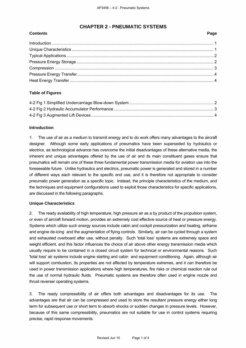
Details of several of the major systems which utilize pneumatics in these ways are discussed in the relevant chapters of this Volume, whilst other specific examples are given below. Pressure Energy Storage 5. Undercarriage Blow-down Systems. Because hydraulic fluids cannot normally be compressed, energy cannot be stored within simple hydraulic systems. However, this disadvantage can be overcome by the integration of pneumatics into hydraulic systems. An application of such hydro-pneumatics is the undercarriage emergency blow-down system. A schematic diagram of such a system is at Fig 1. In this particular example, release of high pressure air (nitrogen is normally used to reduce the risk of a hydraulic oil fire) from the blow-down bottle enables the undercarriage lowering system to be pressurized sufficiently to lower the undercarriage in the event of hydraulic malfunction or failure. Other similar systems feed nitrogen directly into the hydraulic fluid. Although such an arrangement avoids the disadvantage of pressurizing only a set volume of fluid (that displaced within the accumulator by the gas), it does impose a considerable penalty during subsequent fault rectification, because the gas is absorbed into the fluid necessitating replacement of all of the fluid within the hydraulic system.
4-2 Fig 1 Simplified Undercarriage Blow-down System
UndercarriageJacks
Operation of Emergency Selectorallows fluid under gas pressure to
'blow down' Jacks until Down Locksengage. (No retraction is possible
after blow down.)
UndercarriageSelector Valves
Non-return Valve
EmergencyReservoir
High Pressure Nitrogen
Fluid/Gas Separating Piston
Emergency Selector coupledto 'Down' Hydraulic
Return Selector Valve
HydraulicReturn
HydraulicPressure
Revised Jun 10 Page 2 of 4
AP3456 – 4-2 - Pneumatic Systems
6. Fire Extinguishers and Liferafts. There are many other applications in which compressed gases are stored for eventual use as an emergency or occasional energy source. Amongst the most relevant are the use of nitrogen to pressurize engine fire extinguisher bottles for eventual use in propelling extinguishant on to a fire, and the use of carbon dioxide stored with liferafts and life jackets for subsequent release to inflate these items when they are required. Compression
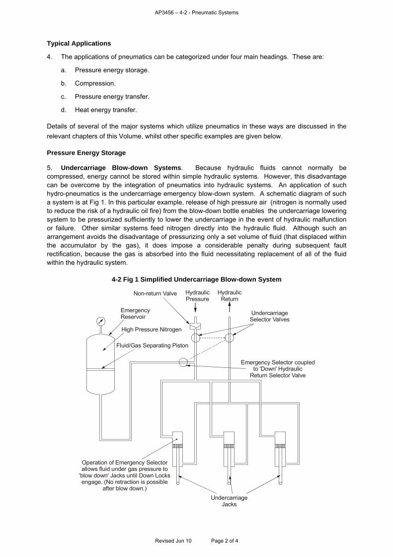
7. Shock Absorbers. Hydraulic systems are frequently configured to use the compressibility of air to absorb shocks and sudden changes in system pressure. The system shown in Fig 1 includes a nitrogen filled hydraulic accumulator. The functions of the accumulator are to smooth out any sudden changes in systems pressure caused by operation of components such as jacks and to protect the system from sudden peaks in pressure which occur when system valves close. The graph at Fig 2a shows the typical pressure variation in a system without an accumulator, whilst Fig 2b shows the comparable variation when an accumulator is used. Hydro-pneumatic shock absorbers, based on a similar principle, are widely used in many undercarriages, and these are discussed in detail in the relevant chapter of this Volume.
4-2 Fig 2 Hydraulic Accumulator Performance
a System Pressure Fluctuations
without Accumulatorb System Pressure Fluctuations
with Accumulator
Ripple Dampenedby Gas Pressurein Accumulator
Nominal SystemPressure
Minimum AcceptablePressure Level
Maximum SafePressure Level
Safety ReliefValve Operates
Ripple caused byoperation of PumpPressure Control
System
Sub-system sValve opens
elected
Time
Pres
sure
Time 8. Seal Inflation. The doors and canopies of pressurized aircraft require to be sealed effectively, to maintain pressurization within the fuselage and to prevent the escape of unacceptable volumes of conditioning air. The sealing of the irregular gaps between such doors and hatches and their frames imposes a significant problem, and seals inflated by compressed air are often used in such situations. The omni-directional force applied to such seals by low pressure air is ideal for such applications, and the air can readily be tapped from the aircraft pressurization system.
Revised Jun 10 Page 3 of 4
AP3456 – 4-2 - Pneumatic Systems
Revised Jun 10 Page 4 of 4
Pressure Energy Transfer
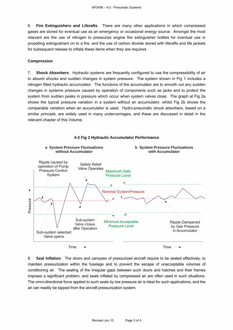
9. Augmented (Blown) Lift Devices and Flying Controls. Within the restrictions of current aerodynamic knowledge and technology, all VSTOL aircraft must be provided with devices which impart energy to the surrounding air stream to provide lift and control forces in the absence of adequate forward air speed. Purpose-designed VSTOL aircraft usually use vectored lift/thrust systems which also provide flight control forces. However, the use of conventional aerodynamic devices enhanced for STOL operation by ducting high energy air streams over them is an effective alternative solution. Fig 3 shows such a system in schematic form.
4-2 Fig 3 Augmented Lift Devices
Fig 3a Wing in Normal Flight
Fig 3b Wing with Blown Flap Extended
When selected, high energy air istapped from the engines and blows overthe upper surface of the flap preventingair stream separation and increasingthe velocity of the air flow over the surface
10. Starters. The abundant availability of high pressure air from gas turbine engines and APUs allows its use for engine starting. This is achieved either by impinging upon the turbine directly, and thus spinning up the engine, or more usually by driving a small turbine which is connected to the main engine through suitable gearing. Both of these applications are dealt with in the appropriate Chapter of this Volume (see Volume 4, Chapter 12). Heat Energy Transfer
11. Air Conditioning and Ice Protection. The compressors of most high performance gas turbine engines are designed to produce volumes of air in excess of engine requirements. Such air at high pressure and at temperatures up to 300 ºC is available through engine compressor bleeds, and, as well as being used in cabin and cockpit pressurization systems, the air provides an effective source of heat for air conditioning and for the ice protection of aerofoils and engine intakes. Both applications are dealt with in Volume 4, Chapter 5.

AP3456 – 4-3 - Electrical Systems
CHAPTER 3 - ELECTRICAL SYSTEMS Contents Page
Introduction.............................................................................................................................................. 1 Sources of Electrical Power .................................................................................................................... 2 Voltage and Frequency Regulation, Power Output Balancing and Fault Protection .............................. 4 Power Distribution Systems .................................................................................................................... 6 System Control and Protection Devices.................................................................................................. 7 Typical Generating Systems ................................................................................................................... 8 Table of Figures
4-3 Fig 1 Aircraft Electrical Power Source .............................................................................................. 2 4-3 Fig 2 Principles of a Brushless AC Generator .................................................................................. 3 4-3 Fig 3 Schematic of a Simple AC Generator Supply .......................................................................... 5 4-3 Fig 4 Split-busbar System (Primary DC Power Source) ................................................................... 7 4-3 Fig 5 Single Channel DC System...................................................................................................... 8 4-3 Fig 6 DC Twin Channel Split-busbar System.................................................................................... 8 4-3 Fig 7 AC Twin Channel Split-busbar System.................................................................................... 9 Introduction
1. Early aircraft had no electrical equipment other than the engine ignition system. Power for this was provided by an engine driven magneto. The introduction of lighting and communications equipment necessitated this source to be augmented, first by a pre-charged battery, and subsequently by on-board generation systems using wind driven direct current (DC) generators fitted with crude regulators to maintain a constant 12 volts output irrespective of the flying speed. As soon as developments in engine power permitted, these systems were replaced by engine driven generators rotating at relatively constant speed and controlled by more effective regulators. Ever-increasing on-board electrical loads necessitated the use of bigger diameter, and therefore heavier, cables. 2. The power output of an electrical generation system is a product of voltage and current. However, electrical cable diameter is dictated by current and the resistance of the cable material, not by voltage. Therefore, within the practical limitations of cable insulation, the higher the system voltage the higher the power capacity for the same physical cable size. The need to control weight led to the use of higher DC voltage systems. Although DC high voltage systems have been tried, the problems of arcing at altitude, and the size of batteries required, rendered such developments impractical. All military aircraft systems now conform to the present 24 volt international standard for aircraft DC systems (note: DC generators and systems are normally rated at 28 V, to maintain a positive charge state to the 24 V batteries). However, alternating current (AC) generation systems are not constrained by the same disadvantages as DC systems; consequently, AC systems were introduced into aircraft to meet the higher on-board power requirements common in the 1960s. The evolution of these systems has led to the 200 V, three-phase, 400 Hz generator systems, now standard in both military and civil aircraft. Components using the AC output include three-phase devices (e.g. motors), single-phase 115 V devices (e.g. radio equipment) and secondary supplies such as transformers. 3. The introduction of solid-state technology to avionic equipment has significantly reduced the power requirements in those aircraft not equipped with high-powered radars, and this has reversed
Revised Jun 10 Page 1 of 9
AP3456 – 4-3 - Electrical Systems
the earlier trend towards ever-larger electrical generation systems. Aircraft now tend to fall into two categories; those with low electrical demands, the electrical systems of which are primarily DC based, and those with high demands, which are primarily AC based. Sources of Electrical Power
4. Fig 1 shows the primary sources of aircraft electrical power:
a. Primary electrical power is provided from a combination of batteries providing DC, and generators providing AC or DC.
b. Conversion of DC to AC or AC to DC, at similar or different voltages, is achieved by the use of inverters, converters, rectifiers and transformer/rectifier units. These equipments are described in para 7. c. Auxiliary electrical power may be provided from either an Auxiliary Power Unit (APU) or a Ground Power Unit (GPU). d. Emergency electrical power is provided by the use of batteries, a Ram Air Turbine (RAT) Unit or a rapid response Emergency Power Unit (EPU).
4-3 Fig 1 Aircraft Electrical Power Source
5. Batteries. Batteries produce DC electrical power by chemical reaction. Although certain types of battery generate electricity by an irreversible chemical action (these are termed primary cell batteries, typical of which is the dry cell battery), other types can be recharged (these are termed secondary cell batteries). The process of recharging and discharging on demand can be repeated for many hundreds of cycles. Both types of battery produce electricity at voltage values dependent upon their
Revised Jun 10 Page 2 of 9
AP3456 – 4-3 - Electrical Systems
construction - most aircraft batteries are configured to produce 24 V. Such batteries have a fixed capacity but can release their charge over a wide range of current flows. They are thus able to provide short peaks of current in excess of 100 A, adequate for engine starting, whilst also being able to provide long-term, low current requirements of considerably less than 10 A. Batteries are an essential part of the aircraft electrical supply system, providing power before and during engine start, being recharged when the main generators come on line, and providing power again during emergencies or after the main engines have been closed down. Small individual rechargeable or single cycle batteries are used in instruments and avionic equipment to provide memory retention, and in lighting systems and safety equipment to provide emergency lighting and communications. 6. Generators. Generators convert mechanical energy derived from the aircraft engines into electrical energy by electro-magnetic induction. Fig 2 shows the principle of operation of a brushless AC generator. Three windings are mounted on a common shaft which is driven through a suitable power take-off from a main engine. The windings rotate within three associated stator windings mounted in the frame of the machine. The permanent magnet induces a single-phase AC output in the pilot exciter coil, which is rectified and controlled before being fed back to the main exciter field coil. The induced output is rectified by the integral diodes and fed to the main field windings. The main generator produces the output which is fed into the aircraft power distribution circuit. The principle of brushless DC generators is similar, although the power is taken from the machine after the second phase of generation and rectification. Most generators are of the brushless variety which avoids the problems of wear in the brushes (DC) or slip rings (AC), and arcing inherent in these simple but less reliable machines. The power rating for typical DC generators is 6 kW to 9 kW (about 200 A to 300 A at 28 V), whilst AC generators produce output levels up to 60 kVA (200 V and 300 A at a 0.8 power factor = 48 kW) (for an explanation of the term, power factor.
4-3 Fig 2 Principles of a Brushless AC Generator
VoltageRegulator
Output Voltage
Sampling
SinglePhase
AC
PilotExciter
MainExciter
MainGenerator
DC
N
SDriveShaft
7. Power Conversion Equipment. Many aircraft electrical systems and components operate at voltages which are different to the primary generation source. For example, aircraft having a 200 V, three-phase AC generation system usually require a 115 V AC supply to power instruments and a 28 V DC supply to power the main DC components and to charge the aircraft batteries. Similarly, aircraft
Revised Jun 10 Page 3 of 9
AP3456 – 4-3 - Electrical Systems
having 28 V DC generation systems require an AC supply to power certain avionic and instrument systems. The following types of power conversion equipment are available to achieve these tasks:
a. Inverters. Inverters change the primary DC supply to a secondary AC supply. Inverters may be either rotary or solid state. A rotary inverter consists of a DC motor driving an AC generator. A solid-state inverter (also known as a static inverter) uses a transistorized switching unit to do the same job, but is often more efficient and more flexible in output.
b. Converters. Converters change the frequency of the primary AC supply to a different secondary frequency. They too may be solid state or rotary devices.
c. Transformers. In the main, transformers are used to change the voltage of a primary AC supply to a higher or lower secondary AC voltage.
d. Transformer/Rectifier Units. A Transformer Rectifier Unit (TRU) is a combination of static transformer and rectifier, for converting an AC input of one voltage into DC outputs of other voltages.
8. Ground, Auxiliary and Emergency Power Units.
a. Ground Power Units. Because of the finite capacity of aircraft batteries, and the varying requirements for electrical power on the ground between flights, most permanent operating bases are equipped with mobile or fixed AC and DC electrical supply units, called Ground Power Units (GPUs). These can be connected directly into the aircraft electrical system, to provide power for aircraft servicing and also for aircraft systems and engine starting (see also Volume 4, Chapter 11, Para 14). During engine start procedures, as generators are brought on line, the GPU supply is normally isolated automatically.
b. Auxiliary Power Units. To avoid dependence upon availability of a GPU, many aircraft are fitted with an Auxiliary Power Unit (APU) capable of providing both electrical and hydraulic power for aircraft starting. Such units each consist of a generator powered by a self contained, small gas turbine engine (see also Volume 4, Chapter 11, Para 6).
c. Emergency Power Units. APUs which can operate during flight are called Airborne Auxiliary Power Units (AAPUs). In addition to their auxiliary uses, they can provide power during emergencies to augment or replace the aircraft primary power generation system. Inherently unstable aircraft, the safety of which is dependent upon the continuous operation of automatic flight control systems, require emergency power supplies which can be brought into full operation within seconds of a primary system failure occurring. Ram Air Turbines (RAT) (propeller-driven generators, which automatically extend into the airstream in the event of a system failure) or turbine powered, rapid response Emergency Power Units (EPUs), are able to fulfil this requirement (see also Volume 4, Chapter 11, Para 10).
Voltage and Frequency Regulation, Power Output Balancing and Fault Protection 9. Voltage Regulation. Aircraft electrical equipment is designed to operate within closely defined voltage limits. To ensure satisfactory operation, the aircraft system voltage must be maintained within a set tolerance over a wide range of engine speeds and electrical loads. This requirement is achieved by the use of automatic voltage regulators, such as that included in Fig 2. These act to adjust the current fed into the generator’s main exciter field coils in an inverse relationship to changes in system voltage. Thus, if system voltage drops because of an increase in the load, the generator exciter current is automatically increased, and, therefore, the generator output increases until the balance is restored. Adjustment of the current in the exciter coil is achieved in modern generators either by pulse or frequency modulation of the supply. However, older machines used a technique which controlled the current in the exciter coil by varying the resistance of a carbon pile placed in series with it.
Revised Jun 10 Page 4 of 9
AP3456 – 4-3 - Electrical Systems
10. Frequency Regulation. The output frequencies of AC generators are dependent upon their speed of rotation. For satisfactory equipment operation, it is imperative that the electrical system frequency is controlled precisely. As the initial drive will originate from an engine auxiliary gearbox, it must remain steady irrespective of variations in engine power settings. The drive shaft will, therefore, go through an intermediate device termed a Constant Speed Drive Unit (CSDU). This will maintain the drive to the generator at a constant rpm (a CSDU would not be required on aircraft fitted with constant speed engines). Fig 3 shows a schematic layout of a simple AC generator supply.
4-3 Fig 3 Schematic of a Simple AC Generator Supply
Engine Auxiliary Gearbox
CSDU ACGenerator
Generator ControlRelay
VoltageRegulator
FrequencyController
FieldRelay
ProtectionUnit
ACBusbar
200 V400 Hz3-Phase
Drive Shafts
Where a CSDU and generator are designed and built as a single unit, it is termed an Integrated Drive Generator (IDG). CSDU and IDG systems utilize electro-mechanical or electro-hydraulic couplings, which work on the principle of sensing variation in system frequency and adjusting generator speed to maintain a constant output irrespective of the input drive speed (within system parameters). The CSDU and IDG systems are able to control frequency within 1%. 11. Balancing of DC Generators. In systems utilizing two or more generators, it is essential that each generator produces an equal output. This is achieved by interconnecting their respective voltage regulators so that the output of each generator is adjusted to balance with those of the others. 12. Parallel Operation of AC Generators. The balancing of AC generators requires not only that the load should be shared, but also that voltage, frequency and phase angles be synchronized. Load sharing is achieved automatically by comparing the level of current flowing from each generator and increasing the output of the more lightly loaded machine until a balance is achieved. Paralleling of generators is achieved automatically by control circuits which sense the frequency and phase angle of each. When the frequencies and phase angles of two generators are matched, bus-tie contactors between them close, thus inter-connecting their frequency control circuits. The control devices for each generator are usually located in dedicated Control and Protection Units (CPUs). 13. Fault Protection. The distribution circuits of both AC and DC generation systems require the addition of protection devices to prevent generator or consumer unit malfunctions from damaging equipment and endangering the aircraft. Typical examples of the malfunctions for which protection is provided include over and under-voltage, over and under-frequency, short circuits (line to line and line to earth faults), phase sequence (three-phase AC only), and reverse current (DC only). The protection devices act to disconnect the relevant generator from the distribution busbar and also to de-excite the generator.
Revised Jun 10 Page 5 of 9

AP3456 – 4-3 - Electrical Systems
Power Distribution Systems
ble generated power to be made available at the power-consuming quipment, an organized form of distribution throughout the aircraft is essential. The precise manner
, the output from the generating sources is coupled to one or more w impedance conductors, referred to as busbars. Busbars are usually located at central points in an
ne, but it must lso work under abnormal conditions. Power to equipment should be maintained, if possible, during primary
ices which are needed after an emergency landing or crash. These might include inertia switch operated fire extinguishers and emergency
uired to ensure safe flight during in-flight emergency situations, such as radio and instrument supplies. They are
ssential Services. Non-essential services are those which are not essential to flight
and may be isolated during an in-flight emergency, either by manual or automatic action.
14. General. In order to enaewill vary dependent upon aircraft type, and the location of consumer components. Aircraft power distribution systems are configured to allow the maximum flexibility in their management if a component or systems failure occurs. 15. Busbars. In most types of aircraftloaircraft, in junction boxes or distribution panels, and provide a convenient point from which supplies can be taken to the consumer unit. Busbars vary in form. In a simple system, a busbar may be a strip of interlinked terminals. In a more complex system, main busbars might be thick metal strips (usually copper) to which input and output supply connections can be made; subsidiary busbars might be flexible copper wire. Busbars are insulated from the main structure and provided with protective covering. 16. Split-busbar Systems. The function of a distribution system is primarily a simple oapower source failures, and faults on the distribution system should have minimum effect on system functioning. These requirements are met in a combined manner by paralleling generators, where appropriate, by providing adequate circuit protection devices, and by arranging for faulty components to be isolated from the distribution system. In addition, it is usual to split busbars and distribution circuits into sections in order to power particular consumer components. The principle of the split-busbar system (see Fig 4) is that consumer services are divided into three categories of importance. If a generation system failure occurs, the distribution system can be progressively modified (manually or automatically) to maintain power supplies to essential consumer loads whilst shedding non-essential loads. The three categories of load are defined as follows:
a. Vital Services. Vital services are those serv
lighting. These services are fed directly from the main and emergency batteries.
b. Essential Services. Essential services are those services which are req
connected to busbars in such a way that they can always be supplied from a generator or from batteries.
c. Non-e
Revised Jun 10 Page 6 of 9
AP3456 – 4-3 - Electrical Systems
4-3 Fig 4 Split-busbar System (Primary DC Power Source)
Non-essentialDC Services
Bus-tieRelay
DC Generators
No 1DC Busbar
No 1
No 1Inverter
No 2 ACBusbar
No 1 ACBusbar
No 3 (Static)Inverter
BatteryBusbar
Batteries
IsolationRelay
No 2DC Busbar
Non-essentialDC Services
Non-essentialAC Services
EssentialAC Services
Vital DCServices
No 2
No 2Inverter
System Control and Protection Devices
17. Control Devices. In aircraft electrical installations, the function of initiating and subsequently controlling the operating sequences of the circuitry is performed principally by switches and relays. A switch is a device designed to complete or interrupt an electrical circuit safely and efficiently as and whenever required. Switches exist to meet a wide range of applications. They may be operated manually or automatically by mechanical means or at predetermined values of pressure, temperature, time or force. Relays are remotely controlled electrical devices capable of switching one or more circuits. Used extensively in electrical and avionic systems, relays are available in a wide range of physical configurations to meet an equally wide range of performance criteria. 18. Protection Devices. An abnormal condition, or fault, may arise in an electrical circuit for a variety of reasons. If allowed to persist, the fault may cause damage to equipment, failure of essential power supplies, fire, or loss of life. It is, therefore, essential to include protection devices in electrical circuits to minimize damage, and safeguard essential supplies, under such fault conditions as over-voltage, over-current or reverse current. The protection devices used include fuses, circuit breakers and reverse current cut-outs (RCCOs). A fuse is a thermal device, designed to protect cables and components against short circuits and overload currents by providing a weak link in the circuit. Rupture of the fuse gives evidence of a system’s malfunction, and, after correction of the fault, the fuse can be replaced. Circuit breakers isolate faulty circuits by means of a mechanical trip, operated by thermal or electro-mechanical means. They can be readily reset in flight, if accessible, after clearance or isolation of the fault. An RCCO senses the difference in voltage between the generator and its busbar. Its contacts remain closed whilst the voltage of the generator is higher than that of the busbar, but open if this situation is reversed.
Revised Jun 10 Page 7 of 9
AP3456 – 4-3 - Electrical Systems
Typical Generating Systems 19. Single Channel DC System. The simplified schematic diagram at Fig 5 shows a single channel system typical of that used in a single-engine training aircraft. It is a simple system, with many automatic features designed to reduce the workload of an inexperienced pilot. The system comprises a brushed DC generator feeding the single busbar through a diode rectifier. The generator is controlled by a carbon pile voltage regulator, and protected by high-current and over-volt relays. The aircraft battery is connected to the busbar through a contactor operated by the battery master switch. This is a two-way feed, allowing the battery to charge when the busbar is energized by the DC generator. The battery contactor is deactivated automatically when an external power supply is connected to the aircraft, or in the event of a crash.
4-3 Fig 5 Single Channel DC System
Over VoltCut-out
Rectifier
High CurrentCut-out
VoltageRegulator
Single Busbar
Non-essentialServices
VitalServices
VitalBusbar
CrashSwitch
BatteryContactor
Battery
BatteryMasterSwitch External
PowerSocket
ExternalPower
Contactor
EssentialServices
GeneratorDC
20. Twin Channel, Split-busbar DC System. The diagram at Fig 6 shows a twin channel, split-busbar system, typical of that used in a twin-engine aircraft with more than one crew member. The diagram has been simplified by excluding the control and protection devices which are present in such a system. The DC generators each feed a discrete busbar connecting non-essential consumer units. Both also feed the essential busbar, as do the batteries. Thus, in the event of a malfunction, power to essential DC consumers can be maintained, in preference to non-essential services. The generators also supply two inverters, which provide AC power to the non-essential AC services. Power from the essential busbar is converted to AC by a third inverter, to feed essential AC consumers. Vital services are powered direct from the battery busbar.
4-3 Fig 6 DC Twin Channel Split-busbar System
No 1 Generator
EssentialAC Services
No 3Inverter
ExternalPower
No 1Inverter
EssentialDC Services
Essential DC Busbar
Batteries
Battery BusbarNon-essentialDC Services
No 1 DC Busbar
Non-essentialAC Services
AC Busbar
No 2 Generator
No 2Inverter
Non-essentialDC Services
No 2 DC Busbar
Vital DCServices
Revised Jun 10 Page 8 of 9
AP3456 – 4-3 - Electrical Systems
Revised Jun 10 Page 9 of 9
21. AC Twin Channel, Split-busbar System. The simplified diagram at Fig 7 shows a twin channel, split-busbar system, typical of that used in a twin-engine combat aircraft with more than one crew member. The two AC generators are regulated by separate, but cross-related, control units. Each AC generator supplies power to an AC busbar. The busbars can be interconnected (if the frequency and phase of each supply are synchronized). Each AC busbar supplies a TRU, which then feeds its respective DC busbars. These can be interconnected, if necessary, and they feed the non-essential services. The TRUs also feed the essential DC busbar which can be interconnected with the battery busbar if necessary. Thus, all similar busbars can be interconnected, but both AC and DC non-essential consumers can be disconnected if a systems malfunction significantly reduces generator capacity. Note that the battery charger is supplied from an AC busbar and, in effect, acts as a TRU.
4-3 Fig 7 AC Twin Channel Split-busbar System
Contactor
Bus-tieRelay
ExternalPowerContactor
No 1 DC Bus
Essential DC Bus Vital DC Bus
Contactor
BatteryNo 2 DC Bus
No 3 AC Bus
No 2 AC BusNo 1 AC Bus
CrashRelay
Cut-out
Control Unit
Contactor
BatteryCharger(TRU)
ACGenerator
ACGenerator
TRUTRU
GPU(External)

AP3456 – 4-4- Powered Flying Controls
CHAPTER 4 - POWERED FLYING CONTROLS Contents Page
Requirement ............................................................................................................................................ 2 Basic Requirements of Powered Flying Control Systems....................................................................... 3 Typical Installation ................................................................................................................................... 5 System Components ............................................................................................................................... 5 Table of Figures
4-4 Fig 1 Stages of Control Power Augmentation................................................................................... 2 4-4 Fig 2 Typical Mixture of Flying Controls............................................................................................ 3 4-4 Fig 3 Feedback.................................................................................................................................. 4 4-4 Fig 4 Essential Features of a Powered Flying Control System......................................................... 5 4-4 Fig 5 Hydraulic Powered Flying Control............................................................................................ 6 4-4 Fig 6 Speed Sensitive Feel Devices ................................................................................................. 7 4-4 Fig 7 'G' Feel Unit.............................................................................................................................. 7 4-4 Fig 8 Trim Systems ........................................................................................................................... 8 4-4 Fig 9 Typical Non-linear Flying Control Mechanism ......................................................................... 9 4-4 Fig 10 Hydraulic System with Manual Reversion ............................................................................. 9 4-4 Fig 11 Redundant Flying Control Components............................................................................... 10
Revised Jun 10 Page 1 of 10
AP3456 – 4-4- Powered Flying Controls
Requirement
1. Introduction. The level of aerodynamic forces needed to control the attitude of an aircraft is proportional to the inherent stability of that aircraft and to the square of its speed. Thus, whilst the forces required to control a low-speed, well-balanced aircraft may well be within the physical capabilities of the pilot, those for a high-speed or high-stability aircraft will certainly not be. In such aircraft, a system of assisted flying controls is required. Where possible, the system merely augments the pilot’s control inputs by the use of aerodynamic devices or power-assisted controls, but more highly loaded aircraft must utilize fully powered systems in which the pilot provides the basic command signal and the system implements that command. Fig 1 shows four levels of control, from a fully manual system, through aerodynamically assisted (servo-tab) and a power-assisted system, to a fully-powered control system.
Inputs are shown thus: Manual Input , Power Input .
4-4 Fig 1 Stages of Control Power Augmentation
Fig 1a – Simple Manual Control Fig 1b – Servo-tab Assisted Control
ControlColumn
FlyingControl
Manual InputKey
Power Input
HingedPoint
Flying ControlMovement
Servo-tabMovement
CableLinkages
Fig 1c – Power-assisted Control Fig 1d – Fully-powered Control
PowerCylinder
ServoValve
FlyingControl
Power FlyingControl Unit
PowerCylinder
ServoValve
FlyingControl
Power FlyingControl Unit
2. Application. The cost and complexity of powered flying controls serve to ensure the retention of manual or assisted control systems wherever possible. Thus, many current aircraft utilize manual or assisted systems for the more lightly-loaded controls such as ailerons and elevators, whilst assisted or fully-powered systems are used for those more heavily-loaded controls such as rudders and roll spoilers. Fig 2 depicts a multi-engine transport aircraft, with high-speed cruise performance, but also with good low-speed handling, which has a mixture of assisted and fully-powered flying controls.
Revised Jun 10 Page 2 of 10
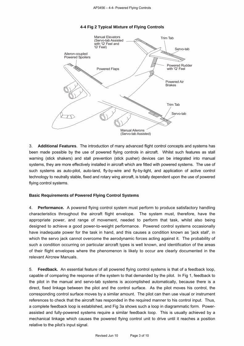
AP3456 – 4-4- Powered Flying Controls
4-4 Fig 2 Typical Mixture of Flying Controls
Aileron-coupledPowered Spoilers
Powered Flaps
Manual Elevators(Servo-tab Assistedwith 'Q' Feel and'G' Feel)
Manual Ailerons(Servo-tab Assisted)
Trim Tab
Servo-tab
Powered Rudderwith 'Q' Feel
Powered AirBrakes
Trim Tab
Servo-tab
3. Additional Features. The introduction of many advanced flight control concepts and systems has been made possible by the use of powered flying controls in aircraft. Whilst such features as stall warning (stick shakers) and stall prevention (stick pusher) devices can be integrated into manual systems, they are more effectively installed in aircraft which are fitted with powered systems. The use of such systems as auto-pilot, auto-land, fly-by-wire and fly-by-light, and application of active control technology to neutrally stable, fixed and rotary wing aircraft, is totally dependent upon the use of powered flying control systems. Basic Requirements of Powered Flying Control Systems
4. Performance. A powered flying control system must perform to produce satisfactory handling characteristics throughout the aircraft flight envelope. The system must, therefore, have the appropriate power, and range of movement, needed to perform that task, whilst also being designed to achieve a good power-to-weight performance. Powered control systems occasionally have inadequate power for the task in hand, and this causes a condition known as 'jack stall', in which the servo jack cannot overcome the aerodynamic forces acting against it. The probability of such a condition occurring on particular aircraft types is well known, and identification of the areas of their flight envelopes where the phenomenon is likely to occur are clearly documented in the relevant Aircrew Manuals. 5. Feedback. An essential feature of all powered flying control systems is that of a feedback loop, capable of comparing the response of the system to that demanded by the pilot. In Fig 1, feedback to the pilot in the manual and servo-tab systems is accomplished automatically, because there is a direct, fixed linkage between the pilot and the control surface. As the pilot moves his control, the corresponding control surface moves by a similar amount. The pilot can then use visual or instrument references to check that the aircraft has responded in the required manner to his control input. Thus, a complete feedback loop is established, and Fig 3a shows such a loop in diagrammatic form. Power-assisted and fully-powered systems require a similar feedback loop. This is usually achieved by a mechanical linkage which causes the powered flying control unit to drive until it reaches a position relative to the pilot’s input signal.
Revised Jun 10 Page 3 of 10
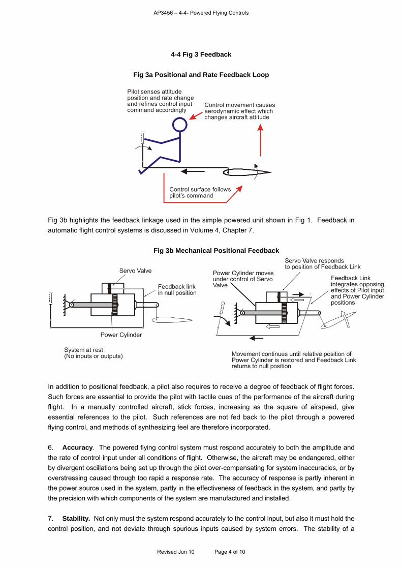
AP3456 – 4-4- Powered Flying Controls
4-4 Fig 3 Feedback
Fig 3a Positional and Rate Feedback Loop
Control movement causesaerodynamic effect whichchanges aircraft attitude
Pilot senses attitudeposition and rate changeand refines control inputcommand accordingly
Control surface followspilot’s command
Fig 3b highlights the feedback linkage used in the simple powered unit shown in Fig 1. Feedback in automatic flight control systems is discussed in Volume 4, Chapter 7.
Fig 3b Mechanical Positional Feedback
System at rest(No inputs or outputs)
Feedback linkin null position
Servo Valve
Power Cylinder
Feedback Linkintegrates opposingeffects of Pilot inputand Power Cylinderpositions
Movement continues until relative position of Power Cylinder is restored and Feedback Linkreturns to null position
Power Cylinder movesunder control of ServoValve
In addition to positional feedback, a pilot also requires to receive a degree of feedback of flight forces. Such forces are essential to provide the pilot with tactile cues of the performance of the aircraft during flight. In a manually controlled aircraft, stick forces, increasing as the square of airspeed, give essential references to the pilot. Such references are not fed back to the pilot through a powered flying control, and methods of synthesizing feel are therefore incorporated. 6. Accuracy. The powered flying control system must respond accurately to both the amplitude and the rate of control input under all conditions of flight. Otherwise, the aircraft may be endangered, either by divergent oscillations being set up through the pilot over-compensating for system inaccuracies, or by overstressing caused through too rapid a response rate. The accuracy of response is partly inherent in the power source used in the system, partly in the effectiveness of feedback in the system, and partly by the precision with which components of the system are manufactured and installed. 7. Stability. Not only must the system respond accurately to the control input, but also it must hold the control position, and not deviate through spurious inputs caused by system errors. The stability of a
Revised Jun 10 Page 4 of 10
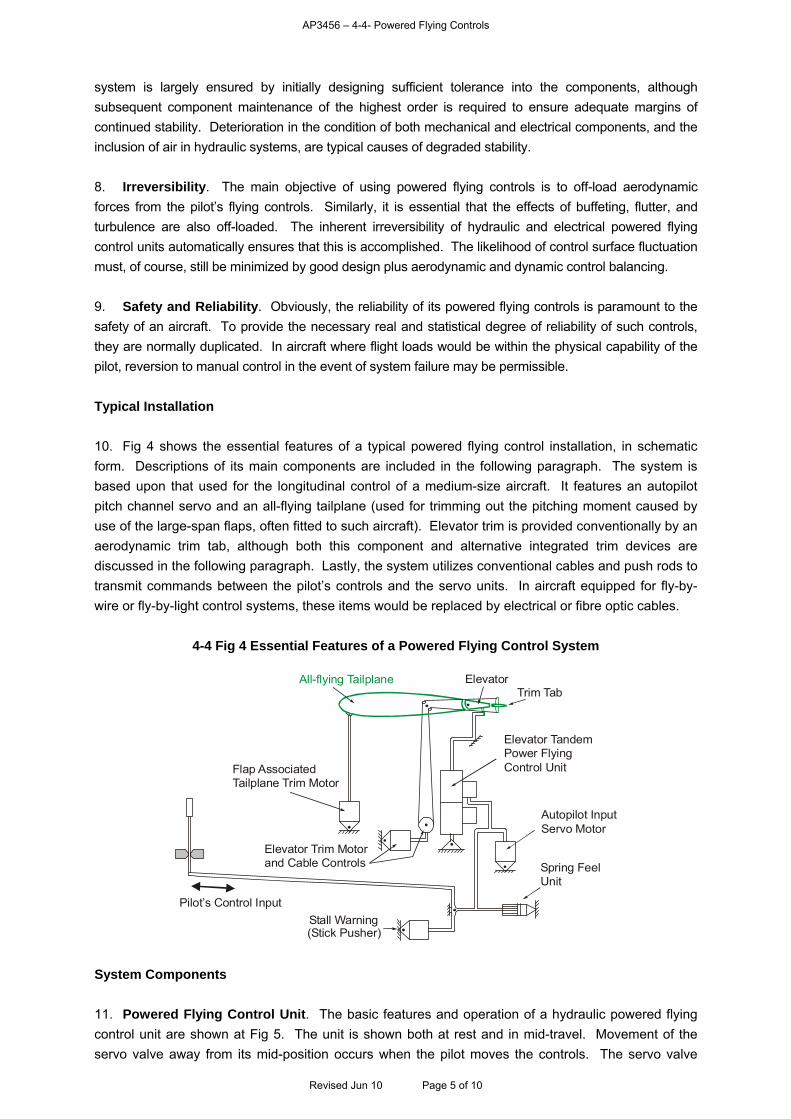
AP3456 – 4-4- Powered Flying Controls
system is largely ensured by initially designing sufficient tolerance into the components, although subsequent component maintenance of the highest order is required to ensure adequate margins of continued stability. Deterioration in the condition of both mechanical and electrical components, and the inclusion of air in hydraulic systems, are typical causes of degraded stability. 8. Irreversibility. The main objective of using powered flying controls is to off-load aerodynamic forces from the pilot’s flying controls. Similarly, it is essential that the effects of buffeting, flutter, and turbulence are also off-loaded. The inherent irreversibility of hydraulic and electrical powered flying control units automatically ensures that this is accomplished. The likelihood of control surface fluctuation must, of course, still be minimized by good design plus aerodynamic and dynamic control balancing. 9. Safety and Reliability. Obviously, the reliability of its powered flying controls is paramount to the safety of an aircraft. To provide the necessary real and statistical degree of reliability of such controls, they are normally duplicated. In aircraft where flight loads would be within the physical capability of the pilot, reversion to manual control in the event of system failure may be permissible. Typical Installation
10. Fig 4 shows the essential features of a typical powered flying control installation, in schematic form. Descriptions of its main components are included in the following paragraph. The system is based upon that used for the longitudinal control of a medium-size aircraft. It features an autopilot pitch channel servo and an all-flying tailplane (used for trimming out the pitching moment caused by use of the large-span flaps, often fitted to such aircraft). Elevator trim is provided conventionally by an aerodynamic trim tab, although both this component and alternative integrated trim devices are discussed in the following paragraph. Lastly, the system utilizes conventional cables and push rods to transmit commands between the pilot’s controls and the servo units. In aircraft equipped for fly-by-wire or fly-by-light control systems, these items would be replaced by electrical or fibre optic cables.
4-4 Fig 4 Essential Features of a Powered Flying Control System
Elevator
Trim Tab
Elevator TandemPower FlyingControl Unit
Autopilot InputServo Motor
Spring FeelUnit
Stall Warning(Stick Pusher)
Pilot’s Control Input
Elevator Trim Motorand Cable Controls
Flap AssociatedTailplane Trim Motor
All-flying Tailplane
System Components
11. Powered Flying Control Unit. The basic features and operation of a hydraulic powered flying control unit are shown at Fig 5. The unit is shown both at rest and in mid-travel. Movement of the servo valve away from its mid-position occurs when the pilot moves the controls. The servo valve
Revised Jun 10 Page 5 of 10
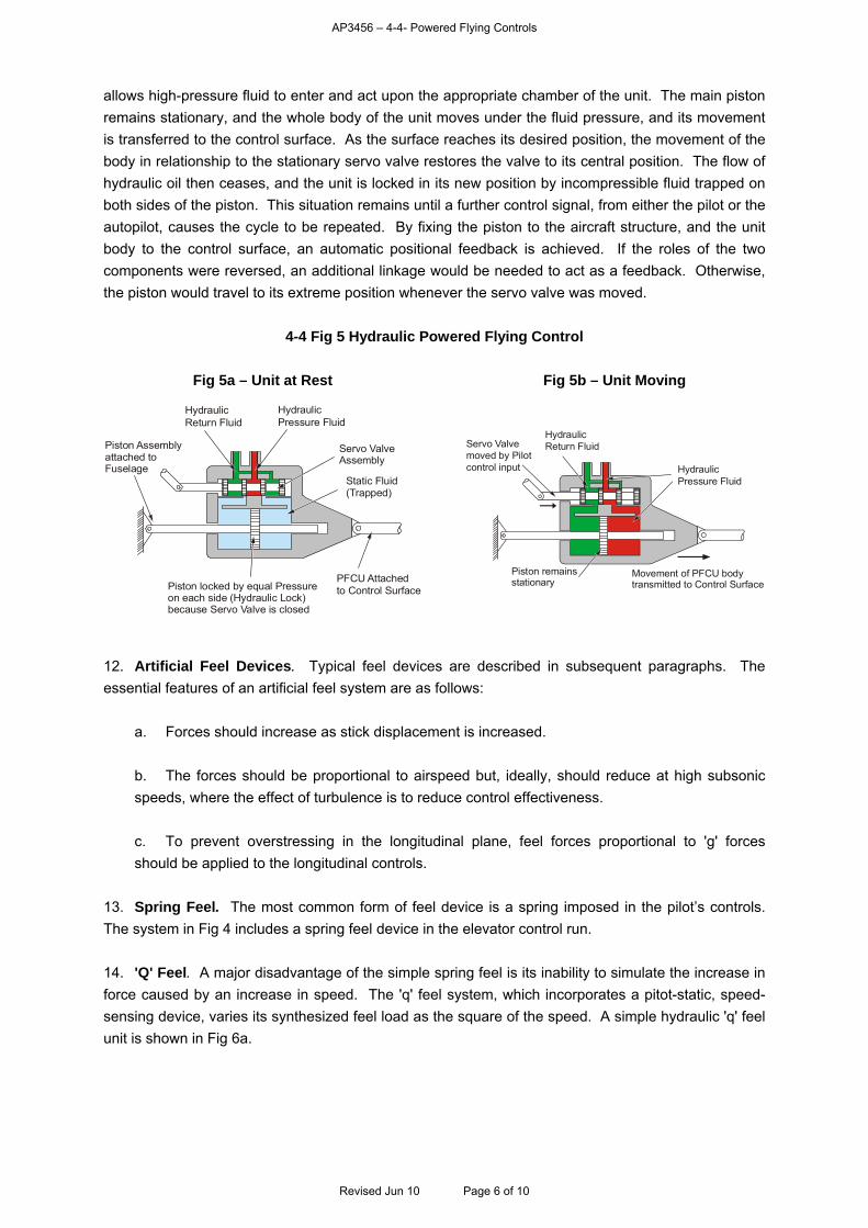
AP3456 – 4-4- Powered Flying Controls
allows high-pressure fluid to enter and act upon the appropriate chamber of the unit. The main piston remains stationary, and the whole body of the unit moves under the fluid pressure, and its movement is transferred to the control surface. As the surface reaches its desired position, the movement of the body in relationship to the stationary servo valve restores the valve to its central position. The flow of hydraulic oil then ceases, and the unit is locked in its new position by incompressible fluid trapped on both sides of the piston. This situation remains until a further control signal, from either the pilot or the autopilot, causes the cycle to be repeated. By fixing the piston to the aircraft structure, and the unit body to the control surface, an automatic positional feedback is achieved. If the roles of the two components were reversed, an additional linkage would be needed to act as a feedback. Otherwise, the piston would travel to its extreme position whenever the servo valve was moved.
4-4 Fig 5 Hydraulic Powered Flying Control
Fig 5a – Unit at Rest Fig 5b – Unit Moving
Piston locked by equal Pressureon each side (Hydraulic Lock)because Servo Valve is closed
HydraulicPressure Fluid
HydraulicReturn Fluid
Servo ValveAssembly
PFCU Attachedto Control Surface
Piston Assemblyattached toFuselage
Static Fluid(Trapped)
Movement of PFCU bodytransmitted to Control Surface
HydraulicPressure Fluid
HydraulicReturn FluidServo Valve
moved by Pilotcontrol input
Piston remainsstationary
12. Artificial Feel Devices. Typical feel devices are described in subsequent paragraphs. The essential features of an artificial feel system are as follows:
a. Forces should increase as stick displacement is increased.
b. The forces should be proportional to airspeed but, ideally, should reduce at high subsonic speeds, where the effect of turbulence is to reduce control effectiveness.
c. To prevent overstressing in the longitudinal plane, feel forces proportional to 'g' forces should be applied to the longitudinal controls.
13. Spring Feel. The most common form of feel device is a spring imposed in the pilot’s controls. The system in Fig 4 includes a spring feel device in the elevator control run. 14. 'Q' Feel. A major disadvantage of the simple spring feel is its inability to simulate the increase in force caused by an increase in speed. The 'q' feel system, which incorporates a pitot-static, speed-sensing device, varies its synthesized feel load as the square of the speed. A simple hydraulic 'q' feel unit is shown in Fig 6a.
Revised Jun 10 Page 6 of 10
AP3456 – 4-4- Powered Flying Controls
4-4 Fig 6 Speed Sensitive Feel Devices
Fig 6a Simple ‘Q’ Feel
Diaphram sensesAirspeed
PitotStatic
Load on Control Column increases asFeel Cylinder Pressure increases
Vent
Diaphram operatedServo Valve
HydraulicReturn
HydraulicPressureTo PFCU
Pressure is an amplified value of Dynamic Pressure
At high subsonic speeds, control surfaces tend to lose power because of compressibility effects. It is, therefore, important to limit or reduce feel forces at these speeds. This is achieved by using a refinement of the 'q' feel system, referred to as the 'Mach Number Corrected 'q' Feel Unit'. This unit has the addition of an altitude capsule in its sensing module. The feel forces generated by the unit are, therefore, proportional to Mach number rather than simply to speed. This arrangement is shown at Fig 6b.
Fig 6b Mach Number Corrected
Mach NoCorrectionBar
PitotStatic
Altitude Capsule
Vent
15. 'G' Feel. Aircraft stress limitations often necessitate limitation of longitudinal control forces when the aircraft is flying at high 'g' loadings. This is accomplished by fitment of a 'g' sensitive device which increases feel forces in proportion to the longitudinal 'g' forces present. The device is usually in the form of a bob-weight. It is often combined with a normal spring feel unit, which tends to reduce the undesirable effects of turbulence and inertia acting on the 'g' feel unit. Fig 7 shows such an arrangement.
4-4 Fig 7 'G' Feel Unit
Bob-weight
Vent
Calibrated BalanceSpring
Simple Feel Spring integralwith Hydraulic Cylinder
Load on Control Column increases as'G' force on weight increases and asFeel Spring is compressed
HydraulicReturn
HydraulicPressure
Revised Jun 10 Page 7 of 10
AP3456 – 4-4- Powered Flying Controls
16. Additional Control Inputs. The use of powered flying control systems allows the integration of additional control inputs such as trim adjustment, stall warning and automatic flight control. Automatic flight control systems are discussed in Volume 4, Chapter 7. 17. Trim Adjustment. Manual control systems utilize fine adjustment of the main or ancillary control surfaces to trim the aircraft flight attitude. This compensates for centre of gravity displacement, or attitude variation, at particular speeds or flap settings. The trim systems allow the main cockpit control forces to be minimized and the control positions to be centralized. Although some applications of powered flying control systems retain the use of ancillary control surfaces for trimming, many systems trim the aircraft by small adjustments of the main control system. However, adjustments to reduce feel forces on the cockpit controls, and to centralize them, remain necessary if the pilot is to retain references and cues during flight. A typical feel trim system is shown at Fig 8a. Its principle of operation is to zero the synthesized feel forces when the aircraft is correctly trimmed. A typical position (datum) trim system is at Fig 8b. Its principle is to apply trim adjustments to the aircraft controls without the pilot’s controls being moved away from their neutral position.
4-4 Fig 8 Trim Systems
Fig 8a - Feel Trim
Trim Motor turns base of Torsion Barto zero feel force experienced by Pilot
Rudder PedalsControl Runto Rudder PFCU
Torsion BarFeel Spring
Rudder Cables
Trim Motor
Fig 8b – Datum Shift Trim
Screw JackTrim Motor
Position of DatumBar and Control Columnshifted by Jack
Datum BarTo PFCU
18. Non-linear Response. Most manual control systems contain a degree of non-linearity in their operation. Small movements of the cockpit controls, when near to the extremes of their travel, produce larger control surface movements than will occur at the centre of their travel. This is a desirable situation, allowing small precise control movements to be made in the critical centre of the control span, and large coarser movements to be made at the extremes. The use of powered flying controls offers the opportunity to increase this non-linearity and thus increase the effectiveness of the control system. The use of non-linear levers and cams, not acceptable in a manual system because of the variation in control loads which they would impose, are permissible in powered systems to which variation in control forces are less significant. A typical non-linear control system is shown at Fig 9.
Revised Jun 10 Page 8 of 10
AP3456 – 4-4- Powered Flying Controls
4-4 Fig 9 Typical Non-linear Flying Control Mechanism
Fig 9a – Differential Aileron Control Fig 9b – Differential Effect
Roll RightRoll Left
Control Column
Roll Right
Roll Left
Right ControlInput
Right ControlInput
Left ControlInput
Left ControlInput
19. Stall Warning and Prevention. The dangers inherent in stalling a high-performance aircraft have led to stall warning systems being fitted to most relevant aircraft. In their simplest form, they consist of an electrical device which shakes the control column so that the pilot experiences cues similar to a stall buffet. The pilot is thus alerted to take the necessary corrective action. However, this is not adequate for many transport aircraft, particularly those with a high tailplane configuration, and stall prevention systems are often fitted to these aircraft. Typical systems, such as that in Fig 4, include a pneumatic jack which gradually imparts a nose-down control input to the aircraft. The pilot can then either accept and supplement the input, or consciously over-ride it, and take alternative measures to avoid the stall. 20. Manual Reversion. As mentioned above, reversion to manual control in the event of failure of a powered flying control system, is an acceptable option for lightly-loaded aircraft. The system of reversion is usually a very simple one and is often engineered to occur automatically in the event of a hydraulic failure. Fig 10 shows a typical system.
4-4 Fig 10 Hydraulic System with Manual Reversion
Fig 10a – Normal Operation Fig 10b – Reversionary Mode
Manual Input movesServo Valve only
Hydraulic Pressure
Hydraulic Pressure
Piston Rodlocked by Plunger Spring
compressed
Piston Rodfree to move
Manual Input movesPFCU and Control
Spring forcesPlunger to disengage
No HydraulicPressure
Hydraulic Failure
21. Multiplication. A more normal arrangement for retaining adequate control, in the event of failure of a powered flying control system, is achieved by multiplication of critical components of that system. The most usual methods of achieving this redundancy of critical components are shown at Fig 11. These include split control surfaces (typical in an aircraft of the type depicted at Fig 2), each section having an independent powered control unit (Fig 11a), and use of tandem jacks (Fig 11b). All of these systems require an interlock within their respective hydraulic jack servo valves to prevent a hydraulic
Revised Jun 10 Page 9 of 10
AP3456 – 4-4- Powered Flying Controls
Revised Jun 10 Page 10 of 10
lock occurring in the redundant jack, and, thus, locking the relevant control surface. The use of parallel jacks is widespread in aircraft in which there is room to site such units adjacent to the control surfaces. However, for aircraft in which this is not possible, particularly combat aircraft and helicopters, the tandem jack arrangement is normally fitted.
4-4 Fig 11 Redundant Flying Control Components
Fig 11a – Parallel Units Fig 11b – Tandem Units
Servo Yoke multipliesControl Input to oneunit if other fails Hydraulic
System 1
ControlInput
HydraulicSystem 2
Divided ControlSurfaces
PFCU 1
PFCU 2
PistonThrust
ControlInput
CylinderThrust
In event of failure, one unit cycles freely leaving other towork normally
HydraulicSystem 2
HydraulicSystem 1
Common Piston Rod
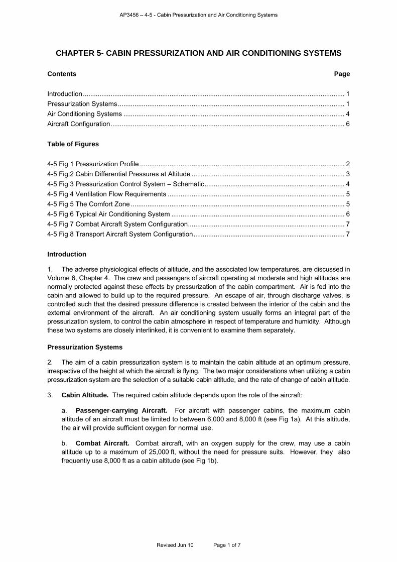
AP3456 – 4-5 - Cabin Pressurization and Air Conditioning Systems
CHAPTER 5- CABIN PRESSURIZATION AND AIR CONDITIONING SYSTEMS
Contents Page
Introduction.............................................................................................................................................. 1 Pressurization Systems........................................................................................................................... 1 Air Conditioning Systems ........................................................................................................................ 4 Aircraft Configuration............................................................................................................................... 6 Table of Figures
4-5 Fig 1 Pressurization Profile ............................................................................................................... 2 4-5 Fig 2 Cabin Differential Pressures at Altitude ................................................................................... 3 4-5 Fig 3 Pressurization Control System – Schematic............................................................................ 4 4-5 Fig 4 Ventilation Flow Requirements ................................................................................................ 5 4-5 Fig 5 The Comfort Zone .................................................................................................................... 5 4-5 Fig 6 Typical Air Conditioning System .............................................................................................. 6 4-5 Fig 7 Combat Aircraft System Configuration..................................................................................... 7 4-5 Fig 8 Transport Aircraft System Configuration.................................................................................. 7 Introduction 1. The adverse physiological effects of altitude, and the associated low temperatures, are discussed in Volume 6, Chapter 4. The crew and passengers of aircraft operating at moderate and high altitudes are normally protected against these effects by pressurization of the cabin compartment. Air is fed into the cabin and allowed to build up to the required pressure. An escape of air, through discharge valves, is controlled such that the desired pressure difference is created between the interior of the cabin and the external environment of the aircraft. An air conditioning system usually forms an integral part of the pressurization system, to control the cabin atmosphere in respect of temperature and humidity. Although these two systems are closely interlinked, it is convenient to examine them separately. Pressurization Systems 2. The aim of a cabin pressurization system is to maintain the cabin altitude at an optimum pressure, irrespective of the height at which the aircraft is flying. The two major considerations when utilizing a cabin pressurization system are the selection of a suitable cabin altitude, and the rate of change of cabin altitude. 3. Cabin Altitude. The required cabin altitude depends upon the role of the aircraft:
a. Passenger-carrying Aircraft. For aircraft with passenger cabins, the maximum cabin altitude of an aircraft must be limited to between 6,000 and 8,000 ft (see Fig 1a). At this altitude, the air will provide sufficient oxygen for normal use.
b. Combat Aircraft. Combat aircraft, with an oxygen supply for the crew, may use a cabin altitude up to a maximum of 25,000 ft, without the need for pressure suits. However, they also frequently use 8,000 ft as a cabin altitude (see Fig 1b).
Revised Jun 10 Page 1 of 7
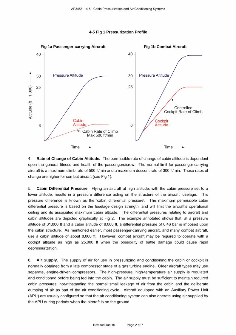
AP3456 – 4-5 - Cabin Pressurization and Air Conditioning Systems
4-5 Fig 1 Pressurization Profile
Fig 1a Passenger-carrying Aircraft Fig 1b Combat Aircraft
Alti
tude
(ft
1,0
00)
Pressure Altitude
CabinAltitude
Cabin Rate of ClimbMax 500 ft/min
Time
40
30
25
8
40
30
25
8
Pressure Altitude
ControlledCockpit Rate of Climb
CockpitAltitude
Time 4. Rate of Change of Cabin Altitude. The permissible rate of change of cabin altitude is dependent upon the general fitness and health of the passengers/crew. The normal limit for passenger-carrying aircraft is a maximum climb rate of 500 ft/min and a maximum descent rate of 300 ft/min. These rates of change are higher for combat aircraft (see Fig 1). 5. Cabin Differential Pressure. Flying an aircraft at high altitude, with the cabin pressure set to a lower altitude, results in a pressure difference acting on the structure of the aircraft fuselage. This pressure difference is known as the 'cabin differential pressure'. The maximum permissible cabin differential pressure is based on the fuselage design strength, and will limit the aircraft’s operational ceiling and its associated maximum cabin altitude. The differential pressures relating to aircraft and cabin altitudes are depicted graphically at Fig 2. The example annotated shows that, at a pressure altitude of 31,000 ft and a cabin altitude of 8,000 ft, a differential pressure of 0.46 bar is imposed upon the cabin structure. As mentioned earlier, most passenger-carrying aircraft, and many combat aircraft, use a cabin altitude of about 8,000 ft. However, combat aircraft may be required to operate with a cockpit altitude as high as 25,000 ft when the possibility of battle damage could cause rapid depressurization. 6. Air Supply. The supply of air for use in pressurizing and conditioning the cabin or cockpit is normally obtained from a late compressor stage of a gas turbine engine. Older aircraft types may use separate, engine-driven compressors. The high-pressure, high-temperature air supply is regulated and conditioned before being fed into the cabin. The air supply must be sufficient to maintain required cabin pressures, notwithstanding the normal small leakage of air from the cabin and the deliberate dumping of air as part of the air conditioning cycle. Aircraft equipped with an Auxiliary Power Unit (APU) are usually configured so that the air conditioning system can also operate using air supplied by the APU during periods when the aircraft is on the ground.
Revised Jun 10 Page 2 of 7
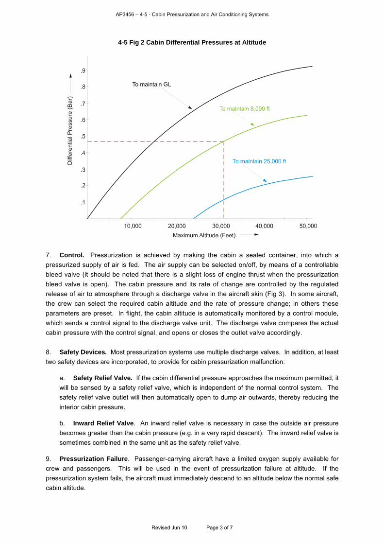
AP3456 – 4-5 - Cabin Pressurization and Air Conditioning Systems
4-5 Fig 2 Cabin Differential Pressures at Altitude
7. Control. Pressurization is achieved by making the cabin a sealed container, into which a pressurized supply of air is fed. The air supply can be selected on/off, by means of a controllable bleed valve (it should be noted that there is a slight loss of engine thrust when the pressurization bleed valve is open). The cabin pressure and its rate of change are controlled by the regulated release of air to atmosphere through a discharge valve in the aircraft skin (Fig 3). In some aircraft, the crew can select the required cabin altitude and the rate of pressure change; in others these parameters are preset. In flight, the cabin altitude is automatically monitored by a control module, which sends a control signal to the discharge valve unit. The discharge valve compares the actual cabin pressure with the control signal, and opens or closes the outlet valve accordingly. 8. Safety Devices. Most pressurization systems use multiple discharge valves. In addition, at least two safety devices are incorporated, to provide for cabin pressurization malfunction:
a. Safety Relief Valve. If the cabin differential pressure approaches the maximum permitted, it will be sensed by a safety relief valve, which is independent of the normal control system. The safety relief valve outlet will then automatically open to dump air outwards, thereby reducing the interior cabin pressure.
b. Inward Relief Valve. An inward relief valve is necessary in case the outside air pressure becomes greater than the cabin pressure (e.g. in a very rapid descent). The inward relief valve is sometimes combined in the same unit as the safety relief valve.
9. Pressurization Failure. Passenger-carrying aircraft have a limited oxygen supply available for crew and passengers. This will be used in the event of pressurization failure at altitude. If the pressurization system fails, the aircraft must immediately descend to an altitude below the normal safe cabin altitude.
Revised Jun 10 Page 3 of 7
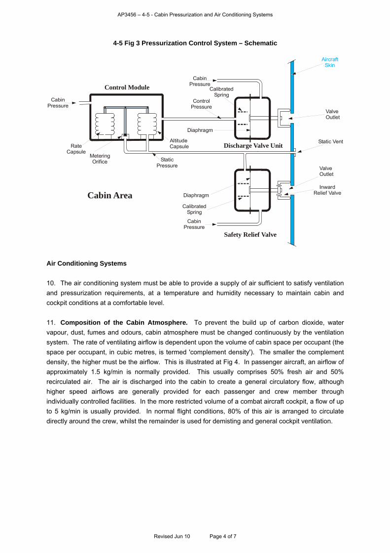
AP3456 – 4-5 - Cabin Pressurization and Air Conditioning Systems
4-5 Fig 3 Pressurization Control System – Schematic
ValveOutlet
Diaphragm
InwardRelief Valve
CabinPressure
CalibratedSpring
Safety Relief Valve
StaticPressure
RateCapsule
CabinPressure
Altitude Capsule
ControlPressure
Cabin Area
Static VentDischarge Valve Unit
AircraftSkin
Control Module
Diaphragm
CalibratedSpring
ValveOutlet
MeteringOrifice
CabinPressure
Air Conditioning Systems
10. The air conditioning system must be able to provide a supply of air sufficient to satisfy ventilation and pressurization requirements, at a temperature and humidity necessary to maintain cabin and cockpit conditions at a comfortable level. 11. Composition of the Cabin Atmosphere. To prevent the build up of carbon dioxide, water vapour, dust, fumes and odours, cabin atmosphere must be changed continuously by the ventilation system. The rate of ventilating airflow is dependent upon the volume of cabin space per occupant (the space per occupant, in cubic metres, is termed 'complement density'). The smaller the complement density, the higher must be the airflow. This is illustrated at Fig 4. In passenger aircraft, an airflow of approximately 1.5 kg/min is normally provided. This usually comprises 50% fresh air and 50% recirculated air. The air is discharged into the cabin to create a general circulatory flow, although higher speed airflows are generally provided for each passenger and crew member through individually controlled facilities. In the more restricted volume of a combat aircraft cockpit, a flow of up to 5 kg/min is usually provided. In normal flight conditions, 80% of this air is arranged to circulate directly around the crew, whilst the remainder is used for demisting and general cockpit ventilation.
Revised Jun 10 Page 4 of 7
AP3456 – 4-5 - Cabin Pressurization and Air Conditioning Systems
4-5 Fig 4 Ventilation Flow Requirements
12. Temperature and Humidity. The range of ambient temperatures and humidity in which a crew can operate comfortably without rapidly becoming fatigued is known as the 'Comfort Zone' (see Fig 5). Air conditioning systems control both temperature and humidity within the cabin to remain within this zone.
4-5 Fig 5 The Comfort Zone
13. Conditioning Systems. Fig 6 shows a typical air conditioning system. The hot air from the engine compressor is cooled by routing it through primary and secondary heat exchangers, and a cold air unit, as necessary. Within the heat exchangers, the hot air is cooled by indirect contact with cold ram air. The cold air unit uses principles of expansion and energy conversion to reduce the air temperature. To provide the final airstream at the temperature required for cabin conditioning, the cooled air passes through a mixture chamber, where it is combined with hot moist by-pass air and recycled cabin air. Any water resulting from the cooling process is separated from the air before it enters the cabin. Most water separators utilize momentum separation techniques to remove the majority of water from the airstream. This type of separator comprises a bank of swirl vanes, or louvres, and a coarse mesh coalescent filter. As the air passes through the unit, its velocity and momentum are changed and any water held within the air coalesces into droplets. These droplets are
Revised Jun 10 Page 5 of 7
AP3456 – 4-5 - Cabin Pressurization and Air Conditioning Systems
then separated from the main airstream and are ducted overboard. Most air conditioning systems provide control and adjustment of air temperature and control of air humidity. Some provide positive filtration of the incoming air, although the majority achieve a degree of filtration only as a secondary function of the water extraction devices used for humidity control.
4-5 Fig 6 Typical Air Conditioning System
Hot Air fromEngine Bleeds
CoolingRam Air
Bleed AirPart-conditioned AirConditioned AirRam Air
PrimaryHeat
Exchanger
Engine
Engine
By-passValve
Bleed AirShut-off Valve
Non-returnValve
Pressure Reducingand
Shut-off Valve
Air from Cabinfor Recycling
CoolingRam Air Secondary
HeatExchanger
Cold AirUnit
TemperatureControl Valve
MixingChamber
Air toCabin
RecycleAir Valve
DrainWaterExtractor
14. Conditioning Failures. Multiple air conditioning systems are usually employed to provide an element of redundancy. However, if the pressurization air supply is suspended (during an airborne emergency, for instance), ambient ram air will normally be used as an alternative supply for conditioning. The temperature in the cabin can therefore by expected to fall rapidly, depending upon the ambient air temperature. Aircraft Configuration 15. Pressurization and air conditioning systems need to be self-contained and, ideally, duplicated to provide an acceptable degree of conditioning in the event of one failure. For combat aircraft, they need to be simple, compact and automatic (or semi-automatic). For transport aircraft the systems must have large capacity and a flexible control system, to cope with widely varying conditions. Ventilation systems need to be capable of operating on the ground. It should be noted that supplies of pressurized and conditioned air are used for other tasks, including pressurization and cooling of avionics modules, sealing of canopies, and supply of pressure for aircrew anti-g clothing. Fig 7 shows a representative system installation for a two seat, single engine combat/training aircraft, whilst Fig 8 shows a typical system for a multi-engine transport aircraft.
Revised Jun 10 Page 6 of 7
AP3456 – 4-5 - Cabin Pressurization and Air Conditioning Systems
Revised Jun 10 Page 7 of 7
4-5 Fig 7 Combat Aircraft System Configuration
4-5 Fig 8 Transport Aircraft System Configuration
Ram Air Duct(Cooling Air)Hot Pressure Air
from Engines and APU
APU
Air Conditioning Units
Pressurization Controllerand Discharge Valves
Cabin Air Supply is ducted totop of Cabin and exhausted
into Freight Bay belowCockpit Air Supply
(also cools avionics)
AP3456 – 4-6- Undercarriages
CHAPTER 6 - UNDERCARRIAGES
Contents Page
Introduction.............................................................................................................................................. 1 Runway Pavements................................................................................................................................. 2 Design Considerations ............................................................................................................................ 2 Typical Configurations............................................................................................................................. 2 Undercarriages........................................................................................................................................ 3 Wheels..................................................................................................................................................... 8 Tyres........................................................................................................................................................ 9 Braking Systems.................................................................................................................................... 10 Braking Control and Anti-skid Systems................................................................................................. 12
Table of Figures
4-6 Fig 1 Undercarriage of the Tornado Aircraft ..................................................................................... 2 4-6 Fig 2 Examples of Retractable Main Undercarriages ....................................................................... 3 4-6 Fig 3 Basic Undercarriage Leg Configurations ................................................................................. 4 4-6 Fig 4 Principle of the Liquid Spring ................................................................................................... 4 4-6 Fig 5 Oleo-pneumatic Absorbers ...................................................................................................... 5 4-6 Fig 6 Undercarriage Retraction Mechanisms ................................................................................... 6 4-6 Fig 7 Up and Down Locks ................................................................................................................. 7 4-6 Fig 8 Aircraft Twin Main Wheel and Axle .......................................................................................... 9 4-6 Fig 9 Construction of a Radial Ply Tyre ............................................................................................ 9 4-6 Fig 10 Brake Assembly ................................................................................................................... 11 4-6 Fig 11 Relationship between and Vertical Load on the Tyres..................................................... 12 4-6 Fig 12 Relationship between and Wheel Slip for Varying Runway Conditions ........................... 12 4-6 Fig 13 Typical Brake System Operation Profile .............................................................................. 13
Introduction
1. The undercarriage of an aircraft includes the wheels, tyres and brakes as well as the main
undercarriage leg components. It performs the essential function of providing an interface between
aircraft and ground during landing, take off, ground manoeuvring and whilst at rest. However, it is
completely redundant during flight, and therefore the design of an undercarriage is usually a critical
compromise between optimising performance on the ground and minimizing weight and drag penalties
in the air. Examples of the extremes of this compromise range between the provision of the minimum
for a Remotely Piloted Vehicle - a detachable wheeled dolly for the aircraft to take off from and a
parachute to lower it safely after flight - to the more generally serviceable - such as the undercarriage
of the Tornado, shown at Fig 1 - which allows the aircraft to be landed at high weights and on a wide
variety of surfaces, and to be manoeuvred rapidly and precisely between the runway and its dispersal
area for replenishment, prior to dispatch on further sorties.
Revised Jun 10 Page 1 of 13
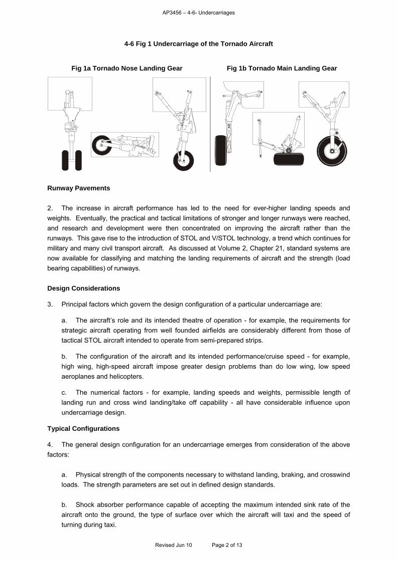
AP3456 – 4-6- Undercarriages
4-6 Fig 1 Undercarriage of the Tornado Aircraft
Fig 1a Tornado Nose Landing Gear Fig 1b Tornado Main Landing Gear
Runway Pavements
2. The increase in aircraft performance has led to the need for ever-higher landing speeds and
weights. Eventually, the practical and tactical limitations of stronger and longer runways were reached,
and research and development were then concentrated on improving the aircraft rather than the
runways. This gave rise to the introduction of STOL and V/STOL technology, a trend which continues for
military and many civil transport aircraft. As discussed at Volume 2, Chapter 21, standard systems are
now available for classifying and matching the landing requirements of aircraft and the strength (load
bearing capabilities) of runways.
Design Considerations
3. Principal factors which govern the design configuration of a particular undercarriage are:
a. The aircraft’s role and its intended theatre of operation - for example, the requirements for
strategic aircraft operating from well founded airfields are considerably different from those of
tactical STOL aircraft intended to operate from semi-prepared strips.
b. The configuration of the aircraft and its intended performance/cruise speed - for example,
high wing, high-speed aircraft impose greater design problems than do low wing, low speed
aeroplanes and helicopters.
c. The numerical factors - for example, landing speeds and weights, permissible length of
landing run and cross wind landing/take off capability - all have considerable influence upon
undercarriage design. Typical Configurations
4. The general design configuration for an undercarriage emerges from consideration of the above
factors:
a. Physical strength of the components necessary to withstand landing, braking, and crosswind
loads. The strength parameters are set out in defined design standards.
b. Shock absorber performance capable of accepting the maximum intended sink rate of the
aircraft onto the ground, the type of surface over which the aircraft will taxi and the speed of
turning during taxi.
Revised Jun 10 Page 2 of 13

AP3456 – 4-6- Undercarriages
c. Fixed (stronger, simpler and lighter) undercarriage or a retractable (less drag) undercarriage.
d. Streamlining and provision of undercarriage doors necessary to reduce drag during flight.
e. Dimensions of the ground track needed to provide stability during landing and taxi.
f. Fuselage or wing space available for stowing and attaching the gear.
g. Basic configuration. For instance, the standard tricycle for good ground manoeuvre and
stability, bicycle (with outriggers) for strength and relative ease of stowage or tail wheel for
simplicity and low cost. The most appropriate undercarriage for a small helicopter may be a pair
of skids, despite the complications which these impose upon ground handling.
The retractable main undercarriages of the Airbus A310 and the BAe 146 are shown in Fig 2. The
A310 undercarriage is a very simple assembly which retracts into a space in the wing root and
fuselage. However, that for the 146 (a high wing aircraft) retracts into the bottom of the fuselage (to
minimize its length and thus maximize its strength) and extends sideways (to give a good wheel track
for stability). This has resulted in the complex, multi-pivoting mechanism shown.
4-6 Fig 2 Examples of Retractable Main Undercarriages
Fig 2a A310 Main Landing Gear Fig 2b BAe 146-200 Main Landing Gear
Undercarriages
5. Undercarriage Legs. The undercarriage leg performs the functions of absorbing the forward, aft
and side loads of landing and braking. Nose and tail undercarriages also require to swivel to allow the
aircraft to be steered. These functions must be performed by as few components as possible, and
Fig 3 shows several undercarriage legs (in schematic form) designed to achieve these objectives.
Revised Jun 10 Page 3 of 13
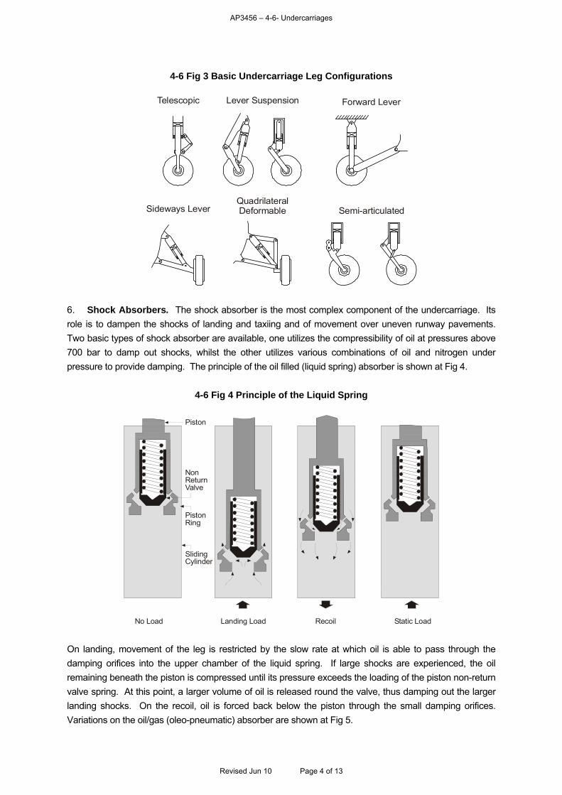
AP3456 – 4-6- Undercarriages
4-6 Fig 3 Basic Undercarriage Leg Configurations
Forward LeverLever SuspensionTelescopic
DeformableQuadrilateral
Semi-articulatedSideways Lever
6. Shock Absorbers. The shock absorber is the most complex component of the undercarriage. Its
role is to dampen the shocks of landing and taxiing and of movement over uneven runway pavements.
Two basic types of shock absorber are available, one utilizes the compressibility of oil at pressures above
700 bar to damp out shocks, whilst the other utilizes various combinations of oil and nitrogen under
pressure to provide damping. The principle of the oil filled (liquid spring) absorber is shown at Fig 4.
4-6 Fig 4 Principle of the Liquid Spring
NonReturnValve
PistonRing
SlidingCylinder
Landing Load Recoil Static LoadNo Load
Piston
On landing, movement of the leg is restricted by the slow rate at which oil is able to pass through the
damping orifices into the upper chamber of the liquid spring. If large shocks are experienced, the oil
remaining beneath the piston is compressed until its pressure exceeds the loading of the piston non-return
valve spring. At this point, a larger volume of oil is released round the valve, thus damping out the larger
landing shocks. On the recoil, oil is forced back below the piston through the small damping orifices.
Variations on the oil/gas (oleo-pneumatic) absorber are shown at Fig 5.
Revised Jun 10 Page 4 of 13
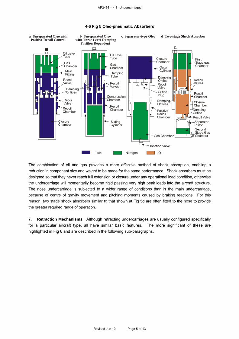
AP3456 – 4-6- Undercarriages
4-6 Fig 5 Oleo-pneumatic Absorbers
a Unseparated Oleo withPositive Recoil Control
c Separator-type Oleo d Two-stage Shock Absorber
Fluid Nitrogen Oil
Oil LevelTube Oil Level
Tube
ClosureChamber
ClosureChamber
RecoilChamber
RecoilChamber
RecoilValve
RecoilValves
Damping Orifices
Damping Orifices
RecoilValve
MainFitting
GasChamber Gas
Chamber
DampingTube
CompressionChamber
SlidingCylinder
OuterCylinder
DampingOrificeRecoilValveOrificePlug
PositiveRecoilChamber
Gas Chamber
Inflation Valve
SecondStage GasChamber
SeparatorPiston
Recoil Valve
DampingOrifice
ClosureChamber
RecoilValves
RecoilChamber
FirstStage gasChamber
The combination of oil and gas provides a more effective method of shock absorption, enabling a
reduction in component size and weight to be made for the same performance. Shock absorbers must be
designed so that they never reach full extension or closure under any operational load condition, otherwise
the undercarriage will momentarily become rigid passing very high peak loads into the aircraft structure.
The nose undercarriage is subjected to a wider range of conditions than is the main undercarriage,
because of centre of gravity movement and pitching moments caused by braking reactions. For this
reason, two stage shock absorbers similar to that shown at Fig 5d are often fitted to the nose to provide
the greater required range of operation.
7. Retraction Mechanisms. Although retracting undercarriages are usually configured specifically
for a particular aircraft type, all have similar basic features. The more significant of these are
highlighted in Fig 6 and are described in the following sub-paragraphs.
Revised Jun 10 Page 5 of 13
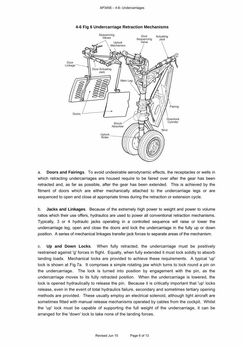
AP3456 – 4-6- Undercarriages
4-6 Fig 6 Undercarriage Retraction Mechanisms
Strut
DownlockCylinder
Fairing
UplockRoller
Doors
ShockAbsorber
Main Leg
DoorLinkage
Door ActuatingJack
SequencingValves
UplockMechanism
ActuatingJack
DoorSequencing
Valve
a. Doors and Fairings. To avoid undesirable aerodynamic effects, the receptacles or wells in
which retracting undercarriages are housed require to be faired over after the gear has been
retracted and, as far as possible, after the gear has been extended. This is achieved by the
fitment of doors which are either mechanically attached to the undercarriage legs or are
sequenced to open and close at appropriate times during the retraction or extension cycle.
b. Jacks and Linkages. Because of the extremely high power to weight and power to volume
ratios which their use offers, hydraulics are used to power all conventional retraction mechanisms.
Typically, 3 or 4 hydraulic jacks operating in a controlled sequence will raise or lower the
undercarriage leg, open and close the doors and lock the undercarriage in the fully up or down
position. A series of mechanical linkages transfer jack forces to separate areas of the mechanism.
c. Up and Down Locks. When fully retracted, the undercarriage must be positively
restrained against 'g' forces in flight. Equally, when fully extended it must lock solidly to absorb
landing loads. Mechanical locks are provided to achieve these requirements. A typical 'up'
lock is shown at Fig 7a. It comprises a simple rotating jaw which turns to lock round a pin on
the undercarriage. The lock is turned into position by engagement with the pin, as the
undercarriage moves to its fully retracted position. When the undercarriage is lowered, the
lock is opened hydraulically to release the pin. Because it is critically important that 'up' locks
release, even in the event of total hydraulics failure, secondary and sometimes tertiary opening
methods are provided. These usually employ an electrical solenoid, although light aircraft are
sometimes fitted with manual release mechanisms operated by cables from the cockpit. Whilst
the 'up' lock must be capable of supporting the full weight of the undercarriage, it can be
arranged for the 'down' lock to take none of the landing forces.
Revised Jun 10 Page 6 of 13
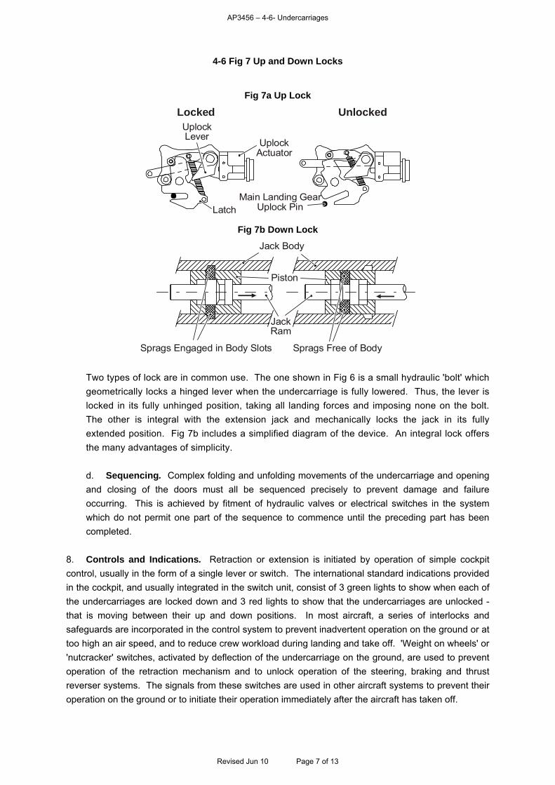
AP3456 – 4-6- Undercarriages
4-6 Fig 7 Up and Down Locks
Fig 7a Up Lock
UnlockedLocked
UplockActuator
UplockLever
LatchMain Landing Gear
Uplock Pin
Fig 7b Down Lock
Jack Body
Piston
JackRam
Sprags Free of BodySprags Engaged in Body Slots
Two types of lock are in common use. The one shown in Fig 6 is a small hydraulic 'bolt' which
geometrically locks a hinged lever when the undercarriage is fully lowered. Thus, the lever is
locked in its fully unhinged position, taking all landing forces and imposing none on the bolt.
The other is integral with the extension jack and mechanically locks the jack in its fully
extended position. Fig 7b includes a simplified diagram of the device. An integral lock offers
the many advantages of simplicity.
d. Sequencing. Complex folding and unfolding movements of the undercarriage and opening
and closing of the doors must all be sequenced precisely to prevent damage and failure
occurring. This is achieved by fitment of hydraulic valves or electrical switches in the system
which do not permit one part of the sequence to commence until the preceding part has been
completed.
8. Controls and Indications. Retraction or extension is initiated by operation of simple cockpit
control, usually in the form of a single lever or switch. The international standard indications provided
in the cockpit, and usually integrated in the switch unit, consist of 3 green lights to show when each of
the undercarriages are locked down and 3 red lights to show that the undercarriages are unlocked -
that is moving between their up and down positions. In most aircraft, a series of interlocks and
safeguards are incorporated in the control system to prevent inadvertent operation on the ground or at
too high an air speed, and to reduce crew workload during landing and take off. 'Weight on wheels' or
'nutcracker' switches, activated by deflection of the undercarriage on the ground, are used to prevent
operation of the retraction mechanism and to unlock operation of the steering, braking and thrust
reverser systems. The signals from these switches are used in other aircraft systems to prevent their
operation on the ground or to initiate their operation immediately after the aircraft has taken off.
Revised Jun 10 Page 7 of 13
AP3456 – 4-6- Undercarriages
9. Steering. Whilst taxiing and during initial stages of take off and final stages of landing, airspeeds are
too low for rudder authority to be maintained. A system of differential operation of the main wheel brakes,
achieved by manipulation of brake pedals attached to the rudder bar, provides a steering force in most
aircraft at these lower speeds. However, precise ground manoeuvring is required in crowded aircraft
dispersal areas, and a system of positively steering the aircraft wheels is therefore necessary. In light
aircraft, such steering is often provided through direct mechanical linkage of the rudder pedals to a
steerable nose or tail wheel. The majority of high performance aircraft utilize steering systems in which the
nose wheel can be controlled hydraulically during taxi, through a small tiller or wheel in the cockpit. To
avoid such a steering system providing an unwanted input at the points of lift off and touch down, the
steerable nose wheel is automatically aligned centrally whenever aircraft weight is lifted off the wheels.
10. Emergency Extension. To avoid the inevitable consequences of a 'wheels up' landing, design
standards require that all aircraft fitted with retractable undercarriages are equipped with at least one
alternative driving force for extending the undercarriage. In the majority of aircraft, this is achieved by
pressurizing the undercarriage hydraulic extension system either directly by the release of compressed
nitrogen into the system or indirectly by release of nitrogen into an associated booster system. Operation
of the emergency extension control lever releases the nitrogen and affects any necessary changes in
hydraulic valve settings. Many aircraft are equipped with a secondary emergency system which releases
the undercarriage up lock allowing the undercarriage to extend under gravitational and aerodynamic
forces. Use of the emergency systems prevents subsequent retraction of the undercarriage, until
necessary engineering actions have been carried out on the ground.
Wheels
11. The design criteria for aircraft wheels are:
a. Light weight.
b. Minimum size.
c. Easy tyre replacement.
d. Accommodation for the brake unit and dissipation of the heat generated during braking.
e. Good fatigue resistance.
Aircraft wheels differ in many ways from those fitted to road vehicles. For instance, aircraft wheels are
made in 2 halves which unbolt to allow the fitment of tyres without stretching their beading over the
wheel rims. Also, the wheels house the wheel bearings, unlike automobile practice in which a
separate axle houses the bearings and the wheels bolt to this axle. A typical wheel and axle
arrangement is shown at Fig 8.
Revised Jun 10 Page 8 of 13
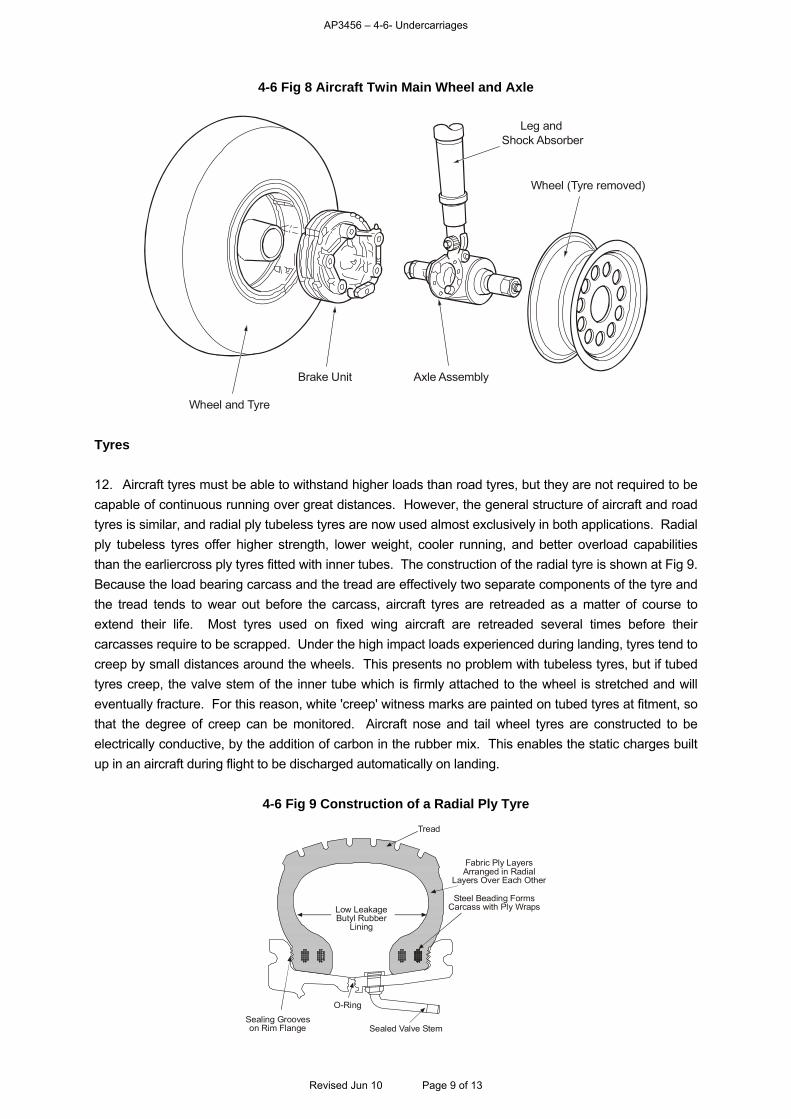
AP3456 – 4-6- Undercarriages
4-6 Fig 8 Aircraft Twin Main Wheel and Axle
Wheel and Tyre
Brake Unit Axle Assembly
Wheel (Tyre removed)
Leg and Shock Absorber
Tyres
12. Aircraft tyres must be able to withstand higher loads than road tyres, but they are not required to be
capable of continuous running over great distances. However, the general structure of aircraft and road
tyres is similar, and radial ply tubeless tyres are now used almost exclusively in both applications. Radial
ply tubeless tyres offer higher strength, lower weight, cooler running, and better overload capabilities
than the earliercross ply tyres fitted with inner tubes. The construction of the radial tyre is shown at Fig 9.
Because the load bearing carcass and the tread are effectively two separate components of the tyre and
the tread tends to wear out before the carcass, aircraft tyres are retreaded as a matter of course to
extend their life. Most tyres used on fixed wing aircraft are retreaded several times before their
carcasses require to be scrapped. Under the high impact loads experienced during landing, tyres tend to
creep by small distances around the wheels. This presents no problem with tubeless tyres, but if tubed
tyres creep, the valve stem of the inner tube which is firmly attached to the wheel is stretched and will
eventually fracture. For this reason, white 'creep' witness marks are painted on tubed tyres at fitment, so
that the degree of creep can be monitored. Aircraft nose and tail wheel tyres are constructed to be
electrically conductive, by the addition of carbon in the rubber mix. This enables the static charges built
up in an aircraft during flight to be discharged automatically on landing.
4-6 Fig 9 Construction of a Radial Ply Tyre
Low LeakageButyl Rubber
Lining
Tread
O-Ring
Sealing Grooveson Rim Flange Sealed Valve Stem
Fabric Ply LayersArranged in Radial
Layers Over Each Other
Steel Beading FormsCarcass with Ply Wraps
Revised Jun 10 Page 9 of 13
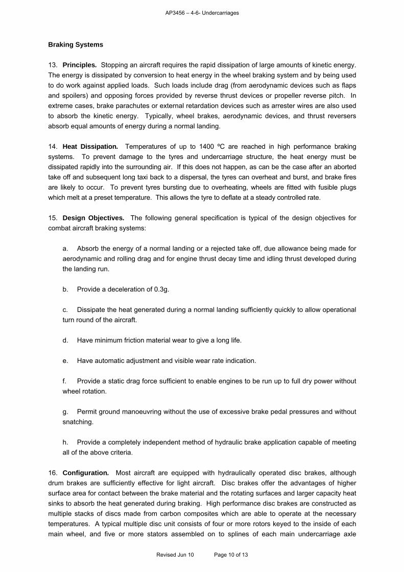
AP3456 – 4-6- Undercarriages
Braking Systems
13. Principles. Stopping an aircraft requires the rapid dissipation of large amounts of kinetic energy.
The energy is dissipated by conversion to heat energy in the wheel braking system and by being used
to do work against applied loads. Such loads include drag (from aerodynamic devices such as flaps
and spoilers) and opposing forces provided by reverse thrust devices or propeller reverse pitch. In
extreme cases, brake parachutes or external retardation devices such as arrester wires are also used
to absorb the kinetic energy. Typically, wheel brakes, aerodynamic devices, and thrust reversers
absorb equal amounts of energy during a normal landing.
14. Heat Dissipation. Temperatures of up to 1400 ºC are reached in high performance braking
systems. To prevent damage to the tyres and undercarriage structure, the heat energy must be
dissipated rapidly into the surrounding air. If this does not happen, as can be the case after an aborted
take off and subsequent long taxi back to a dispersal, the tyres can overheat and burst, and brake fires
are likely to occur. To prevent tyres bursting due to overheating, wheels are fitted with fusible plugs
which melt at a preset temperature. This allows the tyre to deflate at a steady controlled rate.
15. Design Objectives. The following general specification is typical of the design objectives for
combat aircraft braking systems:
a. Absorb the energy of a normal landing or a rejected take off, due allowance being made for
aerodynamic and rolling drag and for engine thrust decay time and idling thrust developed during
the landing run.
b. Provide a deceleration of 0.3g.
c. Dissipate the heat generated during a normal landing sufficiently quickly to allow operational
turn round of the aircraft.
d. Have minimum friction material wear to give a long life.
e. Have automatic adjustment and visible wear rate indication.
f. Provide a static drag force sufficient to enable engines to be run up to full dry power without
wheel rotation.
g. Permit ground manoeuvring without the use of excessive brake pedal pressures and without
snatching.
h. Provide a completely independent method of hydraulic brake application capable of meeting
all of the above criteria.
16. Configuration. Most aircraft are equipped with hydraulically operated disc brakes, although
drum brakes are sufficiently effective for light aircraft. Disc brakes offer the advantages of higher
surface area for contact between the brake material and the rotating surfaces and larger capacity heat
sinks to absorb the heat generated during braking. High performance disc brakes are constructed as
multiple stacks of discs made from carbon composites which are able to operate at the necessary
temperatures. A typical multiple disc unit consists of four or more rotors keyed to the inside of each
main wheel, and five or more stators assembled on to splines of each main undercarriage axle
Revised Jun 10 Page 10 of 13
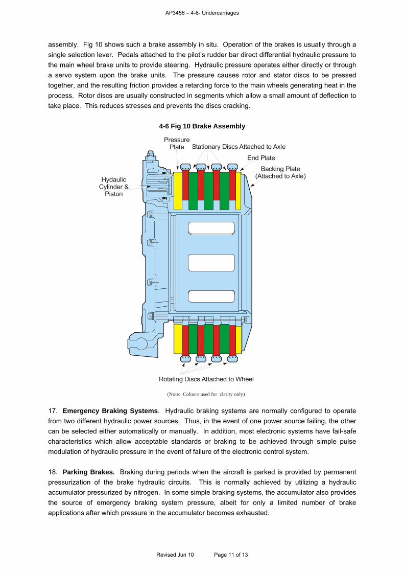
AP3456 – 4-6- Undercarriages
assembly. Fig 10 shows such a brake assembly in situ. Operation of the brakes is usually through a
single selection lever. Pedals attached to the pilot’s rudder bar direct differential hydraulic pressure to
the main wheel brake units to provide steering. Hydraulic pressure operates either directly or through
a servo system upon the brake units. The pressure causes rotor and stator discs to be pressed
together, and the resulting friction provides a retarding force to the main wheels generating heat in the
process. Rotor discs are usually constructed in segments which allow a small amount of deflection to
take place. This reduces stresses and prevents the discs cracking.
4-6 Fig 10 Brake Assembly
Backing Plate(Attached to Axle)
End Plate
Stationary Discs Attached to AxlePressure
Plate
HydaulicCylinder &
Piston
Rotating Discs Attached to Wheel
(Note: Colours used for clarity only)
17. Emergency Braking Systems. Hydraulic braking systems are normally configured to operate
from two different hydraulic power sources. Thus, in the event of one power source failing, the other
can be selected either automatically or manually. In addition, most electronic systems have fail-safe
characteristics which allow acceptable standards or braking to be achieved through simple pulse
modulation of hydraulic pressure in the event of failure of the electronic control system.
18. Parking Brakes. Braking during periods when the aircraft is parked is provided by permanent
pressurization of the brake hydraulic circuits. This is normally achieved by utilizing a hydraulic
accumulator pressurized by nitrogen. In some simple braking systems, the accumulator also provides
the source of emergency braking system pressure, albeit for only a limited number of brake
applications after which pressure in the accumulator becomes exhausted.
Revised Jun 10 Page 11 of 13
AP3456 – 4-6- Undercarriages
Braking Control and Anti-skid Systems
19. Braking Dynamics. To minimize the landing run, it is imperative that brakes apply maximum
retardation force without causing the adhesion between tyre and pavement to be exceeded thus
causing the aircraft wheels to skid. The point of skidding is dependent upon the condition of the
runway surface, the vertical load which the aircraft tyres exert on the ground and the retarding force
applied by the brakes. The mathematical relationship between vertical load and retarding force is
termed 'μ'. Because vertical load is inversely proportional to the aerodynamic lift acting on the aircraft,
it follows that will increase as aircraft speed decreases. Fig 11 shows this relationship for constant
runway conditions.
4-6 Fig 11 Relationship Between and Vertical Load on the Tyres
Maximum Available Friction
Area of PilotControlled Modulation
Aircraft Speed
Whenever braking force is applied to the tyre, a degree of slip occurs between the tyre and the
surface of the pavement. This is defined in terms of the difference between the rotational speed of a
braked wheel and the rotational speed of a similar free rolling wheel. It is expressed as a percentage.
The value of varies with wheel slip, and Fig 12 shows the relationship between maximum available
and wheel slip for varying conditions on the same runway.
4-6 Fig 12 Relationship Between and Wheel Slip for Varying Runway Conditions
0.2
0.3
0.4
0.6
0.8
0.7
0.5
0 10 20 30 40 50 60
Dry
Wet
Snow
Ice
% Slip
0.1
70
Revised Jun 10 Page 12 of 13
AP3456 – 4-6- Undercarriages
Revised Jun 10 Page 13 of 13
20. Control Systems. As can be deduced from the above considerations, the application of
maximum braking effort to minimize the landing run requires the solution of complex dynamic
equations, balancing braking forces with speed, weight and runway conditions. Electronic sensing
has permitted all phases of the braking process to be inter-related and fail safe over-rides to be
employed. A typical brake system operation profile is at Fig 13.
4-6 Fig 13 Typical Brake System Operation Profile
TaxiLanding RunTouchDown
Brakes - No Anti-skid ProtectionBrakes With Anti-skid ProtectionNo Brakes
Aircraft Path
Ground Line
Touchdown Protection(No braking applied)
Note: During take-off,brakes are automatically
applied after lift off
WheelSpin-upoverridestouchdownprotectionsystem
Locked Wheel Protectionfor a wheel below 30% of
aircraft speed(see note below)
Wheels will lock but hazardreduced at such low speeds
Note: A deceleration of the wheels of 26 ft/sec/sec(or 30% differential between wheel speeds)
actuates anti-skid modulation sequence
15 mph
21. Anti-skid Systems. Early mechanical anti-skid systems utilized the inertia of a small flywheel
to sense rapid changes of main wheel rotational speed such as occurs during a skid. On sensing
a skid, the systems reduced hydraulic pressure - thereby reducing braking effort and stopping the
skid. They reinstated pressure when skidding had reduced. The resultant cycling between
skid/no skid conditions caused the braking pressure to continuously pulse or modulate, and the
technique became known as brake modulation. Subsequent electrical systems used sensors to
measure wheel speed and compared the speed to a datum. The use of simple electronic
processing allowed a controlled profile of modulation to be achieved instead of the on/off
characteristics of the earlier mechanical systems, and considerable improvements in braking
efficiency were achieved. Modern anti-skid systems utilize control technology to vary not only the
frequency of modulated braking pulses but also their amplitude (pressure). Thus, the systems can
maintain braking forces at a level immediately below that which would cause skidding for all
speeds and surface conditions. The systems also hold the brakes off until after touch down and
wheel spin up has occurred, and similarly apply braking to spin down the wheels after take off and
undercarriage retraction has taken place. Thus, the systems can relieve the crew of much of the
workload of brake management at the critical periods of landing and take off.
AP3456 – 4-7- Automatic Flight Control Systems
CHAPTER 7 - AUTOMATIC FLIGHT CONTROL SYSTEMS
Contents Page Introduction.............................................................................................................................................. 1 AUTOSTABILIZERS AND BASIC AUTOPILOTS ................................................................................... 2 Autostabilizers ......................................................................................................................................... 2 Basic Autopilot Systems.......................................................................................................................... 3 AUTOMATIC FLIGHT CONTROL SYSTEMS ........................................................................................ 5 Principles of AFCS Operation ................................................................................................................. 5 AFCS Components.................................................................................................................................. 6 AFCS Functions ...................................................................................................................................... 7 Influence of AFCS on Aircraft Design...................................................................................................... 8 Fly-by-wire and Fly-by-light Systems ...................................................................................................... 9 FLIGHT MANAGEMENT SYSTEMS..................................................................................................... 12 Introduction............................................................................................................................................ 12 Flight Planning....................................................................................................................................... 13 Optimized Flight Performance............................................................................................................... 14 FMS Operations .................................................................................................................................... 14 ACTIVE CONTROL TECHNOLOGY (ACT).......................................................................................... 15 Introduction............................................................................................................................................ 15 Employment of ACT .............................................................................................................................. 15 Table of Figures 4-7 Fig 1 Autostabilizer Feedback System.............................................................................................. 2 4-7 Fig 2 Typical Autostabilizer Control Panel ........................................................................................ 3 4-7 Fig 3 Autopilot Loop (Pitch Axis only) ............................................................................................... 4 4-7 Fig 4 Autopilot Control Panel ............................................................................................................ 4 4-7 Fig 5 Basic Flight Control System Operation .................................................................................... 6 4-7 Fig 6 Auto-throttle Control System.................................................................................................... 7 4-7 Fig 7 Typical Auto-land Sequence .................................................................................................... 8 4-7 Fig 8 Fly-by-wire Flight Control System ............................................................................................ 9 4-7 Fig 9 Typical Redundancy in a FBW Control System..................................................................... 11 4-7 Fig 10 Triplex and Quadruplex Voter/Monitor Systems .................................................................. 12 4-7 Fig 11 Relationship between an FMS and the AFCS ..................................................................... 13 4-7 Fig 12 A Typical Pilot/FMS Interface............................................................................................... 14 4-7 Fig 13 Comparison of AAW and Conventional Controls................................................................. 16 4-7 Fig 14 Comparison of Conventional and Control Configured Aircraft............................................. 17 Introduction 1. The Problem. Since the first days of flight, the need to compromise between aircraft performance and controllability of the aircraft has formed a central factor influencing specification and design. The pilot has to contend with a demanding workload, whilst maintaining a span of concentration throughout the whole flight, sometimes of long duration. At the same time, a rapid response is necessary to counter any adverse changes in aircraft attitude. Historically, therefore,
Revised Jun 10 Page 1 of 17
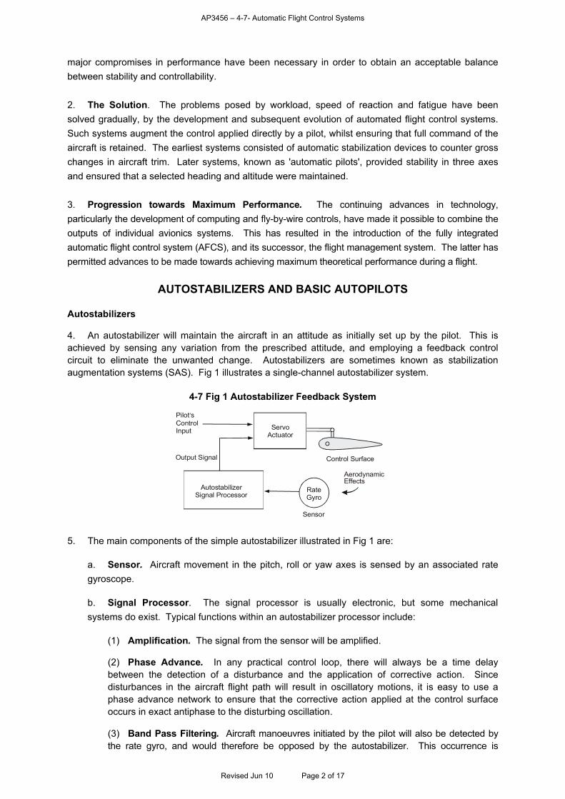
AP3456 – 4-7- Automatic Flight Control Systems
major compromises in performance have been necessary in order to obtain an acceptable balance between stability and controllability. 2. The Solution. The problems posed by workload, speed of reaction and fatigue have been solved gradually, by the development and subsequent evolution of automated flight control systems. Such systems augment the control applied directly by a pilot, whilst ensuring that full command of the aircraft is retained. The earliest systems consisted of automatic stabilization devices to counter gross changes in aircraft trim. Later systems, known as 'automatic pilots', provided stability in three axes and ensured that a selected heading and altitude were maintained. 3. Progression towards Maximum Performance. The continuing advances in technology, particularly the development of computing and fly-by-wire controls, have made it possible to combine the outputs of individual avionics systems. This has resulted in the introduction of the fully integrated automatic flight control system (AFCS), and its successor, the flight management system. The latter has permitted advances to be made towards achieving maximum theoretical performance during a flight.
AUTOSTABILIZERS AND BASIC AUTOPILOTS Autostabilizers 4. An autostabilizer will maintain the aircraft in an attitude as initially set up by the pilot. This is achieved by sensing any variation from the prescribed attitude, and employing a feedback control circuit to eliminate the unwanted change. Autostabilizers are sometimes known as stabilization augmentation systems (SAS). Fig 1 illustrates a single-channel autostabilizer system.
4-7 Fig 1 Autostabilizer Feedback System
AutostabilizerSignal Processor
Pilot sControlInput
’
Output Signal
Rate Gyro
ServoActuator
Control Surface
AerodynamicEffects
Sensor 5. The main components of the simple autostabilizer illustrated in Fig 1 are:
a. Sensor. Aircraft movement in the pitch, roll or yaw axes is sensed by an associated rate gyroscope.
b. Signal Processor. The signal processor is usually electronic, but some mechanical systems do exist. Typical functions within an autostabilizer processor include:
(1) Amplification. The signal from the sensor will be amplified.
(2) Phase Advance. In any practical control loop, there will always be a time delay between the detection of a disturbance and the application of corrective action. Since disturbances in the aircraft flight path will result in oscillatory motions, it is easy to use a phase advance network to ensure that the corrective action applied at the control surface occurs in exact antiphase to the disturbing oscillation.
(3) Band Pass Filtering. Aircraft manoeuvres initiated by the pilot will also be detected by the rate gyro, and would therefore be opposed by the autostabilizer. This occurrence is
Revised Jun 10 Page 2 of 17
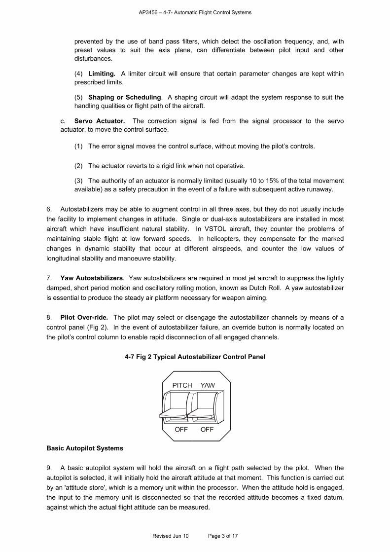
AP3456 – 4-7- Automatic Flight Control Systems
prevented by the use of band pass filters, which detect the oscillation frequency, and, with preset values to suit the axis plane, can differentiate between pilot input and other disturbances.
(4) Limiting. A limiter circuit will ensure that certain parameter changes are kept within prescribed limits.
(5) Shaping or Scheduling. A shaping circuit will adapt the system response to suit the handling qualities or flight path of the aircraft.
c. Servo Actuator. The correction signal is fed from the signal processor to the servo actuator, to move the control surface.
(1) The error signal moves the control surface, without moving the pilot’s controls.
(2) The actuator reverts to a rigid link when not operative.
(3) The authority of an actuator is normally limited (usually 10 to 15% of the total movement available) as a safety precaution in the event of a failure with subsequent active runaway.
6. Autostabilizers may be able to augment control in all three axes, but they do not usually include the facility to implement changes in attitude. Single or dual-axis autostabilizers are installed in most aircraft which have insufficient natural stability. In VSTOL aircraft, they counter the problems of maintaining stable flight at low forward speeds. In helicopters, they compensate for the marked changes in dynamic stability that occur at different airspeeds, and counter the low values of longitudinal stability and manoeuvre stability. 7. Yaw Autostabilizers. Yaw autostabilizers are required in most jet aircraft to suppress the lightly damped, short period motion and oscillatory rolling motion, known as Dutch Roll. A yaw autostabilizer is essential to produce the steady air platform necessary for weapon aiming. 8. Pilot Over-ride. The pilot may select or disengage the autostabilizer channels by means of a control panel (Fig 2). In the event of autostabilizer failure, an override button is normally located on the pilot’s control column to enable rapid disconnection of all engaged channels.
4-7 Fig 2 Typical Autostabilizer Control Panel
PITCH YAW
OFF OFF
Basic Autopilot Systems 9. A basic autopilot system will hold the aircraft on a flight path selected by the pilot. When the autopilot is selected, it will initially hold the aircraft attitude at that moment. This function is carried out by an 'attitude store', which is a memory unit within the processor. When the attitude hold is engaged, the input to the memory unit is disconnected so that the recorded attitude becomes a fixed datum, against which the actual flight attitude can be measured.
Revised Jun 10 Page 3 of 17
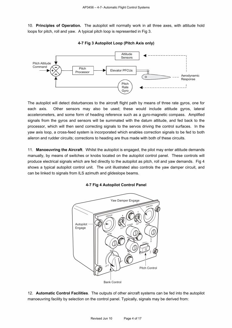
AP3456 – 4-7- Automatic Flight Control Systems
10. Principles of Operation. The autopilot will normally work in all three axes, with attitude hold loops for pitch, roll and yaw. A typical pitch loop is represented in Fig 3.
4-7 Fig 3 Autopilot Loop (Pitch Axis only)
Elevator PFCUs+
Pitch AttitudeCommand Pitch
ProcessorAerodynamicResponse
AttitudeSensors
PitchRateGyro
The autopilot will detect disturbances to the aircraft flight path by means of three rate gyros, one for each axis. Other sensors may also be used; these would include attitude gyros, lateral accelerometers, and some form of heading reference such as a gyro-magnetic compass. Amplified signals from the gyros and sensors will be summated with the datum attitude, and fed back to the processor, which will then send correcting signals to the servos driving the control surfaces. In the yaw axis loop, a cross-feed system is incorporated which enables correction signals to be fed to both aileron and rudder circuits; corrections to heading are thus made with both of these circuits. 11. Manoeuvring the Aircraft. Whilst the autopilot is engaged, the pilot may enter attitude demands manually, by means of switches or knobs located on the autopilot control panel. These controls will produce electrical signals which are fed directly to the autopilot as pitch, roll and yaw demands. Fig 4 shows a typical autopilot control unit. The unit illustrated also controls the yaw damper circuit, and can be linked to signals from ILS azimuth and glideslope beams.
4-7 Fig 4 Autopilot Control Panel
AutopilotEngage
Yaw Damper Engage
Bank Control
Pitch Control
12. Automatic Control Facilities. The outputs of other aircraft systems can be fed into the autopilot manoeuvring facility by selection on the control panel. Typically, signals may be derived from:
Revised Jun 10 Page 4 of 17
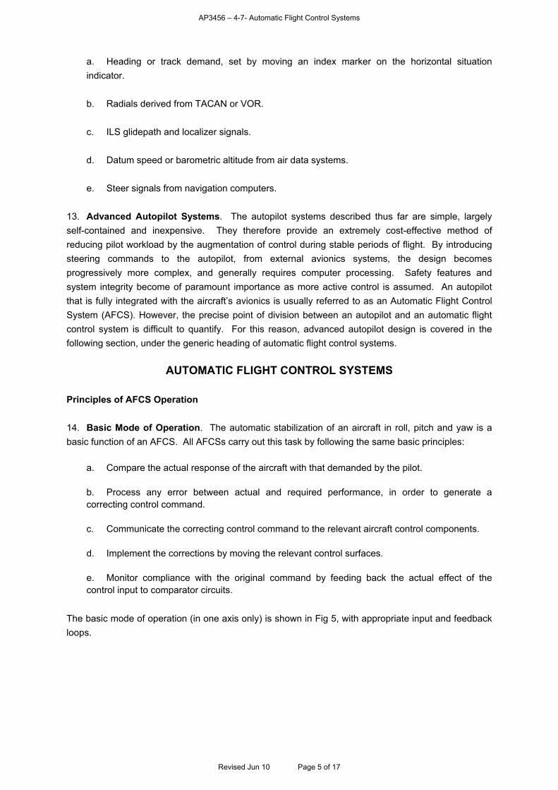
AP3456 – 4-7- Automatic Flight Control Systems
a. Heading or track demand, set by moving an index marker on the horizontal situation indicator. b. Radials derived from TACAN or VOR. c. ILS glidepath and localizer signals. d. Datum speed or barometric altitude from air data systems. e. Steer signals from navigation computers.
13. Advanced Autopilot Systems. The autopilot systems described thus far are simple, largely self-contained and inexpensive. They therefore provide an extremely cost-effective method of reducing pilot workload by the augmentation of control during stable periods of flight. By introducing steering commands to the autopilot, from external avionics systems, the design becomes progressively more complex, and generally requires computer processing. Safety features and system integrity become of paramount importance as more active control is assumed. An autopilot that is fully integrated with the aircraft’s avionics is usually referred to as an Automatic Flight Control System (AFCS). However, the precise point of division between an autopilot and an automatic flight control system is difficult to quantify. For this reason, advanced autopilot design is covered in the following section, under the generic heading of automatic flight control systems.
AUTOMATIC FLIGHT CONTROL SYSTEMS Principles of AFCS Operation 14. Basic Mode of Operation. The automatic stabilization of an aircraft in roll, pitch and yaw is a basic function of an AFCS. All AFCSs carry out this task by following the same basic principles:
a. Compare the actual response of the aircraft with that demanded by the pilot. b. Process any error between actual and required performance, in order to generate a correcting control command. c. Communicate the correcting control command to the relevant aircraft control components. d. Implement the corrections by moving the relevant control surfaces. e. Monitor compliance with the original command by feeding back the actual effect of the control input to comparator circuits.
The basic mode of operation (in one axis only) is shown in Fig 5, with appropriate input and feedback loops.
Revised Jun 10 Page 5 of 17
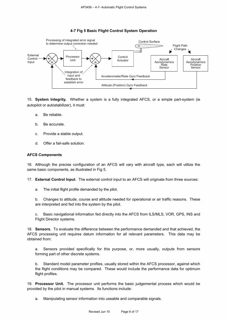
AP3456 – 4-7- Automatic Flight Control Systems
4-7 Fig 5 Basic Flight Control System Operation
Flight PathChanges
Accelerometer/Rate Gyro Feedback
Attitude (Position) Gyro Feedback
Integration ofinput and
feedback toestablish error
ProcessorUnit
Processing of integrated error signal to determine output correction needed
AircraftAerodynamics
RateSensor
AircraftAerodynamics
PositionSensor
ExternalControlInput
+
Control Surface
ControlActuator+
15. System Integrity. Whether a system is a fully integrated AFCS, or a simple part-system (ie autopilot or autostabilizer), it must:
a. Be reliable. b. Be accurate. c. Provide a stable output. d. Offer a fail-safe solution.
AFCS Components 16. Although the precise configuration of an AFCS will vary with aircraft type, each will utilize the same basic components, as illustrated in Fig 5. 17. External Control Input. The external control input to an AFCS will originate from three sources:
a. The initial flight profile demanded by the pilot. b. Changes to attitude, course and altitude needed for operational or air traffic reasons. These are interpreted and fed into the system by the pilot. c. Basic navigational information fed directly into the AFCS from ILS/MLS, VOR, GPS, INS and Flight Director systems.
18. Sensors. To evaluate the difference between the performance demanded and that achieved, the AFCS processing unit requires datum information for all relevant parameters. This data may be obtained from:
a. Sensors provided specifically for this purpose, or, more usually, outputs from sensors forming part of other discrete systems. b. Standard model parameter profiles, usually stored within the AFCS processor, against which the flight conditions may be compared. These would include the performance data for optimum flight profiles.
19. Processor Unit. The processor unit performs the basic judgemental process which would be provided by the pilot in manual systems. Its functions include:
a. Manipulating sensor information into useable and comparable signals.
Revised Jun 10 Page 6 of 17
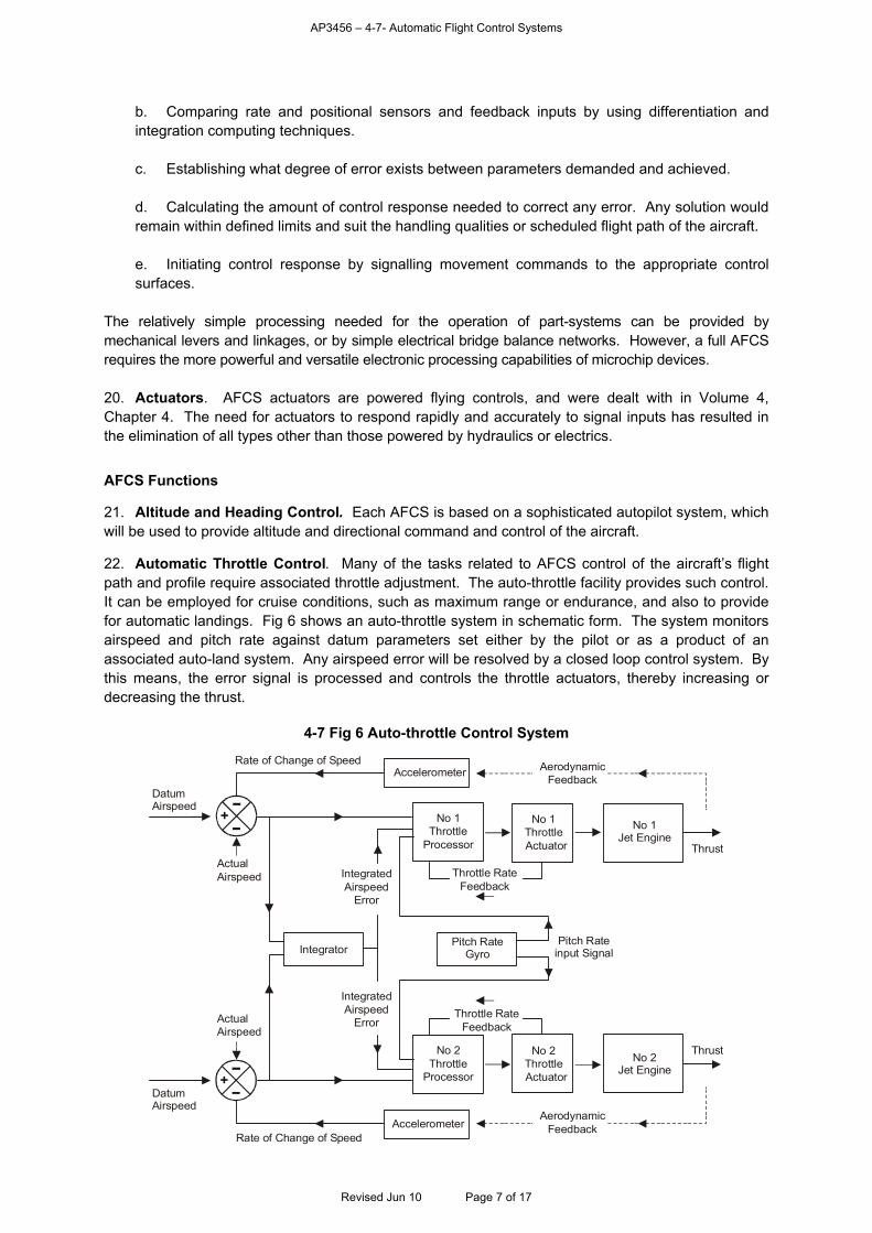
AP3456 – 4-7- Automatic Flight Control Systems
b. Comparing rate and positional sensors and feedback inputs by using differentiation and integration computing techniques. c. Establishing what degree of error exists between parameters demanded and achieved. d. Calculating the amount of control response needed to correct any error. Any solution would remain within defined limits and suit the handling qualities or scheduled flight path of the aircraft. e. Initiating control response by signalling movement commands to the appropriate control surfaces.
The relatively simple processing needed for the operation of part-systems can be provided by mechanical levers and linkages, or by simple electrical bridge balance networks. However, a full AFCS requires the more powerful and versatile electronic processing capabilities of microchip devices. 20. Actuators. AFCS actuators are powered flying controls, and were dealt with in Volume 4, Chapter 4. The need for actuators to respond rapidly and accurately to signal inputs has resulted in the elimination of all types other than those powered by hydraulics or electrics. AFCS Functions 21. Altitude and Heading Control. Each AFCS is based on a sophisticated autopilot system, which will be used to provide altitude and directional command and control of the aircraft. 22. Automatic Throttle Control. Many of the tasks related to AFCS control of the aircraft’s flight path and profile require associated throttle adjustment. The auto-throttle facility provides such control. It can be employed for cruise conditions, such as maximum range or endurance, and also to provide for automatic landings. Fig 6 shows an auto-throttle system in schematic form. The system monitors airspeed and pitch rate against datum parameters set either by the pilot or as a product of an associated auto-land system. Any airspeed error will be resolved by a closed loop control system. By this means, the error signal is processed and controls the throttle actuators, thereby increasing or decreasing the thrust.
4-7 Fig 6 Auto-throttle Control System
Pitch RateGyroIntegrator
ActualAirspeed
AerodynamicFeedback
DatumAirspeed
Throttle RateFeedback
No 1Throttle
Processor
No 1ThrottleActuator
Pitch Rateinput Signal
+
IntegratedAirspeed
Error
No 1Jet Engine
Thrust
AccelerometerRate of Change of Speed
IntegratedAirspeed
ErrorThrottle Rate
Feedback
Thrust
AerodynamicFeedbackAccelerometer
ActualAirspeed
DatumAirspeed
Rate of Change of Speed
No 2Throttle
Processor
No 2ThrottleActuator
No 2Jet Engine
+
Revised Jun 10 Page 7 of 17
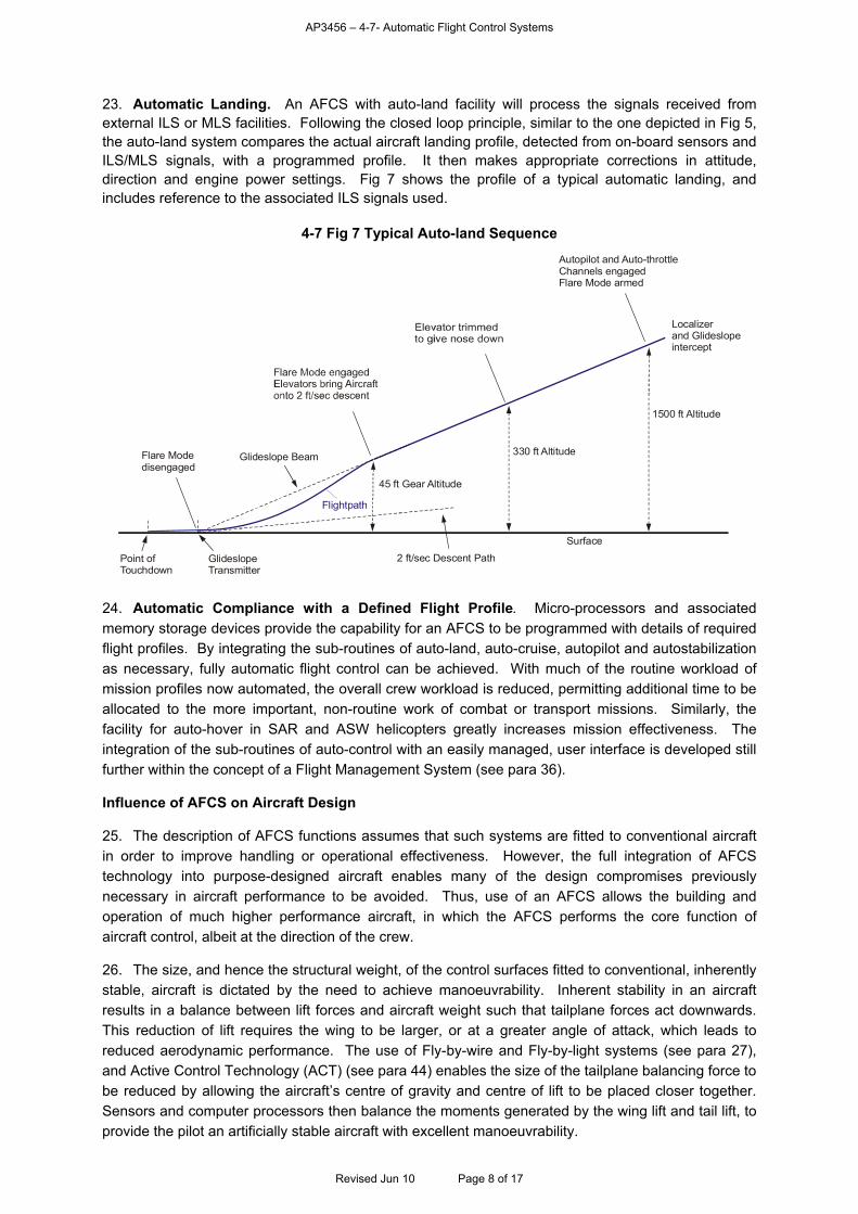
AP3456 – 4-7- Automatic Flight Control Systems
23. Automatic Landing. An AFCS with auto-land facility will process the signals received from external ILS or MLS facilities. Following the closed loop principle, similar to the one depicted in Fig 5, the auto-land system compares the actual aircraft landing profile, detected from on-board sensors and ILS/MLS signals, with a programmed profile. It then makes appropriate corrections in attitude, direction and engine power settings. Fig 7 shows the profile of a typical automatic landing, and includes reference to the associated ILS signals used.
4-7 Fig 7 Typical Auto-land Sequence
Flare Modedisengaged
Point of Touchdown
Flightpath
Glideslope Beam
Localizerand Glideslopeintercept
Autopilot and Auto-throttleChannels engagedFlare Mode armed
330 ft Altitude
45 ft Gear Altitude
2 ft/sec Descent PathGlideslopeTransmitter
1500 ft Altitude
Surface
24. Automatic Compliance with a Defined Flight Profile. Micro-processors and associated memory storage devices provide the capability for an AFCS to be programmed with details of required flight profiles. By integrating the sub-routines of auto-land, auto-cruise, autopilot and autostabilization as necessary, fully automatic flight control can be achieved. With much of the routine workload of mission profiles now automated, the overall crew workload is reduced, permitting additional time to be allocated to the more important, non-routine work of combat or transport missions. Similarly, the facility for auto-hover in SAR and ASW helicopters greatly increases mission effectiveness. The integration of the sub-routines of auto-control with an easily managed, user interface is developed still further within the concept of a Flight Management System (see para 36). Influence of AFCS on Aircraft Design 25. The description of AFCS functions assumes that such systems are fitted to conventional aircraft in order to improve handling or operational effectiveness. However, the full integration of AFCS technology into purpose-designed aircraft enables many of the design compromises previously necessary in aircraft performance to be avoided. Thus, use of an AFCS allows the building and operation of much higher performance aircraft, in which the AFCS performs the core function of aircraft control, albeit at the direction of the crew. 26. The size, and hence the structural weight, of the control surfaces fitted to conventional, inherently stable, aircraft is dictated by the need to achieve manoeuvrability. Inherent stability in an aircraft results in a balance between lift forces and aircraft weight such that tailplane forces act downwards. This reduction of lift requires the wing to be larger, or at a greater angle of attack, which leads to reduced aerodynamic performance. The use of Fly-by-wire and Fly-by-light systems (see para 27), and Active Control Technology (ACT) (see para 44) enables the size of the tailplane balancing force to be reduced by allowing the aircraft’s centre of gravity and centre of lift to be placed closer together. Sensors and computer processors then balance the moments generated by the wing lift and tail lift, to provide the pilot an artificially stable aircraft with excellent manoeuvrability.
Revised Jun 10 Page 8 of 17
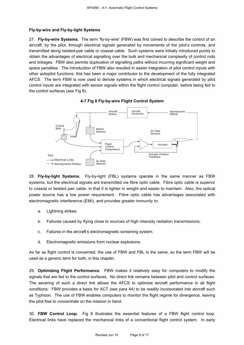
AP3456 – 4-7- Automatic Flight Control Systems
Fly-by-wire and Fly-by-light Systems 27. Fly-by-wire Systems. The term 'fly-by-wire' (FBW) was first coined to describe the control of an aircraft, by the pilot, through electrical signals generated by movements of the pilot’s controls, and transmitted along twisted-pair cable or coaxial cable. Such systems were initially introduced purely to obtain the advantages of electrical signalling over the bulk and mechanical complexity of control rods and linkages. FBW also permits duplication of signalling paths without incurring significant weight and space penalties. The introduction of FBW also resulted in easier integration of pilot control inputs with other autopilot functions; this has been a major contributor to the development of the fully integrated AFCS. The term FBW is now used to denote systems in which electrical signals generated by pilot control inputs are integrated with sensor signals within the flight control computer, before being fed to the control surfaces (see Fig 8).
4-7 Fig 8 Fly-by-wire Flight Control System
AircraftDynamics
ControlStick Motion
Sensors
Air DataSensors
Electrical LinksKey
Aerodynamic Motion
Air DataSensors
FlightControlComputer(s)
Actuator
Actuator PositionFeedback
AircraftMotion
AerodynamicEffects
28. Fly-by-light Systems. Fly-by-light (FBL) systems operate in the same manner as FBW systems, but the electrical signals are transmitted via fibre optic cable. Fibre optic cable is superior to coaxial or twisted pair cable, in that it is lighter in weight and easier to maintain. Also, the optical power source has a low power requirement. Fibre optic cable has advantages associated with electromagnetic interference (EMI), and provides greater immunity to:
a. Lightning strikes. b. Failures caused by flying close to sources of high intensity radiation transmissions. c. Failures in the aircraft’s electromagnetic screening system. d. Electromagnetic emissions from nuclear explosions.
As far as flight control is concerned, the use of FBW and FBL is the same, so the term FBW will be used as a generic term for both, in this chapter. 29. Optimizing Flight Performance. FBW makes it relatively easy for computers to modify the signals that are fed to the control surfaces. No direct link remains between pilot and control surfaces. The severing of such a direct link allows the AFCS to optimize aircraft performance in all flight conditions. FBW provides a basis for ACT (see para 44) to be readily incorporated into aircraft such as Typhoon. The use of FBW enables computers to monitor the flight regime for divergence, leaving the pilot free to concentrate on the mission in hand. 30. FBW Control Loop. Fig 8 illustrates the essential features of a FBW flight control loop. Electrical links have replaced the mechanical links of a conventional flight control system. In early
Revised Jun 10 Page 9 of 17
AP3456 – 4-7- Automatic Flight Control Systems
FBW aircraft, the flight control computer was analogue, but now digital systems are used, enabling complex control law algorithms to be implemented. 31. Benefits of FBW Control. The major benefit of FBW is the ability to tailor the system’s characteristics at each point in the aircraft’s flight envelope. The performance benefits from FBW are often quoted in terms of manoeuvrability, but it is often the avoidance of a manoeuvre, which would stall or over-stress the aircraft, that is a more important benefit. The other benefits of FBW include:
a. Carefree handling, provided by automatic protection against stall and departure (using angle-of-attack control and angle-of-sideslip suppression). In addition, overstressing of the airframe is prevented by automatic limiting of normal acceleration and roll rates. b. Handling qualities which are optimized across the flight envelope, providing for a wide range of aircraft stores, asymmetric configurations and in-flight changes, such as those encountered when ordnance is released. c. Improved agility for fighter aircraft. Aircraft configurations with negative stability assist rapid changes in fuselage aiming and/or velocity vector. This greatly enhances offensive and defensive manoeuvrability. d. Improved aircraft performance, due to increased lift/drag ratio. FBW is lighter than mechanical linkages, and also permits the use of a smaller tailplane, fin and rudder. Drag is also reduced due to the optimized trim setting of controls. e. An extended flight envelope, provided by the use of thrust vectoring to augment or replace aerodynamic control surfaces. f. The ability to reconfigure systems easily following failures or battle damage. This enables missions to be completed, or safe recoveries made. g. Reduced maintenance costs, resulting from a reduction in mechanical complexity and the introduction of built-in test facilities.
32. FBW Integrity. The overall system integrity of FBW must be as high as the mechanical control system it replaces. The probability of a catastrophic failure must not exceed 10-9/hour for civil aircraft and 10-7/hour in military aircraft. In order to achieve this reliability, multiple signal sources and several lanes of computing are necessary to provide redundancy. A system of cross-monitoring is included in order to isolate any failed equipment, thereby ensuring safe operation. The current trend is towards mixed triplex and quadruplex redundancy, as illustrated in Fig 9. A comprehensive built-in test capability is used to identify and locate failures, and to ensure that the system is safe prior to each flight. The back-up systems in FBW usually provide limited flight control capability, although the trend is towards a full capability.
Revised Jun 10 Page 10 of 17
AP3456 – 4-7- Automatic Flight Control Systems
4-7 Fig 9 Typical Redundancy in a FBW Control System
Back-upActuation System
Control Stick
Air Data
Sensors
Flight Control Computer(s)
Flight Control Compute
Back-up Flight Control Computers
Flight Control Computer(s)
Flight Control Computer(s
Flight Contr ol Computer(s
Flight Control Computers
Motion Sensors
Actuator Processor
VoterUnit
VoterUnit
Voter/Monitor Unit
Voter/Monitor Unit
33. Use of Dissimilar Systems. In many early FBW systems, the back-up computer was analogue but digital computers are now employed. Dissimilar hardware is used to avoid failures being repeated in duplicated systems; this may occur through common design errors. System integrity requires back-up digital computers to be procured through alternative requirement documents, using different software, independent programming teams, and utilizing dissimilar operating systems. Fig 9 illustrates a back-up control surface actuation system. This is more common in civil airliners but has been partially used on military jets. Early FBW aircraft, such as the Tornado, reverted to mechanical flight control but only with a 'get you home' capability. FBW is being developed for helicopter use, but the development of full authority flight control is slow because of the complex nature of helicopter flight controls. The only operational FBW in a military helicopter is a simplified flight control system, used as a back-up in event of failure of the mechanical system.
34. Voting and Monitoring. Examples of triplex and quadruplex systems employed in a FBW flight control system are shown in Fig 10. Provided the monitoring is to a high degree of integrity and confidence level, such systems provide sufficient redundancy to survive any two failures, from whatever cause.
a. Monitored Triplex Redundancy. Fig 10a illustrates a monitored triplex redundancy system, consisting of three independent and parallel channels. Each channel incorporates its own monitoring system, to check the channel’s functioning to a high confidence level. If any channel fails, its associated monitoring system will identify the failure, and isolate the output by means of relays. The system illustrated could survive two lane failures, leaving the third to run the service.
Revised Jun 10 Page 11 of 17
AP3456 – 4-7- Automatic Flight Control Systems
4-7 Fig 10 Triplex and Quadruplex Voter/Monitor Systems
Fig 10a Triplex System Fig 10b Quadruplex System
Monitor
Lane 1
LogicCircuits
LogicCircuits
Relay
Relay
Relay
LogicCircuits
Monitor
Lane 3
Lane 2
Monitor
LLaannee 11
LLaannee 22
LLaannee 33
Lane 1
Lane 2
Lane 3
Lane 4
Voter
Voter
Voter
Voter
Relay
Relay
Relay
Relay
b. Quadruplex Monitoring. Fig 10b shows a quadruplex system, which detects failures by cross-comparison of the parallel channels, and uses majority voting to determine the 'odd man out'. Once a failure is identified, that channel is disconnected. This system is able to survive two failures on majority voting. Depending upon the nature of a third channel failure, the system may be able to survive on a single channel.
FLIGHT MANAGEMENT SYSTEMS
Introduction 35. Computerized systems, known as Navigation Management Systems (NMS), were introduced in the early 1980s, to simplify the navigation task and to optimize the use of navigation aids. With the introduction of computer processors in aircraft, along with advanced AFCS and FBW technology, it has been possible to integrate the outputs from multiple aircraft systems, and to correlate aircraft flight conditions with a database containing performance values. By these means, achievements have been made towards attaining the theoretical maximum performance from an aircraft. A Flight Management System (FMS) is a computer-controlled AFCS, which allows the pilot to select specific modes of operation. These might include standard instrument departures and auto-landings. In large aircraft, the FMS has become one of the key avionics systems because of the reductions it can make to the pilot's workload. In military aircraft, the FMS has enabled single-crew operation of advanced combat aircraft. Fig 11 illustrates, in schematic format, the relationship between an FMS and the AFCS.
Revised Jun 10 Page 12 of 17
AP3456 – 4-7- Automatic Flight Control Systems
4-7 Fig 11 Relationship between an FMS and the AFCS
FlightManagement
System
Displays
Aircraft Stick& Controls
Actuators
Central WarningSystem
Aircraft Trims
Attitude / HeadingReference System
Rate Gyros& Accn
Radio Altimeter
Air DataSystem
RadioNavigation Aids
Inertial NavigationSystem
36. The FMS combines navigational and performance data with flight-derived data to determine an automatic flight profile that is normally optimized for specific operational parameters, such as maximum endurance or minimum fuel use. In its most comprehensive form, the FMS is directed to the auto-throttle system to optimize the power controls. An FMS can lead the pilot through the complete profile of the flight: takeoff, climbout, cruise climb, initial level off, step climb, cruise, top-of-descent, descent, approach and landing. Flight Planning 37. Flight Planning Database. The FMS plays a major role in the flight planning task. It will hold a readily available database of air traffic significant points, runway information and navigation beacons. The navigation database is updated in accordance with the AIRAC dates (see Volume 9, Chapter 13). A typical FMS flight plan may contain up to 100 waypoints and the system can store a library of prepared flight plans for future use. As the FMS is essentially just a computer, there are many types and variations. The applications and the extent of the integration and automation vary greatly, as do other criteria such as accuracy. 38. Navigation Aids. The FMS will select and tune navigation aids in accordance with the planned profile. It will then determine the best estimate of aircraft position from all the navigation sources, through a Kalman filter process. Navigation sources will include:
a. Multiple INS.
b. GPS.
c. Air Data.
d. Radio navigation aids such as VOR and DME.
e. ILS/MLS. The FMS will compute and display groundspeed, track and wind velocity. 39. Flight Profile. The FMS will provide both lateral and vertical guidance signals to the AFCS. In the lateral mode, the FMS computes the aircraft's position relative to the planned route, and gives guidance signals to the AFCS to capture and follow the track specified by the flight plan.
Revised Jun 10 Page 13 of 17
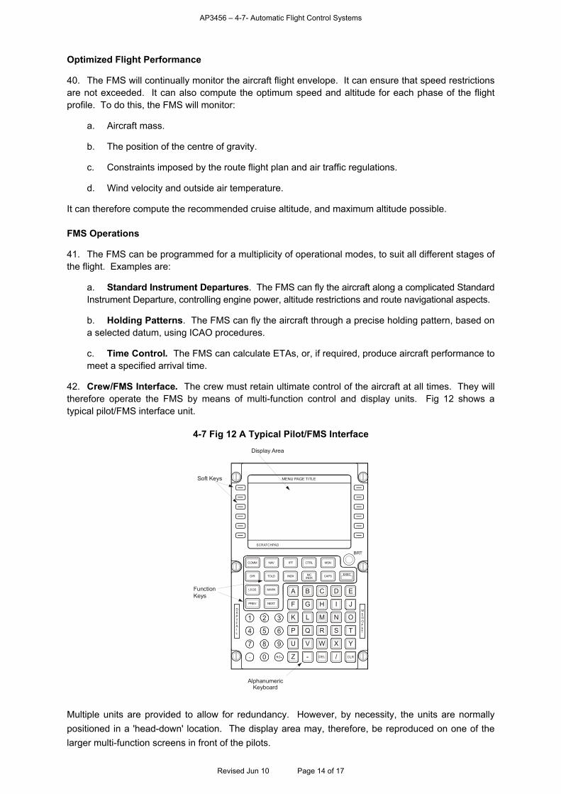
AP3456 – 4-7- Automatic Flight Control Systems
Optimized Flight Performance 40. The FMS will continually monitor the aircraft flight envelope. It can ensure that speed restrictions are not exceeded. It can also compute the optimum speed and altitude for each phase of the flight profile. To do this, the FMS will monitor:
a. Aircraft mass.
b. The position of the centre of gravity.
c. Constraints imposed by the route flight plan and air traffic regulations.
d. Wind velocity and outside air temperature. It can therefore compute the recommended cruise altitude, and maximum altitude possible. FMS Operations 41. The FMS can be programmed for a multiplicity of operational modes, to suit all different stages of the flight. Examples are:
a. Standard Instrument Departures. The FMS can fly the aircraft along a complicated Standard Instrument Departure, controlling engine power, altitude restrictions and route navigational aspects.
b. Holding Patterns. The FMS can fly the aircraft through a precise holding pattern, based on a selected datum, using ICAO procedures.
c. Time Control. The FMS can calculate ETAs, or, if required, produce aircraft performance to meet a specified arrival time.
42. Crew/FMS Interface. The crew must retain ultimate control of the aircraft at all times. They will therefore operate the FMS by means of multi-function control and display units. Fig 12 shows a typical pilot/FMS interface unit.
4-7 Fig 12 A Typical Pilot/FMS Interface
1
A
2 3
4 5 6
7 8 9
. 0 +/-
B C D E
F G H I J
K L M N O
P Q R S T
U V W X Y
Z - DEL / CLR
COMM NAV IFF CTRL MSN
DIR TOLD INDX MCINDX CAPS EXEC
LEGS MARK
PREV NEXT
DSPYFAIL
MSGOFST
MENU PAGE TITLE
SCRATCHPAD
BRT
Display Area
Soft Keys
AlphanumericKeyboard
FunctionKeys
Multiple units are provided to allow for redundancy. However, by necessity, the units are normally positioned in a 'head-down' location. The display area may, therefore, be reproduced on one of the larger multi-function screens in front of the pilots.
Revised Jun 10 Page 14 of 17
AP3456 – 4-7- Automatic Flight Control Systems
ACTIVE CONTROL TECHNOLOGY (ACT) Introduction 43. Passive Technology. Conventional design of airframes has brought aircraft technology to its present high level, but in many cases has reached its limits. Aircraft lifting surfaces have been designed to be strong enough to meet loading requirements, with material added to provide stiffness adequate to keep them free from flutter, divergence and buckling. However, this added stiffness usually means adding structural weight. For a given set of aerodynamic requirements, aircraft design has therefore been a compromise between weight and aerodynamic performance. This legacy of normally stable aircraft with conventional control surfaces is sometimes referred to as 'passive control'. 44. Active Control Systems. The trend in aircraft development is towards high manoeuvrability, lower specific fuel consumption, higher power-to-weight ratios and lower life-cycle cost. An active control system (ACS) may be likened to an AFCS, but designed to provide several special features including:
a. Activation of flight control surfaces to minimize gust loads and bending stresses in the wing. This is done by detection and response to normal accelerations. b. Provision of stability to a naturally unstable aircraft. c. Implementation of pilot manoeuvre demands by more active means than conventional control surfaces.
An ACS requires extensive integration between aerodynamics, structure and electronic system design to achieve these advantages with reliability and safety. Employment of ACT 45. The employment of ACT has become one of the most important aspects of aircraft design and operation, and, in some cases, there is potential for retrofit. ACT is linked to the development of computer technology, sensors and actuators, micro electro-mechanical technology, smart materials and improved knowledge of process laws. Specific uses for ACT include:
a. Gas Turbine Engines. Active control can be used within gas turbine engines, in areas of compression, combustion and airflow. ACT can produce higher pressure ratios, which in turn leads to smaller engines. Better performance and advanced diagnostics can lead to reduction on overall life cycle costs and savings in maintenance.
b. Fluid Aerodynamics. Boundary layer control and vortex flow can be influenced, and used to control flight attitude, thus avoiding the use of control surfaces, which are heavy and energy consuming.
c. Vertical Take-off and Landing Aircraft (VTOL). ACT has proven to be advantageous in controlling VTOL aircraft, particularly when manoeuvring in the hover. The development of the Joint Strike Fighter utilizes this concept, whereas, by contrast, the Harrier still requires much of the hover control to be a manual input from the pilot.
Revised Jun 10 Page 15 of 17
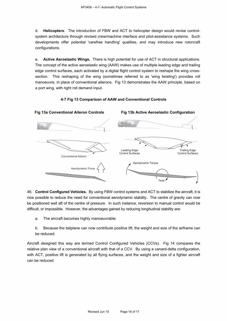
AP3456 – 4-7- Automatic Flight Control Systems
d. Helicopters. The introduction of FBW and ACT to helicopter design would revise control-system architecture through revised crew/machine interface and pilot-assistance systems. Such developments offer potential 'carefree handling' qualities, and may introduce new rotorcraft configurations.
e. Active Aeroelastic Wings. There is high potential for use of ACT in structural applications. The concept of the active aeroelastic wing (AAW) makes use of multiple leading edge and trailing edge control surfaces, each activated by a digital flight control system to reshape the wing cross-section. This reshaping of the wing (sometimes referred to as 'wing twisting') provides roll manoeuvre, in place of conventional ailerons. Fig 13 demonstrates the AAW principle, based on a port wing, with right roll demand input.
4-7 Fig 13 Comparison of AAW and Conventional Controls
Fig 13a Conventional Aileron Controls Fig 13b Active Aeroelastic Configuration
Conventional Aileron
Aerodynamic Force
Leading EdgeControl Surfaces
Trailing EdgeControl Surfaces
Aerodynamic Torque
Twist
46. Control Configured Vehicles. By using FBW control systems and ACT to stabilize the aircraft, it is now possible to reduce the need for conventional aerodynamic stability. The centre of gravity can now be positioned well aft of the centre of pressure. In such instance, reversion to manual control would be difficult, or impossible. However, the advantages gained by reducing longitudinal stability are:
a. The aircraft becomes highly manoeuvrable.
b. Because the tailplane can now contribute positive lift, the weight and size of the airframe can be reduced.
Aircraft designed this way are termed Control Configured Vehicles (CCVs). Fig 14 compares the relative plan view of a conventional aircraft with that of a CCV. By using a canard-delta configuration, with ACT, positive lift is generated by all flying surfaces, and the weight and size of a fighter aircraft can be reduced.
Revised Jun 10 Page 16 of 17
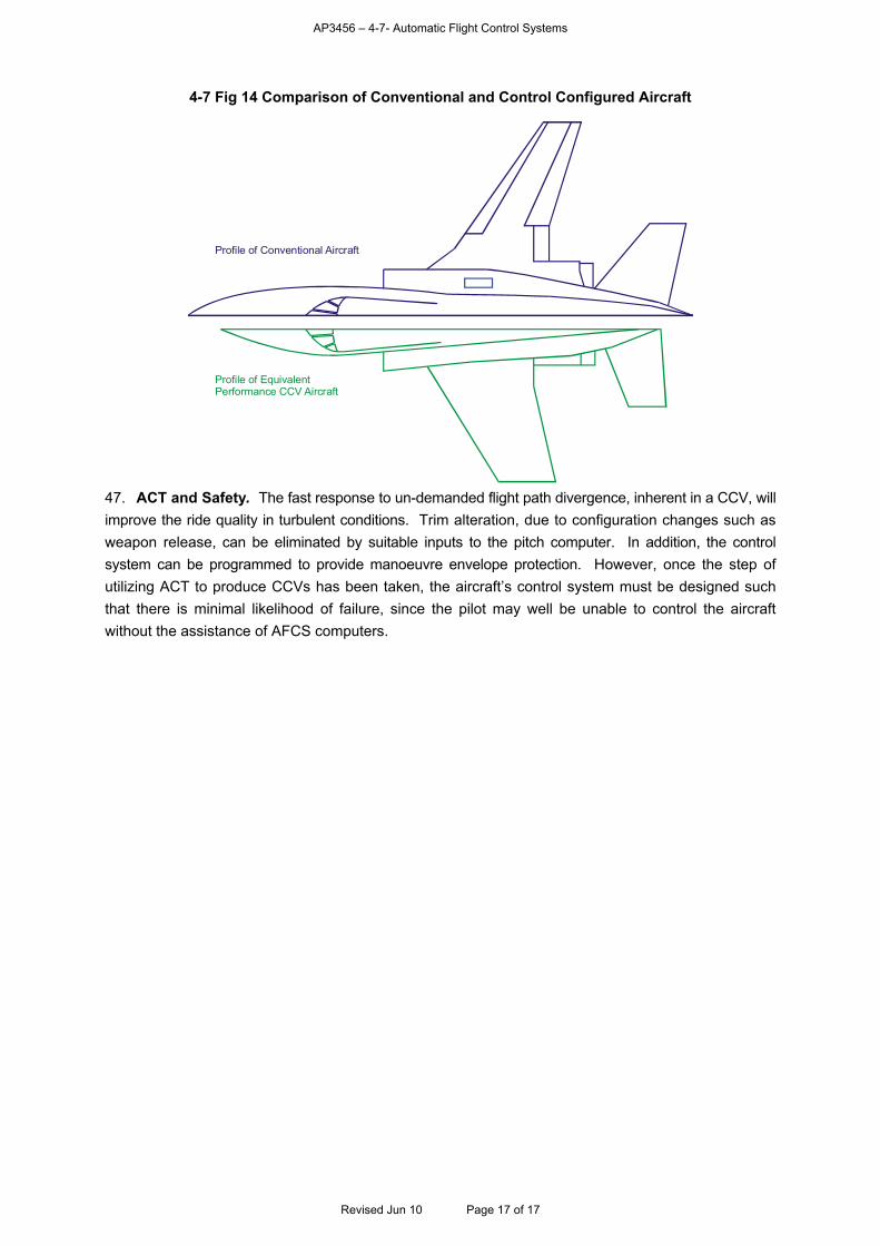
AP3456 – 4-7- Automatic Flight Control Systems
Revised Jun 10 Page 17 of 17
4-7 Fig 14 Comparison of Conventional and Control Configured Aircraft
Profile of Conventional Aircraft
Profile of EquivalentPerformance CCV Aircraft
47. ACT and Safety. The fast response to un-demanded flight path divergence, inherent in a CCV, will improve the ride quality in turbulent conditions. Trim alteration, due to configuration changes such as weapon release, can be eliminated by suitable inputs to the pitch computer. In addition, the control system can be programmed to provide manoeuvre envelope protection. However, once the step of utilizing ACT to produce CCVs has been taken, the aircraft’s control system must be designed such that there is minimal likelihood of failure, since the pilot may well be unable to control the aircraft without the assistance of AFCS computers.

AP3456 – 4-8 - Fire Warning and Extinguisher Systems
CHAPTER 8 - FIRE WARNING AND EXTINGUISHER SYSTEMS Contents Page Introduction.............................................................................................................................................. 1 Fire Detection Systems ........................................................................................................................... 2 Engine Fire Extinguisher Systems .......................................................................................................... 5 Portable Fire Extinguishers ..................................................................................................................... 7 Cabin Protection ...................................................................................................................................... 8 Table of Figures 4-8 Fig 1 Equipment Monitored by a Fire Detection System .................................................................. 2 4-8 Fig 2 Thermal Switch ........................................................................................................................ 3 4-8 Fig 3 Continuous Wire Detection Element ........................................................................................ 3 4-8 Fig 4 Installation of a Continuous Element System .......................................................................... 4 4-8 Fig 5 A Pendulum Inertia Switch ....................................................................................................... 5 4-8 Fig 6 Typical Engine and APU Systems Diagram............................................................................. 6 4-8 Fig 7 Detail of a 2-shot Fire Bottle..................................................................................................... 6 4-8 Fig 8 The BCF Portable Fire Extinguisher ........................................................................................ 8 Introduction 1. The design philosophy used in aircraft is first to prevent fire and secondly to provide adequate fire protection. Protection is usually in the form of fire resistant materials used in the construction of strategic systems and structures and fire retardant materials used in aircraft furnishings. However, in those areas where a risk of fire remains, active aircraft fire protection systems are utilized. These perform two basic, and usually independent, functions:
a. Fire and overheat detection. b. Fire extinguishing.
The fire detection and overheat systems sense the presence of fire or excessive heat. They employ area detectors in large fire zones and spot detectors for individual pieces of equipment. In freight and passenger aircraft, they are often supplemented by smoke detectors positioned in the freight bays, baggage holds, and toilet compartments. In the case of fire, overheat or smoke, the systems provide a visual and aural warning to the crew, identifying the area in which the problem exists. The fire extinguisher system provides a capability for fighting airborne fires in specific major areas, typically the engines and auxiliary power unit (APU). Fire extinguisher systems invariably require crew intervention for their operation in the air. However, in the event of a crash or crash landing, they are activated automatically by switches which close under high retardation forces or through airframe deformation. Aircraft are also equipped with hand-held extinguishers for use against small fires in internal areas and equipment. 2. The most common causes of aircraft fires are:
a. Fuel leaks in the vicinity of hot equipment. b. Hot gas leaks, from engines or ducting, impinging on inflammable materials. c. Electrical or mechanical malfunctions in equipment.
Revised Jun 10 Page 1 of 8

AP3456 – 4-8 - Fire Warning and Extinguisher Systems
The initiating cause is usually equipment failure, although, obviously, damage incurred during combat or a crash landing would provide ample additional cause. It follows, therefore, that the areas in which fire protection systems are deployed should include the engine bays, the APU enclosure, and significant pieces of high-energy equipment. Fig 1 provides a summary of the equipment given protection in a medium-size aircraft. The table includes the temperature at which a fire or overheat warning will be given and the visual warning which the crew will receive. Although the carriage of dangerous cargo in aircraft is adequately legislated for, spontaneous fires can occur in freight and baggage holds. Access to such areas whilst airborne may be possible, allowing the crew to enter them and fight the fires with portable extinguishers.
4-8 Fig 1 Equipment Monitored by a Fire Detection System
Unit/Area Covered Type of Detector Indication
Engine fire detection Graviner continuous wire L or R Fire lights
Fire/short test Graviner continuous wire L or R ENG FIRE DET fault
Engine (cooling air) overheat Thermal switches 860 ºF R and L ENGINE HOT
APU fire detection
Four thermal switches
Three at 450 ºF
One at 600 ºF
APU FIRE light
Radio rack overheat Twelve thermal switches 200 ºF FWD RADIO RACK HOT light
Alternator overheat Thermal switches 250 ºF L or R ALT HOT light
APU alternator overheat Thermal switches 300 ºF APU ALT HOT light
Emergency transformer rectifier overheat Thermal switch 375 ºF TRU HOT light
Tail compartment overheat Two thermal switches 200 ºF AFT EQUIP HOT light
Auxiliary hydraulic pump overheat Thermal switch 300 ºF AUXILIARY HYD HOT light
Pylon overheat Thermal switches 325 ºF L or R PYLON HOT light
Bleed-air duct overheat Thermal switches 550 ºF L or R BLEED AIR HOT light
Flight system hydraulic reservoir overheat Thermal switch 220 ºF FLT HYD HOT light
Combined system hydraulic reservoir overheat Thermal switch 220 ºF CMB HYD HOT light
Wing anti-ice overheat Thermal switches 180 ºF L or R WING HOT light
Cowl anti-ice overheat Thermal switches 675 ºF L or R COWL A/I OVHT
Bootstrap units Thermal switches 450 ºF L or R COOL TURB HOT
Forward radio rack Thermal switches 200 ºF FWD RADIO RACK HOT
Fire Detection Systems
3. The functions of fire detection systems are to:
a. Monitor designated areas or equipment for a rise in temperature, either at a higher rate, or to a higher level, than predetermined acceptable limits. b. Provide a warning to the crew. c. Complete electrical safety circuits within the fire extinguisher systems, to permit necessary operation by the crew.
The electrical safety circuits are provided to prevent accidental operation of extinguishers, and they are over-ridden either by the detection systems or by deliberate manual selection by the crew. The APU fire
Revised Jun 10 Page 2 of 8
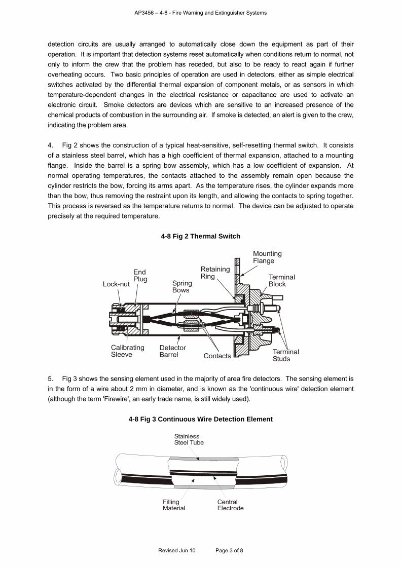
AP3456 – 4-8 - Fire Warning and Extinguisher Systems
detection circuits are usually arranged to automatically close down the equipment as part of their operation. It is important that detection systems reset automatically when conditions return to normal, not only to inform the crew that the problem has receded, but also to be ready to react again if further overheating occurs. Two basic principles of operation are used in detectors, either as simple electrical switches activated by the differential thermal expansion of component metals, or as sensors in which temperature-dependent changes in the electrical resistance or capacitance are used to activate an electronic circuit. Smoke detectors are devices which are sensitive to an increased presence of the chemical products of combustion in the surrounding air. If smoke is detected, an alert is given to the crew, indicating the problem area. 4. Fig 2 shows the construction of a typical heat-sensitive, self-resetting thermal switch. It consists of a stainless steel barrel, which has a high coefficient of thermal expansion, attached to a mounting flange. Inside the barrel is a spring bow assembly, which has a low coefficient of expansion. At normal operating temperatures, the contacts attached to the assembly remain open because the cylinder restricts the bow, forcing its arms apart. As the temperature rises, the cylinder expands more than the bow, thus removing the restraint upon its length, and allowing the contacts to spring together. This process is reversed as the temperature returns to normal. The device can be adjusted to operate precisely at the required temperature.
4-8 Fig 2 Thermal Switch
TerminalBlock
MountingFlange
SpringBows
EndPlug
Lock-nut
RetainingRing
TerminalStudsContacts
DetectorBarrel
CalibratingSleeve
5. Fig 3 shows the sensing element used in the majority of area fire detectors. The sensing element is in the form of a wire about 2 mm in diameter, and is known as the 'continuous wire' detection element (although the term 'Firewire', an early trade name, is still widely used).
4-8 Fig 3 Continuous Wire Detection Element
StainlessSteel Tube
FillingMaterial
CentralElectrode
Revised Jun 10 Page 3 of 8
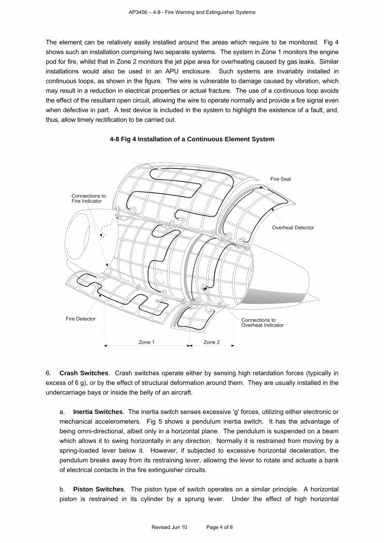
AP3456 – 4-8 - Fire Warning and Extinguisher Systems
The element can be relatively easily installed around the areas which require to be monitored. Fig 4 shows such an installation comprising two separate systems. The system in Zone 1 monitors the engine pod for fire, whilst that in Zone 2 monitors the jet pipe area for overheating caused by gas leaks. Similar installations would also be used in an APU enclosure. Such systems are invariably installed in continuous loops, as shown in the figure. The wire is vulnerable to damage caused by vibration, which may result in a reduction in electrical properties or actual fracture. The use of a continuous loop avoids the effect of the resultant open circuit, allowing the wire to operate normally and provide a fire signal even when defective in part. A test device is included in the system to highlight the existence of a fault, and, thus, allow timely rectification to be carried out.
4-8 Fig 4 Installation of a Continuous Element System
Overheat Detector
Fire Seal
Connections toOverheat Indicator
Connections toFire Indicator
Zone 1 Zone 2
Fire Detector
6. Crash Switches. Crash switches operate either by sensing high retardation forces (typically in excess of 6 g), or by the effect of structural deformation around them. They are usually installed in the undercarriage bays or inside the belly of an aircraft.
a. Inertia Switches. The inertia switch senses excessive 'g' forces, utilizing either electronic or mechanical accelerometers. Fig 5 shows a pendulum inertia switch. It has the advantage of being omni-directional, albeit only in a horizontal plane. The pendulum is suspended on a beam which allows it to swing horizontally in any direction. Normally it is restrained from moving by a spring-loaded lever below it. However, if subjected to excessive horizontal deceleration, the pendulum breaks away from its restraining lever, allowing the lever to rotate and actuate a bank of electrical contacts in the fire extinguisher circuits. b. Piston Switches. The piston type of switch operates on a similar principle. A horizontal piston is restrained in its cylinder by a sprung lever. Under the effect of high horizontal
Revised Jun 10 Page 4 of 8
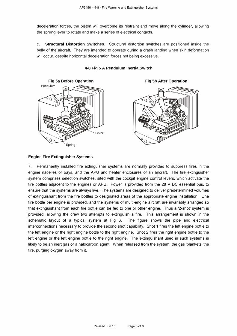
AP3456 – 4-8 - Fire Warning and Extinguisher Systems
deceleration forces, the piston will overcome its restraint and move along the cylinder, allowing the sprung lever to rotate and make a series of electrical contacts. c. Structural Distortion Switches. Structural distortion switches are positioned inside the belly of the aircraft. They are intended to operate during a crash landing when skin deformation will occur, despite horizontal deceleration forces not being excessive.
4-8 Fig 5 A Pendulum Inertia Switch
Fig 5a Before Operation Fig 5b After Operation
Lever
Spring
Pendulum
Engine Fire Extinguisher Systems 7. Permanently installed fire extinguisher systems are normally provided to suppress fires in the engine nacelles or bays, and the APU and heater enclosures of an aircraft. The fire extinguisher system comprises selection switches, sited with the cockpit engine control levers, which activate the fire bottles adjacent to the engines or APU. Power is provided from the 28 V DC essential bus, to ensure that the systems are always live. The systems are designed to deliver predetermined volumes of extinguishant from the fire bottles to designated areas of the appropriate engine installation. One fire bottle per engine is provided, and the systems of multi-engine aircraft are invariably arranged so that extinguishant from each fire bottle can be fed to one or other engine. Thus a '2-shot' system is provided, allowing the crew two attempts to extinguish a fire. This arrangement is shown in the schematic layout of a typical system at Fig 6. The figure shows the pipe and electrical interconnections necessary to provide the second shot capability. Shot 1 fires the left engine bottle to the left engine or the right engine bottle to the right engine. Shot 2 fires the right engine bottle to the left engine or the left engine bottle to the right engine. The extinguishant used in such systems is likely to be an inert gas or a halocarbon agent. When released from the system, the gas 'blankets' the fire, purging oxygen away from it.
Revised Jun 10 Page 5 of 8
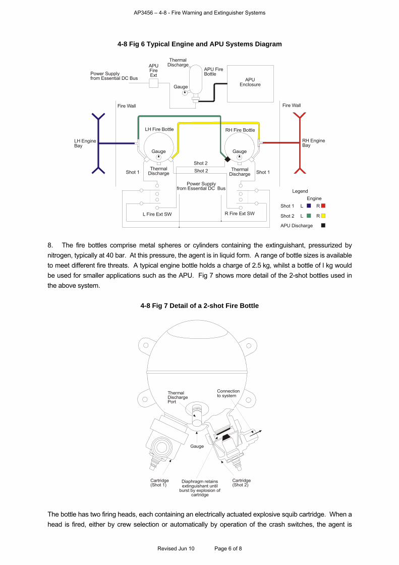
AP3456 – 4-8 - Fire Warning and Extinguisher Systems
4-8 Fig 6 Typical Engine and APU Systems Diagram
R Fire Ext SW
Shot 1ThermalDischarge
RH Fire Bottle
Shot 2Shot 2
Power Supplyfrom Essential DC Bus
L Fire Ext SW
Shot 1Thermal
Discharge
LH Fire Bottle
Fire Wall Fire Wall
LH EngineBay
RH EngineBay
APUEnclosure
APU FireBottle
Gauge
ThermalDischargeAPU
FireExtPower Supply
from Essential DC Bus
Legend
Gauge Gauge
EngineShot 1
Shot 2
APU Discharge
L
L
R
R
8. The fire bottles comprise metal spheres or cylinders containing the extinguishant, pressurized by nitrogen, typically at 40 bar. At this pressure, the agent is in liquid form. A range of bottle sizes is available to meet different fire threats. A typical engine bottle holds a charge of 2.5 kg, whilst a bottle of l kg would be used for smaller applications such as the APU. Fig 7 shows more detail of the 2-shot bottles used in the above system.
4-8 Fig 7 Detail of a 2-shot Fire Bottle
Cartridge(Shot 1)
Gauge
Cartridge(Shot 2)
Diaphragm retains extinguishant until
burst by explosion of cartridge
Connectionto systemThermal
DischargePort
The bottle has two firing heads, each containing an electrically actuated explosive squib cartridge. When a head is fired, either by crew selection or automatically by operation of the crash switches, the agent is
Revised Jun 10 Page 6 of 8
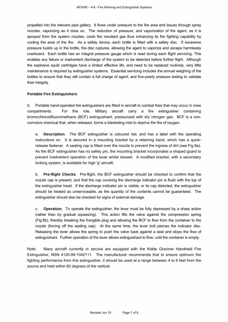
AP3456 – 4-8 - Fire Warning and Extinguisher Systems
propelled into the relevant pipe gallery. It flows under pressure to the fire area and issues through spray nozzles, vaporizing as it does so. The reduction of pressure, and vaporization of the agent, as it is sprayed from the system nozzles, cools the resultant gas thus enhancing its fire fighting capability by cooling the area of the fire. As a safety device, each bottle is fitted with a safety disc. If excessive pressure builds up in the bottle, the disc ruptures, allowing the agent to vaporize and escape harmlessly overboard. Each bottle has an integral pressure gauge which is read during each flight servicing. This enables any failure or inadvertent discharge of the system to be detected before further flight. Although the explosive squib cartridges have a limited effective life, and need to be replaced routinely, very little maintenance is required by extinguisher systems. Essential servicing includes the annual weighing of the bottles to ensure that they still contain a full charge of agent, and five-yearly pressure testing to validate their integrity. Portable Fire Extinguishers
9. Portable hand-operated fire extinguishers are fitted in aircraft to combat fires that may occur in crew compartments. For this role, Military aircraft carry a fire extinguisher containing bromochlorodifluoromethane (BCF) extinguishant, pressurized with dry nitrogen gas. BCF is a non-corrosive chemical that, when released, forms a blanketing mist to deprive the fire of oxygen.
a. Description. The BCF extinguisher is coloured red, and has a label with the operating instructions on. It is secured in a mounting bracket by a retaining band, which has a quick-release fastener. A sealing cap is fitted over the nozzle to prevent the ingress of dirt (see Fig 8a). As the BCF extinguisher has no safety pin, the mounting bracket incorporates a shaped guard to prevent inadvertent operation of the lever whilst stowed. A modified bracket, with a secondary locking system, is available for high 'g' aircraft. b. Pre-flight Checks. Pre-flight, the BCF extinguisher should be checked to confirm that the nozzle cap is present, and that the cap covering the discharge indicator pin is flush with the top of the extinguisher head. If the discharge indicator pin is visible, or its cap distorted, the extinguisher should be treated as unserviceable, as the quantity of the contents cannot be guaranteed. The extinguisher should also be checked for signs of external damage. c. Operation. To operate the extinguisher, the lever must be fully depressed by a sharp action (rather than by gradual squeezing). This action lifts the valve against the compression spring (Fig 8b), thereby breaking the frangible plug and allowing the BCF to flow from the container to the nozzle (forcing off the sealing cap). At the same time, the lever bolt pierces the indicator disc. Releasing the lever allows the spring to push the valve back against a seal and stops the flow of extinguishant. Further operation of the lever allows extinguishant to flow, until the container is empty.
Note: Many aircraft currently in service are equipped with the Kidde Graviner Handheld Fire Extinguisher, NSN 4120-99-1042111. The manufacturer recommends that to ensure optimum fire fighting performance from this extinguisher, it should be used at a range between 4 to 6 feet from the source and held within 60 degrees of the vertical.
Revised Jun 10 Page 7 of 8
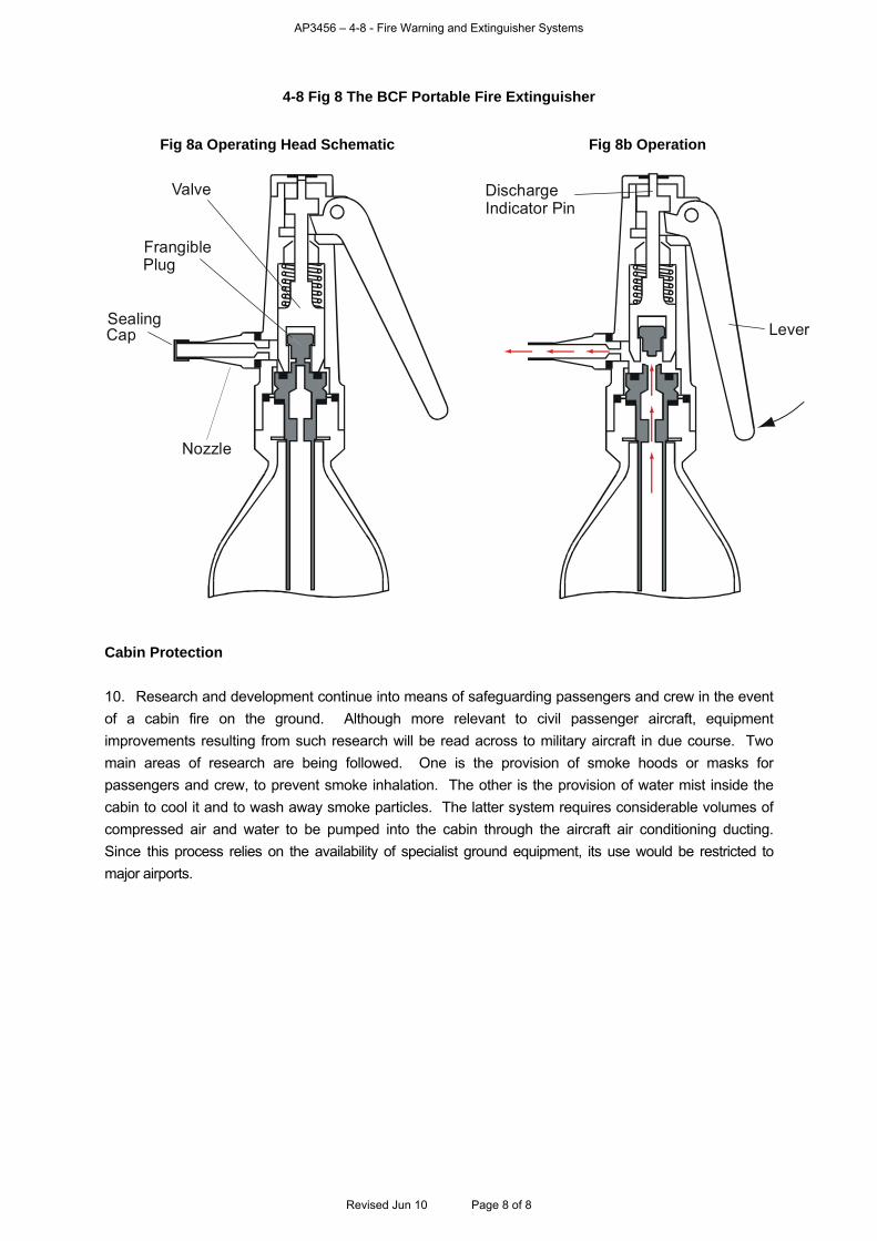
AP3456 – 4-8 - Fire Warning and Extinguisher Systems
Revised Jun 10 Page 8 of 8
4-8 Fig 8 The BCF Portable Fire Extinguisher
Fig 8a Operating Head Schematic Fig 8b Operation
Valve
FrangiblePlug
SealingCap
Nozzle
DischargeIndicator Pin
Lever
Cabin Protection
10. Research and development continue into means of safeguarding passengers and crew in the event of a cabin fire on the ground. Although more relevant to civil passenger aircraft, equipment improvements resulting from such research will be read across to military aircraft in due course. Two main areas of research are being followed. One is the provision of smoke hoods or masks for passengers and crew, to prevent smoke inhalation. The other is the provision of water mist inside the cabin to cool it and to wash away smoke particles. The latter system requires considerable volumes of compressed air and water to be pumped into the cabin through the aircraft air conditioning ducting. Since this process relies on the availability of specialist ground equipment, its use would be restricted to major airports.

AP3456 – 4-9 - Ice and Rain Protection Systems
CHAPTER 9 - ICE AND RAIN PROTECTION SYSTEMS Contents Page
Introduction.............................................................................................................................................. 1 Principles of Operation ............................................................................................................................ 1 Ice Protection Systems............................................................................................................................ 2 Ground De-icing ...................................................................................................................................... 6 Ice Detection............................................................................................................................................ 7 Windscreen Ice and Rain Protection....................................................................................................... 9 Table of Figures
4-9 Fig 1 Aircraft Structure Anti-icing System ......................................................................................... 2 4-9 Fig 2 Typical Wing Leading Edge Anti-icing System ........................................................................ 3 4-9 Fig 3 Integral Engine Anti-icing System ............................................................................................ 3 4-9 Fig 4 Electrically Heated Mats........................................................................................................... 4 4-9 Fig 5 Typical Fluid Anti-icing System ................................................................................................ 5 4-9 Fig 6 Principle of the Air Dam Separator .......................................................................................... 5 4-9 Fig 7 Momentum Separation Device Configuration .......................................................................... 6 4-9 Fig 8 Ice Detection Devices .............................................................................................................. 8 Introduction
1. The operation of military aircraft may necessitate flying in adverse weather conditions. Provision must therefore be made to safeguard the aircraft against icing, the effects of which may endanger performance and safety. The areas on an aircraft which are sensitive to ice formation are:
a. Aerofoil surfaces b. Engine intakes c. Engine internal surfaces d. Rotor blades and propellers e. Windscreens f. Instrumentation probes and vanes g. Control hinges and linkages h. Weapons and weapon carriers.
Principles of Operation
2. Ice protection systems are either active or passive. Active systems operate either by increasing the temperature of local areas of the aircraft to above freezing point, or by chemically reducing the freezing point of precipitation impinging upon the aircraft. Passive methods harness the momentum of the main airstream to separate out precipitation and divert it away. Active systems may be further categorized as either anti-icing or de-icing. Anti-icing systems prevent the formation of ice in critical areas whilst de-icing systems work to remove ice which has already formed.
Revised Jun 10 Page 1 of 9
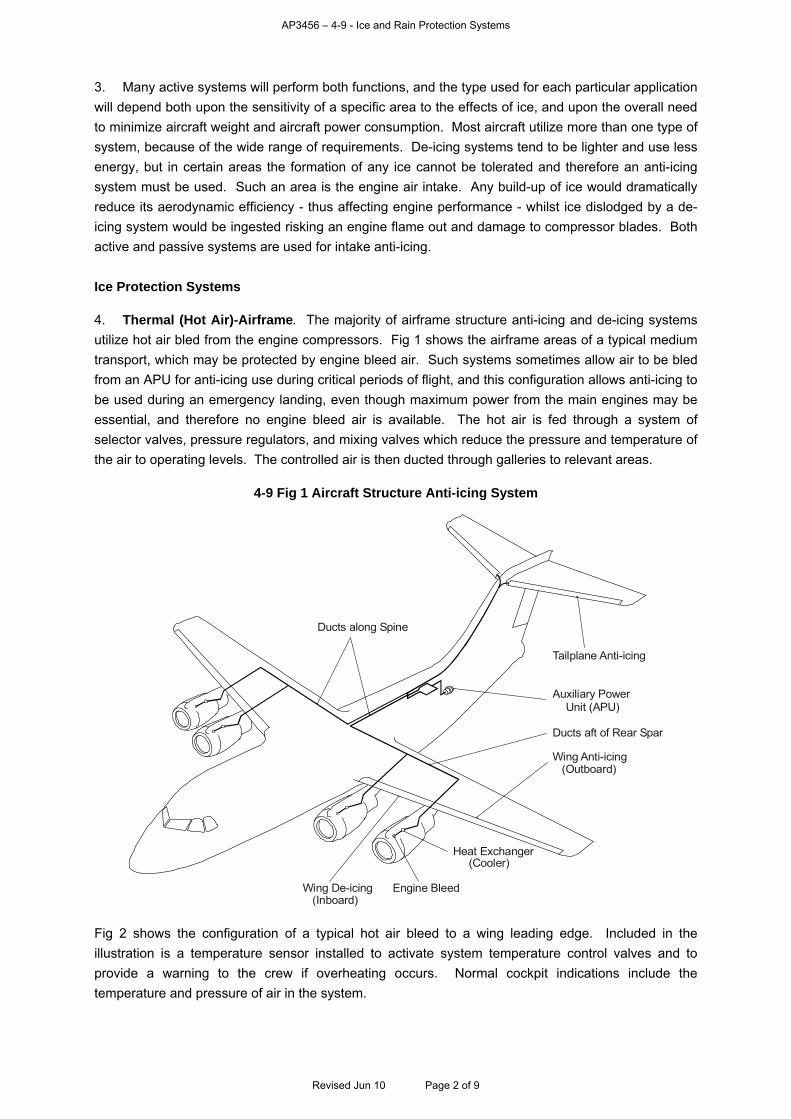
AP3456 – 4-9 - Ice and Rain Protection Systems
3. Many active systems will perform both functions, and the type used for each particular application will depend both upon the sensitivity of a specific area to the effects of ice, and upon the overall need to minimize aircraft weight and aircraft power consumption. Most aircraft utilize more than one type of system, because of the wide range of requirements. De-icing systems tend to be lighter and use less energy, but in certain areas the formation of any ice cannot be tolerated and therefore an anti-icing system must be used. Such an area is the engine air intake. Any build-up of ice would dramatically reduce its aerodynamic efficiency - thus affecting engine performance - whilst ice dislodged by a de-icing system would be ingested risking an engine flame out and damage to compressor blades. Both active and passive systems are used for intake anti-icing. Ice Protection Systems 4. Thermal (Hot Air)-Airframe. The majority of airframe structure anti-icing and de-icing systems utilize hot air bled from the engine compressors. Fig 1 shows the airframe areas of a typical medium transport, which may be protected by engine bleed air. Such systems sometimes allow air to be bled from an APU for anti-icing use during critical periods of flight, and this configuration allows anti-icing to be used during an emergency landing, even though maximum power from the main engines may be essential, and therefore no engine bleed air is available. The hot air is fed through a system of selector valves, pressure regulators, and mixing valves which reduce the pressure and temperature of the air to operating levels. The controlled air is then ducted through galleries to relevant areas.
4-9 Fig 1 Aircraft Structure Anti-icing System
Tailplane Anti-icing
Auxiliary Power Unit (APU)
Ducts aft of Rear Spar
Wing Anti-icing(Outboard)
Ducts along Spine
Wing De-icing(Inboard)
Engine Bleed
Heat Exchanger(Cooler)
Fig 2 shows the configuration of a typical hot air bleed to a wing leading edge. Included in the illustration is a temperature sensor installed to activate system temperature control valves and to provide a warning to the crew if overheating occurs. Normal cockpit indications include the temperature and pressure of air in the system.
Revised Jun 10 Page 2 of 9
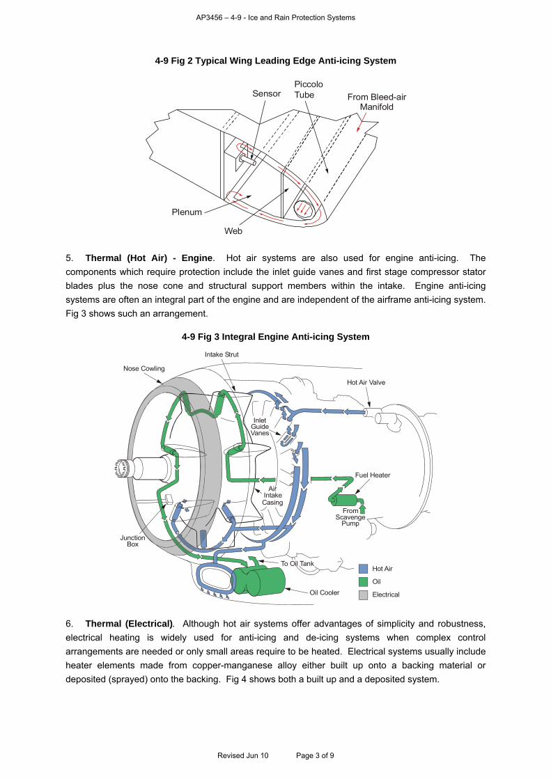
AP3456 – 4-9 - Ice and Rain Protection Systems
4-9 Fig 2 Typical Wing Leading Edge Anti-icing System
Web
Plenum
SensorPiccoloTube From Bleed-air
Manifold
5. Thermal (Hot Air) - Engine. Hot air systems are also used for engine anti-icing. The components which require protection include the inlet guide vanes and first stage compressor stator blades plus the nose cone and structural support members within the intake. Engine anti-icing systems are often an integral part of the engine and are independent of the airframe anti-icing system. Fig 3 shows such an arrangement.
4-9 Fig 3 Integral Engine Anti-icing System
Hot Air
Oil Cooler
To Oil Tank
FromScavenge
Pump
Fuel Heater
Hot Air Valve
Intake Strut
Nose Cowling
InletGuideVanes
AirIntakeCasing
JunctionBox
Oil
Electrical
6. Thermal (Electrical). Although hot air systems offer advantages of simplicity and robustness, electrical heating is widely used for anti-icing and de-icing systems when complex control arrangements are needed or only small areas require to be heated. Electrical systems usually include heater elements made from copper-manganese alloy either built up onto a backing material or deposited (sprayed) onto the backing. Fig 4 shows both a built up and a deposited system.
Revised Jun 10 Page 3 of 9
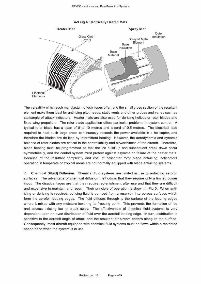
AP3456 – 4-9 - Ice and Rain Protection Systems
4-9 Fig 4 Electrically Heated Mats
ElectricalElements
Heater Mat Spray Mat
Glass ClothLayers
OuterInsulation
Sprayed MetalElementBase
InsulationBase
Material
The versatility which such manufacturing techniques offer, and the small cross section of the resultant element make them ideal for anti-icing pitot heads, static vents and other probes and vanes such as stall/angle of attack indicators. Heater mats are also used for de-icing helicopter rotor blades and fixed wing propellers. The rotor blade application offers particular problems in system control. A typical rotor blade has a span of 8 to 10 metres and a cord of 0.5 metres. The electrical load required to heat such large areas continuously exceeds the power available in a helicopter, and therefore the blades are de-iced by intermittent heating. However, the aerodynamic and dynamic balance of rotor blades are critical to the controllability and airworthiness of the aircraft. Therefore, blade heating must be programmed so that the ice build up and subsequent break down occur symmetrically, and the control system must protect against asymmetric failure of the heater mats. Because of the resultant complexity and cost of helicopter rotor blade anti-icing, helicopters operating in temperate or tropical areas are not normally equipped with blade anti-icing systems. 7. Chemical (Fluid) Diffusion. Chemical fluid systems are limited in use to anti-icing aerofoil surfaces. The advantage of chemical diffusion methods is that they require only a limited power input. The disadvantages are that they require replenishment after use and that they are difficult and expensive to maintain and repair. Their principle of operation is shown in Fig 5. When anti-icing or de-icing is required, de-icing fluid is pumped from a reservoir into porous surfaces which form the aerofoil leading edges. The fluid diffuses through to the surface of the leading edges where it mixes with any moisture lowering its freezing point. This prevents the formation of ice and causes existing ice to break away. The effectiveness of chemical fluid systems is very dependent upon an even distribution of fluid over the aerofoil leading edge. In turn, distribution is sensitive to the aerofoil angle of attack and the resultant air-stream pattern along its top surface. Consequently, most aircraft equipped with chemical fluid systems must be flown within a restricted speed band when the system is in use.
Revised Jun 10 Page 4 of 9
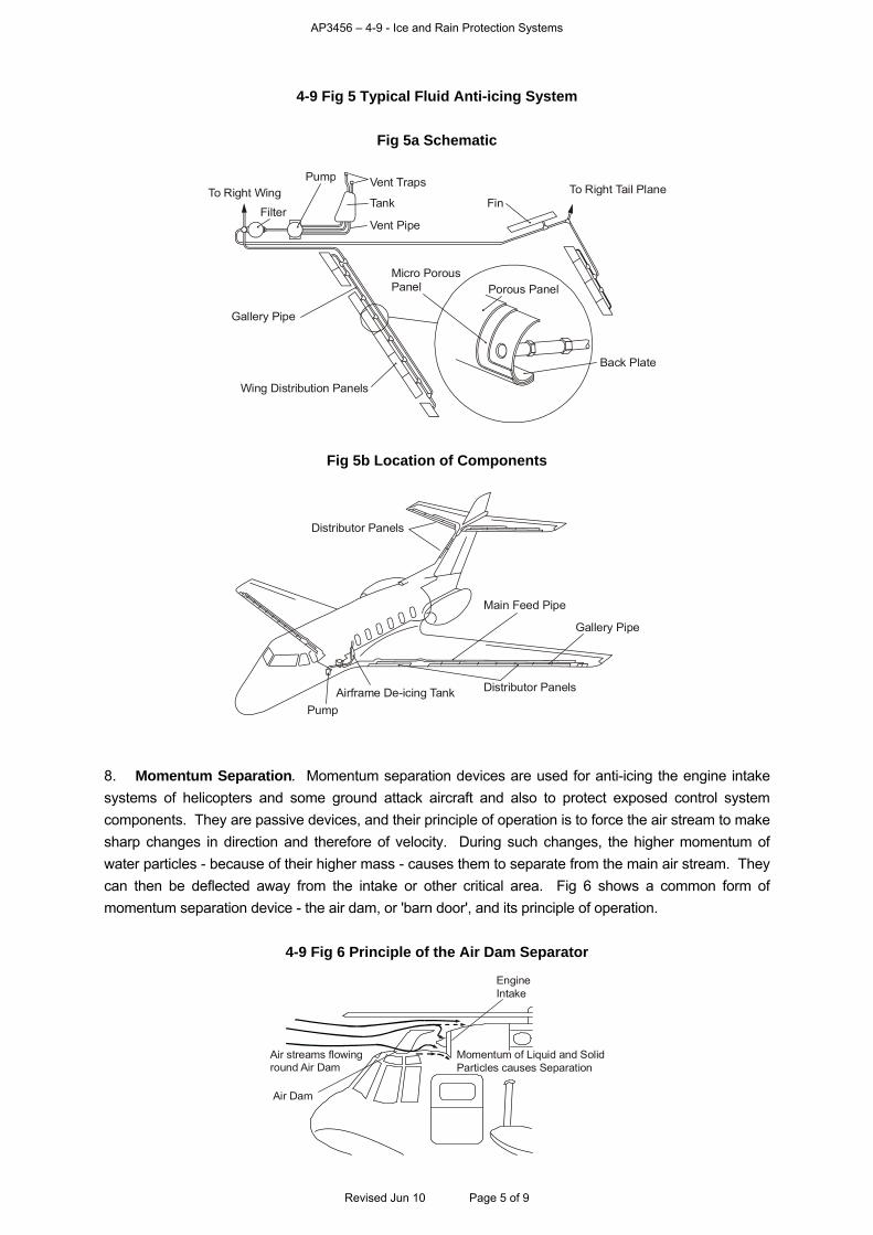
AP3456 – 4-9 - Ice and Rain Protection Systems
4-9 Fig 5 Typical Fluid Anti-icing System
Fig 5a Schematic
Vent Traps
Tank Fin
Micro PorousPanel Porous Panel
Back Plate
Gallery Pipe
Wing Distribution Panels
To Right Tail Plane
Vent Pipe
PumpTo Right Wing
Filter
Fig 5b Location of Components
Main Feed Pipe
Distributor Panels
Gallery Pipe
Distributor PanelsAirframe De-icing TankPump
8. Momentum Separation. Momentum separation devices are used for anti-icing the engine intake systems of helicopters and some ground attack aircraft and also to protect exposed control system components. They are passive devices, and their principle of operation is to force the air stream to make sharp changes in direction and therefore of velocity. During such changes, the higher momentum of water particles - because of their higher mass - causes them to separate from the main air stream. They can then be deflected away from the intake or other critical area. Fig 6 shows a common form of momentum separation device - the air dam, or 'barn door', and its principle of operation.
4-9 Fig 6 Principle of the Air Dam Separator
Air streams flowinground Air Dam
Momentum of Liquid and SolidParticles causes Separation
EngineIntake
Air Dam
Revised Jun 10 Page 5 of 9
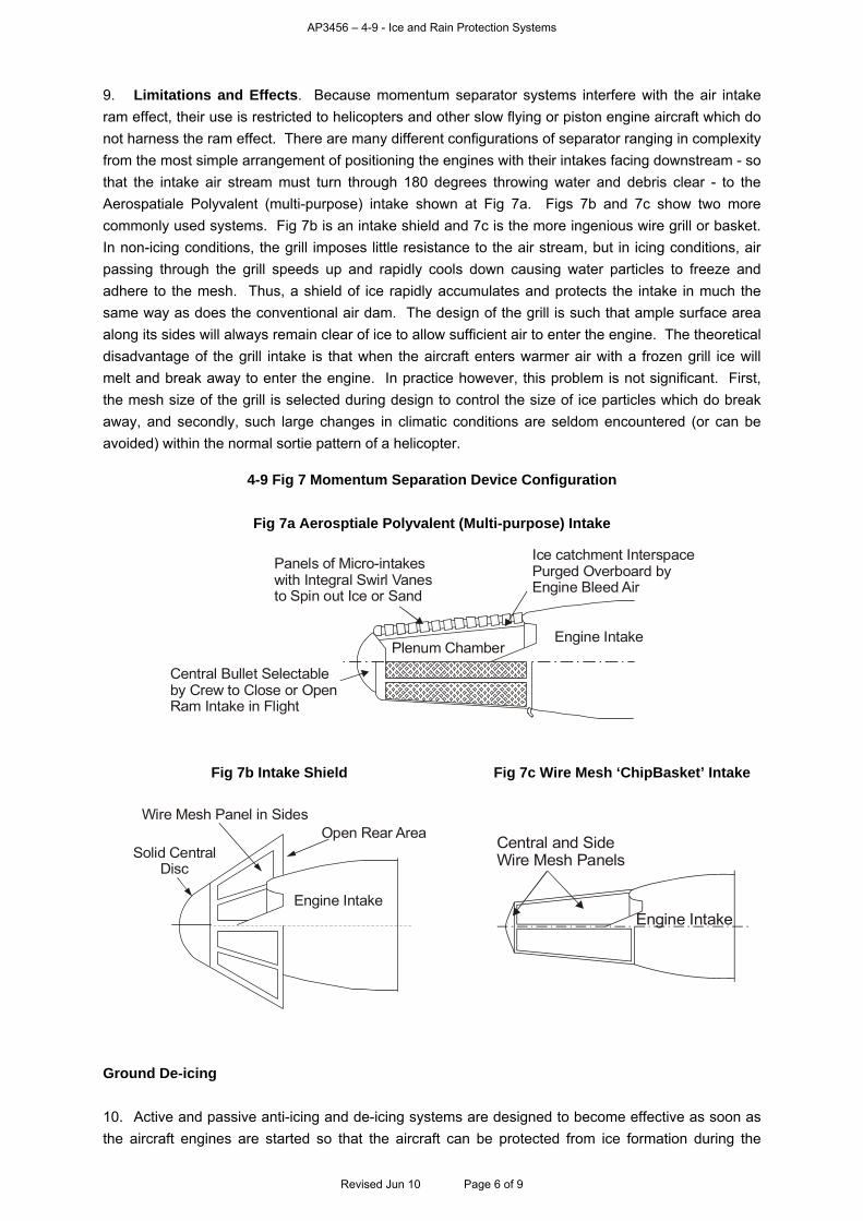
AP3456 – 4-9 - Ice and Rain Protection Systems
9. Limitations and Effects. Because momentum separator systems interfere with the air intake ram effect, their use is restricted to helicopters and other slow flying or piston engine aircraft which do not harness the ram effect. There are many different configurations of separator ranging in complexity from the most simple arrangement of positioning the engines with their intakes facing downstream - so that the intake air stream must turn through 180 degrees throwing water and debris clear - to the Aerospatiale Polyvalent (multi-purpose) intake shown at Fig 7a. Figs 7b and 7c show two more commonly used systems. Fig 7b is an intake shield and 7c is the more ingenious wire grill or basket. In non-icing conditions, the grill imposes little resistance to the air stream, but in icing conditions, air passing through the grill speeds up and rapidly cools down causing water particles to freeze and adhere to the mesh. Thus, a shield of ice rapidly accumulates and protects the intake in much the same way as does the conventional air dam. The design of the grill is such that ample surface area along its sides will always remain clear of ice to allow sufficient air to enter the engine. The theoretical disadvantage of the grill intake is that when the aircraft enters warmer air with a frozen grill ice will melt and break away to enter the engine. In practice however, this problem is not significant. First, the mesh size of the grill is selected during design to control the size of ice particles which do break away, and secondly, such large changes in climatic conditions are seldom encountered (or can be avoided) within the normal sortie pattern of a helicopter.
4-9 Fig 7 Momentum Separation Device Configuration
Fig 7a Aerosptiale Polyvalent (Multi-purpose) Intake
Panels of Micro-intakeswith Integral Swirl Vanesto Spin out Ice or Sand
Ice catchment InterspacePurged Overboard byEngine Bleed Air
Engine IntakePlenum Chamber
Central Bullet Selectableby Crew to Close or OpenRam Intake in Flight
Fig 7b Intake Shield Fig 7c Wire Mesh ‘ChipBasket’ Intake
Engine Intake
Open Rear AreaWire Mesh Panel in Sides
Solid CentralDisc
Engine Intake
Central and SideWire Mesh Panels
Ground De-icing
10. Active and passive anti-icing and de-icing systems are designed to become effective as soon as the aircraft engines are started so that the aircraft can be protected from ice formation during the
Revised Jun 10 Page 6 of 9
AP3456 – 4-9 - Ice and Rain Protection Systems
critical take-off and subsequent climb-out phases of flight. However, if the aircraft has been parked in the open in adverse conditions prior to start-up, significant accretions of ice, snow, or slush may have built up on the aircraft flying surfaces. Such deposits must be removed prior to flight, by the ground crews. After physically removing the majority of such deposits, chemical fluid de-icing is used to complete the task. This is achieved by the application of de-icing fluids in specially prepared thyxotropic paste or gel form by the use of ground-based spray equipment. The effect of applying such a de-icing gel is to melt any ice present and to prevent its reformation until the aircraft is airborne. The principle is also sometimes used for the airborne anti-icing of unheated rotor blades on helicopters which must fly for operational reasons in icing conditions. However, the effectiveness of the gel reduces during flight as it is gradually thrown from the blades by centrifugal forces. Ice Detection
11. Although significant flight hazards are posed by ice build-up, the fact that most active anti-icing and de-icing systems consume considerable amounts of power preclude their use except when icing conditions are actually encountered. Meteorological forecasts go much of the way to alerting crews to the likelihood of entering icing conditions during a particular flight. However, such forecasts are not always sufficient, and the crew must therefore remain alert to the need to activate the anti-icing and de-icing systems at any time. The formation of ice on external visible projections would normally be the first manifestation of having entered icing conditions. For this reason, the majority of aircraft are equipped with flood lights aligned to illuminate relevant areas of the airframe which are visible from the cockpit. Aircraft in which crew visibility is limited are often equipped with illuminated ice accretion probes as shown in Fig 8a. These are positioned to be visible from the cockpit. In addition, most aircraft are equipped with ice detection devices which either provide a positive alert or automatically activate the anti-icing and de-icing systems.
Revised Jun 10 Page 7 of 9
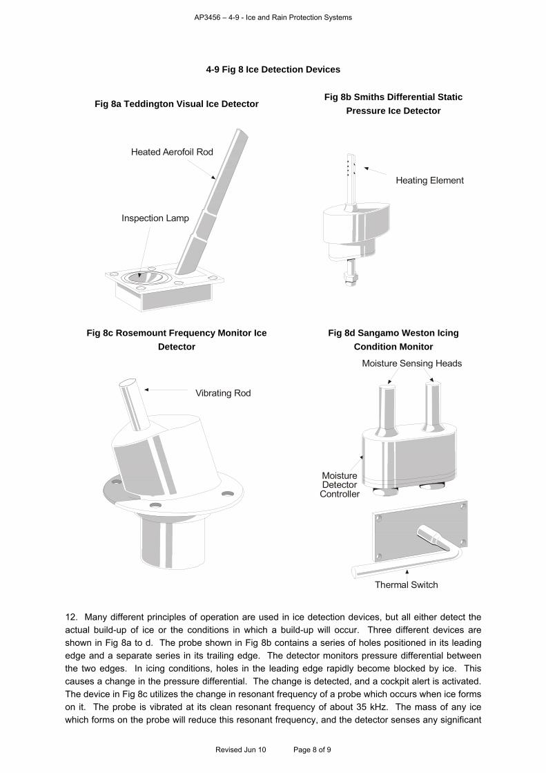
AP3456 – 4-9 - Ice and Rain Protection Systems
4-9 Fig 8 Ice Detection Devices
Fig 8a Teddington Visual Ice Detector Fig 8b Smiths Differential Static
Pressure Ice Detector
Inspection Lamp
Heated Aerofoil Rod
Heating Element
Fig 8c Rosemount Frequency Monitor Ice
Detector
Fig 8d Sangamo Weston Icing
Condition Monitor
Vibrating Rod
Thermal Switch
MoistureDetectorController
Moisture Sensing Heads
12. Many different principles of operation are used in ice detection devices, but all either detect the actual build-up of ice or the conditions in which a build-up will occur. Three different devices are shown in Fig 8a to d. The probe shown in Fig 8b contains a series of holes positioned in its leading edge and a separate series in its trailing edge. The detector monitors pressure differential between the two edges. In icing conditions, holes in the leading edge rapidly become blocked by ice. This causes a change in the pressure differential. The change is detected, and a cockpit alert is activated. The device in Fig 8c utilizes the change in resonant frequency of a probe which occurs when ice forms on it. The probe is vibrated at its clean resonant frequency of about 35 kHz. The mass of any ice which forms on the probe will reduce this resonant frequency, and the detector senses any significant
Revised Jun 10 Page 8 of 9

AP3456 – 4-9 - Ice and Rain Protection Systems
Revised Jun 10 Page 9 of 9
frequency change and activates the cockpit alarm. The device in Fig 8d works on the same principle as a wet and dry bulb hygrometer, and it comprises two heated bulbs, one exposed to the air stream and the other shielded, plus a simple outside air temperature (OAT) probe. The detector monitors the temperature of the bulbs which are heated at a constant rate. When the exposed bulb is in a moist air stream, it loses its heat to the surrounding air at a greater rate than does the dry shielded bulb. The resultant temperature imbalance is detected. If the OAT is detected to be within the icing range, contacts in the probe circuit close, and the alert system is activated. Windscreen Ice and Rain Protection 13. Although de-icing fluid spray systems or hot air jets were utilized to de-ice the windscreens of older aircraft, all current aircraft are fitted with electrically heated screens. The heating elements and associated temperature control and overheat sensors are sandwiched in the glass laminations of the screen. A thin film of gold is used for the heating element, and it is deposited directly onto glass. Electrical connectors formed on the edges of the panel interface with the system electrical supply and temperature controller. The heater systems serve both to de-ice and de-mist the screens. 14. At normal flying speeds, rain falling onto the screens is rapidly dispersed by the airflow. However, to keep the screen clear during landing or during low speed flight, conventional, high-speed windscreen wipers are fitted to most fixed and rotary wing aircraft. The wipers are electrically activated by the crew as and when needed.
AP3456 – 4-10 - Aircraft Fuel Systems
CHAPTER 10 - AIRCRAFT FUEL SYSTEMS Contents Page Principles ................................................................................................................................................. 1 Fuel Storage ............................................................................................................................................ 2 Delivery System Components ................................................................................................................. 3 Design Objectives and Typical Configuration ......................................................................................... 5 Transfer, Cross-feed and Jettison........................................................................................................... 5 Systems Management............................................................................................................................. 6 Refuelling and Additional Fuel................................................................................................................. 7 Tolerance to Manoeuvre and Damage.................................................................................................... 8 Secondary Uses of Fuel .......................................................................................................................... 9 Table of Figures
4-10 Fig 1 Typical Combat Aircraft Tank Configuration .......................................................................... 2 4-10 Fig 2 Arrangement of Tank Groups and Controls........................................................................... 3 4-10 Fig 3 Fuel Injector (Jet) Pump......................................................................................................... 4 4-10 Fig 4 Fuel System with Transfer and Cross-feed ........................................................................... 6 4-10 Fig 5 Tank Jettison System............................................................................................................. 6 4-10 Fig 6 Fuel System Control and Instrumentation Panels ................................................................. 7
Principles 1. The fuel system of an aircraft consists of two distinct sub-systems. One is integral with the engine or Auxiliary Power Unit (APU) and the other with the airframe. A typical engine system comprises a high pressure (HP) pump, final filtration, a fuel control unit (FCU) and a carburation device which introduces the fuel into the combustion system. Details of engine fuel systems are included at Volume 3, Chapter 11. The functions of the aircraft airframe fuel system are to store the fuel until it is required and then to deliver it in quantities appropriate to the power being demanded of the engines or the APU, to a set pressure and quality. 2. To reduce crew workload, and to minimize the risk of a fuel management error occurring during flight, control of the system requires to be automatic or semi-automatic in operation. Also, to provide for the extensions in aircraft range and endurance imposed by a wide variation in operational requirements, the system configuration requires sufficient flexibility to be extended when operations demand greater range or endurance. In many cases, this is achieved by fitting additional tankage or by providing a capability to pick up additional fuel during flight. A typical single-engine fuel system is illustrated in Fig 1. Fuel is held in integral wing and fuselage tanks, with (in this example) the option of extra fuel in an external tank.
Revised Jun 10 Page 1 of 9
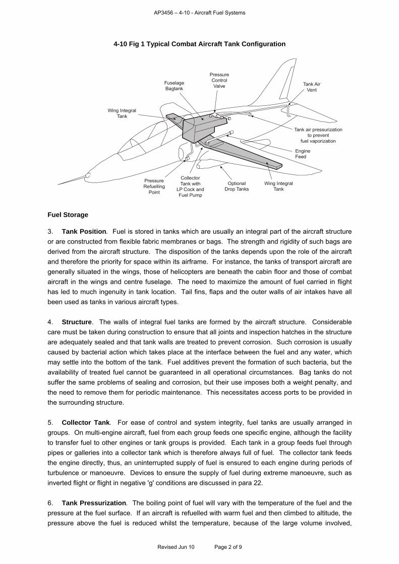
AP3456 – 4-10 - Aircraft Fuel Systems
4-10 Fig 1 Typical Combat Aircraft Tank Configuration
EngineFeed
Tank AirVent
PressureControlValveFuselage
Bagtank
Wing IntegralTank
PressureRefuelling
Point
CollectorTank with
LP Cock andFuel Pump
OptionalDrop Tanks
Wing IntegralTank
Tank air pressurizationto prevent
fuel vaporization
Fuel Storage 3. Tank Position. Fuel is stored in tanks which are usually an integral part of the aircraft structure or are constructed from flexible fabric membranes or bags. The strength and rigidity of such bags are derived from the aircraft structure. The disposition of the tanks depends upon the role of the aircraft and therefore the priority for space within its airframe. For instance, the tanks of transport aircraft are generally situated in the wings, those of helicopters are beneath the cabin floor and those of combat aircraft in the wings and centre fuselage. The need to maximize the amount of fuel carried in flight has led to much ingenuity in tank location. Tail fins, flaps and the outer walls of air intakes have all been used as tanks in various aircraft types. 4. Structure. The walls of integral fuel tanks are formed by the aircraft structure. Considerable care must be taken during construction to ensure that all joints and inspection hatches in the structure are adequately sealed and that tank walls are treated to prevent corrosion. Such corrosion is usually caused by bacterial action which takes place at the interface between the fuel and any water, which may settle into the bottom of the tank. Fuel additives prevent the formation of such bacteria, but the availability of treated fuel cannot be guaranteed in all operational circumstances. Bag tanks do not suffer the same problems of sealing and corrosion, but their use imposes both a weight penalty, and the need to remove them for periodic maintenance. This necessitates access ports to be provided in the surrounding structure. 5. Collector Tank. For ease of control and system integrity, fuel tanks are usually arranged in groups. On multi-engine aircraft, fuel from each group feeds one specific engine, although the facility to transfer fuel to other engines or tank groups is provided. Each tank in a group feeds fuel through pipes or galleries into a collector tank which is therefore always full of fuel. The collector tank feeds the engine directly, thus, an uninterrupted supply of fuel is ensured to each engine during periods of turbulence or manoeuvre. Devices to ensure the supply of fuel during extreme manoeuvre, such as inverted flight or flight in negative 'g' conditions are discussed in para 22. 6. Tank Pressurization. The boiling point of fuel will vary with the temperature of the fuel and the pressure at the fuel surface. If an aircraft is refuelled with warm fuel and then climbed to altitude, the pressure above the fuel is reduced whilst the temperature, because of the large volume involved,
Revised Jun 10 Page 2 of 9
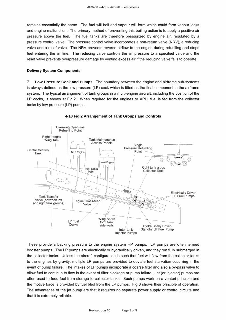
AP3456 – 4-10 - Aircraft Fuel Systems
remains essentially the same. The fuel will boil and vapour will form which could form vapour locks and engine malfunction. The primary method of preventing this boiling action is to apply a positive air pressure above the fuel. The fuel tanks are therefore pressurized by engine air, regulated by a pressure control valve. The pressure control valve incorporates a non-return valve (NRV), a reducing valve and a relief valve. The NRV prevents reverse airflow to the engine during refuelling and stops fuel entering the air line. The reducing valve controls the air pressure to a specified value and the relief valve prevents overpressure damage by venting excess air if the reducing valve fails to operate. Delivery System Components
7. Low Pressure Cock and Pumps. The boundary between the engine and airframe sub-systems is always defined as the low pressure (LP) cock which is fitted as the final component in the airframe system. The typical arrangement of tank groups in a multi-engine aircraft, including the position of the LP cocks, is shown at Fig 2. When required for the engines or APU, fuel is fed from the collector tanks by low pressure (LP) pumps.
4-10 Fig 2 Arrangement of Tank Groups and Controls
Inter-tankInjector Pumps
These provide a backing pressure to the engine system HP pumps. LP pumps are often termed booster pumps. The LP pumps are electrically or hydraulically driven, and they run fully submerged in the collector tanks. Unless the aircraft configuration is such that fuel will flow from the collector tanks to the engines by gravity, multiple LP pumps are provided to obviate fuel starvation occurring in the event of pump failure. The intakes of LP pumps incorporate a coarse filter and also a by-pass valve to allow fuel to continue to flow in the event of filter blockage or pump failure. Jet (or injector) pumps are often used to feed fuel from storage to collector tanks. Such pumps work on a venturi principle and the motive force is provided by fuel bled from the LP pumps. Fig 3 shows their principle of operation. The advantages of the jet pump are that it requires no separate power supply or control circuits and that it is extremely reliable.
Revised Jun 10 Page 3 of 9
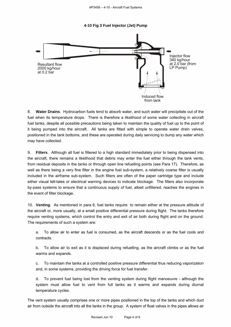
AP3456 – 4-10 - Aircraft Fuel Systems
4-10 Fig 3 Fuel Injector (Jet) Pump
Injector flow340 kg/hourat 2.0 bar (fromLP Pump)
Induced flowfrom tank
Resultant flow2000 kg/hourat 0.2 bar
8. Water Drains. Hydrocarbon fuels tend to absorb water, and such water will precipitate out of the fuel when its temperature drops. There is therefore a likelihood of some water collecting in aircraft fuel tanks, despite all possible precautions being taken to maintain the quality of fuel up to the point of it being pumped into the aircraft. All tanks are fitted with simple to operate water drain valves, positioned in the tank bottoms, and these are operated during daily servicing to dump any water which may have collected. 9. Filters. Although all fuel is filtered to a high standard immediately prior to being dispensed into the aircraft, there remains a likelihood that debris may enter the fuel either through the tank vents, from residual deposits in the tanks or through open line refuelling points (see Para 17). Therefore, as well as there being a very fine filter in the engine fuel sub-system, a relatively coarse filter is usually included in the airframe sub-system. Such filters are often of the paper cartridge type and include either visual tell-tales or electrical warning devices to indicate blockage. The filters also incorporate by-pass systems to ensure that a continuous supply of fuel, albeit unfiltered, reaches the engines in the event of filter blockage. 10. Venting. As mentioned in para 6, fuel tanks require to remain either at the pressure altitude of the aircraft or, more usually, at a small positive differential pressure during flight. The tanks therefore require venting systems, which control the entry and exit of air both during flight and on the ground. The requirements of such a system are:
a. To allow air to enter as fuel is consumed, as the aircraft descends or as the fuel cools and contracts.
b. To allow air to exit as it is displaced during refuelling, as the aircraft climbs or as the fuel warms and expands.
c. To maintain the tanks at a controlled positive pressure differential thus reducing vaporization and, in some systems, providing the driving force for fuel transfer. d. To prevent fuel being lost from the venting system during flight manoeuvre - although the system must allow fuel to vent from full tanks as it warms and expands during diurnal temperature cycles.
The vent system usually comprises one or more pipes positioned in the top of the tanks and which duct air from outside the aircraft into all the tanks in the group. A system of float valves in the pipes allows air
Revised Jun 10 Page 4 of 9

AP3456 – 4-10 - Aircraft Fuel Systems
to enter the tanks when their pressure is lower than the pipe pressure, and air to vent from the tanks when their pressure is higher. The float valves serve to prevent any significant amounts of fuel from entering the vent pipes, but because small amounts of fuel will be carried into the pipes during manoeuvre or during heavy venting, a fuel surge tank is provided at the entrance to the pipe system, to separate out this fuel. Air enters the system through a ram vent in the lower wing surface, thus ensuring that during flight the system pressure is always a little higher than static pressure. During normal operation, air enters and vents from the system as necessary, and any fuel vented with this air collects in the surge tank. When aircraft fuel contents are sufficiently low for the surge tank drain float valves to open, vented fuel is allowed to drain back into the main tanks. However, if relatively cold fuel is pumped into the tanks during replenishment, its volume will increase as the fuel heats up to tank-soak temperature. Any fuel displaced from the tanks through such expansion will vent into the surge tank, and if this becomes over full, excess fuel will drain from the aircraft through the wing vent giving a misleading impression that a tank fuel leak exists. This situation frequently occurs when aircraft are refuelled early in the morning and remain parked in hot sunlight throughout the day. Design Objectives and Typical Configuration 11. Considering the foregoing description, fuel system design must take into account the following criteria:
a. Optimum use of the fuselage space available for fuel storage.
b. Delivery of fuel to the engines and APU at required flow rates and to design pressure and quality.
c. Cross flow of fuel between specific tank groups and engines and the transfer of fuel between tanks both to allow manipulation of the aircraft’s required centre of gravity position during flight and to counter any feasible system malfunction.
d. Ease of system control and monitoring during flight.
e. Rapid and safe fuel replenishment, and the flexibility to satisfy fuel requirements posed by a wide spectrum of operations.
f. Tolerance to aircraft manoeuvre and to damage.
g. Secondary uses of fuel - for example as a coolant.
Transfer, Cross-feed and Jettison 12. Transfer and Cross-feed. In the majority of aircraft, distribution of fuel is critical to aircraft balance. Although devices such as fuel proportioners are used wherever possible to meter the flow from individual tanks and thus achieve a degree of automatic control of fuel distribution, system malfunction, uneven rates of fuel burn between engines, or even the gradual reduction of fuel load during flight will necessitate system management action being taken to redistribute fuel from one tank to another. Fuel transfer is achieved either automatically by the control system sensing an imbalance or by crew selection. Similarly, if an engine is closed down in flight or a lesser imbalance of fuel burn between engines occurs, it will become necessary for the crew to cross-feed fuel from one group of tanks to another engine. To maintain fuel system integrity, transfer and cross-feed networks are independent of each other. Fig 4 shows a typical fuel system with transfer and cross-feed facilities. In this case, the configuration of the multi-engine aircraft allows transfer to be accomplished through a simple gravity feed line between the two tank groups. In other cases, such as depicted in Fig 2, fuel must be transferred by pumps.
Revised Jun 10 Page 5 of 9

AP3456 – 4-10 - Aircraft Fuel Systems
4-10 Fig 4 Fuel System with Transfer and Cross-feed
Tank 2 Tank 4Tank 1
Centre Tank Right Tank
Engines 3 to/from 4Crossflow Valve
LP Cocks(open)
Tank 3
Engines 1 to/from 2Crossflow Valve
Engine 1
Engine 2
Engine 4
Engine 3
Left to/from RightCrossflow Valve
LP FuelPumps
CollectorTanks
InjectorPumps
Centre to RightTransfer Valve
Centre to LeftTransfer Valve
CollectorTanks
Non-returnValves
Left Tank
13. Jettison. Because of undercarriage and structural stress constraints, the maximum permissible take off weight of an aircraft is often considerably higher than its maximum permissible landing weight. It is therefore possible for the crew of such an aircraft to take off at maximum weight, experience an in flight emergency or be recalled for operational reasons, and then be unable to land safely until sufficient fuel has been consumed to bring the weight within safe landing limits. To resolve this problem, most systems incorporate a facility for dumping fuel in flight. The system in Fig 5 includes such a facility. Fuel is pumped, or it feeds by gravity, through a system of valves and pipes to be vented overboard well clear of the fuselage and the jet efflux.
4-10 Fig 5 Tank Jettison System
Engines on cabin roof
LP cock
LP filter
Fuel jettisonvalve
LP pumps(1 per engine) Collector tank
Cabin floor
Fuel jettison outletin undercarriagenacelle clear of fuselage
Individual bag tanksbetween fuselage frames
Systems Management
14. Control. Operation of the fuel system is often automatic or semi-automatic, and many such systems start to operate as soon as the crew has opened the LP cocks and switched on the LP pumps. Control is maintained by float switches sensing changes in fuel levels and operating appropriate valves and pumps. However, crew intervention is normally required to initiate transfer of fuel between tank groups, cross-feed fuel from tank groups to different engines and to jettison fuel.
Revised Jun 10 Page 6 of 9
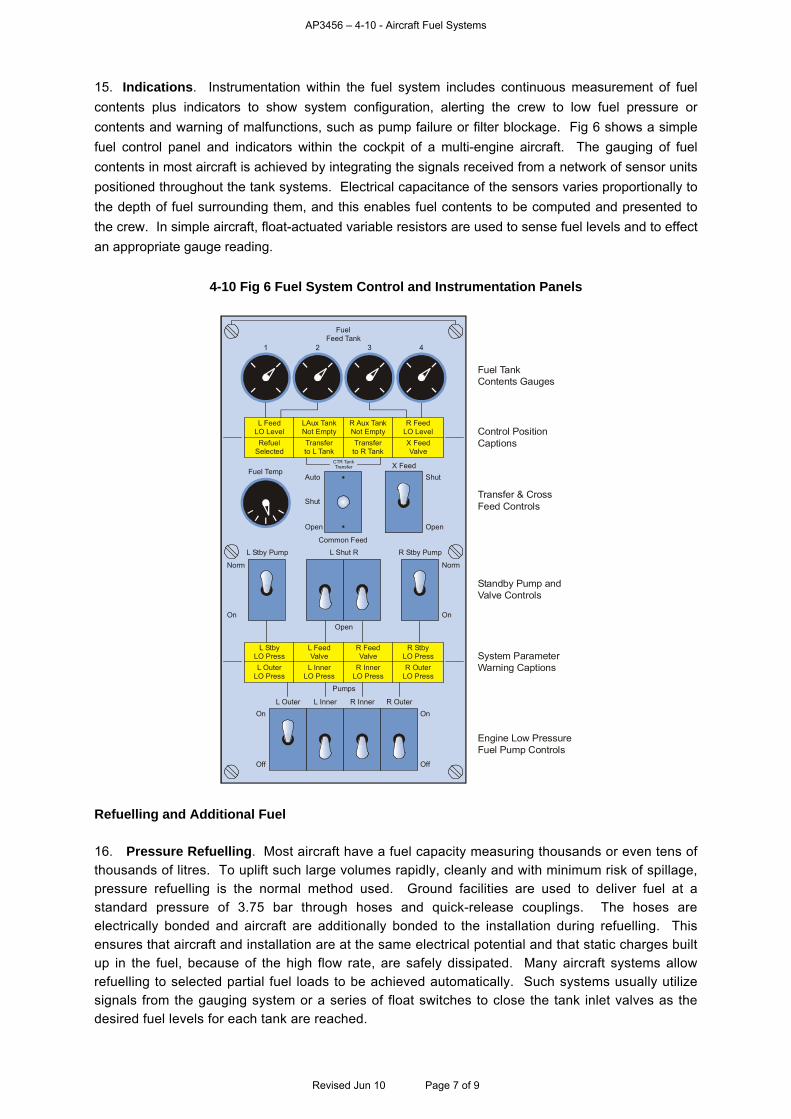
AP3456 – 4-10 - Aircraft Fuel Systems
15. Indications. Instrumentation within the fuel system includes continuous measurement of fuel contents plus indicators to show system configuration, alerting the crew to low fuel pressure or contents and warning of malfunctions, such as pump failure or filter blockage. Fig 6 shows a simple fuel control panel and indicators within the cockpit of a multi-engine aircraft. The gauging of fuel contents in most aircraft is achieved by integrating the signals received from a network of sensor units positioned throughout the tank systems. Electrical capacitance of the sensors varies proportionally to the depth of fuel surrounding them, and this enables fuel contents to be computed and presented to the crew. In simple aircraft, float-actuated variable resistors are used to sense fuel levels and to effect an appropriate gauge reading.
4-10 Fig 6 Fuel System Control and Instrumentation Panels
1
Fuel TankContents Gauges
Control PositionCaptions
Transfer & CrossFeed Controls
Standby Pump andValve Controls
System ParameterWarning Captions
Engine Low PressureFuel Pump Controls
Fuel TempShut
X Feed
Open
Auto
CTR TankTransfer
Shut
Open
Common Feed
2
LAux TankNot Empty
R Aux TankNot Empty
R FeedLO Level
L FeedLO Level
Transferto L Tank
Transferto R Tank
X FeedValve
RefuelSelected
L FeedValve
R FeedValve
R StbyLO Press
L StbyLO Press
L InnerLO Press
R InnerLO Press
R OuterLO Press
L OuterLO Press
FuelFeed Tank
3 4
Norm
R Stby PumpL Shut R
Open
Pumps
L Stby Pump
On
Norm
On
L Outer L Inner R Inner R Outer
Off
On
Off
On
Refuelling and Additional Fuel 16. Pressure Refuelling. Most aircraft have a fuel capacity measuring thousands or even tens of thousands of litres. To uplift such large volumes rapidly, cleanly and with minimum risk of spillage, pressure refuelling is the normal method used. Ground facilities are used to deliver fuel at a standard pressure of 3.75 bar through hoses and quick-release couplings. The hoses are electrically bonded and aircraft are additionally bonded to the installation during refuelling. This ensures that aircraft and installation are at the same electrical potential and that static charges built up in the fuel, because of the high flow rate, are safely dissipated. Many aircraft systems allow refuelling to selected partial fuel loads to be achieved automatically. Such systems usually utilize signals from the gauging system or a series of float switches to close the tank inlet valves as the desired fuel levels for each tank are reached.
Revised Jun 10 Page 7 of 9
AP3456 – 4-10 - Aircraft Fuel Systems
17. Open-line Refuelling. Some smaller turbine powered aircraft and all piston driven aircraft are refuelled at low pressure through open nozzles feeding into the top of the aircraft tank system. The technique is also known as gravity or over-wing refuelling, and it is identical to the system used for motor vehicles. Because the equipment is so widely available, open-line refuelling is often held as the reserve system at remote airfields or in the battlefield. Therefore, many aircraft which are likely to operate in such areas have an added capability for open-line refuelling. The system depicted in Fig 2 shows such a feature on a medium transport aircraft which can be expected to operate into relatively remote airfields. 18. De-fuelling. For operational reasons or during servicing, the requirement often occurs to reduce the fuel load of an aircraft prior to take off. To achieve this, pressure refuelling systems all include a facility for pumping fuel out of the aircraft tanks, after appropriate manipulation of the aircraft system controls. To avoid damage to the aircraft structure, the suction level used for de-fuelling is much lower than the pressure for refuelling. 19. Additional On-board Fuel. During the design phase, the fuel system capacity is optimized for the range or endurance normally required for the aircraft. Thus, if a temporary increase in range or endurance becomes necessary, such as a ferry flight, a fuel load greater than that designed for must be carried. This is usually achieved by trading payload for fuel, fitting additional fuel tanks in the cargo space or on weapons stations. For example, the aircraft depicted at Fig 1 is configured to carry ferry fuel in conventional drop tanks attached to the weapons stations. The arrangements for carrying and managing additional fuel are decided upon at the design phase, and the aircraft fuel system is built to accept the additional tankage as role equipment, to be fitted and removed as necessary. 20. In-flight Refuelling. When carriage of the full payload is required over an extended range, either more frequent refuelling stops must be made or, if this is not possible, the aircraft must be refuelled in flight. Most relevant fixed wing aircraft and some helicopters are equipped for in-flight refuelling. However, the rotors of most helicopters sweep a path so close to the nose of the aircraft that the use of air-to-air refuelling techniques can be impracticable. Nevertheless, helicopters frequently require to be refuelled in mid-sortie, and this is achieved by hovering the aircraft close to the ground (or with the undercarriage just touching) whilst conventional refuelling is carried out. The technique is termed rotors running refuelling (RRR), and it is commonly used to extend the range or endurance of SAR, ASW and battlefield helicopters. Tolerance to Manoeuvre and Damage
21. Manoeuvre. During aircraft manoeuvre or flight in turbulent conditions, fuel in the tanks will be affected by the resultant g forces. The surges of fuel produced will, if uncontrolled, cause interruptions in flow. Indeed, in extreme cases, the rapid movement of significant masses of fuel will tend to de-stabilise the aircraft and cause structural damage to the tanks. These effects are minimized by positioning baffle plates in the tanks. Usually part of the aircraft structure, they effectively divide the tanks into small sub-compartments reducing and absorbing the energy in the surges. 22. Negative 'g' Devices. Although collector tanks (see para 5) ensure a stable fuel flow to the engines in most flight conditions, more positive methods are required for providing fuel during inverted flight or flight in negative 'g' conditions. Many combat or aerobatic training aircraft utilize the fuel recuperator system. The recuperator is a separate container positioned in the engine fuel supply line and always full of fuel. The container is maintained at a pressure of about 0.5 bar, slightly below normal fuel LP pump pressure, by engine bleed air. If LP pump pressure drops, because of tank fuel surging during manoeuvre or inverted flight, fuel from the recuperator is forced into the system and thus maintains the
Revised Jun 10 Page 8 of 9

AP3456 – 4-10 - Aircraft Fuel Systems
Revised Jun 10 Page 9 of 9
engine fuel supply during the limit of its capacity. Another frequently used and more simple device is the double entry LP pump. Situated in the collector tank, this pump has gravity operated flap valves in its lower entry port. During inverted or negative 'g' flight, the valves close allowing the now inverted pump to draw fuel through its upper port to the limit of the collector tank contents. 23. Damage. Many aircraft fires occurring on the ground and in the air have been caused by fuel leaks resulting from damage to the fuel system. Such damage may be caused by enemy action, disintegration of engine components or by ground impact during an otherwise survivable crash landing. Therefore, considerable effort is made to ensure that systems are tolerant to such damage. It is normal for fuel lines which of necessity pass adjacent to engines, to be armoured and fire proofed. One of the more extreme examples of designed damage tolerance is that of the Chinook helicopter. Its fuel tanks are external panniers, and no fuel is carried within the fuselage. The tanks are designed to break away from the fuselage and roll clear of the aircraft on impact. Secondary Uses of Fuel
24. Coolant. The most common secondary use for fuel is as a coolant for lubrication oils or hydraulic fluids. Heat absorbed by the fuel from the fluids is dissipated into the tanks and ultimately through the aircraft structure to atmosphere. Within obvious safety limits, turbine engine fuel can be put to this use before it is burnt. However, the low flash point of gasoline tends to preclude the use of piston engine fuels for cooling purposes. Fuel is also used in supersonic aircraft to cool areas of aerodynamic heating. In such cases, cold fuel from the tanks is pumped through heat exchanger galleries in the hot structure prior to reaching the engines.

AP3456 – 4-11 - Secondary Power Systems,
Auxiliary and Emergency Power Units
CHAPTER 11 - SECONDARY POWER SYSTEMS, AUXILIARY AND EMERGENCY POWER UNITS
Contents Page Introduction.............................................................................................................................................. 1 Modular Secondary Power Systems ....................................................................................................... 2 Auxiliary Power Units............................................................................................................................... 4 Emergency Power ................................................................................................................................... 5 Alternative Sources of Emergency Power............................................................................................... 6 Ground Power Units ................................................................................................................................ 7 Table of Figures
4-11 Fig 1 Secondary Power System Arrangements .............................................................................. 2 4-11 Fig 2 Engine Accessory Gearbox and Secondary Power Generators............................................ 3 4-11 Fig 3 Typical Secondary Power System Module ............................................................................ 4 4-11 Fig 4 Typical APU Cockpit Control Panel ....................................................................................... 5 4-11 Fig 5 Typical RAT Installation ......................................................................................................... 6 Introduction 1. Definitions. Primary power is defined as the basic propulsive force for an aircraft and is provided by its main engines. Secondary power is defined as the electrical, hydraulic and pneumatic power generated to drive the aircraft ancillary systems. When the aircraft is airborne, secondary power is usually generated via a power take-off from the main engines. However, most aircraft have additional integral secondary power sources to augment that of the main engines, for use particularly when the aircraft is on the ground, or in the event of failure of a main engine or other emergency. These additional sources are termed Auxiliary Power Units (APUs) and Emergency Power Units (EPUs) respectively. Secondary power may also be provided at most aircraft fixed operating bases from Ground Power Units (GPUs). GPUs are used to provide power during prolonged periods of maintenance when the power output of APUs may not be adequate or their operation not practicable. 2. Configuration. Although the concept of secondary power and the methods of providing it can be readily defined, the related hardware is less clearly identifiable because many items are constructed to perform dual roles. The schematic diagrams in Fig 1 present typical combinations of equipment and the roles which each item fulfils.
Revised Jun 10 Page 1 of 7
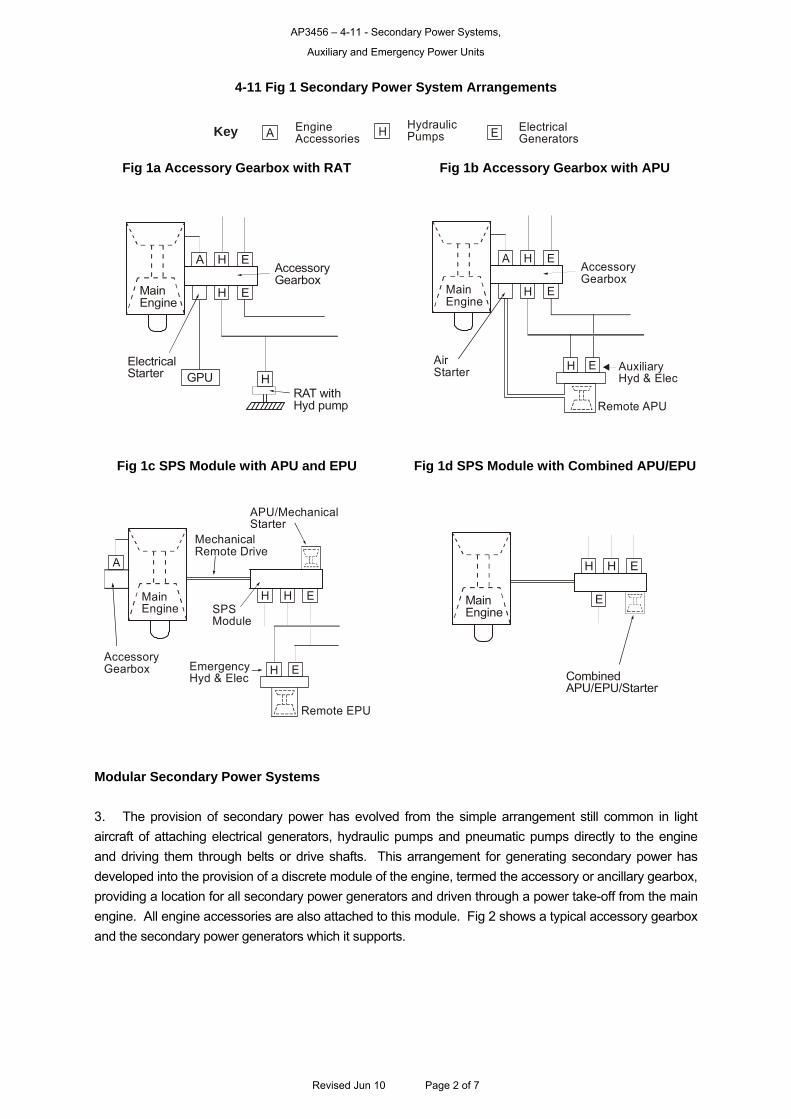
AP3456 – 4-11 - Secondary Power Systems,
Auxiliary and Emergency Power Units
4-11 Fig 1 Secondary Power System Arrangements
KeyHydraulicPumpsHEngine
AccessoriesA ElectricalGeneratorsE
Fig 1a Accessory Gearbox with RAT Fig 1b Accessory Gearbox with APU
RAT withHyd pump
ElectricalStarter
AccessoryGearbox
GPU
MainEngine
A E
E
H
H
H
AirStarter
AccessoryGearbox
MainEngine
A E
E
H
H
Remote APU
H E AuxiliaryHyd & Elec
Fig 1c SPS Module with APU and EPU Fig 1d SPS Module with Combined APU/EPU
Remote EPU
EmergencyHyd & Elec
SPSModule
EH H
H EAccessoryGearbox
A
MechanicalRemote Drive
APU/MechanicalStarter
MainEngine
CombinedAPU/EPU/Starter
EH H
EMainEngine
Modular Secondary Power Systems
3. The provision of secondary power has evolved from the simple arrangement still common in light aircraft of attaching electrical generators, hydraulic pumps and pneumatic pumps directly to the engine and driving them through belts or drive shafts. This arrangement for generating secondary power has developed into the provision of a discrete module of the engine, termed the accessory or ancillary gearbox, providing a location for all secondary power generators and driven through a power take-off from the main engine. All engine accessories are also attached to this module. Fig 2 shows a typical accessory gearbox and the secondary power generators which it supports.
Revised Jun 10 Page 2 of 7
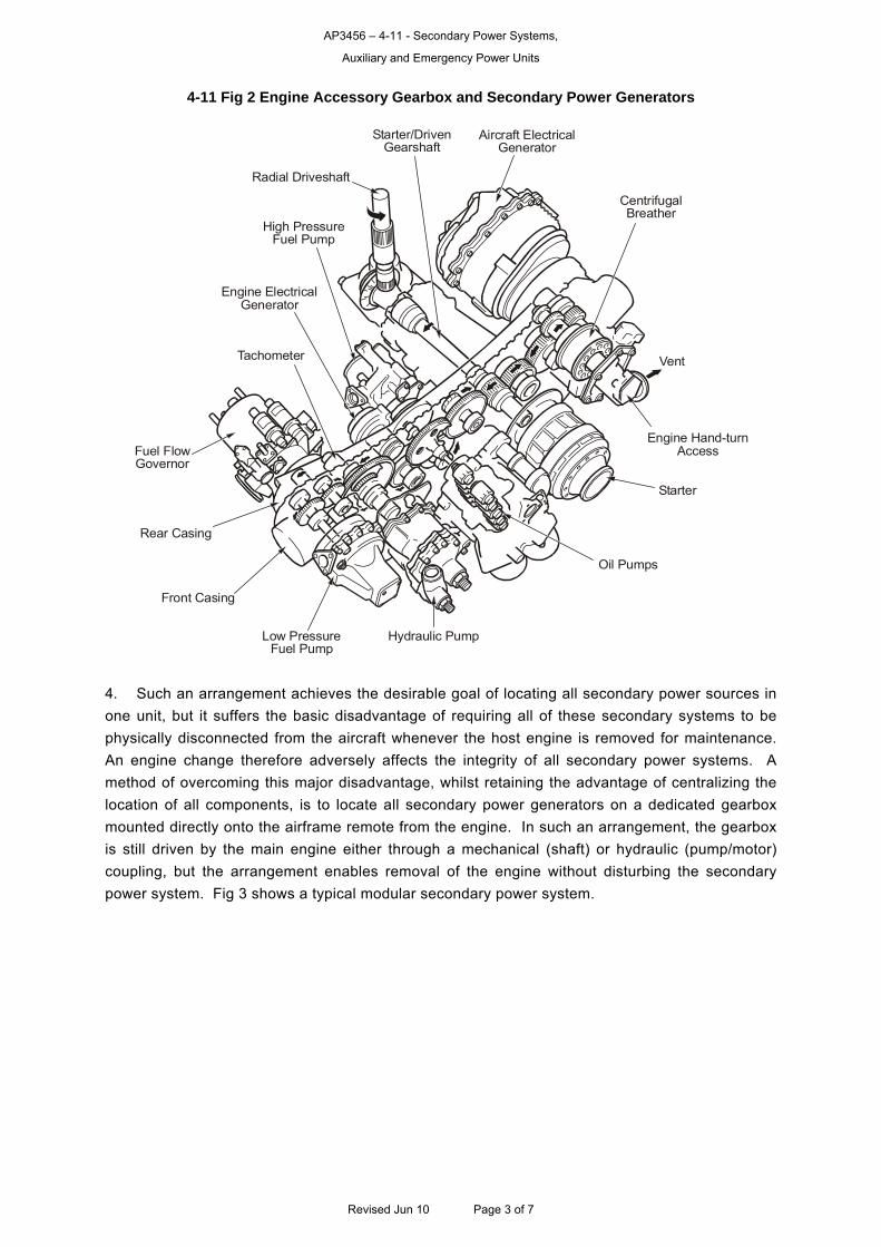
AP3456 – 4-11 - Secondary Power Systems,
Auxiliary and Emergency Power Units
4-11 Fig 2 Engine Accessory Gearbox and Secondary Power Generators
Hydraulic PumpLow PressureFuel Pump
Front Casing
Rear Casing
Fuel FlowGovernor
High PressureFuel Pump
Radial Driveshaft
Starter/DrivenGearshaft
Aircraft ElectricalGenerator
CentrifugalBreather
Vent
Engine Hand-turnAccess
Starter
Oil Pumps
Engine ElectricalGenerator
Tachometer
4. Such an arrangement achieves the desirable goal of locating all secondary power sources in one unit, but it suffers the basic disadvantage of requiring all of these secondary systems to be physically disconnected from the aircraft whenever the host engine is removed for maintenance. An engine change therefore adversely affects the integrity of all secondary power systems. A method of overcoming this major disadvantage, whilst retaining the advantage of centralizing the location of all components, is to locate all secondary power generators on a dedicated gearbox mounted directly onto the airframe remote from the engine. In such an arrangement, the gearbox is still driven by the main engine either through a mechanical (shaft) or hydraulic (pump/motor) coupling, but the arrangement enables removal of the engine without disturbing the secondary power system. Fig 3 shows a typical modular secondary power system.
Revised Jun 10 Page 3 of 7
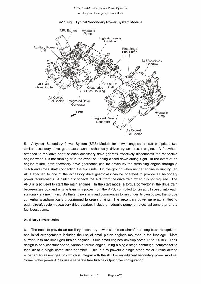
AP3456 – 4-11 - Secondary Power Systems,
Auxiliary and Emergency Power Units
4-11 Fig 3 Typical Secondary Power System Module
Air CooledFuel Cooler
Air CooledFuel Cooler Integrated Drive
Generator
Integrated DriveGenerator
FWD
Cross-driveClutch Housing
Cross-driveShaft
HydraulicPump
HydraulicPump
APU Exhaust
Auxiliary PowerUnit
APU AirIntake Shutter
Left AccessoryGearbox
Right AccessoryGearbox
First StageFuel Pump
5. A typical Secondary Power System (SPS) Module for a twin engined aircraft comprises two similar accessory drive gearboxes each mechanically driven by an aircraft engine. A freewheel attached to the drive shaft of each accessory drive gearbox effectively disconnects the respective engine when it is not running or in the event of it being closed down during flight. In the event of an engine failure, both accessory drive gearboxes can be driven by the remaining engine through a clutch and cross shaft connecting the two units. On the ground when neither engine is running, an APU attached to one of the accessory drive gearboxes can be operated to provide all secondary power requirements. A clutch disconnects the APU from the drive train, when it is not required. The APU is also used to start the main engines. In the start mode, a torque convertor in the drive train between gearbox and engine transmits power from the APU, controlled to run at full speed, into each stationary engine in turn. As the engine starts and commences to run under its own power, the torque convertor is automatically programmed to cease driving. The secondary power generators fitted to each aircraft system accessory drive gearbox include a hydraulic pump, an electrical generator and a fuel boost pump. Auxiliary Power Units
6. The need to provide an auxiliary secondary power source on aircraft has long been recognized, and initial arrangements included the use of small piston engines mounted in the fuselage. Most current units are small gas turbine engines. Such small engines develop some 75 to l00 kW. Their design is of a constant speed, variable torque engine using a single stage centrifugal compressor to feed air to a single combustion chamber. This in turn powers a single stage radial turbine driving either an accessory gearbox which is integral with the APU or an adjacent secondary power module. Some higher power APUs use a separate free turbine output drive configuration.
Revised Jun 10 Page 4 of 7
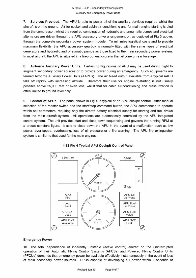
AP3456 – 4-11 - Secondary Power Systems,
Auxiliary and Emergency Power Units
7. Services Provided. The APU is able to power all of the ancillary services required whilst the aircraft is on the ground. Air for cockpit and cabin air-conditioning and for main engine starting is bled from the compressor, whilst the required combination of hydraulic and pneumatic pumps and electrical alternators are driven through the APU accessory drive arrangement or, as depicted at Fig 3 above, through the complete secondary power system module. To minimize logistical costs and to provide maximum flexibility, the APU accessory gearbox is normally fitted with the same types of electrical generators and hydraulic and pneumatic pumps as those fitted to the main secondary power system. In most aircraft, the APU is situated in a fireproof enclosure in the tail cone or rear fuselage. 8. Airborne Auxiliary Power Units. Certain configurations of APU may be used during flight to augment secondary power sources or to provide power during an emergency. Such equipments are termed Airborne Auxiliary Power Units (AAPUs). The air bleed output available from a typical AAPU falls off rapidly with increasing altitude. Therefore their use for engine re-starting is not usually possible above 25,000 feet or even less, whilst that for cabin air-conditioning and pressurization is often limited to ground level only. 9. Control of APUs. The panel shown in Fig 4 is typical of an APU cockpit control. After manual selection of the master switch and the start/stop command button, the APU commences to operate within set parameters, requiring only the aircraft battery electrical supply for starting and fuel drawn from the main aircraft system. All operations are automatically controlled by the APU integrated control system. The unit provides start and close-down sequencing and governs the running RPM at a preset constant figure. It acts to close down the APU in the event of a malfunction such as low power, over-speed, overheating, loss of oil pressure or a fire warning. The APU fire extinguisher system is similar to that used for the main engines.
4-11 Fig 4 Typical APU Cockpit Control Panel
APUFire
LoopFault
APU EXTUsed
APU PWRAvailable
APU OilLo Press
APU FuelLo Press
APU FuelValve
APU NVRLeak
% RPM
APUFire Ext
Stop
Start
TGTC x 100
*
#
Emergency Power 10. The total dependence of inherently unstable (active control) aircraft on the uninterrupted operation of their Automatic Flying Control Systems (AFCSs) and Powered Flying Control Units (PFCUs) demands that emergency power be available effectively instantaneously in the event of loss of main secondary power sources. EPUs capable of developing full power within 2 seconds of
Revised Jun 10 Page 5 of 7
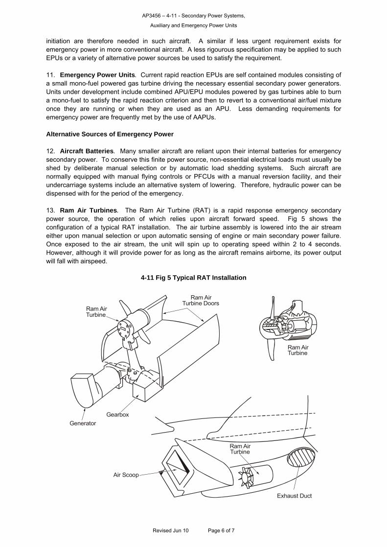
AP3456 – 4-11 - Secondary Power Systems,
Auxiliary and Emergency Power Units
initiation are therefore needed in such aircraft. A similar if less urgent requirement exists for emergency power in more conventional aircraft. A less rigourous specification may be applied to such EPUs or a variety of alternative power sources be used to satisfy the requirement. 11. Emergency Power Units. Current rapid reaction EPUs are self contained modules consisting of a small mono-fuel powered gas turbine driving the necessary essential secondary power generators. Units under development include combined APU/EPU modules powered by gas turbines able to burn a mono-fuel to satisfy the rapid reaction criterion and then to revert to a conventional air/fuel mixture once they are running or when they are used as an APU. Less demanding requirements for emergency power are frequently met by the use of AAPUs. Alternative Sources of Emergency Power 12. Aircraft Batteries. Many smaller aircraft are reliant upon their internal batteries for emergency secondary power. To conserve this finite power source, non-essential electrical loads must usually be shed by deliberate manual selection or by automatic load shedding systems. Such aircraft are normally equipped with manual flying controls or PFCUs with a manual reversion facility, and their undercarriage systems include an alternative system of lowering. Therefore, hydraulic power can be dispensed with for the period of the emergency. 13. Ram Air Turbines. The Ram Air Turbine (RAT) is a rapid response emergency secondary power source, the operation of which relies upon aircraft forward speed. Fig 5 shows the configuration of a typical RAT installation. The air turbine assembly is lowered into the air stream either upon manual selection or upon automatic sensing of engine or main secondary power failure. Once exposed to the air stream, the unit will spin up to operating speed within 2 to 4 seconds. However, although it will provide power for as long as the aircraft remains airborne, its power output will fall with airspeed.
4-11 Fig 5 Typical RAT Installation
Ram AirTurbine
Ram AirTurbine
Ram AirTurbine
Ram AirTurbine Doors
GearboxGenerator
Air Scoop
Exhaust Duct
Revised Jun 10 Page 6 of 7

AP3456 – 4-11 - Secondary Power Systems,
Auxiliary and Emergency Power Units
Revised Jun 10 Page 7 of 7
Ground Power Units
14. The generic term GPU covers a wide range of equipments from the simple, towed trolley-accumulator providing limited DC power, to the multi-purpose unit providing hydraulic and electrical power and engine-start air from a single, self-propelled vehicle. The major advantage of a GPU is that, since it is not part of the aircraft, no weight penalty need be imposed on its construction. It can therefore be built to produce large power outputs, using economical electrical or diesel engine power, and it can be constructed robustly for minimum maintenance. Subject to suitable arrangements for cooling and the extraction of exhaust gases, mobile GPUs can also be used inside hangars or aircraft shelters. Access to an aircraft being prepared for flight or undergoing servicing is always at a premium, and this factor has a major influence on the size and configuration of GPUs, and established maintenance hangars are designed to provide all such services as part of the fixed installations of the building. The services can then be ducted as necessary to the aircraft from permanently mounted power units sited well clear of the work area. Similar arrangements are also made in hardened aircraft shelters (HASs) and on the aircraft servicing platforms (ASPs) of major fixed operating bases.
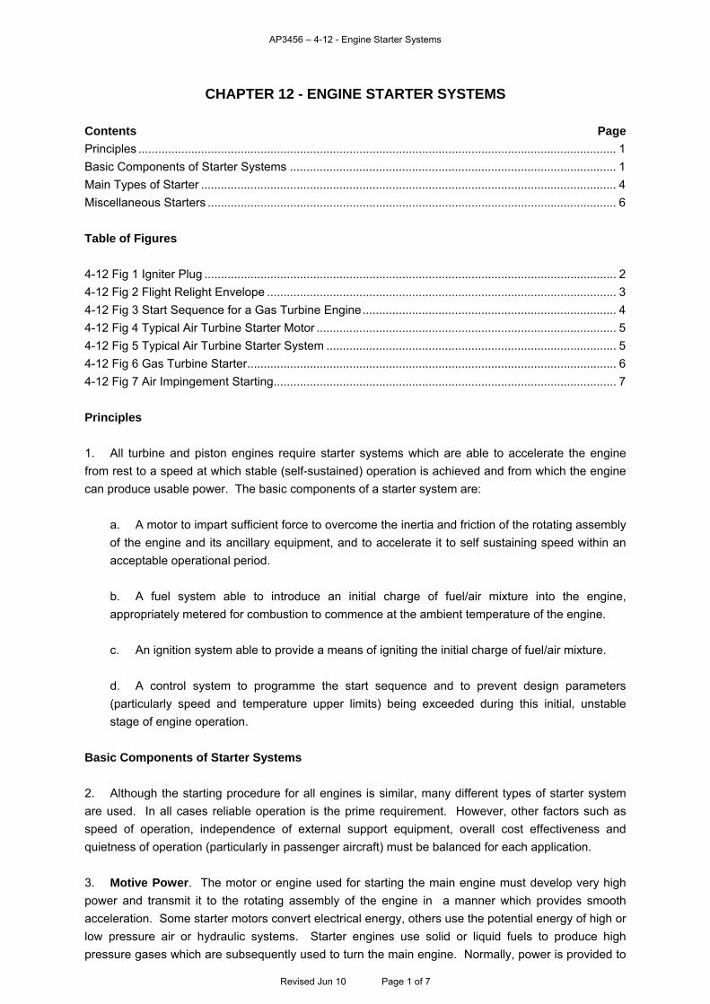
AP3456 – 4-12 - Engine Starter Systems
CHAPTER 12 - ENGINE STARTER SYSTEMS Contents Page
Principles ................................................................................................................................................. 1 Basic Components of Starter Systems ................................................................................................... 1 Main Types of Starter .............................................................................................................................. 4 Miscellaneous Starters ............................................................................................................................ 6
Table of Figures
4-12 Fig 1 Igniter Plug ............................................................................................................................. 2 4-12 Fig 2 Flight Relight Envelope .......................................................................................................... 3 4-12 Fig 3 Start Sequence for a Gas Turbine Engine............................................................................. 4 4-12 Fig 4 Typical Air Turbine Starter Motor ........................................................................................... 5 4-12 Fig 5 Typical Air Turbine Starter System ........................................................................................ 5 4-12 Fig 6 Gas Turbine Starter................................................................................................................ 6 4-12 Fig 7 Air Impingement Starting........................................................................................................ 7
Principles
1. All turbine and piston engines require starter systems which are able to accelerate the engine from rest to a speed at which stable (self-sustained) operation is achieved and from which the engine can produce usable power. The basic components of a starter system are:
a. A motor to impart sufficient force to overcome the inertia and friction of the rotating assembly of the engine and its ancillary equipment, and to accelerate it to self sustaining speed within an acceptable operational period. b. A fuel system able to introduce an initial charge of fuel/air mixture into the engine, appropriately metered for combustion to commence at the ambient temperature of the engine. c. An ignition system able to provide a means of igniting the initial charge of fuel/air mixture. d. A control system to programme the start sequence and to prevent design parameters (particularly speed and temperature upper limits) being exceeded during this initial, unstable stage of engine operation.
Basic Components of Starter Systems
2. Although the starting procedure for all engines is similar, many different types of starter system are used. In all cases reliable operation is the prime requirement. However, other factors such as speed of operation, independence of external support equipment, overall cost effectiveness and quietness of operation (particularly in passenger aircraft) must be balanced for each application. 3. Motive Power. The motor or engine used for starting the main engine must develop very high power and transmit it to the rotating assembly of the engine in a manner which provides smooth acceleration. Some starter motors convert electrical energy, others use the potential energy of high or low pressure air or hydraulic systems. Starter engines use solid or liquid fuels to produce high pressure gases which are subsequently used to turn the main engine. Normally, power is provided to
Revised Jun 10 Page 1 of 7
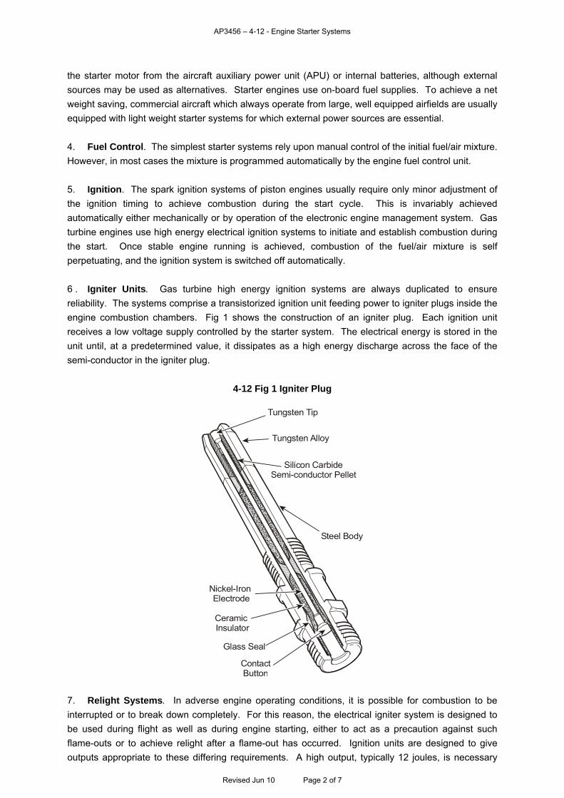
AP3456 – 4-12 - Engine Starter Systems
the starter motor from the aircraft auxiliary power unit (APU) or internal batteries, although external sources may be used as alternatives. Starter engines use on-board fuel supplies. To achieve a net weight saving, commercial aircraft which always operate from large, well equipped airfields are usually equipped with light weight starter systems for which external power sources are essential. 4. Fuel Control. The simplest starter systems rely upon manual control of the initial fuel/air mixture. However, in most cases the mixture is programmed automatically by the engine fuel control unit. 5. Ignition. The spark ignition systems of piston engines usually require only minor adjustment of the ignition timing to achieve combustion during the start cycle. This is invariably achieved automatically either mechanically or by operation of the electronic engine management system. Gas turbine engines use high energy electrical ignition systems to initiate and establish combustion during the start. Once stable engine running is achieved, combustion of the fuel/air mixture is self perpetuating, and the ignition system is switched off automatically. 6 . Igniter Units. Gas turbine high energy ignition systems are always duplicated to ensure reliability. The systems comprise a transistorized ignition unit feeding power to igniter plugs inside the engine combustion chambers. Fig 1 shows the construction of an igniter plug. Each ignition unit receives a low voltage supply controlled by the starter system. The electrical energy is stored in the unit until, at a predetermined value, it dissipates as a high energy discharge across the face of the semi-conductor in the igniter plug.
4-12 Fig 1 Igniter Plug
Tungsten Tip
Tungsten Alloy
Silicon CarbideSemi-conductor Pellet
Steel Body
Nickel-Iron Electrode
Ceramic Insulator
Glass Seal
Contact Button
7. Relight Systems. In adverse engine operating conditions, it is possible for combustion to be interrupted or to break down completely. For this reason, the electrical igniter system is designed to be used during flight as well as during engine starting, either to act as a precaution against such flame-outs or to achieve relight after a flame-out has occurred. Ignition units are designed to give outputs appropriate to these differing requirements. A high output, typically 12 joules, is necessary
Revised Jun 10 Page 2 of 7
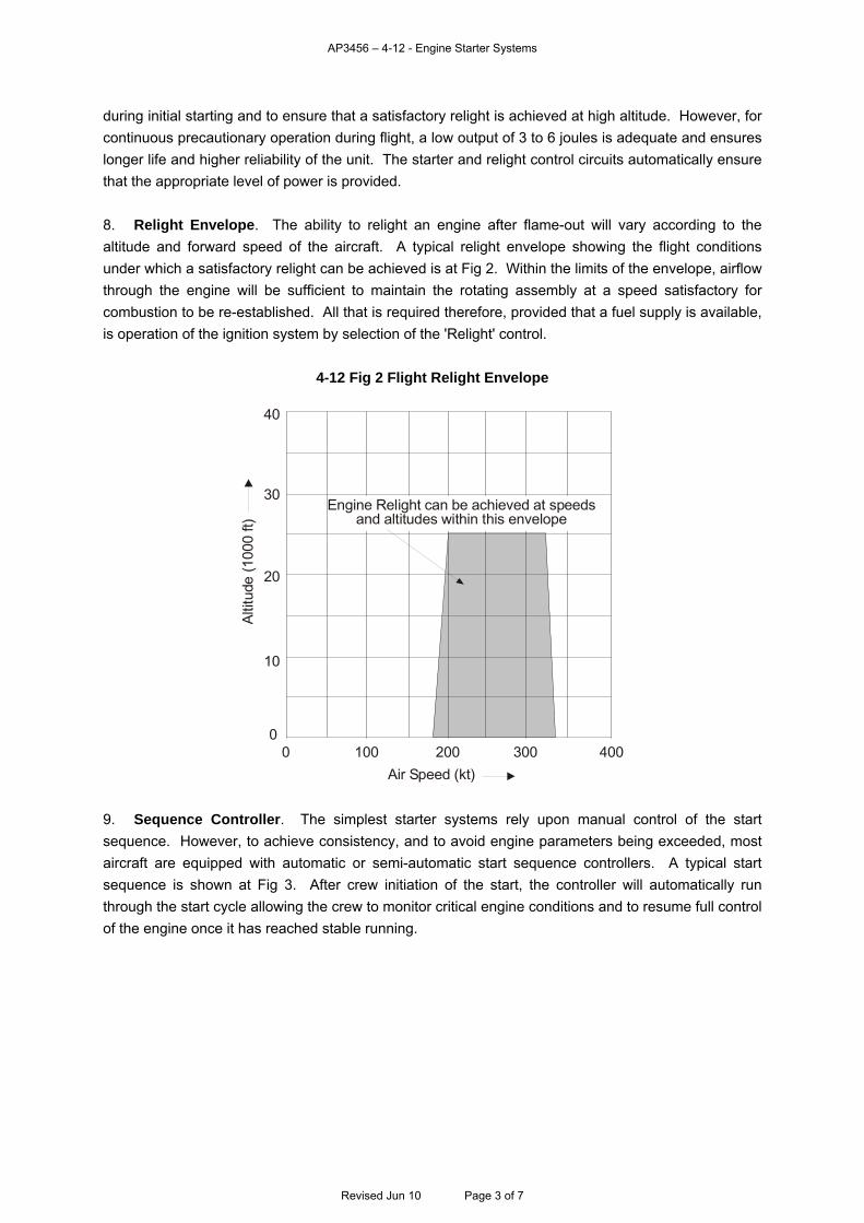
AP3456 – 4-12 - Engine Starter Systems
during initial starting and to ensure that a satisfactory relight is achieved at high altitude. However, for continuous precautionary operation during flight, a low output of 3 to 6 joules is adequate and ensures longer life and higher reliability of the unit. The starter and relight control circuits automatically ensure that the appropriate level of power is provided. 8. Relight Envelope. The ability to relight an engine after flame-out will vary according to the altitude and forward speed of the aircraft. A typical relight envelope showing the flight conditions under which a satisfactory relight can be achieved is at Fig 2. Within the limits of the envelope, airflow through the engine will be sufficient to maintain the rotating assembly at a speed satisfactory for combustion to be re-established. All that is required therefore, provided that a fuel supply is available, is operation of the ignition system by selection of the 'Relight' control.
4-12 Fig 2 Flight Relight Envelope
100 200 300 400
10
20
30
40
Engine Relight can be achieved at speedsand altitudes within this envelope
Air Speed (kt)0
0
Altit
ude
(100
0 ft)
9. Sequence Controller. The simplest starter systems rely upon manual control of the start sequence. However, to achieve consistency, and to avoid engine parameters being exceeded, most aircraft are equipped with automatic or semi-automatic start sequence controllers. A typical start sequence is shown at Fig 3. After crew initiation of the start, the controller will automatically run through the start cycle allowing the crew to monitor critical engine conditions and to resume full control of the engine once it has reached stable running.
Revised Jun 10 Page 3 of 7
AP3456 – 4-12 - Engine Starter Systems
4-12 Fig 3 Start Sequence for a Gas Turbine Engine
60
50
40
30
20
10
30
50
70
90
5 10 15 20 25 30
Ignitors On
HP Fuel On
Light-upAchieved
Self-sustainingrpm Achieved
Automatic StartCycle Complete
StabilizedIdling RPM
StabilizedIdling TGT
% M
axim
um T
urbi
neG
as T
empe
ratu
re (T
GT)
Seconds After Start Initiated
% M
axim
um E
ngin
e rp
m
Start Sequence
TGT
Main Types of Starter
10. Electrical. Electric motors developing sufficient power to accelerate the rotating assembly of a turbine engine are large and heavy in comparison with other types of starter. However, such motors are simple and comparatively cheap to produce and maintain, and electrical power is easy to transmit and control. It is available from internal batteries or APUs and from external power sources. For these reasons, electric starters are in wide spread use. If the starter motor can be configured to perform the dual role of driving the engine for starting and subsequently being driven by the engine to generate electrical power for the aircraft systems, significant advantages of low net weight, simplicity and low cost are available. The so called starter/generator is often used for small turbine engines, APUs and piston engines. Its drive shaft is permanently coupled to the engine, whereas single-role electrical starter motors must be connected to the engine through a clutch mechanism which engages at commencement of the start cycle and disengages as the engine reaches self-sustaining speed. 11. Air Turbine (Low Pressure). Low pressure air starting is widely used for both military and commercial aircraft engines. The air turbine starter is simple and has relatively low airborne weight. A typical air turbine starter is shown below in Fig 4.
Revised Jun 10 Page 4 of 7
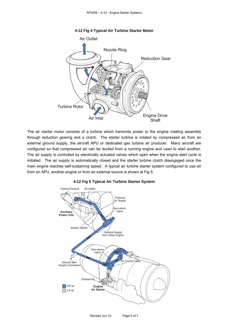
AP3456 – 4-12 - Engine Starter Systems
4-12 Fig 4 Typical Air Turbine Starter Motor
Air Outlet
Nozzle Ring
Reduction Gear
Air Inlet
Turbine Rotor
Engine DriveShaft
The air starter motor consists of a turbine which transmits power to the engine rotating assembly through reduction gearing and a clutch. The starter turbine is rotated by compressed air from an external ground supply, the aircraft APU or dedicated gas turbine air producer. Many aircraft are configured so that compressed air can be ducted from a running engine and used to start another. The air supply is controlled by electrically actuated valves which open when the engine start cycle is initiated. The air supply is automatically closed and the starter turbine clutch disengaged once the main engine reaches self-sustaining speed. A typical air turbine starter system configured to use air from an APU, another engine or from an external source is shown at Fig 5.
4-12 Fig 5 Typical Air Turbine Starter System
Turbine Exhaust Air Intake
AuxiliaryPower Unit
Electric Starter
PressureAir Supply
Non-returnValve
Optional Supplyfrom Other Engine
Ground StartSupply Connection
Exhaust Air
EngineAir Starter
HP air
LP air
Non-returnValve
Revised Jun 10 Page 5 of 7
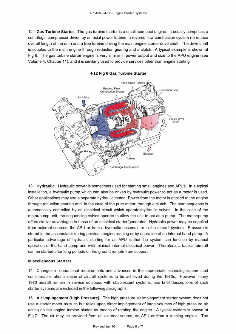
AP3456 – 4-12 - Engine Starter Systems
12. Gas Turbine Starter. The gas turbine starter is a small, compact engine. It usually comprises a centrifugal compressor driven by an axial power turbine, a reverse flow combustion system (to reduce overall length of the unit) and a free turbine driving the main engine starter drive shaft. The drive shaft is coupled to the main engine through reduction gearing and a clutch. A typical example is shown at Fig 6. The gas turbine starter engine is very similar in power output and size to the APU engine (see Volume 4, Chapter 11), and it is similarly used to provide services other than engine starting.
4-12 Fig 6 Gas Turbine Starter
Air Intake
Reverse FlowCombustion System
Free-power Turbine
Reduction Gear
Engine DriveShaft
Exhaust
Turbine
Centrifugal Compressor
13. Hydraulic. Hydraulic power is sometimes used for starting small engines and APUs. In a typical installation, a hydraulic pump which can also be driven by hydraulic power to act as a motor is used. Other applications may use a separate hydraulic motor. Power from the motor is applied to the engine through reduction gearing and, in the case of the pure motor, through a clutch. The start sequence is automatically controlled by an electrical circuit which operateshydraulic valves. In the case of the motor/pump unit, the sequencing valves operate to allow the unit to act as a pump. The motor/pump offers similar advantages to those of an electrical starter/generator. Hydraulic power may be supplied from external sources, the APU or from a hydraulic accumulator in the aircraft system. Pressure is stored in the accumulator during previous engine running or by operation of an internal hand pump. A particular advantage of hydraulic starting for an APU is that the system can function by manual operation of the hand pump and with minimal internal electrical power. Therefore, a tactical aircraft can be started after long periods on the ground remote from support. Miscellaneous Starters 14. Changes in operational requirements and advances in the appropriate technologies permitted considerable rationalization of aircraft systems to be achieved during the 1970s. However, many 1970 aircraft remain in service equipped with obsolescent systems, and brief descriptions of such starter systems are included in the following paragraphs. 15. Air Impingement (High Pressure). The high pressure air impingement starter system does not use a starter motor as such but relies upon direct impingement of large volumes of high pressure air acting on the engine turbine blades as means of rotating the engine. A typical system is shown at Fig 7. The air may be provided from an external source, an APU or from a running engine. The
Revised Jun 10 Page 6 of 7
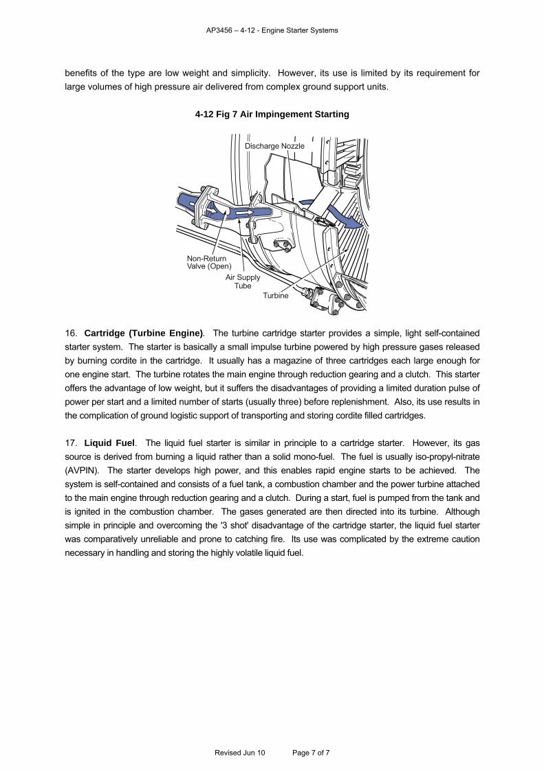
AP3456 – 4-12 - Engine Starter Systems
Revised Jun 10 Page 7 of 7
benefits of the type are low weight and simplicity. However, its use is limited by its requirement for large volumes of high pressure air delivered from complex ground support units.
4-12 Fig 7 Air Impingement Starting
Discharge Nozzle
Non-ReturnValve (Open)
Air SupplyTube
Turbine
16. Cartridge (Turbine Engine). The turbine cartridge starter provides a simple, light self-contained starter system. The starter is basically a small impulse turbine powered by high pressure gases released by burning cordite in the cartridge. It usually has a magazine of three cartridges each large enough for one engine start. The turbine rotates the main engine through reduction gearing and a clutch. This starter offers the advantage of low weight, but it suffers the disadvantages of providing a limited duration pulse of power per start and a limited number of starts (usually three) before replenishment. Also, its use results in the complication of ground logistic support of transporting and storing cordite filled cartridges. 17. Liquid Fuel. The liquid fuel starter is similar in principle to a cartridge starter. However, its gas source is derived from burning a liquid rather than a solid mono-fuel. The fuel is usually iso-propyl-nitrate (AVPIN). The starter develops high power, and this enables rapid engine starts to be achieved. The system is self-contained and consists of a fuel tank, a combustion chamber and the power turbine attached to the main engine through reduction gearing and a clutch. During a start, fuel is pumped from the tank and is ignited in the combustion chamber. The gases generated are then directed into its turbine. Although simple in principle and overcoming the '3 shot' disadvantage of the cartridge starter, the liquid fuel starter was comparatively unreliable and prone to catching fire. Its use was complicated by the extreme caution necessary in handling and storing the highly volatile liquid fuel.

OFFICIAL
UNCONTROLLED DOCUMENT WHEN PRINTED
AP3456 The Central Flying School (CFS)
Manual of Flying
Version 10.0 – 2018
Volume 5 – Flight Instruments
AP3456 is sponsored by the Commandant Central Flying School

OFFICIAL
UNCONTROLLED DOCUMENT WHEN PRINTED
Contents
Commandant CFS - Foreword
Introduction and Copyright Information
AP3456 Contact Details
Chapter Revised
5-1 Introduction to Barometric Height Measurement May 2010
5-2 Altimeters Oct 2011
5-3 Radar Altimeters Jun 2010
5-4 Vertical Speed Indicators May 2010
5-5 Air Speed Indicators May 2010
5-6 Machmeters May 2010
5-7 Combined Speed Indicators May 2010
5-8 Outside Air Temperature Gauges May 2010
5-9 Air Data Computer May 2010
5-10 Direct Indicating Compasses and Direction Indicators May 2010
5-11 Introduction to Gyroscopes Sep 2010
5-12 Gyro-magnetic Compasses May 2010
5-13 Horizontal Situation Indicators May 2010
5-14 Datum Compasses May 2010
5-15 Magnetic Compass Deviations May 2010
5-16 Compass Swinging Procedures May 2010
5-17 The Air Swing May 2010
5-18 A Refined Swing on a Class 2 Base Jul 2011
5-19 The Analysis of the Compass Swing May 2010
5-20 Turn and Slip Indicators May 2010
5-21 Attitude Indicators Jun 2011
5-22 Accelerometers May 2010
5-23 Stall Warning and Angle of Attack Indication May 2010
5-24 Remote Indication and Control May 2010
5-25 Servomechanisms May 2010
5-26 Engine Instruments May 2010
5-27 Miscellaneous Instruments May 2010

AP3456 – 5-1 - Introduction to Barometric Height Measurement
CHAPTER 1 - INTRODUCTION TO BAROMETRIC HEIGHT MEASUREMENT Contents Page Introduction.............................................................................................................................................. 1 The Atmosphere ...................................................................................................................................... 2 Standard Atmospheres............................................................................................................................ 3 Table of Figures 5-1 Fig 1 Decrease in Atmospheric Pressure with Height ...................................................................... 2 5-1 Fig 2 WADC Standard Atmosphere .................................................................................................. 4 Introduction 1. The atmospheric pressure at a point on the Earth’s surface is equivalent to the weight of the whole column of air standing on the area of that point. As distance increases from the Earth, the weight of the air above will be less, therefore atmospheric pressure decreases (Fig 1). Pressure altimeters operate on this principle, and indicate aircraft height relative to a selected pressure datum. Pressure altimeters are, in fact, aneroid barometers graduated to indicate height rather than pressure. In order for such an instrument to be calibrated, certain assumptions must be made concerning the manner in which air pressure decreases with height and this has given rise to a number of model atmospheres. 2. Units of Measurement. The units used in pressure measurement are:
a. Hectopascal. The hectopascal (hPa) is the unit of measurement of pressure in common use. At mean sea level (MSL), the atmospheric pressure is of the order of 1,000 hPa; at 50,000 ft it is of the order of 100 hPa.
b. Inches of Mercury. Some countries (notably the USA), measure pressure in inches of mercury (Hg). At MSL, atmospheric pressure is about 30 inches Hg.
c. Millibar. Although the hPa is now in common usage, the millibar (mb) is still used by many aircrew. The hPa and the mb have equivalent values and so can be considered to be identical for all practical purposes.
Both the hPa and the mb will be found in AP3456, but references to the mb will be gradually replaced by the hPa as chapters are routinely checked and amended.
Revised Mar 12 Page 1 of 4
AP3456 – 5-1 - Introduction to Barometric Height Measurement
5-1 Fig 1 Decrease in Atmospheric Pressure with Height
Limit of Atmosphere
Weight of air in whole column applies at surface
Weight of air in upper portion of column applies at height
Column of Air
The Atmosphere 3. The atmosphere is described in detail in Volume 1, Chapter 1. It is a relatively thin layer of gases surrounding the Earth, becoming more diffuse with increasing height. Water vapour is present in variable amounts, particularly near the surface. 4. The atmosphere can be divided into a number of layers, each with a tendency to a particular temperature distribution. The names, heights and characteristics of these layers may vary according to which standard atmosphere is being defined. However, in all cases the lower layer, the troposphere, is characterized by a fairly regular decrease of temperature with height. The upper limit of the troposphere is named the 'tropopause'. The height of the tropopause varies with latitude, season and weather. In general, it is lowest at the Earth’s poles (around 25,000 ft) and highest over equatorial regions (up to 54,000 ft). The layer above the tropopause is known as the stratosphere. Within this layer, the temperature is assumed to remain more or less constant, although, in reality, there is a noticeable increase near the top of the layer. The upper boundary of the stratosphere is called the 'stratopause', the height of which varies depending on which definition is being employed, but can be taken to be about 30 miles (166,000 ft). 5. Pressure Lapse Rate. As height increases, pressure decreases. However, this decrease is not proportional to the increase in height because the density of air varies with height. It is possible to deduce an expression for the pressure lapse rate at a constant temperature and thus establish a relationship between pressure and height. A practical approximation for the lower levels of the atmosphere, close to sea level, is that a decrease in pressure of one hPa equates to an increase in height of 30 feet. 6. Temperature Lapse Rate. Temperature varies with height in a complex manner. The temperature lapse rate depends on the humidity of the air, and is itself a function of height. This variation greatly affects the relationship between pressure and height. To calibrate an altimeter to indicate barometric height it is necessary to make some assumptions as to the temperature structure of the atmosphere. The relationship can be expressed in mathematical form for each of the various layers of the atmosphere and the instrument can then be calibrated accordingly.
Revised Mar 12 Page 2 of 4
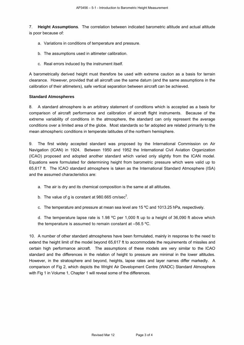
AP3456 – 5-1 - Introduction to Barometric Height Measurement
7. Height Assumptions. The correlation between indicated barometric altitude and actual altitude is poor because of:
a. Variations in conditions of temperature and pressure.
b. The assumptions used in altimeter calibration.
c. Real errors induced by the instrument itself. A barometrically derived height must therefore be used with extreme caution as a basis for terrain clearance. However, provided that all aircraft use the same datum (and the same assumptions in the calibration of their altimeters), safe vertical separation between aircraft can be achieved. Standard Atmospheres 8. A standard atmosphere is an arbitrary statement of conditions which is accepted as a basis for comparison of aircraft performance and calibration of aircraft flight instruments. Because of the extreme variability of conditions in the atmosphere, the standard can only represent the average conditions over a limited area of the globe. Most standards so far adopted are related primarily to the mean atmospheric conditions in temperate latitudes of the northern hemisphere. 9. The first widely accepted standard was proposed by the International Commission on Air Navigation (ICAN) in 1924. Between 1950 and 1952 the International Civil Aviation Organization (ICAO) proposed and adopted another standard which varied only slightly from the ICAN model. Equations were formulated for determining height from barometric pressure which were valid up to 65,617 ft. The ICAO standard atmosphere is taken as the International Standard Atmosphere (ISA) and the assumed characteristics are:
a. The air is dry and its chemical composition is the same at all altitudes.
b. The value of g is constant at 980.665 cm/sec2.
c. The temperature and pressure at mean sea level are 15 ºC and 1013.25 hPa, respectively.
d. The temperature lapse rate is 1.98 ºC per 1,000 ft up to a height of 36,090 ft above which the temperature is assumed to remain constant at –56.5 ºC.
10. A number of other standard atmospheres have been formulated, mainly in response to the need to extend the height limit of the model beyond 65,617 ft to accommodate the requirements of missiles and certain high performance aircraft. The assumptions of these models are very similar to the ICAO standard and the differences in the relation of height to pressure are minimal in the lower altitudes. However, in the stratosphere and beyond, heights, lapse rates and layer names differ markedly. A comparison of Fig 2, which depicts the Wright Air Development Centre (WADC) Standard Atmosphere with Fig 1 in Volume 1, Chapter 1 will reveal some of the differences.
Revised Mar 12 Page 3 of 4
AP3456 – 5-1 - Introduction to Barometric Height Measurement
Revised Mar 12 Page 4 of 4
5-1 Fig 2 WADC Standard Atmosphere
Pressure hPaRelative Density %
Temp Deg C
Upper Limit of ICAO ISA - 65,617 ft (20 km)
Stratopause 104,987 ft (32 km)
Tropopause 36,090 ft (11 km)
Relative DensityPressure
Temperature
–50 –40 –30 –20 –10 0 10 20 30200 400 600 800 100020 40 60 80 100
5
15
25
35
45
55
65
75
85
95
105
115
125
135 +22.473°
–56.5°
+15°
54.26 hPa
226.65 hPa
1.97 hPa
8.242 hPa
Altit
ude
in F
eet
100
0
Che
mos
pher
eSt
rato
sphe
reTr
opos
pher
e
Upper Limit of Wright Air DevelopmentCentre Atmosphere 140,000 ft
AP3456 - 5-2 - Altimeters
Revised Oct 11 Page 1 of 8
CHAPTER 2 - ALTIMETERS Contents Page PRINCIPLE OF OPERATION ................................................................................................................. 1 The Simple Altimeter ............................................................................................................................... 1 Sensitive Altimeters ................................................................................................................................. 2 Servo-assisted Altimeters ........................................................................................................................ 3 Cabin Altimeters ...................................................................................................................................... 3 ERRORS OF THE PRESSURE ALTIMETER ......................................................................................... 3 Instrument and Installation Errors ............................................................................................................ 3 Errors due to Non-standard Atmospheric Conditions .............................................................................. 4 Blockages and Leaks .............................................................................................................................. 6 Table of Figures 5-2 Fig 1 Simple Altimeter – Schematic ................................................................................................. 2 5-2 Fig 2 Servo-assisted Altimeter – Display ........................................................................................... 3 5-2 Fig 3 Effect of Barometric Error ......................................................................................................... 5 5-2 Fig 4 Effect of Temperature Error ..................................................................................................... 5 5-2 Fig 5 Altimeter Temperature Error Correction ................................................................................... 6 5-2 Fig 6 TAP for Temperature Error Correction Example in Fig 5 ......................................................... 8
PRINCIPLE OF OPERATION The Simple Altimeter 1. Air pressure is linked to height and this relationship is exploited by altimeters, which measure pressure but display height. 2. Fig 1 is a schematic diagram showing the main components of a basic, or 'simple' altimeter. Changes in air pressure are detected by an aneroid capsule (constructed from thin, corrugated metal) which is sealed and partially evacuated, and mounted inside a case. The case is fed with static pressure from the aircraft’s static tube or vents. As the aircraft climbs, the static pressure in the case will reduce, and the aneroid capsule will expand, assisted by a leaf spring. The linear movement of the capsule face is magnified and transmitted, via a system of gears and linkages, to a pointer moving over a scale (graduated in feet according to one of the standard atmospheres). Conversely, as the aircraft descends, the static pressure increases, and the capsule is compressed. An equilibrium is maintained between the pressure of the atmosphere on the face of the capsule and the tension of the spring.
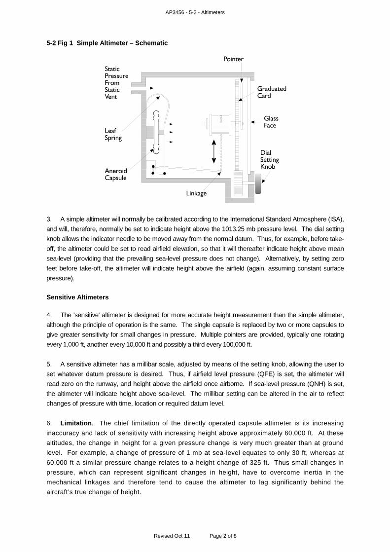
AP3456 - 5-2 - Altimeters
Revised Oct 11 Page 2 of 8
5-2 Fig 1 Simple Altimeter – Schematic
3. A simple altimeter will normally be calibrated according to the International Standard Atmosphere (ISA), and will, therefore, normally be set to indicate height above the 1013.25 mb pressure level. The dial setting knob allows the indicator needle to be moved away from the normal datum. Thus, for example, before take-off, the altimeter could be set to read airfield elevation, so that it will thereafter indicate height above mean sea-level (providing that the prevailing sea-level pressure does not change). Alternatively, by setting zero feet before take-off, the altimeter will indicate height above the airfield (again, assuming constant surface pressure). Sensitive Altimeters 4. The 'sensitive' altimeter is designed for more accurate height measurement than the simple altimeter, although the principle of operation is the same. The single capsule is replaced by two or more capsules to give greater sensitivity for small changes in pressure. Multiple pointers are provided, typically one rotating every 1,000 ft, another every 10,000 ft and possibly a third every 100,000 ft. 5. A sensitive altimeter has a millibar scale, adjusted by means of the setting knob, allowing the user to set whatever datum pressure is desired. Thus, if airfield level pressure (QFE) is set, the altimeter will read zero on the runway, and height above the airfield once airborne. If sea-level pressure (QNH) is set, the altimeter will indicate height above sea-level. The millibar setting can be altered in the air to reflect changes of pressure with time, location or required datum level. 6. Limitation. The chief limitation of the directly operated capsule altimeter is its increasing inaccuracy and lack of sensitivity with increasing height above approximately 60,000 ft. At these altitudes, the change in height for a given pressure change is very much greater than at ground level. For example, a change of pressure of 1 mb at sea-level equates to only 30 ft, whereas at 60,000 ft a similar pressure change relates to a height change of 325 ft. Thus small changes in pressure, which can represent significant changes in height, have to overcome inertia in the mechanical linkages and therefore tend to cause the altimeter to lag significantly behind the aircraft’s true change of height.
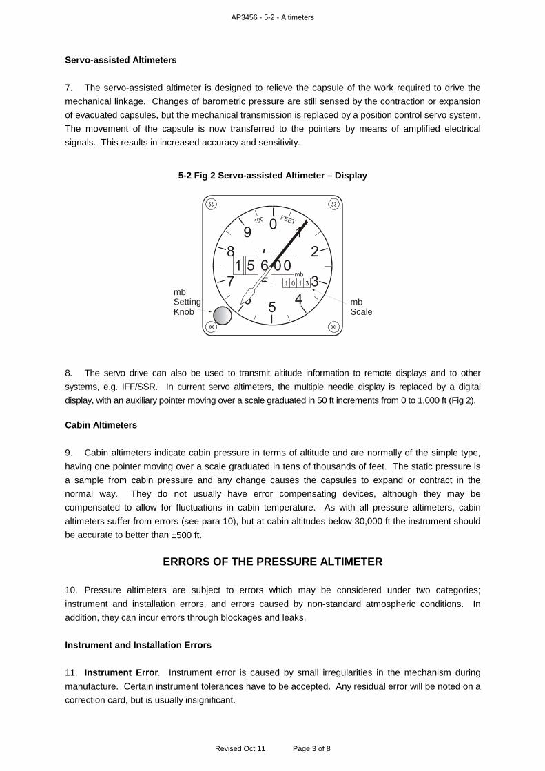
AP3456 - 5-2 - Altimeters
Revised Oct 11 Page 3 of 8
Servo-assisted Altimeters 7. The servo-assisted altimeter is designed to relieve the capsule of the work required to drive the mechanical linkage. Changes of barometric pressure are still sensed by the contraction or expansion of evacuated capsules, but the mechanical transmission is replaced by a position control servo system. The movement of the capsule is now transferred to the pointers by means of amplified electrical signals. This results in increased accuracy and sensitivity.
5-2 Fig 2 Servo-assisted Altimeter – Display
mbSettingKnob
mbScale
8. The servo drive can also be used to transmit altitude information to remote displays and to other systems, e.g. IFF/SSR. In current servo altimeters, the multiple needle display is replaced by a digital display, with an auxiliary pointer moving over a scale graduated in 50 ft increments from 0 to 1,000 ft (Fig 2). Cabin Altimeters 9. Cabin altimeters indicate cabin pressure in terms of altitude and are normally of the simple type, having one pointer moving over a scale graduated in tens of thousands of feet. The static pressure is a sample from cabin pressure and any change causes the capsules to expand or contract in the normal way. They do not usually have error compensating devices, although they may be compensated to allow for fluctuations in cabin temperature. As with all pressure altimeters, cabin altimeters suffer from errors (see para 10), but at cabin altitudes below 30,000 ft the instrument should be accurate to better than ±500 ft.
ERRORS OF THE PRESSURE ALTIMETER 10. Pressure altimeters are subject to errors which may be considered under two categories; instrument and installation errors, and errors caused by non-standard atmospheric conditions. In addition, they can incur errors through blockages and leaks. Instrument and Installation Errors 11. Instrument Error. Instrument error is caused by small irregularities in the mechanism during manufacture. Certain instrument tolerances have to be accepted. Any residual error will be noted on a correction card, but is usually insignificant.
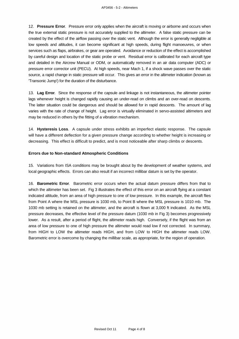
AP3456 - 5-2 - Altimeters
Revised Oct 11 Page 4 of 8
12. Pressure Error. Pressure error only applies when the aircraft is moving or airborne and occurs when the true external static pressure is not accurately supplied to the altimeter. A false static pressure can be created by the effect of the airflow passing over the static vent. Although the error is generally negligible at low speeds and altitudes, it can become significant at high speeds, during flight manoeuvres, or when services such as flaps, airbrakes, or gear are operated. Avoidance or reduction of the effect is accomplished by careful design and location of the static probe or vent. Residual error is calibrated for each aircraft type and detailed in the Aircrew Manual or ODM, or automatically removed in an air data computer (ADC) or pressure error corrector unit (PECU). At high speeds, near Mach 1, if a shock wave passes over the static source, a rapid change in static pressure will occur. This gives an error in the altimeter indication (known as 'Transonic Jump') for the duration of the disturbance. 13. Lag Error. Since the response of the capsule and linkage is not instantaneous, the altimeter pointer lags whenever height is changed rapidly causing an under-read on climbs and an over-read on descents. The latter situation could be dangerous and should be allowed for in rapid descents. The amount of lag varies with the rate of change of height. Lag error is virtually eliminated in servo-assisted altimeters and may be reduced in others by the fitting of a vibration mechanism. 14. Hysteresis Loss. A capsule under stress exhibits an imperfect elastic response. The capsule will have a different deflection for a given pressure change according to whether height is increasing or decreasing. This effect is difficult to predict, and is most noticeable after sharp climbs or descents. Errors due to Non-standard Atmospheric Conditions 15. Variations from ISA conditions may be brought about by the development of weather systems, and local geographic effects. Errors can also result if an incorrect millibar datum is set by the operator. 16. Barometric Error. Barometric error occurs when the actual datum pressure differs from that to which the altimeter has been set. Fig 3 illustrates the effect of this error on an aircraft flying at a constant indicated altitude, from an area of high pressure to one of low pressure. In this example, the aircraft flies from Point A where the MSL pressure is 1030 mb, to Point B where the MSL pressure is 1010 mb. The 1030 mb setting is retained on the altimeter, and the aircraft is flown at 3,000 ft indicated. As the MSL pressure decreases, the effective level of the pressure datum (1030 mb in Fig 3) becomes progressively lower. As a result, after a period of flight, the altimeter reads high. Conversely, if the flight was from an area of low pressure to one of high pressure the altimeter would read low if not corrected. In summary, from HIGH to LOW the altimeter reads HIGH, and from LOW to HIGH the altimeter reads LOW. Barometric error is overcome by changing the millibar scale, as appropriate, for the region of operation.
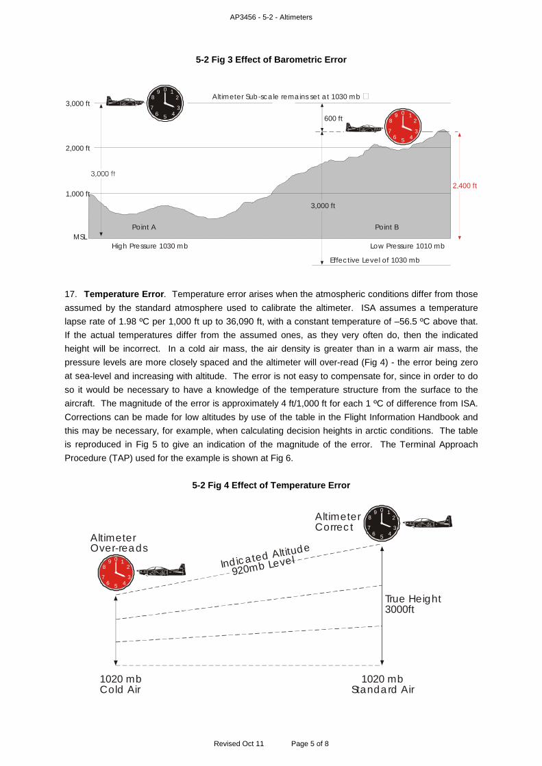
AP3456 - 5-2 - Altimeters
Revised Oct 11 Page 5 of 8
5-2 Fig 3 Effect of Barometric Error
0
00
5
55
6
6
4
44
7
77
3
33
8
88
2
22
9
99
1
600 ft
Altimeter Sub-scale remains set at 1030 mb
High Pressure 1030 mb Low Pressure 1010 mbMSL
1,000 ft
2,000 ft
3,000 ft
Effective Level of 1030 mb
Point A Point B
2,400 ft
3,000 ft
1
1
17. Temperature Error. Temperature error arises when the atmospheric conditions differ from those assumed by the standard atmosphere used to calibrate the altimeter. ISA assumes a temperature lapse rate of 1.98 ºC per 1,000 ft up to 36,090 ft, with a constant temperature of –56.5 ºC above that. If the actual temperatures differ from the assumed ones, as they very often do, then the indicated height will be incorrect. In a cold air mass, the air density is greater than in a warm air mass, the pressure levels are more closely spaced and the altimeter will over-read (Fig 4) - the error being zero at sea-level and increasing with altitude. The error is not easy to compensate for, since in order to do so it would be necessary to have a knowledge of the temperature structure from the surface to the aircraft. The magnitude of the error is approximately 4 ft/1,000 ft for each 1 ºC of difference from ISA. Corrections can be made for low altitudes by use of the table in the Flight Information Handbook and this may be necessary, for example, when calculating decision heights in arctic conditions. The table is reproduced in Fig 5 to give an indication of the magnitude of the error. The Terminal Approach Procedure (TAP) used for the example is shown at Fig 6.
5-2 Fig 4 Effect of Temperature Error
Indicated Altitude
920mb Level
True Height3000ft
AltimeterOver-reads
1020 mbCold Air
1020 mbStandard Air
AltimeterCorrect
0
56 47 3
8 29
0
56 47 3
8 29
1
1
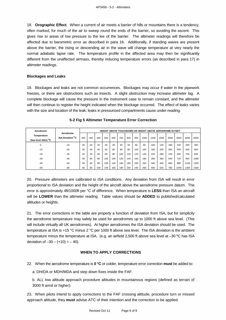
AP3456 - 5-2 - Altimeters
Revised Oct 11 Page 6 of 8
18. Orographic Effect. When a current of air meets a barrier of hills or mountains there is a tendency, often marked, for much of the air to sweep round the ends of the barrier, so avoiding the ascent. This gives rise to areas of low pressure to the lee of the barrier. The altimeter readings will therefore be affected due to barometric error as described in para 16. Additionally, if standing waves are present above the barrier, the rising or descending air in the wave will change temperature at very nearly the normal adiabatic lapse rate. The temperature profile in the affected area may then be significantly different from the unaffected airmass, thereby inducing temperature errors (as described in para 17) in altimeter readings. Blockages and Leaks 19. Blockages and leaks are not common occurrences. Blockages may occur if water in the pipework freezes, or there are obstructions such as insects. A slight obstruction may increase altimeter lag. A complete blockage will cause the pressure in the instrument case to remain constant, and the altimeter will then continue to register the height indicated when the blockage occurred. The effect of leaks varies with the size and location of the leak; leaks in pressurized compartments cause under-reading.
5-2 Fig 5 Altimeter Temperature Error Correction
Aerodrome
Temperature
(Sea level A/Ds) OC
Aerodrome
ISA Deviation OC
HEIGHT ABOVE TOUCHDOWN OR HEIGHT ABOVE AERODROME IN FEET
200 300 400 500 600 700 800 900 1000 1500 2000 3000 4000 5000 6000
0 −15 20 20 20 40 40 40 40 60 60 100 120 180 240 300 360
−10 −25 20 40 40 60 60 80 80 100 100 160 200 300 400 500 600
−20 −35 20 40 60 80 80 100 120 120 140 220 280 420 560 700 840
−30 −45 40 60 80 100 100 120 140 160 180 280 360 540 720 900 1080
−40 −55 40 60 80 100 140 160 180 200 220 340 440 660 880 1100 1320
−50 −65 60 80 100 140 160 180 200 240 260 400 520 780 1040 1300 1560
20. Pressure altimeters are calibrated to ISA conditions. Any deviation from ISA will result in error proportional to ISA deviation and the height of the aircraft above the aerodrome pressure datum. The error is approximately 4ft/1000ft per °C of difference. When temperature is LESS than ISA an aircraft will be LOWER than the altimeter reading. Table values should be ADDED to published/calculated altitudes or heights. 21. The error corrections in the table are properly a function of deviation from ISA, but for simplicity the aerodrome temperature may safely be used for aerodromes up to 1000 ft above sea level. (This will include virtually all UK aerodromes). At higher aerodromes the ISA deviation should be used. The temperature at ISA is +15 °C minus 2 °C per 1000 ft above sea level. The ISA deviation is the ambient temperature minus the temperature at ISA. (e.g. an airfield 2,500 ft above sea level at –30 ºC has ISA deviation of –30 – (+10) = – 40).
WHEN TO APPLY CORRECTIONS 22. When the aerodrome temperature is 0 °C or colder, temperature error correction must be added to:
a. DH/DA or MDH/MDA and step down fixes inside the FAF.
b. ALL low altitude approach procedure altitudes in mountainous regions (defined as terrain of 3000 ft amsl or higher).
23. When pilots intend to apply corrections to the FAF crossing altitude, procedure turn or missed approach altitude, they must advise ATC of their intention and the correction to be applied.

AP3456 - 5-2 - Altimeters
Revised Oct 11 Page 7 of 8
24. Pilots may refuse IFR assigned altitudes if altimeter temperature error will reduce obstacle clearance below acceptable minima. However, once an assigned altitude has been accepted, it must not subsequently be adjusted to compensate for temperature error.
MINIMUM SECTOR ALTITUDE (MSA) 25. When the aerodrome temperature is –30 °C or colder, add 1000ft to the MSA to ensure obstacle clearance.
EXAMPLE 26. SOMEWHERE; ILS/DME Rwy 29; TDZE/THR Elev 220; Surface Temp –30 °C.
Published Altitude HAT Add Altitude to Fly MSA 6700ft N/A 1000ft 7700ft
NDB Mnm Hold 6500ft 6280ft 1140ft 7640ft Turn Inbound 6200ft 5980ft 1080ft 7280ft NDB Inbound 5000ft 4780ft 860ft 5860ft OM Inbound 2680ft 2460ft 450ft 3130ft
DA/DH 820ft 600ft 100ft 920ft
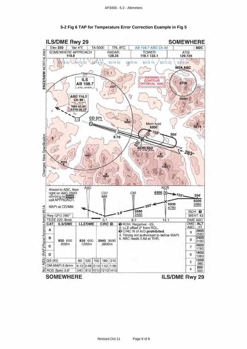
AP3456 - 5-2 - Altimeters
Revised Oct 11 Page 8 of 8
5-2 Fig 6 TAP for Temperature Error Correction Example in Fig 5
AP3456 – 5-3 - Radar Altimeters
CHAPTER 3 - RADAR ALTIMETERS Contents Page Introduction.............................................................................................................................................. 1 Pulse Radar Altimeter.............................................................................................................................. 1 Principle of Operation.............................................................................................................................. 2 Self Test................................................................................................................................................... 3 Figure 5-3 Fig 1 Block Diagram of a Typical Radar Altimeter Installation.......................................................... 2 Introduction 1. Barometric altimeters provide a standard datum for the safe vertical navigation and separation of aircraft; their limitations and errors are considered in Volume 5, Chapter 1. However, the nature of certain air operations (such as low level flying over the desert or sea) determines the need for an indication of actual surface clearance and proximity warning, and additionally, many on-board computing system require an accurate input of the instantaneous vertical distance of an aircraft from the Earth’s surface. These include systems for:
a. Terrain following.
b. Weapon aiming.
c. Navigation.
d. Helicopter automatic transitions to and from the hover. 2. Pulsed radar altimeters are range finding radar devices mounted to point downwards and measure the distance to the ground directly below the aircraft. Early systems had limited value because minimum range, determined by pulse width, was too great for very low level use. However, developed, modern systems can now be used down to zero feet with an accuracy of 1.5 ft. Pulse Radar Altimeter 3. Radar altimeters use conventional pulse radar techniques. The time taken for a short pulse to travel to the ground and back is measured and displayed on an indicator. The display time base is synchronized with the transmitter pulse. From the block diagram, at Fig 1 it can be seen that the main difference from a 'conventional' range finding system is that two aerials are used, one for transmission and one for reception. Due to the very small ranges that have to be measured, very narrow short duration pulses are transmitted at a typical frequency of 4.3 GHz.
Revised Jun 10 Page 1 of 3
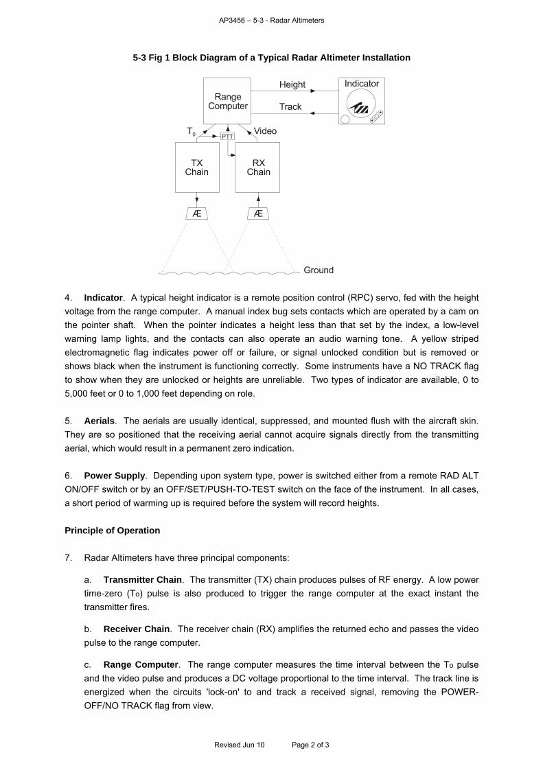
AP3456 – 5-3 - Radar Altimeters
5-3 Fig 1 Block Diagram of a Typical Radar Altimeter Installation
Video
Ground
T0
HeightRange
Computer
Indicator
TXChain
RXChain
Track
ÆÆ
PTT
4. Indicator. A typical height indicator is a remote position control (RPC) servo, fed with the height voltage from the range computer. A manual index bug sets contacts which are operated by a cam on the pointer shaft. When the pointer indicates a height less than that set by the index, a low-level warning lamp lights, and the contacts can also operate an audio warning tone. A yellow striped electromagnetic flag indicates power off or failure, or signal unlocked condition but is removed or shows black when the instrument is functioning correctly. Some instruments have a NO TRACK flag to show when they are unlocked or heights are unreliable. Two types of indicator are available, 0 to 5,000 feet or 0 to 1,000 feet depending on role. 5. Aerials. The aerials are usually identical, suppressed, and mounted flush with the aircraft skin. They are so positioned that the receiving aerial cannot acquire signals directly from the transmitting aerial, which would result in a permanent zero indication. 6. Power Supply. Depending upon system type, power is switched either from a remote RAD ALT ON/OFF switch or by an OFF/SET/PUSH-TO-TEST switch on the face of the instrument. In all cases, a short period of warming up is required before the system will record heights. Principle of Operation 7. Radar Altimeters have three principal components:
a. Transmitter Chain. The transmitter (TX) chain produces pulses of RF energy. A low power time-zero (To) pulse is also produced to trigger the range computer at the exact instant the transmitter fires.
b. Receiver Chain. The receiver chain (RX) amplifies the returned echo and passes the video pulse to the range computer.
c. Range Computer. The range computer measures the time interval between the To pulse and the video pulse and produces a DC voltage proportional to the time interval. The track line is energized when the circuits 'lock-on' to and track a received signal, removing the POWER-OFF/NO TRACK flag from view.
Revised Jun 10 Page 2 of 3

AP3456 – 5-3 - Radar Altimeters
Revised Jun 10 Page 3 of 3
8. The range computer has three states of operation:
a. Search. This is the state of operation if signals are not present or are too weak. The computer searches over the range of voltages from a minimum, equivalent to 0 feet, to a maximum, equivalent to 1,000 or 5,000 feet (depending upon type), 4 times per second. The indicator shows the NO TRACK or yellow striped POWER OFF flag.
b. Lock/Follow.
(1) When a returning signal is detected and tracked for a pre-determined period the system 'locks-on', producing an output voltage proportional to the height.
(2) This internal voltage is fed to the indicator which causes the pointer to move to the correct height. The track line is energized and pulls the POWER-OFF/NO TRACK flag out of view.
(3) The tracking circuits can maintain lock with vertical range changes of up to 2,000 ft/sec.
c. Memory.
(1) If the signal is lost, the circuitry is prevented from reverting to search for approximately 0.2 seconds. If signals are detected during this time, the indicator is unaffected.
(2) If signals are not detected, the range computer goes into its search condition, but the indicator display is held steady for a further 1.0 seconds.
(3) If lock is not obtained within this period, the track line will be de-energized and the indicator will show the NO TRACK or POWER OFF flag.
Self Test 9. The aircrew, or the maintenance crew, can check the operation of the equipment, with the exception of the aerials and their cables, by means of the PUSH-TO-TEST (PTT) button. Detailed instructions for testing the equipment are contained in the relevant Aircrew Manuals.
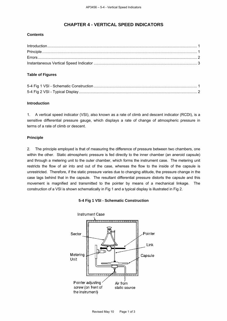
AP3456 – 5-4 - Vertical Speed Indicators
CHAPTER 4 - VERTICAL SPEED INDICATORS Contents Introduction.............................................................................................................................................. 1 Principle................................................................................................................................................... 1 Errors ....................................................................................................................................................... 2 Instantaneous Vertical Speed Indicator .................................................................................................. 3 Table of Figures 5-4 Fig 1 VSI - Schematic Construction .................................................................................................. 1 5-4 Fig 2 VSI - Typical Display ................................................................................................................ 2 Introduction 1. A vertical speed indicator (VSI), also known as a rate of climb and descent indicator (RCDI), is a sensitive differential pressure gauge, which displays a rate of change of atmospheric pressure in terms of a rate of climb or descent. Principle 2. The principle employed is that of measuring the difference of pressure between two chambers, one within the other. Static atmospheric pressure is fed directly to the inner chamber (an aneroid capsule) and through a metering unit to the outer chamber, which forms the instrument case. The metering unit restricts the flow of air into and out of the case, whereas the flow to the inside of the capsule is unrestricted. Therefore, if the static pressure varies due to changing altitude, the pressure change in the case lags behind that in the capsule. The resultant differential pressure distorts the capsule and this movement is magnified and transmitted to the pointer by means of a mechanical linkage. The construction of a VSI is shown schematically in Fig 1 and a typical display is illustrated in Fig 2.
5-4 Fig 1 VSI - Schematic Construction
Revised May 10 Page 1 of 3
AP3456 – 5-4 - Vertical Speed Indicators
5-4 Fig 2 VSI - Typical Display
2
21.5
.51
4
4
60x1000
FT/MIN
Adjustment Screw 3. It is important that any given pressure difference between the inside and outside of the capsule should represent the same rate of climb or descent, regardless of the ambient atmospheric pressure and temperature variations with altitude. The function of the metering unit, in the manner in which it restricts the flow into the case, is to compensate for these changes in ambient conditions. 4. In level flight, the pressure inside the capsule and the case are the same, and the pointer remains at the zero (horizontal) position. When the aircraft climbs, the static pressure decreases and the capsule collapses slightly, causing the pointer to move upwards to indicate a rate of climb. The fall in pressure in the case lags behind that in the capsule until level flight is resumed and the pressures equalize. In a descent, the increase in pressure in the case lags behind the increase in static pressure in the capsule, and the capsule is expanded, causing the pointer to move downwards. Errors 5. The VSI can suffer from the following errors:
a. Instrument Error. Instrument error is the result of manufacturing tolerances and is usually insignificant. Before flight, pilots should ensure that the pointer reads zero, or is within permissible limits. With some VSIs, the zero setting can be adjusted by means of a screw on the face of the instrument.
b. Pressure Error. If the static head or vent is subject to disturbed airflow, the static pressure may be in error, and the VSI will briefly indicate a wrong rate of climb or descent. These disturbances may be due to:
(1) Accelerations (such as take-off or missed approach) or decelerations.
(2) Change of aircraft configuration.
(3) Movement of a shock wave over the static vents (resulting erroneous indications are referred to as Transonic Jump).
c. Lag Error. When an aircraft begins a climb or descent, the instrument will indicate the change in pitch, but there is few seconds delay before the pointer settles at the appropriate rate of climb or descent. This delay is known as 'lag' and is caused by the time required for the pressure difference to develop. A similar delay occurs before the pointer indicates zero when the aircraft is levelled.
Revised May 10 Page 2 of 3

AP3456 – 5-4 - Vertical Speed Indicators
Revised May 10 Page 3 of 3
6. Static Line Blockage. If the static line or vent becomes blocked by ice (or any other obstruction), the VSI will be rendered unserviceable and the pointer will remain at zero regardless of the vertical speed. Instantaneous Vertical Speed Indicator 7. The Instantaneous Vertical Speed Indicator (IVSI), also sometimes referred to as the Inertia Lead VSI, was developed to overcome the initial lag error (described in sub-para 5c) when a climb or descent is started. The IVSI is similar in operation to the VSI, except that two accelerometer units, working in opposite directions, are added to the linkage between the capsule and the pointer. The accelerometer units rely upon inertial mass, which is moved with a change in vertical speed in either direction. At the initiation of a climb or descent, inertia now causes the appropriate accelerometer to produce an immediate response, which is transmitted to the pointer on the instrument face, well before any static pressure differential has been established. After a few seconds, the effect of the accelerometer response dies away, but, by this time, the static pressure change will have become effective in the normal way. Thus, within the IVSI, initial lag error is virtually eliminated. However, because the accelerometers are not vertically stabilized, some error is produced during turns, and at large angles of bank (in excess of 40º), the IVSI is unreliable.
AP3456 – 5-5 - Air Speed Indicators
CHAPTER 5 - AIR SPEED INDICATORS
Contents
Introduction.............................................................................................................................................. 1
Principle................................................................................................................................................... 1
Construction ............................................................................................................................................ 2
Calibration ............................................................................................................................................... 4
ASI Errors ................................................................................................................................................ 4
Blocked or Leaking Pressure Systems ................................................................................................... 5
Table of Figures
5-5 Fig 1 Principle of Air Speed Indicator................................................................................................ 2
5-5 Fig 2 A Combined Pressure Head .................................................................................................... 2
5-5 Fig 3 A Typical Simple ASI................................................................................................................ 3
5-5 Fig 4 A Two Pointer Sensitive ASI .................................................................................................... 3
Introduction
1. A knowledge of the speed at which an aircraft is travelling through the air, ie the air speed, is
essential both to the pilot for the safe and efficient handling of the aircraft and to the navigator as a
basic input to the navigation calculations. The instrument which displays this information is the air
speed indicator (ASI).
Principle
2. An aircraft, stationary on the ground, is subject to normal atmospheric or static pressure which acts
equally on all parts of the aircraft structure. In flight, the aircraft experiences an additional pressure on its
leading surfaces due to a build up of the air through which the aircraft is travelling. This additional
pressure due to the aircraft's forward motion is known as dynamic pressure and is dependent upon the
forward speed of the aircraft and the density of the air according to the following formula:
pt = ½ρV2 + p
where pt = the pitot pressure, (also known as total head pressure or stagnation pressure)
p = the static pressure
= the air density
V = the velocity of the aircraft.
Rearranging the formula, the difference between the pitot and the static pressures is equal to ½ρV2
(the dynamic pressure). The air speed indicator measures this pressure difference and provides a
display indication graduated in units of speed.
3. Fig 1 illustrates the principle, in its most simple form, on which all air speed indicators function. The
ASI is a sensitive differential pressure gauge operated by pressures picked up by a pressure head, which
is mounted in a suitable position on the airframe. The simplest pressure head consists of an open ended
tube, the pitot tube, aligned with the direction of flight, and a second tube, the static tube, which is closed
and streamlined at the forward end but which has a series of small holes drilled radially along its length.
Revised May 10 Page 1 of 6
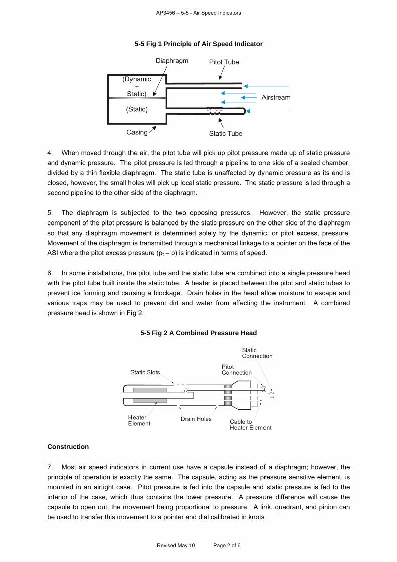
AP3456 – 5-5 - Air Speed Indicators
5-5 Fig 1 Principle of Air Speed Indicator
Diaphragm Pitot Tube
Airstream
Static TubeCasing
(Static)
(Dynamic+
Static)
4. When moved through the air, the pitot tube will pick up pitot pressure made up of static pressure
and dynamic pressure. The pitot pressure is led through a pipeline to one side of a sealed chamber,
divided by a thin flexible diaphragm. The static tube is unaffected by dynamic pressure as its end is
closed, however, the small holes will pick up local static pressure. The static pressure is led through a
second pipeline to the other side of the diaphragm.
5. The diaphragm is subjected to the two opposing pressures. However, the static pressure
component of the pitot pressure is balanced by the static pressure on the other side of the diaphragm
so that any diaphragm movement is determined solely by the dynamic, or pitot excess, pressure.
Movement of the diaphragm is transmitted through a mechanical linkage to a pointer on the face of the
ASI where the pitot excess pressure (pt – p) is indicated in terms of speed.
6. In some installations, the pitot tube and the static tube are combined into a single pressure head
with the pitot tube built inside the static tube. A heater is placed between the pitot and static tubes to
prevent ice forming and causing a blockage. Drain holes in the head allow moisture to escape and
various traps may be used to prevent dirt and water from affecting the instrument. A combined
pressure head is shown in Fig 2.
5-5 Fig 2 A Combined Pressure Head
Static SlotsPitotConnection
Drain HolesHeaterElement Cable to
Heater Element
StaticConnection
Construction
7. Most air speed indicators in current use have a capsule instead of a diaphragm; however, the
principle of operation is exactly the same. The capsule, acting as the pressure sensitive element, is
mounted in an airtight case. Pitot pressure is fed into the capsule and static pressure is fed to the
interior of the case, which thus contains the lower pressure. A pressure difference will cause the
capsule to open out, the movement being proportional to pressure. A link, quadrant, and pinion can
be used to transfer this movement to a pointer and dial calibrated in knots.
Revised May 10 Page 2 of 6
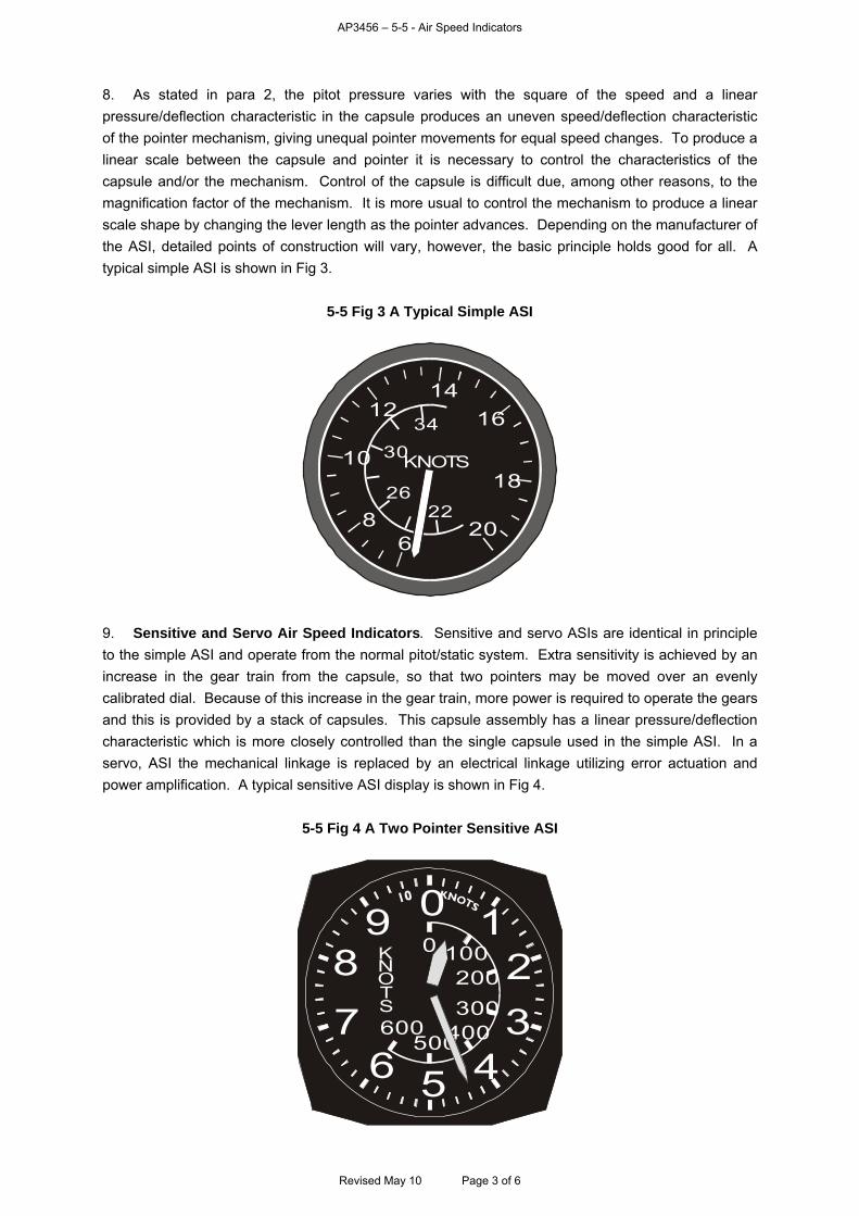
AP3456 – 5-5 - Air Speed Indicators
8. As stated in para 2, the pitot pressure varies with the square of the speed and a linear
pressure/deflection characteristic in the capsule produces an uneven speed/deflection characteristic
of the pointer mechanism, giving unequal pointer movements for equal speed changes. To produce a
linear scale between the capsule and pointer it is necessary to control the characteristics of the
capsule and/or the mechanism. Control of the capsule is difficult due, among other reasons, to the
magnification factor of the mechanism. It is more usual to control the mechanism to produce a linear
scale shape by changing the lever length as the pointer advances. Depending on the manufacturer of
the ASI, detailed points of construction will vary, however, the basic principle holds good for all. A
typical simple ASI is shown in Fig 3.
5-5 Fig 3 A Typical Simple ASI
KNOTS
20
16
1412
10
86
2226
30
34
18
9. Sensitive and Servo Air Speed Indicators. Sensitive and servo ASIs are identical in principle
to the simple ASI and operate from the normal pitot/static system. Extra sensitivity is achieved by an
increase in the gear train from the capsule, so that two pointers may be moved over an evenly
calibrated dial. Because of this increase in the gear train, more power is required to operate the gears
and this is provided by a stack of capsules. This capsule assembly has a linear pressure/deflection
characteristic which is more closely controlled than the single capsule used in the simple ASI. In a
servo, ASI the mechanical linkage is replaced by an electrical linkage utilizing error actuation and
power amplification. A typical sensitive ASI display is shown in Fig 4.
5-5 Fig 4 A Two Pointer Sensitive ASI
0 12
3456
7
89
0 100200
300400500
600
KNOTS
Revised May 10 Page 3 of 6
AP3456 – 5-5 - Air Speed Indicators
Calibration
10. Since dynamic pressure varies with air speed and air density, and since air density varies with
temperature and pressure, standard datum values have to be used in the calibration of air speed
indicators. The values used are the sea level values of the standard ICAO atmosphere. The formula
given in para 2 is only an approximation and one of two formulae is used for calibration of a particular
ASI depending on the speed range of the instrument.
ASI Errors
11. The ASI pointer registers the amount of capsule movement due to dynamic pressure. However, the
dial is calibrated according to the formulae mentioned above which assume constant air density (standard
sea level density) and no instrument defects. Any departure from these conditions or disturbance in the
pitot or static pressures being applied to the instrument will result in a difference between the indicated and
the true air speed and thus an error in the display. There are four sources of error:
a. Instrument error.
b. Pressure error.
c. Compressibility error.
d. Density error.
12. Instrument Error. Instrument error is caused by manufacturing tolerances in the construction of
the instrument. The error is determined during calibration and any necessary correction is combined
with that for pressure error (see para 13).
13. Pressure Error. Pressure error results from disturbances in the static pressure around the
aircraft due to movement through the air. Depending upon aircraft type, the error may be influenced
by:
a. The position of the pressure head, pitot head or static vent.
b. The angle of attack of the aircraft.
c. The speed of the aircraft.
d. The configuration of the aircraft (i.e. 'clean'/flaps/gear/airbrakes/etc).
e. The presence of sideslip.
Most of the error results from variations in the local static pressure caused by the airflow over the
pressure head. In lower speed aircraft the static head is often divorced from the pitot tube and
positioned where the truest indication of static pressure is obtained eg on the fuselage midway
between nose and tail. In such a case, the static pipeline terminates at a hole in a flat brass plate
known as the static vent. It is usual to have two static vents, one either side of the aircraft to balance
out the effects of sideslip which produces an increase of pressure on one side of the aircraft and a
corresponding decrease in pressure on the other side. The use of static vents eliminates almost all
the error caused by the pressure head. Any remaining error is determined by flight trials.
Unfortunately, the use of a static vent becomes less acceptable for high performance aircraft since at
Mach numbers exceeding 0.8, the flow of air around the static vent may be unpredictable. In such
cases, a high-speed pitot-static head is used and, as before, pressure error is determined by flight
trials. The pressure error correction (PEC) is tabulated in the Aircrew Manual for the aircraft type and
is also combined with that for instrument error correction (IEC) and recorded on a correction card
Revised May 10 Page 4 of 6
AP3456 – 5-5 - Air Speed Indicators
mounted adjacent to each ASI. The card correction (IEC + PEC) should be applied to the indicated air
speed (IAS) to obtain calibrated air speed (CAS).
14. Compressibility Error. The calibration formulae contain a factor which is a function of the
compressibility of the air. At higher speeds, this factor becomes significant. However the calibration
formulae use standard mean sea level values and an error is introduced at any altitude where the
actual values differ from those used in calibration. At altitude, the less dense air is more easily
compressed than the denser air at sea level, resulting in a greater dynamic pressure which causes the
ASI to over-read. In addition, compressibility increases with increase of speed; therefore,
compressibility error varies both with speed and altitude. Compressibility error and its correction can
be calculated by using the circular slide rule of the DR Computer Mk4A or 5A. Application of the
compressibility error correction (CEC) to CAS produces equivalent air speed (EAS).
15. Density Error. As has already been explained, dynamic pressure varies with air speed and the
density of the air. Standard mean sea level air density is used for calibration purposes. Thus, for any
other condition of air density, the ASI will be in error. As altitude increases, density decreases and
IAS, and thus EAS, will become progressively lower than true air speed (TAS). The necessary
correction can be calculated from the formula:
oρ
ρTASEAS
where: = the air density at the height of the aircraft
o = the air density at mean sea level.
In practice, the density error correction (DEC) is obtained from a graph or by the use of a circular slide
rule such as the DR Computer Mk 4A/5A.
16. Summary. The relationship between the various air speeds and the associated errors can be
summarized as follows:
CAS = IAS PEC IEC
EAS = CAS CEC
TAS = EAS DEC
Blocked or Leaking Pressure Systems
17. Blockages.
a. Pitot. If the pitot tube is blocked, e.g. by ice, the ASI will not react to changes of airspeed in
level flight. However, the capsule may act as a barometer producing an indication of increase in
speed if the aircraft climbs or a decrease in speed if the aircraft dives. If the pitot tube contains a
small bleed hole for drainage, partial blockage of the 'nose' of the tube (the most common effect
of icing) will result in an under-reading. More extensive icing will cause the reading to reduce
towards zero, as the dynamic pressure leaks away through the bleed hole.
b. Static. If the static tube is blocked, the ASI will over-read at lower altitudes and under-read
at higher altitudes than that at which the blockage occurred.
Revised May 10 Page 5 of 6

AP3456 – 5-5 - Air Speed Indicators
Revised May 10 Page 6 of 6
18. Leaks.
a. Pitot. A leak in the pitot tube causes the ASI to under-read.
b. Static. A leak in the static tube, where the pressure outside the pipe is lower than static (ie
most unpressurized aircraft), will cause the ASI to over-read. Where the outside air is higher than
static (i.e. in a pressurized cabin) the ASI will under-read.
19. Effects. The under- or over-reading of an ASI is potentially dangerous. The former may cause
problems in adverse landing conditions (e.g. in a strong cross-wind), and the latter condition may
result in an aircraft stall at a higher indicated airspeed than that specified for the aircraft.
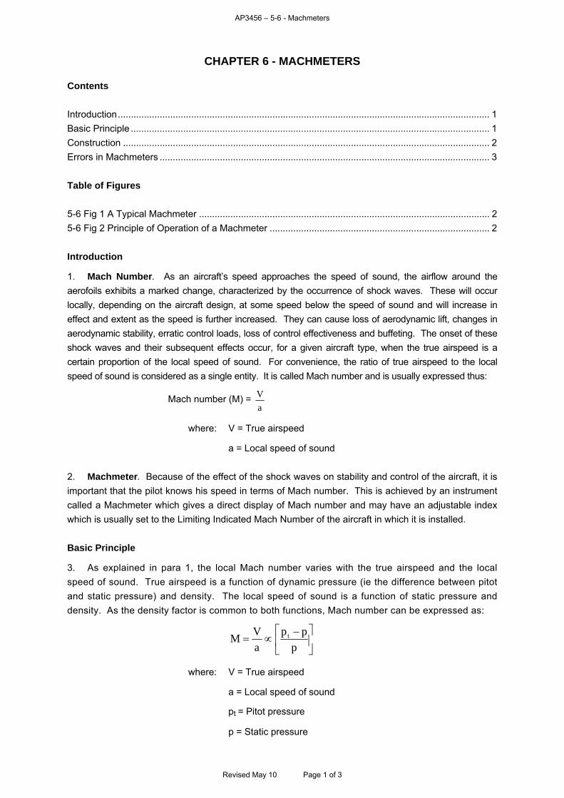
AP3456 – 5-6 - Machmeters
CHAPTER 6 - MACHMETERS Contents Introduction.............................................................................................................................................. 1 Basic Principle ......................................................................................................................................... 1 Construction ............................................................................................................................................ 2 Errors in Machmeters .............................................................................................................................. 3 Table of Figures 5-6 Fig 1 A Typical Machmeter ............................................................................................................... 2 5-6 Fig 2 Principle of Operation of a Machmeter .................................................................................... 2 Introduction
1. Mach Number. As an aircraft’s speed approaches the speed of sound, the airflow around the aerofoils exhibits a marked change, characterized by the occurrence of shock waves. These will occur locally, depending on the aircraft design, at some speed below the speed of sound and will increase in effect and extent as the speed is further increased. They can cause loss of aerodynamic lift, changes in aerodynamic stability, erratic control loads, loss of control effectiveness and buffeting. The onset of these shock waves and their subsequent effects occur, for a given aircraft type, when the true airspeed is a certain proportion of the local speed of sound. For convenience, the ratio of true airspeed to the local speed of sound is considered as a single entity. It is called Mach number and is usually expressed thus:
Mach number (M) = a
V
where: V = True airspeed
a = Local speed of sound 2. Machmeter. Because of the effect of the shock waves on stability and control of the aircraft, it is important that the pilot knows his speed in terms of Mach number. This is achieved by an instrument called a Machmeter which gives a direct display of Mach number and may have an adjustable index which is usually set to the Limiting Indicated Mach Number of the aircraft in which it is installed. Basic Principle
3. As explained in para 1, the local Mach number varies with the true airspeed and the local speed of sound. True airspeed is a function of dynamic pressure (ie the difference between pitot and static pressure) and density. The local speed of sound is a function of static pressure and density. As the density factor is common to both functions, Mach number can be expressed as:
p
pp
a
VM t
where: V = True airspeed
a = Local speed of sound
pt = Pitot pressure
p = Static pressure
Revised May 10 Page 1 of 3
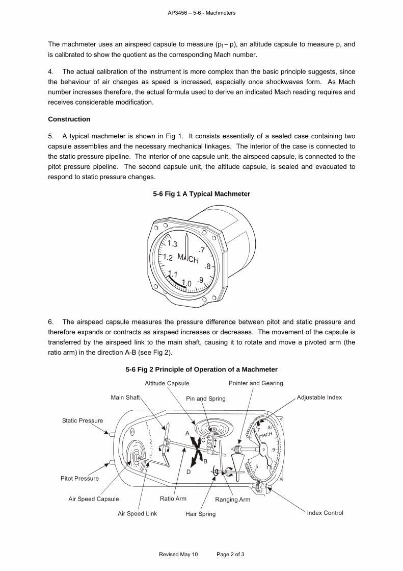
AP3456 – 5-6 - Machmeters
The machmeter uses an airspeed capsule to measure (pt – p), an altitude capsule to measure p, and is calibrated to show the quotient as the corresponding Mach number. 4. The actual calibration of the instrument is more complex than the basic principle suggests, since the behaviour of air changes as speed is increased, especially once shockwaves form. As Mach number increases therefore, the actual formula used to derive an indicated Mach reading requires and receives considerable modification. Construction 5. A typical machmeter is shown in Fig 1. It consists essentially of a sealed case containing two capsule assemblies and the necessary mechanical linkages. The interior of the case is connected to the static pressure pipeline. The interior of one capsule unit, the airspeed capsule, is connected to the pitot pressure pipeline. The second capsule unit, the altitude capsule, is sealed and evacuated to respond to static pressure changes.
5-6 Fig 1 A Typical Machmeter
6. The airspeed capsule measures the pressure difference between pitot and static pressure and therefore expands or contracts as airspeed increases or decreases. The movement of the capsule is transferred by the airspeed link to the main shaft, causing it to rotate and move a pivoted arm (the ratio arm) in the direction A-B (see Fig 2).
5-6 Fig 2 Principle of Operation of a Machmeter
Static Pressure
Main Shaft
Altitude Capsule
Pin and Spring
Pointer and Gearing
Adjustable Index
Index Control
Ranging Arm
Hair Spring
Ratio Arm
Air Speed Link
Air Speed Capsule
Pitot Pressure
A
D
B
C
.7 .8
.9
1.0.5
Revised May 10 Page 2 of 3

AP3456 – 5-6 - Machmeters
Revised May 10 Page 3 of 3
7. The altitude capsule responds to changes of static pressure, expanding or contracting with variation of altitude. The movement of the capsule is transferred to the ratio arm, via a spring and pin, causing it to move in the direction C-D. The pin is pointed at both ends and rests in cups on the altitude capsule and ratio arm (the spring providing the tension necessary to retain the pin in position). 8. The position of the ratio arm depends, therefore, upon both pitot excess and static pressures. Movement of the ratio arm controls the ranging arm which, through linkage and gearing, turns the pointer thus displaying the corresponding Mach number. An increase of altitude and/or airspeed results in a display of higher Mach number. 9. Critical or Limiting Mach Number is indicated by a specially shaped lubber mark located over the dial of the machmeter. It is adjustable so that the relevant Mach number for the particular type of aircraft in which the machmeter is installed may be preset. Presetting can be carried out by an adjusting screw on the front of the instrument. Errors in Machmeters 10. As Mach number is effectively a function of the ratio of pitot excess pressure to static pressure, only those errors in the measurement of this ratio will affect the machmeter. There are only two such errors; instrument error and pressure error. Variations in air density and temperature from the standard mean sea level values have no effect. 11. Instrument Error. Like all instruments, machmeters are subject to tolerances in manufacture which produce errors that vary from instrument to instrument. These are, however, small and are, typically, of the order of 0.01M over a range of 0.5 to 1.0M. 12. Pressure Error. The machmeter operates from the same pressure source as the airspeed indicator and is therefore subject to the same pressure errors. However, the effect of pressure error is relatively greater on the machmeter as the ratio of pitot excess pressure (pt – p) to static pressure (p) is being measured rather than just the pitot excess pressure (pt – p) in the case of the ASI.
AP3456 – 5-7 - Combined Speed Indicators
CHAPTER 7 - COMBINED SPEED INDICATORS Contents Introduction.............................................................................................................................................. 1 Principle................................................................................................................................................... 1 Description............................................................................................................................................... 1 Presentation ............................................................................................................................................ 2 Digital Mach/Air Speed Indicators ........................................................................................................... 3 Range and Accuracy ............................................................................................................................... 3 Table of Figures 5-7 Fig 1 Typical CSI Dial Presentations ................................................................................................ 3 5-7 Fig 2 Typical Digital Mach/Air Speed Indicator ................................................................................. 4 Introduction 1. With the increased complexity of aircraft instrument panels in modern aircraft and the continual search for more room in an already restricted space, it is becoming the practice to combine two or more functions into one instrument. One area where this has been successfully carried out is with speed indicating instruments. A combined instrument showing both indicated air speed and Mach number is now fitted in some aircraft. The instrument can take one of two forms; a simple capsule operated dial presentation or a capsule operated IAS dial with a synchro operated digital Mach number presentation. Principle 2. The construction of the dial-type combined speed indicator is very similar to the machmeter and the same principles are employed. Description 3. The combined speed indicator (CSI) contains an air speed capsule and an altitude capsule. The air speed capsule directly drives, through a normal type linkage, a pointer which is read against a dial calibrated in IAS. The altitude capsule, expanding or contracting, reacts to static pressure and thus altitude. This movement, through a second linkage, modifies a parallel drive from the air speed capsule in a similar manner to the machmeter. This second drive is used to position against the air speed pointer, a rotatable disc graduated in Mach number. The Mach number disc rotates anti-clockwise as altitude increases whilst the pointer rotates clockwise with increasing IAS. Thus, the pointer displays against the Mach number disc the correct Mach number for the particular air speed/altitude combination as well as the IAS against the fixed graduations on the dial. 4. Other functions are sometimes included in the CSI. These include:
a. A limit speed pointer.
b. Limit speed warning.
c. Outputs to control an auto-throttle system.
d. Undercarriage warning.
Revised May 10 Page 1 of 4
AP3456 – 5-7 - Combined Speed Indicators
5. Limit Speed Pointer. Most aircraft performance data list a speed, expressed in Mach number and sometimes the equivalent IAS, which should not be exceeded under normal operating conditions or a speed which should not be exceeded under any conditions. Sometimes there is a somewhat lower speed, usually expressed in knots of IAS, which must not be exceeded at low level. For example, an aircraft may have a limiting Mach number of 0.9M equivalent at sea level (and ISA conditions) to 594 kt, at 10,000 ft to 509 kt, at 20,000 ft to 425 kt, at 30,000 ft to 347 kt, etc. However, at low level it may be restricted to 490 kt. It is possible, by means of a special linkage designed to suit the particular aircraft and connected to the altitude capsule, to display this information on the CSI. This is usually achieved by means of a distinctively coloured pointer - red or chequered. This limit speed pointer is set on the ground to the particular relevant limit speed, in this case 490 kt. As the aircraft climbs, an overriding stop maintains the pointer at this reading until a condition exists where 490 knots is equivalent to 0.9M. From then on, the pointer moves anti-clockwise showing the IAS equivalent of 0.9M. During descent, the pointer will move clockwise until 490 kt is reached when the overriding stop again takes effect and the pointer remains at the maximum figure. At any time the pilot can assess his air speed in relation to his maximum permitted speed by the angle between the IAS pointer and the limit speed pointer. 6. Limit Speed Warning. In some CSIs a limit speed switch is incorporated which is closed when the IAS pointer reaches or exceeds the speed shown by the limit speed pointer. This switch operates either an audio or visual warning or both, to warn the pilot that he has reached his limit speed. 7. Auto-throttle Control. On aircraft where an auto-throttle system is installed, control of this facility may be achieved by a synchro system installed in the CSI. A moveable command pointer, manually set by a knob on the front of the instrument, positions the rotor of a synchro. The rotor of a second synchro is positioned by a low friction drive from the IAS pointer. When the IAS pointer reads the same as the command pointer, there is zero output from the pair of synchros. Any difference between the two pointers produces an error signal which is fed to the auto-throttle system adjusting the throttles so that the aircraft returns to the original selected speed. 8. Undercarriage Warning. An internal switch is fitted in some CSIs which will close at a pre-set figure in the aircraft approach speed range to provide a signal for a visual or audio warning if the undercarriage is not selected down. Presentation 9. A single pointer is read against a fixed IAS dial calibrated in knots and a rotatable disc (the Mach disc) calibrated in Mach number. The Mach disc is set behind and viewed through an aperture positioned either inside or outside the air speed scale. A second pointer, distinctively painted with diagonal lines or chequers, may be incorporated to show the limit speed (VMO) at all altitudes. On some models, two manually positioned bezel mounted lubber marks are available to indicate any desired air speed for reference purposes. A single command lubber positioned manually by a knob on the front of the instrument, allowing the auto-throttle reference speed to be set, may also be incorporated. Typical presentations are shown in Fig 1a and b.
Revised May 10 Page 2 of 4
AP3456 – 5-7 - Combined Speed Indicators
5-7 Fig 1 Typical CSI Dial Presentations
Fig 1a Mach Aperture Inside IAS Scale Fig 1b Mach Aperture Outside IAS Scale
68
10
12
1416
2025
30
35
40
5
6080
100
120
140160
180200
Ground
SETVMO
250300350
400
KNOTS
Digital Mach/Air Speed Indicators 10. A variation of the CSI is a model which shows IAS by a pointer indication and Mach number by a digital display. In this case, the instrument contains two capsules (air speed and altitude) as explained above but these are used only to drive the air speed pointer and a limit speed pointer, if fitted. A synchro drive proportional to Mach number is received from the aircraft's air data computer and a servo loop drives a three counter digital display. Limit speed warning and auto-throttle control can be incorporated as described in paras 6 and 7. 11. Presentation. An air speed pointer is read against a fixed scale and a second pointer, distinctively marked, may be incorporated to show limit speed at all altitudes. A servo driven three-drum counter provides a digital read out of Mach number to two or three places of decimals. A failure flag covers the counters in the event of power failure or loss of the Mach number synchro signal from the air data computer. Moveable index lubber marks may be incorporated in the same manner as for the dial presentation CSI and control of an auto-throttle reference lubber mark by a knob on the front of the instrument may also be included. A typical digital Mach/air speed indicator is shown in Fig 2. Range and Accuracy 12. The operating range of the CSI varies with the particular model but, typically, air speeds up to 800 kt and Mach number up to 2.5 can be covered. Typical instrument accuracies are 3 kt and 0.010M.
Revised May 10 Page 3 of 4

AP3456 – 5-7 - Combined Speed Indicators
Revised May 10 Page 4 of 4
5-7 Fig 2 Typical Digital Mach/Air Speed Indicator
6080
100
120
140160200
250
300
350
400
KNOTS
4 943
MACH
AP3456 – 5-8 - Outside Air Temperature Gauges
CHAPTER 8 – OUTSIDE AIR TEMPERATURE GAUGES Contents Introduction.............................................................................................................................................. 1 DIRECT READING THERMOMETERS.................................................................................................. 2 Mercury Type........................................................................................................................................... 2 Bi-metallic Element Type......................................................................................................................... 2 OAT Indicator .......................................................................................................................................... 3 Errors of Direct Reading Thermometers ................................................................................................. 3 TOTAL AIR TEMPERATURE PROBES.................................................................................................. 4 Total Air Temperature.............................................................................................................................. 4 General Principles ................................................................................................................................... 4 Total Head Thermometer ........................................................................................................................ 4 Rosemount Outside Air Temperature Probe........................................................................................... 5 THERMOMETER ERRORS.................................................................................................................... 6 General Errors ......................................................................................................................................... 6 OAT Thermometer Errors........................................................................................................................ 6 Table of Figures 5-8 Fig 1 Mercury Thermometer – Schematic......................................................................................... 2 5-8 Fig 2 Bi-metallic Thermometer - Schematic...................................................................................... 3 5-8 Fig 3 OAT Indicator ........................................................................................................................... 3 5-8 Fig 4 Total Head Thermometer ......................................................................................................... 5 5-8 Fig 5 Rosemount Probe - Outside View............................................................................................ 5 5-8 Fig 6 Rosemount Probe - Sectional View ......................................................................................... 6 Introduction 1. ..Temperature measurement and the basic principles of temperature sensing elements can be researched in other publications. 2. Thermometers installed in aircraft provide information on:
a. The outside air temperature (OAT), to enable true airspeed and height to be computed from indicated values.
b. The temperature of various compartments within the aircraft (eg bomb bays).
c. The operating temperatures of various engine components, lubricants, exhaust gases, etc. These sensors are covered fully in Volume 5, Chapter 26.
3. This chapter describes two categories of OAT thermometer - those that are direct reading, and those utilizing a 'total air temperature' probe.
Revised May 10 Page 1 of 7

AP3456 – 5-8 - Outside Air Temperature Gauges
DIRECT READING THERMOMETERS 4. Direct reading thermometers, used mainly in slow-speed aircraft, can be considered as single units, even though some of them include a remote indication facility. They are of fairly simple construction, and do not require a power supply. They employ sensing elements based on one of the following physical characteristics:
a. The expansion of mercury when heated.
b. The differential expansions of dissimilar metals, exploited in the use of bi-metallic sensing elements.
Mercury Type 5. The mercury thermometer consists of a steel bulb connected by capillary tubing to a Bourdon pressure gauge. This pressure gauge is linked to the pointer on the indicator gauge by a suitable linkage (Fig 1). (A Bourdon gauge utilizes a flattened tube, bent to a curve or spiral, which tends to straighten under internal pressure.) The mercury-filled bulb is situated in the airstream. An increase in temperature will cause the mercury to expand and flow via the capillary, to the Bourdon tube. The resulting movement of the Bourdon tube is transmitted to the pointer. A decrease in temperature will have the reverse effect.
5-8 Fig 1 Mercury Thermometer – Schematic
AircraftWall
DialBulbSensor
Capillary TubeBourdonTube
Fixed End
Moveable EndSectorGearing
PointerSun Shield
AirVents
6. To minimize errors due to variations in the temperature of components other than the bulb, the volumes of the capillary tube and the Bourdon tube are kept small relative to the volume of the bulb. To compensate for changes of temperature at the indicator, a bi-metallic strip, which reacts in opposition to the motion of the Bourdon tube, is incorporated between the free end of the Bourdon tube and the pointer spindle. Bi-metallic Element Type 7. Bi-metallic devices take advantage of the different rates of thermal expansion in different metals. The sensing element consists of two strips of dissimilar metals, welded together and formed into a helix (see Fig 2). The element is housed in a metal tube, and coils and uncoils as a result of variations in air temperature. One end of the helix is anchored to the tube, while the other end is free to rotate. The free end is attached, via a spindle, to a pointer that moves over the graduated temperature scale.
Revised May 10 Page 2 of 7
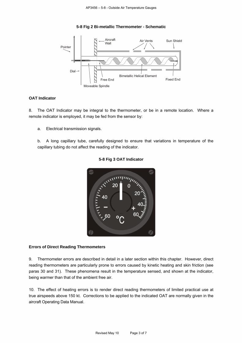
AP3456 – 5-8 - Outside Air Temperature Gauges
5-8 Fig 2 Bi-metallic Thermometer - Schematic
AircraftWall
DialBimetallic Helical Element
Free End
Moveable Spindle
Pointer
Fixed End
Sun ShieldAir Vents
OAT Indicator 8. The OAT Indicator may be integral to the thermometer, or be in a remote location. Where a remote indicator is employed, it may be fed from the sensor by:
a. Electrical transmission signals.
b. A long capillary tube, carefully designed to ensure that variations in temperature of the capillary tubing do not affect the reading of the indicator.
5-8 Fig 3 OAT Indicator
Errors of Direct Reading Thermometers 9. Thermometer errors are described in detail in a later section within this chapter. However, direct reading thermometers are particularly prone to errors caused by kinetic heating and skin friction (see paras 30 and 31). These phenomena result in the temperature sensed, and shown at the indicator, being warmer than that of the ambient free air. 10. The effect of heating errors is to render direct reading thermometers of limited practical use at true airspeeds above 150 kt. Corrections to be applied to the indicated OAT are normally given in the aircraft Operating Data Manual.
Revised May 10 Page 3 of 7
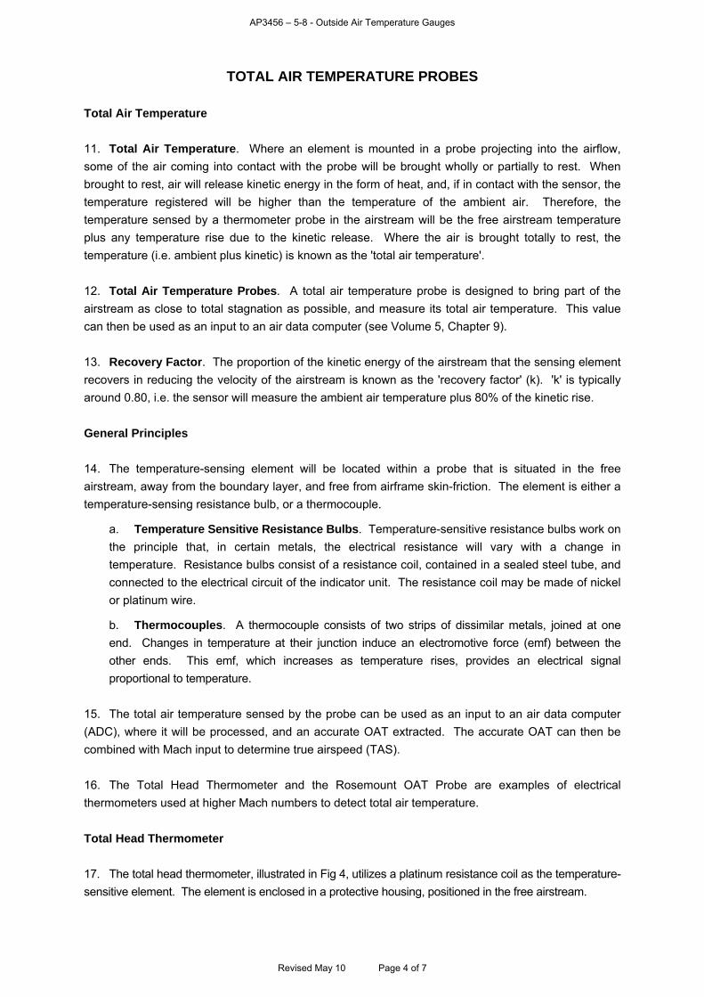
AP3456 – 5-8 - Outside Air Temperature Gauges
TOTAL AIR TEMPERATURE PROBES Total Air Temperature 11. Total Air Temperature. Where an element is mounted in a probe projecting into the airflow, some of the air coming into contact with the probe will be brought wholly or partially to rest. When brought to rest, air will release kinetic energy in the form of heat, and, if in contact with the sensor, the temperature registered will be higher than the temperature of the ambient air. Therefore, the temperature sensed by a thermometer probe in the airstream will be the free airstream temperature plus any temperature rise due to the kinetic release. Where the air is brought totally to rest, the temperature (i.e. ambient plus kinetic) is known as the 'total air temperature'. 12. Total Air Temperature Probes. A total air temperature probe is designed to bring part of the airstream as close to total stagnation as possible, and measure its total air temperature. This value can then be used as an input to an air data computer (see Volume 5, Chapter 9). 13. Recovery Factor. The proportion of the kinetic energy of the airstream that the sensing element recovers in reducing the velocity of the airstream is known as the 'recovery factor' (k). 'k' is typically around 0.80, i.e. the sensor will measure the ambient air temperature plus 80% of the kinetic rise. General Principles 14. The temperature-sensing element will be located within a probe that is situated in the free airstream, away from the boundary layer, and free from airframe skin-friction. The element is either a temperature-sensing resistance bulb, or a thermocouple.
a. Temperature Sensitive Resistance Bulbs. Temperature-sensitive resistance bulbs work on the principle that, in certain metals, the electrical resistance will vary with a change in temperature. Resistance bulbs consist of a resistance coil, contained in a sealed steel tube, and connected to the electrical circuit of the indicator unit. The resistance coil may be made of nickel or platinum wire.
b. Thermocouples. A thermocouple consists of two strips of dissimilar metals, joined at one end. Changes in temperature at their junction induce an electromotive force (emf) between the other ends. This emf, which increases as temperature rises, provides an electrical signal proportional to temperature.
15. The total air temperature sensed by the probe can be used as an input to an air data computer (ADC), where it will be processed, and an accurate OAT extracted. The accurate OAT can then be combined with Mach input to determine true airspeed (TAS). 16. The Total Head Thermometer and the Rosemount OAT Probe are examples of electrical thermometers used at higher Mach numbers to detect total air temperature. Total Head Thermometer 17. The total head thermometer, illustrated in Fig 4, utilizes a platinum resistance coil as the temperature-sensitive element. The element is enclosed in a protective housing, positioned in the free airstream.
Revised May 10 Page 4 of 7
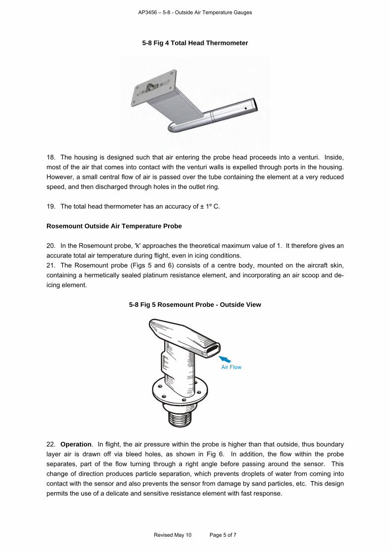
AP3456 – 5-8 - Outside Air Temperature Gauges
5-8 Fig 4 Total Head Thermometer
18. The housing is designed such that air entering the probe head proceeds into a venturi. Inside, most of the air that comes into contact with the venturi walls is expelled through ports in the housing. However, a small central flow of air is passed over the tube containing the element at a very reduced speed, and then discharged through holes in the outlet ring. 19. The total head thermometer has an accuracy of ± 1º C. Rosemount Outside Air Temperature Probe 20. In the Rosemount probe, 'k' approaches the theoretical maximum value of 1. It therefore gives an accurate total air temperature during flight, even in icing conditions. 21. The Rosemount probe (Figs 5 and 6) consists of a centre body, mounted on the aircraft skin, containing a hermetically sealed platinum resistance element, and incorporating an air scoop and de-icing element.
5-8 Fig 5 Rosemount Probe - Outside View
Air Flow
22. Operation. In flight, the air pressure within the probe is higher than that outside, thus boundary layer air is drawn off via bleed holes, as shown in Fig 6. In addition, the flow within the probe separates, part of the flow turning through a right angle before passing around the sensor. This change of direction produces particle separation, which prevents droplets of water from coming into contact with the sensor and also prevents the sensor from damage by sand particles, etc. This design permits the use of a delicate and sensitive resistance element with fast response.
Revised May 10 Page 5 of 7
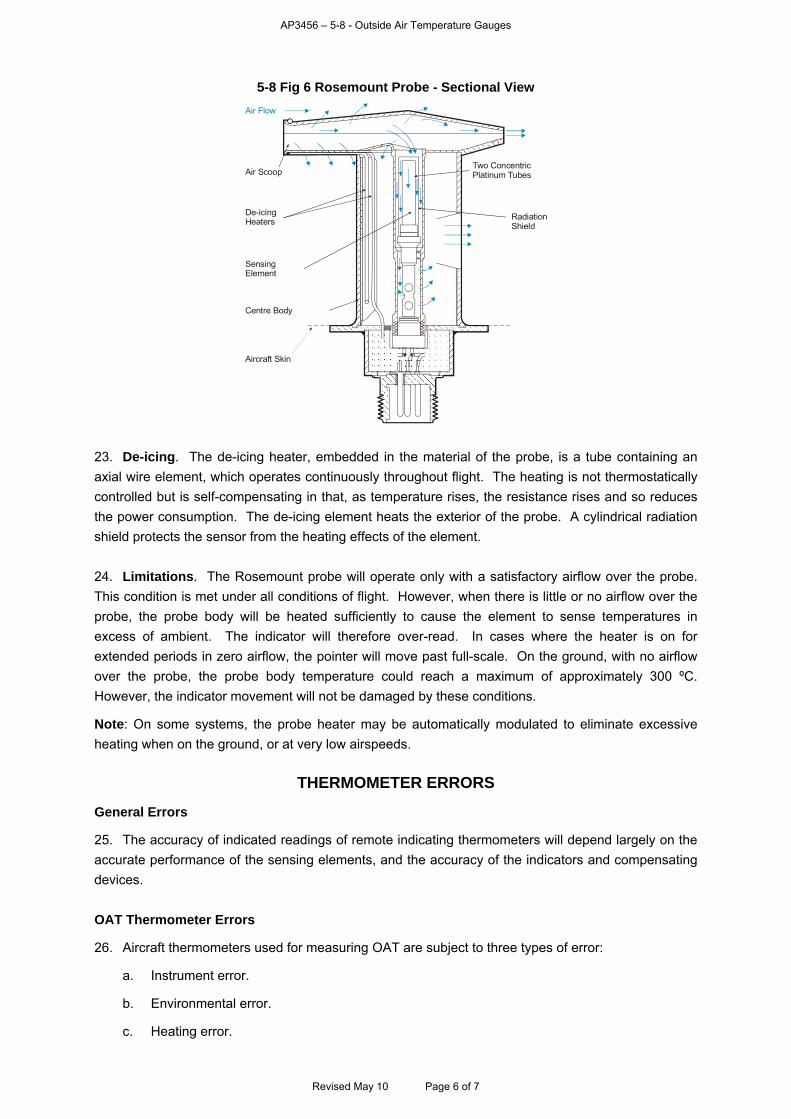
AP3456 – 5-8 - Outside Air Temperature Gauges
5-8 Fig 6 Rosemount Probe - Sectional View
Air Flow
Air ScoopTwo ConcentricPlatinum Tubes
RadiationShield
De-icingHeaters
SensingElement
Centre Body
Aircraft Skin
23. De-icing. The de-icing heater, embedded in the material of the probe, is a tube containing an axial wire element, which operates continuously throughout flight. The heating is not thermostatically controlled but is self-compensating in that, as temperature rises, the resistance rises and so reduces the power consumption. The de-icing element heats the exterior of the probe. A cylindrical radiation shield protects the sensor from the heating effects of the element. 24. Limitations. The Rosemount probe will operate only with a satisfactory airflow over the probe. This condition is met under all conditions of flight. However, when there is little or no airflow over the probe, the probe body will be heated sufficiently to cause the element to sense temperatures in excess of ambient. The indicator will therefore over-read. In cases where the heater is on for extended periods in zero airflow, the pointer will move past full-scale. On the ground, with no airflow over the probe, the probe body temperature could reach a maximum of approximately 300 ºC. However, the indicator movement will not be damaged by these conditions.
Note: On some systems, the probe heater may be automatically modulated to eliminate excessive heating when on the ground, or at very low airspeeds.
THERMOMETER ERRORS
General Errors
25. The accuracy of indicated readings of remote indicating thermometers will depend largely on the accurate performance of the sensing elements, and the accuracy of the indicators and compensating devices. OAT Thermometer Errors
26. Aircraft thermometers used for measuring OAT are subject to three types of error:
a. Instrument error.
b. Environmental error.
c. Heating error.
Revised May 10 Page 6 of 7
AP3456 – 5-8 - Outside Air Temperature Gauges
Revised May 10 Page 7 of 7
27. Instrument Error. Instrument error is caused by imperfections in manufacture or operation of the instrument. The errors are usually small, and may often be allowed for by calibrating the instrument and fitting a correction card to the aircraft. 28. Environmental Errors. Environmental errors such as solar heating or ice accretion can cause errors.
a. Solar Heating. Solar heating effects can be reduced by mounting a flat plate sensitive element beneath the wing or fuselage, or for a probe-mounted element, fitting it in a sun shield through which air is allowed to pass freely (see Fig 2).
b. Ice Accretion. Protection of the sensing element from ice accretion effects can be achieved by incorporating a heater. The sensing element is protected from the heater by a shield, as in the Rosemount probe (see Fig 6).
Residual errors due to environmental effects can not be calculated, therefore corrections can not be made for them. 29. Heating Errors. Heating errors in OAT thermometers are dependent upon the type of temperature-sensing element mounting. The types of mounting are:
a. Probes, protruding from the skin of the aircraft into the airflow.
b. Flat plates, let into the skin of the aircraft. 30. Probe Sensors. As described in para 11, where an element is mounted in a probe projecting into the airflow, some of the air coming into contact with that probe will be brought wholly or partially to rest, and will release kinetic energy in the form of heat. As a result, the temperature registered by the sensor will be in excess of the temperature of the ambient air. Assuming that pressure changes are adiabatic, the rise in temperature at the probe may be calculated from Bernoulli’s equation for compressible flow. Although the equation would assume a full value of adiabatic temperature rise, this is not realized in practice, since no energy exchange is perfect. A useful approximation of the formula for dealing with kinetic heating is:
2T
21 100
VTT
where:
T1 = Correct outside air temperature (ºC) T2 = Indicated outside air temperature (ºC) VT = TAS (kt)
31. Flat Plate Sensors. The flat plate sensor is unaffected by adiabatic heating, as it does not protrude into the airflow. However, the passage of air across a flat plate does heat it due to frictional effects. By coincidence, the heat rise approximates to that generated at a stagnation point probe due to adiabatic heating. For this reason, the same correction formulae are used for flat plate and stagnation point sensors.
AP3456 – 5-9 - Air Data Computer
CHAPTER 9 - AIR DATA COMPUTER Contents Introduction.............................................................................................................................................. 1 Probes ..................................................................................................................................................... 1 Transducers............................................................................................................................................. 2 Air Data Computer................................................................................................................................... 2 Figure 5-9 Fig 1 Air Data System ....................................................................................................................... 3 Introduction 1. Although conventional pressure instruments can provide satisfactory information for the crew, they have a number of limitations, especially in the context of modern aircraft systems. In particular, the information that an instrument measures can only be presented in one form and cannot easily be transmitted for use by other equipment, or to other crew positions, resulting in a need to duplicate the instrument. An Air Data System (ADS) overcomes these limitations. 2. An ADS can take a number of forms which will vary between aircraft types, however all systems are similar in principle and this chapter will describe a typical, rather than any specific, system. 3. The core of an ADS is an Air Data Computer (ADC) which forms an essential part of a modern flight/navigation/weapon aiming system. The ADS measures the basic air inputs of pitot pressure, static pressure, outside air temperature, angle of attack ( angle), sideslip ( angle), and outputs flight parameters for the various systems and displays. A comprehensive ADS thus consists of:
a. Pitot, static and temperature probes to measure the basic air data.
b. Local incidence vanes for angle and angle computation.
c. Transducers to convert the basic air data into electrical or electro-mechanical signals.
d. Air Data Computer to process the data and provide the required outputs to the aircraft systems and displays.
e. Power supplies to provide specific stabilized power for the ADS units. Probes 4. Pitot/Static. Pitot and static pressures are taken from the aircraft’s pressure head or the pitot head and static vents. 5. Temperature. Temperature is determined from outside air temperature (OAT) probes, as described in Volume 5, Chapter 8. 6. Angle of Attack ( Angle). Angle of attack is the angle, in the vertical plane of symmetry of the aircraft, at which the free stream airflow meets an arbitrary longitudinal datum line on the aircraft. It is generally measured by a small pivoted vane whose axis of rotation is nominally horizontal and
Revised May 10 Page 1 of 3

AP3456 – 5-9 - Air Data Computer
athwartships (see Volume 5, Chapter 23). The vane is usually mounted on the side of the fuselage near the nose or on a probe forward of the wing or nose. 7. Angle of Sideslip ( Angle). The sideslip angle is the angle in the horizontal plane at which the free stream airflow meets an arbitrary longitudinal datum line on the aircraft. The sensor is normally identical to the sensor and mounted on the underside of the airframe along the aircraft centre line. In simpler ADS the sensor is often omitted. Transducers 8. Transducers, which convert pressures, temperatures and angles to voltages or digital pulses, are the most vital elements of the air data systems, and are the limiting factors in the system accuracy. Transducers vary in type depending on the parameter which is to be measured, ie pressure transducers, temperature transducers and angular transducers. Various techniques are employed to convert the measured data into usable, repeatable and accurate signals which can be transmitted to the ADC, e.g. using the expansion of a diaphragm or capsule to actuate an electrical pick-off, or to vary the electrical resistance of a wire by changing the wire’s tension. Air Data Computer 9. The air data computer processes the data input from the sensors, applies any necessary corrections, and supplies output data in the form required by other equipment, either directly or via a central computer. Particularly in older systems, where there is no central computer, the same output parameter may be in several forms, e.g. pressure altitude may be processed as a voltage, a synchro output, and a digital code. Fig 1 shows a typical ADS arrangement. 10. Compared with conventional pressure instruments, the ADS has the following advantages:
a. The bulk and complexity of pipe work is avoided.
b. Duplication of units is avoided.
c. Errors can be automatically corrected before display.
d. There are accuracy and sensitivity gains.
e. There is a reduced time lag.
f. There is the potential for flexibility in presentation.
The disadvantage of the ADS is that it needs power to work whereas conventional pressure instruments do not. It is therefore usually necessary to provide back-up systems, either in the form of alternative power supplies or simple pressure instruments.
Revised May 10 Page 2 of 3
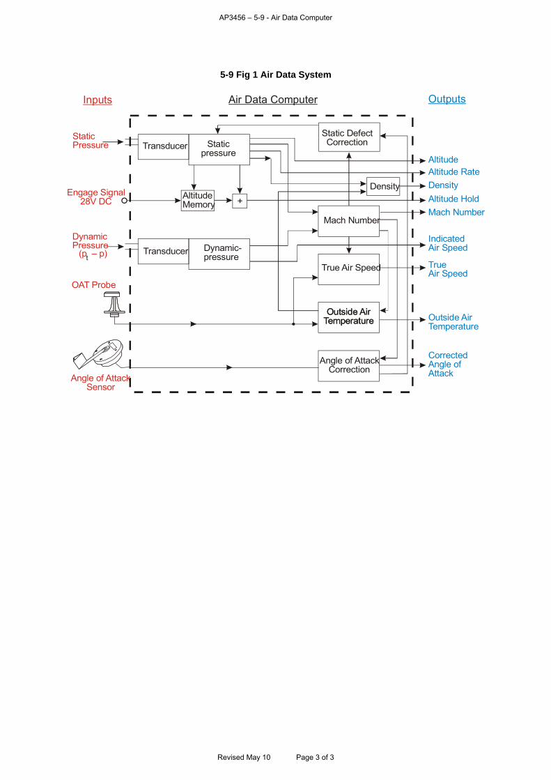
AP3456 – 5-9 - Air Data Computer
Revised May 10 Page 3 of 3
5-9 Fig 1 Air Data System
Inputs Air Data Computer Outputs
AltitudeAltitude RateDensityAltitude HoldMach Number
IndicatedAir Speed
True Air Speed
Outside AirTemperature
CorrectedAngle ofAttack
StaticPressure Transducer Static
pressure
Static DefectCorrection
Density
Mach Number
True Air Speed
Outside AirTemperature
Angle of AttackCorrection
AltitudeMemory +
Engage Signal28V DC
DynamicPressure
(p – p)tTransducer Dynamic-
pressure
OAT Probe
Angle of AttackSensor
Outside AirTemperature
AP3456 – 5-10 - Direct Indicating Compasses and Direction Indicators
CHAPTER 10 DIRECT INDICATING COMPASSES AND DIRECTION INDICATORS
Contents Introduction.............................................................................................................................................. 2 Horizontality............................................................................................................................................. 2 Sensitivity................................................................................................................................................. 3 Aperiodicity .............................................................................................................................................. 3 DICS - ERRORS AND LIMITATIONS..................................................................................................... 3 Turning and Acceleration Errors - Cause................................................................................................ 3 Turning and Acceleration Errors - Effect ................................................................................................. 4 Summary ................................................................................................................................................. 5 Minor Errors............................................................................................................................................. 5 Operational Limitations............................................................................................................................ 6 Advantages.............................................................................................................................................. 6 A PRACTICAL DICS ............................................................................................................................... 6 The E2 Series.......................................................................................................................................... 6 DIRECTION INDICATORS ..................................................................................................................... 7 Operation................................................................................................................................................. 7 Errors ....................................................................................................................................................... 8 Table of Figures 5-10 Fig 1 A Basic DICS ......................................................................................................................... 2 5-10 Fig 2 Pendulous Suspension .......................................................................................................... 2 5-10 Fig 3 Accelerating Force Producing Couple ................................................................................... 4 5-10 Fig 4 Acceleration Causing Tilt ....................................................................................................... 4 5-10 Fig 5 Couple Causing Turn ............................................................................................................. 5 5-10 Fig 6 E2 Compass........................................................................................................................... 6 5-10 Fig 7 E2 Compass - Exploded View ............................................................................................... 7 5-10 Fig 8 Direction Indicator Display ..................................................................................................... 8
Revised May 10 Page 1 of 8
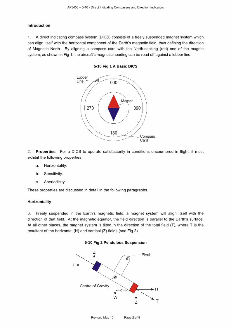
AP3456 – 5-10 - Direct Indicating Compasses and Direction Indicators
Introduction 1. A direct indicating compass system (DICS) consists of a freely suspended magnet system which can align itself with the horizontal component of the Earth’s magnetic field, thus defining the direction of Magnetic North. By aligning a compass card with the North-seeking (red) end of the magnet system, as shown in Fig 1, the aircraft’s magnetic heading can be read off against a lubber line.
5-10 Fig 1 A Basic DICS
Lubber Line
CompassCard
000
090
180
270Magnet
2. Properties. For a DICS to operate satisfactorily in conditions encountered in flight, it must exhibit the following properties:
a. Horizontality.
b. Sensitivity.
c. Aperiodicity.
These properties are discussed in detail in the following paragraphs. Horizontality 3. Freely suspended in the Earth’s magnetic field, a magnet system will align itself with the direction of that field. At the magnetic equator, the field direction is parallel to the Earth’s surface. At all other places, the magnet system is tilted in the direction of the total field (T), where T is the resultant of the horizontal (H) and vertical (Z) fields (see Fig 2).
5-10 Fig 2 Pendulous Suspension
d
Pivot
Centre of Gravity
H
Z
WZ
H
T
Revised May 10 Page 2 of 8
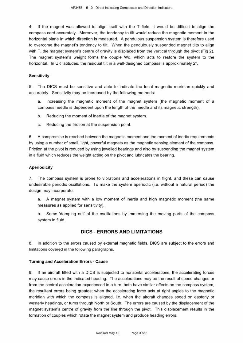
AP3456 – 5-10 - Direct Indicating Compasses and Direction Indicators
4. If the magnet was allowed to align itself with the T field, it would be difficult to align the compass card accurately. Moreover, the tendency to tilt would reduce the magnetic moment in the horizontal plane in which direction is measured. A pendulous suspension system is therefore used to overcome the magnet’s tendency to tilt. When the pendulously suspended magnet tilts to align with T, the magnet system’s centre of gravity is displaced from the vertical through the pivot (Fig 2). The magnet system’s weight forms the couple Wd, which acts to restore the system to the horizontal. In UK latitudes, the residual tilt in a well-designed compass is approximately 2º. Sensitivity 5. The DICS must be sensitive and able to indicate the local magnetic meridian quickly and accurately. Sensitivity may be increased by the following methods:
a. Increasing the magnetic moment of the magnet system (the magnetic moment of a compass needle is dependent upon the length of the needle and its magnetic strength).
b. Reducing the moment of inertia of the magnet system.
c. Reducing the friction at the suspension point. 6. A compromise is reached between the magnetic moment and the moment of inertia requirements by using a number of small, light, powerful magnets as the magnetic sensing element of the compass. Friction at the pivot is reduced by using jewelled bearings and also by suspending the magnet system in a fluid which reduces the weight acting on the pivot and lubricates the bearing. Aperiodicity 7. The compass system is prone to vibrations and accelerations in flight, and these can cause undesirable periodic oscillations. To make the system aperiodic (i.e. without a natural period) the design may incorporate:
a. A magnet system with a low moment of inertia and high magnetic moment (the same measures as applied for sensitivity).
b. Some 'damping out' of the oscillations by immersing the moving parts of the compass system in fluid.
DICS - ERRORS AND LIMITATIONS
8. In addition to the errors caused by external magnetic fields, DICS are subject to the errors and limitations covered in the following paragraphs. Turning and Acceleration Errors - Cause 9. If an aircraft fitted with a DICS is subjected to horizontal accelerations, the accelerating forces may cause errors in the indicated heading. The accelerations may be the result of speed changes or from the central acceleration experienced in a turn; both have similar effects on the compass system, the resultant errors being greatest when the accelerating force acts at right angles to the magnetic meridian with which the compass is aligned, i.e. when the aircraft changes speed on easterly or westerly headings, or turns through North or South. The errors are caused by the displacement of the magnet system’s centre of gravity from the line through the pivot. This displacement results in the formation of couples which rotate the magnet system and produce heading errors.
Revised May 10 Page 3 of 8
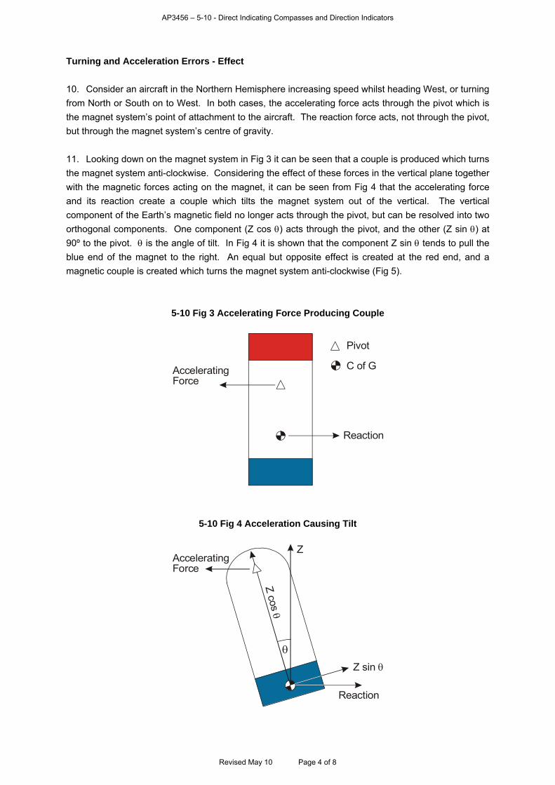
AP3456 – 5-10 - Direct Indicating Compasses and Direction Indicators
Turning and Acceleration Errors - Effect 10. Consider an aircraft in the Northern Hemisphere increasing speed whilst heading West, or turning from North or South on to West. In both cases, the accelerating force acts through the pivot which is the magnet system’s point of attachment to the aircraft. The reaction force acts, not through the pivot, but through the magnet system’s centre of gravity. 11. Looking down on the magnet system in Fig 3 it can be seen that a couple is produced which turns the magnet system anti-clockwise. Considering the effect of these forces in the vertical plane together with the magnetic forces acting on the magnet, it can be seen from Fig 4 that the accelerating force and its reaction create a couple which tilts the magnet system out of the vertical. The vertical component of the Earth’s magnetic field no longer acts through the pivot, but can be resolved into two orthogonal components. One component (Z cos ) acts through the pivot, and the other (Z sin ) at 90º to the pivot. is the angle of tilt. In Fig 4 it is shown that the component Z sin tends to pull the blue end of the magnet to the right. An equal but opposite effect is created at the red end, and a magnetic couple is created which turns the magnet system anti-clockwise (Fig 5).
5-10 Fig 3 Accelerating Force Producing Couple
Pivot
C of GAcceleratingForce
Reaction
5-10 Fig 4 Acceleration Causing Tilt
Z sin
Reaction
ZAcceleratingForce
Z cos
Revised May 10 Page 4 of 8
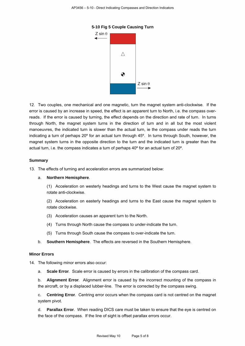
AP3456 – 5-10 - Direct Indicating Compasses and Direction Indicators
5-10 Fig 5 Couple Causing Turn
Z sin
Z sin
12. Two couples, one mechanical and one magnetic, turn the magnet system anti-clockwise. If the error is caused by an increase in speed, the effect is an apparent turn to North, i.e. the compass over-reads. If the error is caused by turning, the effect depends on the direction and rate of turn. In turns through North, the magnet system turns in the direction of turn and in all but the most violent manoeuvres, the indicated turn is slower than the actual turn, ie the compass under reads the turn indicating a turn of perhaps 20º for an actual turn through 45º. In turns through South, however, the magnet system turns in the opposite direction to the turn and the indicated turn is greater than the actual turn, i.e. the compass indicates a turn of perhaps 40º for an actual turn of 20º. Summary
13. The effects of turning and acceleration errors are summarized below:
a. Northern Hemisphere.
(1) Acceleration on westerly headings and turns to the West cause the magnet system to rotate anti-clockwise.
(2) Acceleration on easterly headings and turns to the East cause the magnet system to rotate clockwise.
(3) Acceleration causes an apparent turn to the North.
(4) Turns through North cause the compass to under-indicate the turn.
(5) Turns through South cause the compass to over-indicate the turn.
b. Southern Hemisphere. The effects are reversed in the Southern Hemisphere. Minor Errors
14. The following minor errors also occur:
a. Scale Error. Scale error is caused by errors in the calibration of the compass card.
b. Alignment Error. Alignment error is caused by the incorrect mounting of the compass in the aircraft, or by a displaced lubber-line. The error is corrected by the compass swing.
c. Centring Error. Centring error occurs when the compass card is not centred on the magnet system pivot.
d. Parallax Error. When reading DICS care must be taken to ensure that the eye is centred on the face of the compass. If the line of sight is offset parallax errors occur.
Revised May 10 Page 5 of 8
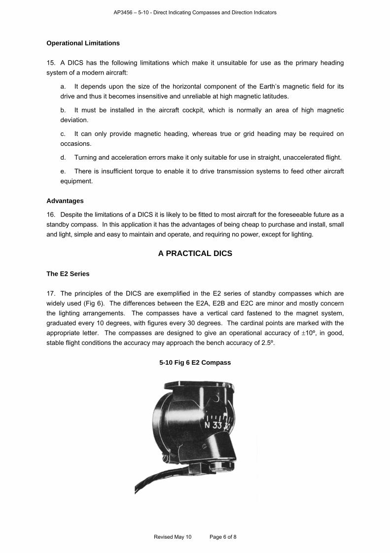
AP3456 – 5-10 - Direct Indicating Compasses and Direction Indicators
Operational Limitations 15. A DICS has the following limitations which make it unsuitable for use as the primary heading system of a modern aircraft:
a. It depends upon the size of the horizontal component of the Earth’s magnetic field for its drive and thus it becomes insensitive and unreliable at high magnetic latitudes.
b. It must be installed in the aircraft cockpit, which is normally an area of high magnetic deviation.
c. It can only provide magnetic heading, whereas true or grid heading may be required on occasions.
d. Turning and acceleration errors make it only suitable for use in straight, unaccelerated flight.
e. There is insufficient torque to enable it to drive transmission systems to feed other aircraft equipment.
Advantages
16. Despite the limitations of a DICS it is likely to be fitted to most aircraft for the foreseeable future as a standby compass. In this application it has the advantages of being cheap to purchase and install, small and light, simple and easy to maintain and operate, and requiring no power, except for lighting.
A PRACTICAL DICS The E2 Series 17. The principles of the DICS are exemplified in the E2 series of standby compasses which are widely used (Fig 6). The differences between the E2A, E2B and E2C are minor and mostly concern the lighting arrangements. The compasses have a vertical card fastened to the magnet system, graduated every 10 degrees, with figures every 30 degrees. The cardinal points are marked with the appropriate letter. The compasses are designed to give an operational accuracy of 10º, in good, stable flight conditions the accuracy may approach the bench accuracy of 2.5º.
5-10 Fig 6 E2 Compass
Revised May 10 Page 6 of 8
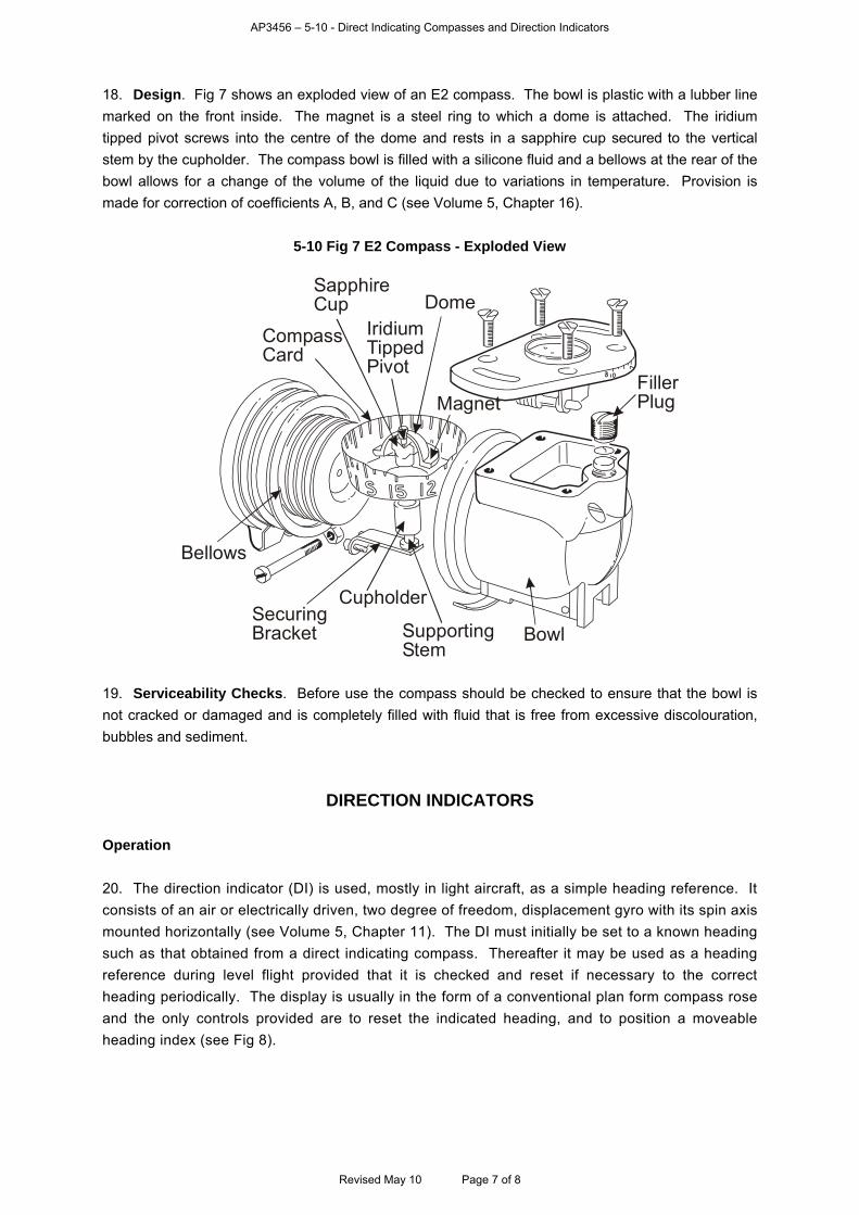
AP3456 – 5-10 - Direct Indicating Compasses and Direction Indicators
18. Design. Fig 7 shows an exploded view of an E2 compass. The bowl is plastic with a lubber line marked on the front inside. The magnet is a steel ring to which a dome is attached. The iridium tipped pivot screws into the centre of the dome and rests in a sapphire cup secured to the vertical stem by the cupholder. The compass bowl is filled with a silicone fluid and a bellows at the rear of the bowl allows for a change of the volume of the liquid due to variations in temperature. Provision is made for correction of coefficients A, B, and C (see Volume 5, Chapter 16).
5-10 Fig 7 E2 Compass - Exploded View
BowlSupportingStem
CupholderSecuringBracket
Bellows
CompassCard
SapphireCup
IridiumTippedPivot
Dome
MagnetFillerPlug
19. Serviceability Checks. Before use the compass should be checked to ensure that the bowl is not cracked or damaged and is completely filled with fluid that is free from excessive discolouration, bubbles and sediment.
DIRECTION INDICATORS Operation 20. The direction indicator (DI) is used, mostly in light aircraft, as a simple heading reference. It consists of an air or electrically driven, two degree of freedom, displacement gyro with its spin axis mounted horizontally (see Volume 5, Chapter 11). The DI must initially be set to a known heading such as that obtained from a direct indicating compass. Thereafter it may be used as a heading reference during level flight provided that it is checked and reset if necessary to the correct heading periodically. The display is usually in the form of a conventional plan form compass rose and the only controls provided are to reset the indicated heading, and to position a moveable heading index (see Fig 8).
Revised May 10 Page 7 of 8
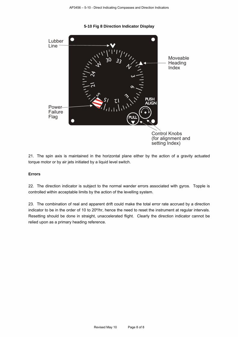
AP3456 – 5-10 - Direct Indicating Compasses and Direction Indicators
Revised May 10 Page 8 of 8
5-10 Fig 8 Direction Indicator Display
LubberLine
PowerFailureFlag
MoveableHeadingIndex
Control Knobs(for alignment andsetting Index)
21. The spin axis is maintained in the horizontal plane either by the action of a gravity actuated torque motor or by air jets initiated by a liquid level switch. Errors 22. The direction indicator is subject to the normal wander errors associated with gyros. Topple is controlled within acceptable limits by the action of the levelling system. 23. The combination of real and apparent drift could make the total error rate accrued by a direction indicator to be in the order of 10 to 20º/hr, hence the need to reset the instrument at regular intervals. Resetting should be done in straight, unaccelerated flight. Clearly the direction indicator cannot be relied upon as a primary heading reference.

AP3456 – 5-11 - Introduction to Gyroscopes
CHAPTER 11 - INTRODUCTION TO GYROSCOPES
Contents Page
Introduction.............................................................................................................................................. 2 Definition of Terms .................................................................................................................................. 4 Classification of Gyroscopes ................................................................................................................... 5 LAWS OF GYRODYNAMICS.................................................................................................................. 5 Rigidity in Space...................................................................................................................................... 5 The First Law of Gyrodynamics............................................................................................................... 5 Precession............................................................................................................................................... 6 The Second Law of Gyrodynamics ......................................................................................................... 6 Direction of Precession............................................................................................................................ 7 CONSERVATION OF ANGULAR MOMENTUM..................................................................................... 7 Explanation.............................................................................................................................................. 7 Cause of Precession ............................................................................................................................... 8 Gyroscopic Resistance............................................................................................................................ 8 Secondary Precession........................................................................................................................... 10 THE RATE GYROSCOPE..................................................................................................................... 11 Principle of Operation ............................................................................................................................ 11 THE RATE-INTEGRATING GYROSCOPE........................................................................................... 13 Principle of Operation ............................................................................................................................ 13 THE DISPLACEMENT GYROSCOPE.................................................................................................. 15 Definition................................................................................................................................................ 15 Wander .................................................................................................................................................. 15 Earth Rotation........................................................................................................................................ 16 Transport Wander.................................................................................................................................. 16 Apparent Wander Table ........................................................................................................................ 18 Practical Corrections for Topple and Drift ............................................................................................. 19 Gimbal Lock........................................................................................................................................... 21 Gimbal Error .......................................................................................................................................... 21 OTHER TYPES OF GYRO.................................................................................................................... 21 The Ring Laser Gyro ............................................................................................................................. 21 Fibre Optic Gyros .................................................................................................................................. 23 Vibrating Gyros...................................................................................................................................... 24
Revised Jul 10 Page 1 of 24
AP3456 – 5-11 - Introduction to Gyroscopes
Table of Figures
5-11 Fig 1 One-degree-of-freedom Gyroscope....................................................................................... 3 5-11 Fig 2 Two-degrees-of-freedom Gyroscope ..................................................................................... 3 5-11 Fig 3 Precession.............................................................................................................................. 6 5-11 Fig 4 Determining Precession ......................................................................................................... 7 5-11 Fig 5 Instant of Spin and Precession .............................................................................................. 9 5-11 Fig 6 Gyroscopic Resistance .......................................................................................................... 9 5-11 Fig 7 Precession Opposed by Secondary Precession.................................................................. 10 5-11 Fig 8 Gyro with One degree of Freedom – Precession................................................................. 11 5-11 Fig 9 Rate Gyroscope ................................................................................................................... 12 5-11 Fig 10 Rate of Turn Indicator ........................................................................................................ 12 5-11 Fig 11 Simple Rate-integrating Gyroscope ................................................................................... 13 5-11 Fig 12 Function of Rate-integrating Gyroscope ............................................................................ 14 5-11 Fig 13 Rate-integrating Azimuth Gyroscope ................................................................................. 14 5-11 Fig 14 Components of Earth Rate................................................................................................. 16 5-11 Fig 15 Apparent Drift ..................................................................................................................... 17 5-11 Fig 16 Transport Wander .............................................................................................................. 18 5-11 Fig 17 Gravity Sensitive Switch..................................................................................................... 20 5-11 Fig 18 Gravity Levelling................................................................................................................. 20 5-11 Fig 19 Synchro Case Levelling Device ......................................................................................... 20 5-11 Fig 20 Schematic Diagram of a Ring Laser Gyro ......................................................................... 21 5-11 Fig 21 Fibre Optic Gyro................................................................................................................. 23 5-11 Fig 22 The 'GyroChip' Vibrating Gyro ........................................................................................... 24
Tables
Table 1 Classification of Gyros................................................................................................................ 5 Table 2 Types of Wander ...................................................................................................................... 15 Table 3 Components of Drift and Topple – Earth Rate and Transport Wander Rate ........................... 19
Introduction
1. Modern technology has brought about many changes to the gyroscope. The conventional spinning
gyroscope is still in current use for flight instruments in smaller and simpler aircraft. More sophisticated
aircraft however, make use of devices which are termed 'gyros', but this is because of the tasks they
perform rather than their manner of operation. Gyroscopes can therefore be categorised as:
a. Spinning Gyroscopes.
b. Optical Gyroscopes.
c. Vibrating Gyroscopes.
This chapter will concentrate for the most part on the spinning gyroscope.
2. A conventional gyroscope consists of a symmetrical rotor spinning rapidly about its axis and free
to rotate about one or more perpendicular axis. Freedom of movement about one axis is usually
achieved by mounting the rotor in a gimbal, as in Fig 1 where the gyro is free to rotate about the YY1
axis. Complete freedom can be approached by using two gimbals, as illustrated in Fig 2.
Revised Jul 10 Page 2 of 24
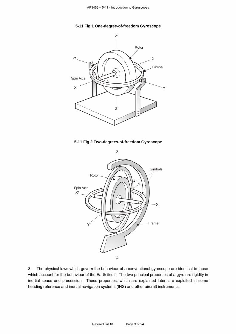
AP3456 – 5-11 - Introduction to Gyroscopes
5-11 Fig 1 One-degree-of-freedom Gyroscope
Rotor
X
Z
Z¹
X¹
Y¹
Y
Spin Axis
Gimbal
5-11 Fig 2 Two-degrees-of-freedom Gyroscope
Rotor
Frame
Z
Z¹
X¹
Y¹
YSpin Axis
X
Gimbals
3. The physical laws which govern the behaviour of a conventional gyroscope are identical to those
which account for the behaviour of the Earth itself. The two principal properties of a gyro are rigidity in
inertial space and precession. These properties, which are explained later, are exploited in some
heading reference and inertial navigation systems (INS) and other aircraft instruments.
Revised Jul 10 Page 3 of 24
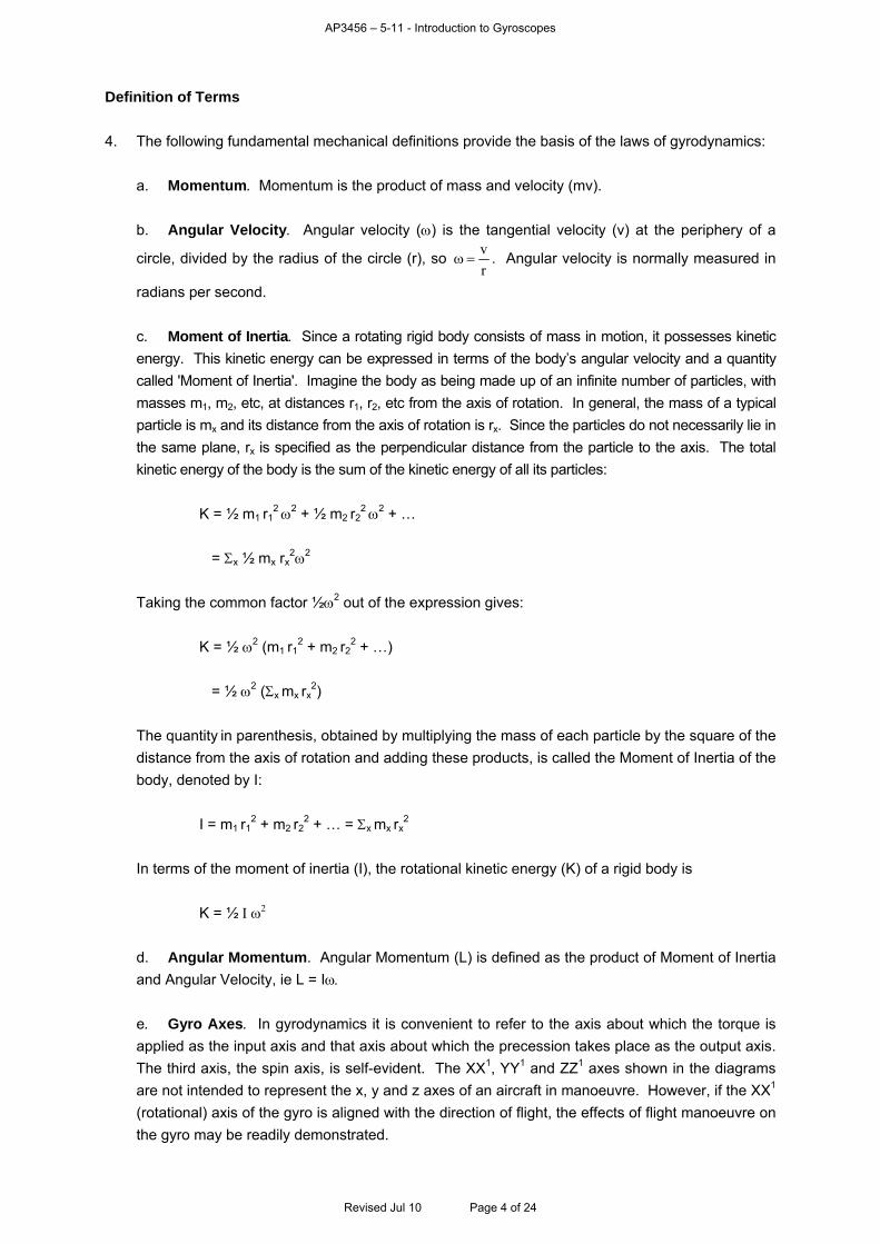
AP3456 – 5-11 - Introduction to Gyroscopes
Definition of Terms
4. The following fundamental mechanical definitions provide the basis of the laws of gyrodynamics:
a. Momentum. Momentum is the product of mass and velocity (mv).
b. Angular Velocity. Angular velocity () is the tangential velocity (v) at the periphery of a
circle, divided by the radius of the circle (r), so r
v . Angular velocity is normally measured in
radians per second.
c. Moment of Inertia. Since a rotating rigid body consists of mass in motion, it possesses kinetic
energy. This kinetic energy can be expressed in terms of the body’s angular velocity and a quantity
called 'Moment of Inertia'. Imagine the body as being made up of an infinite number of particles, with
masses m1, m2, etc, at distances r1, r2, etc from the axis of rotation. In general, the mass of a typical
particle is mx and its distance from the axis of rotation is rx. Since the particles do not necessarily lie in
the same plane, rx is specified as the perpendicular distance from the particle to the axis. The total
kinetic energy of the body is the sum of the kinetic energy of all its particles:
K = ½ m1 r12 2 + ½ m2 r2
2 2 + …
= x ½ mx rx22
Taking the common factor ½2 out of the expression gives:
K = ½ 2 (m1 r12 + m2 r2
2 + …)
= ½ 2 (x mx rx2)
The quantity in parenthesis, obtained by multiplying the mass of each particle by the square of the
distance from the axis of rotation and adding these products, is called the Moment of Inertia of the
body, denoted by I:
I = m1 r12 + m2 r2
2 + … = x mx rx2
In terms of the moment of inertia (I), the rotational kinetic energy (K) of a rigid body is
K = ½
d. Angular Momentum. Angular Momentum (L) is defined as the product of Moment of Inertia
and Angular Velocity, ie L = I
e. Gyro Axes. In gyrodynamics it is convenient to refer to the axis about which the torque is
applied as the input axis and that axis about which the precession takes place as the output axis.
The third axis, the spin axis, is self-evident. The XX1, YY1 and ZZ1 axes shown in the diagrams
are not intended to represent the x, y and z axes of an aircraft in manoeuvre. However, if the XX1
(rotational) axis of the gyro is aligned with the direction of flight, the effects of flight manoeuvre on
the gyro may be readily demonstrated.
Revised Jul 10 Page 4 of 24

AP3456 – 5-11 - Introduction to Gyroscopes
Classification of Gyroscopes
5. Conventional gyroscopes are classified in Table 1 in terms of the quantity they measure, namely:
a. Rate Gyroscopes. Rate gyroscopes measure the rate of angular displacement of a vehicle.
b. Rate-integrating Gyroscopes. Rate-integrating gyroscopes measure the integral of an
input with respect to time.
c. Displacement Gyroscopes. Displacement gyroscopes measure the angular displacement
from a known datum.
Table 1 Classification of Gyros
Type of Gyro Uses in Guidance and Control Gyro Characteristics Rate Gyroscope Aircraft Instruments Modified single-degree-of-freedom gyro.
Rate-integrating
Gyroscope Older IN Systems
Modified single-degree-of-freedom gyro.
Can also be a two-degree-of-freedom gyro.
Displacement
Gyroscope
Heading Reference
Older IN Systems
Aircraft Instruments
Two degrees of freedom.
Defines direction with respect to space, thus
it is also called a space gyro, or free gyro.
6. It should be realized, however, that the above classification is one of a number of ways in which
gyroscopes can be classified. Referring to Table 1, it will be seen that a displacement gyroscope
could be classified as a two-degrees-of-freedom gyro or a space gyro. Note also that the classification
of Table 1 does not consider the spin axis of a gyroscope as a degree of freedom. In this chapter, a
degree of freedom is defined as the ability to measure rotation about a chosen axis.
LAWS OF GYRODYNAMICS
Rigidity in Space
7. If the rotor of a perfect displacement gyroscope is spinning at constant angular velocity, and
therefore constant angular momentum, no matter how the frame is turned, no torque is transmitted to
the spin axis. The law of conservation of angular momentum states that the angular momentum of a
body is unchanged unless a torque is applied to that body. It follows from this that the angular
momentum of the rotor must remain constant in magnitude and direction. This is simply another way
of saying that the spin axis continues to point in the same direction in inertial space. This property of a
gyro is defined in the First Law of Gyrodynamics.
The First Law of Gyrodynamics
8. The first law of gyrodynamics states that:
"If a rotating body is so mounted as to be completely free to move about any axis through the centre of
mass, then its spin axis remains fixed in inertial space however much the frame may be displaced."
9. A space gyroscope loses its property of rigidity in space if the spin axis is subjected to random
torques, some causes of which will be examined later.
Revised Jul 10 Page 5 of 24
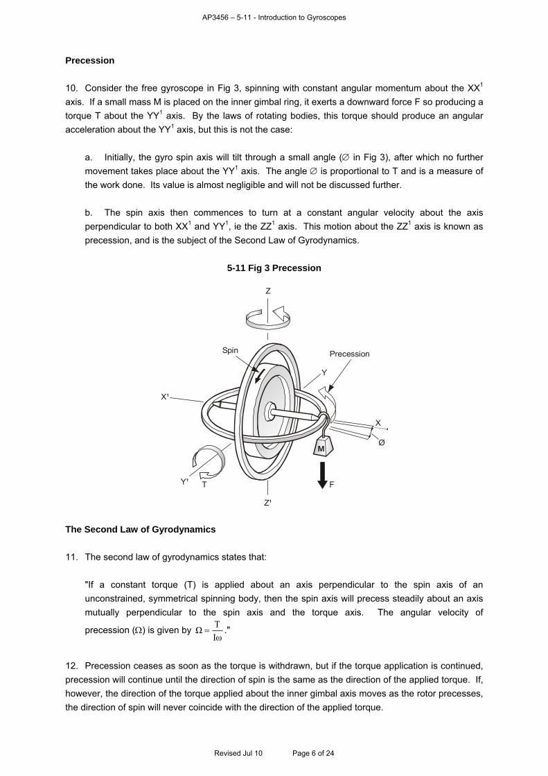
AP3456 – 5-11 - Introduction to Gyroscopes
Precession
10. Consider the free gyroscope in Fig 3, spinning with constant angular momentum about the XX1
axis. If a small mass M is placed on the inner gimbal ring, it exerts a downward force F so producing a
torque T about the YY1 axis. By the laws of rotating bodies, this torque should produce an angular
acceleration about the YY1 axis, but this is not the case:
a. Initially, the gyro spin axis will tilt through a small angle ( in Fig 3), after which no further
movement takes place about the YY1 axis. The angle is proportional to T and is a measure of
the work done. Its value is almost negligible and will not be discussed further.
b. The spin axis then commences to turn at a constant angular velocity about the axis
perpendicular to both XX1 and YY1, ie the ZZ1 axis. This motion about the ZZ1 axis is known as
precession, and is the subject of the Second Law of Gyrodynamics.
5-11 Fig 3 Precession
Spin Precession
Z¹
Z
X¹
T FY¹
Y
X
ØM
The Second Law of Gyrodynamics
11. The second law of gyrodynamics states that:
"If a constant torque (T) is applied about an axis perpendicular to the spin axis of an
unconstrained, symmetrical spinning body, then the spin axis will precess steadily about an axis
mutually perpendicular to the spin axis and the torque axis. The angular velocity of
precession () is given by ωI
TΩ ."
12. Precession ceases as soon as the torque is withdrawn, but if the torque application is continued,
precession will continue until the direction of spin is the same as the direction of the applied torque. If,
however, the direction of the torque applied about the inner gimbal axis moves as the rotor precesses,
the direction of spin will never coincide with the direction of the applied torque.
Revised Jul 10 Page 6 of 24
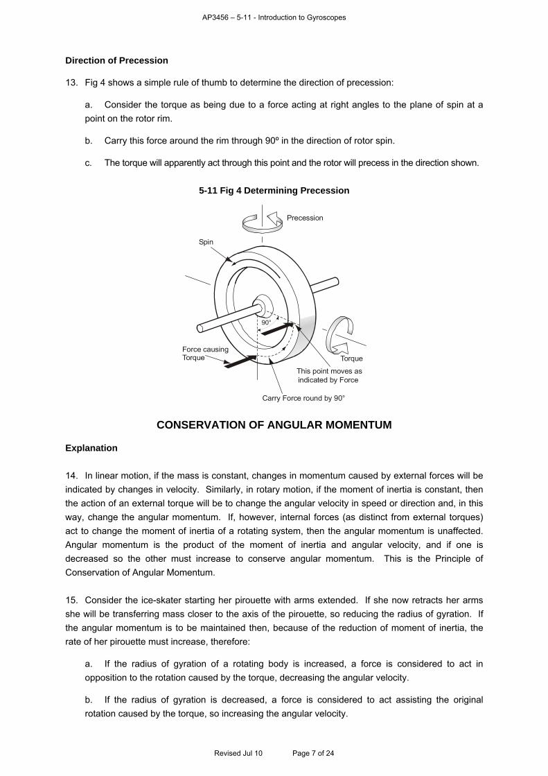
AP3456 – 5-11 - Introduction to Gyroscopes
Direction of Precession
13. Fig 4 shows a simple rule of thumb to determine the direction of precession:
a. Consider the torque as being due to a force acting at right angles to the plane of spin at a
point on the rotor rim.
b. Carry this force around the rim through 90º in the direction of rotor spin.
c. The torque will apparently act through this point and the rotor will precess in the direction shown.
5-11 Fig 4 Determining Precession
Spin
Precession
TorqueForce causingTorque
90°
Carry Force round by 90°
This point moves asindicated by Force
CONSERVATION OF ANGULAR MOMENTUM
Explanation
14. In linear motion, if the mass is constant, changes in momentum caused by external forces will be
indicated by changes in velocity. Similarly, in rotary motion, if the moment of inertia is constant, then
the action of an external torque will be to change the angular velocity in speed or direction and, in this
way, change the angular momentum. If, however, internal forces (as distinct from external torques)
act to change the moment of inertia of a rotating system, then the angular momentum is unaffected.
Angular momentum is the product of the moment of inertia and angular velocity, and if one is
decreased so the other must increase to conserve angular momentum. This is the Principle of
Conservation of Angular Momentum.
15. Consider the ice-skater starting her pirouette with arms extended. If she now retracts her arms
she will be transferring mass closer to the axis of the pirouette, so reducing the radius of gyration. If
the angular momentum is to be maintained then, because of the reduction of moment of inertia, the
rate of her pirouette must increase, therefore:
a. If the radius of gyration of a rotating body is increased, a force is considered to act in
opposition to the rotation caused by the torque, decreasing the angular velocity.
b. If the radius of gyration is decreased, a force is considered to act assisting the original
rotation caused by the torque, so increasing the angular velocity.
Revised Jul 10 Page 7 of 24
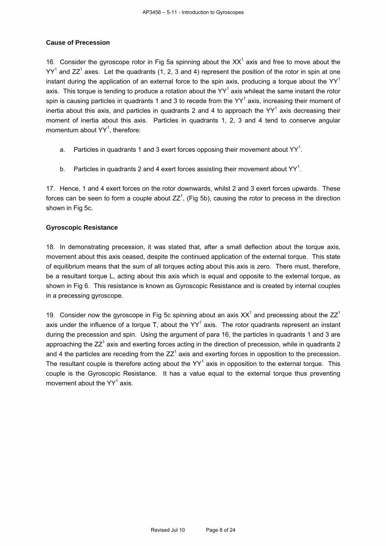
AP3456 – 5-11 - Introduction to Gyroscopes
Cause of Precession
16. Consider the gyroscope rotor in Fig 5a spinning about the XX1 axis and free to move about the
YY1 and ZZ1 axes. Let the quadrants (1, 2, 3 and 4) represent the position of the rotor in spin at one
instant during the application of an external force to the spin axis, producing a torque about the YY1
axis. This torque is tending to produce a rotation about the YY1 axis whileat the same instant the rotor
spin is causing particles in quadrants 1 and 3 to recede from the YY1 axis, increasing their moment of
inertia about this axis, and particles in quadrants 2 and 4 to approach the YY1 axis decreasing their
moment of inertia about this axis. Particles in quadrants 1, 2, 3 and 4 tend to conserve angular
momentum about YY1, therefore:
a. Particles in quadrants 1 and 3 exert forces opposing their movement about YY1.
b. Particles in quadrants 2 and 4 exert forces assisting their movement about YY1.
17. Hence, 1 and 4 exert forces on the rotor downwards, whilst 2 and 3 exert forces upwards. These
forces can be seen to form a couple about ZZ1, (Fig 5b), causing the rotor to precess in the direction
shown in Fig 5c.
Gyroscopic Resistance
18. In demonstrating precession, it was stated that, after a small deflection about the torque axis,
movement about this axis ceased, despite the continued application of the external torque. This state
of equilibrium means that the sum of all torques acting about this axis is zero. There must, therefore,
be a resultant torque L, acting about this axis which is equal and opposite to the external torque, as
shown in Fig 6. This resistance is known as Gyroscopic Resistance and is created by internal couples
in a precessing gyroscope.
19. Consider now the gyroscope in Fig 5c spinning about an axis XX1 and precessing about the ZZ1
axis under the influence of a torque T, about the YY1 axis. The rotor quadrants represent an instant
during the precession and spin. Using the argument of para 16, the particles in quadrants 1 and 3 are
approaching the ZZ1 axis and exerting forces acting in the direction of precession, while in quadrants 2
and 4 the particles are receding from the ZZ1 axis and exerting forces in opposition to the precession.
The resultant couple is therefore acting about the YY1 axis in opposition to the external torque. This
couple is the Gyroscopic Resistance. It has a value equal to the external torque thus preventing
movement about the YY1 axis.
Revised Jul 10 Page 8 of 24
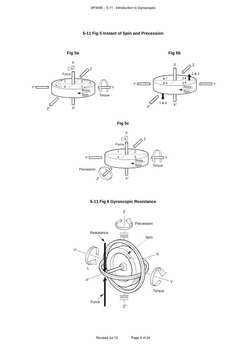
AP3456 – 5-11 - Introduction to Gyroscopes
5-11 Fig 5 Instant of Spin and Precession
Fig 5a Fig 5b
Torque
X
X¹
Force
RotorSpin
YY¹
2
34
1
Z¹
Z
X
X¹
RotorSpin
YY¹
22 & 3
1 & 4
34
1
Z¹
Z
Fig 5c
Torque
X
X¹
Force
Precession
RotorSpin
YY¹
2
34
1
Z
Z¹
5-11 Fig 6 Gyroscopic Resistance
Spin
Torque
Precession
Resistance
X
Z
Z¹
X¹
Y¹
Y
L
Force
Revised Jul 10 Page 9 of 24
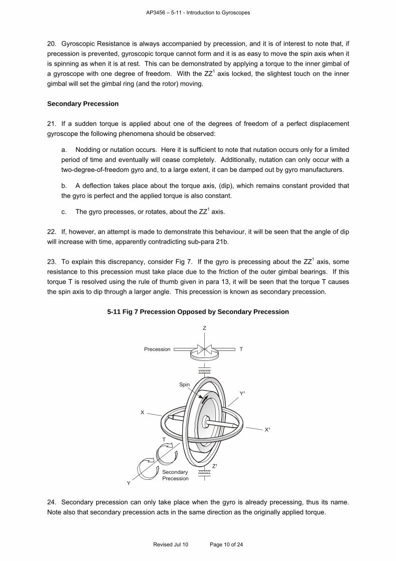
AP3456 – 5-11 - Introduction to Gyroscopes
20. Gyroscopic Resistance is always accompanied by precession, and it is of interest to note that, if
precession is prevented, gyroscopic torque cannot form and it is as easy to move the spin axis when it
is spinning as when it is at rest. This can be demonstrated by applying a torque to the inner gimbal of
a gyroscope with one degree of freedom. With the ZZ1 axis locked, the slightest touch on the inner
gimbal will set the gimbal ring (and the rotor) moving.
Secondary Precession
21. If a sudden torque is applied about one of the degrees of freedom of a perfect displacement
gyroscope the following phenomena should be observed:
a. Nodding or nutation occurs. Here it is sufficient to note that nutation occurs only for a limited
period of time and eventually will cease completely. Additionally, nutation can only occur with a
two-degree-of-freedom gyro and, to a large extent, it can be damped out by gyro manufacturers.
b. A deflection takes place about the torque axis, (dip), which remains constant provided that
the gyro is perfect and the applied torque is also constant.
c. The gyro precesses, or rotates, about the ZZ1 axis.
22. If, however, an attempt is made to demonstrate this behaviour, it will be seen that the angle of dip
will increase with time, apparently contradicting sub-para 21b.
23. To explain this discrepancy, consider Fig 7. If the gyro is precessing about the ZZ1 axis, some
resistance to this precession must take place due to the friction of the outer gimbal bearings. If this
torque T is resolved using the rule of thumb given in para 13, it will be seen that the torque T causes
the spin axis to dip through a larger angle. This precession is known as secondary precession.
5-11 Fig 7 Precession Opposed by Secondary Precession
Spin
SecondaryPrecession
Precession T
T
Z¹
Z
X¹
Y¹
Y
X
24. Secondary precession can only take place when the gyro is already precessing, thus its name.
Note also that secondary precession acts in the same direction as the originally applied torque.
Revised Jul 10 Page 10 of 24
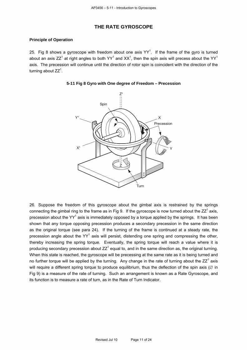
AP3456 – 5-11 - Introduction to Gyroscopes
THE RATE GYROSCOPE
Principle of Operation
25. Fig 8 shows a gyroscope with freedom about one axis YY1. If the frame of the gyro is turned
about an axis ZZ1 at right angles to both YY1 and XX1, then the spin axis will precess about the YY1
axis. The precession will continue until the direction of rotor spin is coincident with the direction of the
turning about ZZ1.
5-11 Fig 8 Gyro with One degree of Freedom – Precession
Precession
Spin
X
Z
Z¹
X¹
Y¹
Y
Turn
26. Suppose the freedom of this gyroscope about the gimbal axis is restrained by the springs
connecting the gimbal ring to the frame as in Fig 9. If the gyroscope is now turned about the ZZ1 axis,
precession about the YY1 axis is immediately opposed by a torque applied by the springs. It has been
shown that any torque opposing precession produces a secondary precession in the same direction
as the original torque (see para 24). If the turning of the frame is continued at a steady rate, the
precession angle about the YY1 axis will persist, distending one spring and compressing the other,
thereby increasing the spring torque. Eventually, the spring torque will reach a value where it is
producing secondary precession about ZZ1 equal to, and in the same direction as, the original turning.
When this state is reached, the gyroscope will be precessing at the same rate as it is being turned and
no further torque will be applied by the turning. Any change in the rate of turning about the ZZ1 axis
will require a different spring torque to produce equilibrium, thus the deflection of the spin axis ( in
Fig 9) is a measure of the rate of turning. Such an arrangement is known as a Rate Gyroscope, and
its function is to measure a rate of turn, as in the Rate of Turn Indicator.
Revised Jul 10 Page 11 of 24
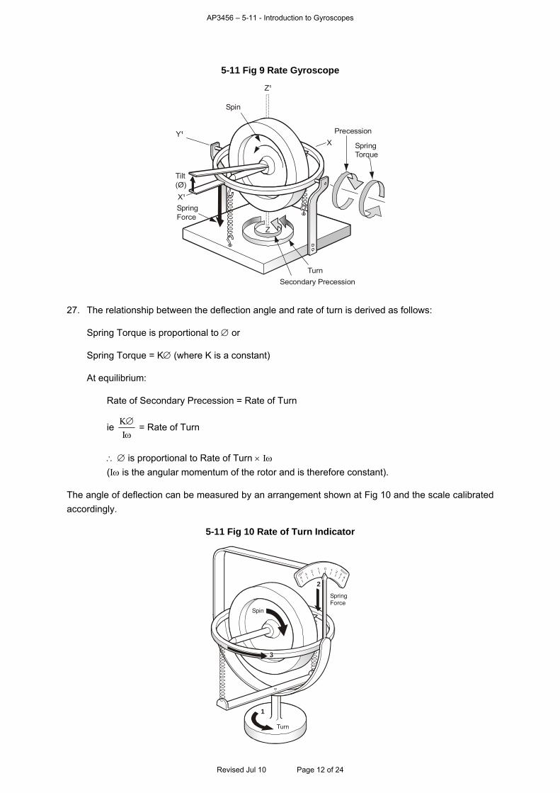
AP3456 – 5-11 - Introduction to Gyroscopes
5-11 Fig 9 Rate Gyroscope
Precession
SpringTorque
Spin
X
Z
Z¹
X¹
Y¹
Turn
SpringForce
Tilt(Ø)
Secondary Precession
27. The relationship between the deflection angle and rate of turn is derived as follows:
Spring Torque is proportional to or
Spring Torque = K (where K is a constant)
At equilibrium:
Rate of Secondary Precession = Rate of Turn
ie
I
K = Rate of Turn
is proportional to Rate of Turn I
(I is the angular momentum of the rotor and is therefore constant).
The angle of deflection can be measured by an arrangement shown at Fig 10 and the scale calibrated
accordingly.
5-11 Fig 10 Rate of Turn Indicator
Spin
1
SpringForce
24
LEFTRIGHT3
21 0 1 2
34
Turn
3
Revised Jul 10 Page 12 of 24
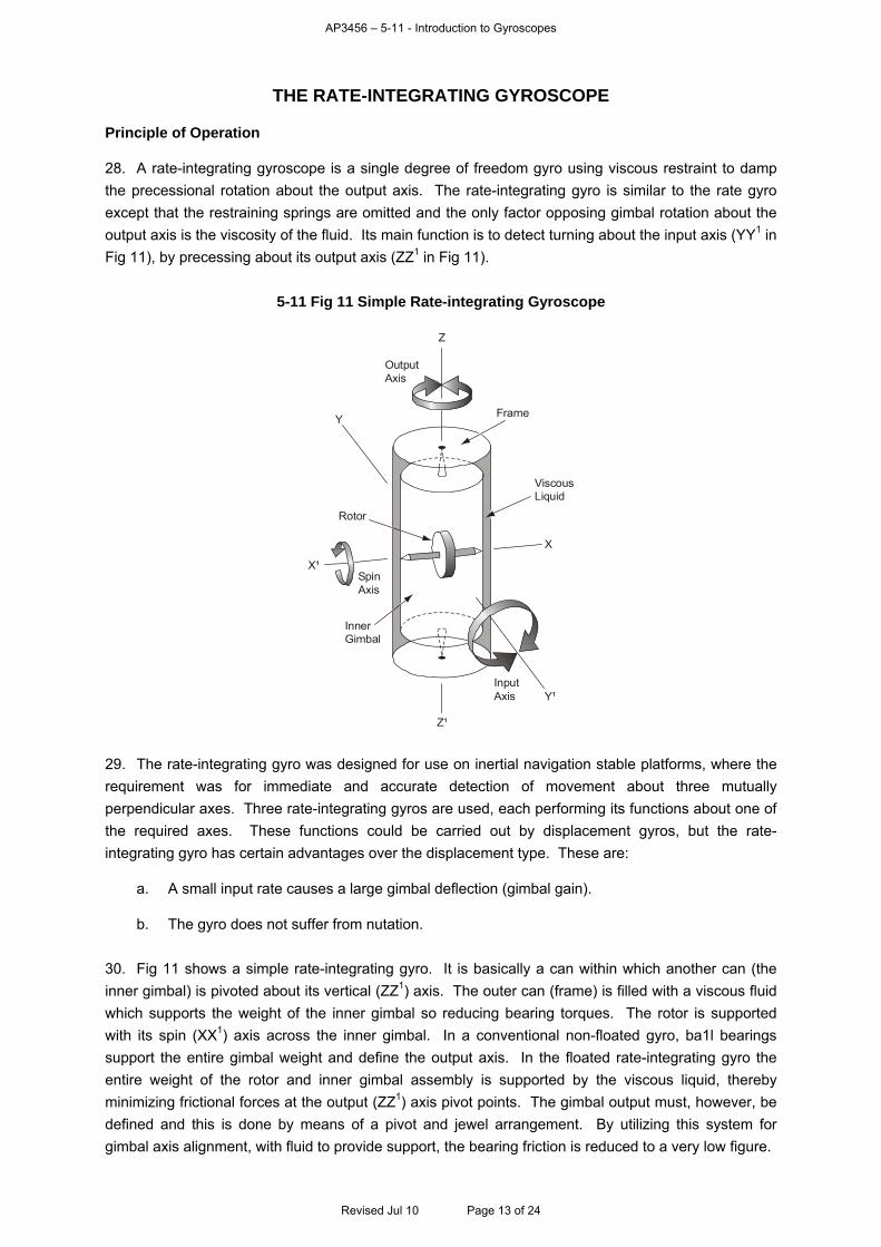
AP3456 – 5-11 - Introduction to Gyroscopes
THE RATE-INTEGRATING GYROSCOPE
Principle of Operation
28. A rate-integrating gyroscope is a single degree of freedom gyro using viscous restraint to damp
the precessional rotation about the output axis. The rate-integrating gyro is similar to the rate gyro
except that the restraining springs are omitted and the only factor opposing gimbal rotation about the
output axis is the viscosity of the fluid. Its main function is to detect turning about the input axis (YY1 in
Fig 11), by precessing about its output axis (ZZ1 in Fig 11).
5-11 Fig 11 Simple Rate-integrating Gyroscope
Y
X
Rotor
SpinAxis
InnerGimbal
InputAxis
Viscous Liquid
Frame
OutputAxis
Z
Z¹
Y¹
X¹
29. The rate-integrating gyro was designed for use on inertial navigation stable platforms, where the
requirement was for immediate and accurate detection of movement about three mutually
perpendicular axes. Three rate-integrating gyros are used, each performing its functions about one of
the required axes. These functions could be carried out by displacement gyros, but the rate-
integrating gyro has certain advantages over the displacement type. These are:
a. A small input rate causes a large gimbal deflection (gimbal gain).
b. The gyro does not suffer from nutation.
30. Fig 11 shows a simple rate-integrating gyro. It is basically a can within which another can (the
inner gimbal) is pivoted about its vertical (ZZ1) axis. The outer can (frame) is filled with a viscous fluid
which supports the weight of the inner gimbal so reducing bearing torques. The rotor is supported
with its spin (XX1) axis across the inner gimbal. In a conventional non-floated gyro, ba1l bearings
support the entire gimbal weight and define the output axis. In the floated rate-integrating gyro the
entire weight of the rotor and inner gimbal assembly is supported by the viscous liquid, thereby
minimizing frictional forces at the output (ZZ1) axis pivot points. The gimbal output must, however, be
defined and this is done by means of a pivot and jewel arrangement. By utilizing this system for
gimbal axis alignment, with fluid to provide support, the bearing friction is reduced to a very low figure.
Revised Jul 10 Page 13 of 24
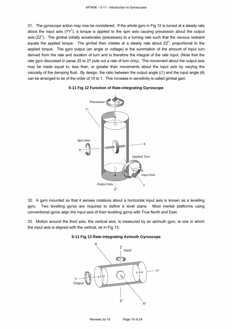
AP3456 – 5-11 - Introduction to Gyroscopes
31. The gyroscope action may now be considered. If the whole gyro in Fig 12 is turned at a steady rate
about the input axis (YY1), a torque is applied to the spin axis causing precession about the output
axis (ZZ1). The gimbal initially accelerates (precesses) to a turning rate such that the viscous restraint
equals the applied torque. The gimbal then rotates at a steady rate about ZZ1, proportional to the
applied torque. The gyro output (an angle or voltage) is the summation of the amount of input turn
derived from the rate and duration of turn and is therefore the integral of the rate input. (Note that the
rate gyro discussed in paras 25 to 27 puts out a rate of turn only). The movement about the output axis
may be made equal to, less than, or greater than movements about the input axis by varying the
viscosity of the damping fluid. By design, the ratio between the output angle () and the input angle (θ)
can be arranged to be of the order of 10 to 1. This increase in sensitivity is called gimbal gain.
5-11 Fig 12 Function of Rate-integrating Gyroscope
Y¹
Y
XSpin Axis
Input Axis
Precession
Output Axis
Applied Turn
0
X¹
Z¹
32. A gyro mounted so that it senses rotations about a horizontal input axis is known as a levelling
gyro. Two levelling gyros are required to define a level plane. Most inertial platforms using
conventional gyros align the input axis of their levelling gyros with True North and East.
33. Motion around the third axis, the vertical axis, is measured by an azimuth gyro, ie one in which
the input axis is aligned with the vertical, as in Fig 13.
5-11 Fig 13 Rate-integrating Azimuth Gyroscope
Y
ZX
Output
Input
Z¹X¹
Y¹
Revised Jul 10 Page 14 of 24
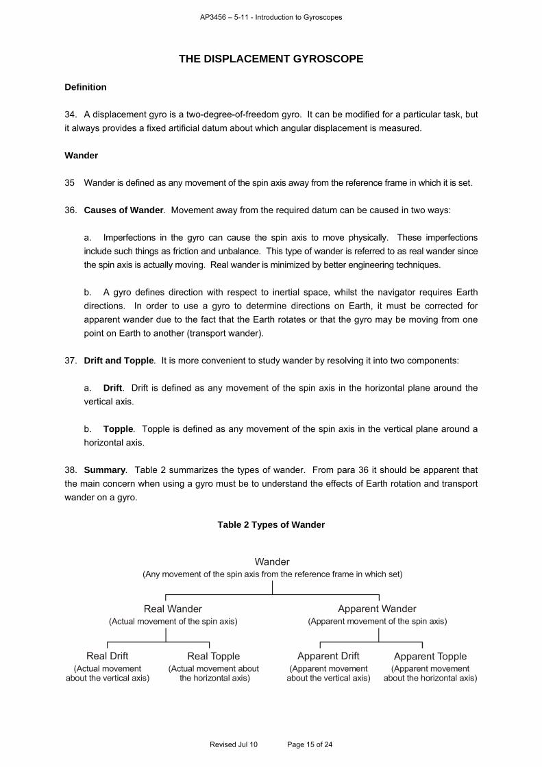
AP3456 – 5-11 - Introduction to Gyroscopes
THE DISPLACEMENT GYROSCOPE
Definition
34. A displacement gyro is a two-degree-of-freedom gyro. It can be modified for a particular task, but
it always provides a fixed artificial datum about which angular displacement is measured.
Wander
35 Wander is defined as any movement of the spin axis away from the reference frame in which it is set.
36. Causes of Wander. Movement away from the required datum can be caused in two ways:
a. Imperfections in the gyro can cause the spin axis to move physically. These imperfections
include such things as friction and unbalance. This type of wander is referred to as real wander since
the spin axis is actually moving. Real wander is minimized by better engineering techniques.
b. A gyro defines direction with respect to inertial space, whilst the navigator requires Earth
directions. In order to use a gyro to determine directions on Earth, it must be corrected for
apparent wander due to the fact that the Earth rotates or that the gyro may be moving from one
point on Earth to another (transport wander).
37. Drift and Topple. It is more convenient to study wander by resolving it into two components:
a. Drift. Drift is defined as any movement of the spin axis in the horizontal plane around the
vertical axis.
b. Topple. Topple is defined as any movement of the spin axis in the vertical plane around a
horizontal axis.
38. Summary. Table 2 summarizes the types of wander. From para 36 it should be apparent that
the main concern when using a gyro must be to understand the effects of Earth rotation and transport
wander on a gyro.
Table 2 Types of Wander
Wander
(Any movement of the spin axis from the reference frame in which set)
Real Wander(Actual movement of the spin axis)
Apparent Wander(Apparent movement of the spin axis)
Apparent Drift(Apparent movement
about the vertical axis)
Real Topple(Actual movement about
the horizontal axis)
Apparent Topple(Apparent movement
about the horizontal axis)
Real Drift(Actual movement
about the vertical axis)
Revised Jul 10 Page 15 of 24
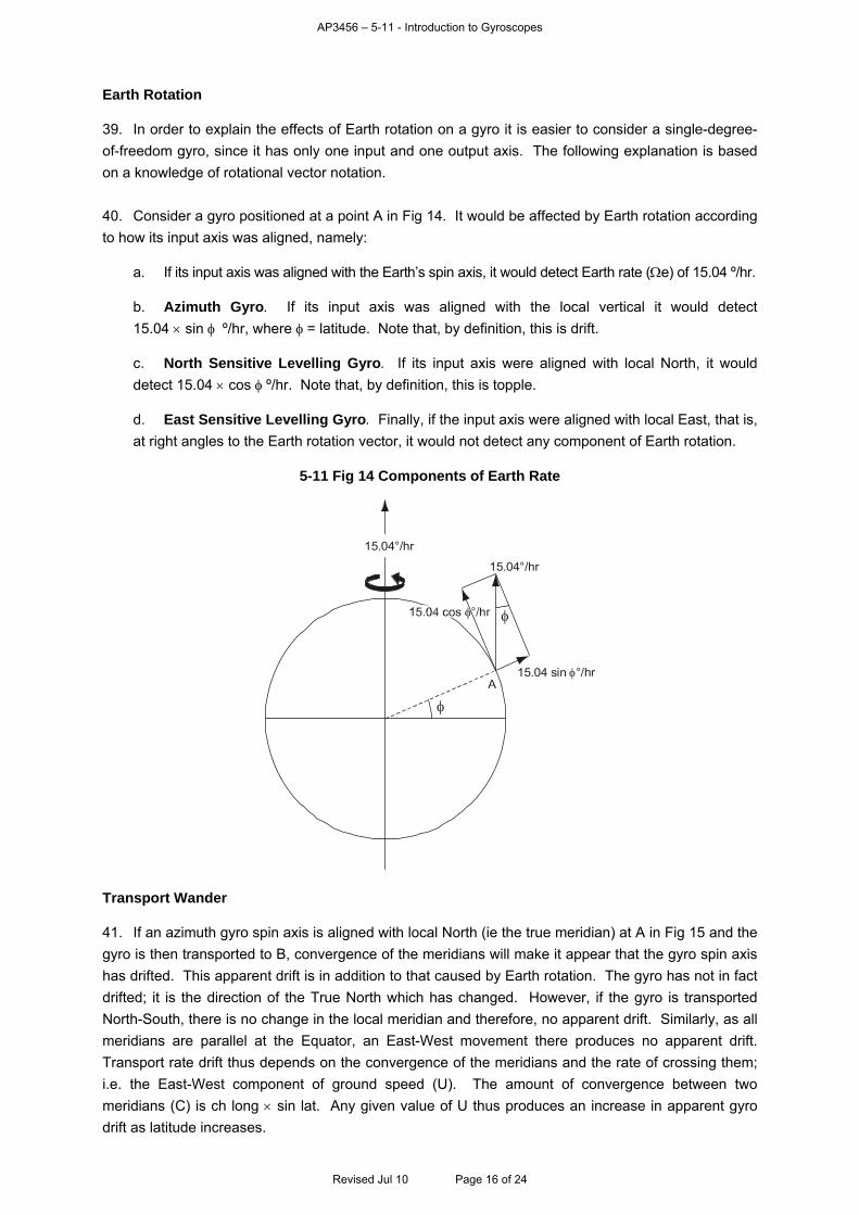
AP3456 – 5-11 - Introduction to Gyroscopes
Earth Rotation
39. In order to explain the effects of Earth rotation on a gyro it is easier to consider a single-degree-
of-freedom gyro, since it has only one input and one output axis. The following explanation is based
on a knowledge of rotational vector notation.
40. Consider a gyro positioned at a point A in Fig 14. It would be affected by Earth rotation according
to how its input axis was aligned, namely:
a. If its input axis was aligned with the Earth’s spin axis, it would detect Earth rate (e) of 15.04 º/hr.
b. Azimuth Gyro. If its input axis was aligned with the local vertical it would detect
15.04 sin º/hr, where = latitude. Note that, by definition, this is drift.
c. North Sensitive Levelling Gyro. If its input axis were aligned with local North, it would
detect 15.04 cos º/hr. Note that, by definition, this is topple.
d. East Sensitive Levelling Gyro. Finally, if the input axis were aligned with local East, that is,
at right angles to the Earth rotation vector, it would not detect any component of Earth rotation.
5-11 Fig 14 Components of Earth Rate
A
15.04°/hr
15.04 sin °/hr
15.04°/hr
Transport Wander
41. If an azimuth gyro spin axis is aligned with local North (ie the true meridian) at A in Fig 15 and the
gyro is then transported to B, convergence of the meridians will make it appear that the gyro spin axis
has drifted. This apparent drift is in addition to that caused by Earth rotation. The gyro has not in fact
drifted; it is the direction of the True North which has changed. However, if the gyro is transported
North-South, there is no change in the local meridian and therefore, no apparent drift. Similarly, as all
meridians are parallel at the Equator, an East-West movement there produces no apparent drift.
Transport rate drift thus depends on the convergence of the meridians and the rate of crossing them;
i.e. the East-West component of ground speed (U). The amount of convergence between two
meridians (C) is ch long sin lat. Any given value of U thus produces an increase in apparent gyro
drift as latitude increases.
Revised Jul 10 Page 16 of 24

AP3456 – 5-11 - Introduction to Gyroscopes
5-11 Fig 15 Apparent Drift
E
A
B
Q
NP
MeridianConvergence Apparent
Drift
The amount of drift due to transport rate may be found as follows:
C (º/hr) = [ch long/hr] sin .
Now, ch long/hr = ch Eastings nm hr( /
60
) sec
and, since 1º = 60 nm and ch Eastings (nm/hr) = U
C = U
60 sec sin (º/hr)
but, sec sin =
sin cos
1
=
tan cos
sin
/hr)( tan 60
U = C
This can be converted to radians/hour by multiplying by 180
π
180
π tan
60
U = C = U tan
18060
π
Now an arc of length 60 nm on the Earth’s surface subtends an angle of 1º (π/180º) at the centre of
the Earth
60180
πR where R= Earth’s radius
or, 18060
π
R
1
Revised Jul 10 Page 17 of 24
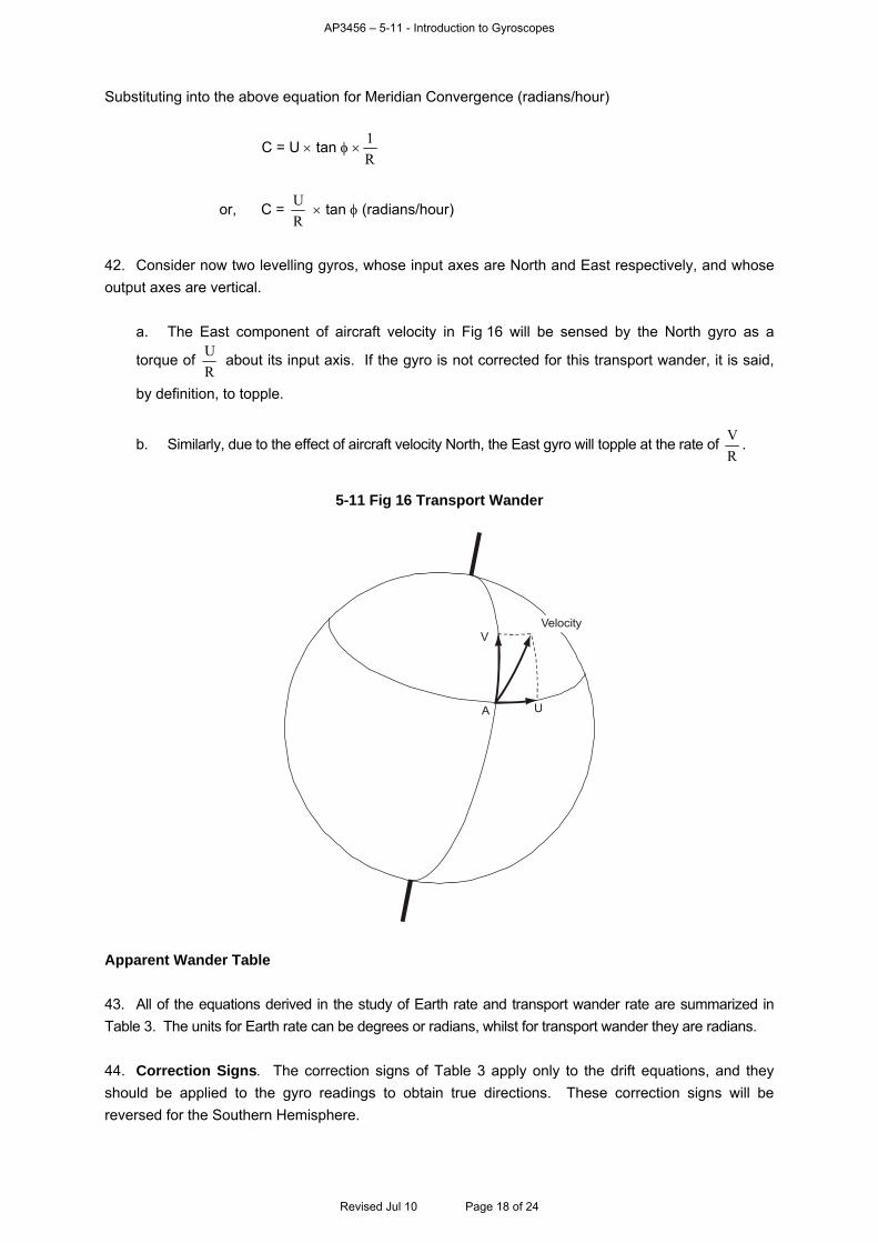
AP3456 – 5-11 - Introduction to Gyroscopes
Substituting into the above equation for Meridian Convergence (radians/hour)
C = U tan R
1
or, C = R
U tan (radians/hour)
42. Consider now two levelling gyros, whose input axes are North and East respectively, and whose
output axes are vertical.
a. The East component of aircraft velocity in Fig 16 will be sensed by the North gyro as a
torque of R
U about its input axis. If the gyro is not corrected for this transport wander, it is said,
by definition, to topple.
b. Similarly, due to the effect of aircraft velocity North, the East gyro will topple at the rate of R
V.
5-11 Fig 16 Transport Wander
VelocityV
A U
Apparent Wander Table
43. All of the equations derived in the study of Earth rate and transport wander rate are summarized in
Table 3. The units for Earth rate can be degrees or radians, whilst for transport wander they are radians.
44. Correction Signs. The correction signs of Table 3 apply only to the drift equations, and they
should be applied to the gyro readings to obtain true directions. These correction signs will be
reversed for the Southern Hemisphere.
Revised Jul 10 Page 18 of 24
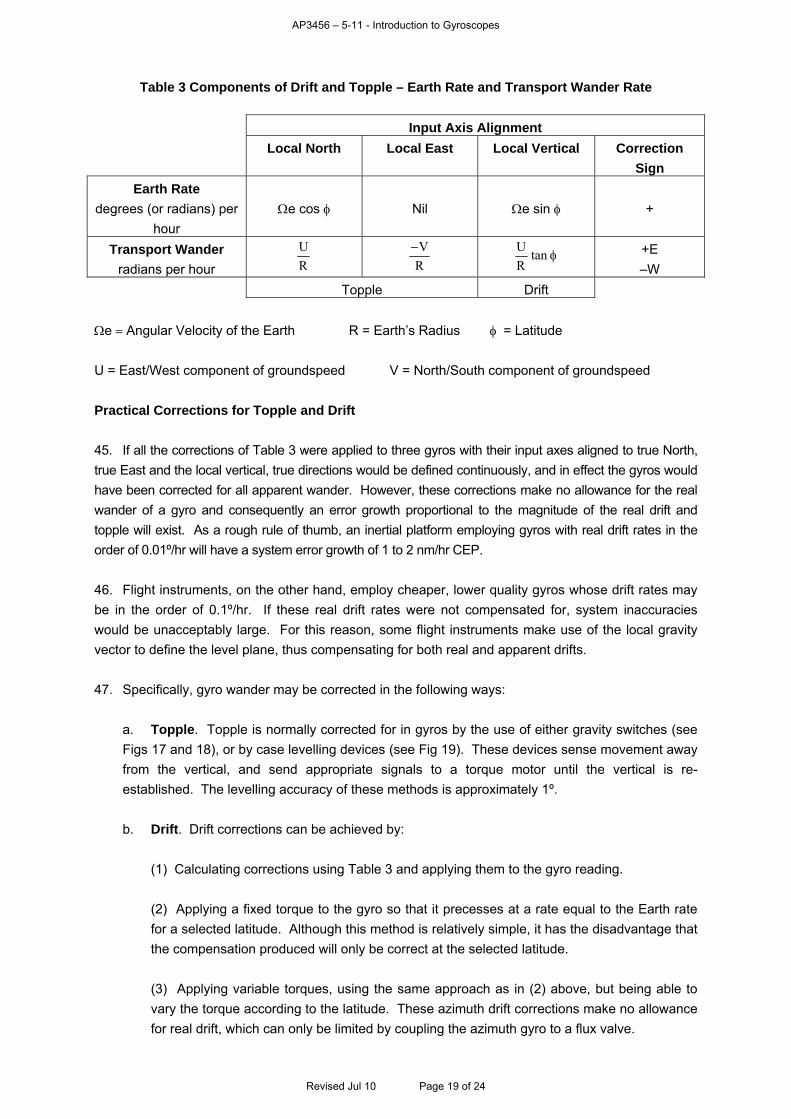
AP3456 – 5-11 - Introduction to Gyroscopes
Table 3 Components of Drift and Topple – Earth Rate and Transport Wander Rate
Input Axis Alignment Local North Local East Local Vertical Correction
Sign Earth Rate
degrees (or radians) per
hour
e cos Nil e sin +
Transport Wander radians per hour R
U
R
V tan
R
U +E
–W
Topple Drift
e Angular Velocity of the Earth R = Earth’s Radius = Latitude
U = East/West component of groundspeed V = North/South component of groundspeed
Practical Corrections for Topple and Drift
45. If all the corrections of Table 3 were applied to three gyros with their input axes aligned to true North,
true East and the local vertical, true directions would be defined continuously, and in effect the gyros would
have been corrected for all apparent wander. However, these corrections make no allowance for the real
wander of a gyro and consequently an error growth proportional to the magnitude of the real drift and
topple will exist. As a rough rule of thumb, an inertial platform employing gyros with real drift rates in the
order of 0.01º/hr will have a system error growth of 1 to 2 nm/hr CEP.
46. Flight instruments, on the other hand, employ cheaper, lower quality gyros whose drift rates may
be in the order of 0.1º/hr. If these real drift rates were not compensated for, system inaccuracies
would be unacceptably large. For this reason, some flight instruments make use of the local gravity
vector to define the level plane, thus compensating for both real and apparent drifts.
47. Specifically, gyro wander may be corrected in the following ways:
a. Topple. Topple is normally corrected for in gyros by the use of either gravity switches (see
Figs 17 and 18), or by case levelling devices (see Fig 19). These devices sense movement away
from the vertical, and send appropriate signals to a torque motor until the vertical is re-
established. The levelling accuracy of these methods is approximately 1º.
b. Drift. Drift corrections can be achieved by:
(1) Calculating corrections using Table 3 and applying them to the gyro reading.
(2) Applying a fixed torque to the gyro so that it precesses at a rate equal to the Earth rate
for a selected latitude. Although this method is relatively simple, it has the disadvantage that
the compensation produced will only be correct at the selected latitude.
(3) Applying variable torques, using the same approach as in (2) above, but being able to
vary the torque according to the latitude. These azimuth drift corrections make no allowance
for real drift, which can only be limited by coupling the azimuth gyro to a flux valve.
Revised Jul 10 Page 19 of 24
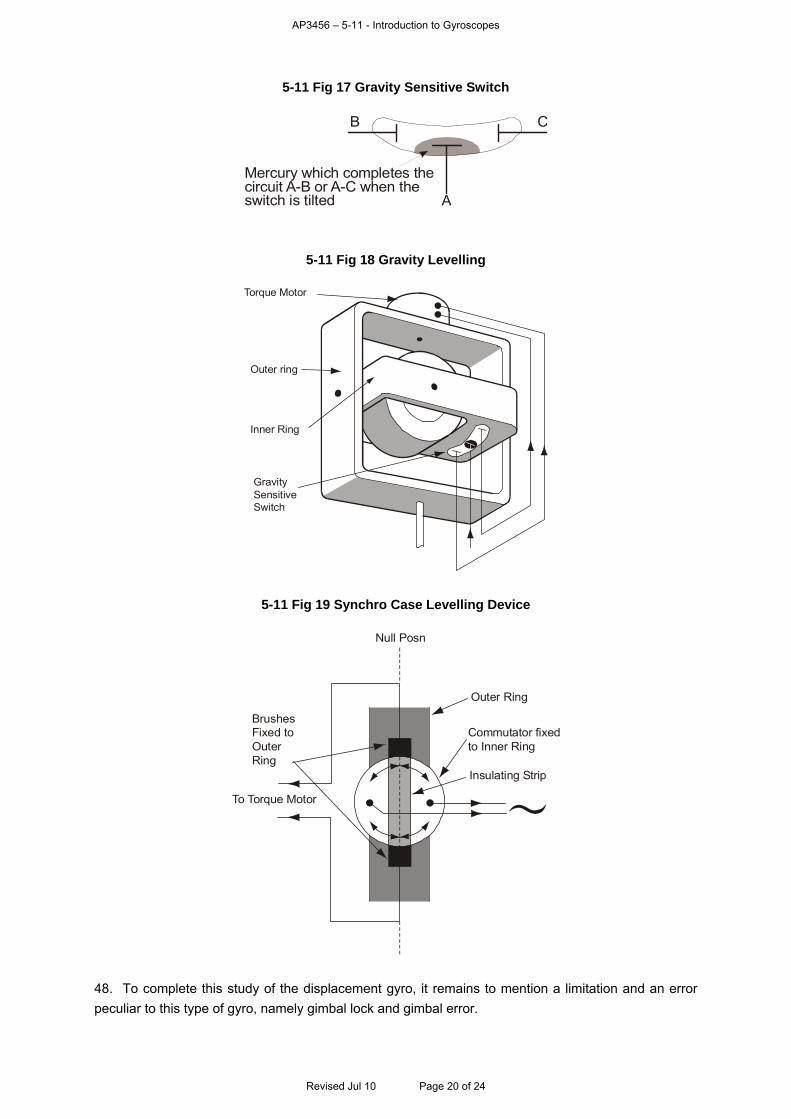
AP3456 – 5-11 - Introduction to Gyroscopes
5-11 Fig 17 Gravity Sensitive Switch
Mercury which completes thecircuit A-B or A-C when the switch is tilted A
B C
5-11 Fig 18 Gravity Levelling
Outer ring
Inner Ring
Gravity Sensitive Switch
Torque Motor
5-11 Fig 19 Synchro Case Levelling Device
Outer Ring
Commutator fixed to Inner Ring
Insulating Strip
To Torque Motor
Brushes Fixed to Outer Ring
Null Posn
48. To complete this study of the displacement gyro, it remains to mention a limitation and an error
peculiar to this type of gyro, namely gimbal lock and gimbal error.
Revised Jul 10 Page 20 of 24
AP3456 – 5-11 - Introduction to Gyroscopes
Gimbal Lock
49. Gimbal lock occurs when the gimbal orientation is such that the spin axis becomes coincident
with an axis of freedom. Effectively the gyro has lost one of its degrees of freedom, and any
attempted movement about the lost axis will result in real wander. This is often referred to as toppling,
although drift is also present.
Gimbal Error
50. When a 2-degree-of-freedom gyroscope with a horizontal spin axis is both banked and rolled, the
outer gimbal must rotate to maintain orientation of the rotor axis, thereby inducing a heading error at
the outer gimbal pick-off. The incidence of this error depends upon the angle of bank and the angular
difference between the spin axis and the longitudinal axis and, as in most systems, the spin axis
direction is arbitrary relative to North, the error is not easily predicted. Although the error disappears
when the aircraft is levelled, it will have accumulated in any GPI equipment, producing a small error in
computed position.
OTHER TYPES OF GYRO
The Ring Laser Gyro
51. The ring laser gyro is one of the modern alternatives to conventional gyros for a number of
applications including aircraft inertial navigation systems and attitude/heading reference systems. The
ring laser gyro has no moving parts and is not a gyroscope in the normal meaning of the word. The
ring laser gyro is, however, a very accurate device for measuring rotation and became the system of
choice for use with strapdown inertial navigation systems. A schematic diagram of a ring laser gyro is
at Fig 20.
5-11 Fig 20 Schematic Diagram of a Ring Laser Gyro
Prism
Cavity
AnodeAnode
Detector
Cathode
CervitMonoblock
PathLengthControl
PathLengthControl
PathLengthControl
Axis of Rotation
Mirror
Mirror
Mirror
Revised Jul 10 Page 21 of 24
AP3456 – 5-11 - Introduction to Gyroscopes
52. Principle of Operation. In ring laser gyros, the rotating mass of the conventional gyro is
replaced by two contra-rotating beams of light. The main body of the gyro consists of a single piece
(or 'monoblock') of a vitreous ceramic of low temperature coefficient (typically 'Cervit' or 'Zerodour'). A
gas-tight cavity is accurately machined into the monoblock and this cavity is then filled with an inert
gas, typically a mixture of Helium and Neon. A DC electrical discharge ionizes the gas and causes the
lasing action. Two beams of light are produced, flowing in opposite directions in the cavity. Mirrors
are used to reflect the beams around the enclosed area, producing a 'laser-in-a-ring' configuration.
The frequency of oscillation of each beam corresponds to the cavity resonance condition. This
condition requires that the optical path length of the cavity be an integral number of wavelengths. The
frequency of each beam is therefore dependant on the optical path length.
53. Effect of Movement. At rest, the optical path length for each beam is identical; therefore, the
frequencies of the two laser beams are the same. However, when the sensor is rotated about the axis
perpendicular to the lasing plane, one beam travels an increased path length, whilst the other travels a
reduced path length. The two resonant frequencies change to adjust to the longer or shorter optical
path, and the frequency difference is directly proportional to the rotation rate. This phenomenon is
known as the Sagnac effect. The frequency difference is measured by the beaming of an output
signal for each wave on to photo detectors spaced one quarter of a wavelength apart, causing an
optical effect known as an interference fringe. The fringe pattern moves at a rate that is directly
proportional to the frequency difference between the two beams. It is converted to a digital output,
where the output pulse rate is proportional to the input turn rate, and the cumulative pulse count is
proportional to the angular change. This effect can be quantified using simplified maths, where it can
be shown that the frequency difference f of the two waves is:
Lλ
ΩA4f Where:
A is the area enclosed by the path.
λ is the oscillating wavelength.
L is the length of the closed path.
Ω is the rate of rotation.
54. Gyro Control. The reason why the two beams have to occupy the same physical cavity is the
sensitivity of laser light to cavity length. If they did not, a temperature induced difference in path length
could result in a large frequency mismatch between the two beams. The path length control
mechanism is used to alter the intensity of the laser and thus control expansion due to excess heat.
To help avoid perceived differences in path length due to flow of the Helium/Neon gas mix, two
anodes are used to balance any flow caused by ionization.
55. Error Sources. Ring laser gyros are subject to a number of errors, the most notable are:
a. Null Shift. Null shift arises due to a difference in path length as perceived by the two
opposite beams, thus producing an output when no rotation exists. The major causes of
perceived path length difference are:
(1) Differential movement of the gas in the cavity.
(2) Small changes in the refractive index of the monoblock material as the direction of travel
of the laser light changes.
b. Lock-in. Lock-in occurs when the input rotation rate of the gyro is reduced below a critical
value causing the frequency difference between the clockwise and anti-clockwise beams to drop
to zero. One of the main causes of this phenomenon is backscatter of light at the mirrors. Some
of the clockwise beam is reflected backwards, thereby contaminating the anti-clockwise beam
Revised Jul 10 Page 22 of 24

AP3456 – 5-11 - Introduction to Gyroscopes
with the clockwise frequency. Similarly, backscattering of the anti-clockwise beam contaminates
the clockwise beam. With low input rotational rates, the two beams soon reach a common
frequency which renders detection of rotation impossible. Several methods are used to ensure
that lock-in is minimized. One method is to physically dither the gyro by inputting a known
rotation rate in one direction, immediately followed by a rotation rate in the opposite direction. As
the dither rate is known, it can be removed at the output stage. The dither ensures that the two
frequencies are kept far enough apart to avoid lock-in.
56. Advantages of the Ring Laser Gyro. The main advantages of the ring laser gyro are:
a. Its performance is unaffected by high 'g'.
b. It has no moving parts and therefore has high reliability and low maintenance requirements.
c. It has a rapid turn-on time.
57. Disadvantage of the Ring Laser Gyro. The technical problems associated with ring laser gyros
can all be overcome. However, solution of these problems inevitably increases costs which are
already very high due to the complex, 'clean-room' manufacturing facilities needed to provide:
a. Precision machining and polishing.
b. High quality mirrors.
c. Very good optical seals.
d. A carefully balanced mix of Helium and Neon, free of contaminants.
58. Summary. While the ring laser gyro represents a major advance over the traditional spinning
gyro, it is only one of a number of possible alternatives. The search for new gyroscopic devices
continues, driven by considerations of both cost and accuracy.
Fibre Optic Gyros
59. As previously outlined, the major disadvantage of ring laser gyros is their high cost due to the
precise engineering facilities required to manufacture them. The fibre optic gyro (see Fig 21), first
tested in 1975, works on the same principal as the ring laser gyro (the Sagnac effect) but no longer
relies on a complex and costly block and mirror system since it uses a coil of fibre optic cable.
5-11 Fig 21 Fibre Optic Gyro
Fibre Optic Loop
Beam SplitterLightSource
Photo Detector
Signal Processor
Converts oto detectorsignals into angular rate
ph
OpticalElectrical
Revised Jul 10 Page 23 of 24
AP3456 – 5-11 - Introduction to Gyroscopes
Revised Jul 10 Page 24 of 24
Vibrating Gyros
60. Vibrating gyros work by exploiting the Coriolis effect and, while not yet as accurate as optical
gyros, are much smaller and cheaper to produce.
61. The 'GyroChip' (Fig 22) uses a vibrating quartz tuning fork as a Coriolis sensor, coupled to a
similar fork as a pickup to produce the rate output signal. The piezoelectric drive tines are driven by
an oscillator to vibrate at a precise amplitude, causing the tines to move toward and away from one
another at a high frequency. This vibration causes the drive fork to become sensitive to angular rate
about an axis parallel to its tines, defining the true input axis of the sensor.
5-11 Fig 22 The 'GyroChip' Vibrating Gyro
FilterAmplifier
AmplitudeController
DriveTines
PickupTines
Pickup Amplifier
Drive Oscillator
FilterAmplifier
SynchDemodulator
DC RateSignal
- +
A
A
62. Vibration of the drive tines causes them to act like the arms of a spinning ice skater, where
moving them in causes the skater’s spin rate to increase, and moving them out causes a decrease in
rate. An applied rotation rate causes a sine wave of torque to be produced, resulting from 'Coriolis
Acceleration', in turn causing the tines of the Pickup Fork to move up and down (not toward and away
from one another) out of the plane of the fork assembly.
63. The pickup tines thus respond to the oscillating torque by moving in and out of plane, causing
electrical output signals to be produced by the Pickup Amplifier. These signals are amplified and
converted into a DC signal proportional to rate by use of a synchronous switch (demodulator) which
responds only to the desired rate signals. The DC output signal of the 'GyroChip' is directly
proportional to input rate, reversing sign as the input rate reverses, since the oscillating torque
produced by Coriolis reverses phase when the input rate reverses.

AP3456 – 5-12 - Gyro-magnetic Compasses
CHAPTER 12 - GYRO-MAGNETIC COMPASSES Contents Page Introduction.............................................................................................................................................. 2 General .................................................................................................................................................... 2 Basic Components .................................................................................................................................. 3 Fluxvalve Theory ..................................................................................................................................... 3 The Transmission/Display System .......................................................................................................... 9 HEADING ERRORS INDUCED BY THE FLUXVALVE ........................................................................ 10 General .................................................................................................................................................. 10 Detector Tilt Error .................................................................................................................................. 10 THEORY OF THE GYRO-MAGNETIC COMPASS .............................................................................. 13 General .................................................................................................................................................. 13 Mechanization ....................................................................................................................................... 13 GYRO-MAGNETIC COMPASS SYSTEM ERRORS ............................................................................ 17 Fluxvalve Tilt Errors............................................................................................................................... 17 Northerly Instability ................................................................................................................................ 18 Hang-off Error........................................................................................................................................ 18 Gimbal Error .......................................................................................................................................... 19 Transmission Errors .............................................................................................................................. 19 Compass Swinging Errors ..................................................................................................................... 19 Variation and Deviation Errors .............................................................................................................. 19 A Refined Compass System.................................................................................................................. 19 Table of Figures 5-12 Fig 1 Detector Unit with Fluxvalve Element .................................................................................... 3 5-12 Fig 2 Vertical Cross-section of a Spoke.......................................................................................... 4 5-12 Fig 3 Magnetic Flux Components ................................................................................................... 4 5-12 Fig 4 Variation of Flux with ........................................................................................................... 4 5-12 Fig 5 Hysteresis Curve for Permalloy.............................................................................................. 5 5-12 Fig 6 Simple Fluxvalve .................................................................................................................... 5 5-12 Fig 7 The Effect of Excitation Current in the Top Leg Only............................................................. 6 5-12 Fig 8 The Effect of the Excitation Current in the Bottom Leg Only ................................................. 6 5-12 Fig 9 The Effect of the Excitation Current in Both Legs .................................................................. 7 5-12 Fig 10 The Combined Effects of the Excitation Current and the Component of the Earth’s Field.. 7 5-12 Fig 11 Detector Unit and Transmission System – Schematic......................................................... 8 5-12 Fig 12 Operation of the Three-spoke Fluxvalve.............................................................................. 8 5-12 Fig 13 Eliminating Latitude Ambiguity ............................................................................................. 9 5-12 Fig 14 Action of the Fluxvalve and Transmission System .............................................................. 9 5-12 Fig 15 Simple Remote Indicating Compass.................................................................................. 10 5-12 Fig 16 Indication of Magnetic North .............................................................................................. 11 5-12 Fig 17 Effect of a Gross Tilt to Port ............................................................................................... 11 5-12 Fig 18 Effect of Change of Dip ...................................................................................................... 11 5-12 Fig 19 Effect of Direction of Tilt ..................................................................................................... 12 5-12 Fig 20 Tilt Exceeds (90º –Dip)...................................................................................................... 12 5-12 Fig 21 Typical Errors in Magnetic Heading Due to Tilt.................................................................. 13 5-12 Fig 22 Basic Gyro-magnetic Compass.......................................................................................... 14
Revised May 10 Page 1 of 20
AP3456 – 5-12 - Gyro-magnetic Compasses
5-12 Fig 23 Gyro Correction Techniques .............................................................................................. 14 5-12 Fig 24 Gyro-magnetic Compass Block Diagram........................................................................... 16 5-12 Fig 25 Typical Gyro Slaving Mechanization (Simplified Schematic) ............................................. 16 5-12 Fig 26 Effect of a Change in H on the Time Constant .................................................................. 17 5-12 Fig 27 Ideal Gyro-magnetic Compass........................................................................................... 20 Introduction 1. The direct indicating compass is subject to errors due to two main causes, magnetic fields of the aircraft structure and flight accelerations. In the case of the direct indicating compasses, magnetic fields due to aircraft magnetism are accentuated by the necessary positioning of the compass so that it can be read by the pilot/navigator, i.e. in the cockpit where the deviating effects due to hard iron (including DC fields) and soft iron fields are large. The pendulously suspended magnet system is subject to errors due to accelerations. 2. In addition to these errors, the effect of reduction in the directional force acting on the detecting element renders the direct reading instrument unreliable in high magnetic latitudes where the horizontal component of the Earth’s magnetic field is weak. This has the effect of making the compass sluggish in indicating a change of heading. After an alteration of heading, the detecting element will oscillate for a considerable time before settling down. 3. A further disadvantage of the direct indicating compass is that indications of direction can be given at only one position in the aircraft. Since the Earth’s magnetic field strength cannot provide sufficient torque for driving repeater indicators from one master detector element, separate compass systems must be provided for each crew member requiring a heading readout. 4. The remote indicating compass was developed to reduce the errors of the direct indicating compass and to evolve an instrument giving automatic continuous direction which could be fed to other instruments. Although a number of these systems have been designed using different detecting and stabilizing techniques, the gyro stabilized remote indicating (gyro-magnetic) compass gradually evolved. General 5. The gyro-magnetic compass consists essentially of a magnetic compass whose indications are stabilized gyroscopically so that the effects of turning and acceleration errors are reduced. A gyroscope is unaffected by changing magnetic fields or by normal aircraft accelerations but its heading indications may be inaccurate due to the effect of precessional forces caused by friction, incorrect balance etc. Since the commonly used detecting element, the fluxvalve, is pendulously suspended, it is affected by accelerations. Therefore, the principle underlying the gyro-magnetic system is to integrate the heading indication of the magnetic compass with the directional properties of a gyroscope so that a compromise between the two is achieved. The net result is to reduce the individual errors of each. The technique most commonly used is to reference the azimuth gyroscope initially to the magnetic meridian and to maintain the relationship by applying precessional forces to the gyroscope based on long-term magnetic azimuth information from the fluxvalve detector. The degree of control of the fluxvalve over the gyroscope, or the monitoring rate, is of considerable importance. For example, in a turn the fluxvalve heading is likely to be in error so the control rate must be engineered so that the induced heading is that of the gyro. At the same time, there must be sufficient control to correct the gyro drift.
Revised May 10 Page 2 of 20
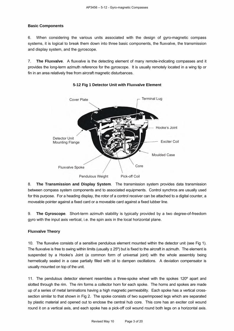
AP3456 – 5-12 - Gyro-magnetic Compasses
Basic Components 6. When considering the various units associated with the design of gyro-magnetic compass systems, it is logical to break them down into three basic components, the fluxvalve, the transmission and display system, and the gyroscope. 7. The Fluxvalve. A fluxvalve is the detecting element of many remote-indicating compasses and it provides the long-term azimuth reference for the gyroscope. It is usually remotely located in a wing tip or fin in an area relatively free from aircraft magnetic disturbances.
5-12 Fig 1 Detector Unit with Fluxvalve Element
Pendulous Weight
Cover Plate
Pick-off Coil
Fluxvalve Spoke
Moulded Case
Exciter Coil
Hooke s Joint’
Detector UnitMounting Flange
Core
Terminal Lug
8. The Transmission and Display System. The transmission system provides data transmission between compass system components and to associated equipments. Control synchros are usually used for this purpose. For a heading display, the rotor of a control receiver can be attached to a digital counter, a moveable pointer against a fixed card or a moveable card against a fixed lubber line. 9. The Gyroscope. Short-term azimuth stability is typically provided by a two degree-of-freedom gyro with the input axis vertical, i.e. the spin axis in the local horizontal plane. Fluxvalve Theory 10. The fluxvalve consists of a sensitive pendulous element mounted within the detector unit (see Fig 1). The fluxvalve is free to swing within limits (usually ± 25º) but is fixed to the aircraft in azimuth. The element is suspended by a Hooke’s Joint (a common form of universal joint) with the whole assembly being hermetically sealed in a case partially filled with oil to dampen oscillations. A deviation compensator is usually mounted on top of the unit. 11. The pendulous detector element resembles a three-spoke wheel with the spokes 120º apart and slotted through the rim. The rim forms a collector horn for each spoke. The horns and spokes are made up of a series of metal laminations having a high magnetic permeability. Each spoke has a vertical cross-section similar to that shown in Fig 2. The spoke consists of two superimposed legs which are separated by plastic material and opened out to enclose the central hub core. This core has an exciter coil wound round it on a vertical axis, and each spoke has a pick-off coil wound round both legs on a horizontal axis.
Revised May 10 Page 3 of 20
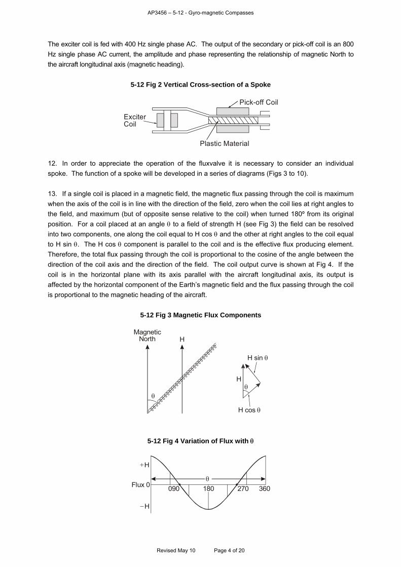
AP3456 – 5-12 - Gyro-magnetic Compasses
The exciter coil is fed with 400 Hz single phase AC. The output of the secondary or pick-off coil is an 800 Hz single phase AC current, the amplitude and phase representing the relationship of magnetic North to the aircraft longitudinal axis (magnetic heading).
5-12 Fig 2 Vertical Cross-section of a Spoke
Plastic Material
ExciterCoil
Pick-off Coil
12. In order to appreciate the operation of the fluxvalve it is necessary to consider an individual spoke. The function of a spoke will be developed in a series of diagrams (Figs 3 to 10). 13. If a single coil is placed in a magnetic field, the magnetic flux passing through the coil is maximum when the axis of the coil is in line with the direction of the field, zero when the coil lies at right angles to the field, and maximum (but of opposite sense relative to the coil) when turned 180º from its original position. For a coil placed at an angle to a field of strength H (see Fig 3) the field can be resolved into two components, one along the coil equal to H cos and the other at right angles to the coil equal to H sin . The H cos component is parallel to the coil and is the effective flux producing element. Therefore, the total flux passing through the coil is proportional to the cosine of the angle between the direction of the coil axis and the direction of the field. The coil output curve is shown at Fig 4. If the coil is in the horizontal plane with its axis parallel with the aircraft longitudinal axis, its output is affected by the horizontal component of the Earth’s magnetic field and the flux passing through the coil is proportional to the magnetic heading of the aircraft.
5-12 Fig 3 Magnetic Flux Components
HMagnetic
North
H cos
H
H sin
5-12 Fig 4 Variation of Flux with
Flux 0
090 180 270 360
H
H
Revised May 10 Page 4 of 20
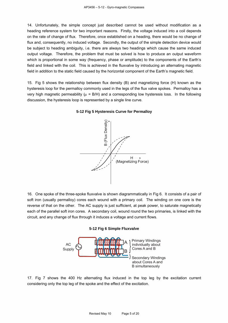
AP3456 – 5-12 - Gyro-magnetic Compasses
14. Unfortunately, the simple concept just described cannot be used without modification as a heading reference system for two important reasons. Firstly, the voltage induced into a coil depends on the rate of change of flux. Therefore, once established on a heading, there would be no change of flux and, consequently, no induced voltage. Secondly, the output of the simple detection device would be subject to heading ambiguity, i.e. there are always two headings which cause the same induced output voltage. Therefore, the problem that must be solved is how to produce an output waveform which is proportional in some way (frequency, phase or amplitude) to the components of the Earth’s field and linked with the coil. This is achieved in the fluxvalve by introducing an alternating magnetic field in addition to the static field caused by the horizontal component of the Earth’s magnetic field. 15. Fig 5 shows the relationship between flux density (B) and magnetizing force (H) known as the hysteresis loop for the permalloy commonly used in the legs of the flux valve spokes. Permalloy has a very high magnetic permeability ( = B/H) and a corresponding low hysteresis loss. In the following discussion, the hysteresis loop is represented by a single line curve.
5-12 Fig 5 Hysteresis Curve for Permalloy
H(Magnetizing Force)
B (F
lux
Den
sity
)
16. One spoke of the three-spoke fluxvalve is shown diagrammatically in Fig 6. It consists of a pair of soft iron (usually permalloy) cores each wound with a primary coil. The winding on one core is the reverse of that on the other. The AC supply is just sufficient, at peak power, to saturate magnetically each of the parallel soft iron cores. A secondary coil, wound round the two primaries, is linked with the circuit, and any change of flux through it induces a voltage and current flows.
5-12 Fig 6 Simple Fluxvalve
Primary Windingsindividually about Cores A and B
Secondary Windingsabout Cores A and B simultaneously
ACSupply
A
B
17. Fig 7 shows the 400 Hz alternating flux induced in the top leg by the excitation current considering only the top leg of the spoke and the effect of the excitation.
Revised May 10 Page 5 of 20
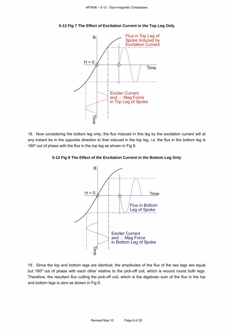
AP3456 – 5-12 - Gyro-magnetic Compasses
5-12 Fig 7 The Effect of Excitation Current in the Top Leg Only
B
H = 0Time
Flux in Top Leg ofSpoke Induced byExcitation Current
Exciter Currentand Mag Forcein Top Leg of Spoke
Time
18. Now considering the bottom leg only; the flux induced in this leg by the excitation current will at any instant be in the opposite direction to that induced in the top leg, i.e. the flux in the bottom leg is 180º out of phase with the flux in the top leg as shown in Fig 8.
5-12 Fig 8 The Effect of the Excitation Current in the Bottom Leg Only
B
H = 0 Time
Flux in BottomLeg of Spoke
Exciter Currentand Mag Forcein Bottom Leg of Spoke
Time
19. Since the top and bottom legs are identical, the amplitudes of the flux of the two legs are equal but 180º out of phase with each other relative to the pick-off coil, which is wound round both legs. Therefore, the resultant flux cutting the pick-off coil, which is the algebraic sum of the flux in the top and bottom legs is zero as shown in Fig 9.
Revised May 10 Page 6 of 20
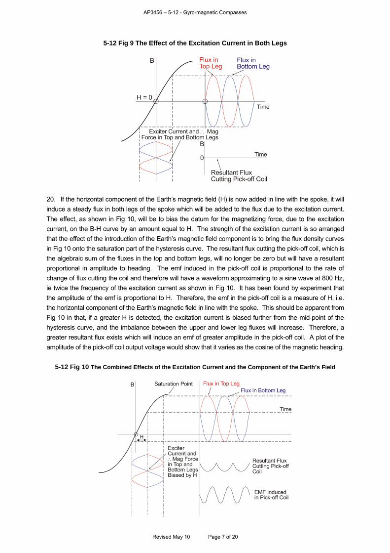
AP3456 – 5-12 - Gyro-magnetic Compasses
5-12 Fig 9 The Effect of the Excitation Current in Both Legs
B
H = 0Time
B
0 Time
Resultant FluxCutting Pick-off Coil
Flux in Top Leg
Flux in Bottom Leg
Exciter Current and Mag Force in Top and Bottom Legs
20. If the horizontal component of the Earth’s magnetic field (H) is now added in line with the spoke, it will induce a steady flux in both legs of the spoke which will be added to the flux due to the excitation current. The effect, as shown in Fig 10, will be to bias the datum for the magnetizing force, due to the excitation current, on the B-H curve by an amount equal to H. The strength of the excitation current is so arranged that the effect of the introduction of the Earth’s magnetic field component is to bring the flux density curves in Fig 10 onto the saturation part of the hysteresis curve. The resultant flux cutting the pick-off coil, which is the algebraic sum of the fluxes in the top and bottom legs, will no longer be zero but will have a resultant proportional in amplitude to heading. The emf induced in the pick-off coil is proportional to the rate of change of flux cutting the coil and therefore will have a waveform approximating to a sine wave at 800 Hz, ie twice the frequency of the excitation current as shown in Fig 10. It has been found by experiment that the amplitude of the emf is proportional to H. Therefore, the emf in the pick-off coil is a measure of H, i.e. the horizontal component of the Earth’s magnetic field in line with the spoke. This should be apparent from Fig 10 in that, if a greater H is detected, the excitation current is biased further from the mid-point of the hysteresis curve, and the imbalance between the upper and lower leg fluxes will increase. Therefore, a greater resultant flux exists which will induce an emf of greater amplitude in the pick-off coil. A plot of the amplitude of the pick-off coil output voltage would show that it varies as the cosine of the magnetic heading.
5-12 Fig 10 The Combined Effects of the Excitation Current and the Component of the Earth’s Field
B
H
Saturation Point
Time
Flux in Top LegFlux in Bottom Leg
Resultant FluxCutting Pick-off Coil
EMF Inducedin Pick-off Coil
ExciterCurrent and
Mag Forcein Top andBottom LegsBiased by H
Revised May 10 Page 7 of 20
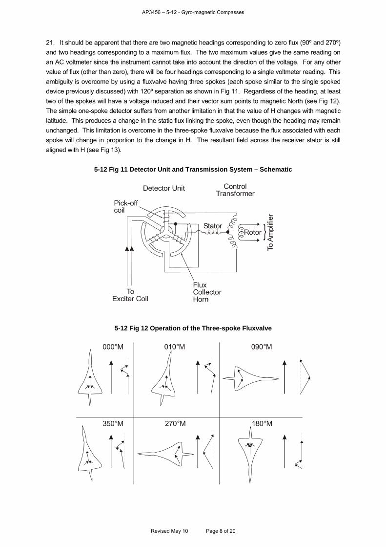
AP3456 – 5-12 - Gyro-magnetic Compasses
21. It should be apparent that there are two magnetic headings corresponding to zero flux (90º and 270º) and two headings corresponding to a maximum flux. The two maximum values give the same reading on an AC voltmeter since the instrument cannot take into account the direction of the voltage. For any other value of flux (other than zero), there will be four headings corresponding to a single voltmeter reading. This ambiguity is overcome by using a fluxvalve having three spokes (each spoke similar to the single spoked device previously discussed) with 120º separation as shown in Fig 11. Regardless of the heading, at least two of the spokes will have a voltage induced and their vector sum points to magnetic North (see Fig 12). The simple one-spoke detector suffers from another limitation in that the value of H changes with magnetic latitude. This produces a change in the static flux linking the spoke, even though the heading may remain unchanged. This limitation is overcome in the three-spoke fluxvalve because the flux associated with each spoke will change in proportion to the change in H. The resultant field across the receiver stator is still aligned with H (see Fig 13).
5-12 Fig 11 Detector Unit and Transmission System – Schematic
ToExciter Coil
FluxCollectorHorn
Pick-offcoil
Detector Unit ControlTransformer
RotorStator
To A
mpl
ifier
5-12 Fig 12 Operation of the Three-spoke Fluxvalve
000°M 010°M 090°M
350°M 270°M 180°M
Revised May 10 Page 8 of 20
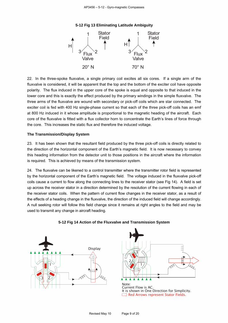
AP3456 – 5-12 - Gyro-magnetic Compasses
5-12 Fig 13 Eliminating Latitude Ambiguity
1
23H
StatorField
FluxValve
20° N
H
1
23
StatorField
FluxValve
70 N°
22. In the three-spoke fluxvalve, a single primary coil excites all six cores. If a single arm of the fluxvalve is considered, it will be apparent that the top and the bottom of the exciter coil have opposite polarity. The flux induced in the upper core of the spoke is equal and opposite to that induced in the lower core and this is exactly the effect produced by the primary windings in the simple fluxvalve. The three arms of the fluxvalve are wound with secondary or pick-off coils which are star connected. The exciter coil is fed with 400 Hz single-phase current so that each of the three pick-off coils has an emf at 800 Hz induced in it whose amplitude is proportional to the magnetic heading of the aircraft. Each core of the fluxvalve is fitted with a flux collector horn to concentrate the Earth’s lines of force through the core. This increases the static flux and therefore the induced voltage. The Transmission/Display System 23. It has been shown that the resultant field produced by the three pick-off coils is directly related to the direction of the horizontal component of the Earth’s magnetic field. It is now necessary to convey this heading information from the detector unit to those positions in the aircraft where the information is required. This is achieved by means of the transmission system. 24. The fluxvalve can be likened to a control transmitter where the transmitter rotor field is represented by the horizontal component of the Earth’s magnetic field. The voltage induced in the fluxvalve pick-off coils cause a current to flow along the connecting lines to the receiver stator (see Fig 14). A field is set up across the receiver stator in a direction determined by the resolution of the current flowing in each of the receiver stator coils. When the pattern of current flow changes in the receiver stator, as a result of the effects of a heading change in the fluxvalve, the direction of the induced field will change accordingly. A null seeking rotor will follow this field change since it remains at right angles to the field and may be used to transmit any change in aircraft heading.
5-12 Fig 14 Action of the Fluxvalve and Transmission System
Display
1
23
3
21
Note:Current Flow is AC.It is shown in One Direction for Simplicity.
Red Arrows represent Stator Fields.
Revised May 10 Page 9 of 20
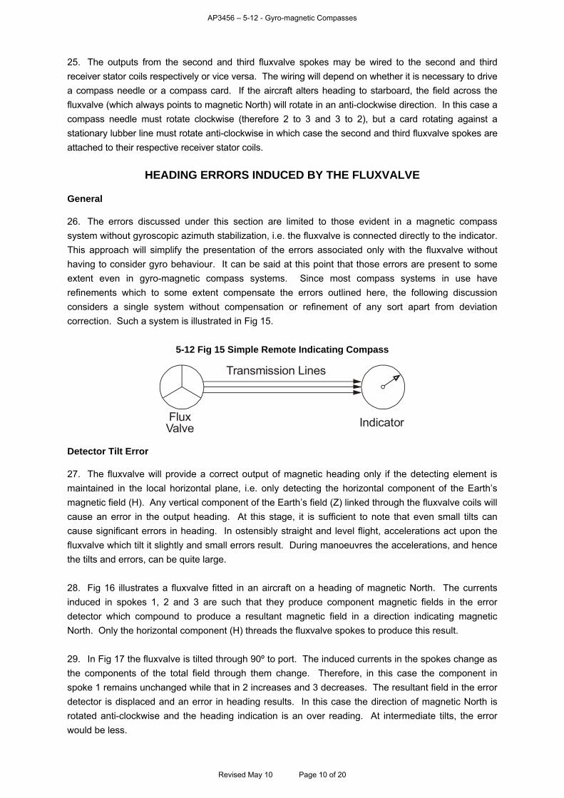
AP3456 – 5-12 - Gyro-magnetic Compasses
25. The outputs from the second and third fluxvalve spokes may be wired to the second and third receiver stator coils respectively or vice versa. The wiring will depend on whether it is necessary to drive a compass needle or a compass card. If the aircraft alters heading to starboard, the field across the fluxvalve (which always points to magnetic North) will rotate in an anti-clockwise direction. In this case a compass needle must rotate clockwise (therefore 2 to 3 and 3 to 2), but a card rotating against a stationary lubber line must rotate anti-clockwise in which case the second and third fluxvalve spokes are attached to their respective receiver stator coils.
HEADING ERRORS INDUCED BY THE FLUXVALVE General 26. The errors discussed under this section are limited to those evident in a magnetic compass system without gyroscopic azimuth stabilization, i.e. the fluxvalve is connected directly to the indicator. This approach will simplify the presentation of the errors associated only with the fluxvalve without having to consider gyro behaviour. It can be said at this point that those errors are present to some extent even in gyro-magnetic compass systems. Since most compass systems in use have refinements which to some extent compensate the errors outlined here, the following discussion considers a single system without compensation or refinement of any sort apart from deviation correction. Such a system is illustrated in Fig 15.
5-12 Fig 15 Simple Remote Indicating Compass
Transmission Lines
FluxValve Indicator
Detector Tilt Error 27. The fluxvalve will provide a correct output of magnetic heading only if the detecting element is maintained in the local horizontal plane, i.e. only detecting the horizontal component of the Earth’s magnetic field (H). Any vertical component of the Earth’s field (Z) linked through the fluxvalve coils will cause an error in the output heading. At this stage, it is sufficient to note that even small tilts can cause significant errors in heading. In ostensibly straight and level flight, accelerations act upon the fluxvalve which tilt it slightly and small errors result. During manoeuvres the accelerations, and hence the tilts and errors, can be quite large. 28. Fig 16 illustrates a fluxvalve fitted in an aircraft on a heading of magnetic North. The currents induced in spokes 1, 2 and 3 are such that they produce component magnetic fields in the error detector which compound to produce a resultant magnetic field in a direction indicating magnetic North. Only the horizontal component (H) threads the fluxvalve spokes to produce this result. 29. In Fig 17 the fluxvalve is tilted through 90º to port. The induced currents in the spokes change as the components of the total field through them change. Therefore, in this case the component in spoke 1 remains unchanged while that in 2 increases and 3 decreases. The resultant field in the error detector is displaced and an error in heading results. In this case the direction of magnetic North is rotated anti-clockwise and the heading indication is an over reading. At intermediate tilts, the error would be less.
Revised May 10 Page 10 of 20

AP3456 – 5-12 - Gyro-magnetic Compasses
5-12 Fig 16 Indication of Magnetic North
1 2
3
Z
HN(M)
N(M)
Plan Viewof Detector1
23
1
3 2
(N)Indicated Components
Received at ErrorDetector
5-12 Fig 17 Effect of a Gross Tilt to Port
N(M)H
H
Z
Dip
Z
1
2
3
1
Plan Viewof Detector
3(N)Indicated
1
23
ComponentsReceived at ErrorDetector
(N) M
2
30. The error also depends on magnetic dip for, if the case at Fig 17 is repeated with a different dip, the components threading the spokes will alter. In Fig 18, the dip is increased, thereby increasing the error and reversing one component in this particular case.
5-12 Fig 18 Effect of Change of Dip
N(M)H
Z
1
2
3
1
Plan Viewof Detector
3
1
23
ComponentsReceived at ErrorDetector
(N) M
2Dip
Z
H
(N)Indicated
Revised May 10 Page 11 of 20

AP3456 – 5-12 - Gyro-magnetic Compasses
31. The direction of tilt relative to the total field is also important. Fig 19 shows how a tilt in the direction of the total field may produce no error. In this case, the flux flow through each spoke changes but the proportion of one to the other remains unchanged. The intensity of the resultant field increases but the direction remains the same. A second case exists in which the tilt is in the opposite sense as in Fig 20. Here, if the tilt exceeds (90º – dip), the flux flow in each spoke is reversed and the error is 180º.
5-12 Fig 19 Effect of Direction of Tilt
N(M)H
Z
2
1
Plan Viewof Detector
3
(N)Indicated
1
23
ComponentsReceived at ErrorDetector
(N) M
21
3
5-12 Fig 20 Tilt Exceeds (90º –Dip)
N(M)H
Z
1
2
3
1Plan Viewof Detector
3
(N) Indicated
1
23
ComponentsReceived at ErrorDetector
(N) M
2
32. Therefore, the error produced by tilting depends on the following factors:
a. Angle of tilt
b. Direction of tilt.
c. Magnetic dip () Typical values of the error in the fluxvalve output are shown against the direction of the axis of tilt for various values of tilt in Fig 21. In general, the bigger the tilt and the dip, the larger the error. Gross errors occur when tilt is greater than (90º due to field reversal (see para 31).
Revised May 10 Page 12 of 20
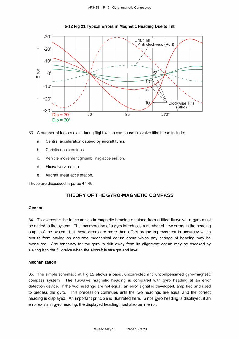
AP3456 – 5-12 - Gyro-magnetic Compasses
5-12 Fig 21 Typical Errors in Magnetic Heading Due to Tilt
-30°
-20°
-10°
+10°
+20°
+30°
0°
90° 180°
10°
10°
270°
5°
10 TiltAnti-clockwise (Port)
°
Dip = 70°Dip = 30°
5°
Clockwise Tilts(Stbd)
Err
or
33. A number of factors exist during flight which can cause fluxvalve tilts; these include:
a. Central acceleration caused by aircraft turns.
b. Coriolis accelerations.
c. Vehicle movement (rhumb line) acceleration.
d. Fluxvalve vibration.
e. Aircraft linear acceleration.
These are discussed in paras 44-49.
THEORY OF THE GYRO-MAGNETIC COMPASS General 34. To overcome the inaccuracies in magnetic heading obtained from a tilted fluxvalve, a gyro must be added to the system. The incorporation of a gyro introduces a number of new errors in the heading output of the system, but these errors are more than offset by the improvement in accuracy which results from having an accurate mechanical datum about which any change of heading may be measured. Any tendency for the gyro to drift away from its alignment datum may be checked by slaving it to the fluxvalve when the aircraft is straight and level. Mechanization 35. The simple schematic at Fig 22 shows a basic, uncorrected and uncompensated gyro-magnetic compass system. The fluxvalve magnetic heading is compared with gyro heading at an error detection device. If the two headings are not equal, an error signal is developed, amplified and used to precess the gyro. This precession continues until the two headings are equal and the correct heading is displayed. An important principle is illustrated here. Since gyro heading is displayed, if an error exists in gyro heading, the displayed heading must also be in error.
Revised May 10 Page 13 of 20
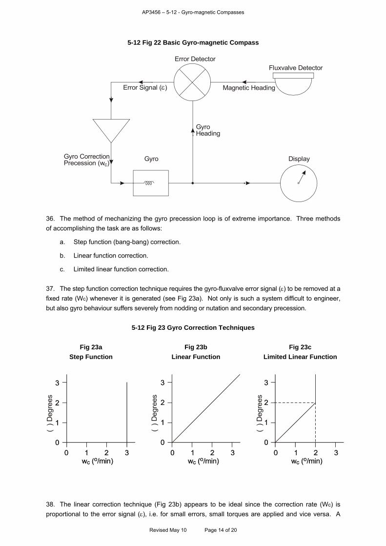
AP3456 – 5-12 - Gyro-magnetic Compasses
5-12 Fig 22 Basic Gyro-magnetic Compass
Error DetectorFluxvalve Detector
Magnetic Heading
GyroHeading
Gyro Display
Error Signal ( )
Gyro CorrectionPrecession (w )c
36. The method of mechanizing the gyro precession loop is of extreme importance. Three methods of accomplishing the task are as follows:
a. Step function (bang-bang) correction.
b. Linear function correction.
c. Limited linear function correction. 37. The step function correction technique requires the gyro-fluxvalve error signal () to be removed at a fixed rate (Wc) whenever it is generated (see Fig 23a). Not only is such a system difficult to engineer, but also gyro behaviour suffers severely from nodding or nutation and secondary precession.
5-12 Fig 23 Gyro Correction Techniques
Fig 23a Step Function
Fig 23b
Linear Function
Fig 23c Limited Linear Function
00
11
22
33
00 11 22 33w ( /min)c ow ( /min)c o
() D
egre
es
00 11 22 33w ( /min)c ow ( /min)c o
00
11
22
33
() D
egre
es
00 11 22 33w ( /min)c ow ( /min)c o
00
11
22
33
() D
egre
es
38. The linear correction technique (Fig 23b) appears to be ideal since the correction rate (Wc) is proportional to the error signal (), i.e. for small errors, small torques are applied and vice versa. A
Revised May 10 Page 14 of 20
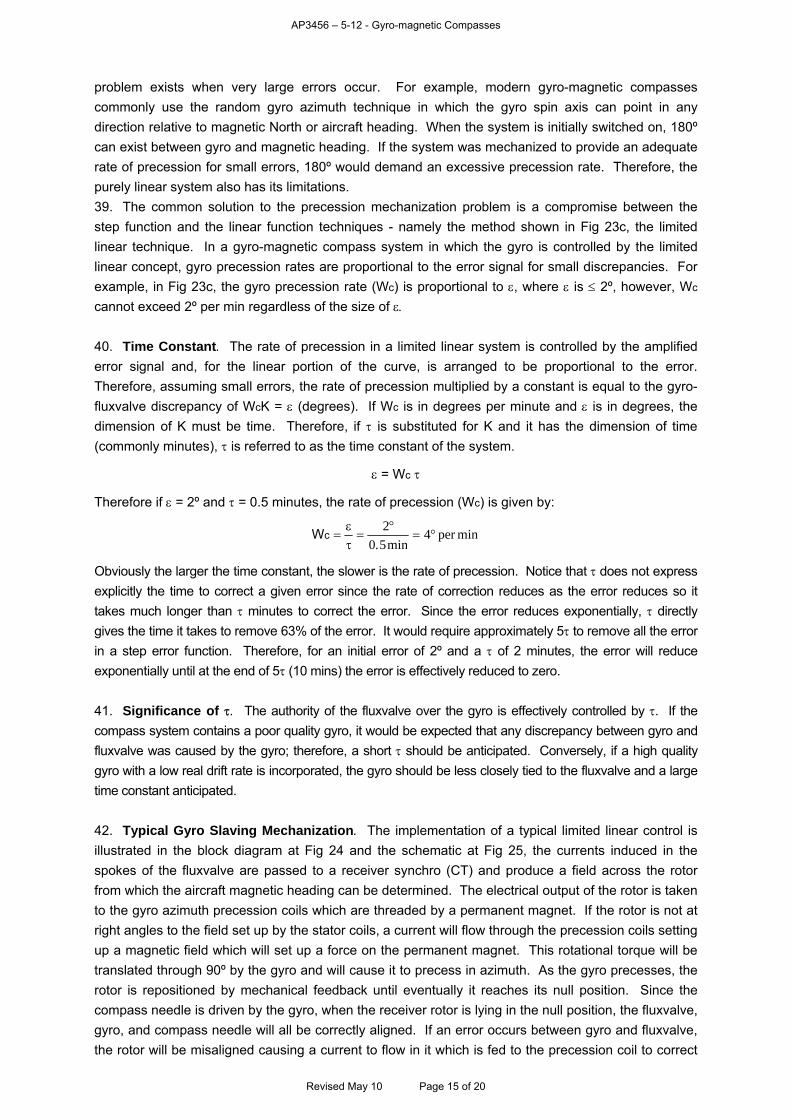
AP3456 – 5-12 - Gyro-magnetic Compasses
problem exists when very large errors occur. For example, modern gyro-magnetic compasses commonly use the random gyro azimuth technique in which the gyro spin axis can point in any direction relative to magnetic North or aircraft heading. When the system is initially switched on, 180º can exist between gyro and magnetic heading. If the system was mechanized to provide an adequate rate of precession for small errors, 180º would demand an excessive precession rate. Therefore, the purely linear system also has its limitations. 39. The common solution to the precession mechanization problem is a compromise between the step function and the linear function techniques - namely the method shown in Fig 23c, the limited linear technique. In a gyro-magnetic compass system in which the gyro is controlled by the limited linear concept, gyro precession rates are proportional to the error signal for small discrepancies. For example, in Fig 23c, the gyro precession rate (Wc) is proportional to , where is 2º, however, Wc cannot exceed 2º per min regardless of the size of 40. Time Constant. The rate of precession in a limited linear system is controlled by the amplified error signal and, for the linear portion of the curve, is arranged to be proportional to the error. Therefore, assuming small errors, the rate of precession multiplied by a constant is equal to the gyro-fluxvalve discrepancy of WcK = (degrees). If Wc is in degrees per minute and is in degrees, the dimension of K must be time. Therefore, if is substituted for K and it has the dimension of time (commonly minutes), is referred to as the time constant of the system.
= Wc
Therefore if = 2º and = 0.5 minutes, the rate of precession (Wc) is given by:
Wc
2
0 54
. minminper
Obviously the larger the time constant, the slower is the rate of precession. Notice that does not express explicitly the time to correct a given error since the rate of correction reduces as the error reduces so it takes much longer than minutes to correct the error. Since the error reduces exponentially, directly gives the time it takes to remove 63% of the error. It would require approximately 5 to remove all the error in a step error function. Therefore, for an initial error of 2º and a of 2 minutes, the error will reduce exponentially until at the end of 5 (10 mins) the error is effectively reduced to zero. 41. Significance of . The authority of the fluxvalve over the gyro is effectively controlled by . If the compass system contains a poor quality gyro, it would be expected that any discrepancy between gyro and fluxvalve was caused by the gyro; therefore, a short should be anticipated. Conversely, if a high quality gyro with a low real drift rate is incorporated, the gyro should be less closely tied to the fluxvalve and a large time constant anticipated. 42. Typical Gyro Slaving Mechanization. The implementation of a typical limited linear control is illustrated in the block diagram at Fig 24 and the schematic at Fig 25, the currents induced in the spokes of the fluxvalve are passed to a receiver synchro (CT) and produce a field across the rotor from which the aircraft magnetic heading can be determined. The electrical output of the rotor is taken to the gyro azimuth precession coils which are threaded by a permanent magnet. If the rotor is not at right angles to the field set up by the stator coils, a current will flow through the precession coils setting up a magnetic field which will set up a force on the permanent magnet. This rotational torque will be translated through 90º by the gyro and will cause it to precess in azimuth. As the gyro precesses, the rotor is repositioned by mechanical feedback until eventually it reaches its null position. Since the compass needle is driven by the gyro, when the receiver rotor is lying in the null position, the fluxvalve, gyro, and compass needle will all be correctly aligned. If an error occurs between gyro and fluxvalve, the rotor will be misaligned causing a current to flow in it which is fed to the precession coil to correct
Revised May 10 Page 15 of 20
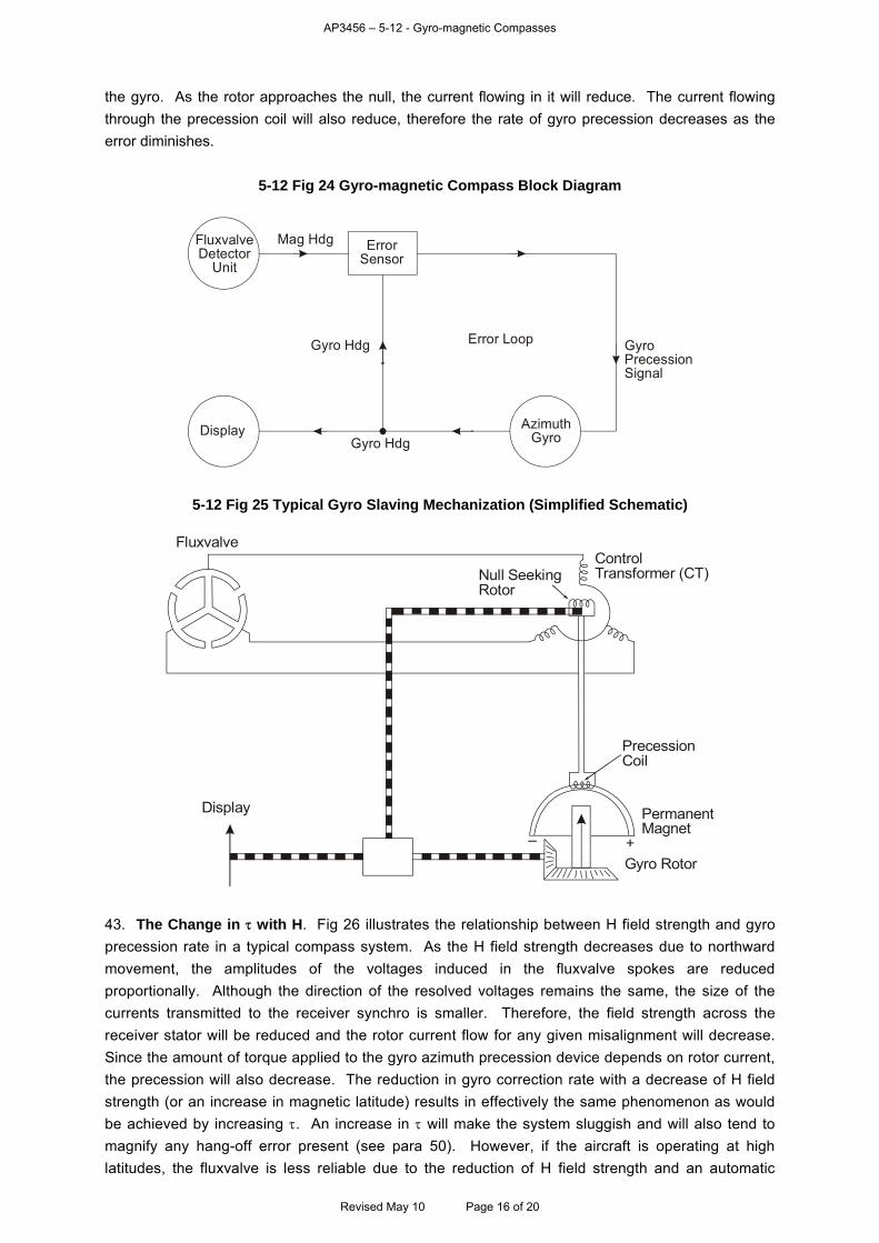
AP3456 – 5-12 - Gyro-magnetic Compasses
the gyro. As the rotor approaches the null, the current flowing in it will reduce. The current flowing through the precession coil will also reduce, therefore the rate of gyro precession decreases as the error diminishes.
5-12 Fig 24 Gyro-magnetic Compass Block Diagram
FluxvalveDetector
Unit
Mag Hdg ErrorSensor
Gyro Hdg
DisplayGyro Hdg
AzimuthGyro
GyroPrecessionSignal
Error Loop
5-12 Fig 25 Typical Gyro Slaving Mechanization (Simplified Schematic)
Fluxvalve
Null SeekingRotor
ControlTransformer (CT)
PrecessionCoil
PermanentMagnet
+–Gyro Rotor
Display
43. The Change in with H. Fig 26 illustrates the relationship between H field strength and gyro precession rate in a typical compass system. As the H field strength decreases due to northward movement, the amplitudes of the voltages induced in the fluxvalve spokes are reduced proportionally. Although the direction of the resolved voltages remains the same, the size of the currents transmitted to the receiver synchro is smaller. Therefore, the field strength across the receiver stator will be reduced and the rotor current flow for any given misalignment will decrease. Since the amount of torque applied to the gyro azimuth precession device depends on rotor current, the precession will also decrease. The reduction in gyro correction rate with a decrease of H field strength (or an increase in magnetic latitude) results in effectively the same phenomenon as would be achieved by increasing . An increase in will make the system sluggish and will also tend to magnify any hang-off error present (see para 50). However, if the aircraft is operating at high latitudes, the fluxvalve is less reliable due to the reduction of H field strength and an automatic
Revised May 10 Page 16 of 20

AP3456 – 5-12 - Gyro-magnetic Compasses
increase of is acceptable. Since changes with H field strength, the H field strength must be quoted with to make meaningful. The H field strength at Greenwich is the common datum quoted by British gyro-magnetic compass system manufacturers.
5-12 Fig 26 Effect of a Change in H on the Time Constant
Fluxvalve
Receiver Stators
ReceiverRotor
GyroPrecessionCoil
PermanentMagnet
Gyro
20° N
H Z
70° N
H Z
Voltages Flying North
Field Field
Current
Torque
Precession
GYRO-MAGNETIC COMPASS SYSTEM ERRORS Fluxvalve Tilt Errors 44. All of the horizontal accelerations which cause fluxvalve tilt can cause heading errors in a simple uncompensated gyro-magnetic compass system. Accelerations are caused by coriolis, vehicle movement (rhumb line), aircraft turns, linear changes of velocity and fluxvalve vibrations. Fluxvalve induced heading errors will not appear immediately in the displayed heading of a gyro-magnetic compass. The rate of heading error incorporation depends on the limiting precession rate and the length of . 45. Turning Error. The amplitude of the displayed heading error in a gyro-magnetic compass due to co-ordinated aircraft turns is less than that shown in Fig 21. Although a high rate of turn in a fast aircraft would show the greatest fluxvalve heading error, little of the error is displayed since the time spent in the turn is minimal. Slow prolonged turns at high speeds generate the greatest errors. The errors decay after level flight is resumed. Fluxvalve induced errors due to tilt can be limited by switching the system to an unslaved directional gyro mode whenever turns are sensed by suitable detection devices.
Revised May 10 Page 17 of 20
AP3456 – 5-12 - Gyro-magnetic Compasses
46. Coriolis Error. An aircraft flying relative to a spherical rotating Earth flies a curved path in space and, in consequence, there will be a central force acting to displace the pendulously suspended fluxvalve. When established on a given heading for approximately 5 the entire error would be included in the gyro-magnetic compass heading display. The error is calculable, depending on groundspeed, latitude, dip and track, and can be compensated automatically. 47. Vehicle Movement Error. Whenever flying a true or magnetic rhumb line the aircraft must turn to maintain a constant track with reference to converging meridians. As with coriolis error, the acceleration displaces the detector from the local horizontal plane and the entire resultant heading error would appear in the displayed heading after about 5. A correction can be applied in a similar manner to the coriolis error. 48. Fluxvalve Vibration. Fluxvalve vibration results in a heading oscillation, the mean of which is not the actual mean heading. Since the gyro slaving loop tends to average fluxvalve headings over a period of time, the gyro would eventually be precessed to the erroneous fluxvalve mean heading. The effect can be limited to small values by careful design of the pendulous detector damping mechanism and through consideration of the location of the detector in the aircraft. Northerly Instability 49. Northerly instability or weaving is a heading oscillation experienced in high speed aircraft attempting to fly straight and level at or near a heading of magnetic North. Starboard bank of the aircraft induces starboard tilt, and this causes an under reading of the heading. Another way of looking at this is to imagine that the magnetic meridian rotates clockwise. Thus, if an aircraft on North banks to starboard to correct a small error, the magnetic meridian rotates in the same direction. The aircraft continues to turn and eventually reaches the false meridian. On levelling out, the fluxvalve senses the true meridian and starts to precess the gyro towards it. The indicated heading changes and the aircraft is banked to port to regain a northerly-indicated heading. This tilts the fluxvalve which rotates the meridian to port. The new false meridian is chased until, upon resuming level flight, the sensor detects the true meridian again and precesses the gyro to starboard. The cyclic pattern is repeated and the amplitude can be as great as 6º. The amplitude of the weave tends to increase with an increase in dip and aircraft velocity, and decreases with an increase in . Weaving can thus be reduced to a certain extent by increasing the time constant of the compass system. However, this leads to a sluggish response and a large hang-off error (para 50). Hang-off Error 50. Gyroscopic drift is a constant source of error signal in a gyro-magnetic compass system, and although it will be compensated for by the precession loop at a rate dependent on , at any given time there must be an increment of error present. This is known variously as hang-off error, stand-off error, or simply as velocity lag. Gyro drift may be due to:
a. Real Drift. Real drift can only be reduced by the incorporation of a high quality azimuth gyro having a low real drift rate.
b. Earth Rate. Apparent azimuth gyro drift due to Earth rotation can be countered by correcting the gyro at a rate of 15 sin lat º/hr. The correction can be supplied through a manually set latitude correction mechanism, automatically from a computer-generated latitude, or through a constantly biased gyro. The latter technique employs a mass imbalance in the gyro which constantly precesses the gyro at a predetermined rate, usually to compensate for an appropriate latitude for the aircraft’s area of operation, say 51 ºN.
Revised May 10 Page 18 of 20
AP3456 – 5-12 - Gyro-magnetic Compasses
c. Transport Wander. To compensate for transport wander due to the convergence of geographic meridians the gyro must be corrected at a rate equal to:
U
60 tan lat º/hr where U = East-West groundspeed
The correction can be applied manually or through a computer using inputs of groundspeed, heading, and latitude. However, although the gyro can be compensated in this way for the apparent change in the direction of geographic North, the output from the fluxvalve is in terms of magnetic North. Therefore, as the aircraft moves over the Earth, there will be a difference between fluxvalve and gyro since the variation is changing (unless the aircraft is flying along an isogonal). To remove this error variation must be applied to the output of the detector unit before the gyro error loop so that both the gyro and fluxvalve give directional information relative to true North. The value of variation can be inserted manually or by means of an automatic variation setting control unit. Failure to update the variation value will result in small hang-off errors.
Gimbal Error 51. When a 2 degree of freedom gyroscope with a horizontal spin axis is both banked and rolled, the outer gimbal must rotate to maintain orientation of the rotor axis, thereby inducing a heading error at the outer gimbal pick-off. The incidence of this error depends upon the angle of bank and the angular difference between the spin axis and the longitudinal axis and as in most systems the spin axis direction is arbitrary relative to North the error is not easily predicted. Transmission Errors 52. Overall system accuracy is lowered by the errors in the synchro systems. Typically, each synchro might be expected to a have an error in the order of 0.1º with an overall system error of perhaps 0.5º. This shows in a compass swing as a D or E error. Compass Swinging Errors 53. It is not possible to obtain absolute accuracy in compass swinging, and even refined methods are considered to be only accurate to 0.2º. Variation and Deviation Errors 54. There are no reliable statistical data on the errors in charted values of variation, but they might be considered to vary between 0.1º and 2º. Over the UK, the uncertainty at height is considered to be within 1º but the value varies both with height and locality. Setting of variation and deviation is likely to be accurate to 0.25º. A Refined Compass System 55. Fig 27 depicts some of the methods of error reduction. Different methods of correction are possible for some of the errors depending on the whims of the individual manufacturer and the users considerations of experience and accuracy. Note that corrections may be made 'up' or 'down' stream of the gyro or a combination of both; there are disadvantages to all approaches.
Revised May 10 Page 19 of 20
AP3456 – 5-12 - Gyro-magnetic Compasses
Revised May 10 Page 20 of 20
5-12 Fig 27 Ideal Gyro-magnetic Compass
Constant
LatLongG/S
Track
Auto Variation
Heading
Earth Rate± Transport Wander
±+
++
–
VerticalGyro
VariableGain
TurnCut-out
DetectorUnit
HeavyDamping
DeviationA to E
CorrectionComputer
Low DriftGyro
Coriolis + Rhumb Line Acceleration
Basic GM Loop
Corrections for Detector TiltCorrections for Hang-off
Other Error Corrections
56. The following description applies to Fig 27:
a. Hang-off. The computer supplies the quantities for Earth rate and meridian convergence to the error detector. Therefore, the rate of gyro drift sensed is reduced considerably and hang-off results from only random drift.
b. Coriolis and Vehicle Movement Accelerations. The corrections for coriolis and vehicle movement are applied at the fluxvalve by reducing or increasing the output from the athwartships spokes.
c. Gimbal Error. Gimbal error is eliminated by the use of a vertical gyro coupled with four-gimbal suspension to keep the azimuth gyro and the azimuth pick-off synchro horizontal.
d. Operation on DG. The fluxvalve monitor and the computer rate of change variation are cut out when on DG. The accuracy of the heading then depends on random drift error, the error in the gyro correction terms and the statistical error ie transmission error.
e. Northerly Instability. Variable gain in the precession amplifier maintains the value of constant, for variable H, thus reducing weaving.
f. Coefficient D and E. A compensation is applied to counter coefficients D and E.
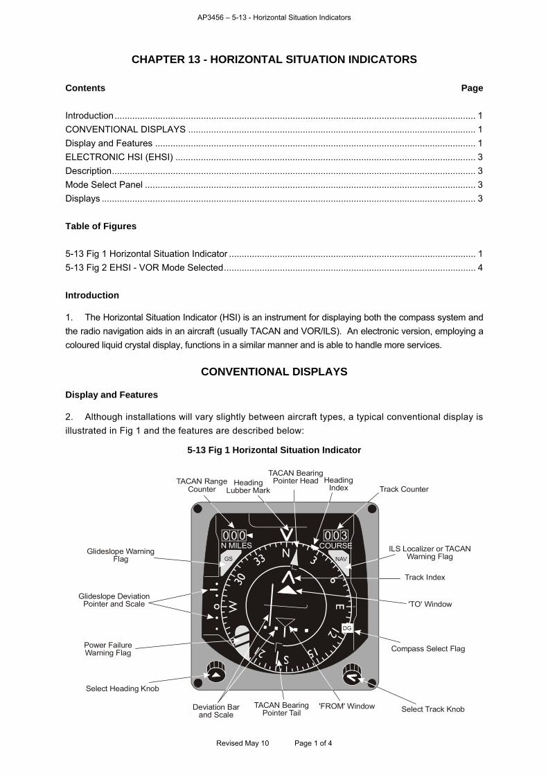
AP3456 – 5-13 - Horizontal Situation Indicators
CHAPTER 13 - HORIZONTAL SITUATION INDICATORS Contents Page Introduction.............................................................................................................................................. 1 CONVENTIONAL DISPLAYS ................................................................................................................. 1 Display and Features .............................................................................................................................. 1 ELECTRONIC HSI (EHSI) ...................................................................................................................... 3 Description............................................................................................................................................... 3 Mode Select Panel .................................................................................................................................. 3 Displays ................................................................................................................................................... 3 Table of Figures 5-13 Fig 1 Horizontal Situation Indicator ................................................................................................. 1 5-13 Fig 2 EHSI - VOR Mode Selected................................................................................................... 4 Introduction 1. The Horizontal Situation Indicator (HSI) is an instrument for displaying both the compass system and the radio navigation aids in an aircraft (usually TACAN and VOR/ILS). An electronic version, employing a coloured liquid crystal display, functions in a similar manner and is able to handle more services.
CONVENTIONAL DISPLAYS Display and Features 2. Although installations will vary slightly between aircraft types, a typical conventional display is illustrated in Fig 1 and the features are described below:
5-13 Fig 1 Horizontal Situation Indicator
NN MILES COURSE
0 030 0 0
GS NAV
DG
TACAN RangeCounter
HeadingLubber Mark
TACAN BearingPointer Head Heading
Index Track Counter
ILS Localizer or TACANWarning Flag
Track Index
'TO' Window
Compass Select Flag
Select Track Knob'FROM' WindowTACAN BearingPointer Tail
Deviation Barand Scale
Select Heading Knob
Power FailureWarning Flag
Glideslope DeviationPointer and Scale
Glideslope WarningFlag
Revised May 10 Page 1 of 4
AP3456 – 5-13 - Horizontal Situation Indicators
a. Heading. Heading is indicated at the top of the display by a rotating compass card moving against a fixed 'V' lubber mark. The card is graduated at 5º intervals and is marked alphanumerically at 30º intervals with the numerical annotations being in tens of degrees.
b. Heading Index. A heading index registers against the outside edge of, and rotates with, the compass card. The index can be manually set relative to the compass card by a select heading knob which is marked with a symbol representing the heading index and is located at the lower left-hand corner of the instrument.
c. Compass Select Flag. When the compass system is set to the directional gyro mode the compass select flag appears with the letters DG displayed.
d. Track Index and Counter. A track index, which is on the centre display assembly, registers against the inside edge of, and rotates with, the compass card. The index can be manually set relative to the compass card by a selector knob at the lower right-hand corner of the instrument. The reciprocal of the track set is indicated by a track index tail on the centre display assembly. A 3-digit display of the selection is given on a track (COURSE) counter at the top right of the display. The selector knob is marked with a symbol representing the track index.
e. Deviation Bar. A deviation bar and a fixed scale of two dots either side of a centre index are on the centre display assembly. The bar moves left or right of the centre index to indicate deviation from the selected track when TACAN or ILS information is selected. The bar indicates the relative position of the chosen track as selected by the track index.
f. TACAN Bearing. The magnetic bearing to a TACAN ground beacon is indicated by a green pointer head when read against the compass card. The tail of the pointer indicates the TACAN radial. The TACAN bearing and radial are also displayed when ILS is selected.
g. To/From Indication. Two triangular indicator windows, 'to' and 'from' are on the centre display assembly. The 'to' window is adjacent to the track index and the 'from' window is adjacent to the tail of the track index. With TACAN selected, a TACAN radial set on the track index and the bearing pointer locked on to a TACAN beacon, a white flag is displayed in the 'to' or 'from' window. The 'to' flag is displayed whenever the bearing from the TACAN is less than 90º from the selected TACAN radial. Conversely the 'from' flag shows white whenever the bearing from the TACAN beacon is 90º or more from the selected TACAN radial.
h. TACAN Range. Range to a TACAN or DME beacon in nautical miles is shown on a 3-digit counter at the upper left corner of the instrument. A yellow bar obscures the counter when range information is invalid. i. Glidepath Deviation Pointer. A pointer to the left of the compass card moves over a fixed vertical scale consisting of two dots above and two dots below a circle (representing the aircraft). The pointer is driven by the ILS equipment and indicates the vertical position of the ILS glidepath relative to the aircraft, eg if the pointer is above the circle the aircraft is below the glidepath.
j. Glidepath Warning. A red flag appears above the glidepath deviation scale when the glidepath information is invalid.
k. ILS Localizer or TACAN Bearing Warning. A red flag appears below the COURSE counter when the ILS localizer or the TACAN bearing information is invalid.
l. Power Failure Warning. An orange flag with black diagonal stripes appears when the power to the HSI has failed or when an invalid signal is transmitted from the compass system.
Revised May 10 Page 2 of 4

AP3456 – 5-13 - Horizontal Situation Indicators
ELECTRONIC HSI (EHSI) Description 3. The EHSI can be configured to provide more information than the HSI and employs a colour active matrix liquid crystal display. It receives inputs from the aircraft compass, TACAN, VOR/ILS and, depending on aircraft fit, UHF and VHF homers and specialist navigational aids. In helicopters, the EHSI is also linked to the hovermeter. Mode Select Panel 4. A mode select panel will be available to each pilot position with buttons for selection of each available feature. A Transfer Mode (TM) switch enables the course selector display of one instrument to be transferred to the other. Therefore, for example, the TACAN radial can be set on one instrument and the ILS QDM on the other. Pushing the TM switch associated with the instrument configured for ILS will transfer the ILS information to the other instrument. Displays 5. In different installations, display colours may vary depending upon which mode is selected. Fig 2 shows a typical instrument in VOR mode. When first switched on or after a power break the EHSI will have no mode indicated in the bottom right hand corner. In most cases, the numbered items described in the key are displayed only when the appropriate inputs are valid. 6. Displays and Controls. Operation of the controls annotated on Fig 2 may depend upon the mode selected. A brief description of each is given below. The relevant Aircrew Manual will set out the precise operation of the system.
a. Heading Select Knob. When enabled by the Heading Select Pushbutton, rotating the Heading Select Knob sets the heading bug. There is a slight ratchet effect to give positive feel. The knob is normally disabled 5 seconds after its last rotation.
b. Heading Select Pushbutton. A positive press of the Heading Select Pushbutton of at least 0.1 sec is required to enable the Heading Select Knob.
c. Track Select Knob. When enabled by the Track Select Pushbutton, rotation of the Track Select Knob allows the track pointer to be set to the required track. Positive feel is given by a slight ratchet effect, one click of the ratchet equating to 1-degree change in selected track. The associated track digital readout (10) follows the pointer setting. The knob is automatically disabled 5 sec after its last rotation.
d. Track Select Pushbutton. A positive press of the Track Select Pushbutton of at least 0.1 sec is required to enable the Heading Select Knob.
e. Aircraft Symbol. The aircraft symbol is always aligned pointing towards the heading lubber line at the top of the instrument. When a navigation mode is active, the symbol represents aircraft orientation against the steering pointer or deviation bar.
f. Integrated Light Sensor. The sensor automatically adjusts the display brightness in daylight. A separate manually operated dimmer sets the brightness for night operations.
g. Mode Displays. The key to Fig 2 describes the numbered indicators shown on the diagram for VOR/ILS mode. In other modes the names, functions and colours of the displayed features may change from those depicted.
h. Functionality. Most coloured symbols are cleared when the service is not activated or the compass input fails. The appropriate Aircrew Manual should be consulted for precise details.
Revised May 10 Page 3 of 4
AP3456 – 5-13 - Horizontal Situation Indicators
Revised May 10 Page 4 of 4
5-13 Fig 2 EHSI - VOR Mode Selected
HDG CRS
IntegratedLight Sensor
Aircraft Symbol
Track Select Knob
Track SelectPushbutton
Heading Select Knob
Heading Select Pushbutton
1. Compass Card. The compass card indicates gyrocompass heading in conjunction with the lubber line (2). The card
rotates clockwise as the aircraft turns left. If the compass fails, the card freezes and a red HDG FAIL caption is superimposed.
2. Lubber Line. The lubber line is the index against which heading is shown on the compass card. 3. Heading Bug. The red heading bug is set by the Heading Select Knob to indicate the required heading. The bug clears if
the compass input fails. 4. Single Bar Pointer (TACAN Bearing). The arrowhead on the green single bar pointer indicates the bearing of the
TACAN station locked on. The pointer clears if a TACAN station is not locked on or if the compass input fails. 5. Double Bar Pointer (VOR Bearing). The arrowhead on the purple double bar pointer indicates the bearing of the VOR
station locked on. The pointer clears if the VOR receiver is not locked to a station or if the compass input fails. 6. TACAN/DME Range Readout. The TACAN/DME readout is a digital display which shows the slant range to a locked on
TACAN or DME station. When not locked on, the display shows 4 dashes. 7. Wind Direction Indicator. The direction from which the wind is blowing is shown by a red diamond. The diamond clears
when there is no source data or if the compass input fails. 8. Wind Speed Readout. Wind speed to the nearest knot is shown by a red digital display. The display clears when there
is no source data or if the compass input fails. 9. Track (Course) Pointer. The cross end of the purple Track Pointer indicates the track selected. 10. Selected Track (Course) Readout. The readout shows the track selected on the Track Pointer (9). 11. Track (Course) Deviation Bar. The purple deviation bar shows track deviation left or right of that selected on the Track
Pointer (9). To return to track, the aircraft should be turned towards the bar until the bar centralizes and then on to a new heading to keep the bar in the centre.
12. Track (Course) Deviation Scale. The scale comprises two white dots to the left and right of the centre of the Track Pointer
(9) creating a scale over which the Track Deviation Bar (11) moves. The outside dots represent full-scale deflection (±10°), the intermediate dots indication ±5°.
13. 'To' Flag. The 'To' Flag is a white arrowhead which is displayed until the aircraft passes over or abeam the locked
station, after which it is replaced by the 'From' Flag. 14. 'From' Flag. The 'From' Flag is a white dotted arrowhead which is displayed once the aircraft has passed over or abeam
the locked station. 15. Mode Annunciator. The selected mode (VOR in the example) is displayed provided the service is on and functioning.
AP3456 – 5-14 - Datum Compasses
CHAPTER 14 - DATUM COMPASSES Contents Page Introduction.............................................................................................................................................. 1 THE MEDIUM LANDING COMPASS...................................................................................................... 2 Description............................................................................................................................................... 2 Operation................................................................................................................................................. 2 THE WATTS DATUM COMPASS MK1A................................................................................................ 3 Principle................................................................................................................................................... 3 Description............................................................................................................................................... 3 Operation................................................................................................................................................. 6 THE PRECISE HEADING TEST SET..................................................................................................... 9 Introduction.............................................................................................................................................. 9 Controls and Indicators ......................................................................................................................... 10 Calibration ............................................................................................................................................. 11 Table of Figures 5-14 Fig 1 Medium Landing Compass .................................................................................................... 2 5-14 Fig 2 General View of the Watts Datum Compass on its Tripod .................................................... 3 5-14 Fig 3 Watts Datum Instrument – Compass-related Features ......................................................... 4 5-14 Fig 4 Schematic Diagram of Compass Box (side view).................................................................. 4 5-14 Fig 5 Clamps and Sighting/Reading Windows................................................................................ 5 5-14 Fig 6 View through Compass Viewing Window .............................................................................. 5 5-14 Fig 7 Example View through the Sighting Telescope ..................................................................... 5 5-14 Fig 8 Reading the bearing on the Azimuth Circle through the Microscope .................................... 6 5-14 Fig 9 Tripod Set-up ......................................................................................................................... 6 5-14 Fig 10 Instrument Set-up................................................................................................................. 7 5-14 Fig 11 Telescope aligned on Datum Line ....................................................................................... 7 5-14 Fig 12 Azimuth Circle Indexed ........................................................................................................ 8 5-14 Fig 13 Compass Aligned with Magnetic North................................................................................ 8 5-14 Fig 14 Sighting Telescope accurately aligned on Aircraft Datum ................................................... 9 5-14 Fig 15 Precise Heading Test Set .................................................................................................. 10 Introduction 1. In order to calibrate an aircraft compass system it is necessary to have an accurate heading datum. A Medium Landing Compass provides a sufficiently accurate datum for simple aircraft compasses. However, where the aircraft compass output is used as an input to a navigation system, the heading datum is provided by the more accurate Watts Datum Compass. In order to overcome the accuracy limitations of the aircraft compass display, the aircraft compass heading is read with the aid of a Precise Heading Test Set (PHTS). This permits the aircraft heading to be recorded to an accuracy of 0.05º. This chapter will describe the Medium Landing Compass, the Watts Datum Compass Mk1A and the PHTS.
Revised May 10 Page 1 of 11
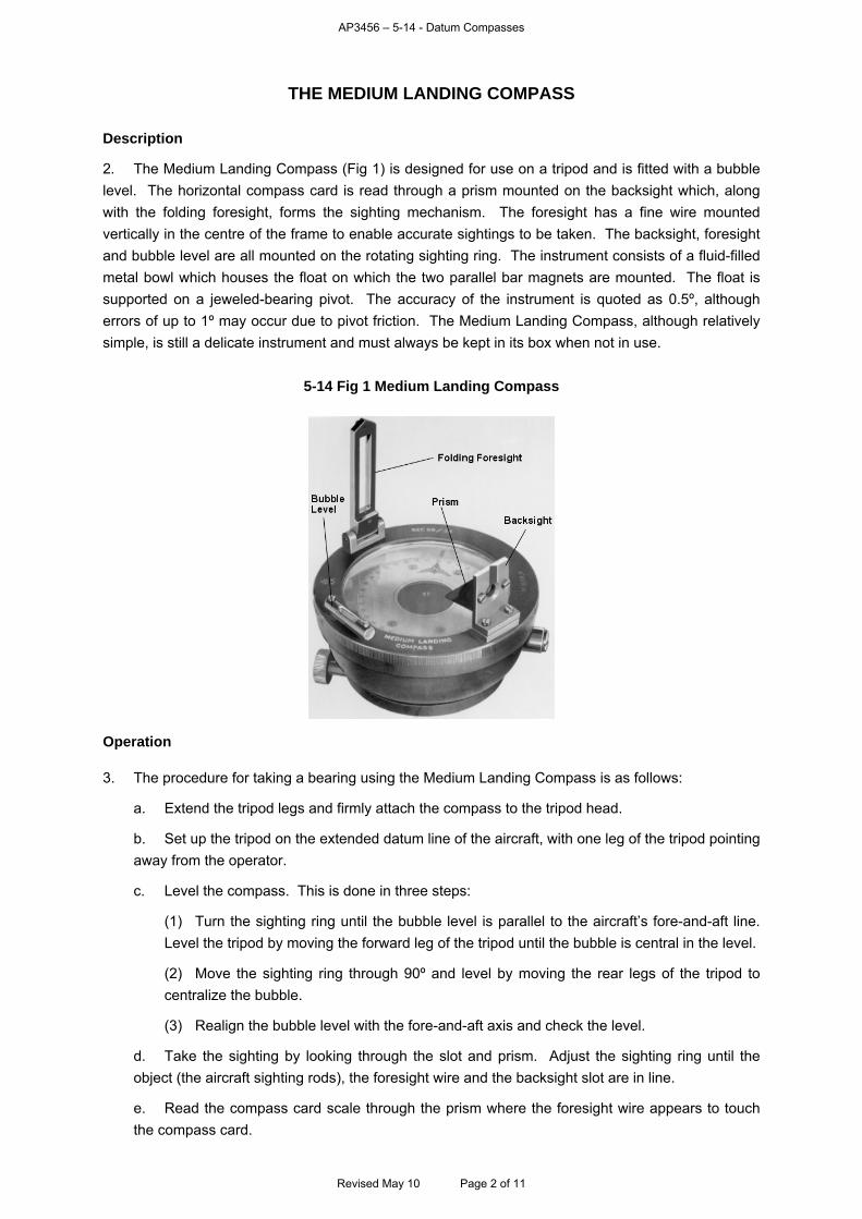
AP3456 – 5-14 - Datum Compasses
THE MEDIUM LANDING COMPASS Description
2. The Medium Landing Compass (Fig 1) is designed for use on a tripod and is fitted with a bubble level. The horizontal compass card is read through a prism mounted on the backsight which, along with the folding foresight, forms the sighting mechanism. The foresight has a fine wire mounted vertically in the centre of the frame to enable accurate sightings to be taken. The backsight, foresight and bubble level are all mounted on the rotating sighting ring. The instrument consists of a fluid-filled metal bowl which houses the float on which the two parallel bar magnets are mounted. The float is supported on a jeweled-bearing pivot. The accuracy of the instrument is quoted as 0.5º, although errors of up to 1º may occur due to pivot friction. The Medium Landing Compass, although relatively simple, is still a delicate instrument and must always be kept in its box when not in use.
5-14 Fig 1 Medium Landing Compass
Operation 3. The procedure for taking a bearing using the Medium Landing Compass is as follows:
a. Extend the tripod legs and firmly attach the compass to the tripod head.
b. Set up the tripod on the extended datum line of the aircraft, with one leg of the tripod pointing away from the operator.
c. Level the compass. This is done in three steps:
(1) Turn the sighting ring until the bubble level is parallel to the aircraft’s fore-and-aft line. Level the tripod by moving the forward leg of the tripod until the bubble is central in the level.
(2) Move the sighting ring through 90º and level by moving the rear legs of the tripod to centralize the bubble.
(3) Realign the bubble level with the fore-and-aft axis and check the level.
d. Take the sighting by looking through the slot and prism. Adjust the sighting ring until the object (the aircraft sighting rods), the foresight wire and the backsight slot are in line.
e. Read the compass card scale through the prism where the foresight wire appears to touch the compass card.
Revised May 10 Page 2 of 11
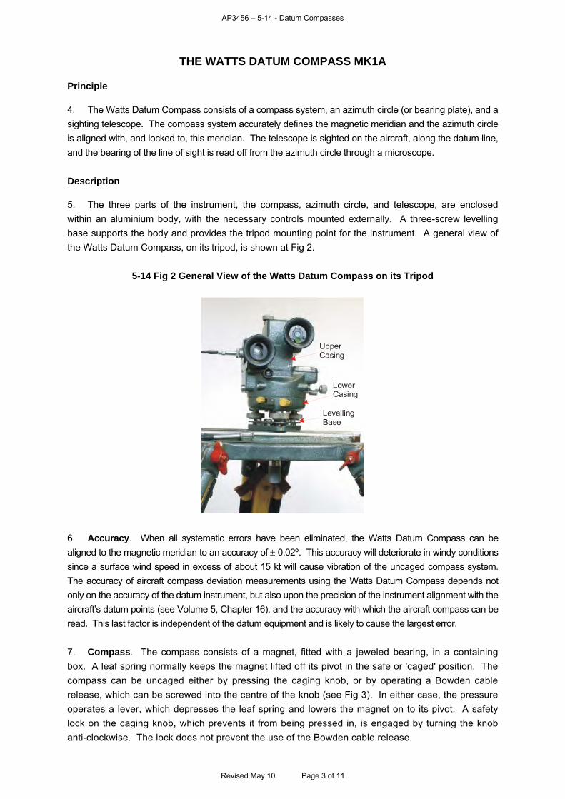
AP3456 – 5-14 - Datum Compasses
THE WATTS DATUM COMPASS MK1A Principle 4. The Watts Datum Compass consists of a compass system, an azimuth circle (or bearing plate), and a sighting telescope. The compass system accurately defines the magnetic meridian and the azimuth circle is aligned with, and locked to, this meridian. The telescope is sighted on the aircraft, along the datum line, and the bearing of the line of sight is read off from the azimuth circle through a microscope. Description 5. The three parts of the instrument, the compass, azimuth circle, and telescope, are enclosed within an aluminium body, with the necessary controls mounted externally. A three-screw levelling base supports the body and provides the tripod mounting point for the instrument. A general view of the Watts Datum Compass, on its tripod, is shown at Fig 2.
5-14 Fig 2 General View of the Watts Datum Compass on its Tripod
UpperCasing
LowerCasing
LevellingBase
6. Accuracy. When all systematic errors have been eliminated, the Watts Datum Compass can be aligned to the magnetic meridian to an accuracy of 0.02º. This accuracy will deteriorate in windy conditions since a surface wind speed in excess of about 15 kt will cause vibration of the uncaged compass system. The accuracy of aircraft compass deviation measurements using the Watts Datum Compass depends not only on the accuracy of the datum instrument, but also upon the precision of the instrument alignment with the aircraft’s datum points (see Volume 5, Chapter 16), and the accuracy with which the aircraft compass can be read. This last factor is independent of the datum equipment and is likely to cause the largest error. 7. Compass. The compass consists of a magnet, fitted with a jeweled bearing, in a containing box. A leaf spring normally keeps the magnet lifted off its pivot in the safe or 'caged' position. The compass can be uncaged either by pressing the caging knob, or by operating a Bowden cable release, which can be screwed into the centre of the knob (see Fig 3). In either case, the pressure operates a lever, which depresses the leaf spring and lowers the magnet on to its pivot. A safety lock on the caging knob, which prevents it from being pressed in, is engaged by turning the knob anti-clockwise. The lock does not prevent the use of the Bowden cable release.
Revised May 10 Page 3 of 11
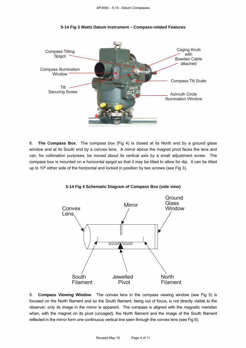
AP3456 – 5-14 - Datum Compasses
5-14 Fig 3 Watts Datum Instrument – Compass-related Features
Compass TiltingSpigot
Compass IlluminationWindow
Compass Tilt Scale
Azimuth CircleIllumination Window
TiltSecuring Screw
Caging Knobwith
Bowden Cableattached
8. The Compass Box. The compass box (Fig 4) is closed at its North end by a ground glass window and at its South end by a convex lens. A mirror above the magnet pivot faces the lens and can, for collimation purposes, be moved about its vertical axis by a small adjustment screw. The compass box is mounted on a horizontal spigot so that it may be tilted to allow for dip. It can be tilted up to 10º either side of the horizontal and locked in position by two screws (see Fig 3).
5-14 Fig 4 Schematic Diagram of Compass Box (side view)
ConvexLens
MirrorGroundGlassWindow
NorthFilament
Jewelled Pivot
SouthFilament
9. Compass Viewing Window. The convex lens in the compass viewing window (see Fig 5) is focused on the North filament and so the South filament, being out of focus, is not directly visible to the observer; only its image in the mirror is apparent. The compass is aligned with the magnetic meridian when, with the magnet on its pivot (uncaged), the North filament and the image of the South filament reflected in the mirror form one continuous vertical line seen through the convex lens (see Fig 6).
Revised May 10 Page 4 of 11
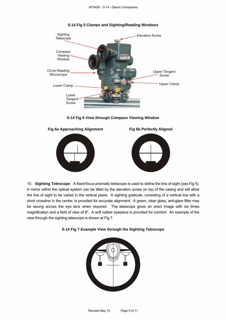
AP3456 – 5-14 - Datum Compasses
5-14 Fig 5 Clamps and Sighting/Reading Windows
SightingTelescope
CompassViewingWindow
Circle ReadingMicroscope
Upper TangentScrew
Upper ClampLower Clamp
LowerTangentScrew
Elevation Screw
5-14 Fig 6 View through Compass Viewing Window
Fig 6a Approaching Alignment Fig 6b Perfectly Aligned
10. Sighting Telescope. A fixed-focus prismatic telescope is used to define the line of sight (see Fig 5). A mirror within the optical system can be tilted by the elevation screw on top of the casing and will allow the line of sight to be varied in the vertical plane. A sighting graticule, consisting of a vertical line with a short crossline in the centre, is provided for accurate alignment. A green, clear glass, anti-glare filter may be swung across the eye lens when required. The telescope gives an erect image with six times magnification and a field of view of 8º. A soft rubber eyepiece is provided for comfort. An example of the view through the sighting telescope is shown at Fig 7.
5-14 Fig 7 Example View through the Sighting Telescope
Revised May 10 Page 5 of 11
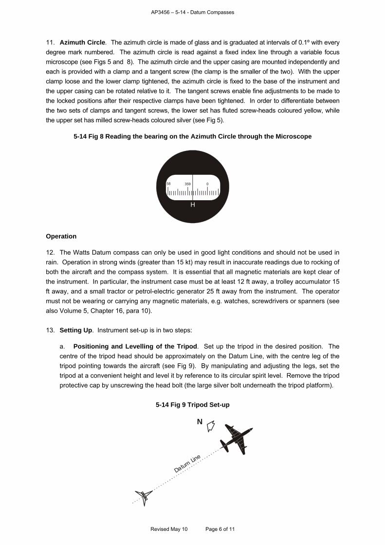
AP3456 – 5-14 - Datum Compasses
11. Azimuth Circle. The azimuth circle is made of glass and is graduated at intervals of 0.1º with every degree mark numbered. The azimuth circle is read against a fixed index line through a variable focus microscope (see Figs 5 and 8). The azimuth circle and the upper casing are mounted independently and each is provided with a clamp and a tangent screw (the clamp is the smaller of the two). With the upper clamp loose and the lower clamp tightened, the azimuth circle is fixed to the base of the instrument and the upper casing can be rotated relative to it. The tangent screws enable fine adjustments to be made to the locked positions after their respective clamps have been tightened. In order to differentiate between the two sets of clamps and tangent screws, the lower set has fluted screw-heads coloured yellow, while the upper set has milled screw-heads coloured silver (see Fig 5).
5-14 Fig 8 Reading the bearing on the Azimuth Circle through the Microscope
35958 0
H
Operation 12. The Watts Datum compass can only be used in good light conditions and should not be used in rain. Operation in strong winds (greater than 15 kt) may result in inaccurate readings due to rocking of both the aircraft and the compass system. It is essential that all magnetic materials are kept clear of the instrument. In particular, the instrument case must be at least 12 ft away, a trolley accumulator 15 ft away, and a small tractor or petrol-electric generator 25 ft away from the instrument. The operator must not be wearing or carrying any magnetic materials, e.g. watches, screwdrivers or spanners (see also Volume 5, Chapter 16, para 10). 13. Setting Up. Instrument set-up is in two steps:
a. Positioning and Levelling of the Tripod. Set up the tripod in the desired position. The centre of the tripod head should be approximately on the Datum Line, with the centre leg of the tripod pointing towards the aircraft (see Fig 9). By manipulating and adjusting the legs, set the tripod at a convenient height and level it by reference to its circular spirit level. Remove the tripod protective cap by unscrewing the head bolt (the large silver bolt underneath the tripod platform).
5-14 Fig 9 Tripod Set-up
N
Datum Line
Revised May 10 Page 6 of 11
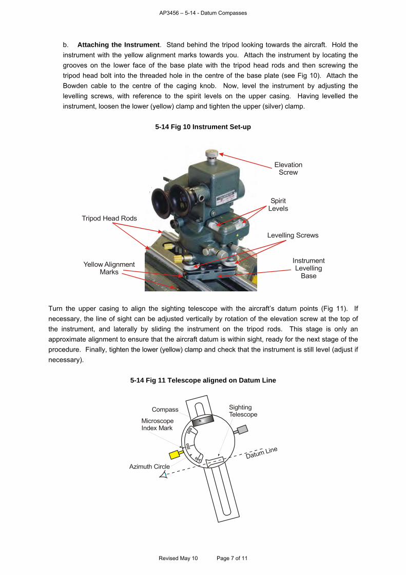
AP3456 – 5-14 - Datum Compasses
b. Attaching the Instrument. Stand behind the tripod looking towards the aircraft. Hold the instrument with the yellow alignment marks towards you. Attach the instrument by locating the grooves on the lower face of the base plate with the tripod head rods and then screwing the tripod head bolt into the threaded hole in the centre of the base plate (see Fig 10). Attach the Bowden cable to the centre of the caging knob. Now, level the instrument by adjusting the levelling screws, with reference to the spirit levels on the upper casing. Having levelled the instrument, loosen the lower (yellow) clamp and tighten the upper (silver) clamp.
5-14 Fig 10 Instrument Set-up
Tripod Head Rods
SpiritLevels
Levelling Screws
InstrumentLevelling
Base
Yellow AlignmentMarks
ElevationScrew
Turn the upper casing to align the sighting telescope with the aircraft’s datum points (Fig 11). If necessary, the line of sight can be adjusted vertically by rotation of the elevation screw at the top of the instrument, and laterally by sliding the instrument on the tripod rods. This stage is only an approximate alignment to ensure that the aircraft datum is within sight, ready for the next stage of the procedure. Finally, tighten the lower (yellow) clamp and check that the instrument is still level (adjust if necessary).
5-14 Fig 11 Telescope aligned on Datum Line
000
350
340
Azimuth Circle
MicroscopeIndex Mark
Sighting Telescope
Datum Line
Compass
Revised May 10 Page 7 of 11
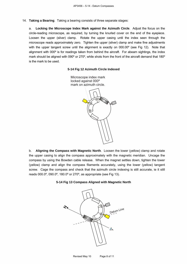
AP3456 – 5-14 - Datum Compasses
14. Taking a Bearing. Taking a bearing consists of three separate stages:
a. Locking the Microscope Index Mark against the Azimuth Circle. Adjust the focus on the circle-reading microscope, as required, by turning the knurled cover on the end of the eyepiece. Loosen the upper (silver) clamp. Rotate the upper casing until the index seen through the microscope reads approximately zero. Tighten the upper (silver) clamp and make fine adjustments with the upper tangent screw until the alignment is exactly on 000.00º (see Fig 12). Note that alignment with 000º is for readings taken from behind the aircraft. For abeam sightings, the index mark should be aligned with 090º or 270º, while shots from the front of the aircraft demand that 180º is the mark to be used.
5-14 Fig 12 Azimuth Circle Indexed
000
350
010
Microscope index marklocked against 000ºmark on azimuth circle.
b. Aligning the Compass with Magnetic North. Loosen the lower (yellow) clamp and rotate the upper casing to align the compass approximately with the magnetic meridian. Uncage the compass by using the Bowden cable release. When the magnet settles down, tighten the lower (yellow) clamp and align the compass filaments accurately, using the lower (yellow) tangent screw. Cage the compass and check that the azimuth circle indexing is still accurate, ie it still reads 000.0º, 090.0º, 180.0º or 270º, as appropriate (see Fig 13).
5-14 Fig 13 Compass Aligned with Magnetic North
000
350
010
Datum LineN
Revised May 10 Page 8 of 11
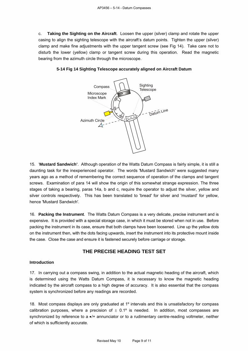
AP3456 – 5-14 - Datum Compasses
c. Taking the Sighting on the Aircraft. Loosen the upper (silver) clamp and rotate the upper casing to align the sighting telescope with the aircraft’s datum points. Tighten the upper (silver) clamp and make fine adjustments with the upper tangent screw (see Fig 14). Take care not to disturb the lower (yellow) clamp or tangent screw during this operation. Read the magnetic bearing from the azimuth circle through the microscope.
5-14 Fig 14 Sighting Telescope accurately aligned on Aircraft Datum
000
350
340
Azimuth Circle
MicroscopeIndex Mark
Sighting Telescope
Datum Line
Compass
15. ‘Mustard Sandwich’. Although operation of the Watts Datum Compass is fairly simple, it is still a daunting task for the inexperienced operator. The words 'Mustard Sandwich' were suggested many years ago as a method of remembering the correct sequence of operation of the clamps and tangent screws. Examination of para 14 will show the origin of this somewhat strange expression. The three stages of taking a bearing, paras 14a, b and c, require the operator to adjust the silver, yellow and silver controls respectively. This has been translated to 'bread' for silver and 'mustard' for yellow, hence 'Mustard Sandwich'. 16. Packing the Instrument. The Watts Datum Compass is a very delicate, precise instrument and is expensive. It is provided with a special storage case, in which it must be stored when not in use. Before packing the instrument in its case, ensure that both clamps have been loosened. Line up the yellow dots on the instrument then, with the dots facing upwards, insert the instrument into its protective mount inside the case. Close the case and ensure it is fastened securely before carriage or storage.
THE PRECISE HEADING TEST SET Introduction 17. In carrying out a compass swing, in addition to the actual magnetic heading of the aircraft, which is determined using the Watts Datum Compass, it is necessary to know the magnetic heading indicated by the aircraft compass to a high degree of accuracy. It is also essential that the compass system is synchronized before any readings are recorded. 18. Most compass displays are only graduated at 1º intervals and this is unsatisfactory for compass calibration purposes, where a precision of 0.1º is needed. In addition, most compasses are synchronized by reference to a /+ annunciator or to a rudimentary centre-reading voltmeter, neither of which is sufficiently accurate.
Revised May 10 Page 9 of 11

AP3456 – 5-14 - Datum Compasses
19. The Precise Heading Test Set (PHTS) is designed to overcome these shortcomings by providing:
a. A display of compass heading by means of veeder counters which can be read to 0.05º.
b. An accurate centre-reading voltmeter. The PHTS is in the form of a hinged rectangular box which opens to reveal the controls and indicators (Fig 15).
5-14 Fig 15 Precise Heading Test Set
CalibrationCard
Connectors toCompass System
FunctionSwitch
Two-positionChange-over
Switch
HeadingCounters
Centre-readingVoltmeter
Zero-adjustingScrew
Controls and Indicators 20. Heading Counters. The left half of the PHTS has two windows displaying a veeder counter indication of compass heading. The left-hand window indicates whole degrees of compass heading from 000º to 359º. The right-hand window indicates tenths of a degree and can be read to an accuracy of at least 0.05º. There is also a calibration certificate and a calibration graph which allows corrections for instrument error to be made to the heading counter readings. 21. Centre-reading Voltmeter. The right-hand half of the PHTS contains a centre-reading voltmeter whose scale is graduated 3-0-3. The voltmeter is used to read the voltages present at the slaving amplifier annunciator output (ie the state of synchronization) and, on some compass systems, the voltages present at the adjustable potentiometers in the remote correction unit (ie the deviation correction voltages for coefficients B and C being fed to the flux valve compensator coils). The voltmeter can be centred by turning a zero-adjuster screw.
Revised May 10 Page 10 of 11
AP3456 – 5-14 - Datum Compasses
Revised May 10 Page 11 of 11
22. Function Switch. A five-position function selector switch is mounted above the voltmeter. The positions are marked SYNC, B-X3-C and B-X1-C. The facilities provided by these positions are:
a. SYNC. When SYNC is selected, the voltmeter shows the DC voltage output from the slaving amplifier, ie when the needle is central, the compass is synchronized.
b. B-X3-C. There are two switch positions against the B-X3-C marking and the use of this switch depends on the type of compass being calibrated. On some compass systems, the two positions, B and C, allow the display of the respective DC voltage corrections to the flux valve compensator coils set in at the B and C potentiometers of the remote corrector unit. On other compass systems, only the left-hand, B position is used and selection between B and C voltage displays is made by inserting the red and white probes, which are part of the test harness, into the sockets adjacent to the B and C potentiometer correction dials as appropriate. In either case the voltage indicated is one third of the actual voltage (as implied by the X3 marking), thus, for example, an indication of 2 volts represents an actual measurement of 6 volts.
c. B-X1-C. These two switch positions operate in the same manner as the B-X3-C function except that the displayed voltage equates to the actual correction voltage set in at the potentiometers rather than one third of the value.
23. Change-over Switch. On some compass systems, because of the design of the test socket, the heading readouts on the PHTS would be 180º removed from the actual heading. The two-position change-over switch permits this anomaly to be corrected if necessary. 24. Test Cable Harness. Two sockets, one on each half of the PHTS, are provided to allow connection of the set to the compass system by means of a cable harness. Because of the variation in the position and type of test sockets on the various compass systems, a different cable harness is required for each type of compass. Reference should be made to the procedures for the particular aircraft/compass system to ensure that the correct cable harness is used. Calibration 25. Like all items of test equipment, the PHTS must be calibrated at regular intervals. Results of the calibration are recorded in the form of a graph on the front of the left-hand half of the set. Corrections to be applied to the PHTS heading counter readings should be extracted from this graph and applied to each reading.

AP3456 – 5-15 - Magnetic Compass Deviations
CHAPTER 15 - MAGNETIC COMPASS DEVIATIONS
Contents Page
Introduction.............................................................................................................................................. 2 The Earth’s Magnetic Field...................................................................................................................... 2 The Aircraft’s Magnetic Field................................................................................................................... 3 The Effect of the Hard Iron Field ............................................................................................................. 3 The Soft Iron Field ................................................................................................................................... 6 Coefficients.............................................................................................................................................. 7 Other Sources of Deviation ................................................................................................................... 11 Total Deviation....................................................................................................................................... 11 Changes in Deviation ............................................................................................................................ 13
Table of Figures
5-15 Fig 1 The Earth’s Magnetic Field Resolved .................................................................................... 2 5-15 Fig 2 Change in the Magnitudes of the X and Y Components with Change of Heading................ 3 5-15 Fig 3 Resolution to the Hard Iron Field ........................................................................................... 4 5-15 Fig 4 Deviating Effect of +P............................................................................................................. 4 5-15 Fig 5 Graphs of Deviation due to P................................................................................................. 5 5-15 Fig 6 Deviating Effect of +Q ............................................................................................................ 5 5-15 Fig 7 Graphs of Deviation due to Q ................................................................................................ 6 5-15 Fig 8 Combined Graphs of Deviation due to P and cZ ................................................................... 7 5-15 Fig 9 Combined Graphs of Deviation due to Q and fZ.................................................................... 8 5-15 Fig 10 The Components of Coefficient D: aX and eY..................................................................... 8 5-15 Fig 11 The Components of Coefficients E and A: bY and dX......................................................... 9 5-15 Fig 12 Combination of Deviation due to Equal Components of +bY and d .................................. 9 5-15 Fig 13 Combination of Deviation due to Equal Components of +bY and +dX................................ 9 5-15 Fig 14 Combination of Deviations due to Unequal Components of +bY and +dX........................ 10 5-15 Fig 15 Combination of Deviations due to Unequal Components of +bY and dX........................ 10 5-15 Fig 16 Graphs of Component Deviations and Total Deviation ..................................................... 12 5-15 Fig 17 Graph of Total Deviation .................................................................................................... 14
Table
Table 1 Soft Iron Components ................................................................................................................ 6
Revised May 10 Page 1 of 14
AP3456 – 5-15 - Magnetic Compass Deviations
Introduction
1. A magnetic sensor influenced only by the Earth’s magnetic field will detect the direction of that
field at its position. If installed in an aircraft, the sensor will also be influenced by the numerous
magnetic fields associated with the aircraft. It will as a result indicate the direction of the resultant of
the Earth’s magnetic field and the magnetic field produced by the aircraft and experienced at the
sensor position. The difference between the direction of the horizontal component of the Earth’s field,
and the direction of the horizontal component of the resultant field, is known as deviation. It is
annotated 'East (positive)' or 'West (negative)', depending on whether the resultant field direction is to
the East or West of the Earth’s field. Deviation can vary with the position of the sensor in the aircraft,
with aircraft heading, with change of geographical position of the aircraft, and with the passage of
time. This chapter will review the causes of deviation.
The Earth’s Magnetic Field
2. Except at the magnetic equator the Earth’s magnetic field is inclined to the Earth’s surface, the
angle of inclination being known as dip. The total field (T) can be resolved into two components, a
horizontal component (H) and a vertical component (Z) as shown in Fig 1. Fluxvalve units use only
the H component to sense the direction of the local magnetic meridian, and H can therefore be
considered to be the directive force acting upon the sensor. Other horizontal magnetic fields will
increase, decrease, or act to deviate this directive force. The Z component is significant only in that it
contributes to the magnetism induced in the magnetic material of the aircraft.
5-15 Fig 1 The Earth’s Magnetic Field Resolved
T
H
Z
H
ZT
T = H
North MagneticLatitude
MagneticEquator
South MagneticLatitude
Angle of Dip
Angle of Dip
3. The H component can itself be resolved into two components relative to the aircraft axes; an X
component along the fore-and-aft axis and a Y component acting athwartships. It is usual and
satisfactory to consider only the situation of the aircraft in a level attitude in which case the three
components, X, Y, and Z, correspond to the three major aircraft axes. By convention the X, Y and Z
components are considered positive when acting forward, starboard and downward respectively.
4. The values of H and Z vary with magnetic latitude, and for any given geographical location the X
and Y components vary with aircraft heading (eg the whole of the H component will equate to a
positive or negative X component when the aircraft is aligned with the magnetic meridian, or to a
positive or negative Y component when the aircraft is at 90º to the meridian - see Fig 2).
Revised May 10 Page 2 of 14
AP3456 – 5-15 - Magnetic Compass Deviations
5-15 Fig 2 Change in the Magnitudes of the X and Y Components with Change of Heading
H = 10 Units
Y+X
Y+X
Y
+X
Y
YX
X
+Y
X
+Y
+X+Y
+X
The Aircraft’s Magnetic Field
5. An aircraft’s magnetic field is derived from innumerable pieces of magnetic material, each of
which will have a different intensity of magnetization and a different capacity to retain magnetism.
However, in order to make a reasonable analysis of the effect of aircraft magnetism on the Earth’s
field, it is convenient to make a somewhat arbitrary division of the magnetism into two constituents, a
permanent field and a temporary field, due to what is known as hard iron and soft iron respectively.
6. Hard Iron. Magnetic material of the aircraft structure which has acquired permanent magnetism
is described as hard iron. This magnetism may have been acquired during manufacture, or during the
flying, servicing, or structural testing of the aircraft. Magnetic components of instruments permanently
installed in the aircraft are included in the general designation hard iron. Although permanent
magnetism can change slowly with time, and rather more rapidly as the result of a lightning strike,
these changes are ignored in the general consideration of compass deviation.
7. Soft Iron. Magnetic material in which temporary magnetism is induced while in the presence of
external fields is described as soft iron. The temporary magnetism may be induced by the Earth’s
field, the hard iron, electrical currents, and weapons or cargo. The effects of electrical currents and
payload are reduced to negligible proportions by the careful selection of the sensor position.
The Effect of the Hard Iron Field
8. The many elements of hard iron together form a permanent magnetic field of irregular shape, but
with an orientation relative to the aircraft axes that does not change with heading; the effect is as if a
permanent magnet were fixed to the aircraft. The hard iron field at the sensor position is therefore
constant in strength and direction relative to the aircraft axes. This field can be resolved into three
component vectors, P, Q and R, aligned with the aircraft axes as shown in Fig 3, analogous to the X,
Y and Z components of the Earth’s field.
Revised May 10 Page 3 of 14
AP3456 – 5-15 - Magnetic Compass Deviations
5-15 Fig 3 Resolution to the Hard Iron Field
R
Q
P
VectorRepresentingthe HardIron Field
9. The fore-and-aft vector, P, will have the greatest deviating effect on H when the aircraft is on an
East or West heading; on North or South the vector merely changes the magnitude of the directive force
(Fig 4). The variation of the deviation due to P is in the form of a sine function as shown in Fig 5, i.e.:
δθ = δmax sin θ
where δθ = deviation on heading θ
and δmax = deviation on heading 090º or 270º
5-15 Fig 4 Deviating Effect of +P
+P = 4 Units
H = 10Units
Resultant
Revised May 10 Page 4 of 14
AP3456 – 5-15 - Magnetic Compass Deviations
5-15 Fig 5 Graphs of Deviation due to P
0
090
180
270
360+P –P
0
090
180
270
360
10. The effect of the athwartships vector, Q, is to produce zero deviation on East and West and
maximum deviation on North and South (Fig 6), i.e. in the form of a cosine function (Fig 7):
δθ = δmax cos θ
where δθ = deviation on heading θ and δmax = deviation on heading 000º or 180º
5-15 Fig 6 Deviating Effect of +Q
+Q = 4 Units
H = 10Units
Resultant
Revised May 10 Page 5 of 14
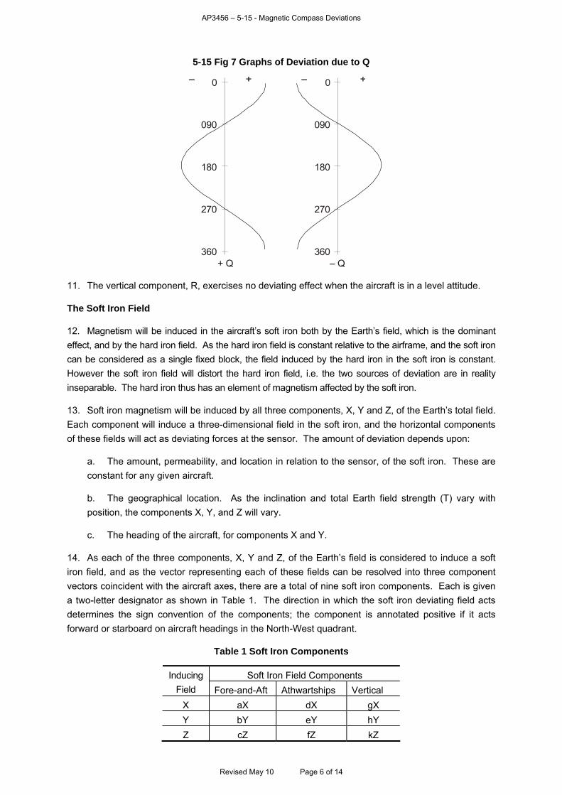
AP3456 – 5-15 - Magnetic Compass Deviations
5-15 Fig 7 Graphs of Deviation due to Q
0
090
180
270
360+ Q – Q
0
090
180
270
360
11. The vertical component, R, exercises no deviating effect when the aircraft is in a level attitude.
The Soft Iron Field
12. Magnetism will be induced in the aircraft’s soft iron both by the Earth’s field, which is the dominant
effect, and by the hard iron field. As the hard iron field is constant relative to the airframe, and the soft iron
can be considered as a single fixed block, the field induced by the hard iron in the soft iron is constant.
However the soft iron field will distort the hard iron field, i.e. the two sources of deviation are in reality
inseparable. The hard iron thus has an element of magnetism affected by the soft iron.
13. Soft iron magnetism will be induced by all three components, X, Y and Z, of the Earth’s total field.
Each component will induce a three-dimensional field in the soft iron, and the horizontal components
of these fields will act as deviating forces at the sensor. The amount of deviation depends upon:
a. The amount, permeability, and location in relation to the sensor, of the soft iron. These are
constant for any given aircraft.
b. The geographical location. As the inclination and total Earth field strength (T) vary with
position, the components X, Y, and Z will vary.
c. The heading of the aircraft, for components X and Y.
14. As each of the three components, X, Y and Z, of the Earth’s field is considered to induce a soft
iron field, and as the vector representing each of these fields can be resolved into three component
vectors coincident with the aircraft axes, there are a total of nine soft iron components. Each is given
a two-letter designator as shown in Table 1. The direction in which the soft iron deviating field acts
determines the sign convention of the components; the component is annotated positive if it acts
forward or starboard on aircraft headings in the North-West quadrant.
Table 1 Soft Iron Components
Soft Iron Field Components Inducing
Field Fore-and-Aft Athwartships Vertical
X aX dX gX
Y bY eY hY
Z cZ fZ kZ
Revised May 10 Page 6 of 14
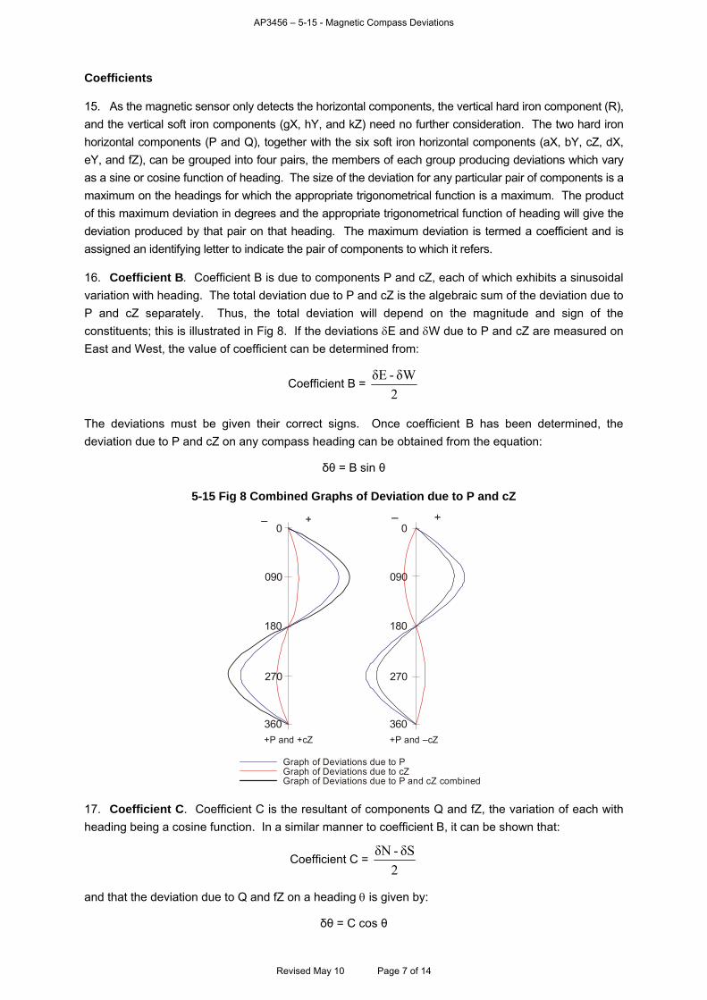
AP3456 – 5-15 - Magnetic Compass Deviations
Coefficients
15. As the magnetic sensor only detects the horizontal components, the vertical hard iron component (R),
and the vertical soft iron components (gX, hY, and kZ) need no further consideration. The two hard iron
horizontal components (P and Q), together with the six soft iron horizontal components (aX, bY, cZ, dX,
eY, and fZ), can be grouped into four pairs, the members of each group producing deviations which vary
as a sine or cosine function of heading. The size of the deviation for any particular pair of components is a
maximum on the headings for which the appropriate trigonometrical function is a maximum. The product
of this maximum deviation in degrees and the appropriate trigonometrical function of heading will give the
deviation produced by that pair on that heading. The maximum deviation is termed a coefficient and is
assigned an identifying letter to indicate the pair of components to which it refers.
16. Coefficient B. Coefficient B is due to components P and cZ, each of which exhibits a sinusoidal
variation with heading. The total deviation due to P and cZ is the algebraic sum of the deviation due to
P and cZ separately. Thus, the total deviation will depend on the magnitude and sign of the
constituents; this is illustrated in Fig 8. If the deviations E and W due to P and cZ are measured on
East and West, the value of coefficient can be determined from:
Coefficient B = 2
δW -δE
The deviations must be given their correct signs. Once coefficient B has been determined, the
deviation due to P and cZ on any compass heading can be obtained from the equation:
δθ = B sin θ
5-15 Fig 8 Combined Graphs of Deviation due to P and cZ
+P and +cZ +P and –cZ
Graph of Deviations due to PGraph of Deviations due to cZGraph of Deviations due to P and cZ combined
0
090
180
270
360
0
090
180
270
360
17. Coefficient C. Coefficient C is the resultant of components Q and fZ, the variation of each with
heading being a cosine function. In a similar manner to coefficient B, it can be shown that:
Coefficient C = 2
δS -δN
and that the deviation due to Q and fZ on a heading is given by:
δθ = C cos θ
Revised May 10 Page 7 of 14
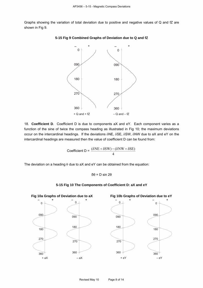
AP3456 – 5-15 - Magnetic Compass Deviations
Graphs showing the variation of total deviation due to positive and negative values of Q and fZ are
shown in Fig 9.
5-15 Fig 9 Combined Graphs of Deviation due to Q and fZ
0
090
180
270
360
+ Q and + fZ – Q and – fZ
0
090
180
270
360
18. Coefficient D. Coefficient D is due to components aX and eY. Each component varies as a
function of the sine of twice the compass heading as illustrated in Fig 10; the maximum deviations
occur on the intercardinal headings. If the deviations NE, SE, SW, NW due to aX and eY on the
intercardinal headings are measured then the value of coefficient D can be found from:
Coefficient D = 4
δSE)NW(δδSW)NE(δ
The deviation on a heading due to aX and eY can be obtained from the equation:
δθ = D sin 2θ
5-15 Fig 10 The Components of Coefficient D: aX and eY
Fig 10a Graphs of Deviation due to aX Fig 10b Graphs of Deviation due to eY
0
090
180
270
360
+ aX
0
090
180
270
360
– aX
0
090
180
270
360
+ eY
0
090
180
270
360
– eY
Revised May 10 Page 8 of 14
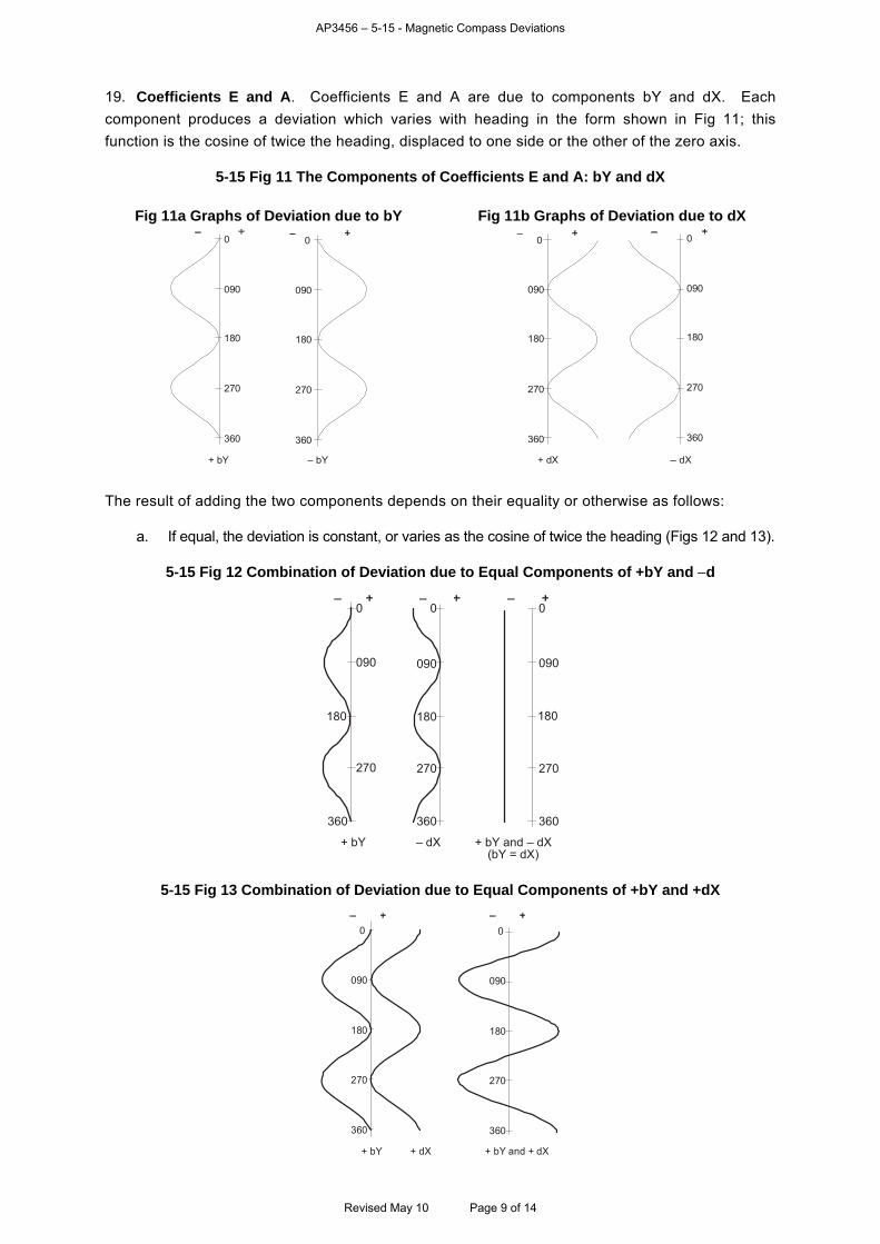
AP3456 – 5-15 - Magnetic Compass Deviations
19. Coefficients E and A. Coefficients E and A are due to components bY and dX. Each
component produces a deviation which varies with heading in the form shown in Fig 11; this
function is the cosine of twice the heading, displaced to one side or the other of the zero axis.
5-15 Fig 11 The Components of Coefficients E and A: bY and dX
Fig 11a Graphs of Deviation due to bY Fig 11b Graphs of Deviation due to dX
+ bY bY
0
090
180
270
360
0
090
180
270
360
0
090
180
270
360
0
090
180
270
360
dX+ dX
The result of adding the two components depends on their equality or otherwise as follows:
a. If equal, the deviation is constant, or varies as the cosine of twice the heading (Figs 12 and 13).
5-15 Fig 12 Combination of Deviation due to Equal Components of +bY and d
0 0
090 090 090
180 180 180
270 270 270
360 360 360
+ bY + bY and – dX(bY = dX)
0
– dX
5-15 Fig 13 Combination of Deviation due to Equal Components of +bY and +dX
0 0
090 090
180 180
270 270
360 360
+ bY + dX + bY and + dX
Revised May 10 Page 9 of 14
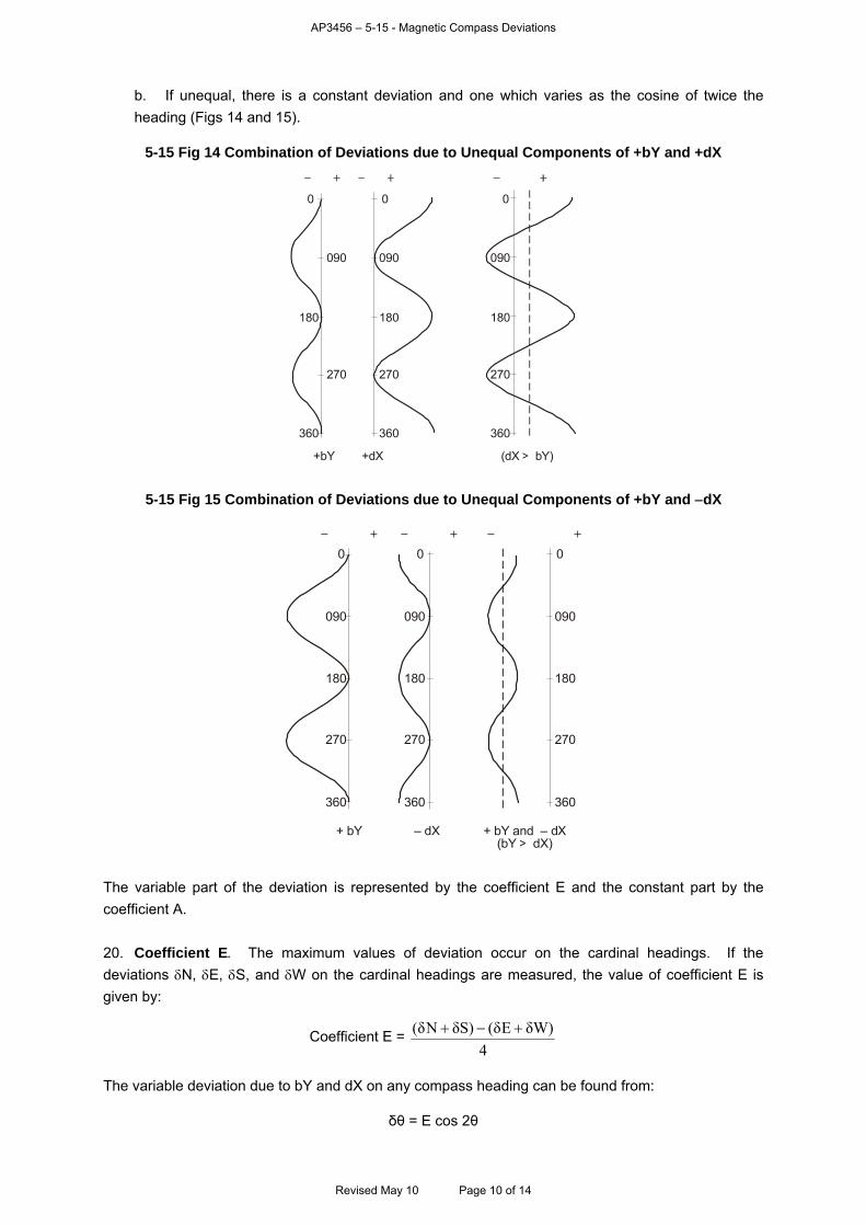
AP3456 – 5-15 - Magnetic Compass Deviations
b. If unequal, there is a constant deviation and one which varies as the cosine of twice the
heading (Figs 14 and 15).
5-15 Fig 14 Combination of Deviations due to Unequal Components of +bY and +dX
0 0 0
090 090 090
270 270 270
360 360 360
180 180 180
+bY +dX (dX bY) >
5-15 Fig 15 Combination of Deviations due to Unequal Components of +bY and dX
0 0
090 090 090
270 270 270
360 360 360
180 180 180
+ bY
0
– dX + bY and – dX(bY dX) >
The variable part of the deviation is represented by the coefficient E and the constant part by the
coefficient A.
20. Coefficient E. The maximum values of deviation occur on the cardinal headings. If the
deviations N, E, S, and W on the cardinal headings are measured, the value of coefficient E is
given by:
Coefficient E = 4
δW)E(δδS)N(δ
The variable deviation due to bY and dX on any compass heading can be found from:
δθ = E cos 2θ
Revised May 10 Page 10 of 14
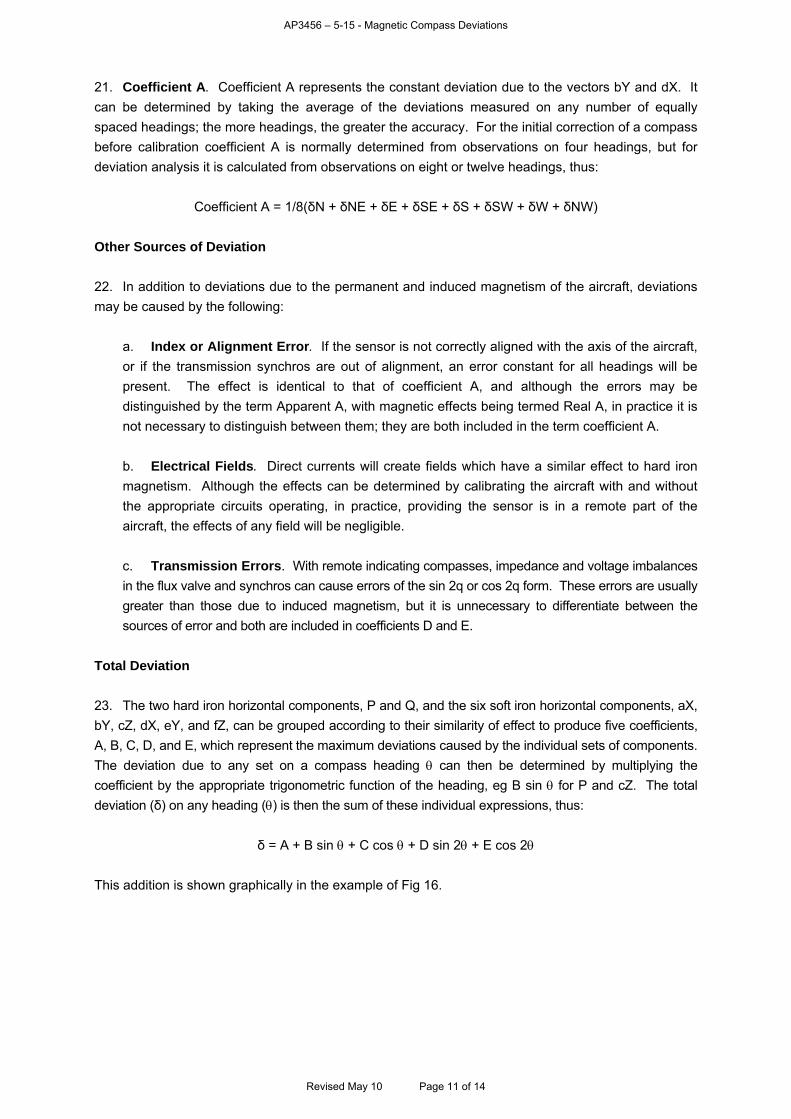
AP3456 – 5-15 - Magnetic Compass Deviations
21. Coefficient A. Coefficient A represents the constant deviation due to the vectors bY and dX. It
can be determined by taking the average of the deviations measured on any number of equally
spaced headings; the more headings, the greater the accuracy. For the initial correction of a compass
before calibration coefficient A is normally determined from observations on four headings, but for
deviation analysis it is calculated from observations on eight or twelve headings, thus:
Coefficient A = 1/8(δN + δNE + δE + δSE + δS + δSW + δW + δNW)
Other Sources of Deviation
22. In addition to deviations due to the permanent and induced magnetism of the aircraft, deviations
may be caused by the following:
a. Index or Alignment Error. If the sensor is not correctly aligned with the axis of the aircraft,
or if the transmission synchros are out of alignment, an error constant for all headings will be
present. The effect is identical to that of coefficient A, and although the errors may be
distinguished by the term Apparent A, with magnetic effects being termed Real A, in practice it is
not necessary to distinguish between them; they are both included in the term coefficient A.
b. Electrical Fields. Direct currents will create fields which have a similar effect to hard iron
magnetism. Although the effects can be determined by calibrating the aircraft with and without
the appropriate circuits operating, in practice, providing the sensor is in a remote part of the
aircraft, the effects of any field will be negligible.
c. Transmission Errors. With remote indicating compasses, impedance and voltage imbalances
in the flux valve and synchros can cause errors of the sin 2q or cos 2q form. These errors are usually
greater than those due to induced magnetism, but it is unnecessary to differentiate between the
sources of error and both are included in coefficients D and E.
Total Deviation
23. The two hard iron horizontal components, P and Q, and the six soft iron horizontal components, aX,
bY, cZ, dX, eY, and fZ, can be grouped according to their similarity of effect to produce five coefficients,
A, B, C, D, and E, which represent the maximum deviations caused by the individual sets of components.
The deviation due to any set on a compass heading can then be determined by multiplying the
coefficient by the appropriate trigonometric function of the heading, eg B sin for P and cZ. The total
deviation (δ) on any heading () is then the sum of these individual expressions, thus:
δ = A + B sin + C cos + D sin 2 + E cos 2
This addition is shown graphically in the example of Fig 16.
Revised May 10 Page 11 of 14
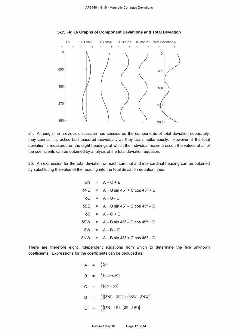
AP3456 – 5-15 - Magnetic Compass Deviations
5-15 Fig 16 Graphs of Component Deviations and Total Deviation
0
090
180
270
360
0
090
180
270
360
+A +B sin +C cos +D sin 2 +E cos 2 Total Deviation
24. Although the previous discussion has considered the components of total deviation separately,
they cannot in practice be measured individually as they act simultaneously. However, if the total
deviation is measured on the eight headings at which the individual maxima occur, the values of all of
the coefficients can be obtained by analysis of the total deviation equation.
25. An expression for the total deviation on each cardinal and intercardinal heading can be obtained
by substituting the value of the heading into the total deviation equation, thus:
δN = A + C + E
δNE = A + B sin 45º + C cos 45º + D
δE = A + B - E
δSE = A + B sin 45º C cos 45º D
δS = A C + E
δSW = A B sin 45º C cos 45º + D
δW = A B E
δNW = A B sin 45º + C cos 45º D
There are therefore eight independent equations from which to determine the five unknown
coefficients. Expressions for the coefficients can be deduced as:
A = Σδ81
B = WδE2
1
C = SδN2
1
D = WNδSWSEδNE4
1
E = WδSEδN4
1
Revised May 10 Page 12 of 14
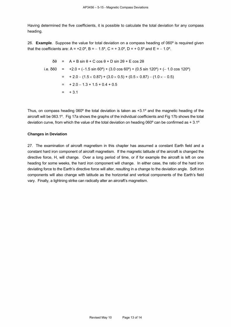
AP3456 – 5-15 - Magnetic Compass Deviations
Having determined the five coefficients, it is possible to calculate the total deviation for any compass
heading.
26. Example. Suppose the value for total deviation on a compass heading of 060º is required given
that the coefficients are: A = +2.0º, B = 1.5º, C = + 3.0º, D = + 0.5º and E = 1.0º.
δθ = A + B sin θ + C cos θ + D sin 2θ + E cos 2θ
i.e. δ60 = +2.0 + (1.5 sin 60º) + (3.0 cos 60º) + (0.5 sin 120º) + ( 1.0 cos 120º)
= + 2.0 (1.5 0.87) + (3.0 0.5) + (0.5 0.87) (1.0 0.5)
= + 2.0 1.3 + 1.5 + 0.4 + 0.5
= + 3.1
Thus, on compass heading 060º the total deviation is taken as +3.1º and the magnetic heading of the
aircraft will be 063.1º. Fig 17a shows the graphs of the individual coefficients and Fig 17b shows the total
deviation curve, from which the value of the total deviation on heading 060º can be confirmed as + 3.1º
Changes in Deviation
27. The examination of aircraft magnetism in this chapter has assumed a constant Earth field and a
constant hard iron component of aircraft magnetism. If the magnetic latitude of the aircraft is changed the
directive force, H, will change. Over a long period of time, or if for example the aircraft is left on one
heading for some weeks, the hard iron component will change. In either case, the ratio of the hard iron
deviating force to the Earth’s directive force will alter, resulting in a change to the deviation angle. Soft iron
components will also change with latitude as the horizontal and vertical components of the Earth’s field
vary. Finally, a lightning strike can radically alter an aircraft’s magnetism.
Revised May 10 Page 13 of 14
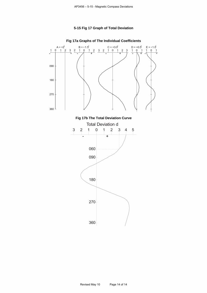
AP3456 – 5-15 - Magnetic Compass Deviations
Revised May 10 Page 14 of 14
5-15 Fig 17 Graph of Total Deviation
Fig 17a Graphs of The Individual Coefficients
1 0 1 2 3 2 1 0 1 2 3 2 1 0 1 2 3 1 0 1 1 0 1A = +2 B = 1.5 E = 1.0C = +3.0 D = +0.5
o o oo o
090
180
270
360
Fig 17b The Total Deviation Curve
3 2 1 0 1 2 3 4 5
060
090
180
270
360
Total Deviation d
AP3456 – 5-16 - Compass Swinging Procedures
CHAPTER 16 - COMPASS SWINGING PROCEDURES Contents Page Introduction.............................................................................................................................................. 1 The Compass Base................................................................................................................................. 2 Occasions for a Compass Swing ............................................................................................................ 3 Preparing to do a Compass Swing.......................................................................................................... 4 Types of Compass Swing........................................................................................................................ 5 The Correcting Swing.............................................................................................................................. 6 The Calibration Swing ............................................................................................................................. 8 Table of Figures 5-16 Fig 1 An Operator ready to take a Bearing on the Fore/Aft Axis of the Aircraft.............................. 2 5-16 Fig 2 Extract from Form 712A showing the Recording of the Correcting Swing ............................ 7 5-16 Fig 3 Corrector Dials for removing Coefficients B and C................................................................ 7 5-16 Fig 4 Extract from Form 712A showing Calibration Phase of Standard Swing .............................. 8 5-16 Fig 5 Residual Deviation Graph constructed from the data in Fig 4 ............................................... 9 5-16 Fig 6 Deviation Card constructed from the Deviation Curve at Fig 5 ........................................... 10 5-16 Fig 7 Deviation Card for use at the Pilot’s Position....................................................................... 10 5-16 Fig 8 Compass Calibration Log Entries for a Refined Swing (Correcting and Calibration) .......... 11 Table Table 1 Summary of the Four Types of Compass Swing ....................................................................... 5 Introduction 1. Compass swinging is a special procedure used to ensure that magnetic compasses are as accurate as possible. It derives its name from the fact that the aircraft containing the compass system is 'swung' through a series of headings. During this process, readings are taken of the aircraft compass systems and these are compared to an accurate datum compass which is independent of the aircraft system. Compass swings are carried out on a specially prepared part of an airfield known as a 'Compass Base'. Fig 1 shows a typical scenario during a compass swing, with the datum compass operator in position to take a bearing on the fore/aft axis of the aircraft at the compass base. This chapter will concentrate on the practical aspects of carrying out a compass swing, but a knowledge of aircraft magnetism, covered in Volume 5, Chapter 15, would be beneficial. The engineering aspects of compass swings are covered in MAA Manual of Maintenance and Airworthiness Processes (MAP-01), Chapter 12.9, and instructions for use of the MOD Form 712A (the Compass Calibration Log) are detailed in MAA Manual of Maintenance and Airworthiness Processes - Supplement, Chapter 2.
Revised Jul 11 Page 1 of 11
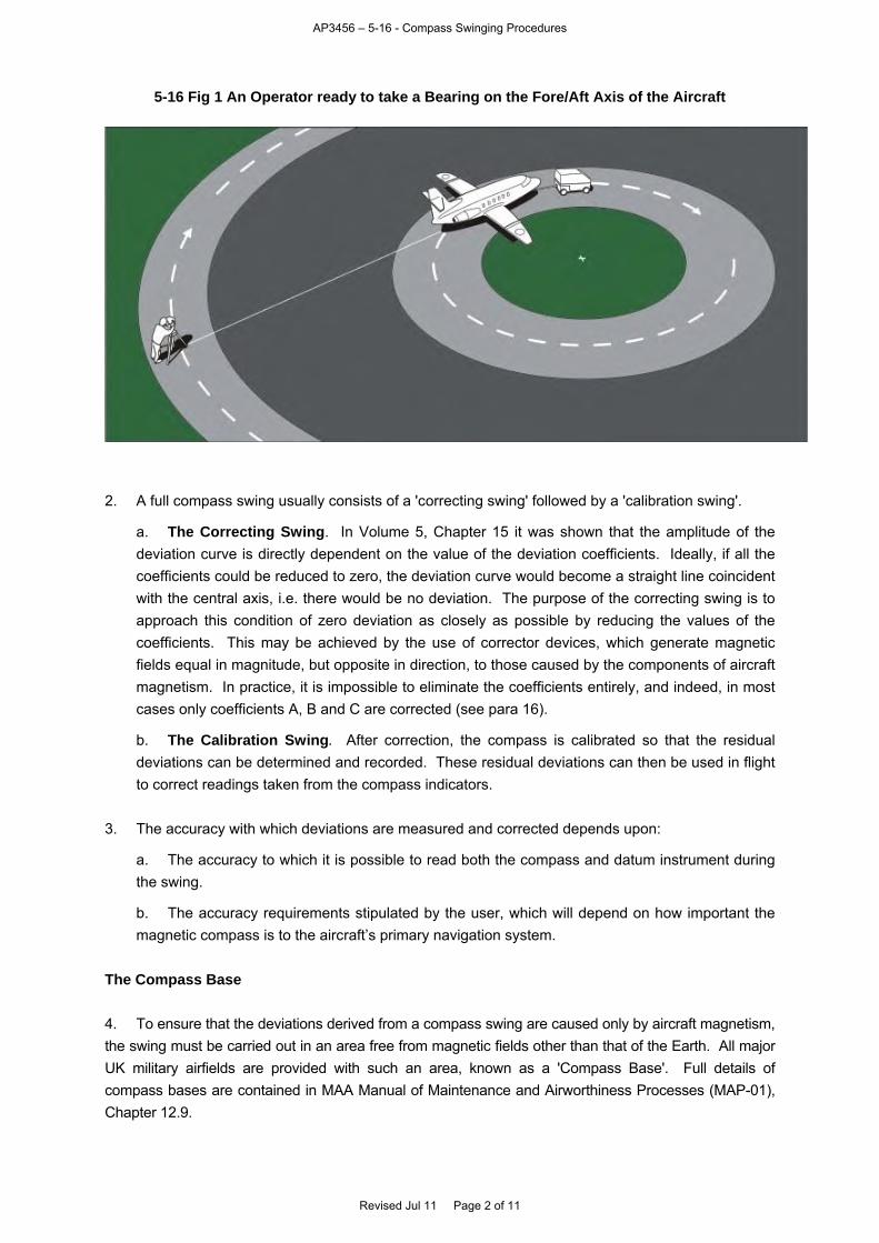
AP3456 – 5-16 - Compass Swinging Procedures
5-16 Fig 1 An Operator ready to take a Bearing on the Fore/Aft Axis of the Aircraft
2. A full compass swing usually consists of a 'correcting swing' followed by a 'calibration swing'.
a. The Correcting Swing. In Volume 5, Chapter 15 it was shown that the amplitude of the deviation curve is directly dependent on the value of the deviation coefficients. Ideally, if all the coefficients could be reduced to zero, the deviation curve would become a straight line coincident with the central axis, i.e. there would be no deviation. The purpose of the correcting swing is to approach this condition of zero deviation as closely as possible by reducing the values of the coefficients. This may be achieved by the use of corrector devices, which generate magnetic fields equal in magnitude, but opposite in direction, to those caused by the components of aircraft magnetism. In practice, it is impossible to eliminate the coefficients entirely, and indeed, in most cases only coefficients A, B and C are corrected (see para 16).
b. The Calibration Swing. After correction, the compass is calibrated so that the residual deviations can be determined and recorded. These residual deviations can then be used in flight to correct readings taken from the compass indicators.
3. The accuracy with which deviations are measured and corrected depends upon:
a. The accuracy to which it is possible to read both the compass and datum instrument during the swing.
b. The accuracy requirements stipulated by the user, which will depend on how important the magnetic compass is to the aircraft’s primary navigation system.
The Compass Base 4. To ensure that the deviations derived from a compass swing are caused only by aircraft magnetism, the swing must be carried out in an area free from magnetic fields other than that of the Earth. All major UK military airfields are provided with such an area, known as a 'Compass Base'. Full details of compass bases are contained in MAA Manual of Maintenance and Airworthiness Processes (MAP-01), Chapter 12.9.
Revised Jul 11 Page 2 of 11
AP3456 – 5-16 - Compass Swinging Procedures
5. In addition to the need to be free from extraneous magnetic fields, a compass base should be sited such that its use does not interfere with normal aircraft movements on the airfield and its surface should not preclude its use in wet weather. It must be large enough (and strong enough) to take all types of aircraft likely to use it, bearing in mind the radii of the aircrafts’ turning circles and the position of any sighting rods (and their path during the swing). The compass base must be clearly and permanently marked to show:
a. The base centre.
b. The central area within which the aircraft’s sensor should remain.
c. The datum compass circle.
d. Areas of magnetic anomalies. 6. Compass bases are subject to periodic re-survey to ensure their continued suitability. Responsibility for surveying compass bases is vested in QinetiQ, Land Magnetic Facilities at MOD Portland Bill. QinetiQ are also the authority on many other aspects of compass swinging, including calibration of datum compasses. 7. Magnetic Anomalies. Compass bases are classified as Class 1 if there are no known magnetic anomalies in excess of 0.1º at 1.5m above ground level, or Class 2 provided any anomalies are less than 0.25º at 1.5m above ground level. If a base is to be used for aircraft which have magnetic detectors significantly below 1.5m, a special survey is required. It is unusual for there to be any natural ferrous deposits on an airfield, and any magnetic interference is therefore most likely due to buried scrap metal, reinforced concrete, drainage systems, wire fences or conduit for electrical cabling. Electro-magnetic interference may be caused by electrical cabling and, if such cables cannot be avoided or re-routed, their effect, with and without current flowing, must be assessed. 8. Changes in Variation. Changes in variation may occur through diurnal changes and magnetic storms. Diurnal changes in variation may vary from a few arc minutes close to the magnetic equator to many degrees close to the magnetic poles. In southern England, the diurnal change varies from about 0.25º in the summer to about 0.07º in the winter. Magnetic storms are usually associated with sunspot activity. Although the frequency of such storms is only about once per year, they may last several hours or even days, and can alter the variation by up to 0.5º in the UK. Occasions for a Compass Swing 9. The engineering responsibility for the calibration and adjustment of aircraft compasses is promulgated in MAA Manual of Maintenance and Airworthiness Processes (MAP-01), Chap 12.9. This document defines the occasions on which a compass swing is required, and these are summarized as follows:
a. As directed in aircraft maintenance schedules.
b. On acceptance by a user unit, if a new-build aircraft has been delivered direct from a contractor.
c. After an aircraft has been in long-term storage.
d. When an aircraft has been subjected to severe static electricity, eg a lightning strike. In this case, particular attention must be paid to compass accuracy and, if necessary, the appropriate demagnetization procedures laid down by the operating authority must be followed.
Revised Jul 11 Page 3 of 11
AP3456 – 5-16 - Compass Swinging Procedures
e. On transfer of an aircraft from one theatre of operations to another, if this entails a large change of magnetic latitude. This need not apply to aircraft on detachment of less than four weeks, unless higher order accuracy is operationally required.
f. Whenever a compass system has been subjected to shock, e.g. after a heavy landing.
g. After an aircraft has been repaired or subjected to conditions likely to affect the accuracy of the compass systems. Examples of such repairs and conditions are:
(1) A change of a component within the compass system likely to create a significant change in deviation, eg flux valve or magnetic compass.
(2) A change of position, replacement, addition or permanent removal of any magnetic material, or alteration to any electrical circuit, in the vicinity of a direct reading compass or a detector unit of a remote reading compass.
h. If it is considered likely that a specific freight load will cause magnetic influence and thereby affect compass readings.
i. Whenever the accuracy of the compass system is in doubt.
Preparing to do a Compass Swing
10. Before starting a compass swing, the following general points should be checked to prevent embarrassment and delay:
a. Ensure that the weather conditions are suitable for carrying out the swing. Except under exceptional circumstances, ground-based compass swinging is only carried out in weather conditions clear of persistent rain and with wind speeds of 15 kt or less.
b. Ensure that the compass base is available for use.
c. Check that the aircraft compasses are fully serviceable.
d. Collect all of the items required for the calibration of the compass, eg Precise Heading Test Set, Watts Datum Compass, corrector keys, sighting rods and Compass Calibration Log (MOD Form 712A).
e. Ensure that non-magnetic tools are available.
f. Remove any items of moveable equipment which may affect the magnetic sensor, eg tool kits or spares in the vicinity of the sensor.
g. Obtain permission from Air Traffic Control to tow or taxi the aircraft to the compass base.
h. Check that the appropriate power source is available and that both the towing vehicle and power set have sufficient fuel.
i. Brief the compass swinging team on the procedures to be followed. Ensure that personnel remove from their person all metallic objects likely to interfere with the swing, e.g. watches, pens, spanners, headgear with metallic badges (see also Volume 5, Chapter 14, para 12). If the swing is to be conducted with engines running, ensure that the datum compass operator uses non-metallic ear defenders rather than a headset.
j. If sighting rods are to be used to act as the datum points of the aircraft (see Volume 5, Chapter 14), ensure that they are attached to the appropriate mountings.
k. Before starting the swing, switch on any aircraft electrical equipment which is likely to cause magnetic deviation in flight, but observe restrictions on ground operation of equipment.
Revised Jul 11 Page 4 of 11
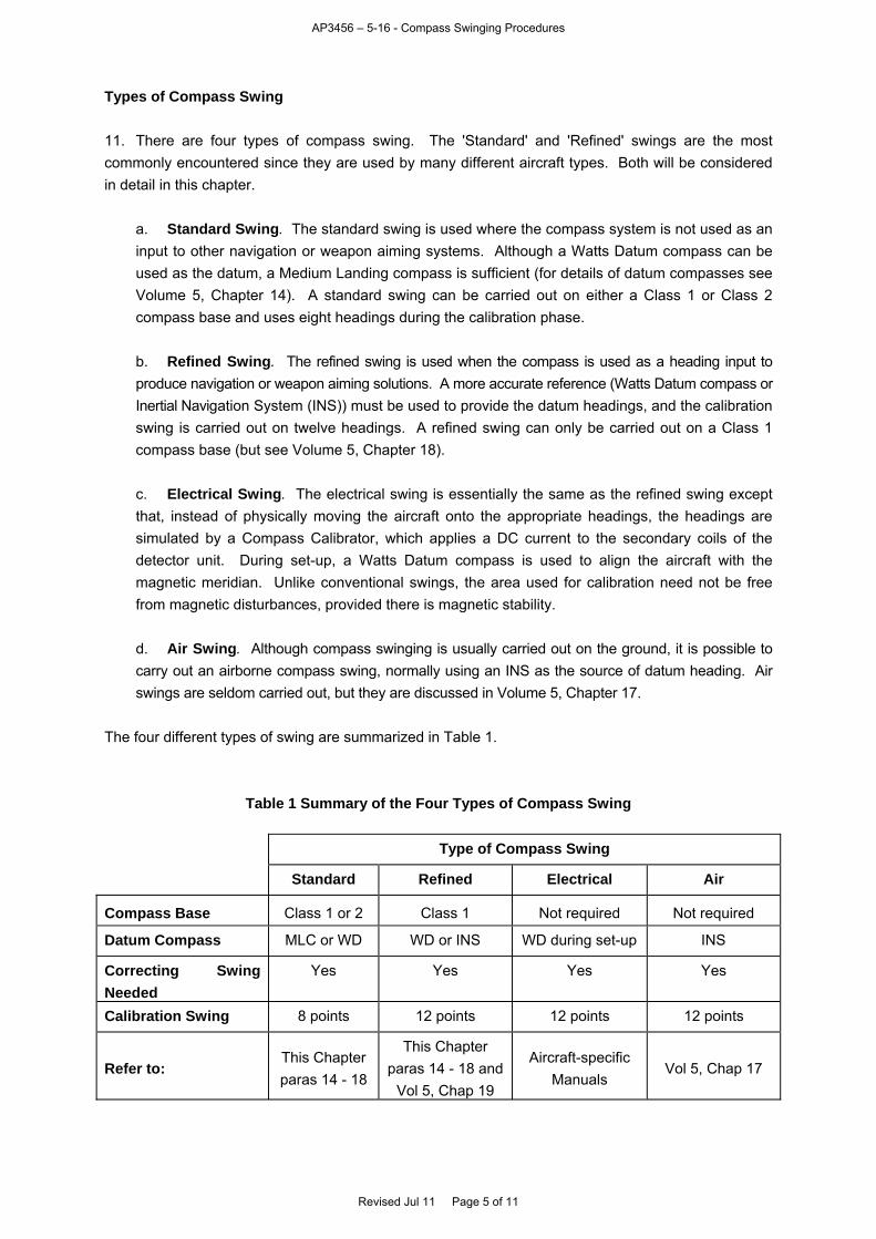
AP3456 – 5-16 - Compass Swinging Procedures
Types of Compass Swing 11. There are four types of compass swing. The 'Standard' and 'Refined' swings are the most commonly encountered since they are used by many different aircraft types. Both will be considered in detail in this chapter.
a. Standard Swing. The standard swing is used where the compass system is not used as an input to other navigation or weapon aiming systems. Although a Watts Datum compass can be used as the datum, a Medium Landing compass is sufficient (for details of datum compasses see Volume 5, Chapter 14). A standard swing can be carried out on either a Class 1 or Class 2 compass base and uses eight headings during the calibration phase.
b. Refined Swing. The refined swing is used when the compass is used as a heading input to produce navigation or weapon aiming solutions. A more accurate reference (Watts Datum compass or Inertial Navigation System (INS)) must be used to provide the datum headings, and the calibration swing is carried out on twelve headings. A refined swing can only be carried out on a Class 1 compass base (but see Volume 5, Chapter 18).
c. Electrical Swing. The electrical swing is essentially the same as the refined swing except that, instead of physically moving the aircraft onto the appropriate headings, the headings are simulated by a Compass Calibrator, which applies a DC current to the secondary coils of the detector unit. During set-up, a Watts Datum compass is used to align the aircraft with the magnetic meridian. Unlike conventional swings, the area used for calibration need not be free from magnetic disturbances, provided there is magnetic stability.
d. Air Swing. Although compass swinging is usually carried out on the ground, it is possible to carry out an airborne compass swing, normally using an INS as the source of datum heading. Air swings are seldom carried out, but they are discussed in Volume 5, Chapter 17.
The four different types of swing are summarized in Table 1.
Table 1 Summary of the Four Types of Compass Swing Type of Compass Swing
Standard Refined Electrical Air
Compass Base Class 1 or 2 Class 1 Not required Not required
Datum Compass MLC or WD WD or INS WD during set-up INS
Correcting Swing Needed
Yes Yes Yes Yes
Calibration Swing 8 points 12 points 12 points 12 points
Refer to: This Chapter paras 14 - 18
This Chapter paras 14 - 18 and
Vol 5, Chap 19
Aircraft-specific Manuals
Vol 5, Chap 17
Revised Jul 11 Page 5 of 11

AP3456 – 5-16 - Compass Swinging Procedures
12. Before detailed examination of the different types of swing, there are some general rules which must be adhered to at all times, to ensure an accurate swing:
a. The aircraft must be positioned within 5º of each of the nominal headings.
b. After each change of heading, chocks should be inserted to ensure that the aircraft does not move whilst readings are being taken.
c. Sighting rods, where used, should be checked for verticality after each change of heading, before sighting with the datum compass.
d. The aircraft compass system must be allowed to settle after each change of heading, before the reading is taken.
e. Great care must be taken to ensure that both the datum and aircraft compasses are read simultaneously, and to their respective limits of accuracy.
The necessary accuracy and limits of the swing are stipulated by operating authorities, but, in general, coefficients should be reduced to less than 1.0º for a standard swing and 0.5º for a refined swing. Specific limits for each aircraft type are contained in the aircraft engineering documents. 13. As mentioned in para 2, compass swings consist of two distinct phases: correction and calibration. The rest of this chapter will describe these two procedures as they apply to the standard and refined swings. Aircraft which use the electrical swing will have the procedures documented in their type-specific manuals. The Correcting Swing 14. Purpose. The purpose of the correcting swing is to reduce all the correctable coefficients to within limits. The correcting swing may have to be repeated several times to achieve the required accuracy. The data from each correcting swing is entered in the appropriate block on the first page of the Compass Calibration Log (MOD Form 712A). 15. Procedure. The correction procedure is common to both Standard and Refined swings, and is as described in the following sub-paras. Fig 2 is an extract from the MOD Form 712A and illustrates, by way of an example, how the results of the correcting swing are recorded.
a. Turn the aircraft onto South, and record the aircraft and datum compass readings.
b. Turn the aircraft onto West, and record the aircraft and datum compass readings.
c. Turn the aircraft onto North, and record the aircraft and datum compass readings.
d. Turn the aircraft onto East, and record the aircraft and datum compass readings.
e. Calculate the deviations (datum heading minus aircraft compass heading).
f. Sum the deviations algebraically and divide by four to find coefficient A.
g. Apply coefficient A to the compass reading (with sign unchanged) and correct the compass (see para 16).
h. Calculate coefficient B using the formula:
Coefficient B = 2
WE
i. Apply coefficient B (sign unchanged) to the resultant compass heading after correcting for coefficient A, and, with the aircraft still on East, correct the compass (see para 16).
Revised Jul 11 Page 6 of 11
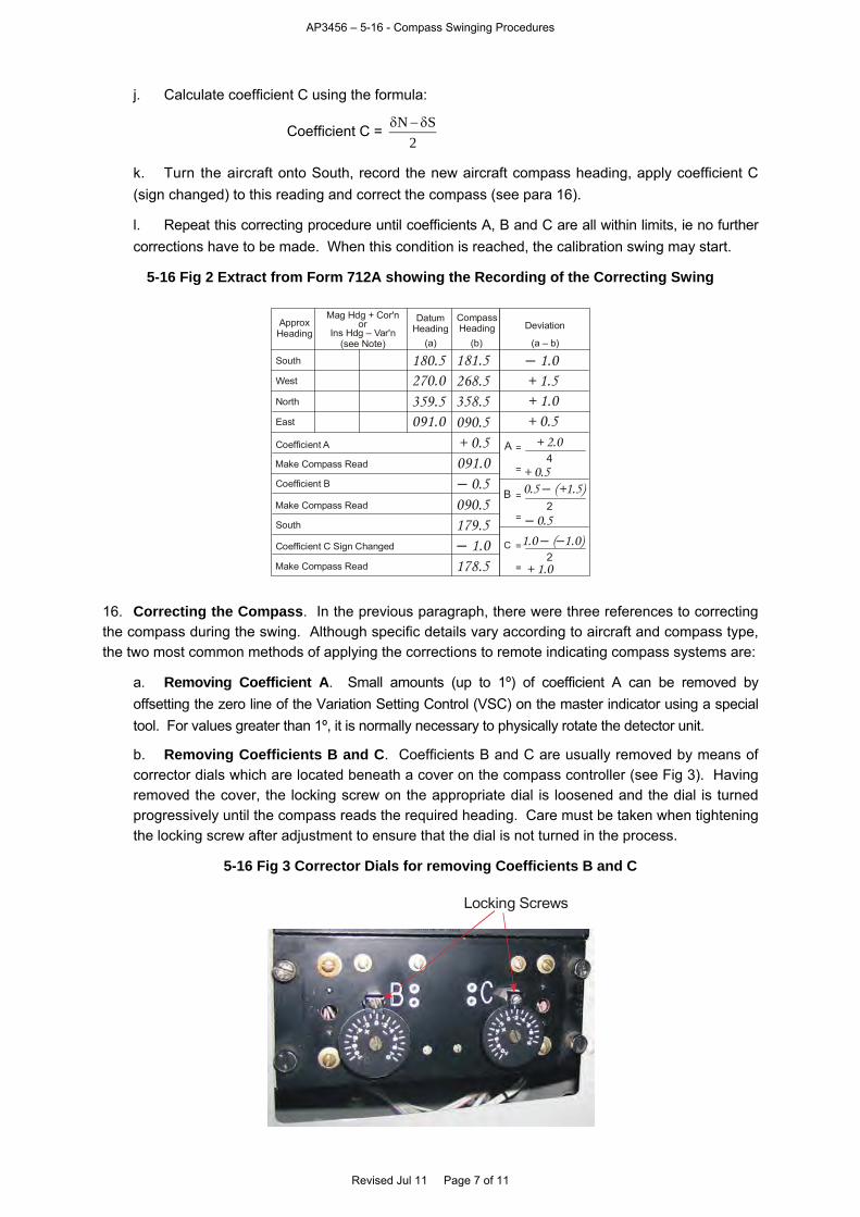
AP3456 – 5-16 - Compass Swinging Procedures
j. Calculate coefficient C using the formula:
Coefficient C = 2
SN
k. Turn the aircraft onto South, record the new aircraft compass heading, apply coefficient C (sign changed) to this reading and correct the compass (see para 16).
l. Repeat this correcting procedure until coefficients A, B and C are all within limits, ie no further corrections have to be made. When this condition is reached, the calibration swing may start.
5-16 Fig 2 Extract from Form 712A showing the Recording of the Correcting Swing
Make Compass Read
A
B
C =
=
=
=
=
=
Make Compass Read
Make Compass Read
South
North
West
East
Coefficient A
Coefficient B
Coefficient C Sign Changed
South
Ins Hdg – Var'n
Mag Hdg + Cor'nor
(see Note)
ApproxHeading
DatumHeading
CompassHeading Deviation
(a) (b) (a – b)
180.5270.0359.5091.0
181.5268.5358.5090.5+ 0.5091.0– 0.5090.5179.5– 1.0178.5
– 1.0
+ 0.5
+ 1.5+ 1.0
+ 2.04
2
2
+ 0.50.5 (+1.5)–
– 0.5
1.0 ( 1.0)– –
+ 1.0
16. Correcting the Compass. In the previous paragraph, there were three references to correcting the compass during the swing. Although specific details vary according to aircraft and compass type, the two most common methods of applying the corrections to remote indicating compass systems are:
a. Removing Coefficient A. Small amounts (up to 1º) of coefficient A can be removed by offsetting the zero line of the Variation Setting Control (VSC) on the master indicator using a special tool. For values greater than 1º, it is normally necessary to physically rotate the detector unit.
b. Removing Coefficients B and C. Coefficients B and C are usually removed by means of corrector dials which are located beneath a cover on the compass controller (see Fig 3). Having removed the cover, the locking screw on the appropriate dial is loosened and the dial is turned progressively until the compass reads the required heading. Care must be taken when tightening the locking screw after adjustment to ensure that the dial is not turned in the process.
5-16 Fig 3 Corrector Dials for removing Coefficients B and C
Locking Screws
Revised Jul 11 Page 7 of 11

AP3456 – 5-16 - Compass Swinging Procedures
The Calibration Swing 17. Purpose. The purpose of the calibration swing is to check that coefficient A has been removed and that the residual deviation is within the limits prescribed in the relevant aircraft documentation. Although the detailed procedure differs slightly between Standard and Refined swings, the final step is essentially the same – the construction of deviation cards for installation in the aircraft. 18. Procedure.
a. Standard Swing. The calibration phase of the Standard Swing proceeds as described in the following sub-paras. Fig 4 is an extract from the MOD Form 712A and illustrates, by way of an example, how the results of the calibration swing are recorded.
(1) Turn the aircraft onto South-West (225º), record the aircraft and datum compass readings.
(2) Turn the aircraft to the right in steps of 45º. At each step, record the aircraft and datum compass readings. The eighth, and final, heading will be South.
(3) Calculate the deviations on each heading and compute coefficient A by dividing their algebraic sum by eight.
(4) If the deviation figures are all within limits, and no further adjustment to coefficient A is required, the swing can be terminated.
Note: In the example at Fig 4, the algebraic sum of the residual deviations on all eight headings is + 4.0º, therefore the value of A is + 0.5º. As this value is within limits, the swing is terminated.
b. Refined Swing. The aircraft is moved through a twelve-point swing starting on 210º. The datum and compass readings are recorded every 30º (see the example in Fig 8). The deviations obtained from this swing form the basis of the Fourier and accuracy analyses, which are described in Volume 5, Chapter 19.
5-16 Fig 4 Extract from Form 712A showing Calibration Phase of Standard Swing
180
ApproxHeading Ins Hdg – Var'n
Mag Hdg + Cor'nor
(see Note)
DatumHeading
CompassHeading Deviation
(d) (e) (d – e)
135
225270315360045090
223.5272.0317.0002.0046.0089.0135.5181.5
222.0271.0316.5002.0046.5089.0135.0180.5
– 0.5
+ 0.5+ 1.0+ 1.5
+ 0.5+ 1.0
0.0
0.0
19. Output. As mentioned in para 17, the final step of the calibration swing is the production of deviation cards, which show the corrections to be made to the compass indications for all headings. These deviation cards are located in the aircraft, in purpose-designed holders, next to the compass systems to which they apply.
a. The Deviation Curve. A deviation curve is plotted from the data derived during the calibration swing. This curve is then used to produce the deviation card. Fig 5 shows a deviation curve plotted from the data at Fig 4. The first step in producing the curve is to choose a suitable
Revised Jul 11 Page 8 of 11
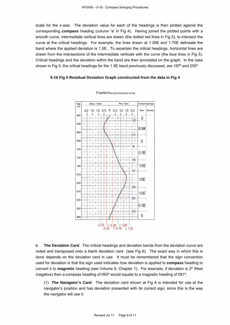
AP3456 – 5-16 - Compass Swinging Procedures
scale for the x-axis. The deviation value for each of the headings is then plotted against the corresponding compass heading (column 'e' in Fig 4). Having joined the plotted points with a smooth curve, intermediate vertical lines are drawn (the dotted red lines in Fig 5), to intersect the curve at the critical headings. For example, the lines drawn at 1.25E and 1.75E delineate the band where the applied deviation is 1.5E. To ascertain the critical headings, horizontal lines are drawn from the intersections of the intermediate verticals with the curve (the blue lines in Fig 5). Critical headings and the deviation within the band are then annotated on the graph. In the case shown in Fig 5, the critical headings for the 1.5E band previously discussed, are 197º and 255º.
5-16 Fig 5 Residual Deviation Graph constructed from the data in Fig 4
0.5 0.5 1.51.5 1.01.0 2.02.0
-0.75-0.25
+ 0.25+ 0.75
+ 1.25+ 1.75
1.0E
0.5E
1.5E
0340
0.5E
0
197
1.0E
295
255
159
110
0
070
020
b. The Deviation Card. The critical headings and deviation bands from the deviation curve are noted and transposed onto a blank deviation card (see Fig 6). The exact way in which this is done depends on the deviation card in use. It must be remembered that the sign convention used for deviation is that the sign used indicates how deviation is applied to compass heading to convert it to magnetic heading (see Volume 9, Chapter 1). For example, if deviation is 2º West (negative) then a compass heading of 093º would equate to a magnetic heading of 091º.
(1) The Navigator’s Card. The deviation card shown at Fig 6 is intended for use at the navigator’s position and has deviation presented with its correct sign, since this is the way the navigator will use it.
Revised Jul 11 Page 9 of 11
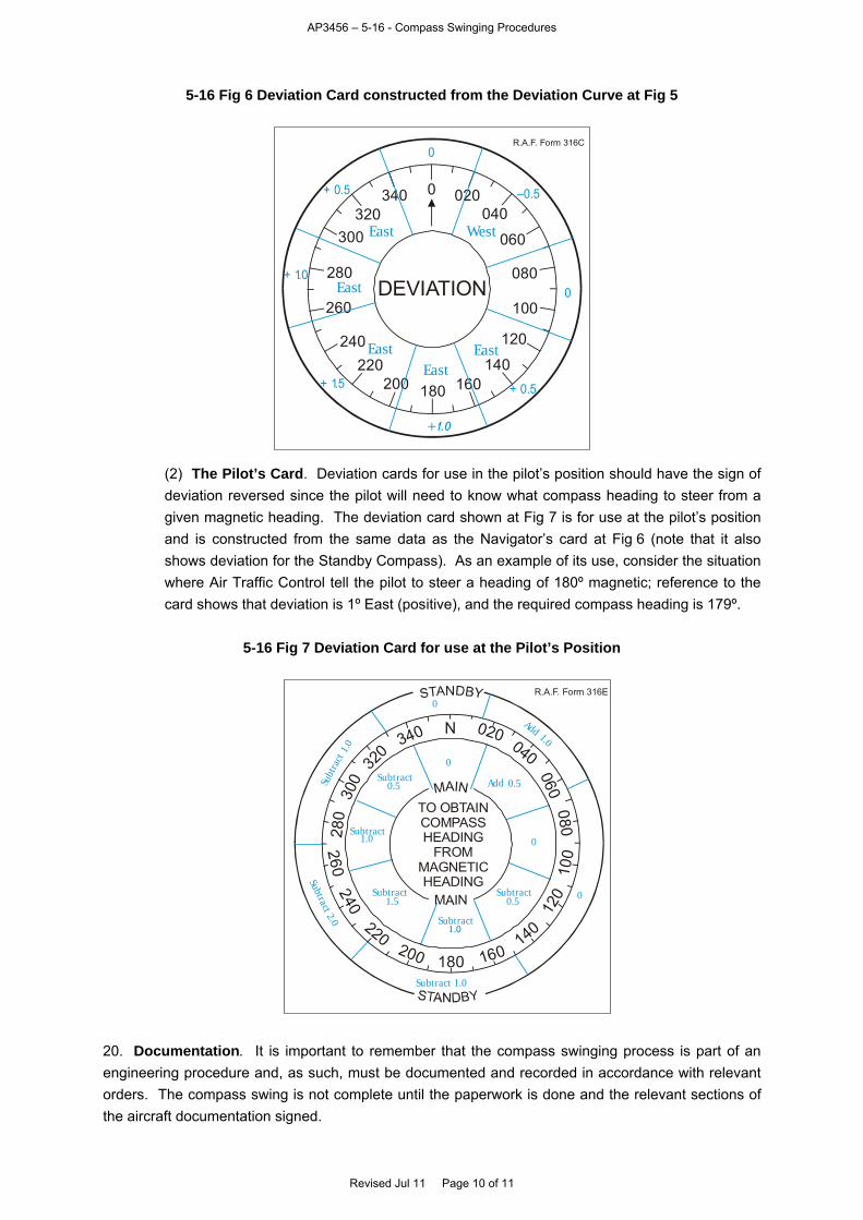
AP3456 – 5-16 - Compass Swinging Procedures
5-16 Fig 6 Deviation Card constructed from the Deviation Curve at Fig 5
DEVIATION
020040
100
0
060
080
120
140160180
340320
300
280
260
240220
200
0
0
–0.5
+ 0.5+ 1.5
+ 1.0
+ 0.5
West
EastEast
East
East
East
R.A.F. Form 316C
(2) The Pilot’s Card. Deviation cards for use in the pilot’s position should have the sign of deviation reversed since the pilot will need to know what compass heading to steer from a given magnetic heading. The deviation card shown at Fig 7 is for use at the pilot’s position and is constructed from the same data as the Navigator’s card at Fig 6 (note that it also shows deviation for the Standby Compass). As an example of its use, consider the situation where Air Traffic Control tell the pilot to steer a heading of 180º magnetic; reference to the card shows that deviation is 1º East (positive), and the required compass heading is 179º.
5-16 Fig 7 Deviation Card for use at the Pilot’s Position
040
100
060080
120
140
160180
320
280
260240
220200
0
0
0.5
0.51.5
1.0
0.5
R.A.F. Form 316E
N 020340
300 MAIN
TO OBTAINCOMPASSHEADING
FROMMAGNETICHEADING
NIAM
Add
Subtract
Subtract
Subtract
Subtract
SubtractSubt
ract
1.0
Add 1.0
0
0
Subtract 2.0
Subtract 1.0
20. Documentation. It is important to remember that the compass swinging process is part of an engineering procedure and, as such, must be documented and recorded in accordance with relevant orders. The compass swing is not complete until the paperwork is done and the relevant sections of the aircraft documentation signed.
Revised Jul 11 Page 10 of 11

AP3456 – 5-16 - Compass Swinging Procedures
Revised Jul 11 Page 11 of 11
5-16 Fig 8 Compass Calibration Log Entries for a Refined Swing (Correcting and Calibration)
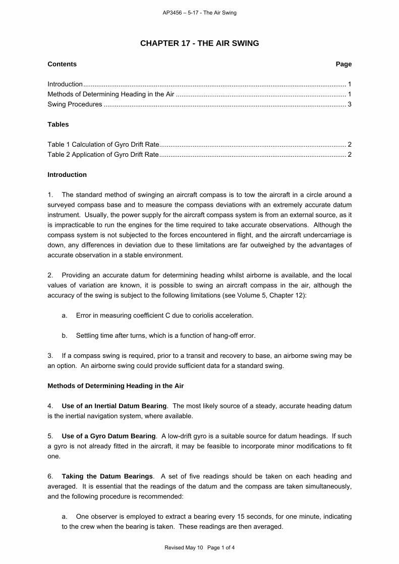
AP3456 – 5-17 - The Air Swing
CHAPTER 17 - THE AIR SWING Contents Page Introduction.............................................................................................................................................. 1 Methods of Determining Heading in the Air ............................................................................................ 1 Swing Procedures ................................................................................................................................... 3 Tables Table 1 Calculation of Gyro Drift Rate..................................................................................................... 2 Table 2 Application of Gyro Drift Rate..................................................................................................... 2 Introduction 1. The standard method of swinging an aircraft compass is to tow the aircraft in a circle around a surveyed compass base and to measure the compass deviations with an extremely accurate datum instrument. Usually, the power supply for the aircraft compass system is from an external source, as it is impracticable to run the engines for the time required to take accurate observations. Although the compass system is not subjected to the forces encountered in flight, and the aircraft undercarriage is down, any differences in deviation due to these limitations are far outweighed by the advantages of accurate observation in a stable environment. 2. Providing an accurate datum for determining heading whilst airborne is available, and the local values of variation are known, it is possible to swing an aircraft compass in the air, although the accuracy of the swing is subject to the following limitations (see Volume 5, Chapter 12):
a. Error in measuring coefficient C due to coriolis acceleration.
b. Settling time after turns, which is a function of hang-off error. 3. If a compass swing is required, prior to a transit and recovery to base, an airborne swing may be an option. An airborne swing could provide sufficient data for a standard swing. Methods of Determining Heading in the Air 4. Use of an Inertial Datum Bearing. The most likely source of a steady, accurate heading datum is the inertial navigation system, where available. 5. Use of a Gyro Datum Bearing. A low-drift gyro is a suitable source for datum headings. If such a gyro is not already fitted in the aircraft, it may be feasible to incorporate minor modifications to fit one. 6. Taking the Datum Bearings. A set of five readings should be taken on each heading and averaged. It is essential that the readings of the datum and the compass are taken simultaneously, and the following procedure is recommended:
a. One observer is employed to extract a bearing every 15 seconds, for one minute, indicating to the crew when the bearing is taken. These readings are then averaged.
Revised May 10 Page 1 of 4
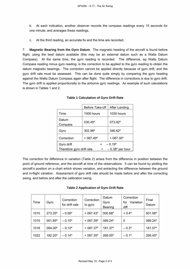
AP3456 – 5-17 - The Air Swing
b. At each indication, another observer records the compass readings every 15 seconds for one minute, and averages these readings.
c. At the third reading, an accurate fix and the time are recorded. 7. Magnetic Bearing from the Gyro Datum. The magnetic heading of the aircraft is found before flight, using the best datum available (this may be an external datum such as a Watts Datum Compass). At the same time, the gyro reading is recorded. The difference, eg Watts Datum Compass reading minus gyro reading, is the correction to be applied to the gyro reading to obtain the datum magnetic bearings. The correction cannot be applied directly because of gyro drift, and the gyro drift rate must be assessed. This can be done quite simply by comparing the gyro heading against the Watts Datum Compass again after flight. The difference in corrections is due to gyro drift. The gyro drift is applied proportionally to the airborne gyro readings. An example of such calculations is shown in Tables 1 and 2.
Table 1 Calculation of Gyro Drift Rate
Before Take-off After Landing
Time 1000 hours 1030 hours
Datum Compass
030.45º 073.92º
Gyro 302.96º 346.62º
Correction + 087.49º + 087.30º
Gyro drift = – 0.19º Therefore gyro drift rate = – 0.38º per hour
The correction for difference in variation (Table 2) arises from the difference in position between the point of ground reference, and the aircraft at time of the observations. It can be found by plotting the aircraft’s position on a chart which shows variation, and extracting the difference between the ground and in-flight variation. Assessment of gyro drift rate should be made before and after the correcting swing, and before and after the calibration swing.
Table 2 Application of Gyro Drift Rate
Time Gyro Correction for drift rate
Correction to gyro
Datum Gyro Bearing
Correction for Variation diff
Final Datum
1010 273.25º – 0.06º + 087.43º 000.68º + 0.4º 001.08º
1015 001.85º – 0.10º + 087.39º 089.24º 0 089.24º
1018 094.00º – 0.12º + 087.37º 181.37º – 0.3º 181.07º
1022 182.20º – 0.14º + 087.35º 269.55º – 0.1º 269.45º
Revised May 10 Page 2 of 4
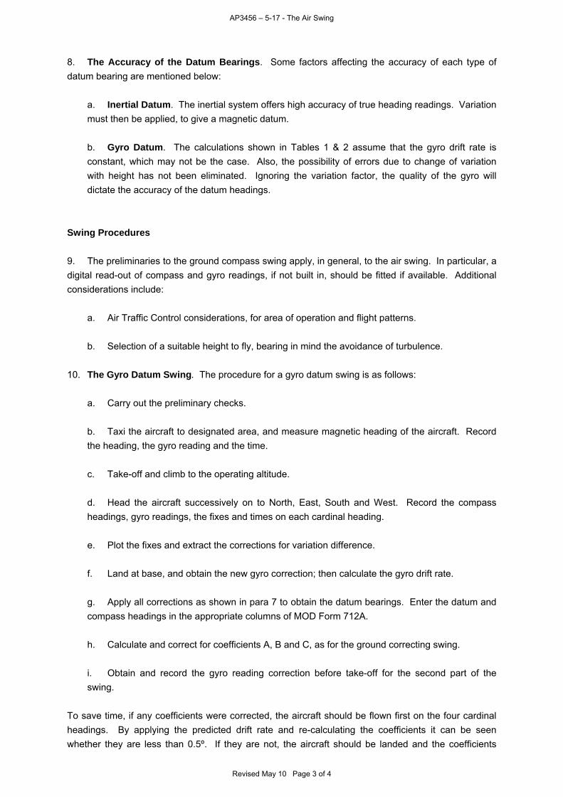
AP3456 – 5-17 - The Air Swing
8. The Accuracy of the Datum Bearings. Some factors affecting the accuracy of each type of datum bearing are mentioned below:
a. Inertial Datum. The inertial system offers high accuracy of true heading readings. Variation must then be applied, to give a magnetic datum.
b. Gyro Datum. The calculations shown in Tables 1 & 2 assume that the gyro drift rate is constant, which may not be the case. Also, the possibility of errors due to change of variation with height has not been eliminated. Ignoring the variation factor, the quality of the gyro will dictate the accuracy of the datum headings.
Swing Procedures 9. The preliminaries to the ground compass swing apply, in general, to the air swing. In particular, a digital read-out of compass and gyro readings, if not built in, should be fitted if available. Additional considerations include:
a. Air Traffic Control considerations, for area of operation and flight patterns.
b. Selection of a suitable height to fly, bearing in mind the avoidance of turbulence. 10. The Gyro Datum Swing. The procedure for a gyro datum swing is as follows:
a. Carry out the preliminary checks.
b. Taxi the aircraft to designated area, and measure magnetic heading of the aircraft. Record the heading, the gyro reading and the time.
c. Take-off and climb to the operating altitude.
d. Head the aircraft successively on to North, East, South and West. Record the compass headings, gyro readings, the fixes and times on each cardinal heading.
e. Plot the fixes and extract the corrections for variation difference.
f. Land at base, and obtain the new gyro correction; then calculate the gyro drift rate.
g. Apply all corrections as shown in para 7 to obtain the datum bearings. Enter the datum and compass headings in the appropriate columns of MOD Form 712A.
h. Calculate and correct for coefficients A, B and C, as for the ground correcting swing.
i. Obtain and record the gyro reading correction before take-off for the second part of the swing.
To save time, if any coefficients were corrected, the aircraft should be flown first on the four cardinal headings. By applying the predicted drift rate and re-calculating the coefficients it can be seen whether they are less than 0.5º. If they are not, the aircraft should be landed and the coefficients
Revised May 10 Page 3 of 4

AP3456 – 5-17 - The Air Swing
Revised May 10 Page 4 of 4
removed as in sub-paras e to h, but if they are less than 0.5º, the calibration swing may proceed as follows:
j. Obtain the readings every 30º. The aircraft may be flown on chords to a circle roughly centred on the airfield.
k. After landing, re-assess the gyro drift rate.
l. Complete the MOD Form 712A and the appropriate deviation card. 11. Airborne Swings against Inertial/Other Datums. Airborne swings against other datums differ from the procedure in para 10 in that it is not necessary to spend time on the ground to determine the gyro corrections and drift. The swing will also only require one flight if the coefficients are less than 0.5º.
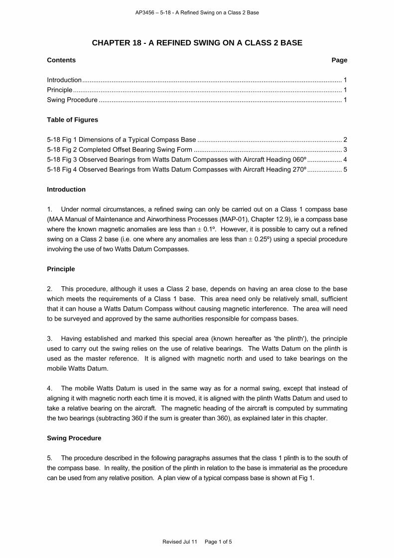
AP3456 – 5-18 - A Refined Swing on a Class 2 Base
CHAPTER 18 - A REFINED SWING ON A CLASS 2 BASE Contents Page Introduction.............................................................................................................................................. 1 Principle................................................................................................................................................... 1 Swing Procedure ..................................................................................................................................... 1 Table of Figures 5-18 Fig 1 Dimensions of a Typical Compass Base ............................................................................... 2 5-18 Fig 2 Completed Offset Bearing Swing Form ................................................................................. 3 5-18 Fig 3 Observed Bearings from Watts Datum Compasses with Aircraft Heading 060º ................... 4 5-18 Fig 4 Observed Bearings from Watts Datum Compasses with Aircraft Heading 270º ................... 5 Introduction 1. Under normal circumstances, a refined swing can only be carried out on a Class 1 compass base (MAA Manual of Maintenance and Airworthiness Processes (MAP-01), Chapter 12.9), ie a compass base where the known magnetic anomalies are less than 0.1º. However, it is possible to carry out a refined swing on a Class 2 base (i.e. one where any anomalies are less than 0.25º) using a special procedure involving the use of two Watts Datum Compasses. Principle 2. This procedure, although it uses a Class 2 base, depends on having an area close to the base which meets the requirements of a Class 1 base. This area need only be relatively small, sufficient that it can house a Watts Datum Compass without causing magnetic interference. The area will need to be surveyed and approved by the same authorities responsible for compass bases. 3. Having established and marked this special area (known hereafter as 'the plinth'), the principle used to carry out the swing relies on the use of relative bearings. The Watts Datum on the plinth is used as the master reference. It is aligned with magnetic north and used to take bearings on the mobile Watts Datum. 4. The mobile Watts Datum is used in the same way as for a normal swing, except that instead of aligning it with magnetic north each time it is moved, it is aligned with the plinth Watts Datum and used to take a relative bearing on the aircraft. The magnetic heading of the aircraft is computed by summating the two bearings (subtracting 360 if the sum is greater than 360), as explained later in this chapter. Swing Procedure 5. The procedure described in the following paragraphs assumes that the class 1 plinth is to the south of the compass base. In reality, the position of the plinth in relation to the base is immaterial as the procedure can be used from any relative position. A plan view of a typical compass base is shown at Fig 1.
Revised Jul 11 Page 1 of 5
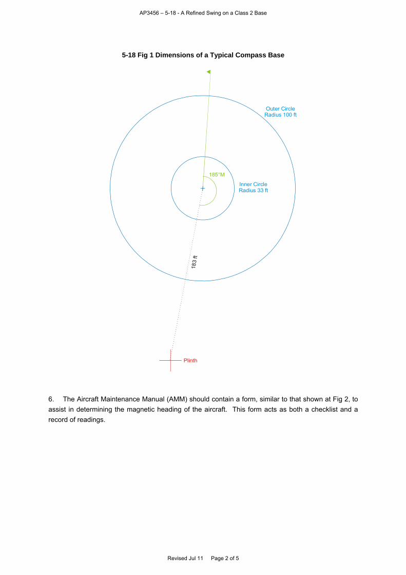
AP3456 – 5-18 - A Refined Swing on a Class 2 Base
5-18 Fig 1 Dimensions of a Typical Compass Base
185°M
Outer CircleRadius 100 ft
Inner CircleRadius 33 ft
Plinth
183
ft
6. The Aircraft Maintenance Manual (AMM) should contain a form, similar to that shown at Fig 2, to assist in determining the magnetic heading of the aircraft. This form acts as both a checklist and a record of readings.
Revised Jul 11 Page 2 of 5
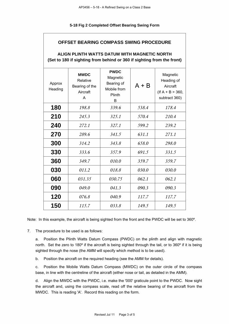
AP3456 – 5-18 - A Refined Swing on a Class 2 Base
5-18 Fig 2 Completed Offset Bearing Swing Form
OFFSET BEARING COMPASS SWING PROCEDURE
ALIGN PLINTH WATTS DATUM WITH MAGNETIC NORTH (Set to 180 if sighting from behind or 360 if sighting from the front)
Approx Heading
MWDC Relative
Bearing of the Aircraft
A
PWDC Magnetic Bearing of
Mobile from Plinth
B
A + B
Magnetic Heading of
Aircraft (If A + B > 360, subtract 360)
180 198.8 339.6 538.4 178.4
210 245.3 325.1 570.4 210.4
240 272.1 327.1 599.2 239.2
270 289.6 341.5 631.1 271.1
300 314.2 343.8 658.0 298.0
330 333.6 357.9 691.5 331.5
360 349.7 010.0 359.7 359.7
030 011.2 018.8 030.0 030.0
060 031.35 030.75 062.1 062.1
090 049.0 041.3 090.3 090.3
120 076.8 040.9 117.7 117.7
150 115.7 033.8 149.5 149.5
Note: In this example, the aircraft is being sighted from the front and the PWDC will be set to 360º. 7. The procedure to be used is as follows:
a. Position the Plinth Watts Datum Compass (PWDC) on the plinth and align with magnetic north. Set the zero to 180º if the aircraft is being sighted through the tail, or to 360º if it is being sighted through the nose (the AMM will specify which method is to be used).
b. Position the aircraft on the required heading (see the AMM for details).
c. Position the Mobile Watts Datum Compass (MWDC) on the outer circle of the compass base, in line with the centreline of the aircraft (either nose or tail, as detailed in the AMM).
d. Align the MWDC with the PWDC, i.e. make the '000' graticule point to the PWDC. Now sight the aircraft and, using the compass scale, read off the relative bearing of the aircraft from the MWDC. This is reading 'A'. Record this reading on the form.
Revised Jul 11 Page 3 of 5
AP3456 – 5-18 - A Refined Swing on a Class 2 Base
e. At the PWDC, take a bearing on the MWDC. This is reading 'B'. Record this reading on the form.
f. Calculate the aircraft magnetic heading by adding together readings 'A' and 'B'. If the resultant is greater than 360, then subtract 360 to arrive at the correct result (see Fig 2). The aircraft heading thus obtained will be used as the entry argument on the compass calibration proforma.
g. Repeat steps c to f each time the heading of the aircraft is changed. 8. Figure 3 shows the observed bearings from the two Watts Datum compasses with the aircraft heading 060º. A similar diagram, with the aircraft on a heading of 270º is shown at Fig 4.
5-18 Fig 3 Observed Bearings from Watts Datum Compasses with Aircraft Heading 060º
MWDC
PWDC
AircraftHeading062.1° M
Relative Bearingof Aircraft from
Mobile (A) is 031.35°
Magnetic Bearingof MWDC from
PWDC (B) is 030.75°
Revised Jul 11 Page 4 of 5
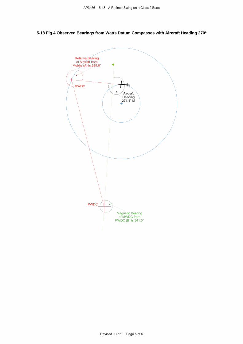
AP3456 – 5-18 - A Refined Swing on a Class 2 Base
Revised Jul 11 Page 5 of 5
5-18 Fig 4 Observed Bearings from Watts Datum Compasses with Aircraft Heading 270º
MWDC
PWDC
AircraftHeading271.1° M
Relative Bearingof Aircraft from
Mobile (A) is 289.6°
Magnetic Bearingof MWDC from
PWDC (B) is 341.5°
AP3456 – 5-19 - The Analysis of the Compass Swing
CHAPTER 19 - THE ANALYSIS OF THE COMPASS SWING Contents Page
THE FOURIER ANALYSIS ..................................................................................................................... 1 Derivation of the Coefficients .................................................................................................................. 1 The Calculated Deviations ...................................................................................................................... 3 Summary of the Fourier Analysis ............................................................................................................ 4 THE ACCURACY ANALYSIS ................................................................................................................. 4 Introduction.............................................................................................................................................. 4 Statistical Analysis of the Swing.............................................................................................................. 4 Further Applications of Statistics ............................................................................................................. 5 Table of Figures
5-19 Fig 1 Deviation Graphs ................................................................................................................... 2 5-19 Fig 2 Compass Calibration Log – Example 1.................................................................................. 6 5-19 Fig 3 Compass Calibration Log – Example 2.................................................................................. 7 5-19 Fig 4 Compass Calibration Log – Example 3.................................................................................. 8 Tables
Table 1 Values of Functions of theta....................................................................................................... 2 Table 2 The Derived Coefficients ............................................................................................................ 3 Table 3 The Calculated Deviations ......................................................................................................... 3 Table 4 The Effect of Carriage of Stores................................................................................................. 5
THE FOURIER ANALYSIS
Derivation of the Coefficients
1. The purpose of the Fourier Analysis is to extract from a set of observations the most accurate
assessment of the deviation coefficients and residual deviations. Volume 5, Chapter 16 described
how the coefficients can be found, but in two cases, B and C, only two readings were used. A more
accurate method is needed.
2. In Volume 5, Chapter 15 it was shown that the deviation caused by coefficient B is a function of
the sine of the heading. The observed deviation on each heading is multiplied by the sine of that
heading, and the results algebraically summed. It can be shown that division of this sum by 2
n,
where n is the number of headings, gives coefficient B. Similar calculations may be done to find
coefficients C, D and E. Coefficient A is derived from the sum of the deviations and the number of
readings. The results can be summarized by the equations:
A = n
δ B =
n
θsinδ2Σ
C = n
2θcosδ2Σ D =
n
2θsinδ2Σ
E = n
2θcosδ2Σ
where is the observed deviation on heading and n is the number of observations.
Revised May 10 Page 1 of 8
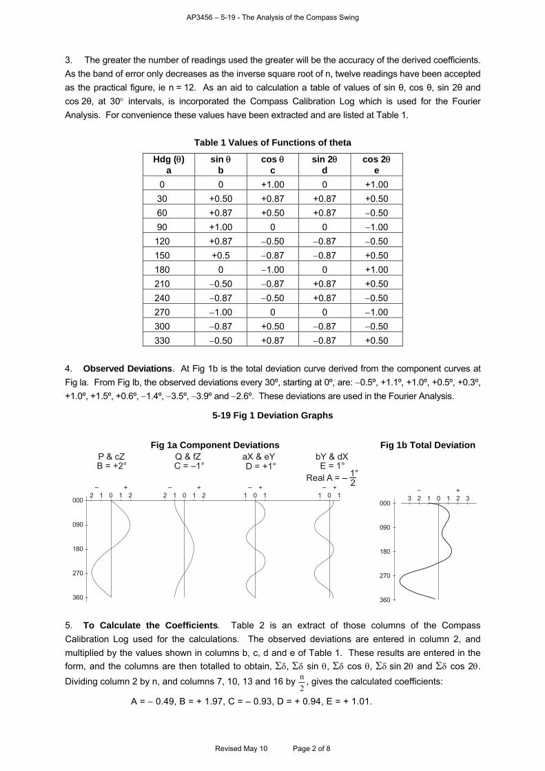
AP3456 – 5-19 - The Analysis of the Compass Swing
3. The greater the number of readings used the greater will be the accuracy of the derived coefficients.
As the band of error only decreases as the inverse square root of n, twelve readings have been accepted
as the practical figure, ie n = 12. As an aid to calculation a table of values of sin θ, cos θ, sin 2θ and
cos 2θ, at 30 intervals, is incorporated the Compass Calibration Log which is used for the Fourier
Analysis. For convenience these values have been extracted and are listed at Table 1.
Table 1 Values of Functions of theta
Hdg () a
sin b
cos c
sin 2 d
cos 2 e
0 0 +1.00 0 +1.00
30 +0.50 +0.87 +0.87 +0.50
60 +0.87 +0.50 +0.87 0.50
90 +1.00 0 0 1.00
120 +0.87 0.50 0.87 0.50
150 +0.5 0.87 0.87 +0.50
180 0 1.00 0 +1.00
210 0.50 0.87 +0.87 +0.50
240 0.87 0.50 +0.87 0.50
270 1.00 0 0 1.00
300 0.87 +0.50 0.87 0.50
330 0.50 +0.87 0.87 +0.50
4. Observed Deviations. At Fig 1b is the total deviation curve derived from the component curves at
Fig la. From Fig lb, the observed deviations every 30º, starting at 0º, are: 0.5º, +1.1º, +1.0º, +0.5º, +0.3º,
+1.0º, +1.5º, +0.6º, 1.4º, 3.5º, 3.9º and 2.6º. These deviations are used in the Fourier Analysis.
5-19 Fig 1 Deviation Graphs
Fig 1a Component Deviations Fig 1b Total Deviation
2 1–
0 1+
2
090
000
180
270
360
2 1–
0 1+
2 1–
0 1+
1–
0
bY & dXE = 1°
aX & eYD = +1°
Q & fZC = –1°
P & cZB = +2°
Real A = – 1°2
1+
2 1–
0 1+23 3
090
000
180
270
360
5. To Calculate the Coefficients. Table 2 is an extract of those columns of the Compass
Calibration Log used for the calculations. The observed deviations are entered in column 2, and
multiplied by the values shown in columns b, c, d and e of Table 1. These results are entered in the
form, and the columns are then totalled to obtain, , sin , cos , sin 2 and cos 2.
Dividing column 2 by n, and columns 7, 10, 13 and 16 by n
2, gives the calculated coefficients:
A = 0.49, B = + 1.97, C = – 0.93, D = + 0.94, E = + 1.01.
Revised May 10 Page 2 of 8
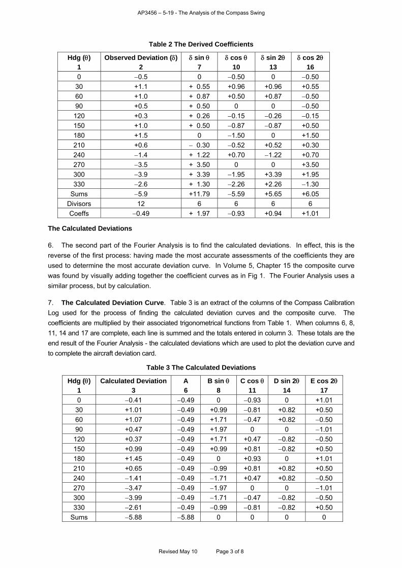
AP3456 – 5-19 - The Analysis of the Compass Swing
Table 2 The Derived Coefficients
Hdg () 1
Observed Deviation ()2
sin 7
cos 10
sin 2 13
cos 2 16
0 0.5 0 0.50 0 0.50
30 +1.1 + 0.55 +0.96 +0.96 +0.55
60 +1.0 + 0.87 +0.50 +0.87 0.50
90 +0.5 + 0.50 0 0 0.50
120 +0.3 + 0.26 0.15 0.26 0.15
150 +1.0 + 0.50 0.87 0.87 +0.50
180 +1.5 0 1.50 0 +1.50
210 +0.6 0.30 0.52 +0.52 +0.30
240 1.4 + 1.22 +0.70 1.22 +0.70
270 3.5 + 3.50 0 0 +3.50
300 3.9 + 3.39 1.95 +3.39 +1.95
330 2.6 + 1.30 2.26 +2.26 1.30
Sums 5.9 +11.79 5.59 +5.65 +6.05
Divisors 12 6 6 6 6
Coeffs 0.49 + 1.97 0.93 +0.94 +1.01
The Calculated Deviations
6. The second part of the Fourier Analysis is to find the calculated deviations. In effect, this is the
reverse of the first process: having made the most accurate assessments of the coefficients they are
used to determine the most accurate deviation curve. In Volume 5, Chapter 15 the composite curve
was found by visually adding together the coefficient curves as in Fig 1. The Fourier Analysis uses a
similar process, but by calculation.
7. The Calculated Deviation Curve. Table 3 is an extract of the columns of the Compass Calibration
Log used for the process of finding the calculated deviation curves and the composite curve. The
coefficients are multiplied by their associated trigonometrical functions from Table 1. When columns 6, 8,
11, 14 and 17 are complete, each line is summed and the totals entered in column 3. These totals are the
end result of the Fourier Analysis - the calculated deviations which are used to plot the deviation curve and
to complete the aircraft deviation card.
Table 3 The Calculated Deviations
Hdg () 1
Calculated Deviation 3
A 6
B sin 8
C cos 11
D sin 2 14
E cos 2 17
0 0.41 0.49 0 0.93 0 +1.01
30 +1.01 0.49 +0.99 0.81 +0.82 +0.50
60 +1.07 0.49 +1.71 0.47 +0.82 0.50
90 +0.47 0.49 +1.97 0 0 1.01
120 +0.37 0.49 +1.71 +0.47 0.82 0.50
150 +0.99 0.49 +0.99 +0.81 0.82 +0.50
180 +1.45 0.49 0 +0.93 0 +1.01
210 +0.65 0.49 0.99 +0.81 +0.82 +0.50
240 1.41 0.49 1.71 +0.47 +0.82 0.50
270 3.47 0.49 1.97 0 0 1.01
300 3.99 0.49 1.71 0.47 0.82 0.50
330 2.61 0.49 0.99 0.81 0.82 +0.50
Sums 5.88 5.88 0 0 0 0
Revised May 10 Page 3 of 8
AP3456 – 5-19 - The Analysis of the Compass Swing
Summary of the Fourier Analysis
8. Any periodic function (the compass swing period is 2) can be broken down into sinusoids of
different amplitudes (the coefficients) and phases (sin, cos, etc). If sufficient readings are available,
the derived parts of the original can be built up again to give the most accurate assessment of the
function. A convenient form for the breaking down and building up processes is the Compass
Calibration Log (Refined Swing).
THE ACCURACY ANALYSIS
Introduction
9. The accuracy analysis gives a statistical assessment of the reliance that can be placed on the
results of the swing, and enables one swing to be compared with another. The analysis is based on
the differences between the observed and calculated deviations, differences which arise because the
aircraft and datum instruments are being used at or beyond their accuracy limits.
10. It will be useful to summarize the following terms which are used in a Fourier Analysis. The
probable error () is the difference between the mean of a series of observations and any single
observation which will not be exceeded on 50% of occasions. Probable error equals 0.674σ, where σ
(sigma) is the standard deviation. Normally the standard deviation is found from: σ =
n
xx 2
where X is the particular reading, and x is the mean of all the readings. As the compass calibration
method does not provide a mean, the calculated deviation is used instead. The probable error
formula then becomes: Single reading = 0.674sn
D2
where D is the difference between the
corresponding observed and calculated deviations and s is the number of unknowns (i.e. the
coefficients). To find the greatest probable error of coefficient A, use is made of the formula: n
A
and for coefficients B, C, D and E of the formula: AEtoB 4.1or,n
2 .
Statistical Analysis of the Swing
11. Fig 2 shows a completed form for the swing used in the Fourier Analysis. Column 4 is D, Column
5 is D2. Thus for the figures used:
ε = ±0.05º
εA = ±0.014º i.e. A = –0.49 ±0.014º
εB to E = ±0.02º i.e. B, C, D and E are within ±0.02º ε of their stated figures.
12. The Meaning of the Probable Errors. The figure for ε of 0.05º means that any single
observed deviation has an evens chance of being within .05º of the calculated deviation, and one
would therefore expect half of the differences to be within 0.05º. Column 4 confirms this. The
coefficient’s probable errors provide a means of comparing one compass swing with another form
of correlation test.
Revised May 10 Page 4 of 8
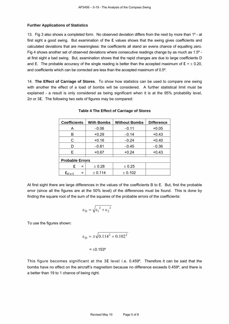
AP3456 – 5-19 - The Analysis of the Compass Swing
Further Applications of Statistics
13. Fig 3 also shows a completed form. No observed deviation differs from the next by more than 1º - at
first sight a good swing. But examination of the ε values shows that the swing gives coefficients and
calculated deviations that are meaningless: the coefficients all stand an evens chance of equalling zero.
Fig 4 shows another set of observed deviations where consecutive readings change by as much as 1.5º -
at first sight a bad swing. But, examination shows that the rapid changes are due to large coefficients D
and E. The probable accuracy of the single reading is better than the accepted maximum of ε = 0.20,
and coefficients which can be corrected are less than the accepted maximum of 0.5º.
14. The Effect of Carriage of Stores. To show how statistics can be used to compare one swing
with another the effect of a load of bombs will be considered. A further statistical limit must be
explained - a result is only considered as being significant when it is at the 95% probability level,
2σ or 3ε. The following two sets of figures may be compared:
Table 4 The Effect of Carriage of Stores
Coefficients With Bombs Without Bombs Difference A 0.06 0.11 +0.05
B +0.29 0.14 +0.43
C +0.16 0.24 +0.40
D 0.81 0.45 0.36
E +0.67 +0.24 +0.43
Probable Errors ε = 0.28 0.25
εB to E = 0.114 0.102
At first sight there are large differences in the values of the coefficients B to E. But, first the probable
error (since all the figures are at the 50% level) of the differences must be found. This is done by
finding the square root of the sum of the squares of the probable errors of the coefficients:
2
22
1D
To use the figures shown:
22
D 102.0114.0
= 0.153º
This figure becomes significant at the 3ε level i.e. 0.459º. Therefore it can be said that the
bombs have no effect on the aircraft’s magnetism because no difference exceeds 0.459º, and there is
a better than 19 to 1 chance of being right.
Revised May 10 Page 5 of 8
Copyright © 2022 FDOKUMEN