HAL Id: hal-02355429https://hal.archives-ouvertes.fr/hal-02355429

Preprint submitted on 8 Nov 2019

HAL is a multi-disciplinary open accessarchive for the deposit and dissemination of sci-entific research documents, whether they are pub-lished or not. The documents may come fromteaching and research institutions in France orabroad, or from public or private research centers.

L’archive ouverte pluridisciplinaire HAL, estdestinée au dépôt et à la diffusion de documentsscientifiques de niveau recherche, publiés ou non,émanant des établissements d’enseignement et derecherche français ou étrangers, des laboratoirespublics ou privés.

Frictionless contact problem for hyperelastic materialswith interior point optimizer

Houssam Houssein, Simon Garnotel, Frédéric Hecht

To cite this version:Houssam Houssein, Simon Garnotel, Frédéric Hecht. Frictionless contact problem for hyperelasticmaterials with interior point optimizer. 2019. hal-02355429

Frictionless contact problem for hyperelastic

materials with interior point optimizer

Houssam Houssein1,2, Simon Garnotel2, Frederic Hecht1

houssein@ljll.math.upmc.fr

simon.garnotel@airthium.com

frederic.hecht@sorbonne-universite.fr

1 Sorbonne Universite, CNRS, Universite de Paris, Inria (Alpines), LaboratoireJacques-Louis Lions (LJLL), F-75005 Paris, France.

2Airthium SAS, Accelair, 1 chemin de la Porte des Loges, 78350, Les Loges-en-Josas, France.

This work was partially funded by the ”Association Nationale de la Recherche etde la Technologie” (ANRT)

Abstract

This paper presents a method to solve the mechanical problems un-dergoing finite deformations and the unilateral contact problems withoutfriction for hyperelastic materials. We apply it to an industrial applica-tion: contact between a mechanical gasket and an obstacle. The mainidea is to formulate the contact problem into an optimization’s one, in or-der to use the Interior Point OPTimizer (IPOPT) to solve it. Finally, theFreeFEM software is used to compute and solve the contact problem. Ourmethod is validated against several benchmarks and used on an industrialapplication example.

Keywords 1 Contact, Frictionless, IPOPT, Interior point, Hertz, Unilateral

1 Introduction

Mechanical contact problems and their simulations are of great importance inthe industry. One of the difficulties encountered in these kinds of problems isthe nonlinearity resulting from the non-penetration between the bodies cominginto contact. Another nonlinearity can come from the material, indeed linearelastic materials are not used in practice to model the materials which can besubmitted to large deformations, instead hyperelastic materials are consideredto model materials like rubber. Hyperelastic materials mechanics are treated in[1, 5, 7, 15, 16].

Several formulations exist for contact problems, we can cite the primal for-mulation where the unknown is the displacement field or the dual formulation

1

where the contact pressure is the unknown of the problem. In this paper, wefollow the contact primal formulation. Different methods can be used to solvea contact problem, like the penalty method, the Lagrangian multiplier method,and the augmented Lagrangian method. For more details about contact me-chanics and methods that can be used for solving the problem, one can refer tothe monographs [12, 22] and the references therein.

In [23], the penalty method was considered for a contact between a hyperelas-tic material and a rigid obstacle, the surface of the rigid obstacle was describedby a C2 function that can be given analytically or by cubic spline interpolation.Mixed formulations are used for example in [9, 10] where the unknowns are thedisplacement field and the contact pressure. A linear elasticity law is used tomodel the material and an Active Set Strategy was used in [10] in order to findthe contact zone. In [17], an algorithm for contact problems involving fluid-structure interactions is presented and uses the semi-smooth Newton method.Several methods can be found in [24], like the Partial Dirichlet-Neumann methodfor unilateral contact. A barrier method was used in [13] to solve the contactproblem.

In this paper, we restrict ourselves to the contact between a hyperelasticbody (where the linear elastic body is a particular case) and a rigid obstacle ora rigid foundation. The dynamical and frictional cases are not treated here. Thegoal of this work is to propose a method that uses the FreeFEM software [8] andits tools to solve the contact problem. As it is formulated as an optimizationproblem, the Interior Point OPTimizer algorithm (IPOPT) [21], which is alreadyinterfaced with FreeFEM [8], is used to solve the optimization problem and toreach the solution. The rigid foundation is supposed to be described by a C2

function, if it is not the case the foundation can be approximated by a splinefunction which is also available in the FreeFEM language.

This paper is organized as follows: in section 2, we present several remindersabout large deformation mechanics and all useful quantities required to intro-duce our contact method, as well as the hyperelastic materials and the for-mulation of the contact problem between a body and a rigid foundation. Insection 3, we present the Interior Point OPTimizer method (IPOPT), used tosolve constrained minimization problems. We also introduce the formulationof our contact problem to be solved. Finally, in section 4, our method is vali-dated against several contact examples and, in section 5, used in an industrialapplication.

2 Nonlinear mechanics

2.1 Large deformation mechanics

Let Ω ⊂ R3 denotes a body and ∂Ω = Γ0 ∪ Γ1 where Γ0 and Γ1 denote respec-tively the disjoint parts of the boundary (Γ0 ∩ Γ1 = ∅) where a displacementand a surface traction t are applied. Assuming the static case, the applicationwhich describes the deformation of the body is called Φ. It transforms the body

2

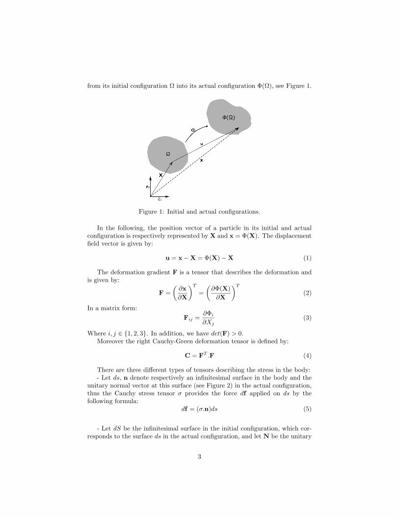
from its initial configuration Ω into its actual configuration Φ(Ω), see Figure 1.

Figure 1: Initial and actual configurations.

In the following, the position vector of a particle in its initial and actualconfiguration is respectively represented by X and x = Φ(X). The displacementfield vector is given by:

u = x−X = Φ(X)−X (1)

The deformation gradient F is a tensor that describes the deformation andis given by:

F =

(∂x

∂X

)T=

(∂Φ(X)

∂X

)T(2)

In a matrix form:

Fij =∂Φi∂Xj

(3)

Where i, j ∈ 1, 2, 3. In addition, we have det(F) > 0.Moreover the right Cauchy-Green deformation tensor is defined by:

C = FT .F (4)

There are three different types of tensors describing the stress in the body:- Let ds, n denote respectively an infinitesimal surface in the body and the

unitary normal vector at this surface (see Figure 2) in the actual configuration,thus the Cauchy stress tensor σ provides the force df applied on ds by thefollowing formula:

df = (σ.n)ds (5)

- Let dS be the infinitesimal surface in the initial configuration, which cor-responds to the surface ds in the actual configuration, and let N be the unitary

3

Figure 2: Infinitesimal surface.

normal vector at dS. Therefore the force df in the actual configuration can alsobe given by:

df = (P.N)dS (6)

Where P denotes the first Piola-Kirchhoff stress tensor and can be obtainedby the following:

P = JσF−T (7)

And J = det(F).- Finally, the force applied at dS in the initial configuration denoted by dF

can be provided by the following equation:

dF = (S.N)dS (8)

S = F−1P denotes the Second Piola-Kirchhoff stress tensor. For more detailsone can refer to [18].

Let ρ be the actual density of the body, f the body force per unit mass appliedon the body (for example the gravity), then the local balance of momentum inthe actual configuration, where the Cauchy stress tensor is taken into account,is described by the following equation:

div(σ) + ρf = 0 (9)

Or, by considering the components, it becomes:

3∑j=1

∂σij∂xj

+ ρfi = 0 i = 1, 2, 3 (10)

The Cauchy stress tensor is symmetric (σ = σT ) by the local balance of an-gular momentum. Note that in the reference configuration the local balance ofmomentum for the body can also be described by:

3∑j=1

∂Pij∂Xj

+ ρ0fi = 0 i = 1, 2, 3 (11)

Where ρ0 is the body density in the reference configuration. In addition, bound-ary conditions must be imposed on the body boundary, therefore if we supposea null displacement on Γ0 and a surface traction t applied on Γ1, we have thefollowing conditions:

u = 0 on Γ0

P.N = t on Γ1

(12)

4

In the following, the admissible displacements set is defined by:

A =v ∈

(H1(Ω)

)3; v = 0 on Γ0

(13)

Where H1(Ω) = W 1,2(Ω) is the Sobolev space. For more details on Sobolevspaces, one can refer to [3, 6].

The weak formulation in the initial configuration is the following:∫Ω

P : Gradv dV −∫

Ω

ρ0f .v dV −∫

Γ1

t.v dA = 0 ∀v ∈ A (14)

Where (Gradv)ij = ∂vi

∂Xjand A : B = tr(ATB).

2.2 Hyperelastic materials

Hyperelastic materials describe a group of materials that can be subject to largedeformations, for example rubber material.

In order to describe the behavior of a material supposed to be isotropic, thestrain energy function Ψ provides a relation between the stress tensors and thedisplacement field, thus the second Piola-Kirchhoff stress tensor can be givenby the following formula:

S = 2.∂Ψ

∂C(15)

Or more explicitly by:

Sij = 2.∂Ψ

∂Cij(16)

Where the tensor C is presented by the equation (4), and the strain energyfunction Ψ depends on the invariants (I1, I2, I3) of the tensor C:

I1 = tr(C)

I2 = 12 ((tr(C))2 − tr(C2))

I3 = det(C) = J2

(17)

We can cite for example two hyperelastic models: the Neo-Hookean and theMooney models. The strain energy functions Ψ of these two models are givenby:

Ψ(I1) = c1(I1 − 3) Neo-Hookean model

Ψ(I1, I2) = c2(I1 − 3) + c3(I2 − 3) Mooney model(18)

Where c1, c2 and c3 are material parameters.The displacement field u, solution of the equation (14), minimizes the total

potential energy E over all admissible displacements. The total potential energyis defined by:

E(v) =

∫Ω

Ψ dV −∫

Ω

ρ0f .v dV −∫

Γ1

t.v dA (19)

5

Thereforeu = argmin

v∈A(E(v)) (20)

Note that the weak formulation (14) presented above can be obtained fromthe minimization problem (20), indeed it can be done by taking the directionalderivative of the energy E to be equal to zero:

DE(u)(v) = 0 ∀ v ∈ A (21)

2.3 Signorini’s contact problem

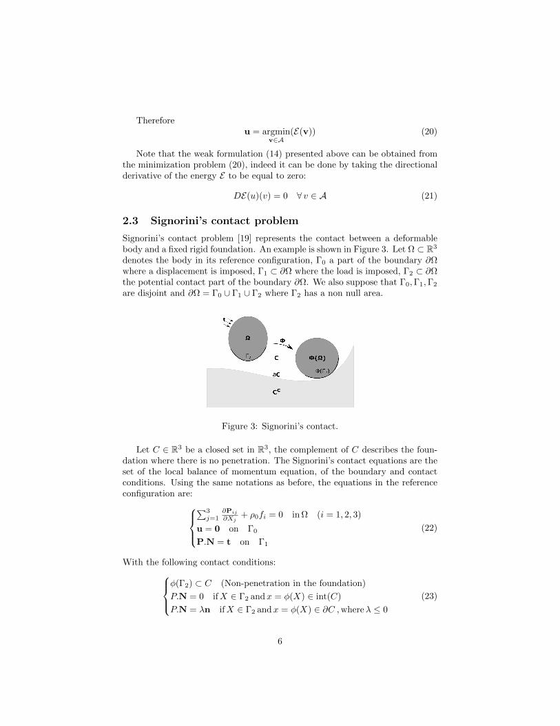
Signorini’s contact problem [19] represents the contact between a deformablebody and a fixed rigid foundation. An example is shown in Figure 3. Let Ω ⊂ R3

denotes the body in its reference configuration, Γ0 a part of the boundary ∂Ωwhere a displacement is imposed, Γ1 ⊂ ∂Ω where the load is imposed, Γ2 ⊂ ∂Ωthe potential contact part of the boundary ∂Ω. We also suppose that Γ0,Γ1,Γ2

are disjoint and ∂Ω = Γ0 ∪ Γ1 ∪ Γ2 where Γ2 has a non null area.

Figure 3: Signorini’s contact.

Let C ∈ R3 be a closed set in R3, the complement of C describes the foun-dation where there is no penetration. The Signorini’s contact equations are theset of the local balance of momentum equation, of the boundary and contactconditions. Using the same notations as before, the equations in the referenceconfiguration are:

∑3j=1

∂Pij

∂Xj+ ρ0fi = 0 in Ω (i = 1, 2, 3)

u = 0 on Γ0

P.N = t on Γ1

(22)

With the following contact conditions:φ(Γ2) ⊂ C (Non-penetration in the foundation)

P.N = 0 ifX ∈ Γ2 andx = φ(X) ∈ int(C)

P.N = λn ifX ∈ Γ2 andx = φ(X) ∈ ∂C ,whereλ ≤ 0

(23)

6

For the hyperelastic materials, the first Piola-Kirchhoff stress tensor can beobtained by:

P =∂Ψ

∂F(24)

The contact formulation described in (22) and (23) can be formulated like in[7] as a constrained minimization problem, i.e if u is the solution of Signorini’scontact problem (22) and (23) then:

u = argminv∈H

(E(v)) (25)

Where E is the total potential energy defined in (19) and H is the set definedby:

H =v ∈

(H1(Ω)

)3; v = 0 on Γ0 ; φ(Γ2) ⊂ C

(26)

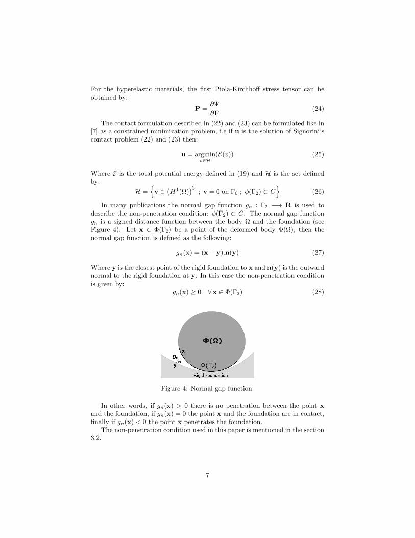
In many publications the normal gap function gn : Γ2 −→ R is used todescribe the non-penetration condition: φ(Γ2) ⊂ C. The normal gap functiongn is a signed distance function between the body Ω and the foundation (seeFigure 4). Let x ∈ Φ(Γ2) be a point of the deformed body Φ(Ω), then thenormal gap function is defined as the following:

gn(x) = (x− y).n(y) (27)

Where y is the closest point of the rigid foundation to x and n(y) is the outwardnormal to the rigid foundation at y. In this case the non-penetration conditionis given by:

gn(x) ≥ 0 ∀x ∈ Φ(Γ2) (28)

Figure 4: Normal gap function.

In other words, if gn(x) > 0 there is no penetration between the point xand the foundation, if gn(x) = 0 the point x and the foundation are in contact,finally if gn(x) < 0 the point x penetrates the foundation.

The non-penetration condition used in this paper is mentioned in the section3.2.

7

3 Minimization problem resolution

3.1 Interior Point Optimizer

One of the open source software for optimization is IPOPT (Interior Point OP-Timizer [21]). IPOPT can solve large scale constrained and unconstrained op-timization problems where the constraints can be nonlinear. In other words, itsolves the following problem:

Minu∈Rn

f(u) such that

gLo ≤ g(u) ≤ gUpuLo ≤ u ≤ uUp

(29)

Where f : Rn → R is the function to minimize and g = (g(1), . . . , g(m)) :Rn → Rm the inequality constraints. The two symbols Lo and Up denoterespectively the lower and upper bounds, and the inequality between vectorsmeans the inequality between the components of the vectors. In addition we

suppose that g(i)Lo, u

(j)Lo ∈ R ∪ −∞ and finally g

(i)Up, u

(j)Up ∈ R ∪ +∞ for all

i = 1, . . . ,m and j = 1, . . . , n. The functions f and g are supposed to besufficiently smooth (For example C2).

By introducing the slack variables s = (s(1), . . . , s(m)) ∈ Rm, the inequalityconstraint equations in (29) can be expressed as:

g(i)(u)− s(i) = 0

g(i)Lo ≤ s(i) ≤ g(i)

Up ∀ i = 1, . . . ,m(30)

Therefore the minimization problem (29) is simplified and can thus be re-formulated as follows:

Min(u,s)∈Rn×Rm

f(u) such that

g(u)− s = 0

(uLo, gLo) ≤ (u, s) ≤ (uUp, gUp)

(31)

Or in a simplified way and without loss of generality the problem can be trans-formed as follows:

Minu∈Rn

f(u) such that

g(u) = 0

u ≥ 0

(32)

IPOPT solves the minimization problem in multiple steps and we will onlydescribe the principal ones, for more details see [20, 21]. The algorithm isbriefly described in Algorithm 1:

The first-order optimality condition is given by:∇f(u) +∇g(u)λ− z = 0

g(u) = 0

UZe− µe = 0

(33)

8

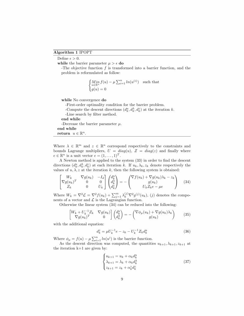
Algorithm 1 IPOPT

Define ε > 0.while the barrier parameter µ > ε do

-The objective function f is transformed into a barrier function, and theproblem is reformulated as follow:

Minu∈Rn

f(u)− µ∑ni=1 ln(u(i)) such that

g(u) = 0

while No convergence do-First-order optimality condition for the barrier problem.-Compute the descent directions (duk , d

λk , d

zk) at the iteration k.

-Line search by filter method.end while-Decrease the barrier parameter µ.

end whilereturn u ∈ Rn.

Where λ ∈ Rm and z ∈ Rn correspond respectively to the constraints andbounds Lagrange multipliers, U = diag(u), Z = diag(z) and finally wheree ∈ Rn is a unit vector e = (1, . . . , 1)T .

A Newton method is applied to the system (33) in order to find the descentdirections (duk , d

λk , d

zk) at each iteration k. If uk, λk, zk denote respectively the

values of u, λ, z at the iteration k, then the following system is obtained: Wk ∇g(uk) −Id∇g(uk)T 0 0

Zk 0 Uk

dukdλkdzk

= −

∇f(uk) +∇g(uk)λk − zkg(uk)

UkZke− µe

(34)

Where Wk = ∇2L = ∇2f(uk) +∑mj=1 λ

(j)k ∇2g(j)(uk), (j) denotes the compo-

nents of a vector and L is the Lagrangian function.Otherwise the linear system (34) can be reduced into the following:[

Wk + U−1k Zk ∇g(uk)

∇g(uk)T 0

](dukdλk

)= −

(∇φµ(uk) +∇g(uk)λk

g(uk)

)(35)

with the additional equation:

dzk = µU−1k e− zk − U−1

k Zkduk (36)

Where φµ = f(u)− µ∑ni=1 ln(ui) is the barrier function.

As the descent direction was computed, the quantities uk+1, λk+1, zk+1 atthe iteration k+1 are given by:

uk+1 = uk + αkduk

λk+1 = λk + αkdλk

zk+1 = zk + αzkdzk

(37)

9

In order to improve the convergence of the algorithm, a linear search methodwith a filter method is used to determine the parameters αk. Using the samenotation as in [21], let θ(u) = ‖g(u)‖ be the constraint violation. At first aparameter αk is proposed, a filter F is a set of R2, it helps to determine ifαk can be accepted as a step size and to avoid cycling between two successivesolutions. Indeed when the optimization starts the filter is initialized as follow:

F0 = (θ, φ) ∈ R2 | θ ≥ θmax (38)

Where θmax is a chosen value. After each iteration the filter is updated accordingto the situation, to:

Fk+1 = Fk ∪ (θ, φ) ∈ R2 | θ ≥ (1− γθ)θ(uk) & φ ≥ φµ(uk)− γφθ(uk) (39)

or to:Fk+1 = Fk (40)

Where (γθ, γφ) ∈]0, 1[2 are two fixed values.The step size αk is accepted if (θ(uk+1(αk)), φµ(uk+1(αk)) /∈ Fk, if it is

not the case, several actions may be possible like the correction of the descentdirection for example.

Finally the barrier parameter µ is decreased and the iteration starts fromthe last converged solution. The solution of the above algorithm, which dependson the barrier parameter u(µ), converges to the solution of the original problem(29) as µ→ 0.

3.2 Formulation of the problem

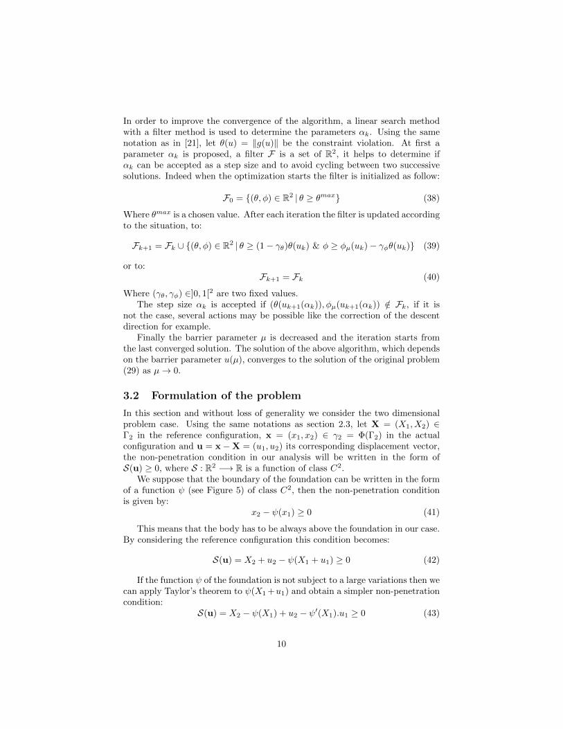
In this section and without loss of generality we consider the two dimensionalproblem case. Using the same notations as section 2.3, let X = (X1, X2) ∈Γ2 in the reference configuration, x = (x1, x2) ∈ γ2 = Φ(Γ2) in the actualconfiguration and u = x−X = (u1, u2) its corresponding displacement vector,the non-penetration condition in our analysis will be written in the form ofS(u) ≥ 0, where S : R2 −→ R is a function of class C2.

We suppose that the boundary of the foundation can be written in the formof a function ψ (see Figure 5) of class C2, then the non-penetration conditionis given by:

x2 − ψ(x1) ≥ 0 (41)

This means that the body has to be always above the foundation in our case.By considering the reference configuration this condition becomes:

S(u) = X2 + u2 − ψ(X1 + u1) ≥ 0 (42)

If the function ψ of the foundation is not subject to a large variations then wecan apply Taylor’s theorem to ψ(X1 +u1) and obtain a simpler non-penetrationcondition:

S(u) = X2 − ψ(X1) + u2 − ψ′(X1).u1 ≥ 0 (43)

10

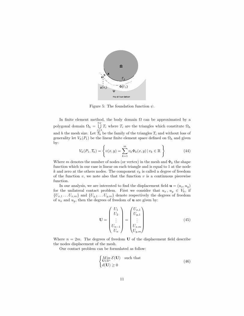
Figure 5: The foundation function ψ.

In finite element method, the body domain Ω can be approximated by a

polygonal domain Ωh =nT⋃i=1

Ti where Ti are the triangles which constitute Ωh

and h the mesh size. Let Th be the family of the triangles Ti and without loss ofgenerality let Vh(P1) be the linear finite element space defined on Ωh and givenby:

Vh(P1, Th) =

v(x, y) =

m∑k=1

vkΦk(x, y) | vk ∈ R

(44)

Where m denotes the number of nodes (or vertex) in the mesh and Φk the shapefunction which in our case is linear on each triangle and is equal to 1 at the nodek and zero at the others nodes. The component vk is called a degree of freedomof the function v, we note also that the function v is a continuous piecewisefunction.

In our analysis, we are interested to find the displacement field u = (ux, uy)for the unilateral contact problem. First we consider that ux , uy ∈ Vh, ifUx,1 . . . Ux,m and Uy,1 . . . Uy,m denote respectively the degrees of freedomof ux and uy, then the degrees of freedom of u are given by:

U =

U1

U2

...Un−1

Un

=

Ux,1Uy,1

...Ux,mUy,m

(45)

Where n = 2m. The degrees of freedom U of the displacement field describethe nodes displacement of the mesh.

Our contact problem can be formulated as follow:MinU∈Rn

E(U) such that

d(U) ≥ 0(46)

11

Where U ∈ Rn is the displacement vector of the body mesh nodes, E(U) is thetotal potential energy of the body and finally d = (d(1), . . . , d(nb)) : Rn → Rnb

represents the non-penetration condition with the rigid foundation for each nodeof the boundary (Γ2) and nb is the number of the boundary (Γ2) nodes.

More precisely d(i) represents the non-penetration condition for the node ibelonging to the boundary (Γ2) and is defined by:

d(i)(U) = S(Dxi, Dyi) (47)

Where S is defined in (42) and (Dxi, Dyi) is the displacement vector for thenode i.

Finally, we obtain a constrained minimization problem which can be solvedby the Interior Point OPTimizer (IPOPT) as we will see in the next section.

4 Numerical validations

In this section, we present several common numerical examples in order to vali-date our method. First, we will present two tests in 2D and 3D on the compres-sion of a hyperelastic cube with two specific types of materials. In these tests thecontact is not taken into account, indeed the goal is to validate our algorithmin solving problems with a hyperelastic material behavior. Next, we present3 contact tests, where 2 are a Hertz contact problem with an explicit analyticsolutions, to validate our contact method for an arbitrary rigid foundation.

In FreeFEM, necessary quantities like the energy and the constraints (Ja-cobian, Hessian) are computed, then IPOPT is used to solve our constrainedminimization problem through its FreeFEM interface. To see how we can useIPOPT with FreeFEM one can refer to [4, 8]. The advantage of this method isthat we have just to formulate our contact problem and IPOPT will act like ablack box to solve the optimization problem.

4.1 Compression of a hyperelastic cube

Here we handle the tests presented in [2]. A unit cube of dimension equal to1m is considered (see Figure 6), the cube can move along the direction X1 andits two faces which are perpendicular to the direction X3 are fixed along thislast direction, finally, the lower face of this cube is fixed along the direction X2.A pressure of f = 0.876Pa is applied on the upper face of the cube.

Two nearly incompressible hyperelastic material models [14] are consideredfor the cube: Neo-Hookean and Mooney. These models describe also the incom-pressibility of the two materials. The goal is to compute the displacement field(specifically the vertical displacement) and to compare it with the theoreticalone. The strain energy functions of these two models are given as follow:

ψ = C10(J−23 I1 − 3) + C01(J−

43 I2 − 3) +

K

2(J − 1)2 (48)

12

Where K = 6(C01+C10)3(1−2ν) [14] and ν is the Poisson’s ratio. The function K

2 (J−1)2

helps to satisfy the incompressibility constraint (J = 1) by penalizing it. Thecoefficients C01, C10 and ν are presented in the table 1:

Figure 6: The cube with the appliedpressure.

Table 1: Material coef-ficients

Coefficients Mooney Neo-Hookean

C10 0.709 1.2345

C01 2.3456 0.

ν 0.499 0.499

The linear finite element P1 [8] was used for this study and the mesh contains200 elements in the two dimensional case. In order to avoid the rigid movementof the structure and using the fact that the problem is symmetric, only half ofthe structure is modeled like we can see in Figure 7 for the two dimensionalcase.

Using IPOPT in order to minimize the total potential energy of the cubeand generate the displacement field, the maximum vertical displacement of theupper face is given in the table 2.

FreeFEM in 2D Mooney Neo-Hookeanw 0.034072 0.078331

Table 2: Vertical displacement w with FreeFEM in 2D

The errors with respect to the theoretical values for our method and Code Aster[2] are presented in the table 3 where we can see similar results.

In the Figure 8a, the deformed shape and the vertical displacement for theNeo-Hookean material case is shown. To see the FreeFEM script of the ex-ample presented above, please visit https://modules.freefem.org/modules/nonlinear-elasticity/.

On the other hand, the exact same results were generated by consideringthe three dimensional case for the two type of materials. In addition, note thatwe obtained the same results for the displacement field by supposing that thecube is in contact on its lower face with a rigid foundation, see Figure 8b forthe three dimensional case.

4.2 Hertz contact problem

A classical contact problem is the contact between two deformable cylinderswhere their axis are parallel, and a theoretical solution exists for this type of

13

Figure 7: The 2D symmetrical modelof the cube.

Table 3: Errors with re-spect to the theoreticalvalues

Errors FreeFEM Code Aster

Errors in 2D (Mooney) 0.19% 0.20%

Errors in 2D (Neo-Hookean) 0.19% 0.20%

(a) 2D case (b) 3D case

Figure 8: Vertical displacement field (Neo-Hookean).

problems (see [11]). In the following, the plane strain situation is consideredand it corresponds to the two dimensional case (2D). In other words, the heightof the cylinders is large. Finally, the frictionless contact is also supposed.

In general, the zone of contact between the cylinders is a strip of width 2a,in the 2D situation the contact becomes between two discs. The quantity ofinterest is the normal pressure at the contact zone. Let a force of magnitudeP be applied on the first cylinder and let this force be normal to its axis inorder to compress the two bodies and let them enter in contact. Therefore,by assuming the hypothesis of small deformations and linear elasticity we canobtain analytically the half length of the contact zone a in addition to the profileof the normal pressure at the contact zone.

14

Let R1 and R2 denote the radius of the cylinders, E1, E2 the Young’s mod-ulus and ν1, ν2 the Poisson’s ratio of the first and second cylinder, then the halfcontact length a is given by:

a =

√4PR

πE∗(49)

Where R and E∗ are computed as follow:1R = 1

R1+ 1

R2

1E∗ =

1−ν21

E1+

1−ν22

E2

(50)

Let x denotes the coordinate along the contact zone, thus the normal pres-sure profile p is given as follow:

p(x) = pmax

√1− x2

a2(51)

Where pmax = 2Pπa , the maximum pressure, is located at the origin of the

contact zone.The second cylinder can be considered as a rigid foundation by taking a

large value of its Young’s modulus E2 → +∞, thus we obtain E∗ → E1

1−ν21

and

the same equations presented above can be used.In the same manner, the second cylinder can be replaced by a plane by

taking R2 → +∞, therefore R→ R1.Next we present the numerical results of two contact examples involving a

deformable cylinder against a rigid foundation. The foundation is respectivelya plane and a cylinder for the first and second example. Due to the two dimen-sional case and the symmetry of the problem, only a quarter of a disc, whichrepresents the cylinder, will be modeled. In the two examples f denotes thepressure applied on the top face of the quarter disc, R1, E1 and ν1 denote re-spectively the radius, Young’s modulus and the Poisson’s ratio of the quarterdisc. Note that the total force applied is equal to P = 2fR1.

4.2.1 Contact with a rigid plane foundation

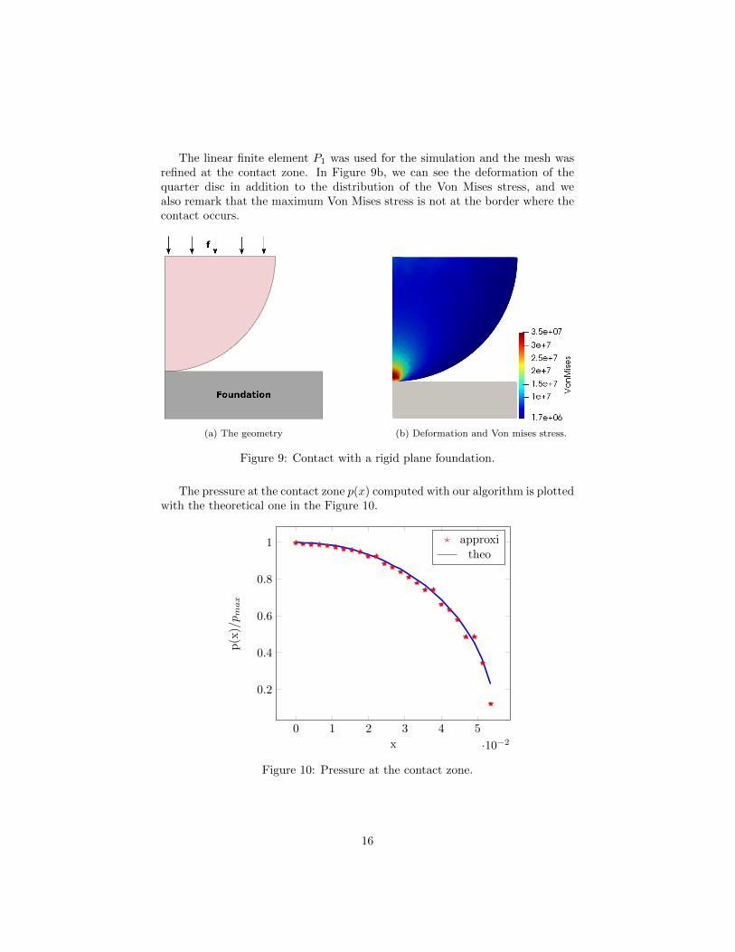
The contact between the quarter disc and the rigid plane is shown below (Figure9a). In order to compare our results to the theoretical one, we suppose thefollowing values: a radius R1 = 1m, a Young’s modulus E1 = 2.1 × 109 Pa, aPoisson’s ratio ν1 = 0.3 and finally a top face pressure of f = 2.75× 106 Pa.

In this case the half contact length a is equal to:

a =

√8fR2

1(1− ν21)

πE1(52)

The maximum pressure and the pressure profile at the contact zone are equal

to: pmax =4fR1

πa(53) p(x) = pmax

√1− x2

a2(54)

15

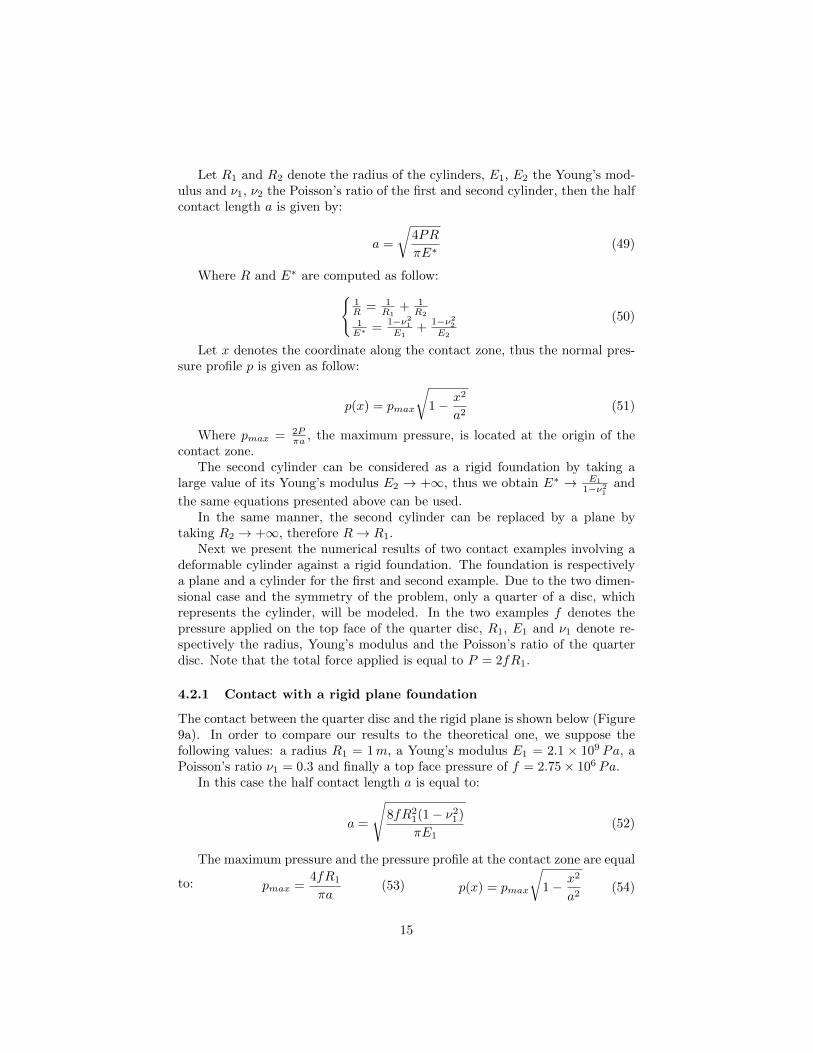
The linear finite element P1 was used for the simulation and the mesh wasrefined at the contact zone. In Figure 9b, we can see the deformation of thequarter disc in addition to the distribution of the Von Mises stress, and wealso remark that the maximum Von Mises stress is not at the border where thecontact occurs.

(a) The geometry (b) Deformation and Von mises stress.

Figure 9: Contact with a rigid plane foundation.

The pressure at the contact zone p(x) computed with our algorithm is plottedwith the theoretical one in the Figure 10.

0 1 2 3 4 5

·10−2

0.2

0.4

0.6

0.8

1

x

p(x

)/pmax

approxitheo

Figure 10: Pressure at the contact zone.

16

4.2.2 Contact with a rigid circular foundation

In this example the contact is between the quarter disc and a rigid cylinder ofradius R2 = 1.2m, also modeled by a quarter disc (Figure 11a). The propertiesof the deformable quarter disc are the following: a radius R1 = 1m, Young’smodulus E1 = 2.1 × 105 Pa, and a Poisson’s ratio ν1 = 0.3. The top facepressure is equal to f = 250Pa.

The half contact length a can be computed analytically by:

a =

√8fR1R(1− ν2

1)

πE1(55)

Where R = R1R2

R1+R2. Using the same formulas, the maximum pressure and the

pressure profile at the contact zone are equal to:

pmax =4fR1

πa(56) p(x) = pmax

√1− x2

a2(57)

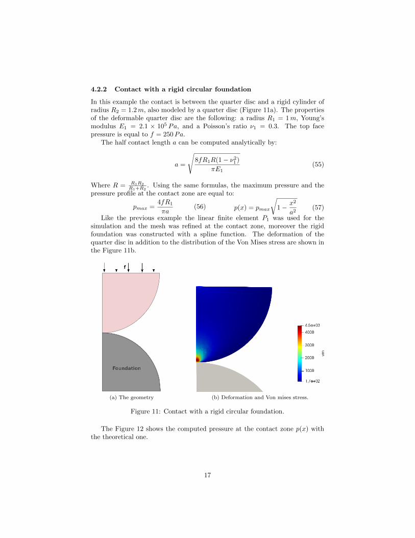
Like the previous example the linear finite element P1 was used for thesimulation and the mesh was refined at the contact zone, moreover the rigidfoundation was constructed with a spline function. The deformation of thequarter disc in addition to the distribution of the Von Mises stress are shown inthe Figure 11b.

(a) The geometry (b) Deformation and Von mises stress.

Figure 11: Contact with a rigid circular foundation.

The Figure 12 shows the computed pressure at the contact zone p(x) withthe theoretical one.

17

0 1 2 3 4

·10−2

0.2

0.4

0.6

0.8

1

x

p(x

)/pmax

approxitheo

Figure 12: Pressure at the contact zone.

4.3 Clamped body contact

In this test an iron square Ω of length equal to 1m is considered, the squareis clamped on its side Γ0 and is initially in contact with a rigid plane on itsside Γ2 (see Figure 13a). The body is subjected by its own weight where ρ =7800 kg.m−3 and g = 9.81m.s−2. The properties of the elastic body are theYoung’s modulus E = 2.1× 1011 Pa and the Poisson’s ration ν = 0.3. This testwas treated in [9]. A uniform mesh was taken with 51 nodes at each side, thefinite element used is the P2 element.

The deformed configuration of the body is shown in the Figure 13b with anamplification factor.

In Figure 14, the contact pressure on the left side Γ2 is plotted in comparisonwith the values found in [9].

5 Industrial application example

In this analysis an O-ring gasket is trapped between two metallic parts (seeFigure 15). As the radius of the gasket section is small compared to its circum-ference, we suppose that we are in the plane strain configuration, thus only asection of the gasket is studied. In this analysis the metallic parts are supposedto be rigid.

The following data are only used to illustrate the behavior of the gasket,thus a radius of R = 0.52m is taken for the gasket section, the gap between thetwo supports is g = 0.2m, the material model considered for this simulation isthe Neo-Hookean model presented in (48), and finally the inner shape of thetwo metallic parts is a square of dimension l = 1m.

18

(a) The geometry (b) The body deformation (amplification factor= 2.105).

Figure 13: The square iron problem.

0 0.2 0.4 0.6 0.8 10

0.2

0.4

0.6

0.8

1

1.2·105

y(m)

p(y

)(P

a)

FreeFEMHild

Figure 14: Contact pressure at the side Γ2 of the body.

The deformed shape of the compressed gasket and the Von-mises stress dis-tribution are shown in the Figure 16.

6 Conclusion

In this work, we formulated the unilateral frictionless contact problem into aconstrained minimization problem and we used IPOPT like a black box to solvethe optimization problem. The proposed method has the advantage of being

19

Figure 15: The two metallic parts where the gasket is trapped.

Figure 16: The deformed shape and the Von-mises stress distribution.

simple to implement in FreeFEM because optimization tools are already avail-able. The results of the nonlinear behavior tests were similar to those obtainedby Code Aster, besides, as we showed in the validation section, our contactmethod gave results close to the analytic one or results done by other methods.In the future, the scope of the method will be extended to the contact betweentwo bodies, and to the dynamic case.

Acknowledgments

We would like to acknowledge Franck Lahaye from , Airthium SAS, for hislinguistic help.

20

References

[1] M. ABBAS, Code Aster [R5.03.19] Loi de comportement hyperelastique :materiau presque incompressible, EDF R&D, 8 2013.

[2] M. ABBAS, Code Aster [V6.04.187] SSNV187 - Validation de la loiELAS HYPER sur un cube, EDF R&D, 5 2018.

[3] R. A. Adams and J. J. Fournier, Sobolev spaces, vol. 140, Elsevier,2003.

[4] S. Auliac, developpement d’outils d’optimisation pour freefem++, PhDthesis, Universite Pierre et Marie Curie-Paris VI, 2014.

[5] J. Bonet and R. D. Wood, Nonlinear continuum mechanics for finiteelement analysis, Cambridge university press, 1997.

[6] H. Brezis, Functional analysis, Sobolev spaces and partial differentialequations, Springer Science & Business Media, 2010.

[7] P. G. Ciarlet, Three-dimensional elasticity, vol. 20, Elsevier, 1988.

[8] F. Hecht, New development in freefem++, J. Numer. Math., 20 (2012),pp. 251–265.

[9] P. Hild, A sign preserving mixed finite element approximation for contactproblems, International Journal of Applied Mathematics and ComputerScience, 21 (2011), pp. 487–498.

[10] S. Hueber and B. I. Wohlmuth, A primal–dual active set strategy fornon-linear multibody contact problems, Computer Methods in Applied Me-chanics and Engineering, 194 (2005), pp. 3147–3166.

[11] K. L. Johnson, Contact mechanics, Cambridge university press, 1985.

[12] N. Kikuchi and J. T. Oden, Contact problems in elasticity: a study ofvariational inequalities and finite element methods, vol. 8, siam, 1988.

[13] G. Kloosterman, R. M. van Damme, A. H. van den Boogaard,and J. Huetink, A geometrical-based contact algorithm using a barriermethod, International Journal for Numerical Methods in Engineering, 51(2001), pp. 865–882.

[14] J.-P. LEFEBVRE, Code Aster [U4.43.01] Operator DEFI MATERIAU,EDF R&D, 7 2018.

[15] G. Marckmann and E. Verron, Comparison of hyperelastic models forrubber-like materials, Rubber chemistry and technology, 79 (2006), pp. 835–858.

21

[16] R. W. Ogden, Large deformation isotropic elasticity–on the correlationof theory and experiment for incompressible rubberlike solids, Proc. R. Soc.Lond. A, 326 (1972), pp. 565–584.

[17] O. Pironneau, Handling contacts in an eulerian frame: a finite elementapproach for fluid structures with contacts, International Journal of Com-putational Fluid Dynamics, 32 (2018), pp. 121–130.

[18] J. N. Reddy, An introduction to continuum mechanics, Cambridge uni-versity press, 2013.

[19] A. Signorini, Sopra alcune questioni di elastostatica, Atti della SocietaItaliana per il Progresso delle Scienze, 21 (1933), pp. 143–148.

[20] A. Wachter, Short tutorial: getting started with ipopt in 90 minutes,in Dagstuhl Seminar Proceedings, Schloss Dagstuhl-Leibniz-Zentrum furInformatik, 2009.

[21] A. Wachter and L. T. Biegler, On the implementation of an interior-point filter line-search algorithm for large-scale nonlinear programming,Mathematical programming, 106 (2006), pp. 25–57.

[22] P. Wriggers, Computational Contact Mechanics, Second Edition,Springer-Verlag, 2006.

[23] P. Wriggers and M. Imhof, On the treatment of nonlinear unilateralcontact problems, Archive of Applied Mechanics, 63 (1993), pp. 116–129.

[24] V. Yastrebov, Computational contact mechanics: geometry, detectionand numerical techniques, PhD thesis, Ecole Nationale Superieure desMines de Paris, 2011.

22