lable at ScienceDirect

European Journal of Mechanics A/Solids 28 (2009) 991–1013

Contents lists avai

European Journal of Mechanics A/Solids

journal homepage: www.elsevier .com/locate/e jmsol

Free vibrations of four-parameter functionally graded parabolic panelsand shells of revolution

Francesco Tornabene*, Erasmo ViolaDISTART – Department, Faculty of Engineering, University of Bologna, Viale Risorgimento 2, 40100 Bologna, Italy

a r t i c l e i n f o

Article history:Received 19 May 2008Accepted 16 April 2009Available online 5 May 2009

Keywords:Functionally graded materialsDoubly curved shellsFSD theoryFree vibrationsGeneralized Differential Quadrature

* Corresponding author. Tel.: þ39 051 209 3379; faE-mail address: francesco.tornabene@mail.ing.unib

0997-7538/$ – see front matter � 2009 Elsevier Masdoi:10.1016/j.euromechsol.2009.04.005

a b s t r a c t

Basing on the First-order Shear Deformation Theory (FSDT), this paper focuses on the dynamic behaviourof moderately thick functionally graded parabolic panels and shells of revolution. A generalization of thepower-law distribution presented in literature is proposed. Two different four-parameter power-lawdistributions are considered for the ceramic volume fraction. Some symmetric and asymmetric materialprofiles through the functionally graded shell thickness are illustrated by varying the four parameters ofpower-law distributions. The governing equations of motion are expressed as functions of five kinematicparameters. For the discretization of the system equations the Generalized Differential Quadrature (GDQ)method has been used. Numerical results concerning four types of parabolic shell structures illustrate theinfluence of the parameters of the power-law distribution on the mechanical behaviour of shell struc-tures considered.

� 2009 Elsevier Masson SAS. All rights reserved.

1. Introduction

Functionally graded materials (FGM) are a class of compositesthat have a smooth and continuous variation of material propertiesfrom one surface to another and thus can alleviate the stressconcentrations found in laminated composites. Typically, thesematerials consist of a mixture of ceramic and metal, or a combina-tion of different materials. Extensive research work has beencarried out on this new class of composites since the concept itselfwas first introduced and proposed in the late 1980s in Japan. One ofthe advantages of using functionally graded materials is that theycan survive environments with high temperature gradients, whilemaintaining structural integrity. Furthermore, the continuouschange in the compositions leads to a smooth change in themechanical properties, which has many advantages over thelaminated composites, where the delamination and cracks are mostlikely to initiate at the interfaces due to the abrupt variation inmechanical properties between laminae.

In the last years, some researchers have analyzed various char-acteristics of functionally graded structures (Ng et al., 2000; Yanget al., 2003; Della Croce and Venini, 2004; Liew et al., 2004; Wu andTsai, 2004; Elishakoff et al., 2005a,b; Patel et al., 2005; Abrate,2006; Pelletier and Vel, 2006; Zenkour, 2006; Arciniega and Reddy,

x: þ39 051 209 3495.o.it (F. Tornabene).

son SAS. All rights reserved.

2007; Nie and Zhong, 2007; Roque et al., 2007; Yang and Shen,2007).

The aim of this paper is to study the dynamic behaviour offunctionally graded parabolic shell structures derived from shells ofrevolution, which are very common structural elements. Asa matter of fact, the approach for studying the vibration of isotropicshell (Tornabene and Viola, 2008) is now extended to shells madeof four parametric functionally graded materials.

The work is based on the First-order Shear Deformation Theory(FSDT) (Reddy, 2003). The geometric model refers to a moderatelythick shell, and the effects of transverse shear deformation as wellas rotary inertia are taken into account. Several studies have beenpresented earlier for the vibration analysis of such revolution shellsand the most popular numerical tool in carrying out these analyseswas the finite element method (Reddy, 2003). The generalizedcollocation method based on the ring element method has alsobeen applied. With regard to the latter method, each static andkinematic variable is transformed into a theoretically infiniteFourier series of harmonic components, with respect to thecircumferential co-ordinate (Viola and Artioli, 2004; Artioli et al.,2005; Artioli and Viola, 2005, 2006). In other words, when dealingwith a completely closed shell, the two-dimensional problem canbe reduced using standard Fourier decomposition. In a panel,however, it is not possible to perform such a reduction operation,and the two-dimensional field must be directly dealt with. In thispaper, the governing equations of motion are a set of five two-dimensional partial differential equations with variable coeffi-cients. These fundamental equations are expressed in terms of

s

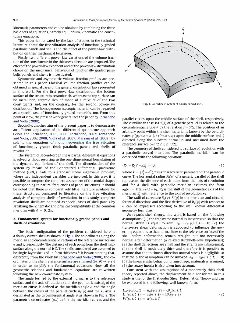
Fig. 1. Co-ordinate system of doubly curved shell.

F. Tornabene, E. Viola / European Journal of Mechanics A/Solids 28 (2009) 991–1013992

kinematic parameters and can be obtained by combining the threebasic sets of equations, namely equilibrium, kinematic and consti-tutive equations.

This paper is motivated by the lack of studies in the technicalliterature about the free vibration analysis of functionally gradedparabolic panels and shells and the effect of the power-law distri-bution on their mechanical behaviour.

Firstly, two different power-law variations of the volume frac-tion of the constituents in the thickness direction are proposed. Theeffect of the power-law exponent and of the power-law distributionchoice on the mechanical behaviour of functionally graded para-bolic panels and shells is investigated.

Symmetric and asymmetric volume fraction profiles are pre-sented in this paper. Classical volume fraction profiles can beobtained as special cases of the general distribution laws presentedin this work. For the first power-law distribution, the bottomsurface of the structure is ceramic rich, whereas the top surface canbe metal rich, ceramic rich or made of a mixture of the twoconstituents and, on the contrary, for the second power-lawdistribution. The homogeneous isotropic material can be regardedas a special case of functionally graded materials, too. From thispoint of view, the present work generalizes the paper by Tornabeneand Viola (2008).

Secondly, another aim of the present paper is to demonstratean efficient application of the differential quadrature approach(Viola and Tornabene, 2005, 2006; Tornabene, 2007; Tornabeneand Viola, 2007, 2008; Viola et al., 2007; Marzani et al., 2008), bysolving the equations of motion governing the free vibrationof functionally graded thick parabolic panels and shells ofrevolution.

The system of second-order linear partial differential equationsis solved without resorting to the one-dimensional formulation ofthe dynamic equilibrium of the shell. The discretization of thesystem by means of the Generalized Differential Quadraturemethod (GDQ) leads to a standard linear eigenvalue problem,where two independent variables are involved. In this way, it ispossible to compute the complete assessment of the modal shapescorresponding to natural frequencies of panel structures. It shouldbe noted that there is comparatively little literature available forthese structures, compared to literature on the free vibrationanalysis of complete shells of revolution. In this study, completerevolution shells are obtained as special cases of shell panels bysatisfying the kinematic and physical compatibility at the commonmeridian with w ¼ 0; 2p.

2. Fundamental system for functionally graded panels andshells of revolution

The basic configuration of the problem considered here isa doubly curved shell as shown in Fig. 1. The co-ordinates along themeridian and circumferential directions of the reference surface are4 and s, respectively. The distance of each point from the shell mid-surface along the normal is z. The shells considered are assumed tobe single-layer shells of uniform thickness h. It is worth noting that,differently from the work by Tornabene and Viola (2008), the co-ordinates of the shell reference surface are changed ðð4;wÞ/ð4; sÞÞin order to simplify the fundamental equations. Now, all thegeometric relations and fundamental equations are re-writtenfollowing the new co-ordinate system.

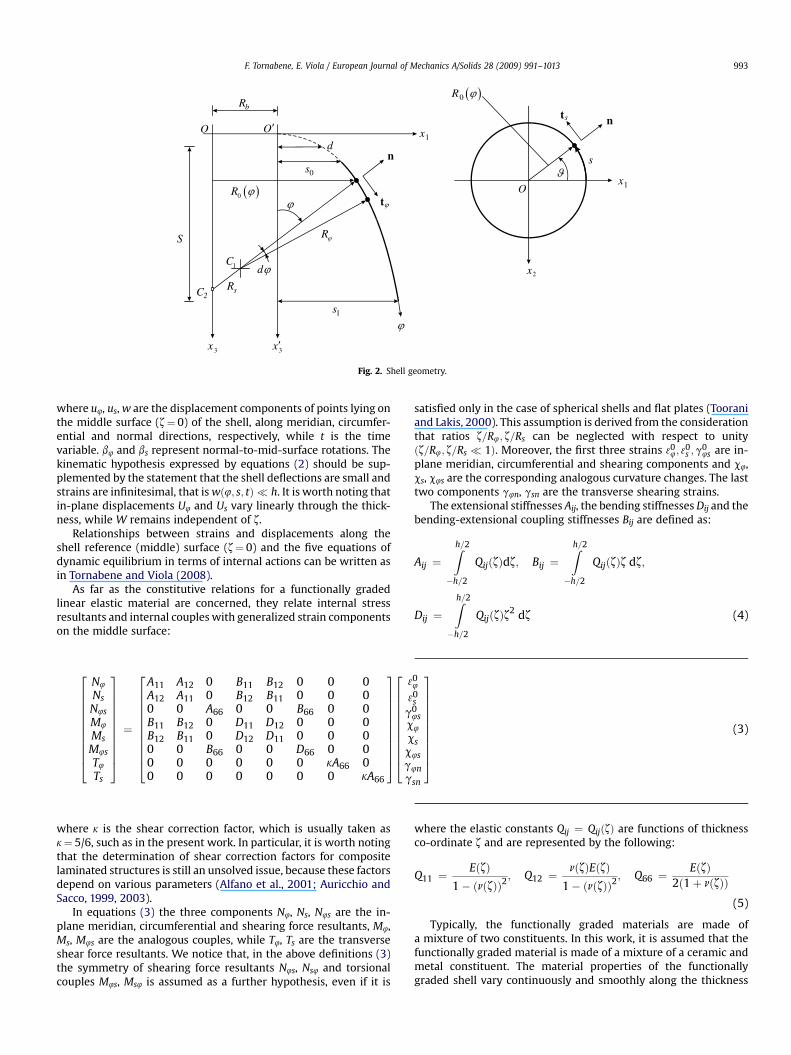
The angle formed by the external normal n to the referencesurface and the axis of rotation x3, or the geometric axis x03 of themeridian curve, is defined as the meridian angle 4 and the anglebetween the radius of the parallel circle R0(4) and the x1 axis isdesignated as the circumferential angle w as shown in Fig. 2. Theparametric co-ordinates (4,s) define the meridian curves and the

parallel circles upon the middle surface of the shell, respectively.The curvilinear abscissa s(4) of a generic parallel is related to thecircumferential angle w by the relation s¼wR0. The position of anarbitrary point within the shell material is known by the co-ordi-nates 4 (40� 4� 41), s (0� s� s0) upon the middle surface, and z

directed along the outward normal n and measured from thereference surface ð�h=2 � z � h=2Þ.

The geometry of shells considered is a surface of revolution witha parabolic curved meridian. The parabolic meridian can bedescribed with the following equation:

ðR0 � RbÞ2�kx03 ¼ 0 (1)

where k ¼ ðs21 � d2Þ=S is a characteristic parameter of the parabolic

curve. The horizontal radius R0(4) of a generic parallel of the shellrepresents the distance of each point from the axis of revolutionand for a shell with parabolic meridian assumes the formR0ð4Þ ¼ k tan 4=2þ Rb. Rb is the shift of the geometric axis of themeridian x03 with reference to the axis of revolution x3.

The radii of curvature R4(4), Rs(4) in the meridian and circum-ferential directions and the first derivative of R4(4) with respect to4 can be expressed according to the well known differentialgeometry formulae.

As regards shell theory, this work is based on the followingassumptions: (1) the transverse normal is inextensible so that thenormal strain is equal to zero: 3n ¼ 3nð4; s; z; tÞ ¼ 0; (2) thetransverse shear deformation is supposed to influence the gov-erning equations so that normal lines to the reference surface of theshell before deformation remain straight, but not necessarilynormal after deformation (a relaxed Kirchhoff-Love hypothesis);(3) the shell deflections are small and the strains are infinitesimal;(4) the shell is moderately thick and therefore it is possible toassume that the thickness-direction normal stress is negligible sothat the plane assumption can be invoked: sn ¼ snð4; s; z; tÞ ¼ 0;(5) the linear elastic behaviour of anisotropic materials is assumed;(6) the rotary inertia is also taken into account.

Consistent with the assumptions of a moderately thick shelltheory reported above, the displacement field considered in thisstudy is that of the First-order Shear Deformation Theory and canbe expressed in the following, well known, form:

U4ð4; s; z; tÞ ¼ u4ð4; s; tÞ þ zb4ð4; s; tÞUsð4; s; z; tÞ ¼ usð4; s; tÞ þ zbsð4; s; tÞWð4; s; z; tÞ ¼ wð4; s; tÞ

(2)

2x

1x

0R

st n

O

s

3x

1xO

0R

R

sR

t

d

1s

0s

d

S

bR

n

3x

O

1C

2C

Fig. 2. Shell geometry.

F. Tornabene, E. Viola / European Journal of Mechanics A/Solids 28 (2009) 991–1013 993

where u4, us, w are the displacement components of points lying onthe middle surface (z¼ 0) of the shell, along meridian, circumfer-ential and normal directions, respectively, while t is the timevariable. b4 and bs represent normal-to-mid-surface rotations. Thekinematic hypothesis expressed by equations (2) should be sup-plemented by the statement that the shell deflections are small andstrains are infinitesimal, that is wð4; s; tÞ � h. It is worth noting thatin-plane displacements U4 and Us vary linearly through the thick-ness, while W remains independent of z.

Relationships between strains and displacements along theshell reference (middle) surface (z¼ 0) and the five equations ofdynamic equilibrium in terms of internal actions can be written asin Tornabene and Viola (2008).

As far as the constitutive relations for a functionally gradedlinear elastic material are concerned, they relate internal stressresultants and internal couples with generalized strain componentson the middle surface:

266666666664

N4

NsN4sM4

MsM4sT4

Ts

377777777775¼

266666666664

A11 A12 0 B11 B12 0 0 0A12 A11 0 B12 B11 0 0 00 0 A66 0 0 B66 0 0B11 B12 0 D11 D12 0 0 0B12 B11 0 D12 D11 0 0 00 0 B66 0 0 D66 0 00 0 0 0 0 0 kA66 00 0 0 0 0 0 0 kA66

377777777775

266666666664

304

30s

g04s

c4csc4sg4ngsn

377777777775

(3)

where k is the shear correction factor, which is usually taken ask¼ 5/6, such as in the present work. In particular, it is worth notingthat the determination of shear correction factors for compositelaminated structures is still an unsolved issue, because these factorsdepend on various parameters (Alfano et al., 2001; Auricchio andSacco, 1999, 2003).

In equations (3) the three components N4, Ns, N4s are the in-plane meridian, circumferential and shearing force resultants, M4,Ms, M4s are the analogous couples, while T4, Ts are the transverseshear force resultants. We notice that, in the above definitions (3)the symmetry of shearing force resultants N4s, Ns4 and torsionalcouples M4s, Ms4 is assumed as a further hypothesis, even if it is

satisfied only in the case of spherical shells and flat plates (Tooraniand Lakis, 2000). This assumption is derived from the considerationthat ratios z=R4; z=Rs can be neglected with respect to unityðz=R4; z=Rs � 1Þ. Moreover, the first three strains 30

4; 30s ;g

04s are in-

plane meridian, circumferential and shearing components and c4,cs, c4s are the corresponding analogous curvature changes. The lasttwo components g4n, gsn are the transverse shearing strains.

The extensional stiffnesses Aij, the bending stiffnesses Dij and thebending-extensional coupling stiffnesses Bij are defined as:

Aij ¼Zh=2

�h=2

QijðzÞdz; Bij ¼Zh=2

�h=2

QijðzÞz dz;

Dij ¼Zh=2

�h=2

QijðzÞz2 dz (4)

where the elastic constants Qij ¼ QijðzÞ are functions of thicknessco-ordinate z and are represented by the following:

Q11 ¼EðzÞ

1� ðnðzÞÞ2; Q12 ¼

nðzÞEðzÞ1� ðnðzÞÞ2

; Q66 ¼EðzÞ

2ð1þ nðzÞÞ(5)

Typically, the functionally graded materials are made ofa mixture of two constituents. In this work, it is assumed that thefunctionally graded material is made of a mixture of a ceramic andmetal constituent. The material properties of the functionallygraded shell vary continuously and smoothly along the thickness

Fig. 3. Variations of the ceramic volume fraction VC through the thickness for different values of the power-law index p: (a) FGM1ða¼1=b¼0=c=pÞ , (b)FGM2ða¼1=b¼0=c=pÞ .

F. Tornabene, E. Viola / European Journal of Mechanics A/Solids 28 (2009) 991–1013994

direction z and are functions of the volume fractions and propertiesof the constituent materials. Young’s modulus E(z), Poisson’s ration(z) and mass density r(z) of the functionally graded shell can beexpressed as a linear combination:

rðzÞ ¼ ðrC � rMÞVC þ rMEðzÞ ¼ ðEC � EMÞVC þ EMnðzÞ ¼ ðnC � nMÞVC þ nM

(6)

where rC, EC, nC, VC and rM, EM, nM, VM represent mass density,Young’s modulus, Poisson’s ratio and volume fraction of theceramic and metal constituent materials, respectively.

In this paper, the ceramic volume fraction VC follows two simplefour-parameter power-law distributions:

Fig. 4. Variations of the ceramic volume fraction VC through the thickness for different(c) FGM1ða¼1=b¼ 1=c¼4=pÞ , (d) FGM2ða¼1=b¼ 1=c¼4=pÞ .

FGM1ða=b=c=pÞ : VC ¼ 1� a12þ z

hþ b

12þ z

h

� � � � �c�p

FGM2ða=b=c=pÞ : VC ¼�

1� a�

12� z

h

�þ b�

12� z

h

�c�p

(7)

where the volume fraction index p (0� p�N) and the parameters a,b, c dictate the material variation profile through the functionallygraded shell thickness. It is worth noting that the volume fractionsof all the constituent materials should add up to unity:

VC þ VM ¼ 1 (8)

In order to choose the three parameters a, b, c in a suitable way,the relation (8) must be always satisfied for every volume fraction

values of the power-law index p: (a) FGM1ða¼1=b¼1=c¼2=pÞ , (b) FGM2ða¼1=b¼1=c¼2=pÞ ,

F. Tornabene, E. Viola / European Journal of Mechanics A/Solids 28 (2009) 991–1013 995

index p. By considering the relation (7), when the power-lawexponent is set equal to zero (p¼ 0) or equal to infinity (p¼N), thehomogeneous isotropic material is obtained (Tornabene and Viola,2008) as a special case of the functionally graded material. In fact,from equations (8), (7) and (6) it is possible to obtain:

p ¼ 0/VC ¼ 1; VM ¼ 0/rðzÞ ¼ rC ; EðzÞ ¼ EC ; nðzÞ ¼ nCp ¼ N/VC ¼ 0; VM ¼ 1/rðzÞ ¼ rM; EðzÞ ¼ EM; nðzÞ ¼ nM

(9)

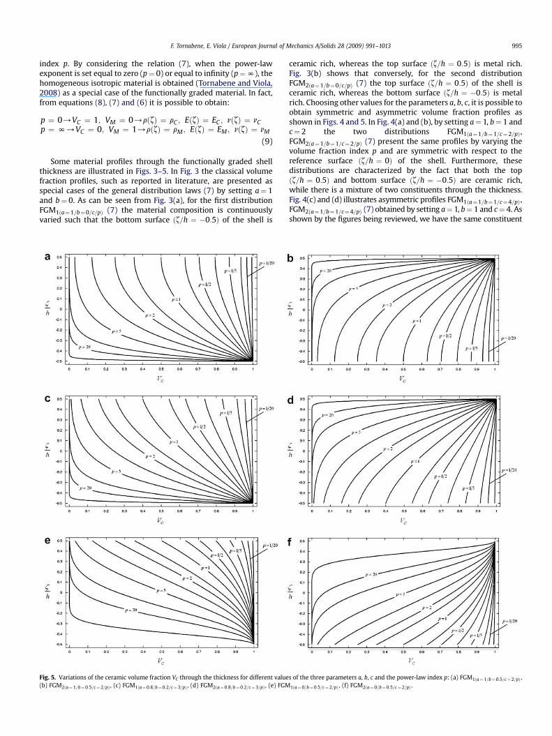
Some material profiles through the functionally graded shellthickness are illustrated in Figs. 3–5. In Fig. 3 the classical volumefraction profiles, such as reported in literature, are presented asspecial cases of the general distribution laws (7) by setting a¼ 1and b¼ 0. As can be seen from Fig. 3(a), for the first distributionFGM1ða¼1=b¼0=c=pÞ (7) the material composition is continuouslyvaried such that the bottom surface ðz=h ¼ �0:5Þ of the shell is

Fig. 5. Variations of the ceramic volume fraction VC through the thickness for different value(b) FGM2ða¼1=b¼0:5=c¼2=pÞ , (c) FGM1ða¼0:8=b¼0:2=c¼3=pÞ , (d) FGM2ða¼ 0:8=b¼0:2=c¼3=pÞ , (e) FGM

ceramic rich, whereas the top surface ðz=h ¼ 0:5Þ is metal rich.Fig. 3(b) shows that conversely, for the second distributionFGM2ða¼1=b¼0=c=pÞ (7) the top surface ðz=h ¼ 0:5Þ of the shell isceramic rich, whereas the bottom surface ðz=h ¼ �0:5Þ is metalrich. Choosing other values for the parameters a, b, c, it is possible toobtain symmetric and asymmetric volume fraction profiles asshown in Figs. 4 and 5. In Fig. 4(a) and (b), by setting a¼ 1, b¼ 1 andc¼ 2 the two distributions FGM1ða¼1=b¼1=c¼2=pÞ,FGM2ða¼1=b¼1=c¼2=pÞ (7) present the same profiles by varying thevolume fraction index p and are symmetric with respect to thereference surface ðz=h ¼ 0Þ of the shell. Furthermore, thesedistributions are characterized by the fact that both the topðz=h ¼ 0:5Þ and bottom surface ðz=h ¼ �0:5Þ are ceramic rich,while there is a mixture of two constituents through the thickness.Fig. 4(c) and (d) illustrates asymmetric profiles FGM1ða¼1=b¼1=c¼4=pÞ,FGM2ða¼1=b¼1=c¼4=pÞ (7) obtained by setting a¼ 1, b¼ 1 and c¼ 4. Asshown by the figures being reviewed, we have the same constituent

s of the three parameters a, b, c and the power-law index p: (a) FGM1ða¼1=b¼0:5=c¼2=pÞ ,

1ða¼0=b¼0:5=c¼2=pÞ , (f) FGM2ða¼0=b¼0:5=c¼ 2=pÞ .

F. Tornabene, E. Viola / European Journal of Mechanics A/Solids 28 (2009) 991–1013996

at the top and bottom surface but, unlike the previous cases (Fig. 4(a)and (b)), profiles are not symmetric with respect to the referencesurface (z/h¼ 0) of the shell. Fig. 5 shows other cases obtained byvarying the parameters a, b, c. These profiles are characterized by thefact that one of the two shell surfaces (the top or bottom surface)presents a mixture of two constituents. For example, by consideringthe FGM1ða¼1=b¼0:5=c¼4=p¼1Þ distribution (Fig. 5(a)), at the topsurface we have a mixture of ceramic and metal made up by fifty percent of ceramic and fifty per cent of metal, while the bottom surface(z/h¼�0.5) is ceramic rich. Fig. 5(b)–(f) illustrates various power-lawdistribution cases obtained by modifying the parameters a, b, c, p.From a design point of view it is important to know if the top surfaceof the shell (z/h¼ 0.5) is ceramic or metal rich, if the bottom surface(z/h¼�0.5) is metal or ceramic rich, or if one of these surfacespresents a mixture of two constituents. One of the aims of this workis to propose a generalization of the power-law distribution pre-sented in literature and to illustrate the influence of the power-lawexponent p and of the choice of the parameters a, b, c on themechanical behaviour of shell structures.

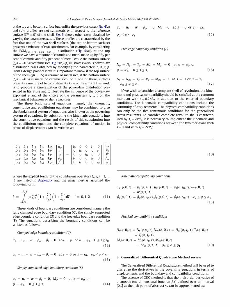
The three basic sets of equations, namely the kinematic,constitutive and equilibrium equations may be combined to givethe fundamental system of equations, also known as the governingsystem of equations. By substituting the kinematic equations intothe constitutive equations and the result of this substitution intothe equilibrium equations, the complete equations of motion interms of displacements can be written as:

266664

L11 L12 L13 L14 L15L21 L22 L23 L24 L25L31 L32 L33 L34 L35L41 L42 L43 L44 L45L51 L52 L53 L54 L55

377775

266664

u4

uswb4

bs

377775 ¼

266664

I0 0 0 I1 00 I0 0 0 I10 0 I0 0 0I1 0 0 I2 00 I1 0 0 I2

377775

2666664

€u4€us€w€b4€bs

3777775 (10)

where the explicit forms of the equilibrium operators Lij, i, j¼ 1, .,5 are listed in Appendix and the mass inertias assumed thefollowing form:

Ii ¼Zh=2

�h=2

rðzÞzi�

1þ z

R4

��1þ z

Rs

�dz; i ¼ 0;1;2 (11)

Three kinds of boundary conditions are considered, namely thefully clamped edge boundary condition (C), the simply supportededge boundary condition (S) and the free edge boundary condition(F). The equations describing the boundary conditions can bewritten as follows:

Clamped edge boundary condition (C)

u4 ¼ us ¼ w ¼ b4 ¼ bs ¼ 0 at 4 ¼ 40 or 4 ¼ 41; 0� s� s0

(12)

u4 ¼ us ¼ w ¼ b4 ¼ bs ¼ 0 at s ¼ 0 or s ¼ s0; 40 � 4� 41

(13)

Simply supported edge boundary condition (S)

u4 ¼ us ¼ w ¼ bs ¼ 0; M4 ¼ 0 at 4 ¼ 40 or

4 ¼ 41; 0 � s � s0 (14)

u4 ¼ us ¼ w ¼ b4 ¼ 0; Ms ¼ 0 at s ¼ 0 or s ¼ s0;

40 � 4 � 41 (15)

Free edge boundary condition (F)

N4 ¼ N4s ¼ T4 ¼ M4 ¼ M4s ¼ 0 at 4 ¼ 40 or

4 ¼ 41; 0 � s � s0 (16)

Ns ¼ N4s ¼ Ts ¼ Ms ¼ M4s ¼ 0 at s ¼ 0 or s ¼ s0;

40 � 4 � 41 ð17Þ

If we wish to consider a complete shell of revolution, the kine-matic and physical compatibility should be satisfied at the commonmeridian with s¼ 0,2pR0 in addition to the external boundaryconditions. The kinematic compatibility conditions include thecontinuity of displacements. The physical compatibility conditionscan only be the five continuous conditions for the generalizedstress resultants. To consider complete revolute shells character-ized by s0¼ 2pR0, it is necessary to implement the kinematic andphysical compatibility conditions between the two meridians withs¼ 0 and with s0¼ 2pR0:

Kinematic compatibility conditions

u4ð4;0; tÞ ¼ u4ð4; s0; tÞ;usð4;0; tÞ ¼ usð4; s0; tÞ;wð4;0; tÞ¼ wð4; s0; tÞ;

b4ð4;0; tÞ ¼ b4ð4; s0; tÞ; bsð4;0; tÞ ¼ bsð4; s0; tÞ 40 � 4 � 41

(18)

Physical compatibility conditions

Nsð4;0; tÞ ¼ Nsð4; s0; tÞ;N4sð4;0; tÞ ¼ N4sð4; s0; tÞ; Tsð4;0; tÞ¼ Tsð4; s0; tÞ;

Msð4;0; tÞ ¼ Msð4; s0; tÞ;M4sð4;0; tÞ¼ M4sð4; s0; tÞ 40 � 4 � 41 (19)

3. Generalized Differential Quadrature Method review

The Generalized Differential Quadrature method will be used todiscretize the derivatives in the governing equations in terms ofdisplacements and the boundary and compatibility conditions.

The essence of GDQ method is that the n-th order derivative ofa smooth one-dimensional function f(x) defined over an interval[0,L] at the i-th point of abscissa xi, can be approximated as:

F. Tornabene, E. Viola / European Journal of Mechanics A/Solids 28 (2009) 991–1013 997

dnf ðxÞdxn jx¼xi

¼XN

j¼1

2ðnÞij f�xj�; i ¼ 1;2;.;N (20)

where 2ðnÞij are the weighting coefficients at the i-th point calculatedfor the j-th sampling point of the domain. In equation (20) N is thetotal number of the sampling points of the grid distribution and f(xj)is the value of the function at the j-th point.

Some simple recursive formulas are available for calculating n-th order derivative weighting coefficients 2ðnÞij by means of Lagrangepolynomial interpolation functions (Shu, 2000). The weightingcoefficients for the first-order derivative are:

2ð1Þij ¼Lð1ÞðxiÞ�

xi � xj�Lð1Þ�xj�; i; j ¼ 1;2;.;N; isj (21)

2ð1Þii ¼ �XN

j¼1; jsi

2ð1Þij ; i; j ¼ 1;2;.;N; i ¼ j (22)

In equation (21) the first derivative of Lagrange interpolatingpolynomials at each point xk, k¼ 1,2,.,N, is:

Lð1ÞðxkÞ ¼YN

l¼1;lsk

ðxk � xlÞ; k ¼ 1;2;.;N (23)

For higher order derivatives (n¼ 2,3,., N� 1), one getsiteratively:

2ðnÞij ¼ n

0@2ðn�1Þ

ii 2ð1Þij �2ðn�1Þ

ij

xi � xj

1A; i; j ¼ 1;2;.;N; isj (24)

2ðnÞii ¼ �XN

j¼1; jsi

2ðnÞij ; i; j ¼ 1;2;.;N; i ¼ j (25)

From the above equations it appears that the weightingcoefficients of the second and higher order derivatives can bedetermined from those of the first-order derivative. Furthermore, it

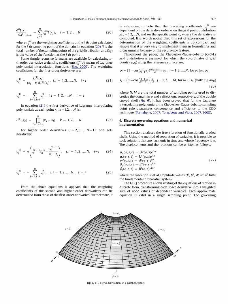
Fig. 6. C-G-L grid distributio

is interesting to note that the preceding coefficients 2ðnÞij aredependent on the derivative order n, on the grid point distributionxj, j¼ 1,2,.,N, and on the specific point xi, where the derivative iscomputed. It is worth noting that, this set of expressions for thedetermination of the weighting coefficients is so compact andsimple that it is very easy to implement them in formulating andprogramming because of the recurrence feature.

Throughout the paper, the Chebyshev-Gauss-Lobatto (C-G-L)grid distribution is assumed, for which the co-ordinates of gridpoints (4i,sj) along the reference surface are:

4i ¼�1�cos

�i�1N�1p

��ð41�40Þ2 þ40; i¼ 1;2;.;N; for4˛½40;41�

sj ¼�

1�cos�

j�1M�1p

��s02 ; j¼ 1;2;.;M; for s˛½0;s0� ðwith s�wR0Þ

(26)

where N, M are the total number of sampling points used to dis-cretize the domain in 4 and s directions, respectively, of the doublecurved shell (Fig. 6). It has been proved that for the Lagrangeinterpolating polynomials, the Chebyshev-Gauss-Lobatto samplingpoint rule guarantees convergence and efficiency to the GDQtechnique (Tornabene, 2007; Tornabene and Viola, 2007, 2008).

4. Discrete governing equations and numericalimplementation

This section analyses the free vibration of functionally gradedshells. Using the method of separation of variables, it is possible toseek solutions that are harmonic in time and whose frequency is u.The displacements and the rotations can be written as follows:

u4ð4; s; tÞ ¼ U4ð4; sÞeiut

usð4; s; tÞ ¼ Usð4; sÞeiut

wð4; s; tÞ ¼ Wð4; sÞeiut

b4ð4; s; tÞ ¼ B4ð4; sÞeiut

bsð4; s; tÞ ¼ Bsð4; sÞeiut

(27)

where the vibration spatial amplitude values U4, Us, W, B4, Bs fulfilthe fundamental differential system.

The GDQ procedure allows writing of the equations of motion indiscrete form, transforming each space derivative into a weightedsum of node values of dependent variables. Each approximateequation is valid in a single sampling point. The governing

n on a parabolic panel.

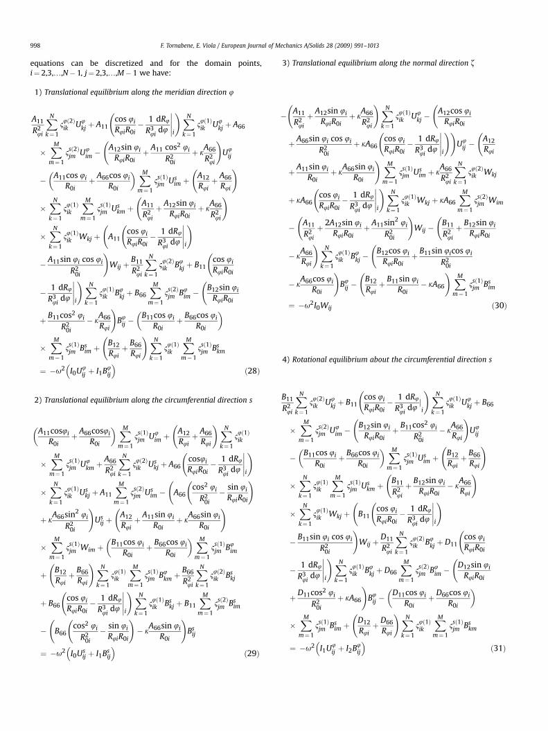
F. Tornabene, E. Viola / European Journal of Mechanics A/Solids 28 (2009) 991–1013998

equations can be discretized and for the domain points,i¼ 2,3,.,N� 1, j¼ 2,3,.,M� 1 we have:

1) Translational equilibrium along the meridian direction 4

A11

R24i

XN

k¼1

24ð2Þik U4

kj þ A11

cos 4i

R4iR0i� 1

R34i

dR4

d4

�����i!XN

k¼1

24ð1Þik U4

kj þ A66

�XM

m¼1

2sð2Þjm U4

im �

A12sin 4i

R4iR0iþ A11 cos2 4i

R20i

þ kA66

R24i

!U4

ij

��

A11cos 4i

R0iþ A66cos 4i

R0i

� XMm¼1

2sð1Þjm Us

im þ

A12

R4iþ A66

R4i

!

�XN

k¼1

24ð1Þik

XMm¼1

2sð1Þjm Us

km þ

A11

R24i

þ A12sin 4i

R4iR0iþ k

A66

R24i

!

�XN

k¼1

24ð1Þik Wkj þ

A11

cos 4i

R4iR0i� 1

R34i

dR4

d4

�����i!

� A11sin 4i cos 4i

R20i

!Wij þ

B11

R24i

XN

k¼1

24ð2Þik B4

kj þ B11

cos 4i

R4iR0i

� 1R3

4i

dR4

d4

�����i!XN

k¼1

24ð1Þik B4

kj þ B66

XMm¼1

2sð2Þjm B4

im �

B12sin 4i

R4iR0i

þ B11cos2 4i

R20i

� kA66

R4i

!B4

ij ��

B11cos 4i

R0iþ B66cos 4i

R0i

�

�XM

m¼1

2sð1Þjm Bs

im þ

B12

R4iþ B66

R4i

!XN

k¼1

24ð1Þik

XMm¼1

2sð1Þjm Bs

km

¼ �u2�

I0U4ij þ I1B4

ij

�ð28Þ

2) Translational equilibrium along the circumferential direction s

�A11cos4i

R0iþ A66cos4i

R0i

� XMm¼1

2sð1Þjm U4

im þ

A12

R4iþ A66

R4i

!XN

k¼1

24ð1Þik

�XM

m¼1

2sð1Þjm U4

km þA66

R24i

XN

k¼1

24ð2Þik Us

kj þ A66

cos4i

R4iR0i� 1

R34i

dR4

d4

�����i!

�XN

k¼1

24ð1Þik Us

kj þ A11

XMm¼1

2sð2Þjm Us

im �

A66

cos2 4i

R20i

� sin 4i

R4iR0i

!

þ kA66sin2 4i

R20i

!Us

ij þ

A12

R4iþ A11sin 4i

R0iþ k

A66sin 4i

R0i

!

�XM

m¼1

2sð1Þjm Wim þ

�B11cos 4i

R0iþ B66cos 4i

R0i

� XMm¼1

2sð1Þjm B4

im

þ

B12

R4iþ B66

R4i

!XN

k¼1

24ð1Þik

XMm¼1

2sð1Þjm B4

km þB66

R24i

XN

k¼1

24ð2Þik Bs

kj

þ B66

cos 4i

R4iR0i� 1

R34i

dR4

d4

�����i!XN

k¼1

24ð1Þik Bs

kj þ B11

XMm¼1

2sð2Þjm Bs

im

�

B66

cos2 4i

R20i

� sin 4i

R4iR0i

!� k

A66sin 4i

R0i

!Bs

ij

¼ �u2�

I0Usij þ I1Bs

ij

�ð29Þ

3) Translational equilibrium along the normal direction z

�

A11

R24i

þ A12sin 4i

R4iR0iþ k

A66

R24i

!XN

k¼1

24ð1Þik U4

kj �

A12cos 4i

R4iR0i

þ A66sin 4i cos 4i

R20i

þ kA66

cos 4i

R4iR0i� 1

R34i

dR4

d4

�����i!!

U4ij �

A12

R4i

þ A11sin 4i

R0iþ k

A66sin 4i

R0i

! XMm¼1

2sð1Þjm Us

im þ kA66

R24i

XN

k¼1

24ð2Þik Wkj

þ kA66

cos 4i

R4iR0i� 1

R34i

dR4

d4

�����i!XN

k¼1

24ð1Þik Wkj þ kA66

XMm¼1

2sð2Þjm Wim

�

A11

R24i

þ 2A12sin 4i

R4iR0iþ A11sin2 4i

R20i

!Wij �

B11

R24i

þ B12sin 4i

R4iR0i

� kA66

R4i

!XN

k¼1

24ð1Þik B4

kj �

B12cos 4i

R4iR0iþ B11sin 4icos 4i

R20i

� kA66cos 4i

R0i

!B4

ij �

B12

R4iþ B11sin 4i

R0i� kA66

! XMm¼1

2sð1Þjm Bs

im

¼ �u2I0Wij ð30Þ

4) Rotational equilibrium about the circumferential direction s

B11

R24i

XN

k¼1

24ð2Þik U4

kj þ B11

cos 4i

R4iR0i� 1

R34i

dR4

d4ji

!XN

k¼1

24ð1Þik U4

kj þ B66

�XM

m¼1

2sð2Þjm U4

im �

B12sin 4i

R4iR0iþ B11cos2 4i

R20i

� kA66

R4i

!U4

ij

��

B11cos 4i

R0iþ B66cos 4i

R0i

� XMm¼1

2sð1Þjm Us

im þ

B12

R4iþ B66

R4i

!

�XN

k¼1

24ð1Þik

XMm¼1

2sð1Þjm Us

km þ

B11

R24i

þ B12sin 4i

R4iR0i� k

A66

R4i

!

�XN

k¼1

24ð1Þik Wkj þ

B11

cos 4i

R4iR0i� 1

R34i

dR4

d4

�����i!

� B11sin 4i cos 4i

R20i

!Wij þ

D11

R24i

XN

k¼1

24ð2Þik B4

kj þ D11

cos 4i

R4iR0i

� 1R3

4i

dR4

d4

�����i!XN

k¼1

24ð1Þik B4

kj þ D66

XMm¼1

2sð2Þjm B4

im �

D12sin 4i

R4iR0i

þ D11cos2 4i

R20i

þ kA66

!B4

ij ��

D11cos 4i

R0iþ D66cos 4i

R0i

�

�XM

m¼1

2sð1Þjm Bs

im þ

D12

R4iþ D66

R4i

!XN

k¼1

24ð1Þik

XMm¼1

2sð1Þjm Bs

km

¼ �u2�

I1U4ij þ I2B4

ij

�ð31Þ

F. Tornabene, E. Viola / European Journal of Mechanics A/Solids 28 (2009) 991–1013 999

5) Rotational equilibrium about the meridian direction 4

�B11cos4i

R0iþ B66cos4i

R0i

� XMm¼1

2sð1Þjm U4

im þ

B12

R4iþ B66

R4i

!XN

k¼1

24ð1Þik

XMm¼1

2sð1Þjm U4

km þB66

R24i

XN

k¼1

24ð2Þik Us

kj þ B66

cos 4i

R4iR0i� 1

R34i

dR4

d4ji

!XN

k¼1

24ð1Þik Us

kj

þB11

XMm¼1

2sð2Þjm Us

im �

B66

cos2 4i

R20i

� sin 4i

R4iR0i

!� k

A66sin 4i

R0i

!Us

ij þ

B12

R4iþ B11sin 4i

R0i� kA66

! XMm¼1

2sð1Þjm Wim þ

�D11cos 4i

R0i

þD66cos 4i

R0i

� XMm¼1

2sð1Þjm B4

im þ

D12

R4iþ D66

R4i

!XN

k¼1

24ð1Þik

XMm¼1

2sð1Þjm B4

km þD66

R24i

XN

k¼1

24ð2Þik Bs

kj þ D66

cos 4i

R4iR0i� 1

R34i

dR4

d4ji

!XN

k¼1

24ð1Þik Bs

kj

þD11

XMm¼1

2sð2Þjm Bs

im �

D66

cos2 4i

R20i

� sin 4i

R4iR0i

!þ kA66

!Bs

ij ¼ �u2�

I1Usij þ I2Bs

ij

�(32)

In equations (28)–(32), 24ð1Þik ; 2sð1Þ

jm ; 24ð2Þik and 2sð2Þ

jm are theweighting coefficients of the first and second derivatives in 4 and sdirections, respectively. Furthermore, N and M are the total numberof grid points in 4 and s directions.

Applying the GDQ methodology, the discretized forms of theboundary and compatibility conditions are given as follows:

8>>>>>>><>>>>>>>:

U4aj ¼ Us

aj ¼ Waj ¼ Bsaj ¼ 0

B11

R4a

XN

k¼1

24ð1Þak U4

kjþB12cos 4a

R0aU4

ajþB12

XMm¼1

2sð1Þjm Us

amþ�

B11

R4aþB12sin 4

R0a

þD12PM

m¼12sð1Þ

jm Bsam ¼ 0 for a ¼ 1;N and j ¼ 1;2;.;M

8>>>>>><>>>>>>:

U4ib ¼ Us

ib ¼ Wib ¼ B4ib ¼ 0

B12

R4i

XN

k¼1

24ð1Þik U4

kbþB11cos 4i

R0iU4

ibþB11

XMm¼1

2sð1Þbm Us

imþ

B12

R4iþB11sin 4i

R0i

þD11PM

m¼12sð1Þ

bm Bsim ¼ 0 for b ¼ 1;M and i ¼ 1;2;.;N

8>>>>>>>>>>>>>>>>>>>>><>>>>>>>>>>>>>>>>>>>>>:

A11

R4a

XN

k¼1

24ð1Þak U4

kjþA12cos4a

R0aU4

ajþA12

XMm¼1

2sð1Þjm Us

amþ�

A11

R4aþA12sin4a

R0a

�

A66PM

m¼12sð1Þ

jm U4amþ

A66

R4a

XN

k¼1

24ð1Þak Us

kj�A66cos 4a

R0aUs

ajþB66

XMm¼1

2sð1Þjm B4

amþ

�kA66

R4aU4

ajþkA66

R4a

XN

k¼1

24ð1Þak WkjþkA66B4

ajþkA66Bsaj ¼ 0

B11

R4a

XN

k¼1

24ð1Þak U4

kjþB12cos4a

R0aU4

ajþB12

XMm¼1

2sð1Þjm Us

amþ�

B11

R4aþB12sin4a

R0a

�

B66PM

m¼12sð1Þ

jm U4amþ

B66

R4a

XN

k¼1

24ð1Þak Us

kj�B66cos 4a

R0aUs

ajþD66

XMm¼1

2sð1Þjm B4

amþ

for a¼ 1;N and j¼ 1;2;.;M

Clamped edge boundary condition (C)

U4aj ¼ Us

aj ¼ Waj ¼ B4aj ¼ Bs

aj ¼ 0 for a ¼ 1;N and j ¼ 1;2;.;M

U4ib ¼ Us

ib ¼ Wib ¼ B4ib ¼ Bs

ib ¼ 0 for b ¼ 1;M and i ¼ 1;2;.;N

(33)

Simply supported edge boundary condition (S)

a�

WajþD11

R4a

XN

k¼1

24ð1Þak B4

kjþD12cos 4a

R0aB4

aj

!Wibþ

D12

R4i

XN

k¼1

24ð1Þik B4

kbþD11cos 4i

R0iB4

ib (34)

Free edge boundary condition (F)

WajþB11

R4a

XN

k¼1

24ð1Þak B4

kjþB12cos4a

R0aB4

ajþB12

XMm¼1

2sð1Þjm Bs

am ¼ 0

B66

R4a

XN

k¼1

24ð1Þak Bs

kj�B66cos4a

R0aBs

aj ¼ 0

WajþD11

R4a

XN

k¼1

24ð1Þak B4

kjþD12cos 4a

R0aB4

ajþD12

XMm¼1

2sð1Þjm Bs

am ¼ 0

D66

R4a

XN

k¼1

24ð1Þak Bs

kj�D66cos 4a

R0aBs

aj ¼ 0

(35)

8>>>>>>>>>>>>>>>>>>><>>>>>>>>>>>>>>>>>>>:

A66PM

m¼12sð1Þ

bm U4im þ

A66

R4i

XN

k¼1

24ð1Þik Us

kb �A66cos 4i

R0iUs

ib þ B66

XMm¼1

2sð1Þbm B4

im þB66

R4i

XN

k¼1

24ð1Þik Bs

kb �B66cos 4i

R0iBs

ib ¼ 0

A12

R4i

XN

k¼1

24ð1Þik U4

kb þA11cos 4i

R0iU4

ib þ A11

XMm¼1

2sð1Þbm Us

im þ

A12

R4iþ A11sin 4i

R0i

!Wib þ

B12

R4i

XN

k¼1

24ð1Þik B4

kb þB11cos 4i

R0iB4

ib þ B11

XMm¼1

2sð1Þbm Bs

im ¼ 0

kA66R4i

PNk¼1

24ð1Þik Wkb þ kA66B4

ib þ kA66Bsib ¼ 0

B66PM

m¼12

sð1Þbm U4

im þB66

R4i

XN

k¼1

24ð1Þik Us

kb �B66cos 4i

R0iUs

ib þ D66

XMm¼1

2sð1Þbm B4

im þD66

R4i

XN

k¼1

24ð1Þik Bs

kb �D66cos 4i

R0iBs

ib ¼ 0

B12

R4i

XN

k¼1

24ð1Þik U4

kb þB11cos 4i

R0iU4

ib þ B11

XMm¼1

2sð1Þbm Us

im þ

B12

R4iþ B11sin 4i

R0i

!Wib þ

D12

R4i

XN

k¼1

24ð1Þik B4

kb þD11cos 4i

R0iB4

ib þ D11

XMm¼1

2sð1Þbm Bs

im ¼ 0

for b ¼ 1;M and i ¼ 1;2;.;N

(36)

F. Tornabene, E. Viola / European Journal of Mechanics A/Solids 28 (2009) 991–10131000

Kinematic and physical compatibility conditions

U4i1 ¼ U4

iM;Usi1 ¼ Us

iM;Wi1 ¼ WiM;B4i1 ¼ B4

iM;Bsi1 ¼ Bs

iM8>>>>>>>>>>>>>>>>>>>>>>>>>>>>>>>>>>>>>>>>>><>>>>>>>>>>>>>>>>>>>>>>>>>>>>>>>>>>>>>>>>>>:

A66PM

m¼12sð1Þ

1m U4imþ

A66

R4i

XN

k¼1

24ð1Þik Us

k1�A66cos 4i

R0iUs

i1þB66

XMm¼1

2sð1Þ1m B4

imþB66

R4i

XN

k¼1

24ð1Þik Bs

k1�B66cos 4i

R0iBs

i1 ¼ A66

XMm¼1

2sð1ÞMmU4

im

þA66

R4i

XN

k¼1

24ð1Þik Us

kM �A66cos 4i

R0iUs

iM þB66

XMm¼1

2sð1ÞMmB4

imþB66

R4i

XN

k¼1

24ð1Þik Bs

kM �B66cos 4i

R0iBs

iM

A12

R4i

XN

k¼1

24ð1Þik U4

k1þA11cos 4i

R0iU4

i1þA11

XMm¼1

2sð1Þ1m Us

imþ

A12

R4iþA11sin 4i

R0i

!Wi1þ

B12

R4i

XN

k¼1

24ð1Þik B4

k1þB11cos 4i

R0iB4

i1þB11

XMm¼1

2sð1Þ1m Bs

im

¼ A12

R4i

XN

k¼1

24ð1Þik U4

kM þA11cos 4i

R0iU4

iMþA11

XMm¼1

2sð1ÞMmUs

imþ

A12

R4iþA11sin 4i

R0i

!WiM þ

B12

R4i

XN

k¼1

24ð1Þik B4

kM þB11cos 4i

R0iB4

iM þB11

XMm¼1

2sð1ÞMmBs

im

kA66

R4i

XN

k¼1

24ð1Þik Wk1þ kA66B4

i1þ kA66Bsi1 ¼ k

A66

R4i

XN

k¼1

24ð1Þik WkM þ kA66B4

iM þ kA66BsiM

B66PM

m¼12sð1Þ

1m U4imþ

B66

R4i

XN

k¼1

24ð1Þik Us

k1�B66cos 4i

R0iUs

i1þD66

XMm¼1

2sð1Þ1m B4

imþD66

R4i

XN

k¼1

24ð1Þik Bs

k1�D66cos 4i

R0iBs

i1 ¼ B66

XMm¼1

2sð1ÞMmU4

im

þB66

R4i

XN

k¼1

24ð1Þik Us

kM �B66cos 4i

R0iUs

iMþD66

XMm¼1

2sð1ÞMmB4

imþD66

R4i

XN

k¼1

24ð1Þik Bs

kM �D66cos 4i

R0iBs

iM

B12

R4i

XN

k¼1

24ð1Þik U4

k1þB11cos 4i

R0iU4

i1þB11

XMm¼1

2sð1Þ1m Us

imþ

B12

R4iþB11sin 4i

R0i

!Wi1þ

D12

R4i

XN

k¼1

24ð1Þik B4

k1þD11cos 4i

R0iB4

i1þD11

XMm¼1

2sð1Þ1m Bs

im

¼ B12

R4i

XN

k¼1

24ð1Þik U4

kM þB11cos 4i

R0iU4

iM þB11

XMm¼1

2sð1ÞMmUs

imþ

B12

R4iþB11sin 4i

R0i

!WiM þ

D12

R4i

XN

k¼1

24ð1Þik B4

kM þD11cos 4i

R0iB4

iM þD11

XMm¼1

2sð1ÞMmBs

im

for i ¼ 2;.;N�1

(37)

Thus, the whole system of differential equations has been dis-cretized and the global assembling leads to the following set oflinear algebraic equations:

Kbb KbdKdb Kdd

dbdd

¼ u2

0 00 Mdd

dbdd

(38)

In the above matrices and vectors, the partitioning is set forth bysubscripts b and d, referring to the system degrees of freedom andstanding for boundary and domain, respectively. In this sense, theb-equations represent the discrete boundary and compatibilityconditions, which are valid only for the points lying on constrainededges of the shell; while the d-equations are the equilibriumequations, assigned on interior nodes. In order to make thecomputation more efficient, kinematic condensation of non-domain degrees of freedom is performed:�

Kdd � KdbðKbbÞ�1Kbd

�dd ¼ u2Mdddd (39)

The natural frequencies of the structure considered can bedetermined by solving the standard eigenvalue problem (39). Inparticular, the solution procedure by means of GDQ technique hasbeen implemented in a MATLAB code. Finally, the results in terms offrequencies are obtained using the eigs function of MATLABprogram.

It is worth noting that, with the present approach, differing fromthe finite element method, no integration occurs prior to the globalassembly of the linear system, and this leads to a further compu-tational cost saving in favour of the differential quadraturetechnique.

5. Results and discussion

This section introduces some results and considerations aboutthe free vibration problem of functionally graded parabolic panelsand shells of revolution. The analysis has been carried out by meansof numerical procedures illustrated above.

Fig. 7. Mode shapes for the FGM1ða¼1=b¼0:5=c¼2=p¼1Þ toro-parabolic panel C-F-C-F.

F. Tornabene, E. Viola / European Journal of Mechanics A/Solids 28 (2009) 991–1013 1001

No literature is available about the results of the GDQ solution forfree vibrations of FGM shells with parabolic meridian. Severalattempts to validate the present formulations have been made for theisotropic and anisotropic cases and can be found in the PhD thesis byTornabene (2007) and in articles by Tornabene and Viola (2007, 2008).

Fig. 8. Mode shapes for the FGM1ða¼1=b¼

In this work, the frequency parameters from the present formulationsare in good agreement with the results presented in the literature andobtained with the finite element method.

Regarding the functionally graded materials, their two constit-uents are taken to be zirconia (ceramic) and aluminium (metal).

1=c¼ 3=p¼1Þ parabolic panel C-F-F-F.

F. Tornabene, E. Viola / European Journal of Mechanics A/Solids 28 (2009) 991–10131002

Young’s modulus, Poisson’s ratio and mass density for the zirconiaare EC¼ 168 GPa, nC¼ 0.3, rC¼ 5700 Kg/m3, and for the aluminiumare EM¼ 70 GPa, nM¼ 0.3, rM¼ 2707 Kg/m3, respectively. Thedetails regarding the geometry of the structures considered areindicated below:

1. Toro-parabolic panel (C-F-C-F)/(S-F-S-F): k ¼ 9; Rb ¼ 9 m;

h ¼ 0:4 m; s1 ¼ 3 m; s0 ¼ �3 m; S ¼ 2 m; w0 ¼ 120�;2. Parabolic panel (C-F-F-F): k ¼ 8; Rb ¼ 0 m; h ¼ 0:2 m;

s1 ¼ 4 m; s0 ¼ 1 m; S ¼ 2 m; w0 ¼ 120�;3. Parabolic toroid (F-C): k ¼ 4:5; Rb ¼ 6 m; h ¼ 0:3 m;

s1 ¼ 0 m; s0 ¼ �3 m; S ¼ 2 m; w0 ¼ 360�;4. Parabolic dome (C-F): k ¼ 8; Rb ¼ 0 m; h ¼ 0:2 m;

s1 ¼ 4 m; s0 ¼ 1 m; S ¼ 2 m; w0 ¼ 360�.

The geometrical boundary conditions for the shell panel areidentified by the following convention. For example, the symbolismC-S-C-F indicates that the edges 4¼ 41, s¼ s0, 4¼ 40, s¼ 0 areclamped, simply supported, clamped and free, respectively (Fig. 6).For the complete shell of revolution, for example, the symbolism C-F indicates that the edges 4¼ 41 and 4¼ 40 are clamped and free,respectively. In this case, the missing boundary conditions are thekinematic and physical compatibility conditions that are applied atthe same meridian for s¼ 0 and s0¼ 2pR0.

In Figs. 7–10, the first mode shapes for theFGM1ða¼1=b¼0:5=c¼2=p¼1Þ toro-parabolic panel (C-F-C-F), theFGM1ða ¼ 1=b ¼ 1=c ¼ 3=p ¼ 1Þ parabolic panel (C-F-F-F),the FGM1ða¼0=b¼�0:5=c¼2=p¼1Þ parabolic toroid (F-C) and the

Fig. 9. Mode shapes for the FGM1ða¼0=b

FGM1ða¼0:8=b¼0:2=c¼3=p¼1Þ parabolic dome (C-F) are illustrated. Inparticular, for the parabolic toroid and dome, there are somesymmetrical mode shapes due to the symmetry of the problemconsidered in three-dimensional space. In these cases, thesymmetrical mode shapes have been summarized in one figure.The mode shapes of all the structures under discussion have beenevaluated by the authors. By using the authors’ MATLAB code, thesemode shapes have been reconstructed in three-dimensional viewby means of considering the displacement field (2) after solving theeigenvalue problem (39).

Tables 1–6 illustrate the first ten frequencies of the four struc-tures under consideration. These tables show how by varying onlythe power-law index p of the volume fraction VC it is possible tomodify natural frequencies of FGM panels and shells of revolution.For the GDQ results presented in Tables 1–6, the grid distributions(26) with N¼M¼ 21 have been taking into account. The results areobtained using various values of the power-law exponent p (i.e.p¼ 0 ceramic rich and p¼N metal rich) for the two power-lawdistributions FGM1ða=b=c=pÞ and FGM2ða=b=c=pÞ. For each power-lawdistribution the same values of the three parameters a, b, c arechosen.

Tables 1–6 show that by considering the two power-lawdistributions FGM1ða=b=c=pÞ and FGM2ða=b=c=pÞ with the same valuesof the four parameters a, b, c, p the natural frequencies are different.In fact, for curved shells it is important, from the dynamic vibrationpoint of view, to know if the top surface of the shell (z¼ h/2) isceramic or metal rich and, inversely, if the bottom surface (z¼�h/2) is metal or ceramic rich, respectively. Using one of the two

¼�0:5=c¼2=p¼1Þ parabolic toroid F-C.

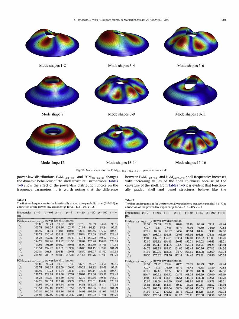
Fig. 10. Mode shapes for the FGM1ða¼0:8=b¼ 0:2=c¼3=p¼ 1Þ parabolic dome C-F.

F. Tornabene, E. Viola / European Journal of Mechanics A/Solids 28 (2009) 991–1013 1003

power-law distributions FGM1ða=b=c=pÞ and FGM2ða=b=c=pÞ changesthe dynamic behaviour of the shell structure. Furthermore, Tables1–6 show the effect of the power-law distribution choice on thefrequency parameters. It is worth noting that the difference

Table 1The first ten frequencies for the functionally graded toro-parabolic panel (C-F-C-F) asa function of the power-law exponent p, for a¼ 1, b¼ 0.5, c¼ 2.

Frequencies[Hz]

p¼ 0 p¼ 0.6 p¼ 1 p¼ 5 p¼ 20 p¼ 50 p¼ 100 p¼N

FGM1ða¼1=b¼0:5=c¼2=pÞ power-law distributionf1 99.88 99.73 99.57 98.95 97.51 95.59 94.66 93.56f2 103.74 103.55 103.36 102.57 101.03 99.15 98.24 97.17f3 111.46 111.23 111.01 110.06 108.42 106.46 105.52 104.41f4 130.73 130.40 130.11 128.77 126.84 124.69 123.67 122.45f5 158.23 157.76 157.38 155.49 153.14 150.72 149.57 148.21f6 184.79 184.26 183.82 181.53 178.67 175.96 174.66 173.09f7 191.80 191.39 191.02 189.01 185.90 182.89 181.43 179.65f8 193.54 192.97 192.51 189.94 186.85 184.15 182.86 181.29f9 202.18 201.81 201.45 199.68 196.50 193.07 191.40 189.38f10 208.93 208.32 207.83 205.00 201.62 198.76 197.38 195.70

FGM2ða¼1=b¼0:5=c¼2=pÞ power-law distributionf1 99.88 99.24 98.81 97.36 96.78 95.27 94.50 93.56f2 103.74 103.05 102.59 100.96 100.29 98.82 98.08 97.17f3 111.46 110.73 110.24 108.46 107.69 106.14 105.36 104.41f4 130.73 129.88 129.30 127.10 126.07 124.36 123.50 122.45f5 158.23 157.19 156.50 153.69 152.32 150.36 149.39 148.21f6 184.79 183.53 182.70 179.27 177.65 175.51 174.42 173.09f7 191.80 190.43 189.54 185.98 184.51 182.28 181.11 179.65f8 193.54 192.18 191.29 187.51 185.74 183.66 182.60 181.29f9 202.18 200.79 199.86 196.38 194.98 192.39 191.05 189.38f10 208.93 207.45 206.48 202.32 200.40 198.22 197.10 195.70

between FGM1ða=b=c=pÞ and FGM2ða=b=c=pÞ shell frequencies increaseswith increasing values of the shell thickness because of thecurvature of the shell. From Tables 1–6 it is evident that function-ally graded shell and panel structures behave like the

Table 2The first ten frequencies for the functionally graded toro-parabolic panel (S-F-S-F) asa function of the power-law exponent p, for a¼ 1, b¼ 0.5, c¼ 1.

Frequencies[Hz]

p¼ 0 p¼ 0.6 p¼ 1 p¼ 5 p¼ 20 p¼ 50 p¼ 100 p¼N

FGM1ða¼ 1=b¼0:5=c¼1=pÞ power-law distributionf1 72.54 72.08 71.79 70.69 71.10 69.96 69.14 67.94f2 77.77 77.31 77.01 75.74 75.93 74.80 74.00 72.85f3 87.86 87.06 86.57 84.57 85.04 84.12 83.38 82.30f4 110.17 108.93 108.18 105.03 105.92 105.11 104.36 103.19f5 139.09 137.67 136.81 133.14 134.08 132.92 131.89 130.28f6 152.89 152.32 151.89 150.65 152.21 149.02 146.65 143.21f7 155.81 155.13 154.65 153.20 154.73 151.56 149.25 145.94f8 164.79 163.98 163.42 161.66 163.45 160.26 157.86 154.36f9 171.59 169.95 168.95 164.70 165.55 163.98 162.69 160.73f10 176.50 175.32 174.56 172.14 174.42 171.28 168.86 165.33

FGM2ða¼ 1=b¼0:5=c¼1=pÞ power-law distributionf1 72.54 71.97 71.62 70.25 70.71 69.79 69.05 67.94f2 77.77 77.17 76.80 75.19 75.45 74.58 73.89 72.85f3 87.86 87.47 87.22 86.12 85.99 84.60 83.65 82.30f4 110.17 109.92 109.72 108.75 108.26 106.29 105.00 103.19f5 139.09 138.58 138.21 136.51 136.39 134.08 132.51 130.28f6 152.89 151.09 149.99 145.97 148.89 147.38 145.78 143.21f7 155.81 154.15 153.15 149.47 151.78 150.13 148.52 145.94f8 164.79 163.09 162.04 158.24 160.94 159.03 157.21 154.36f9 171.59 170.91 170.42 168.16 167.92 165.18 163.34 160.73f10 176.50 175.04 174.14 171.12 173.11 170.68 168.58 165.33

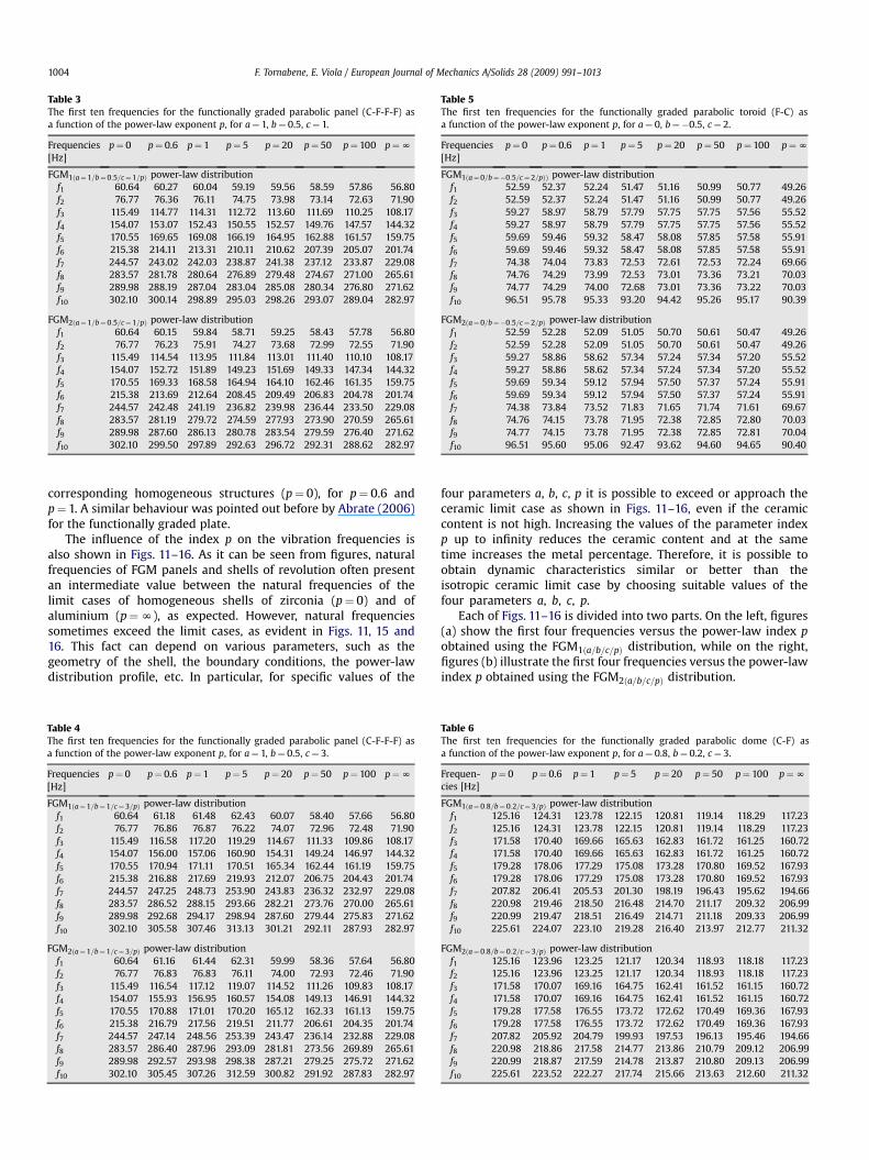
Table 5The first ten frequencies for the functionally graded parabolic toroid (F-C) asa function of the power-law exponent p, for a¼ 0, b¼�0.5, c¼ 2.

Frequencies[Hz]

p¼ 0 p¼ 0.6 p¼ 1 p¼ 5 p¼ 20 p¼ 50 p¼ 100 p¼N

FGM1ða¼0=b¼�0:5=c¼2=pÞÞ power-law distributionf1 52.59 52.37 52.24 51.47 51.16 50.99 50.77 49.26f2 52.59 52.37 52.24 51.47 51.16 50.99 50.77 49.26f3 59.27 58.97 58.79 57.79 57.75 57.75 57.56 55.52f4 59.27 58.97 58.79 57.79 57.75 57.75 57.56 55.52f5 59.69 59.46 59.32 58.47 58.08 57.85 57.58 55.91f6 59.69 59.46 59.32 58.47 58.08 57.85 57.58 55.91f7 74.38 74.04 73.83 72.53 72.61 72.53 72.24 69.66f8 74.76 74.29 73.99 72.53 73.01 73.36 73.21 70.03f9 74.77 74.29 74.00 72.68 73.01 73.36 73.22 70.03f10 96.51 95.78 95.33 93.20 94.42 95.26 95.17 90.39

FGM2ða¼0=b¼�0:5=c¼2=pÞ power-law distributionf1 52.59 52.28 52.09 51.05 50.70 50.61 50.47 49.26f2 52.59 52.28 52.09 51.05 50.70 50.61 50.47 49.26f3 59.27 58.86 58.62 57.34 57.24 57.34 57.20 55.52f4 59.27 58.86 58.62 57.34 57.24 57.34 57.20 55.52f5 59.69 59.34 59.12 57.94 57.50 57.37 57.24 55.91f6 59.69 59.34 59.12 57.94 57.50 57.37 57.24 55.91f7 74.38 73.84 73.52 71.83 71.65 71.74 71.61 69.67f8 74.76 74.15 73.78 71.95 72.38 72.85 72.80 70.03f9 74.77 74.15 73.78 71.95 72.38 72.85 72.81 70.04f10 96.51 95.60 95.06 92.47 93.62 94.60 94.65 90.40

Table 3The first ten frequencies for the functionally graded parabolic panel (C-F-F-F) asa function of the power-law exponent p, for a¼ 1, b¼ 0.5, c¼ 1.

Frequencies[Hz]

p¼ 0 p¼ 0.6 p¼ 1 p¼ 5 p¼ 20 p¼ 50 p¼ 100 p¼N

FGM1ða¼ 1=b¼0:5=c¼1=pÞ power-law distributionf1 60.64 60.27 60.04 59.19 59.56 58.59 57.86 56.80f2 76.77 76.36 76.11 74.75 73.98 73.14 72.63 71.90f3 115.49 114.77 114.31 112.72 113.60 111.69 110.25 108.17f4 154.07 153.07 152.43 150.55 152.57 149.76 147.57 144.32f5 170.55 169.65 169.08 166.19 164.95 162.88 161.57 159.75f6 215.38 214.11 213.31 210.11 210.62 207.39 205.07 201.74f7 244.57 243.02 242.03 238.87 241.38 237.12 233.87 229.08f8 283.57 281.78 280.64 276.89 279.48 274.67 271.00 265.61f9 289.98 288.19 287.04 283.04 285.08 280.34 276.80 271.62f10 302.10 300.14 298.89 295.03 298.26 293.07 289.04 282.97

FGM2ða¼ 1=b¼0:5=c¼1=pÞ power-law distributionf1 60.64 60.15 59.84 58.71 59.25 58.43 57.78 56.80f2 76.77 76.23 75.91 74.27 73.68 72.99 72.55 71.90f3 115.49 114.54 113.95 111.84 113.01 111.40 110.10 108.17f4 154.07 152.72 151.89 149.23 151.69 149.33 147.34 144.32f5 170.55 169.33 168.58 164.94 164.10 162.46 161.35 159.75f6 215.38 213.69 212.64 208.45 209.49 206.83 204.78 201.74f7 244.57 242.48 241.19 236.82 239.98 236.44 233.50 229.08f8 283.57 281.19 279.72 274.59 277.93 273.90 270.59 265.61f9 289.98 287.60 286.13 280.78 283.54 279.59 276.40 271.62f10 302.10 299.50 297.89 292.63 296.72 292.31 288.62 282.97

F. Tornabene, E. Viola / European Journal of Mechanics A/Solids 28 (2009) 991–10131004

corresponding homogeneous structures (p¼ 0), for p¼ 0.6 andp¼ 1. A similar behaviour was pointed out before by Abrate (2006)for the functionally graded plate.

The influence of the index p on the vibration frequencies isalso shown in Figs. 11–16. As it can be seen from figures, naturalfrequencies of FGM panels and shells of revolution often presentan intermediate value between the natural frequencies of thelimit cases of homogeneous shells of zirconia (p¼ 0) and ofaluminium (p¼N), as expected. However, natural frequenciessometimes exceed the limit cases, as evident in Figs. 11, 15 and16. This fact can depend on various parameters, such as thegeometry of the shell, the boundary conditions, the power-lawdistribution profile, etc. In particular, for specific values of the

Table 4The first ten frequencies for the functionally graded parabolic panel (C-F-F-F) asa function of the power-law exponent p, for a¼ 1, b¼ 0.5, c¼ 3.

Frequencies[Hz]

p¼ 0 p¼ 0.6 p¼ 1 p¼ 5 p¼ 20 p¼ 50 p¼ 100 p¼N

FGM1ða¼1=b¼1=c¼3=pÞ power-law distributionf1 60.64 61.18 61.48 62.43 60.07 58.40 57.66 56.80f2 76.77 76.86 76.87 76.22 74.07 72.96 72.48 71.90f3 115.49 116.58 117.20 119.29 114.67 111.33 109.86 108.17f4 154.07 156.00 157.06 160.90 154.31 149.24 146.97 144.32f5 170.55 170.94 171.11 170.51 165.34 162.44 161.19 159.75f6 215.38 216.88 217.69 219.93 212.07 206.75 204.43 201.74f7 244.57 247.25 248.73 253.90 243.83 236.32 232.97 229.08f8 283.57 286.52 288.15 293.66 282.21 273.76 270.00 265.61f9 289.98 292.68 294.17 298.94 287.60 279.44 275.83 271.62f10 302.10 305.58 307.46 313.13 301.21 292.11 287.93 282.97

FGM2ða¼1=b¼1=c¼3=pÞ power-law distributionf1 60.64 61.16 61.44 62.31 59.99 58.36 57.64 56.80f2 76.77 76.83 76.83 76.11 74.00 72.93 72.46 71.90f3 115.49 116.54 117.12 119.07 114.52 111.26 109.83 108.17f4 154.07 155.93 156.95 160.57 154.08 149.13 146.91 144.32f5 170.55 170.88 171.01 170.20 165.12 162.33 161.13 159.75f6 215.38 216.79 217.56 219.51 211.77 206.61 204.35 201.74f7 244.57 247.14 248.56 253.39 243.47 236.14 232.88 229.08f8 283.57 286.40 287.96 293.09 281.81 273.56 269.89 265.61f9 289.98 292.57 293.98 298.38 287.21 279.25 275.72 271.62f10 302.10 305.45 307.26 312.59 300.82 291.92 287.83 282.97

four parameters a, b, c, p it is possible to exceed or approach theceramic limit case as shown in Figs. 11–16, even if the ceramiccontent is not high. Increasing the values of the parameter indexp up to infinity reduces the ceramic content and at the sametime increases the metal percentage. Therefore, it is possible toobtain dynamic characteristics similar or better than theisotropic ceramic limit case by choosing suitable values of thefour parameters a, b, c, p.

Each of Figs. 11–16 is divided into two parts. On the left, figures(a) show the first four frequencies versus the power-law index pobtained using the FGM1ða=b=c=pÞ distribution, while on the right,figures (b) illustrate the first four frequencies versus the power-lawindex p obtained using the FGM2ða=b=c=pÞ distribution.

Table 6The first ten frequencies for the functionally graded parabolic dome (C-F) asa function of the power-law exponent p, for a¼ 0.8, b¼ 0.2, c¼ 3.

Frequen-cies [Hz]

p¼ 0 p¼ 0.6 p¼ 1 p¼ 5 p¼ 20 p¼ 50 p¼ 100 p¼N

FGM1ða¼0:8=b¼0:2=c¼3=pÞ power-law distributionf1 125.16 124.31 123.78 122.15 120.81 119.14 118.29 117.23f2 125.16 124.31 123.78 122.15 120.81 119.14 118.29 117.23f3 171.58 170.40 169.66 165.63 162.83 161.72 161.25 160.72f4 171.58 170.40 169.66 165.63 162.83 161.72 161.25 160.72f5 179.28 178.06 177.29 175.08 173.28 170.80 169.52 167.93f6 179.28 178.06 177.29 175.08 173.28 170.80 169.52 167.93f7 207.82 206.41 205.53 201.30 198.19 196.43 195.62 194.66f8 220.98 219.46 218.50 216.48 214.70 211.17 209.32 206.99f9 220.99 219.47 218.51 216.49 214.71 211.18 209.33 206.99f10 225.61 224.07 223.10 219.28 216.40 213.97 212.77 211.32

FGM2ða¼0:8=b¼0:2=c¼3=pÞ power-law distributionf1 125.16 123.96 123.25 121.17 120.34 118.93 118.18 117.23f2 125.16 123.96 123.25 121.17 120.34 118.93 118.18 117.23f3 171.58 170.07 169.16 164.75 162.41 161.52 161.15 160.72f4 171.58 170.07 169.16 164.75 162.41 161.52 161.15 160.72f5 179.28 177.58 176.55 173.72 172.62 170.49 169.36 167.93f6 179.28 177.58 176.55 173.72 172.62 170.49 169.36 167.93f7 207.82 205.92 204.79 199.93 197.53 196.13 195.46 194.66f8 220.98 218.86 217.58 214.77 213.86 210.79 209.12 206.99f9 220.99 218.87 217.59 214.78 213.87 210.80 209.13 206.99f10 225.61 223.52 222.27 217.74 215.66 213.63 212.60 211.32

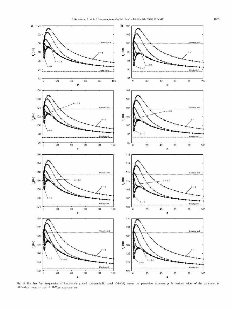
Fig. 11. The first four frequencies of functionally graded toro-parabolic panel (C-F-C-F) versus the power-law exponent p for various values of the parameter b:(a) FGM1ða¼1=0�b�1=c¼2=pÞ , (b) FGM2ða¼1=0�b�1=c¼2=pÞ .

F. Tornabene, E. Viola / European Journal of Mechanics A/Solids 28 (2009) 991–1013 1005

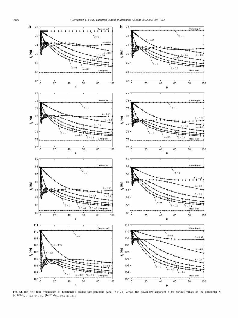
Fig. 12. The first four frequencies of functionally graded toro-parabolic panel (S-F-S-F) versus the power-law exponent p for various values of the parameter b:(a) FGM1ða¼1=0�b�1=c¼1=pÞ , (b) FGM2ða¼1=0�b�1=c¼1=pÞ .

F. Tornabene, E. Viola / European Journal of Mechanics A/Solids 28 (2009) 991–10131006

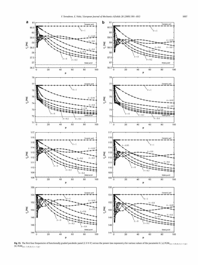
Fig. 13. The first four frequencies of functionally graded parabolic panel (C-F-F-F) versus the power-law exponent p for various values of the parameter b: (a) FGM1ða¼1=0�b�1=c¼1=pÞ ,(b) FGM2ða¼1=0�b�1=c¼1=pÞ .

F. Tornabene, E. Viola / European Journal of Mechanics A/Solids 28 (2009) 991–1013 1007

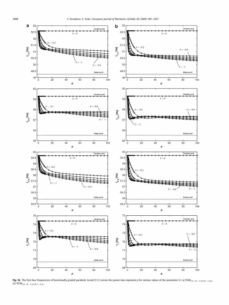
Fig. 14. The first four frequencies of functionally graded parabolic toroid (F-C) versus the power-law exponent p for various values of the parameter b: (a) FGM1ða¼0=�1�b�0=c¼2=pÞ ,(b) FGM2ða¼0=�1�b�0=c¼2=pÞ .

F. Tornabene, E. Viola / European Journal of Mechanics A/Solids 28 (2009) 991–10131008

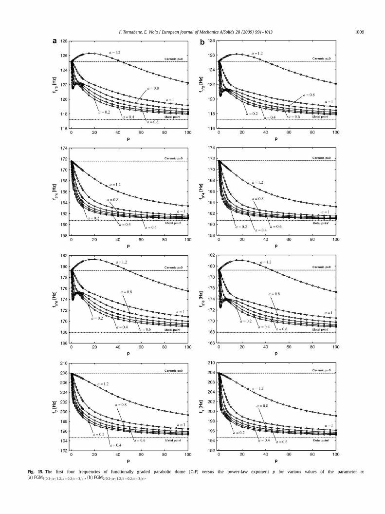
Fig. 15. The first four frequencies of functionally graded parabolic dome (C-F) versus the power-law exponent p for various values of the parameter a:(a) FGM1ð0:2�a�1:2=b¼0:2=c¼3=pÞ , (b) FGM2ð0:2�a�1:2=b¼0:2=c¼3=pÞ .

F. Tornabene, E. Viola / European Journal of Mechanics A/Solids 28 (2009) 991–1013 1009

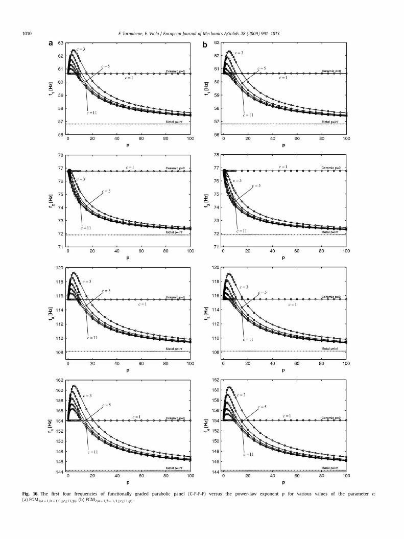
Fig. 16. The first four frequencies of functionally graded parabolic panel (C-F-F-F) versus the power-law exponent p for various values of the parameter c:(a) FGM1ða¼1=b¼1=1�c�11=pÞ , (b) FGM2ða¼1=b¼ 1=1�c�11=pÞ .

F. Tornabene, E. Viola / European Journal of Mechanics A/Solids 28 (2009) 991–10131010

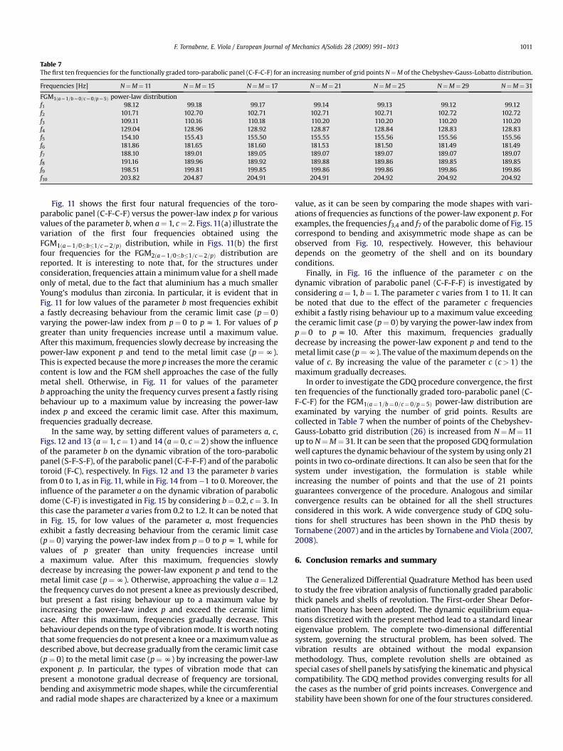
Table 7The first ten frequencies for the functionally graded toro-parabolic panel (C-F-C-F) for an increasing number of grid points N¼M of the Chebyshev-Gauss-Lobatto distribution.

Frequencies [Hz] N¼M¼ 11 N¼M¼ 15 N¼M¼ 17 N¼M¼ 21 N¼M¼ 25 N¼M¼ 29 N¼M¼ 31

FGM1ða¼1=b¼0=c¼0=p¼ 5Þ power-law distributionf1 98.12 99.18 99.17 99.14 99.13 99.12 99.12f2 101.71 102.70 102.71 102.71 102.71 102.72 102.72f3 109.11 110.16 110.18 110.20 110.20 110.20 110.20f4 129.04 128.96 128.92 128.87 128.84 128.83 128.83f5 154.10 155.43 155.50 155.55 155.56 155.56 155.56f6 181.86 181.65 181.60 181.53 181.50 181.49 181.49f7 188.10 189.01 189.05 189.07 189.07 189.07 189.07f8 191.16 189.96 189.92 189.88 189.86 189.85 189.85f9 198.51 199.81 199.85 199.86 199.86 199.86 199.86f10 203.82 204.87 204.91 204.91 204.92 204.92 204.92

F. Tornabene, E. Viola / European Journal of Mechanics A/Solids 28 (2009) 991–1013 1011

Fig. 11 shows the first four natural frequencies of the toro-parabolic panel (C-F-C-F) versus the power-law index p for variousvalues of the parameter b, when a¼ 1, c¼ 2. Figs. 11(a) illustrate thevariation of the first four frequencies obtained using theFGM1ða¼1=0�b�1=c¼2=pÞ distribution, while in Figs. 11(b) the firstfour frequencies for the FGM2ða¼1=0�b�1=c¼2=pÞ distribution arereported. It is interesting to note that, for the structures underconsideration, frequencies attain a minimum value for a shell madeonly of metal, due to the fact that aluminium has a much smallerYoung’s modulus than zirconia. In particular, it is evident that inFig. 11 for low values of the parameter b most frequencies exhibita fastly decreasing behaviour from the ceramic limit case (p¼ 0)varying the power-law index from p¼ 0 to p z 1. For values of pgreater than unity frequencies increase until a maximum value.After this maximum, frequencies slowly decrease by increasing thepower-law exponent p and tend to the metal limit case (p¼N).This is expected because the more p increases the more the ceramiccontent is low and the FGM shell approaches the case of the fullymetal shell. Otherwise, in Fig. 11 for values of the parameterb approaching the unity the frequency curves present a fastly risingbehaviour up to a maximum value by increasing the power-lawindex p and exceed the ceramic limit case. After this maximum,frequencies gradually decrease.

In the same way, by setting different values of parameters a, c,Figs. 12 and 13 (a¼ 1, c¼ 1) and 14 (a¼ 0, c¼ 2) show the influenceof the parameter b on the dynamic vibration of the toro-parabolicpanel (S-F-S-F), of the parabolic panel (C-F-F-F) and of the parabolictoroid (F-C), respectively. In Figs. 12 and 13 the parameter b variesfrom 0 to 1, as in Fig. 11, while in Fig. 14 from�1 to 0. Moreover, theinfluence of the parameter a on the dynamic vibration of parabolicdome (C-F) is investigated in Fig. 15 by considering b¼ 0.2, c¼ 3. Inthis case the parameter a varies from 0.2 to 1.2. It can be noted thatin Fig. 15, for low values of the parameter a, most frequenciesexhibit a fastly decreasing behaviour from the ceramic limit case(p¼ 0) varying the power-law index from p¼ 0 to p z 1, while forvalues of p greater than unity frequencies increase untila maximum value. After this maximum, frequencies slowlydecrease by increasing the power-law exponent p and tend to themetal limit case (p¼N). Otherwise, approaching the value a¼ 1.2the frequency curves do not present a knee as previously described,but present a fast rising behaviour up to a maximum value byincreasing the power-law index p and exceed the ceramic limitcase. After this maximum, frequencies gradually decrease. Thisbehaviour depends on the type of vibration mode. It is worth notingthat some frequencies do not present a knee or a maximum value asdescribed above, but decrease gradually from the ceramic limit case(p¼ 0) to the metal limit case (p¼N) by increasing the power-lawexponent p. In particular, the types of vibration mode that canpresent a monotone gradual decrease of frequency are torsional,bending and axisymmetric mode shapes, while the circumferentialand radial mode shapes are characterized by a knee or a maximum

value, as it can be seen by comparing the mode shapes with vari-ations of frequencies as functions of the power-law exponent p. Forexamples, the frequencies f3,4 and f7 of the parabolic dome of Fig. 15correspond to bending and axisymmetric mode shape as can beobserved from Fig. 10, respectively. However, this behaviourdepends on the geometry of the shell and on its boundaryconditions.

Finally, in Fig. 16 the influence of the parameter c on thedynamic vibration of parabolic panel (C-F-F-F) is investigated byconsidering a¼ 1, b¼ 1. The parameter c varies from 1 to 11. It canbe noted that due to the effect of the parameter c frequenciesexhibit a fastly rising behaviour up to a maximum value exceedingthe ceramic limit case (p¼ 0) by varying the power-law index fromp¼ 0 to p z 10. After this maximum, frequencies graduallydecrease by increasing the power-law exponent p and tend to themetal limit case (p¼N). The value of the maximum depends on thevalue of c. By increasing the value of the parameter c (c> 1) themaximum gradually decreases.

In order to investigate the GDQ procedure convergence, the firstten frequencies of the functionally graded toro-parabolic panel (C-F-C-F) for the FGM1ða¼1=b¼0=c¼0=p¼5Þ power-law distribution areexaminated by varying the number of grid points. Results arecollected in Table 7 when the number of points of the Chebyshev-Gauss-Lobatto grid distribution (26) is increased from N¼M¼ 11up to N¼M¼ 31. It can be seen that the proposed GDQ formulationwell captures the dynamic behaviour of the system by using only 21points in two co-ordinate directions. It can also be seen that for thesystem under investigation, the formulation is stable whileincreasing the number of points and that the use of 21 pointsguarantees convergence of the procedure. Analogous and similarconvergence results can be obtained for all the shell structuresconsidered in this work. A wide convergence study of GDQ solu-tions for shell structures has been shown in the PhD thesis byTornabene (2007) and in the articles by Tornabene and Viola (2007,2008).

6. Conclusion remarks and summary

The Generalized Differential Quadrature Method has been usedto study the free vibration analysis of functionally graded parabolicthick panels and shells of revolution. The First-order Shear Defor-mation Theory has been adopted. The dynamic equilibrium equa-tions discretized with the present method lead to a standard lineareigenvalue problem. The complete two-dimensional differentialsystem, governing the structural problem, has been solved. Thevibration results are obtained without the modal expansionmethodology. Thus, complete revolution shells are obtained asspecial cases of shell panels by satisfying the kinematic and physicalcompatibility. The GDQ method provides converging results for allthe cases as the number of grid points increases. Convergence andstability have been shown for one of the four structures considered.

F. Tornabene, E. Viola / European Journal of Mechanics A/Solids 28 (2009) 991–10131012

In this study, ceramic-metal graded shells of revolution withfour-parameter power-law distributions of the volume fraction ofthe constituents in the thickness direction have been worked out.Various material profiles through the functionally graded shellthickness have been illustrated by varying the four parameters ofpower-law distributions. Symmetric and asymmetric volume frac-tion profiles have been presented. The numerical results haveshown the influence of the power-law exponent, of the power-lawdistribution choice and of the choice of the four parameters on thefree vibrations of functionally graded shells considered. The anal-ysis provides information about the dynamic response of parabolicshell structures for different proportions of the ceramic and metal.For curved shells and panels, it has been observed that the influ-ence of the distribution choice is marked and can be consideredfrom the structural design point of view. In general, it can bepointed out that the frequency vibration of functionally gradedshells and panels of revolution depends on the type of vibrationmode, thickness, power-law distribution, power-law exponent andthe curvature of the structure.

Acknowledgments

This research was supported by the Italian Ministry forUniversity and Scientific, Technological Research MIUR (40% and60%). The research topic is one of the subjects of the Centre of Studyand Research for the Identification of Materials and Structures(CIMEST)-‘‘M. Capurso’’ of the University of Bologna (Italy).

Appendix

The following are the equilibrium operators in equations (10):

L11 ¼A11

R24

v2

v42 þ A11

cos 4

R4R0� 1

R34

dR4

d4

!v

v4þ A66

v2

vs2 �A12sin 4

R4R0

� A11cos2 4

R20

� kA66

R24

L12 ¼ ��

A11cos 4

R0þ A66cos 4

R0

�v

vsþ�

A12

R4þ A66

R4

�v2

v4 vs

L13 ¼

A11

R24

þ A12sin 4

R4R0þ k

A66

R24

!v

v4þ A11

cos 4

R4R0� 1

R34

dR4

d4

!

� A11sin4 cos4

R20

L14 ¼ L41 ¼B11

R24

v2

v42 þ B11

cos 4

R4R0� 1

R34

dR4

d4

!v

v4þ B66

v2

vs2

�B12sin 4

R4R0� B11cos2 4

R20

þ kA66

R4

L15 ¼ L42 ¼ ��

B11cos 4þ B66cos 4�

v þ�

B12 þ B66�

v2

R0 R0 vs R4 R4 v4 vs

L21 ¼�

A11cos 4

R0þ A66cos 4

R0

�v

vsþ�

A12

R4þ A66

R4

�v2

v4 vs

L22 ¼A66

R24

v2

v42 þ A66

cos 4

R4R0� 1

R34

dR4

d4

!v

v4þ A11

v2

vs2

� A66

cos2 4

R20

� sin 4

R4R0

!� k

A66sin2 4

R20

L23 ¼ �L32 ¼�

A12

R4þ A11sin 4

R0þ k

A66sin 4

R0

�v

vs

L24 ¼ L51 ¼�

B11cos 4

R0þ B66cos 4

R0

�v

vsþ�

B12

R4þ B66

R4

�v2

v4 vs

L25 ¼ L52 ¼B66

R24

v2

v42 þ B66

cos 4

R4R0� 1

R34

dR4

d4

!v

v4þ B11

v2

vs2

�B66

cos24

R20

� sin 4

R4R0

!þ k

A66sin 4

R0

L31 ¼ �

A11

R24

þ A12sin 4

R4R0þ k

A66

R24

!v

v4� A12cos 4

R4R0

� A11sin 4 cos 4

R20

� kA66

cos 4

R4R0� 1

R34

dR4

d4

!

L33 ¼ kA66

R24

v2

v42þ kA66

cos 4

R4R0� 1

R34

dR4

d4

!v

v4þ kA66

v2

vs2� A11

R24

� 2A12sin 4

R4R0� A11sin2 4

R20

L34 ¼ � B11

R24

� B12sin 4

R0R4þ k

A66

R4

!v

v4� B12cos 4

R4R0

� B11sin 4 cos 4

R20

þ kA66cos 4

R0

L35 ¼ �L53 ¼�� B12

R4� B11sin 4

R0þ kA66

�v

vs

L43 ¼

B11

R24

þ B12sin 4

R4R0� k

A66

R4

!v

v4þ B11

cos 4

R4R0� 1

R34

dR4

d4

!

� B11sin 4 cos 4

R20

L44 ¼D11

R24

v2

v42þ D11

cos 4

R4R0� 1

R34

dR4

d4

!v

v4þ D66

v2

vs2� D12sin 4

R4R0

� D11cos2 4

R20

� kA66

L45 ¼ ��

D11cos 4

R0þ D66cos 4

R0

�v

vsþ�

D12

R4þ D66

R4

�v2

v4 vs

L54 ¼�

D11cos 4

R0þ D66cos 4

R0

�v

vsþ�

D12

R4þ D66

R4

�v2

v4 vs

L55 ¼D66

R24

v2

v42 þ D66

cos 4

R4R0� 1

R34

dR4

d4

!v

v4þ D11

v2

vs2

� D66

cos2 4

R20

� sin 4

R4R0

!� kA66

References

Abrate, S., 2006. Free vibration, buckling, and static deflection of functionallygraded plates. Compos. Sci. Technol. 66, 2383–2394.

Alfano, G., Auricchio, F., Rosati, L., Sacco, E., 2001. MITC finite elements for laminatedcomposite plates. Int. J. Numer. Methods Eng. 50, 707–738.

F. Tornabene, E. Viola / European Journal of Mechanics A/Solids 28 (2009) 991–1013 1013

Arciniega, R.A., Reddy, J.N., 2007. Large deformation analysis of functionally gradedshells. Int. J. Solids Struct. 44, 2036–2052.

Artioli, E., Gould, P., Viola, E., 2005. A differential quadrature method solution forshear-deformable shells of revolution. Eng. Struct. 27, 1879–1892.

Artioli, E., Viola, E., 2005. Static analysis of shear-deformable shells of revolution viaG.D.Q. method. Struct. Eng. Mech. 19, 459–475.

Artioli, E., Viola, E., 2006. Free vibration analysis of spherical caps using a G.D.Q.numerical solution. ASME. J. Press Vessel Technol. 128, 370–378.

Auricchio, F., Sacco, E., 1999. A mixed-enhanced finite-element for the analysis oflaminated composite plates. Int. J. Numer. Methods Eng. 44, 1481–1504.

Auricchio, F., Sacco, E., 2003. Refined first-order shear deformation theory modelsfor composite laminates. J. Appl. Mech. 70, 381–390.

Della Croce, L., Venini, P., 2004. Finite elements for functionally graded Reissner-Mindlin plates. Comput. Methods Appl. Mech. Eng. 193, 705–725.

Elishakoff, I., Gentilini, C., Viola, E., 2005a. Forced vibrations of functionally gradedplates in the three-dimensional setting. AIAA J. 43, 2000–2007.

Elishakoff, I., Gentilini, C., Viola, E., 2005b. Three-dimensional analysis of an all-around clamped plate made of functionally graded materials. Acta Mech. 180,21–36.

Liew, K.M., He, X.Q., Kitipornchai, S., 2004. Finite element method for the feedbackcontrol of FGM shells in the frequency domain via piezoelectric sensors andactuators. Comput. Methods Appl. Mech. Eng. 193, 257–273.

Marzani, A., Tornabene, F., Viola, E., 2008. Nonconservative stability problems viageneralized differential quadrature method. J. Sound Vib. 315, 176–196.

Ng, T.Y., Lam, K.Y., Liew, K.M., 2000. Effect of FGM materials on the parametricresonance of plate structures. Comput. Methods Appl. Mech. Eng. 190,953–962.

Nie, G.J., Zhong, Z., 2007. Semi-analytical solution for three dimensional vibration offunctionally graded circular plates. Comput. Methods Appl. Mech. Eng. 196,4901–4910.

Patel, B.P., Gupta, S.S., Loknath, M.S., Kadu, C.P., 2005. Free vibration analysis offunctionally graded elliptical cylindrical shells using higher-order theory.Compos. Struct. 69, 259–270.

Pelletier, J.L., Vel, S.S., 2006. An exact solution for the steady-state thermoelasticresponse of functionally graded orthotropic cylindrical shells. Int. J. SolidsStruct. 43, 1131–1158.

Reddy, J.N., 2003. Mechanics of Laminated Composites Plates and Shells. CRC Press,New York.

Roque, C.M.C., Ferreira, A.J.M., Jorge, R.M.N., 2007. A radial basis function for the freevibration analysis of functionally graded plates using refined theory. J. SoundVib. 300, 1048–1070.

Shu, C., 2000. Differential Quadrature and Its Application in Engineering. Springer,Berlin.

Toorani, M.H., Lakis, A.A., 2000. General equations of anisotropic plates and shellsincluding transverse shear deformations, rotary inertia and initial curvatureeffects. J. Sound Vib. 237, 561–615.

Tornabene, F., 2007. Modellazione e Soluzione di Strutture a Guscio in MaterialeAnisotropo. PhD thesis, University of Bologna, DISTART Department.

Tornabene, F., Viola, E., 2007. Vibration analysis of spherical structural elementsusing the GDQ method. Comput. Math. Appl. 53, 1538–1560.

Tornabene, F., Viola, E., 2008. 2-D solution for free vibrations of parabolic shellsusing generalized differential quadrature method. Eur. J. Mech. A – Solids 27,1001–1025.

Viola, E., Artioli, E., 2004. The G.D.Q. method for the harmonic dynamic analysis ofrotational shell structural elements. Struct. Eng. Mech. 17, 789–817.

Viola, E., Dilena, M., Tornabene, F., 2007. Analytical and numerical results forvibration analysis of multi-stepped and multi-damaged circular arches. J. SoundVib. 299, 143–163.

Viola, E., Tornabene, F., 2005. Vibration analysis of damaged circular arches withvarying cross-section. Struct. Integr. Durab. 1, 155–169 (SID–SDHM).

Viola, E., Tornabene, F., 2006. Vibration analysis of conical shell structures usingGDQ method. Far East J. Appl. Math. 25, 23–39.

Yang, J., Kitipornchai, S., Liew, K.M., 2003. Large amplitude vibration of thermo-electro-mechanically stressed FGM laminated plates. Comput. Methods Appl.Mech. Eng. 192, 3861–3885.

Yang, J., Shen, H.S., 2007. Free vibration and parametric resonance of sheardeformable functionally graded cylindrical panels. J. Sound Vib. 261,871–893.

Wu, C.P., Tsai, Y.H., 2004. Asymptotic DQ solutions of functionally graded annularspherical shells. Eur. J. Mech. A – Solids 23, 283–299.

Zenkour, A.M., 2006. Generalized shear deformation theory for bending analysis offunctionally graded plates. Appl. Math. Model. 30, 67–84.