Fractals as Pre-Processing Tool for Computational Intelligence Application

CHAPTER 8

FRACTALS AS PRE-PROCESSING TOOLFOR COMPUTATIONAL INTELLIGENCE APPLICATION

ANA M. TARQUIS1, VALERIANO MÉNDEZ1, JUAN B. GRAU1,JOSÉ M. ANTÓN1, DIEGO ANDINA1�2

1 Dpto. de Matemática Aplicada, E.T.S. de Ingenieros Agrónomos, U.P.M., Av. Complutense s.n.,Ciudad Universitaria, Madrid 28040, Spain.2 Dpto. de Señales, Sistemas y Radiocomunicaiones, E.T.S. Ingenieros de Telecomunicación, U.P.M.,Av. Complutense s.n., Ciudad Universitaria, Madrid 28040, Spain.

Abstract: Preprocessing is the process of adapting the input of our Computational Intelligence (CI)problem to the CI technique applied. Images are inputs of many problems, and Fractalprocessing of the images to extract relevant geometry characteristics is a very importanttool. This chapter is dedicated to Fractal Preprocessing. In Pedology, fractal models werefitted to match the structure of soils and techniques of multifractal analysis of soil imageswere developed as is described in a state-of-the-art panorama. A box-counting methodand a gliding box method are presented, both obtaining from images sets of dimensionparameters, and are evaluated in a discussed case study from images of samples, and thesecond seems preferable. Finally, a comprehensive list of references is given

Keywords: pedology; soil structure; multifractal; soil images; box-counting method; gliding-boxmethod; capacity dimension; information dimension; correlation dimension; multiscaleheterogeneity; fractal models; porous media; partition function

INTRODUCTION

Methods of analysis based on fractal theories have been developed for Pedology todescribe the structure of soil, as natural soils due to a combination of geology, actionof water and air and organisms present a structure down to very small scales thatis in rapport with the physical, biological and agricultural properties. That structuretends to correspond to fractal paradigms as maintaining somehow a fairly similarstructure when reducing the scale to small microscopic ranges. Fractal models witha reduced number of parameters have been developed to describe naturally complexsoils, and different experimental methods were created to compare theory with

193

D. Andina and D.T. Pham (eds.), Computational Intelligence, 193–213.© 2007 Springer.

194 CHAPTER 8

reality or to evaluate parameters, including representative images of soils treatedso as to maintain natural structure features while marking pores or flow patterns,etc. Next section contains a condensed panorama of the corresponding state of artwith references of authors and methods. Third section explains the most commonmethods in subdividing an image to calculate fractal dimensions. Later, two relatedmethods of image description are exposed with formulae, a box-counting methodand a gliding box method, that assume a multifractal structure and the type of imageanalysis resulting in parameters that include capacity, information and correlationdimension. Next, a case study of three obtained images is presented, and using bothmethods a wide range of generalized dimensions is plotted for three samples, andthese results are described and discussed to assess the methods. Finally, conclusionsand a list of references are provided.

1. STATE OF THE ART

Many parameters may be used in the attempt to describe a disordered morphology,but the spatial arrangement of its most prominent features is a challenging problemthroughout a wide range of disciplines (Ripley, 1988; Griffith, 1988; Baveye andBoast, 1998). In the case of 2-dimensional images of soil sections, several workstry to describe the spatial structure applying fractal techniques. Some of them werestudying the spatial arrangement of pore and solid spaces on images of sections ofresin-impregnated soil (Protz and VandenBygaart, 1998; VandenBygaart and Protz,1999). Thin soil sections are analysed by transmitted light to obtain images fromwhich pores, filled with a resin, and solid spaces can be separated using imageanalysis techniques (Morán et al., 1989; Vogel and Kretzschmar, 1996). In other soilscience areas, dye tracers are frequently used to study flow patterns in structuredsoils, and with modern photographic techniques, they may provide excellent spatialresolution of the flow paths (Flury and Fluhler, 1994; 1995). The most commonapproach to describe dye patterns has been by descriptive statistics of the verticalvariation in dye coverage or shape parameters (Flury et al., 1994) based on a blackand white image, as the ones used for soil-pore structure.

A main objective was to extract fractal dimensions which characterize multi-scale and self-similar geometric structures within the images. In other words, weexpect to see that the image viewed at different resolutions looks the same. Ata given resolution we should see the matrix as a collection of subsets similar toeach other and furthermore similar to the whole. If such a hierarchical organizationexists, it can be characterized by a mass fractal dimension D. These structures areeither one of the phases (black or white) or the interface between the two withina 2-dimensional image. That such dimensions can be extracted from soil imagesis evident, from soil pore structure (Brakensiek et al., 1992; Peyton et al., 1994;Crawford et al., 1993; 1995; Anderson et al., 1996; 1998; Pachepsky et al., 1996;Giménez et al., 1997; 1998; Oleschko et al., 1997; 1998a; 1998b; Hallet et al.,1998; Bartoli et al., 1991; 1998; 1999; Dathe et al., 2001; Bird et al., 2000; 2003)or flow paths in soils (Hatano and Booltink, 1992; Hatano et al, 1992; Booltinket al., 1993).

PRE-PROCESSING TOOL FOR COMPUTATIONAL INTELLIGENCE APPLICATION 195

More recently, interest has turned to multifractal analysis of soil images. A mul-tifractal or more precisely a geometrical multifractal (Tel and Vicsek, 1987) isa non-uniform fractal which unlike a uniform fractal exhibits local density fluc-tuations. Its characterization requires not a single dimension but a sequence ofgeneralized fractal dimensions (Pachepsky et al., 2000). A multifractal analysis toextract these dimensions from a soil image may have utility for more complexdistributions, if there is marked variation in local density or porosity.

Multifractal analysis (MFA) has been applied to images of rock pore systems(Muller and McCauley, 1992; Saucier, 1992; Muller et al., 1995; Muller, 1996;Saucier and Muller, 1999; Saucier et al., 2002), reviewed in the context of soils byTarquis et al. (2003) and recently applied to soils by Posadas et al. (2003). In otherareas, researchers have calculated fractal dimensions of dye patterns in horizontalsections of undisturbed soil cores and related them to the outflow of percolatingdye solution. Baveye et al. (1998) calculated the information dimension �D1� andthe correlation dimension �D2� of dye stain patterns in vertical sections in a fieldsoil. Based on these calculations, models have approached the variability showedin the dye images using diffusion limited aggregation techniques (Persson et al.,2001).

Several authors have shown that the exact value of the generalized dimension isnot an easy task (Baveye et al., 1998; Baveye and Boast, 1998; Crawford et al.,1999; Ogawa et al., 1999) pointing to practical difficulties in extracting generalizeddimensions (Vicsek, 1990; Buczkowski et al., 1998). Merits and limitations ofthe multifractal analysis have been discussed by Aharony (1990), Beghdadi et al.(1993), and Andraud et al. (1994). In the same way, Chhabra et al. (1989) pointedout the risks in the estimation of the Hausdorff dimension and cited different sourcesof errors in some physical cases. The difficulties arising in practice are due tothe fact that the relevant quantities used in the multifractal concept are estimatedasymptotically and in image analysis these estimations are much more coarse andlimited by the finite resolution of the image (Ahammer et al., 2003) and the measurebuild on it, as the number of black points in a box (Buczkowski et al., 1998). Alsosome authors have pointed out the influence of the percentage of black pixels ina 2-dimensional image in the Dq obtained (Dathe and Thullner, 2005; Bird et al.,2005; Tarquis et al., 2005; Dathe et al., 2005).

On the other hand, MFA involves partitioning the space of study into boxesto construct samples with multiple scales. The number of the samples at a givenscale is restricted by the size of the partitioning space and data resolution, which isusually another main factor influencing statistical estimation in MFA (Cheng andAgerberg, 1996).

The purpose of this chapter is to ascertain the successful extraction of a spectrumof generalized dimensions from a soil image, trying to avoid all the restrictionsthat the box-counting method has and to discern the existence/non-existence of amultifractal distribution of black or white within the image.

In the following sections, we shall review the box counting algorithm to obtainthe generalized fractal dimensions of multifractal analysis, as well as the gliding-boxmethod. We will show some examples to highlight shortcomings of these methods.

196 CHAPTER 8

2. FRACTAL CALCULATIONS

The main purpose of this section is to introduce some of the fractal methods usedin the context of black and white image analysis of soil structure. A completetreatment of fractal and multifractal theories can be found, among others, in Feder(1989) and Baveye and Boast (1998).

2.1 Box-counting Method

This methodology is classical in this field and has generated a large volume of work.If a fractal line in a 2-dimensional space is covered by boxes of side length d, thenumber of such boxes, n��, needed to cover the line when � → 0 is (Mandelbrot,1982):

(1) n�� = c�−DL

The length of the line studied (e.g., the pore-solid interface), L��, can be definedat different scales and is equal to �n��. At small � values the method provides agood approximation to the length of the line because the resolution of the imageis approached. At larger sizes the difference between �n�� and the “true” lengthincreases. Thus, DL, or capacity dimension, is estimated using small � values(Gimenez et al., 1997b). The box-counting method is also used to obtain a fractaldimension of pore space by counting boxes that are occupied for at least one pixelbelonging to the class “pore” (Gimenez et al., 1997b).

2.2 Dilation Method

Dathe et al. (2001) is the only published report of this method in the soil science.The dilation method follows essentially the same procedure as the box-countingmethod, but instead of using boxes it uses other structuring elements to cover theobject under study, e.g., circles (Dathe et al., 2001). The image is formed by pixels,which are either square or rectangular in shape. If circles are used, the measureof scale is their diameter (as is the side length of the box in the box-countingtechnique). If we want to have the same dilation in any direction, the orthogonal anddiagonal increments should be biased by

√2, which corresponds to the hypotenuse

of a square of unit side length (Kaye, 1989). The length of the studied object iscounted by numbers of circles, and then the slope of the regression line betweenthe log of the object length and the log of the object diameter is defined by therelation:

(2) L�� = c�1−DL

Dathe et al. (2001) applied the box-counting and dilation methods to the sameimages and found non-significant differences in the values of the fractal dimensionsobtained with both methods. They pointed out, however, that fractal dimensions


estimated with both methods are different: the box counting dimension is theKolmogorov dimension while the dimension obtained with the dilation method is theembedding dimension (Mikowski-Bouligand). For further details, see Takayasu’swork (Takayasu, 1990).

2.3 Random Walk

Fractal methods can also be used to describe the dynamic properties of fractalnetworks (Crawford et al., 1993; Anderson et al., 1996]. Characterization of fractalsinvolving space and time are achieved through the use of fractons (Kaye, 1989) orthe spectral dimension (Orbach, 1986). For example, Crawford et al. (1999) relatedmeasurements of the spectral dimension d to diffusion through soil, associating dwith the resistance degree to which the network delay the diffusing particle in agiven direction.

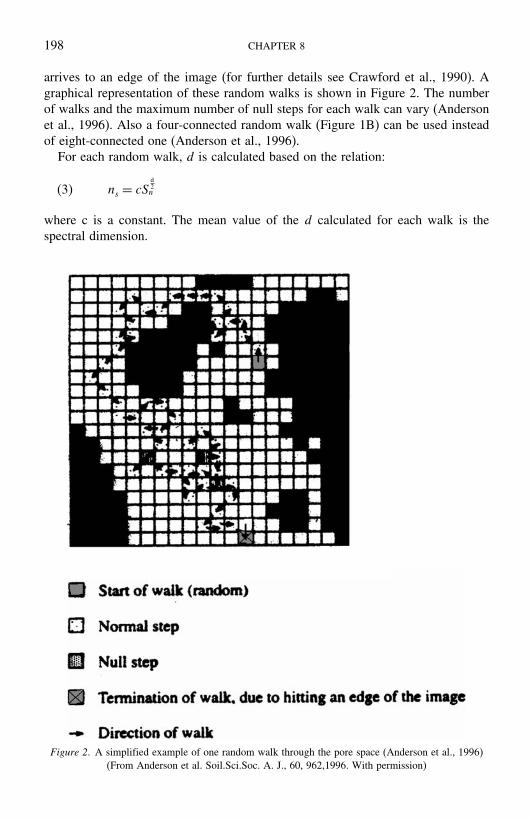
The determination of d is based on random walks, where in each walk thenumber of steps taken �ns� and the number of different pore pixels visited �Sn� arecomputed. At the beginning of the random walk a pore pixel is randomly chosen,then a random step is taken to another pore pixel from the eight pixels surroundingthe present one (see Figure 1A). If the new pore pixel has not been visited by therandom walk, the Sn and ns are increased by one, otherwise only ns is increased.The random walk stops when a certain number of null steps (the step goes into asite that has been used previously during the walk) is achieved or the random walk

Figure 1. Possible steps taken in a: a) eight-connected random walk, and b) four-connected randomwalk. The present position of the pore pixel is marked by an x, and the arrows indicate the possiblenext pore pixel. (From Tarquis et al. In: Scaling Methods in Soil Physics, Pachepsky, Radcliffe and

Selim Eds., CRC Press, 2003. With permission)

198 CHAPTER 8

arrives to an edge of the image (for further details see Crawford et al., 1990). Agraphical representation of these random walks is shown in Figure 2. The numberof walks and the maximum number of null steps for each walk can vary (Andersonet al., 1996). Also a four-connected random walk (Figure 1B) can be used insteadof eight-connected one (Anderson et al., 1996).

For each random walk, d is calculated based on the relation:

(3) ns = cSd2n

where c is a constant. The mean value of the d calculated for each walk is thespectral dimension.

Figure 2. A simplified example of one random walk through the pore space (Anderson et al., 1996)(From Anderson et al. Soil.Sci.Soc. A. J., 60, 962,1996. With permission)


3. CALCULATION OF GENERALIZED FRACTAL DIMENSIONS

3.1 Box-counting Method

Generalized dimensions calculated using the box counting technique basicallyaccounts for the mass contained in each box. An image is divided into n boxes ofsize r (pixels in each dimension making r · r pixels per box), designated as �n�r��,and for each box the fraction ��i� of pore space in that box is defined and calculatedas

(4) �i =mi

M= mi/

n�r�∑i=1

mi

where mi is the number of pore class pixels and M is the total number of pore classpixels in an image. In this case, the pore space area is the measure whereas thesupport is the pore space itself. The next step is to define the generating function��q� r�� as:

(5) ��q� r� =n�r�∑i=1

��i�q� r�� q ∈ R

where

(6) �i�q� r� = �qi =

(mi/

n�r�∑i=1

mi

)q

�i is a weighted measure that represents the percentage of pore space in the ith

box, and q is the weight or moment of the measure. When computing boxes of sizer, the possible values of mi are from 0 to r · r. Therefore, let Nj�r� be the numberof boxes containing j pixels of pore space in that grid. Equations (5) and (6) willthen be (Barnsley et al., 1988):

(7)

��q� r� =n�r�∑i=1

��i�q =

n�r�∑i=1

(mi

M

)q =r·r∑j=1

Nj�r�

(j

M

)q

=r·r∑j=1

Nj�r�

⎛⎜⎜⎝

jr·r∑k=1

kNk�r�

⎞⎟⎟⎠

q

Using the distribution function Nj�r�, calculations become simpler and compu-tational errors are smaller.

A log-log plot of a self-similar measure, ��q� r�, vs. r at various values for qgives

(8) � �q� r� ∼ r−�q�

200 CHAPTER 8

where �q� is the qth mass exponent (Feder, 1989). We can express �q� as:

(9) �q� = −limr→0

log��q� r��

log�r�

Then, the generalized dimension, Dq, can be introduced by the following scalingrelationship (Feder, 1989):

(10) �q� = −limr→0

log��q� r��

log�r�

And, therefore

(11) �q� = �q −1�Dq

For the case that q = 1, Equation (11) cannot be applied and the followingequation should be used:

(12) D1 = limr→0

n�r�∑i=1

�i�1� r� · log��i�1� r�

log r

The generalized dimensions, Dq, for q = 0, 1 and 2 are known as the capac-ity, the information, and the correlation dimensions, respectively (Hentschel andProcaccia, 1983). The capacity dimension is the box-counting or fractal dimension.The information dimension is related to the entropy of the system, whereas thecorrelation dimension computes the correlation of measures contained in boxes ofvarious sizes (Posadas et al., 2003).

Given these definitions and the behaviour to expect in case of a multifractalmeasure, it is again instructive to seek the lower and upper bounds for ��q� r� inorder to establish what scope exists for behaviour other than that associated witha multifractal measure (for further explanation see Bird et al., 2005). FollowingBird et al.’s work (2005), a brief explanation will be shown to establish bounds for��q� r�. Four separate ranges of values of the parameter q should be considered:

Case q > 1

The smallest value that ��q� r� can take corresponds to a uniform distribution ofpore phase over the image. The largest value that ��q� r� can take corresponds tothe case in which each grid block covering the pore phase is entirely filled by porephase. The lower and upper bounds are then as follows:

(13)(

L

r

)2�1−q�

< ��q� r� <

(L

r

)2�1−q�

f �1−q�� q > 1

where f is the fraction of the image occupied by black pixels and L is the lengthof the image.


Case q = 1

The smallest value of the entropy corresponds to the case in which each gridblock covering the pore phase is entirely filled by pore phase. The largest valuecorresponds to a uniform distribution. Lower and upper bounds are then as follows:

(14) 2 ln(

L

r

)+ ln�f� < −

n�r�∑i=1

�i ln��i� < 2 ln(

L

r

)� q = 1

Case 0 ≤ q < 1

The smallest value ��q� r� can take corresponds to the case in which each grid blockcovering the pore phase is entirely filled by pore. The largest value corresponds toa uniform distribution of pore phase over the image. Lower and upper bounds areas follows:

(15)(

L

r

)2�1−q�

f �1−q� < �r�q� r� <

(L

r

)2�1−q�

� 0 ≤ q < 1

Case q < 0

The smallest value ��q� r� can take corresponds to the case in which each grid blockcovering the pore phase is entirely filled by pore. The function is monotonicallydecreasing. Therefore, the value corresponding to r = 1 pixel can be selected as anupper bound.

(16)(

L

r

)2�1−q�

f �1−q� < ��q� r� < L2�1−q�f �1−q�� q < 0

Having defined these bounds, we now seek to examine their significance interms of extracting generalized dimensions from image data. For q > 1 and for0 ≤ q < 1, the bounding functions when plotted on the log-log plot used to extractthe dimension yield two parallel lines with a vertical separation of �1−q� ln�f�.

For q = 1, the bounding functions when included in the plot of entropy againstln�r� again yield two parallel lines of slope 2 with separation of ln�f�. Thus, in thesecases we reach the same impasse as that with the fractal analysis, namely dependingon f , and independent of actual geometry considered, the data can be so constrainedas to yield convincing straight-line fits with associated derived dimensions.

3.2 Gliding Box Method

The gliding-box method was originally used for lacunarity analysis (Allain andCloitre, 1991). Later, it was modified by Cheng (1997a, 1997b) for estimating �q�as follows:

(17) < �q� > +D = − log�< M�q� r� >�

log�r/rmin�

202 CHAPTER 8

Where D is the dimension of the Euclidean space where the image is imbibed(in this case D = 2) and M represents the multiplier measured on each pixel as:

(18) M�q� r� =(

��rmin�

��r�

)q

For further details see Grau et al. (2006). The advantage of using Equation (17)in comparison with Equation (9) is that the estimation is independent of box size rwhich allows the use of two successive box sizes only to estimate �q�. Equation (18)imposes that ��rmin� should not be null.

Once this estimation is done, Equation (8) can be applied to estimate Dq. Forthe case of q = 1 the following relationship is applied based on the work given in(Saucier and Muller, 1999):

(19) D̂1 = 2D2 −D3

4. IMAGES FOR THE CASE STUDY

Three soil samples were selected with the aim to represent a different range invoid pattern distribution in soils and a wide range of porosity values, from 5% ofporosity till 47%. Each of the samples was prepared for image analysis followingthe procedure described by Protz and VandenBygaart (1998).

The data was obtained by imaging thin sections with a Kodak 460 RGB camerausing transmitted and circularly polarized illumination. The data was cropped from3060 × 2036 pixels to 3000 × 2000 pixels. Then, EASI/PACE software classifiedthe data and the void bitmap separated, each individual pixel size was 18�6×18�6microns. The images of these soils are showed in Figure 3.

To avoid any interference of the edge effect for the calculations using the box-counting method, an area of 1024 × 1024 pixels of the left upper corner of theoriginal images was selected.

5. RESULTS OF THE CASE STUDY AND DISCUSSION

5.1 Generating Function with the Box-counting Method

For the three binary images, ��q� r� was calculated and then a bi-log plot of ��q� r�versus r was made to observe the behavior. All plots showed a clear pattern in thedata. In Figure 2, for example, at negative q there were two distinctive areas, onewhere there was a linear relationship between log�r� and log��q� r�� and anotherwhere the value of log ��q� r� was almost constant versus log�r�. The box size atwhich the behavior is different for the three images is around 64 pixels. These twophases were not evident with positive q values (see Figure 4).

The existence of a plateau phase of log��q� r�� can be explained by the natureof the measure under consideration. At r values close to 1, the variation in numberof black pixels is based on a few pixels, having the most simplicity when r = 1


Sample A

Sample B

Sample C

Figure 3. Soil binary images, pore phase in black pixels, of: (a) ADS, (b) BUSO and (c) EHV1. Eachimage has 5.65%, 19.17% and 46.67% of porosity, respectively

204 CHAPTER 8

–150

–100

–50

0

50

100

150

0 2 4 6

Log(r)

Log

X(q

,r)

–150

–100

–50

0

50

100

150

0 2 4 6

Log(r)

Log

X(q

,r)

–150

–100

–50

0

50

100

150

0 2 4 6

Log(r)

Log

X(q

,r)

–10–8–6–4–20246810

B

A

C

Figure 4. Bi-log plot of ��q� r� versus box size �r� at different mass exponent �q�: A): ADS; B)BUSO; C) EVH1

where the measure can only have 0 or 1 value. Thus, for small boxes of size r theproportions among their values are mainly constant. However, when the box sizepasses certain size a scaling pattern begins.


5.2 Generalized Dimensions Using the Box-counting Method

If all of the regression points are considered, the Dq values, obtained mainly forq < 0, were quite different from these obtained if only the regression points inthe linear behavior were chosen (Figure 5). Between both criteria, any Dq canbe obtained, but for q >= 0 the differences are not significant. Many authorshave pointed out this fact since the first applications of multifractal analysis toexperimental results (Tarquis et al., 2005).

The implications of Dq changes, too noticeable in this case, make impossible anycomparison and calculation of the amplitude of the dimensions �D−10 −D+10� as ithas been used in several works.

The differences found among the Dq representation (Figure 5, filled circles) aremainly found in the negative part. In particular, comparing ADS (Figure 5A filledcircles) with the rest it is evident that it doesn’t show a multifractal behavior.

All the D0 obtained have a value of 2 (plane dimension). This overestimation isdue to the fact that the studied range that was selected to have an optimum fit forall the q values. However, looking at the lower and upper bond of the box-countingplots for q = 0 (Figure 6) it is quite clear that regardless the structure in the imagethe linear fit will be obtained with a high r2.

The standard errors (data not shown) of the Dq obtained in the linear behaviorphase are minimum and the r2 of the regression analysis very high. However, thisis not surprising if we realize that only three points are being used. In addition, thenumber of boxes of each size is very low, for size 128 × 128 pixels the numberof boxes is 64, for size 256 × 256 pixels the number of boxes is 16, analyzing animage of 1024 × 1024 pixels that is considered a representative elementary area(VandenBygaart and Protz, 1999).

This size restriction is avoided by using the gliding box method and its resultsare discussed in the next section.

5.3 Generalized Dimensions Using the Gliding Box Method

For the three binary images, < M�q� r� > was calculated and then a bi-log plot of< M�q� r� > versus r/rmin was made. All plots showed a linear relationship, as itwas expected, with an important number of points to calculate a linear regressionand based on the line’s slope estimate Dq (Figure 4). In the case of EHV1 forq < −6 (Figure 4A), the linear relationship is not as clear as in the rest of theimages.

Finally, a comparison between both methods in the Dq values obtained can bestudied in Figure 5. In all of the graphics, Dq appears again with a value of 2imposed by the box gliding method as it was explained in section 3.2.

For ADS (Figure 5A) both curves are similar. On propose, the range of valuesfor Dq has been changed to observe that the image effect could induce to an errorin our conclusions, when in Figure 3 was evident that Dq was an almost constantvalue.

206 CHAPTER 8

1,50

2,50

3,50

4,50

5,50

6,50

–10 –8 –6 –4 –2 0 2 4 6 8 10

q

Dq

1,50

2,50

3,50

4,50

5,50

6,50

–10 –8 –6 –4 –2 0 2 4 6 8 10

q

Dq

1,50

2,50

3,50

4,50

5,50

6,50

–10 –8 –6 –4 –2 0 2 4 6 8 10

q

Dq

A

B

C

Figure 5. Generalized dimensions (Dq) from q = −10 to q = +10 for all points of the regression line(filled square) and for the three selected points based on bi-log plot of X(r,q) (filled circles) of each

image: A) ADS; B) BUSO and C) EVH1


Observing the differences between both methods in BUSO and EVH1 (Figure 5Band 5C respectively) are bigger in the negative q values although in the positivevalues Dq shows a stronger decay (Grau et al., 2006).

6. CONCLUSIONS

Over the last years, the concepts of fractal/multifractal have been increasinglyapplied in analysis of porous materials including soils and in the development offractal models of porous media. In terms of modeling, it is important to charac-terize the multiscale heterogeneity of soil structure in a useful way, but the blindapplication of these analyses does not approach to it.

(a)

0 1 2 3 4 5 6 7 8

2

0

4

6

8

10

12

14

16

log r

log

N

(b)

00 1 2 3 4 5 6 7 8

2

4

6

8

10

12

14

16

log r

log

N

Figure 6. Box counting plots for EHV1 soil images, q = 0, with upper and lower bounds (a) solidphase (b) pore phase. (From Bird et al., J. of Hydrol., 322, 211, 2006. With permission)

208 CHAPTER 8L

og (

<M(r

,q)>

)

–40

–30

–20

–10

0

10

20

3040

–0,1 0,1 0,3 0,5 0,7 0,9 1,1 1,3 1,5

Log(r/rmin)

Log

(<M

(r,q

)>)

0

20

–20

–40

–60

–80

40

0

0 0,2 0,4 0,6 0,8 1 1,2 1,4 1,6

0

20

–20

–40

–60

–80

–100

–120

0,2 0,4 0,6 0,8 1 1,2 1,4 1,6

Log(r/rmin)

Log

(<M

(r,q

)>)

–10–8–6–4–20246810

C

A

B

Figure 7. Bi-log plot of < M�r� q� > versus box size rate �r/rmin� at different mass exponent (q): A):ADS; B) BUSO, C) EVH1


1,990

1,995

2,000

2,005

2,010

2,015

2,020

2,025

2,030

-10 -8 -6 -4 -2 0 2 4 6 8 10q

Dq

0,000

0,500

1,000

1,500

2,000

2,500

3,000

3,500

4,000

-8 -6 -4 -2 0 2 4 6 8-10 10q

Dq

1,00

2,00

3,00

4,00

5,00

6,00

7,00

-10 -8 -6 -4 -2 0 2 4 6 8 10q

Dq

A

B

C

Figure 8. Generalized dimensions (Dq) from q = −10 to q = +10 based on the box-gliding method(empty square) and based on the box-counting method (filled circles) using the same box sizes range:

A) ADS; B) BUSO; C) EVH1

210 CHAPTER 8

The results obtained by the “box-counting” and “gliding-box” methods for mul-tifractal modeling of soil pore images show that “gliding-box” provides more con-sistent results as it creates more number of large size boxes in comparison with thebox-counting method and avoids the restriction that box-counting method imposesto the partition function.

7. ACKNOWLEDGEMENTS

We thank Dr Richard Heck of Guelph University for the soil images. We are veryindebted to Dr. N. Bird, Dr. Q. Cheng and Dr. D. Gimenez for helpful discussions.This work was supported by Techical University of Madrid (UPM) and MadridAutonomous Community (CAM), Project No. M050020163.

REFERENCES

Aharony, A., 1990, Multifractals in physics – successes, dangers and challenges, Physica A. 168:479–489.

Ahammer, H., De Vaney, T.T.J. and Tritthart, H.A., 2003, How much resolution is enough? Influenceof downscaling the pixel resolution of digital images on the generalised dimensions, Physica D. 181(3–4):147–156.

Allain, C. and Cloitre, M., 1991, Characterizing the lacunarity of random and deterministic fractal sets,Physical Review A. 44:3552–3558.

Anderson, A.N., McBratney, A.B. and FitzPatrick, E.A., 1996, Soil Mass, Surface, and Spectral FractalDimensions Estimated from Thin Section Photographs, Soil Sci. Soc. Am. J. 60:962–969.

Anderson, A.N., McBratney, A.B. and Crawford, J.W., Applications of fractals to soil studies. Adv.Agron., 63:1, 1998.

Barnsley, M.F., Devaney, R.L., Mandelbrot, B.B., Peitgen, H.O., Saupe, D. and Voss, R.F., 1988, TheScience of Fractal Images. Edited by H.O. Peitgen and D. Saupe, Springer-Verlag, New York.

Bartoli, F., Philippy, R., Doirisse, S., Niquet, S. and Dubuit, M., 1991, Structure and self-similarity insilty and sandy soils; the fractal approach, J. Soil Sci. 42:167–185.

Bartoli, F., Bird, N.R., Gomendy, V., Vivier, H. and Niquet, S., 1999, The relation between silty soilstructures and their mercury porosimetry curve counterparts: fractals and percolation, Eur. J. Soil Sci.,50(9).

Bartoli, F., Dutartre, P., Gomendy, V., Niquet, S. and Vivier, H., 1998. Fractal and soil structures. In:Fractals in Soil Science, Baveye, Parlange and Stewart, Eds., CRC Press, Boca Raton, 203–232.

Baveye, P. and Boast, C.W. Fractal Geometry, Fragmentation Processes and the Physics of Scale-Invariance: An Introduction. In Fractals in Soil Science, Baveye, Parlange and Stewart, Eds., CRCPress, Boca Raton, 1998, 1.

Baveye, P., Boast, C.W., Ogawa, S., Parlange, J.Y. and Steenhuis, T., 1998. Influence of image resolutionand thresholding on the apparent mass fractal characteristics of preferential flow patterns in field soils,Water Resour. Res. 34, 2783–2796.

Bird, N., Díaz, M.C., Saa, A. and Tarquis, A.M., 2006. Fractal and Multifractal Analysis of Pore-ScaleImages of Soil. J. Hydrol, 322, 211–219.

Bird, N.R.A., Perrier, E. and Rieu, M., 2000. The water retention function for a model of soil structurewith pore and solid fractal distributions. Eur. J. Soil Sci. 51, 55–63.

Bird, N.R.A. and Perrier, E.M.A., 2003. The pore-solid fractal model of soil density scaling. Eur. J. SoilSci. 54, 467–476.

Booltink, H.W.G., Hatano, R. and Bouma, J., 1993. Measurement and simulation of bypass flow in astructured clay soil; a physico-morphological approach. J. Hydrol. 148, 149–168.


Brakensiek, D.L., W.J. Rawls, S.D. Logsdon and Edwards, W.M., 1992. Fractal description of macrop-orosity. Soil Sci. Soc. Am. J. 56, 1721–1723.

Buczhowski, S., Hildgen, P. and Cartilier, L. 1998. Measurements of fractal dimension by box-counting:a critical analysis of data scatter. Physica A 252, 23–34.

Cheng, Q. and Agerberg, F.P. (1996). Comparison between two types of multifractal modeling. Mathe-matical Geology, 28(8), 1001–1015.

Cheng, Q. (1997a). Discrete multifractals. Mathematical Geology, 29(2), 245–266.Cheng, Q. (1997b). Multifractal modeling and lacunarity analysis. Mathematical Geology, 29(7),

919–932.Crawford, J.W., Baveye, P., Grindrod, P. and Rappoldt, C. Application of Fractals to Soil Properties,

Landscape Patterns, and Solute Transport in Porous Media, in Assessment of Non-Point SourcePollution in the Vadose Zone. Geophysical Monograph 108, Corwin, Loague and Ellsworth, Eds.,American Geophysical Union, Wahington, DC, 1999, 151.

Crawford, J.W., Ritz, K. and Young, I.M. Quantification of fungal morphology, gaseous transport andmicrobial dynamics in soil: an integrated framework utilising fractal geometry. Geoderma, 56, 1578,1993.

Crawford, J.W., Matsui, N. and Young, I.M. 1995., The relation between the moisture-release curve andthe structure of soil. Eur. J. Soil Sci. 46, 369–375.

Dathe, A., Eins, S., Niemeyer, J. and Gerold, G. The surface fractal dimension of the soil-pore interfaceas measured by image analysis. Geoderma, 103, 203, 2001.

Dathe, A., Tarquis, A.M. and Perrier, E., 2006. Multifractal analysis of the pore- andsolid-phases in binary two-dimensional images of natural porous structures. Geoderma,doi:10.1016/j.geoderma.2006.03.024, in press.

Dathe, A. and Thullner, M., 2005. The relationship between fractal properties of solid matrix and porespace in porous media. Geoderma, 129, 279–290.

Feder, J., 1989. Fractals. Plenum Press, New York. 283ppFlury, M. and Fluhler, H., 1994. Brilliant blue FCF as a dye tracer for solute transport studies – A

toxicological overview. J.Environ. Qual. 23, 1108–1112.Flury, M. and Fluhler, H., 1995. Tracer characteristics of brilliant blue. Soil Sci. Soc. Am. J. 59, 22–27.Flury, M., Fluhler, H., Jury, W.A. and Leuenberger, J., 1994. Susceptibility of soils to preferential flow

of water: A field study, Water Resour. Res. 30, 1945–1954.Giménez, D., R.R. Allmaras, E.A. Nater and Huggins, D.R., 1997a. Fractal dimensions for volume and

surface of interaggregate pores – scale effects. Geoderma 77, 19–38.Giménez D., Perfect E., Rawls W.J. and Pachepsky, Y., 1997b. Fractal models for predicting soil

hydraulic properties: a review. Eng. Geol. 48, 161–183.Gouyet, J.G. Physics and Fractal Structures. Masson, Paris, 1996.Grau, J., Méndez, V., Tarquis, A.M., Díaz, M.C. and A. Saa, 2006. Comparison of gliding box and

box-counting methods in soil image analysis. Geoderma, doi:10.1016/j.geoderma.2006.03.009, inpress.

Griffith, D.A.. Advanced Spatial Statistics. Kluwer Academic Publishers, Boston, 1988.Hallett, P.D., Bird, N.R.A., Dexter, A.R. and Seville, P.K., 1998. Investigation into the fractal scaling

of the structure and strength of soil aggregates. Eur. J. Soil Sci. 49, 203–211.Hatano, R. and Booltink, H.W.G., 1992. Using Fractal Dimensions of Stained Flow Patterns in a Clay

Soil to Predict Bypass Flow. J. Hydrol. 135, 121–131.Hatano, R., Kawamura, N., Ikeda, J. and Sakuma, T. Evaluation of the effect of morphological features

of flow paths on solute transport by using fractal dimensions of methylene blue staining patterns.Geoderma 53, 31, 1992.

Hentschel, H.G.R. and Procaccia, I. (1983). The infinite number of generalized dimensions of fractalsand strange attractors. Physica D, 8, 435, 1983.

Kaye, B.G. A Random Walk through Fractal Dimensions. VCH Verlagsgesellschaft, Weinheim,Germany, 1989, 297.

Mandelbrot, B.B. The Fractal Geometry of Nature. W.H. Freeman, San Francisco, CA, 1982.McCauley, J.L. 1992. Models of permeability and conductivity of porous media. Physica A 187, 18–54.

212 CHAPTER 8

Moran, C.J., McBratney, A.B. and Koppi, A.J.,1989. A rapid method for analysis of soil macroporestructure. I. Specimen preparation and digital binary production. Soil Sci. Soc. Am. J. 53, 921–928.

Muller, J., 1996. Characterization of pore space in chalk by multifractal analysis. J. Hydrology, 187,215–222.

Muller, J., Huseby, O.K. and Saucier, A. Influence of Multifractal Scaling of Pore Geometry onPermeabilities of Sedimentary Rocks. Chaos, Solitons & Fractals, 5, 1485, 1995.

Muller, J. and McCauley, J.L., 1992. Implication of Fractal Geometry for Fluid Flow Properties ofSedimentary Rocks. Transp. Porous Media 8, 133–147.

Muller, J., Huseby, O.K. and Saucier, A., 1995. Influence of Multifractal Scaling of Pore Geometry onPermeabilities of Sedimentary Rocks. Chaos, Solitons & Fractals 5, 1485–1492.

Ogawa, S., Baveye, P., Boast, C.W., Parlange, J.Y. and Steenhuis, T. Surface fractal characteristics ofpreferential flow patterns in field soils: evaluation and effect of image processing. Geoderma, 88,109, 1999.

Oleschko, K., Fuentes, C., Brambila, F. and Alvarez, R. Linear fractal analysis of three Mexican soilsin different management systems. Soil Technol., 10, 185, 1997.

Oleschko, K. Delesse principle and statistical fractal sets: 1. Dimensional equivalents. Soil&TillageResearch, 49, 255,1998a.

Oleschko, K., Brambila, F., Aceff, F. and Mora, L.P. From fractal analysis along a line to fractals onthe plane. Soil&Tillage Research, 45, 389, 1998b.

Orbach, R. Dynamics of fractal networks. Science (Washington, DC) 231, 814, 1986.Pachepsky, Y.A.,Yakovchenko, V., Rabenhorst, M.C., Pooley, C. and Sikora, L.J. . Fractal parameters

of pore surfaces as derived from micromorphological data: effect of long term management practices.Geoderma, 74, 305, 1996.

Pachepsky, Y.A., Giménez, D., Crawford, J.W. and Rawls, W.J. Conventional and fractal geometry insoil science. In Fractals in Soil Science, Pachepsky, Crawford and Rawls, Eds., Elsevier Science,Amsterdam, 2000, 7.

Persson, M., Yasuda, H., Albergel, J., Berndtsson, R., Zante, P., Nasri, S. and Öhrström, P., 2001.Modeling plot scale dye penetration by a diffusion limited aggregation (DLA) model. J. Hydrol. 250,98–105.

Peyton, R.L., Gantzer, C.J., Anderson, S.H., Haeffner, B.A. and Pfeifer, P. . Fractal dimension todescribe soil macropore structure using X ray computed tomography. Water Resource Research, 30,691, 1994.

Posadas, A.N.D., Giménez, D., Quiroz, R. and Protz, R., 2003. Multifractal Characterization of SoilPore Spatial Distributions. Soil Sci. Soc. Am. J. 67, 1361–1369

Protz , R. and VandenBygaart, A.J. 1998. Towards systematic image analysis in the study of soilmicromorphology. Science Soils, 3. (available online at http://link.springer.de/link/service/journals/).

Ripley, B.D. Statistical Inference for Spatial Processes, Cambridge Univ. Press, Cambridge, 1988.Saucier, A. Effective permeability of multifractal porous media. Physica A, 183, 381, 1992.Saucier, A. and Muller, J. Remarks on some properties of multifractals. Physica A, 199, 350, 1993.Saucier, A. and Muller, J. Textural analysis of disordered materials with multifractals. Physica A, 267,

221, 1999.Saucier, A., Richer, J. and Muller, J., 2002. Statistical mechanics and its applications. Physica A, 311

(1–2): 231–259.Takayasu, H. Fractals in the Physical Sciences. Manchester University Press, Manchester, 1990.Tarquis, A.M., Giménez, D., Saa, A., Díaz, M.C. and Gascó, J.M., 2003. Scaling and Multiscaling of

Soil Pore Systems Determined by Image Analysis. In: Scaling Methods in Soil Physics, Pachepsky,Radcliffe and Selim Eds., CRC Press, 434 pp.

Tarquis, A.M., McInnes, K.J., Keys, J., Saa, A., García, M.R. and Díaz, M.C., 2006. MultiscalingAnalysis In A Structured Clay Soil Using 2D Images. J. Hydrol, 322, 236–246.

Tel, T. and Vicsek, T., 1987. Geometrical multifractality of growing structures, J. Physics A. General,20, L835–L840.

VandenBygaart, A.J. and Protz, R., 1999. The representative elementary area (REA) in studies ofquantitative soil micromorphology. Geoderma 89, 333–346.


Vicsek, T. 1990. Mass multifractals. Physica A, 168, 490–497.Vogel, H.J. and Kretzschmar, A., 1996. Topological characterization of pore space in soil-sample

preparation and digital image-processing. Geoderma 73, 23–38.

Fractals as Pre-Processing Tool for Computational Intelligence Application

Documents

Transcript of Fractals as Pre-Processing Tool for Computational Intelligence Application