arX

iv:0

903.

3476

v1 [

cond

-mat

.sta

t-m

ech]

20

Mar

200

9

Fractality of the non-equilibrium stationary states of open

volume-preserving systems: I. Tagged particle diffusion

Felipe Barra,1 Pierre Gaspard,2 and Thomas Gilbert2

1Departamento de Fısica, Facultad de Ciencias Fısicas y Matematicas,

Universidad de Chile, Casilla 487-3, Santiago Chile2Center for Nonlinear Phenomena and Complex Systems,

Universite Libre de Bruxelles, C. P. 231, Campus Plaine, B-1050 Brussels, Belgium

(Dated: March 20, 2009)

Deterministic diffusive systems such as the periodic Lorentz gas, multi-baker map, as well as spa-tially periodic systems of interacting particles, have non-equilibrium stationary states with fractalproperties when put in contact with particle reservoirs at their boundaries. We study the macro-scopic limits of these systems and establish a correspondence between the thermodynamics of themacroscopic diffusion process and the fractality of the stationary states that characterize the phase-space statistics. In particular the entropy production rate is recovered from first principles usinga formalism due to Gaspard [J. Stat. Phys. 88, 1215 (1997)]. This article is the first of two; thesecond article considers the influence of a uniform external field on such systems.

PACS numbers: 05.45.-a,05.70.Ln,05.60.-k

I. INTRODUCTION

The assumption that the microscopic dynamics of me-chanical systems obeying Newton’s equations are mixingoffers a mechanism by which the entropy can increase to-ward its equilibrium value, as described by Gibbs in 1902[1]. The mixing would indeed allow coarse-grained proba-bilities to reach their equilibrium values after a long time,a result that has received a rigorous meaning in the con-text of modern ergodic theory [2]. The use of the coarse-grained entropy of a physical system, which is the secondingredient of Gibbs’ mechanism, is justified by the factthat, if the entropy should be given according to Boltz-mann by the logarithm of the number of complexions ofa system, then the introduction of cells of non-vanishingsizes is required to perform the counting of complexionsin systems described by continuous coordinates.

The program set up by Gibbs has taken on a newperspective in recent years with its systematic applica-tion to chaotic, deterministic volume-preserving dynam-ical systems sustaining a transport process of diffusion,which therefore fall under the scope of Liouville’s the-orem [3, 4, 5, 6, 7, 8, 9]. In previous works, bothnon-equilibrium stationary states and relaxation to equi-librium were considered, with the common thread thattransport processes are intimately connected to singular-ities of the non-equilibrium measures, characterized byphase-space distributions with fractal properties.

A specific example of the systems of interest is theperiodic Lorentz gas, in which moving particles diffusethrough a lattice interacting only with fixed scatterers.A useful simplification of this process is the multi-bakermap, which is a simple model of deterministic diffusionfor a tracer particle with chaotic dynamics. Other higherdimensional examples are spatially periodic extensionsof systems with many interacting particles, where themotion of a tagged particle is followed as it undergoes

diffusion among the cells.

In refs. [8, 9], these models were studied in the con-text of relaxation to equilibrium. It was shown in thesepapers that the initial non-equilibrium distribution func-tion rapidly develops a fractal structure in phase spacedue to the chaotic nature of the dynamics. This stuc-ture is such that variations of the distribution functionon arbitrarily fine scales grow as the system evolves intime. The final stages of the approach to equilibrium arethen controlled by the decay of fractal, microscopic hy-drodynamic modes of the system –in this case diffusivemodes– which decay with time as exp(−Dk2t), where kis a wave number associated to the macroscopic hydro-dynamic decay, D is the diffusion coefficient, and t is thetime. It is possible to express the rate of entropy pro-duction in this final stage in terms of measures which aredetermined by the non-equilibrium phase-space distribu-tion, specified by the fractal hydrodynamic modes. Themain result is that one obtains by this method exactly theexpression for the rate of entropy production as given byirreversible thermodynamics for these systems [10]. Thesource of this agreement can be traced to the role playedby the fractal hydrodynamic modes, both for requiringa coarse graining of the phase space to properly incor-porate the effects of their fractal properties on entropyproduction in the system, as well as for describing theslowest decay of the system as it relaxes to equilibrium.

The purpose of this paper is to consider in further de-tails the non-equilibrium stationary states of multi-bakermaps and Lorentz gases which occur when their bound-aries are put in contact with particle reservoirs, as wellas to extend these considerations to tagged particle diffu-sion in spatially periodic systems of interacting particles.In the macroscopic limit, we establish the connectionsbetween the statistics of these deterministic systems andthe phenomenological prescriptions of thermodynamic.Though the stationary states of multi-baker maps andLorentz gases have been considered in some details, see

2

especially [11], the problem of computing the entropyproduction associated to the non-equilibrium stationarystate has thus far been limited to the example of themulti-baker map [4]. Here we emphasize the similari-ties between the stationary states of multi-baker maps,Lorentz gases, and spatially periodic many particle sys-tems, undergoing steady mass flows and show how theformalism described in [9] yields an ab initio derivationof the entropy production rate in all these systems.

This paper is the first of two. In the second paper[12], we will consider the Galton board [13, 14], whichis to be understood in this context as a periodic finitehorizon Lorentz gas with a uniform external field andno dissipation mechanism. As was recently proved byChernov and Dolgopyat [15, 16], this system is recurrentand therefore has no drift. We will show how one cancharacterize equilibrium and non-equilibrium stationarystates of such a system, much in the same way as withthe periodic Lorentz gas we consider in this paper.

The plan of the paper is as follows. In Sec. II, we re-view the phenomenology of non-equilibrium diffusive sys-tems and their entropy production. Then, starting fromthe Liouvillian evolution of phase-space distributions, weconstruct the non-equilibrium stationary states of openperiodic Lorentz gases in Sec. III, as well as of multi-bakermaps in Sec. IV, and show how such stationary statesnaturally separate between regular and singular parts.While the regular parts have the form of a local equilib-rium and allow, in the continuum limit, to retrieve thephenomenological solution of a diffusive system undergo-ing a mass flow, the singular parts have no macroscopiccounterpart and encode the dynamical details of the sys-tems’ diffusive properties. In Sec. V, these results areextended to systems of many interacting particles withnon-equilibrium flux boundary conditions. Under the as-sumption that the dynamics of these systems is chaotic,their stationary states are shown to have properties sim-ilar to those of multi-baker maps and Lorentz gases. Thesingular part of the stationary states is at the origin ofthe entropy production rate, as is explained in Sec. VI,where the phenomenological entropy production rate isretrieved from ab initio considerations. Conclusions aredrawn in Sec. VII.

II. PHENOMENOLOGY

The thermodynamics of deterministic models of dif-fusion such as the Lorentz gas and multi-baker map tobe discussed below was extensively reviewed by Gaspardet. al in [17]. In these models, independent tracer par-ticles mimic matter exchange processes of binary mix-tures, i.e. the process of mutual diffusion between thelight tracer particles and the infinitely heavy particlesthat constitute the background.

In such systems, the irreversible production of entropyarises from gradients in the density of tracer particles.For a dilute system, the resulting thermodynamic force

is

~X ( ~X, t) = −~∇P( ~X, t)

P( ~X, t), (1)

where P( ~X, t) denotes the density of tracer particles at

position ~X and time t. Here the Boltzmann constant isset to unity. Close to equilibrium, in the linear range ofirreversible processes, the corresponding current is pro-portional to the thermodynamic force and given by Fick’slaw of diffusion according to

~J ( ~X, t) = −D~∇P( ~X, t) , (2)

where D is the coefficient of diffusion of tracer particles(assumed to be uniform). In this limit, the condition of

mass conservation, ∂tP( ~X, t)+~∇· ~J ( ~X, t) = 0, transposesinto the the Fokker-Planck equation,

∂tP( ~X, t) = D∇2P( ~X, t) . (3)

The product of the thermodynamic force and currentyields the rate of local irreversible production of entropy,

diS( ~X, t)

dt= ~J ( ~X, t) · ~X ( ~X, t) ,

= D [~∇P( ~X, t)]2

P( ~X, t)> 0 . (4)

Our goal in the next sections will be to analyze thestatistics of deterministic models of diffusion, identify theconditions under which their statistical evolution reducesto the evolution of macroscopic densities as described byEq. (3) and analyze the microscopic origins of the pro-duction of entropy prescribed according to Eq. (4), whichmanifest themselves in the fractality of the stationarystates of these models.

III. OPEN PERIODIC LORENTZ GAS

In this section, we consider a two-dimensional finitehorizon periodic Lorentz gas with hexagonal symmetry,in the shape of a cylindrical Lorentz channel of length L,with periodic boundary conditions in the y-direction andabsorbing boundaries at x = ±L/2. Though some of theresults presented in this section are original, for the mostpart this material is a review of existing results that canbe found in Ref. [11] and references therein.

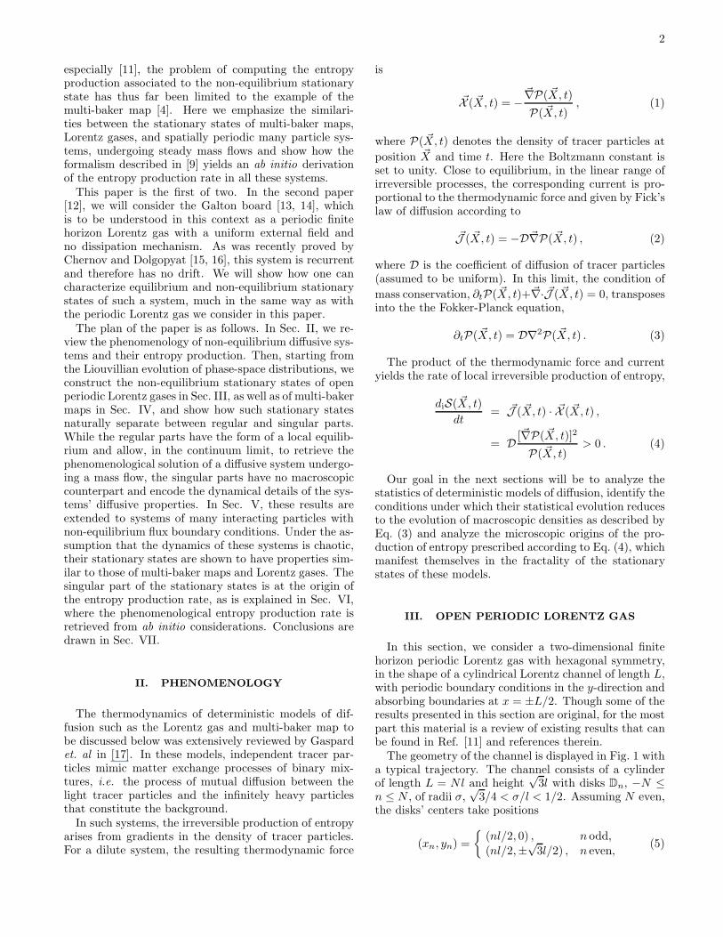
The geometry of the channel is displayed in Fig. 1 witha typical trajectory. The channel consists of a cylinderof length L = Nl and height

√3l with disks Dn, −N ≤

n ≤ N , of radii σ,√

3/4 < σ/l < 1/2. Assuming N even,the disks’ centers take positions

(xn, yn) =

{(nl/2, 0) , n odd,

(nl/2,±√

3l/2) , n even,(5)

3

-L

2l -

L

2

... ... L

2- l

L

2

-3 l

2

0

3 l

2

-3 l

2

0

3 l

2

FIG. 1: Cylindrical Lorentz channel with periodic boundary conditions at the upper and lower borders. The length of the channelis L, with N identical cells of widths l and heights

√3l/2, Nl ≡ L, each containing two disks. The disks have radii σ = 0.44l, and

are positioned at points (x, y) = (nl/2, 0), n = −N +1,−N +3, . . . , N −1, and (nl/2,±√

3l/2), n = −N,−N +2, . . . , N −2, N .The trajectory displayed is that of a particle which initially starts at unit velocity from the left-hand boundary, and is eventuallyabsorbed as it reaches the right-hand boundary. Arrows on the upper and lower borders indicate points where the trajectorywinds around the cylinder.

where the disks at y = ±√

3l/2 are identified. We willalso denote by In the cylinder region around each diskDn,

In ={(x, y) | (n − 1/2)l/2 ≤ x ≤ (n + 1/2)l/2

}. (6)

Thus the interior of the cylinder, where particles propa-gate freely is made up of the union ∪N

n=−N In \ Dn.The associated phase space, defined on a constant en-

ergy shell, is C = ∪Nn=−NCn, where Cn = S1 ⊗ [In \ Dn]

and the unit circle S1 represents all the possible velocity

directions. Particles are reflected with elastic collisionrules on the border ∂C, except at the external borders,corresponding to x = ±L/2, where they get absorbed.Points in phase space are denoted by Γ, Γ = (x, y, vx, vy),with fixed energy E ≡ (v2

x + v2y)/2, and trajectories by

ΦtΓ, with Φt the flow associated to the dynamics of theLorentz channel.

The collision map takes the point Γ = (x, y, vx, vy) ∈∂C to ΦτΓ = (x′, y′, v′x, v′y) ∈ ∂C, where τ is the timethat separates the two successive collisions with the bor-der of the Lorentz channel ∂C, and (v′x, v′y) is obtainedfrom (vx, vy) by the usual rules of specular collisions.Given that the energy E is fixed, the collision map op-erates on a two-dimensional surface, which, given thatthe collision takes place on disk n, is conveniently pa-rameterized by the Birkhoff coordinates (φn, ξn), whereφn specifies the angle along the border of disk n that thetrajectory makes at collision with it, and ξn is the sinusof the angle that the particle velocity makes with respect

to the outgoing normal to the disk after the collision.

A. Non-Equilibrium Stationary State

In order to set up a non-trivial stationary state, weassume that a flux of trajectories is continuously flow-ing through the boundaries. This can be achieved byputting the boundaries in contact with particle reservoirssuch that the phase-space density at x = ±L/2 is fixedaccording to constant values,

ρ(Γ, t)∣∣∣x=±L/2

= ρ±, (7)

corresponding to particle injection rates from the twoends of the channel at x = ±L/2. All the injected par-ticles have the same energy E = (v2

x + v2y)/2 and uni-

form distributions of velocity angles. The evolution ofthe phase-space density ρ is otherwise specified by Li-ouville’s equation, or, equivalently, by the action of the

Frobenius-Perron operator, P t, determined according to

ρ(Γ, t) = P tρ(Γ, 0) ≡∫

C

dΓ′δ(Γ − ΦtΓ′)ρ(Γ′, 0) . (8)

A remarkable result [18] is that the invariant solution ofthis equation, compatible with the boundary conditions(7), is given, for almost every phase point Γ, by

ρ(Γ) =ρ+ + ρ−

2+

ρ+ − ρ−L

[x(Γ) +

∫ −T (Γ)

0

dt x(ΦtΓ)

],

=ρ+ + ρ−

2+

ρ+ − ρ−L

x(Γ) +

K(Γ)∑

k=1

[x(Φ−tkΓ) − x(Φ−tk−1Γ)]

. (9)

4

In these expressions, x(Γ) denotes the projection of the phase point Γ on the horizontal axis, and T (Γ) is the timeit takes the phase point Γ to reach the system boundary backward in time, i.e. such that x(Φ−T (Γ)Γ) = ±L/2. Aswritten in the second line, the time T (Γ) elapses in K(Γ) successive collisions separated by time intervals τn, such

that tk is the time elapsed after k collision events, viz.∑k

j=1 τj = tk. Obviously tK(Γ) = T (Γ). The difference

x(Φ−tkΓ) − x(Φ−tk−1Γ) is the displacement along the x axis between two successive collisions.In the limit of infinite number of cells N , the number of collisions for the trajectory to reach the boundaries becomes

infinite so that the invariant density can be written

ρ(Γ) =ρ+ + ρ−

2+

ρ+ − ρ−L

{x(Γ) +

∞∑

k=1

[x(Φ−tkΓ) − x(Φ−tk−1Γ)]

}. (10)

The two contributions to this expression represent themean linear density profile along the axis, plus fluctu-ations. Notice that the linear profile is itself the sumof two contributions, the first one being the equilibriumdensity and the second one a gradient term. These sta-tionary states are known after Lebowitz and MacLennan[19, 20]. As noted in [18], the fluctuations form the sin-gular part of the invariant density, which builds up ac-cording to which of the two boundaries the phase pointis mapped to.

B. Continuum Limit

The linear part of the invariant density profile (9) hasits origin in the diffusion process which takes place at thephenomenological level. Indeed, in the continuum limit,the phase-space density reduces to the macroscopic den-sity distribution P(X, t), whose evolution is described byEq. (3), with macroscopic position variable X and diffu-sion coefficient, D, which can, in principle, be determinedfrom the underlying dynamics.

In order to obtain Eq. (3) from the Liouvillian evolu-tion, Eq. (8), we let l → 0 and N → ∞ with Nl = Lfixed. All other quantities are fixed, in particular theparticle velocity, which is taken to be unity in the lengthunits of L. In that limit, the macroscopic density can beobtained from the phase-space density by averaging overphase-space regions such that the position variables x(Γ)are identified with the macroscopic position variable X ,here denoted Xn and identified with the cell Cn,

P(Xn, t) =1

l

∫

Cn

dΓρ(Γ, t) . (11)

Note that the volume element is here and throughoutassumed to be properly normalized, i.e.

∫Cn

dΓ = l.

Given non-equilibrium flux boundary conditions withthe stationary state (10), the only contribution to theparticle density P(Xn) is the linear part, which, in thecontinuum limit, yields the stationary solution to Eq. (3),namely

P(X) =P+ + P−

2+

X

L(P+ − P−) , (12)

where P± is equal to ρ± up to a volume factor, and spec-ifies the boundary conditions P(±L/2).

The singular part of the invariant density, on the otherhand, has no macroscopic counterpart. Its integrationover the cell indeed vanishes by isotropy of the underlyingdynamics. Nonetheless, as we will demonstrate shortly, itbears essential information pertaining to the microscopicorigin of entropy production.

In that respect, the phenomenological entropy produc-tion rate (4) can be written

diS(X)

dt= D [∂XP(X)]

2

P(X), (13)

=DL2

(P+ − P−)2

Peq + XL (P+ − P−)

,

where we denoted Peq = (P+ + P−)/2.

C. Numerical Results

We can verify numerically that the invariant density ofthe Lorentz channel has the form (9), with a linear partgiven by the stationary solution of the Fokker-Planckequation (12), and a singular fluctuating part. For thesake of the numerical computation, we let L ≡ 1 andconsider a channel with 2N + 1 disks, N = 25, the left-and right-most ones being only half disks. The macro-scopic position X , −L/2 ≤ X ≤ L/2, will be identifiedwith the cells Cn about the corresponding disks, lettingXn = nl/2, −N ≤ n ≤ N . We then fix the injection ratesρ± and let ρ− > 0 and ρ+ = 0 so as to have P− = 1 andP+ = 0 for the corresponding macroscopic quantities.

Having fixed the geometry of the channel and the in-jection rates, we compute the invariant phase-space den-sity ρ(Γ) in terms of the corresponding density of thecollision map, also called the Birkhoff map, which takestrajectories from one collision event with a disk to thenext one. This is indeed much easier since the numericalintegration of the Lorentz gas relies on an event drivenalgorithm corresponding to integrating the collision map.The conversion between the two phase-space densities ishere trivial because the time scales are uniform.

5

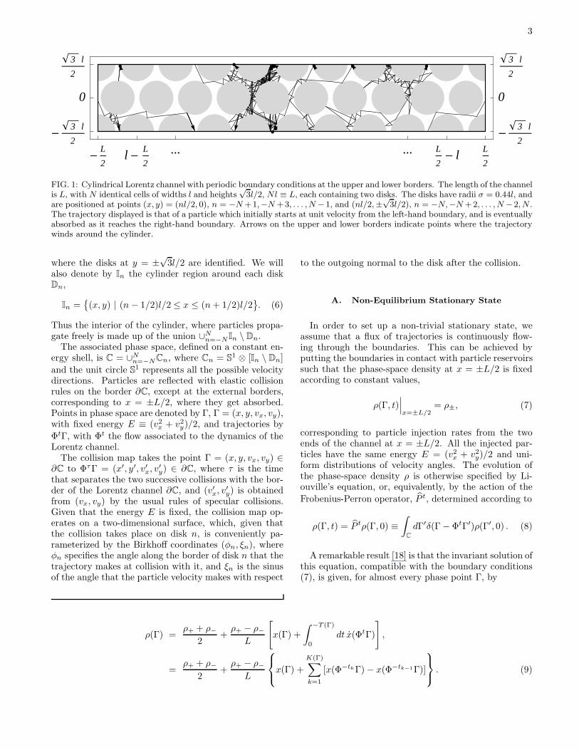
Thus the linear part of the invariant density is com-puted by considering a large set of initial conditions in-jected into the channel from the left end and integratingthem until they reach either ends of the channel, thus ex-iting the system. In the meantime, we record the num-ber of collisions each particle performs with each disk,the ensemble average of which approximates the station-ary distribution P(Xn). Provided N is sufficiently largeand n is not too close to the channel boundaries, thisensemble average is expected to approximate P(X), asspecified by Eq. (12). The result is displayed in Fig. 2and was adjusted by an overall constant so as to matchP− = 1 (and P+ = 0). The agreement is very good.

·

·

· · · · · · · · · · · · · · · · · · · · · · · · · · · · · · · · · · · · · · · · · · · · · · · · ·

-0.4 -0.2 0.0 0.2 0.40.0

0.2

0.4

0.6

0.8

1.0

Xn=n L

2 N

PHX

nL

FIG. 2: Non-equilibrium stationary density of the Lorentzchannel obtained for a cylinder of length L = 1, with 51 disks(N = 25). The solid line is P(X) = 1/2 − X, the solutionof Eq. (12), with P− = 1 and P+ = 0. Notice that the left-and right-most disks are only half disks. Hence the strongboundary effects.

The singular part of the density can also be computedin terms of the statistics of the collision map. For thesake of characterizing this quantity, we notice that theequilibrium Lorentz gas (a single disk on an hexagonalcell with periodic boundary conditions) preserves the Li-ouville measure

dΓ = dx dy dvx dvy ,

= dE dt dφ dξ, (14)

where φ and ξ are the Birkhoff coordinates.For the open Lorentz gas, we associate to each disk

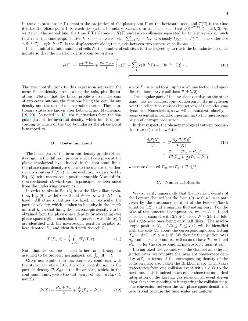
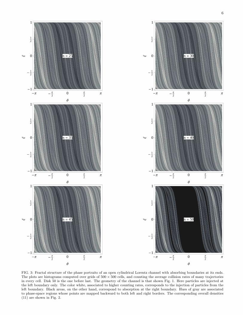
a pair of Birkhoff coordinates, (φn, ξn), and record eachcollision event in a histogram. The results, displayed inFig. 3, show the fractality of the fluctuating part of theinvariant density, with boundary effects vanishing expo-nentially fast with respect to the distance of the disk tothe channel boundaries.

We will see in Sec. VI that the fractality of the sta-tionary measure displayed in Fig. 3 is responsible for theentropy production rate that is associated to the masscurrent in the open Lorentz gas with flux boundary con-ditions.

IV. MULTI-BAKER MAP

The analytic derivation of the entropy production rate(13), relying on the fractality of the invariant measure(10), can be achieved with the multi-baker map. Thisis a simple model of deterministic diffusion that can bethought of as a caricature of the dynamics of the Lorentzgas described above. This model was originally intro-duced in [21], its non-equilibrium stationary state and re-lation to thermodynamics analyzed in [3], and the deriva-tion of the entropy production rate described in [4].

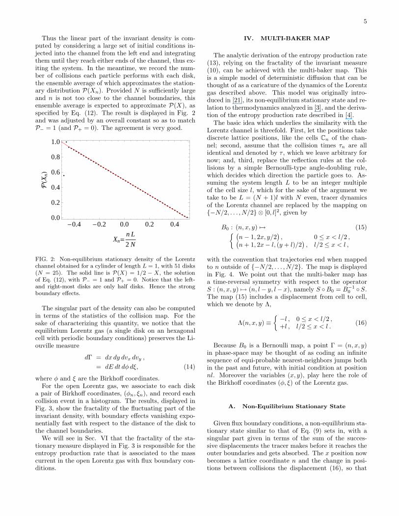
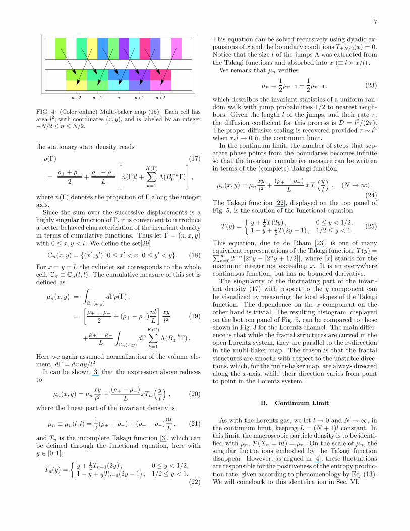
The basic idea which underlies the similarity with theLorentz channel is threefold. First, let the positions takediscrete lattice positions, like the cells Cn of the chan-nel; second, assume that the collision times τn are allidentical and denoted by τ , which we leave arbitrary fornow; and, third, replace the reflection rules at the col-lisions by a simple Bernoulli-type angle-doubling rule,which decides which direction the particle goes to. As-suming the system length L to be an integer multipleof the cell size l, which for the sake of the argument wetake to be L = (N + 1)l with N even, tracer dynamicsof the Lorentz channel are replaced by the mapping on{−N/2, . . . , N/2} ⊗ [0, l]2, given by

B0 : (n, x, y) 7→ (15){ (

n − 1, 2x, y/2), 0 ≤ x < l/2 ,(

n + 1, 2x− l, (y + l)/2), l/2 ≤ x < l ,

with the convention that trajectories end when mappedto n outside of {−N/2, . . . , N/2}. The map is displayedin Fig. 4. We point out that the multi-baker map hasa time-reversal symmetry with respect to the operatorS : (n, x, y) 7→ (n, l− y, l− x), namely S ◦B0 = B−1

0 ◦ S.The map (15) includes a displacement from cell to cell,which we denote by Λ,

Λ(n, x, y) ≡{

−l , 0 ≤ x < l/2 ,+l , l/2 ≤ x < l .

(16)

Because B0 is a Bernoulli map, a point Γ = (n, x, y)in phase-space may be thought of as coding an infinitesequence of equi-probable nearest-neighbors jumps bothin the past and future, with initial condition at positionnl. Moreover the variables (x, y), play here the role ofthe Birkhoff coordinates (φ, ξ) of the Lorentz gas.

A. Non-Equilibrium Stationary State

Given flux boundary conditions, a non-equilibrium sta-tionary state similar to that of Eq. (9) sets in, with asingular part given in terms of the sum of the succes-sive displacements the tracer makes before it reaches theouter boundaries and gets absorbed. The x position nowbecomes a lattice coordinate n and the change in posi-tions between collisions the displacement (16), so that

6

n = 25

-Π -Π

20 Π

2Π

-1

-12

0

12

1

Φ

Ξ n = 30

-Π -Π

20 Π

2Π

-1

-12

0

12

1

Φ

Ξ

n = 35

-Π -Π

20 Π

2Π

-1

-12

0

12

1

Φ

Ξ n = 40

-Π -Π

20 Π

2Π

-1

-12

0

12

1

Φ

Ξ

n = 45

-Π -Π

20 Π

2Π

-1

-12

0

12

1

Φ

Ξ n = 50

-Π -Π

20 Π

2Π

-1

-12

0

12

1

Φ

Ξ

FIG. 3: Fractal structure of the phase portraits of an open cylindrical Lorentz channel with absorbing boundaries at its ends.The plots are histograms computed over grids of 500 × 500 cells, and counting the average collision rates of many trajectoriesin every cell. Disk 50 is the one before last. The geometry of the channel is that shown Fig. 1. Here particles are injected atthe left boundary only. The color white, associated to higher counting rates, corresponds to the injection of particles from theleft boundary. Black areas, on the other hand, correspond to absorption at the right boundary. Hues of gray are associatedto phase-space regions whose points are mapped backward to both left and right borders. The corresponding overall densities(11) are shown in Fig. 2.

7

n - 2 n - 1 n n + 1 n + 2

FIG. 4: (Color online) Multi-baker map (15). Each cell hasarea l2, with coordinates (x, y), and is labeled by an integer−N/2 ≤ n ≤ N/2.

the stationary state density reads

ρ(Γ) (17)

=ρ+ + ρ−

2+

ρ+ − ρ−L

n(Γ)l +

K(Γ)∑

k=1

Λ(B−k0 Γ)

,

where n(Γ) denotes the projection of Γ along the integeraxis.

Since the sum over the successive displacements is ahighly singular function of Γ, it is convenient to introducea better behaved characterization of the invariant densityin terms of cumulative functions. Thus let Γ = (n, x, y)with 0 ≤ x, y < l. We define the set[29]

Cn(x, y) = {(x′, y′) | 0 ≤ x′ < x, 0 ≤ y′ < y}. (18)

For x = y = l, the cylinder set corresponds to the wholecell, Cn ≡ Cn(l, l). The cumulative measure of this set isdefined as

µn(x, y) =

∫

Cn(x,y)

dΓρ(Γ) ,

=

[ρ+ + ρ−

2+ (ρ+ − ρ−)

nl

L

]xy

l2(19)

+ρ+ − ρ−

L

∫

Cn(x,y)

dΓ

K(Γ)∑

k=1

Λ(B−k0 Γ) .

Here we again assumed normalization of the volume ele-ment, dΓ = dx dy/l2.

It can be shown [3] that the expression above reducesto

µn(x, y) = µnxy

l2+

(ρ+ − ρ−)

LxTn

(y

l

), (20)

where the linear part of the invariant density is

µn ≡ µn(l, l) =1

2(ρ+ + ρ−) + (ρ+ − ρ−)

nl

L, (21)

and Tn is the incomplete Takagi function [3], which canbe defined through the functional equation, here withy ∈ [0, 1],

Tn(y) =

{y + 1

2Tn+1(2y) , 0 ≤ y < 1/2,1 − y + 1

2Tn−1(2y − 1) , 1/2 ≤ y < 1.(22)

This equation can be solved recursively using dyadic ex-pansions of x and the boundary conditions T±N/2(x) = 0.Notice that the size l of the jumps Λ was extracted fromthe Takagi functions and absorbed into x (≡ l × x/l) .

We remark that µn verifies

µn =1

2µn−1 +

1

2µn+1, (23)

which describes the invariant statistics of a uniform ran-dom walk with jump probabilities 1/2 to nearest neigh-bors. Given the length l of the jumps, and their rate τ ,the diffusion coefficient for this process is D = l2/(2τ).The proper diffusive scaling is recovered provided τ ∼ l2

when τ, l → 0 in the continuum limit.In the continuum limit, the number of steps that sep-

arate phase points from the boundaries becomes infiniteso that the invariant cumulative measure can be writtenin terms of the (complete) Takagi function,

µn(x, y) = µnxy

l2+

(ρ+ − ρ−)

LxT

(y

l

), (N → ∞) .

(24)The Takagi function [22], displayed on the top panel ofFig. 5, is the solution of the functional equation

T (y) =

{y + 1

2T (2y) , 0 ≤ y < 1/2,1 − y + 1

2T (2y − 1) , 1/2 ≤ y < 1.(25)

This equation, due to de Rham [23], is one of manyequivalent representations of the Takagi function, T (y) =∑∞

n=0 2−n |2ny − [2ny + 1/2]|, where [x] stands for themaximum integer not exceeding x. It is an everywherecontinuous function, but has no bounded derivative.

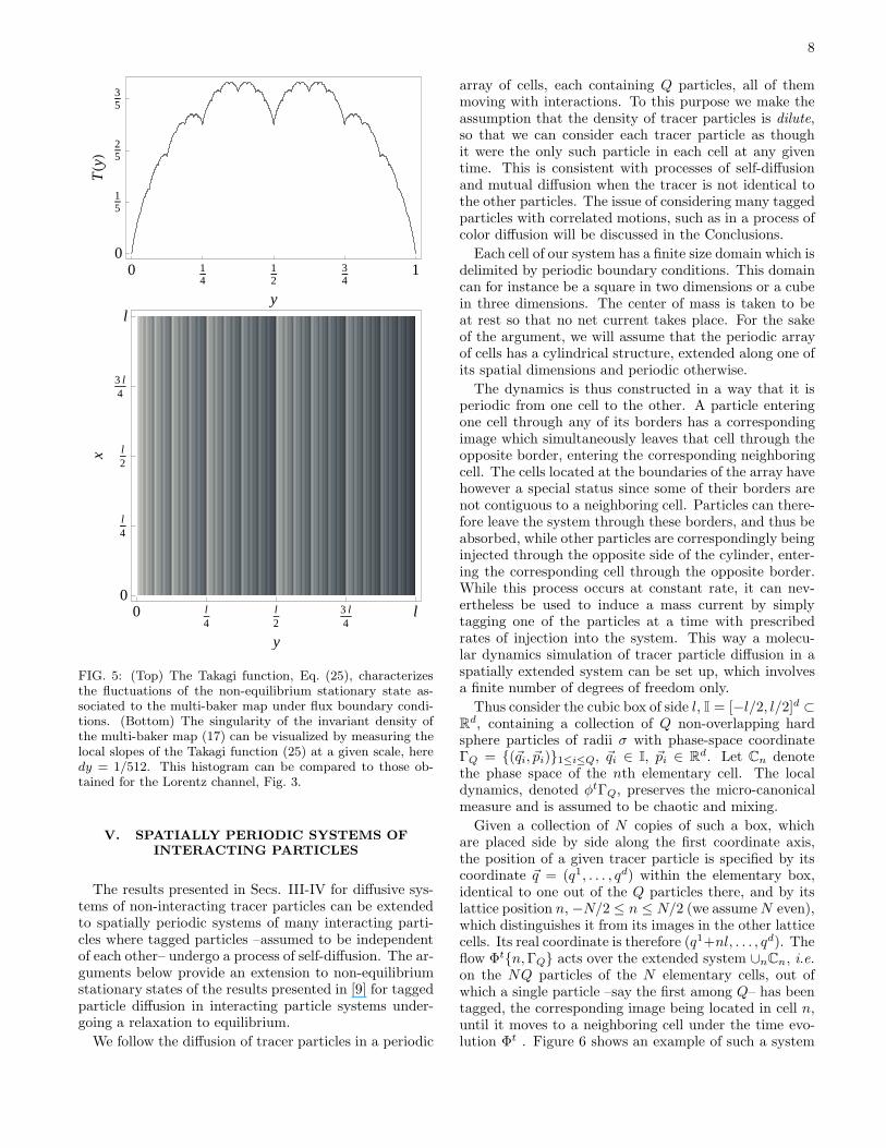
The singularity of the fluctuating part of the invari-ant density (17) with respect to the y component canbe visualized by measuring the local slopes of the Takagifunction. The dependence on the x component on theother hand is trivial. The resulting histogram, displayedon the bottom panel of Fig. 5, can be compared to thoseshown in Fig. 3 for the Lorentz channel. The main differ-ence is that while the fractal structures are curved in theopen Lorentz system, they are parallel to the x-directionin the multi-baker map. The reason is that the fractalstructures are smooth with respect to the unstable direc-tions, which, for the multi-baker map, are always directedalong the x-axis, while their direction varies from pointto point in the Lorentz system.

B. Continuum Limit

As with the Lorentz gas, we let l → 0 and N → ∞, inthe continuum limit, keeping L = (N + 1)l constant. Inthis limit, the macroscopic particle density is to be identi-fied with µn, P(Xn = nl) = µn. On the scale of µn, thesingular fluctuations embodied by the Takagi functiondisappear. However, as argued in [4], these fluctuationsare responsible for the positiveness of the entropy produc-tion rate, given according to phenomenology by Eq. (13).We will comeback to this identification in Sec. VI.

8

0 14

12

34

10

15

25

35

y

THyL

0 l4

l2

3 l4

l0

l4

l2

3 l4

l

y

x

FIG. 5: (Top) The Takagi function, Eq. (25), characterizesthe fluctuations of the non-equilibrium stationary state as-sociated to the multi-baker map under flux boundary condi-tions. (Bottom) The singularity of the invariant density ofthe multi-baker map (17) can be visualized by measuring thelocal slopes of the Takagi function (25) at a given scale, heredy = 1/512. This histogram can be compared to those ob-tained for the Lorentz channel, Fig. 3.

V. SPATIALLY PERIODIC SYSTEMS OF

INTERACTING PARTICLES

The results presented in Secs. III-IV for diffusive sys-tems of non-interacting tracer particles can be extendedto spatially periodic systems of many interacting parti-cles where tagged particles –assumed to be independentof each other– undergo a process of self-diffusion. The ar-guments below provide an extension to non-equilibriumstationary states of the results presented in [9] for taggedparticle diffusion in interacting particle systems under-going a relaxation to equilibrium.

We follow the diffusion of tracer particles in a periodic

array of cells, each containing Q particles, all of themmoving with interactions. To this purpose we make theassumption that the density of tracer particles is dilute,so that we can consider each tracer particle as thoughit were the only such particle in each cell at any giventime. This is consistent with processes of self-diffusionand mutual diffusion when the tracer is not identical tothe other particles. The issue of considering many taggedparticles with correlated motions, such as in a process ofcolor diffusion will be discussed in the Conclusions.

Each cell of our system has a finite size domain which isdelimited by periodic boundary conditions. This domaincan for instance be a square in two dimensions or a cubein three dimensions. The center of mass is taken to beat rest so that no net current takes place. For the sakeof the argument, we will assume that the periodic arrayof cells has a cylindrical structure, extended along one ofits spatial dimensions and periodic otherwise.

The dynamics is thus constructed in a way that it isperiodic from one cell to the other. A particle enteringone cell through any of its borders has a correspondingimage which simultaneously leaves that cell through theopposite border, entering the corresponding neighboringcell. The cells located at the boundaries of the array havehowever a special status since some of their borders arenot contiguous to a neighboring cell. Particles can there-fore leave the system through these borders, and thus beabsorbed, while other particles are correspondingly beinginjected through the opposite side of the cylinder, enter-ing the corresponding cell through the opposite border.While this process occurs at constant rate, it can nev-ertheless be used to induce a mass current by simplytagging one of the particles at a time with prescribedrates of injection into the system. This way a molecu-lar dynamics simulation of tracer particle diffusion in aspatially extended system can be set up, which involvesa finite number of degrees of freedom only.

Thus consider the cubic box of side l, I = [−l/2, l/2]d ⊂R

d, containing a collection of Q non-overlapping hardsphere particles of radii σ with phase-space coordinateΓQ = {(~qi, ~pi)}1≤i≤Q, ~qi ∈ I, ~pi ∈ Rd. Let Cn denotethe phase space of the nth elementary cell. The localdynamics, denoted φtΓQ, preserves the micro-canonicalmeasure and is assumed to be chaotic and mixing.

Given a collection of N copies of such a box, whichare placed side by side along the first coordinate axis,the position of a given tracer particle is specified by itscoordinate ~q = (q1, . . . , qd) within the elementary box,identical to one out of the Q particles there, and by itslattice position n, −N/2 ≤ n ≤ N/2 (we assume N even),which distinguishes it from its images in the other latticecells. Its real coordinate is therefore (q1+nl, . . . , qd). Theflow Φt{n, ΓQ} acts over the extended system ∪nCn, i.e.

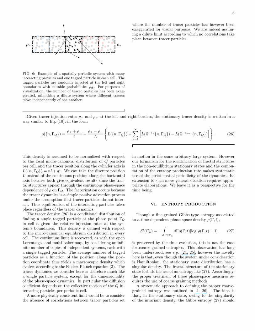
on the NQ particles of the N elementary cells, out ofwhich a single particle –say the first among Q– has beentagged, the corresponding image being located in cell n,until it moves to a neighboring cell under the time evo-lution Φt . Figure 6 shows an example of such a system

9

Ρ- Ρ+

FIG. 6: Example of a spatially periodic system with manyinteracting particles and one tagged particle in each cell. Thetagged particles are randomly injected at the left and rightboundaries with suitable probabilities ρ±. For purposes ofvisualization, the number of tracer particles has been exag-gerated, mimicking a dilute system where different tracersmove independently of one another.

where the number of tracer particles has however beenexaggerated for visual purposes. We are indeed assum-ing a dilute limit according to which no correlations takeplace between tracer particles.

Given tracer injection rates ρ− and ρ+ at the left and right borders, the stationary tracer density is written in away similar to Eq. (10), in the form

ρ({n, ΓQ}) =ρ+ + ρ−

2+

ρ+ − ρ−L

{L({n, ΓQ}) +

∞∑

k=1

[L(Φ−tk{n, ΓQ}) − L(Φ−tk−1{n, ΓQ})

]}. (26)

This density is assumed to be normalized with respectto the local micro-canonical distribution of Q particlesper cell, and the tracer position along the cylinder axis isL({n, ΓQ}) = nl + q1. We can take the discrete positionL instead of the continuous position along the horizontalaxis because both give equivalent results since the frac-tal structures appear through the continuous phase-spacedependence of ρ on ΓQ. The factorization occurs becausethe tracer dynamics is a simple passive advection processunder the assumption that tracer particles do not inter-act. Thus equilibration of the interacting particles takesplace regardless of the tracer dynamics.

The tracer density (26) is a conditional distribution offinding a single tagged particle at the phase point ΓQ

in cell n given the relative injection rates at the sys-tem’s boundaries. This density is defined with respectto the micro-canonical equilibrium distribution in everycell. The continuum limit is recovered, as with the openLorentz gas and multi-baker map, by considering an infi-nite number of copies of independent systems, each witha single tagged particle. The average number of taggedparticles as a function of the position along the posi-tion coordinate thus yields a macroscopic density whichevolves according to the Fokker-Planck equation (3). Thetracer dynamics we consider here is therefore much likea single particle system, except for the dimensionalityof the phase-space dynamics. In particular the diffusioncoefficient depends on the collective motion of the Q in-teracting particles per periodic cell.

A more physically consistent limit would be to considerthe absence of correlations between tracer particles set

in motion in the same arbitrary large system. Howeverour formalism for the identification of fractal structuresin the non-equilibrium stationary states and the compu-tation of the entropy production rate makes systematicuse of the strict spatial periodicity of the dynamics. Itsextension to such more general situation requires appro-priate elaborations. We leave it as a perspective for thetime being.

VI. ENTROPY PRODUCTION

Though a fine-grained Gibbs-type entropy associatedto a time-dependent phase-space density ρ(Γ, t),

St(Cn) = −∫

Γ∈Cn

dΓρ(Γ, t)[log ρ(Γ, t) − 1], (27)

is preserved by the time evolution, this is not the casefor coarse-grained entropies. This observation has longbeen understood, see e.g. [24, 25], however the noveltyhere is that, even though the system under considerationis Hamiltonian, the stationary state distribution has asingular density. The fractal structure of the stationarystate forbids the use of an entropy like (27). Accordingly,the proper treatment of these phase-space measures re-quires the use of coarse graining methods.

A systematic approach to defining the proper coarse-grained entropy was outlined in [4, 26]. The idea isthat, in the stationary state, owing to the singularityof the invariant density, the Gibbs entropy (27) should

10

be evaluated by using a grid of phase space, or partition,G = {dΓj}, into small volume elements dΓj , and a time-dependent state µn(dΓj , t). The entropy associated tocell Cn, coarse grained with respect that grid, is definedaccording to

StG(Cn) = −

∑

j

µn(dΓj , t)

[log

µn(dΓj , t)

dΓj− 1

]. (28)

This entropy changes in a time interval τ according to

∆τSt(Cn) = StG(Cn) − St−τ

G(Cn) , (29)

= St{dΓj}

(Cn) − St{Φτ dΓj}

(ΦτCn) ,

where, in the second line, the collection of partition ele-ments {dΓj} was mapped to {ΦτdΓj}, which forms a par-tition Φτ

G whose elements are typically stretched alongthe unstable foliations and folded along the stable folia-tions.

Following [9], and in a way analogous to the phe-nomenological approach to entropy production [10], therate of entropy change can be further decomposed intoentropy flux and production terms according to

∆τStG(Cn) = ∆τ

eStG(Cn) + ∆τ

i StG(Cn) , (30)

where the entropy flux is defined as the difference be-tween the entropy that enters cell Cn and the entropythat exits that cell,

∆τeSt

G(Cn) = St{Φτ dΓj}

(Cn) − St{Φτ dΓj}

(ΦτCn) . (31)

Collecting Eqs. (29)-(31), the entropy production rate atCn measured with respect to the partition G, is identifiedas

∆τi St

G(Cn) = St{dΓj}

(Cn) − St{Φτ dΓj}

(Cn) . (32)

This formula is equally valid in the non-equilibrium sta-tionary state.

This ab initio derivation of the entropy productionrate for non-equilibrium systems with steady mass cur-rents yields results which are in agreement with the phe-nomenological prescription of thermodynamics. Indeed,as we show below, the entropy production rate of cellCn, Eq. (32), reduces to the phenomenological entropyproduction at corresponding position Xn, Eq. (4), as thegrid elements become small and the dependence on thechoice of partition thus disappears.

A. Multi-baker map

This formalism is particularly transparent for themulti-baker map. Referring to Fig. 4, and having in mindthat measures are time-evolved by the inverse map B−1

0 ,it is easy to see that the bottom horizontal half of cell n ismapped to the left vertical half of cell n+1 and, likewise,the top horizontal half of cell n is mapped to the right

vertical half of cell n − 1. Now the invariant measure(24) is uniform with respect to the x coordinate, whichis the expanding direction, and has a fractal part alongthe y axis, the contracting direction. Thus the entropyof the vertical half of cell n + 1 is half of the entropy ofcell n + 1, but is not equal to the entropy of the bottomor top horizontal halves of that cell, at least not withrespect to the same partition.

This observation yields the identification of the entropyproduction rate, namely the difference between the en-tropies of that cell, measured at two different levels ofresolution, one with respect to volumes dΓ = dxdy, theother with respect to volumes dΓ′ = dx′dy′, where dy′ istwice as large as dy, and dx′ half as large as dx.

To be precise, given a resolution level 2−k, k ∈ N,we consider the collection of cylinder sets dΓk(yj) ={(x, y)|yj ≤ y ≤ yj + 2−kl}, j = 1, . . . , 2k, with yj =2−k(j − 1)l, which partition the square into 2k horizon-tal slabs of widths 2−kl, and, by analogy with Eq. (28),define the k-entropy of cell n to be

Sk(Cn) = −2k∑

j=1

µn(dΓk(yj))

[log

µn(dΓk(yj))

2−k− 1

].

(33)According to Eq. (32), the k-entropy production rate perunit time is

∆τi Sk(Cn) =

1

τ[Sk(Cn) − Sk+1(Cn)] , (34)

=

2k+1∑

j=1

µn(dΓk+1(yj)) log2µn(dΓk+1(yj))

µn(dΓk(yj/2)),

where the index j/2 is the largest integer above j/2.The thermodynamic entropy production rate is recov-

ered in the continuum limit, whereby the local gradientstend to zero and k can be arbitrarily large.

To verify this, we consider the symbolic sequencesωk ≡ {ω0, . . . , ωk−1}, ωj ∈ {0, 1} associated to the 2k

points yj through the dyadic expansions yj = y(ωk) =∑k−1j=0 2−j−1ωj .In terms of the symbolic sequences ωk, the invari-

ant measure associated to the cylinder set dΓ(ωk) ≡dΓ(y(ωk)) becomes, using Eq. (24),

µn(ωk) = 2−kµn + ∇ρ∆T (ωk) ,

= 2−kµn

[1 +

∇ρ

µn2k∆T (ωk)

], (35)

where we wrote the local density gradient ∇ρ ≡ (ρ+ −ρ−)l/L, and ∆T (ωk) = T

(y(ωk)/l + 2−k

)− T

(y(ωk)/l

).

Using the functional equation (25), it is straightforwardto check that

2k∆T (ωk) =k−1∑

j=0

(1 − 2ωj) , (36)

which, up to the scale l, is the displacement associatedto points in the cylinder set dΓ(ωk). Two identities are

11

immediate∑

ωk2k∆T (ωk) = 0,∑

ωk2k∆T (ωk)2 = k.

(37)

Substituting this expression into Eq. (34), we arrive,after expanding in powers of the density gradient, to theexpression

∆τi Sk(Cn) =

1

2τ

(∇ρ)2

µn

×

∑

ωk+1

2k+1[∆T (ωk+1)]2 −

∑

ωk

2k[∆T (ωk)]2

,

=1

2τ

(∇ρ)2

µn=

l2

2τL2

(ρ+ − ρ−)2

µn, (38)

Identifying the diffusion coefficient D = l2D/τ , withD ≡ 1/2 the diffusion coefficient associated to the bi-nary random walk, we recover the phenomenological en-tropy production rate (13) for the macroscopic positionvariable X = nl/L :

limτ,l→0

∆τi Sk(Cn) =

diS(Xn = nl)

dt, (39)

where the limit τ, l → 0 is take with the ration l2/τ fixed.

B. Lorentz gas

This computation transposes verbatim to the non-equilibrium stationary state of the Lorentz gas, Eq. (10),whose entropy production rate is computed as follows.

Let M be a partition of ∂C, the phase space of thecollision map, into non-overlapping sets Aj , M = ∪jAj .We assume that each element of the partition is containedin a cell ∂Cn, i.e. ∀j ∃n : Aj ⊂ ∂Cn. There is thus asub-collection Mn of cells Aj which partition ∂Cn, ∂Cn =∪j : Aj∈Mn

Aj . Moreover we assume all the partitions Mn

are isomorphic, which is to say they can be obtained fromone another by translation.

We construct such a partition of the phase space as-sociated to cell n by dividing up ∂Cn into sets Aj ac-cording to the displacements of points Γ ∈ Aj , such asshown in Fig. 7. Thus a k partition Mk

n of Cn is a col-lection of sets A(ω0, . . . , ωk−1) of points Γ which havecoherent horizontal displacements for the first k steps.These displacements are coded by sequences of symbolsωk which, in this case, take at most 12 possible values,corresponding to the twelve possible transitions to thenearest and next-nearest neighboring disks. However,unlike with Bernoulli processes, not all symbol sequencesare allowed so that the number of sets in the partitionM

kn is much less than 12k. This is referred to as pruning

[27, 28].Assuming ωj ∈ {1, . . . , 12}, we define a(ωj) as the dis-

placement along the horizontal axis corresponding to the

-Π - Π

20 Π

2Π

-1

0

1

Φ

Ξ

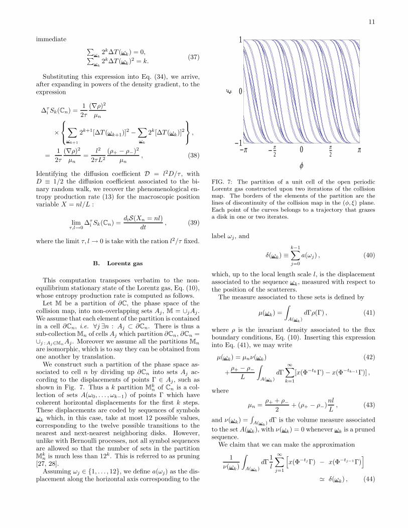
FIG. 7: The partition of a unit cell of the open periodicLorentz gas constructed upon two iterations of the collisionmap. The borders of the elements of the partition are thelines of discontinuity of the collision map in the (φ, ξ) plane.Each point of the curves belongs to a trajectory that grazesa disk in one or two iterates.

label ωj , and

δ(ωk) ≡k−1∑

j=0

a(ωj) , (40)

which, up to the local length scale l, is the displacementassociated to the sequence ωk, measured with respect tothe position of the scatterers.

The measure associated to these sets is defined by

µ(ωk) =

∫

A(ωk)

dΓρ(Γ) , (41)

where ρ is the invariant density associated to the fluxboundary conditions, Eq. (10). Inserting this expressioninto Eq. (41), we may write

µ(ωk) = µnν(ωk) (42)

+ρ+ − ρ−

L

∫

A(ωk)

dΓ

∞∑

k=1

[x(Φ−tkΓ) − x(Φ−tk−1Γ)] ,

where

µn =ρ+ + ρ−

2+ (ρ+ − ρ−)

nl

L, (43)

and ν(ωk) =∫

A(ωk)dΓ is the volume measure associated

to the set A(ωk), with ν(ωk) = 0 whenever ωk is a prunedsequence.

We claim that we can make the approximation

1

ν(ωk)

∫

A(ωk)

dΓ1

l

∞∑

j=1

[x(Φ−tj Γ) − x(Φ−tj−1Γ)

]

≃ δ(ωk) , (44)

12

which we expect to hold provided k is large. This quan-tity therefore plays, for the non-equilibrium stationarystate of the Lorentz gas, a role similar to that played un-der the same conditions by ∆T (ωk)/ν(ωk), Eq. (36), forthe multi-baker map. Indeed the difference between thetwo sides of Eq. (44) is O(1). Under this condition andassuming l ≪ 1, we thus write

µ(ωk) = ν(ωk)µn

[1 +

ρ+ − ρ−µn

l

Lδ(ωk)

], (45)

which can be compared to Eq. (35). When k is large,identities similar to Eq. (37) hold for δ(ωk) :

∑ωk

ν(ωk)δ(ωk) = 0 ,∑ω

kν(ωk)δ(ωk)2 = 2Dk ,

(46)

where the diffusion coefficient D is that of the randomwalk on half integer lattice sites associated to the dis-placements (40) with weights ν(ωk).

The computation of the entropy production rate (32)then proceeds along the lines of Eq. (38), with a similarresult:

∆τi Sk(Cn) =

l2D

τL2

(ρ+ − ρ−)

µn, (47)

in agreement with the phenomenological expressionEq. (13) with diffusion coefficient D = l2D/τ and po-sition Xn = nl/2.

C. Interacting particle system

Here, as in Ref. [9], we assume a partition of phase-space in sets Aj sufficiently small that all points in themhave particle No. 1 flowing through the same sequence ofcells over a large time interval, i.e. such that the set ofpoints Φ−τAj are in the same cell when projected alongthe coordinate of particle No. 1, with 0 ≤ τ ≤ T . Thecorresponding location is L(Φ−τ{n, ΓQ}), ΓQ ∈ Aj . Wedefine the displacement

d(ΓQ, t) = L(Φ−t{n, ΓQ}) − nl , (48)

and write the non-equilibrium stationary state as

µ(Aj) = µnν(Aj) +ρ+ − ρ−

L

∫

Aj

dΓQd(ΓQ, T ) , (49)

where the volume measure ν(Aj) is the micro-canonicalmeasure of the periodic system of Q particles. The inte-gral in this expression encodes the fluctuating part of thenon-equilibrium stationary state. In analogy to Eq. (44),we can write

δ(Aj) =1

ν(Aj)

∫

Aj

dΓQd(ΓQ, T ) , (50)

in terms of which we have the identities∑

j ν(Aj)δ(Aj) = 0 ,∑j ν(Aj)δ(Aj)

2 = 2DT ,(51)

which, apart for their dimensions, are similar to Eqs. (37)and (46).

Proceeding as with the multi-baker map and Lorentzgas, we have the entropy production rate

∆τi ST (Cn) =

DL2

(ρ+ − ρ−)

µn, (52)

independently of the resolution scale set by the time pa-rameter T .

VII. CONCLUSION

In this paper we have considered a large class ofdiffusive deterministic systems with volume-preservingdynamics, and established the fractality of the non-equilibrium stationary states which result from thestochastic injection of particles at the systems’ bound-aries.

Under the assumption that the dynamics is chaotic,the natural non-equilibrium invariant measure is charac-terized by a phase-space density which is the stationarystate of a Liouville or Perron-Frobenius operator withflux boundary conditions, which account for the pres-ence of particle reservoirs. This density naturally splitsinto regular and singular parts. The regular part hasa local equilibrium form, uniform with respect to thescale of macroscopic variables. It is the natural coun-terpart on phase space of the solution of the macroscopictransport equation under non-equilibrium boundary con-ditions, displaying a linear density gradient. In contrast,the singular part varies non-continuously on microscopicscales, reflecting the sensitive dependence on initial con-ditions, and has no macroscopic counterpart.

The fundamental achievement of this paper is to haveexhibited the universal features of the non-equilibriumstationary states of simple low-dimensional deterministicmodels of diffusion, which are shared by higher dimen-sional spatially periodic systems modeling tagged particlediffusion. As already pointed out in [18], the fractality ofthe non-equilibrium stationary states is the key to a sys-tematic computation of the positive entropy productionrate. Indeed the fractality of phase-space distributionsimposes the use of coarse-graining techniques in order todefine the entropy. The coarse-graining of phase-spaceinto partitions of sets of strictly positive volumes resultsinto an entropy which is generally not constant in time.The decomposition of the time evolution of such coarse-grained entropies into entropy flux and entropy produc-tion terms provides a framework in which the positivenessof the entropy production rate can be rigorously estab-lished. Furthermore, in the macroscopic limit, two keyresults are obtained: (i) the entropy production rate isindependent of the coarse graining in the limit of arbi-trarily fine phase-space graining, and (ii) its value is iden-tical to the phenomenological rate of entropy production,according to thermodynamics.

13

In this respect, this paper helps clarify a point thathad been overlooked in previous works. Under the diffu-sive scaling limit, the local particle density gradient is anatural small parameter in the continuous limit: fixingthe injection rates and system size, we let the spacing be-tween cells go to zero in order to obtain the macroscopiclimit. With the identification of this small parameter,it is straightforward to verify that the computation ofthe entropy production of the non-equilibrium stationarystates, whether of multi-baker maps, Lorentz gases, orspatially periodic systems, all yield leading contributionsconsistent with the prescription of thermodynamics.

As we have pointed out, the formalism we use reliessystematically on the spatial periodicity of the dynamics,especially with regards to identifying the rate of entropyproduction. Though this periodicity is convenient as itenables one to clearly identify a separation of scales be-tween microscopic and macroscopic motions, it is a ratherrestrictive and ultimately undesirable feature of our mod-els. One would rather describe the diffusive motion of di-lute tracer particles in arbitrary systems. It is our hopethat this work helps set the stage to achieve this moreambitious goal in future works.

As mentioned in the introduction, this paper is the firstof two. In the companion paper [12], we consider the in-

fluence of an external field on spatially periodic diffusivevolume-preserving systems, i.e. forced systems in whichno dissipative mechanism is present. As proved by Cher-nov and Dolgopyat [15], such systems are recurrent inthe sense that tracer particles keep coming back to theregion of near zero velocity where all the energy is trans-ferred into potential energy, so that no net current takesplace. We show that these systems remain diffusive, al-beit with a velocity-dependent diffusion coefficient whichalters the usual scaling laws and consider their statisticalproperties in some details.

Acknowledgments

This research is financially supported by the BelgianFederal Government (IAP project “NOSY”) and the“Communaute francaise de Belgique” (contract “Actionsde Recherche Concertees” No. 04/09-312) as well as bythe Chilean Fondecyt under International CooperationProject 7070289. TG is financially supported by theFonds de la Recherche Scientifique F.R.S.-FNRS. FB ac-knowledges financial support from the Fondecyt Project1060820 and FONDAP 11980002 and Anillo ACT 15.

[1] J. W. Gibbs, Elementary Principles in Statistical Me-

chanics, (Yale U. Press, New Haven, 1902); reprinted(Dover Publ. Co, New York, 1960).

[2] I. Cornfeld, S. Fomin and Ya. Sinai, Ergodic Theory,(Springer-Verlag, New York, 1982).

[3] S. Tasaki and P. Gaspard, Fick’s law and fractality of

nonequilibrium stationary states in a reversible multi-

baker map, J. Stat. Phys. 81 935 (1995).[4] P. Gaspard, Entropy production in open volume-

preserving systems, J. Stat. Phys. 88 1215 (1997).[5] S. Tasaki and P. Gaspard, Thermodynamic behavior of

an area-preserving multibaker map with energy, Theor.Chem. Acc. 102 385 (1999).

[6] S. Tasaki and P. Gaspard, Entropy Production and

Transports in a Conservative Multibaker Map with En-

ergy, J. Stat. Phys. 101 125 (2000).[7] T. Gilbert and J. R. Dorfman, Entropy Production in a

Persistent Random Walk, Physica A 282 427 (2000).[8] T. Gilbert, J. R. Dorfman and P. Gaspard, Entropy Pro-

duction, Fractals, and Relaxation to Equilibrium, Phys.Rev. Lett. 85 1606 (2000).

[9] J. R. Dorfman, P. Gaspard and T. Gilbert, Entropy pro-

duction of diffusion in spatially periodic deterministic

systems, Phys. Rev. E 66 026110 (2002).[10] S. de Groot and P. Mazur, Non-equilibrium Thermody-

namics, (North-Holland, Amsterdam, 1962); reprinted(Dover Publ. Co., New York, 1984).

[11] P. Gaspard, Chaos, Scattering, and Statistical Mechan-

ics, (Cambridge University Press, Cambridge UK, 1998).[12] F. Barra, P. Gaspard and T. Gilbert, Fractality of

the non-equilibrium stationary states of open volume-

preserving systems: II. Galton boards, preprint (2009).

[13] F. Galton, Natural inheritance, (Macmillan, 1889).[14] M. Barile and E. W. Weisstein, Galton Board,

From MathWorld–A Wolfram Web Resource.http://mathworld.wolfram.com/GaltonBoard.html

[15] N. Chernov and D. Dolgopyat, Diffusive motion and re-

currence on an idealized Galton board, Phys. Rev. Lett.99 030601 (2007).

[16] N. Chernov and D. Dolgopyat, Galton Board: limit the-

orems and recurrence, preprint (2007).[17] P. Gaspard, G. Nicolis and J. R. Dorfman, Diffusive

Lorentz gases and multibaker maps are compatible with

irreversible dynamics, Physica A 323 294-322 (2003).[18] P. Gaspard, Chaos and hydrodynamics, Physica A 240

54 (1997).[19] J. L. Lebowitz, Stationary Nonequilibrium Gibbsian En-

sembles, Phys. Rev. 114 1192 (1959).[20] J. A. McLennan, Statistical Mechanics of the Steady

State, Phys. Rev. 115 1405 (1959).[21] P. Gaspard, Diffusion, effusion, and chaotic scattering:

An exactly solvable Liouvillian dynamics, J. Stat. Phys.68 673 (1992).

[22] T. Takagi, A simple example of continuous function with-

out derivative, Proc. Phy.-Math. Soc. Japan 1 176 (1903).[23] G. de Rham, Sur un exemple de fonction continue sans

derivee, Enseign. Math. 3, 71 (1957); Sur quelques

courbes definies par des equations fonctionnelles Rend.Sem. Mat. Torino 16, 101 (1957).

[24] R. C. Tolman, The Principles of Statistical Mechanics,(Oxford, London, 1938); reprinted (Dover Publications,New York, 1979).

[25] P. and T. Ehrenfest, The Conceptual Foundations of the

Statistical Approach in Mechanics, (Cornell University

14

Press, Ithaca, 1959); reprinted (Dover Publications, NewYork, 2002).

[26] T. Gilbert and J. R. Dorfman, Entropy Production :

From Open Volume Preserving to Dissipative Systems,J. Stat. Phys. 96 225 (1999).

[27] P. Cvitanovic, P. Gaspard, and T. Schreiber, Investiga-

tion of the Lorentz gas in terms of periodic orbits, Chaos

2 85 (1992).[28] P. Cvitanovic, J.-P. Eckmann, and P. Gaspard, Transport

properties of the Lorentz gas in terms of periodic orbits,Chaos, Solitons and Fractals 6 113 (1995).

[29] Such sets are usually referred to in the literature as cylin-der sets.