FPGA-based GNSS "Search Engine" using Parallel Techniques in the Time-Domain

International Global Navigation Satellite Systems Society IGNSS Symposium 2009

Holiday Inn Surfers Paradise, Qld, Australia

1 – 3 December, 2009

FPGA-based GNSS “Search Engine” using Parallel Techniques in the Time-Domain

Shahzad A Malik School of Surveying and Spatial Information Systems University of New South Wales, NSW 2052, Australia

Tel: +61 (2) 93854190, Fax: +61 (2) 93137493 [email protected]

Nagaraj C Shivaramaiah School of Surveying and Spatial Information Systems University of New South Wales, NSW 2052, Australia


Andrew G Dempster School of Surveying and Spatial Information Systems University of New South Wales, NSW 2052, Australia


ABSTRACT

This paper describes an FPGA-based GNSS “Search Engine” architecture

that is capable of acquiring both GPS and Galileo signals. The various GPS and Galileo signals have different frequencies and code structures which

requires a design that can incorporate all of these differences. The proposed

design consists of a number of multi-tap channels that are independently

configurable to be searching for any GNSS signal. It was tested with the GPS L1, Galileo E1 and GPS L2C signals to compare its performance with

different signals. The results showed that an increase in the number of

channels and/or taps decreases the acquisition time. The best acquisition times were achieved when the signals of more than one satellite were being

searched for simultaneously. On the other hand, the worst acquisition times

were observed when only one signal was being searched for. Furthermore, on a chip-by-chip basis, an architecture with less channels/taps benefits

shorter codes whereas an architecture with more channels/taps benefits

longer codes.

KEYWORDS: Search Engine, FPGA, GNSS, Acquisition.

1. INTRODUCTION

The word “navigate” is derived from the Latin "navigare", which means "to sail". But

navigation systems have come a long way since the days of the sailor with his trusty old

compass! Global Navigation Satellite Systems (GNSS) have totally changed the way we

move around today. The first GNSS was the Global Positioning System (GPS) which was

developed by the U.S. Department of Defence (DoD) during the Cold War. It consists of a

constellation of 24 to 32 satellites in one of six Medium Earth Orbits (MEO) providing

positioning information to military and civilian users worldwide. Towards the end of the Cold

War, the USSR (now Russia) launched its own GNSS known as GLONASS for military use.

But it soon became clear that a GNSS has many uses other than the original military purpose,

and so the Europeans proposed their own GNSS – Galileo. Then China launched Beidou,

which was the first Regional Navigation Satellite System (RNSS) and then announced a

GNSS which they named Compass. Japan and India also proposed their own RNSS; the

Quasi-Zenith Satellite System (QZSS) and the Indian RNSS (IRNSS) respectively.

To calculate a position, a GNSS receiver measures the time taken by a satellite signal to reach

the receiver. This is then used to calculate the distance between the satellite and the receiver.

If the receiver is able to find out the distance from at least three satellites, the two-

dimensional position of the receiver could be calculated by geometric trilateration. But this

process is very sensitive to the accuracy of the clock inside the receiver. So, when available,

receivers use positioning information from four or more satellites to adjust the clock errors.

The more satellites the receiver could find, the better the error correction. And that is exactly

what these new systems provide – more satellites. So, a receiver that could find and process

signals from different satellite systems at the same time would provide a more accurate

position as compared to a GPS-only receiver (Dempster and Hewitson, 2007).

Finding the signal from a satellite can be considered to be a three-dimensional search in the

Doppler, code-delay and PRN (pseudorandom noise) spaces. If this search is performed in a

sequential manner, this can take several minutes with the newer satellite signals such as GPS

L2C and Galileo E1 due to their longer code lengths (Dempster 2006). Apart from the

conventional method of sequentially searching this three-dimensional search space, a number

of methods exist that either eliminate one of the two parameters from the search procedure or

implement it in parallel to reduce the signal acquisition time. Software receivers often use

frequency-domain techniques that require both forward and inverse FFTs (Borre et al. 2007),

but such methods can be computationally expensive, particularly for longer codes. On the

other hand, parallel techniques in the time-domain generally consist of a large number of

dedicated correlator “channels” placed in parallel; 16000 in the case of (van Diggelen et al.

2001). Furthermore, the use of Field Programmable Gate Arrays (FPGA) has also been

studied for rapid acquisition of the GPS L1 signal using parallel techniques in the time-

domain (Malik et al. 2009 and Malik et al. 2007).

The aim of the work presented here is to extend the work done by Malik et al. (2009) by

proposing a search engine architecture that is capable of acquiring both GPS and Galileo

signals. The paper is organized as follows; Section 2 describes some characteristics of GPS

and Galileo signals and Section 3 describes the process of acquiring these signals. Section 4

describes the proposed changes to the design proposed by Malik et al. (2009) and Section 5

describes the challenges involved in acquiring the newer GPS and Galileo signals. Section 6

describes the methodology of testing the proposed architecture and Section 7 describes the

results of the tests. Section 8 concludes the paper.

http://en.wikipedia.org/wiki/Latin

2. GNSS Signals 2.1 GPS

GPS uses Direct-Sequence Spread Spectrum (DSSS) to achieve immunity to fading, cross

correlation and interference. In the transmitter the navigation bit-stream is multiplied by a

unique orthogonal code, thereby spreading the energy of the original signal into a much wider

band. These codes are deterministic sequences of pseudorandom bits with noise-like

properties and are hence called pseudorandom noise (PRN) codes. The bits of the code are

called “chips” because they carry no information. Longer codes provide better immunity to

fading, cross-correlation and interference at the expense of added complexity of the receiver.

After spreading the navigation bit-stream, the resultant signal is modulated and then

transmitted. Currently there are two GPS signals being transmitted in the UHF band; one is at

1575.42MHz (L1) and the other is at 1227.60MHz (L2C). Soon GPS will provide a new

signal on 1176.45MHz (L5).

The L1 signal uses Binary Phase Shift Keying (BPSK) modulation. A 1,023 chip long PRN

code called the coarse acquisition (C/A) code is modulated on the in-phase (I) component of

the BPSK bit-stream. This code is repeated every millisecond giving a “chipping rate” of

1.023M chips per second (cps). The code-delay is typically searched for in ½ chip steps which

means that 2046 half-chips need to be searched for during acquisition.

L2C is a “Modernized GPS” signal broadcasted by the new generation of satellites designated

Block IIR-M. It consists of two codes; the L2 CM (civil moderate) which is 20 milliseconds

long and has 10230 chips, and the L2 CL (civil long) which is 1.5 seconds long and has

767250 chips. The two codes are multiplexed together on a chip-by-chip basis to form a code

running at a speed of 1.023 Mcps (Qaiser and Dempster, 2007).

L5 is a civilian safety-of-life (SoL) signal that is planned to be implemented with the first

GPS IIF launch expected in November 2009. It will have higher transmission power than L1

and L2C it will have a wider bandwidth, thereby yielding large processing gains. Two PRN

ranging codes are transmitted on L5: the in-phase code (denoted as the I5-code); and the

quadrature-phase code (denoted as the Q5-code). Both codes are 10,230 bits long and

transmitted at 10.23 MHz (1ms repetition). In addition, the I5 stream is modulated with a 10-

bit Neuman-Hofman code that is clocked at 1kHz and the Q5-code is modulated with a 20-bit

Neuman-Hofman code that is also clocked at 1kHz.

2.2 Galileo

Galileo is a GNSS currently under development by the European Union (EU) and the

European Space Agency (ESA). It is planned to have a total of 30 satellites in 3 orbit planes

out of which 27 would be active and 3 would be in-orbit spares. Galileo is planned to have

four navigation services; the Open Service (OS) which would be free for everyone to access,

the Commercial Service (CS) which would have an accuracy of more than 1m but would

incur a fee, the Public Regulated Service (PRS) and the Safety of Life service (SoL) which are

intended to be used by security authorities. The first GIOVE (Galileo In-Orbit Validation

Element) test satellite, GIOVE-A was successfully launched in 2005. It can transmit at two

frequency bands at one time i.e. either “E1+E5” or “E1+E6”, but not both. Another test

http://en.wikipedia.org/w/index.php?title=Neuman-Hofman&action=edit&redlink=1

satellite, GIOVE-B was launched in April 2008.

The Galileo E1 signal has a code length of 4092 chips and the chipping rate is 1.023 Mcps, so

one code period is 4ms long. It employs Binary Offset Carrier (BOC) modulation which splits

the transmitted energy around the carrier allowing the coexistence of both GPS and Galileo,

and the future combined use of both systems.

The Galileo E5 signal is composed of two data components and two pilot components that are

multiplexed together using a complex sub-carrier modulation known as AltBOC(15,10). Each

component has its own code which is the product of the repetition of a primary code of 10230

chips at 10.23 Mcps, corresponding to 1 ms of signal. E5 has the largest bandwidth

(51.150MHz) of all GNSS signals. The transmitted signal consists of two bands; E5a and

E5b, each 20.46MHz wide.

3. GNSS Signal Acquisition

The purpose of acquisition is to find a satellite signals in the three-dimensional search space

by estimating the Doppler frequency and code-delay of each signal. Figure 1 shows the search

space for a GPS receiver. It consists of 10 visible satellites with uniformly distributed code-

delays and Doppler frequencies in the range of ±4kHz.

Figure 1. Three-dimensional search space for a GPS receiver

Finding a signal involves replicating its code and carrier in the GPS receiver to extract the

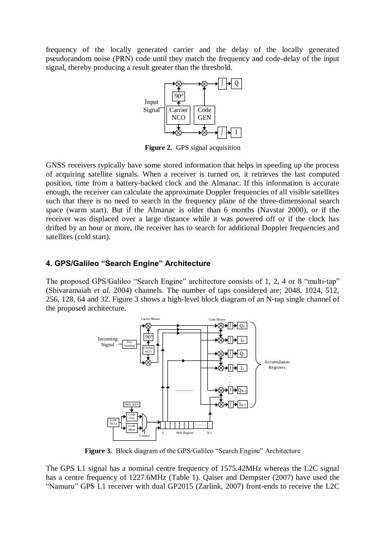
coded positional information in the signal. Figure 2 shows a high-level representation of a

typical acquisition stage in which the signal from the RF front-end is multiplied with a locally

generated carrier signal. The resultant carrier-free signal is then multiplied with a locally

generated pseudorandom noise (PRN) code with a certain delay. The result is then integrated

for a certain length of time depending on the type of signal and the signal-to-noise ratio.

Finally, the integrated result is compared with a threshold to determine whether the signal has

been found or not. If it is greater than the threshold, the frequency of the locally generated

carrier signal and the code-delay is handed over to the tracking loops for further processing.

On the other hand, if it is smaller than the threshold, this process is repeated by changing the

frequency of the locally generated carrier and the delay of the locally generated

pseudorandom noise (PRN) code until they match the frequency and code-delay of the input

signal, thereby producing a result greater than the threshold.

Figure 2. GPS signal acquisition

GNSS receivers typically have some stored information that helps in speeding up the process

of acquiring satellite signals. When a receiver is turned on, it retrieves the last computed

position, time from a battery-backed clock and the Almanac. If this information is accurate

enough, the receiver can calculate the approximate Doppler frequencies of all visible satellites

such that there is no need to search in the frequency plane of the three-dimensional search

space (warm start). But if the Almanac is older than 6 months (Navstar 2000), or if the

receiver was displaced over a large distance while it was powered off or if the clock has

drifted by an hour or more, the receiver has to search for additional Doppler frequencies and

satellites (cold start).

4. GPS/Galileo “Search Engine” Architecture

The proposed GPS/Galileo “Search Engine” architecture consists of 1, 2, 4 or 8 “multi-tap”

(Shivaramaiah et al. 2004) channels. The number of taps considered are; 2048, 1024, 512,

256, 128, 64 and 32. Figure 3 shows a high-level block diagram of an N-tap single channel of

the proposed architecture.

Figure 3. Block diagram of the GPS/Galileo “Search Engine” Architecture

The GPS L1 signal has a nominal centre frequency of 1575.42MHz whereas the L2C signal

has a centre frequency of 1227.6MHz (Table 1). Qaiser and Dempster (2007) have used the

“Namuru” GPS L1 receiver with dual GP2015 (Zarlink, 2007) front-ends to receive the L2C

Input

Signal

90°

Carrier

NCO

Q

Code

GEN

I

∫

∫

.............

..............

0 N-1 Shift Register Control

Incoming Signal

Carrier Mixers Code Mixers

90°

Carrier

NCO

.

.

∫ QN-1

∫ IN-1

∫

∫

∫

∫

I1

Q1

I0

Q0

Accumulation

Registers

Post

Sampling

Code Gen

Code

NCO

PRN_KEY

Code

Mem

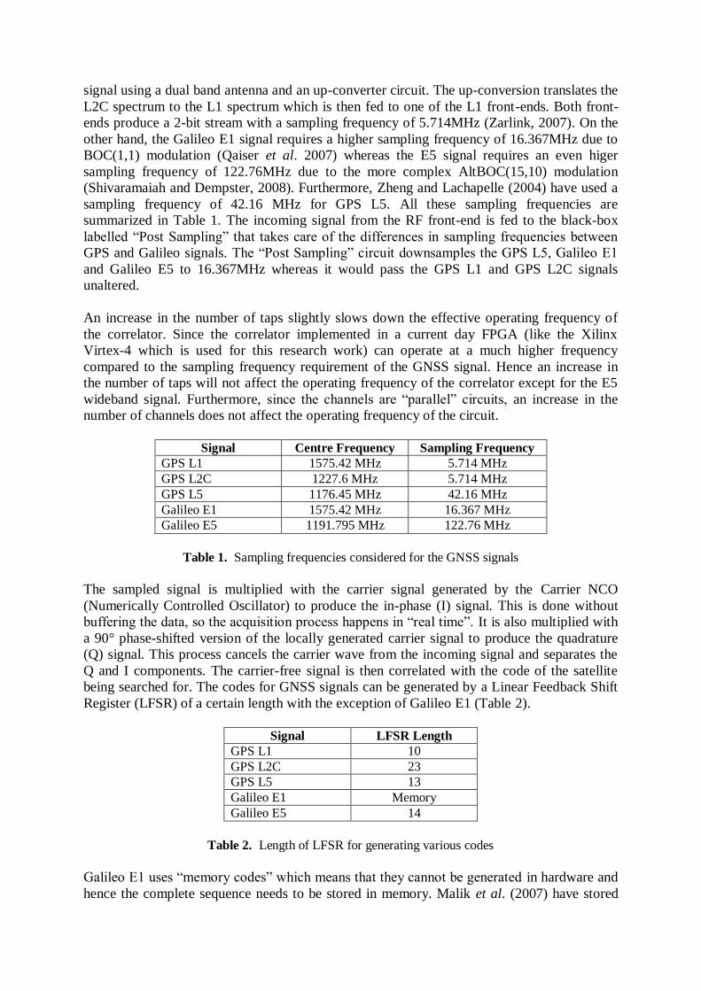
signal using a dual band antenna and an up-converter circuit. The up-conversion translates the

L2C spectrum to the L1 spectrum which is then fed to one of the L1 front-ends. Both front-

ends produce a 2-bit stream with a sampling frequency of 5.714MHz (Zarlink, 2007). On the

other hand, the Galileo E1 signal requires a higher sampling frequency of 16.367MHz due to

BOC(1,1) modulation (Qaiser et al. 2007) whereas the E5 signal requires an even higer

sampling frequency of 122.76MHz due to the more complex AltBOC(15,10) modulation

(Shivaramaiah and Dempster, 2008). Furthermore, Zheng and Lachapelle (2004) have used a

sampling frequency of 42.16 MHz for GPS L5. All these sampling frequencies are

summarized in Table 1. The incoming signal from the RF front-end is fed to the black-box

labelled “Post Sampling” that takes care of the differences in sampling frequencies between

GPS and Galileo signals. The “Post Sampling” circuit downsamples the GPS L5, Galileo E1

and Galileo E5 to 16.367MHz whereas it would pass the GPS L1 and GPS L2C signals

unaltered.

An increase in the number of taps slightly slows down the effective operating frequency of

the correlator. Since the correlator implemented in a current day FPGA (like the Xilinx

Virtex-4 which is used for this research work) can operate at a much higher frequency

compared to the sampling frequency requirement of the GNSS signal. Hence an increase in

the number of taps will not affect the operating frequency of the correlator except for the E5

wideband signal. Furthermore, since the channels are “parallel” circuits, an increase in the

number of channels does not affect the operating frequency of the circuit.

Signal Centre Frequency Sampling Frequency

GPS L1 1575.42 MHz 5.714 MHz

GPS L2C 1227.6 MHz 5.714 MHz

GPS L5 1176.45 MHz 42.16 MHz

Galileo E1 1575.42 MHz 16.367 MHz

Galileo E5 1191.795 MHz 122.76 MHz

Table 1. Sampling frequencies considered for the GNSS signals

The sampled signal is multiplied with the carrier signal generated by the Carrier NCO

(Numerically Controlled Oscillator) to produce the in-phase (I) signal. This is done without

buffering the data, so the acquisition process happens in “real time”. It is also multiplied with

a 90° phase-shifted version of the locally generated carrier signal to produce the quadrature

(Q) signal. This process cancels the carrier wave from the incoming signal and separates the

Q and I components. The carrier-free signal is then correlated with the code of the satellite

being searched for. The codes for GNSS signals can be generated by a Linear Feedback Shift

Register (LFSR) of a certain length with the exception of Galileo E1 (Table 2).

Signal LFSR Length

GPS L1 10

GPS L2C 23

GPS L5 13

Galileo E1 Memory

Galileo E5 14

Table 2. Length of LFSR for generating various codes

Galileo E1 uses “memory codes” which means that they cannot be generated in hardware and

hence the complete sequence needs to be stored in memory. Malik et al. (2007) have stored

GPS L1 codes in dedicated on-chip memory blocks (BlockRAMs) of a Xilinx Virtex-4

FPGA. The proposed search engine uses a similar approach by storing the Galileo E1 codes in

on-chip memory blocks of an FPGA, indicated as “Code Mem” in Figure 3. The remaining

codes are generated by a variable length LFSR indicated as “Code Gen” in Figure 3. There are

two reasons why the remaining codes are “generated” instead of being stored in memory like

Galileo E1;

1. The amount of dedicated memory resources in an FPGA is limited. When the amount

of memory resources required by a design exceeds the number of dedicated memory

resources, the FPGA design tools construct memory elements out of distributed logic

resources which are also limited. It would be more sensible to use these logic

resources for correlators to decrease the acquisition time.

2. Even if the memory resources in an FPGA can store all codes for GPS and Galileo

signals (the latest Virtex-6 FPGAs from Xilinx offer up to 38Mbits of dedicated

memory resources), the power consumption of a code generator would be less than

that of a code memory.

The PRN sequence of the “Code Gen” is controlled by the value stored in the PRN_KEY

register shown in Figure 3. This is the initial value that is loaded into the LFSR of the “Code

Gen”. The outputs of the “Code Mem” and “Code Gen” are fed into a variable length shift

register through a multiplexer. The “Control” signal of the multiplexer controls whether the

Galileo E1 code from the “Code Mem” or one of the generated codes is fed to the shift

register. The length of the shift registers corresponds to the number of code-taps and it

depends on the available resources in the FPGA. Furthermore, the Code NCO controls the

chipping rate of the code and the clock of the shift register. It can generate a clock of

1.023MHz for GPS L1, L2C and Galileo E1 codes or 10.23MHz for GPS L5 and Galileo E5

codes.

The correlation results are integrated for a length depending upon the type of input signal and

its signal-to-noise ratio. The GPS L1 code is 1ms long, so it would be integrated for a period

of 1ms. Similarly, GPS L2C is 20ms long and Galileo E1 is 4ms long, so these signals would

be integrated for 20ms and 4ms respectively. Furthermore, a longer integration interval

accumulates more signal power but consumes more time for search in both code and Doppler

dimensions. So, if the signal is weak (receiver indoors etc.) the accumulation period has to be

increased at the expense of longer acquisition times. For example, in the case of GPS L1, if

the signal is not found with 1ms integration, the receiver would repeat acquisition with an

integration interval of 2ms. For the work presented here it is assumed that the antenna has a

clear view of the sky, so the received signal has a high signal-to-noise ratio. Finally, the

integrated results are stored in the accumulation registers from which they are read and

compared with the predefined threshold.

The GPS L1 search engine architecture designed by Malik et al. (2009) is based on the

Namuru GPS receiver (Mumford et al. 2006). It requires approximately 450 slices for a

single-channel-single-tap correlator and every additional tap requires 50 more slices on a

Xilinx Virtex-4 FPGA. So, the amount of logic resources utilized by a search engine with “X”

channels each with “Y” taps can be approximate by the formula;

Logic resources ≈ X * 450 + 50 * (Y-1)) (1)

The design proposed here is an extension of the search engine proposed by Malik et al.

(2009); however there are a number of differences between the two designs.

1. The design proposed here uses an additional memory resource for storing the Galileo

E1 codes. We assume that these codes are stored in the dedicated memory resources

and hence do not increase the number of slices.

2. The search engine designed by Malik et al. (2009) uses a 10-bit code generator to

generate GPS L1 codes. On the other hand, the design proposed here uses a 23-bit

code generator which is capable of generating all signals listed in Table 2. So, the shift

registers inside the code generator have 13 more bits, which does not significantly

increase the number of slices.

3. To generate a clock of 10.23MHz for the GPS L5 and Galileo E5 codes, an additional

2 bits would be required in the Code NCO, which does not significantly increase the

number of slices.

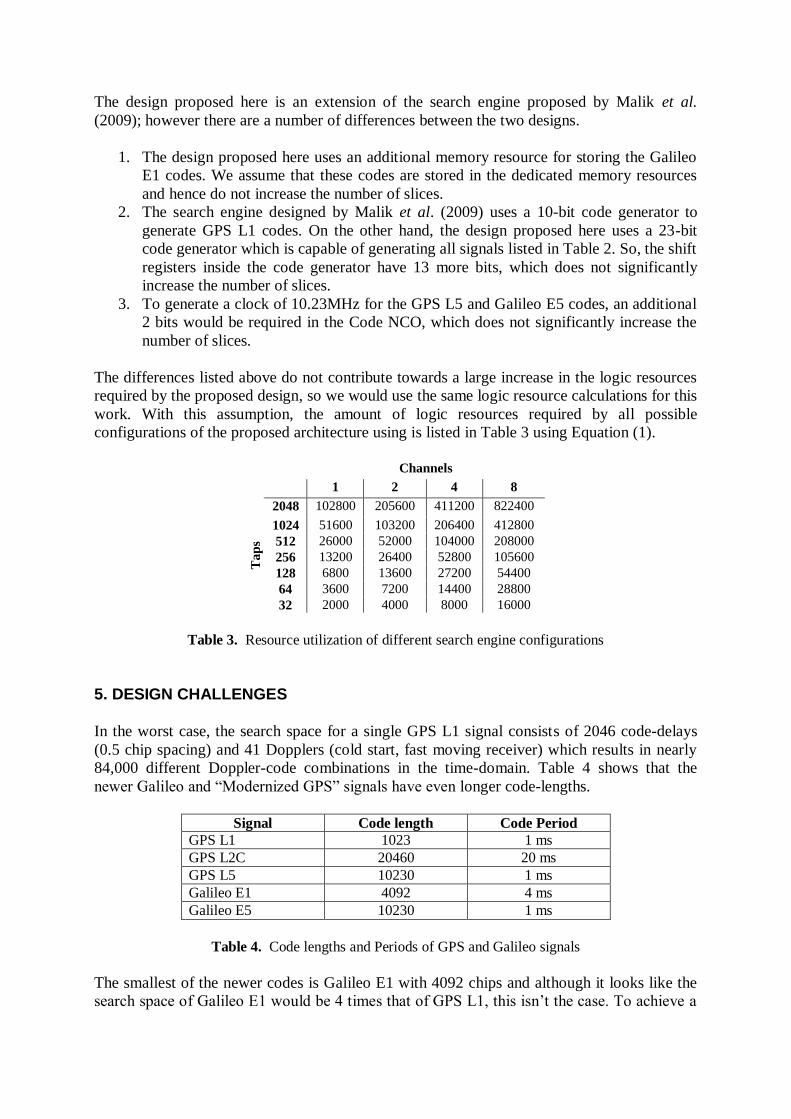
The differences listed above do not contribute towards a large increase in the logic resources

required by the proposed design, so we would use the same logic resource calculations for this

work. With this assumption, the amount of logic resources required by all possible

configurations of the proposed architecture using is listed in Table 3 using Equation (1).

Channels

1 2 4 8

Ta

ps

2048 102800 205600 411200 822400

1024 51600 103200 206400 412800

512 26000 52000 104000 208000

256 13200 26400 52800 105600

128 6800 13600 27200 54400

64 3600 7200 14400 28800

32 2000 4000 8000 16000

Table 3. Resource utilization of different search engine configurations

5. DESIGN CHALLENGES

In the worst case, the search space for a single GPS L1 signal consists of 2046 code-delays

(0.5 chip spacing) and 41 Dopplers (cold start, fast moving receiver) which results in nearly

84,000 different Doppler-code combinations in the time-domain. Table 4 shows that the

newer Galileo and “Modernized GPS” signals have even longer code-lengths.

Signal Code length Code Period

GPS L1 1023 1 ms

GPS L2C 20460 20 ms

GPS L5 10230 1 ms

Galileo E1 4092 4 ms

Galileo E5 10230 1 ms

Table 4. Code lengths and Periods of GPS and Galileo signals

The smallest of the newer codes is Galileo E1 with 4092 chips and although it looks like the

search space of Galileo E1 would be 4 times that of GPS L1, this isn’t the case. To achieve a

similar “average correlation loss” as that of GPS L1 (BPSK, 0.5 chip spacing), a chip spacing

of 0.16 must be used due to the BOC(1,1) modulation used in Galileo E1 (Wilde et al. 2006).

This is because of the narrower central peak and lower side peaks of the E1 autocorrelation

function. So, up to 4092*6 = 24552 code-delays needs to be searched, which results in a

search space of over a million Doppler-code combinations (cold start, fast moving receiver)

for one Galileo E1 satellite.

Therefore, a Galileo E1 search engine with 41 channels, each with 24552 taps could search a

signal in a million Doppler-code combinations within 4ms. But according to Equation (1),

such an architecture would require over 50 million Xilinx Virtex-4 slices. Furthermore, the

Galileo E5 signal requires a code search with an even finer granularity; 0.083 chips, which

results in a much larger search engine in terms of logic resource utilization. With the current

state of FPGA technology, this is not possible in single-chip designs, with the largest Virtex-4

FPGA being just over 50,000 slices.

A more realistic solution exists in implementing a search engine architecture that can easily fit

within the available resources in an FPGA. The two most important parameters of the

proposed design are; (a) the number of channels and (b) the number of taps in each channel.

So, the challenge addressed here is to find the optimum number of channels and taps in each

channel that efficiently utilizes the resources in an FPGA. More importantly, this work aims

to quantify what it means to implement a GPS L2C or a Galileo E1 search engine inside an

FPGA by discussing the trade-offs involved in using one architecture over the other.

6. METHODOLOGY

The methodology employed to find the best GPS/Galileo search engine architecture consists

of testing the design proposed in Section 4 to evaluate its performance. We assume a warm

start and that the receiver has an accurate on-board clock and a valid Almanac. Furthermore,

we assume that the receiver is powered on in a similar position to where it was powered off.

So, the estimated Doppler frequency is accurate enough not to require a search in the

frequency space and the receiver only needs to search in the code and PRN spaces. This can

be done in two ways;

1. del_sat – First exhaust code-delays and then satellite PRNs.

2. sat_del – First exhaust satellite PRNs and then code-delays.

For this work we compared the performance of GPS L1, GPS L2C and Galileo E1 signals.

We calculated the average number of accumulation periods required to find the first four

highest elevation satellites by all possible configurations of the proposed architecture. It is

assumed that once a code aligns with the locally generated code, the receiver will not loose

the signal. In other words, the effect of low SNR is not considered here and the probability of

detection, Pd is 1 and the probability of false-alarm Pfa is “zero”. For the sake of comparison,

the number of accumulation periods was calculated using an integration interval of 1ms for all

three signals considered. So, multiplying the average number of accumulation periods with

the code period (Table 4) would give the mean acquisition time for the particular signal

(Equation 2).

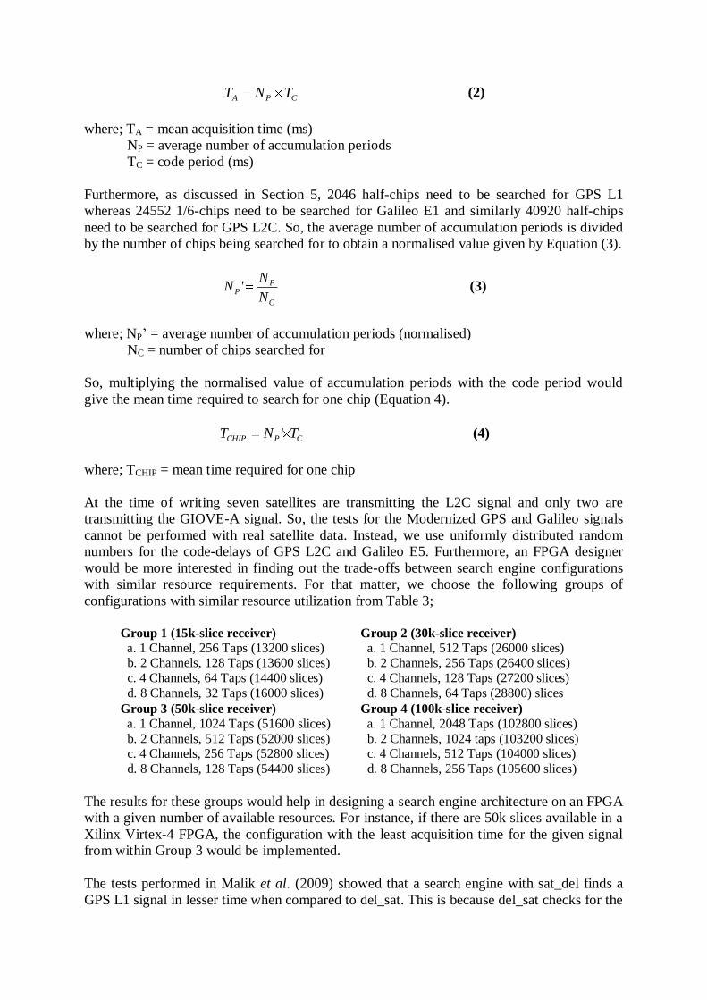
CPA TNT (2)

where; TA = mean acquisition time (ms)

NP = average number of accumulation periods

TC = code period (ms)

Furthermore, as discussed in Section 5, 2046 half-chips need to be searched for GPS L1

whereas 24552 1/6-chips need to be searched for Galileo E1 and similarly 40920 half-chips

need to be searched for GPS L2C. So, the average number of accumulation periods is divided

by the number of chips being searched for to obtain a normalised value given by Equation (3).

C

PP

N

NN ' (3)

where; NP’ = average number of accumulation periods (normalised)

NC = number of chips searched for

So, multiplying the normalised value of accumulation periods with the code period would

give the mean time required to search for one chip (Equation 4).

CPCHIP TNT ' (4)

where; TCHIP = mean time required for one chip

At the time of writing seven satellites are transmitting the L2C signal and only two are

transmitting the GIOVE-A signal. So, the tests for the Modernized GPS and Galileo signals

cannot be performed with real satellite data. Instead, we use uniformly distributed random

numbers for the code-delays of GPS L2C and Galileo E5. Furthermore, an FPGA designer

would be more interested in finding out the trade-offs between search engine configurations

with similar resource requirements. For that matter, we choose the following groups of

configurations with similar resource utilization from Table 3;

Group 1 (15k-slice receiver)

a. 1 Channel, 256 Taps (13200 slices) b. 2 Channels, 128 Taps (13600 slices)

c. 4 Channels, 64 Taps (14400 slices)

d. 8 Channels, 32 Taps (16000 slices)


a. 1 Channel, 512 Taps (26000 slices) b. 2 Channels, 256 Taps (26400 slices)

c. 4 Channels, 128 Taps (27200 slices)

d. 8 Channels, 64 Taps (28800) slices


a. 1 Channel, 1024 Taps (51600 slices)

b. 2 Channels, 512 Taps (52000 slices) c. 4 Channels, 256 Taps (52800 slices)



a. 1 Channel, 2048 Taps (102800 slices)

b. 2 Channels, 1024 taps (103200 slices) c. 4 Channels, 512 Taps (104000 slices)


The results for these groups would help in designing a search engine architecture on an FPGA

with a given number of available resources. For instance, if there are 50k slices available in a

Xilinx Virtex-4 FPGA, the configuration with the least acquisition time for the given signal

from within Group 3 would be implemented.

The tests performed in Malik et al. (2009) showed that a search engine with sat_del finds a

GPS L1 signal in lesser time when compared to del_sat. This is because del_sat checks for the

presence of a signal in all code-delays before moving on to the next signal in the list whereas

sat_del searches for more than one signal at a time. As the number of code-delays to search

for is always greater than the number of satellites in the case of a warm start, del_sat produces

more “wasted” searches because it searches for one signal at a time. We predict that this trend

would be the same for GPS L2C and Galileo E1.

7. RESULTS

The proposed GPS/Galileo search engine architecture was tested under the conditions

mentioned in Section 6. The average number of accumulation periods required for acquiring

the four highest elevation satellites in real time was calculated by a test-bench written in

MATLAB. This value was normalized according to the number of chips searched for and then

scaled by 10,000 to show on a graph. Figure 4 and Figure 5 shows a comparison of NP’ for

Galileo E1 and GPS L2C respectively.

Figure 4. Comparison of NP’ for Galileo E1

with del_sat and sat_del

Figure 5. Comparison of NP’ for GPS L2C

with del_sat and sat_del

The above figures show that, as in Malik et al. (2009), an increase in the number of channels

and/or taps decreases the acquisition time. Now we examine the performance of the proposed

search engine architecture with Galileo E1 and GPS L2C signals at a particular level of

resource allocation. Figures 6-9 (Galileo E1) and Figures 10-13 (GPS L2C) show a similar

comparison for Groups 1, 2, 3 and 4 respectively.

Figure 6. Comparison of NP’ for Galileo E1 with Group 1

Figure 7. Comparison of NP’ for Galileo E1 with Group 2


with Group 3


with Group 4

Figure 10. Comparison of NP’ for GPS L2C with Group 1

Figure 11. Comparison of NP’ for GPS L2C

with Group 2



Each of the points in the graphs represent a configuration in a particular group. These results

show that, as predicted earlier, sat_del is the best search strategy for Galileo E1 and GPS L2C.

This is due to the fact that, as the number of code-delays is larger than the number of satellites

to search for, del_sat produces more wasted searches.

Some interesting results are achieved if NP’ for GPS L1, Galileo E1 and GPS L2C is

compared simultaneously for one search strategy at a time. Figures 14 and Figure 15 shows a

comparison of NP’ for Galileo E1 and GPS L2C with del_sat and sat_del respectively.

Figure 14. Comparison of NP’ for del_sat

Figure 15. Comparison of NP’ for sat_del

A quick look at Figure 14 and 15 suggests that for smaller architectures the performance of

GPS L1 is better than Galileo E1 and GPS L2C. But for larger architectures the performance

of the longer codes is better than GPS L1. It is important to mention here that NP’ is a

normalized quantity, so in reality the values of NP’ shown here are 1/4th

for Galileo E1 and

1/20th

for GPS L2C. We now take a closer look at each level of resource allocation. Figures

16-19 show a comparison of NP’ for Groups 1, 2, 3 and 4 respectively using del_sat.

Figure 16. Comparison of NP’ for Group 1

with del_sat


with del_sat

Figure 18. Comparison of NP’ for Group 3 with del_sat

Figure 19. Comparison of NP’ for Group 4 with del_sat

These results confirm that, for smaller designs (Group 1 and 2) the GPS L1 signal has the

smallest NP’, but as the size of the architecture increases, the longer codes are acquired

relatively more quickly than GPS L1. The curves in Figures 16-19 are flat; this corresponds to

the curves for del_sat obtained by Malik et al. (2009). This is a graphical representation of the

fact that exhausting code-delays before satellites produces wasted searches. No matter how

many channels and/or taps are available in the search engine, the signal would be found in the

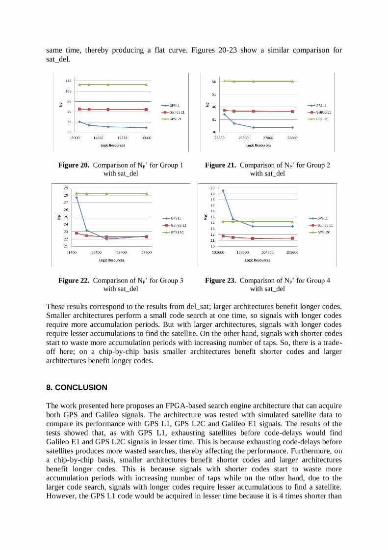
same time, thereby producing a flat curve. Figures 20-23 show a similar comparison for

sat_del.


with sat_del


with sat_del


with sat_del


with sat_del

These results correspond to the results from del_sat; larger architectures benefit longer codes.

Smaller architectures perform a small code search at one time, so signals with longer codes

require more accumulation periods. But with larger architectures, signals with longer codes

require lesser accumulations to find the satellite. On the other hand, signals with shorter codes

start to waste more accumulation periods with increasing number of taps. So, there is a trade-

off here; on a chip-by-chip basis smaller architectures benefit shorter codes and larger

architectures benefit longer codes.

8. CONCLUSION

The work presented here proposes an FPGA-based search engine architecture that can acquire

both GPS and Galileo signals. The architecture was tested with simulated satellite data to

compare its performance with GPS L1, GPS L2C and Galileo E1 signals. The results of the

tests showed that, as with GPS L1, exhausting satellites before code-delays would find

Galileo E1 and GPS L2C signals in lesser time. This is because exhausting code-delays before

satellites produces more wasted searches, thereby affecting the performance. Furthermore, on

a chip-by-chip basis, smaller architectures benefit shorter codes and larger architectures

benefit longer codes. This is because signals with shorter codes start to waste more

accumulation periods with increasing number of taps while on the other hand, due to the

larger code search, signals with longer codes require lesser accumulations to find a satellite.

However, the GPS L1 code would be acquired in lesser time because it is 4 times shorter than

the Galileo E1 code and 20 times shorter than the GPS L2C code.

Future work involves testing the architecture in a scenario where a warm start is required with

a large Doppler search and a scenario where a cold start is required. Also, the effect of low

signal-to-noise ratio could be taken into account, which would require longer integration

intervals and hence longer acquisition times. Furthermore, the use of multi-chip FPGA

designs could be studied for implementing even larger search engine architectures that could

possibly perform millions of searches for the newer GPS L5 and Galileo E5 codes.

REFERENCES

Borre K, Akos DM, Bertelsen N, Rinder P, Jensen SH (2007) A Software-Defined GPS and Galileo Receiver, Birkhäuser Boston,

Dempster AG (2006) Correlators for L2C: Some Considerations, Inside GNSS, October 2006, 32-37

Dempster AG, Hewitson S (2007) The “System of Systems” Receiver: an Australian Opportunity?,

International Global Navigation Satellite Systems Society (IGNSS) Symposium, 4-6 December

2007, The University of New South Wales, Sydney, Australia

Malik SA, Shivaramaiah NC, Dempster AG (2009) Search Engine Trade-offs in FPGA-based GNSS

Receiver Designs, European Navigation Conference ENC-GNSS 2009, CD-ROM proceedings,

3-6 May 2009, Naples, Italy

Malik U, Diessel O, Dempster AG (2007) Fast Code-Phase Alignment of GPS Signals Using Virtex-4

FPGAs, International Global Navigation Satellite Systems Society (IGNSS) Symposium, 4-6

December 2007, The University of New South Wales, Sydney, Australia

Mumford PJ, Parkinson K, Dempster AG (2006) An Open GNSS Receiver Research Platform,

International Global Navigation Satellite Systems Society (IGNSS) Symposium, 17-21 July

2006, Surfers Paradise, Australia

Navstar (2000) GPS Space Segment/Navigation User Interfaces, ICD200C-004, GPS Joint Program

Office, 12 April 2000

Qaiser S, Dempster AG (2007) Receiving the L2C Signal with “Namuru” GPS L1 Receiver,

International Global Navigation Satellite Systems Society (IGNSS) Symposium, 4-6 December

2007, The University of New South Wales, Sydney, Australia

Qaiser S, Wu J, Dempster AG (2007) Loud and Clear: Receiving the new GPS L2C and Galileo

Signals, UNSW Engineers, Issue 15, June 2007, p. 19

Shivaramaiah NC, Dempseter AG (2008) Galileo E5 Signal Acquisition Strategies, Coordinates, August 2008, pp. 12-16

Shivaramaiah NC, HS Jamadagn, Muralikrishna S, Vimala C (2004) Software-Aided Sequential Multi-Tap Correlator for Fast Acquisition, 17th International Technical Meeting of the Satellite

Division of the Institute of Navigation ION GNSS, 21-24 September 2004, Long Beach,

California

Wilde WD, Sleewaegen JM, Simsky A, Vandewiele C, Peeters E, Grauwen J, Boon F (2006) New

Fast Signal Acquisition Unit for GPS/Galileo Receivers, European Navigation Conference

ENC-GNSS 2006, 7-10 May 2006, Manchester

van Diggelen F, Abraham C (2001) Indoor GPS Technology, CTIA Wireless-Agenda, Dallas

Zarlink (2007) GPS Receiver RF Front End, http://www.zarlink.com/zarlink/gp2015-datasheet-sept2007.pdf

Zheng B, Lachapelle G (2004) Acquisition Schemes for a GPS L5 Software Receiver, 17th

International Technical Meeting of the Satellite Division of the Institute of Navigation ION

GNSS, 21-24 September 2004, Long Beach, California

http://www.zarlink.com/zarlink/gp2015-datasheet-sept2007.pdf

FPGA-based GNSS "Search Engine" using Parallel Techniques in the Time-Domain

Documents

Transcript of FPGA-based GNSS "Search Engine" using Parallel Techniques in the Time-Domain