Four essays in unemployment, wage dynamics and subjective ...

Four essays in unemployment, wage dynamics and

subjective expectations

by

Peter Hudomiet

A dissertation submitted in partial fulfillmentof the requirements for the degree of

Doctor of Philosophy(Economics)

in the University of Michigan2015

Doctoral Committee:

Professor Robert J. Willis, ChairProfessor John BoundProfessor Matthew D. ShapiroProfessor Jeffrey M. SmithProfessor Yu Xie

ACKNOWLEDGMENT

Over the past seven years I have received support and encouragement from a great number

of individuals. Robert J. Willis and Gabor Kezdi have been mentors, colleagues, and friends.

Our marathon discussions have been tremendously fruitful to identify intriguing research

questions and bridge theory and practice. I am grateful to the rest of my committee mem-

bers, Matthew Shapiro, John Bound, Jeffrey Smith and Yu Xie for all of the time and effort

through this process. Their impact as motivators and resources has been immeasurable. I

am indebted to Hedvig Horvath, Cynthia Doniger, Pawel Krolikowski, Lasse Brune, Breno

Braga, Reid Dorsey-Palmateer and many other friends in Michigan and in Hungary for the

stimulating discussions, for the feedback, and for being sources of amusement. I am also

grateful for financial support from the ISR-George Katona Research Award Fund in Eco-

nomic Behavior and the Rackham International Student Fellowship. Lastly, I am exceedingly

thankful to my parents for supporting me unequivocally and unconditionally in every aspect

of my life, and to my brother and sister and their families (especially my baby niece, Anna)

for always being there for me when I needed them. Koszi!

ii

TABLE OF CONTENTS

ACKNOWLEDGMENT . . . . . . . . . . . . . . . . . . . . . . . . . . . . . . . . . . . . . . ii

LIST OF FIGURES . . . . . . . . . . . . . . . . . . . . . . . . . . . . . . . . . . . . . . . . . vii

LIST OF TABLES . . . . . . . . . . . . . . . . . . . . . . . . . . . . . . . . . . . . . . . . . . ix

ABSTRACT . . . . . . . . . . . . . . . . . . . . . . . . . . . . . . . . . . . . . . . . . . . . . xviii

Chapter I. The Role of Occupation-specific Adaptation Costs in Explaining the Edu-

cational Gap in Unemployment . . . . . . . . . . . . . . . . . . . . . . . . . . . . . . . . 1

1.1 Introduction . . . . . . . . . . . . . . . . . . . . . . . . . . . . . . . . . . . . . . . . . 1

1.2 Data and descriptive analysis . . . . . . . . . . . . . . . . . . . . . . . . . . . . . . . 7

1.2.1 The Current Population Survey . . . . . . . . . . . . . . . . . . . . . . . . . 7

1.2.2 Basic patterns in unemployment and turnover by education . . . . . . . . 9

1.2.3 Basic patterns in unemployment and turnover by education and occupation 12

1.2.4 Adaptation costs by occupations . . . . . . . . . . . . . . . . . . . . . . . . . 14

1.3 The model . . . . . . . . . . . . . . . . . . . . . . . . . . . . . . . . . . . . . . . . . . 18

1.3.1 The setup of the model . . . . . . . . . . . . . . . . . . . . . . . . . . . . . . . 20

1.3.2 The solution . . . . . . . . . . . . . . . . . . . . . . . . . . . . . . . . . . . . . 24

1.3.3 Calibration of the model . . . . . . . . . . . . . . . . . . . . . . . . . . . . . . 27

1.3.4 Turnover elasticities with respect to adaptation costs . . . . . . . . . . . . 32

iii

1.4 Calibration of the explained educational gap in unemployment . . . . . . . . . . 37

1.4.1 Autocorrelation in match-specific productivity . . . . . . . . . . . . . . . . 40

1.5 Discussion and conclusion . . . . . . . . . . . . . . . . . . . . . . . . . . . . . . . . . 43

1.5.1 Economic mechanisms with large effects on hiring . . . . . . . . . . . . . . 44

1.5.2 Economic mechanisms with small effects on hiring . . . . . . . . . . . . . . 46

Tables and figures . . . . . . . . . . . . . . . . . . . . . . . . . . . . . . . . . . . . . . . . 48

Appendices . . . . . . . . . . . . . . . . . . . . . . . . . . . . . . . . . . . . . . . . . . . . 62

Chapter II. Career Interruptions and Measurement Error in Annual Earnings . . . . . 83

2.1 Introduction . . . . . . . . . . . . . . . . . . . . . . . . . . . . . . . . . . . . . . . . . 83

2.2 Earnings and measurement error models . . . . . . . . . . . . . . . . . . . . . . . . 89

2.2.1 A simple model with labor histories . . . . . . . . . . . . . . . . . . . . . . . 89

2.2.2 Alternative models to explain mean reversion . . . . . . . . . . . . . . . . 93

2.3 Data and descriptive results . . . . . . . . . . . . . . . . . . . . . . . . . . . . . . . 97

2.3.1 The Health and Retirement Study (HRS) . . . . . . . . . . . . . . . . . . . 97

2.3.2 Earnings in the administrative data . . . . . . . . . . . . . . . . . . . . . . . 98

2.3.3 Linking the HRS and administrative data . . . . . . . . . . . . . . . . . . . 100

2.3.4 Labor histories . . . . . . . . . . . . . . . . . . . . . . . . . . . . . . . . . . . . 101

2.3.5 Descriptive properties of measurement error . . . . . . . . . . . . . . . . . . 103

2.4 Structural estimation . . . . . . . . . . . . . . . . . . . . . . . . . . . . . . . . . . . . 109

2.4.1 The earnings and measurement error model . . . . . . . . . . . . . . . . . . 109

2.4.2 Estimation methodology . . . . . . . . . . . . . . . . . . . . . . . . . . . . . . 112

2.4.3 Results . . . . . . . . . . . . . . . . . . . . . . . . . . . . . . . . . . . . . . . . . 115

2.5 Discussion of bias correction . . . . . . . . . . . . . . . . . . . . . . . . . . . . . . . 118

2.6 Conclusion . . . . . . . . . . . . . . . . . . . . . . . . . . . . . . . . . . . . . . . . . . 122

iv


Appendices . . . . . . . . . . . . . . . . . . . . . . . . . . . . . . . . . . . . . . . . . . . . 139

Chapter III. Estimating Second Order Probability Beliefs from Subjective Survival Data174

3.1 Introduction . . . . . . . . . . . . . . . . . . . . . . . . . . . . . . . . . . . . . . . . . 174

3.2 Ambiguity in economics . . . . . . . . . . . . . . . . . . . . . . . . . . . . . . . . . . 179

3.3 Subjective survival probability questions on the HRS . . . . . . . . . . . . . . . 181

3.4 Probability beliefs and the Modal Response Hypothesis . . . . . . . . . . . . . . 184

3.5 Individual subjective survival curves . . . . . . . . . . . . . . . . . . . . . . . . . . 189

3.6 Estimation and identification . . . . . . . . . . . . . . . . . . . . . . . . . . . . . . 192

3.7 Empirical analysis . . . . . . . . . . . . . . . . . . . . . . . . . . . . . . . . . . . . . 193

3.7.1 Sample and measures employed . . . . . . . . . . . . . . . . . . . . . . . . . . 194

3.7.2 Maximum likelihood model estimates . . . . . . . . . . . . . . . . . . . . . . 196

3.8 Conclusion . . . . . . . . . . . . . . . . . . . . . . . . . . . . . . . . . . . . . . . . . . 203


Appendices . . . . . . . . . . . . . . . . . . . . . . . . . . . . . . . . . . . . . . . . . . . . 213

Chapter IV. Stock Market Crash and Expectations of American Households . . . . . . 236

4.1 Introduction . . . . . . . . . . . . . . . . . . . . . . . . . . . . . . . . . . . . . . . . . 236

4.2 Data . . . . . . . . . . . . . . . . . . . . . . . . . . . . . . . . . . . . . . . . . . . . . . 242

4.3 Descriptive analysis . . . . . . . . . . . . . . . . . . . . . . . . . . . . . . . . . . . . . 247

4.4 Structural estimation . . . . . . . . . . . . . . . . . . . . . . . . . . . . . . . . . . . . 252

4.5 Results of the structural model . . . . . . . . . . . . . . . . . . . . . . . . . . . . . 256

4.6 Conclusions and directions for future research . . . . . . . . . . . . . . . . . . . . 265


Appendices . . . . . . . . . . . . . . . . . . . . . . . . . . . . . . . . . . . . . . . . . . . . 273

v

Bibliography . . . . . . . . . . . . . . . . . . . . . . . . . . . . . . . . . . . . . . . . . . . . . . 283

vi

LIST OF FIGURES

1.1 Unemployment rates and basic turnover probabilities by education . . . . . . . 57

1.2 Occupational unemployment and its approximation with turnover rates . . . . 58

1.3 The effect of adaptation costs on unemployment rates and turnover probabili-

ties, baseline specification . . . . . . . . . . . . . . . . . . . . . . . . . . . . . . . . . 59

1.4 Observed and predicted unemployment rates and monthly transition probabil-

ities by education, baseline specification . . . . . . . . . . . . . . . . . . . . . . . . 60

1.5 Observed and predicted unemployment rates by education, alternative values

of autocorrelation . . . . . . . . . . . . . . . . . . . . . . . . . . . . . . . . . . . . . . 61

1.6 The effect of adaptation costs on unemployment rates for various values of

monthly autocorrelation in match-specific productivity . . . . . . . . . . . . . . . 61

2.1 Histogram of measurement error in annual earnings . . . . . . . . . . . . . . . . . 123

2.2 Nonparametric relationship between measurement error and earnings . . . . . . 124

2.3 Histogram of earnings growth after major job loss . . . . . . . . . . . . . . . . . . 125

2.4 Histogram and time series plots of selected coefficients in the baseline specifi-

cation of the structural model . . . . . . . . . . . . . . . . . . . . . . . . . . . . . . 126

2.5 Fraction of reported earnings loss after job loss or job finding . . . . . . . . . . . 127

2.6 Distribution of measurement error in simulated data based on the model . . . . 127

vii

3.1 Distribution of Survival Probabilities to Target Age, by Age of Respondent,

HRS-2002 . . . . . . . . . . . . . . . . . . . . . . . . . . . . . . . . . . . . . . . . . . . 205

3.2 Density of probability beliefs (gi(p)) for different mean (µi) and precision (ni)

values . . . . . . . . . . . . . . . . . . . . . . . . . . . . . . . . . . . . . . . . . . . . . 206

3.3 Average actual and expected survival probabilities and dispersion in beliefs . . 206

3.4 Simulated survey responses based on the mean and the mode models with all

covariates and the empirical distribution of survey responses . . . . . . . . . . . 207

3.5 Estimated distribution of probability beliefs gi(p) of surviving from age 50 to

age 80 . . . . . . . . . . . . . . . . . . . . . . . . . . . . . . . . . . . . . . . . . . . . . 207

4.1 Level and volatility of the DJIA, volume of trade and Google search for ”Dow’ 267

4.2 Histogram of the P0 answers in the total sample and in the final sample . . . . 267

4.3 Standard normal c.d.f. with P0 and P20 shown . . . . . . . . . . . . . . . . . . . . 268

4.4 Cross-sectional distribution of expected returns among stockholders and non-

stockholders . . . . . . . . . . . . . . . . . . . . . . . . . . . . . . . . . . . . . . . . . 268

4.5 Cross-sectional distribution of expected returns among informed and unin-

formed individuals . . . . . . . . . . . . . . . . . . . . . . . . . . . . . . . . . . . . . 269

4.6 Cross-sectional distribution of expected returns by cognition . . . . . . . . . . . 269

viii

LIST OF TABLES

1.1 Logit regressions of unemployment . . . . . . . . . . . . . . . . . . . . . . . . . . . 48

1.2 OLS regressions of unemployment in booms . . . . . . . . . . . . . . . . . . . . . 49

1.3 Logit regressions of monthly transition probabilities . . . . . . . . . . . . . . . . 50

1.4 Length of adaptation periods, MCSUI . . . . . . . . . . . . . . . . . . . . . . . . 51

1.5 OLS regression of log adaptation period by education and occupational work

activities, MCSUI . . . . . . . . . . . . . . . . . . . . . . . . . . . . . . . . . . . . . 51

1.6 Predictive power of occupation work activities on log adaptation costs, MCSUI

and O*NET . . . . . . . . . . . . . . . . . . . . . . . . . . . . . . . . . . . . . . . . 52

1.7 Logit regressions of unemployment and turnover on imputed adaptation costs 53

1.8 Average monthly transition probabilities . . . . . . . . . . . . . . . . . . . . . . . 54

1.9 Calibrated parameters of the model and other implied values . . . . . . . . . . 54

1.10 Elasticities of turnover rates with respect to the length of the adaptation

period, baseline calibration . . . . . . . . . . . . . . . . . . . . . . . . . . . . . . . 54


period, sensitivity analysis . . . . . . . . . . . . . . . . . . . . . . . . . . . . . . . . 55


period, sensitivity analysis . . . . . . . . . . . . . . . . . . . . . . . . . . . . . . . . 55

ix

1.13 Adaptation cost values needed to fit unemployment rates by education groups,

baseline calibration . . . . . . . . . . . . . . . . . . . . . . . . . . . . . . . . . . . . 56

1.14 Adaptation cost values needed to fit unemployment rates by education groups,

calibration with lower autocorrelation . . . . . . . . . . . . . . . . . . . . . . . . . 56

1.15 Standard deviation of productivity shock needed to fit unemployment rates

by education groups, baseline calibration . . . . . . . . . . . . . . . . . . . . . . . 56

1.16 Standard deviation of productivity shock needed to fit unemployment rates

by education groups, calibration with lower autocorrelation . . . . . . . . . . . 56

1.17 OLS regressions of unemployment in recessions . . . . . . . . . . . . . . . . . . . 72

1.18 Logit regressions of monthly employment to unemployment transition proba-

bility . . . . . . . . . . . . . . . . . . . . . . . . . . . . . . . . . . . . . . . . . . . . . 73

1.19 OLS regressions of monthly employment to unemployment transition proba-

bility in booms . . . . . . . . . . . . . . . . . . . . . . . . . . . . . . . . . . . . . . . 74

1.20 OLS regressions of monthly employment to unemployment transition proba-

bility in recessions . . . . . . . . . . . . . . . . . . . . . . . . . . . . . . . . . . . . . 75

1.21 Logit regressions of monthly unemployment to employment transition proba-

bility . . . . . . . . . . . . . . . . . . . . . . . . . . . . . . . . . . . . . . . . . . . . . 76

1.22 OLS regressions of monthly unemployment to employment transition proba-

bility in booms . . . . . . . . . . . . . . . . . . . . . . . . . . . . . . . . . . . . . . . 77

1.23 OLS regressions of monthly unemployment to employment transition proba-

bility in recessions . . . . . . . . . . . . . . . . . . . . . . . . . . . . . . . . . . . . . 78

1.24 Observed and predicted unemployment rates and turnover probabilities by

education, baseline specification . . . . . . . . . . . . . . . . . . . . . . . . . . . . 79

1.25 Imputed adaptation period by detailed occupations, in months . . . . . . . . . 80

x


education, specification with lower autocorrelation . . . . . . . . . . . . . . . . . 81


education, specification with higher autocorrelation . . . . . . . . . . . . . . . . 82

2.1 Type of wage and salary reports . . . . . . . . . . . . . . . . . . . . . . . . . . . . 128

2.2 Components of annual earnings, HRS 1991-2011, 50-60-year-old employees . . 128

2.3 Fraction of successful matches between the HRS and SSA . . . . . . . . . . . . 128

2.4 OLS of successful matches between the HRS and SSA . . . . . . . . . . . . . . . 129

2.5 HRS earnings reports and W2 earnings records . . . . . . . . . . . . . . . . . . . 130

2.6 Reliability ratios and other moments of earnings and error . . . . . . . . . . . . 130

2.7 Detailed labor histories created from the SSA data . . . . . . . . . . . . . . . . 131

2.8 Detailed labor histories and distribution of earnings . . . . . . . . . . . . . . . . 131



2.11 Measurement error by labor histories and earnings . . . . . . . . . . . . . . . . . 133

2.12 Measurement error by earnings in stable years . . . . . . . . . . . . . . . . . . . 133

2.13 GMM estimates of basic moments of earnings and error . . . . . . . . . . . . . 133

2.14 MCMC estimates in the baseline specification, covariates in earnings . . . . . 134

2.15 MCMC estimates in the baseline specification, covariates in the innovation

term of permanent earnings . . . . . . . . . . . . . . . . . . . . . . . . . . . . . . . 135

2.16 MCMC estimates in the baseline specification, other parameters in earnings . 136

2.17 MCMC estimates in the baseline specification, covariates in measurement error137

2.18 MCMC estimates in the baseline specification, other parameters in measure-

ment error . . . . . . . . . . . . . . . . . . . . . . . . . . . . . . . . . . . . . . . . . . 138

xi



2.21 GMM estimates of basic moments of earnings and error by age . . . . . . . . . 150

2.22 GMM estimates of basic moments of earnings and error by gender and education150

2.23 GMM estimates of basic moments of earnings and error by gender and edu-

cation in stable years . . . . . . . . . . . . . . . . . . . . . . . . . . . . . . . . . . . 151

2.24 MCMC estimates by education, covariates in earnings . . . . . . . . . . . . . . . 151

2.25 MCMC estimates by education, covariates in the innovation term of perma-

nent earnings . . . . . . . . . . . . . . . . . . . . . . . . . . . . . . . . . . . . . . . . 152

2.26 MCMC estimates by education, other parameters in earnings . . . . . . . . . . 153

2.27 MCMC estimates by education, covariates in measurement error . . . . . . . . 153


ment error . . . . . . . . . . . . . . . . . . . . . . . . . . . . . . . . . . . . . . . . . . 154

2.29 MCMC estimates by education, covariates in earnings . . . . . . . . . . . . . . . 155

2.30 MCMC estimates by education, covariates in the innovation term of perma-

nent earnings . . . . . . . . . . . . . . . . . . . . . . . . . . . . . . . . . . . . . . . . 156

2.31 MCMC estimates by education, other parameters in earnings . . . . . . . . . . 157

2.32 MCMC estimates by education, covariates in measurement error . . . . . . . . 157


ment errors . . . . . . . . . . . . . . . . . . . . . . . . . . . . . . . . . . . . . . . . . 158

2.34 MCMC estimates with alternative modeling assumptions, covariates in earnings159

2.35 MCMC estimates with alternative modeling assumptions, covariates in the

innovation term of permanent earnings . . . . . . . . . . . . . . . . . . . . . . . . 160

xii

2.36 MCMC estimates with alternative modeling assumptions, other parameters in

earnings . . . . . . . . . . . . . . . . . . . . . . . . . . . . . . . . . . . . . . . . . . . 161

2.37 MCMC estimates with alternative modeling assumptions, covariates in mea-

surement error . . . . . . . . . . . . . . . . . . . . . . . . . . . . . . . . . . . . . . . 162

2.38 MCMC estimates with alternative modeling assumptions, other parameters in

measurement error . . . . . . . . . . . . . . . . . . . . . . . . . . . . . . . . . . . . 163

2.39 MCMC estimates with alternative modeling of reporting transitory shocks,

covariates in earnings . . . . . . . . . . . . . . . . . . . . . . . . . . . . . . . . . . . 164


covariates in the innovation term of permanent earnings . . . . . . . . . . . . . 165


other parameters in earnings . . . . . . . . . . . . . . . . . . . . . . . . . . . . . . 166


covariates in measurement error . . . . . . . . . . . . . . . . . . . . . . . . . . . . 167


other parameters in measurement error . . . . . . . . . . . . . . . . . . . . . . . . 168

2.44 MCMC estimates using alternative samples, covariates in earnings . . . . . . . 169

2.45 MCMC estimates using alternative samples, covariates in the innovation term

of permanent earnings . . . . . . . . . . . . . . . . . . . . . . . . . . . . . . . . . . 170

2.46 MCMC estimates using alternative samples, other parameters in earnings . . 171

2.47 MCMC estimates using alternative samples, covariates in measurement error 172

2.48 MCMC estimates using alternative samples, other parameters in measurement

error . . . . . . . . . . . . . . . . . . . . . . . . . . . . . . . . . . . . . . . . . . . . . 173

3.1 Descriptive statistics, HRS-2002 . . . . . . . . . . . . . . . . . . . . . . . . . . . . 208

xiii

3.2 Actual survival until 2010 and the mean and MRH models of subjective sur-

vival expectations, models without covariates . . . . . . . . . . . . . . . . . . . . 208

3.3 Average partial effects of surviving from age 55 to 75 and from 75 to 95 in

three models with demographic, personality and personal information vari-

ables: actual survival and the mean and MRH models of subjective survival

expectations . . . . . . . . . . . . . . . . . . . . . . . . . . . . . . . . . . . . . . . . 209

3.4 Average partial effects of surviving from age 55 to 75 and from 75 to 95 in three

models with demographic, personality, personal information and subjective

health variables: actual survival and the mean and MRH models of subjective

survival expectations . . . . . . . . . . . . . . . . . . . . . . . . . . . . . . . . . . . 210

3.5 Predictors of belief precision (n) in three versions of the MRH models of sub-

jective survival expectations . . . . . . . . . . . . . . . . . . . . . . . . . . . . . . . 211

3.6 Quantiles of belief precision (n) and probabilities of surviving from age 50 to

age 80 . . . . . . . . . . . . . . . . . . . . . . . . . . . . . . . . . . . . . . . . . . . . 212

3.7 Outputs of the ML estimation models with demographic variables; actual

survival and the mean and MRH models of subjective survival expectations . 221

3.8 Average partial effects of surviving 8 more years in three models with demo-

graphic variables: actual survival and the mean and MRH models of subjective

survival expectations . . . . . . . . . . . . . . . . . . . . . . . . . . . . . . . . . . . 222

3.9 Average partial effects of surviving from age 55 to 75 in three models with

demographic variables: actual survival and the mean and MRH models of

subjective survival expectations . . . . . . . . . . . . . . . . . . . . . . . . . . . . 222

xiv


demographic variables: actual survival and the mean and MRH models of

subjective survival expectations . . . . . . . . . . . . . . . . . . . . . . . . . . . . 222

3.11 Outputs of the ML estimation models with demographic, personality and per-

sonal information variables; actual survival and the mean and MRH models

of subjective survival expectations . . . . . . . . . . . . . . . . . . . . . . . . . . 223

3.12 Average partial effects of surviving 8 more years in three models with demo-

graphic, personality and personal information variables: actual survival and

the mean and MRH models of subjective survival expectations . . . . . . . . . 225


demographic, personality and personal information variables: actual survival

and the mean and MRH models of subjective survival expectations . . . . . . 226


demographic, personality and personal information variables: actual survival

and the mean and MRH models of subjective survival expectations . . . . . . 227

3.15 Outputs of the ML estimation models with demographic, personality, personal

information and subjective health variables; actual survival and the mean and

MRH models of subjective survival expectations . . . . . . . . . . . . . . . . . . 228

3.16 Average partial effects of surviving 8 more years in three models with de-

mographic, personality, personal information and subjective health variables:

actual survival and the mean and MRH models of subjective survival expec-

tations . . . . . . . . . . . . . . . . . . . . . . . . . . . . . . . . . . . . . . . . . . . 230

xv


demographic, personality, personal information and subjective health vari-


expectations . . . . . . . . . . . . . . . . . . . . . . . . . . . . . . . . . . . . . . . . 232


demographic, personality, personal information and subjective health vari-


expectations . . . . . . . . . . . . . . . . . . . . . . . . . . . . . . . . . . . . . . . . 234

4.1 Fraction of rounded and inconsistent probability answers. HRS 2008 . . . . . 270

4.2 Placebo regression results: OLS estimates with proxies for the level (columns

1-2) and heterogeneity (columns 3-4) of expectations in 2004 and 2006 as

dependent variables, and the time of the interview as right-hand side variables 270

4.3 OLS regressions with proxies for the level (columns 1-2), heterogeneity (columns

3-4) and uncertainty (column 5) of expectations. . . . . . . . . . . . . . . . . . . 270

4.4 Date of interview in 2008 and average subjective expected value of yearly

stock returns (m), average subjective standard deviation (sv) and unobserved

cross-sectional heterogeneity in expectations (Std(u)). Results from structural

regressions . . . . . . . . . . . . . . . . . . . . . . . . . . . . . . . . . . . . . . . . . 271

4.5 The effects of recent returns and volatility of the stock market index and the

daily volume of trade of the shares of the DJIA, before and after the crash . . 272

4.6 Stockholders versus non-stockholders. Date of interview in 2008 and aver-

age subjective expected value of yearly stock returns (µ), average subjective

standard deviation (σ) and unobserved cross-sectional heterogeneity in expec-

tations (Std(u)) . . . . . . . . . . . . . . . . . . . . . . . . . . . . . . . . . . . . . . . 274

xvi

4.7 Informed versus uninformed respondents. Date of interview in 2008 and aver-

age subjective expected value of yearly stock returns (µ), average subjective

standard deviation (σ) and unobserved cross-sectional heterogeneity in expec-

tations (Std(u)) . . . . . . . . . . . . . . . . . . . . . . . . . . . . . . . . . . . . . . . 275

4.8 People with above average cognitive capacity versus people with below-average

cognitive capacity. Date of interview in 2008 and average subjective expected

value of yearly stock returns (µ), average subjective standard deviation (σ)

and unobserved cross-sectional heterogeneity in expectations (Std(u)) . . . . . 276

4.9 Stock returns assumed to be distributed Student-t with 3 degrees of freedom.

Date of interview in 2008 and average subjective expected value of yearly

stock returns (µ), average subjective standard deviation (σ) and unobserved

cross-sectional heterogeneity in expectations (Std(u)) . . . . . . . . . . . . . . . . 280

4.10 Stock returns assumed to be distributed Student-t with 3 degrees of freedom.

Date of interview in 2008 and average subjective expected value of yearly



4.11 Stock returns assumed to be distributed log-normal with parameters µi and

σi. Date of interview in 2008 and average subjective expected value of yearly



xvii

ABSTRACT

Four essays in unemployment, wage dynamics and subjective expectations

by

Peter Hudomiet

Chair: Robert J. Willis

This dissertation contains four essays on unemployment differences between skill groups,

on the effect of non-employment on wages and measurement error, and on subjective expec-

tations of Americans about mortality and the stock market.

Chapter 1 tests how much of the unemployment rate differences between education groups

can be explained by occupational differences in labor adjustment costs. The educational gap

in unemployment is substantial. Recent empirical studies found that the largest component

of labor adjustment costs are adaptation costs: newly hired workers need a few month get

up to speed and reach full productivity. The chapter evaluates the effect of adaptation costs

on unemployment using a calibrated search and matching model.

Chapter 2 tests how short periods of non-employment affect survey reports of annual

earnings. Non-employment has strong and non-standard effects on response error in earnings.

xviii

Persons tend to report the permanent component of their earnings accurately, but transitory

shocks are underreported. Transitory shocks due to career interruptions are very large,

taking up several month of lost earnings, on average, and people only report 60-85% percent

of these earnings losses. The resulting measurement error is non-standard: it has a positive

mean, it is right-skewed, and the bias correlates with predictors of turnover.

Chapter 3 proposes and tests a model, the modal response hypothesis, to explain patterns

in mortality expectations of Americans. The model is a mathematical expression of the idea

that survey responses of 0%, 50%, or 100% to probability questions indicate a high level

of uncertainty about the relevant probability. The chapter shows that subjective survival

expectations in 2002 line up very well with realized mortality of the HRS respondents between

2002 and 2010 and our model performs better than typically used models in the literature

of subjective probabilities.

Chapter 4 analyzes the impact of the stock market crash of 2008 on households’ expecta-

tions about the returns on the stock market index: the population average of expectations,

the average uncertainty, and the cross-sectional heterogeneity in expectations from March

2008 to February 2009.

xix

CHAPTER I

The Role of Occupation-specific Adaptation

Costs in Explaining the Educational Gap in

Unemployment

1.1 Introduction

Unemployment rates vary in the population both in the observed cross section and over

time.1 Unskilled workers have higher levels of unemployment, and they are more exposed

to aggregate labor market conditions. For example, between 2005 and 2008, the average

unemployment rate was 3.8 percent among 25 − 55 year old males in the US. This average,

however, masked a large cross-sectional heterogeneity. The unemployment rate was around

2 percent among college graduates, 5 percent among high school graduates, and more than

7 percent among high school dropouts. In the great recession, the unemployment rates

approximately doubled in all groups.2 Perhaps less well known is the fact that the duration

of unemployment, however, is surprisingly similar across workers with different levels of

1See, for example, Clark and Summers (1981), Kydland (1984), Keane and Prasad (1993), Hoynes (1999),Jaimovich and Siu (2009) and Hoynes et al. (2012).

2These numbers are my own estimates from the Monthly Current Population Survey. See Section 1.2 fordetails.

1

schooling, which was first shown by Mincer (1991) using the PSID. This symmetry in the

unemployment to employment hazards has been confirmed in more recent studies (Elsby

et al., 2010; Dickens and Triest, 2012; Foote and Ryan, 2014; Hudomiet, 2014; Cairo and

Cajner, 2014) using larger samples.

This paper quantifies the role of one key economic mechanism that predicts the ap-

proximate symmetry in hiring rates and large differences in layoff and unemployment rates:

adjustment costs due to the relatively low productivity of newly hired workers who need

time to adapt to their new workplaces. I focus on this explanation because recent studies

have found these costs to be relatively large, and to correlate with the skill level of jobs.

Using a Swiss employer survey, Blatter et al. (2012) report that adaptation takes approxi-

mately 80 workdays, on average, during which workers are about 30 percent less productive

than experienced workers. They find that these adaptation costs are 2 − 3 times larger, on

average, than search costs, typically used in macro-labor models. Moreover, large differences

in adaptation costs by major occupational groups were also noted. They found that it takes

considerably longer to become fully productive in occupations that are considered “higher

skilled.”

By combining data about adaptation costs and occupational characteristics from the

O*NET project, I show that adaptation costs have strong positive correlations with three

occupational work activities: 1) interpreting the meaning of information for others; 2) orga-

nizing, planning, and prioritizing work; and 3) developing objectives and strategies. What

is common in these work activities is that they all have many firm-specific elements. It

makes sense that adapting to a new workplace is harder when workers need to acquire many

firm-specific skills.

Another motivation for analyzing occupational adaptation costs is that, as I shall show,

2

occupations, in a regression sense, explain at least two-thirds of the unemployment gap

between workers with different levels of education.3 The occupation of workers is a primary

determinant of employment chances, and mechanisms that operate through occupations are

reasonable candidates for explaining the educational unemployment gap.

The primary question of this paper is what fraction of the educational gap in unem-

ployment can be explained by adaptation cost differences. Given that credible exogenous

variation in adaptation costs is hard to find, and simple occupational averages are likely

endogenous in a simple unemployment regression, I use a calibrated search and matching

model, instead. In the model all parameters except adaptation costs are kept constant across

workers. For the calibration I use empirical estimates of occupation- and education-specific

adaptation costs from a US employer survey, the Multi-City Study of Urban Inequality.

In the baseline specification of the model, adaptation costs explain 68 percent of the un-

employment gap between college and high school graduates.4 Adaptation costs also account

for a larger fraction of the unemployment gap between the medium and highly educated.

They explain 65 percent of the unemployment gap between college graduates and college

dropouts; 70 percent of the gap between college dropouts and high school graduates; and

only 11 percent of the gap between high school dropouts and high school graduates. The

model predicts robustly small differences in hiring rates across occupations/education groups

that are evident in the data. The model also predicts an 18 percent wage differential be-

tween newly hired and experienced workers, which is in between estimated causal effects

3Estimates from the Current Population Survey. See Section 1.2.3 for details.4In an earlier version of this paper that circulated on the web my preferred specification explained consid-

erably less (36%) of this gap. That version only analyzed adaptation cost differences between occupations,while this version looks at costs by occupations and education jointly. It turns out that adaptations costsvary by education even within occupations: higher educated workers take more time to adopt even within de-tailed census occupations. I interpret this as evidence that the census occupations are not detailed enough tocapture the full distribution of adaptation costs. An alternative explanation could be that the high educatedlearn firm-specific skills slower, but that seems implausible.

3

of tenure on wages reported in Topel (1991) and Altonji and Williams (2005). Moreover,

this literature has noted that seniority appears to affect wages at the beginning of the em-

ployment spells more strongly, which is exactly what a model with firm-specific adaptation

costs predicts. My model also predicts higher separation rates among recently hired workers,

although the predicted differences fall short of empirical estimates. The usual interpretation

of the separation-tenure profile is that match quality is higher among high-tenured workers

(Jovanovic, 1979). My model suggests another contributing factor. Newly hired workers are

less productive on average and idiosyncratic productivity shocks are more likely to make the

match surplus negative.

Even though there are numerous theoretical arguments in the economic literature for why

unemployment rates differ by education, we know very little about the relative importance

of the factors highlighted by the theories. Understanding the mechanism is important for

designing appropriate, welfare maximizing policies. Should the government run large scale

training programs to provide employable skills to the unemployed? Should policymakers

make labor market institutions (minimum wages, UI benefits) education-specific in order

to better balance the costs and benefits of these policies? Should the government increase

(or decrease) employment protection in certain jobs where adjustment costs are too low (or

too high)? To answer these questions, we need to understand first what causes the large

cross-sectional differences in unemployment rates. My paper endeavors to achieve this goal.

There might be unemployment rate differences because: 1) Labor adjustment costs differ

according to the skill level of the jobs5; 2) Productivity fluctuate more in low skilled jobs;

3) Low skilled wages are above market-clearing levels (e.g., due to the minimum wage6);

5This idea was suggested first by Oi (1962). Empirical papers in the last 30 years confirmed that recruit-ment costs are substantial and they are likely to be larger in skilled jobs. (Manning, 2011; Lerman et al.,2004; Leuven, 2005; Blatter et al., 2012).

6See Neumark and Wascher (2006) for a review.

4

4) The value of being unemployed is comparatively high for low skilled workers (e.g., the

concave UI benefit formula7 or skill mismatch8); 5) Some selection mechanisms favor high

skilled workers compared to low skilled ones (e.g. low skilled employees might work in

volatile industries). The results of the literature on these subjects are controversial.9 For

the majority of the paper I focus only on adaptation cost differences across occupations and

all other mechanisms are shut off. I come back to the discussion of other mechanisms in

the final sections. Economic mechanisms that predict large effects on layoff rates and small

effects on hiring rates should be preferred, given the strong symmetry in hiring rates across

education and occupation groups.

The elasticity of hiring rates with respect to adaptation costs is robustly small. This quasi-

symmetry is remarkable given that most other mechanisms, including other adjustment costs,

have large effects on hiring as discussed in Section 1.5. Adaptation costs have two opposing

effects on the hiring rate that almost cancel out in equilibrium. The direct price effect is

that longer adaptation increases the cost of hiring, which decreases the value of matches,

leading to fewer jobs and longer unemployment duration. The indirect labor hoarding effect

is that adaptation costs decrease layoff rates in experienced matches, leading to longer lasting

employment spells, which then feeds back positively into job creation. In equilibrium, the

direct effect is slightly larger than the indirect effect leading to similar, but moderately lower

hiring rates in occupations with longer adaptation.

Differences in adaptation costs predict robustly small differences in hiring rates by ed-

7See Meyer (1990), Roed et al. (2002), Wolff and Launov (2004) and Bolvig et al. (2007)8See Lazear and Spletzer (2012) and Sahin et al. (2012).9Another approach used in the literature is to use cross-country variation in labor market institutions

to identify their employment effects on workers with different levels of skill. Nickell (1997), Siebert (1997),Iversen and Wren (1998), Esping-Andersen (2000) and Saint-Paul (2004) argue that labor market rigiditiesin many European countries led to a dual labor market featuring inefficiently high unskilled unemployment.Card et al. (1996) and Oesch (2010), however, using more comprehensive analysis, found little evidence forthis labor market rigidity hypothesis.

5

ucation and occupations. The role of adaptation costs in explaining differences in layoff

rates, and consequently, unemployment rates, however, is sensitive to the choice of certain

parameters of the model. The paper, thus, carries out a detailed sensitivity analysis. The

persistence of match-specific productivity plays a very important role in determining the im-

portance of adaptation, because persistence determines the extent of labor hoarding in the

model. When shocks are permanent, adjustment costs matter less for layoff decisions; firms

only care about the instantaneous values of matches, and care less about future adjustment

costs. When negative shocks are relatively short lived, however, firms are willing to main-

tain unproductive matches to save on the cost of adjusting labor. Thus, when persistence

is low, adaptation costs are more predictive of turnover and unemployment. In my base-

line specification the monthly autocorrelation in match-specific productivity is 0.92, based on

empirical estimates of autocorrelation in plant level productivity reported in Abraham and

White (2006). This value implies that, on average, negative productivity shocks disappear

in 12 months. There are reasons to believe that plant level autocorrelation is not a perfect

substitute for the autocorrelation in match-specific productivity. I discuss alternative ways

of proxying autocorrelation in productivity, but I conclude that it is hard to precisely pin

down its value. As Pissarides (2009) also observed, we know very little about the proper-

ties of idiosyncratic productivity shocks.10 I show that by choosing other reasonable values

for the autocorrelation, the explained unemployment gap between college and high school

graduates can be as low as 35 percent or as high as 122 percent.

In this paper I interpret the cost of adaptation as a special type of labor adjustment cost

a la Oi (1962). One can also think of adaptation as a measure of firm-specific skills, since

adaptation increases the productivity of the workers only at a particular firm. The idea

10Page 1345 in Pissarides (2009).

6

that firm-specific skills matter for equilibrium turnover and unemployment rates goes back

to the early work of Becker (1962), but little empirical work has been done to evaluate the

explanatory power of firm-specific skills due to data limitations. One exception is Cairo and

Cajner (2014) who developed their paper independently. They use a very similar model, and

a measure of on-the-job training from the Employment Opportunity Pilot Project (EOPP)

that is similar to my adaptation cost measures from the MCSUI. They find that the entire

unemployment gap across education groups can be explained by differences in on-the-job

training, together with the volatility of unemployment over the business cycle. The main

difference between their approach and mine is that they use a much lower autocorrelation

in productivity and they only consider educational differences in on-the-job training, while

I discuss occupational differences, too.

The paper is organized as follows. Section 2 introduces basic patterns in unemployment

and turnover by education and occupations. The model with occupation-specific adaptation

costs is derived and calibrated in Section 3. Section 4 carries out the imputation of explained

unemployment and turnover rates by education. Section 6 discusses other economic mech-

anisms that might explain the rest of the unemployment rate differences across education

groups, and capitulates the findings.

1.2 Data and descriptive analysis

1.2.1 The Current Population Survey

The primary dataset used in this paper is the 1978-2013 waves of the Current Population

Survey (CPS). The main advantage of the CPS is its large size, roughly 60, 000 households

in each month, which makes it possible to include detailed occupations in empirical models

7

of unemployment and turnover. The CPS uses a rotating panel survey design which allows

researchers to link around three-fourths of the sample between consecutive months. These

so-called semi-panels (or short panels) have been used by many researchers in the past to

analyze patterns in worker turnover (see e.g. Blanchard and Diamond, 1990 and Shimer,

2012a). The CPS represents the non-institutionalized adult US population cross-sectionally.

The second advantage of the CPS is that it asks detailed questions about the last jobs of

the unemployed. There is information about the last occupations and last industries of the

unemployed, which allows estimating, for example, unemployment to employment transition

probabilities by the last occupation of the unemployed.

I restrict the sample to prime age, 25 to 55 year old, males. The age restriction is applied

to minimize the effect of transitions between employment, schooling and retirement, which

might systematically differ by skills. Females are excluded from the analysis, because they

move considerably more in and out of the labor force and understanding patterns in the

female unemployment rate needs a careful analysis of those movements.

The CPS uses the 3-digit census occupation classifications. In the most recent years

it covered more than 500 different occupations. There have been two major changes in the

classifications in 1983 and 2003 and two minor ones in 1991 and 2011. Available occupational

crosswalks are not suitable for the purposes of this paper. The widely used crosswalks

created by IPUMS,11 for example, are not entirely consistent over time as some occupations

are only available in certain years. Moreover, some of the IPUMS occupations contain

very few workers, and particularly few unemployed persons, which makes the occupation-

specific unemployment rate and transition estimates noisy. To address these issues I created

more aggregated, but consistent occupational crosswalks over time. I use three levels of

11https://usa.ipums.org/usa/volii/occ ind.shtml

8

aggregation: one with 10, one with 48 and one with 191 occupations.12 The main purpose

was to follow the IPUMS crosswalk as much as possible, while ensuring at least around 100

workers in each occupation and month in the sample. The secondary purpose was to have

a good match between the 1980 census definitions (used between 1983 and 2002) and the

2000 census definitions (used after 2002), as the pre-1982 definitions are significantly less

detailed for skilled occupations. Consequently, the quality of the proposed crosswalk in the

most detailed categorization is slightly lower before 1982.

1.2.2 Basic patterns in unemployment and turnover by education

Panels A and B of Figure 1.1 show the level and the logit transformation of the unemployment

rates by workers’ education: (1) high school dropouts (HSD); (2) high school graduates (HS);

(3) some college (SC) and (4) college graduates (BA) among 25 − 55 year old males. The

unemployment rates are computed from the representative, cross-sectional CPS. There is

large heterogeneity in unemployment rates both in the cross-section and over time. Less

educated workers are more likely to be jobless, and the increase in their unemployment rates

in recessions is larger. The unemployment rate fluctuates between 6 and 16 percent among

HSD workers; between 4 and 12 percent among HS workers; between 3 and 9 percent among

SC workers; and between 1.5 and 4.5 percent among BA workers. Interestingly, the percentage

changes over the business cycle appear to be very similar across education groups. This is

even more apparent on Panel B, which shows fluctuations in the logit of the unemployment

rates. The gap between education groups is roughly constant in this logit metric.

Panels C-F of Figure 1.1 show two turnover probabilities that are the most important

determinants of the unemployment rate. The first is the employment to unemployment

12The crosswalk can be downloaded from https://sites.google.com/site/phudomiet/research.

9

transition probability, which is defined as the fraction of workers who are unemployed in

month t+ 1 among those who were employed in month t,

pEUgt = Pr (Uig,t+1|Eigt) . (1.1)

Eigτ and Uigτ indicate that individual i in skill group g at month τ is employed or unemployed.

The second probability considered is the unemployment to employment transition probabil-

ity, which is defined as the fraction of workers who are employed in month t+ 1 among those

who were unemployed in month t ,

pUEgt = Pr (Eig,t+1|Uigt) . (1.2)

These two transition probabilities are not adjusted for time aggregation bias (Shimer, 2012a).

When I calibrate the model, however, I will take time aggregation bias seriously.

Panels C and E show the levels, while D and F show the logarithm of the probabilities.

The log transformation is motivated by the following steady state approximation of the

unemployment rate in group g at time t:

ugt =pEUgt

pEUgt + pUEgt, (1.3)

logit (ugt) ≡ lnuoddsgt = ln pEUgt − ln pUEgt . (1.4)

where ugt is the level, and uoddsgt = ugt/(1 − ugt) is the odds ratio of the unemployment rate.

The two approximations are equivalent and they are based on the following assumptions:

(1) movements in and out of the labor force do not matter for the unemployment rate; (2)

the system is in steady state; and (3) one can use the turnover estimates from the linked

10

CPS to approximate the unemployment rate estimates from the representative cross-sectional

sample. Panels A and B of Figure 1.1 show that these simple approximations work very well.

The imputed and the true unemployment rates are practically the same.13

The advantage of specification (1.4) is its linear representation which allows a simple de-

composition of the unemployment rate differences between group A and B into contributions

of the job loss and job finding probabilities:

lnuoddsAt − lnuoddsBt =(ln pEUAt − ln pEUBt

)−(ln pUEAt − ln pUEBt

). (1.5)

Percentage differences in turnover probabilities translate one-to-one into percentage differ-

ences in the odds ratio of unemployment. By looking at the transformed differences across

groups, we learn whether the unemployment gap is due to differences in hiring or layoffs.

The results of Panels C-F show that the entire educational gap in unemployment is due to

differences in layoffs rather than hiring. Highly educated workers face considerably smaller

chances of job loss, but conditional on being unemployed they face very similar chances of

finding a job compared to less educated workers. In fact, the job finding probability appears

to be slightly higher among less educated workers, particularly after 2000. This is true even

though the job finding probability appears to be strongly cyclical. Recent literature argued

that the job finding probability is the primary source of the business cycle variation in the

aggregate unemployment rate (Davis et al., 2006; Elsby et al., 2009; Fujita and Ramey,

2009; Shimer, 2012a). My results indicate that, instead, the job loss probability is the only

important determinant of the educational gap in unemployment. A model that aims at

explaining cross-skill differences in the unemployment rate should have this property.

13This approximation turns out to work quite poorly for females, which I take as evidence that the femaleunemployment rate heavily depends on movements in and out of the labor force. In this paper, however, Ionly focus on the unemployment rate among prime age males.

11

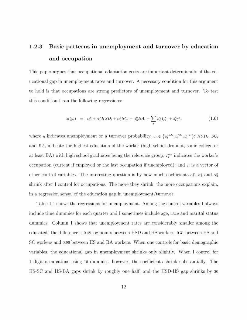
1.2.3 Basic patterns in unemployment and turnover by education

and occupation

This paper argues that occupational adaptation costs are important determinants of the ed-

ucational gap in unemployment rates and turnover. A necessary condition for this argument

to hold is that occupations are strong predictors of unemployment and turnover. To test

this condition I ran the following regressions:

ln (yi) = αy0 + αy1HSDi + αy2SCi + αy3BAi +∑x

βyxIoccxi + z′iγ

y, (1.6)

where y indicates unemployment or a turnover probability, yi ∈{uoddsi , pEUi , pUEi

}; HSDi, SCi

and BAi indicate the highest education of the worker (high school dropout, some college or

at least BA) with high school graduates being the reference group; Ioccx indicates the worker’s

occupation (current if employed or the last occupation if unemployed); and zi is a vector of

other control variables. The interesting question is by how much coefficients αy1, αy2 and αy3

shrink after I control for occupations. The more they shrink, the more occupations explain,

in a regression sense, of the education gap in unemployment/turnover.

Table 1.1 shows the regressions for unemployment. Among the control variables I always

include time dummies for each quarter and I sometimes include age, race and marital status

dummies. Column 1 shows that unemployment rates are considerably smaller among the

educated: the difference is 0.48 log points between HSD and HS workers, 0.31 between HS and

SC workers and 0.96 between HS and BA workers. When one controls for basic demographic

variables, the educational gap in unemployment shrinks only slightly. When I control for

1 digit occupations using 10 dummies, however, the coefficients shrink substantially. The

HS-SC and HS-BA gaps shrink by roughly one half, and the HSD-HS gap shrinks by 20

12

percent. A large fraction of the educational gap in unemployment can be explained by the

one digit occupation of the workers. As I include more and more disaggregated occupation

dummies, the differences shrink even further. When I include 191 occupation dummies in

columns 5, I can explain around one third of the HSD-HS gap and around two thirds of the

educational gap in unemployment among workers with at least a high school degree. By

further including sector dummies, the educational gap slightly shrinks further.

Tables 1.2 shows that one gets the same patterns qualitatively using linear probability

models. In this table I restrict the sample to low unemployment periods, i.e. “booms”.

Table 1.17 in the appendix shows the same OLS regressions in other periods, labeled as

“recessions”. Booms indicate years when the aggregate unemployment rate in the 25-55 year

old male sample was below 5 percent and recessions indicate that it was above 5 percent. The

high unemployment periods using this definition are 1980-1986, 1991-1993 and 2009-2013.

These periods are longer and somewhat lag NBER recessions, while the dot-com recession

in 2001 is entirely missing as it was too mild. There are large differences in unemployment

rates across education groups both in booms and in recessions; one digit occupations explain

around half of the gaps among workers with at least a high school degree; and detailed

occupations explain around two thirds of it. The explained HS-HSD gap is somewhat less.

Overall, occupation choice appears to be a primary reason why educated workers are less

likely to be unemployed. The highly educated work in occupations where unemployment is

a rare phenomenon.

Table 1.3 shows logit regressions in the monthly transition probabilities. The patterns in

the employment to unemployment transition probabilities are similar to the unemployment

regressions. We can see large differences between education groups, and occupations explain

a large fraction of the gap between education groups. The coefficients in the job finding

13

regressions (unemployment to employment transitions) reveal a distinct pattern. First, the

job finding probability is smaller among higher educated workers. The differences are small,

however, at least compared to the differential in job loss probabilities. The 0.047 differen-

tial between HS and BA workers, for example, means that BA workers should expect 4.7

percent longer unemployment duration than HS workers, on average, which is less than one

week. However, after controlling for occupations, the education coefficients turn positive

and they are usually significant. This means that the educated are working in occupations

where finding jobs is harder, but conditional on their occupations, education is slightly pos-

itively associated with job finding chances. This finding, at least qualitatively, is in line

with the adjustment cost mechanism. Appendix Tables 1.18-1.23 shows more detailed logit

specifications and linear probability models. Those results are qualitatively the same.

1.2.4 Adaptation costs by occupations

Using a Swiss employer survey, Blatter et al. (2012) estimate that during the adaptation

period rookies are approximately 30 percent less productive than experienced workers, and

the length of the adaptation period is roughly 80 workdays on average. They also report that

the 30 percent productivity gap appears to be constant across jobs and employers, while the

length of the adaptation period varies greatly.

I use a US employer survey, the Multi-City Study of Urban Inequalities (MCSUI)14.

These data were collected in 1992-1994, in order to understand why high rates of joblessness

have persisted among minorities living in America’s central cities. One important aspect

of the study was the contacting of more than 3000 employers in four large US cities (Los

Angeles, Boston, Detroit and Atlanta) to ask detailed questions about their hiring practices.

14The study was funded by the Russel Sage Foundation and the Ford Foundation. See Holzer (1996) fordetails about the survey.

14

Even though the intent of the study was to understand racial discrimination in hiring, the

exhaustive information about the recruitment process makes this study valuable for broader

purposes. The sampling procedure and the provided weights intend to represent employees

who worked in Los Angeles, Boston, Detroit or Atlanta in 1992. They used the 3-digit 1980

SOC occupation classification to code the position of the workers.

The survey contains a measure of occupational adaptation costs that I use in this paper.

The question reads “How many weeks or months does it take the typical employee in this

position to become fully competent in it?” Unfortunately the survey did not ask questions

about the average productivity difference between rookies and experienced workers, so I rely

on the Blatter et al. (2012) study and assume it is 30 percent in each job.

Table 1.4 provides descriptive statistics about the adaptation period measure. The me-

dian is around 3 months and the mean is around 7 months. The large difference between the

mean and the median is due to quite a few large outliers in the sample. One way of dealing

with these outliers is to apply the log transformation on the reported adaptation periods to

downweight the influence of these outliers. This is the method I applied in this paper.

Table 1.6 shows the coefficients of regressions of log adaptation on various occupational

work activity measures. The coefficients are from simple regressions with only one measure

included at a time. The work activity measures are created from the O*NET data with

a procedure described in Firpo et al. (2011).15 One might expect that adaptation takes

longer when people have to work with others, and when they have to analyze information

and make plans, since these activities are mostly firm-specific. The table supports these

hypotheses. Work activities related to information processing and dealing with people have

15O*NET provides two variables: the “importance” and the “level” of work activities in occupations. Basedon Firpo et al. (2011), I transform the two variables to be between 0 and 1, and then I assign a Cobb-Douglasweight of 2/3 to importance and 1/3 to level to create my final measures.

15

strong positive correlations with adaptation costs, while physical activities and operating

machines are negative predictors of adaptation costs. The three strongest predictors (based

on the t-statistics) are: 1) interpreting the meaning of information for others; 2) organizing,

planning, and prioritizing work; and 3) developing objectives and strategies. Table 1.5 shows

regressions of adaptation on education and various occupational work activity measures. The

three main occupational activities are positive and significant even jointly and the addition of

other work activity measures do not make the fit better. It appears interpreting information

for others, planning and developing strategies are the primary determinants of how long

it takes to get fully productive in occupations. Table 1.5 also shows that adaptation is

significantly and substantially longer in jobs where the highly educated work. Compared to

high school graduates, the average adaptation period is 35 percent shorter for high school

dropouts, 34 percent longer for college dropouts and 73 percent longer for BA workers. When

I include both education and occupational activity measures, the coefficients on education

drop by about half, but remain statistically significant. In some ways it is puzzling that

education remained significant. MCSUI asks employers about the average adaptation in the

given position. If the positions employers have in mind are the same as the occupations

I use, no variable other than occupations should matter. It appears that employers use a

more detailed occupation-specification when answering these questions, and the education

dummies pick up these differences.

Table 1.25 shows the average imputed length of adaptation in 46 detailed occupations:

23 with the shortest and 23 with the longest adaption out of the 191 occupations.16 The

table shows the fitted values of Models 2 and 3 from Table 1.5 and the raw averages by

occupations. My preferred measure is in the first column, which is based on only the three

16The entire table is available on my website at https://sites.google.com/site/phudomiet/research.

16

main work activity measures. The addition of the other activity measures hardly changes

the imputed values, and the raw averages in column 3 are very noisy, since they are based on

very few observations. My preferred measure shows that the distribution of the adaptation

period runs from 1.2 month (waiter’s assistants) to 8.6 month (clergy and religious workers).

This is a very wide distribution. Adaptation is shortest in occupations such as waiters,

laundry workers, food preparation workers, janitors, machine operators, and interviewers.

Adaptation is longest for managers, management support occupations, teachers, scientists,

financial workers, etc. These are in line with expectations.

Table 1.7 shows logit regressions of unemployment and turnover probabilities on imputed

adaptation cost measures. The imputed values are the predicted values from a regression of

log adaptation costs on the three occupational work activity measures, education dummies

(less than high school, high school, some college, and college) and their interactions. Model

1 of Table 1.7 includes no control variables other than year dummies, and model 2 includes

education, age, race, marital status and industry dummies. In model 1 adaptation costs

are significantly and strongly negatively related to unemployment and layoff rates, while the

effect on hiring rates is smaller, but still negative and significant. These are qualitatively in

line with the predictions of a labor hoarding model: turnover costs negatively affect both

job creation and job destruction. In model 2, after controlling for education, age, race and

industries, the elasticities of unemployment and job loss with respect to adaptation decrease

by about 20%, but remain very large and significant; and the elasticity of job finding remains

negative, but turns insignificant. These estimates are suggestive that adaptations costs are

important determinants of turnover and unemployment. They are, however, likely suffer from

omitted variable bias. Occupations differ in many dimensions beyond the cost of adaptation.

To overcome this endogeneity problem the next section turns to a model of turnover and

17

unemployment. In the model I allow occupations to differ only in the average length of

adaptation, and all other differences are shut off.

1.3 The model

The purpose of this model is to analyze how adaptation costs affect turnover and unemploy-

ment rates in equilibrium. I use a Mortensen and Pissarides (1994) (MP) type search and

matching model with endogenous job creation and job destruction as the modeling frame-

work. In this model, unemployment is purely frictional in the sense that all unemployed

persons are searching for jobs. Workers are job-less because it takes time to find new jobs

after separations, not because their reservations wages are too high. In fact, in the standard

setup of the model, used in this paper, workers do not even have a reservation wage: they ac-

cept any job offered to them and wages are determined by a bargaining process in which firms

and workers make an agreement about how to split up the surplus of the match. The rate

at which separations occur and the duration of unemployment are endogenously determined

in the model. Separations occur when idiosyncratic, match-specific shocks make the value

of the match (the surplus) negative. The rate at which the unemployed find jobs depends

on how many vacant jobs are posted by firms and how many individuals are competing for

these positions. In the standard MP model, the probability of finding a job is assumed to

be the same for all workers.

The traditional adjustment cost literature (see e.g. Oi, 1962; Fair, 1985; Shapiro, 1986;

Lazear, 1990) uses a neoclassical framework to analyze the effect of adjustment costs on

unemployment rates. In that framework, job loss and job finding probabilities cannot be

analyzed and job-less workers do not want to work. The MP modeling framework is more

18

suitable to analyze the effect of various parameters on turnover rates, since unemployment

is frictional and turnover is endogenously determined in the model.

My model closely follows the original Mortensen and Pissarides (1994) model, with a few

exceptions. First, as I aim at explaining cross-sectional variation in turnover and unemploy-

ment, I only consider the steady state equilibrium of the model. Second, the labor force in

my model is heterogeneous: workers can work in one of many occupations. Within occupa-

tions, however, workers are homogeneous apart from random shocks to their match-specific

productivity. To keep the model simple and tractable I assume that workers are permanently

assigned to their occupation and they never change their careers. When they lose their jobs,

they only search in their original occupation. This assumption allows for segmenting the

economy into submarkets and applying the standard solution methods on each of them. It

would be interesting to consider a more general model with the possibility of switching occu-

pations. For at least two reasons, however, the general model should behave similarly to the

restricted model that is considered in this paper. First, the size of each occupation should be

stable in steady state. Second, the job finding probabilities are very similar across education

groups and occupations, and thus, cross-occupation flows are unlikely to contribute much to

equilibrium unemployment rates.

The main deviation I introduce to the MP model is the presence of an adaptation period

during which newly hired rookies are less productive than experienced workers. Occupations

only differ in the expected length of the adaptation period, and all other parameters of the

model are kept constant across occupations. I assume that the adaptation period in occu-

pations is exogenous. It reflects how complex the jobs are, and how difficult it is to gain full

competency in them. In reality, the adaptation period might be partly endogenous: Employ-

ers might choose to assign harder and harder tasks for newly hired workers gradually. There

19

might be a production function of experience and employers might be able to manipulate

the speed of gaining experience. In such cases one might think of my simplistic model as the

second step of a two step model. In the first step firms optimize over all possible values of

adaptation. Once they find the optimal production function of experience in each occupa-

tion, they can take the optimal values of adaption from the first step as a given to discover

the optimal turnover decisions in the second step. In this case, my model does not reveal

why adaptation costs are larger in certain occupations, but it still discerns the equilibrium

turnover and unemployment rates given the observed equilibrium values of adaptation.

This is not the first paper to add an adaptation period to a search and matching model.

Mortensen and Nagypal (2007) and Silva and Toledo (2009) use similar models to analyze the

effect of adaptation costs on the business cycle variation of the aggregate unemployment rate.

Some papers discussed the implications of training costs for unemployment rates (Pissarides,

2009; Cheremukhin, 2010; Miyamoto, 2011 and Cheron and Rouland, 2011). These papers

model the cost of training as a onetime cost at the time of hiring, and they do not use

empirical measures of training costs. The recent working paper of Cairo and Cajner (2014)

also uses a similar model to mine.

1.3.1 The setup of the model

In what follows, subscript x refers to occupation x ∈ {1, ..., NX}, and I ignore time subscripts

to simplify notation. I use a continuous time version of the model. Firms can employ one

worker, either a rookie or an experienced one, or zero workers. When they are matched with

an experienced worker in occupation x the match produces flow profit

πx (ε) = sxε, (1.7)

20

where sx is average productivity in occupation x and ε is the idiosyncratic, match-specific

productivity term. The c.d.f of ε is denoted by F (ε) which is assumed to follow a log-normal

distribution,

ln ε ∼ N(0, σ2

). (1.8)

The idiosyncratic shock is temporary and its value is redrawn from this distribution in an

i.i.d. fashion when a new shock arrives with Poisson arrival rate λ. One can think of λ as the

inverse autocorrelation in productivity: when λ is large, new shocks occur more frequently

and present productivity has a smaller predictive power for future productivity. Formally, if

λ is calibrated to be a monthly rate, then a t month autocorrelation in productivity is ρ (t) =

exp (−λt). If the productivity shock is smaller than an endogenously determined productivity

threshold ε, so that the surplus falls below zero, matches get destroyed endogenously. The

endogenous separation rate, fL,enx in the model, is

fL,enx = λF (εx) . (1.9)

Matches can also be destroyed with an additional exogenous rate, fL,ex. Hence, the total job

loss rate is

fLx = λF (εx) + fL,ex. (1.10)

Rookies’ productivity is lower than experienced workers’ productivity by a factor 1− δ,

πRx (ε) = δsxε. (1.11)

Rookies endogenously separate from their employers if the match-specific productivity shock

falls below an endogenously determined productivity threshold εR. Furthermore, I assume

21

that the additional exogenous separation rate is the same for rookies and experienced workers.

The total job loss rate of rookies is

fL,Rx = λF(εRx)

+ fL,ex. (1.12)

We should expect that, in equilibrium, ε < εR so that rookies are more likely to lose their

jobs than experienced workers. Rookies become experienced randomly with a Poisson arrival

rate ϕx. This arrival rate is assumed to be occupation-specific, but the productivity loss,

1− δ, is not. This is in line with the findings of Blatter et al. (2012).

Firms without workers can post a vacancy if they are willing to pay the instantaneous

search cost cx = csx. The search cost is a constant fraction of occupational productivity, sx.

This is a neutrality condition which assures that occupational productivity does not have a

direct effect on turnover. One justification for this assumption is that higher skilled workers

have to be interviewed (the largest component of search costs, see Blatter et al., 2012) by

higher skilled workers.

If there are vx posted vacancies (unfilled jobs) in the economy and nx persons are searching

for them, then matches are formed at rate

mx = ηvαxn1−αx . (1.13)

This function is called the matching function which determines how fast workers can find

jobs and firms can fill their vacancies. The matching function has constant return to scale

(CRS) and it is increasing in both arguments because 0 < α < 1. The job finding rate, fFx ,

22

can be computed by dividing the match rate by the number of searching workers,

fFx =mx

nx= η

(vxnx

)α≡ ηθαx , (1.14)

where θx = vx/nx is called labor market tightness. In a tight labor market with a lot of

unfilled jobs it is easier to find jobs and fF is relatively large. The rate at which vacancies

are filled, qx, can be computed similarly:

qx =mx

vx= ηθα−1x . (1.15)

The vacancy filling rate is decreasing in labor market tightness, because α < 1. In a tight

labor market with a lot of unfilled jobs it is harder to find workers and q is relatively small.

Free entry of firms assures that the value of posting vacancies is zero in equilibrium. The

value of being an unemployed worker, however, is positive. Unemployed workers enjoy a flow

value of bx = bsx and they expect a positive continuation value as well. Similarly to search

costs, the flow value of unemployment is also normalized with occupational productivity, sx.

Wages are determined through Nash wage bargaining, and workers’ bargaining power is

γ. At the time of hiring and at any time when the productivity of the match changes, wages

get renegotiated. It is possible to allow for wage rigidity without changing any predictions

of the model. Wage rigidity does not affect turnover under the following two conditions: 1)

Newly hired workers’ wages are flexible and set by Nash wage bargaining; 2) Workers and

firms never leave surplus on the table. This second condition implies that if, for example, a

negative shock occurs and the firm is not interested in the match at the given level of rigid

wage, workers are willing to renegotiate the wage to save their jobs. Both of these conditions

are reasonable.

23

Finally, the interest rate is r and the initial value of the idiosyncratic shock is fixed at its

mean, εinitial = ε0 = exp(σ2

2

).

1.3.2 The solution

The model can be solved analytically. The Appendix shows how to write the value functions

of the firm and the workers, and then how to solve for all the endogenous parameters.

The equilibrium wages of rookies and experienced workers are

wRx (ε) = (1− γ) b+ γ (δε+ θxc) , (1.16)

wx (ε) = (1− γ) b+ γ (ε+ θxc) . (1.17)

Rookies make less money, because they are less productive than experienced workers. Thus,

the model predicts a wage-tenure profile. Wages increase in the bargaining power of workers

(γ), in productivity (δ and ε), in the flow value of unemployment (b), in search costs (c) and

in labor market tightness (θx). Apart from search costs, these results are intuitive. When

search costs (paid by the firms) are large, the initial surplus needs to be larger so that

firms are compensated for them. A larger initial surplus increases the workers’ share of the

initial surplus, and, consequently, workers demand higher wages. This is a classical hold-up

problem17. Investments made before the first wage negotiation, in this case paying search

costs, have to be shared with the other party. Using similar arguments, one can show that

search costs that are paid by workers, as opposed to firms, decrease, rather than increase,

wages. The effect of search costs on wages is similar to the wage effects of firm-specific skills

described in Becker (1994). In his model, the costs and benefits of acquiring firm-specific

17See Acemoglu and Shimer (1999) for a more detailed discussion of the hold-up problem in search models.

24

skills have to be shared by workers and firms so that neither has an incentive to end the

relationship too early.

Now consider equilibrium turnover. The job loss and job finding rates depend on the

three endogenous parameters (θ, εx and εRx ) as described in (1.10), (1.12) and (1.14). To

characterize the equilibrium we need three conditions. The first one is called the job creation

condition:

c

ηθ1−αx = (1− γ)

δ + ϕx

r+λ+fL,ex

r + λ+ fL,ex + ϕx

(ε0 − εRx

). (1.18)

The left-hand side of (1.18) is the expected total search costs firms pay to fill a vacancy

and the right-hand side is the firms’ share of the initial surplus. The job creation condition

says that new vacancies are posted until labor market tightness reaches a point at which the

expected value of an additional vacancy is zero.

The second equilibrium condition of the model is the job destruction condition of expe-

rienced workers:

b+γ

1− γθxc = εx +

λ

r + λ+ fL,ex

ˆ ∞εx

(ε′ − εx) dF (ε′) . (1.19)

The left-hand side of (1.19) is the outside option of workers and the right-hand side is the

total value of the match. The job destruction condition says that matches are destroyed

when the surplus is below zero, or in other words, when the workers’ outside option exceeds

the total value of the match. The right-hand side has two terms. The first (εx) is the flow

productivity and the second, involving the integral, is the expected continuation value of the

match. One can think of the second term as a labor hoarding term: matches can survive large

negative shocks as long as the surplus is expected to increase soon. In fact, the only incentive

to hoard labor is that the cost of adjustment is smaller than the expected cost associated

25

with a temporary negative shock. When λ is small, and shocks are very permanent, hoarding

labor is not rational, and flow productivity should be the only factor determining turnover

decisions. When λ is large, and productivity shocks are short lived, hoarding labor becomes

more appealing.

The last equilibrium condition is the job destruction condition of rookies, which is

b+γ

1− γθxc = δεRx + λ

δ + ϕx

r+λ+fL,ex

r + λ+ fL,ex + ϕx

ˆ ∞εRx

(ε′ − εRx

)dF (ε′) +

ϕxr + λ+ fL,ex

(εRx − εx

).(1.20)

The left-hand side of (1.20) is the outside option of workers, which is the same for rookies and

experienced workers. The right-hand side consists of the flow productivity of the match and

two labor hoarding terms. The first one, involving the integral, is the expected continuation

value of the match if the worker remains a rookie, and the second one is the expected gain if

he becomes experienced. Rookies might be hoarded not only because a temporary negative

shock is expected to disappear, but also because they might become experienced soon.

Equations (1.18)-(1.20) implicitly determine the three endogenous parameters and, con-

sequently, the job finding and job loss rates. The equilibrium conditions in the standard MP

model are similar, and they can be obtained as limiting cases of my model. For example, if

rookies are as productive as experienced workers (δ → 1 ) or if rookies become experienced

immediately ( ϕx → ∞), the equilibrium conditions collapse to the ones in the standard

model. If rookies never become experienced (ϕx → 0), the equilibrium conditions collapse to

the standard model with average productivity normalized to δ, rather than 1.

26

1.3.3 Calibration of the model

In this section I calibrate the model to fit aggregate turnover and unemployment. The

calibrated parameters might be thought of as estimates for an average or “representative”

occupation. The next sections discuss how turnover and unemployment vary with adaptation

costs.

The model aims at matching empirical average turnover in the CPS between 1994 and

2008. In 1994, the CPS introduced a question about employer change: workers who are

employed both in month t and t + 1 are asked in t + 1 whether they still work for the same

employer as in t. Years before 1994 are dropped, because employer switching, an important

separation margin, cannot be identified in those years. Years after 2008 are dropped because

of the great recession. In each year between 1994 and 2008, the aggregate unemployment

rate in the prime age male sample was below 5 percent.18

Some parameters of the model are calibrated externally, using regular values from the

literature. The first eight rows of Table 1.9 shows the choice of these parameters. The

Cobb-Douglas share of vacancies in the matching function is 0.4, based on a large number of

empirical estimates summarized in Pissarides and Petrongolo (2001). Workers’ bargaining

power is set to 0.6 so that the Hosios condition is satisfied and the market equilibrium is

socially efficient. Aggregate labor market tightness is set to 0.72. This value is based on

empirical estimates from the Job Openings and Labor Turnover Survey and used in most

macro labor papers. One might argue that in my more restricted sample (prime age males)

a different value should be used. It, however, plays no role for the estimates; the model

is entirely indifferent to the choice of aggregate θ. For a formal proof, see Appendix 1.5.2.

18The calibration results are basically equivalent if the years of the mild dot-com recession are dropped,too.

27

Intuitively, the other internally calibrated parameters absorb any mismeasurement in θ. The

interest rate is set to 0.004 which corresponds to ∼ 5 percent annually. The average total

search cost firms pay, which is c/q in the model, is set to 50 percent of the average monthly

wage of an experienced worker. The average wage is computed endogenously from the model.

Blatter et al. (2012) found that total search costs in Switzerland take up roughly 60 percent

of the average monthly wage, while other papers (such as Pissarides, 2009; Ratner, 2013) use

values around 40 percent. I use the middle point between 40 and 60 but I shall investigate

the sensitivity of the model’s predictions to the choice of this parameter.

The productivity of rookies is set to 30 percent lower than that of experienced workers

based on Blatter et al. (2012). The rate of turning experienced is set to ϕ = 0.31, which

corresponds to becoming experienced in about three months, on average. The value of ϕ

was computed from the MCSUI with the following procedure. I assume that true adaptation

costs only depend on the occupation of workers:

ln taix = ln tax +mi. (1.21)

The log reported adaptation period in occupation x by employer i, ln taix, is the sum of an

occupation-specific term, ln tax, and a mean zero measurement error term, mi. Equation (1.21)

is estimated by OLS using 48 occupation dummies. I use the provided sample weights that

intend to make the MCSUI sample represent employees who worked in Los Angeles, Boston,

Detroit or Atlanta in 1992. After that I take the sample average of the occupational log

adaptation periods using the occupational distribution of workers in the CPS sample. The

average rate of turning experienced, then, is the inverse of the exponent of this number,

ϕ = exp (− ln ta) = 1/ta. I run a sensitivity analysis on both δ and ϕ in the next section.

28

The final parameter that is externally calibrated is the autocorrelation in match-specific

productivity. Empirical estimates of this parameter are hard to obtain, because we do not ob-

serve productivity in individual matches. In the baseline calibration I, instead, use measures

of autocorrelation in plant level productivity, but in Section 1.4.1 I shall discuss alterna-

tive strategies. Abraham and White (2006) provides high quality estimates of plant-level

productivity in the manufacturing sector. They find yearly autocorrelation to be relatively

low, between 0.37 and 0.41. The corresponding monthly values are 0.92 and 0.93. I choose

the value of ρ = 0.92. This value implies that the rate at which new i.i.d. shocks arrive is

λ = − ln (0.92) ≈ 0.083, and productivity shocks get redrawn every 1/0.083 ≈ 12 months, on

average. There are reasons to believe that plant level autocorrelation is not a perfect substi-

tute for the autocorrelation in match-specific productivity. For example, as aforementioned,

workers productivity might fluctuate for personal reasons such as sickness, a loss in the

family, interpersonal issues with coworkers, etc. One might think that such negative shocks

disappear quicker than demand shocks. Given that the plant level estimates in Abraham and

White (2006) are already relatively low, I use those numbers in my baseline specification. I

run a sensitivity analysis on this parameter as well.

The model has three equilibrium conditions: the job loss condition of rookies, the job

loss condition of experienced workers and the job finding condition. The three conditions,

together with the job loss and job finding probabilities from the CPS enable calibrating five

parameters internally. These are the productivity thresholds of experienced workers (ε) and

rookies (εR); the dispersion of productivity shocks (σ); the efficiency of the matching function

(η); and the flow value of unemployment (b).

The next issue is the choice of turnover probabilities to match from the CPS. Table 1.8

shows different types of transition probabilities in the CPS. The average E → U transition

29

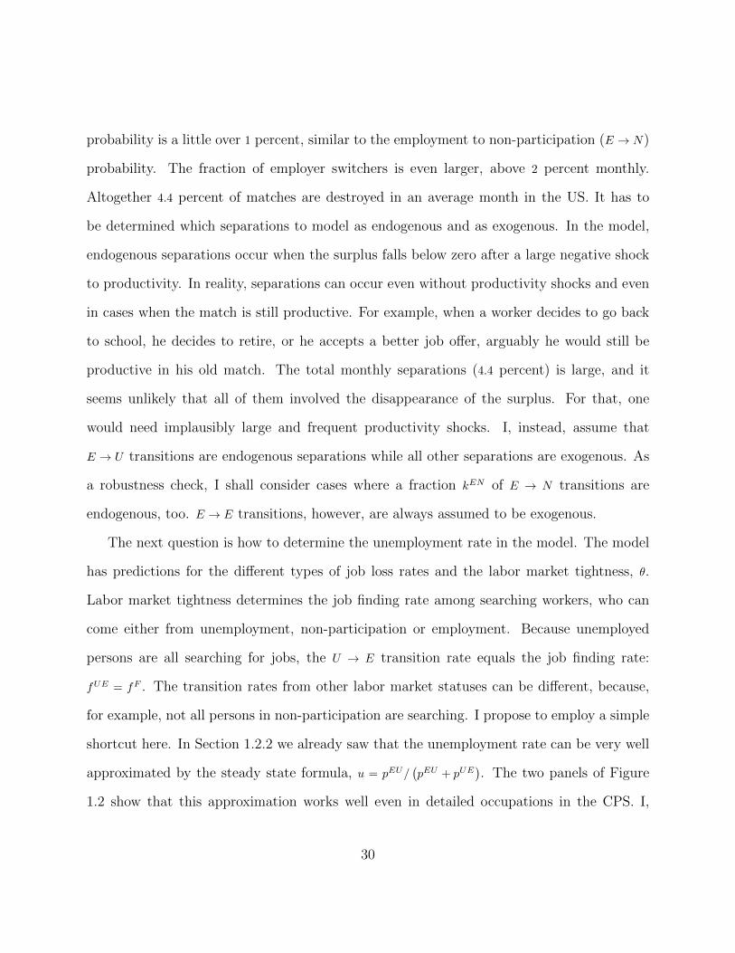
probability is a little over 1 percent, similar to the employment to non-participation (E → N)

probability. The fraction of employer switchers is even larger, above 2 percent monthly.

Altogether 4.4 percent of matches are destroyed in an average month in the US. It has to

be determined which separations to model as endogenous and as exogenous. In the model,

endogenous separations occur when the surplus falls below zero after a large negative shock

to productivity. In reality, separations can occur even without productivity shocks and even

in cases when the match is still productive. For example, when a worker decides to go back

to school, he decides to retire, or he accepts a better job offer, arguably he would still be

productive in his old match. The total monthly separations (4.4 percent) is large, and it

seems unlikely that all of them involved the disappearance of the surplus. For that, one

would need implausibly large and frequent productivity shocks. I, instead, assume that

E → U transitions are endogenous separations while all other separations are exogenous. As

a robustness check, I shall consider cases where a fraction kEN of E → N transitions are

endogenous, too. E → E transitions, however, are always assumed to be exogenous.

The next question is how to determine the unemployment rate in the model. The model

has predictions for the different types of job loss rates and the labor market tightness, θ.

Labor market tightness determines the job finding rate among searching workers, who can

come either from unemployment, non-participation or employment. Because unemployed

persons are all searching for jobs, the U → E transition rate equals the job finding rate:

fUE = fF . The transition rates from other labor market statuses can be different, because,

for example, not all persons in non-participation are searching. I propose to employ a simple

shortcut here. In Section 1.2.2 we already saw that the unemployment rate can be very well

approximated by the steady state formula, u = pEU/(pEU + pUE

). The two panels of Figure

1.2 show that this approximation works well even in detailed occupations in the CPS. I,

30

thus, assume that this formula works in the model, too. Because the U → E transition rate

equals the job finding rate, the unemployment rate can be written as a function of the labor

market tightness and the E → U transition rate. As described in the previous paragraph,

in the baseline specification I assume that the E → U transition rate equals the endogenous

separations in the model. Thus, the unemployment rate can be written as

ux =λF (εx)

λF (εx) + ηθαx. (1.22)

The formula ignores the effect of rookies on the unemployment rate, but given that they take

up a tiny fraction of the employed sample, the bias is negligible.

In the more general case, when some of the endogenous separations are E → N transitions,

the unemployment rate is

ux =kλF (εx)

kλF (εx) + ηθαx, (1.23)

where k is assumed to be the same in each occupation and is a function of kEN .

Rows 9− 11 of Table 1.9 show the most interesting internally calibrated parameters and

rows 12+ show a few other interesting implied values for the representative occupation.

The flow value of unemployment is around 66 percent of the average wage of experienced

workers. There is a large disagreement about the true value of this parameter in the literature.

There are papers using values as low as 40 percent (Shimer, 2005) and as high as 95 percent

(Hagedorn and Manovskii, 2008) of the average wage. My estimated value is roughly in the

middle of the used interval. The standard deviation of match-specific productivity shocks is

0.26, which is reasonable, but is somewhat on the high side of calibrations in other papers.

The scalar of the matching function, sometimes called matching efficiency, is 0.4.

The model predicts that rookies are more likely to be laid off than experienced workers.

31

While the continuous employment to unemployment transition rate is only 0.014 for experi-

enced workers, it is 0.020 for rookies. The last two rows of the table show the average wages

of rookies and experienced workers using formulas (1.16) and (1.17):

E(wR)

= (1− γ) b+ γ(δE(ε|ε > εR

)+ θc

), (1.24)

E (w) = (1− γ) b+ γ (E (ε|ε > ε) + θc) . (1.25)

The model predicts that rookies earn roughly 18 percent less than experienced workers. This

estimate is a pure effect of seniority and it should be comparable to causal estimates of tenure

on wages. Simple OLS estimates of wage differential between newly hired and experienced

workers is around 30 percent, but causal estimates are anywhere between 5 and 25 percent

(Topel, 1991; Altonji and Williams, 2005). Taking this into account, my 18 percent is a

reasonable number.

1.3.4 Turnover elasticities with respect to adaptation costs

The only occupation-specific exogenous parameter in the model is ϕx, the rate at which

rookies turn experienced. To get a sense of the effect of adaptation, I calibrate the elasticities

of turnover and unemployment rates with respect to the length of the adaptation period. As

ϕx is a Poisson process, the expected length of adaptation is

tax =1

ϕx. (1.26)

Table 1.10 shows the elasticities of various endogenous variables with respect to the adapta-

tion period evaluated at the aggregate solution. I use the following numerical approximations

32

to compute the elasticity of any variable y

εyta =∂ ln y

∂ ln ta≈ y (ta + h)− y (ta − h)

2h

ta

y (ta), (1.27)

where ta is the average length of the adaptation period (∼ 3 months in the baseline calibration

of the model); y (t) is the equilibrium value of the variable of interest when the adaptation

period is t, but all other parameters are kept constant at the aggregate value; and h is a

small number. In practice I use h = 10−4.

The model predicts that longer adaptation leads to both less layoff and less hiring, but

the response on the layoff margin is more than ten times larger. The steady state assumption

implies that

εuodds

ta = εfEU

ta − εfUE

ta . (1.28)

As the layoff elasticity is much larger than the hiring elasticity, the model predicts that the

equilibrium unemployment rate is decreasing with the length of the adaption period. The

estimated elasticity of unemployment is −0.541. To get a sense of the magnitude of this

coefficient, let us consider the following back-of-the-envelope calculation. In Section 1.2.2 we

saw that the unemployment gap between BA and HS workers in the logit metric was 0.962.

In order to explain the entire BA-HS gap, thus, we need ln taBA − ln taHS = 0.962/0.541 ≈ 1.78,

the log difference in the adaptation periods between the two groups should be around 1.78.

Alternatively, the ratio taBA/taHS should be around exp (1.78) ≈ 5.9, adaptation in jobs in which

college graduates work should be 6 times longer than in jobs in which high school graduates

work. This would happen, for example, if the average adaptation costs for high school and

college graduates were 4 and 24 weeks, respectively. This differential is not implausible,

33

but it seems somewhat large. In Section 1.2.4 we saw that the log difference in adaptation

between the two groups was around 0.73 rather than 1.78. Based on this simple calculation,

we can expect to explain around 40 percent of the educational gap in unemployment between

BA and HS workers with adaptation costs. This back-of-the envelope calculation, however,

might not be precise due to non-linearities in the model.

The implied close to zero hiring elasticity of adaptation costs is remarkable, given that

most parameters of the model, including other adjustment costs, have large effects on hiring

as shown in Hudomiet (2014). Adaptation costs have two opposing effects on the hiring

rate. The direct effect is that longer adaptation makes turnover more costly, decreasing

the value of the initial surplus, which lowers vacancy creation and, consequently, makes it

harder to find jobs. I call this the price effect : when turnover is costly, there is less of it

in equilibrium. The indirect effect, which I call labor hoarding effect, is that adaptation

makes matches more stable through a decrease in layoffs. Longer lasting matches increase

the value of the initial surplus, since both the firm and the worker expect to enjoy their

share of the match rent for a longer time. Both the price and the labor hoarding effects are

large, but they appear to almost cancel out in equilibrium. Mathematically, one can show

that any reasonably calibrated job destruction condition is steep, and as adaptation costs

only shift the job creation condition, labor market tightness and the job finding probabilities

are not affected strongly by adaptation costs. It is worth noting that the symmetry in the

hiring rates only holds if the model features endogenous job destruction. If job destruction

is exogenous, that is, the labor hoarding effect is shut down, adaptation costs do not have

an indirect positive effect on hiring, and there is nothing to balance out the large negative

price effect of adaptation.

Adaptation costs are also different from other adjustment costs. Beyond the already

34

mentioned price and labor hoarding effects, most adjustment costs affect turnover through

a third channel as well, which I call the bargaining effect. Adjustment costs can change

the bargaining position of workers or firms depending on who pays these costs and when.

Costs that are sunk at the time of hiring, such as search costs, for example, decrease the

bargaining position of the party that paid them. Adaptation costs, however, do not change

the bargaining position of the parties. These costs are not sunk at hiring, and they are

also firm-specific, implying that they cannot be used as a threat in wage negotiations. In

equilibrium, workers and firms split up the cost of adaptation based on their fixed bargaining

power. Rookies are less productive, but they also make less money.

The model predicts that E → N movements are not responsive to adaptation, because in

the baseline specification they are exogenous. The job loss probabilities of rookies are not

changing with the adaptation period either; the elasticity is close to zero, because of the

assumption that becoming experienced is a memoryless Poisson process.

Equation (1.28) can be rewritten as

1 =εf

EU

ta

εuodds

ta− εf

UE

ta

εuodds

ta. (1.29)

The first term shows the ratio of the job loss and the unemployment elasticities. The term

can be interpreted as the ratio of the unemployment elasticity that is due to changes in

layoffs. Similarly, the negative of the second term can be interpreted as the ratio of the

unemployment elasticity due to changes in hiring. The last two lines of Table 1.10 show

the two ratios. Layoffs explain around 110 percent of the unemployment elasticity, while

hiring explains −10 percent of it. Hiring explains a negative fraction of the unemployment

elasticity, because the model predicts that in occupations where adaptation costs are large,

35

both equilibrium unemployment and hiring will be below average, that is, hiring goes in the

wrong direction to explain differences in unemployment.

In order to see how robust my predictions are, I run sensitivity analyses on five externally

calibrated parameters. In each dimension I use relatively wide bounds. Tables 1.11 and 1.12

show the results. Throughout all specifications, the hiring elasticity remains close to zero. It’s

largest absolute value is only −0.079. The layoff and unemployment elasticities are always

substantially larger than the hiring elasticity. Interestingly, the ratios in (1.29) are quite

robustly estimated: Layoffs explain around 110 percent of the unemployment elasticity, and

hiring explains −10 percent of it. The elasticities vary with parameters in the expected way.

When more E → N transitions are endogenous (kNE is larger), the model predicts a lower

elasticity in E → U , but the sum of εfEU

ta and εfEN

ta is roughly a constant. Because I assume

E → N transitions do not contribute to the unemployment rate, larger kNE translates into

a somewhat smaller unemployment elasticity. When adaptation is quicker (ϕ is larger), not

surprisingly, the layoff and unemployment elasticities are less responsive to adaptation costs.

Similarly, when rookies’ productivity (δ) is closer to that of experienced workers, adaptation

costs are less predictive of layoffs and unemployment. Search costs also affect the layoff

elasticity, but the effect is not large.

The parameter with the largest effect on my estimates is the autocorrelation in match-

specific productivity. The more persistent the productivity shocks are, the less predictive

adaptation costs are for layoffs and unemployment. Why is that? The autocorrelation in

productivity is the primary determinant of the extent of labor hoarding in the economy.

When a bad shock hits the match, the parties can choose from two strategies: 1) They either

decide to split up and search for a better match; or 2) they decide to stay together and

persevere. This second strategy is called labor hoarding. Hoarding labor is more profitable

36

when the cost of turnover is high (in order to save on these costs) and when shocks are

relatively short lived (because bad times do not last long and it is worth waiting). When the

autocorrelation is low, negative productivity shocks are expected to go away soon, and thus,

firms are more likely to hoard their workers. And when the autocorrelation is low and labor

hoarding is widespread, as Table 1.12 shows, adaptation costs are more important determi-

nants of equilibrium layoff and unemployment rates. Conversely, when the autocorrelation

is high, there is less incentive to hoard labor and adaptation costs become less predictive

of turnover. At the end of the next section I return to the discussion of which values of

autocorrelation might be reasonable.

1.4 Calibration of the explained educational gap in un-

employment

I use a three step procedure to quantitatively evaluate how much of the unemployment gap

between education groups can be explained by adaptation costs:

1. I estimate average adaptation costs by occupations and education groups from the

MCSUI data.

2. I plug the estimates from step 1 into my model to impute explained turnover and

unemployment rates for each occupation-education cell.

3. I aggregate estimates from step 2 to the four education groups using the observed

distribution of workers in the CPS.

In the first step I estimate adaptation costs by occupational work activities and education

using the empirical model in (1.21). On the right-hand side, I use the three occupational

37

activity measures identified as the best predictors in Section 1.2.4 (interpreting the mean-

ing of information for others; organizing, planning, and prioritizing work; and developing

objectives and strategies) and their full interaction with the four education dummies.

In the second step, I use my model to compute implied unemployment and turnover rates

for a detailed grid of adaptation costs. The grid is wide enough to cover the entire range of

possible cost values from step 1. Once I have a grid of implied turnover and unemployment

rates, I approximate them with fourth order polynomials:

y (ta) ≈ αy0 + αy1ta + αy2 (ta)

2+ αy3 (ta)

3+ αy4 (ta)

4. (1.30)

This approximation, in practice, fits the unemployment and turnover estimates perfectly.

Figure 1.3 shows the model’s predictions and the approximations using the baseline calibra-

tion of the model. The model predicts a smooth effect of adaptation costs, and thus, the

approximation works very well. It works similarly well for other calibrations of the model.

In step 3, I compute average imputed unemployment rates and turnover probabilities for

each education group, where I average the estimates from step 2. The standard errors in

step 3 take into account the imprecision of the estimates in step 1 using the delta method.

The entire procedure can be implemented using the margins post-estimation command in

Stata after fitting model (1.21) and using out-of-sample predictions of functions (1.30) by

education groups in the CPS.

The results using the baseline specification of the model are in Figure 1.4 and appendix

Table 1.24. Adaptation costs, using this specification, explain 11 percent of the unemploy-

ment gap between high school dropouts and high school graduates; 71 percent of gap be-

tween high school graduates and college dropouts; and 65 percent of the gap between college

38

dropouts and college graduates. It appears that adaptation costs are better at explaining

the differences between high and medium skilled workers’ unemployment rates. It is also

possible, however, that this differential reflects measurement error in the adaptation cost

estimates. Employers, when asked about the length of adaptation in a given occupation,

might use a positive anchor to answer the question. In this case the responses would have

a mean-reverting property, and the adaptation cost estimates would be upward biased at

low values. There is some evidence that employers use a positive anchor. Out of the 48

occupations considered, the lowest median adaptation period is still one month, which seems

a little high.

The explained unemployment gaps depend quite substantially on the assumed autocor-

relation in match-specific productivity. This is not surprising, as I showed in the previous

section the turnover elasticities varied with the assumed autocorrelation, too. Figure 1.5 and

appendix Tables 1.26-1.27 show the results using lower and higher autocorrelation. If I use a

value of 0.85 for the autocorrelation, which implies that negative shocks disappear in about

half a year on average, I can explain 25 percent of the HSD-HS gap, 141 percent of the HS-SC

and 106 percent of the SC-BA differential. When I use a value of 0.95, implying that shocks

disappear in about 1.6 years, I can only explain 5 percent of the HSD-HS gap, 35 percent of

the HS-SC and 35 percent of the SC-BA differential.

The explained gaps in employment to unemployment transition probabilities are very

similar to the ones in unemployment. The model, similar to the data, consistently predicts

a small negative effect of adaptation costs on job finding probabilities, independent of the

choice of autocorrelation. The monthly job finding probabilities are predicted to be around

29.5 percent in all education groups.

39

1.4.1 Autocorrelation in match-specific productivity

The explained unemployment gap varies quite substantially with the assumed autocorrela-

tion in match-specific productivity. Figure 1.6 visualizes this sensitivity in another way. The

figure shows the model’s predicted equilibrium unemployment rates as a function of adapta-

tion costs using different values of the autocorrelation. The four lines intersect at the average

adaptation period, because the model is calibrated to match the average unemployment rate

for the average value of adaptation. The three larger values (0.85, 0.92 and 0.95) are the same

as used earlier, with 0.92 being my preferred value. The smallest value (0.71) is the one that

would approximately explain the entire educational gap even between high school dropouts

and high school graduates. A value of 0.71 for the monthly autocorrelation corresponds to

yearly autocorrelation below 0.02 (!), which seems inconceivably small. Another reason why

the 0.71 is unlikely to be appropriate is that, using this value, the model predicts zero un-

employment rates in every occupation where adaptation takes longer than 5.5 months. This

happens because the autocorrelation is so low, and negative shocks disappear so quickly,

that it is even worth keeping matches that produce zero value contemporaneously. In the

MCSUI data there are many occupations with adaptation longer than 5.5 months. The value

of 0.85 is approximately the smallest value that predicts positive unemployment rates in the

entire 0-12 month range. Hence, I consider 0.85 as the lower bar for a reasonable value of

autocorrelation.

What empirical evidence do we have about the autocorrelation in match-specific produc-

tivity? My baseline specification is based on Abraham and White (2006) who found yearly

autocorrelation in plant level TFP to be around 0.37-0.41 using yearly observations on a large

sample of establishments in the manufacturing sector. My preferred 0.92 value is the monthly

equivalent of this number. Foster et al. (2008) estimates plant level productivity dynamics

40

in traditional TFP, as well as revenue and physical TFP. The data they use is available once

every five years. They find the 5-year autocorrelation to be around 0.25-0.3. The monthly

equivalent of this number is around 0.98, considerably higher than in the Abraham and White

(2006) study. Arguably the autocorrelation in match-specific productivity is lower than in

plant level productivity because individuals might also experience shorter lived shocks, such

as individual emotional issues, sickness, etc., which are missing from plant level estimates, as

other co-workers can substitute for temporarily unproductive individuals. For this reason I

prefer using the estimates in Abraham and White (2006) that are on the low end of estimates

in this literature.

An alternative strategy to proxy autocorrelation is to look at wage dynamics. The main

advantage of wage data is that it is based on individual or “match” level information. One

disadvantage, however, is that wages might be more rigid than productivity. Another dis-

advantage is that estimates of autocorrelation are quite sensitive to the wage model used.

For example, as Lillard and Willis (1978) showed, by adding a time-invariant person-specific

random effect to the wage model, the autocorrelation in wages substantially falls. Their pre-

ferred yearly autocorrelation in the residual wages is around 0.35-0.4, which is close to value

used in my baseline specification. Other papers, such as MaCurdy (1982) and Abowd and

Card (1989), however, prefer models with high autocorrelation, close to a unit-root. It seems

intuitive that there is a component of earnings that follows a random walk, for example, due

to promotions and wage renegotiations after workers receive outside wage offers. Such wage

changes, however, are not due to productivity shocks and are not relevant to this paper.

Overall, there is a wide range of estimates in the literature for the autocorrelation depending

on how the wage equation is specified. There are estimates as low as 0.10 (Hospido, 2014;

monthly value is ∼ 0.82), as large as a unit root, and many estimates in between (Lillard,

41

1999; Geweke and Keane, 2000; Alvarez and Arellano, 2004; Hospido, 2012; Altonji et al.,

2013; Lemieux et al., 2014; Guvenen et al., 2015).

Yet another strategy to proxy autocorrelation is to use calibrated values from the macro-

labor literature that fit certain empirical moments. Depending on the model used and the

particular moment that is fit, these calibrated values, however, are different. Fujita and

Ramey (2012) use a value of 0.72 for the monthly autocorrelation to fit the serial correlation

in the aggregate job-loss probabilities over the business cycle. Ratner (2013) uses a value of

0.95 to fit the size of layoffs in firms. Krolikowski (2014) uses a value of 0.88 to fit the rate at

which job loss probabilities fall by tenure.

The recent working paper of Cairo and Cajner (2014) has been developed in parallel with

my paper. They provided estimates of the educational gap in unemployment that can be

explained by educational differences in on-the-job training. The main difference between

their approach and mine is that they use the Fujita and Ramey (2012) calibration of 0.72 for

the monthly autocorrelation, while my preferred number is 0.92. There are other differences

such as: 1) the adaptation period measure is asked in a more consistent way in the MCSUI

and it is available for a markedly larger sample than in the EOPP19; 2) Cairo and Cajner

19Adaptation costs were asked in the EOPP in the following way. First, employers were asked about thecurrent productivity of the last hired worker on a scale of 0 to 100 with 50 being the perceived average ofan experienced worker in the position. Second, they asked about the productivity of the last hired workerat the time of hiring on the same scale. Third, if the initial productivity of the workers was below 50, theyasked the employers about the time it took for the last hire to reach average productivity. No questionabout adaptation was asked if the initial productivity of the last hire was at least 50, not even if his currentproductivity was above his initial one. For example, if a worker’s productivity was 50 to begin with andit went up to 70 over time, the survey did not ask about the length of adaptation. This approach mightbe particularly problematic if employers are overly optimistic about the productivity of their workers, forwhich there is evidence in the EOPP. The sample average of the current productivity of workers was 71 (s.e.0.38) instead of 50 and only 14 percent of employers reported a value below 50. The average employer inthe EOPP thought he employed above average workers. Moreover, two third of the employers reported thatthe initial productivity of their last hire was at least 50. Adaptation period estimates are only available forthe rest of the sample, around 650 observations. The MCSUI data does not suffer from this inconsistency,and adaptation cost information is available for more than 3200 workers.

42

(2014) focus on educational differences in on-the-job training directly, without calibrating

turnover for individual occupations; 3) they analyze educational unemployment rates in the

entire labor force, while I use only prime age males.

Overall, the evidence is quite contradictory about which is the true value of autocorrela-

tion in productivity.

1.5 Discussion and conclusion

Unemployment rates are systematically and substantially larger among less educated versus

highly educated workers. This paper tested how much of this differential can be explained

by a particular form of labor adjustment cost: occupational differences in the average time

it takes for newly hired, inexperienced workers to become fully productive at their firms.

The main message is that occupational differences in adaptation costs are important de-

terminants of turnover and unemployment rate differences. Altogether, according to my

estimates, adaptation costs explain around two thirds of the unemployment differences be-

tween college and high school graduates. The role of adaptation costs, however, is closely

linked to productivity dynamics. In order to pin down the effect of adaptation, we need

to get a better understanding of how productivity shocks hit matches. In the meantime, it

would be advantageous to collect more detailed and more systematic data on adjustment

costs by occupations in general, and adaptation costs, in particular. The type of questions

about adaptation costs analyzed in Blatter et al. (2012) and in this paper are very predictive

of turnover. Collecting such data in more detailed occupations and larger samples could

improve our understanding of labor turnover and unemployment.

A natural question arising from my results is which economic mechanism is possibly

43

responsible for the rest of the gap not explained by adaptation cost differences. A good

explanation should have the property of predicting relatively small differences in hiring rates.

1.5.1 Economic mechanisms with large effects on hiring

One mechanism to explain skill differences in unemployment is that low skilled wages are

above market clearing levels leading to an over-supply of unskilled workers. This could

happen due to the minimum wage, unions’ bargaining practices, mandatory health insur-

ance policies, or any other labor market institutions that compress wage dispersion in the

workforce. Minimum wages, at least in the US, are not indexed to occupational produc-

tivity, and thus, they are more likely to bind for low skilled workers. The minimum wage

literature is rather inconclusive about whether the minimum wage affects employment, but

most economists think the minimum wage does have a small negative effect on employment,

particularly among the lowest skilled workers, such as teens (Neumark and Wascher, 2006).

Collective bargaining might also lead to less dispersed wages20, which might push low skilled

wages above equilibrium levels. It can be shown, however, that this mechanism predicts

comparatively low hiring rates among low skilled workers.

Another candidate mechanism that has been suggested in the literature is that the value

of being unemployed is relatively high for low skilled workers. This could happen because of

the unemployment insurance (UI) system, lack of adequate skills in some worker groups, or

any other factors that influence the utility of working and the utility of not working. The

value of unemployment is a primary factor determining the search effort of the unemployed.

The generosity of the UI system, for example, has been found to be an important determinant

of the unemployment rate (Roed and Zhang, 2003; Schmieder et al., 2010; Hagedorn et al.,

20See, for example, Freeman (1980), Card (2001), Card et al. (2004) and Frandsen (2012).

44

2013). The strong concavity of the UI benefit formula might create a disincentive for low

skilled workers to search for, and firms to create, low skilled jobs. The most credible evidence

we have about the negative employment effects of the UI system, however, is about the effect

of the duration of the UI benefit as opposed to the replacement rate. Benefit duration, how-

ever, does not vary across occupations/education groups. Skill shortage (or skill mismatch)

is another factor that might influence the ratio of workers’ productivity to the value of not

working. Technological change in the last thirty years might have made the skill set of some

workers obsolete (Autor et al., 2003; Acemoglu and Autor, 2011; Jaimovich and Siu, 2012;

Lazear and Spletzer, 2012). If the productivity of these workers fell faster than their outside

option, skill mismatch could have led to excess unemployment. This mechanism, however,

also predicts large differences in hiring rates by skill groups, which is inconsistent with the

empirical evidence. In recent papers, Lazear and Spletzer (2012) and Sahin et al. (2012)

analyzed occupational skill mismatch using occupation-specific online job-vacancy data, the

Help Wanted OnLine Index. They found that occupation-specific labor market tightness

(the ratio of job vacancies and unemployment) shows a large cross-sectional heterogeneity.

As Lazear and Spletzer (2012) observes, this either indicates a shortage of high skilled and

an abundance of low skilled workers, or measurement error. Many low skilled jobs might be

advertised offline, and thus, the lack of enough low skilled vacancies in the online dataset

might be irrelevant for understanding unemployment rate differences by skill. The results

of my paper support the latter measurement error argument, as high skilled workers do not

seem to find jobs quicker than low skilled ones.

45

1.5.2 Economic mechanisms with small effects on hiring

Perhaps the simplest idea to fit the entire unemployment gap is to use different values of

adaptation costs. It is possible that the survey measures of occupational adaptation costs

in the MCSUI data are biased. How large should adaptation cost differences be to explain

the entire unemployment gap by education groups? In Table 1.13 I assume that the average

length of adaptation (∼ 3 months) in the MCSUI is unbiased, and I use my model to find the

average length of adaptation that is needed to fit unemployment rates in the four education

groups. First of all, I cannot fit the unemployment rate among high school dropouts using the

baseline calibration of the model, because the implied unemployment rate is too small even

when adaptation costs are zero. The imputed adaptation costs for the other three education

groups are approximately 2, 4 and 7 months for high school graduates, college dropouts and

college graduates respectively. These numbers are not unrealistic, but they are much more

dispersed than in the MCSUI data. In Table 1.14 I repeat the same exercise using the lower

value of autocorrelation (0.85). In this specification I can fit the unemployment rates in all

four groups. The imputed value for high school dropouts is substantially lower than in the

MCSUI data (0.8 compared to 2.5 months), but it is plausible. Moreover, the imputed values

for the other three groups are actually quite similar to the data.

The variance of idiosyncratic productivity shocks is another parameter that, similarly

to adaptation costs, also has a small hiring and a large layoff elasticity (Hudomiet, 2014).

There are good reasons to believe that the variance of productivity shocks is larger in low

skilled jobs, an example of which being capital-skill complementarity. As Griliches (1969)

and other recent studies (Krusell et al., 2000; Duffy et al., 2004; Parro, 2013) argued, the

elasticity of substitution is larger between capital and unskilled labor than between capital

and high skilled labor. In this case the marginal product of unskilled workers is expected

46

to fluctuate more with demand conditions, since unskilled work is more substitutable with

a relatively fixed production factor, capital (Oi, 1962). Another economic mechanism that

predicts larger productivity fluctuations in low skilled jobs is differences in inventory costs.

One way firms can deal with temporary demand shocks is to increase inventories in bad

times, and sell out these inventories in later periods when the demand conditions improve.

This strategy is more profitable if storing the goods is relatively cheap. One can argue that

high skilled work, such as idea generation, research, innovation, etc., is cheaper to store than

low skilled work, which takes up physical space or is more linked to dealing with customers

(Wen, 2005; Platt and Platt, 2011). It is, however, not trivial to quantify inventory costs

and capital-skill complementarity by occupations.

Tables 1.15 and 1.16 show the values of standard deviation of the shocks that would be

needed to explain the rest of the unemployment gaps, not explained by adaptation costs.

Using the baseline calibration of the model, the standard deviation of shocks in the four

education groups should be 0.78, 0.29, 0.25 and 0.22. The value for high school dropouts is

a little large, but not implausible. The imputed values for the three more educated groups

are actually quite close to each other and they are entirely plausible. The table also shows

the equilibrium values of monthly turnover probabilities. The job finding probability of high

school dropouts is upward biased, but the other probabilities are close to empirical estimates.

When I use lower autocorrelation in Table 1.16, the imputed values are even closer to each

other and all unemployment rates and turnover probabilities are close to empirical estimates.

47

Tables and figures

Table 1.1: Logit regressions of unemploymentLogit of the unemployment rate

(1) (2) (3) (4) (5) (6) (7)

High school dropout 0.481** 0.496** 0.397** 0.344** 0.290** 0.269** 0.267**

(0.008) (0.009) (0.009) (0.009) (0.009) (0.009) (0.009)

High school reference category

Some college -0.307** -0.305** -0.147** -0.106** -0.088** -0.079** -0.078**

(0.008) (0.008) (0.009) (0.009) (0.009) (0.009) (0.009)

BA or more -0.962** -0.901** -0.445** -0.400** -0.333** -0.320** -0.313**

(0.010) (0.010) (0.011) (0.012) (0.012) (0.012) (0.012)

Age 25-29 reference category

Age 30-34 -0.109** -0.100** -0.086** -0.074** -0.069** -0.069**

(0.010) (0.010) (0.010) (0.010) (0.010) (0.010)

Age 35-39 -0.170** -0.159** -0.134** -0.111** -0.100** -0.100**

(0.011) (0.011) (0.011) (0.011) (0.011) (0.011)

Age 40-44 -0.233** -0.214** -0.181** -0.150** -0.131** -0.131**

(0.011) (0.011) (0.011) (0.011) (0.011) (0.011)

Age 45-49 -0.264** -0.240** -0.201** -0.160** -0.137** -0.137**

(0.012) (0.012) (0.012) (0.012) (0.012) (0.012)

Age 50-55 -0.265** -0.238** -0.195** -0.145** -0.115** -0.115**

(0.012) (0.012) (0.012) (0.012) (0.012) (0.012)

Whites reference category

Non whites 0.525** 0.512** 0.516** 0.501** 0.517** 0.518**

(0.008) (0.008) (0.008) (0.008) (0.008) (0.008)

Not married reference category

Married -0.749** -0.735** -0.704** -0.675** -0.668** -0.666**

(0.007) (0.007) (0.007) (0.007) (0.007) (0.007)

Quarter dummies Y Y Y Y Y Y Y

Occupations, 10 categ/s Y


Occupations, 191 categ/s Y Y Y

Industries, 12 categ/s Y


Log likelihood -1,679,795 -1,634,500 -1,618,626 -1,599,715 -1,586,857 -1,579,408 -1,577,514

Observations 8,899,239 8,899,239 8,899,239 8,899,239 8,899,239 8,899,239 8,899,239The table shows the raw coefficients of the logistic model. Robust standard errors clustered on the individual level are inparentheses. ** p<0.01, * p<0.05. Sample: 25-55 year old males, CPS 1978-2013

48

Table 1.2: OLS regressions of unemployment in boomsUnemployment rate

U = 0.038 (1) (2) (3) (4) (5) (6) (7)


(0.001) (0.001) (0.001) (0.001) (0.001) (0.001) (0.001)


Some college -0.011** -0.011** -0.005** -0.004** -0.003** -0.003** -0.003**

(0.000) (0.000) (0.000) (0.000) (0.000) (0.000) (0.000)

BA or more -0.026** -0.023** -0.010** -0.009** -0.008** -0.007** -0.007**

(0.000) (0.000) (0.000) (0.000) (0.000) (0.000) (0.000)


Age 30-34 -0.005** -0.005** -0.004** -0.004** -0.004** -0.004**

(0.001) (0.001) (0.001) (0.001) (0.001) (0.001)

Age 35-39 -0.007** -0.006** -0.005** -0.004** -0.004** -0.004**

(0.001) (0.001) (0.001) (0.001) (0.001) (0.001)

Age 40-44 -0.008** -0.007** -0.006** -0.005** -0.004** -0.004**

(0.001) (0.001) (0.001) (0.001) (0.001) (0.001)

Age 45-49 -0.009** -0.008** -0.006** -0.005** -0.004** -0.004**

(0.001) (0.001) (0.001) (0.001) (0.001) (0.001)

Age 50-55 -0.008** -0.007** -0.006** -0.004** -0.003** -0.003**

(0.001) (0.001) (0.001) (0.001) (0.001) (0.001)


Non whites 0.025** 0.024** 0.025** 0.024** 0.025** 0.025**

(0.001) (0.001) (0.001) (0.001) (0.001) (0.001)


Married -0.033** -0.032** -0.030** -0.029** -0.029** -0.029**

(0.000) (0.000) (0.000) (0.000) (0.000) (0.000)







Observations 5,000,633 5,000,633 5,000,633 5,000,633 5,000,633 5,000,633 5,000,633Robust standard errors clustered on the individual level are in parentheses. ** p<0.01, * p<0.05. Sample: 25-55 year old males,CPS 1978-2013. Boom indicates years when the aggregate unemployment rate was below 5 percent in the sample: 1978-1979,1987-1990 and 1994-2008.

49

Table 1.3: Logit regressions of monthly transition probabilitiesE → U probability U → E probability

(1) (2) (3) (4) (5) (6)

High school dropout 0.537** 0.268** 0.236** 0.034** 0.005 0.000

(0.012) (0.012) (0.012) (0.010) (0.010) (0.010)


Some college -0.319** -0.062** -0.050** 0.004 0.046** 0.049**

(0.012) (0.012) (0.012) (0.010) (0.011) (0.011)

BA or more -0.967** -0.332** -0.311** -0.047** 0.054** 0.064**

(0.013) (0.017) (0.017) (0.012) (0.014) (0.014)


Age 30-34 -0.129** -0.095** -0.090** -0.039** -0.049** -0.051**

(0.014) (0.014) (0.014) (0.012) (0.012) (0.012)

Age 35-39 -0.228** -0.165** -0.153** -0.088** -0.101** -0.102**

(0.014) (0.014) (0.014) (0.012) (0.013) (0.013)

Age 40-44 -0.311** -0.217** -0.194** -0.119** -0.128** -0.129**

(0.015) (0.015) (0.015) (0.013) (0.013) (0.013)

Age 45-49 -0.385** -0.267** -0.238** -0.169** -0.175** -0.175**

(0.016) (0.016) (0.016) (0.014) (0.014) (0.014)

Age 50-55 -0.465** -0.326** -0.287** -0.255** -0.256** -0.256**

(0.016) (0.016) (0.016) (0.014) (0.014) (0.014)


Non whites 0.325** 0.331** 0.355** -0.245** -0.220** -0.218**

(0.012) (0.012) (0.012) (0.010) (0.010) (0.010)


Married -0.545** -0.466** -0.453** 0.197** 0.193** 0.195**

(0.009) (0.009) (0.009) (0.008) (0.008) (0.008)

Quarter dummies Y Y Y Y Y Y

Occupations, 191 categ/s Y Y Y Y

Industries, 38 categ/s Y Y

Log likelihood -411,862 -397,659 -393,962 -173,168 -171,819 -171,459

Observations 6,064,820 6,064,820 6,064,820 295,045 295,045 295,045Sample: 25-55 year old males, CPS 1978-2013. The table shows average log differences in the implied proba-

bilities relative to the baseline. For example, the coefficient on BA in the E → U regressions is βimpliedBA =

1N

∑i

[ln Pr

(PEUi = 1|educ = BA,Xi

)− ln Pr

(PEUi = 1|educ = HS,Xi

)]. More generally, in dimension j and category k the

coefficient is βimpliedjk = 1

N

∑i

[ln Pr

(PEUi = 1|Ij = k,Xi

)− ln Pr

(PEUi = 1|Ij = 0, Xi

)]. Robust standard errors clustered

on the individual level are in parentheses. ** p<0.01, * p<0.05.

50

Table 1.4: Length of adaptation periods, MCSUIAdaptation period in weeks Adaptation period in month

Mean(ta) 29.32 6.90

Median(ta) 12.00 2.82

Mean(ln ta) 2.55 1.10

exp(mean(ln ta)) 12.80 3.01

Observations 3243 3243Adaptation period is the employers’ estimate of the time it takes to become fully competent for an average employee in theposition. The second column is created by dividing the first by 4.25.

Table 1.5: OLS regression of log adaptation period by education and occupationalwork activities, MCSUI

[1] [2] [3] [4] [5] [6]

Education

Less than high school -0.336** -0.242* -0.240* -0.252*

(0.108) (0.105) (0.105) (0.106)

High school reference

Some college 0.353** 0.230** 0.218** 0.222**

(0.057) (0.056) (0.056) (0.057)

At least BA 0.744** 0.349** 0.341** 0.301**

(0.053) (0.060) (0.060) (0.065)

Occupational work activities

Developing Objectives and Strategies 0.970** 1.346** 0.749** 1.001**

(0.280) (0.323) [0.281] (0.326)

Organizing, Planning, and Prioritizing Work 1.505** 1.680** 1.306** 1.621**

(0.310) (0.403) [0.310] (0.400)

Interpreting the Meaning of Information for Others 1.200** 1.316** 0.906** 1.144**

(0.325) (0.398) [0.327] (0.399)

Getting Information -1.258* -1.216*

(0.522) (0.519)

Interacting With Computers 0.439* 0.251

(0.189) (0.190)

Documenting/Recording Information 0.469 0.438

(0.324) (0.323)

Communicating with Supervisors, Peers, Subordinates -1.021* -0.883

(0.495) (0.493)

Constant 2.246** 0.634** 1.381** 0.835** 1.492** 3.552**

(0.035) (0.126) (0.243) (0.130) (0.243) (0.972)

Occupation dummies, 191 categ/s YES

Observations 3,243 3,243 3,243 3,243 3,243 3,243

R-squared 0.069 0.104 0.108 0.118 0.121 0.223The regression coefficients are from regressions of log adaptation period on occupational work activity measures. Adaptationperiod is the employer’s estimate of the time it takes to become fully competent for an average employee in the position. Theoccupational skill measures are continuous variables between 0-1, and they are created from the generalized work activitiesmeasures in the O*NET. ** p<0.01, * p<0.05.

51

Table 1.6: Predictive power of occupation work activities on log adaptation costs,MCSUI and O*NET

# Generalized work activities Coefficients* t-statistics

Information input

1 Getting Information 3.409** 15.130

2 Monitor Processes, Materials, or Surroundings 1.664** 7.361

3 Identifying Objects, Actions, and Events 2.976** 11.821

4 Inspecting Equipment, Structures, or Material -0.439** 3.052

5 Estimating the Quantifiable Characteristics of Products, Events, or Information 1.140** 5.096

Mental processes

6 Judging the Qualities of Things, Services, or People 2.088** 9.967

7 Processing Information 2.470** 14.278

8 Evaluating Information to Determine Compliance with Standards 2.445** 12.618

9 Analyzing Data or Information 2.536** 16.988

10 Making Decisions and Solving Problems 2.608*** 14.653

11 Thinking Creatively 2.486** 16.009

12 Updating and Using Relevant Knowledge 3.031** 16.888

13 Developing Objectives and Strategies 2.755** 17.488

14 Scheduling Work and Activities 2.953** 16.917

15 Organizing, Planning, and Prioritizing Work 3.402** 17.610

Work output

16 Performing General Physical Activities -1.198** 10.035

17 Handling and Moving Objects -1.366** 11.703

18 Controlling Machines and Processes -0.834** 6.773

19 Operating Vehicles, Mechanized Devices, or Equipment -0.614** 5.073

20 Interacting With Computers 1.496** 12.485

21 Drafting, Laying Out, and Specifying Technical Devices, Parts, and Equipment 0.599*** 3.978

22 Repairing and Maintaining Mechanical Equipment -0.541** 4.102

23 Repairing and Maintaining Electronic Equipment -0.216 1.107

24 Documenting/Recording Information 2.265** 13.660

Interacting with others

25 Interpreting the Meaning of Information for Others 3.089** 17.971

26 Communicating with Supervisors, Peers, or Subordinates 3.719** 14.216

27 Communicating with Persons Outside Organization 1.396** 9.208

28 Establishing and Maintaining Interpersonal Relationships 2.912** 12.200

29 Assisting and Caring for Others 0.304 1.936

30 Selling or Influencing Others 0.155 1.359

31 Resolving Conflicts and Negotiating with Others 1.541** 8.834

32 Performing for or Working Directly with the Public -0.263* 2.008

33 Coordinating the Work and Activities of Others 2.501** 12.487

34 Developing and Building Teams 2.208** 11.642

35 Training and Teaching Others 2.164** 12.370

36 Guiding, Directing, and Motivating Subordinates 1.867** 11.637

37 Coaching and Developing Others 2.184** 13.009

38 Provide Consultation and Advice to Others 2.181** 13.819

39 Performing Administrative Activities 1.681** 11.153

40 Staffing Organizational Units 1.793** 10.361

41 Monitoring and Controlling Resources 1.635** 8.909

The regression coefficients are from simple regressions of log adaptation period on occupational work activity measures. Adap-tation period is the employer’s estimate of the time it takes to become fully competent for an average employee in the position.The occupational skill measures are continuous variables between 0-1, and they are created from the generalized work activitiesmeasures in the O*NET. ** p<0.01, * p<0.05.

52

Table 1.7: Logit regressions of unemployment and turnover on imputed adapta-tion costs

(1) (2)

logit(u) logit(pEU

)logit

(pUE

)logit(u) logit

(pEU

)logit

(pUE

)Imputed log adaptation period -1.051** -1.147** -0.119** -0.825** -0.967** -0.063

(0.007) (0.016) (0.019) (0.011) (0.025) (0.032)

High school dropouts 0.238** 0.223** -0.004

(0.010) (0.021) (0.024)


Some college 0.131** 0.224** 0.049

(0.010) (0.020) (0.025)

BA or more -0.059** -0.003 0.030

(0.012) (0.026) (0.035)


Age 30-34 -0.108** -0.087** -0.073**

(0.011) (0.024) (0.028)

Age 35-39 -0.110** -0.154** -0.151**

(0.011) (0.024) (0.028)

Age 40-44 -0.128** -0.172** -0.185**

(0.011) (0.024) (0.028)

Age 45-49 -0.126** -0.229** -0.257**

(0.012) (0.025) (0.029)

Age 50-55 -0.080** -0.257** -0.420**

(0.012) (0.025) (0.030)


Non whites 0.566** 0.392** -0.323**

(0.008) (0.019) (0.022)


Married -0.751** -0.525** 0.282**

(0.007) (0.015) (0.017)

Year dummies Y Y Y Y Y Y

Industries, 38 categ/s Y Y Y

Observations 3,503,304 2,439,158 91,414 3,503,304 2,439,158 91,414Sample: CPS 1994-2008, 25-55 year old males. The imputed adaptation cost values are the predicted values from a regression oflog adaptation on the three occupational work activity measures (interpreting the meaning of information for others; organizing,planning, and prioritizing work; and developing objectives and strategies), education dummies (less than high school, high school,scome college, and college) and their interactions. Robust standard errors clustered on the individual level are in parentheses.** p<0.01, * p<0.05.

53

Table 1.8: Average monthly transition probabilitiesTransition type Description Values

E → U transition Separating into unemployment 0.0114

E → N transition Separating into non-participation 0.0105

E → E transition with separation Employer switching 0.0216

All separations 0.0435

U → E transitions Job finding from unemployment 0.2935

N → E transitions Job finding from non-participation 0.0907

Sample: 25-55 year old males, CPS 1994-2008

Table 1.9: Calibrated parameters of the model and other implied valuesCalibrated parameters Symbol Value Source

Cobb-Douglas share of vacancies α 0.4 Pissarides and Petrongolo (2001)

Workers’ bargaining power γ 0.6 Hosios condition

Labor market tightness θ 0.72 Everyone

Interest rate r 0.004 5% annually

Total search costs* c/q 0.5× E (w) Blatter et al. (2012), Ratner (2013)

Productivity of rookies* δ 0.7 Blatter et al. (2012)

Autocorrelation in ε* exp (−λ) 0.92 Abraham and White (2006)

Rate of turning experienced* ϕ 0.31 own estimates, MCSUI

Flow value of unemployment in avg(wage) b/E (w) 0.659 job creation condition

Sd of match-specific productivity shocks σ 0.261 job loss probability

Scalar in the matching function η 0.399 job finding probability

Implied other values

E → U rate, experienced fEU 0.014

E → N rate, experienced fEN 0.011

E → U rate, rookies fEU,R 0.020

Vacancy filling rate q 0.486

Job finding rate pF 0.350

Mean wage, experienced workers E(w) 1.049

Mean wage, rookies E(wR) 0.862

Sensitivity analyses are carried out on parameters with an asterisk

Table 1.10: Elasticities of turnover rates with respect to the length of the adap-tation period, baseline calibration

Variables Description Values

εuodds

ta Unemployment, odds ratio -0.541

εfEU

ta E → U rate, experienced -0.588

εfEN

ta E → N rate, experienced 0.000

εfEU,R

ta E → U rate, rookies 0.006

εqta Vacancy filling rate 0.071

εfF

ta Job finding rate -0.048

εfEU

ta /εuodds

ta Loss ratio 1.088

εfF

ta /εuodds

ta Finding ratio 0.088

54

Table 1.11: Elasticities of turnover rates with respect to the length of the adap-tation period, sensitivity analysis

Effect of kEN Effect of ϕ Effect of δ

Elasticities of var’s Description 0.2 0.4 0.25 0.5 0.5 0.9

εuodds

a Unemployment, odds ratio -0.463 -0.398 -0.593 -0.419 -0.763 -0.231

εfEU

a E → U rate, experienced -0.511 -0.445 -0.649 -0.452 -0.843 -0.247

εfEN

a E → N rate, experienced -0.102 -0.178 0.000 0.000 0.000 0.000

εfEU,R

a E → U rate, rookies 0.005 0.005 0.010 0.000 0.002 0.005

εqa Vacancy filling rate 0.071 0.070 0.083 0.049 0.119 0.024

εfF

a Job finding rate -0.047 -0.047 -0.055 -0.033 -0.079 -0.016

εfEU

a /εuodds

a Loss ratio 1.102 1.118 1.093 1.079 1.104 1.069

εfF

a /εuodds

a Finding ratio 0.102 0.118 0.093 0.079 0.104 0.069

Calibrated values for agg’

b/E (w) Flow value of unemployment in avg(wage) 0.655 0.651 0.653 0.669 0.639 0.679

σ Sd of match-specific productivity shocks 0.280 0.300 0.282 0.224 0.334 0.190

fEU,R E → U rate, rookies 0.018 0.017 0.021 0.018 0.022 0.015

E(w) Mean wage, experienced workers 1.066 1.086 1.056 1.038 1.074 1.030

E(wR) Mean wage, rookies 0.875 0.889 0.870 0.850 0.746 0.968

Table 1.12: Elasticities of turnover rates with respect to the length of the adap-tation period, sensitivity analysis

Effect of c/q Effect of exp (−λ)

Elasticities of var’s Description 0.4 0.6 0.85 0.95

εuodds

a Unemployment, odds ratio -0.584 -0.506 -1.098 -0.266

εfEU

a E → U rate, experienced -0.644 -0.546 -1.146 -0.312

εfEN

a E → N rate, experienced 0.000 0.000 0.000 0.000

εfEU,R

a E → U rate, rookies 0.020 -0.007 -0.017 0.009

εqa Vacancy filling rate 0.089 0.060 0.072 0.070

εfF

a Job finding rate -0.059 -0.040 -0.048 -0.047

εfEU

a /εuodds

a Loss ratio 1.102 1.079 1.044 1.175

εfF

a /εuodds

a Finding ratio 0.102 0.079 0.044 0.175

Calibrated values for agg’

b/E (w) Flow value of unemployment in avg(wage) 0.721 0.597 0.668 0.640

σ Sd of match-specific productivity shocks 0.228 0.294 0.343 0.272

fEU,R E → U rate, rookies 0.022 0.018 0.025 0.016

E(w) Mean wage, experienced workers 1.039 1.059 1.060 1.082

E(wR) Mean wage, rookies 0.858 0.867 0.875 0.882

55

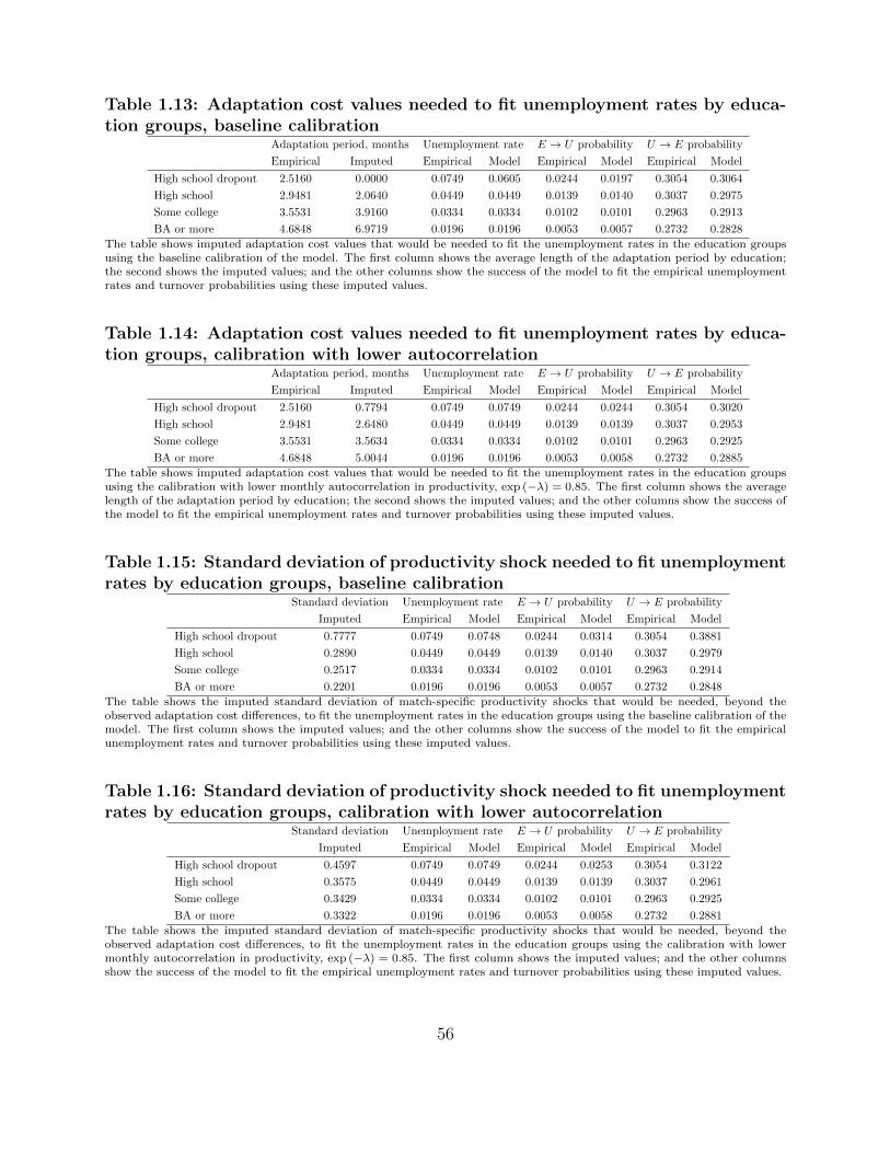
Table 1.13: Adaptation cost values needed to fit unemployment rates by educa-tion groups, baseline calibration

Adaptation period, months Unemployment rate E → U probability U → E probability

Empirical Imputed Empirical Model Empirical Model Empirical Model

High school dropout 2.5160 0.0000 0.0749 0.0605 0.0244 0.0197 0.3054 0.3064

High school 2.9481 2.0640 0.0449 0.0449 0.0139 0.0140 0.3037 0.2975

Some college 3.5531 3.9160 0.0334 0.0334 0.0102 0.0101 0.2963 0.2913

BA or more 4.6848 6.9719 0.0196 0.0196 0.0053 0.0057 0.2732 0.2828

The table shows imputed adaptation cost values that would be needed to fit the unemployment rates in the education groupsusing the baseline calibration of the model. The first column shows the average length of the adaptation period by education;the second shows the imputed values; and the other columns show the success of the model to fit the empirical unemploymentrates and turnover probabilities using these imputed values.

Table 1.14: Adaptation cost values needed to fit unemployment rates by educa-tion groups, calibration with lower autocorrelation

Adaptation period, months Unemployment rate E → U probability U → E probability

Empirical Imputed Empirical Model Empirical Model Empirical Model

High school dropout 2.5160 0.7794 0.0749 0.0749 0.0244 0.0244 0.3054 0.3020

High school 2.9481 2.6480 0.0449 0.0449 0.0139 0.0139 0.3037 0.2953

Some college 3.5531 3.5634 0.0334 0.0334 0.0102 0.0101 0.2963 0.2925

BA or more 4.6848 5.0044 0.0196 0.0196 0.0053 0.0058 0.2732 0.2885

The table shows imputed adaptation cost values that would be needed to fit the unemployment rates in the education groupsusing the calibration with lower monthly autocorrelation in productivity, exp (−λ) = 0.85. The first column shows the averagelength of the adaptation period by education; the second shows the imputed values; and the other columns show the success ofthe model to fit the empirical unemployment rates and turnover probabilities using these imputed values.

Table 1.15: Standard deviation of productivity shock needed to fit unemploymentrates by education groups, baseline calibration

Standard deviation Unemployment rate E → U probability U → E probability

Imputed Empirical Model Empirical Model Empirical Model

High school dropout 0.7777 0.0749 0.0748 0.0244 0.0314 0.3054 0.3881

High school 0.2890 0.0449 0.0449 0.0139 0.0140 0.3037 0.2979

Some college 0.2517 0.0334 0.0334 0.0102 0.0101 0.2963 0.2914

BA or more 0.2201 0.0196 0.0196 0.0053 0.0057 0.2732 0.2848

The table shows the imputed standard deviation of match-specific productivity shocks that would be needed, beyond theobserved adaptation cost differences, to fit the unemployment rates in the education groups using the baseline calibration of themodel. The first column shows the imputed values; and the other columns show the success of the model to fit the empiricalunemployment rates and turnover probabilities using these imputed values.

Table 1.16: Standard deviation of productivity shock needed to fit unemploymentrates by education groups, calibration with lower autocorrelation

Standard deviation Unemployment rate E → U probability U → E probability

Imputed Empirical Model Empirical Model Empirical Model

High school dropout 0.4597 0.0749 0.0749 0.0244 0.0253 0.3054 0.3122

High school 0.3575 0.0449 0.0449 0.0139 0.0139 0.3037 0.2961

Some college 0.3429 0.0334 0.0334 0.0102 0.0101 0.2963 0.2925

BA or more 0.3322 0.0196 0.0196 0.0053 0.0058 0.2732 0.2881

The table shows the imputed standard deviation of match-specific productivity shocks that would be needed, beyond theobserved adaptation cost differences, to fit the unemployment rates in the education groups using the calibration with lowermonthly autocorrelation in productivity, exp (−λ) = 0.85. The first column shows the imputed values; and the other columnsshow the success of the model to fit the empirical unemployment rates and turnover probabilities using these imputed values.

56

Figure 1.1: Unemployment rates and basic turnover probabilities by educationPanel A: Unemployment rates Panel B: Logit of unemployment rates

0.000.020.040.060.080.100.120.140.16

Une

mpl

oym

ent r

ate

1978 1982 1986 1990 1994 1998 2002 2006 2010 2014Date

HS dropouts High schoolSome college CollegeApproximations

-4.7-4.3-3.9-3.5-3.1-2.7-2.3-1.9-1.5

Logi

t une

mpl

oym

ent r

ate

1978 1982 1986 1990 1994 1998 2002 2006 2010 2014Date

HS dropouts High schoolSome college CollegeApproximations

Panel C: Monthly E → U probabilities Panel D: Log monthly E → U probabilities

0.000

0.006

0.012

0.018

0.024

0.030

0.036

0.042

0.048

E -

> U

pro

babi

lity

1978 1982 1986 1990 1994 1998 2002 2006 2010 2014Date

HS dropouts High schoolSome college College

-5.6

-5.3

-5.0

-4.7

-4.4

-4.1

-3.8

-3.5

-3.2

Log

E -

> U

pro

babi

lity

1978 1982 1986 1990 1994 1998 2002 2006 2010 2014Date


Panel E: Monthly U → E probabilities Panel F: Log monthly U → E probabilities

0.160

0.190

0.220

0.250

0.280

0.310

0.340

0.370

0.400

U -

> E

pro

babi

lity

1978 1982 1986 1990 1994 1998 2002 2006 2010 2014Date


-1.80

-1.70

-1.60

-1.50

-1.40

-1.30

-1.20

-1.10

-1.00

Log

U -

> E

pro

babi

lity

1978 1982 1986 1990 1994 1998 2002 2006 2010 2014Date


Sample: 25-55 year old males, CPS 1978-2013. All series are yearly moving averages of the monthly values. The logit of the

unemployment rate is the log odds ratio, logit (u) = ln(

u1−u

). The E → U transition probability is the probability that one

is unemployed at month t+ 1 conditional on being employed at month t. The U → E transition probability is the probabilitythat one is employed at month t + 1 conditional on being unemployed at month t. The approximations in Panel A and B areuapproxgt = pEU/(pEU + pUE). The gray shaded areas indicate NBER recessions.

57

Figure 1.2: Occupational unemployment and its approximation with turnoverrates

Panel A: Using 48 occupations

0

.02

.04

.06

.08

.1

.12

App

roxi

mat

ions

usi

ng tu

rnov

er

0 .02 .04 .06 .08 .1 .12Actual unemployment rate

Panel B: Using 191 occupations

0

.02

.04

.06

.08

.1

.12

.14

.16

App

roxi

mat

ions

usi

ng tu

rnov

er

0 .02 .04 .06 .08 .1 .12 .14 .16Actual unemployment rate

Sample: 25-55 year old males, CPS 1994-2008. Occupational unemployment is defined as ux = Ux/(Ex +Ux), where Ex is thenumber of employed persons with a primary job in occupation x; and Ux is the number of unemployed whose last occupation wasin x. The approximations use the steady state formula uapproxx = pEU

x /(pEUx + pUE

x ), where pEUx is the monthly employment

to unemployment transition probability in occupation x and pUEx is the monthly unemployment to employment transition

probability for persons with the last occupation in x.

58

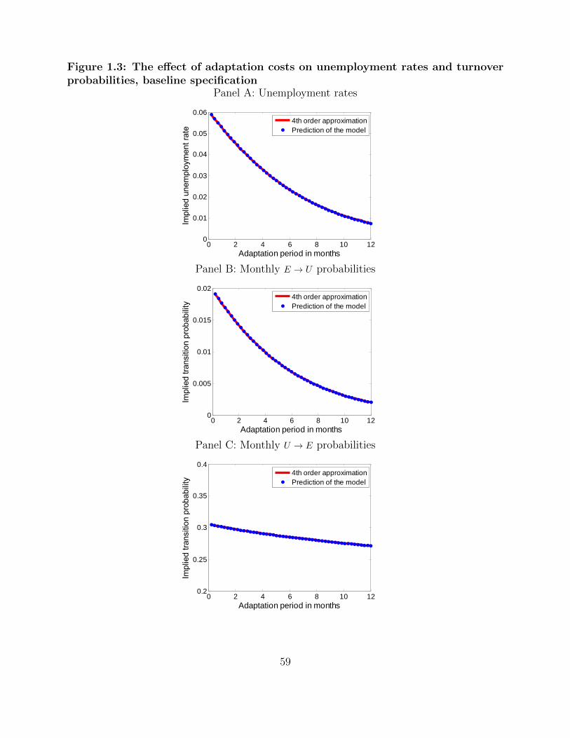
Figure 1.3: The effect of adaptation costs on unemployment rates and turnoverprobabilities, baseline specification

Panel A: Unemployment rates

0 2 4 6 8 10 120

0.01

0.02

0.03

0.04

0.05

0.06

Adaptation period in months

4th order approximationPrediction of the model

Panel B: Monthly E → U probabilities

0 2 4 6 8 10 120

0.005

0.01

0.015

0.02



Panel C: Monthly U → E probabilities

0 2 4 6 8 10 120.2

0.25

0.3

0.35

0.4



59

Figure 1.4: Observed and predicted unemployment rates and monthly transitionprobabilities by education, baseline specification

Panel A: Unemployment rates Panel B: Unemployment rate gap

0

.01

.02

.03

.04

.05

.06

.07

.08

Une

mpl

oym

ent r

ate

HS dropout High school Some college College

Observed Predicted

Explained gap: 11% 71% 65%

0

.005

.01

.015

.02

.025

.03

.035

Une

mpl

oym

ent r

ate

gap

Dropout - HS HS - Some col Some col - College

Observed Predicted

Panel C: Monthly E → U probabilities Panel D: Monthly E → U probability gap

0

.005

.01

.015

.02

.025

E->

U p

roba

bilit

y ra

te


Observed Predicted


0

.002

.004

.006

.008

.01

.012

E->

U p

roba

bilit

y ra

te g

ap


Observed Predicted

Panel E: Monthly U → E probabilities Panel E: Monthly U → E probability gap

.24

.26

.28

.3

.32

.34

.36

U->

E p

roba

bilit

y


Observed Predicted


-.01

0

.01

.02

.03

.04

U->

E p

roba

bilit

y ra

te g

ap


Observed Predicted

Sample: 25-55 year old males, CPS 1994-2008. The graph shows unemployment rates and monthly turnover probabilities byeducation from the CPS; and the model’s predicted values. The model’s predicted continuous transition rates are converted intomonthly transition probabilities by assuming transitions follow a Markov process. The error bars indicate the 95% confidenceintervals.

60

Figure 1.5: Observed and predicted unemployment rates by education, alterna-tive values of autocorrelation

Panel A: Unemployment rates, exp (−λ) = 0.85 Panel B: Unemployment rate gap, exp (−λ) = 0.85

0

.01

.02

.03

.04

.05

.06

.07

.08

Une

mpl

oym

ent r

ate


Observed Predicted


0

.005

.01

.015

.02

.025

.03

.035

Une

mpl

oym

ent r

ate

gap


Observed Predicted

Panel C: Unemployment rates, exp (−λ) = 0.95 Panel D: Unemployment rate gap, exp (−λ) = 0.95

0

.01

.02

.03

.04

.05

.06

.07

.08

Une

mpl

oym

ent r

ate


Observed Predicted


0

.005

.01

.015

.02

.025

.03

.035

Une

mpl

oym

ent r

ate

gap


Observed Predicted

Sample: 25-55 year old males, CPS 1994-2008. The graph shows unemployment rates and monthly turnover probabilities byeducation from the CPS; and the model’s predicted values. The model’s predicted continuous transition rates are converted intomonthly transition probabilities by assuming transitions follow a Markov process. The error bars indicate the 95% confidenceintervals.

Figure 1.6: The effect of adaptation costs on unemployment rates for variousvalues of monthly autocorrelation in match-specific productivity

0 2 4 6 8 10 120

0.02

0.04

0.06

0.08

0.1

0.12

0.14

0.16

0.18


exp(-λ)=0.71exp(-λ)=0.85exp(-λ)=0.92exp(-λ)=0.95

61

APPENDIX A

The value functions in the basic model

Let us consider the value functions of firms. I normalize all values with occupational

productivity, sx. Let sxVx, sxJRx (ε) and sxJx (ε) denote the value of an unfilled job, being

matched with a rookie and with an experienced worker with productivity ε, respectively.

The Bellman equation for the value of vacancies (V ) is

rsxVx = −sxc+ qxsx(JRx(ε0)− Vx

)= 0. (1.31)

The flow value of a vacant job is the instantaneous search cost with a negative sign plus the

expected capital gain, which is the value difference between employing a rookie with initial

productivity ε0 and having no worker, multiplied by the vacancy filling rate. Free entry of

firms assures that the asset value of a vacant job is zero. The Bellman equation for the value

of employing an experiences worker (J) is

rsxJx (ε) = sxε− sxwx (ε) + λsx

ˆ ∞εx

Jx (ε′) dF (ε′)−(λ+ fL,ex

)sxJx (ε) . (1.32)

The employer gets the flow profit minus the wage, plus the expected capital gains. Whenever

a productivity shock or exogenous separation shock occurs, the firm loses the value of the

current state and gains the value of the new state. If the productivity shock is larger than

the productivity threshold εx, the firm receives the value evaluated at the new productivity.

If the shock is smaller than the reservation productivity or an exogenous separation occurs

62

the firms’ new value is sxVx = 0. The Bellman equation for employing a rookie (JR) is

rsxJRx (ε) = sxδε− sxwRx (ε) + λsx

ˆ ∞εRx

JRx (ε′) dF (ε′)

−(λ+ fL,ex

)sxJ

Rx (ε) + ϕxsx

(Jx (ε)− JRx (ε)

). (1.33)

Apart from the last term, the Bellman equation for rookies is similar to that of experi-

enced workers, but the flow productivity is smaller (δ < 1 fraction of experienced workers’

productivity) and the endogenous parameters (the wage, the value of the match and the

productivity threshold) might differ, too. The last term describes the capital gain from ex-

perience as the difference in the values of being matched with an experienced worker and a

rookie, multiplied by the rate at which rookies become experienced (ϕx).

Now let’s consider the value functions of workers. Let sxUx, sxWRx (ε) and sxWx (ε) denote

the value of being unemployed, being a rookie and being an experienced worker, respectively.

The Bellman equation for being unemployed (U ) is

rsxUx = sxb+ fFx sx(WRx

(ε0)− Ux

). (1.34)

The flow value of being unemployed is the instantaneous value sxb, plus the capital gain from

finding a job and becoming a rookie. The Bellman equation for being an experienced worker

(W ) is

rsxWx (ε) = sxwx (ε) + λsx

ˆ ∞εx

Wx (ε′) dF (ε′) +(λF (εx) + fL,ex

)sxUx −

(λ+ fL,ex

)sxWx (ε) . (1.35)

Workers receive the flow wage and the expected capital gain from shocks. If the productivity

shock is larger than the threshold value εx, they gain the value of the new state and lose the

63

value of the current state. If the productivity shock is smaller than the reservation threshold

or an exogenous separation occurs, workers gain the value of being unemployed and lose the

value of the current state. Finally, the Bellman equation for being a rookie (WR) is

rsxWRx (ε) = sxw

Rx (ε) + λsx

ˆ ∞εRx

WRx (ε′) dF (ε′) +

(λF(εRx)

+ fL,ex)sxUx

−(λ+ fL,ex

)sxW

Rx (ε) + ϕxsx

(Wx (ε)−WR

x (ε)). (1.36)

The value of being a rookie is similar to the value of being an experienced worker, but there

is an extra term at the end that describes the capital gain from gaining experience.

Next, I normalize all equations by occupational productivity, sx, and rearrange the value

functions (1.31)-(1.36):

0 = −c+ qxJRx

(ε0), (1.37)

(r + λ+ fL,ex + ϕx

)JRx (ε) = δε− wRx (ε) + λ

ˆ ∞εRx

JRx (ε′) dF (ε′) + ϕxJx (ε) , (1.38)

(r + λ+ fL,ex

)Jx (ε) = ε− wx (ε) + λ

ˆ ∞εx

Jx (ε′) dF (ε′) , (1.39)

rUx = b+ fFx(WRx

(ε0)− Ux

), (1.40)


)WRx (ε) = wRx (ε) + λ

ˆ ∞εRx

WRx (ε′) dF (ε′) +

(λF(εRx)

+ fL,ex)Ux

+ϕxWx (ε) , (1.41)

(r + λ+ fL,ex

)Wx (ε) = wx (ε) + λ

ˆ ∞εx


)Ux. (1.42)

Finally, to close the model, wages are continuously renegotiated and are set by generalized

64

Nash bargaining,

wRx (ε) = arg max{(WRx (ε)− URx (ε)

)γJRx (ε)

1−γ}, (1.43)

wx (ε) = arg max{

(Wx (ε)− Ux (ε))γJx (ε)

1−γ}. (1.44)

The normalized value functions (1.37)-(1.42) together with the wage equations (1.43)-(1.44)

and the matching function (1.13) fully characterize the model.

65

APPENDIX B

Derivation of the equilibrium conditions in the basic

model

The surpluses from the matches can be written as


)SRx (ε) =


) (JRx (ε) +WR

x (ε)− Ux)

= δε+ λ

ˆ ∞εRx

SNx (ε′) dF (ε′) + ϕxSx (ε)− rUx, (1.45)

(r + λ+ fL,ex

)Sx (ε) =

(r + λ+ fL,ex

)(Jx (ε) +Wx (ε)− Ux)

= ε+ λ

ˆ ∞εx

Sx (ε′) dF (ε′)− rUx. (1.46)

By taking the derivatives of both sides with respect to the idiosyncratic productivity ε we

get

∂Sx (ε)

∂ε=

1

r + λ+ fL,ex, (1.47)

∂SRx (ε)

∂ε=

δ + ϕx∂Sx(ε)∂ε

r + λ+ fL,ex + ϕx=

δ + ϕx

r+λ+fL,ex

r + λ+ fL,ex + ϕx. (1.48)

The surpluses are linear functions of the the match-specific productivity. Moreover, the

surpluses equal to zero at the reservation productivity values (εx and εRx ) . Thus, the surpluses

66

can be written as

Sx (ε) =1

r + λ+ fL,ex(ε− εx) , (1.49)

SRx (ε) =δ + ϕx

r+λ+fL,ex

r + λ+ fL,ex + ϕx

(ε− εRx

). (1.50)

By combining equation (1.15), (1.37) and (1.50) we get the job creation condition:

c

ηθ1−αx = JRx

(ε0)

= (1− γ)SRx(ε0)

= (1− γ)δ + ϕx

r+λ+fL,ex

r + λ+ fL,ex + ϕx

(ε0 − εRx

). (1.51)

In the first line I used the Nash formula to rewrite the firms’ value in terms of the surplus:

workers and firms split the surplus according to their bargaining power.

In order to derive the job-destruction condition we need to write rU as a function of the

surplus. I use equation (1.40), (1.14) and (1.15) to get:

rUx = b+ fFx(WRx

(ε0)− Ux

)= b+ fFx γS

Rx

(ε0)

= b+γ

1− γfFxqxc = b+

γ

1− γθxc. (1.52)

To find the reservation productivity below which matches are endogenously destroyed, we

need to find the productivity values at which the surplus becomes zero. By plugging (1.52)

into (1.45) and (1.46) we get the job destruction conditions:

b+γ

1− γθxc = εx + λ

ˆ ∞εx

Sx (ε′) dF (ε′) , (1.53)

b+γ


ˆ ∞εRx

SRx (ε′) dF (ε′) + ϕxSx(εRx). (1.54)

67

By substituting in for the surplus formulas in (1.49) and (1.50) we get

b+γ

1− γθxc = εx +

λ

r + λ+ fL,ex

ˆ ∞εx

(ε′ − εx) dF (ε′) , (1.55)

b+γ


δ + ϕx

r+λ+fL,ex

r + λ+ fL,ex + ϕx

ˆ ∞εRx

(ε′ − εRx

)dF (ε′) +

ϕxr + λ+ fL,ex

(εRx − εx

).(1.56)

Now let us see the wages. I start with the wages of experienced workers. From (1.39)

and the Nash rule we get

(r + λ+ fL,ex

)Jx (ε) = ε− wx (ε) + λ

ˆ ∞εx

Jx (ε′) dF (ε′) , (1.57)

(r + λ+ fL,ex

)(1− γ)Sx (ε) = ε− wx (ε) + λ

ˆ ∞εx

(1− γ)Sx (ε′) dF (ε′) , (1.58)

(r + λ+ fL,ex

)Sx (ε) =

ε− wx (ε)

1− γ+ λ

ˆ ∞εx

Sx (ε′) dF (ε′) . (1.59)

Similarly from (1.35), (1.52) and the Nash rule we get

(r + λ+ fL,ex

)Wx (ε) = wx (ε) + λ

ˆ ∞εx


)Ux, (1.60)

(r + λ+ fL,ex

)(Wx (ε)− Ux) = wx (ε) + λ

ˆ ∞εx

(Wx (ε′)− Ux) dF (ε′)− rUx, (1.61)

(r + λ+ fL,ex

)γSx (ε) = wx (ε) + λ

ˆ ∞εx

γSx (ε) dF (ε′)− b− γ

1− γθxc, (1.62)

(r + λ+ fL,ex

)Sx (ε) =

wx (ε)− bγ

− 1

1− γθxc+ λ

ˆ ∞εx

Sx (ε′) dF (ε′) . (1.63)

By combining (1.59) and (1.63) we get

ε− wx (ε)

1− γ=

wx (ε)− bγ

− 1

1− γθxc, (1.64)

γ (ε− wx (ε)) = (1− γ) (wx (ε)− b)− γθxc, (1.65)

wx (ε) = (1− γ) b+ γ (ε+ θxc) . (1.66)

68

The last equation shows the equilibrium wage of experienced workers. The wages of rookies

can be derived similarly. From (1.38) and the Nash rule


)JRx (ε) = δε− wRx (ε) + λ

ˆ ∞εRx

JRx (ε′) dF (ε′) + ϕxJx (ε) , (1.67)


)(1− γ)SRx (ε) = δε− wRx (ε) + λ

ˆ ∞εRx

(1− γ)SRx (ε′) dF (ε′)

+ϕx (1− γ)Sx (ε) , (1.68)


)SRx (ε) =

δε− wRx (ε)

1− γ+ λ

ˆ ∞εRx

SRx (ε′) dF (ε′) + ϕxSx (ε) . (1.69)

From (1.38), (1.52) and the Nash rule we get


)WRx (ε) = wRx (ε) + λ

ˆ ∞εRx

WRx (ε′) dF (ε′) +

(λF(εRx)

+ fL,ex)Ux

+ϕxWx (ε) , (1.70)


) (WRx (ε)− Ux

)= wRx (ε) + λ

ˆ ∞εRx

(WRx (ε′)− Ux

)dF (ε′)

+ϕx (Wx (ε)− Ux)− rUx, (1.71)


)γSRx (ε) = wRx (ε)− b− γ

1− γθxc+ λ

ˆ ∞εRx

γSRx (ε′) dF (ε′) (1.72)

+ϕxγSx (ε) , (1.73)


)SRx (ε) =

wRx (ε)− bγ

− 1

1− γθxc+ λ

ˆ ∞εRx

SRx (ε′) dF (ε′) (1.74)

+ϕxSx (ε) . (1.75)

69

By combining (1.69) and (1.74) we get

δε− wRx (ε)

1− γ=

wRx (ε)− bγ

− 1

1− γθxc, (1.76)

γ(δε− wRx (ε)

)= (1− γ)

(wRx (ε)− b

)− γθxc, (1.77)

wRx (ε) = (1− γ) b+ γ (δε+ θxc) . (1.78)

70

APPENDIX C

Proof that the model is invariant to the choice of

aggregate θ in Chapter I

θ appears at three places in the equilibrium conditions. The first is the job finding rate

fF = ηθα. As the constant term of the matching function, η, is calibrated to fit the job finding

rate, any change in θ is sucked up by η. The second place where θ appears is the job creation

condition, where the left-hand side is the total expected cost of filling a vacancy:

C =c

ηθ1−α. (1.79)

The total cost of filling a vacancy, however, is one of the moments I am matching. Therefore,

c sucks up any variation in θ1−α/η to fit the total cost C. The third place where θ appears is

the outside option of workers in the job loss conditions:

o =γ

1− γθc =

γ

1− γC

fF. (1.80)

The outside option of workers can be rewritten in terms of only the total search costs (C)

and the job finding rate (fF ), which are targeted moments. Therefore the outside option of

workers is also indifferent to the choice of θ.

Overall, any mismeasurement of θ is sucked up by η and c, and the equilibrium turnover

probabilities are unaffected by it.

71

APPENDIX D

Additional tablesTable 1.17: OLS regressions of unemployment in recessions

Unemployment rate

U = 0.065 (1) (2) (3) (4) (5) (6) (7)


(0.001) (0.001) (0.001) (0.001) (0.001) (0.001) (0.001)


Some college -0.020** -0.021** -0.010** -0.007** -0.006** -0.005** -0.005**

(0.001) (0.001) (0.001) (0.001) (0.001) (0.001) (0.001)

BA or more -0.051** -0.048** -0.023** -0.020** -0.017** -0.016** -0.016**

(0.001) (0.001) (0.001) (0.001) (0.001) (0.001) (0.001)


Age 30-34 -0.008** -0.007** -0.006** -0.005** -0.005** -0.005**

(0.001) (0.001) (0.001) (0.001) (0.001) (0.001)

Age 35-39 -0.012** -0.011** -0.009** -0.008** -0.007** -0.007**

(0.001) (0.001) (0.001) (0.001) (0.001) (0.001)

Age 40-44 -0.017** -0.015** -0.013** -0.011** -0.010** -0.010**

(0.001) (0.001) (0.001) (0.001) (0.001) (0.001)

Age 45-49 -0.019** -0.017** -0.014** -0.012** -0.010** -0.011**

(0.001) (0.001) (0.001) (0.001) (0.001) (0.001)

Age 50-55 -0.020** -0.017** -0.014** -0.011** -0.010** -0.010**

(0.001) (0.001) (0.001) (0.001) (0.001) (0.001)


Non whites 0.037** 0.036** 0.036** 0.035** 0.036** 0.036**

(0.001) (0.001) (0.001) (0.001) (0.001) (0.001)


Married -0.047** -0.047** -0.045** -0.043** -0.043** -0.042**

(0.001) (0.001) (0.001) (0.001) (0.001) (0.001)







Observations 3,898,606 3,898,606 3,898,606 3,898,606 3,898,606 3,898,606 3,898,606Sample: 25-55 year old males, CPS. Robust standard errors clustered on the individual level are in parentheses. ** p<0.01,* p<0.05. Recession indicates years when the aggregate unemployment rate was above 5 percent in the sample: 1980-1986,1991-1993 and 2009-2013.

72

Table 1.18: Logit regressions of monthly employment to unemployment transi-tion probability

Log monthly E → U transition probability

(1) (2) (3) (4) (5) (6) (7)


(0.011) (0.012) (0.012) (0.012) (0.012) (0.012) (0.012)


Some college -0.316** -0.319** -0.129** -0.081** -0.062** -0.054** -0.050**

(0.012) (0.012) (0.012) (0.012) (0.012) (0.012) (0.012)

BA or more -1.011** -0.967** -0.458** -0.420** -0.332** -0.321** -0.311**

(0.013) (0.013) (0.017) (0.017) (0.017) (0.017) (0.017)


Age 30-34 -0.129** -0.123** -0.108** -0.095** -0.088** -0.090**

(0.014) (0.014) (0.014) (0.014) (0.014) (0.014)

Age 35-39 -0.228** -0.218** -0.192** -0.165** -0.151** -0.153**

(0.014) (0.014) (0.014) (0.014) (0.014) (0.014)

Age 40-44 -0.311** -0.292** -0.255** -0.217** -0.193** -0.194**

(0.015) (0.015) (0.015) (0.015) (0.015) (0.015)

Age 45-49 -0.385** -0.360** -0.316** -0.267** -0.235** -0.238**

(0.016) (0.016) (0.016) (0.016) (0.016) (0.016)

Age 50-55 -0.465** -0.436** -0.385** -0.326** -0.284** -0.287**

(0.016) (0.016) (0.016) (0.016) (0.016) (0.016)


Non whites 0.325** 0.325** 0.350** 0.331** 0.351** 0.355**

(0.012) (0.012) (0.012) (0.012) (0.012) (0.012)


Married -0.545** -0.540** -0.504** -0.466** -0.454** -0.453**

(0.009) (0.009) (0.009) (0.009) (0.009) (0.009)







Log likelihood -417,334 -411,862 -407,189 -401,047 -397,659 -394,664 -393,962

Observations 6,064,820 6,064,820 6,064,820 6,064,820 6,064,820 6,064,820 6,064,820Sample: 25-55 year old males, CPS 1978-2013. The table shows average log differences in

the implied probabilities from baseline. For example, the coefficient on BA is βimpliedBA =

1N

∑i

[ln Pr

(PEUi = 1|educ = BA,Xi

)− ln Pr

(PEUi = 1|educ = HS,Xi

)]. More generally, in dimension j and cate-

gory k the coefficient is βimpliedjk = 1

N

∑i

[ln Pr

(PEUi = 1|Ij = k,Xi

)− ln Pr


)]. Robust standard errors

clustered on the individual level are in parentheses. ** p<0.01, * p<0.05.

73

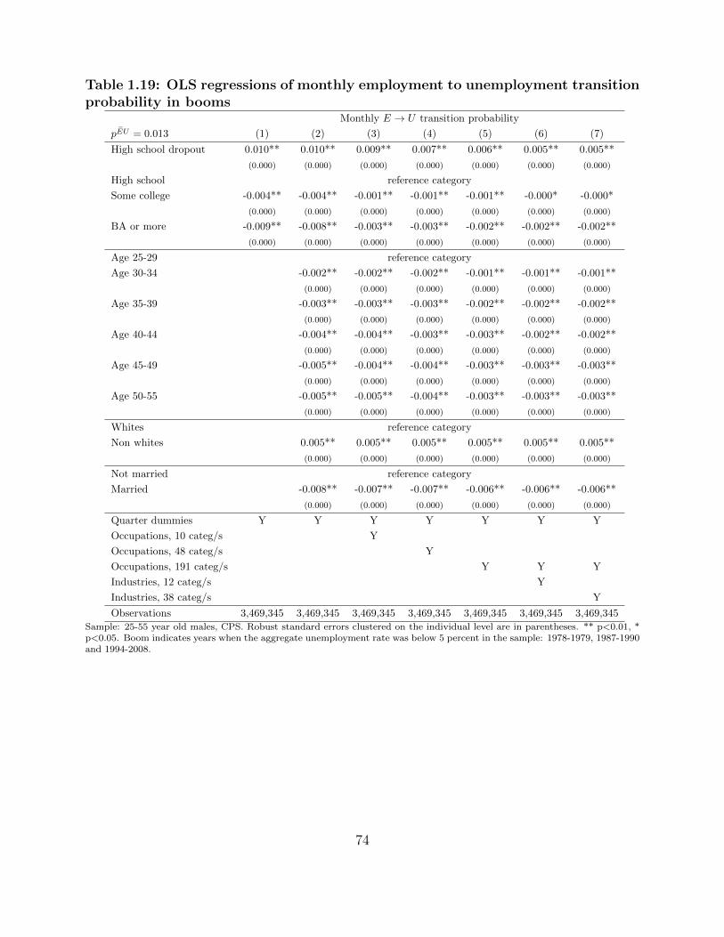
Table 1.19: OLS regressions of monthly employment to unemployment transitionprobability in booms

Monthly E → U transition probability¯pEU = 0.013 (1) (2) (3) (4) (5) (6) (7)


(0.000) (0.000) (0.000) (0.000) (0.000) (0.000) (0.000)


Some college -0.004** -0.004** -0.001** -0.001** -0.001** -0.000* -0.000*

(0.000) (0.000) (0.000) (0.000) (0.000) (0.000) (0.000)

BA or more -0.009** -0.008** -0.003** -0.003** -0.002** -0.002** -0.002**

(0.000) (0.000) (0.000) (0.000) (0.000) (0.000) (0.000)


Age 30-34 -0.002** -0.002** -0.002** -0.001** -0.001** -0.001**

(0.000) (0.000) (0.000) (0.000) (0.000) (0.000)

Age 35-39 -0.003** -0.003** -0.003** -0.002** -0.002** -0.002**

(0.000) (0.000) (0.000) (0.000) (0.000) (0.000)

Age 40-44 -0.004** -0.004** -0.003** -0.003** -0.002** -0.002**

(0.000) (0.000) (0.000) (0.000) (0.000) (0.000)

Age 45-49 -0.005** -0.004** -0.004** -0.003** -0.003** -0.003**

(0.000) (0.000) (0.000) (0.000) (0.000) (0.000)

Age 50-55 -0.005** -0.005** -0.004** -0.003** -0.003** -0.003**

(0.000) (0.000) (0.000) (0.000) (0.000) (0.000)


Non whites 0.005** 0.005** 0.005** 0.005** 0.005** 0.005**

(0.000) (0.000) (0.000) (0.000) (0.000) (0.000)


Married -0.008** -0.007** -0.007** -0.006** -0.006** -0.006**

(0.000) (0.000) (0.000) (0.000) (0.000) (0.000)







Observations 3,469,345 3,469,345 3,469,345 3,469,345 3,469,345 3,469,345 3,469,345Sample: 25-55 year old males, CPS. Robust standard errors clustered on the individual level are in parentheses. ** p<0.01, *p<0.05. Boom indicates years when the aggregate unemployment rate was below 5 percent in the sample: 1978-1979, 1987-1990and 1994-2008.

74

Table 1.20: OLS regressions of monthly employment to unemployment transitionprobability in recessions

Monthly E → U transition probability¯pEU = 0.018 (1) (2) (3) (4) (5) (6) (7)


(0.000) (0.000) (0.000) (0.000) (0.000) (0.000) (0.000)


Some college -0.006** -0.006** -0.002** -0.002** -0.001** -0.001** -0.001**

(0.000) (0.000) (0.000) (0.000) (0.000) (0.000) (0.000)

BA or more -0.013** -0.012** -0.005** -0.005** -0.004** -0.003** -0.003**

(0.000) (0.000) (0.000) (0.000) (0.000) (0.000) (0.000)


Age 30-34 -0.003** -0.003** -0.003** -0.003** -0.003** -0.003**

(0.000) (0.000) (0.000) (0.000) (0.000) (0.000)

Age 35-39 -0.005** -0.005** -0.004** -0.004** -0.004** -0.004**

(0.000) (0.000) (0.000) (0.000) (0.000) (0.000)

Age 40-44 -0.006** -0.006** -0.005** -0.005** -0.004** -0.004**

(0.000) (0.000) (0.000) (0.000) (0.000) (0.000)

Age 45-49 -0.007** -0.007** -0.006** -0.005** -0.005** -0.005**

(0.000) (0.000) (0.000) (0.000) (0.000) (0.000)

Age 50-55 -0.009** -0.008** -0.007** -0.006** -0.006** -0.006**

(0.000) (0.000) (0.000) (0.000) (0.000) (0.000)


Non whites 0.006** 0.006** 0.006** 0.006** 0.006** 0.006**

(0.000) (0.000) (0.000) (0.000) (0.000) (0.000)


Married -0.009** -0.009** -0.008** -0.008** -0.007** -0.007**

(0.000) (0.000) (0.000) (0.000) (0.000) (0.000)







Observations 2,595,475 2,595,475 2,595,475 2,595,475 2,595,475 2,595,475 2,595,475Sample: 25-55 year old males, CPS. Robust standard errors clustered on the individual level are in parentheses. ** p<0.01,* p<0.05. Recession indicates years when the aggregate unemployment rate was above 5 percent in the sample: 1980-1986,1991-1993 and 2009-2013.

75

Table 1.21: Logit regressions of monthly unemployment to employment transi-tion probability

Log monthly U → E transition probability

(1) (2) (3) (4) (5) (6) (7)

High school dropout 0.038** 0.034** 0.024* 0.008 0.005 0.002 0.000

(0.010) (0.010) (0.010) (0.010) (0.010) (0.010) (0.010)


Some college -0.001 0.004 0.037** 0.045** 0.046** 0.048** 0.049**

(0.010) (0.010) (0.010) (0.010) (0.011) (0.011) (0.011)

BA or more -0.047** -0.047** 0.036** 0.044** 0.054** 0.059** 0.064**

(0.012) (0.012) (0.014) (0.014) (0.014) (0.014) (0.014)


Age 30-34 -0.039** -0.045** -0.046** -0.049** -0.050** -0.051**

(0.012) (0.012) (0.012) (0.012) (0.012) (0.012)

Age 35-39 -0.088** -0.096** -0.098** -0.101** -0.101** -0.102**

(0.012) (0.013) (0.013) (0.013) (0.013) (0.013)

Age 40-44 -0.119** -0.126** -0.125** -0.128** -0.128** -0.129**

(0.013) (0.013) (0.013) (0.013) (0.013) (0.013)

Age 45-49 -0.169** -0.174** -0.171** -0.175** -0.174** -0.175**

(0.014) (0.014) (0.014) (0.014) (0.014) (0.014)

Age 50-55 -0.255** -0.258** -0.254** -0.256** -0.255** -0.256**

(0.014) (0.014) (0.014) (0.014) (0.014) (0.014)


Non whites -0.245** -0.232** -0.223** -0.220** -0.218** -0.218**

(0.010) (0.010) (0.010) (0.010) (0.010) (0.010)


Married 0.197** 0.191** 0.195** 0.193** 0.195** 0.195**

(0.008) (0.008) (0.008) (0.008) (0.008) (0.008)







Log likelihood -174,504 -173,168 -172,751 -172,100 -171,819 -171,628 -171,459

Observations 295,045 295,045 295,045 295,045 295,045 295,045 295,045Sample: 25-55 year old males, CPS 1978-2013. The table shows average log differences in

the implied probabilities from baseline. For example, the coefficient on BA is βimpliedBA =

1N

∑i

[ln Pr

(PUEi = 1|educ = BA,Xi

)− ln Pr

(PUEi = 1|educ = HS,Xi

)]. More generally, in dimension j and cate-

gory k the coefficient is βimpliedjk = 1

N

∑i

[ln Pr

(PEUi = 1|Ij = k,Xi

)− ln Pr


)]. Robust standard errors

clustered on the individual level are in parentheses. ** p<0.01, * p<0.05.

76

Table 1.22: OLS regressions of monthly unemployment to employment transitionprobability in booms

Monthly U → E transition probability¯pUE = 0.33 (1) (2) (3) (4) (5) (6) (7)

High school dropout 0.004 0.002 -0.002 -0.005 -0.005 -0.006 -0.006

(0.004) (0.004) (0.004) (0.004) (0.004) (0.004) (0.004)


Some college -0.005 -0.003 0.007 0.010* 0.010* 0.010* 0.011**

(0.004) (0.004) (0.004) (0.004) (0.004) (0.004) (0.004)

BA or more -0.027** -0.027** -0.000 0.003 0.005 0.007 0.009

(0.005) (0.005) (0.005) (0.005) (0.005) (0.005) (0.005)


Age 30-34 -0.015** -0.017** -0.017** -0.018** -0.018** -0.018**

(0.005) (0.005) (0.005) (0.005) (0.005) (0.005)

Age 35-39 -0.030** -0.033** -0.033** -0.033** -0.033** -0.033**

(0.005) (0.005) (0.005) (0.005) (0.005) (0.005)

Age 40-44 -0.040** -0.042** -0.041** -0.042** -0.042** -0.042**

(0.005) (0.005) (0.005) (0.005) (0.005) (0.005)

Age 45-49 -0.056** -0.058** -0.056** -0.056** -0.055** -0.055**

(0.006) (0.006) (0.006) (0.006) (0.006) (0.006)

Age 50-55 -0.086** -0.087** -0.084** -0.084** -0.083** -0.083**

(0.005) (0.005) (0.005) (0.005) (0.005) (0.005)


Non whites -0.070** -0.067** -0.064** -0.062** -0.062** -0.062**

(0.004) (0.004) (0.004) (0.004) (0.004) (0.004)


Married 0.058** 0.057** 0.058** 0.057** 0.057** 0.057**

(0.003) (0.003) (0.003) (0.003) (0.003) (0.003)







Observations 129,968 129,968 129,968 129,968 129,968 129,968 129,968Sample: 25-55 year old males, CPS. Robust standard errors clustered on the individual level are in parentheses. ** p<0.01, *p<0.05. Boom indicates years when the aggregate unemployment rate was below 5 percent in the sample: 1978-1979, 1987-1990and 1994-2008.

77

Table 1.23: OLS regressions of monthly unemployment to employment transitionprobability in recessions

Monthly U → E transition probability¯pUE = 0.26 (1) (2) (3) (4) (5) (6) (7)

High school dropout 0.015** 0.015** 0.013** 0.008* 0.006 0.005 0.005

(0.003) (0.003) (0.003) (0.003) (0.003) (0.003) (0.003)


Some college 0.003 0.005 0.012** 0.013** 0.013** 0.013** 0.013**

(0.003) (0.003) (0.003) (0.003) (0.003) (0.003) (0.003)

BA or more 0.002 0.002 0.018** 0.019** 0.021** 0.022** 0.022**

(0.004) (0.004) (0.004) (0.005) (0.005) (0.005) (0.005)


Age 30-34 -0.007 -0.008 -0.008 -0.008* -0.008* -0.009*

(0.004) (0.004) (0.004) (0.004) (0.004) (0.004)

Age 35-39 -0.018** -0.019** -0.020** -0.021** -0.021** -0.021**

(0.004) (0.004) (0.004) (0.004) (0.004) (0.004)

Age 40-44 -0.025** -0.026** -0.025** -0.026** -0.026** -0.026**

(0.004) (0.004) (0.004) (0.004) (0.004) (0.004)

Age 45-49 -0.034** -0.035** -0.035** -0.036** -0.036** -0.036**

(0.004) (0.004) (0.004) (0.004) (0.004) (0.004)

Age 50-55 -0.048** -0.049** -0.047** -0.048** -0.048** -0.048**

(0.004) (0.004) (0.004) (0.004) (0.004) (0.004)


Non whites -0.053** -0.049** -0.046** -0.046** -0.045** -0.044**

(0.003) (0.003) (0.003) (0.003) (0.003) (0.003)


Married 0.046** 0.043** 0.044** 0.044** 0.044** 0.044**

(0.003) (0.003) (0.003) (0.003) (0.003) (0.003)







Observations 165,077 165,077 165,077 165,077 165,077 165,077 165,077Sample: 25-55 year old males, CPS. Robust standard errors clustered on the individual level are in parentheses. ** p<0.01,* p<0.05. Recession indicates years when the aggregate unemployment rate was above 5 percent in the sample: 1980-1986,1991-1993 and 2009-2013.

78

Table 1.24: Observed and predicted unemployment rates and turnover probabil-ities by education, baseline specification

Unemployment rate E → U probability U → E probability

Observed Predicted Observed Predicted Observed Predicted

High school dropout, HSD 0.0749** 0.0469** 0.0244** 0.0147** 0.3054** 0.2987**

(0.0008) (0.0018) (0.0004) (0.0006) (0.0040) (0.0009)

High school, HS 0.0449** 0.0435** 0.0139** 0.0135** 0.3037** 0.2973**

(0.0003) (0.0009) (0.0001) (0.0003) (0.0026) (0.0004)

Some college, SC 0.0334** 0.0354** 0.0102** 0.0107** 0.2963** 0.2932**

(0.0003) (0.0014) (0.0001) (0.0005) (0.0033) (0.0007)

BA or more, BA 0.0196** 0.0265** 0.0053** 0.0078** 0.2732** 0.2885**

(0.0002) (0.0021) (0.0001) (0.0007) (0.0039) (0.0013)

Differences

HSD-HS 0.0300** 0.0034 0.0105** 0.0012 0.0017 0.0015

(0.0009) (0.002) (0.0004) (0.0007) (0.0047) (0.001)

HS-SC 0.0115** 0.0082** 0.0037** 0.0028** 0.0074 0.0041**

(0.0004) (0.0017) (0.0002) (0.0006) (0.0042) (0.0008)

HS-BA 0.0253** 0.017** 0.0086** 0.0056** 0.0305** 0.0087**

(0.0004) (0.0023) (0.0002) (0.0008) (0.0047) (0.0014)

SC-BA 0.0138** 0.0089** 0.0049** 0.0029** 0.0231** 0.0047**

(0.0004) (0.0026) (0.0002) (0.0008) (0.0051) (0.0015)

Fraction of explained gap

HSD-HS 0.1126 0.1136 0.8774

HS-SC 0.7067 0.7522 0.5475

HS-BA 0.6733 0.6559 0.2868

SC-BA 0.6454 0.5840 0.2032** p<0.01, * p<0.05. Sample: 1994-2008, 25-55 year old males. The odd columns show unemployment rates and monthlyturnover probabilities by education from the CPS with robust standard errors clustered on the individual level. The evencolumns show the model’s predicted values and the fraction of the gap between education groups explained by adaptation costs.The model’s predicted continuous transition rates are converted into monthly transition probabilities by assuming transitionsfollow a Markov process.

79

Table 1.25: Imputed adaptation period by detailed occupations, in months# Occupation Imputation 1 Imputation 2 MCSUI avg # in MCSUI

1 Waiter’s assistant 1.154 1.086 1.654 8

2 Laundry workers 1.177 0.937 1.482 12

3 Metal and plastic processing machine operators 1.275 1.255 2.811 3

4 Crane, derrick, winch, and hoist operators 1.284 1.125 - 0

5 Waiter/waitress, food counter and fountain workers 1.348 1.339 1.342 64

6 Interviewers, enumerators, and surveyors 1.361 1.398 0.941 1

7 Recreation facility attendants 1.362 1.139 2.409 3

8 Vehicle washers and equipment cleaners 1.376 1.352 0.670 2

9 Misc food prep workers 1.380 1.645 1.197 33

10 Textile sewing machine operators 1.410 1.331 1.664 2

11 Janitors 1.428 1.225 1.713 52

12 Mail carriers for postal service 1.448 1.375 1.258 12

13 Cashiers 1.479 1.317 0.863 72

14 Stock and inventory clerks 1.518 1.717 1.544 48

15 Precision woodworking occupations 1.588 1.659 8.327 4

16 Woodworking machine operators 1.620 1.496 10.784 4

17 Auto body repairers 1.627 1.773 6.041 2

18 Other textile, apparel, and furnishings operators 1.653 1.656 3.796 4

19 Postal clerks, excluding mail carriers 1.663 1.649 0.471 1

20 Photographers 1.690 2.309 12.405 2

21 Kitchen workers 1.699 1.480 1.514 5

22 Butchers and meat cutters 1.705 1.719 15.278 2

23 Fishers, hunters, and kindred 1.718 2.156 1.548 3...

169 Farm operators and managers 5.388 5.197 5.647 2

170 Registered nurses 5.393 5.038 4.874 29

171 Physical scientists 5.416 6.011 12.235 1

172 Vocational and educational counselors 5.538 5.965 4.893 10

173 Human resource, marketing, advertising managers 5.558 4.841 4.593 16

174 Managers of properties and real estate 5.646 6.170 2.612 3

175 Other managers 5.679 5.468 3.668 68

176 Secondary school teachers 5.750 6.632 12.144 2

177 Social workers 5.815 5.647 6.943 16

178 Managers in education and related fields 6.040 5.997 15.436 7

179 Financial services sales occupations 6.044 6.435 3.747 3

180 Special education teachers 6.120 6.911 4.440 3

181 Management support occupations 6.140 6.023 2.779 33

182 Postsecondary teachers 6.190 6.441 10.948 26

183 Primary school teachers 6.205 7.832 14.146 17

184 Life scientists 6.378 6.475 - 0

185 Psychologists 6.381 5.937 - 0

186 Financial managers 6.566 6.457 10.261 3

187 Other social scientists and urban planners 6.566 6.500 2.847 2

188 Lawyers and Judges 6.697 5.669 10.786 3

189 Managers of medicine and health occupations 6.858 6.468 6.340 2

190 Management analysts 7.287 6.642 2.824 1

191 Clergy and religious workers 8.683 9.189 14.454 8

All models are based on a fitted regression of log adaptation period on occupational skills or occupation dummies. The tableshows the exponent of the predicted values of those regressions. Imputation 1 and 2 are based occupational work activitymeasures reported as Model 2 and 3 of Table 1.5 respectively. The MCSUI average uses occupation dummies. The table onlyshows occupations with the 23 shortest and 23 longest adaptation periods based on Imputation 1 out of 191 occupations. Therest of the table is available on my wedsite at https://sites.google.com/site/phudomiet/research.

80

Table 1.26: Observed and predicted unemployment rates and turnover probabil-ities by education, specification with lower autocorrelation




(0.0008) (0.0039) (0.0004) (0.0014) (0.0040) (0.0008)

High school, HS 0.0449** 0.0504** 0.0139** 0.0157** 0.3037** 0.297**

(0.0003) (0.0019) (0.0001) (0.0007) (0.0026) (0.0004)

Some college, SC 0.0334** 0.034** 0.0102** 0.0103** 0.2963** 0.2933**

(0.0003) (0.0026) (0.0001) (0.0008) (0.0033) (0.0007)

BA or more, BA 0.0196** 0.0194** 0.0053** 0.0058** 0.2732** 0.289**

(0.0002) (0.0031) (0.0001) (0.001) (0.0039) (0.0012)

Differences

HSD-HS 0.0300** 0.0074 0.0105** 0.0026 0.0017 0.0014

(0.0009) (0.0043) (0.0004) (0.0015) (0.0047) (0.0009)

HS-SC 0.0115** 0.0163** 0.0037** 0.0054** 0.0074 0.0037**

(0.0004) (0.0032) (0.0002) (0.001) (0.0042) (0.0008)

HS-BA 0.0253** 0.031** 0.0086** 0.0099** 0.0305** 0.008**

(0.0004) (0.0036) (0.0002) (0.0012) (0.0047) (0.0013)

SC-BA 0.0138** 0.0146** 0.0049** 0.0046** 0.0231** 0.0043**

(0.0004) (0.004) (0.0002) (0.0013) (0.0051) (0.0014)


HSD-HS 0.2459 0.2436 0.8233

HS-SC 1.4137 1.4628 0.5055

HS-BA 1.2228 1.1547 0.2639

SC-BA 1.0628 0.9243 0.1865** p<0.01, * p<0.05. Sample: 1994-2008, 25-55 year old males. The odd columns show unemployment rates and monthlyturnover probabilities by education from the CPS with robust standard errors clustered on the individual level. The evencolumns show the model’s predicted values and the fraction of the gap between education groups explained by adaptation costs.The model’s predicted continuous transition rates are converted into monthly transition probabilities by assuming transitionsfollow a Markov process. In these specifications the monthly autocorrelation in match-specific productivity shocks is assumedto be exp (−λ) = 0.85.

81

Table 1.27: Observed and predicted unemployment rates and turnover probabil-ities by education, specification with higher autocorrelation




(0.0008) (0.0008) (0.0004) (0.0003) (0.0040) (0.0009)

High school, HS 0.0449** 0.0403** 0.0139** 0.0125** 0.3037** 0.2973**

(0.0003) (0.0004) (0.0001) (0.0002) (0.0026) (0.0004)

Some college, SC 0.0334** 0.0363** 0.0102** 0.011** 0.2963** 0.2932**

(0.0003) (0.0007) (0.0001) (0.0003) (0.0033) (0.0008)

BA or more, BA 0.0196** 0.0315** 0.0053** 0.0093** 0.2732** 0.2883**

(0.0002) (0.0013) (0.0001) (0.0004) (0.0039) (0.0013)

Differences

HSD-HS 0.0300** 0.0016 0.0105** 0.0006 0.0017 0.0015

(0.0009) (0.0009) (0.0004) (0.0004) (0.0047) (0.001)

HS-SC 0.0115** 0.004** 0.0037** 0.0015** 0.0074 0.0041**

(0.0004) (0.0009) (0.0002) (0.0003) (0.0042) (0.0009)

HS-BA 0.0253** 0.0089** 0.0086** 0.0031** 0.0305** 0.009**

(0.0004) (0.0013) (0.0002) (0.0005) (0.0047) (0.0014)

SC-BA 0.0138** 0.0048** 0.0049** 0.0017** 0.0231** 0.0049**

(0.0004) (0.0015) (0.0002) (0.0005) (0.0051) (0.0015)


HSD-HS 0.0528 0.0565 0.8822

HS-SC 0.3487 0.3955 0.5575

HS-BA 0.3498 0.3638 0.2947

SC-BA 0.3507 0.3401 0.2104** p<0.01, * p<0.05. Sample: 1994-2008, 25-55 year old males. The odd columns show unemployment rates and monthlyturnover probabilities by education from the CPS with robust standard errors clustered on the individual level. The evencolumns show the model’s predicted values and the fraction of the gap between education groups explained by adaptation costs.The model’s predicted continuous transition rates are converted into monthly transition probabilities by assuming transitionsfollow a Markov process. In these specifications the monthly autocorrelation in match-specific productivity shocks is assumedto be exp (−λ) = 0.95.

82

CHAPTER II

Career Interruptions and Measurement Error in

Annual Earnings

2.1 Introduction

Even though it is long known that survey data are prone to measurement error, there is an

equally long tradition in applied economics to use survey data as if it were exactly measured.

With better models of survey response error, researchers should be able to use survey data in

ways that take into account potential biases in applied work. Validation studies comparing

survey reports to highly accurate records are helpful in achieving this goal. In the classical

measurement error (CME) model, for example, only an estimate of the noise to total variance

ratio is required to adjust for the attenuation bias. Validation studies can provide estimates

of this ratio, and applied researchers can use them to correct bias even when highly accurate

records are not readily available. Validation studies can also be used to test the assumptions

of the CME model, and if needed, suggest more appropriate models.

This paper aims at characterizing different sources of measurement error in survey re-

83

ports of annual earnings of employees using a long biannual panel dataset, the Health and

Retirement Study, which is linked to the Master Earnings File of the Social Security Adminis-

tration. This administrative data are based on information from the W2 forms of individuals.

The main novelty of this paper is to scrutinize the reporting of partial year earnings in the

survey. Partial year earnings are identified from the administrative data by making use of

employer identifiers. I create a complete labor history of each employee by tracking newly

appearing and disappearing employers. I then compare recorded and reported earnings in

years people experienced career interruptions.

I show that partial year earnings have a strong and non-standard effect on survey re-

sponse error. When people report their annual earnings in surveys, they tend to report the

permanent component of their earnings relatively accurately, but systematically under-report

transitory shocks (Pischke, 1995). People might under-report transitory shocks because it

is cognitively demanding to recall their exact values, or some might prefer reporting their

usual earnings in surveys rather than their actual earnings. Transitory earnings shocks,

however, are typically small. The fact that people do not report their unusual tips, bonuses

or compensations for overtime work accurately makes little difference. Transitory earnings

shocks due to career interruptions, however, are large, equivalent to several months of lost

earnings, on average. In my preferred 50-60-year-old sample around 12.5 percent of person-

years involve either a job loss or a job finding, and respondents only report 60 − 85% of the

earnings losses, on average. In years with job loss, many people report zero earnings in HRS.

Those who report a positive value report around 85% of the earnings losses. In years with

a new job, persons report even less accurately: around 40% of these earnings shocks remain

unreported. It appears that many individuals report their annualized earnings after finding

a new job and forget to report the earnings loss due to not working the entire year. Career

84

interruptions have a strong effect on the variance of measurement error, too. Interviewees

have less problem recalling their annual earnings when nothing interesting happens to their

employment relationship, but the task becomes substantially harder after such large shocks.

Measurement error due to non-employment is not only substantial, but it has non-

standard properties. Researchers typically think of measurement error as pure noise: sup-

posedly it has zero mean, perhaps it is symmetric, perhaps even normally distributed, and

it does not correlate with other variables. None of these properties hold for measurement

error due to career interruptions. First, the error has a small positive mean, because persons

under-report shocks that are negative. Second, the error is asymmetric and skewed to the

right, because persons under-report shocks with negative skewness. Third and most impor-

tantly, the error correlates with predictors of turnover. Higher turnover decreases annual

earnings, because individuals spend less time working. The negative effect of turnover on

earnings, however, is muted in the survey data, as it is under-reported on average.

To identify under-reporting of transitory shocks I use two alternative estimation strate-

gies. My preferred method is a fully specified dynamic earnings and measurement error model

that is estimated by Markov Chain Monte Carlo (MCMC). This model incorporates perma-

nent and transitory earnings, permanent and transitory measurement error, labor histories,

and it deals with missing values and interval earnings responses in a multiple imputation fash-

ion. Permanent earnings follow a random walk (similarly to MaCurdy, 1982), but the mean

and the variance of the random walk innovation are allowed to depend on labor histories.

Transitory earnings on-the-job follow a low order moving average process. The transitory

earnings loss due to career interruptions follows an exponential distribution, which will be

shown to approximate these shocks well. The data includes many missing values that exist

due to non-response in the HRS, non-consent in the administrative data, or because earnings

85

self-reports are not available in the off years of the survey. Moreover, a large fraction of the

earnings data is only available in intervals. Dealing with missing and interval data in panel

models is difficult using standard techniques, such as maximum likelihood or GMM. As a

methodological contribution, I show that it is quite straightforward to model and estimate

them with MCMC. However, MCMC not yet being a standard tool in economics, I shall

provide simple descriptive evidence to support the main claims of the paper.

This paper is most closely related to the literature on measurement error in earnings. A

handbook chapter on the subject by John Bound, Charles Brown and Nancy Mathiowetz

(2001) provides a thorough overview of early developments in this literature. Researchers

consistently found that the mean of the error is small, its variance is large, and the estimated

reliability ratio in log earnings, within the framework of the CME model, is between 0.6 and

0.9.21 The second robust finding was that there is a substantial negative correlation between

measurement error and true earnings, and thus the CME model does not appear to be a

suitable model of measurement error in earnings.22 This property is known as the ”mean

reverting property of the error,” as the negative correlation implies that low income people

tend to report too high and high income people tend to report too low earnings in surveys.

The drive behind this mean reverting property has yet to be identified. It might be that

persons under-report transitory shocks in earnings (Pischke, 1995); it is possible that there

are false matches between the survey and administrative data (Kapteyn and Ypma, 2007); or

there might be error in the administrative data, which can create a spurious mean reversion

(Abowd and Stinson, 2013). My paper is a simple extension of the Pischke (1995) mechanism

with career interruptions. I shall briefly discuss other mechanisms in Section 2.2.

There is another property of measurement error that has received much less attention in the

21Attenuation bias is even larger in log changes in earnings, as earnings are more persistent than the error.22The classical measurement error model assumes that the error is independent of the true value.

86

literature. Using a non-parametric estimation strategy Bollinger (1998) found that mean-

reversion is mostly driven by low earning values in the Current Population Survey: mean

measurement error is significantly and substantially positive at the low end of the earnings

distribution, but at medium and high earnings measurement error becomes mean-zero. In

other words, it becomes more classical. Kristensen and Westergaard-Nielsen (2006) found

the same result using Danish data. In my sample of 50-60-year-old employees, I confirm

the Bollinger result: below $10, 000 per year measurement error is strongly upward biased,

but above this threshold the error is basically mean zero, and there is practically no mean

reversion.23 I also show that these problematic low earnings values are usually associated

with career interruptions. My model, thus, is able to explain all the documented properties

of measurement error: under-reporting transitory earnings shocks leads to mean reversion,

and mean-reversion is strongest at the low end of the earnings distribution because those

values are typically associated with large negative shocks due to non-employment.

My paper is also related to the literature on earnings dynamics. Guvenen et al. (2015), using

earnings data on millions of US workers, found that earnings growth has substantial excess

kurtosis compared to a simple log-normal model. Career interruptions naturally predict

excess kurtosis, as persons receive large negative earnings shocks with a small probability

when they lose their jobs, and they receive a large positive shock after they find a new one.

This paper also has implications for the literature on displaced workers’ earnings. Papers

using survey based measures of earnings, such as the Displaced Worker Supplement of the

Current Population Survey or the Panel Study of Income Dynamics, typically find that

the initial earnings loss after displacement averages 10 − 20% (Ruhm, 1991; Carrington and

Zaman, 1994; Fallick, 1996; Stevens, 1997; Kletzer, 1998). Papers using administrative

23Earnings are adjusted by the CPI to 2000 dollars.

87

earnings records, however, usually find much larger negative effects (Jacobson et al., 1993;

Couch and Placzek, 2010). One explanation for these differences is that displacement is

defined differently in surveys and in administrative data (Flaaen et al., 2013). My paper

suggests an alternative explanation: people might under-report earnings losses in surveys.

The paper is organized as follows. Section 2 introduces a simple model that features career

interruptions and measurement error. Section 3 describes the data and basic properties

of measurement error. Section 4 carries out the estimation of the dynamic earnings and

error model by MCMC. Section 5 discusses implications for bias correction and Section 6

concludes.

88

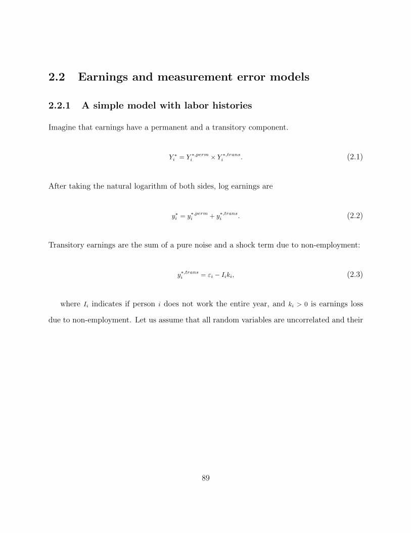
2.2 Earnings and measurement error models

2.2.1 A simple model with labor histories

Imagine that earnings have a permanent and a transitory component.

Y ∗i = Y ∗,permi × Y ∗,transi . (2.1)

After taking the natural logarithm of both sides, log earnings are

y∗i = y∗,permi + y∗,transi . (2.2)

Transitory earnings are the sum of a pure noise and a shock term due to non-employment:

y∗,transi = εi − Iiki, (2.3)

where Ii indicates if person i does not work the entire year, and ki > 0 is earnings loss

due to non-employment. Let us assume that all random variables are uncorrelated and their

89

first and second moments are

E(y∗,permi

)= µy, (2.4)

V ar(y∗,permi

)= Vp, (2.5)

E (εi) = 0, (2.6)

V ar (εi) = Vε, (2.7)

E (Ii) = pI , (2.8)

E (ki) = µk > 0, (2.9)

V ar (ki) = Vk. (2.10)

Let us assume that the administrative data measures earnings accurately, but persons under-

report transitory earnings shocks in the survey.

yai = y∗i , (2.11)

ysi = y∗,permi + τy∗,transi + ξi, (2.12)

where yai is earnings in the administrative data; ysi is earnings in the survey; τ is a measure of

under-reporting (0 ≤ τ ≤ 1); and ξi is a classical measurement error component independent

of everything with first and second moments

E (ξi) = 0, (2.13)

V ar (ξi) = Vξ. (2.14)

Measurement error is simply the difference between the survey and the administrative mea-

90

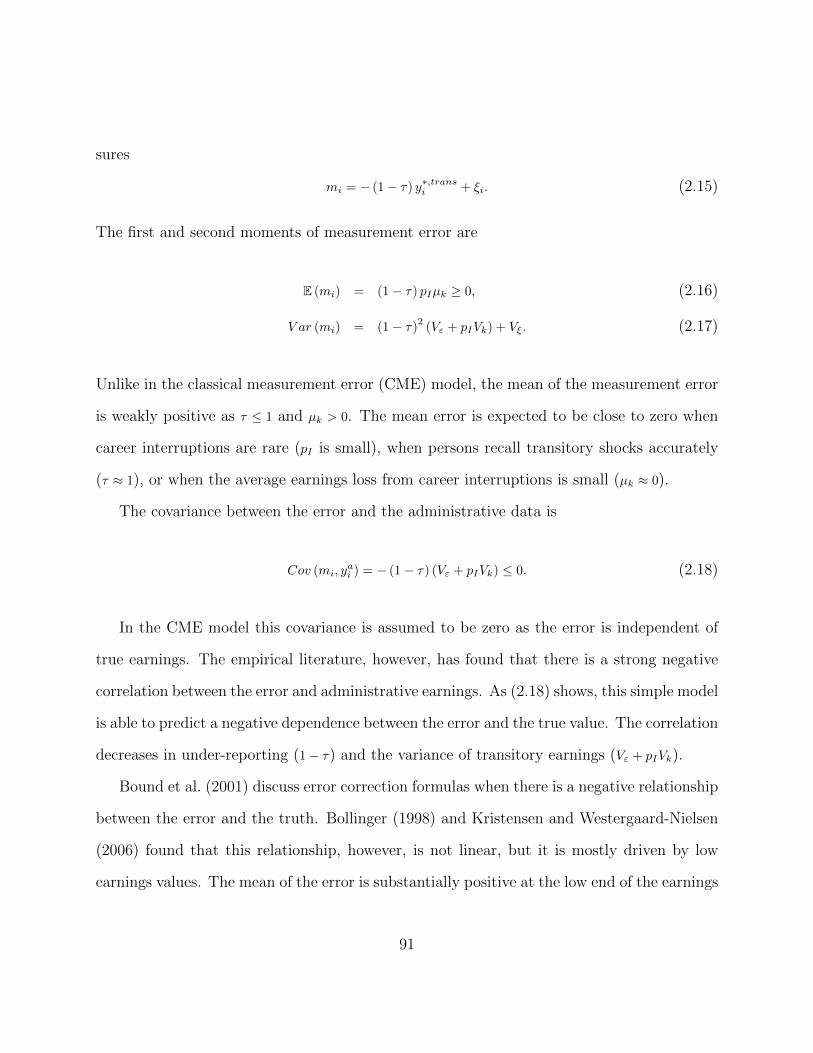
sures

mi = − (1− τ) y∗,transi + ξi. (2.15)

The first and second moments of measurement error are

E (mi) = (1− τ) pIµk ≥ 0, (2.16)

V ar (mi) = (1− τ)2

(Vε + pIVk) + Vξ. (2.17)

Unlike in the classical measurement error (CME) model, the mean of the measurement error

is weakly positive as τ ≤ 1 and µk > 0. The mean error is expected to be close to zero when

career interruptions are rare (pI is small), when persons recall transitory shocks accurately

(τ ≈ 1), or when the average earnings loss from career interruptions is small (µk ≈ 0).

The covariance between the error and the administrative data is

Cov (mi, yai ) = − (1− τ) (Vε + pIVk) ≤ 0. (2.18)

In the CME model this covariance is assumed to be zero as the error is independent of

true earnings. The empirical literature, however, has found that there is a strong negative

correlation between the error and administrative earnings. As (2.18) shows, this simple model

is able to predict a negative dependence between the error and the true value. The correlation

decreases in under-reporting (1− τ) and the variance of transitory earnings (Vε + pIVk).

Bound et al. (2001) discuss error correction formulas when there is a negative relationship

between the error and the truth. Bollinger (1998) and Kristensen and Westergaard-Nielsen

(2006) found that this relationship, however, is not linear, but it is mostly driven by low

earnings values. The mean of the error is substantially positive at the low end of the earnings

91

distribution, while it is close to zero at medium and high levels of earnings. In order to derive

the conditional distribution of the error given true earnings (E (mi|yai )) I make distributional

assumptions: y∗,permi and εi are distributed normally, and ki is a constant, ki = k.24 Using

straightforward algebra (see Appendix B.1) the conditional expectation is

E (mi|yai ) = (1− τ)

[− VεVε + Vp

(yai − µ) +Vp

Vε + VpkPr (Ii = 1|yai )

], (2.19)

Pr (Ii = 1|yai ) =p exp

(k

Vε+Vp

(µ− yi − k

2

))(1− p) + p exp

(k

Vε+Vp

(µ− yi − k

2

)) , (2.20)

where Pr (Ii = 1|yai ) is the probability that person i experienced career interruption conditional

on earning yai .

The first term in the square bracket of (2.19) is linear in earnings (yai ), but the second is

not. In fact it is easy to show that:

limyai→−∞

Pr (Ii = 1|yai ) = 1, (2.21)

limyai→∞

Pr (Ii = 1|yai ) = 0. (2.22)

At the low end of the earnings distribution everyone is a partial year earner, while at the

high end everyone works the entire year. By further assuming that there are no transitory

earnings shocks on the job, Vε = 0, the error mean converges to

limyai→−∞

E (mi|yai ) = (1− τ) k, (2.23)

limyai→∞

E (mi|yai ) = 0. (2.24)

24Assuming stochastic ki makes the derivation substantially more complicated. One can show that thequalitative results are very similar to the simple model discussed here when one uses stochastic k andsimulates the conditional error distribution.

92

The model predicts the Bollinger result. At the low end of the earnings distribution the

mean error is large and positive (equation 2.23), because everyone is a job loser (equation

2.21), and persons only report τ fraction of their earnings losses, k. At the high end of the

earnings distribution, however, the mean of the error is zero (equation 2.24), because no one

is a job loser, and the only source of error is the classical component, ξi, which has a zero

mean.

To sum up, career interruptions can compellingly explain the documented properties of

measurement error. The model predicts mean reversion, as persons under-report transitory

earnings shocks, and predicts that mean reversion is driven by low earnings values where

most of the sample is a partial year earner.

2.2.2 Alternative models to explain mean reversion

There have been extensive discussions in the literature about what might explain the mean-

reverting property of measurement error. The first idea is described in Pischke (1995), who

hypothesized that people under-report transitory shocks in earnings. My model in 2.2.1 is

an extension of the Pischke (1995) mechanism with career interruptions.

Kapteyn and Ypma (2007) proposed another mechanism to explain mean reversion: false

matches between the administrative and survey data. False matches lead to an apparent

mean reversion in survey error, because every mismatched person is linked to an average

earner, on average. False matches might be important in many contexts, especially when

probabilistic matching is used instead of exact identifiers. In the context of HRS, however,

mismatch is unlikely to play an important role. HRS and the Social Security Administration

actively try to avoid false matching by using several variables (Social Security number, name

and birth date) for matching. Moreover, false matches would lead to mean reversion at all

93

earnings levels, not just at the low end. It is hard to argue that only the lowest earners are

mismatched.

Abowd and Stinson (2013) proposed yet another mechanism to explain mean-reversion in the

error: measurement error in the administrative data. The literature almost always assumes

that the administrative earnings records (of employees) are accurate and therefore we can

directly observe the measurement error by subtracting the records from the survey reports.

Imagine, instead, that the administrative and the survey earnings both contain classical

measurement error:

yai = y∗i + ξai , (2.25)

ysi = y∗i + ξsi , (2.26)

E (y∗i ) = µy, (2.27)

V (y∗i ) = Vy, (2.28)

E(ξji

)= 0, (2.29)

V(ξji

)= V jξ , (2.30)

with j ∈ {a, s}. Within the Abowd and Stinson framework the difference between the survey

and administrative measures is the difference between the two measurement error compo-

nents:

mi ≡ ysi − yai = ξsi − ξai . (2.31)

The covariance between mi and the administrative data is negative as

Cov (mi, yai ) = −V aξ . (2.32)

94

There are many reasons to believe that the administrative data contains at least some error:

unofficial income might be missing from it25, there might be coding errors, and the legal

definitions of annual earnings might be different from actual earnings.26 Bound et al. (1994)

report that some outliers in their data seem to indicate problems with the administrative

data.

Measurement error in the administrative data can explain the mean reverting property of

the error, but it is less obvious why only low earnings values are biased. In this paper I

shall maintain the standard assumption that the administrative data are accurate. I believe,

however, it would be an interesting extension to develop a technique to identify measurement

error in the administrative data, which has proven elusive. See Abowd and Stinson (2013)

for more discussion about identification problems.

Lastly, a model of selective memory can also explain the Bollinger finding. This model

assumes that people are more likely to under-report negative than positive earnings shocks.

In the psychology literature Wagenaar (1986), Thompson et al. (1996) and Tourangeau

et al. (2000) discuss that people tend to remember more emotionally intense events better,

but pleasant events are better stored in memory. Moreover, psychologists observed that

people, when faced with a survey question about sensitive topics, tend to bias their answers

toward more favorable outcomes. Some people might think of their earnings as a gauge of

25One might expect that survey reports for this population are more accurate as surveys are collectedanonymously. Unfortunately we know very little on how people with unofficial income respond to questionsabout their earnings in surveys. Hurst et al. (2014) finds strong evidence that the self-employed, who areexpected to have the most unofficial income due to tax incentives, seriously under-report their income insurveys as well.

26The regulations concerning earnings on the W2 forms are quite complex and are not solely based oneconomic considerations. By looking at the instructions we can find, for example, the following list of earningscomponents: ”The cost of accident and health insurance premiums for 2%-or-more shareholder-employees paidby an S corporation”; ”Taxable cost of group-term life insurance in excess of $50,000”, ”Unless excludableunder Educational assistance programs (see page 5), payments for non-job-related education expenses or forpayments under a nonaccountable plan”, etc. It is hard to argue that there are no arbitrary elements in theseinstructions.

95

personal success and they might find it embarrassing to report too low values. It is possible,

for example, that people are more likely to report their usual earnings when they received

a big negative transitory income shock, but they report their total earnings after a positive

shock. Appendix B.2 shows that this mechanism is able to predict the asymmetric behavior

of the error discussed above. I shall show, however, that transitory earnings shocks on the

job are very small. Thus, the selective memory model is unlikely to explain much of the

mean reversion. Consequently, I shall not build this mechanism into my model.

96

2.3 Data and descriptive results

2.3.1 The Health and Retirement Study (HRS)

The survey data used in this project is the HRS, which is a biannual panel survey launched

in 1992. The original sample represented the 51-62-year-old US population, but in 1998 older

cohorts were added to cover everyone 51 and older. Every six years after 1998 the current

51-57-year-old cohort is added to maintain the 51+ age coverage. In this paper I use the

1992 − 2012 waves of the HRS that cover annual earnings between 1991 and 2011. The HRS

is a moderately large panel dataset (∼ 18, 000 observations per wave), allowing me to look at

the earnings history of persons for a relatively long time. The SIPP panels that were used

in recent validation studies cover only 2.5 to 4 years.

The HRS developed a so-called unfolding bracket question sequence to reduce item non-

response. People who answer ”Don’t know” to any of the earnings questions get a series

of follow-up questions about whether their earnings are smaller or higher than some pre-

determined threshold values. Table 2.1 shows that the non-response rate about wage and

salary income fell below 5 percent using this method. The HRS asks about annual gross

earnings in the last calendar year in five categories in the following order: 1. income from

self-employment; 2 wage and salary income; 3 other income from professional practice or

trade; 4 other income from tips, bonuses, commissions; 5 other income e.g. from second jobs

or military reserves. After each question the interviewer says “Other than what you have

already told me about, did you have any income from [Component X]”. If the answer is yes,

persons are asked about its value. In this paper I concentrate on earnings from employment,

so I disregard self-employment income and the sum of components 2-5 is my measure of

survey reported earnings. Table 2.2 shows that wage and salary income is by far the largest

97

component of earnings.

For most of the paper I restrict the sample to the 50-60-year-old grouping. I shall show in

Section 2.3.5 that above age 60, as people approach retirement, their earnings paths become

quite complex: average earnings start falling sharply, and cross-personal variation starts

increasing heavily. My preferred sample uses the relatively stable age range. I also drop

the self-employed from the analysis: All person-year observations are dropped in which the

person reported to be self-employed, or reported any self-employment income or in which

there is any self-employment income in the administrative data.

2.3.2 Earnings in the administrative data

The source of the administrative data is the Detailed and Summary Earnings Records derived

from the Master Earnings File of the Social Security Administration (SSA). For details about

this data, see Olsen and Hudson (2009) and the documents on the SSA27 and HRS websites.28

The data are derived from the W2 forms filed by employers to the Internal Revenue Service

each year. The higher quality Detailed Earnings Records (DER) is available from 1978

onward, and the less detailed Summary Earnings Records (SER) is available from 1951. My

preferred sample uses years between 1991 and 2011.

The data contains employer-employee-year level information and several earnings variables.

To define administrative earnings I consider total compensation and Medicare earnings. The

maximum of total compensation and Medicare earnings is my measure of W2 earnings at

a particular employer, and the sum over all employers is my measure of total annual W2

earnings for an individual in a given year. Total compensation amounts to the Box 1 values

27See http://www.ssa.gov/policy/docs/ssb/v69n3/v69n3p29.html for details.28There are two relatively detailed documents under the data section at hrsonline.isr.umich.edu that can

be accessed after free registration. Note, however, that the Social Security data are restricted and cannot beaccessed online. The website provides information about how to get permission to use the restricted data.

98

of the W2s and it includes wages, bonuses, non-cash payments and tips29. It typically does

not include deferred payments such as contributions to 401k plans, but certain plans are

included. Medicare earnings are based on the Box 5 values of the W2 forms. As opposed

to total compensation, Medicare earnings include most deferred payments. Before 1994,

however, Medicare earnings were capped at the taxable maximum. Before 1991, the Medicare

caps were equal to the Social Security caps (around $50, 000). Since 1994, there has been no

limit on the taxable earnings for Medicare, and between 1991 and 1993 the Medicare and

the Social Security taxable maximums began rapidly diverging.

Zero earnings are typically not recorded in the HRS version of the DER, but they are

available in the SER. I identify zero earnings as either zero records in DER or a missing

information in DER and zero records in SER.

The administrative data also contains self-employment income derived from the Form

1040 Schedule SE reported by the self-employed to the IRS. As discussed earlier, I drop all

person-year observations with any self-employment income.

The administrative data are only available in intervals, although most intervals are narrow. In

the descriptive part of the paper I impute values from these intervals with a simple procedure

outlined in Section 2.3.3, but in the structural estimation I model interval responses in an

interval regression fashion. The first type of interval response is top-coded Medicare earnings,

where Medicare earnings exceed total compensation, but are at the taxable maximum. For

confidentiality reasons the HRS also top-codes earnings above $250, 000 in a given year: When

earnings are above this threshold, researchers only see if they are in one of the following

intervals: [$250, 000, $299, 999]; [$300, 000, $499, 999]; [$500, 000,∞]. This top-coding only affects a

handful of cases. The HRS also rounded earnings below $250, 000 to the closest multiple of

29Only tips that the employee reported to the employer. Allocated tips are not part of Box 1.

99

$100, with the exception of $0−$49, where we can differentiate between a true $0 and a $1−$49

value.

2.3.3 Linking the HRS and administrative data

In order to match the HRS to the SSA data consent is required from the interviewees. Prior

to 2006, consent only covered current and past years, but since 2006, consent covers all future

years as well. For example, if the last consent from individual i was in wave 2000, we can

see his SSA earnings from 1951 to 2000, but if the last consent was in wave 2008, we see his

earnings from 1951 until today. Earnings histories, thus, are sometimes right-censored, but

never left-censored. The coverage, however, is expected to improve over time, as more and

more forward looking consent will be available.

The HRS made a lot of effort to increase the participation rate, but it remained below 100

percent. Generally the HRS has a relatively good coverage rate for earnings before 1992

and a moderately good coverage rate for earnings afterwards. Table 2.3 shows the fraction

successfully matched in a few subgroups. The average match rate among 50-60-year-old

employees between 1991 and 2011 is a little over 60%. The match rate is above 66% among

those who reported positive earnings in the HRS. It appears that persons who do not work

are less likely to consent. The match rate is almost 90% in the first 1992 wave of the survey,

it is between 60% and 70% between 1994 and 2008, and it is around 50% in 2010 and 2012.

Table 2.4 estimates linear probability models of successful matches on basic covariates. The

strongest predictors are interview years, race and marital status. Minorities and singles

are less likely to consent, but education and earnings do not predict the match rate. The

somewhat selective nature of the matched sample might bias some of the estimates. In the

descriptive part of the paper I shall ignore this problem, but in the structural part missing

100

values are imputed with multiple imputation. These imputations assume that the missing

values are conditionally ignorable (Little and Rubin, 2002).

Both HRS and W2 earnings contain quite a few interval responses. In the structural estima-

tion I model them in an interval regression fashion. For the descriptive part of the paper I use

a simple imputation that minimizes the error. When the reported interval (or value) and the

recorded interval overlap, I define measurement error as zero and I assign the middle point

of the overlapping interval to both earnings variables. If the two intervals do not overlap,

I assign the values on the edge of the intervals that minimize the measurement error. The

final (rare) case is when both the HRS report and the W2 record are right-open intervals.

In such cases, I assign 110 percent of the maximum of the two left points of the intervals to

both earnings variables. Finally, I deflated all earnings values with the CPI to 2000 dollars.

2.3.4 Labor histories

The administrative data provides employer-employee-year level information, and it contains

scrambled employer IDs that identify changes of employers for the same person over time,

but do not identify the same employer across individuals. I define job loss in year t as the

disappearance of an employer ID from year t to year t+1, and job finding as the appearance of

a new employer ID from year t−1 to year t. Employer IDs might change due to administrative

reasons, which biases turnover upward, but the extent of it should be negligible compared to

real turnover. Moreover, I am interested in how persons report earnings losses in years when

there is evidence for a career interruption and their administrative earnings fall substantially.

Table 2.7 shows the distribution of detailed labor histories between 1991 and 2011. Col-

umn 1 and 2 use only the matched HRS-SSA sample, and column 3 and 4 add the off years

when HRS responses are not available. In the latter sample, 49% of person-year observations

101

correspond to full year earnings in a single job, when the person held one job, and he also

worked for that employer in year t − 1 and year t + 1. The second largest category is zero

earnings (24%), when the person did not work for any employer in a particular year. Around

6% of person-years involved a job loss without job finding. The majority (4.3%) correspond

to the loss of a single job, and 1.8% involved the loss of at least one of multiple jobs. The

table differentiates between major and minor job losses. Major job loss is the loss of a job

that was the highest paying in year t or t− 1, and minor job loss is the loss of a secondary or

supplemental job that is not the highest paying neither in year t nor in t−1. The table shows

that minor job losses are far more common than major, but not single job losses. Around

4.5% of person-years involved a job finding without a job loss. The majority (2.9%) found

and held a single job. Around 10% of person-year observations involved both a job loss and

a job finding. The majority (5.9%) corresponds to losing and then finding a major job; 1.9%

correspond to losing and finding minor jobs; and around 1− 1% correspond to years when a

major job loss and a minor job finding, or vice versa, occurred.

Overall, there is evidence for quite high turnover in the HRS. Moreover, my procedure

might actually miss some job losses. Persons who lose their jobs but return to the same

employer within a year are mistakenly identified as full year earners. The administrative data,

under current limitations, cannot identify such cases, and there is some evidence that the

extent of this problem is non-negligible. My structural earnings model, thus, shall incorporate

latent job losses as well.

Tables 2.8 and 2.9 show the distribution of earnings by labor histories. As expected,

career interruptions substantially increase the likelihood of making relatively little. Around

44% of annual earnings are below $10, 000 (in 2000 dollars) when persons lose their single

jobs. The number is 24% after losing a major job and only 10% after losing a minor one.

102

The fraction of earnings below $10, 000 is very similar in years with a single, major, or minor

job finding (47%, 27% and 10% respectively). When persons work for the entire year, their

earnings are larger, but still around 9% of the observations are below the $10, 000 threshold.

The distribution of earnings after a minor job loss and a minor job finding is similar to

the distribution of full year earnings. Thus, I aggregate labor histories in the following way:

1. Stable years are observations with positive earnings without any indication of a major

or single job loss or job finding. Stable years include full year earnings, minor job losses

and minor job findings.

2. Major job losses are observations with major or single job losses and either no or only

minor job findings.

3. Major job findings are observations with major or single job findings and either no or

only minor job losses.

4. Major job loss and job findings are observations with both a major job loss and a major

job finding. This category, among others, contains employer-to-employer switches.

5. Zero earnings are observations without any earnings.

Finally, I drop W2 earnings corresponding to the last consented year, since it is not possible

to determine if persons managed to keep their jobs the entire year or not.

2.3.5 Descriptive properties of measurement error

From now on Y ait and yait denote the level and log of annual W2 earnings; Y sit and ysit denote

the level and log annual HRS earnings; and mit denotes the measurement error: mit = ysit−yait.

103

Table 2.6 shows basic moments of earnings and measurement error. The first row is the

classical reliability ratio defined as:

rclassical =V ar (yait)

V ar (yait) + V ar (mit). (2.33)

Under the assumptions of the classical measurement error model, rclassical characterizes the

attenuation bias in simple regressions with the error ridden variable on the right hand side:

β = rclassical × β + op (1) . (2.34)

According to Table 2.6 the reliability ratio is 0.82, which means that, if the CME model

holds, in regressions with earnings on the right hand side, one should divide the coefficient

on earnings by 0.82 to correct for the attenuation bias. Column 5 shows that when earnings

growth (log changes in earnings) is on the right hand side, one should divide the coefficient

by 0.50. Earnings growth is less reliable as earnings are more persistent than measurement

error.

The second row of Table 2.6 shows a more general reliability ratio, rcorrelated, which, as

opposed to the CME model, allows for a non-negative correlation between measurement

error and earnings (Bound et al., 2001):

rcorrelated =V ar (yait)

V ar (yait) + V ar (mit) + 2Cov (yait,mit). (2.35)

The literature consistently finds a strong negative correlation between error and earnings.

The HRS is no exception. The negative correlation decreases the denominator of (2.35), or

in other words, it makes the attenuation bias less strong. As Table 2.6 shows, the correlated

104

reliability ratio is close to one, implying that under the assumptions of the Correlated Mea-

surement Error (CorrME) model, there is no attenuation bias in regressions with earnings on

the right hand side. The negative correlation also increases the reliability ratio in earnings

growth, but it is still well short of one (0.68).

The third row of Table 2.6 shows the regression coefficient of error on earnings:

mit = γm,yayait + υit. (2.36)

As Bound et al. (2001) discuss, regression coefficients are biased even when earnings appear

on the left hand side of regression in the CorrME model, and γm,y∗ is a measure of the bias:

α = γm,ya × α+ op (1) . (2.37)

Similarly to the literature, the γm,ya coefficient is estimated to be around −0.1, meaning that

predictors of earnings are downward biased by about 10% according to the CorrME model.

Columns 2-4 of Table 2.6 show a potential problem with the CorrME model. The basic

model assumes that the negative relationship between the error and earnings is linear as in

(2.36). As the table shows, the relationship is far from linear as seen when the lowest earnings

values are discarded and the negative relationship approaches zero. When I discard earnings

below $10, 000 (in 2000 dollars), γm,ya shrinks from −0.099 to only −0.025, although it is still

statistically significant. Measurement error above $10, 000 appears to be less correlated and

is almost classical. In the case, when the relationship between the error and true earnings is

not linear, rcorrelated and γm,ya still correctly accounts for the bias, as long as total earnings

(as opposed to permanent earnings) are in the regression.

Figure 2.2 visualizes the nonparametric relationship between the error and earnings. The

105

top left panel shows the predicted value of the nonparametric regression between the 1st

and 99th percentile of earnings together with the predicted values of the CME and the basic

CorrME models. The top right panel shows average measurement error in 20 equal sized

quantiles of earnings together with 95% confidence intervals. The lowest earnings are severely

upward biased, but the error appears almost classical above the 15th or 20th percentile of

earnings. Neither the CME nor the CorrME model accurately characterizes measurement

error in earnings. Very similar results were found by Bollinger (1998) using the Current

Population Survey and Kristensen and Westergaard-Nielsen (2006) using a Danish household

survey. The bottom panels of Figure 2.2 show that the CorrME model works much better

for earnings growth. It seems the relationship between error and earnings growth is close to

linear, with perhaps some acceleration at the extremes.

The main claim of my paper is that transitory earnings shocks due to career interruptions

are under-reported in surveys. This mechanism exactly predicts the type of non-parametric

relationship between the error and earnings as in Figure 2.2. Career interruptions lead to

large earnings losses and large positive measurement error at the low end of the earnings

distribution if they are systematically under-reported. Figure 2.1 shows histograms of mea-

surement error together with fitted normal densities. All histograms show excess kurtosis

and right skew compared to the normal plots. The right skew appears strongest in the sam-

ple with partial year earnings. This is additional evidence that negative earnings shocks due

to partial year earnings are under-reported in surveys.

Table 2.11 shows the means of measurement error by labor histories and earnings. Av-

erage error is large and positive below $10, 000, and sharply decreases with earnings. The

averages are very similar across the three types of career interruption (job loss, job finding or

both). Average measurement error is substantially smaller in stable years, but still positive

106

at the low end of the earnings distribution. Table 2.12 further investigates measurement

error in stable years. I restrict the sample to stable years in both year t and t − 1, and I

divide the sample based on whether earnings fell or increased between t − 1 and t. Average

measurement error is close to zero when earnings increased, except in the rare cases they in-

creased but remained under $1, 000. Average error is positive and substantial, however, when

earnings fall. This might indicate that some observations identified as stable actually involve

large negative transitory shocks as well. It is possible that these observations correspond to

person-years with a job loss and a subsequent return to the same employer.

Finally, I fit a simple descriptive earnings and measurement error model a la Pischke

(1995). The model assumes earnings are the sum of a permanent and a transitory component:

yit = µ+ ypermi + ytranit , (2.38)

where ypermi and ytransit are mean zero. Permanent earnings are fixed within person and

transitory earnings follow an MA(1) process:

ytranit = εit − θεi,t−1. (2.39)

The survey reports are

ysit = µ+ δ + τpypermi + τ tytranit +mi + nit, (2.40)

where δ indicates mean error, τp and τ t are the average fraction of permanent and transitory

earnings reported, mi is the permanent measurement error and nit is the transitory measure-

ment error. All error terms are assumed to be uncorrelated with each other and with the

107

other variables of the model.

I estimate this system by GMM using all the first and second moments of earnings in

year t and t+ 2. Apart from the MA(1) coefficient, θ, all parameters are identified, including

the total variance of transitory earnings.

Table 2.21 in Appendix C estimates the model by 2-year age groups between the ages of

50 and 70. It shows that the mean and the variance of earnings is relatively stable between

the ages of 50 and 60, the mean rapidly decreases after age 60, while the variance increases

sharply. From now on I only use the relatively stable 50-60-year-old sample.

The main results are in Table 2.13. Column 1 uses all observations and column 2 restricts

the sample to cases with no indication of career interruption in years t, t + 1 or t + 2. Note

that the model in column 1 is biased because career interruptions lead to non-zero (negative)

mean transitory earnings. Nevertheless, I estimate this model due to its similarities with the

model Pischke (1995) used, and because I believe comparing it to column 2 is worthwhile.

The average measurement error is positive in both cases, but it is close to zero in stable

years. The (inter-personal) variance of permanent earnings is substantial in both models.

The variance of transitory earnings is large in model 1, but it is close to zero when only

stable years are used. Transitory earnings shocks on the job, thus, are small, but transitory

earnings shocks due to career interruptions are large. The main parameters of interest are in

the last two rows. Persons report close to 100% of their permanent earnings, but substantially

less of their transitory earnings: 68% for all observations and 76% when only stable years are

considered. The standard error in the latter case, though, is quite large, perhaps because it

is hard to identify the under-reported component of earnings that are so small.

Overall, the descriptive evidence favors the main claims of the paper that under-reporting

of earnings losses due to career interruptions has a substantial and non-standard effect on

108

measurement error.

2.4 Structural estimation

This section introduces and estimates a dynamic earnings and measurement error model that

features career interruptions and deals with missing values and interval responses.

2.4.1 The earnings and measurement error model

The W2 and HRS earnings are provided in intervals. I assume that there are latent earnings

yait and ysit that are somewhere in the provided intervals:

yjit ∈[yjit, yjit

], (2.41)

where j ∈ {a, s}, and only the lower and upper bar earnings values are observed in the

HRS and SSA data. When the HRS earnings reports are continuous values, I use the trivial

intervals. When the HRS or the SSA earnings are missing, I use the [−∞,∞] intervals.

I assume that the W2 earnings are accurate. Earnings of person i in year t depend

on some potentially time-varying covariates, and they have a permanent and a transitory

component:

yait = β′xit + ypermit + ytranit , (2.42)

ypermit = ypermi,t−1 + νit, (2.43)

ytranit = yMA(q)it −

L∑l=1

Iitlkitl, (2.44)

yMA(k)it = εit −

k∑j=1

θjεi,t−j (2.45)

109

Permanent earnings follow a random walk with innovation term νit. Transitory earnings

on-the-job follow a moving average process with q lags. My preferred model features q = 0

lags.30 Iitl indicates a career interruption of type l ∈ {1, ...;L}, such as a major job loss or a

job finding. Career interruptions affect both permanent and transitory earnings. Transitory

earnings loss due to an l type interruption is denoted by kitl. Career interruptions also affect

the mean and the variance of the random walk innovation term of permanent earnings:

E (υit) =L∑l=1

λml Iitl, (2.46)

V ar (υit) =

L∑l=1

λVl Iitl. (2.47)

The mean of the innovation term is normalized to zero on-the-job, but it is free in other

cases. Among other things, this specification allows for the human capital of individuals to

depreciate when they are not working. The variance of the innovation term can be non-zero

even on-the-job to capture promotions and demotions.

Even though my notations involve summations over labor histories in (2.44)-(2.47),a

maximum of one indicator is one in a particular year for a given individual. In the previous

section, we saw that there are large negative earnings shocks even in stable years, so I allow

for latent job losses on-the-job with probability p. Latent job loss behaves similarly to other

career interruptions: It can change the mean and the variance of permanent earnings and

it can lead to a transitory earnings loss, too. The probability p shall be estimated together

with the other parameters.

30The variance of on-the-job transitory earnings is very small, so it makes little difference how muchstructure one puts on these shocks. The model with no MA lags converges much faster to a stable distribution,so I use this assumption in the baseline case.

110

The HRS earnings reports are

ysit = (β + δ)′xit + τpypermit + τ ty

MA(k)it −

L∑l=1

τkl Iitlkitl +mi + nit. (2.48)

δ is a vector of bias terms in the regression coefficients; τp, τ t and the τkl terms are the

average fractions of the earnings components reported (permanent, on-the-job transitory and

transitory due to career interruption); mi is permanent and nit is transitory measurement

error with mean zero and positive variance. The variance of transitory measurement error

can also depend on labor histories:

V ar (nit) =

L∑l=1

λnl Iitl. (2.49)

I use Markov Chain Monte Carlo (MCMC) for estimation that requires distributional as-

sumptions. I assume that all random variables apart from the kitl and Iitl are distributed

normally and are uncorrelated with each other. The uncorrelatedness assumption is not par-

ticularly restrictive as considerable dependence is already built in the model. Iitl is assumed

to follow a Bernoulli distribution with a constant parameter, p. I assume that the transitory

earnings loss terms, the kitl-s, follow an exponential distribution with p.d.f.

f (kitl) = γl exp (−γlkitl) , (2.50)

kitl ∈ [0,∞] . (2.51)

The motivation for this p.d.f. is the following: Imagine that an l-type career interruption

implies that the person works for Titl and does not work for 12 − Titl months. His earnings

loss is Kitl = 1 − Titl

12 fraction of his earnings potential. Assuming that the fraction Kitl is

111

uniformly distributed between zero and one, and taking log leads to the p.d.f. in (2.50) with

parameter γl = 1, and kitl ≡ 1 − ln (1−Kitl). I allow γl to differ from one, and I will estimate

separate γl terms for each type of career interruption. The average log and level earnings

losses decrease with γl:

E(kitl) =1

γl, (2.52)

E(Kitl) =1

γl + 1, (2.53)

Figure 2.3 shows that this distributional assumption works well. It shows the histogram of

earnings losses from year t−1 to year t for observations when t−1 was a stable year and year

t involved a major job loss. The figure also shows a simulated density that is the sum of two

terms: one with a p.d.f. from (2.50) with γl = 1, and one with the empirical distribution of

earnings changes when both t− 1 and t were stable years. The shape of the two distributions

are similar, but the empirical histogram falls a little short of the simulated one. It appears

persons lose less than half of their earnings after a typical job loss. Consequently we can

expect the corresponding γ term to be above one.

2.4.2 Estimation methodology

I use a Bayesian estimation method, Markov Chain Monte Carlo (MCMC), for estimation.

Gelman et al. (2013) provides a thorough overview of MCMC and other similar techniques.

In some ways, MCMC is a more general version of Maximum Simulated Likelihood. It

requires a fully specified model, but it can be used in very complex cases when it is too

tedious or too slow to simulate the likelihood function.

The unusual feature of MCMC is that it assumes that the parameters of the model being

112

estimated are random. The data generating process is described by the c.d.f. F (y, α), where y

represents the data and α represents the unknown parameters. The goal of the procedure is to

derive the posterior distribution of the parameters, F (α|y). Once the posterior is estimated,

one can use its mean as the estimate, and its standard deviation as the standard error:

α = EF (α|y) , (2.54)

se (α) = StdF (α|y). (2.55)

Alternatively, one can directly define a 95% confidence interval by taking the 2.5th and 97.5th

percentile of F (α|y). In this paper I shall only provide the means and standard errors from

(2.54) and (2.55).

The posterior distributions of the parameters are simulated with the following procedure:

1. Take initial guesses for all αj-s, j ∈ {1, 2, ..., J}. The set of α-s includes the parameters

and potentially other latent or auxiliary random effects, such as the innovation terms

of the random walk, the Iitl and kitl terms, etc.

2. Define a prior distribution for all the parameters f0 (αj). The priors can be defined

individually, jointly or in blocks.

3. Draw new values of the parameters from their posterior distribution conditional on

their prior, the data and other parameters, F (αj |y, α−j , f0 (αj)). One can update the

parameters individually, jointly or in blocks.

4. Repeat step 3 NS times, where NS is the number of simulation draws.

5. Drop the first NB burn-in draws and use the rest NS −NB for inference.

113

The prior distributions are auxiliary objects and researchers almost always choose vague

(or flat or non-informative) priors so that they do not influence the results. One can, for

example, use a prior of N (0, 100) for the distribution of mean log earnings. I also use vague

priors in this project.

The number of necessary simulation draws, NS, sometimes has to be large, because the

consecutive simulation draws can have, and often do have, a large positive autocorrelation,

which decreases the effective sample size of the simulated data. In this project, I use 100, 000

simulation draws for each parameter, and I discard the first 10, 000 burn-in draws.

The most challenging part of the estimation is to derive the posterior distributions, the

F (αj |y, α−j , f0 (αj))-s, of all parameters. In standard cases, there are readily available formu-

las. For example, when the data are distributed normally, means, variances and regression

coefficients can be updated easily. In other cases, the posterior distributions are unknown

or they do not have analytical forms. In such cases the Metropolis-Hastings algorithm can

be used to simulate the posterior distribution. In this project I use the Metropolis-Hastings

algorithm to update the MA coefficients and the earnings loss variables due to career inter-

ruptions: Iitl, kitl and latent transitory measurement error terms due to career interruptions.

Other parameters are updated using the standard Gibbs sampler.

MCMC is particularly useful for models that feature a large number of random effects or

missing data. In such cases the MCMC procedure is substantially simpler than alternatives.

Other features are harder to implement with MCMC. Properly modeling moving average

processes and time-varying variances, such as variances that depend on labor histories, are

harder. The simulation part of the Matlab code of my preferred model has almost 500 lines.

Details can be found on my website.31

31https://sites.google.com/site/phudomiet/research.

114

2.4.3 Results

Tables 2.14-2.18 show the main results of the paper. All of these specifications are estimated

using years between 1991 and 2011, with age ranging between 50 and 60, and no lags in the

moving average process of on-the-job transitory earnings. Appendix C shows results using

alternative modeling assumptions.

The models are run separately for males and females. Tables 2.14 contains the regression

coefficients of mean earnings; Table 2.15 shows the covariates in the means and variances of

the random walk innovation terms; Table 2.16 contains other parameters of earnings; and

Tables 2.17 and 2.18 show parameters of measurement error.

All Tables have six columns corresponding three alternative sets of covariates in earnings

and gender. My preferred model is in Column 2. Column 1 only includes a constant term.

Column 2 adds basic covariates such as race, education, age, GDP gap32. Column 3 adds

year dummies instead of the other macro variables.

The estimated coefficients in mean earnings (Table 2.14) are standard: Minorities earn

less than whites; education increases earnings; the age-earnings profile is an increasing and

concave function; earnings are procyclical (and the cyclicality is stronger for males); male

real earnings were slightly falling between 1991 and 2011 while female earnings stagnated or

slightly increased. Cognition is a strong positive predictor of earnings, and the predictive

power of education substantially decreases with the inclusion of cognition.

The mean and variance of the random walk innovation term (of permanent earnings) are

allowed to depend on labor histories. I include dummies for 1. major job finding; 2. major

job loss and major job finding; 3. zero earnings; and 4. latent job loss in stable years. I

do not include a dummy for major job loss, as it is not separately identified from major job

32I use the IMF GDP gap measures divided by 100.

115

finding. When one loses his job, his permanent earnings are not observed until he finds a

job again. Hence, it is not possible to identify the effect of a job loss and a consequent job

finding separately. My models attribute all changes to job finding.

Moving from non-employment to employment has a small negative effect on permanent

earnings for both males and females. In my preferred Model 2, the permanent earnings

loss is 7.4% for males and 7.7% for females. This mean effect, however, masks a large cross-

sectional heterogeneity. The standard deviation of the random walk innovation is close

to zero on-the-job (0.06 for both males and females), but it jumps up to around 0.4 when

persons find a new job. Not working for an entire year has an even more detrimental effect on

earnings, on average: permanent earnings fall by 24% per year for males and 21% per year for

females. Experiencing both a major job loss and a major job finding, the case that includes

employment-to-employment switches, has a zero effect on permanent earnings, on average,

for males, and a small positive effect for females. Finally, latent job loss in stable years is

associated with a very large negative effect on permanent earnings, too: 21% earnings loss

for males and 17% for females. Some of these earnings losses might be due to demotions; a

reduction in work hours; or losing a job and being rehired in a lower position. The cross-

sectional variation in earnings growth is very large in all cases when career interruptions

occur.

Table 2.16 shows the rest of the parameters in earnings. The cross-sectional variation in

earnings is quite large at age 50 already. Transitory earnings shocks on-the-job, however, are

small: The standard deviation is around 0.04 for males and 0.03 for females. The correspond-

ing variances are practically zero. Transitory earnings shocks due to career interruptions,

however, are very large, on average. The estimated γl coefficients are larger than 1 in all

cases, which means that earnings loss is less than half a year on average. Average earnings

116

losses are between 23% and 45% based on the formula in (2.53). The largest transitory earn-

ings loss is due to major job losses (41% for males and 45% for females) and the smallest is

in latent job losses in stable years (24% for males and 25% for females).

The most important parameters, describing the properties of measurement error, are in

Tables 2.17 and 2.18. The basic covariates have little effect on the mean of the error for

both males and females. The standard deviation of permanent measurement error is small

for both groups (0.16 for males and 0.15 for females). The standard deviation of transitory

measurement error in stable years is also small (0.1 for males and 0.14 for females), but it

is considerably larger when career interruptions occur. Depending on the type of shock,

the standard deviation of the error is between 0.5 and 0.68. Persons report close to 100%

of their permanent earnings, and substantially less of their transitory earnings. Identifying

the fraction of on-the-job transitory earnings reported was an obstacle, likely because these

shocks are very small, on average. In my baseline specification I simply calibrated the

reported fraction to zero.33 The fraction of transitory shocks due to career interruptions

reported are between 50% and 87%. In my preferred model 2, male (female) interviewees

report 84% (∼ 77%) of the transitory shocks due to a major job loss, 62% (69%) of shocks due

to a major job finding, 54% (65%) of shocks associated with both a job loss and a job finding,

and 50% (73%) of shocks due to a latent job loss in stable years. Most parameters are very

similar in the different specifications. The only exception is the fraction of reported earnings

due to a latent job loss. This parameter varies between 50% and 100% in the alternative

models.

Tables 2.24-2.48 in Appendix C carry out several robustness checks. Tables 2.24-2.33

33Table 2.38 in Appendix C show that the main results are robust to alternative assumptions in regard tothis parameter: assuming that people report 50% or 100% of these shocks or that the fraction is estimated.In the case of the fraction being estimated, its standard error is quite large, and the distribution of theparameter does not appear to converge to a stable distribution.

117

estimates separate models by education groups; Tables 2.34-2.38 allow for higher order MA

terms in transitory earnings, Tables 2.39-2.43 make alternative assumptions about the frac-

tion of on-the-job transitory shocks reported, and Tables 2.44-2.48 uses different samples.

The main results of the paper are robust to these changes: transitory earnings shocks due

to career interruptions are large and are severely under-reported in the survey.

2.5 Discussion of bias correction

According to the descriptive results summarized in Table 2.6, respondents report around

1− 0.26 = 74% of their earnings growth, on average. According to Figure 2.2, under-reporting

is an approximately linear function of earnings growth itself. The GMM estimates in Table

2.13 suggest that respondents report around 68% of their transitory earnings shocks. These

results indicate that a simple model, in which measurement error has a classical component

together with a mean-reverting one due to reporting only ∼ 70% of transitory earnings fluc-

tuations, might be a good approximation of the way people report their earnings in surveys.

The MCMC estimates show a somewhat more nuanced picture: earnings losses due to job

finding appears to be less salient than earnings losses due to job losses. The 70% number is

approximately in the middle of the different MCMC estimates, though.

A natural question is: what do these results imply for biases in applied work and what

can researchers do to correct them? The appropriate bias correction formulas depend on

many factors such as:

1. Are earnings on the left- or right-hand side of regressions?

2. Does the researcher aim at including a measure of permanent earnings (or perhaps

human capital or earnings potential) of individuals or their total earnings including

118

short-term transitory fluctuations?

3. Does the researcher model earnings levels or earnings growth?

4. Does the data have reliable measures of career interruptions or not?

5. Do particular variables in the regression correlate with turnover or not?

Discussing all of these is beyond the scope of this paper. I only consider a few interesting

cases.

First, because measurement error in earnings growth appears to be an approximately

linear function of earnings growth, the CorrME error model of Bound et al. (2001) might

work well in these cases. According to Table 2.6, when earnings growth is on the left-hand

side of regressions, the coefficients should be divided by 0.74; and when earnings growth is

on the right-hand side regressions, the coefficients should be divided by 0.68. This simple

procedure only works, however, if the researcher aims at including growth in total earnings,

as opposed growth in permanent earnings. This is the case, for example, if one is interested

in the transitory earnings loss of displaced workers either on the left or right hand side of

regressions.

Second, when one is interested, instead, in permanent earnings growth, the correc-

tion formulas should be adjusted. This is the case if one wants to characterize differen-

tial earnings trends between groups over time, or one is interested in the effect of pro-

motions/demotions/retirement on consumption growth. As people report the permanent

component of their earnings accurately, no correction is needed when earnings growth is on

the left hand side of regressions. Using observed earnings growth, as a proxy for permanent

earnings growth on the right-hand side of regressions, however, should be done with cau-

tion. Not only is earnings growth measured with error, but it is dominated by transitory

119

fluctuations as opposed to permanent changes.

Third, consider the case of using annual earnings (in levels) on the left hand side of regres-

sions as a proxy for permanent earnings, such as in a Mincer earnings function. Interestingly,

my results suggest that using survey-based measures is (slightly) superior to administrative

records. Imagine that administrative and survey earnings take the following form:

yai = ypermi + ytransi , (2.56)

ypermi = β0 + β1xi + ηi, (2.57)

ytransi = εi − Iiki, (2.58)

ysi = ypermi + τytransi +mi, (2.59)

where Ii indicates career interruptions, ki indicates annual earnings losses due to career

interruptions with mean 1/γ, and the coefficient of interest is β1. Under these assumption,

the probability limit of regression coefficients with either yai or ysi on the left hand side of the

regression are

plimβa1 = β1 −1

γβI,x, (2.60)

plimβs1 = β1 −τ

γβI,x, (2.61)

where βI,x is the coefficient from a regression of career interruption on x. The regression

coefficient is biased if variable xit is correlated with career interruptions. The sign of the bias

depends on the sign of βI,x. Variables with a positive effect on turnover have a negative bias,

while negative predictors of turnover are biased upward. The survey-based regression is less

biased than the administrative whenever τ < 1, as persons under-report transitory shocks,

120

and hence, under-report the bias. In the extreme case of τ = 0, the survey based coefficient is

actually unbiased. In most applications the regression coefficient βI,x is likely to be close to

zero, since the unconditional probability of turnover is relatively low to begin with. Overall,

unless variable x is expected to be a very strong predictor of turnover, one might expect

negligible bias in these regressions.

Fourth, consider the case when annual earnings (in levels) appear on the right-hand side

of a regression as proxies of permanent earnings.

zi = β0 + β1ypermi + ηi, (2.62)

yai = ypermi + εi − Iiki, (2.63)

ysi = ypermi + τ (εi − Iiki) +mi. (2.64)

Regression coefficients are inconsistent in this case. Under the assumption that all error

terms are uncorrelated, Pr (Ii = 1) = p and V ar (ki) = 1γ2 , the probability limit of regression

coefficients with either yai or ysi on the right-hand side are

plimβa1 = β1V ar (ypermi )

V ar (ypermi ) + V ar (εi) + pγ2

, (2.65)

plimβs1 = β1V ar (ypermi )

V ar (ypermi ) + τ(V ar (εi) + p

γ2

)+ V ar (mi)

. (2.66)

Under-reporting transitory shocks helps on the right hand side as it decreases the second

term in the denominator of (2.66). The third (classical error) term in (2.66), however,

increases the denominator and increases the bias. The measurement error is large enough

that the bias is stronger when the survey measure is used. The bias is non-negligible in both

cases, though, and it is dominated by terms related to career interruptions. The variance of

121

transitory earnings shocks on-the-job (V ar (εi)) is negligible compared to V ar (ypermi ) , but pγ2

is not. Moreover, as we saw in Tables 2.17 and 2.27, the variance of measurement error is

small in stable years, and much larger in years when career interruptions occur. If researchers

use either yai or ysi as right-hand side variables as proxies of ypermi it is crucial to account for

partial year earnings, by either dropping those values from the regression, or better: modeling

turnover appropriately.

2.6 Conclusion

This paper analyzed the properties of measurement error in annual earnings with a particular

focus on how partial year earnings are reported in a household survey. I find strong evidence

that transitory earnings fluctuations are severely under-reported. Transitory earnings losses

due to career interruptions are very large, on average, and people systematically under-report

these shocks, too. Earnings losses due to recent job losses are reported better, perhaps

because these shocks are more salient. Earnings losses due to recently starting a new job are

reported less accurately, perhaps because people prefer reporting their annualized earnings

after starting new jobs. Overall, career interruptions have large and non-standard effects on

the quality of earnings reports in surveys. The implied error has a small positive mean, it

is right-skewed and it correlates with predictors of turnover. The implied biases are likely

to be relatively small in most cases, as career interruptions are rare. When researchers use

earnings growth in their models, or when they analyze questions that are strongly related to

turnover, more caution is warranted.

122

Tables anmd figures

Figure 2.1: Histogram of measurement error in annual earnings

0.5

11.

52

Den

sity

-10 -5 0 5Measurement error

01

23

4D

ensi

ty-2 -1 0 1 2

Measurement error

All observations All observations in range [−2, 2]

01

23

4D

ensi

ty

-2 -1 0 1 2Measurement error

01

23

Den

sity

-2 -1 0 1 2Measurement error

Stable years* in range[−2, 2] Partial year earnings in range [−2, 2]

Stable years: Positive earnings and no evidence of major job loss or job finding. Major job loss: loss of a job that was the

highest paid one in year t or t− 1. Major job finding: finding a new job that is the highest paid one in year t or t+ 1.

Sample: HRS, 1991-2011, 50-60-year-old employees

123

Figure 2.2: Nonparametric relationship between measurement error and earnings

-.2

-.1

0.1

.2.3

.4.5

.6.7

Pre

dict

ed m

easu

rem

ent e

rror

7 8 9 10 11 12Log earnings

Classical measurement error modelCorrelated measurement error modelNon-parametric regression

Nonparametric regression: error on earnings Mean error by 20 quantiles of earnings

-1-.

8-.

6-.

4-.

20

.2.4

.6.8

1P

redi

cted

mea

sure

men

t err

or

-2 -1 0 1 2Change in log earnings

Classical measurement error modelCorrelated measurement error modelNon-parametric regression

Nonparametric regression: error on earnings growth Mean error by 20 quantiles of earnings growthSample: HRS, 1991-2011, 50-60-year-old employees

124

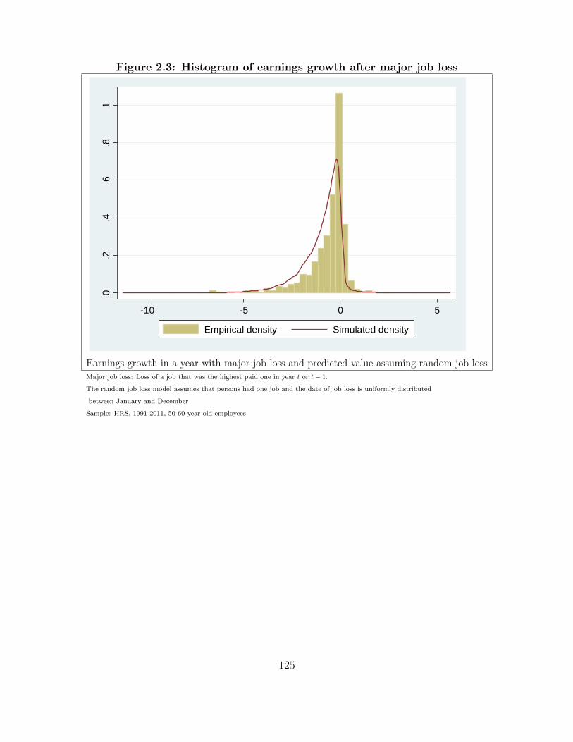
Figure 2.3: Histogram of earnings growth after major job loss

0.2

.4.6

.81

-10 -5 0 5

Empirical density Simulated density

Earnings growth in a year with major job loss and predicted value assuming random job lossMajor job loss: Loss of a job that was the highest paid one in year t or t− 1.

The random job loss model assumes that persons had one job and the date of job loss is uniformly distributed

between January and December


125

Figure 2.4: Histogram and time series plots of selected coefficients in the baselinespecification of the structural model

Histogram of τperm Time series plot of τperm

Histogram of τkloss Time series plot of τkloss

Histogram of τkfind Time series plot of τkfind

Histogram of τkboth Time series plot of τkboth

Histogram of τklatent Time series plot of τklatentThe coefficients are from Model 2 of the baseline specification reported in Table 2.17.


126

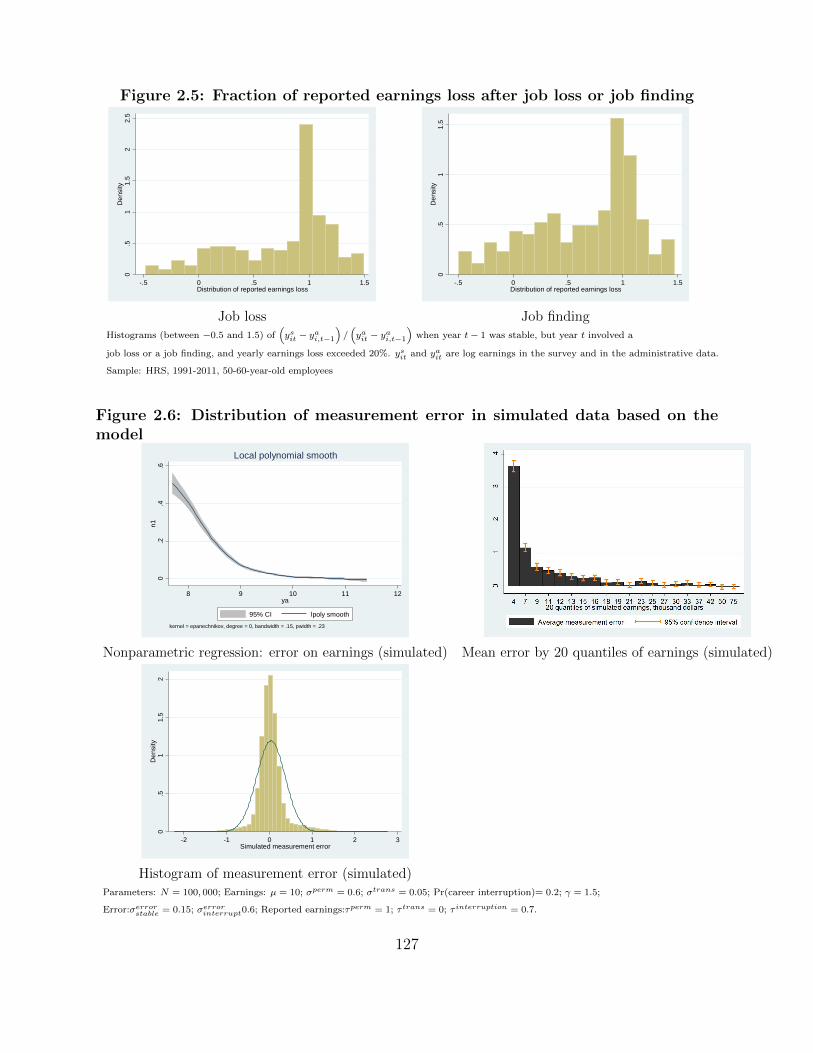
Figure 2.5: Fraction of reported earnings loss after job loss or job finding

0.5

11.

52

2.5

Den

sity

-.5 0 .5 1 1.5Distribution of reported earnings loss

0.5

11.

5D

ensi

ty

-.5 0 .5 1 1.5Distribution of reported earnings loss

Job loss Job findingHistograms (between −0.5 and 1.5) of

(ysit − yai,t−1

)/(yait − yai,t−1

)when year t− 1 was stable, but year t involved a

job loss or a job finding, and yearly earnings loss exceeded 20%. ysit and yait are log earnings in the survey and in the administrative data.


Figure 2.6: Distribution of measurement error in simulated data based on themodel

0.2

.4.6

n1

8 9 10 11 12ya

95% CI lpoly smooth

kernel = epanechnikov, degree = 0, bandwidth = .15, pwidth = .23

Local polynomial smooth

Nonparametric regression: error on earnings (simulated) Mean error by 20 quantiles of earnings (simulated)

0.5

11.

52

Den

sity

-2 -1 0 1 2 3Simulated measurement error

Histogram of measurement error (simulated)Parameters: N = 100, 000; Earnings: µ = 10; σperm = 0.6; σtrans = 0.05; Pr(career interruption)= 0.2; γ = 1.5;

Error:σerrorstable = 0.15; σerror

interrupt0.6; Reported earnings:τperm = 1; τ trans = 0; τ interruption = 0.7.

127

Table 2.1: Type of wage and salary reportsAll observations 50-60-year-old, employees

N Fraction of total N Fraction of total

Continuous value 58,075 32.8 29,858 62.3

Complete bracket 5,181 2.9 2,476 5.2

Half open interval 1,576 0.9 501 1.0

No income 105,919 59.8 12,801 26.7

Missing 6,244 3.5 2,309 4.8

Total 176,995 100.0 47,945 100.0

Sample: HRS, 1991-2011

Table 2.2: Components of annual earnings, HRS 1991-2011, 50-60-year-old em-ployees

Fraction positive Mean* Fraction of total N

Wage and salary income 99.2 36489 93.1 33,090

Tips, bonuses, commissions 10.1 1146 2.9 33,090

Professional practice and trade 3.3 1259 3.2 33,090

2nd job or military reserves 4.3 314 0.8 33,090

Total 100 39209 100.0 33,090

Average earnings adjusted to 2000 dollars with the CPI.


Table 2.3: Fraction of successful matches between the HRS and SSAN Fraction matched

1. All observations 176,995 57.7

2. 50-60-year-old employees 47,945 61.2

3. (2) + non-missing HRS response 45,639 64.2

4. (3) + positive HRS response 33,090 66.2

5. (4) + 1992 wave 4673 88.2

6. (4) + 1994 wave 3681 64.1

7. (4) + 1996 wave 2959 65.4

8. (4) + 1998 wave 3403 73.1

9. (4) + 2000 wave 2590 70.6

10. (4) + 2002 wave 1854 71.2

11. (4) + 2004 wave 2703 73.1

12. (4) + 2006 wave 2314 60.2

13. (4) + 2008 wave 1916 60.1

14. (4) + 2010 wave 3798 48.7

15. (4) + 2012 wave 3199 46.4

Sample: HRS, 1991-2011

128

Table 2.4: OLS of successful matches between the HRS and SSAMatched

Female 0.008

[0.008]

Less than high school -0.014

[0.013]

Some college -0.018

[0.014]

BA -0.009

[0.017]

Postgraduate 0.015

[0.018]

Age - 50 -0.007**

[0.003]

Age - 50, sq 0.001***

[0.000]

Partnered 0.050***

[0.019]

Single -0.023**

[0.010]

Black -0.082***

[0.012]

Hispanic -0.077***

[0.016]

Salaried worker -0.006

[0.009]

log HRS earnings -0.003

[0.004]

1994 wave -0.244***

[0.008]

1996 wave -0.234***

[0.010]

1998 wave -0.156***

[0.009]

2000 wave -0.184***

[0.011]

2002 wave -0.179***

[0.012]

2004 wave -0.152***

[0.010]

2006 wave -0.282***

[0.012]

2008 wave -0.285***

[0.013]

2010 wave -0.386***

[0.010]

2012 wave -0.408***

[0.011]

Constant 0.950***

[0.043]

Observations 33,090

R-squared 0.078

Robust standard errors clustered on the household level in brackets.

*** p<0.01, ** p<0.05, * p<0.1


129

Table 2.5: HRS earnings reports and W2 earnings recordsHRS earnings reports

W2 earnings records Zero $1-$1,000 $1,001-$5,000 $5,001-$10,000 $10,001+ Missing Total

Zero 6,118 53 130 67 242 10 6620

$1-$1,000 367 91 52 11 21 <3 543

$1,001-$5,000 341 37 485 158 174 7 1202

$5,001-$10,000 261 15 157 797 593 16 1839

$10,001+ 921 45 118 317 18373 166 19940

Missing 6,344 103 556 640 9,855 303 17801

Total 14,352 344 1,498 1,990 29,258 503 47,945

Earnings are deflated to 2000 dollars with the CPI.


Table 2.6: Reliability ratios and other moments of earnings and errorLog earnings Earnings growth

All observations Y > $1k Y > $5k Y > $10k All observations

Reliability ratio, classical 0.822*** 0.812*** 0.785*** 0.748*** 0.502***

[0.008] [0.009] [0.012] [0.016] [0.024]

Reliability ratio, correlated 0.982*** 0.920*** 0.834*** 0.777*** 0.682***

[0.015] [0.013] [0.015] [0.018] [0.044]

γm,ya -0.099*** -0.073*** -0.038*** -0.025*** -0.263***

[0.007] [0.005] [0.005] [0.005] [0.021]

Raw moments

Mean earnings 10.167*** 10.202*** 10.296*** 10.411*** -0.003

[0.010] [0.009] [0.008] [0.008] [0.004]

Mean error 0.033*** 0.026*** 0.012*** 0.004 -0.005

[0.003] [0.003] [0.003] [0.003] [0.003]

Variance of earnings 0.849*** 0.701*** 0.502*** 0.369*** 0.255***

[0.018] [0.012] [0.008] [0.006] [0.014]

Variance of error 0.183*** 0.163*** 0.138*** 0.125*** 0.253***

[0.010] [0.009] [0.009] [0.010] [0.022]

Covariance of earnings and error -0.084*** -0.051*** -0.019*** -0.009*** -0.067***

[0.006] [0.004] [0.002] [0.002] [0.006]

Observations 21,394 21,219 20,365 18,805 11,698

Earnings growth is the log difference of earnings in year t and t− 2.

Robust standard errors clustered on the household level in brackets; *** p<0.01, ** p<0.05, * p<0.1.


130

Table 2.7: Detailed labor histories created from the SSA dataMatched sample Including off years

Detailed labor history N Fraction N FractionSingle job, full year earnings 14,570 48.3 28,923 48.8Multiple job, full year earnings 922 3.1 1850 3.1Single job loss 1,183 3.9 2,521 4.3Major job loss 187 0.6 363 0.6Minor job loss 336 1.1 683 1.2Single job finding 852 2.8 1734 2.9Major job finding occurs 174 0.6 336 0.6Minor job finding occurs 275 0.9 554 0.9Minor job loss, minor job finding 577 1.9 1111 1.9Major job loss, minor job finding 274 0.9 574 1.0Minor job loss, major job finding 310 1.0 634 1.1Major job loss, major job finding 1,711 5.7 3,513 5.9Zero earnings 6,603 21.9 14,332 24.2Last observed year 2,170 7.2 2,176 3.7Total 30,144 100.0 59,304 100.0The second sample includes the off years of the survey, when HRS reports are not available.

Major job loss: highest paid job at t or t− 1

Major job finding: highest paid job at t or t+ 1


Table 2.8: Detailed labor histories and distribution of earningsW2 earnings records, row percentages

Detailed labor history Zero $1− $1k $1k − $5k $5k − $10k $10k+ Total

Single job, full year earnings 0 1.1 2.3 5.6 91.0 100.0

Multiple job, full year earnings 0 0.3 1.1 5.1 93.5 100.0

Single job loss 0 10.7 18.4 14.6 56.2 100.0

Major job loss 0 2.1 9.1 12.8 75.9 100.0

Minor job loss 0 0.3 3.9 5.7 90.2 100.0

Single job finding 0 9.2 21.4 16.4 53.1 100.0

Major job finding occurs 0 1.1 10.9 14.9 73.0 100.0

Minor job finding occurs 0 0.0 2.5 8.0 89.5 100.0

Minor job loss, minor job finding 0 0.3 3.6 8.7 87.3 100.0

Major job loss, minor job finding 0 2.2 13.5 16.1 68.2 100.0

Minor job loss, major job finding 0 1.0 16.1 19.4 63.5 100.0

Major job loss, major job finding 0 7.5 11.3 15.0 66.1 100.0

Zero earnings 100 0.0 0.0 0.0 0.0 100.0

Last observed year 1 1.3 4.4 7.7 85.8 100.0

Total 22 1.8 4.0 6.1 66.1 100.0



131

Table 2.9: Detailed labor histories and distribution of earningsW2 earnings records, number of cases

Detailed labor history Zero $1− $1k $1k − $5k $5k − $10k $10k+ Total

Single job, full year earnings 0 160 339 810 13,261 14,570

Multiple job, full year earnings 0 3 10 47 862 922

Single job loss 0 127 218 173 665 1,183

Major job loss 0 4 17 24 142 187

Minor job loss 0 1 13 19 303 336

Single job finding 0 78 182 140 452 852

Major job finding occurs 0 2 19 26 127 174

Minor job finding occurs 0 0 7 22 246 275

Minor job loss, minor job finding 0 2 21 50 504 577

Major job loss, minor job finding 0 6 37 44 187 274

Minor job loss, major job finding 0 3 50 60 197 310

Major job loss, major job finding 0 129 194 256 1,131 1,710

Zero earnings 6,603 0 0 0 0 6,603

Last observed year 17 28 95 168 1,863 2,171

Total 6,620 543 1,202 1,839 19,940 30,144



Table 2.10: Detailed labor histories and distribution of earningsHRS earnings reports, row percentages

Aggregate labor history Zero $1− $1k $1k − $5k $5k − $10k $10k+ Missing Total

Stable year 5.7 0.3 2.1 4.2 86.9 0.8 100.0

Major job loss 25.8 2.1 7.0 8.4 55.8 0.9 100.0

Major job finding 10.3 3.6 11.4 11.0 62.9 0.8 100.0

Major job loss and job finding 14.3 2.1 7.7 9.0 66.3 0.6 100.0

Zero earning 92.6 0.8 2.0 1.0 3.5 0.2 100.0

Total 28.2 0.8 3.1 4.3 63.0 0.6 100.0

HRS earnings reports, number of cases

Zero $1− $1k $1k − $5k $5k − $10k $10k+ Missing Total

Stable year 954 55 344 698 14,500 129 16,680

Major job loss 424 35 115 138 918 14 1,644

Major job finding 138 48 152 147 840 11 1,336

Major job loss and job finding 244 36 131 154 1,134 11 1,710

Zero earning 6,117 53 129 64 230 10 6,603

Total 7,877 227 871 1,201 17,622 175 27,973


Stable years: Positive earnings and no evidence of major job loss or job finding.


132

Table 2.11: Measurement error by labor histories and earningsMean measurement error in earnings W2 earnings records

Aggregate labor history $1− $1k $1k − $5k $5k − $10k $10k+ Total

Stable year 0.554 0.239 0.073 0.004 0.013

Major job loss 0.849 0.383 0.113 -0.011 0.078

Major job finding 0.942 0.454 0.173 0.053 0.184

Major job loss and job finding 0.972 0.419 0.120 0.001 0.089

Total 0.867 0.354 0.099 0.005 0.033


Stable years: Positive earnings and no evidence of major job loss or job finding.


Table 2.12: Measurement error by earnings in stable yearsW2 earnings records, mean measurement error

Sign of change in earnings since last year $1− $5k $5k − $10k $10k+ Total

Negative 0.365 0.128 0.034 0.053

Non-negative 0.153 0.037 -0.008 -0.003

Total 0.265 0.073 0.004 0.013

W2 earnings records, number of cases

Sign of change in earnings since last year $1− $5k $5k − $10k $10k+ Total

Negative 168 333 4,018 4,519

Non-negative 150 499 10,399 11,048

Total 318 832 14,417 15,567


Stable years: Positive earnings and no evidence of major job loss or job finding in year t or t− 1.


Table 2.13: GMM estimates of basic moments of earnings and errorAll observations Stable years

Mean earnings 10.230*** 10.371***

[0.012] [0.013]

Mean error 0.031*** 0.012***

[0.004] [0.004]

Permanent earnings variance 0.609*** 0.479***

[0.015] [0.014]

transitory earnings variance 0.124*** 0.029***

[0.009] [0.004]

Permanent error variance 0.021*** 0.014***

[0.002] [0.002]

Transitory error variance 0.114*** 0.076***

[0.010] [0.010]

Fraction of permanent earnings reported 0.955*** 0.978***

[0.006] [0.006]

Fraction of transitory earnings reported 0.679*** 0.764***

[0.027] [0.051]

N 13,950 7,956

Stable years: Positive earnings and no evidence of major job loss or job finding in year t or t+ 1 or t+ 2.



133

Table 2.14: MCMC estimates in the baseline specification, covariates in earningsMales Females

Model 1 Model 2 Model 3 Model 4 Model 5 Model 6

Constant 10.655*** 10.688*** 10.613*** 10.150*** 9.911*** 9.927***

[0.011] [0.027] [0.020] [0.012] [0.030] [0.020]

Black -0.277*** -0.280*** -0.020 -0.025

[0.029] [0.029] [0.028] [0.028]

Hispanic -0.316*** -0.293*** -0.102** -0.076*

[0.033] [0.033] [0.041] [0.040]

Less than high school -0.286*** -0.286*** -0.240*** -0.259***

[0.033] [0.032] [0.037] [0.036]

Some college 0.105*** 0.111*** 0.214*** 0.218***

[0.027] [0.027] [0.029] [0.028]

BA 0.407*** 0.406*** 0.494*** 0.486***

[0.032] [0.032] [0.036] [0.036]

More than BA 0.490*** 0.489*** 0.769*** 0.754***

[0.032] [0.032] [0.035] [0.035]

Age - 50 0.011*** 0.012*** 0.011*** 0.013***

[0.002] [0.002] [0.002] [0.002]

(Age - 50) squared -0.000** -0.000** -0.000*** -0.000***

[0.000] [0.000] [0.000] [0.000]

Single -0.015** -0.017** -0.004 -0.003

[0.007] [0.007] [0.006] [0.006]

Salaried worker 0.014*** 0.012** 0.020*** 0.020***

[0.005] [0.005] [0.004] [0.004]

GDP gap 0.400*** 0.150***

[0.057] [0.055]

Year-1980 -0.005*** 0.001

[0.001] [0.002]

Year dummies YES YES

*** p<0.01, ** p<0.05, * p<0.1. Sample: HRS, 1991-2011, 50-60-year-old employees

134

Table 2.15: MCMC estimates in the baseline specification, covariates in theinnovation term of permanent earnings

Males Females


Means

Major job finding -0.065*** -0.074*** -0.092*** -0.065*** -0.077*** -0.089***

[0.015] [0.013] [0.014] [0.014] [0.014] [0.013]

Major job loss and job finding 0.024** 0.007 0.015 0.073*** 0.059*** 0.070***

[0.011] [0.011] [0.012] [0.011] [0.010] [0.010]

Zero earnings -0.275*** -0.237*** -0.240*** -0.226*** -0.205*** -0.220***

[0.021] [0.030] [0.022] [0.019] [0.015] [0.015]

Latent job loss in stable years -0.212*** -0.214*** -0.207*** -0.185*** -0.171*** -0.191***

[0.019] [0.020] [0.019] [0.017] [0.016] [0.016]

Standard deviation

Stable years 0.063*** 0.063*** 0.063*** 0.069*** 0.066*** 0.064***

[0.002] [0.002] [0.002] [0.002] [0.001] [0.001]

Major job finding 0.478*** 0.433*** 0.456*** 0.457*** 0.458*** 0.418***

[0.013] [0.012] [0.014] [0.012] [0.012] [0.011]

Major job loss and job finding 0.413*** 0.411*** 0.416*** 0.419*** 0.419*** 0.414***

[0.010] [0.010] [0.010] [0.011] [0.010] [0.011]

Zero earnings 0.785*** 0.810*** 0.797*** 0.662*** 0.631*** 0.669***

[0.035] [0.034] [0.038] [0.025] [0.024] [0.024]

Latent job loss in stable years 0.834*** 0.840*** 0.823*** 0.756*** 0.719*** 0.747***

[0.022] [0.025] [0.026] [0.018] [0.019] [0.017]

Standard deviation, raw coefficients

Constant -2.763*** -2.762*** -2.773*** -2.679*** -2.727*** -2.746***

[0.021] [0.021] [0.022] [0.020] [0.018] [0.019]


[0.031] [0.032] [0.035] [0.031] [0.029] [0.032]


[0.029] [0.030] [0.029] [0.029] [0.027] [0.029]

Zero earnings 2.525*** 2.555*** 2.552*** 2.270*** 2.270*** 2.349***

[0.039] [0.039] [0.044] [0.040] [0.037] [0.031]


[0.026] [0.025] [0.026] [0.023] [0.024] [0.025]


135

Table 2.16: MCMC estimates in the baseline specification, other parameters inearnings

Males Females


Permanent std, age 50 0.608*** 0.520*** 0.520*** 0.652*** 0.582*** 0.576***

[0.009] [0.007] [0.008] [0.009] [0.008] [0.008]

Transitory std 0.041*** 0.042*** 0.040*** 0.027*** 0.030*** 0.030***

[0.001] [0.001] [0.001] [0.002] [0.002] [0.002]

Probability of latent job loss in stable years 0.107*** 0.106*** 0.108*** 0.117*** 0.119*** 0.115***

[0.003] [0.003] [0.003] [0.003] [0.004] [0.003]

Avg transitory earnings loss by labor history

Major job loss 0.409*** 0.407*** 0.414*** 0.454*** 0.454*** 0.446***

[0.005] [0.005] [0.005] [0.005] [0.005] [0.005]


[0.005] [0.005] [0.005] [0.005] [0.005] [0.005]


[0.005] [0.005] [0.005] [0.005] [0.005] [0.005]


[0.007] [0.007] [0.007] [0.005] [0.005] [0.005]

Raw coefficients of transitory earnings loss, γjMajor job-loss 1.448*** 1.457*** 1.413*** 1.204*** 1.206*** 1.242***

[0.030] [0.031] [0.029] [0.023] [0.024] [0.024]


[0.037] [0.037] [0.037] [0.027] [0.028] [0.027]


[0.034] [0.033] [0.033] [0.027] [0.027] [0.026]


[0.081] [0.077] [0.073] [0.064] [0.070] [0.067]


136

Table 2.17: MCMC estimates in the baseline specification, covariates in mea-surement error

Males Females


Constant 0.007* -0.024* -0.017 -0.005 -0.038** -0.009

[0.004] [0.013] [0.012] [0.004] [0.016] [0.015]

Black 0.01 0.004 -0.007 -0.002

[0.011] [0.011] [0.010] [0.010]

Hispanic -0.026** -0.022* -0.033** -0.041***

[0.013] [0.013] [0.014] [0.014]

Less than high school -0.016 -0.023** -0.031*** -0.026**

[0.011] [0.011] [0.012] [0.012]

Some college 0.032*** 0.027*** 0.014 0.011

[0.010] [0.010] [0.009] [0.009]

BA 0.030*** 0.028** -0.01 -0.012

[0.012] [0.012] [0.012] [0.012]

More than BA 0.029** 0.023** 0.006 0.009

[0.012] [0.011] [0.012] [0.013]

Age - 50 0.006* 0.005 0.001 -0.001

[0.003] [0.003] [0.004] [0.004]

(Age - 50) squared -0.000** -0.000* 0 0

[0.000] [0.000] [0.000] [0.000]

Single 0.011 0.01 0.006 0

[0.008] [0.009] [0.007] [0.007]

Salaried worker 0.007 0.008 0.036*** 0.038***

[0.007] [0.006] [0.007] [0.007]

GDP gap 0.093 0.07

[0.097] [0.121]

Year-1980 0 0.001**

[0.001] [0.001]


137

Table 2.18: MCMC estimates in the baseline specification, other parameters inmeasurement error

Males Females


Std permanent error 0.156*** 0.160*** 0.154*** 0.137*** 0.147*** 0.133***

[0.004] [0.004] [0.004] [0.004] [0.005] [0.006]

Std transitory error

Stable years 0.103*** 0.099*** 0.100*** 0.164*** 0.144*** 0.172***

[0.003] [0.004] [0.003] [0.008] [0.010] [0.006]

Major job loss 0.549*** 0.563*** 0.537*** 0.633*** 0.649*** 0.630***

[0.015] [0.018] [0.016] [0.022] [0.021] [0.020]


[0.014] [0.014] [0.013] [0.021] [0.016] [0.015]


[0.020] [0.020] [0.016] [0.022] [0.021] [0.019]


[0.026] [0.023] [0.025] [0.027] [0.033] [0.035]

Fraction of earnings component reported in the survey

Permanent earnings 0.971*** 0.954*** 0.949*** 0.966*** 0.949*** 0.932***

[0.005] [0.006] [0.006] [0.004] [0.005] [0.005]

Transitory on-the-job 0 0 0 0 0 0

Transitory due to job-loss 0.867*** 0.840*** 0.866*** 0.753*** 0.771*** 0.792***

[0.010] [0.010] [0.009] [0.011] [0.010] [0.012]

Transitory due to job finding 0.634*** 0.619*** 0.564*** 0.724*** 0.687*** 0.689***

[0.010] [0.010] [0.010] [0.009] [0.009] [0.010]

Transitory due to job loss and job finding 0.527*** 0.540*** 0.609*** 0.667*** 0.652*** 0.711***

[0.012] [0.010] [0.009] [0.010] [0.009] [0.010]

Transitory due to latent job loss in stable years 0.867*** 0.495*** 0.869*** 0.810*** 0.733*** 1.086***

[0.022] [0.027] [0.023] [0.023] [0.025] [0.022]

The fraction of transitory reports are calibrated to zero in the baseline specification.


138

APPENDIX E

Derivation of the conditional mean of the error in

Section 2.2.1

The earnings model can be summarized by the following equations:

yai = ypermi + εi − Iik, (2.67)

εi ∼ N (0, Vε) , (2.68)

ypermi ∼ N (µ, Vp) , (2.69)

E (Ii) = p, (2.70)

mi = (τ − 1) (εi − Iik) + ξi, (2.71)

σy ≡√Vε + Vp (2.72)

The last equation (2.72) is just a definition to simplify notation. The conditional mean

of the error is

E (mi|yai ) = E (mi|yai , Ii = 0) Pr (Ii = 0|yai ) + E (mi|yai , Ii = 1) Pr (Ii = 1|yai ) . (2.73)

I shall derive each of the four terms on the right hand side of (2.73). The conditional

distribution of earnings given Ii is

f (yi|Ii = 1) =1

σyφ

(yai + k − µ

σy

), (2.74)

f (yi|Ii = 0) =1

σyφ

(yai − µσy

), (2.75)

139

where φ(·) denotes the standard normal p.d.f. The unconditional distribution of earnings is

f (yi) =1− pσy

φ

(yai − µσy

)+

p

σyφ

(yai + k − µ

σy

). (2.76)

Now I use the Bayes Theorem to derive the distribution of Ii given yai .

Pr (Ii = 0|yai ) =f (yait|Ii = 0) Pr (Ii = 0)

f (yait)=

1−pσyφ(yai −µσy

)1−pσyφ(yai −µσy

)+ p

σyφ(yai +k−µ

σy

) (2.77)

=(1− p)φ

(yai −µσy

)(1− p)φ

(yai −µσy

)+ pφ

(yai +k−µ

σy

) , (2.78)

=(1− p) exp

(− (yai −µ)

2

2σ2y

)(1− p) exp

(− (yai −µ)

2

2σ2y

)+ p exp

(− (yai +k−µ)

2

2σ2y

) (2.79)

=(1− p) exp

(− (yai −µ)

2

2σ2y

)(1− p) exp

(− (yai −µ)

2

2σ2y

)+ p exp

(− (yai −µ)

2

2σ2y

)exp

(−k(2(y

ai −µ)+k)2σ2

y

) (2.80)

=(1− p)

(1− p) + p exp(kσ2y

(µ− yai − k

2

)) (2.81)

Pr (Ii = 1|yi) =p exp

(kσ2y

(µ− yai − k

2

))(1− p) + p exp

(kσ2y

(µ− yai − k

2

)) . (2.82)

The expected value of the error conditional on yai and Ii is

E (mi|yai , Ii = 0) = E ((τ − 1) εi|ypermi + εi) = − (1− τ)Vε

Vε + Vp(yai − µ) , (2.83)

E (mi|yai , Ii = 1) = E ((τ − 1) (εi − k) |ypermi + εi + k) = (1− τ)

(− VεVε + Vp

(yai − µ+ k) + k

)(2.84)

= (1− τ)

(− VεVε + Vp

(yai − µ) +Vp

Vε + Vpk

). (2.85)

(2.83)-(2.85) are standard applications of the formulas for the multivariate normal distri-

140

bution. Now we have all the pieces of (2.73).

E (mi|yai ) = (1− τ)

− VεVε + Vp

(yai − µ) + kVp

Vε + Vp

p exp(

kVε+Vp

(µ− yai − k

2

))(1− p) + p exp

(k

Vε+Vp

(µ− yai − k

2

)) .(2.86)

141

APPENDIX F

Measurement error in the Selective Memory Model

Let us assume that log earnings is the sum of a permanent and a transitory component, each

distributed normally.

yai = ypermi + εi, (2.87) ypermi

εi

∼ N

µ

0

,

Vp 0

0 Vε

. (2.88)

Persons report their permanent earnings accurately, but they report only a fraction of their

transitory earnings, depending on the sign of shock.

ysi =

ypermi + τpεi + ξi if εi > 0

ypermi + τnεi + ξi if εi ≤ 0

, (2.89)

τp > τn (2.90)

where ξi is a classical error component. The total measurement error is

mi =

− (1− τp) εi + ξi if εi > 0

− (1− τn) εi + ξi if εi ≤ 0

(2.91)

The following theorems summarize the properties of the measurement error: It has a positive

mean, a negative correlation with true earnings (yai ) and it is convex, implying that the error

is larger at low earnings values.

142

Theorem 1. Under the assumptions of the model average measurement error equals to

E (mi) =τp − τn

4

√Vεφ (0) ≈ 0.1

√Vε (τp − τn) > 0. (2.92)

Proof.

E (mi) = E ((τp − 1) εi + ξi|εi > 0) Pr (εi > 0) + E ((τn − 1) εi + ξi|εi ≤ 0) Pr (εi ≤ 0) (2.93)

= (τp − 1)E (εi|εi > 0) Pr (εi > 0) + (τn − 1)E (εi|εi ≤ 0) Pr (εi ≤ 0) (2.94)

=τp − 1

2E (εi|εi > 0) +

τn − 1

2E (εi|εi ≤ 0) (2.95)

=τp − 1

2

√Vε

φ (0)

1− Φ (0)+τn − 1

2

√Vε−φ (0)

Φ (0)(2.96)

=τp − τn

4

√Vεφ (0) ≈ 0.1

√Vε (τp − τn) (2.97)

Theorem 2. Under the assumptions of the model the conditional expectation of measurement

error is

E (mi|yai ) = (τn − 1)Vε

Vε + Vp(yai − µ) + (τp − τn) [A+B (yai − µ)] (2.98)

where

A =

√VεVpVε + Vp

φ

(√Vε

Vp (Vε + Vp)(yai − µ)

)(2.99)

B =Vε

Vε + VpΦ

(√Vε


)(2.100)

143

Proof.

E (mi|yai ) = E ((τp − 1) εi + ξi|εi > 0, yai ) Pr (εi > 0|yai )

+E ((τn − 1) εi + ξi|εi ≤ 0, ya) Pr (εi ≤ 0|ya) (2.101)

= (τp − 1)E (εi|εi > 0, yai ) Pr (εi > 0|yai )

+ (τn − 1)E (εi|εi ≤ 0, yai ) Pr (εi ≤ 0|yai ) (2.102)

I compute the different terms of (2.102) separately. Using the formulas for the multivariate

normal distribution and the truncated normal distribution,

E (εi|εi > 0, yai ) =

VεVε + Vp

(yai − µ) +A

Φ(√

Vε

Vp(Vε+Vp)(yai − µ)

) , (2.103)

A ≡

√VεVpVε + Vp

φ

(√Vε


), (2.104)

E (εi|εi ≤ 0, yai ) =

VεVε + Vp

(yai − µ)− A

Φ(−√

Vε

Vp(Vε+Vp)(yai − µ)

) , (2.105)

Pr (εi > 0|yai ) = Φ

(√Vε


), (2.106)

Pr (εi ≤ 0|yai ) = Φ

(−

√Vε


). (2.107)

144

By plugging (2.103)-(2.107) into (2.102),

E (mi|yai ) = (τp − 1)

(Vε

Vε + Vp(yai − µ) Φ

(√Vε


)+A

)(2.108)

+ (τn − 1)

(Vε

Vε + Vp(yai − µ)

(1− Φ

(√Vε


))−A

)(2.109)

= (τn − 1)Vε

Vε + Vp(yai − µ) + (τp − τn) [A+B (yai − µ)] (2.110)

B ≡ VεVε + Vp

Φ

(√Vε


)(2.111)

Theorem 3. Under the assumptions of the model, the derivative of the conditional expecta-

tion is

∂

∂yaE (mi|yai ) = (τn − 1)

VεVε + Vp

+ (τp − τn)Vε

Vε + VpΦ

(√Vε


)

145

Proof. Let C denote C ≡ Vε

Vε+Vp.

∂

∂yaiE (mi|yai ) = (τn − 1)C

+ (τp − τn)√CVpφ

′

(√C

Vp(yai − µ)

)√C

Vp

+ (τp − τn)

[CΦ

(√C

Vp(yai − µ)

)]

+ (τp − τn)

[C (yai − µ)φ

(√C

Vp(yai − µ)

)√C

Vp

]= (τn − 1)C

+ (τp − τn)C

[φ′

(√C

Vp(yai − µ)

)+ Φ

(√C

Vp(yai − µ)

)]

+ (τp − τn)

[C (yai − µ)φ

(√C

Vp(yai − µ)

)√C

Vp

]= (τn − 1)C

+ (τp − τn)C

[(−

√C

Vp(yai − µ)

)φ

(√C

Vp(yai − µ)

)+ Φ

(√C

Vp(yai − µ)

)]

+ (τp − τn)

[C (yai − µ)φ

(√C

Vp(yai − µ)

)√C

Vp

]

= (τn − 1)C + (τp − τn)CΦ

(√C

Vp(yai − µ)

)

If τp > τn, the derivative reaches its maximum as yai →∞ and its value is

max∂

∂yaiE (mi|yai ) = (τp − 1)C < 0

Thus the function is always downward sloping and the slope is closest to zero at the high

end of the earnings distribution.

146

Theorem 4. Under the assumptions of the model, the second derivative of the conditional

expectations is

∂2

∂ (yai )2E (mi|yai ) = (τp − τn)

C3/2√Vpφ

(√C

Vp(yai − µ)

)> 0

Proof. It is straightforward after theorem (3)

Therefore the function is negative sloped and convex. We can also see that the function

becomes linear only if τp = τn, that is, the rate of forgetting does not depend on the sign of

the transitory income shock.

147

APPENDIX G

Additional tables

148

Table 2.19: Reliability ratios and other moments of earnings and errorLog earnings Males Females HS dropouts HS Some college College

Reliability ratio, classical 0.792*** 0.819*** 0.747*** 0.811*** 0.812*** 0.823***

[0.014] [0.010] [0.021] [0.015] [0.017] [0.017]

Reliability ratio, correlated 0.983*** 0.987*** 0.981*** 0.982*** 1.019*** 0.995***

[0.030] [0.018] [0.043] [0.027] [0.035] [0.030]

γm,ya -0.122*** -0.104*** -0.160*** -0.108*** -0.125*** -0.105***

[0.013] [0.009] [0.023] [0.011] [0.015] [0.014]

Raw moments

Mean earnings 10.485*** 9.934*** 9.703*** 9.997*** 10.198*** 10.647***

[0.013] [0.013] [0.021] [0.015] [0.019] [0.018]

Mean error 0.041*** 0.027*** -0.001 0.022*** 0.052*** 0.049***

[0.005] [0.004] [0.010] [0.005] [0.007] [0.006]

Variance of earnings 0.675*** 0.848*** 0.767*** 0.716*** 0.757*** 0.761***

[0.024] [0.023] [0.042] [0.026] [0.036] [0.036]

Variance of error 0.177*** 0.188*** 0.260*** 0.167*** 0.175*** 0.164***

[0.016] [0.012] [0.029] [0.016] [0.019] [0.019]

Covariance of earnings and error -0.083*** -0.088*** -0.122*** -0.077*** -0.095*** -0.080***

[0.010] [0.008] [0.021] [0.009] [0.013] [0.011]

Observations 9,053 12,341 3,336 7,384 5,151 5,523



Table 2.20: Reliability ratios and other moments of earnings and errorEarnings growth Males Females HS dropouts HS Some college College

Reliability ratio, classical 0.489*** 0.508*** 0.509*** 0.504*** 0.526*** 0.469***

[0.032] [0.031] [0.048] [0.043] [0.030] [0.055]

Reliability ratio, correlated 0.691*** 0.677*** 0.706*** 0.672*** 0.830*** 0.571***

[0.067] [0.055] [0.095] [0.076] [0.080] [0.080]

γm,ya -0.298*** -0.245*** -0.273*** -0.248*** -0.348*** -0.191***

[0.044] [0.023] [0.061] [0.031] [0.039] [0.045]

Raw moments

Mean earnings growth -0.013** 0.004 0.022* -0.001 0.003 -0.023***

[0.006] [0.005] [0.013] [0.007] [0.008] [0.008]

Mean error growth -0.001 -0.008* -0.008 -0.010* -0.001 0

[0.006] [0.004] [0.012] [0.006] [0.006] [0.006]

Variance of earnings growth 0.224*** 0.274*** 0.348*** 0.254*** 0.245*** 0.216***

[0.020] [0.018] [0.050] [0.023] [0.024] [0.023]

Variance of error growth 0.234*** 0.265*** 0.336*** 0.250*** 0.221*** 0.245***

[0.027] [0.030] [0.054] [0.039] [0.024] [0.050]

Covariance of earnings and error growth -0.067*** -0.067*** -0.095*** -0.063*** -0.085*** -0.041***

[0.011] [0.008] [0.024] [0.009] [0.014] [0.010]

Observations 4,564 7,134 1,592 4,112 2,873 3,121



149

Table 2.21: GMM estimates of basic moments of earnings and error by ageMeans Earnings variance Error variance Fraction reported N

Age Earnings Error Permanent Transitory Permanent Transitory Permanent Transitory

50-51 10.225*** 0.022** 0.581*** 0.083*** 0.016** 0.089*** 0.961*** 0.592*** 1,485

[0.022] [0.009] [0.028] [0.018] [0.006] [0.018] [0.013] [0.097]

52-53 10.238*** 0.045*** 0.612*** 0.160*** 0.021*** 0.093*** 0.965*** 0.695*** 2,339

[0.019] [0.007] [0.025] [0.026] [0.004] [0.011] [0.010] [0.059]

54-55 10.266*** 0.036*** 0.584*** 0.129*** 0.022*** 0.123*** 0.941*** 0.605*** 2,865

[0.016] [0.007] [0.023] [0.021] [0.005] [0.029] [0.013] [0.061]

56-57 10.247*** 0.032*** 0.607*** 0.103*** 0.026*** 0.116*** 0.951*** 0.677*** 3,091

[0.016] [0.007] [0.024] [0.017] [0.005] [0.020] [0.012] [0.064]

58-59 10.187*** 0.026*** 0.614*** 0.154*** 0.01 0.107*** 0.963*** 0.734*** 2,881

[0.017] [0.006] [0.026] [0.016] [0.006] [0.011] [0.012] [0.051]

60-61 10.172*** 0.024*** 0.665*** 0.093*** 0.020*** 0.154*** 0.952*** 0.756*** 2,440

[0.018] [0.008] [0.028] [0.022] [0.007] [0.038] [0.013] [0.094]

62-63 10.013*** 0.059*** 0.784*** 0.178*** 0.022** 0.122*** 0.951*** 0.729*** 1,637

[0.024] [0.009] [0.042] [0.026] [0.009] [0.014] [0.015] [0.074]

64-65 9.765*** 0.073*** 0.915*** 0.252*** 0.044*** 0.197*** 0.906*** 0.787*** 1,081

[0.033] [0.015] [0.051] [0.037] [0.012] [0.052] [0.018] [0.060]

66-67 9.560*** 0.087*** 0.955*** 0.310*** 0.027** 0.194*** 0.950*** 0.727*** 723

[0.042] [0.017] [0.067] [0.054] [0.011] [0.028] [0.021] [0.085]

68-69 9.367*** 0.088*** 0.801*** 0.307*** 0.066* 0.156*** 0.927*** 0.805*** 528

[0.046] [0.020] [0.075] [0.081] [0.037] [0.054] [0.044] [0.115]



Table 2.22: GMM estimates of basic moments of earnings and error by gender andeducation

Means Earnings variance Error variance Fraction reported N


All 10.230*** 0.031*** 0.609*** 0.124*** 0.021*** 0.114*** 0.955*** 0.679*** 13,950

[0.012] [0.004] [0.015] [0.009] [0.002] [0.010] [0.006] [0.027]

Males 10.563*** 0.043*** 0.476*** 0.107*** 0.027*** 0.091*** 0.926*** 0.627*** 5,780

[0.016] [0.005] [0.021] [0.013] [0.004] [0.011] [0.012] [0.051]

Females 9.994*** 0.023*** 0.573*** 0.134*** 0.017*** 0.128*** 0.954*** 0.688*** 8,170

[0.015] [0.005] [0.019] [0.011] [0.003] [0.015] [0.008] [0.032]

HS dropouts 9.774*** -0.003 0.483*** 0.186*** 0.026*** 0.133*** 0.931*** 0.743*** 1,991

[0.027] [0.010] [0.030] [0.031] [0.008] [0.017] [0.020] [0.068]

HS 10.044*** 0.020*** 0.484*** 0.137*** 0.011*** 0.112*** 0.961*** 0.717*** 4,886

[0.018] [0.006] [0.020] [0.014] [0.004] [0.018] [0.008] [0.037]

Some college 10.256*** 0.053*** 0.509*** 0.127*** 0.023*** 0.125*** 0.924*** 0.628*** 3,343

[0.022] [0.008] [0.029] [0.016] [0.005] [0.019] [0.015] [0.046]

BA or more 10.695*** 0.044*** 0.525*** 0.083*** 0.035*** 0.101*** 0.910*** 0.443*** 3,718

[0.021] [0.007] [0.037] [0.013] [0.011] [0.021] [0.016] [0.091]



150

Table 2.23: GMM estimates of basic moments of earnings and error by gender andeducation in stable years

Means Earnings variance Error variance Fraction reported N


All 10.371*** 0.012*** 0.479*** 0.029*** 0.014*** 0.076*** 0.978*** 0.764*** 7,956

[0.013] [0.004] [0.014] [0.004] [0.002] [0.010] [0.006] [0.051]

Males 10.680*** 0.022*** 0.374*** 0.025*** 0.012* 0.056*** 0.973*** 0.636*** 3,346

[0.017] [0.005] [0.020] [0.006] [0.007] [0.008] [0.014] [0.119]

Females 10.145*** 0.006 0.440*** 0.032*** 0.012*** 0.089*** 0.973*** 0.774*** 4,610

[0.016] [0.005] [0.017] [0.005] [0.004] [0.017] [0.009] [0.054]

HS dropouts 9.943*** -0.017* 0.347*** 0.039*** 0.029*** 0.084*** 0.955*** 0.754*** 1,054

[0.029] [0.010] [0.024] [0.011] [0.008] [0.016] [0.016] [0.178]

HS 10.173*** -0.001 0.385*** 0.026*** 0.014*** 0.091*** 0.969*** 0.741*** 2,715

[0.019] [0.007] [0.017] [0.004] [0.005] [0.021] [0.010] [0.085]

Some college 10.393*** 0.027*** 0.385*** 0.042*** 0.009* 0.057*** 0.972*** 0.788*** 1,877

[0.023] [0.007] [0.028] [0.010] [0.005] [0.012] [0.013] [0.062]

BA or more 10.788*** 0.029*** 0.409*** 0.028*** 0.024*** 0.077*** 0.928*** 0.469*** 2,302

[0.021] [0.007] [0.034] [0.008] [0.009] [0.024] [0.022] [0.147]

Stable years: Positive earnings and no evidence of major job loss or job finding in year t or t+ 1 or t+ 2.



Table 2.24: MCMC estimates by education, covariates in earningsLess than HS HS Some college BA or more

Constant 10.410*** 10.748*** 10.883*** 11.013***

[0.051] [0.040] [0.051] [0.048]

Black -0.250*** -0.300*** -0.205*** -0.433***

[0.060] [0.045] [0.060] [0.072]

Hispanic -0.273*** -0.344*** -0.285*** -0.342***

[0.056] [0.062] [0.070] [0.089]

Age - 50 0.013** 0.010*** 0.013*** 0.007*

[0.005] [0.004] [0.004] [0.004]

(Age - 50) squared 0.000 0.000 0.000 0.000

[0.000] [0.000] [0.000] [0.000]

Single -0.005 -0.026* -0.016 -0.017

[0.015] [0.015] [0.016] [0.013]

Salaried worker 0.007 0.006 0.014 0.024***

[0.014] [0.010] [0.010] [0.009]

GDP gap 0.643*** 0.556*** 0.394*** 0.183**

[0.161] [0.111] [0.131] [0.083]

Year-1980 -0.007** -0.007*** -0.011*** 0.002

[0.003] [0.002] [0.003] [0.003]

*** p<0.01, ** p<0.05, * p<0.1. Sample: HRS, 1991-2011, 50-60-year-old male employees

151

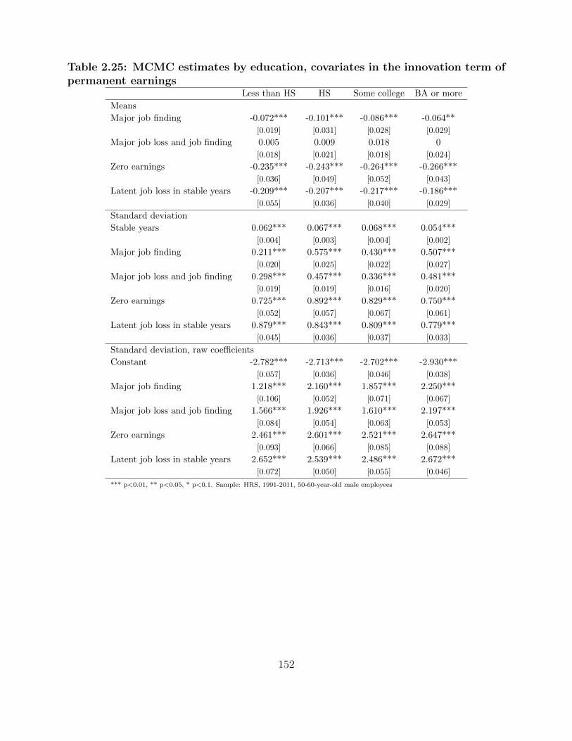
Table 2.25: MCMC estimates by education, covariates in the innovation term ofpermanent earnings

Less than HS HS Some college BA or more

Means

Major job finding -0.072*** -0.101*** -0.086*** -0.064**

[0.019] [0.031] [0.028] [0.029]

Major job loss and job finding 0.005 0.009 0.018 0

[0.018] [0.021] [0.018] [0.024]

Zero earnings -0.235*** -0.243*** -0.264*** -0.266***

[0.036] [0.049] [0.052] [0.043]

Latent job loss in stable years -0.209*** -0.207*** -0.217*** -0.186***

[0.055] [0.036] [0.040] [0.029]

Standard deviation

Stable years 0.062*** 0.067*** 0.068*** 0.054***

[0.004] [0.003] [0.004] [0.002]

Major job finding 0.211*** 0.575*** 0.430*** 0.507***

[0.020] [0.025] [0.022] [0.027]

Major job loss and job finding 0.298*** 0.457*** 0.336*** 0.481***

[0.019] [0.019] [0.016] [0.020]

Zero earnings 0.725*** 0.892*** 0.829*** 0.750***

[0.052] [0.057] [0.067] [0.061]

Latent job loss in stable years 0.879*** 0.843*** 0.809*** 0.779***

[0.045] [0.036] [0.037] [0.033]


Constant -2.782*** -2.713*** -2.702*** -2.930***

[0.057] [0.036] [0.046] [0.038]


[0.106] [0.052] [0.071] [0.067]


[0.084] [0.054] [0.063] [0.053]

Zero earnings 2.461*** 2.601*** 2.521*** 2.647***

[0.093] [0.066] [0.085] [0.088]


[0.072] [0.050] [0.055] [0.046]


152

Table 2.26: MCMC estimates by education, other parameters in earningsLess than HS HS Some college BA or more

Permanent std, age 50 0.508*** 0.463*** 0.523*** 0.582***

[0.017] [0.012] [0.015] [0.015]

Transitory std 0.054*** 0.045*** 0.040*** 0.029***

[0.003] [0.002] [0.003] [0.002]

Probability of latent job loss in stable years 0.087*** 0.102*** 0.115*** 0.120***

[0.007] [0.005] [0.007] [0.006]


Major job loss 0.408*** 0.413*** 0.436*** 0.384***

[0.011] [0.009] [0.011] [0.009]


[0.012] [0.010] [0.011] [0.010]


[0.011] [0.009] [0.010] [0.009]


[0.012] [0.010] [0.011] [0.010]

Raw coefficients of transitory earnings loss, γjMajor job-loss 1.460*** 1.422*** 1.296*** 1.609***

[0.067] [0.052] [0.057] [0.063]


[0.075] [0.069] [0.080] [0.071]


[0.057] [0.057] [0.073] [0.087]


[0.199] [0.164] [0.130] [0.110]


Table 2.27: MCMC estimates by education, covariates in measurement errorLess than HS HS Some college BA or more

Constant -0.065 -0.015 0.006 0.012

[0.041] [0.020] [0.026] [0.030]

Black -0.057*** -0.011 0.035 0.077***

[0.021] [0.017] [0.023] [0.027]

Hispanic -0.066*** -0.049** 0.017 0.102***

[0.019] [0.023] [0.026] [0.039]

Age - 50 0.022** -0.003 0.003 0.013*

[0.011] [0.005] [0.006] [0.007]

(Age - 50) squared -0.002** 0 0 -0.001**

[0.001] [0.000] [0.000] [0.001]

Single 0.014 0.002 0.028* -0.001

[0.021] [0.013] [0.016] [0.019]

Salaried worker 0.01 0.009 0.025** -0.002

[0.020] [0.010] [0.011] [0.014]

GDP gap -0.043 0.221 0.357* -0.196

[0.325] [0.169] [0.188] [0.207]

Year-1980 0 0.001* -0.001 -0.001

[0.001] [0.001] [0.001] [0.001]


153

Table 2.28: MCMC estimates in the baseline specification, other parameters inmeasurement error


Std permanent error 0.112*** 0.129*** 0.149*** 0.167***

[0.012] [0.007] [0.007] [0.008]


Stable years 0.150*** 0.095*** 0.096*** 0.128***

[0.009] [0.005] [0.005] [0.010]

Major job loss 0.585*** 0.566*** 0.532*** 0.497***

[0.037] [0.022] [0.030] [0.023]


[0.043] [0.027] [0.023] [0.017]


[0.035] [0.023] [0.030] [0.026]


[0.044] [0.026] [0.027] [0.026]


Permanent earnings 1.008*** 0.952*** 0.934*** 0.913***

[0.014] [0.009] [0.011] [0.010]

Transitory on-the-job* 0 0 0 0

Transitory due to job-loss 0.667*** 0.844*** 0.857*** 0.942***

[0.028] [0.017] [0.022] [0.022]

Transitory due to job finding 0.283*** 0.793*** 0.502*** 0.629***

[0.034] [0.017] [0.017] [0.024]

Transitory due to job loss and job finding 0.417*** 0.596*** 0.459*** 0.887***

[0.019] [0.018] [0.022] [0.025]

Transitory due to latent job loss in stable years 1.058*** 0.760*** 0.715*** 1.099***

[0.124] [0.060] [0.050] [0.116]

*The fraction of transitory reports are calibrated to zero in the baseline specification.


154

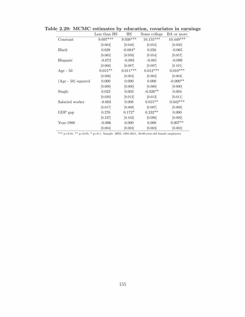
Table 2.29: MCMC estimates by education, covariates in earningsLess than HS HS Some college BA or more

Constant 9.697*** 9.938*** 10.155*** 10.449***

[0.063] [0.048] [0.054] [0.050]

Black 0.028 -0.084* 0.056 -0.065

[0.065] [0.050] [0.054] [0.057]

Hispanic -0.072 -0.093 -0.081 -0.099

[0.066] [0.087] [0.087] [0.101]

Age - 50 0.015** 0.011*** 0.012*** 0.010***

[0.006] [0.004] [0.004] [0.004]

(Age - 50) squared 0.000 0.000 0.000 -0.000**

[0.000] [0.000] [0.000] [0.000]

Single 0.023 0.003 -0.026** 0.004

[0.020] [0.012] [0.013] [0.011]

Salaried worker -0.003 0.008 0.015** 0.042***

[0.017] [0.008] [0.007] [0.008]

GDP gap 0.276 0.172* 0.232** 0.000

[0.237] [0.102] [0.096] [0.092]

Year-1980 -0.006 0.000 0.000 0.007**

[0.004] [0.003] [0.003] [0.003]

*** p<0.01, ** p<0.05, * p<0.1. Sample: HRS, 1991-2011, 50-60-year-old female employees

155

Table 2.30: MCMC estimates by education, covariates in the innovation term ofpermanent earnings


Means

Major job finding -0.128*** -0.053** -0.092*** -0.108***

[0.027] [0.021] [0.030] [0.029]


[0.019] [0.021] [0.021] [0.020]

Zero earnings -0.184*** -0.215*** -0.249*** -0.200***

[0.027] [0.027] [0.045] [0.037]

Latent job loss in stable years -0.113** -0.178*** -0.138*** -0.302***

[0.047] [0.030] [0.028] [0.043]

Standard deviation

Stable years 0.078*** 0.069*** 0.061*** 0.063***

[0.005] [0.002] [0.002] [0.002]


[0.024] [0.018] [0.026] [0.023]


[0.019] [0.018] [0.018] [0.017]

Zero earnings 0.609*** 0.624*** 0.691*** 0.640***

[0.047] [0.039] [0.048] [0.063]


[0.044] [0.028] [0.027] [0.033]


Constant -2.545*** -2.682*** -2.800*** -2.766***

[0.065] [0.032] [0.035] [0.028]


[0.107] [0.052] [0.060] [0.055]


[0.095] [0.046] [0.052] [0.056]

Zero earnings 2.052*** 2.216*** 2.429*** 2.320***

[0.091] [0.069] [0.071] [0.104]


[0.078] [0.042] [0.050] [0.042]


156

Table 2.31: MCMC estimates by education, other parameters in earningsLess than HS HS Some college BA or more

Permanent std, age 50 0.538*** 0.619*** 0.599*** 0.569***

[0.021] [0.015] [0.017] [0.015]

Transitory std 0.055*** 0.031*** 0.030*** 0.018***

[0.004] [0.003] [0.003] [0.003]


[0.009] [0.005] [0.007] [0.005]


Major job loss 0.474*** 0.452*** 0.429*** 0.404***

[0.012] [0.008] [0.010] [0.010]


[0.012] [0.009] [0.010] [0.011]


[0.011] [0.008] [0.009] [0.010]


[0.015] [0.009] [0.008] [0.010]

Raw coefficients of transitory earnings loss, γjMajor job-loss 1.113*** 1.213*** 1.335*** 1.474***

[0.051] [0.039] [0.052] [0.064]


[0.073] [0.046] [0.059] [0.059]


[0.055] [0.046] [0.052] [0.071]


[0.252] [0.125] [0.143] [0.111]


Table 2.32: MCMC estimates by education, covariates in measurement errorLess than HS HS Some college BA or more

Constant 0.028 -0.005 -0.053** -0.061

[0.051] [0.024] [0.024] [0.038]

Black -0.063** 0.003 -0.023 0.02

[0.025] [0.014] [0.018] [0.028]

Hispanic -0.057** -0.038* 0.005 -0.024

[0.025] [0.022] [0.027] [0.048]

Age - 50 -0.012 -0.002 0.002 -0.001

[0.014] [0.006] [0.006] [0.010]

(Age - 50) squared 0.001 0 0 0

[0.001] [0.000] [0.000] [0.001]

Single -0.011 -0.026** 0.025* 0.022

[0.022] [0.011] [0.013] [0.018]

Salaried worker 0.105*** 0.022** 0.035*** 0.063***

[0.031] [0.010] [0.011] [0.017]

GDP gap 0.417 0.312 -0.086 0.096

[0.483] [0.193] [0.180] [0.283]

Year-1980 0 0.001 0.002* 0.002

[0.002] [0.001] [0.001] [0.001]


157

Table 2.33: MCMC estimates in the baseline specification, other parameters inmeasurement errors


Std permanent error 0.128*** 0.089*** 0.148*** 0.193***

[0.018] [0.007] [0.013] [0.010]


Stable years 0.206*** 0.150*** 0.109*** 0.197***

[0.013] [0.011] [0.006] [0.009]

Major job loss 0.617*** 0.596*** 0.598*** 0.613***

[0.035] [0.023] [0.028] [0.029]


[0.038] [0.025] [0.035] [0.026]


[0.043] [0.030] [0.034] [0.018]


[0.069] [0.033] [0.025] [0.046]


Permanent earnings 0.975*** 0.963*** 0.917*** 0.928***

[0.017] [0.007] [0.009] [0.013]

Transitory on-the-job* 0 0 0 0

Transitory due to job-loss 0.440*** 0.782*** 0.870*** 0.738***

[0.042] [0.014] [0.017] [0.032]

Transitory due to job finding 0.539*** 0.659*** 0.677*** 0.867***

[0.026] [0.015] [0.017] [0.024]

Transitory due to job loss and job finding 0.450*** 0.582*** 0.796*** 0.878***

[0.028] [0.016] [0.014] [0.024]


[0.106] [0.026] [0.048] [0.074]

*The fraction of transitory reports are calibrated to zero in the baseline specification.


158

Table 2.34: MCMC estimates with alternative modeling assumptions, covariatesin earnings

Males Females


MA(1) MA(2) No latent MA(1) MA(2) No latent

Constant 10.688*** 10.679*** 10.606*** 9.927*** 9.894*** 9.729***

[0.028] [0.029] [0.030] [0.029] [0.029] [0.030]

Black -0.313*** -0.298*** -0.262*** -0.021 -0.019 -0.026

[0.030] [0.030] [0.031] [0.029] [0.029] [0.030]

Hispanic -0.323*** -0.308*** -0.280*** -0.097** -0.088** -0.034

[0.034] [0.034] [0.036] [0.043] [0.042] [0.043]

Less than high school -0.285*** -0.279*** -0.265*** -0.249*** -0.259*** -0.189***

[0.033] [0.033] [0.033] [0.038] [0.038] [0.037]

Some college 0.088*** 0.093*** 0.086*** 0.203*** 0.224*** 0.193***

[0.028] [0.028] [0.029] [0.029] [0.029] [0.030]

BA 0.395*** 0.411*** 0.361*** 0.485*** 0.500*** 0.437***

[0.033] [0.033] [0.034] [0.037] [0.037] [0.039]

More than BA 0.483*** 0.480*** 0.442*** 0.754*** 0.767*** 0.721***

[0.032] [0.032] [0.034] [0.037] [0.037] [0.039]

Age - 50 0.012*** 0.012*** 0.021*** 0.015*** 0.012*** 0.018***

[0.002] [0.002] [0.004] [0.002] [0.002] [0.004]

(Age - 50) squared -0.000** -0.000** -0.003*** -0.000*** -0.000** -0.002***

[0.000] [0.000] [0.000] [0.000] [0.000] [0.000]

Single -0.006 -0.020** -0.154*** -0.001 0.004 0.045***

[0.008] [0.009] [0.017] [0.007] [0.008] [0.015]

Salaried worker 0.017*** 0.021*** 0.165*** 0.029*** 0.027*** 0.192***

[0.006] [0.006] [0.013] [0.005] [0.005] [0.012]

GDP gap 0.483*** 0.522*** 0.937*** 0.254*** 0.223*** 0.400***

[0.063] [0.067] [0.152] [0.067] [0.066] [0.145]

Year-1980 -0.005*** -0.005*** -0.005*** 0.000 0.001 0.004**

[0.001] [0.001] [0.001] [0.002] [0.002] [0.002]


159

Table 2.35: MCMC estimates with alternative modeling assumptions, covariatesin the innovation term of permanent earnings

Males Females



Means


[0.015] [0.016] [0.015] [0.016] [0.016] [0.014]

Major job loss and job finding 0.003 0.007 -0.021** 0.018 0.041*** 0.021**

[0.013] [0.013] [0.009] [0.013] [0.013] [0.008]

Zero earnings -0.277*** -0.282*** -0.247*** -0.246*** -0.233*** -0.214***

[0.024] [0.023] [0.011] [0.017] [0.018] [0.009]

Latent job loss in stable years -0.311*** -0.357*** -0.264*** -0.271***

[0.027] [0.029] [0.023] [0.024]

Standard deviation

Stable years 0.063*** 0.067*** 0.085*** 0.066*** 0.064*** 0.084***

[0.002] [0.002] [0.000] [0.002] [0.003] [0.000]


[0.014] [0.014] [0.009] [0.015] [0.015] [0.008]


[0.013] [0.012] [0.004] [0.013] [0.014] [0.004]

Zero earnings 0.839*** 0.840*** 0.140*** 0.703*** 0.698*** 0.139***

[0.036] [0.038] [0.003] [0.028] [0.027] [0.002]


[0.026] [0.028] [0.023] [0.025]


Constant -2.767*** -2.697*** -2.461*** -2.721*** -2.751*** -2.473***

[0.030] [0.031] [0.006] [0.034] [0.041] [0.006]


[0.037] [0.038] [0.021] [0.041] [0.048] [0.020]


[0.034] [0.036] [0.020] [0.039] [0.044] [0.020]

Zero earnings 2.594*** 2.526*** 0.496*** 2.370*** 2.393*** 0.499***

[0.043] [0.047] [0.019] [0.046] [0.054] [0.016]


[0.034] [0.037] [0.040] [0.041]


160

Table 2.36: MCMC estimates with alternative modeling assumptions, other pa-rameters in earnings

Males Females




[0.008] [0.008] [0.009] [0.009] [0.008] [0.009]

Transitory std 0.061*** 0.068*** 0.313*** 0.063*** 0.064*** 0.282***

[0.002] [0.002] [0.002] [0.003] [0.002] [0.002]

MA(1) term -0.283*** -0.298*** -0.523*** -0.565***

[0.034] [0.045] [0.034] [0.045]

MA(2) term -0.089** -0.191***

[0.036] [0.044]

Total transitory 0.064*** 0.072*** 0.073*** 0.077***

[0.010] [0.010] [0.012] [0.014]


[0.002] [0.002] [0.002] [0.002]


Major job loss 0.410*** 0.405*** 0.400*** 0.435*** 0.433*** 0.421***

[0.005] [0.005] [0.006] [0.005] [0.005] [0.006]


[0.005] [0.005] [0.007] [0.005] [0.005] [0.007]


[0.004] [0.005] [0.006] [0.005] [0.005] [0.006]


[0.007] [0.007] [0.006] [0.008]


[0.029] [0.030] [0.040] [0.025] [0.025] [0.034]


[0.040] [0.042] [0.060] [0.031] [0.033] [0.045]


[0.035] [0.037] [0.047] [0.033] [0.031] [0.040]


[0.071] [0.074] [0.069] [0.084]


161

Table 2.37: MCMC estimates with alternative modeling assumptions, covariatesin measurement error

Males Females



Constant -0.039* -0.03 -0.02 -0.058*** -0.051*** -0.024

[0.020] [0.020] [0.030] [0.019] [0.019] [0.029]

Black 0.017 0.02 0.025 -0.01 -0.003 0.001

[0.013] [0.013] [0.017] [0.011] [0.011] [0.015]

Hispanic -0.02 -0.027* -0.024 -0.037** -0.036** -0.031

[0.015] [0.014] [0.020] [0.015] [0.015] [0.020]

Less than high school -0.024* -0.025* -0.034** -0.029** -0.023* -0.063***

[0.013] [0.013] [0.017] [0.013] [0.013] [0.017]

Some college 0.033*** 0.034*** 0.052*** 0.021** 0.017 0.031**

[0.011] [0.011] [0.015] [0.011] [0.011] [0.014]

BA 0.02 0.017 0.054*** -0.004 0 0.031*

[0.013] [0.013] [0.018] [0.014] [0.014] [0.018]

More than BA 0.034** 0.027** 0.074*** 0.013 0.019 0.048***

[0.014] [0.014] [0.018] [0.014] [0.014] [0.018]

Age - 50 0.012** 0.010* 0.005 0.003 0.004 0.003

[0.005] [0.005] [0.008] [0.005] [0.005] [0.008]

(Age - 50) squared -0.001*** -0.001** 0 0 -0.001 0

[0.000] [0.000] [0.001] [0.000] [0.000] [0.001]

Single 0.019* 0.012 0.043*** 0.002 0.004 -0.027**

[0.011] [0.010] [0.015] [0.008] [0.008] [0.011]

Salaried worker 0.015* 0.016* -0.02 0.045*** 0.045*** 0.01

[0.009] [0.009] [0.013] [0.009] [0.009] [0.012]

GDP gap 0.205 0.183 0.473** -0.011 -0.05 -0.18

[0.148] [0.149] [0.234] [0.149] [0.149] [0.232]

Year-1980 0 0 0 0.002*** 0.002*** 0

[0.001] [0.001] [0.001] [0.001] [0.001] [0.001]


162

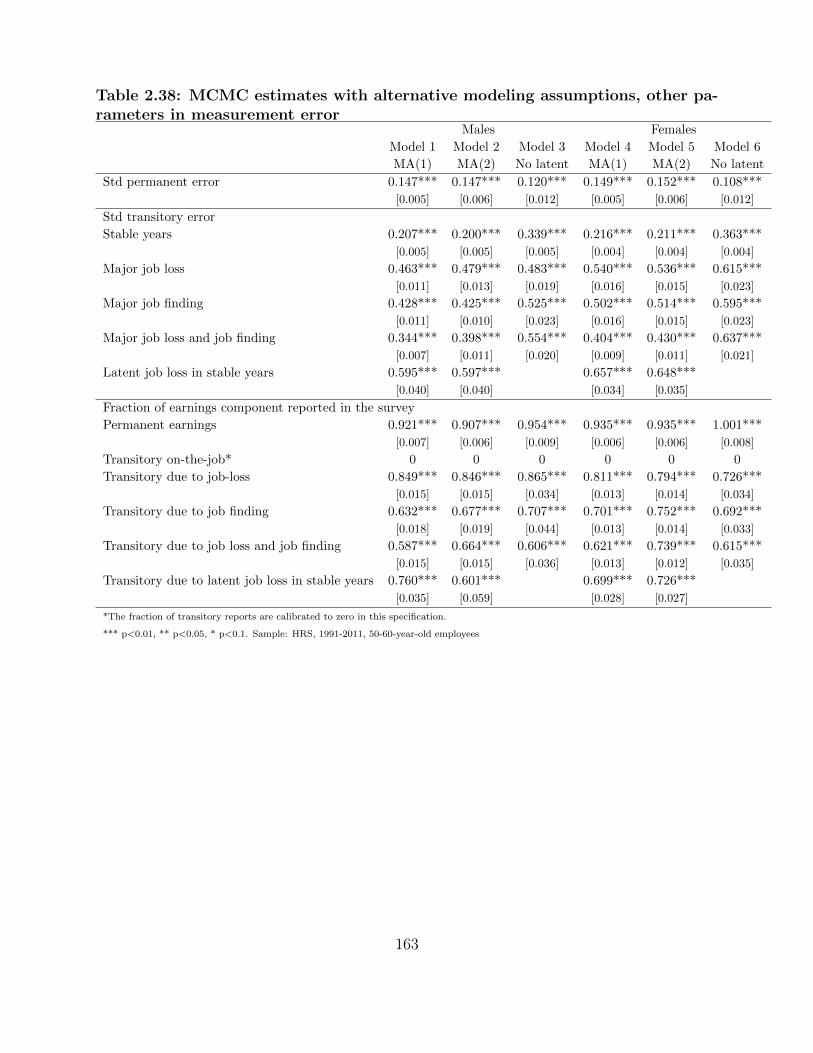
Table 2.38: MCMC estimates with alternative modeling assumptions, other pa-rameters in measurement error

Males Females




[0.005] [0.006] [0.012] [0.005] [0.006] [0.012]


Stable years 0.207*** 0.200*** 0.339*** 0.216*** 0.211*** 0.363***

[0.005] [0.005] [0.005] [0.004] [0.004] [0.004]

Major job loss 0.463*** 0.479*** 0.483*** 0.540*** 0.536*** 0.615***

[0.011] [0.013] [0.019] [0.016] [0.015] [0.023]


[0.011] [0.010] [0.023] [0.016] [0.015] [0.023]


[0.007] [0.011] [0.020] [0.009] [0.011] [0.021]


[0.040] [0.040] [0.034] [0.035]



[0.007] [0.006] [0.009] [0.006] [0.006] [0.008]

Transitory on-the-job* 0 0 0 0 0 0


[0.015] [0.015] [0.034] [0.013] [0.014] [0.034]


[0.018] [0.019] [0.044] [0.013] [0.014] [0.033]

Transitory due to job loss and job finding 0.587*** 0.664*** 0.606*** 0.621*** 0.739*** 0.615***

[0.015] [0.015] [0.036] [0.013] [0.012] [0.035]


[0.035] [0.059] [0.028] [0.027]

*The fraction of transitory reports are calibrated to zero in this specification.


163

Table 2.39: MCMC estimates with alternative modeling of reporting transitoryshocks, covariates in earnings

Males Females


τ trans = 0.5 τ trans = 1 τ trans estim τ trans = 0.5 τ trans = 1 τ trans estim

Constant 10.694*** 10.696*** 10.691*** 9.920*** 9.921*** 9.917***

[0.028] [0.027] [0.027] [0.030] [0.028] [0.027]

Black -0.295*** -0.305*** -0.299*** -0.016 -0.019 -0.015

[0.029] [0.029] [0.029] [0.028] [0.028] [0.027]

Hispanic -0.306*** -0.315*** -0.306*** -0.088** -0.069* -0.117***

[0.033] [0.033] [0.033] [0.041] [0.042] [0.040]


[0.032] [0.031] [0.032] [0.035] [0.034] [0.039]

Some college 0.112*** 0.108*** 0.097*** 0.221*** 0.218*** 0.228***

[0.027] [0.027] [0.028] [0.028] [0.028] [0.028]

BA 0.406*** 0.411*** 0.392*** 0.492*** 0.498*** 0.501***

[0.031] [0.032] [0.032] [0.036] [0.036] [0.036]

More than BA 0.483*** 0.482*** 0.476*** 0.756*** 0.763*** 0.768***

[0.031] [0.031] [0.032] [0.036] [0.035] [0.036]

Age - 50 0.011*** 0.011*** 0.011*** 0.011*** 0.012*** 0.011***

[0.002] [0.002] [0.002] [0.002] [0.002] [0.002]

(Age - 50) squared -0.000** -0.000** -0.000** -0.000*** -0.000*** -0.000***

[0.000] [0.000] [0.000] [0.000] [0.000] [0.000]

Single -0.014* -0.016** -0.013* -0.004 -0.006 -0.005

[0.007] [0.007] [0.007] [0.007] [0.007] [0.007]

Salaried worker 0.014*** 0.015*** 0.014*** 0.021*** 0.020*** 0.020***

[0.005] [0.005] [0.005] [0.004] [0.004] [0.004]

GDP gap 0.414*** 0.445*** 0.393*** 0.160*** 0.148*** 0.161***

[0.057] [0.060] [0.057] [0.053] [0.054] [0.055]

Year-1980 -0.006*** -0.005*** -0.005*** 0.001 0.001 0.001

[0.001] [0.001] [0.001] [0.002] [0.002] [0.001]


164

Table 2.40: MCMC estimates with alternative modeling of reporting transitoryshocks, covariates in the innovation term of permanent earnings

Males Females



Means


[0.014] [0.015] [0.014] [0.014] [0.013] [0.014]

Major job loss and job finding 0.024** 0.016 0.020* 0.068*** 0.065*** 0.063***

[0.011] [0.010] [0.010] [0.011] [0.010] [0.010]

Zero earnings -0.250*** -0.254*** -0.249*** -0.207*** -0.195*** -0.213***

[0.023] [0.028] [0.022] [0.015] [0.017] [0.021]


[0.019] [0.020] [0.019] [0.018] [0.018] [0.018]

Standard deviation

Stable years 0.064*** 0.067*** 0.065*** 0.068*** 0.070*** 0.070***

[0.002] [0.001] [0.002] [0.001] [0.001] [0.001]


[0.014] [0.013] [0.013] [0.013] [0.012] [0.013]


[0.010] [0.010] [0.010] [0.011] [0.010] [0.012]

Zero earnings 0.795*** 0.791*** 0.800*** 0.651*** 0.630*** 0.640***

[0.035] [0.040] [0.044] [0.025] [0.025] [0.023]


[0.024] [0.024] [0.025] [0.021] [0.020] [0.019]


Constant -2.757*** -2.698*** -2.741*** -2.697*** -2.657*** -2.653***

[0.022] [0.021] [0.023] [0.019] [0.017] [0.020]


[0.034] [0.032] [0.034] [0.032] [0.029] [0.032]


[0.030] [0.029] [0.030] [0.027] [0.025] [0.033]

Zero earnings 2.529*** 2.472*** 2.526*** 2.268*** 2.200*** 2.207***

[0.042] [0.040] [0.050] [0.042] [0.035] [0.037]


[0.027] [0.026] [0.028] [0.025] [0.025] [0.025]


165

Table 2.41: MCMC estimates with alternative modeling of reporting transitoryshocks, other parameters in earnings

Males Females




[0.007] [0.007] [0.007] [0.008] [0.008] [0.008]

Transitory std 0.040*** 0.037*** 0.039*** 0.028*** 0.023*** 0.026***

[0.001] [0.001] [0.001] [0.002] [0.002] [0.002]

Probability of latent job loss 0.106*** 0.105*** 0.108*** 0.115*** 0.118*** 0.114***

[0.003] [0.003] [0.003] [0.004] [0.003] [0.004]


Major job loss 0.410*** 0.414*** 0.411*** 0.452*** 0.458*** 0.452***

[0.005] [0.005] [0.005] [0.005] [0.005] [0.005]


[0.006] [0.005] [0.005] [0.005] [0.005] [0.005]


[0.005] [0.005] [0.005] [0.005] [0.005] [0.005]


[0.007] [0.007] [0.007] [0.005] [0.006] [0.006]


[0.029] [0.029] [0.029] [0.023] [0.023] [0.024]


[0.040] [0.036] [0.036] [0.028] [0.025] [0.027]


[0.032] [0.034] [0.032] [0.028] [0.027] [0.027]


[0.069] [0.080] [0.076] [0.069] [0.065] [0.076]


166

Table 2.42: MCMC estimates with alternative modeling of reporting transitoryshocks, covariates in measurement error

Males Females



Constant -0.027** -0.030** -0.017 -0.034** -0.032** -0.030**

[0.014] [0.014] [0.014] [0.016] [0.015] [0.015]

Black 0.003 0.002 0.003 0 -0.005 -0.002

[0.012] [0.011] [0.011] [0.010] [0.009] [0.009]

Hispanic -0.021 -0.019 -0.025** -0.038*** -0.038*** -0.043***

[0.014] [0.013] [0.013] [0.013] [0.013] [0.013]

Less than high school -0.025** -0.026** -0.021* -0.032*** -0.028** -0.025**

[0.012] [0.011] [0.011] [0.012] [0.011] [0.011]

Some college 0.024** 0.026*** 0.026** 0.011 0.017** 0.017*

[0.010] [0.010] [0.010] [0.009] [0.009] [0.009]

BA 0.028** 0.023** 0.029** -0.012 -0.008 -0.006

[0.012] [0.012] [0.012] [0.012] [0.012] [0.012]

More than BA 0.029** 0.022* 0.031*** 0.011 0.015 0.01

[0.012] [0.012] [0.012] [0.012] [0.012] [0.012]

Age - 50 0.007** 0.008** 0.005* 0 0.001 0

[0.003] [0.003] [0.003] [0.004] [0.004] [0.004]

(Age - 50) squared -0.001** -0.001*** -0.000* 0 0 0

[0.000] [0.000] [0.000] [0.000] [0.000] [0.000]

Single 0.019** 0.011 0.014* -0.001 0.003 -0.002

[0.009] [0.008] [0.008] [0.007] [0.007] [0.007]

Salaried worker 0.009 0.012* 0.005 0.037*** 0.035*** 0.033***

[0.007] [0.007] [0.007] [0.007] [0.007] [0.007]

GDP gap 0.059 0.085 0.039 0.041 0.045 -0.087

[0.101] [0.103] [0.097] [0.125] [0.123] [0.120]

Year-1980 0 0 0 0.001** 0.001* 0.001

[0.000] [0.000] [0.000] [0.001] [0.000] [0.000]


167

Table 2.43: MCMC estimates with alternative modeling of reporting transitoryshocks, other parameters in measurement error

Males Females




[0.004] [0.004] [0.004] [0.005] [0.005] [0.005]


Stable years 0.108*** 0.114*** 0.091*** 0.166*** 0.158*** 0.121***

[0.003] [0.004] [0.004] [0.008] [0.008] [0.016]

Major job loss 0.561*** 0.536*** 0.519*** 0.627*** 0.621*** 0.623***

[0.016] [0.014] [0.014] [0.017] [0.019] [0.020]


[0.014] [0.015] [0.012] [0.014] [0.018] [0.015]


[0.017] [0.018] [0.017] [0.020] [0.017] [0.019]


[0.018] [0.023] [0.019] [0.032] [0.023] [0.022]



[0.005] [0.006] [0.005] [0.005] [0.005] [0.005]

Transitory on-the-job 0.5 1 -0.514*** 0.5 1 -3.277***

[0.140] [0.681]


[0.010] [0.010] [0.011] [0.010] [0.010] [0.011]


[0.011] [0.011] [0.009] [0.009] [0.009] [0.008]

Transitory due to job loss and find 0.536*** 0.519*** 0.570*** 0.633*** 0.594*** 0.532***

[0.010] [0.010] [0.010] [0.009] [0.009] [0.010]

Transitory due to latent job loss 0.519*** 0.770*** 0.757*** 0.834*** 0.856*** 0.800***

[0.031] [0.029] [0.029] [0.022] [0.020] [0.023]


168

Table 2.44: MCMC estimates using alternative samples, covariates in earningsMales Females


1980-2011 matched sample 1980-2011 matched sample

with off years no off years with off years no off years

Constant 10.712*** 10.701*** 10.700*** 9.785*** 9.943*** 9.971***

[0.019] [0.024] [0.027] [0.021] [0.025] [0.026]

Black -0.270*** -0.237*** -0.219*** 0.012 -0.025 -0.030

[0.024] [0.029] [0.029] [0.025] [0.027] [0.025]

Hispanic -0.285*** -0.277*** -0.269*** -0.117*** -0.093** -0.095***

[0.029] [0.034] [0.033] [0.037] [0.039] [0.037]


[0.025] [0.030] [0.029] [0.030] [0.033] [0.032]

Some college 0.100*** 0.128*** 0.160*** 0.184*** 0.225*** 0.219***

[0.023] [0.027] [0.026] [0.026] [0.027] [0.026]

BA 0.399*** 0.419*** 0.440*** 0.446*** 0.503*** 0.501***

[0.028] [0.031] [0.031] [0.034] [0.035] [0.034]

More than BA 0.481*** 0.496*** 0.506*** 0.751*** 0.735*** 0.706***

[0.027] [0.030] [0.030] [0.033] [0.035] [0.034]

Age - 50 0.008*** 0.010*** 0.010*** 0.005*** 0.008*** 0.011***

[0.002] [0.002] [0.003] [0.002] [0.002] [0.003]

(Age - 50) squared -0.000** 0.000 0.000 -0.000*** -0.000* 0.000

[0.000] [0.000] [0.000] [0.000] [0.000] [0.000]

Single -0.025*** -0.011 -0.045*** -0.003 -0.001 0.029***

[0.008] [0.008] [0.010] [0.007] [0.007] [0.009]

Salaried worker 0.016*** 0.016*** 0.025*** 0.021*** 0.023*** 0.038***

[0.005] [0.005] [0.007] [0.004] [0.004] [0.006]

GDP gap 0.366*** 0.397*** 0.174* 0.167*** 0.158*** -0.153

[0.041] [0.062] [0.101] [0.040] [0.055] [0.099]

Year-1980 -0.006*** -0.005*** -0.006*** 0.008*** 0.003** 0.003**

[0.001] [0.001] [0.001] [0.001] [0.001] [0.001]


169

Table 2.45: MCMC estimates using alternative samples, covariates in the inno-vation term of permanent earnings

Males Females




Means


[0.011] [0.012] [0.014] [0.011] [0.014] [0.015]

Major job loss and job finding 0.026*** -0.01 -0.044*** 0.089*** 0.049*** 0

[0.009] [0.010] [0.010] [0.009] [0.010] [0.010]

Zero earnings -0.233*** -0.179*** -0.145*** -0.174*** -0.141*** -0.197***

[0.016] [0.016] [0.019] [0.019] [0.010] [0.013]


[0.015] [0.018] [0.012] [0.015] [0.017] [0.016]

Standard deviation

Stable years 0.069*** 0.060*** 0.035*** 0.073*** 0.065*** 0.042***

[0.001] [0.002] [0.002] [0.001] [0.001] [0.004]


[0.011] [0.015] [0.015] [0.010] [0.013] [0.019]


[0.009] [0.011] [0.013] [0.009] [0.010] [0.016]

Zero earnings 0.745*** 0.331*** 0.317*** 0.698*** 0.165*** 0.302***

[0.033] [0.035] [0.034] [0.030] [0.035] [0.030]


[0.018] [0.023] [0.015] [0.017] [0.017] [0.021]


Constant -2.681*** -2.821*** -3.348*** -2.622*** -2.743*** -3.165***

[0.015] [0.026] [0.066] [0.017] [0.021] [0.048]


[0.026] [0.045] [0.095] [0.025] [0.035] [0.069]


[0.022] [0.035] [0.088] [0.024] [0.031] [0.082]

Zero earnings 2.393*** 1.720*** 2.194*** 2.269*** 0.899*** 1.965***

[0.032] [0.102] [0.115] [0.032] [0.235] [0.109]


[0.022] [0.030] [0.066] [0.022] [0.027] [0.051]


170

Table 2.46: MCMC estimates using alternative samples, other parameters inearnings

Males Females





[0.006] [0.008] [0.009] [0.007] [0.008] [0.009]

Transitory std 0.037*** 0.043*** 0.053*** 0.025*** 0.029*** 0.050***

[0.001] [0.001] [0.002] [0.002] [0.002] [0.002]

Probability of latent job loss 0.106*** 0.107*** 0.129*** 0.115*** 0.121*** 0.121***

[0.002] [0.004] [0.004] [0.003] [0.003] [0.004]


Major job loss 0.392*** 0.394*** 0.381*** 0.421*** 0.433*** 0.430***

[0.004] [0.005] [0.006] [0.004] [0.005] [0.006]


[0.005] [0.005] [0.006] [0.005] [0.005] [0.006]


[0.004] [0.005] [0.006] [0.004] [0.005] [0.006]


[0.006] [0.006] [0.006] [0.005] [0.006] [0.006]


[0.029] [0.033] [0.038] [0.025] [0.026] [0.028]


[0.039] [0.038] [0.034] [0.027] [0.027] [0.027]


[0.030] [0.039] [0.039] [0.023] [0.030] [0.027]


[0.070] [0.084] [0.054] [0.063] [0.081] [0.066]


171

Table 2.47: MCMC estimates using alternative samples, covariates in measure-ment error

Males Females




Constant -0.018 -0.021 -0.021 -0.018 -0.027* -0.027*

[0.014] [0.014] [0.014] [0.016] [0.016] [0.014]

Black 0.002 0.004 0.012 -0.007 -0.007 -0.012

[0.012] [0.011] [0.012] [0.010] [0.010] [0.010]

Hispanic -0.015 -0.026** -0.031** -0.039*** -0.043*** -0.043***

[0.013] [0.013] [0.013] [0.014] [0.014] [0.015]

Less than high school -0.032*** -0.026** -0.021* -0.034*** -0.027** -0.028**

[0.012] [0.011] [0.011] [0.012] [0.012] [0.012]

Some college 0.027*** 0.027*** 0.028*** 0.022** 0.01 0.020**

[0.010] [0.010] [0.010] [0.009] [0.009] [0.009]

BA 0.027** 0.021* 0.023* -0.005 -0.011 -0.01

[0.012] [0.011] [0.012] [0.012] [0.012] [0.012]

More than BA 0.027** 0.022* 0.029** 0.013 0.003 0.001

[0.012] [0.011] [0.012] [0.012] [0.013] [0.012]

Age - 50 0.006* 0.007** 0.004 -0.001 0 -0.001

[0.003] [0.003] [0.003] [0.004] [0.004] [0.003]

(Age - 50) squared -0.001** -0.001** -0.000* 0 0 0

[0.000] [0.000] [0.000] [0.000] [0.000] [0.000]

Single 0.012 0.015* 0.006 0 0.008 -0.002

[0.009] [0.008] [0.008] [0.007] [0.007] [0.007]

Salaried worker 0.006 0.011* 0.006 0.035*** 0.045*** 0.030***

[0.007] [0.006] [0.007] [0.007] [0.007] [0.007]

GDP gap 0.101 0.077 0.149 0.051 -0.016 0.089

[0.104] [0.098] [0.098] [0.126] [0.125] [0.106]

Year-1980 0 0 0 0.001 0.001 0.001

[0.000] [0.000] [0.001] [0.001] [0.001] [0.000]


172

Table 2.48: MCMC estimates using alternative samples, other parameters inmeasurement error

Males Females





[0.004] [0.005] [0.007] [0.005] [0.008] [0.005]


Stable years 0.109*** 0.102*** 0.090*** 0.164*** 0.161*** 0.115***

[0.005] [0.004] [0.003] [0.008] [0.011] [0.006]

Major job loss 0.527*** 0.540*** 0.521*** 0.634*** 0.632*** 0.623***

[0.014] [0.015] [0.017] [0.020] [0.021] [0.023]


[0.013] [0.017] [0.015] [0.020] [0.017] [0.025]


[0.017] [0.018] [0.019] [0.018] [0.019] [0.023]


[0.034] [0.027] [0.034] [0.026] [0.034] [0.050]



[0.006] [0.006] [0.010] [0.005] [0.006] [0.007]

Transitory on-the-job* 0 0 0 0 0 0


[0.010] [0.010] [0.009] [0.011] [0.010] [0.008]


[0.011] [0.010] [0.008] [0.010] [0.009] [0.007]

Transitory due to job loss and find 0.540*** 0.566*** 0.656*** 0.632*** 0.712*** 0.706***

[0.010] [0.009] [0.008] [0.010] [0.009] [0.008]

Transitory due to latent job loss 0.986*** 0.587*** 0.889*** 0.827*** 1.013*** 0.859***

[0.042] [0.046] [0.020] [0.023] [0.039] [0.014]

*The fraction of transitory reports are calibrated to zero in this specification.


173

CHAPTER III

Estimating Second Order Probability Beliefs

from Subjective Survival Data

3.1 Introduction

Textbook models of uncertainty usually treat probabilities as known or knowable objects.

This is the case for outcomes of symmetric devices with known properties that are subject to

random forces such as the toss of a coin or die, the shuffling of a deck of cards or the shaking

of an urn containing balls of different colors. In contrast, the probabilities that confront

economic decision makers are usually less precisely known.34, 35

In this paper, we investigate the probability beliefs held by a given individual about

personal mortality risks elicited from survey questions on the Health and Retirement Study

(HRS) that ask respondents about the numerical probability that he or she will survive to

34Frank Knight, as early as in 1921, introduced the distinction between, as he called, “risk” for known and“uncertainty” for unknown probabilities.

35Pate-Cornell (1996) observes that “. . . uncertainties in decision and risk analyses can be divided into twocategories: those that stem from variability in known (or observable) populations and, therefore, representrandomness in samples (aleatory uncertainties), and those that come from basic lack of knowledge aboutfundamental phenomena (epistemic uncertainties also known in the literature as ambiguity).”

174

a given age that is 10-20 years in the future. In forming his belief about mortality risk, a

person might consult a life table based on the experience of millions of individuals. The life

table provides an estimate of the mean probability of survival for persons of given age and sex

with essentially no sampling error. However, the individual may be ambiguous about whether

this probability represents the risk he himself faces. He may have personal information that

makes him think that he has a higher or lower risk than the average person of his age and

sex. Moreover, he may be unsure about the influence that personal information such as the

ages at death of parents and relatives, health history and current symptoms, or exercise and

dietary habits will have on his likely longevity. Finally, in answering the survey question,

a person must construct a probability judgment “on the fly,” accessing whatever frequentist

data or epistemic beliefs he may have stored in his brain and manipulating this information

through reasoning or gut reaction to produce an answer to the specific question about, say,

the probability he will survive to age 80, all within less than a minute.36

In this paper, we assume that probability beliefs about survival are ambiguous in the

sense that an individual has in mind a range of possible values of the probability that can

be described by a density function, g(p), that can take on a variety of shapes depending on

both its mean and the degree of ambiguity. The theory literature calls this density function

second order probability beliefs. (See, for example, Gilboa and Marinacci, 2011).

We compare the predicted survival rates of our sample members to the actual survival

of sample members eight years later, as reported in the 2010 wave of HRS. The predictions

from our models track actual mortality fairly closely for sample members who are below age

80, but begin to diverge substantially at the oldest ages, with older respondents being overly

36The attempt to determine the probabilistic beliefs of lay people using direct questions on surveys hasonly become commonplace in the past two decades (Manski, 2004). There is a related but somewhat separatetradition of eliciting probability beliefs of experts as part of risk assessments in engineering and operationsresearch applications. See Pate-Cornell (1996) for a summary of this tradition.

175

optimistic. The predicted survival rates co-vary with demographic characteristics, health

status, parental mortality, smoking behavior and cognitive status in largely the same way

that they do in regressions that explain actual mortality. Thus, it appears that the subjective

survival probability answers are good candidates for modeling individual level heterogeneity

in survival chances.37

The major contribution of this paper is to provide an estimate of ambiguity about survival

probabilities that is embodied in the spread of g(p). We find that survival expectations are

very uncertain in the Health and Retirement Study (HRS) and that uncertainty varies in

the population: more educated people have more certain beliefs, women have less certain

beliefs, and deterioration of health, especially from previously excellent levels, leads to more

uncertainty about survival chances.

Identifying second order probability beliefs is possible under the assumptions of our survey

response model, the Modal Response Hypothesis (MRH) which is a mapping from probability

beliefs g(p) to survey responses. It assumes that people report the mode of g(p) whenever it

exists and they report 50%, whenever g(p) is so ambiguous that it does not have a unique

mode. The motivation for the MRH is twofold. First, imagine that people estimate the

probabilities of certain events after observing some successes and failures of these events.

Under some conditions a naıve estimator, which is the ratio of “good cases”, is exactly

equal to the mode of the Bayesian updated posterior probability distribution. Moreover,

this estimator is biased in finite samples. The MRH assumes that people report this simple,

37Our findings about the external validity of the HRS subjective probability questions are consistent withthose in earlier papers that have studied these questions in the HRS (Hurd and McGarry, 2002; Smith et al.,2001). The overly optimistic expectations of people over 75 in HRS has also been noted by Hurd et al. (2005)who find the same pattern across eleven European countries in the SHARE (Survey of Health, Ageing andRetirement in Europe). There are also a few papers that use these questions in models of behavior underuncertainty such as, for example, Picone et al. (2004) who find that people who expect to live longer aremore likely to choose medical screening tests.

176

naıve estimator in surveys. The second motivation comes from the literature using numerical

subjective probabilities on surveys. When people are asked to report a numerical probability

using any digit between 0 and 100, an unusually large fraction of answers are heaped on 50.

The excessive use of 50 has been interpreted as occurring because many people treat “50-50”

as a synonym for“I don’t know”or even for“God only knows,”a sentiment that suggests that

the true probability is unknowable (Fischhoff and Bruine De Bruin, 1999; Bruine de Bruin

and Carman, 2012; Lillard and Willis, 2001).38,39 Researchers have realized that these focal

answers might introduce bias into estimates of subjective probabilities. As a remedy,Manski

and Molinari (2010) think of focal responses as extreme versions of rounding, where some

people always round to 0, 50 or 100 percent. Lumsdaine and van Loon (2013) model the

probability of providing a focal answer as a separate equation in their econometric model.

These papers found that accounting for focal responses is important for valid inference.

However, they are agnostic about the reasons so many people provide such answers. Our

approach, instead, is to model focal responses with an economic model and relate it to the

precision of beliefs of individuals. In our model people answer with an epistemic 50 percent

as a way of saying “I am very unsure”, when their beliefs are too ambiguous. As far as we

know the MRH model is the first in the literature that makes use of the focal responses to

learn something about the beliefs of individuals.40

38In recent waves of the Health and Retirement Study, respondents have been asked a follow-up questionif they answered 50 to survival probability question: Do you think that it is about equally likely that youwill die before 75 as it is that you will live to 75 or beyond, or are you just unsure about the chances? Abouttwo-thirds say that they are “just unsure.” In this paper, we use data from the 2002 wave of HRS which didnot have a follow-up question.

39In addition, the answers to the survival questions also exhibit some heaping at 0 and 100. Taken literally,of course, these answers cannot represent rational probability beliefs except, perhaps, in the case of zero forpersons who know themselves to be terminally ill or planning suicide.

40Manski and Molinari (2010) discuss an alternative, more direct approach to learn about the imprecisionof belief. They make use of a follow-up question in a different survey (the ALP) asking about the range ofprobabilities responders had in mind when they provided their answers. Roughly half of the sample reportedthat their answers were “exact”, and the rest reported relatively wide ranges of probabilities with the average

177

For comparison, we present an alternative model of survey response which assumes that

the person reports the mean of g(p). We show that the MRH model can account quite

well for heaping at 0, 50 and 100 while the mean response model cannot. The overuse

of focal responses can be especially problematic when very low or very high probabilities

are modeled since the high ratio of 50 percent responses can arbitrarily push the estimated

mean probabilities away from their true, extreme values. We show in this paper that our

modal response model which explicitly models focal answers works better than the simple

mean model typically used in research on subjective probabilities. When the modal response

model is used for extreme probabilities both the estimated unconditional means and the

average partial effects are closer to ones estimated from realized mortality data. Alternative

models of focal responses, such as Manski and Molinari (2010) and Lumsdaine and van Loon

(2013) might work equally well to reduce this bias and to predict enough focal answers. The

main advantage of the MRH is that it is based on an economic model of limited information

and uncertain beliefs.

Learning about the degree of uncertainty in individuals’ beliefs can be important for

several reasons. First, the value of information about mortality risk, for example, should be

a function of this uncertainty. Uncertain people might value information more, and certain

people might rationally ignore any new information since they have already established a

good understanding of the risks they face. Even in a fully Bayesian Subjective Expected

Utility (SEU) framework the degree of uncertainty might play an important role if the utility

function is not linear in probabilities. This is the case, for example, if people can invest in

width being 18 percent. We believe that this approach is very informative about general uncertainty in thepopulation, but it is less obvious how to make use of the provided ranges. First, the meaning of an “exact”answer is ambiguous. Second, one would expect that 50 percent responders provide wider ranges of possibleprobabilities than people with other answers ending with 0 or 5 (like 10 or 15 percent). However, they didnot find a strong pattern like that in their data.

178

learning about their own mortality risks.41 Second, learning about the degree of uncertainty

in individuals’ beliefs is useful from a survey methodological point of view, too. People whose

probability beliefs are more certain may answer probabilistic survey questions with greater

precision. However, if beliefs are uncertain, as is the case with mortality expectations,

we expect large measurement error in survey responses, that might even account for the

discrepancy between subjective and objective survival probabilities at later ages. Future

research should investigate the potential role of measurement error in subjective expectation

data and its link to uncertainty in individuals’ beliefs. Third, learning about the degree of

uncertainty in individuals’ beliefs might be very important in Non-Bayesian/Non-Expected

Utility models. While we don’t work in these frameworks, empirical evidence on ambiguous

beliefs may be useful to those who do.

The paper is organized as follows. In Section 1 we provide a quick overview of the

literature on ambiguity and its role in economic decisions. Section 2 describes the subjective

survival data in HRS that we use in this paper. Section 3 introduces the MRH model that

can be used to model any subjective expectation data that uses the HRS framework. Section

4 describes a simple and tractable model of individual survival curves. Section 5 discusses

the estimation method and identification and Section 6 shows the results.

3.2 Ambiguity in economics

Knightian uncertainty, epistemic uncertainty and ambiguity are roughly synonymous terms

that figure prominently in a longstanding and ongoing debate about the link between ra-

tionality and probability beliefs, on the one hand, and the relationship between beliefs and

41Another example is Bommier and Villeneuve (2012), who discuss a model of mortality risk aversion,where the utility function is not additively separable over time, and thus, mortality probabilities enter themodel in a non-linear fashion as well.

179

decisions, on the other hand. In an excellent and authoritative review of this debate since

Pascal’s famous bet on the existence of God in 1670, Gilboa and Marinacci (2011) discuss

the different models of expectation formation, including Bayesian and Non-Bayesian models.

They call the model we use in this paper “the smooth model of ambiguity” or “second order

probability beliefs.” In typical models of ambiguity, agents have a set of possible probability

distributions in mind but they are not able to compound this information into a single prob-

ability distribution. The smooth model, however, makes compounding possible. The real

question in the smooth model is whether agents have a preference for known probabilities

(in other words they are ambiguity-averse) or not (in which case they are simple Bayesians).

As Gilboa and Marinacci (2011) write “. . . beyond the above mentioned separation [be-

tween beliefs and utilities], the smooth preferences model enjoys an additional advantage of

tractability. Especially if one specifies a simple functional form for [preferences for known

probabilities], one gets a simple model in which uncertainty/ambiguity attitudes can be an-

alyzed in a way that parallels the treatment of risk attitudes in the classical literature.”, pp.

45.

The major contribution of this paper is to provide an estimate of second order probability

beliefs about survival probabilities that are embodied in the spread of g(p). It is important

to clarify the role of this object in alternative views of uncertainty. Conventional economic

theory of behavior under uncertainty, rooted in subjective expected utility (SEU) theory

(Savage, 1954), is often interpreted as having erased the distinction between known and

unknown probabilities because expected utility is a linear function of probabilities. That is,

assume that the person’s ambiguous probability beliefs are described by g(p). His expected

utility is

EU =

ˆ 1

0

[pUlive + (1− p)Udie] g(p)dp = pUlive + (1− p)Udie, (3.1)

180

where is the mean of this ambiguous distribution. Clearly, expected utility is invariant to a

mean preserving spread of g(p); hence, decisions based on expected utility are unaffected by

ambiguity.

In the famous Ellsberg experiments (Ellsberg, 1961) subjects were presented with choices

of drawing balls from different urns whose compositions were either known or ambiguous.

Most people revealed distaste for ambiguity which was at odds with the SEU theory. The

survey by Gilboa and Marinacci (2011) provides a comprehensive and insightful discussion

of this.

We separate the issues concerning ambiguity of probability beliefs from those concerning

the effects of epistemic uncertainty and ambiguity aversion on decisions. We do so by utilizing

survey data that asks directly about people’s probability beliefs. As Manski (2004) empha-

sizes, this approach differs from the practice in much of applied economics of assuming that

individuals have exogenously given probabilities. It also differs from Savage’s theory which

infers probability beliefs from choice situations. This means that we can explore empirically

how beliefs about risk and uncertainty vary in the population without being required to take

a stand on how decisions are affected by probability beliefs.

3.3 Subjective survival probability questions on the

HRS

The Health and Retirement Study has asked probabilistic expectation questions on various

topics since its beginning in 1992. The survival question that we use in this paper comes

from the 2002 wave and it reads as follows: “What is the percent chance that you will live

to be [TARGET AGE] or more?” The target age exceeds the individual’s age by at least 10

181

years: it is 80 years for people below 70, and 85, 90, 95 and 100 for individuals in successive

five year age intervals.

Although the subjective probability responses in HRS seem reasonable when averaged

across respondents, individual responses appear to contain considerable noise and are often

heaped on values of “0”, “50” and “100” (See for example Manski, 2004, for a discussion).

Considering the whole group of probability questions in HRS-1998, for example, while only

5% of respondents refused to answer the probability questions, 52% of questions were heaped

on either “0” or “100” and an additional 15% were heaped on “50”.

These patterns are illustrated in Figure 3.1 by histograms of responses to the HRS-

2002 survival probability question. We have included separate histograms by the target age

used in the survival question and a total histogram in the six panels of Figure 3.1. Each

histogram shows a high frequency of focal answers, especially at 50. The ratio of 50 responses

is somewhat smaller at old ages where the actual survival probabilities are low, but it still

accounts for 16 percent of the responses for people above 84.

Some psychologists, especially Fischhoff, Bruine de Bruin and their colleagues (Fischhoff

and Bruine De Bruin, 1999; Bruine de Bruin et al., 2000; Bruine de Bruin and Carman, 2012)

have argued that answers of“50”may reflect“epistemic uncertainty;” that is, a failure to have

any probability belief at all about the event in question or, at least, to have no clear idea

of what the probability could be. Alternatively, of course, an answer of “50” might reflect

a very precise belief about the probability that a fair coin will come up heads or perhaps a

somewhat less precise belief that a given event is about equally likely to occur or not occur.

Indeed, while HRS probability questions offer participants a scale of integers from 0 to 100,

the large majority of “non-focal” answers are integers ending in “5” or “0”, suggesting that

responses from most people involve rounding or approximation. See Manski and Molinari

182

(2010) for a discussion of the different rounding practices of survey respondents in the HRS

and of potential remedies.

There has been much less emphasis in the psychological literature on focal answers at “0”

or “100”. When a probability question concerns an event such as the chance of being alive

ten or fifteen years from now, it does not seem credible to assume that a respondent who

gives such an answer of “100” is completely certain he will be alive then and, apart from a

person diagnosed with a terminal illness, an answer of “0” should not be taken at face value,

either.42

Previous researchers have found that the tendency to give focal answers is associated

with low education, lower cognitive ability and it varies with other demographic variables,

too. (Lillard and Willis, 2001; Hurd and McGarry, 1995; Lumsdaine and van Loon, 2013).

These covariates are known to correlate with mortality. Focal responses, thus, might bias

estimated average survival probabilities if we take them at face value and the bias might be

stronger in situations where the underlying probability is far from 50 percent. In order to

test whether this is the case, in the empirical part of the paper we will compare estimated

individual survival curves to actual survival of the respondents eight years later in 2010,

which is the last available wave of the HRS.

42It is possible to regard answers of “0” or “100” as approximations which are no different in kind thanrounded answers of “5”, “40” or “95”. However, in a discussion of Gan et al. (2005), Willis (2005) providesevidence against this interpretation.

183

3.4 Probability beliefs and the Modal Response Hy-

pothesis

In this section, we describe a theoretical model which attempts to relate answers that an

individual gives to a survey question about the subjective probability of a given event and his

underlying probability beliefs. In our model we distinguish between ambiguity and epistemic

uncertainty, with the latter corresponding to cases when information is limited.

Let us assume that person is faced with the problem of estimating the probability pi

of an event A. Initially he has no information about the probability of this event, he has

an uninformed prior ppriori ∼ U(0, 1), where U denotes the uniform distribution. The person

observes event A happening αi − 1 times and not happening βi − 1 times. In the survival

context, for example, this means that a person is aware of αi − 1 people similar to himself

who survived to the given target age and βi − 1 similar people who died before reaching

that age. It is well known that if this new information is used to Bayesian update one’s

beliefs about pi, the posterior distribution has a Beta distribution with parameters αi and

βi, pi ∼ Beta(αi, βi).

When faced with a survey question about the probability of event A, the person might

respond with the mean or the mode of this distribution. When αi and βi are larger than

one43, the mean and the mode of the Beta distribution are

pmeani =αi

αi + βi, (3.2)

pmodei =αi − 1

αi + βi − 2. (3.3)

43Other cases will be discussed below.

184

A Bayesian agent would report pmeani , which is the expected value of the Bayesian updated

posterior distribution. Note that pmodei is exactly equal to the naıve estimator of the proba-

bility that can be computed by the number of “good cases” which is αi − 1 over the number

of all cases which is αi + βi − 2. A frequentist agent, thus, would not report the mean but,

rather, the mode of the distribution gi (p). The modal response hypothesis assumes that peo-

ple report pmodei rather than pmeani to probabilistic survey questions for at least two reasons.

First, as Lillard and Willis (2001) argue, it is cognitively less burdensome for a respondent to

answer a survey probability question quickly by reporting the most likely value of p, given by

the mode of g(p), than it is to report the expected value given by pmeani =´pgi(p)dp. Second,

pmodei is equal to a very simple rule-of-thumb estimator for the probability in question: the

frequentist response. In a survey situation where people have to answer many questions in a

very short timeframe, it seems a reasonable assumption that they give frequentist approxi-

mations to probability questions instead of Bayesian updating their priors. Moreover, in this

model the mode is often a good approximation of the mean.

The formula in (3.3) does not give the mode of the distribution when either αi or βi is

smaller than 1. Whenever αi < 1, βi ≥ 1 the distribution is always decreasing and has a unique

mode at zero. Whenever αi ≥ 1, β < 1 the distribution is always increasing and its unique

mode is at one. Finally, if αi < 1, βi < 1 the distribution has a U-shape and it has two maxima

at zero and one. In this case one finds it more probable that the probability of event A is

zero or one than that it is 50 percent.

We have motivated the use of the Beta distribution with a Bayesian framework where

agents observe certain numbers of successes and failures. As we shall show, however, the

distributions that occur when either αi or βi is smaller than 1 cannot be derived from Bayesian

updating based on evidence. Indeed, these distributions correspond to situations in which,

185

in effect, the agent has very little objective evidence on which to base his beliefs and, lacking

evidence, tends to give conventional “epistemic “ responses to survey questions about his

probabilistic beliefs. In particular, we hypothesize that the person will respond with an

extreme value of either zero or one when g(p) is monotonically decreasing or increasing. When

the distribution is U-shaped, we hypothesize that the person will answer “50” as a synonym

for “God only knows” rather than as necessarily a belief that the outcome in question is

equally likely to occur or not.44

To show how the shape of is related to the amount of evidence on which an individual

bases his beliefs, we introduce two more parameters that are functions of and

µi =αi

αi + βi, (3.4)

ni = αi + βi. (3.5)

µi is the expected value of the distribution of the probability in question, and ni is a measure

of the precision of beliefs. Higher ni means more precise beliefs: that is, a tighter gi(p)

density function. Earlier, we argued that an uninformed agent with a uniform prior over

the unit interval would update his prior after observing α − 1 successes and β − 1 failures in

a sample of N = α + β − 2. Note that B(1, 1) is a uniform distribution so that ni = α + β = 2

for an uninformed agent. Equivalently, such an agent observes no data since N = 0. Thus,

a necessary condition for Bayesian updating is that the agent observes a positive amount of

data, which implies that α > 1, β > 1 and N > 0. As we have seen, any Beta function satisfying

44In the survival context, a U-shaped distribution could represent the beliefs of someone who is unsurewhether he had inherited a genetically transmitted disease. In case he did, he might face a low survivalprobability to the target age, but if he did not he has a high probability of surviving. The posteriordistribution of the survival probability in this case can have a U shape, where the extreme probabilities aremore likely than any middle values. However, it is not plausible that such situations are common enough toaccount for the large number of “50” responses that we see in survey responses.

186

this condition is unimodal where the mode falls in the interval, 0 < p < 1. Conversely, when

α < 1 or β < 1 g(p) may be monotonically increasing, decreasing or U-shaped depending on

the value of µ and if α+β < 1, g(p) is always U-shaped. Obviously, Bayesian updating cannot

be the source of such beliefs since one cannot observe a negative number of signals! That is

why we label such beliefs as “epistemic” and distinguish them from “ambiguous” ones.

In our development of the Beta model, the precision parameter, ni = αi + βi, is assumed

to be an integer equal to two less than the size of the sample that is observed by agent

i. A broader and more useful interpretation of precision is that it measures the confidence

that an individual has in his judgment of the risk of a given event. For instance, educated

individuals can utilize, in addition to their personal experience, a broader knowledge of

evidence about mortality and its causes from past coursework, wider reading and better

informed family and social networks. Thus, we may interpret precision as a measure of a

person’s capacity to assess his survival risks based on his knowledge of mortality risks and his

ability to translate personal information about his own health, health behavior and family

history into its implications for survival chances.

The relationship between ni, µi and g(p) is depicted in Figure 3.2. The figure presents a

matrix of 81 probability density functions—g(p|µ, n) —corresponding to nine different values

of the mean of g(p), given by µi on the horizontal axis, and nine different degrees of precision,

measured by ni, on the vertical axis. The figure also illustrates the boundary between am-

biguous beliefs that can be represented by a second order probability distribution based on

Bayesian principles and epistemic uncertainty in which the individual has too little knowl-

edge about the risk in question to be able to form an evidence-based probability judgment.

Possible ambiguous densities appear in the darkly shaded, inverted U-shaped region in Fig-

ure 3.2 for which ni > 2. Note that throughout this region, reports of pmeani and pmodei tend

187

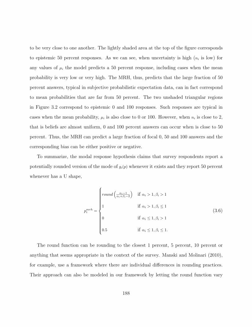
to be very close to one another. The lightly shaded area at the top of the figure corresponds

to epistemic 50 percent responses. As we can see, when uncertainty is high (ni is low) for

any values of µi the model predicts a 50 percent response, including cases when the mean

probability is very low or very high. The MRH, thus, predicts that the large fraction of 50

percent answers, typical in subjective probabilistic expectation data, can in fact correspond

to mean probabilities that are far from 50 percent. The two unshaded triangular regions

in Figure 3.2 correspond to epistemic 0 and 100 responses. Such responses are typical in

cases when the mean probability, µi is also close to 0 or 100. However, when ni is close to 2,

that is beliefs are almost uniform, 0 and 100 percent answers can occur when is close to 50

percent. Thus, the MRH can predict a large fraction of focal 0, 50 and 100 answers and the

corresponding bias can be either positive or negative.

To summarize, the modal response hypothesis claims that survey respondents report a

potentially rounded version of the mode of gi(p) whenever it exists and they report 50 percent

whenever has a U shape,

pmrhi =

round(

αi−1αi+βi−2

)if αi > 1, βi > 1

1 if αi > 1, βi ≤ 1

0 if αi ≤ 1, βi > 1

0.5 if αi ≤ 1, βi ≤ 1.

(3.6)

The round function can be rounding to the closest 1 percent, 5 percent, 10 percent or

anything that seems appropriate in the context of the survey. Manski and Molinari (2010),

for example, use a framework where there are individual differences in rounding practices.

Their approach can also be modeled in our framework by letting the round function vary

188

across individuals.

The hypothesis of this paper is that people answer subjective probabilistic expectation

questions according to the MRH. It would be desirable, however, to test the MRH against

other survey response models. A natural candidate for comparison is the mean model where

people respond a potentially rounded version of the mean of gi(p)

pmmi = round(µi). (3.7)

In the mean model the precision of beliefs (ni) is not identified, only the mean (µi) is. The

mean and the mode models, however, converge to each other as ni goes to infinity. That

is, the mean model is embedded in the MRH, and thus, a relatively small estimated belief

precision (n) would be evidence in favor of the MRH.

3.5 Individual subjective survival curves

In the previous section, we introduced two survey response models that transform second

order probability distributions g(p|µi, ni) into the survey response pmrhi or pmmi . These models

can be applied to any subjective probabilities in the HRS format and not just to survival

data. To close the model, however, we need to specify the mean (µi) and the precision (ni)

of beliefs. There is no unique way of modeling these two variables; it is the task of the

researcher to find the appropriate model in the context of the particular project. In this

section, we show how µi and ni can be modeled in the context of survival probabilities.

The so-called Gompertz model of longevity has been widely used in both demography

and biology because its increasing mortality hazard assumption lines up with mortality data

of humans and other species very well (Vaupel, 1997). The Gompertz model assumes that

189

the hazard of death is exponentially increasing with age:

h(a) = γ0γ1 exp (γ1a) , (3.8)

where γ0 is a positive scale and γ1 is a positive shape parameter. By simple calculation, (3.8)

leads to the following survival probability from age a to age t:

S (a, t) = exp (−γ0 (exp (γ1t)− exp (γ1a))) . (3.9)

The main advantage of subjective survival data is that we can estimate individual hetero-

geneity in survival chances. With objective survival data we can only identify group-specific

survival probabilities by computing the ratio of survivors in a particular group. Unobserved

heterogeneity within groups, however, is not identified. In contrast, subjective survival data

enables us to estimate individual heterogeneity in survival chances as we collect probability

data on the individual level. We follow Vaupel et al. (1979) by allowing the scale parameter

(γ0) to have a gamma distribution with shape parameter k and scale parameter θ and we

assume that the shape parameter (γ1) is fixed in the population:

γ0i ∼ Υ (k, θ) . (3.10)

The expected value of the gamma distribution is kθ and thus both parameters increase

mortality chances and decrease the probability of survival (see equation (3.9)). The main

advantage of using the gamma distribution, as we shall argue, is analytic tractability. Note,

however, that this is a flexible 2 parameter distribution with both parameters being esti-

mated, and hence this assumption is not very restrictive. The first advantage of the gamma

190

distribution is that the average survival probabilities can be derived analytically. As we

show in Appendix C2 in the e-companion online supplement, the average survival probabil-

ities from age a to age t is

E (Si (a, t|k, θ, γ1)) = (1 + θ (exp (γ1t)− exp (γ1a)))−k. (3.11)

The second advantage of the gamma-Gompertz framework is that we can analytically derive

the effect of individual heterogeneity on sample selection. Different survival chances are

modeled by letting γ0 have a distribution in the population. In this paper we refer to γ0 as

“frailty” (Vaupel et al., 1979), which includes genetic, environmental and behavioral factors

that affect the underlying mortality of individuals other than age. As long as survival chances

are heterogeneous in a population, fit individuals will be overrepresented in the sample over

time as frail individuals are more likely to die and not participate in the HRS. By applying

the formula from Vaupel et al. (1979) we can analytically characterize this sample selection.

See the appendix for details. To sum up, we use the following structural equations for

individual survival chances.

µi = Si (a, t) = exp (−γ0i (exp (γ1t)− exp (γ1a))) , (3.12)

γ0i ∼ Υ (k, θ) , (3.13)

θi =1

1θr + (exp (γ1a)− exp (γ1r))

, (3.14)

θr = x′iβθ. (3.15)

θr represents the scale parameter of the gamma distribution in the reference cohort which

is the 50 year old (r = 0.5). Equation (3.14) shows the effect of sample selection. The scale

191

parameter is decreasing with age, as fit individuals are increasingly overrepresented in the

sample. Equation (3.15) shows that we add covariates to the scale parameter of the 50 year

old cohort. Finally the Appendix shows how average partial effects of the different covariates

can be derived after fitting this model.

So far we have only talked about how to model the mean survival probability, µi. For

modeling the precision of beliefs (ni), we use a very simple log-normal framework.

lnni = z′iβn + uni, (3.16)

uni ∼ N(0, σ2n). (3.17)

Equations (3.12)-(3.17) together with the survey response models of the previous section

fully specify our model.

3.6 Estimation and identification

Our structural model has two unobservables: γ0i which is a function of the mean survival

probability and uni which is the unobserved heterogeneity in the precision of beliefs. Based

on the distributional assumptions from the previous section, the model is fully specified and

it can be estimated with maximum likelihood.

We only observe one survival probability answer in HRS. In Section 3, we proposed two

survey response models. The mean model assumed that people report a rounded version of

their true survival chances, while the MRH model assumed that people report a rounded

version of the mode of the distribution of probability beliefs g(p|µi, ni) or 50 percent when the

mode does not exist.

The joint distribution of the two random variables γ0i and uni is complicated because

192

one is gamma, the other is normal and they enter the model in a non-linear fashion. The

estimation of the MRH, thus, can be carried out by maximum simulated likelihood. The

estimation of the mean model is more straightforward as the precision of beliefs plays no role

in the model. The appendix shows how the likelihood function of these two models can be

constructed.

It is worth discussing how our main parameters are identified. We seek to estimate the

following set of parameters: γ1, k, βθ, βn, σn. In the case of the mean model, parameters of

the belief precision, βn and σn are not identified. Parameter γ1 is the shape parameter of

the individual survival function and it is identified from how fast the probability responses

(phrsi ) change with age(∂E(phrsi |a

)/∂a

). Parameters k and βθ determine the scale parameter

of the individual subjective survival curves (γ0i) and they are identified from the location

and dispersion of the individual responses (E(phrsi |xi

)and V

(phrsi |a

)).

The identification of the belief precision parameters βn and σn primarily comes from the

fraction of different focal answers in different demographic groups. If we have many focal

answers, we expect ni to be small. If we have many different types of focal answers (0, 50 and

100), we expect a high σn, indicating a high dispersion of belief precision in the population.

3.7 Empirical analysis

Beliefs about subjective survival probabilities presumably depend on an individual’s knowl-

edge of different risk factors and demographic differences in the society; his personal infor-

mation about his own health, habits and family members’ longevity; his ability to translate

this information into a probability and on his level of optimism or pessimism. In the empir-

ical model estimated in this section, we use the information available in the HRS to try to

193

capture several of the major determinants of beliefs in a parsimonious fashion.

3.7.1 Sample and measures employed

The sample used in the empirical analysis consists of 13,038 age eligible respondents to the

2002 Health and Retirement Study, over age 54 in 2002,45 who provided responses to the

subjective survival probability question. Excluded from the sample are proxy respondents

and non-respondents in the 2000 wave of data collection. Also excluded are persons over

90 who were not asked the survival probability questions and people for whom we did not

have realized survival information in 2010.46 Table 3.1 presents descriptive statistics for the

variables used in our analyses. The average age of our sample members is just over 68 years

(ranging from 54 to 89 years) and on average the target age was 16 years from their current

age. The modal sample member is a white female with a high school education although

there is substantial variance in each of these dimensions.

Our theory suggests that people may utilize personal information in forming their sub-

jective survival beliefs. Parents’ age at death, one’s own current health status and health

behavior are such variables. As Table 3.1 shows, 16 percent of our sample still has a living

mother but only 5 percent has a living father. The average age at death of the mothers is 76

years while the corresponding number for the fathers is 72 years. We construct six variables

about parental mortality. Three of them correspond to the mortality of the same sex parent

(father-son, mother-daughter pairs) and three correspond to the opposite sex parent. Within

each pair we first take the age at death of the parent if he/she is dead. If (s)he is alive we

impute the expected age at death of the parent based on his/her gender and age. In all mod-

45The 2002 HRS is a representative panel sample of the 54+ population and their spouses.46Actual mortality of HRS respondent is very precisely measured from administrative data (the National

Health Index) and it is even available for people who dropped out of the survey in a later wave.

194

els we include dummy variables about whether the parents are alive to control for potential

imputation bias. Finally we create a linear spline from the imputed parental mortality with

a single cut-off point at the age of the interviewee. This approach is motivated by the idea

that individuals might consider parental mortality less informative about their own survival

chances if they have already lived longer than their parents.47 These four splines (two for

each parent) together with the two dummies constitute our six parental mortality variables.

We also include in our analysis three sets of variables on health related behavior. As

Table 3.1 shows, 43 percent of our sample reports regular exercise at least three times a

week. While only 14 percent of the sample smoked in 2002, almost 60 percent reported

having smoked in the past. There is a big variation in the sample in drinking behavior.

Roughly half of our sample (48 percent) reports that they drink alcohol sometimes, but the

majority are not regular alcohol consumers. Among those who are, the average number of

days when they drink is 3.4 days a week, and the average number of alcoholic beverages

consumed is 1.9. Self-rated health in the HRS is measured on a five-point scale–1) Excellent,

2) Very Good, 3) Good, 4) Fair and 5) Poor.48 We translate these into three categories: 1)

excellent/very good; 2) good; 3) fair/poor . We then construct dummy variables representing

the combination of self-rated health in 2000 and 2002 for each respondent with excellent/very

good in both years as the baseline case. In Table 3.1 we only show the marginals of this joint

distribution. As we can see the fraction of people in “excellent/very good” health decreased

from 47 percent in 2000 to 43 percent in 2002. The fraction of people in “good” health did

not change much (31 and 32 percent) and the fraction in “fair/poor” health increased from

47Simple exploratory work suggested that parental mortality has a stronger effect on expectations whenthe parent died at an old age. The specification we use in this paper is not the only way to allow for suchnon-linearity and future work should explore alternative models.

48These three categories represent relatively good, average and relatively bad health. The reason for theaggregation is that we interact subjective health in 2000 and 2002 and adding 5 x 5 = 25 interactions wouldmake the interpretation of these variables difficult.

195

22 to 25 percent.

We also include two cognitive measures (“Vocabulary” and the “27-point cognitive capac-

ity scale”49), and the CESD depression score which measures depressive symptoms.50 Table

3.1 shows that the average member of our sample has higher cognitive and lower depression

scores than the average HRS respondent.

3.7.2 Maximum likelihood model estimates

The objective of this section is to test the modal response hypothesis (MRH) through a

series of performance tests. All the results we present in this section are based on the twelve

estimated models shown in Table 3.2, 3.7, 3.11 and 3.15. Table 3.2 reports models without

covariates, Table 3.7 adds basic demographic information, Table 3.11 expands the model

with cognition, personality and parental mortality and finally 3.15 contains all variables

including subjective health. All tables present three models. The first columns show actual

eight year survival of the HRS respondents between 2002 and 2010 estimated with nonlinear

least squares. The second columns shows results using subjective expectations based on

the mean model and the last two columns show results from the MRH “mode” model. All

the parameters of our model (γ0, θ0.5, n, γ1, k, σn) are assumed to be positive and thus their

logarithms enter the likelihood function. Covariates potentially enter two equations. The first

is the equation of θ0.5, which is the scale parameter of the gamma distribution of the mortality

hazard at the age of 50. In the actual survival models we model γ0 directly. Covariates with

positive coefficients are estimated to increase the mortality hazard and decrease the survival

chances. The magnitudes of these coefficients will be analyzed later when we derive average

49The 27-point scale Langa-Weir method is discussed in Crimmins et al. (2011). HRS cognitive measuresare described in Fisher et al. (2012).

50See Ofstedal et al. (2005).

196

partial effects of them on various survival probabilities. The second equation where covariates

appear is the equation of the precision of beliefs (n). Positive coefficients mean tighter, more

precise probability beliefs.

Panel A of Figure 3.3 compares estimated actual 8 year survival probabilities of HRS

respondents to subjective survival beliefs in 2002 computed from the models in Table 3.2

with no covariates. The horizontal axis shows the current age of respondents in 2002 and the

vertical axis shows the fitted average 8 year survival chances from the three models. As we

discussed in Section 3, heterogeneity in survival chances leads to sample selection as people

with better fitness are more likely to survive and become respondents of the HRS survey at

older ages. In the case of realized survival, only the interpretation of the estimates changes,

but we do not need to make any further adjustments of the parameters. The demography

literature calls survival tables of this sort “Survival probabilities of the survivors.” In the case

of subjective survival chances, however, we do have to properly adjust for the unmeasured

genetic and environmental differences of cohorts as discussed in Section 4. As we can see,

both the mean and the MRH “mode” model track the actual survival chances very well up

until about age 84, when the subjective probabilities become too optimistic. While the 8 year

actual survival chance of a 90 year old is roughly 20 percent, the corresponding numbers in

the MRH and mean models are ˜45 and 55 percent, respectively. Thus, although the MRH

model provides numbers that are closer to the true survival chances at old ages, these numbers

are still too large on average. It is not obvious, however, whether these overly optimistic

numbers are biases in people’s heads or biases due to measurement error in the survey. In

this paper we do not try to separate these two types of bias and we simply compare the

mean, the mode and the actual survival models using the raw data.

Panel B of Figure 3.3 shows the estimated heterogeneity of survival chances in our sample.

197

The different curves correspond to different values of γ0 with lower values meaning better

fitness. As we can see, there is notable variability in survival chances. For example, the

difference in median survival (i.e., half-life) between those in the 10th and 90th percentiles

of the estimated frailty distribution is about 25 years. That is, comparing two groups of 50

year olds, half of those in the 90th percentile are expected to survive to age 70 while among

those in the 10th percentile half are expected to survive to age 95. Using only mortality

data, one cannot identify the unobserved heterogeneity in survival chances.51

The reason the MRH model is somewhat better than the mean model in predicting low

probability events is that the high fraction of 50 percent answers are allowed to be focal

answers that do not arbitrarily push the mean survival chances up. To visualize this effect

we simulated survey responses based on the estimated models of subjective survival chances

in Table 3.15. To get precise numbers, we used 651,900 observations for simulation which is

50 times the size of our dataset (651, 900 = 50×13, 038). As we can see in Figure 3.4, the MRH

model is able to predict histograms of responses that are very similar to the histogram of

actual responses in the bottom panel. The ratio of 50 percent answers is around 25 percent,

while the ratio of 0 and 100 percent answers are both around 10 percent. What is more

important, the MRH model recognizes that the high fraction of focal answers should not be

taken at face value as a large fraction of them only reflect imprecise knowledge. The mean

model, however, takes all the focal answers at face value. Consequently, the mean model

is not able to predict a histogram similar to actual responses, and it seriously biases the

51There is a long history of discussion about the difficulty in separately identifying duration effects andunobserved heterogeneity. See, for example, Vaupel et al. (1979) and Heckman and Singer (1984). Usingsubjective survival data, however, identifying unobserved heterogeneity in frailty is easier, because we observeprobabilities of survival on the individual level. This contrasts with the use of mortality data, where it ishard to know which survivor is fit and which is simply luckier than other non-survivors. Even though weuse a particular functional form for how unobserved heterogeneity enters the model (the gamma-Gompertzframework) it is important to note that these functional form assumptions are not needed for identifyingunobserved heterogeneity in subjective frailty.

198

estimation of low or high probability events.

Much of a person’s personal information about health is likely embodied in his assessment

of the level and trajectory of self-rated health. To explore the effects of other covariates,

we present estimates of models with and without subjective health in Tables 3.4 and 3.3

respectively. Both tables show estimated average partial effects of surviving from age 55

to 75 and from 75 to 95. Appendix B in the e-companion contains more detailed versions

of these tables and further specifications, including models with only demographic variables

and partial effects of surviving from 2002 to 2010.

The tables show that the majority of the coefficients are smaller in absolute value when

subjective as opposed to objective information is used, but the coefficients based on the

MRH are closer to objective values. This pattern is more obvious for low probability events

(surviving from age 75 to 95), as the coefficients are roughly two times as big in the MRH.

Thus, not only the average survival probabilities (Figure 3.3), but the average partial effects

are also closer to objective values compared to the mean model. We take it as evidence

that the MRH model is more successful for modeling subjective probabilistic expectations,

particularly for low probability events, because the bias from focal answers is explicitly

modeled.

However, the majority of the coefficients are still smaller in absolute value in the MRH

than in the actual survival models. There are two potential explanations for this. Either there

is measurement error in the data or people are underestimating the effect of some variables

when forming expectations about their longevity. Without further assumptions, measure-

ment error, other than focal responses, is not identified in our model. Note, however, that

not all coefficients are attenuated equally. In fact two coefficients are systematically higher

in absolute value in the subjective models: same sex parents’ age at death and depression.

199

This is consistent with a model in which agents base their expectations on easily observable

determinants of mortality (parent’s survival) because they have limited information on de-

mographic differences in the society and on the role of different behavioral factors, such as

smoking and exercising, on survival. In this case the partial effects of personal information is

expected to be higher for subjective than for objective survival; and the pattern is expected

to be the reverse for other variables. This is exactly what we see in the data.

Tables 3.3 and 3.4 also show that people are aware that regular exercising is beneficial, and

smoking is harmful for them, although they underestimate the role of these factors. We can

also see that regular but limited alcohol consumption is not damaging, while teetotalling and

heavy drinking are. Even more interesting is the comparison of the models with and without

controlling for subjective health. Not surprisingly both the objective and subjective survival

probabilities are less affected by behavior when subjective health is controlled. However,

the subjective values shrink more strongly. For example, as Table 3.3 shows those who quit

smoking expect a 2 percentage point lower chance of surviving from age 55 to 75 compared

to those who never smoked. However, this effect disappears when subjective health is taken

into account (Table 3.4). It means that healthy quitters falsely believe that their survival

chances are the same as those who never smoked; whereas quitters who had already acquired

a disease understand its consequences.

It is also worth noting the demographic differences in subjective and objective survival.

As expected, females are more likely to live longer and this is reflected in their subjective

expectations. Racial differences, however, are more complex. Conditional on education,

personal information, health and behavior, blacks and Hispanics have a higher chance of

survival than whites in this age range. African Americans’ expectations reflect this difference,

but Hispanics are more pessimistic than Non-Hispanics. Table 3.8-3.10 in the e-companion

200

show roughly similar patterns when only demographic variables enter the model. Finally

even though the educated are more likely to live longer (Table 3.8-3.10), when personality,

personal information and behavior are controlled, the effect of education becomes negative

(!). Further investigation, not shown in the paper, shows that this result is driven by the

cognitive capacity variable. Education and cognition have a strong positive correlation but

cognition is a better predictor of survival than education. Moreover, the educated also have

better subjective health, and thus the effect of education becomes even more negative when

health is controlled (Table 3.4). Moreover, the educated believe themselves to have better

chances of surviving independent of the control variables used.

Finally let us take a look at the estimated distribution of probability beliefs (second

order probability distribution, gi(p)) of HRS respondents. Based on the MRH model without

covariates (Table 3.2) we computed the 10th, 25th, 50th, 75th and 90th quantiles of belief

precision (n) and the scale parameter of the survival function (γ0) for the cohort of age 50.

These numbers can be found in Table 3.6. Figure 3.5 shows the corresponding probability

belief distributions of the probability of surviving from age 50 to age 80. As we can see, there

is an enormous heterogeneity in probability beliefs. The median responder in HRS (3rd row

and 3rd column of Figure 3.5) has a belief distribution that is single peaked but wide, having

significant probability mass for any possible probability values between zero and one. It

means that although the median responder’s best guess for the probability of surviving from

age 50 to age 80 is roughly 50 percent, she is quite unsure about this probability. People

with even less precise beliefs are very unsure. For example, already at the 25th percentile

of belief precision (where n = 1.58) everyone provides a focal response of either 0, 50 or 100.

At the 10th percentile (where n = 0.4) everyone has U-shaped beliefs and, thus, responds

201

with an epistemic 50%52. As we increase belief precision to the 75th percentile, the second

order probability belief distribution becomes quite tight, having most of its mass in the

neighborhood of the mean probability. It means that at least 25 percent of the respondents

have very precise beliefs about their own survival chances.

Determinants of belief precision appear in Table 3.5 and the last columns of Table 3.7,3.11

and 3.15. Positive coefficients mean tighter, more precise beliefs. As we can see more

educated people have more certain beliefs. This is consistent with our hypothesis, discussed

in Section 3, that more educated people may have a broader knowledge of evidence about

mortality and its causes. We can also see that the deterioration of health, especially from

previously excellent levels, leads to more uncertainty about survival chances, perhaps because

of uncertainty about the future course of a new disease. Those who were in poor health both

in 2000 and in 2002, however, hold the most certain and pessimistic beliefs about their

survival chances.

The effect of age and the time horizon of the survival question in HRS have complicated

relations to uncertainty. For a fixed time horizon, the net effect of age on uncertainty is

negative, because the interaction term dominates for any time horizon values used in HRS

(from 11 years to 26 years). Thus, older people seem to have more precise beliefs about

their survival chances which might reflect learning. For a fixed age, the net effect of the time

horizon on uncertainty is also negative, because the interaction term dominates again. This

means that people hold more precise views about their long run than their short run survival

52Note, however, that the particular shape of the distribution of beliefs is only identified from the lognormalfunctional form in the region where n is below 1. Because there are many focal responses in the HRS data, themodel estimates many uncertain responses where n < 1. It is hard to know, however, what the distributionof looks like, conditional on being below 1. The log-normality assumption might or might not describe thisconditional distribution well. It is possible, for example, that no-one has U-shaped beliefs, but all epistemic50 responses come from a uniform distribution. If that is the case, then the log-normality assumption of nis inappropriate.

202

chances.

The two splines measuring same sex parental mortality in Table 3.11 and 3.15 shows a

“V” shape. It means that people are the most unsure about their survival chances when they

are around the age when their same sex parent died. We can also see that active smokers

and those who have already quit have less precise survival expectations compared to those

who never smoked; infrequent alcohol consumption leads to more precise beliefs; women are

less sure than men and depressed people are relatively more certain about their otherwise

poor survival expectations.

3.8 Conclusion

The modal response hypothesis is used in this paper as the foundation for an econometric

model that is intended to provide a mapping between survey responses to probability ques-

tions and the underlying subjective probability beliefs of individuals about their chances of

surviving to a target age. In this paper, we have presented the MRH as a hypothesis designed

to capture the kinds of “gut response” to such questions that would be made after about 15

seconds of consideration by persons who vary in the amount of information they have about

actuarial risks to health, about their own health-related circumstances and in their capacity

to process such information into subjective beliefs. We argued in Section 3 that reporting

the mode is relatively easier from a cognitive point of view than the mean or the median;

the mode is equal to a very simple rule-of-thumb estimator for the probability in question;

and that the mode often provides a good approximation to the expected probability that is

called for in SEU theory.

Our empirical findings suggest that there is considerable heterogeneity in subjective sur-

203

vival risks, some of it associated with age, sex, race, education, health related behavioral

factors, parental mortality and cognitive capacity. We have shown that subjective survival

expectations line up with actual mortality very well when the objective probabilities are

moderate. The subjective survival probabilities, however, become overly optimistic at old

ages when the true survival probabilities are relatively low. We have shown that the MRH

model does a better job compared to a standard mean model in reducing this bias as the

MRH models focal answers in an explicit way. It remains for future research to learn whether

the overly optimistic subjective expectations are biases in the heads of individuals, poten-

tially having behavioral consequences, or they are a result of survey measurement error,

potentially being related to uncertain beliefs.

In the empirical section of this paper, we have also found substantial uncertainty about

mortality risks which is manifested by considerable spread in the estimated distribution of

subjective survival probabilities for a typical respondent. In addition, we found significant

variation in uncertainty, holding expected survival risk constant. It remains for future work

to explore the explanation of these findings more deeply and to see whether survival risk and

uncertainty about this risk play a role in decisions made by HRS respondents.

204

Tables and figures

Figure 3.1: Distribution of Survival Probabilities to Target Age, by Age of Re-spondent, HRS-2002

0.1

.2.3

.40

.1.2

.3.4

0.1

.2.3

.4

0 50 100 0 50 100

age 54-69 age 70-74

age 75-79 age 80-84

age 85-89 Total

Fra

ctio

n

Subjective survival probability to a target age

Note: Target age is 80 years for people below 70, and it is 85, 90, 95 and 100 for individuals in successive five year age intervals

205

Figure 3.2: Density of probability beliefs (gi(p)) for different mean (µi) and pre-cision (ni) values

Figure 3.3: Average actual and expected survival probabilities and dispersion inbeliefs

0.1

.2.3

.4.5

.6.7

.8.9

1P

r(S

urvi

ve to

201

0)

54 59 64 69 74 79 84 89Current age

Mean model Mode modelActual survival

0.1

.2.3

.4.5

.6.7

.8.9

1S

urvi

val p

roba

bilit

ies

50 55 60 65 70 75 80 85 90 95 100Target age

10th quantile 25th quantile50th quantile 75th quantile90th quantile

Panel A: 8 year actual and expected survival Panel B: Heterogeneity in the subjective

probabilities by age in 2002 survival curves, MRH model

206

Figure 3.4: Simulated survey responses based on the mean and the mode modelswith all covariates and the empirical distribution of survey responses

0.0

5.1

.15

.2.2

5.3

Fra

ctio

n

0 20 40 60 80 100Mean model, all covariates

0.0

5.1

.15

.2.2

5.3

Fra

ctio

n

0 20 40 60 80 100Mode model, all covariates

0.0

5.1

.15

.2.2

5.3

Fra

ctio

n

0 20 40 60 80 100Survey responses

Figure 3.5: Estimated distribution of probability beliefs gi(p) of surviving fromage 50 to age 80

207

Table 3.1: Descriptive statistics, HRS-2002mean sd

Alive in 2010 0.77 0.42

Subjective survival probability to target age 48.40 32.13

Age 68.15 8.69

Target age less actual age 15.97 4.17

Female 0.59 0.49

Black 0.12 0.33

Hispanic 0.06 0.24

Years of education 12.54 3.00

Mother is alive 0.16 0.37

Mother’s age of death/100 or current age 0.76 0.15

Father is alive 0.05 0.23

Father’s age of death/100 or current age 0.72 0.14

Exercises at least 3 times a week 0.43 0.49

Ever smoked 0.59 0.49

Smokes now 0.14 0.34

Ever drinks alcohol 0.48 0.50

# of days a week when drinks alcohol 1.10 2.08

# of days a week when drinks alcohol if positive 3.42 2.34

# of drinks when drinks alcohol 0.61 1.18

# of drinks when drinks alcohol if positive 1.92 1.36

Health excellent / very good, 2002 0.43 0.49

Health good, 2002 0.32 0.47

Health fair / poor, 2002 0.25 0.43

Health excellent / very good, 2000 0.47 0.50

Health good, 2000 0.31 0.46

Health fair / poor, 2000 0.22 0.42

Cognition score, std. 0.08 1.01

Vocabulary score, std. 0.11 0.97

CESD depression score, std. -0.04 1.04

N 13038

Table 3.2: Actual survival until 2010 and the mean and MRH models of subjec-tive survival expectations, models without covariates

Actual survival Mean model MRH

ln γ0 -8.404

[0.21]***

ln θ0.5 -11.174 -8.827

[0.150]*** [0.169]***

lnn 1.978

[0.040]***

ln γ1 2.277 2.73 2.397

[0.024]*** [0.012]*** [0.020]***

ln k -0.656 0.121

[0.011]*** [0.025]***

lnσn 0.814

[0.025]***

N 13038 13038 13038

Log-likelihood -57961.459 -47058.606

*, ** and *** denote significance at 10, 5 and 1 percent

208

Table 3.3: Average partial effects of surviving from age 55 to 75 and from 75to 95 in three models with demographic, personality and personal informationvariables: actual survival and the mean and MRH models of subjective survivalexpectations

55-75 75-95

Actual survival Mean MRH Actual survival Mean MRH

Demographics

Education -0.003** 0.009*** 0.009*** -0.004** 0.003*** 0.005***

Female 0.073*** 0.035*** 0.051*** 0.097*** 0.012*** 0.029***

Black 0.043*** 0.031*** 0.07*** 0.058*** 0.011*** 0.04***

Hispanic 0.055*** -0.052*** -0.04** 0.073*** -0.019*** -0.023**

Cognition and personality, standardized scores

Cognition 0.055*** 0.02*** 0.019*** 0.073*** 0.007*** 0.011***

Vocabulary 0.003 0.003 -0.003 0.004 0.001 -0.002

Depression -0.031*** -0.053*** -0.06*** -0.041*** -0.019*** -0.034***

Parents’ age at death, linear splines with cut-off at own age

Same sex, sp1 0.026 0.068 -0.048 0.035 0.024 -0.028

Same sex, sp2 0.159*** 0.314*** 0.415*** 0.21** 0.112*** 0.239***

Same sex lives 0.011 0.001 0.006 0.014 0 0.003

Opp. sex, sp1 0.038 0.186*** 0.156*** 0.051 0.066*** 0.09***

Opp. sex, sp2 0.144** 0.097** 0.116** 0.191** 0.035** 0.067**

Opp. sex lives 0.028 0.007 0.007 0.038 0.002 0.004

Health related behavior

Exercises 0.096*** 0.054*** 0.061*** 0.128*** 0.019*** 0.035***

Ever smoked -0.076*** -0.02*** -0.015** -0.101*** -0.007*** -0.008**

Smokes now -0.097*** -0.059*** -0.06*** -0.128*** -0.021*** -0.035***

Ever drinks 0.056*** 0.044*** 0.033*** 0.074*** 0.016*** 0.019***

# of days drinks 0.007*** 0.004* 0.005** 0.01*** 0.001* 0.003**

# of drinks -0.012*** -0.009** -0.008** -0.016*** -0.003** -0.004**

*, ** and *** denote significance at 10, 5 and 1 percent level; Bold partial effects at the Mean and the MRH models

indicate that they are closer to the partial effects of actual survival.

209

Table 3.4: Average partial effects of surviving from age 55 to 75 and from 75to 95 in three models with demographic, personality, personal information andsubjective health variables: actual survival and the mean and MRH models ofsubjective survival expectations

55-75 75-95

Actual survival Mean MRH Actual survival Mean MRH

Demographics

Education -0.006*** 0.006*** 0.004*** -0.007*** 0.003*** 0.003***

Female 0.067*** 0.026*** 0.039*** 0.086*** 0.01*** 0.024***

Black 0.051*** 0.046*** 0.086*** 0.067*** 0.018*** 0.053***

Hispanic 0.071*** -0.04*** -0.019 0.092*** -0.016** -0.012


Cognition 0.05*** 0.009** 0.008** 0.064*** 0.004** 0.005*

Vocabulary 0.002 0.003 -0.003 0.003 0.001 -0.002

Depression -0.009*** -0.026*** -0.031*** -0.012*** -0.01*** -0.019***


Same sex, sp1 0.019 0.104** -0.022 0.025 0.041** -0.014

Same sex, sp2 0.122** 0.268*** 0.375*** 0.157** 0.105*** 0.231***

Same sex lives 0.011 -0.001 0.002 0.014 0 0.001

Opp. sex, sp1 0.043 0.206** 0.155*** 0.056 0.081*** 0.095***

Opp. sex, sp2 0.093 0.061 0.1** 0.12 0.024 0.061**

Opp. sex lives 0.041 0.006 0.003 0.053 0.002 0.002


Exercises 0.066*** 0.025*** 0.03*** 0.086*** 0.01*** 0.019***

Ever smoked -0.067*** -0.005 -0.002 -0.086*** -0.002 -0.001

Smokes now -0.093*** -0.053*** -0.056*** -0.121*** -0.021*** -0.034***

Ever drinks 0.045*** 0.021*** 0.013* 0.059*** 0.008** 0.008*

# of days drinks 0.005** 0.002 0.003 0.007** 0.001 0.002

# of drinks -0.01** -0.009** -0.007** -0.013** -0.003** -0.004*

Subjective health in 2000/2002

Excel./excel. ref. ref. ref. ref. ref. ref.

Excel./good -0.095*** -0.063*** -0.071*** -0.123*** -0.025*** -0.044***

Excel./poor -0.177*** -0.118*** -0.137*** -0.23*** -0.046*** -0.084***

Good/excel. -0.05*** -0.05*** -0.055*** -0.064*** -0.02*** -0.034***

Good/good -0.095*** -0.097*** -0.113*** -0.124*** -0.038*** -0.069***

Good/poor -0.192*** -0.17*** -0.173*** -0.248*** -0.067*** -0.106***

Poor/excel. -0.124*** -0.1*** -0.108*** -0.161*** -0.04*** -0.066***

Poor/good -0.142*** -0.139*** -0.146*** -0.183*** -0.055*** -0.09***

Poor/poor -0.209*** -0.237*** -0.263*** -0.27*** -0.093*** -0.162***

*, ** and *** denote significance at 10, 5 and 1 percent level; Bold partial effects at the Mean and the MRH models

indicate that they are closer to the partial effects of actual survival.

210

Table 3.5: Predictors of belief precision (n) in three versions of the MRH modelsof subjective survival expectations

lnn)

Model 1 Model 2 Model 3

Demographics

Education 0.056*** 0.051*** 0.053***

Female -0.139*** -0.156*** -0.157***

Black 0.053 0.041 0.02

Hispanic 0.188* 0.155 0.132


Cognition 0.021 0.027

Vocabulary 0.008 0.009

Depression 0.067*** 0.043*


Same sex, sp1 -0.493* -0.493*

Same sex, sp2 0.467 0.5

Same sex lives -0.064 -0.071

Opp. sex, sp1 -0.122 -0.117

Opp. sex, sp2 0.528 0.522

Opp. sex lives 0.026 0.032


Exercises 0.015 0.02

Ever smoked -0.091* -0.091*

Smokes now 0.007 0.006

Ever drinks 0.174*** 0.177***

# of days drinks -0.014 -0.015

# of drinks -0.035 -0.033

Subjective health in 2000/2002

Excel./excel. ref.

Excel./good -0.172**

Excel./poor 0.122

Good/excel. -0.092

Good/good -0.05

Good/poor -0.059

Poor/excel. -0.106

Poor/good -0.042

Poor/poor 0.177**

Age and time horizon of the HRS question; variables divided by 100

Age -2.513* -2.26 -2.333

Horizon -7.503 -9.823 -10.037*

Age X Horizon 25.438** 27.698*** 27.82***

Constant 1.572* 1.845* 1.882**

*, ** and *** denote significance at 10, 5 and 1 percent level

211

Table 3.6: Quantiles of belief precision (n) and probabilities of surviving fromage 50 to age 80

Quantiles n γ0 S(50, 80)

10 0.40 0.000022 0.87

25 1.58 0.000054 0.71

50 7.23 0.000120 0.47

75 33.12 0.000229 0.23

90 130.31 0.000370 0.10

212

APPENDIX H

Derivations

Effect of individual survival heterogeneity on sample selection

In our model there is individual heterogeneity in survival chances. One consequence of this

is that fit individuals will be overrepresented in the sample over time as frail individuals are

more likely to die. This sample selection can be conveniently modeled in our framework. Let

ka and θa denote the shape and scale parameters in cohort a. As Vaupel (1979) shows the

following is true for any cohorts

ka = kr, (3.18)

θa =1

1θr + (exp (γ1a)− exp (γ1r))

, (3.19)

where r is a reference cohort. As we can see, older and younger cohorts share the same shape

parameter ka, but older cohorts have lower scale parameter θa (lower frailty) than younger

cohorts.

Proof of equation (3.11)

The density function of the gamma distribution is

f (x) =1

Υ (k) θkxk−1 exp

(−xθ

)= c (k, θ)xk−1 exp

(−xθ

). (3.20)

213

It is well known that expected value of the gamma function is

E (x) =

ˆ ∞0

xc (k, θ)xk−1 exp(−xθ

)dx = kθ. (3.21)

The expected value of a scaled gamma function is also gamma and its expected value is

E (cx) = ckθ. (3.22)

The expected value of the negative exponentiated gamma function is

E (exp (−x)) =

ˆ ∞0

exp (−x) c (k, θ)xk−1 exp(−xθ

)dx (3.23)

=

ˆ ∞0

c (k, θ)xk−1 exp(−xθ− x)dx =

ˆ ∞0

c (k, θ)xk−1 exp

(− x

θθ+1

)dx = ...(3.24)

Note that this is very similar to the expected value formula of the gamma function, thus

... =(k − 1) θ

θ + 1

c (k, θ)

c(k + 1, θ

θ+1

) =(k − 1) θ

θ + 1

Υ (k − 1)(

θθ+1

)kΥ (k) θk

= ... (3.25)

Note that Γ (k) = (k − 1)Γ (k − 1)and thus

... =k − 1

k − 1

θk

θk(1 + θ)

k= (1 + θ)

k. (3.26)

Thus if γ0i ∼ Υ (k, θ) then

E (Si (a, T )) = E (exp (−γ0i (exp (γ1T )− exp (γ1a)))) = (1 + θ (exp (γ1T )− exp (γ1a)))−k. (3.27)

214

Details about the use of the Delta method to derive average partial

effects

The goal is to derive point estimates and standard errors of the partial effects of any covariate

on the survival probability from age to age

APEj (a1, a2) = Ex

[∂Si (a1, a2)

∂xj

]. (3.28)

The point estimates are

APEj (a, T ) = Ex

[∂ (1 + θ (exp (γ1T )− exp (γ1a)))

−k

∂xj

]= ... (3.29)

Let us denote e(a′, a) = exp (γ1a′)− exp (γ1a). Then

... = Ex

∂(

1 + e(T,a)exp(−β′xi)+e(a,r)

)−k∂xj

(3.30)

= Ex

[−k(

1 +e(T, a)

exp (−β′xi) + e(a, r)

)−k−1e(T, a) exp (−β′xi)βj

(exp (−β′xi) + e(a, r))2

](3.31)

= Ex

[−k (exp (−β′xi) + e(T, r))

−k−1(exp (−β′xi) + e(a, r))

k−1e(T, a) exp (−β′xi)βj

](3.32)

By substituting the estimated coefficients into this formula we have a point estimate for the

average partial effect of xj on the survival probability from age a to age T . The standard

errors can be computed with the delta method. For any differentiable transformation g(β)

and variance-covariance matrix Σ, the variance covariance matrix of the estimator of is

(∇g)T

Σ (∇g). Thus, we only need to compute the first derivatives of g. Let us see them

215

one-by-one.

∂APEj (a, T )

∂βl= −I (j = l)Ex

(k (exp (−β′xi) + e(T, r))

−k−1(exp (−β′xi) + e(a, r))

k−1e(T, a) exp (−β′xi)

)−Ex

(k (k + 1) (exp (−β′xi) + e(T, r))

−k−2(exp (−β′xi) + e(a, r))

k−1e(T, a) exp (−2β′xi)βjxil

)+Ex

(k (k − 1) (exp (−β′xi) + e(T, r))

−k−1(exp (−β′xi) + e(a, r))

k−2e(T, a) exp (−2β′xi)βjxil

)+Ex

(k (exp (−β′xi) + e(T, r))

−k−1(exp (−β′xi) + e(a, r))

k−1e(T, a) exp (−β′xi)βjxil

). (3.33)

∂APEj (a, T )

∂k= −Ex

[(exp (−β′xi) + e(T, r))

−k−1(exp (−β′xi) + e(a, r))


]−Ex

[k (exp (−β′xi) + e(T, r))

−k−1(exp (−β′xi) + e(a, r))


]×

× (− ln (exp (−β′xi) + e(T, r))) + Ex (ln (exp (−β′xi) + e(T, r))) . (3.34)

∂APEj (a, T )

∂γ1= [T exp (γ1T )− r exp (γ1r)] e(T, a) exp (−β′xi)βj ×

×{k (k + 1) (exp (−β′xi) + e(T, r))

−k−2(exp (−β′xi) + e(a, r))

k−1

−k (k − 1) (exp (−β′xi) + e(T, r))−k−1

(exp (−β′xi) + e(a, r))k−2}. (3.35)

By substituting the estimated coefficients into these formulas we have an estimator for the

variance covariance matrix of the average partial effects.

The likelihood function of the mean model

The likelihood function can be written as

li = Pr(pi ≤ Si (a, t) ≤ pi

)(3.36)

216

where pi and pi denote the lower and upper bound probabilities that would be rounded to

the survey response. For example, if the rounding function rounds to the closest 1 percent

and the survey response is 27 percent, then pi = 0.265 and pi = 0.275. If the rounding function

rounds to the closest 5 percent, then the corresponding probabilities would be pi = 0.225 and

pi = 0.275.53 The likelihood function, thus, is

li = Pr

( − ln pi

exp (γ1t)− exp (γ1a)≥ γ0i ≥

− ln piexp (γ1t)− exp (γ1a)

), (3.37)

which can be easily computed from the c.d.f. of the gamma distribution in with parameters

k and θ.

The likelihood function of the modal response model

The estimation of the MRH can be carried out by maximum simulated likelihood (MSL).

MSL computes the likelihood function by drawing many values from the distribution of one

(or several) random variables and computing the average conditional likelihood, conditioning

on those values. In our case, it is worth simulating values from the distribution of uni. A

standard version of the simulated likelihood would look like the following.54

li =1

S

S∑s=1

li (usni) . (3.38)

53As we can see, a response that is not a multiple of 5 percent cannot be a rounded version of a true latentprobability when we round to the closest 5 percent. The rounding model we have in mind is one whereagents only identify bins (e.g. 0%-2.5%, 2.5%-7.5%, . . . , 97.5%-100%) and any response in a particular binonly tells the econometrician that the true latent probability is also in the same bin. An alternative modelwould be that of Manski and Molinari (2010) where they identify individuals’ rounding practices across manyprobability questions and use different rounding functions for each individual.

54Note that in case the simulated values are drawn from the distribution of uni, we do not need to weightthe terms in (3.36) by the density of the draw as the simulation itself already weights the data.

217

where S is the number of simulation draws. The problem with this approach is that our

model is full of discontinuities that make this approach infeasible. Let us rewrite the MRH

formula in Section 3 with µi and ni, and let us denote ni = 1ni

and ni = 1− 1ni

. The MRH model

assumes that the survey response is

pmrhi =

round(µini−1ni−2

)if ni > µi > ni

1 if µi > ni, ni

0 if µi < ni, ni

0.5 if ni < µi < ni.

(3.39)

As we can see, whenever ni ≤ 1 an answer can only be 50 percent. Whenever ni ≤ 2,

an answer can only be 0, 50 or 100 percent. These discontinuities make the simulation

model in (3.38) hard for the following reason. Imagine that during the maximization of the

likelihood function we get into a region where the precision of beliefs ni is always below 2 for

each simulation draw. This could happen if z′iβkn � 2 and σ2,k

n is small, where k indexes the

actual guesses for the parameters. In this case, the likelihood function would be undefined

and the numerical maximization would fail. As a remedy, we recommend drawing separate

simulation values from each region of ni; this assures that the likelihood is well-defined in

218

each iteration of the maximization.55 The likelihood function, thus, is written

li =1

S1

S1∑s=1

li (usni|ni ≤ 1) Pr (ni ≤ 1) +1

S1

S1∑s=1

li (usni|1 < ni ≤ 2) Pr (1 < ni ≤ 2)

+1

S1

S1∑s=1

li (usni|ni > 2) Pr (ni > 2) . (3.40)

Now, whenever z′iβkn � 2 and σ2,k

n is small in a particular iteration for a non-focal answer,

the likelihood is a well-defined, extremely small number. The probabilities of the different

regions of ni are trivial since ni is assumed to have a log-normal distribution. Whenever

ni ≤ 1 an answer can only be fifty and thus the conditional likelihood is

li (usni|ni ≤ 1) =

1 if phrsi = 50

0 otherwise,

(3.41)

where phrsi represents the survey response to the HRS mortality question. When 1 < ni ≤ 2,

it is assured that ni ≥ ni and thus

li (usni|1 < ni ≤ 2) =

Pr(ni < Si (a, t) < ni

)if phrsi = 50

Pr (Si (a, t) ≤ ni) if phrsi = 0

Pr(Si (a, t) ≥ ni

)if phrsi = 100

0 otherwise.

(3.42)

These probabilities can be computed analogously to the mean model derived above. The

55Hill et al. (2004) did not use this trick when they estimated a very similar model. The consequence wasthat they had to make restrictions on their model to be able to carry out the numerical estimation. It turnedout that our model is identified and estimable in practice under mild conditions once these discontinuitiesare properly taken care of.

219

most complicated, although still very straightforward, case is the conditional likelihood in

the region where ni > 2. In this region ni < ni . The only complication is that a 0 and a

100 answer can now be either a focal answer or an exact rounded answer. 50 answers in this

region cannot be focal answers as ni > 2 and thus either αi or βi is larger than one. The

conditional likelihood is

li (usni|ni > 2) =

Pr(Si (a, t) ≤ ni OR Si(a,t)ni−1

ni−2 ≤ pi)

if phrsi = 0

Pr(Si (a, t) ≥ ni OR Si(a,t)ni−1

ni−2 ≥ pi)

if phrsi = 100

Pr(pi ≤ Si(a,t)ni−1

ni−2 ≤ pi)

otherwise.

(3.43)

After straightforward algebra the conditional likelihood becomes

li (usni|ni > 2) =

Pr(Si (a, t) ≤ max

{ni,

pi(ni−2)+1ni

})if phrsi = 0

Pr(Si (a, t) ≥ min

{ni,

pi(ni−2)+1

ni

})if phrsi = 100

Pr(pi(ni−2)+1

ni≤ Si (a, t) ≤ pi(ni−2)+1

ni

)otherwise.

(3.44)

and again these probabilities can be computed analogously to the mean model derived above.

220

APPENDIX I

Additional Tables

Table 3.7: Outputs of the ML estimation models with demographic variables;actual survival and the mean and MRH models of subjective survival expecta-tions

Actual survival Mean MRH

ln γ0 ln θ0.5 ln θ0.5 lnn

Demographics

Education -0.048 -0.13 -0.089 0.056

[0.006]*** [0.007]*** [0.005]*** [0.009]***

Female -0.343 -0.193 -0.209 -0.139

[0.033]*** [0.037]*** [0.027]*** [0.051]***

Black 0.037 -0.007 -0.151 0.053

[0.055] [0.053] [0.038]*** [0.076]

Hispanic -0.157 0.329 0.198 0.188

[0.079]** [0.083]*** [0.062]*** [0.110]*


Age -2.513

[1.478]*

Horizon -7.503

[6.314]

Age X Horizon 25.438

[10.693]**

Constant -7.538 -9.358 -7.234 1.572

[0.223]*** [0.190]*** [0.181]*** [0.946]*

Other parameters

ln γ1 2.268 2.719 2.358

[0.024]*** [0.012]*** [0.020]***

ln k -0.629 0.158

[0.011]*** [0.025]***

lnσn 0.808

[0.025]***

N 13038 13038 13038

Log-likelihood -57714.3 -46739.4


221

Table 3.8: Average partial effects of surviving 8 more years in three modelswith demographic variables: actual survival and the mean and MRH models ofsubjective survival expectations



Demographics

Education 0.008 0.011 0.012 0.056

[0.001]*** [0.002]*** [0.002]*** [0.009]***

Female 0.061 0.017 0.027 -0.139

[0.006]*** [0.004]*** [0.006]*** [0.051]***

Black -0.007 0.001 0.02 0.053

[0.010] [0.005] [0.006]*** [0.076]

Hispanic 0.028 -0.028 -0.026 0.188

[0.014]** [0.008]*** [0.009]*** [0.110]*


Table 3.9: Average partial effects of surviving from age 55 to 75 in three modelswith demographic variables: actual survival and the mean and MRH models ofsubjective survival expectations



Demographics

Education 0.01 0.023 0.021 0.056

[0.001]*** [0.004]*** [0.004]*** [0.009]***

Female 0.074 0.035 0.048 -0.139

[0.008]*** [0.008]*** [0.010]*** [0.051]***

Black -0.008 0.001 0.035 0.053

[0.012] [0.009] [0.011]*** [0.076]

Hispanic 0.034 -0.059 -0.046 0.188

[0.017]** [0.017]*** [0.016]*** [0.110]*


Table 3.10: Average partial effects of surviving from age 75 to 95 in three modelswith demographic variables: actual survival and the mean and MRH models ofsubjective survival expectations



Demographics

Education 0.013 0.007 0.011 0.056

[0.002]*** [0.001]*** [0.002]*** [0.009]***

Female 0.093 0.011 0.025 -0.139

[0.010]*** [0.003]*** [0.007]*** [0.051]***

Black -0.01 0 0.018 0.053

[0.015] [0.003] [0.006]*** [0.076]

Hispanic 0.042 -0.019 -0.024 0.188

[0.022]** [0.006]*** [0.009]*** [0.110]*


222

Table 3.11: Outputs of the ML estimation models with demographic, personalityand personal information variables; actual survival and the mean and MRHmodels of subjective survival expectations



Demographics

Education 0.015 -0.053 -0.037 0.051

[0.006]** [0.008]*** [0.005]*** [0.010]***

Female -0.34 -0.198 -0.215 -0.156

[0.037]*** [0.039]*** [0.029]*** [0.055]***

Black -0.201 -0.177 -0.297 0.041

[0.055]*** [0.053]*** [0.038]*** [0.076]

Hispanic -0.254 0.297 0.171 0.155

[0.078]*** [0.081]*** [0.060]*** [0.106]


Cognition -0.254 -0.115 -0.079 0.021

[0.020]*** [0.021]*** [0.015]*** [0.029]

Vocabulary -0.013 -0.017 0.013 0.008

[0.019] [0.021] [0.015] [0.028]

Depression 0.142 0.303 0.253 0.067

[0.015]*** [0.020]*** [0.015]*** [0.025]***


Same sex, sp1 -0.121 -0.386 0.205 -0.493

[0.153] [0.292] [0.184] [0.291]*

Same sex, sp2 -0.733 -1.784 -1.766 0.467

[0.279]*** [0.214]*** [0.161]*** [0.342]

Same sex lives -0.049 -0.003 -0.025 -0.064

[0.119] [0.059] [0.044] [0.100]

Opp. sex, sp1 -0.177 -1.058 -0.664 -0.122

[0.156] [0.297]*** [0.190]*** [0.292]

Opp. sex, sp2 -0.667 -0.553 -0.494 0.528

[0.282]** [0.210]*** [0.155]*** [0.340]

Opp. sex lives -0.131 -0.037 -0.031 0.026

[0.120] [0.061] [0.045] [0.107]


Exercises -0.445 -0.309 -0.258 0.015

[0.038]*** [0.035]*** [0.025]*** [0.051]

Ever smoked 0.352 0.113 0.063 -0.091

[0.038]*** [0.038]*** [0.027]** [0.054]*

Smokes now 0.447 0.337 0.257 0.007

[0.050]*** [0.053]*** [0.039]*** [0.076]

Ever drinks -0.259 -0.25 -0.141 0.174

[0.044]*** [0.043]*** [0.031]*** [0.062]***

# of days drinks -0.033 -0.021 -0.019 -0.014

[0.011]*** [0.011]* [0.008]** [0.016]

# of drinks 0.056 0.049 0.033 -0.035

[0.019]*** [0.019]** [0.014]** [0.028]

Table continues on the next page...

223

...Table 3.11 continuedActual survival Mean MRH



Age -2.26

[1.471]

Horizon -9.823

[6.149]

Age X Horizon 27.698

[10.367]***

Constant -6.712 -8.595 -5.796 1.845

[0.288]*** [0.239]*** [0.202]*** [0.946]*

Other parameters

ln γ1 2.104 2.684 2.179

[0.041]*** [0.014]*** [0.029]***

ln k -0.573 0.296

[0.011]*** [0.026]***

lnσn 0.773

[0.026]***

N 13038 13038 13038



224

Table 3.12: Average partial effects of surviving 8 more years in three models withdemographic, personality and personal information variables: actual survival andthe mean and MRH models of subjective survival expectations


Demographics

Education -0.003 0.005 0.005

[0.001]** [0.001]*** [0.001]***

Female 0.058 0.017 0.029

[0.006]*** [0.004]*** [0.007]***

Black 0.034 0.015 0.039

[0.009]*** [0.005]*** [0.010]***

Hispanic 0.043 -0.025 -0.023

[0.013]*** [0.008]*** [0.009]**


Cognition 0.043 0.01 0.011

[0.003]*** [0.002]*** [0.003]***

Vocabulary 0.002 0.001 -0.002

[0.003] [0.002] [0.002]

Depression -0.024 -0.026 -0.034

[0.003]*** [0.004]*** [0.007]***


Same sex, sp1 0.02 0.033 -0.027

[0.026] [0.024] [0.027]

Same sex, sp2 0.124 0.152 0.234

[0.047]*** [0.032]*** [0.059]***

Same sex lives 0.008 0 0.003

[0.020] [0.005] [0.006]

Opp. sex, sp1 0.03 0.09 0.088

[0.026] [0.026]*** [0.026]***

Opp. sex, sp2 0.113 0.047 0.065

[0.048]** [0.020]** [0.028]**

Opp. sex lives 0.022 0.003 0.004

[0.020] [0.005] [0.006]


Exercises 0.075 0.026 0.034

[0.007]*** [0.005]*** [0.008]***

Ever smoked -0.06 -0.01 -0.008

[0.007]*** [0.004]*** [0.004]**

Smokes now -0.076 -0.029 -0.034

[0.009]*** [0.006]*** [0.009]***

Ever drinks 0.044 0.021 0.019

[0.008]*** [0.005]*** [0.006]***

# of days drinks 0.006 0.002 0.003

[0.002]*** [0.001]* [0.001]**

# of drinks -0.009 -0.004 -0.004

[0.003]*** [0.002]** [0.002]**


225

Table 3.13: Average partial effects of surviving from age 55 to 75 in three mod-els with demographic, personality and personal information variables: actualsurvival and the mean and MRH models of subjective survival expectations


Demographics

Education -0.003 0.009 0.009

[0.001]** [0.002]*** [0.002]***

Female 0.073 0.035 0.051

[0.009]*** [0.009]*** [0.012]***

Black 0.043 0.031 0.07

[0.012]*** [0.011]*** [0.017]***

Hispanic 0.055 -0.052 -0.04

[0.017]*** [0.016]*** [0.016]**


Cognition 0.055 0.02 0.019

[0.005]*** [0.005]*** [0.005]***

Vocabulary 0.003 0.003 -0.003

[0.004] [0.004] [0.004]

Depression -0.031 -0.053 -0.06

[0.004]*** [0.009]*** [0.013]***


Same sex, sp1 0.026 0.068 -0.048

[0.033] [0.050] [0.047]

Same sex, sp2 0.159 0.314 0.415

[0.060]*** [0.067]*** [0.100]***

Same sex lives 0.011 0.001 0.006

[0.026] [0.010] [0.010]

Opp. sex, sp1 0.038 0.186 0.156

[0.034] [0.054]*** [0.046]***

Opp. sex, sp2 0.144 0.097 0.116

[0.060]** [0.042]** [0.048]**

Opp. sex lives 0.028 0.007 0.007

[0.026] [0.011] [0.011]


Exercises 0.096 0.054 0.061

[0.009]*** [0.011]*** [0.014]***

Ever smoked -0.076 -0.02 -0.015

[0.009]*** [0.007]*** [0.007]**

Smokes now -0.097 -0.059 -0.06

[0.012]*** [0.013]*** [0.015]***

Ever drinks 0.056 0.044 0.033

[0.010]*** [0.010]*** [0.010]***

# of days drinks 0.007 0.004 0.005

[0.002]*** [0.002]* [0.002]**

# of drinks -0.012 -0.009 -0.008

[0.004]*** [0.004]** [0.004]**


226

Table 3.14: Average partial effects of surviving from age 75 to 95 in three mod-els with demographic, personality and personal information variables: actualsurvival and the mean and MRH models of subjective survival expectations


Demographics

Education -0.004 0.003 0.005

[0.002]** [0.001]*** [0.002]***

Female 0.097 0.012 0.029

[0.012]*** [0.003]*** [0.009]***

Black 0.058 0.011 0.04

[0.016]*** [0.004]*** [0.012]***

Hispanic 0.073 -0.019 -0.023

[0.023]*** [0.006]*** [0.010]**


Cognition 0.073 0.007 0.011

[0.008]*** [0.002]*** [0.004]***

Vocabulary 0.004 0.001 -0.002

[0.005] [0.001] [0.002]

Depression -0.041 -0.019 -0.034

[0.005]*** [0.004]*** [0.009]***


Same sex, sp1 0.035 0.024 -0.028

[0.043] [0.018] [0.028]

Same sex, sp2 0.21 0.112 0.239

[0.086]** [0.027]*** [0.071]***


[0.034] [0.004] [0.006]

Opp. sex, sp1 0.051 0.066 0.09

[0.044] [0.020]*** [0.029]***

Opp. sex, sp2 0.191 0.035 0.067

[0.086]** [0.016]** [0.030]**

Opp. sex lives 0.038 0.002 0.004

[0.035] [0.004] [0.006]


Exercises 0.128 0.019 0.035

[0.013]*** [0.004]*** [0.010]***

Ever smoked -0.101 -0.007 -0.008

[0.012]*** [0.003]*** [0.004]**

Smokes now -0.128 -0.021 -0.035

[0.015]*** [0.005]*** [0.010]***

Ever drinks 0.074 0.016 0.019

[0.013]*** [0.004]*** [0.006]***

# of days drinks 0.01 0.001 0.003

[0.003]*** [0.001]* [0.001]**

# of drinks -0.016 -0.003 -0.004

[0.006]*** [0.001]** [0.002]**


227

Table 3.15: Outputs of the ML estimation models with demographic, personality,personal information and subjective health variables; actual survival and themean and MRH models of subjective survival expectations



Demographics

Education 0.026 -0.037 -0.019 0.053

[0.006]*** [0.007]*** [0.005]*** [0.010]***

Female -0.31 -0.152 -0.169 -0.157

[0.036]*** [0.038]*** [0.027]*** [0.054]***

Black -0.24 -0.264 -0.369 0.02

[0.053]*** [0.052]*** [0.036]*** [0.075]

Hispanic -0.332 0.229 0.083 0.132

[0.077]*** [0.078]*** [0.056] [0.105]


Cognition -0.231 -0.052 -0.035 0.027

[0.019]*** [0.020]** [0.015]** [0.028]

Vocabulary -0.011 -0.018 0.011 0.009

[0.018] [0.020] [0.014] [0.028]

Depression 0.043 0.148 0.131 0.043

[0.016]*** [0.020]*** [0.014]*** [0.026]*


Same sex, sp1 -0.09 -0.6 0.094 -0.493

[0.154] [0.281]** [0.172] [0.287]*

Same sex, sp2 -0.567 -1.552 -1.608 0.5

[0.272]** [0.207]*** [0.153]*** [0.337]

Same sex lives -0.051 0.006 -0.007 -0.071

[0.114] [0.057] [0.042] [0.099]

Opp. sex, sp1 -0.203 -1.193 -0.663 -0.117

[0.156] [0.285]*** [0.177]*** [0.287]

Opp. sex, sp2 -0.434 -0.353 -0.427 0.522

[0.274] [0.205]* [0.148]*** [0.336]

Opp. sex lives -0.191 -0.032 -0.014 0.032

[0.116]* [0.059] [0.043] [0.105]


Exercises -0.309 -0.146 -0.13 0.02

[0.038]*** [0.034]*** [0.024]*** [0.051]

Ever smoked 0.31 0.031 0.009 -0.091

[0.038]*** [0.036] [0.026] [0.053]*

Smokes now 0.436 0.308 0.239 0.006

[0.049]*** [0.051]*** [0.037]*** [0.075]

Ever drinks -0.211 -0.119 -0.054 0.177

[0.043]*** [0.042]*** [0.030]* [0.061]***

# of days drinks -0.024 -0.012 -0.011 -0.015

[0.011]** [0.011] [0.008] [0.016]

# of drinks 0.045 0.05 0.029 -0.033

[0.019]** [0.019]*** [0.014]** [0.028]


228




Excel./excel. ref. ref. ref. ref.

Excel./good 0.442 0.363 0.306 -0.172

[0.065]*** [0.055]*** [0.040]*** [0.084]**

Excel./poor 0.827 0.682 0.585 0.122

[0.091]*** [0.121]*** [0.085]*** [0.157]

Good/excel. 0.231 0.29 0.237 -0.092

[0.079]*** [0.061]*** [0.044]*** [0.095]

Good/good 0.445 0.562 0.483 -0.05

[0.059]*** [0.050]*** [0.035]*** [0.074]

Good/poor 0.894 0.983 0.74 -0.059

[0.065]*** [0.087]*** [0.061]*** [0.104]

Poor/excel. 0.579 0.582 0.461 -0.106

[0.119]*** [0.156]*** [0.106]*** [0.196]

Poor/good 0.66 0.805 0.624 -0.042

[0.075]*** [0.088]*** [0.063]*** [0.116]

Poor/poor 0.973 1.372 1.126 0.177

[0.057]*** [0.070]*** [0.052]*** [0.085]**


Age -2.333

[1.449]

Horizon -10.037

[6.053]*

Age X Horizon 27.82

[10.204]***

Constant -7.288 -9.366 -6.379 1.882

[0.293]*** [0.233]*** [0.197]*** [0.933]**

Other parameters

ln γ1 2.088 2.686 2.149

[0.041]*** [0.013]*** [0.029]***

ln k -0.54 0.377

[0.011]*** [0.026]***

lnσn 0.758

[0.026]***

N 13038 13038 13038



229

Table 3.16: Average partial effects of surviving 8 more years in three modelswith demographic, personality, personal information and subjective health vari-ables: actual survival and the mean and MRH models of subjective survivalexpectations


Demographics

Education -0.004 0.003 0.003

[0.001]*** [0.001]*** [0.001]***

Female 0.052 0.013 0.023

[0.006]*** [0.004]*** [0.006]***

Black 0.04 0.023 0.05

[0.009]*** [0.006]*** [0.012]***

Hispanic 0.056 -0.02 -0.011

[0.013]*** [0.007]*** [0.008]


Cognition 0.039 0.004 0.005

[0.003]*** [0.002]** [0.002]**

Vocabulary 0.002 0.002 -0.002

[0.003] [0.002] [0.002]

Depression -0.007 -0.013 -0.018

[0.003]*** [0.003]*** [0.004]***


Same sex, sp1 0.015 0.052 -0.013

[0.026] [0.024]** [0.024]

Same sex, sp2 0.095 0.134 0.217

[0.046]** [0.029]*** [0.055]***

Same sex lives 0.009 -0.001 0.001

[0.019] [0.005] [0.006]

Opp. sex, sp1 0.034 0.103 0.09

[0.026] [0.027]*** [0.025]***

Opp. sex, sp2 0.073 0.03 0.058

[0.046] [0.019] [0.026]**

Opp. sex lives 0.032 0.003 0.002

[0.020]* [0.005] [0.006]


Exercises 0.052 0.013 0.018

[0.006]*** [0.004]*** [0.005]***

Ever smoked -0.052 -0.003 -0.001

[0.006]*** [0.003] [0.004]

Smokes now -0.073 -0.027 -0.032

[0.008]*** [0.006]*** [0.008]***

Ever drinks 0.035 0.01 0.007

[0.007]*** [0.004]*** [0.004]*

# of days drinks 0.004 0.001 0.001

[0.002]** [0.001] [0.001]

# of drinks -0.008 -0.004 -0.004

[0.003]** [0.002]** [0.002]*


230



Excel./excel. ref. ref. ref.

Excel./good -0.074 -0.031 -0.041

[0.011]*** [0.007]*** [0.010]***

Excel./poor -0.139 -0.059 -0.079

[0.016]*** [0.014]*** [0.020]***

Good/excel. -0.039 -0.025 -0.032

[0.013]*** [0.007]*** [0.009]***

Good/good -0.075 -0.048 -0.065

[0.010]*** [0.009]*** [0.015]***

Good/poor -0.15 -0.085 -0.1

[0.012]*** [0.015]*** [0.023]***

Poor/excel. -0.097 -0.05 -0.062

[0.020]*** [0.015]*** [0.020]***

Poor/good -0.111 -0.069 -0.084

[0.013]*** [0.013]*** [0.020]***

Poor/poor -0.163 -0.118 -0.152

[0.010]*** [0.020]*** [0.033]***


231

Table 3.17: Average partial effects of surviving from age 55 to 75 in three mod-els with demographic, personality, personal information and subjective healthvariables: actual survival and the mean and MRH models of subjective survivalexpectations


Demographics

Education -0.006 0.006 0.004

[0.001]*** [0.002]*** [0.001]***

Female 0.067 0.026 0.039

[0.008]*** [0.008]*** [0.010]***

Black 0.051 0.046 0.086

[0.012]*** [0.012]*** [0.020]***

Hispanic 0.071 -0.04 -0.019

[0.017]*** [0.015]*** [0.013]


Cognition 0.05 0.009 0.008

[0.004]*** [0.004]** [0.004]**

Vocabulary 0.002 0.003 -0.003

[0.004] [0.003] [0.003]

Depression -0.009 -0.026 -0.031

[0.003]*** [0.005]*** [0.007]***


Same sex, sp1 0.019 0.104 -0.022

[0.033] [0.048]** [0.042]

Same sex, sp2 0.122 0.268 0.375

[0.058]** [0.059]*** [0.090]***

Same sex lives 0.011 -0.001 0.002

[0.024] [0.010] [0.010]

Opp. sex, sp1 0.043 0.206 0.155

[0.034] [0.053]*** [0.043]***

Opp. sex, sp2 0.093 0.061 0.1

[0.058] [0.038] [0.044]**

Opp. sex lives 0.041 0.006 0.003

[0.025] [0.010] [0.010]


Exercises 0.066 0.025 0.03

[0.008]*** [0.007]*** [0.008]***

Ever smoked -0.067 -0.005 -0.002

[0.009]*** [0.006] [0.006]

Smokes now -0.093 -0.053 -0.056

[0.012]*** [0.012]*** [0.014]***

Ever drinks 0.045 0.021 0.013

[0.010]*** [0.008]*** [0.007]*

# of days drinks 0.005 0.002 0.003

[0.002]** [0.002] [0.002]

# of drinks -0.01 -0.009 -0.007

[0.004]** [0.004]** [0.003]**


232




Excel./good -0.095 -0.063 -0.071

[0.015]*** [0.014]*** [0.017]***

Excel./poor -0.177 -0.118 -0.137

[0.021]*** [0.028]*** [0.034]***

Good/excel. -0.05 -0.05 -0.055

[0.017]*** [0.013]*** [0.015]***

Good/good -0.095 -0.097 -0.113

[0.013]*** [0.017]*** [0.024]***

Good/poor -0.192 -0.17 -0.173

[0.016]*** [0.031]*** [0.038]***

Poor/excel. -0.124 -0.1 -0.108

[0.026]*** [0.031]*** [0.033]***

Poor/good -0.142 -0.139 -0.146

[0.017]*** [0.027]*** [0.033]***

Poor/poor -0.209 -0.237 -0.263

[0.015]*** [0.039]*** [0.054]***


233

Table 3.18: Average partial effects of surviving from age 75 to 95 in three mod-els with demographic, personality, personal information and subjective healthvariables: actual survival and the mean and MRH models of subjective survivalexpectations


Demographics

Education -0.007 0.003 0.003

[0.002]*** [0.001]*** [0.001]***

Female 0.086 0.01 0.024

[0.011]*** [0.003]*** [0.007]***

Black 0.067 0.018 0.053

[0.015]*** [0.005]*** [0.015]***

Hispanic 0.092 -0.016 -0.012

[0.022]*** [0.006]** [0.009]


Cognition 0.064 0.004 0.005

[0.007]*** [0.002]** [0.003]*

Vocabulary 0.003 0.001 -0.002

[0.005] [0.001] [0.002]

Depression -0.012 -0.01 -0.019

[0.004]*** [0.002]*** [0.005]***


Same sex, sp1 0.025 0.041 -0.014

[0.042] [0.019]** [0.026]

Same sex, sp2 0.157 0.105 0.231

[0.080]** [0.026]*** [0.068]***


[0.032] [0.004] [0.006]

Opp. sex, sp1 0.056 0.081 0.095

[0.042] [0.022]*** [0.029]***

Opp. sex, sp2 0.12 0.024 0.061

[0.079] [0.015] [0.029]**

Opp. sex lives 0.053 0.002 0.002

[0.032] [0.004] [0.006]


Exercises 0.086 0.01 0.019

[0.012]*** [0.003]*** [0.006]***

Ever smoked -0.086 -0.002 -0.001

[0.012]*** [0.003] [0.004]

Smokes now -0.121 -0.021 -0.034

[0.015]*** [0.005]*** [0.010]***

Ever drinks 0.059 0.008 0.008

[0.012]*** [0.003]** [0.005]*

# of days drinks 0.007 0.001 0.002

[0.003]** [0.001] [0.001]

# of drinks -0.013 -0.003 -0.004

[0.005]** [0.001]** [0.002]*


234




Excel./good -0.123 -0.025 -0.044

[0.020]*** [0.006]*** [0.013]***

Excel./poor -0.23 -0.046 -0.084

[0.029]*** [0.012]*** [0.025]***

Good/excel. -0.064 -0.02 -0.034

[0.022]*** [0.006]*** [0.011]***

Good/good -0.124 -0.038 -0.069

[0.018]*** [0.008]*** [0.019]***

Good/poor -0.248 -0.067 -0.106

[0.024]*** [0.014]*** [0.029]***

Poor/excel. -0.161 -0.04 -0.066

[0.035]*** [0.013]*** [0.023]***

Poor/good -0.183 -0.055 -0.09

[0.024]*** [0.012]*** [0.025]***

Poor/poor -0.27 -0.093 -0.162

[0.023]*** [0.019]*** [0.042]***


235

CHAPTER IV

Stock Market Crash and Expectations of

American Households

4.1 Introduction

The stock market crash of 2008 and the subsequent financial crisis constitute a rare episode

whose scope and implications fall outside the life experience of American households. Whether

and how those events affect people’s expectations is an important question. To the extent

that expectations guide investment behavior, substantial changes in expectations due to the

financial crash can lead to substantial changes in investment. Besides average beliefs of “the

representative household,” the crisis may have an impact on heterogeneity of such beliefs.

This study uses data from the 2008 wave of the Health and Retirement Study (HRS) to

study the impact of the crisis on people’s expectations. We estimate the effect of the crash on

the population average of expected returns, the population average of the uncertainty about

returns (subjective standard deviation), and the cross-sectional heterogeneity in expected

returns (an indicator of disagreement). We show estimates from simple reduced-form regres-

236

sions on probability answers as well as from a more structural model that focuses on the

parameters of interest and separates survey noise from relevant heterogeneity. The measure-

ment strategy makes use of the fact that the respondents of HRS-2008 answered the survey

during twelve months from February 2008 to February 2009, a time period that includes

the time of the stock market crash in early October. We show that the date of interview is

largely independent of the respondents’ past expectations about the stock market, so even

if the date of interview is non-random, it is unlikely to bias our results.

Our analysis looks at changes in expectations during the HRS sampling period of February

2008 through February 2009. It may be useful to recall some of the important events during

this period. The subprime mortgage crisis began well before 2008, but the Dow Jones peaked

in October 2007 above 14,000. By early 2008, though, the Dow was down to 12,000, and the

rest of the year was characterized by a general decline until the crash of October. March

2008 saw the failed bailout of Bear Sterns and its subsequent sale to JP Morgan, but the rest

of the Spring and the Summer went relatively quietly. On September 15, Lehman Brother

filed for bankruptcy. The financial system was thought to be in severe danger, and it took a

few weeks of uncertainty and heated debates before the U.S. Congress passed the TARP bill

on October 3rd. The Fall of 2008 also witnessed the run-up to the Presidential election on

November 4th, which focused many people’s attention towards economic issues, but it also

led to a natural uncertainty about future economic policy.

Figure 4.1 shows time series of four stock market variables over the course of the HRS

sampling period. We divided the sampling period into four sub-periods on the figure: Febru-

ary to June, July to September, October to November, and December to February 2009. We

shall use these sub-periods throughout our analysis; their definition was based on the stock

market time series we discuss below.

237

The first panel shows the level of the Dow Jones Industrial Average and the VXD annual-

ized volatility index56. After initial ups and downs, the level of the index started a substantial

but gradual decline in June that stopped in August. The stock market crash hit in early

October with a 3000-point drop in the Dow. The stock market experienced large swings

in October and November, and the Dow reached a six-year low of 7500 in late November.

After some recovery and a brief period of stability, the Dow experienced another period of

steady decline in the first months of 2009. During the entire period, volatility showed the

mirror image of the time series in levels, except that its increase started in September, and

it reached its maximum in October and November. The second panel of Figure 4.1 shows

the weekly volume of trade of the shares of the DJIA together with the trend of searches for

the term ’Dow’ on Google57. The latter variable is an indicator for the attention people give

to news about the stock market. The figure shows a strong co-movement of the two time

series: increased attention to stock market news coincided with increased volumes in March

and July of 2008, February of 2009, and, especially, October of 2008. The Google index is

normalized so that its five-year average is one. The maximal 8.8 value in the first week of

October means that almost nine times as many searches were made from the US for the

Dow Jones Industrial Average than in normal times. Looking at the two panels together,

we can see that the volume of trade was the highest at times when the stock market index

was decreasing, when uncertainty was increasing and when people paid a lot of attention to

news about the market.

The main question of this paper is whether and how expectations changed during the

stock market crash in early October 2008 and the following months. We compare post-crash

56The VXD index is derived from prices of options on the DJIA, and it measures the future (30-day)expected volatility of investors. Details of this index can be found at http://www.cboe.com/micro/vxd/.

57http://www.google.com/trends.

238

expectations to those earlier in 2008. It is important to keep in mind that the baseline period

was characterized by early signs of the crisis and a depressed stock market. Nevertheless, the

comparison can shed light on the effect of a large and perhaps qualitatively different event

compared to the more “normal” declining market.

The crash may affect the population average of expected returns for various reasons. If

people are unsure about the parameters of the returns process, they may use recent real-

izations to update their beliefs. In such a case, the crash would have a negative effect on

everyone’s expectations. If, on the other hand, people believe in mean reversion in stock

market prices, the effect may be of the opposite sign. Of course, people may not want to up-

date their beliefs if they don’t learn from the returns. Besides stock prices, the political and

policy news may have also affected people’s expectations about the future of the economy

and the financial sector in general, and the stock market in particular.

Empirical papers about stock market expectations usually find that average expectations

track recent changes in the level of the stock market. When the stock market is increas-

ing, average beliefs become more optimistic and conversely. See, for example, Kezdi and

Willis (2008) about American households and Hurd et al. (2011) about Dutch households.

According to Kezdi and Willis (2008), it took a five hundred point gain in the Dow Jones

to generate a one percentage point gain in expected yearly returns in 2002. With such a

relationship, expected returns of respondents in November 2008 should be more than five

percentage points lower than expected returns of respondents two or three months earlier.

On the other hand, the financial crisis of 2008 may have affected people’s expectations in

qualitatively different ways than the more gradual changes witnessed in 2002, especially if

people had different views about the condition of the economy in 2002 and in 2008. People

may expect asset prices to change in different ways after large sudden changes than gradual

239

trends. This is the conclusion of Calvet et al. (2009b) who, using Swedish data, found that

people tend to invest in well-performing mutual funds but also tend to dispose of winning

individual stocks at the same time.

The effect of the crisis on average uncertainty is more predictably positive. Stock market

risk increased dramatically, as indicated by the trend in volatility on Figure 4.1. Even those

who do not follow the stock market could become more uncertain about the future of the

economy in general and the stock market, in particular, as general uncertainty has been “in

the air” throughout the crisis.

The crisis may also affect the cross-sectional heterogeneity in households’ beliefs. Het-

erogeneity and potential subjectivity of people’s beliefs about future stock market returns

has been the focus of recent developments in finance theory (see Hong and Stein, 2007 for

an overview about disagreement models in finance). Harris and Raviv (1993) and Kandel

and Pearson (1995) show that public announcements can increase disagreement about the

fundamental value of assets if people interpret the news in different ways (see also Kondor,

2009). As Hong and Stein (2007) observe, this pattern is precisely the opposite of what

one would expect based on a simple rational-expectations model with heterogeneous priors,

where public information should have the effect of reducing disagreement, rather than in-

creasing it. Similar mechanisms may increase disagreement after the stock market crash as

well. Dominitz and Manski (forthcoming), for example, assume that the population is a mix

of people who believe in the random walk hypothesis, who believe in the mean reversion of

stock-prices and who believe in the persistence of trends on the financial markets. When

the crash hit the economy and stock prices fell sharply, people holding these various views

should have interpreted its implications in different ways, and consequently the disagreement

among them should have increased. Indeed, a potential explanation of the trading pattern

240

shown in Figure 4.1 is that the increase of disagreement created space for trade as more

optimistic traders wanted to buy and more pessimistic traders wanted to sell. Note that

potential heterogeneity in the effect of the crash implies that the average effect could go

either way.

Our results imply a temporary increase in the population average of expectations right

after the crash. At the same time, average uncertainty increased, perhaps as the result of

increased stock market volatility. Our most robust finding is that cross-sectional heterogene-

ity in expected returns, an indicator of the amount of disagreement, increased substantially

with the stock market crash. The effects are found to be largest among stockholders, those

who follow the stock market and those with higher than average cognitive capacity. The re-

sult on average expectations thus masks a wide distribution of effects of opposing signs. We

also document the co-movement of stock market expectations with ex-post returns, implied

volatility and volume of trade.

Our finding suggests that there is heterogeneity in the cognitive processes (or mental

models) people use to convert public news into personal probability beliefs, in accordance

with some of the disagreement literature we mentioned above. The results on changes in

heterogeneity complement recent empirical investigations that show substantial heterogeneity

in stock market expectations of individual investors (Vissing-Jorgensen, 2004) as well as

households (Calvet et al., 2007, 2009b,a; Dominitz and Manski, 2005; Kezdi and Willis, 2008;

Hurd et al., 2011; Gouret and Hollard, 2011). This paper adds new results to this empirical

literature by showing that the stock market crash and the financial crisis had significant

effects on average expectations, average uncertainty, and perhaps most importantly, the

heterogeneity of expectations.

241

4.2 Data

We use stock market expectations data from HRS-2008. Before turning to our analysis, it is

helpful to provide some background on the evolution of the HRS stock market expectation

questions.

In 2002, HRS introduced probabilistic expectations questions about returns in the stock

market to the battery of subjective expectation questions that have been asked in HRS since

it began in 1992. One motivation for adding these questions is that expectations about

stock returns are a key component in determining retirement saving and portfolio choice.

In addition, stock market expectations are of methodological interest because the history

of stock returns and their daily realizations are public information, enabling researchers to

investigate how news affects the updating of beliefs without the need to adjust for differences

in private information.

Like other HRS probability questions, stock market expectations are asked as a percent

chance based on a “0” to “100” scale where the respondent is told that: ”0” means that you

think there is absolutely no chance, and ”100” means that you think the event is absolutely

sure to happen.

The instruction goes on to say, For example, no one can ever be sure about tomorrow’s

weather, but if you think that rain is very unlikely tomorrow, you might say that there is a

10 percent chance of rain. If you think there is a very good chance that it will rain tomorrow,

you might say that there is an 80 percent chance of rain.

Beginning in 2002, the HRS introduced a question about stock market expectations that

has been asked in every wave of HRS since 2002. We call this the P0 question. It reads: We

are interested in how well you think the economy will do in the next year. By next year at

this time, what is the percent chance that mutual fund shares invested in blue chip stocks

242

like those in the Dow Jones Industrial Average will be worth more than they are today?

Like other HRS subjective probability questions, many answers to the HRS stock market

questions are heaped on “50” (Hurd and McGarry, 2002) and, unlike most other probability

questions, a substantial number of people fail to answer the stock expectation questions at all.

A number of researchers have suggested that “50” is an indicator of “epistemic uncertainty”

or imprecise probability beliefs (Fischhoff and Bruine De Bruin, 1999; Lillard and Willis,

2001). Of course, it is also possible that some people who answer “50” mean that the event

in question has a 50 percent chance of occurring or that they think that the probability falls

within some range such as 40-60 percent and give “50” as rounded approximation (Manski

and Molinari, 2010).

Beginning in 2006 the HRS added an“epistemic” follow-up question to several probability

questions, including the P0 question, to help understand the meaning of “50” answers:

Do you think that it is about equally likely that these mutual fund shares will increase in

worth as it is that they will decrease in worth by this time next year, or are you just unsure

about the chances?

We now turn to a discussion of the 2008 data that we use in this paper. In 2008, HRS

continued to ask the “epistemic” follow-up to persons who answered 50 to P0. For those who

did not respond 50 to P0 or, if they answered “50”, indicated that the shares were equally

likely to increase or decrease in value, HRS added a follow-up question:

By next year at this time, what is the chance they will have grown by x percent or more?

(For negative values of x: By next year at this time, what is the chance they will have

declined by -x percent or more?)

where the probability of a gain of x per cent from the set of {+10, +20, +30, +40} or

243

a loss of –x percent from the set of {-40, -30, -20, -10} is randomly assigned.58 We denote

the answer to this question as Px+ if the random value of x is positive and as Px− if it is

negative. Note that Px+ denotes the probability that returns would be greater than x, while

Px− denotes the probability that they would be less than -x.

The full sample consists of 17,217 individuals from 11,897 households. We restricted the

sample to those 14,735 persons who participated in the last three waves of HRS (2004, 6, and

8). In 2004, the sample was refreshed by a new, younger cohort. Out of the 14,735 people,

2,850 (˜19 percent) did not answer the P0 question (the majority answered ”I do not know”)

leaving us a sample of 11,885 people. As we indicated earlier, HRS did not ask the Px+

or Px− questions from those who told that they were unsure in response to the “epistemic”

follow-up question (2,005 individuals). Answer to the Px+ or the Px− question is missing for

another 486 individuals, and education was missing for an additional 45 individuals. Putting

all these restrictions together, we ended up with a sample of 9,348 individuals. The average

age is 68 years, and 90 percent of the sample is 55 to 89 years old. We divide the sample into

four sub-samples based on the date of the interview (see Figure 4.1). These subsamples are

very unbalanced in terms of the number of observations. 6285 respondents gave interview

between February and June 2008, 2286 between July and September 2008, 556 in October

and November 2008, and 211 between December 2008 and February 2009.

As we see, there are many missing values in the HRS stock market expectation data.

Out of the 14,735 people asked, only 9,348 (63 percent) gave adequate answers to both

questions. The two main sources of missing values are the ”I do not know” answers to any of

the questions and being ”unsure” after giving a 50 percent answer to P0. In the analysis we

58Randomization of x was not complete in the survey: those who gave 0% for the P0 question were assignedto get a random x with x < 0 but not x > 0, while those who answered P0 = 100% were assigned to get arandom x with x > 0 but not x < 0.

244

shall ignore the missing values. We think that their omission does not invalidate our results

for two reasons. First, people who ”do not know” or are “unsure” might not have meaningful

expectations about the stock market and thus they are not part of the population we would

like to represent. These questions are not easy to answer, and if someone has no stocks

and is sure that she will never have to deal with financial assets, she does not have to form

expectations about the one-year-ahead returns asked in the survey. Second, our goal is to

analyze the changes in expectations after the crash. As long as the crash itself did not

result in an increase or decrease of missing answers, the sample selection problem does not

influence our main results. Analysis of the time series of missing answers reveals that the

stock market crash did not bring about more “don’t know” or “unsure” answers. There is

a small temporary decrease in the fraction of ”don’t know” answers in October, but the

decrease is both quantitatively small and statistically insignificant.

The distribution of P0 answers is shown in the histograms of Figure 4.2. In the left

panel we see the above mentioned heaping at 50. The right panel shows that the heaping

disappears if we only leave in those 50 respondents who think that shares were equally likely

to increase or decrease in value (rather than being unsure). Note that HRS did not ask

the follow-up Px questions from the “unsure” people so later in the analysis we will only use

people from the right panel.

Figure 4.2 also highlights another interesting issue, excessive rounding. Table 4.1 shows

that almost 99 percent of the answers are multiples of 5, and more than 80 percent are

multiples of 10. The fact that people give approximate answers to these probability questions

is not surprising, since it is very hard to compute these numbers more precisely. A careful

analysis, thus, should incorporate this feature of the data.

Table 4.1, however, highlights an even more important problem, that of inconsistent

245

answer-pairs to the probability questions. Strongly inconsistent answers are those that con-

tradict the laws of probability: P0 < Px+ or P0+Px− > 100. Zero mass answers are the ones that

imply zero probability of returns between the asked probabilities: P0 = Px+ and P0+Px− = 100.

Nearly 17 percent of the answers are strongly inconsistent, and more than 21 percent imply

zero mass. On top of these problems, Kezdi and Willis (2008) document that many HRS

respondents do not give the same answer to the same probability question (say, P0) when

it is asked twice within the survey twenty minutes apart. Analyzing stock market expecta-

tions in another dataset, Gouret and Hollard (2011) show that few people give answers that

imply the same expectations if they are asked in two slightly different ways within the same

survey. Perhaps surprisingly, both Kezdi and Willis (2008) and Gouret and Hollard (2011)

find no relationship between personal characteristics and the propensity to give problematic

answers, with the potential exception of income and expectations themselves.

We argue that such answers are due primarily to question-specific survey noise due to

inattention. Survey responses are the results of individual behavior under circumstances

that differ from circumstances when making an actual investment decision. Answers are

given in a matter of seconds and there are practically no incentives to get the answers right.

Therefore, we would be wrong to assume that the survey answers are equivalent to the

probabilities that represent people’s subjective return distribution which forms the basis for

their investment decisions. In section 4 we propose a method to separate survey noise from

relevant heterogeneity in expectations.

246

4.3 Descriptive analysis

In this section, we analyze the answers to the probability questions in a direct way. This

should be viewed as preliminary descriptive analysis that cannot estimate the magnitude of

the effect of the stock market crash, for two reasons. First, the probabilities themselves are

not the objects of interest and, second, survey noise can lead to biased estimates (especially

on the heterogeneity of beliefs). At the same time, the descriptive analysis is free of additional

assumptions that we need to make in order to recover more meaningful statistics.

Before the descriptive analysis, it is instructive to discuss how probabilities P0 and Px

are related to the parameters of interest. Standard portfolio choice models include first

and second moments of the (perceived) distribution of future returns as opposed to the

probabilities themselves. With the help of additional distributional assumptions, answers to

two probability questions can help identify the subjective mean and variance of the returns.

Recall that the object of interest is the distribution of the one-year-ahead returns of the stock

market as viewed by the respondent. If we assume that people believe that the distribution

of percentage returns is normal, two points in the subjective distribution identify the entire

distribution and thus both the mean and the variance. Figure 4.3 shows a normal c.d.f. that

is identified by the two points. The figure depicts the case where the mean of returns is 0.07

and standard deviation is 0.15, numbers close to the post-war moments of nominal yearly

returns on the Dow Jones (ending with year 2007). The probability of positive returns is

around 68 per cent (1–0.32), while the probability of returns of at least 20 per cent (0.2) is

around 20 per cent (1–0.80). A respondent with the postwar-pre-2008 distribution in mind

would answer P0 to be 68 per cent and P20 to be 20 per cent.

Using answers to the two probability questions, one can in principle derive the mean (m)

and the standard deviation (sv) of the beliefs of individual i. Intuitively, the mean is identified

247

from the level of the answers, while the standard deviation is identified from the distance

between the two answers (larger distance means smaller variance). Formally, we can take

inverse of the appropriate probabilities:

P0i = Φ

(µiσi

), (4.1)

Px+,i = Φ

(µi − x/100

σi

), (4.2)

Px−,i = Φ

(x/100− µi

σi

), (4.3)

where, P0 is the answer to the probability of positive returns, Px+ is the answer to the

probability of returns at least x per cent, and Pxi is the answer to the probability of losses

of at least x per cent. Note that a mean-preserving spread in uncertainty (svi) pushes the

probabilities towards 0.5, because an increase in svi moves the index towards zero. This is very

much in line with the casual interpretation of a ”fifty-fifty” answer as reflecting ignorance.

Using the example of positive x returns, inverting the probabilities would give this simple

nonlinear but exactly identified system of two equations and two unknowns (µi and σi):

Φ−1 (P0i) =µiσi, (4.4)

Φ−1 (Px+,i) =µi − x/100

σi. (4.5)

Unfortunately, survey answers to the probability questions are not suited for such a direct

transformation at the individual level. The excessive rounding and the relatively high fraction

of inconsistent probability answers discussed in the previous section would invalidate such an

analysis. In the next section, we propose a method for modeling both rounding and survey

noise within a structural model. Before that, we present some basic descriptive results in

248

this section.

In order to see if the stock market crash brought about changes in expectations about

stock market returns, we estimate simple OLS regressions with crude proxies for the subjec-

tive mean (µi) the subjective standard deviation (σi) and the heterogeneity of expectations.

In each regression, the right-hand side variables include three dummies for the four periods

we focus on: February through June 2008 is the reference category, the first dummy is for

July through September 2008, the second dummy is for October through November 2008,

and the third dummy is for December 2008 through February 2009.

We estimate regressions with the probability answers themselves on the left-hand side in

order to assess the effects on the population average of the level of the return distribution. If

people become more pessimistic on average, we expect their answers to both the P0 and the

Px+ question to drop on average. If the second probability question has a negative threshold,

their answerPx− would go up on average. We therefore run two regressions, one with P0 on

the left-hand side, and one with Px+ or 1 − Px− on the left-hand side. In order to partial

out any threshold-specific factors that may bias answers to the second question, the second

regression includes dummies for the different thresholds. The reference category is x = +10.

In order to see the effect of the crash on the cross-sectional heterogeneity of expectations

(which we call disagreement), we look at regressions in which the left-hand side variables are

the absolute values of the residuals from the previous regressions. If disagreement increases,

the residuals from the previous regression would become more dispersed, and their absolute

value would therefore go up.

The effect of the crash on the population average of subjective uncertainty is approxi-

mated by a regression with the difference in the two probability answers on the left-hand

side. Recall from Figure 4.2 that the difference between P0 and Px+ is inversely related to the

249

standard deviation of the subjective distribution. Another way to see the connection is in

terms of the p.d.f.: a larger difference would imply a larger probability mass concentrated on

the support between P0 and Px+, which implies a less dispersed distribution. If the threshold

of the second probability question is negative, the probability mass between P0 and Px− is

given by 1 − (P0 + Px−). In order for an increase in uncertainty to show up with a positive

sign in the regressions, we used the negative of the differences for left-hand side variables:

Px+ − P0 for positive thresholds and [P0 + Px− − 1] for negative thresholds.

Before we turn to the results of the regressions, we address the question of whether the

date of the interview is exogenous to prior stock market expectations. This is our most

important identifying assumption in analyzing the effect of the stock market crash. The

interview date was not randomly assigned. The HRS released the names of all sample

households to its national field staff of interviewers at the beginning of the field period in

February, 2008. Interviews were then completed in a sequence determined by each interviewer

in consultation with regional field supervisors over the entire field period which ended in

February, 2009. Sample members who are hardest to locate, most difficult to schedule and

most reluctant to be interviewed tend to receive interviews relatively late in the field period.

Ultimately, over 90 percent of eligible sample members were interviewed.

In the 2004 and 2006 waves of the survey, HRS collected data on P0 from respondents

in our sample (but there were no second probability questions asked on stock market ex-

pectations). Using these variables we can look at whether the date at which people were

interviewed in 2008 is related to their answers to the P0 questions in previous interviews. We

estimated four regressions with stock market expectation variables from 2004 and 2006 on

the left hand side and interview date in 2008 on the right hand side. The first two regres-

sions have P0 on their left hand side, while the third and fourth regressions have the residuals

250

from those regressions (in each pair one is for 2004 and the other is for 2006). According to

the discussion above, these regressions estimate the “effect” of interview date in 2008 on the

average level of expectations prior to 2008 and heterogeneity of those expectations prior to

2008, respectively. The results from these “placebo” regressions are shown in Table 4.2. The

only significant correlation with interview date in HRS 2008 and previous expectations is

in column [2]: those who answered HRS 2008 between October and November gave slightly

higher P0 answers in 2004 on average. At the same time, no such relationship was found in

more recent 2006. Overall, the results suggest that the date of the interview in HRS 2008

was largely exogenous to stock market expectations prior to 2008, a result that is especially

robust in terms of disagreement.

We can now turn to the effects of the interview date in 2008 on expectations in 2008.

Table 4.3 shows the results. The dependent variables in columns [1] and [2] are the probability

answers, our proxies for the population average of the level of the expectations. The results

from the two regressions are very similar. The summer of 2008 brought no changes, and the

average level was similar to the reference period in December 2008 through February 2009

as well. However, October and November 2008 saw a significant, if temporary, increase in

the average level of expectations.

Columns [3] and [4] report the results on the absolute value of the residual from the

previous regressions, which are our proxies for disagreement. The estimates imply that

disagreement stayed constant before October 2008, but it increased significantly after the

crash. Contrary to the average level of expectations, the increase in disagreement lasted to

the end of the sampling period. Column [5] shows the estimates on the difference between the

two probability questions, which proxy the effects on the population average of uncertainty.

Uncertainty seems to have increased already during the summer, and the crash brought

251

about a substantially larger increase. Similarly to the average level of expectations, though,

average uncertainty returned to its baseline level in the last period.

The results from these regressions suggest that on average, people became more optimistic

but also more uncertain after the crash, but those increases were temporary. Cross-sectional

heterogeneity in expectations also increased after the crash, and that remained high a few

months later as well. Unfortunately, as we highlighted earlier, these results are not suited

for drawing quantitative conclusions for two reasons: they use crude proxies for the left hand

side variables of true interest, and they do not incorporate the complex survey response

problems shown in the previous section.

4.4 Structural estimation

In the previous section we derived the relation between the probability answers and the first

two central moments of the subjective return distribution under the assumption of normally

distributed returns. Because of rounding and response error, as discussed earlier, these

relations cannot be mechanically applied to the data. We incorporate rounding and survey

noise in our model in two steps.

Assume that when making an investment decision, individual i thinks of one-year ahead

returns as R∗i with mean µi and standard deviation σi. Throughout the analysis, we assume

that R∗i is normally distributed. (Results are robust to alternative distributional assumptions

of Student-t and log-normal as presented in the online Appendix B.) The survey answers

of individual i are, however, based on a noisy version of R∗i that we denote as Rji (where j

denotes the question so that j=0,x+ or x-). The noise is assumed to be additive: the mean

of Rji is µi + vji, where vji is a mean-zero noise variable specific to question and individual.

252

The idea behind this assumption is that in a survey situation individuals have little time and

no incentives to retrieve their subjective distribution of stock market returns. As a result,

the subjective distribution they have in mind when answering the questions is likely to be

different from the subjective distribution they would consider in an investment situation.

We allow the noise terms to be different for the two probability questions (P0 and Px) but

correlated across questions: Corr(v0i, vxi) = ρ. The estimation model will allow for estimating

both the variance of the survey noise and the correlation. When estimating the noise variance,

we assume that it is proportional to subjective uncertainty σi. The intuition behind this

assumption is those who have more diffuse expectations are likely to have a harder time

retrieving those expectations. A consequence of this assumption is that V ar[R∗i ]/V ar[Rji] is

constant. That is, this assumption ensures that the signal-to-noise ratio is constant in terms

of perceived stock market returns.

A second feature of our model is that we consider interval responses instead of the reported

probabilities themselves. If the reported probability (Pji) is in a pre-specified interval or ‘bin’

[b1,b2] then the “true” probability (including the noise component vji) is assumed to be in

the same bin but not necessarily the reported probability itself. Because a large fraction of

the answers are multiples of 10 (see section 2), we have defined 10 percentage point wide

bins: [0, 5); [5, 15); ... [95, 100). One consequence of this assumption is that a round answer

can represent any expectation that would lead to probabilities around the particular round

number.

253

The two assumptions are combined to

P0i ∈ [b1, b2)⇐⇒ b1 ≤ Φ

(µi + v0iσi

)< b2, (4.6)

Px+,i ∈ [b1, b2)⇐⇒ b1 ≤ Φ

(µi + vx+,i − x/100

σi

)< b2, (4.7)

Px−,i ∈ [b1, b2)⇐⇒ b1 ≤ Φ

(x/100− µi − vx+,i

σi

)< b2, (4.8)

where, as before, P0 is the probability of positive returns; Px+ is the probability of returns of

at least x per cent; and Px− is the probability of losses of at least x per cent.

Using interval responses is quite common in the literature dealing with subjective prob-

abilities, but the explicit modeling of survey noise and the maximum likelihood approach is

not. For example, Manski and Molinari (2010) argue that, because of rounding, the parame-

ters of interest are only partially identified, and they propose an alternative estimator based

on the theory of partial identification and set estimation. Their conservative strategy re-

sulted in very wide estimated parameter sets, especially on the HRS data, probably because

of excessive rounding. To avoid this problem we have chosen instead to specify the model

fully with distributional assumptions on all the unobserved random variables (see later).

We specify heterogeneity in the subjective mean and variance of returns by equations in

two latent left-hand side variables mi, svi, of the form

µi = αµwi + βµxi + γµzµi + ui, (4.9)

lnσi = ασwi + βσxi + γσzσi. (4.10)

In the equations, w is the vector of date of interview dummies; x is the vector of covariates

such as race, gender, age, education, and cognitive capacity; the z vectors are equation-

254

specific variables. We say more about them later when we discuss identification.

An important issue addressed in this paper is the possibility of increased cross-sectional

heterogeneity in expectations, which may be labeled as disagreement. In order to capture

disagreement, we let unobserved heterogeneity in m vary with the date of the interview.

Variance in u (unobserved heterogeneity in m) measures the heterogeneity of expected returns

among individuals who share the same x and zµ variables. Formally, we let the standard

deviation of u be related to the date of interview dummies (w) and the other covariates (x):

lnStd (ui) = αuwi + βuxi. (4.11)

The last equation is for the standard deviation of the noise, v, which is assumed to be

proportional to σi:

lnStd (vji) = λσi. (4.12)

Equations (4) and (5) describe the parameters of interest as effects on (or correlations with)

the expected value of latent variables (µi, σi), and equation (6) captures the effects on (or

correlations with) the standard deviation of the latent variable mi. These latent variables are

mapped to the probability answers as specified by the interval response model in equations (1)

to (3), which include additive question-specific noise components (v0 and vx), as well. The

model is completed by distributional assumptions on unobservables u and v. We assume

that u, v0 and vx are jointly normally distributed and that unobserved heterogeneity, u, is

independent of survey noise. However, we allow for v0 and vx to be correlated, and we

estimate their correlation. One can argue that the correlation can be different for positive

versus negative thresholds in the second question, and thus we estimate two correlation

coefficients, one for v0 and vx+ and one for v0 and vx−.

255

With these elements the model is complete and can be estimated using Maximum Like-

lihood. Before we turn to the results, it is worthwhile to spend some time on identification

issues. For simplicity, assume for a moment that there are no covariates on the right hand

side of (4)-(6). In this unconditional model we would have six parameters to estimate: µ,

σ, Std(u), λ, Corr(v0, vx+) and Corr(v0, vx−). In order to estimate them we need at least six

moments. Interesting moments are E(Pji), V (Pji), E(P0i − Pxi), V (P0i − Pxi) and the fraction

of inconsistent answers. Intuitively E(Pji) and E(P0i−Pxi) help identify E[µi] and E[σi], while

V (Pji), V (P0i − Pxi) and the fraction of inconsistent answers help identify Std(u), λ and the

correlations.

The estimation models include covariates and some exclusion restrictions as well. We use

two instruments for µ (zµ in equation 4) and one for σ (zσ in equation 5). The first instrument

for µ is the average probability that respondents assigned to the possibility of an economic

recession in the near future in the previous two waves, 2004 and 2006, of the survey. The

second instrument is an average score on nine questions about depressive symptoms of the

interviewees in 2004 and 2006, such as feeling lonely or feeling sad, etc. again from the

previous two waves of the survey. The instrument for σ is the fraction of 50 probability

answers in 2004 and 6. The idea behind using this variable is that people who are generally

uncertain tend to give a lot of 50-50 answers to probability questions.59

4.5 Results of the structural model

The main question addressed by our analysis is how structural parameters of stock market

expectations changed through the sample period. Using the model outlined in the previous

59This approach was first suggested by Lillard and Willis (2001) and has also been used by Sahm (2007)and Pounder (2007).

256

section, we estimate changes in the population average of µi (the subjective expected value

of returns), the population average of svi (the subjective standard deviation of returns),

and the population standard deviation of ui (unexplained heterogeneity in the subjective

expected value). We capture the change of expectations in time by dummy variables for the

four periods: February to June 2008 (the reference period, characterized by relatively high

level of stock market indices and low volatility); July to September 2008 (gradual decline,

relatively low but increasing volatility); October to November 2008 (the aftermath of the

stock market crash and subsequently low levels and high volatility); and December 2008 to

February 2009 (low levels with some further decline, and lower volatility). In order to help

interpret the coefficients, all right-hand side variables except the interview date dummies are

normalized to have zero mean. As a consequence, the regression constant shows the expected

value of the left-hand side variable in the reference period (February through June 2008) for

an average respondent in the sample. Note that the mean of the right-hand-side variables

in the reference period is very close to the overall sample mean. As a result, the regression

constant is very close to the actual average response in the reference period. The results are

shown in table 4.4.

The estimates are in line with the reduced-form OLS results of Table 4.3. Average

optimism about stock market returns increased temporarily in October-November: on av-

erage, people seemed to expect a recovery during this period. By December, the average

expectations returned to where they were prior to the crash. Average uncertainty about

stock market returns increased by 11 per cent during the summer, and it increased again

in October-November, by almost an additional 20 per cent. However, average uncertainty

seemed to return to its initial level afterwards. Unobserved cross-sectional heterogeneity in

expectations increased by 13 per cent in late summer as well, and it increased substantially in

257

the fall. By October and November, the cross-sectional standard deviation was more than 50

per cent larger than it was at the beginning of the year. Heterogeneity decreased somewhat

after December, but it remained larger than before the crash.

The coefficients on the other right-hand side variables indicate that women are signifi-

cantly more pessimistic and more uncertain about stock returns; minorities are substantially

more uncertain; older people are less optimistic and less uncertain; more educated people are

less uncertain; and smarter people are more optimistic and less uncertain. Stockholders and

those who follow the stock market are significantly more optimistic, and the latter are also

less uncertain. The results imply that heterogeneity in beliefs is also different in different

groups; those that are characterized by higher uncertainty on average tend to be more diverse

in their beliefs. The sign on the variables that serve for exclusion restrictions are intuitive:

those who were more pessimistic about the economy in the past have lower expectations

on average, and the same is true for those with more depressive symptoms. The fraction

of fifty-fifty probability answers in the past is a strong predictor of uncertainty about stock

market returns.

The last three lines of Table 4.4 contain estimates for the technical parameters. The

ratio of true uncertainty to total variance that includes uncertainty as well as survey noise

(σ2/(σ2 + V (v)) is constant by assumption and is estimated to be 0.645. This implies that

the noise variance is almost as large as true uncertainty. The noise terms are allowed to

be correlated across questions. The correlation is positive when both probability questions

ask about returns higher than a particular threshold value. It is negative when the second

question is about the probability of returns smaller than the predefined values.

At first sight, it is surprising that the population average of expected returns is negative

during the baseline period. Note, however, that male stockholders who follow the stock

258

market and have above average cognitive capacity expect substantial positive returns on

average; their average µ of 0.06 is close to the pre-2007 historical mean of 0.07.

The coefficients on the interview date dummies in Table 4.4 show overall changes in the

average level, average uncertainty, and heterogeneity of expectations. It is interesting to see

whether those changes were different in different groups. In order to examine such possi-

bilities, we estimated the model with full interaction using dummy variables that split the

sample into two parts. The first model with interactions distinguishes between stockholders

and non-stockholders. The second model looks at those who follow the stock market versus

those who do not. The third model looks at those whose cognitive capacity is above the

average versus those below average. The coefficient estimates of the three models are in the

online Appendix A. The main results are summarized below with the help of three figures.

We first look at stockholders versus non-stockholders. Stockholders include all those who

owned stocks directly, through mutual funds or in tax-sheltered accounts such as 401(k)

accounts. Since asset holdings are defined at the household level, members of the same

household were assigned the same stockholder status. From an asset pricing point of view,

the effect of the crash on stockholders is more interesting than the effect on other households.

Note that stockholding may be endogenous to the financial crisis. Therefore, we used the

pre-crash stock-holding status from the 2006 wave of HRS. Figure 4.4 shows the results

from the interaction model. The figure shows the 25th, 50th and 75th percentile of the

population distribution of subjective expected returns (µi) for the four sampling periods.

The distributions are recovered from the empirical distribution of the covariates and the

normal assumption for the unobservables.

The results of Figure 4.4 indicate that stockholders have substantially higher and less

uncertain expectations, consistently with standard portfolio choice models. Note that the

259

differences are not captured in full by the interaction of stockholding status with interview

date dummies presented in Table 4.6, as the two groups differ in terms of the covariates as

well (e.g. demographics and education). The median of the expected return distribution

among stockholders is positive throughout the sample period, while the median of the non-

holder distribution is negative. Changes in average µ (and average σ, see the online appendix)

are similar in the two groups, heterogeneity among stockholders reacted to the stock market

crash more in relative terms. In October and November 2008, the estimated inter-quartile

range in expected returns rose from about 35 percentage points to almost 60 percentage

points among stockholders and from around 60 percentage points to slightly more than 80

percentage points among non-stockholders.

Next we look at the results for the better informed versus less informed individuals. HRS

2008 asked how closely the respondent follows the stock market. 8.5 per cent answered “very

closely”, and another 36 per cent answered “somewhat closely.” The rest answered “not at all”

or did not know or refused to answer. We merged the “very closely” and “somewhat closely”

categories and called the subsample “informed respondents.” The rest we call “uninformed

respondents.” Being informed and stockholding are of course correlated, but the correlation

is far from being perfect. 70 per cent of stockholders claim to follow the stock market (and

30 per cent do not), while 30 per cent of non-holders claim to follow the stock market (and 70

per cent do not). Note that, similarly to stockholding status, whether one follows the stock

market is potentially endogenous to the stock market crash. Unfortunately, only HRS 2004

contains the information for our sample, and it is missing there for quite a few individuals.

We decided to use the 2008 measures for the analysis despite its potential endogeneity. The

results are very similar if one uses the 2004 measures instead.

Figure 4.5 shows the results on the quartiles of expected returns in a way similar to the

260

previous figure. The results are similar to the stockholder versus non-stockholder compar-

ison, with some qualifications. The two groups differ less in terms of the initial level and

heterogeneity of expectations than stockholders versus non-stockholders. The increase in

the median of the distribution in October and November is more pronounced among the

uninformed respondents, while the increase in the inter-quartile range is only marginally

larger among the informed people. These results show that actual stockholding status is

more strongly related to the effect of the stock market crash on expectations than whether

one follows the stock market.

The third comparison is between those with above average cognitive capacity versus

those with below average cognitive capacity. Cognitive capacity is measured by the principal

component of various measures from HRS 2008. The measures include categories of self-rated

memory, the score on immediate and delayed word recall and serial subtraction of seven from

one hundred, and answers to three computing exercises, one of which is about compound

interest rate. Cognition is correlated with whether one follows the stock market, but the

correlation is not extremely strong (66 per cent of informed respondents are above average

in terms of cognitive scores, compared to 40 per cent of uninformed respondents). Figure 4.6

shows the results again in terms of the estimated quartiles of subjective expected returns.

In terms of the median, the patterns are more similar to what we found for informed versus

uninformed people, while the patterns in terms of the inter-quartile range are closer to the

patterns by stockholding.

The results of the estimates suggest that the effect on the stock market crash on expec-

tations was different in different groups of the population. The most pronounced differences

are found between stockholders and non-stockholders. Differences between informed and

uninformed people or higher cognition versus lower cognition people are similar but weaker.

261

They all suggest, however, that disagreement increased more among those who initially

agreed more.

The final question we investigate in this paper is whether the changes brought by the

stock market crash are close to what one would predict by changes in different stock market

indices. We seek to answer two questions. The first question is whether the patterns of

stock market expectations found above are related to the evolution of the stock market. The

second question is whether the link between the stock market indices and expectations broke

after the crash.

We have created three indicators, all based on the Dow Jones index. The first is the

monthly log-return, defined as the log of the average DJIA index from the five days before

the interview minus the same lagged by one month. The second indicator is the average

of the VXD annualized volatility measure from the five days before the interview. The

third measure is the log of the average daily volume of trade of shares in the DJIA index,

again from the five days before the interview. These indicators are defined from the same

data as the series on Figure 4.1, but their exact definition is somewhat different. The first

indicator enters the equation of expected returns (µ), the VDX indicator enters the equation

of uncertainty (σ), and the trading volume indicator enters the equation of disagreement

(Std(u)). The rationale for the last inclusion is that high trading periods might be the ones

when traders disagree about the fundamental price of assets and thus volume patterns might

be able to predict disagreement.

Table 4.5 contains the estimates from two different specifications. Specification [1] is

identical to the specification of Table 4.4 above, except that the stock market indicators are

entered instead of the date of interview dummies. Specification [2] differs from specification

[1] by allowing for an interaction of the stock market indicators with a dummy variable that

262

is one if the interview date is after the crash (October 2008 through February 2009) and zero

otherwise. If the relationship between the stock market indicators and expectations are the

same before and after the crash, their coefficients should be stable across the specifications,

and all the interaction terms should be zero.

The results for m and sv are rather clear. They indicate that their relation to the stock

market indicator (monthly returns and volatility, respectively) changed dramatically after the

crash. Coefficients in specification [2] suggest that before the crash, an increase in the DJIA

of 1 per cent was followed by the population average of µ higher by 0.3 percentage points

(i.e. 0.003). This magnitude is broadly in line with previous finings by, for example, Kezdi

and Willis (2008). The post-crash relationship is just the opposite; there, the coefficient

implies that the same one per cent increase would be followed by a drop of 0.4 percentage

points (=0.335-0.721). This negative relationship is most likely identified from the fact that

within a one month window from the crash, the monthly log returns indicator was large

and negative, while average expectations were higher than before. Specification [1] shows no

relationship between returns and average expectations, because it shows the mixed results

of a positive relationship between changes in the DJIA and the average level of expectations

in the pre-crash period and the temporary increase in expectations after the crash. The

population average of uncertainty shows a similar pattern; it tracks the volatility index

before the crash in specification [2] closely, but its increase after the crash is smaller than

what the large increase of the VDX would have implied. Again, specification [1] mixes the

two and produces an insignificant estimate.

The results in Table 4.5 are less clear on the association between disagreement and the

volume of trade. Our interpretation of the results is that it was largely similar before and

after the stock market crash. An increase in the volume by one per cent was associated with

263

a subsequent increase in unobserved heterogeneity by somewhat over 0.3 per cent before the

crash in both specifications. The post-crash coefficients suggest a reverse association but

also a huge increase in the intercept. Taken literally, they would imply that disagreement

increased by astronomical magnitudes right after the crash, and from there it tracked trading

volume with a negative coefficient. Recall though that trading volume jumped substantially

right after the crash (see Figure 4.1 above), and it decreased considerably and steadily for

most of the following time in our sampling frame. At the same time, disagreement stayed

substantially higher after the crash than before, and it may have even increased in the

immediate aftermath of the crash when volume dropped the most (although we would not

have enough power to detect that). We argue that the post-crash association between volume

and disagreement was dominated by the large increase in both right after the crash (a strong

positive connection), and subsequent movements are of second order importance.

All the results presented in this section are based on the assumption of normally dis-

tributed subjective yearly returns. We checked the sensitivity of our results to this functional

form assumption by considering two alternatives, the Student-t distribution with various de-

grees of freedom and the shifted log-normal distribution. The Student-t has fatter tails than

the normal. It is motivated by the model of Weitzman (2007) who showed that, if agents

have imperfect knowledge about the “true parameters” governing the stochastic process of

stock market returns, and the parameters are evolving over time, then the posterior distri-

bution of subjective returns can be Student-t. The shifted log-normal form is motivated by

finance theory. While the log-normal is practically identical to the normal for small values

of the return, it is quite different for larger values. All of our important results are robust to

these alternative assumptions. The detailed results are available in the online Appendix B.

264

4.6 Conclusions and directions for future research

Using survey data on households’ subjective probability beliefs about the one-year-ahead

return on the Dow Jones stock market index, we estimated the effect of the stock market crash

on the population average of expected returns, the population average of the uncertainty

about returns (subjective standard deviation) and heterogeneity in expected returns. We

presented estimates both from reduced-form OLS regressions and a structural model that

can estimate relevant heterogeneity in subjective expectations and incorporates survey noise

at the same time.

We used data from the Health and Retirement Study that was fielded in February 2008

through February 2009. We identified the effect of the crash from the date of the interview,

which we showed to be exogenous to previous stock market expectations. The estimated ef-

fects are qualitatively similar in the reduced form regressions and from the structural model,

and they are robust to the functional form assumption for the distribution of stock market

returns. The results show a temporary increase in the population average of expectations

and uncertainty right after the crash. The effect on cross-sectional heterogeneity is more

significant and longer lasting, which implies substantial long-term increase in disagreement.

Stockholders were found to have more positive, less uncertain and less heterogeneous ex-

pectations than non-stockholders, but the stock market crash led to a larger increase in

disagreement among them than among non-stockholders. We found similar but smaller dif-

ferences between those who follow the stock market and those who don’t, as well as between

those whose cognitive capacity is above the average and those whose cognition is below the

average.

The large positive effect of the crash on disagreement suggests that there is heterogeneity

in the cognitive processes (or mental models) people use to convert public news into personal

265

probability beliefs, in line with the models of Harris and Raviv (1993) and Kandel and

Pearson (1995). The differential effects on stockholders versus non-stockholders, and similar

differences between informed and less informed or by cognitive capacity, may be due to the

fact that those different groups receive different signals or process the signals in very different

ways. These results provide empirical evidence for future research on heterogeneous beliefs

in finance theory.

Another natural question for further research is whether the changes in expectations we

document lead to changes in asset allocation. Data from HRS 2009 and 2010 will allow for

a thorough analysis of the effect of the crisis on the reallocation of household portfolios and

the role of expectations.

266

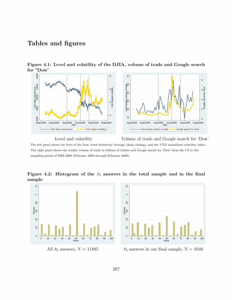
Tables and figures

Figure 4.1: Level and volatility of the DJIA, volume of trade and Google searchfor ”Dow’

.2.4

.6.8

VX

D im

plie

d vo

latil

ity

6000

8000

1000

012

000

1400

0D

JIA

dai

ly c

losi

ng le

vel

01jan2008 01apr2008 01jul2008 01oct2008 01jan2009 01apr2009date

DJIA daily closing level VXD implied volatility

02

46

8G

oogl

e se

arch

for

'dow

'

2030

4050

6070

DJI

A w

eekl

y vo

lum

e of

trad

e

01jan2008 01apr2008 01jul2008 01oct2008 01jan2009 01apr2009date

DJIA weekly volume of trade Google search for 'dow'

Level and volatility Volume of trade and Google search for ’Dow’The left panel shows the level of the Dow Jones Industrial Average (daily closing), and the VXD annualized volatility index.

The right panel shows the weekly volume of trade in billions of dollars and Google search for ”Dow’ from the US in the

sampling period of HRS 2008 (February 2008 through February 2009).

Figure 4.2: Histogram of the P0 answers in the total sample and in the finalsample

0.0

2.0

4.0

6.0

8.1

.12

Den

sity

0 10 20 30 40 50 60 70 80 90 100Value

0.0

2.0

4.0

6.0

8.1

.12

Den

sity

0 10 20 30 40 50 60 70 80 90 100Value

All P0 answers, N = 11885 P0 answers in our final sample, N = 9348

267

Figure 4.3: Standard normal c.d.f. with P0 and P20 shown

The figure shwos the standard normal c.d.f with µ = 0.07 and σ = 0.15.

Figure 4.4: Cross-sectional distribution of expected returns among stockholdersand non-stockholders�

��

��

��

��

-0.5

-0.4

-0.3

-0.2

-0.1

0

0.1

0.2

0.3

0.4

0.5

Feb-Jun 08 Jul-Sep 08 Oct-Nov 08 Dec-Feb08/9

Su

bje

ctiv

e e

xpe

cte

d v

alu

e o

f re

turn

s ( µ

i)

25th percentile50th percentile75th percentile

�

��

��

��

��

-0.5

-0.4

-0.3

-0.2

-0.1

0

0.1

0.2

0.3

0.4

0.5


Su

bje

ctiv

e e

xpe

cte

d v

alu

e o

f re

turn

s ( µ

i)

25th percentile50th percentile75th percentile

Stockholders Non-stockholdersThe figures show the quartiles of the distribution by the date of the interview, estimated from the structural model with interactions.

Detailed results in Table 4.6 in the appendix.

268

Figure 4.5: Cross-sectional distribution of expected returns among informed anduninformed individuals�

��

��

��

��

-0.5

-0.4

-0.3

-0.2

-0.1

0

0.1

0.2

0.3

0.4

0.5


Su

bje

ctiv

e e

xpe

cte

d v

alu

e o

f re

turn

s ( µ

i)25th percentile

50th percentile

75th percentile

�

��

��

��

��

-0.5

-0.4

-0.3

-0.2

-0.1

0

0.1

0.2

0.3

0.4

0.5


Su

bje

ctiv

e e

xpe

cte

d v

alu

e o

f re

turn

s ( µ

i)

25th percentile

50th percentile

75th percentile

Informed UninformedThe figures show the quartiles of the distribution by the date of the interview, estimated from the structural model with interactions.

Detailed results in Table 4.7 in the Appendix. Informed individuals reported to follow the stock market.

Figure 4.6: Cross-sectional distribution of expected returns by cognition�

��

��

��

��

-0.5

-0.4

-0.3

-0.2

-0.1

0

0.1

0.2

0.3

0.4

0.5


Su

bje

ctiv

e e

xpe

cte

d v

alu

e o

f re

turn

s ( µ

i)

25th percentile

50th percentile

75th percentile

�

��

��

��

��-0.5

-0.4

-0.3

-0.2

-0.1

0

0.1

0.2

0.3

0.4

0.5


Su

bje

ctiv

e e

xpe

cte

d v

alu

e o

f re

turn

s ( µ

i)

25th percentile

50th percentile

75th percentile

Above average cognitive capacity Below average cognitive capacityThe figures show the quartiles of the distribution by the date of the interview, estimated from the structural model with interactions.

Detailed results in Table 4.8 in the Appendix.

269

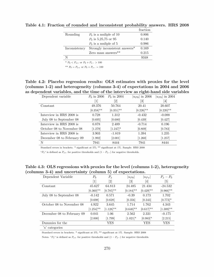
Table 4.1: Fraction of rounded and inconsistent probability answers. HRS 2008fraction

Rounding P0 is a muliple of 10 0.806

P0 is 5,25,75 or 95 0.140

P0 is a muliple of 5 0.986

Inconsistency Strongly inconsistent answers* 0.169

Zero mass answers** 0.215

N 9348

* P0 < Px+ or P0 + Px− > 100

** P0 = Px+ or P0 + Px− = 100

Table 4.2: Placebo regression results: OLS estimates with proxies for the level(columns 1-2) and heterogeneity (columns 3-4) of expectations in 2004 and 2006as dependent variables, and the time of the interview as right-hand side variables

Dependent variable P0 in 2006 P0 in 2004 |uP0| in 2006 |uP0| in 2004

[1] [2] [3] [4]

Constant 49.376 50.764 20.41 20.607

[0.358]** [0.351]** [0.226]** [0.220]**

Interview in HRS 2008 is 0.728 1.312 -0.432 -0.088

July 08 to September 08 [0.695] [0.680] [0.439] [0.427]

Interview in HRS 2008 is 0.878 2.489 -0.714 0.196

October 08 to November 08 [1.279] [1.247]* [0.809] [0.783]

Interview in HRS 2008 is 3.903 -1.819 1.394 1.235

December 08 to February 09 [1.992] [2.001] [1.260] [1.257]

N 7941 8444 7941 8444

Standard errors in brackets. * significant at 5%; ** significant at 1%. Sample: HRS 2008

“Px“ is defined as Px+ for positive thresholds and (1− Px−) for negative thresholds.

Table 4.3: OLS regressions with proxies for the level (columns 1-2), heterogeneity(columns 3-4) and uncertainty (column 5) of expectations.

Dependent Variable P0 Px |uP0| |uPx| Px − P0

[1] [2] [3] [4] [5]

Constant 45.627 64.813 24.485 21.434 -24.532

[0.360]** [0.785]** [0.184]** [0.429]** [0.966]**

July 08 to September 08 -0.142 0.571 -0.39 0.173 1.702

[0.698] [0.628] [0.356] [0.343] [0.773]*

October 08 to November 08 4.922 3.645 1.714 1.762 4.343

[1.254]** [1.128]** [0.640]** [0.617]** [1.389]**

December 08 to February 09 0.041 1.06 2.562 2.331 -0.175

[2.000] [1.799] [1.021]* [0.983]* [2.215]

Dummies for the YES YES YES

’x’ categories


Notes. “Px“ is defined as Px+ for positive thresholds and (1− Px−) for negative thresholds.

270

Table 4.4: Date of interview in 2008 and average subjective expected valueof yearly stock returns (m), average subjective standard deviation (sv) and un-observed cross-sectional heterogeneity in expectations (Std(u)). Results fromstructural regressions

µ ln(σ) ln[Std(u)]

Constant -0.088 -0.606 -1.23

[0.006]** [0.023]** [0.079]**

July 08 to September 08 0.001 0.113 0.131

[0.010] [0.037]** [0.047]**

October 08 to November 08 0.062 0.292 0.569

[0.025]* [0.088]** [0.099]**

December 08 to February 09 -0.028 0.019 0.38

[0.033] [0.119] [0.135]**

Female -0.062 0.235 0.146

[0.009]** [0.034]** [0.044]**

Single 0.004 0.04 0.121

[0.010] [0.039] [0.048]*

Black -0.017 0.589 0.56

[0.025] [0.093]** [0.096]**

Hispanic 0.002 0.387 0.332

[0.027] [0.107]** [0.114]**

Age -0.002 -0.005 -0.004

[0.000]** [0.002]** [0.002]

Years of education 0.002 -0.034 -0.031

[0.002] [0.007]** [0.009]**

Above average cognition 0.031 -0.101 -0.198

[0.010]** [0.037]** [0.048]**

Follow the stock market 0.049 -0.129 -0.073

[0.010]** [0.038]** [0.047]

Stockholder 0.072 -0.058 -0.18

[0.010]** [0.038] [0.050]**

P(economic recession) -0.003

2004-2006 average [0.000]**

Depressive symptoms -0.017

2004-2006 average [0.005]**

Ratio of fifty-fifty answers 1.512

2004-2006 average [0.191]**

Log-likelihood -42277

N 9348

Mean(m) -0.085

Mean(sv) 0.616

Mean(Std(u) 0.343

sv2/(sv2+V(v)) 0.645

Rho(v0,vx-) -0.491

Rho(v0,vx+) 0.252

Standard errors in brackets. * significant at 5%; ** significant at 1%

Reference categories: Interview date March to June, male,

non-Black and non-Hispanic, married

Sample: HRS 2008 271

Table 4.5: The effects of recent returns and volatility of the stock market indexand the daily volume of trade of the shares of the DJIA, before and after thecrash

Specification [1] Specification [2]

µ ln(σ) ln[Std(u)] µ ln(σ) ln[Std(u)]

Constant -0.085 -0.568 -8.955 -0.084 -0.785 -8.454

[0.006]** [0.041]** [2.213]** [0.005]** [0.089]** [2.234]**

Monthly log returns 0.048 0.335

(log of the average of previous 5 days

minus the same one month before) [0.081] [0.104]**

VXD volatility index 0.013 0.977

(average of previous 5 days) [0.151] [0.408]*

Log of volume of trade 0.350 0.327

(average of previous 5 days) [0.097]** [0.099]**

Post-crash dummy -0.007 0.210 19.295

(October 08 to February 09) [0.032] [0.256] [6.101]**

Post-crash dummy interacted with -0.721

monthly log returns [0.257]**


VXD volatility index [0.601]


log of volume of trade [0.271]**

Other covariates YES YES YES YES YES YES

Instruments YES YES YES YES


N 9347 9347


272

APPENDIX J

Detailed estimates from the models with interactions

273

Table 4.6: Stockholders versus non-stockholders. Date of interview in 2008 andaverage subjective expected value of yearly stock returns (µ), average subjectivestandard deviation (σ) and unobserved cross-sectional heterogeneity in expecta-tions (Std(u))


coef interaction with coef interaction with coef interaction with

stockholding stockholding stockholding

Constant -0.091 0.087 -0.597 -0.134 -1.176 -0.229

[0.007]** [0.013]** [0.026]** [0.052]** [0.082]** [0.063]**

July 08 to Sep08 0.008 -0.013 0.135 -0.052 0.158 -0.066

[0.018] [0.022] [0.067]* [0.082] [0.076]* [0.098]

Oct 08 to Nov 08 0.091 -0.031 0.29 -0.066 0.465 0.135

[0.041]* [0.052] [0.155] [0.188] [0.161]** [0.203]

Dec 08 to Feb 09 -0.012 -0.006 -0.113 0.194 0.231 0.251

[0.052] [0.068] [0.173] [0.246] [0.181] [0.268]

Female -0.103 0.05 0.234 0.076 0.157 0.024

[0.016]** [0.019]** [0.059]** [0.073] [0.066]* [0.087]

Single 0.012 -0.017 0.135 -0.169 0.244 -0.232

[0.018] [0.022] [0.062]* [0.081]* [0.070]** [0.096]*

Black 0.015 -0.126 0.539 0.101 0.483 0.276

[0.028] [0.062]* [0.104]** [0.228] [0.107]** [0.241]

Hispanic 0.013 -0.04 0.408 -0.107 0.357 -0.004

[0.035] [0.055] [0.134]** [0.223] [0.139]* [0.242]

Age -0.002 -0.001 -0.011 0.011 -0.012 0.018

[0.001]** [0.001] [0.003]** [0.004]** [0.003]** [0.004]**

Years of education 0.004 -0.001 -0.04 -0.006 -0.033 -0.028

[0.003] [0.004] [0.011]** [0.015] [0.012]** [0.017]

P(economic recession) -0.004 0.001

2004-2006 average [0.000]** [0.000]

Depressive symptoms -0.025 0.007

2004-2006 average [0.008]** [0.010]

Ratio of fifty answers 1.673 -0.42

2004-2006 average [0.249]** [0.261]

Ll -42278.6

N 9348

Mean(µ) -0.083

Mean(σ) 0.622

Mean(Std(u)) 0.355

Var[R∗]/Var[R] 0.652

Rho(v0, vx−) -0.535

Rho(v0, vx+) 0.225

Standard errors in brackets. * Significant at 5%; ** significant at 1%. Sample: HRS 2008

Stockholders are those who own any stock-market based assets (stocks, mutual funds etc.) either directly or through retirement accounts.

Members of the same households are assigned the same stockholding status. For more details see main text and footnotes to Table 4

274

Table 4.7: Informed versus uninformed respondents. Date of interview in 2008and average subjective expected value of yearly stock returns (µ), average sub-jective standard deviation (σ) and unobserved cross-sectional heterogeneity inexpectations (Std(u))



informed informed informed

Constant -0.085 0.06 -0.588 -0.123 -1.084 -0.087

[0.006]** [0.012]** [0.025]** [0.050]* [0.084]** [0.054]

July 08 to Sep08 0.001 -0.004 0.106 0.005 0.165 -0.079

[0.020] [0.023] [0.072] [0.085] [0.080]* [0.097]

Oct 08 to Nov 08 0.136 -0.108 0.311 -0.08 0.528 -0.047

[0.049]** [0.056] [0.186] [0.210] [0.192]** [0.218]

Dec 08 to Feb 09 0.014 -0.064 -0.114 0.138 -0.101 0.582

[0.054] [0.068] [0.211] [0.256] [0.225] [0.276]*

Female -0.096 0.058 0.166 0.128 0.107 0.081

[0.016]** [0.019]** [0.063]** [0.076] [0.070] [0.086]

Single 0.01 -0.029 0.111 -0.096 0.183 -0.058

[0.018] [0.022] [0.069] [0.084] [0.075]* [0.093]

Black 0.01 -0.077 0.458 0.221 0.461 0.244

[0.032] [0.048] [0.122]** [0.180] [0.124]** [0.184]

Hispanic 0.066 -0.158 0.179 0.347 0.173 0.311

[0.032]* [0.054]** [0.135] [0.211] [0.140] [0.219]

Age -0.003 0.001 -0.011 0.01 -0.01 0.011

[0.001]** [0.001] [0.003]** [0.004]** [0.003]** [0.004]**

Years of education 0.006 0 -0.034 -0.018 -0.026 -0.046

[0.003] [0.004] [0.011]** [0.014] [0.012]* [0.016]**

P(economic recession) -0.003 0

2004-2006 average [0.000]** [0.000]

Depressive symptoms -0.022 0

2004-2006 average [0.008]** [0.010]

Ratio of fifty answers 1.634 -0.537

2004-2006 average [0.252]** [0.230]*

Ll -42300.4

N 9348

Mean(µ) -0.08

Mean(σ) 0.608

Mean(Std(u)) 0.376


Rho(v0, vx−) -0.699

Rho(v0, vx+) 0.138


Informed are those who claim to follow the stock market at least occasionally. For more details see main text and footnotes to Table 4

275

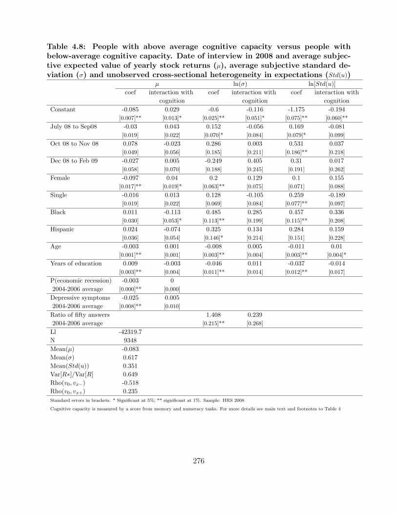
Table 4.8: People with above average cognitive capacity versus people withbelow-average cognitive capacity. Date of interview in 2008 and average subjec-tive expected value of yearly stock returns (µ), average subjective standard de-viation (σ) and unobserved cross-sectional heterogeneity in expectations (Std(u))



cognition cognition cognition

Constant -0.085 0.029 -0.6 -0.116 -1.175 -0.194

[0.007]** [0.013]* [0.025]** [0.051]* [0.075]** [0.060]**

July 08 to Sep08 -0.03 0.043 0.152 -0.056 0.169 -0.081

[0.019] [0.022] [0.070]* [0.084] [0.079]* [0.099]

Oct 08 to Nov 08 0.078 -0.023 0.286 0.003 0.531 0.037

[0.049] [0.056] [0.185] [0.211] [0.186]** [0.218]

Dec 08 to Feb 09 -0.027 0.005 -0.249 0.405 0.31 0.017

[0.058] [0.070] [0.188] [0.245] [0.191] [0.262]

Female -0.097 0.04 0.2 0.129 0.1 0.155

[0.017]** [0.019]* [0.063]** [0.075] [0.071] [0.088]

Single -0.016 0.013 0.128 -0.105 0.259 -0.189

[0.019] [0.022] [0.069] [0.084] [0.077]** [0.097]

Black 0.011 -0.113 0.485 0.285 0.457 0.336

[0.030] [0.053]* [0.113]** [0.199] [0.115]** [0.208]

Hispanic 0.024 -0.074 0.325 0.134 0.284 0.159

[0.036] [0.054] [0.146]* [0.214] [0.151] [0.228]

Age -0.003 0.001 -0.008 0.005 -0.011 0.01

[0.001]** [0.001] [0.003]** [0.004] [0.003]** [0.004]*

Years of education 0.009 -0.003 -0.046 0.011 -0.037 -0.014

[0.003]** [0.004] [0.011]** [0.014] [0.012]** [0.017]

P(economic recession) -0.003 0

2004-2006 average [0.000]** [0.000]

Depressive symptoms -0.025 0.005

2004-2006 average [0.008]** [0.010]

Ratio of fifty answers 1.408 0.239

2004-2006 average [0.215]** [0.268]

Ll -42319.7

N 9348

Mean(µ) -0.083

Mean(σ) 0.617

Mean(Std(u)) 0.351


Rho(v0, vx−) -0.518

Rho(v0, vx+) 0.235


Cognitive capacity is measured by a score from memory and numeracy tasks. For more details see main text and footnotes to Table 4

276

APPENDIX K

Estimates based on alternative functional form

assumptions

In this appendix we re-estimate our structural models with two alternative specifications

for the return distribution, Student-t with various degrees of freedom and shifted log-normal.

Within the Student-t framework, the relation between the probability answers and the esti-

mated parameters is the following:

P0i = T

(µiσi, df

), (4.13)

Px+,i = T

(µi − x/100

σi, df

), (4.14)

Px−,i = T

(x/100− µi

σi, df

), (4.15)

where df is the degrees of freedom of the distribution. Note that since the t distribution is

symmetric, µ can still be interpreted as the mean of the subjective distribution, sv will not

be the subjective standard deviation anymore. According to the properties of the Student-t

distribution, the true standard deviation will be

σRi = σi

√df

df − 2(4.16)

Under the shifted log-normal assumption returns follow , it can be shown that the prob-

277

ability answers are:

P0i = Φ

(µiσi

), (4.17)

Px+,i = Φ

(µi − ln (x/100)

σi

), (4.18)

Px−,i = Φ

(ln (x/100)− µi

σi

), (4.19)

For small return realizations the normal and the shifted log-normal distributions are very

similar. We, however, have quite high subjective variance, and thus a very large fraction of

the return distribution is in a range where the true distributions are different. An important

difference between the normal and the shifted lognormal model is that they have different

moments. It can be shown that the first two moments of the shifted lognormal distribution

are:

µRi = exp

(µi +

σ2i

2

)− 1, (4.20)

σ2Ri =

(exp

(σ1i

)− 1)

exp(2µi + σ2

i

)(4.21)

Because it is skewed, the mean of the distribution will be larger than the estimated µ. The

potential asymmetry of the subjective distribution, thus, can be a reason for having small,

usually negative values for µ.

As we can see, the parameter estimates are very much the same in all specifications,

and the qualitative results do not change. All specifications agree that the crash brought a

moderate increase in uncertainty and a huge increase in disagreement. The normal and the

Student-t models agree that the mean of the subjective distribution was weakly positively

affected by the crash. The log-normal model is also equivalent to the other models if we talk

278

about log-returns instead of actual returns. As we saw earlier, actual returns are non-linear

functions of µ and sv, and the moderate increase in sv must have a positive effect on µR.

According to these estimates, the average µR increased after the crash from 16.5 percent to

72.2 percent, and the overall mean is 21.2 percent. This is clearly implausible.

We can also see that the likelihood is the highest in the original normal case and thus

this model fits the data the best. While asymmetric models could explain how the mean of

the subjective distribution can be positive even if the average P0 value is less than 50, we

can see that the log-normal model does not fit the data well. Further investigation is needed

to test for the potential non-normality of the subjective return distribution.

279

Table 4.9: Stock returns assumed to be distributed Student-t with 3 degrees offreedom. Date of interview in 2008 and average subjective expected value ofyearly stock returns (µ), average subjective standard deviation (σ) and unob-served cross-sectional heterogeneity in expectations (Std(u))


Constant -0.090 -0.871 -1.165

[0.006]** [0.024]** [0.074]**


[0.010] [0.038]** [0.046]**


[0.025]* [0.090]** [0.099]**


[0.034] [0.122] [0.135]**

Female -0.063 0.248 0.157

[0.009]** [0.035]** [0.043]**

Single 0.004 0.040 0.118

[0.010] [0.040] [0.048]*

Black -0.017 0.592 0.562

[0.026] [0.095]** [0.098]**

Hispanic 0.000 0.383 0.327

[0.027] [0.109]** [0.114]**

Age -0.002 -0.006 -0.004

[0.000]** [0.002]** [0.002]


[0.002] [0.007]** [0.009]**


[0.010]** [0.038]* [0.047]**


[0.010]** [0.039]** [0.046]

Stockholder 0.071 -0.047 -0.177

[0.010]** [0.039] [0.049]**


2004-2006 average [0.000]**


2004-2006 average [0.005]**


2004-2006 average [0.196]**

Log-likelihood -43091.9

N 9348

Mean(m) -0.087

Mean(sv) 0.818

Mean(Std(u) 0.364

sv2/(sv2+V(v)) 0.763

Rho(v0,vx-) -0.574

Rho(v0,vx+) 0.193





Table 4.10: Stock returns assumed to be distributed Student-t with 3 degreesof freedom. Date of interview in 2008 and average subjective expected valueof yearly stock returns (µ), average subjective standard deviation (σ) and unob-served cross-sectional heterogeneity in expectations (Std(u))


Constant -0.088 -0.678 -1.213

[0.006]** [0.023]** [0.077]**


[0.010] [0.038]** [0.047]**


[0.025]* [0.088]** [0.099]**


[0.033] [0.120] [0.135]**

Female -0.062 0.239 0.149

[0.009]** [0.034]** [0.043]**

Single 0.004 0.040 0.120

[0.010] [0.039] [0.048]*

Black -0.017 0.590 0.560

[0.025] [0.093]** [0.097]**

Hispanic 0.001 0.386 0.330

[0.027] [0.107]** [0.114]**

Age -0.002 -0.005 -0.004

[0.000]** [0.002]** [0.002]


[0.002] [0.007]** [0.009]**


[0.010]** [0.038]** [0.048]**


[0.010]** [0.038]** [0.046]

Stockholder 0.071 -0.055 -0.180

[0.010]** [0.038] [0.049]**


2004-2006 average [0.000]**


2004-2006 average [0.005]**


2004-2006 average [0.192]**


N 9348

Mean(m) -0.085

Mean(sv) 0.641

Mean(Std(u) 0.348

sv2/(sv2+V(v)) 0.663

Rho(v0,vx-) -0.512

Rho(v0,vx+) 0.238





Table 4.11: Stock returns assumed to be distributed log-normal with parametersµi and σi. Date of interview in 2008 and average subjective expected value ofyearly stock returns (µ), average subjective standard deviation (σ) and unob-served cross-sectional heterogeneity in expectations (Std(u))


Constant -0.108 -0.565 -1.185

[0.006]** [0.023]** [0.078]**


[0.010] [0.038]* [0.047]*


[0.026]* [0.093]** [0.103]**


[0.035] [0.124] [0.139]**

Female -0.067 0.234 0.145

[0.009]** [0.035]** [0.044]**

Single 0.005 0.044 0.127

[0.011] [0.040] [0.049]**

Black -0.013 0.554 0.527

[0.025] [0.092]** [0.094]**

Hispanic 0.005 0.382 0.328

[0.028] [0.109]** [0.115]**

Age -0.002 -0.006 -0.005

[0.000]** [0.002]** [0.002]*


[0.002] [0.007]** [0.009]**


[0.010]** [0.038]* [0.048]**


[0.010]** [0.038]** [0.047]

Stockholder 0.074 -0.054 -0.177

[0.010]** [0.039] [0.050]**


2004-2006 average [0.000]**


2004-2006 average [0.005]**


2004-2006 average [0.196]**


N 9348

Mean(m) 0.210

Mean(sv) 9.017

Mean(Std(u) 0.355

sv2/(sv2+V(v)) 0.644

Rho(v0,vx-) -0.484

Rho(v0,vx+) 0.231





Bibliography

Abowd, J. M. and D. Card (1989, March). On the Covariance Structure of Earnings and

Hours Changes. Econometrica, Econometric Society 57 (2), 411–45.

Abowd, J. M. and M. H. Stinson (2007, September). Estimating Measurement Error in

SIPP Annual Job Earnings: A Comparison of Census Survey and SSA Administrative

Data. Working paper, Federal Committee on Statistical Methodology.

Abowd, J. M. and M. H. Stinson (2013). Estimating Measurement Error in Annual Job

Earnings: A Comparison of Survey and Administrative Data. The Review of Economics

and Statistics 95 (5), 1451–1467.

Abowd, J. M. and A. Zellner (1985). Estimating Gross Labor-Force Flows. Journal of

Business & Economic Statistics 3 (3), pp.254–283.

Abraham, A. and K. White (2006, July). The Dynamics of Plant-Level Productivity in U.S.

Manufacturing. Working Papers 06-20, Center for Economic Studies, U.S. Census Bureau.

Abraham, K. G. and J. R. Spletzer (2009, May). New Evidence on the Returns to Job Skills.

American Economic Review 99 (2), 52–57.

Acemoglu, D. (1999, December). Changes in Unemployment and Wage Inequality: An

Alternative Theory and Some Evidence. American Economic Review 89 (5), 1259–1278.

284

Acemoglu, D. and D. Autor (2011). Skills, Tasks and Technologies: Implications for Employ-

ment and Earnings, Volume 4 of Handbook of Labor Economics, Chapter 12, pp. 1043–1171.

Elsevier.

Acemoglu, D. and R. Shimer (1999, November). Holdups and Efficiency with Search Fric-

tions. International Economic Review 40 (4), 827–49.

Aizcorbe, A. M. (1992, July). Procyclical Labour Productivity, Increasing Returns to Labour

and Labour Hoarding in Car Assembly Plant Employment. Economic Journal 102 (413),

860–73.

Akee, R. (2011, November). Errors in Self-reported Earnings: The Role of Previous Earnings

Volatility and Individual Characteristics. Journal of Development Economics 96 (2), 409–

421.

Albrecht, J. and S. Vroman (2002, February). A Matching Model with Endogenous Skill

Requirements. International Economic Review 43 (1), 283–305.

Altonji, J. G. and C. R. Pierret (2001). Employer Learning and Statistical Discrimination.

The Quarterly Journal of Economics 116 (1), pp.313–350.

Altonji, J. G., A. Smith, and I. Vidangos (2009, February). Modeling Earnings Dynamics.

NBER Working Papers 14743, National Bureau of Economic Research, Inc.

Altonji, J. G., A. A. J. Smith, and I. Vidangos (2013, July). Modeling Earnings Dynamics.

Econometrica, Econometric Society 81 (4), 1395–1454.

Altonji, J. G. and N. Williams (2005, April). Do wages rise with job seniority? A reassess-

ment. Industrial and Labor Relations Review 58 (3), 370–397.

285

Alvarez, J. and M. Arellano (2004). Robust Likelihood Estimation of Dynamic Panel Data

Models. Technical report, CEMFI Working Paper 0421.

Angrist, J. and A. B. Krueger (1999). Empirical Strategies in Labor Economics. In O. Ashen-

felter and D. Card (Eds.), Handbook of Labor Economics (1 ed.), Volume 3, Part A, Chap-

ter 23, pp. 1277–1366. Elsevier.

Angrist, J. D., G. W. Imbens, and D. B. Rubin (1996). Identification of Causal Effects Using

Instrumental Variables. Journal of the American Statistical Association 91 (434), 444–455.

Angrist, J. D. and A. B. Krueger (2001). Instrumental Variables and the Search for Iden-

tification: From Supply and Demand to Natural Experiments. The Journal of Economic

Perspectives 15 (4), 69–85.

Arulampalam, W. and A. L. Booth (2001, August). Learning and Earning: Do Multiple

Training Events Pay? A Decade of Evidence from a Cohort of Young British Men. Eco-

nomica 68 (271), 379–400.

Autor, D. H., L. F. Katz, and M. S. Kearney (2006, May). The Polarization of the U.S.

Labor Market. American Economic Review 96 (2), 189–194.

Autor, D. H., F. Levy, and R. J. Murnane (2003, November). The Skill Content Of Re-

cent Technological Change: An Empirical Exploration. The Quarterly Journal of Eco-

nomics 118 (4), 1279–1333.

Azariadis, C. (1975, December). Implicit Contracts and Underemployment Equilibria. Jour-

nal of Political Economy 83 (6), 1183–1202.

286

Azariadis, C. (1976, February). On the Incidence of Unemployment. Review of Economic

Studies 43 (1), 115–25.

Baily, M. N. (1974, January). Wages and Employment under Uncertain Demand. Review of

Economic Studies 41 (1), 37–50.

Barnichon, R. and A. Figura (2011). Labor Market Heterogeneities, Matching Efficiency,

and the Cyclical Behavior of the Job Finding Rate. Mimeo.

Bartel, A., C. Ichniowski, and K. Shaw (2007, November). How Does Information Technology

Affect Productivity? Plant-Level Comparisons of Product Innovation, Process Improve-

ment, and Worker Skills. The Quarterly Journal of Economics 122 (4), 1721–1758.

Basu, S. (1996, August). Procyclical Productivity: Increasing Returns or Cyclical Utiliza-

tion? The Quarterly Journal of Economics 111 (3), 719–51.

Basu, S. and M. S. Kimball (1997, February). Cyclical Productivity with Unobserved Input

Variation. NBER Working Papers 5915, National Bureau of Economic Research, Inc.

Becker, G. S. (1962). Investment in Human Capital: A Theoretical Analysis. Journal of

Political Economy 70, 9.

Becker, G. S. (1965). A Theory of the Allocation of Time. The Economic Journal 75 (299),

493–517.

Becker, G. S. (1994, July). Human Capital: A Theoretical and Empirical Analysis with

Special Reference to Education (3rd Edition). NBER Books. National Bureau of Economic

Research, Inc.

287

Bernanke, B. S. and M. L. Parkinson (1991, June). Procyclical Labor Productivity and Com-

peting Theories of the Business Cycle: Some Evidence from Interwar U.S. Manufacturing

Industries. Journal of Political Economy 99 (3), 439–59.

Bils, M. J. (1985). Real Wages over the Business Cycle: Evidence from Panel Data. Journal

of Political Economy 93 (4), pp.666–689.

Blanchard, O. and J. Galı (2010, April). Labor Markets and Monetary Policy: A New Key-

nesian Model with Unemployment. American Economic Journal: Macroeconomics 2 (2),

1–30.

Blanchard, O. J. and P. Diamond (1990). The Cyclical Behavior of the Gross Flows of U.S.

Workers. Brookings Papers on Economic Activity 21 (2), 85–156.

Blatter, M., S. Muehlemann, and S. Schenker (2012). The costs of Hiring Skilled Workers.

European Economic Review 56 (1), 20–35.

Blundell, R. and T. Macurdy (1999). Labor Supply: A Review of Alternative Approaches.

In O. Ashenfelter and D. Card (Eds.), Handbook of Labor Economics (1 ed.), Volume 3,

Part A, Chapter 27, pp. 1559–1695. Elsevier.

Bollinger, C. R. (1998, July). Measurement Error in the Current Population Survey: A

Nonparametric Look. Journal of Labor Economics 16 (3), 576–94.

Bolvig, I., I. Hardoy, M. Kauhanen, R. Lilja, M. Roed, and N. Smith (2007). The Labour

Supply of Low-Skilled-Incentives in the Unemployment Insurance Systems: A Comparative

Description Based on Nordic Countries. Nordic Council of Ministers.

288

Bommier, A. and B. Villeneuve (2012, 03). Risk Aversion and the Value of Risk to Life.

Journal of Risk & Insurance 79 (1), 77–104.

Borjas, G. J. (2003, November). The Labor Demand Curve Is Downward Sloping: Reex-

amining The Impact Of Immigration On The Labor Market. The Quarterly Journal of

Economics 118 (4), 1335–1374.

Bosworth, B. P. and R. Smart (2009, January). Evaluating Micro-Survey Estimates of Wealth

and Saving. Working Papers, Center for Retirement Research at Boston College wp2009-4,

Center for Retirement Research.

Bound, J., C. Brown, G. J. Duncan, and W. L. Rodgers (1994). Evidence on the Validity of

Cross-Sectional and Longitudinal Labor Market Data. Journal of Labor Economics 12 (3),

pp.345–368.

Bound, J., C. Brown, and N. Mathiowetz (2001). Measurement Error in Survey Data. In

J. Heckman and E. Leamer (Eds.), Handbook of Econometrics, Volume 5 of Handbook of

Econometrics, Chapter 59, pp. 3705–3843. Elsevier.

Bound, J. and A. B. Krueger (1991, January). The Extent of Measurement Error in Longi-

tudinal Earnings Data: Do Two Wrongs Make a Right? Journal of Labor Economics 9 (1),

1–24.

Bound, J., T. Stinebrickner, and T. Waidmann (2010). Health, economic resources and the

work decisions of older men. Journal of Econometrics 156 (1), 106–129. Structural Models

of Optimization Behavior in Labor, Aging, and Health.

Bowlus, A., H. Liu, and C. Robinson (2002, Part). Business Cycle Models, Aggregation, and

Real Wage Cyclicality. Journal of Labor Economics 20 (2), 308–335.

289

Brown, C. (1990). Empirical Evidence on Private Training. In Research in Labor Economics,

Volume 11, pp. 97–113. JAI Press Inc.

Brownstone, D. and R. G. Valletta (1996). Modeling Earnings Measurement Error: A Mul-

tiple Imputation Approach. The Review of Economics and Statistics 78 (4), pp.705–717.

Bruine de Bruin, W. and K. G. Carman (2012). Measuring Risk Perceptions: What Does

the Excessive Use of 50% Mean? 32 (2), 232–236.

Bruine de Bruin, W., B. Fischhoff, S. G. Millstein, and B. L. Halpern-Felsher (2000, January).

Verbal and Numerical Expressions of Probability: "It’s a Fifty-Fifty Chance".

Organizational Behavior and Human Decision Processes 81 (1), 115–131.

Burdett, K. and D. T. Mortensen (1998, May). Wage Differentials, Employer Size, and

Unemployment. International Economic Review 39 (2), 257–73.

Burnside, C. and M. Eichenbaum (1996, December). Factor-Hoarding and the Propagation

of Business-Cycle Shocks. American Economic Review 86 (5), 1154–74.

Burnside, C., M. Eichenbaum, and S. Rebelo (1993, April). Labor Hoarding and the Business

Cycle. Journal of Political Economy 101 (2), 245–73.

Buttner, T., P. Jacobebbinghaus, and J. Ludsteck (2010). Occupational Upgrading and

the Business Cycle in West Germany. Economics - The Open-Access, Open-Assessment

E-Journal 4 (10), 1–37.

Cahuc, P., F. Marque, and E. Wasmer (2008, August). A Theory Of Wages And Labor

Demand With Intra-Firm Bargaining And Matching Frictions. International Economic

Review 49 (3), 943–972.

290

Cairo, I. and T. Cajner (2014, September). Human Capital and Unemployment Dynamics:

Why More Educated Workers Enjoy Greater Employment Stability. Technical Report

2014-09, Federal Reserve Board, Washington, D.C.

Calvet, L. E., J. Y. Campbell, and P. Sodini (2007, October). Down or Out: Assessing the

Welfare Costs of Household Investment Mistakes. Journal of Political Economy 115 (5),

707–747.

Calvet, L. E., J. Y. Campbell, and P. Sodini (2009a). Fight or Flight? Portfolio Rebalancing

by Individual Investors. The Quarterly Journal of Economics 124 (1), 301–348.

Calvet, L. E., J. Y. Campbell, and P. Sodini (2009b, May). Measuring the Financial Sophis-

tication of Households. American Economic Review 99 (2), 393–98.

Campbell III, C. M. (1997). The Variation in Wage Rigidity by Occupation and Union Status

in the US. Oxford Bulletin of Economics and Statistics 59 (1), 133–147.

Cannell, C. F., G. Fisher, and T. Bakker (1965). Reporting of Hospitalization in the Health

Interview Survey. Technical Report 6, Vital and Health Statistics, Series 2, Public Health

Service, Washington.

Card, D. (2001, January). The Effect of unions on wage inequality in the U.S. labor market.

Industrial and Labor Relations Review 54 (2), 296–315.

Card, D., F. Kramarz, and T. Lemieux (1996, March). Changes in the Relative Structure

of Wages and Employment: A Comparison of the United States, Canada, and France.

Working Paper 5487, National Bureau of Economic Research.

291

Card, D., T. Lemieux, and W. Riddell (2004). Unions and Wage Inequality. Journal of

Labor Research 25 (4), 519–559.

Carrington, W. J. and A. Zaman (1994, April). Interindustry Variation in the Costs of Job

Displacement. Journal of Labor Economics 12 (2), 243–75.

Carroll, R. J., D. Ruppert, L. A. Stefanski, and C. M. Crainiceanu (2006, July). Measurement

Error in Nonlinear Models: A Modern Perspective (2nd ed.). Chapman and Hall/CRC.

Chassamboulli, A. (2011). Cyclical Upgrading of Labor and Employment Differences across

Skill Groups. The B.E. Journal of Macroeconomics 11 (1).

Cheremukhin, A. (2010). Labor Matching Model: Putting the Pieces Together. 2010 Meeting

Papers 260, Society for Economic Dynamics.

Cheron, A. and B. Rouland (2011, December). Inefficient Job Destructions and Training

with Holdup. LABOUR, CEIS 25 (4), 397–420.

Chodorow-Reich, G. and L. Karabarbounis (2013, November). The Cyclicality of the Oppor-

tunity Cost of Employment. Working Paper 19678, National Bureau of Economic Research.

Clark, K. B. and L. H. Summers (1981). Demographic Differences in Cyclical Employment

Variation. Journal of Human Resources 16 (1), 61–79.

Cook, K., D. Dranove, and A. Sfekas (2010). Does Major Illness Cause Financial Catastro-

phe? Health Services Research 45, 418–436.

Cortes, G. M., N. Jaimovich, C. J. Nekarda, and H. E. Siu (2013). The Micro and Macro of

Disappearing Routine Jobs: A Flows Approach. Unpublished manuscript.

292

Couch, K. A. and D. W. Placzek (2010, March). Earnings Losses of Displaced Workers

Revisited. American Economic Review 100 (1), 572–89.

Crifo, P. (2008). Skill Supply and Biased Technical Change. Post-Print hal-00243031, HAL.

Crimmins, E. M., J. K. Kim, K. M. Langa, and D. R. Weir (2011). Assessment of Cognition

Using Surveys and Neuropsychological Assessment: The Health and Retirement Study and

the Aging, Demographics, and Memory Study. Journals of Gerontology: Series B 66B,

i162–i171.

Cristia, J. and J. A. Schwabish (2009). Measurement Error in the SIPP: Evidence from

Administrative Matched Records. Journal of Economic and Social Measurement 34 (1),

1–17.

Davis, S. J., R. J. Faberman, and J. Haltiwanger (2006, Summer). The Flow Approach to

Labor Markets: New Data Sources and Micro-Macro Links. Journal of Economic Perspec-

tives 20 (3), 3–26.

Davis, S. J., R. J. Faberman, and J. Haltiwanger (2012). Labor Market Flows in the Cross

Section and Over Time. Journal of Monetary Economics 59 (1), 1–18.

Davis, S. J. and J. Haltiwanger (1990). Gross Job Creation and Destruction: Microeconomic

Evidence and Macroeconomic Implications. In NBER Macroeconomics Annual 1990, Vol-

ume 5, NBER Chapters, pp. 123–186. National Bureau of Economic Research, Inc.

Davis, S. J. and J. C. Haltiwanger (1992, August). Gross Job Creation, Gross Job De-

struction, and Employment Reallocation. The Quarterly Journal of Economics 107 (3),

819–63.

293

de Bruin, W. B., S. Potter, R. W. Rich, G. Topa, and H. W. V. der Klaauw (2010). Improving

Survey Measures of Household Inflation Expectations. SSRN eLibrary .

Deaton, A. S. (2009, January). Instruments of Development: Randomization in the Tropics,

and the Search for the Elusive Keys to Economic Development. Working Paper 14690,

National Bureau of Economic Research.

Devereux, P. J. (2000, January). Task Assignment over the Business Cycle. Journal of Labor

Economics 18 (1), 98–124.

Devereux, P. J. (2004, January). Cyclical Quality Adjustment in the Labor Market. Southern

Economic Journal 70 (3), 600–615.

Dickens, W. T. (2011). Has the Recession Increased the NAIRU? Technical report, North-

eastern University and The Brookings Institution.

Dickens, W. T. and R. K. Triest (2012). Potential effects of the Great Recession on the

U.S. labor market. Working Papers, Federal Reserve Bank of Boston 12-9, Federal Reserve

Bank of Boston.

Dolado, J., M. Jansen, and J. Jimeno (2009, January). On-the-Job Search in a Matching

Model with Heterogeneous Jobs and Workers. Economic Journal 119 (534), 200–228.

Dominitz, J. and C. F. Manski (2005). Measuring and Interpreting Expectations of Equity

Returns. NBER Working Papers 11313, National Bureau of Economic Research, Inc.

Duffy, J., C. Papageorgiou, and F. Perez-Sebastian (2004, February). Capital-Skill Comple-

mentarity? Evidence from a Panel of Countries. The Review of Economics and Statis-

tics 86 (1), 327–344.

294

Duncan, G. J. and D. H. Hill (1985). An Investigation of the Extent and Consequences of

Measurement Error in Labor-Economic Survey Data. Journal of Labor Economics 3 (4),

pp.508–532.

Egger, H. and V. Grossmann (2005, December). Non-Routine Tasks, Restructuring of Firms,

and Wage Inequality Within and Between Skill-Groups. Journal of Economics 86 (3), 197–

228.

Elder, T. (2013, April). The Predictive Validity of Subjective Mortality Expectations: Evi-

dence From the Health and Retirement Study. Demography 50 (2), 569–589.

Ellsberg, D. (1961). Risk, Ambiguity, and the Savage Axioms. 75 (4), 643–669.

Elsby, M., B. Hobjin, and A. Sahin (2010). The labor market in the Great Recession. Working

Paper Series 2010-07, Federal Reserve Bank of San Francisco.

Elsby, M. W. L. and R. Michaels (2008, February). Marginal Jobs, Heterogeneous Firms,

& Unemployment Flows. NBER Working Papers 13777, National Bureau of Economic

Research, Inc.

Elsby, M. W. L., R. Michaels, and G. Solon (2009, January). The Ins and Outs of Cyclical

Unemployment. American Economic Journal: Macroeconomics 1 (1), 84–110.

Esping-Andersen, G. (2000). Why Deregulate Labour Markets?, Chapter ”Who is Harmed

by Labour Market Regulations? Quantitative Evidence”, pp. 66–98. Oxford: Oxford

University Press.

Evans, P. (1999). Occupational Downgrading and Upgrading in Britain. Economica 66 (261),

pp.79–96.

295

Fair, R. C. (1985, March). Excess Labor and the Business Cycle. American Economic

Review 75 (1), 239–45.

Fallick, B. C. (1996, October). A review of the recent empirical literature on displaced

workers. Industrial and Labor Relations Review 50 (1), 5–16.

Farber, H. S. (1999). Mobility and stability: The dynamics of job change in labor markets. In

O. Ashenfelter and D. Card (Eds.), Handbook of Labor Economics, Volume 3 of Handbook

of Labor Economics, Chapter 37, pp. 2439–2483. Elsevier.

Farber, H. S. (2005). What do we know about job loss in the United States? evidence from

the displaced workers survey, 1984-2004. Economic Perspectives (Q II), 13–28.

Farber, H. S. (2011, May). Job Loss in the Great Recession: Historial Perspective from

the Displaced Workers Survey, 1984-2010. Working Papers 1309, Princeton University,

Department of Economics, Industrial Relations Section.

Fay, J. A. and J. L. Medoff (1985, September). Labor and Output over the Business Cycle:

Some Direct Evidence. American Economic Review 75 (4), 638–55.

Firpo, S., N. M. Fortin, and T. Lemieux (2011, February). Occupational Tasks and Changes

in the Wage Structure. IZA Discussion Papers 5542, Institute for the Study of Labor

(IZA).

Fischhoff, B. and W. Bruine De Bruin (1999). Fifty-Fifty=50%? Journal of Behavioral

Decision Making 12 (2), 149–163.

Fisher, G. G., H. Hassan, J. D. Faul, W. L. Rodgers, and D. R. Weir (2012). Health

296

and Retirement Study - Imputation of Cognitive Functioning Measures: 1992-2010 Early

Release.

Flaaen, A., M. D. Shapiro, and I. Sorkin (2013). Reconsidering the Consequences of Worker

Displacements: Survey versus Administrative Measurements.

Foote, C. L. and R. W. Ryan (2014, January). Labor-Market Polarization Over the Business

Cycle. In NBER Macroeconomics Annual 2014, Volume 29, NBER Chapters. National

Bureau of Economic Research, Inc.

Foster, L., J. Haltiwanger, and C. Syverson (2008, March). Reallocation, Firm Turnover, and

Efficiency: Selection on Productivity or Profitability? American Economic Review 98 (1),

394–425.

Frandsen, B. R. (2012). Why Unions Still Matter: The Effects of Unionization on the

Distribution of Employee Earnings. Working Paper.

Freeman, R. B. Technical report, National Bureau of Economic Research, Inc.

Freeman, R. B. (1980, October). Unionism and the dispersion of wages. Industrial and Labor

Relations Review 34 (1), 3–23.

Fujita, S. and G. Ramey (2009, May). The Cyclicality Of Separation And Job Finding Rates.

International Economic Review 50 (2), 415–430.

Fujita, S. and G. Ramey (2012). Exogenous versus Endogenous Separation. American

Economic Journal: Macroeconomics 4 (4), 68–93.

Galeotti, M., L. J. Maccini, and F. Schiantarelli (2005, April). Inventories, employment and

hours. Journal of Monetary Economics 52 (3), 575–600.

297

Gan, L., M. D. Hurd, and D. L. McFadden (2005, October). Individual Subjective Survival

Curves. In Analyses in the Economics of Aging, NBER Chapters, pp. 377–412. National

Bureau of Economic Research, Inc.

Gathmann, C. and U. Schonberg (2010, January). How General Is Human Capital? A

Task-Based Approach. Journal of Labor Economics 28 (1), 1–49.

Geel, R. and U. Backes-Gellner (2009, September). Occupational Mobility Within and Be-

tween Skill Clusters: An Empirical Analysis Based on the Skill-Weights Approach. Eco-

nomics of Education Working Paper Series 0047, University of Zurich, Institute for Strategy

and Business Economics (ISU).

Gelman, A., J. B. Carlin, H. S. Stern, D. B. Dunson, A. Vehtari, and D. B. Rubin (2013).

Bayesian Data Analysis (Third ed.). Taylor and Francis Group, LLC.

Geweke, J. and M. Keane (2000). An empirical analysis of earnings dynamics among men

in the PSID: 1968-1989. Journal of Econometrics 96, 293–356.

Gilboa, I. and M. Marinacci (2011). Ambiguity and the Bayesian Paradigm. Working Papers

379, IGIER (Innocenzo Gasparini Institute for Economic Research), Bocconi University.

Goos, M. and A. Manning (2007, February). Lousy and Lovely Jobs: The Rising Polarization

of Work in Britain. The Review of Economics and Statistics 89 (1), 118–133.

Gottschalk, P. and M. Huynh (2005, May). Validation Study Of Earnings Data in the

SIPP– Do Older Workers Have Larger Measurement Error? Working Papers, Center for

Retirement Research at Boston College 2005-07, Center for Retirement Research.

298

Gouret, F. and G. Hollard (2011, April). When Kahneman meets Manski: Using dual

systems of reasoning to interpret subjective expectations of equity returns. Journal of

Applied Econometrics 26 (3), 371–392.

Griliches, Z. (1969, November). Capital-Skill Complementarity. The Review of Economics

and Statistics 51 (4), 465–68.

Guvenen, F., F. Karahan, S. Ozkan, and J. Song (2015, January). What Do Data on Millions

of U.S. Workers Reveal about Life-Cycle Earnings Risk? NBER Working Papers 20913,

National Bureau of Economic Research, Inc.

Hagedorn, M., F. Karahan, I. Manovskii, and K. Mitman (2013, October). Unemployment

Benefits and Unemployment in the Great Recession: The Role of Macro Effects. Working

Paper 19499, National Bureau of Economic Research.

Hagedorn, M. and I. Manovskii (2008, September). The Cyclical Behavior of Equilibrium

Unemployment and Vacancies Revisited. American Economic Review 98 (4), 1692–1706.

Hall, R. E. (1995). Lost Jobs. Brookings Papers on Economic Activity 26 (1, 25th A),

221–274.

Hall, R. E. (2005, March). Employment Fluctuations with Equilibrium Wage Stickiness.


Haltiwanger, J. C. and L. J. Maccini (1989, January). Inventories, Orders, Temporary and

Permanent Layoffs: An Econometric Analysis. Carnegie-Rochester Conference Series on

Public Policy 30 (1), 301–366.

299

Hamermesh, D. S. (1987, April). The Demand for Labor in the Long Run. In O. Ashenfelter

and R. Layard (Eds.), Handbook of Labor Economics, Volume 1 of Handbook of Labor

Economics, Chapter 8, pp. 429–471. Elsevier.

Hamermesh, D. S. (1995). Labour Demand and the Source of Adjustment Costs. The

Economic Journal 105 (430), pp.620–634.

Harris, M. and A. Raviv (1993). Differences of Opinion Make a Horse Race. Review of

Financial Studies 6 (3), 473–506.

Hart, R. A. and J. Malley (1996, May). Excess Labour and the Business Cycle: A Com-

parative Study of Japan, Germany, the United Kingdom and the United States. Econom-

ica 63 (250), 325–42.

Hausman, J. (2001, Fall). Mismeasured Variables in Econometric Analysis: Problems from

the Right and Problems from the Left. Journal of Economic Perspectives 15 (4), 57–67.

Heckman, J. (1974). Shadow Prices, Market Wages, and Labor Supply. Econometrica 42 (4),

679–694.

Heckman, J., L. Lochner, and C. Taber (1998, January). Explaining Rising Wage Inequal-

ity: Explanations With A Dynamic General Equilibrium Model of Labor Earnings With

Heterogeneous Agents. Review of Economic Dynamics 1 (1), 1–58.

Heckman, J. and B. Singer (1984, March). A Method for Minimizing the Impact of Dis-

tributional Assumptions in Econometric Models for Duration Data. Econometrica 52 (2),

271–320.

300

Heckman, J. J., L. J. Lochner, and P. E. Todd (2006). Chapter 7 Earnings Functions, Rates

of Return and Treatment Effects: The Mincer Equation and Beyond. In E. Hanushek

and F. Welch (Eds.), Handbook of the Economics of Education, Volume 1, pp. 307–458.

Elsevier.

Heckman, J. J. and S. Urzua (2009, January). Comparing IV with Structural Models: What

Simple IV Can and Cannot Identify. IZA Discussion Papers 3980, Institute for the Study

of Labor (IZA).

Hijzen, A., R. Upward, and P. W. Wright (2010). The Income Losses of Displaced Workers.

Journal of Human Resources 45 (1).

Hill, D., M. Perry, and R. J. Willis (2004). Estimating Knightian Uncertainty from Survival

Probability Questions on the HRS.

Hobijn, B. (2012). The industry-occupation mix of U.S. job openings and hires. Working

Paper Series 2012-09, Federal Reserve Bank of San Francisco.

Hoderlein, S. and J. Winter (2009, January). Structural Measurement Errors in Nonseparable

Models. Boston College Working Papers in Economics 750, Boston College Department of

Economics.

Holzer, H. J. (1996). What Employers Want: Job Prospects for Less-Educated Workers. New

York: Russell Sage Foundation.

Hong, H. and J. C. Stein (2007). Disagreement and the Stock Market. Journal of Economic

Perspectives 21 (2), 109–128.

301

Hospido, L. (2012, April). Modelling heterogeneity and dynamics in the volatility of indi-

vidual wages. Journal of Applied Econometrics 27 (3), 386–414.

Hospido, L. (2014). Wage Dynamics in the Presence of Unobserved Individual and Job

Heterogeneity. Technical report, Bank of Spain and IZA.

Hoynes, H. (1999, June). The Employment, Earnings, and Income of Less Skilled Workers

Over the Business Cycle. NBER Working Papers 7188, National Bureau of Economic

Research, Inc.

Hoynes, H., D. L. Miller, and J. Schaller (2012, Summer). Who Suffers during Recessions?

Journal of Economic Perspectives 26 (3), 27–48.

Hudomiet, P. (2014). The Outs and Ins of Occupational Unemployment. What Can Explain

the Symmetry in Hiring Rates? University of Michigan.

Hudomiet, P., G. Kezdi, and R. J. Willis (2011, April). Stock market crash and expectations

of American households. Journal of Applied Econometrics 26 (3), 393–415.

Hudomiet, P. and R. J. Willis (2013). Estimating Second Order Probability Beliefs from

Subjective Survival Data. Decision Analysis 10 (2), 152–170.

Hurd, M., M. V. Rooij, and J. Winter (2011, April). Stock market expectations of Dutch

households. Journal of Applied Econometrics 26 (3), 416–436.

Hurd, M. D. (2009, May). Subjective Probabilities in Household Surveys. Annual Review of

Economics 1 (1), 543–564.

Hurd, M. D. and K. McGarry (1995). Evaluation of the Subjective Probabilities of Survival

in the Health and Retirement Study. The Journal of Human Resources 30, pp. S268–S292.

302

Hurd, M. D. and K. McGarry (2002, October). The Predictive Validity of Subjective Prob-

abilities of Survival. Economic Journal 112 (482), 966–985.

Hurd, M. D., S. Rohwedder, and J. Winter (2005). Subjective Probabilities of Survival: An

International Comparison. Unpublished manuscript, RAND, Santa Monica, CA.

Hurd, M. D., J. P. Smith, and J. M. Zissimopoulos (2004). The effects of subjective survival

on retirement and Social Security claiming. Journal of Applied Econometrics 19 (6), 761–

775.

Hurst, E., G. Li, and B. Pugsley (2010, December). Are Household Surveys Like Tax Forms:

Evidence from Income Underreporting of the Self-Employed. Working paper, Finance and

Economics Discussion Series, Divisions of Research & Statistics and Monetary Affairs,

Federal Reserve Board, Washington, D.C.

Hurst, E., G. Li, and B. Pugsley (2014). Are Household Surveys Like Tax Forms? Evi-

dence from Income Underreporting of the Self-Employed. The Review of Economics and

Statistics 96 (1), 19–33.

Hyslop, D. R. and G. W. Imbens (2001, October). Bias from Classical and Other Forms of

Measurement Error. Journal of Business & Economic Statistics 19 (4), 475–81.

Imbens, G. M. and J. M. Wooldridge (2008, August). Recent Developments in the Economet-

rics of Program Evaluation. Working Paper 14251, National Bureau of Economic Research.

Imbens, G. W. (2009, April). Better LATE Than Nothing: Some Comments on Deaton

(2009) and Heckman and Urzua (2009). Working Paper 14896, National Bureau of Eco-

nomic Research.

303

Ingram, B. F. and G. R. Neumann (2006, February). The Returns to Skill. Labour Eco-

nomics 13 (1), 35–59.

Iversen, T. and A. Wren (1998). Equality, Employment, and Budgetary Restraint: The

Trilemma of the Service Economy. World Politics 50 (4), pp.507–546.

Jackle, A., E. Sala, S. P. Jenkins, and P. Lynn (2005). Validation of Survey Data on Income

and Employment: The ISMIE Experience. Discussion Papers of DIW Berlin 488, DIW

Berlin, German Institute for Economic Research.

Jacobson, L. S., R. J. LaLonde, and D. G. Sullivan (1993, September). Earnings Losses of

Displaced Workers. American Economic Review 83 (4), 685–709.

Jaimovich, N. and H. E. Siu (2009, June). The Young, the Old, and the Restless: Demo-

graphics and Business Cycle Volatility. American Economic Review 99 (3), 804–26.

Jaimovich, N. and H. E. Siu (2012, August). The Trend is the Cycle: Job Polarization and

Jobless Recoveries. NBER Working Papers 18334, National Bureau of Economic Research,

Inc.

James, J. (2011). Ability Matching and Occupational Choice. Working Paper 1125, Federal

Reserve Bank of Cleveland.

Jovanovic, B. (1979, October). Job Matching and the Theory of Turnover. Journal of

Political Economy 87 (5), 972–90.

Kambourov, G. and I. Manovskii (2009, February). Occupational Specificity Of Human

Capital. International Economic Review 50 (1), 63–115.

304

Kandel, E. and N. D. Pearson (1995). Differential Interpretation of Public Signals and Trade

in Speculative Markets. Journal of Political Economy 103 (4), 831–72.

Kapteyn, A. and J. Y. Ypma (2007). Measurement Error and Misclassification: A Compar-

ison of Survey and Administrative Data. Journal of Labor Economics 25, 513–551.

Keane, M. and E. Prasad (1993, December). Skill Levels and the Cyclical Variability of

Employment, Hours, and Wages. IMF Staff Papers 40 (4), 711–743.

Khalifa, S. (2009, April). Heterogeneous Workers and Occupations: Inequality, Unemploy-

ment, and Crowding Out. Southern Economic Journal 75 (4), 1141–1164.

Khwaja, A. (2010, May). Estimating Willingness to Pay for Medicare Using a Dynamic Life-

cycle Model of Demand for Health Insurance. Journal of Econometrics 156 (1), 130–147.

Killingsworth, M. and J. J. Heckman (1986). Female Labor Supply: A Survey. In O. Ashen-

felter and R. Layard (Eds.), Handbook of Labor Economics (1 ed.), Volume 1, Chapter 02,

pp. 103–204. Elsevier.

Kim, Y. (2005, August). Audit Misperception, Tax Compliance, and Optimal Uncertainty.

Journal of Public Economic Theory 7 (3), 521–541.

Kletzer, L. G. (1998, Winter). Job Displacement. Journal of Economic Perspectives 12 (1),

115–136.

Kondor, P. (2009). The more we know, the less we agree: Higher-order expectations and

public announcements. 2009 Meeting Papers 1018, Society for Economic Dynamics.

Kristensen, N. and N. Westergaard-Nielsen (2006, September). A Large-Scale Validation

305

Study of Measurement Errors in Longitudinal Survey Data. IZA Discussion Papers 2329,

Institute for the Study of Labor (IZA).

Krolikowski, P. (2014, September). Job Heterogeneity and Aggregate Labor Market Fluctu-

ations. Unpublished manuscript.

Krusell, P., L. E. Ohanian, J.-V. Rios-Rull, and G. L. Violante (2000, September). Capital-

Skill Complementarity and Inequality: A Macroeconomic Analysis. Econometrica 68 (5),

1029–1054.

Kydland, F. E. (1984, January). Labor-force heterogeneity and the business cycle. Carnegie-

Rochester Conference Series on Public Policy 21 (1), 173–208.

Kezdi, G. and R. J. Willis (2008). Stock Market Expectations and Portfolio Choice of

American Households. University of Michigan.

Lazear, E. P. (1990, August). Job Security Provisions and Employment. The Quarterly

Journal of Economics 105 (3), 699–726.

Lazear, E. P. and J. R. Spletzer (2012, September). The United States Labor Market: Status

Quo or A New Normal? Working Paper 18386, National Bureau of Economic Research.

Lee, D. S. and T. Lemieux (2009, February). Regression Discontinuity Designs in Economics.

Working Paper 14723, National Bureau of Economic Research.

Lemieux, T., W. B. MacLeod, and D. Parent (2014, February). Performance Pay and Earn-

ings Dynamics. Unpublished manuscript.

Lerman, R. I., S.-M. McKernan, and S. Riegg. (2004). The Scope of Employer-Provided

Training in the United States: Who, What, Where, and How Much? In R. A. S. Christo-

306

pher J. O’Leary and S. A. Wandner (Eds.), Job Training Policy in the United States. W.E.

Upjohn Institute for Employment Research.

Leuven, E. (2005, February). The Economics of Private Sector Training: A Survey of the

Literature. Journal of Economic Surveys 19 (1), 91–111.

Lilien, D. M. and R. E. Hall (1987). Cyclical fluctuations in the labor market. In O. Ashen-

felter and R. Layard (Eds.), Handbook of Labor Economics, Volume 2 of Handbook of Labor

Economics, Chapter 17, pp. 1001–1035. Elsevier.

Lillard, L. and R. J. Willis (2001, June). Cognition and Wealth: The Importance of Prob-

abilistic Thinking. Working Papers wp007, University of Michigan, Michigan Retirement

Research Center.

Lillard, L. A. (1999). Job Turnover Heterogeneity and Person-Job-Specific Time-Series

Wages. Annales d’Economie et de Statistique (55-56), 183–210.

Lillard, L. A. and H. W. Tan (1986). Private Sector Training: Who Gets It and What Are

Its Effects? Technical report, RAND, Santa Monica, CA.

Lillard, L. A. and R. J. Willis (1978, September). Dynamic Aspects of Earning Mobility.

Econometrica 46 (5), 985–1012.

Little, R. J. A. and D. Rubin (2002). Statistical Analysis with Missing Data (Second ed.).

John Wiley and Sons, Inc.

Liu, T. and L. C. Spector (2005, January). Dynamic employment adjustments over business

cycles. Empirical Economics 30 (1), 151–169.

307

Ljungqvist, L. (2002, October). How Do Lay–off Costs Affect Employment? Economic

Journal 112 (482), 829–853.

Lumsdaine, R. L. and R. J. P. van Loon (2013, June). Wall Street vs. Main Street: An

Evaluation of Probabilities. Working Paper 19103, National Bureau of Economic Research.

MaCurdy, T. E. (1982, January). The Use of Time Series Processes to Model the Error

Structure of Earnings in a Longitudinal Data Analysis. Journal of Econometrics 18 (1),

83–114.

Manning, A. (2011). Imperfect Competition in the Labor Market, Volume 4 of Handbook of

Labor Economics, Chapter 11, pp. 973–1041. Elsevier.

Manski, C. F. (2004). Measuring Expectations. Econometrica 72 (5), 1329–1376.

Manski, C. F. and F. Molinari (2010). Rounding Probabilistic Expectations in Surveys.

Journal of Business and Economic Statistics 28 (2), 219–231.

Marchetti, D. J. and F. Nucci (2001, November). Labor Effort over the Business Cycle.

Temi di discussione (Economic working papers) 424, Bank of Italy, Economic Research

and International Relations Area.

Mark R. Rosenzweig, K. I. W. (2000, December). Natural ”Natural Experiments” in Eco-

nomics. Journal of Economic Literature 38 (4), 827–874.

Matzkin, R. L. (2007, November). Nonparametric Survey Response Errors. International

Economic Review 48 (4), 1411–1427.

McArdle, J. J., J. P. Smith, and R. Willis (2009, August). Cognition and Economic Outcomes

308

in the Health and Retirement Survey. Working Paper 15266, National Bureau of Economic

Research.

McFadden, D. (2006). How Consumers Respond to Incentives. Technical report, UC Berkeley.

Working Paper, UC Berkeley.

Meghir, C. and L. Pistaferri (2004, January). Income Variance Dynamics and Heterogeneity.

Econometrica 72 (1), 1–32.

Meyer, B. D. (1990, July). Unemployment Insurance and Unemployment Spells. Economet-

rica 58 (4), 757–82.

Michaels, G., A. Natraj, and J. V. Reenen (2010, June). Has ICT Polarized Skill Demand?

Evidence from Eleven Countries over 25 years. Working Paper 16138, National Bureau of

Economic Research.

Michaillat, P. (2010, November). Do Matching Frictions Explain Unemployment? Not in

Bad Times. CEP Discussion Papers dp1024, Centre for Economic Performance, LSE.

Michaillat, P. (2012, June). Do Matching Frictions Explain Unemployment? Not in Bad

Times. American Economic Review 102 (4), 1721–50.

Miller, R. L. (1971, March). The Reserve Labour Hypothesis: Some Tests of its Implications.

Economic Journal 81 (321), 17–35.

Mincer, J. (1991, September). Education and Unemployment. NBER Working Papers 3838,

National Bureau of Economic Research, Inc.

Miyamoto, H. (2011, July). Efficiency in a search and matching model with training costs.

Economic Modelling 28 (4), 1838–1841.

309

Moffitt, R. A. (1999). Models of Treatment Effects When Responses Are Heterogeneous.

Proceedings of the National Academy of Sciences of the United States of America 96 (12),

6575–6576.

Mortensen, D. and E. Nagypal (2007). Labor-market Volatility in Matching Models with

Endogenous Separations. The Scandinavian Journal of Economics 109 (4), 645–665.

Mortensen, D. T. and C. A. Pissarides (1994, July). Job Creation and Job Destruction in

the Theory of Unemployment. Review of Economic Studies 61 (3), 397–415.

Mortensen, D. T. and C. A. Pissarides (1999a). Job Reallocation, Employment Fluctuations

and Unemployment. In J. B. Taylor and M. Woodford (Eds.), Handbook of Macroeco-

nomics, Volume 1 of Handbook of Macroeconomics, Chapter 18, pp. 1171–1228. Elsevier.

Mortensen, D. T. and C. A. Pissarides (1999b, April). Unemployment Responses to

’Skill-Biased’ Technology Shocks: The Role of Labour Market Policy. Economic Jour-

nal 109 (455), 242–65.

Moscarini, G. (2001, July). Excess Worker Reallocation. Review of Economic Studies 68 (3),

593–612.

Moscarini, G. (2005, March). Job Matching and the Wage Distribution. Econometrica 73 (2),

481–516.

Moscarini, G. and K. Thomsson (2008). Occupational and Job Mobility in the US. Scandi-

navian Journal of Economics, Vol. 109, Issue 4, pp. 807-836, March 2008 .

Moscarini, G. and F. Vella (2008, February). Occupational Mobility and the Business Cycle.

IZA Discussion Papers 3369, Institute for the Study of Labor (IZA).

310

Nadiri, M. I. and S. Rosen (1969, Part I Se). Interrelated Factor Demand Functions. Amer-

ican Economic Review 59 (4), 457–71.

Neumark, D. and W. Wascher (2006, November). Minimum Wages and Employment: A

Review of Evidence from the New Minimum Wage Research. NBER Working Papers

12663, National Bureau of Economic Research, Inc.

Nickell, S. (1997, Summer). Unemployment and Labor Market Rigidities: Europe versus

North America. Journal of Economic Perspectives 11 (3), 55–74.

Nordberg, L., I. Penttila, and S. Sandstrom (2001, November). A study on the effects of

using interview versus register data in income distribution analysis with an application to

the Finnish ECHP-survey in 1996. Working paper 1, Chintex WP 5, Statistics Finland.

Oesch, D. (2010). What explains high unemployment among low-skilled workers? Evidence

from 21 OECD countries. European Journal of Industrial Relations 16 (1), 39–55.

Ofstedal, M. B., G. G. Fisher, and A. R. Herzog (2005). Documentation of Cognitive Func-

tioning Measures in the Health and Retirement Study. Documentation Report DR-006,

HRS.

Oi, W. Y. (1962). Labor as a Quasi-Fixed Factor. Journal of Political Economy 70 (6),

538–555.

Olsen, A. and R. Hudson (2009). Social Security Administration’s Master Earnings File:

Background Information. Social Security Bulletin 69 (3).

Oyer, P. and S. Schaefer (2011). Chapter 20 - Personnel Economics: Hiring and Incentives.

Volume 4, Part B of Handbook of Labor Economics, pp. 1769–1823. Elsevier.

311

Parro, F. (2013, April). Capital-Skill Complementarity and the Skill Premium in a Quanti-

tative Model of Trade. American Economic Journal: Macroeconomics 5 (2), 72–117.

Pate-Cornell, M. E. (1996). Uncertainties in Risk Analysis: Six Levels of Treatment. Reliabil-

ity Engineering & System Safety 54 (2-3), 95 – 111. Treatment of Aleatory and Epistemic

Uncertainty.

Pencavel, J. (1986). Labor Supply of Men: A Survey. In O. Ashenfelter and R. Layard

(Eds.), Handbook of Labor Economics (1 ed.), Volume 1, Chapter 01, pp. 3–102. Elsevier.

Perozek, M. (2008, February). Using Subjective Expectations to Forecast Longevity: Do

Durvey Respondents Know Something We Do not Know? Demography 45 (1), 95–113.

Pfann, G. A. (2006, February). Downsizing and Heterogeneous Firing Costs. The Review of

Economics and Statistics 88 (1), 158–170.

Pfann, G. A. and F. C. Palm (1993, April). Asymmetric Adjustment Costs in Non-linear

Labour Demand Models for the Netherlands and U.K. Manufacturing Sectors. Review of


Philipson, T. (1997, January). Data Markets and the Production of Surveys. Review of


Philipson, T. (2001, July). Data Markets, Missing Data, and Incentive Pay. Economet-

rica 69 (4), 1099–1111.

Picone, G., F. Sloan, and D. Taylor (2004, January). Effects of Risk and Time Preference and

Expected Longevity on Demand for Medical Tests. Journal of Risk and Uncertainty 28 (1),

39–53.

312

Pischke, J.-S. (1995, July). Measurement Error and Earnings Dynamics: Some Estimates

from the PSID Validation Study. Journal of Business & Economic Statistics 13 (3), 305–14.

Pissarides, C. A. (2009, September). The Unemployment Volatility Puzzle: Is Wage Sticki-

ness the Answer? Econometrica 77 (5), 1339–1369.

Pissarides, C. A. and B. Petrongolo (2001, June). Looking into the Black Box: A Survey of

the Matching Function. Journal of Economic Literature 39 (2), 390–431.

Platt, H. and M. B. P. Platt (2011). Revisiting the Labor Hoarding Employment Demand

Model: An Economic Order Quantity Approach. Journal of Financial Transformation 31,

158–163.

Poletaev, M. and C. Robinson (2008, July). Human Capital Specificity: Evidence from the

Dictionary of Occupational Titles and Displaced Worker Surveys, 1984-2000. Journal of

Labor Economics 26 (3), 387–420.

Portugal, P. and O. Blanchard (2001, March). What Hides Behind an Unemployment Rate:

Comparing Portuguese and U.S. Labor Markets. American Economic Review 91 (1), 187–

207.

Poterba, J. M. and L. H. Summers (1986, November). Reporting Errors and Labor Market

Dynamics. Econometrica 54 (6), 1319–38.

Pounder, L. (2007). Life Cycle Consumption Examined. Ph. D. thesis.

Pries, M. and R. Rogerson (2005, August). Hiring Policies, Labor Market Institutions, and

Labor Market Flows. Journal of Political Economy 113 (4), 811–839.

313

Ratner, D. (2013, December). Unemployment Insurance Experience Rating and Labor Mar-

ket Dynamics. Technical Report 2013-86, Finance and Economics Discussion Series, Federal

Reserve Board, Washington, D.C.

Reder, M. W. (1955). The Theory of Occupational Wage Differentials. The American

Economic Review 45 (5), pp.833–852.

Reicher, C. (2011, July). The Aggregate Effects of Long Run Sectoral Reallocation. Kiel

Working Papers 1720, Kiel Institute for the World Economy.

Roback, J. (1982). Wages, Rents, and the Quality of Life. The Journal of Political Econ-

omy 90 (6), pp.1257–1278.

Robinson, C. (2011). Occupational Mobility, Occupation Distance and Specific Human Cap-

ital. University of Western Ontario, CIBC Centre for Human Capital and Productivity

Working Papers 20115, University of Western Ontario, CIBC Centre for Human Capital

and Productivity.

Roed, K., P. Jensen, and A. Thoursie (2002, May). Unemployment Duration, Incentives and

Institutions - A Micro-Econometric Analysis Based on Scandinavian Data. Working Paper

Series 3/2002, Swedish Institute for Social Research.

Roed, K. and T. Zhang (2003, January). Does Unemployment Compensation Affect Unem-

ployment Duration? Economic Journal 113 (484), 190–206.

Rogerson, R. and R. Shimer (2011). Search in Macroeconomic Models of the Labor Market,

Volume 4 of Handbook of Labor Economics, Chapter 7, pp. Pages: 61. Elsevier.

314

Rogerson, R., R. Shimer, and R. Wright (2005). Search-Theoretic Models of the Labor

Market: A Survey. Journal of Economic Literature 43 (4), pp.959–988.

Rosen, S. (1987). The Theory of Equalizing Differences. In O. Ashenfelter and R. Layard

(Eds.), Handbook of Labor Economics (1 ed.), Volume 1, Chapter 12, pp. 641–692. Elsevier.

Rossana, R. J. (1990, February). Interrelated Demands for Buffer Stocks and Productive

Inputs: Estimates for Two-Digit Manufacturing Industries. The Review of Economics and

Statistics 72 (1), 19–29.

Rotemberg, J. J. and L. H. Summers (1990). Inflexible Prices and Procyclical Productivity.

The Quarterly Journal of Economics 105 (4), pp.851–874.

Ruhm, C. J. (1991, March). Are Workers Permanently Scarred by Job Displacements?


Sahin, A., J. Song, G. Topa, and G. L. Violante (2012, August). Mismatch Unemployment.

NBER Working Papers 18265, National Bureau of Economic Research, Inc.

Sahm, C. R. (2007). Stability of Risk Preference. Finance and Economics Discussion Series

2007-66, Board of Governors of the Federal Reserve System (U.S.).

Saint-Paul, G. (2004, Fall). Why are European Countries Diverging in their Unemployment

Experience? Journal of Economic Perspectives 18 (4), 49–68.

Sakellaris, P. and A. Spilimbergo (1999, September). Business Cycles and Investment in

Human Capital: International Evidence on Higher Education. Electronic Working Papers

99-009, University of Maryland, Department of Economics.

Savage, L. J. (1954). The Foundations of Statistics. New York, Wiley.

315

Sbordone, A. M. (1996, October). Cyclical Productivity in a Model of Labor Hoarding.

Journal of Monetary Economics 38 (2), 331–361.

Schmieder, J. F., T. v. Wachter, and S. Bender (2010, February). The Effects of Unem-

ployment Insurance on Labor Supply and Search Outcomes: Regression Discontinuity

Estimates from Germany. IAB Discussion Paper 201004, Institut fur Arbeitsmarkt- und

Berufsforschung (IAB), Nurnberg [Institute for Employment Research, Nuremberg, Ger-

many].

Shapiro, M. D. (1986). The Dynamic Demand for Capital and Labor. The Quarterly Journal

of Economics 101 (3), pp.513–542.

Shimer, R. (2005, March). The Cyclical Behavior of Equilibrium Unemployment and Vacan-

cies. American Economic Review 95 (1), 25–49.

Shimer, R. (2007, September). Reassessing the Ins and Outs of Unemployment. NBER

Working Papers 13421, National Bureau of Economic Research, Inc.

Shimer, R. (2012a, April). Reassessing the Ins and Outs of Unemployment. Review of

Economic Dynamics 15 (2), 127–148.

Shimer, R. (2012b). Wage rigidities and jobless recoveries. Journal of Monetary Eco-

nomics 59 (S), S65–S77.

Siebert, H. (1997, Summer). Labor Market Rigidities: At the Root of Unemployment in

Europe. Journal of Economic Perspectives 11 (3), 37–54.

Silva, J. I. and M. Toledo (2009, May). Labor Turnover Costs and the Cyclical Behavior of

Vacancies and Unemployment. Macroeconomic Dynamics 13 (S1), 76–96.

316

Sloan, F., L. Eldred, T. Guo, and Y. Xu (2013, August). Are people overoptimistic about

the effects of heavy drinking? Journal of Risk and Uncertainty 47 (1), 93–127.

Smith, C. L. (2013). The Dynamics of Labor Market Polarization. Unpublished manuscript.

Smith, V. K., D. H. Taylor, and F. A. Sloan (2001, September). Longevity Expectations

and Death: Can People Predict Their Own Demise? American Economic Review 91 (4),

1126–1134.

Solon, G., W. Whatley, and A. H. Stevens (1997, April). Wage Changes and Intrafirm

Job Mobility over the Business Cycle: Two Case Studies. Industrial and Labor Relations

Review 50 (3), 402–415.

Spitz-Oener, A. (2006, April). Technical Change, Job Tasks, and Rising Educational De-

mands: Looking outside the Wage Structure. Journal of Labor Economics 24 (2), 235–270.

Stevens, A. H. (1997, January). Persistent Effects of Job Displacement: The Importance of

Multiple Job Losses. Journal of Labor Economics 15 (1), 165–88.

Teulings, C. N. (1993). The Diverging Effects of the Business Cycle on the Expected Duration

of Job-Search. Oxford Economic Papers 45 (3), pp.482–500.

Thompson, C. P., J. J. Skowronski, S. F. Larsen, and A. L. Betz (1996). Autobiographical

Memory. Lawrence Erlbaum Associates.

Topel, R. H. (1982, September). Inventories, Layoffs, and the Short-Run Demand for Labor.


Topel, R. H. (1991, February). Specific Capital, Mobility, and Wages: Wages Rise with Job

Seniority. Journal of Political Economy 99 (1), 145–76.

317

Tourangeau, R., L. J. Reps, and K. Rasinski (2000). The Psychology of Survey Response.

Cambridge University Press.

Uren, L. and G. Virag (2011, May). Skill Requirements, Search Frictions, And Wage In-

equality. International Economic Review 52 (2), 379–406.

van Ours, J. C. and G. Ridder (1995). Job Matching and Job Competition: Are Lower

Educated Workers at the Back of the Job Queues? European Economic Review 39, 1717–

1731.

Van Soest, A. H. and A. Kapteyn (2009). Mode and Context Effects in Measuring Household

Assets. SSRN eLibrary .

Vaupel, J., K. Manton, and E. Stallard (1979, August). The impact of heterogeneity in

individual frailty on the dynamics of mortality. Demography 16 (3), 439–454.

Vaupel, J. W. (1997). Trajectories of Mortality at Advanced Ages. In W. KW and F. CE

(Eds.), Between Zeus and the Salmon. National Academy Press, Washington, D.C.

Vissing-Jorgensen, A. (2004, October). Perspectives on Behavioral Finance: Does Irrational-

ity Disappear with Wealth? Evidence from Expectations and Actions. In NBER Macroe-

conomics Annual 2003, Volume 18, NBER Chapters, pp. 139–208. National Bureau of

Economic Research, Inc.

von Wachter, T., E. Handwerker, and A. Hildreth (2009, June). Estimating the TrueCost

of Job Loss: Evidence Using Matched Data from Califormia 1991-2000. Working Papers

09-14, Center for Economic Studies, U.S. Census Bureau.

318

Wagenaar, W. A. (1986). My Memory: A Study of Autobiographical Memory over Six Years.

Cognitive Psychology 18 (2), 225–252.

Weitzman, M. L. (2007, September). Subjective Expectations and Asset-Return Puzzles.


Wen, Y. (2005). Labor Hoarding and Inventories. Working Papers 2005-040, Federal Reserve

Bank of St. Louis.

Willis, R. J. (1987, April). Wage Determinants: A Survey and Reinterpretation of Human

Capital Earnings Functions. In O. Ashenfelter and R. Layard (Eds.), Handbook of Labor

Economics, Volume 1 of Handbook of Labor Economics, Chapter 10, pp. 525–602. Elsevier.

Willis, R. J. (2005). Discussion of Gan L, Hurd MD, McFadden D ”Individual Subjective

Survival Curves”. In D. Wise (Ed.), Analyses in the Economics of Aging. University of

Chicago Press.

Wolff, J. and A. Launov (2004). Unemployment Benefits and Unemployment Rates of Low-

Skilled and Old Workers in West Germany: A Search Equilibrium Approach. 2004 Meeting

Papers 395, Society for Economic Dynamics.

Yamaguchi, S. (2012). Tasks and Heterogeneous Human Capital. Journal of Labor Eco-

nomics 30 (1), pp.1–53.

319

Four essays in unemployment, wage dynamics and subjective ...

Documents

Transcript of Four essays in unemployment, wage dynamics and subjective ...