CER

N-T

HES

IS-2

019-

079

19/0

6/20

19

FORWARD CALORIMETRY IN ALICE AND HIGH

MULTIPLICITY PHYSICS IN PROTON-PROTON

COLLISIONS AT THE LARGE HADRON COLLIDER

By

SANJIB MUHURI

Enrolment No. PHYS04201404002

CI Name; VARIABLE ENERGY CYCLOTRON CENTRE,

KOLKATA

A thesis submitted to

The Board of Studies in Physical Sciences

In partial fulfillment of requirements

For the Degree of

DOCTOR OF PHILOSOPHY

Of

HOMI BHABHA NATIONAL INSTITUTE

June, 2019

STATEMENT BY AUTHOR

This dissertation has been submitted in partial fulfillment of requirements for an advanceddegree at Homi Bhabha National Institute (HBNI) and is deposited in the Library to be madeavailable to borrowers under rules of the HBNI.

Brief quotations from this dissertation are allowable without special permission, providedthat accurate acknowledgment of source is made. Requests for permission for extendedquotation from or reproduction of this manuscript in whole or in part may be granted by theCompetent Authority of HBNI when in his or her judgment the proposed use of the materialis in the interests of scholarship. In all other instances, however, permission must be obtainedfrom the author.

SANJIB MUHURI

i

iii

DECLARATION

I, hereby declare that the investigation presented in the thesis has been carried out by me.The work is original and has not been submitted earlier as a whole or in part for a degree /diploma at this or any other Institution / University.

SANJIB MUHURI

List of Publications arising from the thesis

Journal

1. "Dynamic fuzzy c-means (dFCM) clustering and its application to calorimetricdata reconstruction in high-energy physics"; Radha Pyari Sandhir, Sanjib Muhuri, TapanK. Nayak; Nuclear Instruments and Methods in Physics Research A 681 (2012) 34–43.

2. "Multiplicity distributions in the forward rapidity region in proton-proton colli-sions at the Large Hadron Collider"; Premomoy Ghosh and Sanjib Muhuri; PhysicalReview D 87, 094020 (2013).

3. "Test and characterization of a prototype silicon–tungsten electromagnetic calorime-ter"; Sanjib Muhuri, Sourav Mukhopadhyay, Vinay B. Chandratre, Menka Sukhwani, Satya-jit Jena, Shuaib Ahmad Khan, Tapan K. Nayak, Jogender Saini, Rama Narayana Singaraju,Nuclear Instruments and Methods in Physics Research A 764 (2014) 24–29.

4. "Indication of transverse radial flow in high-multiplicity proton–proton collisionsat the Large Hadron Collider"; Premomoy Ghosh, Sanjib Muhuri, Jajati K Nayak andRaghava Varma; J. Phys. G: Nucl. Part. Phys. 41 (2014) 035106 (14pp).

Communicated.

1. “Do we see change of phase in proton-proton collision at the Large Hadron Col-lider”, Premomoy Ghosh, Sanjib Muhuri, A. K. Choudhuri.

2. “Fabrication and beam test of a silicon-tungsten electromagnetic calorimeter”,Sanjib Muhuri at. al..

Conferences proceedings.

1. "Feasibility Study of a Forward Calorimeter in the ALICE Experiment at CERN";Sanjib Muhuri and T. K. Nayak; Proceedings of the DAE Symp.on Nucl. Phys. 55 (2010).

v

2. "A Fuzzy Clustering Technique for Calorimetric Data Reconstruction"; Radha PyariSandhir, Sanjib Muhuri, and Tapan K. Nayak; Proceedings of the DAE Symp.on Nucl. Phys.55 (2010).

3. "A Forward Calorimeter (FoCal) as upgrade for the ALICE Experiment at CERN";Dr NOOREN, Gerardus, Mr REICHER Martijn, Mr MUHURI Sanjib, Dr GUNJI, Taku, MrTSUJI, Tomoya, and Tapan K. Nayak; QM 2011.

4. "Physics and Design Studies for a Silicon-Tungsten Calorimeter for the ALICEexperiment at CERN"; Sanjib Muhuri, and Tapan K. Nayak; Proceedings of the DAESymp.on Nucl. Phys. 56 (2011).

5. "Low-x Forward Physics With ALICE"; Sanjib Muhuri; QGP Meet - 2012.

6. "Simulation and design studies of ALICE Forward Calorimeter"; Sanjib Muhuri,T. K. Nayak; Proceedings of the DAE Symp.on Nucl. Phys. 57 (2012).

7. "Silicon Pad Detectors for ALICE Forward Calorimeter"; S.R. Narayan, S.A. Khan,J. Saini, P. Bhaskar, Sanjib Muhuri, T.K. Nayak, Y.P. Viyogi, Y.P. Prabhakara Rao, Y. RejeenaRani, S. Mukhopadhyay, V.B.Chandratre, M. Sukhwani and C.K.Pithawa; Proceedings of theDAE Symp.on Nucl. Phys. 57 (2012).

8. "Development and Characterization of Prototype Electromagnetic Calorimeter";Sanjib Muhuri, Tapan. K. Nayak, S. R. Singaraju, Sourav Muhkopadhyay, Shuaib A. Khan,J. Saini, V.B. Chandratre; Proceedings of the DAE Symp.on Nucl. Phys. 58 (2013).

9. "Test and Characterization of a Prototype Silicon-Tungsten Electromagnetic Calorime-ter"; Sanjib Muhuri; IWAD - 2014.

10. "Do we see change of phase in proton-proton collisions at the Large Hadron Col-lider"; Sanjib Muhuri; ICPAQGP - 2015.

11. "Prototype tests of full-depth Si-W electromagnetic calorimeter for ALICE up-grade at CERN"; Sanjib Muhuri, Sourav Mukhopadhay, Sumit Saha, Sanchari Thakur, V.B.Chandratre, Shuaib A. Khan, T. K. Nayak, Jogender Saini, R.N. Singaraju, Menka Sukhwani;

vi

Proceedings of the DAE Symp.on Nucl. Phys. 61 (2016).

12. "Test of prototype electromagnetic calorimeter (FOCAL) using large dynamicrange ASIC ANUINDRA at CERN-SPS"; Sanjib Muhuri, Sinjini Chandra, Sourav Mukhopad-hyay, Jogender Saini, V.B. Chandratre, R.N. Singaraju, T.K. Nayak, Ton van den Brink, S.Chattopadhyay; Proceedings of the DAE Symp.on Nucl. Phys. 62 (2017).

Conferences presentations.1. "ALICE Upgrade: Forward Calorimeter Design Studies”, 4-6 Aug, ALICE-

INDIA Meeting, VECC, 2011.

2. "A Forward Calorimeter (FoCal) as upgrade for the ALICE Experiment at CERN”,Gerardus Nooren, Taku Gunji, Sanjib Muhuri, Martijn Reicher, Tomoya Tsuji, Quark Matter2011.

3." Low-x Forward Physics with ALICE”, 3-6 July, QGP MEET 2012, Quark GluonPlasma, Narosa Publishing House.

4. "Forward Physics with ALICE FOCAL”, 27-28 April, 2013, IIT-B, Mumbai.

5. "Forward Calorimeter for ALICE”, 12-14 Jan, 2014, ALICE-India Meeting. VECC,Kolkata.

6. "Data taking with ALICE PMD at 13TeV pp collision and QA analysis”, 22-24July, 2015, ALICE-India Meeting, IOP, Bhubaneswar.

7. "Forward Calorimetry in ALICE”, 22-24 July, 2015, ALICE-India Meeting, IOP,Bhubaneswar.

8. "Test results from the Si-W calorimeter for FOCAL”, 6-7Jan, 2016, ALICE-IndiaMeeting, SINP, Kolkata.

9. "Data taking with PMD for PbPb collision in RUN-II”, 6-7Jan, 2016, ALICE-IndiaMeeting, SINP, Kolkata.

vii

10. "Invited talk on “Collectivity in small system”, Contemporary issues in High En-ergy Physics, North Bengal University, Siliguri, 21-22 March, 2016.

Other Publications(A) Refereed journals

"Multiple parton interactions and production of charged particles up to the intermediate-pT range in high-multiplicity pp events at the LHC"; Somnath Kar, Subikash Choudhury,Sanjib Muhuri, and Premomoy Ghosh; PHYSICAL REVIEW D 95, 014016 (2017).

(B) Conferences

"Test of a triple GEM chamber with neutrons using alpha beam at VECC cy-clotron"; A. K. Dubey, J. Saini, R. Ravishankar, T. Bandopadhyay, P.P. Bhaduri, R. Adak,S. Samanta, S. Chattopadhyay, G.S.N. Murthy, Z. Ahammed, S.A. Khan, S. Ramnarayan,Sanjib Muhuri, P. Ghosh, S.K. Pal, T.K. Nayak and Y.P. Viyogi; Proceedings of the DAESymp.on Nucl. Phys. 58 (2013).

SANJIB MUHURI

viii

DEDICATIONS

Dedicated to All my ”T EACHERS ......”

From my Grand f ather

To my daughter

Acknowledgements

I am extrememly honored, at this ocassion, to avow all those people and their unconditionalblessings and guidance, without what, probably I could not achieve the present stage of myresearch activity. I would like to begin with my wholehearted gratitude to my supervisor Prof.Tapan Kumar Nayak for his immutable encouragement and pateint guidence and protectingme from any unfavourable annoyances in so cool and clam way. I should begin once morewith my unending obligation to Dr. Premomoy Ghosh, a person you approach and forgetfeeling alone in any circumstances, for his immense support and nurture for doing researchwork with his extraordinary human qualities.I would like to recapitulate reverentially the making of my childhood learnings (Barna-porichay to master of Tense) by my dear Dadu Late Shyamapada Muhuri and my youngerUncle Late Joydeb Muhuri so rigourously each and every step irrespective of any specificimportance. I will remain respectful to my Thakuma - Late Debola Muhuri, Dida - andgrandfather - Bhiswa Ranjan Biswas for being philanthropically protective and extremelycareful irespective even for a amiss. It’s my immense pleasure to respect and gratitude all myteachers and friends of my primary school (Kalipur Nimnobuniyadi primary School) whereI was brought up with in a so naturely and friendly ambience. I would also like to cherishmy school "Shikarpur Vivekananda High School" for providing all necessary support withexcellent teachers. I should admit my fortune being blessed by Mr. Muktaram Howli, myscience teacher and bit more..., who taught me so parently and gave the initial boost to mylife. I would like to acknowledge the guidence from Mr. Haraprashad Maitra, my chemistryteacher during +2 years in Bapuji Vidyamandir at Chakdaha. I am greatly obliged to Mr.Anish Ghosh, an excellent teacher I was gifted in my life who build lot of confidence inme. I am very much delighted to be a student of Mr. Shambhu Manthony, who consistentlyencouraged and protected me from any kind of misdone during my school days and mademe a bit comfortable with english literature. I would also like to acknowledge all my schoolfriends specifically, Mr. Arun Biswas, Mr. Soumen Ghosh, Mr. Pranab Khan, Mrs. PampaBiswas, Mrs. Rakhi Ghosh and others for proving me memorising school days without anyrat-racing bitterness.I must acknowledge my gratifying experiences that I have earned from my university life

xii

at University of Kalyani. It was a heavenly fortune that I could learn physics from some ofbest teachers specifically Prof. Padmanabha Dasgupta, Late Prof. Prasanta Kumar Rudra,Prof. Sidhartha Roy, Prof. Satyabrata Biswas, Prof. Somnath Chakraborty, Prof. ChirantanNeogy, Prof. Nandita Rudra and others. It was only my teachers from department of physics,K.U., because of whom I started understanding the glimse of physics and could dare to carryforward further in physics. On this occassion, I would also like to express lot of thanks tomy friends Mr. Anirban Banerjee, Mr. Kunal Mukherjee, Mr. Shubhendu Nandi, Mr. AvijitMaitra, Mr. Prasanta Jana, Mr. Biswasjit Mondal and others for their constant encouragementand support either this way or other.I would also like to express my sincere respect to Dr. Joydeep Ghosh of Institute of PlasmaResearch for being so kind to me in carrying project under him and encouragment to takedecision always in favor of me in my IPR-days. It would be imcomplete without appreciatingmy dear freind and well-wisher Dr. Deepak Sangwan for his so protecting behavior towardsme and facing hard time in correcting my hindi. I would also like to thank Dr. KshitishBarada and Dr. Prabal Singh for their immense support and togetherness during post M.Sc.course-work at IPR.I would like to recollect my Training days at BARC-Training school which gave me differentavenue in furthering my research work and helped me a lot in starting my research in HighEnergy Physics at Variable Energy Cyclotron Centre afterwards. I was blessed with someprecious teachers like Dr. Prashant Shukla, Dr. Lalit Mohan Panth, Dr. I would also like togratitude friends Mr. Sandip Bhowmik, Mr. Arya Das, Mr. Debes Roy, Mr. Sanat KumarPandit for so brotherly behaviour and constant encouragement at each and every momentduring my training days. I would like to thank a lot for being a part of my life for ever.I would like to express my indebtedness to Mr. Ramanarayan Singaraju for teaching me eachand every steps of doing experiments so patiently and explaining in details repeatedly withoutgetting annoyed. I must recognise his enormous effort to all the test beam without which itwould have not get success at all. I must also be very much thankfull to Mr. Jogender Saini,always appeared more as friend than a colleauge, who always enthusiastically approach toany kind of issue with "N" number of solutions, had it been technical or personal. It’s mypleasure to accept the contribution of Mr. Shuaib Ahmad Khan in many occassion in doingexperiments.I would like to express my wholehearted gratitude to Dr. V. Chandratre of Bhabha AtomicResearch Centre for being so kind in encouraging me blindly in persuing my reseach activity.I am always get overwhealmed by his so outspreaded knowledge in any relevant topics. Imust also admit my gratification because of his pampering sometimes!I am delighted to specify the contribution of Mr. Sourav Mukhopadhyay of BARC for each

xiii

and every step of detector and electronics developement for the forward caloriete. Not onlyacademically, he brings lots of enrichments with his so plesant bothership in our personalrelation which has been extended far beyond our professional life.

I am very much gratefull to Prof. Subhasis Chattopadhyay, Head, EHEPAG, VECC,for his indubitable help for any kind of need, had it been physics discussion, difficultiesin simulation or related to research facilities. I would also like to recapitulate the needfullassistence of Dr. Tapashi Ghosh in learning GEANT4 during my early days of detectorsimulations. It’s my pleasure to mention Dr. Sidharth K. Prasad, Dr. Saikat Biswas, Dr.Mriganka Mondal for valuable discussions many times.

I would also like to commemorate intense help from Dr. Partha Pratim Bhaduri and Dr.Prithwish Trivedy for sharing valuable physics inputs in an effortless manner. I am alsothankful to Dr. Nihar Ranjan Sahoo, Dr. Sudipan De, Dr. Subhash Singha and other PhDstudents of EHEPAG group for sharing many useful discussions.

I would like to express my wholehearted respect to Dr. Y. P. Viyogi, formar Director,IOP and Group-Head, EHEPAG, VECC, for his encouraging supports and suggestions inpersuing the research activity smoothly. I would feel delighted to express my respect to Prof.D. K. Srivastava for his careful guidence and suggestions in need.Its my pleasure to mention unflappable nature of my senior colleauges of EHEPAG, specifi-cally, Dr. Anand Dubey and Dr. Bedangadas Mohanty, which help me a lot in many hardtimes with their useful suggestions. I would like to express my owe to Mr. Vikas Singhalfor helping with an excellent grid computing facility and for his very helping nature in anyneed. It’s my glad to acknowledge Dr. Koushik Mukherjee for being so nice and helpful inall scientific and personal difficulties during my research work. I would also like to thank allthose people of PMD and electronics lab for helping so immediately without expecting anyreturn. I would like to mention Dr. Zubayer Ahmad for his ease approach during discussion.It’s my immense pleasure to recognise Swagata Mallick, Sabir Ali, Dipta Pratim Dutta,Debashis Banerjee, Tapan Kumar Mandi for being so much supportive and heartwarmingassociation during the tedious research period. I would like to recall the amiable presence ofDr. Pintu Bandyopadhyay and Dr. Ritu Banerjee for proving me so caring ambience duringearly days of my research work. It’s my pleasure to memorize Mr. Saroj K. Biswas andSudip Sikdar for their constant encouragement and affectionate words.At this point, I would like to admire few precious friends - Mr. Amlan Ghosh, Mr. KoushikBose, Mr. Santanu Mondal, Mr. Selim Mollah, Mrs. Antara Roy Choudhury, Mr. Debal kole,

xiv

Mr. Mithun Sarkar for their immoderate assistence, warmth and inspiration. I would alsolike to accede the cooperation and favor of my cousin brother Mr. Biplab Biswas for all hisunconditional anticipation.I can not forget the endless support I am rewarded from my younger sister Mrs. MithuMondal without what my journey could have been a mess. Moreover I can not forget theaffectionate moments that I have spent with my niece Swastika Mondal and nephew SaptashaMondal which kept me fresh always in stress. I should also be thankful having Gopal, Sampaas my dearest brother and sister for being so supportive.Last not the least, I should be thankful for being fortunate having Moumita as my soul matefor ever who made my life charming and took away all other pain for carrying my researchwork smooth going. At last to complete the loop, I would like go back to the beginning todedicate my wholehearted devotion and obligation to my parents Mr. Sunil Kumar Muhuriand Mrs. Sabita Muhuri, without whom the journey would have remained unidentified.

Finally I must confess being blessed with the heavenly gift, My Daughter Tua, who mademe so enthusiastic and made me never tired to set for a new aim. I would like to expressmy courtesy to facilities at VECC and and helps from Department of Atomic Energy andDepartment of Science and Technology regarding funding for the project without which itwould have not started at all. I would end with all my relatives, friends, neighbours andcolleagues for their geniality and providing a harmonious working environment.

xv

Synopsis

Introduction:Calorimetry, a unique science to measure heat (energy in the wider sense), provides an excel-lent method to detect and characterize particles of different nature (mass, charge, structure) incollision experiments from low (few hundred MeV) energy to today’s ultra-relativistic high(many TeV) energies. With the increase of collision energy, the number of particles increasesalong with their energies. This results in growing complexities in particle detection, requiringstate of the art technological advancement in calorimetric physics. Silicon, among differentpossible choices as the detector, has lots of advantages over others because of its very goodsignal to noise ratio, insensitiveness to magnetic fields, enriched technologies to achieve veryhigh granularity, and etc. Measurement of each individual particle produced in proton-proton(pp), proton-lead (p-Pb) and lead-lead (Pb-Pb) collisions at the CERN Large Hadron Collider(LHC) gets more complicated in forward rapidities because of the increase in particle den-sity. This requires for a finely segmented and precise calorimeter. An optimized samplingtype (both in longitudinal and transverse direction) silicon (detecting medium) - Tungsten(converter/absorbing medium) calorimeter has been proposed as an upgrade proposal for theALICE experiment at CERN to widen its physics goals. A rigorous study for the design,fabrication, and characterization with prototype calorimeters both with radioactive sourceand CERN beam facilities have been carried out, which shows encouraging results in favourof the feasible and acceptable upgrade. A new proposal for a forward calorimeter (FOCAL)has been prepared to be submitted to ALICE for a possible upgrade of the detector.A phenomenological study with presently available data for the proton-proton collision atLHC energies has been pursued, which is complementing the physics motivation behindbuilding the calorimeter. So far, particle production in proton-proton collision used to beexplained as fundamental interaction between partons which results in only a few particles(3 to 5) in the final state. With the increase in collision energies, proton-proton collisionsproduce events with comparatively high multiplicity (more than one hundred) which needmore fundamental introspection towards particle production mechanisms, such as initialstate effects, multi-partonic interaction, medium formation, etc. In the present scenario,the formation of medium (mostly partonic) draws a lot of attention as a strong reason forproduction of high multiplicity in the proton-proton collisions. A successful explanation withDouble negative binomial distribution (NBD) model for particle production in pp collisionsshows that there exists another mechanism of particle production apart from hard scattering.A phenomenological Blast wave model has been used to characterize these high multiplicitypp events assuming a miniature version of the medium produced in heavy ion collisions. Asatisfactory explanation of the medium formation in pp collision encourages us to further

xvi

investigate its nature of the medium formed in these collisions. Study of the variation indegrees of freedom as a function of mean transverse momentum (representation of the tem-perature of the system) shows a possible existence of partonic medium in pp collision. Theseaspects are discussed below in more detail.

Design and optimization of the Forward Calorimeter:

Limited capability in the forward rapidity region of the ALICE experiment has inspired us toinvestigate the feasibility of instrumenting a new calorimeter to aid a wide range of physicsinterests starting from initial conditions, gluon saturation, parton energy loss and much more.The calorimeter has been designed to cover a pseudorapidity region of 2.5 to 5.5 with fullazimuthal coverage at 400 cm away from the interaction point. The Geant4 package wasused to simulate the geometry and the performance of the calorimeter. The thickness ofthe calorimeter needs to be properly optimized to obtain optimum energy resolution. It isfound that 25 radiation length (XR ) material depth is sufficient for full energy containmentalong the beam direction for gamma or photons of energy ranging from 1 GeV to 200 GeV.Silicon as detector and tungsten as converter/absorber are chosen taking both physics re-quirements and practical limitations into account. Multilayer sampling type calorimeterwith highly segmented detectors of sizes 1 cm2 in most of the layers and 1 mm2 in somehigh-resolution layers are essential to handle a large number of particles produced in pp,p-Pb and Pb-Pb collisions at LHC energies. Two types of detector layers (three high-granularwith 1 mm2 pixels) and rest all layers with 1 cm2 pads) have been used as an optimizationbetween physics requirements and cost estimation. Tungsten as converter is a precise choicebecause of its high-Z and compact structure which will effectively make the electromagneticshower confined within a comparatively narrow cone. In this study, a configuration with 20layers of the absorber (Tungsten of 1 XR thick) and sensors with associated electronics havebeen accommodated. A detailed simulation shows satisfactory results for longitudinal andcumulative energy deposition profile for the energy range of interest. Electron to photondiscrimination as well as direct to decayed photon discrimination efficiency has been investi-gated for this configuration. To find the clusters (hit patch) produced by the electromagneticshowers, soft computing techniques using fuzzy logics have been developed as cluster finders.These have been used and found to differentiate clusters separated by as low as 3 mm apart.

As a part of the calorimeter response to incident particles, minimum ionizing particles(MIP), mostly created by very high energy particles (with kinetic energy larger than therest mass) have been simulated. The most probable value (MPV) of the energy loss for

xvii

MIP is found to be 89 KeV. Responses of photons with a wide range of incident energieshave been simulated to study electromagnetic shower characteristics. The Geant4 packagealong with Fuzzy c-means (FCM) and dynamic FCM clustering algorithms show that theconfiguration is quite efficient in discriminating the photons from up to 200 GeV neutralpions. The transverse profile has been studied which effectively explain the compactnessof the shower produced. Moreover, the primary requirement for a calorimeter is to workreliably in linear region for a wide range of incident energies. The energy resolution of thecalorimeter has been simulated and found to be about 19%. As the physics performancestudy, reconstruction of neutral pion (Invariant Mass) from its decayed photons has beendone rigorously up to 200 GeV for neutral pions.

Fabrication and characterization of FOCAL prototype

After detailed simulations for designing and optimizing, the next effort was put to fabricatea prototype calorimeter. Two generations of detector prototypes were constructed. Firstone is a mini-prototype with 4 layers of silicon pad detectors and tungsten absorbers. Thesecond one was made with full length (20 layers) of silicon detectors and tungsten absorbers,which is a more realistic design, resembling the actual configuration. The silicon detectorswere fabricated on <111> FZ n-type wafers with 3→5 k-Ω resistivities. Each of the siliconpad detector was tested in the laboratory with 60 V as the operating voltage, which affirmsreasonably good signal to noise ratio with full depletion. These detectors are characterizedwith very few nA leakage current and are surrounded by a guard ring. Being physicallyisolated, the probability of having a cross-talk among the silicon pads is ideally zero. Twodifferent kinds of ASICs, namely, MANAS and ANUSANSKAR were used as readoutelectronics.

Detailed characterization of the calorimeter was made using the PS and SPS facilities atCERN. First test was with the mini-prototype with 5 × 5 arrays of 1 cm2 pads and tungstenabsorbers. A devoted trigger system consisting of two pairs of scintillator paddles, a fingerscintillator, and a Cherenkov detector was used in the experiment which helped both inproper positioning of the beam as well as selecting electron or hadron beams. The silicon padarrays, along with backplane PCBs are properly shielded against EMI and ambient light forbetter signal to noise ratio. The detector signals are readout by using a FEE board and furtherprocessed by MARC ASIC, which communicates with the Cluster Read Out ConcentratorUnit System (CROCUS). Finally, the CROCUS interfaces to the data acquisition system via

xviii

fiber optic cable.

Inspired by the performance of the mini-prototype, the full-length prototype was con-structed with 20 layers of tungsten plates and silicon pad sensors of dimension 1 cm2 area(with 6× 6 arrays on a single wafer for this time). Exhaustive tests both in the laboratory andwith SPS beam at CERN have been carried out. A devoted flexible mechanical arrangementwith four movable segments have been made for the experimental setup in which all thethree sides (left, top, bottom) are kept open for taking out connections of readout electronics.Options were kept for position adjustment to make either a continuous full depth calorimeterwith pad detectors only all through or provision to insert two or more high granular layers(1 mm2). Front-end-electronics, read-out-electronics, and data acquisition system used forthe test were same as was used in its earlier mini-version. Like in mini-prototype, a devotedtriggering unit consisting of x-y scintillators, a finger scintillator, and a Cherenkov counterwas used. Operating voltage for the silicon detector for this set-up was fixed at 45 V withfull depletion. The response of the detectors to Sr90 β -source shows clearly distinguishedpeaks corresponds to beta-spectrum and the noise elucidating the good functionality of eachelement of the silicon detector array. To understand the performances of the detector, detailedtests with mini-prototype at T10 beamline at CERN-PS followed by full-length prototypetest at H6 beam line at SPS were done for incident energy range 1 to 6 GeV and 5 to 60GeV electrons respectively. A thorough check and critical analysis have been performedwith both set of data taken in Mini-Prototype and Full-length prototype test. A good MIPresponse found with MPV about 17 ADC both for mini-prototype and full-length prototype,respectively. The variation of total ADC (Experimental measure) with Edep (simulation)shows a good linear behaviour of the mini-prototype. Moreover, partial (only up to 6 XR)longitudinal profile of the electron shower also have been extracted and compared withsimulation and found to be quite promising. This study with Mini-prototype test has beenpublished in NIM.

The test for full length prototype have been performed and data have been analyzed.After checking the MIP signal, electron responses for different incident energies have beenanalyzed and found distinctively separated from each other. The response of electrons (ADC)at each layer for particular incident energy shows a rise initially and falls after a certain depthas expected. Longitudinal profile has been obtained and fitted with a phenomenologicalprofile which shows a nice shift of the shower maximum with an increase in incident energytowards deeper along the depth. Calibration, response of output ADC to incident energy,of the prototype shows a very good linear relationship which is must for accurate energy

xix

measurement. The resolution has been found to be 22%, which is close to the simulatedexpectation. The detailed analyses have been completed and documented as a part of thepresent study.

Study of High Multiplicity events in proton-proton collision with NBD andBlast-Wave model

With the increase in the center of mass energy, the proton-proton collision has now broughtmuch more challenges to both experimentalists and theorists. Previously at comparativelylower energies, pp collision used to be explained with more fundamental two-particle scatter-ing and used as the reference for the system with the higher order of complicacy. Amongvarious physics capabilities with the proposed FOCAL as explained in the previous section,particle production in pp collisions has the most fundamental and impressive expectations forinitial state phenomenon, gluon saturation and existence of medium like signatures. In thisstudy, an effort has been made to better understand the particle production in pp collisions atthe LHC energies in terms of global variables like multiplicity (n), transverse momentum (PT), etc. Multiplicity, the number of particles produced in each individual collision, can be usedas the first primary global observable for characterizing the collision. Presence of variousmechanisms responsible for particle production in a collision is supposed to be reflectedin multiplicity distribution. In the present study, a two-source model (superposition of twoNBDs) has been adopted to explain multiplicity distribution in proton-proton collision atLHC energies. Surprisingly, reasonings other than so far understood hard scattering has beenfound to explain the particle production trend quite effectively. A two-component modelwas studied to better describe particle production at forward rapidities in the small windowfor LHCb experimental data relying on the event selection criterion used by them whichhas the limitation in explaining for large rapidity intervals. This study has been reportedand published in the refereed journal. We analyze the measured spectra of pions, kaons,protons in pp collisions at 0.9, 2.76 and 7 TeV in the light of blast-wave model to extract thetransverse radial flow velocity and kinetic temperature at freeze-out for the system formedin p-p collisions. The dependence of the blast-wave parameters on average charged particlemultiplicity of event sample or the ‘centrality’ of collisions has been studied and comparedwith results of a similar analysis in the nucleus-nucleus (AA) and proton–nucleus (p-A)collisions. We analyze the spectra of K0

S and other strange particles to see the dependence ofblast-wave description on the species of produced particles. Within the framework of theblast-wave model, the study reveals an indication of collective behavior for high-multiplicity

xx

events in p-p collisions at LHC. Strong transverse radial flow in high-multiplicity p-p colli-sions and its comparison with that in p-A and A-A collisions match with predictions fromrecent theoretical works (Shuryak and Zahed 2013 arXiv:hep-ph/1301.4470) that addressesthe conditions for applicability of hydrodynamics in pp and pA collisions. After findingnon-zero collectivity, advocating presence of some medium, an effort was spent to understandthe nature of system produced in HM pp events using simplistic one-dimensional BjorkenHydrodynamic model as well as with more recent 3D hydrodynamic model calculation. Thestudy shows there is indeed a chance of having partonic medium even in pp collision withhigh multiplicity events at LHC energies.

Bibliography

1. L. Evans and P. Bryant, JINST 3, S08001 (2008).2. K, Aamodt et al. (ALICE Collaboration), Eur. Phys. J. C 68, 345 (2010).3. V. Khachatryan et al. (CMS Collaboration), J. High Energy Phys. 01 (2011) 0794. K. Aamodt et al. (ALICE Collaboration), Eur. Phys. J. C5. A. Giovannini and R. Ugoccioni, Phys. Rev. D 68, 034009 686. D. Acosta et al. (CDF Collaboration), Phys. Rev. D 65.7. G. Aad et al. (ATLAS Collaboration), New J. Phys. 13, 072005 (2002).8. I. M. Dremin and V. A. Nechitailo, Phys. Rev. D 84, 1947 (2012).9. R. Aaij et al. (LHCb Collaboration), Eur. Phys. J. C 72, 034026 (2011).10. M. Praszalowicz, Phys. Lett. B 704, 566 (2011).11. R. E. Ansorge et al. (UA5 Collaboration), Z. Phys. C 43.12. I. M. Dremin and V. A. Nechitailo, Phys. Rev. D 70, 357 (1989).13. G. N. Fowler, R. M. Friedlander, R. Weiner, and G. Will, Phys. Rev. Lett. 57, 2119(1986).14. A. B. Kaidalov and K. A. Ter-Martirosyan, Phys. Lett.. 117B, 247 (1982).15. A. Giovannini and R. Ugoccioni, Phys. Rev. D 59, 094020 (1999). 034022 (1999).16. Alexopouls, Phys. Lett. B 435, 453 (1998).17. A. Capella and E. G. Ferreiro, arXiv:1301.3339.18. Collins J C and Perry M J 1975 Phys. Rev. Lett. 34 135319. Shuryak E V 1980 Phys. Rep. 61 7120. Arsene I et al (BRAHMS Collaboration) 2005 Nucl. Phys. A 757 1.21. Adcox K et al (PHENIX Collaboration) 2005 Nucl. Phys. A 757 184.22. Back B B et al (PHOBOS Collaboration) 2005 Nucl. Phys. A 757 28.23. Adams J et al (STAR Collaboration) 2005 Nucl. Phys. A 757 102.

xxi

24. Adams J et al (STAR Collaboration) 2005 Phys. Rev. Lett. 95 152301.25. Adams J et al (STAR Collaboration) 2005 Phys. Rev. C 71 044906.26. Floris M et al (ALICE Collaboration) 2011 J. Phys.: Conf. Ser. 270 012046.27. Khachatryan V et al (CMS Collaboration) 2011 J. High Energy Phys. JHEP05(2011)064.28. Dumitru A et al 2011 Phys. Lett. B 697 21.29. McLerran L 2001 arXiv:hep-ph/0104285v2.30. Shuryak E and Zahed I 2013 Phys. Rev. C 88 044915.31. Abelev B et al (ALICE Collaboration) 2012 Phys. Lett. B 719 29.32. Chatrchyan S et al (CMS Collaboration) 2013 Phys. Lett. B 718 795.33. Aad G et al (ATLAS Collaboration) 2013 Phys. Rev. Lett. 110 182302.34. Chatrchyan S et al (CMS Collaboration) 2013 arXiv:hep-ex/1307.3442.35. The Durham HepData Project http://hepdata.cedar.ac.uk/view/ins1123117.36. The Durham HepData Project http://hepdata.cedar.ac.uk/view/ins890166.37. L.A. Zadeh, Communications of the ACM 37 (3) (1994) 77.38. A. Engelbrecht, in: Computational Intelligence: An Introduction, Wiley Sons, 2007.ISBN 0-470-84870-7.39. S.K. Pal, S. Chattopadhyay, Y.P. Viyogi, Nuclear Instruments and Methods in Physicsresearch Section A 626 (2011) 105.40. S. Chattopadhyaya, Z. Ahammed, Y.P. Viyogi, Nuclear Instruments and Methods inPhysics Research Section A 421 (1999) 558.41. M. Ambriolaa, R. Bellottia, M. Castellanoa, G. De Cataldo, C. De Marzo, Nuclearnstruments and Methods in Physics Research Section A 387 (1997) 83.42. S. Whiteson, D. Whiteson, Engineering Applications of Artificial Intelligence 22 (2009)1203.43. Christian W. Fabjan, Fabiola Gianotti, Reviews of Modern Physics 75 (2003) 1243.44. P.G. Rancoita, Journal of Physics G 10 (1984) 299.45. P.G. Rancoita, A. Seidman, Nuclear Instruments and Methods in Physics ResearchSection A 263 (1988) 84.46. G. Barbiellini, G. Cecchet, J.Y. Hemery, F. Lemeilleur, C. Leroy, G. Levman, P.G.Rancoita, A. Seidman, Nuclear Instruments and Methods in Physics Research Section A235(1985)55.47. G. Barbiellini, G. Cecchet, J.Y. Hemery, F. Lemeilleur, C. Leroy, G. Levman, P.G.Rancoita, A. Seidman, Nuclear Instruments and Methods in Physics Research Section A236(1985) 316.48. G. Ferri, F. Groppi, F. Lemeilleur, S. Pensotti, P.G. Rancoita, A. Seidman, L. Vismara,Nuclear Instruments and Methods in Physics Research Section A 273 (1988) 123.

xxii

49. M. Bocciolini, et al., WIZARD Collaboration, Nuclear Instruments and Methods inPhysics Research Section A 370 (1996) 403.50. G. Abbiendi, et al., OPAL Collaboration, European Physical Journal C 14 (2000) 373.51. Jeremy Rouene, et al., CALICE Collaboration, Nuclear Instruments and Methods inPhysics Research Section A 732 (2013) 470.52. Remi Cornat, et al., CALICE Collaboration, Journal of Physics: Conference Series 160(2009) 012067.53. E. Kistenev, et al., PHENIX Forward Calorimeter Collaboration, Czechoslovak Journalof Physics 55 (2005) 1659.54. V. Bonvicini, et al., IEEE Transactions on Nuclear Science NS-52 (2005) 874.55. D. Strom, et al., IEEE Transactions on Nuclear Science NS-52 (2005) 868.56. T. Peitzmann, et al., ALICE FoCal Collaboration, arXiv:1308.2585 [physics.ins-det].57. S. Agostinelli, et al., Nuclear Instruments and Methods in Physics Research Section A506 (2013) 250.58. J. Allison, et al., IEEE Transactions on Nuclear Science NS-53 (2006) 270.59. P. Courtat, et al., The electronics of the Alice Dimuon Tracking Chambers, ALICE Inter-nal Note, ALICE-INT-2004-026, 2004, hhttp://cds.cern.ch/record/1158633/ files/p242.pdf.

xxiii

Key Finding of the Thesis

The Large Hadron Collider (LHC) at CERN, world’s largest particle accelerator, designedto explore the fundamental particles and their interactions in terms of the Standard Modeland beyond. The design goals are to have proton on proton (pp), proton on lead (p-Pb),lead on lead (Pb-Pb) collisions at centre-of-mass energies of 14 TeV, 8.8 TeV and 5.5 TeV(per nucleon), respectively. ALICE, one among four large scale experiments at CERN,are instrumented to explore especially the early stage of matter (partonic matter) when theuniverse was microsecond old. The aim of this thesis work is to study the state of the matterat initial states in case of heavy-ion collisions which is dominated by gluon dynamics. Aresearch and development of a new silicon-tungsten sampling calorimeter, measures photonsfrom different sources, have been undertaken as the first part of the thesis work. The studyincludes an extensive simulation work for geometry and physics performances followed byfabrication and test of a series of prototype calorimeter both with radioactive source andCERN beam facility. The results were found to be encouraging for building the full size

calorimeter. The energy resolution was found for the prototype test to beσ

E= 0.22⊕ 0.02√

E0for energy range 5 to 60 GeV as is shown in figure-1.

On the other hand, the second part of the thesis is dedicated to the study of particleproduction in proton-proton (pp) collisions using different phenomenological models at LHCenergies. The pp collision at LHC energies have produced events with comparatively highmultiplicity which needs more fundamental introspection towards particle production mecha-nisms, such as initial state effects, medium formation and etc. A Double Negative Binomialdistribution (NBD) model found to explain particle production in pp collisions which showsexistence of mechanisms other than hard scattering. The study with a phenomenologicalBlast wave model indicates the existence of a collectivity in high multiplicity pp events,resulted a larger flow velocity compare to lead-lead and proton-lead collision as is shownin figure-2. A study of degrees of freedom as a function of mean transverse momentum(representing temperature) shows a possible existence of partonic medium in pp collisionwhich might be responsible for the collectivity found.

Table of contents

List of figures xxix

List of tables xli

1 Introduction 11.1 Preamble . . . . . . . . . . . . . . . . . . . . . . . . . . . . . . . . . . . 21.2 Quark-Gluon-Plasma . . . . . . . . . . . . . . . . . . . . . . . . . . . . . 71.3 Relativistic high energy collisions . . . . . . . . . . . . . . . . . . . . . . 11

1.3.1 Aim of high energy collisions . . . . . . . . . . . . . . . . . . . . 121.3.2 Initial conditions . . . . . . . . . . . . . . . . . . . . . . . . . . . 141.3.3 Kinematics . . . . . . . . . . . . . . . . . . . . . . . . . . . . . . 161.3.4 Collision parameters . . . . . . . . . . . . . . . . . . . . . . . . . 181.3.5 Experimental observables . . . . . . . . . . . . . . . . . . . . . . 191.3.6 Signatures of Quark Gluon Plasma . . . . . . . . . . . . . . . . . . 27

1.4 Motivation and skeleton of the thesis work . . . . . . . . . . . . . . . . . . 29

2 Interaction and Detection of particles 312.1 Introduction . . . . . . . . . . . . . . . . . . . . . . . . . . . . . . . . . . 312.2 Interaction of charged particle with matter . . . . . . . . . . . . . . . . . . 31

2.2.1 Interaction of heavy charged particles . . . . . . . . . . . . . . . . 322.2.2 Interaction of electron . . . . . . . . . . . . . . . . . . . . . . . . 33

2.3 Interaction of neutral particle . . . . . . . . . . . . . . . . . . . . . . . . . 362.3.1 Interaction of photon . . . . . . . . . . . . . . . . . . . . . . . . . 362.3.2 Interaction of neutral particle (m=0) . . . . . . . . . . . . . . . . . 38

2.4 Basic measurements . . . . . . . . . . . . . . . . . . . . . . . . . . . . . . 402.4.1 Vertex detection . . . . . . . . . . . . . . . . . . . . . . . . . . . 442.4.2 Particle identification and momentum measurement . . . . . . . . . 452.4.3 Energy measurement . . . . . . . . . . . . . . . . . . . . . . . . . 47

xxvi Table of contents

2.5 Physics of calorimetery . . . . . . . . . . . . . . . . . . . . . . . . . . . . 482.6 Summary . . . . . . . . . . . . . . . . . . . . . . . . . . . . . . . . . . . 52

3 Large Hadron Collider and The ALICE Experiment 533.1 Introduction . . . . . . . . . . . . . . . . . . . . . . . . . . . . . . . . . . 533.2 Large Hadron Collider (LHC) . . . . . . . . . . . . . . . . . . . . . . . . 543.3 A Large Ion Collider Experiment (ALICE) . . . . . . . . . . . . . . . . . . 563.4 Central detectors . . . . . . . . . . . . . . . . . . . . . . . . . . . . . . . 593.5 Forward detectors . . . . . . . . . . . . . . . . . . . . . . . . . . . . . . . 603.6 Photon Multiplicity Detector . . . . . . . . . . . . . . . . . . . . . . . . . 623.7 Summary . . . . . . . . . . . . . . . . . . . . . . . . . . . . . . . . . . . 65

4 Forward Physics and Calorimetry in ALICE 674.1 Introduction . . . . . . . . . . . . . . . . . . . . . . . . . . . . . . . . . . 674.2 Physics motivation . . . . . . . . . . . . . . . . . . . . . . . . . . . . . . 684.3 Calorimetry in high energy physics . . . . . . . . . . . . . . . . . . . . . . 744.4 Summary . . . . . . . . . . . . . . . . . . . . . . . . . . . . . . . . . . . 75

5 FOCAL: Design and Simulation 775.1 Introduction and pre-requisites . . . . . . . . . . . . . . . . . . . . . . . . 775.2 Geometry optimisation . . . . . . . . . . . . . . . . . . . . . . . . . . . . 855.3 Shower reconstruction . . . . . . . . . . . . . . . . . . . . . . . . . . . . 905.4 Response of calorimeter . . . . . . . . . . . . . . . . . . . . . . . . . . . 97

5.4.1 Minimum Ionising particle . . . . . . . . . . . . . . . . . . . . . . 985.4.2 Electromagnetic shower . . . . . . . . . . . . . . . . . . . . . . . 98

5.5 Summary and scope . . . . . . . . . . . . . . . . . . . . . . . . . . . . . . 105

6 FOCAL: Detector Development, Fabrication and Tests 1076.1 Introduction . . . . . . . . . . . . . . . . . . . . . . . . . . . . . . . . . . 1076.2 Test of Si-detector with β -source (Sr90) . . . . . . . . . . . . . . . . . . . 108

6.2.1 Experimental set-up . . . . . . . . . . . . . . . . . . . . . . . . . 1086.2.2 Discussion of laboratory test results . . . . . . . . . . . . . . . . . 109

6.3 Mini-Prototype . . . . . . . . . . . . . . . . . . . . . . . . . . . . . . . . 1116.3.1 Construction and test at CERN-PS . . . . . . . . . . . . . . . . . . 1116.3.2 Test beam results and discussion . . . . . . . . . . . . . . . . . . . 115

6.4 Full-Depth prototype . . . . . . . . . . . . . . . . . . . . . . . . . . . . . 1216.4.1 Fabrication and beam test . . . . . . . . . . . . . . . . . . . . . . 122

Table of contents xxvii

6.4.2 Data analysis and performances . . . . . . . . . . . . . . . . . . . 1266.5 Summary and Scope . . . . . . . . . . . . . . . . . . . . . . . . . . . . . 135

7 High Multiplicity Proton-Proton Physics 1397.1 Introduction . . . . . . . . . . . . . . . . . . . . . . . . . . . . . . . . . . 1397.2 Review and motivation of proton-proton physics . . . . . . . . . . . . . . . 1407.3 Framework and models used for pp physics . . . . . . . . . . . . . . . . . 147

7.3.1 Negative Binomial Distribution (NBD) . . . . . . . . . . . . . . . 1477.3.2 Blast Wave formalism (BW) . . . . . . . . . . . . . . . . . . . . . 1497.3.3 Estimation of energy density . . . . . . . . . . . . . . . . . . . . . 152

7.4 Particle production in pp-collision with NBD and BW model . . . . . . . . 1557.4.1 Particle multiplicity and NBD approach . . . . . . . . . . . . . . . 1557.4.2 Analysis and discussion . . . . . . . . . . . . . . . . . . . . . . . 1567.4.3 Collectivity in pp-collisions and Blast Wave Model . . . . . . . . . 1637.4.4 Results and discussion . . . . . . . . . . . . . . . . . . . . . . . . 166

7.5 Source of collectivity in pp collision. . . . . . . . . . . . . . . . . . . . . . 1787.5.1 Search for signal of phase change . . . . . . . . . . . . . . . . . . 1797.5.2 Analysis, results and discussion . . . . . . . . . . . . . . . . . . . 181

7.6 Summary . . . . . . . . . . . . . . . . . . . . . . . . . . . . . . . . . . . 190

8 Summary 1918.1 Summary and Future Scope . . . . . . . . . . . . . . . . . . . . . . . . . . 191

8.1.1 Forward Calrimetry . . . . . . . . . . . . . . . . . . . . . . . . . . 1918.1.2 Phenomenology with HM pp physics . . . . . . . . . . . . . . . . 194

Bibliography 197

List of figures

1.1 The variation of running coupling constant as a function of momentumtransfer, helps in understanding the phenomenon like colour confinementand asymptotic freedom [9] for strongly interacting quarks and gluons. . . . 6

1.2 The chart shows the list of fundamental particles like quarks, leptons, gaugebosons (gluon, photon, W and Z particles) etc. as predicted by the StandardModel [12]. . . . . . . . . . . . . . . . . . . . . . . . . . . . . . . . . . . 8

1.3 The picture shows different possible stages of an relativistic high energycollision [25]. . . . . . . . . . . . . . . . . . . . . . . . . . . . . . . . . . 12

1.4 Schematic of the QCD-phase diagram [26] which explains the phase transi-tion between partonic to hadronic matter. The phase diagram explain the aimof the relativistic heavy-ion collision which is to explore the different partof the phase diagram in detail to understand the evolution of the universestarting from Big-Bang or the core of the neutron star which are made ofhigh density partonic matter. . . . . . . . . . . . . . . . . . . . . . . . . . 13

1.5 Parton Distribution Functions (PDF) for different type of quarks and gluonare shown in the picture. The distributions are represented as the variationof xf(x) as function of Bjorken-x as published by CTEQ collaboration formomentum transfer Q2=10 GeV/c. . . . . . . . . . . . . . . . . . . . . . . 15

1.6 Variation of Charged particle multiplicity a function of centre of mass energy√S for proton-proton and heavy ion collision. The plot has been generated

taking data from different experiments at different centre of mass ener-gies [52]. It shows the difference in dependence of particle production oncentre of mass energy for pp and heavy ion collision. . . . . . . . . . . . . 21

1.7 Rapidity distribution for net proton for AGS, SPS, RHIC energies togetherwith an extrapolation for LHC energies. The figure describes how the shapeof the rapidity distribution changes with increase of centre of mass energy [54]. 23

xxx List of figures

2.1 The figure represents energy loss per unit length as a function of particlemomentum, following Bethe-Bloch formulation [60]. The formulation foundto describe the energy loss due to collision and radiation over a wide regionof 0.1 < βγ < 100. . . . . . . . . . . . . . . . . . . . . . . . . . . . . . . 33

2.2 Energy loss per unit length as a function of particle momentum for differentparticle following Bethe-Bloch formulation [60]. It illustrates the region forwhich particles can be identified from their energy deposition profile. . . . . 34

2.3 Relative cross-sections for photoelectric, Compton and pair production asa function of photon energy for copper, which express the dominance of aparticular process for a specific photon energy range. . . . . . . . . . . . . 39

2.4 Cross sections for Photoelectric, Compton and Pair production as functionof material-Z and incident energy of particle, illustrates which process isrelevant for a photon of particular energy interacting with a specific material. 40

2.5 Cross sectional view of a complex experiment (ALICE for example) whichexplains how different sub-detectors are stacked into an anoin like structureto measure particles of wide range in mass, type, energy for almost full 4π

coverage. . . . . . . . . . . . . . . . . . . . . . . . . . . . . . . . . . . . 442.6 Sketch of the electromagnetic shower formation following a simplistic Heitler

model [64], which illustrates the the number of secondaries produced within an absorber/converter material as a function of depth in units of radiationlength. . . . . . . . . . . . . . . . . . . . . . . . . . . . . . . . . . . . . . 50

3.1 Schematic representation of the the ALICE experiment at the CERN LHC,embedded in a solenoid with magnetic field B = 0.5 T. It has an excellentmeasurement capability at mid rapidity with ITS, TPC, TRD, TOF, PHOS,EMCal, and HMPID for various type of particles over a wide transversemomentum range. It can also measure cosmic events with the help ofACORDE. Forward detectors like PMD, FMD, V0, T0, MCH and ZDC areused for triggering, event characterisation, and multiplicity studies [68]. . . 56

3.2 The figure shows the rapidity coverage of each individual detector of ALICE.ALICE has an excellent mid-rapidity coverage, whereas forward rapiditymeasurement is restricted by the limited number of detectors and accep-tance [69]. . . . . . . . . . . . . . . . . . . . . . . . . . . . . . . . . . . . 58

3.3 The photograph represents the actual PMD, installed at ALICE experimentat a 360 cm away from the interaction point. . . . . . . . . . . . . . . . . . 63

3.4 The figure shows the schematic representation of the working principle ofPMD. It explains how it responds to charged particles and photons. . . . . . 64

List of figures xxxi

4.1 PDFs inside a hadron as a function of longitudinal momentum fraction (x =Q2

2p.qwith Q2 =−q2 = 10 GeV for the struck parton from CTEQ6 collabora-tion. (Red : Gluon, Green : U p quark, Blue : Down quark, Pink : Strange quark).A continuous rise in gluon distribution function is of prime interest in theBjorken-x sector which might lead to gluon-saturation phenomenon [40–45]. 69

4.2 Contribution of prompt photons from different partonic scattering processes.Leading order isolated photons from quark-gluon Compton Scattering, andquark-antiquark annihilation process can be isolated with proper selectioncriterion from that next to leading order contributions like bremsstrahlung andfragmentation. The figure, indeed, show such an estimation by JETPHOXfor prompt photon production applying isolation cuts [87]. . . . . . . . . . 71

4.3 Feynman diagrams for different QCD processes responsible for promptphoton production. Leading order isolated photons (electromagnetic probe)are mostly produced from a) quark-gluon Compton Scattering, and b) quark-antiquark annihilation process. On the other hand, non-isolated photons fromnext-to-leading order processes like c) bremsstrahlung from a quark, and d)emission during the gluon fragmentation [87] are involved parton-to-hadronfragmentation processes [87]. . . . . . . . . . . . . . . . . . . . . . . . . . 72

4.4 Sensitive regions as function of x and Q2 for different existing experimentswith detectors for hardonic measurements. The expected saturation scale(Qs) is indicated in the figure. Specific acceptance in this schematic diagram,covered by FOCAL, is also shown [87]. . . . . . . . . . . . . . . . . . . . 73

5.1 Density of Photons (/cm2) in proton-proton, proton-Lead, Lead-proton andminimum bias Lead-Lead collisions at LHC energies. . . . . . . . . . . . . 82

5.2 Opening angle of two γ’s coming from symmetric decay of π0, which helpin deciding the design parameter like granularity of the detector to start with. 82

5.3 Pseudo-Rapidity Distribution for photons produced in proton-proton, proton-Lead, Lead-proton and minimum bias Lead-Lead collisions at LHC energiesusing standalone HIJING event generator. It helps in estimating expectedparticle density for particular η-acceptance. . . . . . . . . . . . . . . . . . 83

5.4 Sketch of the Calorimeter with Tungsten as absorber and Silicon as a sensitivemedium (Not in scale).There are three high granular layers (HGL) and 17coarse layers (LGL) with sensor dimensions (1 mm∗1 mm) and (1 cm∗1 cm)respectively. . . . . . . . . . . . . . . . . . . . . . . . . . . . . . . . . . . 86

xxxii List of figures

5.5 Response of a single 1cm ∗ 1cm silicon pad detector at 8th layer of thecalorimeter to an electromagnetic shower produced by a 10 GeV photon.Gaussian fitting to the simulated data is shown by the solid line. The errorbars are representing the statistical error. . . . . . . . . . . . . . . . . . . . 88

5.6 Cumulative energy deposition profile exhibits the development of "layeradded energy deposition" as a function of "layer-number" for EM-showersover a wide range of incident energies. It demonstrates qualitatively an esti-mation of longitudinal leakage incurred in the calorimeter using its saturationtrend (non-saturation) at a depth depending on incoming photon energy. . . 89

5.7 A snap from GEANT4 event display for electromagnetic showers, producedby decayed photons from 10 GeV π0, with corresponding tracks shown bythe solid lines which have been reconstructed using clustering technique forclusters formed at 4th, 8th, 12th layers respectively. . . . . . . . . . . . . . 90

5.8 The flow chart of the dynamic FCM (dFCM) algorithm. . . . . . . . . . . . 93

5.9 Reconstruction of neutral pion of energy 10 GeV (top), 50 GeV (middle),and 100 GeV (bottom) decaying to two photons. GEANT4 event displayfor Longitudinal shower profiles are shown along with clusters found by theFCM algorithm on the 4th, 8th and 12th layers, which are used to find photontracks. XY-hit distributions, representing the lateral spread of shower at aparticular depth (8th layer) with cluster centres superimposed. It shows theeffectiveness of the FCM even for substantially overlapped clusters, foundby the FCM algorithm. . . . . . . . . . . . . . . . . . . . . . . . . . . . . 95

5.10 Invariant Mass (Mγ−γ ) reconstruction from two decayed photons using FCMclustering technique for the proposed FOCAL. The left panel shows for10 GeV, whereas, the right panel is for 30 GeV π0. The error bars in bothcases represents statistical errors only. . . . . . . . . . . . . . . . . . . . . 96

5.11 The left panel shown reconstruction of invariant mass (Mγ−γ ) for 100 GeVπ0, resulting 162 MeV for Mπ0 , little more compare to its actual value. Theright panel summarises the reconstructed invariant masses, calculated for π0

with varying incident energies using FCM, from two decayed photon as afunction of Eπ0 . The errors bars are indicating statistical error. . . . . . . . 96

5.12 The plot illustrates the variation of opening angle (top) and minimum distance(bottom) between two photons, decayed from π0, as a function of E incident

π0 .Both the opening angle and the distance decreases with the increase inincident π0 energy. The results are matching satisfactorily with theoreticalprediction as shown by the dashed curves. The error is within the marker size. 97

List of figures xxxiii

5.13 Response to a Minimum Ionising Particle π+ for single pad detector ofdimension 1cm ∗ 1cm of a particular layer of the calorimeter. The curverepresents fit to simulated data with Landau distribution. . . . . . . . . . . 99

5.14 Longitudinal profile of an EM-Shower from incoming photons with differentincident energies. It represents the variation of energy deposition at a partic-ular layer with a depth of the calorimeter (layer number). The profile showsfirst rising and then followed by a falling trend with a shower maximumdecided by the calorimeter and the incident energy of the incoming particle. 100

5.15 The plot represents the position of shower maximum (tmax) as a functionof incident energy for incoming photon. The position of shower maximum(tmax), expressed in units of radiation length, varies linearly with the loga-rithmic of the incident energy. Importantly it hints about the depth of thecalorimeter and the probable position of the highly granular layers for aspecified energy range in designing a calorimeter. . . . . . . . . . . . . . . 101

5.16 Calibration shows variation of total deposited Energy by the EM-showertriggered by inflowing Gamma with that of incident energy. It assures thethe calorimeter is working in liner region indeed. . . . . . . . . . . . . . . 102

5.17 Energy resolution: represents the efficiency of the calorimeter in measuringthe energy precisely of an inflowing particle. It is represented in termsof percentage of the incident energy that has been measured. Lesser theresolution ( σ

Ein) better will be the calorimeter. The dashed curve represents

two-term resolution formula. The parameter associated with 1√E

used toquote the resolution which is ≈19 % in this case. . . . . . . . . . . . . . . 104

6.1 Experimental arrangement used to test the silicon detectors at VECC labora-tory with the Sr90 β source. . . . . . . . . . . . . . . . . . . . . . . . . . . 108

6.2 Photograph of a single 1 cm2 silicon pad detector mounted on a PCB board. 109

6.3 (Colour online). Response of a single silicon pad detector to Sr90-β source.A clear peak has been detected corresponding to β spectrum of with endpoint energy 0.546 MeV. The signal is well dispersed from the noise peakwhich is around the channel number 20. . . . . . . . . . . . . . . . . . . . 110

6.4 Sketch of the silicon detector array of dimension 5× 5 made of 1 cm2

physically isolated silicon pad detectors which are mounted on the detectorPCB. . . . . . . . . . . . . . . . . . . . . . . . . . . . . . . . . . . . . . . 112

6.5 (Colour online) The figures represent sketches of two different setups of theMini-prototype which had been used for the beam test at CERN-PS. . . . . 112

xxxiv List of figures

6.6 (Colour online) The figure represents the schematic of the mini-prototypewith all different components in sequence as was arranged during the experi-ment. . . . . . . . . . . . . . . . . . . . . . . . . . . . . . . . . . . . . . 113

6.7 (Colour online) Photograph of the actual experimental set-up which was usedat T10 PS Beam Line facility at CERN for the mini prototype test. . . . . . 115

6.8 (Colour online).Response of silicon pad detector arrays to pions, showingthe distribution similar to the minimum ionizing particles. The plot is shownin units of ADC. . . . . . . . . . . . . . . . . . . . . . . . . . . . . . . . . 116

6.9 Response of silicon pad detector arrays, placed at the depth of 2X0 of themini-prototype, for electrons at three different energies. . . . . . . . . . . . 118

6.10 (Colour online) The plots represent the longitudinal shower profile whichhas been reconstructed from data using layer wise energy deposition of theincoming particle over a wide range of energy. . . . . . . . . . . . . . . . . 119

6.11 (Colour online) The plot shows longitudinal shower profile which has beenreconstructed using simulated data with all details of mini-prototype set-upincluded in simulation package. . . . . . . . . . . . . . . . . . . . . . . . 120

6.12 (Colour online) Conversion curve which compare between energy depo-sitions within the calorimeter prototype which were reconstructed usingexperimental data (ADC) and the energy deposition from simulated data(MeV). . . . . . . . . . . . . . . . . . . . . . . . . . . . . . . . . . . . . . 121

6.13 Experimental arrangement for the full-length Prototype with 19 layers ofsilicon pad detector arrays and tungsten plates along with all associatedelectronics for the test at CERN-SPS. . . . . . . . . . . . . . . . . . . . . 122

6.14 (Colour online) Sketch of the silicon detector array of dimension 6×6 madeof 1 cm2 silicon pad detectors which are fabricated on a single wafer andmounted on a detector PCB. . . . . . . . . . . . . . . . . . . . . . . . . . 123

6.15 Schematic of the mechanical frame, designed and developed for the FOCALprototype, is made of stainless steel. There are four movable segments, eachof which can accommodate five detector and absorber layers. Option forelectrical connections are kept both from either side or the top of the frame. 125

6.16 Schematic of the experimental setup for the full-depth prototype calorimeterwhich has been used at CERN-SPS. Different components of the experimen-tal set -up are shown in the figure in a hierarchical order as positioned duringthe experiment. . . . . . . . . . . . . . . . . . . . . . . . . . . . . . . . . 126

List of figures xxxv

6.17 (Colour online). The figures show response of silicon pad detector in termsof the mean (upper) and RMS (lower) values of the pedestal as a functionof electronic channel. Each 32 channels corresponds to one layer of theprototype calorimeter. In RMS plot, sharp drop to zero represent deadchannels which was taken care during offline analysis. . . . . . . . . . . . 127

6.18 (Colour online). The plot shows the ADC distribution for pions as recon-structed from the prototype test data. The distribution reproduce the mini-mum ionising particles response. . . . . . . . . . . . . . . . . . . . . . . . 128

6.19 (Colour online). Energy deposition in unit of ADC at the 7th layer of theSi-W calorimeter prototype for incoming electrons of different energies (5,20, 30, 40, 50 and 60 GeV). Gaussian fits to the curves give the mean ADCvalue of the spectra which are shifting to right gradually with the increase ofincident energy. . . . . . . . . . . . . . . . . . . . . . . . . . . . . . . . . 130

6.20 (Colour online) The figure illustrates the longitudinal shower profile whichhas been reconstructed using experimental data from full depth prototypetest at CERN-SPS. . . . . . . . . . . . . . . . . . . . . . . . . . . . . . . 131

6.21 (Colour online). The plot shows the distribution of total energy deposition asmeasured by the full depth prototype calorimeter. The energy is expressed inunit of ADC as shown in the X-axis of the figure. . . . . . . . . . . . . . . 132

6.22 (Colour online) Calibration Curve from experimental data (ADC) to Incidentenergy of incoming particles (GeV). . . . . . . . . . . . . . . . . . . . . . 133

6.23 (Colour online) The figure presents the energy resolution as a function ofincident energy of incoming electrons from experimental data. The dataresulted resolution expressed with a = 0.053± 0.005 and b = 0.221 ± 0.036

which has been obtained from the fitting withσ

Edep= a⊕ b√

E0over the

incident energy range of 5→ 60 GeV . . . . . . . . . . . . . . . . . . . . . 134

6.24 A series of detector development starting from the 1 cm2 physically isolateddetectors to 6× 6 array of 1 cm2 on a single 4 inch wafer shown. Theproposed final requirement for detector also shown in the sketch. . . . . . . 137

7.1 (Colour online). The plot shows the measured multiplicity density both byALICE [154] and CMS [155] for proton-proton collision at

√S =7 TeV. The

value for the multiplicity density for pp collision reach to a limit where thepossibility of medium formation is predicted energetically. . . . . . . . . . 142

xxxvi List of figures

7.2 (Colour online). Ridge, structure found for particle correlation in ∆η−∆φ

plane, attributed to hydrodynamical description in case of heavy-ion collision,has been found also in proton-proton collision recently. . . . . . . . . . . . 143

7.3 (Colour online). HBT radius (RG) of the fireball, produced in proton-protoncollision at LHC energy, is shown as a function of charged particle multi-

plicity densitydNc

dη[71]. The dimension of fireball for high multiplicity

proton-proton collision is quite indicative about the existence of a collectivemedium. . . . . . . . . . . . . . . . . . . . . . . . . . . . . . . . . . . . . 144

7.4 (Colour online). Theoretical prediction for initial energy density (εini), tem-perature (Tini) and pressure (pini) as a function of multiplicity of producedparticles in pp collision [178] at 7 TeV centre of mass energy. . . . . . . . 145

7.5 (Colour online). Theoretical prediction for the temperature of the fireballformed in small system like in proton-proton as a function of the size of thefireball [186]. . . . . . . . . . . . . . . . . . . . . . . . . . . . . . . . . . 146

7.6 (Colour online). Primary charged particle multiplicity distributions for mini-mum bias events in pp collisions at

√S =7 TeV for five different η-windows

of width ∆η =0.5 within the range 2.0 <η< 4.5. The solid lines representsingle NBD fitting along with the data points, while the dotted lines are fortwo-NBD fits. The error bars include both the statistical and the systematicuncertainties [213]. . . . . . . . . . . . . . . . . . . . . . . . . . . . . . . 158

7.7 (Colour online). Primary charged particle multiplicity distributions for Hard-QCD events in pp collisions at

√S =7 TeV for five different η-windows of

width ∆η =0.5 within the range 2.0 <η< 4.5. The solid lines represent singleNBD fitting along the data points, while the dotted lines are for two-NBD fits.The error bars include both the statistical and the systematic uncertainties[213]. . . . . . . . . . . . . . . . . . . . . . . . . . . . . . . . . . . . . . 159

7.8 (Colour online). Primary charged particle multiplicity distributions for mini-mum bias and Hard-QCD events in pp collisions at

√S =7 TeV for the entire

η-range 2.0 <η< 4.5. The solid and dotted lines are representing single anddouble NBD fitting respectively. The error bars include both the statisticaland the systematic uncertainties [213]. . . . . . . . . . . . . . . . . . . . . 160

7.9 (Colour online). Mass ordering, variation of the inverse slope parameter as afunction of particle species (mass m), found for pPb collision at 5.02 TeV byCMS collaboration which is explained as a signeture for collectivity of thesystem produced in the collision [217]. . . . . . . . . . . . . . . . . . . . . 164

List of figures xxxvii

7.10 (Colour online). Variation of inverse slope parameter (Te f f ective) as a functionof particle mass, following almost same trend as has been found in pPb andPbPb collision which indicate the scope of applying hydrodynamic model tosystem produced in proton-proton collision as well [218]. . . . . . . . . . . 165

7.11 (Colour online).Transverse momentum (pT ) spectra for π±, K±,p( p) withinrapidity range |y| < 1 for minimum bias pp collisions and for K0

S, Λ and Ξ

within rapidity range |y| < 2 for the non-single diffractive (NSD) events of ppcollisions at

√S =7 TeV as measured by CMS collaboration [219, 220]) at

LHC. Uncertainties shown, are obtained by adding statistical and systematicerrors in quadrature [223]. . . . . . . . . . . . . . . . . . . . . . . . . . . 168

7.12 (Colour online). Transverse momentum spectra for π±, K±, p( p) as measuredby CMS collaboration for proton-proton collision at centre of mass energy7 TeV for multiplicity class 131 (highest multiplicity measure at 7 TeV) [223].The solid lines represents the simultaneous blast-wave fitting to the data. . . 169

7.13 (Colour online). Transverse momentum spectra for π±, K±, p(p) as mea-sured by CMS collaboration for proton-proton collision at centre of massenergy 2.76 TeV for multiplicity class 98 (highest multiplicity measure at2.76 TeV) [223]. The solid lines represents the simultaneous blast-wavefitting to the data. . . . . . . . . . . . . . . . . . . . . . . . . . . . . . . . 170

7.14 (Colour online). Transverse momentum spectra for π±, K±, p(p) as mea-sured by CMS collaboration for proton-proton collision at centre of massenergy 0.9 TeV for multiplicity class 75 (highest multiplicity measure at0.9 TeV) [223]. The solid lines represents the simultaneous blast-wave fittingto the data. . . . . . . . . . . . . . . . . . . . . . . . . . . . . . . . . . . . 171

7.15 (Colour online).Transverse radial flow velocity as a function of charged

particle multiplicity density (dnch

dη) for different centre of mass energies (

√S)

as obtained from simultaneous blast wave fit to π±, K±, p( p) data for pp,pPb, and heavy ion collisions at LHC energies [223]. The system formed inpp collision found to flow with higher velocity compare to that in pPb andPbPb collision. . . . . . . . . . . . . . . . . . . . . . . . . . . . . . . . . 174

7.16 (Inverse slope parameter (Tkin: combined effect from flow and temperature)

as a function of charged particle multiplicity density (dNch

dη) for different

centre of mass energies (√

S) as obtained from simultaneous blast wave fit toπ±, K±, p(p) data for pp, pPb, and heavy ion collisions at LHC energies [223].175

xxxviii List of figures

7.17 (Colour online). Transverse momentum spectra for strange particles K0S,

Λ and Ξ as measured by CMS collaboration for minimum bias proton-proton collision at 7 TeV centre of mass energy [223]. The solid lines arerepresenting simultaneous blast-wave fitting to the family of strange particles.176

7.18 (Colour online). Transverse momentum spectra for strange particles K0S, Λ

and Ξ as measured by CMS collaboration for minimum bias proton-protoncollision at 0.9 TeV centre of mass energy [223]. The solid lines arerepresenting simultaneous blast-wave fitting to the data. . . . . . . . . . . . 177

7.19 (Colour online). The figure represents the variation of entropy scaled withcube of transverse momentum (

σ

< pT >3 ) as a function of average transverse

momentum (< pT >). Effectively, the figure shows the variation of degreesof freedom (DOF) for pions, obtained from the published pion-spectra datafrom CMS collaboration. The trend towards saturation at larger < pT > hasbeen observed. The solid lines, joining data points, are to guide the eye. Theerror bars include both the statistical and systematic uncertainties [244]. . . 183

7.20 (Colour online). The figure represents the variation of entropy scaled withcube of transverse momentum (

σ

< pT >3 ) as a function of average transverse

momentum (< pT >). Effectively, the figure shows the variation of degreesof freedom (DOF) for kaons, obtained from the published pion-spectra datafrom CMS collaboration. The trend towards saturation at larger < pT > hasbeen observed. The solid lines, joining data points, are to guide the eye. Theerror bars include both the statistical and systematic uncertainties [244]. . . 185

7.21 (Colour online). The figure shows average transverse momentum (< pT >) asa function of charged particle multiplicity (Nch) for the pT -range 0→ 10 GeVand pseudo-rapidity range ±0.3 . The data (solid red circle) has been takenfrom ALICE collaboration and was compared with the simulated eventsusing PYTHIA8 Tune 4C event generator both with and without ColourReconnection (CR) for pp collisions at 7 TeV. The error bars include boththe statistical and systematic uncertainties [244]. . . . . . . . . . . . . . . . 186

List of figures xxxix

7.22 (Colour online). The figure shows the variation of average transverse momen-tum (< pT >) as a function of charged particle multiplicity (Nch) for kaon(upper panel) and pion (lower panel) for proton-proton collisions at 7 TeV.. The data from was taken from ALICE collaboration and compared withthe simulated events using PYTHIA8 Tune-4C both for colour reconnectionon and off. The plots had been generated for the pT -range up to 2 GeV bothfor kaon and pion. The error bars include both the statistical and systematicuncertainties [244]. . . . . . . . . . . . . . . . . . . . . . . . . . . . . . . 187

7.23 (Colour online). The figure shows the variation ofσ

< pT >3 as a function

of the mean transverse momentum (< pT >) for pions (upper panel) andkaons (lower panel) for proton-proton collision at 7 TeV. The open squaresrepresents simulated data from PYTHIA Tune-4C, whereas, solid squaresare obtained from the measured [217] spectra data by CMS collaboration.The figures clearly shows differences between simulation and experimentas was expected. The error bars include both the statistical and systematicuncertainties [244]. . . . . . . . . . . . . . . . . . . . . . . . . . . . . . . 188

7.24 (Colour online).The figure illustrates the behaviour ofσ

< pT >3 , extracted

for proton-Lead collision at 5.02 TeV, as a function of the average transversemomentum (< pT >) pion (upper) and kaon (lower). The open circlesrepresents data from PYTHIA Tune-4C simulation, whereas, solid circlesare obtained from the CMS collaboration [217]. The error bars include boththe statistical and systematic uncertainties [244]. . . . . . . . . . . . . . . 189

List of tables

1.1 Three generation of quarks are presented in the table along with their relevantquantum numbers. . . . . . . . . . . . . . . . . . . . . . . . . . . . . . . . 4

3.1 The table illustrates the excellent capability of LHC in providing collisionfor different systems like proton-proton, proton-Lead, Lead-Lead and Xenon-Xenon. Moreover, the centre of mass energy varies for different collidingsystems starting from 900 GeV to 14 TeV. . . . . . . . . . . . . . . . . . . 55

3.2 Coverages of each individual detector of ALICE experiment in η−φ plane 57

5.1 Pseudo-rapidity coverage for the proposed FOCAL with a comparison withexisting experiments at the LHC. . . . . . . . . . . . . . . . . . . . . . . . 77

5.2 Comparative properties for optimized absorber/converter of a calorimeter. . 84

6.1 Specifications of the readout ASICS (MANAS and ANUSANSKAR) usedin the mini-tower set-up and tests. . . . . . . . . . . . . . . . . . . . . . . 114

7.1 An overview of the dimension that can be probed with proton and electronof different beam energies using de’Broglie hypothesis. . . . . . . . . . . . 141

7.2 Parameters as extracted from fitting with NBD functions to the multiplicitydistributions for the primary charged particles for minimum bias events inpp collisions at

√S =7 TeV for five small η-windows. . . . . . . . . . . . 157

7.3 Parameters extracted from two NBDs fitting to the multiplicity distributionsfor the primary charged particles in minimum bias events in pp collisions at√

S =7 TeV for five η-windows, and shown in the table in the same order asin table 7.2. . . . . . . . . . . . . . . . . . . . . . . . . . . . . . . . . . . 161

7.4 Parameters as extracted from fitting with single NBD function to the multi-plicity distributions for the primary charged particles for Hard QCD eventsin pp collisions at

√S =7 TeV for five small η-windows. . . . . . . . . . . 161

xlii List of tables

7.5 Parameters extracted from single NBD fitting to the multiplicity distributionsfor the primary charged particles in pp collisions at

√S =7 TeV for η-range

2.5 (2.0<η<4.5) both for minimum bias and "Hard-QCD" events. . . . . . . 1627.6 Parameters extracted from two NBD fitting to the multiplicity distributions

for the primary charged particles in pp collisions at√

S =7 TeV for η-range2.5 (2.0<η<4.5) both for minimum bias and "Hard-QCD" events. . . . . . . 162

7.7 Parameters of BGBW ,Tkin ,β and n, have been extracted from the simulta-neous fit to the published [53] spectra of π±, K± and p( p) for pp collisionsat√

S =0.9, 2.76 and 7 TeV for different event classes depending on averagemultiplicity, Nch , in the pseudo-rapidity range η< 2.4. . . . . . . . . . . . 172

7.8 Parameters of BGBW ,Tkin ,β and n, have been extracted from the simulta-neous fit to the published [31 54] spectra of strange mesons, K0

S, Λ and Ξ forpp collisions at

√S =0.9 and 7 TeV. . . . . . . . . . . . . . . . . . . . . . 178

Chapter 1

Introduction

The Large Hadron Collider (LHC) at CERN is the world’s largest particle accelerator, de-signed to explore the fundamental particles and their interactions in terms of the StandardModel and beyond. It has the capability to accelerate particles at ultra-relativistic energies.The design goals are to have proton on proton (pp), proton on lead (p-Pb), lead on lead(Pb-Pb) collisions at center-of-mass energies of 14 TeV, 8.8 TeV and 5.5 TeV (per nucleon),respectively. Four large scale experiments, ALICE, ATLAS, CMS and LHCb, are instru-mented to explore different physics goals. ATLAS and CMS experiments are dedicated to thestudy of Higgs particles and exploring new particles. LHCb explores the new physics througha precise test of the heavy-flavour sector of the Standard Model. ALICE is specificallydesigned for the study of quark-gluon plasma (QGP), formed in heavy-ion (such as Pb-Pb)collisions.

The aim of the thesis work is to study the state of the matter at initial states in case ofheavy-ion collisions which is dominated by gluon dynamics. These conditions can be wellstudied by measuring high-energy photons at forward rapidities in ALICE. For this purpose,research and development of a new silicon-tungsten calorimeter have been undertaken as apart of the thesis work. After extensive simulation work, the design of the calorimeter was fi-nalised. The silicon pad detectors are designed and fabricated according to our specifications.A series of dedicated tests using high-energy electrons were made at CERN PS and SPS.The test results have shown that the silicon-tungsten calorimeter is suitable for achievingthe desired physics goals of ALICE for probing gluon saturation and related physics. Thesecond part of my thesis is dedicated to the study of QGP in proton-proton collisions usingdifferent phenomenological models.

2 Introduction

In this Chapter, I will first give a preamble to fundamental physics and discoveries leadingto the revelation of quark structure as the building block of matter. Then I briefly discussquantum chromodynamics (QCD) and QGP phase transition and its signatures. At the end ofthis Chapter, I will briefly outline the organisation of the thesis.

1.1 Preamble

The quest of knowing matter down to its tiniest possible constituent has strong philosophicaland scientific history. It probably started long back in 460 BC from the great Greek philoso-pher Democritus with his curiosity about "what happens if you break a matter in halves andhalves and so on". The search, indeed, gave birth to the concept of the particle [1], thoughtas smallest possible bit of matter and named as atom which can not be either created ordestroyed. Interestingly, Maharshi Kanada, a Great Sage and philosopher of ancient India,independently brought similar kind of concept about existence of atoms [2] with differentvariants relying on perception and realism at around 600 BC. It is long after conceiving theconcept about structural constituents which went through lot of ups and down over centuriesuntil the great English chemist John Dalton came up with his experimental results in 1800.The results indicate about the existence of tiny, lumpy and fundamental unit of matter called"atom". It took about 100 years to realise that atom can further be decomposed when J. J.Thomson discovered the electron and subsequently the plum-pudding model in 1897. Infact, the study about knowing deeper in structure of matter got accelerated after this leapand resulted the discovery of positively charged "proton" by Eugen Goldstein in 1900 in hisanode ray experiment. The most important breakthrough experiment in physics, however,came in 1911 with Rutherford Scattering [3] of positively charged alpha particle (α : He4

2

ion) on thin gold foil which explored for the first time a clean schematic about how the atomlooks like with its positively charged massive centroid (nucleus) surrounded by negativelycharged electrons. Paralelly, the discovery of natural and artificial radioactivity opens upa new avenue in probing the structure of matter in controlled experiment. However, thelimit on the highest available energy for the probing particle imposes the dimension ofthe smallest structure that can be explored. The need for an accelerator was immediatelyperceived and the first effort was materialised in 1929 by Ernest O. Lawrence with a cyclicaccelerator. In the meantime, the details about the structure of atom has been postulatedby Neils Bhor in 1912 and successively tuned by Sommerfield and successors to make itmore realistically precise. Moreover, the historic invention of relativity by Albert Einsteincame into the picture and thus the famous E = mc2 withhold the boundary between massand energy and interpreted the conversion of mass into energy and vice versa. The atomic

1.1 Preamble 3

structure however, remain incomplete until 1933 when Chadwick [4] discovered neutron, aproton like but neutral particle, equally responsible in building the atomic nucleus. For nextfew decades, the research was directed in developing theoretical framework and relevantexperiments in understanding strong iteration and strongly interacting matter which led tomany important discoveries regarding new particles like antimatter (e−), muon, pion, neutrinoetc. and breakthrough phenomenon like uncertainty principle, expanding universe, nuclearfission, parity violation, superconductivity and so on. The next boost in understanding theconstituents of matter came up from Murray Gell-Mann [5] and George Zweig [6] in 1964with their independent research on quarks as building blocks for hadron. However, the firstexperimental proof in support of the structure for hadron (proton) established in 1968 withthe results from Deep Inelastic Scattering at Stanford Linear Accelerator Center (SLAC) [7].A more comprehensive study about the partonic structure of hadron came little later byFeynmann in 1971 [8]. At the beginning, Gelmann’s model started with two types of quarks(up and down) as constituents of hadron either as quark-antiquark combination (mesons) orthree quarks combination (baryons). However, for complete description of partonic structureof matter at subatomic level, two more generations of quarks of different properties werepostulated and discovered in experiments subsequently. So, the partonic picture essentiallycame up with three generations or six types (six different flavours more precisely) of quarksalong with their corresponding anti-partner as the fundamental building block of matter.Characteristically, quarks of individual flavours, possesses different properties like mass,electric charge, spin etc. Moreover properties like baryon number, strangeness, charm,beauty etc. which are relevant for strongly interacting particles following correspondingconserved quantities. In addition, explanations of triple quark combinations found difficultiesin accommodating spin-statistics theorem, Pauli exclusion principle to be specific, whichwas rescued by Bogoliubov, Struminsky and Tavkhelidze , Han and Nambu and Miyamotoindependently in the year 1965 with the introduction of a internal quantum number whichwas named colour by Gellmann. Following the concept of colour quantum number, as isformulated in Quantum Chromodynamics, the quarks are ascribed three different colours, red,green and blue, to make them coexist and form colourless particles like proton, neutron etc.Basically, the concept of colour established quarks as real physical entity from Gellmann’smathematical concept. The different identifying properties for all three generations of quarkare summarised as is shown in table 1.1

On the other hand, the theory of strong interaction, Quantum Chromo Dynamics (QCD),can be explained, like other three forces, by a SU(3) gauge group which is the coloursymmetry group obeyed by quarks, following the Yang-Mills principle of local invarianceand quantisation of chromodynamics fields. However, to understand the interaction among

4 Introduction

Table 1.1: Three generation of quarks are presented in the table along with their relevantquantum numbers.Generation Quark-Type (Symbol) Baryon Number Charge Strangeness Charm Bottom Top Mass (MeV)

1st Up (u) 13 +2

3e 0 0 0 0 2→ 8

1st Down (d) 13 −1

3e 0 0 0 0 5→ 15

2nd Strange (s) 13 −1

3e -1 0 0 0 100→ 300

2nd Charm (c) 13 +2

3e 0 1 0 0 1000→ 1600

3rd Bottom (b) 13 −1

3e 0 0 -1 0 4100→ 4500

3rd Top (t) 13 +2

3e 0 0 0 1 180000

quarks, the QCD potential needs to be understood. The lack of existence of colouredparticles in nature imposes some special properties in quark-quark interaction unlike quantumelectrodynamics, an electromagnetic counterpart of QCD. In QCD, the interaction amongquarks is mediated by gluons (g), a gauge boson in QCD. Gluons, having colour chargeunlike photon in QED, can interact among themselves which makes the QCD potentialto be of short range in nature. The QCD contribution to the quark-quark potential can berepresented by a simple expression as is shown in equation 1.1

Vq−q =VQCD(r)+VQED(r),

VQCD(r) =−43

αS

r+ kr,

(1.1)

where the VQED(r) is contribution due to electromagnetic interaction (QED) and coulombicin nature. On the other hand, the QCD, dominantly characterises the properties of interaction,have two contributions.a) −4

3αS

ris Coulombic counterpart of QED in case of strongly interacting particles which

behave like QED at short distances (r<0.1 fm). The contribution, being negative, act as anattractive potential and held the quarks to be tightly bound because of the large value of thestrong coupling constant αS ( 0.2).b) kr represents string tension, increases linearly at large distances (r≥1 fm) which is respon-sible for the colour confinement and thus restrict free coloured quarks. The string constant

1.1 Preamble 5

"k" has values 1GeV/fm, resulted in large value for the interaction potential between twoquarks when separated apart from each other.

The running coupling constant αS determines the strength of strong interaction. Unlikein QED, QCD running coupling constant varies significantly with the distance between twoquarks. Depending on the types of quarks, their colours and the momentum scale involved inthe coupling constant can be represented by equation 1.2

αS(Q2) =αS(µ)

1+αS(µ)

12π(11NC−2N f )ln

(Q2

µ2

) .(1.2)

In the above equation, αS decreases with increase in Q2 (momentum transfer) which makesthe QCD to be oppositely behaved compare to QED. Pictorially, the variation of αS can beexplained with the figure 1.1 The behaviour of αS at large distances and low energy scale,the self-interacting nature of gluons makes the strong interaction anti-screening in natureinstead of screening the effect of colour charge like in QED, resulted confinement of colourcharges where perturbation technique fails to explain. On the other hand, at small distancesand higher energy scale, the quarks can roam around freely since the QCD reach the limitof asymptotic freedom. Essentially, when two quarks are trying to move apart, the forcebetween them increases and the string (gluon) binding them is excited. In the limit whenEstring ≥ 2mq, it breaks up and new quark-antiquark pair produced which render in getting afree colour charge. However, approaching towards asymptotic freedom can lead to form afree coloured quark in a confined region. The limit of asymptotic freedom can be achievedeither with pumping very high energy (relativistic heavy ion collision) or compressing matterto such extent so that constituent nucleon loose individual boundaries and parton becomeclose enough to behave like free particles.

The process of phase change from the confined colourless system to a deconfined partonicmedium is called deconfinement phase transition. The deconfinement QCD phase transitioncan be well understood with the schematic diagram in T −µ-plane as shown in figure 1.4.It is to be noted at this point, that the phase transition, which the system undergoes at suchextreme condition is not only the "confinement⇔ deconfinement phase transition associatedwith iso-spin symmetry of QCD" but is described along with chiral phase transition associatedwith "breaking/restoration of chiral symmetry", an approximate QCD symmetry in the limitof vanishing quark masses. At small distances and large energy scale (Temperature, T>TC),

6 Introduction

Figure 1.1: The variation of running coupling constant as a function of momentum transfer,helps in understanding the phenomenon like colour confinement and asymptotic freedom [9]for strongly interacting quarks and gluons.

1.2 Quark-Gluon-Plasma 7

the system undergoes a phase transition with partons as degrees of freedom. Beyond thetransition temperature, the chiral symmetry is expected to be restored. Usually, with vanishingquark masses, the chiral phase transition is expected to be of either 1st or 2nd order, however,the introduction of physical quark masses describe the phase transition either of 1st orderor of crossover type. The availability of relativistic colliders across the world facilitate inprobing the partonic matter, that might have formed just after the collision, mimicking thebig-bang in small scale. Quark-Gluon-Plasma (QGP), a special state of the partonic mediumhas been experimentally established which will be discussed in more details in the subsequentsection.

There were several experimental attempts in proving the existence of partons (quarksand gluon) and their characterisation since its prediction at different experiments like SLAC,Alternating Gradient Synchrotron (AGS), Super Proton Synchrotron (SPS), Relativistic HeavyIon Collider (RHIC) and very recently Large Hadron Collider (LHC). In fact, the motivationbehind a colliding system like electron-proton, proton-proton, proton-heavy ion, heavy ion-heavy ion for a wide range of centre of mass energy starting from 1 GeV to few TeV, wasto study the properties of fundamental parton-parton scattering to the complicated partonicsystem (QGP for example). The most recent discovery regarding the search for a fundamentalparticle is "Higgs" boson [10, 11], responsible for the mass of quarks, in 2012 was explained,a rare parton-parton scattering process which is experimentally verified by ATLAS and CMSindependently at LHC. This in some sense completes the list of particles, as depicted infigure 1.2, as constituents of standard model prediction.ALICE (A Large Ion Collider Experiment [13]) at LHC, among many other large scaleexperiments, is a unique experiment addressing the physics of strongly interacting matter atextreme energy densities and temperature, known as Quark-Gluon-Plasma [14–17]. QGPcan be produced in relativistic heavy ion collision between nucleus-nucleus and recentlyeven in small systems, formed in proton-nucleus and proton-proton collisions.

However, for the present thesis work, a formal introduction to the field of stronglyinteracting partonic matter (Quark Gluon Plasma) and the relativistic high energy collisionwill be discussed in brief in the subsequent sections.

1.2 Quark-Gluon-Plasma

Quark Gluon Plasma, a deconfined partonic mater constituted with quarks and gluons, is oneof the main aims behind the study of relativistic high energy collisions. It helps in revealingdifferent stages of evolution of the system, starting from the initial partonic matter to finallycreated hadronic phase. Plenty of experimental signatures have confirmed the creation of

8 Introduction

Figure 1.2: The chart shows the list of fundamental particles like quarks, leptons, gaugebosons (gluon, photon, W and Z particles) etc. as predicted by the Standard Model [12].

deconfined parton. However, understanding the details of the partonic phase has become oneof the main focus of relativistic heavy ion collision. Several theoretical and phenomenologicalstudies explored that the partons created in extremely high energy collision likely to be ina plasmatic state, governed by the theory of strong interaction. Quark-Gluon-Plasma, apartonic soup and a phase of quantum chromodynamics, can be created under extremely highenergy and/or density if the temperature of the partonic system is above a critical temperatureTC ( 160 GeV). To be in QGP phase, the system must possess plasmatic characteristics like

a.) Plasma Approximation (ND » 1) - Signifies the number of particles within the Debyesphere, determined by the screening of colour charge, should be large to make the Debyeshielding a statistically valid concept and ensures collective nature of the system to dominateover single one-to-one interaction.

b.) Existence of Bulk Interaction (ΛD « L) - Imposes the properties to be controlledby the bulk of the system rather than the surface/edge effects and so helps in achievingquasi-neutrality for the system.

c.) Existence of Plasma Frequency (ωτ > 1) - Ensures the plasma frequency to belarger compared to the hard sphere collisional frequency. In turns, it will result the stronginteraction to govern the kinematics and the dynamics of the system.

1.2 Quark-Gluon-Plasma 9

The plasmas, in general, could be gases, liquids, or solids depending on the plasma

parameter Γ(Einteraction

EKinetic), which take values ≥ 1 for strongly coupled plasmas and deviate

more for the ideal gas characteristics. For example, QGP at just T > TC (≈ 200 GeV ), with

αS = 0.3→ 0.5, take values 1.5 → 6 for Γ (2CαS

aT 2 ) with C and α are Casimir invariantand inter-parton distance respectively which let the plasma to behave like as strongly in-teracting [18]. Moreover, strongly- coupled QGP (sQGP) has interesting property of shearviscosity-to-entropy density (

η

s), characterising the fluid being a perfect liquid, which get

negligible values (≈ 0.4). The life of a deconfined QGP, produced in high energy heavy ioncollision, evolved through many stages like expansion, cooling down, parton fragmentationbefore finally hadronises to final colourless hadrons. Though the details of all individualstages can not be observed experimentally, but what is measured are time-integrated finalstate observables like momentum spectra of hadrons/photons/leptons, particle multiplicities,system size, flow, energy density and etc. Signatures like final state particle multiplicity havedirect consequence with the entropy of the system whereas high pT particles, expected tocome from early stage high-pT partons or heavy flavours. They carry information aboutthe initial stages of the partonic system produced in high energy collisions. The pT -spectraof produced particles and their yields carries important information like strong radial flow,arises due to the large internal pressure of the partonic medium. Usually, in any experiments,

there are few first-day results like charged particle multiplicity density (dNch

dη) and their

dependence on centrality and centre of mass energy of collision. Simple phenomenologicalmodels like Bjorken model can help in estimating the energy density of the partonic medium

usingdNch

dηat mid-rapidity. The properties, collectivity in specific, of the partonic medium

can be directly probed studying the evolution of anisotropic flow in terms of different flowcoefficients which can be directly correlated to the physical properties like viscosity, initialgeometrical anisotropy, thermodynamical nature and etc. Lattice QCD, a non perturbativeQCD approach and used to study properties partonic system with quarks and gluons, haspredicted the critical values for energy density (εC ≈ (0.34±0.16) GeV/ f m3), temperature(TC = (154±9) MeV ) at which the matter become de-confined and form QGP. The predic-tions are quite consistent with results from other model calculations like Hadron ResonanceGas (HRG) model below T < TC. The first circumstantial evidence about the creation ofpartonic state of matter in Pb + Pb collisions was announced in 2000 by SPS at CERN [19]followed by the official discovery of QGP in Au + Au collisions in 2005 by four experi-mental collaborations at the Relativistic Heavy Ion Collider [20–22]. The formation ofquark-gluon-plasma and their characterisation was studied in relativistic heavy ion collision(HIC) where the predicted thresholds for parameters off QGP can be achieved easily. On

10 Introduction

the other hand, proton-proton (pp) collision, assumed to produce very few particles throughbasic hard scattering among strongly interacting partons, are used as the reference for resultsfrom HIC. However, with the increase of the central of mass energy such as 7 TeV andabove, pp collision has shown to produce a special class of a comparatively large number ofparticles which has potential in terms of energy density and temperature to produce partoniccollective system! A brief discussion about HI and pp collision in respect of quark gluonplasma formation and their properties will be followed in the next subsections.

In view of creating a partonic medium, the relativistic collision between heavy ions (HI)had been always preferable to attain the required threshold energy density. Collision b/wlarge nuclei like Au (RHIC) and Pb (LHC) results head-on collision of Lorentz contracted

discs (pancake) of thickness ≈ 14γ

fm with γ’s 100 and 2500 at highest beam energies at

RHIC and LHC respectively. The volume between two receding pancakes contains a mediumwhich might have created because of soft/hard interactions among constituent partons of twoincoming nuclei with an energy density≈0.5 GeV/fm3, substantially large compared to usualenergy density inside hadron 0.13 GeV/fm3. A naive estimation shows PbPb collision at thecentre of mass energy of 2.76 TeV at LHC can lead to an energy density of 12 GeV/fm3, anorder of magnitude larger than the threshold energy density for partonic medium production[23] which corresponds to QCD based thermal medium of temperature 300 MeV. Interestingto note, in HI collision, an enormous amount of entropy is produced which resulted ≈ 104

(LHC) particles from almost initially zero entropy (two directed disc before collision). Thelifetime (τ) of partonic medium plays a vital role for partonic medium to achieve the thermo-dynamic equilibrium to be in a plasmatic state. Measurement shows lifetime of the partonicmedium for RHIC and LHC at 200 and 2760 GeV are 8.4 fm/c and 10.6 fm/c respectivelywhich assures the condition for thermalisation to be a reasonable assumption. Apart from ahead-on collision, there is plenty of occasion in HI-collisions, where two nucleon interact inan off-centric manner which leads to special anisotropy, turned into momentum anisotropy infinal go, which can be measured experimentally in terms of coefficients of flow.

In contrast, the proton-proton (pp) collision are used to serve the baseline to studyQGP properties in HI collision until the results from CMS collaboration at LHC came upwith a very special class of events in pp collision, called high multiplicity (HM) events.These HM events with an unusually large number of charged particles (Nch ≈ 102) wherespatial correlations resembling those, attributed to QGP in heavy-ion collisions. With theincrease in the centre of mass energy available at LHC, the HM event classes become morefrequent. ALICE and ATLAS collaborations at LHC confirmed the discovery of collectivity

1.3 Relativistic high energy collisions 11

even in small systems like in pp collision which was hardly anticipated by the communityearlier. Strangeness enhancement, a special and hallmark signature for QGP, was reportedimmediately for pp collision by ALICE experiment [24]. These results, though not yetdecisive, but shown potential to find QGP in a smaller system which has become a milestonein the study of QGP. More detail discussion will be followed in this regards in chapter 7.

1.3 Relativistic high energy collisions

The beginning of modern-day experiments at different colliders around the globe might havestarted with the discovery of "atomic structure" from Rutherford scattering back in 1911 [3].However, with the continuous advancement of the particle accelerator and detection tech-niques, the aim of such experiments have shifted from atomic to nucleonic to the quarkonicstructure of matter. After the discovery of proton and neutron as constituents of the nucleus,it took long to discover the structure of proton’s (hadrons in general) in "Deep InelasticScattering" at HERA at SLAC facility in 1968 [7]. The depth of a structure of matter whichcan be probed in a scattering experiment depend on the particle itself and its energy followingde Broglie hypothesis. In general, a scattering experiment has three different adjoint aspects,before - during and after the collision respectively, which need to be regarded accordingly toexplore the relevant physics potential. To start with, there could be two ways, collisions canbe made either in Fixed Target Mode or in Collider mode, both having their own advantagesand disadvantages. Along with state of art technological requirements, to achieve the sameavailable useful energy of collision (centre of mass energy:

√S), collider experiments are

always preferable by a factor of

E f ixed target

Ecollider =(E2

CM−2m2)/2mECM/2

,

for a particle of mass m, however, fixed target experiments are more beneficial for higherluminosity and larger interaction cross-section which are more desirable for investigatingrare physics phenomenon. The need for more and more energies for the collision to probedeeper details of partonic structure of matter and their properties came up with experimentalfacilities like SLAC, SPS, RHIC and LHC and efforts for future colliders like ILC, FCCetc. In the present discussion, a brief review of different aspects of relativistic collisions,like kinematics, initial conditions, collisional parameters, final observables and etc., will beexplored. Quantitatively, particle production in a relativistic high energy collision can beexpressed, assuming QCD factorisation theorem, as

12 Introduction

Particle production = PartonDistributionFunction⊗

CrossSection⊗

Fragmentation

and can be pictorially represented with contribution from stages of evolution from initial tofinal state particles as following the figure 1.3 .

Figure 1.3: The picture shows different possible stages of an relativistic high energy colli-sion [25].

1.3.1 Aim of high energy collisions

Starting from the first relativistic heavy-ion collision experiment at BNL and CERN in1986 with energy 10 GeV per nucleon, the physics goal roams around the understanding offormation and evolution of deconfined partonic matter which advances in steps and reachesto a stage of finer details with latest inputs from LHC experiments. The main goal of therelativistic heavy-ion collision, however, is to explore the phase diagram as shown in 1.4,representing the details of partonic-to-hadronic phase transition and vice versa in µB-T plane.Heavy-ion collision at relativistic energies is supposed to create a deconfined matter at theextreme condition of temperature and energy density coming from "Little Bang", a smallscale laboratory version for "Big Bang", responsible for the creation of the universe. Thepurposes of high energy collision can be categorised naively as following-Properties of matter under extreme energy and density:- Recreating the matter that hadbeen there just when the universe was microsecond old or present in the stellar object likeneutron stars [27, 28]. The matter was supposed to be completely different from stablenuclear matter and is governed by the partonic degrees of freedom.Study of hadronic ⇔ partonic phase transition:- The deconfinement phase transition,responsible to create the state where partons (quarks and gluons) are free due to asymptoticfreedom, can be studied in details along with the nature of transition such as the order ofphase transition and etc. Moreover, The chiral symmetry restoration, where hadrons are found

1.3 Relativistic high energy collisions 13

Figure 1.4: Schematic of the QCD-phase diagram [26] which explains the phase transitionbetween partonic to hadronic matter. The phase diagram explain the aim of the relativisticheavy-ion collision which is to explore the different part of the phase diagram in detail tounderstand the evolution of the universe starting from Big-Bang or the core of the neutronstar which are made of high density partonic matter.

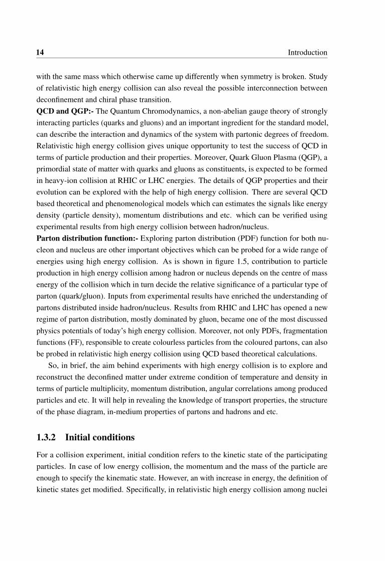
14 Introduction

with the same mass which otherwise came up differently when symmetry is broken. Studyof relativistic high energy collision can also reveal the possible interconnection betweendeconfinement and chiral phase transition.QCD and QGP:- The Quantum Chromodynamics, a non-abelian gauge theory of stronglyinteracting particles (quarks and gluons) and an important ingredient for the standard model,can describe the interaction and dynamics of the system with partonic degrees of freedom.Relativistic high energy collision gives unique opportunity to test the success of QCD interms of particle production and their properties. Moreover, Quark Gluon Plasma (QGP), aprimordial state of matter with quarks and gluons as constituents, is expected to be formedin heavy-ion collision at RHIC or LHC energies. The details of QGP properties and theirevolution can be explored with the help of high energy collision. There are several QCDbased theoretical and phenomenological models which can estimates the signals like energydensity (particle density), momentum distributions and etc. which can be verified usingexperimental results from high energy collision between hadron/nucleus.Parton distribution function:- Exploring parton distribution (PDF) function for both nu-cleon and nucleus are other important objectives which can be probed for a wide range ofenergies using high energy collision. As is shown in figure 1.5, contribution to particleproduction in high energy collision among hadron or nucleus depends on the centre of massenergy of the collision which in turn decide the relative significance of a particular type ofparton (quark/gluon). Inputs from experimental results have enriched the understanding ofpartons distributed inside hadron/nucleus. Results from RHIC and LHC has opened a newregime of parton distribution, mostly dominated by gluon, became one of the most discussedphysics potentials of today’s high energy collision. Moreover, not only PDFs, fragmentationfunctions (FF), responsible to create colourless particles from the coloured partons, can alsobe probed in relativistic high energy collision using QCD based theoretical calculations.

So, in brief, the aim behind experiments with high energy collision is to explore andreconstruct the deconfined matter under extreme condition of temperature and density interms of particle multiplicity, momentum distribution, angular correlations among producedparticles and etc. It will help in revealing the knowledge of transport properties, the structureof the phase diagram, in-medium properties of partons and hadrons and etc.

1.3.2 Initial conditions

For a collision experiment, initial condition refers to the kinetic state of the participatingparticles. In case of low energy collision, the momentum and the mass of the particle areenough to specify the kinematic state. However, an with increase in energy, the definition ofkinetic states get modified. Specifically, in relativistic high energy collision among nuclei

1.3 Relativistic high energy collisions 15

or proton-nuclei and so on, the initial condition includes information about the distributionof parton inside the nucleon/nucleus which is actually taking part during the collision. Theimportance of parton distribution, however, was understood little later after the discovery ofpartonic medium in a nucleus-nucleus collision. There are several model predictions aboutparton distribution [29–35], tuned with experimental inputs, which successfully explain theeffect of the initial state of participants of the collision as well as the particle production afterthe collision. Usually, parton distribution function (PDF) is expressed in term of Bjorken-x,longitudinal momentum fraction of the parent nucleon that is carried by the parton, andbehave differently depending on their flavour. PDFs are, in general, universal in nature, candescribe the structure of hadrons/nuclei and evolve according to DGLAP equation [36–39]as is shown in figure 1.5 from the CTEQ collaboration. At LHC energies, the PDFs, with

Figure 1.5: Parton Distribution Functions (PDF) for different type of quarks and gluon areshown in the picture. The distributions are represented as the variation of xf(x) as function ofBjorken-x as published by CTEQ collaboration for momentum transfer Q2=10 GeV/c.

substantially small bjorken-x and with ability in probing a novel and so far unexplored QCDregime with (x < 10−3), has drawn lots of attraction because of the increasing trend of"Gluon" in particular which is predicted to reach a saturation scale and might form a system

16 Introduction

called colour glass condensate (CGC) [40–46]. The particle production, in turn, will bedominated by gluonic interaction rather than quarks unlike in AGS, SPS and even in RHICenergies. On the other hand, Cold Nuclear Effects (CNM) [47] are also considered as initialstate effects which are mainly attributed to the nuclear parton distribution function and makesit different from that of the proton.

1.3.3 Kinematics

Before going into details about the different aspects of the relativistic heavy ion collision,it is important to understand different variables and notation those are used to describe theparticle interaction in the relativistic domain. It is relevant to adopt the relativistic kinematicsand four vector approaches in understanding the physical interpretation of the results in highenergy collision. In this section, we will briefly discuss variables which should be Lorentzinvariant in nature.To start with, the most basic variable is the particle position and momentum in four dimensionspace, which can be represented as following

xµ =(x0,x1,x2,x3)= (ct,x,y,z) ,

pµ =(

p0, p1, p2, p3)= (EC, px, py, pz

)= muµγ (1, v) ,

where, xµ and pµ represents four vectors for position and momentum respectively with µ

runs from 0→3, while v is the three velocity of the particle. However, the four component forposition and momentum can be reduced to three component assuming the azimuthal anglenegligible (relevant for relativistically high energy particle) and can represented as (t,xT ,z)and (E, pT , pz) respectively in natural unit (ℏ= c = µ0 = ε0 = 1) and xT =

√x2 + y2 and so

for momentum. The invariant quantity in this formalism is the scalar product of two fourvector. It can be represented as

xµxµ = gµνxνxµ = τ2

pµ pµ = gµν pν pµ = m2

xµ pµ = gµνxν pµ = Et− p.r

where, τ2 and m2 are Lorentz invariant quantity and can be related to the proper time, restmass and phase of the particle.

Knowing fundamental variables, the next step is to describe the physics in terms ofLorentz invariant formulation. Mandelstum variable, a numerical notation which carriesinformations regarding energy, momentum and scattering angle in a scattering experiment.

1.3 Relativistic high energy collisions 17

It can be used to derive lorentz invariant quantities such as cross-section of an interaction.Mandelstam variables can be represented for two particle scattering (1,2→ 3,4) phenomenonas following,

s = (p1 + p2)2 = (p1 + p2)

2

t = (p1− p3)2 = (p4− p2)

2

u = (p1− p4)2 = (p3− p2)

2

with, pi’s are four-momenta of the ith particle. Here, (1,2) and (3,4) represents the incomingand the outgoing channels of the scattering respectively. Physically, s and t representsthe square of centre of mass energy and momentum transfer. Being derived from thescalar product of four vectors, Mandelstam variables and other physical entities (e.g. decaywidth, differential and total cross-section as shown in equation 1.3) expressed in terms ofmandelstum variables are always Lorentz invariant.

Γ =p∗

32π2m2i

∫M f i

2dΩ

dσ

dt=

164πspi

2 M f i2

σ =1

64π2sp f

2

pi2

∫M f i

2dΩ∗

(1.3)

Apart from so far discussed fundamentals of relativistic kinematics, there are physicalquantities which make the physics interpretations more straight forward under Lorentztransformation. Rapidity represents particle distribution in a Lorentz invariant way andshows only a shift (additive) by an amount, determined by the boost of the frame. In thenon-relativistic limit, it is reduced to the velocity. Moreover, in collider type of experiments,the transverse momentum component, perpendicular to boost along beam direction (z), isan invariant quantity. In practice, the differential cross-section for a particle produced inthe relativistic collision are expressed in terms of rapidity, transverse momentum and theazimuthal angle which can be represented as

Ed3σ

d p3 =Ed3σ

pT d pT d pLdφ=

d3NpT d pT dydφ

=1

2π

d2Nd pT dy

This way of representing the cross-section helps in extracting yield in a Lorentz invariantway as well as in terms of experimentally measurable variables. More details about theexperimental observables in understanding particle production in the relativistic collisionwill be discussed in the following sections.

18 Introduction

1.3.4 Collision parameters

Once the initial kinematic states of the colliding particle are known or modelled, the nextimportant step would be to understand the parameters, defining the collision, to reveal theproperties of the system produced during the collision. Most important parameters are Impactparameter (corresponding experimental observable is Centrality ) and the Luminosity whichaffect the particle production at the final stage.Impact parameter (b), taken as zero for most central collisions and sum of the radii of theparticipants for extreme peripheral, is considered to be important for the participants with ex-tended structure. Theoretical calculations invoke the initial geometry of the collision throughimpact parameter "b" and obtain prediction as a function of it. However, in experiments, thereis no such direct way to measure the impact parameter of the collision and thus required someindirect methods, like produced particle multiplicity, Forward energy (EF ) from spectatorof the collision, number of participants etc., which results "Centrality" as the observableinheriting initial geometry of the collision. It has been found that the impact parameterholds a direct relationship with centrality which decreases with a decrease in multiplicity andparticipants of the collision. It will be relevant to mention that the experimental results forrelativistic heavy ion collision are always published as a function of centrality classes becauseof the fact that the initial geometry of the collision zone get tampered and the symmetry lostas we move away from central to peripheral collisions. Usually, the relationships betweencentrality and the impact parameter are extracted using Globar model calculations [48–50].For a particular impact parameter, the number of wounded participants or binary collisionsare calculated and subsequently related to the particle multiplicities which will help in de-termining the centrality of the collision and thus comparing theoretical predictions with theexperimental observations. By definition, centrality can be defined as a percentage of the

total nuclear interaction (particle production in experiment) cross-section as c =∫ b

0dσ

dxdx.

As discussed, globaur model calculation can effectively support for centrality measurementin a nucleus-nucleus collision. But for proton-proton collision, there is a lack of such effortto include the initial geometry in the collision. However, as the particle multiplicity has animpact parameter (centrality) dependence, particle production in pp collision at LHC energies(with comparatively large particles) are studied for classes defined by the multiplicity itself.

Luminosity (L) is, on the other hand, measures the ability of a particle accelerator todeliver the desired number of interactions and connect between experimental observation(particle production) with that of theoretical prediction (cross-section) and can be expressedas expressed in equation 1.4

1.3 Relativistic high energy collisions 19

dRdt

= L ·σ . (1.4)

with L as luminosity in units of cm−2s−1, σ being the cross section for a particular

interaction anddRdt

represents the rate of of interaction. Calculation for luminosity differsdepending on whether it is a fixed target or collider type experiment and can be representedby the equations 1.5

L = ΦρT l f or f ixed target experiment,

=N1N2 f Nb

4πσxσyf or collider experiment.

(1.5)

where, Φ is the incident particle flux, ρT and l are the target density and length respectivelyin case of fixed target experiment. And for collider experiment, N1, N2 are intensities oftwo colliding bunches with Nb as the number of bunches in one beam while f and σi are therevolution frequency and beam sizes respectively.

1.3.5 Experimental observables

Knowing initial state and collision parameters, the system formed in a high energy collisionamong hadron and (or) nucleus is characterised with the help of experimentally measuredobservables at the end. There could be different type of measured observables depending on aparticular experiment but all are related to primary measurements like the number of particles(particle multiplicity "N"), energy (momentum) spectrum of produced particles, particleidentity, (Pseudo-)Rapidity distribution, the angular correlation among produced particlesand etc. In this section, we will discuss commonly measured experimental observables inhigh energy collision and their importance in brief.

Particle multiplicity(N)

Particle multiplicity in high energy collision is the primary measurement which, however,contribute most about the particle production mechanisms and serves the basic input forrelevant Monte Carlo calculations and theoretical formulations. Measuring the number ofparticles, produced in a collision and averaged over a large number of events, might explorepossibilities of different particle production mechanisms and any possible correlation if existat the source level. Usually, the multiplicity distribution represents the probability of finding

20 Introduction

a particular number of particles in a collision as a function of multiplicity (P(n) vs n) eitherfor full or for a specified phase-space. In a collision, if the particles are produced froman independent and identical point-like scattering centres, the particle multiplicity followsPoisson distribution which might get smeared or modified for correlated sources. In thebeginning, for e−e− scattering or proton-proton scattering at comparatively low energies (at29 and 62 GeV), multiplicity distribution could be illustrated assuming sources are eitherpoint-like and identical or super-position of many such sources. However, with the discov-ery of KNO [51]-scaling, the importance of the multiplicity distribution was enlightenedagain. With the increase of available centre of mass energy, the particle multiplicity gotdifferent perspectives about production mechanisms starting from QCD hard scattering tonon-perturbative soft production processes. Recently, at LHC energies, multiplicity distri-bution exhibiting profile, comprised of two or even more type of particle sources and canbe explained by single or convoluted Negative Binomial distributions. As the integratedmultiplicity should depend on the number of participants and so on the initial energy densityof the collision, it increases with the increase of centre of mass energy of the collision.However, dependencies of multiplicities on the centre of mass energy behave differentlyfor proton-proton and nucleus-nucleus collisions [52] as shown in figure 1.6. Noticeably,particle production increases more rapidly with centre of mass energy in case of heavy ioncollision than that of proton-proton collision and can be explained by power law as s0.15 ands0.11 for heavy ion and pp collision respectively, which shows a deviation from logarithmicbehaviour for proton-proton collision earlier for comparatively low energies.Beside integrated multiplicities, identified particle multiplicity have different perspectivesin probing the hot and dense matter produced in high energy collision. With the increase inECM off collision, the increased yield for identified particles brings the scope to study therelative abundances of different particles in terms of particle ratios such as Baryon-to-meson,strange-to-non strange etc. Identified particle yields can give important information aboutthe properties of the strongly interacting system like about degrees of freedom, collectivity,quark coalescence etc.

Rapidity distribution

The introduction of rapidity become essential in case of relativistic high energy particleswhere variables transform according to Lorentz prescription and take complicated form ingoing from one frame to other. The rapidity, as expressed by the equation 1.6, distributionbecomes invariant and associated with a shift in the whole distribution under transformation.

1.3 Relativistic high energy collisions 21

Figure 1.6: Variation of Charged particle multiplicity a function of centre of mass energy√S for proton-proton and heavy ion collision. The plot has been generated taking data from

different experiments at different centre of mass energies [52]. It shows the difference independence of particle production on centre of mass energy for pp and heavy ion collision.

22 Introduction

y =12

ln(

E + pz

E− pz

). (1.6)

There can be two extreme limits for the rapidity, (a.) for particles moving perpendicular to thebeam have y = 0 and on the other hand, (b.) for particles moving along the beam will havey =±∞. So, briefly, the rapidity is related to the angle between particle and beam direction.Experimentally, rapidity is hard to calculate as one need both the particle identity as well asthe momentum, however, with the introduction of Pseudo-Rapidity (η), the distribution canbe reconstructed easily as it doesn’t require any particle identity and which can be expressedby equation 1.7

η =12

ln(

p+ pz

p− pz

)=−ln(tan(

θ

2)). (1.7)

Of course, knowing pseudo-rapidity distribution for some identified particles, one can always

transform it to the rapidity distribution using a Jacobian (J =

√1− m2

m2T cosh2y

) and vice

versa. However, both the distribution merged in the limit of massless particle (m = 0) orultra-relativistic particles (pc >> mc2).One of the successful form for rapidity distribution came from "Landau HydrodynamicalModel" back in 1953 [53] and had been experimentally confirmed for AGS to RHIC energies.Following Landau prescription, the rapidity distribution can be expressed as shown inequation 1.8

dNdy

∝ exp(−y2

2ln(γ)

), (1.8)

where, γ is the Lorentz contraction factor (γ =

√sNN

2mN). The gaussian rapidity distribution can

explain data for central AuAu collision up to RHIC energies. However, there is an ambiguitywith the original landau description (with exp(

√L2−λ 2))about, whether the variable (λ )

should be taken as rapidity or pseudo-rapidity. The typical rapidity distribution can berepresented by the figure 1.7 with two peaks corresponding to two fragmentation regionswhich are moving away with the increase in the centre of mass energy, indicating baryondepleted (almost no stopping power) system is expected at LHC energy. Approximately, the

1.3 Relativistic high energy collisions 23

Figure 1.7: Rapidity distribution for net proton for AGS, SPS, RHIC energies togetherwith an extrapolation for LHC energies. The figure describes how the shape of the rapiditydistribution changes with increase of centre of mass energy [54].

24 Introduction

spread in the rapidity can be taken as the difference between two beam rapidities (projectileand target rapidity in case of fixed target experiment) in case of a collider type experiment

and can be taken as ∆y = 2× ln(2Em

). In a collider experiment, naively, the system formedafter collision may have two different regions, central rapidity and fragmentation regionsrespectively. The particles with large rapidity are emerging from the fragmentation regionswhereas, particles with intermediate rapidity are coming from the central rapidity zone. Withthe increase of the ECM, the stretch of the rapidity interval become more and more prominentand can further be classified into even smaller y-windows which can reflect the details ofparticles production mechanism in the collision. (Pseudo-) Rapidity distribution for producedparticles in high energy collisions usually refers to the global properties of the created system.Being simple, (Pseudo-) Rapidity measurement is considered as a first-day observables inany complex high energy experiment, however, many physics issues can be addressed with it.The most commonly measured region for rapidity is mid-rapidity region which is sensitiveto the hadron-production mechanism and may vary depending on the available centre ofmass energies such as baryon-rich system at SPS to baryon-free at LHC energies. Moreover,assuming boost invariant central plateau in rapidity distribution, the energy density can becalculated using Bjorken prescription from rapidity distribution according to the following1-dimension equation 1.9

εBJ ≃

dNch

dη∗ 3

2< PT >

V.

(1.9)

Where,dNch

dηis the number of charged particles per unit pseudorapidity, PT is transverse

momentum and V is the volume of the fireball, created during the collision. The detailsof the energy estimation will be described in more details in 5th chapter in the context ofunderstanding particle production in the proton-proton collision at LHC energies. On theother hand, the stretch of the rapidity distribution contains the longitudinal expansion of theproduced system which illustrates the stopping power (transparency) of the medium formed.Also, particles produced with forward and backward rapidities (fragmentation region) canbe used to study the "limiting fragmentation" phenomenon for particle production. Thevariation of the particle rapidity density as a function of centrality (impact parameter) ofcollision inherit important information about the contribution of the soft (∝ Npart) and hard(∝ Ncollision) processes in particle production mechanisms

1.3 Relativistic high energy collisions 25

Transverse momentum pT -Spectra

Transverse momentum (pT =√

p2x + p2

y) of a produced particle is the momentum componenttransverse to the beam axis and has the property of Lorentz invariance for particles producedin relativistic high energy collision experiments. In any collision, since there is no nettransverse momentum at the beginning, the final state particle must be produced obeyingthe same. However, PT distribution for produced particles follow a particular profile, whichillustrates information regarding different type of interactions that those particles might haveexperienced. It also illustrates the thermal property of the system as well as the explodingnature of the system. In high energy heavy-ion collision, pT -spectra might get affected by col-lision dynamics as well as by the final state hadronisation processes, which might be foldedtogether in the final profile. The particle production mechanisms can be categorized in broadclasses, soft parton scattering followed by string fragmentation and hard parton scatteringfollowed by transverse fragmentation respectively. Usually, the transverse momentum profilecan be considered as the convolution of an exponential (" corresponding to thermal part")and a power law ("hard scattering") contribution [55]. Though the hard component of thespectra is well understood in terms of pQCD calculation followed by fragmentation, however,the soft part is still required conclusive understanding about its origin. The importance oftransverse momentum spectra lies in explaining the particle production mechanisms in theproton-proton collision which differs in case of heavy ion collisions and can contribute inunderstanding the collective flow, recombination, jet quenching etc. [56]. There is varioustheoretical/phenomenological model which can explain the transverse momentum spectrain most of the cases. Following are such few frequently used description for transversemomentum spectra for produced particles in high energy collisions.

Maxwell-Juettner distribution: The model is the relativistic generalisation of theMaxwell-Boltzmann distribution, that explain particle spectra assuming thermal models,introduced back in 1911 by Juettner [57]. The simplistic model can be expressed as shownin equation 1.10 following [58] and does not include the collectivity of the system whichresulted in overestimation in temperature.

f (pT ) =1

4πm2T K2(m/T )e

[−

γ pT mT

]

with, γ(pT ) =

√1+( pT

m

)2,

(1.10)

26 Introduction

where T and m are freeze-out temperature and mass respectively. As expected, the distri-bution can explain the low-PT (≤ 0.5 GeV) part of the whole spectra. However, its majordrawback is the absence of the collectivity in the formulation which does present in theproduced system. Interestingly, an effort to invoke the collective nature in the model is donethrough the temperature as T ∗ = T + km < vT >2 [59], where <vT > is average velocityat-freeze-out and is function of centrality.

Tsallis Distribution: The distribution represents a more generalised form of statisticalapproach which can be applied to a system away from the equilibrium. The distribution canbe represented in terms of transverse mass and temperature as shown in equation 1.11

Ed3Nd p3 =CnmT

(1+(q−1)

mT

T

)−n, (1.11)

where, T represents the temperature at freeze-out (to be noted that the one to one correspon-dence of the parameter "T" to temperature in thermodynamical sense needs to be carefullyused.) and the "n" represents the real power index (however, making it complex, extend

the Tsallis distribution in more wider region of application) and can be taken as1

q−1,

with "q" measure the non-extensivity of the statistical approach. Tsallis distribution, beingmore general, can lead to an exponential distribution in the limit m→ ∞. Moreover, Tsallisdistribution can describe the PT -spectra from an exponential (exp(−mT/T )) form to powerlaw distribution (∝ (pT/nT )−n) with the limit pT → 0 and pT → ∞. So in general, withthe increase of centre of mass energy, produced particles have larger PT which can not beexplained by soft particle production mechanism and need pQCD based calculation for hardscattering phenomenon which can be taken care by default with Tsallis distribution.

Blast-wave approach: However, There are phenomenological models like "Blast-Wavemodel", inspired with the hydrodynamical approach, which can address the PT -spectraincluding both the collective expansion and the thermal nature of the system. This modelassumes local thermal equilibrium at freeze-out (T) and the existence of both transverse andlongitudinal expansion. Adopting a flow profile, defined by βT (r) = βs(

rR)α , the particle

spectra can be expressed as shown in equation 1.12

dNpT d ppT

≈∫ R

0rdr mT I0

(pT sinhρ

T

)K1

(pT coshρ

T

). (1.12)

1.3 Relativistic high energy collisions 27

Though the blast wave model describes the collectivity within the system in terms of tem-perature, collective velocity and the flow profile parameter, the application is restricted tothe softer part of the spectra only. The details of the model description and its application toparticle production will be illustrated in details in 7th chapter.

1.3.6 Signatures of Quark Gluon Plasma

The deconfined partonic medium, expected to be produced in HI (HM pp) collision, need tobe characterised using measurable experimental observables. As the QGP exists only for afew microseconds, it is practically impossible to probe the system with direct measurements.measurement. However, particles produced before, during or after the formation of QGP carryimportant information which collectively can be used both to confirm and characterisation ofthe QGP. Undoubtedly, there can not be a unique signal which alone can be considered as thesmoking gun identification for quark gluon plasma. Rather there are a number of differentsignals, both differential and global, which together may be treated as signatures for QGP.Different bookmark signatures for QGP can be listed as following -a) Photons and Dileptons - Either of these signals, once produced, can traverse throughthe whole evolution of the QGP undisturbed as they only interact electromagnetically notthrough strong interaction. Moreover, photons, produced at different stages like at the verybeginning, during pre-equilibrium, from thermalised or even after hadronisation, carriesthe full history of QGP and serve as a cleanest signature. Differentiation of photons fromdifferent sources can be treated as a good thermometer for QGP. On the other hand, dileptons(lepton-antilepton pair), produced by initial quark-antiquark annihilations and from hadronicmedium later during evolution, can also be treated as a clean probe for studying QGP as theyalso remain undisturbed by the strongly interacting medium.b) Strangeness enhancement - Enhanced strange particle production can be treated as agood signature for QGP medium. For an equilibrated QGP with T > mS, strange quarksand antiquarks can be abundantly produced. Since the threshold energy for strange particleproduction in hadronic phase is much higher (almost by a factor of two) than that of QGP,strange can be produced during QGP phases easily. This enhanced strange production isreflected in the production of strange and multi-strange particles in the final stage which canbe treated as an indication for the formation of deconfined phase.c) J/Ψ suppression - J/Ψ, an cc bound state, formed at the beginning of the mediumformation in relativistic HI (pp) collision. The suppression of J/Ψ, an artefact of Debyescreening attributed specifically to plasma formation, can identify the formation of QGP. Thepresence of QGP is essentially dilute the bonding between cc pair and hence melt the J/Ψ.d) Jet Quenching - The phenomenon of Jet in relativistic heavy ion collision is ascribed to the

28 Introduction

hard probes, characterised with large momentum transfer and associated with hard scatteringin the initial stage just after the collision. When two partons from two incoming nucleonsinteract and a large momentum transfer occurs, the particles (maybe quarks, gluons orphotons) in the outward channel carries large momentum. Being either quarks or gluon, theycan interact with coloured medium if produced and lose substantial amount of energy whichdirectly reflected in the final state hadron production. Usually, partons with large momentumfragment into partons till their energy become critical for further parton production andfollowed by hadronisation which resulted in a spray of particles in the final stage within avery narrow cone. If there are two partons in the hard scattering, two oppositely directedjet will be produced, however for a parton along with gamma in the output channel willproduce a jet along with a photon moving exactly in opposite direction. The two oppositelydirected jet are similar unless the jet producing partons traverse through a strongly interactingmatter like QGP. In the presence of QGP, the jet structure gets modified for the away sideand become diffused whereas the near one remains intact.

e) Elliptic flow - Elliptic flow is one the most important observables in the field ofrelativistic heavy ion collision. A large values for elliptic flow indicates the applicabilityof an ideal (i.e., equilibrium) hydrodynamics which justify the formation of almost perfectfluid at RHIC. The non-zero impact parameter (non-central) for collision between twonucleon coming from opposite direction can vary both in magnitude and direction whichled to an initial asymetry in the geometry of the overlapped zone (interaction zone). To

understand the effect of such asymetry, the distribution of final state particles (Ed3Nd p3 ) ican

be Fourier-decomposed as following

d3NpT d pT dydφ

=d2N

pT d pT dy1

2π[1+∑

∞n=1 2vncosn(φ −φR)] ,

with each terms carrying their usual meaning. The first term in the square bracket is calledthe radial flow whereas, the v1 and v2 are called directed and elliptic flow respectively.The information about the different flow coefficients brings important insights regardingthe hydrodynamics of the produced partonic medium and can serve a good signal for the QGP.

None the less, there are many signals like Constituent quark number scaling, Ratiosof particle yields, quarkonia, the study of heavy flavour and etc. which have their ownsignificance in characterising the partonic medium formed in relativistic heavy ion collision.The remark about the signal of QGP lies in the fact that not a single signal but all relevantindications need to be critically investigated to confirm the creation of QGP.

1.4 Motivation and skeleton of the thesis work 29

1.4 Motivation and skeleton of the thesis work

The present thesis work comprises of two major parts - a. Forward Calorimetry for ALICEexperiment and b. High Multiplicity Proton-Proton Physics respectively. The main physicsmotivation behind the 1st part of the thesis is to probe a so far unrevealed domain of smallBjorken-x regime ≤ 10−4, dominated by gluon dynamics for particle production. Fromtheoretical predictions, there are possibilities of achieving such small-x at forward rapiditywith ALICE experiment at LHC energies. However, limited capability of ALICE experimentin forward rapidity, leave scope for a proposal of a calorimeter which can measure highenergy photons from different sources over a wide range of incident energy (up to 200 GeV ).The thesis is starting with a general introduction about the field of relativistic high energycollision (1st chapter) and followed by an overall discussion about the particle interactionwith matter (2nd chapter). The first two chapters basically contain general relevant informa-tion regarding the thesis work which have been collected from different references. The mainthesis work started with a brief discussion about the LHC and ALICE. The discussion wasaimed to explore the usability of forward rapidity measurement which has been described inbrief in chapter 1.A general discussion about the particle interaction with matter will be introduced in chapter 2.Different techniques of particle detection over a wide range of particle types, their incidentenergies, momentum and etc. will also be covered in chapter 2 which is indeed important tounderstand the detector designing, fabrication and its uses.A formal introduction to the Large Hadron Collider experiment will be presented in chapter 3.Since the present study involves mainly the ALICE detector in specific, a general introductionwill be discussed in this chapter. A brief discussion about different sub-systems of ALICEand their importance will also be discussed. It will essentially help in understanding the needfor a new calorimeter which will come in the next chapter.The major part (1st part) of the thesis is devoted to the design, performance simulation,fabrication and testing of forward calorimeter (FOCAL) which is distributed over chapters 4,5 and 6 of this thesis. It started with the descrition of the calorimetry in ALICE experiment.A brief description of the physics motivation along with its relevance in the high energyphysics measurement behind building the calorimeter has been discussed in chapter 4.

The design and simulation details, which I have carried out during for the thesis work,are explained to study the feasibility of the calorimeter, both technically and physics wise,with the help of Geant4 toolkit in chapter-5. The study aimed to achieve optimal design andperformances for the calorimeter.In continuation of my thesis work, the next chapter (6) mainly addresses the hardware de-

30 Introduction

velopment for fabricating prototype sampling calorimeters with 1 cm2 pad detectors andtungsten absorbers. A series of prototype design, development, fabrication and their test,aiming for the final goal of the full calorimeter, were presented. The details of results fromthe prototype test at laboratory, PS and SPS beamline facilities at CERN-LHC have beenpresented and discussed. The 1st-chapter ends with a short discussion about the future workand scope for building the calorimeter.

As has been discussed, the main aim behind relativistic high energy collision is tounderstand particle production and their subsequent evolution for system produced in proton-proton (pp), proton-nucleus (pA) or nucleus-nucleus (AA) collisions at extreme temperatureand densities. My work regarding particle production in pp collision has been documented inthe 2nd-part (chapter-7) of the thesis work. The particle production in proton-proton collisionsat LHC energies, which earlier used as the reference to understand a more complex systemlike in pA and AA collisions, was studied using a different phenomenological model withpublished data. The chapter was started with a brief history and importance of proton-protoncollisions from low to ultra-relativistic high energy collision, followed by a discussion aboutdifferent phenomenological frameworks (two source model with NBD, Blast-wave approachand etc.), used in this study. The chapter has three sub-sections - firstly understanding themultiplicity distribution in pp collision at LHC energies with NBD model, secondly applyingBW-approach to search for collectivity in pp collision for very special high-multiplicityclasses and their consequences, and lastly understanding the nature of the collectivity in ppcollision, an anomalous signal, with the help of simple Bjorken one dimensional prescriptionfor energy density calculation. In this study, both collectivity and the energy density (thusthe Degree of freedom) was studied as a function of multiplicity classes of proton-protonevents. In the end, the outlook and future scope of the study has been illustrated.

Chapter 2

Interaction and Detection of particles

2.1 Introduction

Understanding of experimental results, in general, need a close look on "how particles interactwith matter and thus deposit energy". Then the rest part will be to collect the deposited energyeither in forms of light or electrical signal and processed it accordingly. In this chapter, wewill discuss the interaction of particles with the matter. Primarily, interaction of particle canbe divided into two broad categories, a) Interaction of charged particles and b) Interactionof neutral particles. The type and intensity of interactions depend both on particle type(mass, charge, energy etc) and the matter (density, elements, structure etc) through which theparticles are moving. The electromagnetic force is the one which is mostly responsible forparticle interaction with matter in connection to particle detection. However, there is scopefor strong and weak interaction as well for particles like neutrons and neutrinos.

2.2 Interaction of charged particle with matter

The interaction of the charged particle with matter can further be divided into two broad cate-gories I) Interaction of electrons (e−) and other charged particles and 2) Heavy chargedparticle. Electron, being lighter mass, become relativistic very quickly and dominated byradiation loses mostly while heavy charged particles undergo both collisional and radiationallooses depending on the energy of the particle. In general, energy loss by a charged particle

32 Interaction and Detection of particles

can be represented as following 2.1

−(

dEdx

)Total

=−(

dEdx

)collision

−(

dEdx

)Radiation(brems/cher)

−(

dEdx

)pair

−(

dEdx

)compton

−(

dEdx

)Photo

−(

dEdx

)had

+O(Other mechanisms),(2.1)

where, −(

dEdx

)represents the energy loss by the particle per unit path length travelled. The

subscripts collision, radiation and etc stands for the corresponding underlying processes ofenergy loss mechanisms. O(Other mechanisms) represents other relatively less contributingprocesses to the total energy loss of the particle. However, the relevance of a particular termin the expression depends on the incident particle and the material medium.

2.2.1 Interaction of heavy charged particles

Heavy charged particles, usually, are those with atomic mass number unity or more bydefinition. Though muons, pions and kaons are not in that sense a heavy charged particle,however, they behave similarly when passing through a material medium and differ fromproton and all because of their small mass and different interaction probability. Primarily,all charged particle loses energy in a matter through collisional/ionisation processes duringits passage through matter. The specific energy loss, energy Loss per unit path length

travelled: −(

dEdx

), can be expressed quantitatively using Bethe-Bloch formula, as is shown

in equation 2.2

−dEdx

=4πk2e4

mec2z2

β 2ρZNA

AB(ν) w ith ,

B(ν) =12

ln(

2meγ2ν2Tmax

I2

)−β

2− δ (βγ)

2−C(I,βγ)

Z.

(2.2)

Where, Tmax =

2me2c2β 2γ2

1+2γme

M+

me

M

2

, represents maximum energy transfer in sin gle

collision and "I" represents mean excitation energy of medium. me and M are mass ofelectron and the incoming particle, whereas γ =

(1−β 2)−1/2 with β being the scaled

velocity (vc

) of the particle. ρ , Z, A stands for mass density, atomic number and mass number

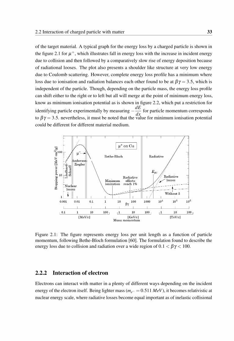
2.2 Interaction of charged particle with matter 33

of the target material. A typical graph for the energy loss by a charged particle is shown inthe figure 2.1 for µ+, which illustrates fall in energy loss with the increase in incident energydue to collision and then followed by a comparatively slow rise of energy deposition becauseof radiational looses. The plot also presents a shoulder like structure at very low energydue to Coulomb scattering. However, complete energy loss profile has a minimum whereloss due to ionisation and radiation balances each other found to be at βγ = 3.5, which isindependent of the particle. Though, depending on the particle mass, the energy loss profilecan shift either to the right or to left but all will merge at the point of minimum energy loss,know as minimum ionisation potential as is shown in figure 2.2, which put a restriction for

identifying particle experimentally by measuring −dEdx

for particle momentum correspondsto βγ = 3.5. nevertheless, it must be noted that the value for minimum ionisation potentialcould be different for different material medium.

Figure 2.1: The figure represents energy loss per unit length as a function of particlemomentum, following Bethe-Bloch formulation [60]. The formulation found to describe theenergy loss due to collision and radiation over a wide region of 0.1 < βγ < 100.

2.2.2 Interaction of electron

Electrons can interact with matter in a plenty of different ways depending on the incidentenergy of the electron itself. Being lighter mass (me− = 0.511 MeV ), it becomes relativistic atnuclear energy scale, where radiative losses become equal important as of inelastic collisional

34 Interaction and Detection of particles

Figure 2.2: Energy loss per unit length as a function of particle momentum for differentparticle following Bethe-Bloch formulation [60]. It illustrates the region for which particlescan be identified from their energy deposition profile.

energy loss mechanism. The inelastic process which is responsible for electron energy loss,can be represented by modified Bethe-Bloch Formula. The expression is different fromnormal Bethe-Bloch form because of fact that electron experience "large angle multiplescattering", "large energy loss possible b/w electron on electron scattering", "indistinguisha-bility of incident and matter electron", "relativistic in nature at nuclear energies". Taking allthese anomalous effects into account, electron energy loss can be expressed by the followingequation 2.3

−dEdx

=4πk2e4

mec2z2

β 2ρZNA

AB(ν) ,

where, B(ν) =12

ln

τ2(τ +2)

2(

Imec2

)2

+F(τ)

2− δ (β )

2−C(I.β )

Z,

with, F(τ) = 1−β2 +

τ2

8− (2τ +1)ln2

(τ +1)2 for electron.

(2.3)

As the energy loss of any particle during passage through matter is a stochastic process,the energy deposition, even for a mono-energetic incident beam, spread (straggling) over a

2.2 Interaction of charged particle with matter 35

certain energy window instead of being a delta function. Usually, the straggling for electronis more compare to heavier charged particle. However, for a thin material, electron can stillresults a landau distribution which looks like a minimum ionisation particle but with valuehigher than usual.

Apart from collisional looses, there are two major radiational looses, Bremstrahlungand Cherenkov radiation respectively, for relativistically energetic electrons. A chargedparticle, moving faster than the speed of light in a medium, emits cherenkov radiationwhich is a result of collective effect (polarisation) of the medium to the fast moving particle.The spectrum of the Cherenkov radiation can be expressed by Frank-Tammas formula asshown equation 2.4

dEdx

=Z2e2

c2

(1− 1

β 2n(w)2

)Θ

(ν− c

n(w)

)ωdω,

where, Θ is Heaviside step function(2.4)

dEdx

is the energy emitted per unit distance traveled by a particle of charge Ze for a frequencyrange dω . On the other hand, an energetic electron can emit Bremsstrahlung, radiation underinfluence of an electric field. Mostly when an electron passes by a strong nuclear electricfield, the amount of bremsstrahlung become significant. However, electron bremsstrahlungis also possible but the contribution is suppressed by the nuclear part. The spectrum of thebremsstrahlung radiation can be illustrated using equation 2.5

P(ω)≈ 82π

e6

m2ec3v2b2 , for ω <<

v2b

,

P(ω)≈ 82π

e6

m2ec3v2b2 e

(−ωbv

), for ω >>

v2b

,

(2.5)

Where, P(ω) represents energy emitted per second by a particle of charge ze. However, theenergy loss by the bremsstrahlung by a charged particle can be represented by equation 2.6

−dEdX

= 4αNAZ2

Az2(

14πε0

e2

mc2

)E ln

(183Z1/3

). (2.6)

where, Z and A are atomic number and mass number of the medium. Important to note,that the bremsstrahlung radiation loss by an incoming charged particle varies inversely withfourth power of the mass, which itself explain why electron is so crucial compare to otherheavy charged particle in this case. In brief, electron loses energy through ionization, varies

36 Interaction and Detection of particles

linearly with "E" and with Z2material , and radiational, varies logarithmically with "E" and

linearly with Z. As is evident, electron will loss energy through radiation at high incidentenergies, while with decrease in energy, ionisation losses will take over. At some particularincident energy (known as critical energy: EC), however, there will be an balance betweentwo processes, resulting a critical energy: EC, and can be defined as shown in equation 2.7(

dEdx

)radiation

=

(dEdx

)collision

, for E = EC,

where, EC =1600mec2

Z,

(2.7)

The expression for EC, as shown, can be approximated using Bethe and Heitler prescription.For the E > EC, the energy of the electron can be expressed in terms of incident energy and

the distance travelled within the medium as E(x) = E0e−

(x

XR

), where XR is the radiation

length and depend on the material as XR =1

Nσradwith N as number of scattering centre

inside the material.

Apart from these two major mechanisms of energy looses by electrons, there are otherimportant elastic process, like multiple scattering which plays important role by increasingthe effective distance of the path inside matter. Usually, the angular distribution for deflectionby multiple scattering can be approximated to a Gaussian distribution.

2.3 Interaction of neutral particle

Primarily, neutral particle can interact with matter either through strong or weak interaction.However, photon, even being neutral, can interact with matter quite differently from othercharged particles. In the following sub-section, we will mainly concentrate on interaction ofphotons with matter and discuss about other neutral particle like neutron and neutrinos.

2.3.1 Interaction of photon

Like in case of charged particles, photon can interact with matter both by Elastic and Inelas-tic scattering processes. In elastic scattering, photon energy remains unchanged apart froma negligible amount which appears as recoiling momentum to the target particle which isrequired for momentum conservation. There are two type of elastic scattering, that a photoncan experience namely Thomson’s scattering and Rayleigh scattering respectively. When aphoton interact with a free electron or nucleus, it undergoes Thomson scattering which can

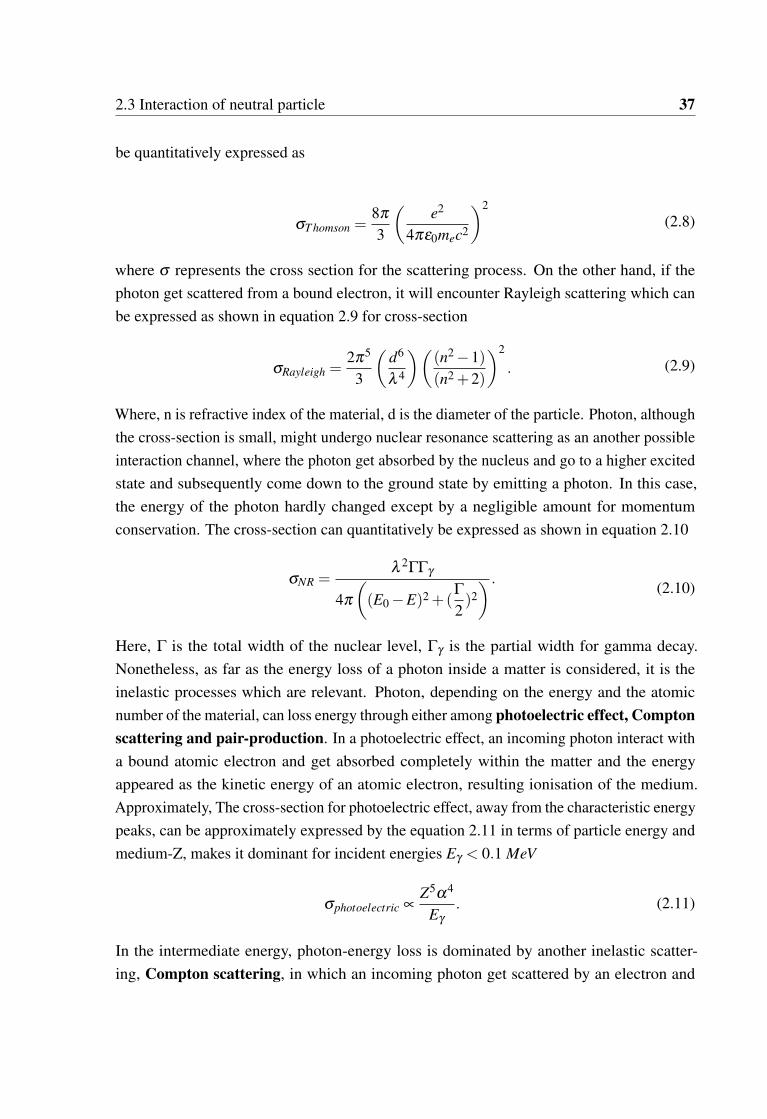
2.3 Interaction of neutral particle 37

be quantitatively expressed as

σT homson =8π

3

(e2

4πε0mec2

)2(2.8)

where σ represents the cross section for the scattering process. On the other hand, if thephoton get scattered from a bound electron, it will encounter Rayleigh scattering which canbe expressed as shown in equation 2.9 for cross-section

σRayleigh =2π5

3

(d6

λ 4

)((n2−1)(n2 +2)

)2

. (2.9)

Where, n is refractive index of the material, d is the diameter of the particle. Photon, althoughthe cross-section is small, might undergo nuclear resonance scattering as an another possibleinteraction channel, where the photon get absorbed by the nucleus and go to a higher excitedstate and subsequently come down to the ground state by emitting a photon. In this case,the energy of the photon hardly changed except by a negligible amount for momentumconservation. The cross-section can quantitatively be expressed as shown in equation 2.10

σNR =λ 2ΓΓγ

4π

((E0−E)2 +(

Γ

2)2) .

(2.10)

Here, Γ is the total width of the nuclear level, Γγ is the partial width for gamma decay.Nonetheless, as far as the energy loss of a photon inside a matter is considered, it is theinelastic processes which are relevant. Photon, depending on the energy and the atomicnumber of the material, can loss energy through either among photoelectric effect, Comptonscattering and pair-production. In a photoelectric effect, an incoming photon interact witha bound atomic electron and get absorbed completely within the matter and the energyappeared as the kinetic energy of an atomic electron, resulting ionisation of the medium.Approximately, The cross-section for photoelectric effect, away from the characteristic energypeaks, can be approximately expressed by the equation 2.11 in terms of particle energy andmedium-Z, makes it dominant for incident energies Eγ < 0.1 MeV

σphotoelectric ∝Z5α4

Eγ

. (2.11)

In the intermediate energy, photon-energy loss is dominated by another inelastic scatter-ing, Compton scattering, in which an incoming photon get scattered by an electron and

38 Interaction and Detection of particles

transferred part of it’s energy to the electron which essentially produce ionisation with inthe medium. The cross-section, as a function of incident photon energy (Eγ ) and materialproperties, can be represented by an approximated formula 2.12

σcompton ∝ Z

(E′γ

Eγ

)2(E′γ

Eγ

+Eγ

E ′γ− sin2

θ

). (2.12)

The contribution of Compton scattering to photon energy loss is a dominant process forincident energy range of 0.1 MeV ≤ Eγ ≤ 10 MeV . However, in case of very high energyphoton, relevant in relativistic heavy ion collision and particle physics, photons loosestheir energy by pair production in which get converted into matter by creating particle-anti-particle pair. Unlike other two processes, pair production has energy threshold Eth

γ >1.02 MeV

and become practically energy independent for Eγ >70

Z1/3 MeV, as the cross section for pairproduction reach a plateau region which can be represented by 2.13

σpair ≈79(4αr2

eZ2) ln(

183Z1/3

). (2.13)

The expression for radiation length, as derived from this equation will become λpair ≈(97

)XR, which is slightly higher compare to electron, reflected as photon is neutral and will

start interacting with matter little later relative to charged electron.However, to understand the importance of all three processes with respect to photon

interaction, it will be more explicit by expressing the cross section as a function of bothphoton energy (Eγ ) and material properties as is shown in figure 2.3 and 2.4 respectivelywhich explains the domain of dominance for Pair production, Compton scattering andphotoelectric effect. For relativistic (beyond 1 MeV) energy, the most important processis the pair production whereas photoelectric effects is most dominant in the low energylimit. However, there is an interplay among photoelectric, Compton and pair productionat intermediate energies (0.5 MeV to 500 MeV) which is taken over by Compton processaround 1 MeV. On the other hand, these processes have strong material dependence ( f (Z))as well which is described in the figure 2.4.

2.3.2 Interaction of neutral particle (m=0)

Apart from photon, other neutral particles, like neutron and neutrinos, interact with matterthrough strong and weak interaction. Interaction of neutron has a strong dependence on the

2.3 Interaction of neutral particle 39

Figure 2.3: Relative cross-sections for photoelectric, Compton and pair production as afunction of photon energy for copper, which express the dominance of a particular processfor a specific photon energy range.

40 Interaction and Detection of particles

Figure 2.4: Cross sections for Photoelectric, Compton and Pair production as function ofmaterial-Z and incident energy of particle, illustrates which process is relevant for a photonof particular energy interacting with a specific material.

energy of the particle. In both the cases primarily the interaction results a secondary parti-cle which went through electromagnetic interaction and produce ionisation in the medium.However, if the energy of the particle is high enough to create further particles, it mightlead to shower of hadron and thus a hadronic shower. Within the present scope, we willrestrict our discussion without going in detail about the hadronic shower formation andtheir characterisation. On the other hand, neutrinos interact with matter weakly either by acharged-current or a neutral-current. As the cross-sections for either with electrons and/or thenuclei within matter are small, comparatively large matter is required to produce measurableamount of secondary charged particles. There are another important mechanism, such astransition radiation, come into the picture when a relativistic particle with large-γ crossesthe boundary between two medium with different refractive indices. The radiation, thusemitted, is strongly forward peaked and varies logarithmically with γ .

2.4 Basic measurements

The discussion so far, regarding the interaction of particles, was intended to understandthe working principle of different particle detection and measurement techniques, used in

2.4 Basic measurements 41

the different field of physics. In this section, we will discuss particle detection techniquesand thus detectors in brief, commonly used in the field of relativistic high energy collisions.Historically, probably the concept of modern detector brought to the field back in 1895 withthe discovery of x-ray by W. C. Röntgen. Since then, the technology of particle detectionhas advanced in close connection with particle physics and vice versa. The developmentof detectors can be divided naively into three ages of technologies, Image tradition, Logictradition and Electronic images. In the early days of Cloud chamber, Emulsion method andBubble chamber, each and every event was imaged by producing ionisation which surroundedby condensed vapour molecules. The picture, so formed, are left as an image for analysisafterwards. The simplistic and innovative approach, however, is restricted with very slowcount rate (few tens/second) and no choice for triggering. The detection techniques changedover to logic tradition in the 1970’s with the invention of Geiger counter, Scintillators with aphotomultiplier, Spark chambers and etc. The incident particle, although, can not be seen,but their presence and characteristics can be reconstructed using logics like coincidences,triggers and decay kinematics. The inherent amplification of the signal and high rate handlingcapability makes the detection techniques robust and appropriate even today. However, withthe boost in available energy of the collision, physics of detection techniques enter a newhorizon, where the complexities in experiments folded by many times. Multi-dimensionalrequirements, like tracking, particle identification, energy measurements, handling the hugeamount of data, reconstruction etc, took the detection techniques to electronic imaging withWire chamber, Silicon detector and so on. In general, a detecting medium can be made ofeither solid, liquid or gas with each having their own advantages and disadvantages.

Gas detector - In the field of nuclear and particle physics, broadly used detecting mediumsare usually gas and solid because of their abundances and ease of use. In case of gas detectors,it can be divided into many categories like Ionisation chamber, Spark Chamber, Geiger-Muller counter and the proportional counter which are different mostly in terms of appliedvoltage across two electrodes and differ in working principle. The multi-wire chamber canwork with both Geiger-Muller counter and proportional counter in principle, however, theregion of working principle depend on the requirement of either only counting of particles ormore. Drift chambers and more advanced time projection chamber fall into the categoriesof proportional counter. The most interesting part of gas detector is, though it creates lessamount of charge in primary interaction it can be multiplied to a large value with externalelectric filed which let the output signal to be substantially large and well separated from thenoise. The main disadvantage of gas detector is the comparatively large dead time which

42 Interaction and Detection of particles

restricts it to be used in high rate measurements. However, with the advancement of moderngas detector technology, the time resolution (resulting less dead time) can be achieved atabout few nanoseconds with Gas Electron Multiplier (GEM). GEMs, in comparison to othergas detectors, produce an intense electric field in small holes in a thin polymer sheet (insteadof a metal mesh or wire) which resulted in large electrons to come out through avalancheswithin these holes. Moreover, a separate electrode is used to collect the electrons followedby the readout.

solid state detector - On the other hand, the use of solid as detecting medium has severaladvantages over gas because of its high density, the possibility of achieving higher granularity,less ionisation energy for charge pair creation and fast signal processing (low dead time).There are two broad categories of solid state detectors namely Scintillator and Semiconductor.

A scintillator, by definition, is a material which absorbs part of the incident particle andemits in the form of light (called scintillation). Usually, the materials which are capable ofexhibiting such phenomenon is called Luminescent materials. Depending on the transitionfrom the excited (resulted because of absorption of energy from the incoming particle) tothe ground state, the energy/frequency of the outgoing light is decided. Among many, highdensity, fast operation speed, low cost, radiation hardness, photon conversion capability,stability are the basic general required properties for a scintillator to be used as a detector.Scintillators can be broadly divided into three categories such as a) organic, b) plastic and c)inorganic scintillators. Organic scintillators are made from "aromatic hydrocarbon" having abenzene ring in it and have luminescence of the order of few nanoseconds. Most commonscintillators are crystalline in nature like anthracene C14H10 and stilbene C14H12. However,there are liquid organic scintillators which are organic solvent like toluene, xylene, benzeneetc in which fluors (solutes) like p-terphenyl, PBD, butyl PBD etc are admixed. On the otherhand, plastic scintillators are a combination of a fluor (solute) suspended in bases such asaromatic plastics, polymers etc. The advantages of plastic scintillators are high light output,fast signal generation (decay time ≈ 2→ 4) and most importantly it can be shaped accordingto the requirement with a high degree of durability. In contrast, inorganic scintillators arecrystals, grown in high temperature furnaces, such as alkali metal halides with a small amountof activator impurity (NaI(Tl), CsI(Tl), CsI and etc. There are also non-alkali scintillatorcrystals like BaF2,CaF2(Eu),ZnS(Ag),CaWO4. The most attractive property of inorganicscintillator is the large photon output (≈ 50000 per MeV ) in comparison to organic scintil-lators. However, the main disadvantages of inorganic scintillators are they are hygroscopic in

2.4 Basic measurements 43

nature and comparatively slow compared to organic one.

On the other hand, the use of semiconductor p-n junction as a particle detection toolwas first realised back in 1950. With technological advancement, the solid state detectors,silicon in specific, was found to fulfil the requirement of very fine granularity up to fewmicrons which helps in achieving very good position resolution. Comparatively less amountof ionisation energy (≈ 3→ 4 eV) for e-h pairs creation in comparison to gas detectors(≈ 30 eV) make it attractive which leads to very good energy resolution. Fast charge collec-tion (δ t ≈ 10ns) is an inherent property of silicon due to its high mobility of charge carriers.Radiation hardness of semiconductor detectors makes it widely acceptable for experimentswith high radiation environments. Naively, solid state detectors can be subdivided into twotypes depending on their working principle like Photo resistors which shows the change inresistance with irradiation and Photo diode which is a depleted semiconductor with largeelectric fields. Silicon, among commonly used semiconductor material like Si, Ge, GaAs,Diamond, found most optimised and suitable candidate due to characteristics like compara-tively low cost can operate in room temperature, optimised energy and position resolutionand widely used in commercial fields make its technological advancement faster.

Conventionally the classification of a detector in a complex experiment can be donedepending on the use into four categories as Vertex detector, Tracking detector, Particleidentification detector and Calorimeter, driven by the requirement of measuring the position,particle identity, momentum and energy. The primary objective of particle detection is tocharacterise an unknown incoming particle by knowing its position and direction, mass(identity), momentum, energy, lifetime, spin and etc. The techniques, commonly used,are tracking (with or without magnetic field), spectroscopy and PID, Cherenkov radiation,calorimeters, Time of Flight measurement and etc. The basic concerns associated with anymeasurement are the type and the specific property of the particle, the maximum numberof particle expected (rate) and etc. In large experimental facilities like RHIC, LHC, FAIR,as the spectrum of particle type, energy, momentum is spread over a wide range, a singledetector can never accomplish the purpose of complete measurement. Hence, a cluster ofdetectors with diverse capabilities are assembled in an order accordingly, which might differfor fixed target and collider experiments. Fixed target experiments are populated with detec-tors mainly in the forward direction after the target, while collider experiments are occupiedwith detectors, arranged in a cylindrical geometry covering the interaction point. The end capof the cylindrical coverage can also be used for measurements which, thus, provide a ≈ 4π

detector coverage for collider experiment. As is shown, for example, in the picture 2.5, the

44 Interaction and Detection of particles

detectors are stacked in an onion-like structure such that low momentum and more sensitiveparticles can be detected first. Usually, calorimeters, which absorbs the particle, are placed atthe outer layer not to affect other measurements. In the following section, a brief discussionabout the generic schematic of the detection technique of a complex experiment will bepresented along with the relevant working principle.

Figure 2.5: Cross sectional view of a complex experiment (ALICE for example) whichexplains how different sub-detectors are stacked into an anoin like structure to measureparticles of wide range in mass, type, energy for almost full 4π coverage.

2.4.1 Vertex detection

The purpose of a Vertex detector is to find the point of interaction or the source of particleemission and so it must be placed immediately next to the interaction point. The vertexdetector is usually composed of a number of layers with desired pixel dimension so that itcan handle a large density of particles coming from an either primary or secondary vertex inan experiment. Primarily, vertex detector serves the purpose of measuring the position and

2.4 Basic measurements 45

angles off any charged particle to a sufficient precision so that different tracks, specifically,primary to secondary (coming from the decay of some other particle) can be disentangled.For a good vertex detector, it must be radiation hard (to handle extreme high multiplicitydensity), highly granular, of excellent position resolution ( about few µm), and has high ratehandling capability (charge collection time: tens of ns). Silicon detector, segmented intostrips, pads or pixels, are commonly used as vertex detector as the necessary requirementscan be easily achieved. As an example, ALICE experiment at CERN has vertex detector,namely Inner Tracking System, composed of 6 layers of silicon detectors with 2 layers eachfor pixel, pad and strip.

2.4.2 Particle identification and momentum measurement

Time projection chamber: Time projection chambers (TPC), invented by David Nygrenin 1974, are considered as the heart of any complex experiment which provides both thetracks and momentum of charged particles traversing through it. TPC, usually cylindricalin geometry, consists of large gas-filled sensitive volume with the central cathode at highpotential and two anodes with readouts at both the end. Time projection chambers arecommonly placed coaxially with the beam line with interaction point as its centre. Dependingon the length along the beam line, there is a number of field cages which are placed tomake the electric field inside the drift volume homogeneous. An additional magnetic fieldparallel to the electric field applied to bend the charged particle tracks which are used toreconstruct the momentum of the corresponding particles. However, the sensitivity and rangeof momentum measurement completely depend on the energy of the particles passing throughthe detector and the applied magnetic field. The TPC works according to the energy lossof charged particle and the ionisation produced by it inside the gaseous medium. The threedimensional reconstruction of the charged particle track is done by reconstructing r−φ fromprojection on the pad plane and the z-position (parallel to beam axis) from the drift time(tdri f t = tin passingthroughT PCvolume− tmeasured signal onthe pad). The momentum of the particlecan be calculated using simple kinematics of a moving charged particle in a combination ofelectric and magnetic field and can be expressed as following 2.14

46 Interaction and Detection of particles

mdvdt

= eE + e[v×B]−Kv

with, K as viscosity o f the medium,

s = R−Rcosφ

2≈ L2

8R,

∆pp

=∆RR≈ ∆s

s.

(2.14)

where, mdvdt

represents the force experienced by a charged particle with K as the frictionalforce constant arising due to interaction with gas, momentum p = eBR, with R being theradius of curvature of the track. The error in both Sagitta and momentum expressed above,thus depend on Length of TPC, Magnetic field applied and the momentum range to bemeasured.

Time of Flight method: In general, "Time of Flight (TOF)" is measured taking differencebetween two detectors with good time resolution, placed at a certain gap (L). Usually, forTOF measurement either scintillator or resistive plate chambers are preferred because of theirexcellent time resolution ( ns and ps respectively). Specifically, TOF is very much useful indiscriminating two particles with different masses but of same momentum. The time of flightdifference (∆t) can be expressed in terms off difference in TOF for two particle of massesm1, m2 and energies E1 , E2 as shown in equation 2.15

∆t = τ1− τ2 =Lc

(1β1− 1

β2

),

where, β =pcE

,

m2 = p2(

τ2

L2 −1)

with, momentum p = βγm and β =Lτ.

(2.15)

In an extreme case, when two particles are of same momentum with pc»m0c2, time differencebecomes

∆t =Lc2p2 (m

21−m2

1).

However, at moderate momentum when particles become relativistic, expression for mass asa funtion of time of flight can be expressed as

2.4 Basic measurements 47

δ (m2) = 2m2 δ pp

+2E2 δτ

τ+2E2 δL

L,

The measurement of mass is contributed by three terms, momentum, time of flight and thelength travelled respectively. The measurement in mass reconstruction can be expressed asfollowing

σ(m2) = 2

(m4(

σp

p

)2

+E4(

στ

τ

)2+E4

(σL

L

)2)1

2.

Neglecting momentum and the length term, the error in mass measurement can be approxi-mated as

σ(m2)≈ 2E2 στ

τ

Although, geometrically the TOF detector can be of any shape, for collider type experi-ment, it is cylindrical and placed coaxially with TPC.

Transition Radiation detection: when the particles become ultra-relativistic (γ ≥ 1000),neither TPC or TOF can individually differentiate particle of different masses effectively,whereas, with the transition radiation can help as has been already discussed earlier. Specifi-cally, the detection of electron get augmented with inclusion of transition radiation detectorto the experiment. An electron emits an X-ray when crossing an interface between twomedium which is introduced by including a radiant in the TRD [61]. The radiated energyspectra can be expressed by 2.16

d2wdωdΩ

=α

π2

(θ

γ−2 +θ 2 +ζ 21− θ

γ−2 +θ 2 +ζ 22

)2

, (2.16)

where, γ»1, ζ 2i =

ω2pi

ω2 = 1− εi(ω). Like in other cases, TRD also placed coaxially with TPCand TRD in a collider experiment, centred at the interaction point itself.

2.4.3 Energy measurement

Apart from particle identification and momentum measurement, another important part of acomplex experimental set up is the calorimeter, a means of energy measurement in whichthe particle will be lost either partially or fully. Depending on the type of the particle, thecalorimeter design might change accordingly but the basic requirements are more or lesssimilar. In an experiment, calorimeter can be of two types hadronic and electromagnetic

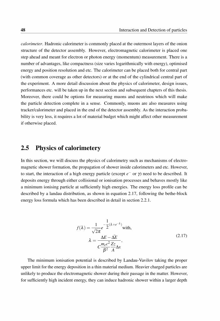
48 Interaction and Detection of particles

calorimeter. Hadronic calorimeter is commonly placed at the outermost layers of the onionstructure of the detector assembly. However, electromagnetic calorimeter is placed onestep ahead and meant for electron or photon energy (momentum) measurement. There is anumber of advantages, like compactness (size varies logarithmically with energy), optimisedenergy and position resolution and etc. The calorimeter can be placed both for central part(with common coverage as other detectors) or at the end of the cylindrical central part ofthe experiment. A more detail discussion about the physics of calorimeter, design issues,performances etc. will be taken up in the next section and subsequent chapters of this thesis.Moreover, there could be options for measuring muons and neutrinos which will makethe particle detection complete in a sense. Commonly, muons are also measures usingtracker/calorimeter and placed in the end of the detector assembly. As the interaction proba-bility is very less, it requires a lot of material budget which might affect other measurementif otherwise placed.

2.5 Physics of calorimetery

In this section, we will discuss the physics of calorimetry such as mechanisms of electro-magnetic shower formation, the propagation of shower inside calorimeters and etc. However,to start, the interaction of a high energy particle (except e− or γ) need to be described. Itdeposits energy through either collisional or ionisation processes and behaves mostly likea minimum ionising particle at sufficiently high energies. The energy loss profile can bedescribed by a landau distribution, as shown in equation 2.17, following the bethe-blockenergy loss formula which has been described in detail in section 2.2.1.

f (λ ) =1√2π

e−

12(λ+e−λ )

with,

λ =∆E− ∆E

Cmec2

β 2ZzA

∆x,

(2.17)

The minimum ionisation potential is described by Landau-Vavilov taking the properupper limit for the energy deposition in a thin material medium. Heavier charged particles areunlikely to produce the electromagnetic shower during their passage in the matter. However,for sufficiently high incident energy, they can induce hadronic shower within a larger depth

2.5 Physics of calorimetery 49

of material as an outcome of strong interaction with matter. The depth of the calorimeterneeds to be an order of magnitude larger compared to its EM-counterpart (e.g. 9.946

0.35 ≈ 28 fortungsten 5.2) for significant contribution to hadronic shower. The relevant length scale incase of hadronic shower formation and propagation in the medium is the interaction length(λI) which is (≈ 20× higher than the radiation length XR).

The physics of an EM-calorimeter is, however, more involved in case of electron orphotons which produce secondary particles in the form of showers within the calorimeterdepth. An electromagnetic shower is produced by an electron or photon with energy (E > EC)when interacting with matter through either pair production (for γ) or Bremsstrahlung (forelectrons). Theoretical calculations [62] show that the probability for energy loss throughbremsstrahlung process decreases rapidly with increase in particle mass according to theexpression for "Total Radiated Power" as shown in equation 2.18

Perpendicular component: Pa⊥v =q2γ4a2

πε0c3 ,

And Parallel component: Pa∥v =q2γ4a2

πε0c3 ,

(2.18)

where q→ charge,a→ acceleration and γ → Lorentz factor. Since Energy E, (E = γmc2),radiated by bremsstrahlung process is found to vary either with m−4 or m−6 as shown inequation 2.18. It is preferable for an electron to lose more energy compared to other heavierparticles like proton, neutron, π etc. Electrons produce EM shower [63] because of its lightermass and electromagnetic nature. The shower propagates through the calorimeter block andleaves its footprints at consecutive detector layers which can be reconstructed afterwards. Incontrary, photons can trigger EM-shower by pair production in the presence of the calorimetermedium following equation 2.13 even if they are not charged in nature. However, because ofneutrality, photons will starts showering little later compare to the electron which is otherwiseidentical as far as shower properties and propagation are concerned. Concurrent natureof EM-showers produced either by electron or photons might invite inaccuracy in photonmeasurements and need proper discrimination technique in an actual experiment.

The energy lost by an electron of initial energy E0 in the form of photon throughbremsstrahlung after travailing a distance of 1 XR on average can be calculated using Heitlercascade model. In this simplistic model, the energy of the emitted bremsstrahlung photonand the remaining electron is assumed as half of the initial energy of the primary electron(

E0

2

). In the next step, as the cross-section for pair production for high energy photons is

50 Interaction and Detection of particles

dominant, it might undergo electron-positron pair creation again after a path length of 1 XR

on average with the photon energy shared equally among two particles. So effectively at adepth of 2 XR, there will be four particles of about same energy (simplified). This process ofcascading will continue until the energy of the particle at a particular step reach the criticalenergy (EC). The energy loss afterwards will be dominated by multiple scattering whichresults in soft particle (photon or electron) production.

Figure 2.6: Sketch of the electromagnetic shower formation following a simplistic Heitlermodel [64], which illustrates the the number of secondaries produced with in an ab-sorber/converter material as a function of depth in units of radiation length.

The electromagnetic shower, as illustrated by the simplistic cascade model, can describemost of the global properties of the EM shower. However, the details of the shower structureneed more involved theoretical calculation, including asymmetric energy sharing and accuratecross-section for the bremsstrahlung and pair-production implemented. The properties of the

2.5 Physics of calorimetery 51

shower, in terms of initial energy, the path length in XR, can be expressed as following-

Number of particles after traveling t XR: N(t) = 2t .

Energy of each particles at t XR depth: E(t) =E0

2t .

Number of particles after reaching E = EC: N(tmax) = 2tmax =E0

EC.

tmax is distance in XR when energy become critical EC:tmax = XRln(

E0

EC

).

(2.19)

In brief, the predictions from the cascade model can be listed as:-(a) The number of particles at a particular depth for the shower is proportional to the incidentenergy of the particle (N(t) ∝ E0), resulting linearity between the output (energy deposition)-to - input (incident energy).(b) The depth with maximum shower particles varies with incident energy logarithmically(tmax ∝ ln(E0)).(c) The shower development is independent of the material, expressing length in XR andenergy in units of EC.(d) The angular spread of particles till shower maximum is small, defined by small openingangle of bremsstrahlung and pair production of high energy particles.

However, a detailed calculation of electromagnetic shower came later from Longo in1975 [65] with a modification to more exact form which describes the profile along the depthof the shower propagation according to the expression as shown in equation 2.20

dEdt

=E0×β × (β t)α−1e−β t

Γ(α)≈ E0tαe−β t , (2.20)

with

tmax =α−1

β= ln

(E0

EC

)+Ceγ ,

with t as the path length in units of radiation length and Ceγ -0.5 and -1.0 for γ and e-induced

shower respectively. Where,dEdt

represents the energy deposition by the shower per unitdepth in the unit of radiation length. α and β are profile parameters of the shower. The term(β t)α−1 with power law dependence explains the fast increase of the profile at the beginningof shower development due to secondary particle production, whereas, e−β t took over forlater part of the profile after the shower maximum.

52 Interaction and Detection of particles

Although, the shower is mostly dominated by radiational loss upto shower maximum, thereis still some probability for soft particle production which might not be able to create furthersecondaries and undergo multiple scattering with a comparatively large opening angle. Onthe other hand, the transverse profile of energy deposition by the EM-shower at a particulardepth illustrates the variation of energy deposition as a function of distance from the showeraxis (direction of shower propagation) which can be expressed by equation 2.21

dEdr

= αe−

(r

RM

)+βe

−

(r

λmin

).

(2.21)

Here,dEdr

is energy deposition per unit radial distance (r) from the shower axis. RM and λmin

are Moliere radius and the range of low energy photons respectively. There are two concentricparts of the transverse profile, inner-part mostly dominated by coulomb scattering wheree± move away from the shower axis due to multiple scattering. The outer-part is populatedwith low energy photon and electrons which are produced because of isotropic processeslike Compton scattering, photo-electric effect and etc. which become more important aftershower maximum.

2.6 Summary

The discussion about the particle interaction and measurement is undoubtedly significantin understanding experimental results. However, at the end, the aim for building andexperimenting with a complex set of detectors in relativistic high energy collisions is toextract the properties the system formed in the collision from a different collisional systemlike pp pA, AA and etc at various collision energies. In the next section, we will discussbriefly the Large Hadron Collider and ALICE experiment in specific, in relevance to thepresent study along with different sub-detectors.

Chapter 3

Large Hadron Collider and The ALICEExperiment

3.1 Introduction

The phenomenal Rutherford experiment opened a new domain of generalised scatteringexperiment to probe the innermost structure of matter. The need for accelerated high energybeam was felt immediately after few years and the discovery of accelerator was done by

Lawrence. During the same period, de-Broglie hypothesis (λ =hπ

p) sets guidance for

the energy of a particle to probe a particular dimension. At a glance, the development ofaccelerators and particle physics are very much entangled and had advanced fulfilling theneed of the other. In general, the accelerator can be defined as a device which acceleratesparticles and thus produces an energetic beam in a controllable manner. Properties of thebeam such as intensity, energy, energy spread, transverse size, angular spread and etc canbe well controlled in an accelerator. The development of accelerator has passed through along journey starting from the early stage Cockroft Walton to Van de Graaff to Tandem tocyclotron and finally to today’s state of the art extremely big accelerators like RelativisticHeavy Ion Collider (RHIC) or Large Hadron Collider (LHC). There are almost 30,000operational accelerators exist around the world. Though it would have been interesting tohave details of different accelerators and their uses, for the present study, we will restrictourselves to the world’s most powerful accelerator Large Hadron Collider and its differentexperiments.

54 Large Hadron Collider and The ALICE Experiment

3.2 Large Hadron Collider (LHC)

Large Hadron Collider, world’s largest and most powerful accelerator, was made operationalin 2008 after an enormous effort of 14 years. The uniqueness of LHC is lies in manyways not only in deliverable physics issues but also regarding the state of art technologicalachievements and their successful implementation. Following are some of the unique anddistinctive features of LHC [66] -

a) Giant accelerator - The accelerator is 27 km long along the circumference and locatedin France and Switzerland. The 4 meter wide circular tunnel has been buried around 50 m to175 m (100 m on average) underground.

b) Practically absolute vacuum - Extreme (ultra high) vacuum - air pressure of ≈10−13 atm. This level of vacuum is maintained over a huge volume of about 9,000 m3 (totalvolume of the LHC’s major vacuum systems)s.

d) world’s largest fridge - It operates at the temperature (≈ 1.9o K) colder than thedeep outer space. It is required to operate superconducting coils, meant to produce a hugemagnetic field of 8.3 Tesla (top field strength of each of the LHC’s 1232 superconductingdipole magnets). Beams are kept in the path by superconducting magnets.

e) Producing and handling the massive amount of data - LHC produces an enormousamount of data with all its big experiments which are enough to fill about 5∗104 TB harddisks per years.

f) Extremely high energy production - LHC can boost proton to a speed close to thatof light (0.999999991∗ c and only about 300mph less than light), which corresponds tocollective energy of LHC’s protons at the top speed of about 362 mega joules.

c) Highest temperature known to mankind- Huge amount of energy generation whichled the temperature for proton-proton collision is ≈ 1016oc in comparison to the core of sun≈ 106oc.

g) Collider with high intensity - At any time, there are 0.00000000047 grams of protonswhich are circulating the LHC ring 11000 times per second.

However, the extremely high energy imparted to the particle by LHC is not a singlestate mechanism. Rather the boost in the energy of the particle happens in stages. In thebeginning, when the energy of proton reaches 50 MeV it fed to PS Booster from the Linac 2.Proton energised to 1.4 GeV at PS Booster before the feed to Proton Synchrotron where itachieves the energy of about 25 GeV. In the next step, the protons are feed to Super ProtonSynchrotron to lift the energy to 450 GeV. At the final stage, The particles are injected toLHC ring where it split into two which are circulated oppositely and achieve the highestenergy of 6.5 TeV (designed for 7 TeV) each. LHC is capable of colliding different types ofparticles apart from proton. Proton, Lead, and Xe have collided at the different centre of mass

3.2 Large Hadron Collider (LHC) 55

energies with various combinations. The details of different colliding system at the differentcentre of mass energies at LHC can be better understood from the following table 3.1

Table 3.1: The table illustrates the excellent capability of LHC in providing collision fordifferent systems like proton-proton, proton-Lead, Lead-Lead and Xenon-Xenon. Moreover,the centre of mass energy varies for different colliding systems starting from 900 GeV to14 TeV.

Colliding system Centre of mass energy (TeV)proton-proton 0.9, 2.36, 2.76, 5.02, 5.44, 7, 8, 13, 14proton-Lead 5.02Lead-proton 5.02Lead-Lead 2.76, 5.02

Xenon-Xenon 5.44

As is explained, being an extremely complex and precision machine, LHC can not bea single purpose facility. Indeed, it has several experiments which cover a wide range ofphysics starting from fundamental particle physics to the physics of quark gluon plasma.It has seven experiments, each with a distinct feature and characterised with the devoteddetector(s). The four major experiments are ATLAS, CMS, ALICE and LHCb respectively.ATLAS and CMS are the general-purpose detectors to investigate the largest range of physicspossible, starting from precision measurements of Higgs boson to searches for new physicsbeyond the Standard Model. Though both the experiments are meant to address samephysics issues which are absolutely necessary to cross confirm any discovery. However,the basic difference between them lies in different technical solutions towards the problemand detector design. On the other hand, LHCb is a specialised experiment to measure thematter-antimatter asymmetry expected to be there in interactions of B-particles. The primarypurpose of the experiment is to answer “the reason behind survival of matter world”. TheLHCb experiment is composed of a number of sub-detectors to detect and measure particlesin one of the beam directions. The ALICE experiment is designed to study the propertiesof quark-gluon plasma, a state of matter comprised of quarks and gluons, under extremelyhigh temperature and density, in which partons become asymptotically free. Such a stateof matter, QGP, is supposed to be existed just after the Big Bang, when our universe wasonly a microsecond old. Unlike other major experiments, ALICE’s main focus is to study therelativistic heavy ion collision and investigate QGP. Apart from these four main experiments,there are few more purpose motivated and small scale experiments exist in LHC - namelyTOTEM, LHCf and MOEDAL respectively. TOTEM and LHCf are to measure forwardparticles, produced in proton-proton or heavy ions collisions. TOTEM is basically coupledwith CMS and positioned on either side of the CMS interaction point. On the other hand,

56 Large Hadron Collider and The ALICE Experiment

LHCf has two detectors which are placed along the LHC beam-line, at 140 metres either sideof the ATLAS interaction point. MOEDAL has been installed near LHCb to search for thehypothetical particle called the magnetic monopole. In the next section, we will focus onALICE experiment, in particular, keeping the relevance about the scope of the Thesis workin mind.

3.3 A Large Ion Collider Experiment (ALICE)

The ALICE [67] experiment, composed of many individual sub-detectors as shown infigure 3.1, has dimensions of 16× 16× 26 m3 and of total weight of 103 ton. ALICE is

Figure 3.1: Schematic representation of the the ALICE experiment at the CERN LHC,embedded in a solenoid with magnetic field B = 0.5 T. It has an excellent measurementcapability at mid rapidity with ITS, TPC, TRD, TOF, PHOS, EMCal, and HMPID for varioustype of particles over a wide transverse momentum range. It can also measure cosmic eventswith the help of ACORDE. Forward detectors like PMD, FMD, V0, T0, MCH and ZDC areused for triggering, event characterisation, and multiplicity studies [68].

specifically designed to handle high particle density, produced in central Lead-Lead collisionat the highest LHC energy. It has a unique feature of low transverse momentum thresholdas pmin ≈0.15 GeV/c while it can identify particles up to 20 GeV/c. Naively, the ALICE

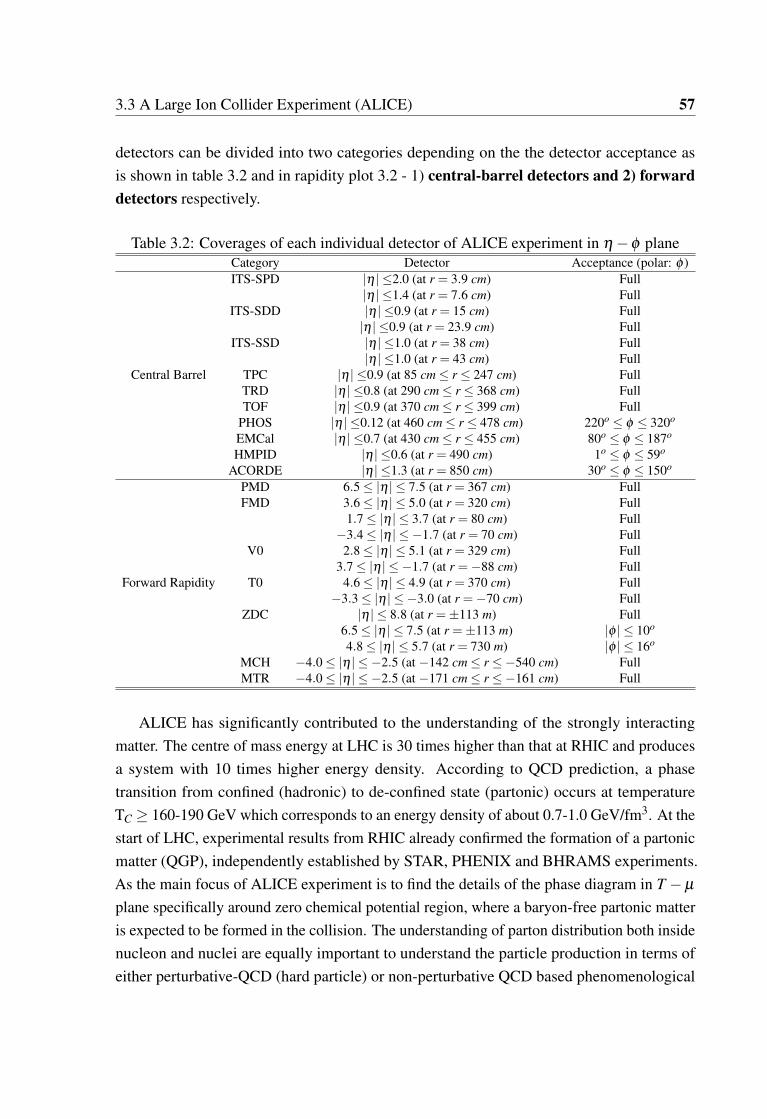
3.3 A Large Ion Collider Experiment (ALICE) 57

detectors can be divided into two categories depending on the the detector acceptance asis shown in table 3.2 and in rapidity plot 3.2 - 1) central-barrel detectors and 2) forwarddetectors respectively.

Table 3.2: Coverages of each individual detector of ALICE experiment in η−φ planeCategory Detector Acceptance (polar: φ )ITS-SPD |η | ≤2.0 (at r = 3.9 cm) Full

|η | ≤1.4 (at r = 7.6 cm) FullITS-SDD |η | ≤0.9 (at r = 15 cm) Full

|η | ≤0.9 (at r = 23.9 cm) FullITS-SSD |η | ≤1.0 (at r = 38 cm) Full

|η | ≤1.0 (at r = 43 cm) FullCentral Barrel TPC |η | ≤0.9 (at 85 cm≤ r ≤ 247 cm) Full

TRD |η | ≤0.8 (at 290 cm≤ r ≤ 368 cm) FullTOF |η | ≤0.9 (at 370 cm≤ r ≤ 399 cm) Full

PHOS |η | ≤0.12 (at 460 cm≤ r ≤ 478 cm) 220o ≤ φ ≤ 320o

EMCal |η | ≤0.7 (at 430 cm≤ r ≤ 455 cm) 80o ≤ φ ≤ 187o

HMPID |η | ≤0.6 (at r = 490 cm) 1o ≤ φ ≤ 59o

ACORDE |η | ≤1.3 (at r = 850 cm) 30o ≤ φ ≤ 150o

PMD 6.5≤ |η | ≤ 7.5 (at r = 367 cm) FullFMD 3.6≤ |η | ≤ 5.0 (at r = 320 cm) Full

1.7≤ |η | ≤ 3.7 (at r = 80 cm) Full−3.4≤ |η | ≤ −1.7 (at r = 70 cm) Full

V0 2.8≤ |η | ≤ 5.1 (at r = 329 cm) Full3.7≤ |η | ≤ −1.7 (at r =−88 cm) Full

Forward Rapidity T0 4.6≤ |η | ≤ 4.9 (at r = 370 cm) Full−3.3≤ |η | ≤ −3.0 (at r =−70 cm) Full

ZDC |η | ≤ 8.8 (at r =±113 m) Full6.5≤ |η | ≤ 7.5 (at r =±113 m) |φ | ≤ 10o

4.8≤ |η | ≤ 5.7 (at r = 730 m) |φ | ≤ 16o

MCH −4.0≤ |η | ≤ −2.5 (at −142 cm≤ r ≤−540 cm) FullMTR −4.0≤ |η | ≤ −2.5 (at −171 cm≤ r ≤−161 cm) Full

ALICE has significantly contributed to the understanding of the strongly interactingmatter. The centre of mass energy at LHC is 30 times higher than that at RHIC and producesa system with 10 times higher energy density. According to QCD prediction, a phasetransition from confined (hadronic) to de-confined state (partonic) occurs at temperatureTC ≥ 160-190 GeV which corresponds to an energy density of about 0.7-1.0 GeV/fm3. At thestart of LHC, experimental results from RHIC already confirmed the formation of a partonicmatter (QGP), independently established by STAR, PHENIX and BHRAMS experiments.As the main focus of ALICE experiment is to find the details of the phase diagram in T −µ

plane specifically around zero chemical potential region, where a baryon-free partonic matteris expected to be formed in the collision. The understanding of parton distribution both insidenucleon and nuclei are equally important to understand the particle production in terms ofeither perturbative-QCD (hard particle) or non-perturbative QCD based phenomenological

58 Large Hadron Collider and The ALICE Experiment

Figure 3.2: The figure shows the rapidity coverage of each individual detector of ALICE.ALICE has an excellent mid-rapidity coverage, whereas forward rapidity measurement isrestricted by the limited number of detectors and acceptance [69].

3.4 Central detectors 59

model prediction (soft particles) at such large centre of mass energy. Expectedly, ALICEputs shades in characterising the partonic medium formed in collision in terms of findingthe Thermal Radiation (estimation of initial temperature [70]), HBT correlation(systemsize and life time [71]), Low-pT Hadron production (to probe hydrodynamical/Thermalproperties of the system), measurement of initial anisotropy, p-QCD predictions(patonicenergy loss, suppression of charmed quarks, characterisation of heavy flavour particles) andanti-matter and Hypernuclei search etc. But recently, there has been path-breaking resultsfrom ALICE in proton-proton collisions. Multiplicity dependent proton-proton collisionindicates the formation of heavy-ion like partonic medium for high multiplicity event classes[72] which draws pp collisions to be reviewed more rigorously than just simple hard scatteringamong partons at LHC energies. The far-ranging physics objectives for strongly interactingmatter can thus be explored with ALICE experiment because of its state of art detectortechnologies adopted for the different sub-detectors.

3.4 Central detectors

As has been discussed, any experiment, in high energy physics, is composed of onion-likemulti-layered detection system around the collision (vertex) point. As illustrated by thefigure 3.2, ALICE has excellent coverages in the central region. It consisted of Inner TrackingSystem (ITS), Time Projection Chamber (TPC), Time of Flight Detector (TOF), TransitionRadiation Detector (TRD), ElectroMagnetic CALorimeter (EMCAL), PHOton Spectrometer(PHOS), High Momentum Particle Identification Detector (HMPID) which are placed in aconcentric manner with full azimuthal coverages except EMCAL and PHOS.

ITS, consisted of six cylindrical layers of silicon detectors, is located at a distancebetween 4 cm to 43 cm from the beamline along the radius. It has a rapidity coverage of|η | < 0.9. There are three different silicon detectors, Silicon Pixel Detectors (SPD), SiliconDrift Detectors (SDD) and Silicon Strip Detectors (SSD) for each consecutive two layersrespectively. Since it is placed very much next to the interaction point, the particle densitycan vary from 1 to 50 per cm2. It is to measure the track of each individual particle with aspecial resolution better than 100 µm.

TPC, the main tracking detector of the central barrel and is considered as the heartof ALICE experiment, is used for charged-particle momentum measurements, particleidentification, vertex determination with good two-track separation efficiency. Like ITS,TPC has also full azimuthal coverages along with pseudo-rapidity |η | < 0.9 for tracks withfull radial track length and |η | < 1.5 for reduced track length. TPC is capable of measuring

60 Large Hadron Collider and The ALICE Experiment

a wide range of transverse momentum starting from 0.1 GeV/c to 100 GeV/c with goodmomentum resolution.

Transition Radiation Detector (TRD), on the other hand, is devoted mainly for electronidentification in the central barrel for momentum range above 1 GeV/c. Light and heavyvector-meson resonances and di-lepton both for pp and AA collisions can be studied usingTRD along with ITS and TPC. It has very good pion rejection capability of factor 100 formomentum beyond 100 GeV. TRD has a good momentum resolution of 3.5 (4.7)% at 5GeV/c [73]. An optimised tracking efficiency of 90% has been achieved with the detectorgranularity of 6 cm2. It has an extent of 2.90 m to 3.68 m along the radius and 7.8 m alongthe beam (7 m is active region).

The Time-Of-Flight detector, a large area array MRPC gas detector with |η |< 0.9 inthe central barrel in ALICE, is meant for Particle Identification (PID) in the intermediatemomentum range (<2.5 GeV/c for π and k and up to 4 GeV/c for protons). The detector hasa polar acceptance of |θ −900|< 450 and has modular structure distributed over 18 sectorsalong φ and 5 segments along z-direction respectively. The TOF detector unit is made of10-gap double-stack MRPC strip of 122 cm long and 13 cm width leading to an active areaof 120×7.4 cm2.

The PHOS, meant to measure photons from different sources in the central barrel ofALICE, is placed just below interaction point at a distance of 4.60 m from the beam axis.Unlike ITS, TPC and all, PHOS has only limited azimuthal coverage of 100 deg and pseudo-rapidity of between -0.12 and 0.12. The PHOS is made of PbWO4(PWO) (know for the fastsignal and good energy resolution) crystals and Avalanche Photon Diodes (APD). There arealtogether 17920 channels each of dimension 22*22*180 mm.

ElectroMagnetic Calorimeter (EMCal), on the other hand, was designed to explore thedetails of jet quenching (high-pt physics) over a large kinematic range. The building blocksof EMCal is large Pb-scintillator and has very limited phase space acceptance with 107 degin azimuth above the TPC and adjacent to HMPID and pseudo-rapidity of < 0.7. Moreover,EMCal, a sampling type calorimeter with cylindrical geometry, is located at 4.5 m awayfrom the beam line and adjacent to ALICE magnet coil which is approximately opposite inazimuth to PHOS.

3.5 Forward detectors

Apart from very rich mid-rapidity measurements, ALICE is also populated with detectorsin forward rapidity which can be used to measure muons, photons, centrality and can servetriggers for other detectors. There are few crucial detectors, namely muon spectrometer

3.5 Forward detectors 61

(MCH and MTR), forward multiplicity detector (FMD), zero degree calorimeter (ZDC), T0,V0 and photon multiplicity detector (PMD), which are used to measure centrality, multiplicityapart from main forward measurement of muon and photons. Moreover these detectors areused to provide triggers for other detectors.

Muon spectrometer - It has a phase space coverage with pseudo-rapidity of -4.0 <η<-2.5 and polar angular range of 171→ 178 deg and extended along the beam direction of−5030 mm ≤ z ≤ −900mm. The components of muon spectrometer are a passive frontabsorber (absorb hadrons and photons from the vertex), 10 detectors planes with a high-granularity, a large dipole magnet, a passive muon-filter wall, four planes of trigger chambers,an inner beam shield (to protect from primary and secondary particles at large rapidities).The main focus of the detector is to measure the muons of momentum ≥4 GeV/c. However,entangled with the mid rapidity, it can probe the e−−µ measurements as well with a reducedrapidity window.

On the other hand, the multiplicity of charged particle in forward rapidity is measured byForward Multiplicity Detector (FMD), which has the pseudo-rapidity coverage of -3.4 <η<-1.7 and 1.7 <η< 5.0 and placed at both side of the interaction vertex. The most important isthe overlap between the FMD and the ITS layers which provides redundancy and cross-checksamong sub-detectors and extend the η-coverages for particle distribution as has been shownin figure 3.2. The optimised design of FMD was achieved by compromising the requiredmultiplicity resolution and the cost and complexity of the detector. Comparatively largereadout time (>1.2 µs) restrict it to be used as a multiplicity trigger unit and thus providesfor offline analysis only. FMD, consisted of three sectors FMD1, FMD2 and FMD3 - amongwhich FMD2 and FMD3 are evenly placed across the IP, is annular in shape which composedof 10 (inner ring - size is constrained by beam pipe) and 20 (outer ring - constrained by theinner wall of TPC) silicon detectors. Inner sensors (radii from 4.2 cm to 17.2 cm) consistof 512 silicon strips, whereas, outer sensors (radii from 15.4 cm to 28.4 cm) are with 256silicon strips, lead to total 51200 readout channels for full FMD.

The centrality measurement in ALICE for heavy ion collision is provided by zero degreecalorimeter (ZDC) placed at 116 m on either side of the Interaction Point. The centralityis estimated by measuring the energy carried in forward direction by the spectator (non-interacting) nucleons of the collision. The centrality information is used as L1 triggerfor the whole experiment. Moreover, being position sensitive, ZDC can provide a goodestimate for the reaction plane of nuclear collision. ZDC has two distinct detectors, ZP (dim:7.04 cm*7.04 cm*100 cm) and ZN (dim: 12 cm*22.4 cm*150 cm) for proton and neutronrespectively. Spectator protons are made separated from that of the neutron by the magnetic

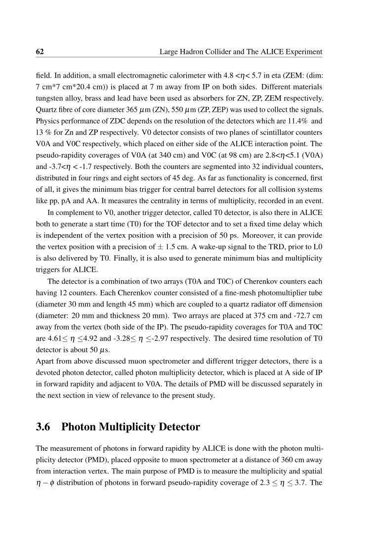
62 Large Hadron Collider and The ALICE Experiment

field. In addition, a small electromagnetic calorimeter with 4.8 <η< 5.7 in eta (ZEM: (dim:7 cm*7 cm*20.4 cm)) is placed at 7 m away from IP on both sides. Different materialstungsten alloy, brass and lead have been used as absorbers for ZN, ZP, ZEM respectively.Quartz fibre of core diameter 365 µm (ZN), 550 µm (ZP, ZEP) was used to collect the signals.Physics performance of ZDC depends on the resolution of the detectors which are 11.4% and13 % for Zn and ZP respectively. V0 detector consists of two planes of scintillator countersV0A and V0C respectively, which placed on either side of the ALICE interaction point. Thepseudo-rapidity coverages of V0A (at 340 cm) and V0C (at 98 cm) are 2.8<η<5.1 (V0A)and -3.7<η < -1.7 respectively. Both the counters are segmented into 32 individual counters,distributed in four rings and eight sectors of 45 deg. As far as functionality is concerned, firstof all, it gives the minimum bias trigger for central barrel detectors for all collision systemslike pp, pA and AA. It measures the centrality in terms of multiplicity, recorded in an event.

In complement to V0, another trigger detector, called T0 detector, is also there in ALICEboth to generate a start time (T0) for the TOF detector and to set a fixed time delay whichis independent of the vertex position with a precision of 50 ps. Moreover, it can providethe vertex position with a precision of ± 1.5 cm. A wake-up signal to the TRD, prior to L0is also delivered by T0. Finally, it is also used to generate minimum bias and multiplicitytriggers for ALICE.

The detector is a combination of two arrays (T0A and T0C) of Cherenkov counters eachhaving 12 counters. Each Cherenkov counter consisted of a fine-mesh photomultiplier tube(diameter 30 mm and length 45 mm) which are coupled to a quartz radiator off dimension(diameter: 20 mm and thickness 20 mm). Two arrays are placed at 375 cm and -72.7 cmaway from the vertex (both side of the IP). The pseudo-rapidity coverages for T0A and T0Care 4.61≤ η ≤4.92 and -3.28≤ η ≤-2.97 respectively. The desired time resolution of T0detector is about 50 µs.Apart from above discussed muon spectrometer and different trigger detectors, there is adevoted photon detector, called photon multiplicity detector, which is placed at A side of IPin forward rapidity and adjacent to V0A. The details of PMD will be discussed separately inthe next section in view of relevance to the present study.

3.6 Photon Multiplicity Detector

The measurement of photons in forward rapidity by ALICE is done with the photon multi-plicity detector (PMD), placed opposite to muon spectrometer at a distance of 360 cm awayfrom interaction vertex. The main purpose of PMD is to measure the multiplicity and spatialη−φ distribution of photons in forward pseudo-rapidity coverage of 2.3 ≤ η ≤ 3.7. The

3.6 Photon Multiplicity Detector 63

estimation of transverse electromagnetic energy and the reaction plane can also be performedwith the help of PMD on an event-by-event basis. Photon multiplicity gives important physicsinformation regarding limiting fragmentation, QGP phase transition, and the disorientedchiral condensates.figure 3.4 The PMD consists of two detector (PRE and CPV) planes separated by a three

Figure 3.3: The photograph represents the actual PMD, installed at ALICE experiment at a360 cm away from the interaction point.

radiation (≈ 1.5 cm) length thick lead converter as shown in picture 3.3. Both the detectorplanes are identical in nature apart from their functionality. The first plane, called chargedparticle veto plane (CPV), is facing incoming particles directly and is used to discriminatehadrons and electrons from that of photons. On the other hand, the second plane, calledpre-shower detector plane, is to detect electromagnetic shower signal (a patch of hit inmultiple detectors), produced either by electron or photons, at pre-shower (before showermaximum is achieved) position. To cope with very high particle density, both the detectorplanes are made up of highly granular hexagonal proportional gas detector of dimension0.22 cm2 for the area and 0.5 cm for the depth along the beam. The working principle ofthe detector explained schematically in figure 3.4 As is pointed out, PMD has performedexcellently in data taking since the beginning of LHC started giving data. At the end of LHC

64 Large Hadron Collider and The ALICE Experiment

3

Pb converter

Ch particle Veto detector

Pre - shower γ - detector

SS support

Honeycomb array γ - cluster

PHOTON Charge particle

honeycomb planes

PHOTON CHARGE PARTICLE

honeycomb

cells

Pb converter

Ch particle Veto Plane

- shower - detector Pre-shower Detector Plane

SS support

Honeycomb array Honeycomb array

Gamma cluster

Charge particle hit

Principle of PMD

CPV#cellSig. #cell Sig.

PRESHOWER

yes0 yes >1no1 yes 1

PhotonHadron

CPV#cellSig. #cell Sig.

PRESHOWER

yes0 yes >1no1 yes 1

PhotonHadron

CPV#cellSig. #cell Sig.

PRESHOWER

yes0 yes >1no1 yes 1

CPV#cellSig. #cell Sig.

PRESHOWER

yes0 yes >1no1 yes 1

PhotonHadron

CPV Plane PMD

Preshower Plane

15/03/2017 ALICE-INDIAmee3ng,VECC,Kolkata

Figure 3.4: The figure shows the schematic representation of the working principle of PMD.It explains how it responds to charged particles and photons.

3.7 Summary 65

RUN 2, PMD is will be dismantled. The ALICE forward rapidity region will have a scope tointroduce a new detector which can extend the photon measurement in forward rapidity to afull extent (both the energy and momentum). A rather unrevealed domain of small Bjorken-xcan be explored if such an extensive photon measurement of different origin can be donewhich has brought the discussion of a new electromagnetic calorimeter.

3.7 Summary

We have discussed the Large Hadron Collider and the ALICE experiment in details. Specif-ically, we have dicussed the relevance of introducing a forward calorimeter. The fact thatALICE has limited forward measurement capability let the possibility to augment the photonmeasurements in forward rapidity. It has great physics implications in the domain of lowBjorken-x regiem which is expected to be dominated by the gluon dynamics. In the nextchapter forward calorimetry in ALICE will be presented.

Chapter 4

Forward Physics and Calorimetry inALICE

4.1 Introduction

A Large Ion Collider Experiment (ALICE) at LHC has 17 detectors stacked into an onionstructure, following the general scheme of the collider experiment. Ideally, a full-4π coveragefor an experiment is desired to capture the full snap of the collision. However, because ofgeometrical constraints, ALICE has almost closed coverage around the interaction pointwhich can be divided into two parts - central barrel and forward region. In a colliderexperiment, detector acceptance is primarily dominated by the central part (mid-rapidity) withforward (backward) part along the beam direction restricted with limited coverages. ALICEhas an excellent mid-rapidity detector coverage which enables measuring different particlesfor a wide range of incident energies. On the other hand, forward rapidity measurementis limited to mostly muon detection and photon counting. Moreover, as far as the photondetection is concerned, ALICE can measure only for a very limited region in mid-rapidity withEMCAL and PHOS. The measurement of direct photons can contribute to the understandingof initial stages of the primordial matter in a more cleaner way. In this context, the inclusionof a calorimeter to measure photon in forward rapidity, can extend the existing physicsreach of ALICE to a new regime of small-x, which is now accessible with LHC energies.Feasibility of a calorimeter at forward rapidity in ALICE experiment has been considered inthis thesis work. A general discussion about the importance of calorimetry and the relevancephysics aspects in small Bjorken-x will be discussed in the subsequent sections.

68 Forward Physics and Calorimetry in ALICE

4.2 Physics motivation

A detailed study of QGP, formed in heavy ion collision has been front-line interest withthe available ultra-high centre of mass energy available at LHC. ALICE is precisely toenlighten the current understanding and dig deeper in this area [74]. Even with the existingexcellent physics capabilities as discussed in chapter-3, ALICE with its present configurationis inadequate to address a number of important issues both in QGP and baseline physics,specifically, in low Bjorken-x domain where gluon dominated dynamics is expected. Thereare several up-gradation proposals regarding central (−1≤ y≤+1) detectors at mid-rapiditylike Inner Tracking System, Time Projection Chambers etc. But, this up-gradation are meantto elevate measurements with the high rate of interactions planned by LHC during RUN-3.As an important complement to the QGP physics at mid-rapidity, an ardent plan for enhance-ment in forward-rapidity (muon arm) has also been adopted. Complete interpretation forthe matter produced in these collisions taking both in mid and forward rapidities togetheris quite entangled and complicated as they are causally disconnected throughout most ofthe evolution of the system. As an obvious effect, the properties of the QGP in the tworegions are expected to be significantly different. Though forward measurements with onlymuons are undoubtedly powerful but have limited scope and are inadequate in framing all therelevant properties of the produced matter at LHC energies. To bridge the gap between anexcellent mid-rapidity measurement capability and restricted forward-rapidity measurement,ALICE collaboration has proposed an upgrade to its present detector configurations suchthat the unravelled area of low-x for parton distribution and their contribution can be betterunderstand.

Partons, responsible degrees of freedom for a de-confined matter, are the relevant par-ticipants in collisions for relativistic high energy collision. Understanding of partons insidehadron/nucleus is extremely important for studying particle production and their mechanism(cross-section) which vary with the centre of mass energy of the collision. Parton distri-bution function (PDF), probability of finding a parton inside hadron/nucleus as a function

of longitudinal momentum fraction "x" (x =pparton

L

phadronL

), behave differently for different type

of partons (up, down, strange, charm, bottom , top and gluon). There are several effort informulating the parton distribution function [29–35], taking input from existing experiment.Figure 4.1 shows parton distributions for up, down, strange and gluons, as formulated byCTEQ-collaboration. Quarks contribute more at large-x with a maximum value around 1/3of the parent hadron. However, with the decrease in x and thus with the increase of centre

4.2 Physics motivation 69

of mass energy (x =2PT√

Se±y:

√S and y are centre of mass energy and rapidity), the quark

contribution decreases and gluons stars dominating with an increasing trend.

Figure 4.1: PDFs inside a hadron as a function of longitudinal momentum fraction (x =Q2

2p.qwith Q2 =−q2 = 10 GeV for the struck parton from CTEQ6 collaboration. (Red : Gluon,Green : U p quark, Blue : Down quark, Pink : Strange quark). A continuous rise in gluondistribution function is of prime interest in the Bjorken-x sector which might lead to gluon-saturation phenomenon [40–45].

Theoretically, the evolution of parton distribution as a function of x and Q2, can be de-scribed by perturbative quantum chromodynamics with DGLAP [36–39] and BFKL [75–77]equation which is established with experimental supports. This QCD evolution leads to astrong rise in the parton-density distributions, particularly for the gluons at very small-x andhas been argued to lead to unitarity violation. The evolution equations, however, are linear incontrary and should not be applicable to high gluon density. Non-linear evolution equations,like JIMWLK [78–84] and the BK equations, have been adopted for the understandinggluon-rich dense regime which might result in saturation phenomenon. There are plentyof theoretical predictions against gluon saturation and a number of phenomenon in hadronproduction which are consistent with saturation models as explained in [40–46]. Moreover,though Parton Distribution functions (PDF) [29–35] in protons are well established bothexperimentally and theoretically for intermediate Bjorken-x, they need more attention insmall Bjorken-x limit to probe the gluon rich domain.

70 Forward Physics and Calorimetry in ALICE

The universality of factorisation for the parton distribution functions (PDFs) can beused in any calculation involving parton-parton scattering which might have been obtainedfrom an independent particular measurement. Scaling of the PDFs, as has been predictedby different parton model and established by experiments, predicts that the dependence isonly on the longitudinal momentum fraction of the struck parton (x = Q2

2p.qwith Q2 =−q2 =

momentum transfer). Experiments, like deep inelastic scattering [85, 86], have contributed alot in obtaining parametrisation of the PDFs for hadron which has been applied successfullyin explaining results from different experiments. However, because of limited kinematiccoverage, no single experiment can explore the complete range of PDFs and thus leavesunconstrained regions of the (x−Q2) phase space. A wide set of experiments starting fromHERA, SPS, RHIC to LHC has contributed substantially in understanding PDFs, specificallyin digging gluon contribution in samll-x part. As of today, at the highest LHC beam energies,partons distribution reach to a regime with small-x of the order of 10−4 to 10−5 at the midrapidity region and which can be extended to as low as 10−6 considering the forward rapidityinto account. As discussed, the regime of small-x is effectively dominated by gluons whichevolve linearly and increases dramatically for x→ 0. However, to respect the unitarity, it cannot increase infinitely and as a result, nonlinear processes like gluon recombination will startgrowing which can be described by JIMWLK equation [78–84]. This non-linear effect willmake the PDF for gluon to grow until it balances gluon splitting and achieves a dynamicequilibrium value, known as gluon saturation with a characteristic scale (Qs), defined asQ2

s ≈xGA(x,Q2)

πR2A

∝ A13 x−λ with A is nuclear mass number and λ to be 0.3. There are many

non-perturbative QCD based model calculation which takes the gluon saturation effect intoaccount for particle production in relativistic heavy ion collision. Colour-Glass Condensate(CGC) [40], is one among most discussed models in describing particle production incorpo-rating gluon saturation phenomenon.

To search for competent and experimentally measurable observables, which contain theinformation about gluon distribution at small-x, electromagnetic probes (e.g. photons) arefound more convenient in reducing the uncertainties compare to hadronic counterpart. Thedominant leading order partonic scattering processes as shown in figure 4.3, such as quark-gluon Compton scattering, quark-anti-quark annihilation, contribute most at the large-x regionwhere the photon is coming out directly from the parton interaction vertex without fragmen-tation. On the other hand, there are next-to-leading order contributions for photons, producedin quark bremsstrahlung or by fragmentation of out-going partons 4.3. However, The latercontributions are involved with "parton-to-photon" fragmentation distributions Dγ|k(z) whichare partly known from existing measurements. At LHC energies, the contribution of prompt

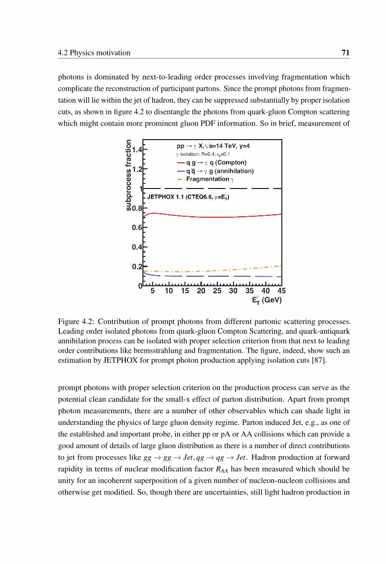
4.2 Physics motivation 71

photons is dominated by next-to-leading order processes involving fragmentation whichcomplicate the reconstruction of participant partons. Since the prompt photons from fragmen-tation will lie within the jet of hadron, they can be suppressed substantially by proper isolationcuts, as shown in figure 4.2 to disentangle the photons from quark-gluon Compton scatteringwhich might contain more prominent gluon PDF information. So in brief, measurement of

Figure 4.2: Contribution of prompt photons from different partonic scattering processes.Leading order isolated photons from quark-gluon Compton Scattering, and quark-antiquarkannihilation process can be isolated with proper selection criterion from that next to leadingorder contributions like bremsstrahlung and fragmentation. The figure, indeed, show such anestimation by JETPHOX for prompt photon production applying isolation cuts [87].

prompt photons with proper selection criterion on the production process can serve as thepotential clean candidate for the small-x effect of parton distribution. Apart from promptphoton measurements, there are a number of other observables which can shade light inunderstanding the physics of large gluon density regime. Parton induced Jet, e.g., as one ofthe established and important probe, in either pp or pA or AA collisions which can provide agood amount of details of large gluon distribution as there is a number of direct contributionsto jet from processes like gg→ gg→ Jet,qg→ qg→ Jet. Hadron production at forwardrapidity in terms of nuclear modification factor RAA has been measured which should beunity for an incoherent superposition of a given number of nucleon-nucleon collisions andotherwise get modified. So, though there are uncertainties, still light hadron production in

72 Forward Physics and Calorimetry in ALICE

forward direction can also contribute to understanding the medium produced and thus therelevant PDFs.

Figure 4.3: Feynman diagrams for different QCD processes responsible for prompt photonproduction. Leading order isolated photons (electromagnetic probe) are mostly producedfrom a) quark-gluon Compton Scattering, and b) quark-antiquark annihilation process. On theother hand, non-isolated photons from next-to-leading order processes like c) bremsstrahlungfrom a quark, and d) emission during the gluon fragmentation [87] are involved parton-to-hadron fragmentation processes [87].

However, with existing experimental facilities, it is impossible to probe the desiredbjorken-x to such a regime where gluon saturation effects contribute significantly which inturn results in the lack of a smoking gun observables. This, indeed, brings the opportunity tomeasure observables (photons) at forward rapidity in ALICE experiment at LHC, which cannavigate to probe small-x domain in a most effective experimental way which might lead tothe study of gluon saturation and its effects on particle productions. Hence a proposal forthe addition of a FOrward CALorimeter to the ALICE experiment is very much timely andsubjective which will enhance the ALICE capability in many ways like• perform unique measurements for prompt isolated photons to prove or refute the existenceof gluon saturation.• complement the forward QGP measurements of the Muon Spectrometer with other impor-tant probes of the QGP, in particular via studies of jet quenching, and• constraint underlying physics mechanisms of new features recently observed in p–Pb andhigh multiplicity pp collisions, like the so-called ridge.Moreover, the possibility of accessing more forward rapidity in ALICE experiment, make PT

measurement more flexible in the higher side without compromising the desired Bjorken-xregime, which assertion the application of pQCD calculations. Important to mention, thatwith different experiments and measurements available presently, the regions in x−Q2

plane which can be probed both for photons and hadron are shown in figure 4.4. The left

4.2 Physics motivation 73

Figure 4.4: Sensitive regions as function of x and Q2 for different existing experimentswith detectors for hardonic measurements. The expected saturation scale (Qs) is indicatedin the figure. Specific acceptance in this schematic diagram, covered by FOCAL, is alsoshown [87].

panel shows coverages achieved by DIS measurements and the photon measurements bydifferent experiments at LHC. The extent of the region in terms of photons measurementwith the inclusion of FOCAL is also shown which surely extend smaller-x part compareto the existing measurements. On the other hand, hadron measurements from RHIC andLHC in terms of x−Q2-reach are also presented where LHCb has coverage competingthe FOCAL. Though not exact, this calculation can be taken as a first approximation ofthe actual regions, specifically for hadron production, which get affected by fragmentation.Whatsoever, the introduction of FOCAL might aid neutral pion (π0) measurement and theeffect of the medium on the spectra which will help in understanding the hot and densestrongly interacting matter away from the mid-rapidity, complementing existing results fromALICE. None the less, there are some more recent discoveries like Cold Nuclear Mattereffects [47, 88–95], ridge structure (∆φ −∆η correlation) in pp and pA collision [96–101],effect of colour reconnection [102–104], possibilities of medium formation in smaller systemetc could be better understood in terms of photons and π0 production at forward rapidity atLHC energies.

74 Forward Physics and Calorimetry in ALICE

4.3 Calorimetry in high energy physics

Calorimetry, a unique science to measure Heat (Energy in the wider sense), delivers re-markable answers in detecting and characterising particles of different nature (mass, charge,structure) right from low energy to today’s ultra-relativistic high energy limit [105]. Growingcomplexities with an increase in available energy of physical processes, in counting andmeasuring particles evolve the calorimetric techniques to a state of art height. Historically,detection of charged particles started with early days hodoscope (Started by Thomas H.Johnson and E.C.Stevensonrefback in 1933), and passed through the ages of cloud chambers,emulsion tracks, bubble and streamer chambers and to more sophisticated techniques likemagnetic spectrometers. Besides these conventional "non-destructive" methods of measure-ment, partial/total absorption techniques like calorimetry were also developed in parallelto ease-handling high multiplicity environment with greater precession. Conceptually, acalorimeter is a block(s) of materials (active and passive) with optimised dimension to absorbtotal energy of the incident particles and its secondaries, produced due to interaction with thecalorimeter block. Only a small fraction (depending on active and passive block combination)of the absorbed energy is convertible into a detectable signal to investigate the kinematic state(mass, energy and direction) of particles. In high energy experiments, linearity between thecalorimeter signals (generated by ionisation charge, scintillation/Cherenkov light, etc) and theincident kinematic state of the incoming particle, need to hold over the desired range of mea-surement. The first large scale calorimeter was used in cosmic ray experiment [106](Murzin,1967) and was followed with fast improvements to fulfil the requirements of complex experi-ments in CERN-ISR, FNAL, CERN-SPS in the 1960’s and 1970’s. Unlike the conventionalnon-destructive methods, a calorimeter has features like1. Capability of measuring both charged and neutral particles.2. Dimension of the calorimeter is comparatively an order of magnitude less (≈ logE)compare to a spectrometer which makes it compact.3. Insensitivity to magnetic field by choosing proper active medium.4. Four-momentum (Px,Py,Pz,E) measurement with desired precession is possible.5. Particle identification can be done for some selected particle like hadron, electron, muon,neutrino by analysing the shower.5. Proper segmentation with high granularity make it usable in high multiplicity environ-ments.5. Low Response time (≈ or ≤ 100 ns) make it fast and compatible with high event rates.5. Energy Resolution (

σ

E) improves with increase in "E".

Depending on the nature and type of interaction of particles, to be measured, calorimeterscan be classified into two broad categories

4.4 Summary 75

(i). Electromagnetic and (ii). Hadronic.Mostly for detection of photons and electrons, the electromagnetic calorimeter is un-paralallyused, whereas, for high energy hadron (capable of producing new particle through stronginteractions within the limit of the calorimeter depth) hadron calorimeter needs to be adopted.The dimension of the hadronic calorimeter is, however, larger by an order defined by the

ratio of the Interaction length to Radiation length (λI

XR). Electromagnetic calorimeters are

widely known to the high energy experimental community for precession measurement ofphotons and leptons.Moreover depending on the design and technology adopted, calorimeters can be categorisedinto two types namely(a) Homogeneous. and (b) Heterogeneous/Sampling type.The same material is used both as a detector as well as the absorber in case of Homoge-neous calorimeter. A medium like NaI, BGO, PbWO4, Glass etc. are used in this type ofcalorimeter. On the other hand, sampling electromagnetic calorimeters, having segmentationeither or both in the transverse and longitudinal direction, comprising of alternating layers ofhigh-density absorber layer and detector layer. Depending on the experimental constraintsand requirements, a choice for the detector medium among possible Gaseous, Liquid, Solidoption can be adopted. Segmented sampling calorimeters with alternate passive and activemediums have great advantages as can be optimised for suitable energy and position res-olutions [105, 107–121]. In the present era of large-scale experiments like Large HadronCollider (LHC), Relativistic Heavy Ion Collider (RHIC), Japan Proton Accelerator ResearchComplex (J-PARC), Anti-proton and Ion Research (FAIR) etc., the necessity for precisionmeasurements of emitted particles and thus underlying physics understanding got manifold.As the collision energy and beam luminosity increases at a steady pace, experimental tech-niques including calorimetry are also getting upgraded continuously to cope up with theemerging demand.

4.4 Summary

A Sampling type electromagnetic calorimeter, using silicon as detector and tungsten asconverters/absorbers, has been considered as a feasible solution for photon (direct/decay)measurement in ALICE experiment. A general overview of the calorimetry has been dis-cussed in brief. The physics motivation of probing small-x regime of parton distributionfunctions and their consequences on particle productions was reviewed in the context of mea-surement in ALICE experiment. The new regime of unexplored small-x physics motivated tostudy for a calorimeter in forward rapidity which potentially extends the physics reach of

76 Forward Physics and Calorimetry in ALICE

ALICE experiment along with present set-up. The details of configurations and calorimetricperformances will be discussed in the next chapter.

Chapter 5

FOCAL: Design and Simulation

5.1 Introduction and pre-requisites

Pre-requisites to start for the design of a calorimeter need careful observations with desiredphysics goals and practical limitations optimised with position and acceptance, materialswith proper choice, cost estimation and etc. For the present thesis work, the calorimeter wasdesigned, keeping in mind its usability at forward rapidity in the ALICE experiment at CERN.Presently ALICE has an excellent mid-rapidity coverage (−1.0≤ η ≤ 1.0), as illustrated intable 3.2, with variety of state-of-art detectors which have contributed in exploring physicsproblems. However limited detector acceptance in the forward rapidity regions inspiredto investigate the feasibility of introducing a new electromagnetic calorimeter which willextend physics reach at small− x. Forward Electromagnetic Calorimeter (FOCAL) has beenfound to be a timely and complementary candidate in forward rapidity (2.5≤ η ≤ 4.5) ofALICE experiment which can extend the search for Gluon saturation, parton energy loss andmany more in terms of photon measurement. According to the present proposal, FOCALwas expected to be placed (considered 3.5 m in the beginning) at 7 m along z-direction fromthe primary vertex among available possible position with pseudo-rapidity coverages as isillustrated in table 5.1 along with a comparison to other existing experiments at LHC.

Table 5.1: Pseudo-rapidity coverage for the proposed FOCAL with a comparison withexisting experiments at the LHC.

ALICE FoCal@3.5 m ALICE FoCal@7 m ATLAS Inner Wheel CMS EndCap LHCb ECAL

η-coverage 2.5→4.5 3.5→5.1 2.5→3.2 1.5→3.0 1.8→4.3

In the beginning, FOCAL was considered at 3.5 m position and proposed to replace theexisting photon multiplicity detector (PMD) at forward rapidity in ALICE. However, 7 m

78 FOCAL: Design and Simulation

distance evolved as a more suitable position for FOCAL along with the pseudo-rapiditycoverage extended in forward direction by 1 unit. However, A detailed study for the geometryoptimisation for FOCAL has been carried out using GEANT4 [122, 123] simulation packagefor a position at 3.5 m away from the primary vertex within the scope of the present thesiswork. As obvious, the design and simulation were started with essential design requirementsas primary guidelines which are discussed below.

Rapidity coverage - The rapidity of the calorimeter, as estimated for the desired bjorken-xlimit, was intended as 2.5 ≤ η ≤ 5.5 which essentially defines its transverse dimensionwithin the detector acceptance. To achieve the desired η-range, the calorimeter must havefull azimuthal coverage with inner (rin) and outer (rout) radii 6 cm and 60 cm respectively.The outer radius is defined by the lower limit of the η-range, whereas, the inner radius isrestricted by the radius of the beam pipe of LHC. But for the sake of convenience, the designadopted was square shape instead of circular, which can always be transferred to a circularshape just by making corner part of detector inactive in the transverse direction.

Depth of the calorimeter - The length of the calorimeter along beamline should be opti-mised, guided by full energy deposition for the incident energy range of incoming particles.As the observables will be high energy photons (up to 200 GeV), coming from relativisticheavy ion collision at LHC energies, the calorimeter should be capable of containing photon(electron) energy deposition with ideally no loss along the depth. High energy photons orelectrons propagate through the calorimeter in the form of electromagnetic shower [124]which has been calculated to be contained in an extent of 25 radiation-length thick materialblock. The radiation length XR, a material independent way of expressing the length forparticle interaction, and can be expressed according to the equation 5.1.

XR ≈A∗716.4

Z(Z +1)ln(

287√Z

)(gm− cm−2)≈ 180∗AZ2 (gm− cm−2).

(5.1)

Where A is the atomic number of the material. However, the thickness in an absolute unitcan vary depending upon the properties of atomic weight and density (Z, ρ) of the materials.

The depth (L) of the calorimeter can be quantified, using electromagnetic showerpropagation model [64], as a function of the energy of an incoming particle and the material

of the calorimeter according to 5.2

5.1 Introduction and pre-requisites 79

L(95%) = tmax +0.08+9.6∗XR,

with shower maximum

tmax = 3.9+ ln(E) ,

(5.2)

where tmax is number of radiation length where the electromagnetic shower reaches itsmaximum value and E is the incident particle energy in GeV.As discussed, it is extremely important to ensure full energy containment as much as possibleto minimise longitudinal leakage which, otherwise, might affect the energy measurementmore seriously than other factors like lateral leakage, noise and etc. So for deciding the depthof the calorimeter, the equation 5.2 provides a crucial input, which explains the depth inwhich 95% of deposited energy will be contained.

Choice of detector - The most important part, however, is the choice of active material(detecting medium) for the calorimeter. Primarily, the choice of the detector should not dilutethe effective density (ρe f f ) of the calorimeter which will otherwise diffuse the transverseshower profile. It guides to choose a relatively high-Z detecting medium among availableoptions for detectors like gas, liquid, Scintillator, semiconductor (Si, Ge, Diamond) etc.Moreover, it must be able to provide the desired energy and position resolution. Acceptanceof a particular detector should have both established technological availabilities and asso-ciated electronics. So, choosing a proper detector medium is a wise and sensitive decision,which balances the physics, technological requirements and cost estimation.

There are two broad class of calorimeter, commonly used in high energy particle physics,namely Homogeneous and Sampling respectively. Inhomogeneous calorimeter, a singleblock of material, made either with scintillating crystal or PbWO4 or noble gas, liquidsfetched with photo-multiplier or avalanche photo-diode or silicon photo diode [125] read-out.The same material block, in case of the homogeneous calorimeter, is used both to produceEM-shower and absorb the energy from the incident photon. A part of deposited energy isconverted into a detectable signal (light converted into electrical pulse) afterwards. As amatter of fact, the whole block will serve the purpose of both passive and active medium forthe calorimeter simultaneously. Excellent energy resolution is one of the main advantages forhomogeneous calorimeter, whereas, disadvantages like "lack of direct longitudinal showerinformation", "highly expensive Crystals", "non-linearity for hadrons measurement" etc.restrict its use in large scale experiments.

80 FOCAL: Design and Simulation

On the other hand, Sampling type electromagnetic calorimeter has its own advantagesand disadvantages as well. Here absorbers/converters and the sensors (active mediums) canbe chosen with wider freedom with respect to dimension, volume, density, compactness etc.In the scope of the present study, Tungsten, a material with high-Z and high-density, has beenchosen as absorber/converter, whereas, silicon sensors was adopted as the detecting (active)medium for the calorimeter. There are plenty of advantages using silicon as the detectorwhich are listed belowLarge ∆E:- Being comparatively high-Z detecting medium, large energy is deposited withinvery thin detector depth.Small diffusion effect:- Helps in achieving better position resolution ≈ 10 µm in compari-son to other gas or liquid detecting medium.Small Ip for e−-h pair production:- Only few eV (≈ 3 eV), in comparison to gas (≈ 25-30 eV) or scintillators (≈ (4→10)×102eV) to produce electron-hole pairs, make it convenienteven though there is no internal amplification.Insentiveness to magnetic field make silicon detector smooth working in complex experi-ments with large magnetics filed like ALICE at LHC.Segmentation to a small scale is technologically available which is required in high-particle-density environment.Silicon detectors can be operated at room temperature with reasonably good signal-to-noise ratio, unlike germanium (Ge) detectors.Synergies with electronics industry make it availability easier compare to other semicon-ductor detectors like Ge or diamond.

Detector Granularity - The calorimeter under consideration will measure high energyphoton of any type irrespective of their source (Direct, Decay or Thermal). In relativisticheavy ion collisions at LHC energies, most of the photons are expected to be decayed photons(coming mainly from π0) which has its own physics importance. Apart from these decayedphotons, prompt photons contribute substantially which need to be detected as preciselyas possible. It will carry novel physics information folded in it specifically for the low-xregime. In this context, discrimination of direct photons from that of decayed photons shouldbe precisely measured. The calorimeter must be efficient to reconstruct π0 from it’s twodecayed photons (π0→ γ + γ) over the desired energy range. Analytically it can be shownthat the separation between two decayed photons decreases with an increase in energy ofthe incident π0 and can be represented in terms of opening angle and energies of delayedphotons as is shown in equation 5.3.

5.1 Introduction and pre-requisites 81

Sin2(Θ

2) =

m2π

4Eγ1Eγ2with,

Sin(Θmin

2) =

mπ

Eπ

=1γ

,

(5.3)

However, the distance between two photons depend on the distance of the detector from theinteraction point as well and can be expressed by equation 5.4

dγ1γ2 = D∗Θ, (5.4)

where D is the distance where the decayed photons are measured. The expression is for π0

decayed into two-photons with Θ as the opening angle and Eγ1 and Eγ1 are energies of thephotons respectively. The two photon separation is represented pictorially in figure 5.2 whichillustrates the average distance between two photons at 350 cm away from the interactionpoint (IP), which shows the minimum separation between two photons for highest energy(200 GeV) π0 is ≈ 3 mm (Θγγ× Distance from IP) using equation 5.4. So a simplistic guessabout the transverse segmentation for the calorimeter for detecting each and every singlephoton, irrespective of how close they are, should be ≈ 3 mm or less than that.

The segmentation (granularity) of detectors are indispensable for the proposed calorimeteras it aimed for forward rapidity region of ALICE experiment, which expects a large numberof incoming particles (0.2 for PbPb, 0.04 for Pb-p, 0.02 for pPb and 0.01 per cm2) even forthe proton-proton collision at top LHC energy. The particle density for photons, expectedat proposed calorimeter coverage, has been estimated using HIJING event generator [126]for p-p, p-Pb, Pb-p and Pb-Pb collisions at 14, 8, 8 and 5.5 TeV centre of mass energiesrespectively and shown in figure 5.1.

The figure 5.1 illustrates how the particle density decreases with the distance from thebeam line. The plot shows the number of particles, passing through the FOCAL coverages,for p-p collision is order of magnitude less compared to Pb-Pb collision. However, since thephysics objectives include both the Pb-Pb and p-p collision, inputs were considered fromPb-Pb particle density estimation for the distances (radius for calorimeter) considered forFOCAL during designing. Moreover, the pseudo-rapidity (η) distribution, as is measured asone of the primary observables in a HEP experiment, is reconstructed for photons only fromsimulated data using HIJING, as shown in figure 5.3. The distribution is characterised withtwo distinct zones, mid-rapidity with plateau region and forward-rapidity with falling trendrespectively. The profiles show symmetric nature for Pb-Pb and p-p collision, whereas, it

82 FOCAL: Design and Simulation

Distance from the center(r in cm)20 40 60 80 100 120

)2/d

A(/

cmγ

dN

-510

-410

-310

-210

-110

1

10

210Photon Density at FOCAL acceptance

Lead-Lead at 5.5 TeV

proton-Lead at 8 TeV

Lead-proton at 8 TeV

proton-proton at 14 TeV

4.76(6cm) (in step of 0.3) 1.76(125cm)

Figure 5.1: Density of Photons (/cm2) in proton-proton, proton-Lead, Lead-proton andminimum bias Lead-Lead collisions at LHC energies.

(GeV)incidenceE0 20 40 60 80 100 120 140 160 180 200

Ope

nnin

g an

gle

in r

ad

4−10

3−10

2−10

1−10

decay0πMinimum openning angle for

(GeV)incidenceE

0 20 40 60 80 100 120 140 160 180 200

(cm

)γ

Dis

tanc

e B

/W t

wo

1−10

1

10 distance at 400cmγ - γ

Figure 5.2: Opening angle of two γ’s coming from symmetric decay of π0, which help indeciding the design parameter like granularity of the detector to start with.

5.1 Introduction and pre-requisites 83

η-8 -6 -4 -2 0 2 4 6 8

η/d γ

dN

1

10

210

310

410Pseudo-rapidity Distribution at FOCAL acceptance

Lead-Lead at 5.5 TeV

proton-Lead at 8 TeV

Lead-proton at 8 TeV

proton-proton at 14 TeV

Figure 5.3: Pseudo-Rapidity Distribution for photons produced in proton-proton, proton-Lead, Lead-proton and minimum bias Lead-Lead collisions at LHC energies using standaloneHIJING event generator. It helps in estimating expected particle density for particular η-acceptance.

84 FOCAL: Design and Simulation

becomes smeared oppositely for the asymmetric collision of p-Pb and Pb-p systems. However,the density of particle, as detected by the calorimeter at a particular depth, will vary accordingto the incident energy of the incoming photons due to electromagnetic shower formationwhich will be combined reflected at final particle density as seen by the different layers ofthe calorimeter. Since the detection of incoming photons will be done by reconstructingthe EM-shower (hits patch at layers), every particle (incoming individual photons and itsshower particles) need to be detected which ideally require finer granularity compare to asestimated from the opening angle of π0-decay as shown in figure- 5.2. It has been found thatdetector of granularity 1 mm2 can satisfactorily reconstruct the shower, however, makingall the layers with such high granularity is both cost and technically not possible because ofhuge number of detector channels. An optimisation with two types of detector granularities,High granular layer (HGL) and Low granular layer (LGL:1cm2) respectively, could be anacceptable solution.

absorber/converter - For each individual detection of photons, the EM-shower should becompact and the transverse spread should be limited within a very small transverse extent.This can be possible with a material of very high-Z as well as of high density simultaneously.In this respect, there could be a different choice among Iron, Lead, Tungsten, Uranium andetc. for the absorber medium of the calorimeter. Important to note, though Lead has high-Z(ZPb =82) as compared to Tungsten (ZW =74) because of higher density for Tungsten it ismore preferable in very high multiplicity density environments where many simultaneousincidents of EM-shower will be expected. Uranium (ZU =92), on the other hand, could havebeen the best for this purpose but because of its radioactive nature, it will bring a higherdegree of complexities in the experiment. For better clarity of choosing proper absorbingmaterial, a comparison among relevant candidates for absorber is shown in the followingtable 5.2.

Table 5.2: Comparative properties for optimized absorber/converter of a calorimeter.Material(Z) Density(g/cm3) XR (cm) RM (cm) λI (cm) (dE

dx )mip (Mev/cm)Fe(26) 7.774 1.757 1.719 16.77 11Cu(29) 8.92 1.436 1.568 18.79 13Pb(82) 11.34 0.56 1.60 17.59 13W(74) 19.25 0.35 0.93 9.946 22U(92) 19.05 0.31 1.009 11.03 21

5.2 Geometry optimisation 85

As is illustrated, tungsten could be considered as a natural choice because of high Z anddensity, compact structure, availability with desired purity and reasonable price. However,the most important property is its smaller Moliere radius, shown in equation 5.5 (0.93 cm fortungsten), which restrict the transverse-shower spread and thus help in disentangling closelyspaced hits patch, formed by EM-showers. Having all these pre-requisites, the physicsof calorimeter will be discussed in brief in the next section to understand the calorimeterperformances.

RM ≈21XR MeV

EC, (5.5)

where EC|SolidorLiquid = 610MeVZ+1.24 , EC|Gas =

710MeVZ+0.92 is the critical energy of the particle

where it stops producing any further secondary particle and starts loosing energy throughcollisional processes only. Physically, Moliere radius signifies that lateral extent of theshower which contains 90% of the shower energy.

5.2 Geometry optimisation

Here we will focus on deciding the design specification of the proposed FOCAL, Samplingtype electromagnetic calorimeter, which has energy degradation with the depth (layers)along the direction of EM-shower propagation. Considering the above design issues, re-garding every individual component, the calorimeter has been opted with silicon sensors asan active medium and high purity (99.9%) tungsten plate as absorber/converter. GEANT4tool-kit [122, 123], meant for geometry simulation and tracking inside the detector, wasused to study the effect of detector geometry and performances. The primary objectiveof the geometry simulation was to search for an optimised design with adequate energyand position resolutions which can handle extreme high particle density environment asrepresented by figure 5.1 and is expected in ALICE experiment. Since the energy depositionis measured by accumulating all the deposited energy samples, collected from each and everyactive segments and layer. It has been found that only a very little fraction (≈ 2% for Si-W),depending on the active-passive combination, of the total energy is deposited in the activemedium by an incident particle. As both the shower formation and the energy deposition arestatistical in nature, more the energy samples collected - more will be the accuracy in theenergy measurement. As a result, more the number of alternative absorbing and detectinglayers, better will be the detector geometry. However, due to low-Z of the detector material,the equivalent "Z" of the calorimeter, (Zequi), will be certainly decreased and might dilute

86 FOCAL: Design and Simulation

the compactness of the configuration which will extend both the depth and the transversedimension to have same energy containment and shower compactness. Altogether, increasingthe number of layers, though have better energy resolution from a statistical point of view,but will invite a loose and extended geometry which will worsen the geometry in other wayaround. Moreover, being sampling calorimeter with small segmentation along the transversedirection which will be read individually, an increase in layer numbers will multiply the costfor readout electronics measurably. An optimised 25 (XR) length thick calorimeter was foundreasonable with the help of geant4 simulation for the incident energy range 1→200 GeVwith an optimised longitudinal leakage. However, a Twenty-Layers configuration for thecalorimeter, comprising of silicon pad detector arrays and tungsten absorbers, alternatelyplaced, has been adopted with proper balance for cost and calorimeter performances. Aschematic of the calorimeter, FOCAL, is shown in figure 5.4 with different parts (detectors,absorber, and readout) pointed. As is explained in the figure 5.4, each layer consisted of

Figure 5.4: Sketch of the Calorimeter with Tungsten as absorber and Silicon as a sensitivemedium (Not in scale).There are three high granular layers (HGL) and 17 coarse layers(LGL) with sensor dimensions (1 mm∗1 mm) and (1 cm∗1 cm) respectively.

5.2 Geometry optimisation 87

a 0.35 cm (1 XR) thick tungsten plate followed by a 0.03 cm thin silicon sensors. Duringsimulation with GEANT4, pure tungsten of density of 19.3 gm/cm3, has been implemented.Because of high-Z and high density, tungsten converts high energy photons or electrons intocomparatively compact electromagnetic showers, which mostly contained within a circularpatch of radius 1 cm. As is discussed, the primary objective of FOCAL, is to reconstructphoton, mostly decayed from π0-mesons, energy and tracks from their electromagneticshower profiles. Typically for tungsten, clusters at each layer, as produced by EM-shower,for two close-by photons, just touch each other when centre-to-centre distance is about 2 cm(2× RM). So the design must be able to find the details of cluster (energy of the cluster: Eclus,centroid of the cluster: rclus) structure for precise tracking of individual incident photon orelectron which can be done if detecting sensors are of dimension about 1 mm or less. Butconstructing a calorimeter with such high segmentation for the full configuration along withall associated stuff throughout is technically difficult and costly beyond the feasible limit.Considering these, a suitable practical optimisation was assumed with a hybrid configurationwith a combination of few high-granular layers (HGL: ≈ 1 mm or less) and all rest are ofcomparatively coarse layers (LGL: ≈ 1 cm) [87]). These HGL-part will help precise trackingby shower reconstruction, while the coarse layers will do the rest like ’energy calculation’and etc. Proper arrangement for HGL and LGL is equally important as a next step forthe configuration. The placement of the HGL was done depending on the position of themaximum of shower profiles for the incident energy range 1→200 GeV, as calculated usingequation 5.2, which varies from 4th-Layer (each of 1 XR) to 12th-Layer. As for an incomingphoton/electron with particular incident energy, shower-maximum has the maximum numberof secondary particles along the shower propagation which in turn give maximum energydeposition. So, a wise distribution for HGLs over the range for shower max, will help thereconstruction of shower clusters even with maximum simultaneous particle incidences andresults in positive impact on tracking and improve the position resolution. In the presentconfiguration, there are three high granular layers, placed at 4th,8th and 12th layers respec-tively, to cover the whole shower-maximum range for incident energy 1 GeV→200 GeVevenly. All the rest layers are occupied with LGL which improve the energy measurements.So, effectively, with the addition of HGLs, there will be four points (Primary vertex alongwith other three from cluster centroids at three HGL) to reconstruct the whole track for thepropagating γ or e−-shower.

As a first result for performance of the designed calorimeter, we have studied the responseof a minimum ionisation particle, as served by pion, by an individual detector as shownin figure 5.13 which will be discussed later in more details in this chapter. However, themost important is the response of an EM-shower, produced by a 10 GeV photon e.g. in a

88 FOCAL: Design and Simulation

single detector segment of 1 cm2 size at 8th-layers (HGL), as shown in figure 5.5, is nicelydeveloped to a Gaussian shape as is expected from energy deposition by a large numberof shower secondaries. On the other hand, the feasibility of the calorimeter in containing

(MeV)depE0 10 20 30 40 50 60

No

of E

ntri

es

0

20

40

60

80

100Response of 1cm*1cm Pad to

010GeV Gamma after 8XMPV = 14.39MeV Sigma = 4.6

Simulated Data

Gaussian Fit

Figure 5.5: Response of a single 1cm ∗ 1cm silicon pad detector at 8th layer of the calorimeterto an electromagnetic shower produced by a 10 GeV photon. Gaussian fitting to the simulateddata is shown by the solid line. The error bars are representing the statistical error.

the highest desired incident energy photon can be understood by studying the cumulativeenergy deposition profile along the depth of the shower propagation. The layer-addedenergy deposition profile as a function of depth in units of layer number is shown in figure 5.6which can be quantitatively expressed as

Enth−layercummulativedeposition = ΣiEdeposition ,

where i runs from 1 to n. For the design configuration under study, the profile shows satura-tion, obtained as a function of layer number, differ for different incident energies. However,the longitudinal depth of the calorimeter can be decided by the profile for the highest desiredphoton energy. As is illustrated by the figure 5.6, 20 XR depth could serve the purpose of fullenergy containment for the highest 200 GeV incident photon energy without any significantlongitudinal loss. For the lower end of the energy range, saturation is well obtained evenbefore 12th layer, whereas, for the higher energies, it reaches almost 18th layers onward

5.2 Geometry optimisation 89

)R

Layer Number (X0 2 4 6 8 10 12 14 16 18 20 22

(MeV

)D

epo

siti

on

Cu

mu

lati

ve E

0

500

1000

1500

2000

2500

3000

3500

fordep

Cummulative E

200 GeV * 1.000

100 GeV * 1.625

50 GeV * 2.850

40 GeV * 3.000

30 GeV * 3.250

20 GeV * 4.000

10 GeV * 5.500

5 GeV * 7.000

1 GeV * 15.00

Figure 5.6: Cumulative energy deposition profile exhibits the development of "layer addedenergy deposition" as a function of "layer-number" for EM-showers over a wide range ofincident energies. It demonstrates qualitatively an estimation of longitudinal leakage incurredin the calorimeter using its saturation trend (non-saturation) at a depth depending on incomingphoton energy.

90 FOCAL: Design and Simulation

to achieve the saturation. As the energy deposition by EM-shower at larger depth diesdown to zero asymptotically, the leakage can only be optimised rather than minimised for acalorimeter with a fixed number of layers.

As the final goal of the calorimeter, is to discriminate the prompt photons from decayedphotons, it must disentangle two photon-induced showers for highest energy neutral pionincidence. The details of shower reconstruction will be discussed in the subsequent section,however, a snap of geant4 event display is shown in figure 5.7, for two photons, decayed from10 GeV π0, with their distinct tracks and shower spreads along the depth of the calorimeter.To be noted, two distinct shower profiles can not be seen so easily for higher energies of

Figure 5.7: A snap from GEANT4 event display for electromagnetic showers, produced bydecayed photons from 10 GeV π0, with corresponding tracks shown by the solid lines whichhave been reconstructed using clustering technique for clusters formed at 4th, 8th, 12th layersrespectively.

incident π0 as they start overlapping which need improved-shower-reconstruction techniqueto disentangling each other.

5.3 Shower reconstruction

Two clusters at a particular layer of the calorimeter, as produced by EM-shower of decayedphoton from π0, are seperated by a distance depending on the incident π0-energy (Eπ0).

5.3 Shower reconstruction 91

Although clusters are well separated for low-Eπ0 , with an increase in incident energy, theclusters start coming closer and at some point, they will start overlapping. For precisereconstruction of cluster information, we need to adopt "a cluster finding algorithm", whichcan efficiently disentangle cluster even if they are overlapped to a certain extent. Forthis study, we have used fuzzy clustering technique, which treats data points from theirdegree of memberships to one or more clusters simultaneously, as is often the case foroverlapping clusters. It is important to note that, there are several clustering algorithmsavailable in the literature such as contiguity method, cellular automata, search neighbourhoodof cells, deterministic annealing, local maxima search, connected-cell search, k-means andetc. However, their effectiveness in case of overlapping cluster either restricted or dependstrongly on the pattern of the clusters, which brings the fuzzy clustering more useful. FuzzyC-Means (FCM) [127–129], type of k-means algorithm, which incorporates fuzzy logic inaddition such that each point is assigned with either weak or strong association to a cluster,defined by the inverse distance to the centre of the cluster. The FCM algorithm can becharacterised by an "objective function: (Jm(U,V,X))", as expressed by the equation 5.6,which weight within groups sum of squared errors Jm.

Jm(U,V,X) =n

∑k=1

C

∑i=1

(uik)m∥xk− vi∥2, (5.6)

with, V = (v1,v2, . . . ,vC) is a set of unknown cluster centres or centres, U consists of thememberships of the kth point to the ith cluster and ∥x∥ =

√xT x is the inner product norm.

The fuzzy factor "m" normalises the summed memberships to 1. The objective of finding aset of cluster by FCM is done by optimising Jm(U,V,X). The membership 5.7 and clustercentres 5.8 can be found following the FCM Theorem, for Dik = ∥xk− vi∥ > 0 ∀ i and k,(U,V) may minimise Jm only if, m > 1,

uik =

[ C

∑j=1

(Dik

D jk

) 2m−1]−1

, (5.7)

where, 1≤ i≤C, 1≤ k ≤ n, and

vi =∑

nk=1(uik)

mxk

∑nk=1(uik)m . (5.8)

92 FOCAL: Design and Simulation

Determination of a particular data point as a part of a cluster is done by checking thememberships of the point associated with each cluster. A point is considered as a part ofa cluster if the membership to the particular cluster is maximum out of all existing point’smemberships to all clusters. The best representation of the results to a data is finally deter-mined by the validity index, which is Xie–Beni index for this particular case which dependson both memberships and geometric distances of data points.

However, there are drawbacks of FCM algorithm such that it depends on the fuzzy factorwhich may vary for different data sets and the fact that it treats outliers in the same way asthe data points within the bulk. To get rid of such effects, FCM algorithm has been modifiedto a new form, called dynamic fuzzy c-means (dFCM), which finds clusters dynamically asdata streams by either deleting or generating clusters as per requirement. The final results forfinding valid clusters is made through satisfying the criterion for validity index. Moreover,there is no need to set the upper limit for the maximum number of clusters to start with(meets practical requirement more reasonably), rather it needs only a minimum. The dFCMalgorithm can be illustrated by the flow-chart as expressed by 5.8 The subsequent steps ofthe algorithm can be described as following:• The algorithm starts assuming a few of the incoming data points a priori which mighthelp to estimate the range of the incoming data. At the beginning, a few parameters, likemembership threshold, the FCM error criteria, the bounds of the variable "C", the number ofclusters etc are specified. Usually, the initial number of points is taken to be low to give thealgorithm to have a brief idea about the data set.

• initially, the number of cluster centres, generated uniformly within the input space,is defined by the minimum value of the variable C is Cmin which must be greater than orequal to 2. Once the initial cluster centres are defined, the memberships for data points to theclusters are found using equation 5.7

• For further data point streaming in, its memberships with present clusters calculated.For maximum membership greater than or equal to the membership threshold µ , simpleAlternating optimisation takes place so that the data point can be assigned to at least one ofthe clusters such that matches or exceeds µ .

• At a given instance, if maximum membership falls below µ for "C" clusters, then thevalidity of the present set of clusters is checked for a range C-2 to C+2 (can be relaxed

5.3 Shower reconstruction 93

Figure 5.8: The flow chart of the dynamic FCM (dFCM) algorithm.

94 FOCAL: Design and Simulation

depending on the requirement) with following steps,

1. Firstly, cluster centres are checked whether they have been updated/generated at aprevious time or not. For yes, the old values are updated using the FCM and thus thevalidity index is evaluated.

2. Otherwise, cluster centres for C-1 are used, and an Cth center is generated by perturbingthe data point. Alternating optimisation performed again and the validity index isevaluated.

3. The cluster centres with the best value for validity index are accepted finally.

• The above described procedure continues till data points stop streaming in.

Application to simulated data: The usability of the FCM algorithm along with its modi-fied version has been checked for data, obtained from GEANT4 simulation with the proposedFOCAL detector. Since the algorithm is primarily developed to reconstruct the π0 fromits decayed photon showers, we have taken single π0 of different incident energies whichdecayed to two photons and forming their corresponding showers within the calorimeter. Asa first step, the algorithm was applied to find clusters information (Rcluster and Ecluster) atthree HGL layers of the calorimeter to reconstruct the path of the shower propagation andthus the decayed photons. Figure 5.9 explain the shower profiles of decayed photons and theirreconstruction for three different incident energies, 10, 50 and 100 GeV respectively [107].The GEANT4 displays are to show the extent of overlapping off showers, increases with anincrease in incident π0 energy, which illustrates the need for applying clustering technique.The xy-hits distribution for the shower at different layers are actually fed to the clusteringalgorithm for finding the cluster centres and cluster energies.

The results obtained using the clustering for layer 8, in terms of lateral shower spread areshown in the right column of figure 5.9. The photon track (red solid lines) is reconstructedjoining three cluster centres at 4th, 8th, 12th layers, obtained from FCM clustering. The FCMalgorithm can satisfactorily reconstruct the photons tracks despite the large extent of overlapamong themselves.

The invariant mass (Mγγ ) of the incident π0 is then calculated using individual decayedphoton (energy and direction) information. The quality of reconstruction of Mγγ is shown infigure 5.10 and figure 5.11 for three different π0 energies [107].

The performance of the clustering, however, was done for a wide range of π0 energy10 GeV→170 GeV which is shown at the right panel of figure 5.11. The plot shows

5.3 Shower reconstruction 95

Figure 5.9: Reconstruction of neutral pion of energy 10 GeV (top), 50 GeV (middle), and100 GeV (bottom) decaying to two photons. GEANT4 event display for Longitudinal showerprofiles are shown along with clusters found by the FCM algorithm on the 4th, 8th and 12thlayers, which are used to find photon tracks. XY-hit distributions, representing the lateralspread of shower at a particular depth (8th layer) with cluster centres superimposed. It showsthe effectiveness of the FCM even for substantially overlapped clusters, found by the FCMalgorithm.

96 FOCAL: Design and Simulation

(MeV)γγM50 100 150 200 250 300

No.

of e

vent

s

0

20

40

60

80

100

120

140

: 30GeV0πIncident energy of Mean: 136.2 +- 1.2Sigma: 29.5 +- 1.1

(MeV)γγM0 50 100 150 200 250 300

No.

of e

vent

s0

50

100

150: 50GeV0πIncident energy of

Mean: 142.2 +- 1.04Sigma: 28.3 +- 1.2

Figure 5.10: Invariant Mass (Mγ−γ ) reconstruction from two decayed photons using FCMclustering technique for the proposed FOCAL. The left panel shows for 10 GeV, whereas, theright panel is for 30 GeV π0. The error bars in both cases represents statistical errors only.

(MeV)γγM0 50 100 150 200 250 300 350

No.

of e

vent

s

0

20

40

60

80

100

120

: 100GeV0πIncident energy of Mean: 162.2 +- 1.6Sigma: 37.0 +- 1.8

Energy (MeV)0πIncident 0 50 100 150 200 250

(M

eV)

γγM

0

100

200

300

400

500

600

Figure 5.11: The left panel shown reconstruction of invariant mass (Mγ−γ ) for 100 GeVπ0, resulting 162 MeV for Mπ0 , little more compare to its actual value. The right panelsummarises the reconstructed invariant masses, calculated for π0 with varying incidentenergies using FCM, from two decayed photon as a function of Eπ0 . The errors bars areindicating statistical error.

the variation of Mγγ as function of incident π0 energy (Eπ0). The statistical errors arecalculated from the rms values of the invariant mass distributions. For almost all the casesof incident energies of π0, the invariant mass distribution shows a peak around the π0-mass

5.4 Response of calorimeter 97

Ope

ning

ang

le (

deg.

)

0.2

0.4

0.6

0.8

1

Energy (GeV)0π20 40 60 80 100 120 140 160 180 200

’s (

cm)

γD

ista

nce

betw

een

two

0

1

2

3

4

5

At a distance of 350 cm

Figure 5.12: The plot illustrates the variation of opening angle (top) and minimum distance(bottom) between two photons, decayed from π0, as a function of E incident

π0 . Both the openingangle and the distance decreases with the increase in incident π0 energy. The results arematching satisfactorily with theoretical prediction as shown by the dashed curves. The erroris within the marker size.

(135MeV/c2). As is shown, however, the reconstruction of Mγγ start deviating at 100 GeVonwards [107]. However, the effect can be attributed to both the detector configuration andthe limitations of the clustering routine together which leaves scope for further improvement.

Finally, the opening angle and the distance between the two decayed photons at a distanceof 350 cm away from the vertex was reconstructed using FCM clustering results about photontracks and direction, as shown in figure 5.12.

The results for two photon separation, using clustering, from simulated data are in goodagreement with the theoretical prediction. The success of shower reconstruction algorithm,however, leave a scope in furthering the study about the calorimeter performances which willbe discussed in detail in the next section.

5.4 Response of calorimeter

In this section, the details of the responses of the proposed calorimeter to different particleswill be discussed for a wide range of incident energy. Moreover, typical calorimeter perfor-mances like linearity b/w input-to-output, energy resolution etc. will be explored with the

98 FOCAL: Design and Simulation

simulated data. The study, especially, is to investigate the feasibility of the calorimeter interms of its basic calorimetric performances.

5.4.1 Minimum Ionising particle

As has been discussed in section 2.2.2, below critical energy, particle loses energy in thematter through collision processes. Usually, for the relativistic particle, energy losses becomeindependent of particle type and energy, as is illustrated by the figure 2.2. Pion, being thelowest mass hadron, become relativistic quickly and can be used to study the response ofminimum ionising particle (MIP). The study of MIP is extremely important since it definesthe sensibility of the sensors to detect any minimum level of signal over noise. To be a

good detector, the MIP-signal should be well above the noise profile which makes theSN

ratio better. During simulation, we have taken π+ to characterise the MIP-response of thedetector, as shown in figure 5.13. The profile is for an energy deposition by π+ in a single1 cm2 silicon pad detector. As is seen, the energy deposition profile in a 300 µm thin silicondetector can be well described by a truncated Landau distribution (to be more precise it mustbe Vavilob-Landau distribution). The most probable value for the energy deposition comesout to be ≈90 KeV which is obvious from the prediction in literature [130]. It is important tonote that π+, with sufficiently high relativistic energy, can produce hadronic shower but atdeeper in depth of the calorimeter. To avoid the contamination from the hadronic shower, itis always preferable to study the MIP-response for earlier layers of the calorimeter. However,interpretation of total energy deposition profile within the entire calorimeter by a MIP-particleneed special attention which included both MIP-signal convoluted with hadronic showercontribution.

5.4.2 Electromagnetic shower

On the other hand, high energy photons create EM-shower and propagate through thecalorimeter. Naturally, during the passage of photons through a calorimeter, it is energydeposition by shower secondaries instead of by a single incident particle as is illustratedin figure 5.5. The energy deposition profile by EM-shower, triggered by a 10 GeV photon,is extracted using simulated data. The signal is a response of a 1 cm ∗ 1 cm ∗ 0.3 mmsilicon pad at 8th layer where shower max is expected for 10 GeV Gamma. A simplisticHeitler model [64] calculation, as used to understand the EM-shower propagation and globalproperties, shows the number of secondary particles, produced at a single pad at 8th-layer,is ≈ (14.39 MeV/ 90 KeV) ≈ 160. However, for the calculation of the total number ofsecondaries need contribution from others nearby pads along with the central pad which

5.4 Response of calorimeter 99

MIP Response

MPV = 0.083 Sigma = 0.008

(MeV)depE0 0.2 0.4 0.6 0.8 1

No

of E

ntri

es

0

100

200

300

400 Simulated DataLandau Fit

Figure 5.13: Response to a Minimum Ionising Particle π+ for single pad detector of dimen-sion 1cm∗1cm of a particular layer of the calorimeter. The curve represents fit to simulateddata with Landau distribution.

contributes most. As the main aim for this simulation is to characterise FOCAL withoptimised geometry and components, the basic calorimetric performances were reconstructedfrom the simulated data both to qualify and quantify its good design and functionality. In theremaining part of the chapter, we will discuss the capability of the calorimeter in recreatingthe shower properties like longitudinal profile, shower maximum as a function of depth andother more general properties like energy calibration, resolution and etc.

Longitudinal shower profile: Differential energy deposition as a function of depth (layer)by an EM-shower within the calorimeter, known as longitudinal shower profile, containsinformation like the required depth of calorimeter, maximum energy deposition at a particularlayer and etc. During simulation, the response of high energy photons for a wide rangeof incident energy (1 GeV → 200 GeV) have been studied. The longitudinal profile, asshown in figure 5.14, get shifted to the right and become more broadened with an anincreased area for increase in incident energy. The profile as a function of layer numbercan be explained using theoretical model prediction (line shown in figure) by Longo andas expressed in equation 2.20. As is expected for a e/γ-triggered EM-showers, the energydeposition first increases with the depth of calorimeter and reaches a maximum called shower-

100 FOCAL: Design and Simulation

)R

Layer Number (X0 5 10 15 20 25

in M

eVD

epE

0

50

100

150

200

250

300

350

400Longitudinal Shower Profile for

200 GeV * 1.0

100 GeV * 1.63

50 GeV * 2.85

40 GeV * 3.0

30 GeV * 3.25

20 GeV * 4.0

10 GeV * 5.5

5 GeV * 7.0

1 GeV * 15.0

Figure 5.14: Longitudinal profile of an EM-Shower from incoming photons with differentincident energies. It represents the variation of energy deposition at a particular layer with adepth of the calorimeter (layer number). The profile shows first rising and then followed by afalling trend with a shower maximum decided by the calorimeter and the incident energy ofthe incoming particle.

maximum. At the shower maximum, the energy of the shower particles degraded to thecritical value (EC), where no further secondary particles are produced. With further increasein depth, the shower profile shows a falling trend representing the losses mostly dominatedby ionisation/collisional mechanisms by the shower particles till the end. For a good designof a calorimeter, the longitudinal profile for the desired energy range must be closed orreach approximately zero deposition within the extent of the calorimeter. The shift in profilewith increase in incident energy can be quantified by plotting the position of the showermaximum as a function of depth of the calorimeter which is shown in figure 5.15. The plotshows the data points from simulation along with the theoretical prediction, as expressed bytmax =

(α−1)β

= ln EoEC

+Ce−/γ . The parameter Ce−/γ takes different values for electron andphotons. The variation, indeed, shows a linearity for shower maximum for the desired energyrange.

Apart from the longitudinal profile, EM-shower develops a transverse profile whichrepresents the distribution of number of hit or energy deposition (corresponds to number of

5.4 Response of calorimeter 101

(MeV)incidenceE1 10 210 310

)R

Po

siti

on

of

Sh

ow

er M

axim

um

(in

X

0

2

4

6

8

10

12

14

16

18

20

= a + b * logEmaxFitted with t

a = 3.7, b = 1.6

Figure 5.15: The plot represents the position of shower maximum (tmax) as a function ofincident energy for incoming photon. The position of shower maximum (tmax), expressedin units of radiation length, varies linearly with the logarithmic of the incident energy.Importantly it hints about the depth of the calorimeter and the probable position of the highlygranular layers for a specified energy range in designing a calorimeter.

102 FOCAL: Design and Simulation

shower particles) about the shower axis (as already explained). However, with LGL part ofthe calorimeter, it is hardly possible to reconstruct the transverse profile as the spread itselfcontained within an area of radius 1 cm (Moliere radius).

Linearity for energy measurement: Like in any general measurement strategy, the calorime-ter should have linearity between the output signal and the incident energy. As has beendiscussed in the physics of calorimetry, the number of shower secondaries varies linearly withthe incoming particle energy. However, the final output, involving two more steps: energy de-position by secondaries and production of measurable signal (light or charge), should followlinearity with the input. Because of statistical nature, the preciseness of Edeposition/measured

will depend on the number of samples (corresponding to the number of layers) collected.In this study with 20-layers, total deposited energy was calculated from the simulation fora known set of incident energy of photons and is plotted in figure 5.16. It shows that thecalorimeter is, indeed, behaving linearly within the expected incident energy range.

(GeV)incidenceE0 20 40 60 80 100

(GeV

)D

epo

siti

on

E

0

0.5

1

1.5

Fitted with F(E) = a + b*Ea = 0.002, b = 0.017

Figure 5.16: Calibration shows variation of total deposited Energy by the EM-showertriggered by inflowing Gamma with that of incident energy. It assures the the calorimeter isworking in liner region indeed.

The figure 5.16, showing the relationship between deposited and the incident energies, iscommonly known as calibration curve which provides the relationship which can be used to

5.4 Response of calorimeter 103

calculate the unknown incident energy for particular measured energy. The results shows,Edeposition follow a linear equation Edeposition = 0.002+0.017∗Eincidence with an offset 0.002which ideally must be zero.

Energy Resolution: Energy resolution (σ

E ), in general, can be defined as resolving powerof an instrument in discriminating two closely spaced incoming particles in the energyspectrum. Calorimetry, being an energy measuring technique, should perform measurementwith the desired energy resolution. The calorimeter under consideration is supposed to beoperational under a moderately high particle density environment where a more or lesscontinuum for the energy spectrum of incoming particles is expected. Before discussingdetails of the energy resolution, we will elaborate on the sources which are affecting theresolution in either way. Resolution can be thought of as an effect of physical processeswhich are statistical in nature and restrict introducing different type of fluctuations, inhibitedin it. There are plenty of sources for such relevant fluctuations contributing to sampling typeelectromagnetic calorimeters and can be categorised as following1) Quantum Fluctuations (which includes shower-fluctuations, photo-electron statistics)varies as 1√

E.

2) Shower Leakage which depends on the calorimeter dimension. Usually, for a particularcalorimeter, it is independent of energy. But longitudinal leakage needs much more attentionas is more influential compared to lateral leakage for the energy resolution.3) Instrumental effects like electronic noise and etc. This class of fluctuation depends onenergy as 1

E .4) Sampling fluctuation is an issue which depends on the numbers of sampling layers andvaries with energy as 1√

E.

5) Landau fluctuation comes into the picture where thin active layers are used in thecalorimeter. Within a thin active length, energy deposition is asymmetrically distributedwhich follows Landau distribution and varies with energy as 1√

E.

6) Track length fluctuation which is effective due to the different path lengths traversed bydifferent particles because of multiple scattering and depends on energy as 1√

E.

Henceforth the generalised energy resolution of a sampling calorimeter is, considering allsuch contributions, can be represented by the following expression

σ(E)E

= a⊕ b√E⊕ c

E+ O(E) , (5.9)

where symbol ⊕ represents quadratic summation.a→ represents defects of the calorimeter of different types like non-uniformities (absorber

104 FOCAL: Design and Simulation

(GeV)incidenceE0 20 40 60 80 100

)d

ep/Eσ

Res

olu

tio

n(

0.05

0.1

0.15

0.2

EFitted with F(E) = a + b/a = 0.00354 (0.354%)b = 0.19049 (19.049%)

Figure 5.17: Energy resolution: represents the efficiency of the calorimeter in measuringthe energy precisely of an inflowing particle. It is represented in terms of percentage ofthe incident energy that has been measured. Lesser the resolution ( σ

Ein) better will be the

calorimeter. The dashed curve represents two-term resolution formula. The parameterassociated with 1√

Eused to quote the resolution which is ≈19 % in this case.

and active layers have irregular shapes), imperfections in the detector mechanical structure,temperature gradients, detector ageing, radiation damage, longitudinal leakage etc. Non-uniformities which might lead to periodic pattern in resolution can be cured in case theyare originated from either detector geometry or readout electronics. On the other hand,mechanical imperfection affect the resolution in a random manner and difficult to cure.b→ stands for stochastic processes, representing fluctuations in signal generation, whichdepends on event-by-event fluctuation in case of sampling calorimeter and limit it to not sogood like homogeneous calorimeters.c→ stands for the noise of readout electronics and depend on detector technique and readoutcircuit mostly.Usually, in literature, values of a and b are quoted as the figure for energy resolution and thusthe performance of a calorimeter.Notably, the relative importance of different terms in the expression for resolution depends

on the incident energy of the incoming particle. Therefore the optimised design for a

5.5 Summary and scope 105

calorimeter can be different depending on energy ranges as might affect the resolution indifferent ways. Energy resolution may vary from an excellent ≈ 2% (for Homogeneous)to a compromising 30% and even worse depending on the choice of dimension, design,active/passive material combination, electronics etc. For the calorimeter under consideration,the resolution for incident energy range 1→200 GeV has been calculated and found to be0.354%+ 0.1905%/

√E, as is shown in figure 5.17, which is indeed quite inspiring for a

sampling calorimeter.

5.5 Summary and scope

The different aspects of the design for a sampling calorimeter using a silicon detector andtungsten absorbers/converters have been discussed. A brief discussion about the requirementsfor the proposed FOCAL has been introduced in the beginning. A short note on the relevantcalorimeter physics, regarding the passage of electromagnetic shower, was presented in thenext. Details of geant4 simulation for FOCAL was done to help in optimising the geometryand to study the feasibility of the calorimeter. As one of the optimal choice, 20 XR thickcalorimeter with 20 layers (1 XR each) was considered as an option in this study. Thecalorimeter was optimised with a hybrid configuration having both HGL and LGL whichmade it an accommodative solution from both physics requirements and budget perspective.A detailed simulation regarding the performances of the calorimeter has been accomplished.The shower reconstruction using a fuzzy clustering method is adopted in this study. Theapplicability of the reconstruction technique was discussed for overlapping showers (hitpatch at a layer) and found performing reasonably good for expected high particle densityenvironment like in ALICE. The chapter ends with reconstruction response of the calorimeterto charged particles (MIP) and photons (triggering EM-shower) for wide incident energy.Simulation results, indeed, shows the potentiality of the designed calorimeter an acceptableoption to pursue the physics interests under consideration.

The feasibility study of the calorimeter in simulation inspires to step forward for designingand developing the calorimeter will all its components. The details of hardware developmentfor a series of prototype calorimeter, aiming for the proposed FOCAL, will be discussed indetails in the next chapter.

Chapter 6

FOCAL: Detector Development,Fabrication and Tests

6.1 Introduction

After successful completion of the conceptual design for the calorimeter configuration, an ef-fort was put in constructing prototype calorimeter as one of the major parts of the thesis work.The hardware development comprises of making of silicon detector, large dynamic rangereadout electronics, detector and readout PCB board, mechanical structure, data ac-quisition and etc. The main focus on FOCAL prototype development, for this study, will beon fabrication and test of a small scale calorimeter arrangement and analysis of results bothfor laboratory and high energy particle beam. As a first step towards detector development,we have started making a 1 cm2, 300 µm thin silicon detector elements and mounted them ona detector PCB. Although, this will invite a lot of dead space and can not be used in the actualexperiment, it can provide important results regarding basic detector characteristics includingnoise and also explore the scope for further developments. Starting from such a simpleprototype with physically isolated 1 cm2 silicon sensors array as the detector, a series ofprototype calorimeters were developed, fabricated and tested both with the radioactive sourceat the laboratory and with a high energy electron beam and published in [120]. Followinga miniature version prototype test and its successful performances, a full depth prototypehas been constructed which will be discussed in more details in this chapter. Analysis oftest beam data, carried at both CERN-PS and CERN-SPS beamline facility, will be pre-sented. Comparison of experimental data with that from simulation will also be analysedin subsequent sections. In the end, the scope for further progress and the final goal will bedescribed.

108 FOCAL: Detector Development, Fabrication and Tests

6.2 Test of Si-detector with β -source (Sr90)

6.2.1 Experimental set-up

A detailed and extensive laboratory based test of each component like single pad detector,readout channels, mechanical arrangement, triggering unit etc. have been performed withradioactive Sr90 β -source (with an endpoint energy of 0.546 MeV). The test set-up, as shownin photograph 6.1, comprises of a 5×5 array of 1 cm2 silicon detector mounted on a PCB,two scintillators - as triggering unit, β -source for low energy electron beam, NIM-basedelectronics and etc. The optimum operating voltage, set for the detector, was 60 V which hasbeen judiciously decided

Figure 6.1: Experimental arrangement used to test the silicon detectors at VECC laboratorywith the Sr90 β source.

depending on the voltage scan (I-V characteristics) of the detectors. As per design, thedetector, however, supposed to depleted fully at 70 → 80 volts with the capacitance of40 pF/cm2. The detector plane, as shown in the photograph 6.2, was interleaved in betweentwo scintillator paddles which serve the purpose of triggering the detector by the method ofcoincidence.

The encapsulated Sr90 source was placed above the top scintillator paddles, as is shownin the experimental set up 6.1. The detector plane was wrapped with a thin aluminium sheetto protect against ambient EMI. The whole experimental arrangement was put inside a box,covered with black paper, to shield from light which otherwise increases the noise in thedetector. Since the radioactive β -source emits a continuum spectra of the electron, it willdeposits energy within the detector truncated at a maximum value, characterised by the

6.2 Test of Si-detector with β -source (Sr90) 109

Figure 6.2: Photograph of a single 1 cm2 silicon pad detector mounted on a PCB board.

end-point energy of the β spectrum. All the individual detector was checked during theexperiment by adjusting the source position (xy-scanning) so that the radiation can hit aparticular pad on the detector plane. However, to start, a run without any source is alwaysperformed to investigate the response of the detector to noise from different sources likefrom detector, readout electronics and experimental ambience and etc., which will set thereference during data analysis.

6.2.2 Discussion of laboratory test results

As discussed, the main aim of the laboratory test was to check the functionality of allindividual detectors. The data from the test with β -source shows two clearly distinguishedpeaks corresponds to β -spectrum and the noise respectively which is described by thefigure 6.3, depicting a reasonably good signal-to-noise ratio ( S

N ). These results elucidatethe good functionality of each element of the silicon detector array. However, for details ofcalorimeter response and energy loss profiles, the calorimeter prototype with both absorberand detector layers must be studied with high energy pion and electron beams which will bediscussed next in this chapter.

110 FOCAL: Detector Development, Fabrication and Tests

Channel No.20 40 60 80 100 120 140 160 180 200

Cou

nts

0

50

100

150

200

Figure 6.3: (Colour online). Response of a single silicon pad detector to Sr90-β source. Aclear peak has been detected corresponding to β spectrum of with end point energy 0.546MeV. The signal is well dispersed from the noise peak which is around the channel number20.

6.3 Mini-Prototype 111

6.3 Mini-Prototype

A miniature version for FOCAL prototype (mini-prototype) with only four layers of detectorsand tungsten absorbers was fabricated as a next step. The test with mini-prototype was to puttogether all components along with the data acquisition system and to study the behaviourand characteristics of the detector. It will also help in estimating the requirements of readoutelectronics which can be feed for next step of developments. Though the mini-prototype islimited with four course layers, still basic characteristics like longitudinal shower profile,calibration of energy deposition, etc., can provide inputs to build the full length calorimeter.The details of the mini-prototype along with test beam results will be discussed in details inthe next two sections.

6.3.1 Construction and test at CERN-PS

As discussed, a mini-prototpe, with active transverse area 5 cm×5 cm and of the longitudinaldimension of ≈ 4 XR, has been constructed to study the response of pion and electronbeams of various energies. Encouraging results from the tests of detectors at laboratory,miniature prototype, comprised of four-layers (Each layer =≈ 3.5 mm thick "W" + ≈ 1 cmfor detector and electronics together) of tungsten (converter/absorber) and 5 ∗ 5 array of1 cm2 silicon detector planes, was constructed. Each layer is a combination of tungstenplate of dimension 10 cm× 10 cm× ≈ 1XR± 0.03 cm, silicon detector array (5 ∗ 5) andfront-end readout electronics. Physically isolated and each individual silicon pad detectors ofdimension 1cm2, as shown in figure 6.2, were assembled in a 5∗5 array. the detector arraywas mounted on a 0.08 cm thick 4-layer detector-PCB which is illustrated in figure 6.4. ThePCB layers serve the purpose of both holding and connecting the detector to the front-end-readout electronics. There altogether four such composite layers (W+Si+electronics) whichare contributing to the depth of 4 XR for the mini-prototype. The density and purity of thetungsten-plates, used as an absorber, was 19.3 gm/cm3 and≈99.9% respectively. There weretwo arrangements which have been used for the mini-prototype. Both the setups, as shown infigure 6.5, contains four layers of detectors. In Set-up-1, four layers of tungsten and silicondetector arrays were assembled alternatively. This gives the behaviour of incoming particlesup to 4 XR in longitudinal depth. However, the Set-up-2 has two additional tungsten layers infront compare to Set-up-1 which could extend the depth up to 6 XR.

The either of the setup was used in a general scheme of the mini-prototype arrangement,as illustrated by the schematic diagram 6.6. Basically, the sketch explains the relative positionof different parts during the actual experiment. The transverse granularity of the detector

112 FOCAL: Detector Development, Fabrication and Tests

Figure 6.4: Sketch of the silicon detector array of dimension 5×5 made of 1 cm2 physicallyisolated silicon pad detectors which are mounted on the detector PCB.

Figure 6.5: (Colour online) The figures represent sketches of two different setups of theMini-prototype which had been used for the beam test at CERN-PS.

6.3 Mini-Prototype 113

Figure 6.6: (Colour online) The figure represents the schematic of the mini-prototype withall different components in sequence as was arranged during the experiment.

plane, used in mini-prototype, was 1 cm∗1 cm (similar to LGL of the proposed calorimeter)where 320 µm is thickness along the depth.

Silicon detector: The silicon detectors are fabricated on ⟨111⟩ FZ n-type wafers with3−5 k-Ω resistivity. The top pads are p+ while the bottom side is n+. The leakage current ofthe detectors is less than a few nA and breakdown voltage is above 250 V. Each pad detectoris surrounded by a guard-ring which help in improving cross-talk among near-by detectorsand make the field uniform inside the detector. All the detectors are appropriately biased. Thesilicon pads found to reach the full depletion at 60 V with detector capacitance of 40 pF/cm2.The detectors were attached to the 0.08 cm thin 4-layers PCB with silver conductive epoxyof resistivity 0.006 Ω-cm. The top of the diode was coated with 1µm thick Al and 0.5µmthick phosphosilicate glass (PSG) passivation. Being physically isolated from each other, theprobability of having a cross talk among adjacent silicon pad elements is ideally zero [120].

Readout Electronics: There were devoted Front End Electronics (FEE) boards which havebeen used to readout detector signal during experiments both at the laboratory and PS-Beamline. Two different kind of ASICs, namely, MANAS [131, 132] and ANUSANSKAR [133]were used for these purposes. Both of these ASICs have 16 pulse processing channels alongwith analogue multiplexed output. Each channel is subsumed of a Charge Sensitive Amplifier(CSA), second order semi Gaussian pulse shapers, track and hold (T&H) circuit and outputbuffer. For ANUSANSKAR, AMI Semiconductor 0.7µm C07-MA technology has beenused whereas for MANAS, SCL 1.2µm C1D twin tub process has been adopted. The size

114 FOCAL: Detector Development, Fabrication and Tests

of the input transistor for both the ASICs is 8000µm ∗ 1.5µm. In ANUSANSKAR, CSAdesign is based on conventional folded cascade architecture with a high value of feedbackresistor, which is implemented through current conveyor method with improved linearity forlarge signals. As the input transistor plays a vital role in determining the noise performanceof the whole amplifier, large area p-type MOS transistor is used as the input device to reducethe flicker noise. The input transistor is biased in subthreshold region with 500 µA biascurrent, ensures appropriate transconductance (gm) to reduce the contribution due to thermalnoise. Semi-Gaussian shaping is implemented using 2nd order Sallen-key filter with wideswing Operational Transconductance Amplifier (OTA) and with a peaking time of 1.2 µs.However, semi Gaussian shapers inside MANAS are implemented through Gm-C filtertopology. The baseline recovery is better than 1% after 4 µs in ANUSANSKAR can beachieved by tailoring the pole-zero locations by external DC voltage control. The T&H blockis used to sample the peak information of the shaped signal. All the 16 channel outputs ofboth the ASICs can be read out serially via analogue multiplexer with a clock rate of 1 MHz.Brief performance summary of both the ASICs are given in Table 6.1 [120, 133].

Table 6.1: Specifications of the readout ASICS (MANAS and ANUSANSKAR) used in themini-tower set-up and tests.

Specification ANUSANSKAR MANASNoise at 0 pF 390 rms electrons 500 rms electronsNoise slope 7e−/pf 11.6 e−/pf

Linear dynamic range +/- 600 fC + 500 fC to -300 fCConversion gain 3.3 mV/fC 3.2 mV/fC

Peaking time 1.2 µs 1.2 µsBaseline recovery 1% after 4 µs 1% after 5 µs

VDD/VSS +/- 2.5 V +/- 2.5 VAnalog readout speed 1 MHz 1 MHzPower consumption ∼15 mW/channel 9 mW/channel

Die area 4.6 mm × 4.6 mm 4.6 mm × 2.4 mmTechnology 0.7 µm standard 1.2 µm standard

CMOS CMOSPackage CLCC-68 TQFP-48

Trigger: A dedicated trigger system consists of two pairs of scintillator paddles, a fingerscintillator and a Cherenkov detector were used during the experiment. The arrangement ofthe trigger detectors with respect to the mini-tower is shown in figure 6.6. The two pairs ofpaddle scintillators are arranged to determine the x-y positions of the incoming beam within

6.3 Mini-Prototype 115

1 cm2 area, while the finger scintillator will pinpoint the position more precisely. The piontrigger is generated using the scintillator paddles along with a small finger scintillator of size3 mm ∗ 3 mm, placed close to the mini-prototype, with the help of coincidence logic. Inaddition, a Cherenkov detector was used to trigger the electron signal. The gas pressure of theCherenkov detector was so adjusted to obtain the highest purity of the electrons dependingon the desired incident energy.

The mini-prototype was placed on a movable table to adjust the detector position withrespect to the beam. The detector set-up, used in the PS-T10 beamline, is shown in figure 6.7.The silicon pad arrays, along with backplane PCBs are properly shielded against EMI and

Figure 6.7: (Colour online) Photograph of the actual experimental set-up which was used atT10 PS Beam Line facility at CERN for the mini prototype test.

ambient light for better Signal-to-Noise ( SN ) ratio. The detector signals are readout using a

FEE board and further processed by a MARC ASIC, which communicates with the ClusterRead Out Concentrator Unit System (CROCUS) [134, 135]. Finally, the CROCUS interfacesto the data acquisition system via fibre optic cable.

6.3.2 Test beam results and discussion

The details of test beam data with the mini-prototype at CERN-PS will be presented anddiscussed in details for different incident particles for wide incident energy in this section.The test beam results will also be compared to those from the simulation for competency.Every minute details of the actual experimental arrangement were taken into account withinthe simulation framework for one to one correspondence. The gap between consecutivetungsten layers was kept as 0.21 cm, out of which 0.03 cm was for the silicon wafer followed

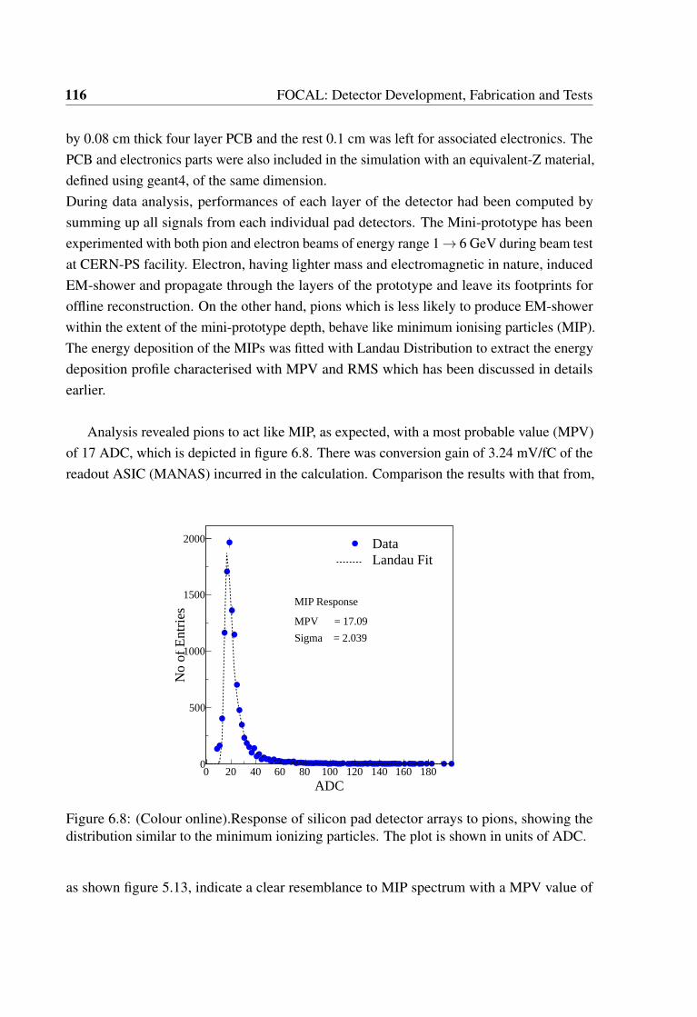
116 FOCAL: Detector Development, Fabrication and Tests

by 0.08 cm thick four layer PCB and the rest 0.1 cm was left for associated electronics. ThePCB and electronics parts were also included in the simulation with an equivalent-Z material,defined using geant4, of the same dimension.During data analysis, performances of each layer of the detector had been computed bysumming up all signals from each individual pad detectors. The Mini-prototype has beenexperimented with both pion and electron beams of energy range 1→ 6 GeV during beam testat CERN-PS facility. Electron, having lighter mass and electromagnetic in nature, inducedEM-shower and propagate through the layers of the prototype and leave its footprints foroffline reconstruction. On the other hand, pions which is less likely to produce EM-showerwithin the extent of the mini-prototype depth, behave like minimum ionising particles (MIP).The energy deposition of the MIPs was fitted with Landau Distribution to extract the energydeposition profile characterised with MPV and RMS which has been discussed in detailsearlier.

Analysis revealed pions to act like MIP, as expected, with a most probable value (MPV)of 17 ADC, which is depicted in figure 6.8. There was conversion gain of 3.24 mV/fC of thereadout ASIC (MANAS) incurred in the calculation. Comparison the results with that from,

MIP Response

MPV = 17.09

Sigma = 2.039

ADC0 20 40 60 80 100 120 140 160 180

No

of E

ntri

es

0

500

1000

1500

2000 DataLandau Fit

Figure 6.8: (Colour online).Response of silicon pad detector arrays to pions, showing thedistribution similar to the minimum ionizing particles. The plot is shown in units of ADC.

as shown figure 5.13, indicate a clear resemblance to MIP spectrum with a MPV value of

6.3 Mini-Prototype 117

83 keV.

On the other hand, from the earlier discussion about EM-shower formation and propaga-tion, electrons is supposed to produce electromagnetic shower within the Mini-prototype,limited by the truncated depth of the mini-prototype. However, the shower shape and energydeposition in each silicon layer has a significance in terms of optimising the granularityas well as transverse and longitudinal leakage of energy in the calorimeter. Figure 6.9provides the energy deposition of electromagnetic showers, produced after 2 XR depth, forthree different incoming electron energies. Experimental results anticipate that, although theshower profile is not so well developed for 1 GeV electron and resulted smeared Gaussian,however, with the increase in incident electron energy, the distribution approaches moretowards expected Gaussian profile. The mean of the distributions shifts steadily with incidentenergy, as shown in figure 6.9. Layerwise energy depositions were reconstructed for differentincident energies of the electron, added over pad element over a detector array, and plottedas a function of longitudinal depth from 1 XR to 6XR. Longitudinal profile for EM-shower,as shown in figure 6.10, describes the mean energy deposition as a function of longitudinaldepth within the extent of Mini-prototype. In this figure 6.10, with the increase of depth, thelayer-wise energy deposition for given incident energy increases at first and then reaches amaximum, known as shower-maximum where further secondary particle production stops.Going further deeper in the depth, the profile downturns because of no further productionof secondaries and the energy losses are mostly dominated by collision and ionisation. Thelimited depth of mini-prototype restricts the full longitudinal profile to be developed evenfor such lower incident energy range (1→6 GeV). In spite of that, the shower-max positionwas found to shift to larger depth with an increase in the incident energy of the particle. Theshower profiles observed in the experimental data are complementary to the simulation asshown in figure 6.11 and was quite encouraging towards making the full-depth calorimeter.The energy depositions, taking all possible combinations of absorber thickness and beamenergies, have been reconstructed and plotted with respect to that found from simulation, asshown in figure 6.12. The relationship, known as "conversion curve" with abscissa as energydeposition from simulated data and ordinate from experimental data, ensured a direct one toone harmonious relationships between data and simulation. In the absence of a calibrationcurve (limited by the lack of full energy reconstruction), it serves to study the linearitychecks of the prototype calorimeter. Moreover, because of limited incident energy range,it was difficult to check the extent of linearity over a wide range of energy. Even thoughindirectly, but conversion curve assures the functionality of the calorimeter working in thelinear domain safely. The electron data corresponding to each layer as well as the sum of

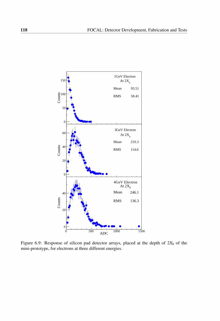
118 FOCAL: Detector Development, Fabrication and Tests

Mean 93.51

RMS 58.41

0 500 1000 1500

Cou

nts

0

50

100

150

Mean 93.51

RMS 58.41

1GeV Electron

0At 2X

Mean 210.3

RMS 114.6

0 500 1000 1500

Cou

nts

0

20

40

60

Mean 210.3

RMS 114.6

3GeV Electron

0At 2X

Mean 246.1

RMS 136.3

ADC0 500 1000 1500

Cou

nts

0

20

40 Mean 246.1

RMS 136.3

4GeV Electron0At 2X

Figure 6.9: Response of silicon pad detector arrays, placed at the depth of 2X0 of themini-prototype, for electrons at three different energies.

6.3 Mini-Prototype 119

)0

Longitudinal Depth (X1 2 3 4 5 6

Mea

n A

DC

100

150

200

250

300

350

400

1GeV

2GeV

3GeV

4GeV

Figure 6.10: (Colour online) The plots represent the longitudinal shower profile which hasbeen reconstructed from data using layer wise energy deposition of the incoming particleover a wide range of energy.

120 FOCAL: Detector Development, Fabrication and Tests

Figure 6.11: (Colour online) The plot shows longitudinal shower profile which has beenreconstructed using simulated data with all details of mini-prototype set-up included insimulation package.

6.4 Full-Depth prototype 121

Edep (MeV)0 5 10 15 20

AD

C

0

200

400

600

800

1000MIP Response

0At 2X

0At 3X

0At 4X(Sum Signal)

0After 2X

(Sum Signal)0

After 3X(Sum Signal)

0After 4X

Figure 6.12: (Colour online) Conversion curve which compare between energy depositionswithin the calorimeter prototype which were reconstructed using experimental data (ADC)and the energy deposition from simulated data (MeV).

signals from different layers is presented in reconstructing the conversion curve in figure 6.12.The data for MIP, is also superimposed on the same figure as shown by the solid red crossmarker. Linearity is observed over a wide range of energy depositions. A linear fit throughthe data points yields, ADC = 46.7×Edep +26, where Edep is expressed in MeV. The offsetis suspected to be contributed by electronics conversion and gain.

The success of the limited length mini-prototype test establishes "the proof for theworking principle" of the calorimeter in terms of responses to MIP and EM-shower. This,indeed, set guidance for improving and developing a full depth prototype calorimeter whichwill be discussed in the next section.

6.4 Full-Depth prototype

In this section, we will discuss the construction of a full-length prototype calorimeter alongwith a brief description of the newly developed read-out electronics. Details of the prototypearrangement and installation at H6 beam line at CERN-SPS will be presented. The resultsfrom test beam data analysis will also be illustrated with emphasis on the discussion. Like in

122 FOCAL: Detector Development, Fabrication and Tests

Figure 6.13: Experimental arrangement for the full-length Prototype with 19 layers ofsilicon pad detector arrays and tungsten plates along with all associated electronics for thetest at CERN-SPS.

earlier, we have compared the experimental data with that of simulation for the full-lengthprototype as well.

6.4.1 Fabrication and beam test

With a wealthy TEST-BEAM with mini-prototype, we have earned experience to improveand step forward to the next level of prototype building. The successor in this series ofprototype development was a full-depth (19XR thick for this case) calorimeter, as shown inthe figure 6.13, with silicon detectors and tungsten absorbers like earlier along with othercomponents like Stainless steel metal frame, Back-Plane PCBs, readout electronics, dataacquisition system etc. Unlike its miniature version, the detector layers, this time, is an arrayof 6×6 of dimension 1 cm× 1 cm× 300 µm silicon pad detectors on a single 4-inch n-typewafer.

6×6 silicon detector array: A new set of silicon detector array had been designed andfabricated for the full depth focal prototype. Unlike earlier, the detector array is now on asingle wafer, resembling toward the final requirement for the proposed FOCAL. Since thedetectors are supposed to work under extreme operating conditions like very high luminosityand radiation environment, it has been designed with high breakdown voltage to avoid anypossible polarity inversion which might occur due to constant operation. On the other hand,experiments in high particle density environment demand minimisation of dead area and fill

6.4 Full-Depth prototype 123

Figure 6.14: (Colour online) Sketch of the silicon detector array of dimension 6×6 made of1 cm2 silicon pad detectors which are fabricated on a single wafer and mounted on a detectorPCB.

factor improvement. Design of silicon PAD was accomplished with multiple guard rings,optimised inter-pixel separation for reduced cross-talk, improved fill factor etc. Alignmentsites were specifically designed and optimised for proper laser alignment of the stacked PADdetectors. The 6∗6 arrays of silicon PADs with 1 cm2 individual pixel size has been designedand developed with two different types of packaging options, firstly with conventional wirebonding and bump-bonding as a second option. The bump bonding is to be done using UnderBall Metallisation (UBM) technique which allows flip chip bonding and thereby enable 3Dpackaging. The highlight of the first design (wire bonding) was an interconnection and routingamong the individual PADs with a single metal. Careful routing ensured minimum crosstalkamong the PADs and also minimum dead area leading to maximum fill factor. An optimallyspaced multiple Guard Rings (GRs) and inter Guard Rings have been incorporated in thedesign to assure uniform field inside, high enough breakdown voltage and reduced surfaceleakage current. The fabrication of the detectors weas carried out on 300 µm thin n-type FZwafer with < 111 > crystal orientation. The starting resistivity of the wafer is 4-5 kΩ-cm.p n junctions were created by implanting p-type impurity from the top side. The fabricatedsilicon PADs are die-attached and mounted on a 0.08 cm thick four layer PCB followed bygold wire bonding to connect each pixel to PCB, as shown in following figure 6.14. Thedetectors were attached to the PCB with silver conductive epoxy of resistivity 0.006 Ω-cm.The fabricated and packaged detectors are then thoroughly tested in the laboratory. It hasbeen found that the detectors have less than 10 nA/cm2 with a breakdown voltage morethan 500 V. With a full depletion achieved around 60V, each PAD detectors showed about

124 FOCAL: Detector Development, Fabrication and Tests

45 pF/cm2→50 pF/cm2 detector capacitance. Each detector array was well wrapped withthin aluminium sheet and black paper against the EMI-protection.

SPS-H6 beam line: The beam test was carried out with H6 beamline at CERN-SPS [136].H6, a secondary particle beam, part of SPS North Area located in EHN1, can provide hadrons,electrons or muons of energies between 10 and 205 GeV/c, depending on H8-Beam condition.A 450 GeV/c typical primary proton beam with intensity 1012 per burst is extracted from theSPS and directed on the T4 primary target. The symmetry on the T4 target should be at least80% for proper operation. Among the three secondary beams that are derived from T4 target,H6 beamline was used for the present prototype experiment. As momenta and polarities ofthe three beams are strongly correlated, the H6 beam always runs at the polarity of H8 beamand typically up to about 50% of the momentum chosen in H8. There are three modes (Highresolution, High transmission and Filter Mode) of operation for the use of this H6 beamline. Filter-Mode of operation customarily serves the purposes for test-beam which can givedifferent types of particles with a wide range of particle energy in a range of 5→205 GeV/c.In addition, it has several possibilities to provide tertiary beams in case required.

Prototype at H6 beam line: Before commissioning at SPS beamline, a meticulous checkfor all the components both separately and after assembling, was done with full Dataacquisition in the laboratory. During the allotted time period, two consecutive prototypeset-ups were placed at the beamline with an option to move the front-set-up (prototypeunder consideration) away from the beam. Primarily at the beginning, 11 layers of detectorswere mounted in alternate layers with full absorber depth. After a successful test, the fullconfiguration with all 19 detector layers was installed. The first set of data was taken withMANAS ASIC (experimentally proved working with HEP experiment ALICE) as readoutelectronics. After completion of data taking for all available energies (5→120 GeV/c),the newly developed large dynamic range ASIC ANUSANSKAR was mounted for fewspecific layers. Details of the test results will be discussed in the results section afterwards.The detector array along with the PCB is interleaved between two 10 cm× 10 cm×0.03 cmtungsten plates in the prototype and connected to the ASICs through patch-bus cable eitherfrom one side or from the top of the mechanical frame, specially developed made of stainlesssteel for this purpose. Proper one to one detector alignment from layer to layer was takencare during assembling of the prototype calorimeter. Two types of readout ASICs, for theprototype test, were used (MANAS and ANUSANSKAR). However, an ANU(INDRA)used here is a modified version of it successor used during mini-protype test. In these

6.4 Full-Depth prototype 125

Figure 6.15: Schematic of the mechanical frame, designed and developed for the FOCALprototype, is made of stainless steel. There are four movable segments, each of which canaccommodate five detector and absorber layers. Option for electrical connections are keptboth from either side or the top of the frame.

19 layers of arrangement, detectors were distributed among five longitudinally movablesegments each with five layers in the mechanical arrangement as shown in figure 6.15. Thismovable segments can be adjusted such that another set of detector layers (e.g. HGL withMAPS) can be inserted at depth with multiple of five XR. It kept an option for a test withHybrid configuration with both LGL and HGL together. The prototype calorimeter wasscrewed firmly on a X-Y moving table (motor driven) taking z as the beam direction. This, inparticular, helped for any necessary alignment of the prototype with respect to the beam lineas well as keep provision for the experiment of another prototype behind it. During laboratorytests, there were few average/faulty PADs (channels) found for several detector layers anddocumented for any future reference. Proper positioning was maintained to allocate bestdetector layers around shower-max region, calculated for the available particle energy. Aschematic of the full-length structure with hierarchical positioning of each component isshown in figure 6.16. For the prototype experiment, the first detector frame starts at 2.4 cm

126 FOCAL: Detector Development, Fabrication and Tests

Figure 6.16: Schematic of the experimental setup for the full-depth prototype calorimeterwhich has been used at CERN-SPS. Different components of the experimental set -up areshown in the figure in a hierarchical order as positioned during the experiment.

away from the starting of the super base of the mechanical frame. All the PAD detectorswere biased with a common operating voltage 45 volt. Other relevant low voltages applied tobias the readout electronics used in the experiment are listed as following -

LV= (VDD,VSS,VCC) =(+2.5, -2.6, 3.3) V, with respect to Ground at 0 V.And 3.3 V for CROCUS and corresponding Currents I = (0.83, 1.05, 0.26)Amp respectively.

Trigger unit: A dedicated trigger system having X-Y scintillator and finger scintillatorwas used. A Cherenkov counter in the upstream was there at beam line in SPS for selectingelectron beams specifically. 3-fold (scintillator) trigger signal was used for π± or e−-datataking whereas a custom pulser signal feed during pedestal mode of data taking. A quickonline analysis of data sample was used for quality assurance and other relevant instantactions like proper alignment of the detector with a beam, beam quality and position ofthe prototype with the beam for better acceptance etc. For better referencing, the pedestalhas been taken before each and every data. As was expected a mere saturation effect wasfound for the higher side of the incident energies with MANAS ASIC because of its limiteddynamic range. The details of the test beam performances will be discussed in the nextsections.

6.4.2 Data analysis and performances

To start with the analysis of test beam data taken with the full depth prototype calorimeter,The first step could have been to study the combined response of noise both from detector andthe readout channel which was measured in absence of beam. The background, commonlyknown as pedestal response, of the system for each detector channel in terms of mean andRMS of noise for the respective channel is shown in figure 6.17. Each 32 channel correspondsto a particular detector layer along the depth of the calorimeter. The mean was found about250 ADC and is stable with time. The RMS (representing the noise) is found between 1.5

6.4 Full-Depth prototype 127

0 200 400 600 800 1000 1200 1400

Ped

esta

l Mea

n (A

DC

)

210

310

410

Mean ADC for each detector channel for all 20 layers.

1 Layers≡32 Channels

Channel Number0 200 400 600 800 1000 1200 1400

Ped

esta

l RM

S (

AD

C)

2−10

1−10

1

10

210

310RMS for each detector channel for all 20 layers.

Figure 6.17: (Colour online). The figures show response of silicon pad detector in terms ofthe mean (upper) and RMS (lower) values of the pedestal as a function of electronic channel.Each 32 channels corresponds to one layer of the prototype calorimeter. In RMS plot, sharpdrop to zero represent dead channels which was taken care during offline analysis.

128 FOCAL: Detector Development, Fabrication and Tests

(ADC)measuredE0 50 100 150 200 250 300 350

Num

ber

of E

vent

s

0

50

100

150

200

250

Response of 120 GeV Pion

Data

Landau Fit

2.5±MPV = 18

Figure 6.18: (Colour online). The plot shows the ADC distribution for pions as reconstructedfrom the prototype test data. The distribution reproduce the minimum ionising particlesresponse.

to 2.5 ADC. Some fluctuations, however, have been found in RMS plot for few particularchannels with either RMS shooting up (noisy channels) or to some larger value or touchingzero (dead channels). Ideally, the dead and noisy channels should be counted during analysis.In our case, for counting of the signal of EM showers, these channels are assigned ADCvalues which are average of its adjacent channels.

The test beam results have been reconstructed and compared both with earlier mini-prototype test results and simulation for the sake of consistency. With SPS this time, theresponse and characterisation of the prototype could be accomplished much more elaboratelywith a wide range of available incident energies for different incoming particles, Undoubt-edly, particles with relativistically high energy deposit minimum amount of energy, as wasprescribed by Bethe-Bloch formula [137] and can be described by Landau distribution [130].Depending on the detecting medium and associated electronics, the Most Probable Value(MPV) of the Landau-distribution fitted to the experimental data was extracted. Pion beamsat an incident energy of 120 GeV were used to obtain the MIP energy deposition. Theresponse of silicon PADs at 2nd layer (after 2XR depth) is shown in figure 6.18 in termsof the ADC values. The data is fitted well with a Landau distribution and provides mostprobable value (MPV) of 18±2.5 in units of ADC in compare to earlier results of 0.083 MeV

6.4 Full-Depth prototype 129

from simulation ( 5.13) and 17.09±2.03 ADC in CERN-PS test beam 6.8. The response forMIP was studied in earlier test beam with bare silicon pad detectors without any absorberplate in front [120]. The MPV of the ADC spectrum obtained in the present study is similarwithin the error bar. Though the measurement was taken with a 2XR material placed in frontit hardly matters for the minimum ionising particle. A clear MIP signal for the calorimeterassures a better Signal to Noise ( S

N ) discrimination capability.

An electromagnetic shower is originated either by bremsstrahlung or pair production,depending on the incident particle e− or γ , and continues to grow along the depth till itreaches the critical energy (EC(MeV )) and then dissipates mostly by collision/ionisationprocesses. However as is discussed already, EM-shower from heavier particles like pions,protons etc. are less likely though there is a probability of hadronic-shower production. ButHadronic shower will start seldom within the extent of the present calorimeter depth. Awide range of incident energy for inflowing electron starting from 5 GeV to 60 GeV wasused to characterise the full-depth prototype calorimeter to EM-shower. The shower shapein terms of energy deposition in each layer has been studied to understand the developmentof EM-shower both in longitudinal and transverse directions. This has been obtained bysumming deposited energy in the unit of ADC for individual silicon PADs of each layer. Fora particular incident electron energy, a number of silicon PADs are hit in each layer whichis facing the transverse plane of the propagating shower. The deposited energy in all PADsof each layer are summed to obtain the total energy deposited in the particular layer. As anexample, the summed energy deposition in units of ADC for the 7th layer of the prototypecalorimeter is presented in figure 6.19 for six different incident energy electrons, 5, 20, 30,40, 50 and 60 GeV respectively. The abscissa gives the total measured ADC, whereas theordinate is expressed in terms of probability where the counts are normalised to the numberof total events in each individual case. All the measured energy spectra are of Gaussian shapewith the mean value shifted towards the right with an increase in incident energy. Theseresults are used later on to obtain longitudinal shower profile, total energy deposition andenergy resolution of the detector which will be discussed shortly.

As already shown in the previous section and discussed in details in [107], energydeposition profile, as a function of layer number (depth in the unit of XR), first rises to achieveshower-maximum and then falls gradually. For the full depth prototype under consideration,19 XR thickness is enough to let the EM-shower develop completely for 5→60 GeV electronwith nominal longitudinal leakage. The longitudinal profile reconstructed from data is fittedwith the same empirical formula dE

dXR= E0 ∗ ta ∗ e−b∗t with E0 as incident energy and "t"

as thickness in unit of radiation length and shown in figure 6.20. A detailed analysis of

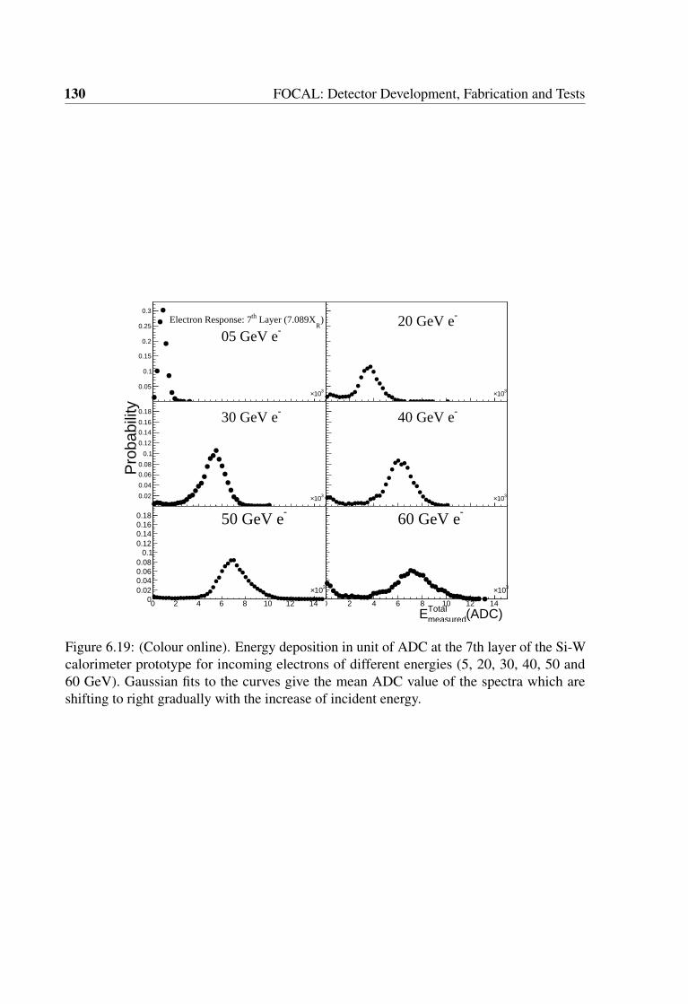
130 FOCAL: Detector Development, Fabrication and Tests

0 2 4 6 8 10 12 14

310×0.05

0.1

0.15

0.2

0.25

0.3

-05 GeV e)

R Layer (7.089XthElectron Response: 7

(ADC) TotalmeasuredE0 2 4 6 8 10 12 14

310×

Pro

babi

lity

0.02

0.04

0.06

0.08

0.1

0.12

0.14

0.16

0.18 -30 GeV e

0 2 4 6 8 10 12 14

310×0

0.020.040.060.08

0.10.120.140.160.18 -

50 GeV e

0 2 4 6 8 10 12 14

310×0.05

0.1

0.15

0.2

0.25

0.3 -20 GeV e

(ADC) TotalmeasuredE0 2 4 6 8 10 12 14

310×

Pro

babi

lity

0.02

0.04

0.06

0.08

0.1

0.12

0.14

0.16

0.18 -40 GeV e

(ADC) TotalmeasuredE

0 2 4 6 8 10 12 14

310×0

0.020.040.060.08

0.10.120.140.160.18 -

60 GeV e

Figure 6.19: (Colour online). Energy deposition in unit of ADC at the 7th layer of the Si-Wcalorimeter prototype for incoming electrons of different energies (5, 20, 30, 40, 50 and60 GeV). Gaussian fits to the curves give the mean ADC value of the spectra which areshifting to right gradually with the increase of incident energy.

6.4 Full-Depth prototype 131

)R

Layer Number(X0 2 4 6 8 10 12 14 16 18 20

Mea

n A

DC

0

2000

4000

6000

8000

marker ==> Data

)-bt*ea*t0

(ADC = E

05 GeV20 GeV30 GeV40 GeV50 GeV60 GeV

Figure 6.20: (Colour online) The figure illustrates the longitudinal shower profile which hasbeen reconstructed using experimental data from full depth prototype test at CERN-SPS.

the longitudinal profile of EM-shower upto 40 GeV can reproduce the trend quite well aspredicted by the empirical model but for higher energies, a flat region instead of a peak hasappeared. The discrepancy at higher incident energies is suspected to be because of thelimited dynamic range (lead to saturation in energy measurement) of the front-end-electronics(MANAS ASIC) used in the experiment. To have a comparative picture, response to electron-induced shower by the full prototype as a whole has been plotted in figure 6.21. Total energydeposition in the calorimeter is obtained by summing the deposited energies of all siliconPADs of all detector layers. Distribution of total measured energy in the unit of ADC over alarge number of events represents the response of the incident electron. Figure 6.21 explainsthe behaviour of total measured energy for six incident electron energies. Gaussian shapeshave developed at each energy and the distributions are well separated from each other.Peaks corresponding to different incident energies shift to the right with the increase ofincident energy. Minor distortion has been found for 50 and 60 GeV electrons and expectedto be attributed to the limited dynamic range of the readout ASICs, mixing of the hadronicshower in EM-shower or late produced γ by strong interaction within the calorimeter depth.Moreover, a slight bulging has been observed for 50 GeV electron which might arise becauseof contamination of low energy electrons. To be a decisive energy measuring instrument, thecalorimeter should ensure linearity between incident energy and the respective measured

132 FOCAL: Detector Development, Fabrication and Tests

(ADC)measuredE0 20000 40000 60000 80000

Prob

abili

ty

0.02

0.04

0.06

0.08

0.1

0.12

0.14

0.16Response of Electron

05 GeV20 GeV30 GeV40 GeV50 GeV60 GeV

Figure 6.21: (Colour online). The plot shows the distribution of total energy deposition asmeasured by the full depth prototype calorimeter. The energy is expressed in unit of ADC asshown in the X-axis of the figure.

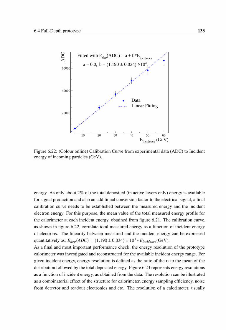
6.4 Full-Depth prototype 133

(GeV)incidenceE10 20 30 40 50 60

AD

C

20000

40000

60000

incidence(ADC) = a + b*EdepFitted with E

a = 0.0, 310× 0.034) ±b = (1.190

DataLinear Fitting

Figure 6.22: (Colour online) Calibration Curve from experimental data (ADC) to Incidentenergy of incoming particles (GeV).

energy. As only about 2% of the total deposited (in active layers only) energy is availablefor signal production and also an additional conversion factor to the electrical signal, a finalcalibration curve needs to be established between the measured energy and the incidentelectron energy. For this purpose, the mean value of the total measured energy profile forthe calorimeter at each incident energy, obtained from figure 6.21. The calibration curve,as shown in figure 6.22, correlate total measured energy as a function of incident energyof electrons. The linearity between measured and the incident energy can be expressedquantitatively as: Edep(ADC) = (1.190±0.034)×103 ∗Eincidence(GeV).As a final and most important performance check, the energy resolution of the prototypecalorimeter was investigated and reconstructed for the available incident energy range. Forgiven incident energy, energy resolution is defined as the ratio of the σ to the mean of thedistribution followed by the total deposited energy. Figure 6.23 represents energy resolutionsas a function of incident energy, as obtained from the data. The resolution can be illustratedas a combinatorial effect of the structure for calorimeter, energy sampling efficiency, noisefrom detector and readout electronics and etc. The resolution of a calorimeter, usually

134 FOCAL: Detector Development, Fabrication and Tests

(GeV)0E10 20 30 40 50 60

/Eσ

0

0.05

0.1

0.15

0.2

0.25

Data

Fit function

Figure 6.23: (Colour online) The figure presents the energy resolution as a function ofincident energy of incoming electrons from experimental data. The data resulted resolutionexpressed with a = 0.053± 0.005 and b = 0.221 ± 0.036 which has been obtained from the

fitting withσ

Edep= a⊕ b√

E0over the incident energy range of 5→ 60 GeV .

6.5 Summary and Scope 135

parametrised in terms of an empirical formula [105]

σ

Edep= a⊕ b√

E0, (6.1)

where, a and b are fit parameters, carrying definite physical importance. Fits to the datapoints yield, a = 0.053±0.005 and b = 0.221±0.036, which can be considered to quote theenergy resolution for the prototype under consideration. However, for sake of completeness,a different empirical formalism as expressed by following equation [105],

σ

Edep= a⊕ b√

E⊕ c

E0, (6.2)

is also applied to understand the resolution. Here, the first term takes into account thecontributions from the compactness of the calorimeter, the second term arises because ofthe schotasticity of the signal production process and the third term is related to the noise.Fits (not shown in the figure) using this formula, yields, a = 0.061±0.008, b = 0.085±0.04and c = 0,48± 22. If a part of the contribution to the energy resolution is accounted forelectronic noise, this formula gives the contribution to the resolution of about 8.5% by

the1√E

contribution which ensures the calorimeter to be as one of the best in its class.

However, to be noted, the last two points (corresponding to 50 and 60 GeV) are sittingaway from the trend. The reason might be partial because of the saturation effect of thereadout electronics and due to shower leakage which might have worsened the resolution.In conclusion regarding the text beam experience for FOCAL prototype, the results, indeed,support the construction according to the conceptual design for the calorimeter, a feasiblesolution as well as the experimental ground for developing full-scale calorimeter in future.

6.5 Summary and Scope

Summarising in brief, the development, fabrication and test of a series of prototype calorime-ter, starting from mini-prototype to full length, for proposed FOCAL have been discussed inthis chapter. In short, mini-prototype establishes the proof of working principle for FOCALin terms of basic calorimetric performances even with the limited depth. Reconstruction ofresponses for minimum ionising particle and EM-shower were described and discussed inregard to detector construction and characterisation. A full-depth silicon-tungsten prototypecalorimeter, as a successor of a Mini-prototype, has also been fabricated and assembled totest at CERN-SPS beamline facility. Details of the construction of the prototype along withits each and every component were presented and discussed. The prototype consisted of

136 FOCAL: Detector Development, Fabrication and Tests

nineteen layers of silicon PAD detector arrays (on a single 4 inch n-type wafer) and severaltungsten layers extending the effective depth of the calorimeter to be about 19 XR . ThePrototype has been tested with 120 GeV pion and 5 to 60 GeV electron. The response of theprototype calorimeter to both MIP (pions) and EM-shower (electrons) has been reproducedand analysed. Clear development of the MIP signal shows an excellent S/N ratio. Widelyseparated EM-shower signal for different energies in the available energy range establisheda very good energy resolution of about 8.5% with three parameter fit. Linear behaviour ofmeasured energy with that of incident energy ensures satisfactory calorimetric performances.Though an issue with saturation due to readout electronics was found but has been taken careof, with the development of a new large dynamic range ASIC as a next step for the calorimeterdevelopment. The development of the silicon detectors for the proposed calorimeter can besummarised pictorially by the following sketch 6.24 Because of the saturation effect found athigher energies of incident particle, a serious effort was put in developing dedicated readoutelectronics. A series of efforts are already in action. ANU chip with the help of BARC hasreached a satisfactory level to handle such requirements of large dynamic range electronics.ANUSANAKAR have already been tested in this series but it has limited dynamic range aswell but helped a lot in understanding the next level development. ANUINDRA on the otherhand, the latest ASIC developed, have a dynamic range of 2.6 pC compared to its earlierversion of 600 fC. Laboratory test results of the chip found to be hopeful in fulfilling therequirement. As a next check, another test with the upgraded electronics was put as next aimshortly.

In continuation of the physics motivation behind the proposed calorimetry for ALICE,we have studied the particle production in proton-proton collision at LHC energies whichotherwise treated as baseline/reference for understanding particle production in heavy ioncollision. In our study, particle production in pp collision found to have origin both fromsoft and hard scattering process. Moreover, probing the system produced in pp collision atLHC energies, revealed unexpected collectivity for high multiplicity events. As a naturalconsequence, pp collision, as a reference for heavy-ion collision, need to be used carefully.The details about particle production in terms of two-source model (NBD), search forcollectivity in pp system with blast-wave model approach will be discussed rigorously inthe next chapter. Moreover, a search for signal related to the degrees of freedom, governingthe system formed in pp collision, has been formulated using Bjorken prescription. Thedetails about Bjorken energy estimation for pp system will also be presented to understandthe nature of collectivity (hadronic/partonic) found in small systems.

6.5 Summary and Scope 137

Figure 6.24: A series of detector development starting from the 1 cm2 physically isolateddetectors to 6× 6 array of 1 cm2 on a single 4 inch wafer shown. The proposed finalrequirement for detector also shown in the sketch.

Chapter 7

High Multiplicity Proton-Proton Physics

7.1 Introduction

With the increase of incident energy of probing particles, the experimental techniques,mostly following Rutherford technique as is represented in equation 7.1, evolved at a steadypace to render physics interests starting from material science to finest structural conceptsconsist of coloured partons [8]. With the advancement of accelerator technology, collimatedTera electron Volt (TeV) energy is now a day available for an experiment in compare toearly days naturally available MeV energies. The finer structure of nucleus and nucleonscan be investigated to a length scale of femtometer following the de’Broglie hypothesisof wave-particle duality, as shown in table 7.1, where sub-nucleonic elements like quarksand gluons become relevant degrees of freedom. Depending on the available energy ofscattering/collision and the choice of system, the physics reach could be of a different kind.for proton-proton, proton - heavy ion and heavy ion - heavy ion collision. Proton-protoncollision illuminates the basics of hard scattering among partons whereas, nucleus-nucleuscollision revealed the properties and evolution of a system which might have formed duringthe collision. The system formed in the nucleus-nucleus collision indicates the formationof a quark-gluon plasma state, as has been discussed in Introduction. Characterisation andquantification of various properties of the Quark-Gluon-Plasma (QGP) need a clean baselineunderstanding which is provided by proton-proton (pp) collision at the same energy. BeforeLHC era, pp collisions was strongly endorsed to yield particles which are the outcome ofhard-scattering between partons followed by hadronisation. However, increase in centre-of-mass energy for pp collision, new speculation noticed regarding the behaviour of the systemassociated with a large number of particle production which could not be explained only byhard-scattering and found mimicking phenomenon more similar to heavy-ion-collision onsmall scale.

140 High Multiplicity Proton-Proton Physics

More specifically, a class of events (known as High Multiplicity (HM) events) in pp-collision was found which are found responsible in deviating pp system from its so farunderlying nature. There are plenty of descriptions, such as hydrodynamic model, saturationmodel (Colour Glass Condensate: CGC) [40–46], Colour Reconnection (CR) model et.c,available in the literature [102–104] in understanding this anomalous aspect in pp collisions.Of course, no single model description can uniquely explain the phenomenon HM pp collisionand associated with advantages and inadequacies of their own. In the present study, we willfocus towards a hydrodynamic inspired model description for pp collision at LHC energies.Even though there can not be a smoking-gun signal/explanation till date to have a conclusivedescription, but it has been found that the particle production mechanism in pp collision iscontributed by soft scattering and hard scattering partially which become more prominent atLHC energies. Not in all, rather pp events tagged with high multiplicity, demand for a newinterpretation away from underlying physics interpretation. In the subsequent sections, first,a NBD model-based approach will be adopted to elucidate on probably more than one typeparticle production mechanism in pp collision. The understanding of the system formed inpp collision was studied using Blastwave model which assumes collectivity for the systemunder study. A positive search for collectivity in pp system appeals for harvesting the sourcefor collectivity. In the last section in this chapter, an effort was made to understand thecollectivity either coming from a partonic or hadronic form of matter using simple Bjorkenformalism [138]. The study will be wrapped up with further possibilities and future scope inthis direction.

(dσ

dΩ

)=

(zZe2

2µv2

)2 1

sin4 θ

2

. (7.1)

where µ → reduced mass, θ → scattering angle

7.2 Review and motivation of proton-proton physics

At ultra-relativistic high energies at LHC, proton-proton collision predicted the existenceof long-awaited Higgs boson [10, 11], responsible for mass generation. On the contrary,pp collision serves more orderly in understanding each aspect of partonic interaction interms of particle production. When a proton approaches a proton relativistically, constituentpartons from both the proton interact strongly among themselves which is calculable usingeither perturbative Quantum Chromodynamics [139–141] or by non-perturbative model

7.2 Review and motivation of proton-proton physics 141

Table 7.1: An overview of the dimension that can be probed with proton and electron ofdifferent beam energies using de’Broglie hypothesis.

Energy λ proton(fm) λ electron (fm)

1 MeV 28.6137 871.920710 MeV 090268 118.0961

100 MeV 02.7888 12.33561 GeV 00.7310 01.2392

10 GeV 00.1138 00.1239100 GeV 00.0123 0.01239

1 TeV 00.0012 0.31–

7 TeV 00.0002 –

calculation depending on momentum transfer scale involved in the interaction. Eventually,scattered partons, can not stay in the coloured state due to colour confinement, will leadto various colourless particles like pion, kaon, proton, neutron and so on at the final stage.There exists models explaining hadronisation mechanisms (more popularly known as Frag-mentation Function, FF) such as recombination [142–147], jet fragmentation [148–152]etc. Assuming factorisation [153], particle production in pp collision can be estimated usingparton distribution, interaction cross-section and fragmentation function respectively. Tillvery recent breakthrough of High Multiplicity (HM) events in pp collisions [156], where anunexpectedly large number of particles has been produced as shown in figure 7.1, pp collisionwas essentially served baseline for more complex systems produced in heavy ion collisions(AA). The properties of a collective system produced in heavy ion (AA) collisions could berepresented by a simple ratio, as is represented in equation 7.2. The particle production inAA collision can be scaled by the number of particles produced in pp collision along witha normalisation factor, defined by the number of the binary collision. Nevertheless, therehad always been a different approach [157, 158, 71, 159] nourished which advocate for thepossibilities of AA-like system on a small scale for pp collision as well. Early in SPS age, ppevents in experiments [160, 161] impelled for the occurrence of high energy density eventsand an inspired quest for evidence of de-confined medium in pp collisions even at

√S = 0.54

TeV at SPS [157] and at√

S = 1.8 TeV [158, 71] at Tevatron, Fermilab.

142 High Multiplicity Proton-Proton Physics

Figure 7.1: (Colour online). The plot shows the measured multiplicity density both byALICE [154] and CMS [155] for proton-proton collision at

√S =7 TeV. The value for

the multiplicity density for pp collision reach to a limit where the possibility of mediumformation is predicted energetically.

7.2 Review and motivation of proton-proton physics 143

Figure 7.2: (Colour online). Ridge, structure found for particle correlation in ∆η−∆φ plane,attributed to hydrodynamical description in case of heavy-ion collision, has been found alsoin proton-proton collision recently.

Scaled Particle production in AA-coll =(

dNdPT dydφ

)AA

N(dN

dPT dydφ)pp

. (7.2)

Studies of properties of final state particles, produced either in pp or in AA collision, areaddressed and compared experimentally in terms of definite global variables [162, 163]like transverse momentum (pT ) distribution, Pseudo-rapidity (η) distribution, Multiplicitydistribution etc and few more derived physics observables such as flow components, Nuclearshadowing, Double ratio, ridge etc. The pp collisions at LHC energies have resulted ina number of unexpected observations, mimicking on a small scale to the signals for ahydrodynamic system formed in relativistic heavy-ion collisions.In the present context of the study, Particle production in pp collision at LHC energieshas been reinstituted using otherwise established model descriptions. There are recentphysics observations in pp collision at LHC such as "ridge" [164] 7.2 in HM-pp eventswhich strengthen the possibility of poking for AA-like system. Ridge, a structure found

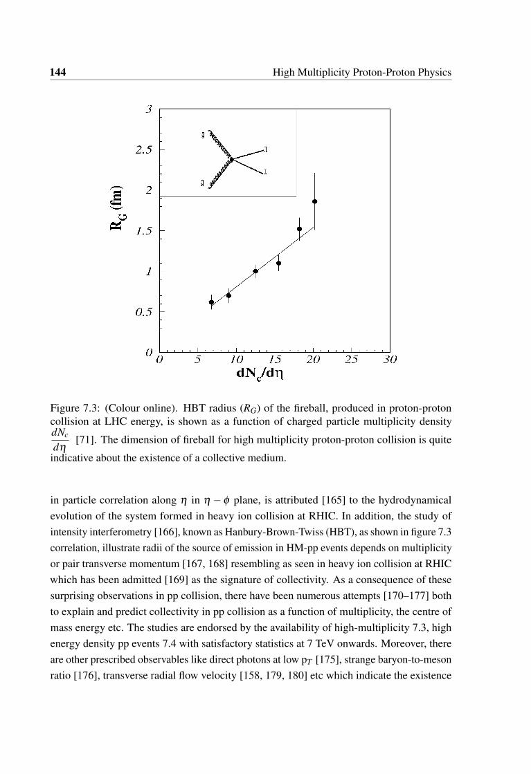
144 High Multiplicity Proton-Proton Physics

Figure 7.3: (Colour online). HBT radius (RG) of the fireball, produced in proton-protoncollision at LHC energy, is shown as a function of charged particle multiplicity densitydNc

dη[71]. The dimension of fireball for high multiplicity proton-proton collision is quite

indicative about the existence of a collective medium.

in particle correlation along η in η − φ plane, is attributed [165] to the hydrodynamicalevolution of the system formed in heavy ion collision at RHIC. In addition, the study ofintensity interferometry [166], known as Hanbury-Brown-Twiss (HBT), as shown in figure 7.3correlation, illustrate radii of the source of emission in HM-pp events depends on multiplicityor pair transverse momentum [167, 168] resembling as seen in heavy ion collision at RHICwhich has been admitted [169] as the signature of collectivity. As a consequence of thesesurprising observations in pp collision, there have been numerous attempts [170–177] bothto explain and predict collectivity in pp collision as a function of multiplicity, the centre ofmass energy etc. The studies are endorsed by the availability of high-multiplicity 7.3, highenergy density pp events 7.4 with satisfactory statistics at 7 TeV onwards. Moreover, thereare other prescribed observables like direct photons at low pT [175], strange baryon-to-mesonratio [176], transverse radial flow velocity [158, 179, 180] etc which indicate the existence

7.2 Review and motivation of proton-proton physics 145

Figure 7.4: (Colour online). Theoretical prediction for initial energy density (εini), tempera-ture (Tini) and pressure (pini) as a function of multiplicity of produced particles in pp collision[178] at 7 TeV centre of mass energy.

146 High Multiplicity Proton-Proton Physics

Figure 7.5: (Colour online). Theoretical prediction for the temperature of the fireball formedin small system like in proton-proton as a function of the size of the fireball [186].

of collectivity in a system. Further, significant theoretical approaches [181–183] supportthe applicability of relativistic hydrodynamics specifically for high multiplicity pp eventsassuming formation of a non-hadronic medium [181] which is 7.4 energetically possible inpp collisions at LHC energies.

A recent calculation shows that because of approximate scale invariance of sQGP, AA-like hydro can be expected in a smaller and hotter system like in larger and cooler systemas explained in figure 7.5 [179]. A pertinent study [184] in search for the change in phasefrom hadronic to partonic in pp collisions, analysing a wide range of centre-of-mass energy,includes the LHC data also. Though a steady and substantial effort made to promote theliquid dynamical behaviour [173, 174] as a manifestation of the de-confined state of quarks,there has been other pictures available in literature such as colour glass condensate [185],colour reconnection [102–104] etc.

Primarily, relative flattening of the pT spectra of identified particles of higher masses inpp collisions at LHC, as observed by the CMS (ref BW 31, 34), encourages to search forpossible collective transverse radial flow in pp collisions at LHC. It is relevant in this context

7.3 Framework and models used for pp physics 147

that flattening of pT -spectra of particles of heavy masses is attributed to the existence of acommon transverse radial flow velocity and studied in heavy ion collisions starting fromSPS to RHIC to LHC. Since LHC has potentially delivered centre of mass energy up to 14TeV, the high-multiplicity events populated more frequently and extend the chance to achievehigher multiplicity classes more and more. Though not yet decisively established whetherQGP has been formed in the proton-proton collision or alike small systems but it has openeda new area taking pp collisions more seriously than just for baseline studies.

7.3 Framework and models used for pp physics

In this section, we will discuss different models and frameworks those will be used for thisstudy of particle production in the pp collision.

7.3.1 Negative Binomial Distribution (NBD)

Long back in 1713 [187], Jakob Bernoulli determined the probability of "k" outcomes inan "n" trials with the help of Binomial expression as expressed in equation 7.3. Since then,Binomial Distribution (BD) had been used abundantly and extensively in almost every field ofscience to understand and predict relevant properties of the system. Ideally BD, in the theoryof probability and statistics, represents discrete distribution having two possible outcomes(true/false, yes/no, success/failure etc). The limiting condition for BD with a number of trialequal "1" is Bernoulli distribution.

Pr(k;n, p) =(n

k

)pk(1− p)n−k, (7.3)

where "k" runs from 1, 0 . . . n and(n

k

)= n!

k!(n−k)! and p represents the probability of kth

outcome. There can be several restrictions/conditions which can twist the BD to take a newform of distribution and make it usable for application to physical problems. For an example,the probability of the number of successes in a sequence of independent and identicalBernoulli trials before a specified number of failures (denoted by "r") can be represented byNegative Binomial Distribution (NBD). It can be expressed according to the equation 7.4

Pr(n,,k)=Γ(k+n)

Γ(k)Γ(n+1)

[n

k+ n

]n [k

k+ n

]k

. (7.4)

148 High Multiplicity Proton-Proton Physics

Where n is the average of the distribution and the parameter k can be related to the dispersion(D: D2 = n2− n2) as following

D2

n2 =1n+

1k. (7.5)

In the present study, the Negative Binomial Distribution was used to understand multi-particle production in a relativistic proton-proton collision at LHC energies. Historically,particle production in either many baryonic or semi leptonic processes at relativisticallyhigh energies, Negative Binomial Distribution (NBD) found to describe particle productionfor both total multiplicities and for a restricted interval in phase space [188]. Though notyet clear about the applicability of NBD in explaining the multi-particle production, therewere several attempts to understand the physical explanation behind it. The first appealingexplanation by Van Hove and Giovannini was in 1987 with the introduction of clans ofparticle production [189, 190]. It had been shown that NBD is a natural outcome for cascadeprocesses with particles, produced from independent clans. Moreover, though there are alsoattempts in understanding particle production in terms of Poisson distribution (assumingevery single final state particle produced and emitted independently) which is again a limitingcase of more general NBD where mean and variance of the distribution are same. In thisconnection, a very recent theoretical approach [191], Glasma flux tube model, has found themultiplicity distribution of multi-particle production could be interpreted as a convolutionof a number of NBD functions which comes as a natural consequence of several impactparameters of the collisions. The model replicates the multiplicity distribution data of ppcollisions in a small pseudo-rapidity window (∆η < 0.5) at the LHC energies. It is importantto mention that Poisson distribution or NBD in explaining multi-particle production in proton-proton collision is justifiable in lower pT range where pQCD has limitation introduced byrunning coupling constant for strong interaction. The lack of a unique theory to explain theparticle production for pp collision over the whole energy range demands phenomenologicalmodels for low energy region to pQCD in high energy regime. There have been severalstudies interpreting proton-proton data at the different centre of mass energies right fromSPS to RHIC to LHC consistently. NBD, an one such successful model description, hadsufficiently described charged particle "multiplicity distributions" in proton-antiproton (pp)collisions at S = 540 GeV at SPS [192] at CERN both for full and limited pseudo-rapidity(η) space intervals. But with the increase in the centre of mass energy, a single NBD is foundnot enough to represent the pp multiplicity distribution for full rapidity intervals but stillcan explain for small rapidity interval satisfactorily as is established by SPS for 900 GeVpp collision. Multiplicity distribution starts building substructures in it with an increase in

7.3 Framework and models used for pp physics 149

the centre of mass energy which can not be described by a single NBD. There had beena proposal and successful implementation of weighted superposition/convolution of morethan one function including NBD [193–196] to illustrate the pp data with an assumption foreach individual function representing a different mechanism for particle production. Such asubstructure in multiplicity distribution found for pp collision at 900 GeV at SPS and 1800GeV at Tevatron [197], was explained by a function convoluted from two NBDs as shown inequation 7.6.

Pn(√

s,ηC) = αso f t(√

s)Pn[nso f t(√

s,ηC),kso f t(√

s,ηC)]

+[1−αso f t(√

s)]Pn[nsemi−hard(√

s,ηC),ksemi−hard(√

s,ηC)],(7.6)

where αso f t is the fraction of "soft" events and is a function of√

s only. The other parametersare bearing their usual meaning, as has already been discussed, for single NBD function.Significantly, particles, produced in pp collision, are differentiated with respect to theirprobable production sources as is mentioned in the equation 7.6 by "soft" and "semi-hard"respectively. Even if not possible to isolate particles of different production mechanisms, butstill, it serves the existence of multi-mechanism particle production even at pp collision atsufficiently high centre of mass energy. According to the two-component model [194], themultiplicity distribution is a convolution of two classes of events, "semi-hard with mini-jetsor jets" and "soft events without mini-jets or jets". It is very much relevant here to mentionthat there is an expectation for further modification to multiplicity distribution for particlesproduced in pp collision with further increase in the centre of mass energy like in LHC. Aframework of the weighted superposition of NBDs representing different classes of events hasbeen extended from the two-component to a three-component model in a recent study [198]with an expectation of a new physics at the LHC at s=14 TeV. The additional componentin the three NBD function is attributed to a new class of high multiplicity events, whichappeared as an elbow structure in the tail of multiplicity distribution of the pp collisions atthe highest LHC energy.

7.3.2 Blast Wave formalism (BW)

A blast wave (BW) is, in general, originated as increased pressure and flow from large energylocalised in a very small volume in space. The flow field can be described in terms of aleading shock wave followed by a "self-similar" subsonic flow. In other ways, the leadingshock wave expands supersonically from an explosive core (source) and always associatedwith a blast wind with a negative pressure which gulps things around back towards the

150 High Multiplicity Proton-Proton Physics

core [199]. Historically, the flow solution for the blast wave came during World War IIby John von Neumann [199, 200] and Geoffrey Ingram Taylor [201, 202] independently.Shortly there was a similar effort for blast wave by three other people L. I. Sedov [203],R. Latter [204], and J. Lockwood-Taylor [205] respectively. Friedlander waveform [206],simplest representation for the blast wave, is one among available solutions depending onboth theoretical and experimental approaches and can be expressed as shown in equation 7.7

Pt = Ps e−t

t∗ (1− tt∗). (7.7)

where Ps is the peak pressure and t∗ is a characteristic time which represents the interval afterwhich the pressure drops to zero for the first time. In the beginning, the relevance to blastwave was restricted to understand the effects after the explosion and associated predictionswhich made the domain bounded within military applications only. Soon after, the essenceof blast wave model understood in much more broader sense and extended to various field ofscience and engineering like calculation of blast load during building designing, outcomeof supernova explosion in astronomy and more recently to the field of relativistic heavyion collision to understand the evolution of a system mimicking the evolution of universein small scale. In the present study, our aim is to understand the proton-proton data atLHC energy applying blast wave model. Understanding the system produced in a hadroniccollision with blast wave description started long back in 1992 by Ekkard Schnedermannnet al [157]. They have developed a phenomenological model assuming thermalisation asthe basic criteria and applied to data successfully measured in central collisions of Sulphur-Sulphur at

√s =200 GeV/A from the NA35 Collaboration at CERN. Taking collectivity into

account, the model could describe almost all hadronic spectra. The success of the modelexplored a new technique in probing and extracting information for the system produced inthe hadronic collision. In the subsequent section, we will be dealing blast wave model thathas been introduced in ref [157] which can be expressed in terms of mT−spectra as shown inequation 7.8

dNmT dmT

∝

∫ R

0r dr mT I0

(pT sinhρ

T

)K1

(pT coshρ

T

), (7.8)

where ρ = tanh−1(β ) with β represents flow velocity. I0 and K1 represent modified Bessel’sfunctions. The transverse flow velocity distribution β (r) in the region 0 ≤ r ≤ R by aself-similar profile, parametrised as 7.9

7.3 Framework and models used for pp physics 151

β (r) = βs( r

R

)n, (7.9)

with βs as surface flow velocity and( r

R

)stands for relative radial coordinate of the collective

system. Using the above formulation, the average transverse flow velocity can be calculated

and found to be β =(

22+n

)βs. It is important to note that the above formulation has

some basic assumptions like a) hard-sphere particle source, b) The source must be locallythermalised, c) there must exist a common outward transverse velocity (collective radialflow velocity), d) Particles undergo instantaneous common freeze-out, e) There exist acommon kinetic freeze-out temperature. Blastwave description of experimental data givestwo important physical parameter β and TKin respectively for the collectively evolving system.To note, TKin, extracted from the BW-fitting to data is not the actual temperature of the system,rather it is a combined effect from both temperature and kinematics of the system and can berepresented as TKin = T + f (β ).

As has been discussed already, blast wave formalism is not developed from 1(st) principle,rather it is a hydrodynamic inspired model taking Boltzmann-Gibbs entropy into accountwhich has a successful domain to explain proton-proton data specifically in low pT range. Itis obvious that this assumption brings some limitation to the model description by themselvessuch as i) applies only to very limited pT range for momentum spectra (up to 1 GeV). ii)can not describe evolution from pp to peripheral to central heavy ion collision. iii) thereis no such guideline for choosing the fitting range which sometimes brings arbitrarinessin the results. Nevertheless, blast wave description has been revived with the indication ofcollectivity even in pp collision which is so far understood as "one to one" binary collision.But at the same time, one has to be careful about the multiplicity in applying BW approachto pp data which otherwise might lead to an insufficient description. With the introductionof non-extensivity in the entropy introduced as by Tsallis [158] (which tends to BG entropy

∑i

pilnpi) for q→ 1), the use of the blastwave representation can be extended more in pT up

to 3 GeV or more. Blastwave with Tsallis modification is known as Tsallis blast wave andcan be represented as shown in equation 7.10

152 High Multiplicity Proton-Proton Physics

d2N2πmT dmT dy

=∫ +yb

−yb

e√

y2b−y2

s mT cosh(ys)dys

∫ R

0rdr

∫π

−π

1+q−1

TET ]−

1q−1 dφ ,

(7.10)

where yb = ln(√

sNN

mN). and all other variables are carrying their usual meaning. In the present

study we will keep Tsallis BW representation out of our discussion and concentrate only inBG-BW description.

7.3.3 Estimation of energy density

In this section, we will search and discuss observables which play an important role inindicating the phase change in a system. In general, the transition of a system during phasechange can either be discrete or continuous depending on the nature of the physical parameterinvolved. According to Ehrenfest’s classification [207], the type of a discrete phase transitionmight be of a different order. The order of phase transition is defined in terms of order of thelowest differential of Gibb’s free energy (G: G=(E +PV - TS)) showing a discontinuity withrespect to the thermodynamic variable and can be generalised as shown in equation 7.11

For nthorder phase transition :⇒(

∂G∂ r

)n

Phase−I=(

∂G∂ r

)n

Phase−II, (7.11)

where "r" represents thermodynamic variables P, V, T with their usual meaning. For example,discontinuity in entropy and volume at the phase boundary of a system indicate to be 1st

order phase transition. On the other hand, continuous phase transition, known as crossovertransition, exhibits a smooth swing of the relevant physical parameter from one phaseto the other. Commonly, a phase transition of a particular kind is characterised with anorder parameter which has "zero" at one phase and "non-zero" for the other. Densityfunction, for example, serves the purpose of the order parameter in liquid-gas phase transition.Practically, search for phase transition in an experiment has a primary constraint in terms ofavailable measured observables. Usually in relativistic heavy ion collisions, global parameterslike energy (E), transverse momentum (PT ), Pseudo-Rapidity (η), rapidity (y), azimuthaldistribution (φ ) etc. are measured directly. On the other hand, few more observables likeflow, mass ordering, shadowing factor etc. can be reconstructed from these basic measured

7.3 Framework and models used for pp physics 153

quantities either by using first principle or model dependent relationships. In the presentcontext of the study, the primary aim is to calculate the energy density (ε) of the system,produced in the proton-proton collision. The methodology we will discuss here is actuallyquite well established and familiar in case of the system produced in heavy ion collision.Though not applicable for proton-proton collision overall collision energies uniformly, but atthe LHC energies pp collision tagged with HM have the potential to be treated differently.A simplistic 1-D model calculation, developed by Bjorken long back in 1982 [138], showsthat the estimation of energy density can be expressed in terms of measured quantities likemultiplicity density and the size of particle emitting source. There are some underlyingassumptions like a) rapidity independence of particle production, b) all relevant functions arehomogeneous in transverse direction which interns assume the ion is infinitely extended intransverse direction and makes the calculation one dimensional along longitudinal direction.,c) System is evolved towards thermalisation which let the landau prescription to be used incalculating energy density, pressure, temperature and etc. According to Bjorken prescription,the energy density of the system produced in the relativistic collision can be expressed asshown in equation 7.12

εBJ ≃

dNch

dη∗ 3

2< PT >

V,

(7.12)

where "V" is the effective volume from where the particle is emitted. Theoretically, V can berepresented as A∗ c∗ τ with A as interaction area and τ as the lifetime of the system. At thispoint, it is customary to discuss the importance of energy density of the system produced inhigh energy collision specifically in contrast to phase transition. The energy density for thesystem with hadrons gas (pion gas for simplicity and also practically pion contribute 80% oftotal particle production) can be expressed as 7.13

επ = gπ

π2

30T 4, (7.13)

where "gπ" is the degeneracy of pion gas which is 3 for π+,π0,π−. It can be used to calculate

the pressure using P =13

ε . On the contrary, the energy density for system comprised ofquarks and gluon only can be expressed as 7.14

154 High Multiplicity Proton-Proton Physics

εqg = gqgπ2

30

(gg +

78

gq

)T 4, (7.14)

where "gg" and "gq" are degeneracies for gluon and quarks. It is obvious from equations7.13 and 7.14 that the value of energy density is different for pionic (hadronic phase) andpartonic (quarks and gluon) phases, determined by the difference in the degeneracy ofthe system. Moreover, the degeneracy is a measure for the elementary constituents of thesystem for example pions of different kinds in the hadron phase and available type of quarksand gluons in partonic phase. A clear discontinuity in parameter

ε

T 4 (representation forthe degeneracy in the system,) with respect to temperature can indicate for possible phasetransition from partonic to hadronic or vice versa. An indication for phase change canbe investigated in relativistic heavy ion or proton-proton collision using experimental databy exploring the degeneracy as a function of temperature. In this regards, calculation of

the energy density from the experimental observables is of prime significance.dNch

dηis

one the most basic and primary measured quantity for particle production in high energycollision. On the other hand, the cross-section "S" can be calculated using HBT-radius of theparticle emitting source and assuming Bjorken picture for the system, produced just afterthe collision. the only caveat in the study is in finding the temperature of the system. Thedirect photon can be one of the cleanest probes to carry information about the temperatureof the system produced in the collision as being not affected by the subsequent evolutionprocesses of the strongly interacting medium. Experimentally, discrimination of directphotons from decay or thermal component is a challenging task and still require advancementfor successful temperature estimation. Heavy flavour particles, reconstructed from theirleptonic decay channel, are among other possible signatures for temperature because ofthe same reason of being not affected by the strong interaction. Even there are still simpleand direct prescription to get imprecision temperature information of the system from thepT -spectra of produced particles. pT -spectra, being basic experimental observable, can beeasily measured both for unidentified and identified particle by the existing experiments likeSPS, RHIC, ALICE etc. over a wide range of centre of mass energy for different collisionsystems like proton-proton, proton-heavy ion, heavy ion- heavy ion etc. Specifically, the lowpT part of the pT -spectra of produced particles from high energy collisions carry informationon temperature along with the transverse expansion of the system. Even though disentanglingthe expansion part from the temperature is not so obvious, for an exclusive measure oftemperature, experimental analysis deal with parameters that reflect the temperature of thesystem. Either the mean transverse momentum, (<pT >), as proposed [208] by Van Hove, or

7.4 Particle production in pp-collision with NBD and BW model 155

the slope of the transverse mass mT -spectra, obtained from the pT -spectra (for a particle ofmass m, mT = (m2 + p2)1/2), can be used for comparing thermal states of the system. In thepresent study, an inclusive measurement of temperature from particle spectra and thus theenergy density was reconstructed and studied as a function of < pT >, a representation fortemperature, for the proton-proton collision at LHC energies. The details of the analysis andresults will be discussed later part of this chapter.

7.4 Particle production in pp-collision with NBD and BWmodel

With the increase in the centre of mass energy of the proton-proton collision, particleproduction started indicating more than just about one-to-one hard scattering. Till recentresults on proton-proton collision at LHC, particle production was conjectured as an outcomeof hard scattering between strongly interacting partons which can be explained by PerturbativeQuantum Chromodynamics (pQCD) satisfactorily. On the other hand, right from pp data atTevatron at the centre of mass energy 630 GeV and 1800 GeV [209] a different trend hasbeen found in particle production which lacks complete explanation using hard scatteringphenomenon only. We have worked to understand particle production in proton-protoncollision at LHC energies keeping other possibilities of particle production in mind during thisstudy. Presuming particle production mechanism of a particular type can be represented by aNegative Binomial distribution function [188], we searched for the existence of mechanismsother than hard scattering in proton-proton collisions. Though the phenomenological studyusing NDB cannot disentangle particles produced from different mechanism it’s successlies in illustrating the significant contribution of non-hard scattering even in proton-protoncollisions which need more exhaustive analysis at LHC energies. In the following subsequentsubsections, we will be discussing particle productions with the help of different distribution(model) functions and their relevant implications.

7.4.1 Particle multiplicity and NBD approach

As has been discussed in section 7.3.1, Negative Binomial distribution was a successfulphenomenological model to understand the particle production since long. The chargedparticle multiplicity distribution in non single-diffractive p p events at

√S =540 GeV energy

at CMS-UA5 experiment found a scaling violation and was described using a two-parameter(mean and width) Negative Binomial Distribution (NBD) function for the first time [210].The width of the distribution was found to decrease linearly with ln(S), in deviation of so

156 High Multiplicity Proton-Proton Physics

far energy independent width of the distribution as has been predicted by KNO scaling [51].However, a deviation from NBD in explaining the multiplicity distribution has been foundsoon at higher energies at

√S =900 GeV and

√S =1800 GeV at UA5 and Tevatron respec-

tively. The appearance of shoulder like structure in the multiplicity distribution called for asuperposition of two NBDs representing two component of particle production as has beenintroduced by Giovannini and Ugoccioni in 1999 as soft and semi-hard component [194].In our study, we have implemented the two-component approach to understand the pp dataat LHC energies. Moreover, it is pertinent to mention that the framework of the weightedsuperposition of different particle source has been extended from the two to three componentmodel [198] in conceding possible new physics at the LHC energies. The third componentwas accredited to explain the eventual appearance of a new elbow structure in the tail ofmultiplicity distribution of the pp collisions at the highest centre-of-mass energy at the LHC.As far as the present study is concerned, the multiplicity distributions for the pp collisions upto√

S = 7 TeV were available and have no such elbow like new structure which has restrictedthe applicability of up to two NBD approach only. In our study, we have analysed LHCbdata in terms of both single NBD and superposition of two NBDs, as has been prescribed bythe two-component model of [194]. As has been discussed already, a two-component NBD-description for the multiplicity distribution of hadronic collisions can be seen as the weightedsuperposition of two events classes, "semi-hard with mini-jets or jets" and "soft" respectively.It is relevant to mention that the "semi-hard" events, hard parton-parton scatterings withhigh momentum transfer, resulting in QCD jets of high pT above a certain threshold are alsoreferred to as "hard-QCD" events. The LHCb experiment has measured [211] multiplicitydistributions of primary charged particles for proton-proton collisions at

√S =7 TeV in

the pseudo-rapidity ranges, −2.5 < η < 2.0 and 2.0 < η < 4.5, for two classes of events:minimum bias and the hard-QCD respectively. The criterion for selecting hard-QCD eventsfrom minimum bias events was to select those events which have at least one particle withpT > 1 GeV/c. A scan with the multiplicity distributions over pseudo-rapidity both with asmall window of η = 0.5 and wide η-range was done for each of the event classes. We haveanalysed all multiplicity distributions in the forward rapidity with NBD-approach which hasbeen found to be successful in describing the same in the mid-rapidity region [212]. We havealso compared our results with similar attempts at mid-rapidity.

7.4.2 Analysis and discussion

We have analysed multiplicity distribution for primary charged particles in proton-protoncollision, published by LHCb experiment [194]. Data are available for five pseudo-rapiditywindows of width ∆η = 0.5 in the η-range, 2.0 <η < 4.5. There were two classes of events,

7.4 Particle production in pp-collision with NBD and BW model 157

minimum-bias and Hard-QCD respectively, are available for both small η-windows and forthe whole η-range. As a first attempt, we have fit minimum bias events with the single NBDfunction as given in Eq. 7.3. The single NBD fitting to multiplicity distribution for all fivesmall η-windows for minimum bias proton-proton collision has been shown by solid lines infigure 7.6. Corresponding fit parameters are tabulated in table 7.2 along with χ2/nd f . Ascan be seen from χ2/nd f values, the single-NBD function is not sufficient in describingthe multiplicity distribution for minimum bias data. Parameters from fitted NBD functionshow consistent dependence on the position of the η-window. Noticeably, the deviationfor the single-NBD fits to the minimum bias data become more prominent as we go far inforward region. However, the average multiplicity (< n >) decreases whereas "k" parameterincreases with the shift in η-window towards a more forward direction. Increasing "k" inturns indicates broadening of the multiplicity distribution for the psedu-rapidity window in themore forward regions. However as can be seen from figure 7.6, the multiplicity distributionsfor the minimum bias events could be better explained by a weighted superposition of twoNBD functions.

Table 7.2: Parameters as extracted from fitting with NBD functions to the multiplicitydistributions for the primary charged particles for minimum bias events in pp collisions at√

S =7 TeV for five small η-windows.η-Window k <n> χ2/nd f

2.0 < η < 2.5 1.92 ± 0.02 3.49 ± 0.03 195.80/182.5 < η < 3.0 1.98 ± 0.02 3.40 ± 0.03 231.59/183.0 < η < 3.5 2.12 ± 0.02 3.26 ± 0.03 228.71/183.5 < η < 4.0 2.35 ± 0.03 3.08 ± 0.03 233.34/184.0 < η < 4.5 2.81 ± 0.05 2.88 ± 0.03 240.78/18

Although from the plots in figure 7.6 and the χ2/nd f , as tabulated in table 7.3, it isindicative that the weighted superposition of two NBDs can describe the minimum biasdata better. At the same time, the fit parameters with large uncertainties for all these smallrapidity intervals are not suitable to extract any systematic behaviour as far as the data trendis concerned. It is customary at this point to recollect that the multiplicity distributions of thecharged hadrons produced in pp collisions at

√S=7 TeV [214] in overlapping pseudo-rapidity

bins of different widths, also fit better [212] to the two-NBD function than a single-NBDfunction.

On the other hand, for hard-QCD events, it is significant to note that an event is called"hard" by LHCb experiment if "at least one particle with transverse momentum greater than1 GeV/c" in the range 2.5 <η< 4.5. The criteria of choosing "Hard" events has experimentalsupport by a similar approach adopted [16] by the CDF experiment at the Tevatron, where

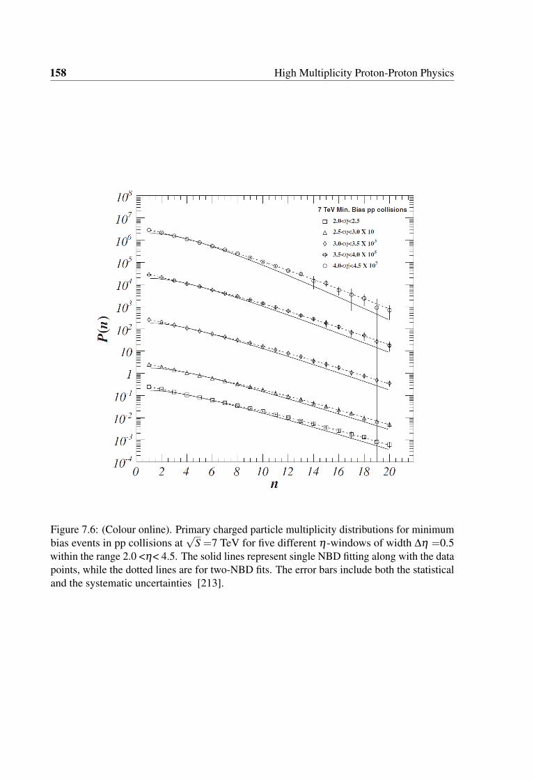
158 High Multiplicity Proton-Proton Physics

Figure 7.6: (Colour online). Primary charged particle multiplicity distributions for minimumbias events in pp collisions at

√S =7 TeV for five different η-windows of width ∆η =0.5

within the range 2.0 <η< 4.5. The solid lines represent single NBD fitting along with the datapoints, while the dotted lines are for two-NBD fits. The error bars include both the statisticaland the systematic uncertainties [213].

7.4 Particle production in pp-collision with NBD and BW model 159

Figure 7.7: (Colour online). Primary charged particle multiplicity distributions for Hard-QCD events in pp collisions at

√S =7 TeV for five different η-windows of width ∆η =0.5

within the range 2.0 <η< 4.5. The solid lines represent single NBD fitting along the datapoints, while the dotted lines are for two-NBD fits. The error bars include both the statisticaland the systematic uncertainties [213].

160 High Multiplicity Proton-Proton Physics

Figure 7.8: (Colour online). Primary charged particle multiplicity distributions for minimumbias and Hard-QCD events in pp collisions at

√S =7 TeV for the entire η-range 2.0 <η< 4.5.

The solid and dotted lines are representing single and double NBD fitting respectively. Theerror bars include both the statistical and the systematic uncertainties [213].

7.4 Particle production in pp-collision with NBD and BW model 161

Table 7.3: Parameters extracted from two NBDs fitting to the multiplicity distributions forthe primary charged particles in minimum bias events in pp collisions at

√S =7 TeV for five

η-windows, and shown in the table in the same order as in table 7.2.η-Window kso f t <n>so f t ksemihard <n>semihard χ2/nd f

2.0 < η < 2.5 3.15 ± 2.56 5.14 ± 2.06 1.92 ± 0.96 1.53 ± 0.80 0.70/142.5 < η < 3.0 2.72 ± 2.23 4.54 ± 1.43 2.31 ± 2.25 1.32 ± 0.54 0.47/143.0 < η < 3.5 3.18 ± 1.65 4.63 ± 2.01 2.05 ± 1.19 1.43 ± 0.83 0.31/143.5 < η < 4.0 1.98 ± 0.54 1.53 ± 0.21 3.99 ± 2.99 4.73 ± 0.35 0.29/144.0 < η < 4.5 2.11 ± 0.95 1.30 ± 0.47 3.55 ± 0.89 3.93 ± 0.80 0.39/14

Table 7.4: Parameters as extracted from fitting with single NBD function to the multiplicitydistributions for the primary charged particles for Hard QCD events in pp collisions at

√S =7

TeV for five small η-windows.η-Window k <n> χ2/nd f

2.0 < η < 2.5 2.83 ± 0.05 4.95 ± 0.05 29.14/182.5 < η < 3.0 3.19 ± 0.04 4.86 ± 0.05 23.59/183.0 < η < 3.5 3.39 ± 0.05 4.64 ± 0.05 87.69/183.5 < η < 4.0 3.53 ± 0.33 4.45 ± 0.02 45.34/184.0 < η < 4.5 3.82 ± 0.06 3.97 ± 0.04 27.47/18

two isolated sub-samples, soft and hard, were disentangled with a criterion "no particle oftransverse energy, ET > 1.1 GeV, as soft events. Although, none of the other experiments atLHC has published multiplicity distribution for the so-called Hard-QCD events during thetime of this work but the invariance of multiplicity distribution for soft events as a functionof√

S has been studied [212] with proton-proton data by CMS experiment [214] in terms oftwo NBDs. The presumptions of this study were a) the two-component model of particleproductions in the proton-proton collision is valid also in the forward region. and b) thecriteria for isolating the hard-QCD events is acceptable. The rest of the work with fittingmultiplicity distributions for the hard-QCD events with a the single-NBD function will bein some sense straight forward. In this context, single-NBD function was used to fit themultiplicity distributions of the produced primary charged particles for the "Hard-QCDevents" as published by LHCb experiments [215]. The in the minimum bias case, here alsothere were data available for multiplicity distribution for five small non-overlapping pseudo-rapidity windows. The relevant plots are shown in figure 7.7 for all five η-windows. As isshown in figure 7.7, the single-NBD function fits reasonably well and explain multiplicitydistributions consistently. χ2/nd f for the respective plots in figure 7.7 are tabulated table 7.4.Two fitting parameters "<n>" and k, tabulated in table 7.4, show a systematic trend as is

162 High Multiplicity Proton-Proton Physics

Table 7.5: Parameters extracted from single NBD fitting to the multiplicity distributions forthe primary charged particles in pp collisions at

√S =7 TeV for η-range 2.5 (2.0<η<4.5)

both for minimum bias and "Hard-QCD" events.Type of events k <n> χ2/nd fMinimum Bias 1.81 ± 0.01 11.63 ± 0.06 853.78/37

Hard QCD 4.32 ± 0.08 19.35 ± 0.15 559.65/37

expected. "<n>" decreases whereas "k" increases with the shift of the -window more towardforward rapidity. Altogether, the single NBD function performs acceptably in describingthe multiplicity distributions for the hard-QCD events in small η-windows in the forwardrapidity region. It was relevant at this point to study the NBD representation the multiplicitydata for proton-proton collision for a wide range of η-coverage, eg ∆η =2.5, in the η-range2.0<η<4.5 for both the event classes minimum bias and "Hard-QCD" events respectively. It isquite obvious from the plots in figure 7.8, that neither the minimum bias nor the "Hard-QCD"events can be described by the single-NBD functions which also understood from the χ2

values for fitting to both the events classes as is listed in table 7.5. Figure 7.8 representsthe primary charged particle multiplicity distributions for minimum-bias and "Hard-QCD"events along with corresponding best fit with a single-NBD function and with a weightedsuperposition of two NBDs. In the case of hard-QCD events, of course, one needs tobe meticulous in adopting the terminology of "two-component model" for the weightedsuperposition of two NBDs. It rather will be relevant in taking the two NBD function just asa functional form far from two component model.

Table 7.6: Parameters extracted from two NBD fitting to the multiplicity distributions for theprimary charged particles in pp collisions at

√S =7 TeV for η-range 2.5 (2.0<η<4.5) both

for minimum bias and "Hard-QCD" events.Type of events kso f t <n>so f t ksemihard <n>semihard χ2/nd fMinimum Bias 2.23 ± 0.15 7.30 ± 0.75 4.11 ± 1.00 23.38 ± 2.04 16.31/33

Hard QCD 4.04 ± 0.62 10.64 ± 1.86 4.20 ± 0.85 24.47 ± 1.42 4.62/33

In table 7.6, we have presented two components of the multiplicity distribution of bothminimum bias and hard-QCD events with suffixes 1 and 2 respectively. The values of the fitparameters were obtained by the best fits in terms of χ2/nd f both the cases. In conclusion,the work revealed the fact that minimum bias proton-proton data at

√S =7 TeV can be well

described with weighted superposition of two NBDs in accordance with the two-componentmodel for particle production. On the other hand, "Hard-QCD" events for small η-windowscan be explained using single NBD, accepting only hard partonic scattering process as a

7.4 Particle production in pp-collision with NBD and BW model 163

mechanism for particle production. However, multiplicity distribution for "Hard-QCD"events for a wide η-window show deviation from single particle production mechanism andcan be described well with double NBD function which indeed contradicts the concept ofthe discussed two-component model. The contradiction could be attributed either to biasedselection criterion of the hard events or to the possibility of a different particle productionmechanism in different phase space and need to be probed more deeply. It is noteworthy tomention here, that there were studies of minimum bias proton-proton data at LHC energiesusing weighted superposition of three NBD function [216]. However, understanding thepresence of the third component is still not conclusive.

7.4.3 Collectivity in pp-collisions and Blast Wave Model

In continuation of the study of proton-proton collision with NBD model, which indicates,particle production in pp-collision is not governed only by pQCD, rather there exist someother particle production mechanism, resulting in softer part of the spectra. There is recentexperimental evidence found in high multiplicity proton-proton collisions which are alreadythere in case of heavy ion collisions and attributed to the hydrodynamical explanations. Ridge,a structure found in pair correlation study at ∆η−∆φ plane, was observed for the first timein heavy-ion collisions at RHIC [165] which was attributed to the hydrodynamical evolutionof the system formed after collisions. Soon after, There was a similar kind of observationwas noticed in proton-proton collisions at LHC(ref:bw16) for a special type of event class,called High-Multiplicity (HM) events. Hanbury-Brown-Twiss (HBT) correlations [166],intensity interferometry used to find the radius of a particle emitting source, is anotherimportant observations which show similar kind of event multiplicity or pair transversemomentum dependence for the radii of the particle emitting source both for pp collisionsat LHC [167, 167] and heavy ion collisions at RHIC [169]. Interestingly, the dependenceagain was illustrated as a signature for collectivity for heavy ion collisions. Moreover, massordering, a dependence of Inverse slope parameter of pT -spectra on particle type and a typicalfor a hydrodynamic description, was found for the first time in heavy ion collisions at RHIC.Later, a similar trend for mass ordering was also observed for small system produced in aproton-Lead collision at LHC energies 7.9 [217].

Very recently, a similar study [218] on mass ordering for HM proton-proton events wasalso found 7.10. The main motivation in revisiting the particle production in pp collisionspecifically at LHC energy in the present study was these above discussed experimentalsignatures that hint a possibility of forming heavy-ion-like hydrodynamical system even inpp collision at small scale. It is relevant to notice, with the availability of large statisticsof high-multiplicity, high energy density pp events, particularly at s = 7 TeV, there are

164 High Multiplicity Proton-Proton Physics

Figure 7.9: (Colour online). Mass ordering, variation of the inverse slope parameter asa function of particle species (mass m), found for pPb collision at 5.02 TeV by CMScollaboration which is explained as a signeture for collectivity of the system produced in thecollision [217].

7.4 Particle production in pp-collision with NBD and BW model 165

Figure 7.10: (Colour online). Variation of inverse slope parameter (Te f f ective) as a function ofparticle mass, following almost same trend as has been found in pPb and PbPb collision whichindicate the scope of applying hydrodynamic model to system produced in proton-protoncollision as well [218].

166 High Multiplicity Proton-Proton Physics

several initiatives [170–177] to adopt different hydrodynamical inspired models in predictingcollective phenomena in small systems produced in pPb and pp collisions at LHC energies.There are other experimental observables like direct photons at low transverse momentum[26], strange baryon-to-meson ratio [176], transverse radial flow velocity [158, 179, 180] etc.exists which are also used to probe the collective nature of the produced system in collisions.However, there are other contemporary frameworks like colour glass condensate [185] inthe literature which explains the appearance of the "ridge" quite successful and does notaccept the existence of hydrodynamical system formed in pp collisions. Nevertheless, recentresults from CMS collaboration [219, 220] shows a relative flattening of the low-pT part ofthe pT -spectra of identified particles with increasing mass in pp collisions at LHC whichtriggered for a search of collective transverse radial flow. Notably, a similar type of flatteningof pT -spectra in heavy-ion collisions at SPS, RHIC and LHC was explained assuming theexistence of a common transverse radial flow velocity.

7.4.4 Results and discussion

The study under the present scope has been done with published data for proton-protoncollision at LHC. A wide range of data in terms of pT -spectra for different identified particleswith different detector coverages are available from different experiments at LHC. However,the phenomenological work, search for collectivity with blast wave approach, is limitedby the relevance to the objective of the topic. There were published data for two differentclasses of particles which have been considered for the present work. Firstly, a class ofparticles [220, 221] with the commonly measured entities such as π±, K±,p(p) over therapidity, (|y| < 1) for the pp collisions at

√S =900, 2760 and 7000 GeV which has been

explored with blast wave approach. On the other hand, the second class of particles consistedwith [219, 222] the strange particles of different degrees of strangeness (single, double etc),K0

S, Λ and Ξ, for NSD type pp collisions at√

S =0.9 and 7 TeV. The data for pT -spectrafor different particles π±, K±,p(p) were accessible with event classes, tagged with "non-overlapping range of event multiplicity" which is assumed to contain the information of"centrality" in case of pp collision. An explicit blast-wave analysis could be performed withthe CMS data [221, 222] which encourage to study the centre-of-mass energy, species andcentrality-dependence of pT -spectra produced in pp collisions at LHC and to compare theresults with similar studies available for heavy ion (AA) and pA collisions. The fact to bementioned at this point, that none of the event generators such as PYTHIA tunes was used inthe study of the inclusive production of π±, K±,p(p) in pp collisions at s = 0.9, 2.76 and 7TeV [34] which can bring an acceptable overall description of data at the finer level such asthe multiplicity (N) dependence of <pT > or ECM,

√S−dependence of dN/dy or <pT > and

7.4 Particle production in pp-collision with NBD and BW model 167

the particle yield ratios etc. Like in the case of non-strange particles, tuned event generatorsare far from explaining in case of strange particle as well in which the discrepancy increaseswith the increase in strangeness.

We have attempted to fit the blast-wave function (BGBW), as has been described inequation 7.8, to the pT -spectra obtained from published data, as measured [219, 220] byCMS experiment. The fitting was done simultaneously for a class of particles (π±, K±,p( p))with all three fit parameters, kinetic freeze-out temperature (Tkin), the radial flow velocity(βS) and the exponent (n) of flow profile, free as is shown in figure 7.11 for NSD pp-eventswith all strange and non-strange particles. The motivation was to obtain the best possiblesimultaneous or combined fits to the data which might shed light on the collective behaviourof the particle emitting source produced in pp collision. The value of χ2/nd f , using theMINUTE program in the ROOT analysis framework [55], was adopted as a sign of bestfitting for the study. To start, we have fitted pT -spectra simultaneously for π±, K±,p( p) withBGBW function for minimum bias pp collisions at

√S =0.9, 2.76 and 7 TeV respectively

as shown in figure 7.11. Blast-wave model, however, could not describe the minimum biasdata satisfactorily. We have explored the advantage of having centrality (multiplicity incase of pp collision) dependent pT -spectra for pp collision which exhibits the fact that high-multiplicity pp events only carry the signatures, which could be attributed to the collectivityin pp collisions. The simultaneous BGBW fitting to the high multiplicity (more central) ppevents was done for the search of collectivity in pp collision explicitly in this study.

Figures 7.12 represents the pT -spectra for π±, K±,p( p) for highest multiplicity class Nch

for pp collision at 7 TeV as measured by CMS [220], fitted simultaneously with BGBWfunction. A similar exercise, simultaneous BGBW fitting as shown in figures 7.13 and 7.14,have been performed with highest available multiplicity classes (Nch =98 and 75) for twodifferent centres of mass energies 2.76 and 0.9 TeV respectively. A rigorous blast-wave fit forall other multiplicity classes for different ECM energies has been studied. However, BGBWfit to a certain multiplicity class was accepted for the signature of collectivity by the qualityof simultaneous fitting depending on the values of χ2/nd f .

Apart from three free parameters, Tkin, βS and n, as have been discussed already, trans-verse radius (R) of the surface of particle emitting source at freeze-out plays a crucial role inBGBW fitting to pT -spectra. The choice of R plays a crucial role in the fitting of pT -spectrawith the blast wave function. Selection of R in this context will be illustrated shortly. Ideally,the radius "R" could be obtained from the pair transverse momentum-dependent HBT radiusfor the source of particle production. Experimentally, HBT radius corresponding to thelowest value of pair transverse momentum (kT ) which represents the radius of the source

168 High Multiplicity Proton-Proton Physics

Figure 7.11: (Colour online).Transverse momentum (pT ) spectra for π±, K±,p(p) withinrapidity range |y| < 1 for minimum bias pp collisions and for K0

S, Λ and Ξ within rapidityrange |y| < 2 for the non-single diffractive (NSD) events of pp collisions at

√S =7 TeV as

measured by CMS collaboration [219, 220]) at LHC. Uncertainties shown, are obtained byadding statistical and systematic errors in quadrature [223].

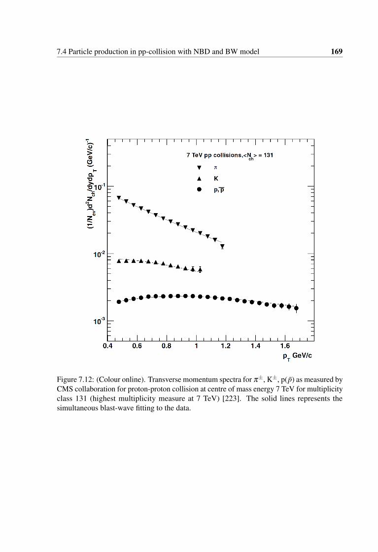
7.4 Particle production in pp-collision with NBD and BW model 169

Figure 7.12: (Colour online). Transverse momentum spectra for π±, K±, p( p) as measured byCMS collaboration for proton-proton collision at centre of mass energy 7 TeV for multiplicityclass 131 (highest multiplicity measure at 7 TeV) [223]. The solid lines represents thesimultaneous blast-wave fitting to the data.

170 High Multiplicity Proton-Proton Physics

Figure 7.13: (Colour online). Transverse momentum spectra for π±, K±, p( p) as measuredby CMS collaboration for proton-proton collision at centre of mass energy 2.76 TeV formultiplicity class 98 (highest multiplicity measure at 2.76 TeV) [223]. The solid linesrepresents the simultaneous blast-wave fitting to the data.

7.4 Particle production in pp-collision with NBD and BW model 171

Figure 7.14: (Colour online). Transverse momentum spectra for π±, K±, p( p) as measuredby CMS collaboration for proton-proton collision at centre of mass energy 0.9 TeV for multi-plicity class 75 (highest multiplicity measure at 0.9 TeV) [223]. The solid lines representsthe simultaneous blast-wave fitting to the data.

172 High Multiplicity Proton-Proton Physics

Table 7.7: Parameters of BGBW ,Tkin ,β and n, have been extracted from the simultaneousfit to the published [53] spectra of π±, K± and p( p) for pp collisions at

√S =0.9, 2.76 and 7

TeV for different event classes depending on average multiplicity, Nch , in the pseudo-rapidityrange η< 2.4.

ECM <Nch> Tkin(MeV) < β > n χ2/nd f0.9 75 106.43±0.10 0.745±0.004 0.584±0.010 0.29

2.76 86 115.55±0.11 0.742±0.005 0.605±0.007 1.252.76 98 110.39±0.13 0.769±0.005 0.521±0.009 0.43

7 98 115.57±0.11 0.766±0.004 0.540±0.006 1.027 109 113.09±0.12 0.779±0.004 0.503±0.006 0.617 120 110.84±0.15 0.790±0.004 0.480±0.006 0.347 131 104.29±0.15 0.809±0.005 0.436±0.005 0.44

of emission close to the freeze-out. There are results from both ALICE [168] and CMScollaboration for HBT radius for the particle emitting source in pp collision depending onpair transverse momentum and the event multiplicity which resembles results in case ofa heavy-ion collision. However, due to lack of multiplicity classes for pp collisions likein heavy-ion, we have used a multiplicity dependent empirical formula(R(Nch) = a.N1/3

ch )for calculating the radius. Here, the parameter a = 0.597±0.009(stat.)±0.057(syst.)fm for0.9 TeV and a = 0.612±0.007(stat.)±0.068(syst.) fm) for 7 TeV was taken from results fromCMS experiment [168]. However, because of the lack of data for "a" for 2.76 TeV, we haveestimated the value by using the method of interpolation.As has been discussed, a good simultaneous fitting of BGBW to the data for particles withdifferent masses indicate the presence of some kind of collectiveness within the particleemitting source. To understanding the collectivity of the source produced in the collision, wehave extracted the values of the BGBW fit parameters for different centre-of-mass energies(ECM), along with respective χ2/nd f which has been tabulated in table 7.7.

To understand the behaviour of the parameters, we need to look back the same kind ofstudy both for heavy-ion (AA) collision and proton-ion (pA) collision which might providesome reference for pp collision. It has been found for heavy ion collision that for the particularcentre of mass energy, TKin increases with the event multiplicities (or centrality) whereas,the average transverse radial flow < β > decreases with increase in multiplicity. From ourstudy for pp collision at 0.9, 2.76 and 7 TeV, it has been revealed that the parameters TKin

and < β > exhibit similar trend to what has been found in AA or pA collisions. Notably,the average radial flow velocity < β > increases with ECM for the highest multiplicity eventclass whereas and the kinetic freeze-out temperature TKin remains constant. The results for

7.4 Particle production in pp-collision with NBD and BW model 173

pp collision has been compared with that of AA and pA collision and shown in figure 7.15for < β > and figure 7.16 for TKin.

To understand the results from the phenomenological study, we need to recall that, ina hydrodynamic picture, the collective radial flow has resulted from the pressure gradientin the system which might be there due to a non-central collision. The resulted radial flowvelocity for the system is more for larger pressure gradient. However, the pressure gradientevolves depending on initial energy density and the spatial size or the lifetime of the systemformed during the collision. As obvious, higher initial energy density and the smaller sizeof the system leads to a larger pressure gradient and thus higher flow velocity. As a naturalconsequence, the smaller system produced in pp collision at LHC energies will hold largerpressure gradient as compared to both heavy-ion collision at SPS, RHIC and LHC and pAcollisions at LHC with similar centrality (multiplicity) class. Consistent results for pressuregradient built depending on the collision energy and system size has already been establishedfrom experiments such as more for PbPb collisions at

√SNN = 2.76 TeV is larger than that

in AuAu at RHIC energies. Moreover, it is also evident, that the pressure gradient in pPbcollisions at

√SNN = 5.02 TeV is larger than PbPb collisions at

√SNN = 2.76 TeV. Besides

experimental evidence, there were recent theoretical attempts [186] which essentially predictsthe flow velocity to be larger for smaller systems at same collision energies. Thus the plotsshown in figure 7.15, is indeed consistent in terms of transverse radial flow velocity as a

function of√

S,dNch

dηand the size of the system produced either in pp or pA or AA collision.

Kinetic freeze-out temperature (Tkin), extracted from simultaneous BGBW fitting to dataand shown in figure 7.16, demonstrates a decreasing nature with an increase in centrality(multiplicity) for each individual case of pp, pA and AA collision. However, comparisonamong different collision systems shows, pPb system freezes out quickly ( with larger Tkin)compared to the AuAu or the PbPb systems whereas, an anomalous behaviour for pp systemwas found which indicates lower Tkin compare to both the pA and AA systems at comparabledNch

dη. The Tkin, found for high-multiplicity pp collisions is fairly comparable with that for

the central AA collisions. However, a theoretical calculation by Shuryak at al . [186] showsfor a particular Tkin, though absolute sizes and multiplicities are quite different for centralAA and pp collisions, pp systems get more explosive in nature compare to AA system. As aresult, according to the hydrodynamic picture, a larger β as a function of initial time "t" andsystem size "r" is observed for a smaller system like pp compare to AA.

After an elaborate study with BGBW model approach to π±, K±,p(p) for differentmultiplicity classes, we have attempted to apply BGBW model in describing pT -spectra forstrange particles like K0

S, Λ and Ξ. The data, used for this study, was taken from recent results

174 High Multiplicity Proton-Proton Physics

Figure 7.15: (Colour online).Transverse radial flow velocity as a function of charged particle

multiplicity density (dnch

dη) for different centre of mass energies (

√S) as obtained from

simultaneous blast wave fit to π±, K±, p(p) data for pp, pPb, and heavy ion collisions atLHC energies [223]. The system formed in pp collision found to flow with higher velocitycompare to that in pPb and PbPb collision.

7.4 Particle production in pp-collision with NBD and BW model 175

Figure 7.16: (Inverse slope parameter (Tkin: combined effect from flow and temperature) as a

function of charged particle multiplicity density (dNch

dη) for different centre of mass energies

(√

S) as obtained from simultaneous blast wave fit to π±, K±, p( p) data for pp, pPb, andheavy ion collisions at LHC energies [223].

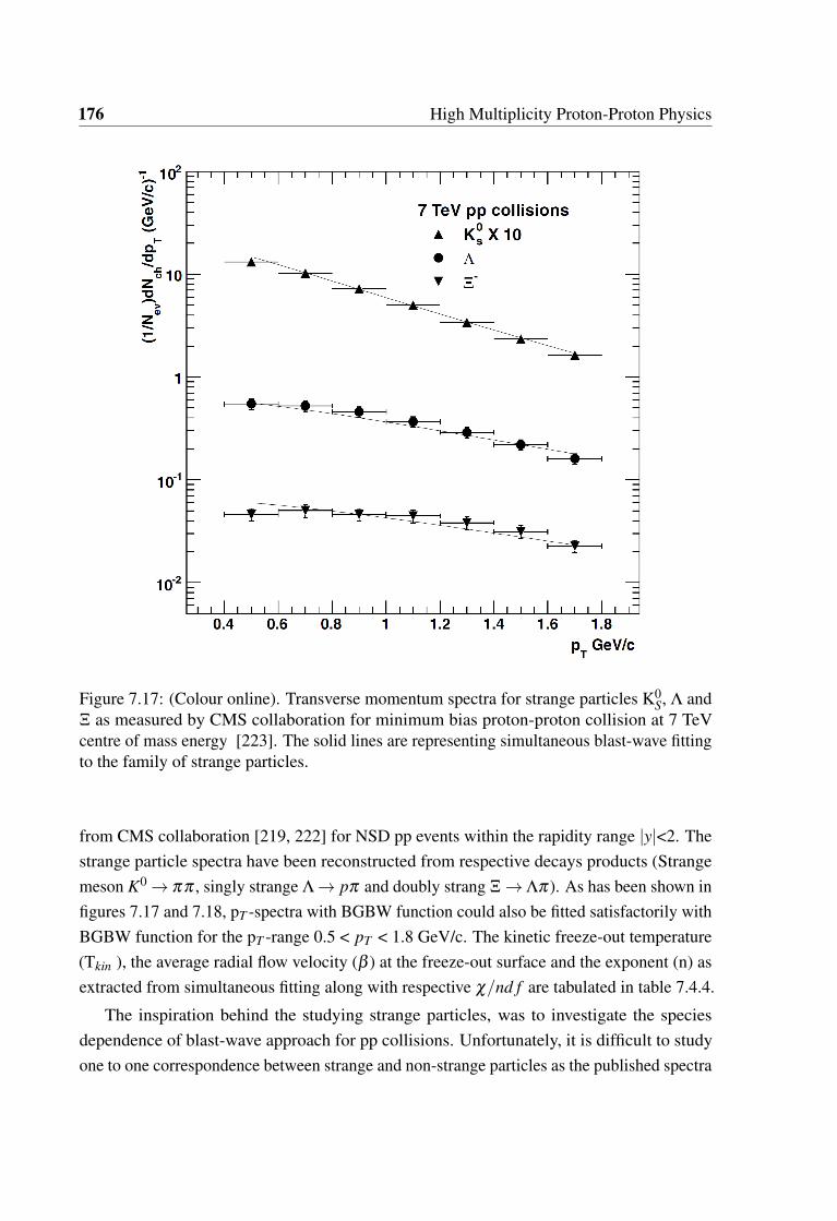
176 High Multiplicity Proton-Proton Physics

Figure 7.17: (Colour online). Transverse momentum spectra for strange particles K0S, Λ and

Ξ as measured by CMS collaboration for minimum bias proton-proton collision at 7 TeVcentre of mass energy [223]. The solid lines are representing simultaneous blast-wave fittingto the family of strange particles.

from CMS collaboration [219, 222] for NSD pp events within the rapidity range |y|<2. Thestrange particle spectra have been reconstructed from respective decays products (Strangemeson K0→ ππ , singly strange Λ→ pπ and doubly strang Ξ→Λπ ). As has been shown infigures 7.17 and 7.18, pT -spectra with BGBW function could also be fitted satisfactorily withBGBW function for the pT -range 0.5 < pT < 1.8 GeV/c. The kinetic freeze-out temperature(Tkin ), the average radial flow velocity (β ) at the freeze-out surface and the exponent (n) asextracted from simultaneous fitting along with respective χ/nd f are tabulated in table 7.4.4.

The inspiration behind the studying strange particles, was to investigate the speciesdependence of blast-wave approach for pp collisions. Unfortunately, it is difficult to studyone to one correspondence between strange and non-strange particles as the published spectra

7.4 Particle production in pp-collision with NBD and BW model 177

Figure 7.18: (Colour online). Transverse momentum spectra for strange particles K0S, Λ and

Ξ as measured by CMS collaboration for minimum bias proton-proton collision at 0.9 TeVcentre of mass energy [223]. The solid lines are representing simultaneous blast-wave fittingto the data.

178 High Multiplicity Proton-Proton Physics

Table 7.8: Parameters of BGBW ,Tkin ,β and n, have been extracted from the simultaneous fitto the published [31 54] spectra of strange mesons, K0

S, Λ and Ξ for pp collisions at√

S =0.9and 7 TeV.

ECM Tkin(MeV) < β > n χ2/nd f

7 149 ± 0.59 0.62 ± 0.006 1.0 ± 0.02 0.850.9 140 ± 0.53 0.54 ± 0.01 1.27 ± 0.12 0.62

of for non-strange particles π±, K±,p(p) and strange particles K0S, Λ and Ξ were measured in

different kinematic-range. Moreover, the multiplicity dependent pT -spectra are not availablein case of strange particles which restrict the study for minimum bias data only. Nevertheless,the difference in BGBW description between strange and non-strange particles have alsobeen observed in case of pp collision which is already there in heavy-ion collisions [224, 225].

Summarising in brief, the blast-wave approach in the search for collectivity in pp collision,revealed that the measured pT -spectra of π±, K±,p(p) for the minimum-bias events of ppcollisions at LHC at

√S =0.9, 2.76 and 7 TeV do not fit the BGBW, whereas, the spectra

for K0S, Λ and Ξ for NSD events at

√S =0.9 and 7 TeV pp collision could be well described

by the blast- wave model. However, HM pp events can be well fitted with BGBW functionwhich resemble similar results for AA collision, indicating the presence of collectivity evenin pp collision.

7.5 Source of collectivity in pp collision.

The boost in centre of mass energy for pp collision at LHC had broadened the physicsunderstanding beyond fundamental hard scattering and entered a new regime with specialevent classes, called high multiplicity, resembling properties found in the peripheral heavy-ion collision. We have found particle production in pp collision at LHC energies can bewell described with two-component model (double NBD) indicating the presence of someother (soft) mechanism apart from hard scattering. Moreover, to understand the nature ofsystem produced in pp collision including the softer part, BGBW model has successfullydescribed the presence of collectivity in HM pp events which is specifically attributed tohydrodynamical nature of the system in case of a heavy-ion collision. In this context, it will berelevant to recall that, in the case of relativistic heavy-ion collisions, the local thermodynamicequilibrium is presumed to study the space-time evolution of the system using relativistichydrodynamics [226]. On the other hand, as considered by most of the topical models, pp

7.5 Source of collectivity in pp collision. 179

collision do not endorse the formation of any medium. An obvious question regarding smallsystem produced in pp collision is about achieving thermalisation to adopt hydrodynamicalpicture. Specifically, the mean free path of constituent particles in comparison to the systemsize along with the lifetime needs to cross-checked. However, a very recent study [227] aboutthe system-size dependence of Knudsen number, a measure of the degree of thermalisationrepresented by the ratio of microscopic to the macroscopic property of the system, whichillustrates that the system produced in AuAu collisions at RHIC and in high-multiplicitypp events at LHC, are similar which let hydrodynamical model to interpret the features ofparticle production in high-multiplicity pp events. Nevertheless, there are recent data of ppcollisions, particularly for the HM events, published by different experiments at the LHCat CERN, unveiling features [228, 229], which are typical of the hydrodynamic mediumformed in the relativistic heavy ion collisions. Immediately after, plenty of phenomenologicalstudies with LHC pp data came up with the existence of [230–232] a collective mediumwhich has been supported substantially by various theoretical approaches [183]. Estimationof initial energy density for HM pp events at LHC energies [181], showed that the systemproduced in pp collision is, indeed, energetically permissible to be comprised of partonsinstead of hadrons. In fact, Campanini and Ferri have shown in their work [184] regardingthe change in phase for pp collision by analysing a wide range of data published by LHCexperiments. From all above evidential observations in pp collisions, it is quite encouragingto follow the similar approach adopted in the search for the QGP in heavy-ion collisions withassuming local thermal equilibrium and search for signals for formation of partonic mediumeven in small systems like produced in pp collision. In our study, We have analysed pp datain the search of a signal of possible change of phase from hadron to parton or vice versa.The analysis is, however, completely data-driven and restricted with the availability of thekinematic range of the data, particles type, multiplicity classes etc.

7.5.1 Search for signal of phase change

As has been already discussed in earlier section that hadronic or partonic system are char-acterised with different degrees of freedom, namely pions (primarily) and partons (quarkand gluons) respectively. Because of these obvious differences, we have put an effort inestimating the degrees of freedom, responsible for the system produced in a high multiplicityproton-proton collision. Estimation of energy density scaled with forth power of temperature,represents the number of degrees of freedom involved as is discussed in the subsection"Estimation of energy density", might give an important insight into the nature of the systemproduced in pp collision. We have calculated

ε

T 4 orσ

T 3 as a function of temperature, usingavailable pp data for different multiplicity classes, as a signal for any possible phase change

180 High Multiplicity Proton-Proton Physics

as is predicted by the LQCD. Here, T represents temperature, ε is the energy-density and σ isthe entropy-density of the system under consideration. A sharp, step-like increase manifeststhe first order phase transition, whereas, a smooth but rapid rise indicates either the crossoveror a second order phase transition. As of present scenario, latest LQCD calculations illustratethe transition as a crossover [233] in the QCD regime. At a temperature lower than the criticalregion of rapid rise, the system is populated mainly by pions, forming a hadron gas, however,the lattice calculation of ε and σ is difficult as is exponentially suppressed [234]. On the otherhand, At a temperature higher than the critical region, where the ideal gas limit of degrees offreedom is reached asymptotically, the system represents an ideal gas comprising of partons.However, due to the lack of a straightforward method of estimation of temperature from data,the predicted temperature dependence of

ε

T 4 orσ

T 3 , as a signal for the phase transition or thecrossover is still a challenging task from experimental point of view. Moreover, the finitesize effect [235, 236] of the system formed in the collision, may diffuse the signal which re-sults smoothing of singularities in the LQCD-predicted dependence of the degrees of freedom.

Assuming non-viscous medium formed during the collision, the energy density can becalculated from the rapidity or the pseudo-rapidity density of the produced particles usingrelativistic hydrodynamics. High multiplicity pp data at

√S =7 TeV are available with

enough statistics from CMS collaboration [237, 238]) which corresponds to the multiplicitydensity as large as ≈30 which is expected to be enough for the formation of non-hadronicmedium. The main objective of this study was to investigate the dependence of (

ε

T 4 ) on thetemperature, not to evaluate the absolute value of the energy-density. Thus, we have adopteda simple 1-dimensional formalism [239] as proposed by Bjorken as has been discussed inequation 7.12 for the estimation of the energy-density. The low-pT part of the pT -spectra,resulted from soft particle production mechanism in high energy collision, contains theinformation about the temperature as well as the transverse expansion of the system. Asthe contributions from temperature and the transverse expansion are twisted together notin an easy way, extraction of the temperature from the pT -spectra is not possible unlessotherwise exclusively experimentally measured. But, the mean transverse momentum, asproposed by Van Hove [208] or the slope of the transverse mass mT -spectra could be used toas a signature of the thermal state of the system. Hence, in our study, we have probed theeffective number of degrees of freedom in pp collisions in terms of the <pT >-dependence of

σ

< pT >3 . It would be pertinent to mention that the inverse slope parameter (Te f f ), extracted

from an exponential fit to the mT -spectra, also contain both the information of thermal stateand the traverse expansion of the system. The contributions are convoluted within the Te f f

7.5 Source of collectivity in pp collision. 181

and can be written as Te f f = T + f (β ), where T and f (β ) represent the temperature and thetransverse expansion of the system respectively.

7.5.2 Analysis, results and discussion

The study under present scope has been carried out with published data by CMS collabo-ration [237, 238] for identified particles pions (π±), kaons (K±), and protons (pp) for ppcollisions at

√S =0.9, 2.76 and 7 TeV respectively. The kinematic cuts for the available data

were in terms ofd < Nch >

dηfor rapidity: |y| < 1, pseudo-rapidity: |η | < 2.4. Importantly,

the data are available for a wide range of multiplicity (Nch) classes starting from 7 to 131with reasonably good statistics. The measured transverse momentum ranges are differentfor different particle classes like 1.0 GeV ≤ pπ

T ≤ 1.2 GeV , 0.2 GeV ≤ pKT ≤ 1.05 GeV and

0.35 GeV ≤ pppT ≤ 1.8 GeV respectively. In fact,

d < Nch >

dη-dependent data for identified

particle give the opportunity to study for any possible change of phase in terms of degrees offreedom as a function of mean transverse momentum (representing temperature) experimen-tally. As is already discussed, the same data set has been used to search for collectivity insmall system produced in pp collision at LHC energies [232] which resulted in a promisingsignature for collectivity. We have extended our study to reveal the source of the collectivityso found in pp collision. It is to be noted at this point that there is a model calculation whichexhibits pT as a function of temperature for identified hadron species, showing the change inshape of pT -spectra due to transverse expansion indeed depend on particle mass like protonsgain most in pT while pions lose some pT . Moreover, a model calculation [240] illustratesproton having a larger flow effect as an of late decoupling from the fireball compare topions. On the other hand, pion has a lot of contamination specifically at lower pT due tofeeding down effects. As a result, Kaon, being weakly affected [241] by either re-scatteringof hadrons or resonance decay, are considered to be a suitable candidate in the search forchange in phase. Therefore, to avoid cumulative effect from transverse expansion of varyingmagnitude (different particles), we have considered individual pT -spectra to extract thetemperature dependent observable for the system. In this study, we have extracted

σ

< pT >3

as a function of < pT > for charged pions and kaons produced in pp collision at√

S =0.9,2.76 and 7 TeV separately. The radians, as appeared in Bjorken energy density 7.12, hasbeen estimated using HBT-radius [242] which depend on the pair transverse momentum

(kT ) and multiplicity. It is important to note here, that for a givendNch

dη, high-kT indicates

the early stage of the collision, whereas low-kT is related to the final stage, close to thefreeze- out. As the analysis aimed to estimate the energy density of the system produced

182 High Multiplicity Proton-Proton Physics

just after the collision, kT of relevance for our work is high-kT , which has been taken as0.5 to 1.0 GeV/c from CMS collaboration [229]). Since the study involves energy densityas a function multiplicity (Nch), we have parametrised the radius of the interaction zone asa function of Nch using R(Nch) = a ·N1/3

ch with a = 0.504±0.009 fm. The entropy (energy)density for different multiplicity classes have been calculated both for pions and kaons andare shown in figures 7.19 and 7.20. In both, the cases, a definite and smooth but rapid risein

σ

< pT >3 with an increase in < pT > is found. This, indeed, indicates release of new

degrees of freedom over a small change in < pT > in lower pT -range. However, in the highpT range, kaons and pions behave differently. No conclusive remarks about phase cannot bemade because of lack of saturation in

σ

< pT >3 in case of pions, whereas kaons at high pT

(high temperature) clearly points towards a saturation which corresponds to highest numberof degrees of freedom for the possible partonic phase. The difference in pions and kaonsbehaviour is rather consistent as has explained in articles [243, 240, 241] at high pT . The lossof pT for pions [243] could be the reason for wearing away of the saturation effect for highmultiplicity pp events. Also, the differential freeze-out of hadron species due to differentelastic cross-sections [240–242] may lead to the early freeze-out for kaon in comparison topion, which may describe the observed difference in response by the pions and the kaons.The reason behind kaon being less affected by the early freeze-out can be understood as thekaons are staying less with the system leading to less effect by the flow of the system. As aresult, kaons are most retrain the temperature information of the system. However, it shouldbe noted that the pT , though, represents the temperature, but it can not give an absolutemeasure for T. Similar arguments stays for

σ

< pT >3 as here also instead of T , < pT > has

been used. The fact of lack of experimentally measured temperature, the study, however, islimited with only qualitative aspects of LQCD-predicted signal for the change in phase ofmatter formed in pp collisions. Importantly, the nature of the signal for phase change from adata-driven approach matches satisfactorily to the results of the latest LQCD calculationspredicting a crossover [233].

Though the multiplicity dependent study of pp collision with a data-driven, simplistic 1-Dhydrodynamical Bjorken model reveals a new feature of possible indication for phase change,a comparison with the conventional Monte Carlo Event Generators is virtually obligatory. Forour study, we have used standard event generators commonly used in the field. PYTHIA8.1Tune 4C, explains [245] global properties like the pT -dependence on Nch in pp collisionsas measured by ALICE, is relevant among various available versions. It is important atthis point to note that PYTHIA along with colour reconnection [102–104], an alternativeexplanation for anomalous behaviour in pp data, can reproduce ALICE results satisfactorilyof pT -dependence on Nch for the pT -range up to 10 GeV/c whereas PYTHIA without CR

7.5 Source of collectivity in pp collision. 183

Figure 7.19: (Colour online). The figure represents the variation of entropy scaled withcube of transverse momentum (

σ

< pT >3 ) as a function of average transverse momentum

(< pT >). Effectively, the figure shows the variation of degrees of freedom (DOF) for pions,obtained from the published pion-spectra data from CMS collaboration. The trend towardssaturation at larger < pT > has been observed. The solid lines, joining data points, are toguide the eye. The error bars include both the statistical and systematic uncertainties [244].

184 High Multiplicity Proton-Proton Physics

can explain so. CR, a final state effect resulting traverse boost to the produced particle ismanifested from multi-partonic interaction. We have generated pp events at

√S =7 TeV

using PYTHIA8.1 Tune 4C event generator both with and without CR. The dependence of< pT > on Nch were plotted and compared with data which has been shown in figure 7.21for unidentified and figure 7.22 identified particles.

Although ALICE publishes data charged hadrons and compare with PYTHIA8.1 Tune4C generated events in the pT -range up to 10 GeV/c, but for our study, we have chosen thesame kinematic range as has been used by the CMS collaboration [237]). We have plotted< pT > as a function of Nch, as obtained from the CMS data [27, 28], for the pseudo-rapidityrange (|η | < 2.4) and the < pT >-ranges (0.1 to 1.2) GeV/c for π±, (0.2 to 1.050) GeV/cfor K±). As is clear from the figure 7.22, though the PYTHIA with CR gives the boost inthe pT of the produced particles, it is still far from the measured values for the kinematicranges under consideration. The exercise, indeed, established the expected results regardingthe mismatch between the data and the PYTHIA simulation. After finding the difference in< pT > as a function of Nch for PYTHIA simulated events, we have calculated the entropydensity (

σ

< pT >3 ) as a function of pT for the simulated data and compared with that of

found from CMS published data, as is shown in figures 7.19 and 7.20.

It is significant in this context, that the temperature of a thermalised partonic medium,if formed, should in principle be reflected by the low-pT particles (usually pT ≤ 2 GeV/c,as has been considered in heavy-ion collisions) and the CMS data can fulfil the desiredrequirement in this respect. As is always advisable, the prediction must be compared toestablished results for similar kind of the system. Though the existence of partonic mediumis beyond doubt in the case of system produced in heavy ion collision, it is to be rememberedthat the extent of the system in AA collision is somewhat obvious. However, there existresults for a small system formed in proton-lead collision, which exhibits stronger evidencefor collectivity

Perception about proton proton collision has unprecedented importance in understandingthe particle production at relativistic high energy collision for different colliding system interms of understanding of new physics processes, structural information inside nucleon, thebaseline for the more complicated system and many more. With the advantage of acceleratortechnologies, the boost in ECM lifted the proton-proton collision to a regime where it isexpected to hold more than reflecting fundamental hard scattering phenomenon. Specifically,during LHC era, search for a small but more complicated system like in heavy-ion collisionin pp (pp) collision reinstitute the concept of the thermalised partonic matter even in ppcollision. It is customary to mention that, prior to LHC, there have been several initiativesand studies [208, 246–250] which have addressed the de-confinement and formation of

7.5 Source of collectivity in pp collision. 185

Figure 7.20: (Colour online). The figure represents the variation of entropy scaled withcube of transverse momentum (

σ

< pT >3 ) as a function of average transverse momentum

(< pT >). Effectively, the figure shows the variation of degrees of freedom (DOF) for kaons,obtained from the published pion-spectra data from CMS collaboration. The trend towardssaturation at larger < pT > has been observed. The solid lines, joining data points, are toguide the eye. The error bars include both the statistical and systematic uncertainties [244].

186 High Multiplicity Proton-Proton Physics

Figure 7.21: (Colour online). The figure shows average transverse momentum (< pT >) asa function of charged particle multiplicity (Nch) for the pT -range 0→ 10 GeV and pseudo-rapidity range ±0.3 . The data (solid red circle) has been taken from ALICE collaborationand was compared with the simulated events using PYTHIA8 Tune 4C event generator bothwith and without Colour Reconnection (CR) for pp collisions at 7 TeV. The error bars includeboth the statistical and systematic uncertainties [244].

7.5 Source of collectivity in pp collision. 187

Figure 7.22: (Colour online). The figure shows the variation of average transverse momentum(< pT >) as a function of charged particle multiplicity (Nch) for kaon (upper panel) andpion (lower panel) for proton-proton collisions at 7 TeV. . The data from was taken fromALICE collaboration and compared with the simulated events using PYTHIA8 Tune-4Cboth for colour reconnection on and off. The plots had been generated for the pT -range upto 2 GeV both for kaon and pion. The error bars include both the statistical and systematicuncertainties [244].

188 High Multiplicity Proton-Proton Physics

Figure 7.23: (Colour online). The figure shows the variation ofσ

< pT >3 as a function of the

mean transverse momentum (< pT >) for pions (upper panel) and kaons (lower panel) forproton-proton collision at 7 TeV. The open squares represents simulated data from PYTHIATune-4C, whereas, solid squares are obtained from the measured [217] spectra data by CMScollaboration. The figures clearly shows differences between simulation and experiment aswas expected. The error bars include both the statistical and systematic uncertainties [244].

7.5 Source of collectivity in pp collision. 189

Figure 7.24: (Colour online).The figure illustrates the behaviour ofσ

< pT >3 , extracted

for proton-Lead collision at 5.02 TeV, as a function of the average transverse momentum(< pT >) pion (upper) and kaon (lower). The open circles represents data from PYTHIATune-4C simulation, whereas, solid circles are obtained from the CMS collaboration [217].The error bars include both the statistical and systematic uncertainties [244].

190 High Multiplicity Proton-Proton Physics

hydrodynamic medium in p p collisions. In the same regards, we have revealed in our studyan indication of a possible change of phase in pp collision in terms of the effective numberof degrees of freedom represented by

σ

< pT >3 . However, there is an obvious issue about

acceptance of the thermal equilibrium for such a small system produced in pp collision. Theconcern can be explored with the fact that measured particle multiplicity in high-multiplicitypp collision at LHC energies is comparable to CuCu collision at

√S=200 GeV at RHIC [182].

We have studied in this work, the dependence of degrees of freedom on < pT > for multi-plicity dependent event classes in pp collision. The study has perceived that the liberationof an effective number of degrees of freedom for a given pseudo-rapidity density and fora given pT -range, depending on multiplicity (centrality) class and is independent of thecentre-of-mass energy.

7.6 Summary

Summarising in brief, pp collision with minimum bias at LHC energies can be describedwith two-component model for a wide pseudo-rapidity window, indicating the possibilityof particle production in pp collision is more than as understand as from hard scattering.Moreover, the phenomenological blast wave model description of pp data established apotential collectivity, more prominent for high multiplicity events. Though there is a lack ofconclusive remarks about the so found collectivity in pp collision, but certainly, it provokes todig more into the matter. At the end, we have adopted a data-driven analysis of the publisheddata for pp collisions at the LHC, in terms of

σ

< pT >3 (DOF) as function of multiplicity

(< pT >) which observe a smooth rise over small pT -range for identified particles pion andkaon. LQCD predicted signal, for the change of phase, has been calculated experimentallyadopting the same procedure that has been followed [14–17] in heavy-ion collisions bycharacterising the medium formed after collisions. Though at the same time the study cannot claim that the experimental verification, for the change of phase in terms of change indegrees of freedom, is done convincingly. Moreover, the usefulness of the species-dependentresponse of the system, in search of a change in the effective number of degrees of freedom,found to be significant in this study and can enhance the relevance in heavy-ion collision.Still and all, the finding can not definitely clinch the signal as a "smoking gun" for a changeof phase in pp collisions, but, it certainly reveals a new feature, significant enough to extendthe study in search of collectivity and nature of collectivity in small systems produced inhigh multiplicity pp collisions.

Chapter 8

Summary

8.1 Summary and Future Scope

The present study comprised of two major topics, Forward-Calorimetry as an ALICE upgradeproposal and studying proton-proton collision at LHC energies with "out-of-the-box" explana-tion. The first part is aimed to enhance the present physics capabilities of ALICE experiment,specifically in froward rapidity region, with an extended physics interests starting fromproton-proton to proton-nucleus to nucleus-nucleus collsion. Whereas in second part, thephysics potential of proton-proton collsion with published data at LHC energies is exploredwhich otherwise served for baseline for the more complex system like in Nucleus-nucleuscollision. Here a brief discussion about the achievements and extent for further work will bepresented for the sake of completeness of the study.

8.1.1 Forward Calrimetry

The study started with an general introduction about the calirimetry, used in relativistichigh energy collision. After brief survey of the field, the Sampling type elctromangeticcalorimeter was discussed in more detail which suits the purpose of the study. As an primaryrequirement, the calorimeter was so choosed that it can measure photons for a wide rangeof energies up to pT ≤ 20 GeV/c and it must be capable of disentangling different types ofphotons depending on their sources (e.g. prompt, thermal and decayed).The final physicsmotivation, however, is to probe the small−x domain of parton distribution which supposedto reach a saturation scale (ΛS) for gluons at LHC energies leading to Color Glass Condensate.Moreover, the photon measurement at forward rapidity has also potential in understandingthe parton energy loss and thus measuring the opacity of the partonic medium. To startwith, an extensive simulation for geometry optimization for calorimeter was performed

192 Summary

using GEANT4 toolkit. 3.5 m along the beam line from the interaction point has beenchoosen as the position for the calirimeter at ALICE experiment which can cover 2.5 to 4.5 inpseudo-rapidity. However, an alternate position at 7 m away from the IP was also consideredas an altenate position which will shift the rapidity coverage by unity. Specification for thecalorimeter was optimised after a thorough simulation which resulted a sampling type, 20 XR

depth calorimeter with full azimuthal coverage. There are 20 layers, comprised of tungstenas absorber and Silicon as detector along with relevant readout electronics, were considered.6 cm and 80 cm were taken as inner and outer radius for the transverse dimention of thecalorimeter. The granularity of the detector ahs been decided by taking input about particledensity (No of partile/cm2) using HIJING event generators, that the calorimeter might face inhigh multiplicity density environment like in ALICE. The study gave an optimized solutionwith 17 low granular layer (LGL: detector size 1 cm2) and rest three high granular layer(HGL: detector size 0.1 cm2). The three HGL layers are interleaved at 4th, 8th, 12th layer toequally distribute the measurement efficiency of calorimeter for the wide range of incidentgamma energy 1 to 200 GeV. Detailed calorimetric performances starting from Mnimumionnising particle response, electromagnetic shower response, calibration of the deposited(simulated) energy with incident energy and finally energy resolution of the calorimeter havebeen completed. The calorimeter found response of 89 KeV as MPV to pion which behavelike minimum ionising particle with nicly developed landau distribution, as is expected for300 µm thin silicon detector. The depth of the calorimeter was found reasonably good toassure full energy containment for the desired incident gamma energy as is illustrated by boththe longitudinal and cummulative energy deposition profile. The optimized congifuration for

the calorimeter resulted a energy resolution ofσ

Ein= 0.035⊕ 0.1905√

E. To check the capability

of the calorimeter in reconstructing the π0 from its two decayed photons, Invariant mass(Mπ0←γγ ) of π0 has been calculated using FCM clustering algorithm and found satisfactoryup to 100 GeV and need improvement beyond.After a satisfactory performances with simulation, we have worked for development andfabrication for prototype calorimeter. At the beginning, a miniature version with four layersof detector, interleaved between 10 cm∗10 cm tungsten plates. 5×5 array of physicallyisolated 1 cm2 detector, mounted of detector PCB, was fabricated and tested initally withradioactive soures at laboratory and then with CERN-PS beam line facility. The results fromthe test beam were quite encouraging in terms MIP-responsed of 17 ADC which has beencross-checked taking detector and electronic parameters into consideration. Moreover, trun-cated longitudinal profile were also reconstructed for all available incident electron energies(1 to 6 GeV). The linerity of the measured energy to the incident energy of the mini-prototypecalorimeter was alco checked and found as expected which has been discussed in detailed in

8.1 Summary and Future Scope 193

the result section of the mini-prototype test.

Taking input from mini-prototype experience, further developement for full depth proto-type was planed and developed. 6×6 array of 1 cm2 detector layer was designed and fabicatedon a single 4 inch wafer and mounted on a detector PCB both to hold and connecting thedetectors to the front end electronics. The same set of tungsten plates, as in mini-prototype,were used for the full depth prototype as well. For readout of the data, MANAS along with anewly developed ANUSANSKAR ASICS were used. Since the test beam with full depthprototype was planed with CERN SPS beam line facility where higher incident energy (5 to60 GeV) for electrons are available. The analysis, as presented in chapter 2, shows expectedperformances of the prototype calorimeter both to pions (MIP) and electrons (EM-shower).As is presented, the calorimeter worked, indeed, in a good linearity and can produce smoothlongitudinal profile for the available incident electron energies. interestingly, the prototype

resulted an energy resolution ofσ

Ein= 0.05⊕ 0.221√

Ewhich close to the results from simula-

tion. However, at the higher end of the incident energy range, with the present configuration,the prototype experience saturation in measuring energy which call for update in the readoutelectronics.

Future scope:

As has been discussed already, with the present setups with both detectors and electronics,there is a need for upgradation to cope up larger energy deposition, expected for higherincident energies. Calculatulation shows, the dynamic range for the electronics requiredin final go need to be ≈1000 MIP (4 pC) which is presently ±500fC for MANAS ASIC.Moreover, in the present study, 4 inch wafer technology has been used for the silicon detectorfabrication which need to be upgraded to 6 inch wafer technology. As has been discussed,the present study is only with LGC layers both in case of mini and the full depth prototypewhich has importance in establishing the proof of concept as well as basis calorimeterperformnces. However, the future scope should entangle both LGL and HGL layers in thecomplete prototype and check for the final calorimeter and physics performances. Aftersuccesful completion of final prototype fabrication, resembling the proposed and designedcalorimeter, an intense work for full size calorimeter aimed to be materialized.

194 Summary

8.1.2 Phenomenology with HM pp physics

In the 2nd part of the study, proton-proton collision has been reviewed differently against theregular understanding of particle production specifically at LHC energies. Proton-proton coll-sion, before LHC era, used to serve the basic purposes of reference for more complex systemlike in nucleus-nucleus collsion. Pediction from pQCD was found providing satisfactorilygood description for particle production in pp collsion where hard scattering among partonsare supposed to be reposible for production mechanism. However, with the increase in centreof mass energies, pp collsion observes a new class of events, known as High Multiplicityevents, characterised by unexpectedly large particle production. The present study revealedthe physics of proton-proton collsion subject to available published data with phenomenolog-ical model approach to understand the global properties like multiplicity, colectivity and etc.Two component model, weighted superimposition of two Negetive Binomial Distribibutonas discussed in section 3.3.1, was applied to to multiplcity distribution for proton-protoncollision at

√S =7 TeV. The study was done for both small and large η-window of 0.5 and

2.5 respectively at forward rapidity with two events classes minimum bias and Hard-QCDevents, based on citerion set by LHCb experiment at CERN. The study unveiled that theminimum bias data can be well described by two NBD model, indicating presence of particleproduction mechanism different from Hard scattering, while the Hard-QCD events can beexplained with a single NBD. However, both the minimum bias and Hard-QCD events forwide η-window can be well described by double NBD. As a concluding remark, the study,indeed, explored the possibility of particles production mechanism (semi-Hard or soft) morethan just hard-scattering even in proton-proton collsion and need further critical investigation.Subsequently, with availability of pp data for different multiplicty classes, Blast-Wave model,a phenomenological model approach to understand the collective movement of an outbrustingsystem, has been adopeted for lower part of the pT -spectra for different identified particles atcentre of mass energies 0.9, 2,76 and 7 TeV respectively, as measured by CMS collaboration.Assuming the system formed in pp collision experience a collective nature, simultaneousfitting with BW function used to extract the the common outward radial velicity (β ) as well asthe kinetic velocity (TKin) at freeze-out as a function of Multiplicity which serve the purposeof centrality in pp colision. Importantly, The β and TKin as a function of multiplicty behavesimilarly as nucleus-nucleus collisions, where collectivity due to de-confinement of quarks isestablished. The excercise with two different species of particles, strange and non-strange,resulted different set of values for β and TKin which can be understood as a result of succes-sive freeze-out as a possible explanation. Importantly, simultaneous fitting with BW functioncould be done satisfactorily depending on chi2/NDF values for high multiplicity pp eventsonly for all available centre of mass energies. The results about collectivity from this study

8.1 Summary and Future Scope 195

observe a theoretical aggrement as has been discussed in section 3.4.4. Although, there is noclear evidence about the source (hadronic or partonic) of collectivity for system produced inpp collsion, but there is obvious hints from similarities with heavy-ion collisions which ofillustrates possible formation of deconfined partonic sytem, responsible for non-perturbativeparticle production mechanism in proton-proton collision.

At the end, a data driven approach was explored to search for a direct evidence forpossible phase transition (parton to hadron or vice versa) event at pp collision. A simplistic1-D hydrodynamical calculation, following Bjorken model, was perfomed to extract theenergy (entropy) density for sysytem using published pp data by CMS collaboration. Due tounavailability of the temparature of the system formed in pp collsion, < pT > has been usedin place of temparature accepting the fact that it, indeed, contain flow contribution alongwith the temparature. Moreover, HBT-radius has been used in finding the volume of the ppsystem. Effective number of Degrees of Freedom (DOF), an LQCD predicted signal forchange of phase, represented as

σ

< pT >3 and responsible in characterising the system, was

calculated as a function of < pT > (multiplicity) as discussed in detail in section 3.5. Asmooth increase for DOF as function of < pT > has been observed both for pion and kaon.However, kaon shows saturating trend at high < pT > while pion lack so within the availablemaximum < pT >. Surely, even though the study can not demand the signal as the "smokinggun" for the change of phase in pp collisions, but it encourage for further excercise towardssearch and characterize the collective medium in pp collision.

Future scope:

The study, inspired by a different thought for relativistic high energy proton-proton collision,explored systemetic understanding about searching for soft particle production mechanismin pp collision and characterizing it assuming a existence of a collective medium. Though,there is no such unique confirmatory signal to endorse the collectivity and deconfinedpartonic phase as it’s source, but, concurrently there are indications pointing towards possiblephase transition even in small system like in pp collision. A recent result about strangenesenhancement [72] in pp collsion, mimicking results from heavy-ion collsion and attributedto Quark-Gluon-Plasma, create a new dimension in the field. However, as emerged fromthe study, there is a scope of reviewing global properties of pp-system as a function ofmultiplicity irrespective of centre of mass energy. Moreover, pp cllision, as may lead to smallscale partonic system, must be cosidered carefully during addressing and comparing results

196 Summary

from nucleus-nucleus and proton-nucleus collision to avoid any artifact that might be comingfrom pp-reference itself.

Bibliography

[1] S. Bethke Prog.. Part. Nucl. Phys., vol. 58, 2007.

[2] “The united states at the lhc,” http://united-states.cern/physics/standard-model-and-beyond.

[3] “Tapan nayak, heavy ions: Results from the large hadron collider,”https://arxiv.org/pdf/1201.4264.pdf.

[4] T. Boeckel and J. Schaffner-Bielich PHYSICAL REVIEW D, vol. 85, p. 103506, 2012.

[5] A. collaboration Journal of Physics: Conference Series, vol. 105, p. 252301, 2010.

[6] “Tapan nayak, quark-gluon plasma: Present and future,”https://arxiv.org/abs/0804.1368v1.

[7] “Particle data group,” http://pdg.lbl.gov/.

[8] Heitler, “The quantum theory of radiation,” Clarendon Press, 1944.

[9] https://cds.cern.ch/record/2282027/plots.

[10] http://inspirehep.net/record/827234/plots.

[11] L. D. McLerran and R. Venugopalan Phys. Rev. D, vol. 49, p. 3352.

[12] L. D. McLerran and R. Venugopalan Phys. Rev. D, vol. 49, p. 2233.

[13] L. D. McLerran and R. Venugopalan Phys. Rev. D, vol. 50, p. 2225.

[14] A. Dumitru and J. Jalilian-Marian Phys. Rev. Lett., vol. 89, p. 022301.

[15] A. Dumitru and J. Jalilian-Marian Phys. Lett. B, vol. 547, p. 23.

[16] F. Gelis and J. Jalilian-Marian Phys. Rev. D, vol. 66, p. 014021.

[17] T. Peitzmann et al. arXiv:1308.2585, 2018.

[18] A. collaboration EPJC, vol. 68, p. 345, 2010.

[19] C. collaboration Phys. Rev.Lett., vol. 105, p. 022002, 2010.

[20] T. Alexopoulos et al. Phys. Lett. B, vol. 528, p. 43, 2002.

198 Bibliography

[21] M. Csanad et al. Universe, vol. 3, p. 9, 2017.

[22] E. Shuryak et al. Phys. Rev. C, vol. 88, p. 044915, 2013.

[23] P. Ghosh et al. PHYSICAL REVIEW D, vol. 87, p. 094020, 2013.

[24] S. Chatrchyan Euro. Phys.J. C, vol. 74, p. 2847, 2014.

[25] S. Kar et al. PHYSICAL REVIEW D, vol. 95, p. 014016, 2017.

[26] V. Khachatryan et al. J. High Energy Phys., vol. JHEP05, p. 064, 2011.

[27] V. Khachatryan et al. Euro. Phys. J. C, vol. 72, p. 2164, 2012.

[28] P. Ghosh et al. J. Phys. G: Nucl. Part. Phys., vol. 41, p. 035106, 2014.

[29] P. Ghosh et al. arXiv:1406.5811 [hep-ph].

[30] “The history of atom,” http://thehistoryoftheatom.weebly.com/democritus.html.

[31] “Maharshi kanada – the propunder of atomic theory,” http://firstip.org/legendary-scientists/maharshi-kanada-the-propunder-of-atomic-theory600-bce.

[32] E. Rutherford Philosophical Magazine Series, vol. 6, 21:125, p. 669—688, 1911.

[33] J. Chadwick Nature, vol. Feb 27, p. 312, 1932.

[34] M. GELL-MANN PHYSICS LETTERS, vol. 8, p. 214, 1964.

[35] “An su3 model for strong interaction symmetry and its breaking,”http://cdsweb.cern.ch/record/352337?ln=en.

[36] E. D. Bloom et al. Phys.Rev.Lett., vol. 23, p. 930–934, 1969.

[37] R. P. Feynman et al. PHYSICAI REVIEW D, vol. 3, 1971.

[38] S. Chatrchyan et al. Physics Letters B, vol. 716, pp. 30–61, 2012.

[39] G. Aad et al. Physics Letters B, vol. 716, pp. 1–29, 2012.

[40] B. Alessandro et al. Jour. of Phys. G: Nucl. and Part. Phys., vol. 32, p. 1295, 2006.

[41] I. Arsene Nucl. Phys. A, vol. 757, pp. 1–27, 2005.

[42] B. B. Back Nucl. Phys. A, vol. 757, pp. 28–101, 2005.

[43] J. Adams Nucl. Phys. A, vol. 757, pp. 102–183, 2005.

[44] K. Adcox Nucl. Phys. A, vol. 757, pp. 184–283, 2005.

[45] R. Pasechnik and M. Sumbera https://arxiv.org/pdf/1611.01533.pdf, 2017.

[46] “U.w. heinz and m. jacob; evidence for a new state of matter: An assessment of theresults from the cern lead beam program,” Theoretical Physics Division: Geneva,Switzerland.

Bibliography 199

[47] J. A. et et al. Nuclear Physics A, vol. 757, pp. 102–183, 2005.

[48] B. B. Back et al. Nucl. Phys. A, vol. 757, pp. 27–101, 2005.

[49] K. Adcox et al. Nucl. Phys. A, vol. 757, pp. 184–283, 2005.

[50] W. Busza, K. Rajagopal, W. van der ScheeK. Adcox, et al. Ann. Rev. Nucl. Part. Sci.,vol. 68, p. 1–49, 2018.

[51] A. Collaboration Nature Physics, vol. 13, p. 535–539, 2017.

[52] P. T. P. N. Itoh Prog. Theor. Phys., vol. 44, p. 291, 1970.

[53] C. P. P. Carruthers Prog. Theor. Phys., vol. 1, p. 147, 1973.

[54] A. D. Martin et al. Eur. Phys. J., vol. 63, p. 189, 2009.

[55] P. M. Nadolsky et al. Phys. Rev. D, vol. 78, p. 013004, 2008.

[56] R. D. Ball et al. Nucl. Phys. B, vol. 809, p. 1, 2009.

[57] R. D. Ball et al. Nucl.Phys. B, vol. 838, p. 136, 2010.

[58] F. Aaron et al. JHEP B, vol. 1001, p. 109, 2010.

[59] S. Alekhin et al. Phys. Rev. D, vol. 81, p. 014032, 2010.

[60] M. Gluck et al. Eur. Phys. J., vol. 53, p. 355, 2008.

[61] V. N. Gribov vol. 15, p. 1218–1237, 1972.

[62] L. N. Lipatov Sov. J. Nucl. Phys., vol. 20, p. 94–102, 1975.

[63] G. Altarelli Nucl. Phys. B, vol. 126, p. 298, 1977.

[64] Y. L. Dokshitzer Sov. Phys. JETP, vol. 46, p. 641–653, 1977.

[65] F. Gelis and J. Jalilian-Marian Phys. Rev. D, vol. 66, p. 094014.

[66] Z.-B. Kang et al. PHYSICAL REVIEW C, vol. 92, p. 054911, 2015.

[67] M. L. Miller et al. Annu. Rev. Nucl. Part. Sci., vol. 57, pp. 205–243, 2007.

[68] P. F. Kolb et al. Nuclear Physics A, vol. 696, p. 197–215, 2001.

[69] P. Huovinen AIP Conference Proceedings, vol. 610, p. 571, 2002.

[70] Z.KOBA et al. Nucl.Phys. B, vol. 40, pp. 317–334, 1972.

[71] L. Landau L. Landau and others SSSR, vol. 17, p. 51, 1953.

[72] A. Alexander and other International Journal of Modern Physics E, vol. 23,p. 1450083, 2014.

[73] K. Saraswat et al. J. Phys. Commun., vol. 2, p. 035003, 2018.

200 Bibliography

[74] F. Juttner et al. Annalen Phys., vol. 339, p. 856, 1911.

[75] G. Wolschin Phys. Rev. C, vol. 94, p. 024911, 2016.

[76] I. G. Bearden and other Phys. Rev.Lett., vol. 78, p. 2080, 1997.

[77] https://arxiv.org/pdf/1111.4188.pdf.

[78] G. E. Knoll, “Radiation detection and measurement,” John Wiley Sons, 1999.

[79] W. Allison Annual Review of Nuclear Science, p. 30, 1980.

[80] E. Longo et al. Nucl. Instrum. Methods, vol. 128, p. 283, 1975.

[81] https://www.nature.com/news/2008/080905/full/news.2008.1085.html.

[82] K. Aamodt et al. JINST, vol. 3, p. S08002, 2008.

[83] P. F. for the ALICE Collaboration Journal of Physics: Conference Series, vol. 455,p. 012004, 2013.

[84] A. Collaboration nature Physics, DOI: 10.1038/NPHYS4111, vol. 24 APRIL 2017,p. 535, 2017.

[85] A. Collaboration JINST, vol. 3, p. S08002, 2008.

[86] https://cds.cern.ch/record/879894/files/lhcc-2005-030.pdf.

[87] L. N. Lipatov Sov. J. Nucl. Phys., vol. 23, p. 338–345, 1976.

[88] V. S. Fadin Phys. Lett. B, vol. 60, p. 50–52, 1976.

[89] I. I. Balitsky and L. N. Lipatov Sov. J. Nucl. Phys., vol. 28, p. 822–829, 1979.

[90] J. Jalilian-Marian et al. Nucl. Phys. B, vol. 504, p. 415, 1997.

[91] J. Jalilian-Marian et al. Phys. Rev. D, vol. 59, p. 014014, 1999.

[92] H. Weigert hep-ph/0004044.

[93] E. Iancu et al. Nucl. Phys. A, vol. 692, p. 583, 2001.

[94] E. Iancu et al. Phys. Lett. B, vol. 510, p. 133, 2001.

[95] A. Mueller Physics Letters B, vol. 523, p. 243–248, 2001.

[96] A. Mueller et al. Nuclear Physics B, vol. 715, p. 440–460, 2005.

[97] Z. Collaboration Physics Letters B, vol. 316, pp. 412–426, 1993.

[98] J. Blumlein et al. hep-ph/9609425, vol. 20 Sep, 1996.

[99] S. Gavin et al. Phys.Rev.Lett., vol. 68, p. 1834, 1992.

[100] R. Vogt Phys.Rev.C, vol. 61, p. 035203, 2000.

Bibliography 201

[101] M. B. Johnson et al. Phys.Rev.Lett., vol. 86, p. 4483, 2001.

[102] B. Z. Kopeliovich et al. Phys. Lett. C, vol. 72, p. 054606, 2005.

[103] I. Vitev et al. Phys. Lett. C, vol. 75, p. 064906, 2007.

[104] R. Neufeld et al. Phys. Lett. B, vol. 704, p. 590, 2011.

[105] X. N. Wang et al. Nucl. Phys. A, vol. A96, p. 788, 2001.

[106] H. Xing et al. Nucl. Phys. A, vol. 879, p. 879, 2012.

[107] M. P. McCumber et al. J. Phys. G, vol. 35, p. 104081, 2008.

[108] J. Y. Jia et al. J. Phys. G, vol. 85, p. 155, 2011.

[109] V. Khachatryan et al. JHEP, vol. 1009, p. 091, 2010.

[110] G. Aad et al. Phys. Rev. Lett., vol. 116, no.17, p. 172301, 2016.

[111] B. Donigus et al. Phys. Conf. Ser., vol. 800, no. 1, p. 012004, 2017.

[112] S. J. Brodsky et al. arXiv:1708.07173v3 [hep-ph], vol. 17 Oct, 2017.

[113] T. Sjostrand et al. Phys. Rev. D, vol. 36, p. 2019, 1987.

[114] A. O. Velasquez et al. Phys. Rev. Lett., vol. 111, p. 042001, 2013.

[115] I. A. M. Cervantes et al. J. Phys. Conf. Ser., vol. 509, p. 012064, 2014.

[116] C. W. Fabjan and F. Gianotti Rev. Mod. Phys., vol. 75, p. 1243, 2003.

[117] V. S. Murzin Progr. Elem.Part.Cosmic Ray Physi., p. 34, 1967.

[118] R. P. Sandhir, S. Muhuri, and T. K. Nayak Nucl. Inst. and Meth. in Physics ResearchA, vol. 681, p. 34, 2012.

[119] G.Barbiellini et al. Nucl. Instr. and Meth. in Phys. Res. A, vol. 235, p. 55, 1985.

[120] G.Barbiellini et al. Nucl. Instr. and Meth. in Phys. Res. A, vol. 236, p. 316, 1985.

[121] G.Ferri et al. Nucl. Instr. and Meth. in Phys. Res. A, vol. 273, p. 123, 1988.

[122] M. Bocciolini et al. Nucl. Instr. and Meth. in Physics Research A, vol. 370, p. 403,1996.

[123] G. Abbiendi et al. Eur. Phys. J., vol. C14, p. 373, 2000.

[124] J. Rouene et al. Nucl. Instr. and Meth. in Physics Research A, vol. 732, p. 470, 2013.

[125] R. Cornat Jour. of Phys. Conference Series, vol. 160, p. 012067, 2009.

[126] G. Mavromanolakis Pramana - J. Phys., vol. 69, p. 1063, 2007.

[127] C. Adloff et al. Nucl. Instr. and Meth. in Physics Research A, vol. 608, p. 372, 2009.

Bibliography 203

[152] Y. L. Dokshitzer et al., “Perturbative qcd for beginners,” Kluwer Acedamic Publishers,2001.

[153] S. A. Bass Journal of Physics, vol. Conference Series 50, p. 279–288, 2006.

[154] R. J. Fries et al. Phys. Rev. Lett., vol. 90, p. 202303, 2003.

[155] R. J. Fries et al. Phys. Rev. C, vol. 68, p. 044902, 2003.

[156] S. A. Voloshin Nucl. Phys. A, vol. 715, p. 379, 2003.

[157] C. Nonaka et al. Phys. Lett. B, vol. 583, p. 73, 2004.

[158] K. Adcox et al. Phys. Rev. Lett., vol. 88, p. 242301, 2002.

[159] R. FIELD and R. FEYNMAN Nuclear Physics B, vol. 136, pp. 1–76, 1978.

[160] T. SJOSTRAND Computer Physics Communications, vol. 39, p. 347—407, 1986.

[161] A. V. A. Metz Progress in Particle and Nuclear Physics, vol. 91, p. 136–202, 2016.

[162] P. K. for CMS collaboration Nuclear Physics A, vol. 904–905, p. 732c–735c, 2013.

[163] A. Ali et al. EPJ H, vol. 36, p. 245, 2011.

[164] J. C. Collins et al. arXiv:hep-ph/0409313v1, 2004.

[165] V. Khachatryan et al. J. High Energy Phys., vol. JHEP09, p. 091, 2010.

[166] V. Hove Phys. Lett. B, vol. 118, p. 138, 1982.

[167] P. Levai et al. Phys. Rev. Lett., vol. 67, p. 1519, 1991.

[168] R. M. Weiner Int. J. Mod. Phys. E, vol. 15, p. 37, 2006.

[169] K. Alpgard et al. Phys. Lett. B, vol. 310, p. 107, 1981.

[170] G. Arnison et al. Phys. Lett. B, vol. 320, p. 107, 1981.

[171] B. Hippolyte et al. Nuclear Physics A, vol. 904–905, pp. 318–325, 2013.

[172] M.V.Savina et al. Kpamicue coodutewix OHHH N°5(9])-98, p. 65, 1998.

[173] J. Adams et al. Phys. Rev. Lett., vol. 95, p. 152301, 2005.

[174] J. Adams et al. Nucl. Phys. A, vol. 757, p. 28, 2005.

[175] G. Goldhaber et al. Phys. Rev., vol. 120, p. 300, 1960.

[176] K. Aamodt et al. Phys. Rev. D, vol. 84, p. 112004, 2011.

[177] V. Khachatryan et al. J. High Energy Phys., vol. JHEP05, p. 029, 2011.

[178] J. Adams et al. Phys. Rev. C, vol. 71, p. 044906, 2005.

204 Bibliography

[179] S. K. Prasad et al. Phys. Rev. C, vol. 82, p. 024909, 2010.

[180] J. Casalderrey-Solana et al. Phys. Rev. Lett., vol. 104, p. 102301, 2010.

[181] D. d’Enterria D et al. Eur. Phys. J. C, vol. 66, p. 173, 2010.

[182] P. Bozek et al. Eur. Phys. J. C, vol. 71, p. 1530, 2011.

[183] K. Werner et al. Phys. Rev. Lett., vol. 106, p. 122004, 2011.

[184] F. Liu et al. Phys. Rev. Lett., vol. 106, p. 242301, 2011.

[185] V. T. V et al. Phys. Rev. C, vol. 86, p. 044902, 2012.

[186] K. Werner et al. Phys. Rev. C, vol. 82, p. 044904, 2010.

[187] K. Werner et al. Phys. Rev. C, vol. 83, p. 044915, 2011.

[188] M. Floris et al. J. Phys.: Conf. Ser., vol. 270, p. 012046, 2011.

[189] M.Csnad et al. arXiv: 1307.2082v2, 2013.

[190] A. Kisiel Phys. Rev. C, vol. 84, p. 044913, 2011.

[191] E. Shuryak Phys. Rev.C, vol. 88, p. 044915, 2013.

[192] R. Campanini vol. 703, pp. 237–245, 2011.

[193] “L. mclerran,” arXiv:hep-ph/0104285v2.

[194] “Binomial distribution.,” https://www.britannica.com/science/binomial-distribution.

[195] J. CUGNO Europhys. Lett, vol. 4(9), pp. 1127–1131, 1987.

[196] V. HOVE Proceedings of the XVII International Symposium, Seewinkel, Austria, June1986, edited by M. MARKYTAN et al. (World Scientific, Singapore), p. 561, 1987.

[197] A. GIOVANNINI Z. Phys. C, vol. 30, p. 391, 1986.

[198] P. Tribedy et al. Nucl. Phys. A, vol. 850, p. 136, 2011.

[199] R. E. Ansorge et al. Z. Phys. C, vol. 43, p. 357, 1989.

[200] G. N. Fowler et al. Phys. Rev. Lett., vol. 57, p. 2119, 1986.

[201] A. Giovannini et al. Phys. Rev. D, vol. 59, p. 094020, 1999.

[202] T. Alexopouls et al. Phys. Lett. B, vol. 435, p. 453, 1998.

[203] W. D. Walker et al. Phys. Rev. D, vol. 69, p. 034007, 2004.

[204] F. Turkot et al. Nucl. Phys. A, vol. 525, p. 165, 1991.

[205] A. Giovannini et al. Phys. Rev. D, vol. 68, p. 034009, 2003.

Bibliography 205

[206] Neumann Collected Works, edited by A. J. Taub, Vol. 6 [Elmsford, N.Y.: PermagonPress, pp. 219–237, 1963.

[207] Bethe Los Alamos Report LA-2000, vol. Ch. 2, 1947.

[208] Taylor Proceedings of the Royal Society A. 201 (1065): 159–174., p. 159–174, 1950.

[209] Taylor Proceedings of the Royal Society A. 201 (1065): 175–186. Bib-code:1950RSPSA.201..175, p. 175–186, 1950.

[210] Sedov Journal of Applied Mathematics and Mechanics, vol. 10, pp. 241–250, 1946.

[211] Latter Journal of Applied Physics, vol. 26, pp. 954–960, 1955.

[212] Lockwood-Taylor Philosophical Magazine, vol. 46, pp. 317–320, 1955.

[213] Dewey 21st International Symposium on Military Aspects of Blast and Shock, vol. Is-rael, 2010.

[214] P. Ehrenfest, “The conceptual foundations of the statistical approach in mechanics,”DOVER PUBLICATIONS, INC, 1990.

[215] L. V. Hove Phys. Lett.B, vol. 118, p. 138, 1982.

[216] F.Rimondia and other Nuclear Physics B, vol. 92, pp. 114–121, 2001.

[217] G. J. Alner et al. Phys. Lett. B, vol. 160, p. 199, 1985.

[218] R. Aaij et al. Eur. Phys. J. C, vol. 72, p. 1947, 2012.

[219] P. Ghosh et al. Phys. Rev. D, vol. 85, p. 054017, 2012.

[220] V. Khachatryan et al. J. High Energy Phys., vol. 01, p. 079, 2011.

[221] G. Aad et al. New J. Phys., vol. 13, p. 053033, 2011.

[222] I. Zborovsky et al. J. Phys. G, vol. 40, p. 055005, 2013.

[223] “The durham hepdata project,” http://hepdata.cedar.ac.uk/view/ins1123117.

[224] “The durham hepdata project,” http://hepdata.cedar.ac.uk/view/ins890166.

[225] H. V. Hecke et al. Phys. Rev. Lett., vol. 81, p. 5764, 1998.

[226] “O. barannikova (star collaboration),” arXiv:nucl-ex/0408022v1.

[227] S. Z. Belenkij Nuovo. Cim. Suppl., vol. 3S10, p. 15, 1956.

[228] N. Sarkar et al. PHYSICAL REVIEW D, vol. 96, p. 044901, 2017.

[229] V. Khachatryan J. High Energy Phys., vol. 09, p. 091, 2010.

[230] V. Khachatryan J. High Energy Phys., vol. 05, p. 029, 2011.

[231] P. Bozek Eur. Phys. J.C, vol. 71, p. 1530, 2011.

206 Bibliography

[232] K. Werner Phys. Rev. Lett., vol. 106, p. 122004, 2011.

[233] S. M. P. Ghosh J. Phys. G, vol. 41, p. 035106, 2014.

[234] Y. Aoki Nature, vol. 443, pp. 675–678, 2006.

[235] F. Karsch Nucl. Phys. A, vol. 698, pp. 199c–208c, 2002.

[236] H.-T. Elze Phys. Lett. B, vol. 179, pp. 385–392, 1986.

[237] L. Palhares J. Phys. G, vol. 37, p. 094031, 2010.

[238] V. Khachatryan Euro. Phys. J. C, vol. 72, p. 2164, 2012.

[239] “The durham hepdata project,” http://hepdata.cedar.ac.uk/view/ins1123117.

[240] J. D. Bjorken Phys. Rev. D, vol. 27, pp. 140–151, 1983.

[241] D. Teaney Phys. Rev. Lett., vol. 86, pp. 4783–4786, 2001.

[242] Phys. Lett. B, vol. 567, pp. 175–178, 2003.

[243] G. Goldhaber Phys. Rev., vol. 120, p. 300, 1960.

[244] S. A. Bass Phys. Rev. C, vol. 61, p. 064909, 2000.

[245] B. Abelev Phys. Lett.B, vol. 727, p. 371, 2013.

[246] K. Redlich Phys. Rev. D, vol. 33, pp. 3747–3752, 1986.

[247] F. Karsch Prog. Part. Nucl. Phys., vol. 62, pp. 503–311, 2009.

[248] T. Alexopoulos Phys. Lett.B, vol. 528, p. 43, 2002.

[249] P. Levai Phys. Rev. Lett., vol. 67, p. 1519, 1991.

[250] J. D. Bjorken Fermilab Report No. FERMILAB-PUB-82-059-THY, 1982.